Branching within Time: an Expressively

Complete and Elementarily Decidable Temporal

Logic for Time Granularity

Massimo Franceschet and Angelo Montanari

Department of Mathematics and Computer Science,University of Udine, Italy

E-mail: {francesc|montana}@dimi.uniud.itNovember 10, 2002

Abstract

Suitable extensions of monadic second-order theories of k successorshave been proposed in the literature to specify in a concise way reac-tive systems whose behaviour can be naturally modeled with respect toa (possibly infinite) set of differently-grained temporal domains. Thisis the case, for instance, of the wide-ranging class of real-time reactivesystems whose components have dynamic behaviours regulated by verydifferent time constants, e.g., days, hours, and seconds. In this paper, wefocus on the theory of k-refinable downward unbounded layered structuresMSO[<tot, (↓i)

k−1i=0 ], that is, the theory of infinitely refinable structures

consisting of a coarsest domain and an infinite number of finer and finerdomains, whose satisfiability problem is nonelementarily decidable. Wedefine a propositional temporal logic counterpart of MSO[<tot, (↓i)

k−1i=0 ]

with set quantification restricted to infinite paths, called CTSL∗k, whichfeatures an original mix of linear and branching temporal operators. Weprove the expressive completeness of CTSL∗k with respect to such a pathfragment of MSO[<tot, (↓i)

k−1i=0 ] and show that its satisfiability problem is

2EXPTIME-complete.

1 Introduction

The ability of providing and relating temporal representations at different ‘grainlevels’ of the same reality is widely recognized as an important research theme fortemporal logic and a major requirement for many applications, including formalspecifications, artificial intelligence, temporal databases, and data mining, e.g.[2, 7, 12].

1

A systematic framework for time granularity, based on a many-level viewof temporal structures, with matching logics and decidability results, has beenproposed in [23]. The many-level temporal structure replaces the flat temporalstructure of standard temporal logics by a temporal universe consisting of a(possibly infinite) set of related differently-grained temporal domains. Such atemporal universe identifies the relevant temporal domains and defines the re-lations between time points belonging to different domains. Suitable temporaloperators make it possible to specify the temporal domain(s) a given formularefers to (contextualization), as well as to constrain the relationships betweenformulae within any given domain (local displacement) and across temporal do-mains (projection). The language for time granularity is the second-order lan-guage MSO[<tot, (↓i)k−1

i=0 ], where <tot is a total ordering over the temporaluniverse and, for every element x of the temporal universe, ↓0 (x), . . . , ↓k−1 (x)are the k elements of the immediately finer temporal domain (if any) into whichx is refined. Such a language can be interpreted over both n-layered and ω-layered structures. The corresponding theories have been proved to be expres-sive enough to capture the key features of metric and layered temporal logics,that is, to define contextualization, displacement, and projection operators [23].

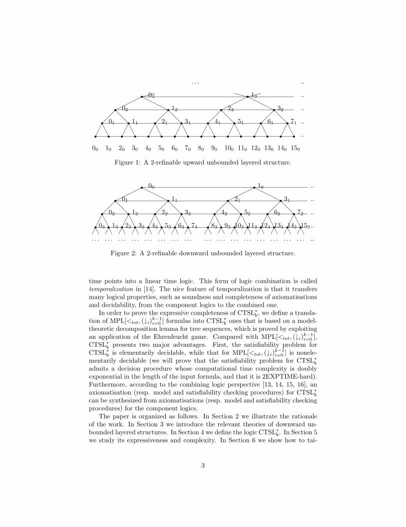
In [28], the decidability of the theory of k-refinable n-layered structures hasbeen proved by mapping its decidability problem into an equivalent one relativeto the finest layer, and, then, by reducing such a problem to the decidabil-ity problem for the monadic second-order theory of one successor MSO[<] [4].The class of k-refinable upward unbounded layered structures, i.e., ω-layeredstructures consisting of a finest temporal domain and an infinite number ofcoarser and coarser domains (cf. Figure 1), and the class of k-refinable down-ward unbounded layered structures, i.e., infinitely refinable structures consistingof a coarsest domain and an infinite number of finer and finer domains (cf.Figure 2), have been investigated in [25]. Both theories have been shown tobe nonelementarily decidable: the first one has been reduced to the monadicsecond-order theory of one successor, properly extended with a suitable par-tition function (the resulting theory has been proved to be the counterpart,in the style of Buchi Theorem, of the class of ω-languages accepted by k-arytree systolic automata, which strictly includes the class of ω-regular languages);the second one has been reduced to the monadic second-order theory of k suc-cessors (with k ≥ 2). An expressively complete temporal logic counterpart ofMFO[<tot, (↓i)k−1

i=0 ], the first-order fragment of the theory of k-refinable upwardunbounded layered structures, has been proposed in [26]. In this paper, we ad-dress the problem of finding a temporal logic counterpart to a suitable fragmentof the theory of k-refinable downward unbounded layered structures.

We first provide an alternative view of these structures as infinite sequencesof infinite k-ary trees. Then, we define a temporal logic counterpart of the the-ory of k-refinable downward unbounded layered structures MSO[<tot, (↓i)k−1

i=0 ]with set quantification restricted to infinite tree paths, MPL[<tot, (↓i)k−1

i=0 ] forshort, and show that it is expressively complete. The resulting logic, that wecalled CTSL∗k (Computational Tree Sequence Logic with k successors), can beviewed as a combined logic that embeds a logic for branching within (discrete)

2

r»»03

. . .

r r02 12©©©©

HHHH

r r r r01 11 21 31¡¡

¡¡

@@

@@

r r r r r r r r¢¢

¢¢

¢¢

¢¢

AA

AA

AA

AA

00 10 20 30 40 50 60 70

rXX »»13

r r22 32©©©©

HHHH

r r r r41 51 61 71

..

..

..

..

..

¡¡

¡¡

@@

@@

r r r r r r r r¢¢

¢¢

¢¢

¢¢

AA

AA

AA

AA

80 90 100 110 120 130 140 150

Figure 1: A 2-refinable upward unbounded layered structure.

r 00

r r01 11©©©©

HHHH

r r r r02 12 22 32¡¡

¡¡

@@

@@

r r r r r r r r03 13 23 33 43 53 63 73 83 93 103 113 123 133 143 153¢¢

¢¢

¢¢

¢¢

AA

AA

AA

AA

¢ ¢ ¢ ¢ ¢ ¢ ¢ ¢A A A A A A A A. . . . . . . . . . . . . . . . . . . . . . . .

r 10

r r21 31©©©©

HHHH

r r r r42 52 62 72

..

..

..

..

¡¡

¡¡

@@

@@

r r r r r r r r¢¢

¢¢

¢¢

¢¢

AA

AA

AA

AA

¢ ¢ ¢ ¢ ¢ ¢ ¢ ¢A A A A A A A A. . . . . . . . . . . . . . . . . . . . . . . . ..

Figure 2: A 2-refinable downward unbounded layered structure.

time points into a linear time logic. This form of logic combination is calledtemporalization in [14]. The nice feature of temporalization is that it transfersmany logical properties, such as soundness and completeness of axiomatisationsand decidability, from the component logics to the combined one.

In order to prove the expressive completeness of CTSL∗k, we define a transla-tion of MPL[<tot, (↓i)k−1

i=0 ] formulas into CTSL∗k ones that is based on a model-theoretic decomposition lemma for tree sequences, which is proved by exploitingan application of the Ehrenfeucht game. Compared with MPL[<tot, (↓i)k−1

i=0 ],CTSL∗k presents two major advantages. First, the satisfiability problem forCTSL∗k is elementarily decidable, while that for MPL[<tot, (↓i)k−1

i=0 ] is nonele-mentarily decidable (we will prove that the satisfiability problem for CTSL∗kadmits a decision procedure whose computational time complexity is doublyexponential in the length of the input formula, and that it is 2EXPTIME-hard).Furthermore, according to the combining logic perspective [13, 14, 15, 16], anaxiomatisation (resp. model and satisfiability checking procedures) for CTSL∗kcan be synthesized from axiomatisations (resp. model and satisfiability checkingprocedures) for the component logics.

The paper is organized as follows. In Section 2 we illustrate the rationaleof the work. In Section 3 we introduce the relevant theories of downward un-bounded layered structures. In Section 4 we define the logic CTSL∗k. In Section 5we study its expressiveness and complexity. In Section 6 we show how to tai-

3

lor the logical framework for downward unbounded layered structures to copewith n-layered ones. Conclusions provide an assessment of the work done, andoutline future research directions.

2 Rationale

The original motivation of our research was the design of a temporal logic em-bedding the notion of time granularity, suitable for the specification of complex(real-time) reactive systems whose components evolve according to differenttime units. However, there are significant similarities between the problemswe encountered in pursuing our goal, and those addressed by current researchon combining logics, theories, and structures. Furthermore, we recently estab-lished interesting connections between multi-level temporal logics and automatatheory that suggests a complementary point of view on time granularity: be-sides an important feature of a representation language, time granularity can beviewed as a formal tool to investigate expressiveness and decidability propertiesof temporal theories. Finally, as a by-product of our work, we defined a uniformframework for time and states that reconciles the tense logic and the logic ofprograms perspectives.

2.1 The specification of granular real-time reactive sys-tems

Timing properties play a major role in the specification of reactive and con-current software systems that operate in real-time, which are among the mostcritical software systems. They constrain the interactions between differentcomponents of the system as well as between the system and its environment,and minor changes in the precise timing of interactions may lead to radicallydifferent behaviors. Temporal logic has been successfully used for modeling andanalyzing the behavior of reactive and concurrent systems, e.g. [22]. It sup-ports semantic model checking, which can be used to verify the consistency ofspecifications, and to check positive and negative examples of system behavioragainst specifications; it also supports pure syntactic deduction, which may beused to prove properties of systems. Unfortunately, most common specificationlanguages are inadequate for real-time applications, because they lack an ex-plicit and quantitative representation of time. A few remarkable exceptions doexist. They are extensions of Petri Nets or metric variants of temporal logic,which support direct and quantitative specifications of temporal properties andrelevant validation activities.

There are, however, systems whose temporal specification is far from beingsimple even with timed Petri Nets or metric temporal logic. Consider the wide-ranging class of real-time systems whose components have dynamic behavioursregulated by very different—even by orders of magnitude—time constants (here-after granular real-time reactive systems). As an example, consider a pondagepower station consisting of a reservoir, with filling and emptying times of days or

4

weeks, generator units, possibly changing state in a few seconds, and electroniccontrol devices, evolving in milliseconds or even less. A complete specificationof the power station must include the description of these components and oftheir interactions. A natural description of the temporal evolution of the reser-voir state will probably use days: “During rainy weeks, the level of the reservoirincreases 1 meter a day”, while the description of the control devices behaviourmay use microseconds: “When an alarm comes from the level sensors, send anacknowledge signal in 50 microseconds”. We say that systems of such a type havedifferent time granularities. It is somewhat unnatural, and sometimes impossi-ble, to compel the specifier to use a unique time granularity, microseconds in theprevious example, to describe the behaviour of all the components. A good lan-guage must allow the specifier to easily describe all simple and intuitively clearfacts (naturalness of the notation). Hence, a specification language for granularreal-time reactive systems must support different time granularities to allow one(i) to maintain the specifications of the dynamics of differently-grained compo-nents as separate as possible (modular specifications), (ii) to differentiate therefinement degree of the specifications of different system components (flexiblespecifications), and (iii) to write complex specifications in an incremental wayby refining higher-level predicates associated with a given time granularity interms of more detailed ones at a finer granularity (incremental specifications).

2.2 The combining logic perspective

Even though the original motivation of our work on time granularity was thedesign of a temporal logic suitable for the specification of granular real-time reac-tive systems, there are significant similarities between the problems it addressesand those dealt with by the current research on logics that model changingcontexts and perspectives. Indeed, even if it has been developed in a tempo-ral framework, our proposal actually outlines the basic features of a generallogic of granularity. In this respect, it can be seen as a generalization of thewell-known Rescher and Garson’s topological logic to layered structures [30].Moreover, it presents interesting connections with the logics of contexts devel-oped in the area of knowledge representation, where modalities are used to shiftvariables, domains, and interpretation functions from one context to another[5]. More generally, the design of these types of logics is emerging as a relevantresearch topic in the broader area of combination of logics, theories, and struc-tures, at the intersection of logic with artificial intelligence, computer science,and computational linguistics [3]. In our work, we devised suitable combinationtechniques both to define temporal logics for time granularity and to prove theirlogical properties, such as axiomatic completeness and decidability [24, 28]. Fur-thermore, we followed the combining logic approach to build a model checkingframework for granular reactive systems and logics [16].

5

2.3 A complementary point of view on time granularity

A complementary point of view on time granularity arises from interesting con-nections that link multi-level temporal logics and automata theory: time gran-ularity can be viewed not only as an important feature of a representationlanguage, but also as a formal tool to investigate the definability of meaningfultiming properties, such as density and exponential grow/decay, as well as theexpressiveness and decidability of temporal theories [25, 27]. In this respect,the number of layers (single vs. multiple, finite vs. infinite) of the underlyingtemporal structure, as well as the nature of their interconnections, play a majorrole: certain timing properties can be expressed using a single layer; others us-ing a finite number of layers; others only exploiting an infinite number of layers.Timing properties of granular reactive systems composed by a finite numberof differently-grained temporal components can be specified by using n-layeredmetric temporal logics. Furthermore, if provided with a rich enough layeredstructure, n-layered metric temporal logics suffice to deal with conditions like“p holds at all even times of a given temporal domain” that cannot be expressedusing flat propositional temporal logics. ω-layered metric temporal logics allowone to express relevant properties of infinite sequences of states over a singletemporal domain that cannot be captured by using flat or n-layered temporallogics. For instance, k-refinable upward unbounded layered logics allow one toexpress conditions like “p holds at all time points ki, for all natural numbersi, of a given temporal domain”, while downward unbounded ones allow one toconstrain a given property to hold true ‘densely’ over a given time interval [27].More precisely, we can state that if a property p holds at two distinct points xand y of a given domain T i, with x < y, then it holds at two distinct points zand w, with x < z < w < y, of the immediately finer domain T i+1. As anotherexample, we can constrain two predicates p and q to be temporally indistin-guishable. We say that p and q are temporally indistingishable if for all timepoints at which both p and q hold, there exists an infinite path, starting at sucha point, such that both p and q hold at each point belonging to the path.

2.4 Reconciling tense logics and logics of programs

As pointed out in [27], logic and computer science communities have tradition-ally followed a different approach to the problem of representing and reasoningabout time and states. Research in philosophy, linguistics, and mathematicallogic resulted in a family of (metric) tense logics that take time as a primitivenotion and define (timed) states as sets of atomic propositions which are true atgiven time points. Recently, a few papers demonstrated the possibility of suc-cessfully exploiting metric (possibly layered) tense logics in computer science,e.g. [23, 24]. On the other hand, most research in computer science concentratedon the so–called temporal logics of programs, which have been successfully usedto specify and verify reactive and concurrent systems, e.g. [11]. In order todeal with real-time systems, such logics have been equipped with a metric oftime, e.g. [1]. The resulting temporal logics, called real-time logics, take state

6

as a primitive notion, and define time as an attribute of states. More precisely,given an ordered set of states S and an ordered set of time points T , real-timelogics are characterized by a weakly monotonic function ρ : S → T that as-sociates a time instant with each state. Real-time logics allow one to modelpairs of states si, sj ∈ S such that si < sj and ρ(si) = ρ(sj) (temporally in-distinguishable states) or ρ(si+1) > ρ(si) + 1 (temporal gaps between states).Providing metric temporal logics with an infinite number of layers (ω-layered),where each time point belonging to a given layer can be decomposed into ktime points of the immediately finer one (k-refinable), makes it possible to rec-oncile metric tense logics and real-time logics of programs. The basic idea isthat any pair of distinct states, belonging to the same course of events, canalways be temporally ordered, provided that we can refer to a sufficiently finetemporal domain. Furthermore, the ordering between pairs of states, which aretemporally indistinguishable with respect to the considered domain, is actuallyinduced by their temporal ordering with respect to a finer domain, with respectto which their are temporally distinguishable. Notice that a finite number oflayers is not sufficient to capture timed state sequences: it is not possible to fixa priori any bound on the granularity that a domain must have to allow oneto temporally order a given set of states, and thus we need to have an infinitenumber of temporal domains at our disposal. In [27], Montanari et al. show howto embed the theory of timed state sequences, underlying real-time logics, intothe theories of upward and downward unbounded metric and layered temporalstructures. Such an embedding allows one to deal with temporal indistinguisha-bility of states and temporal gaps between states. In the granularity setting,temporal indistinguishability and temporal gaps can indeed be interpreted asphenomena due to the fact that real-time logics lack the ability to express prop-erties at the right (finer) level of granularity: distinct states, having the sameassociated time, can always be ordered at the right level of granularity; similarly,time gaps represent intervals in which a state cannot be specified at a finer levelof granularity.

3 Structures and theories of time granularity

In this section, we formally define k-refinable downward unbounded layeredstructures and the corresponding monadic second-order theories.

3.1 Infinite sequences of infinite k-ary trees

According to the original definition given by Montanari et al. in [25], k-refinabledownward unbounded layered structures are triplets 〈⋃i≥0 T i, ↓, <tot〉, where

• {T i}i≥0 are pairwise disjoint copies of N;

• ↓: {0, . . . , k−1}×⋃i≥0 T i → ⋃

i≥1 T i is a bijection such that, for all i ≥ 0,↓|T i : {0, . . . , k − 1} × T i → T i+1 is a bijection;

7

r 00

r r01 11©©©©

HHHH

r r r r02 12 22 32¡¡

¡¡

@@

@@

r r r r r r r r03 13 23 33 43 53 63 73 83 93 103 113 123 133 143 153¢¢

¢¢

¢¢

¢¢

AA

AA

AA

AA

¢ ¢ ¢ ¢ ¢ ¢ ¢ ¢A A A A A A A A. . . . . . . . . . . . . . . . . . . . . . . .

r 10

r r21 31©©©©

HHHH

r r r r42 52 62 72

..

..

..

..

¡¡

¡¡

@@

@@

r r r r r r r r¢¢

¢¢

¢¢

¢¢

AA

AA

AA

AA

¢ ¢ ¢ ¢ ¢ ¢ ¢ ¢A A A A A A A A. . . . . . . . . . . . . . . . . . . . . . . . ..

Figure 3: A 2-refinable downward unbounded layered structure (revisited).

• <tot is such that

1. 〈T 0, <tot|T 0×T 0〉 is isomorphic to N with the usual ordering;

2. t <tot ↓ (j, t), for 0 ≤ j ≤ k − 1;

3. ↓ (j, t) <tot ↓ (j + 1, t), for 0 ≤ j ≤ k − 2;

4. if t <tot t′ and t′ 6∈ ⋃i≥0 ↓i (t), then ↓ (k − 1, t) <tot t′;

5. if t <tot t′ and t′ <tot t′′, then t <tot t′′.

where ↓n (t) ⊆ ⋃i≥0 T i is the set such that ↓0 (t) = {t} and, for every

n ≥ 1, ↓n (t) = {↓ (j, t′) : t′ ∈↓n−1 (t), 0 ≤ j ≤ k − 1}.It is worth noting that the domain

⋃i≥0 T i is structured by ↓ in such a way

that each time point of T0 is the root of a leafless, perfectly balanced k-arytree. The total ordering <tot over

⋃i≥0 T i is induced by the linear ordering of

the trees, for pairs of nodes belonging to different trees, and by the preordervisit of the tree, for pairs of nodes belonging to the same tree (cf. Figure 3).In the following, we make this remark more precise by providing an equivalentcharacterization of k-refinable downward unbounded layered structures as in-finite sequences of infinite k-ary trees. Later, we will exploit this alternativeformulation to obtain a temporal logic counterpart of the theory of k-refinabledownward unbounded layered structures.

We start by defining the notion of Σ-labeled k-ary tree. Let Tk = {0, . . . , k−1}∗ be the set of finite strings over {0, . . . k − 1} and, for x ∈ Tk, let |x| be thelength of x. We denote by ε the empty string (|ε| = 0). Let Σ be a fixed finitealphabet. An infinite Σ-labeled k-ary tree, with k ≥ 1, is a map t : Tk → Σ.For k ≥ 2, Tk(Σ) defines the set of infinite Σ-labeled k-ary trees, while, for k = 1,it defines the set of infinite sequences (or infinite words). A finite sequence (orfinite word) is a map from an initial segment of T1 to Σ. For any 0 ≤ i ≤ k − 1and x ∈ Tk, let ↓i (x) = xi be the i-th son of x. Furthermore, we denote by< the (partial) ordering induced by the proper prefix relation over Tk: x < yiff there exists z 6= ε such that xz = y. The lexicographical (total) orderingon Tk, denoted by <lex, is defined as follows: x <lex y iff x < y or x = zavand y = zbu, with a, b ∈ {0 . . . k − 1} and a < b (over N). Any given tree

8

t ∈ Tk(Σ) can be represented as a structure t = (Tk, <, (↓i)k−1i=0 , (Pa)a∈Σ), where

Pa = {x ∈ Tk | t(x) = a}, for every a ∈ Σ. Given x ∈ Tk, a chain in t, startingat x, is a subset of Tk, linearly ordered by <, such that x is the minimum ofthe chain. A path X in t, starting at x, is a chain, starting at x, such that thereexists no chain Y , starting at x, which properly includes X. A full path in t isa path starting at the root ε of t, that is, a maximal, linearly ordered subsetof t. The i-th layer of t is the finite set {x0, . . . , xki−1} ⊂ Tk such that, forr = 0, . . . , ki − 1, |xr| = i.

An infinite sequence of infinite Σ-labeled k-ary trees is a map ts : TSk → Σ,where TSk = N×Tk. The i-th tree of the sequence is the set {(i, x) ∈ TSk | x ∈Tk}. Let TSk(Σ) be the set of infinite sequences of Σ-labeled infinite k-arytrees. Given 0 ≤ i ≤ k − 1 and (j, x) ∈ TSk, ↓i ((j, x)) = (j, xi) is the i-thprojection of (j, x). A total ordering relation <tot over TSk, which correspondsto the ordering relation <tot over

⋃i≥0 T i, can be defined as follows:

1. (i, ε) <tot (j, ε), j > i ≥ 0;

2. (i, x) <tot ↓j (i, x), for 0 ≤ j ≤ k − 1 and i ≥ 0;

3. ↓j (i, x) <tot ↓j+1 (i, x), for 0 ≤ j ≤ k − 2 and i ≥ 0;

4. if (i, x) <tot (j, y) and either i < j or it is not the case that x < y (overTk), then ↓k−1 (i, x) <tot (j, y), for all i, j ≥ 0;

5. if (i, x) <tot (n, z) and (n, z) <tot (j, y), then (i, x) <tot (j, y).

Furthermore, the domain TSk is partially ordered by two ordering relations <1

and <2 defined as follows: for every (i, x), (j, y) ∈ TSk, (i, x) <1 (j, y) if andonly if i < j (over N) and (i, x) <2 (j, y) if and only if i = j and x < y (overTk). Any given tree sequence ts ∈ TSk(Σ) can be represented as a structurets = (TSk, <tot, (↓i)k−1

i=0 , (Pa)a∈Σ), where Pa = {(j, x) ∈ TSk | ts((j, x)) = a},for every a ∈ Σ. Given ts ∈ TSk(Σ), (j, x) ∈ TSk, and 0 ≤ i ≤ k− 1, we denoteby ts(j,x) and ts(j,x),i the tree rooted at (j, x) and the tree rooted at the i-thson of (j, x), respectively. Accordingly, the i-th tree of ts is denoted by ts(i,ε). Achain (resp. path, full path) in ts is a chain (resp. path, full path) in ts(i,ε), forsome i ≥ 0. We denote by Π(ts) the set of full paths of ts. The i-th layer Li ofts is the set

⋃j≥0{(j, x0), . . . , (j, xki−1)} ⊂ TSk such that, for r = 0, . . . , ki− 1,

|xr| = i. A path P (resp. layer L) in ts can be ordered with respect to <tot

obtaining a sequence (j1, x1)(j2, x2) . . .; we denote by P (i) (resp. L(i)) the i-thelement (ji, xi) of such a sequence. It is worth noting that the restriction of <1

to the elements belonging to the 0-layer is a total ordering, while this is not thecase for all the other finer layers. We will take advantage of this fact when wewill define a combined temporal logic for time granularity.

It is not difficult to show that any given Σ-labeled k-refinable downward un-bounded layered structure 〈⋃i≥0 T i, ↓, <tot〉 corresponds to an infinite sequenceof infinite Σ-labeled k-ary trees ts = (TSk, <tot, (↓i)k−1

i=0 , (Pa)a∈Σ), and viceversa.

9

3.2 Theories of downward unbounded layered structures

In this section, we define the relevant theories of k-refinable downward un-bounded layered structures.

Definition 3.1 Given a finite alphabet Σ, let MSOΣ[c1, . . . , cr, u1, . . . , us, b1, . . . , bt](abbreviated MSOΣ[τ ]) be the second-order language with equality over a setC = {c1, . . . , cr} of constant symbols, a set U = {u1, . . . , us} of unary relationalsymbols, and a set B = {b1, . . . , bt} of binary relational symbols, which is definedas follows:

(i) atomic formulas are of the forms x = y, x = ci, with 1 ≤ i ≤ r, ui(x), with1 ≤ i ≤ s, bi(x, y), with 1 ≤ i ≤ t, x ∈ X, and x ∈ Pa, where x, y areindividual variables, X is a set variable, and Pa, with a ∈ Σ, is a monadicpredicate;

(ii) formulas are built up from atomic formulas by means of the Boolean con-nectives ¬, ∧, ∨, and →, and the quantifiers ∀ and ∃, ranging over bothindividual and set variables.

MSOΣ[τ ]-formulas are interpreted over relational structures consisting of a do-main D and an interpretation function I for the symbols in the vocabulary τ andthe monadic predicates (Pa)a∈Σ. Semantics structures for MSOΣ[τ ] give thesame interpretation to symbols in τ ; they may only differ in the interpretationof the predicates (Pa)a∈Σ.

For any given vocabulary τ , let MFOΣ[τ ] be the first-order fragment ofMSOΣ[τ ] and, whenever MSOΣ[τ ] is interpreted over trees or tree sequences, letMPLΣ[τ ] be the restriction of MSOΣ[τ ] obtained by constraining set variablesto be interpreted over paths (formulas in MPLΣ[τ ] are called path formulas).

Let ϕ(x1, . . . , xn, X1, . . . , Xm) be a formula whose free individual variablesare x1, . . . , xn and free set variables are X1, . . . , Xm. A sentence ϕ is a formuladevoid of free variables. A model for a sentence ϕ is a structure in which ϕis true. Let S be the set of structures over which MFOΣ[τ ] (resp. MPLΣ[τ ],MSOΣ[τ ]) is interpreted. We say that T ⊆ S is definable in MFOΣ[τ ] (resp.MPLΣ[τ ], MSOΣ[τ ]) if there exists a sentence ϕ in MFOΣ[τ ] (resp. MPLΣ[τ ],MSOΣ[τ ]) such that, for every M∈ S, M is a model of ϕ if and only if M∈ T .Whenever no confusion can arise, we will omit the subscript Σ. In the rest ofthe paper, we will focus our attention on the following languages and theories:

• MFO[<], interpreted over finite and infinite sequences;

• MPL[<, (↓i)k−1i=0 ], interpreted over infinite k-ary trees;

• MFO/MPL/MSO[<tot, (↓i)k−1i=0 ] and MFO/MPL/MSO[<1, <2, (↓i)k−1

i=0 ], in-terpreted over infinite sequences of infinite k-ary trees.

It is possible to show that MPL[<1, <2, (↓i)k−1i=0 ] (resp. MSO[<1, <2, (↓i)k−1

i=0 ])is as expressive as MPL[<tot, (↓i)k−1

i=0 ] (resp. MSO[<tot, (↓i)k−1i=0 ]).

10

Proposition 3.2 MPL[<1, <2, (↓i)k−1i=0 ], interpreted over infinite sequences of

infinite k-ary trees, is as expressive as MPL[<tot, (↓i)k−1i=0 ].

Proof.We first show that (i, x) <tot (j, y) if and only if either i = j and x <lex y

or i < j. Consider the direction from left to right. For the sake of conciseness,we use (i, x)<tot(j, y) as a shorthand for either i = j and x <lex y or i < j. Inorder to prove the implication, it suffices to show that axioms (1,2,3) and rules(4,5) of the definition of <tot (over TSk) are sound, that is, they preserve therelation <tot.

1. (i, ε)<tot(j, ε), with 0 ≤ i < j: it immediately follows from i < j.

2. (i, x)<tot ↓j (i, x), for 0 ≤ j ≤ k − 1: it follows from ↓j (i, x) = (i, ↓j (x)),↓j (x) = xj, and x <lex xj.

3. ↓j (i, x)<tot ↓j+1 (i, x), for 0 ≤ j ≤ k− 2 and i ≥ 0: it is analogous to theprevious case.

4. if (i, x)<tot(j, y) and either i < j or it is not the case that x < y (overTk), then ↓k−1 (i, x)<tot(j, y), for all i, j ≥ 0. In the case in which i < j,then ↓k−1 (i, x) = (i, ↓k−1 (x))<tot(j, y), and thus the thesis. Supposethat i = j and x <lex y. Since x < y does not hold, by definition of <lex,there exist a, b, z, u, and v, with |a| = |b| = 1 and |z|, |u|, |v| ≥ 0, suchthat x = zau, y = zbv, and 0 ≤ a < b. Therefore ↓k−1 (x) = x(k − 1) =zau(k − 1) = zau′, with u′ = u(k − 1). This allows us to conclude that↓k−1 (x) <lex y, and thus ↓k−1 (i, x)<tot(j, y).

5. if (i, x)<tot(n, z) and (n, z)<tot(j, y), then (i, x)<tot(j, y): a simple caseanalysis suffices, taking into account that both <lex and <1 are transitiverelations.

Let us prove now the opposite direction, that is, for any given i, j, x, and y,if either i = j and x <lex y or i < j, then (i, x) <tot (j, y). Let i < j.For all z ∈ Tk, it holds that (i, z) <tot (j, ε). The proof is by induction onthe length of z. If |z| = 0, that is, z = ε, the thesis follows from axiom (1).Let |z| = n + 1. By definition, there exist w, with |w| = n and m, with0 ≤ m ≤ k − 1, such that z =↓m (i, w). From axiom (3) and rule (5), itholds that ↓m (i, w) ≤tot ↓k−1 (i, w). Furthermore, by the inductive hypothesis,it holds that (i, w) <tot (j, ε), and thus, by using rule (4), we obtain that↓k−1 (i, w) <tot (j, ε). An application of rule (5) allows us to conclude that(i, z) <tot (j, ε). If y = ε we have the thesis. Otherwise, we need to show that(j, ε) <tot (j, y), for all y, with |y| > 0. This can be proved by a simple inductionon the length of y. Given (i, z) <tot (j, ε) and (j, ε) <tot (j, y), rule (5) allowsus to conclude that (i, z) <tot (j, y). The case in which i = j and x <lex y canbe dealt with in a similar way.

To complete the proof, it suffices to show that the relation <tot can beexpressed in MPL[<1, <2, (↓i)k−1

i=0 ] and that both relations <1 and <2 can be

11

expressed in MPL[<tot, (↓i)k−1i=0 ]. As for the first statement, we just showed that

(i, x) <tot (j, y) if and only if either i = j and x <lex y or i < j. On the groundof this equivalence, it is not difficult to see that x ≤tot y if and only if

x ≤2 y ∨ ∃z(∨

0≤i<j≤k

(↓i (z) ≤2 x∧ ↓j (z) ≤2 y)) ∨ x ≤1 y.

By exploiting the same correspondence, we can also prove the second statement.For all pairs x, y, x ≤1 y if and only if

x ≤tot y ∧ ∃X∃Y ∃r1∃r2(r1 6= r2 ∧ T0(r1)∧T0(r2) ∧ x ∈ X ∧ r1 ∈ X ∧ y ∈ Y ∧ r2 ∈ Y ),

where T0(x) =def ¬∃y∨k−1

i=0 ↓i (y) = x.Furthermore, for all pairs x, y, x ≤2 y if and only if

x ≤tot y ∧ ∃X(x ∈ X ∧ y ∈ X).

The above proposition can be easily generalized to the full second-ordercase. One direction of the proof remains the same (<tot can be defined inMSO[<1, <2, (↓i)k−1

i=0 ] in exactly the same way). To prove the opposite direction,it suffices to show that paths can be defined in MSO[<tot, (↓i)k−1

i=0 ]:

Path(X) =def ∃x(T 0(x) ∧ x ∈ X ∧ ∀y((T 0(y) ∧ x 6= y) → y 6∈ X))∧∀y(y ∈ X → ∨k−1

j=0 (↓j (y) ∈ X ∧∧i 6=j ↓i (y) 6∈ X))∧

∀y(y 6∈ X → ∧k−1i=0 ↓i (y) 6∈ X).

3.3 Contextualization, displacement, and projection op-erators

In [25], Montanari et al. propose MSO[<tot, (↓i)k−1i=0 ] as the language for time

granularity and define its interpretations over both upward and downward un-bounded layered structures. In this section, we show that MPL[<tot, (↓i)k−1

i=0 ],interpreted over downward unbounded layered structures, is expressive enoughto capture the basic temporal operators of contextualization, local displace-ment, and projection (an informal account of these operators can be found inSection 1).

The case of projection is trivial, since the projection symbols ↓i, for 0 ≤ i ≤k − 1, belong to the language. As an example, the condition “p holds at thei-th projection of x” can be written as ∃y(↓i (x) = y∧p(y)). We can also definethe converse relation of abstraction as follows. We say that x can be abstractedin y, notationally ↑ (x) = y, if and only if it holds that

∨k−1i=0 ↓i (y) = x.

Accordingly, the condition “p holds at the abstraction of x” can be written as∃y(↑ (x) = y ∧ p(y)).

As for contextualization, let Ti be a monadic predicate that holds at all timepoints of the i-th layer, for every i ≥ 0 (this form of contextualization has beencalled horizontal contextualization in [25]). Ti can be inductively defined asfollows:

12

T0(x) =def ¬∃y ∨k−1i=0 ↓i (y) = x;

Ti+1(x) =def ∃y(Ti(y) ∧ ∨k−1j=0 ↓j (y) = x).

Finally, local displacement is captured as follows. For every i ≥ 0, let +i1be a binary predicate such that, for all pairs x, y ∈ T i, +i1(x, y) if and only ify is the within T i-successor of x. It can be defined as follows:

+i1(x, y) =def Ti(x) ∧ Ti(y) ∧ x <tot y ∧∀z(Ti(z) ∧ x <tot z → y ≤tot z).

In the following, we will use a functional notation for +i1, that is, we willwrite +i1(x) = y for +i1(x, y). Moreover, we will adopt +ij(x) as an abbrevi-ation for (+i1)j(x).

In [25], Montanari et al. also introduce an alternative form of contextual-ization, called vertical contextualization, which is defined as follows: for everyi ≥ 0, let Di be a monadic predicate that holds at all time points at distance ifrom the origin of the layer they belong to. We show that the combined use ofprojection, local displacement and horizontal contextualization makes it possibleto define vertical contextualization. Given w ∈ {0, . . . , k − 1}∗, we inductivelydefine ↓w (x) as follows. Whenever |w| = 0, ↓w (x) = x. Otherwise, let w = av,with a ∈ {0, . . . , k − 1}. We define ↓av (x) =↓a (↓v (x)). D0(x) can be definedas follows:

D0(x) =def ∃X(x ∈ X ∧ 00 ∈ X ∧ ∀y(y ∈ X →↓0 (y) ∈ X)),

where 00 is the first-order definable origin of coarsest layer (we have that y = 00

if and only if ∀z(y ≤tot z))1.

For all i > 0, let ankn + . . . a0k0 be the k-ary representation of i. Di can be

defined as follows:

Di(x) =def

∨blogk(i)cj=0 ∃z(D0(z) ∧ Tj(z) ∧ +ji(z) = x)∨

∃y(D0(y)∧ ↓a0,...,an (y) = x).

Since second-order quantification (over paths) only occurs in the definitionD0, it immediately follows that horizontal contextualization, local displacement,and projection are also definable in MFO[<tot, (↓i)k−1

i=0 ].

Remark 3.3 In MSO[<tot, (↓i)k−1i=0 ], there is no way to define a binary predicate

EqualT (resp. EqualD) such that, for all x, y, EqualT(x, y) (resp. EqualD(x, y))holds true if and only if there exists i such that both T i(x) (resp. Di(x)) andT i(y) (resp. Di(y)) hold. Indeed, the addition of EqualT (resp. EqualD) makesMSO[<tot, (↓i)k−1

i=0 ] undecidable, a result which is closely related to the undecid-ability of the extension of S2S with a predicate Elevel such that Elevel(x, y)holds true if and only if |x| = |y|, with x, y ∈ {0, 1}∗ [21]. Notice that, fromthe fact that EqualT and EqualD cannot be expressed in MSO[<tot, (↓i)k−1

i=0 ],

1In order to define D0 in MSO[<tot, (↓i)k−1i=0 ], it suffices to add the conjunct Path(X) to the

above definition, that is:

D0(x) =def ∃X(Path(X) ∧ x ∈ X ∧ 00 ∈ X ∧ ∀y(y ∈ X →↓0 (y) ∈ X)).

13

it obviously follows that they cannot be expressed in MPL[<tot, (↓i)k−1i=0 ] and

MFO[<tot, (↓i)k−1i=0 ], but it does not follow that the addition of these predicates to

such theories, or to weaker variants of them devoid of the uninterpreted monadicpredicates Pa, with a ∈ Σ, would make them undecidable. We are currently ex-ploring these decidability problems in a systematic way.

In the following, we will refer to MPL[<1, <2, (↓i)k−1i=0 ], which has been proved

to be as expressive as MPL[<tot, (↓i)k−1i=0 ] (cf. Proposition 3.2). The reason is

that, according to the combining logic perspective, MPL[<1, <2, (↓i)k−1i=0 ] allows

us to specify the behaviour of a (granular) reactive system as a suitable combina-tion of temporal evolutions, modeled by <1, and temporal refinements, modeledby <2 (cf. Figure 3).

We conclude by pointing out that the expressive power of MPL[<1, <2, (↓i

)k−1i=0 ] does not change if we further constrain set variables to only range over

full paths (instead of paths): a full path is just a particular path starting froma point belonging to the first temporal domain; moreover, a path can always beembedded into a unique full path. For instance, the sentence “there is a pathwhose time points are labeled with symbol a”, which is expressed in MPL[<1

, <2, (↓i)k−1i=0 ] by the formula:

∃X∀x(x ∈ X → Pa(x)),

can be captured using full paths by the formula:

∃X∃y(y ∈ X ∧ ∀x(x ∈ X ∧ y ≤2 x → Pa(x))).

3.4 On the relationships with interval structures and the-ories

There exists a natural link between structures and theories of time granular-ity and those developed for representing and reasoning about time intervals.Differently-grained temporal domains can indeed be interpreted as differentways of partitioning a given discrete/dense time axis into consecutive disjointintervals. According to this interpretation, every time point can be viewedas a suitable interval over the time axis and projection implements an inter-vals/subintervals mapping. More precisely, let us define direct constituents of atime point x, belonging to a given domain, the time points of the immediatelyfiner domain into which x can be refined (if any) and indirect constituents thetime points into which the direct constituents of x can be directly or indirectlyrefined (if any). The mapping of a given time point into its direct or indirectconstituents can be viewed as a mapping of a given time interval into (a spe-cific subset of) its subintervals. The existence of such a natural correspondencebetween interval and granularity structures hints at the possibility of defining asimilar connection at the level of the corresponding theories. We are currentlyworking on the problem of establishing such a connection in order to transferdecidability results from the granularity setting to the interval one. Most in-terval temporal logics, such as, for instance, Moszkowski’s Interval Temporal

14

Logic (ITL) [29], Halpern and Shoham’s Modal Logic of Time Intervals (HS)[19], and Chaochen and Hansen’s Neighbourhood Logic (NL) [6], have indeedbeen shown to be undecidable. Decidable fragments of these logics have beenobtained by imposing severe restrictions on their expressive power. As an ex-ample, Moszkowski [29] proves the decidability of the fragment of PropositionalITL with Quantification (over propositional variables) which results from theintroduction of a locality constrain. An ITL interval is a finite or infinite se-quence of states. The locality property states that each propositional variableis true over an interval if and only if it is true at its first state. This prop-erty allows one to collapse all the intervals starting at the same state into asingle interval of length zero, that is, the interval consisting of the first stateonly. By exploiting such a constraint, decidability of Local ITL can be easilyproved by embedding it into Quantified Propositional Linear Temporal Logic(QPTL). We expect that more expressive decidable fragments of interval logicscan be obtained as counterparts of decidable theories of time granularity overfinitely-layered and ω-layered structures.

4 Temporal logics for time granularity

In this section, we first give the definition of basic linear and branching timelogics as well as that of their past and/or directed variants; then, we introducetemporal logics for time granularity.

Let PΣ (P when no confusion can arise) be the finite set of atomic proposi-tional letters {Pa | a ∈ Σ}.

Definition 4.1 ((Past) Directed CTL∗ and (Past) Directed PTL)We inductively define a set of state formulas and a set of path formulas:

• state formulas

(S1) any atomic proposition Pa ∈ PΣ is a state formula;

(S2) if p, q are state formulas, then p ∧ q and ¬p are state formulas;

(S3) if p is a path formula, then Ap and Ep are state formulas;

• path formulas

(P0) any atomic proposition Pa ∈ PΣ is a path formula;

(P1) any state formula is a path formula;

(P2) if p, q are path formulas, then p ∧ q and ¬p are path formulas;

(P3) if p, q are path formulas, then Xp, and pUq are path formulas;

(P4) if p is a path formula, then X0p, . . . ,Xk−1p are path formulas;

(P5) if p, q are path formulas, then X−1p and pSq are path formulas.

15

As for branching time logics, the language of Past (k-ary) Directed CTL∗ (PCTL∗kfor short) is the smallest set of state formulas generated by the above rules. Thelanguage of (k-ary) Directed CTL∗ (CTL∗k) is obtained by eliminating rule (P5),that of Past CTL∗ (PCTL∗) by removing rule (P4), and that of CTL∗ by delet-ing both (P4) and (P5).As for linear time logics, the language of Past (k-ary) Directed PTL (PPTLk) isthe smallest set of path formulas generated by the rules (P0), (P2), (P3), (P4),and (P5). The language of (k-ary) Directed PTL (PTLk) is obtained by deletingrule (P5), that of Past PTL (PPTL) by eliminating rule (P4), and that of PTLby deleting both (P4) and (P5). Formulas Fp and Gp are respectively definedas trueUp and ¬F¬p as usual, where true = Pa ∨ ¬Pa, for some Pa ∈ PΣ.

We interpret (P)PTL over sequences (or unary trees), (P)PTLk over pathsof k-ary trees (with k ≥ 2), and (PD)CTL∗k over k-ary trees (with k ≥ 2).The semantic interpretation for non-directed logics is given as usual [11]. Thesemantic interpretation for (P)CTL∗k coincides with that for (P)CTL∗, exceptfor path formulas of the form Xip, whose interpretation is defined as follows.Given t ∈ Tk(Σ), a path X in t, and a position j in X,

t,X, j |= Xip if and only if X(j + 1) =↓i (X(j)) and t,X, j + 1 |= p.

In the following, we will make use of operators Nip defined as EXip, for alli = 0, . . . , k − 1.

In a similar way, the semantic interpretation for (P)PTLk coincides withthat for (P)PTL, except for formulas of the form Xip, whose interpretation isdefined as follows. Given a (full) path X in a k-ary tree and a position j in X,

X, j |= Xip if and only if X(j + 1) =↓i (X(j)) and X, j + 1 |= p.

Let us now define the Computational Tree Sequence Logic with k successors(CTSL∗k), together with its past variant PCTSL∗k. Let p be a (P)CTL∗k-formula.We call p monolithic if its outermost operator is not a Boolean connective.For example, AG(P ∨ Q) is monolithic, while AGP ∨ Q is not. Formulasof (P)CTSL∗k are obtained by embedding monolithic formulas of (P)CTL∗k into(P)PTL. To avoid confusion, we rename the linear temporal operators X, U,X−1, and S of (P)PTL by © , 4 , ©−1, and 4−1, respectively.

Definition 4.2 (CTSL∗k and PCTSL∗k)We inductively define a set of layered formulas:

(L0) any monolithic formula in CTL∗k is a layered formula;

(L1) any monolithic formula in PCTL∗k is a layered formula;

(L2) if p, q are layered formulas, then p ∧ q and ¬p are layered formulas;

(L3) if p, q are layered formulas, then © p and p4 q are layered formulas;

(L4) if p, q are layered formulas, then ©−1p and p4−1q are layered formulas.

16

The language of PCTSL∗k is the smallest set of formulas generated by rules (L1),(L2), (L3), and (L4), while that of CTSL∗k is obtained by applying rules (L0),(L2), and (L3). Formulas 3p and 2p are respectively defined as true4 p and¬3¬p as usual.

For every k ≥ 2, we interpret (P)CTSL∗k formulas over k-ary tree sequencesas follows. Given a tree sequence ts ∈ TSk(Σ), linear temporal operators © ,4 , ©−1, and 4−1 are interpreted over the first layer L0 of ts, while branchingtemporal operators E and A are interpreted over trees rooted at time pointsin L0. Given a tree sequence ts ∈ TSk(Σ), a position j ≥ 0 in L0, and a(P)CTSL∗k-formula p, we define the satisfiability relation ts, L0, j |= p in termsof the satisfiability relation of (P)CTL∗k (here denoted, to avoid confusion, by|=CTL) as follows:

ts, L0, j |= p iff tsL0(j), L0(j) |=CTL p, p monolithic in (P )CTL∗kts, L0, j |= p ∧ q iff ts, L0, j |= p and ts, L0, j |= q;ts, L0, j |= ¬p iff it is not the case that ts, L0, j |= p;ts, L0, j |= © p iff ts, L0, j + 1 |= p;ts, L0, j |= p4 q iff ts, L0, r |= q for some r ≥ j, and

ts, L0, s |= p for every j ≤ s < r;ts, L0, j |= ©−1p iff j > 0 and ts, L0, j − 1 |= p;ts, L0, j |= p4−1q iff ts, L0, r |= q for some r ≤ j, and

ts, L0, s |= p for every r < s ≤ j.

Given a tree sequence ts ∈ TSk(Σ) and a (P)CTSL∗k-formula p, we say that tsis a model of p if and only if ts, L0, 0 |= p. A set T ⊆ TSk(Σ) is definable in(P)CTSL∗k if there exists a formula p in (P)CTSL∗k such that, for every ts ∈TSk(Σ), ts is a model of p if and only if ts ∈ T .

5 Expressiveness and Complexity of CTSL∗kIn this section, we show that CTSL∗k is as expressive as MPL[<1, <2, (↓i)k−1

i=0 ],when interpreted over k-ary downward unbounded layered structures or, equiv-alently, over infinite sequences of infinite k-ary trees (Theorems 5.7 and 5.15).Furthermore, we prove that its satisfiability problem is 2EXPTIME-complete(Theorem 5.16).

5.1 Preliminaries

We start by recalling some basic definitions and properties of linear and branch-ing time logics, and by stating some auxiliary results about branching time logicswith explicit successors. Given two languages L1 and L2, interpreted over thesame class S of structures, we say that L1 is as expressive as L2 if, for every setT ⊆ S, T is L1-definable if and only if T is L2-definable.

As for linear time logic, it is well-known that, when interpreted over the classof finite sequences as well as over the class of infinite ones, PTL and PPTL areas expressive as MFO[<] [17, 20].

17

Theorem 5.1 (Expressive completeness of PTL and PPTL)PTL and PPTL are as expressive as MFO[<], when interpreted over infinite

(resp. finite) sequences.

In [32], Sistla and Clarke show that the satisfiability problem for PTL isPSPACE-complete.

As for branching time logic, the expressive power of CTL∗ and PCTL∗ isequivalent to the one of monadic second-order logic on infinite binary trees withsecond-order quantifiers over infinite paths [18].

Theorem 5.2 (Expressive completeness of CTL∗ and PCTL∗)CTL∗ and PCTL∗ are as expressive as MPL[<], when interpreted over infi-

nite binary trees.

In [8], Emerson and Jutla prove that the problem of testing satisfiability forCTL∗ is 2EXPTIME-complete.

As pointed out by Hafer and Thomas [18], Theorem 5.2 can be generalized toCTL∗k and PCTL∗k with respect to MPL[<, (↓i)k−1

i=0 ] by incorporating successorsinto both temporal and monadic path logics [18].

Theorem 5.3 (Expressive completeness of CTL∗k and PCTL∗k)CTL∗k and PCTL∗k are as expressive as MPL[<, (↓i)k−1

i=0 ], when interpretedover infinite k-ary trees.

Furthermore, a decision procedure for CTL∗k can be obtained by means of thefollowing non trivial adaptation of the decision procedure for CTL∗ originallydeveloped by Emerson and Sistla [10] and later refined by Emerson and Jutla [8].

Let us assume k = 2 (the generalization to an arbitrary k is straightforward).As a preliminary step, we provide an embedding of PTL2 into PTL. To thisend, we define a translation τ of formulas and models of PTL2, over an alphabetΣ, to formulas and models of PTL, over an extended alphabet Σ× {0, 1}. Themapping of PTL2-formulas into PTL-formulas is defined as follows:

τ(Pa) =∨

i∈{0,1} P(a,i) for a ∈ Στ(α ∧ β) = τ(α) ∧ τ(β)τ(¬α) = ¬τ(α)τ(Xiα) =

∨x∈Σ P(x,i) ∧ Xτ(α) for i ∈ {0, 1}

τ(αUβ) = τ(α)Uτ(β)

Temporal structures for PTL2 over Σ can be viewed as infinite labeled (full)paths, whose nodes are labeled with symbols in Σ and whose transitions arelabeled with symbols in {0, 1}, while temporal structures for PTL over Σ ×{0, 1} can be viewed as infinite labeled sequences, whose nodes are labeled withsymbols in Σ× {0, 1}. We define a bijection τ from temporal structures M forPTL2 over Σ to temporal structures M′ for PTL over Σ×{0, 1} that maps eacha-labeled node of M, with an outgoing transition labeled with i, to an (a, i)-labeled node of M′. As an example, the (full) path . . . a →0 b →1 a →1 . . . is

18

mapped into the sequence . . . (a, 0)(b, 1)(a, 1) . . .. The following lemma can beeasily proved.

Lemma 5.4 For every formula ϕ of PTL2 and temporal structure M, M is amodel for ϕ if and only if τ(M) is a model for τ(ϕ).

As a second preliminary step, we transform CTL∗k-formulas in a normal formsuitable for subsequent manipulation. Such a normal form is a straightforwardgeneralization of the normal form for CTL∗-formulas proposed by Emerson andSistla [10]. This result is formally stated by the following lemma, whose proofis similar to the one for CTL∗ and thus omitted.

Lemma 5.5 For any given CTL∗k-formula ϕ0, there exists a corresponding for-mula ϕ1 in a normal form composed of conjunctions and disjunctions of subfor-mulas of the form Ap, Ep, and AGEp, where p is a pure linear time formulaof PTL2, such that (i) ϕ1 is satisfiable if and only if ϕ0 is satisfiable, and (ii)|ϕ1| = O(|ϕ0|). Moreover, any model of ϕ1 can be used to define a model of ϕ0

and vice versa.

Theorem 5.6 (CTL∗k is elementarily decidable)The satisfiability problem for CTL∗k is 2EXPTIME-complete.

Proof.Hardness follows from 2EXPTIME-hardness of CTL∗ [35]. To show that

it belongs to 2EXPTIME, we outline an algorithm for checking satisfiabilityfor CTL∗k of deterministic doubly exponential time complexity. Given a CTL∗k-formula ϕ0, such an algorithm can be obtained as follows:

1. by exploiting Lemma 5.5, construct an equivalent formula ϕ1 composedof conjunctions and disjunctions of subformulas of the form Ap, Ep, andAGEp, where p is a PTL2-formula;

2. by exploiting Lemma 5.4, replace every maximal PTL2-formula p (over Σ)in ϕ1 by the PTL-formula τ(p) (over Σ× {0, 1}); then, construct a Buchistring automaton Aτ(p) (over Σ × {0, 1}) recognizing the models of τ(p),by using the technique described in [10];

3. for every subformula of the form Ap of ϕ1, determinize the Buchi stringautomaton Aτ(p) for τ(p), using Safra’s construction [31], to obtain anequivalent deterministic Rabin string automaton A′τ(p) (over Σ× {0, 1})for τ(p);

4. program a Rabin tree automaton Aϕ1 (over Σ), accepting the models ofϕ1, which incorporates the string automata built in steps 2 and 3 in asuitable way (see below);

5. test whether Aϕ1 recognizes the empty language using the algorithm pro-posed by Emerson and Jutla [8].

19

Step 4 is as follows. For every subformula Ep of ϕ1, let Ap = (Q, q0, ∆, F )be the Buchi string automaton for p. We construct the Buchi tree automatonAEp = (Q ∪ {q∗}, q0, ∆′, F ∪ {q∗}) for Ep, where ∆′ is defined as follows:

∆′(q, a, q′, q∗) if and only if ∆(q, (a, 0), q′);∆′(q, a, q∗, q′) if and only if ∆(q, (a, 1), q′);∆′(q∗, a, q∗, q∗) if and only if a ∈ Σ.

For every subformula Ap of ϕ1, let Ap = (Q, q0,∆, Γ) be the deterministic Rabinstring automaton for p. We construct the deterministic Rabin tree automatonAAp = (Q, q0, ∆′, Γ) for Ap, where ∆′ is defined as follows:

∆′(q, a, q′, q′′) if and only if ∆(q, (a, 0), q′) and ∆(q, (a, 1), q′′).

For every subformula AGEp of ϕ1, let Ap = (Q, q0, ∆, F ) be the Buchi stringautomaton for p. We construct the Buchi tree automaton AAGEp = (Q ∪{q∗ | q ∈ Q}, q0, ∆′, F ∪{q∗ | q ∈ Q}) for AGEp, where ∆′ is defined as follows:

∆′(q, a, q′, q∗1) if and only if ∆(q, (a, 0), q′) and ∆(q0, (a, 1), q1);∆′(q, a, q∗1 , q′) if and only if ∆(q, (a, 1), q′) and ∆(q0, (a, 0), q1);∆′(q, a, q′, q∗0) if and only if ∆(q, (a, 0), q′) and ∆(q0, (a, 0), q′);∆′(q, a, q∗0 , q′) if and only if ∆(q, (a, 1), q′) and ∆(q0, (a, 1), q′);∆′(q∗, a, q′, q′′) if and only if ∆′(q, a, q′, q′′).

A tree automaton Aϕ1 for ϕ1 is obtained by taking the intersection and/orthe union of the tree automata constructed for the subformulas of ϕ1. Noticethat if ϕ1 does not contain subformulas of the form Xip, then Aϕ1 is symmetric.

By exploiting classical complexity results on string and tree automata [11,33, 34], an easy complexity analysis of the proposed algorithm allows us toconclude that its complexity is (deterministic) 2EXPTIME.

5.2 Expressive completeness of CTSL∗kWe prove that CTSL∗k is as expressive as MPL[<1, <2, (↓i)k−1

i=0 ], when interpretedover infinite sequences of infinite k-ary trees.

For technical reasons, we constrain path variables X to be interpreted overfull paths. As shown in Section 3, such a restriction leaves the expressive powerof monadic path formulas unchanged. For the same reason, we reformulatethe considered monadic languages as follows (without altering their expressivepower). Given the vocabularies τ1 = {ε,<1, <2, (↓i)k−1

i=0 }, τ2 = {ε,<, (↓i)k−1i=0 },

τ3 = {ε,<, ↓} and τ4 = {ε, δ,<, ↓}, we will use:

• MPL[τ1], interpreted over infinite sequences of infinite k-ary trees, whereε is a (first-order definable) constant denoting the root of the first tree ofthe sequence;

• MPL[τ2], interpreted over infinite k-ary trees, where ε is a (first-orderdefinable) constant denoting the root of the tree;

20

• MFO[τ4] (resp. MFO[τ3]), interpreted over finite (resp. infinite) sequences,where ε and δ are constants that respectively denote the first and the lastelement of the sequence, and ↓ is the successor function. It is easy to showthat ε and δ, as well as ↓, are (first-order) definable in terms of <.

One direction of the proof (as usual) is easy: there exists a straightforwardembedding of CTSL∗k into MPL[<1, <2, (↓i)k−1

i=0 ].

Theorem 5.7 (CTSL∗k is a fragment of MPL[<1, <2, (↓i)k−1i=0 ])

For every set T ⊆ TSk(Σ) of infinite sequences of Σ-labeled infinite trees, ifT is definable in CTSL∗k, then T is definable in MPL[<1, <2, (↓i)k−1

i=0 ].

Proof.We prove that every CTSL∗k-formula can be mapped into an equivalent sen-

tence of MPL[τ1], and, thus, that it is equivalent to a MPL[<1, <2, (↓i)k−1i=0 ]-

sentence. To this end, for any ts ∈ TSk(Σ), w ∈ ts, and p ∈ CTSL∗k, we definea translation τw of p into an MPL[τ1]-formula, with free variable w. For anyCTL∗k-formula p, let τw(p) be the MPL[τ2]-formula obtained from p by exploit-ing Theorem 5.3, with the symbol < replaced by <2. The translation τw can bedefined as follows:

τw(p) = τw(p), whenever p is monolithic in CTL∗k;τw(p ∧ q) = τw(p) ∧ τw(q);τw(¬p) = ¬τw(p);τw(© p) = ∃w′(w′ = +0

1(w) ∧ τw′(p));τw(p4 q) = ∃w′(T 0(w′) ∧ w ≤1 w′ ∧ τw′(q)∧

∀w′′((T 0(w′′) ∧ w ≤1 w′′ ∧ w′′ <1 w′) → τw′′(p))).

For any CTSL∗k-formula p, we have that p is equivalent to the MPL[τ1]-sentence ϕp = τε(p).

In order to prove the opposite direction, that is, to show that CTSL∗k is expres-sively complete with respect to MPL[<1, <2, (↓i)k−1

i=0 ], we follow a ‘decomposi-tion method’ similar to that exploited by Hafer and Thomas in [18] to provethe expressive completeness of CTL∗ with respect to MPL[<]. We first decom-pose the model checking problem for an MPL[<1, <2, (↓i)k−1

i=0 ]-formula and atree sequence in TSk(Σ) into a finite number of model checking subproblemsfor formulas and structures that do not refer to the whole tree sequence any-more, but only to certain disjoint components of it. Then, taking advantage ofsuch a decomposition step, we map every MPL[<1, <2, (↓i)k−1

i=0 ]-formula into anequivalent (but sometimes much longer) CTSL∗k-formula.

As a preliminary step, we show that the addition of past operators to CTSL∗kdoes not increase its expressive power.

Lemma 5.8 PCTSL∗k is as expressive as CTSL∗k.

Proof.By exploiting Theorem 5.3, any PCTSL∗k-formula p can be replaced by an

equivalent PCTSL∗k-formula q, whose past operators (if any) are of the forms

21

©−1 and 4−1 only. Let q1, . . . qn be the monolithic CTL∗k-subformulas of q.Regarding q1, . . . qn as additional atomic propositions within q, we may considerq as a PPTL-formula. By exploiting Kamp’s Theorem, q can be replaced by anequivalent PTL-formula r that contains q1, . . . qn as subformulas.

Let ≡n be a relation on TSk(Σ) such that ts ≡n ts′ if and only if ts andts′ satisfy the same sentences of MPL[τ1] of quantifier depth n. It is possible toshow that ≡n is an equivalence relation of finite index. Its equivalence classesare called n-types and are described by path formulas called n-types descriptors.

Definition 5.9 (n-types descriptors)Given ts ∈ TSk(Σ), a sequence of r elements a in ts, a sequence of s full

paths P in ts, and n ≥ 0, an n-type descriptor ψnts,a,P

is a path formula definedas follows:

ψ0ts,a,P

=∧{ϕ(x1 . . . xr, X1 . . . Xs) | ϕ atomic or negated atomic,ts |= ϕ[a, P ]}

ψn+1

ts,a,P=

∧a∈ts ∃xr+1ψ

nts,aa,P

∧ ∨a∈ts ∀xr+1ψ

nts,aa,P

∧∧P⊆Π(ts) ∃Xr+1ψ

nts,a,PP

∧ ∨P⊆Π(ts) ∀Xr+1ψ

nts,a,PP

The relation ≡n can be characterized by an Ehrenfeucht game Gn(ts, ts′) asfollows (basics on Ehrenfeucht games can be found, for instance, in [9]). Aplay of this game is played by two players Spoiler and Duplicator on structurests, ts′ ∈ TSk(Σ) and consists of n rounds. At each round, Spoiler chooses anelement or a full path either from ts or from ts′; Duplicator reacts by choosingan object of the same kind in the other structure. After n rounds, elementsa1, . . . ar (a for short) and full paths P1, . . . Ps (P ) in ts (with n = r + s), andthe corresponding elements b1, . . . br (b) and full paths Q1, . . . Qs (Q) in ts′,have been chosen. Duplicator wins if the map a → b is a partial isomorphismfrom (ts, P ) to (ts′, Q), i.e., it is injective and respects ε, <2, <1, and ↓i, withi = 0, . . . k− 1, as well as membership in Pa, for every a ∈ Σ. The game can benaturally extended to Gn((ts, P ), a, (ts′, Q), b), where a and P (resp. b and Q)are a finite sequence of elements and a finite sequence of full paths in ts (resp.in ts′), respectively.

Let ∼n be a relation such that, for any pair of structures (ts, a, P ) and(ts′, b, Q), (ts, a, P ) ∼n (ts′, b, Q) if and only if Duplicator wins Gn((ts, P ), a, (ts′, Q), b).The following result easily follows from the well-known Ehrenfeucht-Fraısse The-orem.

Theorem 5.10 Given structures ts and ts′, element sequences a in ts and bin ts′, full path sequences P in ts and Q in ts′, the following are equivalentconditions:

1. (ts, a, P ) ∼n (ts′, b, Q);

2. ts′ |= ψnts,a,P

[b,Q];

22

3. a, P satisfy in ts the same formulas of MPL[τ1] of quantifier depth lessthan or equal to n as b,Q in ts′.

Corollary 5.11 Given n ≥ 0 and an MPL[τ1]-formula ϕ(x, X) of quantifierdepth less than or equal to n, ϕ is equivalent to a finite disjunction of formulasψn

ts,a,Psuch that ts |= ϕ[a, P ].

Similar definitions and results hold for k-ary tree structures and infinite (aswell as finite) word structures. In the former case, n-type descriptors are pathformulas in the language of k-ary trees MPL[τ2]. In the latter case, the rules ofthe game are that Spoiler and Duplicator can only pick elements from the givenpair of words; hence, n-type descriptors are formulas in the first-order languageof linear orders MFO[τ3] (resp. MFO[τ4]).

Let ts ∈ TSk(Σ), k0 be an element belonging to the i-th tree of ts, n be aninteger greater than or equal to 0, and m be the index of ≡n. We enlarge thealphabet Σ to Σ1 = Σ× {1, . . . ,m}, where all j ∈ {1 . . . m} serve as indices forall possible n-types. Let π1 (resp. π3) be the finite (resp. infinite) sequence ofroots (ε)0, . . . (ε)i−1 (resp. (ε)i+1, . . .). We denote by v1(ts, k0) (resp. v3(ts, k0))the finite (resp. infinite) word over Σ1 whose l-th letter is (a, j) if π1(l) (resp.π3(l)) carries letter a ∈ Σ and the tree rooted in it has n-type j. Similarly, weenlarge the alphabet Σ to Σ2 = Σ × ({0, . . . , k − 1} × {1, . . . , m})k−1, and wedenote by π2 the finite path from (ε)i up to (and excluding) k0. We denote byv2(ts, k0) the finite word over Σ2 whose l-th letter is (a, (l1, j1), . . . , (lk−1, jk−1))if π2(l) carries letter a ∈ Σ and, for r = 1, . . . , k− 1, the tree rooted in the lr-thson of it has n-type jr.

We need to prove the following auxiliary lemma, which states that combininglocal winning strategies on disjoint parts of two tree sequences it is possible toobtain a global winning strategy on the two tree sequences.

Lemma 5.12 For arbitrary (ts, k0) and (ts′, k′0), if vi(ts, k0) ∼n vi(ts′, k′0),with i = 1, 2, 3, tsk0,i ∼n ts′k0,i, with i = 0, . . . , k− 1, and ts(k0) = ts′(k′0), then(ts, k0) ∼n (ts′, k′0).

Proof.Suppose that Spoiler picks an element k (different from k0) in ts. If k

belongs to some path vi(ts, k0) or to some tsk0,i, then Duplicator chooses k′ ints′ according to the corresponding local winning strategies. If k belongs to thetree k0 belongs to, and neither k <2 k0 nor k0 <2 k, then Duplicator looks forthe last node k1 belonging to the path v2(ts, k0) such that k1 <2 k. Let k2 bethe son of k1 such that there is a path from k2 to k. Suppose that k2 is the i-thson of k1. Duplicator chooses k′1 in the path v2(ts′, k′0) according to his winningstrategy on v2(ts, k0), v2(ts′, k′0). Let k′2 be the i-th son of k′1. Hence, k1 andk′1 have the same label from Σ2 and thus the subtrees rooted in their successorsk2 and k′2 have the same n-type. Hence, by Theorem 5.10 (its variant for k-arytrees), Duplicator has a winning strategy on these subtrees and can use thisstrategy to choose an element k′ corresponding to k in the subtree rooted in

23

k′2. Finally, if k <1 k0 (resp. k0 <1 k) and k is not a root, then Duplicatorchooses k′ in ts′ exploiting his winning strategy on v1(ts, k0), v1(ts′, k′0) (resp.v3(ts, k0), v3(ts′, k′0)).

Suppose now that Spoiler picks a full path P0 in ts. Let A (resp. A′) bethe finite path from the root of the tree k0 (resp. k′0) belongs to up to (andexcluding) k0 (resp. k′0). If k0 ∈ P0, then P0 has the form A, k0, B, where Bis a path on tsk0,i, for some i. Hence, Duplicator chooses a path B′ in ts′k′0,i

according to his local strategy on tsk0,i, ts′k′0,i, and he responds to Spoiler withthe full path A′, k′0, B

′. If k0 6∈ P0 and P0 belongs to the tree k0 belongs to,then P0 = A1k1C, where k1 is the last node of P0 which belongs to A andC is a path on tsk1,i, for some i. Duplicator first chooses k′1 according to hislocal strategy on v2(ts, k0), v2(ts′, k′0). Let A′1 be the finite path from the rootof the tree k′0 belongs to up to (and excluding) k′1. Then, Duplicator picks apath C ′ on ts′k′1,i exploiting his winning strategy on tsk1,i, ts′k′1,i, and, finally,he responds to Spoiler with the full path A′1, k

′1, C

′ . The case in which P0 doesnot belong to the tree k0 belongs to is similar to the previous one, and thus itsanalysis is omitted.

The following lemma states that checking a path formula ϕ(x) at a node k0

belonging to the tree sequence ts corresponds to verifying a number of sentencesthat do not refer to properties of x relative to the whole tree sequence anymore,but only relative to certain disjoint components of it. In particular, these disjointsubstructures are the (above defined) sequences π1 and π3, with the trees rootedat them, the path π2, with the trees rooted at successor nodes that are not onπ2, the node k0, and the k trees rooted at the k successors of k0.

Lemma 5.13 (First Decomposition Lemma)For every MPLΣ[τ1]- formula ϕ(x) of quantifier depth n, there exists a fi-

nite set Φ of elements of the form (ψ1, ψ2, a, β0, . . . , βk−1, ψ3), where ψi, withi = 1, 2, are n-type descriptors in MFOΣi [τ4], ψ3 is an n-type descriptor inMFOΣ1 [τ3], a ∈ Σ, and βi, with i = 0, . . . , k − 1, are n-type descriptors inMPLΣ[τ2], such that, for any ts ∈ TSk(Σ) and any element k0 in ts, it holdsthat:

(ts, k0) |= ϕ(x) if and only if there exists (ψ1, ψ2, a, β0, . . . , βk−1, ψ3)in Φ such that vi(ts, k0) |= ψi, for i = 1, 2, 3, ts(k0) = a, andtsk0,i |= βi, for i = 0, . . . , k − 1.

Proof.By Corollary 5.11, ϕ(x) is equivalent to a finite disjunction

∨{ψnts,k0

| ts |=ϕ[k0]}. Hence, (ts, k0) |= ϕ(x) if and only if there exist ts′, k′0 such that(ts′, k′0) |= ϕ(x) and (ts, k0) |= ψn

ts′,k′0(x). By Theorem 5.10, this holds true

if and only if there exist ts′, k′0 such that (ts′, k′0) |= ϕ(x) and (ts, k0) ∼n

(ts′, k′0). This is equivalent to the existence of ts′′, k′′0 such that (ts′′, k′′0 ) |= ϕ(x),vi(ts, k0) ∼n vi(ts′′, k′′0 ), with i = 1, 2, 3, ts(k0) = ts′′(k′′0 ) and tsk0,i ∼n ts′′k′′0 ,i,with i = 0, . . . , k−1. The implication from right to left follows from Lemma 5.12

24

by setting ts′ = ts′′ and k′0 = k′′0 . To prove the opposite implication, takets′′ = ts and k′′0 = k0. We must show that (ts, k0) |= ϕ(x). Observe that, byhypothesis, (ts, k0) ∼n (ts′, k′0) and (ts′, k′0) |= ϕ(x). Since ϕ(x) is of quantifierdepth n, by applying Theorem 5.10, we have that (ts, k0) |= ϕ(x).

Now, we proceed by invoking the analogous of Theorem 5.10 for words and k-ary trees, to obtain, respectively, appropriate n-type descriptors ψi = ψn

vi(ts′′,k′′0 ),with i = 1, 2, 3, and βi = ψn

ts′′k′′0 ,i

, with i = 0, . . . , k−1, such that vi(ts, k0) |= ψi,

for i = 1, 2, 3, and tsk0,i |= βi, for i = 0 . . . k − 1. By collecting all such n-type descriptors, we obtain a set Φ as required. Since, for every n ≥ 0, theequivalence relation ≡n has finite index, by virtue of Theorem 5.10, there is afinite number of non equivalent n-type descriptors. From this, it follows thatthe set Φ is finite.

It is possible to prove a similar decomposition lemma for the second-order case.To state it, we need the following definition. Let ts ∈ TSk(Σ) and P0 be a fullpath in ts. We denote by v(ts, P0) the infinite word over Σ2 whose i-th letter is(a, (i1, j1), . . . (ik−1, jk−1)) if P0(i) carries letter a ∈ Σ and, for r = 1, . . . , k− 1,the tree rooted in the ir-th son of it has n-type jr. The proof of Lemma 5.14 issimilar to that of Lemma 5.13, and thus omitted.

Lemma 5.14 (Second Decomposition Lemma)For every MPLΣ[τ1]-formula ϕ(X) of quantifier depth n, there exists a finite

set Φ of elements of the form (ψ1, ψ2, ψ3), where ψ1 is an n-type descriptorin MFOΣ1 [τ4], ψ2 is an n-type descriptor in MFOΣ2 [τ3], and ψ3 is an n-typedescriptor in MFOΣ1 [τ3], such that, for any ts ∈ TSk(Σ) and any full path P0

in ts, it holds that:

(ts, P0) |= ϕ(X) if and only if there exists (ψ1, ψ2, ψ3) in Φ such thatvi(ts, k0) |= ψi, with i = 1, 3, and v(ts, P0) |= ψ2.

We are now ready to prove the main theorem.

Theorem 5.15 (Expressive completeness of CTSL∗k)For every set T ⊆ TSk(Σ) of infinite sequences of Σ-labeled infinite trees, if

T is definable in MPL[<1, <2, (↓i)k−1i=0 ], then T is definable in CTSL∗k.

Proof.We prove that every MPL[<1, <2, (↓i)k−1

i=0 ]-sentence corresponds to an equiv-alent CTSL∗k-formula. Without loss of generality, we consider MPL[τ1]-sentenceswith set quantification restricted to full paths only. Let ϕ be an MPL[τ1]-sentence. We focus on the two relevant cases: ϕ = ∃xφ(x) and ϕ = ∃Xφ(X).

Let ϕ = ∃xφ(x). By Lemma 5.13, checking φ(x) in (ts, k0) is equivalentto checking certain sentences ψ1, ψ2, β0, . . . , βk−1, and ψ3, and a label a ∈ Σ,taken from a finite set Φ, in particular substructures of ts. It suffices to considerthe case in which |Φ| = 1.

25

The first-order sentence ψ1 can be mapped into an equivalent PTL-formulah1 (cf. [17, 20]). Given the formula h1, we construct the dual formula h−1

1 ∈PPTL, that is, a formula such that, for every finite word w of length l, (w, 0) |=h1 if and only if (w, l−1) |= h−1

1 . The formula h−11 contains atomic propositions

P(a,j), for (a, j) ∈ Σ1, which must be replaced by suitable CTL∗k-formulas q(a,j).Each formula q(a,j) states that a given node satisfies Pa and the tree rooted atit has n-type j, i.e., it satisfies the j-th n-type descriptor. Hereinafter, we willdenote by pj the CTL∗k-formula equivalent to the j-th n-type descriptor, whoseexistence is guaranteed by Theorem 5.3. Let q(a,j) = Pa ∧ pj and let (h−1

1 )′

be the PCTSL∗k-formula obtained from h−11 by replacing propositions P(a,j) by

formulas q(a,j) (and using the symbols © , 4 , ©−1, and 4−1 for the lineartime operators that occur in h−1

1 ).In a similar way, the first-order sentence ψ3 can be mapped into a PTL-

formula h3. The formula h3 can be turned into a CTSL∗k-formula (h3)′ byreplacing propositions P(a,j) by CTL∗k-formulas q(a,j) as in the previous case(notice that, in this case, linear past operators are not needed).

Finally, the first-order sentence ψ2 can be mapped into an equivalent PTL-formula h2, whose dual version h−1

2 is obtained as already explained in thecase of h1. The PCTL∗k-formula (h−1

2 )′ is obtained by replacing propositionsP(a,(i1,j1),...,(ik−1,jk−1)) by formulas q(a,(i1,j1),...,(ik−1,jk−1)) which states that agiven node satisfies Pa and the tree rooted at its ir-th son has n-type jr, thatis, it satisfies the jr-th n-type descriptor pjr , for r = 1, . . . k − 1. Formally,

q(a,(i1,j1),...,(ik−1,jk−1)) = Pa ∧k−1∧r=1

Nirpjr .

As for the MPL[τ2]-sentences βi, with i = 0, . . . , k − 1, let bi be the indexof the n-type descriptor βi. By exploiting once more Theorem 5.3, we obtain aCTL∗k-formula pbi , for each i = 0, . . . , k − 1.

Merging together the above results, we have that the given MPL[τ1]-formulaϕ is equivalent to the PCTSL∗k-formula:

pϕ = 3(©−1(h−11 )′ ∧ EFp ∧ © (h3)′),

where

p = X−1(h−12 )′ ∧ Pa ∧

k−1∧

i=0

Nipbi .

Theorem 5.8 guarantees that there exists a CTSL∗k-formula p′ϕ (that is, aformula devoid of past operators) which is equivalent to pϕ, and, thus, equivalentto ϕ.

Let ϕ = ∃Xφ(X), with quantifier depth of φ equal to n ≥ 1. By Lemma 5.14,checking φ(X) in (ts, P0) is equivalent to checking certain sentences ψ1, ψ2,and ψ3 in particular substructures of ts. In analogy to the case of first-orderquantification, ψ1, ψ2, and ψ3 can be replaced by a PCTSL∗k formula (h−1

1 )′,

26

a CTL∗k formula (h2)′, and a CTSL∗k formula (h3)′, respectively. It is easy tocheck that the MPL[τ1]-formula ϕ is equivalent to the PCTSL∗k-formula:

pϕ = 3(©−1(h−11 )′ ∧ E(h2)′ ∧ © (h3)′).

Again, by Theorem 5.8, there exists a CTSL∗k-formula p′ϕ which is equivalentto pϕ, and, thus, equivalent to ϕ.

Putting together Theorems 5.7 and 5.15, we have that CTSL∗k is as expressiveas MPL[<1, <2, (↓i)k−1

i=0 ], when interpreted over infinite sequences of infinite k-ary trees. In particular, it holds that every MPL[<1, <2, (↓i)k−1

i=0 ]-sentence canbe encoded into a (sometimes much longer) CTSL∗k-formula.

It is worth noticing that the proposed (combined) temporal logic for timegranularity can be tailored to deal with infinite sequences of finite (unbounded)trees, preserving expressiveness and complexity results. In Section 6, we showhow to deal with infinite sequences of trees of a given depth n, with n ≥ 0(n-layered structures).

5.3 Temporal operators for time granularity

In this section, we show how the basic temporal operators of (horizontal) contex-tualization, local displacement, and projection, as well as the derived operatorsof abstraction and vertical contextualization, can be encoded in CTSL∗k.

We proceed as follows: first, we provide a natural language specification ofa property based on one of these temporal operators; then, we encode it in thelanguage MPL[<1, <2, (↓i)k−1

i=0 ]; finally, we express it in CTSL∗k.

• Projection: “whenever p holds at a given time point, then q holds at itsith projection (if any)”:

– ∀x(∃y(↑ (y) = x) ∧ p(x) → ∃y(↓i (x) = y ∧ q(y)));

– 2AG(X> ∧ p → Niq).

Notice that the formula ∃y(↑ (y) = x) is always true in downward un-bounded layered structures; however, it can be false in n-layered ones (cf.Section 6).

• Abstraction: “whenever p holds at a given time point, then q holds atits abstraction (if any)”:

– ∀x(∃y(↑ (x) = y) ∧ p(x) → ∃y(↑ (x) = y ∧ q(y)));

– 2AG(Xp → q).

• (Horizontal) contextualization: “p holds at all time points of the i-thlayer”:

– ∀x(Ti(x) → p(x));

– 2AXip,

27

where Xi is the concatenation of i next operators X, for every i ≥ 0.

• Local successor: “if p holds at a given time point of the i-th layer, thenq holds at its successor”:

– ∀x(Ti(x) ∧ p(x) → ∃y(y = +i1(x) ∧ q(y)));

– for i = 0, 2(p → © q);for i > 0, 2(

∧ki−2r=0 (Ni

rp → Nir+1q) ∧ (Ni

ki−1p → © Ni0q)),

where, for r, i ≥ 0, Nir = Nj0 . . .Nji−1 , with

∑i−1s=0 ksji−1−s = r, that is,

j0 . . . ji−1 is the k-ary representation of r.

• Local until: “if h holds at a given time point of the i-th layer, then thereexists a time point in its future (belonging to the same layer) at which qholds and p holds until then”:

– ∀z(Ti(z) ∧ h(z) → ∃y(Ti(y) ∧ q(y) ∧ ∀x(Ti(x) ∧ z ≤ x < y →p(x))));

– 2(∧ki−1

s=0 (Nish → ∨ki−1

r=s (Nirq ∧

∧r−1t=s Ni

tp)) ∨∧ki−1s=0 (Ni

sh → (∧ki−1

r=s Nirp)∧© (AXip4 ∨ki−1

r=0 (Nirq ∧

∧r−1t=0 Ni

tp)))).

• (Vertical) contextualization: “p holds at all time points at distance ifrom the origin of the layer they belong to”:

– ∀x(Di(x) → p(x));

– for i = 0, E(p ∧GX0p);

– for i > 0,∧blogk(i)c

j=0 Xbi/kjcNjimodkj p ∧E(G(X0true ∧ Nblogkic+1

i p)).

5.4 Complexity of CTSL∗kWe prove now that the satisfiability problem for CTSL∗k is 2EXPTIME-complete,and thus elementarily decidable.

Theorem 5.16 (CTSL∗k is elementary decidable)The satisfiability problem for CTSL∗k is 2EXPTIME-complete.

Proof.Hardness follows from 2EXPTIME-hardness of the satisfiability problem for

CTL∗ [35]. To show that the satisfiability problem for CTSL∗k is in 2EXPTIME,we reduce it to the satisfiability problem for CTL∗k, which has been shown to be2EXPTIME-complete in Section 5.1 (Theorem 5.6).

To this end, let Σ be a finite alphabet and Σ′ = Σ ∪ {∗}, where ∗ is a newsymbol not belonging to Σ. We define a translation τ that maps CTSL∗k-formulasover PΣ into equisatisfiable CTL∗k-formulas over PΣ′ .

28

For any CTSL∗k-formula α, let

τ(α) = RightPath(P∗) ∧ τ(α),

where

RightPath(P∗) = P∗ ∧ AG(P∗ → (Nk−1P∗ ∧∧k−2

i=0 Ni¬P∗)∧¬P∗ → AX¬P∗)

and τ(α) is recursively defined as follows:

τ(α) = N0α, whenever α monolithic in CTL∗k;τ(©α) = Nk−1τ(α);τ(α4β) = E(GP∗ ∧ τ(α)Uτ(β)).

It is not difficult to show that, for every formula α of CTSL∗k, α is satisfiableover TSk(Σ) if and only if τ(α) is satisfiable over Tk(Σ′).

As for the left to right direction, let α be a formula of CTSL∗k and ts =t0, t1, . . . ∈ TSk(Σ) be a tree sequence that validates α. Consider a tree t ∈Tk(Σ′) built as follows: we label the subtree of t rooted at 0 in the same way inwhich t0 is labeled, the subtree rooted at (k − 1)0 as t1, the subtree rooted at(k−1)(k−1)0 as t2, and so on. Moreover, we label the set of nodes {(k−1)n | n ≥0} with ∗ ∈ Σ′. It is easy to prove, by induction on the structure of α, that tvalidates τ(α).

As for the opposite direction, let α be a formula of CTSL∗k and t ∈ Tk(Σ′)be a tree that validates τ(α). Let ts = t0, t1, . . . be a tree sequence in TSk(Σ)built as follows: t0 is labeled as the subtree of t rooted at 0, t1 is labeled asthe subtree of t rooted at (k − 1)0, t2 is labeled as the subtree of t rooted at(k − 1)(k − 1)0, and so on. It is easy to prove, by induction on the structure ofα, that ts validates α.

6 Coping with n-layered structures

We conclude the paper by showing how to tailor temporal logics for time gran-ularity over downward unbounded layered structures to deal with n-layeredstructures. n-layered structures are layered structures endowed with a finiteand bounded number of temporal domains. Formally, we define a k-refinablen-layered structure as a triplet 〈⋃i≤n T i, ↓, <tot〉, with n ≥ 0, such that:

• {T i}i≤n are pairwise disjoint copies of N;

• ↓: {0, . . . , k − 1} × ⋃i<n T i → ⋃

i≤n T i is a bijection such that, for alli < n, ↓|T i : {0, . . . , k − 1} × T i → T i+1 is a bijection;

• <tot is such that

1. 〈T 0, <tot|T 0×T 0〉 is isomorphic to N with the standard ordering;

2. t <tot↓ (j, t), for 0 ≤ j ≤ k − 1;

29

3. ↓ (j, t) <tot↓ (j + 1, t), for 0 ≤ j ≤ k − 2;

4. if t <tot t′ and t′ 6∈ ⋃ni=0 ↓i (t), then ↓ (k − 1, t) <tot t′;

5. if t <tot t′ and t′ <tot t′′, then t <tot t′′.

where, ↓i (t) ⊆ ⋃i≤n T i is the set such that ↓0 (t) = {t} and, for every

i ≥ 1, ↓i (t) = {↓ (j, t′) : t′ ∈↓i−1 (t), 0 ≤ j ≤ k − 1}.

For every n ≥ 0, n-layered structures can be viewed as infinite sequences of k-ary trees of height n, and vice versa. Moreover, the monadic first-order theoryMFO[<tot, (↓i)k−1

i=0 ] can be adopted as the language for time granularity overn-layered structures or, equivalently, over infinite sequences of finite trees ofheight n. MFO[<tot, (↓i)k−1

i=0 ] is indeed expressive enough to capture the granularprimitives of (horizontal) contextualization, local displacement, and projectionas well as the derived operators of abstraction and vertical contextualization.Projection, abstraction, (horizontal) contextualization, and local displacementcan be expressed as in the case of downward unbounded layered structures. Asfor vertical contextualization, its definition can be simplified as follows:

D0(x) =n∨

i=0

↓0i (00) = x,

where 00 is the (first-order definable) origin of layer zero.For all i > 0, Di(x) can be defined as follows:

Di(x) =n∨

j=0

∃y(Tj(y) ∧ D0(y) ∧ +ji(y) = x).

Remark 6.1 Unlike the case of downward unbounded structures (cf. Remark3.3), by exploiting the finiteness of the layered structure, we can capture thepredicate EqualT as follows:

EqualT(x, y) =n∨

i=0

(Ti(x) ∧ Ti(y)).

On the contrary, there is no way to define the predicate EqualD. Indeed, itis possible to show that the addition of such a predicate to MFO[<tot, (↓i)k−1

i=0 ]would make the theory undecidable.

Let CTSLnk be the temporal logic for time granularity over infinite sequences

of finite trees of height n (n-layered structures). From a syntactical point of view,it coincides with CTSL∗k; however, it is interpreted over infinite sequences offinite k-ary trees of height n (with a strong interpretation for the next operator).

In the following, we show how to reduce the satisfiability problem for CTSLnk

to that for CTSL∗k. Let i ≥ 0 and θi = 2(∧i

j=0 AXjP∗ ∧ AXi+1AG¬P∗),where ∗ 6∈ Σ. The translation τ from CTSL∗k-formulas to CTSL∗k-formulas canbe defined as follows:

30

τ(Pa) = Pa for a ∈ Σ;τ(α ∧ β) = τ(α) ∧ τ(β);τ(¬α) = ¬τ(α);τ(©α) = © τ(α);τ(α4β) = τ(α)4 τ(β);τ(Aα) = Aτ(α) whenever the outermost operator of α (if any) belongs

to {∧ ,¬,A,E};τ(AXα) = AX(P∗ → τ(α));τ(AXiα) = AXi(P∗ → τ(α));τ(A(αUβ)) = P∗ → A(τ(α)U(P∗ ∧ τ(β)));τ(Eα) = Eτ(α) whenever the outermost operator of α (if any) belongs

to {∧ ,¬,A,E};τ(EXα) = EX(P∗ ∧ τ(α));τ(EXiα) = EXi(P∗ ∧ τ(α));τ(E(αUβ)) = P∗ ∧ E(τ(α)U(P∗ ∧ τ(β))).

For every CTSL∗k-formula α and i ≥ 0, let ηi(α) = θi ∧ τ(α). It is not difficultto show that, for every n ≥ 0, the satisfiability of α over infinite sequences offinite k-ary trees of height n can be reduced to the satisfiability of ηn(α) overinfinite sequences of infinite k-ary trees. This is formally stated by the followingtheorem.

Theorem 6.2 For every CTSL∗k-formula α and n ≥ 0, there exists an n-layeredstructure satisfying α if and only if there exists a downward unbounded layeredstructure satisfying ηn(α).

As an immediate corollary of Theorem 6.2, we have that the satisfiabil-ity problem for CTSLn

k is elementarly decidable. As for the expressiveness ofCTSLn

k, the proof given for CTSL∗k also works for CTSLnk. Hence, CTSLn

k is asexpressive as MPL[<1, <2, (↓i)k−1

i=0 ] over infinite sequences of finite k-ary treesof height n. However, since second-order quantification in MPL[<1, <2, (↓i)k−1

i=0 ]over sequences of finite trees is restricted to finite paths (of bounded length), itis not difficult to see that MPL[<1, <2, (↓i)k−1

i=0 ] and MFO[<1, <2, (↓i)k−1i=0 ] have

the same expressive power over infinite sequences of finite k-ary trees of heightn. Therefore, CTSLn

k is as expressive as MFO[<1, <2, (↓i)k−1i=0 ].

7 Conclusions and Future Work

In this paper we proposed a temporal logic for time granularity, that we calledCTSL∗k, which is based on a simple combination of the branching time logicCTL∗k (the extension of CTL∗ with k directed successors) and the linear timelogic PTL. We proved that CTSL∗k is an expressively complete and elementarilydecidable fragment of the theory of k-refinable downward unbounded layeredstructures with set quantification restricted to infinite paths. Furthermore, ac-cording to the adopted combining logic perspective, we have that an axiomati-sation, as well as model and satisfiability checking procedures, for CTSL∗k can

31

be synthesized from the same tools for the component logics. Finally, we showedthat (a minor variant of) CTSL∗k is expressively complete with respect to the firstorder-theory of k-refinable n-layered structures, and that it is still elementarilydecidable. We are currently working at an extension of CTSL∗k able to capturethe full power of the second-order theory of downward unbounded layered (resp.n-layered) structures, preserving its elementary decidability.

References

[1] R. Alur and T.A. Henzinger. Real-time logics: complexity and expressive-ness. Information and Computation, 104:35–77, 1993.

[2] C. Bettini, S. Jajodia, and X. Wang. Time Granularities in Databases,Data Mining, and Temporal Reasoning. Springer, 2000.

[3] P. Blackburn and M. de Rijke. Special issue on combining structures, logics,and theories. Notre Dame Journal of Formal Logic, 37, 1996.

[4] J.R. Buchi. On a decision method in restricted second-order arithmetic. InProc. 1st International Congress on Logic, Methodology, and Philosophy ofScience, pages 1–11. Stanford Univ. Press, 1962.

[5] S. Buvac and I.A. Mason. Propositional logic of context. In Proceedings ofAAAI, Washington, 1993. MIT Press.

[6] Z. Chouchen and M. R. Hansen. An adequate first order interval logic.Lecture Notes in Computer Science, 1536:584–608, 1998.

[7] C.E. Dyreson and R.T. Snodgrass. Temporal granularity. In R. T.Snodgrass, editor, The TSQL2 Temporal Query Language, pages 347–385.Kluwer Academic Press, 1995.

[8] E.A. Emerson and C.S. Jutla. The complexity of tree automata and logicsof programs. In Proceedings of the 29th Annual Symposium on Foundationsof Computer Science, pages 328–337. IEEE, 1988.

[9] H.D. Ebbinghaus and J. Flum. Finite Model Theory. Springer, 1995.

[10] E. A. Emerson and A. P. Sistla. Deciding full branching time logic. Infor-mation and Control, 61(3):175–201, 1984.

[11] E.A. Emerson. Temporal and modal logic. In J. van Leeuwen, editor,Handbook of Theoretical Computer Science, Vol. B, pages 995–1072. Else-vier Science Publishers B.V., 1990.

[12] J. Fiadeiro and T. Maibaum. Sometimes “tomorrow” is “sometimes” -action refinement in a temporal logic of objects. In Proc. of the 1st Inter-national Conference on Temporal Logic (ICTL), LNAI 827, pages 48–66.Springer, 1994.

32

[13] M. Finger and D. Gabbay. Adding a temporal dimension to a logic system.Journal of Logic, Language and Information, 1:203–233, 1992.

[14] M. Finger and D. Gabbay. Combining temporal logic systems. Notre DameJournal of Formal Logic, 37:204–232, 1996.

[15] M. Finger and M. A. Weiss. The unrestricted addition of a temporal dimen-sion to a logic system. In Proceedings of the 3rd International Conferenceon Temporal Logic (ICTL), pages 53–63, 2000.

[16] M. Franceschet, A. Montanari, and M. de Rijke. Model checking for com-bined logics. In Proceedings of the 3rd International Conference on Tem-poral Logic (ICTL), pages 65–73, 2000.

[17] D. Gabbay, A. Pnueli, S. Shelah, and J. Stavi. On the temporal analysisof fairness. In Proc. 7th ACM Symposium on Principles of ProgrammingLanguages, pages 163–173, 1980.

[18] T. Hafer and W. Thomas. Computation tree logic CTL* and path quan-tifiers in the monadic theory of the binary tree. In T. Ottmann, editor,Automata, Languages and Programming, 14th International Colloquium,volume 267 of Lecture Notes in Computer Science, pages 269–279, Karl-sruhe, Germany, 13–17 July 1987. Springer.

[19] J. Y. Halpern and Y. Shoham. A propositional modal logic of time intervals.Journal of the ACM, 38(4):935–962, October 1991.

[20] H. Kamp. Tense Logic and the Theory of Linear Order. PhD Dissertation,University of California, Los Angeles, 1968.

[21] H. Lauchli and C. Savoiz. Monadic second-order definable relations on thebinary tree. Journal of Symbolic Logic, 52:219–226, 1987.

[22] Z. Manna and A. Pnueli. Temporal Verification of Reactive Systems(Safety). Springer, 1995.

[23] A. Montanari. Metric and Layered Temporal Logic for Time Granular-ity. ILLC Dissertation Series 1996-02, Institute for Logic, Language andComputation, University of Amsterdam, 1996.

[24] A. Montanari and M. de Rijke. Two-sorted metric temporal logic. Theo-retical Computer Science, 183:187–214, 1997.

[25] A. Montanari, A. Peron, and A. Policriti. Decidable theories of ω-layeredmetric temporal structures. Logic Journal of the IGPL, 7(1):79–102, 1999.

[26] A. Montanari, A. Peron, and A. Policriti. Extending Kamp theorem withbinary operators to model time granularity. In Proceedings of the 3rd In-ternational Conference on Temporal Logic (ICTL), pages 135–144, 2000.

33

[27] A. Montanari, A. Peron, and A. Policriti. The taming (timing) of the states.Logic Journal of the IGPL, 8(5):681–699, 2000.

[28] A. Montanari and A. Policriti. Decidability results for metric and layeredtemporal logics. Notre Dame Journal of Formal Logic, 37:260–282, 1996.

[29] B. Moszkowski. Reasoning about digital circuits. PhD Dissertation, De-partment of Computer Science, University of Stanford, 1983.

[30] N. Rescher and J. Garson. Topological logic. Journal of Symbolic Logic,33:537–548, 1968.

[31] S. Safra. On the complexity of ω-automata. In Proceedings of the 29thAnnual Symposium on Foundations of Computer Science, pages 319–327,White Plains, New York, 24–26 October 1988. IEEE.

[32] A. P. Sistla and E. M. Clarke. The complexity of propositional lineartemporal logics. Journal of the ACM, 32(3):733–749, 1985.

[33] W. Thomas. Automata on infinite objects. In J. van Leeuwen, editor,Handbook of Theoretical Computer Science, Vol. B, pages 133–191. ElsevierScience Publishers, 1990.

[34] W. Thomas. Languages, automata and logic. In G. Rozenberg and Sa-lomaa A., editors, Handbook of formal languages, Vol. III, pages 389–455.Springer, 1997.

[35] M. Y. Vardi and L. Stockmeyer. Improved upper and lower bounds formodal logics of programs. In ACM Symposium on Theory of Computing(STOC), pages 240–251, Baltimore, USA, May 1985. ACM Press.

34