Branch-and-Cut for Combinatorial OptimizationProblems without Auxiliary Binary Variables

I. R. de Farias, Jr. ¤

State University of New York at Bu®alo403 Bell Hall, Bu®alo, NY 14260-2050

E. L. Johnsony and G. L. Nemhauser y

School of Industrial and Systems EngineeringGeorgia Institute of Technology, Atlanta, GA 30332-0205

February 16, 2000

Abstract

Many optimization problems involve combinatorial constraints on continuous vari-ables. An example of a combinatorial constraint is that at most one variable in a groupof nonnegative variables may be positive. Traditionally, in the mathematical program-ming community, such problems have been modeled as mixed-integer programs byintroducing auxiliary binary variables and additional constraints. Because the numberof variables and constraints becomes larger and the combinatorial structure is not usedto advantage, these mixed-integer programming models may not be solved satisfacto-rily, except for small instances. Traditionally, constraint programming approaches tosuch problems keep and use the combinatorial structure, but do not use linear program-ming bounds in the search for an optimal solution. Here we present a branch-and-cutapproach that considers the combinatorial constraints without the introduction of bi-nary variables. We review the development of this approach and show how strongconstraints can be derived using ideas from polyhedral combinatorics. To illustrate theideas, we present a production scheduling model that arises in the manufacture of ¯beroptic cables.

1 Introduction

Several classes of optimization problems consist of maximizing a linear or a concave quadraticfunction of continuous decision variables subject to linear constraints. When the variables

¤Partially supported by CNPq, Brazilian research agencyyPartially supported by NSF grant DMI-9700285 and ILOG.

1

are subject exclusively to the linear constraints, the resulting problem can be solved inpolynomial time, for example by an interior point algorithm. In many applications, however,the variables are also subject to other constraints that are combinatorial and make the set offeasible solutions non-convex. In this case, the resulting problem may be NP-hard. Examplesof hard combinatorial constraints that often occur in linear or concave quadratic optimizationproblems with linear constraints include:

² special ordered sets of type I (SOS1) constraints² special ordered sets of type II (SOS2) constraints² cardinality constraints² semi-continuous constraints.

A set of variables is SOS1 [5] when at most one variable in the set can be nonzero.This constraint appears, for example, in linear complementarity [14], re¯ning [21], capitalbudgeting, pricing, and manufacturing problems[26].A set of variables is SOS2 [5] when at most two variables in the set can be nonzero, and

in case two variables in the set are nonzero, they must be adjacent in the set. For example,if fx1; x2; x3; x4; x5g is SOS2 and x3 6= 0 in a feasible solution, then x1 = x5 = 0, and atleast one of x2 or x4 must be 0 in that solution. This constraint appears, for example, in thepiecewise linear approximation of nonlinear separable functions and production scheduling[13, 20].A cardinality constraint is a generalization of SOS1 in which no more than a speci¯ed

number of variables is nonzero. A variable xj is semi-continuous when it is either equal to 0or greater than or equal to a positive number, i.e. xj 2 f0g [ [lj; uj], where 0 < lj < uj, anduj 2 <[f1g. Cardinality constraints and semi-continuous variables appear, for example, inportfolio optimization [8], discrete location-allocation [9], and synthesis of process networks[7, 29].Traditionally, these constraints have been modeled by introducing auxiliary binary vari-

ables and additional constraints relating the binary and the continuous variables. For ex-ample, suppose that 0 · x1 · u1; : : : ; 0 · xl · ul. If fx1; : : : ; xlg is SOS1, we introduce thebinary variables y1; : : : ; yl, and the constraints

xj · ujyj; (1)

j 2 f1; : : : ; lg, andlX

j=1

yj · 1:

If fx1; : : : ; xlg is SOS2, we introduce the binary variables y1; : : : ; yl¡1, and the constraints

2

l¡1Xj=1

yj · 1;

x1 · u1y1;

xj · uj¡1yj¡1 + ujyj;

j 2 f2; : : : ; l ¡ 1g, and

xl · ulyl¡1:

If xj is semi-continuous, we introduce the binary variable yj and the constraints

ljyj · xj · ujyj:

These MIP models were introduced ¯rst by Markowitz and Manne [25] and Dantzig [11].Markowitz and Manne showed that piecewise linear approximations to nonlinear separablefunctions, commonly used, for example, in problems with economies of scale, can be modeledas MIPs. Dantzig, motivated by the excitement that followed Gomory's cutting plane algo-rithm [17], modeled several hard combinatorial constraints that occur in practice as MIPs.In general, large instances of these problems have resisted the attack of general purpose MIPsoftware.A di®erent approach was pioneered by Beale and Tomlin [5]. In their seminal paper, they

suggested dispensing with the use of auxiliary binary variables to model piecewise linear ap-proximations to nonlinear separable functions and multiple-choice constraints, and adoptinga specialized branching strategy in a branch-and-bound scheme as a way to enforce the com-binatorial constraints. Later, Beale [2, 3, 4] suggested the use of the same principle to dealwith semi-continuous variables and other variations of special ordered sets. The suggestionscontained in [2, 3, 4, 5] are widely recognized to yield more e®ective branch-and-bound algo-rithms, and they have been implemented in commercial and academic optimization software.More recently, Beaumont [6], building upon earlier work by Balas [1], presented a branch-

and-bound algorithm for disjunctive programming problems that dispenses with the use ofauxiliary binary variables, by branching on the disjunctions, and replacing the continuousrelaxation of the usual MIP formulation, which usually contains several inequalities, witha surrogate inequality that is as strong. Computational results reported in [6] indicate thee®ectiveness of this approach.It has been demonstrated that branch-and-cut approaches, which use the polyhedral

structure of the problem, frequently improve the performance of branch-and-bound methodssubstantially, see, for instance, [10, 19, 27, 28]. However, there has been very little progress

3

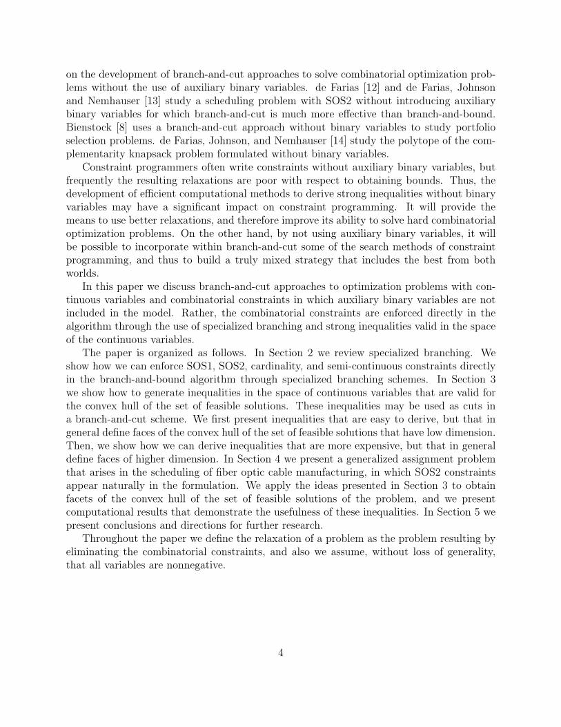
on the development of branch-and-cut approaches to solve combinatorial optimization prob-lems without the use of auxiliary binary variables. de Farias [12] and de Farias, Johnsonand Nemhauser [13] study a scheduling problem with SOS2 without introducing auxiliarybinary variables for which branch-and-cut is much more e®ective than branch-and-bound.Bienstock [8] uses a branch-and-cut approach without binary variables to study portfolioselection problems. de Farias, Johnson, and Nemhauser [14] study the polytope of the com-plementarity knapsack problem formulated without binary variables.Constraint programmers often write constraints without auxiliary binary variables, but

frequently the resulting relaxations are poor with respect to obtaining bounds. Thus, thedevelopment of e±cient computational methods to derive strong inequalities without binaryvariables may have a signi¯cant impact on constraint programming. It will provide themeans to use better relaxations, and therefore improve its ability to solve hard combinatorialoptimization problems. On the other hand, by not using auxiliary binary variables, it willbe possible to incorporate within branch-and-cut some of the search methods of constraintprogramming, and thus to build a truly mixed strategy that includes the best from bothworlds.In this paper we discuss branch-and-cut approaches to optimization problems with con-

tinuous variables and combinatorial constraints in which auxiliary binary variables are notincluded in the model. Rather, the combinatorial constraints are enforced directly in thealgorithm through the use of specialized branching and strong inequalities valid in the spaceof the continuous variables.The paper is organized as follows. In Section 2 we review specialized branching. We

show how we can enforce SOS1, SOS2, cardinality, and semi-continuous constraints directlyin the branch-and-bound algorithm through specialized branching schemes. In Section 3we show how to generate inequalities in the space of continuous variables that are valid forthe convex hull of the set of feasible solutions. These inequalities may be used as cuts ina branch-and-cut scheme. We ¯rst present inequalities that are easy to derive, but that ingeneral de¯ne faces of the convex hull of the set of feasible solutions that have low dimension.Then, we show how we can derive inequalities that are more expensive, but that in generalde¯ne faces of higher dimension. In Section 4 we present a generalized assignment problemthat arises in the scheduling of ¯ber optic cable manufacturing, in which SOS2 constraintsappear naturally in the formulation. We apply the ideas presented in Section 3 to obtainfacets of the convex hull of the set of feasible solutions of the problem, and we presentcomputational results that demonstrate the usefulness of these inequalities. In Section 5 wepresent conclusions and directions for further research.Throughout the paper we de¯ne the relaxation of a problem as the problem resulting by

eliminating the combinatorial constraints, and also we assume, without loss of generality,that all variables are nonnegative.

4

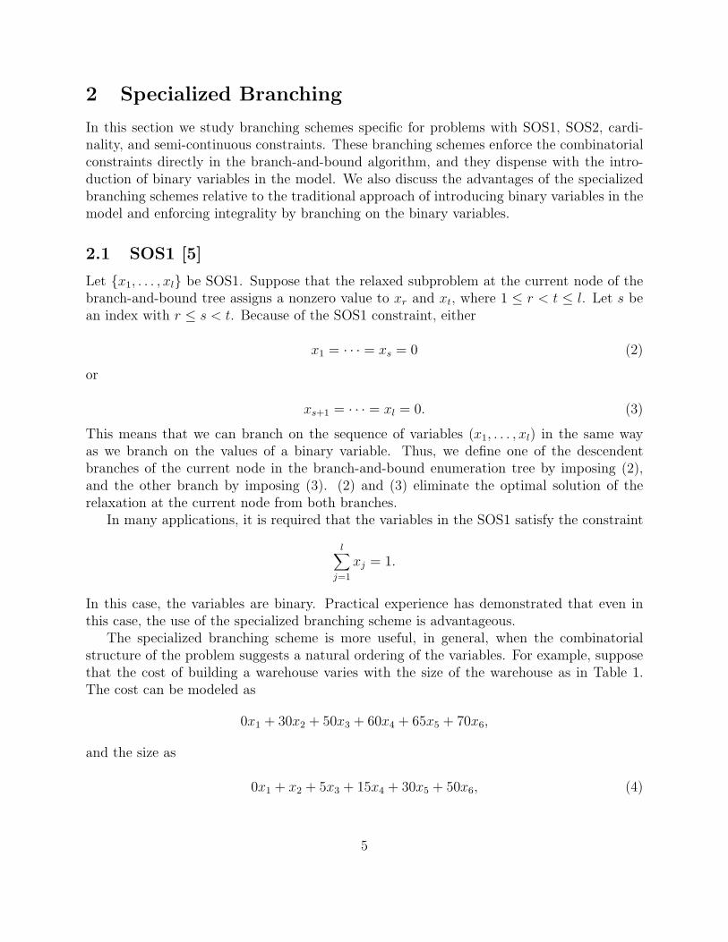
2 Specialized Branching

In this section we study branching schemes speci¯c for problems with SOS1, SOS2, cardi-nality, and semi-continuous constraints. These branching schemes enforce the combinatorialconstraints directly in the branch-and-bound algorithm, and they dispense with the intro-duction of binary variables in the model. We also discuss the advantages of the specializedbranching schemes relative to the traditional approach of introducing binary variables in themodel and enforcing integrality by branching on the binary variables.

2.1 SOS1 [5]

Let fx1; : : : ; xlg be SOS1. Suppose that the relaxed subproblem at the current node of thebranch-and-bound tree assigns a nonzero value to xr and xt, where 1 · r < t · l. Let s bean index with r · s < t. Because of the SOS1 constraint, either

x1 = ¢ ¢ ¢ = xs = 0 (2)

or

xs+1 = ¢ ¢ ¢ = xl = 0: (3)

This means that we can branch on the sequence of variables (x1; : : : ; xl) in the same wayas we branch on the values of a binary variable. Thus, we de¯ne one of the descendentbranches of the current node in the branch-and-bound enumeration tree by imposing (2),and the other branch by imposing (3). (2) and (3) eliminate the optimal solution of therelaxation at the current node from both branches.In many applications, it is required that the variables in the SOS1 satisfy the constraint

lXj=1

xj = 1:

In this case, the variables are binary. Practical experience has demonstrated that even inthis case, the use of the specialized branching scheme is advantageous.The specialized branching scheme is more useful, in general, when the combinatorial

structure of the problem suggests a natural ordering of the variables. For example, supposethat the cost of building a warehouse varies with the size of the warehouse as in Table 1.The cost can be modeled as

0x1 + 30x2 + 50x3 + 60x4 + 65x5 + 70x6;

and the size as

0x1 + x2 + 5x3 + 15x4 + 30x5 + 50x6; (4)

5

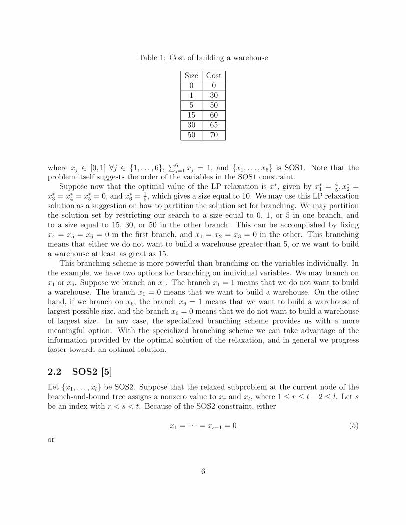
Table 1: Cost of building a warehouse

Size Cost0 01 305 5015 6030 6550 70

where xj 2 [0; 1] 8j 2 f1; : : : ; 6g, P6j=1 xj = 1, and fx1; : : : ; x6g is SOS1. Note that the

problem itself suggests the order of the variables in the SOS1 constraint.Suppose now that the optimal value of the LP relaxation is x¤, given by x¤1 =

45; x¤2 =

x¤3 = x¤4 = x

¤5 = 0, and x

¤6 =

15, which gives a size equal to 10. We may use this LP relaxation

solution as a suggestion on how to partition the solution set for branching. We may partitionthe solution set by restricting our search to a size equal to 0, 1, or 5 in one branch, andto a size equal to 15, 30, or 50 in the other branch. This can be accomplished by ¯xingx4 = x5 = x6 = 0 in the ¯rst branch, and x1 = x2 = x3 = 0 in the other. This branchingmeans that either we do not want to build a warehouse greater than 5, or we want to builda warehouse at least as great as 15.This branching scheme is more powerful than branching on the variables individually. In

the example, we have two options for branching on individual variables. We may branch onx1 or x6. Suppose we branch on x1. The branch x1 = 1 means that we do not want to builda warehouse. The branch x1 = 0 means that we want to build a warehouse. On the otherhand, if we branch on x6, the branch x6 = 1 means that we want to build a warehouse oflargest possible size, and the branch x6 = 0 means that we do not want to build a warehouseof largest size. In any case, the specialized branching scheme provides us with a moremeaningful option. With the specialized branching scheme we can take advantage of theinformation provided by the optimal solution of the relaxation, and in general we progressfaster towards an optimal solution.

2.2 SOS2 [5]

Let fx1; : : : ; xlg be SOS2. Suppose that the relaxed subproblem at the current node of thebranch-and-bound tree assigns a nonzero value to xr and xt, where 1 · r · t¡ 2 · l. Let sbe an index with r < s < t. Because of the SOS2 constraint, either

x1 = ¢ ¢ ¢ = xs¡1 = 0 (5)

or

6

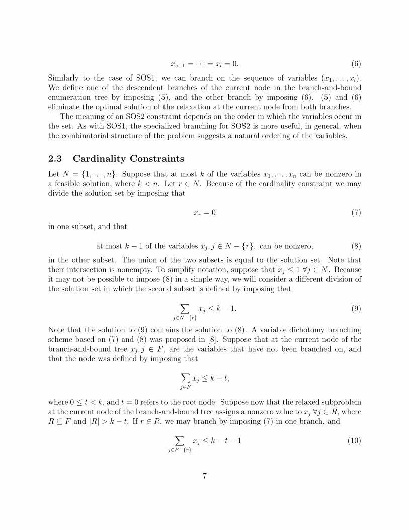
xs+1 = ¢ ¢ ¢ = xl = 0: (6)

Similarly to the case of SOS1, we can branch on the sequence of variables (x1; : : : ; xl).We de¯ne one of the descendent branches of the current node in the branch-and-boundenumeration tree by imposing (5), and the other branch by imposing (6). (5) and (6)eliminate the optimal solution of the relaxation at the current node from both branches.The meaning of an SOS2 constraint depends on the order in which the variables occur in

the set. As with SOS1, the specialized branching for SOS2 is more useful, in general, whenthe combinatorial structure of the problem suggests a natural ordering of the variables.

2.3 Cardinality Constraints

Let N = f1; : : : ; ng. Suppose that at most k of the variables x1; : : : ; xn can be nonzero ina feasible solution, where k < n. Let r 2 N . Because of the cardinality constraint we maydivide the solution set by imposing that

xr = 0 (7)

in one subset, and that

at most k ¡ 1 of the variables xj; j 2 N ¡ frg; can be nonzero, (8)

in the other subset. The union of the two subsets is equal to the solution set. Note thattheir intersection is nonempty. To simplify notation, suppose that xj · 1 8j 2 N . Becauseit may not be possible to impose (8) in a simple way, we will consider a di®erent division ofthe solution set in which the second subset is de¯ned by imposing that

Xj2N¡frg

xj · k ¡ 1: (9)

Note that the solution to (9) contains the solution to (8). A variable dichotomy branchingscheme based on (7) and (8) was proposed in [8]. Suppose that at the current node of thebranch-and-bound tree xj; j 2 F , are the variables that have not been branched on, andthat the node was de¯ned by imposing that

Xj2F

xj · k ¡ t;

where 0 · t < k, and t = 0 refers to the root node. Suppose now that the relaxed subproblemat the current node of the branch-and-bound tree assigns a nonzero value to xj 8j 2 R, whereR µ F and jRj > k ¡ t. If r 2 R, we may branch by imposing (7) in one branch, and

Xj2F¡frg

xj · k ¡ t¡ 1 (10)

7

in the other branch. The inequality (10) does not necessarily eliminate the optimal solutionof the relaxation at the current node from the branch it de¯nes, except after k branches,when t = k.An alternative branching scheme, in which one branches on sets of variables rather than

on individual variables was proposed by de Farias et al. in [16]. Let S µ N , and 0 · s ·minfk; jSjg. We may partition the solution set by imposing that

at most s of the variables xj; j 2 S; can be nonzero, (11)

and

at least s+ 1 of the variables xj; j 2 S; must be nonzero. (12)

Because of the cardinality constraint, (12) implies that

at most k ¡ s¡ 1 of the variables xj; j 2 N ¡ S; can be nonzero. (13)

Again, because it may not be possible to impose (11) and (13) in a simple way, we replace(11) and (13) by

Xj2Sxj · s: (14)

and

Xj2N¡S

xj · k ¡ s¡ 1; (15)

respectively, and we divide the solution set by imposing (14) in one subset and (15) in theother subset. Note that when S = frg and s = 0, this division scheme coincides with thevariable dichotomy division scheme of [8].Suppose that the current node of the branch-and-bound tree was de¯ned by imposing

(14). The case S = N and s = k refers to the root node. Suppose that the relaxedsubproblem at the current node assigns a nonzero value to xj 8j 2 R, where R µ S andjRj > s. We may branch by imposing

Xj2R1

xj · bs2c (16)

in one branch, and

Xj2R¡R1

xj · s¡ bs2c ¡ 1; (17)

in the other branch, where R1 ½ R and jR1j = b jRj2c. Note that (16) and (17) do not

necessarily eliminate the optimal solution of the relaxation at the current node from thebranches they de¯ne. However, they guarantee to eliminate it in about log k branches.

8

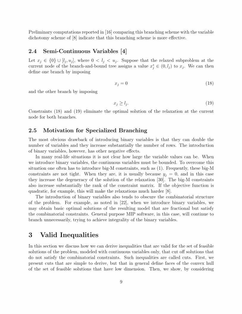
Preliminary computations reported in [16] comparing this branching scheme with the variabledichotomy scheme of [8] indicate that this branching scheme is more e®ective.

2.4 Semi-Continuous Variables [4]

Let xj 2 f0g [ [lj; uj ], where 0 < lj < uj. Suppose that the relaxed subproblem at thecurrent node of the branch-and-bound tree assigns a value x¤j 2 (0; lj) to xj. We can thende¯ne one branch by imposing

xj = 0 (18)

and the other branch by imposing

xj ¸ lj: (19)

Constraints (18) and (19) eliminate the optimal solution of the relaxation at the currentnode for both branches.

2.5 Motivation for Specialized Branching

The most obvious drawback of introducing binary variables is that they can double thenumber of variables and they increase substantially the number of rows. The introductionof binary variables, however, has other negative e®ects.In many real-life situations it is not clear how large the variable values can be. When

we introduce binary variables, the continuous variables must be bounded. To overcome thissituation one often has to introduce big-M constraints, such as (1). Frequently, these big-Mconstraints are not tight. When they are, it is usually because yj = 0, and in this casethey increase the degeneracy of the solution of the relaxation [30]. The big-M constraintsalso increase substantially the rank of the constraint matrix. If the objective function isquadratic, for example, this will make the relaxations much harder [8].The introduction of binary variables also tends to obscure the combinatorial structure

of the problem. For example, as noted in [22], when we introduce binary variables, wemay obtain basic optimal solutions of the resulting model that are fractional but satisfythe combinatorial constraints. General purpose MIP software, in this case, will continue tobranch unnecessarily, trying to achieve integrality of the binary variables.

3 Valid Inequalities

In this section we discuss how we can derive inequalities that are valid for the set of feasiblesolutions of the problem, modeled with continuous variables only, that cut o® solutions thatdo not satisfy the combinatorial constraints. Such inequalities are called cuts. First, wepresent cuts that are simple to derive, but that in general de¯ne faces of the convex hullof the set of feasible solutions that have low dimension. Then, we show, by considering

9

problems with SOS1 constraints, how we can derive cuts that are harder to compute, butthat in general de¯ne faces of higher dimension.

3.1 Simple Inequalities

Given a basic optimal solution of the relaxation in the current node that is not feasible, itis usually easy to derive an inequality that is valid and that cuts o® this solution [23, 24].

Theorem 1 Suppose that at most k of the variables x1; : : : ; xk+1 can be positive, and thatin a basic solution,

x1 = ®10 ¡Pj2N ®1jxj

...xk+1 = ®k+1;0 ¡P

j2N ®k+1;jxj;

where ®i0 > 0 8i 2 f1; : : : ; k + 1g, and xj; j 2 N , are the nonbasic variables. Let

¯j = maxf®1j®10; : : : ;

®k+1;j®k+1;0

g:

Then,

Xj2N

¯jxj ¸ 1 (20)

is a valid inequality.

Proof Because at most k variables can be positive at least one of the following equalitiesmust hold P

j2N®1j®10xj = 1...P

j2N®k+1;j®k+1;0

xj = 1:

This implies that (20) is valid. 2

The inequality (20) cuts o® the current basic optimal solution of the relaxation that doesnot satisfy the cardinality constraint. A similar type of inequality can be derived when thevariables are subject to SOS1 and SOS2 constraints.We now consider the case of semi-continuous constraints.

Theorem 2 Suppose that xr 2 f0g [ [lr; ur], where 0 < lr < ur. Suppose that in a basicoptimal solution of the relaxation,

xr = ®r0 ¡Xj2N

®rjxj;

10

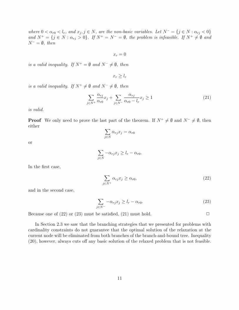
where 0 < ®r0 < lr, and xj; j 2 N , are the non-basic variables. Let N¡ = fj 2 N : ®rj < 0gand N+ = fj 2 N : ®rj > 0g. If N+ = N¡ = ;, the problem is infeasible. If N+ 6= ; andN¡ = ;, then

xr = 0

is a valid inequality. If N+ = ; and N¡ 6= ;, then

xr ¸ lris a valid inequality. If N+ 6= ; and N¡ 6= ;, then

Xj2N+

®rj®r0xj +

Xj2N¡

®rj®r0 ¡ lrxj ¸ 1 (21)

is valid.

Proof We only need to prove the last part of the theorem. If N+ 6= ; and N¡ 6= ;, theneither X

j2N®rjxj = ®r0

or Xj2N

¡®rjxj ¸ lr ¡ ®r0:

In the ¯rst case,

Xj2N+

®rjxj ¸ ®r0; (22)

and in the second case,

Xj2N¡

¡®rjxj ¸ lr ¡ ®r0: (23)

Because one of (22) or (23) must be satis¯ed, (21) must hold. 2

In Section 2.3 we saw that the branching strategies that we presented for problems withcardinality constraints do not guarantee that the optimal solution of the relaxation at thecurrent node will be eliminated from both branches of the branch-and-bound tree. Inequality(20), however, always cuts o® any basic solution of the relaxed problem that is not feasible.

11

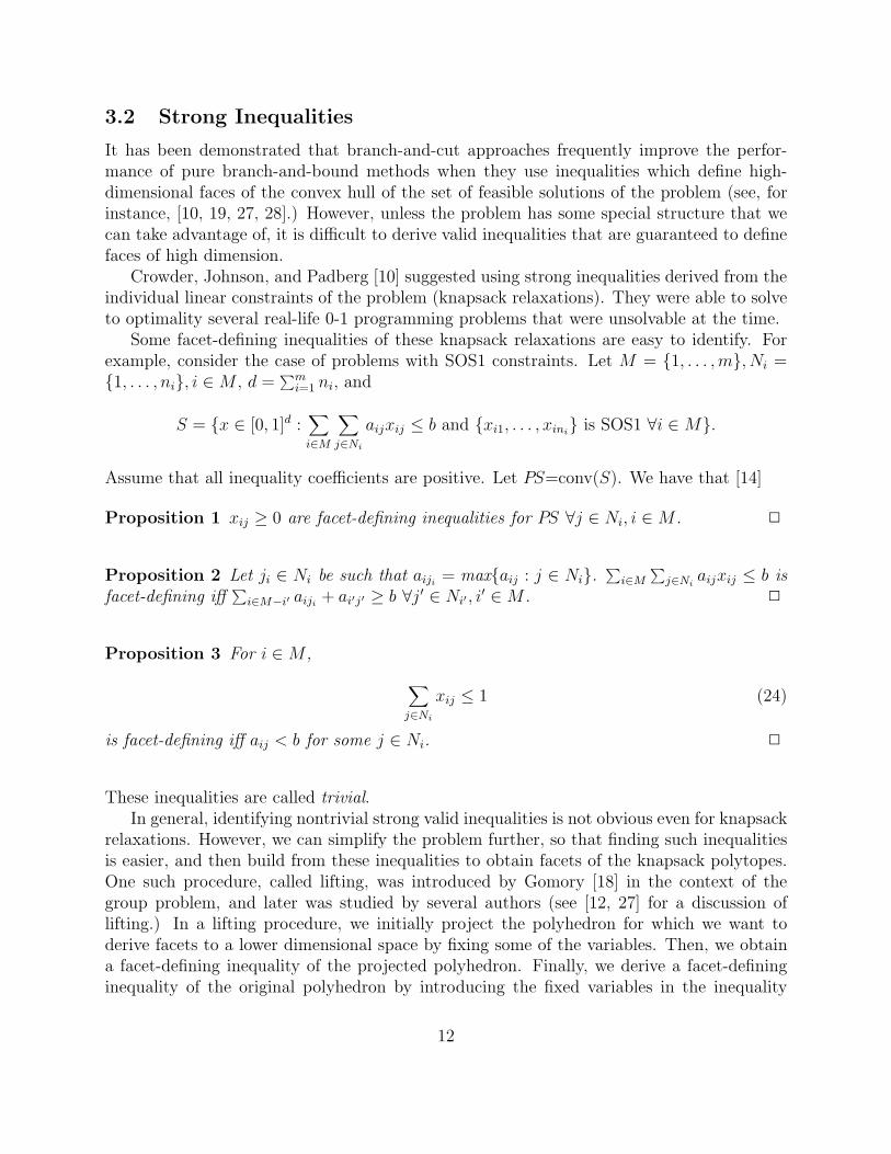
3.2 Strong Inequalities

It has been demonstrated that branch-and-cut approaches frequently improve the perfor-mance of pure branch-and-bound methods when they use inequalities which de¯ne high-dimensional faces of the convex hull of the set of feasible solutions of the problem (see, forinstance, [10, 19, 27, 28].) However, unless the problem has some special structure that wecan take advantage of, it is di±cult to derive valid inequalities that are guaranteed to de¯nefaces of high dimension.Crowder, Johnson, and Padberg [10] suggested using strong inequalities derived from the

individual linear constraints of the problem (knapsack relaxations). They were able to solveto optimality several real-life 0-1 programming problems that were unsolvable at the time.Some facet-de¯ning inequalities of these knapsack relaxations are easy to identify. For

example, consider the case of problems with SOS1 constraints. Let M = f1; : : : ;mg; Ni =f1; : : : ; nig; i 2M , d = Pm

i=1 ni, and

S = fx 2 [0; 1]d : Xi2M

Xj2Ni

aijxij · b and fxi1; : : : ; xinig is SOS1 8i 2Mg:

Assume that all inequality coe±cients are positive. Let PS=conv(S). We have that [14]

Proposition 1 xij ¸ 0 are facet-de¯ning inequalities for PS 8j 2 Ni; i 2M . 2

Proposition 2 Let ji 2 Ni be such that aiji = maxfaij : j 2 Nig.Pi2M

Pj2Ni aijxij · b is

facet-de¯ning i®Pi2M¡i0 aiji + ai0j0 ¸ b 8j0 2 Ni0 ; i0 2M . 2

Proposition 3 For i 2M ,Xj2Ni

xij · 1 (24)

is facet-de¯ning i® aij < b for some j 2 Ni. 2

These inequalities are called trivial.In general, identifying nontrivial strong valid inequalities is not obvious even for knapsack

relaxations. However, we can simplify the problem further, so that ¯nding such inequalitiesis easier, and then build from these inequalities to obtain facets of the knapsack polytopes.One such procedure, called lifting, was introduced by Gomory [18] in the context of thegroup problem, and later was studied by several authors (see [12, 27] for a discussion oflifting.) In a lifting procedure, we initially project the polyhedron for which we want toderive facets to a lower dimensional space by ¯xing some of the variables. Then, we obtaina facet-de¯ning inequality of the projected polyhedron. Finally, we derive a facet-de¯ninginequality of the original polyhedron by introducing the ¯xed variables in the inequality

12

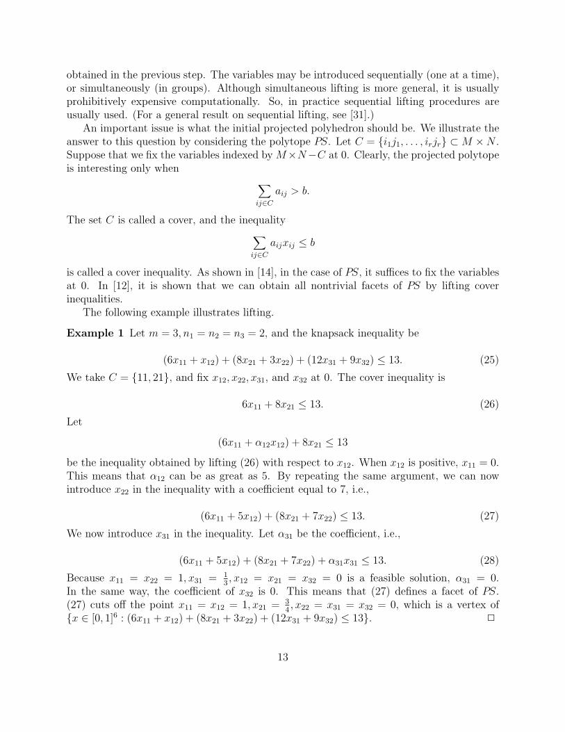
obtained in the previous step. The variables may be introduced sequentially (one at a time),or simultaneously (in groups). Although simultaneous lifting is more general, it is usuallyprohibitively expensive computationally. So, in practice sequential lifting procedures areusually used. (For a general result on sequential lifting, see [31].)An important issue is what the initial projected polyhedron should be. We illustrate the

answer to this question by considering the polytope PS. Let C = fi1j1; : : : ; irjrg ½M £N .Suppose that we ¯x the variables indexed byM£N¡C at 0. Clearly, the projected polytopeis interesting only when X

ij2Caij > b:

The set C is called a cover, and the inequalityXij2C

aijxij · b

is called a cover inequality. As shown in [14], in the case of PS, it su±ces to ¯x the variablesat 0. In [12], it is shown that we can obtain all nontrivial facets of PS by lifting coverinequalities.The following example illustrates lifting.

Example 1 Let m = 3; n1 = n2 = n3 = 2, and the knapsack inequality be

(6x11 + x12) + (8x21 + 3x22) + (12x31 + 9x32) · 13: (25)

We take C = f11; 21g, and ¯x x12; x22; x31; and x32 at 0. The cover inequality is

6x11 + 8x21 · 13: (26)

Let

(6x11 + ®12x12) + 8x21 · 13be the inequality obtained by lifting (26) with respect to x12. When x12 is positive, x11 = 0.This means that ®12 can be as great as 5. By repeating the same argument, we can nowintroduce x22 in the inequality with a coe±cient equal to 7, i.e.,

(6x11 + 5x12) + (8x21 + 7x22) · 13: (27)

We now introduce x31 in the inequality. Let ®31 be the coe±cient, i.e.,

(6x11 + 5x12) + (8x21 + 7x22) + ®31x31 · 13: (28)

Because x11 = x22 = 1; x31 =13; x12 = x21 = x32 = 0 is a feasible solution, ®31 = 0.

In the same way, the coe±cient of x32 is 0. This means that (27) de¯nes a facet of PS.(27) cuts o® the point x11 = x12 = 1; x21 =

34; x22 = x31 = x32 = 0, which is a vertex of

fx 2 [0; 1]6 : (6x11 + x12) + (8x21 + 3x22) + (12x31 + 9x32) · 13g. 2

13

References [12] and [14] contain a polyhedral study of PS. References [12] and [13] containseveral results on lifted cover inequalities for problems with SOS2. Reference [16] containsresults on lifted cover inequalities for problems with cardinality constraints.

4 A Generalized Assignment Problem with SOS2

In this section we present a simpli¯ed version of a production scheduling problem in whichthe concept of SOS2 arises naturally in the formulation. This problem was ¯rst discussedin [20] in the context of ¯ber optic cable manufacturing. References [12] and [13] containa polyhedral discussion of the problem. Based on these polyhedral results, de Farias andNemhauser [15] developed an e±cient branch-and-cut scheme for the 0-1 generalized assign-ment problem.

4.1 Problem Formulation

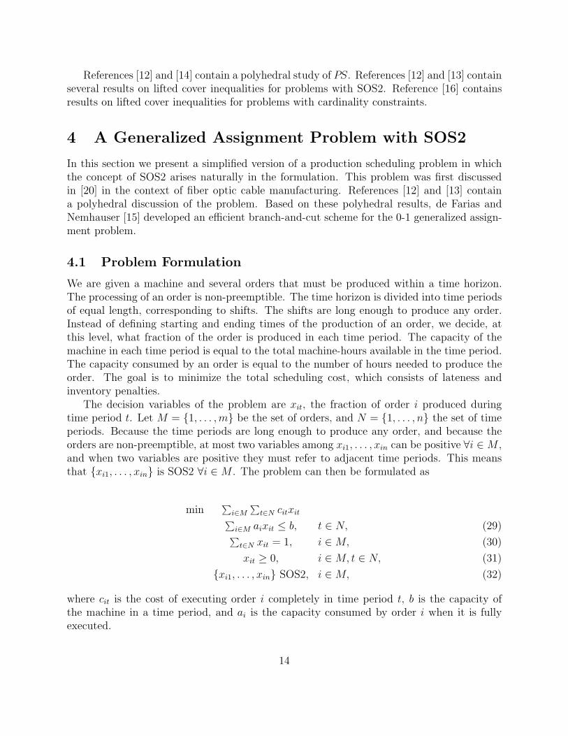
We are given a machine and several orders that must be produced within a time horizon.The processing of an order is non-preemptible. The time horizon is divided into time periodsof equal length, corresponding to shifts. The shifts are long enough to produce any order.Instead of de¯ning starting and ending times of the production of an order, we decide, atthis level, what fraction of the order is produced in each time period. The capacity of themachine in each time period is equal to the total machine-hours available in the time period.The capacity consumed by an order is equal to the number of hours needed to produce theorder. The goal is to minimize the total scheduling cost, which consists of lateness andinventory penalties.The decision variables of the problem are xit, the fraction of order i produced during

time period t. Let M = f1; : : : ;mg be the set of orders, and N = f1; : : : ; ng the set of timeperiods. Because the time periods are long enough to produce any order, and because theorders are non-preemptible, at most two variables among xi1; : : : ; xin can be positive 8i 2M ,and when two variables are positive they must refer to adjacent time periods. This meansthat fxi1; : : : ; xing is SOS2 8i 2M . The problem can then be formulated as

minPi2M

Pt2N citxitP

i2M aixit · b; t 2 N; (29)Pt2N xit = 1; i 2M; (30)

xit ¸ 0; i 2M; t 2 N; (31)

fxi1; : : : ; xing SOS2; i 2M; (32)

where cit is the cost of executing order i completely in time period t, b is the capacity ofthe machine in a time period, and ai is the capacity consumed by order i when it is fullyexecuted.

14

By modifying the objective function coe±cients appropriately, (30) can be replaced by

Xt2N

xit · 1; i 2M (33)

(see [12].) In our polyhedral analysis, we use the inequality formulation, because, in it, theconvex hull of the set of feasible solutions is a full-dimensional polytope.

4.2 Polyhedral Results

Let F be the set of solutions, PF =conv(F ), and LPF the set of solutions of the LP relaxation,i.e. LPF = fx 2 <mn : x satis¯es (29), (33), and (31)g. We can obtain facet-de¯ninginequalities for PF using the procedure illustrated in Section 3.2, i.e. we ¯x some of thevariables, we obtain a facet-de¯ning inequality for the projected polytope, and we lift theinequality with respect to the variables that were ¯xed.

Example 2 Let m = 3; n = 4; a1 = 2; a2 = 4; a3 = 5, and b = 5. Fix xit = 0 8(i; t) 6=(1; 1); (2; 1). The inequality

2x11 + 4x21 · 5 (34)

de¯nes a facet of the resulting polytope. We now lift (34) with respect to x13. Let ®13 bethe lifting coe±cient, i.e.

2x11 + ®13x13 + 4x21 · 5:

Because of the SOS2 constraint, when x13 > 0, x11 = 0. This means that ®13 can be as largeas 1, and therefore,

2x11 + x13 + 4x21 · 5 (35)

de¯nes a facet of PF \ fx 2 <mn : xit = 0 8(i; t)6= (1; 1); (1; 3); (2; 1)g. If we now lift (35)with respect to x14; x23; x24; x12; x22, and x31; : : : ; x34, in the given order, we obtain

2x11 + x13 + x14 + 4x21 + 3x23 + 3x24 · 5; (36)

which de¯nes a facet of PF . Inequality (36) cuts o® the point x11 = 1; x21 =34; x23 = 14,

which is a vertex of LPF that does not satisfy (32). 2

We say that I µM is an l-cover if lb <Pi2I ai < (l+1)b. Given an l-cover I, we denote

a(l)i = maxf0; lb¡P

j2I¡fig ajg, i 2M . The inequality (36) can be generalized as follows.

15

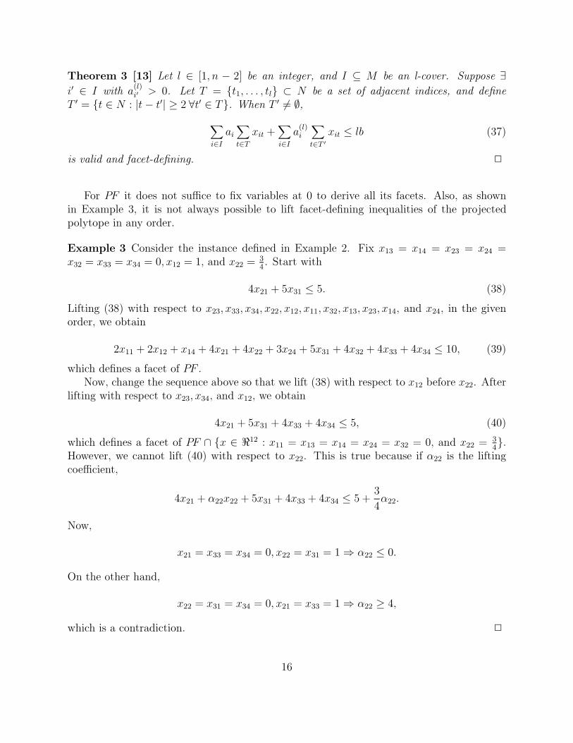
Theorem 3 [13] Let l 2 [1; n ¡ 2] be an integer, and I µ M be an l-cover. Suppose 9i0 2 I with a

(l)i0 > 0. Let T = ft1; : : : ; tlg ½ N be a set of adjacent indices, and de¯ne

T 0 = ft 2 N : jt¡ t0j ¸ 2 8t0 2 Tg. When T 0 6= ;,Xi2IaiXt2Txit +

Xi2Ia(l)i

Xt2T 0

xit · lb (37)

is valid and facet-de¯ning. 2

For PF it does not su±ce to ¯x variables at 0 to derive all its facets. Also, as shownin Example 3, it is not always possible to lift facet-de¯ning inequalities of the projectedpolytope in any order.

Example 3 Consider the instance de¯ned in Example 2. Fix x13 = x14 = x23 = x24 =x32 = x33 = x34 = 0; x12 = 1, and x22 =

34. Start with

4x21 + 5x31 · 5: (38)

Lifting (38) with respect to x23; x33; x34; x22; x12; x11; x32; x13; x23; x14, and x24, in the givenorder, we obtain

2x11 + 2x12 + x14 + 4x21 + 4x22 + 3x24 + 5x31 + 4x32 + 4x33 + 4x34 · 10; (39)

which de¯nes a facet of PF .Now, change the sequence above so that we lift (38) with respect to x12 before x22. After

lifting with respect to x23; x34, and x12, we obtain

4x21 + 5x31 + 4x33 + 4x34 · 5; (40)

which de¯nes a facet of PF \ fx 2 <12 : x11 = x13 = x14 = x24 = x32 = 0, and x22 = 34g.

However, we cannot lift (40) with respect to x22. This is true because if ®22 is the liftingcoe±cient,

4x21 + ®22x22 + 5x31 + 4x33 + 4x34 · 5 + 34®22:

Now,

x21 = x33 = x34 = 0; x22 = x31 = 1) ®22 · 0:

On the other hand,

x22 = x31 = x34 = 0; x21 = x33 = 1) ®22 ¸ 4;

which is a contradiction. 2

16

4.3 Computational Results

We report computational experience using a branch-and-cut scheme without binary variablesand a branch-and-bound algorithm without binary variables to solve the problem. In thebranch-and-cut algorithm we use inequalities (37), plus two other families of inequalitiesdescribed in [13], as cuts.Our computational experiments were performed over a set of 55 test problems randomly

generated. In all test problems each SOS2 had 20 variables, and the number of sets rangedfrom 100 to 200 with intervals of 10. For a given problem size we tested 5 di®erent instances.The size of the problems ranged from 120 constraints (not including nonnegativity) and 2,000variables to 220 constraints and 4,000 variables. Although this study was based on a realapplication, described in detail in [20], and solved by branch-and-bound, it was necessary touse random data in the computation since the real data was no longer available. However,insofar as possible, we based the random data on the type of data in the application. Forother details, such as node selection, branching, and separation strategies we refer to [13].We used an IBM RS6000/590 to run our test problems and MINTO 3.0 as branch-and-boundalgorithm and CPLEX 6.0 as LP solver. We limited the size of the branching tree to 50,000nodes.Of the 55 problems tested, the pure branch-and-bound approach could not ¯nd a feasible

solution for 19 problems, and it could not ¯nd an optimal solution or prove optimality for 5of the remaining problems. With the branch-and-cut approach, all 55 problems were solvedto proven optimality.Table 2 has for each problem size the average CPU time in seconds with and without cut

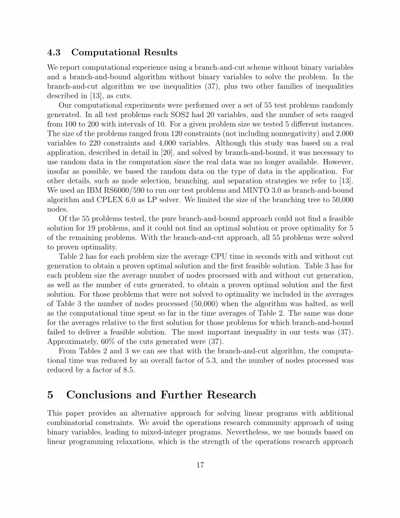
generation to obtain a proven optimal solution and the ¯rst feasible solution. Table 3 has foreach problem size the average number of nodes processed with and without cut generation,as well as the number of cuts generated, to obtain a proven optimal solution and the ¯rstsolution. For those problems that were not solved to optimality we included in the averagesof Table 3 the number of nodes processed (50,000) when the algorithm was halted, as wellas the computational time spent so far in the time averages of Table 2. The same was donefor the averages relative to the ¯rst solution for those problems for which branch-and-boundfailed to deliver a feasible solution. The most important inequality in our tests was (37).Approximately, 60% of the cuts generated were (37).From Tables 2 and 3 we can see that with the branch-and-cut algorithm, the computa-

tional time was reduced by an overall factor of 5.3, and the number of nodes processed wasreduced by a factor of 8.5.

5 Conclusions and Further Research

This paper provides an alternative approach for solving linear programs with additionalcombinatorial constraints. We avoid the operations research community approach of usingbinary variables, leading to mixed-integer programs. Nevertheless, we use bounds based onlinear programming relaxations, which is the strength of the operations research approach

17

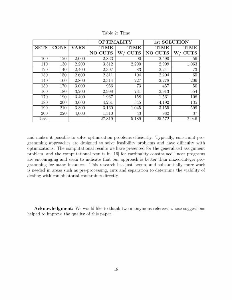
Table 2: Time

OPTIMALITY 1st SOLUTIONSETS CONS VARS TIME TIME TIME TIME

NO CUTS W/ CUTS NO CUTS W/ CUTS100 120 2,000 2,833 90 2,590 56110 130 2,200 3,312 2,290 2,999 1,063120 140 2,400 2,397 83 2,241 73130 150 2,600 2,311 104 2,204 65140 160 2,800 2,314 227 2,278 206150 170 3,000 956 73 457 50160 180 3,200 2,998 731 2,913 554170 190 3,400 1,967 158 1,561 108180 200 3,600 4,261 345 4,192 135190 210 3,800 3,160 1,045 3,155 599200 220 4,000 1,310 43 982 37

Total 27,819 5,189 25,572 2,946

and makes it possible to solve optimization problems e±ciently. Typically, constraint pro-gramming approaches are designed to solve feasibility problems and have di±culty withoptimizations. The computational results we have presented for the generalized assignmentproblem, and the computational results in [16] for cardinality constrained linear programsare encouraging and seem to indicate that our approach is better than mixed-integer pro-gramming for many instances. This research has just begun, and substantially more workis needed in areas such as pre-processing, cuts and separation to determine the viability ofdealing with combinatorial constraints directly.

Acknowledgment: We would like to thank two anonymous referees, whose suggestionshelped to improve the quality of this paper.

18

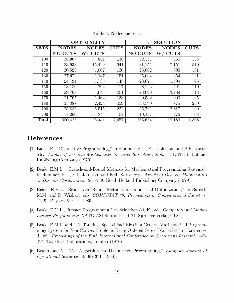
Table 3: Nodes and cuts

OPTIMALITY 1st SOLUTIONSETS NODES NODES CUTS NODES NODES CUTS

NO CUTS W/ CUTS NO CUTS W/ CUTS100 38,967 881 138 32,351 456 135110 33,933 15,429 641 31,251 7,151 510120 30,523 1,067 130 26,662 898 101130 27,679 1,147 151 25,094 654 121140 24,191 1,735 143 23,674 1,499 96150 18,180 792 117 8,243 421 110160 29,708 4,645 201 28,020 3,239 118170 21,707 1,462 138 20,532 900 95180 35,388 2,424 459 33,599 875 250190 25,889 5,515 232 25,791 2,817 169200 14,260 344 107 10,437 276 103

Total 300,425 35,441 2,457 265,654 19,186 1,808

References

[1] Balas, E., \Disjunctive Programming," in Hammer, P.L., E.L. Johnson, and B.H. Korte,eds., Annals of Discrete Mathematics 5: Discrete Optimization, 3-51, North HollandPublishing Company (1979).

[2] Beale, E.M.L., \Branch-and-Bound Methods for Mathematical Programming Systems,"in Hammer, P.L., E.L. Johnson, and B.H. Korte, eds., Annals of Discrete Mathematics5: Discrete Optimization, 201-219, North Holland Publishing Company (1979).

[3] Beale, E.M.L.,\Branch-and-Bound Methods for Numerical Optimization," in Barritt,M.M. and D. Wishart, eds. COMPSTAT 80: Proceedings in Computational Statistics,11-20, Physica Verlag (1980).

[4] Beale, E.M.L.,\Integer Programming," in Schittkowski, K., ed., Computational Mathe-matical Programming, NATO ASI Series, f15, 1-24, Springer-Verlag (1985).

[5] Beale, E.M.L. and J.A. Tomlin, \Special Facilities in a General Mathematical Program-ming System for Non-Convex Problems Using Ordered Sets of Variables," in Lawrence,J., ed., Proceedings of the Fifth International Conference on Operations Research, 447-454, Tavistock Publications, London (1970).

[6] Beaumont, N., \An Algorithm for Disjunctive Programming," European Journal ofOperational Research 48, 362-371 (1990).

19

[7] Biegler, L.T., I.E. Grossmann, and A.W. Westerberg, Systematic Methods of ChemicalProcess Design, Prentice Hall, Inc., Upper Saddle River, NJ (1997)

[8] Bienstock, D., \Computational Study of a Family of Mixed-Integer Quadratic Program-ming Problems," Mathematical Programming, 74, 121-140 (1996).

[9] Brimberg, J., and R.F. Love, \Solving a Class of Two-Dimensional UncapacitatedLocation-Allocation Problems by Dynamic Programming," Operations Research 46, 702-709 (1998)

[10] Crowder, H., E.L. Johnson, and M.W. Padberg, \Solving Large Scale Zero-One LinearProgramming Problems," Operations Research 31, 803-834 (1983).

[11] Dantzig, G.B., \On the Signi¯cance of Solving Linear Programming Problems withSome Integer Variables," Econometrica 28, 30-44 (1960).

[12] de Farias, I.R., \A Polyhedral Approach to Combinatorial Complementarity Problems,"Ph.D. Thesis, School of Industrial and Systems Engineering, Georgia Institute of Tech-nology (1995).

[13] de Farias, I.R., E.L. Johnson, and G.L. Nemhauser, \A Generalized Assignment Prob-lem with Special Ordered Sets: A Polyhedral Approach, to appear in MathematicalProgramming.

[14] de Farias, I.R., E.L. Johnson, and G.L. Nemhauser \Facets of the ComplementarityKnapsack Polytope," LEC-98-08, School of Industrial and Systems Engineering, GeorgiaInstitute of Technology (1998).

[15] de Farias, I.R. and G.L. Nemhauser,\A Family of Inequalities for the Generalized Assign-ment Polytope," LEC, School of Industrial and Systems Engineering, Georgia Instituteof Technology (2000).

[16] de Farias, I.R., E.L. Johnson, E.K. Lee, and J.-P. Richard, \A Branch-and-Cut Ap-proach to Cardinality Constrained Optimization Problems," in preparation.

[17] Gomory, R.E., \Outline of an Algorithm for Integer Solutions to Linear Programs,"Bulletin of the American Mathematical Society, 64, 275-278 (1958).

[18] Gomory, R.E., \On the Relation between Integer and Non-Integer Solutions to LinearPrograms," Proceedings of the National Academy of Science 53, 260-265 (1965).

[19] GrÄotschel, M., M. JÄunger, and G. Reinelt, \A Cutting Plane Algorithm for the LinearOrdering Problem," Operations Research 32, 1195-1220 (1984).

[20] Gue, K.R., G.L. Nemhauser, and M. Padron \Production Scheduling in MultiprocessorFlowshops," IIE Transactions 29, 391-398 (1997).

20

[21] Healy, W.C., \Multiple Choice Programming (A Procedure for Linear Programmingwith Zero-One Variables)," Operations Research 12, 122-138 (1964).

[22] Hooker, J.N., and M.A. Osorio, \Mixed Logical/Linear Programming," GSIA, CarnegieMellon University (1997).

[23] Ibaraki, T., \The Use of Cuts in Complementary Programming," in Balas, E., R.W.Cottle, T.C. Hu, and M.J.L. Kirby, eds., Contributions to Programming and Applica-tions, ORSA (1973).

[24] Jeroslow, R.G., \Cutting Planes for Complementarity Constraints," SIAM Journal ofControl and Optimization, 16, 56-62 (1978).

[25] Markowitz, H.M., and A.S. Manne, \On the Solution of Discrete Programming Prob-lems," Econometrica 25, 84-110 (1957).

[26] Nauss, R.M., \The 0-1 Knapsack Problem with Multiple-Choice Constraints," EuropeanJournal of Operations Research, 2, 125-131 (1978).

[27] Nemhauser, G.L. and L.A. Wolsey, Integer Programming and Combinatorial Optimiza-tion, John Wiley and Sons (1988).

[28] Padberg, M. and G. Rinaldi, \Optimization of a 532 City Symmetric Traveling SalesmanProblem by Branch and Cut," Operations Research Letters 6, 1-7 (1987).

[29] Raman, R., and I.E. Grossmann, \Symbolic Integration of Logic in MILP Branch-and-Bound Methods for the Synthesis of Process Networks," Annals of Operations Research42, 169-191 (1993).

[30] Savelsbergh, M.W.P., personal communication.

[31] Wolsey, L.A., \Facets and Strong Valid Inequalities for Integer Programs," OperationsResearch 24, 267-372 (1976).

21