bradley-terry model for assessing the performance of ten odi ...

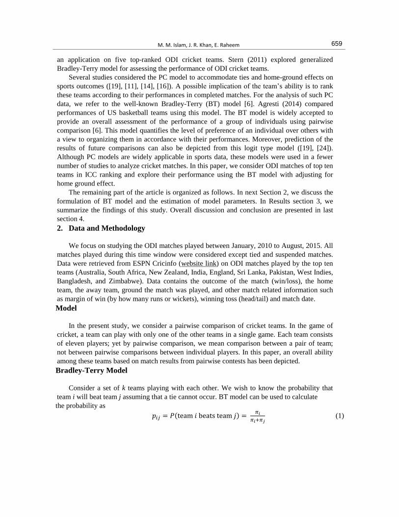
BRADLEY-TERRY MODEL FOR ASSESSING THE PERFORMANCE OF

TEN ODI CRICKET TEAMS

ADJUSTING FOR HOME GROUND EFFECT

Md. Mazharul Islam1, Jahidur Rahman Khan1, Enayetur Raheem2

1Institute of Statistical Research and Training, University of Dhaka 2 Biomedical Research Foundation (BRF), Dhaka, Bangladesh

Abstract: The analysis of sports data, especially cricket is an interesting field for the statisticians.

Every year, a large number of cricket tournaments take place among the cricket playing nations. It

is of interest to study their performance when they play with each other in a one-day international

(ODI) match or a test match. In this study, we assess the performance of top ten cricket teams in the

ODI cricket match and make a comparison among them. The abilities of teams change over time.

As a result, not a single team dominates the game over a long period. Therefore, a paired

comparison method is more reliable and appropriate to compare more than two teams at the same

time based on the outcomes of the matches they play. Arguably, a team’s performance also depends

on whether they play at home or away. In this study, we consider Bradley-Terry model, a widely

accepted model for pairwise comparison. In that, we consider home and away effect to demonstrate

how the home advantages differ among these teams.

Key words: Pairwise comparison, measuring performance in Cricket, home and

away effect.

1. Introduction

The game of cricket is popular in many countries and is getting even more popularity

day-by-day. During 2011 and 2015, a total of 981 cricket matches have been played in different

formats: 210 test matches, 493 ODI matches, and 278 T-20 matches [14]. The International

Cricket Council (ICC) has 106 members: 10 full members, 39 associate members and 56

affiliate members [14]. The number of cricket playing countries varies in ODI and T-20 formats

(all full members plus a few members from the associate and affiliate members), although only

the countries with full-membership play test cricket. Ranking the member countries is an

interesting and ongoing process. It is of great importance to the fans to compare among the

teams particularly ahead of a multi-nation tournament. Normally, a team with a higher rank gets

somewhat more attention. However, upset happens as a team with a higher rank may not

necessarily win over a lower ranked team. Arguably, in a multi-nation tournament, a team with

better performance in the recent past compared to others is more likely to perform better in the

competition such as reaching the quarter-final or semi-final stages. This likelihood may affect

supporters, sponsors, as well as team management towards the selection of players for a

particular game in the tournament.

Journal of Data Science 16(2017), 657-668

Bradley-Terry model for assessing the performance of ten ODI cricket teams adjusting for home ground effect

Cricket is played by two teams with 11 players each. The game is divided into two phases:

batting and bowling. A toss decides which team would bat first or bowl first. Performance can

be measured at the individual level and at the team level over the two phases of a match.

Gweshe and Durbach (2013) studied the efficiency of individual player performance at 2011

world cup cricket using a combined data envelopment analysis (DEA) and stochastic multi

criteria acceptability analysis (SMAA) approach where players specific inputs such as balls

faced by the batsmen and balls bowled by the bowlers are converted outputs indicative of

performance. Substantial discrepancies were identified between the players’ rank ordering by

efficiency and by traditional absolute measures of performance [12]. Moreover, they found the

combination of DEA and SMAA methods appears to be a useful technique to measure the

efficiency of cricket players in the limited over game. Lewis (2008) provided ranking among

players based on individual batting, bowling and all-round (both batting and bowling)

performances in ODI cricket. Predicting match outcomes and identifying factors associated

with it are often of interest that have been found in the literature. Louzada et al. (2014)

considered a linear model to predict match outcomes in the English Premier League. Cerqueira

et al. (2017) proposed a latent causal model to measure the team quality and its correlates.

However, the performance of a cricket team is measured by the outcome of a match - win, loss

or tie. The outcome of a cricket match depends on a number of known and unknown factors. It

has been found in the literature that apart from the strength of each team, the strength of the

opponent, the venue, toss and a number of other factors may influence the result of a match ([9],

[10], [4]). Clarke (1988) studied optimal scoring rates using dynamic programming methods

and suggested that teams would be better served by scoring at higher rates early in the innings.

de Silva and Swartz (1997) showed that toss of a match provides no competitive advantage,

whereas home advantage increases the probability of winning of a team in ODI cricket. Bailey

and Clarke (2006) explored the impact of different factors on the outcome of ODI cricket

matches such as a home ground advantage, team quality, and current form of the players.

Allsopp and Clarke (2004) measured and compared the strength of teams in terms of overall

ratings, which is obtained by combining batting and bowling ratings of the respective teams, for

ODI and test matches for the period of 1997 to 2001 using multiple linear regression

techniques.

Method of paired comparisons (PC) is used often to rank different sports teams, where

preference among teams is often the main objective of interest. PC is a well-established method,

where individuals are asked to repeatedly judge which of the pairwise objects they prefer on the

basis of evaluation [21]. The PC data are expressed as a preference matrix, which is analyzed

through PC models. Thurstone (1927) studied that the outcomes of the pairwise comparison

follow a normal distribution, but Bradley (1953) assumed logistic distribution to present PC

models. Stern (1990a, 1990b) proposed the gamma models for PC. Thurstone-Mosteller model

for PC was used to analyze volleyball data [7], Stern used a PC model to analyze sports datasets

for the National League baseball season, and football data were analyzed by using

Bradley-Terry model ([7], [20], [13]). Neil and Jonathan (2015) investigated the use of

Bradley-Terry models to analyze test match cricket, Abbas and Aslam (2009) showed that any

group of individuals may be ranked using the Cauchy PC model via a Bayesian approach with

658

M. M. Islam, J. R. Khan, E. Raheem

an application on five top-ranked ODI cricket teams. Stern (2011) explored generalized

Bradley-Terry model for assessing the performance of ODI cricket teams.

Several studies considered the PC model to accommodate ties and home-ground effects on

sports outcomes ([19], [11], [14], [16]). A possible implication of the team’s ability is to rank

these teams according to their performances in completed matches. For the analysis of such PC

data, we refer to the well-known Bradley-Terry (BT) model [6]. Agresti (2014) compared

performances of US basketball teams using this model. The BT model is widely accepted to

provide an overall assessment of the performance of a group of individuals using pairwise

comparison [6]. This model quantifies the level of preference of an individual over others with

a view to organizing them in accordance with their performances. Moreover, prediction of the

results of future comparisons can also be depicted from this logit type model ([19], [24]).

Although PC models are widely applicable in sports data, these models were used in a fewer

number of studies to analyze cricket matches. In this paper, we consider ODI matches of top ten

teams in ICC ranking and explore their performance using the BT model with adjusting for

home ground effect.

The remaining part of the article is organized as follows. In next Section 2, we discuss the

formulation of BT model and the estimation of model parameters. In Results section 3, we

summarize the findings of this study. Overall discussion and conclusion are presented in last

section 4.

2. Data and Methodology

We focus on studying the ODI matches played between January, 2010 to August, 2015. All

matches played during this time window were considered except tied and suspended matches.

Data were retrieved from ESPN Cricinfo (website link) on ODI matches played by the top ten

teams (Australia, South Africa, New Zealand, India, England, Sri Lanka, Pakistan, West Indies,

Bangladesh, and Zimbabwe). Data contains the outcome of the match (win/loss), the home

team, the away team, ground the match was played, and other match related information such

as margin of win (by how many runs or wickets), winning toss (head/tail) and match date.

Model

In the present study, we consider a pairwise comparison of cricket teams. In the game of

cricket, a team can play with only one of the other teams in a single game. Each team consists

of eleven players; yet by pairwise comparison, we mean comparison between a pair of team;

not between pairwise comparisons between individual players. In this paper, an overall ability

among these teams based on match results from pairwise contests has been depicted.

Bradley-Terry Model

Consider a set of k teams playing with each other. We wish to know the probability that

team i will beat team j assuming that a tie cannot occur. BT model can be used to calculate

the probability as

𝑝𝑖𝑗 = 𝑃(team 𝑖 beats team 𝑗) = 𝜋𝑖

𝜋𝑖+𝜋𝑗 (1)

659

http://stats.espncricinfo.com/ci/engine/records/index.html


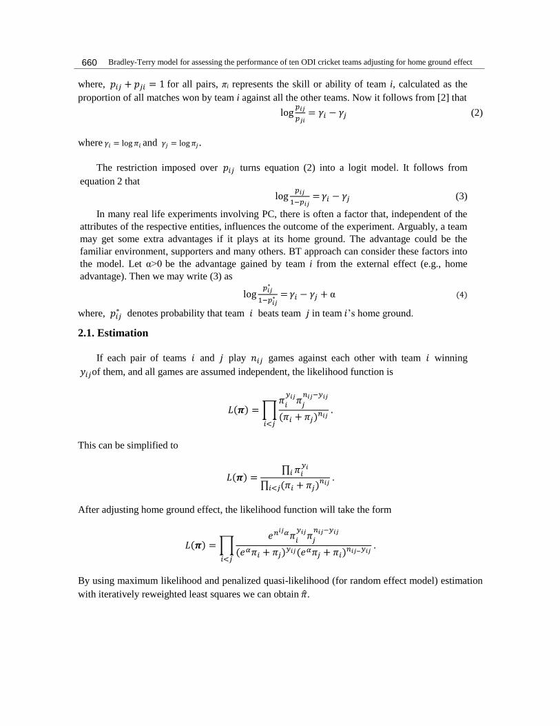
where, 𝑝𝑖𝑗 + 𝑝𝑗𝑖 = 1 for all pairs, πi represents the skill or ability of team i, calculated as the

proportion of all matches won by team i against all the other teams. Now it follows from [2] that

log𝑝𝑖𝑗

𝑝𝑗𝑖= 𝛾𝑖 − 𝛾𝑗 (2)

where 𝛾𝑖 = log 𝜋𝑖 and 𝛾𝑗 = log 𝜋𝑗.

The restriction imposed over 𝑝𝑖𝑗 turns equation (2) into a logit model. It follows from

equation 2 that

log𝑝𝑖𝑗

1−𝑝𝑖𝑗= 𝛾𝑖 − 𝛾𝑗 (3)

In many real life experiments involving PC, there is often a factor that, independent of the

attributes of the respective entities, influences the outcome of the experiment. Arguably, a team

may get some extra advantages if it plays at its home ground. The advantage could be the

familiar environment, supporters and many others. BT approach can consider these factors into

the model. Let α>0 be the advantage gained by team i from the external effect (e.g., home

advantage). Then we may write (3) as

log𝑝𝑖𝑗

∗

1−𝑝𝑖𝑗∗ = 𝛾𝑖 − 𝛾𝑗 + α (4)

where, 𝑝𝑖𝑗∗ denotes probability that team 𝑖 beats team 𝑗 in team 𝑖’s home ground.

2.1. Estimation

If each pair of teams 𝑖 and 𝑗 play 𝑛𝑖𝑗 games against each other with team 𝑖 winning

𝑦𝑖𝑗of them, and all games are assumed independent, the likelihood function is

𝐿(𝝅) = ∏𝜋

𝑖

𝑦𝑖𝑗𝜋𝑗

𝑛𝑖𝑗−𝑦𝑖𝑗

(𝜋𝑖 + 𝜋𝑗)𝑛𝑖𝑗

𝑖<𝑗

.

This can be simplified to

𝐿(𝝅) =∏ 𝜋𝑖

𝑦𝑖𝑖

∏ (𝜋𝑖 + 𝜋𝑗)𝑖<𝑗𝑛𝑖𝑗

.

After adjusting home ground effect, the likelihood function will take the form

𝐿(𝝅) = ∏𝑒𝑛𝑖𝑗𝛼𝜋

𝑖

𝑦𝑖𝑗𝜋𝑗

𝑛𝑖𝑗−𝑦𝑖𝑗

(𝑒𝛼𝜋𝑖 + 𝜋𝑗)𝑦𝑖𝑗(𝑒𝛼𝜋𝑗 + 𝜋𝑖)𝑛𝑖𝑗−𝑦𝑖𝑗

𝑖<𝑗

.

By using maximum likelihood and penalized quasi-likelihood (for random effect model) estimation

with iteratively reweighted least squares we can obtain �̂�.

660


3. Results

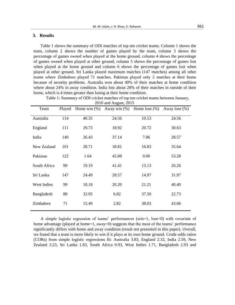
Table 1 shows the summary of ODI matches of top ten cricket teams. Column 1 shows the

team, column 2 shows the number of games played by the team, column 3 shows the

percentage of games owned when played at the home ground, column 4 shows the percentage

of games owned when played at other ground, column 5 shows the percentage of games lost

when played at the home ground and column 6 shows the percentage of games lost when

played at other ground. Sri Lanka played maximum matches (147 matches) among all other

teams where Zimbabwe played 71 matches. Pakistan played only 2 matches at their home

because of security problems. Australia won about 40% of their matches at home condition

where about 24% in away condition. India lost about 28% of their matches in outside of their

home, which is 4 times greater than losing at their home condition.

Table 1: Summary of ODI cricket matches of top ten cricket teams between January,

2010 and August, 2015

Team Played Home win (%) Away win (%) Home lose (%) Away lose (%)

Australia 114 40.35 24.56 10.53 24.56

England 111 29.73 18.92 20.72 30.63

India 140 26.43 37.14 7.86 28.57

New Zealand 101 28.71 18.81 16.83 35.64

Pakistan 122 1.64 45.08 0.00 53.28

South Africa 99 19.19 41.41 13.13 26.26

Sri Lanka 147 24.49 28.57 14.97 31.97

West Indies 99 18.18 20.20 21.21 40.40

Bangladesh 88 32.95 6.82 37.50 22.73

Zimbabwe 71 15.49 2.82 38.03 43.66

A simple logistic regression of teams’ performances (win=1, lose=0) with covariate of

home advantage (played at home=1, away=0) suggests that the most of the teams’ performance

significantly differs with home and away condition (result not presented in this paper). Overall,

we found that a team is more likely to win if it plays at its own home ground. Crude odds ratios

(CORs) from simple logistic regressions fit: Australia 3.83, England 2.32, India 2.59, New

Zealand 3.23, Sri Lanka 1.83, South Africa 0.93, West Indies 1.71, Bangladesh 2.93 and

661


Zimbabwe 6.31.COR is very high (exp (15.73)) for Pakistan because only 2 matches were

played in home ground.

Therefore, two different BT models were considered; one with the overall ability among

these teams, and the other after adjusting for home effects (Table 2). We also tested for

association between winning the toss and winning the match but did not find any statistically

significant association.

Table 2 shows the coefficients of fitted BT models of two scenarios. Matches resulted in

ties or no results were excluded from the analysis. We arbitrarily considered “West Indies” as

our reference category. Exponential of the fitted coefficient implies preference or superiority of

the team with respect to the reference team (West Indies). Team Australia was found to have

the maximum ability among all other teams with an estimated coefficient of 1.18. The exponent

of this estimate is 3.28 for team Australia to team West Indies informs us that the Australia is

ranked significantly higher by over 3 times compare to the West Indies. Our results show that

Australia, England, India, South Africa, and Sri Lanka significantly dominate over West Indies.

Moreover, the ratio for any two teams can be calculated by taking exponential of the difference

between the corresponding teams’ parameter estimates; e.g. Australia is slightly more likely to

defeat England (e(1.18-0.63)=1.73 times) than the reverse, that means Australia is ranked higher

than England.

Table 2: Estimated of parameters of Bradley-Terry models

Model 1 Model 2

Team 𝛾 S.E. 𝒆𝛾 95% CI 𝛾 S.E. 𝒆𝛾 95% CI

Australia 1.18*** 0.29 3.25 1.84-5.75 1.18*** 0.29 3.25 1.84-5.75

Bangladesh -0.21 0.30 0.81 0.45-1.46 -0.51 0.31 0.60 0.33-1.10

England 0.68* 0.29 1.97 1.12-3.48 0.63* 0.30 1.88 1.04-3.38

India 1.01*** 0.27 2.74 1.62-4.66 1.07*** 0.28 2.93 1.68-5.05

New Zealand 0.33 0.29 1.39 0.79-2.46 0.32 0.29 1.37 0.78-2.43

Pakistan 0.38 0.28 1.46 0.84-2.53 0.69* 0.29 1.99 1.13-3.52

South Africa 0.89** 0.29 2.44 1.38-4.30 1.03*** 0.30 2.79 1.56-5.04

Sri Lanka 0.75** 0.27 2.12 1.25-3.59 0.79** 0.29 2.21 1.25-3.89

Zimbabwe -1.17** 0.37 0.31 0.15-0.64 -1.37*** 0.38 0.26 0.12-0.54

West Indies 0.00 - 1.00 - 0.00 - 1.00 -

Home effect (𝜶) - - - - 0.61*** 0.12 1.84 1.45-2.33

S.E. – standard error; CI – confidence interval; •p<0.10, *p<0.05, **p<0.01, ***p<0.001

From Model-2 (Table 2) we find the home effect to be a significant factor on match result.

The estimated coefficient corresponding to home effect is 0.61 (i.e. 1.85 with 95% CI: 1.45-

662


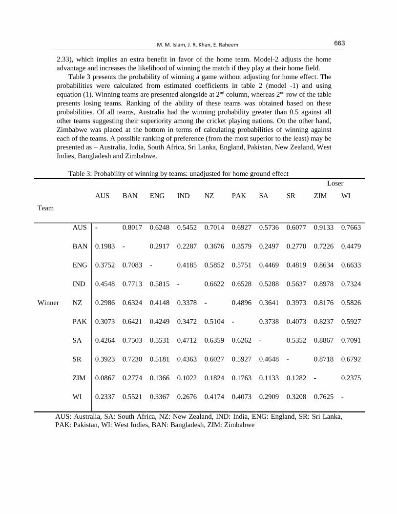
2.33), which implies an extra benefit in favor of the home team. Model-2 adjusts the home

advantage and increases the likelihood of winning the match if they play at their home field.

Table 3 presents the probability of winning a game without adjusting for home effect. The

probabilities were calculated from estimated coefficients in table 2 (model -1) and using

equation (1). Winning teams are presented alongside at 2nd column, whereas 2nd row of the table

presents losing teams. Ranking of the ability of these teams was obtained based on these

probabilities. Of all teams, Australia had the winning probability greater than 0.5 against all

other teams suggesting their superiority among the cricket playing nations. On the other hand,

Zimbabwe was placed at the bottom in terms of calculating probabilities of winning against

each of the teams. A possible ranking of preference (from the most superior to the least) may be

presented as – Australia, India, South Africa, Sri Lanka, England, Pakistan, New Zealand, West

Indies, Bangladesh and Zimbabwe.

Table 3: Probability of winning by teams: unadjusted for home ground effect

Loser

Team

AUS BAN ENG IND NZ PAK SA SR ZIM WI

Winner

AUS - 0.8017 0.6248 0.5452 0.7014 0.6927 0.5736 0.6077 0.9133 0.7663

BAN 0.1983 - 0.2917 0.2287 0.3676 0.3579 0.2497 0.2770 0.7226 0.4479

ENG 0.3752 0.7083 - 0.4185 0.5852 0.5751 0.4469 0.4819 0.8634 0.6633

IND 0.4548 0.7713 0.5815 - 0.6622 0.6528 0.5288 0.5637 0.8978 0.7324

NZ 0.2986 0.6324 0.4148 0.3378 - 0.4896 0.3641 0.3973 0.8176 0.5826

PAK 0.3073 0.6421 0.4249 0.3472 0.5104 - 0.3738 0.4073 0.8237 0.5927

SA 0.4264 0.7503 0.5531 0.4712 0.6359 0.6262 - 0.5352 0.8867 0.7091

SR 0.3923 0.7230 0.5181 0.4363 0.6027 0.5927 0.4648 - 0.8718 0.6792

ZIM 0.0867 0.2774 0.1366 0.1022 0.1824 0.1763 0.1133 0.1282 - 0.2375

WI 0.2337 0.5521 0.3367 0.2676 0.4174 0.4073 0.2909 0.3208 0.7625 -

AUS: Australia, SA: South Africa, NZ: New Zealand, IND: India, ENG: England, SR: Sri Lanka,

PAK: Pakistan, WI: West Indies, BAN: Bangladesh, ZIM: Zimbabwe

663


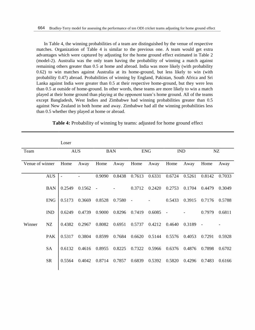
In Table 4, the winning probabilities of a team are distinguished by the venue of respective

matches. Organization of Table 4 is similar to the previous one. A team would get extra

advantages which were captured by adjusting for the home ground effect estimated in Table 2

(model-2). Australia was the only team having the probability of winning a match against

remaining others greater than 0.5 at home and abroad. India was more likely (with probability

0.62) to win matches against Australia at its home-ground, but less likely to win (with

probability 0.47) abroad. Probabilities of winning by England, Pakistan, South Africa and Sri

Lanka against India were greater than 0.5 at their respective home-ground, but they were less

than 0.5 at outside of home-ground. In other words, these teams are more likely to win a match

played at their home ground than playing at the opponent team’s home ground. All of the teams

except Bangladesh, West Indies and Zimbabwe had winning probabilities greater than 0.5

against New Zealand in both home and away. Zimbabwe had all the winning probabilities less

than 0.5 whether they played at home or abroad.

Table 4: Probability of winning by teams: adjusted for home ground effect

Loser

Team AUS BAN ENG IND NZ

Venue of winner Home Away Home Away Home Away Home Away Home Away

Winner

AUS - - 0.9090 0.8438 0.7613 0.6331 0.6724 0.5261 0.8142 0.7033

BAN 0.2549 0.1562 - - 0.3712 0.2420 0.2753 0.1704 0.4479 0.3049

ENG 0.5173 0.3669 0.8528 0.7580 - - 0.5433 0.3915 0.7176 0.5788

IND 0.6249 0.4739 0.9000 0.8296 0.7419 0.6085 - - 0.7979 0.6811

NZ 0.4382 0.2967 0.8082 0.6951 0.5737 0.4212 0.4640 0.3189 - -

PAK 0.5317 0.3804 0.8599 0.7684 0.6620 0.5144 0.5576 0.4053 0.7291 0.5928

SA 0.6132 0.4616 0.8955 0.8225 0.7322 0.5966 0.6376 0.4876 0.7898 0.6702

SR 0.5564 0.4042 0.8714 0.7857 0.6839 0.5392 0.5820 0.4296 0.7483 0.6166

664


ZIM 0.1271 0.0730 0.4403 0.2985 0.2007 0.1196 0.1391 0.0804 0.2566 0.1573

WI 0.3625 0.2352 0.7545 0.6243 0.4952 0.3466 0.3870 0.2545 0.5741 0.4217

Loser

Team PAK SA SR ZIM WI

Venue of winner Home Away Home Away Home Away Home Away Home Away

Winner

AUS 0.7507 0.6196 0.6832 0.5384 0.7316 0.5958 0.9592 0.9270 0.8574 0.7648

BAN 0.3578 0.2316 0.2853 0.1775 0.3353 0.2143 0.8129 0.7015 0.5267 0.3757

ENG 0.6358 0.4856 0.5556 0.4034 0.6124 0.4034 0.9316 0.8804 0.7770 0.6534

IND 0.7307 0.5947 0.6602 0.5124 0.7106 0.5704 0.9549 0.9196 0.8441 0.7455

NZ 0.5595 0.4072 0.4764 0.3298 0.5348 0.3834 0.9083 0.8427 0.7172 0.5783

PAK - - 0.5698 0.4173 0.6260 0.4751 0.9351 0.8863 0.7869 0.6663

SA 0.7208 0.5827 - - 0.7003 0.5582 0.9527 0.9159 0.8375 0.7360

SR 0.6713 0.5249 0.5940 0.4418 - - 0.9409 0.8960 0.8031 0.6881

ZIM 0.1917 0.1137 0.1452 0.0841 0.1767 0.1040 - - 0.3213 0.2038

WI 0.4808 0.3337 0.3988 0.2640 0.4560 0.3119 0.8784 0.7962 - -

AUS: Australia, SA: South Africa, NZ: New Zealand, IND: India, ENG: England, SR: Sri Lanka,

PAK: Pakistan, WI: West Indies, BAN: Bangladesh, ZIM: Zimbabwe

665


4. Conclusion

In this study, we compared the relative performance of ten ODI cricket teams using

Bradley-Terry paired comparison model accounting for home-ground effect. Comparison of team

performance in ODI cricket using win-loss percentages shows that the higher a team’s winning

percentage the stronger the team and vice-versa. This provides a team’s overall ability but does not

quantify the degree to which specific factors such as home and away may have contributed to their

performance. A team is considered superior when performs competitively regardless of playing at

home or away. On the other hand, a team winning on a consistent basis at home and not performing

equally when they play away may be due to the effect of home ground advantage. In some

occasions, a weaker home team may perform better and restrict the winning potential of a stronger

opponent because of the home ground effect. Therefore, we considered statistical models to study

the relative abilities to compete teams based on match outcomes after adjusting for home ground

effects.

The Bradley-Terry model considered in this study distinguishes among these teams by

calculating individual abilities through the outcomes of the played matches. Teams traditionally

perform better at home than away for various reasons, including familiarity with local conditions,

the condition of pitches, crowd support, less travel fatigue, among others. In this paper, we have

justified that adjustment for home and away venue effect is needed and showed how the winning

probabilities differed as a result. Our analysis reveals that most of the team are more likely to win a

match at home than away. Some of these teams have probabilities of winning against any particular

team calculated greater than 0.5 at home ground, whereas those probabilities are less than 0.5 if

they play abroad. Several other factors can be considered to analyze the performance of cricket

teams such toss win, the strength of each team, a number of different types of players, player skills,

team-wise investment in cricket etc. We keep it as a future scope for analyzing ODI cricket

performance data. The interested researcher can consider all ODI cricket playing countries’ data to

explore their performance.

References

[1] Abbas, N. and Aslam, M. (2009). Prioritizing the items through paired comparison

models, a Bayesian approach. Pakistan journal of Statistics, 25(1):59–59.

[2] Agresti, A. (2014). Categorical data analysis. John Wiley & Sons.

[3] Allsopp, P. and Clarke, S. R. (2004). Rating teams and analysing outcomes in one day

and test cricket. Journal of the Royal Statistical Society: Series A (Statistics in

Society), 167(4):657–667.

[4] Bailey, M. and Clarke, S. R. (2006). Predicting the match outcome in one day

international cricket matches, while the game is in progress. Journal of sports

science & medicine, 5(4):480–487.

[5] Bradley, R. A. (1953). Some statistical methods in taste testing and quality evaluation.

Biometrics, 9(1):22–38.

666


[6] Bradley, R. A. and Terry, M. E. (1952). Rank analysis of incomplete block designs: I.

the method of paired comparisons. Biometrika, 39(3/4):324–345.

[7] Cattelan, M., Varin, C., and Firth, D. (2010). Stochastic dynamic thurstone-mosteller

models for sports tournaments. University of Warwick. Centre for Research in Statistical

Methodology.

[8] Cerqueira, P. H., Nakamura, L. R., Pescim, R. R., & Leandro, R. A. (2017).

INVESTIGATING THE UNDERLYING CAUSAL NETWORK ON EUROPEAN

FOOTBALL TEAMS. Journal of Data Science, 15(2).

[9] Clarke, S. R. (1988). Dynamic programming in one-day cricket-optimal scoring rates.

Journal of the Operational Research Society, 39(4):331–337.

[10] de Silva, B. M. and Swartz, T. B. (1997). Winning the coin toss and the home team

advantage in one-day international cricket matches. The New Zealand Statistician,

32(2):16–22.

[11] Glenn, W. and David, H. (1960). Ties in paired-comparison experiments using a

modified thurstone-mosteller model. Biometrics, 16(1):86–109.

[12] Gweshe, T. and Durbach, I. (2013). An analysis of the efficiency of player

performance at the 2011 cricket world cup. ORiON, 29(2):137–153.

[13] Hallinan, S. E. (2005). Paired comparison models for ranking national soccer teams.

PhD thesis, WORCESTER POLYTECHNIC INSTITUTE.

[14] Henery, R. J. (1992). An extension to the Thurstone-Mosteller model for chess.

Journal of the Royal Statistical Society. Series D (The Statistician), 41:559–567.

[15] ICC (2016). Live cricket scores & news international cricket council. pages

Accessed Aug 12, 2016.

[16] Joe, H. (1990). Extended use of paired comparison models, with application to chess

rankings. Journal of the Royal Statistical Society. Series C (Applied Statistics),

39(1):85–93.

[17] Lewis, A. (2008). Extending the range of player-performance measures in one-day

cricket. Journal of the Operational Research Society, 59(6):729–742.

[18] Louzada, F., Suzuki, A. K., & Salasar, L. E. (2014). Predicting Match Outcomes in

the English Premier League: Which Will Be the Final Rank? Journal of Data

Science, 12(2), 235-254.

[19] Neil, D. and Jonathan, G. (2015). Using bradley-terry models to analyse test match

cricket. Working papers.

[20] Schauberger, G. and Tutz, G. (2015). Extended ordered paired comparison models

with application to football data from german bundesliga. AStA Advances in

Statistical Analysis, 99(2):209–227.

[21] Sen, S., Biji, M. S., Chakraborty, S., Sindhu, N. R., & Balasubramanian, S. (2015).

Pairwise Comparison in Repeated Scores-Application in Palliative Cancer

Patients. Journal of Data Science, 13(4), 795-806.

667


[22] Stern, H. (1990a). A continuum of paired comparisons models. Biometrika, 77:265–

273.

[23] Stern, H. (1990b). Models for distributions on permutations. Journal of the

American Statistical Association, 85:558–564.

[24] Stern, S. E. (2011). Moderated paired comparisons: A generalized bradley-terry

for continuous data using a discontinuous penalized likelihood function. Applied

Statistics: Journal of the Royal Statistical Society, Series C, 60(3):397–415.

[25] Thurstone, L. L. (1927). A law of comparative judgment. Psychological review,

34(4):273–286.

Md. Mazharul Islam

Institute of Statistical Research and Training, University of Dhaka

Dhaka–1000, Bangladesh

Jahidur Rahman Khan

Institute of Statistical Research and Training, University of Dhaka

Dhaka–1000, Bangladesh

Enayetur Raheem

Biomedical Research Foundation (BRF), Dhaka, Bangladesh.

668

bradley-terry model for assessing the performance of ten odi ...

Documents

Transcript of bradley-terry model for assessing the performance of ten odi ...