Bolocam: status and observations

Douglas J. Haiga, Peter A.R. Adea,James E. Aguirreb, James J. Bockc, Samantha F.Edgingtond, Melissa L. Enochd, Jason Glennb, Alexey Goldinc, Sunil Golwalad, Kevin Hengb,Glenn Laurentb, Philip R. Maloneyb, Philip D. Mauskopfa, Philippe Rossinota, Jack Sayersd,

Patrick Stoverb, Carole Tuckera

aDepartment of Physics and Astronomy, Cardiff University, 5, The Parade, Cardiff, CF24 3YB

bCenter for Astrophysics & Space Astronomy, Univ. of Colorado, 389-UCB, Boulder, CO80309

cJet Propulsion Laboratory, M/S 169-327, Pasadena, CA 91109

dDepartment of Physics, Caltech, MC 59-33, Pasadena, CA 91125

ABSTRACT

Bolocam is a millimetre-wave (1.1 and 2.1mm) camera with an array of 119 bolometers. It has been commissionedat the Caltech Submillimeter Observatory in Hawaii and is now in routine operation. Here we give an overviewof the instrument and the data reduction pipeline. We discuss models of the sensitivity of Bolocam in differentobserving modes and under different atmospheric conditions. We briefly discuss observations of star-formingGalactic molecular clouds, a blank field survey for sub-millimeter galaxies, preliminary results of a blank-fieldCMB secondary anisotropy survey and discuss observations of galaxy clusters using the Sunyaev-Zel’dovicheffect.

Keywords: Bolocam, CMB, SZ Effect, bolometers, arrays, blank field surveys,PCA, millimetre-wave

1. INTRODUCTION

In recent years the astronomical observations at millimetre and submillimetre wavelengths have become in-creasingly refined and scientifically important. Data available in this relatively unprobed wavelength band arecomplementary to observations in other observed bands and are essential to many areas of investigation includingstudies of star formation, galaxy and galaxy cluster evolution (see e.g. references in Section5 of this paper).

Bolocam is one of the first large-format cameras available for common use at millimetre wavelengths andis highly complementary to other bolometric array cameras like MAMBO (Kreysa, et al., 19991,2), SCUBA(Holland, et al., 19993) and SHARC II (Dowell, et al., 20034) which are probing either different angular resolutionsor wavelengths. Mounted on a 10.4-metre Leighton telescope at the Caltech Submillimeter Observatory (CSO),Mauna Kea, Hawaii, Bolocam has 119 working neutron-transmutation-doped (NTD) Germanium spiderwebbolometers and is currently commissioned for (non-simultaneous) observations at both 1.1mm and 2.1mm.The large field-of-view of the CSO combined with a monolithic array of sensitive bolometers results in a highmapping speed, making Bolocam useful for observations requiring wide angular coverage, such as surveys ofGalactic molecular clouds or blank field surveys of submillimetre galaxies and galaxy clusters.

The technology developed for Bolocam has helped pave the way for a new genre of array instruments atmillimetre-wave telescopes including ACT (Kosowsky, 20035), ACBAR (Runyan, et al., 20036), APEX (Schwan,et al., 20037), ASTE (Ezawa, 20028), SPIRE (Griffin, et al., 20039) and SPT (Carlstrom, et al., 200310). Themanufacture of large single-wafer bolometer and horn arrays along with the development of arrays of cold readoutelectronics are some of the technologies. New observing strategies have been developed and existing ones adapted(some of which were developed by the SHARC II team) in collaboration with the CSO staff to take advantage ofthe receiver capability. Finally, a pioneering software pipeline has been developed including average subtraction

Further author information: (Send correspondence to Douglas Haig)Douglas J. Haig: E-mail: Douglas.Haig@astro.cf.ac.uk, Telephone: +44 (0)29 2087 5106

and principal component analysis methods (PCA) to remove atmospheric fluctuations and allow Bolocam toapproach photon-limited noise performance. These techniques with various optimal filtering methods, have beenimplemented in a number of scientific programmes.

Bolocam achieved first light at the CSO in May 2000 with an engineering detector array, and has since beenin operation on several observing runs. This has led to a number of upgrades, most noticeably to the array,analysis pipeline and filter stack. As of February 2004 it has been open to applications for use from the scientificcommunity at 1.1mm and 2.1mm availability is to follow in the near future.

2. INSTRUMENT LAYOUT AND SPECIFICATION

This section introduces the basic specifications of the Bolocam instrument and details the recent updates andresults of tests performed since the previous SPIE proceedings. For further information on the instrument designrefer to Glenn, et al., 200311 and Glenn, et al., 1998.12

2.1. Cryogenics

For optimum sensitivity the detectors in Bolocam are cooled to 270mK, which is sufficient to achieve photonbackground limited performance at 1.1mm. Simplicity of cryogenic operation is necessary for the facilitation asa common user instrument on the CSO. For this reason the basic dewar design of a stacked nitrogen and heliumtank system, each of 16-litre capacity, is used. A closed-cycle, triple-stage sorption refrigerator (4He/3He/3He)provides a base temperature of 270mK at the bolometers. Such a sub-Kelvin refrigerator was originally designedfor Bolocam in collaboration with Chase Cryogenics to provide automated operation at the telescope withoutpumping on the liquid helium bath. Cycling is necessary once per day taking approximately 2 hours. Details ofthe design and operation can be found in Bahtia et al.13

The detector ultra-cold (UC) stage has a temperature of approximately 270mK and is thermally isolatedfrom 4K by two sets of Vespel legs with a cooled intermediate stage (∼ 450mK). The cold electronic JFETstage is mounted on the 4 K base plate, but as the optimal noise range of these devices occurs between 135K -140K these are also thermally isolated from the 4 K base plate. To reduce the thermal loading on the 4 K stage,a copper finger is attached from the 77K tank and from that temperature the JFETs can self-heat. Whilst inoperation on the telescope Bolocam has a helium hold time of 24 hours. Recent tests involving pumping on thenitrogen tank have shown that this can be increased by almost a factor of 1.5. Components of the cryogenicdesign are shown in Figure 1.

Figure 1. Left: A 3D representation of the Bolocam instrument setup for observations at 1.1 mm. Right: Photographof the Bolocam wafer (without horn-plate) mounted on the thermal isolation stage.

Figure 2. Histograms of the bolometer parameter values for the entire Bolocam array as measured in the laboratory.These parameters are used to calculate the fundamental characteristics, including sensitivity of the instrument assumingperfect removal of sky noise.

2.2. Detectors

The Bolocam detector array consists of a monolithic silicon wafer with 151 (144 read out) etched spider-webbolometers with NTD germanium thermistors (Mauskopf, et al., 199714). The bolometers are divided into six“hextants” connected to 51-pin micro-D-sub connectors.

The latest Bolocam array is the fourth generation wafer and was first utilized in January 2003; it has 119out of 144 working bolometers. Earlier arrays suffered from lower yields at the photolithography or NTD chipbonding stages, which have since been largely remedied with only one broken web and one bolometer with noNTD chip. The remaining bad bolometers are open circuit. Further improvements have been made with later,similar bolometer arrays for SPIRE (Bock, et al., 1998,15 for which the Bolocam array is a prototype). Theseyields are in the high 90% range (83% for Bolocam). For characterization and understanding of the detectorsand electronics noise, 6 bolometers are kept dark (one in each set of electronics).

The parameters characterizing the performance of this array were found using the same method as forprevious arrays (IV curves taken at multiple refrigerator base temperatures with no optical loading). Figure 2shows the distribution of the bolometer parameters for the 119 working detectors. The meaning and method ofcalculations of these parameters are detailed in Glenn et al. (2003).11 To summarize: R0 and ∆ are determinedby the doping concentration in the NTD thermistor chips and define the temperature resistance relation andconsequently contribute towards tuning the responsivity. This is related to the operating temperature-resistanceof the bolometer by Rb = R0 exp

√

∆/Tb (where Tb is the bolometer temperature). The design value for R0 was170Ω, almost exactly the resultant bolometer values. Control of the thermal link to the bath from the bolometeris defined by g and α, which is largely determined by the thickness and material used for the metalization of theweb. The total power on the web is given by P = g(T α

b − T αs ) where Ts is the sink temperature. The thermal

conductance is given by G(Tb) = gαT α−1b . The same array is used for all three wavelengths, and despite the

very different loadings apparent at each one, a compromise G(300mK) has been chosen. Table 1 below showsthe various parameters of the bolometers and the base noise levels (assuming perfect sky removal) at differentwavelengths and sky conditions.

2.3. Electronics and Data Acquisition

The bolometer signals are read out using a gain-stabilized AC biased circuit originally developed for theBOOMERANG experiment (Crill et al., 200316). A custom-built sine-wave voltage generator provides an ACbias current through 2x10MΩ load-resistors to the bolometers with an amplitude stability of several ppm at afrequencies of 0.01 Hz and higher. The bolometer output voltages are fed through cold (120K) JFET buffers toreduce sensitivity to electromagnetic interference on the cold wiring. Both the AC bias generator and pream-plifier cards for the bolometer signals are mounted directly on the cryostat inside an RF-tight enclosure. Theamplified AC signals run through flexible cables from the cryostat to a set of high dynamic range analogue lock-incards. After low pass filtering and a gain stage, DC signals proportional to the bolometer resistances are logged

νcentre (GHz) 140 140 275 275

τatm 0.060 0.100 0.060 0.100

d/fλ 0.8 0.8 1.5 1.5

AΩ(cm2sr) 0.044 0.044 0.012 0.012

εfilt 0.4 0.4 0.35 0.35

εLyot 0.2 0.2 0.55 0.55

Emissivitytel 0.2 0.2 0.1 0.1

Emissivitysky 0.1 0.1 0.25 0.25

∆ν/ν 0.13 0.13 0.16 0.16

Q(parasitic) (pW) 0.4 0.4 6 6

Q(telescope) (pW) 2.1 2.1 5.5 5.5

Q(sky) (pW) 0.4 0.6 8 12.8

Q(total) (pW) 2.9 3.1 20.2 24.3

Teff(RJ) (K) 66 71 99 122

NEP(shot) (10−17 W/√

Hz) 2 2 8 9

NEP(bose) (10−17 W/√

Hz) 2 2 10 12

NEP(bol) (10−17 W/√

Hz) 3 3 5 6

NEP(amp) (10−17 W/√

Hz) 4 4 12 14

NEP(total) (10−17 W/√

Hz) 6 6 18 21

NEFD (mJy√

s) 77 81 42 57

Table 1. Table showing bolometer, telescope and electronics parameters along with theoretical noise limits at 2.1mm and1.1mm at two different sky loading levels. The parameters shown (from top to bottom) are: frequency band centre, skyopacity at 225 GHz (tau), horn spacing in fλ, throughput, optical efficiency due to the dewar optics chain, spillover onthe Lyot stop, emissivity of telescope, emissivity of sky, fractional bandwidth, optical loading from dewar, optical loadingfrom telescope, optical loading from sky, total optical loading, effective Rayleigh-Jeans temperature from total opticalloading, noise equivalent power (NEP) from shot and Bose noise (combine for total photon NEP), bolometer NEP, coldelectronics NEP, total NEP, and the noise equivalent flux density (NEFD).

Description Position Cut-off at 1.1mm (273GHz) Cut-off at 2.1mm (143GHz)

Zotefoam 300K - -

Copper mesh 77K Shield 540 420

Copper mesh 4K Shield 420 255

Copper mesh 4K Lyot stop 420 420

HDPE Lens 4K mini-snout - -

Copper Mesh 300mK 360 232

Copper Mesh 300mK 300 150

Horn Plate 300mK 232 125

Table 2. Components of the optical chain inside the Bolocam dewar detailing the position and cut-off frequency (definedat the 50% transmission point) for the 1.1mm and 2.1mm bands.

by a 16-bit data acquisition system (DAS). These are used as a real-time monitor of the optical loading on thebolometers which is used in the system calibration. Because the dynamic range of the DC signal is approximately106, significantly greater than the dynamic range of the 16-bit DAS, the DC analogue signal is passed througha high pass filter with a time constant of 10.4 seconds. A final gain stage and 16-bit digital sampling of the ACcoupled bolometer signals is then used for the science analysis.

The combination of the cold buffer and warm preamplifier give an average electronics noise level of 15 nV/√

Hz(dominated by the U401 matched pair JFETs) with a white noise spectrum down to frequencies of less than0.01Hz. Given the operating impedances of the bolometers, this contributes to the system NEP of 10-40%depending on the weather conditions.

2.4. Optics

The Bolocam optics box is mounted at the Cassegrain focus of the 10.4m diameter CSO and converts thef/12.4 beam to a f/7.4 beam with a series of two flat mirrors and one off-axis ellipsoidal mirror (see Figure3).The window is made of Zotefoam PPA30, a nitrogen-expanded polypropylene foam with a closed cell structure,forming a good vacuum barrier (see Runyan, et al., 20036). No measurable diffusion of He has been detectedleak-checking at the 10−9 atm cc/sec level. It is measured to have very low refractive index and low loss (on theorder of 0.5−1%) at millimetre wavelengths. The beams then pass through an infrared 10-micron blocking filter,which significantly reduced the absorption of (and in-band re-emission from) the filter stack following it. Theremaining radiation blocking filters are multi-layered copper mesh capacitive/inductive grids, which are placedon the 77K and 4 K radiation shields. These each provide a low pass cut-off and are designed to block theharmonic leaks from the previous filters (the cut-offs are detailed in Table 2). A throughput-limiting apertureat the cold Lyot stop just behind the 4 K filters defines the 8m effective illumination of the primary mirror.Mounted closer to the detectors inside the 4K shield is a high-density polyethelene (HDPE) lens. This convertsthe beam to f/2.8, removing the majority of the field curvature, and feeds a monolithic horn plate containing 144conical horns terminating in cylindrical waveguides. The horns are designed to provide some oversampling of thesky by overillumination of the Lyot stop. Appoximately 55% at 1.1mm and 20% of the beam at 2.1mm fromthe horns couples to the telescope with the rest being intercepted at 4K. The final copper mesh band-definingfilters are mounted directly onto the 300mK horn plate. Figure 3 shows the bandpasses for 1.1mm and 2.1mm.

Bolocam does not operate simultaneously at the three designed frequencies; it has different optimal coppermesh filters and horn plates for each one. The integrating cavity, consisting of the horns and the backshortplate, sandwich the wafer with the bolometers and are adjusted in aperture and cavity depth to optimize photonabsorption (Glenn, et al., 200217). The waveguide cut-off is changed by changing the horn plate in which thediameter of the waveguides are machined to the appropriate size. Currently, the overall optical efficiency of thissetup is approximately 19% for 1.1mm and 8% for 2.1mm, including the efficiency of the detector absorption(≥ 90% Rownd, et al., 200318), the coupling to the Lyot stop (55% and 20% for 1.1mm and 8% for 2.1mm)

Figure 3. Left: CSO and Bolocam optical chain (external to the cryostat). Tertiary mirror is off-axis and the fullshape is shown, note that only the section shown reflecting the rays is physically in the chain. Right: Average (over allbolometers) Bolocam band-passes for 1.1 mm (275 GHz, solid line) and 2.1 mm (150 GHz, dashed line). The band edgesare defined to avoid the atmospheric water lines.

and losses in the filter stack (' 40%). The optical loading on the detectors is a combination of power from the4K and 77K spillover inside the cryostat (parasitic loading), emitted and scattered light from the telescope andwarm optics (telescope loading) and from the emission of the atmosphere (sky loading). Approximate values foreach of these components are given in Table 2 .

3. DATA REDUCTION PIPELINE

The Bolocam data reduction pipeline has gone through many changes since its inception and is still evolving.The advent of large format arrays at these wavelengths has prompted the development of new data analysistechniques. The main source of noise is emission from the varying optical depth through the atmosphere, knownas sky noise. The ultimate aim is to utilize software that will be able to remove as much of the sky noise aspossible, enabling Bolocam to approach the photon and detector noise limit. The large number of detectorsallows us to attempt to achieve this limit via a number of different methods which are described in the followingsections.

The basic Bolocam pipeline is written in IDL and allows a number of different cleaning and mapping algo-rithms to be used depending upon what type of object is being observed; at the moment this has been found tobe mainly dependent on the angular scale relative to a point source object for Bolocam. This system also allowsa number of different preparation modules to be used as well as all the cleaning modules, if the user so desires.Finally, a user with knowledge of IDL can write custom modules within the constraints of the standard inputand outputs of the pipeline. The various sections of the software are described below.

3.1. Merging and Slicing

The first step in the Bolocam Analysis Pipeline is the merging of the various input data. Information comesfrom three sources; the DAS, containing the raw bolometer time traces, the header data, containing the telescopepositioning, and the encoder log, containing the rotator position, observation number, source name and otherancillary data. These are written at 50Hz, 50Hz, and 1Hz, respectively, and are merged into one file. Thissoftware provides data checking and correction to glitches that occur before being fed into the merging computer.

The format of the output files is network common data format (netCDF), written in hour-long sections andsliced according to observation number by the second program in the pipeline. These are sorted by object name.

This is done automatically at the telescope, so the user should not have to use this software at any time afterobservations.

3.2. Average Subtraction

The dominant source of noise in the Bolocam data is the variable emission from the atmosphere, which isseveral orders of magnitude brighter than the astronomical sources. Most of this emission is from water vapour,which fluctuates both spatially and with time. However, with our observing strategies, detailed in (Section 4)the dominant instabilities can be thought of temporally. For such instabilities the Kolmogorov model can beassumed and the instabilities of the atmosphere are dissipated down to smaller and smaller structures resultingin a 1/fn dependence of the atmospheric emission.

Each of the bolometer beams from Bolocam overlap on the primary mirror of the CSO and pass througha significant proportion of the atmosphere (about 5 km) before they completely separate. The majority of thewater vapour is below this altitude, so the dominant sky signal is a common-mode variation with time (thesignal seen by all bolometers), and can be removed with a simple average subtraction. To first approximation,this effectively removes the sky contribution leaving non-common noise sources, such as Johnson noise and theastronomical signal. This method is limited in two ways. The first is that even slight imperfections in the opticalchain can cause mis-matching of beams on the sky such that the common signal template removed is not ideal(even without this, in a perfect optical chain the beams diverge within the atmosphere; imperfection in the opticsmerely aggravates the problem). The second is that if the astronomical source is significantly extended, some ofthis will be included in the common sky model, so its amplitude will be reduced.

3.3. Principal Component Analysis

For observations where the sky and instrument noise dominate over the source signal by many orders of mag-nitude, a more sophisticated method of correlated noise removal has been adopted - the principal componentanalysis (PCA) routine (e.g. Gonzalez and Woods, 199219). The basic assumption in using PCA is that thereis more than one source of correlated noise contributing to the overall time stream detected by each of thebolometers, e.g., sky noise, microphonic or side lobe signal caused by scanning, as well as signals from extendedastronomical structure. However, the majority of the astronomical signals are uncorrelated across the array e.g.,signals from point sources. The PCA algorithm combines the time-ordered data from all of the (119) bolometersinto a set of (119) time traces, each of which is a combination of some or all of the bolometer signals. These timetraces are uncorrelated with each other and correspond to combinations of signals or components present in allof the detectors with varying amplitudes, such as sky temperature variations, scan-synchronous, microphonics,or electrical pickup. The components with the largest amplitude tend to be dominated by a single source, suchas atmospheric fluctuations, but there is not necessarily a one-to-one correspondence between PCA componentsand source origin.

In the PCA analysis, we diagonalize the correlation matrix of the bolometer time-streams (via standardeigenvector algebra) to find the eigenvectors of each signal component. Due to the removal of the majority ofthe DC components by the high-pass filter in the electronics chain (and further subtraction in software), thecovariance matrix is automatically the correlation matrix, easing calculation. The eigenvalues represent themagnitude of the contribution to the data from a particular eigenvector, or signal source. Assuming that thereare only a small number of dominant sources of correlated noise signals that need to be removed, an arbitrarycut can be made on the eigenvalues. By not including the corresponding eigenvectors when inverting the matrixback to the bolometer/time-stream matrix, these contributions can be removed. Removing more eigenvaluesreduces the noise in the resultant time-streams but also attenuates flux from astronomical sources. For pointsources the eigenvalue cut can be more aggressive than for large scale signals, due to the correlation betweenlarge scale signals and low frequency noise sources. However, even for point sources it has been demonstrated insimulations (Section 3.4) that some signal is lost, implying that none of the eigenvectors are orthogonal to pointsource signals. For observations of point sources, eigenvalues larger than 3σ (assuming a Gaussian distributionof eigenvalues) are removed.

3.4. Cleaning Simulations

Although the signal of a point source is correlated in time over only a small number of bolometers, the PCAsky subtraction attenuates the signal from astronomical sources in addition to the atmospheric signal. A set ofMonte Carlo simulations was done to determine the amount by which the flux density of galaxy candidates wasreduced by the cleaning and sky subtraction. The simulations were done in the following manner: A fake source(Gaussian, 30′′ FWHM) was injected into a blank map. A simulated bolometer timestream was generated, fromthe map of the fake source, and that was added to the raw bolometer timestreams of an individual observation.The timestream data were then cleaned with PCA and mapped in the ordinary manner. The resulting source wasfit by a 2-d gaussian to determine the attenuation of the injected source flux. This simulation was repeated 1014times with fake sources injected into random observations at random positions, and ranging in flux density from0.1 to above 1000 mJy. The average reduction in flux density is 0.19± 0.04 for PCA and 0.07± 0.02 for averagesubtraction, independent of flux density to 1 Jy. Consequently, with a good understand of the effect of cleaningon the point sources, the measured fluxes can be corrected. Above 1000 mJy, the amount of attenuation by PCAwas found to depend on the brightness of the source, which is an area of flux density unlikely to be probed formost surveys that are to be performed by Bolocam. The amount of flux density attenuation is determined bythe number of PCA components that are removed from the raw time streams, which is controlled by the cut onthe eigenvalues: a more aggressive cut results in a greater attenuation.

3.5. De-sourcing Module

For the cleaning of the brightest sources, the loss of signal due to the cleaning pipeline can be substantial. Toprevent this on a source of known position, a de-sourcing module has been added. This involves calculation ofthe positions of each of the bolometers relative to the source at each point in time and ’masking’ out those thatfall within two FWHM of the source. The DC levels of the masked-out region are subtracted from the rest of thetimestream. This removes the contribution of the source to the sky template from the non-masked bolometers.This sky template is then removed from all the bolometers in the standard fashion.

3.6. Wiener Filtering

For point sources, the signal-to-noise is not constant throughout the entire temporal or spatial frequency rangeof the data. We filter the coadded map with an optimal filter, g(q), to attenuate signal at length scales bothsmaller and larger than our beam size:

g(q) =s?(q)/J(q)

∫

|s(q)|2/J(q)d2q(1)

where J(q) is the average power spectral density (PSD) squared, s(q) is the Fourier transform of the Bolocambeam shape from map space to map spatial frequency space, q, and ∗ indicates complex conjugation. The factorin the denominator is the appropriate normalization factor so that when convolved with a map, peak heightsare preserved. A 2-d map of Equation 1 is thus convolved with the coadded map to maximize signal-to-noisefor detections of point sources. An analagous filter was applied directly to the demodulated timestreams of thechopped observations, with s(q) represented by a positive and negative beam separated by the chop throw (90”).

3.7. Mapping

A map of a set of data from multiple observations of a source is a simple coadd of all of the data in each skypixel. This is weighted by relative responsivity of each bolometer and noise present in each scan corrected forthe optical depth of the atmosphere when the data was taken. The noise in each scan is calculated from theintegrated PSD of the cleaned data. This ensures that those scans taken that are suffering from particularly highcontributions from noise sources not removed by the cleaning alter the overall maps very little. The calibrationof the map from Volts to Janskys is also performed at this stage. A calibration plot is created comparing theDC read-out of the bolometers at different loading levels (due to sky opacity or elevation) with the measuredsignals from calibration sources of known brightness.

4. OBSERVING STRATEGIES

To take full advantage of the instrument design and algorithms available in the custom-written data reductionpipeline a number of observing strategies have been adopted to obtain the optimum results for different categoriesof observed sources. The following discusses the merits and drawbacks of the various available observing modes.

4.1. Drift Scanning

The use of a large format array of detectors allows simple observing strategies that minimise the requirements onmechanical modulation of the signal. The simplest method previously used on the CSO by the SuZIE instrumentis drift scanning (Mauskopf, 1997,20 Holzapfel, et al., 1997,21 Mauskopf, et al., 200022). It involves movingthe telescope ahead of the source and allowing the rotation of the Earth to cause the source to pass throughthe beam. When the required patch of sky is covered, the telescope is moved ahead of the source again andthe observation is repeated. For larger patches of sky in declination than the array field-of-view (∼ 7.5′), thetelescope merely alters scans at different declinations. By allowing the telescope time to settle between scansit ensures that there will be no microphonic pick up from its movement and it also ensures that the side lobestructure is constant, and is therefore more easily removed. One problem with this strategy is that the signalfrequency is very low, exacerbating susceptibility to 1/f noise spectrum region. As the telescope has to driveacross the field to start again, the percentage of time it is taking useful data (observing efficiency) is reduced,but not as low as other strategies.

Drift scanning also results in a lack of uniform coverage for an arbitrary rotation angle of the array on thesky due to the non-close-packed nature of the bolometer array (1.5, 1.2 and 0.8 fλ spacing at 1.1, 1.4 and2.1mm respectively). The solution is to tilt the array relative to the scanning direction on the sky allowing eachbolometer to be positioned at a slightly different declination from the adjacent pixels. The optimal coverage forBolocam observations at 1.1mm is found to be an angle of 10.9. To further improve the coverage, each set ofconstant declination scans can be repeated with a slight offset from the last set. The optimal array angle anddeclination step is unique to the observed wavelength and map size. A disadvantage to this strategy is that onlyRA scans can be performed. This results in a lack of cross-linking in the final maps and poor discriminationagainst scan-synchronous noise.

4.2. Raster scanning

Following from the idea of drift scanning, raster scanning is simply adding telescope movement to the scanstrategy. This “fast scanning” technique has begun to be used by other millimetre-wave array receivers (e.g.Weferling, et al., 200223). The first advantage of this is the telescope can be driven in both directions, therebyavoiding a wasted pass over the source, resulting in increased efficiency. Secondly, there is a control over theangle at which the telescope can be passed over the source. For example, azimuth scans are done at constant air-mass which means large scale drifts due to seeing different levels of the atmosphere are not introduced. Anotherbeneficial factor of this scan is the introduction of cross-linking due to field rotation over the course of the night.The amount of cross-linking depends on the declination and the length of time observed each night, which insome cases can be significant. Finally, raster scanning allows alternating perpendicular scans, thereby achievingmaximum cross-linking. This however, relies on the data analysis pipeline being able to remove all large scaledrift due to the change in brightness of the atmosphere (which it has proven to be very successful at doing).

A more subtle benefit of this scanning method is the control of the source signal modulation frequency bychanging the telescope drive speed. If there is 1/f noise present in the data, then having the astronomical signalat higher frequencies, yields a higher signal-to-noise in that scan. This has to be balanced against the risk ofintroducing microphonics into the time-stream and at very high scan speeds, reaching the time constant of thebolometers. This is discussed further in Section 5.

4.3. Chopping

Chopping or dual beam switching is a standard technique for reducing sky noise by rapidly modulating thedirection of observation usually with a nutating secondary mirror. Chopping is the predominant observationaltechnique used with single pixel receivers (e.g. Conway, Daintree and Long, (1965)24). Bolocam has also madeobservations while modulating the secondary mirror of the CSO. However, instead of chopping and nodding

Scan Speed Relative Mapping Speed η Relative Mapping Speed with η σf

(”/s) (arcmin2/hr/mJy2) (arcmin2/hr/mJy2) (Hz)

15 1.00 0.95 1.00 0.18

60 1.38 0.85 1.23 0.75

120 1.60 0.73 1.23 1.50

240 2.33 0.57 1.40 3.00

Table 3. The effect of scan speed on mapping speed at 1.1 mm. The first column is scan speed, the second mappingspeed relative to 15”/s scanning, the third is the turnaround inefficiency, the fourth is the relative mapping speeds aftercorrecting for the observing efficiency, and the fifth the 1 σ width of the Gaussian beam in frequency space. The typical1/f knee of the noise lies between 1 and 5 Hz in this space.

(which is a possibility), raster scanning is used to separate the signal from the chop frequency. Currently onlyone scan speed (usually 5′′/sec) and one chop frequency and throw (1Hz and 90′′) have been used. This resultsin a loss of sensitivity to large scale structure and integrated flux; reconstruction methods (such as Emerson,Klein and Haslam, (1979)25) require multiple chop throws and directions to regain it. However, chopping isefficient for small fields (< 20′) and photometry of unresolved sources because the telescope turn around timesare very small in comparison to the scan time.

5. SENSITIVITIES AND PERFORMANCE

The following sections present results on how the performance of Bolocam is affected by the observing strategy,the method of cleaning the data, and the weather conditions. The figure of merit used is the mapping speed,which is the number of square arc-minutes that can be mapped to a noise variance of 1 mJy2 in one hour. Themapping speed is the natural figure for an instrument designed to survey wide areas. The mapping speeds quoteddo not include any inefficiencies due to time lost in scanning turnarounds, time lost to regions with non-uniformcoverage, or time lost to calibration or pointing observations. The first two inefficiencies are straightforwardlycalculated, but depend on the particular scan strategy chosen. All the results presented in this section are forraster scans.

5.1. Effect of Observing Strategy

One important consideration in setting a scan strategy is the scan speed. By increasing the scan speed, onecan attempt to modulate the celestial signal at frequencies faster than the atmospheric fluctuations, much as inchopping. Whether this approach will work depends on whether the observed frequency spectrum of atmosphericfluctuations remains fixed or whether it scales to higher frequencies as the scan speed is increased. That is, itdepends on whether the scan speed is small compared to the rate at which atmospheric fluctuations are beingmodulated (by the wind, say). An inefficiency is incurred from scanning faster, however, as the relative fractionof time spent in turnarounds tturn becomes large compared to the time spent observing tscan. This inefficiencyis η = tscan/(tscan + tturn).

Table 3 shows the results of an empirical study of the effect of scan speed on mapping speed done duringMay 2004. These data were taken when τ(225GHz) ∼ 0.15, which are typically mediocre observing conditionsat 1.1 mm, due both high atmospheric opacity and high loading. The results show consistent improvement inthe mapping speed obtained as the scan speed is increased, even after accounting for the observing inefficiency.

5.2. Mapping Speed vs. Weather

The mapping speeds obtained by Bolocam do not appear to have any simple relationship to simultaneouslymeasured weather variables, including the local temperature, pressure, relative humidity, wind speed, or to theatmospheric opacity as measured by the CSO tipper (τ225). One untested factor is the phase coherence of theatmosphere; during the next observing run the real-time mapping speed will be compared with the SMA phasecoherence monitor data. Figures 4 and 5 show the results of a study of mapping speeds under various conditions

Figure 4. Left: Plot showing probability of obtaining a certain weather grade or better. The dotted line takes intoaccount the percentage of time lost to not being able to observe at all, either through very bad weather or back-upprogrammes. The percentiles show the historical weather fractions obtained at the CSO on Mauna Kea, Hawaii. Middle

and Right: Plots showing the mapping speed of maps optimally filtered for point sources (Wiener filtered) against aselection of weather parameters at 1.1mm. Lower τ and relative humidity allow conditions where high mapping speedsare possible, but a significant fraction of poor mapping speeds are still obtained. The data for all three plots were takenin January ’03, May ’03 and February ’04 on blank field observations.

Figure 5. Left: As left in Figure fig:1.1mapweather but for a 2.1mm observing run in October ’03. Right: Plots showingthe equivalent plots to figure 4 but for 2.1mm. It can be seen the mapping speeds are significantly less dependent on theweather.

at both 1.1 and 2.1 mm, respectively. The mapping speeds were obtained by PCA cleaning, mapping, and Wienerfiltering blank field observations. The scatter plots show the dependence of mapping speed on the two variableswith which they show the clearest relationship, τ225 and the relative humidity (which is plausibly related to theopacity). At 1.1 mm, there is an envelope giving an upper limit to the mapping speed as a function of τ225

which is related to the strong dependence of the responsivity on loading at 1.1 mm. The calibration changesabout a factor of 2 over the range of loading shown in the plot. This envelope is much less apparent at 2.1mm because of the much weaker dependence of the calibration on the loading and the lower overall opacity at2.1 mm. One striking feature at both 1.1 and 2.1 mm is the wide range of mapping speeds obtained when theweather is nominally “good”, that is, τ225 is low. This is presumably due to unremoved atmospheric fluctuations,the presence of which does not correlate with the overall opacity. The lack of a good external predictor of thesensitivity to be expected on a given observing night has given added importance to the ability to obtain realtime mapping speeds, a capability which has recently been implemented and may be used to guide the choiceof observations made in future observing runs. Figure 6 shows the overall cumulative histograms of mappingspeeds obtained with PCA cleaning at both 1.1 and 2.1 mm, accounting for various inefficiencies, such as time

lost to the backup programmes or time during which the weather was too poor to observe at all.

5.3. Effect of Cleaning Methods

Figure 6. Plots showing the probability of obtaining a certain mapping speed and above (cumulative) for 1.1 mm (right)and 2.1 mm (left). Dashed line includes observing efficiency cuts for weather (when the weather is too bad to observe)and back-up programme (often when the weather is below τ (225GHz)= 0.05 other instruments are used to that can onlyobserve in such conditions). Differential mapping speed line indicates the chance of getting that particular mapping speedonly.

Figure 7. Left: Plot comparing Average subtraction and PCA cleaning, showing the probability that a certain mappingspeed or greater will be achieved. Right: A PSD showing the difference between average subtraction cleaning and PCAcleaning for a typical Bolocam blank-field observation. Both plots are for observations at 1.1mm.

Both average subtraction and PCA cleaning achieve significant reductions in the noise level relative to theunprocessed data. PCA typically outperforms average subtraction by a factor of two or three in mapping speed;Figure 7 compares the two methods by showing the cumulative histogram of mapping speeds obtained from

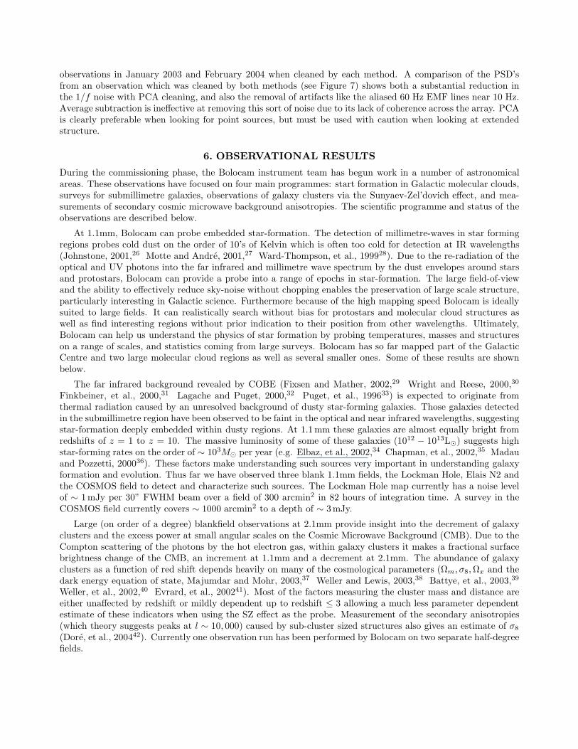
observations in January 2003 and February 2004 when cleaned by each method. A comparison of the PSD’sfrom an observation which was cleaned by both methods (see Figure 7) shows both a substantial reduction inthe 1/f noise with PCA cleaning, and also the removal of artifacts like the aliased 60 Hz EMF lines near 10 Hz.Average subtraction is ineffective at removing this sort of noise due to its lack of coherence across the array. PCAis clearly preferable when looking for point sources, but must be used with caution when looking at extendedstructure.

6. OBSERVATIONAL RESULTS

During the commissioning phase, the Bolocam instrument team has begun work in a number of astronomicalareas. These observations have focused on four main programmes: start formation in Galactic molecular clouds,surveys for submillimetre galaxies, observations of galaxy clusters via the Sunyaev-Zel’dovich effect, and mea-surements of secondary cosmic microwave background anisotropies. The scientific programme and status of theobservations are described below.

At 1.1mm, Bolocam can probe embedded star-formation. The detection of millimetre-waves in star formingregions probes cold dust on the order of 10’s of Kelvin which is often too cold for detection at IR wavelengths(Johnstone, 2001,26 Motte and Andre, 2001,27 Ward-Thompson, et al., 199928). Due to the re-radiation of theoptical and UV photons into the far infrared and millimetre wave spectrum by the dust envelopes around starsand protostars, Bolocam can provide a probe into a range of epochs in star-formation. The large field-of-viewand the ability to effectively reduce sky-noise without chopping enables the preservation of large scale structure,particularly interesting in Galactic science. Furthermore because of the high mapping speed Bolocam is ideallysuited to large fields. It can realistically search without bias for protostars and molecular cloud structures aswell as find interesting regions without prior indication to their position from other wavelengths. Ultimately,Bolocam can help us understand the physics of star formation by probing temperatures, masses and structureson a range of scales, and statistics coming from large surveys. Bolocam has so far mapped part of the GalacticCentre and two large molecular cloud regions as well as several smaller ones. Some of these results are shownbelow.

The far infrared background revealed by COBE (Fixsen and Mather, 2002,29 Wright and Reese, 2000,30

Finkbeiner, et al., 2000,31 Lagache and Puget, 2000,32 Puget, et al., 199633) is expected to originate fromthermal radiation caused by an unresolved background of dusty star-forming galaxies. Those galaxies detectedin the submillimetre region have been observed to be faint in the optical and near infrared wavelengths, suggestingstar-formation deeply embedded within dusty regions. At 1.1mm these galaxies are almost equally bright fromredshifts of z = 1 to z = 10. The massive luminosity of some of these galaxies (1012 − 1013L) suggests highstar-forming rates on the order of ∼ 103M per year (e.g. Elbaz, et al., 2002,34 Chapman, et al., 2002,35 Madauand Pozzetti, 200036). These factors make understanding such sources very important in understanding galaxyformation and evolution. Thus far we have observed three blank 1.1mm fields, the Lockman Hole, Elais N2 andthe COSMOS field to detect and characterize such sources. The Lockman Hole map currently has a noise levelof ∼ 1mJy per 30” FWHM beam over a field of 300 arcmin2 in 82 hours of integration time. A survey in theCOSMOS field currently covers ∼ 1000 arcmin2 to a depth of ∼ 3mJy.

Large (on order of a degree) blankfield observations at 2.1mm provide insight into the decrement of galaxyclusters and the excess power at small angular scales on the Cosmic Microwave Background (CMB). Due to theCompton scattering of the photons by the hot electron gas, within galaxy clusters it makes a fractional surfacebrightness change of the CMB, an increment at 1.1mm and a decrement at 2.1mm. The abundance of galaxyclusters as a function of red shift depends heavily on many of the cosmological parameters (Ωm, σ8, Ωx and thedark energy equation of state, Majumdar and Mohr, 2003,37 Weller and Lewis, 2003,38 Battye, et al., 2003,39

Weller, et al., 2002,40 Evrard, et al., 200241). Most of the factors measuring the cluster mass and distance areeither unaffected by redshift or mildly dependent up to redshift ≤ 3 allowing a much less parameter dependentestimate of these indicators when using the SZ effect as the probe. Measurement of the secondary anisotropies(which theory suggests peaks at l ∼ 10, 000) caused by sub-cluster sized structures also gives an estimate of σ8

(Dore, et al., 200442). Currently one observation run has been performed by Bolocam on two separate half-degreefields.

Figure 8. Left: A 7.5 square degree field of the Perseus molecular cloud region with inset on NGC1333. It is a 40 hourintegration, PCA cleaned to extract the sources. The NGC1333 inset is average cleaned, to preserve larger scale structureand prevent the distortion of the relative amplitudes of the sources. All of the sources are either dense cores of dustand gas which will probably form a star, or are envelopes of dust and gas surrounding an embedded protostar. Right:NGC1333: A very well known region where an open cluster is forming.

Figure 9. Left: IC 348 is a young open cluster in Perseus, and is compared here to a SHARC II map. The 1σ RMS ofthe Bolocam map is about 30 mJy with the SHARC II map RMS being about 100mJy at 350µm. The Bolocam map isabout 64 square arc-minutes and is cleaned with average sky subtraction. Most of these objects are probably very youngprotostars at a stage where they have yet to accrete most of their mass (Class 0 or Class I). Several of these sources werediscovered by the Bolocam map. Right: Map of the B1 Ridge in the Perseus region. It shows an extended ridge of 1mmemission below the bright cores of B1. There are no previously known sources in this ridge region; these newly identifiedsources are probably starless cores, which may collapse to form stars in the future. This is compared with SHARC IIfollow up observations which identifies emission in the same field.

Small field observations (8’x 8’) of known galaxy clusters have been made with Bolocam primarily to detectand characterize the Sunyaev Zel’dovich Effect, mostly at 1.1mm. The higher resolution of Bolocam shouldenable the identification, and therefore removal of point sources to a certain extent, and enables the follow upand greater characterization of these sources by other instruments at shorter wavelengths. Estimates of theHubble Constant, as well as information about the evolution of large scale structure, can be obtained from

such observations. The characterization of previously observed (by other instruments) galaxy clusters with wellunderstood profiles by Bolocam also aids in the identification and characterization of galaxy clusters that maybe found in a 2.1mm blank survey. This has been done infrequently before. Finally, due to the relatively largefields compared to those previously performed by other cameras in the mm and submillimetre bands, theseobservations can potentially probe the effect of the ICM on in-falling galaxies and their star formation rates.Currently point sources have been detected in the Bolocam map of the cluster Abell 1835 which correspondsto those identified by SCUBA (Edge, et al., 1999,43 Zemcov, private communication, 2004), as well as sourcecandidates further from the cluster centre than has previously been probed at 1.1mm. This is being followedup with further integration and comparison to radio maps. A tentative detection of the Sunyaev Zel’dovichincrement has also been noted in the observations made with Bolocam. This analysis is to be performed on otherclusters observed.

7. CONCLUSION

Bolocam has been successfully integrated on the CSO and is now open to observing applications from thescientific community. Mapping speeds of the system have been characterized under a variety of atmosphericconditions using different cleaning algorithms to remove atmospheric noise fluctuations in observations at 1.1and 2.1mm wavelengths. The 50% mapping speeds accounting for weather are 20 arcmin2/mJy2/Hr at 1.1mmand 14 arcmin2/mJy2/Hr at 2.1mm, (not accounting for observing efficiency and using PCA cleaning). TheBolocam team has begun a scientific programme including: blank field surveys at 1.1mm and 2.1mm, surveysof giant molecular clouds at 1.1mm and pointed surveys of galaxy cluster fields.

ACKNOWLEDGMENTS

Douglas Haig would like to acknowledge PPARC for support via a PPARC PhD studentship. We would like toacknowledge support from PPARC grants PPA/Y/S/2000/00101 and PPA/G/O/2002/00015 in the UK and fromgrants NSF/AST-0206158 and NASA/NGT5-50384 and NSF/AST-0098737 in the US. Alexey Goldin would liketo acknowledge support from a National Research Council Fellowship. Sunil Golwala would like to acknowledgethe support from the Caltech Millikan fellowship. Finally we would like to acknowledge the continuing supportfrom the CSO director Tom Phillips and all the CSO staff.

REFERENCES

1. E. Kreysa, H. Gemuend, J. Gromke, C. G. Haslam, L. Reichertz, E. E. Haller, J. W. Beeman, V. Hansen,A. Sievers, and R. Zylka, “Bolometer array development at the Max-Planck-Institut fuer Radioastronomie,”in Proc. SPIE Vol. 3357, p. 319-325, Advanced Technology MMW, Radio, and Terahertz Telescopes, ThomasG. Phillips; Ed., pp. 319–325, July 1998.

2. A. Omont, A. Beelen, F. Bertoldi, P. Cox, C. L. Carilli, R. S. Priddey, R. G. McMahon, and K. G. Isaak,“A 1.2 mm MAMBO/IRAM-30 m study of dust emission from optically luminous z ˜ 2 quasars,” A&A 398,pp. 857–865, Feb. 2003.

3. W. S. Holland, E. I. Robson, W. K. Gear, C. R. Cunningham, J. F. Lightfoot, T. Jenness, R. J. Ivison,J. A. Stevens, P. A. R. Ade, M. J. Griffin, W. D. Duncan, J. A. Murphy, and D. A. Naylor, “SCUBA:a common-user submillimetre camera operating on the James Clerk Maxwell Telescope,” MNRAS 303,pp. 659–672, Mar. 1999.

4. C. D. Dowell, C. A. Allen, R. S. Babu, M. M. Freund, M. Gardner, J. Groseth, M. D. Jhabvala, A. Kovacs,D. C. Lis, S. H. Moseley, T. G. Phillips, R. F. Silverberg, G. M. Voellmer, and H. Yoshida, “SHARCII: a Caltech submillimeter observatory facility camera with 384 pixels,” in Millimeter and SubmillimeterDetectors for Astronomy. Edited by Phillips, Thomas G.; Zmuidzinas, Jonas. Proceedings of the SPIE,Volume 4855, pp. 73-87 (2003)., pp. 73–87, Feb. 2003.

5. A. Kosowsky, “The Atacama Cosmology Telescope,” New Astronomy Review 47, pp. 939–943, Dec. 2003.

6. M. C. Runyan, P. A. R. Ade, R. S. Bhatia, J. J. Bock, M. D. Daub, J. H. Goldstein, C. V. Haynes,W. L. Holzapfel, C. L. Kuo, A. E. Lange, J. Leong, M. Lueker, M. Newcomb, J. B. Peterson, C. Reichardt,J. Ruhl, G. Sirbi, E. Torbet, C. Tucker, A. D. Turner, and D. Woolsey, “ACBAR: The Arcminute CosmologyBolometer Array Receiver,” ApJS 149, pp. 265–287, Dec. 2003.

7. D. Schwan, F. Bertoldi, S. Cho, M. Dobbs, R. Guesten, N. W. Halverson, W. L. Holzapfel, E. Kreysa,T. M. Lanting, A. T. Lee, M. Lueker, J. Mehl, K. Menten, D. Muders, M. Myers, T. Plagge, A. Raccanelli,P. Schilke, P. L. Richards, H. Spieler, and M. White, “APEX-SZ a Sunyaev-Zel’dovich galaxy cluster survey,”New Astronomy Review 47, pp. 933–937, Dec. 2003.

8. H. Ezawa, “The Atacama Submillimeter Telescope Experiment (ASTE) and Observations of Galaxy Clus-ters with Submillimeter Waves,” in ASP Conf. Ser. 268: Tracing Cosmic Evolution with Galaxy Clusters,pp. 357–+, 2002.

9. M. J. Griffin, B. M. Swinyard, and L. G. Vigroux, “SPIRE - Herschel’s Submillimetre Camera and Spec-trometer,” in IR Space Telescopes and Instruments. Edited by John C. Mather . Proceedings of the SPIE,Volume 4850, pp. 686-697 (2003)., pp. 686–697, Mar. 2003.

10. J. E. Carlstrom and The Spt Collaboration, “The 8m South Pole Telescope,” Astronomy in Antarctica, 25thmeeting of the IAU, Special Session 2, 18 July, 2003 in Sydney, Australia 2, 2003.

11. J. Glenn, P. A. R. Ade, M. Amarie, J. J. Bock, S. F. Edgington, A. Goldin, S. Golwala, D. Haig, A. E.Lange, G. Laurent, P. D. Mauskopf, M. Yun, and H. Nguyen, “Current status of Bolocam: a large-formatmillimeter-wave bolometer camera,” in Millimeter and Submillimeter Detectors for Astronomy. Edited byPhillips, Thomas G.; Zmuidzinas, Jonas. Proceedings of the SPIE, Volume 4855, pp. 30-40 (2003)., pp. 30–40, Feb. 2003.

12. J. Glenn, J. J. Bock, G. Chattopadhyay, S. F. Edgington, A. E. Lange, J. Zmuidzinas, P. D. Mauskopf,B. Rownd, L. Yuen, and P. A. Ade, “Bolocam: a millimeter-wave bolometric camera,” in Proc. SPIE Vol.3357, p. 326-334, Advanced Technology MMW, Radio, and Terahertz Telescopes, Thomas G. Phillips; Ed.,pp. 326–334, July 1998.

13. R. S. Bhatia, S. T. Chase, S. F. Edgington, J. Glenn, W. C. Jones, A. E. Lange, B. Maffei, A. K. Mainzer,P. D. Mauskopf, B. J. Philhour, and B. K. Rownd, “A three-stage helium sorption refrigerator for coolingof infrared detectors to 280 mK,” Cryogenics 40, pp. 685–691, 2001.

14. P. D. Mauskopf, J. J. Bock, H. del Castillo, W. L. Holzapfel, and A. E. Lange, “Composite infrared bolome-ters with Si 3 N 4 micromesh absorbers,” Appl. Opt. 36, pp. 765–771, Feb. 1997.

15. J. J. Bock, J. Glenn, S. M. Grannan, K. D. Irwin, A. E. Lange, H. G. Leduc, and A. D. Turner, “Siliconnitride micromesh bolometer arrays for SPIRE,” in Proc. SPIE Vol. 3357, p. 297-304, Advanced TechnologyMMW, Radio, and Terahertz Telescopes, Thomas G. Phillips; Ed., pp. 297–304, July 1998.

16. B. P. Crill, P. A. R. Ade, D. R. Artusa, R. S. Bhatia, J. J. Bock, A. Boscaleri, P. Cardoni, S. E. Church,K. Coble, P. de Bernardis, G. de Troia, P. Farese, K. M. Ganga, M. Giacometti, C. V. Haynes, E. Hivon,V. V. Hristov, A. Iacoangeli, W. C. Jones, A. E. Lange, L. Martinis, S. Masi, P. V. Mason, P. D. Mauskopf,L. Miglio, T. Montroy, C. B. Netterfield, C. G. Paine, E. Pascale, F. Piacentini, G. Polenta, F. Pongetti,G. Romeo, J. E. Ruhl, F. Scaramuzzi, D. Sforna, and A. D. Turner, “BOOMERANG: A Balloon-borneMillimeter-Wave Telescope and Total Power Receiver for Mapping Anisotropy in the Cosmic MicrowaveBackground,” ApJS 148, pp. 527–541, Oct. 2003.

17. J. Glenn, G. Chattopadhyay, S. F. Edgington, A. E. Lange, J. J. Bock, P. D. Mauskopf, and A. T. Lee,“Numerical optimization of integrating cavities for diffraction-limited millimeter-wave bolometer arrays,”Appl. Opt. 41, pp. 136–142, Jan. 2002.

18. B. Rownd, J. J. Bock, G. Chattopadhyay, J. Glenn, and M. J. Griffin, “Design and performance of feedhorn-coupled bolometer arrays for SPIRE,” in Millimeter and Submillimeter Detectors for Astronomy. Edited byPhillips, Thomas G.; Zmuidzinas, Jonas. Proceedings of the SPIE, Volume 4855, pp. 510-519 (2003).,pp. 510–519, Feb. 2003.

19. W. Gonzalez, R., Digital Image Processing, Addison Wesley, US, 1992.

20. P. D. Mauskopf, “Measurements of Anisotropies in the Cosmic Microwave Background at Small and Inter-mediate Angular Scales with Bolometric Receivers at MM Wavelengths,” Ph.D. Thesis , 1997.

21. W. L. Holzapfel, T. M. Wilbanks, P. A. R. Ade, S. E. Church, M. L. Fischer, P. D. Mauskopf, D. E. Osgood,and A. E. Lange, “The Sunyaev-Zeldovich Infrared Experiment: A Millimeter-Wave Receiver for ClusterCosmology,” ApJ 479, pp. 17–+, Apr. 1997.

22. P. D. Mauskopf, P. A. R. Ade, S. W. Allen, S. E. Church, A. C. Edge, K. M. Ganga, W. L. Holzapfel,A. E. Lange, B. K. Rownd, B. J. Philhour, and M. C. Runyan, “A Determination of the Hubble ConstantUsing Measurements of X-Ray Emission and the Sunyaev-Zeldovich Effect at Millimeter Wavelengths in theCluster Abell 1835,” ApJ 538, pp. 505–516, Aug. 2000.

23. B. Weferling, L. A. Reichertz, J. Schmid-Burgk, and E. Kreysa, “Principles of the data reduction and firstresults of the fastscanning method for (sub)millimeter astronomy,” A&A 383, pp. 1088–1099, Mar. 2002.

24. R. G. Conway, E. J. Daintree, and R. J. Long, “Observations of radio sources at 612 and 1400 Mc/s,”MNRAS 131, pp. 159–+, 1965.

25. D. T. Emerson, U. Klein, and C. G. T. Haslam, “A multiple beam technique for overcoming atmosphericlimitations to single-dish observations of extended radio sources,” A&A 76, pp. 92–105, June 1979.

26. D. Johnstone, “JCMT SCUBA-Diving in Nearby Molecular Clouds: The Case for Large Systematic Surveyswith FIRST,” in ESA SP-460: The Promise of the Herschel Space Observatory, pp. 235–+, July 2001.

27. F. Motte and P. Andre, “The circumstellar environment of low-mass protostars: A millimeter continuummapping survey,” A&A 365, pp. 440–464, Jan. 2001.

28. D. Ward-Thompson, F. Motte, and P. Andre, “The initial conditions of isolated star formation - III. Mil-limetre continuum mapping of pre-stellar cores,” MNRAS 305, pp. 143–150, May 1999.

29. D. J. Fixsen and J. C. Mather, “The Spectral Results of the Far-Infrared Absolute SpectrophotometerInstrument on COBE,” ApJ 581, pp. 817–822, Dec. 2002.

30. E. L. Wright and E. D. Reese, “Detection of the Cosmic Infrared Background at 2.2 and 3.5 Microns UsingDIRBE Observations,” ApJ 545, pp. 43–55, Dec. 2000.

31. D. P. Finkbeiner, M. Davis, and D. J. Schlegel, “Detection of a Far-Infrared Excess with DIRBE at 60 and100 Microns,” ApJ 544, pp. 81–97, Nov. 2000.

32. G. Lagache and J. L. Puget, “Detection of the extra-Galactic background fluctuations at 170 mu m,” A&A355, pp. 17–22, Mar. 2000.

33. J.-L. Puget, A. Abergel, J.-P. Bernard, F. Boulanger, W. B. Burton, F.-X. Desert, and D. Hartmann,“Tentative detection of a cosmic far-infrared background with COBE.,” A&A 308, pp. L5+, Apr. 1996.

34. D. Elbaz, C. J. Cesarsky, P. Chanial, H. Aussel, A. Franceschini, D. Fadda, and R. R. Chary, “The bulk ofthe cosmic infrared background resolved by ISOCAM,” A&A 384, pp. 848–865, Mar. 2002.

35. S. C. Chapman, D. Scott, C. Borys, and G. G. Fahlman, “Submillimetre sources in rich cluster fields: sourcecounts, redshift estimates and cooling flow limits,” MNRAS 330, pp. 92–104, Feb. 2002.

36. P. Madau and L. Pozzetti, “Deep galaxy counts, extragalactic background light and the stellar baryonbudget,” MNRAS 312, pp. L9–L15, Feb. 2000.

37. S. Majumdar and J. J. Mohr, “Importance of Cluster Structural Evolution in Using X-Ray and Sunyaev-Zeldovich Effect Galaxy Cluster Surveys to Study Dark Energy,” ApJ 585, pp. 603–610, Mar. 2003.

38. J. Weller and A. M. Lewis, “Large-scale cosmic microwave background anisotropies and dark energy,”MNRAS 346, pp. 987–993, Dec. 2003.

39. R. A. Battye and J. Weller, “Constraining cosmological parameters using Sunyaev-Zel’dovich cluster sur-veys,” Phys. Rev. D 68, pp. 083506–+, Oct. 2003.

40. J. Weller, R. A. Battye, and R. Kneissl, “Constraining Dark Energy with Sunyaev-Zel’dovich Cluster Sur-veys,” Physical Review Letters 88, pp. 231301–+, June 2002.

41. A. E. Evrard, T. J. MacFarland, H. M. P. Couchman, J. M. Colberg, N. Yoshida, S. D. M. White, A. Jenkins,C. S. Frenk, F. R. Pearce, J. A. Peacock, and P. A. Thomas, “Galaxy Clusters in Hubble Volume Simulations:Cosmological Constraints from Sky Survey Populations,” ApJ 573, pp. 7–36, July 2002.

42. O. Dore, J. F. Hennawi, and D. N. Spergel, “Beyond the Damping Tail: Cross-Correlating the KineticSunyaev-Zel’dovich Effect with Cosmic Shear,” ApJ 606, pp. 46–57, May 2004.

43. A. C. Edge, R. J. Ivison, I. Smail, A. W. Blain, and J.-P. Kneib, “The detection of dust in the centralgalaxies of distant cooling-flow clusters,” MNRAS 306, pp. 599–606, July 1999.