Naef, Alain

Working Paper

Blowing against the Wind? A Narrative Approach toCentral Bank Foreign Exchange Intervention

EHES Working Paper, No. 188

Provided in Cooperation with:European Historical Economics Society (EHES)

Suggested Citation: Naef, Alain (2020) : Blowing against the Wind? A Narrative Approachto Central Bank Foreign Exchange Intervention, EHES Working Paper, No. 188, EuropeanHistorical Economics Society (EHES), s.l.

This Version is available at:http://hdl.handle.net/10419/247118

Standard-Nutzungsbedingungen:

Die Dokumente auf EconStor dürfen zu eigenen wissenschaftlichenZwecken und zum Privatgebrauch gespeichert und kopiert werden.

Sie dürfen die Dokumente nicht für öffentliche oder kommerzielleZwecke vervielfältigen, öffentlich ausstellen, öffentlich zugänglichmachen, vertreiben oder anderweitig nutzen.

Sofern die Verfasser die Dokumente unter Open-Content-Lizenzen(insbesondere CC-Lizenzen) zur Verfügung gestellt haben sollten,gelten abweichend von diesen Nutzungsbedingungen die in der dortgenannten Lizenz gewährten Nutzungsrechte.

Terms of use:

Documents in EconStor may be saved and copied for yourpersonal and scholarly purposes.

You are not to copy documents for public or commercialpurposes, to exhibit the documents publicly, to make thempublicly available on the internet, or to distribute or otherwiseuse the documents in public.

If the documents have been made available under an OpenContent Licence (especially Creative Commons Licences), youmay exercise further usage rights as specified in the indicatedlicence.

European Historical Economics Society

EHES Working Paper | No. 188 | June 2020

Blowing against the Wind? A Narrative Approach to Central Bank Foreign Exchange Intervention

Alain Naef,

University of California, Berkeley

EHES Working Paper | No. 188 | June 2020

Blowing against the Wind? A Narrative Approach to Central Bank Foreign Exchange Intervention*

Alain Naef1,

University of California, Berkeley

Abstract Few studies on foreign exchange intervention convincingly address the causal effect of intervention on exchange rates. By using a narrative approach, I address a major issue in the literature: the endogeneity of intraday news which influence the exchange rate alongside central bank operations. Some studies find that interventions work in up to 80% of cases. Yet, by accounting for intraday market moving news, I find that in adverse conditions, the Bank of England managed to influence the exchange rate only in 8% of cases. I use both machine learning and human assessment to confirm the validity of the narrative approach.

JEL Codes: F31, E5, N14, N24

Keywords: intervention, foreign exchange, natural language processing, central bank, Bank of England.

Notice

The material presented in the EHES Working Paper Series is property of the author(s) and should be quoted as such. The views expressed in this Paper are those of the author(s) and do not necessarily represent the views of the EHES or

its members

* Part of this research was supported by the Economic and Social Research Council (grant number ESRC KFW/10324121/0) as well as the Swiss National Science Foundation (grant number P2SKP1_181320). I thank Jiaxin Lei and Gaurav Gandhi for excellent research assistance. For discussions and comments, I am grateful to Marc Adam, Brad DeLong, Simon Hinrischsen, Walter Jansson, Chris Meissner, Eric Monnet, Emi Nakamura, David Romer, Yasmin Shearmur, Jón Steinsson, Tobias Stöhr, Mauricio Villamizar Villegas and Jacob Weber as well as participants at the European Economic History Conference in Paris, all-UC economic history conference, seminars at the Banque of France, Lancaster, UC Berkeley and UC Davis. 1 Corresponding author: Alain Naef, alain.naef@berkeley.edu

2

Intervention on the foreign exchange market is important. Most central banks still

follow exchange rate objectives and over 80% of countries are on fixed exchange regimes

(Taylor 2010; Ilzetzki, Reinhart, and Rogoff 2019). According to recent theoretical

findings, intervention could even be welfare-enhancing (Gabaix and Maggiori 2015;

Hassan, Mertens, and Zhang 2016). Central bankers generally believe that intervention

has an impact on exchange rates (Neely 2008). Academics, on the other hand, have

generated contradictory findings. Most studies trying to assess intervention use daily

data and struggle to deal with the endogeneity caused by intraday changes in market

conditions, making it difficult to assess the effectiveness of intervention.

Our understanding of central bank intervention is limited by a lack of data, as

central banks keep their intervention records secret. In this paper, I unveil hand-

collected intervention data from the UK, spanning over 40 years from 1952 to 1992.

The data is original as it is mainly composed of secret interventions, which were not

communicated to the public (this is still how many central banks operate today). The

database I created is the longest for any advanced economy and is open for replication

unlike other studies on central bank intervention, which are often bound to data

confidentiality. All interventions in the data set are sterilized interventions, a British

institutional feature. As operations were run through the Exchange Equalisation

Account and not the Bank of England directly, all operations had a counterparty

transaction in government bonds.

I find that, after accounting for some of the intraday measurement problems of

previous studies, foreign exchange interventions that go against market trends (“against

the wind”, as central bankers put it) only influence exchange rates in around 8% of

cases. This is in stark contrast to recent literature showing foreign exchange

intervention success rates of up to 80% (Fratzscher et al. 2019). Half of the

interventions considered successful using the previous standard methodologies no longer

count as successful, when measuring whether good or bad news (independent from

central bank interventions) were circulating on a given day. Intervention is particularly

3

ineffective when attempting to reverse the direction of the exchange rate after negative

news affecting the currency. Bank of England intervention was more effective when

trying to tame the appreciation of sterling ( “restraining intervention”) than when

trying to avoid a depreciation of sterling (“defending intervention”).

An intuitive example allows us to understand the shortcomings of most intervention

studies to date. Imagine that today, the People’s Bank of China (PBOC) was trying to

make the renminbi appreciate through foreign exchange intervention. At 10am, they

buy renminbi with their dollar reserves, hoping this will bolster the renminbi’s price.

Now imagine that an hour later, President Trump tweets something signalling an end

to the trade war with China, sparking a stark appreciation of the renminbi. Most studies

on intervention would simply assume that any interventions during that day were going

against the wind, and count this intervention as successful. My narrative approach

accounts for other news during the day to assess whether the intervention was really

going against the wind, or if it merely happened to go in the same direction as the

market.

I use an event study methodology to test the effectiveness of British foreign

exchange intervention between 1952 and 1992. From 1952 to 1986, I rely only on an

event study and a placebo test to measure the effectiveness of intervention. From 1986

to 1992, I also use the narrative approach, which is at the heart of this paper’s key

finding on the impact of intraday news.

Central bank intervention is hard to assess as it is often measured without intraday

data, and therefore not accounting for any changes in market conditions. My paper

deals with these endogeneity problems by relying on narrative evidence about market

conditions written by Bank of England officials. I use a narrative approach as pioneered

by Romer and Romer (1989). I clearly identify days when the currency is hit by negative

news that is not related to the intervention of the central bank. I get this measure by

analyzing the text from the daily reports written by Bank of England employees. To

4

test the robustness of my analysis, I rely on both an external assessment and machine

learning in the form of Natural Language Processing (NLP).

In brief, the main contribution of this paper is to demonstrate how intervention

success is much lower when intraday market news is accounted for. This is the first

study to use a narrative approach to deal with endogeneity issues of central bank

intervention success. The paper also offers a new database for research on central bank

intervention, spanning over 40 years and available for replication.

1. Literature review

Central bank intervention can either be sterilized (with simultaneous bill

purchases that leave the monetary conditions unaffected) or unsterilized (with no

asset purchases, thus affecting the monetary conditions). Unsterilized intervention

affects the exchange rate through changes in interest rates, making the currency

more or less attractive to investors. The effectiveness of sterilized intervention has

long been questioned and the debate is still ongoing.2

The literature identifies three channels through which sterilized intervention

works: portfolio-balance, signaling and coordination. The portfolio-balance channel

has received the most attention in the literature (Cavallino 2019; Gabaix and

Maggiori 2015; Fatum 2015; Dominguez and Frankel 1993). The channel works

through investors portfolio shocks, which affect the amount of bonds in circulation

and their risk premia and by doing so affect the exchange rate. Signaling works

through central banks giving hints of future monetary policy stances to which the

market reacts (Fatum and Hutchison 1999). The coordination channel works when

the market is thin and traders have lost confidence in the ability of macroeconomic

2 For an overview of the literature on central bank intervention, see Sarno and Taylor (2001) and Neely (2005), more recent papers by Adler, Lisack, and Mano (2019); Adler and Mano (2018); Echavarría, Melo-Velandia, and Villamizar-Villegas (2018) and Hu et al. (2016).

5

fundamentals to inform the price, the central bank can step in and provide direction

(Reitz and Taylor 2008). In this paper, I do not choose a channel through which

intervention could work, but focus on methodological issues in current papers on

the topic.

Looking at the empirical literature on intervention, most papers published

fail to identify the causal relationship between intervention and exchange rates as

the two variables are too endogenous. In a cross-country study analyzing 35

countries, Blanchard, Adler, and Filho (2015) demonstrate that sterilized

intervention can hinder unwanted currency appreciation due to capital inflows.

Fratzscher et al. (2019) argue that intervention is effective in over 80% of cases

when managing volatility. Presenting evidence from 33 countries, they argue that

central bank intervention was effective in attaining the goals set by policymakers

from 1995 to 2011. The paper does an excellent job at analyzing new data but does

not offer a convincing identification strategy.

Interestingly, independently of what macroeconomists may think, central

bankers themselves, when surveyed, generally think that intervention is an effective

way to influence exchange rates (Neely 2008).

A key contention in the literature on foreign exchange intervention is that

intervention is not random but happens as a reaction to market conditions. Market

conditions often shift during the day and intervention success is not exogenous to

market conditions. Most articles offer solutions to tackle this endogeneity issue, but

few do so convincingly. Fatum and Hutchison (2006, 392) note that the main issue

of endogeneity “arises in our study (and every intervention study) since the central

bank usually takes its cue to intervene on the basis of observed exchange rate

movements”.

To try to mitigate endogeneity, Fatum and Hutchison (2006) group

interventions into clusters and assess the effectiveness not of the total daily

6

interventions but of a cluster. In their approach, if a central bank sells dollars for

three consecutive days, their measure counts the intervention as successful if after

the third day the exchange rate goes in the expected direction. They admit,

however, that their clustering might make interventions appear more successful

than they are. Fratzscher et al. (2019) use a similar method of grouping

interventions in clusters.

This clustering methodology is problematic, especially if the exchange rate

is considered as a random walk in the medium term. For example, exogenous factors

- such as the publication of better than expected GDP figures when the central

bank is trying to make the currency appreciate - can make intervention seem

successful, when success has little to do with the intervention itself. Following this

logic, the central bank will eventually be successful if it intervenes for long enough

and stops when the exchange rate goes in the desired direction. Success will then

be due to pure luck or exogenous factors. To avoid this issue, I instead assess the

impact of intervention after one day; in addition, my narrative approach factors in

exogenous news (on narrative approaches see Romer and Romer 1989; 1994; 2014;

Monnet 2014). Using a one-day horizon is also in line with findings showing that

most of the impact of intervention lasts one day.3

Kearns and Rigobon (2005) use shifts by both the Bank of Japan and the

Australian Central Bank from small, frequent interventions to large, infrequent

interventions - which they interpret as exogenous shocks - to better understand the

effectiveness of central bank intervention. The authors admit that while useful,

their contribution does not completely deal with the endogeneity problem.

Most studies on intervention effectiveness fail to account for intraday news

changes. Most studies also assume that all interventions go against the wind putting

3 Kearns and Rigobon (2005, 31) show that “almost all of the impact of an intervention occurs during the day it is conducted”.

7

them in one homogenous group. My paper shows that this is not the case and that

the “wind” (or news about the currency) can change during the day. Authors

themselves acknowledge that their studies rarely convincingly address endogeneity.

The main contribution of this paper is to show that by not accounting for intraday

news, most papers on intervention effectiveness provide biased estimates.

2. New confidential data

The issue with studies on central bank intervention is the lack of available data.

And when data are available, it is usually only data on public intervention, though it

has been shown that most central banks intervene in secret (Mohanty and Berger 2013).

Various empirical studies therefore use the same datasets and focus only on countries

with public intervention records such as Turkey, Colombia or Japan. Looking at secret

intervention, my findings have implications for all central banks intervening in secret,

which is under-researched. Almost all interventions in my sample were secret - less than

1% of the operations were publicized (66 out of 8,429). Note that secret intervention

does not mean that the market is unaware of the intervention; it means that the central

bank does not officially announce it. Dominguez (2003) suggests that traders in the

1990s usually knew that the Fed was intervening at least one hour before any news

outlets would report it.

This paper presents the first long run daily database of intervention by an advanced

economy, presenting data for over 40 years. Figure 1 presents the data in 1992-US

dollars. The data offers an aggregate amount of all Bank of England intervention

operations during a given day. This includes intervention in any currency. In practice

interventions were mainly in dollars until 1987 and in deutschmark thereafter (see the

historical section for more details).

8

Figure 1 – Intervention by the Bank of England in million of 1992-dollars. Source: The data have been copied from reports written with typewritters kept at the archives of the Bank of England (archive reference C8). NOTE: The data are cropped at $1bn to improve readabilty but the figures go up to -22$bn for Black Wednesday on 16 September 1992.

The data are negative for sales and positive for purchases of foreign currency.

Intervention data come from the Bank of England dealers’ reports, which offer daily

records.4 The reports were written by the dealers of the Bank of England, foreign

exchange operators who managed sterling on behalf of the government. The archive of

the Bank of England kept printed copies of the reports, which I copied individually to

put together my database.

Another benefit of this data is that it comes directly from policymakers, without

any filter or control. Published data by central banks are likely to be processed before

publication and might not include all operations. It is well known to foreign exchange

traders today that, for example, South Africa and Brazil, publish some of their

operations while keeping a large unpublished derivatives’ book. The dataset presented

4 Bank of England Archives, Cashier's Department: Foreign Exchange and Gold Markets – Dealers’ Reports, C8.

-4,000

-2,000

0

2,000

4,000

1955 1960 1965 1970 1975 1980 1985 1990 1995

Bank of England interventions (million 1992-dollars)

Positive values = dollar and DM purchases (restraining operations)

Negative values = dollar and DM purchases (defending operations)

9

here is much more precise than those of other studies in the field, which rely on proxies,

such as changes in reserve levels or press reports.

3. Historical background 1952-1992

The postwar history of the pound can be separated into three clear phases when

it comes to Bank of England operations on the foreign exchange market. From 1945 to

1987, British policymakers mainly managed the pound against the dollar; from 1987 to

1992, the deutschmark was the reference currency and from 1992 to today, the pound

was left to float freely.

Dollar focus 1952-1987

1939-52 The foreign exchange market is mainly under the control of the state during the war and after.

January 1952 Reopening of the foreign exchange market under the Bretton Woods Fixed regime. Sterling fixed at $2.80 per pound, then $2.40 after the 1967 devaluation.

15 August 1971 Nixon shock: the US closes the gold window, in effect leaving the Bretton Woods agreement. Sterling floats.

18 December 1971 Smithsonian Agreement: 2.25% bands and new parities. 23 June 1972 The United Kingdom withdraws from the Smithsonian

Agreement and starts floating (effectively a sterling devaluation).

22 September 1985 Plaza Accord: coordinated interventions to appreciate the dollar.

Deutschmark focus 1987-1992

22 February 1987 Louvre Accord depreciates the dollar; the UK starts shadowing the deutschmark.

Early 1988 End of official deutschmark shadowing, but the deutschmark remains the main focus.

1 October 1990 Britain joins the European Exchange Rate Mechanism (ERM) with a band of +/- 6% with the ECU (and de facto with the deutschmark).

16 September 1992 Black Wednesday: the UK leaves the ERM, floating the pound.

10

The short timeline above outlines the history of these exchange rate systems

from 1952 to the present day. Most of the time, the pound was either in a fixed exchange

rate system or in a managed float. Only in 1992 was the currency left to float freely.

Characteristics of Bank of England intervention

How did the Bank of England intervene? In the sample presented, interventions by

the Bank of England were frequent and secret. Only 66 of the 8,429 interventions were

publicly communicated, less than 1% of the sample. Secret intervention makes study

of the Bank of England extremely relevant as most central banks today still intervene

in secret as well. Surveying central bankers, Mohanty and Berger (2013) found that

only 18% of central banks frequently communicated their intervention practices. This

means that most central banks intervene in secret, despite the literature arguing that

communicating intervention is more effective (Burkhard and Fischer 2009). Overall,

the Bank was in the market 79.5% of the trading days from 1952 (when the foreign

exchange market reopened after the war) to 1992, when it stopped trying to influence

the exchange rate.

Sterilized intervention by design

An institutional feature of the Bank of England ensured that all interventions were

automatically sterilized. The Bank of England operation were all done through the

EEA (Exchange Equalisation Account), which was independent from the Bank of

England and belonged to the Treasury. Howson (1980) showed that the institutional

structure of the EEA meant that all intervention operations had a counterparty in

Treasury bills. When the Bank of England was selling dollars against pounds, it would

reinvest the newly acquired pounds into British Treasury bills and doing so, sterilizing

the operation. Conversely, when the Bank wanted to buy US dollars, it first had to sell

Treasuries at the EEA to obtain sterling to purchase dollars. This meant that any

operation was automatically sterilized as a feature of the EEA.

11

Goals of Bank of England interventions

When assessing intervention, it is essential to understand what the central bank

was trying to achieve. Today, as during the 2009 crisis, central banks mainly want to

reduce exchange rate volatility (Fratzscher et al. 2019; Mohanty and Berger 2013;

Blanchard, Adler, and Filho 2015). However, during the period observed, the goal of

the Bank of England was different. Interviews with policymakers of the time and

archival records show that policymakers wanted to influence the exchange rate in one

direction or the other.

Although objectives change and are not set in stone, historical analysis shows clear

patterns in the goals of the Bank of England. The Bank intervened either to make the

exchange rate appreciate or depreciate. Below, I present several reports written by the

very people intervening: Bank of England dealers. By analyzing their own assessment

of interventions, the underlying goals of intervention become clear.

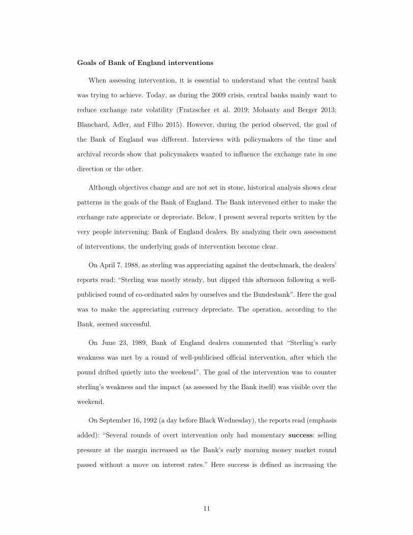
On April 7, 1988, as sterling was appreciating against the deutschmark, the dealers’

reports read: “Sterling was mostly steady, but dipped this afternoon following a well-

publicised round of co-ordinated sales by ourselves and the Bundesbank”. Here the goal

was to make the appreciating currency depreciate. The operation, according to the

Bank, seemed successful.

On June 23, 1989, Bank of England dealers commented that “Sterling’s early

weakness was met by a round of well-publicised official intervention, after which the

pound drifted quietly into the weekend”. The goal of the intervention was to counter

sterling’s weakness and the impact (as assessed by the Bank itself) was visible over the

weekend.

On September 16, 1992 (a day before Black Wednesday), the reports read (emphasis

added): “Several rounds of overt intervention only had momentary success: selling

pressure at the margin increased as the Bank's early morning money market round

passed without a move on interest rates.” Here success is defined as increasing the

12

sterling-deutschmark exchange rate, which was falling against the backdrop of a

growing crisis in the ERM.

These examples show the Bank trying to move the exchange rate, up or down. The

goal was not simply, as it is today, to reduce volatility, but to push the rate in a given

direction. This is an important point to bear in mind when assessing what counts as

success.

4. Does central bank intervention work? Evidence from new data and methodologies

This section assesses the intervention performance of the Bank of England based

on confidential data presented here for the first time. Few papers measuring central

bank intervention effectiveness deal with the direction of the wind effectively. To better

tackle intervention success, I use a narrative approach, detailed below. The advantage

of looking into history is that the reasoning behind the intervention decisions of

policymakers is available. The Bank of England recently changed its information access

policy and now opens most of its archival documents to researchers after a 20-year

period. As the last intervention occurred in 1992, we have recently gained access to the

reasoning of central bankers as they were intervening. As a narrative approach can

contain some subjective assessment, the robustness section uses both human- and

machine-based techniques to control for potential subjectivity in my assessment.

Assessing intervention success – An event study on over 10,000 trading days

Most studies on central bank intervention effectiveness either use GARCH and

other similar models to assess the effect of central bank interventions on market

volatility, or they rely on event study methodologies to assess the effect of the policy

on the exchange rate. GARCH models mainly deal with volatility, when the question

here is to understand whether intervention can influence the direction of the exchange

13

rate. Event studies are more appropriate than traditional regression approaches because

of the stochastic properties of intervention and exchange rate data: intervention occurs

in bursts and the exchange rate changes frequently in a martingale-like fashion. This

makes regression analysis unfit to properly assess the effectiveness of the policy.

For interested readers however, the appendix presents regressions as an alternative

to the approach taken here. Table 6 in the appendix offers a simple parametric approach

and shows that using a naïve regression, intervention can be understood as having the

opposite effect to the intended one. When accounting for intraday factors as outlined

in the narrative approach below, the regression in Table 9 yields similar results to the

event study approach. But as most studies on intervention effectiveness use event

studies, the analysis presented here will offer results that easily can be compared to

other findings.

This methodology relies on three intervention success criteria (SC) and is inspired

by a methodology by Bordo, Humpage, and Schwartz (2015). SC1 measures whether

intervention leads to an appreciation/depreciation of sterling against the dollar (later

deutschmark) between the previous day’s market close and the current day’s market

close. SC2 measures whether the exchange rate depreciates/appreciates less after

intervention between the day’s market close and the previous day’s market close than

it did over the immediately preceding period (also called smoothing). The final criterion,

SC3, combines the first two. The three criteria take the form of a binary variable and

are formalized in the equations on the next page.

14

𝑆𝐶1 =

⎩{⎨{⎧1 {

𝑖𝑓 𝐼𝑡 > 0, 𝑎𝑛𝑑 ∆𝑆𝑡 < 0, 𝑜𝑟

𝑖𝑓 𝐼𝑡 < 0, 𝑎𝑛𝑑 ∆𝑆𝑡 > 00 𝑜𝑡ℎ𝑒𝑟𝑤𝑖𝑠𝑒

 

 

𝑆𝐶2 =

⎩{⎨{⎧1 {

𝑖𝑓 𝐼𝑡 > 0, 𝑎𝑛𝑑 ∆𝑆𝑡−1 > 0 𝑎𝑛𝑑 ∆𝑆𝑡 ≥ 0, 𝑎𝑛𝑑 ∆𝑆𝑡 < ∆𝑆𝑡−1 𝑜𝑟

𝑖𝑓 𝐼𝑡 < 0, 𝑎𝑛𝑑 ∆𝑆𝑡−1 < 0 𝑎𝑛𝑑 ∆𝑆𝑡 ≤ 0, 𝑎𝑛𝑑 ∆𝑆𝑡 > ∆𝑆𝑡−10 𝑜𝑡ℎ𝑒𝑟𝑤𝑖𝑠𝑒

 

𝑆𝐶3 = {1 𝑆𝐶1 = 1 𝑜𝑟 𝑆𝐶2 = 10 𝑜𝑡ℎ𝑒𝑟𝑤𝑖𝑠𝑒

 

where It designates foreign exchange intervention on day t. Positive values are purchase

of foreign exchange (called restraining interventions) and negative values are sales of

foreign exchange (defending interventions). A purchase is expressed as 𝐼 0 and a sale

as 𝐼 0. ∆St is the difference between the spot closing rate on the day of the

intervention and the spot closing rate the day before the intervention. It shows the

effect of the intervention on the exchange rate during the day.

The focus is on the daily effect. This is justified by the type of intervention by the

Bank of England, which was on the market most days as explained above. As we have

seen, Kearns and Rigobon (2005, 31) show that most of the impact of an intervention

occurs during the day it is conducted. This underpins the choice of focusing on the day

of the intervention itself.

As shown in the historical section above, the Bank of England focused on the dollar

until February 1987 and the deutschmark thereafter. To account for this clear difference

in policy, the sample is divided into two subsamples: a dollar sample from the opening

of the foreign exchange market from February 1952 to February 1987. After the Louvre

Accord of February 1987, the British foreign exchange policy focuses mainly on the

deutschmark and this is the second sample. After the Black Wednesday crisis in

15

September 1992, intervention by the Bank of England stopped. Table 1 below is

separated into the three success criteria presented above as well as into defending (to

make the exchange rate appreciate) and restraining interventions (to make the

exchange rate depreciate).

Reversing exchange rate (SC1)

Smoothing appreciation or

depreciation (SC2)

Total success (SC3, sum of SC1 and SC2)

Day count

Success count

Percentage of successful intervention

Success count

Percentage of successful intervention

Success count

Percentage of successful

intervention

Dollar intervention (1952-1987) Defending interventions 2298 434 19% 465 20% 899 39% Restraining interventions 4817 1211 25% 794 16% 2005 42%

Deutschmark intervention (1987-1992) Defending interventions 357 102 29% 61 17% 163 46% Restraining interventions 957 327 34% 179 19% 506 53%

Table 1 – Intervention success according to the three criteria presented above.

Note that these “success” rates do not imply causality; it could be that some of

these “successes” are due to other factors (as we will see in the narrative approach).

The Bank could be trying to make the exchange appreciate on the same day that

improved GDP figures are published. In this case, the intervention would be counted

as successful, but the success would not only be due to intervention but also potentially

due to the GDP figures. The next section deals with this endogeneity problem. But as

stressed in the literature review, most published studies on the topic rely on these

success rates and simply run robustness checks to see if they lie within a realistic frame.

16

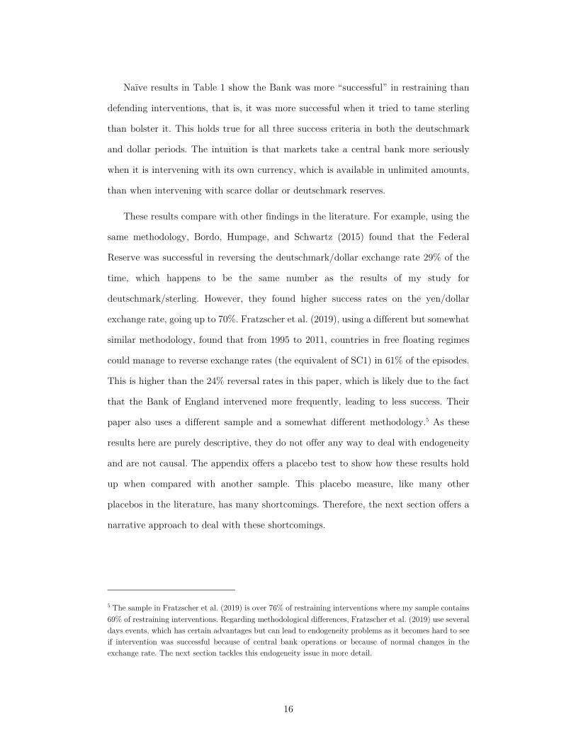
Naïve results in Table 1 show the Bank was more “successful” in restraining than

defending interventions, that is, it was more successful when it tried to tame sterling

than bolster it. This holds true for all three success criteria in both the deutschmark

and dollar periods. The intuition is that markets take a central bank more seriously

when it is intervening with its own currency, which is available in unlimited amounts,

than when intervening with scarce dollar or deutschmark reserves.

These results compare with other findings in the literature. For example, using the

same methodology, Bordo, Humpage, and Schwartz (2015) found that the Federal

Reserve was successful in reversing the deutschmark/dollar exchange rate 29% of the

time, which happens to be the same number as the results of my study for

deutschmark/sterling. However, they found higher success rates on the yen/dollar

exchange rate, going up to 70%. Fratzscher et al. (2019), using a different but somewhat

similar methodology, found that from 1995 to 2011, countries in free floating regimes

could manage to reverse exchange rates (the equivalent of SC1) in 61% of the episodes.

This is higher than the 24% reversal rates in this paper, which is likely due to the fact

that the Bank of England intervened more frequently, leading to less success. Their

paper also uses a different sample and a somewhat different methodology.5 As these

results here are purely descriptive, they do not offer any way to deal with endogeneity

and are not causal. The appendix offers a placebo test to show how these results hold

up when compared with another sample. This placebo measure, like many other

placebos in the literature, has many shortcomings. Therefore, the next section offers a

narrative approach to deal with these shortcomings.

5 The sample in Fratzscher et al. (2019) is over 76% of restraining interventions where my sample contains 69% of restraining interventions. Regarding methodological differences, Fratzscher et al. (2019) use several days events, which has certain advantages but can lead to endogeneity problems as it becomes hard to see if intervention was successful because of central bank operations or because of normal changes in the exchange rate. The next section tackles this endogeneity issue in more detail.

17

Narrative approach – Reading the policymakers’ mind

When trying to assess the performance of foreign exchange intervention,

economists are faced with a challenge. Intervention occurs within a specific context

where policymakers react to adverse market conditions (what central bankers call

“leaning against the wind”). If the exchange rate is depreciating because of poor trade

figures, for example, it is likely that intervention will be less effective than if the central

bank intervenes on a day with more positive news associated with the currency.

Similarly, if traders are bullish about the currency, because of a positive GDP forecast

for example, it will be more difficult for the central bank to tame an increase in the

currency. This paper deals with this issue by using a narrative approach and providing

clear counterfactuals.6 Using daily records of policymakers over a period of almost 10

years, I compare intervention in favorable (with the wind) and unfavorable conditions

(against the wind). Note that the terminology can be slightly misleading as “good news”

for the currency, is favorable to the central bank if it is trying to make the currency

appreciate (as good news makes the currency appreciate), and unfavorable if it is trying

to make it depreciate. I therefore use the terminology intervening “against the wind”

(or against the market trend) and “with the wind” (with the market trend).

Starting in April 1986, the foreign exchange dealers of the Bank of England changed

the way they reported market activity. They started to provide a small paragraph

assessing the situation of the pound for every trading day. These memos were sent to

the Treasury (remember that at the time the Treasury was in charge of monetary and

exchange rate policy in the UK, not the Bank of England). They concisely list whether

any exogenous factors were putting pressure on the sterling exchange rate during the

6 Narrative approaches have been used for other questions but this paper is the first to use the methodology in the context of foreign exchange intervention. For more on narrative approaches, see Romer and Romer (1989, 1994, 2014) or Monnet (2014).

18

day. Table 2 below provides some examples and Table 5 in the appendix presents a

broader sample.

These data are invaluable as they not only list exogenous factors influencing the

exchange rate (say, the publication of a large trade deficit) but also how the market

perceived this in comparison to expectations. This is essential information as bad

market news for a currency, such as a large trade deficit, could actually lead to the

currency’s appreciation if the market was expecting worse figures. Being at the center

of the foreign exchange market and in daily contact with all the main foreign exchange

dealers, Bank of England employees had a good overview of what the market was

expecting. They not only noted any market-moving news but also detailed how it

compared to market expectations. The data are accurate as they were directly recorded

at the end of the trading day. The information is also superior to any information that

can be found in newspapers as the dealers spoke to investment banks daily and had

access to insider information, and they usually knew before other dealers if there would

be changes in the Bank Rate. The reports are consistent and constant which makes

them ideal for our purposes.

I classify the dealers’ assessment of market conditions into three categories

depending on the news regarding the value of sterling. Each day either displays good

news for the currency (for example better trade figures than the market expected),

neutral news (no significant news or change in conditions), or bad news (for example

worse than expected unemployment figures).7

Table 2 below shows examples of the three types of news as expressed by dealers.

The Bank of England dealers are also aware of aspects that technical traders observe,

for example a psychological threshold of 3DM per sterling. Other technical traders

7 Note that these news reports include an assessment by the policymakers of whether the news goes with or against expectations. For example, an increase in unemployment of one percentage point can be good news if the market expected an increase of two percentage points. Similarly, a decrease in the trade deficit can be bad news if the market expected a bigger decrease.

19

known as chartists would also look at momentum and sell after a certain number of

days of currency increase, or other such rules familiar to Bank of England dealers.

These subtleties were also noted by the Bank of England dealers in their records and

might not be found in news reports.

Examples of key sentences GOOD NEWS

for sterling “Sterling benefited from the weekend opinion polls and press comment” “The dollar and sterling both gained on German interest rate rumours” “After an uncertain start, sterling came into strong demand from Europe during the morning, helped by the trade figures.” “Sterling was pulled higher by the strong dollar” “[…] moved steadily higher after the better than expected trade figures” “Sterling was in good demand, helped by the reassuring PPI data and a perception that the recovery is 'on track'.”

NEUTRAL or NO NEWS

“The markets were again quiet” “Sterling was on the sidelines for most of the day”

BAD NEWS for sterling

“New York continues to take a more bearish view of sterling, where more weight is given to devaluation rumours.” “There was also some short covering in front of tomorrow's Mansion House speech by the Chancellor” “Dealers were unimpressed by the CBI survey and sterling tended to move lower with the dollar” “{sterling} tended to soften along with the dollar, and failed to benefit from better than expected output data (industrial production +0.8%, manufacturing +0.6%)” “Sterling ignored better than expected Q2 GDP figures and struggled {…}”

Table 2 – Examples of good, neutral and bad news for the pound. The assessment is done by the author and the robustness section shows assessment by different methods. Table 5 in the appendix shows twenty randomly selected full quotes from reports with their coding. Source: Bank of England archives, Dealers’ reports, reference C8.

These reports are valuable as they show how better than expected news does not

always influence the exchange rate as expected in statements such as “Sterling ignored

better than expected Q2 GDP figures” (Dealers’ Report, July 22, 1994). The dealers

report not only general market expectations, which they gather from their daily market

interactions, but also how the different news items are reflected in intraday price

changes.

20

To see exactly how I classified these statements into good, neutral and bad, Table

5 in the appendix shows the choices I made on a random sample from the reports. I use

content analysis to assess the dealers’ reports on market conditions. Content analysis

includes a wide series of tool to extract meaning from text (Krippendorff 2018;

Neuendorf 2016). I read each paragraph on market conditions and I assessed whether

the general conditions indicated good conditions for the currency of intervention. Data

were then coded into a dummy variable: value 1 for positive news (meant to lead to an

appreciation of the currency); 0 for days with unclear trends or little market activity;

and -1 for days with adverse news (leading to depreciation). I then classified

interventions by whether they went with the market trend, were done without clear

market trend or were done against the market trend. Note that good news about a

currency makes it easier to intervene to bolster its value, but makes it harder to

intervene to restrain its rise.

As content analysis entails a portion of subjective judgment, the robustness section

below offers several ways of controlling for potential subjectivity. The first was by

replacing my personal judgement with a machine learning algorithm; the second, using

Amazon Mechanical Turk (MTurk) to make third parties assess the same paragraphs

I assessed.

Figure 2 shows the reversal success rate (SC1) according to whether interventions

were going with the market, without any significant market direction, or against the

market as explained above. The figure shows how interventions are almost 10 times

less successful when they go against intraday market conditions. This is expected.

However, most studies on intervention effectiveness miss this distinction and measure

the effect of intervention ignoring intraday market information. This sample shows that

this assumption is wrong: almost half of the Bank of England’s interventions during

1986-92 were not going against market forces. Table 11 in the appendix give more

detailed result than presented here.

21

Figure 2 – SC1 or reversal success count taking into account market conditions.

The success rate of 8% for defending interventions going against market trends can

be compared to the benchmark rate of 19%, obtained in the previous section when not

discriminating for market conditions (see Table 1). Put differently, around 50% of the

interventions that were judged successful using the previous standard methodology now

no longer count as successful when accounting for market conditions.

What are concrete examples of the Bank intervening with the wind that we do not

want to count? It can be two things, either the Bank is trying to reinforce a market

trend. Or it can be that the “wind” turned during the day. Below is an example for

each case.

On July 16, 1992 the Bank of England sold deutschemark for 19 million dollars’

worth to strengthen the pound. This intervention was counted as “successful” by the

traditional criteria as the exchange rate reversed from the day before. Dealers reported:

“Sterling opened softer on precautionary selling ahead of today’s trade figures. The

announcement of a smaller-than-expected deficit caused sterling to rally quickly to its

22

highs.” In this case, the dealers probably intervened in the morning to support the

pound and the intervention was only “successful” because of the announcement of the

positive trade figures in the afternoon.

On June 27, 1989, the Bank of England explicitly went with the wind after some

positive market move. The bank followed the direction of the exchange rate and this

intervention should not be counted as successful. The dealers report explain that the

“unexpectedly modest May deficit” figures “sparked of a strong rally in sterling” which

they followed with “aggressive support” in the same direction as the market. In this

case, the Bank explicitly followed the market trend. With my methodology this would

not be counted as a successful against the wind intervention when in other studies it

would. The cause of the reversal of exchange rate from the previous day is clearly due

to the trade figures and not the Bank which simply followed an existing market trend.

In other words, daily studies on intervention success report many “false positive”.

Either because the market conditions change during the day or because the central

bank explicitly intervenes with the wind as seen in the example above. Figure 3

summarizes this main finding by separating with and against the wind intervention

success, in comparison an overall success measure. It shows how against-the-wind

success is much lower than what most studies on the topic have been reporting. The

top line show successes only due to chance or deliberately against the wind. Removing

these success from the middle line (or the one reported in other studies), we obtain the

lower line, which is closer to the actual against-the-wind success. Once the direction of

the wind is accounted for, success rates drop drastically.

23

1-year rolling average of success rate in percent according to wind

Figure 3 – success according to criteria SC3 depending on whether the Bank of England goes with the wind or against the wind, compared wit the baseline in the middle. Success when conditions are neutral are not reported here to ease readability. 1-year rolling window helps the data being readable.

Testing the robustness of the narrative approach – Humans and machines

A frequent criticism to narrative approaches is their subjectivity. What one

researcher might classify a certain way, another might do differently. To mitigate the

issue, I use two forms of robustness check. First I use Amazon Mechanical Turk

(MTurk) to have third party subjects replicate my assessment. Second, I use a machine

learning algorithm to see whether my results are consistent. Neither of these

methodologies offer the same richness of data analysis as the narrative approach, but

they do enable confirmation that the results are unbiased. These two checks do not

measure temporality. When I assessed the direction of the wind by reading the dealers’

0.2

0.3

0.4

0.5

0.6

0.7

0.8

0.9

1.0

I II III IV I II III IV I II III IV I II III IV I II III IV I II III

1987 1988 1989 1990 1991 1992

Success with the windSuccess against the windSucess rate including against and with the wind

Success rate due to pure luck or deliberately with the wind

Success rate as reported in most studies

Actual against the wind success rate

24

reports, I specifically made sure that news affecting the currency occurred at the end

of the day. For example, if the day started with positive news but ended with negative

news, I would record it as a negative day, as this had the most impact on the closing

exchange rate. The machine learning algorithm on the other hand does only looks at

the overall sentiment in the extracts. Equally, as I did brief assessors on Amazon

Mechanical Turk to look for news at the end of the day, it is unclear whether all

assessors understood this instruction well. However, despite the shortcomings of these

tests, they both confirm that the choices made in my assessment are not arbitrary.

Amazon Mechanical Turk

Amazon Mechanical Turk (MTurk) is frequently used in research in psychology,

marketing and experimental economics. For example, Ambuehl, Niederle, and Roth

(2015) use MTurk to question participants’ willingness to take part in a medical trial

depending on the size of compensation. The quality of the results obtained is variable,

but the advantage is that the workers are unbiased as they are only presented with the

text from the dealers’ reports to analyze and have no stake in the study.

I randomly selected 100 excerpts from the dealers’ reports out of the 1,679 trading

days I coded as good, neutral or bad. I then copied the text of these 100 dealer’s reports

into a document so that they are available in digital form. The respondents on Amazon

Mechanical Turk are asked to perform what can be referred to as sentiment analysis.

They are asked to assess whether the Bank of England dealer perceived market

conditions as good, bad, or neutral for sterling. Detailed instructions can be found in

the appendix. Each statement is reviewed by 10 different workers on Amazon

Mechanical Turk. The answers take the form of a dummy variable taking value 1 for

good news, 0 for no news and -1 for bad news, just as for my assessment. I then take

the mode (most frequent answer) of these 10 observations and compare it with my

answer. Using the mode controls for the variability in the answers of different

25

respondents and weeds out lower quality responses while using the consensus.8 On

average, each respondent spent 50 seconds per abstract and was given up to 2 minutes

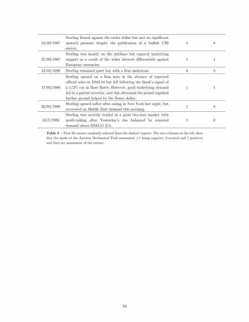
to respond. Extracts in Table 5 compares my assessment with that of the 10 reviewers

for the 20 first statements.

Table 3 below measures the agreement on the randomly selected sample. Just by

chance, agreeing with one of the three choices (1, 0 or -1) should be 33%. Agreement

rates of 77% for positive assessments and 57% for negative assessment are unlikely to

be random, whereas the agreement rates for neutral situation are not clearly better

than random. While these results do not categorically attest to the objectivity of the

analysis, they still show significant overlap for both my positive and negative

assessments and those of both MTurk.

Positive

assessment Neutral

assessment Negative

assessment Total

My assessment 31 41 28 100

Most common answer by 10 MTurk reviewers (mode) 51 26 23 100

Agreement rate 77% 37% 57%

N = 100 text samples

Table 3 – comparing answers by MTurk and the author.

Natural Language Processing algorithm

As a second form of robustness check, I use sentiment analysis done by an

algorithm. Natural Language Processing (NLP) is a set of techniques that use

computational power to analyze large datasets of natural language. The field recently

8 Taking the average and rounding it up leads to similar answers but is less precise as it includes responses from respondents who might not have read the question.

26

blossomed with advances in machine learning, allowing for a much better understanding

of human language. I use a Python script named natural language toolkit (or nltk in

short) set up by Bird, Klein, and Loper (2009). This algorithm is widely used. For

example Yu, Duan, and Cao (2013) use it to show how social media influence stock

returns more than traditional news outlets. Each of the 100 digitized statements

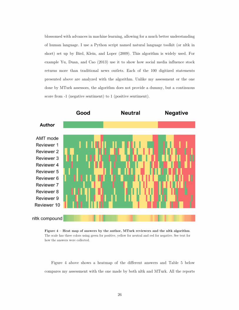
presented above are analyzed with the algorithm. Unlike my assessment or the one

done by MTurk assessors, the algorithm does not provide a dummy, but a continuous

score from -1 (negative sentiment) to 1 (positive sentiment).

Figure 4 – Heat map of answers by the author, MTurk reviewers and the nltk algorithm. The scale has three colors using green for positive, yellow for neutral and red for negative. See text for how the answers were collected.

Figure 4 above shows a heatmap of the different answers and Table 5 below

compares my assessment with the one made by both nltk and MTurk. All the reports

27

I assessed as negative are also assessed as negative by both nltk and MTurk on average

(as the negative coefficient shows). The positive assessments by both other techniques

also yield qualitatively similar results. When it comes to neutral assessment, it seems

that my assessment was more negative than both other assessment methods (as all my

neutral assessments where more often assessed as positive by the two other

methodologies). Note that the fact that there is disagreement between manual analysis

and NLP measures is not a surprise and has been documented in the literature

(Jongeling et al. 2017).

Average score – nltk algorithm

Average score – Amazon

Mechanical Turk mode

Average author score

Assessed as bad by the author -0.08 -0.36 -1

Assessed as neutral by the author 0.12 0.44 0

Assessed as good by the author 0.23 0.70 1

Table 4 – correlation matrix of answers of the author, MTurk and the nltk algorithm. The color coding is from green (good news) to red (bad news).

What accounts for differences in assessment? In few cases, it was a clear mistake

on my side, where I either misjudged or mistyped the assessment. But the large

disagreement over neutral days is justified as the following examples show. “Sterling

was quiet and sluggish after some light, technical selling at the opening”. I rated the

statement neutrally; the modal MTurk response was -1; and the nltk algorithm scored

it -0.40. I gave this statement a neutral score because there seemed to have been little

market activity - as suggested by the word “quiet” (word often used by the dealers).

The nltk algorithm, however, saw the statement as negative, potentially picking up on

negative keywords like “sluggish”. MTurk responses were surprisingly homogenous,

with 8 of 10 saying that the statement was negative, and only 2 labelling it as neutral.

28

A statement I deemed to be neutral but the other systems deemed positive reads:

“Sterling remained quietly on the sidelines and gained ground in effective terms despite

a further erosion in oil prices.” Here the MTurk consensus was 1 and the nltk algorithm

granted a 0.69 score. Here again my justification for the 0 rating was that the market

was mainly quiet, meaning that any news or action by the central bank would be likely

to move the exchange rate, unlike if there was clear market activity due to specific

news moving the price. These examples show that the assessment retains a certain

amount of subjective judgement. However, unlike other narrative approaches that rely

on the reader trusting the assessor, here I have endeavored to benchmark and cross-

check my own judgement against assessments gleaned from two very different

approaches. Table 5 shows that on average my assessment was confirmed by both the

algorithm and the external assessors.

5. Conclusion

Most studies assessing central bank intervention fail to account for exogenous

shocks occurring during the day of central bank intervention. Therefore, they overstate

the impact of central bank intervention, mistaking it for markets simply picking up on

news. Not controlling for the intraday conditions of the currency is problematic when

assessing intervention success. Placebo tests often used in the literature only partially

address the issue. Good market news (or even bad news that is better than expected)

can lead a test to show intervention success when it is only changes in market

conditions.

Presenting a novel dataset spanning over 40 years, this paper uses a narrative

approach to tackle this issue. By reading the daily reports of policymakers at the time,

I show how news affecting the exchange rate during the day can influence intervention

outcomes. Far from the intervention success rates of 80% in certain studies, I show that

when controlling for market conditions, success rates drop as low as 8%. In particular,

29

I show that the Bank of England performs particularly poorly when trying to make

sterling appreciate in negative market conditions.

6. References

Adler, Gustavo, Noëmie Lisack, and Rui C. Mano. 2019. ‘Unveiling the Effects of Foreign Exchange Intervention: A Panel Approach’. Emerging Markets Review, June, 100620. https://doi.org/10.1016/j.ememar.2019.100620.

Adler, Gustavo, and Rui C. Mano. 2018. ‘The Cost of Foreign Exchange Intervention: Concepts and Measurement’. Journal of Macroeconomics, August. https://doi.org/10.1016/j.jmacro.2018.07.001.

Ambuehl, Sandro, Muriel Niederle, and Alvin E. Roth. 2015. ‘More Money, More Problems? Can High Pay Be Coercive and Repugnant?’ The American Economic Review 105 (5): 357–60.

Bird, Steven, Ewan Klein, and Edward Loper. 2009. Natural Language Processing with Python: Analyzing Text with the Natural Language Toolkit. 1 edition. Beijing ; Cambridge Mass.: O’Reilly Media.

Blanchard, Olivier, Gustavo Adler, and Irineu de Carvalho Filho. 2015. ‘Can Foreign Exchange Intervention Stem Exchange Rate Pressures from Global Capital Flow Shocks?’ Working Paper 21427. National Bureau of Economic Research. http://www.nber.org/papers/w21427.

Bordo, Michael D., Owen F. Humpage, and Anna J. Schwartz. 2015. Strained Relations: US Foreign-Exchange Operations and Monetary Policy in the Twentieth Century. Chicago: University of Chicago Press.

Burkhard, Lukas, and Andreas M. Fischer. 2009. ‘Communicating Policy Options at the Zero Bound’. Journal of International Money and Finance 28 (5): 742–54. https://doi.org/10.1016/j.jimonfin.2008.06.006.

Cavallino, Paolo. 2019. ‘Capital Flows and Foreign Exchange Intervention’. American Economic Journal: Macroeconomics 11 (2): 127–70. https://doi.org/10.1257/mac.20160065.

Dominguez, Kathryn, and Jeffrey A. Frankel. 1993. ‘Does Foreign-Exchange Intervention Matter? The Portfolio Effect’. The American Economic Review 83 (5): 1356–69.

Dominguez, Kathryn M. 2003. ‘The Market Microstructure of Central Bank Intervention’. Journal of International Economics 59 (1): 25–45. https://doi.org/10.1016/S0022-1996(02)00091-0.

30

Echavarría, Juan J., Luis F. Melo-Velandia, and Mauricio Villamizar-Villegas. 2018. ‘The Impact of Pre-Announced Day-to-Day Interventions on the Colombian Exchange Rate’. Empirical Economics 55 (3): 1319–36. https://doi.org/10.1007/s00181-017-1299-1.

Fatum, Rasmus. 2015. ‘Foreign Exchange Intervention When Interest Rates Are Zero: Does the Portfolio Balance Channel Matter after All?’ Journal of International Money and Finance 57 (October): 185–99. https://doi.org/10.1016/j.jimonfin.2015.07.015.

Fatum, Rasmus, and Michael Hutchison. 1999. ‘Is Intervention a Signal of Future Monetary Policy? Evidence from the Federal Funds Futures Market’. Journal of Money, Credit and Banking 31 (1): 54–69. https://doi.org/10.2307/2601139.

———. 2006. ‘Effectiveness of Official Daily Foreign Exchange Market Intervention Operations in Japan’. Journal of International Money and Finance 25 (2): 199–219. https://doi.org/10.1016/j.jimonfin.2005.11.007.

Fratzscher, Marcel, Oliver Gloede, Lukas Menkhoff, Lucio Sarno, and Tobias Stöhr. 2019. ‘When Is Foreign Exchange Intervention Effective? Evidence from 33 Countries’. American Economic Journal: Macroeconomics. https://doi.org/10.1257/mac.20150317.

Gabaix, Xavier, and Matteo Maggiori. 2015. ‘International Liquidity and Exchange Rate Dynamics’. The Quarterly Journal of Economics 130 (3): 1369–1420. https://doi.org/10.1093/qje/qjv016.

Hassan, Tarek A, Thomas M Mertens, and Tony Zhang. 2016. ‘Currency Manipulation’. Working Paper 22790. National Bureau of Economic Research. https://doi.org/10.3386/w22790.

Hoshikawa, Takeshi. 2008. ‘The Effect of Intervention Frequency on the Foreign Exchange Market: The Japanese Experience’. Journal of International Money and Finance 27 (4): 547–59. https://doi.org/10.1016/j.jimonfin.2008.01.004.

Howson, Susan. 1980. Sterling’s Managed Float: The Operations of the Exchange Equalisation Account, 1932-39. International Finance Section, Department of Economics, Princeton University. https://www.princeton.edu/~ies/IES_Studies/S46.pdf.

Hu, May, Yunfeng Li, Jingjing Yang, and Chi-Chur Chao. 2016. ‘Actual Intervention and Verbal Intervention in the Chinese RMB Exchange Rate’. International Review of Economics & Finance 43 (May): 499–508. https://doi.org/10.1016/j.iref.2016.01.011.

Ilzetzki, Ethan, Carmen M. Reinhart, and Kenneth S. Rogoff. 2019. ‘Exchange Arrangements Entering the Twenty-First Century: Which Anchor Will Hold?’ The Quarterly Journal of Economics 134 (2): 599–646.

31

Ito, Takatoshi. 2003. ‘Is Foreign Exchange Intervention Effective? The Japanese Experiences in the 1990s’. In Chapters. Edward Elgar Publishing. https://ideas.repec.org/h/elg/eechap/2818_5.html.

Jongeling, Robbert, Proshanta Sarkar, Subhajit Datta, and Alexander Serebrenik. 2017. ‘On Negative Results When Using Sentiment Analysis Tools for Software Engineering Research’. Empirical Software Engineering 22 (5): 2543–84. https://doi.org/10.1007/s10664-016-9493-x.

Kearns, Jonathan, and Roberto Rigobon. 2005. ‘Identifying the Efficacy of Central Bank Interventions: Evidence from Australia and Japan’. Journal of International Economics 66 (1): 31–48. https://doi.org/10.1016/j.jinteco.2004.05.001.

Krippendorff, Klaus. 2018. Content Analysis: An Introduction to Its Methodology. Fourth edition. Los Angeles: SAGE Publications, Inc.

Mohanty, Madhusudan S., and Bat-el Berger. 2013. ‘Central Bank Views on Foreign Exchange Intervention’. BIS working paper No 73.

Monnet, Eric. 2014. ‘Monetary Policy without Interest Rates: Evidence from France’s Golden Age (1948 to 1973) Using a Narrative Approach’. American Economic Journal: Macroeconomics 6 (4): 137–69. https://doi.org/10.1257/mac.6.4.137.

Neely, Christopher. 2005. ‘An Analysis of Recent Studies of the Effect of Foreign Exchange Intervention’. Federal Reserve Bank of St. Louis Working Paper No. 2005-030B.

Neely, Christopher J. 2008. ‘Central Bank Authorities’ Beliefs about Foreign Exchange Intervention’. Journal of International Money and Finance 27 (1): 1–25. https://doi.org/10.1016/j.jimonfin.2007.04.012.

Neuendorf, Kimberly A. 2016. The Content Analysis Guidebook. Second edition. Los Angeles: SAGE Publications, Inc.

Reitz, Stefan, and Mark P. Taylor. 2008. ‘The Coordination Channel of Foreign Exchange Intervention: A Nonlinear Microstructural Analysis’. European Economic Review 52 (1): 55–76. https://doi.org/10.1016/j.euroecorev.2007.06.023.

Romer, Christina D., and David H. Romer. 1989. ‘Does Monetary Policy Matter? A New Test in the Spirit of Friedman and Schwartz’. In NBER Macroeconomics Annual, by Olivier Blanchard and Stanley Fischer, 4:121–70. Cambridge: MIT Press. https://www.journals.uchicago.edu/doi/abs/10.1086/654103.

———. 1994. ‘Monetary Policy Matters’. Journal of Monetary Economics 34 (1): 75–88. https://doi.org/10.1016/0304-3932(94)01150-8.

32

———. 2014. ‘The Incentive Effects of Marginal Tax Rates: Evidence from the Interwar Era’. American Economic Journal: Economic Policy 6 (3): 242–81. https://doi.org/10.1257/pol.6.3.242.

Sarno, Lucio, and Mark P. Taylor. 2001. ‘Official Intervention in the Foreign Exchange Market: Is It Effective and, If so, How Does It Work?’ Journal of Economic Literature 39 (3): 839–68. https://doi.org/10.1257/jel.39.3.839.

Taylor, Alan M. 2010. ‘Global Finance after the Crisis’. Bank of England Quarterly Bulletin 50 (4): 366–77.

Yu, Yang, Wenjing Duan, and Qing Cao. 2013. ‘The Impact of Social and Conventional Media on Firm Equity Value: A Sentiment Analysis Approach’. Decision Support Systems, 1. Social Media Research and Applications 2. Theory and Applications of Social Networks, 55 (4): 919–26. https://doi.org/10.1016/j.dss.2012.12.028.

33

7. Appendix (For Online Publication)

Extract of Amazon Mechanical Turk assessment

Randomly selected date

Text Most common answer by 10

reviewers (mode)

My assessment

18/11/1986 Sterling was steady and market quiet. 1 0

10/12/1986 Sterling was very quiet but was helped by the stronger dollar this afternoon.

1 0

18/12/1986 Sterling was steady against the dollar but therefore lost a little ground in cross-rate terms.

-1 0

22/01/1987 Sterling remained on the sidelines 0 0

12/2/1987 Sterling remained quietly on the sidelines and gained ground in effective terms despite a further erosion in oil prices.

1 0

26/02/1987 Sterling steadied as the oil price climbed back above $16 per barrel.

1 1

18/03/1987

Sterling encountered steady demand throughout the day reflecting the favourable response to the budget and the hope that the 1/2% cut in Base rates might leave scope for another reduction soon.

1 1

16/04/1987 Sterling was helped by the stronger dollar and opened firmer in effective and cross rate terms, but was little changed during the day.

0 0

13/05/1987 Sterling was on the sidelines, but was pulled up against third currencies by the stronger dollar.

1 0

29/05/1987 Sterling was on the sidelines but encountered some data commercial demand and touched DM2.97 1/8 at 5 o'clock.

0 0

16/06/1987

Sterling rallied on the better than expected PSBR data (negative borrowing of £374 mn against an expected requirement of £800 mn), but eased against the firmer dollar this afternoon.

1 1

9/7/1987 Sterling was steady in quiet conditions. 1 0

28/07/1987 Sterling was also quiet, but benefited from the encouraging CBI survey.

1 1

25/08/1987

Sterling weakened generally today as the market focused on the recent falls in oil prices and concerns grew about next week's trade figures. Outward investment flows also contributed to the fall but the market was throughout very orderly.

-1 -1

34

23/09/1987 Sterling firmed against the easier dollar but met no significant upward pressure despite the publication of a bullish CBI survey.

0 0

25/09/1987 Sterling was mostly on the sidelines but enjoyed underlying support as a result of the wider interest differentials against European currencies.

1 1

24/02/1988 Sterling remained quiet but with a firm undertone. 0 0

17/03/1988

Sterling opened on a firm note in the absence of expected official sales at DM3.10 but fell following the Bank's signal of a 1/2% cut in Base Rates. However, good underlying demand led to a partial recovery, and this afternoon the pound regained further ground helped by the firmer dollar.

1 1

26/04/1988 Sterling opened softer after easing in New York last night, but recovered on Middle East demand this morning.

1 0

10/5/1988 Sterling was actively traded in a good two-way market with profit-taking after Yesterday's rise balanced by renewed demand above DM3.15 3/4.

1 0

Table 5 – First 20 extract randomly selected from the dealers’ reports. The two columns on the left show first the mode of the Amazon Mechanical Turk assessment (-1 being negative, 0 neutral and 1 positive) and then my assessment of the extract.

35

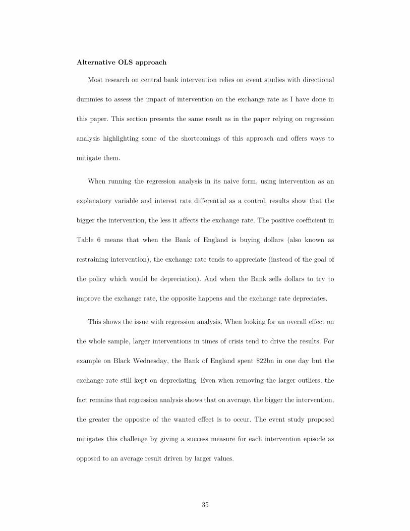
Alternative OLS approach

Most research on central bank intervention relies on event studies with directional

dummies to assess the impact of intervention on the exchange rate as I have done in

this paper. This section presents the same result as in the paper relying on regression

analysis highlighting some of the shortcomings of this approach and offers ways to

mitigate them.

When running the regression analysis in its naive form, using intervention as an

explanatory variable and interest rate differential as a control, results show that the

bigger the intervention, the less it affects the exchange rate. The positive coefficient in

Table 6 means that when the Bank of England is buying dollars (also known as

restraining intervention), the exchange rate tends to appreciate (instead of the goal of

the policy which would be depreciation). And when the Bank sells dollars to try to

improve the exchange rate, the opposite happens and the exchange rate depreciates.

This shows the issue with regression analysis. When looking for an overall effect on

the whole sample, larger interventions in times of crisis tend to drive the results. For

example on Black Wednesday, the Bank of England spent $22bn in one day but the

exchange rate still kept on depreciating. Even when removing the larger outliers, the

fact remains that regression analysis shows that on average, the bigger the intervention,

the greater the opposite of the wanted effect is to occur. The event study proposed

mitigates this challenge by giving a success measure for each intervention episode as

opposed to an average result driven by larger values.

36

Dependent variable – change in exchange rate

Dollar period (1952-1987)

Deutschmark period (1987-1992)

Intercept -0.00056 (0.000101) -0.001126 (0.000828)

Intervention in billion $ 0.029 (0.00150) 0.0125 (0.00168)

Interest rate differential 0.000163 (0.000034)

0.000122 (0.000119)

Adjusted R2 0.05 0.04 Observations 8131 1452

Table 6

Even if the intervention variable is replaced with a dummy variable comparing

restraining and defending intervention to the days with no intervention, the results still

show that intervention to increase the value of the currency has the opposite effect

(result in Table 7 below). In other words, on average, interventions usually have the

opposite effect on the exchange rate. But this does not take into account that

intervention can actually have an effect on some occasions and not on others, which

the event study analysis allows for.

37

Dependent variable – change in exchange rate

Dollar period (1952-1987)

Deutschmark period (1987-1992)

Intercept -0.000586 (0.000178)

-0.001826 (0.001167)

Restraining intervention (1/0) 0.001524 (0.000199)

0.002487 (0.000961)

Defending intervention (1/0) -0.002794 (0.000227)

-0.005275 (0.001059)

Interest rate differential 0.0002 (0.000003) 0.000211 (0.000116)

Adjusted R2 0.07 Observations 8131 1452

Table 7

If a simple OLS approaches yields contradicting results, using variables from the

narrative approach gives a more convincing picture. Table 9 below is echoing Table 11

in the paper. They both break down intervention success depending on the direction of

the wind during the day. Table 9 uses a regression whereas Table 11 uses the event

study with directional dummies.

The results in Table 9 show that when going with the wind, the central bank

achieved the wanted effect of intervention. However, when going against the wind, the

average effect of intervention goes against what the central bank wanted.

38

Dependent variable – change in exchange rate

1987-1992

Intercept 0.0006 (0.0008)

Defending intervention in billion dollar:

Against the wind (Intervention x dummy for bad news) 0.041 (0.003)

With no wind (Intervention x dummy for neutral news) 0.007 (0.016)

With the wind (Intervention x dummy for good news) -0.017 (0.008)

Restraining intervention in billion dollar:

Against the wind (Intervention x dummy for good news) 0.007 (0.002)

With no wind (Intervention x dummy for neutral news) -0.0001 (0.010)

With the wind (Intervention x dummy for bad news) -0.205 (0.029)

Adjusted R2 0.12 Observations 1452

Table 8

39

Comparison with post 1992 placebo

To test if the interventions are better than random at affecting the exchange rate,

I compared them with placebo interventions. Because over the sample analyzed the

Bank was on the market 79.5% of the trading days, days with no intervention might

not offer a good comparison as they would present specific characteristics. I therefore

compare interventions from 1986 to 1992 (when the Bank is intervening) to a placebo

from 1992-1999 (when the Bank is not intervening). These two periods are similar. In

the sample period from 1986-92 the Bank was targeting the Deutschmark exchange rate

and from 1992-99 the Deutschmark was also the reference currency for the pound

(before the introduction of the euro in 1999).

I run two placebo tests. The first is comparing the actual intervention with the

period from 1992-1999 where there are no more interventions (remember the Bank of

England stopped intervening after Black Wednesday in September 1992). The second

placebo does a similar comparison but takes into account the intraday direction or wind

of the market. The first test finds that overall the Bank of England was not better than

random at moving the direction of the exchange rate.

Both test use the same success criteria presented in the methodology. Since there

are no actual interventions occurring during this period, the test mimics what the Bank

would have done. For example, if the exchange rate is dropping from day t-2 to day t-

1, the placebo assumes that the Bank of England would have intervened at this time

to make the exchange rate appreciate again. In this sense, this methodology counts how

often reversal of the exchange rate occurred absent Bank of England operations. This

is then compared to the success of the actual operations of the Bank of England. To

analyze if the placebo is different from the actual interventions, I calculate if the placebo

lies two standard deviations above or below the observed value. The standard deviation

is calculated using a hypergeometric distribution presented below (this is common in

the literature, see for example Bordo, Humpage, and Schwartz 2015). The three

40

equations below give the formalization of success criteria and match the success criteria

presented on page 12.

𝑆𝐶1 𝑝𝑙𝑎𝑐𝑒𝑏𝑜 =

⎩{⎨{⎧1 {

𝑖𝑓 𝑆𝑡 > 𝑆𝑡−1 𝑎𝑛𝑑 𝑆𝑡−1 < 𝑆𝑡−2, 𝑜𝑟

𝑖𝑓 𝑆𝑡 < 𝑆𝑡−1 𝑎𝑛𝑑 𝑆𝑡−1 > 𝑆𝑡−20 𝑜𝑡ℎ𝑒𝑟𝑤𝑖𝑠𝑒

 

 

𝑆𝐶2 𝑝𝑙𝑎𝑐𝑒𝑏𝑜 =

⎩{⎨{⎧1 {

𝑖𝑓 𝑆𝑡−1 > 𝑆𝑡−2 𝑎𝑛𝑑 ∆𝑆𝑡 < ∆𝑆𝑡−1 𝑎𝑛𝑑 ∆𝑆𝑡 > 0 𝑜𝑟

𝑖𝑓 𝑆𝑡−1 < 𝑆𝑡−2 𝑎𝑛𝑑 ∆𝑆𝑡 > ∆𝑆𝑡−1 𝑎𝑛𝑑 ∆𝑆𝑡 < 0 0 𝑜𝑡ℎ𝑒𝑟𝑤𝑖𝑠𝑒

 

𝑆𝐶3 𝑝𝑙𝑎𝑐𝑒𝑏𝑜 = {1 𝑆𝐶1 = 1 𝑜𝑟 𝑆𝐶2 = 10 𝑜𝑡ℎ𝑒𝑟𝑤𝑖𝑠𝑒

 

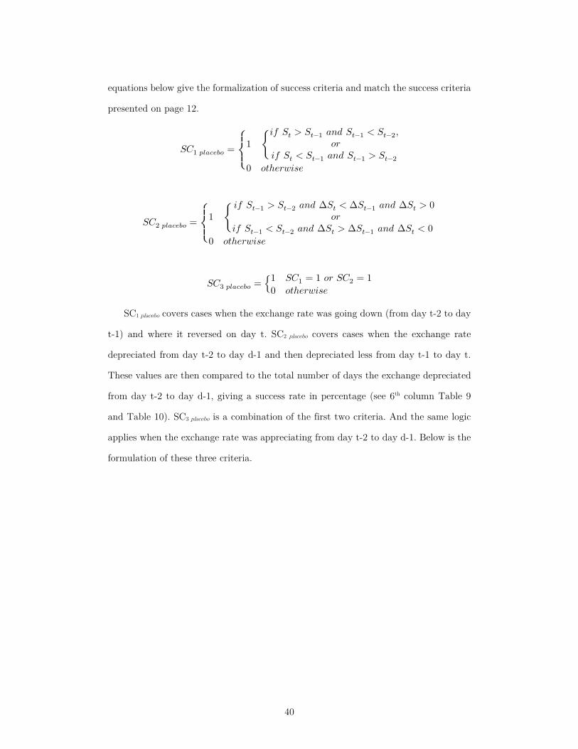
SC1 placebo covers cases when the exchange rate was going down (from day t-2 to day

t-1) and where it reversed on day t. SC2 placebo covers cases when the exchange rate

depreciated from day t-2 to day d-1 and then depreciated less from day t-1 to day t.

These values are then compared to the total number of days the exchange depreciated

from day t-2 to day d-1, giving a success rate in percentage (see 6th column Table 9

and Table 10). SC3 placebo is a combination of the first two criteria. And the same logic

applies when the exchange rate was appreciating from day t-2 to day d-1. Below is the

formulation of these three criteria.

41

Intervention episodes

Intervention success

Placebo episodes

Placebo success

Expected success

Standard deviation

Random range

Is the central bank better than

random?

# % # %

DEFENDING OPERATIONS

Success Criteria 1 427 102 24% 848 455 54% 229 3 222 - 236 NO

Success Criteria 2 427 61 14% 848 162 19% 82 3 76 - 87 NO

Success Criteria 3 427 163 38% 848 617 73% 311 4 302 - 319 NO

RESTRAINING OPERATIONS

Success Criteria 1 1196 327 27% 1000 451 45% 539 8 523 - 556 NO

Success Criteria 2 1196 179 15% 1000 239 24% 286 6 273 - 298 NO

Success Criteria 3 1196 506 42% 1000 690 69% 825 10 805 - 845 NO

Observations sample: 1453

Observations placebo: 1902 Exchange rate days in

both samples 3355

Table 9

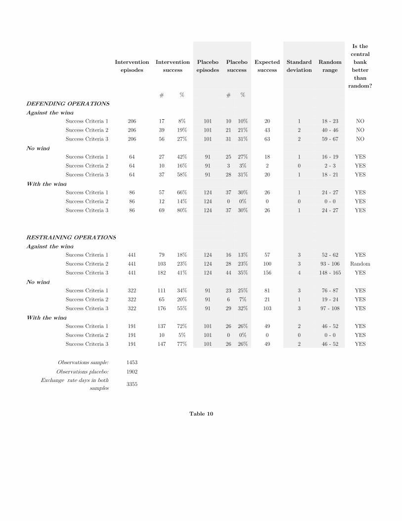
The first test shows that overall, the interventions of the Bank of England did not

influence the exchange rate differently from the placebo (Table 9). When distinguishing

interventions with and against the wind, I find that interventions against the wind

trying to avoid the pound from depreciating (the main mission of the Bank of England

during this period), did not affect the market more than the placebo. Restraining

interventions and intervention going with the wind or with the absence of wind show

an effect significantly different from the placebo. This mirrors the overall findings of

42

the paper which shows that the Bank of England performed particularly poorly when

trying to avoid the exchange rate from falling when intervening against the wind (this

is briefly understood by looking at Table 11 and Table 8).

Intervention

episodes Intervention

success Placebo episodes

Placebo success

Expected success

Standard deviation

Random range

Is the central bank better than

random? # % # % DEFENDING OPERATIONS Against the wind

Success Criteria 1 206 17 8% 101 10 10% 20 1 18 - 23 NO Success Criteria 2 206 39 19% 101 21 21% 43 2 40 - 46 NO Success Criteria 3 206 56 27% 101 31 31% 63 2 59 - 67 NO

No wind Success Criteria 1 64 27 42% 91 25 27% 18 1 16 - 19 YES Success Criteria 2 64 10 16% 91 3 3% 2 0 2 - 3 YES Success Criteria 3 64 37 58% 91 28 31% 20 1 18 - 21 YES

With the wind Success Criteria 1 86 57 66% 124 37 30% 26 1 24 - 27 YES Success Criteria 2 86 12 14% 124 0 0% 0 0 0 - 0 YES Success Criteria 3 86 69 80% 124 37 30% 26 1 24 - 27 YES

RESTRAINING OPERATIONS Against the wind

Success Criteria 1 441 79 18% 124 16 13% 57 3 52 - 62 YES Success Criteria 2 441 103 23% 124 28 23% 100 3 93 - 106 Random Success Criteria 3 441 182 41% 124 44 35% 156 4 148 - 165 YES

No wind Success Criteria 1 322 111 34% 91 23 25% 81 3 76 - 87 YES Success Criteria 2 322 65 20% 91 6 7% 21 1 19 - 24 YES Success Criteria 3 322 176 55% 91 29 32% 103 3 97 - 108 YES

With the wind Success Criteria 1 191 137 72% 101 26 26% 49 2 46 - 52 YES Success Criteria 2 191 10 5% 101 0 0% 0 0 0 - 0 YES Success Criteria 3 191 147 77% 101 26 26% 49 2 46 - 52 YES

                                

Observations sample: 1453                           

Observations placebo: 1902                           Exchange rate days in both

samples 3355                           

Table 10

Different outcomes by type of intervention, wind and success criteria

Table 11 looks at the results in more detail and breaks them down according

to the different success criteria presented in the previous section, and separates

restraining from defending interventions. One particularly striking number is the

8% success rate when the Bank of England was supporting the pound in adverse

market conditions (the most common case).

Against

the wind

No Wind

With the

wind

Defending intervention

Reversing (SC1) 8% 42% 66% Smoothing (SC2) 19% 16% 14% Either reversing or smoothing (SC3) 27% 58% 80%

Restraining intervention

Reversing (SC1) 18% 34% 72% Smoothing (SC2) 23% 20% 5% Either reversing or smoothing (SC3) 41% 55% 77%

Table 11 – Intervention success by success criteria (see previous section for details).

45

Distribution of the different assessment methods

The next three charts show the distribution of the classifications of the dealers’ reports into negative (-1), neutral (0) or good (1) news. The first chart displays my classification, the second Amazon Mechanical Turk and the third the nltk natural language processing algorithm.

Figure 5

Figure 6

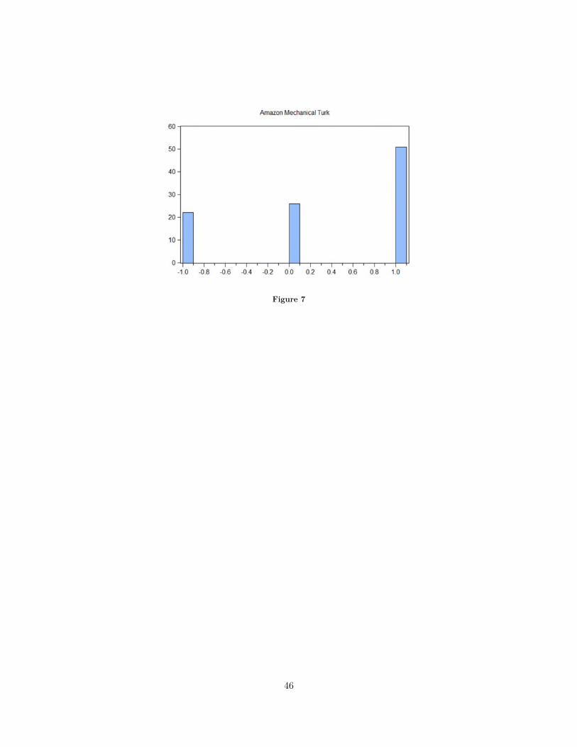
46

Figure 7

European Historical Economics Society

EHES Working Paper Series Recent EHES Working Papers 2020

EHES 187 Denmark and Russia: What can we learn from the historical comparison of two great Arctic agricultural empires?

Elena Korchmina, Paul Sharp

EHES 186 Death, sex and fertility: Female infanticide in rural Spain, 1750-1950, Francisco J. Beltrán Tapia, Francisco J. Marco-Gracia

EHES 185 Growth, War, and Pandemics: Europe in the Very Long-run, Leandro Prados de la Escosura, Carlos-Vladimir Rodríguez-Caballero

EHES 184 Economic Effects of the Black Death: Spain in European Perspective, Carlos Álvarez-Nogal, Leandro Prados de la Escosura, Carlos Santiago-

Caballero

EHES 183 Success through failure? Four Centuries of Searching for Danish Coal, Kristin Ranestad, Paul Richard Sharp

EHES 182 Arresting the Sword of Democles: Dating the Transition to the Post-Malthusian Era in Denmark,

Peter Sandholt Jensen, Maja Uhre Pedersen, Cristina Victoria Radu, Paul

Richard Sharp

EHES 181 Ad maiorem Dei gloriam. Numeracy levels in the Guarani Jesuit missions, Èric Gómez-i-Aznar

EHES 180 Standards of Living and Skill Premia in Eighteenth Century Denmark: What can we learn from a large microlevel wage database?

Peter Sandholt Jensen, Cristina Victoria Radu, Paul Sharp

EHES 179 The Fruits of El Dorado: The Global Impact of American Precious Metals, Leticia Arroyo Abad, Nuno Palma

All papers may be downloaded free of charge from: www.ehes.org The European Historical Economics Society is concerned with advancing education in European economic history through study of European economies and economic history. The society is registered with the Charity Commissioners of England and Wales number: 1052680