Black Sea monitoring and assessment guideline - ANEMONE ...

ANEMONEProject funded by

EUROPEAN UNION

Common borders. Common solutions.

Black Sea monitoring and assessment guideline

Valentina Todorova, Laura Boicenco, Yuriy Denga, Leyla Tolun, Arda M. Tonay, Andra Oros, Valentina Coatu, Luminiţa Lazăr, Valeria Abaza, Oana Marin, Alina Spînu, Florin Timofte, Elena Bişinicu, Oana Vlas, Adrian Filimon, Elena Stoica, Madalina Galatchi, George Tiganov, Marian Paiu, Costin

Timofte, Angelica Paiu, Mihaela Mirea Cândea, Anca Gheorghe, Marina Panayotova, Snejana Moncheva, Kremena Stefanova, Violeta Slabakova, Radoslava Bekova, Valentina Doncheva, Elitsa Stefanova, Svetlana Kovalinishina, Karina Vishnyakova, Tatyana Chuzhekova, Boris Linetskii, Yuri Olenik, Colpan Beken, Hakan Atabay, Fatma Bayram Partal, Güley Kurt, Levent Bat, Fatih Şahin, Aysah Öztekin, Saadet Karakulak, Uğur Uzer, Arda M. Tonay, Ayaka Amaha Ozturk, Zeynep Gülenç

Black Sea monitoring and assessment

guideline

CONSTANȚA, 2021

This document is based on the activities of the ANEMONE project (Assessing the vulnerability of the Black Sea marine ecosystem to human pressures) with the financial support from the Joint Operational Programme Black Sea Basin 2014-2020.

Contributing authors: Andra Oros, Laura Boicenco, Valeria Abaza, Elena Bişinicu, Valentina Coatu, Adrian Filimon, Mădălina Galaţchi, Luminiţa Lazăr, Oana Marin, Alina Spînu, Elena Stoica, Florin Timofte, George Tiganov, Oana Vlas National Institute for Marine Research and Development "Grigore Antipa", NIMRD, Romania. Marian Paiu, Costin Timofte, Angelica Paiu, Mihaela Mirea Cândea, Anca Gheorghe Mare Nostrum NGO, Romania. Valentina Todorova, Marina Panayotova, Snejana Moncheva, Kremena Stefanova, Violeta Slabakova, Radoslava Bekova, Valentina Doncheva, Elitsa Stefanova Institute of Oceanology "Fridtjof Nansen", Bulgarian Academy ofSciences, IO-BAS, Bulgaria Yuriy Denga, Svetlana Kovalinishina, Karina Vishnyakova, Tatyana Chuzhekova, Boris Linetskii, Yuri Olenik Ukrainian Scientific Centre of Ecology of the Sea, UkrSCES, Ukraine. Leyla Tolun, Colpan Beken, Hakan Atabay, Fatma Bayram Partal TUBITAK Marmara Research Center, MRC, Turkey Arda M. Tonay, Ayaka Amaha Ozturk, Zeynep Gülenç Turkish Marine Research Foundation, TUDAV, Turkey Güley Kurt, Levent Bat, Fatih Şahin, Aysah Öztekin Faculty of Fishery, Sinop University, Turkey Saadet Karakulak, Uğur Uzer Faculty of Aquatic Sciences, Istanbul University, Turkey For bibliographic purposes, this document should be cited as:

ANEMONE Deliverable 1.3, 2021. “Black Sea monitoring and assessment guideline”, Todorova V. [Ed], Ed. CD PRESS, 190 pp.

ISBN 978-606-528-527-9

The information included in this publication or extracts thereof is free for citing on the condition that the complete reference of the publication is given as stated above.

Cover page design by Vector new7ducks / Freepik. Cover page photo by NIMRD.

5

Contents

Executive summary .............................................................................................. 14

1 Guideline on Descriptors 1. Theme Non-commercial fish ........................................... 15

1.1 Introduction........................................................................................... 15

1.2 Ecological elements ................................................................................. 16

1.3 Overview of criteria, indicators and thresholds ................................................. 20

1.4 Harmonized approach for indicators and thresholds setting based on the regional progress 33

1.5 Methods and approaches for data integration and overall assessment at descriptor level 34

1.6 Conclusions and recommendations ................................................................ 36

2 Guideline on Descriptors 1. Theme Marine Mammals ................................................ 37

2.1 Introduction........................................................................................... 37

2.2 Ecological elements ................................................................................. 38

2.3 Overview of criteria, indicators and thresholds progress ...................................... 40



2.6 Review of and recommendations from relevant regional projects............................ 57

3 Guideline on Descriptors 1, 4. Theme Pelagic habitats .............................................. 59

3.1 Introduction........................................................................................... 59

3.2 Ecosystem elements ................................................................................. 59

3.3 Overview of criteria Indicators. Good Environmental Status assessment .................... 61

3.4 Approach for thresholds setting ................................................................... 64


3.6 Visualizing Assessment Results for Pelagic Habitats ............................................. 75

4 Guideline on Descriptors 1, 6. Theme Benthic habitats ............................................. 76

4.1 Introduction........................................................................................... 76

4.2 Ecosystem elements ................................................................................. 76

4.3 Assessment of physical loss and physical disturbance .......................................... 80

4.4 Assessment of adverse effects on benthic habitats types ...................................... 86

5 Guideline on Descriptor D5 Eutrophication ........................................................... 109

5.1 Introduction.......................................................................................... 109

5.2 Ecosystem elements ................................................................................ 109


5.4 Knowledge gaps and research needs ............................................................. 123

6 Guideline on Descriptor D8 Contaminants ............................................................ 124

6.1 Overview of criteria and indicators .............................................................. 124

6.2 Harmonized approach for thresholds setting based on the regional progress .............. 134


7 Guideline on Descriptor D9 Contaminants in Seafood ............................................... 147

6

7.1 Introduction.......................................................................................... 147

7.2 Overview of criteria and indicators .............................................................. 147

7.3 Harmonized approach for thresholds setting based on the regional progress .............. 152


8 Guideline on Descriptor D10 Marine Litter............................................................ 163

8.1 Introduction.......................................................................................... 163

8.2 Assessment of monitoring methodologies of marine litter in the Black Sea ................ 164

8.3 Overview of the criteria, indicators and thresholds ........................................... 169



References ....................................................................................................... 181

7

List of figures

Figure 1.1 - Levels and methods of integration for species under Descriptor 1 ........................ 35

Figure 2.1 - Phocoena phocoena ssp. relicta (Abel, 1905) (@Green Balkans NGO) ..................... 38

Figure 2.2 - Delphinus delphis ssp. ponticus (Barabasch-Nikiforov, 1935) (@Mare Nostrum NGO) ... 39

Figure 2.3 - Tursiops truncatus ssp. ponticus (Barabasch-Nikiforov, 1940) (@Mare Nostrum NGO) ... 39

Figure 2.4 - Marine mammals monitoring campaign in costal and shelf areas in 2017 (Panayotova & Bekova, 2018) .................................................................................................... 42

Figure 2.5 - Survey plan for marine mammal monitoring in coastal area (ship-based survey) ....... 45

Figure 2.6 - Cetacean’s sightings observed during the Marmara Sea survey in 2019 summer ......... 46

Figure 2.7 - LTS in Ukrainian territorial waters within the EMBLAS Plus Project, 2019 ................ 49

Figure 2.8 - Levels and methods of integration for mammals under Descriptor 1 ...................... 54

Figure 3.1 - Map of monitoring stations and Marine Reporting Units (MRU) in pelagic broad habitat types in Bulgarian (top), Romanian (middle), Turkish (bottom) Black Sea .............................. 62

Figure 3.2 - Levels and methods of integration for pelagic habitats under D1 ......................... 73

Figure 3.3 - Illustrative example of a visual summary of assessment outputs for Descriptor 1 Pelagic habitats (Bulgarian Monitoring Report, 2018) ................................................................ 75

Figure 4.1 - Seafloor assessment process (ICES Advice, 2019) ............................................. 82

Figure 4.2 - Conceptual relationship between GES for seabed habitats and sub-GES conditions, as expressed through the adverse effects of different pressures (three examples shown) (OSPAR, 2012) ..................................................................................................................... 88

Figure 4.3 - Levels and methods of integration for benthic habitats under Descriptors 1 and 6 ... 106

Figure 4.4 - Illustrative example of a visual summary of assessment outputs for Descriptor 1,6 Benthic Habitats (number and proportion of benthic broad habitats in each category) ....................... 108

Figure 5.1 - Map of the MRU under MSFD in the Bulgarian Black Sea .................................... 112

Figure 5.2 - Delimitation of water bodies based on physical and-biological characteristics and national network of monitoring according to WFD and MSFD ....................................................... 113

Figure 5.3 - Map of the MRU in Turkish marine waters .................................................... 114

Figure 5.4 - Map of the 11 marine assessment regions in Ukrainean marine waters .................. 114

Figure 5.5 - Descriptor 5 (Eutrophication) - parameters, indicators, criteria and thresholds – Romanian Black Sea waters, 2012-2017 (Lazar et.al, 2019) ........................................................... 121

Figure 6.1 - Levels and methods of integration for Descriptor 8 (DG ENV, 2017) ...................... 145

Figure 7.1 - Levels and methods of integration for Descriptor 9 (DG ENV, 2017) ...................... 162

Figure 8.1 - Levels and methods of integration for Descriptor 10 ....................................... 178

List of tables

Table 1.1 - Ecosystem component (fish) and its species groups for consideration under the “species” aspects of Descriptor 1 .......................................................................................... 16

Table 1.2 - List of representative fish by species groups for Bulgaria .................................... 16

Table 1.3 - List of fish species with regional importance for Romanian coast .......................... 17

8

Table 1.4 - List of representative fish by species groups for Turkey ...................................... 18

Table 1.5 - List of non-commercial species with regional importance ................................... 19

Table 1.6 - Indicators and thresholds for coastal fish group ............................................... 21

Table 1.7 - Indicators and thresholds for shelf fish group (pelagic and demersal) ..................... 23

Table 1.8 - Indicators and thresholds for coastal fish group, Romanian coast .......................... 25

Table 1.9 - Indicators and thresholds for coastal fish group, Turkish coast .............................. 26

Table 1.10 - Indicators and thresholds for shelf fish group (pelagic and demersal), Turkish coast .. 29

Table 1.11 - Indicators with regional importance ........................................................... 32

Table 1.12 - Integration methods recommended (ICES, 2018) ............................................ 36

Table 2.1 - Integral values estimated for the three species of cetaceans in the NW Black Sea area* 40

Table 2.2 - Marine mammals group proposed criteria and indicators (relating to D1) ................. 40

Table 2.3 - List of criteria, indicators and thresholds currently applied in Bulgaria ................... 41

Table 2.4 - By-catch thresholds based on Birkun et al., 2014 data ....................................... 43

Table 2.5 - List of criteria, indicators and thresholds currently applied in Romania ................... 44

Table 2.6 - No criteria, indicators and thresholds currently applied in Turkey ......................... 47

Table 2.7 - List of criteria, indicators and thresholds currently applied in Ukraine.................... 48

Table 2.8 - Status of the established indicators and thresholds in the Black Sea area, both in EU countries (EU level) and non-EU countries (Regional level) ............................................... 50

Table 2.9 - Indicators used in the Black Sea region. ........................................................ 52

Table 2.10 - Outcomes from Fifth Meeting of the Black Sea Working Group (19 February 2019) regarding D1 Biodiversity (marine mammals) ................................................................ 53

Table 2.11 - Integration methods recommended (ICES, 2018) ............................................ 56

Table 3.1 - List of representative Black Sea pelagic broad habitat types (+ present) ................. 60

Table 3.2 - Criterion for pelagic broad habitat types ....................................................... 61

Table 3.3 - Number (N) and area (km2) of identified MRUs in the Black Sea ............................ 61

Table 3.4 - Number (N) and area (km2) of identified MRUs in the Bulgarian, Romanian, Ukrainian and Turkish Black Sea ................................................................................................. 63

Table 3.5 - List of the Black Sea pelagic habitat characteristic assessed at the national level under the criteria of MSFD ............................................................................................. 64

Table 3.6 - Ecological quality scale for phytoplankton biomass (mg/m3) for Bulgarian Black Sea Coastal broad habitat ..................................................................................................... 65

Table 3.7 - Threshold values good/not good for phytoplankton abundance (N, cells/L) for Bulgarian Black Sea broad habitat shelf .................................................................................. 66

Table 3.8 - Threshold values good/not good for phytoplankton biomass (mg/m3) for Bulgarian Black Sea broad habitats shelf and open sea ....................................................................... 66

Table 3.9 - Marine water classification system according to WFD and MSFD for the biomass parameter in the summer season ........................................................................................... 67

Table 3.10 - Scales for assessing the state of the marine environment by phytoplankton biomass (mg/m3) ........................................................................................................... 68

Table 3.11 - Threshold values of mesozooplankton biomass (mg/m3) indicator for GES on base of ROC analysis and percentile approach.............................................................................. 69

Table 3.12 - Threshold values GES/Non GES for zooplankton biomass (mg/m3) for Bulgarian Black Sea broad habitat types.............................................................................................. 70

9

Table 3.13 - Threshold values of mesozooplankton abundance (ind/m3) indicator for GES on base of ROC analysis and percentile approach ........................................................................ 70

Table 3.14 - Threshold values GES/Non GES for zooplankton abundance (ind/m3) for Bulgarian Black Sea broad habitat types......................................................................................... 70

Table 3.15 - Threshold values for mesozooplankton biomass (mg/m3) for Romanian Black Sea broad habitat types ..................................................................................................... 71

Table 3.16 - Threshold values for copepoda biomass (mg/m3) for Romanian Black Sea broad habitat types ............................................................................................................... 71

Table 3.17 - Scales for assessing the state of the marine environment by zooplankton biomass (mg/m3) ..................................................................................................................... 72

Table 3.18 - Scales for assessing the state of the marine environment by zooplankton metrics ..... 72

Table 3.19 - Table of evaluation of marine ecosystem state -D1 Biodiversity pelagic habitat ........ 74

Table 4.1 - List of representative Black Sea benthic broad habitat types and characteristic biotopes in Bulgaria (BG), Romania (RO), Turkey (TR) and Ukraine (UA) ........................................... 77

Table 4.2 - Main human activities that affect the seabed through the four pressure subtypes ...... 83

Table 4.3 - Indicators under D2C3, D3C1, D3C2, D3C3, D5C4, D5C5, D5C6, D5C7, D5C8, D6C3, D7C2, D8C2 and D8C4 used in the Black Sea region*) ............................................................... 88

Table 4.4 - ALEX class boundaries and EQR under WFD and GES threshold under MSFD ............... 94

Table 4.5 - GES thresholds for H95 and L95 of commercially exploited species in the Bulgarian Black Sea ................................................................................................................. 95

Table 4.6 - EI class boundaries and EQR under WFD and GES threshold under MSFD ................... 97

Table 4.7 - EEI class boundaries and EQR under WFD and GES threshold under MSFD ................. 98

Table 4.8 - Ecological Status Class boundaries of coastal areas of the Ukrainian Black Sea with salinity within 12-17 ‰ .................................................................................................. 100

Table 4.9 - Ecological Status Class boundaries of coastal areas of the Ukrainian Black Sea with salinity less than 12 ‰ ................................................................................................... 100

Table 4.10 - Ecological Status Class boundaries for Percentage of the sensitive species (Ssp, %) in the Ukrainian Black Sea region .................................................................................... 101

Table 4.11 - GES thresholds defined for coastal and shelf habitats in the Romanian Black Sea ..... 102

Table 4.12 - GES thresholds defined for coastal benthic habitats in the Bulgarian Black Sea ....... 103

Table 4.13 - TUBI class boundaries and EQR under WFD and GES threshold under MSFD ............. 104

Table 4.14 - Assessment framework for benthic broad habitat types using MSFD criteria in the Black Sea ................................................................................................................ 107

Table 5.1 - Criteria, including criteria elements, and methodological standards (ComDec EU/2017/848) ................................................................................................... 109

Table 5.2 - List of representative Black Sea MRU (+ present) ............................................ 111

Table 5.3 - Criteria for marine assessment units (source: DeKoS and DİSSP projects) ................ 114

Table 5.4 - Overview of criteria, indicators, and thresholds (Com Dec EU/2017/848) ............... 115

Table 5.5 - Nutrients threshold for spring, summer and autumn (based on last 10 years statistical data) .............................................................................................................. 118

Table 5.6 - Revised thresholds for chlorophyll a for spring and summer ................................ 118

Table 5.7 - Thresholds for primary and secondary bloom intensity in the BG shelf and open sea based on the application of the biooptical algorithm (Kopelevich et, 2012) and remote-sensing data from MODIS Aqua/Terra, for the period 1999- 2013 .............................................................. 118

Table 5.8 - Revised thresholds for photic limit for spring and summer ................................. 119

10

Table 5.9 - Oxygen saturation (OS%) thresholds ............................................................ 119

Table 5.10 - Thesholds for Zostera noltei indicators* ...................................................... 120

Table 5.11 - Assigned indicators .............................................................................. 120

Table 5.12 - GES thresholds defined for coastal and shelf habitats in the Romanian Black Sea ..... 123

Table 6.1 - Criteria, including criteria elements, and methodological standards (Com Dec EU/2017/848) ................................................................................................... 124

Table 6.2 - Descriptor 8: operational indicators and targets in Bulgaria................................ 130

Table 6.3 - Descriptor 8, criteria D8C1: operational indicators and targets in Romania ............. 131

Table 6.4 - Descriptor 8: operational indicators and targets in Turkey ................................. 132

Table 6.5 - Environmental assessment depending on the pollution factor (Kz) ........................ 133

Table 6.6 - Descriptor 8: operational indicators and targets in Ukraine ................................ 133

Table 6.7 - Indicators under D8C1, D8C2, D8C3, D8C4 used in the Black Sea region. Matrices: W-water, S-sediment, B-biota ............................................................................................ 133

Table 6.8 - Environmental Quality Standards (EQS) for priority substances and certain other pollutants (Directive 2013/39/EU) ........................................................................................ 137

Table 6.9 - Effects Range-Low (ERL) and Environmental Assessment Criteria (EAC) values for contaminants in sediments .................................................................................... 141

Table 6.10 - Indicators EQS for contaminants in sediments in accordance with national environmental regulations (ER) in Ukraine .................................................................................... 142

Table 6.11 - Overview of the recommended thresholds for contaminants used for GES assessment in the Black Sea region ............................................................................................ 143

Table 6.12 - Existing assessment frameworks include (DG ENV, 2017): ................................. 146

Table 7.1 - Criteria, including criteria elements, and methodological standards (Com Dec EU/2017/848) ................................................................................................... 148

Table 7.2 - Descriptor 9: Propose and operational indicators and targets in Black Sea countries ... 150

Table 7.3 - Criteria elements under D9C1 used in the Black Sea region ................................ 151

Table 7.4 - Environmental assessment depending on the pollution factor (Ukraine) ................. 151

Table 7.5 - Maximum levels for certain contaminants in foodstuffs set in the Commission Regulation (EC) No 1881/2006 and thresholds used in the Black Sea region......................................... 154

Table 7.6 - Overview of the most consumed species of fish and sea food monitored for GES assessment in the Black Sea region ......................................................................................... 161

Table 8.1 - Seafloor monitoring data sheet ................................................................. 167

Table 8.2 - Descriptor 10 – Properties and quantities of marine litter do not cause harm to the coastal and marine environment (Relevant pressure is Input of litter) .......................................... 170

Table 8.3 - Indicators under D10C1, D10C2, D10C3 and D10C4 criteria used in Bulgaria ............. 171

Table 8.4 - No common indicators defined for Romania and Bulgaria ................................... 173

Table 8.5 - Beach litter percentile values at EU level ..................................................... 176

Table 8.6 - Mean and median total beach litter abundance per 100 m of beach (Hanke et al., 2019) and % reduction necessary to reach the TV (median compared to TV) for country-MSFD subregions .................................................................................................................... 176

Table 8.7 - Outcomes from Fifth Meeting of the Black Sea Working Group (19 February 2019) ..... 177

11

Acronyms

AA Annual average ACCOBAMS Agreement on the Conservation of Cetaceans of the Black Sea, Mediterranean Sea and

Contiguous Atlantic Area AIS Automatic identification system ALEX Alien Biotic Index ARGO International program that uses profiling floats to observe temperature, salinity, currents,

and, recently, bio-optical properties in the Earth's oceans ASCOBANS Agreement on the Conservation of Small Cetaceans in the Baltic, North East Atlantic, Irish and

North Seas AUC Area Under the Curve BAC Background Assessment Concentrations BAC:DIN Bacillariophyceae:Dinophyceae BOD Biological Oxygen Demand BS Black Sea BS SAP Black Sea Strategic Action Plan BSC Commission on the Protection of the Black Sea Against Pollution BSIMAP Black Sea Integrated Monitoring and Assessment Programme BSMAG Black Sea Monitoring and Assessment Guideline CAD Computer Aided Design CAS Chemical Abstracts Service CBD Convention on Biological Diversity CEMP OSPAR’s Coordinated Environmental Monitoring Programme CHASE HELCOM Hazardous Substances Status Assessment Tool CI Confidence interval COM European Commission CONSDELFIROM

Project “Improving the conservation status of the marine biodiversity from the Romanian coastal zone, particularly for dolphins”

CORINE Coordination of information on the environment (CORINE programme) CR Critical CSWD Commission Staff Working Document CTD Instrument for measuring conductivity (which helps determine salinity), temperature, and

depth CUSUM Cumulative sum control chart CV Coefficient of Variation DCT Data Collection Template DD Data Deficient DDD Dichlorodiphenyldichloroethane DDE Dichlorodiphenyldichloroethylene DDT Dichlorodiphenyltrichloroethane DEHP 2-ethylhexyl)-phthalate DG Directorate General DG ENV Directorate-General for Environment DIN Dissolved Inorganic Nitrogen DIP Dissolved Inorganic Phosphorus DISSP Project "Project of Standardization of marine monitoring" DO Dissolved oxygen EAC Environmental Assessment Criteria EC European Commission EEA European Economic Area EEC European Economic Community EEI Ecological Evaluation Index EEZ Exclusive economic zone EI Ecological index EMBLAS Project Improving Environmental Monitoring in the Black Sea EMS Electronic monitoring system EMSA Existing oil spill surveillance EPA Environment Protection Authority EQR Ecological Quality Ratio EQS The concentration of a particular pollutant or group of pollutants in water, or biota ER Environmental regulations ERL Effects Range-Low ERM Effects Range-Median EU European Commission EUNIS European Nature Information System

12

FAO Food and Agriculture Organization FCS Favourable Conservation Status FPR False positivity rate GBIF Global Biodiversity Information Facility GES Good Environmental Status GIS Geographic Information System GPS Global Positioning System HBCDD Hexabromocyclododecane HCB Hexachlorobenzene HCH Hexachlorocyclohexane HD Habitat Directive HM Heavy metals IBM SPSS Statistical software platform IBSS International Bibliography of the Social Sciences ICES The International Council for the Exploration of the Sea IDW Inverse Distance Weighted IPA Instrument for Pre-accession ISMEIMP Project “Investigations on the State of the Marine Environment and Improving Monitoring

Programs developed under MSFD” IUCN International Union for Conservation of Nature IUU Illegal, unreported, and unregulated IWC International Whaling Commission JRC Joint Research Centre Kz Pollution factor LBS Protocol for the Protection of the Mediterranean Sea against Pollution from Land-Based

Sources LTS Linear transect surveys LUSI Pressure index MAC Maximum allowable concentration M-AMBI(n) Multimetric index MARLEN Project “Marine litter, euthrophication and noise assessment tools” MARPOL The International Convention for the Prevention of Pollution from Ships MAU Marine assessment units MEC Number of Microflagellates, Euglenophyceae, Cyanophyceae as a percentage of the total MEDACES Mediterranean Database of Cetacean Strandings MEDITS Mediterranean International Trawl Survey MEDPOL Programme for the Assessment and Control of Marine Pollution in the Mediterranean MISIS MSFD Guiding Improvements in the Black Sea Integrated Monitoring System ML Mean Length MODIS Moderate Resolution Imaging Spectroradiometer MRU Marine reporting unit MS Member States MSCG Marine Strategy Coordination Group MSFD Marine Strategy Framework Directive NA Not assesesd NE Not evaluated NGO Non-Governmental Organization NIMP National Integrated Monitoring Program NOAA National Oceanic and Atmospheric Administration Marine Debris Program Non-GES Bad Ecological state NRC National Research Council NT Near Threatened NW North-West OAOO One Out All Out OBIS Ocean Biodiversity Information System SEAMAP System Spatial Ecological Analysis of Megavertebrate Populations OS Oxygen saturation OSPAR The Convention for the Protection of the Marine Environment of the North-East Atlantic PAH Polycyclic aromatic hydrocarbon PCB-DL Dioxin-like polychlorinated biphenyls PCDD Polychlorinated dibenzo-p-dioxins PCDF Polychlorinated dibenzofurans PD Population dynamic PFOS Perfluorooctane sulfonic acid and its derivatives PHE Phenols PSU Practical salinity unit

https://www.ospar.org/convention/text

13

RBS Relative benthic status RBSP River Basin Specific Pollutants RIMMEL Project “RIverine and Marine floating macro litter Monitoring and Modelling of Environmental

Loading” ROC Receiver Operating Characteristic curve ROV Remotely Operated Vehicles SA Swept-area SAR Swept-area ratios SCUBA Self-Contained Underwater Breathing Apparatus SDT Sygnal detection theory SE Standard Error SUBIS Fisheries Information System SW South-Western SWD Staff Working Document TEQ toxic equivalents TG ML Technical Subgroup on Marine Litter TG SEABED Technical Subgroup on seabed habitats and sea-floor integrity TN Total Nitrogen TOC Total Organic Carbon TP Total Phosphorus TPH Total petroleum hydrocarbons TPR True positive rate TUBI Turkish Benthic Index TV Threshold value UAV Unmanned Aerial Vehicle UNEP-MAP United Nations Environment Programme - Mediterranean Action Plan US EPA US European Environmental Agency VMS Vessel monitoring system VU Vulnerable WG GES Working Group on Good Environmental Status WFD Water Framework Directive WG DIKE Working Group - Data, Information, and Knowledge Exchange WHO World Health Organization PCDD Sum of dioxins PCDD/F-PCB Sum of dioxins and dioxin-like PCBs TEFs Toxic Equivalency Factors (TEFs) for dioxin-like compounds

14

Executive summary

This Guideline was prepared as part of the ANEMONE Project “Assessing the vulnerability of the Black Sea marine ecosystem to human pressures" funded through the Joint Operational Programme Black Sea Basin 2014-2020. The Black Sea Monitoring and Assessment Guideline (BSMAG) represents the first comprehensive regional recommendation on the implementation of a harmonized methodological framework for the monitoring and assessment of the Black Sea environmental status. BSMAG was developed in line with the European legal requirements laid down in the Martine Strategy Framework Directive that aims at implementing a precautionary and holistic ecosystem-based approach for managing European marine waters. Although in the Black Sea region only Bulgaria and Romania are EU Member States with the obligation to implement the MSFD, Georgia and Ukraine are bound, through their Association Agreements with the EU to implementing the MSFD and Turkey, as a candidate country, is also expected to approximate to EU legislation.

BSMAG advised a common framework for regional-level environmental status assessment of pelagic habitats, benthic habitats biodiversity and seabed integrity, non-commercial fish, marine mammals, eutrophication, contaminants in the marine environment and seafood, and marine litter according to the most recent criteria and methodological standards of COMMISSION DECISION (EU) 2017/848.

The regionally representative ecosystem elements for biodiversity assessment were defined through comparison of the typical benthic and pelagic habitats present at national level and compilation of habitat lists at regional level. A list of fish species of regional importance was also compiled including coastal and demersal shelf fishes. The ecosystem elements were outlined for a comprehensive eutrophication assessment. The existing Environmental Quality Standards (EQS) for priority substances and certain other pollutants in surface waters and biota were compiled. The existing Effects Range-Low (ERL) and Environmental Assessment Criteria (EAC) values for contaminants in sediments were also provided.

A comprehensive overview of the national indicators and thresholds was made for each of the descriptors address in the manual in order to propose regionally agreed criteria, indicators for adverse effects on the state and thresholds for Good Environmental Status (GES), as far as possible, based on the available scientific knowledge.

The Guideline suggested methods for integration of indicators and criteria towards overall status assessment at the level of MSFD descriptors, as far as possible, based on available scientific knowledge. Where data and scientific knowledge were currently insufficient, the Guideline reflected such uncertainties in the proposals made.

15

1 Guideline on Descriptors 1. Theme Non-commercial fish

1.1 Introduction

Descriptor 1 of the MSFD is providing a definition of Good Environmental Status in relation to biological diversity. This equates to a state where there is no further loss of diversity, the deteriorated attributes of biological diversity are restored, and the use of the marine environment is sustainable. The assessment of state is required at three main ecological levels: species, habitats and ecosystems.

Biological diversity, in accordance with the Convention on Biological Diversity (CBD, 1992), is defined as “the variability among living organisms from all sources including, inter alia, [terrestrial,] marine [and other aquatic ecosystems] and the ecological complexes of which they are part; this includes diversity within species, between species and of ecosystems”.

Fish are a marine species group considered by the EU Marine Strategy Framework Directive (MSFD -2008/56/EC) as relevant ecosystem element for assessment of biodiversity in accordance with Good Environmental Status Descriptor 1. The selection of representative species under the group of fish shall be based on the“Criteria and methodological standards, specifications and standardised methods for monitoring and assessment of essential features and characteristics and current environmental status of marine waters under point (a) of Article 8(1) of Directive 2008/56/EC (European Commission, 2008b)” as specified in Commission Decision 2017/848/EU. The Decision sets scientific criteria of ecological relevance that should be used for the selection of species to be assessed, as follows:

Scientific criteria (ecological relevance)

• representative of the ecosystem component (species group), and of ecosystem functioning (e.g. connectivity between populations), being relevant for assessment of state/impacts, such as having a key functional role within the component (e.g. high or specific biodiversity, productivity, trophic link, specific resource or service) or particular life history traits (age and size at breeding, longevity, migratory traits);

• relevant for assessment of a key anthropogenic pressure to which the ecosystem component is exposed, being sensitive to the pressure and exposed to it (vulnerable) in the assessment area;

• present in sufficient numbers or extent in the assessment area to be able to construct a suitable indicator for assessment;

• the set of species selected shall cover, as far as possible, the full range of ecological functions of the ecosystem component and the predominant pressures to which the component is subject;

• if species of species groups are closely associated to a particular broad habitat type they may be included within that habitat type for monitoring and assessment purposes; in such cases, the species shall not be included in the assessment of the species group.

Additional practical criteria (which shall not override the scientific criteria)

• monitoring/technical feasibility;

• monitoring costs;

• adequate time series of the data.

In Commission Decision EU/2017/848, Part II considers the Descriptor 1, linked to the species groups of and sets of five criteria for the determination of GES.The Decision sets out the following criteria to be used for the group of non-commercial fish:

• D1C1 Mortality rate per species from incidental by-catch

• D1C2 Population abundance

• D1C3 Population demographic characteristics

• D1C4 Species distributional range

• D1C5 Extent and condition of the habitat for the species.

The representative set of species to be assessed should be selected, specific to the region or

16

subregion. The Chapter is aimed to contribute to knowledge on fish biodiversity and to provide guideline for the implementation of MSFD in the Black Sea on the following:

• to compile the representative list of fish species from regional importance;

• to develop a common framework for assessing the environmental status of non-commercial fish species in the Black Sea;

• to propose methodological standards for the regional-level assessment of group of non-commercial fish, including threshold values for criteria D1C1 – D1C5;

• to propose a method for assessing overall status of a species group, as far as possible based on available scientific knowledge;

• to identify where data and scientific knowledge are currently insufficient, and reflect such uncertainties in proposals made.

1.2 Ecological elements

Aspects of biodiversity (species) are considered in relation to one “ecosystem component” and its “species groups” (Table 1.1). Each species group shall be assessed using a set of representative species, each of which is assessed using one or more criteria.

Table 1.1 - Ecosystem component (fish) and its species groups for consideration under the “species” aspects of Descriptor 1

Ecosystem component Species group

Fish Coastal fish

Pelagic shelf fish

Demersal shelf fish

In the Black Sea, the group of deep-sea fish is not presented due to specific hydrological conditions. Due to different ecological conditions in Black Sea coastal states, the list of representative species differ by country.

1.2.1 National level

Bulgaria

Based on the available survey data, representative fish species were selected (Table 1.2). The final list includes both commercially exploited and non-commercially exploited species. Distinction between commercial and non-commercial fish was based on landings information. When a species appears rarely in the landing statistics, it was not considered a target species but rather incidental catch. The species list is included in the National monitoring program under MSFD.

Table 1.2 - List of representative fish by species groups for Bulgaria

Coastal fish Demersal shelf fish

Dasyatis pastinaca (Linnaeus, 1758) Dasyatis pastinaca (Linnaeus, 1758)

Acipenser gueldenstaedtii Brandt & Ratzeburg, 1833 Acipenser stellatus Pallas, 1771

Syngnathus typhle Linnaeus, 1758 Gaidropsarus mediterraneus (Linnaeus, 1758)

Syngnathus variegatus Pallas, 1814 Merlangius merlangus (Linnaeus, 1758)

Syngnathus abaster Risso, 1827 Syngnathus variegatus Pallas, 1814

Hippocampus guttulatus Cuvier, 1829 Hippocampus guttulatus Cuvier, 1829

Sciaena umbra Linnaeus, 1758 Trachinus draco Linnaeus, 1758

Diplodus sargus sargus (Linnaeus, 1758) Uranoscopus scaber Linnaeus, 1758

Oblada melanura (Linnaeus, 1758) Parablennius tentacularis (Brunnich, 1768)

Spicara smaris (Linnaeus, 1758) Coryphoblennius galerita (Linnaeus, 1758)

Symphodus roissali (Risso, 1810) Ophidion rochei Muller, 1845

Symphodus cinereus (Bonnaterre, 1788) Callionymus pusillus Delaroche, 1809

17


Symphodus ocellatus (Linnaeus, 1758) Scorpaena porcus Linnaeus, 1758

Trachinus draco Linnaeus, 1758 Gobius niger Linnaeus, 1758

Uranoscopus scaber Linnaeus, 1758 Gobius cobitis Pallas, 1814

Parablennius sanguinolentus (Pallas, 1814) Neogobius melanostomus (Pallas, 1814)

Ophidion rochei Muller, 1845 Mesogobius batrachocephalus (Pallas, 1814)

Scorpaena porcus Linnaeus, 1758 Platichthys flesus (Linnaeus, 1758)

Gobius niger Linnaeus, 1758 Pegusa lascaris (Risso, 1810)

Gobius cobitis Pallas, 1814

Gobius paganellus Linnaeus, 1758

Ponticola cephalargoides (Pinchuk, 1976) Pelagic shelf fish species

Neogobius melanostomus (Pallas, 1814) Diplodus annularis (Linnaeus, 1758)

Mesogobius batrachocephalus (Pallas, 1814) Oblada melanura (Linnaeus, 1758)

Arnoglossus kessleri Schmidt, 1915 Spicara smaris (Linnaeus, 1758)

Platichthys flesus (Linnaeus, 1758)

Pegusa lascaris (Risso, 1810)

Romania

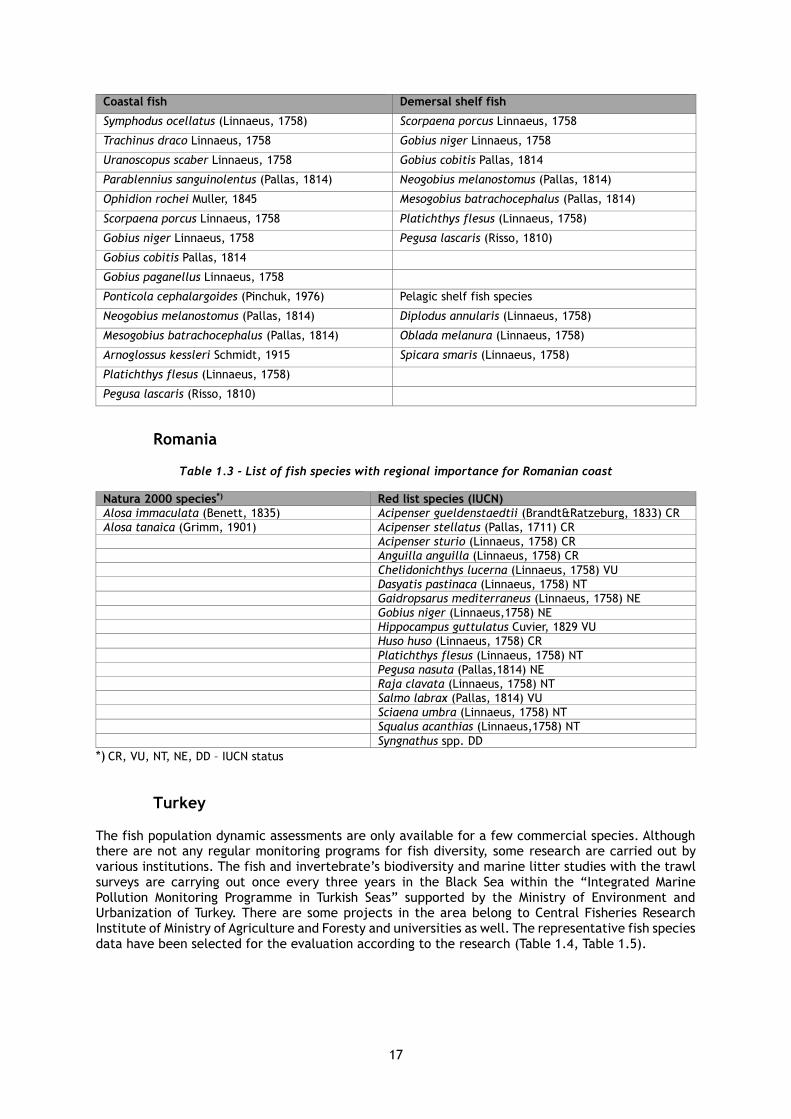
Table 1.3 - List of fish species with regional importance for Romanian coast

Natura 2000 species*) Red list species (IUCN)

Alosa immaculata (Benett, 1835) Acipenser gueldenstaedtii (Brandt&Ratzeburg, 1833) CR

Alosa tanaica (Grimm, 1901) Acipenser stellatus (Pallas, 1711) CR

Acipenser sturio (Linnaeus, 1758) CR

Anguilla anguilla (Linnaeus, 1758) CR

Chelidonichthys lucerna (Linnaeus, 1758) VU

Dasyatis pastinaca (Linnaeus, 1758) NT

Gaidropsarus mediterraneus (Linnaeus, 1758) NE

Gobius niger (Linnaeus,1758) NE

Hippocampus guttulatus Cuvier, 1829 VU

Huso huso (Linnaeus, 1758) CR

Platichthys flesus (Linnaeus, 1758) NT

Pegusa nasuta (Pallas,1814) NE

Raja clavata (Linnaeus, 1758) NT

Salmo labrax (Pallas, 1814) VU

Sciaena umbra (Linnaeus, 1758) NT

Squalus acanthias (Linnaeus,1758) NT

Syngnathus spp. DD

*) CR, VU, NT, NE, DD – IUCN status

Turkey

The fish population dynamic assessments are only available for a few commercial species. Although there are not any regular monitoring programs for fish diversity, some research are carried out by various institutions. The fish and invertebrate’s biodiversity and marine litter studies with the trawl surveys are carrying out once every three years in the Black Sea within the “Integrated Marine Pollution Monitoring Programme in Turkish Seas” supported by the Ministry of Environment and Urbanization of Turkey. There are some projects in the area belong to Central Fisheries Research Institute of Ministry of Agriculture and Foresty and universities as well. The representative fish species data have been selected for the evaluation according to the research (Table 1.4, Table 1.5).

18

Table 1.4 - List of representative fish by species groups for Turkey


Alosa immaculata Bennett, 1835 Dasyatis pastinaca (Linnaeus, 1758)

Chelidonichthys lucerna (Linnaeus, 1758) Raja clavata Linnaeus, 1758

Diplodus annularis (Linnaeus, 1758) Squalus acanthias Linnaeus, 1758

Gaidropsarus mediterraneus (Linnaeus, 1758) Syngnathus acus Linnaeus, 1758

Gobius niger Linnaeus, 1758 Hippocampus guttulatus Cuvier, 1829

Hippocampus hippocampus (Linnaeus, 1758) Hippocampus hippocampus (Linnaeus, 1758)

Chelon auratus (Risso, 1810) Gaidropsarus mediterraneus (Linnaeus, 1758)

Mullus barbatus barbatus Linnaeus, 1758 Merlangius merlangus (Linnaeus, 1758)

Mesogobius batrachocephalus (Pallas, 1814) Mullus barbatus barbatus Linnaeus, 1758

Neogobius melanostomus (Pallas, 1814) Trachinus draco Linnaeus, 1758

Oblada melanura (Linnaeus, 1758) Uranoscopus scaber Linnaeus, 1758

Ophidion rochei Müller, 1845 Parablennius tentacularis (Brünnich, 1768)

Parablennius sanguinolentus (Pallas, 1814) Ophidion rochei Muller, 1845

Parablennius tentacularis (Brünnich, 1768) Scorpaena porcus Linnaeus, 1758

Pomatomus saltatrix (Linnaeus, 1766) Gobius niger Linnaeus, 1758

Sardina pilchardus (Walbaum, 1792) Neogobius melanostomus (Pallas, 1814)

Sardinella aurita Valenciennes, 1847 Mesogobius batrachocephalus (Pallas, 1814)

Sciaena umbra Linnaeus, 1758 Pomatoschistus marmoratus (Risso, 1810)

Scorpaena notata Rafinesque, 1810 Chelidonichthys lucerna (Linnaeus, 1758)

Scorpaena porcus Linnaeus, 1758 Platichthys flesus (Linnaeus, 1758)

Solea solea (Linnaeus, 1758) Scophthalmus maximus (Linnaeus, 1758)

Spicara smaris (Linnaeus, 1758) Arnoglossus kessleri Schmidt, 1915

Symphodus ocellatus (Linnaeus, 1758) Pegusa lascaris (Risso, 1810)

Symphodus roissali (Risso, 1810) Callionymus risso Lesueur, 1814

Symphodus tinca (Linnaeus, 1758) Callionymus pusillus Delaroche, 1809

Trachinus draco Linnaeus, 1758 Gymnammodytes cicerelus (Rafinesque, 1810)

Trachurus mediterraneus (Steindachner, 1868) Serranus hepatus (Linnaeus, 1758)

Umbrina cirrosa (Linnaeus, 1758) Aphia minuta (Risso, 1810)

Uranoscopus scaber Linnaeus, 1758 Symphodus roissali (Risso, 1810)

Zosterisessor ophiocephalus (Pallas, 1814) Symphodus tinca (Linnaeus, 1758)

Chelon auratus (Risso, 1810)

Acipenser gueldenstaedtii (Brandt&Ratzeburg, 1833)

Pelagic shelf fish species

Sardina pilchardus (Walbaum, 1792) Spicara smaris (Linnaeus, 1758)

Sardinella aurita Valenciennes, 1847 Alosa immaculata Bennett, 1835

Sprattus sprattus (Linnaeus, 1758) Diplodus annularis (Linnaeus, 1758)

Trachurus mediterraneus (Steindachner, 1868) Engraulis encrasicolus (Linnaeus, 1758)

Atherina boyeri Risso, 1810 Pomatomus saltatrix (Linnaeus, 1766)

Ukraine

No information available for Ukraine.

19

1.2.2 Regional level

Table 1.5 - List of non-commercial species with regional importance

Species BG RO TR Regional importance

Coastal fish

Dasyatis pastinaca (Linnaeus, 1758) x x x x

Acipenser gueldenstaedtii Brandt & Ratzeburg, 1833 x x x x

Anguilla anguilla (Linnaeus, 1758) x

Syngnathus typhle Linnaeus, 1758 x x

Syngnathus variegatus Pallas, 1814 x x

Syngnathus abaster Risso, 1827 x x x x

Hippocampus guttulatus Cuvier, 1829 x x x x

Sciaena umbra Linnaeus, 1758 x x x x

Diplodus sargus sargus (Linnaeus, 1758) x

Oblada melanura (Linnaeus, 1758) x x

Spicara smaris (Linnaeus, 1758) x x

Symphodus roissali (Risso, 1810) x x

Symphodus cinereus (Bonnaterre, 1788) x

Symphodus ocellatus (Linnaeus, 1758) x x

Trachinus draco Linnaeus, 1758 x x

Uranoscopus scaber Linnaeus, 1758 x x

Parablennius sanguinolentus (Pallas, 1814) x

Ophidion rochei Muller, 1845 x x

Scorpaena porcus Linnaeus, 1758 x x

Gobius niger Linnaeus, 1758 x x x x

Gobius cobitis Pallas, 1814 x

Gobius paganellus Linnaeus, 1758 x

Ponticola cephalargoides (Pinchuk, 1976) x

Neogobius melanostomus (Pallas, 1814) x x

Mesogobius batrachocephalus (Pallas, 1814) x x

Arnoglossus kessleri Schmidt, 1915 x x

Platichthys flesus (Linnaeus, 1758) x x x x

Pegusa lascaris (Risso, 1810) x x x x

Demersal shelf fish species

Squalus acanthias (Linnaeus,1758) x

Dasyatis pastinaca (Linnaeus, 1758) x x x x

Raja clavata (Linnaeus, 1758) x

Acipenser stellatus Pallas, 1771 x x

Acipenser sturio (Linnaeus, 1758) x

Huso huso (Linnaeus, 1758) x

Gaidropsarus mediterraneus (Linnaeus, 1758) x x x x

Merlangius merlangus (Linnaeus, 1758) x x

Syngnathus variegatus Pallas, 1814 x x x x

Hippocampus guttulatus Cuvier, 1829 x x x x

Trachinus draco Linnaeus, 1758 x x

Uranoscopus scaber Linnaeus, 1758 x x

Parablennius tentacularis (Brunnich, 1768) x x

Chelidonichthys lucerna (Linnaeus, 1758) x

Coryphoblennius galerita (Linnaeus, 1758) x

Ophidion rochei Muller, 1845 x x

Callionymus pusillus Delaroche, 1809 x x

Scorpaena porcus Linnaeus, 1758 x x

Gobius niger Linnaeus, 1758 x x x x

Gobius cobitis Pallas, 1814 x

Neogobius melanostomus (Pallas, 1814) x x

Mesogobius batrachocephalus (Pallas, 1814) x x

Platichthys flesus (Linnaeus, 1758) x x

Pegusa lascaris (Risso, 1810) x x

Pelagic shelf fish species

Diplodus annularis (Linnaeus, 1758) x x

Oblada melanura (Linnaeus, 1758) x x

Spicara smaris (Linnaeus, 1758) x x

Salmo labrax (Pallas, 1814) x

20

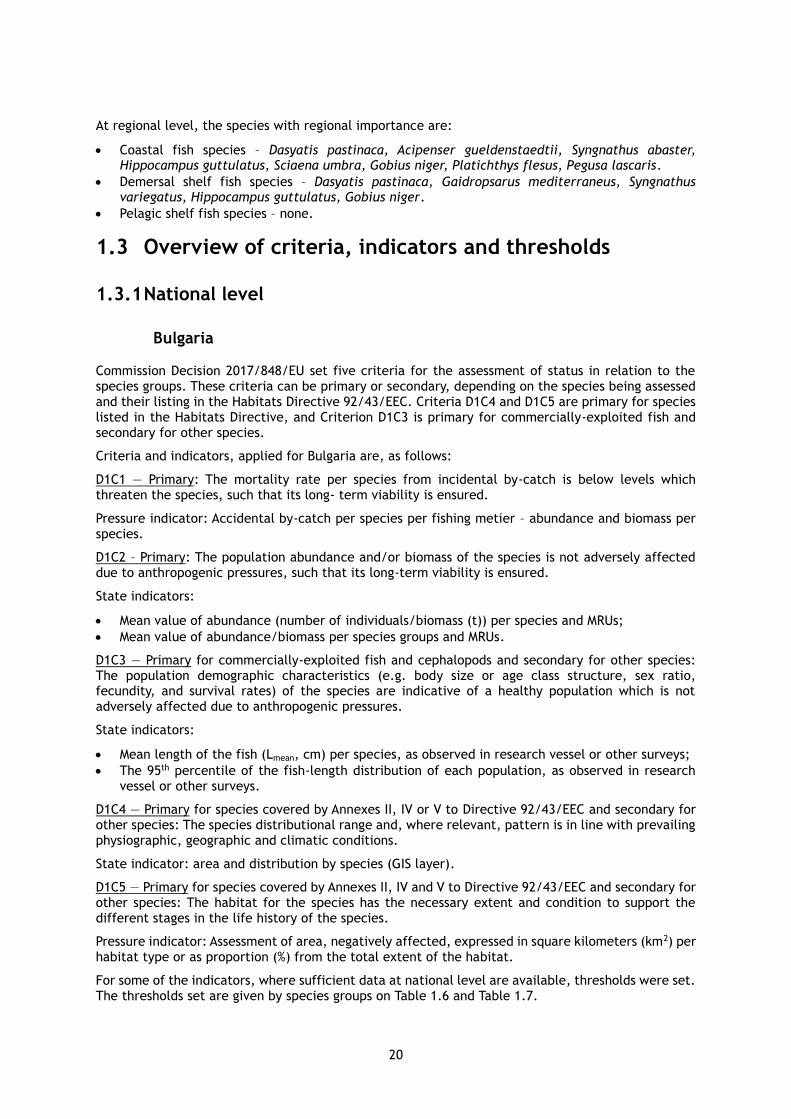
At regional level, the species with regional importance are:

• Coastal fish species – Dasyatis pastinaca, Acipenser gueldenstaedtii, Syngnathus abaster, Hippocampus guttulatus, Sciaena umbra, Gobius niger, Platichthys flesus, Pegusa lascaris.

• Demersal shelf fish species – Dasyatis pastinaca, Gaidropsarus mediterraneus, Syngnathus variegatus, Hippocampus guttulatus, Gobius niger.

• Pelagic shelf fish species – none.

1.3 Overview of criteria, indicators and thresholds


Bulgaria

Commission Decision 2017/848/EU set five criteria for the assessment of status in relation to the species groups. These criteria can be primary or secondary, depending on the species being assessed and their listing in the Habitats Directive 92/43/EEC. Criteria D1C4 and D1C5 are primary for species listed in the Habitats Directive, and Criterion D1C3 is primary for commercially-exploited fish and secondary for other species.

Criteria and indicators, applied for Bulgaria are, as follows:

D1C1 — Primary: The mortality rate per species from incidental by-catch is below levels which threaten the species, such that its long- term viability is ensured.

Pressure indicator: Accidental by-catch per species per fishing metier – abundance and biomass per species.

D1C2 – Primary: The population abundance and/or biomass of the species is not adversely affected due to anthropogenic pressures, such that its long-term viability is ensured.

State indicators:

• Mean value of abundance (number of individuals/biomass (t)) per species and MRUs;

• Mean value of abundance/biomass per species groups and MRUs.

D1C3 — Primary for commercially-exploited fish and cephalopods and secondary for other species: The population demographic characteristics (e.g. body size or age class structure, sex ratio, fecundity, and survival rates) of the species are indicative of a healthy population which is not adversely affected due to anthropogenic pressures.

State indicators:

• Mean length of the fish (Lmean, cm) per species, as observed in research vessel or other surveys;

• The 95th percentile of the fish-length distribution of each population, as observed in research vessel or other surveys.

D1C4 — Primary for species covered by Annexes II, IV or V to Directive 92/43/EEC and secondary for other species: The species distributional range and, where relevant, pattern is in line with prevailing physiographic, geographic and climatic conditions.

State indicator: area and distribution by species (GIS layer).

D1C5 — Primary for species covered by Annexes II, IV and V to Directive 92/43/EEC and secondary for other species: The habitat for the species has the necessary extent and condition to support the different stages in the life history of the species.

Pressure indicator: Assessment of area, negatively affected, expressed in square kilometers (km2) per habitat type or as proportion (%) from the total extent of the habitat.

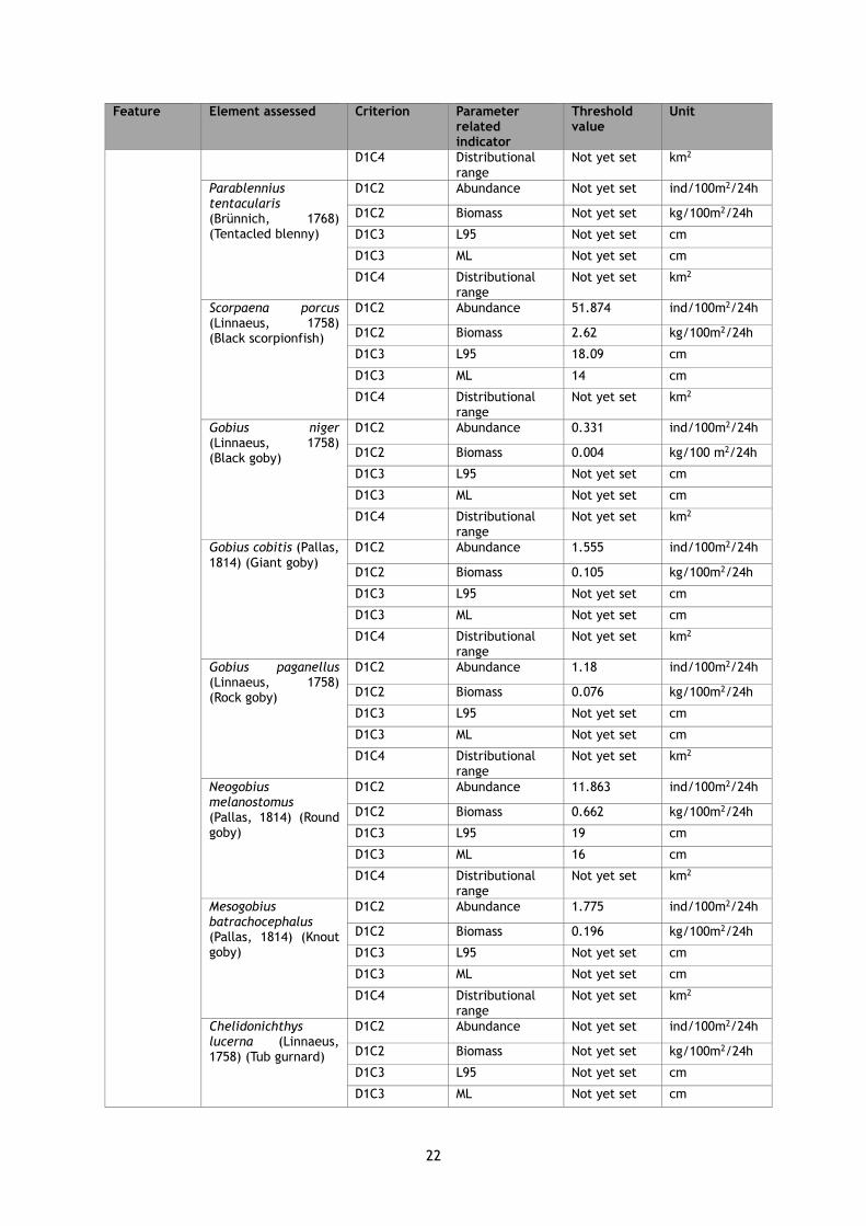
For some of the indicators, where sufficient data at national level are available, thresholds were set. The thresholds set are given by species groups on Table 1.6 and Table 1.7.

21

Table 1.6 - Indicators and thresholds for coastal fish group

Feature Element assessed Criterion Parameter related indicator

Threshold value

Unit

D1 Biodiversity (Coastal fish)

Acipenser stellatus (Pallas, 1771) (Starry sturgeon)

D1C2 Abundance Not yet set ind/100m2/24h

D1C2 Biomass Not yet set kg/100 m2/24h

D1C3 L95 Not yet set cm

D1C3 ML Not yet set cm

D1C4 Distributional range

Not yet set km2

Gaidropsarus mediterraneus (Linnaeus, 1758) (Shore rockling)


D1C2 Biomass Not yet set kg/100m2/24h




Not yet set km2

Merlangius merlangus (Linnaeus, 1758) (Whiting)






Not yet set km2

Hippocampus guttulatus (Cuvier, 1829) (Long-snouted seahorse)

D1C2 Abundance 0.415 ind/100m2/24h

D1C2 Biomass 0.003 kg/100m2/24h




Not yet set km2

Symphodus roissali (Risso, 1810) (Five-spotted wrasse)


D1C2 Biomass 0.081 kg/100 m2/24h




Not yet set km2

Trachinus draco (Linnaeus, 1758) (Greater weever)



D1C3 L95 24.79 cm

D1C3 ML 18 cm


Not yet set km2

Uranoscopus scaber (Linnaeus, 1758) (Stargazer)



D1C3 L95 18.37 cm

D1C3 ML 15 cm


Not yet set km2

Parablennius sanguinolentus (Pallas, 1814) (Rusty blenny)





22


Threshold value

Unit


Not yet set km2

Parablennius tentacularis (Brünnich, 1768) (Tentacled blenny)






Not yet set km2

Scorpaena porcus (Linnaeus, 1758) (Black scorpionfish)



D1C3 L95 18.09 cm

D1C3 ML 14 cm


Not yet set km2

Gobius niger (Linnaeus, 1758) (Black goby)


D1C2 Biomass 0.004 kg/100 m2/24h




Not yet set km2

Gobius cobitis (Pallas, 1814) (Giant goby)






Not yet set km2

Gobius paganellus (Linnaeus, 1758) (Rock goby)






Not yet set km2

Neogobius melanostomus (Pallas, 1814) (Round goby)



D1C3 L95 19 cm

D1C3 ML 16 cm


Not yet set km2

Mesogobius batrachocephalus (Pallas, 1814) (Knout goby)






Not yet set km2

Chelidonichthys lucerna (Linnaeus, 1758) (Tub gurnard)





23


Threshold value

Unit


Not yet set km2

Pegusa lascaris (Risso, 1810) (Sand sole)



D1C3 L95 20.7 cm

D1C3 ML 16 cm


Not yet set km2

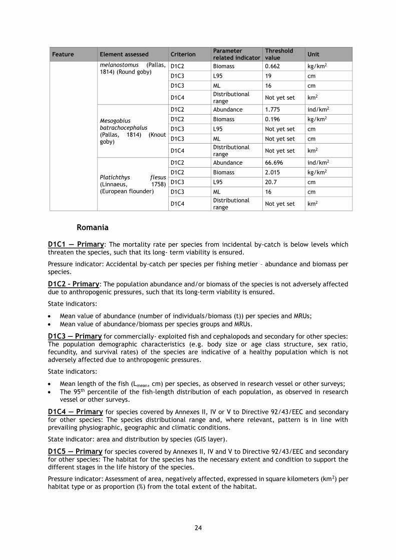
Table 1.7 - Indicators and thresholds for shelf fish group (pelagic and demersal)


Threshold value

Unit

D1 Biodiversity (Shelf fish)


D1C2 Abundance Not yet set ind/km2

D1C2 Biomass Not yet set kg/km2




Not yet set km2


D1C2 Abundance 0.415 ind/km2

D1C2 Biomass 0.003 kg/km2




Not yet set km2




D1C3 L95 24.79 cm

D1C3 ML 18 cm


Not yet set km2




D1C3 L95 18.37 cm

D1C3 ML 15 cm


Not yet set km2




D1C3 L95 18.09 cm

D1C3 ML 14 cm


Not yet set km2







Not yet set km2

Neogobius D1C2 Abundance 11.863 ind/km2

24


Threshold value

Unit

melanostomus (Pallas, 1814) (Round goby)


D1C3 L95 19 cm

D1C3 ML 16 cm


Not yet set km2







Not yet set km2

Platichthys flesus (Linnaeus, 1758) (European flounder)



D1C3 L95 20.7 cm

D1C3 ML 16 cm


Not yet set km2

Romania

D1C1 — Primary: The mortality rate per species from incidental by-catch is below levels which

threaten the species, such that its long- term viability is ensured.

Pressure indicator: Accidental by-catch per species per fishing metier – abundance and biomass per species.

D1C2 – Primary: The population abundance and/or biomass of the species is not adversely affected

due to anthropogenic pressures, such that its long-term viability is ensured.

State indicators:



D1C3 — Primary for commercially- exploited fish and cephalopods and secondary for other species:

The population demographic characteristics (e.g. body size or age class structure, sex ratio, fecundity, and survival rates) of the species are indicative of a healthy population which is not adversely affected due to anthropogenic pressures.

State indicators:



D1C4 — Primary for species covered by Annexes II, IV or V to Directive 92/43/EEC and secondary

for other species: The species distributional range and, where relevant, pattern is in line with prevailing physiographic, geographic and climatic conditions.

State indicator: area and distribution by species (GIS layer).

D1C5 — Primary for species covered by Annexes II, IV and V to Directive 92/43/EEC and secondary

for other species: The habitat for the species has the necessary extent and condition to support the different stages in the life history of the species.

Pressure indicator: Assessment of area, negatively affected, expressed in square kilometers (km2) per habitat type or as proportion (%) from the total extent of the habitat.

25

Table 1.8 - Indicators and thresholds for coastal fish group, Romanian coast


Threshold value



D1C1 Fishing mortality rate

>0.08


D1C3 L95 Not yet set

D1C3 ML Not yet set


Not yet set



D1C2 Biomass Not yet set

D1C3 L95 15 cm

D1C3 ML 13 cm


Not yet set


D1C2 Abundance Not yet set


D1C3 L95 Not yet set

D1C3 ML Not yet set


Not yet set


D1C2 Abundance Not yet set


D1C3 L95 18.2 cm

D1C3 ML 15 cm


Not yet set

Turkey

Although the amount of landed commercial fish species is known, the amount of non-commercial species are not exactly known. However, there are many fish species caught not targeted and are discarded. Turkish fishermen have been recording the fish species which they caught during the fishing activity since 2008 into the "Fisheries Information System (SUBIS)". In the electronic system (SUBIS), only the amounts of the target fish species are recorded, and there is not any data on the fish caught as by-catch and discard. The information about by-catch and discard amount is insufficient since it is not legally required. Likewise, there is no any evaluation criteria for the non-commercial species in the national legislation.

There are some research projects carried out about the monitoring and evaluating of coasts and seas of Turkey with defined collaborative methods and protocols within the EU Water Framework Directive and Marine Strategy Framework Directive and also within the Bucharest Conventions which Turkey is a party of. Biodiversity, abundance and biomass and length data of the species are recorded within the scientific research. Some of the following criteria have been created based on these data.

D1C2 – Primary: The population abundance and/or biomass of the species is not adversely affected

due to anthropogenic pressures, such that its long-term viability is ensured.

State indicators:



D1C3 — Primary for commercially- exploited fish and cephalopods and secondary for other species:

The population demographic characteristics (e.g. body size or age class structure, sex ratio, fecundity, and survival rates) of the species are indicative of a healthy population which is not adversely affected due to anthropogenic pressures.

26

State indicators:



Table 1.9 - Indicators and thresholds for coastal fish group, Turkish coast


Threshold value

Unit


Alosa immaculata Bennett, 1835 (Pontic shad)










Diplodus annularis (Linnaeus, 1758) (Annular seabream)





Oblada melanura (Linnaeus, 1758) (Saddled seabream)





Hippocampus hippocampus (Linnaeus, 1758) (Short-snouted seahorse)





Spicara smaris (Linnaeus, 1758) (Picarel)










Symphodus tinca (Linnaeus, 1758) (East Atlantic peacock wrasse)





Symphodus ocellatus (Linnaeus, 1758) (Ocellated wrasse)








27


Threshold value

Unit



Scorpaena notata Rafinesque, 1810 (Small red scorpionfish)






























Ophidion rochei Muller, 1845 (Roche's snake blenny)










Mullus barbatus barbatus Linnaeus, 1758 (Red mullet)





Parablennius sanguinolentus (Pallas, 1814) (Rusty blenny)





Parablennius D1C2 Abundance Not yet set ind/100m2/24h

28


Threshold value

Unit

tentacularis (Brünnich, 1768) (Tentacled blenny)




Chelon auratus (Risso, 1810) (Golden grey mullet)





Pomatomus saltatrix (Linnaeus, 1766) [Bluefish]





Sardina pilchardus (Walbaum, 1792) (European pilchard)





Sardinella aurita Valenciennes, 1847 (Round sardinella)





Solea solea (Linnaeus, 1758) (Common sole)





Sciaena umbra Linnaeus, 1758 (Brown meagre)





Trachurus mediterraneus (Steindachner, 1868) (Mediterranean horse mackerel)





Umbrina cirrosa (Linnaeus, 1758) (Shi drum)





Zosterisessor ophiocephalus (Pallas, 1814) (Grass goby)





29

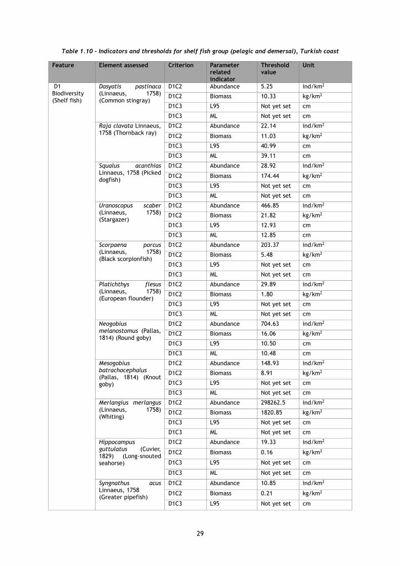
Table 1.10 - Indicators and thresholds for shelf fish group (pelagic and demersal), Turkish coast


Threshold value

Unit

D1 Biodiversity (Shelf fish)

Dasyatis pastinaca (Linnaeus, 1758) (Common stingray)





Raja clavata Linnaeus, 1758 (Thornback ray)



D1C3 L95 40.99 cm

D1C3 ML 39.11 cm

Squalus acanthias Linnaeus, 1758 (Picked dogfish)








D1C3 L95 12.93 cm

D1C3 ML 12.85 cm






Platichthys flesus (Linnaeus, 1758) (European flounder)








D1C3 L95 10.50 cm

D1C3 ML 10.48 cm
















Syngnathus acus Linnaeus, 1758 (Greater pipefish)




30


Threshold value

Unit





D1C3 L95 13.98 cm

D1C3 ML 13.91 cm




D1C3 L95 9.05 cm

D1C3 ML 8.99 cm

Mullus barbatus barbatus Linnaeus, 1758 (Red mullet)








D1C3 L95 11.97 cm

D1C3 ML 11.73 cm

Parablennius tentacularis (Brünnich, 1768) (Tentacled blenny)





Ophidion rochei Muller, 1845 (Roche's snake blenny)










Callionymus risso Lesueur, 1814 (Risso’s dragonet)





Callionymus pusillus Delaroche, 1809 (Sailfin dragonet)





Gymnammodytes cicerelus (Rafinesque, 1810) (Mediterranean sand eel)





Pomatoschistus marmoratus (Risso,



31


Threshold value

Unit

1810) [Marbled goby] D1C3 L95 Not yet set cm


Scophthalmus maximus (Linnaeus, 1758) [Turbot]





Serranus hepatus (Linnaeus, 1758) [Brown comber]





Spicara smaris (Linnaeus, 1758) [Picarel]



D1C3 L95 10.58 cm

D1C3 ML 10.32 cm

Alosa immaculata Bennett, 1835 [Pontic shad]





Diplodus annularis (Linnaeus, 1758) [Annular seabream]





Sprattus sprattus (Linnaeus, 1758) (European sprat)



D1C3 L95 8.19 cm

D1C3 ML 8.14 cm

Trachurus mediterraneus (Steindachner, 1868) (Mediterranean horse mackerel)





Chelon auratus (Risso, 1810) (Golden grey mullet)





Arnoglossus kessleri Schmidt, 1915 (Scaldback)



D1C3 L95 6.54 cm

D1C3 ML 6.44 cm




D1C3 L95 15.19 cm

D1C3 ML 14.99 cm

32


Threshold value

Unit

Aphia minuta (Risso, 1810) (Transparent goby)










Symphodus tinca (Linnaeus, 1758) (East Atlantic peacock wrasse)





Acipenser gueldenstaedtii (Brandt&Ratzeburg, 1833) (Danube sturgeaon)





Ukraine

Information about Ukraine is not available.


The national indicators are classified according to their stage of development and implementation into three categories:

• Fully operational - legally accepted nationally, validated for the relevant pressure and with thresholds established for all species under the relevant pressure;

• Partially operational - legally accepted, validated for pressure but without thresholds yet, at least for some of the species;

• Not operational - any other status of development, proposed for future use.

Table 1.11 - Indicators with regional importance

Country BG RO TR Regional importance

Criteria Indicators

D1C1: The mortality rate per species from incidental by-catch is below levels which threaten the species, such that its long-term viability is ensured.

Accidental by-catch per species per fishing metier – abundance and biomass per species.



Yes

D1C2: The population abundance of the species is not adversely affected due to anthropogenic pressures, such that its long-term viability is ensured.

Mean value of abundance (number of individuals/biomass (t)) per species and MRUs.



Yes

33

Country BG RO TR Regional importance

Criteria Indicators

Mean value of abundance/biomass per species groups and MRUs.



Yes

D1C3: The population demographic characteristics of the species are indicative of a healthy population which is not adversely affected due to anthropogenic pressures.

Mean length of the fish (Lmean, cm) per species, as observed in research vessel or other surveys.



Yes

The 95th percentile of the fish-length distribution of each population, as observed in research vessel or other surveys.



Yes

D1C4: The species distributional range and, where relevant, pattern is in line with prevailing physiographic, geographic and climatic conditions.

Area and distribution by species (GIS layer).



Yes

D1C5: The habitat for the species has the necessary extent and condition to support the different stages in the life history of the species.

Assessment of area, negatively affected, expressed in square kilometers (km2) per habitat type or as proportion (%) from the total extent of the habitat.

Assessment of area, negatively affected, expressed in square kilometers (km2) per habitat type or as proportion (%) from the total extent of the habitat.

Assessment of area, negatively affected, expressed in square kilometers (km2) per habitat type or as proportion (%) from the total extent of the habitat

Yes

All indicators proposed for Descriptor D1 in Commission Decision EU/2017/848 are common and with regional interest, but they are not validated for the relevant pressures.

1.4 Harmonized approach for indicators and thresholds setting based on the regional progress

1.4.1 Bulgaria

The approaches for integration of the individual indicators, criteria and final evaluation of D1 Biodiversity (fish) in Bulgaria are, as follows:

• The integration of individual indicators by species and MRUs for each criterion is carried out under the “One Out All Out” (OAAO) rule.

• The integration of the MRUs for each criterion and type - under the “One Out All Out” (OAAO) rule.

• The integration between criteria for each species - under the “One Out All Out” (OAAO) rule.

• The final assessment for the groups of coastal and shelf fish species is formed by the percentage of species in “Good” status. The threshold value is 90%.

• The final assessment for the Descriptor 1 Biodiversity Fish – “One Out All Out” (OAAO) rule applied to all fish species groups.

34

1.4.2 Romania

The approaches for integration of the individual indicators, criteria and evaluation of D1 Biodiversity (fish) in Romania are, as follows:


• The integration of the MRUs for each criterion and type - under the “One Out All Out” (OAAO) rule.


• The final assessment for the Descriptor 1 Biodiversity Fish – “One Out All Out” (OAAO) rule applied to all fish species groups.

Biological diversity in the sense of Descriptor 1 is a complex and wide-ranging subject, and new knowledge is continually necessary.

1.4.3 Turkey

It is accepted by the institutions that it is necessary to perform a monitoring system and a data base about monitoring the biodiversity of Turkey. Establishing the methods and devices and also the budget to carry out a long term monitoring researches is very important. However, monitoring programme has been initiated within the framework of a simple monitoring mechanism, since the development of the national mechanism in monitoring activities is a long-term work. In addition to this the biologic diversity data base performed. Also, it is available to search species, habitat and defined areas. The approaches for integration of the individual indicators, criteria and final evaluation of D1 Biodiversity (fish) in Turkey have not performed yet.

1.4.4 Ukraine

No information available for Ukraine.


At EU level (Bulgaria and Romania), for the present state of development of indicators, it is not possible a harmonized approach for indicators and thresholds to be set. For the third countries, indicators and thresholds are not set yet or information is not available. The main reasons are limited data availability and different stages of development of indicators at national level.

1.5 Methods and approaches for data integration and overall assessment at descriptor level

1.5.1 EU level

According to the discussions of 15th meeting of the Working Group on Good Environmental Status (WG GES), the levels of integration and different integration methods for species under Descriptor 1 are presented on Figure 1.1 and is representative of a single assessment area. It is shown generically for ecosystem components (birds, mammals, reptiles, fish, cephalopods) – the criteria used, and whether criteria are primary or secondary, differs between ecosystem components and between species.

35

Figure 1.1 - Levels and methods of integration for species under Descriptor 11

The following levels and methods of integration are recommended to WG GES for Figure 1.1:

• Level 1: Measurements of individual parameters — for example abundance of individual species at different times of year in different locations etc. — are combined into a single indicator for individual species. Integration at this level currently follows rules under development by Regional Sea Conventions. Comparability of this level of integration requires technical consideration and is not addressed in the guidance.

• Level 2: Where there is more than one indicator for a species for a particular criterion, the indicators are combined to form a judgement on the status of each criterion. The integration method is not yet defined but could be OOAO or (weighted) averaging. The integration method should be agreed at regional level.

• Level 3: The relevant criteria for each species are integrated to form a judgement on the status of each species. The integration method for species covered by Annexes II, IV and V of the Habitats Directive (92/43/EEC) follows the integration method as per that Directive, to provide a conclusion on status for the species. For other species, the integration method should be agreed at regional or subregional level. Different species may be represented by different numbers of criteria.

• Level 4: The results for each species are brought together to the species group. The integration method is a conditional rule, based on a specific number or proportion of species in a species group achieving good status. For example, if x of y species are in good status, the species group is considered to be in good status. The threshold x would be defined in the determination of GES.

• Level 5: The ecosystem component under D1 is in good environmental status if each species group is in good status. Species groups are therefore integrated to ecosystem component level using OOAO.

1 Document GES_15-2016-02

36

The integration for assessing status follows the species approach (integrating the various criteria for a single species to determine the status of that species). However, Member States may wish additionally to integrate or aggregate the information in alternative ways (such as aggregating species for a particular criterion) to investigate pressures and/or management responses required, or for reporting against specific targets or indicators at national level.

1.5.2 ICES advice

Regarding ICES advice (ICES, 2018), an ecosystem component cannot be considered to be at a good status if one or more of the assessed species groups are considered to be in poor status. It is recommended that a one out, all out (OOAO) integration is used from species group to ecosystem component. This integration will mean that all assessed species groups have to be in good status for the ecosystem component to be in a good status. Other methods could mask groups outside GES and furthermore, as the number of species groups is always 5 or less, OOAO is consistent with the proportional approach for low numbers. The recommended integration methods for the different levels of integration are shown in the Table 1.12 for HD species, D3 species, and other species (ICES, 2018).

Table 1.12 - Integration methods recommended (ICES, 2018)

Level Integration method (s)

From Species group to ecosystem component

Option 1: OOAO Option 2: Proportion of all species in good status above agreed level (across species groups)

From species to species group

Proportional (determined by probability), if number of species in the group>5, OOAO if the number of species is 1 to 5.

From criteria to species (populations)

HD species: OOAO D3 species: as assessed in D3 Other species: one of the options 1- 5 bellow: If D1C1 and D1C2 are both in good status, then determine the average D1C2-D1C5, weighted so the weight of D1C2= weight of D1C3-C5 together. If this average is in good status, the species is in good status. If D1C1 and D1C2 are both in good status, then determine the average D1C3-D1C5. If this average is in good status, the species is in good status. If the weighted average of D1C1 to D1C5 is in good status, the species is in good status. The average is weighted to ensure that the weight of D1C2= weight of D1C1=weight of D1C3-C5 Conditional/OOAO Population model determines weights. This method can be used is a population model suggests appropriate weights of each of the criteria. For example, for long lived species, abundance may be little affected by one poor recruitment year, and it may therefore be desirable to down-weight this. If the criterion D1C1 is not used, for options 1 and 2, D1C2 should be in good status and then the weighted average is considered. For option 3, the weight of D1C2=weight of D1C3-D1C5 combined.

1.5.3 Regional Black Sea level

At the Black Sea level, the levels and methods for integration recommended by WG GES and ICES need further development and discussion. At the current state of knowledge, it is not possible to be recommended a specified approach.

1.6 Conclusions and recommendations

Development of common indicators, thresholds and integration methods for Descriptor 1 Non-commercial fish are not yet finalized at EU level and at regional Black Sea level. Additional efforts are needed at regional level to collect data and develop regionally agreed thresholds.

37

2 Guideline on Descriptors 1. Theme Marine Mammals

2.1 Introduction

The Marine Strategy Framework Directive (MSFD) aims at implementing a precautionary and holistic ecosystem-based approach for managing European marine waters. Marine mammals are included as a functional group for the assessment and reporting under Descriptor 1 - Biodiversity. Conservation of mobile marine megafauna such as cetaceans requires transboundary cooperation, which the MSFD promotes through regional instruments, such as the Regional Sea Conventions and other regional cooperation structures, such as ACCOBAMS (Agreement on the Conservation of Cetaceans of the Black Sea, Mediterranean Sea and Contiguous Atlantic Area). The leading regional intergovernmental actor for the protection of the Black Sea from pollution and other environmental problems is the Commission on the Protection of the Black Sea Against Pollution (Black Sea Commission or BSC). The BSC is the governing and implementing body of the Convention on the Protection of the Black Sea Against Pollution (Bucharest Convention), adopted by the six Black Sea states in 1992. The Convention entered into force on 15th January 1994, but the Commission Secretariat became officially operational only in October 2000, which has seriously hampered the functioning of the BSC in some areas. The Bucharest Convention, together with its satellite documents (four Protocols2, Declarations and the Black Sea Strategic Action Plan (BS SAP 2009)), form the legal basis for the work of the BSC. Moreover, in 2009, a revised and updated version of the 1992 LBS Protocol was adopted3, which however has not since been ratified by the necessary minimum of Contracting Parties.

In the BSC, only Bulgaria and Romania are EU Member States with the obligation to implement the MSFD. Georgia and Ukraine are bound, through their Association Agreements with the EU to implementing the MSFD and Turkey, as a candidate country is also expected to approximate to EU legislation (Roof Report).

Since the 6 riparian countries of Black Sea being Parties to at least one of the Cooperation structures, the BSC and ACCOBAMS can stimulate collaboration among scientists involved in cetacean monitoring and can foster transboundary initiatives that would align with MSFD objectives.

The Chapter is aimed to provide guidance for establishment of a synergetic monitoring and assessment program for D1 – marine mammals at the Black Sea basin level in the frame of “Black Sea Monitoring and Assessment Guideline” (BSMAG). The section provides an overview of the latest established or proposed criteria, indicators and thresholds based on the progress up-to-date (ComDec 848/2017) made in Romania and Bulgaria adding the initiatives from Ukraine and Turkey in order to establish common guidelines. Based on the analysis of the progress made so far, through programs/initiatives, within the four countries, the authors are presenting a guidance document for a future synergic effort in establishing the Good Environmental Status of the Black Sea marine mammals based on the assessment of the established indicators.

An indicator is a scientific assessment tool. It consists of one or several parameters chosen to represent (indicate) a certain situation or aspect and to simplify a complex reality. In the context of the implementation of the MSFD, indicators are specific attributes of each GES criterion that can be measured, and which allow subsequent change in the attribute to be followed over time.

In the context of the Barcelona Convention, a common indicator is a measure that summarizes data into a simple, standardized and communicable figure and is ideally applicable in the whole basin and can be monitored by all Parties, aiming at delivering valuable information to decision-makers. In particular, indicators should contribute to assess effects of measures taken to achieve or maintain GES.

2 Protocol on the Protection of the Marine Environment of the Black Sea from Land-based Sources (1992 LBS Protocol), Protocol on Co-operation in Combating Pollution of the Black Sea Marine Environment by Oil and other harmful Substances in Emergency Situations (1992 Emergency Protocol), Protocol on the Protection of the Black Sea marine Environment against Pollution by

Dumping (1992 Dumping Protocol) and the Black Sea Biodiversity and Landscape Conservation Protocol (2002 CBD Protocol).

3 Protocol on the Protection of the Marine Environment of the Black Sea from Land-Based Sources and Activities (2009 LBSA Protocol).

38

The present chapter was developed in accordance with the requirements of the Article 3(5)b and 5(2) of the Marine Strategy Framework Directive for a better coherence within the same marine region or subregion when it comes to MSFD implementation45. Milieu and the COM also assessed the coherence in the Black Sea region (Bulgaria and Romania) in the CSWD Regional Report and Milieu´s "Article 12 Technical Assessment of the MSFD 2012 obligations - Black Sea".

The determination of GES of marine mammals for pressure in link with other indicators were not assessed in this chapter, these being included in the appropriate Descriptor, eg. D11 - noise pressure, D10 -Marine litter, D8-Contaminants etc. Although the pressure-impact relationship is not yet fully understood, further studies will be necessary to be performed in the future.

The assessment is based on an overview of the proposed core indicators which are developed to regularly assess the status of marine mammals in the Black Sea marine environment against targets that reflect GES. During the past 10 years, the indicators development has been carried out within different projects in Bulgaria and Romania (Technical and administrative support for the joint implementation of the MSFD in Bulgaria and Romania - Phase I; Phase II and Phase III).

The cetacean fauna in the Black Sea includes three subspecies – the harbour porpoise, the common dolphin and the bottlenose dolphin. All three species are covered by Annex IV of the European Habitats Directive and therefore require strict protection by EU member states and two of the species are listed in Annex II, thus requiring member states to designate sites of community interests (NATURA 2000) to ensure conservation of their core habitat. The present state of Black Sea cetacean populations is not certain in spite of research and conservation measures during last twenty years. The insufficient scientific information concerns the population abundance, distribution, migrations, critical habitats, anthropogenic and natural threats as well as some basic aspects of life history and pathology.

The conservation status of Black Sea cetaceans has been reviewed and assessed under initiatives by the European Cetacean Society (1992), the European Commission (1999), the Black Sea Commission (1999 and 2008), ACCOBAMS (2002, 2006 and 2010), the International Whaling Commission (2004), and the IUCN (2008).

2.2 Ecological elements

Group of marine mammals is represented by three species in Black Sea:

a) Harbour porpoise - Phocoena phocoena ssp. relicta (Abel, 1905) (Figure 2.1)

b) Common dolphin - Delphinus delphis ssp. ponticus (Barabasch-Nikiforov, 1935) (Figure 2.2)

c) Bottlenose dolphin - Tursiops truncatus ssp. ponticus (Barabasch-Nikiforov, 1940) (Figure 2.3)

Figure 2.1 - Phocoena phocoena ssp. relicta (Abel, 1905) (@Green Balkans NGO)

4 COM (2014) 97 final: The first phase of implementation of the Marine Strategy Framework Directive (2008/56/EC)

5 The European Commission's assessment and guidance and the CSWD accompanying this report SWD (2014) 49 final.

39

Figure 2.2 - Delphinus delphis ssp. ponticus (Barabasch-Nikiforov, 1935) (@Mare Nostrum NGO)

Figure 2.3 - Tursiops truncatus ssp. ponticus (Barabasch-Nikiforov, 1940) (@Mare Nostrum NGO)

The three species are of regional importance and for the improvement of their population status regional cooperation is needed. Currently, there are two regional studies focusing on the three species of Black Sea cetaceans, one which is still on going the CeNoBS project ― Support MSFD implementation in the Black Sea through establishing a regional monitoring system of cetaceans (D1) and noise monitoring (D11) for achieving GES funded by the DG Environment of the European Commission within the call ― DG ENV/MSFD Second Cycle and of which the results will be available at the end of 2020, and the other, done in 2013 - Studies for carrying out the common fisheries policy: adverse fisheries impacts on cetacean populations in the Black Sea funded by the European Commission.

During July 2013, the first dedicated line-transect cetacean survey in the inshore and offshore waters of the western Black Sea, combined shipboard and aerial line transect survey was conducted to document the distribution and abundance of cetaceans in the western Black Sea including all waters under the jurisdiction of Bulgaria (BG), Romania (RO) and the waters of Ukraine (UA) located to the west of Crimea peninsula. The territorial sea, internal waters and exclusive economic zones (EEZs) of Bulgaria and Romania taken together were considered as a maritime area of the European Union (EU) in the Black Sea (Birkun et al., 2014).

Below are presented the results related to the absolute abundance of all three Black Sea cetacean species/subspecies, including the harbour porpoise (Phocoena phocoena relicta), the common dolphin (Delphinus delphis ponticus) and the bottlenose dolphin (Tursiops truncatus ponticus) for the NW Black Sea area in the Table 2.1, which rounded to thousands reveal estimates of approx. 115,000 cetaceans ± 22,000 individuals.

40

Table 2.1 - Integral values estimated for the three species of cetaceans in the NW Black Sea area*

Parameters Harbour porpoise

Common dolphin

Bottlenose dolphin

Area (km2) 119796.0

Observation effort (total length of transect lines) (km) 60036.5

No. of observations 402 408 275

Estimate of expected values of group size 1.335 1.986 1.836

Mean group size 1.410 2.304 1.866

Estimate of density of groups per 1 km2 0.184 0.254 0.120

Estimate of density of animals (ind/km2) 0.246 0.504 0.221

Estimate of number of animals in surveyed area 29465 60400 26462

*Extended table can be consulted in the report “Studies for carrying out the common fisheries policy: adverse

fisheries impact on cetacean populations in the Black Sea”.

2.3 Overview of criteria, indicators and thresholds progress

In accordance with the Roof Report published in 2018, the Black Sea marine mammals are assessed based on 5 main criteria as showed in the Table 2.2 below. Marine mammals: the incidental by-catch, the population abundance and the distributional range of the harbour porpoise, common dolphin and bottlenose dolphin are used as common indicators for D1C1, D1C2 and D1C4. No common indicators for marine mammals for D1C3 and D1C5 have been defined yet in accordance with the Roof report (2018).

Table 2.2 - Marine mammals group proposed criteria and indicators (relating to D1)

Criteria Indicator in common (RO & BG) Common assessment and threshold (RO+BG)

D1C1 Mammals: Incidental by-catch of harbour porpoise, common dolphin, bottlenose dolphin

To be defined according to the revised GES Decision.

D1C2 Mammals: harbour porpoise, common dolphin, bottlenose dolphin

D1C3 Mammals: To be defined according to the revised GES Decision.

D1C4 Mammals: Harbour Porpoise, Common Dolphin, Bottlenose Dolphin

D1C5 Mammals: To be defined according to the revised GES Decision.


Bulgaria

Considering the new GES Decision (Com.Dec.EU/2017/848), Monitoring program of Bulgaria regarding D1 Biodiversity - Marine mammals include the following criteria and indicators:

• D1C1 — Primary: The mortality rate per species from incidental by-catch is below levels which threaten the species, such that its long- term viability is ensured.

Indicator: accidental by-catch by species and by fishing segments (abundance and biomass by species).

No targets and threshold values have been set due to lack of information on the values of accidental by-catch by species and by fishing metiers.

• D1C2 — Primary: The population abundance of the species is not adversely affected due to anthropogenic pressures, such that its long-term viability is ensured.

Indicator: abundance (number of individuals) per species and MRU.

The abundance of marine mammals should be estimated by line transect method (Buckland et al., 1993; Thomas et al., 2010) and Distance software. Measurement unit is absolute abundance in

41

numbers. Indicator is not validated for the relevant pressures. Thresholds for GES were determined using as a baseline the results from Birkun et.al. (2014) and increasing trend is expected.

• D1C3 — Primary for commercially-exploited fish and cephalopods and secondary for other species: The population demographic characteristics (e.g. body size or age class structure, sex ratio, fecundity, and survival rates) of the species are indicative of a healthy population which is not adversely affected due to anthropogenic pressures.

Indicator: not proposed due to lack of data and information regarding population parameters of three cetacean species.

No targets and threshold values have been set due to lack of information on the reference condition of the demographic characteristics of populations of cetaceans.

• D1C4 — Primary for species covered by Annexes II, IV or V to Directive 92/43/EEC and secondary for other species: The species distributional range and, where relevant, pattern is in line with prevailing physiographic, geographic, and climatic conditions.

Indicators: distributional area by species (GIS layer) and density of distribution (ind/km2).

Distributional area by species (GIS layer) - No targets and threshold values have been set due to lack of information.

Density of distribution - indicator showed the distributional patterns of the species. It is not validated for the relevant pressures. Thresholds for GES were determined using as a baseline the results from Birkun et.al. (2014) and increasing trend is expected.

• D1C5 — Primary for species covered by Annexes II, IV and V to Directive 92/43/EEC and secondary for other species: The habitat for the species has the necessary extent and condition to support the different stages in the life history of the species.

Indicator: Assessment of the area, negatively affected, expressed as square kilometers (km2) for every habitat type or as a proportion (%) from the total extent of the habitat. No targets and threshold values have been set due to lack of information on the area coverage by habitat type, which is negatively affected.

The initial assessment of the status of the marine environment (according to Art. 8), the definitions of good environmental status of the marine environment - the GES (under Article 9) and the identification of environmental targets and related indicators (under Article 10) constitute the first part of the Marine Strategy of Bulgaria (http://www.bsbd.org /bg/page_1722859.html), developed in 2012 by a team of the Institute of Oceanology at the Bulgarian Academy of Sciences (IO-BAS). The monitoring programs on the Descriptors under MSFD Art. 11 are the second part of the Marine Strategy and was developed in 2016 under the Project “Investigations on the State of the Marine Environment and Improving Monitoring Programs developed under MSFD (ISMEIMP)”, funded under EEA Financial Mechanism grant, 2015-2017. The project filled in gaps of information regarding the marine environment in the Bulgarian Black Sea through field surveys, re-analyses of historical and current datasets using advanced statistical approaches ensured improved definitions of GES, revised ecological targets and threshold for good status of the related indicators. The Program of Measures under Art.13 of MSFD is the third part of the Marine Strategy of Bulgaria and was developed during the period 2015-2016 (http://www.bsbd.org/bg/merki_13_rdms.html). Marine strategy of Bulgaria (2016-2021) and Program of measures were adopted by Decision of Council of Ministers No.1111/29.12.2016. The set of thresholds applied for the indicators under all criteria are presented on Table 2.3.

Table 2.3 - List of criteria, indicators and thresholds currently applied in Bulgaria


Target level threshold value

Unit

D1 Biodiversity (Mammals)

Delphinus delphis ponticus Barabasch-Nikiforov, 1935 (Short-beaked Common Dolphin)

D1C2 Abundance 5019 Count

D1C4 Density 0.718 ind/km2


Not yet set km2

Tursiops truncatus D1C2 Abundance 4861 Count

42


Target level threshold value

Unit

ponticus Barabash-Nikiforov, 1940 (Black Sea Bottlenose Dolphin)



Not yet set km2

Phocoena phocoena relicta Abel, 1905 (Black Sea Harbour Porpoise)

D1C2 Abundance 1003 Count



Not yet set km2

Concerning the efforts to overcome the data deficiency of the cetaceans in Bulgarian waters several projects and actions were performed in the past years. These could be used as monitoring and assessment guidance.

Birkun et al., 2014 reports the result of a dedicated survey (aerial and vessel) that took place in July 2013 in Ukrainian, Romanian and Bulgarian Black Sea waters (territorial waters and EEZ). The monitoring methodology was designed in accordance with principles of line transect distance sampling. Beside abundance, density and distribution of cetaceans, the study included cetacean by-catch pilots (D1C1 related information) in Ukraine, Bulgaria and Turkey whose results suggest level of impact of by-catch on cetacean populations, but due to low sample size extent of that impact is not clear (CeNoBS_SoA on D1, 2020).

In 2017, monitoring campaign was executed according to the national monitoring program under D1 (Marine mammals) of MSFD. Ship-based visual survey by line transect method (Figure 2.4) was carried out, covering the whole Bulgarian coastal and shelf area (Panayotova & Bekova, 2018).

Figure 2.4 - Marine mammals monitoring campaign in costal and shelf areas in 2017 (Panayotova & Bekova, 2018)

The obtained data were analyzed by DISTANCE software and the state of populations of cetacean along Bulgarian coast were assessed using above mentioned thresholds for criteria D1C2 and D1C4 (Panayotova& Bekova, 2018).

In the period 2017-2019, Green Balkans NGO has executed 4 dedicated vessel surveys on cetaceans’ abundance, density, and distribution. These surveys deployed line transect distance sampling method and covered only territorial waters of Bulgaria in the Black Sea due to following reasons: same stratum as survey made in July 2013 by Birkun et al.; proper coverage – 7% that is higher than survey in 2013; logistics – feasibility to assure coverage of stratum within reasonable time period with available

43

platform (motor-sailing yacht).

Romania

Considering the new GES Decision (Com.Dec.EU/2017/848), Monitoring program of Romania regarding D1 Biodiversity - Marine mammals include the following criteria and indicators:

• D1C1 — Primary: The mortality rate per species from incidental by-catch is below levels which threaten the species, such that its long- term viability is ensured.

Indicator: accidental bycatch by species and by fishing segments.

In Romania, the ecological state of marine environment was evaluated, the limits and ecological status of marine mammals were established based on D1C1- incidental by-catch by species in fishing gear. It is considered that in order to achieve a good ecological status the number of accidental catches should not exceed 1.7% of the abundance as proposed by ASCOBANS, a method widely accepted by the scientific community (Moffat et al., 2011). The conclusion of the assessment was that Phocoena phocoena relicta population is not in good status. Assessment from Table 2.4 was based on Birkun et al., 2014 data (by-catch and abundance).

Table 2.4 - By-catch thresholds based on Birkun et al., 2014 data

Species

Romanian waters (ind.no.)

By-catch limits

Reported By-catch

Trend GES

Phocoena phocoena relicta 8059 137 208 n/a Non-GES

Delphinus delphis ponticus 5447 92 0 n/a GES

Tursiops truncatus ponticus 6413 109 0 n/a GES

• D1C2 — Primary: The population abundance of the species is not adversely affected due to anthropogenic pressures, such that its long-term viability is ensured.

Indicator: abundance (number of individuals) per species and MRU.No targets and threshold values have been set due to lack of information.

• D1C3 — Primary for commercially- exploited fish and cephalopods and secondary for other species: The population demographic characteristics (e.g. body size or age class structure, sex ratio, fecundity, and survival rates) of the species are indicative of a healthy population which is not adversely affected due to anthropogenic pressures.

Indicator: not proposed due to lack of data and information regarding population parameters of three cetacean species.

No targets and threshold values have been set due to lack of information.

• D1C4 — Primary for species covered by Annexes II, IV or V to Directive 92/43/EEC and secondary for other species: The species distributional range and, where relevant, pattern is in line with prevailing physiographic, geographic and climatic conditions.

Indicators: distributional area by species. No targets and threshold values have been set due to lack of information.

• D1C5 — Primary for species covered by Annexes II, IV and V to Directive 92/43/EEC and secondary for other species: The habitat for the species has the necessary extent and condition to support the different stages in the life history of the species.

Indicator: not proposed due to lack of data and information regarding population parameters of three cetacean species. No targets and threshold values have been set due to lack of information.

Romania produced in 2012 the first report on the state of the Black Sea marine ecosystem (Romanian area) according to art. 8 - Evaluation, art.9 - Determination of good ecological status and art.10 - Establishment of environmental objectives. The national report elaborated in the first cycle of MSFD implementation by the National Institute for Marine Research and Development "Grigore Antipa" was sent to the European Commission according to the deadline in June 2012 and the database was uploaded in October 2012, according to the reporting guide developed by the European Commission.

Preliminary estimation in this report of cetacean population ecological state was based on the visual

44

observations from fishing boat during fishing activities. No dedicated survey was realised for this purpose.

In 2013 and 2014, additional activities were carried out to complete and re-evaluate the definition of good environmental status and environmental objectives according to the requirements of Art. 9 and 10 of the Marine Strategy Framework Directive (2008/56/EC). In 2014, the environmental objectives were assessed and completed according to art. 10 MSFD.

The Program of Measures under Art.13 of MSFD was developed and includes 10 already in place measures for cetaceans, 17 new measures that ensures also the protection of cetaceans and 3 direct measures for cetaceans. The Program of Measures was approved by Goverment Decision. (GD 432/2020 in 2020.

In 2016-2017 was performed a study to develop the set of operational indicators to measure progress towards achieving good ecological status of the marine ecosystem according to MSFD. The main objective of this study was the compilation of the environmental indicator’s sheets for the characterization of the good status of the marine environment, according to the Marine Strategy Framework Directive (2008/56/EC).

In 2018 report takes into account Commission Decision 2017/848 / EU from May 2017 on criteria and methodology standards regarding good environmental status, which replaces Commission Decision 2010/477/EU and Commission Directive 2017/845/EU amending Annex III to the MSFD.

The set thresholds for Romania can be consulted below in table Table 2.5.

Table 2.5 - List of criteria, indicators and thresholds currently applied in Romania

Feature Element assessed Criterion Indicator Threshold value Unit


Delphinus delphis ponticus Barabasch-Nikiforov, 1935 (Short-beaked Common dolphin)

D1C1 Bycatch rate

proposed <1.7 %

Tursiops truncatus ponticus Barabash-Nikiforov, 1940 (Black Sea Bottlenose dolphin)

D1C1 Bycatch rate

proposed <1.7 %

Phocoena phocoena relicta Abel, 1905 (Black Sea Harbour porpoise)

D1C1 Bycatch rate

proposed <1.7 %

Countries that are signatories to the Agreement on the Conservation of Small Cetaceans in the Baltic, North-East Atlantic, Irish and North Seas (ASCOBANS) have agreed on a simple definition of a mortality limit which is set at 1.7% of the best estimate of abundance. This number was initially derived to meet the ASCOBANS interim objective of maintaining cetacean populations at or above 80% of their carrying capacity. A joint International Whaling Commission (IWC)/ASCOBANS workshop in 1999 (Anonymus, 2000) reported that: “using a basic population model for harbour porpoises and assuming no uncertainty in any parameters, the maximum annual by-catch that achieves the ASCOBANS interim objective over an infinite time horizon is 1.7% of the population size in that year”. If uncertainty were to be taken into account, then a figure of less than 1.7% would be needed to achieve the objective. This figure of 1.7% of the best estimate of abundance has been widely cited and used within a European context and was adopted by ASCOBANS at its 3rd Meeting of Parties in 2000 as an interim definition of unacceptable levels of removal for all small cetaceans in the ASCOBANS area (Anonymus, 2000).

Concerning the efforts to overcome the data deficiency of the cetaceans in Romanian waters several projects and actions were performed in the past years. These could be used as monitoring and assessment guidance.

In 2010-2012, Mare Nostrum NGO performed in the frame of the CONSDELFIROM project, data collection on both land and vessel survey using photo-identification method (Paiu et al, 2014), stranding and bycatch (Anton et al., 2012, Paiu et al., 2016) and opportunistic surveys (Paiu & Candea, 2012). Actions which are continuing in the frame of Mare Nostrum program “Monitoring and conservation of Black Sea cetaceans”.

In 2013, Birkun and colleagues were performing a regional survey combining both vessel and aerial

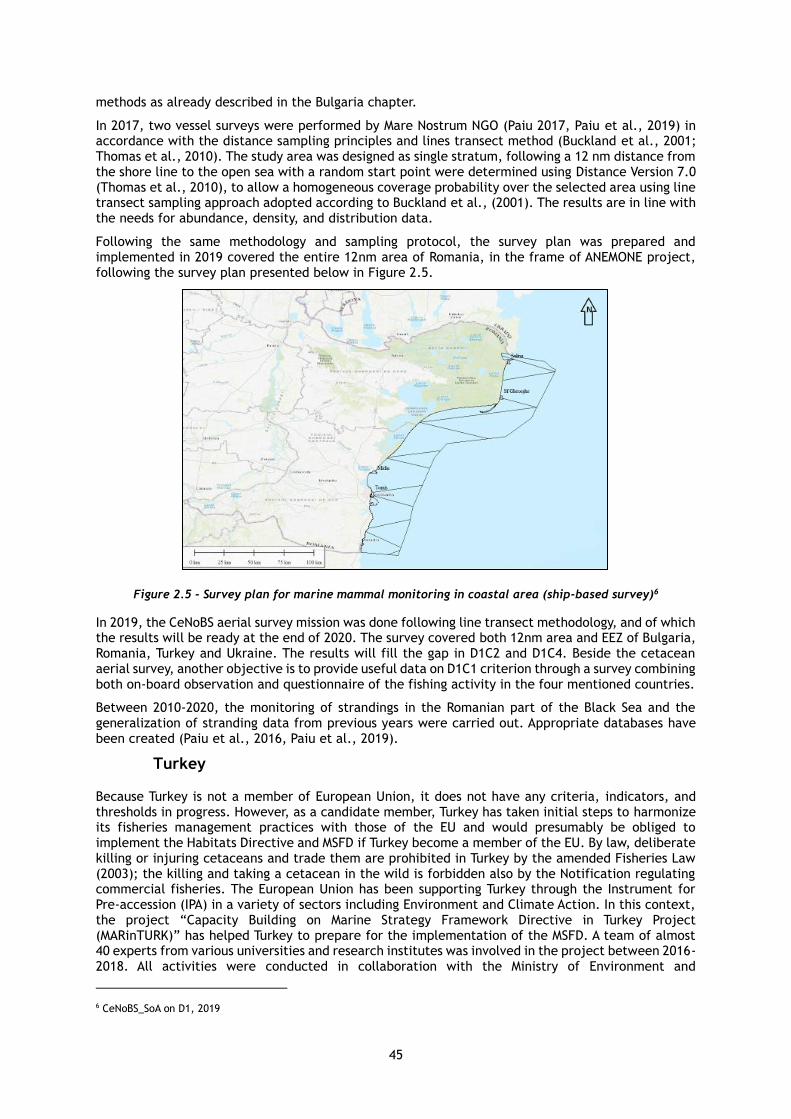
45

methods as already described in the Bulgaria chapter.

In 2017, two vessel surveys were performed by Mare Nostrum NGO (Paiu 2017, Paiu et al., 2019) in accordance with the distance sampling principles and lines transect method (Buckland et al., 2001; Thomas et al., 2010). The study area was designed as single stratum, following a 12 nm distance from the shore line to the open sea with a random start point were determined using Distance Version 7.0 (Thomas et al., 2010), to allow a homogeneous coverage probability over the selected area using line transect sampling approach adopted according to Buckland et al., (2001). The results are in line with the needs for abundance, density, and distribution data.

Following the same methodology and sampling protocol, the survey plan was prepared and implemented in 2019 covered the entire 12nm area of Romania, in the frame of ANEMONE project, following the survey plan presented below in Figure 2.5.

Figure 2.5 - Survey plan for marine mammal monitoring in coastal area (ship-based survey)6

In 2019, the CeNoBS aerial survey mission was done following line transect methodology, and of which the results will be ready at the end of 2020. The survey covered both 12nm area and EEZ of Bulgaria, Romania, Turkey and Ukraine. The results will fill the gap in D1C2 and D1C4. Beside the cetacean aerial survey, another objective is to provide useful data on D1C1 criterion through a survey combining both on-board observation and questionnaire of the fishing activity in the four mentioned countries.

Between 2010-2020, the monitoring of strandings in the Romanian part of the Black Sea and the generalization of stranding data from previous years were carried out. Appropriate databases have been created (Paiu et al., 2016, Paiu et al., 2019).

Turkey

Because Turkey is not a member of European Union, it does not have any criteria, indicators, and thresholds in progress. However, as a candidate member, Turkey has taken initial steps to harmonize its fisheries management practices with those of the EU and would presumably be obliged to implement the Habitats Directive and MSFD if Turkey become a member of the EU. By law, deliberate killing or injuring cetaceans and trade them are prohibited in Turkey by the amended Fisheries Law (2003); the killing and taking a cetacean in the wild is forbidden also by the Notification regulating commercial fisheries. The European Union has been supporting Turkey through the Instrument for Pre-accession (IPA) in a variety of sectors including Environment and Climate Action. In this context, the project “Capacity Building on Marine Strategy Framework Directive in Turkey Project (MARinTURK)” has helped Turkey to prepare for the implementation of the MSFD. A team of almost 40 experts from various universities and research institutes was involved in the project between 2016-2018. All activities were conducted in collaboration with the Ministry of Environment and

6 CeNoBS_SoA on D1, 2019

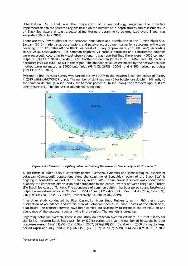
46

Urbanization. An output was the preparation of a methodology regarding the directive implementation in the selected regions based on the number of in-depth studies and assessments. In all Black Sea waters at least a seasonal monitoring programme to be organized every 3 year was suggested (MarinTurk 2018).

There are very few studies for the cetacean abundance and distribution in the Turkish Black Sea. Saydam (2015) made visual observations and passive acoustic monitoring for cetaceans in the area covering up to 120 miles off the Black Sea coast of Turkey (approximately 150.000 km²). According to her visual observations, 1015 common dolphins, 21 harbour porpoises and 4 bottlenose dolphins were recorded. According to visual observations, it was reported that there were 140000 common dolphins (99% CI: 109668 - 143485), 2200 bottlenose dolphin (99 % CI: 150 – 4882) and 5300 harbour porpoises (99% CI: 1068 – 6812) in the region. The abundance values estimated by the passive acoustic method were estimated as 35000 delphinids (99 % CI: 26786– 35046) and 41300 harbour porpoises (99% CI: 8323– 53085).

Systematic line transect survey was carried out by TUDAV in the western Black Sea coasts of Turkey in 2019 within ANEMONE Project. The number of sightings was 40 for bottlenose dolphin (147 ind), 40 for common dolphin (166 ind) and 2 for harbour porpoise (16 ind) along the transects app. 600 km long (Figure 2.6). The analysis of abundance is ongoing.

Figure 2.6 - Cetacean’s sightings observed during the Marmara Sea survey in 2019 summer7

A PhD thesis at Bülent Ecevit University named “Seasonal dynamics and some biological aspects of cetacean (Odontoceti) populations along the coastline of Zonguldak region of the Black Sea” is ongoing in Zonguldak. As part of this thesis, in April 2019, a line transect survey was conducted to quantify the cetaceans distribution and abundance in the coastal waters between Ereğli and Türkali (SW Black Sea coast of Turkey). The abundance of common dolphin, harbour porpoise and bottlenose dolphin were estimated as: 4076 (95% CI: 1564 - 10625; CV = 47%), 933 (95% CI: 434 - 2006; CV = 38%), 946 (95% CI: 268 - 3335; CV = 63%), respectively (Uludüz et al., 2019).

In another study conducted by Uğur Özsandıkçı from Sinop University as his PhD thesis titled "Estimation of Abundance and Distribution of Cetacean Species in Sinop Coasts of the Black Sea", boat-based line transect surveys have been carried out seasonally to estimate the distribution and abundance of the cetacean species living in the region. The analysis is on-going.

Regarding cetacean bycatch, there is one study on cetacean bycatch estimate in turbot fishery for the Turkish western Black Sea coast. Tonay (2016) estimated that the number of bycaught harbour porpoises were: 167(±153) (SE) (CV: 0.92) in 2007; 329(±220) (SE) (CV: 0.67) in 2008 during the legal period (April and July) and 2011(±742) (SE) (CV: 0.37) in 2007; 2249(±806) (SE) (CV: 0.35) in 2008

7 Unpublished data by TUDAV

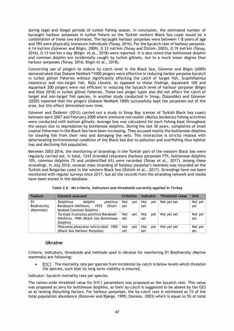
47

during legal and illegal periods of turbot fishing season. In conclusion, the estimated number of bycaught harbour porpoises in turbot fishery on the Turkish western Black Sea coast would be a combination of these two estimates. The bycaught harbour porpoises were between 1–8 years of age and 78% were physically immature individuals (Tonay, 2016). For the bycatch rate of harbour porpoise: 4.14 ind/km (Gönener and Bilgin, 2009), 0.33 ind/km (Tonay and Öztürk, 2003), 0.19 ind/km (Tonay, 2016), 0.13 ind/km x day (Bilgin et al., 2018) were reported. It is also noted that bottlenose dolphin and common dolphin are incidentally caught by turbot gillnets, but to a much lesser degree than harbour porpoises (Tonay, 2016; Bilgin et al., 2018).

Concerning use of pingers to reduce by catch level in the Black Sea, Gönener and Bilgin (2009) demonstrated that Dukane NetMark™1000 pingers were effective in reducing harbor porpoise bycatch in turbot gillnet fisheries without significantly affecting the catch of target fish, Scophthalmus maeoticus and non-target fish, Raja clavata. As opposed to these findings, Aquamark 100 and Aquamark 200 pingers were not efficient in reducing the bycatch level of harbour porpoise (Bilgin and Köse 2018) in turbot gillnet fisheries. These two pinger types also did not affect the catch of target and non-target fish species. In another study conducted in Sinop, Özsandikçi and Gönener (2020) reported that the pingers (Dukane NetMark 1000) successfully kept the porpoises out of the area, but this effect diminished over time.

Gönener and Özdemir (2012) carried out a study in Sinop Bay (center of Turkish Black Sea coast) between April 2007 and February 2008 where intensive red mullet (Mullus barbatus) fishing activities were conducted with bottom gillnets. Average loss was calculated for each fishing boat throughout the season due to depredation by bottlenose dolphins. During the last 30 years, complaints of small coastal fishermen in the Black Sea have been increasing. They accused mainly the bottlenose dolphins for stealing fish from their nets and damaging the nets. This interaction is strictly related with deteriorating environmental condition of the Black Sea due to pollution and overfishing thus habitat loss and declining fish population.

Between 2003-2016, the monitoring of strandings in the Turkish part of the western Black Sea were regularly carried out. In total, 1243 stranded cetaceans (harbour porpoises 77%, bottlenose dolphins 10%, common dolphins 7% and unidentified 6%) were recorded (Tonay et al., 2017). Among these strandings, in July 2016, unusual mass stranding of harbour porpoise’s neonates was recorded on the Turkish and Bulgarian coast in the western Black Sea (Öztürk et al., 2017). Strandings have not been monitored with regular surveys since 2017, but all the records from the stranding network and media have been stored in the database.

Table 2.6 - No criteria, indicators and thresholds currently applied in Turkey

Feature Element assessed Criterion Indicator Threshold value Unit


Delphinus delphis ponticus Barabasch-Nikiforov, 1935 (Short-beaked Common Dolphin)

Not yet set

Not yet set

Not yet set Not yet set

Tursiops truncatus ponticus Barabash-Nikiforov, 1940 (Black Sea Bottlenose Dolphin)

Not yet set

Not yet set


Phocoena phocoena relicta Abel, 1905 (Black Sea Harbour Porpoise)

Not yet set

Not yet set


Ukraine

Criteria, indicators, thresholds and methods used in Ukraine for monitoring D1 Biodiversity (Marine mammals) are following:

• D1C1 – The mortality rate per species from incidental by-catch is below levels which threaten the species, such that its long-term viability is ensured.

Indicator: bycatch mortality rate per species.

The nation-wide threshold value for D1C1 parameters was proposed as the bycatch rate. This value was proposed as zero for bottlenose dolphins, as their by-catch is suggested to be absent by the GES as at lacking disturbing factors. For harbour porpoises, the by-catch rate is estimated as 1% of the total population abundance (Donovan and Bjørge, 1995; Stenson, 2003) which is equal to 5% of total

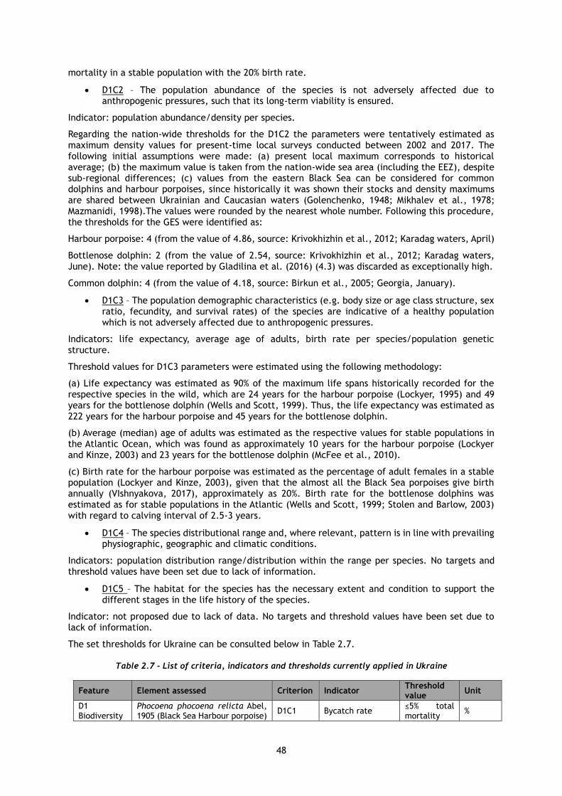
48

mortality in a stable population with the 20% birth rate.

• D1C2 – The population abundance of the species is not adversely affected due to anthropogenic pressures, such that its long-term viability is ensured.

Indicator: population abundance/density per species.

Regarding the nation-wide thresholds for the D1C2 the parameters were tentatively estimated as maximum density values for present-time local surveys conducted between 2002 and 2017. The following initial assumptions were made: (a) present local maximum corresponds to historical average; (b) the maximum value is taken from the nation-wide sea area (including the EEZ), despite sub-regional differences; (c) values from the eastern Black Sea can be considered for common dolphins and harbour porpoises, since historically it was shown their stocks and density maximums are shared between Ukrainian and Caucasian waters (Golenchenko, 1948; Mikhalev et al., 1978; Mazmanidi, 1998).The values were rounded by the nearest whole number. Following this procedure, the thresholds for the GES were identified as:

Harbour porpoise: 4 (from the value of 4.86, source: Krivokhizhin et al., 2012; Karadag waters, April)

Bottlenose dolphin: 2 (from the value of 2.54, source: Krivokhizhin et al., 2012; Karadag waters, June). Note: the value reported by Gladilina et al. (2016) (4.3) was discarded as exceptionally high.

Common dolphin: 4 (from the value of 4.18, source: Birkun et al., 2005; Georgia, January).

• D1C3 – The population demographic characteristics (e.g. body size or age class structure, sex ratio, fecundity, and survival rates) of the species are indicative of a healthy population which is not adversely affected due to anthropogenic pressures.

Indicators: life expectancy, average age of adults, birth rate per species/population genetic structure.

Threshold values for D1C3 parameters were estimated using the following methodology:

(a) Life expectancy was estimated as 90% of the maximum life spans historically recorded for the respective species in the wild, which are 24 years for the harbour porpoise (Lockyer, 1995) and 49 years for the bottlenose dolphin (Wells and Scott, 1999). Thus, the life expectancy was estimated as 222 years for the harbour porpoise and 45 years for the bottlenose dolphin.

(b) Average (median) age of adults was estimated as the respective values for stable populations in the Atlantic Ocean, which was found as approximately 10 years for the harbour porpoise (Lockyer and Kinze, 2003) and 23 years for the bottlenose dolphin (McFee et al., 2010).

(c) Birth rate for the harbour porpoise was estimated as the percentage of adult females in a stable population (Lockyer and Kinze, 2003), given that the almost all the Black Sea porpoises give birth annually (VIshnyakova, 2017), approximately as 20%. Birth rate for the bottlenose dolphins was estimated as for stable populations in the Atlantic (Wells and Scott, 1999; Stolen and Barlow, 2003) with regard to calving interval of 2.5-3 years.

• D1C4 – The species distributional range and, where relevant, pattern is in line with prevailing physiographic, geographic and climatic conditions.

Indicators: population distribution range/distribution within the range per species. No targets and threshold values have been set due to lack of information.

• D1C5 – The habitat for the species has the necessary extent and condition to support the different stages in the life history of the species.

Indicator: not proposed due to lack of data. No targets and threshold values have been set due to lack of information.

The set thresholds for Ukraine can be consulted below in Table 2.7.

Table 2.7 - List of criteria, indicators and thresholds currently applied in Ukraine

Feature Element assessed Criterion Indicator Threshold value

Unit

D1 Biodiversity


D1C1 Bycatch rate ≤5% total mortality

%

49

Feature Element assessed Criterion Indicator Threshold value

Unit

(Mammals) D1C2 Density 4 ind/km2

D1C3 Life expectancy 22 years

D1C3 Av. age of adults 10 years

D1C3 Birth rate ≥20% total abundance

%


D1C1 Bycatch rate 0 %

D1C2 Density 2 ind/km2

D1C3 Life expectancy 45 years

D1C3 Av. age of adults 23 years

D1C3 Birth rate ≥8% total abundance

%

Delphinus delphis ponticus Barabasch-Nikiforov, 1935 (Short-beaked Common dolphin)

D1C2 Density 4 ind/km2

Concerning the efforts to overcome the data deficiency of the cetaceans in Ukrainian waters several projects and actions were performed in the past years. These could be used as monitoring and assessment guidance.

In 2012, ship-based linear transect surveys (LTS) (Figure 2.7) were carried out in coastal waters near Crimea shore (north-eastern part of the Black Sea) (Gladilina and Gol’din, 2016). Linear transect surveys (LTS), both, ship-based and aerial, were designed according to standard principles of distance sampling (Buckland, 2004; Buckland et al., 2001). Density and abundance were estimated by analytical tools based on detection probability functions for distance sampling (Buckland et al., 2001), using Distance software (Thomas et al., 2009, 2010).

Figure 2.7 - LTS in Ukrainian territorial waters within the EMBLAS Plus Project, 2019

In 2012-2013, cetacean photo-identification studies were conducted in Crimea region (north-eastern part of the Black Sea) (Gladilina, 2018). During photoID studies, each dolphin was photographed from

50

both sides, captured dorsal fins were classified and catalogued (Würsig & Jefferson, 1990, Wilson et al., 1999; Urian et al., 2015). The abundance was calculated as a mark-recapture estimate using the Chapman estimator (Chapman, 1951; Caughley, 1977; Wilson et al., 1999; Hammond, 2010) based on repetitive photo identifications, between consecutive years of study.

In 2013, in the frame of EU Project Adverse Fisheries Impacts on Cetacean Populations in the Black Sea (Birkun et al., 2014), described previously covered the Ukrainian waters.

In 2015-2017, PhD project “Harbour porpoise (Phocoena phocoena) in the Azov Sea and the northeastern Black Sea: population morphology and demography” (Vishnyakova, 2017) was completed. Part of this study is about analysis of by-catch rate and was based on the data from the samples of cetaceans found dead on the shore. Assessment was conducted using the Bayesian inference and Siler model with bycatch as mortality risk (Moore & Read, 2008).

In 2015-2018, another PhD project was completed: “Bottlenose dolphin (Tursiops truncatus) in the waters of the northern Black Sea: biology and population structure” (Gladilina, 2018). Parts of these PhD studies were based on strandings which were analysed for population demographic characteristics using morphological, biological data and modelling. The age was identified as the number of growth layer groups (GLGs) in the dentin on the preparations of thin longitudinal sections of teeth which have been stained with Mayer haematoxylin and enclosed in glycerine (Klevezal, 1988; Bjørge et al., 1995). Demographic parameters were estimated using the Bayesian inference and Siler model (Moore & Read, 2008).

In 2016, observations within the offshore waters of Ukrainian EEZ were carried out onboard the research vessel Mare Nigrum and ferries in the frame of EMBLAS Project (Savenko et al., 2017).

In 2016, within EMBLAS Project (Savenko et. al, 2017) 2016-2018, ACCOBAMS Project, identification and initial assessment of cetacean groupings in coastal waters of the north-western Black Sea, Ukrainian sector was performed (Gladilina, et al., 2017a., Gol’din et al., 2017, Gladilina et al., 2018).

In 2016-2019, the monitoring of strandings in the north-western part of the Black Sea and the analysis of strandings data from previous years were carried out. Appropriate databases have been created (Vishnyakova et al., 2017). By-catch, as a cause of death, was diagnosed from the presence of specific evidences: nets and net marks on the body surface and anterior margins of flippers and fins, amputated tail, flukes or flippers, longitudinal cuts on the belly, and evidences for acute asphyxia (Kuiken, 1996).

In 2018-2019, microsatellite genotyping and mtDNA genome sequencing were carried out for harbour porpoises from the Black Sea and the Sea of Azov (Chehida et al., 2020).

In 2019, data collection activities were performed in the frame of CeNoBS project (presented in previous chapters) and EMBLAS-Plus Project (Environmental Monitoring in the Black Sea).


It is to be assumed that there is a major lack of knowledge or gap in available data on both national and regional level in the four of the six Black Sea riparian countries under study. This affects both national and regional measures for assuring good environmental status for the marine mammal representatives in Black Sea. Although in previous chapters punctual progress was presented there is a discrepancy when it comes to establish the indicators and thresholds as can be seen in the table below (Table 2.8). Extracted from the mentioned research actions performed at the regional level, there is a common understanding on the indicators, values (units) to be used in the monitoring programs of the Black Sea countries. This is a solid base in development of the future thresholds values both in regional and EU levels.

Table 2.8 - Status of the established indicators and thresholds in the Black Sea area, both in EU countries (EU level) and non-EU countries (Regional level)

Feature Element assessed

Criterion Indicator Unit BG RO TR UA


Delphinus delphis ponticus

D1C1 By-catch rate % Not set yet

proposed <1.7

Not set yet

Not set yet

D1C2 Abundance Count 5019 Not set Not set Not set

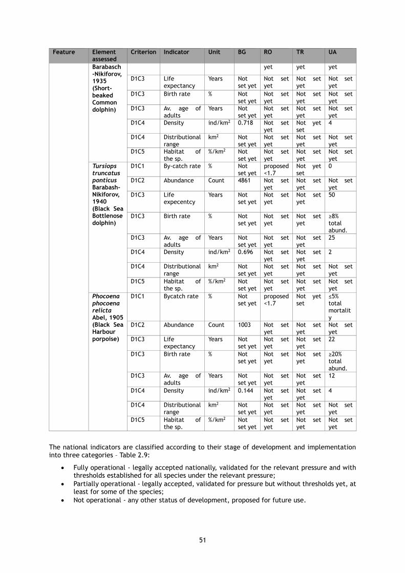
51

Feature Element assessed

Criterion Indicator Unit BG RO TR UA

Barabasch-Nikiforov, 1935 (Short-beaked Common dolphin)

yet yet yet

D1C3 Life expectancy

Years Not set yet

Not set yet

Not set yet

Not set yet

D1C3 Birth rate % Not set yet

Not set yet

Not set yet

Not set yet

D1C3 Av. age of adults

Years Not set yet

Not set yet

Not set yet

Not set yet

D1C4 Density ind/km2 0.718 Not set yet

Not yet set

4


km2 Not set yet

Not set yet

Not set yet

Not set yet

D1C5 Habitat of the sp.

%/km2 Not set yet

Not set yet

Not set yet

Not set yet


D1C1 By-catch rate % Not set yet

proposed <1.7

Not yet set

0

D1C2 Abundance Count 4861 Not set yet

Not set yet

Not set yet

D1C3 Life expecentcy

Years Not set yet

Not set yet

Not set yet

50


Not set yet

Not set yet

≥8% total abund.


Years Not set yet

Not set yet

Not set yet

25


Not set yet

2


km2 Not set yet

Not set yet

Not set yet

Not set yet


%/km2 Not set yet

Not set yet

Not set yet

Not set yet


D1C1 Bycatch rate % Not set yet

proposed <1.7

Not yet set

≤5% total mortality

D1C2 Abundance Count 1003 Not set yet

Not set yet

Not set yet

D1C3 Life expectancy

Years Not set yet

Not set yet

Not set yet

22


Not set yet

Not set yet

≥20% total abund.


Years Not set yet

Not set yet

Not set yet

12


Not set yet

4


km2 Not set yet

Not set yet

Not set yet

Not set yet


%/km2 Not set yet

Not set yet

Not set yet

Not set yet

The national indicators are classified according to their stage of development and implementation into three categories – Table 2.9:

• Fully operational - legally accepted nationally, validated for the relevant pressure and with thresholds established for all species under the relevant pressure;

• Partially operational - legally accepted, validated for pressure but without thresholds yet, at least for some of the species;


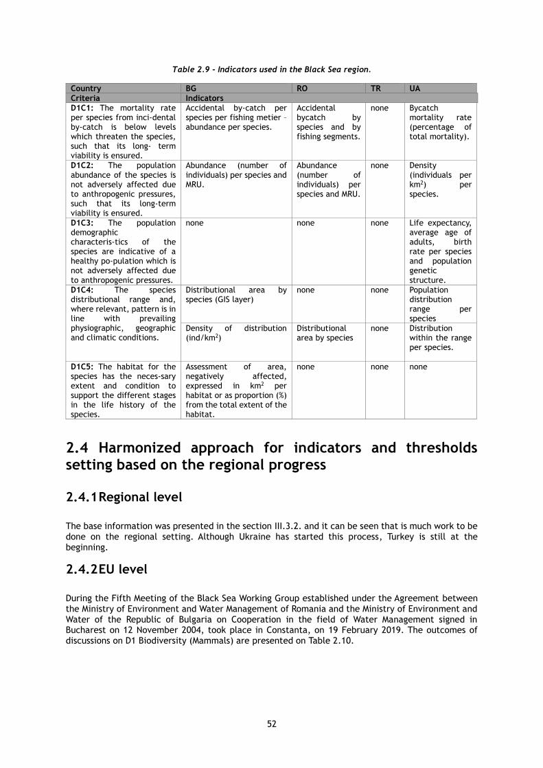
52

Table 2.9 - Indicators used in the Black Sea region.

Country BG RO TR UA

Criteria Indicators

D1C1: The mortality rate per species from incidental by-catch is below levels which threaten the species, such that its long- term viability is ensured.

Accidental by-catch per species per fishing metier – abundance per species.

Accidental bycatch by species and by fishing segments.

none Bycatch mortality rate (percentage of total mortality).

D1C2: The population abundance of the species is not adversely affected due to anthropogenic pressures, such that its long-term viability is ensured.

Abundance (number of individuals) per species and MRU.

Abundance (number of individuals) per species and MRU.

none Density (individuals per km2) per species.

D1C3: The population demographic characteristics of the species are indicative of a healthy population which is not adversely affected due to anthropogenic pressures.

none none none Life expectancy, average age of adults, birth rate per species and population genetic structure.

D1C4: The species distributional range and, where relevant, pattern is in line with prevailing physiographic, geographic and climatic conditions.

Distributional area by species (GIS layer)

none none Population distribution range per species

Density of distribution (ind/km2)

Distributional area by species

none Distribution within the range per species.

D1C5: The habitat for the species has the necessary extent and condition to support the different stages in the life history of the species.

Assessment of area, negatively affected, expressed in km2 per habitat or as proportion (%) from the total extent of the habitat.

none none none



The base information was presented in the section III.3.2. and it can be seen that is much work to be done on the regional setting. Although Ukraine has started this process, Turkey is still at the beginning.

2.4.2 EU level

During the Fifth Meeting of the Black Sea Working Group established under the Agreement between the Ministry of Environment and Water Management of Romania and the Ministry of Environment and Water of the Republic of Bulgaria on Cooperation in the field of Water Management signed in Bucharest on 12 November 2004, took place in Constanta, on 19 February 2019. The outcomes of discussions on D1 Biodiversity (Mammals) are presented on Table 2.10.

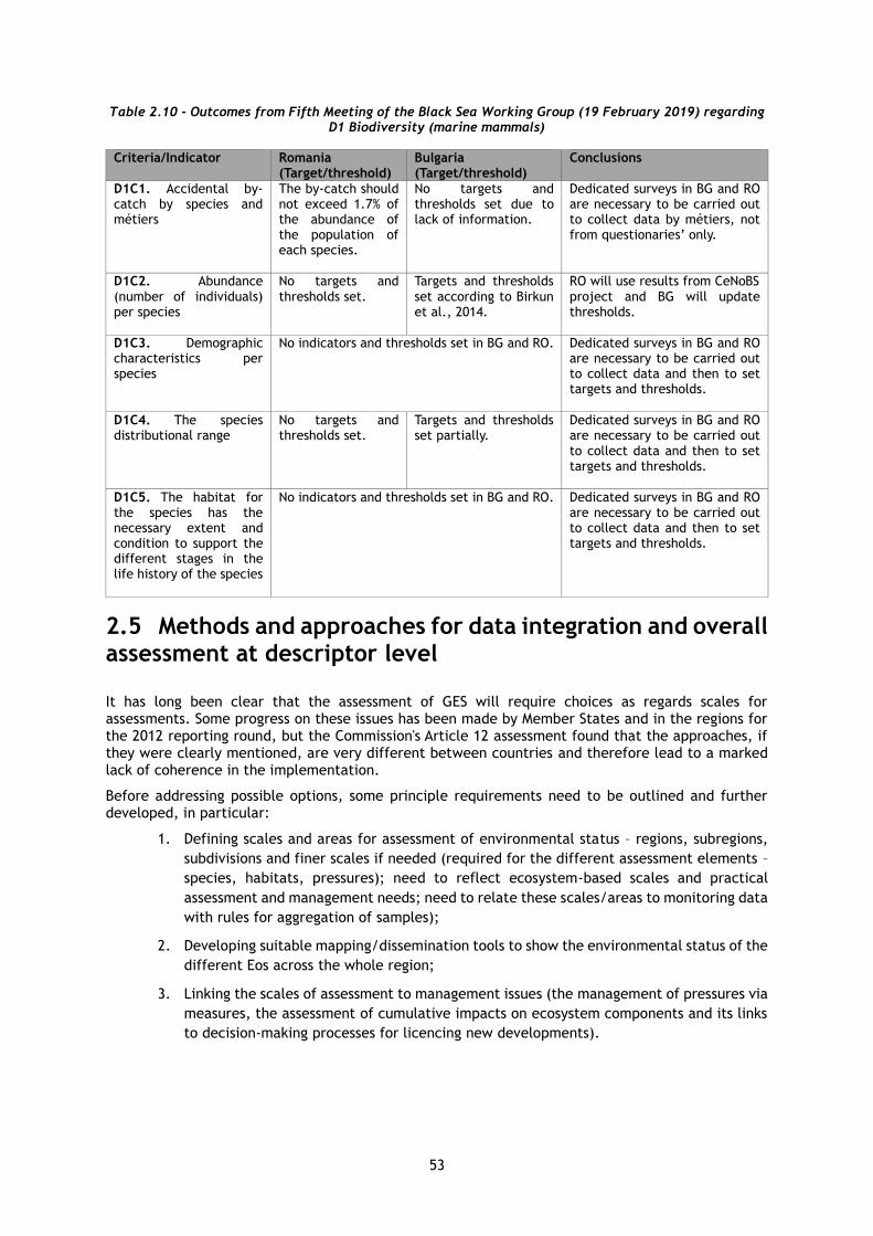
53

Table 2.10 - Outcomes from Fifth Meeting of the Black Sea Working Group (19 February 2019) regarding D1 Biodiversity (marine mammals)

Criteria/Indicator Romania (Target/threshold)

Bulgaria (Target/threshold)

Conclusions

D1C1. Accidental by-catch by species and métiers

The by-catch should not exceed 1.7% of the abundance of the population of each species.

No targets and thresholds set due to lack of information.

Dedicated surveys in BG and RO are necessary to be carried out to collect data by métiers, not from questionaries’ only.

D1C2. Abundance (number of individuals) per species

No targets and thresholds set.

Targets and thresholds set according to Birkun et al., 2014.

RO will use results from CeNoBS project and BG will update thresholds.

D1C3. Demographic characteristics per species

No indicators and thresholds set in BG and RO. Dedicated surveys in BG and RO are necessary to be carried out to collect data and then to set targets and thresholds.

D1C4. The species distributional range

No targets and thresholds set.

Targets and thresholds set partially.

Dedicated surveys in BG and RO are necessary to be carried out to collect data and then to set targets and thresholds.

D1C5. The habitat for the species has the necessary extent and condition to support the different stages in the life history of the species

No indicators and thresholds set in BG and RO. Dedicated surveys in BG and RO are necessary to be carried out to collect data and then to set targets and thresholds.


It has long been clear that the assessment of GES will require choices as regards scales for assessments. Some progress on these issues has been made by Member States and in the regions for the 2012 reporting round, but the Commission's Article 12 assessment found that the approaches, if they were clearly mentioned, are very different between countries and therefore lead to a marked lack of coherence in the implementation.

Before addressing possible options, some principle requirements need to be outlined and further developed, in particular:

1. Defining scales and areas for assessment of environmental status – regions, subregions,

subdivisions and finer scales if needed (required for the different assessment elements –

species, habitats, pressures); need to reflect ecosystem-based scales and practical

assessment and management needs; need to relate these scales/areas to monitoring data

with rules for aggregation of samples);

2. Developing suitable mapping/dissemination tools to show the environmental status of the

different Eos across the whole region;

3. Linking the scales of assessment to management issues (the management of pressures via

measures, the assessment of cumulative impacts on ecosystem components and its links

to decision-making processes for licencing new developments).

54

2.5.1 Methods used in marine mammal assessment

With the purpose to underline the methods used in scientific data collection to support the monitoring programmes for Descriptor 1 – Marine mammals we underline once more the methods already used in the Black Sea region and presented in the present document within the mentioned projects. There are numerous other resources where the methods are presented, and few of them are in fact EC released documents.

With no restriction to the priority to be use, here there are:

• line transect methods (land, vessel or airplane based);

• photo-identification (photoID) and abundance estimation from mark-recapture data;

• observations from land and ship-based platforms of opportunity;

• research of stranded carcasses to collect the data for size, sex and age estimation for life history studies, assessment of individual growth and body condition;

• assessment of demographic parameters: longevity, fecundity, mortality;

• analysis of genetic markers;

• analysis of bycatch rate;

• telemetry;

• acoustic methods, etc.

2.5.2 Integration and aggregation

In accordance with the “Guidance for Assessments Under Article 8 of the Marine Strategy Framework Directive, Integration of assessment results”, ABPmer Report No R.2733, produced for the European Commission, DG Environment, in February 2017 by Walmsley and collegues there are proposed five levels of integration for marine mammals related criteria and indicators. These are represented in the Figure 2.8.

Figure 2.8 - Levels and methods of integration for mammals under Descriptor 1

55

Note that integration at level 5 is not required by the revised Commission Decision, and is thus optional (Walmsley, 2017). The integration methods of Figure 2.8 are:

Level 1: Measurements of individual parameters are combined into a single indicator, such as ‘abundance of grey seals at breeding and haul-out sites, respectively’. This level of integration is not addressed in these guidelines.

Level 2: Where there is more than one indicator for a species for a particular criterion (e.g. habitat extent and habitat quality), the indicators are combined to form a judgement of the status for each criterion. The integration method is as applied under the Habitats Directive.

Level 3: The relevant criteria for each species are integrated to form a judgement on the status for each species (different species may be represented by different numbers of criteria). The integration method is that used under the Habitats Directive (OOAO, and there must be information on at least three parameters (criteria) to provide a judgement of Favourable Conservation Status for a species), such that the species’ status is consistent with that under the Habitats Directive. D1C1 contributes to the assessment of D1C2 for the corresponding species.

Level 4: The results for each species are brought together to the species group. The integration method shall be agreed at Union level, taking into account regional or subregional specificities.

Level 5: The revised Commission Decision only requires reporting of the status of the species group (not ecosystem component), but integration of species groups express the overall status of the mammals ecosystem component may be helpful for communication of assessment results and is included here for that purpose. The applicability of the OOAO approach at this level is dependent on the integration method agreed upon for level 4.

2.5.3 Data integration at national level

Bulgaria

The approaches for integration of the individual indicators, criteria and final evaluation of D1 Biodiversity (marine mammals) in Bulgaria are, as follows:



• The final assessment for the Descriptor 1 Biodiversity Mammals regarding the group of marine mammals is formed by the percentage of species in “Good“ status. The threshold value is 100%.

Romania

The approaches for integration of the individual indicators, criteria and final evaluation of D1 Biodiversity (marine mammals) in Romania are, as follows:



• The final assessment for the Descriptor 1 Biodiversity Mammals regarding the group of marine mammals is formed by the percentage of species in “Good“ status. The threshold value is 100%.

• Sharing data using the open-source platforms, catalogues and data bases (OBIS, OBIS-SEAMAP, GBIF, MEDACES, www.delfini.ro) to make the data accessible to public.

Turkey

There is not an approach for data integration of indicators, criteria at descriptor level, but data sharing is done using the open-source platforms, catalogues and data bases (OBIS, MEDACES) in order to be accessible to public.

56

Ukraine

To aggregate and integrate the marine mammal’s data collected in Ukraine the following approaches is used:

• To collect the data according to standard methodology (see item III.3. and 5.1) and protocols.

• In the frame of EMBLAS-Plus Project the Data Collection Template (DCT) for marine mammals was developed in order to unify data collection process and uploading data to common Black Sea data base (http://blackseadb.org/).

• Sharing data using the open-source platforms, catalogues and data bases (OBIS, OBIS-SEAMAP, GBIF, MEDACES) to make the data accessible to public.

EU level

A report produced by Palialexis et al. (2019) provides an up-to-date threshold setting methodologies applied in EU under MSFD and also in relation to Habitat Directive and Barcelona Convention, concluding that “at the level of the MSFD criteria the operational or developing indicators cover well the population abundance (D1C2) and the distributional range (D1C4) and less the other criteria. This was expected, because of the overlap of the two criteria with the Habitat Directive (European Union, 1992)”.

Regarding ICES advice (ICES, 2018), an ecosystem component cannot be considered to be at a good status if one or more of the assessed species groups are considered to be in poor status. It is recommended that a one out, all out (OOAO) integration is used from species group to ecosystem component. This integration will mean that all assessed species groups have to be in good status for the ecosystem component to be in a good status. Other methods could mask groups outside GES and furthermore, as the number of species groups is always 5 or less, OOAO is consistent with the proportional approach for low numbers. The recommended integration methods for the different levels of integration are shown in the Table 2.11 for HD species, D3 species, and other species (ICES, 2018).

Table 2.11 - Integration methods recommended (ICES, 2018)

Level Integration method (s)

From species group to ecosystem component

Option 1: OOAO Option 2: Proportion of all species in good status above agreed level (across species groups)

From species to species group

Proportional (determined by probability), if number of species in the group>5, OOAO if the number of species is 1 to 5.

From criteria to species (populations)

HD species: OOAO D3 species: As assessed in D3 Other species: One of the options 1- 5 bellow: If D1C1 and D1C2 are both in good status, then determine the average D1C2-D1C5, weighted so the weight of D1C2= weight of D1C3-C5 together. If this average is in good status, the species is in good status. If D1C1 and D1C2 are both in good status, then determine the average D1C3-D1C5. If this average is in good status, the species is in good status. If the weighted average of D1C1 to D1C5 is in good status, the species is in good status. The average is weighted to ensure that the weight of D1C2= weight of D1C1=weight of D1C3-C5 Conditional/OOAO Population model determines weights. This method can be used is a population model suggests appropriate weights of each of the criteria. For example, for long lived species, abundance may be little affected by one poor recruitment year and it may therefore be desirable to down-weight this. If the criterion D1C1 is not used, for options 1 and 2, D1C2 should be in good status and then the weighted average is considered. For option 3, the weight of D1C2=weight of D1C3-D1C5 combined.

57

2.6 Review of and recommendations from relevant regional projects

The analysis revealed (i) the saliency of cetacean conservation, and (ii) heterogeneity among countries in the implementation of the MSFD that may hinder transboundary collaboration. The classification of environmental status of marine mammals can be considered to have three possibilities:

1. In GES – for which monitoring is needed to check status does not deteriorate.

2. Not in GES – for which targets, and measures are needed which should lead to GES being

achieved and maintained, coupled with monitoring to assess progress in status and

against the targets and measures.

3. Unknown status (potentially not in GES) - it will not be possible in all cases to identify

a status which is clearly within or clearly outside GES. Where, based on the current best

available knowledge, interim boundaries or proxies can be determined, the

environmental state within this zone should be classed as 'not in GES'. Where interim

boundaries or proxies cannot be determined, classification needs to rely on qualitative

(normative) description and expert judgement. According to the precautionary

principle, uncertainty of classification must not be used for postponing action. Resulting

actions will depend on the shortcomings in the individual case. Actions include at least

those to address the shortcomings, e.g. through development of improved assessment

methods, more monitoring, complementary research, as well as proportionate measures

(e.g. “no regret” measures where improving status is considered necessary even though

what constitutes ‘good status’ remains to be fully defined).

Integrated monitoring for the purpose of the ecosystem approach should provide the data to allow assessment methods to classify a marine and coastal area as reaching or failing to reach GES, more specifically, providing data:

• For the calculation of the different applicable indicators and the assessment of the different ecological objectives covering the range of ecosystem components, pressures and their impacts.

• Fulfilling the monitoring requirements of different pieces of legislation applying in the region.

• Covering the monitoring needs of more than one Contracting Party.

• Collected in a comparable way between Contracting Parties so as to allow integration of the data.

As general recommendations from relevant regional projects we underline:

1. Given the presence of summer resident groups of bottlenose and common dolphins in

the shallowest coastal waters and small gulfs and bays in the Black Sea, it recommended

to estimate their abundance, using photo-identification as the most precise and

sustainable approach, added by passive acoustic monitoring and, when necessary, linear

transect surveys.

2. It is recommended to continue the studies of cetacean abundance and population

biology in the Black Sea waters, both in coastal waters and offshore waters.

3. It is important to enhance recoding of strandings, stranding response, rescue operations

in the wild, sampling and lab analysis and not last dissemination and integration of data.

4. The evaluation of the threshold setting approaches should be in-line with the concepts

and requirements described in Art. 4 of the Decision 2017/848/EU (European

Commission, 2017) in relation to the Good Environmental Status (GES) determination.

5. Common agreed methods for setting thresholds will secure the harmonization in the

GES determination for the MSFD species providing a base for regional scale

58

determination of GES.

6. Further development and recommendations of threshold values for these criteria will

be developed under the ongoing CeNoBS project. Mainly for D1C1, D1C2 and D1C4 with

additional input in respect to D10C2.

7. More effort and resources should be allocated to develop the marine mammal related

indicators and thresholds. The document provides a serious gap in road map

development of these Descriptor.

8. A technical group should be established to support the work of the competent

authorities and implementation bodies in developing the marine mammal descriptor at

regional level.

59

3 Guideline on Descriptors 1, 4. Theme Pelagic habitats

3.1 Introduction

Habitat aspects of biodiversity are considered in relation to two ecosystem components (pelagic and benthic habitats) and their broad habitat types. Different criteria are relevant for the two ecosystem components, and therefore the integration rules are also different. For pelagic habitats, there is one descriptor.

Descriptor 1 Biodiversity: Biological diversity is maintained. The quality and occurrence of habitats and the distribution and abundance of species are in line with prevailing physiographic, geographic and climatic conditions.

Biological diversity describes the variety of life and operates at various scales, from genes, species to entire ecosystems. Biodiversity therefore refers to all life-forms and their behaviours, the environments or habitats in which they live, and the complex system of relationships between organisms, such as food webs (Descriptor 4). Descriptor 1 addresses a species group within the ecosystem, whereas Descriptor 4 addresses structural and functional aspects of ecosystems as a whole. It addresses ecosystem aspects through food webs by dividing the structure and function of food webs into compartments which share common features, i.e. trophic guilds (ICES, 2014).

The Commission Decision (EU) 2017/848 sets out one criterion, which is primary, and therefore must be addressed: D1C6 Habitat condition (spatial extent of adverse effects).

The Chapter is focused to provide a guidance for establishment of a synergetic monitoring and assessment program for D1 – pelagic habitats at the Black Sea basin level in the frame of “Black Sea Monitoring and Assessment Guideline” (BSMAG). The section provides an overview of the latest proposed criteria, indicators and thresholds based on the progress up to date (based on ComDec 848/2017) made in Romania and Bulgaria taking into account the initiatives of Ukraine and Turkey in order to establish common guidelines.

Based on the analysis of the progress made so far, through programs/initiatives, within the four countries, we are presenting a guidance document for a future synergic effort in establishing the good environmental status of the Black Sea pelagic habitat based on the assessment of the established indicators.

The main aims of this Guideline are:

• To identify the coherence of framework within the different Black Sea countries.

• To develop a common framework for assessing the environmental status of pelagic habitats in the Black Sea.

• To propose methodological standards for the regional level assessment of pelagic habitats and threshold values on the state of the habitats.

• To identify where data and scientific knowledge are currently insufficient and reflect such uncertainties in proposals made.

3.2 Ecosystem elements

For each criterion selected the elements for assessment should be identified, i.e. the features and pressures under Article 8 and the corresponding characteristics of GES under Article 9(1) (e.g. substances, species, habitats).

According to the revised Commission Decision, the elements to be assessed for pelagic habitats are:

• Variable salinity

• Coastal

• Shelf

• Oceanic/beyond shelf.

60

Table 3.1 presented Black Sea pelagic broad habitat types.

Table 3.1 - List of representative Black Sea pelagic broad habitat types (+ present)

Habitat type BG RO TR UA

Variable salinity - + - +

Coastal + + + +

Shelf + + +

+

Oceanic/beyond shelf* + + +

Out of these four habitat types, the coastal, shelf and oceanic/beyond shelf (open sea) waters are considered to be relevant to Bulgaria and Turkey partially (shelf and oceanic are combined), while variable salinity, coastal, shelf and oceanic/beyond shelf – for Romania and Ukraine.

Variable salinity: Retained for situations where estuarine plumes extend beyond waters designated as transitional waters under Directive 2000/60/EC.

Coastal Waters: shallow-depth marine systems that experience significant land-based influences. These systems undergo diurnal fluctuations in temperature, salinity and turbidity, and are subject to wave disturbance. Depth is down to approximately 30 meters, depending on local factors determining the zone boundary (30m for Bulgaria, 30m for RO, TR-40m, UA-30m). Pelagic habitats in this type include the photic zone. It is not only limited to coastal water defined in Article 2(7) of Directive 2000/60/EC.

Shelf Waters: Marine systems away from coastal influence, down to the shelf break. They experience more stable temperature and salinity regimes than coastal systems, and their seabed is below wave disturbance. Depth is up to 200m (BG 30-200m, RO 30-200m, TR 40-200 m, UA 30-200m). In Turkey monitoring studies, habitat types have been determined as coastal and marine. Shelf and beyond shelf are combined in the category marine starting from 40m to 2000m.

Oceanic/beyond shelf – Depth is more than 200m (RO, BG) beyond shelf. It characterizes with stable temperature and salinity regimes.

Scientific criteria (ecological relevance) according to COM DEC 2017/848/EU:

• representative of the ecosystem component (species group or broad habitat type), and of ecosystem functioning (e.g. connectivity between habitats and populations, completeness and integrity of essential habitats), being relevant for assessment of state/impacts, such as having a key functional role within the component (e.g. high or specific biodiversity, productivity, trophic link, specific resource or service) or particular life history traits (age and size at breeding, longevity, migratory traits);



• the set of species or habitats selected shall cover, as far as possible, the full range of ecological functions of the ecosystem component and the predominant pressures to which the component is subject;

• if species of species groups are closely associated to a particular broad habitat type they may be included within that habitat type for monitoring and assessment purposes; in such cases, the species shall not be included in the assessment of the species group.

Additional practical criteria (which shall not override the scientific criteria):




61

3.3 Overview of criteria Indicators. Good Environmental Status assessment

Commission Decision 2017/848/EU sets one primary criterion for pelagic broad habitat types (Table 3.2) which should be assessed in terms of “the extent of habitat adversely affected in square kilometers (km2) as a proportion (%) of the total extent of the habitat type”. For the purpose of the criterion, the plankton composition, abundance and biomass measured in ationnal monitoring programs will be used to the extent possible to assess the structure and functions of pelagic broad habitat types.

Table 3.2 - Criterion for pelagic broad habitat types

Criteria in accordance to the Commission Decision EU/2017/848

Primary or Secondary

Methodological standards

D1C6 —The condition of the habitat type, including its biotic and abiotic structure and its functions (e.g., its typical species composition and their relative abundance, absence of particularly sensitive or fragile species or species providing a key function, size structure of species), is not adversely affected due to anthropogenic pressures.

Primary Use of criteria: The extent to which good environmental status has been achieved shall be expressed for each area assessed as: (a) an estimate of the proportion and extent of

each habitat type assessed that has achieved the threshold value set;

(b) a list of broad habitat types in the assessment area that were not assessed.

Specifications and standardized methods for monitoring and assessment relating to theme Pelagic habitats:

• “Coastal” shall be understood on the basis of physical, hydrological and ecological parameters

and is not limited to coastal water as defined in Article 2(7) of Directive 2000/60/EC.

• Assessments of the adverse effects from pressures, including under D2C3, D5C2, D5C3, D5C4,

D7C1, D8C2 and D8C4, shall be taken into account in the assessments of pelagic habitats under

Descriptor 1.

All reported assessments should be linked to a specific Marine Reporting Unit (MRU), thereby linking the reported information to a specified part of the marine waters. MRU is the area where the assessment applies and the extent to which GES has been achieved is reported for the descriptor (where relevant). The MRUs can be of varying sizes, according to the appropriate scale for the different reports (e.g., region, subdivision, MS waters, WFD coastal waters, etc.) as indicated in the new GES Decision by the scale of assessment to be used - via updates to the schema “4geo.xml” and provision of associated GIS shapefiles and using the template available in the MSFD reporting resources page.

Identified MRUs for the Black Sea countries are presented in the Table 3.3. Figure 3.1 shows Marine Reporting Units (MRUs) in pelagic broad habitat types in Bulgarian and Romanian Black Sea.

Table 3.3 - Number (N) and area (km2) of identified MRUs in the Black Sea

Habitat type BG RO TR* UA

N area N area N area N area

Variable salinity n/a n/a 1 1358.95 - -

3 13258

Coastal 5 2 700 1 1040.17 17 9732 22 2852

Shelf 2 9 928 1 20164.89 5 115113 3 21599

Open sea 1 22 423 1 7058.25 2 * The monitoring studies in Turkey are carried out in 2 classes only (coastal and marine) without discriminating between shelf and beyond shelf due to the fact that the slope is very steep on eastern, in contrast to the western BS coasts of TR, the range of 40-200 m is stuck in a very narrow area.

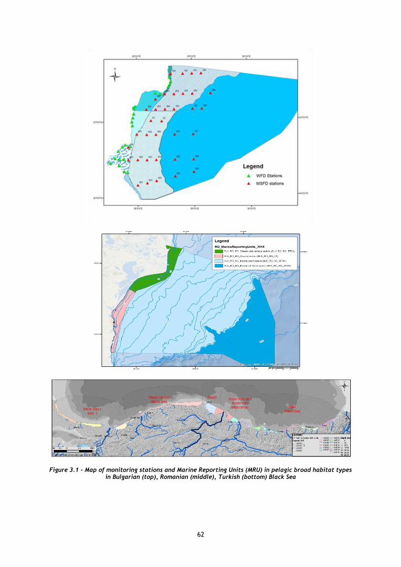
62

Figure 3.1 - Map of monitoring stations and Marine Reporting Units (MRU) in pelagic broad habitat types in Bulgarian (top), Romanian (middle), Turkish (bottom) Black Sea

63

Table 3.4 - Number (N) and area (km2) of identified MRUs in the Bulgarian, Romanian, Ukrainian and Turkish Black Sea

Broad habitat type (code)

MRU name Depth limits (m) Area MRU (km2)

Bulgaria

Coastal (BLK-BG-AA)

BLK-BG-AA-Siviriburun Kaliakra 0-30 162

BLK-BG-AA-Kaliakra Galata 0-30 828

BLK-BG-AA-Galata Emine 0-30 699

BLK-BG-AA-Emine Maslennos 0-30 856

BLK-BG-AA-Maslennos Rezovo 0-30 155

Shelf (BLK-BG-AA) BLK-BG-AA-Northern Shelf 30-200 3879

BLK-BG-AA-Southern Shelf 30-200 5521

Open sea (BLK-BG-AA) BLK-BG-AA-Open Sea >200 22423

Romania

Variable salinity BLK_RO_RG_TT03 0-30 1358.95

Coastal BLK_RO_RG_CT 0-30 1040.17

Shelf BLK_RO_RG_MT01 30-200 20164.89

Open sea BLK_RO_RG_MT02 >200 7058.25

Turkey

Coastal 17 water bodies 0-40 9732

Marine (Shelf and Oceanic/beyond shelf)

5 marine reporting area KARD1-Western Black Sea Region KARD2-West-Central Black Sea Region KARD3-Sinop Region KARD4-Yeşilırmak/Kızılırmak Rivers impact area KARD5-Eastern BlackSea Region

40-2000 115113

Ukraine*

Variable salinity Dnipro 4871

Dniester 2799

Danube 5588

Coastal 22 water bodies 0-30 N/A

Shelf Karkinitskiy 30-200 4239

Kalamitskiy 30-200 4237

Mixing zone 30-200 13123

Oceanic/beyond shelf N/A N/A * For Ukraine, the information included in respect of the MRU is incomplete and reflects only the sites included in ANEMONE project.

The assessment of pelagic habitats under Descriptor 1 should focus on the assessment of plankton communities (phytoplankton and zooplankton) in the water column. The assessment of the extent (volume) of pelagic habitats affected by anthropogenic pressures is practically challenging and not feasible for the assessment process. Therefore, it is recommended to assess pelagic habitats with the help of indicators describing community structure and productivity of the plankton community in the water column.

Assigned Indicators

Assessments typically start with the evaluation of a single element (e.g., species, habitat) for which there is a dataset for the assessment area in the assessment period defined in the national monitoring programs. These then go through several steps in an assessment process. The sequence of those steps is specific to each element and dependent on the scientific indicators used which may act at different levels of integration — some scientific indicators correspond directly to the revised Commission Decision criteria, whereas others are one of a number of scientific indicators that contribute to a criterion and therefore require integration to criterion level. The sequence of those steps may include integration across indicators, criteria and elements.

Relevant available regional indicators should be identified and allocated, to the criteria and assessment areas. Any remaining gaps should be identified. Use national assessments (taking into account existing assessments e.g. under EU legislation, such as WFD), where available, pending the development of regionally coordinated assessments.

64

Additional national indicators for elements that are specific to national waters, if any, can also be incorporated and allocated to the relevant criteria and assessment areas. These need to have a threshold value, where appropriate, and should follow the agreed structure for reporting indicators.

Biodiversity plankton community indicators evaluate the status of the Black Sea as reflected by pelagic plankton communities. The Commission Decision EU/2017/848 requires consistent and comparable determinations of good environmental status with the relevant existing standards and methods for monitoring and assessment laid down in Union legislation. Table 3.5 provides the list of the belonging characteristic (Black Sea pelagic habitat, including the specific biological communities – phytoplankton and zooplankton) that are assessed at the national level under the criteria of MSFD. About 9 phytoplankton and 8 zooplankton indicators were compiled, which were developed and used in the framework of different initiatives (e.g. EU policies, research projects) and in national and international contexts. More of them are not or partly operational, i.e. tested and validated, with associated target values or classification boundaries. Some indicators (plankton biomass and/or abundance) were agreed to be applied among Black Sea countries as quite relevant for the MSFD implementation integration process and support the process between MSFD and the regional BSIMAP.

Table 3.5 - List of the Black Sea pelagic habitat characteristic assessed at the national level under the criteria of MSFD

Indicator/Country BG RO TR* UA

Phytoplankton

Species composition + + +

Abundance (cells/L) + + +

Biomass (mg/m3) + + + +

Size structure +

% MEC +

BAC:DIN (in spring) +

Shannon index + +

Environmental characteristics of species (fresh, marine, etc.)

+ +

% of autotrophic and heterotrophic species +

Zooplankton

Species composition + + +

Abundance (ind/m3) + ind/m3 +

Mesozooplankton biomass (mg/m3) + + - +

Copepoda + (%) + (mg/m3) % & ind/m3 +

Noctiluca scintillans biomass (mg/m3) or (%) Indicator in D5C3 criteria

Indicator in D5C3 criteria

Only abundance ind/m3

+

*Within the scope of the national monitoring project of Turkey, phytoplankton data for 2014-2019 and zooplankton data for 2017-2019 are available. Experts concluded that the present data set is not adequate for threshold estimation. MSFD is not obligatory for Turkey.

3.4 Approach for thresholds setting

The BSC approved the Black Sea Integrated Monitoring and Assessment Programme (BSIMAP) in the end of 2016. BSIMAP was developed in the light of the MSFD, taking into account descriptors, GES and targets. The regional reporting indicators identified previously became part of BSIMAP. Its adoption is a positive step, as it contributes to the harmonization of the reporting format across countries and could provide the basis for comparing general environmental trends of the Black Sea marine environment. National assessments refer to or reuse regional assessments as they are, and complement them with additional elements, whilst seeking harmonization with neighboring countries.

Member States should establish threshold values through regional or subregional cooperation, for the condition of each habitat type, ensuring compatibility with values set under Descriptors 2, 5 and 8.

3.4.1 Phytoplankton

Phytoplankton is one of the basic biological elements in the Water Framework Directive (WFD) and is also considered in 4 descriptors of the Marine Strategy Framework Directive (MSFD): Biodiversity (D1),

65

Non-native species (D2), Food Web (D4) and Eutrophication (D5). Eutrophication is the main and the most widespread problem caused by human pressure. Quickly responding to changes in ecosystem conditions, microalgae are the first to reflect changes in the quality of the aquatic environment. The excessive input of nutrients leads to outbreaks of phytoplankton abundance and biomass up to the level of “bloom”, and changes of size and species structure of phytoplankton community.

A comparison of different methods of assessing the ecological status by phytoplankton indicators shows that the most adequate indicators are phytoplankton biomass and abundance, while assessment by phytoplankton species diversity needs further clarification.Development of criteria for assessing the ecological status by phytoplankton indicators is presented below.

Bulgaria

• Phytoplankton abundance N (cells/L)

• Phytoplankton biomass B (mg/m3)

The critical elements in the general concept for thresholds setting that were taken into consideration for the phytoplankton indicators are related mainly to the following requirement set in Commission Decision EU/2017/848 (paragraph 13): “threshold values should be set at appropriate geographic scales to reflect the different biotic and abiotic characteristics of the regions, subregions and subdivisions; should accommodate the dynamic nature of marine ecosystems and their elements, which can change in space and time through hydrological and climatic variation, should also reflect the fact that marine ecosystems may recover, if deteriorated, to a state that reflects prevailing physiographic, geographic, climatic and biological conditions, rather than return to a specific state of the past”.

Among the various phytoplankton indicators generally proposed so far at European scale, only phytoplankton biomass (mg/m3) and phytoplankton abundance (cells/L) are used due mainly to lack of data of other additional traits measurements (productivity, life forms, functional biodiversity, succession etc.). In order to comply to the above requirements BG experts have revised the approach used in the initial assessment and the threshold are set at seasonal bases for the identified MRUs in the coastal, shelf and open waters, for the upper homogeneous layer e.g. integrated data from the surface to the thermocline or the deep chlorophyll a maximum (if available) in order to assess homogenous habitats (HELCOM, 2012), the depth of which is different, depending on the seasonal variation, using data from periods with different level of anthropogenic pressure, including the very recent period to reflect the climatic footprint in the dynamic and composition of phytoplankton communities and the evolutionary responses.

For the revision of the thresholds a number of statistical methods were used that have been applied in other marine regions (USEPA, 2001) based on the sygnal detection theory (SDT) - ROC curves and combined methodology used by EPA (USEPA, 2001) – SDT, Regime Shift (Rodionov, 2005) and CUSUM (IBM SPSS Statistics) on data for the period 1961-2017 (Mavrodieva et al., 2017, Moncheva & Doncheva, 2017). Due to lack of enough data to arrive to statistically significant output, for some seasons and habitats there are no assigned thresholds values – Table 3.6.

For the WFD (1nm coastal) the following EQRs were accepted: 0.80 (high/good), 063 (good/moderate), 0.43 (moderate/bad) and 0.23 (bad/very bad) and <0.23 (very bad), agreed between RO and BG (Moncheva & Boicenco, 2011, Decision ЕС/2018/229) – Table 3.6. The threshold value good/not good for the shelf and open sea was directly estimated by the above described statistical approach - Table 3.7, Table 3.8.

Table 3.6 - Ecological quality scale for phytoplankton biomass (mg/m3) for Bulgarian Black Sea Coastal broad habitat

Biomass (mg/m3) High Good Moderate Bad Very bad

Winter <550 550-900 900-1600 1600-3000 >3000

Spring <700 700-1210 1210-2280 2280-4300 >4300

Summer <400 400-730 730-1450 1450-2900 >2900

Autumn <700 700-1150 1150-2100 2100-3800 >3800

EQR 1-0.80 0.80-0.63 0.63-0.43 0.43-0.23 0.23-0.0

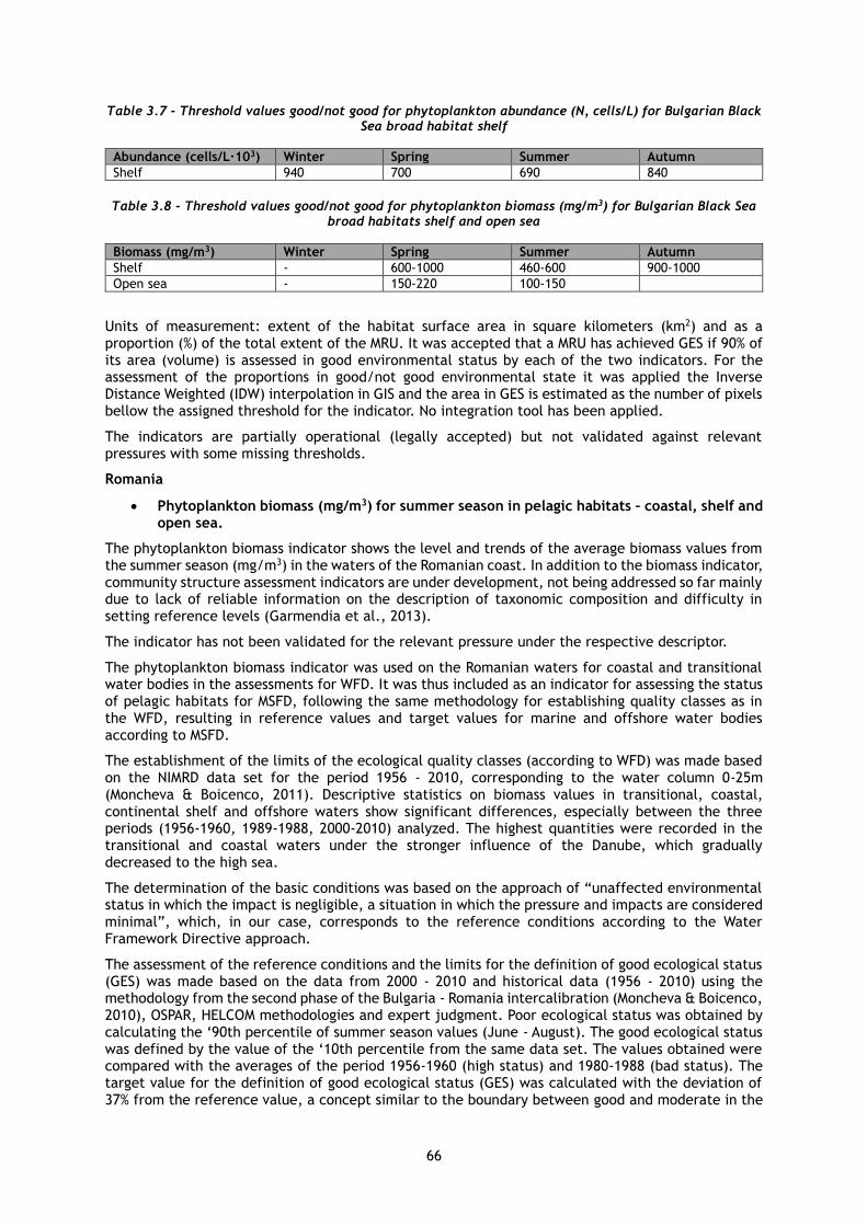
66

Table 3.7 - Threshold values good/not good for phytoplankton abundance (N, cells/L) for Bulgarian Black Sea broad habitat shelf

Abundance (cells/L·103) Winter Spring Summer Autumn

Shelf 940 700 690 840

Table 3.8 - Threshold values good/not good for phytoplankton biomass (mg/m3) for Bulgarian Black Sea broad habitats shelf and open sea

Biomass (mg/m3) Winter Spring Summer Autumn

Shelf - 600-1000 460-600 900-1000

Open sea - 150-220 100-150

Units of measurement: extent of the habitat surface area in square kilometers (km2) and as a proportion (%) of the total extent of the MRU. It was accepted that a MRU has achieved GES if 90% of its area (volume) is assessed in good environmental status by each of the two indicators. For the assessment of the proportions in good/not good environmental state it was applied the Inverse Distance Weighted (IDW) interpolation in GIS and the area in GES is estimated as the number of pixels bellow the assigned threshold for the indicator. No integration tool has been applied.

The indicators are partially operational (legally accepted) but not validated against relevant pressures with some missing thresholds.

Romania

• Phytoplankton biomass (mg/m3) for summer season in pelagic habitats – coastal, shelf and open sea.

The phytoplankton biomass indicator shows the level and trends of the average biomass values from the summer season (mg/m3) in the waters of the Romanian coast. In addition to the biomass indicator, community structure assessment indicators are under development, not being addressed so far mainly due to lack of reliable information on the description of taxonomic composition and difficulty in setting reference levels (Garmendia et al., 2013).

The indicator has not been validated for the relevant pressure under the respective descriptor.

The phytoplankton biomass indicator was used on the Romanian waters for coastal and transitional water bodies in the assessments for WFD. It was thus included as an indicator for assessing the status of pelagic habitats for MSFD, following the same methodology for establishing quality classes as in the WFD, resulting in reference values and target values for marine and offshore water bodies according to MSFD.

The establishment of the limits of the ecological quality classes (according to WFD) was made based on the NIMRD data set for the period 1956 - 2010, corresponding to the water column 0-25m (Moncheva & Boicenco, 2011). Descriptive statistics on biomass values in transitional, coastal, continental shelf and offshore waters show significant differences, especially between the three periods (1956-1960, 1989-1988, 2000-2010) analyzed. The highest quantities were recorded in the transitional and coastal waters under the stronger influence of the Danube, which gradually decreased to the high sea.

The determination of the basic conditions was based on the approach of “unaffected environmental status in which the impact is negligible, a situation in which the pressure and impacts are considered minimal”, which, in our case, corresponds to the reference conditions according to the Water Framework Directive approach.

The assessment of the reference conditions and the limits for the definition of good ecological status (GES) was made based on the data from 2000 - 2010 and historical data (1956 - 2010) using the methodology from the second phase of the Bulgaria - Romania intercalibration (Moncheva & Boicenco, 2010), OSPAR, HELCOM methodologies and expert judgment. Poor ecological status was obtained by calculating the ‘90th percentile of summer season values (June - August). The good ecological status was defined by the value of the ‘10th percentile from the same data set. The values obtained were compared with the averages of the period 1956-1960 (high status) and 1980-1988 (bad status). The target value for the definition of good ecological status (GES) was calculated with the deviation of 37% from the reference value, a concept similar to the boundary between good and moderate in the

67

Water Framework Directive. The assessment was made on four types of waters: waters with variable salinity, coastal, marine and offshore waters (Table 3.9).

Table 3.9 - Marine water classification system according to WFD and MSFD for the biomass parameter in the summer season

Variable salinity waters

Biomass (mg/m3) High Good Moderate Poor Bad

WFD 1000 -1500 1500 -3000 3000 - 4200 6500-8000 > 8000

GES NonGES

MSFD <3000 >3000

Coastal waters


WFD 400 - 700 701 - 950 951 - 2500 2501 – 5000 > 5000

GES NonGES

MSFD <950 >950

Shelf waters


WFD 300 - 500 501 - 800 801-1500 1501- 3000 >3000

GES NonGES

MSFD <800 >801

Open waters


WFD 75 – 150 151 - 250 251-500 501- 800 >800

GES NonGES

MSFD <250 >251

For the MSFD requirements, the good/moderate limit was chosen as the target value for defining the ecological status of each water body. It is considered that the very good ecological status (high) and the good status (good) represent GES, and the other classes, respectively moderate, poor and bad ecological status to characterize an environment that falls into non-GES (Table 3.9).

The 90th percentile of the biomass values of the summer season, from the last 6 years, is related to the target values, thus defining the ecological state (GES or non-GES) of each body of water.

The indicator is operational.

Ukraine

To calculate the RefCon of phytoplankton biomass for the identified MRUs, it was used an array of contemporary data, taking into account the information on phytoplankton biomass before the eutrophication period (50-60th) from literature sources (Ivanov, 1967, 1982). For most MRUs, results of own research, SeaBase UkrSCES database, and data of IBSS were used.

A linear model of transition from recent phytoplankton biomass values to historical values, according to the ratio of the average values of historical and last year phytoplankton biomass for NWBS was applied.

Comparing the long-term data set was noted that phytoplankton biomass in 50-60th ranged from 0.7 to 1g/m3 at the central parts of the sea. The average seasonal values of phytoplankton biomass in the last period are approximately equal, and sometimes significantly lower than historical ones. Therefore, RefCon values were adopted as 75% of the average seasonal values of AcStat, which were then specified, taking into account the usual for the region values of phytoplankton biomass, which are observed in the absence of "blooms". Target concentrations were calculated as:

Target = RefCon +0.5*RefCon

with the rounding of the corresponding values to tens and hundreds, depending on the order of the value. The results of observations and calculated RefCon and Target concentrations for phytoplankton biomass are shown in Table 3.10.

Based on the accepted values of RefCon and Target concentrations for phytoplankton biomass, scales were developed to assess the ecological status of the marine environment by phytoplankton indicators. The EQR limit between very good condition and RefCon is always set at 0.95 (HELCOM, 2010). Thus, this permissible deviation from RefCon (5%) is an estimate of uncertainty for all

68

indicators. The boundaries between classes are calculated by the following formulas:

EQR Ref/High - EQR Good/Moderate = 2*(EQR Good/Moderate - EQR Poor/Bad)

EQR Poor/Bad = 0.19

EQR High/Good = 0.5*EQR Ref/High + 0.5*EQR Good/Moderate = 0.81

EQR Moderate/Poor = 0.5 * EQR Good/Moderate + 0.5*EQR Poor/Bad = 0.43

Scales for assessing the ecological status of the marine environment for phytoplankton are presented in Table 3.10. It should be borne in mind that in the course of further research, these scales may undergo appropriate changes, clarifications and additions. Particular attention should be paid to refining the indicators for the central region due to the small number of observations in recent years.

Table 3.10 - Scales for assessing the state of the marine environment by phytoplankton biomass (mg/m3)

High Good Moderate Poor Bad

Dnipro-Buh

Winter <1000 1000-1250 1250-1850 1850-3700 >3700

Spring <1250 1250-1600 1600-2300 2300-4300 >4300

Summer <1100 1100-1400 1400-2000 2000-4000 >4000

Autumn <1000 1000-1250 1250-1850 1850-3700 >3700

Dniester

Winter <1000 1000-1250 1250-1850 1850-3700 >3700

Spring <1250 1250-1600 1600-2300 2300-4300 >4300

Summer <1100 1100-1400 1400-2000 2000-4000 >4000

Autumn <1000 1000-1250 1250-1850 1850-3700 >3700

Danube

Winter - - - - -

Spring <1500 1500-1900 1900-2800 2800-5300 >5300

Summer <1100 1100-1400 1400-2000 2000-4000 >4000

Autumn <750 750-950 950-1400 1400-2600 >2600

Mixed waters (Zernov Phyllophora field)

Winter <600 600-800 800-1200 1200-2200 >2200

Spring <550 550-750 750-1100 11000-2000 >2000

Summer <600 600-800 800-1200 1200-2200 >2200

Autumn <1000 1000-1250 1250-1850 1850-3700 >3700

Kalamit

Winter <300 300-400 400-600 600-1200 >1200

Spring <900 900-1100 1100-1600 1600-3000 >3000

Summer <900 900-1100 1100-1600 1600-3000 >3000

Autumn <1200 1200-1500 1500-2200 2200-4000 >4000

Central

Winter - - - - -

Spring <190 190-240 240-350-1600 350-650 >650

Summer <500 500-650 650-950 950-1700 >1700

Autumn <550 550-700 700-1000 1000-1900 >1900

Coastal

Winter <1100 1100-1400 1400-2000 2000-4000 >4000

Spring <1400 1400-1700 7400-2500 2500-4700 >4700

Summer <1100 1100-1400 1400-2000 2000-4000 >4000

Autumn <1000 1000-1250 1250-1850 1850-3700 >3700

3.4.2 Zooplankton

The metrices are complemented with an absolute share of ecological groups/species forming the plankton fauna as Copepoda, Cladocera, Meroplankton and Oikopleura dioica, Parasagitta setosa. Zooplankton is indirectly exposed to eutrophication (by altering the amount of food and the size of phytoplankton) and overfishing of commercially exploited fish (through changes in the pelagic food web), while the direct impact is formed by climate change (temperature and salinity regime), fish and jellyfish predation (HELCOM, 2012). Therefore, zooplankton lives between top-down and bottom-

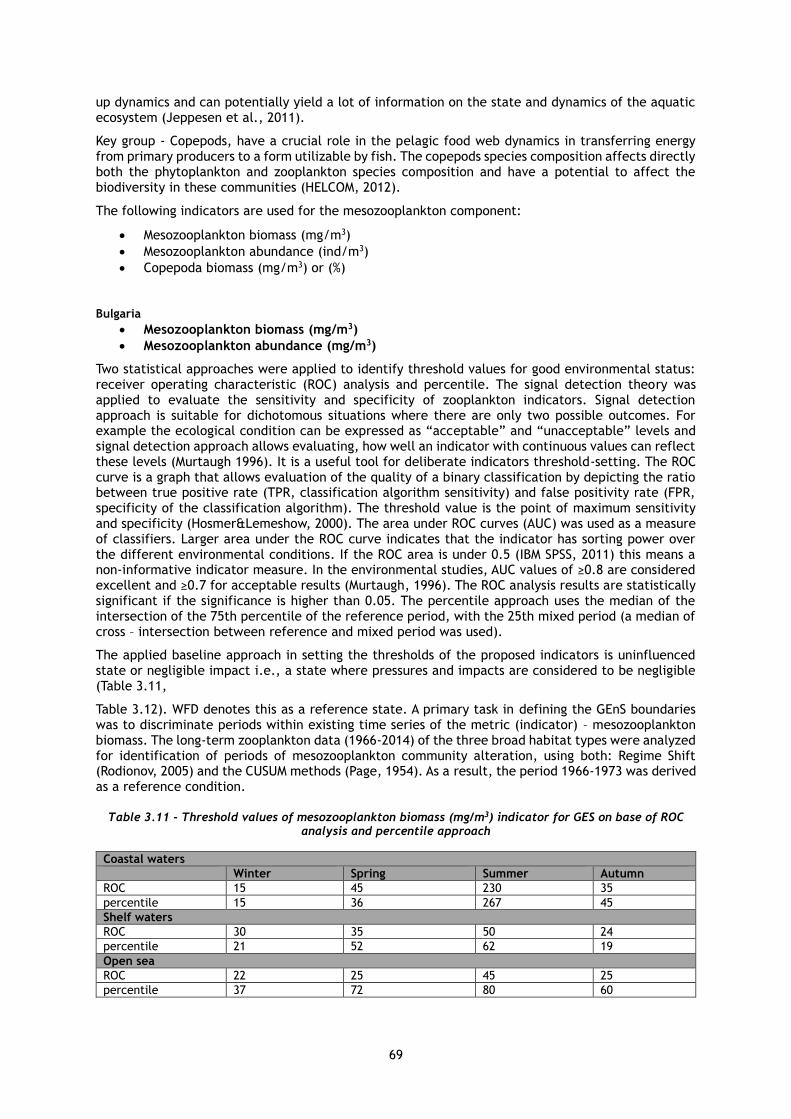
69

up dynamics and can potentially yield a lot of information on the state and dynamics of the aquatic ecosystem (Jeppesen et al., 2011).

Key group - Copepods, have a crucial role in the pelagic food web dynamics in transferring energy from primary producers to a form utilizable by fish. The copepods species composition affects directly both the phytoplankton and zooplankton species composition and have a potential to affect the biodiversity in these communities (HELCOM, 2012).

The following indicators are used for the mesozooplankton component:

• Mesozooplankton biomass (mg/m3)

• Mesozooplankton abundance (ind/m3)

• Copepoda biomass (mg/m3) or (%)

Bulgaria


• Mesozooplankton abundance (mg/m3)

Two statistical approaches were applied to identify threshold values for good environmental status: receiver operating characteristic (ROC) analysis and percentile. The signal detection theory was applied to evaluate the sensitivity and specificity of zooplankton indicators. Signal detection approach is suitable for dichotomous situations where there are only two possible outcomes. For example the ecological condition can be expressed as “acceptable” and “unacceptable” levels and signal detection approach allows evaluating, how well an indicator with continuous values can reflect these levels (Murtaugh 1996). It is a useful tool for deliberate indicators threshold-setting. The ROC curve is a graph that allows evaluation of the quality of a binary classification by depicting the ratio between true positive rate (TPR, classification algorithm sensitivity) and false positivity rate (FPR, specificity of the classification algorithm). The threshold value is the point of maximum sensitivity and specificity (Hosmer&Lemeshow, 2000). The area under ROC curves (AUC) was used as a measure of classifiers. Larger area under the ROC curve indicates that the indicator has sorting power over the different environmental conditions. If the ROC area is under 0.5 (IBM SPSS, 2011) this means a non-informative indicator measure. In the environmental studies, AUC values of ≥0.8 are considered excellent and ≥0.7 for acceptable results (Murtaugh, 1996). The ROC analysis results are statistically significant if the significance is higher than 0.05. The percentile approach uses the median of the intersection of the 75th percentile of the reference period, with the 25th mixed period (a median of cross – intersection between reference and mixed period was used).

The applied baseline approach in setting the thresholds of the proposed indicators is uninfluenced state or negligible impact i.e., a state where pressures and impacts are considered to be negligible (Table 3.11,

Table 3.12). WFD denotes this as a reference state. A primary task in defining the GEnS boundaries was to discriminate periods within existing time series of the metric (indicator) – mesozooplankton biomass. The long-term zooplankton data (1966-2014) of the three broad habitat types were analyzed for identification of periods of mesozooplankton community alteration, using both: Regime Shift (Rodionov, 2005) and the CUSUM methods (Page, 1954). As a result, the period 1966-1973 was derived as a reference condition.

Table 3.11 - Threshold values of mesozooplankton biomass (mg/m3) indicator for GES on base of ROC analysis and percentile approach

Coastal waters

Winter Spring Summer Autumn

ROC 15 45 230 35

percentile 15 36 267 45

Shelf waters

ROC 30 35 50 24


Open sea

ROC 22 25 45 25


70

Table 3.12 - Threshold values GES/Non GES for zooplankton biomass (mg/m3) for Bulgarian Black Sea broad habitat types

Coastal waters


GES NonGES GES NonGES GES NonGES GES NonGES

>16 <16 >50 <50 >250 <250 >40 <40

Shelf waters



>25 <25 >35 <35 >70 <70 >25 <25

Open sea



>23 <23 >30 <30 >45 <45 >25 <25

Table 3.13 - Threshold values of mesozooplankton abundance (ind/m3) indicator for GES on base of ROC analysis and percentile approach

Coastal waters


ROC 900 6000 12000 9000

Percentile 630 5400 12000 10000

Shelf waters

ROC 2200 2500 6000 4000

Percentile 2317 3142 6682 4639

Open sea

ROC 1000 1200 2400 2200

Percentile 850 1550 2065 1200

Table 3.14 - Threshold values GES/Non GES for zooplankton abundance (ind/m3) for Bulgarian Black Sea broad habitat types

Coastal waters



>900 <900 >6000 <6000 >12000 <12000 >9000 <9000

Shelf waters



>2200 <2200 >2500 <2500 >6000 <6000 >4000 <4000

Open sea



>1000 <1000 >1200 <1200 >2400 <2400 >2200 <2200

The indicators are partly operational because they are not validated with pressures yet.

Romania


• Copepoda biomass (mg/m3)

Indicators are used both for cold and warm season. The indicators were not validated for the relevant pressure under the respective descriptor.

Baseline condition, trends and the reference period were assessed using the 90th percentile for obtaining values in order to determine the good environmental status. The determination of the basic conditions was done by addressing the “unaffected environmental state in which the impact is negligible, a situation in which the pressure and impacts are considered minimal”, which in the case of mesozooplankton corresponds to 1960-1969 period.

The assessment of reference conditions and threshold establishment for good ecological status (GES) was made by statistical analysis of data from 1960-2002, as well as on expert judgment. Good

71

ecological status was obtained by calculating the 90th percentile for values from cold and warm season, for each MRU. The values obtained were comparable with the average of 1960-1969 (very good condition) period and 1977-2002 (poor condition) for each indicator (Table 3.15 and Table 3.16), being used to establish threshold values for mesozooplankton biomass (Table 3.15) and for copepoda biomass (Table 3.16).

Table 3.15 - Threshold values for mesozooplankton biomass (mg/m3) for Romanian Black Sea broad habitat types

Variable salinity waters Coastal waters Shelf waters

Season GES Non-GES GES Non-GES GES Non-GES

Warm >240 <240 >210 <210 >70 <70

Cold >15 <15 >30 <30 >15 <15

Table 3.16 - Threshold values for copepoda biomass (mg/m3) for Romanian Black Sea broad habitat types

Variable salinity waters Coastal waters Shelf waters

Season GES Non-GES GES Non-GES GES Non-GES

Warm >45 <45 >65 <65 >45 <45

Cold >10 <10 >15 <15 >13 <13

The indicators are operational, being already used in reports at national level.

Ukraine

In the framework of international projects MISIS and EMBLAS, the following zooplankton indicators were developed and tested: total biomass, percentage of Noctiluca scintillans in total biomass, percentage of Copepoda in total biomass, and Shannon index. They most fully show the changes occurring in the community as a result of eutrophication.

To calculate RefCon zooplankton indices for the identified MRUs, it was used a contemporary data set that takes into account information on the structure of zooplankton before the eutrophication period (50-60s) from literature (Kusmorskaia, 1954; Sazhina et al., 1968; Koval, 1959, 1961, 1968; Zaitsev et al., 2006). Additionally, results of own research, the SeaBase UkrSCES database and IBSS data were used.

Linear model of transition from modern zooplankton values to historical values, according to the ratio of the average historical and modern zooplankton values for the MSFD was applied.

A comparison of historical with recent data were taken under consideration and target concentrations was accepted as 100% of RefCon. Thus, the target concentrations for zooplankton biomass were calculated as:

Target = 0.75 * RefCon

For other indicators, the target concentration was equal to RefCon. Zooplankton biomass is significantly variable depending on the season; therefore, so the values for biomass were defined for each season. For the remaining indicators, average annual values were calculated.

Based on the accepted values of RefCon and Target concentrations for zooplankton metrics, scales were developed to assess the ecological status of the marine environment by zooplankton indicators. The EQR limit between very good condition and RefCon is always set at 0.95 (HELCOM, 2010). Thus, this permissible deviation from RefCon (5%) is an estimate of uncertainty for all indicators. The boundaries between classes are calculated by the following formulas:

EQR Ref/High - EQR Good/Moderate = 2*(EQR Good/Moderate - EQR Poor/Bad)

EQR Poor/Bad = 0.19

EQR High/Good = 0.5*EQR Ref/High + 0.5*EQR Good/Moderate = 0.81

EQR Moderate/Poor = 0.5 * EQR Good/Moderate + 0.5*EQR Poor/Bad = 0.43

Scales for assessing the ecological status of the marine environment for zooplankton are presented in Table 3.17. It should be borne in mind that in the course of further research, these scales may

72

undergo appropriate changes, clarifications and additions. Particular attention should be paid to refining the indicators for the central region due to the small number of observations in recent years.

Table 3.17 - Scales for assessing the state of the marine environment by zooplankton biomass (mg/m3)

Season Region High Good Moderate Poor Bad

Spring Dnipro-Buh 1-0.81 0.81-0.67 0.67-0.43 0.43-0.19 0.19

Dniester 113-92 92-76 76-49 49-22 ≤22

Danube 113-91 91-76 76-49 49-21 ≤21

Kalamit 70-57 57-47 47-30 30-13 ≤13

Mixed waters 106-86 86-71 71-46 46-20 ≤20

Central 141-114 114-94 94-61 61-27 ≤27

Summer Dnipro-Buh 160-129 129-107 107-69 69-30 ≤30

Dniester 449-364 364-301 301-193 193-85 ≤85

Danube 449-364 364-301 301-193 193-85 ≤85

Kalamit 296-239 239-198 198-127 127-56 ≤56

Mixed waters 121-98 98-81 81-52 52-23 ≤23

Central 417-338 338-280 280-179 179-79 ≤79

Autumn Dnipro-Buh 410-332 332-274 274-176 176-78 ≤78

Dniester 191-155 155-128 128-82 82-36 ≤36

Danube 187-152 152-126 126-81 81-36 ≤36

Kalamit 189-153 153-127 127-81 81-36 ≤36

Mixed waters 89-72 72-59 59-38 38-17 ≤17

Central 272-221 221-183 183-117 117-52 ≤52

Table 3.18 - Scales for assessing the state of the marine environment by zooplankton metrics

Season Region High Good Moderate Poor Bad

N.scintillans biomass, %

Dnipro-Buh 26-31 31-37 37-48 48-65 ≥65

Dniester 28-33 33-40 40-51 51-70 ≥70

Danube 28-33 33-40 40-51 51-69 ≥69

Kalamit 44-51 51-62 62-79 79-90 ≥90

Mixed waters 23-27 27-33 33-42 42-57 ≥57

Central 37-43 43-52 52-66 66-90 ≥90

Copepoda biomass, %

Dnipro-Buh 45-38 38-32 32-25 25-18 ≤18

Dniester 37-32 32-26 26-21 21-15 ≤15

Danube 37-31 31-26 26-20 20-15 ≤15

Kalamit 15-13 13-10 10-8 8-6 ≤6

Mixed waters - - - - ≤0

Central 68-58 58-48 48-37 37-27 ≤27

Shannon index, Beat*ex-1

Dnipro-Buh 1.408-1.197 1.197-0.988 0.988-0.778 0.778-0.568 ≤0,568

Dniester 1.345-1.144 1.144-0.944 0.944-0.743 0.743-0.542 ≤0,542

Danube 1.254-1.067 1.067-0.881 0.881-0.693 0.693-0.506 ≤0,506

Kalamit 1.399-1.190 1.190-0.982 0.982-0.773 0.773-0.564 ≤0,564

Mixed waters 1.597-1.359 1.359-1.122 1.122-0.883 0.883-0.644 ≤0,644

Central 1.597-1.359 1.359-1.122 1.122-0.883 0.883-0.644 ≤0,644

Regional level

According to Commission Decision EU/2017/848, threshold values should reflect, where appropriate, the quality level that reflects the significance of an adverse effect for a criterion and should be set in relation to a reference condition. Threshold values should be set at appropriate geographic scales to reflect the different biotic and abiotic characteristics of the regions, subregions and subdivisions. This means that even if the process to establish threshold values takes place at EU level, this may result in the setting of different threshold values, which are specific to a region, subregion or subdivision.

At Black Ssea regional level there are not common agreed harmonized thresholds for biodiversity of pelagic broad habitat types adopted so far. Member states should establish threshold values through regional or subregional cooperation. On the base of national proposed indicators relevant regional once besides those already agreed should be identified and allocated, to the relevant criterion and assessment areas.

73

The geographical scope of WFD and MSFD, which overlaps in coastal waters (1 nm) and territorial waters (12 nm) should be concern. Whether different or equivalent national methods are used to assess the GES, it is obvious that harmonized assessment requires intercalibration and fitting of good status thresholds for the identified common pelagic habitats among the Black Sea countries. It was agreed: GES extended is achieved when 90 % of pelagic broad habitat types in good status is over 80%.


For pelagic habitats, the final level of integration is the criterion D1C6. Because there is only one criterion, the outcome will be the same as for the Descriptor. If there is more than one indicator for the condition of each habitat type, the indicators should be integrated to criterion level for the pelagic broad habitat type. The condition of each pelagic broad habitat type should be determined in each assessment area, based on the value of the indicator compared to the thresholds established.

The assessment should provide an estimate of extent (in km²) of each habitat type that is adversely affected in the assessment area, and as a proportion (%) of the total extent of the habitat type. The assessment of pelagic habitats under Descriptor 1 should focus on the assessment of plankton communities in the water column. The assessment of the extent (volume) of pelagic habitats affected by anthropogenic pressures is practically challenging and not feasible for the assessment process. Therefore, it is recommended to assess pelagic habitats with the help of indicators describing community structure and productivity of the plankton community in the water column.

The abiotic structure of the pelagic habitats is integrated in the assessment of the plankton communities. Species and size composition as well as abundance and distribution of plankton communities depend mostly on water temperature, nutrient availability, and water clarity. Anthropogenic pressures affect the plankton community in a cumulative way and a differentiation of effects from single pressures may not be possible in this assessment, but the assessments of the adverse effects from pressures including under D2C3, D5C2, D5C3, D5C4, D7C1, D8C2 and D8C4 should be taken into account in the assessments of pelagic habitats under D1C6. The integration of the indicators might not be possible quantitatively, since not all indicators describing the plankton communities will have indicator thresholds for example species composition.

Figure 3.2 - Levels and methods of integration for pelagic habitats under D18

8 Document GES_17-2017-02_Guidance_MSFDArt8

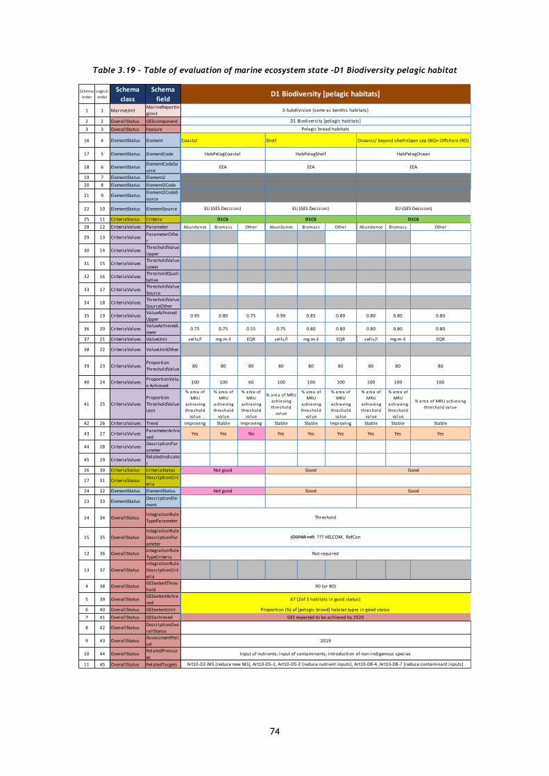
74

Table 3.19 - Table of evaluation of marine ecosystem state -D1 Biodiversity pelagic habitat

Schema

order

Logical

order

Schema

class

Schema

field

1 1 MarineUnitMarineReportin

gUnit

2 2 OverallStatus GEScomponent

3 3 OverallStatus Feature

16 4 ElementStatus Element Coastal Shelf Oceanic/ beyond shelf=Open sea (BG)= Offshore (RO)

17 5 ElementStatus ElementCode

18 6 ElementStatusElementCodeSo

urce

19 7 ElementStatus Element2

20 8 ElementStatus Element2Code

21 9 ElementStatusElement2CodeS

ource

22 10 ElementStatus ElementSource

25 11 CriteriaStatus Criteria

28 12 CriteriaValues Parameter Abundance Biomass Other Abundance Biomass Other Abundance Biomass Other

29 13 CriteriaValuesParameterOthe

r

30 14 CriteriaValuesThresholdValue

Upper


Lower

32 16 CriteriaValuesThresholdQuali

tative


Source


SourceOther

35 19 CriteriaValuesValueAchieved

Upper0.95 0.80 0.75 0.90 0.85 0.80 0.80 0.80 0.80

36 20 CriteriaValuesValueAchievedL

ower0.75 0.75 0.55 0.75 0.80 0.80 0.80 0.80 0.80

37 21 CriteriaValues ValueUnit cells/l mg.m-3 EQR cells/l mg.m-3 EQR cells/l mg.m-3 EQR

38 22 CriteriaValues ValueUnitOther

39 23 CriteriaValuesProportion

ThresholdValue80 80 80 80 80 80 80 80 80

40 24 CriteriaValuesProportionValu

e Achieved100 100 60 100 100 100 100 100 100

41 25 CriteriaValues

Proportion

ThresholdValue

Unit

% area of

MRU

achieving

threshold

va lue

% area of

MRU

achieving

threshold

va lue

% area of

MRU

achieving

threshold

va lue

% area of MRU

achieving

threshold

va lue

% area of

MRU

achieving

threshold

va lue

% area of

MRU

achieving

threshold

va lue

% area of

MRU

achieving

threshold

va lue

% area of

MRU

achieving

threshold

va lue

% area of MRU achieving

threshold va lue

42 26 CriteriaValues Trend Improving Stable Improving Stable Stable Improving Stable Stable Stable

43 27 CriteriaValuesParameterAchie

vedYes Yes No Yes Yes Yes Yes Yes Yes

44 28 CriteriaValuesDescriptionPar

ameter

45 29 CriteriaValuesRelatedIndicato

r

26 30 CriteriaStatus CriteriaStatus

27 31 CriteriaStatusDescriptionCrit

eria

24 32 ElementStatus ElementStatus

23 33 ElementStatusDescriptionEle

ment

14 34 OverallStatusIntegrationRule

TypeParameter

15 35 OverallStatus

IntegrationRule

DescriptionPar

ameter

12 36 OverallStatusIntegrationRule

TypeCriteria

13 37 OverallStatus

IntegrationRule

DescriptionCrit

eria

4 38 OverallStatusGESextentThres

hold

5 39 OverallStatusGESextentAchie

ved

6 40 OverallStatus GESextentUnit

7 41 OverallStatus GESachieved

8 42 OverallStatusDescriptionOve

rallStatus

9 43 OverallStatusAssessmentPeri

od

10 44 OverallStatusRelatedPressur

es

11 45 OverallStatus RelatedTargets

HabPelagCoastal HabPelagShelf

EEA EEA

EU (GES Decision) EU (GES Decision)

D1C6 D1C6

Not required

Not good Good

Not good Good

D1C6

Good

Good

Input of nutrients; input of contaminants; introduction of non-indigenous species

Threshold

(OSPAR ref) ??? HELCOM, RefCon

3-Subdivision (same as benthic habitats)

D1 Biodiversity [pelagic habitats]

EU (GES Decision)

HabPelagOcean

EEA

D1 Biodiversity [pelagic habitats]

Pelagic broad habitats

Art10-D2-NIS (reduce new NIS), Art10-D5-1, Art10-D5-2 (reduce nutrient inputs), Art10-D8-4, Art10-D8-7 (reduce contaminant inputs)

90 (or 80)

67 (2of 3 habitats in good status)

Proportion (%) of [pelagic broad] habitat types in good status

GES expected to be achieved by 2020

2019

75

3.6 Visualizing Assessment Results for Pelagic Habitats

Figure 3.3 - Illustrative example of a visual summary of assessment outputs for Descriptor 1 Pelagic habitats (Bulgarian Monitoring Report, 2018)

MRUArea

assessed

km2

Area assessed

(%)GES km

2 GES % Non GES km2 Non GES % No data km

2 No data %

Sivriburun-

Kaliakran/a n/a n/a n/a n/a n/a n/a n/a

Kaliakra-Galata n/a n/a n/a n/a n/a n/a n/a n/a

Galata-Emine n/a n/a n/a n/a n/a n/a n/a n/aEmine-

c.Maslenn/a n/a n/a n/a n/a n/a n/a n/a

Shelf-north 1634.25 42 0 0 1634.25 42 2244.8 58

Shelf south n/a n/a n/a n/a 0 0 n/a n/a

Open sea n/a n/a n/a n/a 0 0 n/a n/a

76

4 Guideline on Descriptors 1, 6. Theme Benthic habitats

4.1 Introduction

The contribution of seabed habitats and sea-floor integrity to the overall goal of achieving good environmental status (GES) of Europe’s marine waters is addressed by Descriptors 1 and 6 respectively of Directive 2008/56/EC of the European Parliament and of the Council of 17 June 2008 establishing a framework for community action in the field of marine environmental policy.

Descriptor 1 Biodiversity: Biological diversity is maintained. The quality and occurrence of habitats and the distribution and abundance of species are in line with prevailing physiographic, geographic and climatic conditions.

Descriptor 6 Seabed integrity: Sea-floor integrity is at a level that ensures that the structure and functions of the ecosystems are safeguarded and benthic ecosystems, in particular, are not adversely affected.

In Commission Decision EU/2017/848, these two aspects of GES have been brought together via a set of five criteria for the determination of GES in relation to a set of broad habitat types as defined in the Decision, and other habitat types as defined by Member States. For the assessment of benthic habitats Descriptors 1 and 6 are considered together.

The Decision sets out the following criteria to be used for benthic habitats:

• D6C1 Physical loss

• D6C2 Physical disturbance

• D6C3 Adverse effects of physical disturbance on habitats

• D6C4 Extent of habitat loss

• D6C5 Extent of adverse effects on the condition of a habitat.

The main aims of this Guideline are:

• To develop a common framework for assessing the environmental status of seabed habitats and sea-floor integrity in the Black Sea.

• To propose methodological standards for the regional-level assessment of seabed habitats and sea-floor integrity, including threshold values for adverse effects on the state of a habitat (D6C5), and the maximum allowable extent of habitat loss (D6C4) and of habitat adversely affected (D6C5).

• To propose a method for assessing overall status of a habitat, using criteria D6C4 and D6C5, as far as possible, based on available scientific knowledge.

• To ensure, as far as possible, that the methodological standards, data requirements and assessments under the MSFD are compatible with those under the Habitats Directive and Water Framework Directive.

• To identify where data and scientific knowledge are currently insufficient, and reflect such uncertainties in proposals made.


The relevant ecosystem elements of the seabed assessed under MSFD Descriptors 1 together with Descriptor 6 are the benthic broad habitat types. These are listed by Commission Decision EU/2017/848 Annex, Part II - Table 2 and equate to one or more habitat types at hierarchical level 2 of the European nature information system (EUNIS) habitat classification 20199. The major division in

9 https://www.eea.europa.eu/data-and-maps/data/eunis-habitat-classification/eunis-marine-habitat-classification-review-2019/eunis-marine-habitat-classification-2019)

https://www.eea.europa.eu/data-and-maps/data/eunis-habitat-classification/eunis-marine-habitat-classification-review-2019/eunis-marine-habitat-classification-2019

https://www.eea.europa.eu/data-and-maps/data/eunis-habitat-classification/eunis-marine-habitat-classification-review-2019/eunis-marine-habitat-classification-2019

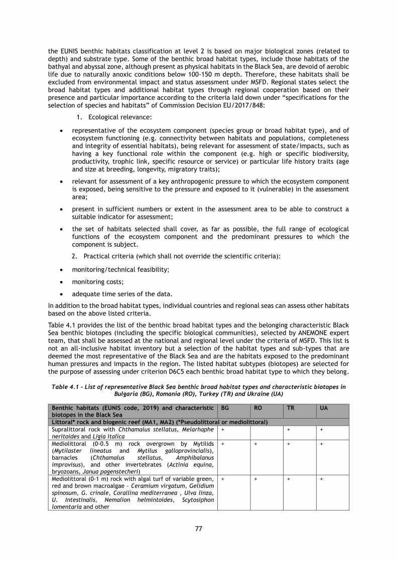
77

the EUNIS benthic habitats classification at level 2 is based on major biological zones (related to depth) and substrate type. Some of the benthic broad habitat types, include those habitats of the bathyal and abyssal zone, although present as physical habitats in the Black Sea, are devoid of aerobic life due to naturally anoxic conditions below 100-150 m depth. Therefore, these habitats shall be excluded from environmental impact and status assessment under MSFD. Regional states select the broad habitat types and additional habitat types through regional cooperation based on their presence and particular importance according to the criteria laid down under “specifications for the selection of species and habitats” of Commission Decision EU/2017/848:

1. Ecological relevance:

• representative of the ecosystem component (species group or broad habitat type), and of ecosystem functioning (e.g. connectivity between habitats and populations, completeness and integrity of essential habitats), being relevant for assessment of state/impacts, such as having a key functional role within the component (e.g. high or specific biodiversity, productivity, trophic link, specific resource or service) or particular life history traits (age and size at breeding, longevity, migratory traits);



• the set of habitats selected shall cover, as far as possible, the full range of ecological functions of the ecosystem component and the predominant pressures to which the component is subject.

2. Practical criteria (which shall not override the scientific criteria):




In addition to the broad habitat types, individual countries and regional seas can assess other habitats based on the above listed criteria.

Table 4.1 provides the list of the benthic broad habitat types and the belonging characteristic Black Sea benthic biotopes (including the specific biological communities), selected by ANEMONE expert team, that shall be assessed at the national and regional level under the criteria of MSFD. This list is not an all-inclusive habitat inventory but a selection of the habitat types and sub-types that are deemed the most representative of the Black Sea and are the habitats exposed to the predominant human pressures and impacts in the region. The listed habitat subtypes (biotopes) are selected for the purpose of assessing under criterion D6C5 each benthic broad habitat type to which they belong.

Table 4.1 - List of representative Black Sea benthic broad habitat types and characteristic biotopes in Bulgaria (BG), Romania (RO), Turkey (TR) and Ukraine (UA)

Benthic habitats (EUNIS code, 2019) and characteristic biotopes in the Black Sea

BG RO TR UA

Littoral* rock and biogenic reef (MA1, MA2) (*Pseudolittoral or mediolittoral)

Supralittoral rock with Chthamalus stellatus, Melarhaphe neritoides and Ligia italica

+ + +

Mediolittoral (0-0.5 m) rock overgrown by Mytilids (Mytilaster lineatus and Mytilus galloprovincialis), barnacles (Chthamalus stellatus, Amphibalanus improvisus), and other invertebrates (Actinia equina, bryozoans, Janua pagenstecheri)

+ + + +

Mediolittoral (0-1 m) rock with algal turf of variable green, red and brown macroalgae - Ceramium virgatum, Gelidium spinosum, G. crinale, Corallina mediterranea , Ulva linza, U. Intestinalis, Nemalion helmintoides, Scytosiphon lomentaria and other

+ + + +

78


BG RO TR UA

Littoral* sediment (MA3, MA4, MA5, MA6) (*Pseudolittoral or mediolittoral)

Mediolittoral coarse sediment (cobbles, gravel, shell hash) typically without or with poor fauna (e.g. Janua pagenstecheri)

+ + + +

Mediolittoral (0-1m) coarse or medium clean sand with Donacilla cornea (and Ophelia bicornis)

+ + + +

Mediolittoral (0-1m) fine sand with Pontogammarus maeoticus

+ + +

Mediolittoral mud in areas with freshwater influence (estuaries) with oligochaetes and chironomids

+ + +

Infralittoral rock and biogenic reef (MB1, MB2)

Upper-infralittoral (1-4 m) rock dominated by Cystoseira bosphorica

+ +

Upper-infralittoral (3-10 m) rock dominated by Cystoseira barbata

+ + + +

Upper infralittorlal (1-10 m) rock with variable annual green and red macroalgae: Ceramium virgatum, Gelidium spinosum, G. crinale, Corallina mediterranea, Ulva rigida, Ulva linza, U. intestinalis, Cladophora sericea, C. albida, Bryopsis plumosa and other

+ + + +

Upper infralittoral (1-10 m) rock with Coccotylus truncatus +

Lower infralittoral (10-18 m) rock with dominant perennial sciaphylic red and brown macroalgae (Phyllophora crispa, Zanardinia typus, Apoglossum ruscifolium) and/or widely adaptive green (Cladophora albida, Cladophora coelothrix) and red macroalgae (Polysiphonia elongata, Gelidium spinosum, Gelidium crinale, Anithamniom cruciatum)

+ +

Infralittoral rock dominated by Mytilids: Mytilaster lineatus, Mytilus galloprovincialis

+ + + +

Infralittoral rock with faunal turf: colonial ascidians (Botryllus schlosseri), hydrozoans, bryozoans and sponges

+ + +

Infralittoral soft rock with piddocks (Pholas dactylus, Barnea candida)

+ + + +

Infralittoral Mytilus galloprovincialis biogenic reefs on muddy shelly sediment, at 3-10 m depth

+

Biogenic reefs of Ostrea edulis and serpulid worms + ?+

Infralittoral coarse sediment (MB3)

Infralittoral coarse sediments (including pebbles, cobbles, fine gravels, coarse sands and shell hash) with varied fauna (typical Branchiostoma lanceolatum, Protodorvillea kefersteini)

+ +

Infralittoral mixed sediment (MB4)

Infralittoral mixed sediment with varied fauna + + + +

Infralittoral sand (MB5)

Zostera noltei meadows (1-3 m) + + + +

Zostera marina meadows (4-7 m) + + +

Mixed meadows with Zostera noltei-Zannichellia palustris-Zostera marina meadows (2-4 m)

+ ?+

Potamogeton petcinatus - Zannichellia palustris meadows in man-made sheltered areas

+ +

Upper-infralittoral (1 -7 m) medium and fine sand dominated by Donax trunculus

+ + + +

Infralittoral (5-15 m) fine and medium sand, dominated by Chamelea gallina (other typical Lentidium mediterraneum, Macomangulus tenuis, Lucinella divaricata)

+ + + +

Lower infralittoral (13-24 m) coarse and medium sand, dominated by Upogebia pusilla

+ + +

Infralittoral mud (MB6)

Infralittoral mud (7-18m) with Mya arenaria, Anadara kagoshimensis, Upogebia pussila, Nephtys sp., Melinna palmata and other polychaetes

+

Infralittoral mud (9-25 m) dominated by Aricidea claudiae, Prionospio maciolekae, Melinna palmata and Lucinella

+

79


BG RO TR UA

divaricata

Circalittoral rock and biogenic reef (MC1, MC2)

Mussel beds of Mytilus galloprovincialis on circalittoral (20-70 m) mud and mixed sediments (mud and shells)

+ + + +

Circalittoral rock overgrown by Mytilus galloprovincialis, hydrozoans and sponges

+ + +

Circalittoral coarse sediment (MC3)

Shallow circalittoral (17-35 m) shelly gravel and coarse sand with varied infauna (typical Modiolus adriaticus, Gouldia minima)

+ + +

Shallow circalittoral shelly organogenic sand with Mytilus biogenic reefs and filamentous/folious algae (Phyllophora field of Zernov)

+

Circalittoral mixed sediment (MC4)

Shallow circalittoral shelly mudy sand/sandy mud with Upogebia pusilla, Heteromastus filiformis, Nephtys hombergii, Aricidea claudiae, Chamelea gallina, Anadara inequivalvis, Mya arenaria

+ + + +

Shallow circalittoral (20-40m) shelly sandy mud/mud with Pitar rudis, Spisula subtruncata, Paphia aurea, Mytilus galloprovincialis, Abra spp., Cardiidae, Nephthys hombergii, Heteromastus filiformis

+ + + +

Circalittoral sand (MC5)

Circalittoral mud (MC6)

Shallow circalittoral mud dominated by Melinna palmata + + + +

Shallow circalittoral mud and organogenic sandy mud with Gouldia minima, Pitar rudis, Aricidea claudiae

+

Offshore circalittoral rock and biogenic reef (MD1, MD2)

Offshore circalittoral coarse sediment (MD3)

Offshore circalittoral mixed sediment (MD4)

Deep circalittoral (60-100 m) shelly mud with Modiolula phaseolina

+ + + +

Offshore circalittoral sand (MD5)

Offshore circalittoral mud (MD6)

Deep circalittoral mud (40-90 m) with Terebellides stroemi, (Amphiura stepanovi, Pachycerianthus solitarius)

+ + + +

Deep circalittoral suboxic muds + + + +

(+) – present / (?+) - possibly present)

Assessments of seabed habitats require the use of maps of habitat types as a prerequisite to estimate the extent of each habitat which is adversely affected by physical disturbance (D6C3) and by all anthropogenic pressures (D6C5). A predictive map of seabed habitats, covering all MSFD regions, including the Black Sea, is provided by EMODnet Seabed Habitats according to the EUNIS typology, and also aggregated to MSFD broad habitat types10. Its level of detail and quality varies according to the quality of the underlying data, e.g. substrate type.

! EMODnet maps can be utilized in national/regional assessments of the Black Sea habitats, particularly where national habitat maps are not available.

10 http://www.emodnet-seabedhabitats.eu/default.aspx?mapInstance=MESHAtlanticMap_&page=1974&LAYERS=EUSMMSFD&zoom=2&Y=51.76&X=2.27

80

4.3 Assessment of physical loss and physical disturbance

4.3.1 Physical loss criteria and methodological standards

Physical loss of the seabed and benthic habitats is assessed under criteria D6C1 and D6C4.

Criterion D6C1: Spatial extent and distribution of physical loss (permanent change) of the natural seabed.

! Physical loss shall be understood as a permanent change to the seabed which has lasted or is expected to last for a period of two reporting cycles (12 years) or more.

The criterion element for assessment is the pressure “physical loss” due to permanent change of seabed substrate or morphology and to extraction of seabed substrate.

Specifications and standardised methods for monitoring and assessment:

• Permanent changes to the seabed from different human activities include permanent changes to natural seabed substrate or morphology via physical restructuring, infrastructure developments and loss of substrate via extraction of the seabed materials.

• Data on physical loss may be collated from mapping of infrastructure and licensed extraction sites.

• D6C1 is assessed as area lost in relation to total natural extent of all benthic habitats in the assessment area.

• Units of measurement: extent of the assessment area physically lost in square kilometres (km2).

• No threshold values are required for D6C1.

• The outcomes of assessment of criterion D6C1 - the distribution and an estimate of the extent of physical loss - shall be used to assess criteria D6C4.

Criterion D6C4: The extent of loss of the habitat type, resulting from anthropogenic pressures, does not exceed a specified proportion of the natural extent of the habitat type in the assessment area.

The criterion elements for assessment are the benthic broad habitat types and other regionally agreed habitat types listed in Table 4.1.


• Assessment of criterion D6C4 shall use the assessment made under criterion D6C1.

• Units of measurement: extent of habitat loss in square kilometres (km2) and as a proportion (%) of the total extent of the habitat type.

• The threshold for the maximum allowable extent of habitat loss as a proportion of the total natural extent of the broad habitat types is proposed to be established at 5 %. This threshold shall not be exceeded by each benthic broad habitat type in each nationally determined assessment area (marine reporting unit - MRU).

• A common regional baseline shall be established for determination of the natural extent of the habitat types. The baseline area for the Black Sea habitats is proposed to be the area in 2008 - the year of MSFD adoption.

• The extent to which good environmental status has been achieved shall be expressed for each area assessed as an estimate of the proportion and extent of loss per habitat type and whether this has achieved the extent value set.

The Commission Decision EU/2017/848 requires consistent and comparable determinations of good environmental status with the relevant existing standards and methods for monitoring and assessment laid down in Union legislation, including Council Directive 92/43/EEC (Habitats Directive). Therefore, the proposed threshold value for GES is founded in the concept of the HD for Favourable Conservation Status (FCS). Criterion D6C4 corresponds to the “range/area covered by habitat type within range’’ criterion of the HD. The conservation status of a habitat in the HD (Article 1(e)) will be taken as “favourable” when area it covers within range is stable (loss and expansion in balance) or increasing and area covered by habitat is not smaller than the favourable reference area, and there are no significant changes in distribution pattern within the range. On the other hand, unfavourable -bad conservation status is assessed if there is a large decrease equivalent to a loss of more than 1 % per

81

year within the reporting period. Consequently, a decline equivalent to a loss of less than 1 % per year is presumed as minor relative to the broad habitat types’ baseline areas and thus a maximum cumulative loss < 5 % over the 6-year reporting cycle is deemed acceptable degree of change. It must be underlined that the established baseline of 2008 (or any other) shall not be further shifted, therefore continuing trends of habitat loss are not allowable over the subsequent reporting cycles and the 5 % threshold shall always be evaluated against the established baseline of 2008 (or other appropriate baseline – see below).

For special habitats the standards for favourable conservation status of range/area laid down by the Habitats Directive, as described above, shall be complied with, in particular by EU member states.

For rare and sensitive habitat subtypes identified at the national level (e.g. biotopes with Cystoseira, Phyllophora, Zostera, Donacilla, Donax, etc.), lower thresholds may be set by Black Sea countries, as appropriate, in order to ensure more rigorous habitat protection.

National area baselines may differ from 2008 for some habitat types/subtypes, if there is evidence for significant habitat loss before that year and if recovery is desirable and feasible (e.g. restoration of seagrass beds, mussel beds, Cystoseira and Phyllophora canopies).

In case that baseline is not known but recovery from habitat loss is deemed necessary, instead of setting extent threshold, a trend (increasing/decreasing) may be used to assess the status in a given period.

The habitat loss extent threshold is already legally established in Bulgaria at 5 %. In the rest of the Black Sea countries, threshold for habitat loss is not established yet, thus the proposed regional threshold in this Guideline may be used as a reference for legal adoption.

At EU level, proposals for threshold values for maximum allowable extent of loss (D6C4) are expected to be delivered in 2021 by the Technical Group on seabed habitats and sea-floor integrity (TG SEABED). The regional threshold can be adjusted as appropriate when the EU guidelines become available.

4.3.2 Physical disturbance criteria and methodological standards

Physical disturbance pressure on the seabed and its impact on benthic habitats are assessed under criteria D6C2 and D6C3, respectively.

D6C2: Spatial extent and distribution of physical disturbance pressures on the seabed.

The criterion element for assessment is the pressure “physical disturbance” to seabed (temporary or reversible).

! Physical disturbance shall be understood as a change to the seabed from which it can recover if the activity causing the disturbance pressure ceases.


• Physical disturbances from different human activities shall be assessed (such as bottom-trawling fishing).

• Units of measurement: extent of the assessment area physically disturbed in square kilometres (km2).

• No threshold values are required for D6C2.

• The outcomes of assessment of criterion D6C2 (the distribution and an estimate of the extent of physical disturbance pressures) shall be used to assess criterion D6C3.

D6C3: Spatial extent of each habitat type which is adversely affected, through change in its biotic and abiotic structure and its functions (e.g. through changes in species composition and their relative abundance, absence of particularly sensitive or fragile species or species providing a key function, size structure of species), by physical disturbance.



• D6C3 is assessed in relation to total natural extent of each benthic habitat type assessed.

82

• For D6C3 species composition shall be understood to refer to the lowest taxonomic level appropriate for the assessment.

• Units of measurement: extent of each habitat type adversely affected in square kilometres (km2) or as a proportion (percentage) of the total natural extent of the habitat in the assessment area.

• ! Member States shall establish threshold values for the adverse effects of physical disturbance, through regional or sub-regional cooperation. No threshold for spatial extent is required!

• The outcomes of assessment of criterion D6C3 (an estimate of the extent of adverse effect by physical disturbance per habitat type in each assessment area) shall contribute to the assessment of criterion D6C5.

4.3.3 Assessment framework for physical loss and physical disturbance

To assess physical loss (D6C1 and D6C4) and physical disturbance (D6C2) on the seafloor, ICES (2019) advises the use of a single assessment process as shown on Figure 4.1.

Figure 4.1 - Seafloor assessment process (ICES Advice, 2019)

Four pressure subtypes were identified as the pathways through which physical loss and physical disturbance operate:

• Abrasion: the scraping of the substrate (e.g., by a trawl door or an anchor). The abrasion pressure subtype can result in physical loss and/or physical disturbance.

• Removal: the net transference of substrate away from the seabed resulting from human activities (e.g., either directly by human activities or indirectly through the modification of hydrodynamics). This pressure subtype can result in physical loss and/or physical disturbance.

• Deposition: the movement of sediment and/or particulates to a new position on top of or in existing substrates (e.g., directly by human activities such as dredge disposal or indirectly through the modification of hydrodynamics). This pressure subtype can result in physical disturbance.

83

• Sealing: the capping of the original substrate with structures (e.g., metal pilings, concrete footings, or blankets) or substrates (e.g. rock or stone fills, dredge disposal) which in and of themselves change the physical habitat. This pressure subtype can result in physical loss.

For each pressure subtype, the main contributing human activities were identified (Table 4.2).

Table 4.2 - Main human activities that affect the seabed through the four pressure subtypes

Pressure subtype Main human activities

Abrasion Fishing with mobile bottom-contacting gears.

Removal Aggregate extraction (removal of sediment for use elsewhere) and dredging (removal of sediment to clear/maintain an area).

Deposition Dredge disposal and fishing with mobile bottom-contacting gears.

Sealing Placement of permanent structures during a variety of activities (e.g., oil and gas extraction, renewable energy, harbours and coastal defence, tourism/recreation, pipelines and cables, wrecks, artificial reefs).

Physical loss is defined by ICES as any human-induced permanent alteration of the physical habitat from which recovery is impossible without further human intervention. An alteration of the physical habitat refers to a change from one EUNIS level 2 habitat type to another EUNIS level 2 habitat type. Recovery indicates the re-establishment of the original natural EUNIS level 2 habitat by means of a human intervention. Two types of physical loss are identified:

• Sealed physical loss results from the placement of structures in the marine environment (e.g., wind turbines, port infrastructure) and from the introduction of substrates that seal off the seabed (e.g., dredge disposal).

• Unsealed physical loss results from changes in physical habitat, either from human activities or from the indirect effects of the placement of man-made structures (e.g., aggregate extraction or a structure causing changes in water flows, ultimately changing the EUNIS level 2 habitat type).

Physical disturbance is defined as a pressure that disturbs benthic biota but does not permanently change the habitat from one EUNIS level 2 habitat type to another EUNIS level 2 habitat type. With sufficient time, recovery can be expected without human intervention.

Steps for assessment of physical loss (D6C1/C4):

1. Identify the competent authorities. Most sealed loss data will be held by the relevant

licensing authorities within the Black Sea States. The identification of unsealed loss

requires further ground-truthing to assess if a change in habitat classification has

occurred.

2. Request spatial data. The minimum data that should be collected for each activity is:

type of activity (e.g., activity, structure type, licence information), geographic location

(preferably in polygon format), and dates/timing/period of the operational phases

(preferably in shapefile or CAD format, or as an attribute for the activity).

3. Produce total footprint of physical loss. Assess the footprint either directly from the

data at hand or, if the original data are points or polylines (and not a polygon), a loss

footprint should be estimated. Unsealed and sealed loss are combined into a single loss

layer.

4. Assessment of physical loss. The single physical loss layer can be used to assess

contemporary total loss under D6C1, and per habitat type under D6C4. The assessment

can be done in km2 and as a proportion of the total spatial extent of the assessed

area/habitat type.

Steps for assessment of physical disturbance (D6C2):

1. Identify the competent authorities. For aggregate extraction and other spatially

localized activities, most data will be held by the relevant licensing authorities within

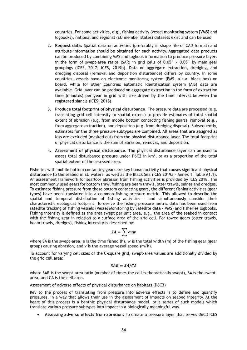
84

countries. For some activities, e.g., fishing activity (vessel monitoring system [VMS] and

logbooks), national and regional (EU member states) datasets exist and can be used.

2. Request data. Spatial data on activities (preferably in shape file or CAD format) and

attribute information should be obtained for each activity. Aggregated data products

can be produced by combining VMS and logbook information to produce pressure layers

in the form of swept-area ratios (SAR) in grid cells of 0.05° × 0.05° by main gear

groupings (ICES, 2017; ICES, 2019b). Data on aggregate extraction, dredging, and

dredging disposal (removal and deposition disturbance) differs by country. In some

countries, vessels have an electronic monitoring system (EMS, a.k.a. black box) on

board, while for other countries automatic identification system (AIS) data are

available. Grid layer can be produced on aggregate extraction in the form of extraction

time (minutes) per year in grid with size driven by the time interval between the

registered signals (ICES, 2018).

3. Produce total footprint of physical disturbance. The pressure data are processed (e.g.

translating grid cell intensity to spatial extent) to provide estimates of total spatial

extent of abrasion (e.g. from mobile bottom contacting fishing gears), removal (e.g.,

from aggregate extraction), and deposition (e.g. from dredging disposal). Subsequently,

estimates for the three pressure subtypes are combined. All areas that are assigned as

loss are excluded (masked out) from the physical disturbance layer. The total footprint

of physical disturbance is the sum of abrasion, removal, and deposition.

4. Assessment of physical disturbance. The physical disturbance layer can be used to

assess total disturbance pressure under D6C2 in km2, or as a proportion of the total

spatial extent of the assessed area.

Fisheries with mobile bottom contacting gears are key human activity that causes significant physical disturbance to the seabed in EU waters, as well as the Black Sea (ICES 2019a - Annex 1, Table A1.1). An assessment framework for seafloor abrasion from fishing activities is provided by ICES 2018. The most commonly used gears for bottom trawl fishing are beam trawls, otter trawls, seines and dredges. To estimate fishing pressure from these bottom contacting gears, the different fishing activities (gear types) have been translated into a common fishing pressure metric. This allowed to describe the spatial and temporal distribution of fishing activities – and simultaneously consider their characteristic ecological footprint. To derive the fishing pressure metric data has been used from satellite tracking of fishing vessels (Vessel Monitoring by Satellite data - VMS) and fisheries logbooks. Fishing intensity is defined as the area swept per unit area, e.g., the area of the seabed in contact with the fishing gear in relation to a surface area of the grid cell. For towed gears (otter trawls, beam trawls, dredges), fishing intensity is described by:

𝑺𝑨 = ∑ 𝒆𝒗𝒘

where SA is the swept-area, e is the time fished (h), w is the total width (m) of the fishing gear (gear group) causing abrasion, and v is the average vessel speed (m/h).

To account for varying cell sizes of the C-square grid, swept-area values are additionally divided by the grid cell area:

𝑺𝑨𝑹 = 𝑺𝑨/𝑪𝑨

where SAR is the swept-area ratio (number of times the cell is theoretically swept), SA is the swept-area, and CA is the cell area.

Assessment of adverse effects of physical disturbance on habitats (D6C3)

Key to the process of translating from pressure into adverse effects is to define and quantify pressures, in a way that allows their use in the assessment of impacts on seabed integrity. At the heart of this process is a benthic physical disturbance model, or a series of such models which translate various pressure subtypes into impact in a biologically meaningful way.

• Assessing adverse effects from abrasion: To create a pressure layer that serves D6C3 ICES

85

advises that the quantification of abrasion is mapped spatially, where both the intensity and depth of disturbance is represented.

• Assessing adverse effects from removal: To create a pressure layer that serves D6C3, ICES advises that the quantification of removal is mapped spatially as the volume of substrate removed, per area, per time.

• Assessing adverse effects from deposition: To create a pressure layer that serves D6C3, ICES advises that the quantification of deposition is mapped spatially as the volume of sediments deposited, per area and per time.

ICES 2019 recommends two methods for assessing the impact from mobile bottom-contacting fishing gear:

• Longevity (LL1). The LL1 method is a statistical model that estimates the habitat-specific longevity composition of the community and the effect of trawling on this composition. The basis of this relationship is that long-lived species have a lower recovery rate because of their lower growth rates and later age-at-maturity; they are thus generally more sensitive to fishing mortality. The model includes an interaction of the effect of trawling and shear stress at the seabed as trawling has lower impacts on habitats with high shear stress (high natural disturbance). The indicator estimates the reduction in proportion of long-lived taxa (maximum lifespan > 10 years) due to trawling. The longevity composition of a benthic community is a proxy for biodiversity and tracks the change in benthic community composition in response to trawling.

• Population dynamic (PD). The PD method is a mechanistic model that estimates the total reduction in community biomass (B) relative to carrying capacity (K), corresponding to the estimated fishing intensity. The impact is given by the equation:

RBS = B/K = 1- F d/r where RBS (relative benthic status) is the total community biomass relative to carrying capacity (B/K) and describes the equilibrium state (the interaction between the depletion caused by fishing and the recovery of the benthic community); F = SAR is defined as the total area swept by trawl gear within a given area of seabed in one year divided by that area of seabed (units y-1); depletion d is the fraction mortality per trawl pass; r is the intrinsic rate of population increase.

The depletion rates are estimated from a meta-analysis that provided gear-specific depletion rates. The recovery rates are derived from a meta-analysis that is longevity specific (Hiddink et al., 2019). Estimating RBS therefore requires only maps of fishing intensity and habitat type – and parameters for impact and recovery rates, which have been taken from meta-analyses of all available studies of towed-gear impacts. The assessment produces a relative benthic state estimate (RBS) for each c-square in the assessed region, based on just two parameter values (depletion d and the intrinsic rate of population increase r, a metric of recovery rate) and the fishing intensity. Relative Benthic Status (RBS) is estimated for each c-square as the sum of the relative biomasses of all the longevity classes. The methods are parameterized for the North Sea and can be used in the Black Sea but have yet to be parameterized.

Data and methodological gaps:

Fishing with mobile bottom-contacting gears. The provision of VMS data has only been mandatory for EU Member states’ vessels larger than 12 m (overall length) since 2012. In the Black Sea region, a large proportion of the fleet is below 12 m and therefore do not currently have VMS on board. In the EU proposal for amending the fisheries control regulation (COM/2018/368 final; EU, 2018) it is stated that “All vessels including those below 12 metres’ length must have a tracking system”. If this proposal is approved, it would greatly improve the ability to document fishing pressure from small-scale fisheries. It is necessary to solve the problems with absent VMS in non-EU countries in the Black Sea region, confidentiality issues in accessing VMS data in some countries, and insufficient spatiotemporal resolution of VMS data.

Aggregate extraction. Licensed areas of the extraction sites are available; however, more detailed data on the location of extraction (within a site) from electronic monitoring system (EMS) on board or AIS are currently no available for the Black Sea (ICES 2019a - Annex 1, Table A1.7). ICES advises adoption of the use of such high-resolution systems and the recording of additional metrics such as volume, over and above the common metric of licence area (km2).

Deposition. Quantification of the spatial extent of deposition resulting from human activities requires

86

hydrodynamic modelling for each region to take into account the dynamism in the spatial distribution of the pressure. This approach is less arbitrary than adopting a “buffer zone” approach, where the impact is assumed to occur in a fixed diameter buffer zone around the activity. However, parameterizing such models is computationally more difficult and the approach is data hungry as it relies on appropriate sediment data and hydrodynamic models. The production of such depositional pressure maps is not currently operational.

Impact indicators. Longevity (LL1) and population dynamic (PD2) methods are not parameterized for the Black Sea. To apply the PD approach to the Black Sea region, the biomass-longevity distribution of untrawled communities will need to be estimated in relation to environmental variables. This will require samples (which can include grabs, cores, video, photo, dredges or trawls) of benthic communities over the main environmental gradients. A significant fraction of these samples need to be taken at no or low trawling locations.

Different approaches to assess benthic impact may be considered in the Black Sea Region. These should take into consideration that systematic review of different responses variables has shown that community biomass is the most sensitive indicator of trawling impacts as it is most responsive, while community abundance and species richness are less sensitive, and diversity indices are not suitable as state indicators for monitoring the effect of bottom trawling (Hiddink et al., in prep in ICES 2018).

4.4 Assessment of adverse effects on benthic habitats types

4.4.1 Criteria and general methodological standards

The assessment of adverse effects from overall anthropogenic pressures on the benthic habitats is encompassed by criterion D6C5.

Criterion D6C5: The extent of adverse effects from anthropogenic pressures on the condition of the habitat type, including alteration to its biotic and abiotic structure and its functions (e.g. its typical species composition and their relative abundance, absence of particularly sensitive or fragile species or species providing a key function, size structure of species), does not exceed a specified proportion of the natural extent of the habitat type in the assessment area.


Specifications and standardized methods for monitoring and assessment:

• Assessments of the adverse effects on the condition of benthic habitats from the pressures including from the criteria D2C3, D3C1, D3C2, D3C3, D5C4, D5C5, D5C6, D5C7, D5C8, D6C3, D7C2, D8C2 and D8C4 shall be taken into account. D6C5 shall integrate the adverse effects from all relevant pressures.

• ! Threshold values for adverse effects on the condition of each habitat type under criteria (and relevant indicators) D2C3, D3C1, D3C2, D3C3, D5C4, D5C5, D5C6, D5C7, D5C8, D6C3, D7C2, D8C2 and D8C4 shall be established through cooperation at Union level, taking into account regional specificities.

• ! Threshold for the maximum allowable extent of those adverse effects as a proportion of the total natural extent of the habitat type, shall be established through cooperation at Union level, taking into account regional specificities.

• Units of measurement for the criteria: extent of habitat adversely affected in square kilometres (km2) and as a proportion (percentage) of the total extent of the habitat type.

• The extent to which good environmental status has been achieved shall be expressed for each area assessed as an estimate of the proportion and extent of adverse effects, including the proportion lost per habitat type and whether this has achieved the extent threshold value set.

• ! Benthic habitat maps are produced at the EU scale, e.g. EMODnet11 . Although these maps need refinement, both in terms of resolution and habitat discrimination, they can

11 http://www.emodnet-seabedhabitats.eu/default.aspx?mapInstance=MESHAtlanticMap_&page=1974&LAYERS=EUSMMSFD&zoom=2&Y=51.76&X=2.27

87

be used in the assessment of the extent of broad habitats types adversely affected by overall anthropogenic pressures under D6C5.

4.4.2 Threshold for the maximum allowable extent of adverse effects

As for habitat loss, the threshold for extent of habitat adversely affected shall be consistent and comparable with the relevant existing standards laid down in Union legislation, in particular with those of the HD. Criterion D6C5 equates to the “specific structures and functions” criterion of the HD. Thus, the proposed regional threshold value for GES of the habitat extent under D6C5 is based on the standards of the HD for FCS of the “specific structures and functions”. The guidelines for reporting under Art. 17 of the HD (DG Environment, 2017) recommend using an indicative value of 90 % of the habitat type area in “good” condition as the threshold to conclude on “favourable” structure and functions. The status is evaluated as unfavourable –bad if > 25 % of the habitat area is “not good” as regards its specific structure and functions. The status is evaluated as unfavourable – inadequate if the condition is not good in 10-25% of habitat area. These values, however, do not include habitat loss, which is evaluated separately in the HD.

! An intermediate value of 15 % of the natural habitat extent adversely affected, including habitat loss, is considered an acceptable degree of change for the broad habitat types and consistent with previously established European standards, therefore it is proposed as regional threshold for GES under criterion D6C5.

The adverse effects extent threshold is legally established in Bulgaria at 20 %. In the rest of the Black Sea countries extent thresholds are not established yet. The recommended regional threshold may be used as a reference for legal adoption nationally.

For special habitats the standards for favourable conservation status of area in favourable conditions set under the HD, as described above, shall be complied with, in particular by EU member states.

For rare and sensitive habitat subtypes identified at the national level (e.g. biotopes with Cystoseira, Phyllophora, Zostera, Donacilla, Donax, etc.), lower extent thresholds for adverse effects may be set by Black Sea countries, as appropriate in order to ensure more rigorous habitat protection.

At EU level, proposals for threshold values for maximum allowable extent of adverse effects (D6C5) are expected to be delivered in 2021 by the TG SEABED. The regional threshold can be adjusted as appropriate when EU guidelines become available.

4.4.3 Adverse effects indicators and thresholds

Anthropogenic pressures can affect seabed habitats in different ways, for example: physical disturbance may damage or kill fragile species, non-indigenous species may predate on native species, nutrient enrichment pressures can lead to enhanced growth of opportunistic benthic algae and ultimately to deoxygenation of the water column and death of the benthic community. These differing types of pressure bring about adverse effects in terms of changes in the biotic and/or abiotic character of a habitat, but all need to be assessed in terms of the degree of these changes from natural conditions. According to each habitat type, the nature of the change and its severity can differ depending on the type of pressure, its intensity and its frequency. Distinguishing an acceptable degree of change from an unacceptable level of change through setting of threshold values provides the basis for assessing the condition of a habitat at a given location. This is illustrated in Figure 4.2.

88

Figure 4.2 - Conceptual relationship between GES for seabed habitats and sub-GES conditions, as expressed through the adverse effects of different pressures (three examples shown) (OSPAR, 2012)

There are a variety of methodologies to assess adverse effects on benthic habitats in current use in the Black Sea region. A substantial part of them were adopted, validated for certain types of pressures and calibrated under the Water Framework Directive (WFD). The applicable indicators that are available nationally are identified and allocated to the relevant criteria in Table 4.3. The national indicators are classified according to their stage of development and implementation into three categories:

• Fully operational - legally accepted nationally, validated for the relevant pressure and with thresholds established for all habitat types under the relevant pressure.

• Partially operational - legally accepted, validated for pressure but without thresholds yet, at least for some of the habitats.


Table 4.3 - Indicators under D2C3, D3C1, D3C2, D3C3, D5C4, D5C5, D5C6, D5C7, D5C8, D6C3, D7C2, D8C2 and D8C4 used in the Black Sea region*)

Country BG RO TR UA

Criteria Indicators

D2C3: Proportion or spatial extent of the broad habitat type which is adversely altered due to non-indigenous species, particularly invasive non-indigenous species

Biomass ratio of bivalve prey/invasive predator Rapana venosa (threshold established)

Biomass ratio of bivalve prey/invasive predator Rapana venosa (considered for the future

assessment) Newly proposed).

ALEX (Alien Biotic Index)

Biomass ratio of bivalve prey/invasive predator Rapana venosa. Newly proposed.

Biomass of bivalve prey Newly proposed.

ALEX (Alien Biotic Index) Newly proposed.

89

Country BG RO TR UA

Criteria Indicators

D3C3: The age and size distribution of individuals in the populations of commercially-exploited species is indicative of a healthy population.

95 percentile of the height (H) and length (L) of the commercially exploited bivalves Donax trunculus, and Chamelea gallina(thresholds established)

95 percentile of the height (H) and length (L) of the commercially exploited bivalves Donax trunculus, and Chamelea gallina (considered for the future assessment) Newly proposed. Not exploited yet , but, most probably, will get legal.

95 percentile of the height (H) and length (L) of the commercially exploited bivalves Chamelea gallina Newly proposed.

95 percentile of the height (H) and length (L) of the commercially exploited bivalves Mytilus galloprovincialis Newly proposed.

D5C4: The photic limit (transparency) of the water column is not reduced, due to increases in suspended algae, to a level that indicates adverse effects of nutrient enrichment.

water transparency depth (m)




D5C5: The concentration of dissolved oxygen is not reduced, due to nutrient enrichment, to levels that indicate adverse effects on benthic habitats (including on associated biota and mobile species) or other eutrophication effects.

concentration (mg/l) of dissolved oxygen in the bottom of the water column (thresholds established for infra- and shallow circalittoral to 40 m depth. Thresholds not established for deep circalittoral.

concentration (mg/l) of dissolved oxygen in the bottom of the water column. Thresholds not established for deep circalittoral.

concentration (mg/l) of dissolved oxygen in the bottom of the water column

concentration (mg/l) of dissolved oxygen in the bottom of the water column

D5C6: The abundance of opportunistic macroalgae is not at levels that indicate adverse effects of nutrient enrichment.

% wet biomass of the tollerant macroalgae (ESGII), standardised for infralittoral rock down to 3 m depth.

% wet biomass of the tollerant macroalgae (ESGII), standardised for infralittoral rock down to 3 m depth.

EEI and EEI-c (Ecological Evaluation Index)

Index of ecological activity of the three dominant species (S / W)3Dp, m2.kg-1

Ecological index EI, standardised for infralittoral rock down to 3 m depth.


90

Country BG RO TR UA

Criteria Indicators

D5C7: The species composition and relative abundance or depth distribution of macrophyte communities achieve values that indicate there is no adverse effect due to nutrient enrichment including via a decrease in water transparency

% wet biomass of the macroalgae from ESGI, standardised for infralittoral rock down to 3 m depth.

% wet biomass of the macroalgae from ESGI, standardised for infralittoral rock down to 3 m depth.

% coverage of the macroflora from ESGI (late-successional taxa such as Cystoseira spp., angiosperm Zostera spp., calcareous red algae such as Phymatolithon lenormandii), and ESG II (tolerant and opportunistic taxa such as filamentous and sheet-like green algae, blue green algae) standardised for infralittoral rock down to 3 m depth.

mean ecological activity of species (S / W)x, m2.kg-1




phytocoenosis surface index (SIph).

Percentage of the sensitive species (Ssp, %)

Lower distribution depth of sensitive taxa Cystoseira barbata and C. bosphorica

Lower distribution depth of sensitive taxa (i.e. Cystoseira, Zostera, Phyllophora) Newly proposed.

Lower distribution depth of seagrass beds.

Lower distribution depth of Phyllophora crispa

Subsurface wet biomass of Zostera noltei, ratio surface/subsurface biomass Zostera noltei, shoot density of Zostera noltei, shoots length of Zostera noltei Thresholds not established.

Subsurface wet biomass of Zostera noltei, ratio surface/subsurface biomass Zostera noltei, shoot density of Zostera noltei, shoots length of Zostera noltei. Newly proposed.

91

Country BG RO TR UA

Criteria Indicators

D5C8: Secondary (except when used as a substitute for D5C5): The species composition and relative abundance of macrofaunal communities, achieve values that indicate that there is no adverse effect due to nutrient and organic enrichment.

multimetric index M-AMBI(n) Thresholds established for coastal waters under WFD.

multimetric index M-AMBI(n) Thresholds established for coastal waters under WFD.

TUBI (Turkish Benthic Index) Thresholds not established for the Black Sea.

multimetric index M-AMBI(n) Newly proposed.

D6C3: Spatial extent of each habitat type which is adversely affected, through change in its biotic and abiotic structure and its functions (e.g. through changes in species composition and their relative abundance, absence of particularly sensitive or fragile species or species providing a key function, size structure of species), by physical disturbance.

Macrozoobenthos

multimetric index M-AMBI(n) Needs validation for the pressure and thresholds calibration for habitat types under pressure.

multimetric index M-AMBI(n) Needs validation for the pressure and thresholds calibration for habitat types under pressure.

TUBI (Turkish Benthic Index) values Needs validation for the pressure and thresholds calibration for habitat types under pressure.

multimetric index M-AMBI(n) Newly proposed. Needs validation for the pressure and thresholds calibration for habitat types under pressure.

% cover of mussel beds of Mytilus galloprovincialis on circalittoral sediment Threshold calibration required.

% cover of mussel beds of Mytilus galloprovincialis on circalittoral sediment; Newly proposed.

% cover of mussel beds of Mytilus galloprovincialis on circalittoral sediment; Newly proposed.

Average height of Mytilus galloprovinciali

Average height of Mytilus galloprovincialis Newly proposed.

PD method Not parametrized.




Seagrass

Subsurface biomass of Zostera noltei, ratio surface/subsurface biomass Zostera noltei, shoot density of Zostera noltei, shoots length of Zostera noltei Thresholds not established.

Subsurface biomass of Zostera noltei, ratio surface/subsurface biomass Zostera noltei, shoot density of Zostera noltei, shoots length of Zostera noltei Newly proposed.

Subsurface biomass of Zostera noltei, ratio surface/subsurface biomass Zostera noltei, shoot density of Zostera noltei, shoots length of Zostera noltei Newly proposed.

Projected cover of seagrass Thresholds not established.

Projected cover of seagrass Newly proposed.

Cover of seagrass Zostera Newly proposed.

Projected cover of seagrass Newly proposed.

D7C2: Spatial extent of each benthic habitat type

Macrozoobenthos

multimetric index M-AMBI(n)

multimetric index M-AMBI(n)

TUBI (Turkish Benthic Index) Thresholds not

multimetric index M-AMBI(n) Newly proposed.

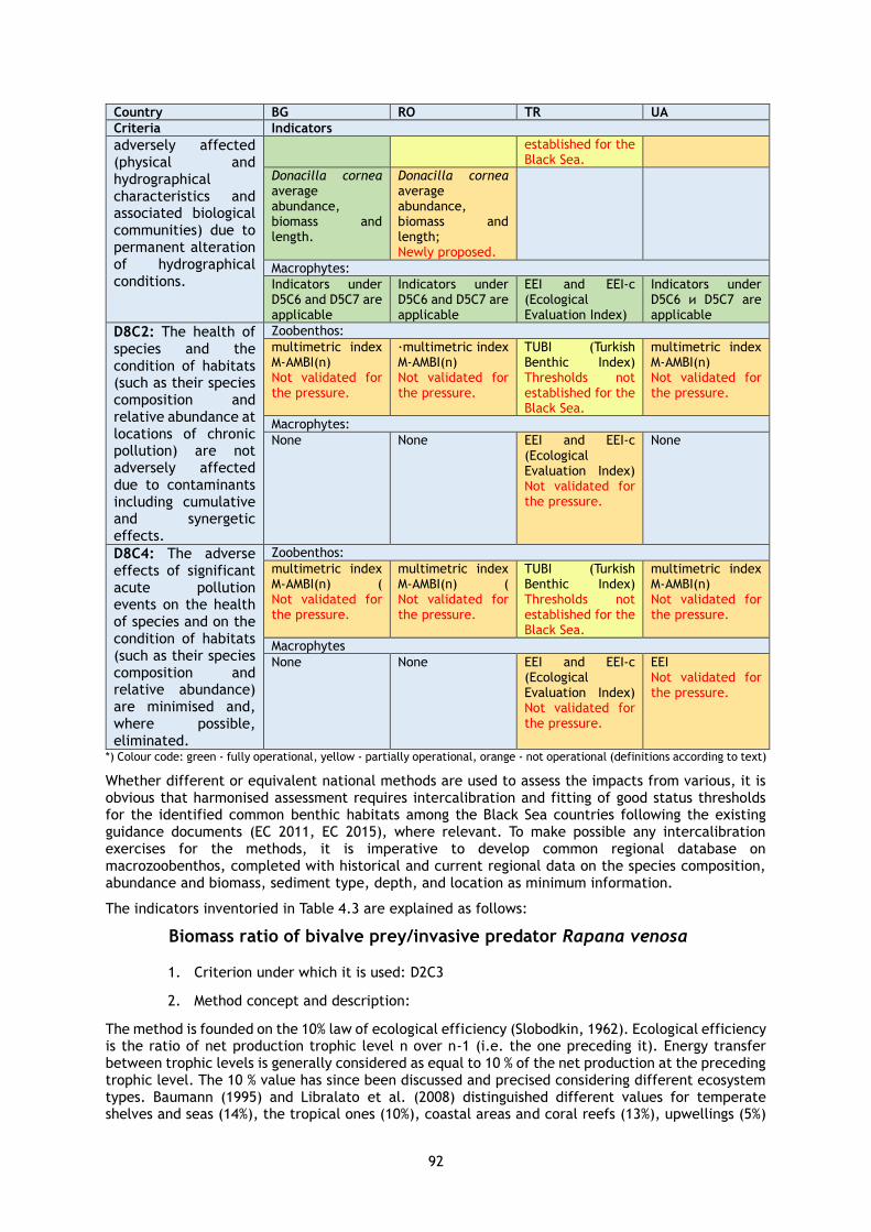
92

Country BG RO TR UA

Criteria Indicators

adversely affected (physical and hydrographical characteristics and associated biological communities) due to permanent alteration of hydrographical conditions.

established for the Black Sea.

Donacilla cornea average abundance, biomass and length.

Donacilla cornea average abundance, biomass and length; Newly proposed.

Macrophytes:

Indicators under D5C6 and D5C7 are applicable

Indicators under D5C6 and D5C7 are applicable


Indicators under D5C6 и D5C7 are applicable

D8C2: The health of species and the condition of habitats (such as their species composition and relative abundance at locations of chronic pollution) are not adversely affected due to contaminants including cumulative and synergetic effects.

Zoobenthos:

multimetric index M-AMBI(n) Not validated for the pressure.

·multimetric index M-AMBI(n) Not validated for the pressure.



Macrophytes:

None None EEI and EEI-c (Ecological Evaluation Index) Not validated for the pressure.

None

D8C4: The adverse effects of significant acute pollution events on the health of species and on the condition of habitats (such as their species composition and relative abundance) are minimised and, where possible, eliminated.

Zoobenthos:

multimetric index M-AMBI(n) ( Not validated for the pressure.

multimetric index M-AMBI(n) ( Not validated for the pressure.



Macrophytes

None None EEI and EEI-c (Ecological Evaluation Index) Not validated for the pressure.

EEI Not validated for the pressure.

*) Colour code: green - fully operational, yellow - partially operational, orange - not operational (definitions according to text)

Whether different or equivalent national methods are used to assess the impacts from various, it is obvious that harmonised assessment requires intercalibration and fitting of good status thresholds for the identified common benthic habitats among the Black Sea countries following the existing guidance documents (EC 2011, EC 2015), where relevant. To make possible any intercalibration exercises for the methods, it is imperative to develop common regional database on macrozoobenthos, completed with historical and current regional data on the species composition, abundance and biomass, sediment type, depth, and location as minimum information.

The indicators inventoried in Table 4.3 are explained as follows:

Biomass ratio of bivalve prey/invasive predator Rapana venosa

1. Criterion under which it is used: D2C3

2. Method concept and description:

The method is founded on the 10% law of ecological efficiency (Slobodkin, 1962). Ecological efficiency is the ratio of net production trophic level n over n-1 (i.e. the one preceding it). Energy transfer between trophic levels is generally considered as equal to 10 % of the net production at the preceding trophic level. The 10 % value has since been discussed and precised considering different ecosystem types. Baumann (1995) and Libralato et al. (2008) distinguished different values for temperate shelves and seas (14%), the tropical ones (10%), coastal areas and coral reefs (13%), upwellings (5%)

93

and lagoons (11%). Christensen and Pauly (1992) summarize many studies with a fairly wide range of values from a few % to the 20s %. Nevertheless, 10 % is taken as a reasonable average for free-living consumers and is used in many models.

In the proposed index biomass (dry weight) is used as a proxy of energy or production.

In addition to the ratio, a reference/baseline value for good status of bivalves biomass is required to be established as well.

3. Formula: Ratio bivalves/Rapana = Biomass bivalves/Biomass R. venosa

4. Units of measurement: Ratio

5. EQR (if relevant): Not relevant

6. Has the indicator been validated for the relevant pressure under the respective

descriptor?

The indicator requires validation with in-situ and experimental data.

7. For which habitats and biotopes is it used?

All habitats within the distribution range of Rapana venosa. R. venosa is known as a habitat generalist, which is distributed across the infra- and circa-littoral sediments and hard bottom in the Black Sea. It is rarely found in deep (offshore) circalittoral zone due to low temperature limitation.

8. Thresholds for GES

Biomass bivalves/Biomass R. venosa ≥ 10

The threshold for GES is based on the 10% trophic efficiency.

ALEX (Alien Biotic Index)

1. Criterion under which it is used: C2D3


The Alien Biotic Index (ALEX) to assess impacts of alien species on benthic communities. The ALEX index classifies the ecological status of water bodies from bad to very good according to the abundance and richness of alien species in the region. ALEX is also important in terms of showing the cumulative effect of alien species in the region.

Species within a benthic community can be classified into 4 biogeographic groups: native species, established species, casual species and invasive species. According to this classification, alien species within a community can be attained to one of the groups indicated below:

• Group I (Native species). Species naturally occurring in the region.

• Group II (Casual alien species). Alien species with only one report in the region and having a few number of individuals without reproductive products.

• Group III (Established alien species). Alien species with self-maintaining populations.

• Group IV (Invasive alien species). Alien species that have overcome biotic and abiotic barriers and are able to expand their geographic range through the production of fertile offspring with noticeable impact on the invaded habitats.

3. Formula

ALEX= [(0x%GI) + (3x(%GII + %GIII)) + (5x(%GIV))]/100

where % GI,II,II,IV is the percentage of the abundance of each biogeographic group.

4. Units of measurement: EQR

5. EQR (if relevant)

EQR is used to define the class boundary values by dividing the continuum of metric values into five equal width classes. Using the EQR approach the equidistant boundaries were set by dividing EQR=1/5

94

(Table 4.4).

• High status: A community which does not have any alien species or have a few number of established or invasive species with low number of individuals.

• Good status: A community which has alien species, but the majority of animal populations (>50%) belong to native species.

• Moderate status: A community that tends to become shifting from the native species-dominated phase to the alien species-dominated phase.

• Poor status: A community which is heavily affected by invasive alien species (group IV) that account for 55%–80% of animal populations.

• Bad status: A community which is extremely affected by invasive alien species (group IV) that account for more than 80% of animal populations.


descriptor?

Yes


ALEX is used in both coastal waters and shelf benthic habitats.


The class boundaries of the impact status and the ecological quality ratios based on ALEX. The values of this index range from 0 to 5. The value 0 means that the community contains no alien species, whereas the value 5 means that the community has been totally invaded by alien species. A community can be evaluated under 5 ecological status classes in terms of the impact of alien species.

Table 4.4 - ALEX class boundaries and EQR under WFD and GES threshold under MSFD

Impact Status EQR ALEX WFD Status MSFD Status

Non-affected 1 < ALE X ≤ 0.8 0 < ALEX ≤ 1 High Good

Slightly affected 0.8 < ALEX ≤ 0.6 1 < ALEX ≤ 2 Good

Moderately affected 0.60< ALEX ≤ 0.40 2 < ALEX ≤ 3 Moderate Not good

Heavily affected 0.40< ALEX ≤ 0.20 3 < ALEX ≤ 4 Poor

Extremely affected 0.20< ALEX≤ 0 4 < ALEX ≤ 5 Bad

The 95 percentile of the height (H) and length (L) of the commercially exploited bivalves

1. Criterion under which it is used: D3C3


The size distribution of individuals in the populations of commercially-exploited species is indicative of a healthy population if it includes a high proportion of old/large individuals. The 95 th percentile of length (height) distribution of each population is one of the properties that reflects the proportion of large individuals.

3. Formula

n=0.95*N

where N = number of values in the data set, and n = nearest ordinal rank of a given value (with the values in the data set sorted from smallest to largest).

4. Units of measurement: Height/length in mm.

5. EQR (if relevant): Not relevant


descriptor?

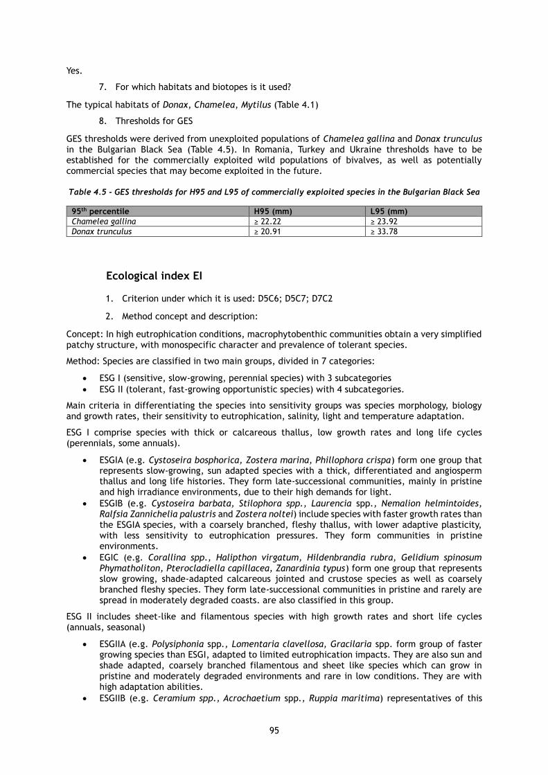
95

Yes.


The typical habitats of Donax, Chamelea, Mytilus (Table 4.1)


GES thresholds were derived from unexploited populations of Chamelea gallina and Donax trunculus in the Bulgarian Black Sea (Table 4.5). In Romania, Turkey and Ukraine thresholds have to be established for the commercially exploited wild populations of bivalves, as well as potentially commercial species that may become exploited in the future.

Table 4.5 - GES thresholds for H95 and L95 of commercially exploited species in the Bulgarian Black Sea

95th percentile H95 (mm) L95 (mm)

Chamelea gallina ≥ 22.22 ≥ 23.92

Donax trunculus ≥ 20.91 ≥ 33.78

Ecological index EI

1. Criterion under which it is used: D5C6; D5C7; D7C2


Concept: In high eutrophication conditions, macrophytobenthic communities obtain a very simplified patchy structure, with monospecific character and prevalence of tolerant species.

Method: Species are classified in two main groups, divided in 7 categories:

• ESG I (sensitive, slow-growing, perennial species) with 3 subcategories

• ESG II (tolerant, fast-growing opportunistic species) with 4 subcategories.

Main criteria in differentiating the species into sensitivity groups was species morphology, biology and growth rates, their sensitivity to eutrophication, salinity, light and temperature adaptation.

ESG I comprise species with thick or calcareous thallus, low growth rates and long life cycles (perennials, some annuals).

• ESGIA (e.g. Cystoseira bosphorica, Zostera marina, Phillophora crispa) form one group that represents slow-growing, sun adapted species with a thick, differentiated and angiosperm thallus and long life histories. They form late-successional communities, mainly in pristine and high irradiance environments, due to their high demands for light.

• ESGIB (e.g. Cystoseira barbata, Stilophora spp., Laurencia spp., Nemalion helmintoides, Ralfsia Zannichelia palustris and Zostera noltei) include species with faster growth rates than the ESGIA species, with a coarsely branched, fleshy thallus, with lower adaptive plasticity, with less sensitivity to eutrophication pressures. They form communities in pristine environments.

• EGIC (e.g. Corallina spp., Halipthon virgatum, Hildenbrandia rubra, Gelidium spinosum Phymatholiton, Pterocladiella capillacea, Zanardinia typus) form one group that represents slow growing, shade-adapted calcareous jointed and crustose species as well as coarsely branched fleshy species. They form late-successional communities in pristine and rarely are spread in moderately degraded coasts. are also classified in this group.

ESG II includes sheet-like and filamentous species with high growth rates and short life cycles (annuals, seasonal)

• ESGIIA (e.g. Polysiphonia spp., Lomentaria clavellosa, Gracilaria spp. form group of faster growing species than ESGI, adapted to limited eutrophication impacts. They are also sun and shade adapted, coarsely branched filamentous and sheet like species which can grow in pristine and moderately degraded environments and rare in low conditions. They are with high adaptation abilities.

• ESGIIB (e.g. Ceramium spp., Acrochaetium spp., Ruppia maritima) representatives of this

96

group are sun and shade adapted, fast growing, filamentous species. Some of them grow in all environments; the species are with high abundances in waters of high, good and moderate conditions.

• ESGIICa (e.g. Chaetomorpha aerea, Ulva rigida, Ulva linza, Porphyra leucostica) form group that represents fast growing, thin filamentous and sheet - like species with high reproductive capacity and short life histories. They can grow in all environments but are abundant in highly degraded environments and disappear in highest degraded environments.

• ESGIICb (e.g. Cladophora sericea, Cladophora vadorum, Cladophora albida, Cladophora vagabunda, Ulva compressa, Ulva flexuosa, Ulva intestinalis, Urospora, Rhizoclonium, Bacillariophyta, Cyanobacteria) represent faster-growing, than these in ESGIICA thin filamentous and sheet-like species with high reproductive capacity and short life histories. They can grow in all environments but mostly are abundant in highly degraded environments.

The assemblage of benthic macrophytes at each transect was assessed according to the biomass (%) of species, dividing samples in the following groups: less than 100% biomass of tolerant species (ESGII), between 0 and 40% biomass of sensitive species (ESGI), 60%-80% and above 80% biomass. The average biomass of sensitive (ESGI) and tolerant (ESGII) species from all the samples collected from replicate transects is calculated. The index is expressed as the proportion of sensitive and tolerant species average biomasses at each transect. As a value of EI, we take the biomass proportion of the most sensitive group. EI takes values in the range of 0-10, divided in five classes: 0-2 bad status, > 2-4 poor status, > 4–6 moderate, > 6-8 good and > 7.8-10 high status (equidistant division of classes).

3. Formulae

The proportion each ESG group within the two main groups ESG I and ESG II was corrected with a coefficient. The criteria for this correction were distribution along the eutrophication gradient, phenotypic plasticity and growth rate. Weight coefficients were defined for different subgroups as follows:

ESG IA–coef=1; ESGIB-coef=0.8

ESGIC-coef=0.6

ESGIIA-coef=0.6

ESGIIB-coef=0.8

ESGIIC-coef=1

After assessing the biomass proportion of every group, it is multiplied by the coefficient of this group, as follows:

ESGI= ESGIA*1+ESGIB*0.8+ESGIC*0.6

ESGII=ESGIIA*0.6+ESGIIB*0.8+ESGIIC*1

To calculate the value of EI we apply the following rules and formulas:

When ESGI = 0 - Bad status, we take the most sensitive group left from ESGII.

In case when ESGI = 0, ESGII (A+B) = 0 and ESGIICa has biomass proportion from 0 - 100%, EI takes values of 0 – 1, and is calculated with the following formula:

EI- bad (0-1) = [ESGIICa/ESGII], when ESGI=0, ESGII(A +B) = 0

When ESGI= 0 and 0%>ESGII(A+B)≤ 100% we have EI with bad status (1-2). In this case the index is expressed as the biomass proportion of the most sensitive subgroup selected from ESGII.

EI- bad (1-2) = [(ESGIIA/(ESGIIA+ESGIIB+ESGIIC))*0.6+ (ESGIIB/(ESGIIA+ESGIIB+ESGIIC)*0.8]+1

When the proportion of sensitive species (ESGI) is between 0 - 40%, EI takes values between 2 - 4 and we have a poor status. The following formula is applied:

EI poor (2-4) = ([(ESGIA/(ESGI+ESGII))*1+(ESGIB/(ESGI+ESGII))*0.8+ (ESGIC/(ESGI+ESGII))*0.6]*5)+2

When the proportion of sensitive species is between 40-60%, EI is between 4-6. At 60-80% biomass proportion, EI is between 6 - 8 and at 80 - 100%, EI is between 8 and 10. In these three cases EI is calculated following this formula:

97

EI high, good, moderate (4-10) = [(ESGIA/(ESGI+ESGII))*1+ (ESGIB/(ESGI+ESGII))*0.8 +(ESGIC/(ESGI+ESGII))*0.6]*10

Where ESGI, II is the biomass (wet weight) of the respective ecological group.

4. Units of measurement: Ecological Index EI is a composite indicator and it does not have

units of measurement.

5. EQR (if relevant), reference conditions

EI EQR = (EI value/RC value)

Referent value is RC=9,32. The value of the reference condition was calculated using the median value of the dataset from the referent sites from the intercalibration exercise in Bulgaria and Romania (Berov et al, 2018).

EI-EQR high-good-moderate = [10* (ESGI/ESGI+ESGII)]/ref value;

EI-EQR poor = [5*(ESGI/ESGI+ESGII]+2]//ref.value;

EI-EQR bad (1-2) = (ESGII(A+B)/ESGII+1)/ref.value, when ESGI=0;

EI-EQR bad (0-1) = (ESGIICa/ESGII)/ref. value, when ESGI=0, ESGII(A+B) = 0.


descriptor?

The Ecological index EI was validated for the relevant pressure for D5C7 under the Intercalibration exercise between Romania and Bulgaria. A modified version of the LUSI pressure index was applied which was adapted to the specific conditions of the western Black Sea coast and local anthropogenic pressures on macroalgal communities (LUSI_BS). The final LUSI score was calculated with the following formula:

LUSI_BS= (score urb + score agric + score indust + score typology + others significant pressures) * correction number


The Ecological index EI is used for ecological status assessment of the costal water bodies in Bulgaria and Romania. Regarding the MSFD broad habitat types, it is used for the evaluation of the following broad habitats: Infralittoral rock and biogenic reef (MB1, MB2); Infralittoral sand (MB5).


Table 4.6 - EI class boundaries and EQR under WFD and GES threshold under MSFD

Biomass proportions of sensitive and tolerant species

EI EQREI WFD status MSFD Status

80-100%ЕSGI 7.8- 10 0.837 – 1 High Good

60-80%ESGI 6-7.8 0.644 – 0.837 Good

40-60%ESGI 4-6 0.429 – 0.644 Moderate Not good

0-40%ESGI 2-4 0.214 – 0.429 Poor

0%ESGI <2 <0.214 Bad

The indicators % wet biomass of the tollerant macroalgae (ESGII) (D5C6) and % wet biomass of the macroalgae from ESGI (D5C7) are derived from EI method with GES thresholds as defined for the groups (Table 4.1): ESGI > 60%, ESGII < 40%, respectively.

Ecological Evaluation Index EEI-c

1. Criterion under which it is used: D5C8, D6C3, D7C2, D8C2, D8C4


Marine macrophytes (macroalgae and angiosperms) were classified into five ecological status groups (ESG), ESGI (IA, IB, IC; Sensitive, late-successional taxa such as Cystoseira spp., Padina pavonica, angiosperms, calcareous algae), and ESGII (IIA, IIB; opportunistic taxa such as filamentous and sheet-like green algae Ulva and Cladophora spp.).

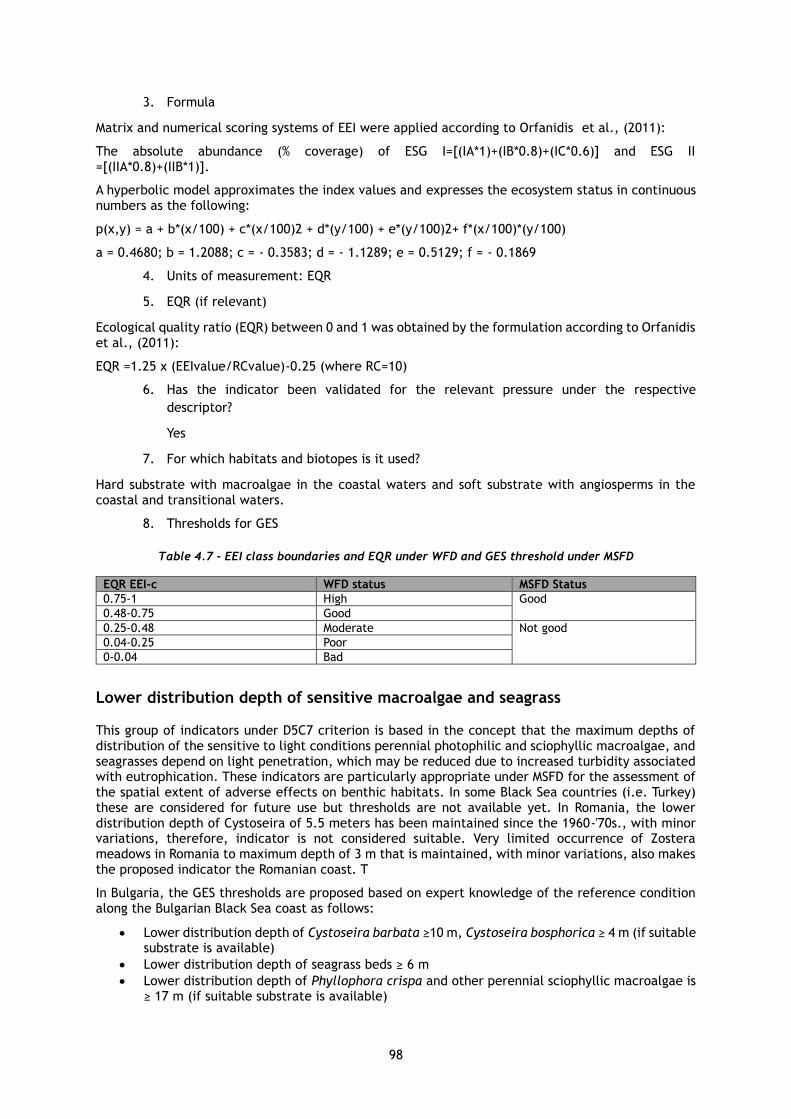
98

3. Formula

Matrix and numerical scoring systems of EEI were applied according to Orfanidis et al., (2011):

The absolute abundance (% coverage) of ESG I=[(IA*1)+(IB*0.8)+(IC*0.6)] and ESG II =[(IIA*0.8)+(IIB*1)].

A hyperbolic model approximates the index values and expresses the ecosystem status in continuous numbers as the following:

p(x,y) = a + b*(x/100) + c*(x/100)2 + d*(y/100) + e*(y/100)2+ f*(x/100)*(y/100)

a = 0.4680; b = 1.2088; c = - 0.3583; d = - 1.1289; e = 0.5129; f = - 0.1869



Ecological quality ratio (EQR) between 0 and 1 was obtained by the formulation according to Orfanidis et al., (2011):

EQR =1.25 x (EEIvalue/RCvalue)-0.25 (where RC=10)


descriptor?

Yes


Hard substrate with macroalgae in the coastal waters and soft substrate with angiosperms in the coastal and transitional waters.


Table 4.7 - EEI class boundaries and EQR under WFD and GES threshold under MSFD

EQR EEI-c WFD status MSFD Status

0.75-1 High Good

0.48-0.75 Good

0.25-0.48 Moderate Not good

0.04-0.25 Poor

0-0.04 Bad

Lower distribution depth of sensitive macroalgae and seagrass

This group of indicators under D5C7 criterion is based in the concept that the maximum depths of distribution of the sensitive to light conditions perennial photophilic and sciophyllic macroalgae, and seagrasses depend on light penetration, which may be reduced due to increased turbidity associated with eutrophication. These indicators are particularly appropriate under MSFD for the assessment of the spatial extent of adverse effects on benthic habitats. In some Black Sea countries (i.e. Turkey) these are considered for future use but thresholds are not available yet. In Romania, the lower distribution depth of Cystoseira of 5.5 meters has been maintained since the 1960-'70s., with minor variations, therefore, indicator is not considered suitable. Very limited occurrence of Zostera meadows in Romania to maximum depth of 3 m that is maintained, with minor variations, also makes the proposed indicator the Romanian coast. T

In Bulgaria, the GES thresholds are proposed based on expert knowledge of the reference condition along the Bulgarian Black Sea coast as follows:

• Lower distribution depth of Cystoseira barbata ≥10 m, Cystoseira bosphorica ≥ 4 m (if suitable substrate is available)

• Lower distribution depth of seagrass beds ≥ 6 m

• Lower distribution depth of Phyllophora crispa and other perennial sciophyllic macroalgae is ≥ 17 m (if suitable substrate is available)

99

Ecological evaluation indices (EEI), calculated by morpho-functional indices of macrophytes: ecological activity of three dominant species (S / W)3Dp, m2·kg-1), mean ecological activity of species (S / W)x, m2·kg-1), phytocoenosis surface index (SIph).

1. Criterion under which it is used: D5C6, D8C4


All of these methods are based on a specific surface (surface, divided by weight) of the whole community.

Three Dominants Ecological Activity (S/W)3Dp has a high indicator sensitivity of the eutrophication level of an ecosystem. This is due to the existing regularities connecting minimal possible values of S/Wp of macrophytes with a certain intensity of the primary production process. In the case of autotrophic process intensification, an increase of limiting barrier takes place for the ecological activity of species. The species, who’s S/Wp becomes less than a certain value, move into the suppressed state and at the stages of more intensive eutrophication disappear from communities’ structure. The lowest S/Wp, coefficients are characteristic of the biggest perennial forms of macrophytes. As a rule, those forms dominate in phytobenthos. Thus, the dominating macrophyte species are the most sensitive in an ecosystem to environmental state aggravation and are the most vulnerable elements of vegetation communities.

Average Species Ecological Activity (S/W)x takes into account the average value of the specific surface of all phytobenthos species in the coastal area being assessed. Such a recording of the complete floristic structure of macrophytobenthos communities is traditional for classical hydrobiological studies. However, identification of complete floristic composition including small epiphytic species is quite a complicated technical task for monitoring. Besides, there are some restrictions from the side of morphofunctional regularities in phytobenthos floristic structure forming. Small short-cycle species having high S/Wp values do not have high indicative sensitivity to habitat. In the ecosystems assessed as ‘Bad – ESC’ they are mass species and show explodes, though their presence in small quantities could be found in the floristic composition of the communities, which develop under reference conditions.

For the SIph parameter coefficients S/Wph of the populations included in the phytocenosis and the sum of absolute values of their biomass are used. The benefit provided by this parameter is that its values could be recalculated based on the available historical databases on macrophytobenthos floristic composition and biomass for any monitored area. The benefit of the S/Wph parameter, being suggested for the first time, is that for its calculation not the absolute, but the relative values of structural parameters are used. Such a recording method reflects only the real morphofunctional portrait of a community and is protected from the influence of other factors, which are not connected directly with the intensity of autotrophic process. For example, changes in biomass or bottom cover decrease as the result of active hydrodynamics could be the reason for significant errors in the parameters calculated on their basis.

3. Formula:

Ecological activity of three dominant species n3

)W/S(3W/S

piDp3

= , where

S/Wpi – the specific surface of all populations in the community

mean ecological activity of species ni

)W/S(W/S

pix

= , where

S/Wpi – the specific surface of all populations in the community

phytocoenosis surface index ))W/S(B(Spipiph = , where

S/Wpi – the specific surface of all populations in the community, and Bpi – the biomass of phytocenosis populations

100

4. Units of measurement:

(S/W)3Dp and (S/W)x,- m2.kg-1

SIph Units

5. EQR (if relevant), reference conditions

Reference conditions were defined as a state in the past, that is considered to reflect the state of least impacted condition. For Ukrainian waters, this is the state in 60th, before the eutrophication.

The high boundaries were set as the reference conditions. The remaining boundaries were set by analyzing a complete historical database from 60th to present.

The main feature of the national waters of Ukraine is the presence of an extensive shelf of numerous limans and large river zones (Danube, Dniester, and Dnieper). As a result, marine coastal waters can be divide into zones with different salinity: 12-17 ‰ - the main part of marine coastal and shelf water areas and zones adjacent to river mouths with salinity below 12 ‰, where a higher level of the production process is observed. Therefore, taking into account the natural differences, EQRs are set separately for areas with different salinity.


descriptor?

The indicator has been validated for the relevant pressure under criteria D5C6.


• Lower infralittoral (10-18 m) rock with dominant perennial sciaphylic red and brown macroalgae (Phyllophora crispa, Zanardinia typus, Apoglossum ruscifolium) and/or widely adaptive green (Cladophora albida, Cladophora coelothrix) and red macroalgae (Polysiphonia elongata, Gelidium spinosum, Gelidium crinale, Anithamniom cruciatum)

• Upper infralittorlal (1-10 m) rock with variable annual green and red macroalgae: Ceramium virgatum, Gelidium spinosum, G. crinale, Corallina mediterranea, Ulva rigida, Ulva linza, U. intestinalis, Cladophora sericea, C. albida, Bryopsis plumosa and other

• Zostera noltei meadows (1-3 m)

• Zostera marina meadows (4-7 m)


There is currently no clear method for deriving Thresholds Value. The proposed approach to combining the calculation method taking into account the variability of the series of macrophytobenthos indicators and the expert judgment method requires further development of verification based on the analysis of databases of other indicators.

Table 4.8 - Ecological Status Class boundaries of coastal areas of the Ukrainian Black Sea with salinity within 12-17 ‰

Ecological status under WFD

(S/W)3Dp, m2.kg-1 EQR (S/W)x, m2·kg-1 EQR SIph units EQR

High (S/W)3Dp < 15 ≥ 0.82 (S/W)x < 60 ≥0.98 SIph < 25 ≥ 0.95

Good 15 ≤ (S/W)3Dp ≤ 30 0.54 60 ≤ (S/W)x ≤ 80 0.79 25 ≤ SIph ≤ 40 0.84

Moderate 31 ≤ (S/W)3Dp ≤ 45 0.37 81 ≤ (S/W)x ≤ 120 0.58 41 ≤ SIph ≤ 55 0.68

Poor 46 ≤ (S/W)3Dp ≤ 60 0.25 121 ≤ (S/W)x ≤ 200 0.17 56 ≤ SIph ≤ 90 0.15

Bad (S/W)3Dp > 60 ≥0 (S/W)x > 200 ≥0 SIph > 90 ≥0

Table 4.9 - Ecological Status Class boundaries of coastal areas of the Ukrainian Black Sea with salinity less than 12 ‰


(S/W)3Dp, m2·kg-1 EQR (S/W)x, m2·kg-1 EQR SIph units EQR

High (S/W)3Dp < 50 ≥ 0,87 (S/W)x < 90 ≥ 0,88 SIph < 20 ≥ 0,71

Good 50 ≤ (S/W)3Dp ≤ 80 0,79 90 ≤ (S/W)x ≤ 150 0,73 20 ≤ SIph ≤ 50 0,39

101


(S/W)3Dp, m2·kg-1 EQR (S/W)x, m2·kg-1 EQR SIph units EQR

Moderate 80 ≤ (S/W)3Dp ≤ 260 0.35 150 ≤ (S/W)x ≤ 350 0.33 50 ≤ SIph ≤ 70 0,23

Poor 260 ≤ (S/W)3Dp ≤ 360 0.16 350 ≤ (S/W)x ≤500 0.14 70 ≤ SIph ≤ 100 0,05

Bad (S/W)3Dp > 360 ≥ 0 (S/W)x > 500 ≥ 0 SIph > 100 ≥ 0

Table 4.10 - Ecological Status Class boundaries for Percentage of the sensitive species (Ssp, %) in the Ukrainian Black Sea region

Ecological status under WFD Ssp, % EQR

High 100 ≥ (Ssp, %)> 86 1,0 -0,86

Good 85≥ (Ssp, %)> 51 0,85 – 0,51

Moderate 50 ≥ (Ssp, %) >21 0,50 – 0,21

Poor 20 ≥ (Ssp, %) >1 0,20 – 0,01

Bad (Ssp, %) = 0 0

M-AMBI*(n) – M-AMBI normalized

1. Criteria under which it is used: D5C8, D6C3, D7C2, D8C2, D8C4

2. Method concept description:

M-AMBI*(n) (Sigovini et al., 2013) is a simplified modification of the original method M-AMBI (Muxika et al., 2007). The original method is based on benthic macroinvertebrates for assessing the ecological quality status of marine and transitional waters. It integrates AMBI (Borja et al., 2000), a biotic index based on species sensitivity/tolerance to pressures with Shannon-Wiener diversity index (H’) (Shannon & Weaver, 1949), and species richness (S) making it compliant to the WFD.

Sigovini et al., argue that factor analysis in M-AMBI should be discarded, since the index does not benefit from it anyway. Instead of using factor analysis, M-AMBI*(n) combines the metrics as an arithmetic mean of their normalized values. By substituting standardization of metrics with their min-max normalization, the index is transformed into the simple mean of the three equally weighted normalized metrics, therefore becoming independent of the number of samples. In the normalization procedure, instead of minimum and maximum values of the dataset, the established Reference values of the metrics are used as maximum and the Bad extremum is used as minimum.

According to geographic intercalibration results, the overall assessment concept is based on the principles that disturbance –sensitive taxa decrease, while tolerant and opportunistic species increase along the increasing pressure gradient, coupled with decrease in species richness and evenness of distribution. These two aspects of the invertebrate community change are reflected by AMBI and S/H’ respectively, combined in a composite index M-AMBI*(n).

3. Formula:

As explained above, the values of the three constituent indices of M-AMBI (AMBI, S and H’) must be first normalized using the following formulae:

AMBI*(n) = 1 – (AMBI – AMBIRef) / (AMBIBad – AMBIRef)

S*(n) = (S – SBad) / (SRef – SBad)

H’*(n) = (H’ – HBad) / (HRef – HBad)

Next step is to calculate the arithmetic mean of the normalized values of AMBI, S and H’.


5. EQR

M-AMBI index was elaborated in the scope of WFD implementation and adapted for MSFD. As the WFD requires EQR values for the “values of the biological quality elements”, the main aim of EQR is to enable comparison between EU Member States assessment methods. Therefore, both M-AMBI and the normalized M-AMBI methods include EQR. In the geographic intercalibration exercise between

102

Bulgaria and Romania, statistical boundary setting using EQRs relative to the reference values of the metrics was used. Thus, High/Good boundary is set as EQR=0.9 from reference value for each of the metrics used S, H’, AMBI and M-AMBI(n). The remaining 4 class boundaries (under WFD) by dividing the continuum of metric values between the established High/Good boundary and the Bad extrema (0 for S, H’, and M-AMBI(n) and 6 for AMBI) into four equal width classes. Using the EQR approach the equidistant boundaries were set by dividing EQR=0.9/4. Thus, EQR=0.68 from reference is set as Good/Moderate boundary under WFD, which is utilized as a threshold for Good/Not good status under MSFD.


descriptor?

For the Descriptor 5 (D5C8) the indicator was validated during the geographic intercalibration exercise between Bulgaria and Romania against the following pressures:

• Point sources: annual mean loads for BOD, suspended solids (SS), total heavy metals, detergents (DET), phenols (PHE), total petroleum hydrocarbons (TPH)

• Diffuse sources: land use based on CORINE landcover within 1000 m stripe of coastal territory including:

Urban area: includes the categories 111 Continuous urban fabric, 112 Discontinuous urban fabric.

Industrial area: includes the categories 121 Industrial or commercial units, 122 Road and rail networks and associated land, 123 Port areas, 124 Airports, 131 Mineral extraction sites, 132 Dump sites, 133 Construction sites.

• Diffuse sources: tourism – input data are overnights spent in the coastal municipalities; relative pressure values at the monitoring sites were calculated in GIS using Spatial Analysis Tool.

• Diffuse sources: navigation – input data is density map of AIS positions data (available at http://www.marinetraffic.com), relative pressure values were calculated in GIS using Spatial Analysis Tool.

Pressure data were collected from both countries.

For D6 (D6C3) and D8 (D8C2 and D8C4), this indicator was not validated against physical pressures and effects of acute and chronic pollution by contaminants. Further work is needed.


M-AMBI*(n) index is used for benthic communities inhabiting sedimentary habitats: sands of different grain size, mud, and combination of them, and mixed sediments, containing different proportion of molluscs’ shells.


For the assessment of environmental status for MSFD purpose, the threshold between good environmental status (GES) and not good environmental status (non-GES) was set as the boundary between good and moderate ecological status established under WFD.

In Romania, apart from the waterbodies falling under WFD assessment requirements (coastal waters and transitional waters), for two circalittoral habitat types reference values and thresholds values have been derived for M-AMBI*(n). These are: Circalittoral mud with Mytilus galloprovincialis banks and Circalittoral mixed sediments with Modiolula phaseolina (Abaza et al., 2018)

Reference conditions for the three M-AMBI *(n) parameters (AMBI, diversity and richness) were calculated using the 0.95 percentile of richness (S) and diversity (H) values and the 0.05 percentile of AMBI values, using the available data (Table 4.11).

Table 4.11 - GES thresholds defined for coastal and shelf habitats in the Romanian Black Sea

Ecological status EQR AMBI H' S M-AMBI*n

Infralittoral sand and mud in waters with variable salinity

Reference conditions 1 1.8 2.9 15 0.90

Good status 0.68 3.21 1.9 10 0.61

Circalittoral sand/mud in waters with variable salinity

103



Good status 0.68 3.21 1.9 10 0.61

Circalittoral mud with Mytilus galloprovincialis biogenic reef and diverse fauna


Good status 0.68 2.8 2.38 16 0.68

Offshore circalittoral mud with Modiolula phaseolina


Good status 0.68 2.06 2.52 14 0.61

In Bulgaria, four classification systems were developed by Todorova (2017) according to the procedures described above for the coastal waters under WFD, which are also applicable under MSFD (Table 4.12) Further work is required to validate the index for physical disturbance and establish thresholds for the benthic habitats beyond coastal waters.

Table 4.12 - GES thresholds defined for coastal benthic habitats in the Bulgarian Black Sea


Upper infralittoral meadium and fine sands dominated by Donax trunculus


Good status 0.68 2.26 2.11 12 0.62

Infralittoral fine and medium sands dominated by Chamelea gallina, Lentidium mediterraneum, Tellina tenuis


Good status 0.68 2.12 2.31 20 0.59

Infralittoral coarse and medium sands dominated by Upogebia pusilla


Good status 0.68 3.62 2.31 24 0.65

Circalittoral shelly sands and gravel with diverse variable fauna


Good status 0.68 3.28 2.58 29 0.64

TUBI (Turkish Benthic Index)

1. Criteria under which it is used: D5C8, D6C3, D7C2, D8C2, D8C4

2. Method description, concept:

Turkey Benthic Index (TUBI) is developed specific to the Aegean-Mediterranean soft substrate benthic fauna in Turkey. The index has two metrics: the Shannon-Weiver’s diversity index (metric 1) and the relative abundance of ecological groups (metric 2).

3. Formula

The formula of Turkish Biotic Index (TUBI) is as follows:

TUBI =𝑀𝑒𝑡𝑟𝑖𝑐1 + (5 − 𝑀𝑒𝑡𝑟𝑖𝑐2)2

2

𝑇𝑈𝐵𝐼 =𝐻′ † +[5 − (

0𝑥𝐺1%+3𝑥𝐺2%+5𝑥𝐺3%100

100)]2

2† 𝐻′ > 5 ⇒ 𝐻′ = 5

4. Units of measurement

Macro-zoobenthic species within a benthic community can be classified into five ecological groups according to their sensitiveness to disturbances Group I (GI, sensitive species), Group II (GII, indifferent species), Group III (GIII, tolerant species), Group IV (GIV, second order of opportunistic

104

species) and GV (GV, first order of opportunistic species). In the calculation of the metric 2 of TUBI, three major ecological groups were considered; Group 1 includes sensitive and indifferent species (GI and GII), Group 2 includes tolerant species (GIII), and Group 3 includes opportunistic species (GIV and GV).


EQRTUBI is used to define the class boundary values by dividing the continuum of metric values into five equal width classes. Using the EQR approach the equidistant boundaries were set by dividing EQR=1/5 (Table V.13).


descriptor?

Yes


TUBI is used for soft bottom benthic habitats.


The values have not been calibrated for the Black Sea coast of Turkey.

Table 4.13 - TUBI class boundaries and EQR under WFD and GES threshold under MSFD

Impact Status EQR TUBI WFD Status MSFD Status

Non-affected 0.8 < TUBI ≤ 1 4 ≤ TUBI ≤ 5 High Good

Slightly affected 0.6≤ TUBI<0.8 3 ≤ TUBI < 4 Good

Moderately affected

0.40≤ TUBI< 0.60 2 ≤ TUBI < 3 Moderate Not good

Heavily affected 0.20≤ TUBI< 0.40 1 ≤ TUBI < 2 Poor

Extremely affected 0 ≤ TUBI< 0.20 0 ≤ TUBI <1 Bad

4.4.4 Integration and aggregation

The assessment of benthic habitats should be based, as far as possible, on outputs of assessments for the relevant pressure-based descriptors, expressed as the extent of impact per pressure. The level 1 and 2 integration rules below relate primarily to these other assessments. The integration methods are summarised in on Figure 4.3 and described below:

• Level 1: Measurements of individual parameters — for example seabed grab or video samples, acoustic surveys etc. These are combined into indicators and maps (often based on modelled data) of habitat types, extent and condition, and the spatial extent, distribution and intensity of physical and other pressures.

• Level 2: The individual indicators and maps (see list in level 1) and benthic composition and quality (to assess the extent of adverse effects from different pressures etc.), are combined to inform the criteria D6C1, D6C2 and D6C3. The latter criteria are outputs from the assessment of the pressure-based descriptors: D6C3 (extent of adverse effects from physical disturbance) and from other relevant pressure descriptors (e.g. extent of adverse effects from nutrient enrichment or hydrographical changes). Where representative subtypes of the broad habitat type are assessed, they may be used to inform/validate the assessments of the other pressure-based criteria (e.g. D6C3), but could also be used directly for D6C5.

o D6C1: This is directly from Descriptor 6, (a map of) the spatial extent and distribution of physical habitat loss);

o D6C2: This is directly from Descriptor 6, (maps of) the spatial extent and distribution of physical disturbance. Individual pressure maps can be produced for smothering, abrasion, extraction etc.

o D6C3: The extent and distribution of broad and other habitat types (habitat maps) is the basis for the assessment of impacts from physical disturbance identified in D6C2. Combining these, together with information on the sensitivity of the habitat types to the

105

pressures, and/or information on the condition of the habitat, provides information on the spatial extent of impacts by physical disturbance. The condition of habitat is assessed e.g. by multimetric indices and can be used both to feed in directly to the condition of the habitat (D6C5) as well as to calibrate the pressure-sensitivity relationship between D6C2 and D6C3 (as well as for other pressures).

• Level 3:

o D6C4: the output from D6C1 (total extent of physical loss in assessment area) is interfaced with the extent of the broad habitat type in the assessment area to derive the extent of loss for the habitat as a proportion (%) of the total habitat area. This should incorporate physical loss from physical infrastructure as well as from e.g. physico-chemical changes or biological exclusion.

o D6C5: the total extent of adverse effects on the broad habitat type from physical disturbance (D6C3) are brought together with the extent of adverse effects from other pressure criteria (e.g. D2C3, D5C5-8, D7C2, D8C2, D8C4), for example by overlaying impact maps on the habitat map. This impact extent is then related to the overall extent of the broad habitat to estimate the proportion (%) of the habitat area which is considered to be adversely affected. In some cases it may be appropriate to simply sum the areas affected by the pressures, but where there are cumulative or synergistic effects, or overlapping pressures, other approaches may be required.

o The extent of habitat loss and the extent of habitat in “not good” condition can be expressed as the proportion (%) of the total extent of the habitat type or an equivalent value (e.g. km2).

• Level 4: The results for criteria D6C4 and D6C5 are brought together for each broad habitat type. A conditional rule is used, where both criteria must be within the levels set for the extent of habitat which may be lost and adversely affected; the sum of the area lost and area adversely affected must not exceed the threshold for the area adversely affected, i.e. area lost should be taken into account in the area adversely affected, as loss is considered the most severe (irreversible) form of adverse effect.

• Level 5: The broad habitat types under D1/D6 are integrated at MRU scale by estimating the proportion of broad habitat types in good status from the number of all habitats present. ! Proportion thresholds is recommended to be set at 100 % (all habitats present in given MRU shall be in good status). As an exception, one of the broad habitat types is allowable to be in “not good” status in a particular MRU on the conditions that < 15 % of its national extent is in “not good” status and < 15 % of overall seabed in the MRU is in “not good” status. The proposed proportion threshold has been already agreed by Bulgaria and Romania within the Black Sea Working Group on MSFD common implementation but the allowable extent in “not good” status has been set at 20 %. The national experts have revised their previous decision due to setting the extent threshold for D6C5 at 15 %.

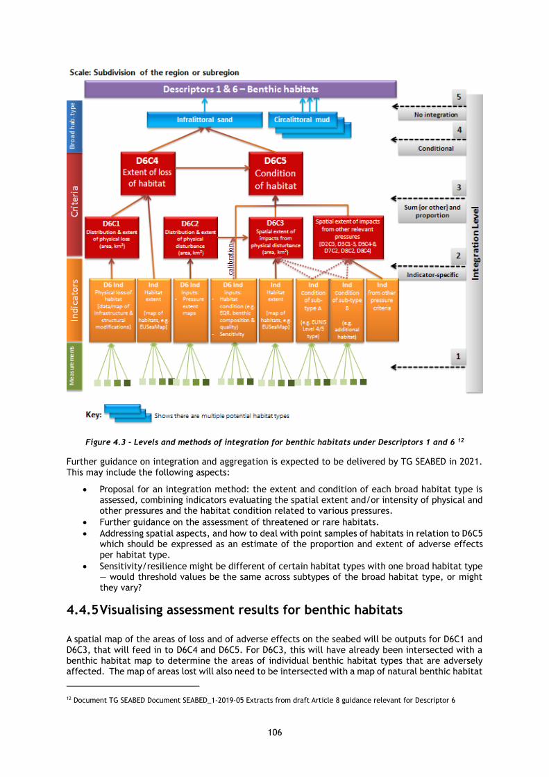
106

Figure 4.3 - Levels and methods of integration for benthic habitats under Descriptors 1 and 6 12

Further guidance on integration and aggregation is expected to be delivered by TG SEABED in 2021. This may include the following aspects:

• Proposal for an integration method: the extent and condition of each broad habitat type is assessed, combining indicators evaluating the spatial extent and/or intensity of physical and other pressures and the habitat condition related to various pressures.

• Further guidance on the assessment of threatened or rare habitats.

• Addressing spatial aspects, and how to deal with point samples of habitats in relation to D6C5 which should be expressed as an estimate of the proportion and extent of adverse effects per habitat type.

• Sensitivity/resilience might be different of certain habitat types with one broad habitat type — would threshold values be the same across subtypes of the broad habitat type, or might they vary?

4.4.5 Visualising assessment results for benthic habitats

A spatial map of the areas of loss and of adverse effects on the seabed will be outputs for D6C1 and D6C3, that will feed in to D6C4 and D6C5. For D6C3, this will have already been intersected with a benthic habitat map to determine the areas of individual benthic habitat types that are adversely affected. The map of areas lost will also need to be intersected with a map of natural benthic habitat

12 Document TG SEABED Document SEABED_1-2019-05 Extracts from draft Article 8 guidance relevant for Descriptor 6

107

types (or the benthic habitat types that were lost would need to be otherwise identified), to determine the area of each benthic habitat type that is lost.

The outcomes are presented for each broad benthic habitat type or additional habitat type, in each assessment area (subdivision of the region or subregion).

Table 4.14 - Assessment framework for benthic broad habitat types using MSFD criteria in the Black Sea

Table 4.14 provides a framework for harmonised reporting of the results. It includes all relevant to the benthic habitats descriptors, ecosystem elements, criteria and habitat condition indicators. In the example table the good status thresholds for habitat condition indicators are those established in Bulgaria. Extent thresholds for habitat loss and adverse effects on habitats, and proportion threshold for overall status of benthic habitats in given MRU at Descriptor1,6 level are those proposed in this Guideline. The integration of adverse effects extent by different pressures is done spatially by aggregation of the impacted areas within habitat types using GIS tools and procedures.

In addition to the presentation of results in maps and tables, a summary can be provided in graphical format (Figure 4.4) showing the overall proportion of benthic habitats achieving good status, not good status and not assessed for each MRU.

GES Descriptor

D2 Non-

indigenous

species

D7 Hydro-

graphical

changes

Feature Benthic broad habitats Benthic broad habitatsPhysical loss of the

seabed

Physical disturbance to

the seabed

Element

Each benthic broad

habitat under relevant

pressure in MRU

Chamelea gallina Donax trunculus Dissolved oxygen Macrozoobenthic

communities

Each benthic broad


pressure in MRU

Each broad habitat

present in MRU

Each broad habitat

present in MRU Physical loss Physical disturbance

Each benthic broad


pressure in MRU

Each benthic broad


pressure in MRU

Each benthic broad


pressure in MRU

Criterion D2C3 D3C3 D3C3 D5C5 D5C8 D7C2 D8C2 D8C4 D6C1 D6C2 D6C3 D6C4 D6C5

Related Pressure Spread of NISChanges to

hydrological conditionsPhysical loss to seabed


seabed


seabedPhysical loss to seabed


seabed

Parameter/ IndicatorBiomass ratio

bivalves / R. venosa L95 L95

Dissolved oxygen

saturation

(bottom water)

Multi-metric

M-AMBI(n)

Multi-metric

M-AMBI(n)

Multi-metric

M-AMBI(n)

Multi-metric

M-AMBI(n)Extent of physical loss

Extent of physical

disturbance

Multi-metric

M-AMBI(n)Habitat extent loss

Habitat extent adverse

effects

Threshold Value 10 23,92 33,78 75 0,68 0,68 0,68 0,68 0,68

Value Achieved Upper

Value Achieved Lower

Value Unit ratio mm mm % saturation EQR EQR EQR EQR EQR

Proportion Threshold Value 5 15

Proportion Value Achieved

Proportion Threshold Value

Unit

proportion (% of total

extent) of habitat

adversely affected


extent) of habitat

adversely affected


extent) of habitat

adversely affected


threshold value


threshold value


extent) of habitat

adversely affected


extent) of habitat

adversely affected


extent) of habitat

adversely affected

Extent in km2 of pressure Extent in km2 of pressure


extent) of habitat

adversely affected


extent) of habitat loss


extent) of habitat

adversely affected

Element Status Contributes to D6C5 Contributes to D6C5 Contributes to D6C5 Contributes to D6C5 Contributes to D6C5 Contributes to D6C5 Contributes to D6C5 Contributes to D6C4 Contributes to D6C3 Contributes to D6C5 Good/Not good Good/Not good

Integration Rule Parameter Under development Under development Under development Not relevant Multi-metric Multi-metric Multi-metric Multi-metric Multi-metric Spatial Spatial

Integration Rule Criteria Spatial Spatial Spatial Spatial Spatial

GES extent Threshold

GES extent Achieved

GES extent UnitProportion (%) of

habitats in good status

GES achieved In GES/Not in GES

D8 Contaminants

Input of contaminants

D6 Sea-floor integrity [D1 Biodiversity - benthic habitats]

Benthic broad habitats

Proportion (%) of benthic broad habitat types

in good status

Benthic broad habitats

Spatial

100

One out all out

D5 Eutrophication

Spatial

D3 Commercial fish and

shellfish

Contributes to D6C5

Input of nutrients, Input of organic matterExtraction of, or mortality to, wild species

90

Proportion (%) of area in good status (not

subject to eutrophication)

EutophicationCommercially-exploited fish and shellfish

In GES/Not in GESIn GES/Not in GES

100

Proportion (%) of species populations in good

status

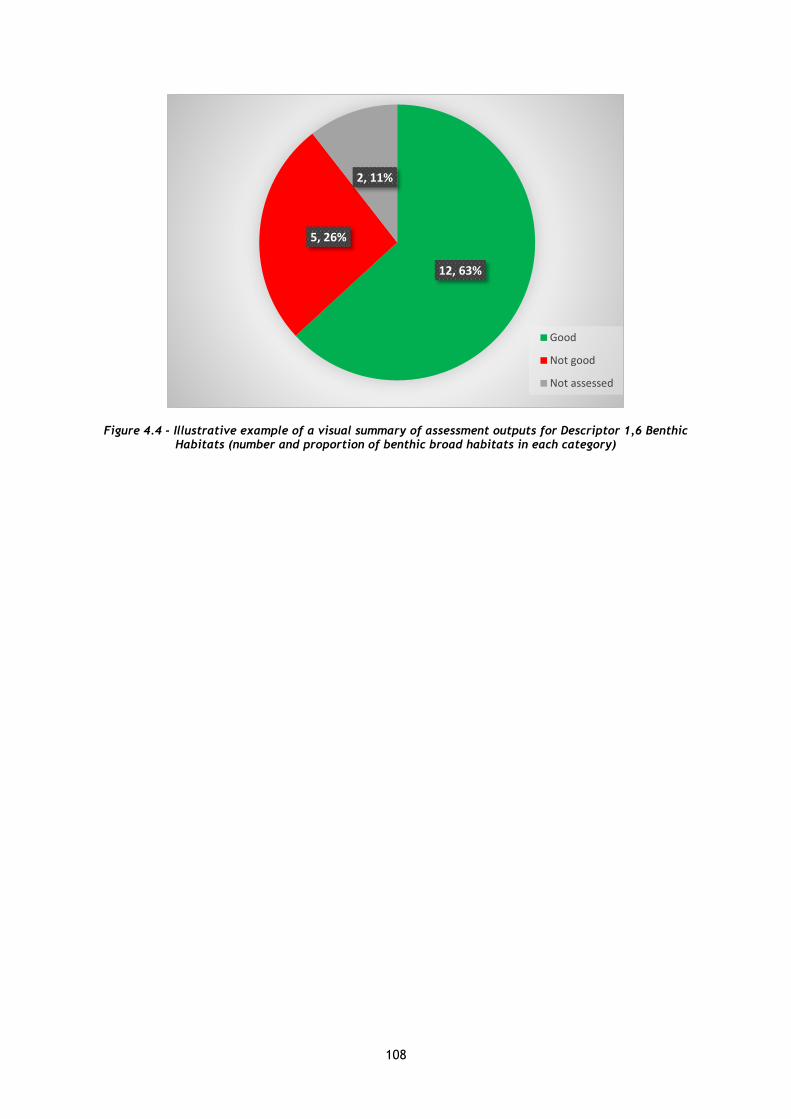
108

Figure 4.4 - Illustrative example of a visual summary of assessment outputs for Descriptor 1,6 Benthic Habitats (number and proportion of benthic broad habitats in each category)

12, 63%

5, 26%

2, 11%

Good

Not good

Not assessed

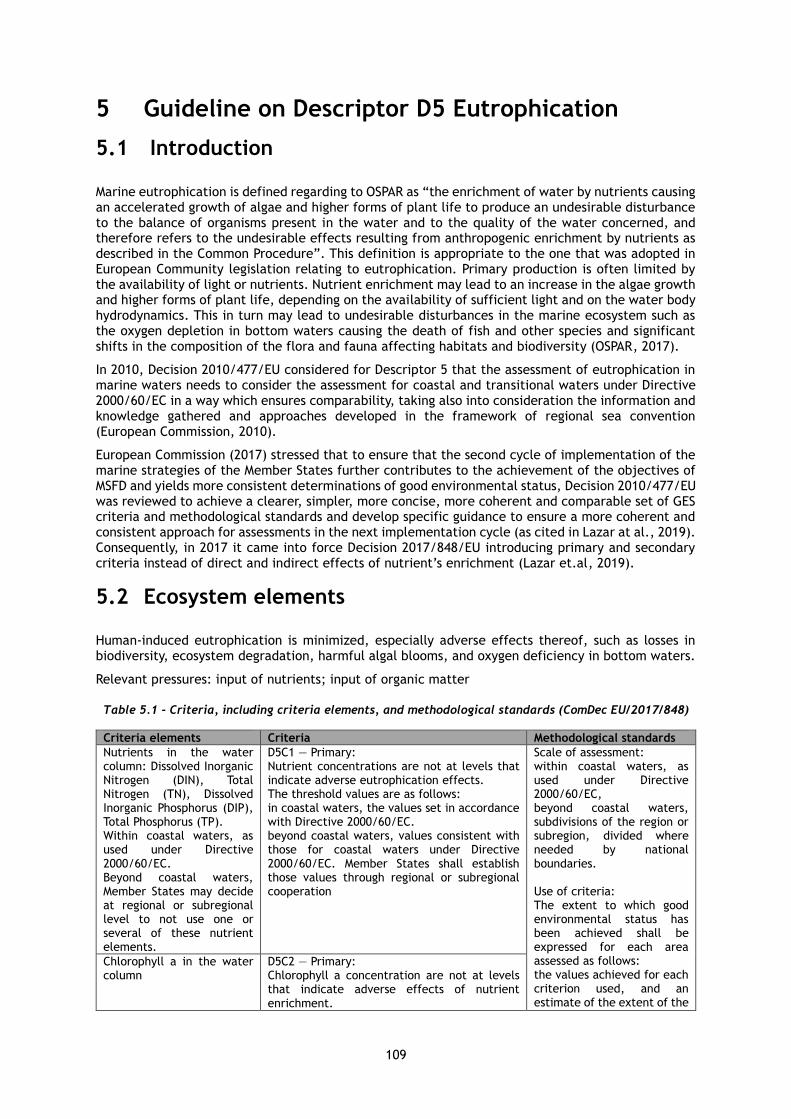
109

5 Guideline on Descriptor D5 Eutrophication

5.1 Introduction

Marine eutrophication is defined regarding to OSPAR as “the enrichment of water by nutrients causing an accelerated growth of algae and higher forms of plant life to produce an undesirable disturbance to the balance of organisms present in the water and to the quality of the water concerned, and therefore refers to the undesirable effects resulting from anthropogenic enrichment by nutrients as described in the Common Procedure”. This definition is appropriate to the one that was adopted in European Community legislation relating to eutrophication. Primary production is often limited by the availability of light or nutrients. Nutrient enrichment may lead to an increase in the algae growth and higher forms of plant life, depending on the availability of sufficient light and on the water body hydrodynamics. This in turn may lead to undesirable disturbances in the marine ecosystem such as the oxygen depletion in bottom waters causing the death of fish and other species and significant shifts in the composition of the flora and fauna affecting habitats and biodiversity (OSPAR, 2017).

In 2010, Decision 2010/477/EU considered for Descriptor 5 that the assessment of eutrophication in marine waters needs to consider the assessment for coastal and transitional waters under Directive 2000/60/EC in a way which ensures comparability, taking also into consideration the information and knowledge gathered and approaches developed in the framework of regional sea convention (European Commission, 2010).

European Commission (2017) stressed that to ensure that the second cycle of implementation of the marine strategies of the Member States further contributes to the achievement of the objectives of MSFD and yields more consistent determinations of good environmental status, Decision 2010/477/EU was reviewed to achieve a clearer, simpler, more concise, more coherent and comparable set of GES criteria and methodological standards and develop specific guidance to ensure a more coherent and consistent approach for assessments in the next implementation cycle (as cited in Lazar at al., 2019). Consequently, in 2017 it came into force Decision 2017/848/EU introducing primary and secondary criteria instead of direct and indirect effects of nutrient’s enrichment (Lazar et.al, 2019).


Human-induced eutrophication is minimized, especially adverse effects thereof, such as losses in biodiversity, ecosystem degradation, harmful algal blooms, and oxygen deficiency in bottom waters.

Relevant pressures: input of nutrients; input of organic matter

Table 5.1 - Criteria, including criteria elements, and methodological standards (ComDec EU/2017/848)

Criteria elements Criteria Methodological standards

Nutrients in the water column: Dissolved Inorganic Nitrogen (DIN), Total Nitrogen (TN), Dissolved Inorganic Phosphorus (DIP), Total Phosphorus (TP). Within coastal waters, as used under Directive 2000/60/EC. Beyond coastal waters, Member States may decide at regional or subregional level to not use one or several of these nutrient elements.

D5C1 — Primary: Nutrient concentrations are not at levels that indicate adverse eutrophication effects. The threshold values are as follows: in coastal waters, the values set in accordance with Directive 2000/60/EC. beyond coastal waters, values consistent with those for coastal waters under Directive 2000/60/EC. Member States shall establish those values through regional or subregional cooperation

Scale of assessment: within coastal waters, as used under Directive 2000/60/EC, beyond coastal waters, subdivisions of the region or subregion, divided where needed by national boundaries. Use of criteria: The extent to which good environmental status has been achieved shall be expressed for each area assessed as follows: the values achieved for each criterion used, and an estimate of the extent of the

Chlorophyll a in the water column

D5C2 — Primary: Chlorophyll a concentration are not at levels that indicate adverse effects of nutrient enrichment.

110


The threshold values are as follows: in coastal waters, the values set in accordance with Directive 2000/60/EC. beyond coastal waters, values consistent with those for coastal waters under Directive 2000/60/EC. Member States shall establish those values through regional or subregional cooperation.

assessment area over which the threshold values set have been achieved. in coastal waters, the criteria shall be used in accordance with the requirements of Directive 2000/60/EC to conclude on whether the water body is subject to eutrophication (5); beyond coastal waters, an estimate of the extent of the area (as a proportion (percentage)) that is not subject to eutrophication (as indicated by the results of all criteria used, integrated in a manner agreed where possible at Union level, but at least at regional or subregional level). Beyond coastal waters, the use of the secondary criteria shall be agreed at regional or subregional level. The outcomes of the assessments shall also contribute to assessments for pelagic habitats under Descriptor 1 as follows: the distribution and an estimate of the extent of the area (as a proportion (percentage)) that is subject to eutrophication in the water column (as indicated by whether the threshold values for criteria D5C2, D5C3 and D5C4, when used, have been achieved); The outcomes of the assessments shall also contribute to assessments for benthic habitats under Descriptors 1 and 6 as follows: the distribution and an estimate of the extent of the area (as a proportion (percentage)) that is subject to eutrophication on the seabed (as indicated by whether the threshold values for criteria D5C4, D5C5, D5C6, D5C7 and D5C8, when used, have been achieved).

Harmful algal blooms (e.g. cyanobacteria) in the water column

D5C3 — Secondary: The number, spatial extent and duration of harmful algal bloom events are not at levels that indicate adverse effects of nutrient enrichment. Member States shall establish threshold values for these levels through regional or subregional cooperation.

Photic limit (transparency) of the water column

D5C4 — Secondary: The photic limit (transparency) of the water column is not reduced, due to increases in suspended algae, to a level that indicates adverse effects of nutrient enrichment. The threshold values are as follows: in coastal waters, the values set in accordance with Directive 2000/60/EC. beyond coastal waters, values consistent with those for coastal waters under Directive 2000/60/EC. Member States shall establish those values through regional or subregional cooperation.

Dissolved oxygen in the bottom of the water column

D5C5 — Primary (may be substituted by D5C8): The concentration of dissolved oxygen is not reduced, due to nutrient enrichment, to levels that indicate adverse effects on benthic habitats (including on associated biota and mobile species) or other eutrophication effects. The threshold values are as follows: in coastal waters, the values set in accordance with Directive 2000/60/EC; beyond coastal waters, values consistent with those for coastal waters under Directive 2000/60/EC. Member States shall establish those values through regional or subregional cooperation.

Opportunistic macroalgae of benthic habitats

D5C6 — Secondary: The abundance of opportunistic macroalgae is not at levels that indicate adverse effects of nutrient enrichment. The threshold values are as follows: in coastal waters, the values set in accordance with Directive 2000/60/EC; should this criterion be relevant for waters beyond coastal waters, values consistent with those for coastal waters under Directive 2000/60/EC. Member States shall establish those values through regional or subregional cooperation.

Macrophyte communities (perennial seaweeds and seagrasses such as fucoids, eelgrass and Neptune grass) of benthic habitats

D5C7 — Secondary: The species composition and relative abundance or depth distribution of macrophyte communities achieve values that indicate there is no adverse effect due to nutrient enrichment

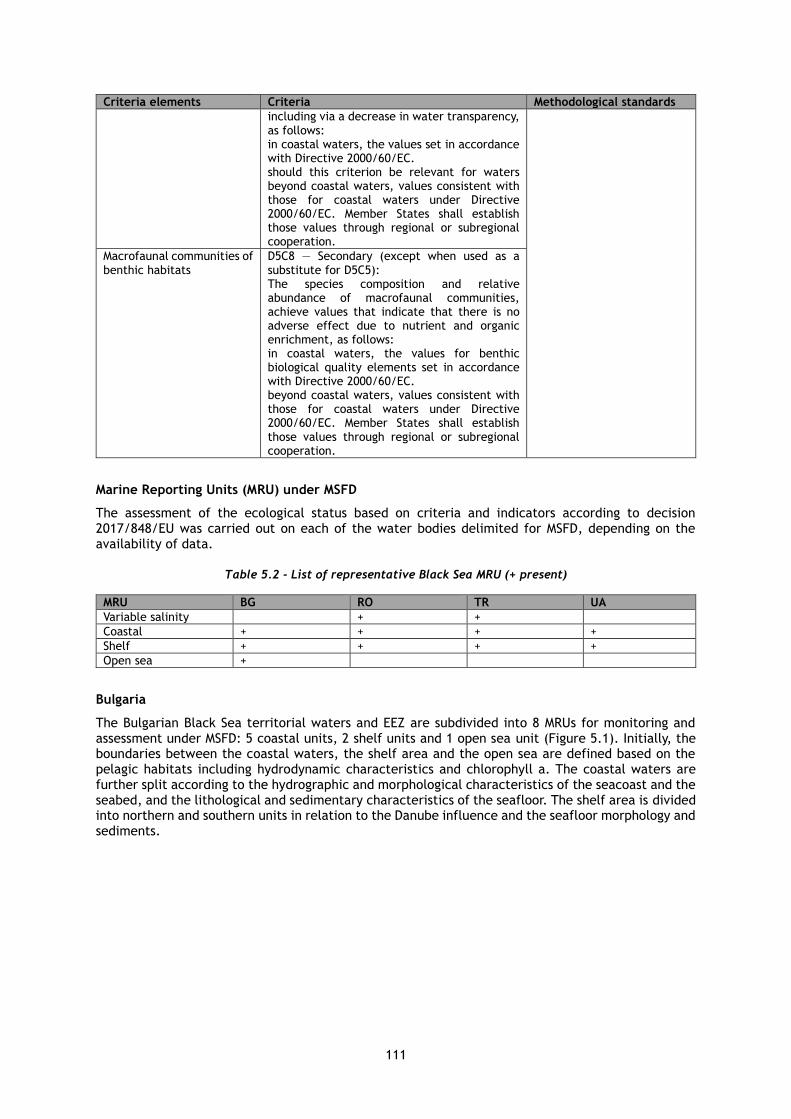
111


including via a decrease in water transparency, as follows: in coastal waters, the values set in accordance with Directive 2000/60/EC. should this criterion be relevant for waters beyond coastal waters, values consistent with those for coastal waters under Directive 2000/60/EC. Member States shall establish those values through regional or subregional cooperation.

Macrofaunal communities of benthic habitats

D5C8 — Secondary (except when used as a substitute for D5C5): The species composition and relative abundance of macrofaunal communities, achieve values that indicate that there is no adverse effect due to nutrient and organic enrichment, as follows: in coastal waters, the values for benthic biological quality elements set in accordance with Directive 2000/60/EC. beyond coastal waters, values consistent with those for coastal waters under Directive 2000/60/EC. Member States shall establish those values through regional or subregional cooperation.

Marine Reporting Units (MRU) under MSFD

The assessment of the ecological status based on criteria and indicators according to decision 2017/848/EU was carried out on each of the water bodies delimited for MSFD, depending on the availability of data.

Table 5.2 - List of representative Black Sea MRU (+ present)

MRU BG RO TR UA

Variable salinity + +

Coastal + + + +

Shelf + + + +

Open sea +

Bulgaria

The Bulgarian Black Sea territorial waters and EEZ are subdivided into 8 MRUs for monitoring and assessment under MSFD: 5 coastal units, 2 shelf units and 1 open sea unit (Figure 5.1). Initially, the boundaries between the coastal waters, the shelf area and the open sea are defined based on the pelagic habitats including hydrodynamic characteristics and chlorophyll a. The coastal waters are further split according to the hydrographic and morphological characteristics of the seacoast and the seabed, and the lithological and sedimentary characteristics of the seafloor. The shelf area is divided into northern and southern units in relation to the Danube influence and the seafloor morphology and sediments.

112

Figure 5.1 - Map of the MRU under MSFD in the Bulgarian Black Sea

Romania

The assessment of the ecological status based on criteria and indicators according to decision 2017/848/EU (Boicenco et al., 2018) was carried out on each of the water bodies of water delimited for MSFD, depending on the availability of data. From the spatial distribution of the average decennial values of salinity from the available data World Ocean data (ftp://ftp.nodc.noaa.gov/) and INCDM (www.nodc.ro), but also from the average monthly amounts of chlorophyll a (2002-2013) (https://Disc.sci.gsfc.nasa.gov/giovanni), the Romanian marine waters were classified in four water bodies (Figure 5.2).

• BLK_RO_RG_TT03_Waters with variable salinity – waters with variable salinity located in the north, under the direct influence of the Danube, from the mouth of the river in the Black Sea, south to the Portiţa, at depths of up to 30m. The waters are delimited by the average seasonal salinity up to 8.0 PSU and an annual average up to 14.5 PSU.

• BLK_RO_RG_CT_Coastal waters - are the coastal water from the central to the south (from Portiţa to Vama Veche), from the base line to the isobath of 30m. The waters are delimited by the average seasonal salinity 8-16 PSU and an annual average up to 16.0 PSU.

• BLK_RO_RG_MT01_Marine Waters – the marine waters area from the 30 m isobath to 200m; The waters inside and outside the continental platform, delimited by the average seasonal and annual salinity in the range 16 – 17, 5PSU.

• BLK_RO_RG_MT02_Offshore Waters – The open area of marine waters, delimited by average seasonal and annual salinity greater than 17.5 PSU, perimeter set for water type with depths of at least 200 m.

113

Figure 5.2 - Delimitation of water bodies based on physical and-biological characteristics and national network of monitoring according to WFD and MSFD

Turkey

NIMP intends to cover all coastal, shelf and open marine waters - under the national jurisdiction - and the underlying seabed under the pressure of human activities. At present, the Programme covers efficiently the coastal waters and partially the marine waters (up to 20-30 nm) being expanded from 12-15 nm from 2011 till 2017.

Coastal water bodies (in relation to WFD) were identified within DeKoS Project (TÜBİTAK-MAM, MoEU- GDEM, 2014) and used as a basis for the coastal waters monitoring under NIMP and the river basin monitoring activities (Table 1.14). Coastal water bodies extend beyond 1 nm (as defined by WFD) depending on the coastal morphology and structures like bays. Initially, 16 coastal water bodies were identified along the Black Sea coast of Turkey and later the Westernmost one was divided into two units after assessing the ecological quality for several years. As a result, there are now 17 units (Table 5.3). It was recommended by DİSSP Project (MoEU, TÜBİTAK-MAM; 2017) that 1 nm or DeKoS units can both be considered in the assessments depending on the purpose of the assessment made, data aggregation principles, or the comparisons to be done with the neighboring countries.

In the DeKoS Project, marine assessment units (MAU) were also identified with expert views by considering the pressures and the ecological/hydrographic characteristics from West to East along the southern Black Sea (Figure 5.3). Five MAUs were identified initially, later the W-E borders of “Sinop” unit was modified by the experts in the DİSSP Project. The units are in fact assumptive and include coastal, transitional (at the river mouths) and marine waters. Each unit was also differentiated based on the depths in relation to the WFD relevant typologies, the benthic habitats, and the deep waters characteristics (Table 5.3).

114

Figure 5.3 - Map of the MRU in Turkish marine waters

Table 5.3 - Criteria for marine assessment units (source: DeKoS and DİSSP projects)

Marine Assessment Units Name

1 a) <40 m* b) 40-200 m** c) >200 m * 30 m is the depth criteria for coastal typology (DeKoS) and later modified to 40 m with DİSSP Project. ** 150-200 m is the suboxic-anoxic boundary changing with location. *** >200 m could be considered anoxic deep waters

Western Black Sea

2 Central -Western Black Sea

3 Sinop area

4 Yeşilırmak / Kızılırmak impact area

5 Eastern Black Sea

Ukraine

During the project “Baltic2Black”, 11 marine assessment regions were also identified with expert views by considering the pressures and the ecological/hydrographic characteristics at the North-Western Black Sea shelf and other regions of coastal and deep waters within the exclusive maritime economic zone of Ukraine (Figure 5.4). The units are in fact assumptive and include coastal (at the river mouths transitional too) and marine waters. Each unit was also differentiated based on the influence of rivers, depth range that is related to the typologies and benthic habitats, and other hydrological and hydrochemical conditions.

Figure 5.4 - Map of the 11 marine assessment regions in Ukrainean marine waters

115

Table 5.4 - Overview of criteria, indicators, and thresholds (Com Dec EU/2017/848)

Criteria Country Indicator

D5C1 BG

DIN, TN, DIP, TP RO

TR

UA

D5C2 BG

Chlorophyll a concentration (μg/l)

RO

TR

UA

D5C3 BG Abundance of a single phytoplankton species Chlorophyll a concentration above the defined bloom threshold Abundance of potentially toxic species exceeding the species-specific threshold Area of pelagic habitats in the shelf and open sea with Chlorophyll a concentration in the surface waters (remote sensing) Noctiluca scintillans (в %) from the total mesozooplankton biomass in spring

RO Noctiluca scintillans biomass (mg/m3)

TR Noctiluca scintillans biomass (%)

UA

D5C4 BG

Photic limit (transparency) of the water column RO

TR

UA

D5C5 BG

The concentration of dissolved oxygen RO

TR

UA

D5C6 BG % of the wet biomass of tolerant species (ESGII) from the total wet biomass. Ecological index EI, applicable for infralitoral rocky habitat down to 3 m depth. Epithytes on the seagrass leaves (additional parameter)

RO % of the wet biomass of tolerant species (ESGII) from the total wet biomass. Ecological index EI, applicable for infralitoral rocky habitat down to 3 m depth.

TR N/A

UA N/A

D5C7 BG % of the wet biomass of macroalgal species from the first ecological group (ESGI) > 60 % normalized for the infralitoral rocky habitat down to 3 m depth Ecological index EI > 6 normalized for for the infralittoral rocky habitat down to 3 m depth Proactive coverage of Cystoseira spp and other macrophytes from the first ecological category (ESGI), ≥ 40% (measured by the method of Orfanidis et al., 2011, as modified by Berov, 2013 in the upper infralitoral, depth between 2, 3 m) Depth distribution of Cystoseira barbata ≥10 m and C. bosphorica ≥ 4m in case a suitable substrate is available) Depth distribution of seagrass medows ≥ 6 Depth distribution of Phyllophora crispa and other perannual sciophilic macrophytes ≥ 17 m (in case a suitable substrate is available) (Berov et al., in prep.) Total benthal proactive coverage by species Phyllophora crispa, Apoglosium ruscifolium, Zanardinia typus, Gelidium spinosum ≥ 35% benthal proactive coverage by species from the second ecological group (ESGII) Cladophora albida, Cladophora coelothrix, Chaetomorpha linum, Ulva rigida) ≤ 15% ( measurements by the method of Berov, 2013; Berov et al., in prep.) Bellow ground biomass of Zostera noltei

RO % of the wet biomass of macroalgal species from the first ecological group (ESGI) > 60 standardized for infralittoral rock down to 3 m depth. Ecological index EI > 6 normalized for for the infralittoral rocky habitat down to 3 m depth Bellow ground biomass of Zostera noltei

TR N/A

UA N/A-

D5C8 BG M-AMBI*n

RO M-AMBI*(n) Mytilus galloprovincialis biogenic circalittoral reefs EQR for all benthic sedimentary habitats / M-AMBI*(n) Modiolula phaseolina circalittoral muds

TR M-AMBI

UA M-AMBI

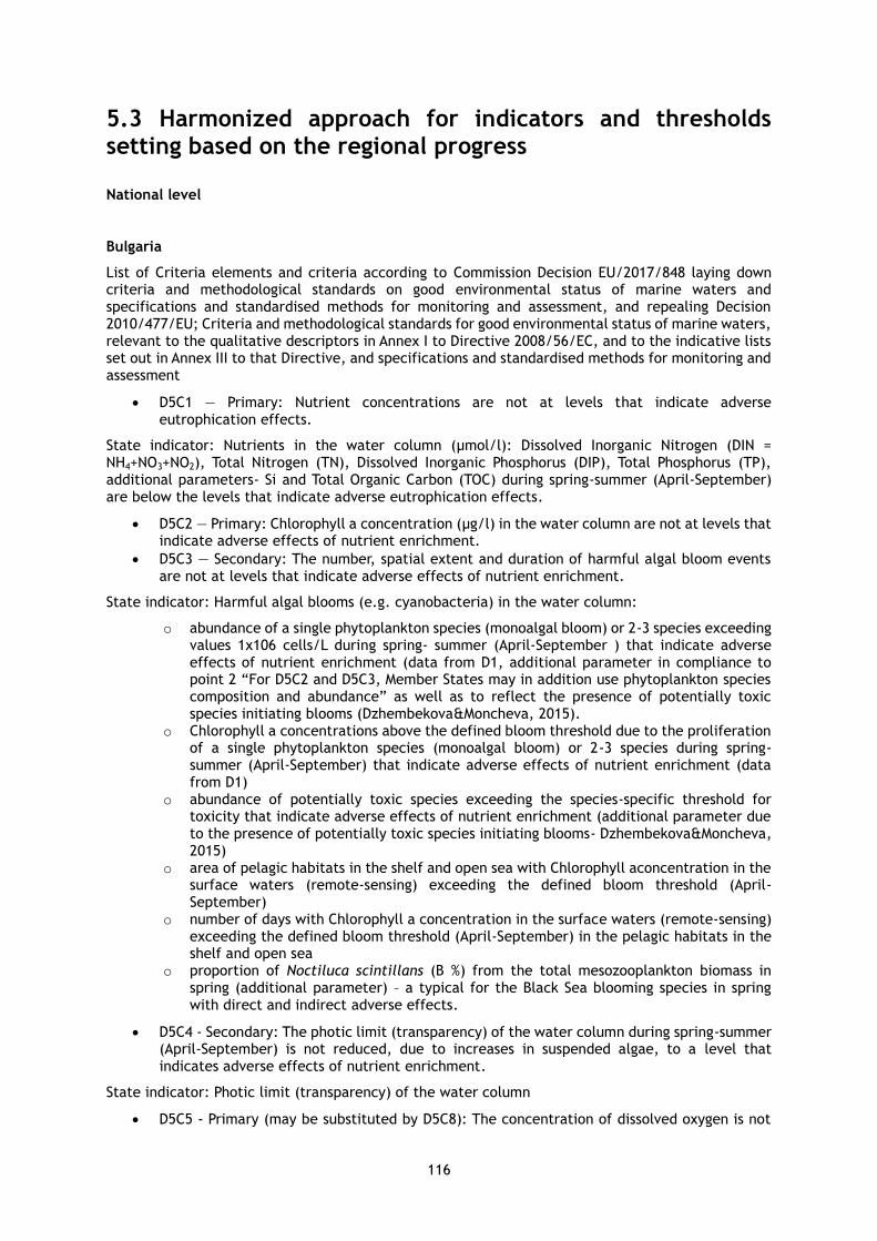
116


National level

Bulgaria

List of Criteria elements and criteria according to Commission Decision EU/2017/848 laying down criteria and methodological standards on good environmental status of marine waters and specifications and standardised methods for monitoring and assessment, and repealing Decision 2010/477/EU; Criteria and methodological standards for good environmental status of marine waters, relevant to the qualitative descriptors in Annex I to Directive 2008/56/EC, and to the indicative lists set out in Annex III to that Directive, and specifications and standardised methods for monitoring and assessment

• D5C1 — Primary: Nutrient concentrations are not at levels that indicate adverse eutrophication effects.

State indicator: Nutrients in the water column (μmol/l): Dissolved Inorganic Nitrogen (DIN = NH4+NO3+NO2), Total Nitrogen (TN), Dissolved Inorganic Phosphorus (DIP), Total Phosphorus (TP), additional parameters- Si and Total Organic Carbon (TOC) during spring-summer (April-September) are below the levels that indicate adverse eutrophication effects.

• D5C2 — Primary: Chlorophyll a concentration (μg/l) in the water column are not at levels that indicate adverse effects of nutrient enrichment.

• D5C3 — Secondary: The number, spatial extent and duration of harmful algal bloom events are not at levels that indicate adverse effects of nutrient enrichment.

State indicator: Harmful algal blooms (e.g. cyanobacteria) in the water column:

o abundance of a single phytoplankton species (monoalgal bloom) or 2-3 species exceeding values 1х106 cells/L during spring- summer (April-September ) that indicate adverse effects of nutrient enrichment (data from D1, additional parameter in compliance to point 2 “For D5C2 and D5C3, Member States may in addition use phytoplankton species composition and abundance” as well as to reflect the presence of potentially toxic species initiating blooms (Dzhembekova&Moncheva, 2015).

o Chlorophyll a concentrations above the defined bloom threshold due to the proliferation of a single phytoplankton species (monoalgal bloom) or 2-3 species during spring- summer (April-September) that indicate adverse effects of nutrient enrichment (data from D1)

o abundance of potentially toxic species exceeding the species-specific threshold for toxicity that indicate adverse effects of nutrient enrichment (additional parameter due to the presence of potentially toxic species initiating blooms- Dzhembekova&Moncheva, 2015)

o area of pelagic habitats in the shelf and open sea with Chlorophyll aconcentration in the surface waters (remote-sensing) exceeding the defined bloom threshold (April-September)

o number of days with Chlorophyll a concentration in the surface waters (remote-sensing) exceeding the defined bloom threshold (April-September) in the pelagic habitats in the shelf and open sea

o proportion of Noctiluca scintillans (B %) from the total mesozooplankton biomass in spring (additional parameter) – a typical for the Black Sea blooming species in spring with direct and indirect adverse effects.

• D5C4 - Secondary: The photic limit (transparency) of the water column during spring-summer (April-September) is not reduced, due to increases in suspended algae, to a level that indicates adverse effects of nutrient enrichment.

State indicator: Photic limit (transparency) of the water column

• D5C5 - Primary (may be substituted by D5C8): The concentration of dissolved oxygen is not

117

reduced, due to nutrient enrichment, to levels that indicate adverse effects on benthic habitats (including on associated biota and mobile species) or other eutrophication effects.

State indicator: Dissolved oxygen (DO, mg/l)/Oxygen saturation (OS,%) in the bottom of the water column. Additional parameter Dissolved oxygen (DO, mg/l)/Oxygen saturation (OS,%) at the surface waters of the water column - an important feature of marine environment directly related to the phytoplankton blooms (D5С2) and (D5С4). Phytoplankton blooms could be associated with surface waters O2 over saturation or deficit depending on the eco physiological features of the species causing adverse effects not necessarily followed by an O2 deficit in the bottom waters.

• D5C6 - Secondary: The abundance of opportunistic macroalgae is not at levels that indicate adverse effects of nutrient enrichment. The abundance/biomass of opportunistic macrophyte species in the coastal waters do not exceed the WFD thresholds.

State indicator: Opportunistic macroalgae of benthic habitats

o % of the wet biomass of tolerant species (ESGII) from the total wet biomass. o Ecological index EI, (Dencheva&Doncheva, 2014, Berov D., 2015), applicable for

infralitoral rocky habitat down to 3 m depth. o Epithytes on the seagrass leaves (additional parameter).

• D5C7 — Secondary: The species composition and relative abundance or depth distribution of macrophyte communities achieve values that indicate there is no adverse effect due to nutrient enrichment including via a decrease in water transparency.

State indicator: Macrophyte communities (perennial seaweeds and seagrasses such as fucoids, eelgrass) of benthic habitats.

o % of the wet biomass of macroalgal species from the first ecological group (ESGI) normalized for the infralitoral rocky habitat down to 3 m depth.

o Ecological index EI, (Dencheva&Doncheva, 2014, Berov D., 2015), normalized for for the infralitoral rocky habitat down to 3 m depth.

o Proactive coverage of Cystoseira spp and other macrophytes from the first ecological category (ESGI), normalized for for the infralitoral rocky habitat down to 3 m depth.

o Depth distribution of Cystoseira barbata and C. bosphorica (in case a suitable substrate is available).

o Depth distribution of seagrass medows. o Depth distribution of Phyllophora crispa and other perannual sciophilic macrophytes (in

case a suitable substrate is available). o Other indicators for lower infralittoral: benthal proactive coverage by species

Phyllophora crispa, Apoglosium ruscifolium, Zanardinia typus, Gelidium spinosum as well as other species from the second ecological group (ESGII).

o Underground biomass of Zostera noltei, ratio below ground/above ground biomass of Zostera noltei, density of Zostera noltei shoots, length of Zostera noltei shoots.

• D5C8 — Secondary (except when used as a substitute for D5C5): The species composition and relative abundance of macrofaunal communities, achieve values that indicate that there is no adverse effect due to nutrient and organic enrichment.

State indicator: Macrofaunal communities of benthic habitats

o Number of species S o Index of biodiversity Shannon H’ o Biotic index AMBI o M-AMBI*n (composite index integrating S, H’ and AMBI)

Environmental targets

• D5С1. Coastal, shelf and open sea marine regions for assessment (MRUs). The identified thresholds (refer to the surface homogenious layer) are given in Table 5.5.

118

Table 5.5 - Nutrients threshold for spring, summer and autumn (based on last 10 years statistical data)

Concentration μM

Spring Summer Autumn

Coastal Shelf Open sea Coastal Shelf Open sea Coastal Shelf Open sea

N-NH4 0.9 0.50 0.50 0.70 0.60 0.50 0.6 0.4 0.4

N-N02 0.3 0.08 0.06 0.12 0.08 0.06 0.10 0.08 0.05

N-N03 1.0 0.50 0.30 0.30 0.25 0.20 0.5 0.45 0.30

P-P04 0.15 0.10 0.10 0.15 0.08 0.08 0.14 0.10 0.07

The thresholds need to be validated. For total N and total P there are no thresholds identified.

Additional parameters:

Si concentration in the surface homogenious layer. No thresholds identified.

TOC, μg/l – no thresholds identified.

• D5C2 Coastal, shelf and open sea marine regions for assessment (MRUs): within the 6 year monitoring cycle the 95 percentile of the monthly chlorophyll a values during spring-summer (April-September) are not above the threshold in more than 10% of the samples in spring and in more than 5% in summer or the trend should be decreasing (BG Initial Assessment Report, art.10 MSFD, Table V.2.1.2, p. 109) as revised during ISMEIM Project –Table 5.6.

Table 5.6 - Revised thresholds for chlorophyll a for spring and summer

Concentration (µg/L)

Spring Summer

1nm Coastal Shelf Open sea 1nm Coastal Shelf Open sea

Chlorophyll a 3.3 3.3 1.4 0.4 1.5 1.4 1.2 0.36

• D5C3

Bloom intensity:

Maintaining the current decreasing trend of spring and summer bloom intensity in compliance to the revised chlorophyll a threshold (based on remote sensing data- Project Devotes) for shelf and open sea – Table 5.7.

Table 5.7 - Thresholds for primary and secondary bloom intensity in the BG shelf and open sea based on the application of the biooptical algorithm (Kopelevich et, 2012) and remote-sensing data from MODIS

Aqua/Terra, for the period 1999- 2013

Pelagic habitat Season Bloom type Threshold

Shelf Spring primary 3.8

Shelf Spring secondary 2.9

Shelf Summer primary 2.7

Shelf Summer secondary 2

Open sea Spring primary 1.5

Open sea Spring secondary 1.1

Open sea Summer primary 1.3

Open sea Summer secondary 1

The proportion of Noctiluca scintillans biomass (B %) of the total mesozooplankton biomass do not exceed 30% in spring.

Additional parameters:

o Abundance of a single phytoplankton species (monoalgal bloom) or 2-3 species exceeding values 1х106 cells/L during spring- summer (April-September) that indicate adverse effects of nutrient enrichment (data from D1) , do not exceed the identified thresholds in more than 10% of the spring and 5% of the summer seasonal measurements.

o Chlorophyll a concentration above the defined bloom threshold due to the proliferation of a single phytoplankton species (monoalgal bloom) or 2-3 species during spring- summer (April-September) that indicate adverse effects of nutrient enrichment (data from D1) do not exceed the identified thresholds in more than 10% of the spring and 5%

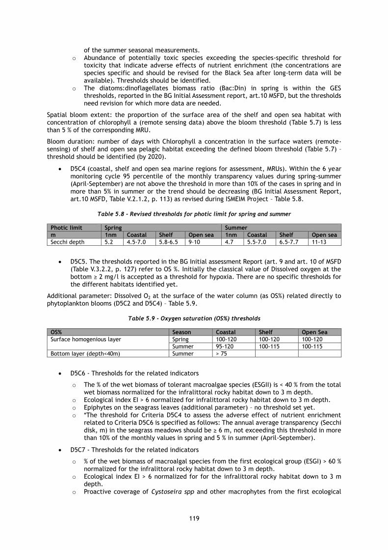
119

of the summer seasonal measurements. o Abundance of potentially toxic species exceeding the species-specific threshold for

toxicity that indicate adverse effects of nutrient enrichment (the concentrations are species specific and should be revised for the Black Sea after long-term data will be available). Thresholds should be identified.

o The diatoms:dinoflagellates biomass ratio (Bac:Din) in spring is within the GES thresholds, reported in the BG Initial Assessment report, art.10 MSFD, but the thresholds need revision for which more data are needed.

Spatial bloom extent: the proportion of the surface area of the shelf and open sea habitat with concentration of chlorophyll a (remote sensing data) above the bloom threshold (Table 5.7) is less than 5 % of the corresponding MRU.

Bloom duration: number of days with Chlorophyll a concentration in the surface waters (remote-sensing) of shelf and open sea pelagic habitat exceeding the defined bloom threshold (Table 5.7) – threshold should be identified (by 2020).

• D5С4 (coastal, shelf and open sea marine regions for assessment, MRUs). Within the 6 year monitoring cycle 95 percentile of the monthly transparency values during spring-summer (April-September) are not above the threshold in more than 10% of the cases in spring and in more than 5% in summer or the trend should be decreasing (BG Initial Assessment Report, art.10 MSFD, Table V.2.1.2, p. 113) as revised during ISMEIM Project – Table 5.8.

Table 5.8 - Revised thresholds for photic limit for spring and summer

Photic limit Spring Summer

m 1nm Coastal Shelf Open sea 1nm Coastal Shelf Open sea

Secchi depth 5.2 4.5-7.0 5.8-6.5 9–10 4.7 5.5-7.0 6.5-7.7 11-13

• D5С5. The thresholds reported in the BG Initial assessment Report (art. 9 and art. 10 of MSFD (Table V.3.2.2, p. 127) refer to OS %. Initially the classical value of Dissolved oxygen at the bottom ≥ 2 mg/l is accepted as a threshold for hypoxia. There are no specific thresholds for the different habitats identified yet.

Additional parameter: Dissolved O2 at the surface of the water column (as OS%) related directly to phytoplankton blooms (D5С2 and D5С4) – Table 5.9.

Table 5.9 - Oxygen saturation (OS%) thresholds

OS% Season Coastal Shelf Open Sea

Surface homogenious layer Spring 100-120 100-120 100-120

Summer 95-120 100-115 100-115

Bottom Iayer (depth<40m) Summer > 75

• D5C6 - Thresholds for the related indicators

o The % of the wet biomass of tolerant macroalgae species (ESGII) is < 40 % from the total wet biomass normalized for the infralittoral rocky habitat down to 3 m depth.

o Ecological index EI > 6 normalized for infralittoral rocky habitat down to 3 m depth. o Epiphytes on the seagrass leaves (additional parameter) – no threshold set yet. o *The threshold for Criteria D5C4 to assess the adverse effect of nutrient enrichment

related to Criteria D5C6 is specified as follows: The annual average transparency (Secchi disk, m) in the seagrass meadows should be ≥ 6 m, not exceeding this threshold in more than 10% of the monthly values in spring and 5 % in summer (April-September).

• D5C7 - Thresholds for the related indicators

o % of the wet biomass of macroalgal species from the first ecological group (ESGI) > 60 % normalized for the infralittoral rocky habitat down to 3 m depth.

o Ecological index EI > 6 normalized for for the infralittoral rocky habitat down to 3 m depth.

o Proactive coverage of Cystoseira spp and other macrophytes from the first ecological

120

category (ESGI), ≥ 40% (measured by the method of Orfanidis et al., 2011, as modified by Berov, 2013 in the upper infralitoral, depth between 2, 3 m).

o Depth distribution of Cystoseira barbata ≥10 m and C. bosphorica ≥ 4m in case a suitable substrate is available).

o Depth distribution of seagrass medows ≥ 6. o Depth distribution of Phyllophora crispa and other perannual sciophilic macrophytes ≥

17 m (in case a suitable substrate is available) (Berov et al., in prep.). o Total benthal proactive coverage by species Phyllophora crispa, Apoglosium ruscifolium,

Zanardinia typus, Gelidium spinosum ≥ 35%. o benthal proactive coverage by species from the second ecological group (ESGII)

Cladophora albida, Cladophora coelothrix, Chaetomorpha linum, Ulva rigida) ≤ 15% (measurements by the method of Berov, 2013; Berov et al., in prep.).

o Bellow ground biomass of Zostera noltei, ratio above ground/bellow ground biomass of Zostera noltei, density of Zostera noltei shoots, length of Zostera noltei shoots – Table 5.10.

Table 5.10 - Thesholds for Zostera noltei indicators*

Z.noltei parameters

Bellow ground biomass (g·m-2)

Ratio above / bellow the ground biomass (ag-bg)

Leaf length (mm)

Shoots density (shoots·m-2)

GES threshold >105.2 <2.4 ≥151.5-≤270.5 ≥500.6-≤696.6 *Based on the methodology of Karamfilov et al., (in review) for seagrass medows located at depthn between 2-3m.

Table 5.11 - Assigned indicators

Indicator/Country BG RO TR* UA

Nutrients in the water column + (spring and summer)

+ (surface, annual average)

+ +

Chlorophyll a in the water column

+ (spring and summer)

+ (warm season)

+ +

Harmful algal blooms in the water column

Noctiluca scintillans biomass (B %)

Noctiluca scintillans biomass (mg/m3)

+ +

Photic limit (transparency) of the water column


+ (warm season)

+ +

Dissolved oxygen in the bottom of the water column


+ + +

Opportunistic macroalgae of benthic habitats

+ (%)

+ (%) ESG II < 40 %

Macrophyte communities of benthic habitats

+ (ESGI, Ecological index)

+ (ESGI, Ecological index)

Macrofaunal communities of benthic habitats

+ +

Romania

Environmental targets has been defined according to the MSFD requirements as follows (Figure 5.5):

121

Figure 5.5 - Descriptor 5 (Eutrophication) - parameters, indicators, criteria and thresholds – Romanian Black Sea waters, 2012-2017 (Lazar et.al, 2019)

• D5C1

In variable salinity and coastal waters, all measured values are lower than the maximum allowable concentrations according to national legislation. In marine waters, the 75th percentile of annual mean concentrations of nutrients should not exceed the target values.

• D5C2

The 75th percentile of summer chlorophyll a concentration should not exceed the threshold values.

• D5C3

Noctiluca scintillans biomass 50th percentile is lower than the target value for each water body and season.

• D5C4

In variable salinity and coastal waters all measured values should not be lower than the minimum permitted by national legislation. Beyond coastal waters - the 10th percentile of all sea water transparency values measured in the warm season (May-September) is not less than the threshold value.

• D5C5

The 10th of all dissolved oxygen values at the water-sediment interface (for stations with a maximum depth of 50m) measured in the warm season (May-September) is not less than the threshold value.

• D5C6

The abundance of opportunistic macroalgae is not at levels that indicate negative effects of nutrient enrichment.

ESG II < 40 % from total biomass

• D5C7 - Indicators not developed yet and environmental targets not established.

• D5C8

The species composition and relative abundance of macrofaunal communities, achieve values that

122

indicate that there is no adverse effect due to nutrient and organic enrichment.

Environmental targets

• D5C1- DIN, TN, DIP, TP

Variable salinity & coastal waters – National legislation (WFD) – Ord.161/2006

TP – 0.1mg/L – 3.23 µM

N-NO3 – 1.5 mg/L -107.14 µM

N-NO2 – 0.03mg/L – 2.14 µM

N-NH4 – 0.1mg/L – 7.14 µM

Marine waters

DIP – 0.23µM DIN –10.50 µM

• D5C2- Chlorophyll a concentration – warm season (May – August)

Variable salinity waters – 11.88 µg/L Coastal waters – 5.97µg/L Marine waters – 4.11µg/L – Northern area; 2.79µg/L – Southern area

• D5C3 — Secondary: Harmful algal bloom events - Noctiluca scintillans biomass

Variable salinity waters – 240 mg/m3 warm season (May-October); 70mg/m3 cold season (November – April). Coastal waters - 350 mg/m3 warm season; 100mg/m3 cold season Marine waters - 240 mg/m3 warm season; 60mg/m3 cold season

• D5C4 — Secondary: The photic limit (transparency) of the water column - Secchi Disk (transparency)

Variable salinity & coastal waters - National legislation (WFD) – Ord.161/2006 – 2.0m

Marine waters – 6.8m

• D5C5 — Primary: The concentration of dissolved oxygen

Marine waters - 5mg/L, no less than 60% at water-sediment interface

• D5C6 — Secondary: The abundance of opportunistic macroalgae

Biomass proportion of sensitive and opportunistic species from the total biomass

ESG II ≤40%

• D5C7- indicators not developed yet and GES not established.

• D5C8 Secondary: The species composition and relative abundance of macrofaunal communities

M-AMBI*(n) ≥ 0.68 Mytilus galloprovincialis biogenic circalittoral reefs EQR≥0.68 for all benthic sedimentary habitats (Table 5.12).

M-AMBI*(n) ≥ 0.61 Modiolula phaseolina circalittoral muds.

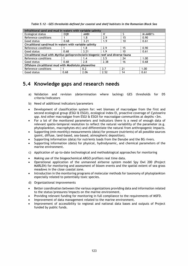
123

Table 5.12 - GES thresholds defined for coastal and shelf habitats in the Romanian Black Sea

Infralittoral sand and mud in waters with variable salinity



Good status 0.68 3.21 1.9 10 0.61

Circalittoral sand/mud in waters with variable salinity


Good status 0.68 3.21 1.9 10 0.61

Circalittoral mud with Mytilus galloprovincialis biogenic reef and diverse fauna


Good status 0.68 2.8 2.38 16 0.68

Offshore circalittoral mud with Modiolula phaseolina


Good status 0.68 2.06 2.52 14 0.61

5.4 Knowledge gaps and research needs

a) Validation and revision (determination where lacking) GES thresholds for D5 criteria/indicators

b) Need of additional indicators/parameters

• Development of classification system for: wet biomass of macroalgae from the first and second ecological group (ESGI & ESGII), ecological index EI, proactive coverage of Cystoseira spp. And other macroalgae from ESGI & ESGII for macroalgae communities at depths >3m.

• For a lot of the monitored parameters and indicators there is a need of enough data of relevant spatio-temporal resolution to reflect the natural variability of the parameter (e.g. phytoplankton, macrophytes etc) and differentiate the natural from anthropogenic impacts.

• Supporting (min monthly) measurements (data) for pressure (nutrients) of all possible sources (point, diffuse, land-based, sea-based, atmospheric deposition).

• Supporting information (data) for nutrients loads from the Danube and the BG rivers.

• Supporting information (data) for physical, hydrodynamic, and chemical parameters of the marine environment.

c) Application of up-to-date technological and methodological approaches for monitoring

• Making use of the biogeochemical ARGO profilers real time data.

• Operational application of the unmanned airborne system model Spy Owl 200 (Project MARLEN) for monitoring and assessment of bloom events and the spatial extent of sea grass meadows in the close coastal zone.

• Introduction in the monitoring programs of molecular methods for taxonomy of phytoplankton especially related to potentially toxic species.

d) Organizational improvements

• Better coordination between the various organizations providing data and information related to the status/pressures/impacts on the marine environment.

• Providing relevant funding for monitoring in full compliance to the requirements of MSFD.

• Improvement of data management related to the marine environment.

• Improvement of accessibility to regional and national data bases and outputs of Project funded by public funds.

124

6 Guideline on Descriptor D8 Contaminants

6.1 Overview of criteria and indicators

6.1.1 Commission Decision EU/2017/848 criteria and methodological standards

Descriptor 8: Concentrations of contaminants are at levels not giving rise to pollution effects.

Relevant pressures: Input of other substances (e.g. synthetic substances, non-synthetic substances, radionuclides).

According to the Commission Decision EU/2017/848 laying down criteria and methodological standards on good environmental status of marine waters and specifications and standardized methods for monitoring and assessment, and repealing Decision EU/2010/477, the following recommendations, with relevance for contaminants, could be underlined:

• compared to the elements set out in previous Decision 2010/477/EU, the number of criteria that need to be assessed could be reduced, applying a risk-based approach to those which are retained in order to focus on the main anthropogenic pressures affecting marine waters.

• to ensure comparability, specifications and standardized methods for monitoring and assessment should be defined, considering existing specifications and standards at European or international level, including regional or sub regional level.

• the collective pressure of human activities needs to be kept within levels compatible with the achievement of good environmental status, ensuring that the capacity of marine ecosystems to respond to human-induced changes is not compromised.

• the extent to which good environmental status is being achieved could be express as the proportion of their marine waters over which the threshold values have been achieved or as the proportion of criteria elements (species, contaminants, etc.) that have achieved the threshold values.

• it is important to focus on the predominant pressures and their environmental impacts on the different ecosystem elements in each region or subregion in order to monitor and assess their marine waters in an efficient and effective manner and to facilitate prioritization of actions to be taken to achieve good environmental status.

• criteria, including threshold values, methodological standards, specifications and standardized methods for monitoring and assessment should be based on the best available science. However, additional scientific and technical progress is still required to support the further development of some of them and should be used as the knowledge and understanding become available.

According to the Commission Decision (EU) 2017/848, criteria and methodological standards on good environmental status of marine waters for Descriptor 8 are presented in the Table 6.1.

Table 6.1 - Criteria, including criteria elements, and methodological standards (Com Dec EU/2017/848)


(1) Within coastal and territorial waters: (a) contaminants selected in

accordance with Directive 2000/60/EC: (i) contaminants for which an

environmental quality standard is laid down in Part A of Annex I to Directive 2008/105/EC;

(ii) River Basin Specific

Pollutants under Annex VIII to Directive 2000/60/EC, in

D8C1 — Primary: Within coastal and territorial waters, the concentrations of contaminants do not exceed the following threshold values: (a) for contaminants set out under

point 1(a) of criteria elements, the values set in accordance with Directive 2000/60/EC;

(b) when contaminants under point

(a) are measured in a matrix for which no value is set under Directive 2000/60/EC, the

Scale of assessment: — within coastal and territorial

waters, as used under Directive 2000/60/EC,

— beyond territorial waters,

subdivisions of the region or subregion, divided where needed by national boundaries.

Use of criteria: The extent to which good environmental status has been achieved shall be expressed for

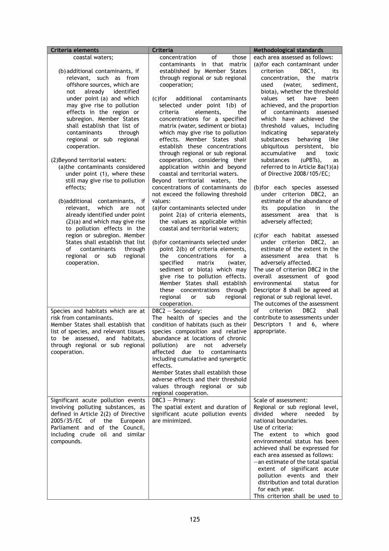
125


coastal waters;

(b) additional contaminants, if

relevant, such as from offshore sources, which are not already identified under point (a) and which may give rise to pollution effects in the region or subregion. Member States shall establish that list of contaminants through regional or sub regional cooperation.

(2) Beyond territorial waters:

(a) the contaminants considered under point (1), where these still may give rise to pollution effects;

(b) additional contaminants, if

relevant, which are not already identified under point (2)(a) and which may give rise to pollution effects in the region or subregion. Member States shall establish that list of contaminants through regional or sub regional cooperation.

concentration of those contaminants in that matrix established by Member States through regional or sub regional cooperation;

(c) for additional contaminants

selected under point 1(b) of criteria elements, the concentrations for a specified matrix (water, sediment or biota) which may give rise to pollution effects. Member States shall establish these concentrations through regional or sub regional cooperation, considering their application within and beyond coastal and territorial waters.

Beyond territorial waters, the concentrations of contaminants do not exceed the following threshold values: (a) for contaminants selected under

point 2(a) of criteria elements, the values as applicable within coastal and territorial waters;

(b) for contaminants selected under

point 2(b) of criteria elements, the concentrations for a specified matrix (water, sediment or biota) which may give rise to pollution effects. Member States shall establish these concentrations through regional or sub regional cooperation.

each area assessed as follows: (a) for each contaminant under

criterion D8C1, its concentration, the matrix used (water, sediment, biota), whether the threshold values set have been achieved, and the proportion of contaminants assessed which have achieved the threshold values, including indicating separately substances behaving like ubiquitous persistent, bio accumulative and toxic substances (uPBTs), as referred to in Article 8a(1)(a) of Directive 2008/105/EC;

(b) for each species assessed

under criterion D8C2, an estimate of the abundance of its population in the assessment area that is adversely affected;

(c) for each habitat assessed

under criterion D8C2, an estimate of the extent in the assessment area that is adversely affected.

The use of criterion D8C2 in the overall assessment of good environmental status for Descriptor 8 shall be agreed at regional or sub regional level. The outcomes of the assessment of criterion D8C2 shall contribute to assessments under Descriptors 1 and 6, where appropriate.

Species and habitats which are at risk from contaminants. Member States shall establish that list of species, and relevant tissues to be assessed, and habitats, through regional or sub regional cooperation.

D8C2 — Secondary: The health of species and the condition of habitats (such as their species composition and relative abundance at locations of chronic pollution) are not adversely affected due to contaminants including cumulative and synergetic effects. Member States shall establish those adverse effects and their threshold values through regional or sub regional cooperation.

Significant acute pollution events involving polluting substances, as defined in Article 2(2) of Directive 2005/35/EC of the European Parliament and of the Council, including crude oil and similar compounds.

D8C3 — Primary: The spatial extent and duration of significant acute pollution events are minimized.

Scale of assessment: Regional or sub regional level, divided where needed by national boundaries. Use of criteria: The extent to which good environmental status has been achieved shall be expressed for each area assessed as follows: — an estimate of the total spatial

extent of significant acute pollution events and their distribution and total duration for each year.

This criterion shall be used to

126


trigger assessment of criterion D8C4.

Species of the species groups, as listed under Table 1 of Part II, and benthic broad habitat types, as listed under Table 2 of Part II.

D8C4 — Secondary (to be used when a significant acute pollution event has occurred): The adverse effects of significant acute pollution events on the health of species and on the condition of habitats (such as their species composition and relative abundance) are minimized and, where possible, eliminated.

Scale of assessment: As used for assessment of the species groups or benthic broad habitat types under Descriptors 1 and 6. Use of criteria: The outcomes of assessment of criterion D8C4 shall contribute, where the cumulative spatial and temporal effects are significant, to the assessments under Descriptors 1 and 6 by providing: (a) an estimate of the abundance

of each species that is adversely affected;

(b) an estimate of the extent of

each broad habitat type that is adversely affected.

The use of criterion D8C4 in the overall assessment of good environmental status for Descriptor 8 shall be agreed at regional or sub regional level.

Specifications and standardized methods for monitoring and assessment:

1. For criteria elements under D8C1, the selection under points 1(b) and 2(b) of additional

contaminants that may give rise to pollution effects shall be based on a risk assessment.

For these contaminants, the matrix and threshold values used for the assessment shall

be representative of the most sensitive species and exposure pathway, including hazards

to human health via exposure through the food chain.

2. For the purposes of this Decision:

• Criterion D8C1: for the assessment of contaminants in coastal and territorial waters, Member States shall monitor the contaminants in accordance with the requirements of Directive 2000/60/EC and the assessments under that Directive shall be used where available. Information on the pathways (atmospheric, land- or sea-based) for contaminants entering the marine environment shall be collected, where feasible.

• Criteria D8C2 and D8C4: biomarkers or population demographic characteristics (e.g. fecundity rates, survival rates, mortality rates, and reproductive capacity) may be relevant to assess the health effects.

• Criteria D8C3 and D8C4: for the purposes of this Decision, monitoring is established as needed once the acute pollution event has occurred, rather than being part of a regular monitoring program under Article 11 of Directive 2008/56/EC.

• Criterion D8C3: Member States shall identify the source of significant acute pollution events, where possible. They may use the European Maritime Safety Agency satellite-based surveillance for this purpose.

3. Contaminants shall be understood to refer to single substances or to groups of

substances. For consistency in reporting, the grouping of substances shall be agreed at

Union level.

4. Species composition shall be understood to refer to the lowest taxonomic level

appropriate for the assessment.

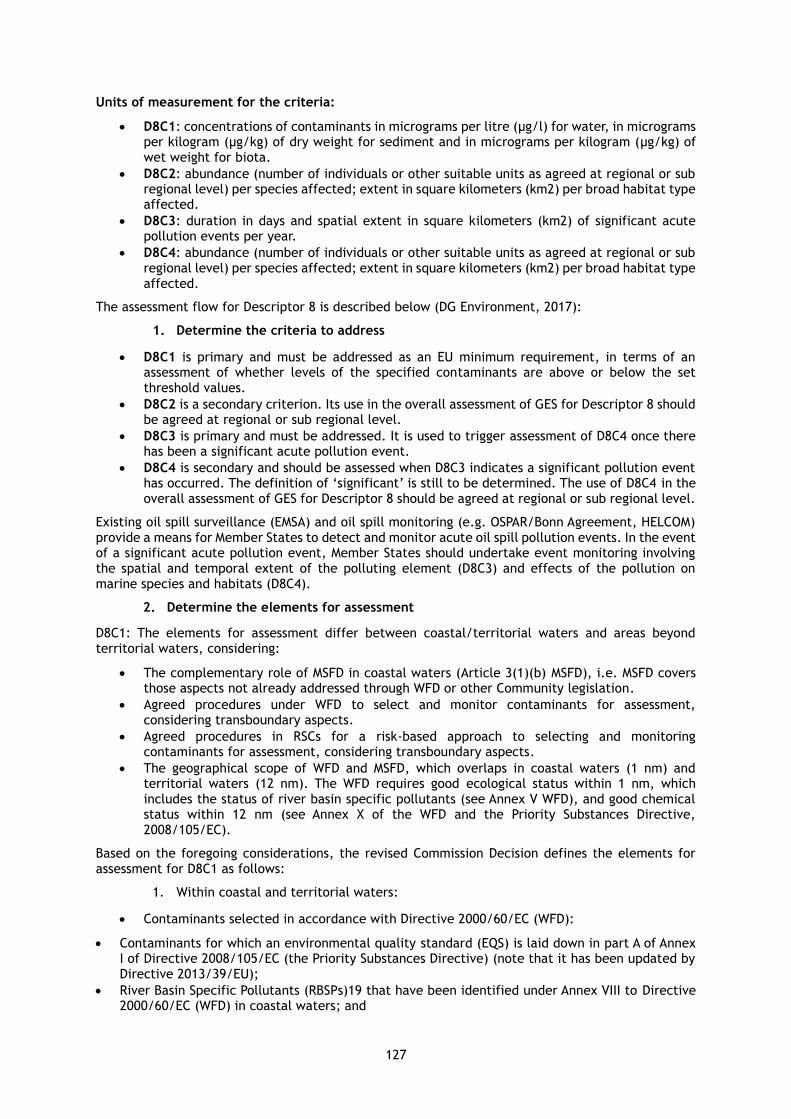
127

Units of measurement for the criteria:

• D8C1: concentrations of contaminants in micrograms per litre (μg/l) for water, in micrograms per kilogram (μg/kg) of dry weight for sediment and in micrograms per kilogram (μg/kg) of wet weight for biota.

• D8C2: abundance (number of individuals or other suitable units as agreed at regional or sub regional level) per species affected; extent in square kilometers (km2) per broad habitat type affected.

• D8C3: duration in days and spatial extent in square kilometers (km2) of significant acute pollution events per year.

• D8C4: abundance (number of individuals or other suitable units as agreed at regional or sub regional level) per species affected; extent in square kilometers (km2) per broad habitat type affected.

The assessment flow for Descriptor 8 is described below (DG Environment, 2017):

1. Determine the criteria to address

• D8C1 is primary and must be addressed as an EU minimum requirement, in terms of an assessment of whether levels of the specified contaminants are above or below the set threshold values.

• D8C2 is a secondary criterion. Its use in the overall assessment of GES for Descriptor 8 should be agreed at regional or sub regional level.

• D8C3 is primary and must be addressed. It is used to trigger assessment of D8C4 once there has been a significant acute pollution event.

• D8C4 is secondary and should be assessed when D8C3 indicates a significant pollution event has occurred. The definition of ‘significant’ is still to be determined. The use of D8C4 in the overall assessment of GES for Descriptor 8 should be agreed at regional or sub regional level.

Existing oil spill surveillance (EMSA) and oil spill monitoring (e.g. OSPAR/Bonn Agreement, HELCOM) provide a means for Member States to detect and monitor acute oil spill pollution events. In the event of a significant acute pollution event, Member States should undertake event monitoring involving the spatial and temporal extent of the polluting element (D8C3) and effects of the pollution on marine species and habitats (D8C4).

2. Determine the elements for assessment

D8C1: The elements for assessment differ between coastal/territorial waters and areas beyond territorial waters, considering:

• The complementary role of MSFD in coastal waters (Article 3(1)(b) MSFD), i.e. MSFD covers those aspects not already addressed through WFD or other Community legislation.

• Agreed procedures under WFD to select and monitor contaminants for assessment, considering transboundary aspects.

• Agreed procedures in RSCs for a risk-based approach to selecting and monitoring contaminants for assessment, considering transboundary aspects.

• The geographical scope of WFD and MSFD, which overlaps in coastal waters (1 nm) and territorial waters (12 nm). The WFD requires good ecological status within 1 nm, which includes the status of river basin specific pollutants (see Annex V WFD), and good chemical status within 12 nm (see Annex X of the WFD and the Priority Substances Directive, 2008/105/EC).

Based on the foregoing considerations, the revised Commission Decision defines the elements for assessment for D8C1 as follows:

1. Within coastal and territorial waters:

• Contaminants selected in accordance with Directive 2000/60/EC (WFD):

• Contaminants for which an environmental quality standard (EQS) is laid down in part A of Annex I of Directive 2008/105/EC (the Priority Substances Directive) (note that it has been updated by Directive 2013/39/EU);

• River Basin Specific Pollutants (RBSPs)19 that have been identified under Annex VIII to Directive 2000/60/EC (WFD) in coastal waters; and

128

• Additional contaminants, if relevant, which may give rise to pollution effects in the marine region or subregion. Member States shall establish the list of additional contaminants through regional or sub regional cooperation. Some additional contaminants may already be identified for monitoring by RSCs. Additional contaminants may reflect, for example, offshore pollution and atmospheric deposition of contaminants.

2. Beyond territorial waters:

• The contaminants considered under point (1) where they still may give rise to pollution effects. Contaminants can be removed from the list of those monitored through a risk-based approach.

• Additional contaminants, if relevant, which are not already identified above, and which may give rise to pollution effects in the region or subregion. The list of additional contaminants should be established through regional or sub regional cooperation.

For criteria elements under D8C1, the selection of additional contaminants within and beyond coastal and territorial waters that may give rise to pollution effects shall be based on a risk assessment. For these contaminants, the matrix and threshold values used for the assessment shall be representative of the most sensitive species and exposure pathway, including hazards to human health via exposure through the food chain. The resulting lists of contaminants should be treated individually or as groups, as agreed at Union level.

D8C2: Member States should establish a list of species, and relevant tissues to be assessed, and (benthic) habitats, at risk of adverse effects from contaminants, including cumulative and synergistic effects, through regional or sub regional cooperation.

D8C3: The elements for assessment are significant acute pollution events involving polluting substances, including crude oil and similar compounds. ‘Polluting substances’ are defined in Article 2(2) of Directive 2005/35/EC of the European Parliament and of the Council as the substances covered by Annexes I (oil) and II (noxious liquid substances in bulk) to MARPOL 73/78. The spatial extent and duration of such events needs to be monitored. Note that there is not yet an agreed definition of ‘significant’ in this context. This needs to be agreed.

D8C4: The species of the species groups assessed under Descriptor 1 and benthic broad habitat types assessed under Descriptors 1 and 6.

3. Determine scales and areas for assessment

The revised Commission Decision indicates the following spatial scales for assessment:

• D8C1 and D8C2:

• Within coastal and territorial waters: as used under Directive 2000/60/EC. This implies the use of WFD water bodies in coastal waters, and other polygons if defined for territorial waters, and will facilitate the reuse of information from WFD. Note that for good ecological status, WFD requires Member States to define water bodies for assessment (i.e. assessment units) within 1 nm.

• Beyond territorial waters: subdivisions of the region or subregion, divided where needed by national boundaries.

• D8C3: Region or subregion, divided where needed by national boundaries.

• D8C4: The same assessment scales and areas as used for the species groups or benthic broad habitat types under Descriptors 1 and 6.

4. Assign indicators to criteria

• Relevant regional indicators that are available should be identified and allocated to the selected contaminants, biological effects and associated assessment areas.

• Any remaining gaps should be identified. Use national assessments (considering existing assessments e.g. under EU legislation such as WFD, Habitats Directive), where available, pending the development of regionally coordinated assessments.

• Additional national indicators for elements that are specific to national waters, if any, can also be incorporated and allocated to the relevant criteria and assessment areas. These need to have a threshold value, where appropriate, and should follow the agreed structure for reporting indicators.

129

The scales for assessment consider the different approaches of Member States to monitoring beyond 1 nm and/or 12 nm, such as offshore monitoring, modelling, or extrapolation of WFD results from within 1 nm and/or 12 nm to larger areas.

5. Establish threshold values

The threshold values for assessment are:

D8C1: For contaminants selected in accordance with Directive 2000/60/EC, the values set in accordance with Directive 2000/60/EC, i.e.:

• the environmental quality standards (EQS) for WFD priority substances established by EQS Directive;

• the national values set by Member States.

For additional contaminants listed through regional or sub regional cooperation, threshold values for the concentrations in the specified matrix (water, sediment or biota), which may give rise to pollution effects, shall be established by Member States through regional or sub regional cooperation.

D8C2: Threshold values for adverse effects (including cumulative and synergistic effects) on the health of species and the condition of habitats (e.g. species composition and their relative abundance at locations of chronic pollution), should be set by Member States through regional or sub regional cooperation.

D8C3: No threshold values are required.

D8C4: No threshold values are required.

6. Determine if threshold values are achieved

• D8C1: The status of each contaminant in each relevant matrix should be determined, based on its concentration compared to the relevant threshold value established in Step 5.

• D8C2: The status of each species or habitat assessed should be determined, based on the selected indicators for adverse effects and their estimated current state compared to the threshold values established in Step 5.

• D8C3: No status assessment required, but there is need to quantify the extent and duration of significant pollution events. The occurrence of a significant pollution event (identified from monitoring this criterion) should trigger the assessment of criterion D8C4.

• D8C4: No status assessment required. The adverse effects of significant pollution events on the health of species and the condition of habitats should be monitored and, where the cumulative spatial and temporal effects are significant, the outputs should contribute to assessments under Descriptors 1 and 6. This is in the form of the number of each species and/or the extent of each broad habitat type that is adversely affected.

7. Integrate indicators and criteria

The indicators should be integrated, based on the integration methods presented in section VII.3

6.1.2 Black Sea D8 criteria and indicators

National and regional approaches are presented in Table 6.3 to Table 6.7.

Bulgaria

The Bulgarian monitoring program under Descriptor 8 has been prepared in accordance with the requirements of the Water Framework Directive (WFD) and the Directive for setting environmental quality standards (Directive 2008/105 / EC, as amended by Directive 2013/39 / EU), and that it covers all elements of the GES definition (8.1). The monitoring of priority substances in surface waters is in accordance with the Ordinance on Environmental Quality Standards (EQS) for priority substances and some other pollutants. It transposes into Bulgarian legislation Directive 2013/39 / EU amending the WFD and Directive 2008/105 / EU.

The methodology for assessing the status of surface waters in Bulgaria has been in the application of

130

the provisions of Directive 2008/105 / EU and Directive 2013/39 / EU. The national methodology is developed for chemical elements (Cd,Ni,Pb and Hg) and for organic pollutant in the water for the application of WFD assessment.The application of the methodology is not mandatory – According to National methodology for assessment of the Chemical status of surface water bodies the calculated 95 percentile of the results must be compared with MAC – EQS to evaluate accidental excesses of the maximum allowable concentration according to Directive 2013/39 / EU. The upper 95% confidence level value must be compared with threshold for the average concentration –AA-EQS according to Directive 2013/39 / EU.

The table below (Table 6.2) was filled according to MSFD national program of measures. At national level, there are no environmental quality standards for marine sediments to be used to assess the state of sediment pollution. According to National Approach to evaluation of trends in changing concentrations of pollutants in sediment and biota it is recommended to analyse the trend of polluters in sediments.

Table 6.2 - Descriptor 8: operational indicators and targets in Bulgaria

Proposed indicator

GES Proposed target Environmental objectives

Concentration of priority and specific substances in the water matrix

the concentrations of the observed pollutants in water and biota are below their maximum permissible and average annual values according to the environmental quality standards of the marine environment applied according to the Water Framework Directive 2000/60 / EC and Directive 2008/105 / EC, as amended by Directive 2013 / 39 / EC.

D8C1 — Primary: The concentrations of the observed pollutants (priority substances and specific pollutants) in the biota are equal to or lower than the defined environmental quality standards for priority substances and certain other pollutants in the marine environment applied according to Directive 2008/105 / EC, as amended by Directive 2013/39 / EC. transposed into national law through the EQS Regulation on priority substances and certain other pollutants, adopted by Council of Ministers Decree 256/2010 in force from 11.12.2015 The Ordinance on Environmental Quality Standards for Priority Substances and Certain Other Pollutants, adopted by a decree of the Council of Ministers № 256 / 1.11.2010, in force since 11.12.2015 (NQFS)

Pressure objective Pressure limitation from point and diffuse sources of pollution, including from the atmosphere. Progress towards good environmental status will be reported as pollution gradually decreases, ie. presence of pollutants in the marine environment as well as their biological impacts are maintained within acceptable limits so as to ensure that there are no significant impacts on or risk to the marine environment

Concentration of metals and synthetic contaminants in the biota matrix:

The concentrations of the observed pollutants (priority substances and specific pollutants) in the biota are equal to or lower than the defined environmental quality standards for priority substances and certain other pollutants in the marine. environment applied according to Directive 2008/105 / EC, as amended by Directive 2013/39 / EC.

The concentrations of contaminates in biota do not increase and are less than the EQS values.

Concentration of priority and specific substances in superficial marine sediments.

Concentrations of the relevant contaminants (measured in sediment) do not have an increasing trend

Threshold values do not exist. The long term trend of pollutants in sediments is decreasing.

The concentrations of contaminates in sediment decrease.

131

Romania

In Romania, indicators and targets were defined for the criteria D8C1 (Table 6.3). The other criteria of the Descriptor 8 (D8C2, D8C3, D8C4) are not yet operational.

Table 6.3 - Descriptor 8, criteria D8C1: operational indicators and targets in Romania

Proposed indicator GES Proposed target Environmental objectives

Heavy metals concentration in superficial marine sediments.

Concentrations of the relevant contaminants measured in appropriate matrices (water, sediment or biota) are lower than concentrations at which negative effects may occur or demonstrate a downward tendency. – Coastal waters (up to 12 nautical miles): the concentrations of relevant contaminants, measured in appropriate matrices (water, sediment or biota) complies with environmental quality standards used in the WFD in 12 nm zone (for priority substances) or 1 nm area (for all other substances). – Waters of the wide area (from 1 or 12 nautical miles, respectively): the concentrations of relevant contaminants in the appropriate matrices (water, sediment or biota) comply with environmental quality standards or demonstrate a downward tendency.

The 75th percentile of heavy metals concentrations in sediments is less than the levels from which adverse effects are expected (ERL/US EPA; SQC/Ord. 161/2006)

Status Objective: The concentrations of contaminates in water, sediment and biota do not increase. Pressure Objective: The intake of contaminants in the marine environment is reduced. Impact Objective: The percentage of samples of water, sediment and biota that exceed the values proposed as a limit for GES is reduced (< 25%).

Heavy Metals concentration in marine waters

The 75th percentile of heavy metals concentrations in marine waters is less than the levels from which adverse effects are expected (Directive 2013/39/EU)

Concentration of synthetic contaminants in superficial marine sediments.

The 75th percentile of the concentrations of synthetic contaminants in sediments is less than the levels from which adverse effects are expected (ERL/US EPA; EAC/OSPAR)

Concentration of synthetic contaminants in marine waters

The 75th percentile of the concentrations of synthetic contaminants in marine waters is less than the levels from which adverse effects are expected (Directive 2013/39/EU)

Concentration of polynuclear aromatic hydrocarbons in superficial marine sediments.

The 75th percentile of polynuclear aromatic hydrocarbons concentrations measured in sediments is less than the levels from which adverse effects are expected (ERL/US EPA; EAC/OSPAR)

Concentration of polynuclear aromatic hydrocarbons in marine waters

The 75th percentile of polynuclear aromatic hydrocarbons concentrations in marine waters is less than the levels from which adverse effects are expected (Directive 2013/39/EU)

Turkey

Turkey is intending to implement ecosystem-based environmental management of its national marine waters in line with the MSFD. However, the MSFD is not obligatory in Turkey yet. Under the projects such as “The Capacity Building on Marine Strategy Framework Directive in Turkey (MarinTurk)” completed in 2017 and the ongoing National Marine Strategy Framework project, GES definitions, indicators and targets were discussed and reported by the experts for the criteria D8C1, D8C2, D8C3, D8C4 (Table 6.4). They are not operational since there is not a legal basis for the implementation of the MSFD in Turkey yet.

Additionally, in Turkey, marine environmental monitoring is complex, since existing monitoring is divided between a large number of ministries, universities, local governmental bodies and NGOs. Some of this monitoring is routine and repeated on a regular basis, while other work is project based, and thus of limited sustainability. The national monitoring program does not cover the contaminants in the water matrix yet. However, the Environmental Quality Criteria were established for the specific pollutants (additional to the priority substances of the WFD) and started to be measured in project basis with limited spatial coverage and temporal frequency.

132

Table 6.4 - Descriptor 8: operational indicators and targets in Turkey

Indicator GES Proposed Target Environmental objectives

Level of the selected priority substances in appropriate matrices

Concentrations of the relevant contaminants measured in appropriate matrices (water, sediment or biota) are lower than the established threshold values

A numerical target will be proposed after the statistically meaningful number of the stations were monitored

Status objective: The concentrations of contaminates in water, sediment and biota do not increase and are less than the EQS values Pressure Objective: Implementation of the IPPC directive Impact Objective: Achieving Good Ecological Status D1 and D4 indicators Operational Objectives: *Standardized monitoring program (including water matrix) for MSFD purposes *Usage of passive samplers for water matrix *Determination of the background levels for heavy metals and PAH * Establish a National IPPC directive

Ratio of the measured / reference level of the selected heavy metals and/or PAH in sediment

PAH and metals in the sediment matrix should be close to the background level (in the areas where the background levels are known)

A numerical target will be proposed after the statistically meaningful number of the stations were monitored and the background levels were determined in the sub regional scale

Trend (at least 10 years) of the heavy metals and/or PAH levels in sediment

Concentrations of the relevant contaminants (measured in sediment) do not have an increasing trend

A numerical target will be proposed after the statistically meaningful number of the stations were monitored

Number of accidental /illegal pollution events and area of the spill

Decreasing number of accidental / illegal pollution events

A numerical target will be proposed after the accidental pollution events were reported

Status objective: Decreasing number of accidental / illegal pollution events Pressure Objective: Implementation of the Emergency Response Plans Impact Objective: D1 and D4 indicators Operational Objectives: Reporting and documentation of the accidents for the purpose of MSFD Effective post spill cleaning operations

Ukraine

Determination of the ecological status of the Black and Azov Seas within the territorial waters of Ukraine and the exclusive maritime economic zone of Ukraine by the content of pollutants is carried out according to EU Directive 2013/39 / EU (MAC-EQS) and environmental regulations (ER).

The pollution factor (Kz) is used to assess the ecological condition. Kz reflects the concentration of all pollutants of the same type in a certain period in a given area. This coefficient is calculated as the sum of the ratios of the concentration of each pollutant to its maximum allowable concentration in accordance with the regulations, referred to the number of measurements performed in a given period. The accuracy of the reflection of the ecological condition with the help of the coefficient depends on the number of monitoring stations in the studied area and the number of observations for a specific period.

When assessing the ecological status of the marine environment, separate groups of pollutants (such as pesticides, PCBs, PAHs, HM) are considered. The ecological condition of the district is determined by the worst Kz indicator for any of the assessed groups. In each of the assessed groups of pollutants,

133

the Kz is determined for each pollutant that is included in it, at the maximum permissible concentration set for it, this makes it possible to identify possible sources of pollution (Table 6.5, Table 6.6).

Table 6.5 - Environmental assessment depending on the pollution factor (Kz)

Kz Pesticides, PCB’s, PAH’s Kz heavy metals Ecological condition

For sea water Kz is distributed on the following scale

less than 0.5 less than 0.5 Very good

from 0.5 to 1.0 from 0.5 to 1.0 Good

from 1.0 to 2.5 from 1.0 to 2.5 Satisfactory

from 2.5 to 5.0 from 2.5 to 5.0 Bad

more than 5.0 more than 5.0 Very bad

For superficial marine sediments Kz is distributed on the following scale





more than 25.0 more than 2.5 Very bad

Table 6.6 - Descriptor 8: operational indicators and targets in Ukraine

Proposed indicator GES Proposed target Environmental objectives

Heavy metals concentration in marine water.

Kz for individual groups of substances does not exceed 1

Maintaining indicators of Kz at a low level in marine areas with good environmental status and a decrease in indicators of Kz compared to those assessed in the previous year in areas with poor environmental conditions.

Status Objective: The concentrations of contaminates in water, sediment and biota do not increase. Pressure Objective: The intake of contaminants in the marine environment is reduced. Impact Objective: Kz of water, sediment and biota in areas with poor ecological status is reduced.

Pesticides in marine waters

PCB’s in marine waters

PAH’s in marine waters

Heavy metals in superficial marine sediments.

Pesticides in superficial marine sediments.

PCB’s in superficial marine sediments.

PAH’s in superficial marine sediments.

Table 6.7 - Indicators under D8C1, D8C2, D8C3, D8C4 used in the Black Sea region. Matrices: W-water, S-sediment, B-biota

Country BG RO TR UA

Criteria Indicators

D8C1 Primary: Within coastal, territorial and beyond territorial waters, the concentrations of contaminants do not exceed the threshold values.

fully operational 1.Heavy metals in W,S,B 2.Synthetic contaminants in W, S, B; 3.Polynuclear aromatic hydrocarbons in W, S, B. 4. Radionuclides -W

fully operational 75 percentile of contaminants concentrations 1. Heavy metals in W, S, B; 2.Synthetic contaminants in W, S, B; 3.Polynuclear aromatic hydrocarbons in W, S, B.

fully operational 1. Heavy metals in S, B; 2.Synthetic contaminants in S, B; 3.Polynuclear aromatic hydrocarbons in S, B. (The National Monitoring program doesn’t include the water

partially operational Kz for individual groups of substances does not exceed 1 1. Heavy metals in W, S, B; 2. Pesticides contaminants in W, S, B. 3.PCB’s contaminants in W, S, B. 4. PAH’s

134

Country BG RO TR UA

Criteria Indicators

matrix yet) contaminants in W, S, B.

D8C2 — Secondary: The health of species and the condition of habitats (such as their species composition and relative abundance at locations of chronic pollution) are not adversely affected due to contaminants including cumulative and synergetic effects.

not operational not operational not operational not operational

D8C3 — Primary: The spatial extent and duration of significant acute pollution events are minimized.

not operational not operational partially operational

not operational

D8C4 — Secondary The adverse effects of significant acute pollution events on the health of species and on the condition of habitats (such as their species composition and relative abundance) are minimized and, where possible, eliminated.

not operational not operational not operational not operational

6.2 Harmonized approach for thresholds setting based on the regional progress

According to Commission Decision EU/2017/848, until Member States have established threshold values through Union, regional or sub regional cooperation, they may use any of the following to express the extent to which good environmental status is being achieved:

• national threshold values, provided the obligation of regional cooperation laid down in Articles 5 and 6 of Directive 2008/56/EC is complied with;

• directional trends of the values;

• pressure-based threshold values as proxies.

The established threshold values shall follow, where possible, the following principles:

• be part of the set of characteristics used by Member States in their determination of good environmental status;

• where appropriate, distinguish the quality level that reflects the significance of an adverse effect for a criterion and be set in relation to a reference condition;

• be set at appropriate geographic scales of assessment to reflect the different biotic and abiotic characteristics of the regions, subregions and subdivisions;

• be set based on the precautionary principle, reflecting the potential risks to the marine environment;

• make use of best available science;

• be based on long time-series data, where available, to help determine the most appropriate value;

• reflect natural ecosystem dynamics, including predator-prey relationships and hydrological and climatic variation, also acknowledging that the ecosystem or parts thereof may recover, if deteriorated, to a state that reflects prevailing physiographic, geographic, climatic and biological conditions, rather than return to a specific state of the past;

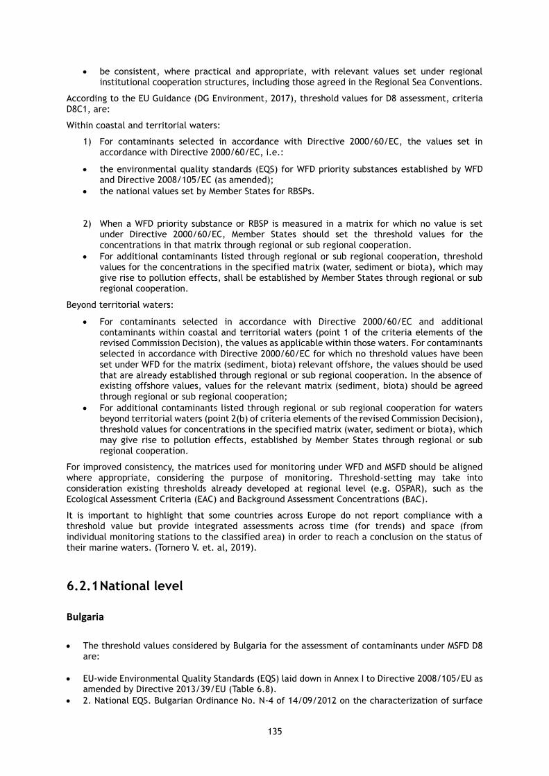
135

• be consistent, where practical and appropriate, with relevant values set under regional institutional cooperation structures, including those agreed in the Regional Sea Conventions.

According to the EU Guidance (DG Environment, 2017), threshold values for D8 assessment, criteria D8C1, are:

Within coastal and territorial waters:

1) For contaminants selected in accordance with Directive 2000/60/EC, the values set in accordance with Directive 2000/60/EC, i.e.:

• the environmental quality standards (EQS) for WFD priority substances established by WFD and Directive 2008/105/EC (as amended);

• the national values set by Member States for RBSPs.

2) When a WFD priority substance or RBSP is measured in a matrix for which no value is set under Directive 2000/60/EC, Member States should set the threshold values for the concentrations in that matrix through regional or sub regional cooperation.

• For additional contaminants listed through regional or sub regional cooperation, threshold values for the concentrations in the specified matrix (water, sediment or biota), which may give rise to pollution effects, shall be established by Member States through regional or sub regional cooperation.

Beyond territorial waters:

• For contaminants selected in accordance with Directive 2000/60/EC and additional contaminants within coastal and territorial waters (point 1 of the criteria elements of the revised Commission Decision), the values as applicable within those waters. For contaminants selected in accordance with Directive 2000/60/EC for which no threshold values have been set under WFD for the matrix (sediment, biota) relevant offshore, the values should be used that are already established through regional or sub regional cooperation. In the absence of existing offshore values, values for the relevant matrix (sediment, biota) should be agreed through regional or sub regional cooperation;

• For additional contaminants listed through regional or sub regional cooperation for waters beyond territorial waters (point 2(b) of criteria elements of the revised Commission Decision), threshold values for concentrations in the specified matrix (water, sediment or biota), which may give rise to pollution effects, established by Member States through regional or sub regional cooperation.

For improved consistency, the matrices used for monitoring under WFD and MSFD should be aligned where appropriate, considering the purpose of monitoring. Threshold-setting may take into consideration existing thresholds already developed at regional level (e.g. OSPAR), such as the Ecological Assessment Criteria (EAC) and Background Assessment Concentrations (BAC).

It is important to highlight that some countries across Europe do not report compliance with a threshold value but provide integrated assessments across time (for trends) and space (from individual monitoring stations to the classified area) in order to reach a conclusion on the status of their marine waters. (Tornero V. et. al, 2019).


Bulgaria

• The threshold values considered by Bulgaria for the assessment of contaminants under MSFD D8 are:

• EU-wide Environmental Quality Standards (EQS) laid down in Annex I to Directive 2008/105/EU as amended by Directive 2013/39/EU (Table 6.8).

• 2. National EQS. Bulgarian Ordinance No. N-4 of 14/09/2012 on the characterization of surface

136

waters (SG 22 of 05/03/2013). specific pollutants, chemical elements and other substances

Romania

The threshold values considered by Romania for the assessment of contaminants under MSFD D8 are:

1. EU-wide Environmental Quality Standards (EQS)

laid down in Annex I to Directive 2008/105/EU as amended by Directive 2013/39/EU (Table 6.8). The EQS is the concentration of a particular pollutant or group of pollutants in water, or biota which should not be exceeded in order to protect human health and the environment.

EQS are set as a maximum allowable concentration (MAC-EQS) or an annual average (AA-EQS), protecting aquatic organisms from acute and chronic effects, respectively. Water EQS are expressed as total concentrations in the whole water sample except in the case of cadmium, lead, mercury and nickel where the water EQS refer to the dissolved concentration, e.g., the dissolved phase of a water sample obtained by filtration through a 0.45 μm filter or any equivalent pre-treatment, or, where specifically indicated, to the bioavailable concentration.

Additionally, EQSs in biota have been set for some priority substances to protect against secondary poisoning or to protect human health. Depending on the bioaccumulation potential of the pollutant and the protection goal, EQSbiota concerns the concentration in either mussels or fish at trophic level 4 or 4.5.

Applying the MAC-EQS means that the measured concentration at any representative monitoring point within the water body does not exceed the standard. However, in accordance with Section 1.3.4 of Annex V to Directive 2000/60/EC, countries may introduce statistical methods, such as a percentile calculation (e.g. 75th value of monitoring data, used in Romania), to ensure an acceptable level of confidence and precision for determining compliance with the MAC-EQS.

2. Maximum levels

for certain contaminants in foodstuffs set in the Commission Regulation (EC) No 1881/2006 and amendments in order to prevent contaminated foodstuff from being placed on the market.

3. Effects Range-Low (ERL)

values developed by the United States Environmental Protection Agency (US EPA) for assessing the ecological significance of sediment concentrations. ERL is the lower tenth percentile of the data set of concentrations in sediments, which were associated with biological effects, resulted from a large database compiled from many studies (Long et al., 1995). Adverse effects on organisms are rarely observed when concentrations fall below the ERL value. The 50th percentile of data from the above mention database were named the “Effects Range-Median” (ERM) values, representative of concentrations above which effects frequently occur. (Table 6.9).

4. Environmental Assessment Criteria (EAC)

developed by OSPAR and the International Council for the Exploration of the Sea for assessing the ecological significance of sediment concentrations (OSPAR, 2004). Environmental Assessment Criteria (EAC) are assessment tools intended to represent the contaminant concentration in sediment and biota below which no chronic effects are expected to occur in marine species, including the most sensitive species. Concentrations below the EACs are considered to present no significant risk to the environment and to that extent EACs may be considered as being related to the EQSs applied to concentrations of contaminants in water (under the Water Framework Directive) (Table 6.9).

5. National EQS,

besides the threshold values and assessment criteria agreed at EU or regional level, EU countries have also indicated some national standards used for the assessment of some contaminants. (Tornero et. al, 2019).

Romania: national standards for copper (30 µg/L Cu in seawater and 40 µg/g Cu in sediments), and nickel in sediment (35 µg/g Ni), values recommended in national legislation (Order of Minister of Environment and Water Management no. 161/2006 approving the Normative for surface waters quality classification for establishing ecological status of water bodies).

137

Table 6.8 - Environmental Quality Standards (EQS) for priority substances and certain other pollutants (Directive 2013/39/EU)

AA : annual average.

MAC : maximum allowable concentration.

Unit : (μg/l) for columns (4) to (7) (μg/kg wet weight) for column (8)

No Name of substance CAS number (1)

AA-EQS (2) Inland surface waters (3)

AA-EQS (2) Other surface waters

MAC-EQS (4) Inland surface waters (3)

MAC-EQS (4) Other surface waters

EQS Biota (12)

(1) Alachlor 15972-60-8

0.3 0.3 0.7 0.7

(2) Anthracene 120-12-7 0.1 0.1 0.1 0.1

(3) Atrazine 1912-24-9

0.6 0.6 2.0 2.0

(4) Benzene 71-43-2 10 8 50 50

(5) Brominated diphenylethers (5)

32534-81-9

0.14 0.014 0.0085

(6) Cadmium and its compounds (depending on water hardness classes) (6)

7440-43-9

≤ 0.08 (Class 1) 0.08 (Class 2) 0.09 (Class 3) 0.15 (Class 4) 0.25 (Class 5)

0.2 ≤ 0.45 (Class 1) 0.45 (Class 2) 0.6 (Class 3) 0.9 (Class 4) 1.5 (Class 5)

≤ 0.45 (Class 1) 0.45 (Class 2) 0.6 (Class 3) 0.9 (Class 4) 1.5 (Class 5)

(6a) Carbon-tetrachloride (7)

56-23-5 12 12 not applicable

not applicable

(7) C10-13 Chloroalkanes (8)

85535-84-8

0.4 0.4 1.4 1.4

(8) Chlorfenvinphos 470-90-6 0.1 0.1 0.3 0.3

(9) Chlorpyrifos (Chlorpyrifos-ethyl)

2921-88-2

0.03 0.03 0.1 0.1

(9a) Cyclodiene pesticides: Aldrin (7) Dieldrin (7) Endrin (7)

309-00-2 60-57-1 72-20-8 465-73-6

Σ = 0.01 Σ = 0.005

not applicable

not applicable

138






EQS Biota (12)

Isodrin (7)

(9b) DDT total (7), (9) not applicable

0.025 0.025 not applicable

not applicable

para-para-DDT (7) 50-29-3 0.01 0.01 not applicable

not applicable

(10) 1,2-Dichloroethane 107-06-2 10 10 not applicable

not applicable

(11) Dichloromethane 75-09-2 20 20 not applicable

not applicable

(12) Di(2-ethylhexyl)-phthalate (DEHP)

117-81-7 1.3 1.3 not applicable

not applicable

(13) Diuron 330-54-1 0.2 0.2 1.8 1.8

(14) Endosulfan 115-29-7 0.005 0.0005 0.01 0.004

(15) Fluoranthene 206-44-0 0.0063 0.0063 0.12 0.12 30

(16) Hexachloro-benzene 118-74-1 0.05 0.05 10

(17) Hexachloro-butadiene

87-68-3 0.6 0.6 55

(18) Hexachloro-cyclohexane

608-73-1 0.02 0.002 0.04 0.02

(19) Isoproturon 34123-59-6

0.3 0.3 1.0 1.0

(20) Lead and its compounds

7439-92-1

1.2 (13) 1.3 14 14

(21) Mercury and its compounds

7439-97-6

0.07 0.07 20

(22) Naphthalene 91-20-3 2 2 130 130

(23) Nickel and its compounds

7440-02-0

4 (13) 8.6 34 34

(24) Nonylphenols (4-Nonylphenol)

84852-15-3

0.3 0.3 2.0 2.0

(25) Octylphenols ((4-(1,1′,3,3′-tetramethylbutyl)-phenol))

140-66-9 0.1 0.01 not applicable

not applicable

139






EQS Biota (12)

(26) Pentachloro-benzene

608-93-5 0.007 0.0007 not applicable

not applicable

(27) Pentachloro-phenol 87-86-5 0.4 0.4 1 1

(28) Polyaromatic hydrocarbons (PAH) (11)

not applicable

not applicable

not applicable

not applicable

not applicable

Benzo(a)pyrene 50-32-8 1,7 × 10–4

1,7 × 10–4

0.27 0,027 5

Benzo(b)fluor-anthene

205-99-2 see footnote 11

see footnote 11

0.017 0,017 see footnote 11

Benzo(k)fluor-anthene


see footnote 11

0.017 0,017 see footnote 11

Benzo(g,h,i)-perylene


see footnote 11

8.2 × 10–3 8,2 × 10–4 see footnote 11

Indeno(1,2,3-cd)-pyrene


see footnote 11

not applicable

not applicable

see footnote 11

(29) Simazine 122-34-9 1 1 4 4

(29a)

Tetrachloro-ethylene (7)


not applicable

(29b)

Trichloro-ethylene (7)


not applicable

(30) Tributyltin compounds (Tributyltin-cation)

36643-28-4

0.0002 0.0002 0.0015 0,0015

(31) Trichloro-benzenes 12002-48-1


not applicable

(32) Trichloro-methane 67-66-3 2.5 2.5 not applicable

not applicable

(33) Trifluralin 1582-09-8


not applicable

(34) Dicofol 115-32-2 1.3 × 10–3

3.2 × 10–5

not applicable (10)

not applicable (10)

33

(35) Perfluorooctane 1763-23- 6.5 × 10 1.3 × 10 36 7.2 9.1

https://eur-lex.europa.eu/legal-content/EN/TXT/?uri=uriserv:OJ.L_.2013.226.01.0001.01.ENG&toc=OJ:L:2013:226:TOC#ntr10-L_2013226EN.01001402-E0010




140






EQS Biota (12)

sulfonic acid and its derivatives (PFOS)

1 –4 –4

(36) Quinoxyfen 124495-18-7

0.15 0.015 2.7 0.54

(37) Dioxins and dioxin-like compounds

See footnote 10 in Annex X to Directive 2000/60/EC

not applicable

not applicable

Sum of PCDD+PCDF+PCB-DL 0,0065 μg.kg–

1 TEQ (14)

(38) Aclonifen 74070-46-5

0.12 0.012 0.12 0.012

(39) Bifenox 42576-02-3

0.012 0.0012 0.04 0.004

(40) Cybutryne 28159-98-0

0.0025 0.0025 0.016 0.016

(41) Cypermethrin 52315-07-8

8 × 10–5 8 × 10–6 6 × 10–4 6 × 10–5

(42) Dichlorvos 62-73-7 6 × 10–4 6 × 10–5 7 × 10–4 7 × 10–5

(43) Hexabromocyclododecane (HBCDD)

See footnote 12 in Annex X to Directive 2000/60/EC

0.0016 0.0008 0.5 0.05 167

(44) Heptachlor and heptachlor epoxide

76-44-8/1024-57-3

2 × 10–7 1 × 10–8 3 × 10–4 3 × 10–5 6.7 × 10–3

(45) Terbutryn 886-50-0 0.065 0.0065 0.34 0.034

(1) CAS: Chemical Abstracts Service. (2) This parameter is the EQS expressed as an annual average value (AA-EQS). Unless otherwise specified, it applies to the total concentration of all isomers. (3) Inland surface waters encompass rivers and lakes and related artificial or heavily modified water bodies. (4) This parameter is the EQS expressed as a maximum allowable concentration (MAC-EQS). Where the MAC-EQS are marked as “not applicable”, the AA-EQS values are considered protective against short-term pollution peaks in continuous discharges since they are significantly lower than the values derived on the basis of acute toxicity. (5) For the group of priority substances covered by brominated diphenylethers (No 5), the EQS refers to the sum of the concentrations of congener numbers 28, 47, 99, 100, 153 and 154. (6) For Cadmium and its compounds (No 6) the EQS values vary depending on the hardness of the water as specified in five class categories (Class 1: < 40 mg CaCO3/l, Class 2: 40 to < 50 mg CaCO3/l, Class 3: 50 to < 100 mg CaCO3/l, Class 4: 100 to < 200 mg CaCO3/l and Class 5: ≥ 200 mg CaCO3/l). (7) This substance is not a priority substance but one of the other pollutants for which the EQS are identical to those laid down in the legislation that applied prior to 13 January 2009.

https://eur-lex.europa.eu/legal-content/EN/TXT/?uri=uriserv:OJ.L_.2013.226.01.0001.01.ENG&toc=OJ:L:2013:226:TOC#ntc1-L_2013226EN.01001402-E0001







141

(8) No indicative parameter is provided for this group of substances. The indicative parameter(s) must be defined through the analytical method. (9) DDT total comprises the sum of the isomers 1,1,1-trichloro-2,2 bis (p-chlorophenyl) ethane (CAS number 50-29-3; EU number 200-024-3); 1,1,1-trichloro-2 (o-chlorophenyl)-2-(p-chlorophenyl) ethane (CAS number 789-02-6; EU Number 212-332-5); 1,1-dichloro-2,2 bis (p-chlorophenyl) ethylene (CAS number 72-55-9; EU Number 200-784-6); and 1,1-dichloro-2,2 bis (p-chlorophenyl) ethane (CAS number 72-54-8; EU Number 200-783-0). (10) There is insufficient information available to set a MAC-EQS for these substances. (11) For the group of priority substances of polyaromatic hydrocarbons (PAH) (No 28), the biota EQS and corresponding AA-EQS in water refer to the concentration of benzo(a)pyrene, on the toxicity of which they are based. Benzo(a)pyrene can be considered as a marker for the other PAHs, hence only benzo(a)pyrene needs to be monitored for comparison with the biota EQS or the corresponding AA-EQS in water. (12) Unless otherwise indicated, the biota EQS relate to fish. An alternative biota taxon, or another matrix, may be monitored instead, as long as the EQS applied provides an equivalent level of protection. For substances numbered 15 (Fluoranthene) and 28 (PAHs), the biota EQS refers to crustaceans and mollusks. For the purpose of assessing chemical status, monitoring of Fluoranthene and PAHs in fish is not appropriate. For substance number 37 (Dioxins and dioxin-like compounds), the biota EQS relates to fish, crustaceans and mollusks, in line with section 5.3 of the Annex to Commission Regulation (EU) No 1259/2011 of 2 December 2011 amending Regulation (EC) No 1881/2006 as regards maximum levels for dioxins, dioxin-like PCBs and non-dioxin-like PCBs in foodstuffs (OJ L 320, 3.12.2011, p. 18). (13) These EQS refer to bioavailable concentrations of the substances. (14) PCDD: polychlorinated dibenzo-p-dioxins; PCDF: polychlorinated dibenzofurans; PCB-DL: dioxin-like polychlorinated biphenyls; TEQ: toxic equivalents according to the World Health Organization 2005 Toxic Equivalence Factors.’

Table 6.9 - Effects Range-Low (ERL) and Environmental Assessment Criteria (EAC) values for contaminants in sediments

Chemical ERL EAC

Organic contaminants (ng/g d.w.)

PCB 28 - 1.7

PCB 52 - 2.7

PCB 101 - 3.0

PCB 118 - 0.6

PCB 138 - 7.9

PCB 153 - 40

PCB 180 - 12

HCB 20.0 -

Lindane 3.0 -

Dieldrin 2.0 -

DDE (p,p’) 2.2 -

Naphthalene 160.000 -

Phenanthrene 240.000 -

Anthracene 85.000 -

Fluoranthene 600.000 -

Pyrene 665.000 -

Benzo[a]anthracene 261.000 -

Chrysene 384.000 -

Benzo[a]pyrene 430.000 -

Benzo (g,h,i)perylene 85.000 -

Indeno(1,2,3-c,d)pyrene 240.000 -

Heavy metals (µg/g d.w.)

Cadmium (Cd) 1.2 -

Chromium (Cr) 81 -

Copper (Cu) 34 -

Lead (Pb) 46.7 -

Nickel (Ni) 20.9 -

Mercury (Hg) 0.15 -

Zinc (Zn) 150 -

Turkey

The threshold values that will be considered by Turkey for the assessment of contaminants in environmental matrices when the MSFD will be operational, are:

• Usage of the EU/2013/39/ Environmental Quality Standards for Priority Substances:

Concentration of particular pollutants and group of pollutants in water and/or biota matrix should

not be exceeding the Maximum Allowable Concentrations (MAC-EQS) or Annual Average






https://eur-lex.europa.eu/legal-content/EN/AUTO/?uri=OJ:L:2011:320:TOC



142

Concentrations (AA-EQS) (Table 6.8). These values are used for the biota matrix at present

situation. It will be operational for the water matrix when the National Monitoring program will

cover the water matrix.

• Usage of Effect Range Low (ERL) values (US EPA, Long et al., 1995) for the sediment matrix:

Theses values are used for the contaminants measured in the sediment matrix (Table 6.9).

• Usage of the National Surface Water Directive: This directive considers surface water including

coastal and transitional waters and includes the annex including EQS values(2013/39/EU) for the

Priority Substances adopted from WFD and EQS developed for the Specific Pollutants of Turkey.

Since the water matrix is not covered in the National Monitoring Program at present, this directive

is not operational for the MSFD purpose.

Ukraine

The threshold values considered by Ukraine for the assessment of contaminants under MSFD D8 are:

• For the assessment of contaminants in water and biota used EU-wide Environmental Quality

Standards (EQS) laid down in Annex I to Directive 2008/105/EU as amended by Directive

2013/39/EU (Table 6.8).

• For the assessment of contaminants in marine sediments used national EQS, determined in

environmental regulations (ER) (Table 6.10).

Table 6.10 - Indicators EQS for contaminants in sediments in accordance with national environmental regulations (ER) in Ukraine

Name of substance EQS

Metals (all in mg/kg of dry matter)

Cadmium 0.80

Cobalt 20

Copper 35

Arsenic 29

Molybdenum 10

Nickel 35

Tin 20

Mercury 0.30

Lead 85

Chromium 100

Zink 140

Barium 200

Polycyclic aromatic hydrocarbons (all in µg/kg of dry matter)

Anthracene 50

Benz(a)anthracene 20

Benz(ghi)perylene 20

Benz(a)pyrene 25

Benz(k)fluoranthene 25

Indeno(1,2,3-cd)pyrene 25

Phenanthrene 45

Fluoranthene 15

Chrysene 20

Sum of oil hydrocarbons (all in mg/kg of dry matter)

1. Equivalents of Simard 50

Organochlorine pesticides and PCBs (all in µg/kg of dry matter)

-HCH 2.5

DISSP 1.0

-HCH (lindane) 0.05

Sum of HCH isomers 5.0

DDT (plus metabolites) 2.5

Dieldrin 0.5

Endrin 1.0

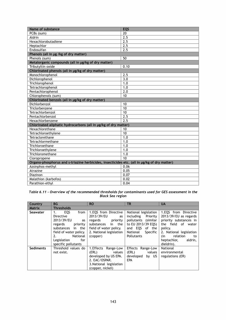
143

Name of substance EQS

PCBs (sum) 20

Aldrin 2.5

Hexachlorobutadiene 2.5

Heptachlor 2.5

Endosulfan 2.5

Phenols (all in µg /kg of dry matter)

Phenols (sum) 50

Metalorganic compounds (all in µg/kg of dry matter)

Tributyltin oxide 0.10

Chlorinated phenols (all in µg/kg of dry matter)

Monochlorophenol 2.5

Dichlorophenol 3.0

Trichlorophenol 1.0

Tetrachlorophenol 1.0

Pentachlorophenol 2.0

Chlorophenols (sum) 10

Chlorinated benzols (all in µg/kg of dry matter)

Dichlorbenzol 10

Triclorbenzene 10

Tetrachlorbenzol 10

Pentachlorbenzol 2.5

Hexachlorbenzene 2.5

Chlorinated aliphatic hydrocarbons (all in µg/kg of dry matter)

Hexachlorethane 10

Tetrachloroethylene 10

Tetraclorethane 1.0

Tetrachlormethane 1.0

Trichloroethane 1.0

Trichloroethylene 1.0

Trichloromethane 1.0

Cloropropene 10

Organo-phosphorus and s-triazine herbicides, insecticides etc. (all in µg/kg of dry matter)

Azsinphos-methyl 0.06

Atrazine 0.05

Diazinon 0.07

Malathion (karbofos) 0.02

Parathion-ethyl 0.04

Table 6.11 - Overview of the recommended thresholds for contaminants used for GES assessment in the Black Sea region

Country BG RO TR UA

Matrix Thresholds

Seawater

1. EQS from Directive 2013/39/EU as regards priority substances in the field of water policy. 2. National Legislation for specific pollutants

1.EQS from Directive 2013/39/EU as regards priority substances in the field of water policy. 2. National legislation (copper)

National legislation including Priority pollutants (similar to EU 2013/39 EQS) and EQS of the National Specific Pollutants

1.EQS from Directive 2013/39/EU as regards priority substances in the field of water policy. 2. National legislation (in relation to heptachlor, aldrin, dieldrin).

Sediments

Threshold values do not exist.

1.Effects Range-Low (ERL) values developed by US EPA. 2. EAC/OSPAR. 3.National legislation (copper, nickel)

Effects Range-Low (ERL) values developed by US EPA

National environmental regulations (ER)

144


At European level, MSFD Expert Network on Contaminants, established by the Joint Research Centre (JRC) to support the MSFD implementation, works towards comparable MSFD Descriptor 8 and 9 assessments, compiling information related to substances, matrices and threshold values/reference levels (Tornero et al., 2019), aiming at equal levels of protection across European Seas. This is part of an on-going process to help regulators to assess relevant contaminants in their jurisdictional area, thus aiming at EU national authorities but also at Regional Sea Conventions in the shared marine regions. So far, environmental quality standards are established by European legislation for a part of contaminants, only in seawater and biota, as there are no regulated thresholds values in sediments.

In cases where no threshold values are laid down, countries should establish threshold values through European, regional or sub regional cooperation, for instance by referring to existing values or developing new ones in the framework of the Regional Sea Conventions. Until such threshold values are established, EU recommendation is that Member States should be able to use national threshold values, directional trends or pressure-based threshold values as proxies.

According to Commission Decision (EU) 2017/848, threshold values should reflect, where appropriate, the quality level that reflects the significance of an adverse effect for a criterion and should be set in relation to a reference condition. Threshold values should be set at appropriate geographic scales to reflect the different biotic and abiotic characteristics of the regions, subregions and subdivisions. This means that even if the process to establish threshold values takes place at EU level, this may result in the setting of different threshold values, which are specific to a region, subregion or subdivision.

At regional level (Black Sea Convention) there are not common agreed harmonized thresholds for contaminants adopted so far.


The degree of integration across criteria is not yet determined. The revised Commission Decision requires outputs separately for each criterion, but also specifies that the use of D8C2 and D8C4 in the overall assessment of GES for Descriptor 8 shall be agreed at regional or sub regional level. This includes whether the criteria feed into the assessment of Descriptor 8 or not, and the possible integration methods to be used.

For D8C1 and D8C2, each assessed criterion should be within threshold values. D8C3 requires the definition of a ‘significant acute pollution event’; when this occurs, D8C4 should be assessed and reported on. There are no threshold values for D8C3 and D8C4. D8C2 and D8C4 should contribute, where appropriate, to the assessment under Descriptors 1 and 6.

Figure 6.1 shows the levels of integration and integration methods for Descriptor 8. According EC MSFD CIS Guidance (DG ENV, 2017), the levels of integration and integration methods for Descriptor 8 build on the assessment of single substances which are combined to indicators of single substances (e.g. individual metals) or groups of substances (e.g. PAHs, PCBs) per matrix or across matrices at the relevant assessment scale. The revised Commission Decision states that ‘contaminants shall be understood to refer to single substances or to groups of substances’ and ‘the grouping of substances shall be agreed at Union level’ so that a consistent approach is used. The Figure VII.1 is representative of a single assessment area, for which the outputs of the assessment can be presented. There is no need to aggregate across spatial areas.

The integration methods of Figure 6.1 are:

Level 1: Measurements of individual elements, i.e. each substance is measured in the relevant matrices (sediment, water, biota) and compared to the matrix-specific threshold value. For the purpose of D8C1 ‘contaminants’ are understood to refer to single substances or to groups of substances. For consistency in reporting, the grouping of substances (which substances and the method for combining them in one group) shall be agreed at EU level. This concerns the grouping of individual substances to a group of substances, for example, polyaromatic hydrocarbons (PAHs) or

145

polychlorinated biphenyls (PCBs).

Level 2: The integration method differs between the criteria:

• D8C1: The results for the various contaminants under D8C1 are not integrated. They are presented individually and as a proportion of contaminants meeting the threshold values. The persistent, bio accumulative and toxic substances (PBTs) (listed in Directive 2013/39/EU) should be presented separately.

• D8C2: The results for the species and habitat types assessed under D8C2 are presented per species and per habitat type for each parameter. The species- and habitat-specific outputs contribute to the assessment of species and habitats under Descriptors 1 and 6. The use of the criterion in the overall assessment of GES for Descriptor 8, and any additional output presentation, shall be agreed at regional or sub regional level.

• D8C3: The outcome shall be expressed as an estimate of the total spatial extent of significant pollution events and their distribution and total duration for each year. The use of the criterion in the assessment of GES for D8 requires agreement. This could be agreed at regional or sub regional level alongside the use of D8C4 in the overall assessment for Descriptor 8.

• D8C4: The results for the species and habitat types assessed under D8C4 are not integrated; the outputs contribute to the assessment of species and habitats under Descriptors 1 and 6. The use of the criterion in the overall assessment of GES for Descriptor 8 shall be agreed at regional or sub regional level.

Level 3: Good environmental status for Descriptor 8 is expressed for each criterion individually. The possible integration of criteria to descriptor level, and whether and how the criteria contribute to the overall Descriptor 8 assessment needs to be agreed at regional or sub regional level.

Figure 6.1 - Levels and methods of integration for Descriptor 8 (DG ENV, 2017)

The following open issues remain for further consideration (DG ENV, 2017):

D8C1:

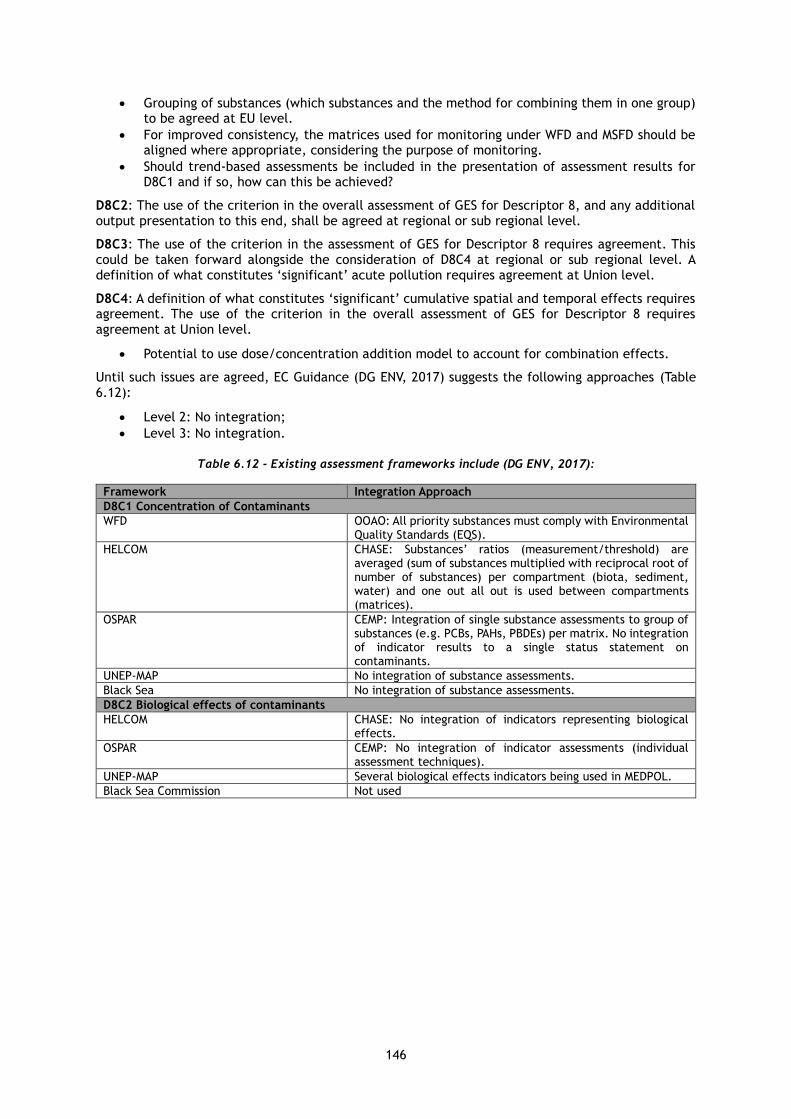
146

• Grouping of substances (which substances and the method for combining them in one group) to be agreed at EU level.

• For improved consistency, the matrices used for monitoring under WFD and MSFD should be aligned where appropriate, considering the purpose of monitoring.

• Should trend-based assessments be included in the presentation of assessment results for D8C1 and if so, how can this be achieved?

D8C2: The use of the criterion in the overall assessment of GES for Descriptor 8, and any additional output presentation to this end, shall be agreed at regional or sub regional level.

D8C3: The use of the criterion in the assessment of GES for Descriptor 8 requires agreement. This could be taken forward alongside the consideration of D8C4 at regional or sub regional level. A definition of what constitutes ‘significant’ acute pollution requires agreement at Union level.

D8C4: A definition of what constitutes ‘significant’ cumulative spatial and temporal effects requires agreement. The use of the criterion in the overall assessment of GES for Descriptor 8 requires agreement at Union level.

• Potential to use dose/concentration addition model to account for combination effects.

Until such issues are agreed, EC Guidance (DG ENV, 2017) suggests the following approaches (Table 6.12):

• Level 2: No integration;

• Level 3: No integration.

Table 6.12 - Existing assessment frameworks include (DG ENV, 2017):

Framework Integration Approach

D8C1 Concentration of Contaminants

WFD OOAO: All priority substances must comply with Environmental Quality Standards (EQS).

HELCOM CHASE: Substances’ ratios (measurement/threshold) are averaged (sum of substances multiplied with reciprocal root of number of substances) per compartment (biota, sediment, water) and one out all out is used between compartments (matrices).

OSPAR CEMP: Integration of single substance assessments to group of substances (e.g. PCBs, PAHs, PBDEs) per matrix. No integration of indicator results to a single status statement on contaminants.

UNEP-MAP No integration of substance assessments.

Black Sea No integration of substance assessments.

D8C2 Biological effects of contaminants

HELCOM CHASE: No integration of indicators representing biological effects.

OSPAR CEMP: No integration of indicator assessments (individual assessment techniques).

UNEP-MAP Several biological effects indicators being used in MEDPOL.

Black Sea Commission Not used

147

7 Guideline on Descriptor D9 Contaminants in Seafood

7.1 Introduction

Descriptor 9 considers the presence of hazardous substances (e.g. chemical elements and compounds) or group of substances that are toxic, persistent and liable to bio-accumulate and other substances or group of substances which give rise to an equivalent level of concern in wild caught fish, crustaceans, molluscs, echinoderms, roe and seaweed harvested in the different regions destined for human consumption against regulatory levels set for human consumption (JRC Task Group Report 2010). The term “regulatory levels set for human consumption” are considered to be the regulatory levels set in community legislation for public health reasons (EC No 1881/2006) or other national/international standards/regulations which are not in contradiction with the EU legislation but include additional contaminants established by risk-based approaches.

The Commission Decision EU/2017/848 laying down criteria and methodological standards on good environmental status of marine waters and specifications and standardized methods for monitoring and assessment, replaces a previous legal instrument from 2010 and provides:

• More flexibility: Member States can focus their efforts on the main problems for their marine waters. They can for example de-select criteria that are not relevant for their seas or apply a risk-based approach to the implementation of their marine strategies.

• Comparable and consistent outcomes across Member States: The new framework focuses on measuring the extent to which good environmental status is. This requires the setting of "threshold values", thereby contributing to an improved and clearer way to achieving environmental objectives.

• Specific situations pertaining to each marine region or subregion: It pushes for more cooperation among Member States in a regional or subregional context, often through the work developed by Member States in Regional Sea Conventions. This not only reduces duplication but ensures that Member States focus on what is most relevant.

• Facilitating the work of Member States: Through the use of existing obligations under other EU legislation (e.g., Water Framework Directive, Habitats Directive, Birds Directive, Common Fisheries Policy) avoids parallel processes that would otherwise create unnecessary burden.

7.2 Overview of criteria and indicators

7.2.1 Commission Decision EU/2017/848, criteria and methodological standards

Descriptor 9 necessarily implicates a balance between health information and environmental assessment. The presence of contaminants, in fish and other seafood, above the health regulatory levels might have a negative influence both on the health of the consumer and on the sustainable use of marine resources, and consequently on the environment (JRC Task Group 9 Report 2010). Good Environmental Status should be achieved when contaminants are below the levels fixed for human consumption n (Decision EU/2017/848); the absence of human health hazards may however involve environmental pollution effects, since these could be present at lower contaminants concentration. The evaluation is carried out for each assessment area by taking into account the concentration of each contaminant have been detected in seafood (for each species and tissues in which used) that weather the threshold values set have been achieved and the proportion of the contaminants achieved their threshold values.

According to the Commission Decision EU/2017/848, criteria and methodological standards on good environmental status of marine waters for Descriptor 9 are presented in the Table 7.1.

148

Descriptor 9: Contaminants in fish and other seafood for human consumption do not exceed levels established by Union legislation or other relevant standards.

Table 7.1 - Criteria, including criteria elements, and methodological standards (Com Dec EU/2017/848)


Contaminants listed in Regulation (EC) No 1881/2006. For the purposes of this Decision, Member States may decide not to consider contaminants from Regulation (EC) No 1881/2006 where justified on the basis of a risk assessment. Member States may assess additional contaminants that are not included in Regulation (EC) No 1881/2006. Member States shall establish a list of those additional contaminants through regional or subregional cooperation. Member States shall establish the list of species and relevant tissues to be assessed, according to the conditions laid down under ‘specifications’. They may cooperate at regional or subregional level to establish that list of species and relevant tissues.

D9C1 — Primary: The level of contaminants in edible tissues (muscle, liver, roe, flesh or other soft parts, as appropriate) of seafood (including fish, crustaceans, mollusks, echinoderms, seaweed and other marine plants) caught or harvested in the wild (excluding fin-fish from mariculture) does not exceed: (a) for contaminants listed in Regulation (EC) No 1881/2006, the maximum levels laid down in that Regulation, which are the threshold values for the purposes of this Decision; (b) for additional contaminants, not listed in Regulation (EC) No 1881/2006, threshold values, which Member States shall establish through regional or subregional cooperation.

Scale of assessment: The catch or production area in accordance with Article 38 of Regulation (EU) No 1379/2013 of the European Parliament and of the Council (1). Use of criteria: The extent to which good environmental status has been achieved shall be expressed for each area assessed as follows: — for each contaminant, its concentration in seafood, the matrix used (species and tissue), whether the threshold values set have been achieved, and the proportion of contaminants assessed which have achieved their threshold values.


1. When Member States establish the list of species to be used under D9C1, the species

shall:

• be relevant to the marine region or subregion concerned;

• fall under the scope of Regulation (EC) No 1881/2006;

• be suitable for the contaminant being assessed;

• be among the most consumed in the Member State or the most caught or harvested for consumption.

2. Exceedance of the standard set for a contaminant shall lead to subsequent monitoring to

determine the persistence of the contamination in the area and species sampled.

Monitoring shall continue until there is sufficient evidence that there is no risk of failure.

3. For the purposes of this Decision, the sampling for the assessment of the maximum levels

of contaminants shall be performed in accordance with Article 11 of Regulation (EC) No

882/2004 of the European Parliament and of the Council (1) and with Commission

Regulation (EU) No 589/2014 (2) and Commission Regulation (EC) No 333/2007 (3).

4. Within each region or subregion, Member States shall ensure that the temporal and

geographical scope of sampling is adequate to provide a representative sample of the

specified contaminants in seafood in the marine region or subregion.

Units of measurement for the criteria:

• D9C1: concentrations of contaminants in the units set out in the Annex to Regulation (EC) No 1881/2006.

The ASSESSMENT FLOW for Descriptor 9 is described below (DG Environment, 2017 R2733):

There is only one criterion for Descriptor 9, and therefore no integration among criteria is required.

149

1. Determine the criteria to address

• D9C1 is primary and must be addressed as an EU minimum requirement.

2. Determine the elements for assessment

The elements for assessment are:

• The contaminants (and the relevant species and tissues specified) listed in Regulation (EC) No 1881/2006 (those relevant to fish and seafood).

• Member States may decide not to consider contaminants from Regulation (EC) No 1881/2006, where they do not pose a risk in the marine region or subregion (i.e. justified on the basis of a risk assessment).

• Member States may assess additional contaminants, a list of which should be established by Member States through regional or subregional cooperation (including the species and relevant tissues in which they are to be monitored).

Only limits for unprocessed seafood should be used (JRC, 2015a), and not limits relating to, for example, PAHs in smoked seafood, since the levels of PAHs may be affected by the smoking process, and unrelated to contaminants in the marine environment.

Where Member States establish a list of contaminants and the species and relevant tissues in which they are to be assessed, in addition to those in Regulation (EC) 1881/2006, the revised Commission Decision sets out specifications for the species, which shall:

• be relevant to the marine region or subregion concerned;

• fall under the scope of Regulation (EC) No 1881/2006; and

• be suitable for the contaminant being assessed;

• be among the most consumed in the Member State or the most caught or harvested for consumption.

3. Determine scales and areas for assessment

The revised Commission Decision indicates the following spatial scales for assessment:

• The catch or production areas in accordance with Article 38 of Regulation (EU) No 1379/2013 (common organization of the markets).

Article 38 of Regulation (EU) No 1379/2013 states the catch or production area is ‘the sub-area or division listed in the FAO fishing areas’. For reference, the relevant subareas and divisions can be found at the following links:

• Mediterranean and Black Sea (Area 37): www.fao.org/fishery/area/Area37/en

These are smaller areas than those recommended for the assessment of Descriptor 3.

For the purposes of the assessment, these catch or production areas can be aggregated to the level of the region or subregion, as recommended for the assessment under Descriptor 3.

4. Assign indicators to criteria

• Relevant regional indicators that are available should be identified and allocated to the Commission Decision criteria (mapping of RSC indicators against the revised Commission Decision criteria is provided in Appendix A). These should make use of the results of sampling and testing under Reg (EC) No 1881/2006 where appropriate but may require additional sampling for any additional substances selected.

• Where regional assessments are not available, national assessments making use of the results of sampling and testing under Reg (EC) No 1881/2006 should be used.

• Additional national indicators for elements that are specific to national waters, if any, should be incorporated into the assessment. These need to have a threshold value, where appropriate, and should follow the agreed structure for reporting indicators (MSCG_17-2015-04), pending guidance on reporting requirements from WG DIKE.

5. Establish threshold values

• For contaminants listed in Regulation (EC) No 1881/2006, the maximum levels for different fish and shellfish species (in specific tissue types).

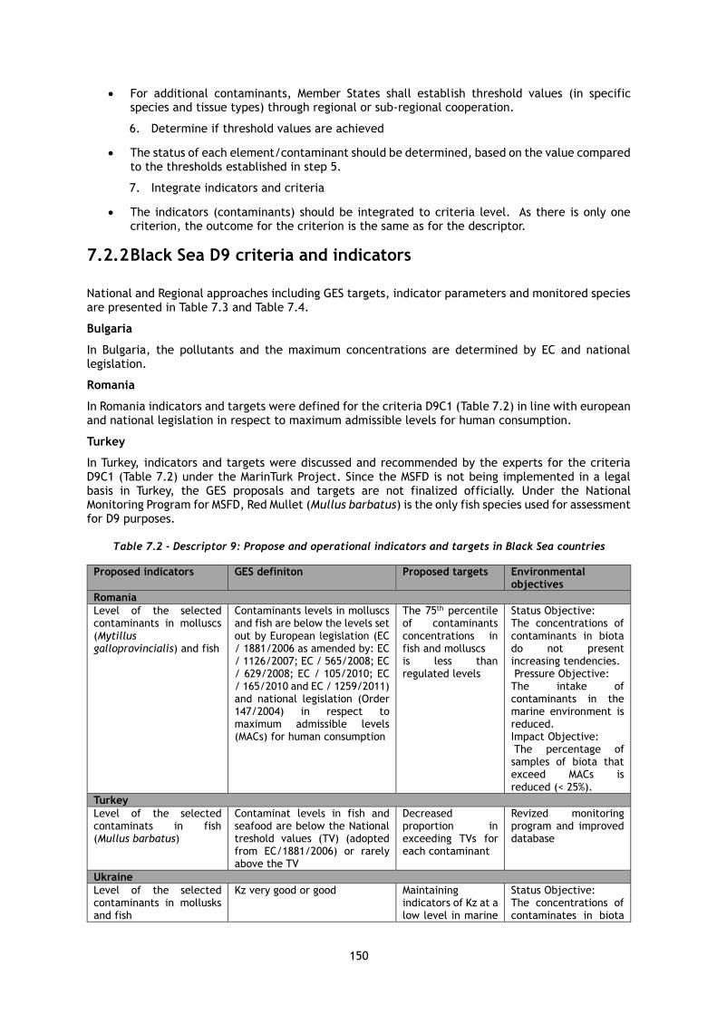
150

• For additional contaminants, Member States shall establish threshold values (in specific species and tissue types) through regional or sub-regional cooperation.

6. Determine if threshold values are achieved

• The status of each element/contaminant should be determined, based on the value compared to the thresholds established in step 5.

7. Integrate indicators and criteria

• The indicators (contaminants) should be integrated to criteria level. As there is only one criterion, the outcome for the criterion is the same as for the descriptor.

7.2.2 Black Sea D9 criteria and indicators

National and Regional approaches including GES targets, indicator parameters and monitored species are presented in Table 7.3 and Table 7.4.

Bulgaria

In Bulgaria, the pollutants and the maximum concentrations are determined by EC and national legislation.

Romania

In Romania indicators and targets were defined for the criteria D9C1 (Table 7.2) in line with european and national legislation in respect to maximum admissible levels for human consumption.

Turkey

In Turkey, indicators and targets were discussed and recommended by the experts for the criteria D9C1 (Table 7.2) under the MarinTurk Project. Since the MSFD is not being implemented in a legal basis in Turkey, the GES proposals and targets are not finalized officially. Under the National Monitoring Program for MSFD, Red Mullet (Mullus barbatus) is the only fish species used for assessment for D9 purposes.

Table 7.2 - Descriptor 9: Propose and operational indicators and targets in Black Sea countries

Proposed indicators GES definiton Proposed targets Environmental objectives

Romania

Level of the selected contaminants in molluscs (Mytillus galloprovincialis) and fish

Contaminants levels in molluscs and fish are below the levels set out by European legislation (EC / 1881/2006 as amended by: EC / 1126/2007; EC / 565/2008; EC / 629/2008; EC / 105/2010; EC / 165/2010 and EC / 1259/2011) and national legislation (Order 147/2004) in respect to maximum admissible levels (MACs) for human consumption

The 75th percentile of contaminants concentrations in fish and molluscs is less than regulated levels

Status Objective: The concentrations of contaminants in biota do not present increasing tendencies. Pressure Objective: The intake of contaminants in the marine environment is reduced. Impact Objective: The percentage of samples of biota that exceed MACs is reduced (< 25%).

Turkey

Level of the selected contaminats in fish (Mullus barbatus)

Contaminat levels in fish and seafood are below the National treshold values (TV) (adopted from EC/1881/2006) or rarely above the TV

Decreased proportion in exceeding TVs for each contaminant

Revized monitoring program and improved database

Ukraine

Level of the selected contaminants in mollusks and fish

Kz very good or good Maintaining indicators of Kz at a low level in marine

Status Objective: The concentrations of contaminates in biota

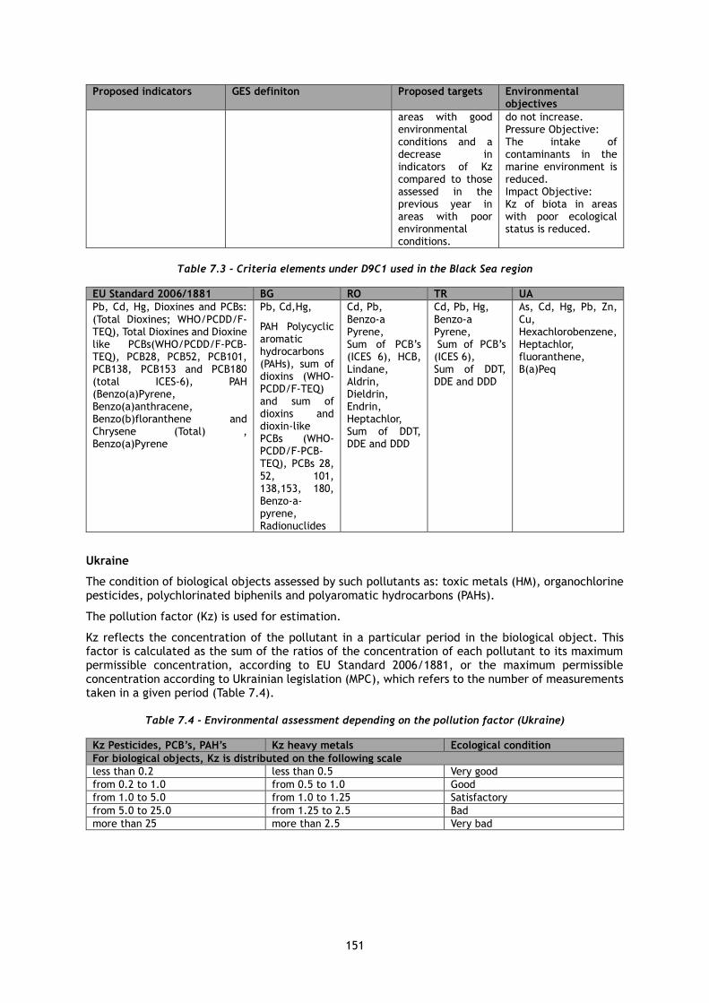
151

Proposed indicators GES definiton Proposed targets Environmental objectives

areas with good environmental conditions and a decrease in indicators of Kz compared to those assessed in the previous year in areas with poor environmental conditions.

do not increase. Pressure Objective: The intake of contaminants in the marine environment is reduced. Impact Objective: Kz of biota in areas with poor ecological status is reduced.

Table 7.3 - Criteria elements under D9C1 used in the Black Sea region

EU Standard 2006/1881 BG RO TR UA

Pb, Cd, Hg, Dioxines and PCBs: (Total Dioxines; WHO/PCDD/F-TEQ), Total Dioxines and Dioxine like PCBs(WHO/PCDD/F-PCB-TEQ), PCB28, PCB52, PCB101, PCB138, PCB153 and PCB180 (total ICES-6), PAH (Benzo(a)Pyrene, Benzo(a)anthracene, Benzo(b)floranthene and Chrysene (Total) , Benzo(a)Pyrene

Pb, Cd,Hg,

PAH Polycyclic aromatic hydrocarbons (PAHs), sum of dioxins (WHO-PCDD/F-TEQ) and sum of dioxins and dioxin-like PCBs (WHO-PCDD/F-PCB-TEQ), PCBs 28, 52, 101, 138,153, 180, Benzo-a-pyrene, Radionuclides

Cd, Pb, Benzo-a Pyrene, Sum of PCB’s (ICES 6), HCB, Lindane, Aldrin, Dieldrin, Endrin, Heptachlor, Sum of DDT, DDE and DDD

Cd, Pb, Hg, Benzo-a Pyrene, Sum of PCB’s (ICES 6), Sum of DDT, DDE and DDD

As, Cd, Hg, Pb, Zn, Cu, Hexachlorobenzene, Heptachlor, fluoranthene, B(a)Peq

Ukraine

The condition of biological objects assessed by such pollutants as: toxic metals (HM), organochlorine pesticides, polychlorinated biphenils and polyaromatic hydrocarbons (PAHs).

The pollution factor (Kz) is used for estimation.

Kz reflects the concentration of the pollutant in a particular period in the biological object. This factor is calculated as the sum of the ratios of the concentration of each pollutant to its maximum permissible concentration, according to EU Standard 2006/1881, or the maximum permissible concentration according to Ukrainian legislation (MPC), which refers to the number of measurements taken in a given period (Table 7.4).

Table 7.4 - Environmental assessment depending on the pollution factor (Ukraine)

Kz Pesticides, PCB’s, PAH’s Kz heavy metals Ecological condition

For biological objects, Kz is distributed on the following scale





more than 25 more than 2.5 Very bad

152

7.3 Harmonized approach for thresholds setting based on the regional progress

According to Commission Decision EU/2017/848, until Member States have established threshold values through Union, regional or subregional cooperation, they may use any of the following to express the extent to which good environmental status is being achieved:

• national threshold values, provided the obligation of regional cooperation laid down in Articles 5 and 6 of Directive 2008/56/EC is complied with;

• directional trends of the values;

• pressure-based threshold values as proxies.

The established threshold values shall follow, where possible, the following principles:

• be part of the set of characteristics used by Member States in their determination of good environmental status;

• where appropriate, distinguish the quality level that reflects the significance of an adverse effect for a criterion and be set in relation to a reference condition;

• be set at appropriate geographic scales of assessment to reflect the different biotic and abiotic characteristics of the regions, subregions and subdivisions;

• be set on the basis of the precautionary principle, reflecting the potential risks to the marine environment;

• make use of best available science;

• be based on long time-series data, where available, to help determine the most appropriate value;

• reflect natural ecosystem dynamics, including predator-prey relationships and hydrological and climatic variation, also acknowledging that the ecosystem or parts thereof may recover, if deteriorated, to a state that reflects prevailing physiographic, geographic, climatic and biological conditions, rather than return to a specific state of the past;

• be consistent, where practical and appropriate, with relevant values set under regional institutional cooperation structures, including those agreed in the Regional Sea Conventions.

According to the EU Guidance (DG Environment, 2017), threshold values for D9 assessment, criteria D9C1, are:

• For contaminants listed in Regulation (EC) No 1881/2006, the maximum levels for different fish and shellfish species (in specific tissue types).

• For additional contaminants, Member States shall establish threshold values (in specific species and tissue types) through regional or subregional cooperation.

It is important to highlight that some countries across Europe do not report compliance with a threshold value but provide integrated assessments across time (for trends) and space (from individual monitoring stations to the classified area) in order to reach a conclusion on the status of their marine waters. (Tornero et. al, 2019).

7.3.1 National and regional levels

Maximum levels for certain contaminants in foodstuffs set in Commission Regulation (EC) No 1881/2006 and amendments in order to prevent contaminated foodstuff from being placed on market. Regional/National threshold values used in the assessment of the Criteria Elements (Contaminants) and most common species used for monitoring are given in the Table 7.5 and Table 7.6.

At European level, MSFD Expert Network on Contaminants, established by the JRC to support the MSFD implementation, works towards comparable MSFD Descriptor 8 and 9 assessments, compiling information related to substances, matrices and threshold values/reference levels (Tornero et al., 2019), aiming at equal levels of protection across European Seas. This is part of an on-going process to help regulators to assess relevant contaminants in their jurisdictional area, thus aiming at EU national authorities but also at Regional Sea Conventions in the shared marine regions.

In cases where no threshold values are laid down, countries should establish threshold values through

153

European, regional or subregional cooperation, for instance by referring to existing values or developing new ones in the framework of the Regional Sea Conventions. Until such threshold values are established, EU recommendation is that Member States should be able to use national threshold values, directional trends or pressure-based threshold values as proxies.

At regional level (the Black Sea Convention) there are not common agreed harmonized thresholds for contaminants in the fish and seafood for human consumption adopted so far.

Bulgaria

The threshold have been considered by Bulgaria for the assessment of contaminants under MSFD D9 are adopted from the Commission Regulation (EC) No 1881/2006 and its amendments transposed into Bulgarian national legislation in Ordinance No. 5 / 9.02.2015.

Romania

The threshold values considered by Romania for the assessment of contaminants under MSFD D9 are adopted from the Commission Regulation (EC) No 1881/2006 and its amendments or refers to national legislation (Order 147/2004) setting maximum levels for certain contaminants in foodstuffs in the in order to prevent contaminated foodstuff from being placed on the market.

Turkey

The threshold values considered by Turkey for the assessment of contaminants under MSFD D9 are adopted from the Commission Regulation (EC) No 1881/2006 and amendments Maximum levels for certain contaminants in foodstuffs set in the in order to prevent contaminated foodstuff from being placed on the market.

Ukraine

The threshold values considered by Ukraine for the assessment of contaminants under MSFD D9 are adopted from the Commission Regulation (EC) No 1881/2006 and its amendments, or the maximum admissible concentration in foodstuffs according to Ukrainian legislation (MAC).

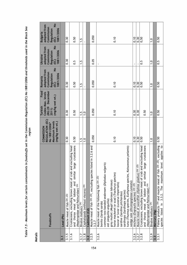
154

Table

7.5

- M

axim

um

levels

for

cert

ain

conta

min

ants

in f

oodst

uff

s se

t in

the C

om

mis

sion R

egula

tion (

EC)

No 1

881/2

006 a

nd t

hre

shold

s use

d i

n t

he B

lack S

ea

regio

n

Meta

ls

Foodst

uff

s

CO

MM

ISSIO

N

REG

ULAT

ION

(EC)

No 1

881/2

006*

Maxim

um

levels

(m

g/k

g w

et

wt.

)

Turk

ish

Food

Codex M

ax.

levels

(R

G:2

9

Decem

ber

2011)

(mg/k

g w

et

wt.

)

Rom

ania

adopte

d f

rom

C

om

mis

sion

Regula

tion

(EC

) N

o

1881/2

006

Ukra

ine

adopte

d f

rom

C

om

mis

sion

Regula

tion

(EC

) N

o

1881/2

006

Bulg

ari

a

adopte

d f

rom

C

om

mis

sion

Regula

tion

(EC

) N

o

1881/2

006

3.1

Lead (

Pb)

3.1

.5

Musc

le m

eat

of

fish

(24)

(25)

0.3

0

0.3

0

0.3

0

0.3

0

0.3

0

3.1

.6

Cru

staceans,

exclu

din

g b

row

n m

eat

of

cra

b a

nd e

xclu

din

g h

ead

and

thora

x

meat

of

lobst

er

and

sim

ilar

larg

e

cru

staceans

(Nephro

pid

ae a

nd P

alinuri

dae)

(26)

0.5

0

0.5

0

0.5

0

0.5

0.5

0

3.1

.7

Biv

alv

e m

ollusc

s (2

6)

1.5

1.5

1.5

1.5

1.5

3.1

.8

Cephalo

pods

(wit

hout

vis

cera

) (26)

1.0

1.0

-

-

3.2

C

adm

ium

(C

d)

3.2

.5

Musc

le m

eat

of

fish

(24)

(25) ,

exclu

din

g s

pecie

s list

ed in 3

.2.6

and

3.2

.7

0.0

50

0.0

50

0.0

50

0.0

5

0.0

50

3.2

.6

Musc

le m

eat

of

the f

ollow

ing f

ish (2

4)

(25)

bonit

o (

Sard

a s

ard

a)

com

mon t

wo-b

anded s

eabre

am

(D

iplo

dus

vulg

ari

s)

eel (A

nguil

la a

nguil

la)

gre

y m

ullet

(Mugil

labro

sus

labro

sus)

hors

e m

ackere

l or

scad (

Tra

churu

s sp

eci

es)

lo

uvar

or

luvar

(Luvaru

s im

peri

ali

s)

sard

ine (

Sard

ina p

ilch

ard

us)

sa

rdin

ops

(Sard

inops

speci

es)

tu

na (

Thunnus

speci

es,

Euth

ynnus

speci

es,

Kats

uw

onus

pela

mis

) w

edge s

ole

(D

icolo

goglo

ssa c

uneata

)

0.1

0

0.1

0

0.1

0

-

0.1

0

3.2

.6

Anchovy (

Engra

uli

s sp

eci

es)

(24)

(25)

0.1

0

0.3

0

0.1

0

- 0.1

0

3.2

.7

Musc

le m

eat

of

sword

fish

(Xip

hia

s gla

diu

s) (

24)

(25)

0.3

0

0.3

0

0.3

0

- 0.3

0

3.2

.8

Cru

staceans,

exclu

din

g b

row

n m

eat

of

cra

b a

nd e

xclu

din

g h

ead

and

thora

x

meat

of

lobst

er

and

sim

ilar

larg

e

cru

staceans

(Nephro

pid

ae a

nd P

ali

nuri

dae)

(26)

0.5

0

0.5

0

0.5

0

0.5

0,5

0

3.2

.9

Biv

alv

e m

ollusc

s (2

6)

1.0

1.0

1.0

1.0

1.0

3.3

M

erc

ury

(H

g)

3.3

.1

Fis

hery

pro

ducts

(26) and m

usc

le m

eat

of

fish

(24)

(25) ,

exclu

din

g

specie

s list

ed

in

3.3

.2.

The

maxim

um

le

vel

applies

to

0.5

0

0.5

0

0.5

0

0.5

0.5

0

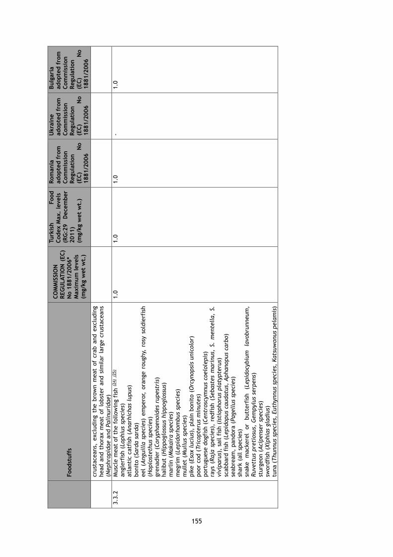
https://eur-lex.europa.eu/eli/reg/2006/1881/oj#ntr24-L_2006364EN.01001501-E0024












155

Foodst

uff

s

CO

MM

ISSIO

N

REG

ULAT

ION

(EC)

No 1

881/2

006*

Maxim

um

levels

(m

g/k

g w

et

wt.

)

Turk

ish

Food

Codex M

ax.

levels

(R

G:2

9

Decem

ber

2011)

(mg/k

g w

et

wt.

)

Rom

ania

adopte

d f

rom

C

om

mis

sion

Regula

tion

(EC

) N

o

1881/2

006

Ukra

ine

adopte

d f

rom

C

om

mis

sion

Regula

tion

(EC

) N

o

1881/2

006

Bulg

ari

a

adopte

d f

rom

C

om

mis

sion

Regula

tion

(EC

) N

o

1881/2

006

cru

staceans,

exclu

din

g t

he b

row

n m

eat

of

cra

b a

nd e

xclu

din

g

head a

nd t

hora

x m

eat

of

lobst

er

and s

imilar

larg

e c

rust

aceans

(Nephro

pid

ae a

nd P

ali

nuri

dae)

3.3

.2

Musc

le m

eat

of

the f

ollow

ing f

ish (2

4)

(25)

angle

rfis

h (

Lophiu

s sp

eci

es)

atl

anti

c c

atf

ish (

Anarh

ichas

lupus)

bonit

o (

Sard

a s

ard

a)

eel

(Anguil

la s

peci

es)

em

pero

r, o

range r

oughy,

rosy

sold

ierf

ish

(Hoplo

steth

us

speci

es)

gre

nadie

r (C

ory

phaenoid

es

rupest

ris)

halibut

(Hip

poglo

ssus

hip

poglo

ssus)

m

arl

in (

Makair

a s

peci

es)

m

egri

m (

Lepid

orh

om

bus

speci

es)

m

ullet

(Mull

us

speci

es)

pik

e (

Eso

x l

uci

us)

, pla

in b

onit

o (

Orc

ynopsi

s unic

olo

r)

poor

cod (

Tri

copte

rus

min

ute

s)

port

uguese

dogfi

sh (

Centr

osc

ym

nus

coelo

lepis

) ra

ys

(Raja

speci

es)

, re

dfi

sh (

Sebast

es

mari

nus,

S.

mente

lla,

S.

viv

iparu

s),

sail f

ish (

Isti

ophoru

s pla

typte

rus)

sc

abbard

fis

h (

Lepid

opus

caudatu

s, A

phanopus

carb

o)

seabre

am

, pandora

(Pagell

us

speci

es)

sh

ark

(all s

pecie

s)

snake

mackere

l or

butt

erf

ish

(Lepid

ocy

biu

m

lavobru

nneum

, Ruvett

us

pre

tiosu

s, G

em

pylu

s se

rpens)

st

urg

eon (

Aci

pense

r sp

eci

es)

sw

ord

fish

(Xip

hia

s gla

diu

s)

tuna (

Thunnus

speci

es,

Euth

ynnus

speci

es,

Kats

uw

onus

pela

mis

)

1.0

1.0

1.0

-

1.0



156

Dio

xin

s and P

CBs

(31)

Foodst

uff

s

CO

MM

ISSIO

N

REG

ULAT

ION

(E

C)

No 1

881/2

006

am

ended

by

CO

MM

ISSIO

N

REG

ULAT

ION

(E

U)

No 1

259/2

011

Maxim

um

levels

Turk

ey

Nati

onal

Food

Codex M

ax.

levels

(R

G:2

9 D

ecem

ber

2011)

(adopte

d

from

C

om

.Reg.

(EU

) N

o1881/2

006

Rom

ania

adopte

d f

rom

C

om

mis

sion

Regula

tion (

EC

) N

o

1881/2

006

am

ended

by

CO

MM

ISSIO

N

REG

ULAT

ION

(E

U)

No 1

259/2

011

Ukra

ine

adopte

d f

rom

C

om

mis

sion

Regula

tion

(EC

) N

o 1

881/2

006

am

ended

by

CO

MM

ISSIO

N

REG

ULAT

ION

(EU

) N

o 1

259/2

011

Bulg

ari

a

adopte

d f

rom

C

om

mis

sion

Regula

tion (

EC

) N

o

1881/2

006

am

ended

by

CO

MM

ISSIO

N

REG

ULAT

ION

(E

U)

No 1

259/2

011

Sum

of

dio

xin

s (W

HO

-PC

DD

/F-T

EQ

) (

32)

5.3

M

usc

le m

eat

of

fish

and f

ishery

pro

ducts

and p

roducts

th

ere

of,

exclu

din

g eel

(25)

(3

4). The m

axim

um

le

vel

applies

to c

rust

aceans,

exclu

din

g t

he b

row

n m

eat

of

cra

b a

nd e

xclu

din

g h

ead a

nd t

hora

x m

eat

of

lobst

er

and

sim

ilar

larg

e

cru

staceans

(Nephro

pid

ae

and

Pali

nuri

dae)

3.5

pg/g w

et

wt.

3.5

pg/g w

et

wt.

-

- 3.5

pg/g w

et

wt

5.4

M

usc

le m

eat

of

eel

(Anguil

la a

nguil

la)

and p

roducts

th

ere

of

3.5

pg/g w

et

wt.

3.5

pg/g w

et

wt.

-

- 3.5

pg/g w

et

wt

Sum

of

dio

xin

s and d

ioxin

-lik

e P

CBs

(WH

O-P

CD

D/F

-PC

B-T

EQ

) (

32)

5.3

M

usc

le m

eat

of

fish

and f

ishery

pro

ducts

and p

roducts

th

ere

of,

exclu

din

g eel

(25)

(3

4) .

The m

axim

um

le

vel

applies

to c

rust

aceans,

exclu

din

g t

he b

row

n m

eat

of

cra

b a

nd e

xclu

din

g h

ead a

nd t

hora

x m

eat

of

lobst

er

and

sim

ilar

larg

e

cru

staceans

(Nephro

pid

ae

and

Pali

nuri

dae)

6.5

pg/g w

et

wt.

6.5

pg/g w

et

wt.

-

- 8.0

pg/g w

et

wt.

5.4

M

usc

le m

eat

of

eel

(Anguil

la a

nguil

la)

and p

roducts

th

ere

of

10.0

pg/g w

et

wt.

10.0

pg/g w

et

wt.

-

- 12.0

pg/g w

et

wt.

PC

B28,

PCB52,

PC

B101,

PC

B138,

PC

B153

ve

PC

B180 (

Sum

of

ICES-6

) (

32)

5.3

M

usc

le m

eat

of

fish

and f

ishery

pro

ducts

and p

roducts

th

ere

of,

exclu

din

g eel

(25)

(3

4) .

The m

axim

um

le

vel

applies

to c

rust

aceans,

exclu

din

g t

he b

row

n m

eat

of

cra

b a

nd e

xclu

din

g h

ead a

nd t

hora

x m

eat

of

lobst

er

and

sim

ilar

larg

e

cru

staceans

(Nephro

pid

ae

and

Pali

nuri

dae)

75 n

g/g w

et

wt.

75 n

g/g w

et

wt.

75 n

g/g w

et

wt.

75 n

g/g w

et

wt.

75 n

g/g w

et

wt.

5.4

M

usc

le m

eat

of

eel

(Anguil

la a

nguil

la)

and p

roducts

th

ere

of

300 n

g/g w

et

wt.

300 n

g/g w

et

wt.

-

- 300 n

g/g w

et

wt











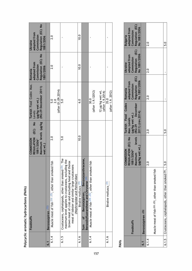
157

Poly

cyclic a

rom

ati

c h

ydro

carb

ons

(PA

Hs)

Foodst

uff

s C

OM

MIS

SIO

N

REG

ULAT

ION

(E

C)

No

1881/2

006*

Maxim

um

le

vels

(μ

g/k

g

wet

wt.

)

Turk

ish Food Codex M

ax.

Levels

(μ

g/k

g w

et

wt.

) (R

G:2

9 D

ecem

ber

2011)

Rom

ania

adopte

d f

rom

C

om

mis

sion

Regula

tion (E

C)

No

1881/2

006

Ukra

ine

adopte

d f

rom

C

om

mis

sion

Regula

tion (E

C)

No

1881/2

006

6.1

Benzo(a

)pir

en (

35)

6.1

.4

Musc

le m

eat

of

fish

(24)

(25) ,

oth

er

than s

moked f

ish

2.0

5.0

2.0

(a

fter

01.0

9.2

014)

2.0

2.0

6.1

.5

Cru

staceans,

cephalo

pods,

oth

er

than s

moked

(26) .

The

maxim

um

level

applies

to c

rust

aceans,

exclu

din

g t

he

bro

wn m

eat

of

cra

b a

nd e

xclu

din

g h

ead a

nd t

hora

x

meat

of

lobst

er

and s

imilar

larg

e c

rust

aceans

(Nephro

pid

ae a

nd P

ali

nuri

dae)

5.0

5.0

-

-

6.1

.6

Biv

alv

e m

ollusc

s (2

6)

10.0

6.0

10.0

10.0

Sum

of

Benzo(a

)pir

en,

Benzo(a

)anth

racene,

Benzo(b

)flu

ora

nth

ene a

nd C

hry

sene (3

6)

6.1

.4

Musc

le m

eat

of

fish

(24)

(25) ,

oth

er

than s

moked f

ish

30.0

(a

fter

1.9

.12012)

12 µ

g/kg w

et

wt.

(a

fter

1.9

.2014)

- -

6.1

.6

Biv

alv

e m

ollusc

s (2

6)

35.0

(a

fter

1.9

. 2012)

- -

PA

Hs

Foodst

uff

s

CO

MM

ISSIO

N

REG

ULAT

ION

(EC

) N

o

1881/2

006*

Maxim

um

le

vels

(μ

g/k

g w

et

wt.

)

Turk

ish

Food

Codex

Max.

Levels

(μ

g/k

g w

et

wt.

) (R

G:2

9

Decem

ber

2011)

(rev.

2014)

Rom

ania

adopte

d f

rom

C

om

mis

sion

Regula

tion

(EC

) N

o 1

881/2

006

Ukra

ine

adopte

d f

rom

C

om

mis

sion

Regula

tion

(EC

) N

o 1

881/2

006

Bulg

ari

a

adopte

d f

rom

C

om

mis

sion

Regula

tion

(EC

) N

o 1

881/2

006

6.1

Benzo(a

)pir

en (

35)

6.1

.4

Musc

le m

eat

of

fish

(24)

(25) ,

oth

er

than s

moked f

ish

2.0

2.0

2.0

2.0

2.0

6.1

.5

Cru

staceans,

cephalo

pods,

oth

er

than s

moked

(26) .

5.0

5.0

-

- 5.0













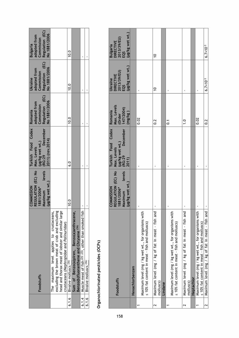
158

Foodst

uff

s

CO

MM

ISSIO

N

REG

ULAT

ION

(EC

) N

o

1881/2

006*

Maxim

um

le

vels

(μ

g/k

g w

et

wt.

)

Turk

ish

Food

Codex

Max.

Levels

(μ

g/k

g w

et

wt.

) (R

G:2

9

Decem

ber

2011)

(rev.

2014)

Rom

ania

adopte

d f

rom

C

om

mis

sion

Regula

tion

(EC

) N

o 1

881/2

006

Ukra

ine

adopte

d f

rom

C

om

mis

sion

Regula

tion

(EC

) N

o 1

881/2

006

Bulg

ari

a

adopte

d f

rom

C

om

mis

sion

Regula

tion

(EC

) N

o 1

881/2

006

The

maxim

um

le

vel

applies

to

cru

staceans,

exclu

din

g t

he b

row

n m

eat

of

cra

b a

nd e

xclu

din

g

head a

nd t

hora

x m

eat

of

lobst

er

and s

imilar

larg

e

cru

staceans

(Nephro

pid

ae a

nd P

ali

nuri

dae)

6.1

.6

Biv

alv

e m

ollusc

s (2

6)

10.0

6.0

10.0

10.0

10.0

Sum

of

Benzo(a

)pir

en,

Benzo(a

)anth

racene,

Benzo(b

)flu

ora

nth

ene a

nd C

hry

sene (3

6)

6.1

.4

Musc

le m

eat

of

fish

(24)

(25) ,

oth

er

than s

moked f

ish

- -

-

- -

6.1

.6

Biv

alv

e m

ollusc

s (2

6)

- -

-

- -

Org

anochlo

rinate

d p

est

icid

es

(OC

Ps)

Foodst

uff

s

CO

MM

ISSIO

N

REG

ULAT

ION

(EC

) N

o

1881/2

006*

Maxim

um

le

vels

(μ

g/k

g w

et

wt.

)

Turk

ish

Food

Codex

Max.

Levels

(μ

g/k

g w

et

wt.

) (R

G:2

9

Decem

ber

2011)

Rom

ania

M

ax.

Levels

(O

rder

147/2

004)

(mg/k

g )

Ukra

ine

DIR

EC

TIV

E

2013/3

9/E

U)

EQ

S

(µg/k

g w

et

wt.

)

Bulg

ari

a

DIR

EC

TIV

E

2013/3

9/E

U)

EQ

S

(µg/k

g w

et

wt.

)

H

exachlo

rbenzen

1

Maxim

um

level (m

g /

kg w

et

wt.

, fo

r org

anis

ms

wit

h

≤ 1

0% f

at

conte

nt

in m

eat

- fi

sh a

nd m

ollusc

s)

- -

0.0

2

-

2

Maxim

um

level

(mg /

kg o

f fa

t in

meat

- fi

sh a

nd

mollusc

s)

- -

0.2

10

10

Lin

dane

1

Maxim

um

level (m

g /

kg w

et

wt.

, fo

r org

anis

ms

wit

h

≤ 1

0% f

at

conte

nt

in m

eat

- fi

sh a

nd m

ollusc

s)

- -

0.1

-

2

Maxim

um

level

(mg /

kg o

f fa

t in

meat

- fi

sh a

nd

mollusc

s)

- -

1.0

-

H

epta

chlo

r

1

Maxim

um

level (m

g /

kg w

et

wt.

, fo

r org

anis

ms

wit

h

≤ 1

0% f

at

conte

nt

in m

eat

- fi

sh a

nd m

ollusc

s)

- -

0.0

2

-

2

Maxim

um

level

(mg /

kg o

f fa

t in

meat

- fi

sh a

nd

- -

0.2

6.7

×10

-3

6.7

×10

-3





159

Foodst

uff

s

CO

MM

ISSIO

N

REG

ULAT

ION

(EC

) N

o

1881/2

006*

Maxim

um

le

vels

(μ

g/k

g w

et

wt.

)

Turk

ish

Food

Codex

Max.

Levels

(μ

g/k

g w

et

wt.

) (R

G:2

9

Decem

ber

2011)

Rom

ania

M

ax.

Levels

(O

rder

147/2

004)

(mg/k

g )

Ukra

ine

DIR

EC

TIV

E

2013/3

9/E

U)

EQ

S

(µg/k

g w

et

wt.

)

Bulg

ari

a

DIR

EC

TIV

E

2013/3

9/E

U)

EQ

S

(µg/k

g w

et

wt.

)

mollusc

s)

A

ldri

n

1

Maxim

um

level (m

g /

kg w

et

wt.

, fo

r org

anis

ms

wit

h

≤ 1

0% f

at

conte

nt

in m

eat

- fi

sh a

nd m

ollusc

s)

- -

0.0

2

-

2

Maxim

um

level

(mg /

kg o

f fa

t in

meat

- fi

sh a

nd

mollusc

s)

- -

0.2

-

D

ield

rin

1

Maxim

um

level (m

g /

kg w

et

wt.

, fo

r org

anis

ms

wit

h

≤ 1

0% f

at

conte

nt

in m

eat

- fi

sh a

nd m

ollusc

s)

- -

0.2

-

2

Maxim

um

level

(mg /

kg o

f fa

t in

meat

- fi

sh a

nd

mollusc

s)

- -

0.2

-

Endri

n

1

Maxim

um

level (m

g /

kg w

et

wt.

, fo

r org

anis

ms

wit

h

≤ 1

0% f

at

conte

nt

in m

eat

- fi

sh a

nd m

ollusc

s)

- -

0.0

5

-

2

Maxim

um

level

(mg /

kg o

f fa

t in

meat

- fi

sh a

nd

mollusc

s)

- -

0.5

-

Sum

of

DD

T,

DD

E a

nd D

DD

1

Maxim

um

level (m

g /

kg w

et

wt.

, fo

r org

anis

ms

wit

h

≤ 1

0% f

at

conte

nt

in m

eat

- fi

sh a

nd m

ollusc

s)

- -

0.1

-

2

Maxim

um

level

(mg /

kg o

f fa

t in

meat

- fi

sh a

nd

mollusc

s)

- -

1.0

-

(24)

Fis

h lis

ted in t

his

cate

gory

as

defi

ned in c

ate

gory

(a),

wit

h t

he e

xclu

sion o

f fi

sh liv

er.

(2

5)

Where

fis

h a

re inte

nded t

o b

e e

ate

n w

hole

, th

e m

axim

um

level

shall a

pply

to t

he w

hole

fis

h.

(26)

Foodst

uff

s fa

llin

g w

ithin

cate

gory

(c)

and (

f) o

f th

e l

ist

in A

rtic

le 1

of

Regula

tion (

EC)

No 1

04/2000,

as

appro

pri

ate

(sp

ecie

s as

list

ed i

n t

he r

ele

vant

entr

y).

In c

ase

of

dri

ed,

dilute

d,

pro

cess

ed a

nd/or

com

pound f

oodst

uff

s Art

icle

2(1

) and 2

(2)

apply

. (3

1)

Dio

xin

s (s

um

of

poly

chlo

rinate

d d

ibenzo-p

ara

-dio

xin

s (P

CD

Ds)

and p

oly

chlo

rinate

d d

ibenzofu

rans

(PCD

Fs)

, expre

ssed a

s W

orl

d H

ealt

h O

rganiz

ati

on (

WH

O)

toxic

equiv

ale

nt

usi

ng t

he W

HO

-toxic

equiv

ale

ncy f

acto

rs (

WH

O-T

EFs)

) and s

um

of

dio

xin

s and d

ioxin

-lik

e P

CBs

(sum

of

PCD

Ds,

PCD

Fs

and p

oly

chlo

rinate

d b

iphenyls

(PCBs)

, expre

ssed a

s W

HO

to

xic

equiv

ale

nt

usi

ng t

he W

HO

-TEFs)

. W

HO

-TEFs

for

hum

an r

isk a

ssess

ment

base

d o

n t

he c

onclu

sions

of

the W

HO

meeti

ng i

n S

tockholm

, Sw

eden,

15 t

o 1

8 J

une 1

997 (

Van

den B

erg

et

al.

, (1

998)

Toxic

Equiv

ale

ncy F

acto

rs (

TEFs)

for

PCBs,

PCD

Ds,

PCD

Fs

for

Hum

ans

and f

or

Wildlife

. Envir

onm

enta

l H

ealt

h P

ers

pecti

ves,

106 (

12),

775)

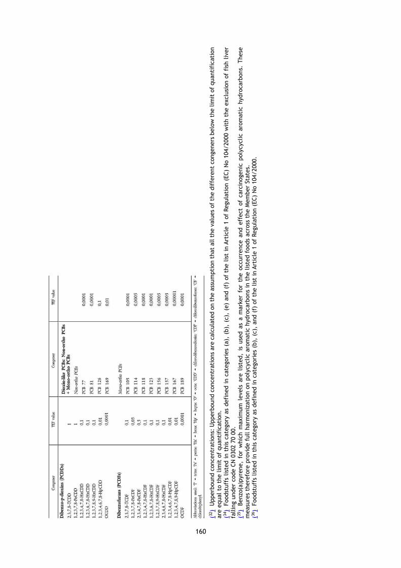
https://eur-lex.europa.eu/eli/reg/2006/1881/oj#ntc24-L_2006364EN.01001501-E0024




160

(32)

Upperb

ound c

oncentr

ati

ons:

Upperb

ound c

oncentr

ati

ons

are

calc

ula

ted o

n t

he a

ssum

pti

on t

hat

all t

he v

alu

es

of

the d

iffe

rent

congeners

belo

w t

he lim

it o

f quanti

ficati

on

are

equal to

the lim

it o

f quanti

ficati

on.

(34)

Foodst

uff

s list

ed i

n t

his

cate

gory

as

defi

ned i

n c

ate

gori

es

(a),

(b),

(c),

(e)

and (

f) o

f th

e l

ist

in A

rtic

le 1

of

Regula

tion (

EC)

No 1

04/2000 w

ith t

he e

xclu

sion o

f fi

sh l

iver

fallin

g u

nder

code C

N 0

302 7

0 0

0.

(35)

Benzo(a

)pyre

ne,

for

whic

h m

axim

um

levels

are

lis

ted,

is u

sed a

s a m

ark

er

for

the o

ccurr

ence a

nd e

ffect

of

carc

inogenic

poly

cyclic a

rom

ati

c h

ydro

carb

ons.

These

m

easu

res

there

fore

pro

vid

e f

ull h

arm

oniz

ati

on o

n p

oly

cyclic a

rom

ati

c h

ydro

carb

ons

in t

he lis

ted f

oods

acro

ss t

he M

em

ber

Sta

tes.

(3

6)

Foodst

uff

s list

ed in t

his

cate

gory

as

defi

ned in c

ate

gori

es

(b),

(c),

and (

f) o

f th

e lis

t in

Art

icle

1 o

f Regula

tion (

EC)

No 1

04/2000.





161

Table 7.6 - Overview of the most consumed species of fish and sea food monitored for GES assessment in the Black Sea region

Common /scientific name BG RO TR UA

Sprat / Sprattus sprattus X X

European anchovy / Engraulis encrasicolus X X

Atlantic horse mackerel / Trachurus trachurus X

Atlantic bonito / Sarda sarda X

Horse mackerel / Trachurus mediterraneus

Turbot / Scophthalmus maximus

Whiting / Merlangius merlangus X X X X

Red Mullet (Mullus barbatus) X X

Veined rapa whelk / Rapana venosa X X X

Mediterranean mussel / Mytilus galloprovincialis X X X


Figure VII.1 shows the levels of integration and integration methods for Descriptor 9. The figure is representative of a single assessment area. According to EC MSFD CIS Guidance (DG ENV, 2017), there is no need to aggregate across spatial areas.

The integration methods of Figure 7.1 are:

Level 1: Measurements of individual elements i.e. each substance is measured in the relevant matrix (species and tissue) and compared to the matrix-specific threshold value. For example, concentrations of mercury in the muscle tissue of different species of fish, concentrations of dioxins and PCBs in fish liver, are combined to produce information on levels of contaminants in different tissues of different species of fish and shellfish, which can be assessed against the maximum permitted levels under Regulation (EC) No 1881/2006, or levels for additional contaminants and matrices agreed through regional or subregional cooperation. This level of integration is not addressed in the Guidance (DG ENV. 2017).

162

Figure 7.1 - Levels and methods of integration for Descriptor 9 (DG ENV, 2017)

If a primary criterion cannot be assessed due to a lack of data, then the resultant assessment cannot be assigned a status (i.e. it is ‘not assessed’). It also means that the Member State should take action on monitoring and assessment tools to ensure that at the next update under Article 8 MSFD an assessment of the criterion can be undertaken.

The following open issues remain for further consideration at European level (DG ENV, 2017):

• Should the results consider each sample individually (whether met or exceeded threshold values), or average the concentrations for a set of samples (same species/contaminant)? The former risks a huge amount of data that is difficult to interpret; the latter risks masking samples with high concentrations that would have been unfit for human consumption. An alternative approach would be to summarize, by contaminant, the number of samples that have met or exceeded the threshold (species/matrix is not relevant).

• Related to the above, additional summary presentation of results, in terms of number or proportion of samples exceeding thresholds for each contaminant. This should also express e.g., number of monitoring stations/total number of samples, also possibly standard deviation or 95th of the measured reported concentration.

163

8 Guideline on Descriptor D10 Marine Litter

8.1 Introduction

8.1.1 Purpose and objective of the chapter

Marine litter is defined as “any persistent, manufactured or processed solid material discarded, disposed of or abandoned in the marine and coastal environment” (UNEP 2005, 2009). This becomes a serious problem and become quickly a European concern. The EU Marine Strategy Framework Directive (MSFD, 2008/56/EC) establishes a framework within which EU Member States shall act to achieve or maintain good environmental status (GES) of their marine waters by 2020. The provisions of MSFD D10 aim to protect the marine environment against harm caused by litter.

The chapter is intended to provide a step-by-step approach to designing and implementing a guideline for monitoring marine litter. Using definitions and terminology that are widely accepted and understood by the user group is the key to creating a harmonized approach and increasing the potential for sharing data and information. The decision to produce this guideline reflects the lack of regional agreed methodology to report on the distribution and abundance of marine litter, a topic that is attracting increasing concern. A uniform way of monitoring allows for regional interpretation of the litter situation in the Black Sea area and comparisons between regions.

The collection of data provides information on amounts, trends and sources of marine litter. This information can be used to focus on effective mitigating measures and to test the effectiveness of existing legislation and regulations. The ultimate aim is that the amount of litter entering the marine environment is minimized.

8.1.2 Marine litter as a concern at the Black Sea

Marine litter (also called marine debris) has long been on the political and public agenda. It is recognized as a worldwide rising pollution problem affecting all the oceans and coastal areas of the world (Galgani et al., 2015; Ryan 2015; Thompson 2015). The increasing production and use of durable synthetic materials such as plastics has led to a gradual, but significant accumulation of litter in the marine environment, making it ever more difficult to tackle (Barnes et al., 2009; Kühn et al., 2015).

The Black Sea is represented by the Black Sea Commission (BSC) or Bucharest Convention which works to protect the marine environment in this region. However, there is limited assessment of marine litter in the Black Sea, and a lack of comprehensive and systematic monitoring. As such, there is a lack of comparable and reliable data. There are limited data regarding the quantities and composition of marine litter in the Black Sea.

BSC (2007) reports that some governmental and private institutions and NGOs in Bulgaria, Romania, Russia, Turkey and Ukraine have conducted marine litter research using different approaches and methods, including aerial surveys.

National reviews are scarce and there is no aggregated information available. Daily activities of the population in the Black Sea catchment area affect the Black Sea environment and, probably, provide to marine litter problem which is originated from the problem of solid waste pollution (BSC 2007).

Solid waste management is one of the major environmental problems in the Black Sea region (Celik, 2002) and is a likely source of marine litter. Although very few studies of its extensiveness and sources have been made, illegal marine dumping has been known in all Black Sea coastal states for many years.

Illegal, unreported and unregulated (IUU) fishing in the Black Sea is also considered an important source of marine litter due to discarded and abandoned nets (UNEP, 2009).

In some areas, the high concentrations of fixed and floating illegal, unreported and unregulated fishing gear has resulted in the reduction of habitat space, obstacles for migration and an increase in incidental mortality (by-catch) of cetaceans, fishes and crustaceans (BSC, 2007; UNEP, 2009). Although no special research on abandoned nets has been conducted in the Black Sea region, the

164

problem of ‘ghost’ fishing undoubtedly exists, at least in the shelf area. Ingestion and entanglement also present an important threat. Also, there is no information regarding amounts and composition, transport, origin and impacts of marine litter on the seafloor or in the water column.

Marine debris is a complex cultural and multi-sectoral problem that imposes tremendous ecological, economic, and social costs.

8.1.3 The role of the monitoring and assessment

Monitoring and assessment are essential steps towards addressing specific questions about marine litter. They are needed to assess the state or level of pollution and provide objective information to design mitigation measures as well as to assess their effectiveness and promote adaptive management. But it is critical to understand the underlying policy concerns as this will help to determine the nature and extent of the approach (UNEP, 2019).

Monitoring should be set as an on-going long-term process based on a series of repeated measurements made to detect a baseline condition (e.g. number and types of items) and temporal changes in marine litter. Assessments use such information in a critical and contextualized way to design and evaluate public policies and mitigation measures.

Monitoring is crucial to assess the efficacy of measures implemented to reduce the abundance of marine litter, but it is complicated by large spatial and temporal heterogeneity in the amounts of litter and by our limited understanding of the pathways followed and its long-term fate. Even when sampling methods are similar, comparative studies are often compromised by a lack of information on factors influencing the depositional environment (prevailing winds, local and offshore currents, proximity to land based sources) for the different sampling areas. In such cases, even when differences in litter loads can be demonstrated between sites it is difficult to interpret these because the sources of the variability remain unknown.

Thus, one of the substantial barriers to addressing marine debris is the absence of adequate scientific research, assessment, and monitoring. There is a gap in scientific research to better understand the sources, fates, and impacts of marine debris (NRC 2008). Scalable, statistically rigorous and, where possible, standardized monitoring protocols are needed to monitor changes in conditions as a result of efforts to prevent and reduce the impacts of marine debris. Although monitoring of marine debris is currently carried out (often on the basis of voluntary efforts by non-governmental organizations), the protocols used tend to be very different, preventing comparisons and harmonization of data across regions or timescales (Cheshire et al., 2009).

Data from shorelines are more abundant but lack consistency in monitoring approaches. Hence it is apparent that more regular and harmonized monitoring will be required in order to detect changes in relation to policy measures implemented for example in response to MSFD.

8.2 Assessment of monitoring methodologies of marine litter in the Black Sea

To effectively manage, and thereby mitigate the impacts from marine litter, there is a need to develop a good understanding of the problem and specifically to understand the principal types and sources of litter in the marine environment. To achieve this aim is a need to ensure that relevant, quality data are available that allow a comprehensive analysis of the nature and sources of litter and how these are changing through time and in response to management interventions.

8.2.1 Bulgaria

Marine litter along the Bulgarian coast has been monitored under the national program for monitoring under MSFD. All monitoring guidelines, protocols and methodologies have been described in the program. In general, the methodology applied follows the standardized protocols, according to Guidance on monitoring of Marine Litter in the European Seas (2013).

165

D10C1. Indicator 1 (beach/shoreline litter >2.5 cm)

Monitoring of the marine macro litter on the coastline covers 10 unprotected beaches/shorelines along the Bulgarian Black Sea coast. The monitoring includes classification of the litter items according to the official “master list categories and subcategories” and counting of the individual items. All data are filled in standardized protocols, according to Guidance on monitoring of Marine Litter in the European Seas (2013). Additionally, the monitoring of marine macro litter on the coastline includes UAV observations of 2 not easily accessible beaches/shorelines along the Bulgarian Black Sea coast. The frequency of beach macro litter monitoring is planned four times per year in spring, summer, autumn and winter.

D10C1. Indicator 2 (floating litter >2.5 cm)

The programme covers coastal, shelf and open sea areas. Based on the type of the pressure and impact as well as on the origin of the marine litter, 8 monitoring polygons is the coastal area, 4 - in the shelf region and 2- in the open sea are selected. The visual observations from boats/vessels should ensure the detection of litter items in the size range of 2.5cm to > 50cm, therefore along with the observation transect the speed of the boat/vessel should not be higher than 6knots. The transect length should correspond approximately to 30min of observation for each survey. The frequency of floating macrolitter monitoring should be at least one per year. The optimal option is 2 times per year. All data are filled in standardized protocols, according to Guidance on monitoring of Marine Litter in the European Seas (2013).

D10C1. Indicator 1 (seafloor litter >2.5 cm)

The programme covers coastal and shelf areas. Based on the type of the pressure and impact as well as origin of the marine litter, 8 monitoring polygons are determined in the coastal area and 4 in the shelf region.

Monitoring of the seafloor litter in the coastal area is carried out using the line transect sampling method as follows:

• underwater visual surveys with scuba diving (0-15m);

• underwater visual surveys with ROV (15-30m).

For the aims of the survey, the area of each polygon is divided into two depth strata-Stratum 1 (0-15m) and Stratum 2 (15-30 m). The total number of monitoring transect in the coastal area is 40.

Monitoring of seafloor litter in the shelf area covers depths between 30 and 100m. Sampling of seafloor litter will be carried with a beam trawl. For the aims of the survey, the area of each polygon is divided into 3 depths strata Stratum 1(30-50m), Stratum 2(50-75m) and Stratum 3 (75-100m). The hauls are positioned following a depth stratum of each polygon with random drawing of the positions within each stratum. The number of positions in each stratum is proportional to the surface of these strata and the hauls are made in the same position from year to year. The haul duration is fixed at 30 minutes at 3 knots.

The frequency of seafloor litter monitoring should be at least one per year. The optimal option is 2 times per year. All data are filled in standardized protocols, according to Guidance on monitoring of Marine Litter in the European Seas (2013) and Cheshire (2009).

D10C2. Indicator 1 (beach/shoreline litter <5 mm)

The monitoring of the marine microlitter on the coastline covers 10 unprotected beaches/shorelines along the Bulgarian Black Sea coast. The monitoring includes classification of the litter items according to the official “master list categories and subcategories “and counting of the individual items. On each 100 m coastline, five replicate samples are collected. Each replicate is separated by at least 5m. Replicates can be distributed in a stratified random manner so as to be representative of an entire beach or a specific section of beach.

All data and meta are filled in standardized protocols, according to Guidance on monitoring of Marine Litter in the European Seas (2013).

D10C2. Indicator 2 (floating litter <5 mm)

Monitoring of the floating microlitter in the surface layer of the water column will be carried out jointly with D10C1, indicator 2. The total number of monitoring polygons is 14, of which 8 are in the coastal area, 4 in the shelf and 2 in the open sea. Seawater samples will be taken by nets. During

166

trawls it should be maintain a steady linear course for 30 minutes at a constant speed. Microparticles will be recorded as the total quantity of such captured by the net during the period it is deployed. The sample is transferred to a metal or glass container for subsequent density separation.

D10C2. Indicator 3 (seafloor litter <5 mm)

Monitoring of the seafloor micro litter will be carried out jointly with D10C1, indicator 3. The total number of monitoring polygons is 12, of which 8 are in the coastal area and 4 in the shelf. Material can be collected using any approach that recovers a sample of relatively undisturbed surface sediment from the seabed (e.g. Van veen grab, multi corer, box core etc.). Once recovered onto the vessel a small sample of sediment around 250 ml is recovered to represent the location of the original 5 cm surface to sub surface of the seabed. The sample is transferred to a metal or glass container for subsequent density separation.

D10C3. Indicators 1 -3 and D10C4

No monitoring programs established for these criteria.

8.2.2 Romania

Monitoring of macro-litter on the Romanian Black Sea beaches is done by using the Marine Litter Watch mobile app and following the work protocol described in the EU MSFD TG10 “Guidance on Monitoring of Marine Litter in European Seas–2013-JRC Scientific and Policy Reports “(Galgani et al., 2013). The methodology implies the visual identification of 100 m long fixed section of beach covering the whole area between the water edges (where possible and safe) or from the strandline to the back of the beach. All litter items (> 2.5 cm) provided by the mobile application categorized according to TSG – ML code given in the Annex 8.1. of the Guidance were gathered, sorted and quantified.

The implementation of bottom litter assessment activities in Romania were carried out together with the implementation of scientific fishing activities. From all the methods assessed, trawling (otter trawl) has been shown to be the most suitable for large scale evaluation and monitoring (Goldberg, 1995, Galgani et al., 1995, 1996, 2000). Nevertheless, there are some restrictions in rocky areas and in soft sediments, as the method may be restricted and/or underestimate the quantities present. This approach is however reliable, reproducible, allowing statistical processing and comparison of sites. As recommended by UNEP (Cheshire, 2009), sites should be selected to ensure that they (i) comprise areas with uniform substrate (ideally sand/silt bottom); (ii) consider areas generating/accumulating litter, (iii) avoid areas of risk (presence of munitions), sensitive or protected areas; (iv) do not impact on any endangered or protected species. Sampling units should be stratified relative to sources (urban, rural, close to riverine inputs) and impacted offshore areas (major currents, shipping lanes, fisheries areas, etc.). General strategies to investigate seabed litter are similar to methodology for benthic ecology and place more emphasis on the abundance and nature of items (e.g. bags, bottles, pieces of plastics) rather than their mass. The occurrence of International Bottom Trawls Surveys such as IBTS (Atlantic), BITS (Baltic) and MEDITS (Mediterranean/Black Sea) provide useful and valuable means for monitoring marine litter. These are using common gears depending on region (GOV nets in Atlantic, MEDITS net in the Mediterranean) and provide some harmonized and common conditions of sampling (20 mm mesh, 30-60 min tows, large sampling surface covered) and hydrographical and environmental information (surface& bottom temperature, surface & bottom salinity, surface & bottom current direction & speed, wind direction & speed, swell direction and height).For the Mediterranean and Black Sea Region, the protocol is derived from the MEDITS protocol (Bertan et al., 2007).The hauls are positioned following a depth stratified sampling scheme with random drawing of the positions within each stratum. The number of positions in each stratum is proportional to the surface of these strata and the hauls are made in the same position from year to year. The following depths (10 – 50; 50 – 100; 100 – 200; 200 – 500; 500 - 800 m) are fixed in all areas as strata limits. The total number of hauls for the Mediterranean Sea is 1385, covering the shelves and slopes from 11 countries in the Mediterranean. The haul duration is fixed at 30 minutes on depths less than 200m and at 60 minutes at depths over 200m (defined as the moment when the vertical net opening and door spread are stable), using the same GOC 73 trawl with 20 mm mesh nets (Bertran et al., 2007) and sampling between May and July, at 3 knots between 20 and 800 m depth. Qualitative and quantitative data on the bottom litter (Table 8.1) have to be connected to data regarding the characteristics of the haul (date, code of haul, the GPS positions of the haul (start

167

and end), trawled distance, average speed, characteristics of the haul (horizontal opening), depth of haul etc.), contained in file TA. Data related to the fishing set and gear performance allows calculating the sampled surfaces for each haul and estimating a standardized index of total and by categories litter abundance per square kilometer.

Table 8.1 - Seafloor monitoring data sheet

Campaign: Date: Haul:

Total weight of litter in the haul (kg):

Type of Litter Weight (kg) (mandatory for category and subcategory)

Number (facultative for subcategory)

Number (mandatory for category)

L0 No litter in the net

L1 Plastic a. Bags

b. Bottles

c. Food wrappers

d. Sheets (table covers, etc.)

e. Hard plastic objects (crates, containers, tubes, ashtrays, lids, etc.)

f. Fishing nets

g. Fishing lines

h. Other fishing related (pots, floats, etc.)

i. Ropes/strapping bands j others

L2 Rubber a. Tires

b. Other (gloves, boots/shoes, oilskins etc.)

L3 Metal a. Beverage cans

b. Other food cans/wrappers

c. Middle size containers (of paint, oil, chemicals)

d. Large metallic objects (barrels, pieces of machinery, electric appliances)

e. Cables

f. Fishing related (hooks, spears, etc.)

g. remnant from the war

L4 Glass / Ceramic/ Concrete a. Bottles

b. Pieces of glass

c. Ceramic jars

d. Large objects (specify)

L5 Cloth (textil)/ natural fibres a. Clothing (clothes, shoes)

b. Large pieces (carpets, mattresses, etc) (specify)

c. Natural ropes

d. Sanitaries (diapers, cottonbuds, etc.)

L6 Wood processed (palettes, crates, etc.)

L7 Paper and cardboard

The marine floating litter assessment is poorly addressed in Romania, thus the only protocol used was based on the line transect methodology (Suaria et al., 2015) during the surveys that took place within EC Project CoCoNet in 2014.

The marine microlitter monitoring in Romania is currently based on seasonal analysis of microplastics (size 1 – 5 mm) from the upper max. 5 cm of the beach sediments. The method of determining the type and abundance of microplastic pollution on the Romanian sandy beaches is based on the recommendations of the Technical Subgroup on Marine Litter (TG ML) of the European Commission's Marine Strategy Framework Directive (MSFD) given in the Guidance on Monitoring of Marine Litter in European Seas produced in 2013“(Galgani et al., 2013). Generally, the protocol involves the following major steps:(1) selecting the survey site; (2) collection of the sand samples from replicate sampling squares (quadrat) positioned randomly along two transects of the survey site at least 100m in length; (3) sieving the sand at a later date and at another location(e.g. laboratory) toreta in all items in the sand that are between 1 and 5mm in size; (4) density separation of microplastics by means of a salt water solution (approximately 35g/L); (5) classifying by the size, shape and color and recording of each microplastic item found under the stereomicroscope or digital microscope. The microplastics are classified into the most commonly recorded categories (filament, film, foam, fragment, pellet and irregular form/other). However, the microplastic items could be classified in much greater detail according to the List of Categories of Litter Items of the MSFD guidelines (Galgani et al., 2013).

168

8.2.3 Turkey

In the national level, marine litter monitoring studies have been carried out within the scope of Descriptive 10. Several monitoring surveys were conducted in Turkish Black Sea coasts for beach litter (Topçu et al., 2013; Terzi & Seyhan 2017; Aytan et al., 2020; Öztekin et al., 2020; Terzi et al., 2020), seafloor litter (Topçu & Öztürk, 2010; Öztekin & Bat 2017) and microlitter (Aytan et al., 2016; Öztekin & Bat 2017). The main protocol used for marine litter is JRC's Guidance on Monitoring of Marine Litter in European Seas (2013), and also used Guidelines published by OSPAR Commission and National Oceanic and Atmospheric Administration (NOAA) Marine Debris Program. Sea Monitoring Guides (2017) used for monitoring surveys in the national level, published by the Ministry of Environment and Urbanization in coordination with TUBITAK-MAM.

The main protocol used for macro-litter on beaches is JRC's Guidance on Monitoring of Marine Litter in European Seas Guide, where 100 m transect sampling unit is a fixed section of beach covering the whole area between the water edges (where possible and safe) or from the strandline to the back of the beach and categorization generally according to OSPAR guidelines, JRC's Guidance on Monitoring of Marine Litter in European Seas (2013) and Sea Monitoring Guides (2017) JRC. Abundance of marine litter is reported in items/km2 and per meter, g and kg/ km2 and per meter.

For macro litter on sea floor, investigations are carried out within the scientific fishing activities. The most common protocols are provided for monitoring according to JRC “Guidance on Monitoring of Marine Litter in European Seas”; (i) Shallow coastal waters (<20 m)- SCUBA, (ii) Margin / continental plate (<800m) - bottom trawls surveys MEDITS protocol (Mediterranean/Black Sea), (iii) deep sea floor – ROV.JRC JRC Guidance on Monitoring of Marine Litter in European Seas (2013) and Sea Monitoring Guides (2017) used for categorization of litter items. Abundance of marine litter is reported in units per square kilometres.

For floating litter, investigations are inadequate in national level.

For microlitter, the most common methods are JRC's Guidance on Monitoring of Marine Litter in European Seas (2013) and National Oceanic and Atmospheric Administration (NOAA) Marine Debris Program. The sampling of microplastics (i) quadrat samples for 1-5mm microplastics (1-5 mm visual examination according to type and colour) and bulk samples for <1 mm microplastic for beaches, (ii) Manta nets for sea surface samples, (iii) Niskin bottles attached to a CTD-Rosette or Plankton nets-bongo nets for column samples and (iv) bulk samples with Grab, box core and core samplers for sea floor. Sieving, density separation and wet peroxide oxidation steps are applied in laboratories. Type, colour and size is used for categorization under the microscope. The polymer analyses are used as a verification step.

In the monitoring studies methodologies show differences. For this, common research approaches, methods and evaluating criteria are necessary. For example, general litter lists differ for national level. This situation is related to the habits of the nations such as nutrition, life, etc. and considering this situation, additions or subtractions should be made to the litter lists. So standardization of the methodology and also updates are required in the light of the new investigations.

8.2.4 Ukraine

Monitoring of marine litter along the Ukrainian coast has been conducted in accordance of EU MSFD TG10 “Guidance on Monitoring of Marine Litter in European Seas” (2013) (which includes monitoring guidelines, protocols and methodologies). Ukraine has also developed and approved the Resolution “On approval of the Procedure for state water monitoring”, which also includes monitoring indicators and periodicity for marine litter (Resolution of the Cabinet of Ministers of Ukraine from 19.09.2018 №758). Monitoring of riverine litter in Ukraine has been conducted in accordance “JRC Technical Report. Riverine Litter Monitoring - Options and Recommendations” (MSFD GES TG Marine Litter, 2016).

For floating marine litter monitoring (floating marine and riverine litter) used of the JRC Floating Litter Monitoring Application (App), which was developed within the project RIMMEL.

169

For monitoring of beach litter used of the Marine LitterWatch App, which was developed by European Environment Agency.

D10.1.1 Trends in the amount of litter washed ashore and/or deposited on coastlines, including analysis of its composition, spatial distribution and, where possible, source (beach/shoreline litter)

Monitoring of the marine macro litter on the coastline covers 3 unprotected beaches along the Ukrainian Black Sea coast, of which - 1 beach is located within the Odesa city, the other 2 not easily accessible beaches in the Odesa region. All data are filled in standardized protocols based on the Marine LitterWatch App. The obtained data is uploaded to Marine LitterWatch Web portal (EEA DiscoMap).

D10.1.2 Trends in the amount of litter in the water column (including floating at the surface) and deposited on the seafloor, including analysis of its composition, spatial distribution and, where possible, source

Floating litter >2.5 cm, sea

Monitoring of floating litter are carried out on shelf (territorial waters of Ukraine), open sea areas (Odesa-Batumi, Odesa-Istanbul), and also partially – coastal (within the Odesa city). Monitoring of floating litter on the shelf and open sea areas is carried out within the general monitoring of the Black Sea, in the intervals between stops of the research vessel. The frequency of floating macrolitter monitoring depends on the availability of resources and funding.

The observation of floating marine litter is much depending on the observation conditions, in particular on the sea state and wind speed. The organization of monitoring must be flexible enough to take this into account and to re-schedule observations to meet appropriate conditions (Guidance on monitoring of Marine Litter in the European Seas, 2013).

Floating litter >2.5 cm, river

One of the main sources of litter in the marine environment are rivers. Therefore, it is important to conduct monitoring of litter that enters the marine environment from rivers. Monitoring of floating riverine litter are carried out on 2 rivers in Ukraine (Danube and Dniester).

Monitoring floating riverine litter can be stationary, from the shore or structures located in the river (e.g., bridge, pontoon, pier, quay wall, etc.). Alternatively, boats can be used in bigger rivers and estuaries, allowing both stationary and dynamic monitoring (e.g., transects). Observation of river surface is carried out from 0.5 - to 1-hour surveys and documented by tablet computer application (Toward a Harmonized Approach for Monitoring of Riverine Floating Macro Litter Inputs to the Marine Environment, 2017). The frequency of floating litter monitoring should be ideally once a week.

Monitoring of macro/micro litter in the water column, on the bottom and its effects on marine animals is not carried out.

8.3 Overview of the criteria, indicators and thresholds

8.3.1 The common MSFD indicators

Monitoring and assessment are essential steps to characterize the baseline and to provide objective information on the design of mitigation measures as well as to evaluate implementation measure effectiveness through the promotion of adaptive management. It is also critical to understand the overarching policy frameworks as this will help to determine the nature and extent of the approach. For the monitoring of marine litter in European countries, the Marine Strategy Framework Directive (MSFD) emerges as the main policy framework. Of the 11 descriptors listed in Annex I of the MSFS for determining Good Environmental Status, Descriptor 10 has been defined, as “Properties and quantities of marine litter do not cause harm to the coastal and marine environment”.

The revised Commission Decision 848/2017 identified the following criteria and associated 4 indicators for Descriptor 10 (Table 8.2), to be considered for regular monitoring purposes.

170

Table 8.2 - Descriptor 10 – Properties and quantities of marine litter do not cause harm to the coastal and marine environment (Relevant pressure is Input of litter)


Litter (excluding micro-litter), classified in 9 main categories) Member States may define further subcategories.

D10C1 – Primary: The composition, amount and spatial distribution of litter on the coastline, in the surface layer of the water column, and on the seabed, are at levels that do not cause harm to the coastal and marine environment.

Scale of assessment: Subdivisions of the region or sub region, divided where needed by national boundaries. Use of criteria: The extent to which good environmental status has been achieved shall be expressed for each criterion separately for each area assessed as follows: (a) the outcomes for each criterion (amount of litter or micro-litter per category) and its distribution per matrix used under D10C1 and D10C2 and whether the threshold values set have been achieved. (b) the outcomes for D10C3 (amount of litter and micro-litter per category per species) and whether the threshold values set have been achieved. The use of criteria D10C1, D10C2 and D10C3 in the overall assessment of good environmental status for Descriptor 10 shall be agreed at Union level. The outcomes of criterion D10C3 shall also contribute to assessments under Descriptor 1, where appropriate

Micro-litter (particles < 5mm), classified in the categories 'artificial polymer materials' and 'other'.

D10C2 – Primary: The composition, amount and spatial distribution of micro litter on the coastline, in the surface layer of the water column, and in seabed sediment, are at levels that do not cause harm to the coastal and marine environment. Member States shall establish threshold values for these levels through cooperation at Union level, taking into account regional or sub regional specificities.

Litter and micro-litter classified in the categories 'artificial polymer materials' and 'other', assessed in any species from the following groups: birds, mammals, reptiles, fish or invertebrates. Member States shall establish that list of species to be assessed through regional or sub regional cooperation

D10C3 – Secondary: The amount of litter and micro-litter ingested by marine animals is at a level that does not adversely affect the health of the species concerned. Member States shall establish threshold values for these levels through regional or sub regional cooperation.

Species of birds, mammals, reptiles, fish or invertebrates which are at risk from litter. Member States shall establish that list of species to be assessed through regional or sub regional cooperation.

D10C4 – Secondary: The number of individuals of each species which are adversely affected due to litter, such as by entanglement, other types of injury or mortality, or health effects. Member States shall establish threshold values for the adverse effects of litter, through regional or sub regional cooperation.

Scale of assessment: As used for assessment of the species group under Descriptor 1.Use of criteria: The extent to which good environmental status has been achieved shall be expressed for each area assessed as follows: – for each species assessed under criterion D10C4, an estimate of the number of individuals in the assessment area that have been adversely affected. The use of criterion D10C4 in the overall assessment of good environmental status for Descriptor 10 shall be agreed at Union level. The outcomes of this criterion shall also contribute to assessments under Descriptor 1, where appropriate.

Besides, the following specific guidance and standardized monitoring and assessment methods were detailed:

• For D10C1: litter shall be monitored along the coastline and may additionally be monitored in

the surface layer of the water column and on the seabed. Information on the source and pathway

of the litter shall be collected, where feasible.

• For D10C2: micro-litter shall be monitored in the surface layer of the water column and in the

171

seabed sediment and may additionally be monitored along the coastline. Micro-litter shall be

monitored in a manner that can be related to point sources for inputs (such as harbours, marinas,

wastewater treatment plants, storm-water effluents), where feasible.

• For D10C3 and D10C4: the monitoring may be based on incidental occurrences (e.g., stranding of

dead animals, entangled animals in breeding colonies, and affected individuals per survey).

Finally, the units for reporting litter quantities were agreed as follows:

D10C1: amount of litter per category in number of items: – per 100 meters (m) along the coastline, – per square kilometer (km2) for surface layer of the water column and for seabed, D10C2: amount of micro-litter per category in number of items and weight in grams (g): – per square meter (m2) for surface layer of the water column, – per kilogram (dry weight) (kg) of sediment for the coastline and for seabed.

D10C3: amount of litter/micro-litter in grams (g) and number of items per individual for each species in relation to size (weight or length, as appropriate) of the individual sampled.

D10C4: number of individuals affected (lethal; sub-lethal) per species.


Bulgaria

The indicators applied in Bulgaria follow the ComDec 848/2017 - Table 8.3. The indicators are classified according to their stage of development and implementation into three categories:

• Fully operational - legally accepted nationally, validated with thresholds established.

• Partially operational - legally accepted, validated, but without thresholds.


Table 8.3 - Indicators under D10C1, D10C2, D10C3 and D10C4 criteria used in Bulgaria

Criteria Indicators

D10C1 (Primary) The composition, amount and special distribution of litter on the coastline, in the surface layer of the water column, and on the seabed, are at levels that do not cause harm to the coastal and marine environment

1. The amount of beach litter>2.5 cm per category in number of items and weight per 100 meters (m) on coastline.

2. The amount of floating litter>2.5 cm in the surface layer of the water column per category in number of items per square milometer (km2).

3. The amount of litter>2.5 cm on these a bed per category in number of items per square kilometer (km2).

D10C2 (Primary) The composition, amount and spatial distribution of micro-litter on the coastline, in the surface layer of the water column, and in seabed sediment, are levels that do not cause harm to the coastal and marine environment

1. The amount of beach litter<5mm per category in number of items and weight in gram (g) per kilogram (dry weight) (kg) of sediment;

2. The amount of litter<5mm in the surface layer of the water column per category in number of items and weight in gram (g) per 100 m2;

3. The amount of litter<5mm on these abed per category in number of items and weight in gram (g) per kilogram (dry weight) (kg) of sediment;

D10C3 (Secondary) The amount of litter and micro litter ingested by marine animals is at a level that does not adversely affect the health of the species concerned

1. The amount of litter>2.5 cm ingested by fishing grams (g) and number of items per individual for each species in relation to size (weight or length) of individual sampled. Fishes that will be monitor: Sprattus sprattus, Scophthalmus maximus, Merlangius merlangus, Mullus barbatus ponticus, Trachurus mediterraneus, Squalus acanthias, Engraulisen crasicolus, Alosa immaculata.

2. The amount of litter>2.5 cm ingested by marine mammals in grams (g) and number of items per individual for each species in relation to size (weight or

172

Criteria Indicators

length) of individual sampled. Marine mammals that will be monitor: Phocoena phocoena, Tursiops truncates,Delphinus delphis.

3: The amount of litter>2.5 cm ingested by birds in grams (g) and number of items per individual for each species in relation to size (weight or length) of individual sampled. Birds that will be monitor: medium (hooded) cormorant and Puffinus yelkouan.

4. The amount of microlitter ingested by fishes in grams (g) and number of items per individual for each species in relation to size (weight or length) of individual sampled. Fishes that will be monitor: Sprattus sprattus, Scophthalmus maximus, Merlangius merlangus, Mullus barbatus ponticus, Trachurus mediterraneus, Squalus acanthias, Engraulisen crasicolus, Alosa immaculata.

5. The amount of microlitter ingested by marine mammals in grams (g) and number of items per individual for each species in relation to size (weight or length) of individual sampled. Marine mammals that will be monitor: Phocoena phocoena, Tursiops truncates,Delphinus delphis.

6 .The amount of microlitter ingested by birds in grams (g) and number of items per individual for each species in relation to size (weight or length) of individual sampled. Birds that will be monitor: medium (hooded) cormorant and Puffinus yelkouan.

D10C4 (Secondary) The number of individuals of each species which are adversely affected due to litter, such as by entanglement, other types of injury or mortality, or health effects

1. Number of individuals affected lethal per species

2. Number of individuals affected sub-lethal per species

In the Roof report is mentioned the fact that for Descriptor 10no common indicators have been defined between Romania and Bulgaria.

Bulgaria is already following the approved draft version of the Commission Decision (November 2016). There are defined several indicators for litter and micro-litter in different matrices following the requirement of revised GES Decision and the Guidance on Monitoring on Marine Litter in European Seas (2013) (Table 8.4). There is a lack of monitoring data to define basic and threshold values and to assess indicators.

173

Table 8.4 - No common indicators defined for Romania and Bulgaria

Descriptor 10 –Marine litter does not cause harm to the marine environment

Criteria Indicator in common (RO+BG) Common assessment and threshold (RO+BG)

D10C1 To be defined according to the revised GES Decision.








GES: No common GES definitions between Bulgaria and Romania regarding D10.

Romania

For Descriptor 10, no common indicators have been defined between Romania and Bulgaria, as stated in the ROOF report.

In Romania, there is a lack of monitoring data to define and assess indicators and thresholds.

GES: No common GES definitions between Bulgaria and Romania regarding D10.

Good environmental status is achieved when the impact of marine litter and their decomposition products is reduced, ceasing to cause harm to the marine and coastal environment.

Targets: There are no agreed common environmental targets for D10 according to the conceptual use of targets as expressed in the Common Understanding document (e.g., as "operational tools", such as necessary levels of reduction in each pressure at its sources).

Status assessment: as there are no agreed common indicators, a common status assessment for D10 is not possible at the moment.

Turkey

Turkey as a candidate state of the EU is seeking to harmonize national legislation for the implementation of the MSFD. For Descriptor 10, monitoring studies have increased in recent years to reveal the current situation. Within this scope, The Establishment of Turkey Marine Environment Strategy Project which is owned by the Ministry of Environment and Urbanization and conducted in coordination with TUBITAK-MAM. It is aimed to creating a “National Marine Environment Strategy and National Marine Environment Management Action Plan” that covers all the dimensions of research, monitoring, evaluation, socio-economic analysis and measures programs that cover all aspects of protecting marine areas and ensuring sustainable use for all Turkish seas within the framework of United Nations Goals on Sustainable Development, European Union requirements and Regional Maritime Contracts responsibilities. For Descriptor 10, draft GES definitions are included in the project (detailed information about the project can be provided from TÜBİTAK-MAM).

The Ministry of Environment and Urbanization issued the "Circular on the Preparation and Implementation of Marine Litter Province Action Plans" dated 10.06.2019 and numbered 2019/09 in order to prevent damage to marine environment and to develop measures against marine litter. This circular was sent to 28 seashore cities, and it was requested to prepare 5-year Marine Litter City Action Plans on a provincial basis.

It is essential to plan new measures to prevent or reduce the harm of existing marine litter to the marine environment, with the principle of prevention at the source of priority. Action plans need to be created, implemented and followed in order to bring an integrated approach to the fight against marine litter, to ensure unity in applications, and to follow up with regular and continuous monitoring studies.

In this framework, in coordination with the relevant institutions / organizations in all provinces that have a coastline:

174

• Prevention of contamination of the marine environment with wastes.

• Carrying out training and awareness raising activities to strengthen the social and cultural infrastructure.

• It is essential to work towards cleaning existing marine litters.

This Circular, which includes precautions both directly and indirectly for the prevention of marine litter, the Basel Convention to which our country is a party, the MARPOL Convention, the Barcelona Convention, the Bucharest Convention, the Environmental Law No. 2872, the Metropolitan Municipality Law No. 5216, the Law of Municipalities No. 5393, No. 1 The Presidential Decree was prepared on the basis of the relevant provisions of the Waste Management Regulation, Waste Collection and Control of Waste from Ships and Regulation on Water Pollution Control.

This Circular aims to prevent the occurrence of marine litter in provinces with seashore, to establish a commission for the preparation and implementation of Marine Litter Provincial Action Plans, which include activities related to the management of marine litter in the jurisdiction of our country, to determine the works / procedures required by the relevant institutions / organizations and to report the activities carried out.

Ukraine

In Ukraine, there is a lack of monitoring data to define and assess indicators and thresholds, and there is no developed regulatory base and national/regional plans an integrated approach to the fight against marine litter.

In Ukraine, the monitoring of marine litter has been partially started since 2016 and was carried out only within the framework of international projects. That is why it is important to plan new measures to prevent or reduce the harm of existing marine litter, with the principle of prevention the generation of litter.

The priority to reduce waste generation should be the introduction of an effective waste management system based on the waste management hierarchy, which provides:

• waste prevention;

• preparation for reuse;

• waste recycling;

• other types of waste disposal, including energy utilization;

• waste disposal - their burial in specially equipped places / facilities and destruction (disposal) (Order of the Cabinet of Ministers of Ukraine from 08.11.2017 No.820-r).

No less important measures to prevent the formation of garbage are raising activities to strengthen the ecological responsibility and awareness of population.


The EU Technical Group Marine Litter (TGML) has the leading role in setting baseline and threshold values for marine litter in Europe. The EU Commission Decision from 2017 requires the use of baseline values and threshold values of beach litter types based on abundance data, instead of trends of these abundances. In addition, the European Plastics strategy has already set an aspirational reduction target of 30% for litter items found on beaches (EU, 2018). To assess the achievement of this reduction target, for each survey site or larger geographical unit and litter type, baseline values need to be defined.

In 2017, it was suggested by the TGML that the calculation of baselines should in the first instance be at the level of the individual beach (i.e. survey site). This is in line with results on OSPAR beach litter data, which show that beach-related trend analyses give the most statistically significant results (Schulz et al., 2017). The MSFD Technical Group on Marine Litter has developed an approach for a European beach litter threshold value setting and assessment method that has been presented to MSFD GES 22 and was commented. All MS delegates within TG-ML had again occasion to provide input before submitting the final document now to MSCG for adoption.

Commission Decision EU/2017/848 requires that criteria elements, threshold values and methodological standards are established through Union, regional, or subregional cooperation.

175

In cases where threshold values should be established through cooperation at Union level (for the descriptors on marine litter, underwater noise and seabed integrity), this is done in the framework of the Common Implementation Strategy set up by the Member States and the Commission for the purposes of Directive 2008/56/EC. Once established through Union, regional or subregional cooperation, these threshold values will become part of Member States' sets of characteristics for good environmental status when they are sent to the Commission as part of Member States' reporting under Article 17(3) of Directive 2008/56/EC.

The report “A European Beach Litter Threshold Value and Assessment Method”, published in 2019 stated the fact that TG-ML concluded that a threshold value cannot be based on quantitative ecological and socio- economic harm due to a lack of scientific harm data. Of the remaining options, the use of the 10thpercentile value of the total litter abundance values from all European beaches from the baseline period 2015-2016 was selected and applied, as it appears to be sufficiently precautionary while being based on already existing beach abundances in the EU. The baseline dataset was developed within the TG-ML.

Application of this method to the baseline dataset resulted in a proposed threshold value of 13 litter items per 100 m of beach length. It is acknowledged that this is an ambitious TV, which will probably require substantial and sustained measures and a longer period to achieve. Intermediate targets over time towards the proposed TV, e.g. one target per MSFD cycle, are proposed.

A consensus was reached among the experts that it is currently not possible to derive quantitative dose-effect relationships for ecological harm caused by beach litter, although litter is evidently causing harm (Werner et al.,2016). From a practical point of view, it was considered unfeasible to develop harm-based TVs for beach litter based on field and laboratory studies. Therefore, it was decided to apply the precautionary principle, as indicated in the MSFD (EU 2008, EU 2017), and to select a relatively low threshold value. Furthermore, in addition to the ecological harm criterion, the general public has a clear desire for clean beaches because litter on beaches is regarded as a direct hindrance to human activities, causing socio-economic harm. Therefore, a TV for marine beach litter should express the need to strongly reduce litter in the environment. The strong ambition to reduce marine litter, which is evident through the measures currently implemented at national and EU level, supports this choice for an ambitious TV for beach litter. Finally, it was concluded that a TV should be data-based, which is common practice for EU WFD and MSFD indicators.

Since it is not possible to derive a threshold value based on harm data, two alternative approaches were considered, namely (a) the use of median beach litter abundances in nearly-pristine areas (e.g. Greenland, 1.8 items/100 m) and (b) the use of a low percentile value (e.g. the 10th, 5thor 1stpercentile value) of baseline datasets calculated from the results of all beach litter surveys in the EU.

For the beach litter TV, the 10thpercentile value was selected over the lower 5thpercentile value because it is practically more feasible to reach. In addition, the 10thpercentile value is statistically more robust than the 5thpercentile value.

The threshold value is realistic and acceptable

One European TV for beach litter is needed, because the potential ecological and socio-economic harm caused by litter at a certain pollution level is expected to be comparable on all EU beaches. It would be difficult to explain, from the viewpoint of ecological and socio-economic harm, why different EU regions should have different beach litter TVs, related to a different level of protection.

It was decided by TG-ML 2019 that the TV should be based on the total abundance of beach litter. It was also agreed that an additional TV for individual litter categories or litter category groups is not necessary, since about 90% of the litter items recorded on beaches are made of plastic.

The TV should be feasible and should not take too many years to reach in order to remain motivating. To this end, it was proposed by TG-ML that intermediate targets can be set on the way towards reaching the ultimate TV.

The assessment value is robust

It was agreed in TG-ML that the median assessment value is suitable for beach litter assessment, because it is robust against extreme values which frequently occur in beach litter monitoring, and because median beach litter abundances show a good correlation with mean beach litter abundances. Furthermore, it is necessary to define a minimum number of assessment surveys to obtain sufficiently

176

robust median assessment values (Table 8.5). This minimum number was optimized using the 90% confidence interval of the median and appeared to be 40 surveys per country-region.

EU wide threshold value for beach litter

Table 8.5 - Beach litter percentile values at EU level

No. of surveys Mean Median 1 perc. 5 perc. 10 perc.

1470 504 133 2 7 13

Reduction % to TV 98 95 90

The 10th percentile value is close to 10 items/100 m, for which the TG-ML jointly estimated that the potential ecological and socio-economic harm at the beach is low. In addition, the 10th percentile value has been recommended as being a pragmatic and robust indicator for setting reference levels, e.g. in the EU Guidance document for deriving Environmental Quality Standards (EC 2018, Oste et al., 2012; Annex 1). Therefore, this value was selected for further testing in this study as the European TV for beach litter.

The application of the above-mentioned methods, combining a threshold value setting with high ambition and with a low risk of ecological and socio-economic harm, with consideration of its achievability in time, and using the 10th percentile value of the total abundances of litter occurring on EU beaches in 2015-2016 (Table 8.6), results in a threshold value of 13 litter items / 100 m beach length.

Table 8.6 - Mean and median total beach litter abundance per 100 m of beach (Hanke et al., 2019) and % reduction necessary to reach the TV (median compared to TV) for country-MSFD subregions

Country subregion No. of surveys Mean (TA/100m) Median (TA/100m) Reduction % to TV (13)

BG_BlackSea 32 222 174 93

RO_BlackSea 9 20 15 13

While the proposed beach litter threshold is based on the ultimate aim of achieving GES in European Seas, its implementation will require a stringent introduction of measures at different levels and a set of additional marine litter TVs for concentrations and impacts in the different marine compartments.

The TG-ML recognizes that the proposed TV for beach litter is ambitious, and that for most countries it will take several MSFD cycles to reach it, after the implementation of extensive and sustained measures to reduce and eliminate litter inputs in the marine environment.

Percentile method

The percentile method has frequently been used in environmental assessment methods, in case real reference values from pristine reference areas are missing, and feasible threshold values must be set using a pragmatic statistical method. Some of these applications are described below.

The 5th and 10th percentile value of a large dataset are commonly used practical methods to calculate threshold or reference values, e.g., in case real ecotoxicological threshold values cannot be derived such as for beach litter (EU, 2018). For the 10th percentile two applications are described in the EU Technical guidance for deriving environmental quality standards, one of them using 10th percentile of a set of concentrations of chemicals in sediment which cause benthic effects, as a lower effect value (ERL, Effect Range Low).

In addition, a Dutch study (Oste et al., 2012) has recommended the use of 10th percentile values as the most robust percentile value for setting reference background levels for metals in European waters if data are not accessible from “pristine areas”, but only from more or less locally impacted areas. However, median values were found to be the most robust estimator for reference values if the dataset only included data from known “pristine” areas.

In European intercalibration studies for marine benthic assessments, the 95th or 99th percentile value of large benthic datasets (data from impacted and less disturbed areas combined) have been used to estimate benthic reference values (Van Hoey et al., 2019). For beach litter data, this can be translated into the use of the 5th or 1st percentile value for setting a threshold value.

177


As it was mentioned before, there is needed a lot of joint work at regional level, in order to really have a regional progress in terms of marine litter.

During the Fifth Meeting of the Black Sea Working Group established under the Agreement between the Ministry of Environment and Water Management of Romania and the Ministry of Environment and Water of the Republic of Bulgaria on Cooperation in the field of Water Management signed in Bucharest on 12 November 2004, took place in Constanta, on 19 February 2019. The outcomes of discussions on D10Marine litter are presented on Table 8.7.

Table 8.7 - Outcomes from Fifth Meeting of the Black Sea Working Group (19 February 2019)

Criterion/Indicator Romania Bulgaria Conclusions

D.10.C1. 1 Beach litter

JRC Protocol No threshold values/GES/target defined

JRC Protocol No threshold values/GES/target defined

For Romania: there should be a dedicated beach litter monitoring program funded accordingly. More data needed to set trends and define GES/targets.

D.10.C1. 2 Floating litter

Not yet monitored JRC protocol Drone testing No threshold values/GES/target

More data needed to set trends and define GES/targets

D.10.C1. 3 Seabed litter

JRC Protocol (item/m2) Bottom trawl surveys (together with fisheries surveys) No threshold values/GES/target

JRC Protocol (item/m2) Bottom trawl Experimental beam trawl, divers No threshold values/GES/target

For Romania: there should be a dedicated seabed litter monitoring program funded accordingly. More data needed to set trends and define GES/targets.

D.10.C.1. 4 Microlitter

Samples collected. To be developed

To be developed

D.10.C. 5. Microlitter in biota

To be developed To be developed


The extent to which GES is achieved for a specific geographic area needs to be clearly communicated. This involves the aggregation and integration across the many individual assessments and data sets relating to the eleven descriptors in order to reach conclusions on whether GES has been achieved or not. Aggregation and integration need to take into consideration and be balanced with appropriate details and scales for identifying and implementing any necessary management actions via national Programmes of Measures (Article 13).

In the Black Sea Commission (BSC), only Bulgaria and Romania are EU Member States with the obligation to implement the MSFD. The MSFD was adopted shortly before the Black Sea Strategic Action Plan (BS SAP) 2009 was approved. The underlying philosophies of the MSFD and the BS SAP are different but complementary. The BS SAP is based on targeting environmental priority problems for the Black Sea; its management targets do not directly state what the environmental status should be as a result of the activities undertaken under the BS SAP. In the framework of the Final Diagnostic Report 2010 (produced by the BSC Permanent Secretariat with the financial support of the European Environment Agency (EEA), a summary of the suitability of Black Sea data (of BSIS and external data sources) for calculation of BSC and EEA indicators and MSFD descriptors was prepared.

As a result, some indicators were identified for almost all MSFD descriptors (except Descriptor 10). In 2015, the BSC approved regional reporting indicators, to be reported annually to the BSC by the

178

Advisory Groups to the BSC. The indicators are grouped in six tables, according to the thematic focus of Advisory Groups (e.g., Biodiversity, Land-based pollution etc.). Some of the agreed indicators are also quite relevant for the MSFD implementation process. The BSC approved the Black Sea Integrated Monitoring and Assessment Programme (BSIMAP) in October 2016. BSIMAP was developed in the light of the MSFD, taking into account descriptors, GES and targets. The regional reporting indicators identified previously became part of BSIMAP. Its adoption is a positive step, as it contributes to the harmonization of the reporting format across countries and could provide the basis for comparing general environmental trends of the Black Sea marine environment. However, more efforts are needed towards harmonization of methodological approaches in determining GES by descriptors, criteria and/or indicators at the regional level, in order to better align the MSFD, BS SAP 2009 and BSIMAP implementation processes in the future.

As a result, at the present moment, Bulgaria and Romania do not consider that the BSC regional reporting indicators would provide an adequate basis for MSFD monitoring and assessment and are therefore progressing with the identification of common indicators under the MSFD. In the scope of regional coordination, Romania and Bulgaria have jointly identified and set up a number of common indicators specifically for MSFD which cover some aspects (criteria) of most descriptors. They are working towards providing common assessments for these indicators in a regional roof report for the 2018 assessment, taking into account the revised Commission Decision. These common indicators were set up under the project ‘Administrative and technical support for MSFD implementation in Bulgaria and Romania’, funded by the European Commission. Both Member States have a willingness to share the data and knowledge gained during the implementation of the MSFD with other Black Sea countries, to support the integration process between MSFD and the regional BSIMAP as far as possible.

There are proposed a series of levels and methods of integration for Descriptor 10 at European level that can be applied in the Black Sea region. This can be observed in the Figure 8.1.

Figure 8.1 - Levels and methods of integration for Descriptor 1013

13 Document of the Working Group on Good Environmental Status, 2017

179

The integration methods are:

Level 1: Measurements of individual elements — for example, of the quantity of litter of different subcategories in the different matrices in different time periods — are combined into individual indicators. Comparability of this level of integration requires technical consideration and is not addressed in the Guidance.

Level 2: The results for various indicators relating to the criteria D10C1 (litter), D10C2 (micro-litter), D10C3 (ingestion) and D10C4 (effects on biota) are integrated to the criterion level. The integration method varies by criterion:

• D10C1and D10C2: Assessment methods, indicators and definition of threshold values are to be developed at Union level (by the Technical Group on Marine Litter).

• D10C3and D10C4: The level of ingestion and adverse effects (lethal and sub-lethal) on species should be kept separate for the individual species, so that they can contribute to assessments under Descriptor 1 if required.

Level 3: The use of the criteria for the assessment of good environmental status for Descriptor 10 is to be agreed at Union level. The outputs from D10C3 and D10C4 may also feed into assessments under Descriptor 1 for particular species.

The integration methods for Descriptor 10 still need to be determinate. The revised Commission Decision has provided the scope for use of criteria in the assessment of Descriptor 10 to be agreed at Union level. In relation to the integration method for D10C1 and D10C2 at level 2, this includes whether the distribution of litter or micro-litter needs to be integrated with the composition of litter or micro-litter, and whether different matrices need to be integrated.

Further guidance is needed refining the master list of elements for its relevance and practical application in each matrix. This includes clarification:

• of "undefined" litter relevant for litter monitoring since not attributable to source;

• food waste is not included yet and if required in what form it should be included (HELCOM also notes that food waste is not recommended for the ‘beach’ matrix in JRC (2013).

• These specifications in relation to and the appropriateness of the master list should be developed by Task Group on Marine Litter (TG Litter) and agreed at Union level for EU-wide use.

If any aspects of a primary criterion cannot be assessed due to a lack of data then the resultant assessment cannot be assigned a status (i.e. it is ‘not assessed’). It also means that the Member State should take action on monitoring and assessment tools to ensure that at the next update under Article 8 MSFD an assessment of all relevant aspects can be undertaken.

During the 17th meeting of the Working Group on Good Environmental Status was proposed an assessment flow for Descriptor 10, in 7 steps, as follows:

STEP 1 – Determine the criteria to address

• D10C1 and D10C2 are primary criteria and must be addressed;

• D10C and D1C4 are secondary criteria.

STEP 2 – Determine the elements for assessment

The revised Commission Decision lists elements for assessment. These are:

• D10C1: artificial polymer materials, rubber, cloth/textiles, paper/ cardboard, processed/worked wood, metal, glass/ceramics, chemicals, undefined, and food waste (Member States may define further sub-categories).

• D10C2: micro-litter (particles <5 mm), classified in the categories ‘artificial polymer materials’ and ‘other’.

• D10C3: Litter and micro-litter from the categories ‘artificial polymer materials’ and ‘other’, in any species of birds, mammals, reptiles, fish or invertebrates.

• D10C4: Species of birds, mammals, reptiles, fish or invertebrates which are at risk from litter.

For D10C1 and D10C2, these must be monitored in the following matrices:

• D10C1: the coastline must be monitored for litter; the surface layer of the water column and the seabed are optional.

180

• D10C2: the surface layer of the water column and the seabed sediment must be monitored for micro-litter; the coastline is optional.

For D10C3, Member States should establish a list of species to be assessed for this criterion (if the criterion is assessed) through regional or subregional cooperation. For D10C4, Member States should establish a list of species for assessment (if the criterion is assessed) through regional or subregional cooperation. It should be based on the risk from marine litter (e.g., from entanglement, other types of injury or mortality or health effects). The species may be any species of birds, mammals, reptiles, fish or invertebrates.

STEP 3 – Determine scales and areas for assessment

The assessment scales are:

• D10C1, D10C2, D10C3: subdivisions of the region or subregion, subdivided where needed by national boundaries.

• D10C4: the scales and areas used for the corresponding species groups under Descriptor 1.

STEP 4 – Assign indicators

• Identify the relevant regional indicators that are available and can contribute to the assessment in relation to the types of litter and matrices, and allocate them to the revised Commission Decision criteria.

• Any remaining gaps should be identified. Use national assessments (taking into account existing assessments e.g., under EU legislation), where available, pending the development of regionally coordinated assessments.

• Additional national indicators for elements that are specific to national waters, if any, can also be incorporated and allocated to the relevant criteria and assessment areas. These need to have a threshold value, where appropriate.

STEP 5 – Establish threshold values

Threshold values should be established by Member States:

• D10C1 and D10C2: through cooperation at Union level, taking into account regional or subregional specificities;

• D10C3 and D10C4: through cooperation at regional or sub-regional level.

STEP 6 – Determine if threshold values are achieved

• The status of each element in each matrix should be determined, based on the value compared to the thresholds established in step 5.

STEP 7 – Integrate indicators

• The indicators should be integrated to criteria level, based on the integration methods presented previous.

181

References

Publications Office of the European Union, Luxembourg, ISBN 978-92-79-99232-2, doi:10.2760/16318, JRC115475

Abaza, V., C. Dumitrache, A.-D. Spinu, A. Filimon, 2018. Ecological quality assessment of circalittoral broad habitats using M-AMBI*(n) index. Journal of Environmental Protection and Ecology, 19 (2): 564-572

BAP Project, 2019. An investigation on reducing the discard amount of the trawl fishery (FYO-2019-20955), Istanbul University.

Anton E., Paiu M., Cândea M., 2012. Observations on dolphin sightings at the romanian coast and measures to reduce accidental catches in fishing nets. Recherches Marines. 42: 149 – 158.

Aytan Ü, Sahin FBE, Karacan F. Beach litter on Sarayköy Beach (SE Black Sea): density, composition, possible sources and associated organisms. Turkish Journal of Fisheries and Aquatic Science, 20(2), 137-145, 2020. https://doi.org/10.4194/1303-2712-v20_2_06.

Aytan Ü, Valente A, Senturk Y, Usta R, EsensoySahin FB, Mazlum RE, Agirbas E. First evaluation of neustonic microplastics in Black Sea waters. Marine Environmental Research, 119:22-30, 2016 http://dx.doi.org/10.1016/j.marenvres.2016.05.009

Barnes, D. K. A., Galgani, F., Thompson, R. C., & Barlaz, M. (2009): Accumulation and fragmentation of plastic debris in global environments. Philosophical Transactions of the Royal Society B, 364, 1985–1998.

Berov D, Deyanova D, Klayn S and Karamfilov V. ,2015. Distribution, structure and state of seagrass habitats in the SW Black Sea (Burgas Bay, Bulgaria). In: Proceedings of the 4th Mediterranean Seagrass Workshop, 18–22 May, Sardinia 2015, Oristano, Italy, 52.

Berov D. V. Karamfilov, G. Hiebaum, 2013. An Adaptation of the EEI-C Ecological Status Evaluation Method-Results from an Experimental Study of the Eutrophication Impact on Macroalgal Communities in the SW Black Sea . The 4th Bi-annual Black Sea Scientific Conference 28 – 31 October 2013, Constanta, Romania „Black Sea – Challenges Towards Good Environmental Status”.

Berov D., Todorov E., Marin O, Salas Herrero F, 2018 - Coastal Black Sea Geographic Intercalibration Group. Macroalgae and angiosperms ecological assessment methods; EUR 29556; Publications Office of the European Union, Luxembourg, ISBN 978-92-79-98336-8, doi:10.2760/28858, JRC114306.

Bertrand, J., A. Souplet, L., Gil de Soula, G., Relini, C., Politou. 2007. International bottom trawl survey in the Mediterranean (MEDITS), Instruction manual, Version 5. pp. 62. http://www.sibm.it/SITO%20MEDITS/file.doc/MEDITS-Handbook_V5-2007.pdf

Bilgin S., Köse Ö., 2018. Testing two types of acoustic deterrent devices (pingers) to reduce harbor porpoise, Phocoena phocoena (Cetacea: Phocoenidae), by catch in turbot (Psetta maxima) set gillnet fishery in the Black Sea, Turkey. Cah. Biol. Mar, 59, 473-479.

Bilgin S., Köse O., Yesilcicek, T., 2018. Incidental catches of endangered (Phocoena phocoena) and vulnerable (Delphinus delphis) cetaceans and catch composition of turbot bottom gillnet fisheries in the southeastern Black Sea, Turkey. Cah. Biol. Mar, 59, 571-577.

Birkun A. Jr., Komakhidze A., Mukhametov L., Krivokhizhin S., Shpak O., Komakhidze G., Goradze I. & Kryukova A., 2005. Field research in the Georgian Black Sea – exceedingly important wintering habitat of cetaceans.

Birkun A. Jr., Northridge S. P., Willsteed E. A., James F. A., Kilgour C., Lander M. and Fitzgerald G. D., 2014. Studies for carrying out the common fisheries policy: adverse fisheries impact on cetacean populations in the Black Sea. Final report to the European Commission, Brussels: 347p.

Bjørge A., Hohn A. A., Kvam T., Lockyer C., Schweder T. & Aarefjord, H. 1995. Report of the harbour porpoise age determination workshop, Oslo, 21–23 May 1990. Report of the International Whaling Commission (Special Issue 16): 477–496.

Boicenco L., Abaza V., Anton E., Bișinicu E,. Buga L., Coatu V., Damir N,. Diaconeasa D., Dumitrache C., Filimon A., Galațchi M., Golumbeanu M., Harcotă G., Lazăr L., Marin O., Mateescu R., Maximov

182

V., Mihailov E., Nenciu M., Nicolaev S., Niță V., Oros A., Pantea E., Radu G., Spinu A., Stoica E., Tabarcea C., Timofte F, Țiganov G., Țoțoiu A, Vlas O., Vlăsceanu E., Zaharia T., 2018 - Study on elaboration of the report on the ecological status of the Black Sea ecosystem according to the provisions of Marine Strategy Framework Directive (2008/56/EC), 331 pp.(in Romanian)

Boicenco L., Buga L., Zaharia T., Nicolaev S., 2018. Implementation of Marine Strategy Framework Directive in Romania. J. Environ Prot Ecol, 19(1): 196–207.

Borja, A., J. Franco, V. Perez, 2000. A Marine Biotic Index to Establish the Ecological Quality of Soft-Bottom Benthos within European Estuarine and Coastal Environments. Marine Pollution Bulletin, 40 (12): 1110-1114.

BSC, 2007 Marine litter in the Black Sea Region: A review of the problem. Istanbul, Turkey: Black Sea Commission Publications 2007-1.

Buckland S. T., 2004. Advanced Distance Sampling: Estimating Abundance of Biological Populations. Oxford University Press, New York.

Buckland S. T., Anderson D. R., Burnham K. P., Laake J. L., Borchers D. L., Thomas L., 2001. Introduction to Distance Sampling: estimating Abundance of Biological Populations (New edition edition). OUP Oxford, Oxford; New York.

Buckland, S.T., Anderson, D.R., Burnham, K.P., Laake, J.L., 2005. Distance Sampling.Wiley Online Library.

Caughley G., 1977. Analysis of vertebrate populations. London-New York-Sydney-Toronto: John Wiley & Sons Ltd., 1977. – 234 p.

Celik, F. 2002 A case study: Interstate highway in the Black Sea coast. Proc. 4th Conf. on Turkish Coast and Coastal Areas (Izmir, Turkey, 5-8 November 2002), Vol. II: 847-856. (In Turkish)

CeNoBS, 2019. State of the art on D1 criteria in Bulgaria and Romania and proposals for developing regional indicators. Contract No 110661/2018/794677/SUB/ENV.C2. Constanta. 1-45p.

Chapman C. J., 1951. Some properties of the hypergeometric distribution with applications to zoological censuses. University of California Public Static, 1: 131-160.

Chehida Y. B., Thumloup J., Vishnyakova K., Gol’din P. & Fontaine M. C., 2020. Genetic homogeneity in the face of morphological heterogeneity in the harbor porpoise from the Black Sea and adjacent waters (Phocoena phocoena relicta). Heredity, 124(3), 469-484.

Cheshire, A.C., Adler, E., Barbière, J., Cohen, Y., Evans, S., Jarayabhand, S., Jeftic, L., Jung, R.T., Kinsey, S., Kusui, E.T., Lavine, I., Manyara, P., Oosterbaan, L., Pereira, M.A., Sheavly, S., Tkalin, A., Varadarajan, S., Wenneker, B., Westphalen, G. 2009. UNEP/IOC Guidelines on Survey and Monitoring of Marine Litter. UNEP Regional Seas Reports and Studies, No. 186; IOC Technical Series No. 83: xii + 120 pp.

Çinar, M. E., & Bakir, K. (2014). ALien Biotic IndEX (ALEX)–A new index for assessing impacts of alien species on benthic communities. Marine Pollution Bulletin, 87(1-2): 171-179.

Çinar, M. E., Bakır, K., Öztürk, B., Katağan, T., Dağlı, E., Açık, Ş., Doğan, A. & Bitlis Bakır, B. 2015. TUBI (TUrkish Benthic Index): A new biotic index for assessing impacts of organic pollution on benthic communities. Journal of the Black Sea/Mediterranean Environment, 21(2): 135-168.

COMMISSION DECISION (EU) 2017/848 of 17 May 2017 laying down criteria and methodological standards on good environmental status of marine waters and specifications and standardised methods for monitoring and assessment, and repealing Decision 2010/477/EU.

Commission Regulation (EC) No 1881/2006 of 19 December 2006 setting maximum levels for certain contaminants in foodstuffs.

Dencheva K. Doncheva V. 2014. - Ecological Index (EI) - tool for estimation of ecological status in coastal and transitional waters in compliance with European Water Framework Directive, in: Proceedings of Twelfth International Conference on Marine Sciences and Technologies September 25th - 27th, 2014, Varna, Bulgaria. Varna, pp. 219–226.

Developing the selectivity of the deep trawl net used in the western Black Sea (FDK-2018-30202), Istanbul University, BAP Project, 2018.

183

DG Environment, 2017. Guidance for assessments under Article 8 of the Marine Strategy Framework Directive. Integration of assessments results, 17th meeting of the Working Group on Good Environmental Status (WG GES).

DG Environment. 2017. Reporting under Article 17 of the Habitats Directive: Explanatory notes and guidelines for the period 2013-2018. Brussels. 188pp

Directive 2000/60/EC of the European parliament and of the council of 23 October 2000 establishing a framework for Community action in the field of water policy.

Directive 2008/105/EC of the European parliament and of the council of 16 December 2008 on environmental quality standards in the field of water policy, amending and subsequently repealing Council Directives 82/176/EEC, 83/513/EEC, 84/156/EEC, 84/491/EEC, 86/280/EEC and amending Directive 2000/60/EC of the European Parliament and of the Council.

Directive 2008/56/EC of the European parliament and of the council of 17 June 2008 establishing a framework for community action in the field of marine environmental policy (Marine Strategy Framework Directive).

Directive 2013/39/EU of the European parliament and of the council of 12 August 2013 amending Directives 2000/60/EC and 2008/105/EC as regards priority substances in the field of water policy.

Donovan G. P. and Bjørge A., 1995. Harbour porpoises in the North Atlantic: edited extract from the report of the IWC Scientific Committee, Dublin 1995. Rep. int. Whal. Commn (Special Issue 16), pp.3-26.

Dzhembekova N., S. Moncheva, 2015. Recent trends of potentially toxic phytoplankton species along the Bulgarian Black Sea area. Proceedings 12 International Conference on Marine Science and technology “Black Sea 2014”, Varna, Bulgria, 25-27 September 2014, 321-329. ISSN 1314-0957

EC 2018. EU guidance document no. 27. Technical guidance for deriving environmental quality standards. Technical Report, updated version.

EC, 2011. Common Implementation Strategy for the Water Framework Directive (2000/60/EC). Guidance Document 14. Guidance on the Intercalibration Process 2008–2011. Office for Official Publications of the European Communities, Luxembourg (2011). file:///C:/Users/XPS/Downloads/Guidance%20No%2014%20-%20Intercalibration%20process%202008-2011.pdf

EC, 2015. Guidance Document No. 30. Procedure to fit new or updated classification methods to the results of a completed intercalibration exercise. Office for Official Publications of the European Communities, Luxembourg (2015).

EU. 1992. Directive (EU) 1992/43 of the European Parliament and of the Council of 21 May 1992 on the conservation of natural habitats and of wild fauna and flora. 44 pp. http://data.europa.eu/eli/dir/1992/43/oj.

EU. 2008. Directive (EU) 2008/56 of the European Parliament and of the Council of 17 June 2008 establishing a framework for community action in the field of marine environmental policy (Marine Strategy Framework Directive). 22 pp. http://data.europa.eu/eli/dir/2008/56/oj.

EU. 2017. Decision (EU) 2017/848 of the European Parliament and of the Council of 17 May 2017 laying down criteria and methodological standards on good environmental status of marine waters and specifications and standardised methods for monitoring and assessment, and repealing Decision 2010/477/EU. 32 pp. http://data.europa.eu/eli/dec/2017/848/oj

European Commission, 2018. A European Strategy for Plastics in a Circular economy

European Commission. 2018. Reporting on the 2018 update of articles 8, 9 & 10 for the Marine Strategy Framework Directive. DG Environment, Brussels. pp 72 (MSFD Guidance Document 14).

Eutrophication Status of the OSPAR Maritime Area- Third Integrated Report on the Eutrophication Status of the OSPAR Maritime Area, 2017

Galgani F., Hanke G., Maes T., 2015. Global distribution, composition and abundance of marine litter. In M. Bergmann, L. Gutow, & M. Klages (Eds.), Marine anthropogenic litter (pp. 29–56). Berlin: Springer.

http://data.europa.eu/eli/dir/1992/43/oj

184

Galgani F., Hanke G., Werner S., Oosterbaan L., Nilsson P., Fleet D., Kinsey S., Thompson R.C., Van Franeker J., Vlachogianni T., Scoullos M., Mira Veiga J., Palatinus A., Matiddi M., Maes T., Korpinen S., Budziak A., Leslie H., Gago J., Liebezeit G., 2013. Guidance on Monitoring of Marine Litter in European Seas. MSFD Technical Subgroup on Marine Litter (TSG-ML) Scientific and Technical Research series, Report EUR 26113 EN. Publication office of the European Union.

Garmendia M., Borja A., Franco J., Revilla M., 2013. Phytoplankton composition indicators for the assessment of eutrophication in marine waters: Present state and challenges within the European directives. Marine Pollution Bulletin 66: 7–16.

GES_15-2016-02, 2016. Progress on Art. 8 MSFD assessment guidance. 15th meeting of the Working Group on Good Environmental Status (WG GES), 21 June 2016.

Gladilina E. V. & Gol’din P. E., 2016. Abundance and Summer Distribution of a Local Stock of Black Sea Bottlenose Dolphins, Tursiops truncatus (Cetacea, Delphinidae), in Coastal Waters near Sudak (Ukraine, Crimea). Vestnik zoologii, 50(1), 49-56

Gladilina E. V., Vishnyakova K. A., Neprokin O. O., Ivanchikova Yu. F., Derkacheva T. A., Kryukova A. A., Savenko O. V. & Gol’din P. E., 2017a. Linear transect surveys of abundance and density of cetaceans in the area near the Dzharylgach Island in the north-western Black Sea. Vestnik zoologii, 51(4): 335-342)

Gladilina E., Shpak O., Serbin V., Kryukova A., Glazov D. & Gol’din P., 2018. Individual movements between local coastal populations of bottlenose dolphins (Tursiops truncatus) in the northern and eastern Black Sea. Journal of the Marine Biological Association of the United Kingdom, 98(2): 223-229

Gladilina O. V., 2018. The bottlenose dolphin (Tursiops truncatus) in the waters of the northern Black Sea: biology and population structure. – Manuscript. Dissertation submitted for the completion of the degree of Candidate of Sciences in Biology, qualification 03.00.08 – zoology. – Schmalhausen Institute of Zoology, National Academy of Sciences of Ukraine. Kyiv, 2018

Göktürk D. 2012. Monoflament and Multiflament gillnet selectivity used in the western Black Sea. Istanbul University, Science institute, PhD thesis, Istanbul.

Gol’din P., Gladilina E., Savenko O., Vishnyakova K., Neprokin O., Ivchenko Ye., 2017. Identification and initial assessment of cetacean groupings in coastal waters of the north-western Black Sea, Ukrainian sector (progress report). MoU ACCOBAMS N° 09/2016/FAC, 100 p.

Goldberg, E.D. 1995. Emerging problems in the coastal zone for the twenty-first century. Marine Pollution Bulletin. 31, 152-158.

Gol'din P., Gladilina E., Savenko O., Vishnyakova K., Ivanchikova J., Derkacheva T., Gulak B., Kriukova A., Polyanska K., Neprokin O., 2017. Data on cetacean occurrence collected during the project “Identification and initial assessment of cetacean groupings in coastal waters of the north-western Black Sea, Ukrainian sector” funded by ACCOBAMS. v1. Ukrainian Scientific Centre of Ecology of the Sea (UkrSCES). Dataset/Occurrence. http://seamap.env.duke.edu/dataset/2020

Golenchenko A. P., 1948. The wealth of fish in the Black Sea and perspectives for its utilization'. Rybn. Khoz, 4, 3-9.

Gönener S., Bilgin S., 2009. The effect of pingers on harbor porpoise, Phocoena phocoena bycatch and fishing effort in the turbot gill net fishery in the Turkish Black Sea Coast. Turkish Journal of Fisheries and Aquatic Sciences 9: 151-157.

Gönener S., Özdemir S., 2012. Investigation of the interaction between bottom gillnet fishery (Sinop, Black Sea) and bottlenose dolphins (Tursiops truncatus) in terms of economy. Turkish Journal of Fisheries and Aquatic Sciences 12: 115-126.

Hammond P. S., 2010. Estimating the abundance of marine mammals. In Marine mammal ecology and conservation: a handbook of techniques, eds I.L. Boyd, W.D. Bowen, S. Iverson, 42-67. Oxford: Oxford University Press.

HELCOM, 2010. HELCOM Initial Holistic Assessment. Balt. Sea Environ. Proc. No. 122. http://www.helcom.fi/Lists/Publications/BSEP122.pdf

HELCOM, 2012. Development of a set of core indicators: Interim report of the HELCOM CORESET project. PART A.

185

Hiddink, J. G., Jennings, S., Sciberras, M., Bolam, S. G., Cambiè, G., McConnaughey, R. A., Mazor, T., et al., 2019 Assessing bottom-trawling impacts based on the longevity of benthic invertebrates. Journal of Applied Ecology, 56: 1075–1083. https://doi.org/10.1111/1365-2664.13278.

ICES, 2014. Report of the Workshop to review the 2010 Commission Decision on criteria and methodological standards on good environmental status (GES) of marine waters; Descriptor 4 Foodwebs, 26–27 August 2014, ICES Headquarters, Denmark. ICES CM 2014\ACOM:60. 23 pp. http://www.ices.dk/sites/pub/Publication%20Reports/Expert%20Group%20Report/acom/2014/WKGM SFDD4/WKGMSFDD4%20Final%20Report%202014.pdf. Accessed 2 April 2016.

ICES, 2017. EU request on indicators of the pressure and impact of bottom-contacting fishing gear on the seabed, and of trade-offs in the catch and the value of landings. ICES Special Request Advice, eu.2017.13. 27 pp. https://doi.org/10.17895/ices.advice.5657.

ICES, 2018. Interim Report of the Working Group on the Effects of Extraction of Marine Sediments on the Marine Ecosystem (WGEXT), 16–19 April 2018, Copenhagen, Denmark. ICES CM 2018/HAPISG:05. 49 pp.

ICES, 2018. Report of the Workshop on MSFD biodiversity of species D1 aggregation (WKDIVAGG), 1–4 May 2018, ICES HQ, Copenhagen, Denmark. ICES CM 2018/ACOM:47. 53 pp.

ICES, 2019a. EU request to advise on a seafloor assessment process for physical loss (D6C1, D6C4) and physical disturbance (D6C2) on benthic habitats. ICES Special Request Advice, sr.2019.25. 42 pp. http://www.ices.dk/sites/pub/Publication%20Reports/Advice/2019/Special_Requests/eu.2019.25.pdf

ICES, 2019b. Technical guideline document for assessing fishing impact from mobile bottom-contacting fishing gears (version 1; 7 February 2019) within: 2018 Report of the Working Group on Fisheries Benthic Impact and Trade-offs (WGFBIT).

International Whaling Commission, 2000b. Report of the Scientific Committee, Annex O. Report of the IWC-ASCOBANS Working Group on harbour porpoises. Journal of Cetacean Research and Management 2 (Supplement), 2, p297-305.

Ioakeimidis, C., Zeri, C., Kaberi, H., Galatchi, M., Antoniadis, K., Streftaris, N.,Galgani, F., Papathanassiou, E., Papatheodorou, G., 2014. A comparative study ofmarine litter on the seafloor of coastal areas in the Eastern Mediterranean andBlack Seas. Mar. Pollut. Bull. 89 (1e2), 296e304.

Jeppesen E., Kronvang B., Olesen JE., Søndergaard M., Hoffmann CC., Andersen HE., Lauridsen TL., Liboriussen L., MeerhoffM., Beklioglu M., Özen A., (2011). Climate change effect on nitrogen loading from catchment in Europe: implications fornitrogen retention and ecological state of lakes and adapta-tions. Hydrobiologia, 663:1-21.

JRC, 2015. Review of Commission Decision 2010/477/EU concerning MSFD criteria for assessing good environmental status, Descriptor 9, contaminants in fish and other seafood for human consumption do not exceed levels established by Community legislation or other relevant standards. Document version 8.0: ComDecRev_D9_V8, 30 April 2015). Ispra: European Commission Joint Research Centre, Institute for Environment and Sustainability, Water Resources Unit. 23 pages.

JRC, 2016. Technical Report. Riverine Litter Monitoring - Options and Recommendations. MSFD GES TG Marine Litter, 2016. http://ec.europa.eu/environment/marine/good-environmental-status/descriptor-10/pdf/MSFD_riverine_litter_monitoring.pdf

Klevezal G. A., 1988. Registering structures of mammals in zoological research. Moscow: Nauka. In Russian.

Kopelevich, O. V., 2012. Application of data on seawater light scattering for the study ofmarineparticles: A selectivereview focusing onRussian literature.Geo-Marine Letters.http://dx.doi.org/10.1007/S00367-012-0278-y.2012.

Krivokhizhin S. V., Birkun A. A., & Radygin G. Yu., 2012. Seasonal changes in the distribution and abundance of cetaceans off the coast of Southeast Crimea. In Modern fisheries and environmental problems of the Azov-Black Sea region: proceedings of the VII International Conference. June 20-23 (p. 115). In Russian

Kühn, S., Bravo Rebolledo, E. L., & van Franeker, J. A., 2015. Deleterious effects of litter on marine life. In M. Bergmann, L. Gutow, & M. Klages (Eds.), Marine anthropogenic litter: 75–116.

186

Kuiken T., Draft standard protocol for the basic postmortem examination and tissue sampling of small cetaceans / T.

Lazar L., Boicenco L., Marin O., Culcea O., Pantea E., Bișinicu, E., 2019. Black Sea Eutrophication Status - The Integrated Assessment Limitations and Obstacles, CERCETARI MARINE, VOL.49: 57-74.

Libralato et al., 2008. Novel index for quantification of ecosystem effects of fishing as removal of secondary production. MEPS 355, 107-129.

Lockyer C. & Kinze C., 2003. Status, ecology and life history of harbour porpoise (Phocoena phocoena), in Danish waters. NAMMCO Scientific Publications, 5:143-175.

Lockyer C., 1995. Investigation of aspects of the life history of the harbour porpoise, Phocoena phocoena, in British waters. Rep. int. Whal. Commn (Special Issue 16): 189-197.

Lockyer C., 2003. Harbour porpoises (Phocoena phocoena) in the North Atlantic: Biological parameters. NAMMCO Scientific Publications, 5:71-89.

Long, E. R., D. D. MacDonald, S. L. Smith, and F. D. Calder, 1995. Incidence of adverse biological effects within ranges of chemical concentrations in marine and estuarine sediments. Environmental Management 19(1): 81-97.

MarinTurk, 2018. Proposed Revision of Turkish Mediterranean & Black Sea Monitoring Programmes for MSFD Purposes. Capacity Building on Marine Strategy Framework Directive in Turkey. Project Identification No: EuropeAid/135965/IH/SER/TR Contract No: TR2011/0327.21.06.01

Mazmanidi N., Komakhidze A., 1998. On the Biodiversity of the Georgian Black Sea Coast.

McFee W.E., Schwacke J. H., Stolen M. K., Mullin K. D. & Schwacke L. H., 2010. Investigation of growth phases for bottlenose dolphins using a Bayesian modeling approach. Marine Mammal Science, 26(1): 67-85.

Baumann M., 1995. A comment on transfer efficiencies. Fisheries Oceanography 4:3, 264-266.

Mikhalev Y. A., Savusin V. P. & Zelyonaya F. E., 1978. On the numbers of Black Sea dolphins. In Marine Mammals Proc. 7th All-Union Conf. On Research, Conservation and Rational Use of Marine Mammals, Moscow, 1978: 226-227 (in Russian)

Minicheva, G. G., 2013. Use of the macrophytes’ morphofunctional parameters to assess ecological status class in accordance with the EU WFD.

Minicheva, G., Afanasyev, D., & Kurakin, A., 2014. Black Sea monitoring guidelines: Macrophytobenthos.

Moffat C., Aish A., Howkridge J. M., Miles H., Mitchell P. I., McQuatters-Gollop A., Frost M., Greenstreet S., Pinn E., Proudfoot R., Sanderson W. G. & Tasker M.L., 2011. Advice on United Kingdom biodiversity indicators and targets for the Marine Strategy Framework Directive. Healty and Biologicall Diverse Sea Evidence Group Report to the Department for Environment, Food and Rural Affairs. 210pp.u. http://doi.org/10.13155/53809

Moncheva S., Boicenco L. (Eds). State of Environment Report of the Western Black Sea based on Joint MISIS cruise. MISIS Joint Cruise Scientific Report. 2014. 401 pp.

Moncheva S., L. Boicenco, 2011. Compliance of national assessment methods with the WFD requirements (Romania and Bulgaria) WFD Intercalibration Phase 2: Milestone 4b report- Black Sea GIG, ECOSTAT Meeting, 17-19 October, Ispra.

Moore J. E. & Read A. J., 2008. A Bayesian uncertainty analysis of cetacean demography and bycatch mortality using age-at-death data. Ecological Applications, 18(8), 1914-1931.

Muxika, I., A. Borja, J. Bald, 2007. Using historical data, expert judgment, multivariate analysis in assessing reference conditions and benthic ecological status, according to the European Water Framework Directive. Marine Pollution Bulletin, 55: 16-29.

NRC (National Research Council) Committee on the Effectiveness of International and National Measures to Prevent and Reduce Marine Debris and Its Impacts, 2008. Tackling Marine Debris in the 21st Century. The National Academies Press, Washington, D.C. 224p.

Order 147/2004 for the approval of the veterinary sanitary norms and for the food safety regarding

187

the pesticide residues from the products of animal and non-animal origin and the residues of veterinary medicines in the products of animal origin.

Order of the Cabinet of Ministers of Ukraine "On approval of the National Waste Management Strategy in Ukraine until 2030" (08.11.2017 № 820-r). https://zakon.rada.gov.ua/laws/show/820-2017-р

Orfanidis, S., Panayotidis, P., Stamatis, N., 2001. Ecological evaluation oftransitional and coastal waters: a marine benthic macrophytes-based model. Mediterranena Marine Science, 2: 45–65.

Orfanidis, S., Panayotidis, P., Ugland, K.I., 2011. Ecological Evaluation Index (EEI) application: a step forward in functional groups, formula, and reference conditions value. Mediterranena Marine Science, 12: 199–231.

OSPAR,2004. OSPAR/ICES Workshop on the evaluation and update of background reference concentrations (B/RCs) and ecotoxicological assessment criteria (EACs) and how these assessment tools should be used in assessing contaminants in water, sediment and biota. The Hague Final Report.

Oste, L., Zwolsman, G.J., Klein, J., 2012. Methods to derive natural background concentrations of metals in surface water. Deltares report1206111-005

Özsandikçi U., Gönener S., 2020. Effectiveness of Pingers on the Harbor Porpoise Phocoena phocoena relicta Abel, 1905 (Cetacea: Phocoenidae) in Turkey as Revealed by Shore-based Observations. Acta Zoologica Bulgarica. 72(1): 155 - 159

Öztekin A, Bat L, Baki OG., 2020. Beach litter pollution in Sinop Sarikum Lagoon coast of the southern Black Sea. Turk. J. Fish. Aquat. Sci. 20, 197–205. https://doi.org/10.4194/1303-2712-v20_3_04.

Öztekin A, Bat L., 2017. Microlitter Pollution in Sea Water: A Preliminary Study from Sinop Sarikum Coast of the Southern Black Sea. Turkish Journal of Fisheries and Aquatic Sciences, 17,1431–1440. https://doi.org/10.4194/1303-2712-v17_6_37.

Öztekin A, Bat L., 2017. Seafloor Litter in the Sinopİnceburun Coast in the Southern Black Sea. International Journal of Environment and Geoinformatics (IJEGEO). Vol: 4 Issue:3.

Paiu R. M., 2012. Monitorizarea delfinilor din Marea Neagra raport 2012. Mare Nostrum NGO. 1-18.

Paiu R. M., 2017b. Increase the regional capacity for developing cetacean distribution and abundance studies. Final Report. ACCOBAMS Secretariat. 1-74.

Paiu R. M., Candea M. E., 2014. Monitorizarea și conservarea delfinilor din Marea Neagră, raport 2014. Mare Nostrum NGO. 1-19.

Paiu R. M., Candea M. E., 2016. Correlation of cetacean stranding events between 2010-2014 at the Romanian coast. Cercetari Marine. 46: 144–155.

Paiu R. M., Fujioka E., Paiu A., Mirea Candea M. E., Gheorghe A. M., Timofte C., 2019b. Integration of cetacean monitoring data into databases such as OBIS-SEAMAP, to advance spatially-explicit ecological assessments. Marina RRI-SIS Conference. 12-21.

Paiu R. M., Olariu B., Paiu A.I., Mirea Candea M. E., Gheorghe A. M., Murariu D., 2019c. Cetaceans in the coastal waters of southern Romania: initial assessment of abundance, distribution, and seasonal trends. Journal of Black Sea / Mediterranean Environment. 25(3): 266–279.

Palialexis A., Connor D., Damalas D., Gonzalvo J., Micu D., Mitchel I., Korpinen S., Rees A. F. & Somma F., 2019. Indicators for status assessment of species, relevant to MSFD Biodiversity Descriptor. EUR 29820 EN, Publications Office of the European Union, Luxembourg, 2019, ISBN 978-92-76-09156-1, doi:10.2760/282667, JRC117126

Panayotova M., Daskalov G., Todorova V., Georgieva I., Bekova R., Klayin S., Biserkov V., 2018. Mapping and assessment of the ecosystem services to fisheries in the Black Sea. Presented at the 4th Joint Meeting of the Advisory Group on the Conservation of Biological Diversity and the Advisory Group on the Environmental Aspects of Management of Fisheries and Other Living Resources, 6 April 2005, the Black Sea Commission, Istanbul, Turkey

Pearson, T. & R. Rosenberg, 1978. Macrobenthic succession in relation to organic enrichment and pollution of the marine environmenta.

Regulation (EU) No 1379/2013 of the European Parliament and of the Council of 11 December 2013 on the common organisation of the markets in fishery and aquaculture products.

188

RESEARCH REPORT "Baseline assessment and definition of good ecological status (DES) of biocenoses and biodiversity of the Black Sea within the exclusive maritime economic zone of Ukraine" UkrSCES, 2018 http://www.sea.gov.ua/img/reports/2018/Theme_2.pdf

Resolution of the Cabinet of Ministers of Ukraine "About the statement of the Order of implementation of the state monitoring of waters" from 19.09.2018 №758. http://zakon.rada.gov.ua/laws/show/758-2018-%D0%BF

Ryan, P. G., 2015. A brief history of marine litter research. In M. Bergmann, L. Gutow, & M. Klages (Eds.), Berlin: Springer, Marine anthropogenic litter:1–25.

Savenko O. V, Vishnyakova K. O., Gol’din P. E., Gladilina O. V., Neprokin O. O., Ivchenko E. O., Sibileva T. V., 2017. Estimation of the status of Black Sea marine mammal populations in 2017. Scientific report. Odesa: UkrSCES

Savenko O. V., Vishnyakova K. O., Gulak B. S., Gol’din P. E., Gladilina O. V., Neprokin O. O., Sibileva T. V., 2016. Estimation of the status of Black Sea marine mammal populations in 2016. Scientific report. Odesa: UkrSCES

Savenko O., Pogojeva M., Bukreev S. & Fedorov A., 2017. Marine mammals. In: EMBLAS Final Scientific Report of the National Pilot Monitoring Studies and Joint Open Sea Surveys in Georgia, Russian Federation and Ukraine.

Saydam G., 2015. Cetacean distribution in the Southern Black Sea: An acoustic approach (Master’s thessis, Middle East Technical University, Institute of Marine Sciences)

Schulz M, Van Loon W, D. Fleet, P. Baggelaar, E. van der Meulen, 2017. OSPAR standard method and software for statistical analysis of beach litter data, Mar. Pollut. Bull., 122: 166-175.

Sea Monitoring Guides, 2017. The Ministry of Environment and Urbanization.TUBITAK-MAM GebzeKocaeli.

Shannon, C.E. & W. Weaver, 1949. The Mathematical Theory of Communication. University of Illinois Press, Urbana

Sigovini, M., E. Keppel, D. Tagliapietra, 2013. M-AMBI revisited: looking inside a widely-used benthic index. Hydrobiologia, 717: 41-50

Slobodkin, L., 1962. Energy in animal ecology. Adv. Ecol.1: 69–101.

Slobodnik, J. et al., 2016. National Pilot Monitoring Studies and Joint Open Sea Surveys in Georgia, Russian Federation and Ukraine, 2016. Final Scientific Report, EU/UNDP Project: Improving Environmental Monitoring in the Black Sea e Phase II (EMBLAS-II) ENPI. ENPI/2013/313-169, December 2017. [Electronic resource]. Access mode: http://emblasproject. org/wp-content/uploads/2018/08/EMBLAS-II_NPMS_JOSS_2016_ScReport_Final3. Pdf

Stenson G. B., 2003. Harbour porpoise (Phocoena phocoena) in the North Atlantic: Abundance, removals, and sustainability of removals. NAMMCO Scientific Publications, 5, pp.271-302.

Stolen M. K. & Barlow J., 2003. A model life table for bottlenose dolphins (Tursiops truncatus) from the Indian River Lagoon System, Florida, USA. Marine mammal science, 19(4), pp.630-649.

Suaria, G., Melinte-Dobrinescu, M. C., Ion, G., Aliani, S., 2015. Abundance and composition of solid waste materials on the western part of the Turkish Black Sea seabed. Marine Environmental Research 107, 45-49.

Technical Group on Marine Litter, 2019. A European Beach Litter Threshold Value and Assessment Method, 25th Meeting of the Marine Strategy Coordination Group (MSCG)

Terzi Y, Erüz C, Özşeker K., 2020. Marine litter composition and sources on coasts of south-eastern Black Sea: A long-term case study. Waste Management, 105, 139-147.

Terzi Y, Seyhan K., 2017. Seasonal and spatial variations of marine litter on the south-eastern Black Sea coast. Marine Pollution Bulletin 120(1-2):154-158. https://doi.org/10.1016/j.marpolbul.2017.04.041

NIMP, 2019. The integrated monitoring project of the marine pollution in the Black Sea, Project of Turkish Ministry of Environmental and Urban.

189

Thomas L., Buckland S. T., Rexstad E. A., Laake J. L., Strindberg S., Hedley S. L., Bishop J. R. B., Marques T. A., Burnham K. P., 2010. Distance software: design and analysis of distance sampling surveys for estimating population size. Journal of Applied Ecology 47, pp. 5–14

Thomas L., Laake J. L., Rexstad E., Strindberg S., Marques F. F. C., Buckland S. T., Borchers D. L., Anderson D. R., Burnham K. P., Burt M. L., Hedley S. L., Pollard J. H., Bishop J. R. B. & Marques T. A., 2009. Distance 6.0. Release 2. Research Unit for Wildlife Population Assessment, University of St. Andrews, UK. http://www.ruwpa.st-and.ac.uk/distance/

Thompson, R. C., 2015. Microplastics in the marine environment: Sources, consequences and solutions. In M. Bergmann, L. Gutow, & M. Klages (Eds.), Marine anthropogenic litter (pp.185–200). Berlin: Springer.

Todorova V., 2017. Zoobenthic indicators for assessment of sandy bottom habitats. In: Todorova V. and Milkova T. (Eds). Final project report „Investigations on the State of the Marine Environment and Improving Monitoring Programs developed under MSFD (ISMEIMP)”, IO-BAS and BSBD-Varna, 2017, ISBN:978-619-7244-02-1, 23-47.



Todorova V., Abaza V., Dumitrache C., Todorov E., Wolfram G., Salas Herrero F., 2018. Coastal and Transitional waters Black Sea Geographic Intercalibration Group. Benthic invertebrate fauna ecological assessment methods, EUR 29555, Publications Office of the European Union, Luxembourg, 2018, ISBN 978-92-79-98333-7, doi:10.2760/31396, JRC114342

Todorova, V. & Ts. Konsulova, 2005. “Manual for collection and treatment of soft bottom macrozoobenthos samples”. IO-BAS fund

Todorova, V., V. Abaza, C. Dumitrache, E. Todorov, G. Wolfram, F. Salas Herrero, 2018. Coastal and transitional waters Black Sea Geographic Intercalibration Group. Benthic invertebrate fauna ecological assessment methods. EUR 29555, Publication Office of the European Union, Luxembourg. ISBN 978-92-79-98333-7. Doi: 10.2760/31396, JRC114342

Tonay A. M., 2016. Estimates of cetacean bycatch in the turbot fishery on the Turkish Western Black Sea coast in 2007 and 2008. Journal of the Marine Biological Association of the United Kingdom, 96(04): 993-998.

Tonay A. M., Öztürk B., 2003. Cetacean bycatches in turbot fishery on the western coast of the Turkish Black Sea. In: I. K. Oray, M. S. Çelikkale, G. Özdemir (Eds) International Symposium of Fisheries and Zoology (In memory of Ord. Prof. Dr. Curt KOSSWIG in His 100th Birth Anniversary), Istanbul, pp. 131 - 138.

Topçu EN, Öztürk B., 2010. Abundance and composition of solid waste materials on the western part of the Turkish Black Sea seabed. Aquatic Ecosystem Health & Management, 13(3):301–306.

Topçu EN, Tonay AM, Dede A, Öztürk AA, Öztürk B., 2013. Origin and abundance of marine litter along sandy beaches of the Turkish Western Black Sea Coast. Marine Environmental Research 85:21-28.

Tornero, V., Hanke, G.,2019. Marine chemical contaminants – support to the harmonization of MSFD D8 methodological standards: Matrices and threshold values/reference levels for relevant substances. EUR (where available), Publications Office of the European Union, 2019, ISBN 978-92-79-98395-5, doi 10.2760/052740, JRC114795.

Toward a Harmonized Approach for Monitoring of Riverine Floating Macro Litter Inputs to the Marine Environment - 2017. https://doi.org/10.3389/fmars.2017.00086

Uludüz N., Gladilina E., Yanchukov A., Sözen M., 2019. Primary Abundance Estimation of the Black Sea Cetaceans in the Adjacent Waters of Zonguldak, Turkey. Conference: VI Ecology and Evolutionary Biology Symposium, 10-12 July, Ankara, Turkey

190

UNEP, 2005. Marine litter: An analytical overview. Nairobi: UNEP.

UNEP, 2009. Marine litter: A global challenge. Nairobi: UNEP.

UNEP, 2019. Guidelines for the monitoring and assessment of plastic litter in the ocean.

Urian K., Gorgone A., Read A., Balmer B., Wells R. S., Berggren P., Durban J., Eguchi T., Rayment W. and Hammond P. S., 2015. Recommendations for photo-identification methods used in capture-recapture models with cetaceans. Marine Mammal Science 31, 298–321.

Van Hoey, G., Bonne, W., Muxica, I., Josefson, A., Borgersen, G., Rygg, B., G., Borja, A., Philips, G., Miles, Al., Dubois, S., Desroy, N., Buchet, R., Ximenes, MC., O’Beirn, F., Witt, J., Heyer, K., van Loon, W., Ruiter, H., Neto, J., Marques, JC., Garcia, E., Puente, A., Salas Herrero., F. 2019. Coastal waters Northeast Atlantic Geographic Intercalibration Group. Benthic invertebrate fauna ecological assessment methods; EUR 29640 EN,

Vishnyakova K. O., 2017. Harbour porpoise (Phocoena phocoena) in the Azov Sea and the northeastern Black Sea: population morphology and demography. – Manuscript. Dissertation submitted for the completion of the degree of Candidate of Sciences in Biology, qualification 03.00.08 – zoology. – Schmalhausen Institute of Zoology, National Academy of Sciences of Ukraine. Kyiv, 2017

Vishnyakova K., Savenko O., Gladilina E., Gol'din P. & Neprokin O., 2017. Data on cetacean strandings on the Ukrainian coast of the Black Sea (2017). Version 1.5. Ukrainian Scientific Centre of Ecology of the Sea (UkrSCES). Dataset/Occurrence. http://www.iobis.org/explore/#/dataset/4586

Walmsley S. F., Weiss A., Claussen U., Connor D., 2017. Guidance for Assessments Under Article 8 of the Marine Strategy Framework Directive, Integration of assessment results. ABPmer Report No R.2733, produced for the European Commission, DG Environment, February 2017.

Wells R. S. & Scott M. D., 1999. Bottlenose dolphin (Tursiops truncatus). in S. H. Ridgway and R. Harrison (Eds.), Handbook of marine mammals. Volume 6. The second book of dolphins. Academic Press, Inc., San Diego and London: 137- 182.

Werner, S., Budziak, A., van Franeker, J., Galgani, F., Hanke, G., Maes, T., Matiddi, M., Nilsson, P., Oosterbaan, L., Priestland, E., Thompson, R., Veiga, J., Vlachogianni, T., 2016. Harm caused by Marine Litter. MSFD GES TG Marine Litter -Thematic Report.JRC Technical report.EUR 28317 EN.doi:10.2788/69036.

Wilson B., Hammond P. S., & Thompson P. M., 1999. Estimating size and assessing trends in a coastal bottlenose dolphin population. Ecological Applications 9, 288–300.

Würsig B. & Jefferson T. A., 1990. Methods of photo-identification for small cetaceans. Report International Whaling Commission 12 (special issue), 43–52.

Joint Operational Programme Black Sea Basin 2014-2020National Institute for Marine Research and Development “Grigore Antipa” (NIMRD) Constanta, Romania 2021

Joint Operational Programme Black Sea Basin 2014-2020 is co-financed by the European Union through the EuropeanNeighbourhood Instrument and by the participating countries: Armenia, Bulgaria, Georgia, Greece, Republic of

Moldova, Romania, Turkey and Ukraine.This publication has been produced with the financial assistance of the European Union.

The contents of this publication are the sole responsibility of NIMRD and can in no way betaken to reflect the views of the European Union.

Project funded by

EUROPEAN UNION

Partners:

Coordinator - National Institute for Marine Research and Development “Grigore Antipa” (NIMRD) (Romania)

Project partner 2 - Mare Nostrum Non-Governmental Organization (Romania)

Project partner 3 - Institute of Oceanology - Bulgarian Academy of Sciences (IO-BAS) (Bulgaria)

Project partner 4 - Ukrainian Scientific Center of Ecology of Sea (UkrSCES) (Ukraine)

Project partner 5 - Scientific and Technological Research Council of Turkey/Marmara Research Center (TUBITAK-MAM) (Turkey)

Project partner 6 - Turkish Marine Research Foundation (TUDAV) (Turkey)

Black Sea monitoring and assessment guideline - ANEMONE ...

Documents

Transcript of Black Sea monitoring and assessment guideline - ANEMONE ...