Bidding for Industrial Plants: Does Winning a ‘Million Dollar Plant’ Increase Welfare?

Michael Greenstone MIT, American Bar Foundation and NBER

Enrico Moretti University of California, Berkeley and NBER

November 2004 We thank Alberto Abadie, Michael Ash, Hal Cole, David Card, Gordon Dahl, Thomas Davidoff, Michael Davidson, Rajeev Dehejia, Stefano Della Vigna, Mark Duggan, Jinyong Hahn, Robert Haveman, Vernon Henderson, Ali Hortacsu, Matthew Kahn, Tom Kane, Brian Knight, Alan Krueger, Steve Levitt, Boyan Jovanovic, David Lee, Therese McGuire, Derek Neal, Matthew Neidell, Aviv Nevo, John Quigley, Karl Scholz, Chad Syverson, Duncan Thomas and seminar participants at Berkeley, Brown, Chicago, Columbia, Illinois, Michigan, NYU, NBER Summer Institute, Rice, Stanford, UCLA, Wharton, and Wisconsin for very helpful discussions. Adina Allen, Ben Bolitzer, Justin Gallagher, Genevieve Pham-Kanter, Yan Lee, Sam Schulhofer-Wohl, Antoine St-Pierre, and William Young provided outstanding research assistance. Greenstone acknowledges generous funding from the American Bar Foundation. Moretti thanks the UCLA Senate for a generous grant.

Bidding for Industrial Plants: Does Winning a ‘Million Dollar Plant’ Increase Welfare?

Abstract

Increasingly, local governments compete by offering substantial subsidies to industrial plants to

locate within their jurisdictions. This paper uses a novel research design to estimate the local consequences of successfully bidding for an industrial plant, relative to bidding and losing, on labor earnings, public finances, and property values. Each issue of the corporate real estate journal Site Selection includes an article titled "The Million Dollar Plant" that reports the county where a large plant chose to locate (i.e., the 'winner'), as well as the one or two runner-up counties (i.e., the 'losers'). We use these revealed rankings of profit-maximizing firms to form a counterfactual for what would have happened in the winning counties in the absence of the plant opening. We find that the plant opening announcement is associated with a 1.5% trend break in labor earnings in the new plant's industry in winning counties, as well as increased earnings in the same industry in counties that neighbor the winner. Further, there is modest evidence of increased expenditures for local services, such as public education.

Property values may provide a summary measure of the net change in welfare, because the costs and benefits of attracting a plant should be capitalized into the price of land. If the winners and losers are homogeneous, a simple model suggests that any rents should be bid away. We find a positive, relative trend break of approximately 1.1-1.7% in property values. Since the winners and losers have similar observables in advance of the opening announcement, the property value results may be explained by heterogeneity in subsidies from higher levels of government (e.g., states) and/or systematic underbidding. Overall, the results undermine the popular view that the provision of local subsidies to attract large industrial plants reduces local residents' welfare. Michael Greenstone Enrico Moretti MIT Department of Economics University of California, Berkeley 50 Memorial Drive, E52-359 Department of Economics Cambridge, MA 02142-1347 Berkeley, CA 94720-3880 and NBER and NBER mgreenst@mit.edu moretti@econ.berkeley.edu

Introduction

Over the past 30 years, state and local governments have assumed a greater responsibility for

economic development. For example, they frequently offer substantial subsidies to businesses to locate

within their jurisdictions. These incentives can include tax breaks, low-cost or free land, the issuance of

tax-exempt bonds, training funds, the construction of roads, and other infrastructure investments. These

policies are controversial: local politicians and the subsidized companies usually extol the benefits of

these deals, while critics complain that they are a waste of public monies.1 It is difficult to evaluate these

competing claims, because there is little systematic evidence on the consequences of these policies.2

The traditional approach to evaluating policies designed at attracting new plants is to calculate the

number of jobs gained and the cost of the tax breaks awarded to firms. For example, it is widely cited

that Mercedes received a $250 million ($165,000 per job) incentive package for locating in Vance,

Alabama, the Toyota plant in Georgetown, Kentucky was awarded $200 million ($80,000 per job) and

Boeing was given $50 million ($100,000 per job) in tax abatements to locates its corporate headquarters

in Chicago (Mitol 2001; Trogen 2002). This “accounting” approach produces eye-catching statistics, but

it has two important limitations. First, these calculations are done ex-ante and are rarely verified ex-post.

Second, and more fundamentally, this approach does not offer a framework for determining whether the

policies increase or decrease welfare of local residents. For example, is $165,000 per job a good deal for

the residents of Vance, Alabama?

Economic theory provides mixed results on this question, as emphasized by Glaeser (2001) in a

recent survey.3 On the one hand, some models suggest that the attraction of new businesses generates

positive spillovers and/or increases producer surplus. In these cases, local subsidies may be welfare

enhancing or, at least, neutral for local residents. On the other hand, there are models that indicate that

local subsidies may reflect government officials’ private interests by providing for their own financial

gain or satisfying Leviathan goals. In these settings, local government officials grant subsidies whose

costs to local residents are larger than the benefits and therefore reduce residents’ welfare.

This paper empirically assesses the consequences for counties of successfully bidding for large

industrial plants on county-level earnings, property values, and government finances. The empirical 1 For example, a recent front-page article in the New York Times describes the experience of several localities that provided generous subsidies to attract large manufacturing firms in the 1980s and 1990s and apparently obtained limited benefits to the local economy. (“Paying for Jobs Doesn’t Always Pay Off”, New York Times, November 10, 2003). 2 In a recent survey of the literature, Glaeser (2001) concludes that, although location based-incentives “seem to be a permanent part of the urban economic landscape, economists do not yet know why these incentives occur and whether they are in fact desirable”. Further a Standard & Poor’s publication states, “Economic development wars of recent years have not developed a sufficient track record to assess their true cost-benefit ratio” (Standard & Poor’s 1993). Bartik (1991) provides the most comprehensive evidence.

challenge is that plants choose to locate where their expected profits are highest, which are a function of

their location-specific expected future costs of production and any subsidies. A plant’s expected future

costs of production in a county depend on many unobservable factors, including the presence of a suitable

transportation infrastructure, the availability of workers with particular skills, and the local regulatory

environment. These factors are typically difficult to measure and their relative importance varies across

plants based on plants’ unobserved production functions. Similarly, the subsidies are likely to be a

function of a number of unmeasured factors, including any potential spillovers and the degree of local

politicians’ malfeasance.

Heterogeneity in the factors that determine variation in costs of production and subsidies across

counties is likely to bias standard estimators. Valid estimates of the impact of a plant opening require the

identification of a county that is identical to the county where the plant decided to locate in both expected

future production costs and the factors that determine subsidies. We have little faith in our ability to

ascertain and measure all these factors.

As a solution, we rely on the revealed rankings of profit-maximizing firms to identify a valid

counterfactual for what would have happened in the absence of the plant opening. These rankings come

from the corporate real estate journal Site Selection, which includes a regular feature titled the “Million

Dollar Plants” that describes how a large plant decided where to locate. When firms are considering

where to open a large plant, they typically begin by considering dozens of possible locations. They

subsequently narrow the list to roughly 10 sites, among which 2 or 3 finalists are selected. The “Million

Dollar Plants” articles report the county that the plant ultimately chose (i.e., the ‘winner’), as well as the

one or two runner-up counties (i.e., the ‘losers’). The losers are counties that have survived a long

selection process, but narrowly lost the competition. Our identifying assumption is that the losers form a

valid counterfactual for the winners, after adjustment for differences in pre-existing trends. Even if this

assumption is invalid, we suspect that this pairwise sampling approach is preferable to the leading

alternative of comparing winners to the other 3,000 U.S. counties.

Consistent with our assumption, we find that before the announcement of the winner county,

winning and losing counties have similar trends in wage bill, employment, per capita income and

employment-population ratio. Several other observable characteristics are also similar. By contrast,

trends in the winning counties tend to be different from trends in all other US counties. Notably in the 8

years before the announcement of the winner, the trends in property values in winning and losing counties

are virtually identical. Under the plausible assumption that property markets are forward-looking, this

finding suggests that not only are winning and losing counties similar in the years before the

3 See also the classic Oates (1972) and Zodrow and Mieszkowski (1986) papers on tax competitions and the provision of local public goods. Wilson (1999) provides another recent review of this literature.

2

announcement, but the expected future changes in economic activity that are capitalized into property

values are also ex-ante similar. Overall, these findings lend credibility to the identifying assumption that

the losers form a valid counterfactual for the winners.

The primary employment result is that in the new plants’ 1-digit industry the wage bill increased

by a statistically significant $16.8 million per year in winning counties (relative to losing ones) after the

opening announcement (relative to the period before). This is 1.5% of the average wage bill in the plant’s

1-digit industry in winning counties in the year before the announcement. Taken literally, this implies

that six years later the wage bill in the new plant’s 1-digit industry is roughly $100 million higher due to

the plant opening than predicted by pre-existing trends. We also find evidence of positive trend breaks in

the total wage bill in the new plant’s industry in counties that neighbor the winner.4 These results provide

some of the first ex-post estimates of the increase in local economic activity due to the successful

attraction of a large, new plant and indicate that the new activity doesn’t crowd out existing activity

locally.

However, by themselves, these findings are not informative about whether the subsidies increase

local residents’ welfare because they do not account for their cost. Direct information on the cost of the

subsidies is unavailable. We follow the stylized Roback (1982) model and argue that the net welfare

effect of attracting a plant will be reflected in property values. This is because property values capitalize

the increased economic activity in the county (i.e. the benefit of the subsidy) and the increase in property

taxes--or reduction in public services--necessary to pay for the subsidy (i.e. the cost of the subsidy).5

We derive a simple model that demonstrates that in the presence of bidding for plants by

counties, a successful bid may cause property values to increase, decrease or remain unchanged. When

counties are homogeneous and politicians solely maximize residents’ welfare, the successful attraction of

a plant will leave property values unchanged. This is because counties raise their bids until the costs

equal the benefits and they are indifferent about winning or losing. When counties are not homogenous

or if states pay for part of the subsidy, the successful attraction of a plant may result in increased property

values. This is because the county that has the most attractive characteristics or the largest contribution

from state government can bid less than the second best county, and still win the plant. Finally when local

politicians derive private benefits from granting subsidies, they will overbid, and property values may

decrease.

4 See Hanson (1998) for evidence that local shocks affect neighboring jurisdictions and that this effect dissipates with distance. See Chapter 2 of Bartik (1991) for a review of the effects of state and local economic development programs on employment and economic growth in local areas. On a related topic, Evans and Topoleski (2002) examine the social and economics consequences of the opening of an Indian casino. 5 Gyourko and Tracy (1991) demonstrate that the efficient provision of public services is capitalized into land. They find that with services held constant, higher taxes are associated with lower land values.

3

Ultimately, the question of the effect of successfully attracting a plant on property values is an

empirical one. Using a unique self-collected data file, we find that the successful attraction of a plant

results in increased property values. Specifically, we find that in winning counties there is a relative trend

break of approximately 1.1-1.7% in annual property values after the plant opening announcement. If our

model’s assumptions are valid, this finding can be interpreted as an increase in welfare for local residents.

Even if the assumptions are not valid, the property value results appear to undermine the popular view

that the provision of local subsidies to attract large industrial plants decreases welfare.

The final part of the paper estimates the effect of winning a plant on local government finances. A

widespread concern about the provision of subsidies is that local governments pay for them by cutting

important services, such as education and police protection.6 Using data from the Annual Survey of

Governments, we find that local governments in winning counties experienced positive and roughly equal

trend breaks in revenues and expenditures. Notably, there is a substantial increase in education spending

and no change in police expenditures. Overall, there is little evidence of deterioration in the provision of

vital public services in counties that win “Million Dollar” plants.

We want to emphasize that the focus of this paper is the credible estimation of the consequences

for a county of successfully bidding for a new plant, relative to bidding and losing. There are a number of

related policy and/or welfare questions, only some of which this paper can address. For example, the

analysis does not provide evidence on whether states or the nation as a whole benefit from tax

competitions between local governments to attract new business. Further, it is not informative about

whether individual counties should pursue industrial development policies at all. However, since

virtually all large plant openings induce tax competitions between jurisdictions, the salient question for a

local government interested in attracting one of these plants is not whether to bid at all but what are the

consequences of successfully bidding. The analysis is structured to inform this very question.7

The paper proceeds as follows. Section I reviews the theoretical explanations for the provision of

local subsidies by local governments to attract plants and the determinants of plants’ location decisions.

It also provides a case study of BMW’s decision to locate a new plant in South Carolina and intuitively

describes our research design. Section II reviews the Roback (1982) model in the context of a plant

opening and presents a stylized model of counties’ decisions to bid for a plant and the effect of winning

on property values. Section III describes the data sources and presents some summary statistics. Section

6 Glaeser (2001) emphasizes the importance of answering this question empirically, “Economists need to estimate what happens when localities are deprived of the marginal dollar. Does this loss lead to eliminating very valuable services or are fairly marginal services cut off?” (pp. 11-12). 7 If outcomes in counties that bid and lose are similar to counties without industrial development policies, then the analysis sheds light on the broader question of the consequences of whether industrial development policies are welfare enhancing. There is no a priori reason to believe that this condition does or does not hold.

4

IV explains the econometric model and Section V describes the results. Section VI interprets the results

and VII concludes.

I. Local Subsidy and Plant Location Decisions

This section is divided into two parts. The first reviews the existing theoretical literature on why

local governments use incentives to attract some plants to their jurisdictions. The second subsection

provides a case study of BMW’s decision to locate a car assembly plant in the Greenville-Spartanburg

area of northwestern South Carolina and, more generally, describes the intuition of our research design.

A. Why do Local Governments Offer Subsidies to Some New Plants?

In standard models, the provision of incentives to firms reduces the welfare of a locality’s

residents.8 This is because the incentives lead to inefficiently high levels of local production. Yet, in the

real world, large businesses frequently receive subsidies in exchange for their location decision. The

implication is that the standard models may be unable to capture an important feature of these location

decisions. Here, we review a recent line of research that provides a number of possible explanations for

why localities provide incentives to newly locating firms. This review aims to highlight some of the

“structural” forces that are likely to underlie our “reduced-form” estimates of the welfare consequences of

successfully attracting a plant.9

The first set of theories emphasizes the idea that local governments aim to maximize only the

welfare of their residents. One example is the case where agglomeration economies are associated with

the location of the firm. For example, firms in the same industry may experience productivity increases

as the number or size of geographically concentrated firms increase (Henderson 2003; Garcia-Mila and

McGuire 2001). These spillovers may be due to the sharing of information, the number of high skilled

workers (Rauch 1993; Glaeser et al. 1995; Moretti 2004a and 2004b), or that the new firms will attract

other firms in the future. Regardless of their source, in the presence of these spillovers, localities will bid

to attract the firms that produce them and the resulting subsidies allow the firm to capture the spillovers

that they produce.

Glaeser (2001) suggests that local incentives may represent bids by communities to attract firms

that will generate producer surplus for the current residents of the community. Conventional welfare

analysis suggests that there may be welfare triangles to be gained by local workers. In particular, if the

8 See Wilson (1999) for a review of the theoretical literatures on tax incentives. 9 This review follows a recent paper by Glaeser (2001). See that paper for further details.

5

labor supply curve is upward sloping, inframarginal workers are made better off by the presence of the

new firm. The size of the bids will reflect the welfare gains generated. 10

Another explanation for tax incentives is that these upfront payments are compensation for future

tax payments (Wilson 1996). In particular, once a plant begins to operate at a site it can be costly to

change its location, because of the “sunk” nature of many industrial investments (see e.g., Goolsbee and

Gross 2000 and Ramey and Shapiro 2001). The resulting immobility makes firms easy targets for local

tax collectors. Since it is difficult for governments to credibly commit in advance to future tax rates, the

upfront tax incentives compensate firms for future expropriation.

All of the previous theories are consistent with local politicians solely acting in the interests of

their citizens, but an alternative view is that local incentives are due to corruption and influence or a

desire on the politician’s part to maximize the size of government. In the case of corruption and

influence, the side-payments may occur through direct payoffs, contributions to re-election campaigns, or

future employment for politicians or their friends or family (Glaeser 2001). The magnitude of these

bribes will depend on the probability of detection and the punishment. An alternative possibility is

derived from the Leviathan view of government (Brennan and Buchanan 1980). As applied to this case,

politicians will seek to maximize the welfare of their citizens and the size of government or the tax base.

For the purposes of our paper, it is worth noting that the first set of models--where local subsidies

are motivated by agglomeration economies or increases in producer surplus or compensation for ex-post

expropriation--suggest that subsidies may be welfare enhancing or, at least, neutral for local residents.

(We will show later under what conditions subsidies can be welfare enhancing or welfare neutral.) The

second set of models--where local subsidies reflect government officials’ private interests--suggest that

subsidies may be welfare decreasing. We return to this point in Section II, where we incorporate these

two alternative views in a simple theoretical framework.

B. A Case Study of the BMW Plant Location Decision and a New Research Design

In this subsection, we use a concrete example to illustrate how a particular firm selected a site for

its new plant. In particular, we use information from the “Million Dollar Plant” series in the corporate real

estate journal Site Selection to describe BMW’s 1992 decision to site a manufacturing plant in the

Greenville-Spartanburg area of South Carolina. Notably, this is one of the plants in our sample. A second

goal of this case study is to highlight the empirical difficulties that arise when estimating the effect of

plant openings on local economies. Further, we use this case study to informally explain why our

10 It is also possible that the new firm generates consumer surplus for the residents. The consumer gains are possible if there are local markets for outputs (e.g., sports teams). Because we focus mainly on manufacturing plants, this possibility is less relevant for our purposes.

6

research design may circumvent these identification problems. A more formal analysis is conducted in

Section II.

After overseeing a worldwide competition and considering 250 potential sites for its new plant,

BMW announced in 1991 that they had narrowed the list of potential candidates to 20 counties. Six

months later, BMW announced that the two finalists in the competition were Greenville-Spartanburg,

South Carolina, and Omaha, Nebraska. Finally, in 1992 BMW announced that they would site the plant in

Greenville-Spartanburg and that they would receive a package of incentives worth approximately $115

million funded by the state and local governments.

Why did BMW choose Greenville-Spartanburg? It seems reasonable to assume that firms are

profit maximizers and choose to locate where their expectation of the present discounted value of the

stream of future profits is greatest. Two factors determine their expected future profits. The first is the

plant’s expected future costs of production in a location, which is a function of the location’s expected

supply of inputs and the firm’s production technology. The second factor is the present discounted value

of the subsidy it receives at the site.

The BMW case provides a rare opportunity to observe the determinants of these two key site-

selection factors. Consider first the county’s expected supply of inputs. According to BMW, the

characteristics that made Greenville-Spartanburg more attractive than the other 250 sites initially

considered were: low union density, a supply of qualified workers; the numerous global firms, including

58 German companies, in the area; the high quality transportation infrastructure, including air, rail,

highway, and port access; and access to key local services.

For our purposes, the important point to note here is that these county characteristics are a first

potential source of unobserved heterogeneity. While these characteristics are well documented in the

BMW case, they are generally unknown. If these characteristics also affect the outcomes of interest (i.e.,

labor earnings, property values and county finances), a standard regression that compares Greenville-

Spartanburg with the other 3000 US counties will yield biased estimates of the effect of the plant opening.

A standard regression will overestimate the effect of plant openings on outcomes, if, for example,

counties that have more attractive characteristics (e.g., better transportation infrastructure) tend to have

better outcomes (e.g., higher earnings).

Now, consider the second determinant of BMW’s decision, the subsidy. The BMW “Million

Dollar Plant” article explains why the Greenville-Spartanburg and South Carolina governments were

willing to provide BMW with $115 million in subsidies.11 According to local officials, the facility’s

estimated five-year economic impact on the region was $2 billion (although this number surely does not

7

account for opportunity cost). As a part of this $2 billion, the plant was expected to create 2,000 direct

jobs and lead to another 2,000 jobs in related industries by the late 1990s.12 As we argued in subsection

A, Greenville-Spartanburg’s subsidy for BMW may be rationalized by the 2000 “spillover” jobs

indirectly created by the new plant. As an example, Magna International began construction on an $80

million plant that was to produce roofs, side panels, doors and other major pieces for the BMW plant in

1993.13

It is notable that some counties may benefit more from a particular plant, depending on their

industrial structure, labor force skills, unemployment rate and all the other factors that affect spillovers.

For this reason, the factors that determine the total size of the spillover (and presumably the size of the

subsidy) represent a second potential source of unobserved heterogeneity. If this unobserved

heterogeneity is correlated with outcomes, standard regression equations will be misspecified due to

omitted variables, just as described above. For example, if counties that have more to gain in terms of

spillovers (and therefore offer more generous subsidies) also have better outcomes, then a regression that

compares the winners with the other 3000 US counties will overestimate the effect of plant openings on

outcomes.

In order to make valid inferences in the presence of these two forms of heterogeneity, knowledge

of the exact form of the selection rule that determines plants’ location decisions is generally necessary.

As the BMW example demonstrates, the two factors that determine plant location decisions—the

expected future supply of inputs in a county and the magnitude of the subsidy--are generally unknown to

researchers and in the rare cases where they are known they are difficult to measure. In short, we have

little faith in our ability to ascertain and measure all this information. Thus, the effect of a plant opening

is very likely to be confounded by differences in factors that determine the plants’ profitability at the

chosen location.

As a solution to this identification problem, we rely on the revealed rankings of profit-

maximizing firms to identify a valid counterfactual for what would have happened in the absence of the

plant opening. In particular, the “Million Dollar Plants” articles typically report the county that the plant

chose (i.e., the ‘winner’), as well as its 2nd choice (i.e., the ‘loser’). For example, in the BMW case, the

loser is Omaha, Nebraska. In the subsequent analysis we assume that the winning and losing counties are

11 Ben Haskew, chairman of the Spartanburg Chamber of Commerce, summarized the local view when he said, “The addition of the company will further elevate an already top-rated community for job growth” (Venable, 1992, p. 630). 12 Interestingly, BMW later decided to open a second plant in the Greenville-Spartanburg area and relocated its U.S. headquarters from New Jersey to South Carolina. 13 Although the Magna Plant was slated to hire 300 workers, state and local governments only provided about $1.5 million in incentives. Interestingly, the incentives offered to Magna are substantially smaller (even on a proportional basis) than those received by BMW, implying that local governments appear to be judicious in concentrating the incentives on plants that are likely to have the largest spillovers.

8

identical in expected future profits, controlling for differences in pre-existing trends. Although this

assumption is unlikely to hold exactly, we suspect that this pairwise approach is preferable to using

regression adjustment to compare the winners to the other 3,000 U.S. counties or a matching procedure

based on observable variables.14 In Section V, we present empirical evidence that suggests that this

identifying assumption may be valid.

II. Land Prices and Welfare When Counties Bids for Plants

This section presents a simple framework that guides the empirical analysis and helps to interpret

the resulting estimates. One of the paper’s empirical goals is to test whether the successful attraction of a

new plant affects housing prices. The first subsection presents a stylized model that specifies some

assumptions under which the change in land values induced by the exogenous opening of a plant can be

interpreted as a change in residents’ welfare. In the second subsection, we allow counties to bid for plants

and specify some assumptions about the bidding process. The goal of this subsection is to show under

what conditions a successful bid for a plant will result in higher or lower property values (and therefore

welfare).

A. Land Prices and Welfare

Here, we follow the stylized Roback (1982) model, which is often used to model firm location

decisions. We assume that individuals are perfectly mobile, have identical tastes and a fixed labor supply.

Further, they rent land for homes in the county where they work. All firms are assumed to have constant

returns to scale technologies and there is a fixed supply of land in each county.15 In equilibrium, firm’s

unit costs equal the nationally determined product price and individuals’ utility cannot be increased by

moving to a different county.

Now, suppose that a county is exogenously assigned a new plant. This case may be unrealistic,

but it is a useful starting point for expository purposes. Importantly, all other producers and all workers

continue to choose their location to maximize profits and utility, respectively.

The opening of the new plant causes land values and nominal wages to increase in the county.

The increase in land values occurs for two reasons. First, the new plant will directly increase the demand

through its land purchase and by increasing the number of workers who need housing. Second, if there

are agglomeration economies, the presence of the new plant will lower the costs of production for other

14 Propensity score matching is an alternative approach (Rosenbaum and Rubin 1983). Its principal shortcoming relative to our approach is its assumption that the treatment (i.e., winner status) is “ignorable” conditional on the observables. As it should be clear from the example, adjustment for observable variables through the propensity score is unlikely to be sufficient. 15 See Hoehn, Berger, and Blomquist (1987) for a model that allows for flexible city boundaries.

9

firms in the county. In the parlance of Roback, this is referred to as a productive amenity. And, in the

presence of a productive amenity, firms will bid up the price of land to gain access to the spillovers. In

order to retain workers, firms must pay higher wages to compensate them for the higher rental rate of

land, so that real wages are unchanged. This is necessary because in equilibrium workers’ utility must be

constant across counties.

With this set-up, the increase in land values provides a one-time gain to property owners in the

county that receives the new plant. This is the only change in welfare experienced by the county’s

residents. This is because the increase in wages is offset by the higher prices that workers face to rent

land (e.g., for apartments/houses), leaving their utility is unchanged. Further, the higher rental rate of

land counterbalances any spillovers available to firms. Thus, under these assumptions, changes in land

values translate one-to-one in changes in residents’ welfare.

B. A Stylized Model of Bidding for Plants and Land Values

In the previous subsection, the opening of a new plant increased property values because we

assumed that the county does not have to incur any costs to attract the plant. In practice, local

governments frequently provide subsidies in exchange for a plant’s location decision. In this subsection,

and the remainder of the paper, we consider the possibility that the 3,000 U.S. counties compete for the

new plant by offering subsidies or bids.

We assume that a county’s residents elect a mayor that acts as their agent to bid to attract plants

to its jurisdiction. A successful bid involves a trade-off for the county. On the one hand, subsidies are

costly to the county, because they involve the provision of services and may reduce the future stream of

tax revenues. The increase in public services includes the special services for the new plant stipulated by

the incentive package (e.g., the construction of roads, or other infrastructure investments, tax abatements,

job training funds, provision of low-cost or free land, the issuance of tax-exempt bonds, provision of

cheap electric power, etc.), as well as the standard public services (e.g., garbage removal and police

protection). We assume that the county’s incentive package is financed by property taxes, so that its cost

is capitalized into land values.16

On the other hand, the new plant directly increases the level of economic activity in the county,

which raises the value of land. As the BMW case demonstrates, the presence of the new plant may also

raise the value of land indirectly by generating spillovers, if, for example, it attracts other plants and/or

lowers the costs of production for other plants. Thus, property values capitalize both the costs (i.e., the

16 In the Annual Survey of Governments data, property taxes account for 49% of total revenues from own sources. For comparison, total sales and gross receipts taxes account for only 4.5% of total revenues.

10

increased property taxes and/or reduced services) and benefits (i.e., the increased economic activity) of

attracting the plant.

This subsection’s goal is to theoretically analyze when the successful attraction of a plant will

increase or decrease property values (and therefore welfare) in the presence of county bidding. We

denote property values as P, and assume that the change in property values for the winning county can be

expressed as ∆Pij = Vij – Cij. Vij denotes the benefit of new plant j for county i, and it is equivalent to the

increase in property values (in the absence of a subsidy). The size of this benefit is exogenous and known

to the county. We also assume that it is known to all the other counties bidding on the plant. Cij is the

cost to the county of the subsidy provided to the plant.

In the real world, it is often the case that the state bears part of the cost of the incentive package.

In this case the total subsidy received by the plant is Bij = Cij + Sij, where Sij denotes the state’s

contribution. We assume that S is exogenous to the county and is provided by the state to account for the

benefits to other counties in the state.

The plants are the other side of this two-sided matching problem and we assume that they will

locate in the county where their future profits are maximized. As described above, two factors determine

their expected future profits in a given county: the subsidy and the expected future costs of production in

that county. It is likely that there is heterogeneity in the maximum subsidy that counties are willing to

offer, due to differences in counties characteristics (recall Section I-B). In order to obtain the highest

subsidy, we assume that the firms conduct an English auction in the presence of independent, or private,

values. We further assume that there is not any collusion in the bidding among counties.

The firm’s choice also depends on the location-specific production costs. It is likely that there is

heterogeneity in a plant’s valuation of a county due to differences in the expected supply of future inputs.

In the BMW case, recall these factors included the presence of qualified workers, the presence of German

companies and air, rail, highway, and port access. We denote the value to the firm of all these factors as

Zij. A higher Zij implies that production costs of firm j are lower in county i. We assume that Z is

exogenous to the county and is known to all counties.

We also assume each county has rational expectations about the plant’s production costs in all

other counties, (i.e., Zij for all i) and all other counties’ bids (i.e., Bij for all i). This assumption prevents

firms from increasing the subsidy that a county offers by exaggerating the benefits of locating in a

different county. If this assumption is incorrect, it would cause counties to “overbid.” It is not evident

why such overbidding would be an equilibrium strategy.

Overall, the total value for a firm of locating in a particular county is the sum of the subsidy and

the county-specific cost advantages. It seems reasonable to presume that a plant will select the county

where this sum, Bij + Zij, is maximized.

11

1. Homogeneous Counties. In general, counties differ in their valuations of a new plant, Vij, and

the plants’ valuation of the county, Zij. Here, we begin by considering the case where counties are

homogeneous in V and Z: Vij = V0 and Zij = Z0 for all i. This would be the case if our key identifying

assumption that winners and losers are identical were valid. The homogeneity case is important because

in our empirical analysis, we will retain the homogeneity assumption when comparing winners and losers.

Later, we analyze the more general model that allows for heterogeneity in V and Z to investigate how our

conclusions differ if this identification assumption is not valid. Under homogeneity, the firm simply

chooses the county that offers the highest subsidy, B. We consider four cases.

Case 1. This case is the simplest. We assume that the county’s mayor maximizes residents’

welfare and the state provides no subsidy (i.e., S = 0). The mayor raises the bid until she is indifferent

between winning and losing. Formally, the equilibrium bid, B*, is determined by

(1) B* = V0

Consequently, ∆P = V0 – B* = 0 and the successful attraction of the plant does not change land prices or

residents’ welfare.

Case 2. We now allow states to subsidize the incentives offered to the plant but retain the other

assumptions. It is possible that different states provide different level of incentives if, for example, the

magnitude of spillovers in neighboring counties differs across states. Here, the county that receives the

most generous incentive from the state will win the new plant. The mayor of the county located in the

most generous state does not need to raise the bid until she is indifferent between having the plant and not

having the plant. She can win the plant by setting the county’s bid at the point that makes the mayor of

the county with the second most generous state subsidy indifferent between winning and losing. The

optimal bid B* is

(2) B* = V0 + Smax-1

where Smax-1 is the incentive provided by the second most generous state.

Specifically, land values increase by the difference between the state subsidy provided by the

most and 2nd most generous states: ∆P = V0 – (B*-Smax) = Smax - Smax-1 >0, where Smax is the incentive

provided by the most generous state. Importantly, the source of the increase in housing values is the

heterogeneity in the state subsidies and the county’s capture of part of the state subsidy.

Case 3. We now allow for the possibility that the mayor may have her own goals. In particular,

we assume the mayor benefits from a higher incentive package because opportunities for graft or

enlarging government are increasing in B. We define this personal benefit as T = f(B), with f’>0: the

higher the subsidy provided by the mayor to the firm, the larger the kickback. Due to an exogenously

determined probability of detection and punishment, the mayor chooses B to maximize her utility U,

which depends on residents’ increase in welfare ∆P and her benefit T: U = U(∆P, T); where U1 > 0 and U2

12

≥ 0. In the case where U2 = 0, there is no principal-agent problem and the mayor’s and residents’ interests

are perfectly aligned. If U2 > 0, the mayor’s objective function includes residents’ welfare as well as her

own private gain from the subsidy. For simplicity, we assume that U(∆P,T) is separable in its first and

second argument and T is a fixed fraction γ of the bid (i.e., T = γ B), where 0 ≤ γ ≤ 1. Thus, U = ∆P + γB.

We assume U2 ≠ 0 but reinstate the assumption that states do not subsidize the bid (i.e. S = 0). In

this case, the mayor raises her bid to the point that makes her indifferent between having the plant and not

having the plant. If all the mayors behave in the same way, the mayor’s optimal bid is

(3) B* = V0 / (1-γ)

In this case, the mayor overbids, by choosing B* which is larger than the value of the plant to the

residents. Such overbidding causes land values in the winning county to decline relative to the losing

county. The magnitude of the decline depends on the mayor’s weight on her own welfare: ∆P= - (γ / (1-

γ)) V0 ≤ 0.

Case 4. When U2 ≠ 0 and there is a positive state subsidy (i.e., Sij>0), the change in land prices

cannot be signed. The state subsidy increases land values, as shown above in case 2, but the inclusion of

the mayor’s personal gain in the objective function results in a decrease in land values as in Case 3.

Depending on the magnitude of these two effects, land values may increase or decrease in the winner

relative to the loser.17

2. Heterogeneous Counties. Although the key assumption in our empirical analysis is that the

winning and losing counties are homogeneous, it is important to understand the consequences if this

assumption is not valid. Here, we allow for heterogeneity in counties’ valuations of attracting the plant,

V, and plants’ valuations of counties, Z. In section I-B, we used the BMW example to argue that the

effect of the plant opening could be confounded by these two sources of unobserved heterogeneity across

counties. Specifically, we suspect that a naive estimator that ignores the presence of unobserved

heterogeneity will be biased. This subsection formalizes this point.

For simplicity, we retain the assumptions that Sij = 0 and U2 = 0. If V and Z vary across counties,

the firm chooses where to locate based not only on the bid B, but also on Z. Specifically, the value for

firm j of choosing county i is Bij+Zij. Assume for simplicity that there are only two levels of V, high V

(VH) and low V (VL); and two levels of Z, high Z (ZH) and low Z, (ZL). Consider first the case where V

and Z are positively correlated, so that the county with high V also has high Z. Thus, one county will

gain the most from attracting firm j and is also the least cost production location for firm j. Its optimal

bid is such that the county with low Z and low V is indifferent between having the plant and not having

the plant:

13

(4) B* = VL - (ZH – ZL).

In this case, the county that is the best match enjoys a rent that is capitalized into land values.

Land values increase by an amount proportional to the difference in V and the difference in Z: ∆P = (VH -

VL) + (ZH - ZL) >0. Importantly, the increase in land values is due to the underlying differences in V and

Z.

Consider now the case where V and Z are negatively correlated. County 1 has high V and low Z;

while county 2 has high Z and low V. If VH+ZL > VL + ZH, county 1 wins the plant by bidding an amount

B* that makes county 2 indifferent between having the plant and not having the plant:

(5) B* = VL + (ZH - ZL)

The winner county enjoys a rent that is capitalized in land values, although the rent is lower than the rent

in the case of positive correlation between Z and V: ∆P = (VH - VL) - (ZH - ZL) >0. A similar conclusion

applies if VH+ZL < VL + ZH. In this case county 2 is the winner and its land prices increase by ∆P = (ZH -

ZL) - (VH - VL) >0. Again, the heterogeneity is the source of the change in prices.18 The implications for

our empirical analysis are discussed further in the econometrics section.

III. Data Sources and Summary Statistics

A. Data Sources

We implement the design using data on winning and losing counties. Each issue of the corporate

real estate journal Site Selection includes an article titled the “Million Dollar Plants” that describes how a

large plant decided where to locate.19 These articles always report the county that the plant chose (i.e., the

‘winner’), and usually report the runner-up county or counties (i.e., the “losers”).20 As the BMW case

study indicated, the winner and losers are usually chosen from an initial sample of “semi-finalist” sites

that in many cases number more than a hundred.21 The articles tend to focus on large plants, and our

impression is that they provide a representative sample of all new large plant openings in the US. The

articles usually indicate the plant’s output, which we use to assign the plant to the relevant 1-digit

industry.

17 In this case, the optimal bid is B* = (V0 + Smax-1 )/ (1-γ). The change in land prices is ∆P= - (γ / (1-γ)) V0 + Smax – (1/(1-γ)) Smax-1. 18 In the unlikely case that VH + ZL = VL + ZH, the two counties are equivalent, and the winner is randomly determined. 19 In 1985, the journal Industrial Development changed its name to Site Selection. Henceforth, we refer to it as Site Selection. Also, in some years the feature “Million Dollar Plants” was titled “Location Reports.” 20 In some instances the “Million Dollar Plants” articles do not identify the runner-up county. For these cases, we did a Lexis/Nexis search for other articles discussing the plant opening and in 4 cases were able to identify the losing counties. The Lexis/Nexis searches were also used to identify the plant’s industry when this was unavailable in Site Selection. 21 The names of the semi-finalists are rarely reported.

14

These data have two important limitations. First, the magnitude of the subsidy offered by the

winning counties is in many cases unobserved and the bid is almost always unobserved for losing

counties. This is unfortunate, because an interesting check of the validity of our research design would be

to test whether the subsidies offered are equal in the winning and losing counties. Second, in many cases

the articles do not report the expected size of the plant.

In order to conduct the analysis, we collected the most detailed and comprehensive county-level

data available on employment, government finances, and property values available for the period from

1970 through 1999. The employment data comes from the Census Bureau’s County Business Patterns

(CBP) data file. These annual data report the number of employees and the total wage bill at the county

by industry level. In order to protect the confidentiality of the respondents, these data are “zeroed out” for

many industry by county cells. Consequently, we conduct our analysis at the 1-digit industry by county

level.22 The CBP data are used to test whether a plant opening is associated with changes in wage bill

trends in its industry, as well as other industries. We focus on the total wage bill rather than total

employment since the latter cannot detect changes in the skill content of labor. Unfortunately, the CBP

does not report hourly wages.

We also test whether the successful attraction of a plant affects property values.23 We are

unaware of any existing electronic files of annual county-level property value data, so we created our own

county by year data file on property values from two sources. First, we contacted all the state and county

governments in our winner and loser samples directly and requested all their historical data on property

values.24 These data exist because governments determine the value of property in their jurisdictions for

the purpose of assessing property taxes.

Second, we supplemented these data by hand entering data from the 1972, 1977, 1982, 1987, and

1992 Census of Governments, Volume 2 Taxable Property Values and Assessment-Sales Price Ratios.

The censuses reports market values in the year before each census was conducted. In years where data

was unavailable from both sources, we estimated county-level property values by linearly interpolating

the Census of Government data, which likely causes the true variation to be understated.

22 For the purposes of the analysis, we divide output into the 5 broad “1-digit” industries defined by the CBP for which uncensored wage bill data are available in most years. These industries are: Manufacturing; Transportation and Public Utilities; Trade (Wholesale plus Retail); Finance, Insurance, and Real Estate; Services. At this level of aggregation, 17% of the cells are “zeroed” out. 23 Ideally, we would have also examined the effect on property rental rates, but we were unable to find a source for annual or other high frequency rental data. 24 We attempted to get this data for the primary sample of 166 counties dating back to the early 1970s. We collected at least 1 year of property value data from 153 counties. In general, these governments did not have data from the earlier years. For example, we have nonmissing property value date for 68 counties in 1977, 102 in 1980, 149 in 1990, and 153 in 1998.

15

One limitation of these data is that our measure of property values is the sum of the values of land

and structures across residential and industrial land. The drawback of this measure of property values is

that it will include the value of the new plants’ structures, which mechanically causes measured property

values to increase. Unfortunately, a series for land values only is unavailable for many of the counties in

our sample. This issue is discussed more extensively in the subsequent description of the property value

results, but we note here that the estimated increase in property values appears to be substantially larger

than any reasonable estimate of the mean value of new plants’ buildings.

Despite our extensive data collection efforts, the property value data are missing for some

counties. Our preferred property value sample is comprised of 30 of the 82 winners and 62 of the 129

losers. The Data Appendix provides more details on the property value data.

The Annual Survey of Governments: Finance Statistics Series (ASG) is used to determine the

fiscal consequences for local governments of new plant openings. The ASG is an annual survey of

governments that asks detailed questions on governments’ expenditures by function (e.g., education,

administration, and public assistance) and type (i.e., intergovernmental transactions, current operations,

and capital outlays). The data also contains information on revenues by source, indebtedness, and cash

and securities holdings. We aggregate these data to the county level. This aggregation is done on the

sample of governmental units that are surveyed continuously from 1970 through 1999 so that the units are

held fixed. In our “Million Dollar Plant” sample of 166 winning and losing counties, 150 counties have

at least one governmental unit that reports continuously. The continuous reporters comprise only 12.5%

of all governmental units in these counties but account for approximately 75% of revenues and

expenditures. This is because large government units are sampled with certainty, while smaller units are

sampled with “varying probabilities within an area, type of government, and size ordering” (Census

Bureau, 1990, p. 1-1).25

B. Summary Statistics

Table 1 presents summary statistics on the sample of plant location decisions that form the basis

of the analysis. The first panel indicates that in our primary sample there are 82 separate plant openings

and an average of 1.6 losers per winner or a total of 129 losers. There are 166 counties in this sample, so

25 According to the data documentation, the following governments are sampled with certainty: “all county governments with a population of 50,000 or more, municipal governments with a population of 25,000 or more; township government in the New England and Middle Atlantic states with a population of 25,000 or more; school districts with an enrollment of 5,000 or more; and special districts with long-term debt outstanding of $10 million, or total revenue or expenditure of $5 million.”

16

the average county appears roughly 1.3 times.26 The second panel reports the distribution of the number

of losers per winner. We refer to the winner and accompanying loser(s) associated with each plant

opening announcement as a “case.” In 57 of the 82 cases there is a single loser and in 14 there are 2

losers. The table also reveals that 63 of the 82 plants were in the manufacturing industry. Thus, our

analysis is most informative about the consequences of attracting industrial plants. The final panel lists

the distribution of the year of the announcement about the plant opening. 22 of the plant openings were

announced in 1991 and 1992, suggesting that they may be countercyclical. Appendix Table 2 reports the

identity of each plant, its industry, and the winning and losing counties.

Although we do not know the determinants of the counties’ valuations of plants (i.e., Vij) or the

plants’ valuations of counties (i.e., Zij), Table 2 presents the means across counties of some likely

determinants of these variables in the three years before the announcement of the plant opening. These

means are reported for winners, losers, and the entire U.S. in columns (1), (2), and (4), respectively.27

Column (3) presents the t-statistic and p-value from the test that the entries in (1) and (2) are equal. We

expect that winning and losing counties are similar so that any differences in columns (1) and (2) will be

small. In contrast, we expect that a comparison of the winners (or losers) with all U.S. counties is likely

to produce larger differences.

The first two panels reveal that the winning and losing counties are similar in both the levels and

pre-announcement trends of the primary outcome variables. Specifically, the first panel reports the means

of three outcome variables in the three years before the announcement of the plant opening. The mean

total wage bill in the new plant’s industry is approximately $1,127 million in winning counties, compared

to $1,145 million in losing counties. This difference is not statistically meaningful and indicates that

there were similar levels of activity in the two sets of counties. The count of full-time employees leads to

the same conclusion. In contrast, the corresponding figures for all the US counties are much smaller.28

The third row of this panel indicates that the hypothesis of equivalent aggregate property values across

winning and losing counties cannot be rejected at conventional significance levels.

The second panel compares trends in the outcome variables in the three years before the

announcement. The growth rates in earnings, employment and land values are not statistically different in

26 127 counties appear once in the data. 33 counties appear twice and 6 counties are present three times. Through the entire empirical analysis, we exclude the 7 counties with populations exceeding 2 million. In these counties, it would be difficult to detect the impact of a plant opening. 27 The losing county entries in column 2 are calculated in the following manner. First, we calculate the mean across all the losers for a given case. Second, we calculate the overall loser average as the unweighted mean across all cases so that each case is given equal weight. 28 The figures in the top panel of column 4 are a weighted average for years 1982 to 1993, with weights proportional to the number of Million Dollar cases in each year and industry. The figures in panels 2 to 5 of column 4 are a weighted average for years 1982 to 1993, with weights proportional to the number of Million Dollar cases in each year (see bottom of Table 1 for the distribution of cases across years).

17

winning and losing counties. We return to this issue in Section V, where we graphically show that the

trends in wage bill, employment and land values in the 8 years before the announcement are similar in

winning and losing counties. For now, we note that the finding that both the level and growth rate of

property values is similar in winning and losing counties is an especially important test of the validity of

our research design, if property markets are forward looking. Under the plausible assumption that

property markets are forward looking, this finding indicates that the expected future changes in the level

of economic activity capitalized into property values are also ex-ante comparable. Overall, the first two

findings provide reassuring evidence on the quality of this research design

The third panel reports mean levels and changes of socioeconomic and demographic variables. In

general, the null hypothesis of equal means in winning and losing counties cannot be rejected with

conventional criteria. This is true both for the levels of the variables in the 3 years preceding the plant

opening announcement and the percent growth in those years for selected variables. There are two

important exceptions where the p-value is .05 or less: level of per capita income and fraction of college

graduates. However, for these two variables, the losers’ mean is closer to the winners’ mean than is the

mean across all U.S. counties in column (4). Furthermore, for per capita income, the percent growth is not

statistically different in winners and losers counties. Interestingly, there are important differences between

all U.S. counties and the winning counties. In particular, the winners are richer, have a substantially

larger population, a higher employment-population ratio, a better educated population, and fewer people

over the age of 65.

The fourth and fifth panels show the geographic distribution of plants across the four regions of

the U.S. and the industry distribution of the labor force within the categories. Here, the means across the

winning and losing counties are not well balanced. For example, 66% of the winners are in the South

compared to 39% of the losers. This is potentially problematic, since it suggests that there may be

unobserved differences (e.g., union density) across the winning and losing counties.

This finding underscores the value of our identification strategy’s reliance on comparisons of

changes in outcomes between winners and losers, rather than cross sectional comparisons. In this setting

cross-sectional differences will only bias the results if levels of these variables determine future changes.

This would be the case if, for example, union density predicts growth in employment and property values.

As the next section discusses, we estimate models that include region by year fixed effects to account for

the uneven distribution of winner and losers across regions. We also estimate models on a restricted

sample that is limited to cases where the winner and loser counties are both from the South. To preview

the results, our findings are unaffected by these specification checks, implying that the geographic

imbalance does not explain our results.

18

IV. Econometric Model

In light of the firm’s selection rule, the goal is to estimate the causal effect of winning a plant on

county-level outcomes. This section discusses the 2-step econometric model used to estimate this effect.

In the first step, we fit the following equation:

(6) Yijct = αic + πWτ Wijcτ + πLτ Lijcτ + µit + ηijτ + ξijct, or ∑−=τ

17

19∑−=τ

17

19

(6’) Yjct = αc + πWτ Wjcτ + πLτ Ljcτ + µt + ηjτ + ξjct, ∑−=τ

17

19∑−=τ

17

19

where i references industry, j indicates a case, c denotes county, and t indexes year. τ also denotes year,

but it is normalized so that for each case the year the plant opening is announced is τ = 0.29 The outcome

variable in equation (6), Yijct, is total wages. The outcome variable in (6’), Yjct, is a county-level measure

of property values or a government finance variable. ξijct and ξjct are the respective stochastic error terms.

αic (αc) is a full set of industry x county (county) fixed effects that adjust for permanent

differences in the intercept of the outcome variables. These account for all fixed county characteristics.

µit (µt) is a vector of indicators that nonparametrically controls for industry x year (year) effects. In some

specifications the sample includes the entire U.S., while in others we restrict it to our “Million Dollar

Plant” sample of 166 counties. The use of the smaller sample is equivalent to imposing the restriction

that the industry x year (year) effects are the same in the 166 counties and the remainder of the country.

ηijτ (ηjτ) is a set of separate fixed effects for each of the cases interacted with an indicator for whether τ

>= -8 and τ <= 5. We restrict attention to these values of τ, because the sample is balanced over this

range.

Wijcτ and Wjcτ are indicator variables. Wijcτ (Wjcτ) equals 1 for observations on the new plant’s

industry in winning counties (the new plant’s county) for a given value of τ. Lijcτ and Ljcτ are defined

analogously for losing counties. In the cases with multiple losers, this indicator variable will equal 1 for

observations from multiple counties within a case.

The vectors πW and πL are the parameters of interest in these equations. They measure the period-

specific means of the dependent variables in winning and losing counties, respectively, where the means

are conditional on all the indicator variables described above. The period is determined by the years since

(or until) the plant opening announcement. Thus, the effect of winner or loser status is allowed to vary

with τ. For example, πWτ when τ = 3 is the conditional mean of the outcome in winning counties 3 years

19

after the announcement and πLτ when τ = -3 is the conditional mean in the losing counties 3 years before

the announcement.

A few details about the identification of the π’s bear highlighting. First, and most importantly,

the case fixed effects (i.e., ηijτ and ηjτ) guarantee that the π’s are identified from comparisons within a

winner-loser pair for τ >= -8 and τ <= 5 and are a way to retain the intuitive appeal of pairwise

differencing in a regression framework. Second, it is possible to separately identify the π’s and the

industry x year (year) effects because the plant opening announcements occurred in multiple years.

Third, some counties are winner and/or losers multiple times and any observation from these counties will

simultaneously identify multiple π’s. Fourth, the specification does not control for time-varying

covariates, such as the variables listed in Table 2. This is because many, if not all, of these variables (e.g.,

per capita income and population) may be affected by the plant opening so are likely endogenous.

Table 2 suggested that there might be important unmeasured region-specific determinants of the

outcome variables (e.g., differences in union density). Since the analysis is at the industry x county level

in (6) and county level in (6’), it is possible to include region x year fixed effects in order to

nonparametrically adjust for all unobservables that vary across regions over time. As a test of robustness,

we present results from specifications that include these fixed effects.

The 2nd step provides a method to summarize the π’s to infer the effect of attracting a plant. To

implement this step, we stack the vectors πW and πL for -8<= τ <=5 into a 28 x 1 vector. This vector is

the dependent variable in the following equation:

(7) πsτ = θ + δ 1(Winner) + ψ trend + λ (trend * 1(Winner))

+ γ (trend * 1(τ >= 0))

+ β (trend * 1(Winner) * 1(τ >= 0)) + υSτ,

where s indexes winner status and τ remains the year relative to the plant opening announcement. This

equation allows for a differential intercept for the winner parameters. It also includes a common time

trend, ψ. The parameter λ measures whether the time trend differs for winners, while γ captures whether

the trend differs after the announcement of the plant opening (i.e., when τ >= 0). 30 31

29 The date when the plant begins production is unknown, so we use the year of the announcement of the winner county as τ = 0. In most cases, the construction of the new plant starts immediately after the announcement. 30 We include the winner fixed effect in (7), because (6) and (6’) include all periods (i.e., from –19<= τ <=17), while the second step only uses observations where –8<= τ <=5. For this reason, the winner fixed effect in (7) is not collinear with the county by industry (county) fixed effects (6) and (6’). We also experimented with models that include the interaction of winner status and a dummy equal to one if τ >= 0 to allow for a mean shift in addition to the trend break. The findings from this approach are qualitatively similar. 31 Since the estimated π’s for winners (losers) are obtained from a balanced panel, their standard errors are virtually identical. Consequently, the fact that the π’s are estimated is unlikely to be a source of heteroskedasticity in the

20

β is the parameter of interest. It measures the difference in the time trend specific to winners

(relative to losers) after the announcement of the plant’s opening (relative to before the announcement).

Formally, the consistency of this parameter requires the assumption that cov[(trend * 1(Winner) * 1(τ >=

0)), υWτ] = 0 is valid.

It is instructive to consider this assumption in the context of Section II-B. In that section, we state

that plants will plants will choose to locate in the county where the sum of the subsidy (i.e., Bij) and the

negative of its expected production costs (i.e., Zij) are greatest. It is likely that these same unobserved

variables predict the outcome variables in (6) and (6’). Thus, consistent estimation requires the

assumption that Bij and Zij are individually equal between the winner and loser counties, after adjustment

for the covariates in (6) or (6’) and (7). Notice, this is stronger than assuming that the sum of Bij and Zij is

equal after adjustment.

The differential growth rates in the South and Rust Belt in this period and the fact that the

winners are disproportionately from the South and the losers from the Rust Belt provide a basis for

concern that the identifying assumption may not hold. Specifically, it is possible that on average BWinner +

ZWinner = BLoser + ZLoser, but the winners have an advantage in production costs (i.e., ZWinner > ZLoser) and the

losers value winning a plant more and therefore make larger bids (BLoser > BWinner). This would be a

source of bias if Z and/or B are a proxy for a county’s future growth and (6) or (6’) and (7) fail to fully

adjust for these differences.

Consequently, it is especially important to clarify how we have guarded against inconsistent

estimation. Specifically, the identifying assumption is that the industry by county fixed effects, industry

by year fixed effects, case fixed effects, region by year fixed effects and the detrending by winner status

and τ >= 0 together condition out any differences in Bij and Zij between winners and losers. As a

robustness check, we also report the results from the fitting of (6) or (6’) and (7) on a subsample that is

restricted to cases where the winner and loser are both from the South.32 This sample restriction removes

the possibility that the results are due to differential growth rates across regions (e.g., the Rust Belt and

South). Notably, the paper’s findings are similar in the full and restricted samples.

It is noteworthy that if the identifying assumption is invalid, the bias cannot be signed a priori.

This is because the sign of the bias depends on whether cov(Bij,υWτ) + cov(Zij,υWτ) is < 0 or > 0. One can

think of cases where the sum is positive and cases where it is negative. For example, it is possible that

cov(Bij,υWτ) < 0 if counties with bad future outcomes (i.e., declining wage bills or land prices) are the

ones that have the most to gain by attracting a new plant. At the same time, it is plausible that estimation of equation (7). Regardless, the subsequent results are insensitive to weighting by the square root of the inverse of the standard errors of the π’s from equation (6).

21

cov(Zij,υWτ) > 0, since counties with characteristics that firms find desirable may also have good future

outcomes (i.e., increasing wage bills or land prices).

V. Results

This section is divided into three subsections. The first reports the estimates of winner status on

workers’ earnings within the winning county and its surrounding counties. Separate results are reported

for the new plant’s 1-digit industry and for all other industries. The second subsection reports the

association between winner status and property values. Under some assumptions, property values may

provide a measure of overall welfare (Section II). The third subsection examines the association between

winner status and a series of local government revenue and expenditures categories.

A. Employment Outcomes

Columns (1) and (2) of Table 3 report the estimated πW’s and πL’s and their standard errors from

the fitting of equation (6) on total wage bill data from the CBP for all counties from 1970-1998. Recall, τ

is normalized so that τ = 0 is the year that the plant location decision is announced. Each row reports the

estimated πW and πL for a given value of τ. Consequently, the point estimates are annual measures of the

total wage bill in millions of dollars by winner/loser status in the 1-digit industry of the new plant for 5

=> τ >= -8. These estimates are conditioned on county by industry, industry by time, and case fixed

effects. Column (3) reports the difference between the estimates of πW and πL within each row.

The top panel of Figure 1 separately plots the estimates of πW and πL against τ. In order to get the

lines on the same scale, the winner’s line is shifted up so that the difference between the lines is 0 when τ

= -1. This same normalization is used in all the subsequent figures. The bottom panel of Figure 1 plots the

difference in the estimated πW and πL against τ and is a graphical version of column (3) of Table 3. From

these graphs, it is evident that in the 1-digit industry of the new plant, the winning and losing counties

have almost identical trends from τ = -8 through τ = -1. A statistical test confirms that the trends in the

wage bill in the winning and losing counties are statistically indistinguishable in the 8 years before the

plant opening announcement (e.g., the t-statistic associated with the test of equal trends is 0.37.)

Importantly, this is consistent with our identifying assumption that losing counties provide a valid

counterfactual.

However beginning with the year that the plant opening is announced, there is a sharp increase in

the trend in the wage bill in the 1-digit industry of the new plant in the winning counties. In contrast, the

32 Specifically, a case is required to have a winner and at least 1 loser located in the South. For cases with multiple losers, the sample is restricted to the losers located in the South.

22

losing counties’ trend is largely unchanged. The figure also demonstrates that it is appropriate to model

the effect of the plant opening announcement with a trend-break, rather than the more typical difference

in differences mean shift.

Table 4 reports estimates of β and its standard error that result from fitting equation (7). In

column (1) (a), the πW’s and πL’s used to obtain these estimates are those that were presented in Table 3

and the top panel of Figure 1.33 The column (1) (a) parameter estimate suggests that in the new plant’s 1-

digit industry, the wage bill increased by a statistically significant $16.8 million per year in winning

counties (relative to losing ones) after the announcement of the plant’s opening (relative to the period

before the announcement).34 This is 1.5% of the average wage bill in winning counties in the year τ = -1.35

Taken literally, this implies that by the end of the period (i.e., τ = 5) the wage bill in the new plant’s 1-

digit industry is roughly $100 million (9%) higher due to the plant opening than predicted by pre-existing

trends.

It is possible that this finding is due to differences in regional growth rates, rather than the plant

openings. For example, the column (1) (a) estimate may largely be due to comparisons of losing Rust

Belt counties that are on a downward trend (even after adjustment for pre-existing trends) and willing to

bid a lot to winning Southern counties that are on an upward trend (even after adjustment). This

possibility is supported by the geographic imbalance among winners and losers documented in Table 2.

However, it is undermined by the similar trends in the wage bill prior to the plant opening announcement

among winners and losers (recall Figure 1).

Nevertheless, this is an important issue and we implement two specification checks to explore it.

The first check involves the addition of region by year fixed effects to equation (6), so the πW’s and πL’s

are adjusted for all time varying region-specific factors. The results from the estimation of the version of

equation (7) that uses these π’s are presented in column (1) (b). Notably, the point estimate is essentially

unchanged by the inclusion of the region by year fixed effects. In the second check, we restrict the

sample of winners and losers to cases where both the winner and loser are located in the South. This

restriction reduces the number of cases from 82 to 54. The results are not shown in the table, but the

point estimate and standard error (in parentheses) are 31.7 and (7.0), respectively. These two

specification checks demonstrate that the column (1) (a) result is not due to unobserved regional shocks.

33 In all the subsequent figures, specification (a) is used to obtain the πW’s and πL’s. 34 When the 1st step standard errors are clustered by county and year, and the 2nd step is weighted by the 1st step standard errors, the results are virtually identical. For example, the β coefficient (standard error) from the column (1) (a) specification is 16.6 (5.3). 35 In the column (1) (a) specification when the dependent variable is the ln of the total wage bill, the parameter estimate and standard error are 0.0079 (0.0037).

23

Column (2) reports the results when the estimated π’s are obtained from fitting equation (6) on

the restricted sample of 166 winning and losing counties (rather than the entire U.S.). As before, the π’s

are used to estimate β from equation (7). The estimates in (a) and (b) suggest that the trend in the wage

bill increased by $13.2 and $12.6 million, respectively. In the context of the standard errors, these

estimates are essentially identical to those in column (1). The point estimate (standard error) based on

cases where both the winner and the loser are from the South is not shown in the table, but it is 28.0 (6.0).

Figure 2 presents the column (2) (a) results graphically.

As mentioned above, we focus on the total wage bill rather than total employment since the latter

cannot detect changes in the skill content of labor. However, the employment results are generally similar

to the wage bill ones. For example, Appendix Figure 1 presents graphs that are analogous to Figure 2 for

total employment, rather than the total wage bill.36

Returning to Table 4, column (3) reports a “naïve” estimator that is obtained by using a standard

regression to test for a trend break in the winners after the announcement relative to before, controlling

for observable characteristics. It is labeled “naïve” because the losers are not used as a counterfactual, so

it is not conditioned on case fixed effects. This is the estimator that would typically be used in the absence

of the Million Dollar Plant research design. Interestingly, the point estimates here are roughly 50% larger

than those in column (1) and almost double the column (2) estimates.37 This highlights the value of our

research design.

Column (1) of Table 5 and Figure 3 test whether the announcement of the new plant opening is

associated with changes in employment in other industries in the winning county. The point estimates in

columns (1) (a) and (1) (b) suggest that the trend in the wage bill increased by $42.0-32.1 million, which

is approximately 0.9-1.1% of the τ = -1 level. The column (a) estimate would be judged statistically

significant by conventional criteria, but the column (b) one is imprecise.

The remainder of Table 5 and Figures 4 and 5 examines whether the successful attraction of the

new plant affects the trend in the wage bill in counties that neighbor the winner. Here, a neighbor is

defined as a county that physically abuts a county or is connected by a bridge or boat. We compare the

neighbors of winners to the neighbors of losers. This part of the analysis offers an opportunity to assess

whether the wage bill gains “spillover” to neighboring counties or is zero sum locally.

In Figure 4, there appears to be a trend break in the total wage bill in the same 1-digit as the new

plant. The estimates in column 2 of Table 5 confirm this visual impression. They suggest that the post-

announcement trend increased by $36.5-40.4 million, or approximately 1.2-1.5%. This estimate borders

36 The corresponding coefficient (standard error) from the employment regression on the sample of Million Dollar Plant counties is 467.3 (176.2). The coefficient from a regression that includes all U.S. counties is 287.8 (192.0). 37 Estimates are based on data from the entire U.S. as in column (1).

24

on statistical significance as judged by conventional criteria. Figure 5 plots the results for all other 1-digit

industries from the (a) specification. The bottom panel reveals that the relative downward trend before

the announcement of the plant opening in winning counties is halted, but the data are noisy. This is

reflected in the large point estimate ($33.8-161.7 million) and standard errors in column (3) of Table 5.

These results suggest that the gains in the winning counties are not the result of losses in their

neighbors. Put another way, the effect of the plant opening announcement is not zero sum locally and, in

fact, appears to spillover to neighboring counties.38 The poor precision of the “other industries” estimates

temper any conclusions about spillovers outside the new plant’s industry.39

B. Property Values

Here, we assess whether winner status is associated with changes in property values. In a model

with rational, perfect-foresight agents, the net effect of winning the plant should be capitalized into

property values immediately after the announcement. In this case, it would be appropriate to test for an

immediate mean shift in property values. As the Data Appendix describes, property values are only

reappraised every few years in many states, so that changes in property values will emerges only

gradually in our sample. Consequently, we continue to use the trend break model specified in equation

(7).

The property value results are presented in Table 6 and Figure 6. In columns (1) and (2) of Table

6, the sample is limited to the “Million Dollar Plant” counties with nonmissing property value data for –8

<= τ <= 5. This sample includes 32 of the 82 winners and 69 of the 129 losers. Column (3) adds the

sample restriction that all observations from California are dropped, which reduces the sample by 2

winners and 7 losers. This restriction is imposed, because Proposition 13 restricts annual increases in

property values in California to 2% annually.40 This is the preferred sample.

In column (1) of Table 6, the point estimates imply that the trend in the property values increased

by $103-140 million in winning counties (relative to losing ones) after the announcement of the plant’s

opening (relative to the period before the announcement). These estimates would not be judged to be

statistically different than zero by conventional criteria. Nevertheless, this is approximately 0.6-0.8% of

the average property value in winning counties at τ = -1. The column (2) specifications add California by

38 We also explored whether there are effects on the wage bill at the state level. The point estimates are large and positive but the standard errors are so large that they have little empirical content. 39 As a test of robustness, we included a full set of state by year fixed effects in equation (6) in order to control for all time-varying state factors. This is very demanding of the data due to the small number of observations from each state. Nevertheless, the estimated trend breaks are generally of a larger magnitude across all the dependent variables in Tables 4 and 5. 40 See the Data Appendix for a further discussion of the difficulties with California data.

25

year fixed effects to (6’) in order to account for the effect of Proposition 13. These estimates are

modestly larger than those in column (1) but overall indicate a similar conclusion.

Figure 6 is based on the preferred sample that excludes California counties. This figure shows

that the two sets of counties had remarkably similar trends in aggregate property values prior to the

announcement of the plant opening. This result is similar to the findings for the wage bill in Figures 1

and 2, however it may provide an even more meaningful test of our identifying assumption. Specifically,

due to the forward-looking nature of property markets, it suggests that the expectations about future

economic activity are similar in winning and losing counties in advance of the plant opening

announcement. Figure 6 also reveals a dramatic upward trend break in property values in winners that

coincides with the announcement of the plant opening.

The corresponding point estimates in column (3) of Table 6 indicate that the trend break in

winning counties ranges from $176-278 million. Conventional criteria would judge these estimates to be

statistically different from zero. They are approximately 1.1-1.7% of the τ = -1 property values in winning

counties. They suggest that by the end of the examined period (i.e., 6 years after τ = -1), property values

in winning counties had increased by $1.0-1.7 billion (1983$), or 6.6-10.2%, relative to losing counties.

To put this in context, the mean six-year change in property values in the years before the opening

announcement is 57.2%.41

As a robustness check, we also estimated models based on a sample that is restricted to cases

where the winner and the loser are both from the South. The point estimate (standard error) from this

restricted sample is 417.5 (104.4), which is larger than the estimates in Table 6.

Recall, a shortcoming of our measure of property values is that it includes the value of land and

structures. It is natural to wonder whether the property value results are mechanically due to the addition

of the new plant’s building to the assessment roles. In the extreme where the property value results

entirely reflect the new plant’s structures, the estimates in this subsection would not reflect an increase in

local residents’ wealth.

Some back of the envelope calculations suggest that this is not a first-order concern. According

to Site Selection, the average total investment among the top 10 plant openings in 1991 was $390 million

(1983$). This figure is almost certainly larger than the mean total investment of the plants in our

sample.42 Site Selection is vague about what variables enter the total investment numbers, but based on

our reading of the articles it seems likely that they include the costs of land, structures, equipment, and

41 The point estimate (standard error) on the 1-digit wage bill is 15.0 (13.6) for this sample with specification (a). 42 We suspect that on average the plants in our sample are smaller than the ones on the Top 10 list. For example, our sample includes 12 plants with 1991 announcement dates but only 2 of them qualified for the top 10 list. We were unable to locate top 10 lists for other years.

26

perhaps job training for new employees.43 It is evident that the new plants’ structures can only account

for a small portion of the total increase in property values, even in the unrealistic case where the $390

million investment is correct for our sample and it only describes the cost of structures.

Overall, the property value results fail to provide evidence that the successful attraction of a big

plant reduces property values.44 The implication is that the county’s share of the tax incentives is smaller

than the local benefits of the plant opening.45

C. Local Government Finance Outcomes

A widespread concern about the provision of these subsidies is that local governments fund them

with cuts in important services, such as education and police protection. Table 7 empirically explores this

issue. For a series of local government finance variables, column (1) reports the estimated β and standard

error from equation (7). In this table, the π’s that are used as the dependent variables in (7) are obtained

from the estimation of equation (6’) on the sample of 150 “Million Dollar Plant” counties that have at

least one governmental unit reporting consecutively from 1970 through 1999.46 Column (2) reports the

mean of the budget variables in winning counties at τ = -1 and column (3) lists the ratio of the point

estimate in column (1) to this mean.

The table is divided into separate panels for expenditures, revenues, and indebtedness and within

these broad categories separate results for subcategories are reported. In viewing these results, it is

important to bear in mind that according to the ASG data the trend in population increased by

approximately 0.8% in winning counties after the announcement. Thus, these counties were gaining

residents. The Table reports the effects in absolute terms. It is straightforward to obtain per-capita effects

by subtracting 0.008 from the entries in column 3.

The first panel reports the expenditure results. The “Total” row suggests that the trend in total

expenditures increased by $17.2 million or 1.8% of the τ = -1 mean. The category can be divided into

current expenditures, capital outlays, and payments to other governmental units. In percentage terms, the

increase was roughly equivalent in the current and capital categories.

43 The Bureau of Economic Analysis’ National Economic Accounts reports the total stock of private fixed assets in the manufacturing sector. This figure includes the value of structures, equipment, and software but excludes land. Notably, structures only account for 42% of this total. This is further evidence that the $390 million figure greatly overstates the share of investment devoted to structures. 44 We also tried to estimate (6’) with a full set of state by year fixed effects. This specification is excessively demanding of the data, because the property value data contain observations from 29 states and 92 counties, but only 17 of these states have multiple counties. The resulting estimates were so imprecise that they lacked meaning. 45 See Chapter 5 of Bartik (1991) for a review of the limited literature on the effect of economic development policies on local property values. Also see Dye and Merriman (2000) for the effects of tax incremental financing schemes that fund economic development projects on property values. 46 The region by year fixed effects are not included in this version of (6’).

27

The “selected sub-categories” results reveal where the extra money was targeted. The trend break

in capital education expenditures was 4.8% of the τ = -1 mean and this accounted for roughly 55% of the

increase in capital expenditures. This finding and the current education expenditure results suggests that

spending per pupil may have increased, although this calculation is speculative and requires a number of

assumptions to be valid.47 Interestingly, the trend break in housing and community development

expenditures was larger than the overall trend break in expenditures. The increase in spending on

publicly operated utilities is consistent with the expansion of the manufacturing sector. Notably, the

results suggest that spending on police protection was unchanged but on a per capita basis it declined

modestly.

The second panel reveals that the trend in revenues increased by $18.5 million. Approximately

1/3 of this increase was due to higher transfers from state governments, underscoring that states are an

important source for the subsidies used to attract new plants. The results also reveal trend breaks in local

tax revenues and utility charges of roughly $4 million. The larger trend break on utility expenditures

compared to the charges trend break implies that the new plants may receive discounts on utility fees.

A comparison of the first and second panels reveals that the trend break in expenditures is

roughly equal to the trend break in revenues. This is to be expected since local governments are generally

required to balance their budgets annually. It is notable though that the balance was not achieved through

cutbacks in valuable public services.

In light of this finding, it is initially surprising that the trend in long-term debt increased by $16.3

million. The final entry in the table demonstrates that this is largely explained by the $12.8 million trend

break in nonguaranteed debt, which is a form of debt that is not guaranteed by the full faith and credit of

the government. This type of debt is generally issued under the authority of a government body to gain

tax-exempt status, but it is used for private purposes and the government generally does not have any

obligation to repay it.48 It seems sensible to conclude that this is one of the types of incentives given to

the new plants.

VI. Interpretation

The results suggest that the successful attraction of a ‘Million Dollar’ plant is on average

associated with an increase in property values. Under the assumptions detailed in Section II, this increase

in property values may be interpreted as an increase in welfare for residents of the winner county.

47 For example, the ASG population variable is a measure of all residents. It is not possible to separately determine the number of students in public schools. 48 According to the ASG manual, this type of bond has been used to fund industrial and commercial development, pollution control, private hospital facilities, sports stadiums, and shopping malls (Census 1999, Section 9.3).

28

There are at least three different explanations for this result. First if the identifying assumption

that winning and losing counties are ex-ante homogeneous is valid and the model in Section II is correct,

then the results indicate that the effect of state subsidies dominates any malfeasance by politicians. The

implication is that the increase in winners’ property values is due to the transfer of resources from states

to winning counties.

It is also possible that the new plant affects property values in the neighbors of winners (recall the

wage bill results in columns (2) and (3) of Table 5) and/or the entire state. In this case, the state subsidies

may be justified from an efficiency standpoint. Unfortunately, this possibility cannot be tested directly,

because property value data on the neighbors of winners and entire states is unavailable. If this possibility

has no empirical basis, then we speculate that winning counties gain at the expense of the rest of the state.

A second explanation is that both winning and losing counties systematically bid less than the

benefit of attracting these plants. In this case, the counties do not compete away all the rents and this

causes property values to increase in winning counties, relative to losing ones. The unappealing feature

of this explanation is that there is not a readily apparent friction that would explain such systematic

mistakes.

A third explanation is that winning and losing counties are not ex-ante homogeneous, which

would invalidate our identifying assumption. In this case the findings may reflect the combined effect of

unobserved heterogeneity in counties’ valuations of plants and plants’ valuations of counties (the terms V

and Z in Section II). However, the similarity of the pre-announcement levels and trends in the wage bill,

property values, and observable characteristics of winning and losing counties, as well as the robustness

of the results to the inclusion of region-year effects and limiting the sample to cases where both the

winner and loser are located in the South, suggests that our research design is valid. The similarity in the

trends in property values in the 8 years before the announcement is especially reassuring. Under the

plausible assumption that property markets capitalize expected future economic activity, this finding

indicates that there were not differences in expectations about future economic outcomes in winning and

losing counties in advance of the announcement of the plant opening.

Another central issue of interpretation is whether there is a connection between property values

and residents' welfare. As Section II highlighted, the validity of the welfare interpretation rests on the

validity of the Roback model’s assumptions, some of which may not be justified. For example, the model

assumes that there is no involuntary unemployment and moving is costless. Further, the ideal measure of

property values would solely reflect the value of land. Since the available measure of property values

include both the value of structures and land, the property value results overestimate the increase in

welfare for landowners. This is because they reflect the value of new structures, or improvements to old

ones, in addition to the change in the price of land.

29

Even if the Roback assumptions fail to hold, this paper’s results still provide new estimates of the

impact of successfully bidding for a large industrial plant on workers' earnings, property values and

government finances. It is widely believed that all three of these outcomes are important measures of a

policy's efficacy and local economic well-being.

There are at least four limitations to the paper’s analysis that bear highlighting. First, the analysis

fails to shed any light on the precise mechanism or channel by which counties benefit from attracting a

“Million Dollar” plant. For example, we cannot ascertain whether the increase in employment is due to

increases in demand, agglomeration economies, or other type of externalities. In future work, we will use

this same research design to directly test the agglomeration theory by exploring whether the opening of a

“Million Dollar Plant” lowers the production costs of other plants in the same industry in winning

counties.

A second limitation is that the external validity of the results is unknown. In particular, the 82

plants in our sample likely differ from the average industrial plant in many important dimensions so we

suspect that these results do not generalize to the opening of any plant. The most important dimension in

which the “Million Dollar” plants differ from the average plant is in their size. Although we do not know

the exact selection rule that determines which plants are featured in the “Million Dollar Plant” articles, it

is quite clear that large plants are the focus.

We suspect that the 82 plants in our sample are a reasonably representative sample of all new

large plant openings in the US. It is precisely these large plants that generate the type of bidding wars

that are of interest to the public and policymakers, and that we seek to study in this paper. In this respect,

our sample of large plants is the correct one for exploring the positive effects of winning a plant.

However, the results cannot inform the normative question of which types of plants should be subsidized.

A third important limitation is that in general we don’t observe the magnitude of the subsidies

offered either by the winners or losers. This implies that we cannot measure how much an extra dollar of

subsidies is worth. Moreover, the paper’s results do not provide guidance on whether a local government

should increase or decrease its bid for a particular plant.

Fourth, the focus of this paper is on local communities. As we mentioned from the outset, the

question of whether states or the nation as a whole benefit from tax competitions between local

governments to attract new business is beyond the scope of this paper.

VI. Conclusions

This paper makes two contributions. Substantively, it provides credible estimates of the effect of

successfully bidding for an industrial plant, relative to bidding and losing, on local economies. We find

that the announcement of a “Million Dollar” plant opening is associated with a 1.5% increase in the trend

30

in earnings in the new plant’s industry in winning counties (relative to losing ones) after the

announcement (relative to the period before). We also find evidence of positive trend breaks in total

wages in other industries in the same county and in neighboring counties, although these estimates are

less precise. These results provide some of the first ex-post estimates of the increase in local economic

activity due to the successful attraction of a large, new plant and indicate that the new activity doesn’t

crowd out existing activity locally.

Under some assumptions, property values may provide a summary measure of the net change in

welfare, because the costs and benefits of attracting a plant should be capitalized into the price of land. If

the winners and losers are homogeneous, a simple model suggests that any rents should be bid away. The

most reliable data suggest that there is a positive, relative trend break of 1.1-1.7% in property values.

Since winners and losers appear to have similar observable characteristics and similar expected future

changes in property values in advance of the opening announcement, the property value results may be

explained by heterogeneity in subsidies from higher levels of government (e.g., states) and/or systematic

underbidding. Overall, the results undermine the popular view that the provision of local subsidies to

attract large industrial plants reduces local residents' welfare.

The analysis further reveals that local government finances in winning counties are not adversely

affected by the successful bidding for a plant. Local governments in winning counties experienced

positive and roughly equal trend breaks in revenues and expenditures. Notably, there is a substantial

increase in education spending.

The second contribution of the paper is methodological. The paper demonstrates that it is

possible to use the revealed rankings of profit-maximizing agents to identify a credible counterfactual. In

our particular case, we show that losing counties—counties that have survived a long selection process,

but narrowly lost the competition—may form a valid counterfactual for what would have happened in the

absence of the plant opening in winning counties. The same methodology may be useful in other contexts

(e.g., auctions) to make causal inferences.

31

References Bartik, Timothy J. 1991. Who Benefits from State and Local Economic Development Policies?, W.E. Upjohn Institute for Employment Research: Kalamazoo, Michigan.

Black, Dan A. and William H. Hoyt. 1989. “Bidding for Firms.” The American Economic Review 79(5): 1249-1256. Brennan, Geoffrey, and James Buchanan. 1980. The Power to Tax: Analytical Foundations of a Fiscal Constitution. Cambridge University Press: New York. Dye, Richard F. and David F. Merriman. 2000. “The Effects of Tax Incremental Financing on Economic Development.” Journal of Urban Economics 47: 306-328. Evans, William N. and Julie H. Topoleski. 2002. “The Social and Economics Impact of Native American Casinos.” Working Paper No. 9198. Cambridge, MA: NBER. Garcia-Mila, Teresa and Therese J. McGuire. 2001. “Tax Incentives and the City.” Brookings-Wharton Papers on Urban Affairs, edited by W. G. Gale and J. Rothenberg Pack, Washington, DC: Brookings Institution Press, 2002, pp. 95-114. Glaeser, Edward L. 2001. “The Economics of Location-Based Tax Incentives.” Discussion Paper No. 1932. Cambridge, MA: Harvard Institute of Economic Research. Glaeser, Edward, Jose Scheinkman, and Andre Schleifer. 1995. “Economic Growth in a Cross-Section of Cities.” Journal of Monetary Economics 36: 117-43. Glaeser, Edward, Hedi Kallal, Jose Scheinkman and Andre Schleifer. 1992. “Growth in Cities.” Journal of Political Economy 100: 1126-1152. Goolsbee, Austan and David B. Gross. 2000. “Estimating the Form of Adjustment Costs with Data on Heterogeneous Capital Goods.” Mimeograph, University of Chicago.

Gordon, Roger H., and John D. Wilson. 1998. “Tax Structure and Government Behavior: A Principal–Agent Model of Government.” Mimeograph. Michigan State University. Gyourko, Joseph and Joseph Tracy. 1991. “The Structure of Local Public Finance and the Quality of Life.” Journal of Political Economy 99(4): 774-806. Hanson, Gordon H. 1998. “Market Potential, Increasing Returns, and Geographic Concentration.” Working Paper No. 6429. Cambridge, MA: NBER. Henderson, Vernon. 1982. “Evaluating Consumer Amenities and Interregional Welfare Differences.” Journal of Urban Economics 11: 32-59. Henderson, Vernon. 2003. “Marshall’s Scale Economies.” Journal of Urban Economics 53: 1-28. Henderson, Vernon, Ari Kuncoro, and Matt Turner. 1995. “Industrial Development in Cities.” Journal of Political Economy 103(5): 1067-1090.

32

Hoehn, John P., Mark C. Berger, and Glenn C. Blomquist. 1987. “A Hedonic Model of Interregional Wages, Rents and Amenity Values.” Journal of Regional Science 27: 605-20. Hsieh, Chang-Tai and Enrico Moretti. 2003. “Can Free Entry be Inefficient? Fixed Commissions and Social Waste in the Real Estate Industry." Journal of Political Economy (forthcoming). Mitol, Jennifer A. 2001. “Boeing is Wind Under Chicago’s Wings.” Available at: http://more.abcnews.go.com/sections/business/dailynews/boeing010511.html. Moretti, Enrico. 2004a. “Estimating the Social Return to Higher Education: Evidence from Longitudinal and Repeated Cross-Sectional Data." Journal of Econometrics. Moretti, Enrico. 2004b. "Workers' Education, Spillovers and Productivity: Evidence from Plant-Level Production Functions", American Economic Review. Oates, Wallace E. 1972. Fiscal Federalism. Harcourt Brace Jovanovich: New York. Ramey, Valerie A. and Matthew D. Shapiro. 2001. “Displaced Capital: A Study of Aerospace Plant Closings.” Journal of Political Economy 109: 958-992. Rauch, James E. 1993. “Productivity Gains from Geographic Concentration of Human Capital: Evidence from Cities.” Journal of Urban Economics 34(3): 380-400. Roback, Jennifer 1982. “Wages, Rents and the Quality of Life”, Journal of Political Economy ", 90(6), 1257-1278. Rosen, Sherwin. 1974. “Hedonic Prices and Implicit Markets: Product Differentiation in Pure Competition.” Journal of Political Economy 82: 34-55. Rosenbaum, Paul and Donald Rubin. 1983. “The Central Role of the Propensity Score in Observational Studies for Causal Effects.” Biometrika 70: 41-55. Site Selection, Various Issues, 1982-93. Standard and Poor’s. October 25, 1993. Credit Week Municipal: The Authority on Credit Quality. Tiebout, Charles M. 1956. “A Pure Theory of Local Expenditures.” Journal of Political Economy 64(5): 416-24. Trogen, Paul. 2002. “Which Economic Development Policies Work: Determinants of State per Capita Income.” Mimeograph, East Tennessee State University. U.S. Census Bureau. 1999. “Government Finance and Employment Classification Manual.” Mimeograph, Department of Commerce. U.S. Census Bureau. 2003. “User Guide to Historical Data Base on Individual Government Finances.” Electronic File, Department of Commerce. Venable, Tim. 1992. “BMW Drives into South Carolina with $300 Million Auto Plant.” Site Selection August: 630-1.

33

Wilson John D. 1996. “The Tax Treatment of Imperfectly Mobile Firms: Rent-Seeking, Rent-Protection, and Rent-Destruction.” in The Political Economy of Trade Policy: Papers in Honor of Jagdish Bhagwati, edited by Robert C. Feenstra, Gene M. Grossman, and Douglas A. Irwin. MIT Press: Cambridge, MA. Wilson, John D. 1999. “Theories of Tax Competition.” National Tax Journal 52: 269-304. Zodrow, George R. and Peter Mieszkowski. 1986. “Pigou, Tiebout, Property Taxation, and the Underprovision of Local Public Goods.” Journal of Urban Economics 19: 356-70.

34

DATA APPENDIX: Property Value Data

There are a number of issues about the property value data that may affect the interpretation of the paper’s results. First, the linear interpolation procedure causes the true variability in the data to be understated and biases the standard errors in the regressions downwards. Further, it may obscure the timing of changes in property values associated with plant openings.

Second, the data measure the aggregate market value of all land and structures across residential and industrial land.49 In many states, the assessed value differs from the market value but, in these cases, an assessment rate is available that allows for the conversion to market values. It was not possible to obtain separate measures of the value of the land, excluding the structures, for our entire sample. A drawback of this measure of property values is that it will include the value of the new plant’s structure, which mechanically causes measured property values to increase. This issue is discussed more extensively in the subsequent description of the property value results, but we note here that the estimated increase in property values appears to be substantially larger than any reasonable estimate of the mean value of new plants’ buildings.

Third, there are important differences across states in the statutes that govern assessments. One important difference is that the frequency of appraisals varies dramatically across states. For our purposes it is important to note that because the property assessment cycles are mandated by the state, it is unlikely that the timing of assessment is systematically correlated with plant openings. Appendix Table 1 reports the distribution of state mandated property assessment cycles for the 31 states represented in the preferred property value sample. 14, or almost half of the states, require that all properties are reassessed or revalued every year, but 12 states reassess less frequently than once every 3 years. Interestingly, Connecticut allows 10 years between revaluations. In many of the states that allow for more than a year between reappraisals, 1/x of the properties are reassessed each year, where x is the number of years between mandated revaluations.

The relevance for our analysis is that these data are not designed to give accurate measures of property values each year. This is relevant because a model with rational, perfect-foresight agents would predict that the net effect of winning the plant should be capitalized into property values immediately after the announcement. Thus, it would be appropriate to estimate this effect with a 1-time change in mean property values. In light of the infrequent reappraisals in many states, a trend break model is more appropriate and this model is discussed further in the econometrics section.

A related issue is that since the reappraisal dates are unobserved, there are likely to be jumps in the property value data. It is possible that these jumps could induce a spurious correlation between plant opening announcements and property values. Further, the longer the period between reappraisals, the more difficult it is to detect changes in property values associated with a plant opening in the first few years after its opening. Consequently, we drop all observations from counties with at least one annual change in property values greater than 70% or less than –70%.

Due to the passage of Proposition 13 in 1978, the California data present a set of unique issues. Proposition 13 limits the increase in the assessed value of a home to 2% per year, unless there is a transfer of ownership or substantial improvements are made. As a consequence, it is difficult to detect positive changes in property values in California. To the best of our knowledge, no other states place a cap on the increase in assessed property values.50 In our preferred sample, we drop all California counties from the sample. We also demonstrate that the results are robust to including these counties in the sample, with or without California by year fixed effects.

49 States have different names for the market value of land and structures. The most frequently used ones are “fair market value”, “full cash value”, or “true cash value”. 50 Appendix D of the 1992 Census of Governments, Volume 2 Taxable Property Values, Number 1 Assessed Valuations for Local General Property Taxation lists the state-specific requirements for periodic valuation of real property. According to this Appendix, California is the only state that places a cap on the increase in property values.

35

For a different set of reasons, another state for which we are not completely certain that the property value data fully reflect market value is Indiana. We re-estimated all the property value models excluding observations from Indiana counties and obtained estimates that are similar to the ones in Table 6.51

Due to these data challenges, we correlated our measure of property values for counties in MSAs with an annual MSA-level produced by the Office of Federal Housing Enterprise Oversight (OFHEO) in order to ascertain its meaningfulness.52 The OFHEO price index is based on repeated sales of the same property. For our purposes, one limitation is that the index is available for metropolitan areas, but not for counties, so that the match with our property value data is not perfect. For those observations that we can match, the correlation in the annual percentage change is 0.54.

Finally we note that when we estimate our property value models dropping the set of counties for which the property value data are entirely from the Annual Survey of Governments, we obtain estimates that are qualitatively similar, although less precise than the estimates reported in Table 6.

51 For example, the model in column 3a yields an estimate of 283.0 (98.0). 52 The OFHEO price index is available from www.ofheo.gov.

36

Table 1: “The Million Dollar Plant” Sample (1) Number of Observations Winners 82 Losers 129 Distribution of the Number of Loser Counties per Winner

1 57 2 14 3 7 4 2 7 1 8 1 Distribution of Cases Across Industries Manufacturing 63 Transportation and Public Utilities 8 Trade 4 Finance, Insurance and Real Estate 1 Services 6 Distribution of Year of Announcement of Plant Location

1982 5 1983 3 1984 3 1985 6 1986 6 1987 8 1988 9 1989 7 1990 6 1991 12 1992 10 1993 7 Notes: The “Million Dollar Plant” sample is derived from various issues of Site Selection. See the text for more details.

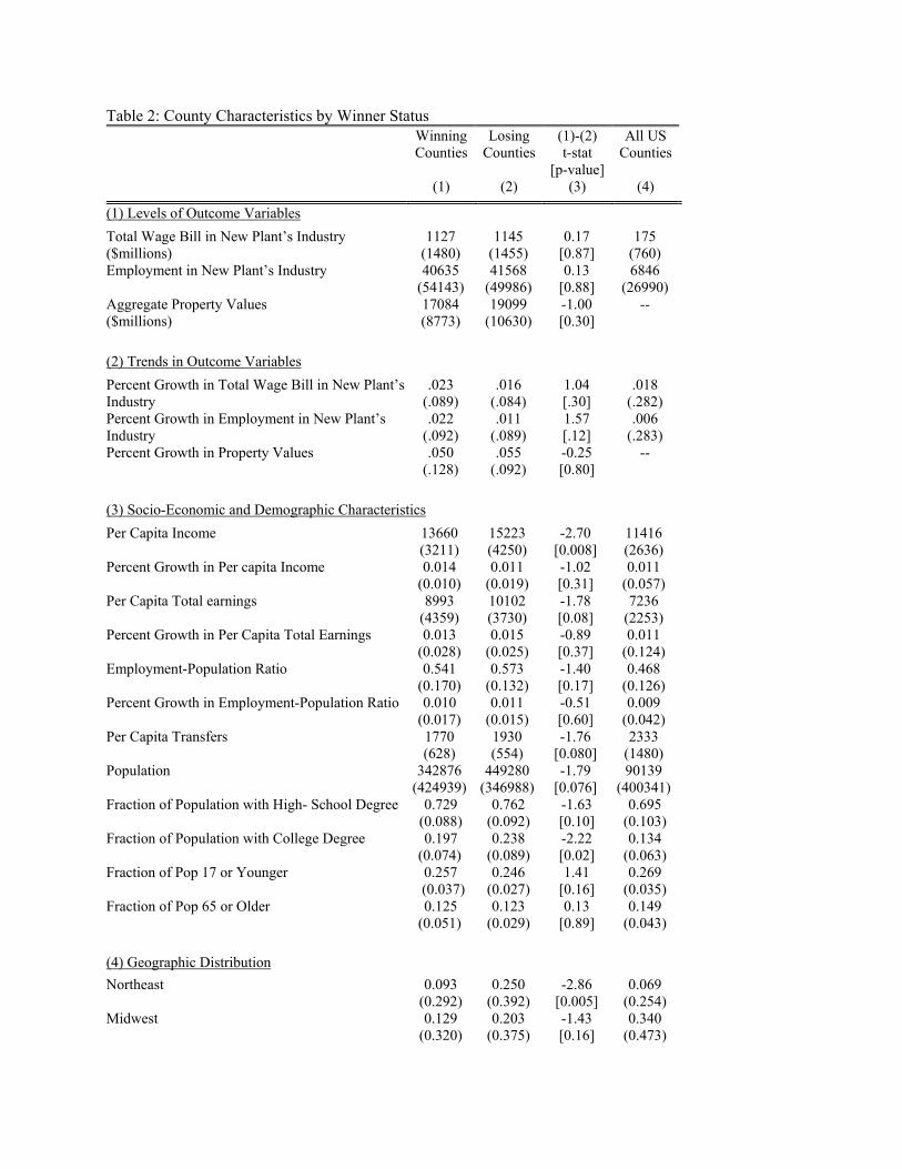
Table 2: County Characteristics by Winner Status Winning

Counties Losing

Counties (1)-(2) t-stat

[p-value]

All US Counties

(1) (2) (3) (4)

(1) Levels of Outcome Variables Total Wage Bill in New Plant’s Industry ($millions)

1127 (1480)

1145 (1455)

0.17 [0.87]

175 (760)

Employment in New Plant’s Industry 40635 (54143)

41568 (49986)

0.13 [0.88]

6846 (26990)

Aggregate Property Values ($millions)

17084 (8773)

19099 (10630)

-1.00 [0.30]

--

(2) Trends in Outcome Variables Percent Growth in Total Wage Bill in New Plant’s Industry

.023 (.089)

.016 (.084)

1.04 [.30]

.018 (.282)

Percent Growth in Employment in New Plant’s Industry

.022 (.092)

.011 (.089)

1.57 [.12]

.006 (.283)

Percent Growth in Property Values

.050 (.128)

.055 (.092)

-0.25 [0.80]

--

(3) Socio-Economic and Demographic Characteristics Per Capita Income 13660

(3211) 15223 (4250)

-2.70 [0.008]

11416 (2636)

Percent Growth in Per capita Income 0.014 (0.010)

0.011 (0.019)

-1.02 [0.31]

0.011 (0.057)

Per Capita Total earnings 8993 (4359)

10102 (3730)

-1.78 [0.08]

7236 (2253)

Percent Growth in Per Capita Total Earnings 0.013 (0.028)

0.015 (0.025)

-0.89 [0.37]

0.011 (0.124)

Employment-Population Ratio 0.541 (0.170)

0.573 (0.132)

-1.40 [0.17]

0.468 (0.126)

Percent Growth in Employment-Population Ratio 0.010 (0.017)

0.011 (0.015)

-0.51 [0.60]

0.009 (0.042)

Per Capita Transfers 1770 (628)

1930 (554)

-1.76 [0.080]

2333 (1480)

Population 342876 (424939)

449280 (346988)

-1.79 [0.076]

90139 (400341)

Fraction of Population with High- School Degree 0.729 (0.088)

0.762 (0.092)

-1.63 [0.10]

0.695 (0.103)

Fraction of Population with College Degree 0.197 (0.074)

0.238 (0.089)

-2.22 [0.02]

0.134 (0.063)

Fraction of Pop 17 or Younger 0.257 (0.037)

0.246 (0.027)

1.41 [0.16]

0.269 (0.035)

Fraction of Pop 65 or Older 0.125 (0.051)

0.123 (0.029)

0.13 [0.89]

0.149 (0.043)

(4) Geographic Distribution Northeast 0.093

(0.292) 0.250

(0.392) -2.86

[0.005] 0.069

(0.254) Midwest 0.129

(0.320) 0.203

(0.375) -1.43 [0.16]

0.340 (0.473)

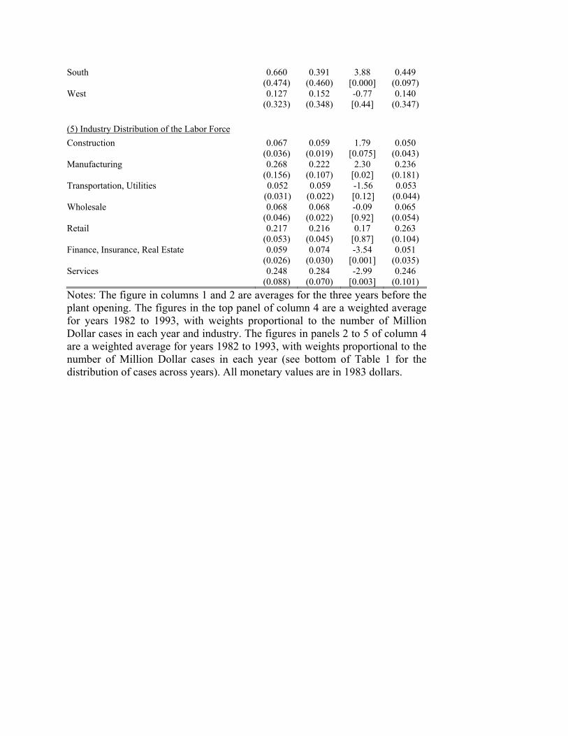
South 0.660 (0.474)

0.391 (0.460)

3.88 [0.000]

0.449 (0.097)

West 0.127 (0.323)

0.152 (0.348)

-0.77 [0.44]

0.140 (0.347)

(5) Industry Distribution of the Labor Force Construction 0.067

(0.036) 0.059

(0.019) 1.79

[0.075] 0.050

(0.043) Manufacturing 0.268

(0.156) 0.222

(0.107) 2.30

[0.02] 0.236

(0.181) Transportation, Utilities 0.052

(0.031) 0.059

(0.022) -1.56 [0.12]

0.053 (0.044)

Wholesale 0.068 (0.046)

0.068 (0.022)

-0.09 [0.92]

0.065 (0.054)

Retail 0.217 (0.053)

0.216 (0.045)

0.17 [0.87]

0.263 (0.104)

Finance, Insurance, Real Estate 0.059 (0.026)

0.074 (0.030)

-3.54 [0.001]

0.051 (0.035)

Services 0.248 (0.088)

0.284 (0.070)

-2.99 [0.003]

0.246 (0.101)

Notes: The figure in columns 1 and 2 are averages for the three years before the plant opening. The figures in the top panel of column 4 are a weighted average for years 1982 to 1993, with weights proportional to the number of Million Dollar cases in each year and industry. The figures in panels 2 to 5 of column 4 are a weighted average for years 1982 to 1993, with weights proportional to the number of Million Dollar cases in each year (see bottom of Table 1 for the distribution of cases across years). All monetary values are in 1983 dollars.

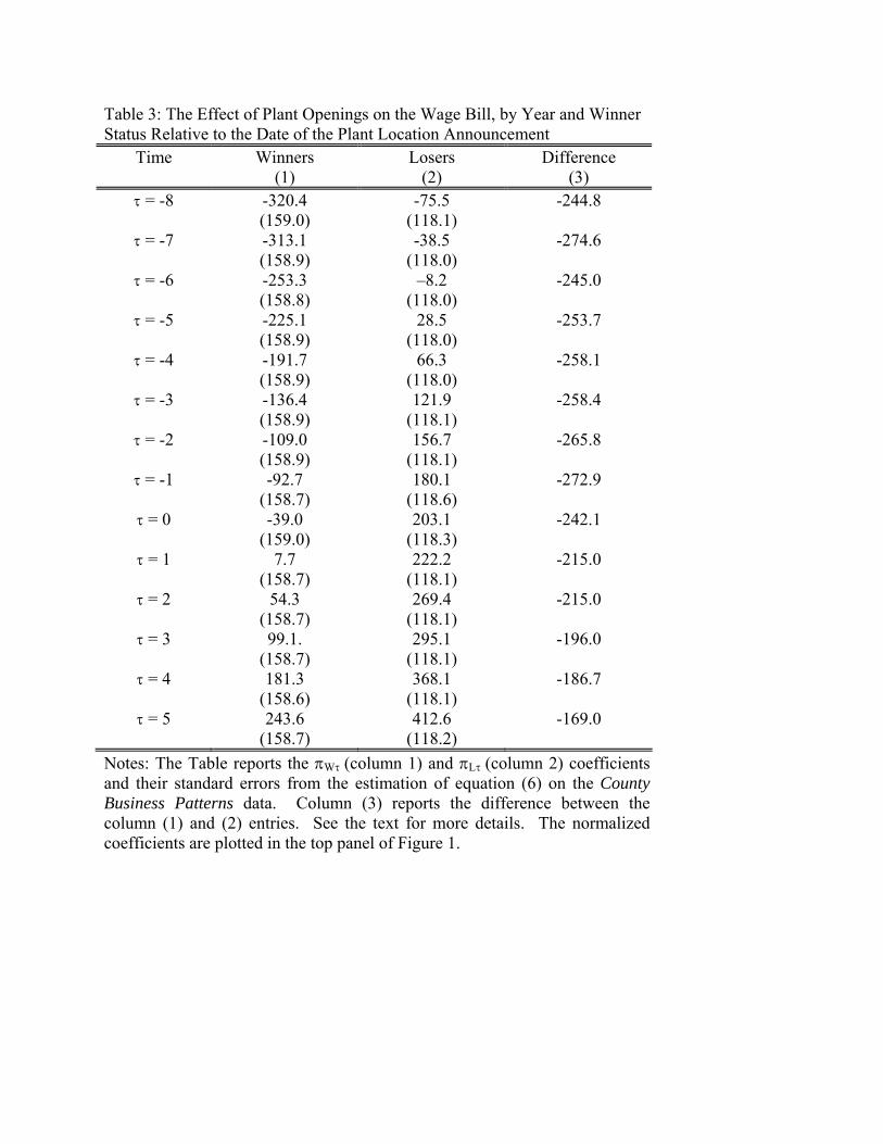
Table 3: The Effect of Plant Openings on the Wage Bill, by Year and Winner Status Relative to the Date of the Plant Location Announcement

Time Winners (1)

Losers (2)

Difference (3)

τ = -8 -320.4 (159.0)

-75.5 (118.1)

-244.8

τ = -7 -313.1 (158.9)

-38.5 (118.0)

-274.6

τ = -6 -253.3 (158.8)

–8.2 (118.0)

-245.0

τ = -5 -225.1 (158.9)

28.5 (118.0)

-253.7

τ = -4 -191.7 (158.9)

66.3 (118.0)

-258.1

τ = -3 -136.4 (158.9)

121.9 (118.1)

-258.4

τ = -2 -109.0 (158.9)

156.7 (118.1)

-265.8

τ = -1 -92.7 (158.7)

180.1 (118.6)

-272.9

τ = 0 -39.0 (159.0)

203.1 (118.3)

-242.1

τ = 1 7.7 (158.7)

222.2 (118.1)

-215.0

τ = 2 54.3 (158.7)

269.4 (118.1)

-215.0

τ = 3 99.1. (158.7)

295.1 (118.1)

-196.0

τ = 4 181.3 (158.6)

368.1 (118.1)

-186.7

τ = 5 243.6 (158.7)

412.6 (118.2)

-169.0

Notes: The Table reports the πWτ (column 1) and πLτ (column 2) coefficients and their standard errors from the estimation of equation (6) on the County Business Patterns data. Column (3) reports the difference between the column (1) and (2) entries. See the text for more details. The normalized coefficients are plotted in the top panel of Figure 1.

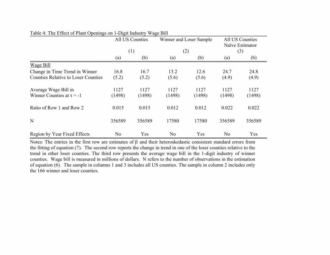
Table 4: The Effect of Plant Openings on 1-Digit Industry Wage Bill All US Counties Winner and Loser Sample All US Counties

Naïve Estimator

(1)

(2)

(3) (a) (b) (a) (b) (a) (b)

Wage Bill Change in Time Trend in Winner Counties Relative to Loser Counties

16.8 (5.2)

16.7 (5.2)

13.2 (5.6)

12.6 (5.6)

24.7 (4.9)

24.8 (4.9)

Average Wage Bill in Winner Counties at τ = -1

1127 (1498)

1127 (1498)

1127 (1498)

1127 (1498)

1127 (1498)

1127 (1498)

Ratio of Row 1 and Row 2

0.015 0.015 0.012 0.012 0.022 0.022

N 356589 356589 17580 17580 356589 356589

Region by Year Fixed Effects No Yes No Yes No Yes Notes: The entries in the first row are estimates of β and their heteroskedastic consistent standard errors from the fitting of equation (7). The second row reports the change in trend in one of the loser counties relative to the trend in other loser counties. The third row presents the average wage bill in the 1-digit industry of winner counties. Wage bill is measured in millions of dollars. N refers to the number of observations in the estimation of equation (6). The sample in columns 1 and 3 includes all US counties. The sample in column 2 includes only the 166 winner and loser counties.

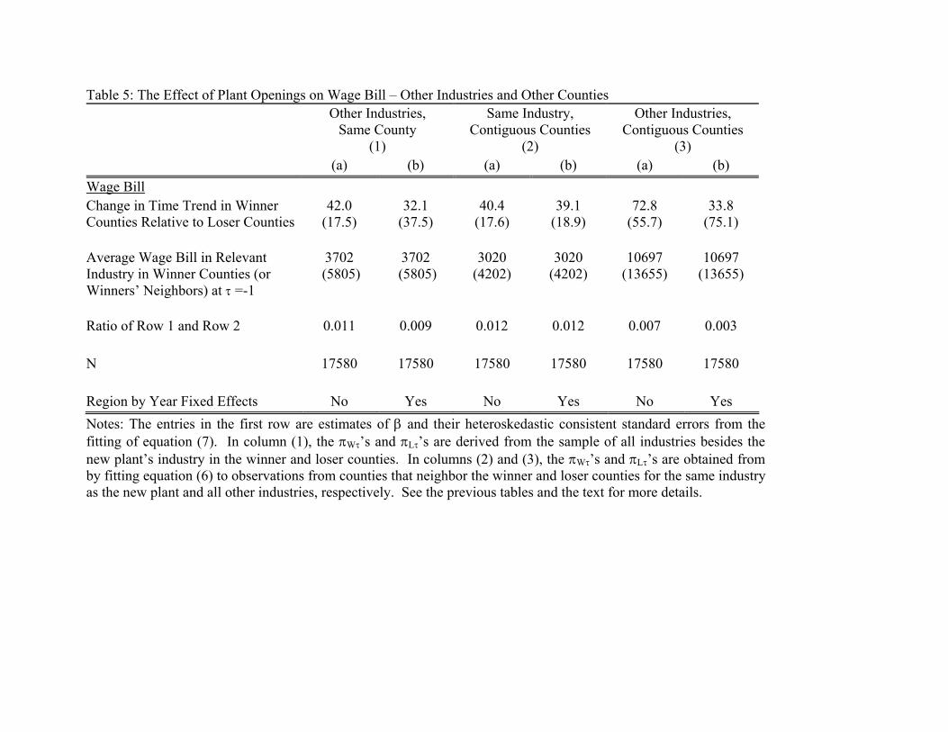
Table 5: The Effect of Plant Openings on Wage Bill – Other Industries and Other Counties Other Industries,

Same County Same Industry,

Contiguous Counties Other Industries,

Contiguous Counties

(1)

(2)

(3) (a) (b) (a) (b) (a) (b)

Wage Bill Change in Time Trend in Winner Counties Relative to Loser Counties

42.0 (17.5)

32.1 (37.5)

40.4 (17.6)

39.1 (18.9)

72.8 (55.7)

33.8 (75.1)

Average Wage Bill in Relevant Industry in Winner Counties (or Winners’ Neighbors) at τ =-1

3702 (5805)

3702 (5805)

3020 (4202)

3020 (4202)

10697 (13655)

10697 (13655)

Ratio of Row 1 and Row 2

0.011 0.009 0.012 0.012 0.007 0.003

N 17580 17580 17580 17580 17580 17580

Region by Year Fixed Effects No Yes No Yes No Yes Notes: The entries in the first row are estimates of β and their heteroskedastic consistent standard errors from the fitting of equation (7). In column (1), the πWτ’s and πLτ’s are derived from the sample of all industries besides the new plant’s industry in the winner and loser counties. In columns (2) and (3), the πWτ’s and πLτ’s are obtained from by fitting equation (6) to observations from counties that neighbor the winner and loser counties for the same industry as the new plant and all other industries, respectively. See the previous tables and the text for more details.

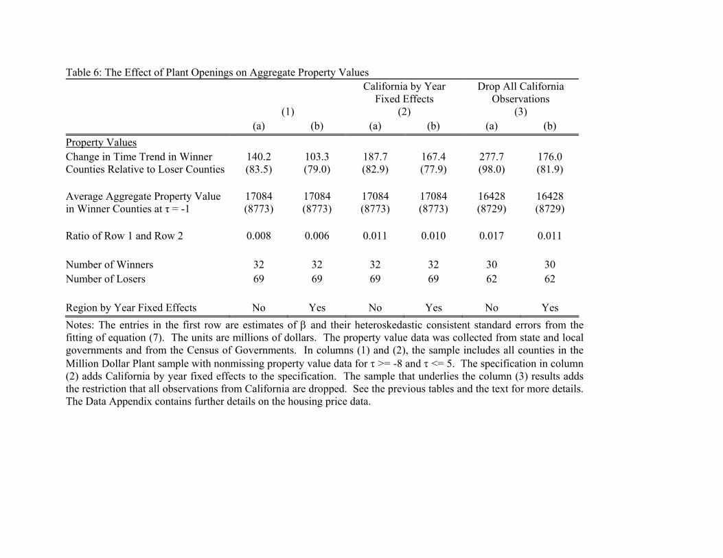
Table 6: The Effect of Plant Openings on Aggregate Property Values California by Year

Fixed Effects Drop All California

Observations

(1)

(2)

(3) (a) (b) (a) (b) (a) (b)

Property Values Change in Time Trend in Winner Counties Relative to Loser Counties

140.2 (83.5)

103.3 (79.0)

187.7 (82.9)

167.4 (77.9)

277.7 (98.0)

176.0 (81.9)

Average Aggregate Property Value in Winner Counties at τ = -1

17084 (8773)

17084 (8773)

17084 (8773)

17084 (8773)

16428 (8729)

16428 (8729)

Ratio of Row 1 and Row 2

0.008 0.006 0.011 0.010 0.017 0.011

Number of Winners 32 32 32 32 30 30Number of Losers

69 69 69 69 62 62

Region by Year Fixed Effects No Yes No Yes No Yes Notes: The entries in the first row are estimates of β and their heteroskedastic consistent standard errors from the fitting of equation (7). The units are millions of dollars. The property value data was collected from state and local governments and from the Census of Governments. In columns (1) and (2), the sample includes all counties in the Million Dollar Plant sample with nonmissing property value data for τ >= -8 and τ <= 5. The specification in column (2) adds California by year fixed effects to the specification. The sample that underlies the column (3) results adds the restriction that all observations from California are dropped. See the previous tables and the text for more details. The Data Appendix contains further details on the housing price data.

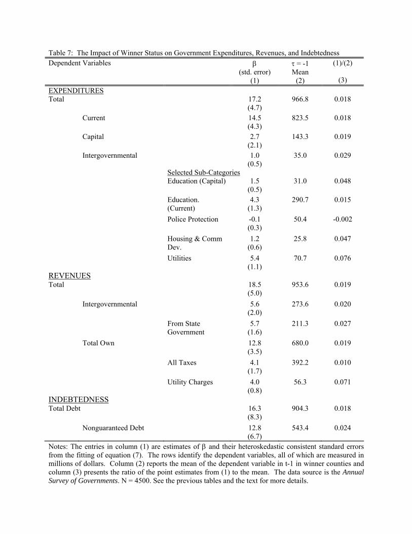
Table 7: The Impact of Winner Status on Government Expenditures, Revenues, and Indebtedness Dependent Variables β

(std. error) (1)

τ = -1 Mean

(2)

(1)/(2)

(3) EXPENDITURES Total 17.2

(4.7) 966.8 0.018

Current 14.5 (4.3)

823.5 0.018

Capital 2.7 (2.1)

143.3 0.019

Intergovernmental 1.0 (0.5)

35.0 0.029

Selected Sub-Categories Education (Capital) 1.5

(0.5) 31.0 0.048

Education. (Current)

4.3 (1.3)

290.7 0.015

Police Protection -0.1 (0.3)

50.4 -0.002

Housing & Comm Dev.

1.2 (0.6)

25.8 0.047

Utilities 5.4 (1.1)

70.7 0.076

REVENUES Total 18.5

(5.0) 953.6 0.019

Intergovernmental 5.6 (2.0)

273.6 0.020

From State Government

5.7 (1.6)

211.3 0.027

Total Own 12.8 (3.5)

680.0 0.019

All Taxes 4.1 (1.7)

392.2 0.010

Utility Charges 4.0 (0.8)

56.3 0.071

INDEBTEDNESS Total Debt 16.3

(8.3) 904.3 0.018

Nonguaranteed Debt 12.8 (6.7)

543.4 0.024

Notes: The entries in column (1) are estimates of β and their heteroskedastic consistent standard errors from the fitting of equation (7). The rows identify the dependent variables, all of which are measured in millions of dollars. Column (2) reports the mean of the dependent variable in t-1 in winner counties and column (3) presents the ratio of the point estimates from (1) to the mean. The data source is the Annual Survey of Governments. N = 4500. See the previous tables and the text for more details.

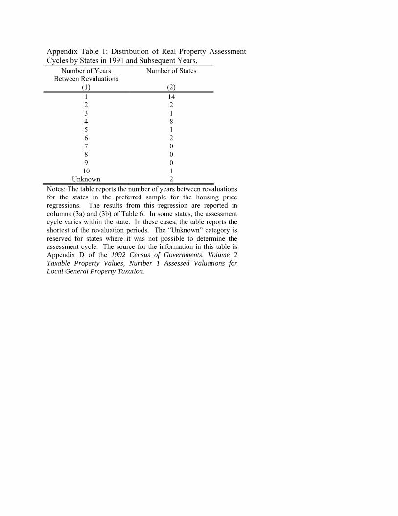
Appendix Table 1: Distribution of Real Property Assessment Cycles by States in 1991 and Subsequent Years.

Number of Years Between Revaluations

Number of States

(1) (2) 1 14 2 2 3 1 4 8 5 1 6 2 7 0 8 0 9 0

10 1 Unknown 2

Notes: The table reports the number of years between revaluations for the states in the preferred sample for the housing price regressions. The results from this regression are reported in columns (3a) and (3b) of Table 6. In some states, the assessment cycle varies within the state. In these cases, the table reports the shortest of the revaluation periods. The “Unknown” category is reserved for states where it was not possible to determine the assessment cycle. The source for the information in this table is Appendix D of the 1992 Census of Governments, Volume 2 Taxable Property Values, Number 1 Assessed Valuations for Local General Property Taxation.

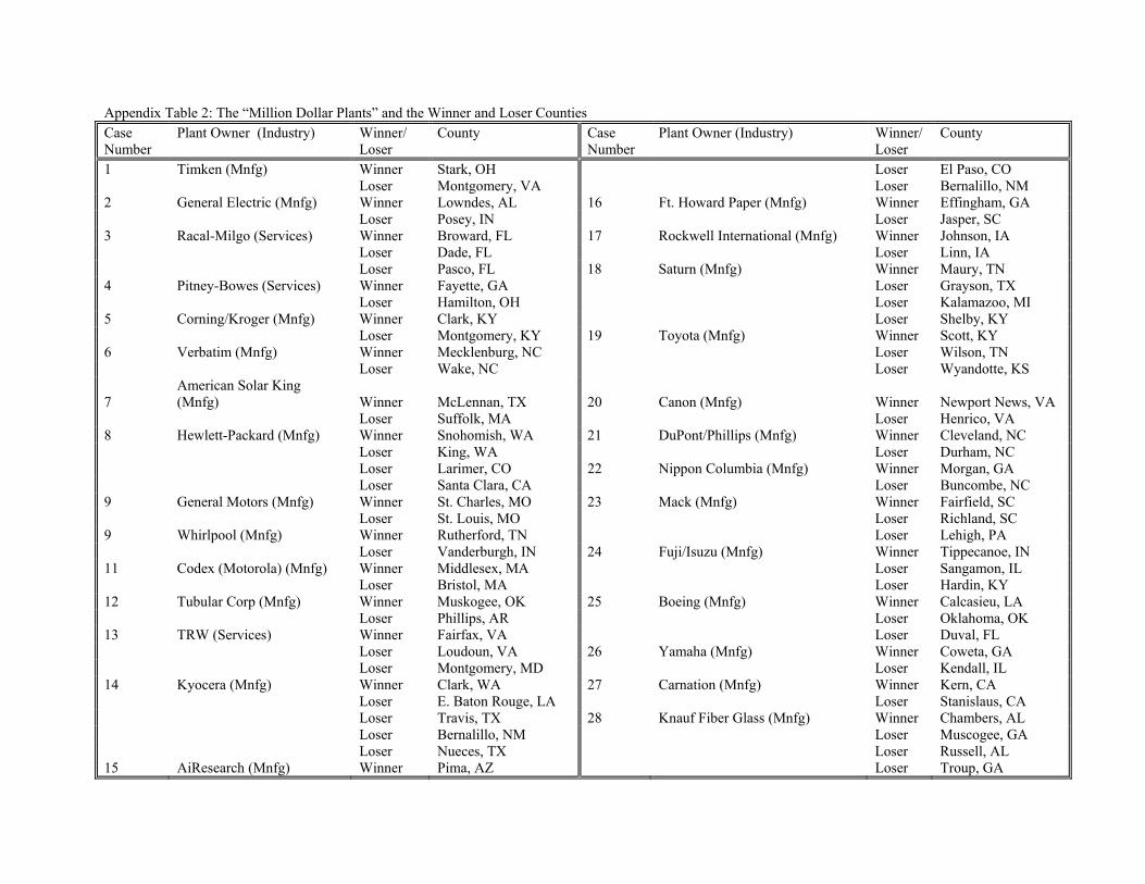
Appendix Table 2: The “Million Dollar Plants” and the Winner and Loser Counties Case

Number Plant Owner (Industry) Winner/

Loser County Case Plant Owner (Industry)

Number Winner/Loser

County

1 Timken (Mnfg) Winner Stark, OH Loser El Paso, CO Loser Montgomery, VA Loser Bernalillo, NM2 General Electric (Mnfg) Winner Lowndes, AL 16 Ft. Howard Paper (Mnfg) Winner Effingham, GA Loser Posey, IN Loser Jasper, SC 3 Racal-Milgo (Services) Winner Broward, FL 17 Rockwell International (Mnfg) Winner Johnson, IA Loser Dade, FL Loser Linn, IA Loser Pasco, FL 18 Saturn (Mnfg) Winner Maury, TN 4 Pitney-Bowes (Services) Winner Fayette, GA Loser Grayson, TX Loser Hamilton, OH Loser Kalamazoo, MI5 Corning/Kroger (Mnfg) Winner Clark, KY Loser Shelby, KY Loser Montgomery, KY 19 Toyota (Mnfg) Winner Scott, KY 6 Verbatim (Mnfg) Winner Mecklenburg, NC Loser Wilson, TN Loser Wake, NC Loser Wyandotte, KS

7 American Solar King (Mnfg) Winner McLennan, TX 20 Canon (Mnfg) Winner Newport News, VA

Loser Suffolk, MA Loser Henrico, VA 8 Hewlett-Packard (Mnfg) Winner Snohomish, WA 21 DuPont/Phillips (Mnfg) Winner Cleveland, NC Loser King, WA Loser Durham, NC Loser Larimer, CO 22 Nippon Columbia (Mnfg) Winner Morgan, GA Loser Santa Clara, CA Loser Buncombe, NC 9 General Motors (Mnfg) Winner St. Charles, MO 23 Mack (Mnfg) Winner Fairfield, SC Loser St. Louis, MO Loser Richland, SC9 Whirlpool (Mnfg) Winner Rutherford, TN Loser Lehigh, PA Loser Vanderburgh, IN 24 Fuji/Isuzu (Mnfg) Winner Tippecanoe, IN 11 Codex (Motorola) (Mnfg) Winner Middlesex, MA Loser Sangamon, IL Loser Bristol, MA Loser Hardin, KY 12 Tubular Corp (Mnfg) Winner Muskogee, OK 25 Boeing (Mnfg) Winner Calcasieu, LA Loser Phillips, AR Loser Oklahoma, OK13 TRW (Services) Winner Fairfax, VA Loser Duval, FL Loser Loudoun, VA 26 Yamaha (Mnfg) Winner Coweta, GA Loser Montgomery, MD Loser Kendall, IL14 Kyocera (Mnfg) Winner Clark, WA 27 Carnation (Mnfg) Winner Kern, CA Loser E. Baton Rouge, LA Loser Stanislaus, CA Loser Travis, TX 28 Knauf Fiber Glass (Mnfg) Winner Chambers, AL Loser Bernalillo, NM Loser Muscogee, GA Loser Nueces, TX Loser Russell, AL 15 AiResearch (Mnfg) Winner Pima, AZ Loser Troup, GA

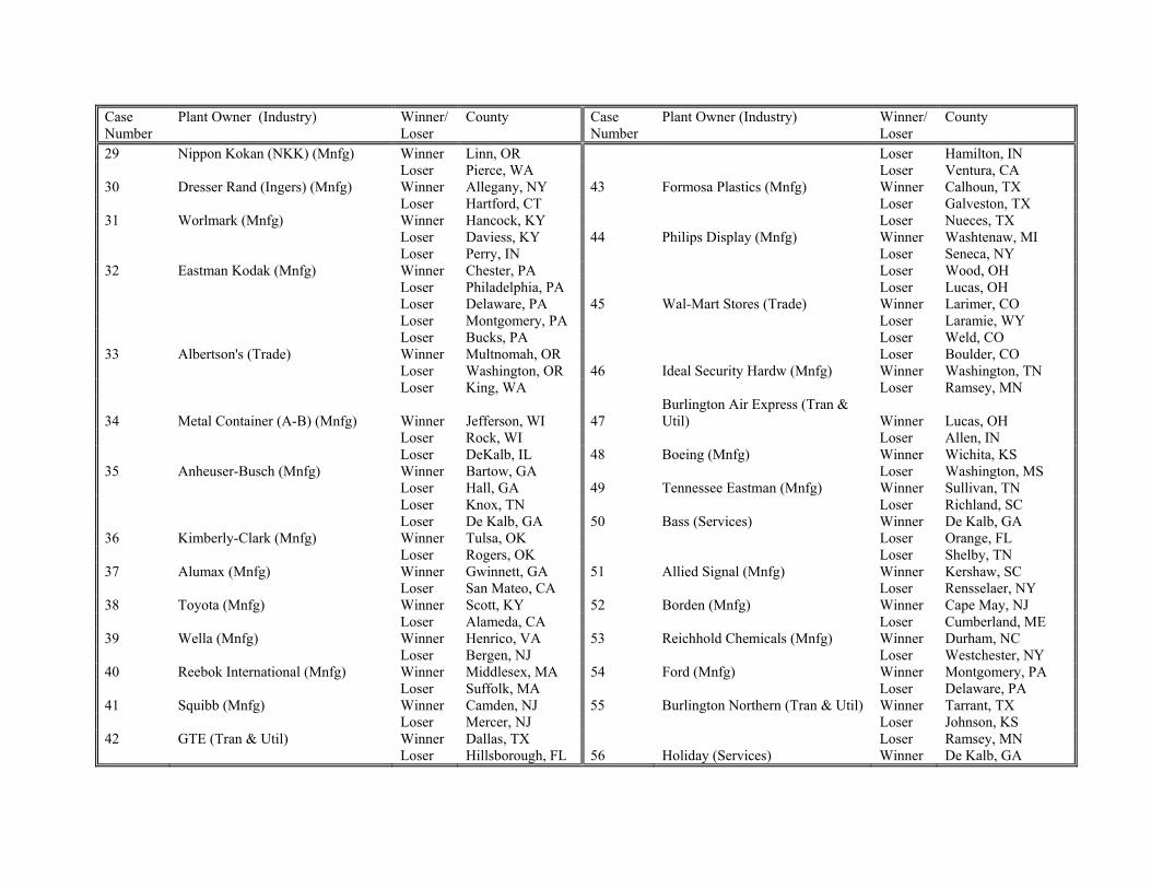
Case Number

Plant Owner (Industry) Winner/Loser

County Case Plant Owner (Industry) Number

Winner/Loser

County

29 Nippon Kokan (NKK) (Mnfg) Winner Linn, OR Loser Hamilton, IN Loser Pierce, WA Loser Ventura, CA30 Dresser Rand (Ingers) (Mnfg) Winner Allegany, NY 43 Formosa Plastics (Mnfg) Winner Calhoun, TX Loser Hartford, CT Loser Galveston, TX31 Worlmark (Mnfg) Winner Hancock, KY Loser Nueces, TX Loser Daviess, KY 44 Philips Display (Mnfg) Winner Washtenaw, MI Loser Perry, IN Loser Seneca, NY 32 Eastman Kodak (Mnfg) Winner Chester, PA Loser Wood, OH Loser Philadelphia, PA Loser Lucas, OH Loser Delaware, PA 45 Wal-Mart Stores (Trade) Winner Larimer, CO Loser Montgomery, PA Loser Laramie, WY Loser Bucks, PA Loser Weld, CO 33 Albertson's (Trade) Winner Multnomah, OR Loser Boulder, CO Loser Washington, OR 46 Ideal Security Hardw (Mnfg) Winner Washington, TN Loser King, WA Loser Ramsey, MN

34 Metal Container (A-B) (Mnfg) Winner Jefferson, WI 47 Burlington Air Express (Tran & Util) Winner Lucas, OH

Loser Rock, WI Loser Allen, IN Loser DeKalb, IL 48 Boeing (Mnfg) Winner Wichita, KS 35 Anheuser-Busch (Mnfg) Winner Bartow, GA Loser Washington, MS Loser Hall, GA 49 Tennessee Eastman (Mnfg) Winner Sullivan, TN Loser Knox, TN Loser Richland, SC Loser De Kalb, GA 50 Bass (Services) Winner De Kalb, GA 36 Kimberly-Clark (Mnfg) Winner Tulsa, OK Loser Orange, FL Loser Rogers, OK Loser Shelby, TN37 Alumax (Mnfg) Winner Gwinnett, GA 51 Allied Signal (Mnfg) Winner Kershaw, SC Loser San Mateo, CA Loser Rensselaer, NY 38 Toyota (Mnfg) Winner Scott, KY 52 Borden (Mnfg) Winner Cape May, NJ Loser Alameda, CA Loser Cumberland, ME 39 Wella (Mnfg) Winner Henrico, VA 53 Reichhold Chemicals (Mnfg) Winner Durham, NC Loser Bergen, NJ Loser Westchester, NY 40 Reebok International (Mnfg) Winner Middlesex, MA 54 Ford (Mnfg) Winner Montgomery, PA Loser Suffolk, MA Loser Delaware, PA 41 Squibb (Mnfg) Winner Camden, NJ 55 Burlington Northern (Tran & Util) Winner Tarrant, TX Loser Mercer, NJ Loser Johnson, KS42 GTE (Tran & Util) Winner Dallas, TX Loser Ramsey, MN Loser Hillsborough, FL 56 Holiday (Services) Winner De Kalb, GA

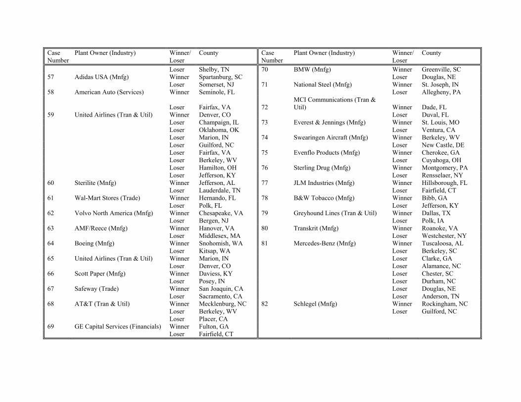
Case Number

Plant Owner (Industry) Winner/Loser

County Case Plant Owner (Industry) Number

Winner/Loser

County

Loser Shelby, TN 70 BMW (Mnfg) Winner Greenville, SC 57 Adidas USA (Mnfg) Winner Spartanburg, SC Loser Douglas, NE Loser Somerset, NJ 71 National Steel (Mnfg) Winner St. Joseph, IN 58 American Auto (Services) Winner Seminole, FL Loser Allegheny, PA

Loser Fairfax, VA 72MCI Communications (Tran & Util) Winner Dade, FL

59 United Airlines (Tran & Util) Winner Denver, CO Loser Duval, FL Loser Champaign, IL 73 Everest & Jennings (Mnfg) Winner St. Louis, MO Loser Oklahoma, OK Loser Ventura, CA Loser Marion, IN 74 Swearingen Aircraft (Mnfg) Winner Berkeley, WV Loser Guilford, NC Loser New Castle, DE Loser Fairfax, VA 75 Evenflo Products (Mnfg) Winner Cherokee, GA Loser Berkeley, WV Loser Cuyahoga, OH Loser Hamilton, OH 76 Sterling Drug (Mnfg) Winner Montgomery, PA Loser Jefferson, KY Loser Rensselaer, NY 60 Sterilite (Mnfg) Winner Jefferson, AL 77 JLM Industries (Mnfg) Winner Hillsborough, FL Loser Lauderdale, TN Loser Fairfield, CT 61 Wal-Mart Stores (Trade) Winner Hernando, FL 78 B&W Tobacco (Mnfg) Winner Bibb, GA Loser Polk, FL Loser Jefferson, KY 62 Volvo North America (Mnfg) Winner Chesapeake, VA 79 Greyhound Lines (Tran & Util) Winner Dallas, TX Loser Bergen, NJ Loser Polk, IA 63 AMF/Reece (Mnfg) Winner Hanover, VA 80 Transkrit (Mnfg) Winner Roanoke, VA Loser Middlesex, MA Loser Westchester, NY64 Boeing (Mnfg) Winner Snohomish, WA 81 Mercedes-Benz (Mnfg) Winner Tuscaloosa, AL Loser Kitsap, WA Loser Berkeley, SC 65 United Airlines (Tran & Util) Winner Marion, IN Loser Clarke, GA Loser Denver, CO Loser Alamance, NC66 Scott Paper (Mnfg) Winner Daviess, KY Loser Chester, SC Loser Posey, IN Loser Durham, NC67 Safeway (Trade) Winner San Joaquin, CA Loser Douglas, NE Loser Sacramento, CA Loser Anderson, TN68 AT&T (Tran & Util) Winner Mecklenburg, NC 82 Schlegel (Mnfg) Winner Rockingham, NC Loser Berkeley, WV Loser Guilford, NC Loser Placer, CA 69 GE Capital Services (Financials) Winner Fulton, GA Loser Fairfield, CT

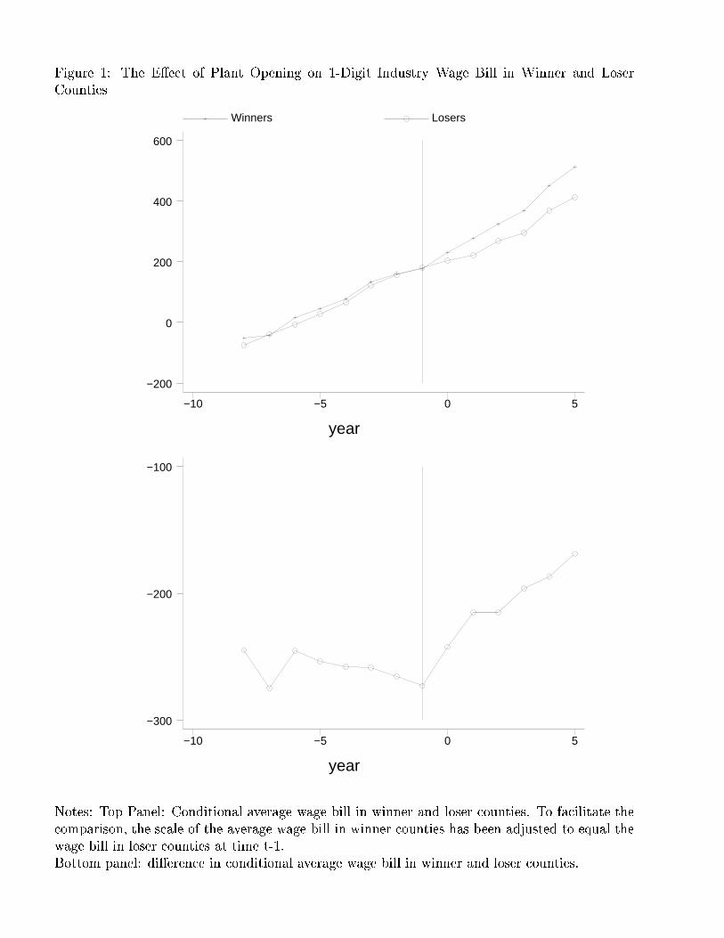
������������ ������������������ �"!$#�%&�('*)+�%���%��,��%-�/.10*�2�����435%�6���78�9�8:<;=#���?>@��!2!A�2%B;C�2%�%����#�%D6CEF��7G��H ���D%I�G�2�7

year

Winners Losers

−10 −5 0 5

−200

0

200

400

600

year

−10 −5 0 5

−300

−200

−100

JK���9�7� @�L��)M��#�%��!N H ��%�6��O�9�2��%P#�!Q#SR���9#���UT@#��� V��2!�!Q�2%WTA�2%�%���X#Y%�6Z!���7G��[������%&�9���7�\]�^�4�_#�����!2�O�`#Y�GX�9������ab)�#��G��7G��%dcI�9�D*7G��#�!2*�Y�L�G��e#SR���9#���*T]#���eV��2!�!���%fTA�2%�%D��]������%&�9���7��P#�7@V���%(#�6hg��78�9�6W�G�i�jI�P#Y!k�9��T@#���lV���!2!k��%W!2��7���������%&�9�2�7K#Y���9��ab*�8.`��\>@�Y�G�9��am)P#�%D�!N "6D������G�%���l��%(����%�6��O�9����%P#�!k#nR���G#���lT]#��� VD�2!2!��2%oTA�2%D%���K#�%�6W!���7G���������%&�G�2�7�\

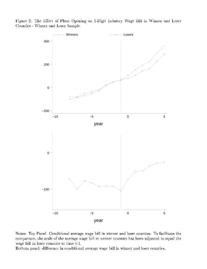
���������qpr ������������������ �"!$#�%&�('*)+�%���%��,��%-�/.10*�2�����435%�6���78�9�8:<;=#���?>@��!2!A�2%B;C�2%�%����#�%D6CEF��7G��H ���D%I�G�2�7�.s;C��%�%���[#Y%�6(EF��7G��[tD#Yab)�!�

year

Winners Losers

−10 −5 0 5

−200

0

200

400

year

−10 −5 0 5

−100

0

JK���9�7� @�L��)M��#�%��!N H ��%�6��O�9�2��%P#�!Q#SR���9#���UT@#��� V��2!�!Q�2%WTA�2%�%���X#Y%�6Z!���7G��[������%&�9���7�\]�^�4�_#�����!2�O�`#Y�GX�9������ab)�#��G��7G��%dcI�9�D*7G��#�!2*�Y�L�G��e#SR���9#���*T]#���eV��2!�!���%fTA�2%�%D��]������%&�9���7��P#�7@V���%(#�6hg��78�9�6W�G�i�jI�P#Y!k�9��T@#���lV���!2!k��%W!2��7���������%&�9�2�7K#Y���9��ab*�8.`��\>@�Y�G�9��am)P#�%D�!N "6D������G�%���l��%(����%�6��O�9����%P#�!k#nR���G#���lT]#��� VD�2!2!��2%oTA�2%D%���K#�%�6W!���7G���������%&�G�2�7�\

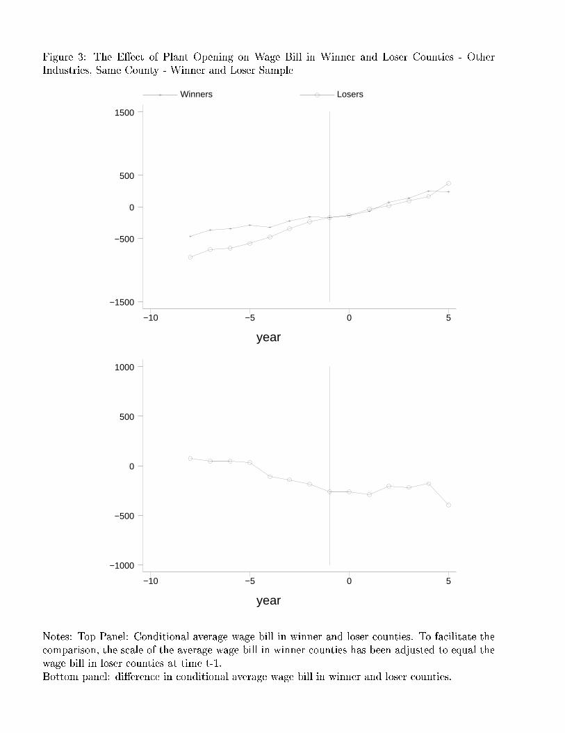
���������WuD Z���DM��������f���e�"!2#�%&��'*)+�%���%�����%B;=#���(>@��!2!]��%v;C��%�%���b#Y%�6<EQ��7�� H ����%&�9���7w.i'*�G����35%�6D��7�G�G�2�7�c+tD#Yab H ����%&�5:�.s;C��%�%���A#Y%�6MEQ��7��[tD#�a4)�!�

year

Winners Losers

−10 −5 0 5

−1500

−500

0

500

1500

year

−10 −5 0 5

−1000

−500

0

500

1000

JK���9�7� @�L��)M��#�%��!N H ��%�6��O�9�2��%P#�!Q#SR���9#���UT@#��� V��2!�!Q�2%WTA�2%�%���X#Y%�6Z!���7G��[������%&�9���7�\]�^�4�_#�����!2�O�`#Y�GX�9������ab)�#��G��7G��%dcI�9�D*7G��#�!2*�Y�L�G��e#SR���9#���*T]#���eV��2!�!���%fTA�2%�%D��]������%&�9���7��P#�7@V���%(#�6hg��78�9�6W�G�i�jI�P#Y!k�9��T@#���lV���!2!k��%W!2��7���������%&�9�2�7K#Y���9��ab*�8.`��\>@�Y�G�9��am)P#�%D�!N "6D������G�%���l��%(����%�6��O�9����%P#�!k#nR���G#���lT]#��� VD�2!2!��2%oTA�2%D%���K#�%�6W!���7G���������%&�G�2�7�\

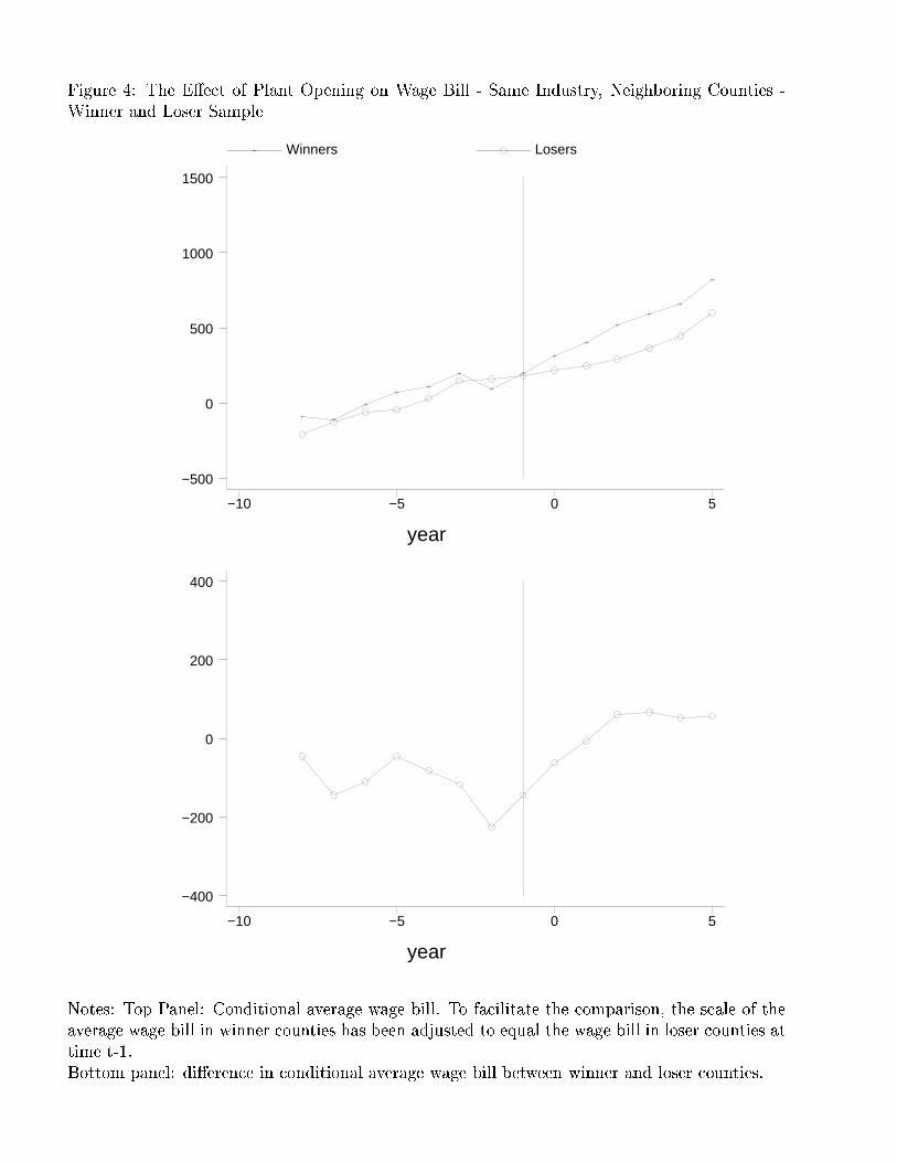
���������wx� l����f������/�y���]�"!$#�%&�y'*)��%��2%��W��%�;,#Y��4>@�2!�!L.*tD#�a4z35%�6���78�9�:�c�JK��2���{V+����2%�� H ���D%I�G�2�7l.;C��%�%���A#Y%�6MEQ��7��[tD#�a4)�!�

year

Winners Losers

−10 −5 0 5

−500

0

500

1000

1500

year

−10 −5 0 5

−400

−200

0

200

400

JK���9�7� ]�L��)q�^#�%��!N H ��%D6����G�2��%P#Y!Q#SR���G#��� T]#���yV���!2!N\|�L�b�_#����2!2�O�`#Y�GX�9�Dy����ab)P#Y�G�27��%dc��G��y7�S#�!�U���^�9��#SR���9#���[T@#���*V���!2!P��%bTA�2%D%���}������%&�G�2�7}�P#�7}V���%o#�6~g��7�G�6��9�U�jI�P#�!+�9��KT]#Y��XV���!2!P��%f!2��7G��}�����D%I�G�2�7]#Y��G�2a4X�.9��\>@�Y�G�9��am)P#�%D�!N "6D������G�%���l��%(����%�6��O�9����%P#�!k#nR���G#���lT]#��� VD�2!2!�V�/�5T@��%MTA��%�%���A#�%�6(!2��7���������%&�9�2�7�\

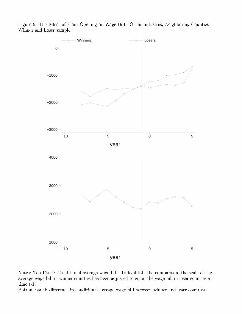
���������y�{ ]����w��������X���s�"!$#Y%I�*'*)��%��2%D�f��%(;,#���i>@��!2!�.�'X�9����X35%�6��D7�9��7�cQJ[��2���IV+���G��%�� H ����%&�9�2�7K.;C��%�%���A#Y%�6MEQ��7��A79#Yab)�!�

year

Winners Losers

−10 −5 0 5

−3000

−2000

−1000

0

year

−10 −5 0 5

1000

2000

3000

4000

JK���9�7� ]�L��)q�^#�%��!N H ��%D6����G�2��%P#Y!Q#SR���G#��� T]#���yV���!2!N\|�L�b�_#����2!2�O�`#Y�GX�9�Dy����ab)P#Y�G�27��%dc��G��y7�S#�!�U���^�9��#SR���9#���[T@#���*V���!2!P��%bTA�2%D%���}������%&�G�2�7}�P#�7}V���%o#�6~g��7�G�6��9�U�jI�P#�!+�9��KT]#Y��XV���!2!P��%f!2��7G��}�����D%I�G�2�7]#Y��G�2a4X�.9��\>@�Y�G�9��am)P#�%D�!N "6D������G�%���l��%(����%�6��O�9����%P#�!k#nR���G#���lT]#��� VD�2!2!�V�/�5T@��%MTA��%�%���A#�%�6(!2��7���������%&�9�2�7�\

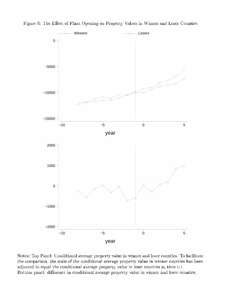
���������e�D "����U���k����K�����s!2#�%&�X'e)+�%D�2%��z��%(�"�G��)+��8�5:o�|#�!2�D�7��2%o;C��%�%���A#Y%�6MEQ��7�� H ����%&�G�2�7

year

Winners Losers

−10 −5 0 5

−15000

−10000

−5000

0

year

−10 −5 0 5

−2000

−1000

0

1000

2000

JK���9�7� ��L��)b��#�%��!N H ��%�6��O�9�2��%P#�!P#SR���9#���[)����)+���5:yR�#Y!2��A�2%wTA��%�%���|#�%D6b!���7G��|������%&�9���7�\��^�l�_#����2!2�O�`#Y�G�G��l����a4)P#���27G��%dcr�G��l7G�S#Y!2l���L�9��l����%�6����G�2��%�#�!d#SR���9#���U)����)+���5:fR�#Y!2��e��%WTA��%�%���K������%&�9���7A�P#�7AV+��%#�6~g��7�G�6W�9�z�jI�P#�!Q�G��l����%�6D���9����%P#�!k#SR���G#���l)����)����5:oRY#�!���e�2%W!2��7G���������%&�9���7K#Y���G�2a4X�.9��\>@�Y�G�9��am)P#�%D�!N "6D������G�%���l��%(����%�6��O�9����%P#�!k#nR���G#��� )��G��)+��8�5:�RY#�!2�De�2%oTA�2%�%D��K#�%�6W!2��7G��A������%&�9���7�\

� )�)��%�6����(���2�����Gi�� |���DU������/�X�����"!$#�%&�['*)+�%���%��z��%���.10*�������@35%�6���78�9�:(�"a4)�!2�n:{a4�%&�A�2%o;C�2%D%���#�%�6ZEF��7G�� H ���D%I�G�2�7�.s;C��%�%���[#Y%�6(EF��7G��[tD#Yab)�!�

year

Winners Losers

−10 −5 0 5

5000

10000

15000

20000

25000

year

−10 −5 0 5

−12000

−10000

−8000

−6000

−4000

−2000

JK���9�7� K�^��)��^#�%��!N H ��%�6��O�9����%P#�!L#SR���9#���w�ab)D!2�n:{ab�%I�X�2%MTA��%�%���e#�%�6q!���7G��*������%&�9�2�7�\e�L�f�_#����2!2�O�`#Y�G�G��f����ab)�#��G��7G��%dcL�9��f7G�S#Y!2f�Y���9��b����%�6D���9����%P#�!|#SR���9#�����a4)�!2�n:{a4�%&�i��%�TA�2%D%���i������%&�9���7U�P#�7iV+��%#�6~g��7�G�6W�9�z�jI�P#�!Q�G��l����%�6D���9����%P#�!k#SR���G#���l�a4)�!��~:{a4�%&�K�2%o!���7G���������%&�G�2�7[#Y���G�2a4X�.9��\>@�Y�G�9��am)P#�%D�!N "6D������G�%���l��%(����%�6��O�9����%P#�!k#nR���G#��� �a4)�!2�n:{ab�%&�A�2%oTA�2%�%D��A#�%�6(!2��7G���������%&�9���7�\