Bias in Telephone Samples Telephone surveys, the staple of ...

Al-Baghal LCM Survey Methods

1

Bias in Telephone Samples

Telephone surveys, the staple of many social surveys, face a number of difficulties that

place into question the efficacy of the method. First, respondents are wary of calls from unknown

individuals, in response to telemarketing and other security issues (Tourangeau 2004). Second

call screening devices, such as caller identification (Caller-ID) and answering machines have

grown in popularity. These devices allow potential respondents to decide when and for whom to

answer the telephone, possibly avoiding the initial contact and survey request (Tuckel and

O’Neill 1995, 1996, 2001). A third issue is the dedication of telephone lines to facsimile

machines and Internet connections, thereby precluding possible contact (Tuckel and O’Neill

2001). Finally, there has been a general increase in cellular telephone usage in lieu of landline

service, although the extent of this is still undetermined (Steeh 2004, Tourangeau 2004). These

factors, and possibly others, have all probably contributed to the overall decline in telephone

survey response rate (Steeh 1981, Groves and Couper 1998, Steeh et al 2001, Tuckel and O’Neill

2002). The decline in response rates may lead to increased nonresponse error, although the

overall effect of this on telephone surveys is not clear (Keeter et al 2000).

Decreased landline ownership, however, will lead to coverage errors that could be

removed by including cellular phones in a telephone sample. Whether this noncoverage will lead

to a bias or little or no effects as in nonresponse studies is unknown. It is known that

noncoverage of those without telephone service at all can bias results (Botman and Allen 1990,

Groves 1989, Thornberry and Massey 1988, Hall et al 1999). The size of this population is small;

in 2003, the estimated percentage of households with a telephone stood at 95.3 percent (FCC

2004). Changes in this number are likely to happen rapidly, as people choose cellular technology

as their only source of telephone communication. Findings from the Consumer Expenditure


2

Interview Survey (CEIS) showed that households reporting a cell phone bill rose from two

percent in 1994 to 25 percent in 2001, increasing to 47 percent in 2003 (Tucker et al 2004).

Those reporting only a cell phone bill in the survey rose from one to four percent from 2001 to

2003 (Tucker et al 2004). Data from the February 2004 CPS supplement indicated that the cell

only population stood at 6 percent, and 5.1 percent of households owned no phone at all (Tucker

et al 2004). This is significant in that the cell only population now outnumbers the population

with no phone. These numbers are not only changing fast, but the CPS data failed to measure all

potential respondents due to a survey error (a faulty skip pattern which systematically did not

ask questions of some of the sample), so new measures may be more accurate in estimating cell

only prevalence (Tucker et al 2004).

Coverage error in telephone samples therefore now come from several sources, rather

than just from those who do not own telephones. Each of these sources of error may have

different effects on the estimates of interest. For example, Brick et al (1995) note that population

members owning a phone but not covered in list-assisted designs are likely different than those

not owning a phone at all. Similarly, those owning a cell phone only are likely to be different

from landline owners that are not covered in list-assisted samples, or from those who own no

phone at all. This follows the same idea that different sources of nonresponse leads to differential

effects on estimates (Groves 1989). Following this logic, coverage error is parameterized by

Equation 1:

cellc list ntc list ntcellY

N N NNY Y Y YN N N N

= + + + (1)


3

Where Y is the statistic of interest for the full population;

N = total population of interest

Nc= number of population covered in the telephone frame,

Y c = value of statistic of interest for population covered in the telephone frame

Ncell= number of population in cell phone only population

Y cell = value of statistic of interest for population in cell phone only population

Nlist = number of population not covered by list-assisted sample frame

Y list = value of statistic of interest for population not covered by list-assisted sample frame

Nnt = number of population not owning a telephone

Y nt = value of statistic of interest for population not owning a telephone

This equation is similar in structure to the one presented by Groves (1989) for nonresponse. Each

source of error contributes to the equation depending on the size on the noncovered populations

and difference between each one and the covered population. Research in Slovenia estimated a

cell only population of about 10 percent, and that the effect of not including these cell only

respondents changes the distributions of estimates (Vehovar et al 2004).

The equation can be altered as the sample design changes. If cellular numbers are

included in the sample, then the portion of the equation in this equation is removed. Similarly, if

a method alternative to list-assisted sampling is employed this term would drop. The term for

those not owning a telephone would never drop in a telephone survey, unless it was included as a

mixed-mode design that incorporated methods that could reach this population. In this case, all

of the terms bias would be dropped.


4

Measurement error in questionnaires

Coverage error has often been estimated directly from survey data. Telephone ownership

estimates often come from face to face surveys (Brick et al 1995, Federal Communication

Commission 2003, Thornberry and Massey 1988). Estimates of coverage error in list-assisted

frames for telephone samples have similarly come from survey data (Brick et al 1995). Survey

data are often measured with error, however, which makes interpretation of the resulting

estimates difficult (Biemer and Trewin 1997). When these data are used to estimate and model

coverage error, the resulting estimate for coverage error will be inaccurate. For example, if one is

estimate the value of Ncell from survey data, and that data is measured with error, then the

estimate of Ncell becomes

ˆ ( )cell i i i i ii i i i

N y µ ε µ ε= = + = +∑ ∑ ∑ ∑

where iy is an indicator for population member i, 0 indicating owning a landline, 1 indicating

owning only a cell phone. iµ is the true value for population member i for the indicator, and iε

is the measurement error of the true indicator for population member i. Since the true value is

binary, the error terms can take on three values: -1 if iµ =1 (i.e. respondent is cell only but

reports owning landline); 1 if iµ = 0 (i.e. respondent owns a landline, but reports being cell

only); or 0, i.e. iµ = iy , the respondent reports the true value. If the errors sum to zero, then the

estimate on the number owning a cell phone only is equal to the true value. If however, it is not,

then the analysis become more complicated. Let ii

η µ=∑ , i.e. the true population size, and

ii

ζ ε=∑ , the sum of the errors. In this case, Equation 1 would be estimated by (assuming the

remaining parts are known population estimates):


5

ˆ ˆ ˆ ˆˆ

ˆ ˆ ˆˆ ˆ

c list ntc list ntcell

c list ntc list ntcell cell

N N NY Y Y YYN N N NN N NY Y YY YN N N N N

η ζ

η ζ

+= + + + =

+ + + + (2)

where Y is the estimated population value. Equation 2 is the same as Equation 1 with the

addition of ˆ cellYNζ . Thus, estimation of coverage error incorporates a term that is a function of

the size of the errors when population size is estimated directly from survey data. In the likely

event that the statistic of interest (i.e. Y) was also measured with error in the cell population, then

cellY would be by a similar true and error value, and an additional two terms would be added to

Equation 2.

A number of methods have been developed to estimate the prevalence of error in

objective measures. These have relied heavily on remeasurement methods, where a second

source of data (e.g. records, multiple questions within one survey, or multiple measures across

time) is collected (Biemer 2004). The reliability of the multiple measures, κ , is an oft-used

statistic that measures chance-adjusted agreement (Biemer 2004). Reinterview data that allows

for ‘better’ methods and/or ability for reconciliation has been used as a gold-standard to assess

error in the original measure (Sinclair and Gastwirth 1993). This technique often fails to meet the

assumptions, which makes its efficacy uncertain (Sinclair and Gastwirth 1993). When such

assumptions (and thus methods) fail, using Latent Class Models (LCM) may be advantageous

(Biemer 2004). LCM are based on theory similar to that underlying factor analysis, but uses

categorical data, where the latent ‘true’ measure(s) is extracted from multiple observed indicators

(also categorical), which may be measured with error (Hagenaars 1993).


6

Error in categorical data is itself categorical. In binary data, error can be classified as

false positive (i.e. iy =1| iµ =0) or false negative (i.e. iy =0| iµ =1). Let θ be the probability of a

false positive and φ be the probability of a false negative. The complements are:1-θ , the

specificity, and 1- φ the sensitivity of the test (Hui and Walter 1980). Let π represent the true

probability (prevalence) of iµ occurring in the population. Further, let A, B, C, etc., represent

indicators of the underlying latent variable, with a,b,c, etc. be the value of the observed

indicators obtained from the survey. Let X represent the latent ‘true’ value of iµ , and x represent

the possible values of the latent variable X. LCM estimates X, θ , and φ given the indicators A,

B, C, etc. Depending on the number of indicators and on whether the multiple indicators were

collected in one survey or across time, the models developed to date diverge and make different

assumptions. All LCM can be seen in terms of log-linear analysis with latent categorical

variables, and thus all belong to the same family of estimation procedures (Hagenaars 1993).

Using three indicators from one survey, Biemer and Witt (2001) estimate a log-linear

model incorporating latent class variables to estimate error in drug use reports. For three

measures across time, Markov assumptions have been placed on the LCM (Biemer and Bushery

1997)1. When only two indicators are available, the Hui-Walter LCM is most appropriate

(Biemer 2004). This method has been applied to labor force data to estimate misclassification

error. The data were collected over two interview periods and involved three category observed

and latent variables (Sinclair and Gastwirth 1993). Biemer and Witt (1996) applied the method to

drug use data prior to the redesign of the National Household Survey on Drug Abuse (NHSDA),

with both indicators coming from the same survey data.

1 Markov assumptions are that the error in the first measure is independent of the error in the other two measures, the second measure error is conditionally independent on the first and only the first, and the third is conditionally independent on the first and second, but does not impact the other measure.


7

In the current application, two indicator variables from the same survey are used (A,B),

to determine error in reports about belonging to the cell only population. This makes the Hui-

Walter method most appropriate. Hui and Walter (1980) developed the model to examine the

accuracy of a new diagnostic test (specifically, in medicine/epidemiology) compared to a

standard test with unknown error rates. There are two indicators of X, A and B. In order to

achieve a model that is identifiable, several assumptions are made. First, the sample must be

divided into two mutually exclusive subpopulations (e.g. by gender). Let g denote the

subpopulations, for g =(1,2). Further, these two subgroups are assumed to have the same error

rates, i.e. 1 2g gθ θ θ= == = and 1 2g gφ φ φ= == = . However, these two subgroups are assumed to have

different prevalence rates, i.e. 1 2g gπ π= =≠ . Finally, conditional on X, A and B are independent,

i.e. | | |a b x a x b xπ π π= .

Previous research has assumed equality in error rates across the two groups used, with

little examination of such an assumption (Sinclair and Gastwirth 1993, Biemer and Witt 1996).

This research has applied only to two populations of interest. Different selections in populations

should lead to different estimates of error and of the true underlying value. In this way, the Hui-

Walter test can be examined for possible instabilities or possible violations of assumptions, as

well as different effects of population types on error rates. If two groupings (4 populations, e.g.

men/women and white/non-white) similar in size produce vastly different results, then two

possibilities arise. One is that the groups are vastly different, e.g. that gender leads to less error

than race. The other is that one of the two groupings violate the assumptions of the Hui-Walter

method. Some groupings may not follow the assumptions laid out, while others may.

The Hui-Walter parameters are all estimated through maximum likelihood methods (see

Hui and Walter [1980] p. 168 for the equation to be maximized) or Bayesian techniques using


8

the EM algorithm (Pouillot et al 2002). There are in general, for R (i.e. A,B) indicators, (2 1)R g−

degrees of freedom in which to estimate (2R+1)g parameters (Hui and Walter 1980). Thus, when

there are two indicators and two subpopulation, the degrees of freedom and the number of

parameters to estimate are both equal to 6, so the model is saturated. No model diagnostics are

estimable with zero degrees of freedom. Further, the assumptions of all LCM, including the Hui-

Walter, are not always tenable, especially the conditional independence of errors in indicators, in

particular when the two indicators come from the same interview (Biemer 2004). For these

reasons, the Hui-Walter and other LCM are most appropriate as diagnostic tools for individual

questions, to identify those that are problematic (possibly error-prone) (Biemer 2004). The Hui-

Walter method is therefore used in this analysis as a diagnostic tool to identify the more

appropriate (less error-prone) indicator of the cell-only population. This is done in order to most

accurately estimate the coverage error by not including cell only into a telephone sample, by

minimizing the effect of Nζ .

Methods

The data to examine these errors came from a dual-frame sample national survey. The

two frames covered all fifty states. The first used a standard list-assisted RDD sample design to

reach the landline owning population. The other frame contained the known possible cell phone

number universe, with sampled units selected randomly.2 The RDD sample was stratified by

county, and the cell sample was stratified by county and carrier. A total of 12,448 numbers were

selected, 8,000 from the cell phone frame, and 4,448 from the RDD frame (using 1+ list assisted

2 Survey Sampling International used a database creating 1000 blocks (as opposed to the standard RDD 100-blocks). The numbers were generated from known cell exchanges. This provided a universe of 282,722,000 potential cellular phone numbers, while the RDD frame had a universe of 264,362,500 possible numbers.


9

methods). Attempts to contact and complete surveys for sample members from both frames were

by telephone from Westat’s Telephone Research Center (TRC).3 Portions of the samples were

released the summer of 2004, between July 19 and September 5. The survey asked up to 48

questions and lasted an average of 8.3 minutes.

The survey designers expected a significantly lower response rate for the cell phones and

so selected more numbers from the cell phone frame. However, the difference in response rates,

while significant, was not as large as expected. The unweighted landline overall response rate

(completed screener and completed survey) calculated AAPOR’s response rate 3 (RR3) criteria

was 31.9%, while the cell phone overall unweighted RR3 was 20.7%, giving a total overall RR3

across surveys of 24.3%.4 This, in combination with similar rates of nonworking

numbers/ineligible respondents (56.7% for landline, 52.4% for cell phones), resulted in more cell

phone surveys being completed. There were 768 surveys completed on a cell phone and 556

surveys by landline, for 1324 completed surveys overall.

There were two questions from which estimates of the cell only population could be

derived. The first was the second question asked of cell respondents, which asked “Is the cell

phone your only phone or do you also have a regular telephone at home?” (Measure A).5

Respondents answering yes to this question are coded ‘1’, while those indicating owning a

landline are coded ‘0’. The second question came in the middle of the survey, in a set of

questions taken from the CPS February 2004 supplement on telephone usage. It asked of all

respondents, “I would like to ask about any regular telephone numbers that your household has.

These numbers can be used for different reasons, including making or receiving calls, for

3 No provisions were made for non-English speaking respondents, or respondents using a telephone device for the deaf, so these portions of the population are not represented in this survey. 4 The more stringent RR1 (not estimating ineligibles from the unknown eligibility numbers) for the landline overall was 29.0%, for cell 20.2%, for a total RR1 of 23.8%.


10

computer lines, or for a fax machine. How many different regular telephone numbers does your

household have?” (Measure B).6 Depending on their response to this question, respondents were

routed to alternative questions asking about how many (or if) of these lines were answered by the

respondent or anyone else in the household. An indicator of cell only status was created from

these respondents, with respondents answering they owned zero ‘regular’ telephones coded ‘1’,

and those responded they owned one or more coded as a ‘0’.

Data for each question had missing data. The first measure (A) had only one missing

case, while the second (B) had ten missing cases. These cases were imputed by calculating

probabilities of belonging to one of the two categories, cell only or landline only. Probabilities

were calculated by first estimating a logistic regression using Measure A as the dependent

variable. The equation was taken from a previous paper that examined this probability (Albaghal

2005)7. Since these variables were selected for Measure A, the same method and variables were

applied to Measure B to remain consistent. Both equations and methods used can be found in

Appendix A. In both cases, all missing data were imputed as ‘0’, indicating these respondents

were expected to own a landline.

Several demographic variables were also imputed. Race, income, and age were all

imputed. There were 70 missing cases for age, 26 for race, and 270 for income. Age was imputed

first, then race, and then income, with the each successive imputation including the previously

imputed values. The complete methods can be found in Appendix A. The imputed values for

these variables were used to estimate probabilities for the cell only variables as mentioned above.

5 Landline respondents were asked a similar question whether their landline was their only phone or whether they owned a cell phone as well. 6 This question differed slightly from the version CPS asked in the Feb. 2004 supplement. This asked: “First I would like to ask about any regular, landline telephone numbers in your household. These numbers are for phones plugged into the wall of your home and they can be used for different reasons, including making or receiving calls, for computer lines or for a fax machine. How many different landline telephone numbers does your household have?” 7 Conference paper, presented at 2005 Annual Midwest Political Science Association Conference.


11

While this can create the processing errors mentioned previously (Biemer and Lyberg 2003), it is

not examined in the study. Further, due to the small number of data imputed on the dependent

variables, the hope is that the error introduced is also small.

We treat landline respondents as if they have known true values on the measure of

interest - that is, whether they are cell only or not (i.e. X=0) - and the probabilities of interest are

fixed for these respondents. Therefore, for the examination of error, only cell phone responses

(n=768) are used. When examining national estimates (weighted) the entire sample is used

(n=1324), as the weights were developed for this complete data set.

Weights adjusted for unequal probabilities of selection and nonresponse, and post-

stratified to the entire population. Unequal probabilities of selection arose for sample members

who own more than one landline/cell phone and/or those who own a combination of the two

devices. When presenting national estimates, I use weights applying Taylor series approximation

to estimate standard errors. To calculate the LCM, I use the TAGS module developed for the R

statistical package (Pouillot et al 2002).

Results

Table 1 presents the crosstabulation of responses to the two measures. This shows that

although the majority of respondents show a concordance in response (the diagonal), a

significant number gave contradictory responses (the off-diagonal). This discordance occurs

exclusively in the lower off-diagonal cell, with respondents responding to the first measure as

‘cell-only’, but in the second measure indicating they owned a landline. These 43 cases make up

about 5.5% of the cell phone respondents, and about 3.2% of the overall sample (n=1324).


12

Table 1: Response Distributions for Two Cell Only Measures (Cell Respondents)

Measure B = Landline Owner B = Cell Only Total A = Landline Owner 585

(100.0) 0 (0.0)

585 (100.0)

A = Cell Only 43 (23.5)

140 (76.5)

183 (100.0)

Estimates of the cell only population and the coverage error that arises from failure to

include this population depends on how these cases are classified. Weighted data give national

estimates of the cell only population as 10.5% of households if Measure A is used, and 8.6%

from Measure B8. The weighted estimate, standard errors (through Taylor Series approximation),

and confidence intervals for the national estimates of cell only households are given in Table 2.

Although these numbers are not statistically significantly different from one another, they are

practically different from one another. Using the point estimates leads to two percent variations

in the estimates at the national level, and while using the confidence interval estimates would

lead to overlap in estimates, large variations can still occur. For example, the lower 95%

confidence interval for the Measure B national estimate is 6.8%, while the upper estimate from

Measure A is 12.6%, a change of nearly six percent in estimates.

Table 2: National Estimates of Cell Only from Two Measures Measure A National

Estimate Measure B National Estimate

Estimate (Standard Error)

10.54% (1.03%)

8.62% (0.94%)

Lower 95% CI 8.51% 6.77% Upper 95% CI 12.57% 10.47%

Table 3 presents a breakdown of the demographic characteristics of the cell only owners

and their landline owning counterparts. These results divide the cell sample according to the

results from Measure A. Dividing the sample by the second measure, on how many regular

8 The weights are developed by Westat. The larger number, from Measure A, is the estimate given by Westat .


13

phones are owned results in similar distributions, none of these demographics estimates are

different beyond what is accountable to sampling error. Cell only respondents are younger, are

more likely to be men, make less money, are more likely to be a minority group, are more likely

to live alone (although the average number per household is the same), and are less likely to be

married or own their home. These findings parallel findings in Europe (Vehovar et al 2004).

However, the differences in the percentage of blacks and Hispanics are not significant, and

education level is the same, indicating these groups are not appropriate for use with the Hui-

Walter method. The remainder of the divisions apparently meet the criteria that the two

populations have different prevalence of cell only status.

Table 3. Breakdown of Cell Only and Landline Owners Owning Cell Phone Only Landline Owning

Mean Age 32.1 40.8* Median Income $25,001-35,000 $50,001-75,000*

Median Education Some college less than 4 year degree

Some college less than 4 year degree

Percent Female 40% 51%* Percent White 63% 71%* Percent Black 16% 15%

Percent ‘Other’ Race 21% 14%^ Percent Hispanic 11% 10%

Number in Household 2.2 2.3 Percent Single HH 34% 18%* Percent Married 19% 55%*

Percent Owning Home 26% 69%* ^ difference significant at p<.10 level, *difference significant at p<.05 level. Baseline 768 cell phone responder cases, 183 cell only, 585 landline owning, although some cells have slightly smaller n due to missing data.

It is possible that in some of these groups the error rate is not uniform, which violates an

assumption of the Hui-Walter method. There is, however, no reason to assume a priori that the

contrasting groups suffer from differential error rates. To form two populations, age is grouped

18-39 years and 40 and over years old. Income is grouped as above or below $50,000. I examine

two racial categories: white and non-white. Using level of education as a measure of cognitive


14

ability, and thus propensity to err, very few differences occur across all demographic groups. The

median in all populations is the same, “some college, less than 4-year degree”. Table 4 presents

the results from applying the Hui-Walter method to the different groups that are significantly

different in prevalence. The tables include estimates of percent of false positives for Measures A

and B (False Pos-A,B), the percent of false negatives (False Neg-A,B), the ‘true’ value estimate

from the LCM, and the actual estimates from Measures A and B for the two populations.

Table 4: Hui-Walter Estimates Based on Different Subgroups Population N False

Pos-A False Pos-B

False Neg-A

False Neg-B

‘True’ Estimate- A Estimate-B

Gender Men 394 0.2549 0.2766 0.2157 Women 374

0.0292 0.000 0.000 0.1537 0.1738 0.1979 0.1471

Race Nonwhite 236 0.2839 0.2839 0.2034 White 532

0.000 0.000 0.000 0.2350 0.2180 0.2180 0.1729

Age 18-39 416 0.3389 0.3389 0.2548 40 + 352

0.000 0.000 0.000 0.2350 0.1193 0.1193 0.0966

Marital Not married 404 0.3469 0.3614 0.2871 Married 353

0.0222 0.000 0.000 0.1723 0.0787 0.0992 0.0652

Home owner Don’t own 312 0.4239 0.4295 0.3365 Own 449

0.0097 0.000 0.000 0.2061 0.0982 0.1069 0.0780

HH Size Single HH 164 0.3659 0.3780 0.3659 Multi HH 599

0.0673 0.000 0.000 0.000 0.1319 0.1987 0.1319

Income Below $50K 383 0.3397 0.3446 0.2663 Above $50K 449

0.0075 0.000 0.000 0.2160 0.1259 0.1325 0.0987

The results seemingly indicate that Measure B (asking about ‘regular phones’) is the

more error prone of the two questions, with high levels of estimated false negatives amongst

almost all populations. Except for household composition, the estimated rate of false negatives

ranged from about 15% to 23.5% of the responses across populations. Contrasting households

compositions, however, led to an estimate of no error in Measure B and an estimate of nearly 7%


15

false positives in Measure A. This is higher than the estimates of false positives in Measure A

across the remaining populations, which ranged from zero to about three percent. When

estimates of no error for one measure occurred (i.e. race and age for Measure A, household

composition for Measure B), the ‘true’ value is simply the estimate from the measure found to

have no error.

For all subpopulations, there were no estimated cases of false positives for Measure B or

false negatives for Measure A. This follows as a result of the sampling zero in the upper off-

diagonal cell. If the results are accurate, this indicates too many reported being cell only in

response to Measure A, and not enough reported this status Measure B. Thus, in the case of

accuracy of the Hui-Walter method, these two measures would be bounds on the range of the cell

only population. The fact that some tests identify one measure as error free while others

estimates error to be present in that measure, however signals the possibility of inaccuracy in

estimates. Especially telling is the fact that Measure B is estimated to have no error in the

comparison involving household composition (single person vs. multi-person household), while

it is otherwise estimated to have a large amount of error (false negatives). This may be in part

due to the unequal population sizes of the two types of households, but equality in size is not a

requirement for the Hui-Walter test. The fact that there is no error found in Measure A in two of

the tests is also questionable, but since the remainder of tests (sans household composition) show

low levels of error associated with Measure A, this result is at least more plausible.

To examine these estimates further, two new populations were formed, based on race

crossed with gender, which displayed different error distributions as separate subgroups. Thus

white men are compared with white women, and non-white men compared with non-white

women. Table 5 presents the result to the Hui-Walter estimates for these two groups. The


16

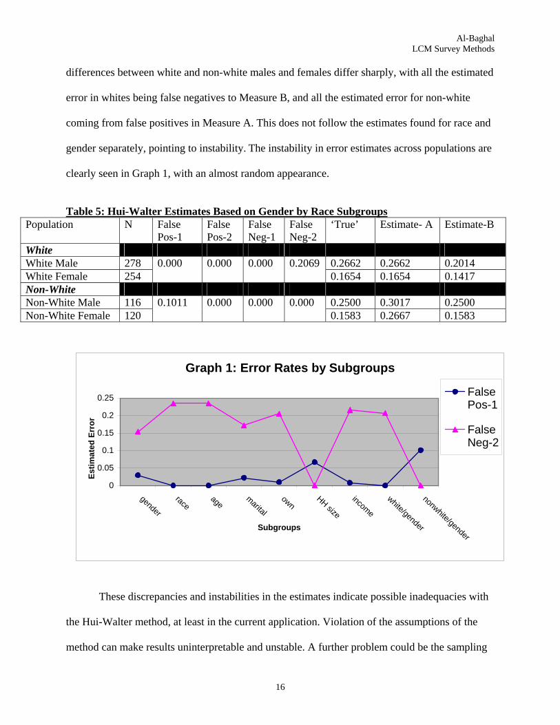
differences between white and non-white males and females differ sharply, with all the estimated

error in whites being false negatives to Measure B, and all the estimated error for non-white

coming from false positives in Measure A. This does not follow the estimates found for race and

gender separately, pointing to instability. The instability in error estimates across populations are

clearly seen in Graph 1, with an almost random appearance.

Table 5: Hui-Walter Estimates Based on Gender by Race Subgroups

Population N False Pos-1

False Pos-2

False Neg-1

False Neg-2


White White Male 278 0.2662 0.2662 0.2014 White Female 254

0.000 0.000 0.000 0.2069 0.1654 0.1654 0.1417

Non-White Non-White Male 116 0.2500 0.3017 0.2500 Non-White Female 120

0.1011 0.000 0.000 0.000 0.1583 0.2667 0.1583

These discrepancies and instabilities in the estimates indicate possible inadequacies with

the Hui-Walter method, at least in the current application. Violation of the assumptions of the

method can make results uninterpretable and unstable. A further problem could be the sampling

Graph 1: Error Rates by Subgroups

0

0.05

0.1

0.15

0.2

0.25

gender

raceage

marital

ownHH size

income

white/gender

nonwhite/genderSubgroups

Estim

ated

Err

or

FalsePos-1

FalseNeg-2


17

zero in the upper cell of the off-diagonal. We examine these possibilities by changing some of

the 43 discordant cases to fall into the upper off-diagonal. Two new variable codings were

created. The first recoded all of the female discordant cases (n=19) from the lower to the upper

off-diagonal cell. This creates a clear violation of the Hui-Walter method, as the error rates in the

in the two populations are completely different. The second coding randomly assigned the 43

discordant cases into either the upper or lower off-diagonal. This removes the sampling zero

noted previously. In both cases, the men and women comprise the two populations. Table 6

presents the Hui-Walter estimates from the two different codings.

Table 6: Hui-Walter Estimates with Reassignment of Discordance Based on Gender

Population N False Pos-A

False Pos-B

False Neg-A

False Neg-B


Error by Gender Men 394 0.2738 0.2766 0.2157 Women 374

0.000 0.0315 0.000 0.1463 0.1471 0.1979 0.1471

Error Random Men 394 0.2538 0.2538 0.2386 Women 374

0.000 0.0331 0.000 0.1411 0.1684 0.1684 0.1765

The results further indicate difficulty with viewing the Hui-Walter method as accurate,

due to fluctuations in findings. In both cases, all of the error came from Measure B. While this

occurred in previous estimations, these two cases led to part of the error in Measure B estimated

as coming from false positives. While changes in estimates are expected as the data was

manipulated, it is difficult to understand why all of the error is estimated from B (thus Measure

A equals the ‘True’ estimate). This instability may be more expected in the assignment of

discordant cases by gender, as the assumptions are violated by choice, and because there is a

sampling zero in both lower (for males) and upper (for females) off-diagonal cells. The error

estimates, however, are almost identical for the random assignment of discordant cases, which

may actually make the assumptions more tenable, and eliminates the sampling zeros. Since both


18

cells of the off-diagonal have cases, it seems questionable that there is no error estimates in

Measure A, especially when previous estimates of the error across genders found error in A

(Table 4).

Discussion

While these estimates may be confusing and unstable, this does not mean they have no

use. As Biemer (2004) points out, even in the face of the stringent assumptions, such models can

point to flawed questions post-data collection. As such, it seems apparent from the majority of

results that Measure A more accurately gauges the cell only population and is more appropriate

for use in data collection for estimation of coverage error. Only in two groupings did the error in

Measure A (false positives) exceed that for Measure B.

It is possible that the error arises from the fact that ‘regular telephone’ is not defined in

Measure B. The 43 respondents with discordant answers to Measures A and B have a lower

median education level (4.5, in between high school and some college, to 5, some college) and

significantly fewer college graduates (about 33% to 14%) than the remainder of the population,

which may indicate the potential for greater error. The discordant responders were also

significantly younger than the remainder of the cell respondents, 28.8 to 39.3 mean age. A

younger generation may think of cellular telephones as ‘regular’ as they have become an integral

part of their daily life.

There is some support this possibility. Following the question about numbers and usage

of ‘regular telephones’ a similar series of questions were asked about cellular phones in the

household. In 14 of the 43 discordant cases, the difference between the number of ‘regular

telephones’ and cellular phones was zero. This indicates the possibility that these individuals


19

view cellular telephones as ‘regular’, and that when responding to these two questions, the

understood reference is the same set of telephones.

There is, however, evidence that Measure B may be better if the goal is to measure

telephone coverage of households, further placing into question the efficacy of the Hui-Walter

test in this instance. First, two of the discordant respondents indicated that of the ‘regular

telephones’ they identified, none them were answered. Since they were answering by cell phone,

it can be assumed they meant landline telephones when referring to ‘regular telephones’, and

therefore gave a false positive for Measure A.

Second, the two measures differ in the exact concepts they measure. Measure A asks

whether the respondent’s cell phone is his or her only phone or whether he or she has another

‘regular’ phone. This wording may also serve the purpose of cueing the respondent as to what

‘regular’ refers to, decreasing the likelihood errors are made in reference to what ‘regular’ means

in later in the survey when Measure B is asked. Measure B, conversely, asks about telephones in

the household. Children living at home with their parents, shared rental units, and students in

communal facilities may have landline telephones in their households, but not feel they

themselves have access to that connected line. Indeed, only two of the 43 discordant cases live

by themselves. The remaining members of a household also are likely to use some telephone

technology, other than the cell phone used during the interview. It could easily be that the

discrepancies in questions led to the discordance in answers. If so, when calculating household

coverage rather than personal coverage, as this is the purpose of this survey, Measure B may

actually be more accurate, indicating a lower prevalence than estimates from Measure A.


20

Conclusions

The growing difficulties in telephone surveys should lead researchers to examine

different ways to overcome these problems. Researchers could find alternate modes of surveys

to employ, or to alter techniques in telephone surveys. Adding cell phones to survey samples

does some of both. However, the prevalence and potential for the coverage error incurred by not

including these depends on estimates that likely to come from surveys themselves. If the measure

of prevalence also contains error, then estimates of coverage error become difficult to interpret

and inaccurate.

The Hui-Walter method for estimating the true prevalence and error rates (false positives

and negatives) when two indicators but no gold standard is available provides a possible tool to

assess measurement error in surveys. There are a number of assumptions placed on the data,

which possibly may be violated in survey data. Still, the tests may provide an insight into which

questions may be most flawed. It may still be necessary, however, to examine additional

variables that are measured in the same survey context that may give clues which questions were

the most flawed.

This study continues initial research in the potential coverage error of cell phones and

measurement error generally in surveys. More research should focus on accurate measurements

of the cell only population, and the potential it has to bias results by not including it in survey

samples. More work on the efficacy of methods such as the Hui-Walter and other latent class

models to estimate measurement error in surveys is also worthwhile. It is possible that such

assumptions made the models are untenable in a survey setting, and thus are inappropriate for

this application. The potential benefits seem clear, however, and if barriers do exist, researchers

should develop techniques to overcome them.


21

Appendix A. Imputation Method. Age To impute data, the method began with the age variable. Categorical means were calculated first using the following set of variables: Education, Gender, Hispanic origin, Black, Other Race, Ownership of Home, Occupational Status (last week), Marital Status This led to 550 combinations. If a respondent with missing data had matching values to any of these 550 combinations, their age was imputed to equal the mean of that combination. Since missing data on age still existed, using the data set with the newly imputed data, means were again calculated, except using the set of variables above minus one, in this case it was both racial categories. Again, age for missing cases was imputed to equal the mean of the combination they matched. Using the new data, the means were recalculated replacing marital status with racial categories. The method continued to use the above variables in all combination until all missing data for age was imputed. To multiply impute race, the data set created with complete age data was used. A propensity equation was calculated for both black and other races using logistic regression. The models initially used the variables that were found to be related through chi-square tests. Race For black respondents these variables were: age, education, cell response, Hispanic, Occupational Status, South region, West region For ‘other’ respondents these variables were: age, education, cell response, Hispanic, West region The equations estimated were used to calculate probabilities of respondents being either black or other based on their given data on the independent variables. The threshold was set at 0.3, i.e. those above the 0.3 threshold were then counted as black or other. Since not all these data were available, again different combinations were calculated, similar to the method used in age. The final equations were: 1. black = ((1)/(1+e**-(-.4475 -(.0228*age) - (.1244*educ)+ (.3346*cell)-(1.2746*hisp) - (.3850*work status) + (.5986*south) -(.8765*west)))) other = ((1)/(1+e**-(-2.2609 -(.0330*age) - (.0893*educ)+ (.5693*cell)-(2.6346*hisp) +(1.3262*west)))) 2. black = ((1)/(1+e**-(-.6021 -(.0213*age) - (.1144*educ)+ (.3110*cell)- (.3757*work status) + (.5448*south) -(.9882*west))));


22

other = ((1)/(1+e**-(-1.2914 -(.0348*age) - (.0042*educ)+ (.5366*cell) + (1.3926*west)))); 3. (LAST STEP NEEDED TO COMPLETE ‘OTHER’) black = ((1)/(1+e**-(-1.057 -(.0221*age) + (.3170*cell) - (.4457*work status) + (.5444*south) -(1.0102*west)))); other = ((1)/(1+e**-(-1.3450 -(.0336*age) + (.5255*cell) +(1.3951*west)))); 4. (LAST STEP NEEDED TO COMPLETE BLACK) black = ((1)/(1+e**-(-1.2875 -(.0214*age) + (.2429*cell)+ (.5764*south) -(1.0041*west)))); There were five cases where the respondent self-identified as both black and some other race. In order to achieve mutual exclusive classification, these respondents were assigned to either the black or other group based on the probability calculated from equations used for imputation. This led to four of the five categorized as black, with the remaining one classified as ‘other’. Income Income was done in two stages. First, whether the respondent made above or below $50,000 was imputed, as there was more complete data on these variables, and thus less error prone data to be used on the second stage. The method used here combined the method used for race and age. Equations were first estimated for the probability of above $50,000 with the threshold set at 0.5, i.e. those with probabilities greater than 0.5 were counted as making above, those with probabilities equal to 0.5 or below were counted as below. The second stage followed the same exact procedure as was used in age, except the median instead of mean was used, and the combination of variables were different. However, the variables used in both stages of imputation for income were used. These variables were selected by examining chi-square tests from the data set incorporating the imputed values for age and race. After the data was fully imputed for the first stage, data were separated by the above/below variable, and the second stage was completed on both sets using the same categorizing variables. After imputation, there were 658 cases below and 666 cases above. The variables: Age, Education, Black, Other race, Gender, Occupational Status Marital Status Ownership of Home The equations for stage one: 1.income = ((1)/(1+e**-(-3.4615 -(.0110*age) +(.4823*educ) -(.4873*black2)-(.3933*race2) -(.2516*gender) + (.5075*work status) + (.6338*married) + (1.3033*own)))); 2. income = ((1)/(1+e**-(-3.5818 -(.0137*age) +(.4893*educ) -(.4787*blacknew)-(.3933*other) -(.2995*gender) + (.4980*work status) + (0.6316*married) + (1.3036*own)))); 3.income = ((1)/(1+e**-(-3.5818 -(.0137*age) +(.4893*educ) -(.4787*blacknew)-(.3933*other) -(.2995*gender) + (.4980*work status) + (0.6316*married) + (1.3036*own))));


23

4. income = ((1)/(1+e**-(-3.5384 -(.0149*age) +(.5788*educ) -(.5528*blacknew)-(.4013*other) -(.4426*gender) + (0.6848*married) +(1.3981*own)))); 5. income = ((1)/(1+e**-(-3.5366 -(.0012*age) +(.5377*educ) -(.6411*blacknew)-(.5188*other) -(.2707*gender) + (0.8244*married) +(0.6084*work status)))); 6. income = ((1)/(1+e**-(-2.8651 -(.0151*age) +(.5814*educ) -(.5623*blacknew)-(.4133*other) -(.4521*gender) + (1.6504*own)))); 7.income = ((1)/(1+e**-(-3.0983 -(.0046*age) +(.5620*educ) -(.6606*blacknew)-(.5219*other) -(.3965*gender) + (0.8154*married)))); 8. income = ((1)/(1+e**-(-2.5926 -(.0009*age) +(.5422*educ) -(.7003*blacknew)-(.4832*other) -(.2847*gender) + (0.5666*work status)))); 9. income = ((1)/(1+e**-(-2.1269 -(.0029*age) +(.5605*educ) -(.7404*blacknew)-(.5097*other) -(.3974*gender)))); 10. income = ((1)/(1+e**-(-0.0085 -(.0154*age) +(1.5857*own) -(.6343*blacknew)-(.5097*other) -(.4110*gender)))); 11. income = ((1)/(1+e**-(-0.4705 -(.0050*age) +(0.8325*married) -(.7556*blacknew)-(.5332*other) -(.3609*gender)))); 12. (FINAL STEP) income = ((1)/(1+e**-(0.5027 -(.0029*age) + -(.8394*blacknew)-(.4956*other) -(.3541*gender))));

Bibliography

Al-Baghal, M Tarek (2005) “Can You Hear Me Now?: The Differences in Voting Behavior Between Cell and Landline Respondents” Presented at the 2005 Annual Midwest Political Science Association Conference, Chicago, Il. Biemer, Paul and Stokes, Lynn (1991) "Approaches to the Modeling of Measurement Errors," in P. Biemer et al. (eds.) Measurement Errors in Surveys, New York: Wiley, pp. 487-516. Biemer, Paul, and Trewin, David (1997) “A Review of Measurement Error Effects on the Analysis of Survey Data,” Ch. 27 in Lyberg, L. et al. Survey Measurement and Process Quality, pp. 603-632. Biemer, Paul and Witt. Michael (1997). “Estimation of Measurement Bias in Self-Reports of Drug Use With Application to the NHSDA.” Journal of Official Statistics, 12(3):275-300. Biemer, Paul and Bushery, John (2001) "Application of Markov Latent Class Analysis to the CPS," Survey Methodology, 26(2):136-152


24

Biemer, P. P, & Wiesen, C. (2002). Measurement Error Evaluation of Self-Reported Drug Use: A latent class analysis of the U.S. National Household Survey on Drug Abuse. Journal of the Royal Statistical Society, A, 165(1): 97-119 Biemer, Paul (2004) “Modeling Measurement Error to Identify Flawed Questions,” in S. Presser et al. (eds.) Methods For Testing and Evaluation Survey Questionnaires, New York: Wiley pp. 225-246. Botman, Steven, and Allen, Karen (1990) “Some Effects of Undercoverage in a Telephone Survey of Teenagers” Proceedings of the Survey Research Methods Section, American Statistical Association Brick, Michael J., Waksberg, Joseph, Kulp, Dale, & Starer, Amy (1995) "Bias in List-Assisted Telephone Samples," Public Opinion Quarterly, 59(2):218-235. Federal Communication Commission (FCC) (2003) News Release: “FCC RELEASES NEW TELEPHONE SUBSCRIBERSHIP REPORT”, April 10, 2003. www.ftc.gov Groves, Robert M. (1989) Survey Errors and Survey Costs , New York: Wiley Groves, Robert M., and Kahn, R.L. (1979) Surveys by Telephone: A National Comparison with Personal Interviews, Academic Press, Inc. Groves, Robert M. (1990), “Theories and Methods of Telephone Surveys.” Annual Review of Sociology, 16: 221-240. Groves, Robert M., and Couper, Mick P. (1998), Nonresponse in Household Interview Surveys, New York: Wiley Hagenaars, Jacques A. (1993) Loglinear Models with Latent Variables Thousand Oaks, CA: Sage. Hall, John, Kenney, Genevieve, Shapiro, Gary, and Flores-Cervantes, Ismael (1999) “Bias from Excluding Households Without Telephones in Random Digit Dialing Surveys: Results of Two Surveys” Proceedings of the Survey Research Methods Section, American Statistical Association Hui, S.L. and S.D. Walter (1980). “Estimating the Error Rates of Diagnostic Tests,” Biometrics, 36, 167-171. Keeter, Scott, Miller, Chris, Kohut, Andrew, Groves, Robert, Presser, Stanley (2000) “Consequences of Reducing Nonresponse in a National Telephone Survey.” Public Opinion Quarterly, 64:125-148. Sinclair, Michael D., and Gastwirth, Joseph L. (1993) “Evaluating reinterview survey methods for measuring response errors.” Proceedings of the 1993Annual Research Conference of the Bureau of the Census. Washington, DC: U.S. Dept. of Commerce


25

Steeh, Charlotte (1981). "Trends in Nonresponse Rates, 1952 - 1979," The Public Opinion Quarterly 45: 40-57 Steeh, Chorlotte, Kirgis, N., Cannon, B., and DeWitt, J., (2001)"Are They Really as Bad as They Seem? Nonresponse Rates at the End of the Twentieth Century," Journal of Official Statistics, 17: 227-247. Steeh, Charlotte (2004) “Surveys Using Cellular Telephones” Presented at the 2004 AAPOR Meeting, May 15th-18th, Phoenix, AZ. Tourangeau, Roger (2004) “Survey Research and Societal Change” Annual Review of Psychology 55: 775-801 Tuckel, Peter and O’Neill, H. (2002), “The vanishing respondent in telephone surveys”, Journal of Advertising Research, 42(5): 26-48 Tucker, Clyde, Brick, Michael J., Meekins, Brian, and Moganstein, David “Household Telephone Service and Usage Patterns in the U.S. in 2004” Presented at the 2004 AAPOR Meeting, May 15th-18th, Phoenix, AZ. Vehovar, V., Belak, E., Batagelj, Z., and Cikic, S. (2004) “Mobile Phone Surveys: The Slovenian Case Study” Metodološki zvezki, 1(1): 1-19

Bias in Telephone Samples Telephone surveys, the staple of ...

Documents

Transcript of Bias in Telephone Samples Telephone surveys, the staple of ...