BBA-402-Financial Management_BBA.pdf - VENKATESHWARA

FINANCIAL MANAGEMENT

VENKATESHWARAOPEN UNIVERSITY

www.vou.ac.in


www.vou.ac.in

FINANCIAL MANAGEMENTFINANCIAL MANAGEM

ENT

13 MM

BBA

vou

Typewritten text

[BBA-402]


BBA

vou

Typewritten text

[BBA-402]

Copyright © IM Pandey, 2019

All rights reserved. No part of this publication which is material protected by this copyright noticemay be reproduced or transmitted or utilized or stored in any form or by any means now known orhereinafter invented, electronic, digital or mechanical, including photocopying, scanning, recordingor by any information storage or retrieval system, without prior written permission from the Publisher.

Information contained in this book has been published by VIKAS® Publishing House Pvt. Ltd. and hasbeen obtained by its Authors from sources believed to be reliable and are correct to the best of theirknowledge. However, the Publisher and its Authors shall in no event be liable for any errors, omissionsor damages arising out of use of this information and specifically disclaim any implied warranties ormerchantability or fitness for any particular use.

Vikas® is the registered trademark of Vikas® Publishing House Pvt. Ltd.

VIKAS® PUBLISHING HOUSE PVT LTDE-28, Sector-8, Noida - 201301 (UP)Phone: 0120-4078900 Fax: 0120-4078999Regd. Office: A-27, 2nd Floor, Mohan Co-operative Industrial Estate, New Delhi 1100 44Website: www.vikaspublishing.com Email: [email protected]

BOARD OF STUDIES

Prof Lalit Kumar SagarVice Chancellor

Dr. S. Raman IyerDirectorDirectorate of Distance Education

SUBJECT EXPERT

Dr. Richa AgarwalDr. Babar Ali KhanDr. Adil Hakeem Khan

Associate ProfessorAssistant ProfessorAssistant Professor

COURSE CO-ORDINATOR

Mr. Tauha KhanRegistrar

Unit 1: Introduction to Financial Functions

Nature, Scope, Objectives, Importance and changing role of finance

function, Maximization of Profit vs. Maximization of wealth.

Unit 2: Financial Forecasting

Planning for funds requirement, Preparation of cash budget, Performa

Income Statement and Balance sheet etc.

Unit 3: Sources of Capital

Preferred stock and Common stock, Long term debt, Retained earning

& their Features, Choice for sources of funds, Capital structure

planning.

Unit 4: Cost of Capital

Cost of Equity capital, preferred capital, Long term debt, Detained

Charges, Computation and composite cost of capital

Unit 5: Capital Budgeting

Concepts and steps in Capital Budgeting, Average rate of return, pay

back period, Present value method, Internal rate of return.

Unit 6: Analysis and Interpretation of Leverage

Meaning, Types of Significance of leverages, Calculation and

Interpretation of Financial, Operating and Composite leverages.

Unit 7: Working Capital Management

Definition, Financing current assets, Hedging approach, Level of

current and Liquid assets, Factors affecting the requirement for

working capital.

Unit 8: Management of Cash and Marketable Securities

Motives for holding cash, Problems and ways of controlling the level

of cash inflow and out-flow of cash.

Unit 9: Management of Accounts Receivable

Credit and Collection policies, Credit standards and Credit terms and

their Evaluation, Controlling the level of accounts receivable.

Unit 10: Dividend Policy

Classification of dividend, Factors governing dividend policies.

Unit 1: Introduction toFinancial Functions

(Pages: 3-25)

Unit 2: Financial Forecasting

(Pages: 27-41)

Unit 3: Source of Capital

(Pages: 43-72)

Unit 4: Cost of Capital

(Pages: 73-112)

Unit 5: Capital Budgeting

(Pages: 113-137)

Unit 6: Analysis andInterpretation of leverage

(Pages: 139-176)

Unit 7: Working CapitalManagement

(Pages: 177-210)

Unit 8: Management of Cashand Marketable Securities

(Pages: 211-215)

Unit 9: Management ofAccounts Receivable

(Pages: 217-254)

Unit 10: Dividend Policies

(Pages: 255-282)

SYLLABI-BOOK MAPPING TABLEFinancial Management

Syllabi Mapping in Book

CONTENTS

INTRODUCTION 1

UNIT 1 INTRODUCTION TO FINANCIAL FUNCTIONS 3-25

1.0 Introduction

1.1 Unit Objectives

1.2 Scope of Finance1.2.1 Real and Financial Assets

1.2.2 Equity and Borrowed Funds

1.2.3 Finance and Management Functions

1.3 Financial Functions1.3.1 Investment Decision; 1.3.2 Financing Decision

1.3.3 Dividend Decision; 1.3.4 Liquidity Decision

1.3.5 Financial Procedures and Systems

1.4 Financial Manager’s Role1.4.1 Fund Raising

1.4.2 Fund Allocation

1.4.3 Profit Planning

1.4.4 Understanding Capital Markets

1.5 Financial Goal: Profit Maximization versus Wealth Maximization1.5.1 Profit Maximization

1.5.2 Objections to Profit Maximization

1.5.3 Maximizing Profit after Taxes

1.5.4 Maximizing EPS

1.5.5 Shareholders’ Wealth Maximization (SWM)

1.5.6 Need for a Valuation Approach

1.5.7 Risk-return Trade-off

1.6 Agency Problems: Manager’s versus Shareholders’ Goals

1.7 Financial Goal and Firm’s Mission and Objectives

1.8 Organization of the Finance Functions1.8.1 Status and Duties of Finance Executives

1.8.2 Controller’s and Treasurer’s Functions in the Indian Context

1.9 Summary

1.10 Key Terms

1.11 Answers to ‘Check Your Progress’

1.12 Questions and Exercises

1.13 Further Reading

Endnotes/References

UNIT 2 FINANCIAL FORECASTING 27-41

2.0 Introduction

2.1 Unit Objectives

2.2 Planning for Funds Requirement

2.3 Preparation of Cash Budget

2.4 Pro Forma Income Statement

2.5 Balance Sheet

2.6 Summary

2.7 Key Terms




Endnotes/References

UNIT 3 SOURCE OF CAPITAL 43-72

3.0 Introduction

3.1 Unit Objectives

3.2 Preferred Stock and Common Stock3.2.1 Default Risk and Credit Rating

3.3 Long-Term Debt and Retained Earnings

3.4 Choice of Sources of Funds3.4.1 Debentures and Bonds

3.5 Capital Structure Planning3.5.1 Capital Structure Practices in India

3.6 Summary

3.7 Key Terms




Endnotes/References

UNIT 4 COST OF CAPITAL 73-112

4.0 Introduction

4.1 Unit Objectives

4.2 Significance of the Cost of Capital

4.3 The Concept of the Opportunity Cost of Capital

4.4 Cost of Debt

4.5 Cost of Preference Capital

4.6 Cost of Equity Capital

4.7 Cost of Equity and the Capital Asset Pricing Model (CAPM)

4.8 Cost of Equity: CAPM vs Dividend-Growth Model

4.9 The Weighted Average Cost of Capital

4.10 Flotation Costs, Cost of Capital and Investment Analysis

4.11 Calculation of the Cost of Capital in Practice: Case of Larsen

and Toubro Limited

4.12 Divisional and Project Cost of Capital

4.13 Summary

4.14 Key Terms




Endnotes/References

UNIT 5 CAPITAL BUDGETING 113-137

5.0 Introduction

5.1 Unit Objectives

5.2 Concepts and Steps

5.3 Average Rate of Return

5.4 Payback Period

5.5 Present Value Method

5.6 Internal Rate of Return

5.7 Summary

5.8 Key Terms




Endnotes/References

UNIT 6 ANALYSIS AND INTERPRETATION OF LEVERAGE 139-176

6.0 Introduction

6.1 Unit Objectives

6.2 Financial Leverage6.2.1 Meaning of Financial Leverage

6.2.2 Measures of Financial Leverage

6.3 Financial Leverage and the Shareholders’ Return

6.4 Combining Financial and Operating Leverages6.4.1 Composite Leverage: Combined Effect of Operating and Financial Leverages

6.5 Financial Leverage and the Shareholders’ Risk

6.6 Summary

6.7 Key Terms

6.8 Answers to ‘Check your Progress’



UNIT 7 WORKING CAPITAL MANAGEMENT 177-210

7.0 Introduction

7.1 Unit Objectives

7.2 Concepts and Definition7.2.1 Focusing on Management of Current Assets

7.2.2 Focusing on Liquidity Management

7.3 Financing Current Assets7.3.1 Matching Approach; 7.3.2 Conservative Approach

7.3.3 Aggressive Approach

7.3.4 Short-term vs. Long-term Financing: A Risk-Return Trade-off

7.4 Hedging Approach7.4.1 Risk Hedging with Options

7.5 Level of Current and Liquid Assets

7.6 Factors Affecting the Requirement of Working Capital7.6.1 Determinants of Working Capital

7.6.2 Issues in Working Capital Management

7.7 Summary

7.8 Key Terms




UNIT 8 MANAGEMENT OF CASH AND MARKETABLE SECURITIES 211-215

8.0 Introduction

8.1 Unit Objectives

8.2 Motives for Holding Cash

8.3 Ways of Controlling Cash In-flow and Outflow

8.4 Summary

8.5 Key Terms



8.8 Further Reading

UNIT 9 MANAGEMENT OF ACCOUNTS RECEIVABLE 217-254

9.0 Introduction

9.1 Unit Objectives

9.2 Credit Policy: Nature and Goals9.2.1 Goals of Credit Policy

9.3 Optimum Credit Policy: A Marginal Cost–Benefit Analysis

9.4 Credit Policy Variables9.4.1 Credit Standards; 9.4.2 Credit-Granting Decision

9.4.3 Collection Policy and Procedures

9.5 Credit Evaluation of Individual Accounts9.5.1 Credit Information; 9.5.2 Credit Investigation and Analysis

9.5.3 Credit Limit; 9.5.4 Collection Efforts

9.6 Monitoring Receivables

9.7 Factoring9.7.1 Nature of Factoring; 9.7.2 Factoring Services

9.7.3 Types of Factoring; 9.7.4 Costs and Benefits of Factoring

9.8 Summary

9.9 Key Terms




UNIT 10 DIVIDEND POLICIES 255-282

10.0 Introduction

10.1 Unit Objectives

10.2 Objectives of Dividend Policy10.2.1 Firm’s Need for Funds

10.2.2 Shareholders’ Need for Income

10.3 Practical Considerations in Dividend Policy10.3.1 Firm’s Investment Opportunities and Financial Needs

10.3.2 Shareholders’ Expectations

10.3.3 Constraints on Paying Dividends

10.4 Stability of Dividends10.4.1 Constant Dividend Per Share or Dividend Rate

10.4.2 Constant Payout

10.4.3 Constant Dividend Per Share Plus Extra Dividend

10.4.4 Merits of Stability of Dividends

10.4.5 Danger of Stability of Dividends

10.5 Target Payout and Dividend Smoothing: Lintner’s Model of Corporate Dividend Behaviour

10.6 Forms of Dividends10.6.1 Cash Dividend

10.6.2 Bonus Shares

10.6.3 Advantages of Bonus Shares

10.6.4 Limitations of Bonus Shares

10.6.5 Conditions for the Issue of Bonus Shares

10.7 Share Split10.7.1 Bonus Share versus Share Split

10.7.2 Reasons for Share Split

10.7.3 Reverse Split

10.8 Dividend Policy Analysis: Case of (L&T) Limited

10.9 Summary

10.10 Key Terms




Self-Instructional

Material 1

Introduction

NOTES

INTRODUCTION

About three decades ago, the scope of financial management was confined to the raising

of funds. Little significance was attached to the analytical thinking in financial decision-

making and problem solving. As a consequence, the earlier finance textbooks were

structured around this theme and contained a description of the instruments and the

institutions of raising funds and of major events, like promotion, reorganization,

readjustment, merger and consolidation when funds were raised. In the mid-1950s, the

emphasis shifted to the judicious utilization of funds. The modern thinking in financial

management accords a far greater importance to management decision-making and

policy. Today, financial managers do not perform the passive role of scorekeepers of

financial data and information, and arranging funds, whenever directed to do so. Rather,

they occupy key positions in top management areas and play a dynamic role in solving

complex management problems. They are now responsible for shaping the fortunes of

the enterprise and are involved in the most vital management decision of allocation of

capital. It is their duty to ensure that the funds are raised most economically and used in

the most efficient and effective manner. Because of this change in emphasis, the

descriptive treatment of the subject of financial management is being replaced by analytical

content and sound theoretical underpinnings.

This book, Financial Management, combines theory with practical applications.

With a strong foundation, readers can easily understand the theories and methods, decision

criteria, and financial policies and strategies necessary to manage funds and create and

enhance the value of the firm. The book aims at assisting the reader to develop a thorough

understanding of the concepts and theories underlying financial management in a

systematic way. To accomplish this purpose, the recent thinking in the field of finance

has been presented in a lucid, simple, unambiguous and precise manner. Concepts are

made clear in simple language before introducing complicated and sophisticated techniques

and theories.

This book has been written, keeping with the self-instructional mode or the SIM

(Self Instructional Material) format for Distance Learning. Each unit begins with an

Introduction to the topic, followed by an outline of the Unit Objectives. The detailed

content is then presented in a simple and organized manner, interspersed with

‘Check Your Progress’ questions to test the student’s understanding of the topics covered.

A Summary along with a list of Key Terms and a set of Questions and Exercises is

provided at the end of each unit for effective recapitulation. Relevant illustrations have

been included for better understanding of the topics.

Self-Instructional

Material 3

Introduction to

Financial Functions

NOTES

UNIT 1 INTRODUCTION TO

FINANCIAL FUNCTIONS

Structure

1.0 Introduction

1.1 Unit Objectives

1.2 Scope of Finance1.2.1 Real and Financial Assets



1.3 Financial Functions1.3.1 Investment Decision; 1.3.2 Financing Decision

1.3.3 Dividend Decision; 1.3.4 Liquidity Decision


1.4 Financial Manager’s Role1.4.1 Fund Raising




1.5 Financial Goal: Profit Maximization versus Wealth Maximization1.5.1 Profit Maximization


1.5.3 Maximizing Profit after Taxes





1.6 Agency Problems: Manager’s versus Shareholders’ Goals

1.7 Financial Goal and Firm’s Mission and Objectives

1.8 Organization of the Finance Functions1.8.1 Status and Duties of Finance Executives


1.9 Summary

1.10 Key Terms




Endnotes/References

1.0 INTRODUCTION

The financial function is that managerial activity which is concerned with the planning

and controlling of the firm’s financial resources. It was a branch of economics till 1890,

but as a separate discipline, it is of recent origin. Still, it has no unique body of knowledge

of its own, and draws heavily on economics for its theoretical concepts even today.

The subject of the finance function is of immense interest to both academicians

and practising managers. It is of great interest to academicians because the subject is

still developing, and there are still certain areas where controversies exist for which no

unanimous solutions have been reached as yet. Practising managers are interested in

this subject because among the most crucial decisions of the firm are those which relate

Self-Instructional

4 Material

Introduction to

Financial Functions

NOTES

to finance, and an understanding of the theory of the financial function provides them

with conceptual and analytical insights to make those decisions skilfully.

1.1 UNIT OBJECTIVES

After going through this unit, you will be able to:

• Explain the nature and scope of finance function and its interaction with other

management functions

• Review the changing role of the finance manager and the various areas he has to

be responsible for

• Focus on the shareholders’ wealth maximization (SWM) principle as an

operationally desirable finance decision criterion

• Discuss agency problems arising from the relationship between shareholders and

managers

• Illustrate organization of finance function

1.2 SCOPE OF FINANCE

What is finance? What are a firm’s financial activities? How are they related to the

firm’s other activities? Firms create manufacturing capacities for production of goods;

some provide services to customers. They sell their goods or services to earn profit.

They raise funds to acquire manufacturing and other facilities. Thus, the three most

important activities of a business firm are:

• Production

• Marketing

• Finance

A firm secures whatever capital it needs and employs it (finance activity) in

activities, which generate returns on invested capital (production and marketing activities).

1.2.1 Real and Financial Assets

A firm requires real assets to carry on its business. Tangible real assets are physical

assets that include plant, machinery, office, factory, furniture and building. Intangible

real assets include technical know-how, technological collaborations, patents and

copyrights. Financial assets, also called securities, are financial papers or instruments

such as shares and bonds or debentures. Firms issue securities to investors in the primary

capital markets to raise necessary funds. The securities issued by firms are traded –

bought and sold – by investors in the secondary capital markets, referred to as stock

exchanges. Financial assets also include lease obligations and borrowing from banks,

financial institutions and other sources. In a lease, the lessee obtains a right to use the

lessor’s asset for an agreed amount of rental over the period of lease. Funds applied to

assets by the firm are called capital expenditures or investment. The firm expects to

receive return on investment and might distribute return (or profit) as dividends to investors.


There are two types of funds that a firm can raise—equity funds (simply called equity)

and borrowed funds (called debt). A firm sells shares to acquire equity funds. Shares

Self-Instructional

Material 5

Introduction to

Financial Functions

NOTES

represent ownership rights of their holders. Buyers of shares are called shareholders

(or stockholders), and they are the legal owners of the firm whose shares they hold.

Shareholders invest their money in the shares of a company in the expectation of a

return on their invested capital. The return of shareholders consists of dividend and

capital gain. Shareholders make capital gains (or loss) by selling their shares.

Shareholders can be of two types—ordinary and preference. Preference

shareholders receive dividend at a fixed rate, and they have a priority over ordinary

shareholders. The dividend rate for ordinary shareholders is not fixed, and it can vary

from year to year depending on the decision of the board of directors. The payment of

dividends to shareholders is not a legal obligation; it depends on the discretion of the

board of directors. Since ordinary shareholders receive dividend (or repayment of invested

capital, only when the company is wound up) after meeting the obligations of others,

they are generally called owners of residue. Dividends paid by a company are not

deductible expenses for calculating corporate income taxes, and they are paid out of

profits after corporate taxes. As per the current laws in India, a company is required to

pay 12.5 per cent tax on dividends.

A company can also obtain equity funds by retaining earnings available for

shareholders. Retained earnings, which could be referred to as internal equity, are

undistributed profits of equity capital. The retention of earnings can be considered as a

form of raising new capital. If a company distributes all earnings to shareholders, then, it

can re-acquire new capital from the same sources (existing shareholders) by issuing

new shares called rights shares. Also, a public issue of shares may be made to

attract new (as well as the existing) shareholders to contribute equity capital.

Another important source of securing capital is creditors or lenders. Lenders

are not the owners of the company. They make money available to the firm as loan or

debt and retain title to the funds lent. Loans are generally furnished for a specified

period at a fixed rate of interest. For lenders, the return on loans or debt comes in the

form of interest paid by the firm. Interest is a cost of debt to the firm. Payment of

interest is a legal obligation. The amount of interest paid by a firm is a deductible expense

for computing corporate income taxes. Thus, interest provides tax shield to a firm. The

interest tax shield is valuable to a firm. The firm may borrow funds from a large number

of sources, such as banks, financial institutions, public or by issuing bonds or debentures.

A bond or a debenture is a certificate acknowledging the amount of money lent by a

bondholder to the company. It states the amount, the rate of interest and the maturity of

the bond or debenture. Since bond or debenture is a financial instrument, it can be traded

in the secondary capital markets.


There exists an inseparable relationship between finance on the one hand and production,

marketing and other functions on the other. Almost all business activities, directly or

indirectly, involve the acquisition and use of funds. For example, recruitment and promotion

of employees in production is clearly a responsibility of the production department; but it

requires payment of wages and salaries and other benefits, and thus, involves finance.

Similarly, buying a new machine or replacing an old machine for the purpose of increasing

productive capacity affects the flow of funds. Sales promotion policies come within the

purview of marketing, but advertising and other sales promotion activities require outlays

of cash and therefore, affect financial resources.

Check Your Progress

1. What is the

advantage enjoyed

by financial assets

vis-à-vis real assets

in a business?

2. What are the main

types of

shareholder funds

available to a

company?

3. Which are the major

ways in which a

company may be

able to raise new

capital?

4. Why are borrowed

funds often

preferred over

equity by firms to

fund their

businesses?

Self-Instructional

6 Material

Introduction to

Financial Functions

NOTES

Where is the separation between production and marketing functions on the one

hand and the finance function of making money available to meet the costs of production

and marketing operations on the other hand? Where do the production and marketing

functions end and the finance function begin? There are no clear-cut answers to these

questions. Though the finance function of raising and using money has a significant

effect on other functions, yet it needs not necessarily limited or constrained to the general

running of the business. A company in a tight financial position will, of course, give more

weight to financial considerations, and devise its marketing and production strategies in

the light of the financial constraint. On the other hand, management of a company,

which has a reservoir of funds or a regular supply of funds, will be more flexible in

formulating its production and marketing policies. In fact, financial policies will be devised

to fit production and marketing decisions of a firm in practice.

1.3 FINANCE FUNCTIONS

It may be difficult to separate the finance functions from production, marketing and

other functions, but the functions themselves can be readily identified. The functions of

raising funds, investing them in assets and distributing returns earned from assets to

shareholders are respectively known as financing decision, investment decision and

dividend decision. A firm attempts to balance cash inflows and outflows while performing

these functions. This is called liquidity decision, and we may add it to the list of important

finance decisions or functions. Thus, finance functions include:

• Long-term asset-mix or investment decision

• Capital-mix or financing decision

• Profit allocation or dividend decision

• Sort-term asset-mix or liquidity decision

A firm performs finance functions simultaneously and continuously in the normal

course of the business. They do not necessarily occur in a sequence. Finance functions

call for skilful planning, control and execution of a firm’s activities.

Let us note at the outset that shareholders are made better off by a financial

decision that increases the value of their shares. Thus while performing the finance

functions, the financial manager should strive to maximize the market value of shares.

This point is elaborated in detail later on in the unit.

1.3.1 Investment Decision

A firm’s investment decisions involve capital expenditures. They are, therefore, referred

to as capital budgeting decisions. A capital budgeting decision involves the decision

of allocation of capital or commitment of funds to long-term assets that would yield

benefits (cash flows) in the future. Two important aspects of investment decisions are:

(a) the evaluation of the prospective profitability of new investments, and (b) the

measurement of a cut-off rate against that the prospective return of new investments

could be compared. Future benefits of investments are difficult to measure and cannot

be predicted with certainty. Risk in investment arises because of the uncertain returns.

Investment proposals should, therefore, be evaluated in terms of both expected return

and risk. Besides the decision to commit funds in new investment proposals, capital

budgeting also involves replacement decisions, that is, decision of recommitting funds

when an asset becomes less productive or non-profitable.

Self-Instructional

Material 7

Introduction to

Financial Functions

NOTES

There is a broad agreement that the correct cut-off rate or the required rate of

return on investments is the opportunity cost of capital.1 The opportunity cost of

capital is the expected rate of return that an investor could earn by investing his or her

money in financial assets of equivalent risk. However, there are problems in computing

the opportunity cost of capital in practice from the available data and information. A

decision maker should be aware of these problems.

1.3.2 Financing Decision

Financing decision is the second important function to be performed by the financial

manager. Broadly, he or she must decide when, where from and how to acquire funds to

meet the firm’s investment needs. The central issue before him or her is to determine

the appropriate proportion of equity and debt. The mix of debt and equity is known as the

firm’s capital structure. The financial manager must strive to obtain the best financing

mix or the optimum capital structure for his or her firm. The firm’s capital structure

is considered optimum when the market value of shares is maximized.

In the absence of debt, the shareholders’ return is equal to the firm’s return. The

use of debt affects the return and risk of shareholders; it may increase the return on

equity funds, but it always increases risk as well. The change in the shareholders’ return

caused by the change in the profits is called the financial leverage. A proper balance

will have to be struck between return and risk. When the shareholders’ return is

maximized with given risk, the market value per share will be maximized and the firm’s

capital structure would be considered optimum. Once the financial manager is able to

determine the best combination of debt and equity, he or she must raise the appropriate

amount through the best available sources. In practice, a firm considers many other

factors such as control, flexibility, loan covenants, legal aspects etc. in deciding its capital

structure.

1.3.3 Dividend Decision

Dividend decision is the third major financial decision. The financial manager must decide

whether the firm should distribute all profits, or retain them, or distribute a portion and

retain the balance. The proportion of profits distributed as dividends is called the dividend-

payout ratio and the retained portion of profits is known as the retention ratio. Like

the debt policy, the dividend policy should be determined in terms of its impact on the

shareholders’ value. The optimum dividend policy is one that maximizes the market

value of the firm’s shares. Thus, if shareholders are not indifferent to the firm’s dividend

policy, the financial manager must determine the optimum dividend-payout ratio. Dividends

are generally paid in cash. But a firm may issue bonus shares. Bonus shares are

shares issued to the existing shareholders without any charge. The financial manager

should consider the questions of dividend stability, bonus shares and cash dividends in

practice.

1.3.4 Liquidity Decision

Investment in current assets affects the firm’s profitability and liquidity. Current assets

management that affects a firm’s liquidity is yet another important finance function.

Current assets should be managed efficiently for safeguarding the firm against the risk

of illiquidity. Lack of liquidity (or illiquidity) in extreme situations can lead to the firm’s

insolvency. A conflict exists between profitability and liquidity while managing current

assets. If the firm does not invest sufficient funds in current assets, it may become

Self-Instructional

8 Material

Introduction to

Financial Functions

NOTES

illiquid and therefore, risky. But it would lose profitability, as idle current assets would not

earn anything. Thus, a proper trade-off must be achieved between profitability and

liquidity. The profitability-liquidity trade-off requires that the financial manager should

develop sound techniques of managing current assets. He or she should estimate firm’s

needs for current assets and make sure that funds would be made available when needed.

In sum, financial decisions directly concern the firm’s decision to acquire or dispose

off assets and require commitment or recommitment of funds on a continuous basis. It is

in this context that finance functions are said to influence production, marketing and

other functions of the firm. Hence finance functions may affect the size, growth,

profitability and risk of the firm, and ultimately, the value of the firm. To quote Ezra

Solomon:2

‘The function of financial management is to review and control decisions to commit

or recommit funds to new or ongoing uses. Thus, in addition to raising funds, financial

management is directly concerned with production, marketing and other functions, within

an enterprise whenever decisions are made about the acquisition or distribution of assets.’


For the effective execution of the finance functions, certain other functions have to be

routinely performed. They concern procedures and systems and involve a lot of paper

work and time. They do not require specialised skills of finance. Some of the important

routine finance functions are:

• Supervision of cash receipts and payments and safeguarding of cash balances

• Custody and safeguarding of securities, insurance policies and other valuable

papers

• Taking care of the mechanical details of new outside financing

• Record keeping and reporting

The finance manager, in the modern enterprises, is mainly involved in the managerial

finance functions; executives at lower levels carry out the routine finance functions.

The financial manager’s involvement in the routine functions is confined to setting up of

rules of procedures, selecting forms to be used, establishing standards for the employment

of competent personnel and to check the performance to see that the rules are observed

and that the forms are properly used.

The involvement of the financial manager in the managerial financial functions is

recent. About three decades ago, the scope of finance functions or the role of the

financial manager was limited to routine activities. How the scope of finance function

has widened or the role of the finance manager has changed is discussed in the following

section.

1.4 FINANCIAL MANAGER’S ROLE

Who is a financial manager?3 What is his or her role? A financial manager is a person

who is responsible, in a significant way, to carry out the finance functions. It should be

noted that, in a modern enterprise, the financial manager occupies a key position. He or

she is one of the members of the top management team, and his or her role, day-by-day,

is becoming more pervasive, intensive and significant in solving the complex funds

management problems. Now his or her function is not confined to that of a scorekeeper

maintaining records, preparing reports and raising funds when needed, nor is he or she a

Check Your Progress

5. List the main areas

of financial decision

making.

6. Define opportunity

cost of capital.

Self-Instructional

Material 9

Introduction to

Financial Functions

NOTES

staff officer–in a passive role of an adviser. The finance manager is now responsible for

shaping the fortunes of the enterprise, and is involved in the most vital decision of the

allocation of capital. In his or her new role, he or she needs to have a broader and far-

sighted outlook, and must ensure that the funds of the enterprise are utilised in the most

efficient manner. He or she must realise that his or her actions have far-reaching

consequences for the firm because they influence the size, profitability, growth, risk and

survival of the firm, and as a consequence, affect the overall value of the firm. The

financial manager, therefore, must have a clear understanding and a strong grasp of the

nature and scope of the finance functions.

The financial manager has not always been in the dynamic role of decision-making.

About three decades ago, he or she was not considered an important person, as far as

the top management decision-making was concerned. He or she became an important

management person only with the advent of the modern or contemporary approach to

the financial management. What are the main functions of a financial manager?

1.4.1 Fund Raising

The traditional approach dominated the scope of financial management and limited the

role of the financial manager simply to funds raising. It was during the major events,

such as promotion, reorganization, expansion or diversification in the firm that the financial

manager was called upon to raise funds. In his or her day-to-day activities, his or her

only significant duty was to see that the firm had enough cash to meet its obligations.

Because of its central emphasis on the procurement of funds, the finance textbooks, for

example, in the USA, till the mid1950s covered discussion of the instruments, institutions

and practices through which funds were obtained. Further, as the problem of raising

funds was more intensely felt in the special events, these books also contained detailed

descriptions of the major events like mergers, consolidations, reorganizations and

recapitalisations involving episodic financing.4 The finance books in India and other

countries simply followed the American pattern. The notable feature of the traditional

view of financial management was the assumption that the financial manager had no

concern with the decision of allocating the firm’s funds. These decisions were assumed

as given, and he or she was required to raise the needed funds from a combination of

various sources.

The traditional approach did not go unchallenged even during the period of its

dominance. But the criticism related more to the treatment of various topics rather than

the basic definition of the finance function. The traditional approach has been criticised

because it failed to consider the day-to-day managerial problems relating to finance of

the firm. It concentrated itself to looking into the problems from management’s–the

insider’s point of view.5 Thus, the traditional approach of looking at the role of the

financial manager lacked a conceptual framework for making financial decisions,

misplaced emphasis on raising of funds, and neglected the real issues relating to the

allocation and management of funds.


The traditional approach outlived its utility in the changed business situation particularly

after the mid-1950s. A number of economic and environmental factors, such as the

increasing pace of industrialisation, technological innovations and inventions, intense

competition, increasing intervention of government on account of management inefficiency

and failure, population growth and widened markets, during and after mid-1950s,

Self-Instructional

10 Material

Introduction to

Financial Functions

NOTES

necessitated efficient and effective utilisation of the firm’s resources, including financial

resources. The development of a number of management skills and decision-making

techniques facilitated the implementation of a system of optimum allocation of the firm’s

resources. As a result, the approach to, and the scope of financial management, also

changed. The emphasis shifted from the episodic financing to the financial management,

from raising of funds to efficient and effective use of funds. The new approach is

embedded in sound conceptual and analytical theories.

The new or modern approach to finance is an analytical way of looking into the

financial problems of the firm. Financial management is considered a vital and an integral

part of overall management. To quote Ezra Solomon:6

‘In this broader view the central issue of financial policy is the wise use of funds,

and the central process involved is a rational matching of advantages of potential uses

against the cost of alternative potential sources so as to achieve the broad financial goals

which an enterprise sets for itself.’

Thus, in a modern enterprise, the basic finance function is to decide about the

expenditure decisions and to determine the demand for capital for these expenditures. In

other words, the financial manager, in his or her new role, is concerned with the efficient

allocation of funds. The allocation of funds is not a new problem, however. It did exist

in the past, but it was not considered important enough in achieving the firm’s long run

objectives.

In his or her new role of using funds wisely, the financial manager must find a

rationale for answering the following three questions:7

• How large should an enterprise be, and how fast should it grow?

• In what form should it hold its assets?

• How should the funds required be raised?

As discussed earlier, the questions stated above relate to three broad decision

areas of financial management: investment (including both long and short-term assets),

financing and dividend. The ‘modern’ financial manager has to help making these decisions

in the most rational way. They have to be made in such a way that the funds of the firm

are used optimally. We have referred to these decisions as managerial finance functions

since they require special care and extraordinary managerial ability.

As discussed earlier, the financial decisions have a great impact on all other business

activities. The concern of the financial manager, besides his traditional function of raising

money, will be on determining the size and technology of the firm, in setting the pace and

direction of growth and in shaping the profitability and risk complexion of the firm by

selecting the best asset mix and financing mix.


The functions of the financial manager may be broadened to include profit-planning

function. Profit planning refers to the operating decisions in the areas of pricing, costs,

volume of output and the firm’s selection of product lines. Profit planning is, therefore, a

prerequisite for optimising investment and financing decisions.8 The cost structure of the

firm, i.e. the mix of fixed and variable costs has a significant influence on a firm’s

profitability. Fixed costs remain constant while variable costs change in direct

proportion to volume changes. Because of the fixed costs, profits fluctuate at a higher

degree than the fluctuations in sales. The change in profits due to the change in sales is

referred to as operating leverage. Profit planning helps to anticipate the relationships

between volume, costs and profits and develop action plans to face unexpected surprises.

Check Your Progress


tasks of the finance

manager in today’s

business

environment?

8. Define profit

planning.

Self-Instructional

Material 11

Introduction to

Financial Functions

NOTES


Capital markets bring investors (lenders) and firms (borrowers) together. Hence the

financial manager has to deal with capital markets. He or she should fully understand

the operations of capital markets and the way in which the capital markets value securities.

He or she should also know how risk is measured and how to cope with it in investment

and financing decisions. For example, if a firm uses excessive debt to finance its growth,

investors may perceive it as risky. The value of the firm’s share may, therefore, decline.

Similarly, investors may not like the decision of a highly profitable, growing firm to distribute

dividend. They may like the firm to reinvest profits in attractive opportunities that would

enhance their prospects for making high capital gains in the future. Investments also

involve risk and return. It is through their operations in capital markets that investors

continuously evaluate the actions of the financial manager.

1.5 FINANCIAL GOAL: PROFIT MAXIMIZATION

VERSUS WEALTH MAXIMIZATION

The firm’s investment and financing decisions are unavoidable and continuous. In order

to make them rationally, the firm must have a goal. It is generally agreed in theory that

the financial goal of the firm should be shareholders’ wealth maximization (SWM),

as reflected in the market value of the firm’s shares. In this section, we show that the

shareholders’ wealth maximization is theoretically logical and operationally feasible

normative goal for guiding the financial decision-making.

1.5.1 Profit Maximization

Firms, producing goods and services, may function in a market economy, or in a

government-controlled economy. In a market economy, prices of goods and services are

determined in competitive markets. Firms in the market economy are expected to produce

goods and services desired by society as efficiently as possible.

Price system is the most important organ of a market economy indicating what

goods and services society wants. Goods and services in great demand command higher

prices. This results in higher profit for firms; more of such goods and services are

produced. Higher profit opportunities attract other firms to produce such goods and

services. Ultimately, with intensifying competition, an equilibrium price is reached at

which demand and supply match. In the case of goods and services, which are not

required by society, their prices and profits fall. Producers drop such goods and services

in favour of more profitable opportunities.9 Price system directs managerial efforts

towards more profitable goods or services. Prices are determined by the demand and

supply conditions as well as the competitive forces, and they guide the allocation of

resources for various productive activities.10

A legitimate question may be raised: Would the price system in a free market

economy serve the interests of the society? Adam Smith has given the answer many

years ago. According to him:11

‘(The businessman), by directing...industry in such a manner as its produce may

be of greater value...intends only his own gain, and he is in this, as in many other cases,

led by an invisible hand to promote an end which was not part of his intention...pursuing

his own interest he frequently promotes that of society more effectually than he really

intends to promote it.’

Self-Instructional

12 Material

Introduction to

Financial Functions

NOTES

Following Smith’s logic, it is generally held by economists that under the conditions

of free competition, businessmen pursuing their own self-interests also serve the interest

of society. It is also assumed that when individual firms pursue the interest of maximizing

profits, society’s resources are efficiently utilised.

In the economic theory, the behaviour of a firm is analysed in terms of profit

maximization. Profit maximization implies that a firm either produces maximum output

for a given amount of input, or uses minimum input for producing a given output. The

underlying logic of profit maximization is efficiency. It is assumed that profit maximization

causes the efficient allocation of resources under the competitive market conditions, and

profit is considered as the most appropriate measure of a firm’s performance.


The profit maximization objective has been criticised. It is argued that profit maximization

assumes perfect competition, and in the face of imperfect modern markets, it cannot be

a legitimate objective of the firm. It is also argued that profit maximization, as a business

objective, developed in the early 19th century when the characteristic features of the

business structure were self-financing, private property and single entrepreneurship.

The only aim of the single owner then was to enhance his or her individual wealth and

personal power, which could easily be satisfied by the profit maximization objective.12

The modern business environment is characterised by limited liability and a divorce

between management and ownership. Shareholders and lenders today finance the business

firm but it is controlled and directed by professional management. The other important

stakeholders of the firm are customers, employees, government and society. In practice,

the objectives of these stakeholders or constituents of a firm differ and may conflict with

each other. The manager of the firm has the difficult task of reconciling and balancing

these conflicting objectives. In the new business environment, profit maximization is

regarded as unrealistic, difficult, inappropriate and immoral.13

It is also feared that profit maximization behaviour in a market economy may tend

to produce goods and services that are wasteful and unnecessary from the society’s

point of view. Also, it might lead to inequality of income and wealth. It is for this reason

that governments tend to intervene in business. The price system and therefore, the

profit maximization principle may not work due to imperfections in practice. Oligopolies

and monopolies are quite common phenomena of modern economies. Firms producing

same goods and services differ substantially in terms of technology, costs and capital. In

view of such conditions, it is difficult to have a truly competitive price system, and thus,

it is doubtful if the profit-maximizing behaviour will lead to the optimum social welfare.

However, it is not clear that abandoning profit maximization, as a decision criterion,

would solve the problem. Rather, government intervention may be sought to correct

market imperfections and to promote competition among business firms. A market

economy, characterised by a high degree of competition, would certainly ensure efficient

production of goods and services desired by society.14

Is profit maximization an operationally feasible criterion? Apart from the aforesaid

objections, profit maximization fails to serve as an operational criterion for maximizing

the owner’s economic welfare. It fails to provide an operationally feasible measure for

ranking alternative courses of action in terms of their economic efficiency. It suffers

from the following limitations:15

• It is vague

• It ignores the timing of returns

• It ignores risk

Self-Instructional

Material 13

Introduction to

Financial Functions

NOTES

Definition of profit: The precise meaning of the profit maximization objective is unclear.

The definition of the term profit is ambiguous. Does it mean short- or long-term profit?

Does it refer to profit before or after tax? Total profits or profit per share? Does it mean

total operating profit or profit accruing to shareholders?

Time value of money: The profit maximization objective does not make an explicit

distinction between returns received in different time periods. It gives no consideration

to the time value of money, and it values benefits received in different periods of time as

the same.

Uncertainty of returns: The streams of benefits may possess different degree of

certainty. Two firms may have same total expected earnings, but if the earnings of one

firm fluctuate considerably as compared to the other, it will be more risky. Possibly,

owners of the firm would prefer smaller but surer profits to a potentially larger but less

certain stream of benefits.

1.5.3 Maximizing Profit After Taxes

Let us put aside the first problem mentioned above, and assume that maximizing profit

means maximizing profits after taxes, in the sense of net profit as reported in the profit

and loss account (income statement) of the firm. It can easily be realised that maximizing

this figure will not maximize the economic welfare of the owners. It is possible for a firm

to increase profit after taxes by selling additional equity shares and investing the proceeds

in low-yielding assets, such as the government bonds. Profit after taxes would increase

but earnings per share (EPS) would decrease. To illustrate, let us assume that a

company has 10,000 shares outstanding, profit after taxes of ̀ 50,000 and earnings per

share of ̀ 5. If the company sells 10,000 additional shares at ̀ 50 per share and invests

the proceeds (` 500,000) at 5 per cent after taxes, then the total profits after taxes will

increase to ̀ 75,000. However, the earnings per share will fall to ̀ 3.75 (i.e., ̀ 75,000/

20,000). This example clearly indicates that maximizing profits after taxes does not

necessarily serve the best interests of owners.


If we adopt maximizing EPS as the financial objective of the firm, this will also not

ensure the maximization of owners’ economic welfare. It also suffers from the flaws

already mentioned, i.e. it ignores timing and risk of the expected benefits. Apart from

these problems, maximization of EPS has certain deficiencies as a financial objective.

For example, note the following observation:16

... For one thing, it implies that the market value of the company’s shares is a function of

earnings per share, which may not be true in many instances. If the market value is not

a function of earnings per share, then maximization of the latter will not necessarily

result in the highest possible price for the company’s shares. Maximization of earnings

per share further implies that the firm should make no dividend payments so long as

funds can be invested internally at any positive rate of return, however small. Such a

dividend policy may not always be to the shareholders’ advantage.

It is, thus, clear that maximizing profits after taxes or EPS as the financial objective fails

to maximize the economic welfare of owners. Both methods do not take account of the

timing and uncertainty of the benefits. An alternative to profit maximization, which solves

these problems, is the objective of wealth maximization. This objective is also considered

consistent with the survival goal and with the personal objectives of managers such as

recognition, power, status and personal wealth.

Self-Instructional

14 Material

Introduction to

Financial Functions

NOTES


What is meant by shareholders’ wealth maximization (SWM)? SWM means maximizing

the net present value of a course of action to shareholders. Net present value (NPV)

or wealth of a course of action is the difference between the present value of its benefits

and the present value of its costs.17 A financial action that has a positive NPV creates

wealth for shareholders and, therefore, is desirable. A financial action resulting in negative

NPV should be rejected since it would destroy shareholders’ wealth. Between mutually

exclusive projects the one with the highest NPV should be adopted. NPVs of a firm’s

projects are addititive in nature. That is

NPV(A) + NPV(B) = NPV(A + B)

This is referred to as the principle of value-additivity. Therefore, the wealth

will be maximized if NPV criterion is followed in making financial decisions.18

The objective of SWM takes care of the questions of the timing and risk of the

expected benefits. These problems are handled by selecting an appropriate rate (the

shareholders’ opportunity cost of capital) for discounting the expected flow of future

benefits. It is important to emphasise that benefits are measured in terms of cash

flows. In investment and financing decisions, it is the flow of cash that is important, not

the accounting profits.

The objective of SWM is an appropriate and operationally feasible criterion to

choose among the alternative financial actions. It provides an unambiguous measure of

what financial management should seek to maximize in making investment and financing

decisions on behalf of shareholders.19

Maximizing the shareholders’ economic welfare is equivalent to maximizing the

utility of their consumption over time. With their wealth maximized, shareholders can

adjust their cash flows in such a way as to optimise their consumption. From the

shareholders’ point of view, the wealth created by a company through its actions is

reflected in the market value of the company’s shares. Therefore, the wealth maximization

principle implies that the fundamental objective of a firm is to maximize the market

value of its shares. The value of the company’s shares is represented by their market

price that, in turn, is a reflection of shareholders’ perception about quality of the firm’s

financial decisions. The market price serves as the firm’s performance indicator. How is

the market price of a firm’s share determined?


SWM requires a valuation model. The financial manager must know or at least assume

the factors that influence the market price of shares, otherwise he or she would find

himself or herself unable to maximize the market value of the company’s shares. What

is the appropriate share valuation model? In practice, innumerable factors influence the

price of a share, and also, these factors change very frequently. Moreover, these factors

vary across shares of different companies. For the purpose of the financial management

problem, we can phrase the crucial questions normatively: How much should a particular

share be worth? Upon what factor or factors should its value depend? Although there

is no simple answer to these questions, it is generally agreed that the value of an asset

depends on its risk and return.

Self-Instructional

Material 15

Introduction to

Financial Functions

NOTES

Exhibit 1.1: BHEL’S Mission and Objectives

BHEL defines its vision, mission, values and objectives as follows:

• Vision To become a world class, innovative, competitive and profitable engineering

enterprise providing total business solutions.

• Business mission To be the leading Indian engineering enterprise providing quality

products, systems and services in the fields of energy, transportation, industry, infrastructure

and other potential areas.

• Values

o Meeting commitments made to external and internal customers.

o Fostering learning, creativity and speed of response.

o Respect for dignity and potential of individuals.

o Loyalty and pride in the company.

o Team playing.

o Zeal to excel.

o Integrity and fairness in all matters.

• Objectives BHEL defines its objectives as follows:

o Growth To ensure a steady growth by enhancing the competitive edge of BHEL in

existing business, new areas and international operations so as to fulfil national

expectations for BHEL.

o Profitability To provide a reasonable and adequate return on capital employed, primarily

through improvements in operational efficiency, capacity utilisation and productivity,

and generate adequate internal resources to finance the company’s growth.

o Customer focus To build a high degree of customer confidence by providing increased

value for his money through international standards of product quality, performance and

superior customer service.

o People orientation To enable each employee to achieve his potential, improve his

capabilities, perceive his role and responsibilities and participate and contribute positively

to the growth and success of the company. To invest in human resources continuously

and be alive to their needs.

o Technology To achieve technological excellence in operations by development of

indigenous technologies and efficient absorption and adaptation of imported technologies

to sustain needs and priorities, and provide a competitive advantage to the company.

o Image To fulfil the expectations which shareholders like government as owner,

employees, customers and the country at large have from BHEL.

Source: BHEL’s Annual Reports.


Financial decisions incur different degree of risk. Your decision to invest your money in

government bonds has less risk as interest rate is known and the risk of default is very

less. On the other hand, you would incur more risk if you decide to invest your money in

shares, as return is not certain. However, you can expect a lower return from government

bond and higher from shares. Risk and expected return move in tandem; the greater the

risk, the greater the expected return. Figure 1.1 shows this risk-return relationship.

Self-Instructional

16 Material

Introduction to

Financial Functions

NOTES

Fig. 1.1 The Risk-return Relationship

Financial decisions of the firm are guided by the risk-return trade-off. These

decisions are interrelated and jointly affect the market value of its shares by influencing

return and risk of the firm. The relationship between return and risk can be simply

expressed as follows:

Return = Risk-free rate + Risk premium (1)

Risk-free rate is a rate obtainable from a default-risk free government security. An

investor assuming risk from her investment requires a risk premium above the risk-

free rate. Risk-free rate is a compensation for time and risk premium for risk. Higher

the risk of an action, higher will be the risk premium leading to higher required return on

that action. A proper balance between return and risk should be maintained to maximize

the market value of a firm’s shares. Such balance is called risk-return trade-off, and

every financial decision involves this trade-off. The interrelation between market value,

financial decisions and risk-return trade-off is depicted in Figure 1.2. It also gives an

overview of the functions of financial management.

The financial manager, in a bid to maximize shareholders’ wealth, should strive to

maximize returns in relation to the given risk; he or she should seek courses of actions

that avoid unnecessary risks. To ensure maximum return, funds flowing in and out of the

firm should be constantly monitored to assure that they are safeguarded and properly

utilised. The financial reporting system must be designed to provide timely and accurate

picture of the firm’s activities.

Fig. 1.2 An Overview of Financial Management

Check Your Progress

9. What should be the

financial goal of a

firm?

10. Why are indicators

like profits after

taxes and earnings

per share not the

best ways to decide

financial goals of a

firm?

11. Define risk-free

rate.

Self-Instructional

Material 17

Introduction to

Financial Functions

NOTES

1.6 AGENCY PROBLEMS: MANAGER’S VERSUS

SHAREHOLDERS’ GOALS

In large companies, there is a divorce between management and ownership. The decision-

taking authority in a company lies in the hands of managers. Shareholders as owners of

a company are the principals and managers are their agents. Thus, there is a principal-

agent relationship between shareholders and managers. In theory, managers should

act in the best interests of shareholders; that is, their actions and decisions should lead to

SWM. In practice, managers may not necessarily act in the best interest of shareholders,

and they may pursue their own personal goals. Managers may maximize their own

wealth (in the form of high salaries and perks) at the cost of shareholders, or may play

safe and create satisfactory wealth for shareholders than the maximum. They may

avoid taking high investment and financing risks that may otherwise be needed to

maximize shareholders’ wealth. Such ‘satisficing’ behaviour of managers will frustrate

the objective of SWM as a normative guide. It is in the interests of managers that the

firm survives in the long run. Managers also wish to enjoy independence and freedom

from outside interference, control and monitoring. Thus, their actions are very likely to

be directed towards the goals of survival and self-sufficiency20. Further, a company is a

complex organization consisting of multiple stakeholders such as employees, debt-holders,

consumers, suppliers, government and society. Managers in practice may, thus, perceive

their role as reconciling conflicting objectives of stakeholders. This stakeholders’ view

of managers’ role may compromise with the objective of SWM.

Shareholders continuously monitor modern companies that would help them to

restrict managers’ freedom to act in their own self-interest at the cost of shareholders.

Employees, creditors, customers and government also keep an eye on managers’ activities.

Thus, the possibility of managers pursuing exclusively their own personal goals is reduced.

Managers can survive only when they are successful; and they are successful when

they manage the company better than someone else. Every group connected with the

company will, however, evaluate management success from the point of view of the

fulfilment of its own objective. The survival of management will be threatened if the

objective of any of these groups remains unfulfilled. In reality, the wealth of shareholders

in the long run could be maximized only when customers and employees, along with

other stakeholders of a firm, are fully satisfied. The wealth maximization objective may

be generally in harmony with the interests of the various groups such as owners,

employees, creditors and society, and thus, it may be consistent with the management

objective of survival.21 There can, however, still arise situations where a conflict may

occur between the shareholders’ and managers’ goals. Finance theory prescribes that

under such situations, shareholders wealth maximization goal should have precedent

over the goals of other stakeholders.

The conflict between the interests of shareholders and managers is referred to as

agency problem and it results into agency costs. Agency costs include the less than

optimum share value for shareholders and costs incurred by them to monitor the actions

of managers and control their behaviour. The agency problems vanish when managers

own the company. Thus, one way to mitigate the agency problems is to give ownership

rights through stock options to managers. Shareholders can also offer attractive monetary

and non-monetary incentives to managers to act in their interests. A close monitoring by

other stakeholders, board of directors and outside analysts also may help in reducing the

agency problems. In more capitalistic societies such as USA and UK, the takeovers and

acquisitions are used as means of disciplining managers.

Check Your Progress

12. When could an

agency problem

arise while

managing a

business?

13. What could be

the adverse

results of an

agency problem?

Self-Instructional

18 Material

Introduction to

Financial Functions

NOTES

1.7 FINANCIAL GOAL AND FIRM’S MISSION AND

OBJECTIVES

In SWM, wealth is defined in terms of wealth or value of the shareholders’ equity. This

basis of the theory of financial management is the same as that of the classical theory of

the firm: maximization of owners’ welfare. In the professionally managed firms of our

times, managers are the agents of owners and act on their behalf.

SWM is a criterion for financial decisions, and therefore, valuation models provide

the basic theoretical and conceptual framework. Is wealth maximization the objective

of the firm? Does a firm exist with the sole objective of serving the interests of owners?

Firms do exist with the primary objective of maximizing the welfare of owners, but, in

operational terms, they always focus on the satisfaction of its customers through the

production of goods and services needed by them. As Drucker puts it:22

‘What is our business is not determined by the producer, but by the consumer. It

is not defined by the company’s name, statutes or articles of incorporation, but by the

want the consumer satisfies when he buys a product or a service. The question can

therefore be answered only by looking at the business from the outside, from the point of

view of the customer and the market.’

Firms in practice state their vision, mission and values in broad terms, and are also

concerned about technology, leadership, productivity, market standing, image, profitability,

financial resources, employees’ satisfaction etc. For example, BHEL, a large Indian

company with sales of ` 72.87 billion (` 7,287 crore),23 net assets of ` 92.97 billion

(` 9,297 crore) and a profit after tax of ̀ 4.68 billion (` 468 crore) for the year 2001–02

and employing 47,729 employees states its multiple objectives in terms of leadership,

growth, profitability, consumer satisfaction, employees needs, technology and image (see

Exhibit 1.1). The stated financial goals of the firm are: (a) sales growth; (b) reasonable

return on capital; and (c) internal financing.

Objectives vs. decision criteria: Objectives and decision criteria should be

distinguished. Wealth maximization is more appropriately a decision criterion, rather

than an objective or a goal.24 Goals or objectives are missions or basic purposes –

raison deter of a firm’s existence. They direct the firm’s actions. A firm may consider

itself a provider of high technology, a builder of electronic base, or a provider of best and

cheapest transport services. The firm designs its strategy around such basic objectives

and accordingly, defines its markets, products and technology. To support its strategy,

the firm lays down policies in the areas of production, purchase, marketing, technology,

finance and so on.25

The first step in making a decision is to see that it is consistent with the firm’s

strategy and passes through the policy screening. The shareholders’ wealth maximization

is the second-level criterion ensuring that the decision meets the minimum standard of

the economic performance. It is important to note that the management is not only the

agent of owners, but also trustee for various stakeholders (constituents) of an economic

unit. It is the responsibility of the management to harmonise the interests of owners with

that of the employees, creditors, government, or society. In the final decision-making,

the judgment of management plays the crucial role. The wealth maximization criterion

would simply indicate whether an action is economically viable or not.

Check Your Progress

14. State the financial

goals of a firm.

15. Which is the first

step in making a

decision?

Self-Instructional

Material 19

Introduction to

Financial Functions

NOTES

1.8 ORGANIZATION OF THE FINANCE FUNCTIONS

The vital importance of the financial decisions to a firm makes it imperative to set up a

sound and efficient organization for the finance functions. The ultimate responsibility of

carrying out the finance functions lies with the top management. Thus, a department to

organize financial activities may be created under the direct control of the board of

directors. The board may constitute a finance committee. The executive heading the

finance department is the firm’s chief finance officer (CFO), and he or she may be

known by different designations. The finance committee or CFO will decide the major

financial policy matters, while the routine activities would be delegated to lower levels.

For example, at BHEL a director of finance at the corporate office heads the finance

function. He is a member of the board of directors and reports to the chairman and

managing director (CMD). An executive director of finance (EDF) and a general

manager of finance (GMF) assist the director of finance. EDF looks after funding,

budgets and cost, books of accounts, financial services and cash management. GMF is

responsible for internal audit and taxation.

The reason for placing the finance functions in the hands of top management may

be attributed to the following factors: First, financial decisions are crucial for the survival

of the firm. The growth and development of the firm is directly influenced by the financial

policies. Second, the financial actions determine solvency of the firm. At no cost can a

firm afford to threaten its solvency. Because solvency is affected by the flow of funds,

which is a result of the various financial activities, top management being in a position to

coordinate these activities retains finance functions in its control. Third, centralisation of

the finance functions can result in a number of economies to the firm. For example, the

firm can save in terms of interest on borrowed funds, can purchase fixed assets

economically or issue shares or debentures efficiently.

1.8.1 Status and Duties of Finance Executives

The exact organization structure for financial management will differ across firms. It

will depend on factors such as the size of the firm, nature of the business, financing

operations, capabilities of the firm’s financial officers and most importantly, on the financial

philosophy of the firm. The designation of the chief financial officer (CFO) would also

differ within firms. In some firms, the financial officer may be known as the financial

manager, while in others as the vice-president of finance or the director of finance or the

financial controller. Two more officers—treasurer and controller—may be appointed

under the direct supervision of CFO to assist him or her. In larger companies, with

modern management, there may be vice-president or director of finance, usually with

both controller and treasurer reporting to him.26

Figure 1.3 illustrates the financial organization of a large (hypothetical) business

firm. It is a simple organization chart, and as stated earlier, the exact organization for a

firm will depend on its circumstances. Figure 1.3 reveals that the finance function is one

of the major functional areas, and the financial manager or director is under the control

of the board of directors. Figure 1.4 shows the organization of the finance function of a

large, multi-divisional Indian company.

The CFO has both line and staff responsibilities. He or she is directly concerned

with the financial planning and control. He or she is a member of the top management,

and he or she is closely associated with the formulation of policies and making decisions

Self-Instructional

20 Material

Introduction to

Financial Functions

NOTES

for the firm. The treasurer and controller, if a company has these executives, would

operate under CFO’s supervision. He or she must guide them and others in the effective

working of the finance department.

Fig. 1.3 Organization of Finance Function

Fig. 1.4 Organization for Finance Function in a Multi-divisional Company

The main function of the treasurer is to manage the firm’s funds. His or her major

duties include forecasting the financial needs, administering the flow of cash, managing

credit, floating securities, maintaining relations with financial institution and protecting

funds and securities. On the other hand, the functions of the controller relate to the

management and control of assets. His or her duties include providing information to

formulate accounting and costing policies, preparation of financial reports, direction of

internal auditing, budgeting, inventory control, taxes etc. It may be stated that the

controller’s functions concentrate the asset side of the balance sheet, while treasurer’s

functions relate to the liability side.

Self-Instructional

Material 21

Introduction to

Financial Functions

NOTES


The controller and the treasurer are essentially American terms. Generally speaking, the

American pattern of dividing the financial executive’s functions into controllership and

treasurership functions is not being widely followed in India. We do have a number of

companies in India having officers with the designation of the controller, or the financial

controller. The controller or the financial controller in India, by and large, performs the

functions of a chief accountant or management accountant. The officer with the title of

treasurer can also be found in a few companies in India.

The controllership functions, as stated by the Financial Executives’ Institute of

the USA, can prove to be useful under the Indian context. But presently the company

secretary in India performs some of these duties. His or her duties, for example, include

asset control and protection, maintaining records and preparing reports and government

reporting. The economic appraisal function is generally performed at the top level in

India. Some companies do have separate economics and statistical departments for this

purpose. Some other functions, such as internal audit, can be brought within the fold of

the controllership functions, if this concept is developed in the Indian context.

It should be realised that the financial controller does not control finances; he or

she develops, uses and interprets information—some of which will be financial in nature—

for management control and planning. For this reason, the financial controller may simply

be called as the controller. Management of finance or money is a separate and important

activity. Traditionally, the accountants have been involved in managing money in India.

But the difference in managing money resources and information resources should be

appreciated.

In the American business, the management of finance is treated as a separate

activity and is being performed by the treasurer. The title of the treasurer has not found

favour in India to the extent the controller has. The company secretary in India discharges

some of the functions performed by the treasurer in the American context. Insurance

coverage is an example in this regard. The function of maintaining relations with investors

(particularly shareholders) may now assume significance in India because of the

development in the Indian capital markets and the increasing awareness among investors.

The general title, financial manager or finance director, seems to be more popular

in India. This title is also better than the title of treasurer since it conveys the functions

involved. The main function of the financial manager in India should be the management

of the company’s funds. The financial duties may often be combined with others. But

the significance of not combining the financial manager’s duties with others should be

realised. The managing of funds—a very valuable resource—is a business activity

requiring extraordinary skill on the part of the financial manager. He or she should

ensure the optimum use of money under various constraints. He or she should, therefore,

be allowed to devote his or her full energy and time in managing the money resources

only.

1.9 SUMAMRY

• The finance functions can be divided into three broad categories: (1) investment

decision, (2) financing decision, and (3) dividend decision. In other words, the

firm decides how much to invest in short-term and long-term assets and how to

raise the required funds.

Check Your Progress

16. What are the

major roles that

the Chief Finance

Officer (CFO) of

a firm is expected

to play in today’s

business

environment?

17. State the main

function of a

treasurer.

Self-Instructional

22 Material

Introduction to

Financial Functions

NOTES

• In making financial decisions, the financial manager should aim at increasing the

value of the shareholders’ stake in the firm. This is referred to as the principle of

shareholders’ wealth maximization (SWM).

• Wealth maximization is superior to profit maximization since wealth is precisely

defined as net present value and it accounts for time value of money and risk.

• Shareholders and managers have the principal-agent relationship. In practice,

there may arise a conflict between the interests of shareholders and managers.

This is referred to the agency problem and the associated costs are called agency

costs. Offering ownership rights (in the form of stock options) to managers can

mitigate agency costs.

• The financial manager raises capital from the capital markets. He or she should

therefore know how the capital markets function to allocate capital to the competing

firms and how security prices are determined in the capital markets.

• Most companies have only one chief financial officer (CFO). But a large company

may have both a treasurer and a controller, who may or may not operate under

CFO.

• The treasurer’s function is to raise and manage company funds while the controller

oversees whether funds are correctly applied. A number of companies in India

either have a finance director or a vice-president of finance as the chief financial

officer.

1.10 KEY TERMS

• Bond: A bond or a debenture is a certificate acknowledging the amount of money

lent by a bondholder to the company.

• Financial assets: Financial assets, also called securities, are financial papers or

instruments such as shares and bonds or debentures.

• Opportunity cost of capital: It is the expected rate of return that an investor

could earn by investing his or her money in financial assets of equivalent risk.

• Profit planning: It refers to the operating decisions in the areas of pricing, costs,

volume of output and the firm’s selection of product lines.

• Risk-free rate: It is a rate obtainable from a default-risk free government security.

1.11 ANSWERS TO ‘CHECK YOUR PROGRESS’

1. Financial assets like shares and bonds can be bought or sold more easily. Real

assets like plant and machinery, building etc. are not as liquid as financial assets

are.

2. Mostly equity funds consisting of ordinary shares and undistributed profits (retained

earnings) but also preference shares.

3. By issuing new shares to the general public as well as by issuing new shares to

existing shareholders which are known as rights shares.

4. A firm borrows money from lenders; they are not owners of the business. There

are three reasons for preferring borrowed funds: (1) Unlike dividends on

shareholder funds, the amount of interest paid on borrowed funds by a firm saves

taxes as it is treated as a deductible expense while computing income tax payable

Self-Instructional

Material 23

Introduction to

Financial Functions

NOTES

by a firm. (2) The shareholder return will be higher if the interest rate on borrowed

funds is less than return from assets or business. (3) It is relatively easy to raise

borrowed funds from a financial institution or bank than issuing equity funds.

5. The main areas of financial decision making are (1) the investment decision (or

capital budgeting decision), (2) the financing decision (or capital structure decision),

(3) the dividend decision (or profit allocation decision) and (4) the liquidity decision

(or working capital management decision).

6. The opportunity cost of capital is the expected rate of return that an investor

could earn by investing his or her money in financial assets of equivalent risk.

7. A finance manager is responsible for carrying out the firm’s finance functions.

This includes raising funds as well as allocation of funds in an efficient manner.

He is also part of the profit planning process.

8. Profit planning refers to the operating decisions in the areas of pricing, costs,

volume of output and the firm’s selection of product lines.

9. The main financial goal of a firm is to create value for shareholders by maximizing

the wealth of shareholders.

10. This is because measures like profits after taxes and earnings per share ignore

timing of returns and also ignore risks. The timing of returns is important as the

time value of money changes depending on when the value of benefits is received.

Further, the streams of benefits may possess different degrees of uncertainty.

11. Risk-free rate is a rate obtainable from a default-risk free government security.

12. An agency problem may arise when managers stop acting in the best interests of

shareholders and start pursuing their own goals.

13. An agency problem will result in agency costs. These costs include lowering of

shareholder value as well as costs incurred by shareholders to monitor the actions

of managers.

14. The stated financial goals of the firm are: (a) sales growth; (b) reasonable return

on capital; and (c) internal financing.

15. The first step in making a decision is to see that it is consistent with the firm’s

strategy and passes through the policy screening.

16. The CFO, heading the finance function of a company, is often a member of the

Board of Directors and reports to the Chairman and Managing Director of the

Company. Typically, the CFO supervises the work of the Treasurer and the

Controller, who in turn look after various functional areas.

17. The main function of the treasurer is to manage the firm’s funds. His or her major

duties include forecasting the financial needs, administering the flow of cash,

managing credit, floating securities, maintaining relations with financial institution

and protecting funds and securities.

1.12 QUESTIONS AND EXERCISES

Short-Answer Questions

1. Distinguish between:

(a) Tangible and intangible real assets

(b) Preference and ordinary shares

Self-Instructional

24 Material

Introduction to

Financial Functions

NOTES

2. Write a short note financial procedures and systems.

3. What are the limitations of profit maximization?

4. Write a short note on risk-return trade off.

5. Distinguish between objective and decision criteria.

Long-Answer Questions

1. Define the scope of financial management. What role should the financial manager

play in a modern enterprise?

2. How does the ‘modern’ financial manager differ from the ‘traditional’ financial

manager? Does the ‘modern’ financial manager’s role differ for the large diversified

firm and the small to medium size firm?

3. ‘... the function of financial management is to review and control decisions to

commit or recommit funds to new or ongoing uses. Thus, in addition to raising

funds, financial management is directly concerned with production, marketing,

and other functions within an enterprise whenever decisions are made about the

acquisition or destruction of assets’ (Ezra Solomon). Elucidate.

4. ‘The profit maximization is not an operationally feasible criterion’. Do you agree?

Illustrate your views.

5. In what ways is the wealth maximization objective superior to the profit

maximization objective? Explain.

6. How should the finance function of an enterprise be organized? What functions

does the financial officer perform?

7. Should the titles of controller and treasurer be adopted under the Indian context?

Would you like to modify their functions in view of the company practices in

India? Justify your opinion.

8. When can there arise a conflict between shareholders’ and managers’ goals?

How does the wealth maximization goal take care of this conflict?

1.13 FURTHER READING

Pandey, IM. 2009. Financial Management. India: Vikas Publishing Pvt Ltd.

Kuchal. SC. 1999. Financial Management: An Analytical and Conceptual Approach.

India: Chaitanya Publishing house.

Horne Van, C. James. 2001. Financial Management and Policy. New Delhi: Prentice

Hall.

Endnotes

1. Robichek, A., Financial Research and Management Decision, John Wiley, 1967, p. 6.

2. Solomon, Ezra, The Theory of Financial Management, Columbia University Press, 1969, p. 3.

3. Different titles are used for the persons performing the finance functions. The title, financial

manager, is more popular and easily understood. A discussion of the labels of financial

executives follows later in this unit.

4. For a detailed discussion, see Archer, S.M. and D’Ambrosio; S.A., Business Finance: Theory

and Practice, Macmillan, 1966, Unit 1.

5. Solomon, op. cit., p. 5.

Self-Instructional

Material 25

Introduction to

Financial Functions

NOTES

6. Ibid., p. 2.

7. Solomon, op. cit., pp. 8–9.

8. Mao, James C.T., Quantitative Analysis of Financial Decisions, Macmillan, 1969, p. 4.

9. Solomon, Ezra and Pringle John J., An Introduction to Financial Management, Prentice-Hall

of India, 1978, pp. 6–7.

10. Ibid.

11. Adam Smith, The Wealth of Nations, Modern Library, 1937, p. 423, quoted in Solomon and

Pringle, op. cit.

12. Solomon, op. cit.

13. Anthony, Robert B., The Trouble with Profit Maximization, Harvard Business Review, 38,

(Nov.–Dec. 1960), pp. 126–34.

14. Solomon and Pringle, op. cit., pp. 8–9.


16. Porterfield, James C.T., Investment Decision and Capital Costs, Prentice-Hall, 1965.


18. The net present value or wealth can be defined more explicitly in the following way:

∑−

−

+

=−

+

+

+

+

+

==

n

tt

t

n

nC

k

CC

k

C

k

C

k

CW

1

002

21

)1()1(...

)1()1(NPV

where C1, C

2 ... represent the stream of cash flows (benefits) expected to occur if a course of

action is adopted, C0 is the cash outflow (cost) of that action and k is the appropriate

discount rate (opportunity cost of capital) to measure the quality of C’s; k reflects both

timing and risk of benefits, and W is the net present value or wealth which is the difference

between the present value of the stream of benefits and the initial cost. The firm should adopt

a course of action only when W is positive, i.e. when there is net increase in the wealth of the

firm. This is a very simple model of expressing wealth maximization principle. A complicated

model can assume capital investments to occur over a period of time and k to change with

time.


20. Donaldson, G., Managing Corporate Wealth: The Operations of a Comprehensive Financial

Goals System, New York : Praeger, 1984.

21. For a detailed discussion, see Solomon, op. cit.

22. Drucker, Peter, The Practice of Management, Pan Books, 1968, p. 67.

23. 1 crore = 10 million; 10 lakh = 1 million; 1 lakh = 100 thousand.

24. Some people make a difference between objectives and goals. We use them interchangeably

here.

25. Solomon and Pringle, op. cit.

26. Cohen, J.B. and Robbins, S.M., The Financial Manager, Harper and Row, 1966, pp. 11–12.

Self-Instructional

Material 27

Financial Forecasting

NOTES

UNIT 2 FINANCIAL FORECASTING

Structure

2.0 Introduction

2.1 Unit Objectives

2.2 Planning for Funds Requirement

2.3 Preparation of Cash Budget

2.4 Pro Forma Income Statement

2.5 Balance Sheet

2.6 Summary

2.7 Key Terms




Endnotes/References

2.0 INTRODUCTION

Cash is the most important current asset for the operations of any firm. It is the basic

input needed to keep the business running and is also the ultimate output expected to be

realized by selling the service or product manufactured by the firm. The firm should

keep a sufficient amount of cash at all times. Cash shortage will disrupt the firm’s

manufacturing operations while excessive cash will simply remain idle, without contributing

anything towards the firm’s profitability. Hence, a major function of the financial manager

is to maintain a sound cash position. Large holding of current assets, especially cash,

strengthens the firm’s liquidity position (and reduces riskiness), as well as reduces the

overall profitability. Thus, a risk-return trade-off is involved in holding current assets.

The basis for financial planning, analysis and decision making is the financial

information. Financial information is needed to predict, compare and evaluate the firm’s

earning ability. It is also required to aid in economic decision making—investment and

financing decision making. The financial information of an enterprise is contained in the

financial statements or accounting reports. Three basic financial statements of great

significance to owners, management and investors are balance sheet, profit and loss

account and cash flow statement.

2.1 UNIT OBJECTIVES


• Explain the importance of planning required for funds

• Discuss the preparation of cash budget

• Understand the meaning of pro forma income statement

• Discuss the significance of a balance sheet

Self-Instructional

28 Material


NOTES

2.2 PLANNING FOR FUNDS REQUIREMENT

Cash Planning

Cash flows are inseparable part of the business operations of firms. A firm needs cash

to invest in inventory, receivable and fixed assets and to make payment for operating

expenses in order to maintain growth in sales and earnings. It is possible that the firm

may be making adequate profits but may suffer from the shortage of cash as its growing

needs may be consuming cash very fast. The ‘cash poor’ position of the firm can be

corrected if its cash needs are planned in advance. At times, a firm can have excess

cash with it if its cash inflows exceed cash outflows. Such excess cash may remain idle.

Again, such excess cash flows can be anticipated and properly invested if cash planning

is resorted to. Cash planning is a technique to plan and control the use of cash. It helps

to anticipate the future cash flows and needs of the firm and reduces the possibility of

idle cash balances (which lowers firm’s profitability) and cash deficits (which can cause

the firm’s failure).

Cash planning protects the financial condition of the firm by developing a projected

cash statement from a forecast of expected cash inflows and outflows for a given

period. The forecasts may be based on the present operations or the anticipated future

operations. Cash plans are very crucial in developing the overall operating plans of the

firm.

Cash planning may be done on daily, weekly or monthly basis. The period and

frequency of cash planning generally depends upon the size of the firm and philosophy

of management. Large firms prepare daily and weekly forecasts. Medium-size firms

usually prepare weekly and monthly forecasts. Small firms may not prepare formal cash

forecasts because of the non-availability of information and small-scale operations.

However, if the small firms prepare cash projections, it is done on monthly basis. As a

firm grows and business operations become complex, cash planning becomes inevitable

for its continuing success.

2.3 PREPARATION OF CASH BUDGET

Cash budget is the most significant device to plan for and control cash receipts and

payments. A cash budget is a summary statement of the firm’s expected cash inflows

and outflows over a projected time period. It gives information on the timing and magnitude

of expected cash flows and cash balances over the projected period. This information

helps the financial manager to determine the future cash needs of the firm, plan for the

financing of these needs and exercise control over the cash and liquidity of the firm.1

The time horizon of a cash budget may differ from firm to firm. A firm whose

business is affected by seasonal variations may prepare monthly cash budgets. Daily or

weekly cash budgets should be prepared for determining cash requirements if cash

flows show extreme fluctuations. Cash budgets for a longer intervals may be prepared

if cash flows are relatively stable.

Cash forecasts are needed to prepare cash budgets. Cash forecasting may be

done on short or long-term basis. Generally, forecasts covering periods of one year or

less are considered short-term and those extending beyond one year are considered

long-term.

Check Your Progress

1. Define cash

planning.

2. What are the factors

on which the period

and frequency of

cash planning

depends?

Self-Instructional

Material 29


NOTES

Short-term Cash Forecasts

It is comparatively easy to make short-term cash forecasts. The important functions of

carefully developed short-term cash forecasts are:

• To determine operating cash requirements

• To anticipate short-term financing

• To manage investment of surplus cash

Short-run cash forecasts serve many other purposes. For example, multi-divisional

firms use them as a tool to coordinate the flow of funds between their various divisions

as well as to make financing arrangements for these operations. These forecasts may

also be useful in determining the margins or minimum balances to be maintained with

banks. Still other uses of these forecasts are:2

• Planning reductions of short and long-term debt

• Scheduling payments in connection with capital expenditures programmes

• Planning forward purchases of inventories

• Checking accuracy of long-range cash forecasts

• Taking advantage of cash discounts offered by suppliers

• Guiding credit policies

Short-term Forecasting Methods

Two most commonly used methods of short-term cash forecasting are:

• Receipt and disbursements method

• Adjusted net income method

The receipts and disbursements method is generally employed to forecast for

limited periods, such as a week or a month. The adjusted net income method, on the

other hand, is preferred for longer durations ranging between a few months to a year.

Both methods have their pros and cons. The cash flows can be compared with budgeted

income and expense items if the receipts and disbursements approach is followed. On

the other hand, the adjusted income approach is appropriate in showing a company’s

working capital and future financing needs.

Illustration 2.1: Short-term Cash Forecasting3

Suppose that a firm makes 80 per cent of its sales on a 30-day credit. Its actual experience

shows that 80 per cent of debtors are realized after one month and 20 per cent after two

months after goods are sold. With this information, the expected cash receipts from

sales can be calculated if sales forecast are available. For example, sale receipts for

January, February, March and April are calculated in Table 2.1 on the basis of assumed

sales forecasts.

Table 2.1 Estimated Sales Receipts

(` '000)

Actual Forecast

Nov. Dec. Jan. Feb. Mar. Apr.

Total sales 500 600 550 660 700 1,000

Credit sales (80%) 400 480 440 528 560 800

Collections

One month – 320 384 352 422 448

Two months – – 80 96 88 106

Self-Instructional

30 Material


NOTES

Total collections 464 448 510 554

Cash sales 110 132 140 200

Total sales receipts 574 580 650 754

It can be seen from Table 2.1 that total sales for January are estimated to be

` 550,000, of which 80 percent (i.e., ` 440,000) are credit sales and 20 percent (i.e.,

` 110,000) are cash sales. The 80 percent of credit sales or ̀ 352,000 are expected to be

received in February and 20 percent or ` 88,000 is expected to be realized in March.

Sales of other months are also shown in the same way.

It can easily be noted that cash receipts from sales will be affected by changes in

sales volume and the firm’s credit policy. To develop a realistic cash budget, these

changes should be accounted for. If the demand for the firm’s products slackens, sales

will fall and the average collection period is likely to be longer which increases the

chances of bad debts. In preparing cash budget, account should be taken of sales

discounts, returns, allowances and bad debts as they reduce the amount of cash collections

from debtors.

Non-operating cash inflows include sale of old assets and dividend and interest

income. The magnitude of these items is generally small. When internally generated

cash flows are not sufficient, the firm resorts to external sources. Borrowings and issuance

of securities are external financial sources. These constitute financial cash inflows.

The next step in the preparation of a cash budget is the estimate of cash outflows.

Cash outflows include: (i) operating outflows—cash purchases, payments of payables,

advances to suppliers, wages and salaries and other operating expenses (ii) capital

expenditures (iii) contractual payments—repayment of loan and interest and tax payments

and (iv) discretionary payments—ordinary and preference dividend. In case of credit

purchases, a time lag will exist for cash payments. This will depend on the credit terms

offered by the suppliers.

It is relatively easy to predict the expenses of the firm over short run. Firms

usually prepare capital expenditure budgets. Therefore, capital expenditures are

predictable for the purposes of cash budget. Similarly, payments of dividend do not

fluctuate widely and are paid on specific dates. Cash outflow can also occur when the

firm repays its long-term debt. Such payments are generally planned and therefore,

there is no difficulty in predicting them.

Once the forecasts for cash receipts and payments have been developed, they

can be combined to obtain the net cash inflow or outflow for each month. The net

balance for each month would indicate whether the firm has excess cash or deficit. The

peak cash requirements would also be indicated. If the firm has a policy of maintaining

some minimum cash balance, arrangements must be made to maintain this minimum

balance in periods of deficit. The cash deficit can be met by borrowing from banks.

Alternatively, the firm can delay its capital expenditures or payments to creditors or

postpone payment of dividends.

One of the significant advantages of cash budget is to determine the net cash

inflow or outflow so that the firm is enabled to arrange finances. However, the firm’s

decision for appropriate sources of financing should depend upon factors such as cost

and risk. Cash budget helps a firm to manage its cash position. It also helps to utilize

ideal funds in better ways. On the basis of cash budget, the firm can decide to invest

surplus cash in marketable securities and earn profits.

The preparation of a cash budget is explained in Illustration 2.1.

Self-Instructional

Material 31


NOTES

Illustration 2.2: Preparing cash budget

On the basis of the following information, prepare a cash budget for Marshall

Manufacturing Company for the first six months of 2004:

1. Prices and costs are assumed to remain unchanged

2. Credit sales are 75 per cent of total sales

3. The 60 per cent of credit sales are collected after one month, 30 percent after

two months and 10 per cent after three months

4. Actual and forecast sales are as follows:

Actual (`’000) Forecast (`’000)

Oct. 2003 120,000 Jan. 2004 60,000

Nov. 2003 140,000 Feb. 2004 80,000

Dec. 2003 160,000 Mar. 2004 80,000

Apr. 2004 120,000

May 2004 100,000

June 2004 80,000

July 2004 120,000

5. The company expects a profit margin of 20 per cent

6. Anticipated sales of each month are purchased and paid in the preceding month

7. The anticipated operating expenses are as follows:

(`’000) (`’000)

Jan. 12,000 Apr. 20,000

Feb. 16,000 May 16,000

Mar. 20,000 June 14,000

8. Interest on 12 per cent debenture ̀ 100 million is to be paid in each quarter

9. An advance tax of ̀ 20 million is due in April

10. A purchase of equipment of ̀ 12 million is to be made in June

11. The company has a cash balance of ̀ 40 million at 31 December 2004, which is

the minimum balance to be maintained. Funds can be borrowed in multiples of

` 2 million on a monthly basis at 18 per cent annum

12. Interest is payable on the first of the month after the borrowing

13. Rent is ̀ 0.80 million per month

In Table 2.2, cash inflows are estimated in accordance with the company’s total

sales and collection policy. For example, of the total sales of ̀ 60 million for January,

25 per cent (` 15 million) are collected as cash sales in January: 60 per cent of credit

sales (60 per cent of ̀ 45 million = ̀ 27 million) are collected in February, 30 per cent

(` 135 million) in March and remaining 10 per cent (` 4.5 million) in April. Similarly, the

sales of other months are broken.

Self-Instructional

32 Material


NOTES

Table 2.2 Cash Budget

Actual 2003 Forecast 2004

Oct. Nov. Dec. Jan. Feb. Mar. Apr. May June

A. Cash Receipts ( `̀̀̀ ’000)

Total sales 120,000 140,000 160,000 60,000 80,000 80,000 120,000 100,000 80,000

Credit sales 90,000 105,000 120,000 45,000 60,000 60,000 90,000 75,000 60,000

Cash sales collection 30,000 35,000 40,000 15,000 20,000 20,000 30,000 25,000 20,000

1 month 60% – 54,000 63,000 72,000 27,000 36,000 36,000 54,000 45,000

2 months 30% – – 27,000 31,500 36,000 13,500 18,000 18,000 27,000

3 months 10% – – – 9,000 10,500 12,000 4,500 6,000 6,000

Total receipt (A) 127,500 93,500 81,500 88,500 103,000 98,000

B. Cash Payments ( `̀̀̀ ’000)

Purchases 64,000 64,000 96,000 80,000 64,000 96,000

Rent 800 800 800 800 800 800

Operating exps. 12,000 16,000 20,000 20,000 16,000 14,000

Equipment – – – – – 12,000

Interest – – 3,000 – – 3,000

Advance tax – – – 20,000 – –

Total payment (B) 76,800 80,800 119,800 120,800 80,800 125,800

C. Cash Balance ( `̀̀̀ ’000)

Net cash balance (A) – (B) 50,700 12,700 (38,300) (32,300) 22,200 (27,800)

Total cash 90,700 103,400 65,100 32,800 63,000 27,080

Beginning of month borrowings* – – – 8,000 – 14,000

Interest on borrowings – – – – (120) –

Repayment of borrowings – – – – (8,000) –

Total end of month cash balance 90,700 103,400 65,100 40,800 54,880 41,080

* To maintain minimum cash balance of ` 40,000, the company will borrow.

Section B of Table 2.2 shows all anticipated cash payments. Anticipated sales for

each month are purchased and paid in the preceding month. As the profit margin is 20

per cent, the cost of purchases will be 80 per cent of sales. Thus, for the month of

February, purchases equal to 80 per cent of its anticipated sales of ̀ 80 million (i.e., ̀ 64

million purchases) will be made and paid in January. Other items of cash outflows shown

are rent, wages and salaries, taxes, capital expenditures and interest on debt. The quarterly

payment of interest will be made in March and June. In order to maintain a minimum

cash balance of ̀ 40 million, ̀ 8 million will have to be borrowed in the month of April.

Interest at 18 per cent on this amount will be paid only in May.

The difference between total receipts and total payments gives us the net cash

flow. To this is added the beginning of month’s balance to get the total cash balance in a

particular month. In April the total balance is ̀ 32.8 million, therefore, to maintain the

minimum requirements of ̀ 40 million a borrowing of ̀ 8 million will be made. In May

there is a cash balance of ̀ 62.88 million after paying interest of ̀ 0.12 million, therefore,

` 8 million can be repaid without impairing the minimum cash balance requirement.

Again, ` 14 million will have to be borrowed in June to maintain cash balance at ̀ 40

million.

The virtues of the receipt and payment methods are:

• It gives a complete picture of all the items of expected cash flows.

• It is a sound tool of managing daily cash operations.

Self-Instructional

Material 33


NOTES

This method, however, suffers from the following limitations:

• Its reliability is reduced because of the uncertainty of cash forecasts. For

example, collections may be delayed, or unanticipated demands may cause

large disbursements.

• It fails to highlight the significant movements in the working capital items.

Sensitivity Analysis

The estimates of cash flows may be considered based on expected or most probable

values. In practice, many alternatives are possible because of uncertainty. One useful

method of getting insights about the variability of cash flows is sensitivity analysis. A

firm can, for example, prepare cash budget based on three forecasts: optimistic, most

probable and pessimistic. On the basis of its experience, the firm would know that sales

could decrease at the most by 20 per cent under unfavourable conditions as compared to

the most probable estimate. Thus, cash budget can be prepared under three sales

conditions. Knowledge of the outcome of extreme expectations will help the firm to be

prepared with contingency plans. A cash budget prepared under worst conditions will

prove to be useful to the management to face those circumstances.

Long-term cash Forecasting

Long-term cash forecasts are prepared to give an idea of the company’s financial

requirements in the distant future. They are not as detailed as the short-term forecasts

are. Once a company has developed long-term cash forecast, it can be used to evaluate

the impact of, say, new product developments or plant acquisitions on the firm’s financial

condition three, five, or more years in the future. The major uses of the long-term cash

forecasts are:4

• It indicates as company’s future financial needs, especially for its working capital

requirements.

• It helps to evaluate proposed capital projects. It pinpoints the cash required to

finance these projects as well as the cash to be generated by the company to

support them.

• It helps to improve corporate planning. Long-term cash forecasts compel each

division to plan for future and to formulate projects carefully.

Long-term cash forecasts may be made for two, three or five years. As with the

short-term forecasts, company’s practices may differ on the duration of long-term

forecasts to suit their particular needs.

The short-term forecasting methods, i.e., the receipts and disbursements method

and the adjusted net income method, can also be used in long-term cash forecasting.

Long-term cash forecasting reflects the impact of growth, expansion or acquisitions and

it also indicates financing problems arising from these developments.

Managing Cash Collections and Disbursements

Once the cash budget has been prepared and appropriate net cash flow established, the

financial manager should ensure that there does not exist a significant deviation between

projected cash flows and actual cash flows. To achieve this, cash management efficiency

will have to be improved through a proper control of cash collection and disbursement.

The twin objectives in managing the cash flows should be to accelerate cash collections

as much as possible and to decelerate or delay cash disbursements as much as possible.

Self-Instructional

34 Material


NOTES

Accelerating Cash Collections

A firm can conserve cash and reduce its requirements for cash balances if it can speed

up its cash collections. The first hurdle in accelerating the cash collection could be the

firm itself. It may take a long time to process the invoice. Days taken to get the invoice

to buyers adds to order processing delay. In India, yet another problem is with regard to

the extra time enjoyed by the buyers in clearing of bills, particularly, the government

agencies take time beyond what is allowed by sellers in paying bills. Cash collections

can be accelerated by reducing the lag or gap between the time a customer pays bill and

the time the cheque is collected and funds become available for the firm’s use.

The amount of cheques sent by customer which are not yet collected is called

collection or deposit float. Within this time gap, the delay is caused by the mailing time,

i.e. the time taken by cheque in transit and the processing time, i.e., the time taken by the

firm in processing cheque for internal accounting purposes. This also depends on the

processing time taken by the bank as well as the inter bank system to get credit in the

desired account. The greater the firm’s deposit float, the longer the time taken in converting

cheques into usable funds. In India, these floats can assume sizeable proportions as

cheques normally take a longer time to get realized than in most countries.5 An efficient

financial manager will attempt to reduce the firm’s deposit float by speeding up the

mailing, processing and collection times. How can this be achieved? A firm can use

decentralized collection system and lock-box system to speed up cash collections and

reduce deposit float.

Illustration 2.3

XY Ltd. has a ` 1.20 lakh balance available in its bank account as well as this is the

balance shown in its ledger. XY Ltd. receives a cheque of ` 50,000 that it records in its

books and deposits in the bank. It will take 3 days for the amount to be credited to XY

Ltd’s bank account. How much is the deposit (collection) float today?

XY Ltd.’s book balance increases, but its bank balance remains unaltered until

` 50,000 get credited. Thus, the float is a negative float of ̀ 50,000:

Deposit float = Balance available in bank – Balance in books

= 120,000 – 170,000 = – 50,000

Decentralized Collections

A large firm operating over wide geographical areas can speed up its collections by

following a decentralized collection procedure. A decentralized collection procedure,

called concentration banking in USA, is a system of operating through a number of

collection centres, instead of a single collection centre centralized at the firm’s head

office. The basic purpose of the decentralized collections is to minimize the lag between

the mailing time from customers to the firm and the time when the firm can make use of

the funds. Under decentralized collections, the firm will have a large number of bank

accounts operated in the areas where the firm has its branches. All branches may not

have the collection centres. The selection of the collection centre will depend upon the

volume of billing. The collection centres will be required to collect cheques from customers

and deposit in their local bank accounts. The collection centre will transfer funds above

some predetermined minimum to a central or concentration bank account, generally

at the firm’s head office, each day. A concentration bank is one where the firm has a

major account—usually disbursement account.6 Funds can be transferred to a central or

Self-Instructional

Material 35


NOTES

concentration bank by wire transfer or telex or fax or electronic mail. Decentralized

collection procedure is, thus, a useful way to reduce float.

Decentralized collection system saves mailing and processing time and, thus,

reduces the deposit float and consequently, the financing requirements. For example,

suppose a company has credit sales of ̀ 146 crore per year. Its collections will average

` 40 lakh per day (146 crore ÷ 365). If the company could reduce its mailing and

processing time from five days to three days and deposit cheques into the bank two days

earlier, outstanding balance would be reduced by ̀ 80 lakh. If the annual borrowing rate

was 18 per cent, the company has saved an opportunity cost of ̀ 14.40 lakh on annual

basis. Thus, a decentralized collection system results in potential savings which should

be compared with the cost of maintaining the system. The system should be adopted

only when savings are greater than cost.

2.4 PRO FORMA INCOME STATEMENT

A pro-forma income statement is similar to a historical income statement; difference

being that it projects the future rather than the past. It is an important tool for planning

future business operations. In case it is predicted that there will be a downturn in

profitability, one can make operational changes such as decreasing costs or increasing

prices before these projections become reality.

Pro forma income statements provide an important benchmark for operating a

business. They are used to determine whether expenses will be higher in the first quarter

of the year or in the second. They are also used to determine whether sales can be

expected to run above average or not; they provide valuable information regarding right

choices to be made for business. A pro forma income statement includes revenue,

operational expenses and non-operational expenses and Cost of Goods Sold (COGS).

2.5 BALANCE SHEET

Balance sheet is the most significant financial statement. It indicates the financial

condition or the state of affairs of a business at a particular moment of time. More

specifically, balance sheet contains information about resources and obligations of a

business entity and about its owners’ interests in the business at a particular point of

time. Thus, the balance sheet of a firm prepared on 31 March 2009 reveals the firm’s

financial position on this specific date. In the language of accounting, balance sheet

communicates information about assets, liabilities and owner’s equity for a business

firm on a specific date. It provides a snapshot of the financial position of the firm at the

close of the firm’s accounting period.

Assets are valuable economic resources owned by the firm. They embody future

benefits and are measured in monetary terms. Assets represent—(a) stored purchasing

power (e.g., cash), (b) money claims (e.g., receivables, stock) and (c) tangible and

intangible items that can be sold or used in business to generate earnings. Tangible items

include land, building, plant, equipment or stocks of materials and finished goods, and all

such other items which have physical substance. Intangible items do not have any physical

existence, but they are of value to a firm. They include patents, copyrights, trade name

or goodwill.

Check Your Progress

3. Define a cash

budget.

4. What are the most

commonly used

short-term

forecasting

methods?

5. Define deposit

float.

Self-Instructional

36 Material


NOTES

Assets are classified as—(1) current assets and (2) fixed (long-term) assets.

Current assets, sometimes called liquid assets, are those resources of a firm which

are either held in the form of cash or are expected to be converted in cash within the

accounting period or the operating cycle of the business. The accounting period is of

one-year duration. The operating cycle is the time taken to convert the raw materials

into finished goods, sell finished goods, and convert receivables (goods sold on credit)

into cash. Mostly, operating cycle is equal to or less than the accounting period. Current

assets include cash, tradable (marketable) securities, debtors (account receivables) and

stock of raw material, work-in-process and finished goods.

Fixed assets are long term in nature; they are held for periods longer than the

accounting period. They include tangible fixed assets like land, building, machinery,

equipment, furniture, etc. These assets are normally recorded at cost. Costs of tangible

fixed assets are allocated over their useful lives. The amount so allocated each year is

called depreciation. Costs of tangible fixed assets are reduced every year by the amount

of depreciation. Depreciating an asset is a process of allocating cost and does not involve

any cash outlay. Intangible fixed assets represent the firm’s rights and include patents,

copyrights, franchises, trademarks, trade names and goodwill. Costs of intangible fixed

assets are amortized over their useful lives. In India, the term gross block is used for

the original cost of total fixed assets. When accumulated depreciation is subtracted from

the gross block, the difference is called the net block.

Firm’s obligations are called liabilities. Liabilities represent debts payable in the

future by the firm to its lenders and creditors. They represent economic obligations to

pay cash or to provide goods or services in some future period. Generally, borrowing

money or purchasing goods or services on credit creates liabilities. Examples of liabilities

are creditors, bills payable, wages and salaries payable, interest payable, taxes payable,

bonds, debentures, borrowing from banks and financial institutions, public deposits etc.

Liabilities are of two types—(1) current liabilities; and (2) long-term (fixed) liabilities.

Current liabilities are debts payable within an accounting period. Current assets are

converted into cash to pay current liabilities. Sometimes new current liabilities may be

incurred to liquidate the existing ones. The typical examples of current liabilities are

creditors, bills payable, bank overdraft, tax provision (payable), provision for dividends,

outstanding expenses and incomes received in advance. Long-term liabilities are the

obligations or debts payable in a period of time greater than the accounting period. Long-

term liabilities usually represent borrowing for a long period of time. They include

debentures, bonds, and secured long-term loans from financial institutions.

Owners’ equity (or simply equity) is the financial interests of the owners. The

owners’ interest is residual in nature, reflecting the excess of the firm’s assets over its

liabilities. As liabilities are the claims of outside parties, equity represents owners’ claim

against the business entity as of the balance sheet date. But the nature of the owners’

claim is not the same as that of the creditors. Creditors’ claims are defined and have to

be met within a specified period. The claim of owners change and the amount payable to

them can be determined only when the firm is liquidated. Since assets are recorded at

cost, there can be considerable difference between the owners’ book claim and the real

claim.

Initially, owners’ equity arises on account of the funds invested by them. But it

changes due to the earnings of the firm and their distribution. The firm’s earnings (or

losses) do not affect the creditors’ claims. Owners’ equity will increase when the firm

Self-Instructional

Material 37


NOTES

makes earnings and retains whole or part. If the firm incurs losses, owners’ claim will be

reduced. In case of joint stock companies, owners are called shareholders (or

stockholders in USA). Therefore, owners’ equity is referred to as shareholders’ equity

or shareholders’ funds. Shareholders’ equity has two parts—(i) paid-up share capital,

and (ii) reserves and surplus (retained earnings)—representing undistributed profits.

Paid-up share capital is the amount of funds directly contributed by the shareholders

through purchase of shares. Reserves and surplus or retained earnings are

undistributed (book) profits. Paid-up share capital and reserve and surplus together are

called net worth.

Summarized Balance Sheet in Practice: Example of GNFC

How do companies present their balance sheet in the published annual report? Table 2.3

gives summarized balance sheet of Gujarat Narmada Valley Fertilizers Company Limited

(GNFC) as on 31 March 20X1 and 20X1.

The following significant points may be noted in GNFC’s balance sheet for the

year 20X1:

• GNFC’s sources of funds include shareholders’ funds (equity or net worth)—

` 844.51 crore and loan funds crore (borrowings, both long- and short term)—

` 845.16. GNFC’s capital employed (CE) is ̀ 1,689.67 crore:

CE Net worth Borrowings

844.51 845.16

Rs 1,689.67 crore

= +

= +

=

• GNFC’s sources of funds do not include current liabilities—` 347.21 crore. It

has shown net current assets (NCA)—the difference between current assets

(CA) and current liabilities (CL)—as application of funds. GNFC’s net current

assets are ̀ 503.97 crore:

NCA CA CL

851.18 347.21

Rs 503.97 crore

= −

= −

=

• GNFC’s application of funds includes net fixed assets (NFA), investments,

(INVT), net current assets (NCA) and other assets (OA). The total application

of funds represents GNFC’s net assets of ̀ 1,689.67 crore:

= +

= + + +

=

NA NFA INVT + NCA + OA

954.82 227.07 503.97 3.81

Rs 1,689.67 crore

• GNFC’s sources of funds are equal to application of funds. In other words,

GNFC’s capital employed finances its net assets.

Note that GNFC has contingent liabilities of ` 186.20 crore. They appear as a

note to the balance sheet. Contingent liabilities are not actual current liabilities; they are

liabilities contingent upon the occurrence of some future event.

Self-Instructional

38 Material


NOTES

Table 2.3 Gujarat Narmada Valley Fertilizers Company

Balance Sheet as on 31 March

(` lakh)

20X1 20X0

SOURCES OF FUNDS

Shareholders’ Funds

Share Capital 146.48 146.48

Reserves and Surplus 698.03 636.07

Total Shareholders Funds 844.51 782.55

Loan Funds

Secured Loans 558.22 524.64

Unsecured Loans 286.94 343.52

Total Debt 845.16 868.16

Total Funds 1,689.67 1,650.71

APPLICATION OF FUNDS

Fixed Assets

Gross Block 1,724.33 1,660.18

Less: Accumulated Depreciation 903.92 842.71

Net Block 820.41 817.47

Capital Work in Progress 134.41 62.43

Total Net Fixed Assets 954.82 879.90

Investments 227.07 229.72

Current Assets, Loans & Advances

Inventories 243.10 226.51

Sundry Debtors 235.87 248.25

Cash and Bank Balance 17.50 18.16

Loans and Advances 354.71 338.82

851.18 831.74

Less: Current Liabilities & Provisions

Current Liabilities 204.87 167.34

Provisions 142.34 128.29

347.21 295.63

Net Current Assets 503.97 536.11

Miscellaneous Expenditure 3.81 4.98

Total Assets 1,689.67 1,650.71

Contingent Liabilities 186.20 220.82

2.6 SUMMARY

• Cash planning is a technique to plan and control the use of cash. It helps to

anticipate the future cash flows and needs of the firm and reduces the possibility

of idle cash balances (which lowers firm’s profitability) and cash deficits (which

can cause the firm’s failure).

• Cash planning protects the financial condition of the firm by developing a projected

cash statement from a forecast of expected cash inflows and outflows for a

given period.

Check Your Progress

6. What is a pro forma

income statement?

7. Define a balance

sheet.

8. What are the two

types of assets?

9. Define the term

liabilities.

10. What are the two

types of liabilities?

Self-Instructional

Material 39


NOTES

• Cash plans are very crucial in developing the overall operating plans of the firm.

• Cash planning may be done on daily, weekly or monthly basis. The period and

frequency of cash planning generally depends upon the size of the firm and

philosophy of management.

• Cash budget is the most significant device to plan for and control cash receipts

and payments. A cash budget is a summary statement of the firm’s expected

cash inflows and outflows over a projected time period.

• Cash forecasts are needed to prepare cash budgets. Cash forecasting may be

done on short or long-term basis.

• It is comparatively easy to make short-term cash forecasts.

• Two most commonly used methods of short-term cash forecasting are—receipt

and disbursements method and adjusted net income method.

• It is relatively easy to predict the expenses of the firm over short run. Firms

usually prepare capital expenditure budgets. Therefore, capital expenditures are

predictable for the purposes of cash budget.

• One of the significant advantages of cash budget is to determine the net cash

inflow or outflow so that the firm is enabled to arrange finances.

• One useful method of getting insights about the variability of cash flows is sensitivity

analysis.

• Long-term cash forecasts are prepared to give an idea of the company’s financial

requirements in the distant future. They are not as detailed as the short-term

forecasts are.

• The amount of cheques sent by customer which are not yet collected is called

collection or deposit float.

• A pro-forma income statement is similar to a historical income statement; difference

being that it projects the future rather than the past. It is an important tool for

planning future business operations.

• Balance sheet is the most significant financial statement. It indicates the financial

condition or the state of affairs of a business at a particular moment of time.

• Assets are valuable economic resources owned by the firm. Assets are classified

as— (1) current assets and (2) fixed (long-term) assets.

• Current assets, sometimes called liquid assets, are those resources of a firm

which are either held in the form of cash or are expected to be converted in cash

within the accounting period or the operating cycle of the business.

• Fixed assets are long term in nature; they are held for periods longer than the

accounting period.

• Firm’s obligations are called liabilities. Liabilities represent debts payable in the

future by the firm to its lenders and creditors.

• Liabilities are of two types: (1) current liabilities; and (2) long-term (fixed) liabilities.

• Current liabilities are debts payable within an accounting period. Current assets

are converted into cash to pay current liabilities.

• Long-term liabilities are the obligations or debts payable in a period of time greater

than the accounting period.

Self-Instructional

40 Material


NOTES

• Shareholders’ equity has two parts— (i) paid-up share capital, and (ii) reserves

and surplus (retained earnings)—representing undistributed profits.

• Paid-up share capital is the amount of funds directly contributed by the shareholders

through purchase of shares.

• Reserves and surplus or retained earnings are undistributed (book) profits. Paid-

up share capital and reserve and surplus together are called net worth.

2.7 KEY TERMS

• Cash Planning: Cash planning is a technique to plan and control the use of cash.

• Cash budget: A cash budget is a summary statement of the firm’s expected

cash inflows and outflows over a projected time period.

• Balance sheet: Balance sheet is the most significant financial statement. It

indicates the financial condition or the state of affairs of a business at a particular

moment of time.

• Assets: Assets are valuable economic resources owned by the firm. They embody

future benefits and are measured in monetary terms.

• Liabilities: Firm’s obligations are called liabilities. Liabilities represent debts

payable in the future by the firm to its lenders and creditors.


1. Cash planning is a technique to plan and control the use of cash. It helps to

anticipate the future cash flows and needs of the firm and reduces the possibility

of idle cash balances (which lowers firm’s profitability) and cash deficits (which

can cause the firm’s failure).

2. The period and frequency of cash planning generally depends upon the size of the

firm and philosophy of management.

3. A cash budget is a summary statement of the firm’s expected cash inflows and

outflows over a projected time period.

4. Two most commonly used methods of short-term cash forecasting are:

• Receipt and disbursements method

• Adjusted net income method

5. The amount of cheques sent by customer which are not yet collected is called

collection or deposit float.

6. A pro-forma income statement is similar to a historical income statement; difference

being that it projects the future rather than the past. It is an important tool for

planning future business operations.

7. Balance sheet is the most significant financial statement. It indicates the financial

condition or the state of affairs of a business at a particular moment of time.

8. Assets are classified as— (1) current assets and (2) fixed (long-term) assets.

9. Firm’s obligations are called liabilities. Liabilities represent debts payable in the

future by the firm to its lenders and creditors.

10. Liabilities are of two types— (1) current liabilities; and (2) long-term (fixed)

liabilities.

Self-Instructional

Material 41


NOTES



1. What is the importance of cash planning?

2. Distinguish between current assets and fixed assets.

3. Distinguish between current and long-term liabilities.

4. What is paid-up-share capital and reserves and surplus or retained earnings?


1. Distinguish between short-term and long-term forecasting.

2. Discuss the two commonly used short-term forecasting methods. What are the

important functions of short-term cash forecasts?

3. What is decentralized collection?






Hall.

Endnotes

1. Van Horne, J.C. Financial Management and Policy, Prentice-Hall of India, p. 422. Also

see Weston, J.F. and Copeland, T.E., Managerial Finance, Dryden Press, 1986, pp. 223–

26 for an illustrative discussion on cash budgeting.

2. Conference Board, Cash Management, New York: The Conference Board Inc., 1973, p. 5.

3. See Van Horne, op. cit., p. 425, and Weston, and Copeland, op. cit., pp. 223–28, for a

detailed illustration and discussion on the receipts and disbursements method.

4. Conference Board, Cash Management, New York: The Conferenc Board Inc., 1973, p. 13.

5. Ramamoorthy, V.E., op. cit., p. 136.

6. Van Horne, op. cit., p. 423.

Self-Instructional

Material 43

Source of Capital

NOTES

UNIT 3 SOURCE OF CAPITAL

Structure

3.0 Introduction

3.1 Unit Objectives

3.2 Preferred Stock and Common Stock3.2.1 Default Risk and Credit Rating

3.3 Long-Term Debt and Retained Earnings

3.4 Choice of Sources of Funds3.4.1 Debentures and Bonds

3.5 Capital Structure Planning3.5.1 Capital Structure Practices in India

3.6 Summary

3.7 Key Terms




Endnotes/References

3.0 INTRODUCTION

Assets can be real or financial; securities, like shares and bonds are called financial

assets, while physical assets like plant and machinery are called real assets. The concepts

of return and risk, as the determinants of value, are as fundamental and valid to the

valuation of securities as to that of physical assets. It should also be noted that ordinary

shares are riskier than bonds (or debentures), and also that some shares are more risky

than others. It, therefore, naturally follows that investors would commit funds to shares

only when they expect that rates of return are commensurate with risk.

Capital structure is the permanent financing of the company represented primarily

by long-term debt and shareholder’s funds but excluding all short-term credit. As such,

a company’s capital structure is only a part of its financial structure.

3.1 UNIT OBJECTIVES


• Discuss preferred and common stock

• Understand the concept of long-term debt and retained earnings

• Explain the various sources of funds

• Understand the concept of capital structure planning

3.2 PREFERRED STOCK AND COMMON STOCK

Perpetual bonds, also called consols, have an indefinite life and therefore, have no

maturity value. Perpetual bonds or debentures are rarely found in practice. After the

Napoleanic War, England issued these types of bonds to pay off many smaller issues

Self-Instructional

44 Material

Source of Capital

NOTES

that had been floated in prior years to pay for the war.1 In case of the perpetual bonds,

as there is no maturity, or terminal value, the value of the bonds would simply be the

discounted value of the infinite stream of interest flows.

Suppose that a 10 per cent, ` 1,000 bond will pay ` 100 annual interest into

perpetuity? What would be its value of the bond if the market yield or interest rate were

15 per cent? The value of the bond is determined as follows:

0

INT 100Rs 667

0.15d

Bk

= = =

If the market yield is 10 per cent, the value of the bond will be ̀ 1,000 and if it is

20 per cent the value will be ` 500. Thus the value of the bond will decrease as the

interest rate increases and vice-versa. Table 3.1 gives the value of a perpetual bond

paying annual interest of ̀ 100 at different discount (market interest) rates.

Table 3.1 Value of a Perpetual Bond at Different Bond at Different Discount Rates

Discount Rate (%) Value of Bond (`)

5 2,000

10 1,000

15 667

20 500

25 400

30 333

Bond Values and Interest Rates

We notice from calculations in Table 3.1 that the value of the bond declines as the

market interest rate (discount rate) increases. Bond values decline with rising interest

rates because the bond cash flows (interest and principal repayment) are discounted at

higher interest rates. Figure 3.1 shows the value of a 10-year, 12 per cent, ̀ 1,000 bond

for the market interest rates ranging from 0 per cent to 30 per cent. You may notice from

the figure that there is a negative relationship between bond values and the market

interest rates.

Fig. 3.1 Interest Rate and Bond Value

Self-Instructional

Material 45

Source of Capital

NOTES

Bond Maturity and Interest Rate Risk

As explained above, the value of a bond depends upon the market interest rate. As

interest rate changes, the value of a bond also varies. There is an inverse relationship

between the value of a bond and the interest rate. The bond value would decline when

the interest rate rises and vice versa. For instance, the value of the perpetual bond in

Table 3.1 declines to ̀ 667 from ̀ 1,000 when interest rate rises from 10 per cent to 15

per cent, resulting in a loss of ` 333 in value to bondholders. Interest rates have the

tendency of rising or falling in practice. Thus, investors of bonds are exposed to the

interest rate risk; that is, the risk arising from the fluctuating interest rates.

The intensity of interest rate risk would be higher on bonds with long maturities

than bonds with short maturities. This point can be verified by examining Table 3.2

where values of 10 per cent 5-year and 10-year bonds (maturity value of ̀ 1,000) and a

perpetual bond are given. These values are also plotted in Figure 3.2. At 10 per cent

market interest rate, values of all three bonds are same, viz., ̀ 1,000. When the market

interest rate rises to, say, 15 per cent, then the value of 5-year bond falls to ` 832,

10-year bond to ̀ 749 and perpetual bond still further to ̀ 667. Similarly, the value of

long-term bond will fluctuate (increase) more when rates fall below 10 per cent.

Table 3.2 Bond Value at Different Interest Rates

Present Value (`)

Dis. rate (%) 5-Yr bond 10-Yr bond Perp. bond

5 1,216 1,386 2,000

10 1,000 1,000 1,000

15 832 749 667

20 701 581 500

25 597 464 400

30 513 382 333

The differential value response to interest rates changes between short and long

term bonds will always be true. Thus, two bonds of same quality (in terms of the risk of

default) would have different exposure to interest rate risk—the one with longer maturity

is exposed to greater degree of risk from the increasing interest rates.2

Fig. 3.2 Value of Bonds at Varying Interest Rates

The reason for this differential responsiveness is not difficult to understand. For

example, in the case of 10-year bond, one would get just ̀ 100 even if interest rate rises

to, say, 15 per cent. In case of 5-year bond, one can, at least, sell the bond after five

years, and reinvest money to receive ` 150 for the next five years.

Self-Instructional

46 Material

Source of Capital

NOTES

Bond Duration and Interest Rate Sensitivity

We have discussed that bond prices are sensitive to changes in the interest rates, and

they are inversely related to the interest rates. The intensity of the price sensitivity

depends on a bond’s maturity and the coupon rate of interest. The longer the maturity of

a bond, the higher will be its sensitivity to the interest rate changes. Similarly, the price of

a bond with low coupon rate will be more sensitive to the interest rate changes.

A bond’s maturity and coupon rate provide a general idea of its price sensitivity to

interest rate changes. However, the bond’s price sensitivity can be more accurately

estimated by its duration. A bond’s duration is measured as the weighted average of

times to each cash flow (interest payment or repayment of principal). Duration calculation

gives importance to the timing of cash flows; the weight is determined as the present

value of cash flow to the bond value. Hence, two bonds with similar maturity but different

coupon rates and cash flow patterns will have different durations.

Let us consider two bonds with five-year maturity. The 8.5 per cent rate bond of

` 1,000 face value has a current market value of ` 954.74 and a YTM of

10 per cent, and the 11.5 per cent rate bond of ̀ 1,000 face value has a current market

value of ` 1,044.57 and a yield to maturity of 10.6 per cent. Table 3.3 shows the

calculation of duration for the two bonds. Each cash flow is discounted at YTM to

calculate its present value. Next we find out the proportion of the present value of each

flow to the value of the bond. The duration of the bond is calculated as the weighted

average of times to the proportion of the present value of cash flows.

We can notice from Table 3.3 that 71.4 per cent of the present value of cash

flows of the 8.5 per cent bond and 65.2 per cent of the 11.5 per cent bond occur in the

last year. The duration of 8.5 per cent bond (the lower coupon bond) is higher than the

duration of 11.5 per cent bond (the higher coupon bond).

The volatility or the interest rate sensitivity of a bond is given by its duration and

YTM. A bond’s volatility, referred to as its modified duration, is given as follows:

DurationVolatility of bond

(1 YTM)=

+(1)

Table 3.3 Duration of Bonds (8.5 Per cent Bond)

Present Proportion Proportion

Cash Value at of Bond of Bond

Year Flow 10% Price Price × Time

1 85 77.27 0.082 0.082

2 85 70.25 0.074 0.149

3 85 63.86 0.068 0.203

4 85 58.06 0.062 0.246

5 1,085 673.70 0.714 3.572

943.14 1.000 4.252

(11.5 Per cent Bond)

Present Proportion Proportion

Cash Value at of Bond of Bond

Year Flow 10.6 % Price Price × Time

1 115 103.98 0.101 0.101

2 115 94.01 0.091 0.182

Self-Instructional

Material 47

Source of Capital

NOTES

3 115 85.00 0.082 0.247

4 115 76.86 0.074 0.297

5 1,115 673.75 0.652 3.259

1,033.60 1.000 4.086

The volatilities of the 8.5 per cent and 11.5 per cent bonds are as follows:

4.252Volatility of 8.5% bond 3.87

(1.100)

4.086Volatility of 11.5% bond 3.69

(1.106)

= =

= =

The 8.5 per cent bond has higher volatility. If YTM increases by 1 per cent, this

will result in 3.87 per cent decrease in the price of the 8.5 per cent bond and a 3.69

per cent decrease in the price of the 11.5 per cent bond.

Residual Maturity (Number of Years)

31-Mar-07 30-Sep-07 31-Mar-08

Fig. 3.3 Yield Curve (Government of India Bonds)

Source: Reserve Bank of India

Term Structure of Interest Rates

So far in our discussion, we did not explicitly mention whether there was one single

interest rate or several rates. In fact, there are several interest rates in practice. Both

companies and the Government of India offer bonds with different maturities and risk

features. Debt in a particular risk class will have its own interest rate.

A yield curve for the Government of India bonds of different maturities is shown

in Figure. 3.3. Yield curve shows the relationship between the yields to maturity of

bonds and their maturities. It is also called the term structure of interest rates. In

Figure 3.3, the yield curve has an upward slope. The upward sloping yield curve implies

that the long-term yields are higher than the short-term yields. This is the normal shape

of the yield curve, which is generally verified by historical evidence. However, many

economies in high-inflation periods have witnessed the short-term yields being higher

than the long-term yields. The inverted yield curves result when the short-term rates

are higher than the long-term rates.

What are the explanations for the shape of the yield curve? There are three

theories that explain the yield curve or the term structure of interest rates— (1) expectation

theory, (2) liquidity premium theory, and (3) market segmentation theory.

Self-Instructional

48 Material

Source of Capital

NOTES

1. Expectation Theory

The expectation theory supports the upward sloping yield curve since investors always

expect the short-term rates to increase in the future. This implies that the long-term

rates will be higher than the short-term rates. But in the present value terms, the return

from investing in a long-term security will equal to the return from investing in a series of

a short-term security. Let us consider an example.

Suppose you have an investment horizon of three years. You have two choices:

either you invest in a three-year bond, or you invest in one-year bond each year for three

years. Assume that YTM on a three-year bond is 5.8 per cent. The current YTM on

one-year bond is 5.3 per cent. You expect that the interest rate on one-year bond one

year from now will be 5.7 per cent and after two years 6.3 per cent. What should you

do? The future values of your investment from the three-year bond and the series of

one-year bonds are

FV, 3-year bond = (1.058)3 = 1.183

FV, series of one-year bonds = (1.053) (1.057) (1.063) = 1.183

You may notice that there is no advantage in buying a three-year bond at the

current yield of 5.8 per cent as compared to buying one-year bond every year and

reinvesting the proceeds. Investing in the three-year bond will be beneficial if you expected

one-year rates to remain constant at the current level. Since the future values from the

alternative investments are the same, you would be indifferent between them. The

expectation theory does assume that capital markets are efficient, there are no transaction

costs and the investors’ sole purpose is to maximize their returns. The long-term rates

are geometric average of current and expected short-term rates.

A significant implication of the expectation theory is that given their investment

horizon, investors will earn the same average expected returns on all maturity combinations.

Hence, a firm will not be able to lower its interest cost in the long run by the maturity

structure of its debt.

2. Liquidity Premium Theory

We have seen that the expectation theory postulates an upward-sloping yield curve.

This assumes that investors always expect yields to increase in the future. The theory

does not explain reason for this behaviour. The liquidity or risk premium theory provides

an explanation for the expectation of the investors. We have explained earlier that the

prices of the long-term bonds are more sensitive than the prices of the short-term bonds

to the changes in the market rates of interest. Hence investors prefer short-term bonds

to the long-term bonds. The investors can be compensated for this risk by offering

then higher returns on long-term bonds. This extra return, which is called liquidity

premium, gives the yield curve its upward bias. However, the yield curve could still be

inverted if the declining expectations and other factors have more effect than the liquidity

premium.

The liquidity premium theory means that rates on long-term bonds will be higher

than on the short-term bonds. From a firm’s point of view, the liquidity premium theory

suggests that as the cost of short-term debt is less, the firm could minimise the cost of its

borrowings by continuously refinancing its short-term debt rather taking on long-term

debt.

Self-Instructional

Material 49

Source of Capital

NOTES

3. Segmented Markets Theory

The segmented markets theory assumes that the debt market is divided into several

segments based on the maturity of debt. In each segment, the yield of debt depends on

the demand and supply. Investors’ preferences of each segment arise because they

want to match the maturities of assets and liabilities, to reduce the susceptibility to

interest rate changes. For example, the liabilities of pension funds are long-term and

they would like to ensure that they have sufficient funds to service these liabilities.

Therefore, they will invest their funds in long-maturity investments to ensure certainty of

returns. On the other hand, the deposits of commercial banks are mostly short-term in

nature. Hence, they match their liabilities by lending for short-terms or investing in short-

term securities.

The segmented markets theory approach assumes investors do not shift from one

maturity to another in their borrowing-lending activities and therefore, the shift in yields

are caused by changes in the demand and supply, for bonds of different maturities.

Overall, it implies that investors strongly prefer to invest in assets with maturities matching

their liabilities, and borrowers prefer to issue liabilities that match the maturity of their

assets.

3.2.1 Default Risk and Credit Rating

The Central and State Governments, government bodies, and public sector and private

sector companies issue bonds. There is a difference between the government bonds and

corporate bonds. Generally, the government is not expected to become insolvent. Investors

consider their investment safe when they invest in the government bonds; they do not

fear that the government will default on its bonds. On the other hand, companies do get

into financial problems and may become bankrupt. Hence there are chances that

companies may default on their bonds. Bondholders will never get more than the promised

payments from companies, but financially distressed companies may not pay the full

promised amount.

Default risk is the risk that a company will default on its promised obligations to

bondholders. Bondholders can avoid the default risk by investing their funds in the

government bonds instead of the corporate bonds. However, they may invest in corporate

bonds if they are compensated for assuming the default risk. Hence companies, in order

to induce investors to invest in their bonds, offer a higher return than the return on the

government bonds. This difference, called default premium, is compensation for the

default risk. Thus, the default premium is the spread between the promised return on

a corporate bond and the return on a government bond with same maturity. The default

premium will be higher for bonds with higher chances of default.

How do investors assess the default risk of bonds? In most countries there are

credit rating companies that rate bonds according to their safety. In USA, Moody’s

and Standard and Poor’s and others provide bond ratings. In India, the Credit Rating

Information Services Limited (CRISIL), Investment Information and Credit Rating Agency

(ICRA), and Credit Analysis and Research Limited (CARE) provide bond and other

debt ratings. Table 3.4 provides debenture ratings scheme of CRISIL. Debentures (bonds)

with highest safety are rated as AAA (triple A). Debentures rated BBB (triple B) and

above are investment grade debentures. Debentures rated below BBB are speculative

grade, and they are also known as junk bonds or high yield bonds.

Self-Instructional

50 Material

Source of Capital

NOTES

Table 3.4 CRISIL’s Debenture Ratings

High Investment Grades

AAA (Triple A): Highest Safety Debentures rated ‘AAA’ are judged to offer highest

safety of timely payment of interest and principal.

Though the circumstances providing this degree

of safety are likely to change, such changes as can

be envisaged are most unlikely to affect adversely

the fundamentally strong position of such issues.

AA (Double A): High Safety Debentures rated ‘AA’ are judged to offer high

safety of timely payment of interest and principal.

They differ in safety from ‘AAA’ issues only

marginally.

Investment Grades

A: Adequate Safety Debentures rated ‘A’ are judged to offer adequate

safety of timely payment of interest and principal;

however, changes in circumstances can adversely

affect such issues more than those in the higher

rated categories.

BBB (Triple B): Moderate Safety Debentures rated ‘BBB’ are judged to offer

sufficient safety of timely payment of interest and

principal for the present; however, changing

circumstances are more likely to lead to a weakened

capacity to pay interest and repay principal than

for debentures in higher rated categories.

Speculative Grades

BB (Double B): Inadequate Safety Debentures rated ‘BB’ are judged to carry

inadequate safety of timely payment of interest

and principal; while they are less susceptible to

default than other speculative grade debentures in

the immediate future, the uncertainties that the

issuer faces could lead to inadequate capacity to

make timely interest and principal payments.

B: High Risk Debentures rated ‘B’ are judged to have greater

susceptibility to default; while currently interest

and principal payments are met, adverse business

or economic conditions would lead to lack of ability

or willingness to pay interest or principal.

C: Substantial Risk Debentures rated ‘C’ are judged to have factors

present that make them vulnerable to default; timely

payment of interest and principal is possible only if

favourable circumstances continue.

D: In Default Debentures rated ‘B’ are judged to have greater

susceptibility to default; while currently interest

and principal payments are met, adverse business

or economic conditions would lead to lack of ability

or willingness to pay interest or principal.

Notes:

1. CRISIL may apply “+” (plus) or “–” (minus) signs for ratings from AA to D to reflect comparative

standing within the category.

2. The contents within parenthesis are a guide to the pronunciation of the rating symbols.

3. Preference share rating symbols are identical to debenture rating symbols except that the

letters “pf” are prefixed to the debenture rating symbols, e.g. pfAAA (“pf Triple A”).

Source: Credit Rating Information Services of India Limited (CRISIL), www.crisil.com

Self-Instructional

Material 51

Source of Capital

NOTES

Valuation of Preference Shares

A company may issue two types of shares—(a) ordinary shares and (b) preference

shares. Owners of shares are called shareholders, and capital contributed by them is

called share capital.

Preference shares have preference over ordinary shares in terms of payment of

dividend and repayment of capital if the company is wound up. They may be issued with

or without a maturity period. Redeemable preference shares are shares with maturity.

Irredeemable preference shares are shares without any maturity.3 The holders of

preference shares get dividends at a fixed rate. With regard to dividends, preference

shares may be issued with or without cumulative features. In case of cumulative

preference shares, unpaid dividends accumulate and are payable in the future. Dividends

in arrears do not accumulate in the case of non-cumulative preference shares.

Features of Preference and Ordinary Shares

The following are the features of preference and ordinary shares:

• Claims: Preference shareholders have a claim on assets and incomes prior to

ordinary shareholders. Equity (ordinary) shareholders have a residual claim on a

company’s incomes and assets. The Equity shareholders are the legal owners of

the company.

• Dividend: The dividend rate is fixed in the case of preference shares. Preference

shares may be issued with cumulative rights, i.e., dividend will accumulate until

paid-off. In the case of equity shares neither the dividend rate is known, nor does

dividend accumulate. Dividends paid on preference and equity shares are not tax

deductible.

• Redemption: Both redeemable and irredeemable preference shares can be issued

in India. Redeemable preference shares have a maturity date while irredeemable

preference shares are perpetual. Equity shares have no maturity date.

• Conversion: A company can issue convertible preference shares. That is, after

a stated period, such shares can be converted into ordinary shares.

Like bonds, it is relatively easy to estimate cash flows associated with preference

shares. The cash flows may include annual preference dividend and redemption value

on maturity, in case of redeemable preference shares. The value of the preference

share would be the sum of the present values of dividends and the redemption value.

ILLUSTRATION 3.1: Value of a Preference Share

Suppose an investor is considering the purchase of a 12-year, 10 per cent ` 100 par

value preference share. The redemption value of the preference share on maturity is

` 120. The investor’s required rate of return is 10.5 per cent. What should she be willing

to pay for the share now?

The investor would expect to receive ̀ 10 as preference dividend each year for

12 years and ` 110 on maturity (i.e., at the end of 12 years). We can use the present

value annuity factor to value the constant stream of preference dividends and the present

value factor to value the redemption payment.

0 12 12

1 1 12010 ×

0.105 0.105 × (1.105) (1.105)

10 × 6.506 120 × 0.302 65.06 36.24 Rs 101.30

P

= − +

= + = + =

Self-Instructional

52 Material

Source of Capital

NOTES

Note that the present value of ` 101.30 is composite of the present value of

dividends, ` 65.06 and the present value of the redemption value, ̀ 36.24. The ̀ 100

preference share is worth ` 101.3 today at 10.5 per cent required rate of return. The

investor would be better off by purchasing the share for ̀ 100 today.

A formula similar to the valuation of bond can be used to value preference shares

with a maturity period:

Value of preference share = Present value of dividends + Present value of maturity

value

1 2 n0 1 2

PDIV PDIV PDIV...

(1 ) (1 ) (1 ) (1 )

n

n n

p p p p

PP

k k k k

= + + + +

+ + + +

10

1

PDIV

(1 ) (1 )

n

n

t tt p p

PP

k k=

= +

+ +∑ (2)

PDIVt is the preference dividend per share in period t, k

p the required rate of

return of preference share and Pn the value of the preference share on maturity. Since

PDIV is an annuity, Equation (2) can also be written as follows:

0

1 1PDIV ×

(1 ) (1 )

n

n n

p p p p

PP

k k k k

= − +

+ + (3)

Note that the term within parentheses on the right-hand side of the equation is the

present value factor for an annuity of ` 1.

Valuing Irredeemable preference share

How can we value an irredeemable preference share? Consider that a company has

issued ̀ 100 irredeemable preference shares on which it pays a dividend of ̀ 9. Assume

that this type of preference share is currently yielding a dividend of 11 per cent. What is

the value of the preference share? The preference dividend of ` 9 is a perpetuity.

Therefore, the present value of the preference share is

0

PDIV 9Rs 81.82

0.11p

Pk

= = =

Yield on preference share

We can ask a different question. If the price of the preference share is ` 81.82, what

return do investors require? In that case, we will have to solve the following equation:

= = =

9 981.82 ; 0.11 or 11 per cent

81.82p

p

kk

The rate kp, is the preference share’s yield-to-maturity. For a preference share

with maturity (Equation 3), kp can be found out by trial and error.

Valuation of Ordinary Shares

The valuation of ordinary or equity shares is relatively more difficult. The difficulty

arises because of two factors:4 First, the rate of dividend on equity shares is not known;

also, the payment of equity dividend is discretionary i.e., dependent on the company’s

discretion. Thus, the estimates of the amount and timing of the cash flows expected by

Self-Instructional

Material 53

Source of Capital

NOTES

equity shareholders are more uncertain. In the case of debentures and preference shares,

the rate of interest and dividend, respectively, are known with certainty. It is, therefore,

easy to make the forecasts of cash flows associated with them. Second, the earnings

and dividends on equity shares are generally expected to grow, unlike the interest on

bonds and preference dividend. This feature of variable dividend on equity shares makes

the calculation of share value difficult.

Dividend Capitalization

The general principle of valuation applies to the share valuation. The value of a share

today depends on cash inflows expected by investors and the risks associated with those

cash inflows. Cash inflows expected from an equity share consist of dividends that the

owner expects to receive while holding the share and the price, which he expects to

obtain when the share is sold. The price, which the owner is expected to receive when

he sells the share, will include the original investment plus a capital gain (or minus a

capital loss).

Normally a shareholder does not hold shares in perpetuity. He holds shares for

some time, receives the dividends and finally, sells them to a buyer to obtain capital

gains. But when he sells the share, the new buyer is also simply purchasing a stream of

future dividends and a liquidating price when he in turn sells the share. The logic can be

extended further. The ultimate conclusion is that, that for shareholders in general, the

expected cash inflows consist only of future dividends and, therefore, the value of an

ordinary share is determined by capitalising the future dividend stream at the opportunity

cost of capital. The opportunity cost of capital bond is the return that the shareholder

could earn from an investment of equivalent risk in the market. The value of a share is

the present value of its future stream of dividends. How can a share be valued?

Single Period Valuation

Let us assume that an investor intends to buy a share and will hold it for one year.

Suppose he expects the share to pay a dividend of ̀ 2 next year, and would sell the share

at an expected price of ̀ 21 at the end of the year. If the investor’s opportunity cost of

capital or the required rate of return (ke) is 15 per cent, how much should he pay for the

share today?

The present value of the share today, P0, will be determined as the present value

of the expected dividend per share, at the end of the first year, DIV1, plus the present

value of the expected price of the share, after a year, P1.

1 10

DIV

1 e

PP

k

+

=

+(4)

0

2 21Rs 20

1.15P

+

= =

Equation (4) gives the ‘fair’ or ‘reasonable’ price of the share since it reflects

the present value of the share. The investor would buy the share if the actual price were

less than ̀ 20. In a well-functioning capital market, there ought not to be any difference

between the present value and market value of the share. Investors would have full

information and it would be reflected in the market price of the share, in a well-functioning

market. In practice, there could be a difference between the present value and the

market value of a share. An under-valued share has a market price less than the

share’s present value. On the other hand, an over-valued share has a market price

higher than the share’s present value.

Self-Instructional

54 Material

Source of Capital

NOTES

It may be seen in the example that the share value after a year represents an

expected growth (g) or capital gain of 5 per cent:

1 0

0

=P P

gP

−

; 21 20

0.05 or 5 per cent20

g−

= =

An investor can, thus, represent his expectation with regard to the future share

price in terms of expected growth. If the share price is expected to grow at g per cent,

then we can write P1 as follows:

1 0(1 )P P g= + ; We can rewrite Equation (4) as

1 00

DIV (1 )

1 e

P gP

k

+ +

=

+ (5)

Simplifying Equation (5), share valuation can be5:

10

DIV

e

Pk g

=

−(6)

In other words, the present value of a share is determined by its expected dividend,

discounted (divided) by the difference of the shareholders capitalization, or required,

rate of return (ke) and growth rate (g). In the example, if the investor would have

expected the share price to grow at 5 per cent, the value of the share today using

Equation (6) will be

0

2 2Rs 20

0.15 0.05 0.10P = = =

−

Multi-period Valuation

In the preceding section, we discussed a single-period share valuation model, where the

investor was expected to hold the share for one year and then sell it at the end of the

year. The investor will receive dividend for one year, DIV1, and the share value, P

1,

when he sells the share at the end of the year. The value of the share today is given by

Equation (4).

Why does the new investor purchase the share at the end of one year? Because

he also expects a stream of dividends during the period he holds the share plus the

liquidating price of the share. What determines the next year’s price (P1) if the share is

held for one year? The price next year (P1) will depend on expected dividend in year 2

and expected price of the share at the end of year 2. For example, if we consider that

DIV2 = ` 2.10 and P

2 = ` 22.05, then P

1 is

1

2.10 22.05Rs 21

1.15P

+

= =

Today’s price (P0) can be calculated as the discounted value of dividends in years

1 and 2 and liquidating price at the end of year 2 as follows:

0 2

2 2.10 22.05= Rs 20

1.15 (1.15)P

+

= +

Thus, if Equation (4) holds, P1 should be given by the following formula:

2 21

DIV

1 e

PP

k

+=

+(7)

Self-Instructional

Material 55

Source of Capital

NOTES

We can express P0 as follows:

0 1 1

1(DIV )

1 e

P Pk

= +

+

By substituting the value of P1 from Equation (8), we obtain the share price today

as given below:

2 20 1

1 DIVDIV

1 1e e

PP

k k

+

= + + +

1 2 20 2

DIV DIV

1 (1 )e e

PP

k k

+

= +

+ +(8)

We can further extend the time horizon. We can, for example, determine the

price of the share after 2 years (P2):

3 32

DIV

1 e

PP

k

+

=

+(9)

and determine today’s price, P0, in terms of dividends for 3 years and price after 3 years.

If the final period is n, we can write the general formula for share value as follows:

1 20 2

DIV DIV DIV

(1 ) (1 ) (1 )n n

ne e e

PP

k k k

+

= + + +

+ + +

� (10)

01

DIV

(1 ) (1 )

nt n

t nt e e

PP

k k=

= +

+ +∑ (11)

How does Equation (11) work? Consider an example, as given in Illustration 3.2.

ILLUSTRATION 3.2: Value of Share Under Constant Growth

Suppose the price of a share today (P0) is ̀ 20 and it is expected to increase at an annual

rate of 5 per cent. Thus, the price after a year will be: ` 20 (1.05) = ` 21; after two

years: ̀ 21 (1.05) = ̀ 22.05 and so on. Further, assume that the expected dividend after

a year (DIV1) is ` 2, and it is also expected to grow at a rate of 5 per cent per annum.

Thus, the expected dividend after two years will be: ` 2 (1.05) = ` 2.10; after three

years: ` 2.10 (1.05) = ` 2.21 and so on. Suppose the opportunity cost of capital is 15

per cent, what would be the price of share if it were held for 5 years?

The price would equal the present value of dividends for 5 years plus the present

value of the share price at the end of 5 years. That is:

0 2 3 4 5 5

2.00 2.10 2.21 2.32 2.43 25.53

(1.15) (1.15) (1.15) (1.15) (1.15) (1.15)

7.31 12.69 Rs 20

P

= + + + + +

= + =

The present value of the stream of dividends is ` 7.31 and of the share price at

the and of five years is ` 12.69. The total present value of the share is ` 20.

We use the values in Illustration 3.2 to show the present values of dividend stream

[SPV (DIVt)] and the future price [PV (P

n)] separately in Table 3.5. You can see from

Table 3.5 and Figure 3.4 that as the time horizon lengthens, the proportion of present

value contributed by the dividends increases. The present value of future (terminal or

liquidating) price declines as the time horizon increases; it is almost zero for 50-year or

higher time horizon. You may also notice that after about 50 years the present value

Self-Instructional

56 Material

Source of Capital

NOTES

contribution of additional dividends is insignificant. The total present value of dividends

plus terminal price remains the same, i.e. ̀ 20, irrespective of the time horizon.6

In principle, the time horizon n could be very large; in fact, it can be assumed to

approach infinity (∞). If the time horizon, n, approaches to infinity, then the present

value of the future price will approach to zero. Thus the price of a share today is the

present value of an infinite stream of dividends.

=∞

=∞= + + +

+ + +

1 20 2

DIV DIV DIV...

(1 ) (1 ) (1 )

n

n

e e e

Pk k k (12)

=∞

=

=

+∑0

1

DIV

(1 )

nt

tt e

Pk

(13)

It will be observed that the procedure for calculating the share value is similar to

the calculation of an asset’s present value; cash flows in terms of dividend stream are

discounted by the opportunity cost of capital or the capitalization rate. It must be

remembered that the formula for determining the share price, i.e.,

Fig. 3.4 Present value of dividends and future share price

Table 3.5 Present Values of Dividends and Future Price

under Various Time Horizons

Year (n) DIVt SPV (DIVt ) Pt PV (Pt ) Total PV

1 2.00 1.74 21.00 18.26 20.00

2 2.10 3.33 22.05 16.67 20.00

3 2.21 4.78 23.15 15.22 20.00

4 2.32 6.10 24.31 13.90 20.00

5 2.43 7.31 25.53 12.69 20.00

10 3.10 11.95 32.58 8.05 20.00

20 5.05 16.76 53.07 3.24 20.00

25 6.45 17.94 67.73 2.06 20.00

50 21.84 19.79 229.35 0.21 20.00

75 73.97 19.98 776.65 0.02 20.00

100 250.48 20.00 2,630.03 0.00 20.00

Equations (12) and (13) does not ignore terminal value of the share and capital

gains. The basis of formula was the assumption that value is determined by expected

dividends and the terminal price, Pn.7 The term representing the terminal price has

disappeared from the formula because, as we have shown in Table 3.5 and Figure 3.4,

Check Your Progress

1. What is interest risk

rate?

2. What is a yield

curve?

3. Define default risk.

4. What is meant by

default premium?

5. Define share capital.

Self-Instructional

Material 57

Source of Capital

NOTES

as the holding period approaches infinity, the present value of the terminal price

approaches zero.

Dividends, DIVt, in Equation (11 or 13) represent stream of expected dividends.

In practice, DIVt could rise, fall, remain constant, or fluctuate randomly. In the following

sections we discuss the cases of rising, falling and constant dividends.

3.3 LONG-TERM DEBT AND RETAINED EARNINGS

Long-term debt appears on the balance sheet of a company. It refers to the money a

company owes which it doesn’t expect to pay off in the next year. Long term debt

includes mortgages on corporate buildings and / or land, bank loans, bonds issued to

fixed income investors from whom the corporation raises money in exchange for the

promise to return those funds in the future, while paying interest at the same time.

Financing agreements would be considered long-term debt. Other securities such as

commercial papers and repos are not considered to be long-term debt because their

maturities are shorter than one year. A firm must disclose its long term debt along with

its interest rate and date of maturity in its balance sheet.

Retained Earnings

Retained earnings are the profits that have been generated by a company. They are not

paid as dividends to shareholders (stockholders), but are either reinvested in the business

or to pay off a debt. The reinvestment may be used to purchase new capital assets, for

funding new projects, developing new products.

The retained earnings provide funds to finance the firm’s long-term growth. It is

the most significant source of financing a firm’s investments in practice. Retained earnings

are preferred because, unlike external equity, they do not involve any flotation costs.

Generally, retained earnings should be used as a source of internal financing only when

a company has profitable investment opportunities. Retained earnings are also source of

equity capital. Most firms distribute only a part of the profit and retain the rest. This is

internal financing of capital. Retained earnings are a part of equity capital, because it

belongs to the shareholders.

Retained earnings is obtained by adding net income to (or subtracting any net

losses from) beginning retained earnings and subtracting any dividends paid to

shareholders. The formula is:

Retained Earnings (RE) = Beginning RE + Net Income – Dividends

3.4 CHOICE OF SOURCES OF FUNDS

The sources of funds are classified into two main types—ownership funds and debt

funds. Some securities are of hybrid type with features of both ownership and debt

securities. A holder of ownership securities enjoys ownership rights; whereas a holder

of debt security enjoys the rights as a lender but the holder of a hybrid security enjoys a

mix of rights depending upon the terms and conditions.

One can include subsidy and tax incentives as the sources of funds. These sources

are available in a limited way, subject to qualification of projects and businesses. Usually,

small entrepreneurs and export-oriented units qualify for subsidy on their qualified

investments. Tax incentives are also available to desired investments made by any firm.

Check Your Progress

6. What is meant by

long-term debt?

7. Define retained

earnings.

Self-Instructional

58 Material

Source of Capital

NOTES

Types of Ownership Securities

For non-corporate (sole-proprietorship and partnership) businesses, there is a single

type of ownership security available and that is the owners’ capital. Owners (sole-

proprietor or partners) bring capital and enjoy the rights to participate in managing business

(depending upon agreement) and the right to share profit or loss (usually in the proportion

of every partner’s share in capital). Therefore, the material given in this chapter on the

types of ownership security is more appropriate for corporate form of business.

Common or Equity Shares

In case of a company, total ownership fund is called a ‘stock’ and it is divided into

smaller units called ‘shares’ or ‘common shares’.8 This allows a company to obtain

funds from several owners, who are called ‘shareholders’ or ‘members’. However, a

private company can issue shares only privately through friends and relatives but a

public9 company can issue shares to the public. The salient rights and obligations of

equity shareholders are listed below:

• Shareholders have dividend rights, but getting it is uncertain depending upon the

profits of the company and decision of the company to distribute profits as

dividends.

• Shareholders enjoy the right to vote on matters defined by the Companies Act

1956, which includes right to elect their representatives on the Board of Directors.

Right to vote can be exercised in person or via proxy.

• Shareholders have pre-emptive right which means a right to get allotment from

the issue of new shares.

• Shareholders have residual rights on surplus funds in the event of liquidation of

the company.

• Shareholders have the right to transfer shares, albeit with restrictions if the shares

are in a private company.

• Shareholders’ liability for the debt of the company is limited to the par value of

shares held by them.

A firm has to pay tax on its profit and when distributed as dividends, the firm

again pays dividend distribution tax, subject to law and the shareholders also pay personal

income tax on dividend income.

Equity shares give permanent funds to the business and put no pressure on the

liquidity of the firm because dividends are payable only if profit is earned and capital is

never repayable. However, equity shares have other implications too. It is usually more

costly than debt funds and after the successful project, if the firm does not grow enough

or does not adjust the dividends policy, it can sit on a large cash balance. Demoralized

shareholders’ action of selling shares can create a situation where some management

group can take over the firm.

Types of common shares

Firms issue different types of common shares (so, common shares are not common

anymore). In India, a different type of common share issue was opened for the first time

by Tata Motors in September 2008. Tata Motors announced that they would issue two

types of shares on pre-emptive right basis; one at ` 340 on one-vote-one-share basis

and another at ̀ 305 with lower voting right (one-tenth vote per share) and 5 per cent

extra dividends. This creates two categories or types of common shares.

Self-Instructional

Material 59

Source of Capital

NOTES

In the West, some types of common shares are entitled to dividends from a particular

income stream. Also other varieties or types of common stock are found.

The suppliers of common share capital are promoters, friends and relatives

(sometimes called ‘love money’), general public, venture capitalists, angel capitalists

and charitable venture capitalists. Some of these are described below.

Venture capitalists

Usually, start-up businesses with new ideas (like information technology businesses, bio-

technology businesses are the current examples) are risky and therefore, it is unlikely

that regular suppliers of funds will fund such projects. Such ventures may be potentially

quite profitable but very risky. Some investors (usually wealthy individuals, investment

banks and other financial institutions) see an opportunity here. They pool their own

funds to form a venture capital fund with the purpose of finding and providing equity

capital to such high potential growth firms. Venture capitalists also provide technical and

managerial expertise and keep a say in the firm’s decisions. In the initial agreement,

venture capitalist inserts an exit clause, which is via taking the firm public or sale of

business. As per this clause, after a pre-determined number of years, the new venture

will ‘go public’ (means will become a company and will make initial public offering of

shares), or sell the firm and the venture capitalist walks out with his share from the

proceeds.

The entrepreneur, while getting the much-needed funds and technical and

managerial expertise, faces the risk of interference in the activities of business and more

important the risk of losing ownership and control of business upon going public.

Angel capitalists

Angel investors are those that ‘save struggling firms with both finance and know-how

when no one else will’ (Van Osnabrugge and Robinson, 2004). Historically, it was

appropriate to say that angel investors were willing to accept more risk than venture

capitalists. There is hardly any angel investing in India, but in the West, this is quite

common. Angel capitalists and venture capitalists are quite similar in nature except for

risk taking. Angel funds can be considered for project investment as a part of turning

around a sick business, where venture capitalist is not available.

Charitable venture capitalists

Charitable venture capitalists are not present in the Indian market but the West has

adopted this mechanism for regional growth. These are venture capitalists with a charitable

purpose, which fund the early-stage high potential small businesses. This kind of venture

capitalists are established privately as non-profit organizations with the support of

operating funds from the government (like state government and municipal corporations)

and funds for investing are provided by charitable organizations and foundations. Operating

funds are used for the operating expenses of the fund and investible funds are used for

financing different ventures in the region.

Charitable venture capitalists operate exactly like venture capitalists but have a

broader list of businesses that they support (usually ones that are likely to result into a

positive regional growth in terms of employment and tax revenue). Charitable venture

capitalists do make profit but reinvest the same for further investment purposes. Those

who are interested to learn about such funding organizations may have a look at an

example10 from the US. There is a scope for such organizations in different regions of

India also.

Self-Instructional

60 Material

Source of Capital

NOTES

Preference Shares

Preference shares are also ownership shares but with a difference. Preference

shareholders enjoy preferential rights over the rights of equity shareholders. They have

a right to get dividends (subject to an upper limit specified in the issue document) before

any dividend is paid to the equity shareholders. They also have a right to get their money

back before anything is paid back to the equity shareholders in the event of winding up

of the business and if there is a surplus of proceeds after paying all the liabilities of the

company. In exchange of these two important rights (which protect their monetary

interest to some extent), the preference shareholders forgo their voting rights on issues

that are not concerning them directly. However, continuous non-payment of dividends

will restore their voting right. Preference shares and their types under the heading ‘hybrid

securities’ have been discussed because preference shares have a mix of characteristics

of equity shares and bonds.

Deferred Shares

Deferred shares are the type of ownership security that offers a more proportionate

right of voting. The owner of one deferred share can have more than one vote, depending

upon the terms of issue. In exchange of these extraordinary voting rights, the deferred

shareholders’ right to get dividend is deferred until a specified amount of dividend is paid

to the equity shareholders. As a result of these disproportionate voting rights and deferred

dividend rights, the owners of deferred shares can have a control over the management

of the company with less investment. Also, they stand a chance of earning windfall

dividend income if the company make extraordinary profits.

Deferred shares were innovated for promoters of businesses. Promoters have

ideas and willingness to take risk but may not have enough money to preserve the

controlling interest in the company promoted by them. By way of buying deferred shares,

promoters can get controlling interest in the company with little investment. However,

deferred shares are not allowed anymore.

Implications of deferred share capital on the firm’s cost of funds, liquidity and

future growth options are the same as that of equity shares.

Subsidy and Tax Incentives

The central government and state governments offer incentives for investment through

subsidies, tax incentives and concessions in land and utility prices. Schemes vary from

state to state. Usually, subsidy and tax incentives are offered to encourage small

entrepreneurs and women entrepreneurs, as well as to promote investment in desired

locations and businesses.

For example, the central government developed a scheme11 for capital investment

subsidy in 1997 for units in ‘growth centres’ for the north eastern region and other areas.

The central government announces subsidy plans for different regions from time to

time. One needs to read the current industrial policy of the Government of India, with

special attention to the applicable subsidy based on the classification of the zone in

which the business is set up.

Many states, through the state finance corporations or state industrial development

corporations provide subsidy to small-scale industries (SSIs) for investment in plant and

machinery and provide industrial land, sheds, water and electricity at preferential rates.

Subsidy is shown as capital and is tax-free.

Self-Instructional

Material 61

Source of Capital

NOTES

Types of Debt Securities

Debt funds or loan funds are different from ownership funds in terms of the rights of the

lenders. Suppliers of debt funds are entitled to interest (rather than dividends) on their

funds at a rate decided in the agreement and that is payable by the firm whether the firm

earned profits or not. However, the suppliers of funds have no right to manage the firm

or appoint their representative on the Board of Directors. Rights and obligations of

lenders and borrowers are determined by the terms of agreement. Sources of long-term

debt, used for financing projects, can be mainly divided in three categories—term loan,

lease and debentures or bonds.

Interest paid on term loan and bonds is tax deductible as legitimate business expense

for the firm and the supplier of the loan pays income tax on interest receipt. In case of

lease, if it is an operating lease the entire lease rental is tax deductible for the lessee

(borrower). But, if it is a finance lease (also called as capital lease), then the entire lease

rent may not be deductible for tax purpose and only the interest portion in the rent may

be allowed as deduction.

Loan or debt can be designed with several features (Box 3.1).

Box 3.1 Features of Debt Securities

• Par Value

• Maturity Period

o Call and put provisions

o Deferred callable bonds

• Maturity Value (at par, at premium or at discount)

• Interest

o Rate of Interest

– Fixed rate

– Floating (variable) rate

– Reverse floaters

– Asset backed

– Catastrophe bonds

o Timing of Payment of Interest

– At regular interval of time

– Ballooning

– On maturity

o Method Payment

• Other Provisions

o Security

o Dividend restrictions

o Subordination of future debt

o Conversion

Term Loan

Term loan is usually supplied by commercial banks and financial institutions. Term loan

is for a specific term (period) at a fixed or variable interest rate, with interest payable

periodically, issued against some security and usually with several negative covenants

attached. Negative covenants include, periodic reporting of accounting and other

Self-Instructional

62 Material

Source of Capital

NOTES

information, prior approval of the lender before some activities or changes are undertaken,

appointment of members of Board of Directors and so on.

Term loans usually cost less than equity shares. Often, they may cost less than

other debt funds too, if the firm is in a position to negotiate better terms with the funding

institutions. Depending upon the terms and conditions, the firm can avoid liquidity implication,

especially if project cash flow is ascertained with a reasonable degree of certainty and

servicing of term loan is matched with project cash flow. Idle float (time difference

between obtaining funds and spending it on project) can be minimized at a small

commitment fee to reduce the cost of term loan.

A firm has to prepare a loan application with several information, documentations

and calculations. The lender will evaluate the loan application to determine the

creditworthiness of the applicant firm based on the firm’s management, track record,

project feasibility. A long-term relationship with lending institution helps in quick approval

of loan and in obtaining favourable terms and conditions of loans.

Lease

Lease is of two types—operating and finance (or capital) lease. Operating lease implies

short-term rights of use of an asset. Therefore, lease rent on operating lease is like any

other revenue expense. Operating lease does not amount to financing acquisition of an

asset. Finance lease is for almost the entire life of an asset and therefore, it is a mode of

financing.

A firm can acquire assets on lease instead of borrowing funds and then buying

assets. In some situations lease arrangement is very helpful. A lessee (borrower) may

get hundred per cent finance (except down payment) for the assets and it may turn out

to be more convenient and at times cheaper too. Lease payment is negotiable and

therefore, one can create a better match of lease payment with project cash flow. Lease

arrangement may be found cheaper in three waysif the lessor (lender) has access to

cheaper funds or the lessor specializes in the assets that the lessee wants or the lessor is

in higher tax bracket than the lessee. Otherwise, leasing is usually expensive.

3.4.1 Debentures and Bonds

Companies can divide their loan requirements in units of small denominations and issue

them to several parties. These units are called ‘debentures’ or ‘bonds’. If these units are

backed by collateral, then they are called ‘bonds’; otherwise they are called ‘debentures’.

Publicly issued debentures and bonds are listed in the bonds market to facilitate trading

and enhance liquidity. In the following discussion, the term ‘bond’ will be used to denote

bonds as well as debentures.

Main Features of Bonds

Issue price: Bonds are issued at par or at premium or at discount, depending upon the

coupon rate versus current market expectations. The market expects a rate on a bond

of a firm depending upon the risk-free rate and default possibility of the firm. If the

market expected rate is higher than the coupon rate offered, bonds will be issued at a

discount and vice-a-versa. If the two rates are equal, then the bonds can be issued at

par.

Maturity period: The firm has to determine the maturity period of bonds. Several

factors are considered in determining the maturity period, like the firm’s needs, market

Self-Instructional

Material 63

Source of Capital

NOTES

situation, cost of funds and so on. A firm may include a call provision, which allows the

firm to issue bonds for a specific maturity period with an option to call back the bonds on

and after a specified time. Usually, call-premium is embedded with call-option, which

means the firm will pay a premium over the par value if bonds are called earlier than the

maturity date. It is also possible to offer a right to bondholders to put the bonds back with

the firm. This right is called a ‘put option’. Usually, a bondholder can exercise a put

option after a certain date and accept repayment at discount over the par value. Call and

put provisions are helpful in reducing maturity risk premium.

Maturity value: The terms of issue will specify the maturity amount payable on the

maturity date. Bonds may be repaid either at par or at premium or at discount.

Interest: Bonds may carry a fixed coupon rate, usually payable semi-annually or

quarterly. Variable rate bonds are gradually becoming popular. The different types of

bonds/debentures would be briefly touched upon in the next section, to bring out different

interest rates and interest payment terms.

Interest is usually paid through cheques issued by the firm upon due date. However,

firms may attach post-dated interest coupons with the bonds certificate. These post-

dated interest coupons are detachable and can be sold in the market separately from the

bond itself.

Supervision: Since bonds are held by public, by law, a firm has to appoint ‘bond trustees’

to oversee the firm’s compliance with terms and conditions of issue of bonds and other

laws applicable to the bondholders’ rights.

Other provisions: Several other provisions can be included in the bond contract (known

as bond indenture). Dividend restrictions can be imposed to conserve cash flow needed

for reducing the chance of default; rights of the current bondholders over future

bondholders, if any, especially if the same assets are used as collateral for future bonds;

conversion option, if any; call or put provision with call or put -date and call-premium or

put-discount, if any.

Carefully designed (mix and match of various terms including the maturity period,

interest payment terms, call and put features and others) bonds can cost less and help

matching debt servicing cash flow with project cash flow.

Types of bonds

A mix and match of features can create a new type of bonds. Some important types of

bonds are:

Zero-coupon bonds: Zero-coupon bonds, also known as deep-discount bonds or strip-

bonds, are issued at discount, pay no interest during the life of bonds and repay the par

value at the time of maturity. Usually, zero-coupon bonds are auctioned in which investors

make offer price (which is at the present value of future maturity price). Financing a

long gestation period project with zero-coupon bonds is at times desirable for conserving

the much-needed cash flow and for reducing cost of debt.

Floating rate bonds: These are also known as variable rate bonds on which interest

rate is usually linked with treasury bill rate or inflation index or LIBOR (London Inter-

Bank Offer Rate) or any other factor as per the terms in the issue of bonds. One can

build caps and floors of interest rate. In case of a cap variable, the rate cannot go above

the cap rate and in case of a floor variable, the rate cannot go below the floor rate.

Floating rate bonds remove maturity risk premium from the cost of bonds to the extent

of cap and floor, if any.

Self-Instructional

64 Material

Source of Capital

NOTES

Reverse floaters: Reverse floaters are variable rate bonds but the interest rate on

them moves inverse to the change in price index or treasury bill returns. The rate on

reverse floaters declines when index or treasury bill rates increase and vice-versa.

Asset-backed bonds: These are also variable rate bonds but the interests rate on

these bonds are tied with the income on some specified assets.

Catastrophe bonds: These bonds offer no or very low interest rate in a normal situation

but extremely high rate in the event of a pre-defined catastrophe (like, hurricane, tsunami,

or earthquake).

Here, only those types of bonds that have bearing on interest payment schemes

are listed, while other types are excluded.

Public Deposits

Companies can accept deposits directly from the public. This is an important source of

financing the medium-term requirements of the company. Legalities and procedure for

inviting public deposits are relatively very simple. It is popular among pensioners, who

would get higher returns on their deposits than bank deposits. Public deposits are

unsecured and still usually they cost less than loans. Public deposits come without any

negative covenants. The maximum duration of public deposits is specified by Reserve

Bank of India, though the issue of public deposit is governed by Companies Act, 1956.

3.5 CAPITAL STRUCTURE PLANNING

According to Gerstenberg, capital structure refers to ‘the make up of a firm’s capitalisation’.

In other words, it represents the mix of different sources of long-term funds (such as

equity shares, preference shares, long-term loans, retained earnings) in the total

capitalisation of the company. For example, a company has equity shares of ̀ 1,00,000,

debentures 1 1,00,000, preference shares of ̀ 100,000 and retained earnings of ̀ 50,000.

The term capitalisation is used for total long-term funds. In this case it is off 3,50,000.

The term ‘capital structure is used, for the mix of capitalisation, In this case it will be said

that the capital structure of the company consists of ̀ ,10,000 in equity shares, ̀ 1,00,000

in preference shares, ̀ 1,00,000 in debentures and ̀ 50,000 in retained earnings.

The capital structure of a company is to be determined initially at the time the

company is floated. Great caution is required at this stage, since the initial capital structure

will have long-term implications. Of course, it is not possible to have an ideal capital

structure but the management should set a target capital structure and the initial capital

structure should be framed and subsequent changes in the capital structure should be

done keeping in view the target capital structure. Thus, the capital structure decision is

a continuous one and has to be taken whenever a firm needs additional finances.

Following are the factors which should be kept in view while determining the

capital structure of a company:

(1) Trading on Equity

A company may raise funds either by issue of shares or by debentures. Debentures

carry a fixed rate of interest and this interest has to be paid irrespective of profits. Of

course, preference shares are also entitled to a fixed rate of dividend but payment of

dividend depends upon the profitability of the company. In case the rate of return (ROD)

on the total capital employed (shareholders’ funds plus long-term borrowed funds) is

Check Your Progress

8. Classify sources of

funds into two main

types.

9. What are deferred

shares?

10. What are the two

types of lease?

11. Define floating rate

bonds.

Self-Instructional

Material 65

Source of Capital

NOTES

more than the rate of interest on debentures or rate of dividend on preference shares, it

is said that the company is trading on equity. For example, the total capital employed in.

a company is a sura of ̀ 2 lakhs. The capital employed consists of equity shares of ̀ 10

each. The company makes a profit of ̀ 30,000 every year. In such a case the company

cannot pay a dividend of more than 15 per cent on the equity share capital. However, if

the funds are raised in the following manner, and other things remain the same, the

company may be in a position to pay a higher rate of return on equity shareholders’

funds:

(a) ` 1 lakh is raised by issue of debentures, carrying interest at 10 per cent p.a.

(b) ` 50,000 is raised by issue of preference shares, carrying dividend at 12 per cent

(c) ` 50,000 is raised by issue of equity shares

In the above case out of the total profit of ` 30,000, ` 10,000 will be used for

paying interest while ` 6,000 will be used for paying preference dividends. A sum of

` 14,000 will be left for paying- dividends to the equity shareholders. Since the amount

of equity capital is ̀ 50,000, the company can give a dividend of 28 per cent. Thus, the

company can pay a higher rate of dividend than the general rate of earning on the total

capital employed,12 This is the benefit of trading on equity.

Limitations

The trading on equity is subject to the following limitations:

• A company can have trading on equity only when the rate of return on total

capital employed is more than the rate of interest/dividend on debentures/preference

shares.

• Trading on equity is beneficial only for companies which have stability in their

earnings. This is because both interest and preference dividend impose a recurring-

burden on the company. In the absence of stability in profits the company will run

into serious financial difficulties in periods of trade depression.

• Every rupee of extra borrowings increases the risk and hence the rate of interest

expected by the subsequent lenders goes on increasing. Thus, borrowings become

costlier which ultimately result in reducing the amount of profits available for

equity shareholders.

(2) Retaining Control

The capital structure of a company is also affected by the extent to which the promoter/

existing management of the company desire to maintain control over the affairs of the

company. The preference shareholders and debentureholders have not much say in the

management of the company. It is the equity shareholders who select the team of

managerial personnel. It is necessary, therefore, for the promoters to own majority of

the equity share capital in order to exercise effective control over the affairs of the

company. The promoters or the existing management are not interested in losing their

grip over the affairs of the company and at the same time, they need extra funds. They

will, therefore, prefer preference shares or debentures over equity shares so long they

help them in retaining control over the company.

(3) Nature of Enterprise

The nature of enterprise also to a great extent affects the capital structure of the company.

Business enterprises which have stability in their earnings or which enjoy monopoly

Self-Instructional

66 Material

Source of Capital

NOTES

regarding their products may go for debentures or preference shares since they will

have adequate profits to meet the recurring cost of interest/fixed dividend. This is true in

case of public utility concernes. On the other hand, companies which do not have this

advantage should rely on equity share capital to a greater extent for raising their funds.

This is, particularly, true in case of manufacturing enterprises.

(4) Legal Requirements

The promoters of the company have also to keep in view the legal requirements while

deciding about the capital structure of the company. This is particularly true in case of

banking companies which are not allowed to issue any other type of security for raising

funds except equity share capital on account of the Banking Regulation Act.

(5) Purpose of Financing

The purpose of financing also to some extent affects the capital structure of the company.

In case funds are required for some directly productive purposes, for example, purchase

of new machinery, the company can afford to raise the funds by issue of debentures.

This is because the company will have the capacity to pay interest on debentures out of

the profits so earned. On the other hand, if the funds are required for non-productive

purposes, providing more welfare facilities to the employees such as construction of

school or hospital building for company’s employees, the company should raise the funds

by issue of equity shares.

(6) Period of Finance

The period for which finance is required also affects the determination of capital structure

of companies. In case, funds are required, say for 3 to 10 years, it will be appropriate to

raise them by issue of debentures rather than by issue of shares. This is because in case

the funds are raised by issue of shares, their repayment after 8 to 10 years (when they

are not required) will be subject to legal complications. Even if such funds are raised by

issue of redeemable preference shares, their redemption is also subject to certain legal

restrictions. However, if the funds are required more or less permanently, it will be

appropriate to raise them by issue of equity shares.

(7) Market Sentiments

The market sentiments also decide the capital structure of the company. There are

periods when people want to have absolute safety. In such cases, it will be appropriate

to raise funds by issue of debentures. At other periods, people may be interested in

earning high speculative incomes; at such times, it will be appropriate to raise funds, by

issue of equity shares. Thus, if a company wants to raise sufficient funds, it must take

into account market sentiments, otherwise its issue may not be successful.

(8) Requirement of Investors

Different types of securities are to be issued for different classes of investors. Equity

shares are best suited for bold or venturesome investors. Debentures are suited for

investors who are very cautious while preference shares are suitable for investors who

are not very cautious. In order to collect funds from different categories of investors, it

will be appropriate for the companies to issue different categories of securities. This is

particularly true when a company needs heavy funds.

Self-Instructional

Material 67

Source of Capital

NOTES

(9) Size of the Company

Companies which are of small size have to rely considerably upon the owners funds for

financing. Such companies find it difficult to obtain long-term debt. Large companies are

generally considered to be less risky by the investors and, therefore, they can issue

different types of securities and collect their funds from different sources. They are in a

better bargaining position and can get funds from the sources of their choice.

(10) Government Policy

Government policy is also an important factor in planning the company’s capital structure.

For example, a change in the lending policy of financial institutions may mean a complete

change in the financial pattern. Similarly, by virtue of the Securities & Exchange Board

of India Act, 1992 and the Rules made thereunder, the Securities & Exchange Board of

India can also considerably affect the capital issue policies of various companies. Besides

this, the monetary and fiscal policies of the Government also affect the capital structure

decision.

(11) Provision for the Future

While planning capital structure the provision for future should also be kept in view, It

will always be safe to keep the best security to be issued in the last instead of issuing all

types of securities in one instalment. In the words of Gerestenberg, ‘Manager of corporate

financing operations must always think of rainy days or the emergencies. The general

rule is to keep your best security or some of your best securities till the last.’13

Thus, there are many factors which are to be considered while designing an

appropriate capital structure of a company. As a matter of fact, some of them are

conflicting in nature. The relative weightage assigned to each of these factors will vary

widely from company to company depending upon the characteristics of the company,

the general economic conditions and the circumstances under which the company is

operating. Companies issue debentures and preference shares to enlarge the earnings

on equity shares, while equity shares are issued to serve as a cushion to absorb the

shocks of business cycles and to afford flexibility. Of course, greater the operating risk,

the less debt the firm can use, hence in spite of the fact that the debt is cheaper the

company should use it with caution. Moreover, it should be remembered that ‘Financial

theory has not developed to the point where data related to these considerations are fed

at one end of a computer and an ideal financial structure pops out of the other.

Consequently, human judgment must be used to resolve the many conflicting forces in

laying plans for the types of funds to be sought.’14

3.5.1 Capital Structure Practices in India

A number of research studies have been conducted regarding the choice of capital

structure, i.e., debt and equity mix in the total capitalisation of a firm. These studies have

revealed the following:

1. Capital structure and cost of capital: Traditional view, that the cost of capital

is affected by the debt and equity mix still holds good. The study conducted by

Sarma and Rao (1968)15 and Pandey (1981)16 confirmed this viewpoint.

Chakraborty’s (1977)17 study on debt-equity also revealed this fact. According to

his study, the average cost of capital for all the consumer goods industry was the

highest while it was the lowest for the intermediate goods firms. This was primarily

Self-Instructional

68 Material

Source of Capital

NOTES

because of low debt content in the total, capital structure in case of former category

of industry as compared to the latter.

2. Choice, between debt and equity: The earlier studies conducted by Bhatt

(1990)18 and Pandey (1984)19 revealed that corporate managers generally prefer

borrowings to owned funds because of the advantage of the lower cost and no

dilution of existing management control over the company. However, in a recent

study conducted by Babu and Jain (1998)20 it has been found that the corporate

firms in India are now showing almost an equal preference for debt and equity in

designing their capital structure. Freedom in paying dividend and easy to raise

money are the reasons cited for equity preference. Moreover, due to increasing

competition, returns have become uncertain. Hence, companies will not prefer

debt over equity though debt is a cheaper source of finance because of tax

advantage.

3. Share Valuation: According to the study conducted by Prasanna Chandra (1975),

a significant relationship existed between share price and variables like return,

risk, growth size, leverage. Thus, the leverage or the debt-equity mix in the capital

structure is also one of the factors affecting the value of a share of a firm.21

3.6 SUMMARY

• Perpetual bonds, also called consols, have an indefinite life and therefore, have no

maturity value. Perpetual bonds or debentures are rarely found in practice.

• Interest rate risk is the risk arising from the fluctuating interest rates.

• The intensity of interest rate risk would be higher on bonds with long maturities

than bonds with short maturities.

• A bond’s maturity and coupon rate provide a general idea of its price sensitivity to

interest rate changes.

• A bond’s duration is measured as the weighted average of times to each cash

flow (interest payment or repayment of principal).

• Yield curve shows the relationship between the yields to maturity of bonds and

their maturities. It is also called the term structure of interest rates.

• There are three theories that explain the yield curve or the term structure of

interest rates— (1) the expectation theory, (2) the liquidity premium theory, and

(3) the market segmentation theory.

• Default risk is the risk that a company will default on its promised obligations to

bondholders.

• The default premium is the spread between the promised return on a corporate

bond and the return on a government bond with same maturity.

• A company may issue two types of shares: (a) ordinary shares and (b) preference

shares.

• Owners of shares are called shareholders, and capital contributed by them is

called share capital.

• Redeemable preference shares are shares with maturity. Irredeemable preference

shares are shares without any maturity.

Check Your Progress

12. Define capital

structure.

13. Why great caution

is to be exercised at

the initial stage of

floating a company?

Self-Instructional

Material 69

Source of Capital

NOTES

• In the case of cumulative preference shares unpaid dividends accumulate and

are payable in the future. Dividends in arrears do not accumulate in the case of

non-cumulative preference shares.

• Long-term debt refers to the money a company owes which it doesn’t expect to

pay off in the next year.

• Retained earnings are the profits that have been generated by a company. They

are not paid as dividends to shareholders (stockholders), but are either reinvested

in the business or to pay off a debt.

• The sources of funds are classified into two main types—ownership funds and

debt funds.

• In case of a company, total ownership fund is called a ‘stock’ and it is divided into

smaller units called ‘shares’ or ‘common shares’.

• Deferred shares are the type of ownership security that offers a more proportionate

right of voting.

• Sources of long-term debt, used for financing projects, can be mainly divided in

three categories—term loan, lease and debentures or bonds.

• Term loan is usually supplied by commercial banks and financial institutions. Term

loan is for a specific term (period) at a fixed or variable interest rate, with interest

payable periodically, issued against some security and usually with several negative

covenants attached.

• Companies can divide their loan requirements in units of small denominations and

issue them to several parties. These units are called ‘debentures’ or ‘bonds’.

• According to Gerstenberg, capital structure refers to ‘the make-up of a firm’s

capitalisation’. In other words, it represents the mix of different sources of long-

term funds (such as equity shares, preference shares, long-term loans, retained

earnings etc.) in the total capitalisation of the company.

• The capital structure of a company is to be determined initially at the time the

company is floated. Great caution is required at this stage, since the initial capital

structure will have long-term implications.

3.7 KEY TERMS

• Interest risk: Interest rate risk is the risk arising from the fluctuating interest

rates.

• Default risk: Default risk is the risk that a company will default on its promised

obligations to bondholders.

• Default premium: Default premium is the spread between the promised return

on a corporate bond and the return on a government bond with same maturity.

• Retained earnings: Retained earnings are the profits that have been generated

by a company. They are not paid as dividends to shareholders (stockholders), but

are either reinvested in the business or to pay off a debt.

• Deferred shares: Deferred shares are the type of ownership security that offers

a more proportionate right of voting.

Self-Instructional

70 Material

Source of Capital

NOTES


1. Interest rate risk is the risk arising from the fluctuating interest rates.

2. Yield curve shows the relationship between the yields to maturity of bonds and

their maturities.

3. Default risk is the risk that a company will default on its promised obligations to

bondholders.

4. Default premium is the spread between the promised return on a corporate bond

and the return on a government bond with same maturity.

5. Capital contributed by shareholders is called share capital.

6. Long-term debt refers to the money a company owes which it doesn’t expect to

pay off in the next year.

7. Retained earnings are the profits that have been generated by a company. They

are not paid as dividends to shareholders (stockholders), but are either reinvested

in the business or to pay off a debt.

8. The sources of funds are classified into two main types—ownership funds and

debt funds.

9. Deferred shares are the type of ownership security that offers a more proportionate

right of voting.

10. Lease is of two types— operating and finance (or capital) lease.

11. Floating rate bonds are also known as variable rate bonds on which interest rate

is usually linked with treasury bill rate or inflation index or LIBOR (London Inter-

Bank Offer Rate) or any other factor as per the terms in the issue of bonds.

12. According to Gerstenberg, capital structure refers to ‘the make up of a firm’s

capitalisation’. In other words, it represents the mix of different sources of long-

term funds (such as equity shares, preference shares, long-term loans, retained

earnings etc.) in the total capitalisation of the company.

13. The capital structure of a company is to be determined initially at the time the

company is floated. Great caution is required at this stage, since the initial capital

structure will have long-term implications.



1. Distinguish between redeemable preference shares and irredeemable preference

shares.

2. What are the factors which makes the valuation of ordinary or equity shares

difficult?

3. Distinguish between an under-valued and an over-valued share.

4. Distinguish between operating and finance lease.

5. Write a short note on public deposits.

6. What are the limitations of trading on equity?

Self-Instructional

Material 71

Source of Capital

NOTES


1. Discuss the theories that explain the yield curve or the term structure of interest

rates.

2. Why do preference shares have preference over ordinary shares? Discuss the

features of preference and ordinary shares.

3. Discuss the main features of bonds. Explain the important types of bonds.

4. What are the factors which are to be kept in mind while determining the capital

structure of a company?






Hall.

Endnotes

1. Weston, J.F. and E.F. Brigham, Managerial Finance, Dryden, 1975, p. 538.

2. Weston and Brigham, op. cit., 1975, p. 545. Also , see Nelson, C.R, The Term Structure of

Interest Rates, in J.L. Bicksler, Ed., Handbook of Financial Economics, North-Holland

Publishing Co., 1980, for a review of the interest rate structure theory.

3. In some countries like in India, companies are not allowed to issue irredeemable preference

shares.

4. Weston and Brigham, op. cit., 1975.

5. 1 00

DIV (1 )

1 e

P gP

k

+ +

=

+

0 0 1 0 0DIVeP P k P P g+ = + +

P0 + P

0k

e – P

0 – P

0g = DIV

1 0 1( ) DIVeP k g− =

10

DIV

e

Pk g

=

−

6. The logic of share valuation is given in the original work of Williams, op. cit., 1938, and in

the work of Gordon, Myron, The Investment, Financing and Valuation of the Corporation,

Richard D. Irwin, 1962. Also, see Brealey, R. and S. Myers, Principles of Corporate

Finance, McGraw Hill, 1991, pp. 49–52.

7. Brealey and Myers, op. cit., 1991, p. 51.

8. In Western countries, the term ‘common stock’ is used for ‘share’ or ‘common share’ and

the same is now being accepted here in India.

9. Not to confuse with public sector companies. A public sector company is owned by

government, whereas a public company is defined by the Companies Act, 1956, and is

owned by shareholders.

10. For example http://www.jumpstartinc.org/ located in Cleveland, Ohio, USA.

11. See document on website http://unpan1.un.org/intradoc/groups/public/documents/

APCITY/UNPAN011381.pdf

12. Tax factor has been ignored.

13. Financial Organisation and Management of Business, p. 201.

Self-Instructional

72 Material

Source of Capital

NOTES

14. Johnson R. W., Financial Management (1977), p. 234

15. Sarma L. and K. Rao, “Leverage and Value of Firms”, Journal of Finance, September,

(1.969).

16. Pandey, I.M., “Capital Structure and Cost of Capital”, (1981), Vikas, New Delhi.

17. Chakraborty, S.K., “Corporate and Cost of Capital”, Calcutta, ICWA, 1977.

18. Bhat, Ramesh, “Determinants of Financial Leverage: Some Further Evidence”,

The Chartered Accountant (December, 1980), pp. 451-456.

19. Pandey, I.M., “Financing Decision : A Survey of Management Understanding”,. Economic

and Political Weekly, February, 1984.

20. Babu Suresh and Jain R.K. “The Debt of Equity Route.” The Chartered Accountant,

September, 1998.

21. Chandra P. “Valuation of Equity Shares in India (1975)”. Sultan Chand & Sons. Delhi.

Self-Instructional

Material 73

Cost of Capital

NOTES

UNIT 4 COST OF CAPITAL

Structure

4.0 Introduction

4.1 Unit Objectives

4.2 Significance of the Cost of Capital

4.3 The Concept of the Opportunity Cost of Capital

4.4 Cost of Debt

4.5 Cost of Preference Capital

4.6 Cost of Equity Capital

4.7 Cost of Equity and the Capital Asset Pricing Model (CAPM)

4.8 Cost of Equity: CAPM vs Dividend-Growth Model

4.9 The Weighted Average Cost of Capital

4.10 Flotation Costs, Cost of Capital and Investment Analysis

4.11 Calculation of the Cost of Capital in Practice: Case of Larsen

and Toubro Limited

4.12 Divisional and Project Cost of Capital

4.13 Summary

4.14 Key Terms




Endnotes/References

4.0 INTRODUCTION

The opportunity cost of capital (or simply, the cost of capital) for a project is the discount

rate for discounting its cash flows. The project’s cost of capital is the minimum required

rate of return on funds committed to the project, which depends on the riskiness of its

cash flows. Since the investment projects undertaken by a firm may differ in risk, each

one of them will have its own unique cost of capital. It should be clear at the outset that

the cost of capital for a project is defined by its risk, rather than the characteristics of the

firm undertaking the project.

The firm represents the aggregate of investment projects undertaken by it.

Therefore, the firm’s cost of capital will be the overall, or average, required rate of

return on the aggregate of investment projects. Thus the firm’s cost of capital is not the

same thing as the project’s cost of capital. Can we use the firm’s cost of capital for

discounting the cash flows of an investment project? The firm’s cost of capital can be

used for discounting the cash flows of those investment projects, which have risk equivalent

to the average risk of the firm. As a first step, however, the firm’s cost of capital can be

used as a standard for establishing the required rates of return of the individual investment

projects. In the absence of a reliable formal procedure of calculating the cost of capital

for projects, the firm’s cost of capital can be adjusted upward or downward to account

for risk differentials of investment projects. That is, an investment project’s required

rate of return may be equal to the firm’s cost of capital plus or minus a risk adjustment

factor, depending on whether the project’s risk is higher or lower than the firm’s risk.

There does exit a methodology to calculate the cost of capital for projects. The objective

method of calculating the risk-adjusted cost of capital for projects is to use the capital

asset pricing model (CAPM), as we show later in this unit.

Self-Instructional

74 Material

Cost of Capital

NOTES

4.1 UNIT OBJECTIVES


• Explain the significance of the cost of capital

• Understand the concept of the opportunity cost of capital

• Discuss cost of debt

• Understand the concept of cost of preference capital

• Discuss cost of equity capital and the dividend-growth model

• Explain the Capital Asset Pricing model (CAPM)

• Distinguish between CAPM and the dividend-growth model

• Discuss the weighted average cost of capital (WACC)

• Analyse flotation costs, cost of capital and investment

• Describe the process of calculating the cost of capital in case of a real company

• Discuss divisional and project cost of capital

4.2 SIGNIFICANCE OF THE COST OF CAPITAL

We should recognize that the cost of capital is one of the most difficult and disputed

topics in the finance theory. Financial experts express conflicting opinions as to the

correct way in which the cost of capital can be measured. Irrespective of the

measurement problems, it is a concept of vital importance in the financial decision-

making. It is useful as a standard for:

• Evaluating investment decisions

• Designing a firm’s debt policy

• Appraising the financial performance of top management

Investment Evaluation

The primary purpose of measuring the cost of capital is its use as a financial standard for

evaluating the investment projects. In the NPV method, an investment project is accepted

if it has a positive NPV. The project’s NPV is calculated by discounting its cash flows by

the cost of capital. In this sense, the cost of capital is the discount rate used for evaluating

the desirability of an investment project. In the IRR method, the investment project is

accepted if it has an internal rate of return greater than the cost of capital. In this

context, the cost of capital is the minimum required rate of return on an investment

project. It is also known as the cut-off rate or the hurdle rate.

An investment project that provides a positive NPV when its cash flows are

discounted by the cost of capital makes a net contribution to the wealth of shareholders.

If the project has zero NPV, it means that its cash flows have yielded a return just equal

to the cost of capital, and the acceptance or rejection of the project will not affect the

wealth of shareholders. The cost of capital is the minimum required rate of return on

the investment project that keeps the present wealth of shareholders unchanged. It may

be, thus, noted that the cost of capital represents a financial standard for allocating the

firm’s funds, supplied by owners and creditors, to the various investment projects in the

most efficient manner.

Self-Instructional

Material 75

Cost of Capital

NOTES

Designing Debt Policy

The debt policy of a firm is significantly influenced by the cost consideration. As we

shall learn later on, debt helps to save taxes, as interest on debt is a tax-deductible

expense. The interest tax shield reduces the overall cost of capital, though it also increases

the financial risk of the firm. In designing the financing policy, that is, the proportion of

debt and equity in the capital structure, the firm aims at maximizing the firm value by

minimizing the overall cost of capital.

The cost of capital can also be useful in deciding about the methods of financing

at a point of time. For example, cost may be compared in choosing between leasing and

borrowing. Of course, equally important considerations are control and risk.1

Performance Appraisal

The cost of capital framework can be used to evaluate the financial performance of top

management.2 Such an evaluation will involve a comparison of actual profitability of the

investment projects undertaken by the firm with the projected overall cost of capital, and

the appraisal of the actual costs incurred by management in raising the required funds.

The cost of capital also plays a useful role in dividend decision and investment in

current assets.

4.3 THE CONCEPT OF THE

OPPORTUNITY COST OF CAPITAL

Decision-making is a process of choosing among alternatives. In the investment decisions,

an individual or a manager encounters innumerable competing investment opportunities

to choose from. For example, you may invest your savings of ̀ 1,000 either in 7 per cent,

3 year postal certificates or in 6.5 per cent, 3 year fixed deposit in a nationalized bank. In

both the cases, the government assures the payment, so the investment opportunities

reflect equivalent risk. You decide to deposit your savings in the bank. By this action, you

have foregone the opportunity of investing in the postal certificates. You have, thus,

incurred an opportunity cost equal to the return on the foregone investment opportunity.

It is 7 per cent in case of your investment. The opportunity cost is the rate of return

foregone on the next best alternative investment opportunity of comparable risk.

Thus, the required rate of return on an investment project is an opportunity cost.

Shareholders’ Opportunities and Values

In the case of companies, there is a divorce between management and ownership. In an

all-equity financed company, management makes investment decisions, but shareholders

supply the capital. Therefore, a question may be raised: whose opportunity cost (or the

required rate of return) should be considered in evaluating the investment projects?

Since the firm’s objective is to maximize the shareholder’s wealth, the investment projects

should be analyzed in terms of their values to shareholders. To appreciate this point,

suppose you are the owner-manager of a firm. You make the investment decisions and

you supply funds to finance the investment projects. You will use your required rate of

return to evaluate the investment projects. Your required rate of return will depend on

investment opportunities of equivalent risk available to you in the financial markets.

Thus, the required rate of return (or the opportunity cost of capital) is market-determined

rate.

Check Your Progress

1. Define the firm’s

cost of capital.

2. Why is the cost of

capital important?

Self-Instructional

76 Material

Cost of Capital

NOTES

Suppose you appoint a manager to manage your business. She has the responsibility

for the investment decisions. Whose opportunity cost should the manager use? Since

you are the supplier of funds and you own the firm and the manager is acting on your

behalf, you will require her to use your required rate of return in making investment

decisions. If she is unable to earn returns equal to your required rate of return, you can

ask her to return the money to you, which you can invest in securities in the financial

markets and earn the required rate of return.

Assume that you convert your firm into a joint-stock company where you invite

other shareholders to contribute the capital and share ownership with them. Now many

shareholders own the firm. The manager should consider all owners’ (shareholders’)

required rate of return in evaluating the investment decisions. If the manager is unable to

earn the rates on the investment projects, which the shareholders could themselves earn

on alternative investment opportunities, they will be within their rights to ask for returning

their funds. Thus, management acts as an agent of shareholders. It should evaluate

investment opportunities using the shareholders’ opportunity cost; that is, the rate the

shareholders would use if they were themselves appraising the investment opportunities.

Hence, in an all-equity financed firm, the equity capital of ordinary shareholders

is the only source to finance investment projects, the firm’s cost of capital is equal

to the opportunity cost of equity capital, which will depend only on the business

risk of the firm.

Creditors’ Claims and Opportunities

In practice, both shareholders and creditors (debt-holders) supply funds to finance a

firm’s investment projects. Investors hold different claims on the firm’s assets and cash

flows, and thus, they are exposed to different degrees of risk. Creditors have a priority

claim over the firm’s assets and cash flows. The firm is under a legal obligation to pay

interest and repay principal. Debt holders are, however, exposed to the risk of default.

Since the firm’s cash flows are uncertain, there is a probability that it may default on its

obligation to pay interest and principal. Preference shareholders hold claim prior to ordinary

shareholders but after debt holders. Preference dividend is fixed and known, and the

firm will pay it after paying interest but before paying any ordinary dividend. Because

preference dividend is subordinated to interest, preference capital is more risky than

debt. Ordinary shareholders supply capital, either in the form of retained earnings or by

purchasing new shares. Unlike creditors, they are owners of the firm and retain its

control. They delegate powers to management to make investment decisions on their

behalf in such a way that their wealth is maximized. However, ordinary shareholders

have claim on the residual assets and cash flows. The payment of ordinary dividend is

discretionary. Ordinary shareholders may be paid dividends from cash remaining after

interest and preference dividends have been paid. Also, the market price of ordinary

share fluctuates more widely than that of the preference share and debt. Thus, ordinary

share is more risky than both preference share and debt. Various forms of corporate

debt can also be distinguished in terms of their differential riskiness. If we compare

corporate bonds and government bonds, the latter are less risky since it is very unlikely

that the government will default in its obligation to pay interest and principal.

Risk Differences in Shareholders’ and Creditor Claims

Investors will require different rates of return on various securities since they have risk

differences. Higher the risk of a security, the higher the rate of return demanded by

investors. Since ordinary share is most risky, investors will require highest rate of return

Self-Instructional

Material 77

Cost of Capital

NOTES

on their investment in ordinary shares. Preference share is more risky than debt; therefore,

its required rate of return will be higher than that of debt. The risk-return relationship for

various securities is shown in Figure 4.1. It may be observed in the figure that the

required rate of return of any security is composed of two rates—a risk-free rate and a

risk-premium. A risk-free will require compensation for time value and its risk-premium

will be zero. Government securities, such as the treasury bills and bonds, are examples

of the risk-free securities. Investors expect higher rates of return on risky securities.

The higher the risk of a security, the higher will be its risk-premium and therefore, a

higher required rate of return.

Fig. 4.1 Risk-return Relationships of Various Securities

Since the firm sells various securities to investors to raise capital for financing

investment projects, it is, therefore, necessary that investment projects to be undertaken

by the firm should generate at least sufficient net cash flow to pay investors—shareholders

and debt holders—their required rates of return. In fact, investment projects should yield

more cash flows than to just satisfy the investors’ expectations, in order to make a net

contribution to the wealth of ordinary shareholders. Viewed from all investors’ point of

view, the firm’s cost of capital is the rate of return required by them for supplying

capital for financing the firm’s investment projects by purchasing various securities.

It may be emphasized that the rate of return required by all investors will be an overall

rate of return—a weighted rate of return. Thus, the firm’s cost of capital is the ‘average’

of the opportunity costs (or required rates of return) of various securities, which have

claims on the firm’s assets. This rate reflects both the business (operating) risk and the

financial risk resulting from debt capital. Recall that the cost of capital of an all-equity

financed firm is simply equal to the ordinary shareholders’ required rate of return, which

reflects only the business risk.

General Formula for the Opportunity Cost of Capital

How does a firm know about the required rates of return of investors? The required

rates of return are market-determined. They are established in the capital markets by

the actions of competing investors. The influence of market is direct in the case of new

issue of ordinary and preference shares and debt. The market price of securities is a

function of the return expected by investors. The demand and supply forces work in

Self-Instructional

78 Material

Cost of Capital

NOTES

such a way that equilibrium rates are established for various securities. Thus, the

opportunity cost of capital is given by the following formula:

1 20 2(1 ) (1 ) (1 )

n

n

C C CI

k k k= + + +

+ + +

� (1)

where I0 is the capital supplied by investors in period 0 (it represents a net cash inflow to

the firm), Cn are returns expected by investors (they represent cash outflows to the

firm) and k is the required rate of return or the cost of capital.

In terms of Equation (1), the cost of capital is the internal rate of return, which

equates the present values of inflows and outflows of a financial opportunity.3 The

outflows in Equation (1) represent the returns that investors could earn on the alternative

investment opportunities of equivalent risk in the financial markets.

In the case of retained earnings, firms are not required to pay any dividends; no

cash outflow takes place. Therefore, retained earnings have no explicit cost of capital.

But they have a definite opportunity cost. The opportunity cost of retained earnings is

the rate of return, which the ordinary shareholders would have earned on these funds if

they had been distributed as dividends to them. The firm must earn a rate of return on

retained funds which is at least equal to the rate that shareholders could earn on these

funds to justify their retention.

Weighted Average Cost of Capital vs Specific Costs of Capital

A firm obtains capital from various sources. As explained earlier, because of the risk

differences and the contractual agreements between the firm and investors, the cost of

capital of each source of capital differs. The cost of capital of each source of capital is

known as component, or specific, cost of capital. The combined cost of all sources of

capital is called overall, or average cost of capital. The component costs are combined

according to the weight of each component capital to obtain the average costs of capital.

Thus, the overall cost is also called the weighted average cost of capital (WACC).

Suppose a firm has the cost of equity of 11 per cent and cost of debt of 6 per cent.

In the beginning of the year, the firm considers Project A, which has an expected rate of

return of 10 per cent. The firm decides to finance this project by debt. If the component

cost of capital is used to evaluate Project A, the firm will accept it since its IRR (10 per

cent) is greater than the component cost (6 per cent.). After some time, the company

considers Project B, which has same risk as Project A and also has an expected rate of

return of 10 per cent. The firm finds that Project A has exhausted its borrowings capacity,

and hence, it will have to raise equity funds to finance Project B. Using the component

cost of capital as the cut-off rate, the firm will reject Project B since its expected rate of

return (10 per cent) is less than the component cost (11 per cent). Thus, out of two

projects that are economically identical, the firm accepts one and rejects another simply

because it associates the method of financing with the investment projects. What is

wrong with this policy? It fails to consider the relationships between component costs.

The various sources of capital are related to each other. The firm’s decision to use debt

in a given period reduces its future debt capacity as well as increases risk of shareholders.

The shareholders will require a higher rate of return to compensate for the increased

risk. Similarly, the firm’s decision to use equity capital would enlarge its potential for

borrowings in the future. Over the long run, the firm is expected to maintain a balance

between debt and equity. The mix of debt and equity is called the firm’s capital structure.

Because of the connection between the sources of capital and the firm’s desire to have

Self-Instructional

Material 79

Cost of Capital

NOTES

a target capital structure in the long run, it is generally agreed that the cost of capital

should be used in the composite, overall sense.4 That is, in terms of the weighted average

cost of capital.

The overall cost of capital is the weighted average cost of the various sources of

capital. For example, if the long-run proportions of debt and equity in the above mentioned

example respectively are 60 per cent and 40 per cent, then the combined cost of capital

is: 0.06 × 0.60 + 0.11 × 0.40 = 0.8 or 8 per cent. Thus, both Projects A and B should be

accepted since each of them is expected to yield a rate of return higher than the overall

cost of capital. Accepting both Projects A and B will maximize the shareholders’ wealth.

In practice, firms do not use the same debt-equity mix to finance their capital

expenditures every year. They raise funds in ‘lumps’. They may issue bonds at one time

and at another time, they may either issue ordinary shares or may use retained earnings.

The target capital structure is a policy decision. Firms may not hold the target capital

structure in a particular year. But they maintain it in the long run. Therefore, in spite of

‘lumpy’ financing by firms at different points in time, the overall cost of capital, rather

than the component cost of capital, should be used in evaluating investment projects. It

is not correct to associate a particular source of financing with a particular investment

project.

Like the firm’s WACC, we can also calculate the project’s WACC. The debt

capacity of the project may be different from the firm’s overall debt capacity. Therefore,

the capital structure of the project should be considered in calculating its WACC. In

practice, financial managers, for convenience, may use the firm’s capital structure to

estimate the project’s WACC.

You must remember that the relevant cost in the investment decisions is the future

cost or the marginal cost. Marginal cost is the new or the incremental cost that the

firm incurs if it were to raise capital now, or in the near future. The historical cost that

was incurred in the past in raising capital is not relevant in financial decision-making.

Historical costs may be significant to the extent that they help in predicting the future

costs and in providing an evaluation of the past performance when compared with

standard, or predetermined, costs.

Determining Component Costs of Capital

Generally, the component cost of a specific source of capital is equal to the investors’

required rate of return, and it can be determined by using Equation (1). But the investors’

required rate of return should be adjusted for taxes in practice for calculating the cost of

a specific source of capital to the firm.5 In the investment analysis, net cash flows are

computed on an after-tax basis, therefore, the component costs, used to determine the

discount rate, should also be expressed on an after-tax basis.

4.4 COST OF DEBT

A company may raise debt in a variety of ways. It may borrow funds from financial

institutions or public either in the form of public deposits or debentures (bonds) for a

specified period of time at a certain rate of interest. A debenture or bond may be issued

at par or at a discount or premium as compared to its face value. The contractual rate of

interest or the coupon rate forms the basis for calculating the cost of debt.

Check Your Progress

3. Define the concept

of opportunity cost

of capital.

4. What is weighted

average cost of

capital?

5. Define marginal

cost.

Self-Instructional

80 Material

Cost of Capital

NOTES

Debt Issued at Par

The before-tax cost of debt is the rate of return required by lenders. It is easy to compute

before-tax cost of debt issued and to be redeemed at par; it is simply equal to the

contractual (or coupon) rate of interest. For example, a company decides to sell a

new issue of 7 year 15 per cent bonds of ̀ 100 each at par. If the company realizes the

full face value of ̀ 100 bond and will pay ̀ 100 principal to bondholders at maturity, the

before-tax cost of debt will simply be equal to the rate of interest of 15 per cent. Thus:

0

INT

Bikd == (2)

where kd is the before-tax cost of debt, i is the coupon rate of interest, B

0 is the issue

price of the bond (debt) and in Equation (2) it is assumed to be equal to the face value

(F), and INT is the amount of interest. The amount of interest payable to the lender is

always equal to:

Interest = Face value of debt × Interest rate

The before-tax cost of bond in the example is:

= =

Rs 150.15 or 15%

Rs 100dk

We could arrive at same results as above by using Equation (1): cash outflow are

` 15 interest per year for 7 years and ̀ 100 at the end of seventh year in exchange for

` 100 now. Thus:

=

= + + +

+ + + +

+ + + +

+ + + +

= ∑ +

+ +

= +

2 3 4

5 6 7 7

71

7, 7 ,

15 15 15 15100

(1 ) (1 ) (1 ) (1 )

15 15 15 100

(1 ) (1 ) (1 ) (1 )

15 100100

(1 ) (1 )

100 15 (PVFA ) 100 (PVF )d d

d d d d

d d d d

n

tt

d d

k k

k k k k

k k k k

k k

By trial and error, we find that the discount rate (kd), which solves the equation, is

15 per cent:

= + = + =100 15 (4.160) 100 (0.376) 62.40 37.60 100

Clearly, the before-tax cost of bond is the rate, which the investment should yield

to meet the outflows to bondholders.

Debt Issued at Discount or Premium

Equations (1) and (2) will give identical results only when debt is issued at par and

redeemed at par. Equation (1) can be rewritten as follows to compute the before-tax

cost of debt:

nd

n

td

tn

t k

B

kB

)1()1(

INT

10

+

+

+

∑=

=

(3)

Self-Instructional

Material 81

Cost of Capital

NOTES

where Bn is the repayment of debt on maturity and other variables as defined earlier.6

Equation (3) can be used to find out the cost of debt whether debt is issued at par or

discount or premium, i.e., B0 = F or B

0 > F or B

0 < F. Let us consider an example.

Illustration 4.1: Cost of a Bond Sold at Discount

Assume that in the preceding example of 7 year 15 per cent bonds, each bond is sold

below par for ̀ 94. Using Equation (3), kd is calculated as:

=

= ∑ +

+ +

= +

7

71

7, 7,

15 10094

(1 ) (1 )

94 15(PVF A ) 100(PVF )d d

tt

d d

k k

k k

By trial and error, kd = 16.5 per cent. Let us try 17%:

+

+ = <

15(3.922) 100(0.333)

58.83 33.30 91.13 94

Since PV at 17% is less than the required PV (` 94), let us try 16%:

= + = + = >15(4.038) 100(0.354) 60.57 35.40 95.97 94

The discount rate kd should lie between 16 – 17%. By interpolation, we find:

PV required 94.00

1.97

PV at 16% 95.97

3.84

PV at 17% 92.13

= + − =

=

= + = + =

1.9716% (17% 16% ) 16.5%

3.84

16.5 per cent, Equation (3) is satisfied

94 15(3.980) 100(0.343) 59.70 34.30 94

d

d

k

k

If the discount or premium is adjusted for computing taxes, the following short-

cut method can also be used to calculate the before-tax cost of debt:

( )0

0

1INT

1( )

2

d

F BnkF B

+ −

=

+

(4)

Thus, using data of Illustration 4.1, we obtain:

115 (100 94) 15.867 0.164 or 16.4%

1 97(100 94)2

dk+ −

= = =

+

Note that the short-cut method gives approximately the same result as Equation

(3). The principal drawback of the method is that it does not consider the sinking fund

payments or the annual compounding.7

It should be clear from the preceding discussion that the before-tax cost of bond

to the firm is affected by the issue price. The lower the issue price, the higher will be the

before-tax cost of debt. The highly successful companies may sell bond or debenture at

a premium (B0 > F); this will pull down the before-tax cost of debt.

Self-Instructional

82 Material

Cost of Capital

NOTES

Tax Adjustment

The interest paid on debt is tax deductible. The higher the interest charges, lower will be

the amount of tax payable by the firm. This implies that the government indirectly pays

a part of the lender’s required rate of return. As a result of the interest tax shield, the

after-tax cost of debt to the firm will be substantially less than the investors’ required

rate of return. The before-tax cost of debt, kd, should, therefore, be adjusted for the tax

effect as follows:

)1(debt ofcost tax-After Tkd −= (5)

where T is the corporate tax rate. If the before-tax cost of bond in our example is 16.5

per cent, and the corporate tax rate is 35 assumed per cent,8 the after-tax cost of bond

will be:

(1 ) 0.1650 (1 0.35) 0.1073 or 10.73%dk T− = − =

It should be noted that the tax benefit of interest deductibility would be available

only when the firm is profitable and is paying taxes. An unprofitable firm is not required

to pay any taxes. It would not gain any tax benefit associated with the payment of

interest, and its true cost of debt is the before-tax cost.

It is important to remember that in the calculation of the average cost of capital,

the after-tax cost of debt must be used, not the before-tax cost of debt.

Illustration 4.2: Cost of a Bond Sold at Discount and Redeemable at Premium

A 7 year, ` 100 debenture of a firm can be sold for a net price of ` 97.75. The rate of

interest is 15 per cent per year, and bond will be redeemed at 5 per cent premium on

maturity. The firm’s tax rate is 35 per cent. Compute the after-tax cost of debenture.

The annual interest will be: F × i = ̀ 100 × 0.15 = ̀ 15, and maturity price will be:

` 100 (1.05) = ̀ 105. We can use Equation (3) to compute the after-tax cost of debenture:

=

= ∑ +

+ +7

1

15 10597.75

(1 ) (1 )

n

td dk k

By trial and error, we find:

= + =16% : 15(4.038) 105(0.354) 97.75dk

The after-tax cost of debenture will be:

− = − =(1 ) 0.16(1 0.35) 0.104 or 10.4%dk T

Cost of Existing Debt

Sometimes a firm may like to compute the ‘current’ cost of its existing debt. In such a

case, the cost of debt should be approximated by the current market yield of the debt.

Suppose that a firm has 11 per cent debentures of ̀ 100,000 (` 100 face value) outstanding

at 31 December 2009 to be matured on 31 December 2014. If a new issue of debentures

could be sold at a net realizable price of ̀ 80 in the beginning of 2010, the cost of the

existing debt, using short-cut method (Equation 4), will be

11 1/5(100 80) 150.167 or 16.7%

1/2(100 80) 90dk+ −

= = =

+

If T = 0.35, the after-tax cost of debt will be:

(1 ) 0.167(1 0.35) 0.109 or 10.9%dk T− = − =

Self-Instructional

Material 83

Cost of Capital

NOTES

4.5 COST OF PREFERENCE CAPITAL

The measurement of the cost of preference capital poses some conceptual difficulty. In

the case of debt, there is a binding legal obligation on the firm to pay interest, and the

interest constitutes the basis to calculate the cost of debt. However, in the case of

preference capital, payment of dividends is not legally binding on the firm and even if the

dividends are paid, it is not a charge on earnings; rather it is a distribution or appropriation

of earnings to preference shareholders. One may, therefore, be tempted to conclude

that the dividends on preference capital do not constitute cost. This is not true.

The cost of preference capital is a function of the dividend expected by investors.

Preference capital is never issued with an intention not to pay dividends. Although it is

not legally binding upon the firm to pay dividends on preference capital, yet it is generally

paid when the firm makes sufficient profits. The failure to pay dividends, although does

not cause bankruptcy, yet it can be a serious matter from the ordinary shareholders’

point of view. The non-payment of dividends on preference capital may result in voting

rights and control to the preference shareholders. More than this, the firm’s credit standing

may be damaged. The accumulation of preference dividend arrears may adversely affect

the prospects of ordinary shareholders for receiving any dividends, because dividends

on preference capital represent a prior claim on profits. As a consequence, the firm may

find difficulty in raising funds by issuing preference or equity shares. Also, the market

value of the equity shares can be adversely affected if dividends are not paid to the

preference shareholders and, therefore, to the equity shareholders. For these reasons,

dividends on preference capital should be paid regularly except when the firm does not

make profits or it is in a very tight cash position.

Irredeemable Preference Share

The preference share may be treated as a perpetual security if it is irredeemable.9 Thus,

its cost is given by the following equation:

0

PDIV

Pk p = (6)

where kp is the cost of preference share, PDIV is the expected preference dividend,

and P0 is the issue price of preference share.

Illustration 4.3: Cost of Irredeemable Preference Share

A company issues 10 per cent irredeemable preference shares. The face value per

share is ̀ 100, but the issue price is ̀ 95. What is the cost of a preference share? What

is the cost if the issue price is ̀ 105?

We can compute cost of a preference share as follows:

Issue price ̀ 95:

= = =

0

PDIV 100.1053 or 10.53%

95pk

P

Issue price ̀ 105:

= = =

0

PDIV 100.0952 or 9.52%

105pk

P

Check Your Progress

6. How is the cost of

debt calculated?

7. What forms the

basis of calculating

the cost of debt?

Self-Instructional

84 Material

Cost of Capital

NOTES

Redeemable Preference Share

Redeemable preference shares (that is, preference shares with finite maturity) are also

issued in practice. A formula similar to Equation (3) can be used to compute the cost of

redeemable preference share:

01

PDIV

(1 ) (1 )

nt n

t nt

p p

PP

k k=

= ∑ +

+ +(7)

The cost of preference share is not adjusted for taxes because preference dividend

is paid after the corporate taxes have been paid. Preference dividends do not save any

taxes.10 Thus, the cost of preference share is automatically computed on an after-tax

basis. Since interest is tax deductible and preference dividend is not, the after-tax cost of

preference share is substantially higher than the after-tax cost of debt.

4.6 COST OF EQUITY CAPITAL

Firms may raise equity capital internally by retaining earnings. Alternatively, they could

distribute the entire earnings to equity shareholders and raise equity capital externally by

issuing new shares. In both cases, shareholders are providing funds to the firms to

finance their capital expenditures. Therefore, the equity shareholders’ required rate of

return would be the same whether they supply funds by purchasing new shares or by

foregoing dividends, which could have been distributed to them. There is, however, a

difference between retained earnings and issue of equity shares from the firm’s point of

view. The firm may have to issue new shares at a price lower than the current market

price. Also, it may have to incur flotation costs. Thus, external equity will cost more to

the firm than the internal equity.

Is Equity Capital Free of Cost?

It is sometimes argued that the equity capital is free of cost. The reason for such argument

is that it is not legally binding for firms to pay dividends to ordinary shareholders. Further,

unlike the interest rate or preference dividend rate, the equity dividend rate is not fixed.

It is fallacious to assume equity capital to be free of cost. As we have discussed earlier,

equity capital involves an opportunity cost; ordinary shareholders supply funds to the

firm in the expectation of dividends and capital gains commensurate with their risk of

investment. The market value of the shares, determined by the demand and supply

forces in a well functioning capital market, reflects the return required by ordinary

shareholders. Thus, the shareholders’ required rate of return, which equates the present

value of the expected dividends with the market value of the share, is the cost of equity.

The cost of external equity would, however, be more than the shareholders’ required

rate of return if the issue price were different from the market price of the share.

In practice, it is a formidable task to measure the cost of equity. The difficulty

derives from two factors: First, it is very difficult to estimate the expected dividends.

Second, the future earnings and dividends are expected to grow over time. Growth in

dividends should be estimated and incorporated in the computation of the cost of equity.

The estimation of growth is not an easy task. Keeping these difficulties in mind, the

methods of computing the cost of internal and external equity are discussed below.

Check Your Progress

8. Define preference

share.

9. What is redeemable

preference share?

10. State the reason

behind not adjusting

the cost of

preference for taxes.

Self-Instructional

Material 85

Cost of Capital

NOTES

Cost of Internal Equity: The Dividend-growth Model

A firm’s internal equity consists of its retained earnings. The opportunity cost of the

retained earnings is the rate of return foregone by equity shareholders. The shareholders

generally expect dividend and capital gain from their investment. The required rate of

return of shareholders can be determined from the dividend valuation model.11

Normal growth: The dividend-valuation model for a firm whose dividends are expected

to grow at a constant rate of g is as follows:

gkP

e −

=1

0

DIV(8)

w h e r e D I V1 = DIV

0 (1 + g).

Equation (8) can be solved for calculating the cost of equity ke as follows:

gP

ke +=

0

1DIV(9)

The cost of equity is, thus, equal to the expected dividend yield (DIV1/P

0) plus

capital gain rate as reflected by expected growth in dividends (g). It may be noted that

Equation (9) is based on the following assumptions:12

• The market price of the ordinary share, P0, is a function of expected dividends.

• The dividend, DIV1, is positive (i.e., DIV

1 > 0).

• The dividends grow at a constant growth rate g, and the growth rate is equal

to the return on equity, ROE, times the retention ratio, b (i.e., g = ROE × b).

• The dividend payout ratio [i.e., (1 – b)] is constant.

The cost of retained earnings determined by the dividend-valuation model implies

that if the firm would have distributed earnings to shareholders, they could have invested

it in the shares of the firm or in the shares of other firms of similar risk at the market

price (P0) to earn a rate of return equal to k

e. Thus, the firm should earn a return on

retained funds equal to ke to ensure growth of dividends and share price. If a return less

than ke is earned on retained earnings, the market price of the firm’s share will fall. It

may be emphasized again that the cost of retained earnings will be equal to the

shareholders’ required rate of return since no flotation costs are involved.

Illustration 4.4: Constant-Growth Model and the Cost of Equity

Suppose that the current market price of a company’s share is ` 90 and the expected

dividend per share next year is ` 4.50. If the dividends are expected to grow at a

constant rate of 8 per cent, the shareholders’ required rate of return is:

= +1

0

DIVek g

P

= + = + =

Rs 4.500.08 0.05 0.08 0.13 or 13%

Rs 90ek

If the company intends to retain earnings, it should at least earn a return of 13 per

cent on retained earnings to keep the current market price unchanged.

Supernormal growth: A firm may pass through different phases of growth. Hence,

dividends may grow at different rates in the future. The growth rate may be very high

for a few years, and afterwards, it may become normal, indefinitely, in the future. The

Self-Instructional

86 Material

Cost of Capital

NOTES

dividend-valuation model can also be used to calculate the cost of equity under different

growth assumptions. For example, if the dividends are expected to grow at a super-

normal growth rate, gs, for n years and thereafter, at a normal, perpetual growth rate of,

gn, beginning in year n + 1, then the cost of equity can be determined by the following

formula:

00

1

DIV (1 )

(1 ) (1 )

tns n

t nt e e

g PP

k k=

+

= +

+ +∑ (10)

Pn is the discounted value of the dividend stream, beginning in year n + 1 and

growing at a constant, perpetual rate gn, at the end of year n, and therefore it is equal to:

ne

nn

gkP

−

=+1DIV

(11)

When we multiply Pn by 1/(1 + k

e)n we obtain the present value of P

n in year 0.

Substituting Equation (11) in Equation (10), we get:

∑=

+

+

×

−

+

+

+

=

n

tn

ene

n

te

ts

kgkk

gP

1

100

)1(

1DIV

)1(

)1(DIV(12)

The cost of equity, ke, can be computed by solving Equation (12) by trial and

error.

Illustration 4.5: Cost of Equity: Two-Stage Growth

Assume that a company’s share is currently selling for ̀ 134. Current dividends, DIV0

are ̀ 3.50 per share and are expected to grow at 15 per cent over the next 6 years and

then at a rate of 8 per cent forever. The company’s cost of equity can be found out as

follows:

=

= + ×

+ − +

= + +

+ + +

+ + + + ×

+ + + − +

∑6

7

61

2 3

4 5 6 6

3.50(1.15) DIV 1134

(1 ) ( 0.08) (1 )

4.03 4.63 5.33

(1 ) (1 ) (1 )

6.13 7.05 8.11 8.11(1.08) 1

(1 ) (1 ) (1 ) ( 0.08) (1 )

t

tt e e e

e e e

e e e e e

k k k

k k k

k k k k k

= + +

+ + +

+

−

1, 2, 3,

4, 5, 6,

6,

4.03(PV A ) 4.63(PV A ) 5.33(PV A )

6.13(PV A ) 7.05(PV A ) 8.11(PV A )

8.76(PV A )

0.08

e e e

e e e

e

k k k

k k k

k

ek

By trial and error, we find that ke = 0.12 or 12 per cent:

= + + +

+ + +

−

134 4.03(0.893) 4.63(00.797) 5.33(0.712) 6.13(0.636)

8.767.05(0.567) 8.11(0.507) (0.507)

0.12 0.08

Zero-growth: In addition to its use in constant and variable growth situations, the dividend

valuation model can also be used to estimate the cost of equity of no-growth companies.

The cost of equity of a share on which a constant amount of dividend is expected

perpetually is given as follows:

Self-Instructional

Material 87

Cost of Capital

NOTES

1

0

DIVek

P= (13)

The growth rate g will be zero if the firm does not retain any of its earnings; that

is, the firm follows a policy of 100 per cent payout. Under such case, dividends will be

equal to earnings, and therefore Equation (13) can also be written as:

0) (since EPSDIV

0

1

0

1=== g

PPke (14)

which implies that in a no-growth situation, the expected earnings–price (E/P) ratio may

be used as the measure of the firm’s cost of equity.

Cost of External Equity: The Dividend-growth Model

The firm’s external equity consists of funds raised externally through public or right

issues. The minimum rate of return, which the equity shareholders require on funds

supplied by them by purchasing new shares to prevent a decline in the existing market

price of the equity share, is the cost of external equity. The firm can induce the existing

or potential shareholders to purchase new shares when it promises to earn a rate of

return equal to:

gP

ke +=

0

1DIV

Thus, the shareholders’ required rate of return from retained earnings and external

equity is the same. The cost of external equity is, however, greater than the cost of

internal equity for one reason. The selling price of the new shares may be less than the

market price. In India, the new issues of ordinary shares are generally sold at a price

less than the market price prevailing at the time of the announcement of the share issue.

Thus, the formula for the cost of new issue of equity capital may be written as follows:

gP

kI

e +=1DIV

(15)

where PI is the issue price of new equity. The cost of retained earnings will be less than

the cost of new issue of equity if P0 > P

I.

Illustration 4.6: Cost of Internal and External Equity

The share of a company is currently selling for ` 100. It wants to finance its capital

expenditures of ̀ 100 million either by retaining earnings or selling new shares. If the

company sells new shares, the issue price will be ̀ 95. The dividend per share next year,

DIV1, is ̀ 4.75 and it is expected to grow at 6 per cent. Calculate (i) the cost of internal

equity (retained earnings) and (ii) the cost of external equity (new issue of shares).

Equation (9) can be used to calculate the cost of internal equity:

= + = + =

Rs 4.750.06 0.0475 0.06 0.1075 o r 10.75%

Rs 100ek

The cost of external equity can be calculated as follow:

= + = + =

Rs 4.750.06 0.05 0.06 0.11 or 11%

Rs 95ek

Self-Instructional

88 Material

Cost of Capital

NOTES

It is obvious that the cost of external equity is greater than the cost of internal

equity because of the under-pricing (cost of external equity = 11 per cent > cost of

internal equity = 10.75 per cent).

Earnings–Price Ratio and the Cost of Equity

As a general rule, it is not theoretically correct to use the ratio of earnings to price as a

measure of the cost of equity. The earnings–price (E/P) ratio does not reflect the true

expectations of the ordinary shareholders. For example, if the current market price of a

share is ̀ 500 (face value being ̀ 100) and the earning per share is ̀ 10, the E/P ratio

will be: ` 10 ÷ ` 500 = 0.02 or 2 per cent. Does this mean that the expectation of

shareholders is 2 per cent? They would, in fact, expect to receive a stream of dividends

and a final price of the share that would result in a return significantly greater than the E/

P ratio. Thus, the dividend valuation model gives the most of valid measure of the cost of

equity.

There are exceptions, however. One exception that we have already pointed out

is the no-growth firms. The cost of equity in the case of the no-growth firms is equal to

the expected E/P ratio:

1

0

1

0

DIV

EPS (1 )

ek gP

bbr

P

= +

−

= + )( brg =∵

0

1EPS

P= )0( =b∵

where b is the earnings retention rate, EPS1 is the expected earnings per share and r is

the return investment (equity).

Another situation where the expected earnings–price ratio may be used as a

measure of the cost of equity is expansion, rather than growth faced by the firm. A firm

is said to be expanding, not growing, if the investment opportunities available to it are

expected to earn a rate of return equal to the cost of equity.13 For example, Equation (9)

may be written as follows:

)(

)1(EPS10

rbk

bP

e −

−

= (16)

If r = ke, then

eeee kbk

b

bkk

bP 111

0

EPS

)1(

)1(EPS

)(

)1(EPS=

−

−

=

−

−

=

and solving for ke, we get

0

1EPS

Pke =

Illustration 4.7: Earnings–Price Ratio and the Cost of Equity

A firm is currently earning ` 100,000 and its share is selling at a market price of ̀ 80.

The firm has 10,000 shares outstanding and has no debt. The earnings of the firm are

expected to remain stable, and it has a payout ratio of 100 per cent. What is the cost of

equity? If the firm’s payout ratio is assumed to be 60 per cent and that it earns 15 per

Self-Instructional

Material 89

Cost of Capital

NOTES

cent rate of return on its investment opportunities, then, what would be the firm’s cost of

equity?

In the first case, since expected growth rate is zero, we can use expected earnings–

price ratio to compute the cost of equity. Thus:

= =

Rs 100.125 or 12.5%

Rs 80ek

The earnings per share are ̀ 100,000 ̧10,000 = ̀ 10. If the firm pays out 60 per

cent of its earnings, the dividends per share will be: ` 10 × 0.6 = ̀ 6, and the retention

ratio will be 40 per cent. If the expected return on internal investment opportunities is 15

per cent, then the firm’s expected growth is: 0.40 × 0.15 = 0.06 or 6 per cent. The firm’s

cost of equity will be:

= + = + =

Rs 60.06 0.075 0.06 0.135 or 13.5%

Rs 80ek

4.7 COST OF EQUITY AND THE

CAPITAL ASSET PRICING MODEL (CAPM)

The Capital Asset Pricing Model (CAPM) provides an alternative approach for the

calculation of the cost of equity. As per the CAPM, the required rate of return on equity

is given by the following relationship:

( )e m jf fk R R R β= + − (17)

Equation (17) requires the following three parameters to estimate a firm’s cost of

equity:

• Risk-free rate (Rf): The yields on the government Treasury securities are

used as the risk-free rate. You can use returns either on the short-term or the

long-term Treasury securities. It is a common practice to use the return on the

short-term Treasury bills as the risk-free rate. Since investments are long-

term decisions, many analysts prefer to use yields on long-term government

bonds as the risk-free rate. You should always use the current risk-free rate

rather than the historical average.

• Market risk premium (Rm – R

f): The market risk premium is measured as

the difference between the long-term, historical arithmetic averages of market

return and the risk-free rate. Some people use a market risk premium based

on returns of the most recent years. This is not a correct procedure since the

possibility of measurement errors and variability in the short-term, recent data

is high. If you use the current long-term government bonds as the risk-free

rate, then the market risk premium should also be based on the historical

average return of the long-term bond. On the other hand, if you use the current

yield on long-term government bonds as the risk-free rate, then the market

risk premium should also be based on the historical average yield of long-term

government bonds. You should be consistent; you should match the estimation

of the market risk premium with the maturity of the security used as the risk-

free rate.

• Beta of the firm’s share (b): Beta (b) is the systematic risk of an ordinary

share in relation to the market. The share returns are regressed to the market

Check Your Progress

11. Is equity cost free?

12. Can you use

earnings–price ratio

as the cost of

equity?

Self-Instructional

90 Material

Cost of Capital

NOTES

returns to estimate beta. A broad-based index like the BSE’s Sensitivity Index

(Sensex) is used as a proxy for the market.

Suppose in the year 2002 the risk-free rate is 6 per cent, the market risk premium

is 9 per cent and beta of L&T’s share is 1.54. The cost of equity for L&T is:

& 0.06 0.09 1.54 0.1986 20%L Tk = + × = ≈

4.8 COST OF EQUITY:

CAPM VERSUS DIVIDEND-GROWTH MODEL

The dividend-growth approach has limited application in practice because of its two

assumptions. First, it assumes that the dividend per share will grow at a constant rate, g,

forever. Second, the expected dividend growth rate, g, should be less than the cost of

equity, ke, to arrive at the simple growth formula. That is:

gP

ke +=

0

1DIV

Fig. 4.2 Cost of equity under CAPM

These assumptions imply that the dividend-growth approach cannot be applied to

those companies, which are not paying any dividends, or whose dividend per share is

growing at a rate higher than ke, or whose dividend policies are highly volatile. The

dividend-growth approach also fails to deal with risk directly. In contrast, the CAPM has

a wider application although it is based on restrictive assumptions. The only condition for

its use is that the company’s share is quoted on the stock exchange. Also, all variables in

the CAPM are market determined and except the company specific share price data,

they are common to all companies. The value of beta is determined in an objective

manner by using sound statistical methods. One practical problem with the use of beta,

however, is that it does not normally remain stable over time.

4.9 THE WEIGHTED AVERAGE COST OF CAPITAL

Once the component costs have been calculated, they are multiplied by the proportions

of the respective sources of capital to obtain the weighted average cost of capital

(WACC). The proportions of capital must be based on target capital structure. WACC is

the composite, or overall cost of capital. You may note that it is the weighted average

concept, not the simple average, which is relevant in calculating the overall cost of

capital. The simple average cost of capital is not appropriate to use because firms hardly

use various sources of funds equally in the capital structure.

Self-Instructional

Material 91

Cost of Capital

NOTES

The following steps are involved for calculating the firm’s WACC:

• Calculate the cost of specific sources of funds

• Multiply the cost of each source by its proportion in the capital structure

• Add the weighted component costs to get the WACC

In financial decision-making, the cost of capital should be calculated on an after-

tax basis. Therefore, the component costs should be the after-tax costs. If we assume

that a firm has only debt and equity in its capital structure, then the WACC (k0) will be:

ED

Ek

ED

DTkk

wkwTkk

ed

eedd

+

+

+

−=

+−=

)1(

)1(

0

0

(18)

where k0 is the WACC, k

d (1 – T) and k

e are, respectively, the after-tax cost of debt and

equity, D is the amount of debt and E is the amount of equity. In a general form, the

formula for calculating WACC can be written as follows:

�+++= 3322110 wkwkwkk (19)

where k1, k

2, … are component costs and w

1, w

2, … weights of various types of

capital, employed by the company.

Weighted marginal cost of capital (WMCC): Marginal cost is the new or the

incremental cost of new capital (equity and debt) issued by the firm. We assume that

new funds are raised at new costs according to the firm’s target capital structure. Hence,

what is commonly known as the WACC is in fact the weighted marginal cost of capital

(WMCC); that is, the weighted average cost of new capital given, the firm’s target

capital structure.

Book Value vs Market Value Weights

You should always use the market value weights to calculate WACC. In practice,

firms do use the book value weights. Generally, there will be difference between the

book value and market value weights, and therefore, WACC will be different. WACC,

calculated using the book-value weights, will be understated if the market value of the

share is higher than the book value and vice versa.

Illustration 4.8: Weighted Average Cost of Capital

Lohia Chemicals Ltd has the following book value capital structure on 31 March 2004:

Source of Amount Proportion

Finance (`’ 000) (%)

Share capital 450,000 45

Reserves and surplus 150,000 15

Preference share capital 100,000 10

Debt 300,000 30

1,000,000 100

The expected after-tax component costs of the various sources of finance for

Lohia Chemicals Ltd are as follows:

Source Cost (%)

Equity 18.0

Reserve and surplus 18.0

Preference share capital 11.0

Debt 8.0

Self-Instructional

92 Material

Cost of Capital

NOTES

The weighted average cost of capital of Lohia Chemicals Ltd, based on the existing

capital structure, is computed in Table 4.1.

Table 4.1 Computation of Weighted Average Cost of Capital

Amount Proportion After-tax Weighted

Source (`’ 000) (%) Cost (%) Cost (%)

(1) (2) (3) (4) (5 = 3 × 4)

Equity capital 450,000 45 18 8.1

Reserves &

surplus 150,000 15 18 2.7

Preference

capital 100,000 10 11 1.1

Debt 300,000 30 8 2.4

1,000,000 100 WACC 14.3

Suppose Lohia Chemicals Ltd has 45,000,000 equity shares outstanding and that

the current market price per share is ̀ 20. Assume that the market values and the book

values of debt and the preference share capital are the same. If the component costs

were the same as before, the market value weighted average cost of capital would be

about 15 per cent:

Table 4.2 Computation of Weighted Average Cost of Capital (Market-value Weights)

Amount Proportion After-tax Weighted

Source (`’ 000) (%) Cost (%) Cost (%)

(1) (2) (3) (4) (5 = 3 × 4)

Equity

capital 900,000 69.2 18 12.5

Preference 100,000 7.7 11 0.8

capital

Debt 300,000 23.1 8 1.8

1,300,000 100.1 WACC 15.1

It should be noticed that the equity capital for Lohia Chemicals Ltd is the total

market value of the ordinary shares outstanding, which includes retained earnings

(reserves). It is obvious that the market value weighted cost of capital (15.1 per cent) is

higher than the book value weighted cost of capital (14.3 per cent), because the market

value of equity share capital (` 900,000,000) is higher than its book value (` 600,000,000).

Why do managers prefer the book value weights for calculating WACC? Besides

the simplicity of the use, managers claim following advantages for the book value weights:

• Firms in practice set their target capital structure in terms of book values.

• The book value information can be easily derived from the published sources.

• The book value debt-equity ratios are analysed by investors to evaluate the

risk of the firms in practice.

The use of the book-value weights can be seriously questioned on theoretical

grounds. First, the component costs are opportunity rates and are determined in the

capital markets. The weights should also be market-determined. Second, the book-value

weights are based on arbitrary accounting policies that are used to calculate retained

earnings and value of assets. Thus, they do not reflect economic values. It is very

difficult to justify the use of the book-value weights in theory.

Market-value weights are theoretically superior to book-value weights. They reflect

economic values and are not influenced by accounting policies. They are also consistent

with the market-determined component costs. The difficulty in using market-value weights

Self-Instructional

Material 93

Cost of Capital

NOTES

is that the market prices of securities fluctuate widely and frequently. A market value

based target capital structure means that the amounts of debt and equity are continuously

adjusted as the value of the firm changes.

4.10 FLOTATION COSTS, COST OF CAPITAL AND

INVESTMENT ANALYSIS

A new issue of debt or shares will invariably involve flotation costs in the form of legal

fees, administrative expenses, brokerage or underwriting commission. One approach is

to adjust the flotation costs in the calculation of the cost of capital. Let us take an

example to illustrate the point.

Suppose that a firm is considering an investment project, which involves a net

cash outlay of ̀ 450,000, and that it is expected to generate an annual net cash inflow of

` 150,000 for 7 years. The project’s target debt ratio is 50 per cent. The flotation costs

of debt and share issues are estimated at 10 per cent of the amount raised. To finance

the project, the firm will issue 7-year 15 per cent debentures of ̀ 250,000 at par (` 100

face value), and new shares of ` 250,000. The issue price of a share is

` 20 and the expected dividend per share next year is ̀ 1.80. Dividends are expected to

grow at a compound rate of 7 per cent forever. Assume that corporate tax rate is 50 per

cent. What is the NPV of the project?

The project’s NPV can be calculated using WACC adjusted for flotation costs as

the discount rate. Under this procedure, the before-tax cost of debt is given by the

following equation:

∑=

+

+

=−

n

tt

d

tt

k

BfB

1

0)1(

INT)1( (20)

and the cost of equity as follows:

gfP

ke +

−

=

)1(

DIV

0

1(21)

where f is the fraction of flotation costs. Thus, before-tax cost of debt in the example

will be:

∑= +

+

+

=−

7

17)1(

100

)1(

15)10.01(100

t dt

d kk

By trial and error, we find kd = 17.6 per cent. If tax rate is 50 per cent, the after-

tax cost of debt will be: 0.176 (1 – 0.50) = 0.088 or 8.8 per cent. The cost of equity will

be as follows:

Rs 1.800.07 0.10 0.07 0.17 or 17%

Rs 20 (1 0.1)ek = + = + =

−

The ‘flotation-costs adjusted’ weighted average cost of capital will be:

0.088 0.50 0.17 0.50 0.13 or 13%ok = × + × =

The NPV of the investment project using the discount rate of 13 per cent is:

Self-Instructional

94 Material

Cost of Capital

NOTES

7

1

150,000NPV 450,000

(1.13)

450,000 150,000 4,423 Rs 213,450

tt=

= − +

= − + × =

∑

This is not a correct procedure. Flotation costs are not annual costs; they are

one-time costs incurred when the investment project is undertaken and financed. If the

cost of capital is adjusted for the flotation costs and used as the discount rate, the effect

of the flotation costs will be compounded over the life of the project. Thus, the net

present value of the investment project will be biased. The correct procedure is to adjust

the investment project’s cash flows for the flotation costs and use the weighted average

cost of capital, unadjusted for the flotation costs, as the discount rate.14 Since the flotation

costs are incurred at the time the investment project is financed, they can be added to

the project’s initial cost. The flotation costs in the example are: 0.1 (2,50,000 + 2,50,000)

= ̀ 50,000. Thus, the net cash outlay of the project will be ̀ 500,000. Since the component

costs are not adjusted for flotation costs, the after-cost of debt will be: 0.15 (1 – 0.5) =

0.075 or 7.5 per cent and the cost of equity will be

= + = + =

Rs 1.800.07 0.09 0.07 0.16 or 16 per cent

Rs 20ek

WACC, without the adjustment of floatation costs, will be

= × + × =0.075 0.5 0.16 0.5 0.12 or 12%ok

The NPV of the investment project will be:

=

− +∑7

1

150,000NPV 500,000

(1.12)tt

=

= − + ×

=

500,000 150,000 4.564

Rs 184,600

The project’s NPV in the example is overstated when we adjust flotation costs in

computing the discount rate.

In some situations, it may not be possible to exactly apportion flotation costs to

given projects, particularly when the firm raises large amount of capital for unidentified

future investments.

4.11 CALCULATION OF THE COST OF CAPITAL

IN PRACTICE: CASE OF LARSEN AND

TOUBRO LIMITED

The elegance of a theory lies in its practical application. The theory of measuring cost of

capital is not simple. How can we estimate cost of capital in practice? We will use the

data of L&T to calculate its cost of capital in the year 2002. L&T was founded in the

year 1938. It is a large engineering company with diversified activities. L&T’s main

activities include dairy equipment, cement and cement equipment, steel, paper, nuclear

power and space exploration, hydraulic excavators, switch gears, electronics controls,

valves, welding alloys, computer peripherals, test and measuring equipment. It had total

Check Your Progress

13. State the limited

application in

practice behind the

dividend-growth

approach.

14. List the steps

involved in

calculating the

firm’s WACC.

15. What are flotation

costs?

Self-Instructional

Material 95

Cost of Capital

NOTES

sales of ̀ 83,590 million, total gross assets of ̀ 156,540 million and net profit of ̀ 3,470

million in 2002. The capital structure of the company is given in Table 4.3.

Table 4.3 L&T’s Capital Structure, 2001-02

Source of BV BV MV MV

Capital (` Weights (` Weights

million) million)

Short term debt 9,033.8 0.13 9,033.8 0.11

Long term debt 26,420.3 0.39 26,420.3 0.33

Debt 35,454.1 0.52 35,454.1 0.44

Equity 33,074.5 0.48 44,943.5 0.56

Total capital 68,528.6 1.00 80,397.6 1.00

Source: CMIE database.

Note: Equity excludes revaluation reserves

The market capitalization (the market value of equity) of L&T in March 2002 is

` 44,943.5 million. The market value of debt is assumed to be equal to the book value.

Table 4.4 provides data on L&T’s EPS, DPS, payout, market value, dividend

yield, earnings yield, and ROE for the years 1993 to 2002.

Table 4.4 L&T’s Financial Data, 1993–2002

EPS DPS BV MV ROE EY DY Payout

Year (` million) (` million) (` million) (` million) (%) (%) (%) (%)

Mar 93 15.64 3.50 64.46 287.50 18.75 2.30 1.43 62.06

Mar 94 19.17 4.00 69.12 240.00 13.27 3.19 1.39 43.62

Mar 95 12.09 5.00 89.74 268.75 13.47 5.04 2.08 41.36

Mar 96 13.44 6.00 110.62 262.00 12.15 5.00 2.23 44.64

Mar 97 16.55 6.00 122.80 253.00 13.48 6.32 2.29 36.25

Mar 98 21.39 6.50 135.88 230.00 15.74 8.45 2.57 30.39

Mar 99 18.94 6.50 147.41 211.25 12.85 8.23 2.83 34.32

Mar 00 13.74 6.50 153.83 397.73 8.93 6.50 3.08 47.31

Mar 01 8.85 6.50 155.10 232.08 5.71 2.23 1.63 73.45

Mar 02 16.51 7.00 163.56 201.28 10.06 7.11 3.02 42.40

Average 13.63 5.75 121.25 258.36 11.44 5.44 2.25 45.58

Source: CMIE database.

Estimation of L&T’s Cost of Equity

There are two approaches for calculating the cost of equity:

• Constant dividend–growth model

• Capital asset pricing model (CAPM)

Dividend–Growth Model: The formula for calculating the cost of equity is as follows:

gP

ke +=

0

1DIV

where the first term, DIV1/P

0, is the expected dividend yield and the second term, g, is

the expected (constant) growth in dividends. L&T’s dividend yield in 2002 is 3.02 per

cent. The dividend yield of the company has varied from 1.39 per cent to 3.08 per cent

Self-Instructional

96 Material

Cost of Capital

NOTES

with an average yield of 2.25 per cent. We assume that the current dividend yield of 3.02

per cent is a fair approximation of L&T’s expected yield.

Estimation of growth rate: In practice, three methods may be used to estimate the

growth rate:

(1) Internal growth: Internal growth is the product of retention ratio and return on

equity (ROE):

Retention ratio ROEg = ×

This approach may be used when the firm has a stable dividend policy. L&T’s

payout ratio has fluctuated over years. However, on an average, it has distributed

about 45 per cent of its net profit and retained 55 per cent in the past decade. In

the most recent year (2002), it retained about 58 per cent of its profit. The company’s

ROE in 2002 is 10.06 per cent and 10-year average is 11.44 per cent. Assuming

that the current retention ratio of 58 per cent and ROE of 10.06 per cent will

continue in the future, then L&T’s dividend is expected to grow at 6.1 per cent

per year:

= ×

= × =

Retention ratio ROE

0.58 0.106 0.061 or 6.1%

g

The constant growth model has its limitations. It is not applicable to those

companies, which have highly unstable dividend policy (or retention ratio) and

fluctuating ROE. One way to overcome this limitation is to estimate ke for a large

sample of companies of equivalent risk in the same industry and use the average

ke as an approximation of the cost of equity of the company under consideration.

It is difficult to find similar companies like L&T. It is a diversified company but

with a major presence in the engineering industry. One could calculate cost of

equity of the industries where L&T has its operations and then, estimate the

weighted average cost of equity using the proportion of L&T’s investment in

each business. In practice, this estimate of L&T’s cost of equity may be relatively

more reliable that the one based exclusively on its own data.

(2) Past average growth: In practice, growth may be based on past EPS rather

than DPS since companies do not change their DPS frequently with changes in

EPS. Thus, DPS grows at a slower rate. The average of EPS past growth rates

may be used as a proxy for the future growth. There are two alternatives available

for calculating the average (1) the arithmetic average and (2) the geometric

average. These two methods will give different estimates of the average growth

rate. The geometric average will give a compounded average and is preferable

when there is much variability in EPS data. Table 4.5 shows the calculation of the

arithmetic average and the geometric average. The EPS growth in 1993 is

calculated as: g1= (EPS

93– EPS

92) ¸ EPS

92. Growth for other years is calculated

similarly. The arithmetic average growth (for 10-year period from 1993 to 2002)

is found as follows:

1 2Arithmetic average ng g g

n

+ + ⋅⋅⋅ +

=

The geometric mean is calculated as follows:

( ) ( ) ( ) 1111mean Geometric/1

21 −+×⋅⋅⋅⋅⋅×+×+=n

nggg

Self-Instructional

Material 97

Cost of Capital

NOTES

Table 4.5 EPS Growth of L&T, 1993–2002

Year EPS gEPS (1 + gEPS)

Mar-92 7.82 —

Mar-93 5.64 – 0.279 0.721

Mar-94 9.17 0.626 1.626

Mar-95 12.09 0.318 1.318

Mar-96 13.44 0.112 1.112

Mar-97 16.55 0.231 1.231

Mar-98 21.39 0.292 1.292

Mar-99 18.94 – 0.115 0.885

Mar-00 13.74 – 0.275 0.725

Mar-01 8.85 – 0.356 0.644

Mar-02 16.51 0.866 1.866

Average

Arithmetic 0.142

Geometric 0.078

An alternative method for calculating the compounded growth rate is as follows:

0

0

1

0

1 10

EPS EPS (1 )

EPS(1 )

EPS

EPS1

EPS

16.511 1.078 1

7.82

0.078 or 7.8%

nn

n n

n

n

g

g

g

g

= +

+ =

= −

= − = −

=

(22)

(3) Regression approach for estimating growth or log-linear approach: Both

the arithmetic average and the geometric average methods of calculating growth

have limitations. Simple average gives equal weight to each year’s earnings.

Both techniques are quite inadequate to use when earnings are widely fluctuating.

The regression technique estimates growth over time (t) incorporating all

observations.

The linear regression model is as follows:

btat +=EPS (23)

The linear model indicates growth in terms of rupees, rather than in percentage

terms.

We know that the following formula explains the compound growth in EPS (or

any other variable):

tt g)1(EPSEPS 0 += (24)

If we take the natural logarithm of EPSt and EPS

0, Equation (24) can be written

as follows:

)+(1ln +EPS ln=EPS ln 0 gtt (25)

Self-Instructional

98 Material

Cost of Capital

NOTES

where ln EPSt is natural logarithm of EPS

t. The regression model can be written

as follows:

ln EPSt = a + bt (26)

where a = ln EPS0 and b = ln (1 + g). The slope of the regression line is b = ln

(1 + g) and it is estimated as follows:

1

2

1

( ) ln EPS

ln (1+ )=

n

t

tn

t

t

t t

g

y

=

=

−∑

∑(27)

where yt is tt −

Using the data in Table 4.6, we obtain

5.6717ln (1 ) 0.0687

82.50g+ = =

Taking antilog on both sides, we get:

1 1.0712

1.0712 1 0.0712 or 7.12%

g

g

+ =

= − =

Table 4.6 Log-linear Regression Growth Estimate for L&T

Year t y = −t t EPS ln (EPS) y ln (EPS) y2

1993 1 – 4.50 5.64 1.7299 – 7.7845 20.25

1994 2 – 3.50 9.17 2.2159 – 7.7558 12.25

1995 3 – 2.50 12.09 2.4924 – 6.2309 6.25

1996 4 – 1.50 13.44 2.5982 – 3.8974 2.25

1997 5 – 0.50 16.55 2.8064 – 1.4032 0.25

1998 6 0.50 21.39 3.0629 1.5315 0.25

1999 7 1.50 18.94 2.9413 4.4119 2.25

2000 8 2.50 13.74 2.6203 6.5508 6.25

2001 9 3.50 8.85 2.1804 7.6315 12.25

2002 10 4.50 16.51 2.8040 12.6178 20.25

Sum 25.4517 5.6717 82.50

The growth rates estimated according to the different methods are summarized

in Table 4.7. The growth rate estimated by log-linear model is the most appropriate since

L&T’s EPS are highly variable. Thus, for the calculation of the L&T’s cost of equity, we

shall assume that the future dividend rate will be the same as the current dividend yield

(3.02%) is and that the future growth will be 7.1 per cent. According to the dividend–

growth model, L&T’s cost of equity will be as follows:

1

0

DIV

3.02% 7.12% 10.14%

e

e

k gP

k

= +

= + =

Self-Instructional

Material 99

Cost of Capital

NOTES

Table 4.7 Estimate of Growth Rates and Cost of Equity

Method Growth Rate (%) Cost of Equity (%)

Internal growth 6.10 9.12

Arithmetic average 14.20 17.22

Geometric average 7.80 10.82

Log–linear growth 7.12 10.14

For different growth rates, L&T’s cost of equity is calculated in Table 4.7. It

varies from 9.12 per cent to 17.22 per cent. The geometric average and the log-linear

growth methods give almost the same estimates for the growth rate and the cost of

capital, i.e., about 10–11 per cent, for L&T.

Capital Asset Pricing Model and L&T’s Cost of Equity

A more objective alternative model for calculating L&T’s cost of equity is the capital

asset pricing model (CAPM). The use of CAPM requires the following information:

• Expected risk-free rate of return

• Expected risk premium

• Beta of L&T’s returns

Risk-free rate: The risk-free rate is generally approximated by the highly liquid

government security. The yield on 91-day T-bills in India in March 2002 was about 6 per

cent. This rate could be used as a proxy for the risk-free rate.

Market premium: The market premium is the excess of the expected market return

over the expected risk-free rate of return. We can use the historical average over a very

long period as a proxy for the market premium. There are no estimates of the market

premium available in India. We will use 9 per cent as the market premium in our

calculations.

L&T’s beta: We use 5-year monthly data from April 1997 to March 2002 for calculating

L&T's beta. We can calculate L&T's beta through the following regression equation:

α β ε= + +L&TR MarketR

We use the regression analysis under the Tools wizard of the Excel to calculate

L&T beta. Table 4.8 provides the beta coefficient and other regression statistics.

Table 4.8 Beta for L&T

Regression Statistics

Alpha Beta

Coefficient – 0.0014 1.5439

t-value – 0.2543 9.4639

P-value 0.8002 0.0000

Multiple R 0.7791

R Square 0.6070

Adjusted R Square 0.6002

Standard Error 0.0429

F-value 89.5650

P-value 0.0000

Observations 60

Self-Instructional

100 Material

Cost of Capital

NOTES

L&T’s beta is 1.54. This implies that L&T has above average risk of the market.

The correlation coefficient of 0.78 between the market returns and L&T’s returns

indicates high positive relationship. Given the risk-free rate of return of 6 per cent, risk

premium of 9 per cent and beta of 1.54, the cost of equity of L&T is 20 per cent:

L&T’s cost of equity = Risk free rate + (Market rate

Risk free rate) L&T’s beta

= 0.06+(0.09 1.54)

.1986 0.20 or 20%

-

-−

×

= ≈

The CAPM-based cost of equity for L&T (20%) is much higher than the estimates,

according to the dividend-growth model. CAPM is theoretically superior to the dividend-

growth model. We shall use 20 per cent as L&T’s cost of equity.

L&T’s Cost of Debt

L&T has both short-term (mostly bank borrowing) and long-term debt in its capital

structure. It also has current liabilities such as creditors. What is the cost of current

liabilities? Should it be included in the computation of the weighted cost of capital? There

is no unanimity on this issue. The majority view is that current liabilities do not involve

any explicit cost, and therefore, should be excluded from the cost of capital calculation.

An alternative view is that they involve implicit cost since creditors build it in the price of

their products. How can we compute the implicit cost of current liabilities? Since they

involve the same risk as bank borrowings, the before-tax cost of current liabilities can be

treated as equal to the cost of bank borrowing. We have ignored current liabilities in the

calculation of L&T’s cost of capital.

In the year 2002, L&T has a debt ratio of 52 per cent, comprising 13 per cent

short-term debt and 39 per cent long-term debt. This implies that of total debt, short-

term debt is 25 per cent (13%/52%) and long-term debt 75 per cent (39%/52%). Over

the last five years (from 1998 to 2002), there has been some increase in short-term debt

and long-term debt and a decline in L&T’s equity. The cost of the short-term debt was

about 16 per cent and long-term debt about 14 per cent in 2002. We may assume that

L&T will incur these costs in obtaining debt in the future as well. Further, we assume

that L&T’s short-term debt will continue to be 25 per cent of total debt and long-term

debt 75 per cent, and that corporate tax rate will be approximately 35 per cent. The

after-tax weighted cost of L&T’s debt will be:

After-tax weighted cost of debt:

= 0.16(1 0.35) 0.25 + 0.14(1 0.35) 0.75

= 0.026 + 0.068

= 0.094 or approx. 9.4%

− × − ×

L&T’s Weighted Average Cost of Capital

We have estimated L&T’s cost of equity and cost of debt. If we know L&T’s target

capital structure, we can estimate L&T’s weighted average cost of capital. Theoretically,

the target capital structure should be stated in terms of market value. However, target

capital structure in practice may be expressed in terms of book value. Let us assume

that L&T will maintain its current capital structure in the future. Its weighted average

cost of capital will be as follows:

Self-Instructional

Material 101

Cost of Capital

NOTES

Weights WACC

Source of Cost of Book Market Book Market

Capital Capital Value Value Value Value

Equity 0.200 0.48 0.56 0.096 0.112

Debt 0.094 0.52 0.44 0.049 0.041

Total 0.145 0.153

L&T’s weighted average cost of capital is approximately 14.5 per cent at book

value weights and 15.3 per cent at market value weights. Its market value weighted

average cost of capital is slightly higher than the book value weighted average cost of

capital since the market value of equity is more than the book value. If L&T is considering

an investment project of ‘average risk’ (that is, similar to L&T’s risk) that has the

same capital structure as the firm, then it can use 15 per cent as discount rate to

compute the project’s NPV. L&T cannot use its WACC for evaluating those projects

that have higher or lower risk than the firm.

L&T’s Cost of Capital Revisited: Data from 2003–04 to 2006–07

During the year 2003–04, L&T’s capital and assets were restructured due to business

reorganization. The paid up equity capital reduced to one-tenth in the year 2003–04. The

company also issued bonus share in the ratio of 1:1 in 2006. Table 4.9 provides earnings

and dividend data for L&T during the four year period from 2003–04 to 2006–07.

Table 4.9 L&T Earnings Data: 2004 to 2007

Year EPS DPS Payout RE NW ROE MP

(`) (%) (%) (%) (`) (Cr.) (%) (`)

2004 42.8 18.1 42.2 57.8 2696.2 19.8 574.4

2005 77.6 32.1 41.3 58.7 3298.3 29.8 497.6

2006 76.1 26.2 34.5 65.5 4588.8 22.0 1216.3

2007 100.4 30.6 30.5 69.5 5730.7 24.5 1619.2

Average 74.2 26.7 37.1 62.9 4078.5 24.0 976.8

The 4-year average ROE is 24 per cent and average retention ratio is about 63

per cent. Both ROE and retention ratio are showing increasing trend. We could reasonably

assume that L&T’s ROE will be about 25 per cent and retention ratio about 70 per cent.

Thus, expected growth rate will be:

g = ROE × Retention ratio = 25% × 0.70 = 17.5%

The dividend yield in 2007 is: DPS/MP = 30.6/1619.2 = 2.0% (approx.). Thus,

L&T’s cost of equity, using internal growth model, is:

L&T’s cost of equity

= dividend yield + expected growth

= 2% + 17.5% = 19.5%

L&T’s growth expectations have increased significantly in the last four years.

Consequently, its ROE has also increased.

Self-Instructional

102 Material

Cost of Capital

NOTES

Fig. 4.3 L&T’s Beta based on Monthly Returns Data from Apr-04 to Mar-07

Alternatively, we can use CAPM to calculate L&T’s ROE. We have discussed

in Chapter 6 that keeping in mind the current conditions, risk-free rate in India may be

approximated at about 8 per cent and risk premium at 12 per cent. Further, using monthly

return data from April 2004 to March 2007, L&T’s beta is estimated as 1.16 (see Figure

4.3). L&T’s beta has reduced from 1.54 to 1.16. The company’s cost of equity as per

CAPM is follows:

L&T’s cost of equity

= risk-free rate + risk premium × L&T’s beta

= 8% + 12% × 1.16 = 21.9%

Notice that the CAPM-based cost of equity is much higher than the cost of equity

based on the constant-growth model. The CAPM-based cost of equity is more objective

and reliable estimate.

In the last four years, L&T’s capital structure has undergone changes as the

company is financially more conservative. It employs almost about 75 per cent

equity and 25 per cent debt, mostly long-term debt (see Table 4.10). A triple-A company

like L&T is able to raise debt at about 15 per cent interest rate. Assuming 35 per cent

corporate tax rate, the after-tax cost of debt is: (1 – 0.35) × 15% = 9.75 per cent.

Table 4.10 L&T’s Debt and Equity Ratios

LTD STD Debt Equity

Year ratio (%) ratio (%) ratio (%) ratio (%)

2004 24.2 8.6 32.9 67.1

2005 28.1 7.8 35.9 64.1

2006 20.0 4.2 24.2 75.8

2007 20.0 6.5 26.5 73.5

L&T’s weighted average cost of capital is calculated as follows:

L&T’s WACC = 21.9% × 0.75 + 9.75% × 0.25

= 18.9% or 19%.

This estimate of L&T’s WACC is about 3.5 per cent higher than the estimate

based on data until 2002. There are two reasons for this: (a) higher risk premium and

(b) lower debt ratio.

Self-Instructional

Material 103

Cost of Capital

NOTES

4.12 DIVISIONAL AND PROJECT COST OF CAPITAL

We emphasize again that the required rate of return, or the cost of capital is a market

determined rate and it reflects compensation to investors for the time value of money

and risk of the investment project. It is, thus, composed of a risk-free rate (compensation

for time) plus a risk-premium rate (compensation for risk). Investors are generally risk-

averse, and demand a premium for bearing risk. The greater the risk of an investment

opportunity, the greater the risk-premium required by investors. Therefore, the required

rate of return of a division or a project depends on its risk. Since investors are risk-

averse, divisions and projects with differing risks should be evaluated using their risk-

adjusted required rates of return.

The firm’s risk is composed of its overall operating risk and financial risk.

Operating risk arises due to the uncertainty of cash flows of the firm’s investments.

Financial risk arises on account of the use of debt for financing investments. The

firm’s risk is also a composite risk of assets financed by the firm. Thus, the firm’s cost of

capital reflects the rate of return required on its securities commensurate with the

perceived ‘average’ risk. The firm’s cost of capital, therefore, cannot be used for evaluating

individual divisions or investment projects that have different degrees of risk. The firm’s

cost of capital as a required rate of return for all projects may work well in case of

companies that have a single line of business or where different businesses are highly

correlated. In highly diversified, multiple-business firms like L&T, or Grasim Industries

Limited, all projects cannot have same risk. Even Hidustan Unilever Limited (HUL),

which basically operates in fast moving consumer products markets, has distinct markets

for its consumer products. In each market segment, HUL is exposed to different degrees

of competition and other environmental forces, which results in different risks for all its

market segments. Hence, it is essential to estimate the required rate of return for each

market segment or division than using the firm’s cost of capital as a single, corporate-

wide required rate of return for evaluating projects of divisions. Further, projects within

a single division may differ in risk. For example, the risk of introducing a new, innovative

product will be higher than the expansion of an existing product. Hence, there is need for

calculating the required rate of return for projects within a division.

The capital asset pricing model is helpful in determining the required rate of return

(or the cost of capital) for a division or a project. The risk-free rate and the market

premium for divisions or projects are same as for the firm. What we need is the divisional

or project betas. In practice, it is difficult to estimate divisional or project betas. What

approach could we follow to estimate the required rate of return of a division or a

project?

The Pure-play Technique

Suppose that Surya Enterprises Limited has three divisions: Pharmaceuticals Division,

Financial Services Division and Power Generation Division. The company’s cost of

capital is 12 per cent. Since the company has three diverse businesses with different

operating characteristics, it cannot use its overall cost of capital as the required rate of

return for its divisions. It should estimate the required rate of return for each division

separately. Suppose Surya is considering an investment in the Pharmaceuticals Division,

and therefore, it would like to estimate the required rate of return for the division. A most

commonly suggested method for calculating the required rate of return for a division (or

project) is the pure-play technique. The basic idea is to use the beta of the comparable

Self-Instructional

104 Material

Cost of Capital

NOTES

firms, called pure-play firms, in the same industry or line of business as a proxy for the

beta of the division or the project. The application of the pure-play approach for calculating

the Pharmaceuticals Division’s cost of capital will involve the following steps:

Identify comparable firms: The critical step is the identification of comparable or

pure-play firms. These firms should have business identical to the division or the project.

It is rare to find perfectly comparable or pure-play firms in practice, as any two firms in

the same line of business cannot have exactly similar features; they would have some

differences. However, it is not impossible to identify approximately equivalent matches

in terms of product line and product mixes. One or two good matches would suffice as

proxy for the division or the project. If good matches cannot be found, the average data

of a broader sample of firms should be used to even out the differences.

Surya has identified the following three pure-play firms:(` million)

Sales Assets Debt Market

Firm value equity

Excel Pharma 1,000 650 325 645

Sunshine Pharma 800 700 180 700

Kiran Pharma 1,400 1,250 625 750

Estimate equity betas for comparable firms: Once the comparable or the pure-play

firms have been identified, their betas should be calculated using CAPM framework and

a market index such as Sensex. Alternatively, we can use betas computed by organizations

like the Bombay Stock Exchange or the National Stock Exchange or any other agency.

These betas are based on the share price and the market index data. Hence they are the

equity betas for the pure-play firms. An equity beta (be) is also called levered beta (b

l).

The equity betas for Excel, Sunshine and Kiran, estimated using the CAPM

approach, are 1.24, 0.94 and 1.05.

Estimate asset betas for comparable firms: The comparable firms also employ debt

to finance their assets. The equity betas of these firms are affected by their debt ratios.

The firm may have a different target capital structure that the debt ratios of the proxy

firms. Therefore, the pure-play technique requires that the levered equity betas of the

proxy firms should be changed to unlevered or all-equity beta. Unlevered or all-equity

betas are also called asset betas. Unlevered (or asset) beta is the weighted average of

beta for debt and equity (or levered) beta:

+

=

+

=

V

E

V

D

V

E

V

D

ldu

eda

βββ

βββ

If we consider that debt is risk free, then bd is zero, and we can find unlevered

beta as follows:

β = β = β −

1u l lE D

V V(28)

where bu is the beta of the pure-play firm after removing the effect of leverage;

bl is its equity beta with leverage; and E/V is the ratio of the pure-play firm’s equity to its

total market value. Note that Equation (28) is based on two important assumptions. First,

that debt is risk free and hence the beta for debt is zero. Second, all pure-play firms

Self-Instructional

Material 105

Cost of Capital

NOTES

maintain target capital structures and therefore, the amounts of debt change with the

change in the values of firms.15 The unlevered or all-equity beta is also called the asset

beta as it incorporates only the firm’s operating risk and is not influenced by the financial

risk arising from the use of debt.

The unlevered or asset betas for Excel, Sunshine and Kiran are as follows:

Asset Beta for Excel

82.0665.024.1645325

64524.1 =×=

+

×=aβ

Asset Beta for Sunshine

β = × = × =

+

7000.94 0.94 0.795 0.75

180 700a

Asset Beta for Kiran

55.0545.005.1750625

75005.1 =×=

+

×=aβ

Calculate the division’s beta: We can use the average asset beta of the pure-play

firms as a proxy for the asset beta of the Pharmaceutical Division of Surya Enterprises

Limited. We can use either simple or the weighted average. We can use either sales or

assets or the value of the firms as weights. The theory does not tell us whether we

should use simple or weighted average and what should be the weights. In practice,

financial analysts will have to use their judgment. We think that since there is no theory

and since we do not know the nature of measurement error, a simple average will do a

good job. For illustration, we calculate the weighted beta using assets as weights:

Weighted asset beta

650 700 1,2500.82 0.75 0.55 0.67

2,600 2,600 2,600= × + × + × =

Calculate the division’s all-equity cost of capital: Suppose that the risk-free rate is

6 per cent and market risk premium is 9 per cent. The Pharmaceutical Division’s all-

equity cost of capital is:

β= + ×

= + × =

risk – premium

0.06 0.09 0.67 0.12 or 12%

a f a

a

k r

k

The all-equity cost of capital is without financial risk. As it reflects only the business

risk, it is also referred to as the asset or unlevered cost of capital.

Calculate the division’s equity cost of capital: The asset (or unlevered) beta for the

Pharmaceutical Division is 0.67. We need to convert the asset (unlevered) beta into the

equity (levered) beta for calculating the cost of equity for the Pharmaceutical Division.

To obtain the equity beta, the asset beta should be relevered to reflect the target capital

structure of the Pharmaceutical Division. What is the target capital structure of the

Pharmaceutical Division? Surya Enterprises Limited may use the firm’s target capital

structure for the Pharmaceutical Division as well. Alternatively, it may decide the

Pharmaceutical Division’s target capital structure based on the average debt ratio of the

pure-play firms. The average debt ratio (D/V) of the pure-play firms is 0.33. Using this

ratio, the equity beta for the Pharmaceutical Division is 1.00:

Self-Instructional

106 Material

Cost of Capital

NOTES

00.149.167.033.01

167.0

1

1

1

=×=

−

=

−

=

−=

=

V

D

V

D

V

E

lu

uul

ββ

βββ

(29)

Now we can calculate the cost of equity for the Pharmaceutical Division as

follows:

ke = 0.06 + 0.09 × 1.00 = 0.15 or 15%

Calculate the division’s cost of capital: The cost of capital for the division is the

weighted average of the cost of equity and the cost of debt. We have estimated the

target debt ratio for the Pharmaceutical Division as 0.33. Suppose the cost of debt

(before tax) for the Pharmaceutical Division is 10 per cent and tax rate is 35 per cent, its

weighted cost of capital can be calculated as follows:

12%or 12.0)67.0(15.0)33.0)(35.01(10.0

)1(0

=+−=

+

−=

V

Ek

V

DTkk ed (30)

It should be clear from the approach discussed here that each division has its own

operating risk and debt capacity. Therefore, for calculating the cost of capital for each

division, you should determine its operating risk and debt capacity. Assets of the firm are

the aggregate of assets of the divisions. Therefore, the beta of assets for the firm should

be the weighted average of betas for the divisions:

=

×

+

× + ⋅⋅⋅

+ ×

Firm's asset beta beta of division 1weight of division 1

beta of division 2weight of division 2beta of division

weight of division nn

It seems plausible that weights may be expressed in terms of market value of

assets. In practice, the market value of assets of divisions are not available, therefore,

weights may be expressed in terms of book value assets or sales.

The calculated average asset beta for the firm may be more than its observed

asset beta. This may happen because of the synergy effect. A vertically integrated firm

is likely to be more efficient than if the divisions operate as independent, separate firms.

The vertically integrated firms are able to reduce operating cost. This premium resulting

from diversification should be allocated to the divisions. Management will have to use its

judgment in doing so as there is no formula available. Yet another problem that may arise

in moving from a single cut-off rate to multiple cut-off rates, relates to the behaviour of

managers. Some managers may resist the change. For some divisions (with higher risks),

the divisional cut-off rates will be higher than the corporate-wide cut-off rate. These

divisions are likely to get fewer funds allocated to them. They may therefore oppose the

Self-Instructional

Material 107

Cost of Capital

NOTES

system of the multiple cut-off rates. Management must take all into confidence and

convince them that the use of a single, corporate-wide cut-off rate use is biased in

favour of the investment projects of high-risk divisions since their expected returns will

be higher. In the long-term, this approach will make the firm highly risky. Ideally, the firm

would like to balance risk by having a portfolio of high risk and low risk projects.

Illustration 4.9: Calculation of Beta and Cost of Capital for a Division

Sinhgarh Engineering Company wants to diversify into fertilizer business and organise it

as a new division. The company found a comparable fertilizer company of roughly the

same characteristics as the proposed division. It has equity beta of 1.35, and debt ratio

of 0.72. The corporate tax rate is 35 per cent. Sinhgarh will have a debt ratio of 0.50 for

the proposed fertilizer business. The risk-free rate is 8 per cent and the risk premium is

10 per cent. Calculate the cost of equity for the proposed new division.

First, we shall ‘unlever’ the levered equity beta (that is, calculate the asset beta)

of the comparable (pure-play) firm:

( )β β

= − = − = 1 1.35 1 0.72 0.38a e

D

V

We can use the asset beta of the comparable firm as a proxy for the asset beta of

the fertilizer division.

Second, we can now ‘lever’ the asset beta to obtain the equity beta for the division

by incorporating its debt ratio:

β

β = = = × = −−

1 10.38 0.38 2.00 0.76

1 0.501

a e D

V

The equity beta for the division is lower than that of the comparable firm since it

will employ less debt.

Third, we can calculate the division’s cost of equity as follows:

= + × =0.08 0.10 0.76 0.156 or 15.6%ek

The Cost of Capital for Projects

The procedure described for calculating the cost of capital for divisions can be followed

in the case of large projects. Many times it may be quite difficult to identify comparable

(pure-play) firms. The risk of a project depends on its operating leverage. So you can

estimate a project’s beta based on its operating leverage. You may also consider the

variability of the project’s earnings to estimate the beta.

A simple practical approach to incorporate risk differences in projects is to adjust

the firm’s or division’s WACC (upwards or downwards), and use the adjusted WACC

to evaluate the investment project:

Adjusted WACC = WACC R± (31)

That is, a project’s cost of capital is equal to the firm’s or division’s weighted

average cost of capital plus or minus a risk adjustment factor, R. The risk adjustment

factor would be determined on the basis of the decision maker’s past experience and

judgment regarding the project’s risk. It should be noted that adjusting of division’s WACC

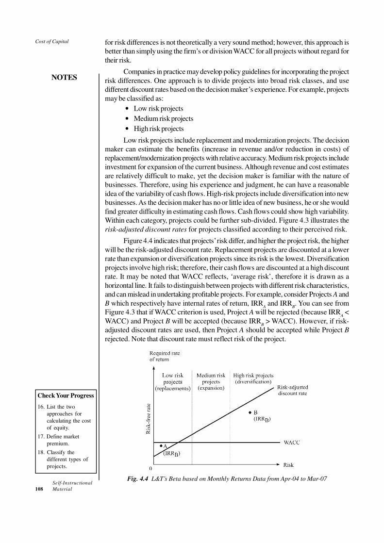
Self-Instructional

108 Material

Cost of Capital

NOTES

for risk differences is not theoretically a very sound method; however, this approach is

better than simply using the firm’s or division WACC for all projects without regard for

their risk.

Companies in practice may develop policy guidelines for incorporating the project

risk differences. One approach is to divide projects into broad risk classes, and use

different discount rates based on the decision maker’s experience. For example, projects

may be classified as:

• Low risk projects

• Medium risk projects

• High risk projects

Low risk projects include replacement and modernization projects. The decision

maker can estimate the benefits (increase in revenue and/or reduction in costs) of

replacement/modernization projects with relative accuracy. Medium risk projects include

investment for expansion of the current business. Although revenue and cost estimates

are relatively difficult to make, yet the decision maker is familiar with the nature of

businesses. Therefore, using his experience and judgment, he can have a reasonable

idea of the variability of cash flows. High-risk projects include diversification into new

businesses. As the decision maker has no or little idea of new business, he or she would

find greater difficulty in estimating cash flows. Cash flows could show high variability.

Within each category, projects could be further sub-divided. Figure 4.3 illustrates the

risk-adjusted discount rates for projects classified according to their perceived risk.

Figure 4.4 indicates that projects’ risk differ, and higher the project risk, the higher

will be the risk-adjusted discount rate. Replacement projects are discounted at a lower

rate than expansion or diversification projects since its risk is the lowest. Diversification

projects involve high risk; therefore, their cash flows are discounted at a high discount

rate. It may be noted that WACC reflects, ‘average risk’, therefore it is drawn as a

horizontal line. It fails to distinguish between projects with different risk characteristics,

and can mislead in undertaking profitable projects. For example, consider Projects A and

B which respectively have internal rates of return, IRRA and IRR

B. You can see from

Figure 4.3 that if WACC criterion is used, Project A will be rejected (because IRRA <

WACC) and Project B will be accepted (because IRRB > WACC). However, if risk-

adjusted discount rates are used, then Project A should be accepted while Project B

rejected. Note that discount rate must reflect risk of the project.

Fig. 4.4 L&T’s Beta based on Monthly Returns Data from Apr-04 to Mar-07

Check Your Progress

16. List the two

approaches for

calculating the cost

of equity.

17. Define market

premium.

18. Classify the

different types of

projects.

Self-Instructional

Material 109

Cost of Capital

NOTES

4.13 SUMMARY

• The primary purpose of measuring the cost of capital is its use as a financial

standard for evaluating the investment projects.

• The cost of capital is the minimum required rate of return on the investment

project that keeps the present wealth of shareholders unchanged.

• The cost of capital can also be useful in deciding about the methods of financing

at a point of time.

• The cost of capital also plays a useful role in dividend decision and investment in

current assets.

• The opportunity cost is the rate of return foregone on the next best alternative

investment opportunity of comparable risk.

• The cost of capital of each source of capital is known as component, or specific,

cost of capital.

• Marginal cost is the new or the incremental cost that the firm incurs if it were to

raise capital now, or in the near future.

• The before-tax cost of debt is the rate of return required by lenders. It is easy to

compute before-tax cost of debt issued and to be redeemed at par; it is simply

equal to the contractual (or coupon) rate of interest.

• The cost of preference capital is a function of the dividend expected by investors.

Preference capital is never issued with an intention not to pay dividends.

• The dividend-growth approach has limited application in practice because of its

two assumptions. First, it assumes that the dividend per share will grow at a

constant rate, g, forever. Second, the expected dividend growth rate, g, should be

less than the cost of equity, ke, to arrive at the simple growth formula.

• WACC is the composite or overall cost of capital.

• Flotation costs are not annual costs; they are one-time costs incurred when the

investment project is undertaken and financed.

• There are two approaches for calculating the cost of equity—constant dividend–

growth model and the capital asset pricing model (CAPM).

• The firm’s risk is composed of its overall operating risk and financial risk. Operating

risk arises due to the uncertainty of cash flows of the firm’s investments. Financial

risk arises on account of the use of debt for financing investments.

4.14 KEY TERMS

• Cost of capital: The cost of capital is the minimum required rate of return on the

investment project that keeps the present wealth of shareholders unchanged.

• Opportunity cost: The opportunity cost is the rate of return foregone on the

next best alternative investment opportunity of comparable risk.

• Marginal cost: Marginal cost is the new or the incremental cost that the firm

incurs if it were to raise capital now, or in the near future.

• Cost of preference capital: The cost of preference capital is a function of the

dividend expected by investors.

Self-Instructional

110 Material

Cost of Capital

NOTES

• Flotation costs: Flotation costs are not annual costs; they are one-time costs

incurred when the investment project is undertaken and financed.

• Weighted average cost of capital (WACC): The component costs are combined

according to the weight of each component capital to obtain the average costs of

capital. Thus, the overall cost is also called the weighted average cost of capital

(WACC).


1. The cost of capital is the minimum required rate of return on the investment

project that keeps the present wealth of shareholders unchanged.

2. The cost of capital can also be useful in deciding about the methods of financing

at a point of time. The cost of capital also plays a useful role in dividend decision

and investment in current assets.

3. The opportunity cost is the rate of return foregone on the next best alternative

investment opportunity of comparable risk.

4. The combined cost of all sources of capital is called overall, or average cost of

capital. The component costs are combined according to the weight of each

component capital to obtain the average costs of capital. Thus, the overall cost is

also called the weighted average cost of capital (WACC).

5. Marginal cost is the new or the incremental cost that the firm incurs if it were to

raise capital now, or in the near future.

6. A company may raise debt in a variety of ways. It may borrow funds from

financial institutions or public either in the form of public deposits or debentures

(bonds) for a specified period of time at a certain rate of interest. A debenture or

bond may be issued at par or at a discount or premium as compared to its face

value.

7. The contractual rate of interest or the coupon rate forms the basis for calculating

the cost of debt.

8. The cost of preference capital is a function of the dividend expected by investors.

9. Redeemable preference shares are shares with finite maturity.

10. The cost of preference share is not adjusted for taxes because preference dividend

is paid after the corporate taxes have been paid.

11. It is sometimes argued that the equity capital is free of cost. The reason for such

argument is that it is not legally binding for firms to pay dividends to ordinary

shareholders. Further, unlike the interest rate or preference dividend rate, the

equity dividend rate is not fixed.

12. As a general rule, it is not theoretically correct to use the ratio of earnings to price

as a measure of the cost of equity. The earnings–price (E/P) ratio does not reflect

the true expectations of the ordinary shareholders.

13. The dividend-growth approach has limited application in practice because of its

two assumptions. First, it assumes that the dividend per share will grow at a

constant rate, g, forever. Second, the expected dividend growth rate, g, should be

less than the cost of equity, ke, to arrive at the simple growth formula.

Self-Instructional

Material 111

Cost of Capital

NOTES

14. The following steps are involved for calculating the firm’s WACC:

• Calculate the cost of specific sources of funds

• Multiply the cost of each source by its proportion in the capital structure

• Add the weighted component costs to get the WACC

15. Flotation costs are not annual costs; they are one-time costs incurred when the

investment project is undertaken and financed.

16. There are two approaches for calculating the cost of equity:

• Constant dividend–growth model

• Capital asset pricing model (CAPM)

17. The market premium is the excess of the expected market return over the expected

risk-free rate of return.

18. Projects may be classified as:

• Low risk projects

• Medium risk projects

• High risk projects



1. Why and how the cost of debt is adjusted for taxes?

2. What are the consequences of not paying dividends on preference capital?

3. State the reasons behind the measurement of the cost of equity being a difficult

task.

4. ‘The use of the book-value weights can be seriously questioned on theoretical

grounds.’ Give reasons.

5. Distinguish between operating and financial risk.


1. Explain the dividend-growth model for calculating equity.

2. Discuss weighted average cost of capital. What are the limitations of book-value

weights? Why is market-value weights considered to be superior?

3. Distinguish between cost of equity calculated by the dividend-growth model and

the CAPM. Which method is better?

4. Explain the steps in pure-play technique of determining the divisional cost of

capital.

5. How is the cost of capital of projects determined?





Self-Instructional

112 Material

Cost of Capital

NOTES


Hall.

Endnotes

1. Quirin, G. D., The Capital Expenditure Decision, Richard D. Irwin, 1967, p. 92.

2. Bhattacharya, S.K., A Cost-of-Capital Framework for Management Control, Economic and

Political Weekly, Vol. 35, 29 August, 1970.

3. Porterfield J.T.S., Investment Decisions and Capital Costs, Prentice-Hall, 1965, p. 45.

4. Barges, A., The Effect of Capital Structure and the Cost of Capital, Prentice-Hall, 1963, p. 2.

5. It is argued later in the chapter that flotation costs should not be incorporated in the

computation of the cost of capital, rather they should be adjusted in the investment project’s

cash flows.

6. Financial institutions generally require principal to be amortized periodically. The issue of

bond or debenture by a company may also provide for periodical amortization. When principal

is repaid each period instead of a lump sum at maturity, cash outflows each period will include

interest and principal, and interest each period will be calculated on the outstanding principal.

The following formula can be used to calculate the before-tax cost of debt in this situation:

∑= +

+

=

n

tt

d

tt

k

BB

10

)1(

INT

where INTt and B

t are respectively the periodical payment of interest and principal.

7. Quirin, op. cit., 1967.

8. Currently (2010) the corporate tax rate in India is 30 per cent plus 3 per cent education cess.

Hence, it is about 31 per cent.

9. In India, irredeemable preference shares cannot be issued.

10. In fact, companies in India now (2010) will have to pay tax at 15 per cent and surcharge of 3 per

cent on the amount of dividend distributed. Thus, the effective cost of preference capital to

a company would be more than that shown by Equation (6) or (7). The same argument will be

applicable to the equity capital.

11. The cost of equity can also be determined by using the capital asset pricing model. This is

discussed in a later section.

12. Gordon, M., The Investment, Financing and Valuation of the Corporation, Richard D. Irwin,

1962.

13. Solomon, E., The Theory of Financial Management, Columbia University Press, 1963, p. 64.

14. Keene, Simon E., The Investment Discount Rate—In Defence of the Market Rate of Interest,

Accounting and Business Research (Summer 1976); and Ezzell, John R. and R. Pourr Porter,

Floatation costs and the Weighted Average Cost of Capital, Journal of Financial and

Quantitative Analysis, 11, (Sept. 1976). Also, refer Van Horne, op. cit.,

15. The implication is that the amount of debt, and hence the interest tax shield will fluctuate with

the firm’s operations. This means that the interest tax shield will be as risky as the operations.

Thus, we do not make any adjustment for interest tax shield in unlevering (or levering beta).

This point is explained in a subsequent chapter.

Self-Instructional

Material 113

Capital Budgeting

NOTES

UNIT 5 CAPITAL BUDGETING

Structure

5.0 Introduction

5.1 Unit Objectives

5.2 Concepts and Steps

5.3 Average Rate of Return

5.4 Payback Period

5.5 Present Value Method

5.6 Internal Rate of Return

5.7 Summary

5.8 Key Terms




Endnotes/References

5.0 INTRODUCTION

An efficient allocation of capital is the most important finance function in the modern

times. It involves decisions to commit the firm’s funds to the long-term assets. Capital

budgeting or investment decisions are of considerable importance to the firm since they

tend to determine its value by influencing its growth, profitability and risk. In this unit we

focus on the nature and evaluation of capital budgeting decisions.

5.1 UNIT OBJECTIVES


• Discuss the concepts and steps involved in capital budgeting

• Explain the concept of average rate of return

• Understand the concept of payback period

• Discuss the present value method

• Explain the concept of internal rate of return

5.2 CONCEPTS AND STEPS

Capital expenditure or investment planning and control involve a process of facilitating

decisions covering expenditures on long-term assets. Since a company’s survival and

profitability hinges on capital expenditures, especially the major ones, the importance of

the capital budgeting or investment process cannot be over-emphasised. A number of

managers think that investment projects have strategic elements, and the investment

analysis should be conducted within the overall framework of corporate strategy. Some

managers feel that the qualitative aspects of investment projects should be given due

importance.

Self-Instructional

114 Material

Capital Budgeting

NOTES

Capital Investments

Strictly speaking, capital investments should include all those expenditures, which are

expected to produce benefits to the firm over a long period of time, and encompass both

tangible and intangible assets. Thus, R&D (research and development) expenditure is a

capital investment. Similarly, the expenditure incurred in acquiring a patent or brand is

also a capital investment. In practice, a number of companies follow the traditional

definition, covering only expenditures on tangible fixed assets as capital investments

(expenditures). The Indian companies are also influenced considerably by accounting

conventions and tax regulations in classifying capital expenditures. Large expenditures

on R&D, advertisement, or employees training, which tend to create valuable intangible

assets, may not be included in the definition of capital investments since most of them

are allowed to be expensed for tax purposes in the year in which they are incurred.

From the point of view of sound decision-making, these expenditures should be treated

as capital investments and subjected to proper evaluation.

A number of companies follow the accounting convention to prepare asset wise

classification of capital expenditures, which is hardly of much use in decision-making.

Some companies classify capital expenditures in a manner, which could provide useful

information for decision-making. Their classification is (i) replacement, (ii) modernisation,

(iii) expansion, (iv) new project, (v) research and development, (vi) diversification, and

(vii) cost reduction.

Capital Investment Planning And Control

At least five phases of capital expenditure planning and control can be identified:

• Identification (or origination) of investment opportunities

• Development of forecasts of benefits and costs

• Evaluation of the net benefits

• Authorisation for progressing and spending capital expenditure

• Control of capital projects

The available literature puts the maximum emphasizes on the evaluation phase.

Two reasons may be attributed to this bias. First, this phase is easily amenable to a

structured, quantitative analysis. Second, it is considered to be the most important phase

by academicians. Practitioners, on the other hand, consider other phases to be more

important.1 The capital investment planning and control phases are discussed below.

Investment Ideas: Who Generates?: Investment opportunities have to be

identified or created; they do not occur automatically.2, 3 Investment proposals of various

types may originate at different levels within a firm. Most proposals, in the nature of cost

reduction or replacement or process or product improvements take place at plant level.

The contribution of top management in generating investment ideas is generally confined

to expansion or diversification projects. The proposals may originate systematically or

haphazardly in a firm. The proposal for adding a new product may emanate from the

marketing department or from the plant manager who thinks of a better way of utilising

idle capacity. Suggestions for replacing an old machine or improving the production

techniques may arise at the factory level. In view of the fact that enough investment

proposals should be generated to employ the firm’s funds fully well and efficiently, a

systematic procedure for generating proposals may be evolved by a firm.

Self-Instructional

Material 115

Capital Budgeting

NOTES

In a number of Indian companies, the investment ideas are generated at the plant

level. The contribution of the board in idea generation is relatively insignificant. However,

some companies depend on the board for certain investment ideas, particularly those

that are strategic in nature. Other companies depend on research centres for investment

ideas.

Is the investment idea generation primarily a bottom-up process in India? In UK,

both bottom-up, as well as top-down processes exist.4 The Indian practice is more like

that in USA. Project initiation is a bottom-up process in USA, with about more than

three-fourths of investment proposals coming from divisional management and plant

personnel.5 However, we should note that the small number of ideas generated at the

top may represent a high percentage in terms of investment value, so that what looks to

be an entirely bottom-up process may not be really so.

Indian companies use a variety of methods to encourage idea generation. The

most common methods used are—(a) management sponsored studies for project

identification, (b) formal suggestion schemes, and (c) consulting advice. Most companies

use a combination of methods. The offer of financial incentives for generating investment

idea is not a popular practice. Other efforts employed by companies in searching

investment ideas are—(a) review of researches done in the country or abroad,

(b) conducting market surveys, and (c) deputing executives to international trade fairs

for identifying new products/technology.

Once the investment proposals have been identified, they are be submitted for

scrutiny. Many companies specify the time for submitting the proposals for scrutiny.

Developing Cash Flow Estimates: Estimation of cash flows is a difficult task

because the future is uncertain. Operating managers with the help of finance executives

should develop cash flow estimates. The risk associated with cash flows should also be

properly handled and should be taken into account in the decision making process.

Estimation of cash flows requires collection and analysis of all qualitative and quantitative

data, both financial and non-financial in nature. Large companies would generally have

a management information system (MIS) providing such data.

Executives in practice do not always have clarity about estimating cash flows. A

large number of companies do not include additional working capital while estimating the

investment project cash flows. A number of companies also mix up financial flows with

operating flows. Although companies claim to estimate cash flows on incremental basis,

some of them make no adjustment for sale proceeds of existing assets while computing

the project’s initial cost. The prevalence of such conceptual confusion has been observed

even in the developed countries. For example, in the seventies, a number of UK companies

were treating depreciation as cash flows.6

In the past, most Indian companies chose an arbitrary period of 5 or 10 years for

forecasting cash flows. This was so because companies in India largely depended on

government-owned financial institutions for financing their projects, and these institutions

required 5 to 10 years forecasts of the project cash flows.

Project Evaluation: The evaluation of projects should be performed by a group

of experts who have no axe to grind. For example, the production people may be generally

interested in having the most modern type of equipments and increased production even

if productivity is expected to be low and goods cannot be sold. This attitude can bias

their estimates of cash flows of the proposed projects. Similarly, marketing executives

may be too optimistic about the sales prospects of goods manufactured, and overestimate

Self-Instructional

116 Material

Capital Budgeting

NOTES

the benefits of a proposed new product. It is, therefore, necessary to ensure that projects

are scrutinised by an impartial group and that objectivity is maintained in the evaluation

process.

A company in practice should take all care in selecting a method or methods of

investment evaluation. The criterion selected should be a true measure of the investment’s

profitability (in terms of cash flows), and it should lead to the net increase in the company’s

wealth (that is, its benefits should exceed its cost adjusted for time value and risk). It

should also be seen that the evaluation criteria do not discriminate between the investment

proposals. They should be capable of ranking projects correctly in terms of profitability.

The net present value method is theoretically the most desirable criterion as it is a true

measure of profitability; it generally ranks projects correctly and is consistent with the

wealth maximisation criterion. In practice, however, managers’ choice may be governed

by other practical considerations also.

A formal financial evaluation of proposed capital expenditures has become a

common practice among companies in India. A number of companies have a formal

financial evaluation of almost three-fourths of their investment projects. Most companies

subject more than 50 per cent of the projects to some kind of formal evaluation. However,

projects, such as replacement or worn-out equipment, welfare and statutorily required

projects below certain limits, small value items like office equipment or furniture,

replacement of assets of immediate requirements, etc., are not often formally evaluated.

Methods of Evaluation: As regards the use of evaluation methods, most Indian

companies use payback criterion. In addition to payback and/or other methods, companies

also use internal rate of return (IRR) and net present (NPV) methods. A few companies

use accounting rate of return (ARR) method. IRR is the second most popular technique

in India.

The major reason for payback to be more popular than the DCF techniques is the

executives’ lack of familiarity with DCF techniques. Other factors are lack of technical

people and sometimes unwillingness of top management to use the DCF techniques.

One large manufacturing and marketing organisation, for example, thinks that conditions

of its business are such that the DCF techniques are not needed. By business conditions

the company perhaps means its marketing nature, and its products being in seller’s

markets. Another company feels that replacement projects are very frequent in the

company, and therefore, it is not necessary to use the DCF techniques for such projects.

Both these companies have fallacious approaches towards investment analysis. They

should subject all capital expenditures to formal evaluation.

The practice of companies in India regarding the use of evaluation criteria is

similar to that in USA. Almost four-fifths of US firms use either the internal rate of

return or net present value models, but only about one-fifth use such discounting techniques

without using the payback period or average rate of return methods.7 The tendency of

US firms to use naive techniques as supplementary tools has also been reported in

recent studies. However, firms in USA have come to depend increasingly on the DCF

techniques, particularly IRR. The British companies use both DCF techniques and return

on capital, sometimes in combination sometimes solely, in their investment evaluation;

the use of payback is widespread.8 In recent years the use of the DCF methods has

increased in UK, and NPV is more popular than IRR.9 However, this increase has not

reduced the importance of the traditional methods such as payback and return on

investment. Payback continues to be employed by almost all companies.

Self-Instructional

Material 117

Capital Budgeting

NOTES

One significant difference between practices in India and USA is that payback is

used in India as a ‘primary’ method and IRR/NPV as a ‘secondary’ method, while it is

just the reverse in USA. Indian managers feel that payback is a convenient method of

communicating an investment’s desirability, and it best protects the recovery of capital—

a scarce commodity in the developing countries.

Cut-off Rate: In the implementation of a sophisticated evaluation system, the

use of a minimum required rate of return is necessary. The required rate of return or the

opportunity cost of capital should be based on the riskiness of cash flows of the investment

proposal; it is compensation to investors for bearing the risk in supplying capital to finance

investment proposals.

Not all companies in India specify the minimum acceptable rate of return. Some

of them compute the weighted average cost of capital (WACC) as the discount rate.

Unfortunately, all companies do not follow correct methodology of calculating the WACC.

Almost all companies use the book value weights.

Business executives in India are becoming increasingly aware of the importance

of the cost of capital, but they perhaps lack clarity about its computation. Arbitrary

judgment of management also seems to play a role in the assessment of the cost of

capital. The fallacious tendency of equating borrowing rate with minimum required rate

of return also persists in the case of some companies.10 In USA, a little more than 50 per

cent companies have been found using WACC as cut-off rate.11 In UK, only a very

small percentage of firms were found attempting any calculation of the cost of capital.12

As in USA and UK, companies in India have a tendency to equate the minimum rate

with interest rate or cost of specific source of finance. The phenomenon of depending

on management judgement for the assessment of the cost of capital is prevalent as

much in USA and UK as in India.

Recognition of Risk: The assessment of risk is an important aspect of an

investment evaluation. In theory, a number of techniques are suggested to handle risk.

Some of them, such as the computer simulation technique are not only quite involved

but are also expensive to use. How do companies handle risk in practice?

Companies in India consider the following as the four most important contributors

of investment risk—selling price, product demand, technological changes and

government policies. India is fast changing from sellers’ market to buyers’ market as

competition is intensifying in a large number of products; hence uncertainty of selling

price and product demand are being realised as important risk factors. Uncertain

government policies (in areas such as custom and excise duty and import policy, the

foreign investment etc.), of course, are a continuous source of investment risk in developing

countries like India.

Sensitivity analysis and conservative forecasts are two equally important

and widely used methods of handling investment risk in India. Each of these techniques

is used by a number of Indian companies with other methods while many other companies

use either sensitivity analysis or conservative forecasts with other methods. Some

companies also use shorter payback and inflated discount rates (risk-adjusted discount

rates).

In USA, risk adjusted discount rate is more popular than the use of payback and

sensitivity analysis.13, 14 The British companies hardly use sensitivity analysis.15 The

contrasts in risk evaluation practices in India, on the one hand, and USA and UK, on the

other, are sharp and significant. Given the complex nature of risk factors in developing

Self-Instructional

118 Material

Capital Budgeting

NOTES

countries, risk evaluation cannot be handled through a single number such as the NPV

calculation based on conservative forecasts or risk-adjusted discount rate. Managers

must know the impact on project profitability of the full range of critical variables. An

American businessman states: ‘there appear to be more corporations using sensitivity

analysis than surveys indicate. In some cases firms may not know that what they are

undertaking is called ‘sensitivity analysis’, and it probably is not in the sophisticated,

computer oriented sense... Typically, analysts or middle managers eliminate the alternative

assumptions and solutions in order to simplify the decision- making process for higher

management.’16

Capital Rationing: Indian companies, by and large, do not have to reject profitable

investment opportunities for lack of funds, despite the capital markets not being so well

developed. This may be due to the existence of the government-owned financial system,

which is always ready to finance profitable projects. Indian companies do not use any

mathematical technique to allocate resources under capital shortage which may

sometimes arise on account of internally imposed restrictions or management’s reluctance

to raise capital from outside. Priorities for allocating resources are determined by

management, based on the strategic need for and profitability of projects.

Authorization: It may not be feasible in practice to specify standard administrative

procedures for approving investment proposals. Screening and selection procedures

may differ from one company to another. When large sums of capital expenditures are

involved, the authority for the final approval may rest with top management. The approval

authority may be delegated for certain types of investment projects. Delegation may be

affected subject to the amount of outlay, prescribing the selection criteria and holding the

authorised person accountable for results.

Funds are appropriated for capital expenditures after the final selection of

investment proposals. The formal plan for the appropriation of funds is called the capital

budget. Generally, the senior management tightly controls the capital expenditures.

Budgetary controls may be rigidly exercised, particularly when a company is facing

liquidity problem. The expected expenditure should become a part of the annual capital

budget, integrated with the overall budgetary system.

Top management should ensure that funds are spent in accordance with

appropriations made in the capital budget. Funds for the purpose of project implementation

should be spent only after seeking formal permission from the financial manager or any

other authorised person.

In India, as in UK, the power to commit a company to specific capital expenditure

and to examine proposals is limited to a few top corporate officials. However, the duties

of processing the examination and evaluation of a proposal are somewhat spread

throughout the corporate management staff in case of a few companies.

Senior management tightly control capital spending. Budgetary control is also

exercised rigidly. The expected capital expenditure proposals invariably become a part

of the annual capital budget in all companies. Some companies also have formal long-

range plans covering a period of 3 to 5 years. Some companies feel that long-range

plans have a significant influence on the evaluation and funding of capital expenditure

proposals.

Control and Monitoring: A capital investment reporting system is required to

review and monitor the performance of investment projects after completion and during

their life. The follow-up comparison of the actual performance with original estimates

Self-Instructional

Material 119

Capital Budgeting

NOTES

not only ensures better forecasting but also helps to sharpen the techniques for improving

future forecasts. Based on the follow-up feedback, the company may reappraise its

projects and take remedial action.

Indian companies practice control of capital expenditure through the use of regular

project reports. Some companies require quarterly reporting, others need monthly, half-

yearly and yet a few companies require continuous reporting. In most of the companies,

the evaluation reports include information on expenditure to date, stage of physical

completion, and approved and revised total cost.

Most of the companies in reappraising investment proposals, consider comparison

between actual and forecast capital cost, saving and rate of return. They perceive the

following advantages of reappraisal—(i) improvement in profitability by positioning the

project as per the original plan; (ii) ascertainment of errors in investment planning which

can be avoided in future; (iii) guidance for future evaluation of projects; and (iv) generation

of cost consciousness among the project team. A few companies abandon the project if

it becomes uneconomical. The power of review is generally invested with the top

executives of the companies in India.

5.3 AVERAGE RATE OF RETURN

The accounting rate of return (ARR), also known as the return on investment (ROI),

uses accounting information, as revealed by financial statements, to measure the profitability

of an investment. The accounting rate of return is the ratio of the average after tax

profit divided by the average investment. The average investment would be equal to half

of the original investment if it were depreciated constantly. Alternatively, it can be found

out by dividing the total of the investment’s book values after depreciation by the life of

the project. The accounting rate of return, thus, is an average rate and can be

determined by the following equation:

investment Average

income AverageARR = (1)

In Equation (1) average income should be defined in terms of earnings after taxes

without an adjustment for interest viz. EBIT (1 – T) or net operating profit after tax.

Thus

2)(

/)1(EBIT

ARR0

1

n

n

t

t

II

nT

+

−

=

∑= (2)

where EBIT is earnings before interest and taxes, T tax rate, I0 book value of investment

in the beginning, In book value of investment at the end of n number of years.17

Illustration 5.1: Accounting Rate of Return

A project will cost ` 40,000. Its stream of earnings before depreciation, interest and

taxes (EBDIT) during first year through five years is expected to be ̀ 10,000, ̀ 12,000,

` 14,000, ` 16,000 and ` 20,000. Assume a 50 per cent tax rate and depreciation on

straight-line basis. Project’s ARR is computed in Table 5.1.

centper 1610020,000

3,200=Return of Rate Accounting =×

Check Your Progress

1. Identify the five

phases of capital

expenditure

planning and

control.

2. Define capital

budget.

3. Name the two

important and

widely used

methods of handling

investment risk in

India.

Self-Instructional

120 Material

Capital Budgeting

NOTES

A variation of the ARR method is to divide average earnings after taxes by the

original cost of the project instead of the average cost. Thus, using this version, the ARR

in Illustration 5.1 would be: ̀ 3,200 ÷ ̀ 40,000 × 100 = 8 per cent. This version of the

ARR method is less consistent as earnings are averaged but investment is not.18

Table 5.1 Calculation of Accounting Rate of Return

( `̀̀̀)

Period 1 2 3 4 5 Average

Earnings before depreciation, 10,000 12,000 14,000 16,000 20,000 14,400

interest and taxes (EBDIT)

Depreciation 18,000 18,000 18,000 18,000 18,000 18,000

Earnings before interest and taxes (EBIT) 12,000 14,000 16,000 18,000 12,000 16,400

Taxes at 50% 11,000 12,000 13,000 14,000 16,000 13,200

Earnings before interest and after taxes 1,000 12,000 13,000 14,000 16,000 13,200

[EBIT (1– T)]

Book value of investment:

Beginning 40,000 32,000 24,000 16,000 18,000

Ending 32,000 24,000 16,000 18,000 —

Average 36,000 28,000 20,000 12,000 14,000 20,000

Acceptance Rule

As an accept-or-reject criterion, this method will accept all those projects whose ARR is

higher than the minimum rate established by the management and reject those projects

which have ARR less than the minimum rate. This method would rank a project as

number one if it has highest ARR and lowest rank would be assigned to the project with

lowest ARR.

Evaluation of ARR Method

The ARR method may claim some merits:

• Simplicity: The ARR method is simple to understand and use. It does not involve

complicated computations.

• Accounting data: The ARR can be readily calculated from the accounting data;

unlike in the NPV and IRR methods, no adjustments are required to arrive at

cash flows of the project.

• Accounting profitability: The ARR rule incorporates the entire stream of income

in calculating the project’s profitability.

The ARR is a method commonly understood by accountants, and frequently used as a

performance measure. As a decision criterion, however, it has serious shortcomings.

• Cash flows ignored: The ARR method uses accounting profits, not cash flows,

in appraising the projects. Accounting profits are based on arbitrary assumptions

and choices and also include non-cash items. It is, therefore, inappropriate to rely

on them for measuring the acceptability of the investment projects.

• Time value ignored: The averaging of income ignores the time value of money.

In fact, this procedure gives more weightage to the distant receipts.

Self-Instructional

Material 121

Capital Budgeting

NOTES

• Arbitrary cut-off: The firm employing the ARR rule uses an arbitrary cut-off

yardstick. Generally, the yardstick is the firm’s current return on its assets (book-

value). Because of this, the growth companies earning very high rates on their

existing assets may reject profitable projects (i.e., with positive NPVs) and the

less profitable companies may accept bad projects (i.e., with negative NPVs).

The ARR method continues to be used as a performance evaluation and control

measure in practice. But its use as an investment criterion is certainly undesirable. It

may lead to unprofitable allocation of capital.

5.4 PAYBACK PERIOD

Payback (PB) is one of the most popular and widely recognized traditional methods of

evaluating investment proposals. Payback is the number of years required to recover

the original cash outlay invested in a project. If the project generates constant annual

cash inflows, the payback period can be computed by dividing cash outlay by the annual

cash inflow. That is:

C

C0

Inflow Cash Annual

Investment Initial=Payback = (3)

Illustration 5.2: Payback (Constant Cash Flows)

Assume that a project requires an outlay of ̀ 50,000 and yields annual cash inflow of

` 12,500 for 7 years. The payback period for the project is:

years 412,000 Rs

50,000 RsPB ==

Unequal cash flows: In case of unequal cash inflows, the payback period can be found

out by adding up the cash inflows until the total is equal to the initial cash outlay. Consider

the following example.

Illustration 5.3: Payback (Uneven Cash Flows)

Suppose that a project requires a cash outlay of ̀ 20,000, and generates cash inflows of

` 8,000; ` 7,000; ` 4,000; and ` 3,000 during the next 4 years. What is the project’s

payback? When we add up the cash inflows, we find that in the first three years

` 19,000 of the original outlay is recovered. In the fourth year cash inflow generated is

` 3,000 and only ̀ 1,000 of the original outlay remains to be recovered. Assuming that

the cash inflows occur evenly during the year, the time required to recover ̀ 1,000 will

be (` 1,000/` 3,000) × 12 months = 4 months. Thus, the payback period is 3 years and

4 months.

Acceptance Rule

Many firms use the payback period as an investment evaluation criterion and a method

of ranking projects. They compare the project’s payback with a predetermined, standard

payback. The project would be accepted if its payback period is less than the maximum

or standard payback period set by management. As a ranking method, it gives highest

ranking to the project, which has the shortest payback period and lowest ranking to the

project with highest payback period. Thus, if the firm has to choose between two mutually

exclusive projects, the project with shorter payback period will be selected.

Check Your Progress

4. Define accounting

rate of return.

5. What are the merits

of ARR method?

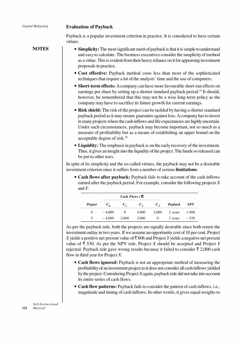
Self-Instructional

122 Material

Capital Budgeting

NOTES

Evaluation of Payback

Payback is a popular investment criterion in practice. It is considered to have certain

virtues.

• Simplicity: The most significant merit of payback is that it is simple to understand

and easy to calculate. The business executives consider the simplicity of method

as a virtue. This is evident from their heavy reliance on it for appraising investment

proposals in practice.

• Cost effective: Payback method costs less than most of the sophisticated

techniques that require a lot of the analysts’ time and the use of computers.

• Short-term effects: A company can have more favourable short-run effects on

earnings per share by setting up a shorter standard payback period.19 It should,

however, be remembered that this may not be a wise long-term policy as the

company may have to sacrifice its future growth for current earnings.

• Risk shield: The risk of the project can be tackled by having a shorter standard

payback period as it may ensure guarantee against loss. A company has to invest

in many projects where the cash inflows and life expectancies are highly uncertain.

Under such circumstances, payback may become important, not so much as a

measure of profitability but as a means of establishing an upper bound on the

acceptable degree of risk.20

• Liquidity: The emphasis in payback is on the early recovery of the investment.

Thus, it gives an insight into the liquidity of the project. The funds so released can

be put to other uses.

In spite of its simplicity and the so-called virtues, the payback may not be a desirable

investment criterion since it suffers from a number of serious limitations:

• Cash flows after payback: Payback fails to take account of the cash inflows

earned after the payback period. For example, consider the following projects X

and Y:

Cash Flows (`̀̀̀)

Project C0

C1

C2

C3

Payback NPV

X – 4,000 0 4,000 2,000 2 years + 806

Y – 4,000 2,000 2.000 0 3 years – 530

As per the payback rule, both the projects are equally desirable since both return the

investment outlay in two years. If we assume an opportunity cost of 10 per cent, Project

X yields a positive net present value of ̀ 806 and Project Y yields a negative net present

value of ` 530. As per the NPV rule, Project X should be accepted and Project Y

rejected. Payback rule gave wrong results because it failed to consider ` 2,000 cash

flow in third year for Project X.

• Cash flows ignored: Payback is not an appropriate method of measuring the

profitability of an investment project as it does not consider all cash inflows yielded

by the project. Considering Project X again, payback rule did not take into account

its entire series of cash flows.

• Cash flow patterns: Payback fails to consider the pattern of cash inflows, i.e.,

magnitude and timing of cash inflows. In other words, it gives equal weights to

Self-Instructional

Material 123

Capital Budgeting

NOTES

returns of equal amounts even though they occur in different time periods. For

example, compare the following projects C and D where they involve equal cash

outlay and yield equal total cash inflows over equal time periods:

Cash Flows (`̀̀̀)

Project C0

C1

C2

C3

Payback NPV

C – 5,000 3,000 2,000 2,000 2 years + 881

D – 5,000 2,000 3,000 2,000 2 years + 798

Using payback period, both projects are equally desirable. But Project C should be

preferable as larger cash inflows’ come earlier in its life. This is indicated by the NPV

rule; project C has higher NPV (` 881) than Project D (` 798) at 10 per cent opportunity

cost. It should be thus clear that payback is not a measure of profitability. As such, it is

dangerous to use it as a decision criterion.

• Administrative difficulties: A firm may face difficulties in determining the

maximum acceptable payback period. There is no rational basis for setting a

maximum payback period. It is generally a subjective decision.

• Inconsistent with shareholder value: Payback is not consistent with the

objective of maximising the market value of the firm’s shares. Share values do

not depend on payback periods of investment projects.21

Let us re-emphasise that the payback is not a valid method for evaluating the acceptability

of the investment projects. It can, however, be used along with the NPV rule as a first

step in roughly screening the projects. In practice, the use of DCF techniques has been

increasing but payback continues to remain a popular and primary method of investment

evaluation (Exhibit 5.1).

Exhibit 5.1: Capital Budgeting Methods in Practice

• In a study of the capital budgeting practices of fourteen medium to large size

companies in India, it was found that all companies, except one, used payback. With

payback and/or other techniques, about two-thirds of companies used IRR and

about two-fifths NPV. IRR was found to be the second most popular method.

• The reasons for the popularity of payback in order of significance were stated to be

its simplicity to use and understand, its emphasis on the early recovery of investment

and focus on risk.

• It was also found that one-third of companies always insisted on the computation

of payback for all projects, one-third for majority of projects and remaining for some

of the projects. For about two-thirds of companies standard payback ranged between

3 and 5 years.

• Reasons for the secondary role of DCF techniques in India included difficulty in

understanding and using these techniques, lack of qualified professionals and

unwillingness of top management to use DCF techniques. One large manufacturing

and marketing organisation mentioned that conditions of its business were such

that DCF techniques were not needed. Yet another company stated that replacement

projects were very frequent in the company, and it was not considered necessary to

use DCF techniques for evaluating such projects.

Source: Pandey, I.M., “Capital Budgeting Practices of Indian Companies”, MDI

Management Journal, Vol. 2, No. 1 (Jan. 1989).

Self-Instructional

124 Material

Capital Budgeting

NOTES

Payback Reciprocal and the Rate of Return

Payback is considered theoretically useful in a few situations. One significant argument

in favour of payback is that its reciprocal is a good approximation of the rate of return

under certain conditions.22

The payback period is defined as follows:

C

C0

(annuity) inflowcash Annual

investment Initial=Payback = (4)

The formula for the present value of an annuity is given by the following equation (i in

the original equation is being replaced by r, the internal rate of return).

+

−=

+

−

=n

n

rr

C

r

C

r

rCC

)1(

1)1(

11

0

Multiplying both sides by r, we get

01

(1 )

= −

+ n

rC C Cr

Solving for r, we find

+

−=nrC

C

C

Cr

)1(

1

00(5)

where C0 is the initial investment, C is annual cash inflow, r is rate of return and n is the

life of investment.

In Equation (5), the first right-hand term is the reciprocal of the payback period.

The second right-hand term is payback reciprocal multiplied by 1/(1 + r)n. If n is very

large or extends to infinity, the second term becomes insignificant (almost equal to zero),

and we are left with the term C/C0. Thus, IRR is equal to the reciprocal of payback.23

The reciprocal of payback will be a close approximation of the internal rate of

return if the following two conditions are satisfied:

• The life of the project is large or at least twice the payback period.

• The project generates equal annual cash inflows.

The payback reciprocal is a useful technique to quickly estimate the true rate of

return. But its major limitation is that every investment project does not satisfy the

conditions on which this method is based. When the useful life of the project is not at

least twice the payback period, the payback reciprocal will always exceed the rate of

return. Similarly, it cannot be used as an approximation of the rate of return if the project

yields uneven cash inflows.

5.5 PRESENT VALUE METHOD

The net present value (NPV) method is the classic economic method of evaluating the

investment proposals. It is a DCF technique that explicitly recognizes the time value of

Check Your Progress

6. Define payback.

7. State the limitation

of payback

reciprocal.

Self-Instructional

Material 125

Capital Budgeting

NOTES

money. It correctly postulates that cash flows arising at different time periods differ in

value and are comparable only when their equivalents—present values—are found out.

The following steps are involved in the calculation of NPV:

• Cash flows of the investment project should be forecasted based on realistic

assumptions.

• Appropriate discount rate should be identified to discount the forecasted cash

flows. The appropriate discount rate is the project’s opportunity cost of capital,

which is equal to the required rate of return expected by investors on investments

of equivalent risk.

• Present value of cash flows should be calculated using the opportunity cost of

capital as the discount rate.

• Net present value should be found out by subtracting present value of cash outflows

from present value of cash inflows. The project should be accepted if NPV is

positive (i.e., NPV > 0).

Let us consider an example.

Illustration 5.4: Calculating Net Present Value

Assume that Project X costs ` 2,500 now and is expected to generate year-end cash

inflows of ̀ 900, ̀ 800, ̀ 700, ̀ 600 and ̀ 500 in years 1 through 5. The opportunity

cost of the capital may be assumed to be 10 per cent.

The net present value for Project X can be calculated by referring to the present value

table (Table C at the end of the book). The calculations are shown below:

2 3 4 5

1, 0.10 2, 0.10 3, 0.10

4, 0.10 5, 0.10

Rs 900 Rs 800 Rs 700 Rs 600 Rs 500NPV Rs 2,500

(1+0.10) (1+0.10) (1+0.10) (1+0.10) (1+0.10)

NPV [Rs 900(PVF )+Rs 800(PVF )+Rs 700(PVF )

+Rs 600(PVF )+Rs 500(PVF )]

= + + + + −

=

− Rs 2,500

NPV [Rs 900 0.909+Rs 800 0.826+Rs 700 0.751+Rs 600 0.683+Rs 500 0.620] Rs 2,500

NPV Rs 2,725 Rs 2,500=+ Rs 225

= × × × × × −

= −

Project X’s present value of cash inflows (` 2,725) is greater than that of cash

outflow (` 2,500). Thus, it generates a positive net present value (NPV = + ` 225).

Project X adds to the wealth of owners; therefore, it shoul d be accepted.

The formula for the net present value can be written as follows:

∑=

−

+

=

−

+

++

+

+

+

+

+

=

n

tt

t

nn

Ck

C

Ck

C

k

C

k

C

k

C

1

0

033

221

)1(NPV

)1()1()1()1(NPV �

(6)

where C1, C

2... represent net cash inflows in year 1, 2..., k is the opportunity cost of

capital, C0 is the initial cost of the investment and n is the expected life of the investment.

It should be noted that the cost of capital, k, is assumed to be known and is constant.

Why is NPV Important?

A question may be raised: why should a financial manager invest ̀ 2,500 in Project X?

Project X should be undertaken if it is best for the company’s shareholders; they would

like their shares to be as valuable as possible. Let us assume that the total market value

Self-Instructional

126 Material

Capital Budgeting

NOTES

of a hypothetical company is ̀ 10,000, which includes ̀ 2,500 cash that can be invested

in Project X. Thus, the value of the company’s other assets must be ̀ 7,500. The company

has to decide whether it should spend cash and accept Project X or to keep the cash and

reject Project X. Clearly Project X is desirable since its PV (` 2,725) is greater than the

` 2,500 cash. If Project X is accepted, the total market value of the firm will be: ̀ 7,500

+ PV of Project X = ` 7,500 + ` 2,725 = ` 10,225; that is, an increase by ` 225. The

company’s total market value would remain only ̀ 10,000 if Project X were rejected.

Why should the PV of Project X reflect in the company’s market value? To answer

this question, let us assume that a new company X with Project X as the only asset is

formed. What is the value of the company? We know that the market value of a company’s

shares is equal to the present value of the expected dividends. Since Project X is the only

asset of Company X, the expected dividends would be equal to the forecasted cash

flows from Project X. Investors would discount the forecasted dividends at a rate of

return expected on securities equivalent in risk to company X. The rate used by investors

to discount dividends is exactly the rate, which we should use to discount cash flows of

Project X. The calculation of the PV of Project X is a replication of the process, which

shareholders will be following in valuing the shares of company X. Once we find out the

value of Project X, as a separate venture, we can add it to the value of other assets to

find out the portfolio value.

The difficult part in the calculation of the PV of an investment project is the

precise measurement of the discount rate. Funds available with a company can either be

invested in projects or given to shareholders. Shareholders can invest funds distributed

to them in financial assets. Therefore, the discount rate is the opportunity cost of investing

in projects rather than in capital markets. Obviously, the opportunity cost concept makes

sense when financial assets are of equivalent risk as compared to the project.

Self-Instructional

Material 127

Capital Budgeting

NOTES

Table 5.1 Interpretation of NPV

Amount outstanding Return on outstanding Total outstanding Repayment from Balance

in the beginning amount at 10% flows cash at the end outstanding

Year `̀̀̀ `̀̀̀ `̀̀̀ `̀̀̀ `̀̀̀

1 2,725.00 272.50 2,997.50 900 2,097.50

2 2,097.50 209.75 2,307.25 800 1,507.25

3 1,507.25 150.73 1,657.98 700 957.98

4 957.98 95.80 1,053.78 600 453.78

5 453.78 45.38 499.16 500 (0.84)*

* Rounding off error.

An alternate interpretation of the positive net present value of an investment is

that it represents the maximum amount a firm would be ready to pay for purchasing the

opportunity of making investment, or the amount at which the firm would be willing to

sell the right to invest without being financially worse-off. The net present value (` 225)

can also be interpreted to represent the amount the firm could raise at the required rate

of return (10%), in addition to the initial cash outlay (` 2,500), to distribute immediately

to its shareholders and by the end of the projects’ life to have paid off all the capital

raised and return on it.24 The point is illustrated by the calculations shown in Table 5.1.

Calculations in Table 5.1 are based on the assumption that the firm chooses to

receive the cash benefit resulting from the investment in the year it is made. Any pattern

of cash receipts, such that the net present value is equal to ̀ 225, can be selected. Thus,

if the firm raises ` 2,500 (the initial outlay) instead of ` 2,725 (initial outlay plus net

present value) at 10 per cent rate of return, at the end of fifth year after having paid the

principal sum together with interest, it would be left with ̀ 363, whose present value at

the beginning of the first year at 10 per cent discount rate is ` 225. It should be noted

that the gain to shareholders would be more if the rate of raising money is less than 10

per cent. (Why?)

Acceptance Rule

It should be clear that the acceptance rule using the NPV method is to accept the

investment project if its net present value is positive (NPV > 0) and to reject it if the net

present value is negative (NPV < 0). Positive NPV contributes to the net wealth of the

shareholders, which should result in the increased price of a firm’s share. The positive

net present value will result only if the project generates cash inflows at a rate higher

than the opportunity cost of capital. A project with zero NPV (NPV = 0) may be accepted.

A zero NPV implies that project generates cash flows at a rate just equal to the opportunity

cost of capital. The NPV acceptance rules are:

• Accept the project when NPV is positive NPV > 0

• Reject the project when NPV is negative NPV < 0

• May accept the project when NPV is zero NPV = 0

The NPV method can be used to select between mutually exclusive projects; the

one with the higher NPV should be selected. Using the NPV method, projects would be

ranked in order of net present values; that is, first rank will be given to the project with

highest positive net present value and so on.

Self-Instructional

128 Material

Capital Budgeting

NOTES

Evaluation of the NPV Method

NPV is the true measure of an investment’s profitability. It provides the most acceptable

investment rule for the following reasons:

• Time value: It recognises the time value of money—a rupee received today is

worth more than a rupee received tomorrow.

• Measure of true profitability: It uses all cash flows occurring over the entire

life of the project in calculating its worth. Hence, it is a measure of the project’s

true profitability. The NPV method relies on estimated cash flows and the discount

rate rather than any arbitrary assumptions, or subjective considerations.

• Value-additivity: The discounting process facilitates measuring cash flows in

terms of present values; that is, in terms of equivalent, current rupees. Therefore,

the NPVs of projects can be added. For example, NPV (A + B) = NPV (A) +

NPV (B). This is called the value-additivity principle. It implies that if we

know the NPVs of individual projects, the value of the firm will increase by the

sum of their NPVs. We can also say that if we know values of individual assets,

the firm’s value can simply be found by adding their values. The value-additivity

is an important property of an investment criterion because it means that each

project can be evaluated, independent of others, on its own merit.

• Shareholder value: The NPV method is always consistent with the objective of

the shareholder value maximisation. This is the greatest virtue of the method.

Are there any limitations in using the NPV rule? The NPV method is a theoretically

sound method. In practice, it may pose some computational problems.

• Cash flow estimation: The NPV method is easy to use if forecasted cash flows

are known. In practice, it is quite difficult to obtain the estimates of cash flows

due to uncertainty.

• Discount rate: It is also difficult in practice to precisely measure the discount

rate.

• Mutually exclusive projects: Further, caution needs to be applied in using the

NPV method when alternative (mutually exclusive) projects with unequal lives,

or under funds constraint are evaluated. The NPV rule may not give unambiguous

results in these situations.

• Ranking of projects: It should be noted that the ranking of investment projects

as per the NPV rule is not independent of the discount rates.25 Let us consider an

example.

Suppose two projects—A and B—both costing ̀ 50 each. Project A returns ̀ 100

after one year and ̀ 25 after two years. On the other hand, Project B returns ̀ 30 after

one year and ̀ 100 after two years. At discount rates of 5 per cent and 10 per cent, the

NPV of projects and their ranking are as follows:

NPV at 5% Rank NPV at 10% Rank

Project A 67.92 II 61.57 I

Project B 69.27 I 59.91 II

It can be seen that the project ranking is reversed when the discount rate is

changed from 5 per cent to 10 per cent. The reason lies in the cash flow patterns. The

Self-Instructional

Material 129

Capital Budgeting

NOTES

impact of the discounting becomes more severe for the cash flow occurring later in the

life of the project; the higher is the discount rate, the higher would be the discounting

impact. In the case of Project B, the larger cash flows come later in the life. Their

present value will decline as the discount rate increases.

5.6 INTERNAL RATE OF RETURN

The internal rate of return (IRR) method is another discounted cash flow technique,

which takes account of the magnitude and timing of cash flows.26 Other terms used to

describe the IRR method are yield on an investment, marginal efficiency of capital, rate

of return over cost, time-adjusted rate of internal return and so on. The concept of

internal rate of return is quite simple to understand in the case of a one-period project.

Assume that you deposit ̀ 10,000 with a bank and would get back ̀ 10,800 after one

year. The true rate of return on your investment would be:

8%or,08.0108.1000,10000,10

800,10

000,10

10,00010,800return of Rate =−=−=

−=

The amount that you would obtain in the future (` 10,800) would consist of your

investment (` 10,000) plus return on your investment (0.08 × ̀ 10,000):

10,000 (1.08) = 10,800

10,000 = 10,800

(1.08)

You may observe that the rate of return of your investment (8 per cent) makes

the discounted (present) value of your cash inflow (` 10,800) equal to your investment

(` 10,000).

We can now develop a formula for the rate of return (r) on an investment (C0)

that generates a single cash flow after one period (C1) as follows:

10

1

0

01−=

−

=

C

C

C

CCr (7)

Equation (7) can be rewritten as follows:

)1(

1

10

0

1

r

CC

rC

C

+

=

+=

(8)

From Equation (8), you may notice that the rate of return, r, depends on the

project’s cash flows, rather than any outside factor. Therefore, it is referred to as the

internal rate of return. The internal rate of return (IRR) is the rate that equates the

investment outlay with the present value of cash inflow received after one period. This

also implies that the rate of return is the discount rate which makes NPV = 0. There is

no satisfactory way of defining the true rate of return of a long-term asset. IRR is the

best available concept. We shall see that although it is a very frequently used concept in

finance, yet at times it can be a misleading measure of investment worth.27 IRR can be

determined by solving the following equation for r:

Check Your Progress

8. What is net present

value method?

9. What is value-

additivity

principle?

Self-Instructional

130 Material

Capital Budgeting

NOTES∑=

+

=

+

++

+

+

+

+

+

=

n

tt

t

nn

r

CC

r

C

r

C

r

C

r

CC

1

0

33

221

0

)1(

)1()1()1()1(�

0)1(

0

1

=−

+

∑=

Cr

Cn

tt

t(9)

It can be noticed that the IRR equation is the same as the one used for the NPV

method. In the NPV method, the required rate of return, k, is known and the net present

value is found, while in the IRR method the value of r has to be determined at which the

net present value becomes zero.

Uneven Cash Flows: Calculating IRR by Trial and Error

The value of r in Equation (9) can be found out by trial and error. The approach is to

select any discount rate to compute the present value of cash inflows. If the calculated

present value of the expected cash inflow is lower than the present value of cash outflows,

a lower rate should be tried. On the other hand, a higher value should be tried if the

present value of inflows is higher than the present value of outflows. This process will

be repeated unless the net present value becomes zero. The following illustration explains

the procedure of calculating IRR.

Illustration 5.5: Trial and Error Method for Calculating IRR

A project costs ̀ 16,000 and is expected to generate cash inflows of ̀ 8,000, ̀ 7,000

and ` 6,000 at the end of each year for next 3 years. We know that IRR is the rate at

which project will have a zero NPV. As a first step, we try (arbitrarily) a 20 per cent

discount rate. The project’s NPV at 20 per cent is:

1, 0.20 2, 0.20 3, 0.20NPV Rs 16,000+Rs 8,000(PVF )+Rs 7,000(PVF ) + Rs 6,000(PVF )

Rs 16,000+Rs 8,000 0.833+Rs 7,000 0.694 + Rs 6,000 0.579

Rs 16,000+Rs 14,996= Rs 1,004

= −

= − × × ×

= − −

A negative NPV of ̀ 1,004 at 20 per cent indicates that the project’s true rate of return

is lower than 20 per cent. Let us try 16 per cent as the discount rate. At 16 per cent, the

project’s NPV is:

1, 0.16 2, 0.16 3, 0.16NPV Rs 16,000+Rs 8,000(PVF )+Rs 7,000(PVF )+Rs 6,000(PVF )

Rs 16,000+Rs 8,000 0.862+Rs 7,000 0.743+Rs 6,000 0.641

Rs 16,000+Rs 15,943= Rs 57

= −

= − × × ×

= − −

Since the project’s NPV is still negative at 16 per cent, a rate lower than 16 per cent

should be tried. When we select 15 per cent as the trial rate, we find that the project’s

NPV is ̀ 200:

1, 0.15 2, 0.15 3, 0.15NPV Rs 16,000 + Rs 8,000(PVF ) + Rs 7,000(PVF ) + Rs 6,000(PVF )

Rs 16,000 + Rs 8,000 0.870 + Rs 7,000 0.756 + Rs 6,000 0.658

Rs 16,000 + Rs 16,200 = Rs 200

= −

= − × × ×

= −

The true rate of return should lie between 15–16 per cent. We can find out a close

approximation of the rate of return by the method of linear interpolation as follows:

Self-Instructional

Material 131

Capital Budgeting

NOTES

Difference

PV required ` 16,000

200

PV at lower rate, 15% 16,200

257

PV at higher rate, 16% 15,943

r = 15% + (16% – 15%)200/257

= 15% + 0.80% = 15.8%

Level Cash Flows

An easy procedure can be followed to calculate the IRR for a project that produces

level or equal cash flows each period. To illustrate, let us assume that an investment

would cost ` 20,000 and provide annual cash inflow of ` 5,430 for 6 years. If the

opportunity cost of capital is 10 per cent, what is the investment’s NPV? The ̀ 5,430 is

an annuity for 6 years. The NPV can be found as follows:

3,648 Rs=4.3555,430 Rs+20,000 Rs =)5,430(PVFA Rs +20,000 Rs=NPV 6,0.10 ×−−

How much is the project’s IRR? The IRR of the investment can be found out as follows:

683.35,430 Rs

20,000 RsPVFA

)5,430(PVFA Rs20,000 Rs

0=)5,430(PVFA Rs+20,000 RsNPV

6,

6,

6,

==

=

−=

r

r

r

The rate, which gives a PVFA of 3.683 for 6 years, is the project’s internal rate of

return. Looking up PVFA in Table (given at the end of the book) across the 6-year row,

we find it approximately under the 16 per cent column. Thus, 16 per cent is the project’s

IRR that equates the present value of the initial cash outlay (` 20,000) with the constant

annual cash inflows (` 5,430 per year) for 6 years.

NPV Profile and IRR

We repeat to emphasise that NPV of a project declines as the discount rate increases,

and for discount rates higher than the project’s IRR, NPV will be negative. NPV profile

of the project at various discount rates is shown in Table 5.2 and Figure 5.1. At 16 per

cent, the NPV is zero; therefore, it is the IRR of the project. As you may notice, we

have used the Excel spreadsheet to make the computations and create the chart using

the Excel chart wizard.

Table 5.2 NPV Profile

1 NPV Profile

Discount

2 Cash Flow rate NPV

3 – 20000 0% 12,580

4 5430 5% 7,561

5 5430 10% 3,649

6 5430 15% 550

7 5430 16% 0

8 5430 20% (1,942)

9 5430 25% (3,974)

Self-Instructional

132 Material

Capital Budgeting

NOTES

Fig. 5.1 NPV Profile

Acceptance Rule

The accept-or-reject rule, using the IRR method, is to accept the project if its internal

rate of return is higher than the opportunity cost of capital (r > k). Note that k is also

known as the required rate of return, or the cut-off, or hurdle rate. The project shall be

rejected if its internal rate of return is lower than the opportunity cost of capital (r < k).

The decision maker may remain indifferent if the internal rate of return is equal to the

opportunity cost of capital. Thus the IRR acceptance rules are:

• Accept the project when r > k

• Reject the project when r < k

• May accept the project when r = k

The reasoning for the acceptance rule becomes clear if we plot NPVs and discount

rates for the project given in Table 5.2 on a graph like Figure 5.1. It can be seen that if

the discount rate is less than 16 per cent IRR, then the project has positive NPV; if it is

equal to IRR, the project has a zero NPV; and if it is greater than IRR, the project has

negative NPV. Thus, when we compare IRR of the project with the opportunity cost of

capital, we are in fact trying to ascertain whether the project’s NPV is positive or not. In

case of independent projects, IRR and NPV rules will give the same results if the firm

has no shortage of funds.

Evaluation of IRR Method

IRR method is like the NPV method. It is a popular investment criterion since it measures

profitability as a percentage and can be easily compared with the opportunity cost of

capital. IRR method has following merits:

Self-Instructional

Material 133

Capital Budgeting

NOTES

• Time value: The IRR method recognises the time value of money.

• Profitability measure: It considers all cash flows occurring over the entire life

of the project to calculate its rate of return.

• Acceptance rule: It generally gives the same acceptance rule as the NPV

method.

• Shareholder value: It is consistent with the shareholders’ wealth maximisation

objective. Whenever a project’s IRR is greater than the opportunity cost of capital,

the shareholders’ wealth will be enhanced.

Like the NPV method, the IRR method is also theoretically a sound investment evaluation

criterion. However, IRR rule can give misleading and inconsistent results under certain

circumstances. Here we briefly mention the problems that IRR method may suffer

from.

• Multiple rates: A project may have multiple rates, or it may not have a unique

rate of return. As we explain later on, these problems arise because of the

mathematics of IRR computation.

• Mutually exclusive projects: It may also fail to indicate a correct choice between

mutually exclusive projects under certain situations. This pitfall of the IRR method

is elaborated later on in this unit.

• Value additivity: Unlike in the case of the NPV method, the value additivity

principle does not hold when the IRR method is used—IRRs of projects do not

add.28 Thus, for Projects A and B, IRR(A) + IRR(B) need not be equal to IRR

(A + B). Consider an example given below.

The NPV and IRR of Projects A and B are given below:

Project C0 C1 NPV @ 10% IRR

( `̀̀̀) ( `̀̀̀) ( `̀̀̀) (%)

A – 100 + 120 + 9.1 20.0

B – 150 + 168 + 2.7 12.0

A + B – 250 + 288 + 11.8 15.2

It can be seen from the example that NPVs of projects add:

%2.1512%+20%)IRR()IRR(+)IRR(

while,8.117.21.9)(NPV)(NPV)(NPV

≠=+≠

=+=+=+

BABA

BABA

5.7 SUMMARY

• Capital investments should include all those expenditures, which are expected to

produce benefits to the firm over a long period of time, and encompass both

tangible and intangible assets.

• The available literature puts the maximum emphasizes on the evaluation phase.

Two reasons may be attributed to this bias. First, this phase is easily amenable to

a structured, quantitative analysis. Second, it is considered to be the most important

phase by academicians.

• Sensitivity analysis and conservative forecasts are two equally important and

widely used methods of handling investment risk in India.

Check Your Progress

10. Define internal rate

of return.

11. What is the main

difference in the

concepts of NPV

and IRR?

Self-Instructional

134 Material

Capital Budgeting

NOTES

• The formal plan for the appropriation of funds is called the capital budget.

• The accounting rate of return is the ratio of the average after tax profit divided by

the average investment. The average investment would be equal to half of the

original investment if it were depreciated constantly.

• The ARR is a method commonly understood by accountants, and frequently used

as a performance measure.

• The payback (PB) is one of the most popular and widely recognized traditional

methods of evaluating investment proposals. Payback is the number of years

required to recover the original cash outlay invested in a project.

• Payback is a popular investment criterion in practice. It is considered to have

certain virtues.

• In spite of its simplicity and the so-called virtues, the payback may not be a

desirable investment criterion since it suffers from a number of serious limitations.

• Payback is considered theoretically useful in a few situations. One significant

argument in favour of payback is that its reciprocal is a good approximation of the

rate of return under certain conditions.

• The net present value (NPV) method is the classic economic method of evaluating

the investment proposals. It is a DCF technique that explicitly recognizes the time

value of money. It correctly postulates that cash flows arising at different time

periods differ in value and are comparable only when their equivalents—present

values—are found out.

• NPV is the true measure of an investment’s profitability.

• The internal rate of return (IRR) method is another discounted cash flow technique,

which takes account of the magnitude and timing of cash flows.

• The internal rate of return (IRR) is the rate that equates the investment outlay

with the present value of cash inflow received after one period.

• IRR method is like the NPV method. It is a popular investment criterion since it

measures profitability as a percentage and can be easily compared with the

opportunity cost of capital.

5.8 KEY TERMS

• Capital budget: The formal plan for the appropriation of funds is called the

capital budget.

• Accounting rate of return: The accounting rate of return is the ratio of the

average after tax profit divided by the average investment.

• Payback: Payback is the number of years required to recover the original cash

outlay invested in a project.


1. At least five phases of capital expenditure planning and control can be identified:

• Identification (or origination) of investment opportunities

• Development of forecasts of benefits and costs

Self-Instructional

Material 135

Capital Budgeting

NOTES

• Evaluation of the net benefits

• Authorization for progressing and spending capital expenditure

• Control of capital projects

2. The formal plan for the appropriation of funds is called the capital budget.

3. Sensitivity analysis and conservative forecasts are two equally important and

widely used methods of handling investment risk in India.

4. The accounting rate of return is the ratio of the average after tax profit divided by

the average investment.

5. The ARR method may claim some merits:

• Simplicity: The ARR method is simple to understand and use. It does not

involve complicated computations.

• Accounting data: The ARR can be readily calculated from the accounting

data; unlike in the NPV and IRR methods, no adjustments are required to

arrive at cash flows of the project.

• Accounting profitability: The ARR rule incorporates the entire stream of

income in calculating the project’s profitability.

6. Payback is the number of years required to recover the original cash outlay invested

in a project.

7. The payback reciprocal is a useful technique to quickly estimate the true rate of

return. But its major limitation is that every investment project does not satisfy the

conditions on which this method is based.

8. The net present value (NPV) method is the classic economic method of evaluating

the investment proposals. It is a DCF technique that explicitly recognizes the time

value of money. It correctly postulates that cash flows arising at different time

periods differ in value and are comparable only when their equivalents—present

values—are found out.

9. The discounting process facilitates measuring cash flows in terms of present

values; that is, in terms of equivalent, current rupees. Therefore, the NPVs of

projects can be added. For example, NPV (A + B) = NPV (A) + NPV (B). This

is called the value-additivity principle.

10. The internal rate of return (IRR) is the rate that equates the investment outlay

with the present value of cash inflow received after one period.

11. In the NPV method, the required rate of return, k, is known and the net present

value is found, while in the IRR method the value of r has to be determined at

which the net present value becomes zero.


Short Answer Questions

1. What are the shortcomings of ARR method?

2. What are the advantages of reappraisal perceived by companies?

3. Write a short note on steps involved in the calculation of NPV.

Self-Instructional

136 Material

Capital Budgeting

NOTES

Long Answer Questions

1. Discuss the merits and limitations of payback.

2. Explain the reasons behind NPV being considered as the most acceptable

investment rule. What are the limitations of the NPV method?

3. Discuss the merits and demerits of IRR method.






Hall.

Endnotes

1. Hastie, K. L., One Businessman’s View of Capital Budgeting, Financial Management, 3

(Writer 1974), pp. 36, 196.

2. Haynes, W.W. and Solomon, M.B., A Misplaced Emphasis in Capital Budgeting, Quarterly

Review of Economics and Business, (Jan.-Feb. 1964), pp. 95–106.

3. King, P., Is the Emphasis of Capital Budgeting Theory Misplaced? Journal of Business

Finance and Accounting, (Spring 1975), pp. 69–82.

4. Rockley, L.E., Investment for Profitability, Business Books, 1973.

5. Petty, J.W., and Scott, D.F., Capital Budgeting Practices in large US Firms: A Retrospective

Analysis and Update, in Derkindem and Crum (Ed.), Readings in Strategy for Corporate

Investments, Pitman, 1981.

6. Rockley, op. cit.

7. Schall, L.D., Sundem, G.L. and Geijsbeak, W.R., “Survey and Analysis of Capital Budgeting

Methods”, Journal of Finance, (March 1978), pp. 281–87.


9. Pike, R.H., “Capital Budgeting Survey: An Update”, Bradford University Discussion Paper,

1992.

10. Pandey, I.M., “Financing Decision: A Survey of Management Understanding”,

Management Review: Economic & Political Weekly, (Feb. 1984), pp. 27–31.

11. Petty and Scott, op. cit.


13. Schall et al., op. cit.

14. Petty and Scott, op. cit.


16. Hastie, op. cit.

17. We assume straight-line depreciation.

18. See Quirin, G.D., The Capital Expenditure Decision, Richard D. Irwin, 1977, p. 33.

19. Weston, J.F. and Brighane, E.F., Managerial Finance, Holt, Rinehart & Winston, 1972, p.

145.

20. Quirin, op. cit., pp. 31–32.

21. See Porterfield, J.T.S., Investment Decisions and Capital Costs, Prentice-Hall, 1965, p. 22.

Self-Instructional

Material 137

Capital Budgeting

NOTES

22. Gordon, Myron, “Payoff Period and Rate of Profit”, Journal of Business, XXVIII, No. 4,

pp. 253–60.

23. In fact, the optimal cut-off for the payback can be computed from the present value of an

annuity formula:

+

−=n

rrrC

C

)1(

11=cutoffOptimal

0 .

24. Bierman, H. and Smidt, S., The Capital Budgeting Decision, Macmillan, 1975, p. 73.

25. Bierman and Smidt, op. cit., p. 31.

26. The use of IRR for appraising capital investment was emphasised in the formal terms, for

the first time, by Joel Dean. See, Dean, Joel, Capital Budgeting, Columbia University

Press, 1951, and his article, “Measuring the Productivity of Capital in Solomon”, E. (Ed.),

The Management of Corporate Capital.

27. Brealey, R. and Myers, S., Principles of Corporate Finance, McGraw Hill, 1991, p. 8.

28. Copeland, T.E. and Weston, J.F., Financial Theory and Corporate Policy, Addison-

Wesley, 1983, p. 32.

Self-Instructional

Material 139

Analysis and

Interpretation of

Leverage

NOTES

UNIT 6 ANALYSIS AND

INTERPRETATION OF

LEVERAGE

Structure

6.0 Introduction

6.1 Unit Objectives

6.2 Financial Leverage6.2.1 Meaning of Financial Leverage


6.3 Financial Leverage and the Shareholders’ Return

6.4 Combining Financial and Operating Leverages6.4.1 Composite Leverage: Combined Effect of Operating and Financial Leverages

6.5 Financial Leverage and the Shareholders’ Risk

6.6 Summary

6.7 Key Terms

6.8 Answers to ‘Check your Progress’



6.0 INTRODUCTION

Given the capital budgeting decision of a firm, it has to decide the way in which the

capital projects will be financed. Every time the firm makes an investment decision, it is

at the same time making a financing decision also. For example, a decision to build a

new plant or to buy a new machine implies specific way of financing that project. Should

a firm employ equity or debt or both? What are implications of the debt-equity mix?

What is an appropriate mix of debt and equity?

6.1 UNIT OBJECTIVES


• Explain the concept of financial leverage

• Discuss the relationship between financial leverage and shareholder’s return

• Analyse the combined effect of financial and operating leverages

• Understand the relationship between financial leverage and shareholder’s risk

6.2 FINANCIAL LEVERAGE

The assets of a company can be financed either by increasing the owner claims or the

creditor claims. The owner claims increase when the firm raises funds by issuing ordinary

shares or by retaining the earnings; the creditors’ claims increase by borrowing. The

various means of financing represent the financial structure of an enterprise. The left-

hand side of the balance sheet (liabilities plus equity) represents the financial structure

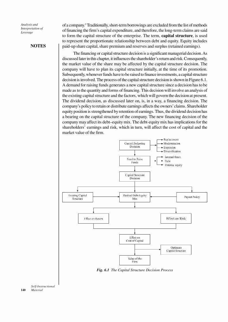
Self-Instructional

140 Material

Analysis and

Interpretation of

Leverage

NOTES

of a company.1 Traditionally, short-term borrowings are excluded from the list of methods

of financing the firm’s capital expenditure, and therefore, the long-term claims are said

to form the capital structure of the enterprise. The term, capital structure, is used

to represent the proportionate relationship between debt and equity. Equity includes

paid-up share capital, share premium and reserves and surplus (retained earnings).

The financing or capital structure decision is a significant managerial decision. As

discussed later in this chapter, it influences the shareholder’s return and risk. Consequently,

the market value of the share may be affected by the capital structure decision. The

company will have to plan its capital structure initially, at the time of its promotion.

Subsequently, whenever funds have to be raised to finance investments, a capital structure

decision is involved. The process of the capital structure decision is shown in Figure 6.1.

A demand for raising funds generates a new capital structure since a decision has to be

made as to the quantity and forms of financing. This decision will involve an analysis of

the existing capital structure and the factors, which will govern the decision at present.

The dividend decision, as discussed later on, is, in a way, a financing decision. The

company’s policy to retain or distribute earnings affects the owners’ claims. Shareholder

equity position is strengthened by retention of earnings. Thus, the dividend decision has

a bearing on the capital structure of the company. The new financing decision of the

company may affect its debt–equity mix. The debt-equity mix has implications for the

shareholders’ earnings and risk, which in turn, will affect the cost of capital and the

market value of the firm.

Fig. 6.1 The Capital Structure Decision Process

Self-Instructional

Material 141

Analysis and

Interpretation of

Leverage

NOTES

The management of a company should seek answers to the following questions

while making the financing decision:

• How should the investment project be financed?

• Does the way in which the investment projects are financed matter?

• How does financing affect the shareholders’ risk, return and value?

• Does there exist an optimum financing mix in terms of the maximum value to the

firm’s shareholders?

• Can the optimum financing mix be determined in practice for a company?

• What factors in practice should a company consider in designing its financing

policy?

We will provide answers to these questions in this and next two chapters.

6.2.1 Meaning of Financial Leverage

As stated earlier, a company can finance its investments by debt and equity. The company

may also use preference capital. The rate of interest on debt is fixed irrespective of the

company’s rate of return on assets. The company has a legal binding to pay interest on

debt. The rate of preference dividend is also fixed; but preference dividends are paid

when the company earns profits. The ordinary shareholders are entitled to the residual

income. That is, earnings after interest and taxes (less preference dividends) belong to

them. The rate of the equity dividend is not fixed and depends on the dividend policy of

a company.

The use of the fixed-charges sources of funds, such as debt and preference

capital along with the owners’ equity in the capital structure, is described as financial

leverage or gearing or trading on equity. The use of the term trading on equity is

derived from the fact that it is the owner’s equity that is used as a basis to raise debt;

that is, the equity that is traded upon. The supplier of debt has limited participation in the

company’s profits and, therefore, he will insist on protection in earnings and protection in

values represented by ownership equity.2

The financial leverage employed by a company is intended to earn more return on

the fixed-charge funds than their costs. The surplus (or deficit) will increase (or decrease)

the return on the owners’ equity. The rate of return on the owners’ equity is levered

above or below the rate of return on total assets. For example, if a company borrows

` 100 at 8 per cent interest (that is, ` 8 per annum) and invests it to earn 12 per cent

return (that is, ̀ 12 per annum), the balance of 4 per cent (` 4 per annum) after payment

of interest will belong to the shareholders, and it constitutes the profit from financial

leverage. On the other hand, if the company could earn only a return of 6 per cent on

` 100 (` 6 per annum), the loss to the shareholders would be ` 2 per annum. Thus,

financial leverage provides the potentials of increasing the shareholders’ earnings as

well as creating the risks of loss to them. It is a double-edged sword. The following

statement very well summarizes the concept of financial leverage:3

This role of financial leverage suggests a lesson in physics, and there might be

some point in considering the rate of interest paid as the fulcrum used in applying forces

through leverage. At least it suggests consideration of pertinent variables; the lower the

interest rate, the greater will be the profit, and the less the chance of loss; the less the

amount borrowed the lower will be the profit or loss; also, the greater the borrowing, the

greater the risk of unprofitable leverage and the greater the chance of gain.

Self-Instructional

142 Material

Analysis and

Interpretation of

Leverage

NOTES


The most commonly used measures of financial leverage are:4

1. Debt ratio: The ratio of debt to total capital, i.e.,

V

D

ED

DL =

+

=1

where D is value of debt, E is value of shareholders’ equity and V is value of total

capital (i.e., D + E). D and E may be measured in terms of book value. The book

value of equity is called net worth. Shareholder’s equity may be measured in

terms of market value.

2. Debt–equity ratio: The ratio of debt to equity, i.e.,

E

DL =2 (1)

3. Interest coverage: The ratio of net operating income (or EBIT) to interest

charges, i.e.,5

Interest

EBIT3 =L (2)

The first two measures of financial leverage can be expressed either in terms of

book values or market values. The market value to financial leverage is theoretically

more appropriate because market values reflect the current attitude of investors. But it

is difficult to get reliable information on market values in practice. The market values of

securities fluctuate quite frequently.

There is no difference between the first two measures of financial leverage in

operational terms. They are related to each other in the following manner.6

21

21 1

D EL DL

L D E V= = =+ + (3)

E

D

VD

VD

L

LL =

−

=

−

=

11 1

12 (4)

These relationships indicate that both these measures of financial leverage will

rank companies in the same order. However, the first measure (i.e. D/V) is more specific

as its value will range between zero to one. The value of the second measure (i.e. D/E)

may vary from zero to any large number. The debt–equity ratio, as a measure of financial

leverage, is more popular in practice. There is usually an accepted industry standard to

which the company’s debt-equity ratio is compared. The company will be considered

risky if its debt–equity ratio exceeds the industry standard. Financial institutions and

banks in India also focus on debt-equity ratio in their lending decisions.

The first two measures of financial leverage are also measures of capital gearing.

They are static in nature as they show the borrowing position of the company at a point

of time. These measures, thus, fail to reflect the level of financial risk, which is inherent

in the possible failure of the company to pay interest and repay debt.

The third measure of financial leverage, commonly known as coverage ratio,

indicates the capacity of the company to meet fixed financial charges. The reciprocal of

interest coverage, that is, interest divided by EBIT, is a measure of the firm’s income

gearing. Again, by comparing the company’s coverage ratio with an accepted industry

Self-Instructional

Material 143

Analysis and

Interpretation of

Leverage

NOTES

standard, investors can get an idea of financial risk. However, this measure suffers from

certain limitations.7 First, to determine the company’s ability to meet fixed financial

obligations, it is the cash flow information, which is relevant, not the reported earnings.

During recessionary economic conditions, there can be wide disparity between the earnings

and the net cash flows generated from operations. Second, this ratio, when calculated

on past earnings, does not provide any guide regarding the future riskiness of the company.

Third, it is only a measure of short-term liquidity rather than of leverage.

Financial Leverage of Companies in India

How much financial leverage do Indian companies employ? Companies differ in the use

of financial leverage since it depends on a number of factors such as the size, nature of

product, capital intensity, technology, market conditions, management attitude etc. In

Table 6.1, we provide the measures of financial leverage for a few large companies in

India for the financial year 2008. As you may observe, companies show wide variations

in the use of financial leverage. Banks or finance companies employ very high amount

of dent. Housing Development Finance Corporation has the highest debt ratio of 91 per

cent and its debt-equity ratio is 10:1. Infosys does not use any debt. Amongst

manufacturing companies, Ranbaxy has the highest debt ratio followed by Tata Steel,

Reliance Energy and Tata Motors. In spite of high debt, these companies have sufficient

interest coverage due to their high profitability.

Table 6.1 Financial Leverage of Large Indian Companies, 2008

Company Balance Sheet Gearing Income Gearing

Debt Debt-equity Interest Interest to

ratio ratio coverage EBIT ratio

Bajaj Auto 0.223 0.288 321.569 0.003

BHEL 0.010 0.010 87.305 0.011

Bharti Airtel 0.291 0.410 17.772 0.056

Cipla 0.035 0.036 73.400 0.014

Dr. Reddy’s 0.069 0.074 28.059 0.036

Grasim

Industries 0.320 0.472 33.754 0.030

HDFC Bank 0.487 0.948 1.515 0.660

Hindalco

Industries 0.371 0.589 15.787 0.063

HUL 0.025 0.025 203.926 0.005

Housing Dev.

Fin. Corp. 0.910 10.078 1.536 0.651

ICICI Bank 0.741 2.865 1.223 0.818

ITC 0.018 0.019 245.400 0.004

Infosys 0.000 0.000 - -

L&T 0.264 0.358 7.068 0.141

Mahindra 0.305 0.439 73.627 0.014

Maruti Suzuki

India 0.095 0.106 61.777 0.016

NTPC 0.332 0.498 5.337 0.187

ONGC 0.006 0.006 7.544 0.133

Self-Instructional

144 Material

Analysis and

Interpretation of

Leverage

NOTES

Ranbaxy 0.560 1.273 8.502 0.118

Reliance

Comm. 0.415 0.710 8.562 0.117

Reliance

Energy 0.385 0.627 3.976 0.252

Reliance Industries 0.302 0.432 12.185 0.082

Satyam 0.002 0.002 207.732 0.005

SBI 0.641 1.785 1.324 0.755

TCS 0.006 0.006 1216.067 0.001

Tata Motors 0.365 0.574 6.834 0.146

Tata Steel 0.404 0.679 25.698 0.039

Wipro 0.025 0.025 442.139 0.002

* Source: CMIE database.

6.3 FINANCIAL LEVERAGE AND THE

SHAREHOLDERS’ RETURN

The primary motive of a company in using financial leverage is to magnify the shareholders’

return under favourable economic conditions. The role of financial leverage in magnifying

the return of the shareholders is based on the assumptions that the fixed-charges funds

(such as the loan from financial institutions and banks or debentures) can be obtained at

a cost lower than the firm’s rate of return on net assets (RONA or ROI). Thus, when

the difference between the earnings generated by assets financed by the fixed-charges

funds and costs of these funds is distributed to the shareholders, the earnings per share

(EPS) or return on equity (ROE) increases. However, EPS or ROE will fall if the

company obtains the fixed-charges funds at a cost higher than the rate of return on the

firm’s assets. It should, therefore, be clear that EPS, ROE and ROI are the important

figures for analyzing the impact of financial leverage.

EPS and ROE Calculations

EPS is calculated by dividing profit after taxes, PAT also called net income, NI,

by the number of shares outstanding. PAT is found out in two steps. First, the interest on

debt, INT, is deducted from the earnings before interest and taxes, EBIT, to obtain the

profit before taxes, PBT. Then, taxes are computed on and subtracted from PBT to

arrive at the figure of PAT. The formula for calculating EPS is as follows:8

Profit after taxEarnings per share =

Number of sharesPAT (EBIT INT)(1 )

EPS =T

N N

− −= (5)

where T is the corporate tax rate and N is the number of ordinary shares outstanding. If

the firm does not employ any debt, then the formula is:

EBIT(1 )EPS =

T

N

−(6)

ROE is obtained by dividing PAT by equity (E). Thus, the formula for calculating

ROE is as follows:9

Check Your Progress

1. Define capital

structure.

2. What is financial

leverage?

3. What does the third

measure of financial

leverage indicate?

Self-Instructional

Material 145

Analysis and

Interpretation of

Leverage

NOTES

Profit after taxReturn on equity =

Value of equity

(EBIT INT)(1 )ROE =

T

E

− −(7)

For calculating ROE either the book value or the market value equity may be

used.

How does the financial leverage affect EPS and ROE? We shall describe two

situations to illustrate the impact of the financial leverage on EPS and ROE. First, we

shall analyze the impact of the alternative financial plans on EPS and ROE assuming

that EBIT is constant. Second, we shall assume that EBIT varies and shows the effect

of the alternative financial plans on EPS and ROE under the conditions of varying EBIT.

Analyzing Alternative Financial Plans: Constant EBIT

Suppose a new firm, Brightways Ltd, is being formed. The management of the firm is

expecting a before-tax rate of return of 24 per cent on the estimated total investment of

` 500,000. This implies EBIT = ̀ 500,000 × 0.24 = ̀ 120,000. The firm is considering

two alternative financial plans: (i) either to raise the entire funds by issuing 50,000 ordinary

shares at ̀ 10 per share, or (ii) to raise ̀ 250,000 by issuing 25,000 ordinary shares at

` 10 per share and borrow ̀ 250,000 at 15 per cent rate of interest. The tax rate is 50

per cent. What are the effects of the alternative plans for the shareholders’ earnings?

Table 6.2 shows calculations.

Table 6.2 Effect of Financial Plan on EPS and ROE: Constant EBIT

Financial Plan

Debt–equity All-equity

(`) (`)

1. Earnings before interest and taxes, EBIT 120,000 120,000

2. Less: Interest, INT 0 37,500

3. Profit before taxes, PBT = EBIT – INT 120,000 82,500

4. Less: Taxes = T (EBIT – INT) 60,000 41,250

5. Profit after taxes, PAT = (EBIT – INT) (1 – T) 60,000 41,250

6. Total earnings of investors, PAT + INT 60,000 78,750

7. Number of ordinary shares, N 50,000 25,000

8. EPS = (EBIT – INT) (1 – T)/N 1.20 1.65

9. ROE = (EBIT – INT) (1 – T)/E 12.0% 16.5%

From Table 6.2, we see that the impact of the financial leverage is quite significant

when 50 per cent debt (debt of ̀ 250,000 to total capital of ̀ 500,000) is used to finance

the investment. The firm earns ̀ 1.65 per share, which is 37.5 per cent more than ̀ 1.20

per share earned with no leverage. ROE is also greater by the same percentage.

Table 6.3 Gain from Financial Leverage

`

1. EBIT on assets financed by debt, ̀ 250,000 × 0.24 60,000

2. Less: Interest, ̀ 250,000 × 0.15 37,500

3. Surplus earnings to the shareholders, ̀ 250,000 × (0.24 – 0.15) 22,500

4. Less: Taxes at 50 per cent 11,250

5. After tax surplus earnings accruing to the shareholders (leverage gain) 11,250

Self-Instructional

146 Material

Analysis and

Interpretation of

Leverage

NOTES

EPS is greater under the debt-equity plan for two reasons. First, under this plan,

the firm is able to borrow half of its funds requirements at a cost (15 per cent) lower

than its rate of return on total investment (24 per cent). Thus, it pays a 15 per cent

(or 7.5 per cent after tax) interest on the debt of ` 250,000 while earns a return of 24

per cent (or 12 per cent after tax) by investing this amount. The difference of 9 per cent

(or 4.5 per cent after tax) accrues to the shareholders as owners of the firm without any

corresponding investment. The difference in terms of rupees is ̀ 22,500 before taxes

and ` 11,250 after taxes. Thus, the gain from the financial leverage is as shown in

Table 6.3.

Second, under the debt-equity plan, the firm has only 25,000 shares as against

50,000 shares under the all-equity plan. Consequently, the after-tax favourable leverage

of ̀ 11,250 dividend by 25,000 shares increases EPS by Re 0.45 from ̀ 1.20 to ̀ 1.65.

Interest Tax Shield

Another important way of explaining the effect of debt is to see the impact of the

interest charges on the firm’s tax liability. The interest charges are tax deductible and,

therefore, provide tax shield, which increases the earnings of the shareholders. See line

6 in Table 6.2 that compares the total earnings of all investors (shareholders as well debt

holders) under two alternative financial plans. The total earnings are more by ̀ 18,750

under the debt-equity plan that is exactly the amount of tax saved (i.e. ` 60,000 –

` 41,250), on account of the tax deductibility of the interest charges. The interest tax

shield under the second financial plan could be directly found out as:

Interest tax shield Tax rate Interest

0.5 37,500 = Rs 18,750

= ×

= ×

It is the fact of the tax deductibility of the interest charges, which makes the use

of the debt in the capital structure beneficial to a firm.

Instead of following the long procedure discussed in Table 6.2, Equation 5 or 7

can be used to examine the effect of the alternative financial plans on the shareholders’

return. Suppose that the management of the firm in the example is considering a third

alternative. They want to use 75 per cent debt and 25 per cent equity to finance the

assets. Under this financial plan, for raising equity investment of ̀ 125,000, the firm will

sell 12,500 shares and pay ̀ 56,250 interest on a debt of ̀ 375,000 at 15 per cent. EPS

and ROE will be as follows:

(EBIT INT)(1 )EPS =

(120,000 56,250)(1 0.50) 31,875

12,500 12,500

Rs 2.55

(EBIT INT)(1 ) 31,875ROE = 25.5%

125,000

T

N

T

E

− −

− −= =

=

− −= =

Under the third alternative financial plan of 75 per cent debt, EPS and ROE are

more than double as compared with all-equity, no-leverage financial plan.

In the example, we assume that the firm earns EBIT of 24 per cent on its investment

(or ` 500,000 × 0.24 = ̀ 120,000). Since the firm pays 15 per cent on debt and earns

more (24 per cent) on these funds, the effect of leverage is favourable. The more debt

Self-Instructional

Material 147

Analysis and

Interpretation of

Leverage

NOTES

the firm uses, the greater is the EPS or ROE. The 24 per cent overall return is an

expected figure. Suppose that, for some reason, the firm may not be able to earn 24 per

cent before-tax return on its total capital, rather it can earn only 12 per cent return (i.e.,

EBIT = ̀ 60,000). What would be the impact on EPS and ROE? We can use Equations

5 and 7 to calculate EPS and ROE:

No debt plan

%6500,000

30,000ROE

60.0 Re50,000

30,000

50,000

)5.01)(060,000(EPS

==

==−−

=

50% debt plan

(60,000 37,500)(1 0.5) 11,250EPS

25,000 25,000

Re 0.45

11,250ROE 4.5%

250,000

− −= =

=

= =

75% debt plan

(60,000 56,250)(1 0.5) 1,875EPS

12,500 12,500

Re 0.15

1,875ROE 1.5%

125,000

− −= =

=

= =

We can see from the calculations above that the effect of financial leverage is

unfavourable. EPS and ROE decline as more debt is used. Why is the effect of financial

leverage unfavourable? It is unfavourable because the firm’s rate of return on total

funds or assets is less than the cost of debt. The firm is paying 15 per cent on debt and

earning a return of 12 per cent on funds employed. The shareholders will have to meet

the deficit of 3 per cent. As a result, EPS and ROE decline. If the rate of return on

assets were just equal to the cost of debt, it can be seen that financial leverage will have

no impact on the shareholders’ return. EPS and ROE would be the same under all plans.

We are thus led to an important conclusion: The financial leverage will have a

favourable impact on EPS and ROE only when the firm’s return on investment

(ROI) exceeds the interest cost of debt (i). The impact will be unfavourable if the

return on investment is less than the interest cost. It is in this sense that the financial

leverage is said to be a double-edged sword.

Effect of Leverage on ROE and EPS

Favourable ROI > i

Unfavourable ROI < i

Neutral ROI = i

These conclusions become very clear if we rewrite the formula for ROE. Suppose

r is the before-tax return on assets or investment i.e. EBIT divided by V = E + D, and

i is the interest rate on debt. Equation 7 can be written as follows:

Self-Instructional

148 Material

Analysis and

Interpretation of

Leverage

NOTES

( )( ) [ ]( )

( )

1 ( ) 1ROE

ROE ( ) 1

rV iD T r E D iD T

E E

Dr r i T

E

− − + − −= =

= + − −

(8)

For an all-equity capital structure firm, D/E will be zero. Therefore, ROE for

such firm is simply the after-tax return on assets:

)1(ROE Tr −= (9)

A comparison of Equations (8) and (9) clearly shows that ROE is more by

[(r – i) D/E] (1 – T) factor when the firm uses debt. It is also indicated that if the return

on assets exceeds the interest rate (r > i), ROE will increase linearly with increase in

the financial leverage (viz., D/E). The effect of leverage will depend on both D/E and

the spread between the rate of return on assets (r) and interest cost (i). If the return on

assets equals the interest rate (r = i), no benefit of the financial leverage will be obtained;

that is, (r – i) D/E (1 – T) = 0. The leverage effect will be unfavourable when the return

on assets is less than the interest rate (when r < i, then (r – i) D/E (1 – T), would

become negative). Equation (8) also shows that for a given level of financial leverage

with the interest rate and tax rate being constant, ROE will increase or decline with the

increase or decline in the rates of return on assets. The following section illustrates the

behaviour of EPS with varying EBIT.

Analyzing Alternative Financial Plans:Varying EBIT

In the previous example, we assumed EBIT as constant. In practice, EBIT for any firm

is subject to various influences. For example, because of the fluctuations in the economic

conditions, sales of a firm change and as a result, EBIT also varies. In a given period, the

actual EBIT of the firm may be more or less than anticipated. It is therefore useful to

analyze the impact of the financial leverage on EPS (and ROE) for possible fluctuations

in EBIT (or r).

EBIT–EPS analysis: Suppose that Brightways Ltd may face any of the four possible

economic conditions: very poor, poor, normal and good. The firm may have a 5 per cent

chance of performing very poorly and earning a negative 5 per cent return on its total

assets [EBIT = (–0.05) × ̀ 500,000 = –` 25,000]. If the economic condition is neither

very poor nor normal, the firm may be able to manage a return of 10 or 15 per cent. It

may have 10 per cent chance of earning 10 per cent return (EBIT = ̀ 50,000). Under

normal economic conditions, the firm has a 35 per cent chance of earning 24 per cent

return (EBIT = ̀ 120,000) and a 30 per cent chance of earning 32 per cent return (EBIT

= ̀ 160,000). If the economic conditions are really favourable, the firm can earn as high

as 60 per cent return (EBIT = ̀ 300,000). But there is only 5 per cent possibility that the

economic conditions will prove to be so good. Brightways’ possible levels of sales and

operating expenses with their probability of occurrence are given in Table 6.4.

Table 6.4 Expected Sales, EBIT, ROI with Associated Probabilities

(` ’000)

Economic Conditions

Very poor Poor Normal Good

Probability 0.05 0.10 0.15 0.35 0.30 0.05

Sales (`) 510 660 710 800 880 1,160

Self-Instructional

Material 149

Analysis and

Interpretation of

Leverage

NOTES

Costs:

Variable (`) 255 330 355 400 440 580

Fixed (`) 280 280 280 280 280 280

Total Costs (`) 535 610 635 680 720 860

EBIT (`) – 25 50 75 120 160 300

ROI (r) – 5% 10% 15% 24% 32% 60%

The behaviour of EPS (and ROE) with fluctuating EBIT (or return on assets)

under the alternative financial plans is analyzed in Table 6.5. The summary of the effect

of the increasing financial leverage on EPS with changing EBIT (see Tables 6.6 and

6.7) provides interesting insights.

Table 6.5 Impact of Financial Leverage: Varying EBIT

(` ’ 000)

Economic Conditions

Very poor Poor Normal Good

Plan I: No debt

EBIT – 25.00 50.00 75.00 120.00 160.00 300.00

Less: Interest 0.00 0.00 0.00 0.00 0.00 0.00

PBT – 25.00 50.00 75.00 120.00 160.00 300.00

Less:

Tax, 50% –12.50* 25.00 37.50 60.00 80.00 150.00

PAT – 12.50 25.00 37.50 60.00 80.00 150.00

No. of

shares (’000) 50.00 50.00 50.00 50.00 50.00 50.00

EPS (`̀̀̀) – 0.25 0.50 0.75 1.20 1.60 3.00

ROE (%) – 2.50 5.00 7.50 12.00 16.00 30.00

Plan II: 25% debt

EBIT – 25.00 50.00 75.00 120.00 160.00 300.00

Less:

Interest 18.75 18.75 18.75 18.75 18.75 18.75

PBT – 43.75 31.25 56.25 101.25 141.25 281.25

Less:

Tax, 50% – 21.88* 15.63 28.13 50.63 70.63 140.63

PAT – 21.87 15.62 28.12 50.62 70.62 140.62

No. of

shares (’000) 37.50 37.50 37.50 37.50 37.50 37.50

EPS (`̀̀̀) – 0.58 0.42 0.75 1.35 1.88 3.75

ROE (%) – 5.80 4.20 7.50 13.50 18.80 37.50

Plan III: 50% debt

EBIT – 25.00 50.00 75.00 120.00 160.00 300.00

Less:

Interest 37.50 37.50 37.50 37.50 37.50 37.50

PBT – 62.50 12.50 37.50 82.50 122.50 262.50

Less:

Tax, 50% – 31.25* 6.25 18.75 41.25 61.25 131.25

PAT – 31.25 6.25 18.75 41.25 61.25 131.25

No. of

shares (’000) 25.00 25.00 25.00 25.00 25.00 25.00

EPS (`̀̀̀) – 1.25 0.25 0.75 1.65 2.45 5.25

ROE (%) – 12.50 2.50 7.50 16.50 24.50 52.50

Self-Instructional

150 Material

Analysis and

Interpretation of

Leverage

NOTES

Plan IV: 75% debt

EBIT – 25.00 50.00 75.00 120.00 160.00 300.00

Less:

Interest 56.25 56.25 56.25 56.25 56.25 56.25

PBT – 81.25 – 6.25 18.75 63.75 103.75 243.75

Less: – 40.63* – 3.13 9.38 31.88 51.88 121.88

Tax, 60%

PAT – 40.62 – 3.12 9.37 31.87 51.87 121.87

No. of

shares (’000) 12.50 12.50 12.50 12.50 12.50 12.50

EPS (`̀̀̀) – 3.25 – 0.25 0.75 2.55 4.15 9.75

ROE (%) – 32.50 – 2.50 7.50 25.50 41.50 97.50

* It is assumed that losses will be set off against other profits or tax credit will be available to the

firm.

Financial Plan I does not employ any leverage. As EBIT increases, EPS also

increases. In fact, EPS increases with improved EBIT under all financial plans (Table

6.6). What is important to note is that as the financial leverage is increased, EPS is

further magnified. Take the example of normal and good years. When EBIT increases

from ` 120,000 to ` 160,000—an increase by 33 per cent, EPS under no financial

leverage plan increases proportionately (i.e., by 33 per cent). But EPS increases faster

under the high financial leverage plans; it increases by 40 per cent when debt is 25 per

cent, by 48 per cent when debt is 50 per cent and by 63 per cent when debt is 75 per

cent. Same conclusions can be drawn from Table 6.7 for the behaviour of ROE in

relation to return on assets (r). It may be worth repeating that the favourable effect of

the increasing financial leverage during normal and good years is on account of the fact

that the rates of return on assets (investment) exceed the cost on debt.

Financial leverage works both ways. It accelerates EPS (and ROE) under

favourable economic conditions, but depresses EPS (and ROE) when the procedings

are not good for the firm. It can be seen from Tables 6.6 and 6.7 that EPS or ROE is

lower with debt in the capital structure in the poor years. With no leverage plan, if the

firm’s return on assets is positive, although low, the shareholders do obtain positive EPS

or ROE. For example, when the firm’s return (r) is 10 per cent, EPS under no leverage

plan is Re 0.40 (or ROE is 4 per cent). But it becomes lower with more debt used, and

even turns negative under very high leverage plan, such as Financial Plan IV. The

unfavourable effect on EPS (and ROE) is more severe with more debt in the capital

structure when EBIT (or r) is negative.

Table 6.6 Summary of the Behaviour of EPS with Fluctuating EBIT under

Alternative Financial Plans

Financial Plan

No 25% 50% 75%

Economic debt debt debt debt

Conditions EBIT I EPS II EPS III EPS IV EPS

Very poor – 25,000 – 0.25 – 0.58 – 1.25 – 3.25

Poor 50,000 0.50 0.42 0.25 – 0.25

75,000 0.75 0.75 0.75 0.75

Normal 1,20,000 1.20 1.35 1.65 2.55

1,60,000 1.60 1.88 2.45 4.15

Good 3,00,000 3.00 3.75 5.25 9.75

Self-Instructional

Material 151

Analysis and

Interpretation of

Leverage

NOTES

Table 6.7 Summary of the Behaviour of ROE with Fluctuating Return on Assets

under Alternative Financial Plans

Financial Plan

Economic Return No 25% 50% 75%

Conditions on assets debt I debt II debt III debt IV

Very poor – 5% – 2.5% – 5.8% – 12.5% – 32.5%

Poor 10% 5.0% 4.2% 2.5% – 2.5%

15% 7.5% 7.5% 7.5% 7.5%

Normal 24% 12.0% 13.5% 16.5% 25.5%

32% 16.0% 18.8% 24.5% 41.5%

Good 60% 30.0% 37.5% 52.5% 97.5%

The reason again lies in the relationship between the return on assets and the cost

of debt. If the cost of debt were more than the return on assets, EPS (or ROE) would

depress with more leverage. It is indicated from Table 6.6 or Table 6.7 that when the

firm earns 15 per cent return on its assets, which is equal to the cost of debt, EPS (or

ROE) is the same under all financial plans. Whatever the firm earns on the funds raised

through debt is exactly paid to the suppliers of debt as interest charges.

Variability of EPS: Yet another significant point to be noted from Table 6.6 is that the

higher the financial leverage, the wider the range over which EPS varies with fluctuating

EBIT. For example, when no debt is used (Financial Plan I), EPS ranges between a

negative ̀ 0.25 to a positive ̀ 3.00—a range of ̀ 3.25. Under Financial Plan II, where

25 per cent debt is introduced in the capital structure, EPS ranges from a negative

` 0.58 to a positive ̀ 3.75—a range of ̀ 4.33. The range of EPS increases to ̀ 6.50 and

` 13.00 when debt is respectively 50 per cent and 75 per cent. The range for ROE

shows the similar behaviour (Table 6.7). Thus, for any given level of variability in EBIT

(or r), the increased financial leverage increases the degree of variability in EPS (or

ROE). The indiscriminate use of financial leverage without taking into account the

uncertainty surrounding EBIT (or r) can lead a firm into financial difficulties. More

about the risk of the financial leverage is explained in the next section.

EBIT–EPS chart: One convenient and useful way of showing the relationship between

EBIT and EPS for the alternative financial plans is to prepare the EBIT–EPS chart. The

chart is easy to prepare since, for any given level of financial leverage, EPS is linearly

related to EBIT.10 As noted earlier, the formula for calculating EPS is:

(EBIT INT)(1 )EPS

(1 )[EBIT INT]

T

NT

N

− −=

−= −

(10)

Equation (10) can also be written as follows:

EBIT)1(

INT)1(

INT)1(

EBIT)1(

EPS

N

T

N

T

N

T

N

T

−+

−−=

−−

−=

(11)

We assume that the level of debt, the cost of debt and the tax rate are constant.

Therefore, in Equations (10) and (11), the terms (1 – T)/N and INT (which is equal to

Self-Instructional

152 Material

Analysis and

Interpretation of

Leverage

NOTES

interest rate times debt, iD) are constant; EPS will increase if EBIT increases and fall if

EBIT declines.

Under the assumptions made, the first part of Equation (11) is a constant and can

be represented by a. EBIT is a random variable since it can assume a value more or less

than expected. The term (1 – T)/N is also a constant and can be shown as b. Thus, the

EPS formula can be rewritten as:

EPS = EBITa b+ × (12)

Equation (12) clearly indicates that EPS is a linear function of EBIT.

The EBIT–EPS analysis shown in Table 6.8 could be worked out with the help of

Equation (12). As an illustration, we work out Equation (12) for Financial Plan IV: equity

` 125,000, 15 per cent debt ̀ 375,000, number of shares 12,500 and tax rate 50 per cent.

The values of a and b (’000 eliminated) are:

(1 ) 0.5INT = – 56.25 2.25

12.5(1 ) 0.5

0.0412.5

Ta

NT

bN

−=− × =−

−= = =

EPS for various levels of EBIT will be as shown in Table 6.8.

Table 6.8 EPS Calculations for Financial Plan IV: EPS = a + b EBIT

(1 – T)/N EBIT = b EBIT + a = EPS = a + b

= b × EBIT

(0.04) (– 25) = – 1.00 + – 2.25 = – 3.25

(0.04) (50) = 2.00 + – 2.25 = – 0.25

(0.04) (75) = 3.00 + – 2.25 = 0.75

(0.04) (120) = 4.80 + – 2.25 = 2.55

(0.04) (160) = 6.40 + – 2.25 = 4.15

(0.04) (300) = 12.00 + – 2.25 = 9.75

Because of the linear relation between EPS and EBIT, the EBIT–EPS chart can

be drawn easily. We can use the following information of Financial Plans I and III in our

example to draw EBIT– EPS chart in Figure 6.2.

EPS

EBIT (` ’000) No debt 50% debt

– 25,000 – 0.25 – 1.25

0 0.00 – 0.75

25,000 0.25 – 0.25

50,000 0.50 0.25

75,000 0.75 0.75

1,00,000 1.00 1.25

1,25,000 1.25 1.75

1,50,000 1.50 2.25

1,75,000 1.75 2.75

2,00,000 2.00 3.25

Self-Instructional

Material 153

Analysis and

Interpretation of

Leverage

NOTES

In Figure 6.2, EBIT is shown on a horizontal line and EPS on a vertical line. If we

identify any two points of EPS for two given levels of EBIT and join them in a straight

line, we obtain EPS-line for a particular financial plan. For example, at EBIT of ̀ 50,000

and ̀ 75,000, two points of EPS are respectively Re 0.25 and Re 0.75 for Financial Plan

III. If we join these two points in a straight line, we get EPS-line for Financial Plan III.

The EPS-line can be similarly drawn for 100 per cent equity plan. We can see from

Figure 6.2 that EPS-lines for all-equity and 50 per cent debt plans intersect at EBIT

` 75,000. EPS under both plans are same at this level of EBIT. Figure 6.3, drawn

similarly as Figure 6.2, shows four financial plans together.

Fig. 6.2 EBIT–EPS chart

The steep solid lines in Figure 6.3 show the relation between EBIT and EPS. The

line relating EBIT and EPS becomes steeper with more debt in the capital structure, and

steeper the line, the more the profit potential to the shareholders with increasing EBIT.

If EBIT is declining, the loss to the shareholders will be magnified. The point of intersection

of four EBIT–EPS lines in Figure 6.3 indicates the indifference point or the EBIT–

EPS break-even point at which EPS is same regardless of the level of the financial

leverage. In the example (see Table 6.6), EPS is same for all financial plans when the

firm earns a 15 per cent return on assets or EBIT of ` 75,000.

EPS

EBIT No debt 25% debt 50% debt 75% debt

– 25,000 – 0.25 – 0.583 – 1.25 – 3.25

0 0.00 – 0.250 – 0.75 – 2.25

25,000 0.25 0.083 – 0.25 – 1.25

50,000 0.50 0.417 0.25 – 0.25

75,000 0.75 0.750 0.75 0.75

1,00,000 1.00 1.083 1.25 1.75

1,25,000 1.25 1.417 1.75 2.75

1,50,000 1.50 1.750 2.25 3.75

1,75,000 1.75 2.083 2.75 4.75

2,00,000 2.00 2.417 3.25 5.75

Self-Instructional

154 Material

Analysis and

Interpretation of

Leverage

NOTES


The 15 per cent return on assets is just equal to the cost of debt. It can also be

noticed from Figure 6.3 that below the ‘indifference point’ the EBIT–EPS lines shift

more towards the right when the level of financial leverage increases, indicating

unfavourable effect because of a low rate of return on assets than the interest cost. The

EBIT–EPS line shifts more towards the left beyond the ‘indifference point’ when the

level of the financial leverage increases. This indicates a favourable effect of leverage

because the return on assets exceeds the interest rate. We thus again reach the conclusion

that the shareholders will benefit by the use of the financial leverage in terms of the

increased EPS if return on assets is higher than the interest cost, and will have reduced

EPS if return on assets is lower than the interest cost; the shareholders’ earnings will not

be affected by the level of leverage if return on assets is just equal to the interest cost.

Calculation of indifference point: The break-even, or indifference, point between

two alternative methods of financing can be determined by a formula. In the earlier

example, suppose the firm is considering only two financial plans—an all-equity plan

(Financial Plan I) and a 25 per cent debt and 75 per cent equity plan (Financial Plan II).

The firm wants to know the level of EBIT at which EPS would be the same under both

the plans. To find out the break-even level of EBIT, we may set the EPS formulae of

two plans equal. The EPS formula under all-equity plan is

1

EBIT)1(EPS

N

T−=

where N1 is number of ordinary shares under first plan and since the firm has no

debt, no interest charges exist. The EPS formula under debt–equity plan is:

2

(1 ) (EBIT INT)EPS

T

N

− −

=

where INT is the interest charges on debt and N2 is the number of ordinary

shares under second plan. Setting the two formulae equal, we have:

1 2

(1 ) EBIT (1 ) (EBIT INT)T T

N N

− − −

= (13)

Self-Instructional

Material 155

Analysis and

Interpretation of

Leverage

NOTES

Using the values for Financial Plans I and II given in the example, we can determine

EBIT as follows:

000,75 Rs125.0

375,9EBIT

EBIT375.0EBIT5.0375,9

375,9EBIT5.0000,50

500,37EBIT5.0

500,37

)750,18EBIT)(5.01(

000,50

EBIT)5.01(

==

−=

−=

−−

=

−

We can simplify Equation (13) as follows:

INTEBIT21

1×

−

=

NN

N(14)

Thus, in the example:

50,000EBIT 18,750

50,000 37,500

4 18,750 Rs 75,000

= ×

−

= × =

Sometimes a firm may like to make a choice between two levels of debt. Then,

the indifference point formula will be:

2

2

1

1 )INTEBIT()1()INTEBIT()1(

N

T

N

T −−

=

−−

(15)

where INT1 and INT

2 represent the interest charges under the alternative financial

plans. After simplifying Equation (15), we obtain:

21

1221 INTINTEBIT

NN

NN

−

×−×

= (16)

Many other combinations of the methods of financing may be compared. The

firm may compare between an all-equity plan and an equity-and-preference share plan.

Then the indifference point formula will be:

21

PDIVEBIT)1()EBIT)(1(

N

T

N

T −−=

−

(17)

Equation (17) can be simplified as follows:

TNN

N

−

×

−

=

1

PDIVEBIT

21

1 (18)

ILLUSTRATION 6.1: Calculation of Indifferent Points

Calculate the level of EBIT at which the indifference point between the following financing

alternatives will occur:

• Ordinary share capital ` 10 lakh or 15% debentures of ` 5 lakh and ordinary

share capital of ` 5 lakh.

• Ordinary share capital of ` 10 lakh or 13% preference share capital of ̀ 5 lakh

and ordinary share capital of ̀ 5 lakh.

Self-Instructional

156 Material

Analysis and

Interpretation of

Leverage

NOTES

• Ordinary share capital of ` 10 lakh or ordinary share capital of ` 5 lakh, 13%

preference share capital of ` 2 lakh and 15% debenture of ` 3 lakh.

• Ordinary share capital of ̀ 6 lakh and 15 debentures of ̀ 4 lakh or ordinary share

capital of ` 4 lakh, 13% unit preference share capital of ` 2 lakh and 15%

debentures of ̀ 4 lakh.

• Ordinary share capital of ̀ 8 lakh and 13% preference share capital of ̀ 2 lakh

or ordinary share capital of ̀ 4 lakh, 13% preference share capital of ̀ 2 lakh and

15% debentures of ̀ 4 lakh.

Assume that the corporate tax rate is 50 per cent and the price of the ordinary

share is ` 10 in each case.

The indifference points for the various combinations of the methods of finance

are calculated as follows:

(i) Ordinary shares vs. ordinary shares and debentures:

1

1 2

EBIT INT

100,00075,000

100,000 50,000

Rs 150,000

N

N N= ×

−

= ×−

=

(ii) Ordinary shares vs. ordinary and preference shares:

1

1 2

PDIVEBIT=

1

100,000 65,000

100,000 50,000 1 0.5

2 130,000 Rs 260,000

N

N N T×

− −

= ×− −

= × =

(iii) Ordinary shares vs. ordinary and preference shares and debentures

1

1 2

PDIVEBIT INT

(1 )

100,000 26,00045,000

100,000 50,000 (1 0.5)

2 (45,000 52,000) Rs 194,000

N

N N T

= × + − −

= × + − −

= × + =

(iv) Ordinary shares and debentures vs. ordinary and preference shares and debentures:

12

1 2

21

1 2

PDIVEBIT INT

(1 )

INT

60,000 26,00060,000

60,000 40,000 (1 0.5)

40,00060,000

60,000 40,000

(3 112,000) (2 60,000)

Rs 216,000

N

N N T

N

N N

= × + − −

− × −

= × + − −

− × −

= × − ×

=

Self-Instructional

Material 157

Analysis and

Interpretation of

Leverage

NOTES

(v) Ordinary shares and preference shows vs. ordinary and preference shares and

debentures:

1 2

1 2

2 1

1 2

PDIVEBIT INT

(1 )

PDIV

(1 )

80,000 26,00060,000

80,000 40,000 1 0.5

40,000 26,000

80,000 40,000 1 0.5

2 112,000 1 52,000

Rs 172,000

N

N N T

N

N N T

= × + − −

− × − −

= × + − −

− × − −

= × − ×

=

6.4 COMBINING FINANCIAL AND OPERATING

LEVERAGES

Operating leverage affects a firm’s operating profit (EBIT), while financial leverage

affects profit after tax or the earnings per share. The combined effect of two leverages

can be quite significant for the earnings available to ordinary shareholders.

Degree of Operating Leverage

The degree of operating leverage (DOL) is defined as the percentage change in the

earnings before interest and taxes relative to a given percentage change in sales. Thus:

%Change in EBITDOL =

%Change in Sales

EBIT/EBITDOL =

Sales/Sales

∆

∆(19)

The following equation is also used for calculating DOL:

FvsQ

vsQ

−−

−=

)(

)(DOL (20)

where Q is the units of output, s is the unit selling price, v is the unit variable cost

and F is the total fixed costs. Equation (20) can also be written as follows:

ContributionDOL =

EBIT(21)

Since contribution = EBIT + Fixed cost, Equation (21) can be expressed as follows:

EBIT1

EBIT

Cost Fixed+EBITDOL

F+== (22)

Suppose that in the earlier example of Brightways Ltd the management had

developed the following income statement based on an expected sales volume of 100,000

units:

Check Your Progress

4. State the primary

motive of a

company in using

financial leverage.

5. What are the

assumptions on

which the role of

financial leverage is

based upon?

Self-Instructional

158 Material

Analysis and

Interpretation of

Leverage

NOTES

`

Sales (100,000 units at ̀ 8) 800,000

Less: Variable costs (100,000 at ̀ 4) 400,000

Contribution 400,000

Less: Fixed costs 280,000

EBIT 120,000

Applying Equation (20), DOL is:

33.3000,120

000,400 Rs

280,000 Rs)4 Rs8 Rs(000,100

)4 Rs8 Rs(000,100DOL

==

−−

−=

DOL of 3.33 implies that for a given change in Brightways’ sales, EBIT will

change by 3.33 times.

Let us suppose in the case of Brightways that a technical expert appointed by the

management tells them that they can choose a more automated production processes

which will reduce unit variable cost to ̀ 2 but will increase fixed costs to ̀ 480,000. If

the management accepts the expert’s advice, then the income statement will look as

follows:

`

Sales (100,000 at ̀ 8) 800,000

Less: Variable costs (100,000 at ̀ 2) 200,000

Contribution 600,000

Less: Fixed costs 480,000

EBIT 120,000

With high fixed costs and low variable costs, DOL for Brightways will be:

0.5000,120 Rs

000,600 RsDOL ==

If Brightways Ltd chooses the high-automated technology and if its actual sales

happen to be more than expected, its EBIT will increase greatly; an increase of 100 per

cent in sales will lead to a 500 per cent increase in EBIT.

Degree of Financial Leverage

We have seen earlier in this chapter that financial leverage affects the earnings per

share. When the economic conditions are good and the firm’s EBIT is increasing, its

EPS increases faster with more debt in the capital structure. The degree of financial

leverage (DFL) is defined as the percentage change in EPS due to a given percentage

change in EBIT:

EBIT in Change %

EPS in Change %DFL =

orEBIT/EBIT

EPS/EPS DFL

∆

∆= (23)

Self-Instructional

Material 159

Analysis and

Interpretation of

Leverage

NOTES

In the case of Brightways Ltd, when EBIT increases from ̀ 120,000 to ̀ 160,000,

EPS increases from ` 1.65 to ` 2.45, when it employs 50 per cent debt and pays

interest charges of ̀ 37,500 (see Table 6.6). Applying Equation (23), DFL at EBIT of

` 120,000 is:

(2.45 1.65)/1.65DFL

(160,000 120,000)/120,000

0.4851.456

0.333

−=

−

= =

This implies that for a given change in EBIT, EPS will change by 1.456 times.

The following equation can also be used to calculate DFL:

PBT

INT1

PBT

EBIT

INTEBIT

EBITDFL +==

−

= (24)

We know that EBIT = Q (p – v) – F (and EBIT – INT = PBT). Thus Equation

(24) can also be written as follows:

INT)(

)(DFL

−−−

−−=

FvsQ

FvsQ(25)

The numerator of Equation (24) or (25) is earnings before interest and taxes and

the denominator is profit before taxes.

In the example, Brightways Ltd was considering four alternative debt levels (see

Table 6.5). Applying Equation (24), DFL for those alternatives at EBIT of

` 120,000 is given below:

Table 6.9 Degree of Financial Leverage of Alternative Financial Plans

at EBIT of ` 120,000

Debt Level DFL

0 1.000

25% 1.185

50% 1.456

75% 1.882

It is indicated from Table 6.9 that if the firm does not employ any debt, EPS will

increase at the same rate at which EBIT increases. EPS increases faster for a given

increase in EBIT when debt is introduced in the capital structure; more the debt in the

capital structure, the greater the increase in EPS. The opposite will happen if EBIT

declines—the greater will be the fall in EPS with more debt in the capital structure.

6.4.1 Composite Leverage: Combined Effect of Operating and

Financial Leverages

Composite leverage is used to calculate the combined effect of operating and financial

leverages.

Thus, composite leverage can be computed by multiplying operating leverage and

the financial leverage by way of a formula:

Composite leverage = Operating leverage × financial leverage

Self-Instructional

160 Material

Analysis and

Interpretation of

Leverage

NOTES

Operating and financial leverages together cause wide fluctuation in EPS for a given

change in sales. If a company employs a high level of operating and financial leverage,

even a small change in the level of sales will have dramatic effect on EPS. A company

with cyclical sales will have a fluctuating EPS; but the swings in EPS will be more

pronounced if the company also uses a high amount of operating and financial leverage.

The degrees of operating and financial leverages can be combined to see the

effect of total leverage on EPS associated with a given change in sales. The degree of

combined leverage (DCL) is given by the following equation:

Sales in Change %

EPS in Change %

EBIT in Change %

EPS in Change %

sales in Change %

EBIT in Change %

=

×=

(26)

Yet another way of expressing the degree of combined leverage is as follows:

INT)(

)(

INT)(

)(

)(

)(DCL

−−−

−=

−−−

−−×

−−

−=

FvsQ

vsQ

FvsQ

FvsQ

FvsQ

vsQ

(27)

Since Q (s – v) is contribution and Q (s – v) – F – INT is the profit after interest

but before taxes, Equation (27) can also be written as follows:

ContributionDCL

Profit before taxesEBIT+Fixed costs

PBTPBT+INT+ INT+

1PBT PBT

F F

=

=

= = +(28)

For Brightways Ltd when it used less automated production processes, the

combined leverage effect at a sales of ` 8 lakh (100,000 units at ` 8) and 50 per cent

debt level is:

85.4500,82

00,0004

7,500380,0002)48(000,100

4)100,000(8=DCL

==

−−−

−

In the case of Brightways Ltd the combined effect of leverage is to increase EPS

by 4.85 times for one unit increase in sales when it chooses less automated production

process and employs 50 per cent debt. Thus, if the Brightways’ sales increase by 10

per cent from ̀ 8 lakh to ̀ 8.80 lakh, then EPS will increase by: 10% × 4.85 = 48.5%.

EPS at the sales level of ̀ 8 lakh is ̀ 1.65 then the new EPS will be:

EPS 1.65 1.485 Rs 2.45= × =

Firms can employ operating and financial leverages in various combinations.

Brightways Ltd, for example, can either choose high-automated production processes

and high degree of operating leverages or low automated production processes and low

degree of operating leverage associated with high or low level of debt. The following are

the possible combinations of operating and financial leverages for Brightways Ltd:

Self-Instructional

Material 161

Analysis and

Interpretation of

Leverage

NOTES

Table 6.10 Combinations of Operating and Financial Leverage for Brightways Ltd

Low Automation High Automation

DOL DFL DCL DOL DFL DCL

3.33 1.000 3.33 5.00 1.000 5.00

3.33 1.185 3.95 5.00 1.185 5.93

3.33 1.455 4.85 5.00 1.456 7.28

3.33 1.882 6.27 5.00 1.882 9.41

Table 6.10 indicates that the largest effect of leverage (9.41 times) will be obtained

when the firm combines higher amount of operating leverage (5.00 times) with the

highest level of debt (DFL = 1.882). If the company has this combination, EPS will

increase by 9.41 times than the increase in sales. Thus, if Brightways’ sales increase

from ` 8 lakh to ` 11.60 lakh—an increase of 45 per cent and EPS increases from

` 2.55 to ` 13.35—an increase by 423 per cent (i.e., 45 per cent × 9.41). Detailed

calculations are given in Table 6.11.

Table 6.11 Brightways Ltd: EPS Calculations for Change in Sales

Units sold 100,000 145,000

Sales (at ` 8) 800,000 1,160,000

Less: Variable costs (at ̀ 2) 200,000 290,000

Contribution 600,000 870,000

Less: Fixed costs 480,000 480,000

EBIT 120,000 390,000

Less: Interest 56,250 56,250

PBT 63,750 333,750

Less: Taxes (50%) 31,875 166,875

PAT 31,875 166,875

No. of shares 12,500 12,500

EPS 2.55 13.35

% Change in sales:1,160,000 800,000

45%800,000

−=

% Change in EPS:13.35 2.55

423%2.55

−=

This combination can, however, prove risky for the company. If sales decline, the

adverse effect on EPS will be very severe. The right combination of operating and

financial leverages will differ among companies. It would generally be governed by the

behaviour of sales. Public utilities such as electricity companies can afford to combine

high operating leverage with high financial leverage since they generally have stable or

rising sales. A company whose sales fluctuate widely and erratically should avoid use of

high leverage since it will be exposed to a very high degree of risk.

6.5 FINANCIAL LEVERAGE AND THE

SHAREHOLDERS’ RISK

We have seen that financial leverage magnifies the shareholders’ earnings. We also find

that the variability of EBIT causes EPS to fluctuate within wider ranges with debt in the

capital structure. That is, with more debt, EPS rises and falls faster than the rise and fall

in EBIT. Thus, financial leverage not only magnifies EPS but also increases its variability.

Check Your Progress

6. Define the degree of

operating leverage.

7. What is the degree

of financial

leverage?

Self-Instructional

162 Material

Analysis and

Interpretation of

Leverage

NOTES

The variability of EBIT and EPS distinguish between two types of risk—operating

risk and financial risk. The distinction between operating and financial risk was long

ago recognized by Marshall in the following words:11

... Let us suppose that two men are carrying on similar business, the one working

with his own, the other chiefly with borrowed, capital. There is one set of risks

common to both, which may be described as the trade risk of the particular

business in which they are engaged.... But there is another set of risks, the burden

of which has to be borne by the man working with borrowed capital, and not by

another.

Operating Risk

Operating risk can be defined as the variability of EBIT (or return on assets). The

environment—internal and external—in which a firm operates, determines the variability

of EBIT. So long as the environment is given to the firm, operating risk is an

unavoidable risk. A firm is better placed to face such risk if it can predict it with a fair

degree of accuracy.

The variability of EBIT has two components:12

• variability of sales

• variability of expenses

Variability of sales: The variability of sales revenue is in fact a major determinant of

operating risk. Sales of a company may fluctuate because of three reasons. First, the

changes in general economic conditions may affect the level of business activity. Business

cycle is an economic phenomenon, which affects sales of all companies. Second, certain

events affect sales of companies belonging to a particular industry. For example, the

general economic conditions may be good but a particular industry may be hit by recession.

Other factors may include the availability of raw materials, technological changes, actions

of competitors, industrial relations, shifts in consumer preferences and so on. Third,

sales may also be affected by the factors, which are internal to the company. The

change in management, the product-market decisions of the company and its investment

policy, or strike in the company have a great influence on the company’s sales.

Variability of expenses: Given the variability of sales, the variability of EBIT is further

affected by the composition of fixed and variable expenses. Higher the proportion of

fixed expenses relative to variable expenses, higher the degree of operating leverage.

We have seen in the previous section that operating leverage affects EBIT. High operating

leverage leads to faster increase in EBIT when sales are rising. In bad times when sales

are falling, high operating leverage becomes a nuisance; EBIT declines at a greater rate

than fall in sales. Operating leverage causes wide fluctuations in EBIT with varying

sales. Operating expenses may also vary on account of changes in input prices, and may

also contribute to the variability of EBIT.

Financial Risk

For a given degree of variability of EBIT, the variability of EPS (and ROE) increases

with more financial leverage. The variability of EPS caused by the use of financial

leverage is called financial risk. Firms exposed to same degree of operating risk can

differ with respect to financial risk when they finance their assets differently. A totally

equity financed firm will have no financial risk. But when debt is used, the firm adds

financial risk. Financial risk is, thus, an avoidable risk if the firm decides not to use

any debt in its capital structure.

Self-Instructional

Material 163

Analysis and

Interpretation of

Leverage

NOTES

Measuring the Operating and Financial Risk

How do we measure the riskiness of EBIT and EPS? We can use two measures of risk:

the standard deviation and coefficient of variation. We first calculate the extent of

Brightways’ operating risk by determining the standard deviation and coefficient of

variation of its expected earnings before interest and taxes. Table 6.12 shows the

calculations.13

Table 6.12 indicates that the expected EBIT (` 120,000) has a standard deviation of ±

` 62,809, which means that on an average, EBIT will range between ` 57,191 to

` 182,809. The coefficient of variation, calculated by dividing standard deviation by the

expected value of EBIT, is 52.34 per cent. Brightways Ltd’s shareholders will be exposed

to this risk even if the company does not use debt. In the absence of debt in the capital

structure, the variability of the earnings available to the shareholders will be same as the

variability of EBIT. The use of debt accentuates the variability of the shareholders’

earnings.

Table 6.12 Standard Deviation and Coefficient Variation of Expected EBIT:

Brightways Ltd

Prob. EBITj – EBIT

j – P

j[EBIT –

Pj

EBITj

PjEBIT

jE (EBIT) E (EBIT)2 E [(EBIT)2]

0.05 – 25 – 1.25 – 145 21,025 1,051.25

0.10 50 5.00 – 70 4,900 490.00

0.15 75 11.25 – 45 2,025 303.75

0.35 120 42.00 0 0 0

0.30 160 48.00 40 1,600 480.00

0.05 300 15.00 180 32,400 1,620.00

E (EBIT) =120.00 σ2 = 3,945.00

3,945 62.809σ = = CV = 62.809/120 = 0.5234

We can use the following formulae to calculate the expected earnings per share,

E (EPS) and its variance (σ2), standard deviation (σ) and coefficient of variation (CV):

1 1 2 2

1

(EPS) EPS EPS EPS

EPS

j j

n

j j

j

E P P P

P

=

= × + × + +

=∑

�

(29)

σ

=

= − + −

+ + −

= −∑

�

2 2 21 1 2 2

2

2

1

(EPS) [EPS (EPS)] [EPS (EPS)]

[EPS (EPS)]

[EPS (EPS)]

j j

n

j jj

E P E P

E P

E P (30)

)EPS()EPS( 2σσ = (31)

CV (EPS)/E (EPS)=σ (32)

Plan I

Self-Instructional

164 Material

Analysis and

Interpretation of

Leverage

NOTES 2 2 2

2 2

2 2

(EPS) ( 0.25 0.05) (0.50 0.10) (0.75 0.15)

(1.20 0.35) (1.60 0.30) (3.00 0.05)

1.20

(EPS) ( 0.25 1.20) 0.05 (0.50 1.20) 0.10

(0.75 1.20) 0.15 (1.20 1.20) 0.35

(1.60 1.20) 0.30 (3.00 1.20) 0.05

E

σ

= − × + × + ×

+ × + × + ×

=

= − − × + − ×

+ − × + − ×

+ − × + − ×

0.3945

(EPS) 0.3945 0.6281

CV 0.6281/1.20 0.5234 or 52.34%

σ

=

= =

= =

Plan II

2 2 2

2 2

2 2

(EPS) ( 0.58 0.05) (0.42 0.10) (0.75 0.15)

(1.35 0.35) (1.88 0.30) (3.75 0.05)

1.35

(EPS) ( 0.58 1.35) 0.05 (0.42 1.35) 0.10

(0.75 1.35) 0.15 (1.35 1.35) 0.35

(1.88 1.35) 0.30 (3.75 1.35) 0.05

E

σ

= − × + × + ×

+ × + × + ×

=

= − − × + − ×

+ − × + − ×

+ − × + − ×

0.6990=

%93.61or6193.035.1/8361.0CV

8361.06990.0)EPS(

==

==σ

Plan III

(EPS) ( 1.25 0.05) (0.25 0.10) (0.75 0.15)

(1.65 0.35) (2.45 0.30) (5.25 0.05)

1.65

E = − × + × + ×

+ × + × + ×

=

2 2 2

2 2

2 2

(EPS) ( 1.25 1.65) 0.05 (0.25 1.65) 0.10

(0.75 1.65) 0.15 (1.65 1.65) 0.35

(2.45 1.65) 0.30 (5.25 1.65) 0.05

1.578

(EPS) 1.578 1.2562

CV 1.2562/1.65 0.7613 or 76.13%

σ

σ

= − − × + − ×

+ − × + − ×

+ − × + − ×

=

= =

= =

Plan IV

2 2 2

2 2

2 2

(EPS) ( 3.25 0.05) (0.25 0.10) (0.75 0.15)

(2.55 0.35) (4.15 0.30) (9.75 0.05)

2.55

(EPS) ( 3.25 2.55) 0.05 (0.25 2.55) 0.10

(0.75 2.55) 0.15 (2.55 2.55) 0.35

(4.15 2.55) 0.30 (9.75 2.55) 0.05

E

σ

= − × + × + ×

+ × + × + ×

=

= − − × + − ×

+ − × + − ×

+ − × + − ×

6.312

(EPS) 6.312 2.5124

2.5124/2.55 0.9852 or 98.52%CV

σ

=

= =

= =

Self-Instructional

Material 165

Analysis and

Interpretation of

Leverage

NOTES

Data in Table 6.13 shows that the shareholders are always exposed to basic

business risk. With variations in sales and expenses, EBIT fluctuates. The variability of

EPS measured in terms of the coefficient of variation is same as that of EBIT when the

firm does not use any debt.

Table 6.13 Variability of EBIT and EPS—Summary

Debt Ratio Expected Standard Coefficient of

Value (`) Deviation (`) Variation

EBIT

120,000 62,809 0.5234

EPS

0 1.20 0.6281 0.5234

25% 1.35 0.8361 0.6193

50% 1.65 1.2562 0.7613

75% 2.55 2.5124 0.9852

An increase in debt increases both the expected value of EPS and its standard

deviation or coefficient of variation. Figure 6.4 shows the relationship of expected EPS

and its standard deviation with debt. It is clearly indicated that debt increases both risk

and return. The relationship between debt ratio and risk measured by the standard deviation

is upward curvilinear. If we draw a graph relating debt ratio and coefficient of variation,

a linear relationship will be found. What is important to note is that financial leverage

adds to financial risk.

Fig. 6.4 Expected EPS and standard deviation

There is yet another way to see the risk of using debt. If we assume many

possible levels of EBIT, then a continuous probability distribution of EPS can be drawn.14

Assuming only two levels of leverage, the probability distributions will look as shown in

Figure 6.5. From the figure, we can see that the low-leverage financial plan has the

tighter, more peaked, distribution. It will have smaller standard deviation or coefficient of

variation. The high-leverage financial plan has higher expected EPS and is also more

risky as it shows greater dispersion or variability.

Self-Instructional

166 Material

Analysis and

Interpretation of

Leverage

NOTES

Fig. 6.5 Probability distribution of EPS

Risk-Return Trade-off

We have now a lot of information about Brightways Ltd We know the firm’s expected

EPS and its variability. We also know expected EPS and its variability, in relation to the

alternative levels of debt.

We find from Table 6.13 that for a given degree of operating risk (i.e., variability

of EBIT), an increase in debt increases expected EPS as well as its variability. How

much debt should Brightways employ? In fact, the firm faces a trade-off between risk

and return. If the firm wants higher return (EPS or ROE) for the shareholders for a

given level of EBIT, it will have to employ more debt and will also be exposed to greater

risk (as measured by standard deviation or coefficient of variation). It should be noted

that EBIT is a random variable. In an uncertain world, the actual EBIT may be so low

that the solvency of the firm may be threatened.

Financial leverage increases the chance or probability of insolvency. Suppose

two firms are identical except that one is levered and another is not. Each firm has an

expected EBIT of ̀ 50,000. The interest burden of levered firm is ̀ 20,000. If the actual

EBIT happens to be ̀ 10,000 in one year for both firms, the levered firm will not be able

to meet its obligation to pay interest. The non-levered firm’s shareholders still get a

return of ` 10,000 (taxes are ignored). The levered firm can legally be forced into

liquidation for non-payment of interest charges. If the insolvency proceedings actually

follow, the levered firm will have to incur costs in the form of liquidation fees and other

legal expenses. If the firm is not liquidated, it may be reorganized. During the reorganization

period, its earnings will be reduced because of the additional costs and reduced sales

volume due to the adverse effect on the firm’s goodwill. If liquidation becomes

unavoidable, the additional costs incurred would result in a decline in the net value of the

firm’s assets available to the shareholders after the creditors claims have been satisfied.

Leverage has benefits as well as costs—it is not an unmixed blessings.

Illustrative solved problems

PROBLEM 6.1: AB Ltd needs ̀ 10 lakh (one million) for expansion. The expansion is

expected to yield an annual EBIT of ̀ 160,000. In choosing a financial plan, AB Ltd has

an objective of maximizing earnings per share. It is considering the possibility of issuing

equity shares and raising debt of ` 100,000, or ` 400,000 or ` 600,000. The current

market price per share is ̀ 25 and is expected to drop to ̀ 20 if the funds are borrowed

in excess of ̀ 500,000. Funds can be borrowed at the rates indicated below: (a) up to

` 100,000 at 8%; (b) over ̀ 100,000 up to ̀ 500,000 at 12%; (c) over ̀ 500,000 at 18%.

Self-Instructional

Material 167

Analysis and

Interpretation of

Leverage

NOTES

Assume a tax rate of 50 per cent. Determine the EPS for the three financing alternatives.

Solution:

The EPS is determined as follows:

Alternatives

I II III

(` 100,000 (` 400,000 (` 600,000

debt) ` debt) ` debt) `

EBIT 160,000 160,000 160,000

Interest 8,000 44,000 74,000

PBT 152,000 116,000 86,000

Taxes at 50% 76,000 58,000 43,000

PAT 76,000 58,000 43,000

No. of shares 36,000 24,000 20,000

EPS 2.11 2.42 2.15

The second alternative maximizes EPS; therefore, it is the best financial alternative

in the present case.

The interest charges for alternatives II and III are calculated as follows:

Interest calculation, alternative II

` `

100,000 @ 8% 8,000

300,000 @ 12% 36,000

Total 44,000

Interest Calculation, Alternative III

` `

100,000 @ 8% 8,000

400,000 @ 12% 48,000

100,000 @ 18% 18,000

Total 74,000

The number of shares are found out by dividing the amount to be raised through

equity issue by the market price per share. The market price per share is ̀ 25 in case of

first two alternatives and ̀ 20 in case of the last alternative.

PROBLEM 6.2: A company needs ` 500,000 for construction of a new plant. The

following three financial plans are feasible: (i) The company may issue 50,000 ordinary

shares at ̀ 10 per share. (ii) The company may issue 25,000 ordinary shares at ̀ 10 per

share and 2,500 debentures of ̀ 100 denominations bearing a 8 per cent rate of interest.

(iii) The company may issue 25,000 ordinary shares at ̀ 10 per share and 2,500 preference

shares at ` 100 per share bearing a 8 per cent rate of dividend.

If the company’s earnings before interest and taxes are ` 10,000, ` 20,000

` 40,000, ` 60,000 and ` 100,000, what are the earnings per share under each of the

three financial plans? Which alternative would you recommend and why? Determine

the indifference points by formulae and graphically. Assume a corporate tax rate of 50

per cent.

Self-Instructional

168 Material

Analysis and

Interpretation of

Leverage

NOTES

Solution:

The earnings per share under the three financial plans are calculated as follows:

First Alternative:

` ` ` ` `

EBIT 10,000 20,000 40,000 60,000 1,00,000

Interest 0 0 0 0 0

PBT 10,000 20,000 40,000 60,000 1,00,000

Taxes @ 50% 5,000 10,000 20,000 30,000 50,000

PAT 5,000 10,000 20,000 30,000 50,000

No. of shares 50,000 50,000 50,000 50,000 50,000

EPS 0.10 0.20 0.40 0.60 1.00

Second Alternative:

` ` ` ` `

EBIT 10,000* 20,000 40,000 60,000 100,000

Interest 20,000* 20,000 20,000 20,000 20,000

PBT (10,000)* 0 20,000 40,000 80,000

Taxes (5,000)* 0 10,000 20,000 40,000

@ 50%

PAT (5,000)* 0 10,000 20,000 40,000

No. of 25,000* 25,000 25,000 25,000 25,000

shares

EPS (0.20)* 0.00 0.40 0.80 1.60

* It is assumed that the company will be able to set-off losses against other profits. If the

company has no profits from other operations, losses will be carried forward.

Third Alternative:

` ` ` ` `

EBIT 10,000 20,000 40,000 60,000 100,000

Interest 0 0 0 0 0

PBT 10,000 20,000 40,000 60,000 100,000

Taxes @ 50% 5,000 10,000 20,000 30,000 50,000

PAT 5,000 10,000 20,000 30,000 50,000

Pref. Dividend 20,000 20,000 20,000 20,000 20,000

PAT for ordinary

shareholders (15,000) (10,000) 0 10,000 30,000

No. of shares 25,000 25,000 25,000 25,000 25,000

EPS (0.60) (0.40) 0.00 0.40 1.20

The choice of the financial plan will depend on the state of economic conditions.

If the company’s sales are increasing, the earnings per share will be maximum under the

second financial alternative. Under favourable conditions, debt financing gives more

benefit than equity or preference financing. Debt capital is cheaper than preference

capital because interest on debt is tax deductible while preference dividend is not.

Self-Instructional

Material 169

Analysis and

Interpretation of

Leverage

NOTES


The indifference points are determined by formula and graphically as follows:

(i) Indifference point between first and second alternatives:

1 2

(1 )EBIT (EBIT INT)(1 )T T

N N

− − −=

1

1 2

EBIT INT

50, 00020, 000

50,000 25, 000

EBIT 2 20,000 Rs 40,000

N

N N= ×

−

= ×−

= × =

(ii) Indifference point between first and third alternatives:

1 2

1

1 2

(1 )EBIT (1 )EBIT PDIV

PDIVEBIT

1

50,000 20,000

50,000 25,000 1 0.5

EBIT 2 40,000 Rs 80,000

T T

N N

N

N N T

− − −=

= ×− −

= ×− −

= × =

PROBLEM 6.3: Two firms A and B have the following information:

(` lakh)

Sales Variable Costs Fixed Costs

Firm A 1,800 450 900

Firm B 1,500 750 375

You are required to calculate (a) profit to sales ratio, (b) break-even point, and

(c) the degree of operating leverage for both firms.

Comment on the positions of the firms. If sales increase by 20 per cent what shall

be the impact on the profitability of the two firms?

Self-Instructional

170 Material

Analysis and

Interpretation of

Leverage

NOTES

Solution:

(a) (i) Contribution ratio: Contribution/Sales

Firm A: 1, 800 450 1,350

0.75 or 75%1,800 1,800

−= =

Firm B: 1,500 750 750

0.50 or 50%1,500 1,500

−= =

(ii) Profit margin: Profit/Sales

Firm A: 1,350 900 450

0.25 or 25%1, 800 1, 800

−= =

Firm B: 750 375 370

0.25 or 25%1,500 1,500

−= =

(b) Break-even point

Firm A: 900

Rs 1, 2000.75

=

Firm B: 375

Rs 7500.50

=

(c) Degree of operating leverage: Contribution/EBIT

Firm A: 1,350

3.0450

=

Firm B: 750

2.0375=

Firm A has a higher contribution ratio as well as a higher operating leverage.

Therefore, under favourable economic conditions, the firm’s profit margin (EBIT/Sales

ratio) will increase at a fast rate. Firm B has a lower contribution ratio but a lower break-

even point and operating leverage as compared to Firm A. Its profits would grow relatively

at a lower rate. At present, the profit margin for the two firms is same, but it would

change with change in sales. If sales increase by 20 per cent, then profit margin would

be as follows:

(1,800 1.20)0.75 900 720 :

1,800 1.20 2,160

0.33 or 33%

(1,500 1.20)0.50 375 525 :

1,500 1.20 1,800

0.29 or 29%

Firm A

Firm B

× −=

×

=

× −=

×

=

You may notice that 20 per cent increase in sales led to 60 per cent increase in

profits (from ` 450 lakh to ` 720 lakh) for A and 40 per cent increase for B (for ̀ 375

lakh to ̀ 525 lakh). This has changed the profit margin for A higher than B.

PROBLEM 6.4: Consider the following information for Kaunark Enterprise:

` in lakh

EBIT 1,120

PBT 320

Fixed cost 700

Self-Instructional

Material 171

Analysis and

Interpretation of

Leverage

NOTES

Calculate percentage change in earnings per share if sales increased by 5 per

cent.

Solution:

(a) Degree of operating leverage

Contribution EBIT + Fixed CostDOL =

EBIT EBIT

1,120 7001.625

1,120

=

+= =

(b) Degree of financial leverage

EBIT 1,120DFL 3.5

PBT 320= = =

(c) Degree of combined leverage

DCL DOL DFL = 1.625 3.5 = 5.6875= × ×

Change in EPS can be calculated as:

% Change in EPSDCL =

% Change in Sales

% Change in EPS5.6875 =

5

% change in EPS = 5 5.6875 = 28.4375%×

PROBLEM 6.5: Arun Chemicals Ltd is considering expansion of its plant capacity to

meet the growing demand. The company would finance the expansion either with 15 per

cent debentures or issue of 10 lakh shares at a price of ` 16 per share. The funds

requirement is ̀ 160 lakh. The company’s profit and loss statement before expansion is

as follows.

` lakh

Sales 1,500

Less: Costs 1,050

EBIT 450

Less: Interest 50

PBT 400

Less: Tax at 51.75% 207

PAT 193

Number of shares (lakh) 50

EPS (`) 3.86

The company’s expected EBIT with associated probabilities after expansion is as

follows:

EBIT (` lakh) Probability

250 0.10

450 0.30

540 0.50

600 0.10

Self-Instructional

172 Material

Analysis and

Interpretation of

Leverage

NOTES

You are required to calculate the company’s expected EBIT and EPS and standard

deviation of EPS and EBIT for each plan.

Solution:

(a) 1 1 2 2 3

3

(EBIT) EBIT EBIT EBIT

Plan I and II: (EBIT) = 250 0.10 + 450 0.30

+ 540 0.50 + 600 0.10

= 490

E P P

P

E

= × + × +

× +

× ×

× ×

�

(b) σ

σ

= − +

− + − +

= − × + − ×

+ − × + − ×

=

= =

�

2 2

1 1 2

2 3

2 3 3

2 2

2 2

(EBIT) [EBIT (EBIT)] [EBIT

(EBIT)] [EBIT (EBIT)]

(250 490) 0.10 (450 490) 0.30

(540 490) 0.50 (600 490) 0.10

8,700

(EBIT) 8,700 93.27

E P

E P E P

(i) Plan I: issue of 15% debenture (` lakh)

EBIT 250 450 540 630

Less: Interest* 74 74 74 74

PBT 176 376 466 556

Tax at 51.75% 91 195 241 288

PAT 85 181 225 268

No. of shares 50 50 50 50

EPS 1.70 3.62 4.50 5.36

* Includes existing and incremental interest.

2 2 2

2

2

(EPS) 1.70 0.10 3.62 0.30 4.50 0.50

5.36 0.10

4.036

(EPS) (1.70 4.036) 0.10 (3.62 4.036)

0.30 (4.50 4.036) 0.50

(5.36 4.036) 0.10

0.8805

(EPS) 0.8805 0.94

E = × + × + ×

+ ×

=

σ = − × + −

× + − ×

+ − ×

=

σ = =

(ii) Plan II : Issue of shares (` lakh)

EBIT 250 450 540 630

Less: Interest 50 50 50 50

PBT 200 400 490 580

Tax at 51.75% 104 207 254 300

PAT 96 193 236 280

No of shares* 60 60 60 60

EPS 1.60 3.22 3.93 4.67

* Includes existing and new shares.

Self-Instructional

Material 173

Analysis and

Interpretation of

Leverage

NOTES

2 2 2

2

2

(EPS) 1.60 0.10 3.22 0.30 3.93

0.50 4.67 0.10

3.558

(EPS) (1.60 3.558) 0.10 (3.22 3.558)

0.30 (3.93 3.558) 0.50

(4.67 3.558) 0.10

0.610496

(EPS) 0.610496 0.7813

E = × + × +

× + ×

=

σ = − × + −

× + − ×

+ − ×

=

σ = =

Plan I (issue of debenture) has not only a higher expected EPS but also a higher

standard deviation as well. The coefficient of variation is: 0.94/4.036 = 0.233 or 23.3%.

The coefficient of variation of EPS under Plan II is: 0.7813/3.558 = 0.2196 or 21.96%.

Thus Plan I has higher return as well as higher risk. The firm’s overall risk is reflected

by the variability of EBIT. The coefficient of variation of EBIT is: 93.27/490 = 0.1903 or

19.03%.

6.6 SUMMARY

• The term, capital structure, is used to represent the proportionate relationship

between debt and equity.

• The use of the fixed-charges sources of funds, such as debt and preference

capital along with the owners’ equity in the capital structure, is described as

financial leverage or gearing or trading on equity.

• The first two measures of financial leverage are also measures of capital gearing.

• The third measure of financial leverage, commonly known as coverage ratio,

indicates the capacity of the company to meet fixed financial charges.

• One convenient and useful way of showing the relationship between EBIT and

EPS for the alternative financial plans is to prepare the EBIT–EPS chart.

• Operating leverage affects a firm’s operating profit (EBIT), while financial leverage

affects profit after tax or the earnings per share. The combined effect of two

leverages can be quite significant for the earnings available to ordinary shareholders.

• The degree of operating leverage (DOL) is defined as the percentage change in

the earnings before interest and taxes relative to a given percentage change in

sales.

• The degree of financial leverage (DFL) is defined as the percentage change in

EPS due to a given percentage change in EBIT.

• Operating and financial leverages together cause wide fluctuation in EPS for a

given change in sales.

• The variability of EBIT and EPS distinguish between two types of risk—operating

risk and financial risk.

• Operating risk can be defined as the variability of EBIT (or return on assets). The

environment—internal and external, in which a firm operates, determines the

variability of EBIT.

• The variability of EBIT has two components—variability of sales and variability

of expenses.

Check Your Progress

8. Define operating

risk.

9. State the two

components of the


10. Define financial

risk.

Self-Instructional

174 Material

Analysis and

Interpretation of

Leverage

NOTES

• Financial risk is an avoidable risk if the firm decides not to use any debt in its

capital structure.

6.7 KEY TERMS

• Capital structure: The term capital structure is used to represent the proportionate

relationship between debt and equity.

• Financial leverage: The use of the fixed-charges sources of funds, such as debt

and preference capital along with the owners’ equity in the capital structure, is

described as financial leverage or gearing or trading on equity.

• Degree of operating leverage: The degree of operating leverage (DOL) is

defined as the percentage change in the earnings before interest and taxes relative

to a given percentage change in sales.

• Degree of financial leverage: The degree of financial leverage (DFL) is defined

as the percentage change in EPS due to a given percentage change in EBIT.

• Operating risk: Operating risk can be defined as the variability of EBIT (or

return on assets). The environment—internal and external, in which a firm operates,

determines the variability of EBIT.

• Financial risk: Financial risk is an avoidable risk if the firm decides not to use

any debt in its capital structure.


1. The term capital structure is used to represent the proportionate relationship

between debt and equity.

2. The use of the fixed-charges sources of funds, such as debt and preference

capital along with the owners’ equity in the capital structure, is described as

financial leverage or gearing or trading on equity.

3. The third measure of financial leverage, commonly known as coverage ratio,

indicates the capacity of the company to meet fixed financial charges.

4. The primary motive of a company in using financial leverage is to magnify the

shareholders’ return under favourable economic conditions.

5. The role of financial leverage in magnifying the return of the shareholders is

based on the assumptions that the fixed-charges funds (such as the loan from

financial institutions and banks or debentures) can be obtained at a cost lower

than the firm’s rate of return on net assets (RONA or ROI).

6. The degree of operating leverage (DOL) is defined as the percentage change in

the earnings before interest and taxes relative to a given percentage change in

sales.

7. The degree of financial leverage (DFL) is defined as the percentage change in

EPS due to a given percentage change in EBIT.

8. Operating risk can be defined as the variability of EBIT (or return on assets). The

environment—internal and external—in which a firm operates, determines the


Self-Instructional

Material 175

Analysis and

Interpretation of

Leverage

NOTES

9. The variability of EBIT has two components:

• Variability of sales

• Variability of expenses

10. Financial risk is an avoidable risk if the firm decides not to use any debt in its

capital structure.



1. Distinguish between capital and income gearing.

2. Distinguish between operating and financial leverage.

3. State the combined effect of operating and financial leverage.

4. Write a short note on the two components of the variability of EBIT.


1. Discuss the measures of financial leverage.

2. How do you measure operating and financial risk?

3. What is EBIT-EPS analysis?






Hall.

Endnotes

1. In USA the right-hand side of the balance sheet is used to show liabilities and equity.

2. Waterman, Merwin H., Trading on Equity, in Eitman, W.J. (ed.), Essays on Business

Finance, Masterco Press, 1953.

3. Ibid.

4. Bierman, H., Jr., Financial Policy, Macmillan, 1970.

5. Fixed charges may also include sinking funds (SF). Then the ratio will be as follows:

3

EBIT

Interest + (Sinking fund/1 Tax rate)L =

−

Depreciations, being a non-cash item, may be included in the numerator of the equation.

6. Since, V

D

ED

DL =

+

=1 then VLD 1= . Similarly, since ,2E

DL = then ELD 2= .

Thus, V

DVL

V

ELLELVL

−=== 22121 , or

V

DLLL 221 −= or 1221 LLLL −= .

Since, 1D

LV= or

( )2

121

LL

L=+

or ( )

12

11

LL

L=−

.

Self-Instructional

176 Material

Analysis and

Interpretation of

Leverage

NOTES

7. Bierman, op. cit., 1970, p. 89.

8. If a company uses preference capital, then EPS may be calculated as follows:

(EBIT INT)(1 ) PDIVEPS=

T

N

− − −

Notice that PDIV, the preference dividend, is not tax deductible.

9. ROE can also be found out by dividing the earnings per share by the equity capital

(book value) per share.

10. Bierman, op. cit., 1970.

11. Marshall, A., The Principles of Economics. Macmillan 8th ed., 1952, pp. 589–90.

12. Solomn, E. and J.J. Pringle, An Introduction to Financial Management, Prentice-Hall

of India, 1978, pp. 470–71.

13. The expected EBIT can be calculated as follows:

INT + fContribution ContributionDCL = = = 1 +

EBIT - INT PBT PBT

and standard deviation of EBIT as:

2

1

222

211 )]EBIT(EBIT[()]EBIT(EBIT[()]EBIT(EBIT[()EBIT( EPEPEP

n

jjj∑

=

−=−+−= �σ

where Pj is probability of occurrence of EBIT in jth event.

14. Weston, J.F. and E.F. Brigham, Managerial Finance, Halt, Rinehart & Weston, 1972, p.

256.

Self-Instructional

Material 177

Working Capital

Management

NOTES

UNIT 7 WORKING CAPITAL

MANAGEMENT

Structure

7.0 Introduction

7.1 Unit Objectives

7.2 Concepts and Definition7.2.1 Focusing on Management of Current Assets


7.3 Financing Current Assets7.3.1 Matching Approach; 7.3.2 Conservative Approach


7.3.4 Short-term vs. Long-term Financing: A Risk-Return Trade-off

7.4 Hedging Approach7.4.1 Risk Hedging with Options

7.5 Level of Current and Liquid Assets

7.6 Factors Affecting the Requirement of Working Capital7.6.1 Determinants of Working Capital


7.7 Summary

7.8 Key Terms




7.0 INTRODUCTION

The management of current assets is similar to that of fixed assets in the sense that in

both cases a firm analyses their effects on its return and risk. The management of fixed

and current assets, however, differs in three important ways: First, in managing fixed

assets, time is a very important factor; consequently, discounting and compounding

techniques play a significant role in capital budgeting and a minor one in the management

of current assets. Second, the large holding of current assets, especially cash, strengthens

the firm’s liquidity position (and reduces riskiness), but also reduces the overall profitability.

Thus, a risk-return trade off is involved in holding current assets. Third, levels of fixed

as well as current assets depend upon expected sales, but it is only current assets which

can be adjusted with sales fluctuations in the short run. Thus, the firm has a greater

degree of flexibility in managing current assets. The two main sources of working capital

are trade credit and bank borrowing. Commercial paper is another important source of

short-term funds. This unit will discuss various aspects of working capital management.

7.1 UNIT OBJECTIVES


• Discuss working capital management

• Examine how current assets are financed

• Discuss the hedging approach

• Describe the factors affecting the requirement of working capital

Self-Instructional

178 Material

Working Capital

Management

NOTES

7.2 CONCEPTS AND DEFINITION

There are two concepts of working capital—gross and net.

•••• Gross working capital refers to the firm’s investment in current assets. Current

assets are the assets which can be converted into cash within an accounting

year and include cash, short-term securities, debtors, (accounts receivable or

book debts) bills receivable and stock (inventory).

•••• Net working capital refers to the difference between current assets and current

liabilities. Current liabilities are those claims of outsiders which are expected

to mature for payment within an accounting year and include creditors (accounts

payable), bills payable, and outstanding expenses. Net working capital can be

positive or negative. A positive net working capital will arise when current assets

exceed current liabilities. A negative net working capital occurs when current

liabilities are in excess of current assets.

The two concepts of working capital—gross and net—are not exclusive; rather,

they have equal significance from the management viewpoint.

7.2.1 Focusing on Management of Current Assets

The gross working capital concept focuses attention on two aspects of current assets

management: (1) How to optimise investment in current assets? (2) How should

current assets be financed?

The consideration of the level of investment in current assets should avoid

two danger points—excessive or inadequate investment in current assets. Investment

in current assets should be just adequate to the needs of the business firm. Excessive

investment in current assets should be avoided because it impairs the firm’s

profitability, as idle investment earns nothing. On the other hand, inadequate amount

of working capital can threaten solvency of the firm because of its inability to meet

its current obligations. It should be realised that the working capital needs of the

firm may be fluctuating with changing business activity. This may cause excess or

shortage of working capital frequently. The management should be prompt to initiate

an action and correct imbalances.

Another aspect of the gross working capital points to the need of arranging

funds to finance current assets. Whenever a need for working capital funds arises

due to the increasing level of business activity or for any other reason, financing

arrangement should be made quickly. Similarly, if suddenly, some surplus funds

arise they should not be allowed to remain idle, but should be invested in short-term

securities. Thus, the financial manager should have knowledge of the sources of

working capital funds as well as investment avenues where idle funds may be

temporarily invested.


Net working capital is a qualitative concept. It indicates the liquidity position of the firm

and suggests the extent to which working capital needs may be financed by permanent

sources of funds. Current assets should be sufficiently in excess of current liabilities to

constitute a margin or buffer for maturing obligations within the ordinary operating cycle

of a business. In order to protect their interests, short-term creditors always like a company

to maintain current assets at a higher level than current liabilities. It is a conventional rule

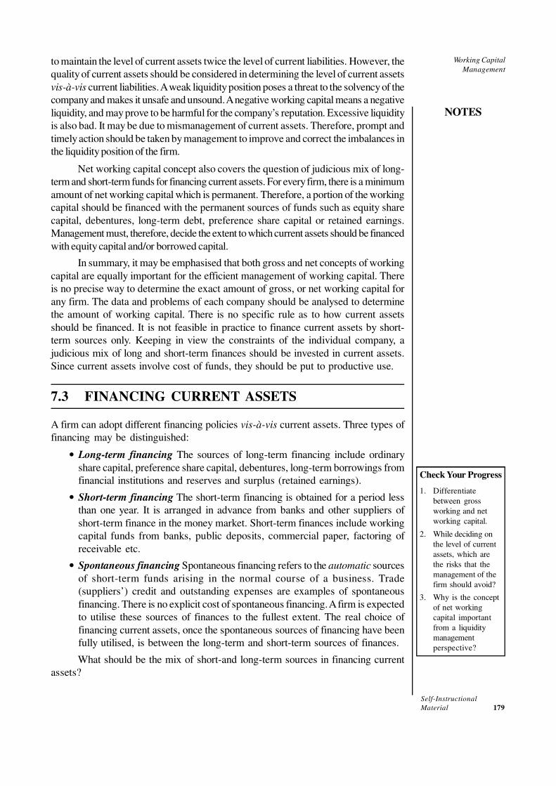
Self-Instructional

Material 179

Working Capital

Management

NOTES

to maintain the level of current assets twice the level of current liabilities. However, the

quality of current assets should be considered in determining the level of current assets

vis-à-vis current liabilities. A weak liquidity position poses a threat to the solvency of the

company and makes it unsafe and unsound. A negative working capital means a negative

liquidity, and may prove to be harmful for the company’s reputation. Excessive liquidity

is also bad. It may be due to mismanagement of current assets. Therefore, prompt and

timely action should be taken by management to improve and correct the imbalances in

the liquidity position of the firm.

Net working capital concept also covers the question of judicious mix of long-

term and short-term funds for financing current assets. For every firm, there is a minimum

amount of net working capital which is permanent. Therefore, a portion of the working

capital should be financed with the permanent sources of funds such as equity share

capital, debentures, long-term debt, preference share capital or retained earnings.

Management must, therefore, decide the extent to which current assets should be financed

with equity capital and/or borrowed capital.

In summary, it may be emphasised that both gross and net concepts of working

capital are equally important for the efficient management of working capital. There

is no precise way to determine the exact amount of gross, or net working capital for

any firm. The data and problems of each company should be analysed to determine

the amount of working capital. There is no specific rule as to how current assets

should be financed. It is not feasible in practice to finance current assets by short-

term sources only. Keeping in view the constraints of the individual company, a

judicious mix of long and short-term finances should be invested in current assets.

Since current assets involve cost of funds, they should be put to productive use.

7.3 FINANCING CURRENT ASSETS

A firm can adopt different financing policies vis-à-vis current assets. Three types of

financing may be distinguished:

• Long-term financing The sources of long-term financing include ordinary

share capital, preference share capital, debentures, long-term borrowings from

financial institutions and reserves and surplus (retained earnings).

• Short-term financing The short-term financing is obtained for a period less

than one year. It is arranged in advance from banks and other suppliers of

short-term finance in the money market. Short-term finances include working

capital funds from banks, public deposits, commercial paper, factoring of

receivable etc.

• Spontaneous financing Spontaneous financing refers to the automatic sources

of short-term funds arising in the normal course of a business. Trade

(suppliers’) credit and outstanding expenses are examples of spontaneous

financing. There is no explicit cost of spontaneous financing. A firm is expected

to utilise these sources of finances to the fullest extent. The real choice of

financing current assets, once the spontaneous sources of financing have been

fully utilised, is between the long-term and short-term sources of finances.

What should be the mix of short-and long-term sources in financing current

assets?

Check Your Progress

1. Differentiate

between gross

working and net

working capital.

2. While deciding on

the level of current

assets, which are

the risks that the

management of the

firm should avoid?

3. Why is the concept

of net working

capital important

from a liquidity

management

perspective?

Self-Instructional

180 Material

Working Capital

Management

NOTES

Depending on the mix of short- and long-term financing, the approach followed

by a company may be referred to as:

• Matching approach

• Conservative approach

• Aggressive approach

7.3.1 Matching Approach

The firm can adopt a financial plan which matches the expected life of assets with the

expected life of the source of funds raised to finance assets. Thus, a ten-year loan may

be raised to finance a plant with an expected life of ten years; stock of goods to be sold

in thirty days may be financed with a thirty-day commercial paper or a bank loan. The

justification for the exact matching is that, since the purpose of financing is to pay for

assets, the source of financing and the asset should be relinquished simultaneously. Using

long-term financing for short-term assets is expensive as funds will not be utilised for the

full period. Similarly, financing long-term assets with short-term financing is costly as

well as inconvenient as arrangement for the new short-term financing will have to be

made on a continuing basis.

When the firm follows matching approach (also known as hedging approach),

long-term financing will be used to finance fixed assets and permanent current assets

and short-term financing to finance temporary or variable current assets. However, it

should be realised that exact matching is not possible because of the uncertainty about

the expected lives of assets.

Figure 7.1 is used to illustrate the matching plan over time.1 The firm’s fixed

assets and permanent current assets are financed with long-term funds and as the level

of these assets increases, the long-term financing level also increases. The temporary or

variable current assets are financed with short-term funds and as their level increases,

the level of short-term financing also increases. Under matching plan, no short-term

financing will be used if the firm has a fixed current assets need only.

Fig. 7.1 Financing Under Matching Plan

7.3.2 Conservative Approach

A firm in practice may adopt a conservative approach in financing its current and

fixed assets. The financing policy of the firm is said to be conservative when it depends

more on long-term funds for financing needs. Under a conservative plan, the firm finances

its permanent assets and also a part of temporary current assets with long-term financing.

Self-Instructional

Material 181

Working Capital

Management

NOTES

In the periods when the firm has no need for temporary current assets, the idle long-

term funds can be invested in the tradable securities to conserve liquidity. The conservative

plan relies heavily on long-term financing and, therefore, the firm has less risk of facing

the problem of shortage of funds. The conservative financing policy is shown in Figure

7.2.2 Note that when the firm has no temporary current assets [e.g., at (a) and (b)]; the

long-term funds released can be invested in marketable securities to build up the liquidity

position of the firm.

Fig. 7.2 Conservative Financing


A firm may be aggressive in financing its assets. An aggressive policy is said to be

followed by the firm when it uses more short-term financing than warranted by the

matching plan. Under an aggressive policy, the firm finances a part of its permanent

current assets with short-term financing. Some extremely aggressive firms may

even finance a part of their fixed assets with short-term financing. The relatively

more use of short-term financing makes the firm more risky. The aggressive financing

is illustrated in Figure 7.3.3

Fig. 7.3 Aggressive Financing

7.3.4 Short-term vs. Long-term Financing: A Risk-Return

Trade-off

A firm should decide whether or not it should use short-term financing. If short-term

financing has to be used, the firm must determine its portion in total financing. This

Self-Instructional

182 Material

Working Capital

Management

NOTES

decision of the firm will be guided by the risk-return trade-off. Short-term financing may

be preferred over long-term financing for two reasons: (i) the cost advantage and (ii)

flexibility.4 But short-term financing is more risky than long-term financing.

Cost: Short-term financing should generally be less costly than long-term financing. It

has been found in developed countries, like USA, that the rate of interest is related to the

maturity of debt. The relationship between the maturity of debt and its cost is called the

term structure of interest rates. The curve, relating to the maturity of debt and

interest rates, is called the yield curve. The yield curve may assume any shape, but it is

generally upward sloping. Figure 7.4 shows the yield curve. The figure indicates that

more the maturity greater the interest rate.

Fig. 7.4 Yield Curve

The justification for the higher cost of long-term financing can be found in the

liquidity preference theory. This theory says that since lenders are risk averse, and

risk generally increases with the length of lending time (because it is more difficult to

forecast the more distant future), most lenders would prefer to make short-term loans.

The only way to induce these lenders to lend for longer periods is to offer them higher

rates of interest.

The cost of financing has an impact on the firm’s return. Both short and long-term

financing have a leveraging effect on shareholders’ return. But the short-term financing

ought to cost less than the long-term financing; therefore, it gives relatively higher return

to shareholders.

It is noticeable that in India short-term loans cost more than long-term loans.

Banks are the major suppliers of the working capital finance in India. Their rates of

interest on working capital finance are quite high. The main source of long-term

loans are financial institutions which till recently were not charging interest at

differential rates. The prime rate of interest charged by financial institutions is lower

than the rate charged by banks.

Flexibility It is relatively easy to refund short-term funds when the need for funds

diminishes. Long-term funds such as debenture loan or preference capital cannot be

refunded before time. Thus, if a firm anticipates that its requirements for funds will

diminish in near future, it would choose short-term funds.

Risk Although short-term financing may involve less cost, it is more risky than

long-term financing. If the firm uses short-term financing to finance its current

assets, it runs the risk of renewing borrowings again and again. This is particularly so in

Self-Instructional

Material 183

Working Capital

Management

NOTES

the case of permanent assets. As discussed earlier, permanent current assets refer to

the minimum level of current assets which a firm should always maintain. If the firm

finances its permanent current assets with short-term debt, it will have to raise new

short-term funds as debt matures. This continued financing exposes the firm to certain

risks. It may be difficult for the firm to borrow during stringent credit periods. At times,

the firm may be unable to raise any funds and consequently, its operating activities may

be disrupted. In order to avoid failure, the firm may have to borrow at most inconvenient

terms. These problems are much less when the firm finances with long-term funds.

There is less risk of failure when the long-term financing is used.

Risk-return trade-off Thus, there is a conflict between long-term and short-term

financing. Short-term financing is less expensive than long-term financing, but, at

the same time, short-term financing involves greater risk than long-term financing.

The choice between long-term and short-term financing involves a trade-off between

risk and return. This trade-off may be further explained with the help of an example

in Illustration 7.1.

Illustration 7.1: Working Capital Financing: Risk-return Trade-off

Suppose that a firm has an investment of ` 50 crore in assets, ` 30 crore invested in

fixed assets and ` 20 crore in current assets. It is expected that assets will yield a

return of 18 per cent before interest and taxes. Tax rate is assumed to be 35 per cent.

The firm maintains a debt ratio of 60 per cent. Thus, the firm’s assets are financed

by 40 per cent equity that is ` 20 crore equity funds are invested in its total assets.

The firm has to decide whether it should use a 12 per cent short-term debt or a 14

per cent long-term debt to finance its current assets. The financing plans would

affect the return on equity funds differently. The calculations of return on equity are

shown in Table 7.1.

Table 7.1 Effect of Long-Term and Short-Term Financing

Financing Plan

Conservative Moderate Aggressive

`̀̀̀ ’000 `̀̀̀ ’000 `̀̀̀ ’000

Fixed assets 300,000 300,000 300,000

Current assets 200,000 200,000 200,000

Total assets 500,000 500,000 500,000

Short-term debt (12%) 60,000 150,000 300,000

Long-term debt (14%) 240,000 150,000 0

PBIT 90,000 90,000 90,000

Interest 40,800 39,000 36,000

EBT 49,200 51,000 54,000

Tax (35%) 17,220 17,850 18,900

Net income 31,980 33,150 35,100

Return on equity 16.00% 16.58% 17.55%

SF/TF 12% 30% 60%

* SF = Short-term financing, TF = Total financing.

It is shown in Table 7.1 that return on equity is highest under the aggressive plan

and lowest under the conservative plan. The results of moderate plan are in between

Self-Instructional

184 Material

Working Capital

Management

NOTES

these two extremes. However, the aggressive plan is the most risky as short-term financing

as a ratio of total financing is maximum in this case. The short-term financing to total

financing ratio is minimum in case of the conservative plan and, therefore, it is less risky.

Let us summarise our discussion on the structure and financing of current assets.

The relative liquidity of the firms assets structure is measured by current assets to fixed

assets (or current assets to total assets) ratio. The greater this ratio, the less risky as

well as less profitable will be the firm and vice versa. Similarly, the relative liquidity of

the firm’s financial structure can be measured by the short-term financing to total financing

ratio. The lower this ratio, the less risky as well as profitable will be the firm and vice

versa. In shaping its working capital policy, the firm should keep in mind these two

dimensions—relative asset liquidity (level of current assets) and relative financing

liquidity (level of short-term financing) of the working capital management. A firm will

be following a very conservative working capital policy if it combines a high level of

current assets with a high level of long-term financing (or low level of short-term

financing). Such a policy will not be risky at all but would be less profitable. An aggressive

firm, on the other hand, would combine low level of current assets with a low level of

long-term financing (or high level of short-term financing). This firm will have high

profitability and high risk. In fact, the firm may follow a conservative financing policy to

counter its relatively liquid assets structure in practice. The conclusion of all this is that

the considerations of assets and financing mix are crucial to the working capital

management.

7.4 HEDGING APPROACH

The term derivatives can simply be understood as those items that do not have their own

independent values, rather they have derived values. Derivatives have a significant place

in finance and risk management. A derivative is a financial instrument whose pay-off is

derived from some other asset which is called an underlying asset. An option is a

derivative. For example, in case of a stock option, the underlying asset is share (stock)

of a company. The value of the stock option depends on the value of the share. Options

are more complicated derivatives. There are a large number of simple derivatives like

futures or forward contracts or swaps.

Firms do not like risk; they do not consider it desirable. Firms will take risks only

when they are appropriately compensated for the risk. By reducing risk, they can avoid

cash flow fluctuations and thus, increase value of their assets or investments. Not

surprisingly, firms always look for ways and means of reducing their risk. Derivatives

are tools to reduce a firm’s risk exposure. A firm can do away with unnecessary parts of

risk exposure and even convert exposures into quite different forms by using derivatives.

Hedging is the term used for reducing risk by using derivatives.

There are several advantages of better risk management through hedging:

1. Debt capacity enhancement: Financial risk management helps to

understand and manage investment and financing risk. It reduces a firm’s

costs of financial distress. Hence, the firm can increase debt capacity

and interest tax shield.

2. Increased focus on operations: Financial risk management requires

managers to hedge against possible movements in interest rates and

exchange rates. These factors are not under the control of managers nor

can they predict their behaviour. Hedging against such risks encourages

Check Your Progress


long-term and

short-term sources

for financing

working capital?

5. What should be the

mix of short-term

and long term

sources in financing

current assets?

Self-Instructional

Material 185

Working Capital

Management

NOTES

managers to concentrate their efforts on improving operations rather than

worrying about factors that are not in their control.

3. Isolating managerial performance: Hedging helps to separate out the

effects of fluctuating external factors (interest or exchange rate) and good

or bad management on the firm’s profitability. If a company that always

hedges its risk suffers a loss or its profits drop, then it means bad management.

In the following sections, we shall discuss how risk can be hedged by using options,

futures and forward contracts, and swaps.

7.4.1 Risk Hedging with Options

An option is a right to buy or sell an asset at a specified exercise price at a specified

period of time. Option is a right and does not constitute any obligation on the part of the

buyer or seller of the option to buy or sell the underlying asset.

A foreign currency option is a handy method of reducing foreign exchange risk.

Similarly, options on interest rates and commodities are quite popular with managers to

reduce risk. Many options trade on option exchanges. However, in practice, banks and

companies strike private option deals.

How does option help reducing risk of a company? Consider an example. Suppose

Indian Oil Company (IOC) imports thousands of barrels of oil. The company is expecting

increase in the price of oil. The company can lock in the price of oil by purchasing an

option to buy oil at a predetermined future date at a specified exercise price. For example,

it could acquire 3-month option to buy 3,000 barrels of oil at an exercise price of $50.

There is no free lunch; IOC will have to pay option premium to the seller of the option.

Assume that this premium is $0.60 per barrel. By incurring a small cost (option premium),

IOC has bought an insurance against increase in the oil price.

Suppose the oil price at the time of option expiry is $52 per barrel. Since the oil

price is higher than the exercise price of $50, IOC will gain by exercising the option. It

will be able to buy oil at $50 while the actual price (called spot price) is $52. In practice,

firms may collect the difference between the exercise price and the oil price. Since IOC

paid a premium to acquire the option, its net payoff is:

Net pay-off = (52 – 50) × 3,000 – 0.60 × 3,000

= 6,000 – 1,800 = $4,200

The cost of oil to IOC is: 50 × 3,000 = $1,50,000. Thus, the net cost to the company

is: 1,50,000 – 4,200 = $1,45,800.

On the other hand, if the oil price is below the exercise price, IOC will let the

option expire as it is worthless for the company. If the oil price is $49, it is in IOC’s

interest to buy oil from the market at $49 spot price rather than pay an exercise price

of $50. Thus, the cost of oil to the company is: 49 × 3,000 = $1,47,000. IOC has a

net loss from option in the form of option premium: 0.60 × 3,000 = $1,800. The net

cost to the company is: 1,47,000 + 1,800 = $1,48,800.

We may observe from this example that buying an option shields a company

from increases in the prices while the company can continue benefiting from the

decease in the prices. Thus, option creates an opportunity to guard against risk and

benefit from changes in the prices. The cost of this opportunity is option premium.

Let us consider another example. Suppose ONGC sells oil to Indian Petrochemical

Limited (IPCL). ONGC wants to protect itself from a potential fall in oil prices. What

Self-Instructional

186 Material

Working Capital

Management

NOTES

should it do? It should buy a put option—a right to sell oil at a specified exercise price at

a specified time. ONGC will be able to protect itself from falling prices and at the same

time benefit from increase in the oil prices. Suppose ONGC buys the put option with the

` 25,000 exercise price at a premium of ` 50 per barrel. If the price of oil on the day

option expires is less than the exercise price, ONGC will exercise the option since it will

fetch the locked in price of ̀ 25,000 per barrel. On the other hand, if the oil price is more

than the exercise price, it will allow the option to lapse as it can getsell the oil at a higher

price. In both situations there is a cost in the form of option premium involved.

Illustration 7.2: Hedging with Options

A goldsmith from Surat plans to import 1,000 troy ounces of gold in three months. He

suspects fluctuations in the gold prices. The price could be $320, $340 or $360 an ounce.

The goldsmith is thinking of buying a 3-month call option on 1,000 ounces of gold with an

exercise price of $340. The option will cost $4 per ounce. What is the total cost to the

goldsmith under different gold prices?

The goldsmith would exercise the call option when the gold price is more than the

exercise price, otherwise he would allow it to lapse. When the gold price is higher than

the exercise price, the goldsmith’s payoff will be the difference between the gold price

and the exercise price. The total cost to the gold smith is as follows:

Gold Price, Dollar per ounce

$320 $340 $360

Cost of 1,000 ounces 3,20,000 3,40,000 3,60,000

Less: Pay-off on call option 0 0 20,000

Plus: option premium 4,000 4,000 4,000

3,24,000 3,44,000 3,44,000

Forward Contracts

We do frequently enter into arrangements or under-standing now for buying or selling

items in the future. These arrangements, when formalized, are referred to as forward

contracts. Let us clarify further with the help of an example. Suppose you have

been admitted to a post-graduate management programme of one of the prestigious

management institutes in India. To cope with the academic workload and, particularly,

to do assignments in finance and quantitative courses, you intend to buy a desktop

computer. You approach a computer dealer on 1 July. When you go to the computer

shop, you find that the computer make of your choice is not available for immediate

delivery. The shopkeeper offers to deliver the computer of your choice to you after

15 days (15 July) for ` 30,000. He also states that if you don’t accept the offer, and

if you want to buy the computer after 15 days, you will have to pay the actual or the

spot price on that day which could be more than ` 30,000. You agree to the

shopkeeper’s offer. In fact, you have entered into a forward contract with the shopkeeper.

You are under an obligation to buy the computer and pay to the shopkeeper ` 30,000

after 15 days and the shopkeeper is obliged to deliver the computer to you. As you agree

to buy the computer, you are buying a forward contract. You will be taking delivery of

the computer, called deliverable instrument, on the due date. The shopkeeper, by

handing over the computer to you, will be making delivery to you. Table 7.2 illustrates

the forward contract vis-à-vis your computer deal.

Self-Instructional

Material 187

Working Capital

Management

NOTES

Table 7.2 Example of Forward Contract for Computer Purchase

1 July 2009 15 July 2009

Buyer of Forward Contract Buyer of Forward Contract

1. Agrees to pay price of ` 30,000 1. Makes payment of ` 30,000

2. Agrees to take delivery of computer 2. Takes delivery of computer due date

on agreed (15 July)

Seller of Forward Contract Seller of Forward Contract

1. Agrees to make delivery of computer 1. Makes delivery of computer

on agreed due date (15 July)

2. Agrees to receive purchase price of 2. Receives payment of ` 30,000

` 30,000 on agreed due date (15 July)

After 15 days, when you take delivery of the computer, you discover that the

actual price of the computer, called spot price, is ` 31,000. You have a gain of

` 1,000 since you shall pay ` 1,000 less than the current price. Forward contract is a

very simple tool of hedging risk. A forward contract is an agreement between two

parties to exchange an asset for cash at a predetermined future date for a price that

is specified today.

Suppose that when you approach the shopkeeper for buying a computer, he

has it for immediate delivery. You will pay him the cash and take the delivery. This

is a cash transaction where the exchange takes place immediately. Forward contracts

must be differentiated from the cash transactions.

You would notice that a forward contract is similar to an option in hedging

risk, but there is a significant difference. In case of a forward contract, both the

buyer and the seller are bound by the contract; the buyer must take the delivery and

the seller must make the delivery at the agreed price on the specified due date.

Under an option, the buyer has a right to decide whether or not she would exercise

the option.

Forward contracts are flexible. They are tailor-made to suit the needs of the

buyers and sellers. You can enter into a forward contract for any goods, commodities

or assets. You can choose your delivery date for any quantity of goods or commodities.

For example, you need a small quantity of gold, say, two troy ounce, after 45 days.

You can fix the price of two troy ounce of gold today by an agreement with a gold

supplier forward. After 45 days, you will take the delivery of gold by paying the

agreed price. There should always be willing buyers and sellers for entering into a

forward contract. Though forward contracts are entered into for different goods,

commodities or assets, etc., but the foreign currencies forwards have the largest

trading.

Illustration 7.3: Hedging through Forward Contract

An Indian company has ordered machinery from USA. The price of $5,00,000 is payable

after six months. The current exchange rate is ̀ 45.75/$. At the current exchange rate,

the company would need: 45.75 × 5,00,000 = ̀ 22,875,000. But the company anticipates

depreciation of Indian rupee over time. The cost to the company in Indian rupees will

increase if rupee depreciates when payment is made after six months. What should the

company do? The company can lock in the exchange rate by entering into a forward

contract and forget about any fluctuation in the exchange rate. Suppose the six-month

forward exchange rate is ̀ 45.95. The company can buy dollars forward. At the time of

making payment, it will exchange ̀ 22,975,000 for buying $5,00,000.

Self-Instructional

188 Material

Working Capital

Management

NOTES

Futures Contracts

Suppose a farmer produces barley. He is expecting to have an excellent yield of barley;

but he is worried. He is concerned about the future prices of barley. The farmer fears

fall in the barley prices in the future. How can he protect himself from the potential of

falling price of barley? The farmer supplies barley to a breakfast cereal manufacturer.

The farmer can reduce his risk exposure and worries if he could lock in the barley price

today. He can do so by entering into a contract today with the manufacturer who wants

to buy barley for delivery in the future. The farmer agrees today to sell barley to the

manufacturer at a specified future date at a price agreed upon today. The manufacturer

is in a different position from the farmer; he is worried that the barley price might

increase in the future. He can fix the barley price ahead of time, and take delivery in the

future. He would agree to buy barley at a predetermined price on a specified due date.

In fact, the manufacturer and the farmer have entered into a futures contract.

The farmer will deliver barley to the manufacturer in the future and receive the

agreed price, and the manufacturer will take delivery of barley and pay to the farmer.

What are the consequences of doing so? First, there is no exchange of money when

the contract is entered. The barley farmer agrees to sell barley on a specified future

date at a price agreed upon today. The miller agrees to buy at the same price and on

the same due date. Second, the contract is binding on both the parties. The barley

farmer must sell the barley and the miller must buy irrespective of the actual price

in the future.

You may be wondering that futures contracts are like forward contracts. It is

true that future contracts are no different from forward contracts as they serve the

same purpose and operate through a contract between counterparties. The difference

is in terms of standardization and method of operation. Futures contracts have

standardized contract size and they trade only on the organized exchanges. Thus,

future contracts are forwards contracts traded on organized exchanges in standardized

contract size. For example, the standard contract size for barley in the barley

international exchange is 20 metric ton. You can enter into barley futures contracts

for 20 metric ton or its multiples. If your requirement is less than 20 metric ton, then

you should enter into a forward contract as it can be custom made for your specific

requirement.

Both the farmer and the manufacturer have hedged risk and both have less

risk than before. The farmer has protected himself against risk by selling barley

futures; his action is called a short hedge. The short hedge is a common occurrence

in business, and it takes place whenever a firm or an individual is holding goods or

commodities (or any other asset) or is expecting to receive goods or commodities.

Farmers anticipate receiving commodities from harvesting agriculture commodities.

A producer of petrochemical products may carry inventory of oil. In our example,

the manufacturer has protected himself against risk by buying barley futures; his

action is referred to as a long hedge. Generally, a long hedge occurs when a person or

the firm is committed to buy at a fixed price.

Like options, one could use futures contracts to hedge risk. But, as with forward

contract and option, there is a difference between these two instruments as well. Unlike

options but like forward contracts, future contracts are obligations; on the due date the

seller (farmer) has to deliver barley to the buyer (miller) and the buyer will pay the seller

the agreed price.

Self-Instructional

Material 189

Working Capital

Management

NOTES

In the futures contracts, like in the forward contracts, one party would lose and

another will gain. The profit and loss will depend on the agreed futures price and the

actual spot at the time of contract maturity. Suppose the futures price of barley is

` 20,000 per metric ton and the market price turns out to be ̀ 21,500 per metric ton on

the due date. The barley farmer will receive ̀ 1,500 per metric ton less. His loss is the

miller’s gain; he will pay ` 1,500 per metric ton less. Thus, the seller of the contract

gains when the contracted price is more than the actual market price later on. The buyer

of the contract will gain when the contracted price is less than the actual market price.

Both the barley farmer and the miller are able to hedge their risk. The farmer has

locked in the selling price and the miller has locked in the buying price. Both can

concentrate on their operations, instead of worrying about the fluctuations in the barley

price.

Illustration 7.4: Hedging with Futures

A coal mining company is concerned about short-term volatility in its revenues. Coal

currently sells for ̀ 7,000 per ton. But the price could fall as low as ̀ 6,500 per ton or as

high as ̀ 7,400 per ton. The company will supply about 5,000 tons to the market next

month. What are the consequences if the company does not hedge? What is the cost to

the company if it enters into a futures contract to deliver 5,000 tons of coal at an agreed

price of ̀ 7,050 per ton next month?

If the company does not hedge risk, it will not know what the selling price will be after

one month and its revenues will depend on the actual price after one month. If the

company hedges through the coal futures, it will lock in the selling price which in the

present case is ̀ 7,050 per ton. Thus, the company’s position will be as shown below:

Hedging Risk

Futures price 7,050 7,050 7,050

Spot price 7,400 7,000 6,500

Profit/loss –350 +50 +550

Financial Futures

Futures are traded in a wide variety of commodities: wheat, sugar, gold, silver, copper,

oranges, coco, oil soybean, etc. Commodity prices fluctuate far and wide. For large

buyers of a commodity whose prices swing downward and upward, there are significant

cost implications. These companies reduce their risk of upward movements in prices by

hedging with commodity futures.

There are firms which do not have commodity prices exposure but they have

significant exposure of interest rates and exchange rates fluctuations. These firms

can hedge their exposure through financial futures. Financial futures, like the

commodity futures, are contracts to buy or sell financial assets at a future date at a

specified price. Financial futures, introduced for the first time in 1972 in USA, have

become very popular. Now the trading in financial futures far exceeds trading in

commodity futures.

Futures Contracts vs. Forward Contracts

Futures contracts originated for hedging risk of agricultural commodities and later on

many more commodities were covered under futures contracts. In terms of the basic

nature, forward contracts and futures contracts are same. But in the operating terms

there are the following differences.

Self-Instructional

190 Material

Working Capital

Management

NOTES

Table 7.3 Examples of Listed Futures Contracts

Contract Contract size Exchange

Corn 5,000 bushels CBT

Soybeans 5,000 bushels CBT

Wheat 5,000 bushels KC

Barley 20 metric ton WPG

Rye 21 metric ton WPG

Pork bellies 40,000 lbs CME

Cotton 50,000 lbs CTN

Orange juice 15,000 lbs. CTN

Sugar (world) 1,12,000 lbs. CSCE

Coffee 37,500 lbs. CSCE

Gold 100 troy oz. CMX

Crude oil (light sweet) 1,000 barrels NYM

Eurodollar $1 million LIFFE

German Mark 1,25,000 marks IMM

Treasury bonds $1,00,000 CBT

Treasury notes $1,00,000 CBT

S&P Index 500 times Index CME

NYSE Composite 501 times Index NYFE

Major Market Index 250 times Index CBT

CBT = Chicago Board of Trade

KC = Kansas City

WPG = Winnipeg

CME = Chicago Mercantile Exchange

CTN = New Cotton Exchange

CSCE = Coffee, Sugar, and Cocoa Exchange

CMX = Commodity Exchange in New York

NYM = New York Mercantile

IMM = International Monetary Market in Chicago

LIFFE = London International Financial Futures Exchange

NYFE = New York Futures Exchange

Organized futures exchanges: Forward contracts are contracts between two parties,

called the counterparties and they are not traded on any exchange. Future contracts

are traded in the organized future exchanges. As stated earlier, futures contracts are

forward contracts traded on the futures exchanges. The Chicago Board of Trade is

the largest futures exchange. Other exchanges include Commodity Exchange in New

York, International Monetary Market in Chicago, London International Financial Futures

Exchange, etc., In a futures exchange the delivery dates are specified, but there is

choice of delivery dates. The futures prices would be higher as the delivery date extends.

For example, the December 2004 futures contract will have a higher price than, say, the

October 2004 futures contract.

Standardized contracts: Futures contracts are standar-dized contracts in terms of the

amount or quantity as well as the quality of the product. The seller of the futures contract

Self-Instructional

Material 191

Working Capital

Management

NOTES

will have to deliver goods or commodities of a specified quality. Forward contracts are

non-standard. They are custom-made depending on the requirements of the

counterparties. Table 7.3 gives examples of futures contracts in certain commodities,

products and financial instruments, contract size and the exchange where these futures

contracts are traded. For example, you may notice that if you want to enter into a barley

futures contract, the minimum size of the contract is 20 metric ton.

Margin: The buyers and sellers of the futures contracts are required to deposit some

cash or securities as margin. This is done to ensure that the buyers and sellers honour

the deal. In case of forward contracts, there is no formal requirement of margin.

Marked to market: This is a significant difference between forward contracts and

futures contracts. Forward contracts are settled on the due date. But in the case of

futures contracts, there is daily closing and reopening of the position which is called

marked to market. Consider an example to understand the meaning of marked to

market. Suppose you have a futures contract to deliver 1,000 troy ounces of gold at $300

per troy ounce. Assume that the price of the gold futures next day is $305 per troy ounce

of gold. You have a loss on your sales of 1,000 troy ounces of gold: 1,000 (305 – 300) =

$5,000. You will be required to pay this amount to the futures exchange. After the first

day your loss is $5 per troy ounce and now your obligation is to deliver gold at $305 per

troy ounce. This is like buying back your future position each day and then entering into

a new futures contract. The buyer of the gold has a reverse position. He makes a profit

of $5 due to increase in the futures price. He will receive this profit from the exchange.

On the part of the buyer of gold, this is like selling back the futures position each day and

then entering into a new futures contract. This is referred to marked to market. Marked

to market means that profit and loss on a futures contract are calculated each day, and

if there is a profit, you receive profit from the exchange but if there is a loss, you pay loss

to the exchange.

Delivery: A seller of the futures contract may wait for the contract to mature and then

make the delivery. In practice, the seller of the futures contracts buys back the futures

just before delivery. Most forward contracts are made to give and take delivery.

Futures and Spot Prices of Financial Futures

The price of a commodity or financial asset for immediate delivery is known as the spot

price. The futures price and spot price today will not be the same. Let us first explain

the futures and spot prices of a financial asset. The difference in the prices will be on

account of the financial cost and dividend or interest associated with a financial security.

Suppose a person owns a share that he can sell immediately for cash or sell at a later

date at the futures price. If he sells the financial asset at the spot price immediately

instead of selling share futures, he will earn interest on the amount received, but he will

have to forgo any dividend on the share that he would have received by holding the

asset. Let us consider another example where a person wants to buy a share. He can

buy it immediately at spot price, or enter into a futures contract and take delivery in the

future at futures price. Under the futures contract, there will be no outgo of cash and the

buyer has an opportunity of earning interest on the purchase price. But, since the buyer

will not hold the share, he will lose the opportunity of earning dividends (or interest in

case of a debt security). Thus, the relationship between the spot and the future prices

will be as follows:

Self-Instructional

192 Material

Working Capital

Management

NOTES

Futures price Spot price (1+ ) dividend foregonetrf

= −

Future price Dividend foregoneSpot price

(1+ ) (1 )t tr rf f

= +

+

(1)

Alternatively, we can write the following equation:

Dividend foregone Future priceSpot price

(1 ) (1+ )t tr rf f

− =

+ (2)

Note that rf is the risk-free rate of interest. Let us consider an example of the stock

index futures.

Stock Index Futures Stock index futures are futures contracts on stock market

indices. For example, stock index futures are available on New York Stock Exchange,

S&P500, S&P100 and the Major market Index, etc. What is the relationship between

the stock index futures and spot prices?

Suppose the stock index is at 2,500. The risk-free interest rate is 6 per cent

per annum. The average annul dividend yield is 2 per cent. How much would be the

one-year stock index futures?

1 1Futures price = 2,500 (1.06) 2,500 (0.02) 2,600− =

Stock index futures, like other futures contracts, are traded in organized

exchanges and have standardized size. For example, the S&P500 index has a contract

size of $500 times the index.

On 20 November 2004, a broker is anticipating rise in S&P500 when the

December S&P500 futures is at 1,200. The broker purchases one December contract

for 1,200 × $500 = $600,000. The S&P500 index increases to 1,250 by 20 December

2004. The broker decides to sell his contract. How much profit does the broker

make?

The broker’s profit is: (1,250 – 1,200) × $500 = $125,000.

Spot and Future Prices of Commodity Futures: There is a difference between the

spot and futures prices of financial assets and commodities. In case of commodity

futures, there is no dividend forgone. Further, the buyer of commodity futures does

not need to store commodity as delivery will be in the future. Therefore, he avoids

storage cost. Also, the buyer does not have commodity in hand which does not give

him a comfort or convenience of meeting sudden requirements. Thus, the buyer saves

storage cost but loses in terms of convenience yield.5 The spot and futures prices

relationship in case of commodities futures is given as follows:

t t tf f f

Spot price

Future price Storage costs Convenience yield= +

(1+ r ) (1+ r ) (1+ r )−

(3)

tf

t tf f

Future price

(1+ r )

Storage costs Convenience yield= Spot price +

(1+ r ) (1+ r )−

(4)

Self-Instructional

Material 193

Working Capital

Management

NOTES

The difference between the present value storage costs and convenience yield is

net convenience yield (NCY). In practice, it can be inferred as the difference between

the present value of futures price and spot price.

Illustration 7.5: Convenience Yield

Suppose the spot price for wheat was $2.85 per bushel in September 2004. The one-

year futures price was $3.38 per bushel. The interest rate is 6 per cent. What is the net

convenience yield?

1

3.38= 2.85 + PV (storage costs - convenience yield)

(1.06)

PV (NCY) = 3.19 - 2.85 = $ 0.34

Trading in the futures contracts runs into billions of dollars each day. Since the futures

contracts are traded on the organized exchanges, there is high degree of liquidity. But

the futures contracts may not suit the needs of all. The contract size is standardized and

the delivery dates are specified in each year. If the futures contracts are not suitable for

the needs of a company, it can buy or sell forward contracts.

7.5 LEVEL OF CURRENT AND LIQUID ASSETS

Current Assets to Fixed Assets Ratio

The financial manager should determine the optimum level of current assets so that the

wealth of shareholders is maximized. A firm needs fixed and current assets to support a

particular level of output. However, to support the same level of output, the firm can

have different levels of current assets. As the firm’s output and sales increase, the need

for current assets increases. Generally, current assets do not increase in direct proportion

to output; current assets may increase at a decreasing rate with output. This relationship

is based upon the notion that it takes a greater proportional investment in current assets

when only a few units of output are produced, than it does later on, when the firm can

use its current assets more efficiently.

Exhibit 7.1 Levels of Current Assets: Some Examples

of Indian Companies

Current assets form a significant portion of total assets of many Indian companies.

Consider the following examples:

BHEL GNFC L&T Voltas

Sales 7651.1 1476.7 8782.5 1232.3

Total assets (TA) 9600.4 1991.9 17095.9 862.9

Current assets (CA) 8601.0 882.9 11398.4 658.4

CA/TA 89.6 44.3 66.7 76.3

CA/Sales 112.4 59.8 129.8 53.4

Note: Data for the year 2003, except in case of BHEL.

• Voltas Voltas is a large, well-diversified, private sector marketing-cum-

manufacturing organization. In 2003, the company’s current assets are three-

fourths of total assets and more than half of sales.

Check Your Progress

6. What is a

derivative?

7. Define hedging.

8. How are future

contracts different

from forward

contracts?

Self-Instructional

194 Material

Working Capital

Management

NOTES

• L&T Limited L&T is also a diversified company in the private sector. In 2003, its

current assets are two-thirds of total assets and about one and a third times of

sales.

• GNFC GNFC is a joint sector (joint venture between state of Gujarat and private

sector) company manufacturing fertilizers, industrial products (methanol, formic

acid, nitric acid, amonium nitrate, liquid nitrogen etc.) and electronic products. Its

current assets in the year 2003 are less than half of total assets and 60 per cent of

sales.

• BHEL BHEL was started as a large public sector company. Its shares have been

partly divested now. It has a dominant position in the power sector. Its

manufacturing operations are spread into industrial and transportation sectors

also. A large number of its products are long production-cycle products. The

company’s main customers are State Electricity Boards who fail to pay their due

on time. BHEL’s current assets in 2002 are 90 per cent of total assets and 112 per

cent of sales.

The level of the current assets can be measured by relating current assets to fixed

assets. Dividing current assets by fixed assets gives CA/FA ratio. Assuming a constant

level of fixed assets, a higher CA/FA ratio indicates a conservative current assets

policy and a lower CA/FA ratio means an aggressive current assets policy, assuming

other factors to be constant. A conservative policy implies greater liquidity and lower risk;

while an aggressive policy indicates higher risk and poor liquidity. Moderate Coverage)

current assets policy falls in the middle of conservative and aggressive policies. The

current assets policy of the most firms may fall between these two extreme policies. The

alternative current assets policies may be shown with the help of Figure 7.5.

In Figure 7.5 alternative A indicates the most conservative policy, where CA/FA

ratio is greatest at every level of output. Alternative C is the most aggressive policy, as

CA/FA ratio is lowest at all levels of output. Alternative B lies between the conservative

and aggressive policies and is an average policy.

Fig. 7.5 Alternative Current Asset Policies

Liquidity vs Profitability: Risk–Return Trade-off

The firm would make just enough investment in current assets if it were possible to

estimate working capital needs exactly. Under perfect certainty, current assets holdings

would be at the minimum level. A larger investment in current assets under certainty

would mean a low rate of return on investment for the firm, as excess investment in

current assets will not earn enough return. A smaller investment in current assets, on the

other hand, would mean interrupted production and sales, because of frequent stock-

outs and inability to pay to creditors in time due to restrictive policy.

Self-Instructional

Material 195

Working Capital

Management

NOTES

As it is not possible to estimate working capital needs accurately, the firm must

decide about levels of current assets to be carried. Given a firm’s technology and

production policy, sales and demand conditions, operating efficiency etc., its current

assets holdings will depend upon its working capital policy. It may follow a conservative

or an aggressive policy. These policies involve risk–return trade-offs. A conservative

policy means lower return and risk, while an aggressive policy produces higher return

and risk.

The two important aims of the working capital management are: profitability

and solvency. Solvency, used in the technical sense, refers to the firm’s continuous

ability to meet maturing obligations. Lenders and creditors expect prompt settlements of

their claims as and when due. To ensure solvency, the firm should be very liquid, which

means larger current assets holdings. If the firm maintains a relatively large investment

in current assets, it will have no difficulty in paying claims of creditors when they become

due and will be able to fill all sales orders and ensure smooth production. Thus, a liquid

firm has less risk of insolvency; that is, it will hardly experience a cash shortage or a

stock-out situation. However, there is a cost associated with maintaining a sound liquidity

position. A considerable amount of the firm’s funds will be tied up in current assets, and

to the extent this investment is idle, the firm’s profitability will suffer.

To have higher profitability, the firm may sacrifice solvency and maintain a relatively

low level of current assets. When the firm does so, its profitability will improve as fewer

funds are tied up in idle current assets, but its solvency would be threatened and would

be exposed to greater risk of cash shortage and stock-outs.

Illustration 7.6: Working Capital Risk-return Trade-off

Suppose, a firm has the following data for some future year:

`

Sales (100,000 units @ ̀ 15) 1,500,000

Earnings before interest and taxes 150,000

Fixed assets 500,000

The three possible current assets holdings of the firm are: ̀ 5,00,000, ̀ 4,00,000 and

` 3,00,000. It is assumed that fixed assets level is constant and profits do not vary with

current assets levels. The effect of the three alternative current assets policies is shown

in Table 7.4.

Table 7.4 Effect of Alternative Working Capital Policies

Working Capital Policy Conservative A Moderate B Aggressive B

Sales 1,500,000 15,00,000 1,500,000

Earnings before 150,000 150,000 150,000

interest & taxes

(EBIT)

Current assets 500,000 400,000 300,000

Fixed assets 500,000 500,000 500,000

Total assets 1,000,000 900,000 800,000

Return on total assets 15% 16.67% 18.75%

(EBIT/Total assets)

Current assets/Fixed assets 1.00 0.80 0.60

Self-Instructional

196 Material

Working Capital

Management

NOTES

The calculations in Table 7.4 indicate that alternative. A, the most conservative

policy, provides greatest liquidity (solvency) to the firm, but also the lowest return on

total assets. On the other hand, alternative C, the most aggressive policy, yields highest

return but provides lowest liquidity and thus, is very risky to the firm. Alternative B

demonstrates a moderate policy and generates a return higher than alternative A but

lower than alternative C and is less risky than alternative C but more risky than

alternative A.

Illustration 7.6 is a simple example of risk–return trade-off. The calculation of

risk-return trade-off is difficult and returns are affected differently by different assets,

and generalization is not possible.

7.6 FACTORS AFFECTING THE REQUIREMENT OF

WORKING CAPITAL

The firm should maintain a sound working capital position. It should have adequate

working capital to run its business operations. Both excessive as well as inadequate

working capital positions are dangerous from the firm’s point of view. Excessive working

capital means holding costs and idle funds which earn no profits for the firm. Paucity of

working capital not only impairs the firm’s profitability but also results in production

interruptions and inefficiencies and sales disruptions.

The dangers of excessive working capital are as follows:6

• It results in unnecessary accumulation of inventories. Thus, chances of inventory

mishandling, waste, theft and losses increase.

• It is an indication of defective credit policy and slack collection period.

Consequently, higher incidence of bad debts results, which adversely affects profits.

• Excessive working capital makes management complacent which degenerates

into managerial inefficiency.

• Tendencies of accumulating inventories tend to make speculative profits grow.

This may tend to make dividend policy liberal and difficult to cope with in future

when the firm is unable to make speculative profits.

Inadequate working capital is also bad and has the following dangers:7

• It stagnates growth. It becomes difficult for the firm to undertake profitable projects

for non-availability of working capital funds.

• It becomes difficult to implement operating plans and achieve the firm’s profit

target.

·• Operating inefficiencies creep in when it becomes difficult even to meet day-to-

day commitments.

• Fixed assets are not efficiently utilised for the lack of working capital funds.

Thus, the firm’s profitability would deteriorate.

• Paucity of working capital funds render the firm unable to avail attractive credit

opportunities etc.

• The firm loses its reputation when it is not in a position to honour its short-term

obligations. As a result, the firm faces tight credit terms.

An enlightened management should, therefore, maintain the right amount of working

capital on a continuous basis. Only then a proper functioning of business operations will

Self-Instructional

Material 197

Working Capital

Management

NOTES

be ensured. Sound financial and statistical techniques, supported by judgement, should

be used to predict the quantum of working capital needed at different time periods.

A firm’s net working capital position is not only important as an index of liquidity

but it is also used as a measure of the firm’s risk. Risk in this regard means chances of

the firm being unable to meet its obligations on due date. The lender considers a positive

net working as a measure of safety. All other things being equal, the more the net

working capital a firm has, the less likely that it will default in meeting its current financial

obligations. Lenders such as commercial banks insist that the firm should maintain a

minimum net working capital position.

7.6.1 Determinants of Working Capital

There are no set rules or formulae to determine the working capital requirements of

firms. A large number of factors, each having a different importance, influence working

capital needs of firms. The importance of factors also changes for a firm over time.

Therefore, an analysis of relevant factors should be made in order to determine total

investment in working capital. The following is the description of factors which generally

influence the working capital requirements of firms.8

Nature of Business

Working capital requirements of a firm are basically influenced by the nature of its

business. Trading and financial firms have a very small investment in fixed assets, but

require a large sum of money to be invested in working capital. Retail stores, for example,

must carry large stocks of a variety of goods to satisfy varied and continuous demands

of their customers. A large departmental store like Wal-Mart may carry, say, over 20,000

items. Some manufacturing businesses, such as tobacco manufacturers and construction

firms, also have to invest substantially in working capital and a nominal amount in fixed

assets. In contrast, public utilities may have limited need for working capital and have to

invest abundantly in fixed assets. Their working capital requirements are nominal because

they may have only cash sales and supply services, not products. Thus, no funds will be

tied up in debtors and stock (inventories). For the working capital requirements most of

the manufacturing companies will fall between the two extreme requirements of trading

firms and public utilities. Such concerns have to make adequate investment in current

assets depending upon the total assets structure and other variables.

Market and Demand Conditions

The working capital needs of a firm are related to its sales. However, it is difficult to

precisely determine the relationship between volume of sales and working capital needs.

In practice, current assets will have to be employed before growth takes place. It is,

therefore, necessary to make advance planning of working capital for a growing firm on

a continuous basis.

Growing firms may need to invest funds in fixed assets in order to sustain growing

production and sales. This will, in turn, increase investment in current assets to support

enlarged scale of operations. Growing firms need funds continuously. They use external

sources as well as internal sources to meet increasing needs of funds. These firms face

further problems when they retain substantial portion of profits, as they will not be able

to pay dividends to shareholders. It is, therefore, imperative that such firms do proper

planning to finance their increasing needs for working capital.

Self-Instructional

198 Material

Working Capital

Management

NOTES

Sales depend on demand conditions. Large number of firms experience seasonal

and cyclical fluctuations in the demand for their products and services. These business

variations affect the working capital requirement, specially the temporary working capital

requirement of the firm. When there is an upward swing in the economy, sales will

increase; correspondingly, the firm’s investment in inventories and debtors will also

increase. Under boom, additional investment in fixed assets may be made by some firms

to increase their productive capacity. This act of firms will require further additions of

working capital. To meet their requirements of funds for fixed assets and current assets

under boom period, firms generally resort to substantial borrowing. On the other hand,

when there is a decline in the economy, sales will fall and consequently, levels of inventories

and debtors will also fall. Under recession, firms try to reduce their short-term borrowings.

Seasonal fluctuations not only affect working capital requirement but also create

production problems for the firm. During periods of peak demand, increasing production

may be expensive for the firm. Similarly, it will be more expensive during slack periods

when the firm has to sustain its working force and physical facilities without adequate

production and sales. A firm may, thus, follow a policy of level production, irrespective

of seasonal changes in order to utilise its resources to the fullest extent. Such a policy

will mean accumulation of inventories during off-season and their quick disposal during

the peak season.

The increasing level of inventories during the slack season will require increasing

funds to be tied up in the working capital for some months. Unlike cyclical fluctuations,

seasonal fluctuations generally conform to a steady pattern. Therefore, financial

arrangements for seasonal working capital requirements can be made in advance.

However, the financial plan or arrangement should be flexible enough to take care of

some abrupt seasonal fluctuations.

Technology and Manufacturing Policy

The manufacturing cycle (or the inventory conversion cycle) comprises the purchase

and use of raw materials and the production of finished goods. Longer the manufacturing

cycle, larger will be the firm’s working capital requirements. For example, the

manufacturing cycle in the case of a boiler, depending on its size, may range between

six to twenty-four months. On the other hand, the manufacturing cycle of products such

as detergent powder, soaps, chocolate etc. may be a few hours. An extended

manufacturing time span means a larger tie-up of funds in inventories. Thus, if there are

alternative technologies of manufacturing a product, the technological process with the

shortest manufacturing cycle may be chosen. Once a manufacturing technology has

been selected, it should be ensured that manufacturing cycle is completed within the

specified period. This needs proper planning and coordination at all levels of activity.

Any delay in manufacturing process will result in accumulation of work-in-process and

waste of time. In order to minimise their investment in working capital, some firms,

specifically those manufacturing industrial products, have a policy of asking for advance

payments from their customers. Non-manufacturing firms, service and financial enterprises

do not have a manufacturing cycle.

A strategy of level or steady production may be maintained in order to resolve the

working capital problems arising due to seasonal changes in the demand for the firm’s

product. A steady or level production policy will cause inventories to accumulate

during the off-season periods and the firm will be exposed to greater inventory costs and

risks. Thus, if costs and risks of maintaining a constant production schedule are high, the

Self-Instructional

Material 199

Working Capital

Management

NOTES

firm may adopt a variable production policy, varying its production schedules in

accordance with changing demand. Those firms, whose productive capacities can be

utilised for manufacturing varied products, can have the advantage of diversified activities

and solve their working capital problems. They will manufacture the original product line

during its increasing demand and when it has an off-season, other products may be

manufactured to utilise physical resources and working force. Thus, production policies

will differ from firm to firm, depending on the circumstances of individual firm.

Credit Policy

The credit policy of the firm affects the working capital by influencing the level of

debtors. The credit terms to be granted to customers may depend upon the norms of the

industry to which the firm belongs. But a firm has the flexibility of shaping its credit

policy within the constraint of industry norms and practices. The firm should use discretion

in granting credit terms to its customers. Depending upon the individual case, different

terms may be given to different customers. A liberal credit policy, without rating the

credit-worthiness of customers, will be detrimental to the firm and will create a problem

of collection later on. The firm should be prompt in making collections. A high collection

period will mean tie-up of large funds in debtors. Slack collection procedures can increase

the chance of bad debts.

In order to ensure that unnecessary funds are not tied up in debtors, the firm

should follow a rationalised credit policy based on the credit standing of customers and

other relevant factors. The firm should evaluate the credit standing of new customers

and periodically review the credit-worthiness of the existing customers. The case of

delayed payments should be thoroughly investigated.

Availability of Credit from Suppliers

The working capital requirements of a firm are also affected by credit terms granted by

its suppliers. A firm will needless working capital if liberal credit terms are available to it

from suppliers. Suppliers’ credit finances the firm’s inventories and reduces the cash

conversion cycle. In the absence of suppliers’ credit the firm will have to borrow funds

for bank. The availability of credit at reasonable cost from banks is crucial. It influences

the working capital policy of a firm. A firm without the suppliers’ credit, but which can

get bank credit easily on favourable conditions, will be able to finance its inventories and

debtors without much difficulty.

Operating Efficiency

The operating efficiency of the firm relates to the optimum utilisation of all its resources

at minimum costs. The efficiency in controlling operating costs and utilising fixed and

current assets leads to operating efficiency. The use of working capital is improved and

pace of cash conversion cycle is accelerated with operating efficiency. Better utilisation

of resources improves profitability and, thus, helps in releasing the pressure on working

capital. Although it may not be possible for a firm to control prices of materials or wages

of labour, it can certainly ensure efficient and effective use of its materials, labour and

other resources.

Price Level Changes

The increasing shifts in price level make the functioning of the financial manager difficult.

She should anticipate the effect of price level changes on working capital requirements

Self-Instructional

200 Material

Working Capital

Management

NOTES

of the firm. Generally, rising price levels will require a firm to maintain higher amount of

working capital. Same levels of current assets will need increased investment when

prices are increasing. However, companies that can immediately revise their product

prices with rising price levels will not face a severe working capital problem. Further,

firms will feel effects of increasing general price level differently as prices of individual

products move differently. Thus, it is possible that some companies may not be affected

by rising prices while others may be badly hit.


Working capital management refers to the administration of all components of working

capital–cash, marketable securities, debtors (receivable) and stock (inventories) and

creditors (payables). The financial manager must determine levels and composition of

current assets. He must see that right sources are tapped to finance current assets, and

that current liabilities are paid in time.

There are many aspects of working capital management which make it an important

function of the financial manager:9

• Time Working capital management requires much of the financial manager’s

time.

• Investment Working capital represents a large portion of the total investment in

assets.

• Criticality Working capital management has great significance for all firms but it

is very critical for small firms.

• Growth The need for working capital is directly related to the firm’s growth.

Empirical observations show that the financial managers have to spend much of

their time to the daily internal operations, relating to current assets and current liabilities

of the firms. As the largest portion of the financial manager’s valuable time is devoted to

working capital problems, it is necessary to manage working capital in the best possible

way to get the maximum benefit.

Investment in current assets represents a very significant portion of the total

investment in assets. For example, in the case of the large and medium public limited

companies in India, current assets constitute about 60 per cent of total assets or total

capital employed.10 In a large company such as Bharat Heavy Electricals Limited (BHEL)

current assets as a percentage of total assets may be as high as, say, 90 per cent. (See

Exhibit 7.1 for examples of other companies). This clearly indicates that the financial

manager should pay special attention to the management of current assets on a continuing

basis. Actions should be taken to curtail unnecessary investment in current assets.

Working capital management is critical for all firms, but particularly for small

firms. A small firm may not have much investment in fixed assets, but it has to invest in

current assets. Small firms in India face a severe problem of collecting their debtors

(book debts or receivables). Further, the role of current liabilities in financing current

assets is far more significant in case of small firms, as, unlike large firms, they face

difficulties in raising long-term finances.

There is a direct relationship between a firm’s growth and its working capital

needs. As sales grow, the firm needs to invest more in inventories and debtors. These

needs become very frequent and fast when sales grow continuously. The financial

manager should be aware of such needs and finance them quickly. Continuous growth in

sales may also require additional investment in fixed assets.

Self-Instructional

Material 201

Working Capital

Management

NOTES

It may, thus, be concluded that all precautions should be taken for the effective

and efficient management of working capital. The finance manager should pay particular

attention to the levels of current assets and the financing of current assets. To decide the

levels and financing of current assets, the risk–return implications must be evaluated.

The Cost Trade-off

A different way of looking into the risk-return trade-off is in terms of the cost of maintaining

a particular level of current assets. There are two types of costs involved: cost of

liquidity and cost of illiquidity. If the firm’s level of current assets is very high, it has

excessive liquidity. Its return on assets will be low, as funds tied up in idle cash and

stocks earn nothing and high levels of debtors reduce profitability. Thus, the cost of

liquidity (through low rates of return) increases with the level of current assets.

The cost of illiquidity is the cost of holding insufficient current assets. The firm

will not be in a position to honour its obligations if it carries too little cash. This may force

the firm to borrow at high rates of interest. This will also adversely affect the credit-

worthiness of the firm and it will face difficulties in obtaining funds in the future. All this

may force the firm into insolvency. Similarly, the low level of stocks will result in loss of

sales and customers may shift to competitors. Also, low level of debtors may be due to

tight credit policy, which would impair sales further. Thus, the low level of current assets

involves costs that increase as this level falls.

In determining the optimum level of current assets, the firm should balance the

profitability-solvency tangle by minimising total costs—cost of liquidity and cost of

illiquidity. This is illustrated in Figure 7.6. It is indicated in the figure that with the level of

current assets the cost of liquidity increases while the cost of illiquidity decreases and

vice versa. The firm should maintain its current assets at that level where the sum of

these two costs is minimised. The minimum cost point indicates the optimum level of

current assets in Figure 7.6.

Fig. 7.6 Cost Trade-off

Estimating Working Capital Needs

The most appropriate method of calculating the working capital needs of a firm is the

concept of operating cycle. However, a number of other methods may be used to

determine working capital needs in practice. We shall illustrate here three approaches

which have been successfully applied in practice:

Self-Instructional

202 Material

Working Capital

Management

NOTES

• Current assets holding period To estimate working capital requirements on the

basis of average holding period of current assets and relating them to costs based

on the company’s experience in the previous years. This method is essentially

based on the operating cycle concept.

• Ratio of sales To estimate working capital requirements as a ratio of sales on the

assumption that current assets change with sales.

• Ratio of fixed investment To estimate working capital requirements as a

percentage of fixed investment.

To illustrate the above methods of estimating working capital requirements and

their impact on rate of return we shall take examples of two hypothetical firms (as given

in Table 7.5).

Table 7.5 Data for Two Firms

Firm A Firm B

`̀̀̀ `̀̀̀

Material cost:

Raw material consumed 248,000 248,000

Less: By-product 68,800 68,800

Net material cost 179,200 179,200

Manufacturing cost

Labour 171,200 171,200

Maintenance 160,000 160,000

Power and fuel 57,600 57,600

Factory overheads 240,000 240,000

Depreciation 160,000 320,000

Total manufacturing cost 788,800 948,800

Total product cost 968,000 1,128,000

Annual sales 1,448,000 1,448,000

PBIT 480,000 320,000

Investment 1,600,000 3,200,000

Period 1 year 1 year

Plant life 10 year 10 year

PBDIT 640,000 640,000

ROI [PBIT/(investment – depreciation)] 33.3% 11.1%

The calculations are based on the following assumptions regarding each of the three

methods:

Method 1: Inventory: one month’s supply of each of raw material, semifinished

goods and finished material. Debtors: one month’s sales. Operating cash: one month’s

total cost.

Method 2: 25–35% of annual sales.

Method 3: 10–20% of fixed capital investment.

The following calculations based on data of firm A are made to show how three

methods work. You may complete calculations for firm B.

Method 1: Current Assets Holding Period

Let us first compute inventory requirements as shown below:

Raw material: one month’s supply:

` 248,000 ÷ 12 = ̀ 20,667

Self-Instructional

Material 203

Working Capital

Management

NOTES

Semi-finished material: one month’s supply (based on raw material plus assume one-

half of normal conversion cost):` 20,667 + (` 171,200 + ̀ 160,000 + ̀ 57,600) 1/2 ÷ 12

= ̀ 20,667 + 16,200 = ̀ 36,867

Finished material: one month’s supply:

80,666 Rs=12968,000 Rs ÷

The total inventory needs are:

138,200 Rs=80,666 Rs+36,867 Rs+20,667 Rs

After determining the inventory requirements, projection for debtors and operating cash

should be made.

Debtors: One month’s sales:

120,667 Rs121,448,000 Rs =÷

Operating cash: One month’s total cost:

80,667 Rs12968,000 Rs =÷

Thus the total working capital required is:

339,533 Rs=80,666 Rs+120,667 Rs+138,200 Rs

Method 2: Ratio of Sales

The average ratio is 30 per cent. Therefore, 30 per cent of annual sales, ̀ 1,448,000 is

` 434,400.

Method 3: Ratio of Fixed Investment

The ratio of current assets to fixed investment ranges between 10 to 20 per cent. We

shall use the average rate of 15 per centages. The 15 per cent of fixed investment,

` 1,600,000 is ̀ 240,000.

The first method gives details of the working capital items. This approach is subject to

error if markets are seasonal. As per the first method the working capital requirement is

` 339,533. If this figure is considered in calculating the rate of return, it is lowered from

33.3 per cent to 27 per cent. On the other hand, the return of Firm B drops from 11.1 per

cent to 9.9 per cent. The estimated working capital for firm B as per the first method is

` 366,200. Rates of return are calculated as follows:

%9.9]200,366)000,320000,200,3[(

000,320=BFirm

%27]533,339)000,160000,600,1[(

000,480=AFirm

capital Working+investment fixedNet

PBIT=return of Rate

=

+−

=

+−

You may notice that investments have been taken net of depreciation.

The second method has a limited reliability. Its accuracy is dependent upon the accuracy

of sales estimates. The rate of return of Firm A drops to 25.6 per cent and that of Firm

B to 9.7 per cent when the working capital computed by this method is incorporated.

Third method relates working capital to investment. If estimate of investment is inaccurate,

this method cannot be relied upon. This method is not generally used in practice to

estimate working capital needs. The rates of return from Firms A and B are respectively

28.6 per cent and 9.5 per cent when the working capital computed by this method is

considered.

Self-Instructional

204 Material

Working Capital

Management

NOTES

A number of factors will govern the choice of methods of estimating working capital.

Factors such as seasonal variations in operations, accuracy of sales forecasts, investment

cost and variability in sales price would generally be considered. The production cycle

and credit and collection policy of the firm would have an impact on working capital

requirements. Therefore, they should be given due weightage in projecting working capital

requirements.

Example 7.1. From the following projects of ABC Ltd. for the coming year, your are

asked to determine the working capital needs of the company.

Annuals Sales: ̀ . 15,60,000

Cost of production (including depreciation of ̀ . 1,30,000): ̀ . 12,50,000

Raw material purchases: ̀ . 7,00,000

Opening Stock of raw materials: ̀ . 1,50,000

Using stock of raw materials: ̀ . 1,30,000

Inventory Norms:

Raw materials: 2 months

Work-in-process: 1/2 month

Finished goods: 1 month

The firm enjoys credit of 1 month or its purchases and also extends credit of 1 month an

its supplier. It may be assumed that production is carried out evenly cash balance the

year and the minimum cash balance to be maintained is ̀ 50,000.

Solution: Determination of net working capital

(I) Current Assets: (`)

Cash Balance 50,000

Inventories:

Raw materials

Opening Stock 1,50,000

Add: Purchase 7,00,000

Less: Closing Stock 1,30,000

Annual Consumption 7,20,000

Two months’ requirement (7,20,000 × 2/12) 1,20,000

Work-in-process (11,20,000 × 1/24) 46,667

Finished goods (11,20,000 × 1/12) 93,333

Debtors (11,20,000 × 1/12) 93,333

Total Current Assets 4,03,333

(II) Current liabilities:

Trade creditors (7,00,000 × 1/12) 58,333

(III) Net working capital (I – II) `. 3,45,000

Note: Depreciation is excluded from the cost of production.

Example 7.2. Determination of operating cycle from the information provided below,

calculate the operating cycle of the manufacturing company in days:

Self-Instructional

Material 205

Working Capital

Management

NOTES

Period Covered: 365 days

Average period of credit allowed by suppliers: 15 days

Average debtors outstanding ` 4,50,000

Raw material consumption ` 45,00,000

Total production cost ̀110,00,000

Total cost of sales ̀120,00,000

Sales for the year ̀170,00,000

Value of average stock maintained:

Raw materials ` 3,30,000

Work-in-process ` 3,60,000

Finished goods ` 3,80,000

Solution: (Days)

(a) Raw material holding period 27

(365 days × 330/4500)

(b) Less creditors payment period 15

(c) Work-in-process holding period

(365 days × 380/11000) 13

(d) Finished goods holding period

(365 days × 450/17000) 10

Duration of operating cycle 47

Example 7.2. DEF Co. wants to purchase a business and has consulted year. The

company wants you to advise them regarding the average amount of working capital.

Which will be required in the first year’s working.

You are given the following estimates and are instructed to add 10% to your computed

figure to allow for contiguities:

Data for the year

(` in ’000s)

(i) Average amount backed up for stocks:

Stocks of finished product 6,000

Stocks of stores material, etc. 7,000

(ii) Average credit given:

Inland sales 4 weeks’ credit 3,20,000

Export sales 2 week’ credit 90,000

(iii) Lag in payment of wages and other outgoings:

Wages 1 week 1,80,000

Stock, row materials etc. 1/2 months 50,000

Rent, royalties, etc. 3 months 5,000

Clerical staff 1/2 month 65,000

Managers 1/2 month 15,000

Miscellaneous expenses 1 month 30,000

Self-Instructional

206 Material

Working Capital

Management

NOTES

(iv) Payment in advance:

Sundry expenses (quarterly) 9,000

The calculations have to be made for the average amount of working capital required.

Solution:

Statement to Determine Net Working Capital

Amount (` in ’000s)

(A) Current Assets

(i) Stocks of finished products 6,000

(ii) Stock of stores, materials, etc. 7,000

(iii) Debtors:

– Inland sales 4

3, 20,00052

×

24,615

– Export sales 2

9,00052

×

3,462

(iv) Advance payment for sundry expenses 1

9,0004

×

2,250

Total Investment in current assets 43,327

(B) Current Liabilities

(i) Wages 1

180,00052

×

3,462

(ii) Stock, row materials, etc. 1/ 2

50,00012

×

6,250

(iii) Rent, royalties, etc. (5,000 × 3/12) 1,250

(iv) Clerical staff 1/ 2

50,00012

×

2,708

(v) Managers 1/ 2

15,00012

×

625

(vi) Miscellaneous expenses 1

30,00012

×

2500

Total current liabilities 16,795

(C) Net working Capital:

(i) Current Assets – Current liabilities 26,532

(ii) Add: 10% Contingency Allowance 2,653

Average amount of working capital required 29,185

Check Your Progress

9. What is excessive

working capital?

10. What are the

dangers of excessive

working capital?

11. What does

operating efficiency

of the firm relates

to?

Self-Instructional

Material 207

Working Capital

Management

NOTES

7.7 SUMMARY

• There are two concepts of working capital—gross and net.

o Gross working capital

o Net working capital

• The gross working capital concept focuses attention on two aspects of current

assets management: (1) How to optimise investment in current assets? (2) How

should current assets be financed?

• A firm can adopt different financing policies vis-à-vis current assets. Three types

of financing may be distinguished: Long-term financing, Short-term financing,

Spontaneous financing.

• Depending on the mix of short- and long-term financing, the approach followed

by a company may be referred to as:

o Matching approach

o Conservative approach

o Aggressive approach

• The term derivatives can simply be understood as those items that do not have

their own independent values, rather they have derived values. Derivatives have

a significant place in finance and risk management. A derivative is a financial

instrument whose pay-off is derived from some other asset which is called an

underlying asset.

• The dangers of excessive working capital are as follows:

o It results in unnecessary accumulation of inventories. Thus, chances of inventory


o It is an indication of defective credit policy and slack collection period.

Consequently, higher incidence of bad debts results, which adversely affects

profits.

o Excessive working capital makes management complacent which degenerates


o Tendencies of accumulating inventories tend to make speculative profits grow.

This may tend to make dividend policy liberal and difficult to cope with in

future when the firm is unable to make speculative profits.

• There are many aspects of working capital management which make it an important

function of the financial manager:

o Time: Working capital management requires much of the financial manager’s

time.

o Investment: Working capital represents a large portion of the total investment

in assets.

o Criticality: Working capital management has great significance for all firms

but it is very critical for small firms.

o Growth: The need for working capital is directly related to the firm’s growth.

Self-Instructional

208 Material

Working Capital

Management

NOTES

7.8 KEY TERMS

• Hedging: Making an investment to reduce the risk of adverse price movements

in an asset. Normally, a hedge consists of taking an offsetting position in a related

security, such as a futures contract.

• Fixed Assets: Assets which are purchased for long-term use and are not likely

to be converted quickly into cash, such as land, buildings, and equipment.

• Liquid Assets: An asset is said to be liquid if it is easy to sell or convert into cash

without any loss in its value.

• Futures Contract: Futures contract is a contract where both parties agree to

buy and sell a particular asset of specific quantity and at a predetermined price.

• Forward Contract: A forward contract is a private agreement between two

parties giving the buyer an obligation to purchase an asset (and the seller an

obligation to sell an asset) at a set price at a future point in time.


1. Gross working capital refers to the firm’s total investment in current assets, while

net working capital is the difference between current assets and current liabilities.

The difference between current assets and current liabilities has to be financed

by the firm either from long term funds or short-term bank borrowings.

2. First, the management should realise that the level of current assets should not be

either excessive or inadequate. Excessive investment in working capital assets

ties up funds and reduces the firm’s profitability, while inadequate investment

threatens solvency of the firm as the firm may not be able to meet current

obligations.

3. Net working capital is the difference between current assets and current liabilities

(including short-term bank borrowings). The difference is financed by permanent

sources of funds. This difference constitutes a margin or buffer for maturing

obligations within the operating cycle of the business. The net working capital

concept also points to the fact that working capital should be financed by a judicious

mix of long-term and short-term funds.

4. The main long-term sources include ordinary and preference share capital,

debentures, long term borrowings from banks and financial institutions and retained

earnings. The main short-term financing sources include working capital funds

from banks, money market instruments like commercial paper, public deposits

and factoring of receivables. Spontaneous financing represented by trade credit

and outstanding expenses also support the financing of current assets.

5. There is no set formula for deciding the break-up. The ‘matching approach’

suggests that long term financing be used to finance fixed assets and permanent

current assets, while short-term financing should be used to finance temporary or

variable current assets. Overall, a firm in practice adopts a conservative approach

in financing its current and fixed assets when it depends more on long-term funds

for financing needs. On the other hand, an aggressive policy would be implied

when a firm uses more short-term financing than suggested by the matching plan.

Usually, short-term financing is more risky but less expensive than long-term

financing, and hence there is a risk-return trade-off.

Self-Instructional

Material 209

Working Capital

Management

NOTES

6. A derivative is a financial instrument whose pay-off is derived from some other

asset which is called an underlying asset.

7. Hedging is a term used for reducing risk by using derivatives.

8. Although future contracts are similar to forward contracts as they serve the

same purpose and operate through a contract between counterparties. The

difference is in terms of standardization and method of operation. Futures contracts

have standardized contract size and they trade only on the organized exchanges.

Thus, future contracts are forward contracts traded on organized exchanges in

standardized contract size.

9. Excessive working capital means holding costs and idle funds which earn no

profits for the firm.

10. The dangers of excessive working capital are as follows:

• It results in unnecessary accumulation of inventories. Thus, chances of inventory


• It is an indication of defective credit policy and slack collection period.

Consequently, higher incidence of bad debts results, which adversely affects

profits.

• Excessive working capital makes management complacent which degenerates


• Tendencies of accumulating inventories tend to make speculative profits grow.

This may tend to make dividend policy liberal and difficult to cope with in

future when the firm is unable to make speculative profits.

11. The operating efficiency of the firm relates to the optimum utilization of all its

resources at minimum costs.



1. What are the two concept of working capital?

2. What are the three types of financing?

3. What are the advantages of better risk management through hedging?

4. Write a short note differentiating between futures contracts and forward contracts.

5. What do you understand by operating efficiency?

6. What is the importance of working capital for a manufacturing firm?


1. Discuss in detail the three approaches of financing current assets.

2. What are the factors affecting the requirement of working capital?

3. What are the determinants of working capital?

4. What are the issues in working capital management?

5. What are the methods of estimating working capital needs?

6. How is working capital affected by (a) sales, (b) technology and production

policy, and (c) inflation? Explain.

Self-Instructional

210 Material

Working Capital

Management

NOTES






Hall.

Endnotes

1. Weston and Brigham, op. cit., p. 510.

2. Ibid., p. 511.

3. Ibid.

4. Also see Western and Brigham, op. cit., pp. 512–13.

5. Brealey, Richard A. and Stewart C. Myers, Principles of Corporate Finance, New York, Irwin

McGraw-Hill, sixth edition, 2000, pp. 767–68.

6. Also see, Ramamoorthy, V.E., Working Capital Management, IFMR, Chennai, 1976, p. 11.

7. Ibid., p. 11.

8. Ibid., pp. 51–63.

9. Weston, J. Fred and Eugene F. Brigham, Managerial Finance, Illinois: Dryden Press, 1975,

pp. 123–24.

10. Reserve Bank of India, Finance of Medium and Large Public Limited Companies, various

issues of Reserve Bank of India Bulletin.

Self-Instructional

Material 211

Management of Cash and

Marketable Securities

NOTES

UNIT 8 MANAGEMENT OF CASH

AND MARKETABLE

SECURITIES

Structure

8.0 Introduction

8.1 Unit Objectives

8.2 Motives for Holding Cash

8.3 Ways of Controlling Cash In-flow and Outflow

8.4 Summary

8.5 Key Terms



8.8 Further Reading

8.0 INTRODUCTION

The large holding of current assets, especially cash, strengthens the firm’s liquidity position

(and reduces riskiness), as well as reduces the overall profitability. Thus, a risk-return

trade-off is involved in holding current assets. The levels of fixed as well as current

assets depend upon expected sales but it is only current assets which can be adjusted

with sales fluctuations in the short run. Thus, the firm has a greater degree of flexibility

in managing current assets.

8.1 UNIT OBJECTIVES


• Explain the motives for holding cash

• Discuss the ways of controlling cash in-flow and outflow

8.2 MOTIVES FOR HOLDING CASH

The firm’s need to hold cash may be attributed to the following three motives:1

1. Transaction motive: The transactions motive requires a firm to hold cash to

conduct its business in the ordinary course. The firm needs cash primarily to

make payments for purchases, wages and salaries, other operating expenses,

taxes, dividends. The need to hold cash would not arise if there were perfect

synchronization between cash receipts and cash payments, i.e., enough cash is

received when the payment has to be made. But cash receipts and payments are

not perfectly synchronized. For those periods, when cash payments exceed cash

receipts, the firm should maintain some cash balance to be able to make required

payments. For transactions purpose, a firm may invest its cash in marketable

securities. Usually, the firm will purchase securities whose maturity corresponds

with some anticipated payments, such as dividends, or taxes in the future. Notice

Self-Instructional

212 Material



NOTES

that the transactions motive mainly refers to holding cash to meet anticipated

payments whose timing is not perfectly matched with cash receipts.

2. Precautionary motive: The precautionary motive is the need to hold cash to

meet contingencies in the future. It provides a cushion or buffer to withstand

some unexpected emergency. The precautionary amount of cash depends upon

the predictability of cash flows. If cash flows can be predicted with accuracy,

less cash will be maintained for an emergency. The amount of precautionary

cash is also influenced by the firm’s ability to borrow at short notice when the

need arises. Stronger the ability of the firm to borrow at short notice, less the

need for precautionary balance. The precautionary balance may be kept in cash

and marketable securities. Marketable securities play an important role here. The

amount of cash set aside for precautionary reasons is not expected to earn anything;

therefore, the firm should attempt to earn some profit on it. Such funds should be

invested in high-liquid and low-risk marketable securities. Precautionary balance

should, thus, be held more in marketable securities and relatively less in cash.

3. Speculative motive: The speculative motive relates to the holding of cash for

investing in profit-making opportunities as and when they arise. The opportunity

to make profit may arise when the security prices change. The firm will hold

cash, when it is expected that interest rates will rise and security prices will fall.

Securities can be purchased when the interest rate is expected to fall; the firm

will benefit by the subsequent fall in interest rates and increase in security prices.

The firm may also speculate on materials’ prices. If it is expected that materials’

prices will fall, the firm can postpone materials’ purchasing and make purchases

in future when price actually falls. Some firms may hold cash for speculative

purposes. By and large, business firms do not engage in speculations. Thus, the

primary motives to hold cash and marketable securities are: the transactions and

the precautionary motives.

8.3 WAYS OF CONTROLLING CASH IN-FLOW AND

OUTFLOW

Cash is the most important current asset for the operations of any firm. It is the basic

input needed to keep the business running and is also the ultimate output expected to be

realized by selling the service or product manufactured by the firm. The firm should

keep a sufficient amount of cash at all times. Cash shortage will disrupt the firm’s

manufacturing operations while excessive cash will simply remain idle, without contributing

anything towards the firm’s profitability. Hence, a major function of the financial manager

is to maintain a sound cash position.

Cash is the money which a firm can disburse immediately without any restriction.

It includes coins, currency and cheques held by the firm and balances in its bank accounts.

At certain times, near-cash items (like marketable securities or bank times deposits) are

also included in the term cash. The basic characteristic of near-cash assets is that they

can readily be converted into cash. Generally, when a firm has excess cash, it invests it

in marketable securities. This kind of investment contributes some profit to the firm.

Facets of Cash Management

Cash management is concerned with the managing of — (i) cash flows into and out of

the firm (ii) cash flows within the firm and (iii) cash balances held by the firm at a point

Self-Instructional

Material 213



NOTES

of time by financing deficit or investing surplus cash. It can be represented by a cash

management cycle as shown in Figure 8.1.

Fig. 8.1 Cash Management Cycle

Management of cash is also important as it is difficult to predict cash flows

accurately, particularly the inflows and there is no perfect agreement between the inflows

and outflows of cash. Sometimes, cash outflows will exceed cash inflows ( as payments

for taxes, dividends or seasonal inventory build up) while at other times, cash inflow will

be more than cash payments (as there may be large cash sales and debtors may be

realized in large sums promptly). Management of cash is also critical since cash constitutes

the smallest portion of the total current assets, yet the management’s precious time is

devoted in managing it. A lot of innovations have been done in cash management

techniques, recently. An obvious aim of the firm these days is to manage its cash affairs

in such a way as to keep cash balance at a minimum level and to invest the surplus cash

in profitable investment opportunities.

A firm should chart out strategies concerning the facets of cash management

which are as follows:

• Cash planning: Cash inflows and outflows must be drawn out to project

cash surplus or deficit for each part of the planning period and for this purpose,

a cash budget must be prepared.

• Managing the cash flows: The management of a firm should ensure the

proper and uninterrupted flow of cash. The cash inflows should be accelerated

while, as far as possible, the cash outflows should be slowed down.

• Optimum cash level: The firm must take a decision regarding the suitable

level of cash balances. The cost of excess cash and danger of cash deficiency

needs to be compared to figure out the appropriate level of cash balances.

The firm should decide about the division of such cash balance between

alternative short-term investment opportunities such as bank deposits,

marketable securities or inter-corporate lending.

The ideal cash management system will depend on the firm’s products, organization

structure, competition, culture and options available. The task is complex, and decisions

taken can affect important areas of the firm. For example, to improve collections if the

credit period is reduced, it may affect sales. However, in certain cases, even without

fundamental changes, it is possible to significantly reduce cost of cash management

system by choosing a right bank and controlling the collections properly.

Check Your Progress

1. List the three

motives which may

be attributed to a

firm's need to hold

cash.

2. Define cash.

3. What does cash

management consist

of?

Self-Instructional

214 Material



NOTES

8.4 SUMMARY

• The firm’s need to hold cash may be attributed to the following three motives—

transaction motive, precautionary motive and speculative motive.

• The transactions motive requires a firm to hold cash to conduct its business in the

ordinary course.

• The firm needs cash primarily to make payments for purchases, wages and salaries,

other operating expenses, taxes, dividends.

• The precautionary motive is the need to hold cash to meet contingencies in the

future. It provides a cushion or buffer to withstand some unexpected emergency.

• The speculative motive relates to the holding of cash for investing in profit-making

opportunities as and when they arise. The opportunity to make profit may arise

when the security prices change.

• Cash is the most important current asset for the operations of any firm. It is the

basic input needed to keep the business running and is also the ultimate output

expected to be realized by selling the service or product manufactured by the

firm.

• Cash shortage will disrupt the firm’s manufacturing operations while excessive

cash will simply remain idle, without contributing anything towards the firm’s

profitability.

• Cash is the money which a firm can disburse immediately without any restriction.

It includes coins, currency and cheques held by the firm and balances in its bank

accounts.

• Cash management is concerned with the managing of: (i) cash flows into and out

of the firm (ii) cash flows within the firm and (iii) cash balances held by the firm

at a point of time by financing deficit or investing surplus cash.

• Management of cash is also important as it is difficult to predict cash flows

accurately, particularly the inflows and there is no perfect agreement between

the inflows and outflows of cash.

• Management of cash is also critical since cash constitutes the smallest portion of

the total current assets, yet the management’s precious time is devoted in managing

it.

• The ideal cash management system will depend on the firm’s products, organization

structure, competition, culture and options available.

8.5 KEY TERMS

• Cash: Cash is the money which a firm can disburse immediately without any

restriction. It includes coins, currency and cheques held by the firm and balances

in its bank accounts.

• Cash management: Cash management is concerned with the managing of: (i)

cash flows into and out of the firm (ii) cash flows within the firm and (iii) cash

balances held by the firm at a point of time by financing deficit or investing surplus

cash.

Self-Instructional

Material 215



NOTES


1. The three motives that may be attributed to a firm’s need to hold cash are—

transaction motive, precautionary motive and speculative motive.

2. Cash is the money which a firm can disburse immediately without any restriction.

It includes coins, currency and cheques held by the firm and balances in its bank

accounts.

3. Cash management is concerned with the managing of: (i) cash flows into and out

of the firm (ii) cash flows within the firm and (iii) cash balances held by the firm

at a point of time by financing deficit or investing surplus cash.



1. State the importance of cash.

2. Why is management of cash important?

3. What are the strategies of cash management which a firm should follow?


1. Discuss in detail the three motives which are attributed to a firm’s need to hold

cash.

2. Explain the various ways of controlling cash-inflow and outflow.

8.8 FURTHER READING





Hall.

Endnote

1. Pogue, G.A., Faucett, R.B. and Bussard, R.N., Cash Management: A Systems Approach,

Industrial Management Review, (Feb. 1970), pp. 55–74.

Self-Instructional

Material 217

Management of

Accounts Receivable

NOTES

UNIT 9 MANAGEMENT OF

ACCOUNTS RECEIVABLE

Structure

9.0 Introduction

9.1 Unit Objectives

9.2 Credit Policy: Nature and Goals9.2.1 Goals of Credit Policy

9.3 Optimum Credit Policy: A Marginal Cost–Benefit Analysis

9.4 Credit Policy Variables9.4.1 Credit Standards; 9.4.2 Credit-Granting Decision


9.5 Credit Evaluation of Individual Accounts9.5.1 Credit Information; 9.5.2 Credit Investigation and Analysis

9.5.3 Credit Limit; 9.5.4 Collection Efforts

9.6 Monitoring Receivables

9.7 Factoring9.7.1 Nature of Factoring; 9.7.2 Factoring Services

9.7.3 Types of Factoring; 9.7.4 Costs and Benefits of Factoring

9.8 Summary

9.9 Key Terms




9.0 INTRODUCTION

Trade credit happens when a firm sells its products or services on credit and does not

receive cash immediately. It is an essential marketing tool, acting as a bridge for the

movement of goods through the production and distribution stages to customers. A

firm grants trade credit to protect its sales from the competitors and to attract the

potential customers to buy its products at favourable terms. Trade credit creates

accounts receivable or trade debtors (also referred to book debts in India) that the

firm is expected to collect in the near future. The customers from whom receivables

or book debts have to be collected in the future are called trade debtors or simply as

debtors and represent the firm’s claim or asset. A credit sale has three characteristics:1

First, it involves an element of risk that should be carefully analyzed. Cash sales are

totally riskless, but not the credit sales, as the cash payments are yet to be received.

Second, it is based on economic value. To the buyer, the economic value in goods or

services passes immediately at the time of sale, while the seller expects an equivalent

value to be received later on. Third, it implies futurity. The buyer will make the cash

payment for goods or services received by him, in a future period.

Debtors constitute a substantial portion of current assets of several firms. For

example in India, trade debtors, after inventories, are the major components of current

assets. They form about one-third of current assets in India. Granting credit and creating

debtors amount to blocking of the firm’s funds. The interval between the date of sale

and the date of payment has to be financed out of working capital. This necessitates

the firm to get funds from banks or other sources. Thus, trade debtors represent

Self-Instructional

218 Material

Management of

Accounts Receivable

NOTES

investment. As substantial amounts are tied-up in trade debtors, it needs careful analysis

and proper management.

9.1 UNIT OBJECTIVES


• Emphasize the need and goals of establishing a sound credit policy

• Describe how an optimum credit policy can be established

• Explain the credit policy variables

• Indicate the credit procedure for and control of individual accounts

• Discuss methods of monitoring receivables

• Discuss the nature and costs and benefits of factoring

9.2 CREDIT POLICY: NATURE AND GOALS

A firm’s investment in accounts receivable depends on: (a) the volume of credit

sales, and (b) the collection period. For example, if a firm’s credit sales are ` 30 lakh

per day and customers, on an average, take 45 days to make payment, then the firm’s

average investment in accounts receivable is:

Daily credit sales Average collection period×

Rs 30 lakh × 45 = Rs 1,350 lakh

The investment in receivables may be expressed in terms of costs of sales

instead of sales value.

The volume of credit sales is a function of the firm’s total sales and the percentage

of credit sales to total sales. Total sales depend on market size, firm’s market share,

product quality, intensity of competition, economic conditions etc. The financial

manager hardly has any control over these variables. The percentage of credit sales to

total sales is mostly influenced by the nature of business and industry norms. For

example, car manufacturers in India, until recently, were not selling cars on credit.

They required the customers to make payment at the time of delivery; some of them

even asked for the payment to be made in advance. This was so because of the absence

of genuine competition and a wide gap between demand for and supply of cars in

India. This position changed after economic liberalization which led to intense

competition. In contrast, the textile manufacturers sold two-thirds of their total sales

on credit to the wholesale dealers. The textile industry is still going through a difficult

phase.

There is one way in which the financial manager can affect the volume of credit

sales and collection period and consequently, investment in accounts receivable. That

is through the changes in credit policy. The term credit policy is used to refer to the

combination of three decision variables: (i) credit standards, (ii) credit terms, and (iii)

collection efforts, on which the financial manager has influence.

• Credit standards are the criteria to decide the types of customers to whom

goods could be sold on credit. If a firm has more slow-paying customers, its

investment in accounts receivable will increase. The firm will also be exposed

to higher risk of default.

Self-Instructional

Material 219

Management of

Accounts Receivable

NOTES

• Credit terms specify duration of credit and terms of payment by customers.

Investment in accounts receivable will be high if customers are allowed extended

time period for making payments.

• Collection efforts determine the actual collection period. The lower the

collection period, the lower will be the investment in accounts receivable and

vice versa.

9.2.1 Goals of Credit Policy

A firm's credit policy aims at maximizing shareholders’ wealth through increase in

sales leading to net improvement in profitability. Increased sales will not only increase

operating profits, but will also require additional investment and costs. Hence, a trade-

off between incremental return and cost of incremental investment is involved.

A firm may follow a lenient or a stringent credit policy. The firm, following a

lenient credit policy, tends to sell on credit to customers on very liberal terms and

standards; credits are granted for longer periods even to those customers whose

creditworthiness is not fully known or whose financial position is doubtful. In contrast,

a firm following a stringent credit policy sells on credit on a highly selective basis,

only to those customers who have proven creditworthiness and who are financially

strong. In practice, firms follow credit policies ranging between stringent to lenient.

Marketing Tool

Why at all do firms sell on credit? Firms use credit policy as a marketing tool for

expanding sales. In a declining market, it may be used to maintain the market share.

Credit policy helps to retain old customers and create new customers by weaning

them away from competitors. In a growing market, it is used to increase the firm’s

market share. Under a highly competitive situation or recessionary economic

conditions, a firm may loosen its credit policy to maintain sales or to minimize erosion

of sales.

In practice, companies may grant credit for several other reasons such as the

company position, buyer’s status and requirement, dealer relationship, transit delays,

industrial practice, etc. (see Exhibit 9.1)

Maximization of sales vs. incremental profit: Is sales maximization the goal of the

firm’s credit policy? If it was so, the firm would follow a very lenient credit policy,

and would sell on credit to everyone. Firms in practice do not follow very loose credit

policy just to maximize sales. Sales do not expand without costs. The firm will have

to evaluate its credit policy in terms of both return and costs of additional sales.

Additional sales should add to the firm’s operating profit. There are three types of

costs involved:

• Production and selling costs

• Administration costs

• Bad-debt losses

Production and selling costs: These costs increase with expansion in sales. If sales

expand within the existing production capacity, then only the variable production and

selling costs will increase. If capacity is added for sales expansion resulting from

loosening of credit policy, then the incremental production and selling costs will include

both variable and fixed costs.

Self-Instructional

220 Material

Management of

Accounts Receivable

NOTES

The difference between incremental sales revenue (∆ SALES) and the

incremental production and selling costs (∆ COST) is the incremental contribution (∆

CONT) of the change in the credit policy. Note that a tight credit policy means rejection

of certain types of accounts whose creditworthiness is doubtful. This results into loss

of sales and consequently, loss of contribution. This is an opportunity loss to the

firm. As the firm starts loosening its credit policy, it accepts all or some of those

accounts which the firm had earlier rejected. Thus, the firm will recapture lost sales

and thus, lost contribution. The opportunity cost of lost contribution declines with the

loosening of credit policy.

Administration costs: Two types of administration costs are involved when the

firm loosens its credit policy: (a) credit investigation and supervision costs and

(b) collection costs. The firm is required to analyze and supervise a large number of

accounts when it loosens its credit policy. Similarly, the firm will have to intensify its

collection efforts to collect outstanding bills from financially less sound customers.

The incremental costs of credit administration will be nil if the existing credit

department, without any additional costs, can implement the new credit policy. This

will be the case when the credit department has idle capacity.

Bad-debt losses: Bad-debt losses arise when the firm is unable to collect its accounts

receivable. The size of bad-debt losses depends on the quality of accounts accepted

by the firm. Thus a firm tends to sell to customers with relatively less credit standing

when it loosens its credit policy. Some of these customers delay payments, and some

of them do not pay at all. As a result, bad-debt losses increase. The firm can certainly

avoid or minimize these losses by adopting a very tight credit policy. Is minimisation

of bad-debt losses a goal of credit policy? If it was so, no firm will ever sell on credit

to anyone. If this happens, then the firm is not availing the opportunity of using credit

policy as a marketing tool for expanding sales, and will incur opportunity cost in

terms of lost contribution.

Thus, the evaluation of a change in a firm’s credit policy involves analysis of:2

• opportunity cost of lost contribution

• credit administration costs and bad-debt losses

These two costs behave contrary to each other. Consider Figure 9.1. You can

see that as the firm moves from tight to loose credit policy, the opportunity cost declines

(that is, the firm recaptures lost sales and thus, lost contribution), but the credit

administration costs and bad-debt losses increase (that is, more accounts have to be

handled which also include bad accounts which ultimately fail to pay). How should

the firm determine its credit policy? The firm’s credit policy will be determined by the

trade-off between opportunity cost and credit administration costs and bad debts losses.

In the Figure 9.1, this trade-off occurs at point A where the total of opportunity costs

of lost contribution and credit administration costs and bad-debts losses is minimum.

Does point A represent optimum credit policy? How can a firm establish an optimum

credit policy?

Exhibit 9.1 Why do companies in India Grant Credit?

Companies in practice feel the necessity of granting credit for several reasons:

• Competition: Generally the higher the degree of competition, the more is the credit

granted by a firm. However, there are exceptions such as firms in the electronics

industry in India.

Self-Instructional

Material 221

Management of

Accounts Receivable

NOTES

• Company’s bargaining power: If a company has a higher bargaining power vis-á-

vis its buyers, it may grant no or less credit. The company will have a strong bargaining

power if it has a strong product, monopoly power, brand image, large size or strong

financial position.

• Buyer’s requirements: In a number of business sectors buyers/dealers are not able

to operate without extended credit. This is particularly so in the case of industrial

products.

• Buyer’s status: Large buyers demand easy credit terms because of bulk purchases

and higher bargaining power. Some companies follow a policy of not giving much

credit to small retailers since it is quite difficult to collect dues from them.

• Relationship with dealers: Companies sometimes extend credit to dealers to build

long-term relationships with them or to reward them for their loyalty.

• Marketing tool: Credit is used as a marketing tool, particularly when a new product

is launched or when a company wants to push its weak product.

• Industry practice: Small companies have been found guided by industry practice or

norm more than the large companies. Sometimes companies continue giving credit

because of past practice rather than industry practice.

• Transit delays: This is a forced reason for extended credit, in the case of a number

of companies in India. Most companies have evolved systems to minimize the impact

of such delays. Some of them take the help of banks to control cash flows in such

situations.

Source: Pandey, I.M. and Bhat, R., Managing Corporate Funds, Ch. 8 (unpublished

monograph).

9.3 OPTIMUM CREDIT POLICY: A MARGINAL

COST–BENEFIT ANALYSIS

The firm’s operating profit is maximized when total cost is minimized for a given

level of revenue. Credit policy at point A in Figure 9.1 represents the maximum

operating profit (since total cost is minimum). But it is not necessarily the optimum

credit policy. Optimum credit policy is one which maximizes the firm’s value. The

value of the firm is maximized when the incremental or marginal rate of return of

an investment is equal to the incremental or marginal cost of funds used to finance

the investment. The incremental rate of return can be calculated as incremental

operating profit divided by the incremental investment in receivables. The incremental

cost of funds is the rate of return required by the suppliers of funds, given the risk of

investment in accounts receivable. Note that the required rate of return is not equal to

the borrowing rate. Higher the risk of investment, higher the required rate of return.

As the firm loosens its credit policy, its investment in accounts receivable becomes

more risky because of increase in slow-paying and defaulting accounts. Thus the

required rate of return is an upward sloping curve.

In sum, we may state that the goal of the firm’s credit policy is to maximize the

value of the firm. To achieve this goal, the evaluation of investment in accounts

receivable3 should involve the following four steps:

• Estimation of incremental operating profit

• Estimation of incremental investment in accounts receivable

• Estimation of the incremental rate of return of investment

• Comparison of the incremental rate of return with the required rate of return

Consider an example.4

Self-Instructional

222 Material

Management of

Accounts Receivable

NOTES

Fig. 9.1 Costs of Credit Policy

Illustration 9.1: Marginal Cost–Benefit Analysis of Credit Policy

In 20X1, the Standard Furniture Mart has total sales of ̀ 600 lakh and after-tax profit

of ` 69 lakh. Standard’s profit margins have been declining over last two-three years.

The proprietor of the company thought that this could be due to about 10 per cent of

total sales to customers who are not financially very strong. He thought that perhaps

the cost of maintaining these accounts is high which may be causing a decline in the

firm’s profit margin. He therefore asked his financial manager to analyze the impact

of tightening the credit policy by discontinuing sales to these customers.

The financial manager should first calculate the incremental operating profit to

be foregone by changing the credit policy. He should ascertain the behaviour of costs.

Assume that after analyzing past data, he has determined cost behaviour as given in

Table 9.1. The financial manager, on investigation, found that bad-debt losses and

collection costs are entirely attributable to the marginal accounts.

Table 9.1 Standard Furniture Mart’s Behaviour of Cost (Percentage)

Fixed Variables Total

Cost Cost Cost

Cost of goods sold – 82.00 82.00

Administrative costs 2.50 4.00 6.50

Selling costs 2.80 5.70 8.50

Bad-debt losses – 0.05 0.05

Collection costs – 0.02 0.02

5.30 91.77 97.07

Standard’s variable production, administrative and selling costs are 91.7

per cent of sales (bad-debt losses and collection costs excluded). Thus contribution is

8.3 per cent of sales: 100 – 91.7 = 8.3 per cent. By tightening its credit policy, Standard

can expect to lose sales of ` 60 lakh (10 per cent of total sales of ` 600 lakh). Thus,

the lost contribution will be ` 4.98 lakh:

Change in contribution = Change in sales × Contribution ratios

∆ CONT = SALES × c = – 60 × 0.083 = –4.98 lakh (1)

Self-Instructional

Material 223

Management of

Accounts Receivable

NOTES

Since bad-debt losses and collection costs were entirely attributable to the

marginal accounts, with the discontinuance of sales to those customers, these costs

will be avoided. We should subtract these avoidable costs from the contribution to

find lost operating profit, which is equal to ` 4.56 lakh:

= −

Change in Change in Additional

operating profit contribution cost

∆ OP = ∆ CONT – SALES (b + d)

=– 4.98 – [– 60 (0.0005 + 0.0002)]

=– 4.98 + 0.04 = – ` 4.94 lakh (2)

where b is bad-debt losses ratio and d is collection–expense ratio.

The next step is to determine the investment in accounts receivable (arising on

account of marginal accounts). The financial manager found out that the average

collection period of marginal accounts was 60 days against 45 days of all other accounts,

and 80 per cent of sales to marginal accounts are on credit. Thus the sales value tied

down in accounts receivable is ` 8 lakh:

Investment in AverageCred it sales= ×

accoun ts receivable collection periodper day

SALES × 60(0.8)INVST = × ACP = × 60 = Rs 8 lakh

360 360

f(3)

In Equation (3), f is the fraction of credit sales in total sales. Note that not all of

` 8 lakh represent out-of-pocket cash investment; it includes profit margin. Therefore,

one view is that investment in accounts receivable should be measured in terms of

either variable cost or total cost. Considering only the variable costs, Standard’s average

investment in accounts receivable (including bad-debt losses and collection charges)

is: ` 7.34 lakh.

8 × 0.9177 = ` 7.34 lakh

We can now calculate the rate of return which the marginal accounts generate:

Operating p rofit after taxRate of retu rn =

Investment in accounts receivable

∆OPAT ∆OP(1 - T)= =∆INVST ∆INVST

r (4)

In our example, assuming tax rate (T) of 35 per cent, the rate of return is 43.8

per cent

4.941 (1 – 0.35)= = 0.438 or 43.8 per cent

7.34r

If the sales value is used in determining the investment in accounts receivable,

the rate of return works out as 40.1 per cent.

Given the risk of marginal accounts, is this an adequate return? Standard’s

required rate of return for average risk project is 20 per cent. The financial manager

thought it appropriate to add additional 5 per cent for risk premium since marginal

Self-Instructional

224 Material

Management of

Accounts Receivable

NOTES

accounts are highly risky. Comparing the expected rate of return 40.1 per cent (or

43.8 per cent), with the required rate of return of 25 per cent, Standard should continue

with its policy of selling to the marginal accounts. Marginal accounts make a net

contribution to operating profits:

=

Investment inExpected Required– ×

return return receivables

= (0.401 – 0.25) × 8 = ` 1.21 lakh

In fact, there is a scope of further loosening the credit policy. If Standard does

so, its administrative costs, bad debt losses and collection costs will increase. The

expected rate of return will fall. Thus, loosening of credit policy causes return to fall.

Where should Standard stop? The firm will obtain the maximum value for the credit

policy when the incremental rate of return on investment in receivable is equal to the

opportunity cost of capital (the incremental cost of funds).5

As the investment in accounts receivable is increased two things happen: First,

the marginal expected rate of return falls. Second, risk increases, so the required rate

of return increases. This is shown in Figure 9.2. The optimum investment lies at a

level of investment below that which maximizes operating profit. In the figure operating

profit is maximum at the point at which incremental rate of return is zero.

Fig. 9.2 Optimum Level of Receivables

9.4 CREDIT POLICY VARIABLES

In establishing an optimum credit policy, the financial manager must consider the

important decision variables which influence the level of receivables. As stated in the

preceding section, the major controllable decision—variables—includes the following:

• Credit standards and analysis

• Credit terms

• Collection policy and procedures

The financial manager or the credit manager may administer the credit policy

of a firm. It should, however, be appreciated that credit policy has important

implications for the firm’s production, marketing and finance functions. Therefore, it

Check Your Progress

1. What does a firm’s

investment in

accounts receivable

depends on?

2. What does a firm’s

credit policy aim

at?

3. What are the four

steps involved in

the evaluation of

investment in

accounts?

Self-Instructional

Material 225

Management of

Accounts Receivable

NOTES

is advisable that a committee that consists of executives of production, marketing and

finance departments formulates the firm’s credit policy. Within the framework of the

credit policy, as laid down by this committee, the financial or credit manager should

ensure that the firm’s value of share is maximized. He does so by answering the

following questions:

• What will be the change in sales when a decision variable is altered?

• What will be the cost of altering the decision variable?

• How would the level of receivables be affected by changing the decision

variable?

• How are expected rate of return and cost of funds related?

The most difficult part of the analysis of impact of change in the credit policy

variables is the estimation of sales and costs. Even if sales and costs can be estimated,

it would be difficult to establish an optimum credit policy, as the best combination of

the variables of credit policy is quite difficult to obtain. For these reasons, the

establishment of credit policy is a slow process in practice. A firm will change one or

two variables at a time and observe the effect. Based on the actual experience, variables

may be changed further, or the change may be reversed. It should also be noted that

the firm’s credit policy is greatly influenced by economic conditions. As economic

conditions change, the credit policy of the firm may also change. Thus, the credit

policy decision is not one time static decision. The impacts of changes in the major

decision variables of credit policy are discussed below.6

9.4.1 Credit Standards

Credit standards are the criteria which a firm follows in selecting customers for the

purpose of credit extension. The firm may have tight credit standards; that is, it may

sell mostly on cash basis, and may extend credit only to the most reliable and financially

strong customers. Such standards will result in no bad-debt losses, and less cost of

credit administration. But the firm may not be able to expand sales. The profit sacrificed

on lost sales may be more than the costs saved by the firm. On the contrary, if credit

standards are loose, the firm may have larger sales. But the firm will have to carry

larger receivables. The costs of administering credit and bad-debt losses will also

increase. Thus, the choice of optimum credit standards involves a trade-off between

incremental return and incremental costs.

Credit analysis Credit standards influence the quality of the firm’s customers. There

are two aspects of the quality of customers: (i) the time taken by customers to repay

credit obligations and (ii) the default rate. The average collection period (ACP)

determines the speed of payment by customers. It measures the number of days for

which credit sales remain outstanding. The longer the average collection period, the

higher is the firm’s investment in accounts receivable. Default rate can be measured

in terms of bad-debt losses ratio—the proportion of uncollected receivables. Bad-

debt losses ratio indicates default risk. Default risk is the likelihood that a customer

will fail to repay the credit obligation. On the basis of past practice and experience,

the financial or credit manager should be able to form a reasonable judgment regarding

the chances of default. To estimate the probability of default, the financial or credit

manager should consider three C ’s: (a) character, (b) capacity, and (c) condition.7

Self-Instructional

226 Material

Management of

Accounts Receivable

NOTES

• Character refers to the customer’s willingness to pay. The financial or credit

manager should judge whether the customers will make honest efforts to honour

their credit obligations. The moral factor is of considerable importance in credit

evaluation in practice.

• Capacity refers to the customer’s ability to pay. Ability to pay can be judged by

assessing the customer’s capital and assets which he may offer as security.

Capacity is evaluated by the financial position of the firm as indicated by analysis

of ratios and trends in firm’s cash and working capital position. The financial or

credit manager should determine the real worth of assets offered as collateral

(security).

• Condition refers to the prevailing economic and other conditions which may

affect the customers’ ability to pay. Adverse economic conditions can affect the

ability or willingness of a customer to pay. An experienced financial or credit

manager will be able to judge the extent and genuineness to which the customer’s

ability to pay is affected by the economic conditions.

Information on these variables may be collected from the customers themselves,

their published financial statements and outside agencies which may be keeping credit

information about customers. A firm should use this information in preparing categories

of customers according to their creditworthiness and default risk. This would be an

important input for the financial or credit manager in formulating its credit standards.

The firm may categorize its customers, at least, in the following three categories:

• Good accounts; that is, financially strong customers.

• Bad accounts; that is, financially very weak, high risk customers.

• Marginal accounts; that is, customers with moderate financial health and risk

(falling between good and bad accounts).

The firm will have no difficulty in quickly deciding about the extension of

credit to good accounts and rejecting the credit request of bad accounts. Most of the

firm’s time will be taken in evaluating marginal accounts; that is, customers who are

not financially very strong but are also not so bad to be outrightly rejected. A firm can

expand its sales by extending credit to marginal accounts. But the firm’s costs and

bad-debt losses may also increase. Therefore, credit standards should be relaxed till

the point where incremental return equals incremental cost. Consider an example

given in Illustration 9.2.

Illustration 9.2 Analyzing Change in Credit Standards

The Peacock Silk Company is contemplating to alter its credit standards. On the basis

of the financial position and probabilities of default, the company has divided its

customers into four risk categories. The company’s potential sales to each category,

starting from low to high risk, is ` 1.2 crore, ` 1.0 crore, ` 0.55 crore and ` 0.40

crore, and the average collection period is 30 days, 35 days, 45 days and 60 days. The

bad-debt ratio is negligible in case of first two categories while it is 2.0 per cent and

5.0 per cent respectively in case of third and fourth categories. Currently, the company

extends unlimited credit to the first three categories of customers and none to the last

category. The company’s variable cost ratio is approxima-tely 80 per cent, and after-

tax required rate of return is 15 per cent. The corporate tax rate is 35 per cent. The

company wants to extend full credit to category four customers. It is expected that 5

per cent collection costs will have to be spent for this category of customers. The

analysis is shown in Table 9.2.

Self-Instructional

Material 227

Management of

Accounts Receivable

NOTES

Since the marginal rate of return, 39 per cent, is more than the marginal cost of

funds, 15 per cent (or there is net increase in after-tax operating profits by ` 1 lakh),

the firm can relax its credit standards and extend credit to high-risk customers.

Table 9.2 Peacock Silk Company: Analysis of Decision to Relax Credit Standards

(` in lakh)

1. Incremental sales, ∆SALES 40.0

2. Incremental contribution, ∆CONT

= ∆SALES × c = 40 (1 – 0.80) 8.0

3. Incremental bad-debt loss and collection costs,

∆SALES (b + d) = 40 × (0.05 + 0.05) 4.0

4. Incremental after-tax operating profit,

∆OPAT = [∆CONT – ∆SALES (b + d)] (1 – T)

= (8.0 – 4.0) (1 – 0.35) 2.6

5. Incremental investment in receivables

∆INVST : (∆SALE× ACP 360) = 40 360 × 60 6.7

6. Marginal rate of return, ∆OPAT / ∆INVST 39%

7. Net increase in operating profits,

∆OPAT – k ∆INVST = 2.6 – 0.15 × 6.7 1.6

Numerical credit scoring: A variety of factors influence a customer’s creditworthiness.

This makes credit investigation a difficult task. A firm can use numerical credit scoring

to appraise credit applications when it is dealing with a large number of small

customers. The firm, based on its past experience or empirical study, may identify

both financial and non-financial attributes that measure the credit standing of a

customer. The numerical credit scoring models may include:

• Ad hoc approach

• Simple discriminant analysis

• Multiple discriminant analysis

Ad hoc approach A firm may develop its own ad hoc approach of numerical credit

scoring to determine the creditworthiness of customers. The attributes identified by

the firm may be assigned weights, depending on their importance and be combined to

create an overall (simple or weighted) score or index. For example, a bank may

consider the attributes given in Table 9.3 while considering a car loan to a customer.

Table 9.3 Ad Hoc Approach: Car Loan Decision

Attribute Feature Points

• Telephone Yes 1

No 0

• Employment Employed 2

Self-employed 1

Unemployed 0

Self-Instructional

228 Material

Management of

Accounts Receivable

NOTES

• Income More than ` 5 lakh 4

` 2.5 lakh to ` 5 lakh 3

` 1.0 lakh to ` 2.5 lakh 2

Less than ` 1.0 lakh 1

• Bank accounts More than one 2

One 1

None 0

• Residence Own 3

Rented: house 2

Flat 1

• Marital status Married 3

Unmarried 2

Divorced 1

• Age Under 25 2

25 to 35 3

Over 35 1

• Integrity Excellent 3

Good 2

Fair 1

Bad 0

Suppose you are 23 years of age and unmarried, and have just graduated from

one of the IIMs and got a job of `. 7.5 lakh per annum. You have taken a flat on rent

connected with a telephone. Your integrity is assessed to be excellent. What is your

credit score if you apply for the bank loan for buying a car? Your score is 16 points;

that is, telephone-1 point; employment-2 points; income-4 points; bank account-1

point; residence-1 point; marital status-2 points; age-2 points; integrity-3 points. If

the cut-off score is 12, bank may grant you loan.

Simple discriminant analysis A firm can use more objective methods of

differentiating between good and bad customers. For example, empirical analysis

may show that the ratio of earnings before depreciation, interest and taxes (EBDIT)

to sales is a significant factor in discriminating good customers from bad customers.8

How can the firm determine the cut-off EBDIT to sales ratio? The following steps are

involved. First, arrange the paying (good) and non-paying (bad) customers by the

magnitude of EBDIT to sales ratio. Second, select a cut-off point to divide the array

into two parts with a minimum number of misclassifications. The cut-off point is

selected by visual inspection. The firm can consider granting credit to those customers

who have EBDIT to sales ratio above the cut-off point.

It may still be better if the firm uses two factors to distinguish between good

and bad customers. Two ratios—EBDIT to sales and operating cash flows to sales—

together are better indicator of a customer’s financial health than one ratio alone.9 A

combination of these ratios may be plotted on a graph for paying and non-paying

customers as shown in Figure 9.3. A straight line in the graph should separate the two

groups of customers in a manner that there are minimum misclassifications. This line

will tell us how much importance should be given to each ratio. In our example, the

discriminant index is:

Z = 30 EBDIT/S ratio + 16 OCF/S ratio

= 1.88 EBDIT/S ratio + 1 OCF/S ratio

Self-Instructional

Material 229

Management of

Accounts Receivable

NOTES

Fig. 9.3 Discriminant analysis based on EBDIT/S and OCF/S ratios

A customer will be considered creditworthy if his Z score is 30 or more.

Multiple-discriminant analysis: In practice, the credit worthiness of a customer will

depend on many factors that may interact with each other. The technique of multiple-

discriminant analysis combines many factors according to the importance (weight) to

be given to each factor and it determines a composite score to differentiate good

customers from bad customers. Altman, focusing on the financial attributes of firms

in the USA, used multiple-discriminant analysis (MDA) to predict bankruptcy of

firms.10 Similar studies have been conducted in India as well. Altman derived the

following discriminant function:

Z = 0.012 (NWC/TA) + 0.014 (RE/TA) + 0.033

(EBIT/S) + 0.006 (MV/D) + 0.010 (S/TA)

where NWC = net working capital; TA = total assets; RE = retained earnings; EBIT

= earnings before interest and taxes; S = sales; MV = market value of equity and D =

book value of debt.

On the basis of statistical analysis, Altman’s model established a cut-off Z score

of 2.675; firms with a score above 2.675 are financially strong while those that have

score below 2.675 have a very high likelihood of becoming bankrupt.

Illustration 9.3 Credit Model

You are considering extending credit to firms X and Y which have the following financial

ratios. What are their Z scores if you use Altman’s model?

Firm NWC/TA RE/TA EBIT/S MV/D S/TA

X 20% 10% 7.5% 360% 2.8

Y 16% 12% 6.5% 210% 2.5

Z Score for the firms are calculated as given below:

Z Score for firm X:0.012 × 20 + 0.014 × 10 + 0.033 × 7.5 + 0.006 × 360 + 0.010 ×

2.8 = 2.8155

Z Score for firm Y:0.012 × 16 + 0.014 × 12 + 0.033 × 6.5 + 0.006 × 210 + 0.010 ×

2.5 = 1.8595

Self-Instructional

230 Material

Management of

Accounts Receivable

NOTES

Since the cut-off score (in Altman’s model) is 2.675, firm X with a higher score

(2.8155) may be extended credit while firm Y (with a lower score of 1.8595) should

be denied credit.

Credit scoring models, such as MDA, are based on objective factors, and help a

firm to quickly distinguish between good and bad customers. The firm can devote

enough time in evaluating the marginal customers. A credit appraiser in the firm can

consistently and objectively apply credit standards based on credit scoring models.

Credit scoring models can mislead since they are based on the past data. The

firm may refuse credit to a number of marginally good customers. Similarly, a customer

who has been regular in paying the dues in the past may fail to do so in the future. A

firm need to go beyond credit scoring models in evaluating credit-granting decisions;

it may have to rely on good judgement also.

9.4.2 Credit-Granting Decision

Once a firm has assessed the creditworthiness of a customer, it has to decide whether

or not credit should be granted. The firm should use the NPV rule to make the decision.

If the NPV is positive, credit should be granted. Figure 9.4 shows the choice in a

credit granting decision. If the firm chooses not to grant any credit, the firm avoids the

possibility of any loss but loses the opportunity of increasing its profitability. On the

other hand, if it grants credit, then it will benefit only if the customer pays. There is

some probability that the customer will default, and then the firm may lose its

investment. The expected net payoff of the firm is the difference between the present

value of the net benefit and present value of the expected loss.

Fig. 9.4 Credit-granting Decision

Suppose a customer wants to purchase goods of ` 20,000 on 4-month credit

from Karima Wholesale Dry-fruits Merchants & Company. There is 90 per cent

probability that the customer will pay in four months and 10 per cent probability that

he will not pay anything. The firm’s investment (say, equal to the cost of goods sold)

Self-Instructional

Material 231

Management of

Accounts Receivable

NOTES

is ̀ 14,000. The firm’s required rate of return is 18 per cent. Should credit be granted?

If the firm does not give any credit, it loses a possibility of making any profits. On the

other hand, if it offers credit, its expected payoff is as follows:

(REV) (1 )COSTNPV COST

(1 ) (1 )t t

p p

k k

−

= − − + +

1/3 1/3

0.9 (20,000) (1 0.9) 14,000NPV 14,000

(1.18) (1.18)

NPV 3,034 1,325 Rs 1,709

−

= − −

= − =(5)

Since the expected net pay-off is a positive NPV, Karima should extend credit

to the customer. Let us ask a different question. What should be the probability of

collection that the firm incurs no loss? We can find out the probability of collection at

which NPV is zero. That is:

1/3 1/3

(20,000) (1 ) 14,000NPV 14,000

(1.18) (1.18)

p p −

= − −

18,926 14,000 13,248 13,248

32,174 27,248

0.85

p p

p

p

− = −

=

=

If the chances that the customer will make payment are better than 85 per cent,

Karima Company should extend credit of ` 20,000 for four months to the customer.

Let us take another example. Suppose a new customer has asked for a credit of

` 11,000 for three months. There is 85 per cent probability that he will make payment

after the stipulated time and 15 per cent probability that he will not pay. The firm’s

cost of the credit (investment) is ̀ 8,000, and it has a required rate of return of 15 per

cent. If the firm grants credit, the expected net pay-off is:

1/4 1/4

(1 0.85) 8,0000.85(11,000)NPV 8,000

(1.15) (1.15)

NPV 1,029 1,159 Rs 130

−= − −

= − = −

The firm will decide not to extend credit since NPV is negative. But, what if

the customer actually pays and places a repeat order with the firm? If the customer

has paid once, there is a high probability, say 95 per cent, that he will pay in the

second period. The firm’s pay-off in the second period is:

1/4 1/4

(1 0.95) 8,0000.95(11,000)NPV 8,000

(1.15) (1.15)

NPV 2,091 386 Rs 1,705

−= − −

= − =

The pay-off from the second period is a positive NPV of `. 1,705. The present

value this pay-off is:

=1 4PV of second period pay-off = 1.705/(1.15) 1,646

The firm has an expected loss of ` 130 from the initial order. But it has an 85

per cent chance that the customer will pay for the initial order and repeat the order

Self-Instructional

232 Material

Management of

Accounts Receivable

NOTES

that will give the firm a net benefit of ̀ 1,646 today. Therefore, the total expected pay-

off is: –130 + 0.85 × 1,646 = ` 1,269. The firm should decide to grant credit in spite

of the possibility of a loss on the initial order because if the customer proves trustworthy,

the firm will get repeat orders and ultimately, its benefits will far exceed the expected

loss. Thus, in their credit granting decisions, firms should have a long-term perspective

and should think in terms of securing dependable customers who will stay with the

firm for a long period.

Credit terms: The stipulations under which the firm sells on credit to customers are

called credit terms. These stipulations include: (a) the credit period, and (b) the cash

discount.

Credit period: The length of time for which credit is extended to customers is called

the credit period. It is generally stated in terms of a net date. For example, if the

firm’s credit terms are ‘net 35’, it is expected that customers will repay credit obligation

not later than 35 days. A firm’s credit period may be governed by the industry norms.

But depending on its objective, the firm can lengthen the credit period. On the other

hand, the firm may tighten its credit period if customers are defaulting too frequently

and bad-debt losses are building up.

A firm lengthens credit period to increase its operating profit through expanded

sales. However, there will be net increase in operating profit only when the cost of

extended credit period is less than the incremental operating profit. With increased

sales and extended credit period, investment in receivables would increase. Two factors

cause this increase: (a) incremental sales result in incremental receivables and

(b) existing customers will take more time to repay credit obligation (i.e., the average

collection period will increase), thus increasing the level of receivables. Let us consider

an example.

Illustration 9.4: Change in Credit Period Policy

Sudarsan Trading Limited is considering to increase its credit period from ‘net 35’ to

‘net 50.’ The firm’s sales are expected to increase from ` 120 lakh to ` 180 lakh and

average collection period to increase from 35 days to 50 days. The bad-debt loss ratio

and collection costs ratio are expected to remain at 5 per cent and 6 per cent respectively.

The firm’s variable costs ratio is 85 per cent, corporate tax rate is 35 per cent and the

after-tax required rate of return is 20 per cent.

Table 9.4 contains the analysis of the impact of changing the credit period. Note

that incremental investment in receivables is calculated, assuming that credit period

will increase from 35 days to 50 days for all customers.

The firm’s decision to relax credit period is not beneficial; the expected return of

11.7 per cent is much less than the cost of funds of 20 per cent. If the firm goes ahead

with its decision, it will decrease its operating profit by Rs 1.11 lakh.

You may notice in Table 9.4, the way in which the incremental investment in

receivables has been calculated. Incremental investment in receivables can be calculated

by using the following formula:

New level of receivables - old level of receivables

= (New sales/360)× (New average collection period )

-(Old sales/360)× (Old average collection period)

SALES SALES= × ACP – × ACP

360 360

n on o (6)

Self-Instructional

Material 233

Management of

Accounts Receivable

NOTES

where SALESn is new sales, SALES0 is present sales, ACPn is new average collection

period and ACP0 is old collection period.

For a quick calculation, we can use the following equation to determine the net increase

in operating profit:

c b d T k

c b d T k

− − −

− − − −

= [∆SALES × ∆SALES ( + )] (1 ) ×∆INVST

= ∆SALES ( )(1 ) ×∆INVST(7)

where ( INVST) is equal to: incremental investment

INVST = (SALES ×ACP – SALES ×ACP )/360)n n o o∆ (8)

Similarly, the expected rate of return can be calculated as follows:

c b d Tr

− − −∆SALES ( )(1 )=

∆ INVST

Note that c is contribution ratio, b bad-debt ratio, d collection cost, ACP collection

period and T tax rate.

Table 9.4 Sudarsan Trading Limited: Analysis of the Impact of Change in Credit Period

(` lakh)

1. Incremental sales, ∆ SALES 60.0

2. Incremental contribution,

∆ CONT = ∆ SALES × c, 60 × 0.15 9.0

3. Incremental bad-debt and collection costs,

∆ COST = ∆ SALES (b + d)

= 60.0 × (0.05 + 0.06) 6.6

4. Incremental operating profit,

∆ OP = ∆ CONT – ∆ COST, 9.0 – 6.6 2.4

5. Incremental after-tax operating profit,

∆ OPAT = ∆ OP (1 – T), 2.4 (1 – 0.35) 1.56

6. Incremental investment in receivables,

∆ INVST = (SALESn/360) × ACPn

– (SALES0/360) × ACP0

= (180/360 × 50) – (120/360 × 35) 13.33

7. Marginal rate of return,

∆ OPAT/∆ INVST, 1.56 ÷ 13.33 11.7%

8. Net increase in operating profits,

∆ OPAT – k ∆ INVST, 1.56 – 0.2 × 13.33 –1.11

Illustration 9.5: Collection Period Analysis

An analysis of Delite Plastics Private Limited’s credit policy reveals that it is very

loose, and as a result, the firm’s collection period is very long as well as bad-debt

losses are building up. The firm, therefore, is considering tightening up its credit

standards by shortening credit period from 45 days to 30 days. The expected result of

this policy would be to reduce sales from ̀ 600,000 to ̀ 500,000 and bad-debt losses

ratio from 4 per cent to 2 per cent and collection expenses from 2 per cent to 1

per cent of total sales. The firm’s variable cost ratio is 80 per cent, tax rate is 40

per cent and the after-tax cost of funds is 12 per cent.

The first step is to determine the change in the after-tax operating profit. Sales

are expected to decline by ` 100,000. Contribution ratio is: 1 – 0.8 = 0.2; therefore,

decline in total contribution is:

CONT SALES (100,000) 0.2 Rs (20,000)c∆ = ∆ × = × =

Self-Instructional

234 Material

Management of

Accounts Receivable

NOTES

Because of the tightening of the credit policy, both bad-debt losses and collection

costs will decline. The decline will be equal to the difference between current losses

minus new loss. The decline in these two costs will be:

n n o o

n n o o

n n n o o o

b b

d d

b d b d

−

−

−

−

∆COST = Bad debt losses + Collection costs

= SALES × SALES × )

+(SALES × SALES × )

= SALES ( + ) SALES ( + )

In our example, the cost will decline by:

−

− −

∆COST = 500,000 (0.02 + 0.01) 600,000 (0.04 + 0.02)

= 15,000 36,000 = (Rs 21,000)

Thus, the change in operating profit is:

−

− − −

∆OP = ∆CONT ∆COST

= 20,000 ( 21,000) = +Rs 1,000

and the change in after-tax operating profit is:

∆ OPAT = ∆ OP (1 – T) = 1,000 (1 – 0.4) = ` 600

Next step is to calculate investment in receivables; since both sales and average

collection period decline, investment in receivables will also decline. It is given by the

difference between new level of receivables minus current level of receivables:

−

−

−

SALES SALES∆INVST = × ACP × ACP

360 360

500,000 600,000= × 30 × 45

360 360

= 41,667 75,000 = – (Rs 33,333)

n on o

Since investment declines, the opportunity cost of funds tied in receivables will

also reduce:

k × ∆INVST = 0.12 × – (33,333) = – (` 4,000)

The net increase in the after-tax operating profit is:

∆OPAT – k × ∆ INVST = 600 – (– 4,000) = ` 4,600

The firm should introduce the change. Alternatively, to arrive at the decision, the

expected rate to return (r) could be compared with the cost of funds (k). The expected

rate of return in the example is:

∆OPAT 4,600= = = 0.138 or 13.8%∆INVST 33,333

r

Since r = 13.8 per cent is greater than k = 12 per cent, the policy change is beneficial

to the firm. One could have arrived at the results by using the following equation:

= ∆ × − + − + −

− × − ×

0 0 0

0 0

[ SALES {SALES ( ) SALES ( )}](1 )

[ {(SALES ACP SALES ACP )}/ 360]

n n n

n n

c b d b d T

k(9)

Using data in example, we obtain:

= [– 100,000 × 0.2 – {500,000 (0.02 + 0.001)

Self-Instructional

Material 235

Management of

Accounts Receivable

NOTES

– 600,000 (0.04 + 0.02)}] (1 – 0.4) – [0.12{500,000 ×

30 – 600,000 × 45)/360}]

= [ – 20,000 – (– 21,000)] (1 – 0.4) – 0.12 (– 33,333)

= 1,000 (1 – 0.4) – (– 4,000)

= 600 + 4,000 = ` 4,600

Cash discounts: A cash discount is a reduction in payment offered to customers to

induce them to repay credit obligations within a specified period of time, which will

be less than the normal credit period. It is usually expressed as a percentage of sales.

Cash discount terms indicate the rate of discount and the period for which it is available.

If the customer does not avail the offer, he must make payment within the normal

credit period.

In practice, credit terms would include: (a) the rate of cash discount, (b) the

cash discount period, and (c) the net credit period. For example, credit terms may be

expressed as ‘2/10, net 30.’ This means that a 2 per cent discount will be granted if

the customer pays within 10 days; if he does not avail the offer he must make payment

within 30 days.

A firm uses cash discount as a tool to increase sales and accelerate collections

from customers. Thus, the level of receivables and associated costs may be reduced.

The cost involved is the discounts taken by customers.

Illustration 9.6: Analyzing Cash Discount Decision

The Swan Fabric Limited is considering of introducing a cash discount. The company’s

credit terms are ‘net 40’, and would like to change to ‘1/15, net 40.’ The current

average collection period is 60 days and is expected to decrease to 30 days with the

new credit terms. It is expected that 50 per cent of customers will take advantage of

the changed credit terms. Swan’s annual sales are ` 6,000,000, and required rate of

return is 15 per cent. Assume corporate tax rate of 50 per cent.

Note that Swan is not expecting any change in sales. The decision under

consideration will be analyzed in terms of cost of cash discount and saving of

opportunity cost of reduced investment in receivables. The cost of cash discount is:

Cost of cash d iscoun t = Sales × Percentage of taking

d iscoun t × Percentage d iscoun t

= 6,000,000 × 0.5 × 0.01 = Rs 30,000

Since the firm can deduct cash discount of ` 30,000 for taxes, its after tax cost

will be: 30,000 × 0.5 = ` 15,000.

Next step is to determine the change in investment in receivables. It can be found

out as the difference between new level of receivables minus current level of

receivables:

−

−

0

0

SALES SALES∆INVST = × ACP × ACP

360 360

= [SALES (ACP ACP )]/360

n

n

Thus in our example, it is:

= [6,000,000 (30 – 60)]/360 = ` 500,000

Self-Instructional

236 Material

Management of

Accounts Receivable

NOTES

The net change in the firm’s operating profit is:

−

−

∆OPAT = 15,000 + 0.15 × 500,000

= 15,000 + 75,000 = Rs 60,000

The new credit terms are expected to be beneficial to the firm.


A collection policy is needed because all customers do not pay the firm’s bills in time.

Some customers are slow-payers while some are non-payers. The collection efforts

should, therefore, aim at accelerating the collections from slow-payers and reducing

the bad-debt losses. A collection policy should ensure prompt and regular collection.

Prompt collection is needed for fast turnover of working capital, keeping collection

costs and bad-debts within limits and maintaining collection efficiency. Regularity in

collections keeps debtors alert, and they tend to pay their dues promptly.

The collection policy should lay down clear-cut collection procedures. The

collection procedures for past dues or delinquent accounts should also be established

in unambiguous terms. The slow-paying customers should be handled very tactfully.

Some of them may be permanent customers. The collection process initiated quickly,

without giving any chance to them, may antagonize them, and the firm may lose them

to competitors.

The responsibility for collection and follow-up should be explicitly fixed. It

may be entrusted to the accounts or sales department, or to a separate credit department.

The co-ordination between accounts and sales departments is necessary and must be

ensured formally. The accounting department maintains the credit records and

information. If it is responsible for collection, it should consult the sales department

before initiating an action against non-paying customers. Similarly, the sales department

must obtain past information about a customer from the accounting department before

granting credit to the customer.

Though collection procedures should be firmly established, individual cases

should be dealt with on their merits. Some customers may be temporarily in tight

financial position and in spite of their best intentions may not be able to pay on due

date. This may be due to recessionary conditions, or other factors beyond the control

of the customers. Such cases need special considerations. The collection procedure

against them should be initiated only after they have overcome their financial difficulties

and do not intend to pay promptly.

The firm should decide about offering cash discount for prompt payment. Cash

discount is a cost to the firm for ensuring faster recovery of cash. Some customers fail

to pay within the specified discount period, yet they may make payment after deducting

the amount of cash discount. Such cases must be promptly identified and necessary

action should be initiated against them to recover the full amount.

In practice, companies may take certain precautions vis-à-vis collections. Some

companies require their customers to give pre-signed cheques. Bills discounting is

another practice in India. Unfortunately, it is not very popular with a number of

companies. Some companies provide a penal rate of interest for debtors who fail to

pay in time. Exhibit 9.2 gives a brief account of the credit policy and practices at

Siemens (India).

Self-Instructional

Material 237

Management of

Accounts Receivable

NOTES

Exhibit 9.2 Credit Policy and Practices at Siemens India

Siemens (India) is a large, heavy engineering company. The following is the summary

of the company’s credit policy and practices (in the beginning of 90s).

• The company sells about 85 per cent of its products through dealers, and the

remaining 15 per cent is sold directly to large corporate customers. Generally, a 45-

day credit is extended to dealers, but a lot of variation exists for different dealers.

• The company grants credit to dealers for three reasons:

(a) It is an industry norm in this sector to grant credit.

(b) The time lag between delivery of goods and the receipt of payments by the

company’s customers are large. Therefore, they expect company to extend credit

to them. (c) The company wants its dealers to make about 5 per cent profits,

and credit is extended to enable them to achieve this goal.

• The company has a system of centralized control and decentralized collections. The

control office receives a statement of sales and daily from all branches to initiate

appropriate actions, if any. The company also requires its dealers to give a 3 monthly

forecast of their requirements. No large changes are permitted in orders, and dealers’

requirements are shipped regularly, without their enquiries. Branch managers are

authorized to decide credit for both dealers and corporate clients.

• The company sells to corporate clients only through a bank guarantee. Initially new

dealers are given no credit. After dealing with the company for some time, they are

granted credit.

• The company follows a rigorous system of credit evaluation for both corporate clients

as well as dealers. Branches involve corporate office in the evaluation of dealers.

The customers are required to make payments by demand drafts. Local customers

could pay by cheques.

• It is the responsibility of salesmen to collect dues if they are delayed. For delayed

payments, the company charges a penalty interest rate of 22 per cent. However, if a

dealer has no defaults, he gets a quarter of percentage of sales as bonus. The company

hardly faces the problem of bad debts. Also, cheques received from customers have

hardly bounced.

Source: Based on information collected by Amardeep Singh and Varun Kapur.

9.5 CREDIT EVALUATION OF

INDIVIDUAL ACCOUNTS

For effective management of credit, the firm should lay down clear cut guidelines and

procedures for granting credit to individual customers and collecting individual

accounts. The firm need not follow the policy of treating all customers equal for the

purpose of extending credit. Each case may be fully examined before offering any

credit terms. Similarly, collection procedure will differ from customer to customer.

With the permanent, but temporarily defaulting, customers, the firm may not be very

strict in following the collection procedures.

The credit evaluation procedure of the individual accounts should involve the

following steps: (1) credit information, (2) credit investigation, (3) credit limits, and

(4) collection procedures.11

Check Your Progress

4. What are credit

standards?

5. What does the

numerical credit

scoring model

include?

6. What is a cash

discount?

7. Why is a collection

policy needed?

Self-Instructional

238 Material

Management of

Accounts Receivable

NOTES

9.5.1 Credit Information

In extending credit to customers, the firm would ensure that receivables will be collected

in full and on due date. Credit should be granted to those customers who have the

ability to make the payment on time. To ensure this, the firm should have credit

information concerning each customer to whom the credit will be granted.

Little progress has been made in India in the matter of developing the sources

of credit information in the name of secrecy and confidentiality. The sources of credit

information in advanced countries include independent information service companies,

banks, fellow business firms and associates, competitors, suppliers etc. In India, banks

are sometimes used to collect information about potential customers.

Collecting credit information involves cost. The cost of collecting information

should, therefore, be less than the potential profitability. For small accounts,

comprehensive information may not be collected; the decision to grant credit may be

made on the basis of limited information. In addition to cost, the time required to

collect information should also be considered. The decision to grant credit cannot be

delayed for long because of the time involved in collecting the credit information.

Depending on these two factors of time and cost, any, or a combination of the following

sources may be employed to collect the information.

Financialb statement: One of the easiest ways to obtain information regarding the

financial condition and performance of the prospective customer is to scrutinize his

financial statements—balance sheet and the profit and loss account. The published

financial statements of public limited companies are easily available. The real difficulty

arises in obtaining the financial statements from partnership firms or individuals,

particularly the audited accounts since they do not have legal obligation to audit their

accounts. The credit granting firm must insist on the audited financial statements. In

case of firms that have seasonal sales, data on monthly sales, inventory and cash

flows ought to be sought and analyzed.

Bank references: Another source of collecting credit information is the bank where

the customer maintains his account. In advanced countries like USA, many banks

have large credit departments which can provide detailed credit information. The

firm should seek to obtain the information through its bank. A customer can also be

requested to instruct his banker to provide information required by the firm. In India,

banks as a source of information are not very useful because of their indifference in

providing information. A bank does not provide unambiguous answers to the enquiries

made by a firm. Even if it provides information to the firm about the conduct of the

customer’s account, it can not be taken as a complete basis for believing that the

customer will be able to settle his dues in time. More information from other sources

may be collected to supplement it.

Trade references: A firm can ask the prospective customer to give trade references.

It may insist to give the names of such persons or firms with whom the customer has

current dealings. This is a useful source to obtain credit information at no cost. The

trade referees may be contacted personally to obtain all relevant information required

by a firm. A customer can, however, furnish misleading references. To guard against

this, the honesty and seriousness of the referees should be examined. The firm can

insist on furnishing of the references of people or firms of repute.

Self-Instructional

Material 239

Management of

Accounts Receivable

NOTES

Other sources: A firm can also obtain information about the prospective customer

from the credit rating organizations (such as CRISIL, CARE or ICRA) and trade and

industry associations. In advanced countries like the USA, credit bureau reports are

an important source of information about a customer.

9.5.2 Credit Investigation and Analysis

After having obtained the credit information, the firm will get an idea regarding the

matters which should be further investigated. The factors that affect the extent and

nature of credit investigation of an individual customer are:12

• The type of customer, whether new or existing.

• The customer’s business line, background and the related trade risks.

• The nature of the product—perishable or seasonal.

• Size of customer’s order and expected further volumes of business with him.

• Company’s credit policies and practices.

Analysis of credit file: The firm should maintain a credit file for each customer. It

should be updated with the information about the customer collected from the reports

of salesmen, bankers and directly from the customer. The firm’s trade experiences

with the customer and his performance report based on financial statements submitted

by him should also be recorded in his credit file. A regular examination of the customer’s

credit file will reveal to the firm the credit standing of the customer. Whenever the

firm experiences a change in the customer’s paying habit or receives a request for

extended credit terms or large order on credit, his credit file should be thoroughly

scrutinized. The intensity and depth of credit review on investigation will depend

upon the quality of the customer’s account and the amount of credit involved. A little

review will be required in case of the customers who have had clear deals with the

firm in the past. But a comprehensive investigation will be required in case of the

customers whose quality of accounts is falling and who have not been able to honour

the firm’s credit terms regularly in the past.

Analysis of financial ratios: The evaluation of the customer’s financial conditions

should be done very carefully. The financial statements submitted by the prospective

customer will form a basis to analyze the performance and trends of his business

activities. Ratios should be calculated to determine the customer’s liquidity position

and ability to repay debts. The performance of the customer should be compared with

industry average and his nearest competitors. This will be helpful in determining

whether his relatively poor performance is due to some general economic condition

affecting the whole industry, or it is due to the internal inefficiencies of the applicant.

Analysis of business and its management: Besides appraising the financial strength

of the applicant, the firm should also consider the quality of management and the

nature of the customer’s business. The firm should conduct a management audit to

identify the management weaknesses of the customer’s business. An over-centralized

structure of the customer’s business, without proper management systems, can

degenerate into mismanagement, over-trading and business failure.

If the nature of the customer’s business is highly fluctuating or he has financially

weak buyers or his business depends on a few buyers, then it is relatively risky to

extend credit to him. The implications of these aspects should be fully understood

before extending credit to customers.

Self-Instructional

240 Material

Management of

Accounts Receivable

NOTES

9.5.3 Credit Limit

A credit limit is a maximum amount of credit which the firm will extend at a point of

time. It indicates the extent of risk taken by the firm by supplying goods on credit to

a customer.13 Once the firm has taken a decision to extend credit to the applicant, the

amount and duration of the credit have to be decided. The decision on the magnitude

of credit will depend upon the amount of contemplated sale and the customer’s financial

strength. In case of customers who are frequent buyers of the firm’s goods, a credit

limit can be established. This would avoid the need to investigate each order from the

customers. Depending on the regularity of payment, the line of credit for a customer

can be fixed on the basis of his normal buying pattern. For example, if a customer

normally buys goods of ` 25,000 per month on an average, for him the line of credit

can be fixed at this level. In case of a customer who is not fairly regular in settling the

dues, the credit limit may be fixed with reference to the outstanding amount.

The credit limit must be reviewed periodically. If tendencies of slow paying are

found, the credit can be revised downward. At times, a customer may ask for the

amount of credit in excess of his credit limit. The firm may at such times agree to his

request if the product has a high margin or if additional sales help to use the unutilized

capacity of the firm, and the cost of expected delayed payment or bad-debt loss is less

than the expected incremental profit.

The firm has not only to determine the amount of credit but also the duration of

credit. Keeping in view the industry norm, the normal collection period should be

determined. Some customers can seek relaxation in the collection period. As has been

discussed earlier, a longer collection period involves costs—the opportunity costs of

funds being tied-up for a longer period and the cost of possible bad-debt losses. But

if the extended credit period motivates sales, a comparison between the cost of extended

credit period and the additional profit resulting from the increased sale should be

made. If profits exceed costs, the collection period may be extended, otherwise not.

9.5.4 Collection Efforts

The firm should follow a well laid-down collection policy and procedure to collect

dues from its customers. When the normal credit period granted to a customer is over,

and he has not made the payment, the firm should send a polite letter to him reminding

that the account is overdue. If the customer does not respond, the firm may send

progressively strong-worded letters. If receivable still remains uncollected, letters

may be followed by telephone, telegram, and personal visit of the firm’s representative.

If the payment is still not made, the firm may initiate a legal action against the customer.

Before taking the legal action, the firm must examine the customer’s financial condition.

If it is weak, legal action against him will simply hasten his insolvency. The firm will

not be able to get anything from the customer. Under such situation, it is better to be

patient and wait, or accept reduced payment in the settlement of the account.

9.6 MONITORING RECEIVABLES

A firm needs to continuously monitor and control its receivables to ensure the success

of collection efforts. Two traditional methods of evaluating the management of

receivables are: (1) average collection period (ACP) and (2) aging schedule. These

methods have certain limitations to be useful in monitoring receivables. A better

approach is the collection experience matrix.

Self-Instructional

Material 241

Management of

Accounts Receivable

NOTES

1. Average Collection Period

We have earlier defined average collection period as:

×

=

Debtors 360ACP

Credit sales

The average collection period so calculated is compared with the firm’s stated

credit period to judge the collection efficiency. For example, if a firm’s stated credit

period is 25 days and the actual collection period is 40 days, then one may conclude

that the firm has a lax system of collection. An extended collection period delays cash

inflows, impairs the firm’s liquidity position and increases the chances of bad-debt

losses. The average collection period measures the quality of receivables since it

indicates the speed of their collectability.

There are two limitations of this method. First, it provides an average picture

of collection experience and is based on aggregate data. For control purposes, one

needs specific information about the age of outstanding receivables. Second, it is

susceptible to sales variations and the period over which sales and receivables have

been aggregated. Thus, average collection period cannot provide a very meaningful

information about the quality of outstanding receivables.14

2. Aging Schedule

The aging schedule removes one of the limitations of the average collection period. It

breaks down receivables according to the length of time for which they have been

outstanding. Let us now illustrate aging schedule of receivables:

If the firm’s stated credit period is 25 days, the aging schedule indicates that 50

per cent of receivables remain outstanding beyond this period. A significant amount

of receivables remains uncollected, much longer than the firm’s credit period. Thus,

aging schedule provides more information about the collection experience. It helps to

spot out the slow-paying debtors. However, it also suffers from the problem of

aggregation, and does not relate receivables to sales of the same period.

Outstanding Outstanding (`) Percentage

0–25 200,000 50.0

26–35 100,000 25.0

36–45 50,000 12.5

46–60 30,000 7.5

Over 60 20,000 5.0

400,000 100.0

3. Collection Experience Matrix

The major limitations of the traditional methods is that they are based on aggregated

data and fail to relate outstanding receivables of a period with the credit sales of the

same period. Thus, using the traditional methods, two analysts can come up with

entirely different signals about the status of receivables if they aggregate sales and the

receivables data differently. Using disaggregated data for analyzing collection

experience can eliminate this problem. The key is to relate receivables to sales of the

Self-Instructional

242 Material

Management of

Accounts Receivable

NOTES

same period. When sales over a period of time are shown horizontally and associated

receivables vertically in a tabular form, a matrix is constructed. Therefore, this method

of evaluating receivables is called collection experience matrix. Consider an

example.15

Suppose the financial manager of a firm is analyzing its receivables from the

credit sales of past six months starting from July to December. The credit sales of the

company are as follows:

` lakh ` lakh

July 400 October 220

August 410 November 205

September 370 December 350

From the sales ledger, the financial manager gathered outstanding receivables

data for each month’s sales. For example, he found that for July, there was a sale for

` 400 lakh, the outstanding receivables during July, August and September were

` 330 lakh, ̀ 242 lakh and ̀ 80 lakh. Similarly, he ascertained receivables for sales of

other months. This information is shown in Table 9.5.

Table 9.5 Sales and Receivables from July to December

(` lakh)

Month July Aug. Sept. Oct. Nov. Dec.

Sales 400 410 370 220 205 350

Receivables

July 330

Aug. 242 320

Sept. 280 245 320

Oct. 240 276 210 162

Nov. 240 240 272 120 160

Dec. 240 240 240 240 130 285

Table 9.6 Collection Experience Matrix

(` lakh)

Month July Aug. Sept. Oct. Nov. Dec.

Sales 400 410 370 220 205 350

Receivables (%)

July 82.5

Aug. 60.5 78.0

Sept. 20.0 59.8 86.5

Oct. 0 18.5 56.8 73.6

Nov. 0 0 19.5 54.5 78.0

Dec. 0 0 0 18.2 63.0 81.4

How do we interpret information contained in Table 9.5? We can convert the

table to a collection experience matrix by dividing the outstanding receivables in each

column by sales amount in that column. This is shown in Table 9.6, which contains

information on the percentage of receivables to the credit sales from which those

receivables have originated. For example, for the sales of July, 82.5 per cent receivables

(i.e., 330/400) were outstanding at the end of July, 60.5 per cent (i.e., 242/400) at the

Self-Instructional

Material 243

Management of

Accounts Receivable

NOTES

end of August and 20 per cent (i.e., 80/400) at the end of September. In other words,

17.5 per cent receivables were paid by the end of July, 39.5 per cent by the end of

August (viz., 39.5 – 17.5 = 22 per cent additional receivables were paid in August),

80 per cent by the end of September (viz., 80 – 39.5 = 41.5 per cent additional

receivables were paid during September) and remaining receivables were collected

during October so that the balance of book debts became nil at the end of October.

Receivables of other months can also be analyzed in the same way. Thus, when we

read a column top-down, we get an idea of the manner in which the firm collects a

given month’s sales. How well does the firm collect current month’s sales? This can

be ascertained by reading the diagonals drawn in Table 9.6. For example, the top

diagonal shows the manner in which current month’s sales are collected. The next

diagonal shows receivables one month older and so on. For the firm in our example,

we find in Table 9.6 that about 80 per cent of sales in a given month remain uncollected

by the end of that month. In other words, about 20 per cent of sales in a given month

are collected in the same month. If the percentages increase as we move down any

diagonal, it implies that the firm is unable to collect its receivables faster. This requires

an investigation for appropriate remedial action.

9.7 FACTORING

Credit management is a specialized activity, and involves a lot of time and effort of a

company. Collection of receivables poses a problem, particularly for small-scale

enterprises. Banks have the policy of financing receivables. However, this support is

available for a limited period and the seller of goods and services has to bear the risk

of default by debtors. A company can assign its credit management and collection to

specialist organizations, called factoring organizations. Factoring is a popular

mechanism of managing, financing and collecting receivables in developed countries

like USA and UK, and has extended to a number of other countries in the recent past,

including India. Subsidiaries of four Indian banks provide factoring services. In this

section, we explain the nature and types of factoring services and its costs and benefits.

9.7.1 Nature of Factoring

Factoring is a unique financial innovation. It is both a financial as well as a management

support to a client. It is a method of converting a non-productive, inactive asset (i.e.,

a receivable) into a productive asset (viz., cash) by selling receivables to a company

that specializes in their collection and administration.16 For a number of companies,

cash may become a scarce resource if it takes a long time to receive payment for

goods and services supplied by them. Such a current asset in the balance sheet is, in

fact, illiquid and serves no business purpose; it is much better to sell that asset for

cash which can be immediately employed in the business. A ‘factor’ makes the

conversion of receivables into cash possible.

One can define factoring as ‘a business involving a continuing legal relationship

between a financial institution (the factor) and a business concern (the client) selling

goods or providing services to trade customers (the customers) whereby the factor

purchases the client’s accounts receivable and in relation thereto, controls the credit,

extended to customers and administers the sales ledger.’17 Factoring may also be

defined as ‘a contract between the suppliers of goods/services and the factor under

which:

Self-Instructional

244 Material

Management of

Accounts Receivable

NOTES

(a) the supplier and its customers (debtors) other than those for the sale of goods

bought primarily for their personal, family or household use;

(b) the factor is to perform at least two of the following functions

(i) finance for the supplier, including loans and advance payments;

(ii) maintenance of accounts (ledgering relating to the receivables);

(iii) collection of accounts (ledgering relating to the receivables) and

(iv) protection against default in payment by debtors;

(c) notice of assignment of the receivables is to be given to debtors’.18

The agreement between the supplier and the factor specifies the factoring

procedure. Usually, the firm sends the customer’s order to the factor for evaluating

the customer’s creditworthiness and approval. Once the factor is satisfied about the

customer’s creditworthiness and agrees to buy receivables, the firm despatches goods

to the customer. The customer will be informed that his account has been sold to the

factor, and he is instructed to make payment directly to the factor. To perform his

functions of credit evaluation and collection for a large number of clients, a factor

may maintain a credit department with specialized staff. Once the factor has purchased

a firm’s receivables and if he agrees to own them, he will have to provide protection

against any bad-debt losses to the firm.

9.7.2 Factoring Services

While purchase of receivables is fundamental to the functioning of factoring, the factor

provides the following three basic services to clients:19

• Sales ledger administration and credit management

• Credit collection and protection against default and bad-debt losses

• Financial accommodation against the assigned book debts (receivables)

Credit administration: A factor provides full credit administration services to his

clients. He helps and advises them from the stage of deciding credit extension to

customers to the final stage of book debt collection. The factor maintains an account

for all customers of all items owing to them, so that collections could be made on due

date or before. He helps clients to decide whether or not and how much credit to

extend to customers. He provides clients with information about market trends,

competition and customers and helps them to determine the creditworthiness of

customers. He makes a systematic analysis of the information regarding credit for its

proper monitoring and management. He prepares a number of reports regarding credit

and collection, and supplies them to clients for their perusal and action.

Credit collection and protection: When individual book debts become due from the

customer, the factor undertakes all collection activity that is necessary. He also provides

full or partial protection against bad-debts. Because of his dealings with a variety of

customers and defaults with different paying habits, he is in a better position to develop

appropriate strategy to guard against possible defaults.

Financial assistance: Often factors provide financial assistance to the client by

extending advance cash against book debts. Customers of “clients” become debtors

of a factor and have to pay to him directly in order to settle their obligations. Factoring

thus involves an outright purchase of debts, allowing full credit protection against any

Self-Instructional

Material 245

Management of

Accounts Receivable

NOTES

bad debts and providing financial accommodation against the firm’s book debts. In

USA, the maximum advance a factor provides is equal to the amount of factored

receivables less the sum of (i) the factoring commission, (ii) interest on advance, and

(iii) reserve that the factor requires to cover bad-debts losses. The amount of reserve

depends on the quality of factored receivables and usually ranges between 5 to 20 per

cent in the USA.

In view of the services provided by a factor, factoring involves the purchase of

a client’s book debts with the purpose of facilitating credit administration, collection

and protection. It is also a means of short-term financing. It provides protection against

the default in payment for book debts. For these services, the factor, however, charges

a fee from the client. Thus, factoring has a cost.

Other services: In developed countries like the USA, factors provide many other

services. They include: (i) providing information on prospective buyers; (ii) providing

financial counselling; (iii) assisting the client in managing its liquidity and preventing

sickness; (iv) financing acquisition of inventories; (v) providing facilities for opening

letters of credit by the client etc.20

Factoring and Short-term Financing

Although factoring provides short-term financial acco-mmodation to the client, it differs

from other types of short-term credit in the following manner:21

• Factoring involves ‘sale’ of book debts. Thus, the client obtains advance cash

against the expected debt collection and does not incur a bad-debt.

• Factoring provides flexibility as regards credit facility to the client. He can

obtain cash either immediately or on due date or from time to time, as and

when he needs cash. Such flexibility is not available from formal sources of

credit.

• Factoring is a unique mechanism which not only provides credit to the client

but also undertakes the total management of client’s book debts.

Factoring and Bills Discounting

Factoring should be distinguished from bill discounting. Bill discounting or invoice

discounting consists of the client drawing bills of exchange for goods and services on

buyers, and then discounting it with bank for a charge. Thus, like factoring, bill

discounting is a method of financing. However, it falls short of factoring in many

respects. Factoring is all of bills discounting plus much more. Bills discounting has

the following limitations in comparison to factoring:

• Bills discounting is a sort of borrowing while factoring is the efficient and

specialized management of book debts along with enhance-ment of the client’s

liquidity.

• The client has to undertake the collection of book debt. Bill discounting is

always ‘with recourse’, and as such, the client is not protected from bad-debts.

• Bills discounting is not a convenient method for companies having large number

of buyers with small amounts since it is quite inconvenient to draw a large

number of bills.

Self-Instructional

246 Material

Management of

Accounts Receivable

NOTES

9.7.3 Types of Factoring

The factoring facilities available worldwide can be broadly classified into four main

groups:22

1. Full service non-recourse (old line)

2. Full service recourse factoring

3. Bulk/agency factoring

4. Non-notification factoring

Full service non-recourse: Under this method, book debts are purchased by the

factor, assuming 100 per cent credit risk. The full amount of invoices have to be paid

to clients in the event of debt becoming bad. He also advances cash upto 80–90 per

cent of the book debts immediately to the client. Customers are required to make

payment directly to the factor. The factor maintains the sales ledger and accounts and

prepares age-wise reports of outstanding book debts.

Non-recourse factoring is most suited to the following situations where:23

• amounts involved per customer are relatively substantial and financial failure

can jeopardize client’s business severely;

• there are a large number of customers of whom the client cannot have personal

knowledge; and

• the client prefers to obtain 100 per cent cover under factoring rather than take

insurance policy which provides only 70–80 per cent cover.

Non-recourse factoring is very popular in the USA, where it is also known as

‘old-line’ factoring. Old-line factors are true factors and they differ from those who

merely finance receivables.

Full service recourse factoring: In this method of factoring, the client is not protected

against the risk of bad-debts. He has no indemnity against unsettled or uncollected

debts. If the factor has advanced funds against book debts on which a customer

subsequently defaults, the client will have to refund the money.

Most countries practice recourse factoring since it is not easy to obtain credit

information, and the cost of bad-debt protection is very high. This type of factoring is

often used as a method of short-term financing, rather than pure credit management

and protection service. It is less risky from the factor’s point of view, and thus, it is

less expensive to the client than non-recourse factoring. This type of factoring is also

preferred when large spread of customers with relatively low amount per customer is

involved, or the client is selling to high-risk customers.24

Advance factoring and maturity factoring: The non-recourse and recourse factoring

can be further classified into:

• Advance factoring

• Maturity factoring

As discussed above, under the advance factoring, the factor advances cash

against book debts due to the client immediately. Maturity factoring implies that

payment will be made to the client on maturity. In the case of non-recourse maturity

factoring, payment is on maturity or when the book debts are collected, or on the

insolvency of the customers. In the case of recourse maturity factoring, the factor

Self-Instructional

Material 247

Management of

Accounts Receivable

NOTES

pays to the client when the books debts have been collected. The client with sound

financial condition and liquidity may prefer maturity factoring.

Bulk/agency factoring: This type of factoring is basically used as a method of financing

book debts. Under this the client continues to administer credit and operate sales

ledger. The factor finances the book debts against bulk either on recourse or without

recourse. This sort of factoring became popular with the development of mini-

computers market where marketing and credit management was not a problem but

the firms needed temporary financial accommodation. Those companies which have

good systems of credit administration, but need finances, prefer this form of factoring.

Non-notification factoring: In this type of factoring, customers are not informed

about the factoring agreement. It involves the factor keeping the accounts ledger in

the name of a sales company to which the client sells his book debts. It is through this

company that the factor deals with the client’s customers. The factor performs all his

usual functions without a disclosure to customers that he owns the book debts. This

type of factoring is available in the UK to financially strong companies.

9.7.4 Costs and Benefits of Factoring

There are two types of costs involved:

• the factoring commission or service fee

• the interest on advance granted by the factor to the firm.

Factoring commission is paid for credit evaluation and collection and other

services and to cover bad-debt losses. It is usually expressed as a percentage of net

face value of receivables factored, and in developed countries like USA, it ranges

between 1 to 3 per cent.25 In India, a charge of around 2.5 to 3 per cent is envisaged.

In fact, factoring commission will depend on the total volume of receivables, the size

of individual receivables, and the quality of receivables. The commission is expected

to be higher for ‘without recourse’ factoring since the factor assumes the entire credit

risk.

The interest on advance would be higher than the prevailing prime rate of interest

or the bank overdraft rate. In USA, factors charge a premium ranging between 2 to 5

per cent over and above the prime rate of interest. If this rule is applied to India where

the prime rate of interest on the working capital finance is about 16 per cent, then the

interest rate on advances by factors may range between 18 to 23 per cent. However,

in the opinion of experts, factors should not charge more than what the banks are

charging since they would be in competition with them as regards the financing of

receivables.26

If factoring is so expensive, why should firms go for it? There are certain benefits

which result from factoring receivables, and they more than offset the costs of factoring.

Factoring has the following benefits:

• Factoring provides specialized service in credit management, and thus, helps

the firm’s management to concentrate on manufacturing and marketing.

• Factoring helps the firm to save cost of credit administration due to the scale of

economics and specialization.

Technical or marketing entrepreneurs often start many firms, and they may fail

or may lack expertise to provide adequate attention to credit control and financial

management. This leads to inefficient management of working capital and the

Self-Instructional

248 Material

Management of

Accounts Receivable

NOTES

undertaking of unwarranted risks. By utilizing a factoring facility, companies are able

to access specialist management service in the highly specialized field of credit

management, covering efficient credit control and protection, sales ledger accounting

and credit collection. As a company grows, the factor will involve more professionals

to handle these problems. Thus the management time is released to focus on technology,

production, marketing, personnel and other managerial functions.

A factor is in a position to employ specialists for the credit control and

management since he has to cater to a larger number of firms and has substantial

funds to invest, whereas for a small growing company its level of business operations

deter the use of expensive functional specialists. The credit management specialization

by the factor and his employment of highly skilled personnel for many clients, allows

enormous benefits for his individual clients. Thus, the firm can save costs of credit

administration. It does not require a credit department; it does not have to incur costs

of credit investigation, evaluation and collection and the bad-debt losses. A factor,

who specializes in credit administration, is better placed to control bad debt losses

than the credit department or the financial manager of a small or medium size firm,

due to his experience and specialization in handling receivables of a variety of firms.

Once the business of a factor grows, he can develop such a degree of

specialization in certain areas that his services are also demanded by large firms who

are not in a position to perform similar services as diligently and efficiently. Large

firms can particularly use the services of factors for the purpose of preventing defaults

and bad debts. In this area the factor has the advantage of dealing with certain industries

and a large number of customers with different profiles and habits. Thus, he is able to

inculcate distinct skills of analyzing the debt paying habits of customers.

A firm should evaluate costs and benefits of factoring to arrive at a decision

regarding the employment of a factor. Let us consider an example to illustrate the

trade-off between costs and benefits of factoring.

Illustration 9.7: Analysis of Factoring Decision

A small firm has credit sales of ̀ 80 lakh and its average collection period is 80 days.

The past experience indicates that bad-debt losses are around 1 per cent of credit

sales. The firm spends about ` 1,20,000 per annum on administering its credit sales.

This cost includes salaries of one officer and two clerks who handle credit checking,

collection, etc., and telephone and telex charges. These are avoidable costs. A factor

is prepared to buy the firm’s receivables. He will charge 2 per cent commission. He

will also pay advance against receivables to the firm at an interest rate of 18 per cent

after withholding 10 per cent as reserve. What should the firm do?

Let us first calculate the average level of receivables. The collection period is

80 days and credit sales are ` 80 lakh; therefore, the average level of receivables is

(assuming 360 days in a year):

8,000,000Average level of receivables = × 80

360

= Rs 1,777,778

The advance, which the factor will pay, will be the average level of receivables

less factoring commission, reserve and interest on advance. The factoring commission

is 2 per cent of average receivables (80 days):

Factoring commission = 0.02 × 1,777,778 = ` 35,556

Self-Instructional

Material 249

Management of

Accounts Receivable

NOTES

and reserve is:

Reserve = 0.10 × 1,777,778 = ` 177,778

Thus, the amount available for advance is:

− −Advance available = 1,777,778 35,556 177,778

= Rs 1,564,444

However, the factor will also deduct 18 per cent interest before paying the

advance for 80 days. Therefore, the amount of advance to be paid by the factor is:

Advance to be paid

−= 1,564,444 (0.18 × 1,564,444 × 80/ 360)

−= 1,564,444 62,578 = Rs 1,501,866

What is the annual cost of factoring to the firm? The annual costs include the

following:

Factoring commission: 35,556 × 360/80 160,002

Interest charges: 62,578 × 360/80 281,601

` 441,603

The firm saves the following costs:

Cost of credit administration 120,000

Cost of bad-debt loss, 0.01 × 8,000,000 80,000

` 200,000

The net cost of factoring to the firm is:

Net cost of factoring = 441,603 – 200,000 = ` 241,603

The effective rate of interest of firm is:

0

241,603Effective rate of annual cost =

1,501,866

= .161 or 16.1 per cen t

The annual percentage cost of 16.1 per cent of factoring receivables can be

compared with the cost of other possible sources of short-term financing.

Ideally, factoring should benefit all—client, customer and factor. This may not

happen because of the lack of clarity as regards the roles of the client and the factor,

inept handling of credit and other functions by the client and the factor, overestimation

of benefits or underestimation of costs etc. The client should understand that the

factor can function efficiently with his full cooperation. For example, it is not possible

for a factor to resolve all disputes arising between the client and the factor, particularly

those which are technical in nature. Similarly, a conflict may arise between the client

and the factor as regards the question of credit-risk. The factor may like to reduce or

enhance credit limit to customers depending on his assessment of the credit risk which

the client may not agree with. Factoring benefits the client, but the overall benefits in

the long-run occur from the good management of production and marketing operations.

Factoring, by ensuring the credit collection, helps the firm to concentrate on production

and marketing.

Check Your Progress

8. What is a firm

required to do for

the effective

management of

credit?

9. What are the

factors that affect

the extent and

nature of credit

investigation of an

individual

customer?

10. List two traditional

methods of

evaluating the

management of

receivables?

11. What is factoring?

12. What are the four

main groups of

factoring facilities?

Self-Instructional

250 Material

Management of

Accounts Receivable

NOTES

9.8 SUMMARY

• Trade credit creates debtors (book debts) or accounts receivable. It is used as a

marketing tool to maintain or expand the firm’s sales.

• A firm’s investment in accounts receivable depends on volume of credit sales

and collection period.

• The financial manager can influence volume of credit sales and collection period

through credit policy. Credit policy includes credit standards, credit terms, and

collection efforts.

• Credit standards are criteria to decide to whom credit sales can be made and

how much. If the firm has soft standards and sells to almost all customers, its

sales may increase but its costs in the form of bad-debt losses and credit

administration will also increase. Therefore, the firm will have to consider the

impact in terms of increase in profits and increase in costs of a change in credit

standards or any other policy variable.

• The incremental return that a firm may gain by changing its credit policy should

be compared with the cost of funds invested in receivables. The firm’s credit

policy will be considered optimum at the point where incremental rate of return

equals the cost of funds.

• The cost of funds is related to risk; it increases with risk. Thus, the goal of

credit policy is to maximize the shareholders wealth; it is neither maximization

of sales nor minimization of bad-debt losses.

• The conditions for extending credit sales are called credit terms and they include

the credit period and cash discount.

• Cash discounts are given for receiving payments before than the normal credit

period. All customers do not pay within the credit period. Therefore, a firm has

to make efforts to collect payments from customers.

• Collection efforts of the firm aim at accelerating collections from slow-payers

and reducing bad-debt losses. The firm should in fact thoroughly investigate

each account before extending credit. It should gather information about each

customer, analyze it and then determine the credit limit. Depending on the

financial condition and past experience with a customer, the firm should decide

about its collection tactics and procedures.

• There are three methods to monitor receivables. The average collection period

and aging schedule are based on aggregate data for showing the payment

patterns, and therefore, do not provide meaningful information for controlling

receivables. The third approach that uses disaggregated data is the collection

experience matrix. Receivables outstanding for a period are related to credit

sales of the same period. This approach is better than the two traditional methods

of monitoring receivables.

• Factoring involves sale of receivables to specialized firms, called factors. Factors

collect receivables and also advance cash against receivables to solve the client

firms’ liquidity problem. For providing their services, they charge interest on

advance and commission for other services.

Self-Instructional

Material 251

Management of

Accounts Receivable

NOTES

9.9 KEY TERMS

• Trade Credit: Trade credit is the credit extended by one trader to another for

the purchase of goods and services. Trade credit facilitates the purchase of

supplies without immediate payment.

• Credit Policy: Credit policy are clear, written guidelines that set (1) the terms

and conditions for supplying goods on credit, (2) customer qualification criteria,

(3) procedure for making collections, and (4) steps to be taken in case of

customer delinquency.

• Financial Statement: A financial statement (or financial report) is a formal

record of the financial activities of a business, person, or other entity. Relevant

financial information is presented in a structured manner and in a form easy to

understand.

• Factoring: Factoring is a financial transaction and a type of debtor finance in

which a business sells its accounts receivable (i.e., invoices) to a third party

(called a factor) at a discount.


1. A firm’s investment in accounts receivable depends on: (a) the volume of

credit sales, and (b) the collection period.

2. A firm’s credit policy aims at maximizing shareholders’ wealth through increase

in sales leading to net improvement in profitability.

3. To achieve this goal, the evaluation of investment in accounts receivable should

involve the following four steps:

• Estimation of incremental operating profit

• Estimation of incremental investment in accounts receivable

• Estimation of the incremental rate of return of investment

• Comparison of the incremental rate of return with the required rate of return

4. Credit standards are the criteria which a firm follows in selecting customers

for the purpose of credit extension. The firm may have tight credit standards;

that is, it may sell mostly on cash basis, and may extend credit only to the most

reliable and financially strong customers.

5. The numerical credit scoring models may include:

• Ad hoc approach

• Simple discriminant analysis

• Multiple discriminant analysis

6. A cash discount is a reduction in payment offered to customers to induce them

to repay credit obligations within a specified period of time, which will be less

than the normal credit period.

7. A collection policy is needed because all customers do not pay the firm’s bills

in time. Some customers are slowpayers while some are non-payers. The

collection efforts should, therefore, aim at accelerating the collections from

Self-Instructional

252 Material

Management of

Accounts Receivable

NOTES

slow-payers and reducing the bad-debt losses. It should ensure prompt and

regular collection.

8. For effective management of credit, the firm should lay down clear cut guidelines

and procedures for granting credit to individual customers and collecting

individual accounts.

9. The factors that affect the extent and nature of credit investigation of an individual

customer are:

• The type of customer, whether new or existing.

• The customer’s business line, background and the related trade risks.

• The nature of the product—perishable or seasonal.

• Size of customer’s order and expected further volumes of business with

him.

• Company’s credit policies and practices

10. Two traditional methods of evaluating the management of receivables are:

(1) average collection period (ACP) and (2) aging schedule.

11. Factoring is a method of converting a non-productive, inactive asset (i.e., a

receivable) into a productive asset (viz., cash) by selling receivables to a

company that specializes in their collection and administration.

12. The factoring facilities available worldwide can be broadly classified into four

main groups:

• Full service non-recourse (old line)

• Full service recourse factoring

• Bulk/agency factoring

• Non-notification factoring



1. What are the goals of credit policy?

2. Write a short note on marketing tools.

3. What are collection procedures?

4. What is credit limit?

5. What are factoring services?


1. Illustrate with the help of graphs, the marginal cost-benefit analysis.

2. Discuss in detail the three credit policy variables.

3. Discus how credit for individual accounts is evaluated?

4. Discuss the methods for evaluating the management of receivables?

5. Describe the different types of factoring.

Self-Instructional

Material 253

Management of

Accounts Receivable

NOTES






Hall.

Endnotes

1. Ramamoorthy, V.E., Working Capital Management, Chennai: Institute for Financial

Management and Research, 1976, p. 183.

2. Solomon, E. and J.J. Pringle, An Introduction to Financial Management, Prentice-Hall of

India, 1977, pp. 200–01.

3. The analytical approach discussed in this next section is based on Oh, J.S., “Opportunity

Cost in the Evaluation of Investment in Accounts Receivables”, Financial Management,

Summer 1976; and Dyle, E.A., “Another Look at the Evaluation of Investments in Account

Receivables”, Financial Management, Winter 1977.

4. See the case titled, Allen Distribution Company in Butters, et. al., Case Problems in Finance,

Richard D. Irwin, 1981, for a detailed practical situation.

5. Solomon and Pringle, op. cit., 1977, p. 204.

6. See Oh, op. cit., 1976, and Dyle, op. cit., 1977, for the approach adopted here.

7. Two more C ’s may be added to this: capital and collateral. See, Weide, J.V. and S.E.

Maier, Managing Corporate Liquidity: An Introduction to Working Capital Management,

John Wiley, 1985, p. 258. Also, see Weston, J.F. and T.E. Copeland, Managerial Finance,

Dryden Press, 1986, pp. 341–42.

8. Gupta, L.C., Financial Ratios as Forewarning Indicators of Corporate Sickness. Bombay,

ICICI, 1979.

9. Ibid.

10. Altman, E.I., Financial Ratios, Discriminant Analysis and the Prediction of Corporate

Bankruptcy, Journal of Finance, 23, pp. 589–609 (September 1968).

11. See Van Horne, J.C., Financial Management and Policy, Prentice-Hall of India, 1985, pp.

398–405; and Ramamoorthy, op. cit., 1976, pp. 188–202.

12. Ramamoorthy, op. cit., 1976, p. 195.

13. Van Horne, op. cit., 1985, p. 402.

14. For a discussion of the limitations of average collection period and aging schedule, see

Lewellen, W.G. and R.W. Johnson, Better Way to Monitor Accounts Receivables, Harvard

Business Review, (May–June, 1972), pp. 101–19.

15. See Lewellen and Johnson, op. cit. 1972, for a detailed discussion of the logic and example

of collection experience matrix.

16. Westlake, M., Factoring, Pitman, 1975, p. 1.

17. Biscoe, P.N., Law and Practice of Credit Factoring, Butterworth & Company, 1975, p. 5.

18. Definition given by the Unidroit Convention on International Factoring held in Ottawa,

Canada, May 1988, quoted in the Reserve Bank of India, Report of the Study Group for

Examining Introduction of Factoring Services in India, Reserve Bank of India, December

1988, pp. 44–45.

19. For a detailed discussion, see Phelps, C.W., The Role of Factoring, Commercial Credit

Company, 1956, pp. 17–47.

Self-Instructional

254 Material

Management of

Accounts Receivable

NOTES

20. Reserve Bank of India (R.B.I.), Report of the Study Group for Examining the Introduction

of Factoring Services in India, Bombay, Reserve Bank of India, 1988, p. 17.

21. Gupta, G.P., et. al., Factoring—An Innovative Financial Service for Small Scale Sector,

(Internal Document), Industrial Development Bank of India, August 1985.

22. Phelps, op. cit., 1956, R.B.I., op. cit., Gupta, et. al., op. cit.,1985.

23. Gupta, et. al., op. cit., 1985, p. 10.

24. Gupta, et. al., op. cit., 1985; p. 11.

25. R.B.I., op. cit., 1988, p. 111.

26. R.B.I., ibid.

Self-Instructional

Material 255

Dividend Policies

NOTES

UNIT 10 DIVIDEND POLICIES

Structure

10.0 Introduction

10.1 Unit Objectives

10.2 Objectives of Dividend Policy10.2.1 Firm’s Need for Funds


10.3 Practical Considerations in Dividend Policy10.3.1 Firm’s Investment Opportunities and Financial Needs



10.4 Stability of Dividends10.4.1 Constant Dividend Per Share or Dividend Rate





10.5 Target Payout and Dividend Smoothing: Lintner’s Model of Corporate Dividend

Behaviour

10.6 Forms of Dividends10.6.1 Cash Dividend

10.6.2 Bonus Shares




10.7 Share Split10.7.1 Bonus Share versus Share Split



10.8 Dividend Policy Analysis: Case of (L&T) Limited

10.9 Summary

10.10 Key Terms




10.0 INTRODUCTION

Earnings distributed to shareholders are called dividends. The percentage of earnings

paid as dividends is called payout ratio. A high payout ratio means more dividends and

less funds for expansion and growth. A low payout, on the other hand, results in a higher

growth. Does dividend policy affect the market value of the firm? Whether dividend will

increase value or not may depend on the profitable investment opportunities available to

the firm.

In Walter’s view it depends on the profitability of investment opportunities available

to the firm and the cost of capital. If the firm has profitable opportunities, its value will be

maximum when 100 per cent of earnings are retained. Walter’s formula for the market

price of shares is:

Self-Instructional

256 Material

Dividend Policies

NOTES

k

kr

kP

/)DIVEPS(DIV −+=

where r is return on investment opportunities and k is the cost of capital. Gordon

also arrives at the same conclusion with the help of the following formula:

rbkP

−

=1

0

DIV

where b is the retention ratio and rb = g is growth in dividends.

Yet another view is that because of the uncertainty of capital gains, investors like

more dividends. This implies that, the market price of shares of high-payout companies

will command premium.

Miller and Modigliani do not agree with the view that dividends affect the market

value of shares. According to them if the investment policy of the firm is given, then

dividend policy is a trade-off between cash dividends and issue of ordinary shares. The

share price will be adjusted by the amount of dividend distributed. Thus, the existing

shareholder is neither better off nor worse off. His wealth remains unchanged. For their

view, M–M assume perfect capital market, no transaction costs and no taxes.

The practical world is not simple; there exist transaction costs as well as taxes. In

such a world, one view is that investors like cash dividends. Thus there is a clientele for

high-payout shares.

Except tax-exempt investors, there does not seem to be a strong reason for investors

to prefer high-payout shares. In fact, in a tax-differential world, where capital gains are

taxed at low rate, investors in high-tax brackets would prefer low-payout shares. In an

extreme situation like the one currently prevailing in India, where dividends are not taxed

while capital gains are taxed, investors will prefer dividends. Thus, there does not seem

to be a consensus on whether dividends matter or not. In practice, a number of factors

will have to be considered before deciding about the appropriate dividend policy of the

firm.

On the one hand, we have the view that dividends increase the value of the share.

On the other hand, there is the view that dividends are bad as they result into the payment

of higher taxes (because of the difference in the ordinary income and capital gains tax

rates), and thus, they reduce the shareholders’ wealth. We also have a moderate view,

which asserts that because of the information value of dividends, some dividends should

be always paid to maintain the value of the share. Given these theoretical differences,

how do companies set their dividend policies in practice? What factors do they consider

in setting their policies?

10.1 UNIT OBJECTIVES


• Explain the objectives of dividend policy

• Understand the factors that influence a firm’s dividend policy

• Focus on the importance of the stability of dividend.

• Discuss the significance and implications of bonus shares and stock splits

• Explain the corporate behaviour of dividends

Self-Instructional

Material 257

Dividend Policies

NOTES

10.2 OBJECTIVES OF DIVIDEND POLICY

A firm’s dividend policy has the effect of dividing its net earnings into two parts:

retained earnings and dividends. The retained earnings provide funds to finance the

firm’s long-term growth. It is the most significant source of financing a firm’s investments

in practice. Dividends are paid in cash. Thus, the distribution of earnings uses the available

cash of the firm. A firm which intends to pay dividends and also needs funds to finance

its investment opportunities will have to use external sources of financing, such as the

issue of debt or equity. Dividend policy of the firm, thus, has its effect on both the long-

term financing and the wealth of shareholders. As a result, the firm’s decision to pay

dividends may be shaped by the following two possible viewpoints.

10.2.1 Firm’s Need for Funds

When dividend decision is treated as a financing decision, the net earnings of the firm

may be considered as a source of long-term funds. With this approach, dividends will be

paid only when the firm does not have profitable investment opportunities. The firm

grows at a faster rate when it accepts highly profitable investment projects. External

equity could be raised to finance investments. But retained earnings are preferred because,

unlike external equity, they do not involve any flotation costs. The distribution of cash

dividends causes a reduction in internal funds available to finance profitable investment

opportunities and consequently, either constrains growth or requires the firm to find

other costly sources of financing.1 Thus, firms may retain their earnings as a part of

long-term financing decision. The dividends will be paid to shareholders when a firm

cannot profitably reinvest earnings. With this approach, dividend decision is viewed merely

as a residual decision.


One may argue that capital markets are not perfect; therefore, shareholders are not

indifferent between dividends and retained earnings. Because of the market imperfections

and uncertainty, shareholders may prefer the near dividends to the future dividends and

capital gains. Thus, the payment of dividends may significantly affect the market price

of the share. Higher dividends may increase the value of the shares and low dividends

may reduce the value. It is believed by some that, in order to maximise wealth under

uncertainty, the firm must pay enough dividends to satisfy investors.2 Investors in high

tax brackets, on the other hand, may prefer to receive capital gains rather than dividends.

Their wealth will be maximised if firms retain earnings rather than distributing them.

The management of a firm, while evolving a dividend policy, must strike a proper

balance between the above-mentioned two approaches. When the firm increases the

retained portion of the net earnings, shareholders’ current income in the form of dividends

decreases. But the use of retained earnings to finance profitable investments will increase

the future earnings. On the other hand, when dividends are increased, shareholders’

current income will increase, but the firm may have to forego some investment

opportunities for want of funds and consequently, the future earnings may decrease.

Management should develop a dividend policy, which divides the net earnings into

dividends and retained earnings in an optimum way to achieve the objective of maximising

the wealth of shareholders. The development of such policy will be greatly influenced by

investment opportunities available to the firm and the value of dividends as against capital

Check Your Progress

1. Why is a firm’s

dividend policy

important?

2. Why is dividend

decision some-

times known as a

residual decision?

Self-Instructional

258 Material

Dividend Policies

NOTES

gains to the shareholders. The other possible aspects of the dividend policy relate to the

stability of dividends, the constraints on paying dividends and the forms of dividends.

10.3 PRACTICAL CONSIDERATIONS IN DIVIDEND

POLICY

The view that dividends are irrelevant is not entirely correct, once we modify the

assumptions underlying this view to consider the realities of the world. In practice, every

firm follows some kind of dividend policy. The typical dividend policy of most firms is to

retain between one-third to half of the net earnings and distribute the remaining amount

to shareholders. Companies in India specify dividends in terms of a dividend rate (a

percentage of the paid-up capital per share). Most of them also tend to increase dividend

rate particularly when their profits increase substantially.

There are a very few exceptions to the practice of paying high dividends and

continuously increasing dividends. The Chairman and Managing Director of the Great

Eastern Shipping Company Limited, is in favour of not paying any dividends. Deliberating

on the company’s dividend policy in his 1992–93 Chairman’s Statement, he stated:“... We do not intend to maintain dividends as a percentage of the face value of

your share, nor do we intend to maintain dividend at a fixed rupee value.... it is our

intention to retain as much profit as we possibly can, ideally we should like to

retain all our earnings, we certainly believe that to be in the shareholders’ interest,

… payment of dividends is an inefficient way of increasing shareholders’ wealth.

That, had we been a new company the most sensible policy may well have been to

pay no dividends and accumulate our profits. This is a policy followed by the

most successful companies in the world. We have been inhibited in doing so by

tradition and conventional wisdom. …”

The following questions relate to the dividend policy of a firm:

• What are the firm’s financial needs given its growth plans and investment

opportunities?

• Who are the firm’s shareholders and what are their preferences with regard to

dividend payments?

• What are the firm’s business risks?

• What are the firm’s constraints–financial and legal–in paying dividends?

• Is control a consideration for the firm?

• Should the firm follow a stable dividend policy?

• How should the firm pay dividends—cash dividend or bonus shares or shares

buyback?

It is not easy to answer these questions. A number of factors will have to be

evaluated to analyse each of these questions to evolve a long-term dividend policy for

the firm. Broadly speaking, to develop a long-term dividend policy, the directors of a

company should aim at bringing a balance between the desires of shareholders and the

needs of the company. The factors that generally influence the dividend policy of the

firm are discussed below.3

10.3.1 Firm’s Investment Opportunities and Financial Needs

Firms should tailor their dividend policies to their long-term investment opportunities to

have maximum financial flexibility and avoid financial frictions and costs of raising external

Self-Instructional

Material 259

Dividend Policies

NOTES

funds. Growth firms have a large number of investment opportunities requiring substantial

amount of funds. Hence they will give precedence to the retention of earnings over the

payment of dividends in order to finance its expanding activities. For matured firms,

investment opportunities occur infrequently. These firms may distribute most of their

earnings. The retained earnings of these firms during periods, when they do not have

investment opportunities, may be invested in short-term securities yielding nominal returns.

Some of these firms may follow the policy of paying 100 per cent dividends and raise

external funds when investment opportunities occur.

Generally, retained earnings should be used as a source of internal financing only

when a company has profitable investment opportunities. If shareholders themselves

have better investment opportunities, the earnings should be distributed to them so that

they may be able to maximise their wealth. Theoretically, when the company has an

internal rate of return greater than the return required by shareholders, it would be to the

advantage of shareholders to allow the reinvestment of earnings by the company. When

the company does not have highly profitable opportunities and earns a rate on investment,

which is lower than the rate required by shareholders, it is not in the interest of shareholders

to retain earnings.

It is sometimes argued that, even if the company has highly profitable investment

opportunities, earnings should be distributed and funds should be raised externally to

finance the investment. This will exert a discipline on the company’s management in

proper deployment of funds. But companies in practice prefer to retain earnings because

issuing new share capital is inconvenient as well as involves flotation costs. If the company

raises debt, the financial obligations and risk will increase. As a matter of fact, directors

may neither follow a practice of paying 100 per cent dividends, nor a practice of retaining

100 per cent earnings. The company may have a target payout ratio consistent with its

investment opportunities and may like to achieve it slowly and steadily. In the absence of

profitable investment opportunities, it can pay some ‘extra’ dividend, but still retaining

some earnings for the continued existence of the enterprise. Though shareholders are

the owners of the company and directors should follow a policy desired by them, yet

they cannot sacrifice the interests of other groups, such as debt-holders, employees,

society and customers. Shareholders are the residual claimants to the earnings of the

company. Directors must retain some earnings, whether or not profitable investment

opportunities exist, to maintain the company as a sound and solvent enterprise and to

have financial flexibility. Only a financially sound and flexible company can discharge its

debt obligations, provide monetary benefits to its employees, produce quality products

for its customers and make social contributions by paying taxes and making donations.4

Thus, depending on the needs to finance their long-term investment opportunities,

companies may follow different dividend policies. Mature companies that have fewer

investment opportunities may generally have high payout ratios. Shareholders of these

companies would be more interested in dividends, as they obtain higher return on their

investments outside the company. The share prices of such companies are very sensitive

to dividend changes. The directors of these companies retain only a small portion of the

earnings to meet emergent financial needs and to finance the occasional investment

opportunities and distribute the rest. Growth companies, on the other hand, have plenty

of investment opportunities and hence, they may have low payout ratios. They are

continuously in need of funds to finance their fast growing fixed assets. The distribution

of earnings will reduce the funds of the company. Therefore, sometimes growth companies

retain most of their earnings and issue bonus shares, regularly or from time to time, to

Self-Instructional

260 Material

Dividend Policies

NOTES

satisfy the dividend needs of shareholders. These companies would slowly increase the

amount of dividends as the profitable investment opportunities start fading.


Legally, the board of directors has discretion to decide the distribution of the earnings of

a company. Shareholders are the legal owners of the company, and directors, appointed

by them, are their agents. Therefore, directors should give due importance to the

expectations of shareholders in the matter of dividend decision. Shareholders’ preference

for dividends or capital gains may depend on their economic status and the effect of tax

differential on dividends and capital gains. In most countries, dividend income is taxed at

a rate higher than the capital gains. A wealthy shareholder, in a high income-tax bracket,

may be interested in capital gains than current dividends. On the other hand, a retired

person with small means, whose main source of income is dividend, would like to get

regular dividend and may not be interested in capital gains.5 The ownership concentration

in a firm may define the shareholders’ expectations.

In case of a closely held company, the body of the shareholders is small and

homogeneous and management usually knows the expectations of shareholders.

Therefore, they can easily adopt a dividend policy, which satisfies most shareholders. If

most of the shareholders are in high tax brackets and have a preference for capital gains

to current dividend incomes, the company can establish a dividend policy of paying

sufficient dividends and retaining the earnings within the company, subject to its growth

opportunities.

It is a formidable task to ascertain the preferences of shareholders in a widely

held company. The number of shareholders is very large, they are dispersed and they

may have diverse desires regarding dividends and capital gains. Hence it is not possible

in case of widely held company to follow a dividend policy, which equally satisfies all

shareholders. The firm may follow a dividend policy, which serves the purpose of the

dominating group, but does not completely neglect the desires of others. Shareholders of

a widely held company may be divided, for example, into four groups: small, retired,

wealthy and institutional shareholders.6

Small shareholders are not the frequent purchasers of the shares. They hold a

small number of shares in a few companies with the purpose of receiving dividend

income, or sometimes making capital gains. They may not have a definite investment

policy. They purchase shares only when their savings permit. Retired and old

persons generally invest in shares to get a regular income. They use their savings or

provident or pension funds to purchase shares. These persons may, therefore, select

shares of the companies that have a history of paying regular and liberal dividends.

However, a retired person who has some source of income and is in a high tax bracket

may be interested in capital gains as well. Wealthy investors are very much concerned

with the dividend policy followed by a company. They have a definite investment policy

of increasing their wealth and minimising taxes. These persons are in high tax brackets

and the dividends received in cash by them would be taxed at a high rate. Therefore,

they generally prefer a dividend policy of retaining earnings and distributing bonus shares.

The wealthy shareholders’ group is quite dominating in many companies as they hold

relatively large blocks of shares and are able to influence the composition of the board of

directors by their significant voting rights. On the dividend policies of these companies,

this group will have a considerable influence. Institutional investors purchase large

blocks of shares to hold them for relatively long periods of time. Institutional investors,

Self-Instructional

Material 261

Dividend Policies

NOTES

unlike wealthy shareholders, are not concerned with personal income taxes but with

profitable investments. Most institutional investors avoid speculative issues, seek

diversification in their investment portfolio and favour a policy of regular cash dividend

payments.

It should be obvious from the above discussion that, in the case of a widely held

company, the interests of the various shareholders’ groups are in conflict. It is not easy

to reconcile these conflicting interests of the different types of shareholders. However,

the board of directors should consider two points.7 First, the board should adopt a dividend

policy, which gives some consideration to the interests of each of the groups comprising

a substantial proportion of shareholders. Second, the dividend policy, once established,

should be continued as long as it does not interfere with the financing needs of the

company. A definite dividend policy, followed for a long period in the past, tends to

create a particular kind of clientele for the company. That is, it attracts those investors

who consider the dividend policy in accord with their investment requirements. If the

company suddenly changes its dividend policy, it may work to the detriment of these

shareholders, as they may have to switch to other companies to fulfil their investment

needs. Thus, an established dividend policy should be changed slowly and only after

having analysed its probable effects on the existing shareholders.


Most companies recognise that the shareholders have some desire to receive dividends,

although shareholders are also interested in the capital gains. How much dividend should

a company pay? The company’s decision regarding the amount of earnings to be distributed

as dividends depends on legal and financial constraints.

Legal restrictions The dividend policy of the firm has to evolve within the legal

framework and restrictions. The directors are not legally compelled to declare dividends.

For example, the Indian Companies Act provides that dividend shall be declared or paid

only out of the current profits or past profits after providing for depreciation. However,

the Central Government is empowered to allow any company to pay dividend for any

financial year out of the profits of the company without providing for depreciation. The

Central Government shall give such relief only when it is in the public interest. The

dividend should be paid in cash, but a company is not prohibited to capitalise profits or

reserves (retained earnings) for the purpose of issuing fully paid bonus shares (stock

dividend). It has been held in some legal cases that capital profits should not be

distributed as dividends unless (i) the distribution is permitted by the company’s Articles

of Association and (ii) the profits have been actually realised.

The legal rules act as boundaries within which a company can operate in terms of

paying dividends. Acting within these boundaries, a company will have to consider many

financial variables and constraints in deciding the amount of earnings to be distributed as

dividends.

Liquidity The payment of dividends means cash outflow. Although a firm may have

adequate earnings to declare dividend, it may not have sufficient cash to pay dividends.

Thus, the cash position of the firm is an important consideration in paying dividends; the

greater the cash position and overall liquidity of a company, the greater will be its ability

to pay dividends. A mature company is generally liquid and is able to pay large amount of

dividends. It does not have much investment opportunities; much of its funds are not tied

Check Your Progress

3. Should mature

companies and

growth companies

follow the same

dividend policies?

4. Can different

types of share-

holders have

different types of

dividend expecta-

tions?

5. What are the

important

variables affecting

the firm’s decision

to pay dividends?

Self-Instructional

262 Material

Dividend Policies

NOTES

up in permanent working capital and, therefore, it has a sound cash position. On the

other hand, growing firms face the problem of liquidity. Even though they make good

profits, they continuously need funds for financing growing fixed assets and working

capital. Because of the insufficient cash or pressures on liquidity, in case of growth

firms, management may follow a conservative dividend policy.

Financial condition and borrowing capacity: The financial condition or capability of

a firm depends on its use of borrowings and interest charges payable. A high degree of

financial leverage makes a company quite vulnerable to changes in earnings, and also,

it becomes quite difficult to raise funds externally for financing its growth. A highly

levered firm is, therefore, expected to retain more to strengthen its equity base. However,

a company with steady growing earnings and cash flows and without much investment

opportunities, may follow a high dividend payment policy in spite of high amount of debt

in its capital structure. A growth firm lacking liquidity may borrow to pay dividends. But

this is not a sound policy. This will adversely affect the firm’s financial flexibility. Financial

flexibility includes the firm’s ability to access external funds at a later date. The firm

may lose the flexibility and capacity of raising external funds to finance growth opportunities

in the future.

Access to the capital market: A company that is not sufficiently liquid can still pay

dividends if it is able to raise debt or equity in the capital markets. If it is well established

and has a record of profitability, it will not find much difficulty in raising funds in the

capital markets. Easy accessibility to the capital markets provides flexibility to the

management in paying dividends as well as in meeting the corporate obligations. A fast

growing firm, which has a tight liquidity position, will not face any difficulty in paying

dividends if it has access to the capital markets. A company that does not have sound

cash position and it is also unable to raise funds, will not be able to pay dividends. Thus,

the greater is the ability of the firm to raise funds in the capital markets, greater will be

its ability to pay dividends even if it is not liquid.

Restrictions in loan agreements: Lenders may generally put restrictions on dividend

payments to protect their interests when the firm is experiencing low liquidity or low

profitability. As such, the firm agrees as part of a contract with a lender to restrict

dividend payments. For example, a loan agreement may prohibit payment of dividends

as long as the firm’s debt-equity ratio is in excess of, say, 1.5:1 or when the liquidity ratio

is less than, say, 2:1 or may require the firm to pay dividends only when some amount of

current earnings has been transferred to a sinking fund established to retire debt. These

are some of the examples of the restrictions put by lenders on the payment of dividends.

When these restrictions are put, the company is forced to retain earnings and have a low

payout.

Inflation: Inflation can act as a constraint on paying dividends. Our accounting system

is based on historical costs. Depreciation is charged on the basis of original costs at

which assets were acquired. As a result, when prices rise, funds equal to depreciation

set aside would not be adequate to replace assets or to maintain the capital intact.

Consequently, to maintain the capital intact and preserve their earnings power, firms

earnings may avoid paying dividends. On the contrary, some companies may follow a

policy of paying more dividends during high inflation in order to protect the shareholders

from the erosion of the real value of dividends. Companies with falling or constant

profits may not be able to follow this policy.

Control: The objective of maintaining control over the company by the existing

management group or the body of shareholders can be an important variable in influencing

Self-Instructional

Material 263

Dividend Policies

NOTES

the company’s dividend policy. When a company pays large dividends, its cash position

is affected. As a result, the company will have to issue new shares to raise funds to

finance its investment programmes. The control of the existing shareholders will be

diluted if they do not want or cannot buy additional shares. Under these circumstances,

the payment of dividends may be withheld and earnings may be retained to finance the

firm’s investment opportunities.

10.4 STABILITY OF DIVIDENDS

Stability of dividends is considered a desirable policy by the management of most

companies in practice. Shareholders also seem generally to favour this policy and value

stable dividends higher than the fluctuating ones. All other things being the same, the

stable dividend policy may have a positive impact on the market price of the share.

Stability of dividends also means regularity in paying some dividend annually, even

though the amount of dividend may fluctuate over years, and may not be related with

earnings. There are a number of companies, which have records of paying dividend for

a long, unbroken period. More precisely, stability of dividends refers to the amounts paid

out regularly. Three forms of such stability may be distinguished:

• Constant dividend per share or dividend rate

• Constant payout

• Constant dividend per share plus extra dividend

10.4.1 Constant Dividend Per Share or Dividend Rate

In India, companies announce dividend as a per cent of the paid-up capital per share.

This can be converted into dividend per share. A number of companies follow the

policy of paying a fixed amount per share or a fixed rate on paid-up capital as dividend

every year, irrespective of the fluctuations in the earnings. This policy does not imply

that the dividend per share or dividend rate will never be increased. When the company

reaches new levels of earnings and expects to maintain them, the annual dividend per

share or dividend rate may be increased. The earnings per share and the dividend per

share relationship under this policy is shown in Figure 10.1.

Fig. 10.1 Constant Dividend Per Share Policy

It is easy to follow this policy when earnings are stable. However, if the earnings

pattern of a company shows wide fluctuations, it is difficult to maintain such a policy.

With earnings fluctuating from year to year, it is essential for a company, which wants to

follow this policy to build up surpluses in years of higher than average earnings to maintain

dividends in years of below average earnings. In practice, when a company retains

earnings in good years for this purpose, it earmarks this surplus as dividend equalisation

Self-Instructional

264 Material

Dividend Policies

NOTES

reserve. These funds are invested in current assets like tradable (marketable) securities,

so that they may easily be converted into cash at the time of paying dividends in bad

years.

A constant dividend per share policy puts ordinary shareholders at per with

preference shareholders irrespective of the firm’s investment opportunities or the

preferences of shareholders.8 Those investors who have dividends as the only source of

their income may prefer the constant dividend policy. They do not accord much importance

to the changes in share prices. In the long run, this may help to stabilise the market price

of the share.9


The ratio of dividend to earnings is known as payout ratio. Some companies may

follow a policy of constant payout ratio, i.e., paying a fixed per centage of net earnings

every year. With this policy the amount of dividend will fluctuate in direct proportion to

earnings. If a company adopts a 40 per cent payout ratio, then 40 per cent of every

rupee of net earnings will be paid out. For example, if the company earns ̀ 2 per share,

the dividend per share will be Re 0.80 and if it earns ̀ 1.50 per share the dividend per

share will be Re 0.60. The relation between the earnings per share and the dividend per

share under this policy is exhibited in Figure 10.2.

Fig. 10.2 Dividend Policy of Constant Payout Ratio

This policy is related to a company’s ability to pay dividends. If the company

incurs losses, no dividends shall be paid regardless of the desires of shareholders. Internal

financing with retained earnings is automatic when this policy is followed. At any given

payout ratio, the amount of dividends and the additions to retained earnings increase

with increasing earnings and decrease with decreasing earnings. This policy does not

put any pressure on a company’s liquidity since dividends are distributed only when the

company has profits.10


For companies with fluctuating earnings, the policy to pay a minimum dividend per share

with a step-up feature is desirable. The small amount of dividend per share is fixed to

reduce the possibility of ever missing a dividend payment. By paying extra dividend (a

number of companies in India pay an interim dividend followed by a regular, final

dividend) in periods of prosperity, an attempt is made to prevent investors from expecting

that the dividend represents an increase in the established dividend amount. This type of

policy enables a company to pay constant amount of dividend regularly without a default

and allows a great deal of flexibility for supplementing the income of shareholders only

when the company’s earnings are higher than the usual, without committing itself to

Check Your Progress

6. Should a com-

pany follow a

stable dividend

policy? What are

advantages and

disadvantages of

following such a

policy?

7. What is the

danger in adopting

a stable dividend

policy?

Self-Instructional

Material 265

Dividend Policies

NOTES

make larger payments as a part of the future fixed dividend. Certain shareholders like

this policy because of the certain cash flow in the form of regular dividend and the option

of earning extra dividend occasionally.

We have discussed three forms of stability of dividends. Generally, when we

refer to a stable dividend policy, we refer to the first form of paying constant dividend

per share. A firm pursuing a policy of stable dividend, as shown in Figure 10.1, may

command a higher price for its shares than a firm, which varies dividend amount with

cyclical fluctuations in the earnings as depicted in Figure 10.2.


The stability of dividends has several advantages as discussed below:

• Resolution of investors’ uncertainty.

• Investors’ desire for current income.

• Institutional investors’ requirements.

• Raising additional finances.

Resolution of investors’ uncertainty: We have argued in the previous chapter that

dividends have informational value, and resolve uncertainty in the minds of investors.

When a company follows a policy of stable dividends, it will not change the amount of

dividends if there are temporary changes in its earnings. Thus, when the earnings of a

company fall and it continues to pay same amount of dividend as in the past, it conveys

to investors that the future of the company is brighter than suggested by the drop in

earnings. Similarly, the amount of dividends is increased with increased earnings level

only when it is possible to maintain it in future. On the other hand, if a company follows

a policy of changing dividends with cyclical changes in the earnings, shareholders would

not be certain about the amount of dividends.

Investors’ desire for current income: There are many investors, such as old and

retired persons, women etc., who desire to receive regular periodic income. They invest

their savings in the shares with a view to use dividends as a source of income to meet

their living expenses. Dividends are like wages and salaries for them. These investors

will prefer a company with stable dividends to the one with fluctuating dividends.

Institutional investors’ requirements Financial, educational and social institutions and

unit trusts also invest funds in shares of companies. In India, financial institutions such as

IFCI, IDBI, LIC, and UTI are some of the largest investors in corporate securities.

Every company is interested to have these financial institutions in the list of their investors.

These institutions may generally invest in the shares of those companies, which have a

record of paying regular dividends. These institutional investors may not prefer a company,

which has a history of adopting an erratic dividend policy. Thus, to cater the requirement

of institutional investors, a company prefers to follow a stable dividend policy.

Raising additional finances: A stable dividend policy is also advantageous to the

company in its efforts to raise external finances. Stable and regular dividend policy tends

to make the share of a company as quality investment rather than a speculation. Investors

purchasing these shares intend to hold them for long periods of time. The loyalty and

goodwill of shareholders towards a company increases with stable dividend policy. They

would be more receptive to an offer by the company for further issues of shares. A

history of stable dividends serves to spread ownership of outstanding shares more widely

among small investors, and thereby reduces the chance of loss of control. The persons

Check Your Progress

8. What were

Lintner’s main

findings in his

study of US

companies with

regard to their

dividend policies?

Self-Instructional

266 Material

Dividend Policies

NOTES

with small means, in the hope of supplementing their income, usually purchase shares of

the companies with a history of paying regular dividends. A stable dividend policy also

helps the sale of debentures and preference shares. The fact that the company has been

paying dividend regularly in the past is a sufficient assurance to the purchasers of these

securities that no default will be made by the company in paying their interest or preference

dividend and returning the principal sum. The financial institutions are the largest

purchasers of these securities. They purchase debentures and preference shares of

those companies, which have a history of paying stable dividends.


The greatest danger in adopting a stable dividend policy is that once it is established, it

cannot be changed without seriously affecting investors’ attitude and the financial standing

of the company. If a company, with a pattern of stable dividends, misses dividend

payment in a year, this break will have an effect on investors more severe than the

failure to pay dividend by a company with unstable dividend policy. The companies with

stable dividend policy create a ‘clientele’ that depends on dividend income to meet their

living and operating expenses. A cut in dividend is considered as a cut in ‘salary.’ Because

of the serious depressing effect on investors due to a dividend cut, directors have to

maintain stability of dividends during lean years even though financial prudence would

indicate elimination of dividends or a cut in it. Consequently, to be on the safe side, the

dividend rate should be fixed at a conservative figure so that it may be possible to

maintain it even in lean periods of several years. To give the benefit of the company’s

prosperity, extra or interim dividend, can be declared. When a company fails to pay

extra dividend, it does not have a depressing effect on investors as the failure to pay a

regular dividend does.

10.5 TARGET PAYOUT AND DIVIDEND

SMOOTHING: LINTNER’S MODEL OF

CORPORATE DIVIDEND BEHAVIOUR

We have discussed stability of dividends in terms of stable dividends per share (or dividend

rate) and stable payout ratio. A stable payout ratio results into fluctuating dividend per

share pattern, which could be a cause of uncertainty for investors. In practice, firms

express their dividend policy either in terms of dividend per share or dividend rate. Does

this mean that payout ratio is not considered important by firms while determining their

dividend policies? Lintner,11 in his study of American companies, found that firms generally

think in terms of proportion of earnings to be paid out. Investment requirements are not

considered for modifying the pattern of dividend behaviour. Thus firms generally have

target payout ratios in view while determining change in dividend per share (or dividend

rate).

What are the perceptions of managers of companies in India about the payment

of dividends? A study12 shows that managers are strongly in favour of companies regularly

paying dividends and striving to move towards a target payout. The dividend policy

should be stable, and should be changed only when it can be maintained in the future.

Managers feel that current dividends depend on current earnings, the future earnings

potential as well as on dividends paid in the previous year. Dividends must be paid even

when a company needs funds for undertaking profitable investment projects.

Self-Instructional

Material 267

Dividend Policies

NOTES

How can Lintner’s model be expressed in formal terms? Let us assume that a

firm has EPS1, as the expected earnings per share in year 1, and p as the target payout

ratio. If the firm strictly follows stable payout policy, the expected dividend per share,

DIV1 will be:

DIV1 = pEPS

1(1)

and dividend change (as compared to the dividend per share for the previous

year, DIV0) will be:

DIV1 – DIV

0 = pEPS

1 – DIV

0(2)

But, in practice, firms do not change the dividend per share (or dividend rate)

immediately with change in the earnings per share. Shareholders like a steadily growing

dividend per share. Thus, firms change their dividends slowly and gradually even when

there are large increases in earnings. This implies that firms have standards regarding

the speed with which they attempt to move towards the full adjustment of payout to

earnings. Lintner has, therefore, suggested the following formula to explain the change

in dividends of firms in practice:

DIV1 – DIV

0 = b (pEPS

1 – DIV

0) (3)

where b is the speed of adjustment. A conservative company will move slowly

towards its target payout.

The implications of Equation (3) are (i) that firms establish their dividends in

accordance with the level of current earnings, and (ii) that the changes in dividends over

time do not correspond exactly with changes in earnings in the immediate time period. In

other words, the expected dividend per share (DIV1) depends on the firm’s current

earnings (EPS1) as well as the dividend per share of the previous year (DIV

0); the

previous year’s dividend per share (DIV0) depends on that year’s earnings per share

(EPS0) and the dividend per share in the year before (DIV

-1).

Lintner’s model can be expressed in the form of the following regression equation:

tttt

ttttt

ttttt

ebba

ebbpa

epba

+−++=

++−+=

+−+=−

−−

−−

−−

1*

1

11

11

DIV)1(DIVDIV

DIVDIVEPSDIV

)DIVEPS(DIVDIV

(4)

where DIVt is the dividend per share in year t, b is the adjustment factor, DIV*

t

= pEPSt is desired dividend per share, p is the target payout ratio; DIV

t–1 is dividend per

share in year t – 1 and e is the error term.13

We can interpret the term (1 – b) as a safety factor that the management observes

by not increasing the dividend payment to the levels where it cannot be maintained.

Together coefficients a and b can be used to test the hypothesis that management is

more likely to increase dividend over time rather than cut them.

10.6 FORMS OF DIVIDENDS

The usual practice is to pay dividends in cash. Other options are payment of the bonus

shares (referred to as stock dividend in USA) and shares buyback. In this section,

we shall also discuss share split. The share (stock) split is not a form of dividend; but its

effects are similar to the effects of the bonus shares.

Self-Instructional

268 Material

Dividend Policies

NOTES

10.6.1 Cash Dividend

Companies mostly pay dividends in cash. A company should have enough cash in its

bank account when cash dividends are declared. If it does not have enough bank balance,

arrangement should be made to borrow funds. When the company follows a stable

dividend policy, it should prepare a cash budget for the coming period to indicate the

necessary funds, which would be needed to meet the regular dividend payments of the

company. It is relatively difficult to make cash planning in anticipation of dividend needs

when an unstable policy is followed.

The cash account and the reserves account of a company will be reduced when

the cash dividend is paid. Thus, both the total assets and the net worth of the company

are reduced when the cash dividend is distributed. The market price of the share drops

in most cases by the amount of the cash dividend distributed.14

10.6.2 Bonus Shares

An issue of bonus shares is the distribution of shares free of cost to the existing

shareholders. In India, bonus shares are issued in addition to the cash dividend and not in

lieu of cash dividend. Hence companies in India may supplement cash dividend by bonus

issues. Issuing bonus shares increases the number of outstanding shares of the company.

The bonus shares are distributed proportionately to the existing shareholder. Hence

there is no dilution of ownership. For example, if a shareholder owns 100 shares at the

time when a 10 per cent (i.e., 1:10) bonus issue is made, she will receive 10 additional

shares. The declaration of the bonus shares will increase the paid-up share capital and

reduce the reserves and surplus (retained earnings) of the company. The total net worth

(paid-up capital plus reserves and surplus) is not affected by the bonus issue. In fact, a

bonus issue represents a recapitalisation of reserves and surplus. It is merely an accounting

transfer from reserves and surplus to paid-up capital. The following example illustrates

this point.

Illustration 10.1: The Effect of Bonus Share

The following is the capital structure of Walchand Sons & Company

Walchand pays bonus shares in 1:10 ratio. At the time of the issue of bonus shares, the market

price per share is ̀ 30. The bonus shares are issued at the market price - a premium of ̀ 20 over the

face value of ` 10 each share.

`̀̀̀ in crore

Paid-up share capital (1crore shares, ̀ 10 par) 10

Share premium 15

Reserves and surpluses 8

Total net worth 33

A 1:10 bonus issue implies an issue of 10 lakh new shares to the existing shareholders.

Thus, a shareholder holding 10 shares shall get one additional share. At a price of ̀ 30

per share, the total value of new shares issued will be ̀ 3 crore. This amount would be

transferred from the reserves and surplus account into the paid-up share capital account

and the share premium account. The share capital account will be increased by ` 1

crore (10 lakh × ` 10) and the remaining ` 2 crore will be transferred to the share

premium account. The new capitalisation will be as follows:

Self-Instructional

Material 269

Dividend Policies

NOTES

`̀̀̀ in crore

Paid-up share capital (1.10 crore shares, ` 10 par) 11

Share premium 17

Reserves and surpluses 5

Total net worth 33

Notice that the total net worth of the company does not change by the bonus

shares; only the balance of the paid-up share capital is readjusted.

Does the issue of bonus shares increase the wealth of shareholders? Normatively

speaking, the issue of bonus shares does not affect the wealth of shareholders. The

earnings per share and market price per share will fall proportionately to the bonus

issue. For example, as a result of increasing the number of shares by 10 per cent, the

earnings per share of Walchand Company will decrease by 10 per cent. The market

price per share will also fall by 10 per cent, all other things being equal. Suppose the net

earnings of the company are ̀ 2.20 crore. The earnings per share before the declaration

of the bonus issue is ` 2.20 (` 2.20 crore/1.00 crore) and after the bonus shares, the

earnings per share are ̀ 2 (` 2.20 crore/1.10 crore). However, the proportional earnings

of shareholders will remain unchanged. Thus, the total earnings of a shareholder holding

100 shares before the bonus shares is ̀ 220 (` 2.20 × 100) and his total earning will still

be ̀ 220 after the bonus issue (` 2.00 × 110). Similarly, the market price per share will

drop by ̀ 2.73; that is, ̀ 30 (1 – 1.00/1.10). The total market value of the shareholder’s

holdings after the bonus shares is ̀ 3,000 (` 27.27 × 110), same as the total value before

the bonus shares. Thus, the bonus shares have no impact on the wealth of shareholders.

In practice, it is observed that, immediately after the announcement of bonus issue, the

market price of a company’s share changes depending on the investor’s expectations.

Sometimes a sharp decline in the share price may be observed if the bonus issue falls

short of the investors’ expectation.

It may be emphasised here that the market value of the share may improve as a

result of the bonus issue if it is followed by increased dividends in the immediate future.

If the dividends do not increase, it is likely that the market price may fall. This is confirmed

by an empirical study conducted under the Indian context.15


Prima facie the bonus shares do not affect the wealth of the shareholders. In practice,

however, they carry certain advantages both for shareholders and the company.16

Shareholders: The following are advantages of the bonus shares to shareholders:

Tax benefit: One of the advantages to shareholders in the receipt of bonus shares is the

beneficial treatment of such dividends with regard to income taxes. When a shareholder

receives cash dividend from company, this is included in his ordinary income and taxed

at ordinary income tax rate. But the receipt of bonus shares by the shareholder is not

taxable as income. Further, the shareholder can sell the new shares received by way of

the bonus issue to satisfy his desire for income and pay capital gain taxes, which are

usually less than the income taxes on the cash dividends. The shareholder could sell a

few shares of his original holding to derive capital gains. But selling the original shares

are considered as a sale of asset by some shareholders. They do not mind selling the

shares received by way of the bonus shares as they consider it a windfall gain and not a

Self-Instructional

270 Material

Dividend Policies

NOTES

part of the principal. Note that in India as per the current law investors do not pay any

taxes on dividends but they have to pay tax on capital gains. Hence, the Indian law

makes bonus shares less attractive than dividends.

Indication of higher future profits: The issue of bonus shares is normally interpreted

by shareholders as an indication of higher profitability. When the profits of a company do

not rise, and it declares a bonus issue, the company will experience a dilution of earnings

as a result of the additional shares outstanding. Since a dilution of earnings is not desirable,

directors usually declare bonus shares only when they expect rise in earnings to offset

the additional outstanding shares. Bonus shares, thus, may convey some information

that may have a favourable impact on value of the shares. But it should be noticed that

the impact on value is that of the growth expectation and not the bonus shares per se.

Future dividends may increase: If a company has been following a policy of paying

a fixed amount of dividend per share and continues it after the declaration of the bonus

issue, the total cash dividends of the shareholders will increase in the future. For example,

a company may be paying a Re 1 dividend per share and pays 1:1 bonus shares with the

announcement that the cash dividend per share will remain unchanged. If a shareholder

originally held 100 shares, he will receive additional 100 shares. His total cash dividend

in future will be ̀ 200 (` 1 × 200) instead of ̀ 100 (` 1 × 100) received in the past. The

increase in the shareholders’ cash dividend may have a favourable effect on the value of

the share. It should be, however, realised that the bonus issue per se has no effect on the

value of the share; it is the increase in earnings from the company’s invests that affects

the value.

Psychological value: The declaration of the bonus issue may have a favourable

psychological effect on shareholders. The receipt of bonus shares gives them a chance

to sell the shares to make capital gains without impairing their principal investment. They

also associate it with the prosperity of the company. Because of these positive aspects

of the bonus issue, the market usually receives it positively. The sale of the shares,

received by way of the bonus shares, by some shareholders widens the distribution of

the company’s shares. This tends to increase the market interest in the company’s

shares; thus supporting or raising its market price.

Company: Bonus shares are also advantageous to the company. The advantages are:

• Conservation of cash: The declaration of a bonus issue allows the company to

declare a dividend without using up cash that may be needed to finance the

profitable investment opportunities within the company. The company is, thus,

able to retain earnings and at the same time satisfy the desires of shareholders to

receive dividend. We have stated earlier that directors of a company must consider

the financial needs of the company and the desires of shareholders while making

the dividend decision. These two objectives are often in conflict. The use of

bonus issue represents a compromise which enables directors to achieve both

these objectives of a dividend policy. The company could retain earnings without

declaring bonus shares issue. But the receipt of bonus shares satisfies shareholders

psychologically. Also, their total cash dividend can increase in future, when cash

dividend per share remains the same. Note that in India, bonus shares cannot be

issued in lieu of dividends; hence the cash conservation argument for issuing

bonus shares is not a strong argument.

• Only means to pay dividend under financial difficulty and contractual

restrictions: In some situations, even if the company’s intention is not to retain

Check Your Progress

9. What are the

major ways of

making pay-

ments to

shareholders?

10. What is the

effect of issuing

bonus shares to

existing

shareholders?

What are the

advantages?

11. Write a brief

note on bonus

shares?

12. What are the

various forms of

dividends?

Self-Instructional

Material 271

Dividend Policies

NOTES

earnings, the bonus issue (with a small amount of dividend) is the only means to

pay dividends and satisfy the desires of shareholders. When a company is facing

a stringent cash situation, the only way to replace or reduce cash dividend is the

issue of bonus shares. The declaration of the bonus issue under such a situation

should not convey a message of the company’s profitability, but financial difficulty.

The declaration of the bonus issue is also necessitated when the restrictions to

pay the cash dividend are put under loan agreements. Thus, under the situations

of financial stringency or contractual constrain in paying cash dividend, the bonus

issue is meant to maintain the confidence of shareholders in the company.

• More attractive share price: Sometimes the intention of a company in issuing

bonus shares is to reduce the market price of the share and make it more attractive

to investors. If the market price of a company’s share is very high, it may not

appeal to small investors. If the price could be brought down to a desired range,

the trading activity would increase. Therefore, the bonus issue is used as a means

to keep the market price of the share within a desired trading range. As we shall

discuss below, this objective can also be achieved by share split.


Bonus shares have the following limitations:

• Shareholders’ wealth remains unaffected

• Costly to administer

• Problem of adjusting EPS and P/E ratio

Bonus shares are considered valuable by most shareholders. But they fail to

realise that the bonus shares do not affect their wealth and therefore, in itself it has no

value for them. The declaration of bonus shares is a method of capitalising the past

earnings of the shareholders. Thus, it is a formal way of recognising something (earnings),

which the shareholders already own. It merely divides the ownership of the company

into a large number of share certificates. Bonus shares represent simply a division of

corporate pie into a large number of pieces.17 In fact, the bonus issue does not give any

extra or special benefit to a shareholder. His proportionate ownership in the company

does not change. The chief advantage of the bonus share issue is that it has a favourable

psychological impact on shareholders. The issue of bonus shares gives an indication of

the company’s growth to shareholders. Shareholders welcome the distribution of bonus

shares since it has informational value.

The disadvantage of bonus issues from the company’s point of view is that they

are more costly to administer than cash dividend.18 The company has to now print

certificates and post them to thousands of shareholders. The bonus issue can be

disadvantageous if the company declares periodic small bonus shares. The investment

analysts do not adjust the earnings per share for small issues of bonus shares. They

adjust only the significant issues of bonus shares. When the earnings per share are not

adjusted, the measured growth in the earnings per share will be less than the true growth

based on the adjusted earnings per share. As a result the price–earnings ratio would be

distorted downwards.


In India, bonus shares are issued in addition to, and not in lieu of, cash dividends. A

company is not allowed to declare bonus shares unless partly paid-up shares have been

Check Your Progress

13. What is meant by

a share split?

What are the ad-

vantages of a

share split?

14. Discuss in brief

some of the

main reasons for

share splitting?

Self-Instructional

272 Material

Dividend Policies

NOTES

converted into fully paid-up shares. Bonus shares are made out of share premium and

free reserve, which includes investment allowance reserve but excludes capital reserve

on account of assets revaluation. In no time the amount of bonus issue should exceed

the paid-up capital. A company can declare bonus shares once in a year. The company’s

shareholders should pass a resolution approving the proposal of the bonus issue, clearly

indicating the rate of dividend is payable on the increased capital. Company intending to

issue bonus shares should not be in default of payments of statutory dues to employees

and term loans to financial institutions.

The maximum bonus shares ratio is 1:1; that is, one bonus share for one fully

paid-up share held by the existing shareholders. However, two criteria are required to be

satisfied within the limit of the maximum ratio. They are:

• Residual reserve criterion

• Profitability criterion.

Residual reserve criterion: It requires that reserve remaining after the amount capitalised

for bonus issue should be at least equal to 40 per cent of the increased paid-up capital.

Redemption reserve and capital reserve on account of assets revaluation are excluded

while investment allowance reserve is included in computing the minimum residual reserve.

This criterion can be expressed as follows:

(Pre-bonus reserve) Pre-bonus paid-up capital

Bonus ratio 0.4 (1 + Bonus ratio)

Pre-bonus paid-up capital

−

× ≥

×

(5)

Profitability criterion: It requires that 30 per cent of the previous three years’ average

pre-tax profit (PBT) should be at least equal to 10 per cent of the increased paid-up

capital. This criterion can be expressed as follows:

0.3 × three year average PBT 0.1(1 + bonus ratio)

× pre–bonus paid-up capital

≥

Consider an example. A company has the following data:

`̀̀̀

Paid-up share capital 80

Reserves 100

Net worth 180

Average PBT of previous three years 50

We can plug these data respectively in Equations (1) and (2) as follows to determine

the maximum bonus ratio:

Residual reserve criterion

− × ≥ + ×

− × ≥ + ×

≥ ×

≥

100 (80 Bonus ratio) 0.4(1 Bonus ratio) 80

100 (80 Bonus ratio) 32 32 Bonus ratio)

68 112 Bonus ratio

68/112 Bonus ratio or 17:28 Bonus ratio

Self-Instructional

Material 273

Dividend Policies

NOTES

Profitability criterion

× ≥ + ×

≥ + ×

≥ ×

≥

0.3 50 0.1(1 Bonus ratio) 80

15 8 8 Bonus share

7 8 Bonus ratio

7/8 Bonus ratio or 7 : 8 Bonus ratio

Note that 68/112 is less than 7/8. Therefore, the company will be allowed to declare

bonus issue in the ratio of 68:112 (or 17:28). The increased paid-up capital and residual

reserve will be as follows:

`̀̀̀

Paid-up share capital (80 + 80 × 17/28) 128.57

Reserve (100 – 80 × 17/28) 51.43

180.00

You may notice that residual reserve (` 51.43) is 40 per cent of the increased

paid-up capital (` 128.57).

10.7 SHARE SPLIT

A share split is a method to increase the number of outstanding shares through a

proportional reduction in the par value of the share. A share split affects only the par

value and the number of outstanding shares; the shareholders’ total funds remain unaltered.

Consider an example.The following is the capital structure of Walchand Sons & Company

`̀̀̀

Paid-up share capital (1 crore ̀ 10 par) 10

Share premium 15

Reserves and surplus 8

Total net worth 33

Walchand Company split their shares two-for-one. The capitalisation of the

company after the split is as follows:

`̀̀̀

Paid-up share capital (2 crore ̀ 5 par) 10

Share premium 15

Reserves and surplus 8

Total net worth 33

10.7.1 Bonus Share vs. Share Split

As with the bonus share the total net worth does not change and the number of outstanding

shares increases substantially with the share split. The bonus issue and the share split

are similar except for the difference in their accounting treatment. In the case of bonus

shares, the balance of the reserves and surpluses account decreases due to a transfer to

the paid-up capital and the share premium accounts. The par value per share remains

Self-Instructional

274 Material

Dividend Policies

NOTES

unaffected. With a share split, the balance of the equity accounts does not change, but

the par value per share changes. The earnings per share will be diluted and the market

price per share will fall proportionately with a share split. But the total value of the

holdings of a shareholder remains unaffected with a share split.


The following are reasons for splitting of a firm’s ordinary shares:19

• To make trading in shares attractive

• To signal the possibility of higher profits in the future

• To give higher dividends to shareholders

To make shares attractive: The main purpose of a stock split is to reduce the market

price of the share in order to make it attractive to investors. With reduction in the market

price of the share, the shares of the company are placed in a more popular trading

range. For example, if the shares of a company are sold in the lots of 100 shares, it

requires ` 10,000 to buy 100 shares selling for ` 100 per share. A five-for-one split

would lower the price to ̀ 20 per share and the total cost of 100 shares to ̀ 2,000. The

wealthy investor can still purchase shares of ̀ 10,000 by acquiring a larger number of

shares (500 share at ` 20). But a small investor can also afford to buy 100 shares for

` 2,000 for which she otherwise needed ̀ 10,000 before the split. Thus, the reduction in

the market price, caused by the share split, motivates more investors, particularly those

with small savings, to purchase the shares. This helps in increasing the marketability and

liquidity of a company’s shares.

Indication of higher future profits: The share splits are used by the company

management to communicate to investors that the company is expected to earn higher

profits in future. The market price of high-growth firm’s shares increases very fast. If

the shares are not split periodically, they fall outside the popular trading range. Therefore,

these companies resort to share splits from time to time. The share split like bonus

shares, thus, has an informational value that the firm is expected to perform efficiently

and profitably and that the shares have been split to avoid future high price per share.

Increased dividend: When the share is split, seldom does a company reduce or increase

the cash dividend per share proportionately. However, the total dividends of a shareholder

increase after a share split. For example, a company may be paying a cash dividend of

` 3 per share before the share split. But after a split of three-of-one, the company may

pay a cash dividend of ` 1.50 per share. A shareholder holding 100 shares before the

split will receive a total cash dividend of ` 300. The number of shares owned by the

shareholder will increase to 300 after the split and his total cash dividend will be ̀ 450.

The increased dividends may favourably affect the after-split market price of the share.

It should be noted that the share split per se has no effect on the market price of share.


Under the situation of falling price of a company’s share, the company may want to

reduce the number of outstanding shares to prop up the market price per share. The

reduction of the number of outstanding shares by increasing per share par value is

known as a reverse split. For example, a company has 20 lakh outstanding shares of

` 5 par value per share. Suppose it declares a reverse split of one-for-four. After the

split, it will have 5 lakh shares of ̀ 20 par value per share. The reverse split is sometimes

Self-Instructional

Material 275

Dividend Policies

NOTES

used to stop the market price per share below a certain level, say, ̀ 10 per share which

is par value of most shares in India. The reverse split is generally an indication of financial

difficulty, and is, therefore, intended to increase the market price per share.20

10.8 DIVIDEND POLICY ANALYSIS:

CASE OF (L&T) LIMITED

We have already analysed in earlier chapters L&T’s cost of capital and capital structure,

respectively. In this section, we shall analyse L&T’s dividend policy. Table 10.1 provides

financial data for L&T from the year 1990 to the year 2003.

Table 10.1 L&T’s EPS, DPS and other financial data

EPS DPS Payout P/E DY EY Price

Year `̀̀̀ `̀̀̀ % times % % `̀̀̀

Mar–90 6.3 2.3 37.2 13.0 3.1 7.7 82.0

Mar–91 9.4 3.0 31.8 12.0 2.7 8.3 112.5

Mar–92 7.8 2.4 30.8 49.9 0.9 2.0 390.1

Mar–93 5.6 3.3 57.6 31.5 2.0 3.2 177.7

Mar–94 9.2 4.0 44.0 29.4 1.5 3.4 269.9

Mar–95 12.1 4.8 39.5 21.5 1.9 4.7 259.9

Mar–96 13.4 5.6 41.4 18.0 2.5 5.6 242.1

Mar–97 16.6 6.0 36.3 12.1 3.0 8.3 199.9

Mar–98 21.4 6.5 30.4 11.4 2.7 8.8 243.0

Mar–99 18.9 6.5 34.4 12.4 2.8 8.1 233.9

Mar–00 13.7 6.5 47.4 20.9 2.3 4.8 287.4

Mar–01 8.9 6.5 73.5 25.0 2.9 4.0 221.2

Mar–02 16.5 7.0 42.5 11.0 3.9 9.1 180.8

Mar–03 17.4 7.5 43.1 10.6 4.1 9.4 184.7

Average 12.7 5.1 42.2 19.9 2.6 6.2 220.4

Behaviour of EPS, DPS and payout L&T’s EPS has grown faster than its DPS. EPS

has shown wide fluctuations, while DPS has been slowly and steadily growing (Figure

10.3).

Fig. 10.3 L&T's EPS and DPS during 1990–2003

Self-Instructional

276 Material

Dividend Policies

NOTES

Fig. 10.4 L&T's Payout Ratio, 1990–2003

Consequently, dividend payout ratio shows wide variations—ranging between 30

per cent in 1992 to 74 per cent in 2001 (Figure 10.4). The average payout during 1990 to

2003 is 42 per cent.

Behaviour of share price Figure 10.5 shows that L&T’s share price after reaching

peak in 1992 (the year of stock scam in india), has been fluctuating within a narrow

range. There does seem to be significant correlation between L&T’s share price and

EPS or DPS or payout ratio.

Earnings and dividend yields L&T’s dividend yield declined from 1990 to 1993, and

after that , it has been increasing except in 1994 and 2000. It has, however, remained

below 3 per cent. The average dividend yield from 1990 to 2003 is 2.6 per cent. L&T’s

earnings yield showed a high degree of variability (Figure 10.6). It peaked to 9.4 per

cent in 2003. The average earnings yield during 1990 to 2003 was 6.2 per cent.

Target payout We can use Lintner’s model to explain L&T’s dividend behaviour. We

obtained the following results when we regressed DIVt (we use the term DIV for DPS)

with EPSt and DIV

t–1.

Fig. 10.5 L&T's Share Price Behaviour, 1990–2003

Self-Instructional

Material 277

Dividend Policies

NOTES

Fig. 10.6 L&T's Earnings and dividend yield

DIVt = a + b

1 EPS

t + b

2 DIV

t – 1 + e

t

1DIV851.0039EPS.0620.0DIV−

++= ttt

It may be seen from the results that L&T’s dividend decision is influenced much

more by the past dividend than by current EPS. Assuming that L&T’s expected EPS in

2004 is ̀ 20, then, the expected dividend per share will be:

7.8 Rs5.7851.020039.0620.0DIV2004 =×+×+=

We may recall that the target payout ratio, DIV* = pEPS. Therefore, the coefficient b1

= 0.039 = bp (where p is the target payout and b is the speed of adjustment factor) and

the coefficient b2 = 0.851 = 1 – b. Thus the value of b (adjustment factor) and p (target

payout) is given as follows:

26.0149.0/039.0

039.0149.0

149.0851.01

851.01

039.0

==

=

=−=

=−

=

p

p

b

b

bp

L&T’s empirically determined target payout is 26 per cent. However, Its actual

average payout during 1990-2003 is 42 per cent.

10.9 SUMMARY

• Dividends may take two forms: cash dividend and bonus shares (stock dividend).

In India, bonus shares cannot be issued in lieu of cash dividends. They are paid

with cash dividends.

• Bonus shares have a psychological appeal. They do not increase the value of

shares.

• Companies generally prefer to pay cash dividends. They finance their expansion

and growth by issuing new shares or borrowing. This behaviour is based on the

belief that shareholders are entitled to some return on their investment.

Self-Instructional

278 Material

Dividend Policies

NOTES

• Most companies have long-term payment ratio targets. But they do not apply

target payout ratios to each year’s earnings. They try to stabilise dividend payments

by moving slowly towards the target payout each year.

• Also, they consider past dividends and current as well as future earnings in

determining dividend payment. Investors recognise this. Any extreme changes

are read as signals of management’s expectations about the company’s performance

in future. Thus dividends have information contents.

• Companies like to follow a stable dividend policy since investors generally prefer

such a policy for the reason of certainty.

• A stable dividend policy does not mean constant dividend per share. It means

reasonably predictable dividend policy. Companies determine dividend per share

or dividend rate keeping in mind their long-term payout ratio.

• The firm’s ability to pay dividend depends on its funds requirements for growth,

shareholders’ desire and liquidity. A growth firm should set its dividend rate at a

low level (because of its high needs for funds) and move towards its target slowly.

• In addition to cash dividends, companies issue bonus shares to shareholders. Bonus

shares have no real economic gain; it has psychological value and information

content.

• Shareholders expect that the company in the future will improve its performance

and it will apply dividend rate to the enhanced capital. In this hope the price may

increase. If the actual experience is poor performance and no increase in dividends,

share will decline. Share split has the same effect as the bonus shares.

10.10 KEY TERMS

• Dividend: A sum of money paid regularly (typically annually) by a company to its

shareholders out of its profits (or reserves).

• Shareholder: An owner of shares in a company.

• Widely Held Company: A widely held company or a publicly listed/ traded

company is basically a company that has issued securities/ shares through an

initial public offering (IPO) in the primary market, has a mandated statutory basic

paid up capital, and is traded on at least one stock exchange or in the over the

counter (OTC) market. The shares of the company are widely distributed over

millions of shareholders (not restricted to just a handful of shareholders, as in

privately held companies) and are traded daily over the stock exchanges.

• Bonus Shares: The distribution of shares free of cost to the existing shareholders

is known as bonus shares.

• Share split: A share split is a method to increase the number of outstanding

shares through a proportional reduction in the par value of the share.


1. A firm’s net earnings can be divided into two parts: retained earnings and dividends.

The firm can use the retained earnings to finance its long term growth. On the

other hand, the shareholders also want to have some money in hand, which is

Self-Instructional

Material 279

Dividend Policies

NOTES

possible only when cash dividend is paid. The shareholders may prefer dividends

now, rather than dividends or capital gains at a later date. The management of the

firm, while deciding on a dividend policy, has to strike a balance between these

two alternatives.

2. In this approach, the firm’s requirements are seen as primary. Dividends will be

paid only if the firm does not have profitable investment opportunities. Of course

fresh equity may be raised to finance new opportunities. However, retained

earnings are preferred over fresh equity as floatation costs are not there in the

case of retained earnings. This approach also assumes that shareholders prefer

wealth maximisation rather than current dividends.

3. Usually these two types of companies follow different dividend policies. Mature

companies usually have fewer investment opportunities, and hence often follow

high dividend payout ratios. On the other hand, growth companies have plenty of

investment opportunities and hence usually follow a low payout ratio.

4. Yes, dividend expectations vary among shareholders. For example, a wealthy

shareholder may prefer capital gains rather than current dividends. In contrast, a

retired person may prefer a higher quantum of current regular dividends.

Institutional investors, who buy shares in bulk and hold them for relatively long

periods of time, are not so concerned about personal income taxes but with

profitable investments. They prefer a policy of regular cash dividend payments.

5. The firm’s decision to pay dividends may be affected by the following two possible

view points

(a) Firm’s need for future funds

(b) Shareholder’s need for income

6. A stable dividend policy has a number of advantages. First, it accepts that

shareholders usually require a certain amount of current income. Second, the

investors’ uncertainty regarding income is removed. For example, the investor

knows that once the dividend rate has been raised, it means that the management

is confident of maintaining the raised level of dividend payout for some time.

Further, a stable dividend policy usually satisfies the requirement of institutional

investors. Raising additional finances also become easier as a stable and regular

dividend policy provides positive signals to the market and prospective investors.

However, one disadvantage of following a stable dividend policy is that once a

dividend payout rate is established, any reduction would send out very negative

signals to the market.

7. The greatest danger in adopting a stable dividend policy is that once it is established,

it cannot be changed without affecting investor’s attitude and the financial standing

of the company.

8. Lintner’s study found that firms usually consider a dividend policy in terms of

proportion of earnings to be paid out. Investment requirements are not considered

for modifying the dividend behaviour pattern. Firms therefore generally have target

payout ratios in mind while determining change in dividend per share.

9. The most common method of payment to shareholders is distribution of dividends

in cash. Another way of rewarding shareholders is to issue bonus shares free of

cost to the existing shareholders. The third method is for companies to buy back

shares from existing shareholders and thus lower the number of shares issued.

Self-Instructional

280 Material

Dividend Policies

NOTES

10. The total net worth of a company is not increased by the issue of bonus shares. It

is an accounting transfer from reserves and surplus to paid-up capital. Bonus

shares therefore do not increase the economic gain to shareholders; however

issuance of bonus shares has psychological value and information content as the

indication is that future dividends may increase. As bonus shares are issued to

existing shareholders proportionately, there is no dilution of ownership. However,

instead of earning dividend, the shareholder has the option of selling the bonus

shares in the market and making capital gains. The difference in taxation treatment

of dividend and capital gains would decide which is better to shareholders from a

taxation point of view. In the case of bonus shares there is no outgo of cash in the

case of bonus shares unlike cash dividend payment. Finally, a bonus issue may

make the share price more attractive for shareholders.

11. Bonus share is a form of payment of dividend. An issue of bonus shares is the

distribution of shares free of cost to the existing shareholders.

12. The usual form of dividend payment are:

(a) Cash dividend (b) Bonus Shares

13. A share split is a method to increase the number of outstanding shares through a

proportional reduction in the par value of shares of a company. By lowering the

par value, the shares become more attractive as the market trading range is

lowered. A share split is also often used by the management of the company to

indicate to the market that profits of the company will continue to increase in

future. Also often it is observed that a company does not reduce the dividend

proportionately after a stock split.

14. Some of the main reasons for splitting a firm’s shares are:

(a) To make trading in shares attractive

(b) Indication of higher future profits

(c) To give higher dividends to the shareholders



1. Explain the nature of the factors which influence the dividend policy of a firm.

2. What are the factors that influence management’s decision to pay dividend of a

certain amount?

3. What is a bonus issue or stock dividend? What are its advantages and

disadvantages?

4. What are the different payout methods? How do shareholders react to these

methods?

5. Explain a stock split? Why is it used? How does it differ from a bonus shares?


1. ‘The primary purpose for which a firm exists is the payment of dividend.

Therefore, irrespective of the firm’s needs and the desires of shareholders, a firm

should follow a policy of very high dividend payout.’ Do you agree? Why or why

not?

Self-Instructional

Material 281

Dividend Policies

NOTES

2. What is a stable dividend policy? Why should it be followed? What can be the

consequences of changing a stable dividend policy?

3. How is the corporate dividend behaviour determined? Explain Lintner’s model in

this regard.

4. Bonus shares represent simply a division of corporate pie into a large number of

pieces.’ Explain.

5. What are the effects of bonus issue and share split on the earnings per share and

the market price of the share?






Hall.

Endnotes

1. Rozeff, M.S., “Growth, Beta and Agency Costs as Determinants of Dividends Payout Ratios”.

Journal of Financial Research, 5 (fall 1982), pp. 249–59; Weston, J.F. and Copeland, T.E.,

Managerial Finance, Dryden Press, 1986, p. 659.

2. This is the bird-in-the-hand argument expounded by Gordon, M.J., The Investment, Financing

and Valuation of Corporation, Richard D. Irwin, 1962.

3. A variety of factors are indicated to influence a firm’s dividend policy. See Hastings, P.G., The

Management of Business Finance, Von Nostrand Co., 1966; Weston, J.F. and Brigham, E.F.,

Managerial Finance, Dryden Press, 1972, pp. 346–49; Brandt, L.K., Analysis for Financial

Management, Prentice-Hall, 1972; Van Horne, J.C., Finance Management and Policy, Prentice-

Hall of India, 1976, pp. 287–90.

4. Hasting, op. cit.

5. Dividend income in India has been completely exempted from tax while on capital gains, the

tax rate is 20 per cent. Thus, the Indian shareholders may prefer dividend over capital gains.

The companies, on the other hand, will have to pay tax at 12.5 per cent on the dividends

distributed to shareholders. Thus, the effective corporate tax rate would be higher (than 35

per cent) for the dividend distributing companies.

6. Hasting's, op. cit., p. 378.

7. Hasting's, ibid., p. 380.

8. Brandt, op. cit., p. 447.

9. Ibid.

10. Ibid., pp. 448–49.

11. Lintner, J., “Distribution of Incomes of Corporations Among Dividends, Retained Earning,

and Taxes”, American Economic Review, 46 (May 1956), pp. 97–133.

12. Bhat, Ramesh and Pandey, I.M., “Dividend Decisions: A Study of Managers’ Perception”,

Decision, Vol. 21, Nos. 1&2, January–June 1994.

13. In practice, the target payout may not be known. Hence, Equation (4) can be written as

follows:

DIVt = a + b

1 EPS

t + b

2 DIV

t–1 + e

t

where b1 = bp (adjustment factor multiplied by target payout), and b

2 = 1 – b (one minus

adjustment factor).

Self-Instructional

282 Material

Dividend Policies

NOTES

14. Hastings, op.cit., p.370.

15. Gupta, L.C., Bonus Shares, Macmillan Co. of India Ltd.

16. For a discussion of pros and cons of bonus shares (stock dividend), see Gupta, op. cit.,

Porterfield, J.T.S., “Dividends, Dilution and Delusion”, Harvard Business Review, 37 (Nov.–

Dec. 1959), pp. 156–57; Barker, C.A., “Evaluation of Stock Dividends”, Harvard Business

Review, 36 (July–August 1958); Eismann, P.C. and Moser, E.A., “Stock Dividends:

Management’s View”, Financial Analysis Journal, (July–Aug. 1978), pp. 77–80.

17. Porterfield, James, T.S., “Dividend, Dilution and Delusion”, Harvard Business Review,

November–December 1959, pp. 156–61.

18. Van Horne, James, C., Financial Management and Policy, Prentice-Hall of India, 1971, p.

277.

19. Hausman, W.H., et. al., “Stock Splits, Price Changes and Trading Profit: A Synthesis”, Journal

of Business, 44 (Jan. 1971), pp. 69–77. Also see Barker, C.A., “Effective Stock Splits”, Harvard

Business Review, 34 (Jan.–Feb. 1956) pp. 101–06.

20. West, R.R. and Brouilette, A.B., “Reverse Stock Splits”, Financial Executives, 38 (Jan. 1970),

pp. 12–17.

1. Directorate of Distance Education, B.R.A. Bihar University, Muzaffarpur

2. Arcade Business College, Rajendra Nagar, Patna

3. B.M.D. College, Dayalpur, Vaishali

4. B.P.S. College, Desari, Vaishali

5. Balmiki Teachers' Training College, Vaishali

6. Chanakya Institute of IT & Management, Near V.K.S. University, Ara

7. Chetan Sadhan Institute & Technology, Juran Chapra, Muzaffarpur

8. Darbhanga National College, Mohalla+PO-Lalbagh, Near (C.M. Science College), Dist- Darbhanga

9. Dr. Jagannath Mishra College, Muzaffarpur

10. Dr. Zakir Hussain Institute, Baily Road, Hartali Mod, Patna

11. Dr. Zakir Hussain Institute, Banka

12. Dr. Zakir Hussain Institute, Bhagalpur

13. Dr. Zakir Hussain Institute, Munger

14. Fundamental College of Education, Bhagalpur

15. Gurukul Institute, Sitamarhi

16. Helping Hand College of Education, Technical Chowk, NayaTola, Muzaffarpur

17. J.P. Institute of Paramedical Science & Higher Edu., Old Motihari Road, Bairia Gola Road, Near KolhuaChowk, Muzaffarpur

18. Jawahar Lal Nehru Memorial College, Nawahi, Sursand, Sitamarhi

19. Jyoti Institute of Technology, Aghoria Bazar, Muzaffarpur

20. L.N. Mishra College of Business Management, Bhagwanpur, Muzaffarpur

21. L.N.D. College, Motihari

22. Laxman Foundation, Akharaghat Road, Muzaffarpur

23. M.D.D.M. College, Muzaffarpur

24. M.G.C.S.M. College, Kalisthan Road, Begusarai

25. Mahatma Buddha Teachers' Training College, Sitamarhi

26. Muzaffarpur Eye Hospital, Juran Chapra, Road No. 02, Muzaffarpur-842001

27. N.G.M. College, Raxaul

28. Om Sai Nursing Home, Juran Chapra, Muzaffarpur-842001

29. Priya Rani Degree College, Bairgania, Sitamarhi

30. R.N. College, Hajipur, Vaishali

31. R.N. Institute of Health Science, Juran Chapra, Muzaffarpur-842001

32. R.S.S. Science College, Sitamarhi

33. Romaela Institute of Rehabilitation Training & Research, Motihari

34. S.R.A.P. College, Bara Chakia, Motihari

35. Shayam Nandan Sahay College, Dheeranpatti, Muzaffarpur

36. Vaishali Institute of Rural Management, Narayanpur Anant Station Road, Muzaffarpur

37. Zakir Husain Institute, Bela Road, Mithanpura, Muzaffarpur

B. R. Ambedkar Bihar University

(Directorate of Distance Education)

List of Study Centres



www.vou.ac.in


www.vou.ac.in


[MBA]

FINANCIAL MANAGEM

ENT13 MM

BBA-402-Financial Management_BBA.pdf - VENKATESHWARA

Documents

Transcript of BBA-402-Financial Management_BBA.pdf - VENKATESHWARA