Bayesian estimation of evoked and induced responses

Bayesian Estimation of Evoked andInduced Responses

Karl Friston,1 Richard Henson,2 Christophe Phillips,3 andJeremie Mattout1*

1The Wellcome Dept. of Imaging Neuroscience, University College London, London, United Kingdom2MRC Cognition and Brain Sciences Unit, Cambridge, United Kingdom3Centre de Recherches du Cyclotron, Universite de Liege, Liege, Belgium

� �

Abstract: We describe an extension of our empirical Bayes approach to magnetoencephalography/electroencephalography (MEG/EEG) source reconstruction that covers both evoked and induced re-sponses. The estimation scheme is based on classical covariance component estimation using restrictedmaximum likelihood (ReML). We have focused previously on the estimation of spatial covariancecomponents under simple assumptions about the temporal correlations. Here we extend the scheme,using temporal basis functions to place constraints on the temporal form of the responses. We show howthe same scheme can estimate evoked responses that are phase-locked to the stimulus and inducedresponses that are not. For a single trial the model is exactly the same. In the context of multiple trials,however, the inherent distinction between evoked and induced responses calls for different treatments ofthe underlying hierarchical multitrial model. We derive the respective models and show how they can beestimated efficiently using ReML. This enables the Bayesian estimation of evoked and induced changes inpower or, more generally, the energy of wavelet coefficients. Hum Brain Mapp 27:722–735, 2006.© 2006 Wiley-Liss, Inc.

� �

INTRODUCTION

Many approaches to the inverse problem acknowledgenon-uniqueness or uncertainty about any particular solu-tion; a nice example of this is multistart spatiotemporallocalization [Huang et al., 1998]. Bayesian approaches ac-commodate this uncertainty by providing a conditional den-sity on an ensemble of possible solutions. Indeed, the ap-proach described in this article is a special case of “ensemble

learning” [Dietterich, 2000] because the variational free en-ergy (minimized in ensemble learning) and the restrictedmaximum likelihood (ReML) objective function (used be-low) are the same thing under a linear model. Recently,uncertainty has been addressed further by Bayesian modelaveraging over different solutions and forward models [Tru-jillo-Barreto et al., 2004]. The focus of this article is on com-puting the dispersion or covariance of the conditional den-sity using computationally efficient, analytic techniques.This approach eschews stochastic or complicated descentschemes by making Gaussian assumptions about randomeffects in the forward model.

In a series of previous communications we have intro-duced a solution to the inverse problem of estimating dis-tributed sources causing observed responses in magnetoen-cephalography (MEG) or electroencephalography (EEG)data. The ill-posed nature of this problem calls for con-straints, which enter as priors, specified in terms of covari-ance components. By formulating the forward model as ahierarchical system one can use empirical Bayes to estimate

Contract grant sponsor: Wellcome Trust.*Correspondence to: Jeremie Mattout, The Wellcome Department ofImaging Neuroscience, Institute of Neurology, UCL, 12 QueenSquare, London WC1N 3BG, United Kingdom. E-mail: [email protected] for publication 2 March 2005; Accepted 12 August 2005DOI: 10.1002/hbm.20214Published online 1 February 2006 in Wiley InterScience (www.interscience.wiley.com).

� Human Brain Mapping 27:722–735(2006) �

© 2006 Wiley-Liss, Inc.

these priors. This is equivalent to partitioning the covarianceof observed data into observation error and a series ofcomponents induced by prior source covariances. This par-titioning uses ReML estimates of the covariance compo-nents. The ensuing scheme has a number of advantages inrelation to alternative approaches such as “L-Curve” analy-sis. First, it provides a principled and unique estimation ofthe regularization, implicit in all inverse solutions to distrib-uted sources [Phillips et al., 2005]. Second, it accommodatesmultiple priors, which are balanced in an optimal fashion (tomaximize the evidence or likelihood of the data) [Phillips etal., 2005]. Third, the role of different priors can be evaluatedin terms of the evidence of different models using Bayesianmodel comparison [Mattout et al., submitted]. Finally, thescheme is computationally efficient, requiring only the in-version of c � c matrices where c is the number of channels.

Because the scheme is based on covariance componentestimation, it operates on second-order data matrices (e.g.,sample covariance matrices). Usually these matrices summa-rize covariances over peristimulus time. Current implemen-tations of ReML in this context make some simplifying as-sumptions about the temporal correlations. In this work, werevisit these assumptions and generalize the previousscheme to accommodate temporal constraints that assure theconditional separability of the spatial and temporal re-sponses. This separability means one can use the covarianceof the data over time to give very precise covariance com-ponent estimates. Critically, this estimation proceeds in low-dimensional channel space. After ReML, the covariancecomponents specify matrices that are used to compute theconditional means and covariances of the underlyingsources.

To date, the ReML estimates have been used to constructconditional (maximum a posteriori) estimates of the sourcesat a particular time. We show below that the same frame-work can easily provide images of energy expressed in anytime-frequency window, for example oscillations in the5–25-Hz frequency band from 150–200 msec during a faceperception task [Henson et al., 2005a]. The analysis of bothevoked responses that are time-locked to trial onset andinduced responses that are not use exactly the same modelfor a single trial; however, temporal priors on evoked andinduced responses are fundamentally different for multipletrials. This is because there is a high correlation between theresponse evoked in one trial and that of the next. Con-versely, induced responses have a random phase-relation-ship over trials and are, a priori, independent. We willconsider the implication these differences have for the ReMLscheme and the way data are averaged before estimation.

This work comprises five sections. In the first we brieflyreprise the ReML identification of conditional operatorsbased on covariances over time for a single trial. We thenconsider an extension of this scheme that accommodatesconstraints on the temporal expression of responses usingtemporal basis functions. In the third section we show howthe same conditional operator can be used to estimate re-sponse energy or power. In the fourth section we consider

extensions to the model that cover multiple trials and showthat evoked responses are based on the covariance of theaverage response over trials, whereas global and inducedresponses are based on the average covariance. In the fifthsection we illustrate the approach using toy and real data.

Basic ReML Approach to Distributed SourceReconstruction

Hierarchical linear models

This section has been covered fully in our earlier descrip-tions, so we focus here on the structure of the problem andon the nature of the variables that enter the ReML scheme.The empirical Bayes approach to multiple priors in the con-text of unknown observation noise rests on the hierarchicalobservation model

y � Lj�ε(1)

j � ε�2�

Cov(vec(ε(1))) � V(1) R C(1)

Cov(vec(ε(2))) � V(2) R C(2)

C(1) � � �i(1)Qi

(1)

C(2) � � �i(2)Qi

(2) (1)

where y represents a c � t data matrix of channels � timebins. L is a c � s lead-field matrix, linking the channels to thes sources, and j is an s � t matrix of source activity overperistimulus time. ε(1) and ε(2) are random effects, represent-ing observation error or noise and unknown source activity,respectively. V(1)and V(2) are the temporal correlation ma-trices of these random effects. In our previous work we haveassumed them to be the identity matrix; however, they couldeasily model serial correlations and indeed non-stationarycomponents. C(1)and C(2) are the spatial covariances fornoise and sources, respectively; they are linear mixtures ofcovariance components Qi

(1) and Qi(2) that embody spatial

constraints on the solution. V(1) R C(1) represents a paramet-ric noise covariance model [Huizenga et al., 2002] in whichthe temporal and spatial components factorize. Here thespatial component can have multiple components estimatedthrough �i

(1), whereas the temporal form is fixed. At thesecond level, V(2) R C(2) can be regarded as spatiotemporalpriors on the sources p(j) � N(0, V(2) R C(2)), whose spatialcomponents are estimated empirically in terms of �i

(2).The ReML scheme described here is based on the two

main results for vec operators and Kronecker tensor prod-ucts

vec(ABC) � �CT R A�vec(B)tr(ATB) � vec(A)Tvec�B) (2)

The vec operator stacks the columns of a matrix on top ofeach other to produce a long column vector. The trace op-erator tr(A) sums the leading diagonal elements of a matrixA and the Kronecker tensor product A R B replaces each

� Induced Responses �

� 723 �

element Aij of A with AijB to produce a larger matrix. Theseequalities enable us to express the forward model in equa-tion (1) as

vec�y)�(I � L�vec�j� � vec�ε�1��

vec�j� � vec�ε�2�� (3)

and express the conditional mean j and covariance � as

vec� j� � ��V�1��1 � LTC�1��1�vec�y�

� �V�2� � C�2�LT��V�2� � LC�2�LT � V�1� � C�1��1vec�y�

� � �V�2��1 � C�2��1 � V�1��1 � LTC�1��1L��1 (4)

The first and second lines of equation (4) are equivalent bythe matrix inversion lemma. The conditional mean vec( j ) ormaximum a posteriori (MAP) estimate is the most likelysource, given the data. The conditional covariance � encodesuncertainty about vec(j) and can be regarded as the disper-sion of a distribution over an ensemble of solutions centeredon the conditional mean.

In principle, equation (4) provides a viable way of com-puting conditional means of the sources and their condi-tional covariances; however, it entails pre-multiplying avery long vector with an enormous (st � ct) matrix. Thingsare much simpler when the temporal correlations of noiseand signal are the same i.e., V(1) � V(2) � V. In this specialcase, we can compute the conditional mean and covariancesusing much smaller matrices.

j�My� � V � CM�C�2�LTC�1

C�LC�2�LT � C�1�

C � �LTC�1��1L�C�2��1��1 (5)

Here M is a (s � c) matrix that corresponds to a MAPoperator that maps the data to the conditional mean. Thiscompact form depends on assuming the temporal correla-tions V of the observation error and the sources are thesame. This ensures the covariance of the data cov(vec(y)) �� and the sources conditioned on the data � factorize intoseparable spatial and temporal components

� � V � C� � V � C (6)

This is an important point because equation (6) is notgenerally true if the temporal correlations of the error andthe sources are different, i.e., V(1) V(2). Even if a priorithere is no interaction between the temporal and spatialresponses, a difference in the temporal correlations from thetwo levels induces conditional spatiotemporal dependen-cies. This means that the conditional estimate of the spatialdistribution changes with time. This dependency precludes

the factorization implicit in equation (5) and enforces afull-vectorized spatiotemporal analysis equation (4), whichis computationally expensive.

For the moment, we will assume the temporal correlationsare the same and then generalize the approach in the nextsection for some special cases of V(1) V(2).

Estimating the covariances

Under the assumption that V(1) � V(2) � V, the onlyquantities that need to be estimated are the covariance com-ponents in equation (1). This proceeds using an iterativeReML scheme in which the covariance parameters maximizethe log-likelihood or log-evidence

� � max�

ln p�y��, Q� � REML�vec�y�vec�y�T, V � Q�

(7)

In brief, the � � REML(A,B) operator decomposes a sam-ple covariance matrix A into a number of specified compo-nents B � {B1, . . .} so that A ¥i �iBi. The ensuing covari-ance parameters � � {�i, . . .} render the sample covariancethe most likely. In our application, the sample covariance issimply the outer product of the vectorized data vec(y)vec(y)T

and the components are V R Qi. Here, Q � {Q1(1), . . . ,

LQ1(2)LT, . . .} are the spatial covariance components from the

first level of the model and the second level after projectiononto channel space through the lead-field.

ReML was originally formulated in terms of covariancecomponent analysis but is now appreciated as a special caseof expectation maximization (EM). The use of the ReMLestimate properly accounts for the degrees of freedom lost inestimating the model parameters (i.e., sources) when esti-mating the covariance components. The “restriction” meansthat the covariance component estimated is restricted to thenull space of the model. This ensures that uncertainty aboutthe source estimates is accommodated in the covarianceestimates. The details of ReML do not concern us here (theycan be found in Friston et al. [2002] and Phillips et al. [2005]).The key thing is how the data enter the log-likelihood that ismaximized by ReML1

ln p�y��, Q� � �12 tr��1vec�y�vec�y�T� �

12 ln��

� �12 tr�C�1yV�1yT� �

12 ln�C�rank�V� (8)

The second line uses the results in equation (2) and showsthat the substitutions vec(y)vec(y)T 3 yV�1yT/rank(V) and VR Q 3 Q do not change the maximum of the objective

1Ignoring constant terms. The rank of a matrix corresponds to thenumber of dimensions it spans. For full-rank matrices, the rank isthe same as the number of columns (or rows).

� Friston et al. �

� 724 �

function. This means we can replace the ReML arguments inequation (7) with much smaller (c � c) matrices.

� � REML�vec�y�vec�y�T, V � Q�

� REML�yV�1yT/rank�V�, Q� (9)

Assuming the data are zero mean, this second-order ma-trix yV�1yT/rank(V) is simply the sample covariance matrixof the whitened data over the t time bins, where rank(V) � t.The greater the number of time bins, the more precise is theReML covariance component estimators.

This reformulation of the ReML scheme requires the tem-poral correlations of the observation error and the sources tobe the same. This ensures � � V R C can be factorized andaffords the computational saving implicit in equation (9).There is no reason, however, to assume that the processesgenerating the signal and noise have the same temporalcorrelations. In the next section we finesse this unlikelyassumption by restricting the estimation to a subspace de-fined by temporal basis functions.

A Temporally Informed Scheme

In this section we describe a simple extension to the basicReML approach that enables some constraints to be placedon the form of evoked or induced responses. This involvesrelaxing the assumption that V(1) � V(2). The basic idea is toproject the data onto a subspace (via a matrix S) in which thetemporal correlation of signal and noise are rendered for-mally equivalent. This falls short of a full spatiotemporalmodel but retains the efficiency of ReML scheme above andallows for differences between V(1) and V(2) subject to theconstraint that STV(2)S � STV(1)S.

In brief, we have already established a principled andefficient Bayesian inversion of the inverse problem for EEGand MEG using ReML. To extend this approach to multipletime bins we need to assume that the temporal correlationsof channel noise and underling sources are the same. Inreality, sources are generally smoother than noise because ofthe generalized convolution implicit in synaptic and popu-lation dynamics at the neuronal level [Friston, 2000]. Byprojecting the time-series onto a carefully chosen subspace,however, we can make the temporal correlations of noiseand signal formally similar. This enables us to solve a spa-tiotemporal inverse problem using the reformulation of theprevious section. Heuristically, this projection removeshigh-frequency noise components so that the remainingsmooth components exhibit the same correlations as signal.We now go through the math that this entails.

Consider the forward model, where for notional simplic-ity V(1) � V:

y � LkST � ε�1�

k � ε�2�

Cov�vec�ε�1�� V � C�1�

Cov�vec�ε�2�� STVS � C�2� (10)

This is the same as equation (1) with the substitution j� kST. The only difference is that the sources are estimatedin terms of the activity k of temporal modes. The orthonor-mal columns of the temporal basis set S define these modeswhere STS � Ir. When S has fewer columns than rows r � t,it defines an r-subspace in which the sources lie. In otherwords, the basis set allows us to preclude temporal responsecomponents that are, a priori, unlikely (e.g., very high fre-quency responses or responses before stimulus onset). Thisrestriction enables one to define a signal that lies in thesubspace of the errors.

In short, the subspace S encodes prior beliefs about whenand how signal will be evoked. They specify temporal priorson the sources through V(2) � SSTV(1)SST. This ensures thatSTV(2)S � STV(1)S because STS � Ir and renders the restrictedtemporal correlations formally equivalent. We will see laterthat the temporal priors on sources are also their posteriors,V(2) � V because the temporal correlations are treated asfixed and known.

The restricted model can be transformed into a spatiotem-porally separable form by post-multiplying the first line ofequation (10) by S to give

yS � Lk � ε�S�

k � ε�2�

Cov�vec�ε�S�� STVS � C�1�


In this model, the temporal correlations of signal andnoise are now the same. This restricted model has exactly thesame form as equation (1) and can be used to provide ReMLestimates of the covariance components in the usual way,using equation (9)

� � REML�1r

yS(STVS)�1STyT, Q� (12)

These are then used to compute the conditional momentsof the sources as a function of time

j � kST � MySST

� � V � CV � SSTVSST (13)

The temporal correlations V are rank deficient and non-stationary because the conditional responses do not span thenull space of S. This scheme does not represent a full spa-tiotemporal analysis; it is simply a device to incorporateconstraints on the temporal component of the solution. Afull analysis would require covariances that could not befactorized into spatial and temporal factors. This wouldpreclude the efficient use of ReML covariance estimationdescribed above. In most applications, however, a full tem-poral analysis would proceed using the above estimates


� 725 �

from different trial types and subjects [e.g., see Kiebel andFriston, 2004b].

In the examples in the section about applications, wespecify S as the principal eigenvector of a temporal priorsource covariance matrix based on a windowed autocorre-lation (i.e., Toeplitz) matrix. In other words, we took aGaussian autocorrelation matrix and multiplied the rowsand columns with a window-function to embody our apriori assumption that responses are concentrated early inperistimulus time. The use of prior constraints in this way isvery similar to the use of anatomically informed basis func-tions to restrict the solution space anatomically [see Phillipset al., 2002]. Here, S can be regarded as a temporally in-formed basis set that defines a signal subspace.

Estimating Response Energy

In this section we consider the estimation of evoked andinduced responses in terms of their energy or power. Theenergy is simply the squared norm (i.e., squared length) ofthe response projected onto some time-frequency subspacedefined by W. The columns of W correspond to the columnsof a [wavelet] basis set that encompasses time-frequencies ofinterest; for example, a sine–cosine pair of windowed sinu-soids of a particular frequency. We deal first with estimatingthe energy of a single trial and then turn to multiple trials.The partitioning of energy into evoked and induced compo-nents pertains only to multiple trials.

For a single trial the energy expressed by the ith source is

ji,•WWTji,•T (14)

where ji,• is the ith row of the source matrix over all timebins. The conditional expectation of this energy obtains byaveraging over the conditional density of the sources. Theconditional density for the ith source over time is

p�ji,•�y, �� N� ji,•, CiiV�

j i,• � Mi,•ySST (15)

and the conditional expectation of the energy is

�ji,•WWTji,•T p � tr�WWT�ji,•

T ji,• p� � tr�WWT� ji,•T ji,• � CiiV��

� Mi,•yGyTMi,•T �Ciitr�GV�

G � SSTWWTSST (16)

Note that this is a function of yGyT, the correspondingenergy in channel space Ey. The expression in equation (16)can be generalized to cover all sources, although this wouldbe a rather large matrix to interpret

E � �jGjT p � MEyMT � C tr�GV�

Ey � yGyT (17)

The matrix E is the conditional expectation of the energyover sources. The diagonal terms correspond to energy atthe corresponding source (e.g., spectral density if W com-prised sine and cosine functions). The off-diagonal termsrepresent cross energy (e.g., cross-spectral density or coher-ence).

Equation (17) means that the conditional energy has twocomponents, one attributable to the energy in the condi-tional mean (the first term) and one related to conditionalcovariance (the second). The second component may seem alittle counterintuitive: it suggests that the conditional expec-tation of the energy increases with conditional uncertaintyabout the sources. In fact, this is appropriate; when condi-tional uncertainty is high, the priors shrink the conditionalmean of the sources toward zero. This results in an under-estimate of energy based solely on the conditional expecta-tions of the sources. By including the second term the energyestimator becomes unbiased. It would be possible to dropthe second term if conditional uncertainty was small. Thiswould be equivalent to approximating the conditional den-sity of the sources with a point mass over its mean. Theadvantage of this is that one does not have to compute the s� s conditional covariance of the sources. However, we willassume the number of sources is sufficiently small to useequation (17).

In this section we have derived expressions for the con-ditional energy of a single trial. In the next section we revisitthe estimation of response energy over multiple trials. In thiscontext, there is a distinction between induced and evokedenergy.

Averaging Over Trials

With multiple trials we have to consider trial-to-trial vari-ability in responses. Conventionally, the energy associatedwith between-trial variations, around the average or evokedresponse, is referred to as induced. Induced responses arenormally characterized in terms of the energy of oscillationswithin a particular time-frequency window. Because by def-inition they do not show a systematic phase relationshipwith the stimulus, they are expressed in the average energyover trials but not in the energy of the average. In this article,we use the term global response in reference to the totalenergy expressed over trials and partition this into evokedand induced components. In some formulations, a thirdcomponent due to stationary, ongoing activity is considered.Here, we will subsume this component under induced en-ergy. This is perfectly sensible, provided induced responsesare compared between trials when ongoing or baselinepower cancels.

Multitrial models

Hitherto we have dealt with single trials. When dealingwith multiple trials, the same procedures can be adopted butthere is a key difference for evoked and induced responses.The model for n trials is


� 726 �

Y � Lk�1��In � S�T � ε�1�

k�1� � �1n � k�2�� ε�2�

k�2� � ε�3�

Cov�vec�ε�1�� In � V � V�1�

Cov�vec�ε�2�� In � STVS � C�2�


where 1n � [1,…1] is a 1 � n vector and Y � [y1. . .yn

represents data concatenated over trials. The multiple trialsinduce a third level in the hierarchical model. In this three-level model, sources have two components: a componentthat is common to all trials k(2) and a trial-specific componentε(2). These are related to evoked and induced response com-ponents as follows.

Operationally we can partition the responses k(1) in sourcespace into a component that corresponds to the averageresponse over trials, the evoked response, and an orthogonalcomponent, the induced response.

k�e� � k�1��1n� � Ir� � k�2� � ε�2��1n

� � Ir)k�i� � k�1��In � 1n

�1n� � Ir� (19)

where 1n� � [1/n, . . . , 1/n]T is the generalized inverse of 1n

and is simply an averaging vector. As the number of trials nincreases, the random terms at the second level are averagedaway and the evoked response k(e) 3 k(2) approximates thecommon component. Similarly, the induced response k(i) 3ε(2) becomes the trial-specific component. With the definitionof evoked and induced components in place we can nowturn to their estimation.

Evoked responses

The multitrial model can be transformed into a spatio-temporally-separable form by simply averaging the data Y�� Y(1n

� R It) and projecting onto the signal subspace. This isexactly the same restriction device used above to accommo-date temporal basis functions but applied here to the trial-average. This corresponds to post multiplying the first levelby the trial-averaging and projection operator 1n

� R S to give

Y� S�Lk(e)�ε� (1)

k(e)�ε(e)

Cov(vec(ε� (1)))�STVS R C� (1)

Cov(vec(ε(e)))�STVS R C(e) (20)

Here C� (1) � (1/n)C(1) and C(e) � (1/n)C(2) � C(3) is amixture of trial-specific and nonspecific spatial covariances.This model has exactly the same form as the single-trialmodel; enabling ReML estimation of C� (1) and C(e) that areneeded to form the conditional estimator M (see equation[4])

� � REML�1r

Y� S(STVS)�1STY� T, Q� (21)

The conditional expectation of the evoked response am-plitude (e.g., event-related potential [ERP], or event-relatedfield [ERF]) is simply

j�e� � MY� SST

M � C�e�LT�LC�e�LT � C� �1��1

C� �1� � � �i�1�Qi

�1�

C�e� � � �i�e�Qi

�e� (22)

The conditional expectation of evoked power is then

E�e� � MEy�e�MT � C tr�GV�

Ey�e� � Y� GY� T

C � �LTC� �1��1L � C�e��1��1 (23)

where Ey(e) is the evoked cross-energy in channel space. In

short, this is exactly the same as a single-trial analysis butusing the channel data averaged over trials. This averagingis not appropriate, however, for the induced responses con-sidered next.

Induced responses

To isolate and characterize induced responses, we effec-tively subtract the evoked response from all trials to give Y� Y((In � 1n

�1n) R It), and project this mean-corrected dataonto the signal subspace. The average covariance of theensuing data is used and then decomposed using ReML.This entails post-multiplying the first level of the multitrialmodel by (In � 1n

�1n) R S to give

Y�In � S� � Lk�i� � ε�1�

k�i� � ε�i�

Cov�vec�ε�1�� In � STVS � C�1�

Cov�vec�ε�i�� In � STVS � C�i� (24)

In this transformation k(i) is a large s � nr matrix thatcovers all trials. Again this model has the same spatiotem-porally separable form as the previous models, enabling anefficient ReML estimation of the covariance components ofC(1) and C(i)

� � REML� 1nr

Y(In � S(STVS)�1ST)YT, Q� (25)

The first argument of the ReML function is just the covari-ance of the whitened, mean-corrected data averaged overtrials. The conditional expectation of induced energy, pertrial, is then

E�i� �1n

MY(In R G)YTMT �1n

C tr�In � GV�

� MEy�i�MT � C tr�GV�

Ey�i� �

1n

Y�In � G�YT (26)


� 727 �

where Ey(i) is the induced cross-energy per trial, in channel

space. The spatial conditional projector M and covariance Care defined as above (equations [22] and [23]). Although itwould be possible to estimate the amplitude of inducedresponses for each trial, this is seldom interesting.

Summary

The key thing to take from this section is that the estima-tion of evoked responses involves averaging over trials andestimating the covariance components. Conversely, the anal-ysis of induced responses involves estimating covariancecomponents and then averaging. In both cases, the iterativeReML scheme operates on small c � c matrices.

The various uses of the ReML scheme and conditional esti-mators are shown schematically in Figure 1. All applications,be they single trial or trial averages, estimates of evoked re-sponses, or induced energy, rest on a two-stage procedure inwhich ReML covariance component estimators are used toform conditional estimators of the sources. The second thing totake from this figure is that the distinction between evoked andinduced responses only has meaning in the context of multiple

trials. This distinction rests on an operational definition, estab-lished in the decomposition of response energy in channelspace. The corresponding decomposition in source space af-fords the simple and efficient estimation of evoked and in-duced power described in this section. Interestingly, however,conditional estimators of evoked and induced components arenot estimates of the fixed k(2) and random ε(2) effects in thehierarchical model. These estimates would require a fullmixed-effects analysis. This will be the subject of a subsequentarticle. Another interesting issue is that evoked and inducedresponses in channel space (where there is no estimation perse) represent a bi-partitioning of global responses. This is notthe case for their conditional estimates in source space. In otherwords, the conditional estimate of global power is not neces-sarily the sum of the conditional estimates of evoked andinduced power.

Applications

In this section we illustrate the above procedures usingtoy and real data. The objective of the toy example is toclarify the nature of the operators and matrices, to highlightthe usefulness of restricting the signal space and to showalgorithmically how evoked and induced responses are re-covered. The real data are presented to establish a degree offace validity, given that face-related responses have beenfully characterized in term of their functional anatomy. Thetoy example deals with the single-trial case and the real data,looking for face-specific responses, illustrates the multitrialcase.

Toy example

We generated data according to the model in equation (10)using s � 128 sources, c � 16 channels, and t � 64 time bins.The lead field L was a matrix of random Gaussian variables.The spatial covariance components comprised

Q1�1� � Ic

Q1�2� � DDT

Q2�2� � DFDT (27)

where D was a spatial convolution or dispersion operator,using a Gaussian kernel with a standard deviation of fourvoxels. This can be considered a smoothness or spatial co-herence constraint. F represents structural or functional MRIconstraints and was a leading diagonal matrix encoding theprior probability of a source at each voxel. This was chosenrandomly by smoothing a random Gaussian sequence raisedto the power four. The noise was assumed to be identicallyand independently distributed, V(1) � V � It. The signalsubspace in time S was specified by the first r � 8 principaleigenvectors of a Gaussian auto-correlation matrix of stan-dard deviation 2, windowed with a function of peristimulustime t2exp(�t/8). This constrains the prior temporal corre-lation structure of the sources V(2) � SSTVSST, which aresmooth and restricted to earlier time bins by the window-function.

Figure 1.Restricted maximum likelihood (ReML) scheme. Schematic show-ing the various applications of the ReML scheme in estimatingevoked and induced responses in multiple trials. See main text foran explanation of the variables.


� 728 �

The hyperparameters were chosen to emphasize the MRIpriors � � [�1

(1), �1(2), �2

(2)] � [1, 0, 8] and provide a signal tonoise of about one; measured as the ratio of the standarddeviation of signal divided by noise, averaged over chan-nels. The signal to noise in the example shown in Figure 2was 88%. The spatial coherence and MRI priors are shown atthe top of Figure 2. The resulting spatial priors are shownbelow and are simply �1

(2)Q1(2) � �2

(2)Q2(2). The temporal priors

SSTVSST are shown on the middle right. Data (middlepanel) were generated in source space using random Gauss-ian variates and the spatial and temporal priors above, ac-cording to the forward model in equation (10). These werepassed through the lead-field matrix and added to observa-tion noise to simulate channel data. The lower left panelsshow the channel data with and without noise.

ReML solution

The simulated channel data were used to estimate thecovariance components and implicitly the spatial priors us-ing equation (12). The resulting estimates of � � [�1

(1), �1(2),

�2(2)] are shown in Figure 3 (upper panel). The small bars

represent 90% confidence intervals about the ReML esti-mates, based on the curvature of the log-likelihood in equa-tion (7). The large bars are the true values. The ReMLscheme correctly assigns much more weight to the MRIpriors to provide the empirical prior in the lower panel (left).This ReML estimate (left) is virtually indistinguishable fromthe true prior (right).

Conditional estimates of responses

The conditional expectations of sources, over time, areshown in Figure 4 using the expression in equation (13). Theupper left panel shows the true and estimated spatial profileat the time-bin expressing the largest activity (maximal de-flection). The equivalent source estimate over time is shownon the right. One can see the characteristic shrinkage of theconditional estimators in relation to the true values. The fullspatiotemporal profiles are shown in the lower panels.

Conditional estimates of response energy

To illustrate the estimation of energy, we defined a time-frequency window W � [w(t)sin(�t), w(t)cos(�t)] for one

Figure 2.Simulated data. The spatial smoothness or co-herence and MRI priors are shown in the toppanels. These are prior covariance compo-nents, over sources, shown in image format.The smoothness component is stationary (i.e.,does not change along the diagonals), whereasthe fMRI prior changes with source location.The resulting spatial priors �1

(2)Q1(2) � �2

(2)Q2(2)

are shown below. The temporal priors on thesources SSTVSST are shown on the middleright. Again, these are depicted as a covariancematrix over time bins. Notice how this priorconcentrates signal variance in the first fortytime bins. Data (middle panel) were generatedin source space, using random Gaussian vari-ates according to the forward model in equa-tion (10) and the spatial and temporal priorsabove. These were passed thought the lead-field matrix to simulate channel data. In thisexample, the lead field matrix was simply amatrix of independent Gaussian variates. Thelower left panels show the channel data after(left) and before (right) adding noise, overtime bins.


� 729 �

frequency, �, over a Gaussian time window, w(t). This time-frequency subspace is shown in the upper panels of Figure5. The corresponding energy was estimated using equation(17) and is shown with the true values in the lower panels.The agreement is evident.

Analysis of real data

We used MEG data from a single subject while they madesymmetry judgments on faces and scrambled faces (for adetailed description of the paradigm see Henson et al.[2003]). MEG data were sampled at 625 Hz from a 151-channel CTF Omega system (VSM MedTech, Coquitlam,Canada) at the Wellcome Trust Laboratory for MEG Studies,Aston University, England. The epochs (80 face trials, col-lapsing across familiar and unfamiliar faces, and 84 scram-bled trials) were baseline-corrected from �100 msec to 0msec. The 500 msec after stimulus onset of each trial enteredthe analysis. A T1-weighted MRI was also obtained with aresolution 1 � 1 � 1 mm3. Head-shape was digitized with a3D Polhemus Isotrak (Polhemus, Colchester, VT) and usedto coregister the MRI and MEG data. A segmented corticalmesh was created using Anatomist (http://brainvisa.info//)[Mangin et al., 2004], with approximately 4,000 dipoles ori-ented normal to the gray matter. Finally, a single-shell

spherical head model was constructed using BrainStorm(http://neuroimage.usc.edu/brainstorm/) [Baillet et al.,2004] to compute the forward operator L.

The spatial covariance components comprised

Q1�1� � Ic

Q1�2� � DDT (28)

where spatial smoothness operator D was defined on thecortical mesh using a Gaussian kernel with a standard de-viation of 8 mm. We used only one, rather smooth spatialcomponent in this analysis. This was for simplicity. A morethorough analysis would use multiple components andBayesian model selection to choose the optimum number of

Figure 3.Restricted maximum likelihood (ReML) solution. The ReML esti-mates of � � [�1

(1), �1(2), �2

(2)] are shown in the upper panel. Thesmall bars represent 90% confidence intervals about the ReMLestimates based on the curvature of the log likelihood. The largebars are the true values. The ReML scheme correctly assigns moreweight to the MRI priors to provide the empirical prior in thelower panel (left). This ReML estimate is virtually indistinguishablefrom the true prior (right).

Figure 4.Conditional estimates of responses. The upper panel shows thetrue and estimated spatial profile at the time-bin expressing thelargest activity (upper left). The equivalent profile, over time, isshown on the upper right for the source expressing the greatestresponse. These graphs correspond to sections (dotted lines)though the full spatiotemporal profiles shown in image format(lower panels). Note the characteristic shrinkage of the maximumaposteriori (MAP) estimates relative to the true values that fol-lows from the use of shrinkage priors (that shrink the conditionalexpectations to the prior mean of zero).


� 730 �

components [Mattout et al., submitted]. As with the simu-lated data analysis, the noise correlations were assumed tobe identical and independently distributed, V(1) � It and thesignal subspace in time S was specified by the first r � 50principal eigenvectors of the windowed auto-correlationmatrix used above.

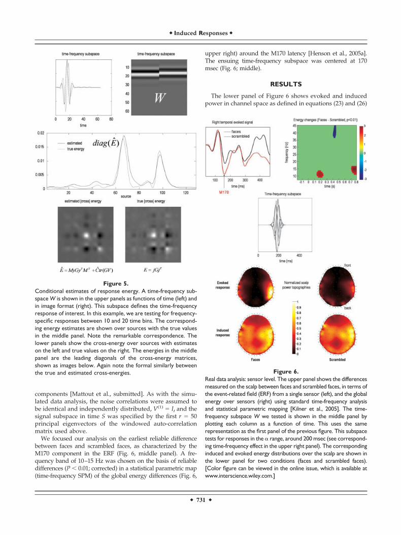
We focused our analysis on the earliest reliable differencebetween faces and scrambled faces, as characterized by theM170 component in the ERF (Fig. 6, middle panel). A fre-quency band of 10–15 Hz was chosen on the basis of reliabledifferences (P � 0.01; corrected) in a statistical parametric map(time-frequency SPM) of the global energy differences (Fig. 6,

upper right) around the M170 latency [Henson et al., 2005a].The ensuing time-frequency subspace was centered at 170msec (Fig. 6; middle).

RESULTS

The lower panel of Figure 6 shows evoked and inducedpower in channel space as defined in equations (23) and (26)

Figure 5.Conditional estimates of response energy. A time-frequency sub-space W is shown in the upper panels as functions of time (left) andin image format (right). This subspace defines the time-frequencyresponse of interest. In this example, we are testing for frequency-specific responses between 10 and 20 time bins. The correspond-ing energy estimates are shown over sources with the true valuesin the middle panel. Note the remarkable correspondence. Thelower panels show the cross-energy over sources with estimateson the left and true values on the right. The energies in the middlepanel are the leading diagonals of the cross-energy matrices,shown as images below. Again note the formal similarly betweenthe true and estimated cross-energies. Figure 6.

Real data analysis: sensor level. The upper panel shows the differencesmeasured on the scalp between faces and scrambled faces, in terms ofthe event-related field (ERF) from a single sensor (left), and the globalenergy over sensors (right) using standard time-frequency analysisand statistical parametric mapping [Kilner et al., 2005]. The time-frequency subspace W we tested is shown in the middle panel byplotting each column as a function of time. This uses the samerepresentation as the first panel of the previous figure. This subspacetests for responses in the � range, around 200 msec (see correspond-ing time-frequency effect in the upper right panel). The correspondinginduced and evoked energy distributions over the scalp are shown inthe lower panel for two conditions (faces and scrambled faces).[Color figure can be viewed in the online issue, which is available atwww.interscience.wiley.com.]


� 731 �

respectively. Power maps were normalized to the same max-imum for display. In both conditions, maximum power islocated over the right temporal regions; however, the rangeof power values is much wider for the evoked response.Moreover, whereas scalp topographies of induced responsesare similar between conditions, the evoked energy is clearlyhigher for faces, relative to scrambled faces. This suggeststhat the M170 is mediated by differences in phase-lockedactivity.

This is confirmed by the power analysis in source space(Fig. 7), using equations (23) and (26). Evoked and inducedresponses are generated by the same set of cortical regions.The differences between faces and scrambled faces in termsof induced power, however, are weak compared to theequivalent differences in evoked power (see the scale bars inFig. 7). Furthermore, the variation in induced energy overchannels and conditions is small relative to evoked power.This nonspecific profile suggests that ongoing activity maycontribute substantially to the induced component. As men-tioned above, the interesting aspect of induced power usu-ally resides in trial-specific differences. A full analysis ofinduced differences will be presented elsewhere. Here wefocus on the functional anatomy implied by evoked differ-entials. The functional anatomy of evoked responses, in thiscontext, is sufficiently well known to establish the face va-lidity of our conditional estimators:

The upper panel of Figure 8 shows the cortical projectionof the difference between the conditional expectations ofevoked energy for faces versus scrambled faces. The largestchanges were expressed in the right inferior occipital gyrus(IOG), the right orbitofrontal cortex (OFC), and the horizon-

tal posterior segment of the right superior temporal sulcus(STS). Figure 9 shows the coregistration of these energychanges with the subject’s structural MRI. Happily, the “ac-tivation” of these regions is consistent with the equivalentcomparison of fMRI responses [Henson et al., 2003].

The activation of the ventral and lateral occipitotemporalregions is also consistent with recent localizations of theevoked M170 [Henson et al., 2005b; Tanskanen et al., 2005].This is to be expected given that the most of the energychange seems to be phase-locked [Henson et al., 2005a].Indeed, the conditional estimates of evoked responses at thelocation of the maximum of energy change in the right IOGand right posterior STS show a deflection around 170 msecthat is greater for faces than scrambled faces (Fig. 8, lowerpanel).

We have not made any inferences about these effects.SPMs of energy differences would normally be constructedusing conditional estimates of power changes over subjects.It is also possible, however, to use the conditional densitiesto compute a posterior probability map (PPM) of non-zerochanges for a single subject. We will demonstrate inferenceusing these approaches elsewhere.

CONCLUSION

We have described an extension of our empirical Bayesapproach to MEG/EEG source reconstruction that coversboth evoked and induced responses. The estimation schemeis based on classical covariance component estimation usingrestricted maximum likelihood (ReML). We have extendedthe scheme using temporal basis functions to place con-

Figure 7.Real data analysis: source level. Reconstructedevoked and induced responses are shown forboth faces and scrambled face trials. Thesedata correspond to conditional expectationsrendered onto a cortical surface. These viewsof the cortical surface are from below. (i.e.,left is on the right). Evoked power was nor-malized to the maximum over corticalsources. [Color figure can be viewed in theonline issue, which is available at www.interscience.wiley.com.]


� 732 �

straints on the temporal form of the responses. We showhow one can estimate evoked responses that are phase-locked to the stimulus and induced responses that are not.This inherent distinction calls for different transformationsof a hierarchical model of multiple trial responses to provideBayesian estimates of power.

Oscillatory activity is well known to be related to neuralcoding and information processing in the brain [Fries et al.,2001; Hari and Salmelin, 1997; Tallon-Baudry et al., 1999].Oscillatory activity refers to signals generated in a particularfrequency band time-locked but not necessarily phase-locked to the stimulus. Classical data averaging approachesmay not capture this activity, which calls for trial-to-trialanalyses. Localizing the sources of oscillatory activity on atrial-by-trial basis is computationally demanding, however,and requires data with low signal-to-noise ratio. This is whyearly approaches were limited to channel space [e.g., Tallon-Baudry et al., 1997]. Recently, several inverse algorithmshave been proposed to estimate the sources of inducedoscillations. Most are distributed (or imaging) methods,since equivalent current dipole models are not suitable forexplaining a few hundreds of milliseconds of nonaveragedactivity. Among distributed approaches, two main types canbe distinguished: the beamformer [Cheyne et al., 2003; Grosset al., 2001; Sekihara et al., 2001] and minimum-norm-based

techniques [David et al., 2002; Jensen and Vanni, 2002],although both can be formulated as (weighted) minimumnorm estimators [Hauk, 2004]. A strict minimum norm so-lution obtains when no weighting matrix is involved [Ha-malainen et al., 1993] but constraints such as fMRI-derivedpriors have been shown to condition the inverse solution[Lin et al., 2004]. Beamformer approaches implement a con-strained inverse using a set of spatial filters (see Huang et al.[2004] for an overview). The basic principle employed bybeamformers is to estimate the activity at each putativesource location while suppressing the contribution of othersources. This means that beamformers look explicitly foruncorrelated sources. Although some robustness has beenreported in the context of partially correlated sources [VanVeen et al., 1997], this aspect of beamforming can be annoy-ing when trying to characterize coherent or synchronizedcortical sources [Gross et al., 2001].

Recently, we proposed a generalization of the weighted-minimum norm approach based on hierarchical linear mod-els and empirical Bayes, which can accommodate multiplepriors in an optimal fashion [Phillips et al., 2005]. The ap-proach involves a partitioning of the data covariance matrixinto noise and prior source variance components, whoserelative contributions are estimated using ReML. Eachmodel (i.e., set of partitions or components) can be evaluated

Figure 8.Real data analysis: evoked responses. The up-per panel shows the reconstructed evokedpower changes between faces and scrambledfaces. The lower panel shows the recon-structed evoked responses associated withthree regions where the greatest energychange was elicited. [Color figure can beviewed in the online issue, which is available atwww.interscience.wiley.com.]


� 733 �

using Bayesian model selection [Mattout et al., submitted].Moreover, the ReML scheme is computationally efficient, re-quiring only the inversion of small matrices. So far this ap-proach has been limited to the analysis of evoked responses,because we have focused on the estimation of spatial covari-ance components under simple assumptions about the tempo-ral correlations. In this article, we provided the operationalequations and procedures for obtaining conditional estimatesof responses with specific temporal constraints over multipletrials. The proposed scheme offers a general Bayesian frame-work that can incorporate all kind of spatial priors such asbeamformer-like spatial filters or fMRI-derived constraints.Furthermore, basis functions enable both the use of computa-tionally efficient ReML-based variance component estimationand the definition of priors on the temporal form of the re-sponse. This implies a separation of the temporal and spatialdependencies both at the sensor and source levels using aKronecker formulation [Huizenga et al., 2002]. Thanks to thisspatiotemporal approximation, the estimation of induced re-sponses from multitrial data does not require a computation-ally demanding trial-by-trial approach [Jensen and Vanni,2002] or drastic dimension reduction of the solution space[David et al., 2002].

The approach described in this article allows for spatio-temporal modeling of evoked and induced responses underthe assumption that there is a subspace S in which temporalcorrelations among the data and signal have the same form.Clearly this subspace should encompass as much of thesignal as possible. In this work, we used the principal eig-envariates of a prior covariance based on smooth signalsconcentrated early in peristimulus time. This subspace istherefore informed by prior assumptions about how andwhen signal is expressed. A key issue here is what wouldhappen if the prior subspace did not coincide with the truesignal subspace. In this instance there may be a loss ofefficiency as experimental variance is lost to the null space ofS; however, there will be no bias in the (projected) responseestimates. Similarly, the estimate of the error covariancecomponents will be unbiased but lose efficiency as highfrequency noise components are lost in the restriction. Putsimply, this means the variability in the covariance param-eter estimates will increase, leading to a slight overconfi-dence in conditional inference. The overconfidence problemis not an issue here because we are only interested in theconditional expectations, which would normally be taken toa further (between-subject) level for inference.

As proof of principle, we used a toy example and asingle-subject MEG data set to illustrate the methodology forsingle-trial and multiple-trial analyses, respectively. The toydata allowed us to detail how spatial and temporal priorsare defined whereas the real data example provisionallyaddressed the face validity of the extended framework. Infuture applications, the priors will be considered in greaterdepth, such as fMRI-derived constraints in the spatial do-main and autoregressive models in the temporal domain.Importantly, SPM of the estimated power changes in a par-ticular time-frequency window, over conditions or over sub-

Figure 9.Visualization on the subject MRI. The regions identified as showingenergy changes for faces versus scrambled faces in Figure 8 areshown coregistered with a MRI scan: the right orbitofrontal cortex(OFC; upper panel), the right inferior occipital gyrus (IOG; middlepanel), and the posterior right superior temporal sulcus (STS;lower panel). These source estimates are shown both as corticalrenderings (from below) and on orthogonal sections through astructural MRI, using the radiological convention (right is left).


� 734 �

jects, can be now achieved at the cortical level [Brookes et al.,2004; Kiebel and Friston, 2004a]. Finally, with the appropri-ate wavelet transformation, instantaneous power and phasecould also be estimated to study cortical synchrony.

ACKNOWLEDGMENTS

This work was supported by the Wellcome Trust and by aMarie Curie Fellowship from the EU (to J.M.). We thank ourreviewers for helpful guidance in presenting this work.

REFERENCES

Baillet S, Mosher JC, Leahy RM (2004): Electromagnetic brain imag-ing using brainstorm. Proceedings of the 2004 IEEE InternationalSymposium on Biomedical Imaging (ISBI)., 15–18 April 2004,Arlington, VA.

Brookes MJ, Gibson AM, Hall SD, Furlong PL, Barnes GR, Hill-ebrand A, Singh KD, Holliday IE, Francis ST, Morris PG (2005):A general linear model for MEG beam former imaging. Neuro-image 23:936–946.

Cheyne D, Gaetz W, Garnero L, Lachaux J-P, Ducorps A, SchwartzD, Varela FJ (2003): Neuromagnetic imaging of cortical oscilla-tions accompanying tactile stimulation. Brain Res Cogn BrainRes 17:599–611.

David O, Garnero L, Cosmelli D, Varela J (2002): Estimation ofneural dynamics from MEG/EEG cortical current density maps:application to the reconstruction of large-scale cortical syn-chrony. IEEE Trans Biomed Eng 49:975–987.

Dietterich TG (2000): Ensemble methods in machine learning. Pro-ceedings of the First International Workshop on Multiple Clas-sifier Systems. London: Springer-Verlag; p 1–15.

Fries P, Reynolds JH, Rorie AE, Desimone R (2001): Modulation ofoscillatory neuronal synchronization by selective visual atten-tion. Science 291:1506–1507.

Friston KJ (2000): The labile brain I. Neuronal transients and non-linear coupling. Philos Trans R Soc Lond B Biol Sci 355:215–236.

Friston KJ, Penny W, Phillips C, Kiebel S, Hinton G, Ashburner J(2002): Classical and bayesian inference in neuroimaging: theory.Neuroimage 16:465–483.

Gross J, Kujala J, Hamalainen M, Timmermann L, Schnitzler A,Salmelin R (2001): Dynamic imaging of coherent sources: study-ing neural interactions in the human brain. Proc Natl Acad SciUSA 98:694–699.

Hamalainen M, Hari R, Ilmoniemi R, Knuutila J, Lounasmaa O(1993): Magnetoencephalography: theory, instrumentation andapplications to noninvasive study of human brain functions. RevMod Phys 65:413–497.

Hari R, Salmelin R (1997): Human cortical oscillations: a neuromag-netic view through the skull. Trends Neurosci 20:44–49.

Hauk O (2004): Keep it simple: a case for using classical minimumnorm estimation in the analysis of EEG and MEG data. Neuro-image 21:1612–1621.

Henson RN, Goshen-Gottstein Y, Ganel T, Otten LJ, Quayle A, RuggMD (2003): Electrophysiological and haemodynamic correlates offace perception, recognition and priming. Cereb Cortex 13:793–805.

Henson R, Kiebel S, Kilner J, Friston K, Hillebrand A, Barnes GR,Singh KD (2005a): Time-frequency SPMs for MEG data on faceperception: power changes and phase-locking. Presented at the11th Annual Meeting of the Organization for Human Brain Map-ping, 12–16 June 2005, Toronto, Canada.

Henson R, Mattout J, Friston K, Hassel S, Hillebrand A, Barnes GR,Singh KD (2005b): Distributed source localization of the M170

using multiple constraints. Presented at the 11th Annual Meetingof the Organization for Human Brain Mapping, 12–16 June 2005,Toronto, Canada.

Huang M, Aine CJ, Supek S, Best E, Ranken D, Flynn ER (1998):Multi-start downhill simplex method for spatio-temporal sourcelocalization in magnetoencephalography. ElectroencephalogrClin Neurophysiol 108:32–44.

Huang MX, Shih JJ, Lee DL, Harrington DL, Thoma RJ, WeisendMP, Hanlon F, Paulson KM, Li T, Martin K, Miller GA, CaniveJM (2004): Commonalities and differences among vectorizedbeamformers in electromagnetic source imaging. Brain Topogr16:139–158.

Huizenga HM, de Munk JC, Waldorp LJ, Grasman RP (2002): Spa-tiotemporal EEG/MEG source analysis based on a parametricnoise covariance model. IEEE Trans Biomed Eng 49:533–539.

Jensen O, Vanni S (2002): A new method to identify sources ofoscillatory activity from magnetoencephalographic data. Neuro-image 15:568–574.

Kiebel SJ, Friston KJ (2004a): Statistical parametric mapping forevent-related potentials: I. Generic considerations. Neuroimage22:492–502.

Kiebel SJ, Friston KJ (2004b): Statistical parametric mapping forevent-related potentials: II. A hierarchical temporal model. Neu-roimage 22:503–520.

Kilner JM, Kiebel SJ, Friston KJ (2005): Applications of random fieldtheory to electrophysiology. Neurosci Lett 374:174–178.

Lin FH, Witzel T, Hamalainen MS, Dale AM, Belliveau JW, StufflebeamSM (2004): Spectral spatiotemporal imaging of cortical oscillations andinteractions in the human brain. Neuroimage 23:582–595.

Mangin JF, Riviere D, Cachia A, Duchesnay E, Cointepas Y, Pap-adopoulos-Orfanos D, Scifo P, Ochiai T, Brunelle F, Regis J(2004): A framework to study the cortical folding patterns. Neu-roimage 23:129–138.

Mattout J, Phillips C, Rugg MD, Friston KJ. MEG source localisationunder multiple constraints: an extended Bayesian framework.Neuroimage (submitted).

Phillips C, Mattout J, Rugg MD, Maquet P, Friston KJ (2005): Anempirical Bayesian solution to the source reconstruction prob-lem in EEG. Neuroimage 24:997–1011.

Phillips C, Rugg MD, Friston KJ (2002): Anatomically informedbasis functions for EEG source localization: combining func-tional and anatomical constraints. Neuroimage 16:678–695.

Sekihara K, Nagarajan SS, Poeppel D, Marantz A, Miyashita Y(2001): Reconstructing spatio-temporal activities of neuralsources using an MEG vector beamformer technique. IEEE TransBiomed Eng 48:760–771.

Tallon-Baudry C, Bertrand O, Delpuech C, Pernier J (1997): Oscilla-tory �-band (30–70Hz) activity induced by a visual search task inhumans. J Neurosci 17:722–734.

Tallon-Baudry C, Bertrand O (1999): Oscillatory gamma activity inhumans and its role in object representation. Trends Cogn Sci3:151–162.

Tanskanen T, Nasanen R, Montez T, Paallysaho J, Hari R (2005):Face recognition and cortical responses show similar sensitivityto noise spatial frequency. Cereb Cortex 15:526–534.

Trujillo-Barreto NJ, Aubert-Vazquez E, Valdes-Sosa PA (2004):Bayesian model averaging in EEG/MEG imaging. Neuroimage21:1300–1319.

Van Veen BD, van Drongelen W, Yuchtman M, Suzuki A (1997):Localization of brain electrical activity via linearly constrainedminimum variance spatial filtering. IEEE Trans Biomed Eng44:867–880.


� 735 �

Bayesian estimation of evoked and induced responses

Documents

Transcript of Bayesian estimation of evoked and induced responses