Battery Based Energy Storage Emulation in Low Voltage Grids
125
Battery Based Energy Storage Emulation in Low Voltage Grids June 2019 Master's thesis Master's thesis Nora Plassbak Sagatun 2019 Nora Plassbak Sagatun NTNU Norwegian University of Science and Technology Faculty of Information Technology and Electrical Engineering Department of Electric Power Engineering
-
Upload
khangminh22 -
Category
Documents
-
view
1 -
download
0
Transcript of Battery Based Energy Storage Emulation in Low Voltage Grids

Battery Based Energy StorageEmulation in Low Voltage Grids
June 2019
Mas
ter's
thes
is
Master's thesis
Nora Plassbak Sagatun
2019N
ora Plassbak Sagatun
NTNU
Nor
weg
ian
Univ
ersi
ty o
fSc
ienc
e an
d Te
chno
logy
Facu
lty o
f Inf
orm
atio
n Te
chno
logy
and
Ele
ctric
alEn
gine
erin
gDe
part
men
t of E
lect
ric P
ower
Eng
inee
ring


Battery Based Energy Storage Emulationin Low Voltage Grids
Nora Plassbak Sagatun
Master of Energy and Environmental EngineeringSubmission date: June 2019Supervisor: Elisabetta TedeschiCo-supervisor: Santiago Sanchez
Norwegian University of Science and TechnologyDepartment of Electric Power Engineering


Preface
This master thesis concludes my five years degree in Energy and Environmental Engi-
neering at the Norwegian University of Science and Technology. I would like to thank
my co-supervisor Post-Doctor Santiago Sanchez for his help and support with both the
simulation models and the laboratory work. Moreover, I want to thank my supervisor Pro-
fessor Elisabetta Tedeschi for her support on the topic, as well as great advice regarding
the structure of the thesis. My supervisor and co-supervisor also encouraged me to write
an academic paper with the most important findings and results from this thesis. The paper
is written as a contribution to the EEEIC conference in Genoa, Italy, June 2019, a confer-
ence I will attend to present the findings. The academic paper is attached to the appendix
of this thesis.
Furthermore, I benefited from debating the issues of my thesis with my friends at NTNU.
It has been a pleasure to share my victories and frustrations with you. Lastly, I want to
thank my family for their encouragement, and for proofreading the thesis. Thank you.
Trondheim, June 2019
Nora Plassbak Sagatun


Summary
The electrical grid is in the midst of a significant transition. One of the most impor-
tant trends which modernizes the grid is the increased penetration of distributed energy
resources. Distributed generation causes for bidirectional power flow and a decentral-
ized grid design. The integration of renewable energy sources comes with challenges,
especially in regards to planning and operation. The challenges are primarily due to the
intermittent characteristics of renewables, as they are usually weather dependent. The in-
tegration of energy storage systems to the low voltage grid supports the use of renewable
energy sources.
The work of this thesis concerns the grid integration of a battery energy storage system.
The components involved in the system are described theoretically. Moreover, the battery
pack is designed to fulfill the set requirements and tested computationally. A DC-DC con-
verter is presented with an outline of the inner current control and outer voltage control.
The battery and converter are implemented in the MATLAB/Simulink environment, and
the results are presented. Further, the power hardware in the loop (PHIL) methodology
is explained. The battery pack and DC-DC converter are combined with a physical grid
connection using a physical voltage source converter by employing the PHIL technique.
The emulation of the energy storage system is presented through the laboratory results.
The work of the thesis can be split up in three main parts: design, simulation, and labo-
ratory work. The design process includes designing the battery storage system. Different
battery types are outlined, and the lithium-ion battery is chosen. Further, the battery ratings
are designed in correspondence with given requirements and rated data for the lithium-ion
battery. The DC-DC converter components are designed, as well as the current and voltage
control. The simulation process gives the results from the battery and DC-DC converter
modeled as an average model. The laboratory work implements the power hardware in the
iii

loop methodology to connect the battery energy storage emulation to physical laboratory
equipment.
The computational results showed a functioning control strategy for both the voltage and
current control loops. The DC-DC converter and the battery provided acceptable voltage
and current outputs, which enabled the further laboratory testing. From the laboratory
work, the voltage and current responded quickly, and the simulated and physical sensor
voltage behaved identically. The current from the physical equipment experienced a higher
level of noise than the simulated current, due to the use of sensors rated to much higher
currents, leading to a sensitive low current operation. To summarize, this thesis presents
a functioning power hardware in the loop strategy for the emulation of an energy storage
system connected to a low voltage grid.
iv

Sammendrag
Det elektriske nettet er i ferd med a moderniseres betydelig. En av de mest vesentlige tren-
dene som kan modernisere kraftnettet er økt penetrasjon av distribuerte energiressurser.
Distribuert generasjon forarsaker bidireksjonal kraftflyt og et desentralisert nettdesign. In-
tegrasjonen av fornybare energikilder kommer med utfordringer, særlig nar det gjelder
planlegging og drift. Dette skyldes hovedsakelig de periodiske egenskapene ved fornybar
energi, da de ofte er væravhengige. Integrasjonen av energilagringssystemer til lavspen-
ningsnettet støtter bruken av fornybare energikilder.
Denne avhandlingen tar for seg netteverksintegrasjonen av et batteri energilagringssystem.
Komponentene som er involvert i systemet beskrives teoretisk. Batteripakkene er designet
for a møte de gitte kravene og testes gjennom simuleringer. En DC-DC omformer presen-
teres med en forklaring av indre strømløkkeregulering og ytre spenningsløkkeregulering.
Batteriet og omformeren er implementert i MATLAB/Simulink, og resultatene presen-
teres. Videre forklares power hardware in the loop (PHIL) metoden. Batteripakken og
DC-DC omformeren kombineres med en fysisk nettforbindelse ved bruk av en spen-
ningskildeomformer ved a benytte PHIL-teknikken. Emuleringen av energilagringssys-
temet presenteres gjennom laboratorieresultatene.
Arbeidet i denne avhandlingen kan deles opp i tre hoveddeler: design, simulering og lab-
oratoriearbeid. Designprosessen omfatter a utforme batterisystemet. Ulike batterityper er
skissert, og litium-ionbatteriet er valgt. DC-DC omformerens komponenter er kalkulert,
samt en regulering av strøm og spenningskontroll. Simuleringsprosessen gir resultatene fra
batteriet og DC-DC omformeren modellert som en gjennomsnittsmodell. Laboratoriear-
beidet implementerer PHIL strategien for a koble det emulerte batterilagringssystemer til
fysisk laboratorieutstyr.
v

Simuleringsresultatene viste en fungerende kontrollstrategi for bade spennings- og
strømkontrollsløyfene. Spenningene og strømmene ut av batteripakken og DC-DC om-
formeren var akseptable. Dette muliggjorde videre laboratorietesting. Eksperimenter
i laboratoriet viser at den simulerte og fysiske sensorspenningen oppførte seg identisk.
Strømmen fra det fysiske utstyret opplevde et høyere støyniva enn den simulerte strømmen,
noe som bunner i bruken av sensorer som er vurdert til mye høyere strømmer som fører til
en sensitiv lavstrømsdrift. For a oppsummere, presenterer denne oppgaven en fungerende
PHIL strategi for emulering av et energilagringssystem koblet til et lavspenningsnett.
vi

Contents
Preface i
Summary iii
Sammendrag v
Table of Contents vii
List of Figures xi
Abbreviations xiv
1 Introduction 1
1.1 Background and Motivation . . . . . . . . . . . . . . . . . . . . . . . . 1
1.2 Problem Definition . . . . . . . . . . . . . . . . . . . . . . . . . . . . . 3
1.3 Methodology . . . . . . . . . . . . . . . . . . . . . . . . . . . . . . . . 4
1.4 Relation to Specialization Project . . . . . . . . . . . . . . . . . . . . . . 5
1.5 Limitation of Scope . . . . . . . . . . . . . . . . . . . . . . . . . . . . . 6
1.6 Structure of Thesis . . . . . . . . . . . . . . . . . . . . . . . . . . . . . 6
2 Components and Definitions 9
2.1 Distributed Generation . . . . . . . . . . . . . . . . . . . . . . . . . . . 10
2.2 Energy Storage Systems . . . . . . . . . . . . . . . . . . . . . . . . . . 10
2.3 Bidirectional DC-DC Converter . . . . . . . . . . . . . . . . . . . . . . 12
2.4 Voltage Source Converter . . . . . . . . . . . . . . . . . . . . . . . . . . 13
vii

2.5 Microgrid . . . . . . . . . . . . . . . . . . . . . . . . . . . . . . . . . . 14
3 Battery Energy Storage System 17
3.1 Battery Energy Storage System Technologies . . . . . . . . . . . . . . . 18
3.1.1 Outline of Battery Types . . . . . . . . . . . . . . . . . . . . . . 18
3.1.2 Lithium-Ion based BESS . . . . . . . . . . . . . . . . . . . . . . 19
3.2 Battery Model . . . . . . . . . . . . . . . . . . . . . . . . . . . . . . . . 20
3.2.1 Computational Battery Model . . . . . . . . . . . . . . . . . . . 20
3.2.2 Internal Resistance . . . . . . . . . . . . . . . . . . . . . . . . . 22
3.3 Battery Design . . . . . . . . . . . . . . . . . . . . . . . . . . . . . . . 22
3.4 Battery System Implementation in Simulink . . . . . . . . . . . . . . . . 25
4 DC-DC Converter 29
4.1 Boost Converter Topology . . . . . . . . . . . . . . . . . . . . . . . . . 30
4.2 Average Converter Model . . . . . . . . . . . . . . . . . . . . . . . . . . 33
4.3 Converter Control . . . . . . . . . . . . . . . . . . . . . . . . . . . . . . 34
4.3.1 Inner Current Control Loop . . . . . . . . . . . . . . . . . . . . 34
4.3.2 Outer Voltage Control Loop . . . . . . . . . . . . . . . . . . . . 34
4.3.3 Proportional Integral Regulator . . . . . . . . . . . . . . . . . . 35
4.3.3.1 PI Current Controller . . . . . . . . . . . . . . . . . . 37
4.3.3.2 PI Voltage Controller . . . . . . . . . . . . . . . . . . 38
5 Power Hardware in the Loop 41
5.1 PHIL Concept . . . . . . . . . . . . . . . . . . . . . . . . . . . . . . . . 42
5.2 HIL and PHIL Applications . . . . . . . . . . . . . . . . . . . . . . . . . 43
5.3 PHIL Structure . . . . . . . . . . . . . . . . . . . . . . . . . . . . . . . 44
5.4 Discretization Algorithm . . . . . . . . . . . . . . . . . . . . . . . . . . 45
6 Computational Results 49
6.1 DC-DC Converter connected to Battery System . . . . . . . . . . . . . . 50
6.2 Battery Model . . . . . . . . . . . . . . . . . . . . . . . . . . . . . . . . 52
6.3 Discrete Model . . . . . . . . . . . . . . . . . . . . . . . . . . . . . . . 53
viii

6.4 Implementation of Noise . . . . . . . . . . . . . . . . . . . . . . . . . . 55
6.5 Discussion of Computational Results . . . . . . . . . . . . . . . . . . . . 56
7 Laboratory Work 59
7.1 Laboratory Setup . . . . . . . . . . . . . . . . . . . . . . . . . . . . . . 60
7.1.1 Controlled Voltage Source . . . . . . . . . . . . . . . . . . . . . 61
7.1.2 Voltage Source Converter . . . . . . . . . . . . . . . . . . . . . 62
7.1.3 Real Time Simulator . . . . . . . . . . . . . . . . . . . . . . . . 62
7.2 Laboratory Results . . . . . . . . . . . . . . . . . . . . . . . . . . . . . 63
7.2.1 Current Results . . . . . . . . . . . . . . . . . . . . . . . . . . . 64
7.2.2 Voltage Results . . . . . . . . . . . . . . . . . . . . . . . . . . . 65
7.3 Discussion of Laboratory Work . . . . . . . . . . . . . . . . . . . . . . . 67
8 Concluding Remarks 69
Further Work . . . . . . . . . . . . . . . . . . . . . . . . . . . . . . . . . . . 71
Bibliography 73
Appendices 85
A Academic Paper 87
B Computational Result:
Charge of Battery 95
C Computational Models 97
C.1 Computation Model for sections 6.1 and 6.2 . . . . . . . . . . . . . . . . 97
C.2 Computation Model for section 6.3 . . . . . . . . . . . . . . . . . . . . . 99
C.3 Computation Model for section 6.4 . . . . . . . . . . . . . . . . . . . . . 101
D MATLAB Script for Simulink Parameters 103
ix

x

List of Figures
1.1 Simplified illustration of a traditional power system . . . . . . . . . . . . 1
1.2 Simplified illustration of a modern power system . . . . . . . . . . . . . 2
1.3 Line diagram of paper scope . . . . . . . . . . . . . . . . . . . . . . . . 4
2.1 Illustration of a bidirectional converter. . . . . . . . . . . . . . . . . . . . 13
2.2 Voltage Source Converter topology used as a rectifier . . . . . . . . . . . 14
3.1 Equivalent battery model from Simulink. . . . . . . . . . . . . . . . . . . 21
3.2 The nominal discharge curve of the battery. . . . . . . . . . . . . . . . . 26
3.3 Discharge curves for three different discharge currents . . . . . . . . . . 27
4.1 Boost converter topology. . . . . . . . . . . . . . . . . . . . . . . . . . . 30
4.2 Boost converter average model. . . . . . . . . . . . . . . . . . . . . . . . 33
4.3 Conceptual equivalent circuit of the the inner current control loop. . . . . 34
4.4 Conceptual per phase equivalent circuit of the the outer voltage control loop 35
4.5 Standard block diagram for a PI controller in the Laplace domain. . . . . 36
5.1 Power hardware in the loop concept . . . . . . . . . . . . . . . . . . . . 42
5.2 Outline of PHIL Structure for emulation of ESS. . . . . . . . . . . . . . . 45
5.3 Illustration of discretization objective. . . . . . . . . . . . . . . . . . . . 46
xi

6.1 Resulting graphs from the bidirectional converter model. The top graph
shows the voltage and current error from the controller. The middle graph
is the current output and the bottom graph shows the voltage output of the
converter. . . . . . . . . . . . . . . . . . . . . . . . . . . . . . . . . . . 51
6.2 Resulting graphs from the discharging battery model. The top graph shows
the state of charge, the middle graph is the current out from the battery and
the bottom graph shows the voltage over the battery system. . . . . . . . 52
6.3 Discharge curve with the discharge current observed is the resulting scope. 53
6.4 The top graph shows the current output iout and the discretized current
output iK . The bottom graph shows the voltage output vout and the dis-
cretized voltage output vDC of the converter. . . . . . . . . . . . . . . . . 54
6.5 The top graph shows the current output iout and the discretized current
output iK with the inclusion of noise. The bottom graph shows the voltage
output vout and the discretized voltage output vDC of the converter with
the inclusion of noise. . . . . . . . . . . . . . . . . . . . . . . . . . . . . 55
6.6 Discharge curve with the discharge current observed is the resulting scope. 57
7.1 Norwegian Smart grid Laboratory. (1): 200kVA Controlled Voltage Source,
(2): 60 kVA 3− φ VSC, (3): OPAL-RT. . . . . . . . . . . . . . . . . . . 60
7.2 200kVA Controlled Voltage Source . . . . . . . . . . . . . . . . . . . . . 61
7.3 60 kVA 3− φ VSC . . . . . . . . . . . . . . . . . . . . . . . . . . . . . 62
7.4 OPAL-RT. . . . . . . . . . . . . . . . . . . . . . . . . . . . . . . . . . . 63
7.5 Current output iout from the continuous model as the blue, green and or-
ange line and ik from the physical measurement as the black line. . . . . 65
7.6 Voltage output vDC from the continuous model and vout logged from the
physical equipment perfectly correlated. . . . . . . . . . . . . . . . . . . 66
B.1 Resulting graphs from charging the battery model. The top graph shows
the state of charge, the middle graph is the current out from the battery and
the bottom graph shows the voltage over the battery system. . . . . . . . 96
C.1 Simulink Model of average boost converter . . . . . . . . . . . . . . . . 98
xii

C.2 Simulink model of voltage and current control . . . . . . . . . . . . . . . 98
C.3 Simulink model setup prepared for real time simulations . . . . . . . . . 99
C.4 Simulink model of average boost converter with discretization signals re-
trieved . . . . . . . . . . . . . . . . . . . . . . . . . . . . . . . . . . . . 100
C.5 Simulink model with the implementation of the discretization algorithm . 100
C.6 Simulink model of average boost converter with the implementation of
noise at the current and voltage output . . . . . . . . . . . . . . . . . . . 101
xiii

Abbreviations
AC = Alternating Current
BESS = Battery Energy Storage System
CIL = Controller in the loop
DC = Direct Current
DER = Distributed Energy Resource
DG = Distributed Generation
DOD = Depth Of Discharge
DSO = Distribution System Operators
DUT = Device Under Testing
ESS = Energy Storage System
FACT = Flexible AC transmission system
FPGA = Field-Programmable Gate Array
GFC = Grid Forming Converter
HIL = Hardware In The Loop
HV = High Voltage
IEC = International Electrotechnical Commission
IEEE = Institute of Electrical and Electronics Engineers
xiv

IGBT = Insulated Gate Bipolar Transistor
KCL = Kirchhoff’s current law
KVL = Kirchhoff’s voltage law
LTC = Load Tap Changer
MG = Microgrid
MMC = Modular Multi-level Converter
MOSFET = Metal-Oxide Semiconductor Field-Effect Transistor
PHIL = Power Hardware In The Loop
PI = Proportional-Integral
PID = Proportional-Integral-Derivative
PLL = Phase Locked Loop
PV = Photovoltaic System
RTS = Real Time Simulation
SOC = State Of Charge
UAV = Unmanned Aerial Vehicle
VSC = Voltage Source Converter
VSM = Virtual Synchronous Machine
xv

xvi

Chapter 1
Introduction
1.1 Background and Motivation
The electrical grid is in the midst of a significant transition. As the world’s population
continues to grow, more people require electricity as well as the ever attention to climate
change mitigation is growing [1; 2]. At present, the traditional distribution grid typically
has a centralized design with unidirectional power flow. A centralized power system is
structured with large power plants based on, among others, hydropower or oil and gas
which feed power to the transmission system which further distributes the power to distri-
bution grids and end-users, as illustrated in figure 1.1.
Figure 1.1: Simplified illustration of a traditional power system
One of the most significant trends which modernizes the grid is the increased penetra-
tion of distributed energy resources. Distributed generation causes for bidirectional power
1

Chapter 1. Introduction
flow and a decentralized grid design [3], which is made evident in figure 1.2. This leads to
an increased concern for the control of distribution grids.
Figure 1.2: Simplified illustration of a modern power system
The motivations for implementing distributed generators in the power system lead to
several benefits and challenges. The implementation can result in lower power prices,
higher reliability, decreased emissions of greenhouse gases, and the alleviation of poverty
in regions where electricity is not necessarily a given. Higher penetration of distributed
energy resources will also initiate lower transmission losses and higher flexibility of the
grid. However, when a distributed generator is connected to the distribution grid, it leads
to complicated control and regulation to avoid challenges regarding, for instance, voltage
fluctuations and negative externalities on power quality [4]. Consequently, power elec-
tronics will be an efficient and reliable interface to the grid [5].
The integration of renewable energy sources comes with challenges, especially in re-
gards to planning and operation. The challenges are primarily due to the intermittent
characteristics of renewables, as they are usually weather dependent. The integration of
energy storage systems (ESSs) to the low voltage grid supports the use of renewable en-
ergy sources. When the renewables experience peak generation, the energy storage system
enables for a storing of the excess energy, and when the renewables experience weather
2

1.2 Problem Definition
challenges such as cloud cover or no wind, the ESS can distribute the stored energy to the
power grid. This is one of many advantages with the connection of ESS to a low voltage
grid. Other advantages include power quality improvement, peak shaving, cost reduction,
and mitigation of greenhouse gases.
Most power electronic converters used for grid interfacing of distributed generation
have a unidirectional power flow. However, to enable for charging and discharging of a
battery energy storage system (BESS), a bidirectional power flow converter is required.
Conventionally, an independent buck converter and an independent boost converter can be
used in parallel to achieve the bidirectional power flow. However, the demand for complex
control, as well as compact and efficient grid integration works in favor of the bidirectional
converter. A bidirectional DC-DC converter is widely used in the ESS application, partic-
ularly in low voltage grids in the range of 50 to 1000 V AC. The bidirectional converter
connects the energy storage technology to an additional converter that links the DC side
with the AC grid. It supports the step up of a voltage from the battery side to a grid side,
as well as stepping down the voltage in the opposite direction. This leads to improved
performance of the system as the converter allows for an efficient control of the voltage
levels [6; 7].
1.2 Problem Definition
The work of this thesis concerns the grid integration of a battery energy storage system.
The components involved in the system are described theoretically. Moreover, the battery
pack is designed to fulfill the set requirements and tested computationally. A DC-DC
converter is presented with an outline of the inner current control and outer voltage control.
The battery and converter are implemented in the MATLAB/Simulink environment, and
the results are presented. Further, the power hardware in the loop (PHIL) methodology
is explained. The battery pack and DC-DC converter are combined with a physical grid
connection using a physical voltage source converter by employing the PHIL technique.
The emulation of the energy storage system is presented through the laboratory results.
3

Chapter 1. Introduction
Figure 1.3: Line diagram of paper scope
The aim of this thesis is to develop an emulation of a battery energy storage system in
a low voltage grid connection conducted with a power hardware in the loop methodology.
The aim will be achieved by reaching the following objectives:
1. Design and study a battery energy storage system.
2. Investigate and describe a DC-DC converter and design its current and voltage con-
trol.
3. Review the power hardware in the loop concept and create a structure suitable for
an energy storage system emulation.
4. Develop a simulated computational model for testing of the battery pack and DC-DC
converter to review the design and control setup.
5. Implement the power hardware in the loop structure with the simulated model in
a real-time simulation connected with physical laboratory equipment to obtain an
emulation of the battery and DC-DC converter in connection with a physical low
voltage grid.
1.3 Methodology
The methodologies used in this thesis include:
• Analytical calculations are used in the design process of the thesis. The battery
design is conducted using the analytical calculations to size the battery to fulfill the
set requirements. Further, the components of the DC-DC converter, as well as the
tuning of the converter’s PI regulators are attained from analytical calculations.
4

1.4 Relation to Specialization Project
• Computational simulation is used to test the energy storage system with the DC-DC
converter. The simulations are used to confirm a functional control strategy, as well
as to confirm the desired voltage output. Further, the simulation model tests the
discretization algorithm and the impact of noise in the system.
• Power hardware in the loop laboratory setup is the final methodology used in the
thesis. The technique involves the simulated computational model implemented
in a real-time simulator with the connection of physical laboratory equipment of a
voltage source converter and a digital amplifier.
1.4 Relation to Specialization Project
The primary objective of the specialization project [8] was to review microgrids and the
contribution of microgrids to the shift towards a modern power system, to investigate and
to describe the current and voltage control of voltage source converters (VSCs) which are
integrated in an islanded grid, to analyze the hierarchical structure of droop based control
of microgrid and describe the algorithmic approach for the roles in the control and lastly to
develop a model in Simulink for testing of a microgrid structure which investigates some
of the theoretically explained control strategies. Even though this thesis has pivoted into
a more focused direction of a power hardware in the loop emulation of an ESS, the spe-
cialization project functioned as a good basis for the work. The voltage source converter
control is not included in this thesis as the VSC included in the scope is a physical labora-
tory converter and not a part of the simulation model.
Parts of section 1.1 from the introduction are based on the specialization project. Fur-
ther, in chapter 2, section 2.1 and 2.5 are strongly based on [8]. As the voltage source
converter held a primary role of the specialization project, parts of that information is
collected in section 2.4. The thesis could potentially be combined with the models from
the specialization project to obtain an all-around adaptable model for testing of microgrid
operation. This proposal is in detail described in chapter 8, Further Work.
5

Chapter 1. Introduction
1.5 Limitation of Scope
The problem definition and scope open for several interesting focus areas. However, as
the objectives for the thesis includes both computational modeling and laboratory work,
the limitation of the scope was necessary due to time constraints. The scope covers the
process of discharging the battery to the distribution grid. The charging of the battery
from the grid is excluded from the scope. However, the charging of the battery model
is included in appendix B, but without the DC-DC converter. The bidirectionality of the
DC-DC converter is excluded from the scope due to time constraints. This causes the DC-
DC converter to act as a unidirectional boost converter, which is what it is modeled as in
this thesis. The scope includes a physical voltage source converter from the laboratory.
Thus this is not modeled computationally. However, the modeling and control of a voltage
source converter was the scope of the specialization paper leading up to this thesis. This
also leads to the constraint on components. Other grid components that could be supported
by the ESS, such as PV, wind turbines, or loads are not included in the scope of the thesis.
Moreover, other energy storage technologies than batteries are mentioned, but not studied
in detail. The scope includes an outline of different rechargeable battery types, but only
lithium-ion is used further for testing. The DC-DC converter is tested as an average model;
the switching model is mentioned but not described in detail.
1.6 Structure of Thesis
This thesis is structured with sections enumerated as X.Y.Z.A where X is the number of
the chapter, Y is the number of the section, Z is the number of the subsection, and A is
the number of the subsubsection within the chapter X. Tables and figures are expressed as
X.Y, where Y is the number of the figure or table, while X is the number of the chapter
where the figure or table is inserted. Equations are expressed on the form (X.Y), and as
with figures, X is the number of the chapter and Y is the number of the equation in chapter
X. References are cited in the text with square brackets [], and are listed according to the
IEEE citation style.
6

1.6 Structure of Thesis
Chapter 2 gives the reader a qualitative description of the system components consid-
ered in the thesis as well as it provides context for the motivation of the thesis scope. The
terms discussed are distributed generation, energy storage systems, bidirectional DC-DC
converters, voltage source converters, and microgrids.
Chapter 3 describes the battery system. This includes an outline of different battery
types and a more detailed description of the use of lithium-ion used in a battery energy
storage system. Further, the battery model is described and designed. Lastly, the chapter
presents the implementation of the battery pack in Simulink.
Chapter 4 presents the DC-DC converter used further in the thesis. The boost con-
verter topology is described and analyzed, and the average model is presented. Section 4.3
includes the converter control with the inner current control loop and outer voltage control
loop, as well as the tuning of the PI regulators used.
Chapter 5 presents the concept of power hardware in the loop. Further, the chapter
describes the applications of hardware in the loop and power hardware in the loop for
different tests and across a number of industries. The chapter provides the PHIL structure
used in the thesis, as well as the discretization algorithm later used to support this testing
methodology.
Chapter 6 provides the computational results obtained from the simulation process.
The battery system and DC-DC converter is implemented in a MATLAB/Simulink model
and tested to analyze the functionality of the control as well as the voltage and current
output. The chapter includes the results from the battery pack with the voltage and current
output, state of charge, and discharge curve. Further, the discretized model is presented,
with and without the implementation of noise in the model. Lastly, the chapter includes a
discussion of the computational results.
Chapter 7 presents the laboratory work conducted in the thesis. The chapter includes
information about the laboratory and the components used, the current and voltage results
from the PHIL laboratory tests as well as a discussion of the results.
Chapter 8 provides the concluding remarks from the thesis and the proposals for fur-
ther work.
7

Chapter 1. Introduction
8

Chapter 2
Components and Definitions
The purpose of this chapter is to give a qualitative description of the system considered
in the thesis. This includes a presentation of the terms distributed generation (DG), en-
ergy storage system (ESS), bidirectional converter, and voltage source converter (VSC).
As these components all can be combined to form a functional microgrid, this is also a
concept studied in this chapter. A description of the role of power electronic interfaces in
a microgrid is included.
There is a long way between the traditional grid structure and a smarter, greener, and
more efficient modern grid. These steps include the connection of more distributed gen-
eration, with the environmental aspects of renewable energy sources as well as the low
transmission losses. Further, the connection of energy storage systems causes numerous
advantages in a grid with a high penetration of distributed generation. In the control and
stability of the grid, the connection of power electronic converters as bidirectional DC-DC
converters and voltage source converters holds an important role. A microgrid consisting
of the above-mentioned components can prove to be both more efficient, more reliable,
and a grid with less emissions than the tradition grid structure.
9

Chapter 2. Components and Definitions
2.1 Distributed Generation
There are several ways of defining distributed generation. The issues defining DGs include
the purpose, the location, the rating of DG, the power delivery area, the technology, the
environmental impact, the mode of operation, the ownership and the penetration of DG
[9]. However, all of these factors might not be relevant to this thesis, hence the definition
chosen for this paper uses more general terms: distributed generation refers to small gener-
ating units and the joint energy storage and power generation systems installed at the user
end, which meet specific user needs. DGs are limited to scale of a few dozen kilowatts to
tens of megawatts [10]. In this report, DGs are given in kilowatts.
The technology behind DGs is based on renewable energy sources (RES), non-renewable
electricity generators, and energy storage systems (ESS). Common renewable energy sources
used in distributed generation may include photovoltaic systems (PV) and wind energy
systems. Distributed energy resources (DER) also include controllable loads such as plug-
in vehicles and power electronic loads [11]. The grid can take advantage of ancillary
services provided by the increasing popularity of electric vehicles [12]. Typical non-
renewable DGs are diesel engine generators, single shaft microturbines, and reciprocat-
ing engines [13]. Solid oxide fuel cells can be both categorized as a renewable and a
non-renewable DG, depending on where the hydrogen comes from. Battery systems and
hydrogen storage systems, as well as flywheel systems are primarily used as ESS [14; 15].
2.2 Energy Storage Systems
The term energy storage implies the capture of energy which is produced at one time, but
can be used at a later time. The implementation of energy storage systems in low voltage
grids is becoming more popular, usually to support power distribution with renewable
energy sources. However, implementation of ESSs has numerous other advantages. Some
of them are listed below with a short explanation or example of application [16].
10

2.2 Energy Storage Systems
• Power quality improvement The challenge regarding power quality problems in
distribution networks can appear as voltage drops, dynamic voltage increase, or har-
monic pollution. A distribution grid connected ESS can provide an output of active
and reactive power, while simultaneously maintain a four-quadrant operation. This
leads to the ESS as an important factor of power quality management of distribution
grids. [17; 18; 19].
• Mitigation of voltage deviation Over-voltages are a common issue observed with
the integration of PVs to the grid. Distribution systems usually include on-load
tap-changing transformers (LTC) at the substation for the control of the network
voltage magnitude within rated limits. Previously, in the traditional grid structure,
DSOs could set the limits of the LTCs sufficiently high to ensure voltage within the
limits. This proves more difficult for PVs as the output happens at a low demand
area such as a residential area in the middle of the day. This can cause overvoltages
exceeding the limits. With the increasing integration of PVs in the grid, one single
tap setting of a voltage regulator would unlikely maintain a voltage level acceptable
to the end feeder. Further, varying cloud cover can complicate the voltage control
more, which can cause fluctuating voltages. ESSs enable the mitigation of many of
these unwanted impacts of PVs. Most of the ESS methods of obtaining this change is
through the utilization of real and reactive power injections and absorption [20; 21].
• Frequency regulation The advantage of frequency regulation by energy storage
systems are especially important in isolated microgrids. A battery energy storage
system (BESS) device effectively reduces the peak frequency deviations with the
provision of fast active power compensation [22].
• Load leveling and peak shaving Peak shaving refers to the technique of mitigating
the effects of large energy loads during a certain period by either advancing or delay-
ing its effects before the power system can accept the load. With the implementation
of ESS, the system can be charged when the supply system is experiencing minimal
load. When the energy load is high (such as at its peak), it is discharged to provide
additional power [23].
11

Chapter 2. Components and Definitions
• Facilitation of renewable energy source (RES) integration With the intermittent
behavior of RESs like PV and wind turbines, ESS can be used to shift the generation
from the renewable energy source to be used when the demand requires it. When
the RESs experience peak generation, the ESS enables for a storing of the excess
energy. When the RESs are not in the condition to generate sufficient power, the
ESS can distribute the stored energy [24].
• Cost reduction Implementing ESS in low voltage grids can lead to cost reduction
in numerous ways. One of the services the ESS can provide which leads to cost
reduction is the process of peak shaving. The ESS can be charged at a time of day
when the system load is low, as well as the electricity prices. When the ESS feeds
this power to the system at a high load high priced time of day, this leads to a decline
in costs for end-users [23].
• Operating reserves Many ESSs as batteries, capacitors, and flywheels interact with
the capability of serving operating reserves such as the spinning reserve. The spin-
ning reserve is the generation capacity that is on the line. The reserve is unloaded
and can relatively quickly respond to compensate for generation or transmission out-
ages. A grid-connected ESS can also have a supplemental reserve for the generation
which might be off-line, as well as backup supply which works, as the name implies,
as a backup for the other reserves. The backup reserve has the slowest respond time
[25].
2.3 Bidirectional DC-DC Converter
A bidirectional DC-DC converter is a converter that enables bidirectional power flow. A
grid-connected bidirectional DC-DC converter can both provide power to the grid and
the converter connected component. Bidirectional energy transfer has become a well-
established part of numerous modern power conversion systems [6]. This makes the tech-
nology especially suitable for a grid-connected ESS. Bidirectional converters enable the
increasing and decreasing of voltage for maintaining a stable power flow [7]. This type
of converter is the main device used to interface a battery or supercapacitor, because it
12

2.4 Voltage Source Converter
can convert the low DC voltage from the battery to a higher DC voltage to the grid when
the battery discharges, as well as it converts the high side DC voltage from the grid to the
low DC battery voltage when the battery system is charging [26]. This increases system
reliability. Bidirectional DC-DC converters are also used in electric vehicles for capturing
the kinetic energy of the motor and charging the battery during the regenerative braking
by the reverse power flow of energy [27]. Figure 2.1 illustrates the bidirectional power
flow of a DC-DC converter. The bidirectionality is realized through the use of two unidi-
rectional semiconductors. These include transistors, MOSFET, and IGBT power switches
with parallel diodes. The diodes in parallel enable the two-sided power flow.
Figure 2.1: Illustration of a bidirectional converter.
2.4 Voltage Source Converter
The power system is dependent on control of both power and voltage to ensure stability
and reliability, which might be a challenge when loads and generators are varying. A volt-
age source converter (VSC) works in favor of the superior control, due to among others,
its modularity, independence of the AC network, the independent control of active and
reactive power, the low power operation and the power reversal [28]. The voltage source
converter can generate variable voltage and frequency AC output from a constant fre-
quency, DC voltage source [29]. The two-level VSC is the simplest form of a three-phase
VSC. This type can be compared to a six pulse bridge, but with two significant tweaks.
13

Chapter 2. Components and Definitions
The first is the replacement of the thyristors with insulated-gate bipolar transistors (IGBT)
with a parallel inverse diode. The second is the replacement of the reactors with capacitors
on the DC-side. VSCs also comes in the form of more complicated three-level converters
and modular multi-level converters (MMCs). VSCs are widely used in power systems for
distributed generation, HVDC applications, and back to back systems. VSCs provide volt-
age regulation and harmonic compensation as required for the system [30]. Further, VSCs
can provide ancillary services such as reactive support by generating units and loads [31],
and can control a seamless power supply from intermittent DERs [32]. Figure 2.2 shows
the topology of a two-level voltage source converter used as a rectifier.
Figure 2.2: Voltage Source Converter topology used as a rectifier
2.5 Microgrid
Prior to the process of defining a microgrid (MG), distribution grids and low voltage (LV)
power systems needs to be defined. The distribution grid is a part of the transmission
system which distributes power from the regional grid to the consumer through both high
voltage and low voltage lines. For the use of electricity in buildings, the voltage needs to
be transformed down to low voltage. International standards for electrical power systems
generally define low voltage to be beneath 1000 V. The low voltage supply system is by
International Electrotechnical Commission (IEC) defined as the voltage in the range 50 to
14

2.5 Microgrid
1000 V AC or 120 to 1500 V DC in 60038:2009 IEC Standard Voltages.
For the purpose of this thesis, the microgrid definition from the EU research project
[33; 34] is used:
Microgrids comprise LV distribution systems with distributed energy resources
(DER) (microturbines, fuel cells, PV, etc.) together with storage devices (fly-
wheels, energy capacitors and batteries) and flexible loads. Such systems can
be operated in a non-autonomous way, if interconnected to the grid, or in an
autonomous way, if disconnected from the main grid. The operation of mi-
crosources in the network can provide distinct benefits to the overall system
performance, if managed and coordinated efficiently.
In other words, a microgrid is a low voltage distribution system with a cluster of dis-
tributed energy resources, ESSs and loads [35]. A microgrid system can operate either
connected or disconnected from the main grid. It has clear electrical boundaries and acts
as one single controllable entity with respect to the main grid. The operation of distributed
generators in the network can improve the system performance of the entire grid system if
it is managed and coordinated successfully [36; 37].
There are several advantages to implementing MGs [38; 39]. The implementation
will contribute to the shift to smarter grids and will work as a beneficial solution for pilot
projects, which enables testing of modern smart grid technologies [40]. As mentioned pre-
viously, MGs provide a solution to more efficiently integrating DERs [41; 42]. Moreover,
from the end user perspective, increased reliability can be experienced, as the MG can
switch to islanded mode if a fault is detected in the main grid. With DGs and autonomous
control structures, microgrids alleviate the dependency and consequently, the pressure on
the transmission system. With local generation of energy, distribution losses and costs will
decrease. However, the implementation of MGs also causes challenges. It is essential that
a grid ensures reliable operation and control, which in the case for MGs might be more de-
manding. For instance, there are challenges regarding the start-up of island mode, as well
as the balancing of generators and loads [43]. The ESSs required for the MGs need to be
15

Chapter 2. Components and Definitions
adequate and reliable, and there are challenges with regards to the balancing of generation
and loads when the demand is uncertain, as well as the scale of the reserve [40]. There is
also a challenge regarding the components, as it must be confirmed that all components
are compatible with each other.
16

Chapter 3
Battery Energy Storage System
This chapter will provide a thorough explanation of the modeling of a battery pack, as
well as the computational model later used in Simulink. Section 3.1 provides an outline of
rechargeable battery types, and describes a lithium-ion based BESS. Section 3.2 explains
the computational battery model characteristics. Section 3.3 presents the calculation,
which leads to the final battery system design, which is further used in this thesis. The last
section discusses how the battery behaves in the MATLAB/Simulink environment through
a computational implementation.
In the aim of matching the grid electricity supply with the demand, energy storage
systems are essential. However, in a well-operated grid, this is not the only role of an ESS.
In a low voltage grid, a BESS can contribute significantly in the frequency regulation and
in maintaining stability in the grid [44; 45]. Further, energy storage can store available
energy for consumption at a more beneficial time, as well as for the case of emergencies
[46]. This causes for peak load reduction. BESS implementation also enables the provi-
sion of ancillary services to networks. These advantages lead to a more efficient use of
RES, which contributes to economic benefits [47]. The most researched energy storage
technologies include batteries, supercapacitors, and flywheels [48]. This thesis will focus
on the application of a battery energy storage system.
17

Chapter 3. Battery Energy Storage System
3.1 Battery Energy Storage System Technologies
3.1.1 Outline of Battery Types
There are mainly four major secondary battery technologies, Lead-Acid, Lithium-Ion (Li-
Ion), Nickel Cadmium (NiCd) and Nickel-Metal-Hydride (NiMH) [49]. The battery type
used in further in this thesis is the Li-ion battery. This section will defend this decision as
well as give a short comparison between the options.
Nickel Cadmium batteries are a cost-efficient battery type [50]. The model provides
more watt-hours of operation than the other types per shift. Further, NiCd performs well
even under extreme circumstances, both in severely cold and warm temperatures. The
NiMH battery type holds the advantage of providing a remarkable operation life between
charges [51]. The battery design of NiMH holds an operation time of 30-40% longer
than of NiCd. However, NiMH has a more inferior operation under extreme temperature
conditions. Lead-Acid batteries hold some similarities to NiCd [52]. The battery type
has a lower price, but requires more maintenance and have a shorter operation time. Fur-
thermore, Lead-acid batteries, as NiMH have a weaker operation in both high and low
temperatures.
A significant drawback of various battery types is their susceptibility to the memory
effect. This causes the battery to remember the discharge depth, which in turn reduces the
effective capacity of the battery. The memory effect affects battery types as NiCd, NiMH,
NiO(OH) and Ni(OH)2 [53]. Therefore, the types require a periodic discharge to be sure
that the memory effect is not exhibited. This induces a significant decrease in work voltage
capacity. The memory effect does not apply to Li-ion or Lead Acid, which leads to more
straightforward maintenance procedures and lower cost of preservation resources [54; 55].
A further advantage of the Li-ion battery is its characteristic of having a high energy
density, causing it to be a leading battery type in appliances as electronics, electric vehicles,
and renewable energy sources [56]. Moreover, Li-ion batteries have a significantly lower
18

3.1 Battery Energy Storage System Technologies
self-discharge rate than both NiCd and NiMH forms. A third advantage of the Li-ion
battery type is the lack of required maintenance to assure an acceptable operation.
3.1.2 Lithium-Ion based BESS
Lithium-ion technology based BESS is increasingly popular. This is due to its advantages
mentioned above, as well as other characteristics. These include high cycle efficiency,
low self-charge, high nominal cell voltage, and long life cycle. The charging process of
lithium-ion batteries can be intermittent, and the process is more advanced for the nickel-
based battery types. These assets lead to the lithium-ion battery to be suitable for storing
renewable energy such as wind or solar energy.
A commitment to a lithium-ion based BESS leads to some safety measures to prevent
damage [57; 58]. These measures include a control system for the management of depth of
discharge (DOD), an integrated safety valve, and a vent that opens when the temperature
exceeds a certain point. DOD is another method of expressing the battery’s state of charge
(SOC), which are complementary values. Further in this thesis, the term state of charge
will be used. The BESS requires a control system that can manage the SOC of the battery
because the SOC of a lithium-ion battery is affecting the life cycle of the battery [59].
There should be an integrated safety valve in the battery to stabilize the pressure in a cell
when it experiences an overcharge. That is when the cell is charged to a voltage level
over the design specifications. The cells of the battery can also undergo over-discharge,
when the cell is discharged to a voltage level below the rated specifications. Lithium-
ion batteries are fragile and the stability of the battery can be reduced with low and high
temperatures. The temperature rise in a lithium-ion battery cell can be divided into three
states. The first and second stages are the onset and acceleration, respectively. The third
stage is called thermal runaway, which will lead to a rapid rise in temperature, and flame
[60]. Therefore, most batteries include a vent that opens when the temperature exceeds a
specific limit. This prevents the battery from exploding. When the vent has opened, the
battery is no longer usable.
19

Chapter 3. Battery Energy Storage System
3.2 Battery Model
This section explains the development of the battery model. The computational model and
its behavior are presented.
3.2.1 Computational Battery Model
The state of charge (SOC) of the battery can be expressed as in equation (3.1) [61; 62].
The SOC is ranging from 1 (fully charged) to 0 (fully discharged).
SOC = (1−∫ibdt
Q) (3.1)
Where ib is the battery current, and Q is the battery capacity. The terminal voltage vb
is calculated as shown in equation (3.2). The open circuit voltage is expressed as E0. The
internal resistance is denoted Rb. K denotes the polarization voltage. A and B are the
exponential zone voltage and the exponential capacity respectively.
vb = E0 +Rb · ib −KQ
Q+∫ibdt
+A · exp(−B∫ibdt) (3.2)
∫ibdt is the actual battery charge, in Ampere-hours (Ah), the same unit as the capacity.
The three model parameters A, B and K can be derived by the end of the exponential zone
(Vexp andQexp), the fully charged voltage (Efull) and the end of the nominal zone (Enom
and Qnom) [49]. The exponential zone voltage is given in equation (3.3) with the unit V.
A = Efull − Eexp (3.3)
The exponential capacity is given in (3.4) in (Ah)−1
B =3
Qexp(3.4)
Equation (3.5) presents the polarization voltage K in volts.
K =(Efull − Enom +A · (exp(−B ·Qnom)− 1)) · (Q−Qnom)
Qnom(3.5)
20

3.2 Battery Model
Figure 3.1: Equivalent battery model from Simulink.
In the conceptual scheme in figure 3.1, Ebatt is the nonlinear voltage. Exp(s) denotes
the exponential zone dynamics and Sel(s) represents the battery mode, where Sel(s) = 0
when the battery is discharging and 1 when the battery is charging. i∗, ib and it are respec-
tively the low frequency current dynamics, the battery current and the extracted capacity
[63].
The discharge model of the Lithium-Ion battery is given as in equation (3.6) and the
charge model is given in (3.7).
f1(it, i∗, i) = E0 −K ·Q
Q− it · i ∗ −K ·Q
Q− it · it+A · exp(−B · it) (3.6)
f2(it, i∗, i) = E0 −K ·Q
it+ 0.1 ·Q · i ∗ −K ·Q
Q− it · it+A · exp(−B · it) (3.7)
21

Chapter 3. Battery Energy Storage System
3.2.2 Internal Resistance
The battery’s internal resistance has a significant impact on the voltage drop caused by the
current deviation. Reference [49] discovered a mismatch between the internal resistance
provided by the manufacturer’s data sheet and the current variation. Therefore, a new
relation was proposed as in equation (3.8).
η = 1− Inom ·Rb
Vnom(3.8)
Where η is the efficiency coefficient. The nominal discharge curve is dependent on the
rated current, Inom, which therefore can be expressed as in equation (3.9). From the
datasheet [64], it is remarked that the standard discharge of the battery after a standard
charge is given at 0.2.
Inom = Qnom · 0.2/1hr (3.9)
Which results in the final equation of efficiency:
η = 1− 0.2 ·Rb ·Qnom
Vnom(3.10)
Rewriting equation (3.10) gives the internal battery resistance expressed from the nom-
inal voltage, the efficiency and the nominal capacity.
Rb = Vnom ·1− η
0.2 ·Qnom(3.11)
3.3 Battery Design
After choosing the battery type and studying the battery model, the battery can be de-
signed. The design of the battery pack is based upon data sheet [64]. The battery system
is modeled to supply a load of 15 kW for 5 hours. The output voltage vb is modeled to
96 V and is intended to be connected to a boost converter. However, as the design imple-
mentation in Simulink was a significant part of achieving the objectives of the thesis, the
step by step procedure followed was the modeling of two identical batteries in series with
22

3.3 Battery Design
the output voltage of 48 V. Therefore, this section presents the design of one of these two
identical batteries.
The nominal voltage of one battery cell is given at 3.7 V. The output voltage is depen-
dent on the number of battery cells connected in series. The number of batteries in series
ns is calculated as the fraction of the total battery voltage and the voltage of one battery
cell as in (3.12).
ns =48
3.7= 12.97 ≈ 13 (3.12)
Thirteen batteries in series give a final output voltage of 48.1V . The load is attained in
(3.13).
15kW · 5h = 75kWh (3.13)
The capacity required of the battery pack is obtained from the system load and output
voltage:
75kWh
48.1V= 1559.25Ah (3.14)
The capacity per cell is given as 2.6 Ah. The capacity of the battery pack is dependent
on the number of batteries in parallel, np.
np =1559.25
2.6= 599.71 ≈ 600 (3.15)
The battery efficiency coefficient of a lithium-ion battery is expected at 80 −90% [65].
It is assumed that the battery pack holds an efficiency of 90%. The internal impedance
given in the datasheet is set to 6 180 mΩ. However, considering section 3.2.2, the internal
resistance will be calculated based on the nominal voltage, the efficiency, and the nominal
capacity.
Rb = Vnom ·1− η
0.2 ·Qnom(3.16)
23

Chapter 3. Battery Energy Storage System
The internal resistance is obtained in (3.17), where it can be noted that the calculated
internal resistance of the battery is one order less than the value given in the datasheet.
Rb = 48.1V · 1− 0.9
0.2 · 1559.25Ah= 0.0154Ω (3.17)
The size and weight of a BESS are important factors within several areas of use. For a
battery system in an electric vehicle, the size and weight are significant for obvious reasons
such as the total vehicle volume, speed, as well as the efficiency [66]. For a PV - BESS
installation, the battery pack is usually placed in a temperature-controlled room within the
residential/office building on which the PVs are placed. In that regard, the battery sizing
could be designed with the room area as a basis [67]. The volume of one battery cell is
given with a diameter of 19mm and a height of 70.5mm. In the aim of calculating the
volume of the entire battery pack, the shape is approximated to a rectangular prism. The
width and the length is calculated with relation to np and ns as shown in equation (3.18)
and (3.19). It should be noted that as the battery pack consists of two battery models, with
the same design, in series. This is taken into consideration when calculating the length of
the battery pack in equation (3.19).
W = 19mm · 10−3 · 600 = 11.4m (3.18)
L = 19mm · 10−3 · 13 · 2 = 0.494m (3.19)
Which gives the final volume of the battery package:
V = 11.4m · 0.494m · 70.5mm · 10−3 = 0.397m3 (3.20)
In the volume calculations of the battery pack, it can be noted that the shape of the
battery pack is not optimal with the short height and long width. Therefore, the battery
cells should, in practice, be stacked and piled optimally. Multiplying the number of batter-
ies in series of both battery models with the number of batteries in parallel gives the final
number of battery cells of 15600. The manufacturer’s specification [68] characterizes one
24

3.4 Battery System Implementation in Simulink
battery with the weight 45.5 grams. This gives the final weight of the battery pack of:
45.5g · 15600 = 709.8kg (3.21)
3.4 Battery System Implementation in Simulink
All the retrieved values are collected in table 3.1 and implemented in the Simulink battery
model. The data regarding voltage, current, and capacity levels were retrieved from the
datasheet [64]. From there, the voltages were multiplied with ns, while the capacity and
current values were multiplied with np as described above. The values in table 3.1, as
well as the discharge curves included in this section, is the resulting characteristics of one
battery model. As previously noted, the battery pack used further in this thesis connects
two identical battery models in series. Consequently, the current and capacity values are
the same, while the voltage over the battery system is twice the size of the voltages in this
section.
Table 3.1: Battery Block Parameters
Parameter Value
Nominal Voltage (V) 48.1
Rated Capacity (Ah) 1559.25
Cut-off Voltage (V) 39
Fully Charged Voltage (V) 54.6
Nominal Discharge Current (A) 312
Internal Resistance (Ohms) 0.0154
Capacity at Nominal Voltage (Ah) 1560
Exponential Zone Voltage (V) 51.86
Exponential Zone Capacity (Ah) 76.61
Figure 3.2 illustrates the nominal discharge characteristic curve of the battery using
the model values from Table 3.1. The nominal discharge current is given at 312A from the
manufacturer’s datasheet [64]. The yellow section of the graph represents the exponential
25

Chapter 3. Battery Energy Storage System
voltage drop when the battery is charged. This section lasts from t = 0h to t = 0.23h
which lasts for 13.8 minutes. The second zone is the area which represents the charge
that can be extracted from the battery until the voltage is below the nominal voltage. The
nominal voltage can be retrieved from table 3.1 as the nominal voltage of one cell multi-
plied with number of cells in series of one battery model, 48.1V . After the second section,
when the discharge curve reaches 48.1V , the voltage experience a rapid drop. This section
represents the total discharge of the battery to the final time of 5 hours.
Figure 3.2: The nominal discharge curve of the battery.
The discharge curves for specified discharge currents are shown in figure 3.3. The
discharge currents have been decided based on the battery features. The lowest current of
312A is the nominal discharge curve from figure 3.2 and the largest current of 780A is the
rapid charge current as retrieved from the datasheet multiplied with np. The comparison
of figure 3.2 and 3.3 shows that the lower discharge currents lead to a larger nominal area
of operation, as assumed. The values written above the graph are respectively the nominal
voltage, the internal resistance as well as the polarization voltage (K), the exponential zone
voltage (A) and the exponential capacity (B) as previously explained in section 3.2.
26

3.4 Battery System Implementation in Simulink
Figure 3.3: Discharge curves for three different discharge currents
27

Chapter 3. Battery Energy Storage System
28

Chapter 4
DC-DC Converter
This chapter will present the DC-DC converter technology used further in the thesis to
obtain the desired results. The model includes a DC-DC converter to step up the volt-
age from the battery voltage to a voltage suitable for feeding a voltage source converter.
Consequently, the topology and behavior of the converter in this chapter focus on a boost
topology. The topology, characteristics, and derivation of model components are presented
in section 4.1. In the simulation process, an average model is used. The average model is
explained and illustrated in section 4.2. Further, the converter control is described. Sec-
tion 4.3 describes the roles of both inner current control and outer voltage control, as well
as a thorough presentation of the current and voltage PI regulators.
The DC-DC converter holds a significant role in the scope of this thesis. The converter
steps up the voltage from the battery system to the voltage source converter. The DC-DC
converter is in the computational simulations designed in an average model. The converter
controls the current and the voltage by a control strategy based on PI regulators.
29

Chapter 4. DC-DC Converter
4.1 Boost Converter Topology
Figure 4.1: Boost converter topology.
Figure 4.1 shows a boost converter, where the switches are operated in a reversed biased
fashion. Hence, when S1 is on, S2 is off and vice versa. In binary form, the open switch
is denoted as S = 0 and the closed switch, when the switch is on, is denoted as S = 1.
Case 1
S1 = 1 : close
S2 = 0 : open
(4.1)
Case 2
S1 = 0 : open
S2 = 1 : close
(4.2)
When S2 is on, the input supplies the inductor with energy. When S1 is on, the con-
verter output receives the input energy and the inductor energy. In continuous-conduction
mode, the steady state time integral of the inductor voltage over one period must be zero,
which gives the following expression of the voltages, where ton is the time where S1 is
closed and toff is the time where S1 is open during one period [69]:
vbton + (vb − vo)toff = 0 (4.3)
30

4.1 Boost Converter Topology
Equation (4.3) can be rewritten as in equation (4.4) when both sides are divided by the
switching period Ts.
vovb
=Tstoff
=1
1−D (4.4)
Where D denotes the duty cycle of the converter. The fraction Vout
Vincan be expressed
as a gain, g to simplify the duty cycle equation at nominal operation.
D =g − 1
g(4.5)
The circuit can be assumed to be lossless, giving Pb = Po. The nominal converter cur-
rent in the high voltage and low voltage side is expressed as in (4.6) and (4.7), respectively.
io =Pb
Vout(4.6)
ib =Pb
Vin(4.7)
The switching period, Ts, is expressed in equation (4.8), where fsw is the switching
frequency.
Ts =1
fsw(4.8)
The inductor current ripple of the boost converter is set to 4%, which gives the value
of α as 0.04. This enables the calculation of the current ripple:
∆I = α · ib (4.9)
By the edge of continuous conduction, the inductor current at boundary level iLB is
obtained as in equation (4.10).
iLB =1
2il,peak =
1
2
vbLton =
Tsvo2L
D(1−D) (4.10)
Rewriting the last formulation enables the expression for the inductor:
31

Chapter 4. DC-DC Converter
L =Tsvo2iLB
·D(1−D) (4.11)
The resistor, R, from figure 4.1 is obtained as in (4.12). The value represents losses
in the DC-DC converter from the copper resistivity and switching losses. The rate L/R
of the inductor with losses is the circuit’s time constant. With the value of R in equation
(4.12), the step response of the current through the inductor should experience a smooth
behavior, and facilitate the voltage control.
R =v2bPb· 0.005 (4.12)
The non-ideal DC voltage ripple of the offset is set to 5%, which enables the calculation
of ∆V:
∆Vo = αv · vo (4.13)
The capacitance can be calculated on the premise that all the ripple current component
of S1 flows through the capacitor Cdc. The peak to peak voltage ripple is given as:
∆Vo =∆Q
Cdc=IoDTsCdc
(4.14)
Using the assumption of constant output current gives the expression in equation (4.14).
∆Vo =VoR
DTsCdc
(4.15)
This leads to the final expression of the capacitance as:
Cdc =vo ·D · Ts
∆V ·R (4.16)
32

4.2 Average Converter Model
4.2 Average Converter Model
The digital platform based real-time simulation of boost converters is an acknowledged
concept in the field of power electronics. Real-time simulations are necessary to get a
proper analysis of the converter operation in a complex power electronic model [70]. In
the simulation of boost converters, there are mainly two alternatives: a switching model
or an average model. This thesis uses an average model to design the converter. The av-
erage model causes for less complexity. Further, the simulation time domain is faster of
the grid-connected average converters, without losing data from the converter dynamics
or accuracy [71; 72]. In the average model, the voltage over the switches or the current
through the switches are averaged over one switching period of the model, and the power
electronic converter is simulated [70; 73]. The average model ensures the converter oper-
ation and simultaneously obeys the specifications from the user. The model is not suitable
if the objective of the analysis is to evaluate the switching frequency ripple, as this is not
included in the model [74].
Figure 4.2: Boost converter average model.
The model is illustrated in the conceptual scheme in figure 4.2. In the model the voltage
over S2 (see figure 4.1) and the current through S1 are averaged over one switching period
TS . S2 is on during the time DTs and S1 is on during the period (1−D)Ts.
33

Chapter 4. DC-DC Converter
4.3 Converter Control
4.3.1 Inner Current Control Loop
The inner current loop gives a fast current response. The control is based on a reference
current input, iref . The controller performs a reference tracking of the current, which
ensures that the actual current is approximately equal to the reference current. The per-
unit (pu) system is used.
Figure 4.3: Conceptual equivalent circuit of the the inner current control loop.
Figure 4.3 illustrates the inner current loop in an equivalent circuit in a conceptual
matter, where the controllable units are clarified. x represents the terminal denoted in
figure 4.1. Vt,x is the terminal voltage, iin,x is the inner current, Vo,x is the voltage out of
the inner loop and Vg,x is the grid voltage. The circuit elements Lx and R represents the
line impedance, and Cx is the parallel capacitance. The resulting control figure to the right
shows the inner loop. The resulting KCL and KVL representation of the system is shown
in equations (4.17) and (4.18) [75].
iinx = Cxd
dtVb,x + io,x (4.17)
Vt,x = Lxd
dtiin,x +Riin,x + Vb,x (4.18)
4.3.2 Outer Voltage Control Loop
The outer voltage loop ensures that the voltage is equal to the reference voltage and that
any transients are overcome in the fastest feasible time. Figure 4.4 shows the conceptual
34

4.3 Converter Control
equivalent circuit of the outer voltage loop control, with the same denotations as used in
section 4.3.1.
Figure 4.4: Conceptual per phase equivalent circuit of the the outer voltage control loop
The resulting circuit to the right of figure 4.4 shows the outer voltage control where
io,x is based on the load or the grid supply. The resulting KCL representation of the system
is shown in equation (4.19).
iin,x = Cxd
dtVo,x + io,x (4.19)
4.3.3 Proportional Integral Regulator
The Proportional Integral (PI) regulator is widely used in the industry. This is mainly due
to the reduced number of parameters that need to be tuned. PI controllers can provide
control signals proportional to the error between the actual output and the reference signal
with proportional action. Further, PI regulators can provide control signals to the integral
of the error with integral action. With a step reference signal, the integral action of the PI
controller enables the elimination of steady-state error of the response to anticipate output
changes [28]. Figure 4.5 illustrates the block diagram of a standard PI controller in the
Laplace domain. The disturbance is denoted as D in the figure. The further description
of a PI controller is with reference to [76]. PI regulators are used in both the current and
voltage control for the DC-DC converter.
The equations (4.20) and (4.21) describe the behaviour of a PI controller [76].
γ = yref − y (4.20)
35

Chapter 4. DC-DC Converter
Figure 4.5: Standard block diagram for a PI controller in the Laplace domain.
u = Kp(yref − y) +Kiγl − d (4.21)
Where yref is the reference value of the system, y denotes the output of the system, u
is the controller output, d is the term for decoupling, and Kp and Ki are the proportional
and integral gains. The PI controller has the additional state γl, l denotes the different PI
loops. Equations (4.20) and (4.21) can be represented in the Laplace domain as in (4.22).
U = (Kp +Ki
s)(Yref − Y )−D (4.22)
When designing a PI controller, the system should first be represented in its standard
form, as shown in equation (4.23).
H(s) =b
s(4.23)
Where b is the plant parameter. This allows for a representation of a closed loop
characteristic:
A(s) = s2 +Kpbs + bKi (4.24)
The standard second order equation is:
s2 + 2ρω0s+ ω20 (4.25)
36

4.3 Converter Control
Where ρ represents the damping ratio and ω0 denotes the response speed. When com-
bining (4.24) and (4.25), the controller gains will be set to:
Kp =2ρω0
b(4.26)
Ki =ω20
b(4.27)
4.3.3.1 PI Current Controller
In the boost converter topology in figure 4.1, the battery voltage expression is:
vb = Rib +Ldibdt
+ vt (4.28)
From following the topology in 4.1, vt will equal vo when S1 is closed. When S1 is
open, vt will be 0 when S1 is open. This gives the expression of vt as in equation (4.29).
vt = vo · S1 (4.29)
In equation (4.28), the controlled link is voS1, which further is expressed as µ.
Ldibdt
= vb −Rib − µ (4.30)
The losses of Rib can be neglected when tuning the PI regulator.
Kp(i∗b − ib) +Ki
∫ t
0
(i∗b − ib)dt = vb − µ (4.31)
Here, i∗b is the reference current of the battery. The difference from the reference
current to the actual current is the system error, e.
µ = −(Kpe+Ki
∫ t
0
edt) + vb (4.32)
Expanding µ gives a further expression of the average duty value (D).
37

Chapter 4. DC-DC Converter
D = [−(Kpe+Ki
∫ t
0
edt) + vb] ·1
vo(4.33)
To simplify the expression, the output voltage can be approximated at its nominal value
vo:
D = [−(Kpe+Ki
∫ t
0
edt) + vb] ·1
vo(4.34)
The analog sensors of the current controller are denoted as Ta and the time constant of
the controller is expressed as in equation (4.35)
τ =L
ωbR(4.35)
Where ωb is the base angular frequency, and L and R are the inductance and resistance,
respectively. From this, the current proportional gain Kp and the current integral gain, Ki
can be calculated.
Kp =L
2ωbTa(4.36)
Ki =Kp
τ(4.37)
4.3.3.2 PI Voltage Controller
Following the alternating current ia in figure 4.1, it can be observed that the current equals
ib when S1 is on, and that the current is 0 when S2 is off. Consequently, ia can be expressed
as:
ia = ib · S1 (4.38)
The current dynamics can be written as in equation (4.39).
ia − io = Cdcdvodt
(4.39)
38

4.3 Converter Control
ia is the controllable signal and is denoted as µv . Denoting the deviation between the
reference voltage and vo as the error ev , the expression of µv becomes:
µv = Kpv · ev +Kiv
∫ t
0
edt+ io (4.40)
In the voltage control loop design, it is possible to use an approximation model of the
current controlled loop. This approximation uses a first-order model with a time constant
of Te. The time constant Te is calculated as in equation (4.41) [77].
Te = 2 · Ta (4.41)
Where, Ta is the time constant used in the current controller for ib described above.
The proportional characteristics between ia and ib allow the hierarchical control strategy.
The dynamic of the system modeled is given in equation (4.39). The PI voltage controller
is tuned by applying symmetrical optimum to the per unit system in accordance with refer-
ence [77]. When applying symmetrical optimum to the outer system, the lead compensator
of the open loop transfer function is as in equation (4.42).
Hol(s) = Kp(s+ z)
s
1
s+ p
b
s(4.42)
The PI controller can be expressed as in equation (4.43)
PI(s) = Kpv +Kiv
s=sKpv +Kiv
s= K
s+ z
s(4.43)
Where Kpv is the voltage proportional gain and Kiv is the voltage integral gain. In the
simplification process, Kpv is denoted as K and Kiv is denoted as Kz. Finding the values
of the controller gains, b is represented in (4.44) and p is represented in (4.45), where Te
is retrieved from equation (4.41).
b =ωb
Cpu(4.44)
p =1
Te(4.45)
39

Chapter 4. DC-DC Converter
The constant z is calculated as the fraction between p and a gain α, as in equation
(4.46). The gain, α, is an input which compiles if it obtains a value higher than 1. In this
project, as in [77], α is set to 6.
z =p
α(4.46)
ωm is the geometric mean of the zero and pole, and is calculated as follows:
ωm =√zp (4.47)
Further, the voltage proportional gain is obtained as in equation (4.48), this leads to
(4.49), which gives the voltage integral gain.
Kpv =ωm · Cpu
ωb(4.48)
Kiv = z ·Kpv (4.49)
40

Chapter 5
Power Hardware in the Loop
This chapter will present the testing method power hardware in the loop (PHIL). Section
5.1 explains the conceptual basis of the hardware in the loop strategy, and how power
hardware in the loop is a beneficial extension of this strategy for the purpose of this the-
sis. Moreover, section 5.2 presents how the testing technology can be applied in other
industries and purposes. The PHIL structure used further is then presented in section 5.3,
before section 5.4 gives the theoretical discretization algorithm used to enable the model
to emulate the energy storage system for testing.
Results based on simulations have the risk of differing between different programs,
mathematical models, and the complexity of the model. On the other hand, laboratory
experiments usually come at a high cost and require a long developing period. Therefore,
the PHIL technique is in this case used to test the system dynamics and acquire realistic
results [78]. Hardware in the loop simulation is a method of simulating a model based on a
real-time simulation where the physical inputs and outputs are connected to the designated
components. Under controlled circumstances, this enables tests with realistic results. The
purpose of the simulation model is to attain realistic behavior. The accuracy requirements
must be assessed individually for each application it is intended for.
41

Chapter 5. Power Hardware in the Loop
5.1 PHIL Concept
The term HIL (Hardware In the Loop) or CIL (Controller in the loop) is based on one sim-
ulation which combines testing of both hardware and software. The hardware is connected
to the model loop, where the software modeled controls the control strategy of the process.
This allows for an analysis of the system under realistic conditions. A dynamic and struc-
tured HIL test setup allows one to complete standardized tests in the development process
and after completion. The HIL framework consists of a control unit, a system model, and
inputs and outputs. The testing usually occurs with low power signal interfaces. How-
ever, in some cases, high voltage and high current interfaces are required in HIL. In that
case, it is required with high voltage and high current, high frequency and high accuracy
amplifiers. This is necessary to interface with the controllers and protection systems. Con-
sequently, the power rating is relatively low, and the amplifier load cannot influence the
simulation. To solve these issues, PHIL simulation is introduced. PHIL is the integrated
simulation of a complete system. In the system, one part is simulated numerically, while
the other is tested using physical devices. Figure 5.1 illustrates the PHIL concept. Here,
the amplifier has the capability to feed the device under the test, as well as to absorb power
generated by the devices. In the PHIL tests, the global simulation is influenced by the
amplifier loads [79].
Figure 5.1: Power hardware in the loop concept
PHIL simulators can be used to simulate communication networks, as well as the in-
42

5.2 HIL and PHIL Applications
teraction with hardware. This enables the integration of multiple protocols and systems
into one single system. In the PHIL system aspects, the emulation of a microgrid and
loads can be modeled to analyze the subsystem interaction. In the system, each subsystem
can be modeled in three ways. Either, the subsystem is the actual system operating under
nominal ratings. Secondly, the subsystem can be scaled down to an analog model. Lastly,
the subsystem can be an emulated PHIL model. In this regard, the power tests can be con-
ducted without detailed models, which leads to a possibility of managing tests too risky to
do with the actual physical system [79].
5.2 HIL and PHIL Applications
HIL systems are growing more popular over a variety of fields, among others due to the
growing complexity within software-based control systems [80]. HIL is among other fields
actively used in the field of unmanned aerial vehicle (UAV). The aerospace field was the
first to use HIL testing to analyze safety-critical software systems with the objectives of
developing safer systems quicker while simultaneously reducing costs [81]. Reference
[82] designed a HIL for autopilot based on X-plane. Reference [83] analyzed the HIL use
for the UAV controlled system. Reference [83] and [84] based their UAV HIL models on
MATLAB/Simulink. The HIL testing technology is also used in the automotive industry.
Reference [85] reports that 90% of the faults found in traditional test drives were found
significantly quicker and cheaper with HIL simulations in the automotive industry.
PHIL testing can be applied in numerous fields. In grid application, it can be used for
grid emulation, PV-inverter emulation, wind-generator emulation as well as grid inverter
emulation. Reference [86] tested a 500kW photovoltaic array inverter. The emulation of
the PV array was conducted with the use of a real-time simulator with a DC amplifier, and
an AC amplifier was used to emulate the power grid. In [87], an equivalent circuit model
of pressure retarded osmosis is used to develop a PHIL emulator to represent an osmotic
power plant with the use of a real-time simulator. Reference [88] uses hardware in the
loop testing to verify algorithms regarding the output characteristics of a wind turbine.
43
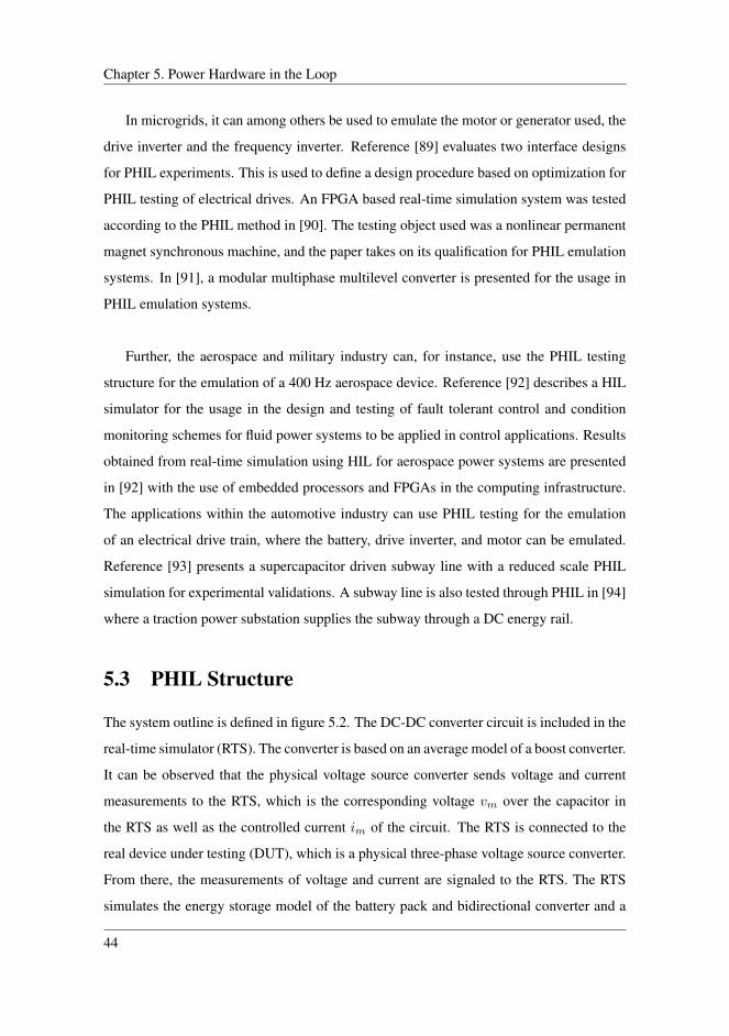
Chapter 5. Power Hardware in the Loop
In microgrids, it can among others be used to emulate the motor or generator used, the
drive inverter and the frequency inverter. Reference [89] evaluates two interface designs
for PHIL experiments. This is used to define a design procedure based on optimization for
PHIL testing of electrical drives. An FPGA based real-time simulation system was tested
according to the PHIL method in [90]. The testing object used was a nonlinear permanent
magnet synchronous machine, and the paper takes on its qualification for PHIL emulation
systems. In [91], a modular multiphase multilevel converter is presented for the usage in
PHIL emulation systems.
Further, the aerospace and military industry can, for instance, use the PHIL testing
structure for the emulation of a 400 Hz aerospace device. Reference [92] describes a HIL
simulator for the usage in the design and testing of fault tolerant control and condition
monitoring schemes for fluid power systems to be applied in control applications. Results
obtained from real-time simulation using HIL for aerospace power systems are presented
in [92] with the use of embedded processors and FPGAs in the computing infrastructure.
The applications within the automotive industry can use PHIL testing for the emulation
of an electrical drive train, where the battery, drive inverter, and motor can be emulated.
Reference [93] presents a supercapacitor driven subway line with a reduced scale PHIL
simulation for experimental validations. A subway line is also tested through PHIL in [94]
where a traction power substation supplies the subway through a DC energy rail.
5.3 PHIL Structure
The system outline is defined in figure 5.2. The DC-DC converter circuit is included in the
real-time simulator (RTS). The converter is based on an average model of a boost converter.
It can be observed that the physical voltage source converter sends voltage and current
measurements to the RTS, which is the corresponding voltage vm over the capacitor in
the RTS as well as the controlled current im of the circuit. The RTS is connected to the
real device under testing (DUT), which is a physical three-phase voltage source converter.
From there, the measurements of voltage and current are signaled to the RTS. The RTS
simulates the energy storage model of the battery pack and bidirectional converter and a
44

5.4 Discretization Algorithm
load. As illustrated in the figure, the RTS sends a voltage signal to the physical equipment
to a controlled voltage source.
Figure 5.2: Outline of PHIL Structure for emulation of ESS.
5.4 Discretization Algorithm
As illustrated in figure 5.2, a voltage source model is required to send the voltage reference
to the controlled voltage source. In order to obtain the voltage model, a discrete model
at the capacitor of figure 5.2 is obtained in the following subsection. The discretization
aims to model the parallel connection of a controlled current source and the capacitor into
its Thevenin equivalent circuit, as represented in figure 5.3. This procedure enables an
emulation of the energy storage system up to the controlled current source of the high
voltage side of the converter.
45

Chapter 5. Power Hardware in the Loop
Figure 5.3: Illustration of discretization objective.
From Kirchhoff’s current law, the current loop can be described as:
Cdvdc(t)
dt= i(t)− iload(t) (5.1)
Where, i(t) is controllable and iload(t) is the disturbance. The expression can further
be represented in the Laplace domain as in equation (5.2).
CsVDC(s) = I(s)− Iload(s) (5.2)
where, VDC(s), i(s) and iload(s) are the same variables as above in the Laplace domain.
The trapezoidal approach of discretizing continuous signals leads to [95]:
s =2(z − 1)
T (z + 1)(5.3)
The system in the z-domain is represented as follows:
C2(z − 1)
T (z + 1)Vdc(z) = I(z)− Iload(z) (5.4)
2C(z − 1)Vdc(z) = T (z + 1)I(z)− T (z + 1)Iload(z) (5.5)
The trapezoidal approach asserts that a signal multiplied with z equals the signal one
sample time ahead. This is implemented in discrete form equation (5.6) and reordered in
equation (5.7).
46

5.4 Discretization Algorithm
vdc,k+1 − vdc,k =T
2C(ik+1 + ik)− T
2C(iL,k+1 + iL,k) (5.6)
vdc,k+1 = vdc,k +T
2C(ik+1 + ik − iL,k+1 − iL,k) (5.7)
Using the instant time current gives the following expression in (5.8).
vdc,k = vdc,k−1 +T
2C(ik − ik−1 − iL,k−1 − iL,k) (5.8)
The circuit at the right side of figure 5.3 can be obtained from (5.8). Equation (5.8) is
used in the computational model to obtain the same signals as the continuous time model.
Consequently, it is obtained that ∆t = T2 . The voltage drop is obtained with the measured
current ik and the computed resistor ∆t/C. The output voltage is vm = vdc,k, and the
controlled voltage source is calculated with the remaining part of the terms.
47

Chapter 5. Power Hardware in the Loop
48

Chapter 6
Computational ResultsThe objective of this chapter is to test the control configurations from the literature review.
The chapter will give a good evaluation of the discrete design implemented, as it can be
compared to the continuous model. The most extensive part of this thesis, aside from the
laboratory work, is the computational results. The resulting developed model consists of
a battery model connected to a bidirectional DC-DC converter. To develop the resulting
model, a step - by - step methodology was used. First, the battery design was developed
and tested, as shown in chapter 3. The bidirectional converter was designed as an average
model, and the current and voltage control was implemented as in section 4. This chapter
takes on the resulting graphs from the model of a battery pack connected to a bidirec-
tional converter with an implemented current and voltage control. Section 6.1 presents
the resulting graphs of the bidirectional converter control with the battery pack. Secondly,
the battery model is tested computationally with the system designed according to 3.3. In
section 6.3, the discretization algorithm is tested through simulations and compared to the
continuous model results. Section 6.4 shows how the implementation of noise affects the
resulting output of the model. The chapter ends with a discussion of the computational
results.
The simulations are conducted in the MATLAB/Simulink environment. Simulink is a
block diagram tool that supports multidomain simulations. The designs are model-based,
and there are automatic code generation, continuous test, and verification of the embedded
systems. The program includes a graphical editor and customizable block libraries [96].
49

Chapter 6. Computational Results
6.1 DC-DC Converter connected to Battery System
The DC-DC converter is modeled to regulate voltage and current. Table 6.1 lists the param-
eters of the converter considered during the simulations. During the control, all parameters
(except time) are converted into the per unit (pu) system. The DC-DC converter model is
created in MATLAB/Simulink as an average model with a current and voltage control. The
nominal voltage of the battery pack was 96V , and the converter was modeled to provide
an output voltage of 650V . The input voltage parameter for the design of the converter
is 300V , which means that the converter can be applied to an extension of both two and
three battery packs. This section addresses the current output Iout and the voltage output
Vout. Furthermore, the section includes the current and voltage errors from the controller
in the per unit system, to ensure functioning control, which are attained with the use of
Proportional Integral (PI) regulators.
Table 6.1: Converter Parameters
Base Parameters Actual Value
Power 20 kVA
Frequency 50 Hz
Switching Frequency 10 kHz
Input Voltage 300 V
Output Voltage 650 V
Nominal Current 33.33 A
Inductance 5.625 mH
Resistance 22.5 mΩ
Capacitance 55.556 µF
Figure 6.1 presents the resulting graphs of a 10 seconds simulation of the model. The
uppermost graph takes on the control of the converter. The voltage and current errors are
depicted in the per unit system. Both error curves show an initial oscillation before stabi-
lizing at zero. The middle graph presents the current out of the converter, which stabilizes
at 12.3A. The voltage graph at the bottom of Vout stabilizes at 650V , as expected.
50

6.1 DC-DC Converter connected to Battery System
Figure 6.1: Resulting graphs from the bidirectional converter model. The top graph shows thevoltage and current error from the controller. The middle graph is the current output and the bottomgraph shows the voltage output of the converter.
51

Chapter 6. Computational Results
6.2 Battery Model
The battery system is connected to the low voltage side of the converter. It is computation-
ally modeled with the standard Simulink/Simscape library lithium-ion battery. The design
is conducted according to section 3.3.
Figure 6.2: Resulting graphs from the discharging battery model. The top graph shows the state ofcharge, the middle graph is the current out from the battery and the bottom graph shows the voltageover the battery system.
52

6.3 Discrete Model
The battery starts with an initial full battery with the SOC of 100%. From there, after
10 seconds, the battery SOC drops to 99.98774 %, which leads to an average decline in
charge of 1.226 · 10−3% per second. The battery current ib stabilizes at 69.5 A, after an
oscillating initialization. The battery voltage over the battery system is stabilizing at 116.6
V. Figure 6.3 presents the discharge curve for one of the two batteries in series with the
correct value of the discharge current at 69.5 A.
Figure 6.3: Discharge curve with the discharge current observed is the resulting scope.
6.3 Discrete Model
The objective of the discretization was to emulate the continuous model. Therefore, the
comparison between the two is best done if both models are scoped in the same graphs.
Figure 6.4 presents the continuous model results iout and vout as the green lines, and the
discrete signals iK and vDC as the yellow lines. It can be observed that both the discrete
and continuous signals behave identically, which is why the signals from the continuous
model are represented with thicker green lines to depict both results. The signals behave
similarly to the signals presented in 6.1.
53

Chapter 6. Computational Results
Figure 6.4: The top graph shows the current output iout and the discretized current output iK . Thebottom graph shows the voltage output vout and the discretized voltage output vDC of the converter.
54

6.4 Implementation of Noise
6.4 Implementation of Noise
Figure 6.5: The top graph shows the current output iout and the discretized current output iK withthe inclusion of noise. The bottom graph shows the voltage output vout and the discretized voltageoutput vDC of the converter with the inclusion of noise.
To ensure realistic simulation results in view of the experimental validation, noise was
added to the computational model in the output voltage and current. The noise was mod-
eled in Simulink as a random number, changing by the rate of the switching frequency
given in table 6.1. The output number of the noise was a normally distributed random sig-
nal. The variance of the noise was attained from tests at the Norwegian Smart Grid Labo-
ratory. The voltage variance is set to 0.1150, and the current variance is set to 0.0609. The
55
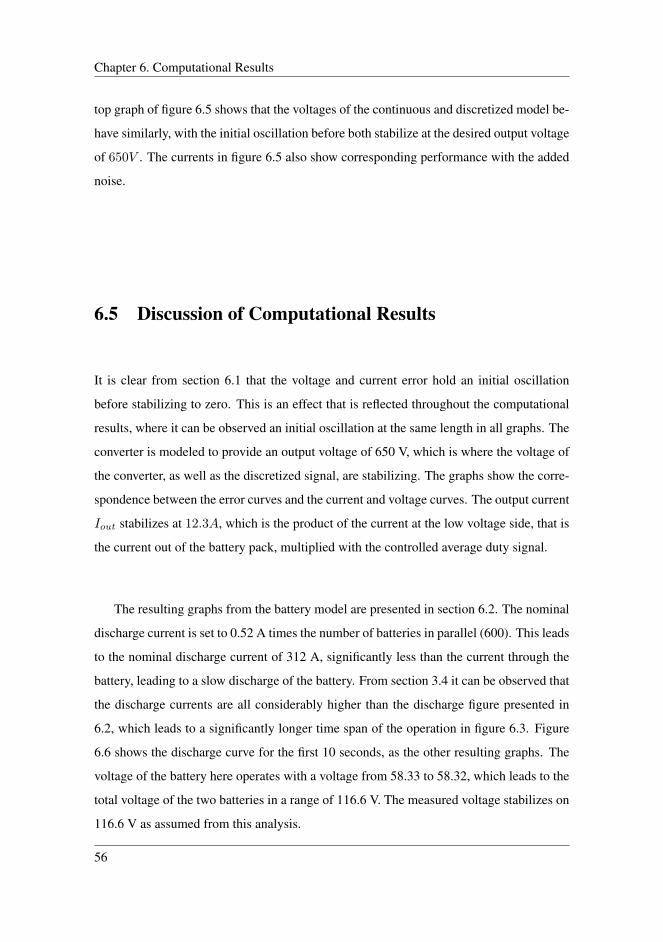
Chapter 6. Computational Results
top graph of figure 6.5 shows that the voltages of the continuous and discretized model be-
have similarly, with the initial oscillation before both stabilize at the desired output voltage
of 650V . The currents in figure 6.5 also show corresponding performance with the added
noise.
6.5 Discussion of Computational Results
It is clear from section 6.1 that the voltage and current error hold an initial oscillation
before stabilizing to zero. This is an effect that is reflected throughout the computational
results, where it can be observed an initial oscillation at the same length in all graphs. The
converter is modeled to provide an output voltage of 650 V, which is where the voltage of
the converter, as well as the discretized signal, are stabilizing. The graphs show the corre-
spondence between the error curves and the current and voltage curves. The output current
Iout stabilizes at 12.3A, which is the product of the current at the low voltage side, that is
the current out of the battery pack, multiplied with the controlled average duty signal.
The resulting graphs from the battery model are presented in section 6.2. The nominal
discharge current is set to 0.52 A times the number of batteries in parallel (600). This leads
to the nominal discharge current of 312 A, significantly less than the current through the
battery, leading to a slow discharge of the battery. From section 3.4 it can be observed that
the discharge currents are all considerably higher than the discharge figure presented in
6.2, which leads to a significantly longer time span of the operation in figure 6.3. Figure
6.6 shows the discharge curve for the first 10 seconds, as the other resulting graphs. The
voltage of the battery here operates with a voltage from 58.33 to 58.32, which leads to the
total voltage of the two batteries in a range of 116.6 V. The measured voltage stabilizes on
116.6 V as assumed from this analysis.
56

6.5 Discussion of Computational Results
Figure 6.6: Discharge curve with the discharge current observed is the resulting scope.
The battery charging process is not an extensive part of the computational results, but
it is included in appendix B. As the battery, in that case, is only connected to a controlled
current source without a DC-DC converter nor a control system, the results are bound to
be less realistic than the results included in this chapter. However, with the same current
rating of the source, it creates a basis for comparisons. This leads to the resulting charging
graphs with no oscillating part, and the system stabilizes instantly. The state of charge
is increasing with 1.238 · 10−3% per second, while the discharged battery decreases its
SOC with 1.226 ·10−3% per second. These values are relatively similar, due to the similar
current running through the battery (though in opposite directions). The battery current ib
running through the discharging battery in section 6.2 is not exactly 69.5, which can be
the reason why the SOC does not behave inversely proportional.
Section 6.3 shows the comparison of the continuous model versus the discretized
model. The resulting graph verifies the discretization algorithm based on the signals
matching each other throughout the ten seconds. Noise was added to the signals in section
6.4. This was done to ensure a realistic result to later establish a smooth transition to the
physical equipment in the laboratory. The voltage variance of noise was higher than the
current noise but caused for a lower percentage of the signal in the case of a high voltage
low current model. The simulated model of the energy storage system has a capacitance of
55.556µF , which is a relatively low capacitance. This is designed according to equation
4.30 in section 4.1. However, the capacitor in the physical converter at the laboratory has
57

Chapter 6. Computational Results
a value of 14mF , which is significantly larger. Additionally, the current step from 1 to
12.3 amperes is relatively big, which leads to a slow response. This makes a high and low
frequency oscillation in both the voltages and currents.
58

Chapter 7
Laboratory Work
This chapter will provide a presentation of the laboratory work conducted to test the theo-
retical ideas and simulated models. The model uses a PHIL testing strategy, as presented
in chapter 5, of a simulated model like the one in chapter 6. The first section introduces the
testing site, the laboratory setup, and the physical equipment used to obtain the results.
The results are presented in section 7.2, where both the real-time simulation (RTS) and
physical sensor signals are included. The current and voltage graphs prove the function-
ality of the power hardware in the loop testing method. Lastly, the results are discussed
and analyzed deeper in section 7.3.
The computational results showed a functioning controller. With the smart grid lab-
oratory facilities of SINTEF and NTNU, the system was tested with the use of physical
equipment as well as the simulated model. This chapter presents a functioning emulation
of an energy storage system, as well as confirming the functionality of PHIL.
59

Chapter 7. Laboratory Work
7.1 Laboratory Setup
The Norwegian national smart grid laboratory in Trondheim is built by NTNU and SIN-
TEF. The laboratory is system oriented, and its purpose is to provide a state of the art in-
frastructure for research and development, verification and testing over various use cases
of smart grid application. The laboratory design enables the possibility of integrating RTS
and physical power system assets in a PHIL setup with a rating up to 200 kVA, 400 V
AC or 700 V DC. The laboratory can be used to test numerous systems such as smart
home management systems, multi-terminal HVDC grid connecting offshore wind farms,
frequency support from wind turbines, product testing and verification, microgrids and
lastly, the use of this thesis, power hardware in the loop.
Figure 7.1: Norwegian Smart grid Laboratory. (1): 200kVA Controlled Voltage Source, (2): 60kVA 3− φ VSC, (3): OPAL-RT.
The laboratory testing was conducted in the Norwegian Smart Grid Laboratory de-
picted in figure 7.1. The model was implemented with an OPAL - RT simulator with a
60

7.1 Laboratory Setup
sampling time Ts = 100µs, which signaled the physical laboratory equipment.
7.1.1 Controlled Voltage Source
Figure 7.2 shows the controlled voltage source used in the laboratory setup. It is a 200kVA
digital amplifier. It is of the model COMPISO System Unit 200-1GAMP6. The amplifier
works as a turnkey PHIL solution for electrical power system testing. The unit includes
six four-quadrant digital power amplifiers that can operate DC up to 5 kHz full span output
voltage. The system provides the power path, safety infrastructure, and software applica-
tions to the configuration of running tests [97].
Figure 7.2: 200kVA Controlled Voltage Source
61

Chapter 7. Laboratory Work
7.1.2 Voltage Source Converter
The voltage source converter used in the laboratory setup is presented in figure 7.3. The
converter is rated at 60 kVA AC / DC. It includes an LCL filter, a contactor, and a charging
circuit.
Figure 7.3: 60 kVA 3− φ VSC
7.1.3 Real Time Simulator
In the testing, the Opal-RT 5700 in figure 7.4 is used. This is a complete simulation system.
The OP5700 includes a target computer, a reconfigurable field-programmable gate array
(FPGA), signal conditioning for up to 256 I/O lines and 16 high-speed fiber-optic small
form-factor pluggable ports. The AC input is rated to 100-240 V, and 60-50 Hz [98].
62

7.2 Laboratory Results
Figure 7.4: OPAL-RT.
7.2 Laboratory Results
This section presents the laboratory results of the output voltage and current for both the
physical measurements, as well as the one included in the discretized simulation model.
The objective of this section is to obtain an emulation of the battery and the DC-DC con-
verter in a real-time simulation connected with a physical voltage source converter and a
controlled voltage source through the power hardware in the loop testing strategy. The
included results presented are a collection of logged data from the system under differ-
ent conditions: constant current, a slight increase of current, rapid increase of current and
rapid decreasing of current. The change in current was physically increased and decreased
by turning a rotary control knob. The degree of rotation corresponded with the current
output, while the speed of rotation corresponded with the current change velocity, as the
testing occurred in real-time. The time periods between the data logs are averaged with a
dotted grey line.
63

Chapter 7. Laboratory Work
7.2.1 Current Results
Figure 7.5 presents the resulting current from the laboratory tests. This graph contains
two different measurements. The black line represents the current ik, the signal from the
real-time simulator, which represents the simulation. The gray dashed line represents a
constant estimated average between data logs. The blue, green, and orange lines are the
output current data logs from the physical laboratory equipment, iout. The data logs are
explained below.
1. The first section is logged from t = 321 s to t = 347 s. It is in figure 7.5 illustrated
as the blue area. The section is initialized with 10 seconds of constant current. From
t = 331 s to t = 347 s the current ramp has an average increase of 0.1 amperes per
second.
2. The second section is logged from t = 374 s to t = 397 s. This area is in figure 7.5
the green area. The section starts with a 16-second current ramp. The current ramp
has an average increase of 0.13 amperes per second. From there, the current remains
unchanged for 7 seconds.
3. The third section is logged from t = 479 s to t = 493 s. In figure 7.5, the section is
represented as the decreasing orange area. From t = 479 s to t = 489 s the decreasing
current ramp has an average decrease of 0.36 amperes per second. The graph ends
with an unchanged current in the third section of 5 seconds.
64

7.2 Laboratory Results
Figure 7.5: Current output iout from the continuous model as the blue, green and orange line andik from the physical measurement as the black line.
7.2.2 Voltage Results
Figure 7.6 shows the voltage output graph from the laboratory tests. The voltage output
vDC from the continuous model and vout from the physical equipment are perfectly cor-
related. Consequently, it looks like only one value is measured at each time, even though
in fact, both the voltage from the simulation model and the value from the physical equip-
ment test is included. The voltage is kept around the value of 650, but with some apparent
noise. The blue, green, and orange lines represent vout and vDC at the three data logs
explained below.
1. The first section is logged from t = 321 s to t = 347 s. It is in figure 7.6 illustrated
as the blue area. The amplitude of the noise in the first section is largest at the value
of 649.751 V at t = 336 s, with the amplitude 0.249.
65

Chapter 7. Laboratory Work
2. The second section is logged from t = 374 s to t = 397 s. This area is in figure 7.6
represented as the green area. The voltage deviates most from 650 V at t = 388 s at
the value of 649.462 V. This leads to an amplitude of 0.538.
3. The third section is logged from t = 479 s to t = 493 s. In figure 7.6, the section is
illustrated as the orange area. The section has a clear amplitude at its most deviating
point in t = 488 s with the value of 650.843 V, which gives the largest amplitude of
0.843.
Figure 7.6: Voltage output vDC from the continuous model and vout logged from the physicalequipment perfectly correlated.
66

7.3 Discussion of Laboratory Work
7.3 Discussion of Laboratory Work
Section 7.2.1 presents the current output iout from the physical sensors and ik from the
simulation model. It is clear that the noise of the physical equipment is significantly larger
than the noise in the simulation. When considering the constant current in the first part
of the first data log in figure 7.5, the noise from the simulation model is nearly insignif-
icant with a top amplitude of 0.03 A, while the noise of the physical equipment is at top
amplitude of 0.72 A. This notable noise from the physical equipment is the result of us-
ing sensors rated to higher currents, leading to a sensitive low current operation. It would
be interesting to conduct the same tests under similar circumstances with current sensors
rated to low current operation, to obtain an improved review of the current output, iout.
In comparing figure 7.5 and figure 7.6, some conclusions can be drawn. The first sec-
tion leaves the current unchanged for the longest time span: 10 seconds, while the second
and third data logs leave the current unchanged for 7 and 5 seconds respectively. In figure
7.6, this shows clearly that within the first ten seconds, the voltage signal is experiencing
a noticeably stable behavior. This can also, to a smaller degree, be observed at the end of
the second and third data log. The beginning of the second and third data log is initialized
at a constant current, which also leads to stable behavior in the voltage outputs.
Section 7.2.2 examines the amplitude of the noise in the voltage output. The first
section shows that after t = 331 s, when the current starts to increase, the voltage noise
amplitude is also increased. However, the amplitude of the voltage through the current
ramp period of the first section is quite similar with no clear peak. This is because the
current is increased in a fairly steady process. The largest amplitude of the first section is
on 0.249, with a deviation of 38.3·10−3% of the mean voltage output at 650 V. The second
data log has two clearly larger sections of noise where the current has not been increased
as continuously. The voltage deviates most at t = 388 s, at the end of the increasing ramp.
The most significant deviation of 649.462 V leads to an 8.28 ·10−3% disparity of the mean
voltage output.
67

Chapter 7. Laboratory Work
The third section is noteworthy. It is the smallest data logging of only 14 seconds. The
current is decreasing at a very high rate of 0.36 amperes per second, compared to the rate
of 0.1 and 0.13 from the other data logs. As assumed, this leads to a significant voltage
deviation. At the time of the steepest decreasing ramp, the voltage level is measured to
650.843 V. This is a 0.13% deviation from the mean voltage output. Despite the deviations
and noise even at a constant current, the resulting graphs are within acceptable voltage and
current levels. Even in the most discontinuous current rates, the system behaved stable.
The voltage signals experienced noise, but always with a mean of 650V, and the signals
followed the current signals with a fast response.
The change in current was managed manually by turning a rotary control knob. Con-
sequently, the rate of change of current was not changed at a constant velocity in the data
logs. The current change was operated at the slowest rate for the first section, and the high-
est rate for the third section. The erratic behavior of the current compels for an interesting
review of the voltage error, as discussed in this section. However, if the testing were con-
ducted in changing the current with constant rates of amperes per second, it would open
to a discussion of how much the current rate affects the voltage noise with more realistic
quantitative conclusions.
68

Chapter 8
Concluding Remarks
This thesis has discussed an energy storage emulation for the application of a low voltage
grid connection. The BESS is simulated in the MATLAB/Simulink environment, which
illustrated that the battery pack complied with the requirements. A bidirectional DC-DC
converter is connected to the energy storage system. The converter behavior is explained,
as well as an included part about converter control based on an average model. The volt-
age and current control were based on PI regulation to ensure system stability. Preceding
the laboratory testing, the PHIL technique was implemented to acquire realistic results. In
order to obtain the voltage model for the PHIL setup, a discrete model was derived theo-
retically before it was tested through simulation. This chapter takes on the most essential
concluding remarks attained from the process.
An outline of different rechargeable battery types with advantages and disadvantages
has been explained. The thesis continued with a lithium-ion battery, mainly due to its high
energy density and the lack of memory effect in the battery. The computational battery
model was then retrieved from the Simulink/Simscape library. The battery was designed
for a load of 15 kW for 5 hours. The design was derived, and the Simulink implementa-
tion confirmed that the battery was able to supply the required load. However, the BESS
later used with the connection to the converter had a significantly lower current running
through the battery. This resulted in a state of charge which is above 99.98% in the entire
69

Chapter 8. Concluding Remarks
simulation time. With employing the stabilized battery current, the discharge curve of the
battery showed that the voltage over the battery was within its rated limits.
The bidirectional converter is in the thesis simplified with a boost topology to be ap-
plied to step up the voltage from the battery and control the current and voltage of the
system. As the objective of the thesis did not include an analysis of the switching fre-
quency ripple, the converter was designed as an average model, due to its advantages with
a faster simulation time domain and a less complex design. In the converter control, PI
regulators were used both in the outer voltage control and inner current control. For the
tuning of the PI voltage regulator, the symmetrical optimum method was applied. The
computational results of the converter presented acceptable results. The voltage and cur-
rent error started with a limited error oscillation, before the errors both stabilized at zero
as designed. The converter was modeled to a voltage output of 650 V, which is what was
attained from the computational results.
For the laboratory testing, a power hardware in the loop methodology was used. This
methodology combines testing of both hardware and software, leading to time and cost-
effective testing with realistic results. The PHIL structure included a real-time simulation
of the emulated energy storage system connected to a real three-phase VSC device under
testing. To send the reference voltage to the controlled voltage source, a discrete model
was derived using the trapezoid approximation. From the computational results, it can be
concluded with that the discretization algorithm performed in accordance with the goal
of mimicking the continuous model, as the signals both in the current and voltage output
behaved identically.
To ensure realistic simulation results in view of the experimental validation, noise was
added to the computational model in the output voltage and current. The variance of the
noise was attained from tests at the Norwegian Smart Grid Laboratory. This lead to a
smooth transition from the simulated model to the physical laboratory equipment. The
laboratory results from the current signal depicts an acceptable outcome where the current
70

from the physical signals and the current from the simulated model follows the same val-
ues. However, the noise of the physical equipment was significantly larger than the noise in
the simulation. This was due to the use of sensors at the laboratory rated to relatively much
higher currents, leading to a sensitive low current operation. The voltage signals from the
physical laboratory equipment and simulation model responded identically throughout the
entire simulation, which describes a successful PHIL test of an emulation of a battery
energy storage system.
Further Work
There are numerous ways of taking the system proposed in this thesis further. This section
will provide some of the proposals for further work.
The model designed in this thesis included a DC-DC boost converter, with the inten-
tion of it to act as a bidirectional converter for the purposes of discharging the battery. It
would be interesting to take the model further with the development of an actual bidirec-
tional converter. In that case, the model could also be taken through the charging process
of the battery. Different battery types were described in the thesis, but only lithium-ion
was used. It would be interesting to see how the other battery types behaved differently
and conduct detailed testings of different battery types for an energy storage emulation.
The Simulink/Simscape battery from the library can be modeled as different battery types.
The computational model consisting of a DC-DC converter and a battery model can be
expanded. This can potentially be modeled as a microgrid. First of all, a voltage source
converter can be modeled as in [8] with a voltage and current control and a phase locked
loop. This VSC can be connected to an AC grid with a grid forming converter like the
one in [8]. The AC grid can be expanded with several VSCs connected to grid sources.
A PV model can be implemented from the Simulink/Simscape library with an MPPT to
ensure a realistically strong performance. The cloud cover for the PV can be varied ei-
ther randomly or by implementing actual weather data for a specific geographical area
in a MATLAB function implemented in the PV model. This will ensure a PV RES with
71

relatively realistic behavior. Further, a wind turbine can be implemented to another VSC
in the grid. The wind speed can be modeled in the same way as the cloud cover of the
PV: either with a random variance or with the implementation of real weather data. Loads
should also be implemented in the system to model a microgrid. The decision of what the
load should represent depends on the scope of the work. Among others, the loads could
copy the behavior of a neighborhood, office buildings, or stores. The load rating should be
set as realistic values for the said loads, and with the peak and low load periods at the parts
of the day where the grid would usually experience peaks and low load conditions. For
instance, a household usually has a high load in the mornings and the evening, and in Nor-
way, the difference between winter and summer should also be taken into consideration.
This would lead to a demand for a further advanced control system. A droop based control
strategy which has been explained in [8] could further be implemented with power control
in the voltage source converters for an improved regulation of the system. The microgrid
could alternatively be controlled with a virtual synchronous machine (VSM) scheme. If
both control schemes, both droop- and VSM-based, are tested, the microgrid would create
a consistent basis of comparison between the control models. With the loads, the PV, the
wind turbine(s) and the ESS, as well as a grid forming converter, the model is versatile,
and several tweaks can be done to the model to test it for different scenarios.
Oil and gas companies have an increased interest in offshore microgrids, with an im-
plementation of energy storage systems and offshore wind parks to supply oil platforms.
This can be further analyzed and tested in Simulink. When the simulation model is devel-
oped according to the previous paragraph, the work required to change it to an offshore
microgrid would include a higher voltage level of the grid, a higher rating of the wind
turbines and a completely different load behavior. A gathering of data from offshore oil
platforms would be necessary to model the gas turbines as loads with the ratings realisti-
cally obtained.
72

Bibliography
[1] M. Roser and E. Ortiz-Ospina, World Population Growth, 2018. [Online]. Available:
https://ourworldindata.org/world-population-growth
[2] I. E. Agency, World Energy Statistics 2017, 2017. [Online]. Available:
https://www.oecd-ilibrary.org/content/publication/world energy stats-2017-en
[3] S. Chakraborty, M. G. Simoes, and W. E. Kramer, Power Electronics for Renewable
and Distributed Energy Systems. Springer, London, 2013.
[4] G. Pepermans, J. Driesen, D. Haeseldonckx, R. Belmans, and W. D’haeseleer,
“Distributed generation: definition, benefits and issues,” Energy Policy, vol. 33,
no. 6, pp. 787 – 798, 2005. [Online]. Available: http://www.sciencedirect.com/
science/article/pii/S0301421503003069
[5] F. Blaabjerg, Z. Chen, and S. Kjær, “Power electronics as efficient interface of re-
newable energy sources,” vol. 3, 09 2004, pp. 1731 – 1739 Vol.3.
[6] A. Kumar, A. H. Bhat, and P. Agarwal, “Comparative analysis of dual active bridge
isolated dc to dc converter with flyback converters for bidirectional energy trans-
fer,” in 2017 Recent Developments in Control, Automation Power Engineering (RD-
CAPE), Oct 2017, pp. 382–387.
[7] H. Bai and C. Mi, “Eliminate reactive power and increase system efficiency of iso-
lated bidirectional dual-active-bridge dc–dc converters using novel dual-phase-shift
control,” IEEE Transactions on Power Electronics, vol. 23, no. 6, pp. 2905–2914,
Nov 2008.
73

[8] N. P. Sagatun, “Control structure for islanded microgrids,” Dec 2018.
[9] T. Ackermann, G. Andersson, and L. Sodera, “Distributed generation: a definition,”
Electric Power Systems Research, vol. 57, no. 3, pp. 195–204, 2001.
[10] F. H. Guan, D. M. Zhao, X. Zhang, B. T. Shan, and Z. Liu, “Research on distributed
generation technologies and its impacts on power system,” 2009 International Con-
ference on Sustainable Power Generation and Supply, pp. 1–6, 2009.
[11] Nwulu, N. I., and X. Xia, “Optimal dispatch for a microgrid incorporating renewables
and demand response,” Renewable Energy, vol. 101, pp. 16–28, 2017.
[12] E. Pritchard, L. Mackey, D. Zhu, D. Gregory, and G. Norris, “Modular electric gen-
erator rapid deployment dc microgrid,” 2017 IEEE Second International Conference
on DC Microgrids, pp. 106–110, 2017.
[13] S. Ahmadi, H. Bevrani, S. Shokoohi, and E. Hasanii, “An improved droop control for
simultaneous voltage and frequency regulation in an ac microgrid using fuzzy logic,”
Iranian Conference on Electrical Engineering, vol. 13, no. 23, pp. 1486–1491, 2015.
[14] M. Arlt, G. F. Cardoso, and D. Weng, “Hydrogen storage applications in indus-
trial microgrids,” 2017 IEEE Green Energy and Smart Systems Conference, pp. 1–6,
2017.
[15] O. M. Toledo, D. O. Filho, and A. S. A. C. Diniz, “Distributed photovoltaic
generation and energy storage systems: A review,” Renewable and Sustainable
Energy Reviews, vol. 14, no. 1, pp. 506 – 511, 2010. [Online]. Available:
http://www.sciencedirect.com/science/article/pii/S136403210900207X
[16] C. K. Das, O. Bass, G. Kothapalli, T. S. Mahmoud, and D. Habibi, “Overview of
energy storage systems in distribution networks: Placement, sizing, operation, and
power quality,” Renewable and Sustainable Energy Reviews, vol. 91, pp. 1205 –
1230, 2018. [Online]. Available: http://www.sciencedirect.com/science/article/pii/
S1364032118301606
74

[17] Z. Lu, G. Bao, H. Xu, X. Dong, Z. Yuan, and C. Lu, “Battery energy storage system
based power quality management of distribution network,” in Informatics in Con-
trol, Automation and Robotics, D. Yang, Ed. Berlin, Heidelberg: Springer Berlin
Heidelberg, 2012, pp. 599–606.
[18] S. Koohi-Kamali, V. Tyagi, N. Rahim, N. Panwar, and H. Mokhlis, “Emergence of
energy storage technologies as the solution for reliable operation of smart power
systems: A review,” Renewable and Sustainable Energy Reviews, vol. 25, pp. 135
– 165, 2013. [Online]. Available: http://www.sciencedirect.com/science/article/pii/
S1364032113002153
[19] P. F. Ribeiro, B. K. Johnson, M. L. Crow, A. Arsoy, and Y. Liu, “Energy storage
systems for advanced power applications,” Proceedings of the IEEE, vol. 89, no. 12,
pp. 1744–1756, Dec 2001.
[20] O. Babacan, W. Torre, and J. Kleissl, “Siting and sizing of distributed energy storage
to mitigate voltage impact by solar pv in distribution systems,” Solar Energy, vol.
146, pp. 199–208, 04 2017.
[21] K. H. Chua, Y. S. Lim, P. Taylor, S. Morris, and J. Wong, “Energy storage system for
mitigating voltage unbalance on low-voltage networks with photovoltaic systems,”
IEEE Transactions on Power Delivery, vol. 27, no. 4, pp. 1783–1790, Oct 2012.
[22] P. Mercier, R. Cherkaoui, and A. Oudalov, “Optimizing a battery energy storage
system for frequency control application in an isolated power system,” IEEE Trans-
actions on Power Systems, vol. 24, no. 3, pp. 1469–1477, Aug 2009.
[23] J. Leadbetter and L. Swan, “Battery storage system for residential electricity
peak demand shaving,” Energy and Buildings, vol. 55, pp. 685 – 692, 2012,
cool Roofs, Cool Pavements, Cool Cities, and Cool World. [Online]. Available:
http://www.sciencedirect.com/science/article/pii/S0378778812004896
[24] S. Teleke, M. E. Baran, S. Bhattacharya, and A. Q. Huang, “Rule-based control of
battery energy storage for dispatching intermittent renewable sources,” IEEE Trans-
actions on Sustainable Energy, vol. 1, no. 3, pp. 117–124, Oct 2010.
75

[25] S. X. Chen, H. B. Gooi, and M. Q. Wang, “Sizing of energy storage for microgrids,”
IEEE Transactions on Smart Grid, vol. 3, no. 1, pp. 142–151, March 2012.
[26] D. Ravi, B. Reddy, S. S. L., and P. Samuel, “Bidirectional dc to dc converters: An
overview of various topologies, switching schemes and control techniques,” Interna-
tional Journal of Engineering and Technology, vol. 7, pp. 360–365, 09 2018.
[27] F. Caricchi, F. Crescimbini, F. G. Capponi, and L. Solero, “Study of bi-directional
buck-boost converter topologies for application in electrical vehicle motor drives,” in
APEC ’98 Thirteenth Annual Applied Power Electronics Conference and Exposition,
vol. 1, Feb 1998, pp. 287–293 vol.1.
[28] S. Agrawal and R. S. Geetha, “Controllers for voltage source converters,” in 2013
International Conference on Emerging Trends in Communication, Control, Signal
Processing and Computing Applications (C2SPCA), 2013, pp. 1–8.
[29] V. Chitra, Fuzzy-Based Matrix Converter Drive for Induction Motor, 01 2017.
[30] A. Manoloiu, H. A. Pereira, R. Teodorescu, M. Bongiorno, M. Eremia, and S. R.
Silva, “Comparison of pi and pr current controllers applied on two-level vsc-hvdc
transmission system,” in 2015 IEEE Eindhoven PowerTech, 2015, pp. 1–5.
[31] F. Blaabjerg, Y. Yang, and K. Ma, “Power electronics - key technology for renewable
energy systems - status and future,” 2013 3rd International Conference on Electric
Power and Energy Conversion Systems, pp. 1–6, 2013.
[32] K. M. Son, K. Lee, D. Lee, T. C. E. Nho, and H. Kim, “Grid interfacing storage
system for implementing microgrid,” Transmission Distribution Conference Expo-
sition: Asia and Pacific, vol. 53, pp. 1–4, 2009.
[33] Proposal/ Contract no.: PL019864, “More microgrids: Advanced architectures and
control concepts for more microgrids,” FP6 STREP, 2006-2009.
[34] ENK5-CT-2002-00610, “Microgrids: Large scale integration of micro-generation to
low voltage grids,” 2003-2005.
76

[35] K. Sarwagya and P. K. Nayak, “An extensive review on the state-of-art on micro-
grid protection,” in 2015 IEEE Power, Communication and Information Technology
Conference (PCITC), Oct 2015, pp. 862–866.
[36] A. Vukojevic, “Lessons learned from microgrid implementation at electric utility,”
2018 IEEE Power Energy Society Innovative Smart Grid Technologies Conference,
pp. 1–5, 2018.
[37] N. Hatziargyriou, “Microgrids architectures and control,” John Wiley and Sons Ltd,
p. 4, 2014.
[38] Y. Zhou and C. N.-M. Ho, “A review on microgrid architectures and control meth-
ods,” in 2016 IEEE 8th International Power Electronics and Motion Control Confer-
ence (IPEMC-ECCE Asia), May 2016, pp. 3149–3156.
[39] B. Yu, J. Guo, C. Zhou, Z. Gan, J. Yu, and F. Lu, “A review on microgrid technol-
ogy with distributed energy,” in 2017 International Conference on Smart Grid and
Electrical Automation (ICSGEA), May 2017, pp. 143–146.
[40] A. Hirsch, Y. Parag, and J. Guerrero, “Microgrids: A review of technologies,
key drivers, and outstanding issues,” Renewable and Sustainable Energy Reviews,
vol. 90, pp. 402 – 411, 2018. [Online]. Available: http://www.sciencedirect.com/
science/article/pii/S136403211830128X
[41] C. Wang, J. Yan, C. Marnay, N. Djilali, E. Dahlquist, J. Wu, and H. Jia,
“Distributed energy and microgrids (dem),” Applied Energy, vol. 210, pp. 685
– 689, 2018. [Online]. Available: http://www.sciencedirect.com/science/article/pii/
S0306261917316550
[42] S. Parhizi, H. Lotfi, A. Khodaei, and S. Bahramirad, “State of the art in research on
microgrids: A review,” IEEE Access, vol. 3, pp. 890–925, 2015.
[43] T. Del Carpio Huayllas, D. Ramos, and R. Vasquez-Arnez, “Microgrid systems: Cur-
rent status and challenges,” 12 2010, pp. 7 – 12.
77
[44] Y. Wu, N. Chen, D. Jiang, L. Zhang, L. Qu, and M. Qian, “Study on energy storage
system participating in frequency regulation of wind farm based on polyline fuzzy
neural network,” in 2018 5th IEEE International Conference on Cloud Computing
and Intelligence Systems (CCIS), Nov 2018, pp. 1086–1090.
[45] Hongyan Piao, Shifeng Chen, Haichao Lv, and Haoming Liu, “Control strategy of
battery energy storage system to participate in the second frequency regulation,” in
2015 International Symposium on Smart Electric Distribution Systems and Technolo-
gies (EDST), Sep. 2015, pp. 53–57.
[46] P. Stenzel, T. Kannengießer, L. Kotzur, P. Markewitz, M. Robinius, and D. Stolten,
“Emergency power supply from photovoltaic battery systems in private households
in case of a blackout – a scenario analysis,” Energy Procedia, vol. 155, pp.
165 – 178, 2018, 12th International Renewable Energy Storage Conference,
IRES 2018, 13-15 March 2018, Dusseldorf, Germany. [Online]. Available:
http://www.sciencedirect.com/science/article/pii/S1876610218310129
[47] Y. Liu, C. Lin, and S. Chen, “Analysis of load electricity consumption on a low-
voltage distribution system with community energy storages,” in 2017 IEEE 3rd In-
ternational Future Energy Electronics Conference and ECCE Asia (IFEEC 2017 -
ECCE Asia), June 2017, pp. 2048–2052.
[48] F. Dıaz-Gonzalez, A. Sumper, O. Gomis-Bellmunt, and R. Villafafila-Robles, “A
review of energy storage technologies for wind power applications,” Renewable
and Sustainable Energy Reviews, vol. 16, no. 4, pp. 2154 – 2171, 2012. [Online].
Available: http://www.sciencedirect.com/science/article/pii/S1364032112000305
[49] O. Tremblay, L. Dessaint, and A. Dekkiche, “A generic battery model for the dy-
namic simulation of hybrid electric vehicles,” in 2007 IEEE Vehicle Power and
Propulsion Conference, Sep. 2007, pp. 284–289.
[50] O. Vigerstol, “Nickel cadmium batteries for outside telecom plants,” in Fourteenth
Annual Battery Conference on Applications and Advances. Proceedings of the Con-
ference (Cat. No.99TH8371), Jan 1999, pp. 313–317.
78

[51] M. M. Moorthi, “Field experience with large nickel metal hydride (nimh) batteries in
stationary applications,” in INTELEC 06 - Twenty-Eighth International Telecommu-
nications Energy Conference, Sep. 2006, pp. 1–7.
[52] D. Gies, “New approaches to safe ventilation of equipment containing lead acid and
nicd batteries,” in 2015 IEEE Symposium on Product Compliance Engineering (IS-
PCE), May 2015, pp. 1–5.
[53] M. Gonzalez, F. J. Ferrero, J. C. Anton, and M. A. Perez, “Considerations to improve
the practical design of universal and full-effective nicd/nimh battery fast-chargers,”
in APEC ’99. Fourteenth Annual Applied Power Electronics Conference and Expo-
sition. 1999 Conference Proceedings (Cat. No.99CH36285), vol. 1, March 1999, pp.
167–173 vol.1.
[54] S. M. Mousavi, S. H. Fathi, and G. H. Riahy, “Energy management of wind/pv and
battery hybrid system with consideration of memory effect in battery,” in 2009 Inter-
national Conference on Clean Electrical Power, June 2009, pp. 630–633.
[55] S. F. Pensabene and J. W. Gould, “Batteries: Unwanted memory spooks nickel-
cadmium cells: New understanding of an undesirable phenomenon is the first step
in avoiding it,” IEEE Spectrum, vol. 13, no. 9, pp. 33–37, Sep. 1976.
[56] S. Podder and M. Z. R. Khan, “Comparison of lead acid and li-ion battery in solar
home system of bangladesh,” in 2016 5th International Conference on Informatics,
Electronics and Vision (ICIEV), May 2016, pp. 434–438.
[57] “Lithium-ion battery overview,” in Lighting Global. International Finance Group.,
2012.
[58] C. Orendorff, D. H. Doughty, and E. P. Roth, “General discussion of li ion battery
safety.” Proposed for publication in The ECS Interface.
[59] T. Guena and P. Leblanc, “How depth of discharge affects the cycle life of lithium-
metal-polymer batteries,” in INTELEC 06 - Twenty-Eighth International Telecommu-
nications Energy Conference, Sep. 2006, pp. 1–8.
79

[60] J. McDowall, “Understaning lithium - ion technology.” Saft America Inc., 2008.
[61] X. Liu, P. Wang, and P. C. Loh, “A hybrid ac/dc microgrid and its coordination
control,” IEEE Transactions on Smart Grid, vol. 2, no. 2, pp. 278–286, June 2011.
[62] S. Sanchez, M. Molinas, M. Degano, and P. Zanchetta, “Stability evaluation of a dc
micro-grid and future interconnection to an ac system,” Renewable Energy, vol. 62,
pp. 649 – 656, 2014. [Online]. Available: http://www.sciencedirect.com/science/
article/pii/S096014811300428X
[63] “MATLAB Simscape Power Systems Documentation Battery Toolbox,” R2018a, the
MathWorks, Natick, MA, USA.
[64] Lithium-Ion Battery Datasheet, EEMB Co., Ltd, 8 2016.
[65] L. Valøen and M. I Shoesmith, “The effect of phev and hev duty cycles on battery
and battery pack performance,” 03 2019.
[66] R. Sadoun, N. Rizoug, P. Bartholumeus, B. Barbedette, and P. LeMoigne, “Sizing
of hybrid supply (battery-supercapacitor) for electric vehicle taking into account the
weight of the additional buck-boost chopper,” in 2012 First International Conference
on Renewable Energies and Vehicular Technology, March 2012, pp. 8–14.
[67] H. C. Hesse, M. Schimpe, D. Kucevic, and A. Jossen, “Lithium-ion battery storage
for the grid—a review of stationary battery storage system design tailored for
applications in modern power grids,” Energies, vol. 10, no. 12, 2017. [Online].
Available: http://www.mdpi.com/1996-1073/10/12/2107
[68] Lithium-Ion Battery Specification, EEMB Co., Ltd, 2 2016.
[69] N. Mohan, T. M. Undeland, and W. P. Robbins, Power Electronics. Converters, Ap-
plications and Design, 3rd ed. John Wiley and Sons, Inc, 2003.
[70] M. Matar and R. Iravani, “Fpga implementation of the power electronic converter
model for real-time simulation of electromagnetic transients,” IEEE Transactions on
Power Delivery, vol. 25, no. 2, pp. 852–860, April 2010.
80

[71] J. Channegowda, B. Saritha, H. R. Chola, and G. Narayanan, “Comparative eval-
uation of switching and average models of a dc-dc boost converter for real-time
simulation,” in 2014 IEEE International Conference on Electronics, Computing and
Communication Technologies (CONECCT), Jan 2014, pp. 1–6.
[72] A. Harumwidiah, M. Ashari, and D. C. Riawan, “Modelling back-to-back converter
with average model in wind power system using dfig,” in IPTEK, Journal of Pro-
ceeding Series, vol. 1, 2014, pp. 435–440.
[73] C. Jaen, R. Pindado, J. Pou, and V. Sala, “Adaptive model applied to pwm dc-dc
converters using averaging techniques,” in 2006 IEEE International Symposium on
Industrial Electronics, vol. 2, July 2006, pp. 1347–1352.
[74] A. Davoudi, J. Jatskevich, P. L. Chapman, and A. Khaligh, “Averaged-switch model-
ing of fourth-order pwm dc–dc converters considering conduction losses in discontin-
uous mode,” IEEE Transactions on Power Electronics, vol. 22, no. 6, pp. 2410–2415,
Nov 2007.
[75] F. R. Quintela, R. C. Redondo, N. R. Melchor, and M. Redondo, “A general approach
to kirchhoff’s laws,” IEEE Transactions on Education, vol. 52, no. 2, pp. 273–278,
May 2009.
[76] S. Sanchez, “Stability investigation of power electronics systems - a microgrid case,”
Thesis for the degree of Philosopiae Doctor, 2015.
[77] S. Sanchez, G. Bergna, and E. Tedeschi, “Tuning of control loops for grid-connected
modular multilevel converters under a simplified port representation for large sys-
tem studies,” in 2017 Twelfth International Conference on Ecological Vehicles and
Renewable Energies (EVER), April 2017, pp. 1–8.
[78] S. Sanchez, S. D’Arco, A. Holdyk, and E. Tedeschi, “An approach for small scale
power hardware in the loop emulation of hvdc cables,” in 2018 Thirteenth Interna-
tional Conference on Ecological Vehicles and Renewable Energies (EVER).
[79] OPAL - RT, “POWER HIL (P-HIL): A Revolution in the Industry,” Web Site Presen-
tation. [Online]. Available: https://www.opal-rt.com/power-hardware-in-the-loop/
81

[80] M. Lauritzsen, “Hardware-in-the-loop testing systems for rov control systems,”
2014. [Online]. Available: http://hdl.handle.net/11250/238916
[81] D. Maclay, “Simulation gets into the loop,” IEE Review, vol. 43, no. 3, pp. 109–112,
May 1997.
[82] W. Adiprawita, A. Suwandi Ahmad, and J. Sembiring, “Hardware in the loop simula-
tion for simple low cost autonomous uav (unmanned aerial vehicle) autopilot system
research and development,” 01 2007.
[83] E. R. Mueller, “Hardware -in -the -loop simulation design for evaluation of un-
manned aerial vehicle control systems,” 08 2007.
[84] D. Jung and P. Tsiotras, “Modeling and hardware-in-the-loop simulation for a small
unmanned aerial vehicle,” vol. 1, 05 2007.
[85] N. Schetinin, N. Moriz, B. Kumar, A. Maier, S. Faltinski, and O. Niggemann, “Why
do verification approaches in automation rarely use hil-test?” in 2013 IEEE Interna-
tional Conference on Industrial Technology (ICIT), Feb 2013, pp. 1428–1433.
[86] J. Langston, K. Schoder, M. Steurer, O. Faruque, J. Hauer, F. Bogdan, R. Bravo,
B. Mather, and F. Katiraei, “Power hardware-in-the-loop testing of a 500 kw photo-
voltaic array inverter,” in IECON 2012 - 38th Annual Conference on IEEE Industrial
Electronics Society, Oct 2012, pp. 4797–4802.
[87] R. S. Kaarthik, J. Maisonneuve, and P. Pillay, “Real-time emulation of a pressure-
retarded osmotic power generation system,” IEEE Transactions on Industry Applica-
tions, vol. 53, no. 6, pp. 5768–5776, Nov 2017.
[88] Seung-Ho Song, Byoung-Chang Jeong, Hye-In Lee, Jeong-Jae Kim, Jeong-Hun Oh,
and G. Venkataramanan, “Emulation of output characteristics of rotor blades using a
hardware-in-loop wind turbine simulator,” in Twentieth Annual IEEE Applied Power
Electronics Conference and Exposition, 2005. APEC 2005., vol. 3, March 2005, pp.
1791–1796 Vol. 3.
82

[89] S. Lentijo, S. D’Arco, and A. Monti, “Comparing the dynamic performances of
power hardware-in-the-loop interfaces,” IEEE Transactions on Industrial Electron-
ics, vol. 57, no. 4, pp. 1195–1207, April 2010.
[90] A. Schmitt, J. Richter, U. Jurkewitz, and M. Braun, “Fpga-based real-time simulation
of nonlinear permanent magnet synchronous machines for power hardware-in-the-
loop emulation systems,” in IECON 2014 - 40th Annual Conference of the IEEE
Industrial Electronics Society, Oct 2014, pp. 3763–3769.
[91] A. Schmitt, M. Gommeringer, J. Kolb, and M. Braun, “A high current, high frequency
modular multiphase multilevel converter for power hardware-in-the-loop emulation,”
in PCIM Europe 2014; International Exhibition and Conference for Power Electron-
ics, Intelligent Motion, Renewable Energy and Energy Management, May 2014, pp.
1–8.
[92] M. Karpenko and N. Sepehri, “Hardware-in-the-loop simulator for research on fault
tolerant control of electrohydraulic flight control systems,” in 2006 American Control
Conference, June 2006, pp. 7 pp.–.
[93] A. Allegre, A. Bouscayrol, J. Verhille, P. Delarue, E. Chattot, and S. El-Fassi,
“Reduced-scale-power hardware-in-the-loop simulation of an innovative subway,”
IEEE Transactions on Industrial Electronics, vol. 57, no. 4, pp. 1175–1185, April
2010.
[94] C. Mayet, A. Bouscayrol, P. Delarue, E. Chattot, and I. Dekik, “Reduced-scale-power
hardware-in-the-loop simulation of a subway line,” in 2015 IEEE Vehicle Power and
Propulsion Conference (VPPC), Oct 2015, pp. 1–6.
[95] J. Balchen, T. Andresen, and B. Foss, Reguleringsteknikk. NTNU, Institutt for
teknisk kybernetikk, 2004. [Online]. Available: https://books.google.no/books?id=
2L HtQEACAAJ
[96] A. A. Giordano and A. H. Levesque, Getting Started with Simulink. Wiley, 2015.
[Online]. Available: https://ieeexplore.ieee.org/document/8044034
83

[97] COMPISO System Unit 200-1GAMP6, EGSTON Power, 2019.
[98] S. S. Noureen, V. Roy, and S. B. Bayne, “An overall study of a real-time simula-
tor and application of rt-lab using matlab simpowersystems,” in 2017 IEEE Green
Energy and Smart Systems Conference (IGESSC), Nov 2017, pp. 1–5.
84

Appendices
85

86

Appendix A
Academic Paper
The academic paper includes some of the most important findings and results from the the-
sis. The paper is written as a contribution to the International Conference on Environment
and Electrical Engineering (EEEIC) 2019.
87

Energy Storage Emulation in Islanded Low VoltageGrid
Nora Plassbak SagatunDepartment of Electric
Power EngineeringNorwegian University ofScience and Technology
Trondheim, [email protected]
Santiago SanchezDepartment of Electric
Power EngineeringNorwegian University ofScience and Technology
Trondheim, [email protected]
Elisabetta TedeschiDepartment of Electric
Power EngineeringNorwegian University ofScience and Technology
Trondheim, [email protected]
Abstract—With an increased integration of grid-connected dis-tributed generators in the power systems, the control structuresare increasingly complex. This paper discusses a distributedenergy storage technology based on battery banks. The energystorage is connected to a bidirectional DC-DC converter. Thedesign of the battery pack and control of the converter is includedin the paper. Additionally, the energy storage system is emulatedwith a laboratory setup through the use of a power hardwarein the loop architecture. The simulations are carried out inMATLAB/Simulink and Opal-RT.
Index Terms—ESS, battery system, bidirectional converter,converter control, PHiL
I. INTRODUCTION
The electrical grid is in the midst of a significant transition.As the world‘s population continue to grow, more people arein need for electricity as well as the ever attention to climatechange mitigation is growing. This has lead to several arisingtrends regarding the electricity grid. One of the clearest andmost impacting of the trends is the growing use of distributedgenerators. When a distributed generator is connected to thedistribution grid, it requires advanced control and regulationto avoid fault in system resonance and interference [1].
The technology behind DGs includes renewable energysources (RES), non renewable electricity generators andenergy storage systems (ESS). Common renewable energysources used in distributed generation may include photo-voltaic systems (PV) and wind energy systems. Distributedenergy resources (DER) also include controllable loads such asplug in vehicles and power electronic loads [2], [3]. Due to theintermittent behaviour of RESs, energy storage systems playa crucial role within the power distribution in a low-voltagegrid. Battery systems and hydrogen storage systems, as wellas flywheels are primarily used as ESS. The implementationof ESSs supports the inertia of the grid, hence decreasing thechance of instability [4]. This is particularly important whenthe grid has a high degree of stochastic load penetration.
A bidirectional DC-DC converter is widely used in the ESSapplication, particularly in low voltage grids. The bidirectionalconverter connects the energy storage technology to an addi-tional converter that links the DC side with the AC grid (see
Fig. 1. Line diagram of paper scope
Fig. 1). An application of the energy storage system as seen inFig. 1 requires an additional two-level voltage source converterto coordinate the power flow between the AC and DC buses.The converter’s bidirectional characteristic allows for powerflow both ways. This leads to an improved performance of thesystem as the converter allows for an efficient control of thevoltage levels [5], [6].
The paper opens with an explanation of the battery modelused in the study. Further, a section on the bidirectional con-verter explains its behaviour and the control using Proportional- Integral (PI) regulators for voltage and current stability.Section 4 explains the Power Hardware in the Loop (PHiL)technique used to carry out laboratory testing and explains thediscretization algorithm used to achieve the provided results.The computational results from implementation of the batterybank and discretized converter is given in section 5, along withthe final laboratory testing results.
II. BATTERY SYSTEM
A. Battery Model
The state of charge (SOC) of the battery can be expressedas in equation (1) [7], [8].
SOC = 100(1 −∫ibdt
Q) (1)
Where ib is the battery current and Q is the battery capacity.The terminal voltage Vb is calculated as shown in (2). Theopen circuit voltage is expressed as V0, the internal resistanceis denoted Rb. K denotes the polarization voltage. A and Bare the exponential zone voltage and the exponential capacityrespectively.
Ebatt = E0+Rb·ib−KQ
Q+∫ibdt
+A·exp(−B∫ibdt) (2)

Fig. 2. Equivalent battery model from Simulink.
In the conceptual scheme in Fig. 2, Ebatt is the nonlinearvoltage. Exp(s) denotes the exponential zone dynamics andSel(s) represents the battery mode, where Sel(s) = 0 whenthe battery is discharging and 1 when the battery is charging.i∗, ib and it are respectively the low frequency currentdynamics, the battery current and the extracted capacity.The discharge model of the Lithium-Ion battery is given in (3)and the charge model is given in (4).
f1(it, i∗, i) = E0 −K · Q
Q− it· i∗
−K · Q
Q− it· it+A · exp(−B · it) (3)
f2(it, i∗, i) = E0 −K · Q
it+ 0.1 ·Q · i∗
−K · Q
Q− it· it+A · exp(−B · it) (4)
B. Internal resistance
The battery’s internal resistance has a significant impacton the voltage drop caused by current deviation. Reference[9] discovered a mismatch between the internal resistanceprovided by the manufacturer’s data sheet and the current vari-ation. Therefore, a new relation was proposed as in equation(5).
η = 1 − Inom ·RVnom
(5)
Where η is the efficiency coefficient. The nominal dischargecurve is dependent on the rated current, Inom, which thereforecan be expressed as in (6).
Inom = Qnom · 0.2/1hr (6)
Substituting (5) and (6) allows the expression of the internalbattery resistance as a function of the nominal voltage, theefficiency and the nominal capacity.
R = Vnom · 1 − η
0.2 ·Qnom(7)
(a) Bidirectional Converter Topology.
(b) Boost converter average model.
Fig. 3. Bidirectional Converter.
III. BIDIRECTIONAL CONVERTER
A. Converter Behaviour
Figure 3a shows a boost converter, where the witches areoperated in a complementary fashion. Hence, when the firstswitch, S1 is on, the second switch, S2, is off and vice versa.In binary form the open switch is denoted as S = 0 and theclosed switch, when the switch is on, is denoted as S = 1.
B. Converter Control
1) Inner Current Control Loop: PI regulators are usedin both the current and voltage control for the bidirectionalconverter [10]. In the boost converter topology in Fig. 3a, thebattery voltage expression is:
vb = Rib +Ldibdt
+ vt (8)
Where vt equals vout when S1 is closed. When S1 is open,vt will be 0. This gives the expression of vt as in (9) .
vt = vo · S1 (9)
In (8), the controlled link is voS1, which further is expressedas µ.
Ldibdt
= vb −Rib − µ (10)
The losses of Rib can be neglected when tuning the PIregulator.
Kp(i∗b − ib) +Ki
∫ t
0
(i∗b − ib)dt = vb − µ (11)
Here, i∗b is the reference current of the battery. The differencefrom the reference current to the actual current is the systemerror and is denoted e.
µ = −(Kpe+Ki
∫ t
0
edt) + vb (12)

Expanding µ gives a further expression of the average dutyvalue (D). To simplify the expression, the the output voltagecan be approximated at its nominal value vo:
D = [−(Kpe+Ki
∫ t
0
edt) + vb] ·1
vo(13)
The analog sensors of the current controller is denoted asTa and the time constant of the controller is expressed as in(14)
τ =L
ωbR(14)
Where ωb is the base angular frequency, and L and R are theinductance and resistance, respectively. From this, the currentproportional gain Kp and the current integral gain, Ki can becalculated.
Kp =L
2ωbTa, Ki =
Kp
τ(15)
2) Outer Voltage Control Loop: Following the alternatingcurrent ia in figure 3a, it can be observed that the currentequals ib when S1 is on, and that the current is 0 when S2 isoff. Consequently, ia can be expressed as:
ia = ib · S1 (16)
The current dynamics can be written as in (17).
ia − io = Cdcdvodt
(17)
The controllable signal ia is denoted as µv . Denoting thedeviation between the reference voltage and vo as the errorev , the expression of µv becomes:
µv = Kpv · ev +Kiv
∫ t
0
edt+ io (18)
In the voltage control loop design, it is possible to usean approximation model of the current controlled loop. Thisapproximation uses a first order model with a time constantTe. The time constant Te is calculated as in (19) [10].
Te = 2 · Ta (19)
Where, Ta is the time constant used in the current controllerfor ib described above. The proportional characteristics be-tween ia and ib allows the hierarchical control strategy. Thedynamic of system modelled is given in (20).
Cdcdvodt
= ia − io (20)
Where ia is the proportional current of the inner loop asseen in figure 3a. The PI voltage controller has been tunedby applying symmetrical optimum to the per unit system innaccordance of Ref. [10].
Kpv =ωm · Cpu
ωb, Kiv = z ·Kpv (21)
Fig. 4. Outline of PHiL Structure for emulation of ESS.
Fig. 5. Illustration of discretization objective.
IV. POWER HARDWARE IN THE LOOP
A. PHiL Structure
Results based on simulations have the risk of differing be-tween different programs, mathematical models and complex-ity of the model. On the other hand, laboratory experimentsusually comes at a high cost and requires a long developingperiod. Therefore, the PHiL technique is in this case usedto test the system dynamics and acquire realistic results [3],[11]. The system outline is defined in Fig. 4. The convertercircuit is based on an average model of the boost converter andconnected to the Device Under Testing (DUT) which is a three-phase voltage source converter. From there, the measurementsof voltage and current are signaled to the Real Time Simulator(RTS). The RTS simulates the energy storage model connectedto the bidirectional converter and a load. As illustrated, avoltage source model is required to send the voltage referenceto the controlled voltage source. In order to obtain the voltagemodel a discrete model at the capacitor of Fig. 4 is obtainedin the following subsection
B. Discretization Algorithm
The aim of the discretization is to model the parallelconnection of a current controlled source and the capacitorinto its Thevenin equivalent circuit, as represented in Fig. 5.This procedure enables an emulation of the energy storagesystem up to the current controlled source of the high voltageside of the converter.

The Kirchhoff’s current law can be described as:
Cdvdc(t)
dt= i(t) − iload(t) (22)
where, i(t) is controllable and iload(t) is the disturbance.The expression can further be represented in the Laplacedomain as in (23).
CsVDC(s) = I(s) − Iload(s) (23)
where, VDC(s), i(s) and iload(s) are the same variables asabove in the Laplace domain.
The trapezoidal approach of discretizing continuous signalsleads to:
s =2(z − 1)
T (z + 1)(24)
The system in the z-domain is represented as follows:
C2(z − 1)
T (z + 1)Vdc(z) = I(z) − Iload(z) (25)
2C(z − 1)Vdc(z) = T (z + 1)I(z) − T (z + 1)Iload(z) (26)
The trapezoidal approach obtains a signal multiplied with zequals the signal one sample time ahead. This is implementedin discrete form (27) and reordered in (28).
vdc,k+1 − vdc,k =T
2C(ik+1 + ik)− T
2C(iL,k+1 + iL,k) (27)
vdc,k+1 = vdc,k +T
2C(ik+1 + ik − iL,k+1 − iL,k) (28)
Now using the instant time current gives the followingexpression in (29). (29) is used in the computational modelto obtain the same signals as the continuous time model.
vdc,k = vdc,k−1 +T
2C(ik − ik−1 − iL,k−1 − iL,k) (29)
Finally, the circuit at the right had of Fig. 5 can be obtainedfrom (29). Therefore, ∆t = T
2 , the voltage drop is obtainedwith the measured current ik and the computed resistor ∆t/C,the output voltage is vm = vdc,k and the controlled voltagesource is calculated with the remaining part of the terms.
V. COMPUTATIONAL RESULTS
A. Design of Battery
The design of the battery pack is based upon data sheet[12]. The battery system is modelled to supply a load of 15kW for 5 hours. Consequently, the energy capacity of theESS is 75 kWh. The output voltage vb is modelled to 48 Vand is intended to be connected to a boost converter.
Nominal voltage of one battery cell is given at 3.7 V.The output voltage is dependent on the number of batterycells connected in series. The number of batteries in series iscalculated as the fraction of the total battery voltage and the
TABLE IBATTERY BLOCK PARAMETERS
Parameter Value
Nominal Voltage (V) 48.1Rated Capacity (Ah) 1559.25Cut-off Voltage (V) 39Fully Charged Voltage (V) 54.6Nominal Discharge Current (A) 312Internal Resistance (Ohms) 0.0154Capacity at Nominal Voltage (Ah) 1560Exponential Zone Voltage (V) 51.86Exponential Zone Capacity (Ah) 76.61
voltage of one battery cell. This leads to final ns of 13. Thecapacity required of battery pack is obtained from the systemload and output voltage, which gives a capacity of 1559.25Ah. The capacity per cell is given as 2.6 Ah. The capacity ofthe battery pack is dependent on the number of batteries inparallel.
np =1559.25
2.6= 599.71 ≈ 600 (30)
The battery efficiency coefficient of a lithium-ion battery istypically 80 − 90% [13]. It is assumed that the battery packholds an efficiency of 90%. The internal impedance given inthe data sheet is set to 6 180 mΩ. However, considering sec-tion II-B, the internal impedance will be calculated accordingto (7), resulting in R = 0.0154 Ω.
B. Energy Storage Implementation in Simulink
All the retrieved values are collected in table I and im-plemented in the Simulink battery model. The data regardingvoltages were retrieved from the data sheet and multiplied withns, while the capacity and current values were multiplied withnp as described above.
Figure 6 illustrates the nominal discharge characteristiccurve of the battery using the model values from Table I. Thenominal discharge current is set at 312A. The exponentialvoltage drop when the battery is charged is represented bythe yellow section of the graph. This section lasts from t = 0to t = 0.23 which is at 13.8 minutes. The second zone is thearea in where the charge can be extracted from the batteryuntil the voltage is below the nominal voltage. The nominalvoltage is here set to the default value of 7.2V . After this,the voltage drops rapidly and this section represents the totaldischarge of the battery at 5 hours.
C. Discretization of Converter
To ensure realistic simulation results in view of the experi-mental validation, noise was added to the computational modelin the output voltage and current. The variance of the noise isattained from tests at the Norwegian Smart Grid Laboratory.Voltage variance is set to 0.1150 and current variance is setto 0.0609. The model setup of the energy storage systemhas a low capacitance from design. Besides, the capacitorin the physical converter at the laboratory has a value of14mF which is larger. Additionally, the current step from 1

Fig. 6. The nominal discharge curve of the battery.
Fig. 7. Voltage output Vout from the continuous model and vDC from thediscrete model.
to 12 amperes is relatively big. This causes a slow responsewhich leads to large and low frequency oscillation in boththe voltages and currents. Figure 7 shows that the voltagesof the continuous and discretized model behave similarly,with the initial oscillation before both stabilize at the desiredoutput voltage of 650V . The currents in Fig. 8 also showcorresponding performance with the added noise.
D. Laboratory Implementation
The laboratory testing was conducted in the NorwegianSmart Grid Laboratory (see Fig. 9). The model was imple-mented with an OPAL - RT simulator with a sampling timeTs = 100µs, which signalled the physical laboratory equip-ment. The following results in Fig. 10 and 11 are obtainedfrom a closed loop test at three different sections from logging.The blue section represents an initial steady state operationbefore the current is gradually increased, which also increasesthe amplitude of the voltage noise. The green section shows afurther increase in current, while the orange section representsthe section of fast decrease which gives the largest impact onthe voltage. The dashed gray line between the logged signalsare the estimated average value of respectively voltages andcurrents. Figure 10 depicts the voltage graph with an averagevoltage level of 650V . Figure 11 shows the current ik from
Fig. 8. Current output iout from the continuous model and iK from thediscrete model.
Fig. 9. Norwegian Smart grid Laboratory. (1): 200kVA Controlled VoltageSource, (2): 60 kVA 3− φ VSC, (3): OPAL-RT.
the physical measurement as the black line which is alwayswithin the continuous model current iout.
VI. CONCLUDING REMARKS
This paper discusses an energy storage emulation for the ap-plication of low voltage grid connection. A battery modelled isdescribed theoretically and designed to meet set requirements.The ESS is simulated in the MATLAB/Simulink environment,which illustrated that the battery pack complied with therequirements. A bidirectional DC-DC converter is connected tothe energy storage pack. The converter behaviour is explained,as well as an included part about converter control basedon an average model. The voltage and current control wasbased on PI regulation to ensure system stability. Precedingthe laboratory testing, the PHiL technique was implementedto acquire realistic results. In order to obtain the voltage model
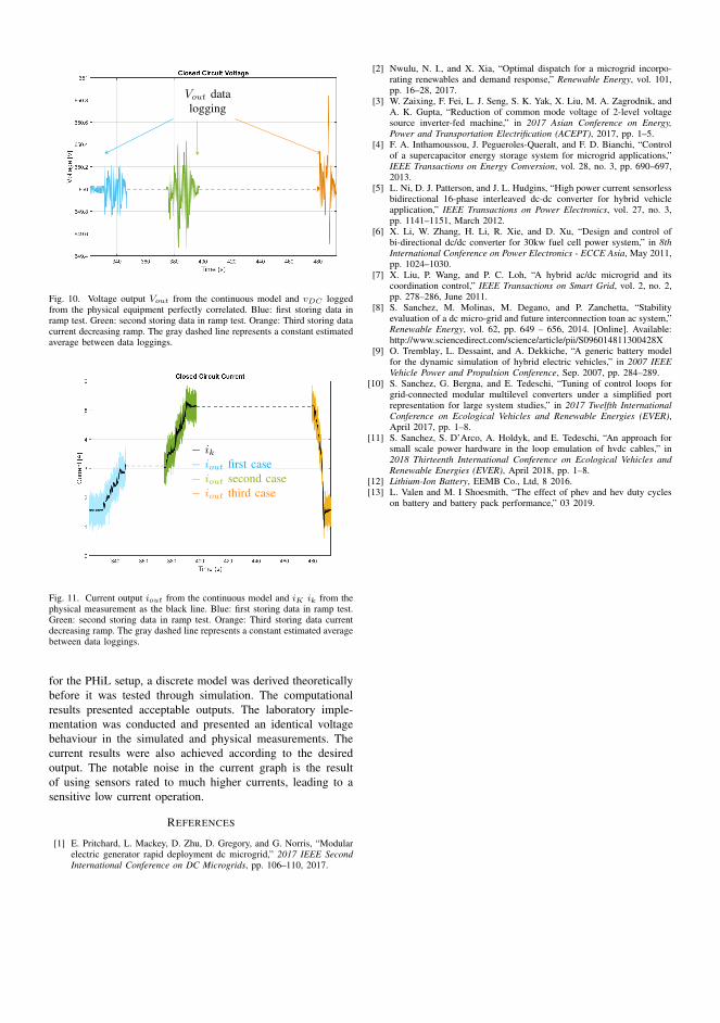
Vout datalogging
Fig. 10. Voltage output Vout from the continuous model and vDC loggedfrom the physical equipment perfectly correlated. Blue: first storing data inramp test. Green: second storing data in ramp test. Orange: Third storing datacurrent decreasing ramp. The gray dashed line represents a constant estimatedaverage between data loggings.
− ik− iout first case− iout second case− iout third case
Fig. 11. Current output iout from the continuous model and iK ik from thephysical measurement as the black line. Blue: first storing data in ramp test.Green: second storing data in ramp test. Orange: Third storing data currentdecreasing ramp. The gray dashed line represents a constant estimated averagebetween data loggings.
for the PHiL setup, a discrete model was derived theoreticallybefore it was tested through simulation. The computationalresults presented acceptable outputs. The laboratory imple-mentation was conducted and presented an identical voltagebehaviour in the simulated and physical measurements. Thecurrent results were also achieved according to the desiredoutput. The notable noise in the current graph is the resultof using sensors rated to much higher currents, leading to asensitive low current operation.
REFERENCES
[1] E. Pritchard, L. Mackey, D. Zhu, D. Gregory, and G. Norris, “Modularelectric generator rapid deployment dc microgrid,” 2017 IEEE SecondInternational Conference on DC Microgrids, pp. 106–110, 2017.
[2] Nwulu, N. I., and X. Xia, “Optimal dispatch for a microgrid incorpo-rating renewables and demand response,” Renewable Energy, vol. 101,pp. 16–28, 2017.
[3] W. Zaixing, F. Fei, L. J. Seng, S. K. Yak, X. Liu, M. A. Zagrodnik, andA. K. Gupta, “Reduction of common mode voltage of 2-level voltagesource inverter-fed machine,” in 2017 Asian Conference on Energy,Power and Transportation Electrification (ACEPT), 2017, pp. 1–5.
[4] F. A. Inthamoussou, J. Pegueroles-Queralt, and F. D. Bianchi, “Controlof a supercapacitor energy storage system for microgrid applications,”IEEE Transactions on Energy Conversion, vol. 28, no. 3, pp. 690–697,2013.
[5] L. Ni, D. J. Patterson, and J. L. Hudgins, “High power current sensorlessbidirectional 16-phase interleaved dc-dc converter for hybrid vehicleapplication,” IEEE Transactions on Power Electronics, vol. 27, no. 3,pp. 1141–1151, March 2012.
[6] X. Li, W. Zhang, H. Li, R. Xie, and D. Xu, “Design and control ofbi-directional dc/dc converter for 30kw fuel cell power system,” in 8thInternational Conference on Power Electronics - ECCE Asia, May 2011,pp. 1024–1030.
[7] X. Liu, P. Wang, and P. C. Loh, “A hybrid ac/dc microgrid and itscoordination control,” IEEE Transactions on Smart Grid, vol. 2, no. 2,pp. 278–286, June 2011.
[8] S. Sanchez, M. Molinas, M. Degano, and P. Zanchetta, “Stabilityevaluation of a dc micro-grid and future interconnection toan ac system,”Renewable Energy, vol. 62, pp. 649 – 656, 2014. [Online]. Available:http://www.sciencedirect.com/science/article/pii/S096014811300428X
[9] O. Tremblay, L. Dessaint, and A. Dekkiche, “A generic battery modelfor the dynamic simulation of hybrid electric vehicles,” in 2007 IEEEVehicle Power and Propulsion Conference, Sep. 2007, pp. 284–289.
[10] S. Sanchez, G. Bergna, and E. Tedeschi, “Tuning of control loops forgrid-connected modular multilevel converters under a simplified portrepresentation for large system studies,” in 2017 Twelfth InternationalConference on Ecological Vehicles and Renewable Energies (EVER),April 2017, pp. 1–8.
[11] S. Sanchez, S. D’Arco, A. Holdyk, and E. Tedeschi, “An approach forsmall scale power hardware in the loop emulation of hvdc cables,” in2018 Thirteenth International Conference on Ecological Vehicles andRenewable Energies (EVER), April 2018, pp. 1–8.
[12] Lithium-Ion Battery, EEMB Co., Ltd, 8 2016.[13] L. Valen and M. I Shoesmith, “The effect of phev and hev duty cycles
on battery and battery pack performance,” 03 2019.

94

Appendix B
Computational Result:
Charge of Battery
In the charging of the battery, the battery model is designed as in accordance with section
3.3. However, the DC-DC converter and control system is disconnected, as the system
is modelled for the discharging process. The battery is set to start of fully discharged,
with a SOC of 0 %, and is charged to the SOC of 0.01238 % after ten seconds. This
leads to an average charge of 1.238 · 10−3% per second. The circuit consists of a battery
and a controlled current source set to 69.5 A to obtain a good basis of comparison to the
discharge results. This is shown through the results in figure B.1 as a negative current flow
ib through the battery. The voltage is increasing from 109.29 V to 109.37 V.
95

Figure B.1: Resulting graphs from charging the battery model. The top graph shows the state ofcharge, the middle graph is the current out from the battery and the bottom graph shows the voltageover the battery system.
96

Appendix C
Computational Models
C.1 Computation Model for sections 6.1 and 6.2
Figures C.1, C.2 and C.3 presents the computational Simulink model which enabled the
results presented in sections 6.1 and 6.2. Figure C.1 depicts the setup for the boost con-
verter average model with the battery. Figure C.2 shows the current and voltage control of
the system, where the voltage control has the green background and the current controllers
has the blue background. Figure C.3 shows the system setup and the powergui. For the use
of a real time simulator, it is required that all circuits are placed in one sub-module, while
the scopes are placed in another sub-module. Figures C.2 and C.3 are left unchanged when
obtaining the results in the other sections of chapter 6.
97

Figure C.1: Simulink Model of average boost converter
Figure C.2: Simulink model of voltage and current control
98

Figure C.3: Simulink model setup prepared for real time simulations
C.2 Computation Model for section 6.3
Figures C.4 and C.5 presents the computational Simulink model which enabled the results
presented in section 6.3. It can be observed that the current signal IK and voltage signal
Vout are retrieved from the boost average model and used in the implemented discretization
algorithm.
99

Figure C.4: Simulink model of average boost converter with discretization signals retrieved
Figure C.5: Simulink model with the implementation of the discretization algorithm
100

C.3 Computation Model for section 6.4
In section 6.4, noise is introduced to the model. This can be observed in figure C.6 as an
addition to iout and Vout.
Figure C.6: Simulink model of average boost converter with the implementation of noise at thecurrent and voltage output
101

102

Appendix D
MATLAB Script for Simulink
Parameters
%SYSTEM PARAMETERS
%Base Parameters
Tsg = 100e-6;
Pb=20e3; %VA
V_dc= 650; %V
f=50; %Hz
wb=2*pi*f;
Fsw=10*10ˆ3;
Ta=0.15*10ˆ(-3);
%Battery Bank
V_nom1cell = 3.7; %Nominal voltage in 1 cell [V]
V_nom = 48; %V
n_s = 13; %Number of cells in series
Q_nom = 1559.25; %Nominal capacitance [Ah]
103

n_p = 600; %Number of cells in parallel
Z_int = 0.91; %total impedance
%Boost Converter
V_out = V_dc; %[V]
V_in = 300;
gain=V_out/V_in;
D_nom= (gain-1)/gain;
D = D_nom; %Duty Cycle
I_nom = Pb/V_out;
Ihigh_nom = Pb/V_in;
alpha = 0.04; %current ripple
deltaI = alpha*Ihigh_nom;
I_LB= deltaI/2;
T_s = 1/(Fsw);
L_boost=(T_s*V_out)/(2*I_LB)*D*(1-D);
%Resistor asummed to be 1 perscent of losses
R_boost=V_inˆ2/Pb*0.005;
alpha_V=0.05;
deltaV=alpha_V*V_out;
R_load = V_outˆ2/Pb;
C_boost= V_out*D*T_s/(deltaV*R_load);
Zbase_boost=V_out/I_nom;
Cbase_boost = 1/(wb*Zbase_boost);
Cpu_boost = C_boost/Cbase_boost;
%Boost Current Control
Ta_bd = 2e-4;
tau_boost=L_boost/R_boost;
Kp_boost=L_boost/(2*wb*Ta_bd);
Ki_boost=Kp_boost*wb/tau_boost;
%Boost voltage Control
p_bd=1/(2*Ta_bd);
z_bd=p_bd/5;
wm=sqrt(p_bd*z_bd);
Kpv_boost=(wm*Cpu_boost)/wb;
104

Kiv_boost=z_bd*Kpv_boost;
105