1

Basic Well Logging By Mandeep Kumar (only well logging related chapters are available in this

Let me know if any mistake)

CONTENTS

Page No.

List of Abbreviations 02

Chapter 4. Well Logging

4.1 Open Hole Logging

4.2 Cased Hole Logging

4.3 Production Logging

Chapter 7. Log Interpretation

7.1 Qualitative Interpretation

7.2 Quantitative Log Interpretation

7.3 Geo Frame

7.4 ElanPlus

Chapter 9. Correlation and Fault identification from Log Data

9.1 Correlation

9.2 fault Identification

References

2

LIST OF ABBREVIATIONS

a Tortuosity factor

API American Petroleum Institute

IR Resistivity index (Rt/Ro)

m Cementation index

n Saturation exponent

Rclay Resistivity of clay/shale

Rmc Resistivity of mud cake

Rmf Resistivity of mud filtrate

Ro Resistivity of formation (100% saturated with formation water)

Rt True resistivity of undisturbed formation

Rw Resistivity of formation water

Rxo Resistivity of flushed zone

Shc Hydrocarbon saturation in Virgin zone

Sw Water saturation in virgin zone

Temp. Temperature

U___ Prefix used for undisturbed zone (e.g. UWAT -> water in undisturbed zone)

WAT Water

X___ Prefix used to indicate flushed zone (e.g. XWAT -> water in flushed zone)

ρb bulk density (from log)

ρΦ Density porosity

ρΦ clay Clay porosity calculated from density log

фN Neutron porosity (shale corrected)

фNclay Neutron porosity for clay

фS Sonic Porosity

Ωm ohm meter

µs/ft micro second per feet

cc Cubic centimeter

mV millivolt

ppk Part per thousand

pu porosity unit

CAL Caliper

CBL Cement bond log

CCL Casing collar locator

CFS Continuous Flowmeter

CNCF Field normalised compensated neutron porosity

DAL Dual acoustic log

DLL Dual latero-log

FBS Full Bore Spinner

GR Gamma ray

HDIL High definition induction log

3

HSC Hollow Steel Carrier

HSE Health and explosive safety

MIT Multi-finger Imaging Tool

MLL Micro latero-log

PCE Pressure control equipments

SP Spontaneous potential

SPM Shots per meter

TCL Tubing collar locator

VDL Variable density log

WGI Well geometry indicator

ZDL Density (from electron density)

4

Chapter 4 WELL LOGGING

Well log is a continuous record of measurement made in bore hole, in response to variation in

some physical properties of rocks through which the bore hole is drilled. Traditionally Logs

are display on grid papers. Now the log may be taken as films, images, and in digital format.

Evolution:

In 1912 Conrad Schlumberger gave the idea of using electrical measurements to map

subsurface rock bodies. And in 1919 Conrad Schlumberger and his brother Marcel began to

work on well logs. The first electrical resistivity well log was taken in France, in 1927. The

instrument which was used for this purpose is called Sonde which was stopped at periodic

intervals in bore hole and resistivity was plotted on graph paper.

In 1929 the electrical resistivity logs are introduce on commercial scale in Venezuela, USA

and Russia for correlation and identification of Hydrocarbon bearing strata. The photographic

film recorder was developed in 1936. The dip meter log were developed in 1930 and the

Gamma Ray and Neutron Log in 1941.

Overview:

Logging service companies utilize a variety of logging units, depending on the location

(onshore or offshore) and requirements of the logging run. Each unit will contain many

components such as logging cable, winch to raise and lower the cable in the well, self-

contained 120-volt AC generator, set of surface control panels, down-hole tools (sonde and

cartridges) and digital recording system.

The entire process involves the application of many electronic systems and it gives key

information which helps in lithology and minerals grade/quality identification, inter-borehole

correlation, structure mapping, dip determination, in-situ stress orientation, porosity

calculation and fluid salinity determination. Electric line is the common term for the armored,

insulated cable used to conduct current to down-hole tools used for well logging.

Log types Physical Measurement Scale Source

Density Electron Density 1.8 to 2.8 g/cc Cs-137 (Active)

Neutron Hydrogen index -0.06 to 0.54 pu Am-Be (Active)

Gamma ray Natural Radioactivity 0 to 150 gAPI Passive

SP logging Natural electric potential 0 to 100 mV Passive

Resistivity Resistivity 0.2 to 2000 Ωm Current electrode

Acoustic Transit time 40 to 140 µs/ft Piezoelectric crystal

Caliper Borehole diameter 6 to 16 inches ----------

Table 5 (Logging tools and measurements)

5

The logging can be subdivided into open-hole operations and cased-hole operations.

Typically the wireline tools are cylindrical in shape, usually from 1.5 to 5‟‟ in diameter.

"Open Hole" tool combinations can extent to over 100 ft. long, "Cased Hole" tool

combinations are often limited in length by the height restrictions imposed by constraints of

"Lubricator" pipe section required to contain the well pressure while deploying cased hole

tools. There are many types of logging tools, ranging from common measurements (pressure

and temperature), to advance rock properties and fracture analysis, fluid properties in the

wellbore, or formation properties extending several meters into the rock formation.

Figure 1 (Logging Assembly, Logging Basics)3

6

4.1 Open Hole Logging:

Open hole logging operations or reservoir evaluation, involves the deployment of tools into a

freshly drilled well. As the tool string traverses the wellbore, the individual tools gather

information about the surrounding formations. A typical open hole log will have information

about the density, porosity, permeability, lithology, presence of hydrocarbons, and oil and

water saturation.

a) Spontaneous Potential (SP) log The SP log is a measure of the natural potential of the borehole with the help of a fixed

electrode on surface and an electrode on the sonde. SP log is used for:

Formation water resistivity estimation

Bed Boundary characterisation

As an indicator of the permeability

For calculation the shale volume

Principle: Three factors are necessary for SP current:

Conductive fluid in the borehole

Permeable Beds

Difference in the salinity of the mud and the formation water

The SP deflection originated when SP current originate into the borehole mud which are

caused by the electromotive forces into the formation, these are electrokinetic and

electrochemical in nature.

Electrochemical component involves development of the SP potential when mud and

formation have different salinity and porous-permeable bed is present between two

impermeable shale beds. In this case either +ve deflection is shown by log if salinity of the

mud is more than that of the formation fluid or -ve deflection when mud salinity is less

than that of the formation water.

As shown in upper part of figure 3, the development of the SP potential in the porous

& permeable sand due to the movement of the charge between high saline formation

water to the less saline mud. Cl- ions travels to the mud because these are having more

mobility than the Na+ ions, so producing a -ve charge into the mud in-front of the

sand bed.

In lower part of the same figure the movements of the Na+ ions takes place from the

shale into the mud, as shale is semi-permeable membrane for the +ve ions (due to the

-ve charge on its surface). This produce the +ve charge in front of the shale bed.

due to the combined effect of these two SP current produced as shown in the figure 4 .

Electrokinetic component involves creation of the SP response when an electrolyte flow

through a porous, permeable non metallic medium. It depends on the difference in the

pressure which cause movements to the electrolytes and resistance to the flow of the

electrolytes. Electrokinetic component is negligible in case of formation water is saline

(resistivity less than 0.1 ohm-m) and the differential pressure has normal value (only a few

hundred pounds per square inches or less). However electrokinetic component become

7

important if pressure differential is large ( in depleted formation at low pressure when

heavy drilling mud is used). In that case mud cake and shale electrokinetic potential may

not cancel each other.

Electrokinetic component is also become significant in case of very low permeable

formation so that little or no mud cake is formed, than the hydrostatic head of the mud is

applied to the formation. If formation water is brackish and mud is resistive and formation

is clean (and has some porosity), the electrokinetic effect may be larger, sometime

exceeding 200mV. These effects are difficult to detect and affect the value of the Rw.

SP tools consist an electrode on the sonde, a 1.5V battery is introduces in the circuit for

amplification. Another end of the tools is earthen. Reading of the SP is recorded with the

help of the galvanometer so only change in potential is recorded not the absolute value.

Generally

If there is more difference between mud and formation fluid the SP curve will spread

widely (SP current spread over large area), and sharp if difference is less.

For a better resolution the thickness of the beds should be 20 times more than the

borehole diameter.

Shale base line is drawn on the thick shale interval when SP curve does not move for

some interval. And maximum deflection of the SP opposite to the permeable bed is called

static SP. Shale base line shift occur when water of different salinity separated by the

impermeable bed

Water Resistivity: when SP deflection is more the difference in the salinity of the mud and

the formation water more. Negative deflection mean formation water is more saline than

the mud and vice-versa.

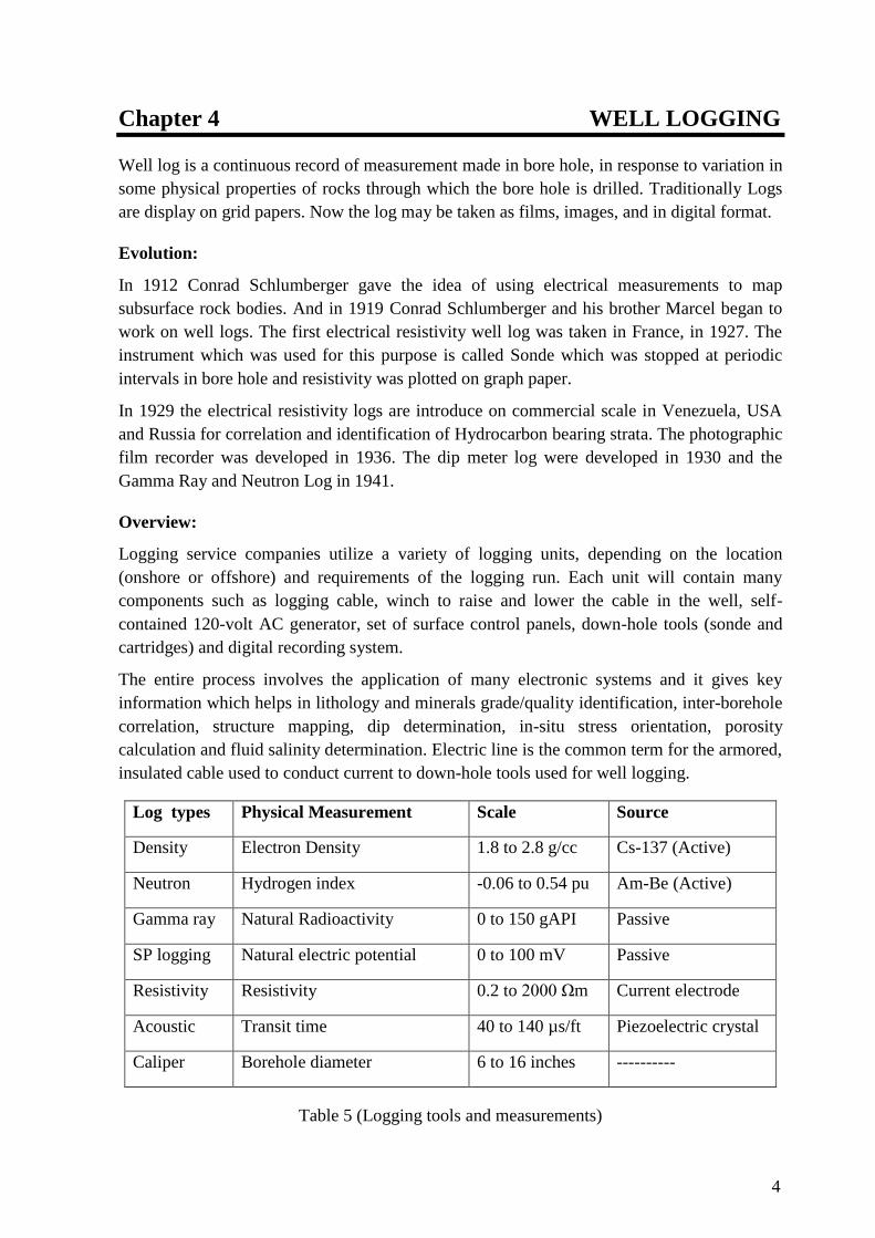
Figure 3 (Electrochemical component of SP, Page-220)4

8

SSP = −Klog(Rmf )e

(Rw )e

SSP = static SP value; (Rmf)e = equivalent mud filtrate resistivity.

(Rw)e = equivalent formation water resistivity; K = temperature dependant coefficient

(65+0.24*T oC).

Shale volume calculation: Volume of the shale in water wetted shaly-sandstone can be

calculated:

VVsh % = (1 −PSP

SSP ) ∗ 100 PSP = SP read in the water bearing shaly-sand zone

(read from log).

SSP = maximum SP value in clean sand zone

b) Gamma Ray Log (GR)

Natural Gamma ray log is used to detect the intensity and counts natural radioactivity into

the formation. It can be represented in two forms one with the combined effect of the all

radioactive substance [resent into the formations, and another way is: representing the

counts of different peaks (known as spectral gamma ray log). Main elements which

contribute to the radioactivity of the formations are uranium (U), thorium (Th), and

potassium (K).

The tool contains scintillation counters to quantify the amount of Gamma radiation

received. The counter contains:

Figure 4 (SP Current, Page-53)9

9

a high resolution 2”x12” Cesium Iodide (CsI) crystal optically coupled to

A photo-multiplier tube (PMT), which convert counts into electric signal and hence

we can calculate the intensity and counts of the radioactivity present into the

formation.

Simple gamma ray log is used in depth correlation in different operation in a well. And

also used for lithology identification and calculation of the gamma ray index and then

volume of the shale.

Each element (eg U, Th, K) contribute to the value of the gamma which are abundant in

different minerals. So gamma log should not be used as indicator of shale. In most shale's

K have fairly constant value (around 2% to 3.5%). Since shale is the mixture of the several

types of the minerals yet potassium is a fairly good indicator of the shale. However

potassium occur in feldspar and clay minerals so in sand- shale mixture, both feldspar and

clay minerals have potassium so provide false indication for shale.

Distribution of the uranium is irregular since it is not associated with the main rock

forming minerals. In average shale‟s uranium contributes to 10- 30 % of shale

radioactivity. But in certain cases it increases dramatically. Distribution of the uranium is

not related to the clay volume so it is a poor shale indicator.

Behavior of the thorium is not fully understood. Experiences show that it average content

12ppm (8 to 18 ppm) for typical shale, contributing 40 to 50 % of overall shale

radioactivity. So considering a constant average value and contribution to overall

radioactivity of shale it is considered a good shale indicator.

So for shale indicator good is thorium > potassium

K Th U

Abundance in earth's crust (Serra 1979) 2.59 % 12 ppm ~3 ppm

Gamma ray/ weight (Adam and Weaver

1958)

1 1300 3600

Principal peak used to identify

(Schlumberger 1972)

1.46

MeV

2.62

MeV

1.76 MeV (U-Ra

series)

Table 6 (Abundance of Radioactive Element, Page-76)1

Generally:

Radioactivity can also occur due to the presence of radioactive minerals in feldspar

minerals in sand and mica, gluconite etc.

Change in grain size is not always related to the change in shale amount in linear way,

e.g. in turbidites, grain size variation is not related to the variation in the clay volume

Calculation of the shale volume:

Gamma ray index =GR(log) − GR( min)

GR(max) −GR(min)

10

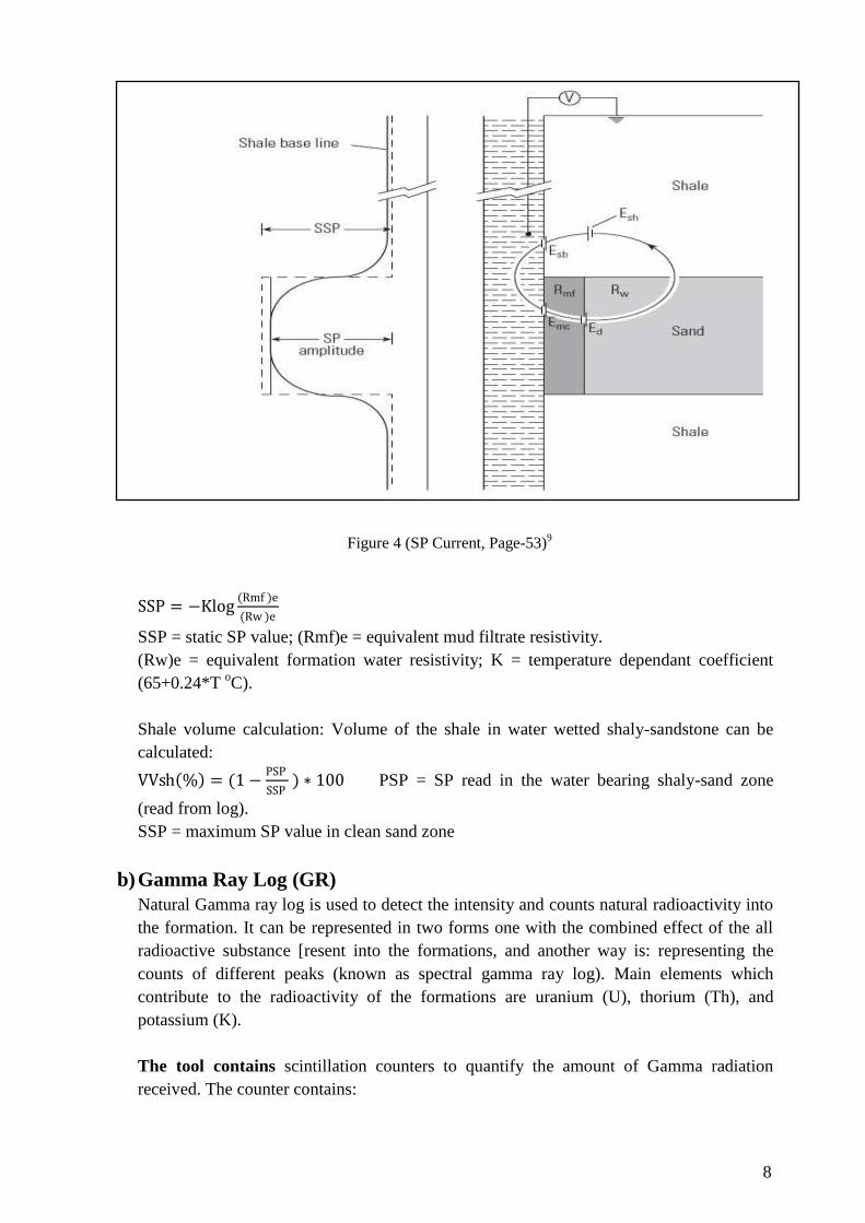
Out of the above given relations in figure Stuiber's relation is most preferred.

c) Resistivity log

Resistivity log is used to measure the borehole resistivity with the help of some electrode

arrangement. This is one of the most important and the foremost log to be recorded in a

well. The resistivity of the formation is a key parameter in determining water saturation

which is used to find out the hydrocarbon saturation. With a few rare exceptions, such as

metallic sulfide and graphite, dry rocks are good electrical insulators. So the formation

resistivity depends on: the fluid type and permeability for the flowing the current into the

formation. The borehole formations resistivity is usually from 0.2 to 1000 ohm-m. There

are two principles for recording formation resistivity, these are:

Sending a current into the formation (or measuring the ease of electrical flow through

it). This is used when conductive mud is present into the formation. Because electrical

connection is required between current electrode and formation.

Inducing an electrical current into the formation (and measuring how large it is).

Generally this is used when the formation mud is non conductive, although it can

work in conductive mud also.

Choice of the induction or the laterolog depends upon the resistivity of the formation.

If Rmf/Rw is less than three than we use laterolog.

Figure 5 (relation Between GR-Index and Vsh, Chapter 4.1 Page-28)6

11

Use induction log if Rmf/Rw is more than three or induction fresh or oil base mud is

used or Rt is less than 80-100 ohm-m.

In a basic resistivity tools initially normal and lateral devices(figure-below) are used

which are differ in the electrode arrangement / spacing and depth of penetration. In these

devices currents were passed through the formation by means of an electrode, and voltages

were measured between receiver electrodes. The measured voltages provided the

information about the resistivity of the borehole formations.

In highly resistive formations, and for the measurements of the deep resistivity focusing

electrode logs, which are called laterologs and spherically focused devices. In these

devices the two current electrode (bucker electrode) are used around main electrode (all

having same voltage) for focusing the current and for finding the deep resistivity (figure-

below). The deep-reading devices include the Laterolog 7, the Laterolog 3, and the deep

laterolog or the DLL - dual laterolog tool.

The DLL (Dual Latero Log) is a focused logging system that is typically used in wells

drilled with high- salinity mud. In a laterolog-type system, the measure current is forced to

flow perpendicular to the borehole (in a `lateral' direction) by the potential lines created by

the focusing currents emitted by the bucker electrodes surrounding the central current

measure electrode.

Figure 6 (Normal and lateral Device, Page 7-2)2

12

Figure 7 (Focusing electrode, Page 7-7)2

A Dual Laterolog system consists of

An electronics section

A mandrel section supports the electrodes which are connected to the active electronic

circuitry housed in the electronics section.

These are low frequency `conduction' type devices and require that the borehole fluids (i.e.

drilling mud) be conductive. The two measurements have different depths of investigation

and are called Deep Resistivity (RD) and Shallow Resistivity (RS).

Two modes of operation for Shallow are: Standard Shallow Mode (StdSh) and Enhanced

Shallow (EnhSh) Mode. The EnhSh mode of operation provides a shallow measurement

with increased depth of investigation.

The Deep is operated in one of two modes; Standard Return Deep (SrtnDp)- when current

return is to the Armor up-hole from tool string; and Groningen Return Deep (GrtnDp)-

when current return is to a Groningen return electrode below tool string. The vertical

resolution is 2 feet.

The most serious limitations for DLL occur in cases where the resistivity contrast between

the formation and the mud are below 1 or above 10000. The laterolog does not operate in

oil based mud or air-filled holes.

MLL (Micro Latero-Log) tool is used to obtain more information about resistivity at

shallower depths of investigations. MLL is a padded tool and it has a smaller depth of

investigation (0.75 inch) and smaller resolution (1.15 inch). MLL is mainly used to get the

resistivity of the flushed zone (RXO). The MLL works in the same principle as the DLL

tool.

The MLL tool contains a measuring pad which contains 9 electrodes out of which

measuring electrode is the central one surrounded by eight guards or focusing electrode.

The MLL also contains a caliper arm. The current to the measure electrode is measured

13

with respect to earth potential. A bridle is also connected and the bridle electrode for the

MLL is considered to be at earth potential and is used as the reference voltage.

High Definition Induction Log (HDIL):

HDIL tool from Baker Hughes is one of the best ways to measuring resistivity. The HDIL

tool has 6 depth of investigations i.e. 10 inch, 20 inch, 30 inch, 60 inch, 90 inch and 120

inch.

This tool contains

transmitter coil

7 receiver induction coils.

We can vary the focusing of an induction instrument by modifying the coil array to

achieve greater depth of investigation or resolution. The measurements are made by

several simple coil arrays and their signals are combined, in software, to achieve focusing.

The advantage of this technique is that measurements can be combined from arrays at

different points in the well. It is this fact which enables us to reduce the cave effect. So,

another advantage is different focusing schemes can be used in different circumstances.

The HDIL tool also contains a lead electrode at the centre portion for the measurement of

Spontaneous Potential (SP). There are 8 eight operating frequencies and 112 measuring

channels.

Use of Electrical Resistivity log:

For calculation of the Rw using Inverse Archie in clean sand zone

Differentiate between water and hydrocarbon bearing zone: resistivity log is used to

differentiate between high resistive hydrocarbon and conductive formation water in

porous and permeable sand.

For Hydrocarbon saturation:

Using Archie equation we can calculate the water saturation and Hydrocarbon saturation

in a formation is:

SHC = 1 − SW

d) Density Log

It records the response of the bulk density of the borehole formations (including minerals

and borehole fluid). It is used to calculate the porosity, hydrocarbon density (indirectly),

acoustic impedance, lithology indicator and to identify certain minerals. In this formation

is bombard with the medium to high energy gamma rays (0.2 to .02 MeV) and to measure

their attenuation between source and the receiver. Attenuation depends on the number of

electron in the formation so we can have an idea of the bulk density of the formation.

Gamma ray interact with the formation in three ways

14

1. Pair Production: Occur at high energy (>1MeV), as in density tool the source emits

gamma ray of less energy so pair production not occur in the formation.

2. Compton Scattering: It occurs at medium energy (2MeV to 75keV). In this gamma

ray interact with an atom and cause the ejection of an electron from the outermost

shell (compton electron). The gamma ray continues after losing some its energy

(function of scattering angle). The amount of the compton scattering is proportional to

the amount of electron in the formation, so the electron density of the formation can

be derived from compton scattering. And electron density of the formation is closely

related to the bulk density

3. Photo Electric Effect: This occur low energy level (<100keV, <200keV for low

atomic number e.g. H, C, O). When gamma ray collides with an atom, atom absorbs

its energy and emits a kinetic electron. Photoelectric effect is lithology dependant as:

Pe =Z3.62

10

Primarily relation between bulk density and electron density used was as:

ρe =1

2∗ A

Z∗ ρb forbulk density and electron density to be equal A/Z of an atom should

be related to 1/2 or 0.5. But in case of the hydrogen it is 0.992 so above given relation is

modifies as:

ρb = 1.070ρe − 0.188

The energy spectrum of the gamma ray fall within the Compton scattering is counted for

calculation of the electron density and hence bulk density of the formation.

In this a radioactive source and two detectors are used for borehole compensation, mud

cake correction etc.

The source and detector in the density log are mounted on the plough shaped pad which is

pressed against the borehole wall. So density log refer to the only one side of the borehole

formation/wall.

Normally in the density plot the mud cake and borehole corrections are automatically

applied. Investigation depth of the density log is normally upto 13 cm.

Density log is used to calculate the bulk density of the formation but it is required to

quantify the material involved (mineral) its density and type of fluid:

bulkdensity ρb = ρf fluiddensity + 1 − ∅ × ρma (matrixdensity)

Therefore: ∅ =ρma −ρb

ρma −ρf

Depth

15

Errors occur when:

Density varies from actual value we suppose for the borehole formation in estimation of

porosity

When large cavities are there in bore (i.e. bad borehole)

And when formation fluid varies, especially when it is a gas.

e) Neutron Log

Neutron log provide the reaction of the formation of the when high density neutron are

bombarded on the borehole formations. Reaction is related to the hydrogen richness of the

formation (hydrogen index). Hydrogen index is related to the %age of the hydrogen in the

formation. So if the formation is filled with water neutron log can act as a porosity

indicator.

It is also used to distinguish between oil and gas zones. When a neutron collide with the

particles of same size (H- nuclei) elastic scattering occur and neutron loses some of its

energy. Collision with other higher nucleus does not cause much lost of the energy. So we

can detect the presence of the Hydrogen with help of the Neutron logging by recording the

lost in the energy of the detected waves at the detector.

Into the tool a chemical source [e.g. plutonium-beryllium (Pu/Be) or americium-beryllium

(Am/Be)] is used in the most of the logging to produce fast neutron. When neutron travels

through the formation it slows from epithermal (having energy of around 1eV) to thermal

stage (~0.025eV), they then diffuse randomly without losing more energy until they are

captures by the nucleus of atoms such as chlorine, hydrogen, or silica. The capturing

nucleus become extremely excited and produces gamma rays of capture. Depending on the

tool type either these capture gamma or neutron (unaffected) are detected.

Neutron energy stage Energy

Fast >100 KeV

Intermediate 100 KeV to 100 eV

Slow <100 eV

Epithermal 0.1 to 100 eV

Thermal < 0.02 eV

Table 1 (Energy stages of Neutron, Page-135)1

Two detectors are used in the neutron logging, which detect on the basis of ionization

capability of the particles. A detector is consist of the target material and Proportional gas

into it (He3 gas is used). The source and detector are placed in a skid pressed against the

borehole wall. Detectors are placed so that these only detect the neutron in the thermal

energy zone.

16

Figure8 (Neutron tool, Page-136)1

Source produce initial energy around 4 MeV (means velocity of 2800 am/µ sec), but after

some successive collisions (around 100) the fast neutron have slow down from epithermal

to thermal level (0.25 eV of energy and 0.22cm/sec velocity). For this much reduction in

the neutron energy collision required are: 18 (elastic) collision with H-nuclei, or 257 (non-

elestic) collision with silicon nuclei, or 368 with calcium nuclei. So the effect of the H-

collision is dominant. Chlorine have larger capture cross section for the thermal neutron

which creates error in our reading.

f) Acoustic Log

In acoustic or sonic logging travel time measurements are made which are useful for

porosity (primary porosity) determination, lithology indication, qualitative estimation of

permeability, studying the mechanical properties, strength of the formation and fracture

characterization, understanding the anisotropy of the formation and for calculation of

impedance (with the help of density log) for seismic correlation. In open-hole logging

measurements the sonic tool is used for determining the porosity indirectly by measuring

the travel times.

A piezoelectric substance is used as source and detector of the acoustic waves. In source

electric signal is transmitted to the pressure waves and opposite principle for receiver.

Source frequency is typically between 10-40 Hz (10000-40000 cycles per second). At 10-

20 kHz acoustic waves have wavelength between 7.5 – 75 cm over the velocity range of

1500 m/s to 7500 m/s.

Modern sonic tools have both sources and receiver combinations more than one, which

depends on the tool types and with intention to reduce most of borehole& tool noise. BHC

(Borehole compensated sonic tool) has source and two receiver combination, near and far

receiver. The near receiver is designed to travel only through the borehole mud. As too

have its considerable part into the mud so to receive the effect of the formation: we

subtract the „reading of short spaced detector‟ from reading of long spaced to receive‟

(Figure 9 ).

17

Figure 9 (Sketch of borehole with sonic tool)

But due to the borehole effect the common path of both receivers may become unequal so

a second inverted array is also used to average out the effect of both array to reduce

borehole (or tilt effect).

Path of penetration of the sonic waves is very little (between 2.5 – 25 cm) the penetration

depends on the wavelength of the signal. So for a particular formation penetration is grater

in high velocity formation (λ=v/υ).

Use of log: 1

v=

∅

VL+

1−∅

Vma as interval transit time = V(velocity)

∆t = ∅∆tL + (1 − ∅)∆tma (this is called Wyllie Equation)

∅ = porosity, VL = velocity of the formation fluid, Vma= velocity of matrix material

Similarly∆t𝑚𝑎 and ∆t𝐿 are interval transit times of matrix and formation fluid.

g) Well bore Geometry Indicator (WGI)

WGI or Caliper tool measures the size of the borehole. It consists of:

six arms (telescopic)

a disc magnet and,

A magneto-resistive sensor circuit (or sensor bridge) on both the upper and lower

hinge of the arms.

Working- To push the arms against the borehole a spring is located at the inner side of

each arm. When the arms are pushed outward by the spring, the magnet disc also rotates

making the orientation of the magnetic field changed as measured by the sensor. The

change in magnetic field direction is sensed as a measure of the angle between the arm and

18

the housing of the tool. The output each sensor bridge is the sine and cosine of the angle

made by the arm. And from the outputs of both the sensor bridges (upper and lower)

tangent is calculated (using software) separately and the effective bore hole diameter is

calculated.

The tool diameter (when the arms are at the closed position) is 92 mm and the tool radius

used in the formula is 44 mm (theoretical). Thus each WGI tool measures six independent

diameters. The resolution of this tool is 0.036 ° and the maximum radius that can be

measured without considerable errors is 13 inch. Any stray magnetic field can affect the

measurement of the magneto-resistive sensor bridge. The uses of WGI tool are:

To measure the borehole size,

To get the details of the borehole caving,

To calculate the amount cement to be used for casing etc.

h) Advanced Logging tools

1. Sonic Scanner Tool:

Schlumberger has designed this tool using the latest acoustic technology for advanced

acoustic acquisition, which can be used in both open and cased well.

In addition to axial and azimuthal measurements, the tool makes a radial measurement

to probe the formation for near-wellbore slowness and far-field slowness. Typical

depths of investigation equal two to three times the borehole diameter.

The new Sonic Scanner acoustic scanning platform provides advanced types of

acoustic measurements, including borehole compensated monopole with long and

short spacing, cross-dipole, and cement bond quality. These measurements are then

converted into useful information about the drilling environment and the reservoir,

which assists in making decisions that reduce overall drilling costs, improve recovery,

and maximize productivity.

Figure 2 (Sonic Scanner Tool)

19

To enable a deeper understanding of acoustic behavior in and around the borehole, the

Sonic Scanner tool allows accurate radial and axial measurements of the stress-

dependent properties of rocks near the wellbore. The Sonic Scanner platform provides

multiple depths of investigation, excellent waveform quality and presentations that

reduce the complexity of sonic logging, without compromising the depth of

information.

The Ultrasonic Imaging Tool (USIT) is a continuously rotating pulse-echo type tool

with nearly 100% coverage of the casing wall. The transducer (“sensor”) rotates,

emitting and receiving signals reflected back from the casing wall. Preferable to run

CBL with it for overall well integrity picture.

2. Nuclear Magnetic Resonance (NMR) Tool:

In NMR tool a spinning nucleus acts as a tiny bar magnet oriented along the spin

rotation axis. First, the tool‟s, permanent magnetic field aligns or polarizes the spin

axes of the protons in a particular direction. This process, called polarization,

increases exponentially in time with a time constant. Next the tools oscillating field is

applied to tip these protons away from their new equilibrium position. In the

meanwhile resonance occurs and a magnetic signal is generated. The response occur

only in the hydrogen that are free (are not clay bound) so in this way we can get

response only from the free hydrogen and can get clay free porosity with NMR tool.

NMR is unique since it can provide: Lithology independent total and effective

porosities. Pore size distribution. Irreducible water saturations. Residual hydrocarbon

saturations. Hydro carbon type identification. Permeability estimates. Hydrogen

Index, build up and decay of polarization.

3. MDT:

MDT stands for Modular Dynamic Formation Tester. Through this log we can obtain

the Formation Pressure and Formation Fluid Sample. The formation pressure can be

plotted with respect to the depth. Through these pressure points we can establish the

gas water contact, oil water contact, oil gas contact etc.

MDT tools offer multiple sampling during a single wireline run and rapid pressure

measurements using a new generation quartz gauge that stabilize quickly to accurately

measure formation pressure. The tool can be configured to provide a range of options

not previously available from a wireline tester, e.g. by monitoring the fluid resistivity

as it drawn into the tool and rejecting contaminated fluid, the operator can ensure that

only uncontaminated formation fluid sample are collected. Or by measuring pressure

interference during drawdown, horizontal and vertical permeabilities can be

determined.

20

4. Formation Micro Imager (FMI) Tool:

The FMI provides an electrical borehole image generated from up to 192 micro-

resistivity measurements. Special focusing circuitry ensures that the measuring

currents are forced into the formation, where they modulate in amplitude with the

formation conductivities to produce low-frequency signals rich in petrophysical and

lithological information and a high-resolution component that provides the micro-

scale information used for imaging and dip interpretation. Image calibration is

achieved through calibration with low frequency, deeper resistivity measurements

available from the tool signal or input from other resistivity measurements. Image

normalization further increases the completeness and reliability of this versatile tool

for geological and reservoir characterization.

The combination of measuring button diameter, pad design, and high-speed telemetry

system produces a vertical and azimuthal resolution of 0.2 in. [0.51 cm] for the FMI

tool. This means that the dimensions of a feature larger than 0.2 in. can be estimated

from the image.

The answers provided by the FMI tool help in understanding the reservoir structure,

identify and evaluate sedimentary features and fractures, visualize rock texture, and

complement coring programs. FMI data are increasingly used for geo-mechanical

analysis of the reservoir. Drilling-induced features such as breakouts are readily

identified.

21

4.2 Cased-Hole Logging:

Cased-hole logging operations focus on the optimization of the completed oil well through

mechanical services and logging technologies. At this point in the well's life, the well is

encased in steel pipe, cemented into the well bore and may or may not be producing. A

typical cased-hole log may show cement quality, production information, and formation data.

Mechanical services uses jet perforating guns, setting tools, and dump bailors to optimize the

flow of hydrocarbons.

a) Sonic Logging

Acoustic (sonic) logging, introduced in 1948, has emerged as a very versatile tool for

formation evaluation. The method is based on transmission of sound waves in the vicinity

of the borehole. The old sonic tools (such as BHC) measure formation velocity (or

slowness) of the compressional waves by detecting the first arrivals only and

determination of porosity from velocity using Wyllie eqn. Later tools such as Long

Spacing Sonic (LSS) or Array Sonic (AS) record the full waveform and provide

compressional, shear and Stoneley slowness sand amplitudes.

Working: The near and far receivers record timings of the first arrivals which are P head

waves traveling along the borehole wall with formation velocity. The time difference

between the first arrivals at near and far receivers divided by receivers spacing gives

transit time or slowness.

Sonic tools are comprised of transmitter which converts electrical energy into acoustic

energy and a receiver that do the reverse. The transmitter emits sound wave that travels to

the receiver through borehole fluid, and surrounding formation. The compressional wave

that travels through the formation usually arrives first at the receiver and is the ones of

interest in sonic logging. The typical resulting acoustic wave train reaching the receiver is

given below:

Figure 10 (Sonic waves received by sonic tool, Page-173)4

22

Wave Propagation Principles:

Normally propagation of seismic wave in formations is visualized mainly by-

Snell Law: this law gives direction of propagation of waves at interface.

Fermat Principle: waves will travel least time path.

Huygens Principle: every point on a wave front acts as source for generation of

spherical secondary wavelets, and envelop to these wavelets will give new wave front.

Uses of Sonic Log are:

Seismic Data calibration

Synthetic Seismograms

Porosity Determination

• Wyllie Time average Equation

• Raymer-Hunt Equation

Stratigraphic correlation

Identification of Lithologies

Compaction and Overpressures

b) CBL-VDL:

This is a sonic logging tool which is run in under cased hole condition. This tool is

basically designed for Cement Integrity Evaluation.

The CBL – VDL tool contains

o transmitter and

o Two receivers (nearest receiver at 3 feet and the other at 5 feet distance).

The transmitter is a piezoelectric transducer and the transmitting frequency is about 20

kHz. There are totally five possible paths through which the return sound signals can be

arrived; through body (attenuated due to its design), through well bore fluid, through

casing, through cement and through formation. The CBL measurement is the amplitude (in

millivolts) of the first arrival signal E1 of the 3 feet receiver.

CBL- measures the casing to cement bond (low DOI)

VDL- measures the cement to formation bond (high DOI)

23

CBL:

The CBL measurement is the amplitude in mill volts of the first arrival E1 at the 3 feet

receiver. It is a function of the attenuation due to the shear coupling of the cement sheath

to the casing. The attenuation rate depends on the cement compressive strength, the casing

diameter, the pipe thickness, and the percentage of bonded circumference. A time gate

opens at the first motion detection point. A peak search is performed on the received

signal within this gate. The maximum value of the signal within this gate is the amplitude.

First motion is detected when the receiver signal exceeds the detection level. The first

arrival peak is assumed to be from the wave travelling through the bonded casing. The

amount of compression of wave amplitude in bonded casing arrivals is proportional to the

circumference of the casing bonded to the cement.

CBL also measures the travel time (TT) of the acoustic signal to travel from the

transmitter to the 3 feet receiver. The TT curve can be used in checking tool centralization

and fast formation arrivals.

VDL: The Variable Density Log takes the measurements from all the different paths of the sonic

wave. The signals will become black lines where the positive half arrivals are greater than

the threshold appeared and white spaces for negative half arrivals. Thus the amplitude and

thus the intensity of the black lines in the log represent the amplitude of the incoming

sonic waves. Usually in a recorded log the lines appears represents the well bore fluid

arrival, the casing arrival, the cement arrival and the formation arrival sequentially from

left to the right.

Figure 11 (CBL tool, Chapter5 Page 5-2)7

24

c) Perforations:

To establish the fluid communication between borehole and formation we do perforation.

The desired casing intervals are perforated by guns using shaped charges. A shaped charge

consists of four basic components- the outer case, explosive powder, primer and metallic

liner. Generally, outer case is made of steel or zinc, and the explosive is RDX. The

metallic liner, which is the most important element of the shaped charge, is formed from

mixtures of copper, lead, zinc, tin or tungsten (as shown in figure 15).

The shaped charges are installed in a perforating gun where a detonating cord (prima cord)

runs along the gun‟s length and makes contact with each charge at its primer region. The

detonating cord is attached with an electric detonating cap. After proper positioning of the

gun in the well, a current is sent into the cap which initiates the detonating cord, which the

premier explosives.

The perforation is carried out in either:-

(i) Over Balanced Condition (ii) Under Balanced Condition

(i) Over Balanced Condition: In this condition mud column pressure is greater than that

of formation pressure. During the job of perforation well fluids are prevented from

entering the well-bore and the job can be executed without any safety hazards.

Following two types of gun used in this technique:

(a) Throw Away Gun (TAG): It can be used single time only.

(b) Hollow Steal Carrier Gun (HSC): It can be reused.

(ii) Under Balanced Condition: In this condition mud column pressure is less than that of

formation pressure conditions. This job is carried out by using pressure control equipment

as the well may become active immediately after perforation. The advantage of this kind

of perforation is that the well can be put on production immediately afterwards.

It can be further divided as:

a) Through Tubing Perforation (TTP)

b) Tubing Conveyed Perforation (TCP)

Figure 12 (Shaped Charge, Chapter 7 Page 7-1)7

25

a) Throw Tubing Perforation (TTP)

Throw Tubing Perforation (TTP) is done in under balanced conditions which require

tubing fitted with pressure control equipment to take care of the possible up surging

flow soon after perforation. Since the charges have to pass through tubing, they are

smaller in size with lesser depth of penetration.

b) Tubing Conveyed Perforation (TCP)

Tubing Conveyed Perforation (TCP) is another technique where the entire perforation

assembly is lowered into the well on the end of the tubing string itself. It can use large

diameter, high performance charges in under balanced condition.

4.3 Production Logging:

Production Logging is the measurement of fluid parameters on a zone by zone basis to yield

information about the

type of fluid

Amount of Fluid

Well completion problems

Zone from which it is coming

Zone by Zone Perforating Efficiency can be found with the help of Production Logs. This

knowledge would be of great help in deciding the Perforation Policy, Fracture / Acid jobs,

Completion strategy, Field development and Reservoir management.

Production logging is used for the following purposes:

Evaluation of flowing wells

Production profile distribution

Zonal productivity and skin factors

Monitoring

Changes in production profile

Changes in flowing fluids- water or gas breakthrough

Flow profile

Zone contribution

Down-hole reservoir data

Type of production problems

Absorption profile for Injector wells

Diagnosis

Source of High GOR or Water-cut

Detection of leaks or cross-flows

Production enhancement

Data for workover planning

Completion and treatment effectiveness

Flow outside presumed path

Casing/tubing leak

Packer, B/P setting

26

The most significant part of production logging operation is that the logging is carried out

during the flowing condition of the well. Before carrying out the operation, Pressure control

equipments (PCE) are installed on the well-head to control any excess pressure coming from

the well bore. The PCE equipments are attached in this order on top of the well-head:

Blow out Preventer (BOP)

Tool trap

Raiser pipes

Pack-off

BOP is same as that used in drilling but is smaller. Its function is however, the same.

The tool-trap is a special pipe where the cross-section diameter of the pipe can be controlled

from the outside. During the opening of the master valve of the well, the tool may be

subjected to excess pressure and break away from the wireline. The tool trap will prevent the

tools from falling into the well.

Raiser pipes are normal pipes and are used mainly to accommodate the complete tool

assembly as well as to provide enough height to the assembly for pressure control.

Pack-off is the solution to closing the well during experience of excess pressure. It is mainly

made of a rubber with a hole large enough for only the cable to run. It has an inlet and outlet

valve which is attached to a hand pumped hydraulic- system. The rubber expands upon

increase of pressure and catches the wireline.

Tool description and usage:

Gamma Ray tool measures the natural radioactivity of the formation and used for depth

correction and correlation. Increased gamma ray activity is indicative of radioactive

shales.

CCL tool (Casing Collar Locator)identifies the collars/joints in the down-hole tubular and

used for depth ties. It sometimes responds to damages in tubing / casing also.

QPC tool (Quartz Pressure Crystal) measures the pressure in well-bore. It contains a

piezo-electric quartz crystal which sends an electrical signal upon experiencing pressure.

The deflection in signal defines the pressure change. Difference between FBHP (Flowing

Bottom Hole Pressure) and SBHP (Shut-In Bottom Hole Pressure) is indicative of skin

around bore-hole. Pressure gradient is indicative of nature of fluid present in well-bore.

FDR tool (Radioactive Fluid Density) identifies the nature of fluid by measuring its

density. Individual phase holdup calculation needs density data to ultimately calculate

flow rates of different phases. It uses a radioactive source sending a neutron source

collimated only onto borehole fluid.

Temperature tool measures the temperature in the well. It consists of a Platinum rod as a

temperature probe.

27

Figure 13 Typical production logging tool stack

Capacitance tool indicates the type of fluid and Holdup and its readings are also used for

rate calculations of oil, gas and water. The tool has two capacitor plates and works on the

basis of dielectric constant of the fluid present between the plates. Dielectric constant of

water is 86 and for oil and gas it is 1-6. The capacitance changes with different fluids with

different amount of oil or gas in water. The tool is calibrated for water and air before run-

in. The oscillator circuit present in the electronics gives the result in counts per second

(cps). If water-cut is more than 40%, the electronics show it as complete water producing

resulting in error sometimes.

Flow meter measures the fluid velocity which can be converted to total flow rate:

Flow rate = fluid velocity ∗ (cross sectional area of the pipe)

Flow meters are of 2 types: Full-bore and Jeweled type flow meter.

28

The tool has a very sensitive spinner attached to a sensor. The sensor has 2 magnets

attached placed 180o apart.

The magnet senses the no. of times the spinner blades have cut its magnetic field. The

value is given in terms of counts. Spinner response is directly proportional to relative fluid

velocity.

All the information obtained from the Production Logs will help and guide the Reservoir

Engineer in deciding the future course of actions such as Work Over, Water injection

schemes for Reservoir Pressure Maintenance, Infill Drilling and Completion Strategy etc.

Multi-Finger Imaging Tool (MIT): MIT40 tool was introduced for the first time in

ONGC by Logging services-Mehsana. Tool measures an accurate Caliper measurement of

Casing and provides 3D view of the internal surface of the Casing. It has 40 independent

inner radius measurements at one point by an array of 40 Arms (Fingers).

Processed output is viewed as 3D view using WIVA Software (Procured with tool).

Applications of MIT40 tool is for:

Corrosion assessment

Casing Deformation

Perforation Mapping

3D visualization

Quantification of scale build-up

Accurate location of holes or anomalies in casing

Tool specifications:

No. of Fingers : 40

Finger length : 7”

Tool diameter : 2 ¾”

Measurements range : Casing size : 5.5” to 7”

Temperature rating : 177 oC

Pressure rating : 138 MPa ( ≈ 20000 psi )

Radial Accuracy : ± 0.5mm

Figure 14 (MIT tool)

29

Chapter 7 LOG INTERPRETATION

A well log contains key information about the formation drilled, in different petrophysical

measurements. i.e.:

Prospective zones of hydrocarbon.

Reservoir type and thickness.

Estimation of Porosity, permeability.

Fluid type present in the pores and saturation level

Assessment of reservoir information from the log is called well log interpretation. The

interpretation of the well log includes both qualitative and quantitative evaluation. In

qualitative interpretation we identify the lithology, hydrocarbon type etc. by seeing log plots

and in quantitative interpretation estimation of reservoir parameters were done like Vclay,

effective porosity, and hydrocarbon saturation in order to calculate the amount of

hydrocarbon that can be economically produced.

7.1 Qualitative Interpretation:

Steps involved in qualitative interpretation:

Oil

Bearing

Hydrocarbon Bearing

Reservoir Gas

Bearing

Rock Water Bearing

Non Reservoir

The analysis of log data to identify the potential hydrocarbon zone is an important aspect

in log analysis. A scanning technique is required to sort out the reservoir from non

reservoir.

For differentiating reservoir and non-reservoir zone following logs are used:

Caliper: In sand bearing zone caliper show less diameter due to the mud cake

Gamma Ray: Gamma ray show less reading in sand lithology

SP: SP log show deflection from shale base line in sand bearing zone

Density and neutron logs (commonly called lithologs) are preferably used for

sand-shale differentiation. In water/oil bearing zone neutron-density cross over

occurs.

And for differentiating water bearing zones from oil bearing following logs are used

30

Log type Response in hydrocarbon bearing zone Response in water bearing zone

SP The SP deflection is reduced (but more than

shale interval)

The SP deflection is increased

Sonic log Its gives high porosity value than actual It‟s give true porosity value

Density

log

In gas bearing zones- Bulk density is too low,

but in case of oil little or no deflection

compared to water bearing zone

It give true formation density

Neutron

log

In gas bearing zone give low value; but in

case of oil little or no deflection compared to

water bearing zone

It‟s give true limestone-porosity

Neutron-

density log

(lithologs)

Negative cross-over in gas bearing zone (both

decrease)

Approx Overlap each other in water/oil

bearing zone.

Approx Overlap each other in

water bearing zone.

Resistivity Its reads high value in hydrocarbon zone It has reads low value in this zone

Table 2 (Response of logs in water and hydrocarbon bearing zone)

7.2 Quantitative Log Interpretation:

The aim of well log interpretation is to identify potential hydrocarbon bearing zone by

determining porosity, true resistivity and then converting the raw log data into estimated

quantities of oil, gas and water occupied in a formation (Ref. 5). The basic steps required

for quantitative interpretations of logs are as below:

a) To obtain information on lithology of formation.

b) Estimation of clay volume

c) Estimation of the porosity

d) Estimation of effective porosity

e) Determine the formation water resistivity(Rw)

f) Estimation of water saturation (Sw)

g) Estimation of reserves of hydrocarbon

a) To obtain information on lithology of the formation: Information on

lithology of formations are in general obtained from cores and cuttings. The well logs

also are of great help in this regard. Pe (photoelectric) log gives valuable information

as some common minerals can immediately be recognized from the log values.

Table 3 gives the log value of some of the common lithologies found in the

formations.

Various cross plots of the logs also help in identification of the lithology of the formation.

31

M Vs N plots also help us in determining the lithology of the formations. M and N are

computed from PHIN, RHOB and DT logs.

Lithology Gamma Ray

Neutron/Density

separation*

Sonic

Sand Low +6 to +8pu 52.5 - 55.5 msec/ft

Limestone Low 0 pu 47.5 msec/ft

Dolomite Low -12 to -14pu 42.5 msec/ft

Shale High -6 to -30 pu 50 msec/ft

Anhydrite Low Φb = 3.0 g/cc

Φn = -1 pu

50 msec/ft

Salt Low Φb = 2.0 g/cc

Φn = 0 pu

67 msec/ft

Coal ------ Φb = < 2.0 g/cc

Φn = > 40 pu

> 100 msec/ft

Table 3 (Lithology response from (N-D ) crossover and Photoelectric log, Page C-2)8

b) Estimation of clay volume: By using SP, GR and Neutron-Density logs shale

volume can be estimated with the following relations :

Using SP: Vclay = 1−PSP

SSP × 100 %

Hear PSP is SP log deflection measured from shale base line in front of the sand zone

SSP is the maximum deflection in front of clean sand zone in same formation

Using GR:Vclay =GR Log −GR Min

GR Max −GR Min

GRlog is reading of GR log in front of the sand zone

GRmin is the minimum reading of the gamma ray in front of the clean sand

GRmax is the maximum reading of the gamma ray in front of the shale

Using Neutron-Density: for oil and water bearing zoneVclay =Фn − Фd

Фnclay − Фdclay

Фnis the neutron log reading in sand zone

Фd is the density log reading in sand zone

Фnclay is the average neutron log reading for shale in that formation

Фdclayis the average density log reading for shale in that formation

We choose the minimum value of the Vclay (Vclaymin) from above three methods.

Preference is given to the D-N>Gamma>SP.

32

c) Estimation of the porosity: Porosity can be estimated using sonic, neutron and

density

From sonic ∆t = ∅ ∆tL + (1 − ∅)∆tma

In this ∆t is transit time from the sonic log

∆tlis transit time of the formation fluid, which we need to provide

∆tma is the transit time of the matrix, which we need to provide

From Density log: ∅d =ρma − ρb

ρma − ρf

ρmais density of the matrix, which we need to provide (eg. 2.65 for quartz bearing

sand)

ρfis density of the formation fluid (eg. 1 g/cc for water bearing sand zone)

ρmais density from the log

From Neutron: Neutron porosity (ΦN) can be directly utilised by adding 0.03 (into

fractional value of the porosity) in sand bearing formation

d) Estimation of effective porosity: Can be calculated from Neutron-Density log

by using minimum clay volume (calculated in step-b). Sonic porosity is also effective

porosity, we can compare these both.

Using Density-Neutron Log

∅effective = 7 ∗ (∅d − Vclaymin ∗ Фdclay + 2 ∗ (∅N − Vclaymin ∗ ФNclay

9

Φd is porosity calculated from density (in step-c) log at the depth for which we are

calculating effective porosity ( i.e. zone of interest)

Vclaymin (calculated in step-b)

Φdclay is the average density porosity for clay in same formation in which our zone

of interest exist

ΦN is neutron porosity (see step-c) at the depth for which we are calculating effective

porosity (i.e. zone of interest)

ΦNclay is the average neutron porosity for clay in same formation in which our zone

of interest exist

e) Determination of the resistivity of water (Rw):The resistivity of water

saturating the formation can be estimated by number of formulas, some of which are

discussed here:

Using the SP log: S SP = −K log(Rmf )e

(Rw )e

SSP is the SP log value in measures from shale base line

K is a constant K = 65 + 0.24 ∗ Temprature( in ℃)

33

K = 61 + 0.133 ∗ Temprature( in ℉)

(Rmf)e is mud filtrate resistivity at formation temperature

(Rw)e is resistivity of the formation fluid at formation temperature

As we know the resistivity of the mud filtrate at surface temperature so we can use

chart provided by the Schlumberger for calculating the Rmf at formation temperature

Table 16 (Rw versus Rweq and Formation Temperature by Schlumberger)

34

By using this chart we can switch Rw from one zone to another zone in a formation.

For rough estimation If Rmf at 75oF is lower than 0.1 then we can use(Rmf)e = Rmf.

Using Resistivity-porosity cross plot

This plot also known as “Hingle plot” is a plot constructed on a linear- logarithmic

scale. Each point of the reservoir zone is plotted on the graph and a straight line is

drawn from the 0% porosity mark passing through the most North westerly or the

upper left points.

Figure 17 (Hingle Plot, Page-655)9

35

This line passes through the 100% water saturated points of the reservoir in the zone.

Any point below this line represents a water saturation of less than 100%. The Y

intercept indicate a value of Ro. Porosity of the 100% water saturated point is

calculated and then formation factor is calculated by Humble equation or Archie

equation.

The formation water resistivity Rw is then calculated by the relation;

Rw= Ro/ F where Ro (=Rt) is the resistivity of rock when 100% water saturation lone

cut Rt axis.

F is formation factor which depends on the formation matrix property

F = a /фm

.

Where a: tortuosity factor (generally taken 1 for rough estimation), m: cementation

factor (generally taken 2 for rough estimation) and Φ is porosity (effective porosity)

The above given relation is modified for the most formation called

Humble Relation: F = 0.62/ф2.15

From inverse Archie: Select a clean sand zone which has zero clay content and have

100% water saturation.

So in this case Ro=Rt and Archie equation becomeSwn =F.Rw

Ro

n is generally taken 2 (saturation exponent)

For this relation Formation factor can be calculated from effective porosity by

formula given above.

f) Estimation of Sw:

Estimation of Sw for clean formation: The formation free from clay (shaly) content

is generally called as clean formation. The clean formation is free from any type of

conducting material except formation fluid which is present in the pores of the

reservoir. In such formation water saturation of the porous layer in the formation can

be estimated using:

Archie water saturation equation which is only applicable in clean formation:

Sw n =F.Rw

Rt and F =

a

∅m (calculated in previous step)

Usually n = 2 and m= 2.16, a=0.62

Rw for using in this formula first need to be corrected for formation

temperature from figure-17

Sw in Shaly sand: Shale is a sedimentary rock composed of clay mineral, silt and

carbonates etc. Clay particle are having cation (+ve ions) exchange capacity. When

they are immersed in water, the Coulomb force holding the positive ion on surface of

36

clay are reduced by dielectric properties of water. So by this way clay also contributes

in conductivity of the formation so in clay bearing formation resistivity reading

different from resistivity of the sand. So if the resistivity of the shale is less than that

of the water bearing formation than in that case clay content will contributes to the

increase in water saturation when we use Archie equation. So if enough shale is

present in a reservoir, it may be very difficult or perhaps impossible to determine if a

zone is productive(Hilchi1987).

Measurement Effect

SP SP decreased with respect to shale baseline

GR GR value increased

Sonic Read high porosity due to increased DT

Neutron Read high porosity due to water is part of clay structure

Density Read high or low depends upon shale density in formation

Resistivity Read high or low depends upon shale and formation fluid

resistivity in formation

Table 4 (Effect of the clay content on log reading)

The first step in shaly sand analysis is to determine the volume of clay (calculated in

step-b. The minimum value of shale volume among volume estimated using different

logs, is taken as volume of shale at that point in the formation.

The value of shale volume (Vsh), thus determine is used for porosity correction in

shaly formation through the following relation (Dewan,1983)

The water saturation in shaly formation can be estimated by equation given below

(Page-72)10

Indonesian equation:

Sw = Rt(−1/n) ∗

Vsh(10Vsh /2)

Rsh

+∅(m/2)

(a ∗ Rw )

(−2/n)

Vsh is volume of clay calculated in step-b

And Rsh is the average resistivity of the shale for same formation in which we are

calculating the value of the Sw

Simandux Equation:

Swn = a ∗ Rw ∗ ∅−m ∗ 1/Rt − Vsh ∗ Sw /Rsh

For Mehsana area the Indonesian formula for water saturation is being.

37

g) Estimation of reserves of hydrocarbon: As we can estimate the saturation of

the hydrocarbon by Shc=1-Sw

And areal extent and thickness of the formation can be calculated from the correlation

for pay sand from different wells in a reservoir. Hence we can calculate the volume of

the hydrocarbon bearing sand in a reservoir.

So volume of the extractable oil of a formation in a reservoir can be calculated by

using effective porosity, Shc, movability of the hydrocarbon, effective porosity.

7.3 GEO-Frame:

Geo-frame is software designed by the Schlumberger for the Petro-physical, Reservoir,

Geological, seismic related processing and interpretation work in the field of geosciences. In

the oil industry Geo-Frame is use for the:

Well Log processing and interpretation. (Petrophysical Analysis)

Seismic data processing and interpretation before of the development of the oil field

Reservoir Modelling etc.

Petrophysical Modules In Geo-frame:

Following modules are used for the correction, interpretation, processing and presentation

of the borehole log data.

1) Well Composite Plus: This module is used to display, presentation of the log curves.

2) Well Edit Plus: This modules is used to editing, merging, splicing the log data of

different stages.

3) Preplus: For applying environment correction to the log data.

4) Elan Plus: For processing of the log data and generation of a paralog.

5) Res Sum: For calculation of the average reservoir parameters in a borehole.

7.4 ElanPlus

ElanPlus is a Petrophysical modules of the Geo-Frame which is used to „solve‟ all the

response equations simultaneously to compute volumes of minerals/rocks and fluids. It has

the flexibility to process different intervals with different mineral combinations using same

suit of logs and combining them linearly or probabilistically to give realistic results with

minimum number of measurements.

38

Petrophysical Model:

A petrophysical model consisting of Quartz and Clay as minerals/rocks and, gas, oil and

water as fluids is used for processing of log data. Four response equations corresponding

to RHOB, NPHI, CUDC_IND and GR were used for computing different volumes. The

ElanPlus program evaluates formation according to a petrophysical model that has three

primary components: tools, volumes and response parameters.

Logs are reconstructed theoretically by solving the “Forward Problem”. Volumes of

formation components are determined by solving the “Inverse Problem” and Response

parameters can be estimated by solving the “Calibration Problem” all by suitable

rearrangement of response equation.

Solving the simultaneous system of logging tool response equations through statistical

approach by using weighted least square minimization technique performs inversion of

logs. It involves minimization of objective function i.e., summation of square of errors

between measured and reconstructed logs by incorporating the total uncertainties on tools,

parameters and response equations. Global minimum for objective function is ensured

only for a particular combination of input and output parameters.

Volumetric Analysis

Volumes of various formation components have been computed using a shaly sand

petrophysical model consisting of Quartz, Clay as minerals/rocks and, Gas, Oil &Water as

fluids. Computations are validated through reconstruction of theoretical logs and matching

with the measured logs within the desired limit of Standard Deviation of

Reconstruction(SDR) value.

Solution Technique of ElanPlus Model3:

The ElanPlus analysis is a statistical method designed for quantitative formation

evaluation of open-hole logs. The evaluation is done by solving simultaneous equations

described by one or more interpretation models. Log measurements, or tools, and response

parameters are used together in response equations to compute volumetric results for

formation components (minerals and fluids). The following system of equations is built to

Figure 18 (Solution Matrix of Response parameter, tool response and volumes used in Elan Plus)3

39

conduct a volumetric analysis:

Where:

αi,j =response parameters

A, B, C, D, E, and F = minerals and fluid Volumes to be evaluated

1,2,3,4,5,6, and 7 = tool responses

Tool Responses Illite Kaolinite Chlorite Calcite Dolomite Quartz Siderite

Neutron Porosity 0.352 0.507 0.583 0.000 0.018 0.000 0.184

Comp. Slowness (μs/ft) 130 130 80 47.8 43.5 55.5 44.0

Gamma Ray (gAPI) 160 100 74 11 8 20 0

Bulk Density (g/cc) 2.61 2.55 2.81 2.71 2.847 2.65 3.89

Potassium 0.043 0.001 0.004 0.008 0.000 0.000 0.000

Thorium 20.0 25.0 11.0 1.00 0.100 0.00 0.4

Clay CEC 0.16 0.09 0.15 - - - -

Table 5 (Typical response parameters for an ElanPlus analysis)3

The above system of equations is solved at every depth level for minerals and fluid

volumes. To help optimize the solution, a set of constraints can fix the upper and lower

limits on the output volumes. Once the volumes are calculated, the tool responses are

reconstructed using the same system of equations. The reconstructed logs are compared

against input data to determine the quality of volumetric results. The deviation of

reconstructed tools from the true log readings, taking into consideration the uncertainty of

each tool, is called the incoherence function. It is this function that the solver tries to

minimize to achieve the most probable answer.

Figure 19 (work flow chart of the E-Lan Plus, Page-40)11

40

Figure 25 (Correlation of three wells)

Chapter 9 CORRELATION AND FAULT FROM LOG DATA

9.1 Correlation:

Correlation is a technique of the identification of the lateral extent of different formation by

studying lithology from log data of different wells.

In many basins, interpretation of well log data is the primary method for development of a

stratigraphic framework which can be used for mapping and prediction of reservoir intervals.

Unlike correlation of beds in outcrop where surfaces can be physically traced, correlation of well

logs requires predicting lithofacies from well to well. With this approach, different surfaces need

to be identified in wells and mapped, which may contains unconformities and flooding surfaces.

41

Recognition of basic stratal elements is the first step toward building a sequence

stratigraphic framework whether working with subsurface data or outcrops (study of

fault from outcrop pattern of beds etc.). Clearly, lamina, laminasets, beds and bedsets

are below resolution of some subsurface tools such as seismic reflection data, but

these stratal elements are resolvable with different types of well log data.

This method is facilitated by identification of stacking patterns of different beds from

well log signature.

Stacking patterns of different sedimentary structures provides a useful method for

interpretation of physical processes that have affected various depositional

environments and how these environments evolved through time.

9.2 Fault Identification:

When faulting tale place then there is displacement of beds which cause repetition or

reduction of the number of beds which are reconstructed from well log data from wells

drilled through fault plane.

First of all we required to identify all of the sand formations and giving them all some

names. Identification of the different formation and giving them names (as given in

figure R1 to R10) depends upon the field experience and the variation of the lithology

from one formation to another formation, when we study from top to the bottom.

In case of the normal fault(see figure below): If the two of the three wells cuts the

fault plane then we can see maximum number of the formation in the well which is

not cutting the fault plane.

a) Then if the top of the formation of different wells is almost same in all wells

then we can conclude that top of all three wells are in same side (up-thrown or

down-thrown side).

b) The well which is nearer to the top of the well appears to have missing

formation (compared to well in undisturbed zone) at less depth.

c) well which is far from the top of the well appears to have missing formation at

more depth.

d) So if we have plotted the wells section assuming the well are in a line then we

can draw a line which pass through the missing formation in both wells which

represent fault.

e) Now for the attitude of the formations between two wells we need the

formation data of another well which drilled through the fault plane between

previous two wells. As formations are not so smooth as shown in figure near

the fault due to the shearing in the formation nearer to the fault, because fault

is not just a line it is a region in which movements take place.

In case of the reverse fault: If the two of the three wells cuts the fault plane then we

can see minimum number of the formation in the well which is not cutting the fault

plane. This occur because in reverse fault & thrusts relative movements of fault

blocks is toward each other, due to which formation undergoing faulting are repeated

in a well cutting the fault plane.

42

a) See the formation in the well and identify and note the repeating formation.

Now plot a section cutting three well in a line (if not cutting three wells

assume so) by choosing appropriate vertical and horizontal scale.

b) If we look at the formation in wells (cutting fault plane) then we can pick the

depth which has same formation at its top and bottom.

c) Now we can mark such depth as fault plane in well. Similarly we can mark

that depth in both of wells cutting the fault plane.

d) If we meet these two points we can get the fault plane. But for getting the true

information about the attitude of the fault plane we need data of other wells

drilled through fault plane.

In This figure double arrow shows the movements of the normal fault.

Figure 26 (Normal fault modified from, Page-7)13

………Sand

……. Shale

……. Coal

R1-R10 Beds of sand and coal

43

RFERENCES

1. The Geological Interpretation of Well Log, Second Edition Rivesed, 2002 Dr. M.

Rider

2. Log Interpretation Principle/Application, 1989 M/s Schlumberger

3. Crain's Petrophysical Handbook, M/s Crain

4. Petrophysics MSc Course Notes, Dr. Paul Glover

5. Petroleum Geology of Cambay Basin, Gujrat, 2004 LR Chowdhary

6. Shaly-Sand Petrophysics, 2011 WATFA

7. Schlumberger Cased_Hole Principles by M/s Schlumberger

8. Baker Hughes Wellsite Geology Reference Guide, April 1996 M/s Baker Hughes

9. Well Logging for Earth Scientist Second Edition, Darwin V. Ellis

10. Well Logging and Formation Evaluation, 2005 Toby Darling

11. Formation Evaluation Based on Logging Data of of Upper Assam Basin,

Pradyut Bora, Senior Geologist Geology & Reservoir Department OIL

12. ONGC Ltd, 7th international Conference and Exposition on Petroleum Geophysics

Hydrabad (2008).P-123 Evolutionary History of Pericratonic Cambay Basin, India

by S. Rangarajan.

13. Optimizing Exploitation Strategy of Multi Layered Reservoir for Higher Recovery

(A Case study of an Aging Field, Cambay Basin) By P.K. Dubey, P.K. Mishra,

Ashok Walia, J.P. Lohiya ONGC Ltd. (research paper presented at SPE Oil and

Gas India conference and Exhibition Mumbai)