1

ISSN 1750-4171

DEPARTMENT OF ECONOMICSDEPARTMENT OF ECONOMICSDEPARTMENT OF ECONOMICSDEPARTMENT OF ECONOMICS

DISCUSSION PAPER SERIESDISCUSSION PAPER SERIESDISCUSSION PAPER SERIESDISCUSSION PAPER SERIES

Banking Efficiency and Stock Market Performance:

An Analysis of Listed Indonesian Banks

Muliaman D. Hadad, Maximilian J. B. Hall, Karligash Kenjegalieva, Wimboh Santoso, Ricky

Satria and Richard Simper

WP 2008 - 07

Dept Economics Loughborough University Loughborough LE11 3TU United Kingdom Tel: + 44 (0) 1509 222701 Fax: + 44 (0) 1509 223910

http://www.lboro.ac.uk/departments/ec

2

Banking Efficiency and Stock Market Performance:

An Analysis of Listed Indonesian Banks

Muliaman D. Hadad*1, Maximilian J. B. Hall2, Karligash A. Kenjegalieva2, Wimboh Santoso*1, Ricky Satria*1 and Richard Simper1,3

1 Bank Indonesia, Jl. MH. Thamrin 2, Jakarta, 10350 Indonesia.

2 Department of Economics, Loughborough University, Ashby Road, Loughborough, England, LE11 3TU.

ABSTRACT

This paper examines the monthly efficiency and productivity of listed Indonesian banks

and their market performance through the prism of two modelling techniques, efficiency

and super-efficiency, over the period January 2006 to July 2007. Within this research

strategy we employ Tone’s (2001) non-parametric, Slacks-Based Model (SBM) and

Tone’s (2002) super-efficiency SBM combining them with recent bootstrapping

techniques, namely the non-parametric truncated regression analysis suggested by Simar

and Wilson (2007). In the case of the SBM efficiency scores, the Simar and Wilson

methodology was adapted to two truncations, whereas in the super-efficiency framework

the original technique was utilised. As suggested by neo-classical theory, we find that the

stock market values banks in accordance with their performance. Moreover, it is found

that the JCI index of the Indonesian Stock Exchange is positively related to bank

efficiency. Another interesting finding is that the coefficient for the share of foreign

ownership is negative and statistically significant in the super-efficiency modelling. This

suggests that Indonesian banks with foreign ownership tend to be less efficient than their

domestic counterparts. Finally, Malmquist productivity results suggest that, over the

study’s horizon, the sample banks displayed volatile productivity patterns in their profit-

generating operations.

JEL Classification: C23; C52; G21

Keywords: Indonesian Banking; Emerging Markets; Productivity; Efficiency

3

1. INTRODUCTION

Since the seminal paper by Benston (1965), who found that both unit and

branching New England banks experienced economies of scale in the majority of their

product business, efficiency analysis in banking has grown in complexity and has given

greater insight into potential problems that banks and financial systems can face.

However, within the literature, the majority of early papers (pre-1990s), considered

changes in bank scale economies primarily based on North American financial markets

(see Murray and White, 1983, for an early Canadian example). This was due to the

widely available data sets arising from US banks filling in a Call Report on form

FFIEC032 quarterly, or questionnaires concerning employee costs, etc., that were sent

out to banks, for example, by the authors in the latter paper. Given these comprehensive

data sets, researchers then had the ability to determine cost or profit efficiencies for

various banking types (see Fan and Shaffer, 2004). Hence, the analysis of bank

efficiency is well developed in North American cases, while problems with data

collection and specifically the inputs/outputs/prices variables needed in efficiency

modelling have led to under-researched systems elsewhere in the World.

Indeed, despite the development of S.E. Asian banking systems, there is a

dearth of studies that estimate scale and/or X-efficiencies in banks in this region

compared with the number of North American studies. Some early papers that do exist

include: Pulley and Braunstein (1992), which was expanded by McKillop et al. (1996) for

Japanese banks; Kwan (2002), for Hong Kong banks; Gilbert and Wilson (1998), for

Korean banks; Dogan and Fausten (2003), for Malaysian banks; Chu and Lim (1998), for

Singaporean banks; Unite and Sullivan (2003), for Philippine banks; and Leightner and

Knox Lovell (1998), for Thai banks. As various techniques in both non-parametric and

parametric approaches have advanced, these early examples have been updated by, for

example: Drake et al. (2006) expanding the findings of Kwan (2002), by incorporating

environmental factors in the efficiency scores for Hong Kong banks; and, by Drake et al.

(2008) expanding McKillop et al. (1996) by considering the correlation of efficiency

scores across three different modelling methodologies for Japanese banks. Therefore,

given the growing importance of S.E. Asian banking systems, it is both timely and

4

warranted that these newer markets, such as Indonesian banking, should now be

considered.

However, to the authors’ knowledge, there has been few (if any) published

papers focusing on Indonesian banking markets, although some cross-country

comparative S.E. Asian papers do exist; see, for example, Williams and Nguyen (2005).

Comparative analysis of Indonesian banks is warranted for many reasons, yet the latter

paper assumes that a common frontier can be modelled over a number of S.E. Asian

countries, implying that their business techniques and environments are similar. If we

just consider population statistics this assumption is unlikely to hold true: Indonesia, 231

million; Hong Kong, 7 million; Japan, 127 million; Singapore, 5 million; and Thailand,

63 million. Further, since the Asian financial crisis in 1997, Asian countries have been

changing their once restrictive banking practices at different speeds and for different

motives (in Indonesia’s case, in part due to the removal of the Soeharto regime and all

that that entailed; see Hill and Shiraishi, 2007). Hence, by definition, they are unlikely to

compete in the same input and output markets and therefore estimating a common

frontier without taking into account external factors could lead to misleading results; see

Drake et al (2006) and Kenjegalieva et al (2007).

This study, therefore, represents one of the first to examine the efficiency of

listed Indonesian banks, utilising monthly supervisory data collected by Bank Indonesia

during 2006 and 2007. In addition, we utilise a recent advancement in non-parametric

modelling by estimating monthly efficiencies using a technique proposed by Tone (2001

and 2002) which takes into account the radial-slacks when estimating Data Envelopment

Scores. Further, this is the first study, to the authors’ knowledge, that then takes these

monthly efficiency scores and, using a recent modelling program proposed by Simar and

Wilson (2007), regresses these scores on stock prices, thereby testing the efficient

markets hypothesis for the Indonesian stock exchange.

The paper is structured as follows. A brief review of the Indonesian banking

industry and performance indicators are provided in Section 2. Section 3 explains the

modelling methodology adopted and discusses the data utilised. Section 4 outlines the

empirical results and Section 5 summarises and concludes.

5

2. THE INDONESIAN BANKING INDUSTRY: A BRIEF REVIEW

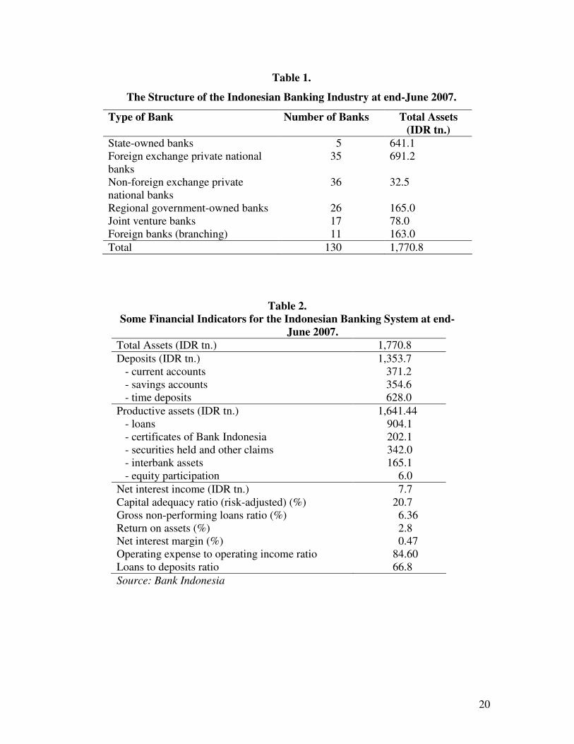
As demonstrated in Table 1, at the end of June 2007 there were 130 banks

operating in Indonesia with a combined balance sheet of over IDR 1,770 trillion (US$

190 billion). This comprised 5 state-owned banks, 35 foreign exchange private national

banks, 36 non-foreign exchange private national banks, 26 regional government-owned

banks, 17 joint venture banks and 11 foreign banks. This total compares with a figure of

222 banks in existence at end-December 1997, the shrinkage being largely due to post-

crisis liquidation and suspension, engineered by the Indonesian Bank Restructuring

Agency (IBRA) under agreement with the IMF (Jao, 2001, Ch.2), and mergers.

INSERT TABLE 1

Some indicators of industry performance are presented in Table 2. Positive

features are the capital adequacy ratio of 21% (up from 13% at end-December 2000), the

gross NPL ratio of 6.4% (down from 19% at end-December 2000) and the return on

assets ratio of 2.8% (up from 0.9% at end-December 2000). Continuing excess liquidity

in the banking system, however, is reflected in the relatively-low 67% loans to deposits

ratio, although this has recently improved (46% at end-December 2000).

INSERT TABLE 2

3. DATA AND MODELLING METHODOLOGY

3.1 Estimation of Efficiency

Data Envelopment Analysis (DEA) originated from Farrell’s (1957) seminal work

and was later elaborated on by Charnes et al. (1978), Banker et al. (1984) and Färe et al.

(1985). The objective of DEA is to construct a relative efficiency frontier through the

envelopment of the Decision Making Units (DMUs) where the ‘best practice’ DMUs

6

form the frontier. In this study, we utilize a DEA model which takes into account input

and output slacks, the so-called Slacks-Based Model (SBM), which was introduced by

Tone (2001) and ensures that, in non-parametric modelling, the slacks are taken into

account in the efficiency scores. Or, as Fried et al. (1999) argued, in the ‘standard’ DEA

models based on the Banker et al. (1984) specification “the solution to the DEA problem

yields the Farrell radial measure of technical efficiency plus additional non-radial input

savings (slacks) and output expansions (surpluses). In typical DEA studies, slacks and

surpluses are neglected at worst and relegated to the background at best” (page 250).

Indeed, in the analysis of public sector Decision Making Units (DMUs), for which DEA

was originally proposed by Farrell, the idea of slacks was not a problem unlike it is when

DEA is employed to measure cost efficiencies in a ‘competitive market’ setting. That is,

in a ‘competitive market’ setting, output and input slacks are essentially associated with

the violation of ‘neo classical’ assumptions. For example, in an input-oriented approach,

the input slacks would be associated with the assumption of strong or free disposability of

inputs which permits zero marginal productivity of inputs and hence extensions of the

relevant isoquants to form horizontal or vertical facets. In such cases, units which are

deemed to be radial- or Farrell- efficient (in the sense that no further proportional

reductions in inputs is possible without sacrificing output), may nevertheless be able to

implement further additional reductions in some inputs. Such additional potential input

reductions are typically referred to as non-radial input slacks, in contrast to the radial

slacks associated with DEA or Farrell inefficiency, that is, radial deviations from the

efficient frontier. In addition, to rank the best performers among the listed Indonesian

banks, we employ the super-efficiency SBM model proposed by Tone (2002).

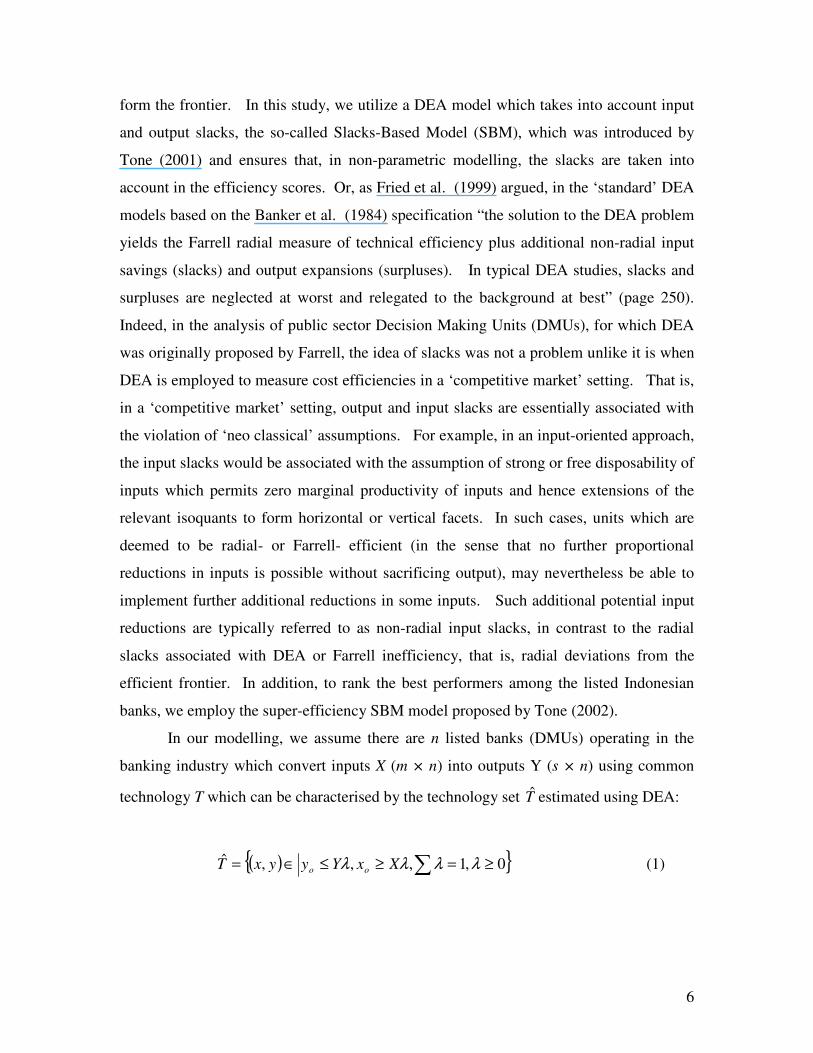
In our modelling, we assume there are n listed banks (DMUs) operating in the

banking industry which convert inputs X (m × n) into outputs Y (s × n) using common

technology T which can be characterised by the technology set T̂ estimated using DEA:

( ){ }0,1,,,ˆ ≥=≥≤∈= ∑ λλλλ XxYyyxT oo (1)

7

where xo and yo represent observed inputs and outputs of a particular DMU and λ is the

intensity variable. T̂ is a consistent estimator of the unobserved true technology set

under variable returns to scale. This means that, given our aim of analyzing the impact of

market driven factors on the SBM efficiency scores, the assumptions outlined in Simar

and Wilson (2007) hold, hence allowing for the provision of consistent estimators of the

parameters in a fully specified, semi-parametric Data Generating Process (DGP).

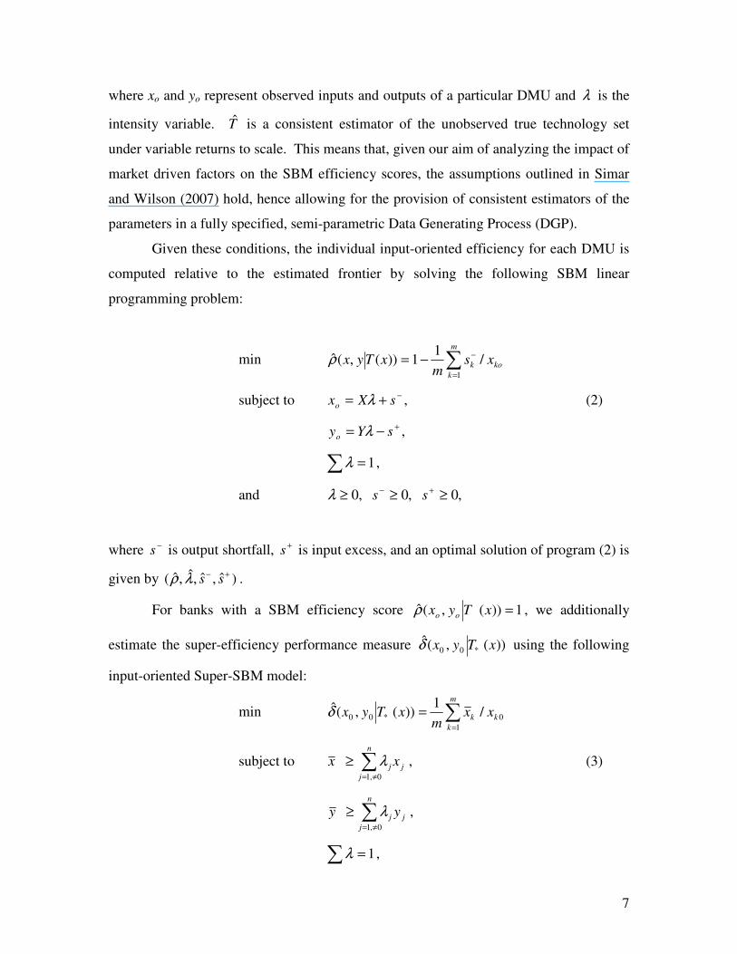
Given these conditions, the individual input-oriented efficiency for each DMU is

computed relative to the estimated frontier by solving the following SBM linear

programming problem:

min ∑=

−−=m

k

kok xsm

xTyx1

/1

1))(,(ρ̂

subject to −+= sXxo λ , (2)

+−= sYyo λ ,

∑ = 1λ ,

and ,0,0,0 ≥≥≥ +− ssλ

where −s is output shortfall, +

s is input excess, and an optimal solution of program (2) is

given by )ˆ,ˆ,ˆ,ˆ( +− ssλρ .

For banks with a SBM efficiency score 1))(,(ˆ =xTyx ooρ , we additionally

estimate the super-efficiency performance measure ))(,(ˆ *00 xTyxδ using the following

input-oriented Super-SBM model:

min ∑=

=m

k

kk xxm

xTyx1

0*00 /1

))(,(δ̂

subject to ∑≠=

≥n

j

jj xx0,1

λ , (3)

∑≠=

≥n

j

jj yy0,1

λ ,

∑ = 1λ ,

8

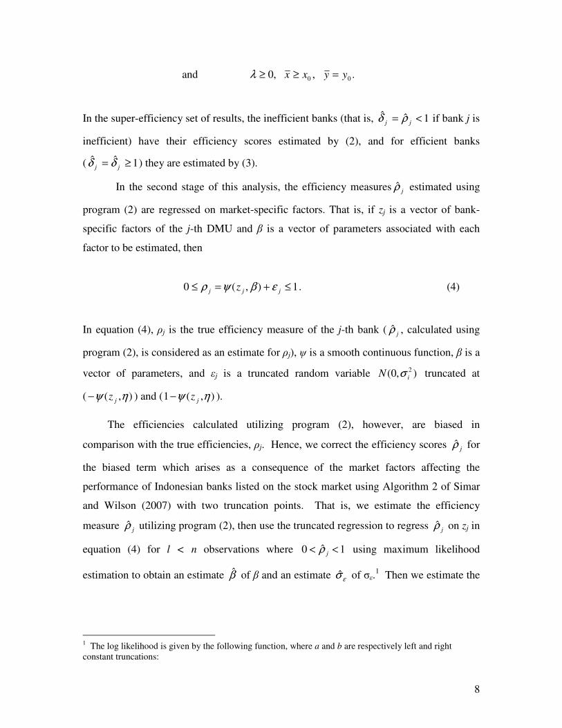
and .,,0 00 yyxx =≥≥λ

In the super-efficiency set of results, the inefficient banks (that is, 1ˆˆ <= jj ρδ if bank j is

inefficient) have their efficiency scores estimated by (2), and for efficient banks

( 1ˆˆ ≥= jj δδ ) they are estimated by (3).

In the second stage of this analysis, the efficiency measures jρ̂ estimated using

program (2) are regressed on market-specific factors. That is, if zj is a vector of bank-

specific factors of the j-th DMU and β is a vector of parameters associated with each

factor to be estimated, then

1),(0 ≤+=≤ jjj z εβψρ . (4)

In equation (4), ρj is the true efficiency measure of the j-th bank ( jρ̂ , calculated using

program (2), is considered as an estimate for ρj), ψ is a smooth continuous function, β is a

vector of parameters, and εj is a truncated random variable ),0( 2

iN σ truncated at

( ),( ηψ jz− ) and ( ),(1 ηψ jz− ).

The efficiencies calculated utilizing program (2), however, are biased in

comparison with the true efficiencies, ρj. Hence, we correct the efficiency scores jρ̂ for

the biased term which arises as a consequence of the market factors affecting the

performance of Indonesian banks listed on the stock market using Algorithm 2 of Simar

and Wilson (2007) with two truncation points. That is, we estimate the efficiency

measure jρ̂ utilizing program (2), then use the truncated regression to regress jρ̂ on zj in

equation (4) for l < n observations where 1ˆ0 << jρ using maximum likelihood

estimation to obtain an estimate β̂ of β and an estimate εσ̂ of σε.1 Then we estimate the

1 The log likelihood is given by the following function, where a and b are respectively left and right constant truncations:

9

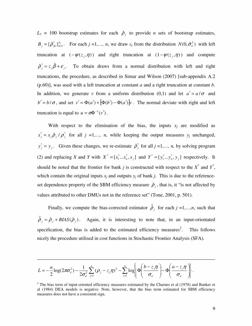
L1 = 100 bootstrap estimates for each jρ̂ to provide n sets of bootstrap estimates,

1

1

* }ˆ{ L

bjbjB == ρ . For each j =1,…, n, we draw εj from the distribution )ˆ,0( 2

εσN with left

truncation at ( ),( ηψ jz− ) and right truncation at ( ),(1 ηψ jz− ) and compute

jjj z εβρ += ˆˆ * . To obtain draws from a normal distribution with left and right

truncations, the procedure, as described in Simar and Wilson (2007) [sub-appendix A.2

(p.60)], was used with a left truncation at constant a and a right truncation at constant b.

In addition, we generate v from a uniform distribution (0,1) and let σ/aa =′ and

σ/bb =′ , and set [ ]vabav )()()( ′Φ−′Φ+′Φ=′ . The normal deviate with right and left

truncation is equal to )(1vu ′Φ= −σ .

With respect to the elimination of the bias, the inputs xj are modified as

** /ˆjjjj xx ρρ= for all j =1,…, n, while keeping the output measures yj unchanged,

jj yy =* . Given these changes, we re-estimate *ˆjρ for all j =1,…, n, by solving program

(2) and replacing X and Y with ],...[ **

1

*

jn xxxX = and ],...[ **

1

*

jn yyyY = respectively. It

should be noted that the frontier for bank j is constructed with respect to the X* and Y*,

which contain the original inputs xj and outputs yj of bank j. This is due to the reference-

set dependence property of the SBM efficiency measure jρ̂ , that is, it “is not affected by

values attributed to other DMUs not in the reference set” (Tone, 2001, p. 501).

Finally, we compute the bias-corrected estimator jρ̂̂ for each j =1,…,n, such that

)ˆ(ˆˆ̂jjj BIAS ρρρ += . Again, it is interesting to note that, in an input-orientated

specification, the bias is added to the estimated efficiency measures2. This follows

nicely the procedure utilised in cost functions in Stochastic Frontier Analysis (SFA).

∑∑==

−Φ−

−Φ−−−−=

n

i

jjn

j

jj

zazbz

nL

11

2

2

2 log)(2

1)2log(

2 εεε

εσ

η

σ

ηηρ

σπσ .

2 The bias term of input-oriented efficiency measures estimated by the Charnes et al (1978) and Banker et al (1984) DEA models is negative. Note, however, that the bias term estimated for SBM efficiency measures does not have a consistent sign.

10

The second bootstrap procedure of Algorithm 2 of Simar and Wilson (2007) is

similar to Algorithm 1. The only difference is that, in Algorithm 1, jρ̂ is used as a

dependent variable of the truncated regression whereas, in Algorithm 2, the bias-

corrected estimate, jρ̂̂ , is used. This second bootstrapping technique ensures that the

problem of serial correlation of the efficiency measures is avoided. The following steps

are performed in the second bootstrap procedure of Algorithm 2:

1. Estimate the truncated regression of jρ̂̂ on zj in (4) for m=n observations using

maximum likelihood estimation to obtain estimates for β̂ and εσ̂ .

2. Compute a set of L bootstrap estimates (we set L to equal 1000 replications) for β and

σε, L

bbA 1

** })ˆ,ˆ{( == εσβ , in the following way: for each j =1,…, m, draw εj from the normal

distribution )ˆ,0( 2

εσN with left truncation at ( ),( ηψ jz− ) and right truncation at

( ),(1 ηψ jz− ) and compute jjj z εβρ += ˆˆ̂ * ; then estimate the truncated regression of *ˆ̂jρ

on zj using maximum likelihood methods to obtain the parameter estimates )ˆ,ˆ( **

εσβ .

Once the set of L bootstrap parameter estimates for β and σε have been obtained, the

percentile bootstrap confidence intervals can then be constructed.

In addition, we analysed the determinants of the super-efficiency of Indonesian

banks using Algorithms 1 and 2. Since super-efficiency scores jδ̂ have only one

boundary at zero we employ the original methodology of Simar and Wilson (2007),

changing the value of the left truncation point. In other words, the following regression

is estimated:

jjj z εβψδ +=≤ ),(0 , (5)

where δj is the true efficiency measure of the j-th bank ( jδ̂ , calculated using programs (2)

and (3), is considered as an estimate for δj), ψ is a smooth continuous function, β is a

vector of parameters, and εj is a truncated random variable ),0( 2

iN σ truncated at

11

( ),( ηψ jz ). The reference set dependency is dealt with in a similar manner to the

efficiency estimates jρ̂ .

3.2. Productivity Analysis in the SBM Context

The measurement and analysis of productivity growth have attracted increased

interest among researchers studying bank performance. A Malmquist index of

productivity change, initially defined by Caves, Christensen and Diewert (1982) and

extended by Färe et al. (1992) by merging it with Farrell’s (1957) efficiency

measurement, has become increasingly popular. However, as discussed earlier, if the

technology is estimated using the DEA models suggested by Charnes et al. (1978) or

Banker et al. (1984), input and output slacks are ignored. Hence, for the estimation of

the Malmquist productivity index, similar to the study of Liu and Wang (2008), we utilise

SBM and super-SBM models introduced by Tone (2001) and Tone (2002) respectively.

However, unlike Liu and Wang (2008), we employ an input-oriented modification of the

models.

Accordingly, the individual input-oriented efficiency for each DMU in period t is

computed relative to the estimated frontier of period t by solving the SBM linear

programming problems (2) and (3) above. The performance measures for the DMU o

operated in time t+1, ))(,(ˆ 111 xTyx tt

o

t

o

+++ρ and ))(,(ˆ 1

*

1

0

1

0 xTyx ttt +++δ , can also be obtained

using models (2) and (3) by changing t to t+1.

The Malmquist productivity index of the DMUo between periods t and t+1 is

estimated as follows, in line with Färe et al. (1992):

21

1

11111

1,

))(,(ˆ

))(,(ˆ

))(,(ˆ

))(,(ˆ

=

+

+++++

+

xTyx

xTyx

xTyx

xTyxM

tt

o

t

o

tt

o

t

o

tt

o

t

o

tt

o

t

ott

oρ

ρ

ρ

ρ. (6)

If the productivity measure 11, >+tt

oM , then this implies a productivity gain for DMUo

between period t and t+1, and, contrariwise, a 11, <+tt

oM indicates a productivity loss.

12

11, =+tt

oM implies that DMUo has no change in its productivity. The productivity

measure 1, +tt

oM can also be decomposed into two indices which capture technical

efficiency change (TECo) between periods t and t+1, and the technological (frontier)

change (FSo), (i.e., the shift of the technology between two periods), as follows:

21

1111

11111

1,

))(,(ˆ

))(,(ˆ

))(,(ˆ

))(,(ˆ

))(,(ˆ

))(,(ˆ

×=×=

++++

+++++

+

xTyx

xTyx

xTyx

xTyx

xTyx

xTyxFSTECM

tt

o

t

o

tt

o

t

o

tt

o

t

o

tt

o

t

o

tt

o

t

o

tt

o

t

o

oo

tt

oρ

ρ

ρ

ρ

ρ

ρ

.

(7)

TECo measures the efficiency improvement of DMUo, which, in the case where TECo=1,

shows that the bank is still in the same position relative to the efficient boundary. When

TECo > 1, the bank has moved closer to the frontier, whereas for TECo < 1 the bank has

moved away from the frontier during the two periods. With regard to FSo, an FSo < 1

indicates a negative shift of the frontier (or regression), FSo > 1 a positive shift (progress)

and FSo = 1 implies no shift in the technological frontier.

3.3. Data and Inputs/Outputs Used

As stated in the introduction, this is the first paper to utilise monthly supervisory

data from Bank Indonesia and covers the period from 2006 to 2007. All (24) listed banks

feature in the sample.

In relation to our choice of inputs and outputs, recently banking studies have been

criticised for neglecting the profit side of banking operations. It has been shown, for

example, that banks exhibiting the highest inefficiencies and highest costs may be able to

generate greater profits than more cost-efficient banks (Berger and Mester, 1997). A

further criticism of many previous studies of banking efficiency is that they have not

adequately taken account of technical change and variations in efficiency through time.

Hence, variations in banking efficiency / performance can come from many sources, and

it is imperative that all possible sources of variation are examined and to explain the often

13

pronounced differences in profitability across different banks in a sample. Our choice of

inputs and outputs and modelling methodology addresses both issues.

The outputs used in this study embrace: Y1: Net interest Income; Y2: Net Trading

Income [(income from forex/derivative transactions - loss from forex/derivative

transactions) + (securities appreciation - securities depreciation)]; and Y3: Net off-

balance sheet income (income from dividends/commissions/fees and provisions –

expenses deriving from dividends/commissions/fees and provisions). The inputs follow

previous profit-based studies [for example, Drake et al (2006)], where: X1 is total

employee expenses (total salaries and wages + education and training costs); X2 is total

non-employee expenses (research and development costs + rent + advertising,

maintenance and repair costs + goods and services costs + other non-employee costs);

and X3 is provision for earning assets losses.

With respect to the last-mentioned input variable (i.e., provisions), it has long

been argued in the literature that the incorporation of risk/loan quality is vitally important

in studies of banking efficiency. Akhigbe and McNulty (2003), for example, utilising a

profit function approach, include equity capital “to control, in a very rough fashion, for

the potential increased cost of funds due to financial risk” (page. 312). Altunbas et al.

(2000) and Drake and Hall (2003) also find that failure to adequately account for risk can

have a significant impact on relative efficiency scores. In contrast to Akhigbe and

McNulty (2003), however, Laevan and Majnoni (2003) argue that risk should be

incorporated into efficiency studies via the inclusion of loan loss provisions. That is,

“following the general consensus among risk agent analysts and practitioners, economic

capital should be tailored to cope with unexpected losses, and loan loss reserves should

instead buffer the expected component of the loss distribution. Consistent with this

interpretation, loan loss provisions required to build up loan loss reserves should be

considered and treated as a cost; a cost that will be faced with certainty over time but that

is uncertain as to when it will materialise” (page 181). We agree with this view and

hence also incorporate provisions as an input/cost in the DEA relative efficiency analysis

of Indonesian banks.

14

4. RESULTS

4.1 First Stage: SBM Efficiency and Super-Efficiency Estimates

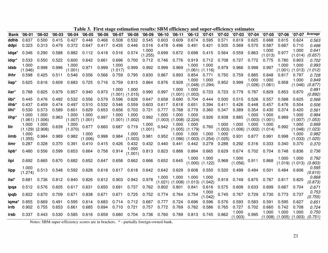
The SBM efficiency and super-efficiency scores for Indonesian banks listed on

the Indonesian Stock Exchange (IDX) are presented in Table 3. According to the SBM

efficiency results, the three most efficient banks over the studied period are “idsb”, “iihp”

and “iimb”.3 Under the super-efficiency framework, the same banks, along with the “liir”

bank, are found to have average efficiency levels above unity. Interestingly, with the

exception of the “iihp” bank (which is partially foreign in ownership), these banks are

domestically-owned.

The two least efficient banks, with average efficiency levels less than 50%, are

the domestically owned “ddpi” and “iimr” banks. Moreover, the latter is found to be the

most inefficient bank among the listed banks over the analysed period, with efficiency

levels ranging between 28% and 44%. Other listed banks which have not achieved their

frontiers in the analysed time span are the domestic bank “ddhb” and the partially

foreign-owned “iibi”, “iihb” and “iihi” banks. These banks are at best only 78%

efficient. Although the domestic banks “ihhr”, “ipqa”, “irrb” and the partially foreign-

owned bank “iqma” are found to consistently use their resources inefficiently, they do

appear to operate sometimes close to the best practice frontier with their highest

efficiency measures ranging between 84% and 90%. The remaining banks have

relatively-high efficiency levels and are considered further in the super-efficiency

analysis.

INSERT TABLE 3

Although the partially foreign-owned bank “idqa” operated with no input slacks

(i.e.,efficiently, according to the input-oriented SBM) in Sept 2006 and in May and July

2007, its efficiency level showed considerable fluctuation over the analysed period. For

example, it was only 11% in May 2006, which is the lowest efficiency estimate among

3 Codes are used to preserve the confidentiality of the data.

15

the considered banks during the sample period, and its highest efficiency was 126% - the

sixth highest super-efficiency score of the sample.

4.2 Second Stage: Determinants of Efficiency

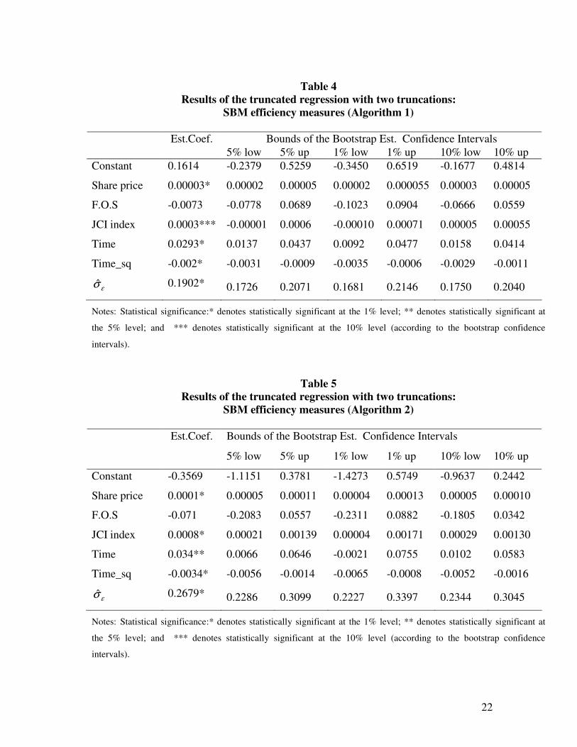
Tables 4 and 5 present the results of the truncated regression analysis for the SBM

efficiency measures utilising Algorithms 1 and 2 respectively of the Simar and Wilson

(2007) technique with left and right truncation points. The analysis of the factors

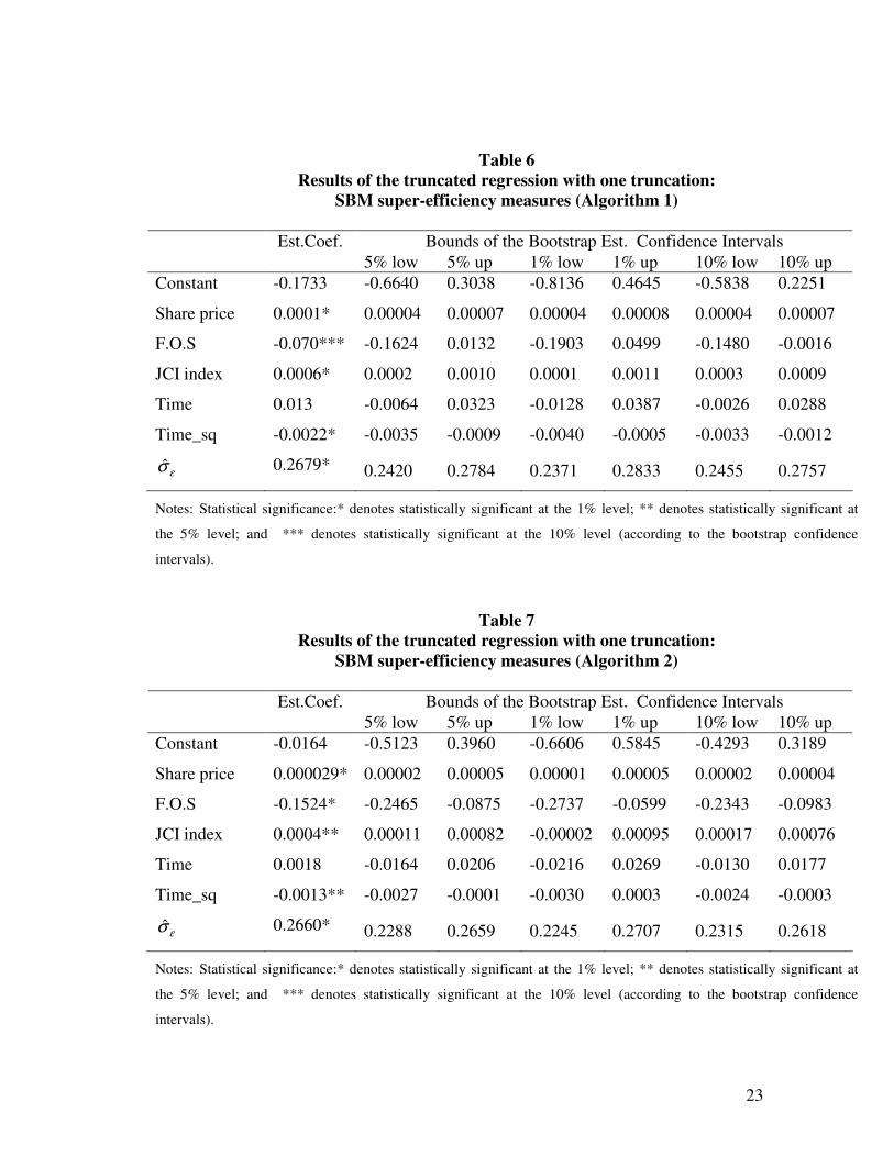
affecting the SBM super-efficiency scores using the aforementioned algorithms with left

truncation is shown in Tables 6 and 7; whilst the results of the first part of the

bootstrapping procedure of Algorithm 2, for both the SBM efficiency and SBM super-

efficiency models, are reported in the Appendix. To assess the relationship between the

performance of the banks and their market values, in the model specification we include

banks’ share prices. In addition, to capture the effect of the overall condition of the

Indonesian stock market, the JCI index is included. Nearly half of the listed banks are

partially-owned by foreign investors, with ownership shares ranging from 1.6% to 79.4%.

This factor is also incorporated in the study. Finally, in order to assess the dynamics of

the changes in the banks’ performance, time and time squared (Time_sq) variables are

also included.

INSERT TABLES 4 AND 5

In all the aforementioned models, share prices are positive and significant at the

1% level of significance. This is evidence confirming neo-classical theory which states

that the stock market values banks in accordance with their performance. A similar

finding is reported by Beccalli et al. (2006), who investigate the relationship between the

operating efficiency of European banks and their stock market performance. Moreover,

the positive and significant coefficient for the JCI index implies that the efficiencies of

the banking firms are also positively related to the overall performance of the market.

This is an expected result given that banks form an integral part of the economy. The

16

correlation between the stock market index’s performance and that of banking efficiency

can also be explained through the intimate link between the bank and the firms that make

up its clientele. Strong performances by the latter would automatically result in improved

performance of the former through increased demand for banking services.

INSERT TABLES 6 and 7

Another interesting finding is that the coefficient for the variable capturing the

share of foreign ownership (“F.O.S”) is negative and statistically significant in the super-

efficiency model. This suggests that the performance of Indonesian banks with foreign

ownership tends to lag behind that of their domestic counterparts. Our results are thus

different from those pertaining to many studies of banking industries in emerging,

transition and developed countries (see Bonin et al. (2005), Fries and Taci (2005),

Havrylchyk, (2006), Sathye (2003), Sturm and Williams (2004) and Fukuyama et al.

(1999)). However, they are in line with those of Hasan and Marton (2003), who find

evidence in favour of inferior operating performance of foreign banks vis-à-vis their

domestic counterparts in their studies of transition banking. In addition, more recently

Lensink et al. (2008) provide evidence of a negative effect of foreign ownership on bank

efficiency in their analysis of over 2000 banks in 105 countries. While these authors cite

conditions of the banking system and of the economy as reasons for the under-

performance of foreign banks, in our study it may be the sub-prime market distress that is

responsible, given the relative stability in the Indonesian banking system and wider

economy during 2006/07 (see Adiningsih, 2007).

The positive coefficient for the ‘Time’ variable in the two-truncation regression

models suggests that Indonesian banks improved their efficiency profiles over time.

However, the negative coefficient of the ‘Time_sq’ variable in all models implies that

long-term banking efficiency is in decline. This result may be driven by the fact that the

banks show greater focus towards obtaining quick profits rather than being profit-driven

by stable long-term investments. Although our sample covers only 19 time periods,

another possible explanation lies in the absence of a ‘long memory’ strategy among

banks in their profit-generating policy.

17

4.3 Results of the Productivity Analysis

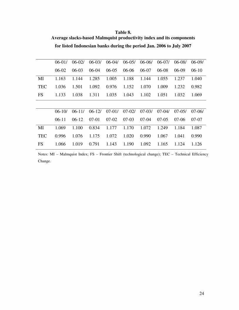
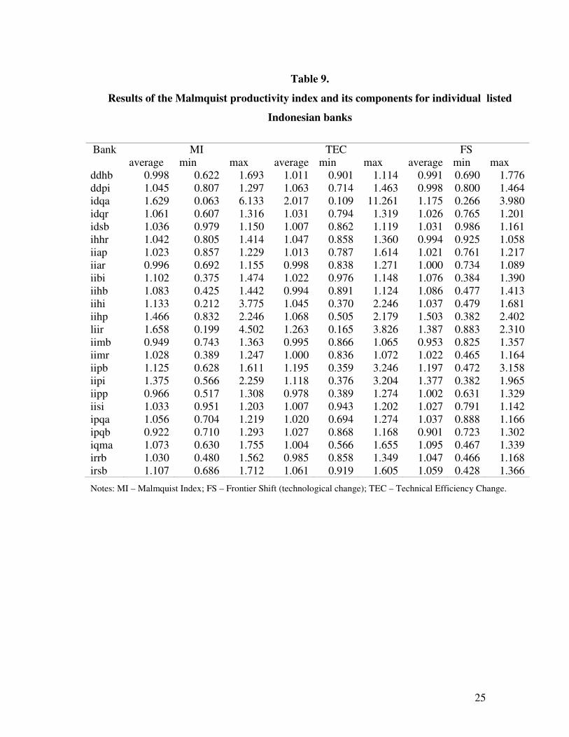
Tables 8 and 9 provide a summary of the average and individual Malmquist

productivity index and its components for the listed banks studied respectively.

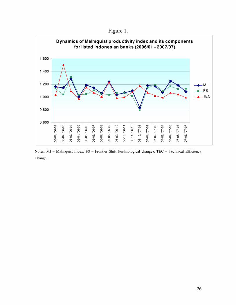
Interestingly, during the period analysed, the trend of the index is found to be primarily

determined by technological changes (that is, frontier shifts). Between April and

December 2006, however, the main driver of productivity was the changes in profit (that

is, technical) efficiency (see Figure 1). This time span corresponds to the beginning of

difficulties in the U.S. sub-prime market, hence suggesting that, anticipating the situation

in the global market, Indonesian banks concentrated mainly on improving technical

efficiency during this period. In general, the results show that, over the study’s horizon,

the sample banks displayed volatile productivity patterns in their profit-generating

operations. Furthermore, in the period between December 2006 and January 2007, the

steep decline in productivity can be traced to technological regression.

INSERT TABLES 8 AND 9

At the individual level (see Table 9), although some banks displayed somewhat

steadier changes in their productivity (e.g., “ddhb”, “ddpi”, “idqr”, “idsb”, “ihhr”, “iiap”,

“iiar”, “iihb”, “iimb”, “iisi”, “ipqa”, “ipqb” and “irsb”), several banks experienced sharp

productivity fluctuations. These banks are “iihi”, “iihp”, “iiir” and “iipi”. However, the

most extreme instability in productivity and its constituents is displayed by bank “idqa”.

Its monthly Malmquist productivity index ranged from a low of 0.06 to a high of 6.13.

Although the deviation in technological change of this bank was considerable, the main

source of “idqa’s” volatile productivity stems from severe deviations in technical

efficiency.

The unstable pattern of the productivity index, and the associated volatility in

technical efficiency, thus raise associated questions and concerns about the profit-

generating activity of Indonesian banks. Given the recent distress in the sub-prime

market, an important policy implication of our results is the possible need for a close

18

scrutiny of the profit-generating technology of Indonesian banking to identify and

eliminate investments bearing inappropriate risk profiles.

5. SUMMARY AND CONCLUSIONS

Combining the non-parametric models of Tone (2001 and 2002) with an

adaptation of Simar and Wilson’s (2007) bootstrapping methodology and adopting a

profit-based approach, we have analysed the efficiency of Indonesian banks listed on the

Jakarta Stock Exchange during most of the period 2006/07. To our knowledge, this

represents the first published efficiency study focusing solely on Indonesian banks and

certainly the first to use confidential monthly supervisory data collated by the central

bank, Bank Indonesia.

Our findings support the idea of an efficient Indonesian stock market, with the

market valuing banks in accordance with their performance. Moreover, we find a

positive correlation between the JCI index of the Indonesian Stock Exchange and bank

efficiency. Interestingly, we also find that, under the super-efficiency analysis, those

banks with foreign stakeholders tend to perform less well than their purely domestic

counterparts. Finally, our Malmquist analysis demonstrates that Indonesia’s listed banks

displayed volatile productivity patterns in their profit-generating operations during

2006/07. Although the trend of the index is found to be mainly driven by technological

changes during this period, with technological regression causing the steep decline in

productivity revealed between December 2006 and January 2007, changes in technical

[profit-based] efficiency did act as the driver of productivity over the period April to

December 2006.

The implications of this study for Indonesian policymakers are three-fold. Firstly,

resources should be devoted to trying to understand the reasons for the marked

differences recorded in individual banks’ profit-based efficiency. The findings can then

be shared with the industry with a view to raising overall levels of efficiency. Secondly,

outliers, at both ends of the efficiency spectrum (as demonstrated by the recent

nationalization of Northern Rock, previously one of the most efficient UK banks-see

19

Hall, 2008), merit closer supervisory scrutiny. And thirdly, the results should be used to

identify those banks which might usefully benefit from ‘assisted mergers’ as part of the

continuing process of consolidation aimed at enhancing banking sector stability.

20

Table 1.

The Structure of the Indonesian Banking Industry at end-June 2007.

Type of Bank Number of Banks Total Assets

(IDR tn.)

State-owned banks 5 641.1 Foreign exchange private national banks

35 691.2

Non-foreign exchange private national banks

36 32.5

Regional government-owned banks 26 165.0 Joint venture banks 17 78.0 Foreign banks (branching) 11 163.0

Total 130 1,770.8

Table 2.

Some Financial Indicators for the Indonesian Banking System at end-

June 2007. Total Assets (IDR tn.) 1,770.8

Deposits (IDR tn.) 1,353.7 - current accounts 371.2 - savings accounts 354.6 - time deposits 628.0

Productive assets (IDR tn.) 1,641.44 - loans 904.1 - certificates of Bank Indonesia 202.1 - securities held and other claims 342.0 - interbank assets 165.1 - equity participation 6.0

Net interest income (IDR tn.) 7.7 Capital adequacy ratio (risk-adjusted) (%) 20.7 Gross non-performing loans ratio (%) 6.36 Return on assets (%) 2.8 Net interest margin (%) 0.47 Operating expense to operating income ratio 84.60 Loans to deposits ratio 66.8

Source: Bank Indonesia

21

Table 3. First stage estimation results: SBM efficiency and super-efficiency estimates Bank ‘06-01 ‘06-02 ‘06-03 ‘06-04 ‘06-05 ‘06-06 ‘06-07 ‘06-08 ‘06-09 ‘06-10 ‘06-11 ‘06-12 ‘07-01 ‘07-02 ‘07-03 ‘07-04 ‘07-05 ‘07-06 ‘07-07 Average

ddhb 0.637 0.500 0.415 0.427 0.448 0.468 0.508 0.532 0.545 0.603 0.609 0.674 0.595 0.571 0.619 0.625 0.688 0.615 0.624 0.563

ddpi 0.323 0.313 0.479 0.372 0.647 0.417 0.435 0.446 0.516 0.478 0.496 0.491 0.421 0.505 0.569 0.570 0.587 0.687 0.710 0.498

idqa* 0.346 0.290 0.588 0.882 0.112 0.418 0.516 0.574 1.000

(1.255) 0.699 0.672 0.698 0.415 0.564 0.559 0.863

1.000 (1.013)

0.977 1.000

(1.014) 0.641

(0.657)

idqr* 0.533 0.550 0.522 0.600 0.642 0.661 0.696 0.700 0.712 0.746 0.776 0.919 0.712 0.708 0.727 0.772 0.775 0.780 0.803 0.702

idsb 1.000

(1.046) 0.998 0.996

1.000 (1.001)

0.971 0.999 1.000

(1.017) 0.999 0.992 0.999 0.969

1.000 (1.061)

1.000 (1.116)

0.979 0.966 0.998 0.997 1.000

(1.001) 1.000

(1.013) 0.993

(1.012)

ihhr 0.598 0.425 0.511 0.546 0.556 0.566 0.759 0.795 0.830 0.867 0.893 0.854 0.771 0.750 0.759 0.885 0.848 0.817 0.797 0.728

iiap* 0.625 0.616 0.609 0.683 0.725 0.716 0.759 0.815 0.864 0.876 0.928 1.000

(1.048) 1.000

(1.294) 0.952 0.999

1.000 (1.026)

1.000 (1.061)

0.958 1.000

(1.046) 0.849

(0.877)

iiar* 0.788 0.825 0.979 0.857 0.940 0.973 1.000

(1.001) 1.000

(1.015) 0.990 0.997

1.000 (1.001)

1.000 (1.003)

0.723 0.723 0.779 0.787 0.829 0.853 0.870 0.891

(0.892)

iibi* 0.445 0.476 0.492 0.532 0.556 0.579 0.596 0.626 0.647 0.658 0.690 0.704 0.444 0.500 0.515 0.526 0.557 0.588 0.625 0.566

iihb* 0.437 0.459 0.474 0.497 0.510 0.532 0.546 0.559 0.603 0.617 0.618 0.651 0.394 0.411 0.426 0.448 0.457 0.476 0.504 0.506

iihi* 0.530 0.573 0.589 0.601 0.629 0.653 0.656 0.703 0.721 0.777 0.768 0.779 0.360 0.347 0.389 0.354 0.430 0.374 0.420 0.561

iihp* 1.000

(1.061) 1.000

(1.006) 0.963

1.000 (1.007)

1.000 (1.001)

0.997 1.000

(1.001) 1.000

(1.002) 0.992

1.000 (1.003)

1.000 (1.008)

1.000 (2.224)

0.926 0.938 0.885 1.000

(1.003) 1.000

(1.001) 0.989

1.000 (1.007)

0.984 (1.053)

Iiir 1.000

(1.129) 1.000

(2.908) 0.639

1.000 (1.070)

0.677 0.660 0.687 0.719 1.000

(1.001) 0.942

1.000 (1.005)

1.000 (1.179)

0.760 1.000

(1.003) 1.000

(1.006) 1.000

(1.002) 1.000

(1.014) 0.992

1.000 (1.048)

0.899 (1.023)

iimb 1.000

(1.355) 0.984 0.989 0.982

1.000 (1.006)

0.998 0.984 1.000

(1.003) 0.981 0.952

1.000 (1.086)

1.000 (1.003)

1.000 (1.254)

1.000 (1.025)

0.931 0.877 0.991 0.998 1.000

(1.033) 0.982

(1.025)

iimr 0.287 0.328 0.370 0.391 0.410 0.415 0.426 0.432 0.432 0.440 0.441 0.442 0.279 0.288 0.292 0.316 0.333 0.340 0.370 0.370

iipb* 0.480 0.556 0.599 0.653 0.664 0.758 0.914 1.000

(1.001) 0.813 0.823 0.888 0.884 0.665 0.629 0.674 0.702 0.704 0.748 0.836 0.736

iipi 0.692 0.665 0.670 0.682 0.652 0.647 0.658 0.662 0.666 0.652 0.645 1.000

(1.000) 1.000

(1.122) 0.968

1.000 (1.056)

0.911 0.868 1.000

(1.019) 1.000

(1.013) 0.792

(0.803)

iipp 1.000

(1.274) 0.513 0.548 0.592 0.628 0.618 0.617 0.618 0.642 0.642 0.629 0.608 0.550 0.520 0.499 0.494 0.501 0.484 0.606

0.595 (0.610)

iisi* 0.681 0.736 0.812 0.840 0.826 0.812 0.903 0.942 0.978 1.000

(1.021) 1.000

(1.008) 1.000

(1.013) 1.000

(1.042) 0.919 0.749 0.875 0.787 0.817 0.825

0.868 (0.873)

ipqa 0.512 0.576 0.605 0.617 0.631 0.650 0.691 0.737 0.762 0.802 0.801 0.841 0.616 0.575 0.608 0.633 0.699 0.687 0.704 0.671

ipqb 0.822 0.670 0.709 0.671 0.838 0.671 0.671 0.725 0.752 0.774 0.764 0.754 1.000

(1.042) 0.745 0.767 0.729 0.730 0.773 0.737

0.753 (0.755)

iqma* 0.855 0.669 0.491 0.595 0.614 0.683 0.714 0.712 0.687 0.777 0.724 0.696 0.596 0.576 0.593 0.583 0.591 0.595 0.627 0.651

irrb 0.902 0.755 0.653 0.661 0.685 0.694 0.710 0.721 0.757 0.772 0.769 0.782 0.586 0.765 0.727 0.702 0.660 0.742 0.708 0.724

irsb 0.337 0.443 0.530 0.585 0.616 0.659 0.680 0.704 0.736 0.760 0.789 0.813 0.745 0.862 1.000

(1.003) 0.995

1.000 (1.008)

1.000 (1.005)

1.000 (1.003)

0.750 (0.751)

Notes: SBM super-efficiency scores are in brackets. * - partially foreign-owned bank.

22

Table 3. Results of truncated regression with two truncations: SBM efficiency measures (Algorithm 2)

Table 4

Results of the truncated regression with two truncations:

SBM efficiency measures (Algorithm 1)

Bounds of the Bootstrap Est. Confidence Intervals Est.Coef.

5% low 5% up 1% low 1% up 10% low 10% up

Constant 0.1614 -0.2379 0.5259 -0.3450 0.6519 -0.1677 0.4814

Share price 0.00003* 0.00002 0.00005 0.00002 0.000055 0.00003 0.00005

F.O.S -0.0073 -0.0778 0.0689 -0.1023 0.0904 -0.0666 0.0559

JCI index 0.0003*** -0.00001 0.0006 -0.00010 0.00071 0.00005 0.00055

Time 0.0293* 0.0137 0.0437 0.0092 0.0477 0.0158 0.0414

Time_sq -0.002* -0.0031 -0.0009 -0.0035 -0.0006 -0.0029 -0.0011

εσ̂ 0.1902* 0.1726 0.2071 0.1681 0.2146 0.1750 0.2040

Notes: Statistical significance:* denotes statistically significant at the 1% level; ** denotes statistically significant at

the 5% level; and *** denotes statistically significant at the 10% level (according to the bootstrap confidence

intervals).

Table 5

Results of the truncated regression with two truncations:

SBM efficiency measures (Algorithm 2)

Bounds of the Bootstrap Est. Confidence Intervals Est.Coef.

5% low 5% up 1% low 1% up 10% low 10% up

Constant -0.3569 -1.1151 0.3781 -1.4273 0.5749 -0.9637 0.2442

Share price 0.0001* 0.00005 0.00011 0.00004 0.00013 0.00005 0.00010

F.O.S -0.071 -0.2083 0.0557 -0.2311 0.0882 -0.1805 0.0342

JCI index 0.0008* 0.00021 0.00139 0.00004 0.00171 0.00029 0.00130

Time 0.034** 0.0066 0.0646 -0.0021 0.0755 0.0102 0.0583

Time_sq -0.0034* -0.0056 -0.0014 -0.0065 -0.0008 -0.0052 -0.0016

εσ̂ 0.2679* 0.2286 0.3099 0.2227 0.3397 0.2344 0.3045

Notes: Statistical significance:* denotes statistically significant at the 1% level; ** denotes statistically significant at

the 5% level; and *** denotes statistically significant at the 10% level (according to the bootstrap confidence

intervals).

23

Table 6

Results of the truncated regression with one truncation:

SBM super-efficiency measures (Algorithm 1)

Bounds of the Bootstrap Est. Confidence Intervals Est.Coef.

5% low 5% up 1% low 1% up 10% low 10% up

Constant -0.1733 -0.6640 0.3038 -0.8136 0.4645 -0.5838 0.2251

Share price 0.0001* 0.00004 0.00007 0.00004 0.00008 0.00004 0.00007

F.O.S -0.070*** -0.1624 0.0132 -0.1903 0.0499 -0.1480 -0.0016

JCI index 0.0006* 0.0002 0.0010 0.0001 0.0011 0.0003 0.0009

Time 0.013 -0.0064 0.0323 -0.0128 0.0387 -0.0026 0.0288

Time_sq -0.0022* -0.0035 -0.0009 -0.0040 -0.0005 -0.0033 -0.0012

εσ̂ 0.2679* 0.2420 0.2784 0.2371 0.2833 0.2455 0.2757

Notes: Statistical significance:* denotes statistically significant at the 1% level; ** denotes statistically significant at

the 5% level; and *** denotes statistically significant at the 10% level (according to the bootstrap confidence

intervals).

Table 7

Results of the truncated regression with one truncation:

SBM super-efficiency measures (Algorithm 2)

Bounds of the Bootstrap Est. Confidence Intervals Est.Coef.

5% low 5% up 1% low 1% up 10% low 10% up

Constant -0.0164 -0.5123 0.3960 -0.6606 0.5845 -0.4293 0.3189

Share price 0.000029* 0.00002 0.00005 0.00001 0.00005 0.00002 0.00004

F.O.S -0.1524* -0.2465 -0.0875 -0.2737 -0.0599 -0.2343 -0.0983

JCI index 0.0004** 0.00011 0.00082 -0.00002 0.00095 0.00017 0.00076

Time 0.0018 -0.0164 0.0206 -0.0216 0.0269 -0.0130 0.0177

Time_sq -0.0013** -0.0027 -0.0001 -0.0030 0.0003 -0.0024 -0.0003

εσ̂ 0.2660* 0.2288 0.2659 0.2245 0.2707 0.2315 0.2618

Notes: Statistical significance:* denotes statistically significant at the 1% level; ** denotes statistically significant at

the 5% level; and *** denotes statistically significant at the 10% level (according to the bootstrap confidence

intervals).

24

Table 8.

Average slacks-based Malmquist productivity index and its components

for listed Indonesian banks during the period Jan. 2006 to July 2007

06-01/

06-02

06-02/

06-03

06-03/

06-04

06-04/

06-05

06-05/

06-06

06-06/

06-07

06-07/

06-08

06-08/

06-09

06-09/

06-10

MI 1.163 1.144 1.285 1.005 1.188 1.144 1.055 1.237 1.040

TEC 1.036 1.501 1.092 0.976 1.152 1.070 1.009 1.232 0.982

FS 1.133 1.038 1.311 1.035 1.043 1.102 1.051 1.032 1.069

06-10/

06-11

06-11/

06-12

06-12/

07-01

07-01/

07-02

07-02/

07-03

07-03/

07-04

07-04/

07-05

07-05/

07-06

07-06/

07-07

MI 1.069 1.100 0.834 1.177 1.170 1.072 1.249 1.184 1.087

TEC 0.996 1.076 1.175 1.072 1.020 0.990 1.067 1.041 0.990

FS 1.066 1.019 0.791 1.143 1.190 1.092 1.165 1.124 1.126

Notes: MI – Malmquist Index; FS – Frontier Shift (technological change); TEC – Technical Efficiency

Change.

25

Table 9.

Results of the Malmquist productivity index and its components for individual listed

Indonesian banks

MI TEC FS Bank

average min max average min max average min max ddhb 0.998 0.622 1.693 1.011 0.901 1.114 0.991 0.690 1.776 ddpi 1.045 0.807 1.297 1.063 0.714 1.463 0.998 0.800 1.464 idqa 1.629 0.063 6.133 2.017 0.109 11.261 1.175 0.266 3.980 idqr 1.061 0.607 1.316 1.031 0.794 1.319 1.026 0.765 1.201 idsb 1.036 0.979 1.150 1.007 0.862 1.119 1.031 0.986 1.161 ihhr 1.042 0.805 1.414 1.047 0.858 1.360 0.994 0.925 1.058 iiap 1.023 0.857 1.229 1.013 0.787 1.614 1.021 0.761 1.217 iiar 0.996 0.692 1.155 0.998 0.838 1.271 1.000 0.734 1.089 iibi 1.102 0.375 1.474 1.022 0.976 1.148 1.076 0.384 1.390 iihb 1.083 0.425 1.442 0.994 0.891 1.124 1.086 0.477 1.413 iihi 1.133 0.212 3.775 1.045 0.370 2.246 1.037 0.479 1.681 iihp 1.466 0.832 2.246 1.068 0.505 2.179 1.503 0.382 2.402 liir 1.658 0.199 4.502 1.263 0.165 3.826 1.387 0.883 2.310 iimb 0.949 0.743 1.363 0.995 0.866 1.065 0.953 0.825 1.357 iimr 1.028 0.389 1.247 1.000 0.836 1.072 1.022 0.465 1.164 iipb 1.125 0.628 1.611 1.195 0.359 3.246 1.197 0.472 3.158 iipi 1.375 0.566 2.259 1.118 0.376 3.204 1.377 0.382 1.965 iipp 0.966 0.517 1.308 0.978 0.389 1.274 1.002 0.631 1.329 iisi 1.033 0.951 1.203 1.007 0.943 1.202 1.027 0.791 1.142 ipqa 1.056 0.704 1.219 1.020 0.694 1.274 1.037 0.888 1.166 ipqb 0.922 0.710 1.293 1.027 0.868 1.168 0.901 0.723 1.302 iqma 1.073 0.630 1.755 1.004 0.566 1.655 1.095 0.467 1.339 irrb 1.030 0.480 1.562 0.985 0.858 1.349 1.047 0.466 1.168 irsb 1.107 0.686 1.712 1.061 0.919 1.605 1.059 0.428 1.366

Notes: MI – Malmquist Index; FS – Frontier Shift (technological change); TEC – Technical Efficiency Change.

26

Figure 1.

Dynamics of Malmquist productivity index and its components

for listed Indonesian banks (2006/01 - 2007/07)

0.600

0.800

1.000

1.200

1.400

1.60006-0

1/ '0

6-0

2

06-0

2/ '0

6-0

3

06-0

3/ '0

6-0

4

06-0

4/ '0

6-0

5

06-0

5/ '0

6-0

6

06-0

6/ '0

6-0

7

06-0

7/ '0

6-0

8

06-0

8/ '0

6-0

9

06-0

9/ '0

6-1

0

06-1

0/ '0

6-1

1

06-1

1/ '0

6-1

2

06-1

2/ '0

7-0

1

07-0

1/ '0

7-0

2

07-0

2/ '0

7-0

3

07-0

3/ '0

7-0

4

07-0

4/ '0

7-0

5

07-0

5/ '0

7-0

6

07-0

6/ '0

7-0

7

MI

FS

TEC

Notes: MI – Malmquist Index; FS – Frontier Shift (technological change); TEC – Technical Efficiency

Change.

27

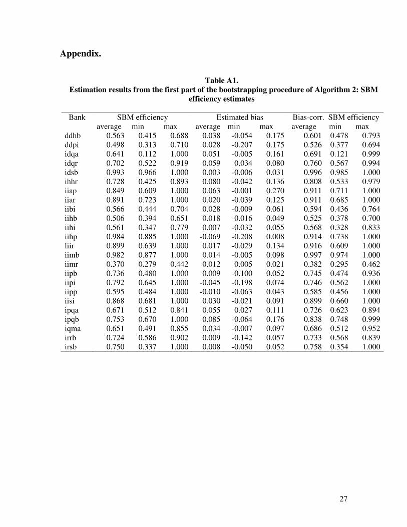
Appendix.

Table A1.

Estimation results from the first part of the bootstrapping procedure of Algorithm 2: SBM

efficiency estimates

SBM efficiency Estimated bias Bias-corr. SBM efficiency Bank average min max average min max average min max

ddhb 0.563 0.415 0.688 0.038 -0.054 0.175 0.601 0.478 0.793 ddpi 0.498 0.313 0.710 0.028 -0.207 0.175 0.526 0.377 0.694 idqa 0.641 0.112 1.000 0.051 -0.005 0.161 0.691 0.121 0.999 idqr 0.702 0.522 0.919 0.059 0.034 0.080 0.760 0.567 0.994 idsb 0.993 0.966 1.000 0.003 -0.006 0.031 0.996 0.985 1.000 ihhr 0.728 0.425 0.893 0.080 -0.042 0.136 0.808 0.533 0.979 iiap 0.849 0.609 1.000 0.063 -0.001 0.270 0.911 0.711 1.000 iiar 0.891 0.723 1.000 0.020 -0.039 0.125 0.911 0.685 1.000 iibi 0.566 0.444 0.704 0.028 -0.009 0.061 0.594 0.436 0.764 iihb 0.506 0.394 0.651 0.018 -0.016 0.049 0.525 0.378 0.700 iihi 0.561 0.347 0.779 0.007 -0.032 0.055 0.568 0.328 0.833 iihp 0.984 0.885 1.000 -0.069 -0.208 0.008 0.914 0.738 1.000 liir 0.899 0.639 1.000 0.017 -0.029 0.134 0.916 0.609 1.000 iimb 0.982 0.877 1.000 0.014 -0.005 0.098 0.997 0.974 1.000 iimr 0.370 0.279 0.442 0.012 0.005 0.021 0.382 0.295 0.462 iipb 0.736 0.480 1.000 0.009 -0.100 0.052 0.745 0.474 0.936 iipi 0.792 0.645 1.000 -0.045 -0.198 0.074 0.746 0.562 1.000 iipp 0.595 0.484 1.000 -0.010 -0.063 0.043 0.585 0.456 1.000 iisi 0.868 0.681 1.000 0.030 -0.021 0.091 0.899 0.660 1.000 ipqa 0.671 0.512 0.841 0.055 0.027 0.111 0.726 0.623 0.894 ipqb 0.753 0.670 1.000 0.085 -0.064 0.176 0.838 0.748 0.999 iqma 0.651 0.491 0.855 0.034 -0.007 0.097 0.686 0.512 0.952 irrb 0.724 0.586 0.902 0.009 -0.142 0.057 0.733 0.568 0.839 irsb 0.750 0.337 1.000 0.008 -0.050 0.052 0.758 0.354 1.000

28

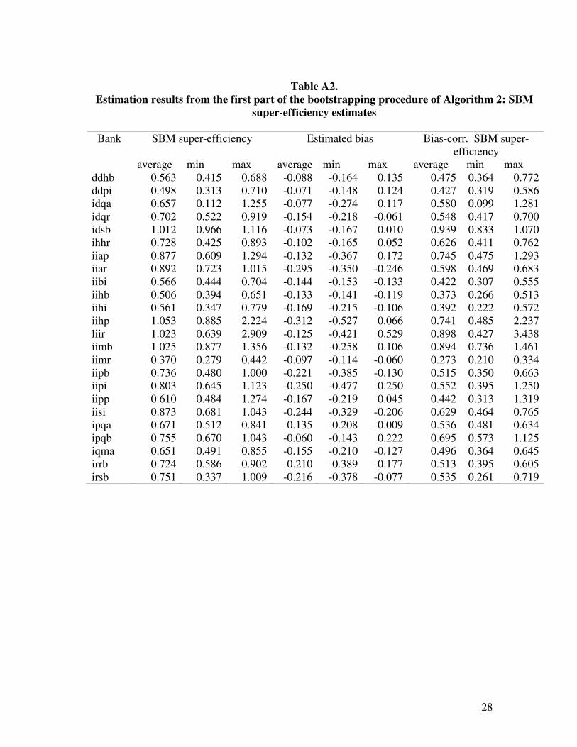
Table A2.

Estimation results from the first part of the bootstrapping procedure of Algorithm 2: SBM

super-efficiency estimates

SBM super-efficiency Estimated bias Bias-corr. SBM super- efficiency

Bank

average min max average min max average min max ddhb 0.563 0.415 0.688 -0.088 -0.164 0.135 0.475 0.364 0.772 ddpi 0.498 0.313 0.710 -0.071 -0.148 0.124 0.427 0.319 0.586 idqa 0.657 0.112 1.255 -0.077 -0.274 0.117 0.580 0.099 1.281 idqr 0.702 0.522 0.919 -0.154 -0.218 -0.061 0.548 0.417 0.700 idsb 1.012 0.966 1.116 -0.073 -0.167 0.010 0.939 0.833 1.070 ihhr 0.728 0.425 0.893 -0.102 -0.165 0.052 0.626 0.411 0.762 iiap 0.877 0.609 1.294 -0.132 -0.367 0.172 0.745 0.475 1.293 iiar 0.892 0.723 1.015 -0.295 -0.350 -0.246 0.598 0.469 0.683 iibi 0.566 0.444 0.704 -0.144 -0.153 -0.133 0.422 0.307 0.555 iihb 0.506 0.394 0.651 -0.133 -0.141 -0.119 0.373 0.266 0.513 iihi 0.561 0.347 0.779 -0.169 -0.215 -0.106 0.392 0.222 0.572 iihp 1.053 0.885 2.224 -0.312 -0.527 0.066 0.741 0.485 2.237 liir 1.023 0.639 2.909 -0.125 -0.421 0.529 0.898 0.427 3.438 iimb 1.025 0.877 1.356 -0.132 -0.258 0.106 0.894 0.736 1.461 iimr 0.370 0.279 0.442 -0.097 -0.114 -0.060 0.273 0.210 0.334 iipb 0.736 0.480 1.000 -0.221 -0.385 -0.130 0.515 0.350 0.663 iipi 0.803 0.645 1.123 -0.250 -0.477 0.250 0.552 0.395 1.250 iipp 0.610 0.484 1.274 -0.167 -0.219 0.045 0.442 0.313 1.319 iisi 0.873 0.681 1.043 -0.244 -0.329 -0.206 0.629 0.464 0.765 ipqa 0.671 0.512 0.841 -0.135 -0.208 -0.009 0.536 0.481 0.634 ipqb 0.755 0.670 1.043 -0.060 -0.143 0.222 0.695 0.573 1.125 iqma 0.651 0.491 0.855 -0.155 -0.210 -0.127 0.496 0.364 0.645 irrb 0.724 0.586 0.902 -0.210 -0.389 -0.177 0.513 0.395 0.605 irsb 0.751 0.337 1.009 -0.216 -0.378 -0.077 0.535 0.261 0.719

29

REFERENCES:

Adiningsih, S. (2007), “Indonesia: Ten Years After the Economic Crisis,” Institute of

Development Studies Bulletin, 38, 45-58.

Akhigbe, A. and McNulty, J.E. (2003), “The Profit Efficiency of Small US Commercial

Banks,” Journal of Banking and Finance, 27, 307-325.

Altunbas, Y., Liu, M-H., Molyneux, P. and Seth, R. (2000), “Efficiency and Risk in

Japanese Banking,” Journal of Banking and Finance, 24, 1605-1628.

Banker, R.D., Charnes, A. and Cooper, W.W. (1984), “Some Models for the Estimation

of Technical and Scale Inefficiencies in Data Envelopment Analysis,”

Management Science, 30, 1078–1092.

Beccalli, E., Casu, B. and Girardone, C. (2006), "Efficiency and Stock Performance in

European Banking", Journal of Business Finance and Accounting, 33 (1), 245-

262.

Benston, G.J. (1965), “Branch Banking and Economies of Scale,” The Journal of

Finance, 20, 312-331.

Berger, A.N. and Mester, L.J. (1997), “Inside the Black Box: What Explains Differences

in the Efficiencies of Financial Institutions”, Journal of Banking and Finance, 21

(7), 895 – 947.

Bonin, J.P., Hasan, I. and Wachtel, P. (2005), "Bank Performance, Efficiency and

Ownership in Transition Countries", Journal of Banking and Finance, 29 (1), 31-

53.

Caves, D.W., Christensen, L.R. and Diewert, W.E. (1982), “The Economic Theory of

Index Numbers and the Measurement of Input, Output, and Productivity”,

Econometrica, 50 (6), 1393-1414.

Charnes, A., Cooper, W. and Rhodes, E. (1978), “Measuring the Efficiency of Decision-

Making Units,” European Journal of Operational Research, 2, 429–444.

Chu, S.F. and Lim, G.H. (1998), “Share performance and profit efficiency of banks in an

oligopolistic market: evidence from Singapore,” Journal of Multinational

Financial Management, 8, 55-168.

30

Dogan, E. and Fausten, D.K. (2003), "Productivity and Technical Change in Malaysian

Banking: 1989–1998," Asia-Pacific Financial Markets, 10, 205-237.

Drake, L. and Hall, M. J. B. (2003), “Efficiency in Japanese Banking: An Empirical

Analysis,” Journal of Banking and Finance, 27 (5), 891-917.

Drake, L., Hall, M.J.B. and Simper, R. (2006), “The Impact of Macroeconomic and

Regulatory Factors on Bank Efficiency: A Non-Parametric Analysis of Hong

Kong’s Banking System," Journal of Banking and Finance, 30 (5), 1443-1466.

Drake, L., Hall, M.J.B. and Simper, R. (2008), “Bank Modelling Methodologies: A

Comparative Non-Parametric Analysis of Efficiency in the Japanese Banking

Sector” forthcoming, Journal of International Financial Markets, Institutions &

Money, (forthcoming).

Fan. L. and Shaffer, S. (2004), “Efficiency Versus Risk in Large Domestic US Banks,”

Managerial Finance, 30, 1-19.

Fare, R., Grosskopf, S. and Lovell, C.A.K. (1985), The Measurement of Efficiency of

Production. Kluwer- Nijhoff Publishing, Boston.

Färe, R., Grosskopf, S., Lindgren, B. and Roos, P. (1992), “Productivity Change in

Swedish Pharmacies 1980–1989: A Non-Parametric Malmquist Approach”,

Journal of Productivity Analysis, 3, 85–102.

Farrell, M.J. (1957), “The Measurement of Productive Efficiency,” Journal of the Royal

Statistical Society, Ser. A, 120, 253-281.

Fried, H.O., Schmidt, S.S. and Yaisawarng, S. (1999), “Incorporating the Operating

Environment into a Nonparametric Measure of Technical Efficiency,” Journal of

Productivity Analysis, 12, 249-267.

Fries, S. and Taci, A. (2005), "Cost Efficiency of Banks in Transition: Evidence from

289 Banks in 15 Post-Communist Countries", Journal of Banking and Finance,

29 (1), 55-81.

Fukuyama, H., Guerra, R. and Weber, W.L. (1999), "Efficiency and Ownership:

Evidence from Japanese Credit Cooperatives", Journal of Economics and

Business, 51 (6), 473-487.

Gilbert, R.A. and Wilson, P.W. (1998), “Effects of Deregulation on the Productivity of

Korean Banks,” Journal of Economics and Business, 50, 133-155.

31

Hall, M. J. B. (2008), “The Sub-prime Crisis, the Credit Squeeze and Northern Rock: The

Lessons to Be Learned”, Journal of Financial Regulation and Compliance, 16 (1),

19-34.

Havrylchyk, O. (2006), “Efficiency of the Polish banking industry: Foreign versus

domestic banks”, Journal of Banking and Finance, 30 (7), 1975-1996.

Hasan, I. and Marton, K. (2003), “Development and Efficiency of the Banking Sector in

a Transitional Economy: Hungarian Experience”, Journal of Banking and

Finance, 27 (12), 2249-2271.

Hill, H. and Shirishi, T. (2007), “Indonesia After the Asian Crisis,” Asian Economic

Policy Review, 2, 123-141.

Jao, Y.C. (2001), The Asian Financial Crisis and the Ordeal of Hong Kong, Quorum

Books, Greenwood Publishing.

Kenjegalieva, K., Simper, R., Weyman-Jones, T. G., and Zelenyuk, V., (2007),

“Comparative Analysis of Banking Production Frameworks in Eastern European

Financial Markets,” Department of Economics Discussion Paper, Loughborough

University, UK.

Kwan, S. H. (2002), "The X-Efficiency of Commercial Banks in Hong Kong," HKIMR

Working Paper No. 12/2002.

Laeven, L. and Majnoni, G. (2003), “Loan Loss Provisioning and Economic Slowdowns:

Too Much, Too Late?” Journal of Financial Intermediation, 12, 178-197.

Leightner, J.E. and Knox-Lovell, C.A. (1998), “The Impact of Financial Liberalization on

the Performance of Thai Banks,” Journal of Economics and Business, 50, 115-

131.

Lensink, R., Meesters, A. and Naaborg, I. (2008), “Bank Efficiency and Foreign

Ownership: Do Good Institutions Matter?”, Journal of Banking and Finance, 32

(5), 834-844.

Liu, F.F. and Wang, P. (2008), “DEA Malmquist Productivity Measure: Taiwanese

Semiconductor Companies”, International Journal of Production Economics,

112, 367-379.

32

McKillop, D.G., Glass, J.C. and Morikawa, Y. (1996), "The Composite Cost Function

and Efficiency in Giant Japanese Banks," Journal of Banking & Finance, 20 (10),

1651-1671

Murray, J.D. and White, R.W. (1983), “Economies of Scale and Economies of Scope in

Multiproduct Financial Institutions: A Study of British Columbia Credit Unions,”

The Journal of Finance, 38, 887-901.

Pulley, L.B. and Braunstein, Y.B. (1992), “A Composite Cost Function for Multiproduct

Firms With an Application to Economies of Scope in Banking,” Review of

Economics and Statistics, 74, 214-230.

Sathye, M. (2003), “Efficiency of Banks in a Developing Economy: The Case of India,”

European Journal of Operational Research, 148 (3), 662-671.

Simar, L. and Wilson, P.W. (2007), “Estimation and Inference in Two-Stage, Semi-

Parametric Models of Production Processes,” Journal of Econometrics, 136 (1),

31-64.

Sturm, J.E. and Williams, B. (2004), “Foreign Bank Entry, Deregulation and Bank

Efficiency: Lessons from the Australian Experience,” Journal of Banking and

Finance, 28 (7), 1775-1799.

Tone, K. (2001), “A Slacks–Based Measure of Efficiency in Data Envelopment

Analysis,” European Journal of Operational Research, 130, 498–509.

Tone, K. (2002), “A Slacks-Based Measure of Super-Efficiency in Data Envelopment

Analysis,” European Journal of Operational Research, 143, 32-41.

Unite, A.A. and Sullivan, M.J. (2003), “The Effect of Foreign Entry and Ownership

Structure on the Philippine Domestic Banking Market,” Journal of Banking and

Finance, 27 (12), 2323-2345.

Williams, J. and Nguyen, N. (2005), “Financial Liberalisation, Crisis, and Restructuring:

A Comparative Study of Bank Performance and Bank Governance in South East

Asia,” Journal of Banking and Finance, 29 (8/9), 2119-2154.