l/IT-ZHM?— /<0~I/oI.3lF - t1S'Q <o - \/c l' X

received

MAY 0 1 1836OSJi

DISTRIBUTION OF THIS DOCUMENT IS UNLIMITED&

DISCLAIMER

Portions of this document may be illegible in electronic image products. Images are produced from the best available original document.

This is the second volume of the publications, which contain the presentations given at the BALTIC A III, International Conference on Plant Condition & Life Management, Helsinki - Stockholm, June 6-8, 1995. BALTICA III provides forum for the transfer of technology from applied research to practice.

The BALTICA III Conference on Plant Condition & Life Management aims to review and disseminate experience in plant condition and life management. The conference focuses on recent applications that have been demonstrated for the benefit of safe and economical operation of power plants. Practical approach is emphasised, including the presenta­tions that aim to provide insight into new techniques, improvements in assessment methodologies as well as maintenance strategies. Compared to earlier occasions in the BALTICA series, a new aspect is in the applications of knowledge-based systems in the service of power plant life management.

Earlier BALTICA occasions:

BALTICA I Materials Aspects in Life Extension of Power Plants, Helsinki - Stockholm - Helsinki, September 19 - 22, 1988

BALTICA II International Conference on Plant Life Management & Extension, Helsinki - Stockholm - Helsinki, October 5-6, 1992

BALTICA II International Symposium on Life and Performance of High Temperature Materials and Structures, Tallinn, Estonia, October 7 - 8, 1992.

ISBN 951-38-4542-7 ISSN 0357-9387 CDC 621.311.22:621.18:669.14620.17/. 18:62-7:681.518

VTT SYMPOSIUM 151 UDC 621.311.22:621.18:669.14 620.17/. 18:62-7:681.518

Keywords:power plants, maintenance, boilers, steel, condition monitoring, cracking, corrosion, service life, optimization, automation

BALTICA IIIInternational conference on plant

condition & life managementVol II

Helsinki - Stockholm, June 6-8, 1995

Edited by

Seija Hietanen Pertti Auerkari

VTT Manufacturing Technology

Organized by

VTT Manufacturing Technology

Supported by

Helsinki Energy I VO Group

Kunnossapitoyhdistys ry. The SPRINT Office of the CEC

TECHNICAL RESEARCH CENTRE OF FINLAND ESPOO 1995

ISBN 951-38-4542-7 ISSN 0357-9387Copyright © Valtion teknillinen tutkimuskeskus (VTT) 1995

JULKAISIJA - UTGIVARE - PUBLISHER

Valtion teknillinen tutkimuskeskus (VTT), Vuorimiehentie 5, PL 2000, 02044 VTT puh. vaihde (90) 4561, telekopio (90) 456 4374

Statens tekniska forskningscentral (VTT), Bergsmansvagen 5, PB 2000, 02044 VTT tel. vaxel (90) 4561, telefax (90) 456 4374

Technical Research Centre of Finland (VTT), Vuorimiehentie 5, P.O.Box 2000, FIN-02044 VTT, Finland phone internal. + 358 0 4561, telefax + 358 0 456 4374

VTT Valmistustekniikka, Materiaalien ja rakenteiden kayttdtekniikka,Kemistintie 3, PL 1704, 02044 VTTpuh. vaihde (90) 4561, telekopio (90) 456 7002, (90) 456 7010

VTT Tillverkningsteknik, Material- och strukturell integritet, Teknikvagen 4 B, PB 1704, 02044 VTT tel. vaxel (90) 4561, telefax (90) 456 7002, (90) 456 7010

VTT Manufacturing Technology, Materials and Structural Integrity,Tekniikantie 4 B, P.O.Box 1704, FIN-02044 VTT, Finlandphone internal. + 358 0 4561, telefax + 358 0 456 7002, (90) 456 7010

VTT OFFSETPAINO, ESPOO 1995

PREFACE

This is the second volume of the publications containing the presentations to be given at the international conference, BALTICA III, Plant Condition & Life Management, Helsinki - Stockholm, June 6- 8, 1995.

The opening address and the preface can be found in full in the first volume (VTT Symposium 150). Here we would like to repeat our gratitude towards the authors and delegates for their contribution to the BALTICA III.

Seija Hietanen Pertti Auerkari

BALTICA III Editors April, 1995

357

358

CONTENTS OF VOLUME IIPage

Session 5: Experience in life assessment, extension and retrofitting

Methodology for the use of weld repairs without post weld heat treatment on creep resisting steels 363S. J. Brett

Monitoring technology development for Korean NPP lifetime management 379T. E. Jin, H.J. Choi, I.S. Jeong & S.Y. Hong

Cracking and corrosion in black liquor recovery boilers 389H. Hdnninen, P. Pohjanne & P. Nieminen

Some effects of the solution heat treatment temperature on the properties of Grade P 91 417K. Borggreen

Life assessment of Inconel 700 blades from a gas turbine 433R. Gommans

Assessment of thermal exposure in compound tubes on thebasis of microstructural changes 451J. Salonen & M. Mdkipdd

The ‘PLUS’ system on-line operations and maintenance softwarefor power plant 461G. T. Jones, J.D. Sanders, P. Jarvis & C.J. Coomber

Software systems for plant life management: the experience from the European projects SPRINT SP249 and BE5935

Optimisation of power plant component life assessment resulting from the SP249 project and the SP249 knowledge-based system 485 A. Jovanovic

LA consolidated approach to component life assessment inSPRINT project SP249 499J.M. Brear, G.T. Jones, A.S. Jovanovic, M. Friemann & Th. Geyer

359

Structure and use of the SP249 knowledge based system 515A. Jovanovic & M. Friemann

SP249 guidelines for defect assessment 533J.M. Brear & M. Ober

A worked example using the SP249 advanced assessment route:The Carregado Unit 6 final superheater outlet header 549J.M. Brear, P. Jarvis, G.T. Jones, A.S. Jovanovic, M. Friemann,B. Kluttig, M. Ober, A. Batista, C.L. de Araujo & A. Pires

Decision support system for planning of inspections in power plants.Part I - Methodology 563A. Jovanovic, S.M. Psomas & P. Auerkari

Decision support system for planning of inspections in power plants.Part II - Applications 581A. Jovanovic, S.M. Psomas, H.P. Filingsen, H.R Kautz, U. McNiven,J. Romberg & P. Auerkari

Workshop on new technologies for improved service performance

How to evaluate the effectiveness of a maintenance program? 597K. Laakso, S. Hdnninen & L. Hallin

Unit condition analysis at the Israel Electric Corporation 607J. Rezek

Trends in life management of ’’Eesti Energia” power plants 621H. Tallermo, I. Klevtsov, V. Arras & J. Gorokhov

Creep deformation and rupture of ferritic tubular components subjected to complex stressing conditions 629J.M. Church & R. Hurst

Statistical approach to the lifetime assessment of steam powerplant components 653J.K. Petrenja

360

Hierarchical reliability study - A method for planning maintenance activities in the process industry A. Toola

Manual ultrasonic inspection of austenitic and dissimilar welds P. Kauppinen, P. Sdrkiniemi & H. Jeskanen

APPENDIX 1 Contents of Volume I

362

METHODOLOGY FOR THE USE OF WELD REPAIRS WITHOUT POST WELD HEAT TREATMENT ON CREEP RESISTING STEELS.

Dr. S J Brett National Power pic, UK

Abstract

Many high temperature components in National Power plant operating typically at temperatures of 540°C or 565°C are made from CrMoV creep resisting steels. The welding of these materials usually requires a high preheat (250°C) and post weld heat treatment (705°C) making repair a costly and time consuming exercise, particularly where repairs result in unplanned outage time. The availability of a rapid repair method which dispenses with the need for heat treatment, often referred to as "cold welding", has clear financial benefits.

Over the past decade a significant number of cold welds have been carried out on stations in National Power. Most of these welds have been made with high nickel electrodes without either preheat or post weld heat treatment. This paper describes the factors which need to be considered when deciding to carry out such repairs and the methodology adopted by National Power to control and monitor the use of this technique and to obtain maximum benefit from it.

1 INTRODUCTION

The UK's state-owned Central Electricity Generating Board was privatised in 1990 and transformed into three separate generating companies. National Power is the largest successor company and was allocated the greater part of the CEGB's fossil-fired plant.

Most of the main high temperature pressure-containing components, eg headers, steam lines, steam chests and casings, etc, are constructed from CrMoV or CrMo steels. Welding codes have demanded rigorous heat treatment when weld repairing CrMoV or all but the thinnest sections of CrMo. This has led to significant costs, both in terms of the repairs themselves, particularly with the need for steelwork restraint during post weld heat treatment, and in terms of lost generation during

363

unplanned outages. The potential for saving these costs has been a major driving force for the investigation of methods of weld repairing without heat treatment, often referred to as "cold welding".

Over the past decade a significant number of cold welds have been carried out on CrMoV and other low alloy components in those stations now operated by National Power [1][2],

2 HISTORICAL BACKGROUND

The problem of repairing CrMoV components is common to many electricity utilities worldwide. While investigating cold welding itself, the CEGB also obtained useful information from outside the UK, principally from the former Soviet Union and the USA.

2.1 EXTERNAL EXPERIENCE

Information from the Soviet Union was provided in the 1980s by VTI, the All-Union Heat Engineering Institute in Moscow, and TsKTI, the Central Boiler and Turbine Institute in Leningrad. A weld repair method employing high nickel electrodes and dispensing with both preheat and post weld heat treatment had been developed and used on CrMoV castings since about 1965 [3][4][5]. This had become the standard repair technique for CrMoV castings throughout the Soviet Union. As well as a pre-existing electrode TsT-28, two electrodes had been developed specifically for cold welding: one (ANZhR-1) by the Paton Electric Welding Institute in Kiev, and the other (TsT-36) by TsNIITMash in Moscow. In general the weld repairs had enjoyed a high level of success. It should be noted however that many of the repairs had been carried out on original manufacturing defects and had subsequently experienced relatively low operating stresses. A ferritic ViCr’/zMo electrode had also been investigated, but had not been so widely applied at that time.

Information emerged from the USA via for example an EPRI-organised workshop on turbine casing repairs in 1985 [6] and also through direct contacts with organisations involved in these activities. Cold weld repairs had been made on both CrMoV and CrMo components. In general most repairs had been carried out with E-NiCrFe-3 electrodes (eg Inconel 182) with fewer examples of matching ferritic (eg E-8018, E-9018) repairs, although some utilities seemed to prefer the latter. Pre­heat was widely used. While many utilities had carried out repairs infrequently on an ad hoc basis, some had used such techniques more extensively. The Tennessee Valley Authority for example had carried out some 60 repairs to casings and numerous repairs to steam chests and valves. They were unusual in preferring E-NiCrFe-2 (eg Incoweld A) as

364

a consumable. The overall picture was of a lower level of success than was achieved in the Soviet Union. However, while the repairs were again mainly to large castings, they tended to be carried out on defects caused by high operating stresses, typically thermal fatigue.

2.2 CEGB DEVELOPMENTS

Investigations into potential cold welding methods began within the CEGB in the late 1970s, concentrating on the use of either Inconel 182, the high nickel electrode most widely used in the electricity industry at that time, or a matching ’/zCrMoV weld metal. The latter was unusual for welding CrMoV in the UK where historically 2CrMo electrodes had been used.

The key factor required for successful cold welding was identified as heat affected zone (HAZ) grain refinement. For ’/z CrMoV weld metal this was achieved by controlled weld deposition and the use of "two layer" refinement techniques in which the heat input of successive weld passes was used to further refine the grain structure in the HAZ of earlier passes. For Inconel 182, in contrast it was found that the intrinsic low heat input of the electrodes produced an acceptably fine HAZ structure without the need for any special control of welding speed.

This meant that high nickel electrodes were easier to use in most practical repair situations and further development concentrated on this type of repair. A programme of laboratory testing to validate its use was followed by a series of weld procedure approval tests on a number of weld geometries. It was established that such repairs were resistant to reheat cracking and brittle fracture but more vulnerable to either fatigue or thermal fatigue. However, the work generated sufficient confidence to enable cold welds to be carried out in selected locations in CEGB plant from about 1983 onwards [7][8].

3 NATIONAL POWER

The formation of National Power necessitated a huge exercise to create the working framework for the new independent power company covering all aspects of its operations and business. Welding was one technical area among many which needed to be considered.

As far as welding without heat treatment was concerned, National Power inherited a variety of repairs. Different regions of the CEGB had adopted different policies both with respect to the repair option favoured and to the detailed way in which they were carried out. In order to gain maximum benefit from the use of this technique it was necessary to collate and analyse past experience and to evolve a consistent company-

365

wide methodology for controlling future repairs.

The need to establish a consistent methodology identified the following specific actions:

(i) The creation of an inventory of cold welds from records available from the old organisational structure.

(ii) A review of all cold welds known to have cracked in service.

(iii) In the light of the above, estimates of the likely satisfactory operating period for cold welds in terms of specific joint types and station operating regimes.

(iv) The issuing of updated guidelines for the monitoring of cold welds and for the future use of such repairs.

(v) Further development work to provide improvements in existing techniques or provide the basis for new techniques.

All these have now been achieved. Operational experience to date, current policy and areas for possible future developments are discussed in the following sections.

4 OPERATIONAL EXPERIENCE

4.1 TYPES OF REPAIR

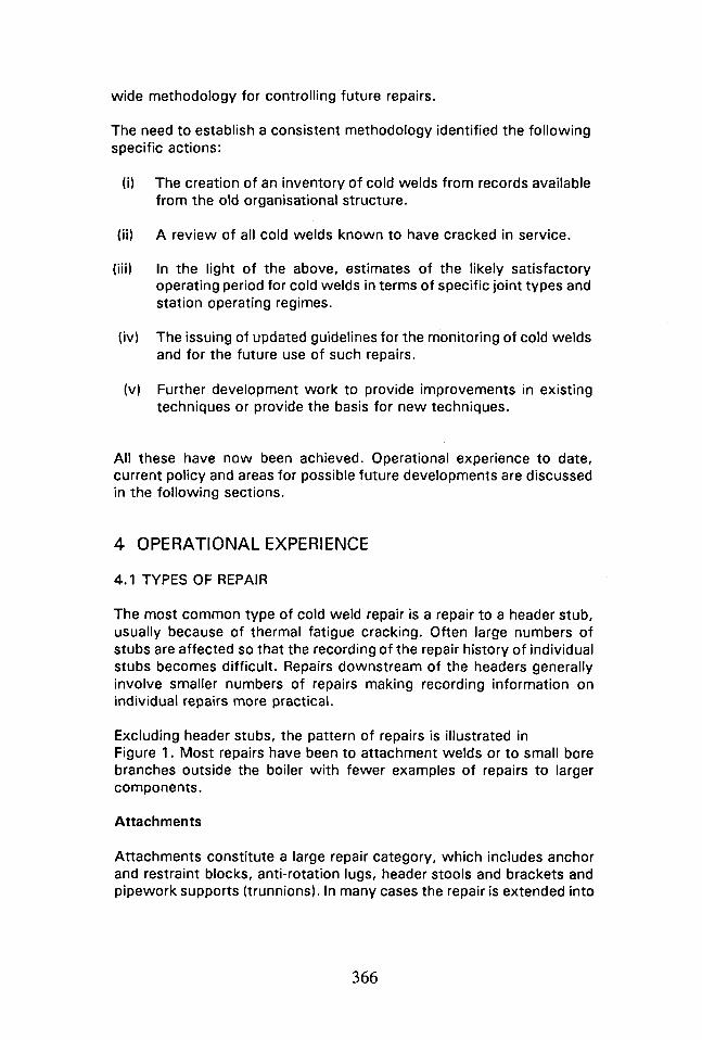
The most common type of cold weld repair is a repair to a header stub, usually because of thermal fatigue cracking. Often large numbers of stubs are affected so that the recording of the repair history of individual stubs becomes difficult. Repairs downstream of the headers generally involve smaller numbers of repairs making recording information on individual repairs more practical.

Excluding header stubs, the pattern of repairs is illustrated in Figure 1. Most repairs have been to attachment welds or to small bore branches outside the boiler with fewer examples of repairs to larger components.

Attachments

Attachments constitute a large repair category, which includes anchor and restraint blocks, anti-rotation lugs, header stools and brackets and pipework supports (trunnions). In many cases the repair is extended into

366

a "raft" on the main component side of the weld to separate a fillet weld toe from the weld fusion boundary. The largest, eg trunnions may constitute major repair operations and a local repair may be more appropriate than a full repair. An example of a steam pipe trunnion is shown in Figure 2.

A distinction can be made between lagged and unlagged welds. Fully lagged attachments are less likely to suffer from thermal fatigue cracking and more likely to be repaired for creep cracks or original manufacturing defects. Unlagged attachments are more likely to suffer from thermal fatigue and a cold weld may be vulnerable to recracking by this mechanism. Where possible the risk can be reduced by fully lagging the attachment but, where this is done, the effect of overheating the assembly in service must be considered.

Small Bore Branches

Common types of repair on chests, headers and pipework are to small bore branches. Besides header stubs, large numbers of repairs have been carried out to drains, vents, thermocouple pockets, etc. Cracking may be caused by thermal fatigue, creep, or incorrect material. If the branch is small it is usual to carry out a complete rather than a local weld repair. Local repairs might be more appropriate for larger branches. As in the case of attachment welds a raft construction is often employed. An example showing a raft (in this case a test piece) is shown in Figure 3.

Repairs to Component Bodies

A number of repairs have been carried out to component bodies, ie away from integral welds or joining welds, involving significant excavations of parent material. Most defects occurring in low stress locations in castings are original casting defects. Usually these can be justified by structural assessment and left in service but some defects have required repair. Repairs up to, and including, full through-wall repairs have been carried out to headers, steam chests and other castings or forgings under appropriate conditions. Such large repairs are monitored closely in subsequent service. An example of a major through-wall repair to a steam chest roof is illustrated in Figure 4.

Build-up Repairs

These are classified as repairs carried out on the surfaces of components which do not require significant excavation into the component body. A typical example would be a build-up to restore a damaged surface profile such as a keyway.

367

Large Butt Welds

The majority of large butt welds are found on steam lines but some are also found on headers or as integral welds on steam chests. Examples of the latter are shown in Figure 5. A number of repairs have been carried out, usually because of creep cracking. In the case of steam chest welds these have tended to be small local repairs but, for steam line welds the repairs have been extended to full weld replacements. The cold weld repair of a steam pipe weld is a major undertaking and requires a full understanding of the nature of the cracking. A small number of such repairs have been carried out after plant breakdowns and operated satisfactorily to a planned outage at which time they were replaced with conventional repairs.

4.2 EXPERIENCE

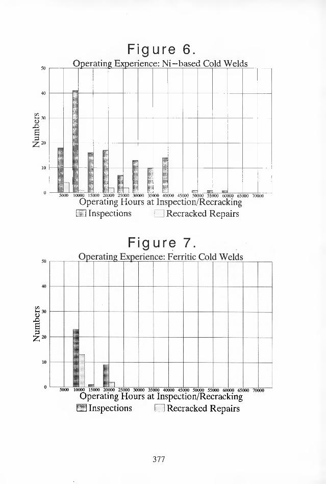
The majority of cold welds to date have been made with high nickel weld metals of the E-NiCrFe-3 or E-NiCrFe-2 type (eg Inconel 182 or Incoweld A respectively). Figure 6 shows the recracking history for 139 repairs for which detailed subsequent inspection history is available. Broadly, service experience has confirmed a modest probability of recracking out to about 25 000 hrs (a recracking rate of ~5% can be inferred). Recracking has generally been attributed to thermal fatigue. There have been no confirmed examples of reheat cracking. Beyond this period there are no examples of recracking although the number of welds inspected at these longer operating times is currently more limited.

In contrast Figure 7 shows equivalent data for a smaller number of ferritic cold weld repairs. The recracking rate is much higher at approximately 50% but it should be emphasised that these repairs were mainly local repairs carried out without controlled deposition rates. The recracking was generally found to be reheat cracking and a higher success rate would be expected for repairs employing two layer refinement techniques.

The experience reinforces a bias towards nickel-based cold welding, particulary where temporary repairs are envisaged. If left in place indefinitely nickel-based welds can be expected to fail eventually either by Type IV cracking or by more typical transition joint failure modes eg low ductility interfacial fracture. Such welds are, essentially, transition joints of various geometries installed in unconventional plant locations. Based on operational experience of boiler transition joints incorporating high nickel fillers, however, failures of this type are sufficiently long term that in most repair situations they would not be expected to occur within the operating period required of the weld repair.

368

5 CURRENT POLICY

The underlying philosophy with respect to cold weld repair can be summarised in the following questions which are asked when contemplating such a repair:

a. ) Is repair necessary at all?

Justifying a defect for further service by structural assessment may be a more efficient solution to the problem. Clearly however, where unplanned outage time is involved, an assessment will entail its own cost and time penalties and these need to be taken into account.

b. ) What is the defect necessitating repair?

Investigation of the original defect should provide the best indication of the likely loading a repair will experience in service and the suitability of a cold weld repair.

c. ) Can the cause of the problem be removed or reduced?

Where adverse loading leading to cracking in service can be corrected, it may be possible either to justify not repairing at all or to give the resulting repair the best chance of survival.

d. ) How long must the repair survive?

In many cases temporary repairs are carried out following plant breakdowns with the possibility of carrying out permanent repairs at the next planned outage. The viability of a cold weld repair in a given situation will vary with the length of subsequent service required from it.

e. ) What would be the consequence of failure?

The effects of possible failure must be considered in the light of the position and geometry of the repair. Care must be taken to ensure for example that a recracked cold weld would not constitute a greater risk than the original defect.

Past policy has been to either replace cold welds eventually with conventional heat treated repairs or to inspect them at every subsequent major outage. For many repairs this is unduly conservative. The existence of a database of repairs now allows experience over all National Power stations to be aggregated and for some families of

369

repairs to be left in place indefinitely, subject to satisfactory overall experience established by sample inspections.

Where cold welds are found to recrack the best strategy for replacement will depend critically on the reasons for recracking. In some cases, eg where a relatively long period of operation has elapsed since the initial repair and the costs of conventional repair are high, a further cold weld may be justifiable.

6 FUTURE IMPROVEMENTS TO COLD WELDING

While the cold welds carried out to date have achieved significant cost savings there is continuing interest in further developments and in extending applications. Possible areas of future interest are discussed below.

6.1 ALTERNATIVE WELDING PROCESSES

In general manual metal arc welding is likely to remain the most practical process for the various repair situations which arise. Alternative processes may have a role however in certain applications. One possible example could be the use of flux-cored welding of larger repairs to reduce welding time.

6.2 ALTERNATIVE WELD METALS

The E-NiCrFe-3/2 types of consumable currently used have much higher creep strength than they need to have for cold welding applications. A weaker alternative such as the Soviet TsT-36 electrode could provide benefits in terms of minimising the mismatch of properties at the weld/parent interface and also of more rapid stress relaxation in service.

National Power retains an interest in extending the application of ferritic cold welds. The advantages and disadvantages of ferritic and nickel- based repairs can be summarised as follows:

370

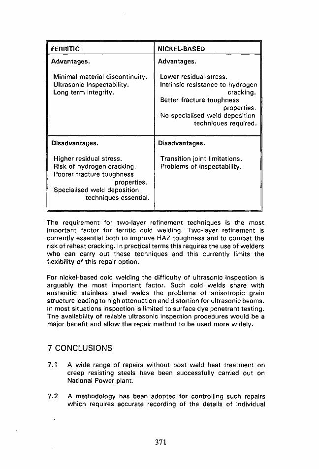
FERRITIC NICKEL-BASED

Advantages. Advantages.

Minimal material discontinuity. Ultrasonic inspectability.Long term integrity.

Lower residual stress.Intrinsic resistance to hydrogen

cracking.Better fracture toughness

properties. No specialised weld deposition

techniques required.

Disadvantages. Disadvantages.

Higher residual stress.Risk of hydrogen cracking. Poorer fracture toughness

properties.Specialised weld deposition

techniques essential.

Transition joint limitations. Problems of inspectability.

The requirement for two-layer refinement techniques is the most important factor for ferritic cold welding. Two-layer refinement is currently essential both to improve HAZ toughness and to combat the risk of reheat cracking. In practical terms this requires the use of welders who can carry out these techniques and this currently limits the flexibility of this repair option.

For nickel-based cold welding the difficulty of ultrasonic inspection is arguably the most important factor. Such cold welds share with austenitic stainless steel welds the problems of anisotropic grain structure leading to high attenuation and distortion for ultrasonic beams. In most situations inspection is limited to surface dye penetrant testing. The availability of reliable ultrasonic inspection procedures would be a major benefit and allow the repair method to be used more widely.

7 CONCLUSIONS

7.1 A wide range of repairs without post weld heat treatment on creep resisting steels have been successfully carried out on National Power plant.

7.2 A methodology has been adopted for controlling such repairs which requires accurate recording of the details of individual

371

repairs, both in terms of the defects repaired and of their subsequent behaviour in service.

8 ACKNOWLEDGEMENTS

The author would like to acknowledge the help and advice of colleagues within National Power in the preparation of this paper.

9 REFERENCES

1. S J BRETTCold Welding in the UK Electricity Supply Industry.TWI Seminar: Repair Welding without Post Weld Heat Treatment - Problems and Solutions. Institute of Materials, London, 1993.

2. K C MITCHELL"Cold Weld" Repair Applications in the UK.Welding and Repair Technology for Fossil Power Plants, EPRI Conference, Williamsburg, USA, March 1994.

3. V N ZEMZIN et alUsing High-nickel Electrodes for Repair Welding of Defects in Cast Casting Components for Steam Turbines.Series: Advanced Methods of Treating Construction Materials. Leningrad Organisation of the "Znanie" Association, Leningrad, 1974.

4. R Z SHRON et alAn Analysis of the Damage to Cast Turbine Components and the Effectiveness of Repair Welds to Them.Teploenergetika, No.7, 1987, pp 16-19.

5. G G BARINOV and F A KHROMCHENKOThe Special Features of Carrying Out Repair Welds to Through Wall Cracks in Turbine Casings.Energetik, No.5, 1986, pp 16-17.

6. EPRI Document CS-4676-SR Edited by R ViswanathanWorkshop Proceedings: Life Assessment and Repair of Steam Turbine Casings,Palo Alto, California, June 4, 1985 (Proceedings 1986).

372

7. S J BRETTRepair of CrMoV Components Using Inconel 182 Electrodes Without Heat Treatment.Repair and Reclamation (Conference) Paper 26, The Royal Society, London,Metals Society/Welding Institute, 1984.

8. S J BRETTThe Weld Repair of CrMoV Turbine Casings Using High-nickel Electrodes Without Heat Treatment.Materials Development in Turbo-machinery Design. Second Parsons International Turbine Conference. The Institute of Metals, London, and Parsons Press, Trinity College, Dublin, 1989, pp 166-172.

373

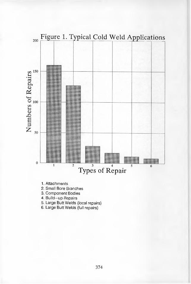
200Figure 1. Typical Cold Weld Applications

Types of Repair

1. Attachments2. Small Bore Branches3. Component Bodies4. Build-up Repairs5. Large Butt Welds (local repairs)6. Large Butt Welds (full repairs)

374

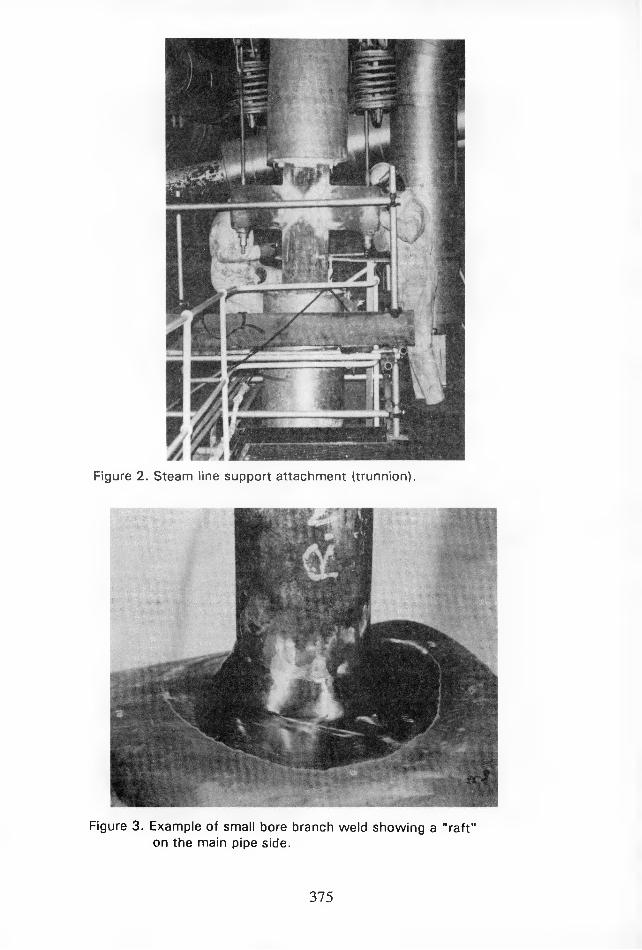
Figure 2. Steam line support attachment (trunnion).

Figure 3. Example of small bore branch weld showing a "raft" on the main pipe side.

375

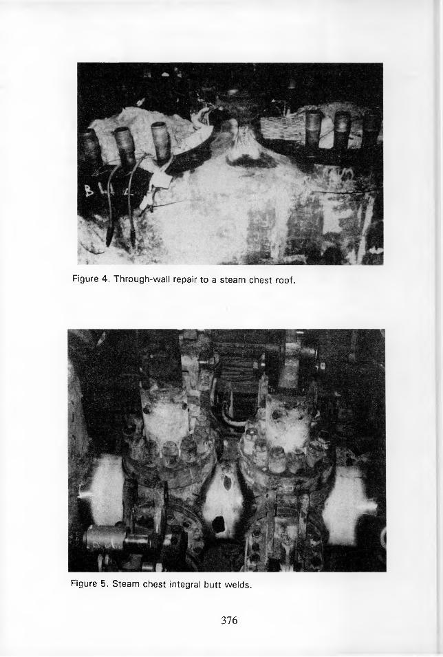
Figure 4. Through-wall repair to a steam chest roof.

Figure 5. Steam chest integral butt welds.

376

Num

bers

N

umbe

rsFigure 6.

cDperating Experience: bii-based Cold Wek s

||

ill I9

pliiiiiii [ilini:pi[ | | J

iii-

ESS?

5000 10000 15000 20000 25000 30000 35000 40000 45000 50000 55000 60000 65000 70000

Operating Hours at Inspection/Recracking I I Inspections □ Recracked Repairs

Operating Experience: Ferritic Cold Welds

5000 10000 15000 20000 25000 30000 35000 40000 45000 50000 55000 60000 65000 70000

Operating Hours at Inspection/RecrackingInspections E3 Recracked Repairs

377

378

MONITORING TECHNOLOGY DEVELOPMENT FOR KOREAN NPP LIFETIME MANAGEMENT

T.E. Jin and HJ. Choi Power Engineering Research Institute Korea Power Engineering Company P.O. Box 631, Young-Dong, Seoul, Korea

I.S. Jeong and S.Y. Hong Nuclear Division, Research Center Korea Electric Power Corporation Moonji-Dong 103-16, Yusung-Ku, Daejon, Korea

ABSTRACT

With the nuclear power plant lifetime management emerging as a big issue in Korea, the on-going feasibility study to cope such a problem is presented together with the current status and the long-term plan as well. Furthermore, from the viewpoint of plant life extension, the necessary technical development of the monitoring system is described in this paper. This system is designed to monitor the various failure mechanisms of irradiation embrittlement, fatigue and erosion/corrosion in a simultaneous manner.

1. INTRODUCTION

During the last 20 years in Korea, more than 10 nuclear power plant (NPP) units were built and have been in service to cope with the problem of supplying

the electric power in parallel with the rapidly growing economy. During that

period, with the national consensus to set the economic welfare as its primary

goal, the public acceptance of nuclear industry was taken for granted. Such a

favorable situation, however, has changed to pose serious concern in terms of economic as well as environmental issues.

To overcome these issues, Korean authorities have been considered the plant lifetime management together with lifetime extension. As part of the long term

nuclear power plant lifetime management program by Korea Electric Power

Corporation (KEPCO), the plant lifetime management (PLIM) project of the

NPPs in Korea was started in 1993. In this respect, a PLIM program conducted

in a timely and proper manner can provide an alternative to the above issues

379

in part, by achieving continued operation, lower production costs, improving

plant reliability objectives and regulatory requirements. Achievements of the

full design life plus the continued operation of the nuclear power plant may be

another extra benefits which can be anticipated. Previous technical investigations performed as part of PLIM programs have already demonstrated

such substantial benefits to the utility and its customers.

Most of the NPPs maintenance procedures in Korea have primarily been

performed so far on the corrective basis, involving equipment modifications and

plant upgrading activities. In order to avoid unscheduled outages and to improve

the plant availability, there arise strong needs for preventive and predictive maintenance strategies. In what follows, the master plan of Korea PLIM project and its related activities of plant life assessment are introduced. Such activities

are then classified into ten main tasks.Focusing on the feasibility establishment of extending the Kori Unit 1 service

life, the technical development for aging evaluations of major critical

components are also studied. Therefore, in this paper, the technical development, to date, concerning the monitoring of various failure mechanisms

of irradiation embrittlement, fatigue and erosion/corrosion is presented, with some graphical illustrations.

2. CURRENT PLIM STATUS AND PLAN

2.1 Current Status

The first nuclear power plant in Korea, Kori Unit 1, which started its

commercial operation in 1978, is scheduled to be shutdown in 2008 according

to its 30-year design life. In Korea, operating license is based on the design life

of the nuclear power plant. The Kori Unit 1 was thus selected as the lead plant in the overall Korean PLIM project.

Upon taking the time required for planning and constructing new alternative

plants into account, the feasibility study to provide the rationale for its original design life and to support the continued operation as long as technically

achievable beyond the design limit is now under way. In the end, the successful/ completion of the integrated Korea PLIM master plan is anticipated to pave the

way for the systematic approach to the enhanced short and long term plant maintenance strategy for other NPPs in Korea.

380

As the sole utility in Korea, KEPCO guides the overall project processes and

planning, while Korea Power Engineering Company (KOPEC) conducts the

engineering works and other PLIM-related studies including the key technology

research activities. Additional nationwide organizations and/or institutes will

join the PLIM project as the program progresses.

2.2 PLIM Long Term Program

The master plan for PLIM including the lifetime extension of Kori Unit 1 and

other NPPs in Korea will be performed in three phases. Such categorization

genetically stems from the level of details and refinement that are to be

accomplished during each phase of the project. Specifically, the feasibility study

is the goal in the phase I and the detailed evaluation and engineering for plant life extension will constitute the workscope for the phase II. For the next phase

HI in this project, the implementation of the lifetime management program will be made, based on the results obtained in the preceding phases I and II. The

major workscope to be addressed during each phase are tabulated in Table 1.

Table I - Major Workscope for Each Phase of PLIM Project

Phase Duration ActivitiesI (Feasibility) 3 years Amendment of design life

Feasibility study- Technical- Economic- Regulatory

PLIM technology developmentII (Detail Engineering) 3 years Detailed assessment of

- Major components- Grouped components

Regulatory requirement Implementation plan

m (Implementation) 6-7 years Kori unit-1 implementation

2.3 PLIM PHASE I STUDY

The major workscope of this phase I involves overall PLIM planning and

establishment of feasibility for the life extension of Kori Unit 1. With the Kori Unit 1 being the the lead plant, the detailed workscope then consists of the

following 10 tasks.

381

Task 1 : PLIM project general plan and design life review

Task 2 : Screening major SSCs

Task 3 : Data survey and review to identify missing and deficient dataTask 4 : Evaluation of a reactor pressure vessel

Task 5 : Evaluation of major SSCsTask 6 '• Monitoring systems for the PLIMTask 7 : Survey and review of PLIM regulationTask 8 : Economic evaluation

Task 9 : PLIM technology development for plant life extension

Task 10 : Feasibility study reports

Technical, economic, and licensing issues for the feasibility study are also

reviewed. The consumed and remaining life for major components and systems

will be evaluated on the technical basis, together with any necessary

recommendations. Further to be studied are economic feasibility, license

renewal feasibility, recommended monitoring technologies, and other PLIM- related technologies and SSCs screening procedures. In addition, the updated

version of Phase II draft planning for the Kori Unit 1 will be proposed.

3. TECHNICAL DEVELOPMENT

In this section, a prototype software package of the KOrea Synthetic

MOnitoring System (KOSMOS) to monitor the critical components of NPPs

against the degradation mechanisms of irradiation embrittlement, thermal

fatigue and erosion/corrosion is introduced.

3.1 Radiation Embrittlement Monitoring System

The neutron irradiation embrittlement, especially in the core-belt region of

the reactor pressure vessel, increases the probability of brittle fracture.The current regulation, 10CFR50, Appendix G [1] prescribes a minimum

acceptable upper-shelf energy, i.e, 50 ft-lbs of Charpy energy, to be maintained

for the vessel material. The irradiation effects result in reduction of upper-shelf

energy, hence lowering the fracture toughness of the material at operating temperatures.

382

Under the plant heat-ups and cool-downs, the quarter and three quarters

thicknesses from the vessel inside wall are the locations of primary concern.

The irradiation effects as defined by RTndt are then to be taken into account

for the development of allowable pressure-temperature limits in accordance

with the ASME Code [2], which is manifested by 10CFR50, Appendix G.The KOSMOS incorporates the daily updated effective-full-power-year

(EFPY), the pressure-temperature limit curves, and other actual operating condition to generate the dynamic pressure-temperature curves. This is made

possible by readily evaluating the temperature and thermal stress distributions

using the real time conditions obtained through the on-line monitoring. Upon

comparing these results with the pressure-temperature limit curves, the

damage due to neutron irradiation embrittlement can be assessed, in accordance

with the requirements in U.S. NRC Regulatory Guide 1.99 [3] and following

ASME Code formula, Sec. HI Appendix G [2].

KIC =26.78+1.233 Exp [0.0145( T—RTNDT+160) ] (1)

Where T means the temperature and RTndt means the nil ductility

temperature.

Based on the aforementioned discipline, the radiation Embrittlement Monitoring System (EMS) as part of KOSMOS performs the on-line

monitoring of the allowable pressure and temperature of the reactor pressure

vessel. Specifically, upon reading the pressure and temperature from the

instrument panel, the temperature and stress distributions[4] inside the vessel are calculated via the Green's function technique, which are in turn utilized to

determine the stress intensity factors for a prescribed crack configuration. By

applying Regulatory Guide 1.99 to neutron radiation levels and the surveillance

data, the RTndt and the reference stress intensity factors Km are evaluated to

be compared with those provided in ASME Section XI Appendix G and

10CFR50 Appendix G. In this way, the safety and integrity of reactor pressure vessels can be assessed.

As an efficient tool in using the EMS with convenience and ease, the commercial software package EASE+ [5,6] is utilized. As a result, the input status, the pressure-temperature curve, and the corresponding allowances are

displayed on a screen, indicating whether the current temperature and pressure

stays within the technical operation specifications or not. The final screen

383

PRES

SURE

. KSI

display of the EMS is given in Fig.l.

m1 —

COOLOOKN f*-7 Llhff'tS CUSV£

■ 1 7/' /y

* s ■’EL. Oil VEF

L' D

JI-TE.INM>

ffIC

iATitIFYs

H 103 2BB 300 -<00 300 330TEWERftTURE, F

SAFEderation Mithin Technical Spec. RPU Safe fron Bril fie Fracture.Rate within safety Units

Figure 1 - Screen Display of the Embrittlement Monitoring System

3.2 Fatigue Monitoring System

As an important potential failure mechanism for the critical components in the NPPs, the fatigue damage accumulation during plant operation should be estimated. The code procedures defined in ASME Sec. IE, NB-3222.4 stipulate that the following cumulative usage factors (CUE) be evaluated in the design process, based on the conservative set of design transients and frequency of occurrences. [2]

CUF = 2 ”,t'lN, (2)

These factors are calculated by combining the effects of individual design transients to stress cycles for the entire service life, as documented in the Design Stress Report (DSR). A list of design transients which are used in typical fatigue evaluations is shown in Table II.

Furthermore, the technical specifications require the counting of the plant operating cycles for the fatigue usage factor [1] to remain below unity throughout the given plant lifetime. It is not an easy task for plant operators,

384

Table II - Design Transient and Life Occurrences

Loading Transients Life OccurrencesPlant heatup, lOOF/hr 200Plant cooldown, lOOF/hr 200Plant loading, 5%/min 18,300Plant unloading, 5%/min 18,30010% step load increase 2,00010% step load decrease 2,000Steady state fluctuation InfiniteReactor trip 400Hydrostatic test, 3125psia 5Loss of reactor coolant flow (*) 80Loss of turbine generator load (*) 80Loss of power (*) 40

* : Abnormal Transient Condition

however, to determine whether the actual transient history during plant operation conform to the design assumptions. The development of the Fatigue

Monitoring System (FMS), which constitutes the additional part of the

KOSMOS, is required as a precise means of quantifying the fatigue damage.

To convert the monitored plant data in the form of peak stress versus time

history, the transfer function approach is utilized. The peak stresses consist of those due to thermal transients and those due to piping loads. The stresses due

to thermal transients are calculated with the aid of Green's functions obtained

for any desired monitoring locations. On the other hand, the stresses due to

piping loads involving internal pressure and thermal expansion are evaluated

based on the direct multiplication of plant parameters by the transfer matrices.

The transient stresses can also be classified into two parts. The first part

depends on instantaneous transducer readings of stresses due to pressure and

thermal expansion at monitoring locations. The second part arises from the

prior thermal transient history such as the thermal stresses at a nozzle due to

rapid changes of fluid temperature, etc.

By extracting significant maxima and minima (peak and valley stresses) from

the peak stress versus time data, the stress amplitude versus frequency spectra

can be obtained using the rainflow counting method. The coupling of the

information thus obtained with the appropriate material fatigue S-N curve then

leads to the direct calculation of fatigue usage factors for the actual range of

plant operating cycles. In this way, the cumulative fatigue usage is readily

monitored and updated continuously for any selected monitored locations.

385

Similar to the RMS, the current Fatigue Monitoring System (FMS) is performed in a continual manner together with the necessary monitoring data supplied every 30 seconds. The software package EASE+ is also utilized for the sake of easy display of changing monitoring status of the FMS. The final display of the FMS on a screen is shown in Fig.2. As a result, the FMS can

«*KSel8c«BINleu atiXflct Ions H»5£Done HgSSu 11'”T *JaTiie

Figure 2 - Screen Display of the Fatigue Monitoring System

assess the age-related material degradation of various plant components due to thermal fatigue, in accordance with the fatigue analysis procedures described

in ASME Section m. Another main utility benefit obtainable from the fatigue

transient monitoring lies is its capacity to accumulate and analyze data required for the efficient plant operation and maintenance throughout the plant design/operating life. Furthermore, The FMS as part of KOSMOS can give rise to the enhanced plant availability, without the necessity of all-out post-transient fatigue analyses.

3.3 Erosion/Corrosion Monitoring System

In the turbine island of the nuclear power plants the important failure mechanism is erosion/corrosion in carbon steel piping, especially turbine extraction lines etc.. The following Keller [7] equation is used as a basic criteria for the erosion corrosion rates.

386

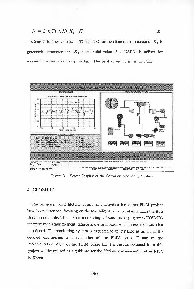
S = C AT) AX) Kc-Ks (3)

where C is flow velocity, f(T) and f(X) are nondimensional constant, Kc is

geometric parameter and Ks is an initial value. Also EASE+ is utilized for

erosion/corrosion monitoring system. The final screen is given in Fig.3.

.MODE. RCTIUE5lot-Oar PLOT - 1«a*HelP mump tew ...................... SiSScTlons MgSorie......ia'Quit''rWaTue

Figure 3 - Screen Display of the Corrosion Monitoring System

4. CLOSURE

The on-going plant lifetime assessment activities for Korea PLIM project have been described, focusing on the feasibility evaluation of extending the Kori Unit 1 service life. The on-line monitoring software package system KOSMOS for irradiation embrittlement, fatigue and erosion/corrosion assessment was also introduced. The monitoring system is expected to be installed as an aid in the detailed engineering and evaluation of the PLIM phase II and in the implementation stage of the PLIM phase III. The results obtained from this project will be utilized as a guideline for the lifetime management of other NPPs

in Korea.

387

REFERENCES

1. U.S. Nuclear Regulatory Commission, "Code of Federal Regulation", 10CFR50, 1992.

2. ASME Boiler and Pressure Vessel Code, 1989.3. U.S. Nuclear Regulatory Commission, "Revision 2 to Regulatory Guide 1.99",

May 1988.

4. B.A. Boley and J.H. Weiner, Theory of Thermal Stresses, Krieger

Publishing Company, Inc., Malabar, FLA, 1985.5. Expert-EASE Systems, "EASE+ Reference Manual", Version 3.2, 1991.

6. Expert-EASE Systems, "EASE+ Developer's Guide", Version 3.2, 1991.

7. V.H. Keller, "Erosion Korrosion an Na'dampfturbinen", VGB Kraftwerks- technik, Vol.54, May,1974, pp 292-295.

388

CRACKING AND CORROSION IN BLACK LIQUOR RECOVERY BOILERS

H. Hanninen, Prof.Helsinki University of Technology Laboratory of Engineering Materials FIN-02150 Espoo, Finland

P. Pohjanne, M.Sc.VTT Manufacturing Technology FIN-02044 VTT, Finland

P. Nieminen, M.Sc.Finnish Recovery Boiler Committee c/o Ekono Energy Ltd FIN-00131 Helsinki, Finland

Abstract

In the compound tubes of black liquor recovery boilers cracking and corrosion attack has been observed both in Finland and in Sweden, especially, in the floor tube surfaces. Cracks typically initiate in the stainless steel cladding and penetrate through the cladding to the stainless steel/low alloy steel interface, where the cracks normally grow along the interface and do not penetrate into the low alloy steel. This kind of corrosion problems exist in addition to floor tubes also at air ports and smelt spout openings. The cracking mechanism is suggested to be either stress corrosion cracking or thermal fatigue. A special case of cracking has been the compound tube weldments in the waterwall where cracking is starting from the waterside. The environmental, mechanical and metallurgical effects on these cracking phenomena are evaluated. Attention is also paid to the possible methods for mitigation of the recovery boiler failures.

389

INTRODUCTION

Cracking and corrosion problems in Black Liquor Recovery Boilers

(BLRB) are the most frequent causes for pressure boundary maintenance,

inspection and replacement. Cracking and corrosion can occur during boiler

operation in firing black liquor or during shut-down periods in markedly

varying environments. Corrosion mechanisms during operation in

waterwalls, superheater, generating section and economizer differ

depending on flue gas and deposit chemistries as well as gas and metal

temperatures. Typical gas temperatures and compositions of fireside

deposits in recovery boilers are shown in Figure 1.

Carbon steels are the primary construction materials for the pressure

boundary of recovery boilers. Most surface regions in the heat transfer

surfaces (generating bank and economizer) are made of C-steel tubing

having acceptable corrosion resistance. Superheater tubes operating at

temperatures above 400°C are constructed from various grades of

chromium-molybdenum low alloy steels. Use of solid stainless steel tubes is

not acceptable because of their susceptibility to waterside Stress Corrosion

Cracking (SCC). The lower waterwalls are subject to most corrosive

conditions by sulphur-bearing gases in the recovery boilers. Compound

tubing has been widely installed in the lower waterwall section for

protecting the C-steel tubing from corrosion and erosion processes. As an

other method to prevent corrosion and erosion, studding has been employed.

The studs allow a layer of solidified smelt to form on the outside diameter

of the floor tubes. This solidified smelt layer protects the tubes reducing the

corrosion and erosion rates substantially. Frequent re-studding of larger

recovery boilers has made studding uneconomical and nowadays compound

tubing is the most widely selected alternative for lower furnace. As a third

390

method of corrosion protection, thermally sprayed coatings containing

chromium, nickel and/or aluminium can be employed. Compound tubing

has also disadvantages such as cost (three times as much as C-steel tubing

(Thielsch and Cone 1993), fabrication problems in welding and certain

types of new corrosion problems during operation. Several overviews of

common corrosion problems affecting recovery boilers have been recently

presented (Hupa et al. 1988; Singbeil and Gamer 1989; Sharp 1992; Bama

etal. 1993)

This paper emphasises the cracking and corrosion problems mainly in

Finland and in Sweden. The mechanisms are discussed and they are tried to

be related to the environment and temperature conditions both during

operation and shut-down periods. Also addressed is the materials research

carried out by Finnish Recovery Boiler Committee.

PREVAILING CONDITIONS IN FINNISH RECOVERY

BOILERS

There are four main modes of operation in a recovery boiler which are

considered to have an influence on cracking and corrosion at furnace floor:

- start-up

- regular operation

- shut-down

- water-washing.

Finnish Recovery Boiler Committee has conducted a survey of different

practices of the above mentioned modes. The survey took place in 1992 and

was answered by all Finnish kraft pulp mills running recovery boilers. The

391

following is a brief summary of the results obtained from boilers having a

compound tube furnace floor.

The rate of pressure increase on the water side of the furnace tubes

increases from 5-10 bar/h at the beginning of the start-up to 15 - 20 bar/h

when reaching the nominal pressure of the boiler. The rate of temperature

increase changes respectively from 20 to 70°C/h. The furnace floor is

usually not covered with black liquor nor with any other substance. The

start-up burners usually bum heavy fuel oil. The typical number of oil

burners used is between 2 and 6. The burners are normally fired 4 - 10 h

prior to the introduction of black liquor to the furnace and 2 - 5 h along with

the black liquor firing.

The typical analyses of black liquors fired during regular operation are

shown on Table 1. This table contains besides the Finnish liquors some

samples from the USA which are somewhat different due to the different

wood species the pulps originate from. The Finnish recovery boilers have

typically a liquor capacity of 600 - 2 000 tn dry solids per day; the new

boilers are bigger - around 3 000 tn ds/d. The steam production varied

between 90 - 300 tn/h and the drum pressure between 70 - 100 bar. Typical

black liquor dry solids contents are 65 - 72%. Some boilers have

temperature probes in the furnace floor. The measurements during regular

operation show that furnace floor metal temperatures vary between 290 -

305°C.

During the boiler shut-down the liquor spray to the furnace is ceased in 4 -

8 h after the first actions of decreasing the firing. The oil burners are

normally fired 4-8 h prior the black liquor firing is stopped and 2 - 6 h by

themselves without the black liquor firing. After the shut-down the furnace

392

floor is usually covered with the molten char bed, in the middle of which

there is usually a little solidified bed. The Finnish recovery boilers are

typically shut down 3 to 5 times a year. The rate of pressure decrease is

typically 5-15 bar/h and the rate of temperature decrease is 30 - 60°C/h,

respectively.

The remainders of the char bed are typically water washed from the furnace

floor 8 - 12 h after the fires have been lit off. The water washing lasts 6-12

h. The purpose of the water washing is usually to clean up the plugged

superheaters, to clean up the furnace floor in order to inspect it or wash the

entire interior of the boiler. The washing water is typically either feed water

or condensate, and its temperature varies between 80 - 110°C. The drum is

usually depressurized at the time of the water washing. The washing water,

which first reaches the furnace floor comes typically from the superheaters

and from the front-end parts of the generating bank. The solidified

remainders of the char bed are normally removed with high-pressure water.

The floor is dried with oil burners or with hot/cold air from air ports.

50% of the Finnish recovery boilers having compound furnace floor tubes

have experienced cracks in the furnace floor area to some extent. Cracks

typically appear at the crown of the tube, on the sides of the tube and close

to fin welds. 25% of the boilers have experienced pitting/corrosion in the

same areas. Compound fins between the floor tubes have also suffered from

similar phenomena as the floor tubes. Major research efforts have been

carried out to clarify during which of the above presented operation phase

the cracks and corrosion pits are generated and how to mitigate these

phenomena.

393

FIRESIDE CORROSION IN LOWER FURNACE

Corrosion in the fireside surfaces of tubing within the lower furnace is

mainly caused by sulphur bearing compounds such as gaseous hydrogen

sulfide and flowing smelt. During recent years operation of recovery boilers

has markedly changed including increased capacity and increases in liquor

sulphidity and chloride contents as well as higher dry content in firing. The

effects of these changes on corrosion properties are still largely undefined

(Klarin 1993).

In the lower furnace fireside conditions, corrosion of C-steel tubing ranges

up to 0.8 mm/year (Bama et al. 1993). However, the corrosion rate is

strongly dependent on temperature. Corrosion is caused by free hydrogen

sulfide in the combustion gas which reacts with iron and porous

nonprotecting iron sulfide (FeS) layer forms on the iron surface. For a

hydrogen sulfide to oxygen ratio of approx. 1 in the gas, the formation of

FeS occurs at a maximum rate. The form of corrosion is typically uniform

general wastage showing highest penetration at the crown of the tube where

the temperature is highest. To avoid lower furnace corrosion in boilers

operating at higher pressures and temperatures pin studding, thermally

sprayed coatings and compound tubing have been employed.

Thermally sprayed coatings alloyed with chromium, nickel and/or

aluminium have been used in many recovery boilers. The coatings are

typically less than 1 mm thick. Failure of coatings due to thermal, chemical

or mechanical loading has caused spalling of the coatings indicating

improper material selection and/or application technique. In using Ni-rich

coatings sulphidation risks have to be taken into account. Recently, chro-

394

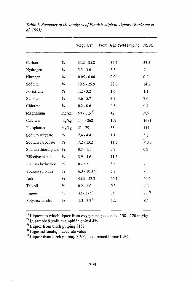
Table 1. Summary of the analyses of Finnish sulphate liquors (Bachman et al. 1995).

"Regulars" From High Yield Pulping NSSC

Carbon % 33.2 - 35.8 34.4 33.5

Hydrogen % 3.3 -3.6 3.3 4

Nitrogen % 0.06 - 0.08 0.06 0.2

Sodium % 19.5-25.9 28.6 14.2

Potassium % 1.2-3.2 1.6 1.1

Sulphur % 4.6-5.7 3.7 7.6

Chlorine % 0.2 - 0.6 0.5 0.4

Magnesium mg/kg 50-115 ^ 42 509

Calcium mg/kg 114-262 102 1671

Phosphorus mg/kg 51-79 53 444

Sodium sulphate % 2.4 - 4.4 1.1 5.8

Sodium carbonate % 7.2-13.2 11.6 <0.5

Sodium thiosulphate % 0.5- 1.1 0.7 0.2

Effective alkali % 3.9-5.6 11.5 -

Sodium hydroxide % 0-2.2 8.5 -

Sodium sulphide % 6.3 -10.3 2) 5.8 -

Ash % 45.5 - 52.3 56.1 40.6

Tall oil % 0.2- 1.0 0.3 4.6

Lignin % 32 - 37 3) 35 27 4)

Polysaccharides % 1.3-2.2 5) 3.2 8.4

^ Liquors to which liquor from oxygen stage is added 150 - 220 mg/kg2) In sample 9 sodium sulphide only 4.4%3) Liquor from birch pulping 31%4) Lignosulfonate, inaccurate value5) Liquor from birch pulping 3.6%, heat treated liquor 1.2%

395

mized tubes have been installed in the USA as an alternative material to

compound tubes. Chromizing process is performed by diffusion of Cr into

the metal surface at elevated temperatures. An Fe-Cr alloy containing up to

40% Cr in the layer of 0.25...0.5 mm thick is produced. Entire panels of

wall can be treated in chromizing furnaces at one time (Moskal 1992).

Potential advantages of the chromized tubes are lower cost compared to

stainless steel compound tubes and potential resistance to thermal fatigue

cracking together with good general corrosion resistance in fireside gases.

However, hydroxide corrosion at air ports may be a local problem.

Compound tubes consist of a stainless steel outer layer (1.5...1.65 mm)

(AISI 304 or AISI 304L) metallurgically bonded to the C-steel (ASTM

A210 Grade Al). In this structure stainless steel prevents corrosion due to

hydrogen sulfide - oxygen gas environment in the furnace, while C-steel

gives the resistance to SCC in high temperature boiler water. C-steel is the

pressure carrying material and provides good heat transfer. Essential for the

heat transfer of the tubes is a good bond between the stainless steel and C-

steel. Delamination can result from contamination of the surfaces prior to

the extrusion of the tubing. Wide bond defects would cause a risk of

overheating and subsequent spalling of the stainless steel layer.

The metallurgical bond between the outer stainless steel layer and the C-

steel causes carbon migration from C-steel into the stainless steel already

during the production (hot extrusion at about 1200°C) of the compound

tubes. Excess service temperature, i.e., at least 500°C widens the

decarburized zone of the C-steel close to the interface; below 500°C there is

practically no carbon migration and, thus, there is about 200°C margin from

normal boiler tube service temperature to overheating.

396

Physical and mechanical properties of compound tube materials differ

markedly at room temperature. In compound tubes, the thermal expansion

of the outer stainless steel layer is restricted by its bonding to the C-steel

substrate. Owing to these differences high tensile stresses arise in the outer

austenite layer and compressive stresses in the C-steel of the compound

tube when cooled from service temperature to room temperature.

Temperature fluctuations during service cause also stresses in the structure.

Typically in thermal fatigue tests the metallurgical bond remains intact and

fatigue properties are determined by the component materials.

Corrosion phenomena have occurred on compound tubes at the air ports in

some BLRB and on the floor tubes in many plants. Corrosion of the air

ports can be avoided by changing design of the air ports or by overlay

welding of the tubes with a high-nickel material. Corrosion and cracking of

the floor tubes is still not resolved.

FLOOR TUBE CRACKING AND CORROSION

Cracking of compound floor tubes has taken place in many recovery boilers

and has been subject of active research in Finland (Pohjanne et al. 1992;

Karjalainen 1992; Klarin 1993) and in Sweden (Ingevald and Kiesling

1992; Eilerson and Leijonberg 1992). During inspections cracking has been

observed over the whole floor surface. According to the failure analyses

cracks have initiated at the surface of the stainless steel cladding. Cracks

penetrate through the cladding to the stainless/low alloy steel interface, but

do not usually penetrate into the low alloy steel. Cracks, after reaching the

interface, usually continue growing along the interface in the cladding,

Figure 2. The fracture surfaces of the examined cracks are very similar to

transgranular SCC fracture surfaces, Figure 2c. Therefore, Pohjanne et al.

397

(1992) have studied the SCC susceptibility of compound tubes in simulated

boiler washing water conditions. Compound tubes were found to be

susceptible to cracking only in washing solution containing high amounts of

chlorides (HCl-addition). Thus, the hypothesis that water washing is

causing SCC of compound tubes was not definitely proved. There can also

be some other situations than water washing, which may cause SCC or

pitting corrosion of compound tubes. Cracking may also occur during other

phases of shut-down periods or during start-up, if the floor is not properly

dried or if it is covered with black liquor. SCC of welded AISI 316L, 317L

and 317LM stainless steels has been observed, when exposed to black

liquor at 366 K (Manning et al. 1984) and of AISI 304L, AISI 316L and

AISI 317L at 423 K (not at 373 K) in hot alkaline solutions containing 5%

NaOH, 2% Na2S, 2% Na2C03, 0.2% Na2S04 and 0.1% NaCl (SCC occurred

in sodium sulfide containing solution also without NaCl) (Honda et al.

1991). All the possible critical operating periods should be carefully studied

in the future for finding the conditions causing tube cracking. The existence

of pitting corrosion in floor tubes in some plants is most probably related to

the same corrosion problem.

Often thermal fatigue during operation has been proposed to be the

mechanism of compound tube cracking in the floor tubes similar to cracking

in smelt spout openings and air ports (Odelstam 1987; Ingevald and

Kiessling 1992). On the floor tubes formation of a thick layer of frozen,

insulating smelt takes place and therefore the furnace floor of the recovery

boiler is not expected to experience significant thermal cycles or corrosion

by sulphur-bearing gases. However, it has also been argued that due to their

lower melting point K-enriched smelts may penetrate through the frozen,

insulating layer close to the floor tubes, where the bed height is low (Klarin

1993). From in situ temperature measurements in Sweden it has been

398

suggested that temperature peaks of up to 100°C in the cladding surface

layer result in partial melting of the salt cake on the tube surface and a

simultaneous formation of a steam bubble inside the tube. The release of the

steam bubble causes a cooling cycle and the process repeats itself, and a

large number of cycles is able to cause thermal fatigue cracking in the

austenitic cladding material, Figure 3. It is expected that the tube surface

reaches a temperature of 450°C while the C-steel tube temperature is around

300°C, which results in plastic cycling of the stainless steel cladding.

Thermal fatigue may not be the only mechanism in most of the cracking

cases, since fracture surfaces do not reveal any striations typical for fatigue,

cracking can be observed after short operation periods and no overheating

has been detected in stainless steel cladding (sensitization) or in the low

alloy steel (decarburization or spheroidization of pearlite). Therefore, it has

been proposed that, the local sulphur containing corrosive media play also

an important role in the floor tube cracking if it is caused by a thermal

fatigue type of mechanism.

In Sweden in some cases cracks in the floor tubes have started from the

waterside and are clearly of thermal fatigue type. In these cases thermal

cycling has resulted from disturbances of the water flow inside the tube

(internal scaling causing poor heat transfer, tube blockage resulting in

insufficient coolant flow or low water level) (Ingevald and Kiessling 1992).

Also overheating of compound tubes has been found, which has resulted in

structural changes (spheroidization of pearlite and increase of decarburized

layer as well as sensitization of the stainless steel layer) in the interface

zone. Failure mechanism of overheated tube is typically tube wastage

followed by creep rupture through growth of creep cracks first initiating in

the carburized zone in the stainless steel cladding and subsequently growing

through the tube wall.

399

CRACKING AND CORROSION IN SMELT SPOUT OPENINGS

AND AIR PORTS

AISI 304L stainless steel cladding can be corroded in small patches around

boiler tube openings (wastage). The cause of this corrosion has been

attributed to molten hydroxide salts condensing when the combustion gas is

contacted by the relatively cool air from around the casing of the tubes.

Sodium hydroxide can exist only near tube openings, where rapid corrosion

of stainless steel is possible (Paul et al. 1993). The reason for this corrosion

attack is that molten NaOH can readily react with Cr203 (the passive layer

on AISI 304L stainless steel) in air and to form nonprotective sodium

chromate, Na2Cr04. This corrosion does not penetrate rapidly into C-steel,

when the stainless steel layer has been corroded through and C-steel is

exposed. However, an approach to avoid this localized corrosion problem is

to use alternate materials (Alloy 825, Alloy 600 or Alloy 625) as a local

weld overlay. High Ni-alloys resist hydroxide corrosion, but with them

sulphidation risks need to be considered.

Cracking has also often been localized to smelt spout openings and air

ports. An example of this cracking can be seen in Figure 4, where a network

of cracks is visible after dye penetrant testing. Thermal fatigue has been the

most plausible mechanism for this kind of cracking of compound tubes.

Cracking sometimes penetrates directly into C-steel, but normally this

cracking behaves also like in the floor tubes where cracks propagate

typically along the interface. Since especially some branched cracks

resemble here also SCC, a question if SCC mechanism is able to operate in

molten salt environments or are the cracks related to water washing of the

boiler can be asked. Compound tubes manufactured from Alloys 625 or 825

400

have been used for smelt spout openings to resist thermal fatigue cracking

with some success.

CRACKING OF COMPOUND TUBE WELDMENTS

Cracking of compound tube welds has taken place in many recovery boilers.

The failure analyses have shown that the reason for cracking has usually

been mixing of the austenitic stainless steel filler metal and the C-steel base

metal of the tube, which has resulted in hard martensite films or in some

cases, especially, when repair welds with high heat input have been

performed in untempered martensite formation through the whole weld

(Hanninen and Simonen 1989). Typical examples of these failures are

shown in Figure 5. Cracks initiate from the waterside of the tube at the root

of the weld and penetrate then in the hard weld metal by a stress corrosion

cracking mechanism. In some cases cracking has also started inside the

weld metal and grown then through the weld resulting in a leakage. When

mechanical properties of these welds were studied by impact and bend tests,

it was observed that the welds are very brittle and they may have been

embrittled during the exposure to recovery boiler conditions. High residual

hydrogen contents in these welds indicate that during operation hydrogen

absorption is taking place into the waterwall materials. In order to avoid this

kind of cracking problems and decrease of mechanical properties of the

compound tube welds, guidelines for welding of the compound tubes have

been recommended in Finland (ETY-Finnish Recovery Boiler Committee

1988). Before welding of the unalloyed component the stainless steel is

removed by machining close to the joint in order to minimize dilution; C-

steel component is welded with an unalloyed filler metal; austenitic

stainless steel component is then welded with an overalloyed austenitic

filler metal, thus, compensating dilution, Figure 6. In this way a brittle

401

martensitic microstucture can be avoided in the butt weld and the welds will

not be embrittled during service nor be susceptible to SCC from the boiler

waterside.

CORROSION AND CRACKING IN UPPER FURNACE

Many incidents in BLRB are related to the superheaters, the generating

bank and the economizers. Main causes of failures are high stresses due to

insufficient thermal expansion possibilities that results in fatigue cracks in

supports and tie bars. Another common reason is vibrations that may be

caused by the sootblowers.

The environment in the upper furnace of the recovery boiler is generally

oxidizing and therefore corrosion by combustion gases is less severe than in

the lower furnace. However, sulphidation, acid corrosion and corrosion due

to moisture during shut-down periods can be observed.

HIGH TEMPERATURE WATER CHEMISTRY IN POWER

PLANTS

To maintain a reliable boiler operation, corrosion from waterside of the

boiler must be prevented. Typical improper chemical cleaning and poor

feed water quality are the reasons for waterside corrosion. Poor feedwater

can cause excessive corrosion of the tubes, deposits on the tube surfaces,

which result in possible hydrogen attack in tube wall or raise in temperature

of the tube wall, which in turn causes accelerated fireside corrosion.

Prevention of boiler water carryover and operation of dearators efficiently

are also critical in preventing waterside corrosion and cracking. Waterside

402

corrosion fatigue cracking is a common failure caused by inadequate water

chemistry and cyclic and residual stressed due to various kinds of

attachment welds. Thus, corrosion fatigue occurs in places where thermal

expansion is restricted or constrained during transient operating conditions.

Damage is often characterised by multiple cracks, which initiate from inside

of the tube; cracks are wide and oxide filled (Paul et al. 1992).

Successful water chemistry control requires regular and continuous

monitoring of such water chemistry parameters as dissolved oxygen

content, pH, conductivity and impurity contents. At present the chemical

monitoring is applied mainly in low pressure, low temperature conditions or

by using grab samples. However, these methods have some shortcomings,

because parameters such as pH, conductivity and redox potential are

changing as a function of the temperature. In addition, local effects can

produce changes from the bulk chemistry in these parameters. Therefore,

electrodes and measurement systems designed for the on-line monitoring of

the water chemistry parameters at high temperatures and pressures can

improve the knowledge of actual operating conditions in power plants. The

advantages of the on-line monitoring are that monitoring can be carried out

simultaneously at several critical parts and that the on-line monitoring is a

sensitive method which makes it possible to keep the water chemistry in the

operating limit. Also the effects of different operating conditions, i.e., boiler

shut-down and start-up, to the water chemistry can be evaluated.

The on-line high temperature high pressure water chemistry monitoring

system developed by VTT Manufacturing Technology and Imatra Power

Company (IVO) has been successfully in operation at several places, i.e., in

the OECD Halden Reactor since March 1987 and in the Loviisa PWR plants

since June 1988. The measurement system has been proven to give reliable

403

and useful information over very long measurement periods. The obtained

results are used to get more information concerning the influence of the

chemical parameters (e.g., pHT, redox potential) on the behaviour of

corrosion reactions during the shut-down and to find a proper shut-down

procedure (Makela et al. 1989, Aaltonen & Makela 1992).

AGEING AND LIFE PREDICTION OF BLRBs

Corrosion and cracking problem of the compound floor tubes is still not

resolved. Shot peening has been tried in several boilers as a remedy for

cracking but without any success. Other alternate methods to avoid cracking

could be thermally sprayed coatings, overlay welding or new more

corrosion resistant tubings.

Thermal spray coatings alloyed with chromium and nickel and/or

aluminium, e.g., 45 CT containing 45% Cr and 50% Ni, have been used in

some boilers. Failure of coatings due to thermal, chemical or mechanical

loading has in some cases caused spalling of the coating indicating

improper material selection and/or application technique. These problems

can be minimized by proper selection of the coating. To ensure adequate

corrosion resistance the coating must have low through thickness porosity

and good adhesion to the base material. To minimize thermal stresses the

composition of the coating must be selected so that the thermal expansion

coefficient is equal or close to the base material. Also the spraying process

itself and the groundwork, e.g., shot peening and cleaning, must be carefully

performed. Overlay welding has been applied in some boilers as a remedy

for floor tube cracking by welding with AISI 309 type filler material.

404

Due to corrosion and cracking problems in 304L/4L7 type tube

manufacturers have developed alternate materials showing improved

corrosion resistance. High nickel alloys like Alloy 825 and Alloy 625

compound tubes have been tested as an alternate tube material for boiler

openings, where rapid corrosion of AISI 304L stainless steel has occurred

(Paul et al. 1992). New Sanicro 38/4L7 stainless steel compound tube

containing 20% Cr, 38% Ni and 2.5% Mo, is proposed as a substitute for

304L/4L7 tubes for BLRB floor tubes and lower furnace. The advantages of

Sanicro 38 compared to AISI 304L are improved corrosion resistance and

higher resistivity against thermal fatigue.

CONCLUDING REMARKS

General understanding of cracking and corrosion mechanisms is crucial in

inspections and maintenance of the BLRBs. Various forms of cracking and

corrosion demand also various types of inspection methods (visual, dye-

penetrant, magnetic particle, ultrasonic, radiography, eddy current,

metallographic replica and hydrostatic tests and even in some cases

Barkhausen noise measurements have been applied). Therefore

development of the inspection techniques for quick and reliable detection of

the cracks is very important. In addition to development of the inspection

testing Finnish Recovery Boiler Committee has undertaken a study of the

behaviour of various surface coatings in the furnace floor conditions and on

the possibilities to mitigate cracking by shot peening. Additionally, a project

on thermal fatigue is ongoing for understanding the recovery boiler thermal

fatigue problems. In Finland high technology power plant water chemistry

monitoring electrodes and systems have been developed which could be

405

easily used in BLRB water chemistry control and monitoring on-line, thus,

saving analysis costs and enabling more reliable continuous monitoring.

REFERENCES

1. Aaltonen, P. and Makela, K. High temperature water chemistry in power

plants. Int. Symposium on Life and Performance of High Temperature

Materials and Structures, Baltica II, Tallinn, Estonia, Oct. 7 - 8, 1992. VTT

and SCEMM. 4 p.

2. Backman, R., Hupa, M., Soderhjelm, L. Black liquor combustion

properties. Helsinki, Finland, Finnish Recovery Boiler Committee Report,

1995.

3. Bama, J., Rogan, R. Mattie and S. Allison, Fire-side corrosion

inspections of black liquor recovery boilers. TAPPI Kraft Recovery

Operations Short Course, January 4-8, 1993, Orlando, FL. 16 p.

4. Eilerson, T. and Leijonberg, A. Recovery boiler furnace floor - smelt side

damages. TAPPI 7th Int. Symposium on Corrosion in the Pulp and Paper

Industry, Orlando, FL, November 16-20, 1992, pp. 259 - 265.

5. ETY-Finnish Recovery Boiler Committee, 1988, Guidelines for

protection of recovery boilers (in Finnish).

6. Honda, M., Tamada, A., Kato, K. and Kobayashi, Y. Stress corrosion

cracking of stainless alloys in alkaline-sulfide solutions. NACE Corrosion

Conference, Paper No. 191, Cincinnatti, 1991.

406

7. Hupa, M. et al. Fireside corrosion in kraft recovery boilers - an overview.

Materials Performance, July, 1988, pp. 41 - 45.

8. Hanninen, H. and Simonen, J. Absorption of hydrogen to compound tube

weldments in a recovery boiler. 6th Int. Symposium on Corrosion in the

Pulp and Paper Industry, Helsinki, August 29 - September 1, 1989, pp. 138 -

150.

9. Ingevald, S. and Kiessling, S. L. Stress and corrosion induced damages in

the lower furnace of recovery boilers. Ref. 4, 1992, pp. 285 - 297.

10. Karjalainen, L. Cracking failures in composite tubes in kraft recovery

boilers. Ref. 4, 1992, pp. 243 - 250.

11. Klarin, A. Floor tube corrosion in recovery boilers. Tappi Journal, vol.

76, no. 12, 1993, pp. 183 - 188.

12. Manning, P., Tuff, W., Zordan, R. and Schuur, P. Evaluation of high

performance alloys used in the pulp and paper industry. Materials

Performance, vol. 23, no. 1, 1984, pp. 19 - 29.

13. Moskal, M. A critical review of tube selection for recovery boilers. Ref.

4, 1992, pp. 217-229.

14. Makela, K., Aaltonen, P. and Paavola, A. Corrosion in nuclear power

plants moderated with water chemistry. Water Chemistry of Nuclear

Reactor Systems, Bournemouth, UK, Oct. 23 - 27, 1989. British Nuclear

Energy Society. 4 p.

407

15. Odelstam, T. BLRB composite tubes - 15 years of experience. Kraft

Recovery Operations Seminar, Orlando, 1987. Pp. 277 - 288.

16. Paul, L., Bama, J., Danielson, M. and Harper, S. Corrosion-resistant

tube materials for extended life of openings in recovery boilers. Tappi

Journal, vol. 76, no. 8, 1993, pp. 73 - 77.

17. Paul, L., Miglin, M. and Van Der Sluys, W. Mechanisms of corrosion

fatigue in power plant boiler tubing. Corrosion 1992, Paper No. 156. 20 p.

18. Pohjanne, P., Hanninen, H., Makipaa, M. and Ehmsten, U. Cracking of

compound tubes in black liquor recovery boilers. Ref. 4, 1992, pp. 319 -

324.

19. Sharp, W. Overview of recovery boiler corrosion. Ref. 4, 1992, pp. 23 -

31.

20. Singbeil, D. and Gamer, A. Tappi Journal, vol. 72, no. 6, 1989, pp. 136-

141; 133-137.

21. Thielsch, H. and Cone, F. Potential failure mechanisms in composite

tubing. TAPPI Engineering Conference, 1993. Pp. 233 - 257.

408

1080 1300F

16201710F

1620 1800F350 460F (Low Odor)500 650F (Direct Conlacl)

Jnbr0'-Gcnerating Section

50% Na2C03 40% Na2S04

5% NaCl 5% Other

lower Furnace

65% Na;CO| 10% Na?S 15% Na2S04 5% NaCl 5% Other

70% NajCOj 20% Na?S

5% NaCl 5% Other

Fig. 1. Typical gas temperatures and compositions of fireside deposits in the recovery boilers (Bama et al. 1993).

409

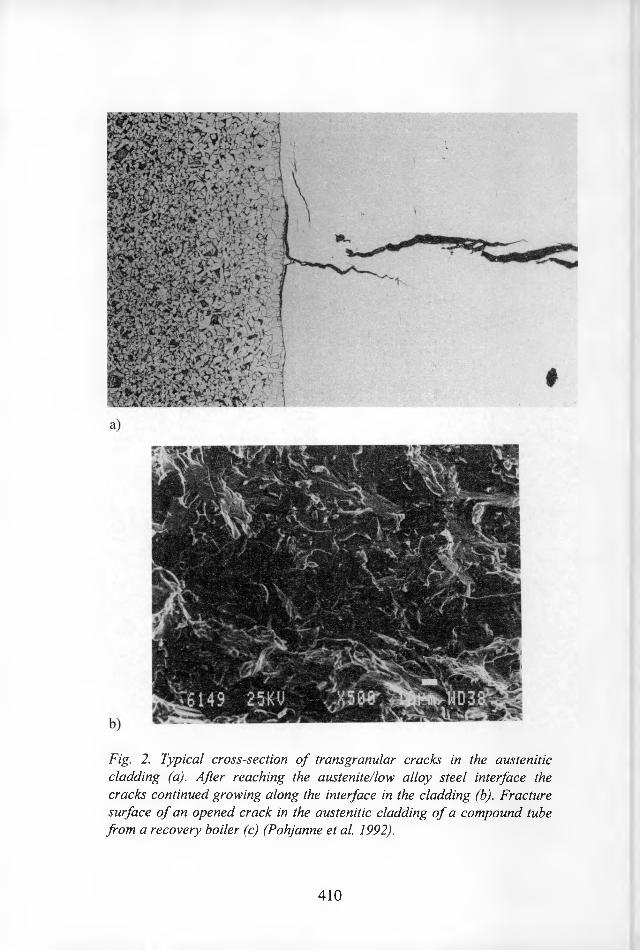
Fig. 2. Typical cross-section of transgranular cracks in the austenitic cladding (a). After reaching the austenite/low alloy steel interface the cracks continued growing along the interface in the cladding (b). Fracture surface of an opened crack in the austenitic cladding of a compound tube from a recovery boiler (c) (Pohjanne et al. 1992).

410

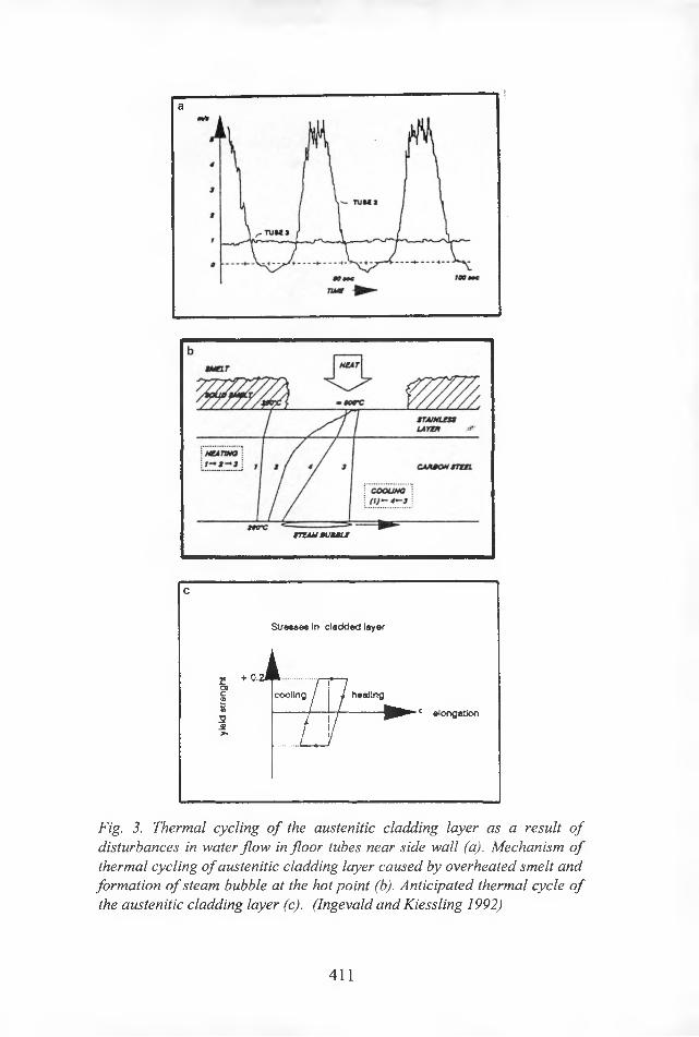
H£AT\

mjjdmjBMU

c

Stresses In cladded layer

2 + o.ai

c?© cooling / 1 healing

£s ---------4---- ‘rj------------ •longatlon

3. t 1 />»

Fig. 3. Thermal cycling of the austenitic cladding layer as a result of disturbances in water flow in floor tubes near side wall (a). Mechanism of thermal cycling of austenitic cladding layer caused by overheated smelt and formation of steam bubble at the hot point (b). Anticipated thermal cycle of the austenitic cladding layer (c). (Ingevald and Kiessling 1992)

411

Fig. 4. Dye penetrant testing of a smelt spout opening showing marked cracking in the lower part of the opening.

412

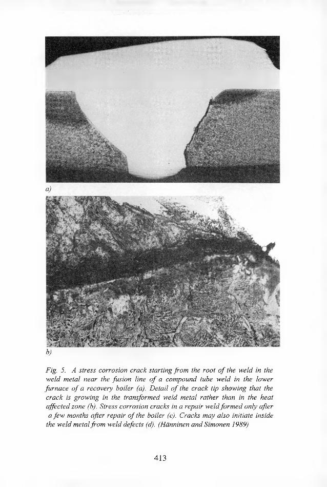
b)

Fig. 5. A stress corrosion crack starting from the root of the weld in the weld metal near the fusion line of a compound tube weld in the lower furnace of a recovery boiler (a). Detail of the crack tip showing that the crack is growing in the transformed weld metal rather than in the heat affected zone (b). Stress corrosion cracks in a repair weld formed only after a few months after repair of the boiler (c). Cracks may also initiate inside

the weld metal from weld defects (d). (Hanninen and Simonen 1989)

413

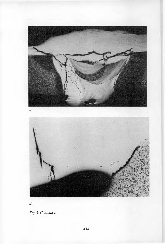
d)

Fig. 5. Continues.

414

2-3

Fig. 6. Recommended form of the weld groove preparation (a) and order of weld passes (b) (ETY-Finnish Recovery Boiler Committee 1988).

Hardcopy device

Fig. 7. Flow through water chemistry cell with electrodes developed at VTT Manufacturing Technology.

415

416

SOME EFFECTS OF THE SOLUTION HEAT TREATMENT TEMPERATURE ON THE PROPERTIES OF GRADE P 91

Kjeld Borggreen FORCE Institute The Metallurgy Department Broendby, Denmark

Abstract

The martensitic 9% Cr-steel Grade P 91 (X 10 CrMoVNb 9 1) has been given different solution heatments. The austenitization temperature has been varied systematically in the temperature range 820 - 1200°C, whereas the tempering has been made at a fixed temperature of 760°C. Hardness, creep rupture strength, and microstructure have been investigated and corre­lated with the austenitization temperature.

It was found that the hardness is only a weak function of the solution treat­ment temperature within the range 860 - 1200°C for the steel in both hard­ened and hardened plus tempered condition. All hardness values of the hardened plus tempered samples were in the acceptable range. The micro­structure is also a weak function of the solution treatment temperature above and below approx. 960°C. At this critical temperature a visible change in microstructure occurs. The creep rupture strength is a strong function of the solution treatment temperature, and for an austenitization temperature of 860 - 900°C the rupture time is reduced by a factor of 20 or more compared to the as-delivered condition.

1 INTRODUCTION

The development of creep resistant steels for use in high pressure steam piping in power plants is at a great pace. Notable is in particular the devel­opment of the martensitic 9 - 12% Cr-steels, among which several new types in surprisingly short time have reached the status of being adopted in the codes and standards or have been installed in new supercritical plants on a permanent or provisional basis [1], ASTM Grade P91 (DIN X 10

417

CrMoVNb 9 1) has marked itself as the future steel for steam pipes and headers. Recently a review of the development of this steel has been pub­lished [2]. The mechanical and metallurgical properties and peculiarities of P91 has been mentioned at several occasions [3-7].

It appears to be a common property for all the martensitic steels that incor­rect hardening procedures may result in materials with unacceptable creep properties - often reaching the level of low alloy steels - without being recognizable in the hardness, tensile properties, or microstructure. This un­acceptable condition of the material may therefore not be noticed in the quality control at the steel work or in the product control at the constructor.

It has already been demonstrated that the well known martensitic 12% Cr- steel DIN X 20 CrMoV 12 1 is disposed to form unacceptable microstruc­tures, if the austenitization temperature has been below the intended range, or the chemical composition has been at the boarder line of the tolerance box [8], Furthermore, at several occasions material with unacceptable properties have been found in power plants although serious accidents have seldom occurred [9], From a metallurgical point of view P91 resembles X 20 CrMoV 12 1, and it is therefore expected to possess the same weak­ness with respect to susceptibility to the hardening procedure. For this rea­son it is of importance to investigate the microstructure and creep strength of P91 after it has been given incorrect solution treatments at varying tem­peratures, however, a correct tempering.

Condition monitoring of build-in components of P91 must in general be made non-destructively and on-site. The methods adopted for the present investigation were therefore chosen among methods for field use only, i.e. replication technique, light microscopy, and hardness testing by use of portable equipment. More advanced laboratory test methods were for the same reasons avoided, although being relevant for the investigations.

418

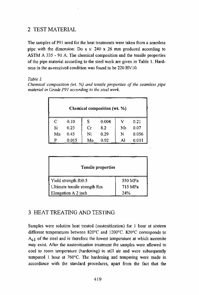
2 TEST MATERIAL

The samples of P91 used for the heat treatments were taken from a seamless pipe with the dimension: Do x s: 240 x 26 mm produced according to ASTM A 335 - 91 A. The chemical composition and the tensile properties of the pipe material according to the steel work are given in Table 1. Hard­ness in the as-received condition was found to be 220 HV10.

Table 1.Chemical composition (wt. %) and tensile properties of the seamless pipe material in Grade P91 according to the steel work.

Chemical composition (wt. %)

c 0.10 S 0.004 V 0.21Si 0.23 Cr 8.2 Nb 0.07Mn 0.45 Ni 0.29 N 0.056P 0.015 Mo 0.92 Al 0.011

Tensile properties

Yield strength Rt0.5 550 MPaUltimate tensile strength Rm 715 MPaElongation A 2 inch 24%

3 HEAT TREATING AND TESTING

Samples were solution heat treated (austenitization) for 1 hour at sixteen different temperatures between 820°C and 1200°C. 820°C corresponds to Aci of the steel and is therefore the lowest temperature at which austenite may exist. After the austenitization treatment the samples were allowed to cool to room temperature (hardening) in still air and were subsequently tempered 1 hour at 760°C. The hardening and tempering were made in accordance with the standard procedures, apart from the fact that the

419

austenitization temperatures were chosen from a much larger range than the allowed 1040 - 1090°C [10]. After the heat treatment the samples were investigated with respect to hardness, microstructure, and for some of them also creep strength.

After the heat treatment hardness and microstructure were determined for both hardened and hardened plus tempered samples. Several different etching procedures were used for the microstructural investigations. Finally, the short term creep rupture strength was found for selected samples, and isostress extrapolations were made to typical service temperatures.

4 HARDNESS

The hardness of both hardened and hardened plus tempered material is hardly a function of the austenitization temperature if this has not been too low. Above 860°C the hardness is 410 - 450 HV10 for hardened material and 210 - 240 HV10 for hardened plus tempered material. The acceptable hardness range of P91 is 200 - 250 HV. The lower limit can be deduced from the acceptable range for the tensile properties, and the upper limit is given in the standards [10, 11]. The hardness as function of the solution treatment temperature for both P91 and X 20 CrMoV 12 1 is shown in Figure 1.

From a practical point of view the results raise a number of questions. First of all, it is not possible from hardness data to judge whether the austenitiza­tion temperature has been within the correct range or not. This is inde­pendent of whether the hardness is measured before or after the tempering. Secondly, all hardness values are for the chosen tempering temperature (760°C) within the acceptable range independent of the austenitization tem­perature. If a lower tempering temperature had been chosen, even lower austenitization temperatures might have resulted in correct hardness of the final product. It may therefore be concluded that the hardness of P91 entirely reflects the tempering procedure. It cannot from hardness values be judged whether the hardening has been correctly accomplished.

420

Hardness, HV10

o P91□ X 20 CrMoV 12 1~

Hardened

Hardened and tempered

Austenitization temperature, °CFigure 1.The Vickers-hardness of hardened and hardened plus tempered P91 and X20 CrMoV 12 1 shown as function of the austenitization temperature. P91 and X 20 CrMoV 12 1 have been tempered at 760X1 and 770X2, respectively.

From a metallurgical point of view it is interesting that the hardness of P91 remains at the same level down to a solution treatment temperature as low as 860°C, below which it suddenly drops. This is different from X 20 CrMoV 12 1 in hardened condition, for which the hardness already drops for solution treatment temperatures below 950°C. In Figure 2 is shown the solubility of carbon in austenite in X 20 CrMoV 12 1 [3], For this steel all carbon is in solid solution at temperatures above approx. 1000°C, whereas for P91 all carbon is in solution already above approx. 850°C provided a fully austenitic microstructure. This, however, is only the case for P91 at temperatures above Ac3 ~ 900°C. It therefore seems plausible that the observed differences between the two types of steel in the behaviour of the hardness on the austenitization temperature are related to the differences in carbon content. The less carbon in the steel, the less dependent is the hard­ness on the solution treatment procedure. All newcoming martensitic steels in general have low carbon content, and quality assessment by use of hard­ness measurement may for these steels as well as P91 be excluded.

421

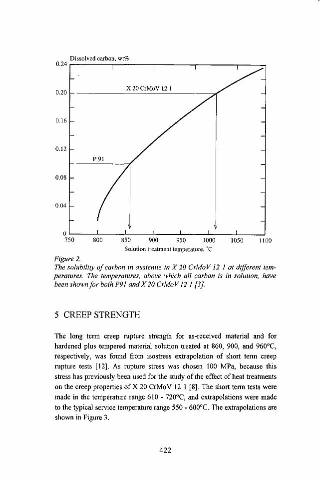
Dissolved carbon, wt%

X 20 CrMoV 12 1

Solution treatment temperature, °CFigure 2.The solubility of carbon in austenite in X 20 CrMoV 12 1 at different tem­peratures. The temperatures, above which all carbon is in solution, have been shown for both P91 and X 20 CrMoV 12 1 [3].

5 CREEP STRENGTH

The long term creep rupture strength for as-received material and for hardened plus tempered material solution treated at 860, 900, and 960°C, respectively, was found from isostress extrapolation of short term creep rupture tests [12], As rupture stress was chosen 100 MPa, because this stress has previously been used for the study of the effect of heat treatments on the creep properties of X 20 CrMoV 12 1 [8], The short term tests were made in the temperature range 610 - 720°C, and extrapolations were made to the typical service temperature range 550 - 600°C. The extrapolations are shown in Figure 3.

422

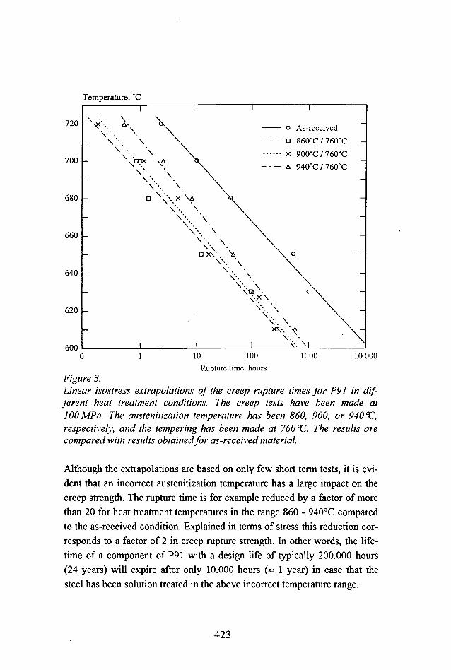
Temperature, "C

o As-received

------□ 860°C / 760°Cx 900°C / 760°C

— A 940°C / 760°C

640 -

620 -

10.000Rupture time, hours

Figure 3.Linear isostress extrapolations of the creep rupture times for P91 in dif­ferent heat treatment conditions. The creep tests have been made at 100 MPa. The austenitization temperature has been 860, 900, or 940 °C, respectively, and the tempering has been made al 760 °C. The results are compared with results obtainedfor as-received material.

Although the extrapolations are based on only few short term tests, it is evi­dent that an incorrect austenitization temperature has a large impact on the creep strength. The rupture time is for example reduced by a factor of more than 20 for heat treatment temperatures in the range 860 - 940°C compared to the as-received condition. Explained in terms of stress this reduction cor­responds to a factor of 2 in creep rupture strength. In other words, the life­time of a component of P91 with a design life of typically 200.000 hours (24 years) will expire after only 10.000 hours (» 1 year) in case that the steel has been solution treated in the above incorrect temperature range.

423

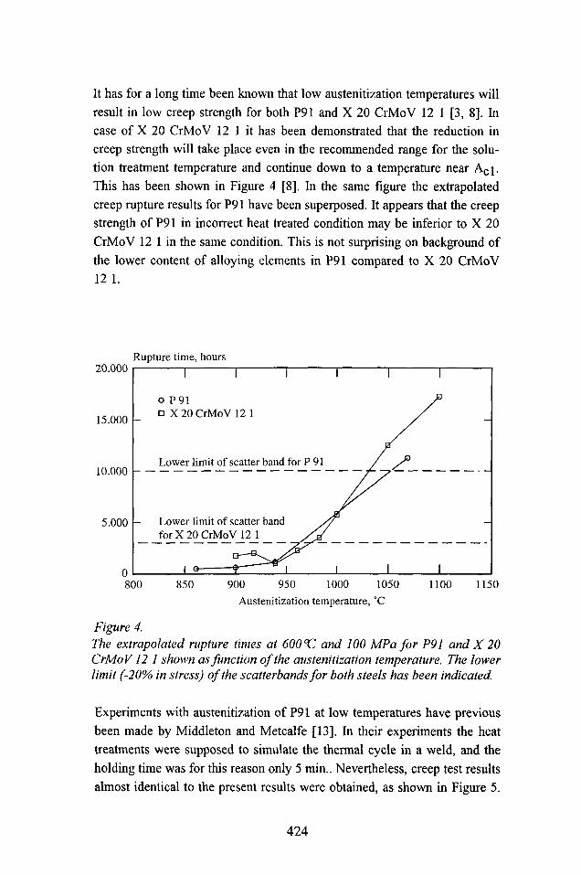
It has for a long time been known that low austenitization temperatures will result in low creep strength for both P91 and X 20 CrMoV 12 1 [3, 8]. In case of X 20 CrMoV 12 1 it has been demonstrated that the reduction in creep strength will take place even in the recommended range for the solu­tion treatment temperature and continue down to a temperature near Aci. This has been shown in Figure 4 [8], In the same figure the extrapolated creep rupture results for P91 have been superposed. It appears that the creep strength of P91 in incorrect heat heated condition may be inferior to X 20 CrMoV 12 1 in the same condition. This is not surprising on background of the lower content of alloying elements in P91 compared to X 20 CrMoV 12 1.

Rupture time, hours20.000

o P91□ X 20 CrMoV 12 115.000

Lower limit of scatter band for P 9110.000

Lower limit of scatter band for X 20 CrMoV 12 1

5.000 -

>0 950 1000 10Austenitization temperature, °C

Figure 4.The extrapolated rupture times at 600 “C and 100 MPa for P91 and X 20 CrMoV 12 1 shown as function of the austenitization temperature. The lower limit (-20% in stress) of the scatterbands for both steels has been indicated.

Experiments with austenitization of P91 at low temperatures have previous been made by Middleton and Metcalfe [13], In their experiments the heat treatments were supposed to simulate the thermal cycle in a weld, and the holding time was for this reason only 5 min.. Nevertheless, creep test results almost identical to the present results were obtained, as shown in Figure 5.

424

Cerjak and Schuster have investigated the effect of more realistic weld thermal cycles on the creep strength of P91 and the martensitic cast steel DIN G-X 12 CrMoWVNbN 10 1 [14], For both steels a minimum in the creep strength was found for a thermal cycle peak temperature around 875°C.

Rupture time, hours16.000

o 570°C, 95 MPa□ eOO’C, 95 MPa

12.000

8.000 -

4.000 -

Austenitization temperature, °C

Figure 5.Measured creep rupture times at 570°C and 600X7 and 95 MPa for P91 shown as function of the austenitization temperature. The holding time was only 5 min. to simulate a weld temperature cycle. Tempering was made at 730X7 [13].

It may therefore be concluded that P91, X 20 CrMoV 12 1, and probably a number of other martensitic 9 - 12% Cr-steels are susceptible to solution treatments in the temperature range 850 - 950°C. Hardening from this tem­perature range will result in microstructures with absolute inferior creep properties far below the lower limit of the scatter band and almost at the level of the creep strength of the low alloy ferritic steel DIN 10 CrMo 9 10.

425

6 MICROSTRUCTURE

Preliminary tests with different etching agents showed surprisingly little dif­ferences. It was therefore found most suitable in case of P91 to maintain the etching procedures found useful for X 20 CrMoV 12 1. For this steel elec­trolytic etching with oxalic acid solution is most commonly used in the field with chemical etching with picrinic acid solution as an alternative [9], In case of P91 the difference between the results of the two etching methods was smaller than for X 20 CrMoV 12 1.

As a part of the microstructural investigation the grain size of the prior austenite was counted. The ASTM grain size number as function of the austenitization temperature above 940°C is shown in Figure 6. Heat treat­ments below this temperature resulted in grain structures which were diffi­cult to distinguish. The formation of niobium carbonitrides prevents grain growth in P91 resulting in a relative fine grain size even at high heat treat­ment temperatures. For X 20 CrMoV 12 1 in correctly heat treated condi­tion the grains are often millimetre large, because this steel does not contain niobium. The content of the figure seems to indicate that the austenitization temperature for P91 with advantage can be chosen in the high end of the allowed range or even beyond in order to increase creep strength without deteriorating the impact properties of the steel. It may be concluded that grain size counting for P91 to some extend can be used for assessment of the austenitization temperature in the high temperature range.

The fine structure of the microstructure of P91 is difficult to ascertain by means of optical microscopy. The reason for this is that the microstructure is dense and low in contrast. Experience from the present project shows that even trained personal will have difficulties in distinguishing between the microstructures of the steel in its different heat treated conditions.

The microstructure of the steel in its as-received condition is shown in Figure 7. Hardening and tempering on basis of a solution treatment tem­perature as low as 980°C still results in a microstructure almost identical to the as-received microstructure. The solution treatment temperature must be below 940°C before the microstructure in the hardened and tempered con­dition becomes different from in the as-received condition. In any case, the difference between microstructures obtained for austenitization tempera-

426

tures above and below 940 - 980°C is indistinct, which may be seen by comparing Figure 7 with Figures 8 and 9.

ASTM - grain size number

Austenitization temperature, °C

Figure 6.Austenite grain size of P91 shown as function of the austenitization tem­perature. The individual grains could not be distinguished for material heat treated at temperatures below approx. 950 TT.

The very modest change in the microstructure as function of the austeniti­zation temperature makes it difficult to determine the heat treatment proce­dure of P91 on basis of microstructural investigations of for instance repli­cas taken on-site of the component. With some experience it may be pos­sible to distinguish between tempered microstructures formed by hardening from above or below the critical temperature range 940 - 980°C. There are evidence that this critical temperature range also divide the steel in two classes; one with acceptable creep properties and one with strongly inferior creep properties. Further tests are required to support this theory.

427

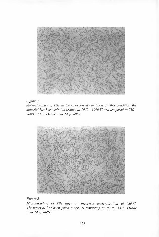
Figure 7.Microstructure of P91 in the as-received condition. In this condition the material has been solution treated at 1040 - 1090°C and tempered at 730 - 760 CC. Etch: Oxalic acid. Mag. 800x.

Figure 8.Microstructure of P91 after an incorrect austenitization at 980‘O. The material has been given a correct tempering at 760 °C. Etch: Oxalic acid. Mag. 800x.

428

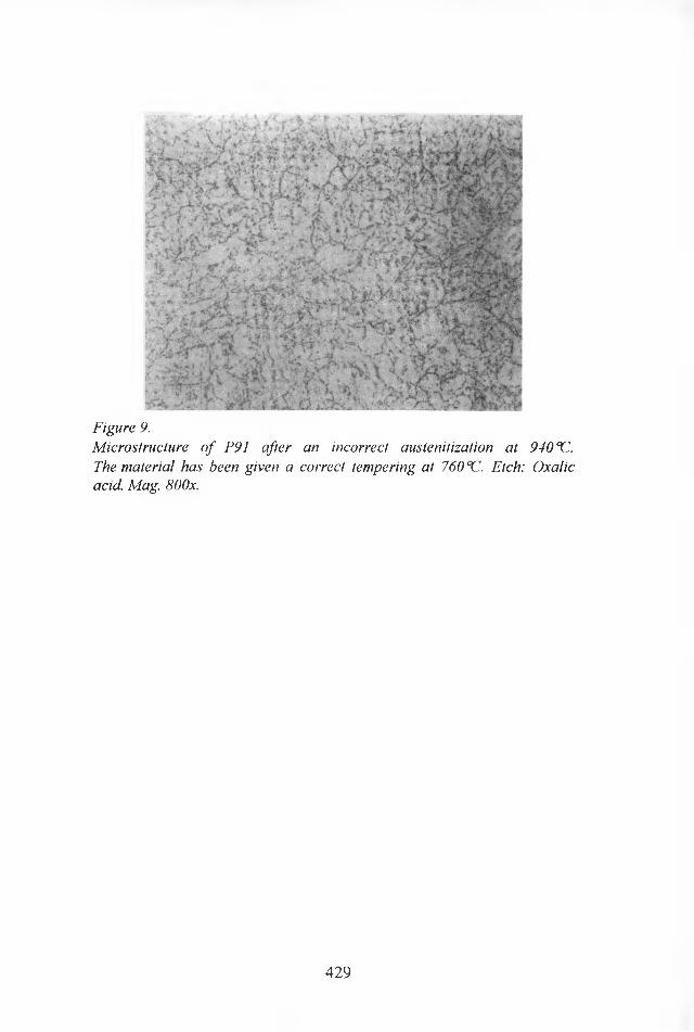
I -'A

■rJs v

Figure 9.Microstructure of P91 after an incorrect austenitization at 940X1. The material has been given a correct tempering at 760 X. Etch: Oxalic acid. Mag. 800x.

429

7 CONCLUSIONS

The effect of the austenitization temperature on the properties of P91 has been studied and compared to the results of a similar study of X 20 CrMoV 12 1. For the exploitation of the properties non-destructive techniques appropriate for field use have been used. The reason for this is that the out­come of the study should be applicable for on-site condition monitoring of power plant components.

The hardness of P91 varies only slightly with the solution treatment tem­perature in the temperature range 860 - 1200°C. This is independent of whether the material has been tempered or not. In tempered condition the hardness was always in the acceptable range 200 - 250 HV10 independent of the solution treatment temperature. In practice, therefore hardness measurements cannot be used to judge, whether the austenitization tempera­ture has been within the correct range or not.

The creep rupture strength was determined for the material in different heat treated conditions by use of isostress extrapolation of short term results. It was found that for material solution treated in the temperature range 860 - 940°C a reduction in lifetime by a factor of 20 or more compared to the as- received state may be expected. Similar observations have been made for other martensitic 9 - 12% Cr-steels. Correct heat treatment procedures are therefore of outermost importance to the future safe operation of high pres­sure steam components of this type of steel.

The microstructure is very immune to the solution treatment temperature. However, for the trained operator it may be possible to judge, whether the material has been heat treated above or below a critical temperature which is in the range 940 - 980°C. In practice, microstructural studies by means of light optical microscopy may only be of limited use for uncovering the actual heat treatment procedure of a component in P91.

430

8 ACKNOWLEDGEMENTS

Part of the experimental work has been made by Tim Holst and Naveed R. Hussain from The Technical University of Denmark at their trainee period at FORCE Institute, for which they are acknowledged.

9 REFERENCES

1. Proceedings of the International VGB Conference on Fossil-fired Power Plants with Advanced Design Parameters. Kolding, 16th - 18th June 1993, VGB-TB 140, VGB-Kraftwerkstechnik GmbH 1993.

2. Blum, R., Miisch, H., Wachter, O., Tolksdorf, E. Proceedings of the VGB Conference on Materials and Welding Technology in Power Plants 1994. Essen, 15th - 16th March 1994, p. 15.1 - 15.43.

3. Kalwa, G., Schnabel, E. VGB-Konferenz, Werkstoffe und Schweiss- technik im Kraftwerke 1989. Essen, 1st - 2nd March 1989, p. 162 - 185.

4. Briihl, F., Haarmann, K., Kalwa, G., Weber, H., Zschau, M. VGB Kraftwerkstechnik, 1989, Vol. 69, No. 12, p. 1214 - 1224.

5. Briihl, F., Cerjak, H., Musch, H., Niederhoff, K., Zschau, M. VGB Kraftwerkstechnik, 1989, Vol. 69, No. 12, p. 1225 - 1231.

6. Briihl, F. Verhalten des 9%-Chromstahles X 10 CrMoVNb 9 1 und seiner Schweissverbindungen im Kurz- und Langzeitversuch, Dr. Thesis. Diisseldorf, May 1989.

7. Guntz, G., Julien, M., Kottmann, G., Pellicani, F.,Pouilly, A., Vail- lant, J.C. The T 91 Book. Vallourec Industries, France 1990.

8. Borggreen, K., Mortensen, P.B. Long term properties of X 20 CrMoV 12 1. Part 1: Report part. Part 2: Appendices. FORCE Insti­tute, Report No. 91.84, Broendby, November 1989. (In Danish.)

431

9. Borggreen, K. Proceedings of the International Conference on Plant Life - Management and Extension (Baltica II). Helsinki - Stockholm 5th - 6th October 1992.

10. Mannesmannrohren-Werke AG,Werkstoffblatt 434 R: T 91, P 91, September 1989,Werkstoffblatt 435 R: X 10 CrMoV Nb 9 1, January 1991.

11. Bendick, W., Rasche, E., Haarmann, K., Zschau, M. 3R Interna­tional, 1993, Vol. 32, No. 9, p. 494 - 499.

12. Borggreen, K., Storesund, J. Remanent life assessment by use of miniature creep test specimens. Nordtest project 1035-92. FORCE Institute, Report No. 95.09, March 1995.

13. Middleton, C.J., Metcalfe, E. Proceedings of the Institution of Me­chanical Engineers International Conference on Steam Plant for the 1900s. London, 4th - 6th April 1990, IMechE 1990, C386/027, p. 275 - 282.

14. Cerjak, H., Schuster, F. Proceedings of the Second European Con­ference on Joining Technology, (EUROJOIN 2). Florence, Italy, 16th - 18th May 1994, p. 157- 167.

432

LIFE ASSESSMENT OF INCONEL 700 BLADES FROM A GAS TURBINE

Rob Gommans, senior metallurgist Cor Heber, senior maintenance engineer DSM Services Geleen, The Netherlands

Abstract

DSM is operating a Westinghouse W301 gas turbine since 1968. The original set of 1st stage blades, made from Inconel 700, were used untill 1978 and were then replaced by a spare set of blades. The original set was re-conditioned in 1982, but no condition assessment was performed at that time. It was planned that the re-conditioned original set should replace the spare set during a revision in 1993. Questions arose about the condition and the residual life of the blades. Therefore an investigation program was initiated.

This paper describes the investigations performed, which included microscopy and creep testing. It showed to be difficult to obtain original creep data needed for the interpretation of the creep test results.

The creep strength of the Inconel 700 blades showed to be above average and the blades were in excellent condition. The estimated residual life of the blades turned out to be more than sufficient.

1 INTRODUCTION

DSM is a highly integrated, international chemical company that

produces plastics, resins, rubbers, fertilizers and raw materials for the

production of fibres, fine chemicals and plastic products. In Geleen (The

Netherlands) DSM operates about 30 process plants. DSM Utilities

operates ten boilers, which generate steam and/or electricity for these

process plants. In one of these boilers a gas turbine is used in a

433

combined cycle plant. This gas turbine is of an older heavy-duty type in

which wrought Inconel 700 is used for the blades of the 1st and 2nd

stages.

2 OPERATING HISTORY OF THE GAS TURBINE

The gas turbine was built by Werkspoor, Amsterdam, in license of

Westinghouse (W301 type) and was commissioned in June 1968. The

normal operating conditions are:

- speed : 3600 rpm (60 Hz)

- load : 30 MW

- fuel : natural gas

The power turbine consists of four stages, see figures 1 and 2. The

materials in the hot section are shown in table 1.

In January 1978 the 1st and 2nd stage blades were replaced by a spare set

of blades. In 1993 this spare set reached its 75,000 hours design limit

and should therefore be replaced by the original set of blades.

Table 1 Materials used for the blades and vanes in the hot section of the Westinghouse W301 gas turbine

stage blades vanes

1 Inconel 700 Udimet 500

2 Inconel 700 Udimet 500

3 Inconel X-750 AISI 314

4 Inconel X-750 AISI 314

434

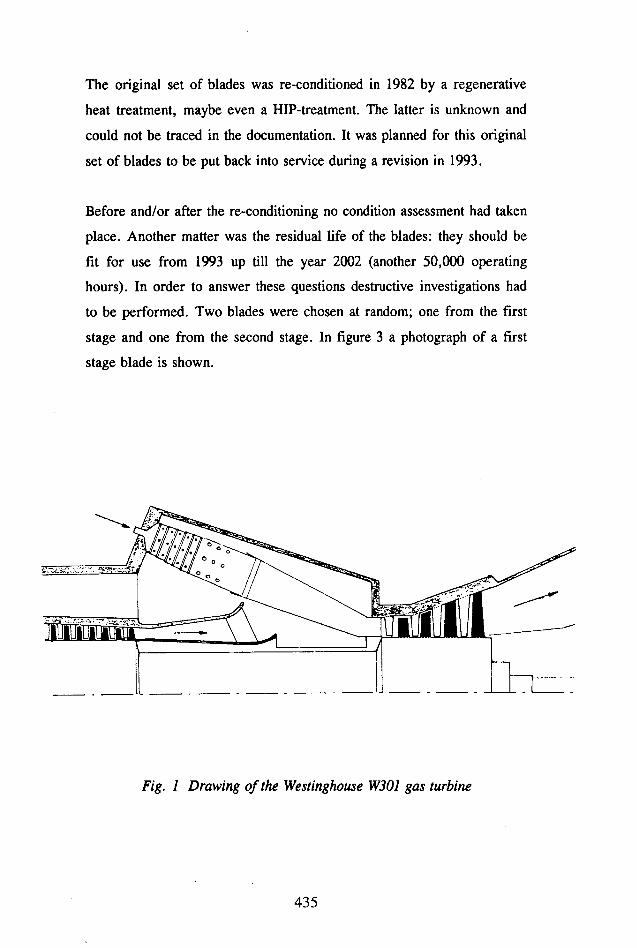
The original set of blades was re-conditioned in 1982 by a regenerative

heat treatment, maybe even a HIP-treatment. The latter is unknown and

could not be traced in the documentation. It was planned for this original

set of blades to be put back into service during a revision in 1993.

Before and/or after the re-conditioning no condition assessment had taken

place. Another matter was the residual life of the blades: they should be

fit for use from 1993 up till the year 2002 (another 50,000 operating

hours). In order to answer these questions destructive investigations had

to be performed. Two blades were chosen at random; one from the first

stage and one from the second stage. In figure 3 a photograph of a first

stage blade is shown.

Fig. 1 Drawing of the Westinghouse W301 gas turbine

435

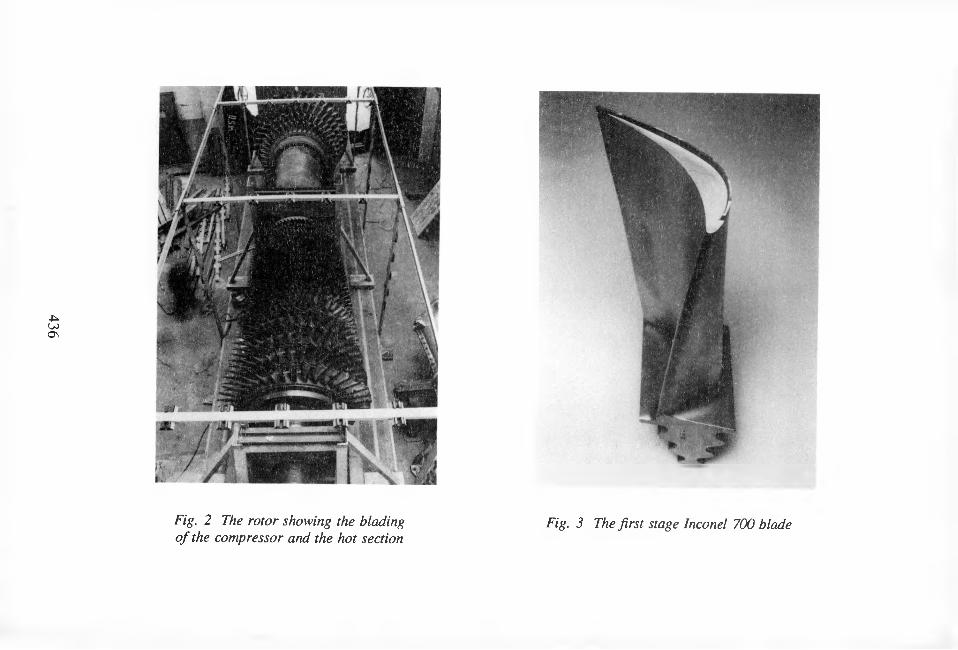
436

Fig. 2 The rotor showing the blading of the compressor and the hot section

Fig. 3 The first stage Inconel 700 blade

3 EXPERIMENTS

The chemical composition of the blades was determined using a Texas

Nuclear "Metallurgist" analyser. The results are compared to the

compositions given in the material specification.

Microscopic investigations were performed. Samples were taken at

various positions in the blades, which included: foot; blade at 1/3 heigth;

tip; leading and trailing edges.

Creep testing was performed using constant load creep rigs with conti­

nuous elongation measurement. Blades of this gas turbine are fairly

large, which is normally observed for gas turbines of an older type.

Therefore, it was possible to machine four normal size creep specimens

(0 8 mm) from the blades. The centre of the specimens was at 1/3 height

of the blade, since this is the highest stressed area of an uncooled blade.

All creep tests were performed at 788°C (1450°F), since this

temperature was specified in the material specification. It was decided

that the iso-stress method could not be used for the accelerated creep tes­

ting, because micro-structural changes would occur at higher

temperatures (the last step in the heat treatment is 815°C). The applied

stresses were chosen so that the longest rupture time would be less than

3,000 hours.

Furthermore, samples of the creep test specimens were prepared for

microscopic investigation.

437

4 RESULTS

4.1 CHEMICAL COMPOSITION

The chemical composition determined is given in weigth-% in table 2.

The Al- and C-contents are not stated, because they cannot be measured

by the aparatus used. However, from these measurements it can be

concluded that both blades meet the requirements of the original Inconel

700 material specification.

TABLE 2 Composition of the Is' and 2nd stage blades and comparison to the Inconel 700 specification

Ni Co Cr Mo Al Ti Fe Zr C

stage 1 47 27.8 15.4 4.0 - 2.5 0.8 0.15 -

stage 2 46 28.3 14.3 3.9 - 2.7 1.3 0.15 -

spec min bal 24 13 2.5 2.5 1.7 - - 0.10max 34 17 4.0 3.5 2.8 4 0.20

4.2 MICROSCOPIC INVESTIGATIONS

The standard heat treatment for this Inconel 700 alloy is specified as

follows:

solution annealing : 1204°C (2200°F) / 2 hours / AC

age hardening : 871°C (1600°F) / 24 hours / AC

stress relieving : 815°C (1500°F) / 8 hours / AC

This heat treatment was also applied during the regenerative heat

treatment. The micro-structure of Inconel 700 in this condition consists

of fine intra-granular r’ particles, carbide particles (most probably of an

438

M23C6 type; both within the grains and at the grain boundaries), and the

usual random dispersion of larger angular Ti(C,N) particles. The volume

fraction of the r’-phase is estimated at 15-20%, which is common for

alloys used in the Sixties. This is a common micro-structure for this

material after the specified heat treatment.

In the creep specimens r’-depletion was observed at the grain boundaries

transverse to the applied stress. Voids and microcracks formed in the

depleted zones along these grain boundaries. Fracture occurred

intergranularly by growth and interlinkage of these microcracks. This

failure mode is normal for alloys with high contents of M23C6 carbides.

Many grains in the material are twinned. The grain size at the outer

surfaces is ASTM 4 - 4V2; inside the blade ASTM 2 is measured, see

figure 4. Occasionally, some very large grains are observed; their size is

estimated at ASTM 00. This grain structure is found in the samples from

both the blades and the creep specimens, so this grain growth did not

occur during the creep testing.

4.3 CREEP TESTING

In table 3 the results of the creep tests are given. The minimum creep

rate has been determined from the measured creep curves. In figure 5 a

graph shows the relation between the minimum creep rate and the applied

stress. The Norton exponent is determined at a value slightly above 10.

This indicates that power-law creep (climb of dislocations) is the

gouverning deformation mechanism in the stress-temperature regime

under discussion.

439

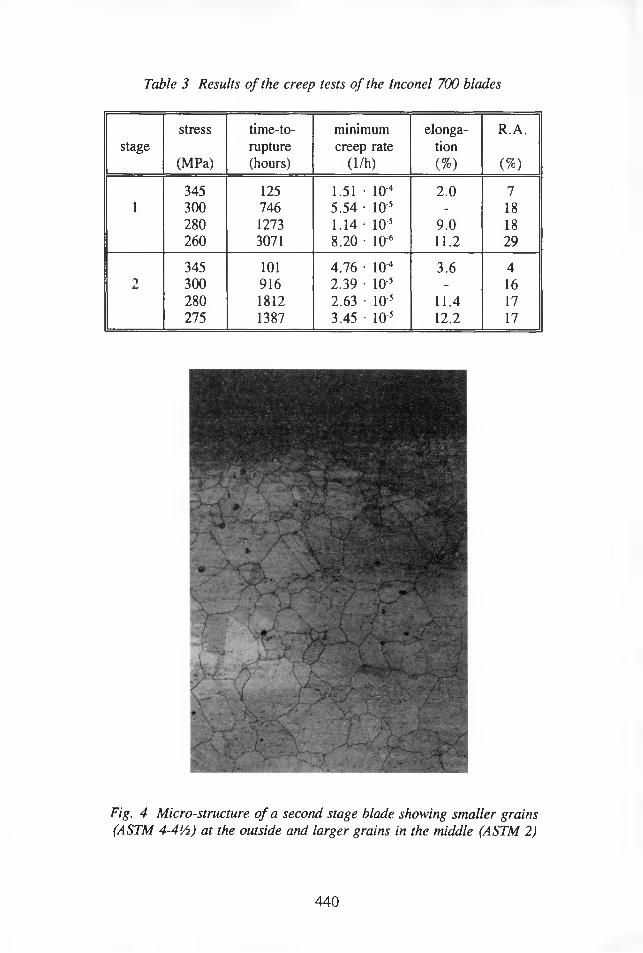
Table 3 Results of the creep tests of the Inconel 700 blades

stress time-to- minimum elonga- R.A.stage rupture creep rate tion

(MPa) (hours) (1/h) (%) (%)

345 125 1.51 ■ 104 2.0 71 300 746 5.54 • 10'5 - 18

280 1273 1.14 • 10'5 9.0 18260 3071 8.20 • lO'6 11.2 29

345 101 4.76 • 10'4 3.6 49Zr 300 916 2.39 • 105 - 16

280 1812 2.63 • lO'5 11.4 17275 1387 3.45 • 105 12.2 17

Fig. 4 Micro-structure of a second stage blade showing smaller grains (ASTM 4-4'/i) at the outside and larger grains in the middle (ASTM 2)

440

k [Us]

1E-07 -

5E-08 -

2E-08

IE-08

n = 105E-09

2E-09 ■' 'L

Fig. 5 Relation between the minimum creep rate and the applied stress. The Norton exponent is about 10.

5 DISCUSSION

5.1 MICROSCOPIC INVESTIGATIONS

The amounts and distribution of r’ and carbides is considered to be

"normal" for a wrought nickel-base superalloy of an older type.

The large grain sizes observed in the blades in combination with the low

ductility observed at the short-term creep tests, caused some concern

about the impact ductility of the blades. Therefore, impact testing was

performed at room temperature and at the service temperature (about

441

750°C). Four Charpy-V specimens were machined from the larger 2nd

stage blade. The results were 58 and 90 Joule at room temperature;

47 and 48 Joule at the service temperature. These results gave more

confidence in the impact ductility of the blade material. It was also

concluded that the large grain size was a result of grain growth during

the solution annealing during the re-conditioning procedure. This is also

not unusual for alloys.that do not form MC-type carbides.

5.2 DATA ANALYSIS OF THE CREEP STRENGTH

It turned out that Inconel 700 has not been manufactured since 1970.

Furthermore, the material was used mainly in the USA, not in Europe.

These facts indicate that it is difficult to obtain data for this alloy.

Literature searches could not indicate data sources for the creep strength

of this alloy. After extensive search two sources for creep data were

found, see Ref. [1, 2], The number of data was 27 and 71 respectively;

in total 98 data. The test temperatures were between 650 and 871 °C; the

rupture time was usually less than 3,000 hours (although six tests

exceeded 10,000 hours).

The raw creep data were analyzed using Larson-Miller regression. Two

2nd grade polynomes were used to fit the data:

a = ai * Plm2 + t>i ' Plm + Cl (1)

Plm = % a2 + b2 • o + C2 (2)

with: o Plm

TCa/b/c

= stress [N/mm2, MPa]= Larson-Miller parameter = T ( C + log tj = rupture time [hours]= temperature [K]= Larson-Miller constant = constant

442

In a diagram of the Larson-Miller parameter vs. stress this results in a

parabole with a vertical axis (Eq. 1) or a horizontal axis (Eq. 2). The

first tends to increase the 100,000 hours creep strength; the second

indicates clearly not enough long-term creep data are available.

The Larson-Miller constants and the polynomial constants from the

regression analyses are given in table 4. The correlation coefficients are

0.983 and 0.940 for the equations 1 and 2 respectively.

Table 4 Results of the regression analysis using two types of 2nd order Larson-Miller polynomial equations

C a b c

Eq. 1 27.28 - 8.5627 ■ lO'9 + 4.2627 • lO4 - 2.4217

Eq. 2 23.48 - 5852.3 + 19923 + 14189

Figure 6 and 7 show the good correlation between creep data and the

results of the data analysis.

If both Larson-Miller equations, calculated at the test temperature

(788°C), are plotted in one figure, it can be observed that no large

differences occur between both equations in the investigated stress and

temperature regimes (see figure 8). Also, it can be observed that the

creep data at 788°C correlate very well with the calculated rupture times.

The results of the creep tests are also plotted in a diagram of rupture

time vs. stress, see figures 9 and 10. It is obvious that the rupture times

of the material from the blades are much higher than the rupture times

predicted by the data analysis. It was therefore concluded that the creep

strength of these blades was about 10% higher than the strength of

"normal" Inconel 700 material.

443

Stre

ss [N

/mm

2] St

ress

[Nlm

m2]

1,000

36,00030,000 32,000 34,000

Larson Miller parameter (C=27.28)

Fig. 6 Result of the regression analysis of creep data. Larson-Miller parameter vs. stress according to Eq. 1

200 -

24,000 26,000 28,0

Larson Miller parameter (C=23.48)

Fig. 7 Result of the regression analysis of creep data. Larson-Miller parameter vs. stress according to Eq. 2

444

The relatively low rupture times for the highest stress (345 MPa) can be

explained by the large grain size in the rupture area. This resulted in a

lower ductility (see also table 3) and a short rupture life. Compare the

grain structure of creep sample 1 (blade 1; 345 MPa) and sample 2

(blade 1, 300 MPa) in figure 11. It can be observed that the sample with

the large grains does not show creep cracks apart from the main rupture.

The sample with the small grains shows many secondary creep cracks at

the outer surfaces.

Stress [N/mm2]

10,000 30,000Time to rupture [hours]

Fig. 8 The time-to-rupture is calculated from equations 1 and 2 as a function of stress at 788°C (1450°F). The data

points show good correlation to both equations

445

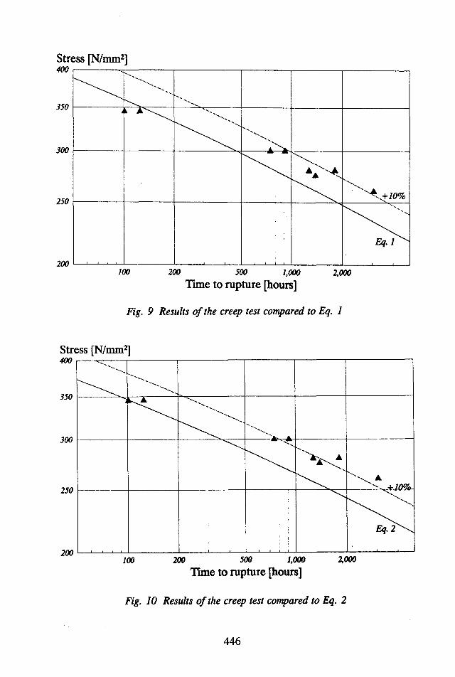
100 200 500 1,000 2,000

Time to rupture [hours]

Fig. 9 Results of the creep test compared to Eq. 1

A

Time to rupture [hours]

Fig. 10 Results of the creep test compared to Eq. 2

446

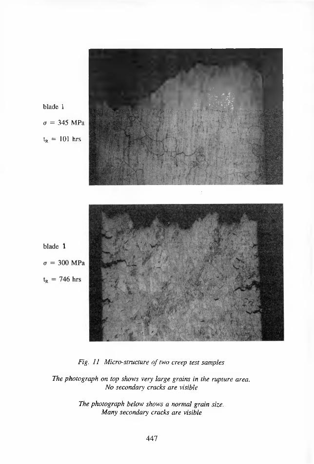
blade 1

a = 345 MPa

tR — 101 hrs

Fig. 11 Micro-structure of two creep test samples

The photograph on top shows very large grains in the rupture area. No secondary cracks are visible

The photograph below shows a normal grain size.Many secondary cracks are visible

447

5.3 SERVICE CONDITIONS

The service conditions for the 1st and 2nd stages in the gas turbine are

determined as follows. The stress is calculated from the centrifugal

forces and their rotating speed. Influence of bending stresses is not

included.

The temperature is estimated from a linear interpolation between the inlet

and outlet temperatures of the turbine (respectively 788 and 426°C). This

resulted in the following service conditions:

1st stage : T = 740°C - o = 225 MPa

2nd stage : T = 660°C - a = 217 MPa

The gas turbine has to generate base-load electricity in the winter period,

and therefore operates about 4,000 to 5,000 hours per year. The number

of starts and stops is limited to about ten per year; up till 1993 about 300

start/stops were made.

5.4 RESIDUAL LIFE ESTIMATE

In making a residual life estimate one has to make sure that the

deformation mechanism of the component (i.e. the blades) is similar to

the deformation mechanism of the creep tests. The service conditions of

the blades are comparable to the conditions of the creep tests, so that the

deformation mechanisms are expected to be similar. In this case the

deformation mechanism will be power-law creep (climb of dislocations).

The residual life estimate was made using the results of the data analysis

(paragraph 5.2) and the service conditions given in paragraph 5.3. From

this it is calculated that the residual life of the 2nd stage blades is more

than 106 hours; so unlimited life is available. This is caused by the

relatively low temperature of the 2nd stage blades.

448

The 1st stage blades have a moderate residual life. Using the results of

the creep data analysis it is calculated that the rupture life is:

- using Eq. 1 : 117.000 hours

- using Eq. 2 : 67.000 hours

From the creep test it is known that the material has an "above average"

creep rupture strength (about +10 %). In the service conditions (see

paragraph 5.3) it is mentioned that the bending stresses are not included.

In general it is known that the bending stresses are about 10 % of the

total stress. Both facts compensate each other, so it can be concluded that

the residual life will be between 67,000 and 117,000 hours.

Taking into account that the turbine operates not more than 5,000 hours

each year, the residual life of the 1st stage blades is estimated at 15 to 23

years. This implies that the gas turbines can be used up till the year 2002

with its re-conditioned original set of Inconel 700 1st and 2nd stage blades.

Whether or not a HIP-treatment has been carried out during the

reconditioning procedure can not be determined from the microstructural

investigations. However, the fact that the rupture times of the blades are

higher than the rupture time for "normal" Inconel 700, does indicate that

the blades received such a HIP-treatment. More important in this respect

is the observation that the blades are in good condition and that their

creep strength is above average.

449

6 CONCLUSIONS

It is possible that the blades received a HIP-treatment in addition to the

regenerative heat treatment, but no absolute certainty can be given. The

blades are in a good condition without creep damage and with an above

average creep rupture strength.

The residual life of the blades is estimated at:

- first stage : between 67,000 and 117,000 hours

- second stage : more than 106 hours

With this residual life it is possible to operate the re-conditioned original

set of Inconel 700 blades up to the year 2002.

ACKNOWLEDGEMENTS

DSM’s permission to publish the results is acknowledged.

Mr. B. Cornelissen (creep testing) and mr. L. Koersvelt (creep data

analysis) are thanked for their assistance during the investigations of the

blades and the preparation of this paper. Mr. P. Aeckerlin from Gerard

de Bruyn (INCO Alloys representative in The Netherlands) and Dr. H.

Kolkman from the National Aerospace Laboratory (Emmeloord, The

Netherlands) supplied the "raw" creep data for Inconel 700.

REFERENCES

1 Rowe, J. P. & Freeman, J. W. Relations between micro-structure

and creep-rupture properties of nickel-base alloys as revealed by

over-temperature exposures, Washington. NASA, 1962

(TN D-1325)

2 Aeckerlin, P. J. (Gerard de Bruijn) private communication

450

ASSESSMENT OF THERMAL EXPOSURE IN COMPOUND TUBES ON THE BASIS OF MICRO- STRUCTURAL CHANGES

Jorma Salonen Senior Research Scientist

Martti Makipaa Senior Research Scientist

VTT Manufacturing Technology PO. Box 1703, FIN-02044 VTT Finland

Abstract

In order to clarity the microstructural changes occurring in high temperature test pieces of compound tube material were annealed in a temperature range 540 - 720 °C for 1 1000 h. The microstructure of the test pieces was investigated with an optical microscope and with a scanning electron microscope and the hardness of the material was measured. On the basis of the results the time-temperature- dependence of the observed changes was determined. The results of this research can be used in estimations of the amount of thermal exposure of components after a long term service of after over heating on the basis of microstructural changes.

1 INTRODUCTION

Because of the strong temperature dependence of the propagation speed of most failure mechanisms, it is important to know the actual temperature during service of power plant components used in high temperatures, e.g., in failure analyses where the conditions leading to the failure are investigated, and in estimations of the residual life time. It is often difficult to arrange a direct measurement of the temperature, but a high temperature frequently causes changes in the material on the basis of which it is possible to estimate the prevailing temperatures. The esti­mation requires, however, a reference material, and up to this date no extensive enough reference material to make quantitative temperature estimations has been published. VTT Manufacturing Technology has therefore developed an investi­gation method, containing a large collection of reference pictures, to be used as a tool in drawing conclusions regarding high temperature components.

451

2 INVESTIGATION METHODS AND MATERIALS

The material investigated was an unused commercial compound tube. The base material of the tube was unalloyed steel ASME SA 210 and the material of the cladding was austenitic stainless steel AISI 304 L.

Test pieces detached from the tube material were annealed in a temperature range 540 - 720 °C for 1 - 1000 h. The hardness of the base material of the test pieces was measured as Vickers hardness numbers and the changes in microstructure were studied with an optical microscope and a scanning electron microscope (SEM). In the microscopic examinations the aim was to quantitatively measure the dispersion of the carbide laminae of the pearlite grains in the ferritic-pearlitic base material and the decarburization depth in the base material on the interface of the austenitic steel.

3 RESULTS

3.1 CHANGES IN MICROSTRUCTURE

In the microscopic investigations the annealing was observed to cause breaking and speroidization of the originally nearly unbroken carbide lamellae which is followed by a gradual coarsening of the carbides. The following stages were used for the classification of the observed changes:A microstructure of unused tube, ferrite and pearlite B first signs of speroidization of pearliteC appreciable speroidization, but some carbide lamellae still evident D speroidization complete, but the carbides are still in former pearlitic areas E carbides are dispersed, but there is still little trace of pearlitic areas F original pearlitic areas can not be observed, some carbides have grown consid­

erably.Examples of the observed microstructural changes are seen in micrographs taken with a scanning electron microscope. Figures 1-3.

The combined effect of annealing time and temperature is often described with the Larson-Miller-parameter Plm

452

Plm = Tx (log t + C), where (1)

T is the annealing temperature (°C) t is the annealing time (h)C is constant.

When the Larson-Miller parameter is in force the temperature-time-combinations leading to the same result produces in the 1/T - log t -coordinate system a series of straight lines converging to the point (1/T = 0, log t = -C).

The results are presented according to the above mentioned classification in a 1/T - log t -coordinate system in Figure 4. The results follow well the correlation according to the Larson-Miller-parameter with value 14 of the constant C. By the help of Figure 4 the service temperature can be determined on the basis of ob­served changes in the microstructure, if the service time is known.

3.2 HARDNESS CHANGES

Changes of the microstructure occurring during annealing or usage also cause changes in the mechanical properties of steel, such as the hardness. In Figure 5 the hardness of the steel is presented in the 1/T - log t -coordinate system. An approximate line above which the thermal stress has, on the basis of the hardness, caused the tensile strength to fall below the minimum tensile strength specified for the steel, has also been marked in the Figure. If the original hardness is known or it can be measured, the service temperature can be estimated on the basis of hardness changes, as well as changes in microstructure. Time-temperature combi­nations that cause the same hardness are approximately on lines parallel with the lines leading to the same microstructure in Figure 4.

3.3 DECARBURIZATION OF CARBON STEEL ON THE INTERFACE

From the carbon steel, on the interface of the austenitic steel, the layer thickness of complete decarburization (almost fully ferritic structure) and partial decar­burization (a clearly changed structure because of the decarburization) was mea­sured. An example of decarburization that has occurred during annealing is shown in Figure 6. Because the kinetics of decarburization as well as of microstructural changes follow the Arrhenius equation, the temperature-time combinations lead­

453

ing to the same decarburization depth should be on the same line in the 1/T - log t -coordinate system. The results of the thickness measurements of the decar­burization layer are presented in Figures 7 and 8. The figures show that the tem­perature-time combinations leading to the same decarburization are approxi­mately on lines that have the same slope as the lines in Figure 4 leading to the same change in the microstructure.

DISCUSSION

When comparing material changes that are defined in different ways and caused by annealing and usage, it can be shown that both hardness changes in the base material of a compound tube and microstructural changes, as well as the decar­burization of the boundary surface are all suitable for assessment of the thermal exposure of components. The kinetics of all the phenomena mentioned above fol­low in the whole investigated time-temperature-area quite well the correlation according to the Larson-Miller parameter, Plm = T x (log t + 14), which, there­fore, can be used for extrapolation of the results for service times exceeding the longest test annealings. Observable changes in the microstructure occur when the parameter value is 13,5 x 103 and observable changes in the hardness and decar­burization layer with an approximate value of 13,0 x 103. Decarburization and hardness are, in other words, more sensitive indicators of , e.g., overheating, but they require knowledge of the hardness and decarburization depth of the as-deliv­ered material. Assessment based on changes in the microstructure is not an equally sensitive method, but, on the other hand, does not require reference values of the unused material. The observation limit that clearly exceeds the usual ser­vice values can be considered as the largest limitation of the methods described. The observation limit Plm (C = 14) - 13 x 103 of the hardness and decarburiza­tion depth of compound tubes corresponds for example to a service time of 100 000 hours and an operating temperature of 410 °C. Consequently, the over­heating from the usual operating temperature of about 300 °C must be quite remarkable to cause observable changes. On the other hand, when the temperature is rising the time corresponding to the observation limit shortens fast, so that tem­perature fluctuations in the temperature range of 300 - 550 °C can be observed with this method. The method has been applied to an estimation of the thermome­chanical history of compound tubes together with TEM and SEM investigations 121.

454

REFERENCES

1. Jorma Salonen, unpublished.

2. Martti Makipaa, Jorma Salonen, Pertti Nenonen and Tero Hakkarainen. Studies with TEM, SEM and optical microscope on the cracking of BLRB composite floor tubes.

455

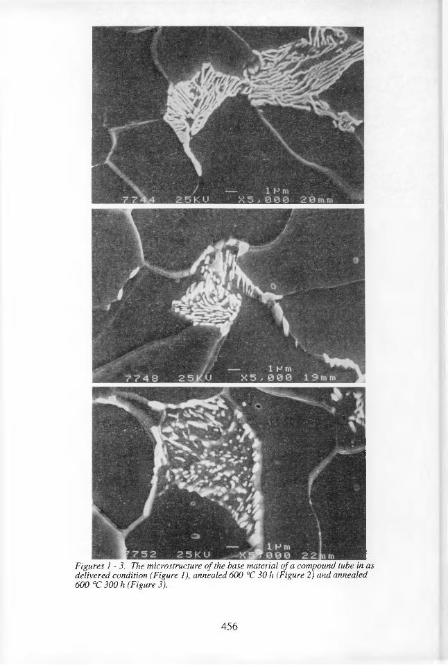
Figures 1-3. The microstructure of the base material of a compound tube in as delivered condition (Figure 1), annealed 600 °C 30 h (Figure 2) and annealed 600 °C 300 h (Figure 3).

456

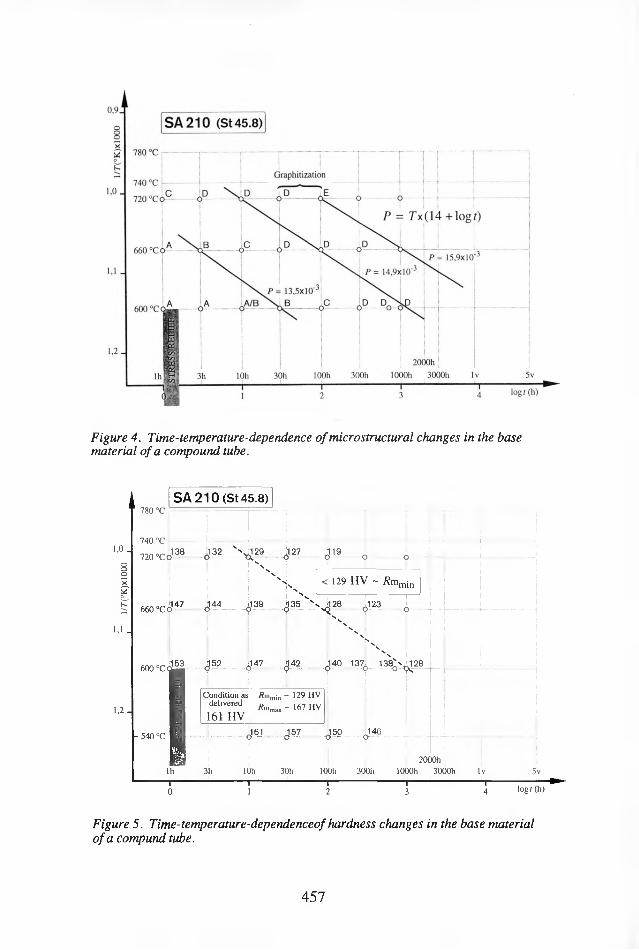
SA 210 (St 45.8)

Graphitization740 eC

o

P = rx(14+logr)

oP= 15,9x10'

/■= 14,9X10'

/*= 13,5x10 5D D

2000hlOOOh 3000h

Figure 4. Time-temperature-dependence of microstructural changes in the base material of a compound tube.

1,0

u.

1,2

SA 210 (St 45.8)780 °C

740 °C -

720 °C0138 432 129 127 119

< 129 HV ~ /?mmjn

660 °C 6J47 ^44 6139 j35 X 128 0123

600 °C J53 J52 0147 1447 J42 140 137, 138>^128s w O O O Os

Condition as ~ 129 HVdelivered

161 HV- 540 °C o161 157 ^50 0146

3h2000h

30h 100H 300H 1000b 3000h Iv 5v

log / (h)

Figure 5. Time-temperature-dependenceof hardness changes in the base material of a compund tube.

457

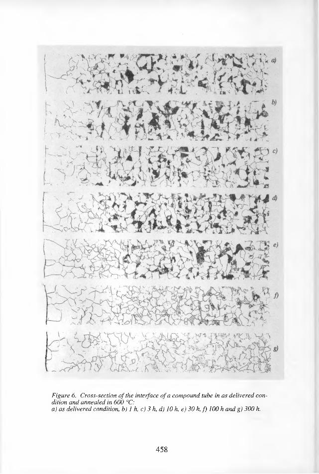
Figure 6. Cross-section of the interface of a compound tube in as delivered con­dition and annealed in 600 °C:a) as delivered condition, b) 1 h, c) 3 h, d) 10 h, e) 30 h, f) 100 h and g) 300 h.

458

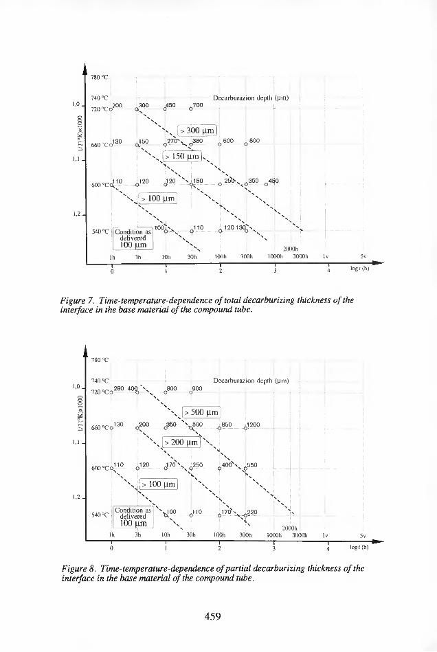
1,0 _

1,1 -

1,2

780 °C

740 °C

720 °C0'200 300 450 _700

Decarburazion depth (pm)

>s [>300 jimj660 «Co130 ......o]50 o270'vo380 o600 o800

600 “c a;,110

''s [> 150 M.m]v>x i

120....... o120 .MlSO........ 1 2b>^o350 O450

1_________ [ :N>.

XJ> 100 |im]

540 °C Condition as delivered 100 pm

lOOX o110 120 130N.

2000hlh 3h lOh 30h 100b 300h lOOOh 3000H

-I------------------ 1------------------ \------------------ 1------------5v

logt(h)

Figure 7. Time-temperature-dependence of total decarburizing thickness of the interface in the base material of the compound tube.

1,0.

1,1 -

1,2

780 °C

740 °C

720 °CO 280 40V'N <>“.....^Decarburazion depth (pm)

.800 900

X |> 500 |dm]660 "CO130------O;,200 ,350 'J500 1850 i1200o 15, 0 0

x [ >200 tun IX

600»co110......o'20..........o,70Xo250 o400 'v o550['n 1 i sk

X. |> 100 |xm| X

540 "CCondition as

delivered 100 Jim

i00 o110.........o170 s> o220INn | | | 2000h (

lh 3h lOh 30h 100b 300h lOOOh 3000h Iv1------------------ 1------------------ 1------------------ 1------------------ 1

5v

0 logr(h)

Figure 8. Time-temperature-dependence of partial decarburizing thickness of the interface in the base material of the compound tube.

459

460

THE 'PLUS' SYSTEMON-LINE OPERATIONS & MAINTENANCE SOFTWARE

FOR POWER PLANT

G T Jones J D Sanders

P Jarvis C J Coomber

ERA Technology Ltd Cleeve Road, Leatherhead,

Surrey KT22 7SA United Kingdom

ABSTRACT

ERA has developed a unique Plant Life Usage Surveillance System (PLUS) for creep-fatigue

assessment of turbine and boiler pressure parts based on on-line operational monitoring. Integrated

with off-line condition/inspection data, PLUS can provide more accurate real-time optimisation of

plant life usage, and additionally performs as an operations adviser and a maintenance planning tool.

This paper provides a description of a PLUS system, with reference to a case study application.

The particular concern in this case is ligament cracking in steam headers arising from increased

cyclic operation. Key issues regarding susceptibility to cracking and meaningful life monitoring are

given to demonstrate the benefits of on-line life surveillance.

1 Introduction

There is a growing awareness by power plant operators of the benefits to be gained by applying

on-line plant condition monitoring techniques. This is taking place for a number of reasons. The

market is demanding plant, which was designed principally for base-load, to operate more flexibly.

Experience has shown that even plant that has been designed for cyclic operation, can fail by

creep-fatigue mechanisms induced by operational transients not allowed for in design. Competition

is also forcing operators to reduce costs by demanning, increased run times between outages, and

reduced maintenance schedules. All these factors make once-off investment in all forms of condition

monitoring increasingly attractive.

This paper describes a system designed to monitor thick section, high temperature components

on-line for creep-fatigue degradation. ERA'S Plant Life Usage Surveillance (PLUS) System was

originally designed to address the problem of ligament cracking of steam headers prevalent in

Europe and the US. It is, however, equally applicable to other components such as main steam

G:BCS3ADMI\GTJ\0135-95.SAM

461

pipework (and connected vessels), and steam turbine valves, chests, casings and rotors. There is

also considerable interest in applying it to Heat Recovery Steam Generators (HRSG) which are

notoriously susceptible to creep-fatigue failures.

The basis function of PLUS is to convert signals, obtained from sensors (usually just thermocouples

and pressure transducers) strategically connected to critical locations on plant, to local stress and

strain values in real-time.

Using built-in advanced algorithms these values are converted and summed to give a realistic

measure of damage accumulation in real-time, or at convenient periodic intervals. It therefore

serves as both a life usage monitor an operations adviser (or alarm system) and thereby may be

utilised as a damage controller, and a maintenance planning tool. It may also be used as a simulator

to assess likely effects of changes in operation model.

2 Scope of the PLUS System

PLUS is a fully integrated on-line system, with real time data monitoring and processing, providing

periodic on-line analysis with facilities for integration of off-line inspection/interrogation data. It is

fully customised for each application and enables plant specific geometry, design and history to be

accommodated together with the specific local operational behaviour. This is achieved by the

incorporation of component specific temperature/pressure to stress calibration based on off-line FE

analysis using operator specific on-line data. Life prediction algorithms are implemented according

to the components and degradation processes being monitored.

Depending on the requirements of the application, using temperature surveillance and calculational

methods, future PLUS system can be made to monitor and predict crack propagation, or monitor

cracked components using sensors to signal local failures.

The scope of the PLUS System developed on a UNIX Workstation is shown in Fig. 1. This figure

highlights the key components which facilitate various features, the more important ones being:

1 Data capture module connects PLUS system with the site sensor data collection system. Its

precise structure is therefore dependant upon the nature of the existing facilities.

2 Data validation module interrogates the sensor signals and applies a number of consistency

checks and marks data deemed to be faulty. This module is also responsible for filing the

data in a time order, such that any file can be retrieved by means of a time and date identity.

3 The database module holds relevant aspects of the component geometry: the component

specific stress functions and selected inspection data pertinent to the assessment. Using

template objects it allows customers to process additional monitoring points on components

of similar geometry. It also holds the damage history for all monitored components.

G:BC63ADMI\GTJ\0135-95.SAM

462

4 The display module allows the operator to select a location on a component and to display

the stress at that location in real-time.

5 The life analyses modules in PLUS are determined by the components and degradation

mechanisms being monitored. The analysis modules are periodically activated by the

operator to assess the consumed life based on newly available on-line plant data and the

last calculated life usage for each component.

3 Case Study

The PLUS System addressed here was commissioned to monitor the creep-fatigue damage

accumulation, predict crack initiation in the platen, final and reheater outlet stub headers and

manifolds, as well as to monitor creep-corrosion damage in the associated boiler tubing in 8 boiler

units of 350 and 650 MW. The significance of ligament cracking on plant integrity and the benefits of

life monitoring are demonstrated by consideration of the background to the problem.

3.1 Nature and Incidence of Ligament Cracking

Temperature transients and cyclic stresses are not explicitly considered during header design, ie.

rigorous cyclic fatigue calculations are not normally done for headers, since it is intended that these

be accommodated by operating limits on temperature ramp rates during start-up and shutdown.

These limits are set to avoid high strain thermal fatigue and hence fatigue cracking. Experience

shows, however, that even where the specified limits, using data from standard thermocouples, is

adhered to, severe local transients can occur under non-steady operation. These local transients are

generally not detected but are the significant factor leading to ligament cracking.

Ligament cracking develops from the inside crotch comer of the header and tube intersection and

propagates along both the header and the tube internal walls. The classical form of ligament

cracking occurs where the adjacent tube penetrations are closely spaced such that crotch comer

cracks propagate across the ligament, shown in Fig. 2. This classic form is particularly severe since

it can result in catastrophic failure. Ligament cracking along the circumferential direction may result

in fast fracture with the header breaking in two. Where adjacent element rows are closely aligned

along the length of the header, ligament cracks may also develop in the axial direction where the

crack surface are normal to the dominant hoop pressure stress. This again raises the possibility of

catastrophic failure. Localised cracking with a star burst distribution, illustrated in Fig. 3, where the

cracks radiate out from the perimeter of the tube hole is associated with isolated or more widely

spaced penetrations. Starburst cracking is unlikely to cause catastrophic failure but may cause

steam leaks.

Ligament cracks removed from service (both in the US and Europe) have been found, without

exception, to be consistent with high strain thermal fatigue generated by severe thermal transients.

That is the cracks are straight transgranular gaping and oxide filled with no associated creep

damage.

IG:BC63ADMI\GTJ\0135-95.SAM

463

All studies support the pattern of development in which multiple cracks first initiate from the inside

comers of the tube penetrations, but growth is dominated by the primary cracks which propagate

across the ligament and towards the outer wall. European experience indicates that crack initiation

occurs relatively early (10,000 to 20,000 hours of operation), with a relatively long propagation period

generally exceeding 50,000 hours. This is contrary to the US experience where crack initiation

occurs much later, i.e. over 100,000 hours, and crack propagation is generally much more rapid.

The difference in behaviour may be attributed to differing operating practices. Oxide notching has

been proposed as a crack initiation mechanism however this is not supported by European

investigations.

Although no creep damage is observed for headers operating in the creep regime, creep relaxation of

high transient stresses contributes to the crack initiation and propagation mechanisms. Assessment

methods are therefore based on creep-fatigue analysis.

3.1.1 Factors Affecting Susceptibility to Ligament Cracking

Analysis of the available data on the incidence of ligament cracking in Europe (Table 1) and US

(Table 2) reveals that the European and US experience exhibits common factors as summarised

below:

1 Header Type Superheater Outlet headers were found to be susceptible to ligament

cracking. The US and European experience indicates that secondary and final superheater

outlet headers were the most susceptible. There is also European experience, but little US

experience of cracking in primary and interstage superheaters.

2 Boiler Maker and Unit Size The European experience indicates that all makes and sizes of

unit are susceptible to ligament cracking, with some manufacturers' components being

inexplicably more vulnerable. Larger units, supported by US experience, also show

increased incidences of cracking.

3 Header Geometry The susceptibility to cracking increases with decreasing ligament width

and with increasing wall thickness, with all headers exceeding a certain thickness exhibiting

cracking.

4 Operating Hours and Starts Figures 4 and 5 show graphs comparing observed cracking

data in Europe with plant operating hours and number of starts respectively. No correlation is

evident between incidences of cracking and operating hours or number of operating cycles.

Cracking has been observed after comparatively few cycles, less than 500, contradicting the

view that ligament cracking is a two shifting problem.

G;BC63ADMI\GTJ\0135-95.SAM

464

3.1.2 Predictive Assessment and the Requirement for Plant Monitoring

Concern about the incidences of ligament cracking led to quantitative assessments being carried out

on ex-service headers in Europe.

Finite element analyses were carried out for typical service start-up and shut-down cycles, and crack

initiation times and propagation rates were determined using high strain fatigue cyclic endurance and

creep ductility exhaustion models.

The analyses predicted considerably longer crack initiation endurances and much slower crack

growth rates than that determined by oxide dating techniques applied to the removed samples. The

conclusion was that additional cycles were present that were not considered in the analysis.

Temperature monitoring to investigate the cause of thermal cycles responsible for ligament cracking

has confirmed that temperature ramp rates associated with normal two shifting operating cycles are

insufficient to generate the plastic strain ranges required to account for observed cracking. However

much more severe local transients were identified under certain operating conditions. Analysis of

monitored data indicated that major contributors to ligament cracking are:

1. Spraying operations during cold start-ups

2. Emergency shut downs following tube leaks

3. Temperature cycles during hot starts (for example problems with coal flow and mills)

The fact that thermocoupling and continuous monitoring of vulnerable headers confirmed the

occurrence of previously undetected transients, demonstrates the importance of on-line monitoring

for accurate life prediction for headers.

3.2 Plant Monitoring Requirements

In the past, vulnerable headers were extensively thermocoupled for analytical purposes. However, it

has been found that the thermal stresses can be adequately described by data from a limited number

of strategically positioned thermocouples.

Inlet steam temperatures are normally obtained from thermocouples on inlet tubes. The accuracy of

the estimate and definition of critical locations are improved as the number of tubes being monitored

increases. Additional thermocouples are also required to provide back-up in the event of

thermocouple failure.

G:BC63ADMI\GTJ\0135-95. SAM

Thermocouples were installed on the two lead units of the case study plant. The selection of the

thermocouple locations was based on the identification of critical components using previous

analyses and taking existing thermocouple locations into account.

The thermocouples installed provided preliminary surveillance data for the finite element analyses

performed during PLUS customisation. A selection of these thermocouples was then used for the

on-going monitoring by PLUS ensuring that sufficient redundancy is provided.

3.3 Stress Calculation

For the purposes of PLUS it is assumed that the ligament stresses can be uniquely determined from

a number of temperature differences and rates of temperature change within the header. The

process undertaken to generate the stress functions used by PLUS is illustrated in Fig. 6.

1 Each geometry under consideration is modelled using 3-D finite element analyses

techniques. For the case study, analysis of 32 geometries was required.

2 Surveillance data from the thermocouples and pressure transducers are processed and

analysed to identify the thermal boundary conditions, typical and exceptional transients

experienced by the components. Some of the thermocouple surveillance data are also used

to validate the FE heat transfer analyses output.

3 A wide range thermal transients using realistic heat transfer coefficients, steam ramp rates

and temperature changes are analysed for each geometry. The outputs of the thermal

analyses are compared with plant data. Thermal boundary and heat transfer conditions are

refined until an optimum correlation is achieved. Figure 7 provides an example of the

comparison of the FE thermal transient results and measured temperatures.

4 Finite element stress analysis is then performed for the thermal transients. The outputs of

these analyses provide inputs to and validation of the stress functions generated in step 5.

The hoop stress at a crotch comer location under a hot start condition is shown in Fig. 8.

5 Multiple parameter linear regression analysis is then carried out to relate the ligament

stresses from step 4 to the temperature differences and rates of temperature change. This

analysis produces relationships (stress functions) of the type

a = F(ATj, Tj)

where AT,- - temperature difference

7, - rate of temperature change

An example of the stress functions so developed is given in Fig. 9.

G: BC63 ADMINGT JV0135-95. SAM

466

These functions enable direct calculation of stress and therefore strain from measured

temperature values obtained during PLUS operation, providing input to the creep-fatigue

calculation.

6. The stress functions are implemented in the PLUS system to provide real-time variations of

ligament stresses as shown in Fig. 10. These real-time displays provide the operator with an

instantaneous output of the ligament stress which can be compared with a stress limit set to

prevent crack initiation in a specified number of starts. Stress limits can be periodically

updated by PLUS using the latest calculations of life usage.

3.4 Creep-fatigue Damage Calculation

The methodology adopted for PLUS assumes that any arbitrary cycle can be separated into an

elastic-plastic cyclic component and stress relaxation dwell component. The elastic-plastic cycling

causes low cycle fatigue damage and stress relaxation causes creep damage by a process of

ductility exhaustion. Both of these components contribute to the overall damage which is calculated

using the ’linear damage summation rule'.

In carrying out the analysis each transient is resolved into discrete cycles. The hysteresis loop for

each cycle is constructed from the strain-time data generated by the stress functions by means of

the offset zero form of the Ramberg-Osgood equation

where A and P are temperature and strain rate dependant materials parameters.

The fatigue damage component, Df, is obtained from the relationship

n — ^ f~ Nfct)

where s/ is the total strain range of the cycle

and Nf is the fatigue endurance as a function of the total strain range of the cycle

described by means of a suitable parametric equation.

The creep damage component, Dc, is calculated by a means of the ductility exhaustion approach

using:

tdDc= j

06(0

(£W)dt

where is the dwell time

e(t) is the instantaneous strain rate obtained from the stress relaxation relationship

G:8C63ADMK3TJV)135-95.SAM

467

cr = ao[l-P//ln(/+l)]

!,« da/d( aoP" 1 8W=“----------

with a0 - peak stress at start of the dwell

t - time

- temperature dependant materials parameter.

The total creep-fatigue damage for each cycle, Dt, is calculated using the linear damage rule

Df = Df+Dc

3.4.1 The Creep-fatigue Crack Initiation Program

Built into the PLUS system consists of the evaluation of the above two types of damage mechanisms

algorithms, shown in Fig. 11. The modules read in the time and temperature data collected by the

monitoring system and calculate the associated stress and strain using the stress functions. After

resolving the data into cycles and dwells, the two algorithms establish the LCF damage and creep

damage components for each identified cycle and dwell period respectively.

The total damage for each location is established and stored in the PLUS database. Cyclic life usage

calculated from monitored data |s shown in Fig 12.

The creep-fatigue life analyses are performed periodically by PLUS using past life estimates and

newly available plant data. PLUS is set up to automatically update the life estimate on a monthly

basis. The life analysis may also be performed at any time upon user instruction. The operator may

initialise the life analysis in two ways. A commit may be initiated where new off-line data is supplied,

and the life estimates are updated based on these and latest available on-line data, the results are

stored in the data base. Alternatively, life calculations may be performed at any time using the latest

available data. The results are displayed to the operator but not stored.

3.5 Steady State Creep Damage Calculation

For periods of steady operation the accumulation of steady state creep is determined in PLUS using

Dc = S?K^^ + Dc*’,'

where tr is the allowable rupture time at the current operating temperature and stress

/ is the time for which the operating temperature and stress remain constant

Dcinjj is defined by a clock setting exercise using inspection and condition

assessments

G:BC63ADMl\GTJ\0135-95.SAM

468

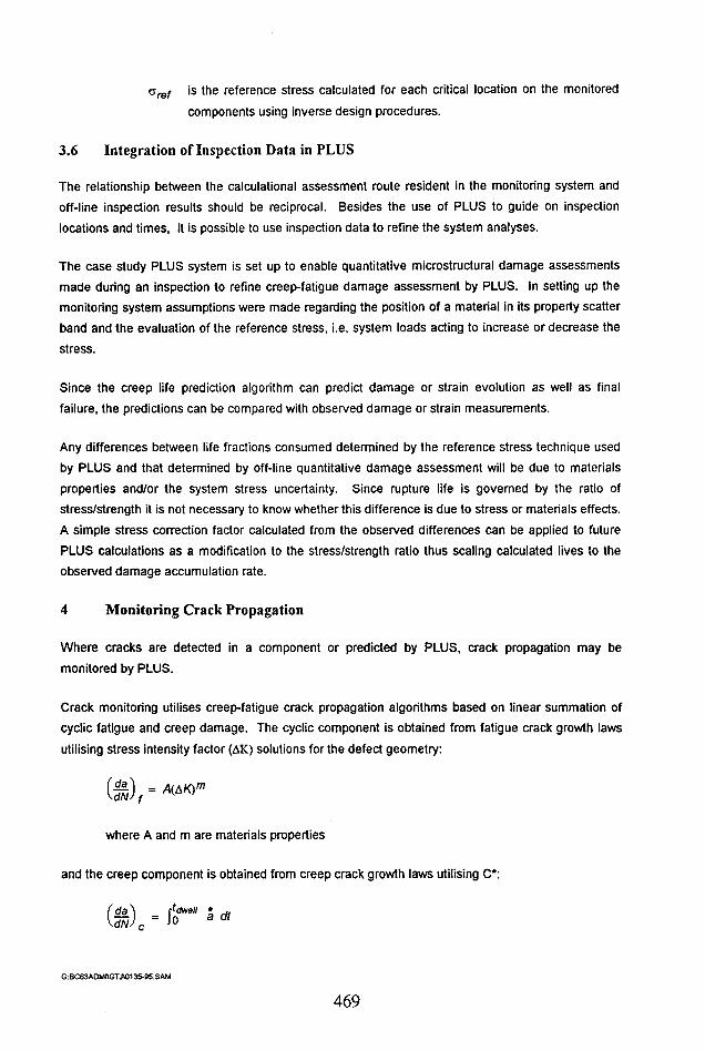
is the reference stress calculated for each critical location on the monitored

components using inverse design procedures.aref

3.6 Integration of Inspection Data in PLUS

The relationship between the calculational assessment route resident in the monitoring system and

off-line inspection results should be reciprocal. Besides the use of PLUS to guide on inspection

locations and times, it is possible to use inspection data to refine the system analyses.

The case study PLUS system is set up to enable quantitative microstructural damage assessments

made during an inspection to refine creep-fatigue damage assessment by PLUS. In setting up the

monitoring system assumptions were made regarding the position of a material in its property scatter

band and the evaluation of the reference stress, i.e. system loads acting to increase or decrease the

stress.

Since the creep life prediction algorithm can predict damage or strain evolution as well as final

failure, the predictions can be compared with observed damage or strain measurements.

Any differences between life fractions consumed determined by the reference stress technique used

by PLUS and that determined by off-line quantitative damage assessment will be due to materials

properties and/or the system stress uncertainty. Since rupture life is governed by the ratio of

stress/strength it is not necessary to know whether this difference is due to stress or materials effects.

A simple stress correction factor calculated from the observed differences can be applied to future

PLUS calculations as a modification to the stress/strength ratio thus scaling calculated lives to the

observed damage accumulation rate.

4 Monitoring Crack Propagation

Where cracks are detected in a component or predicted by PLUS, crack propagation may be

monitored by PLUS.

Crack monitoring utilises creep-fatigue crack propagation algorithms based on linear summation of

cyclic fatigue and creep damage. The cyclic component is obtained from fatigue crack growth laws

utilising stress intensity factor (AK) solutions for the defect geometry:

where A and m are materials properties

and the creep component is obtained from creep crack growth laws utilising C*:

G:BC63ADMt\GTJ\0135-95.SAM

469

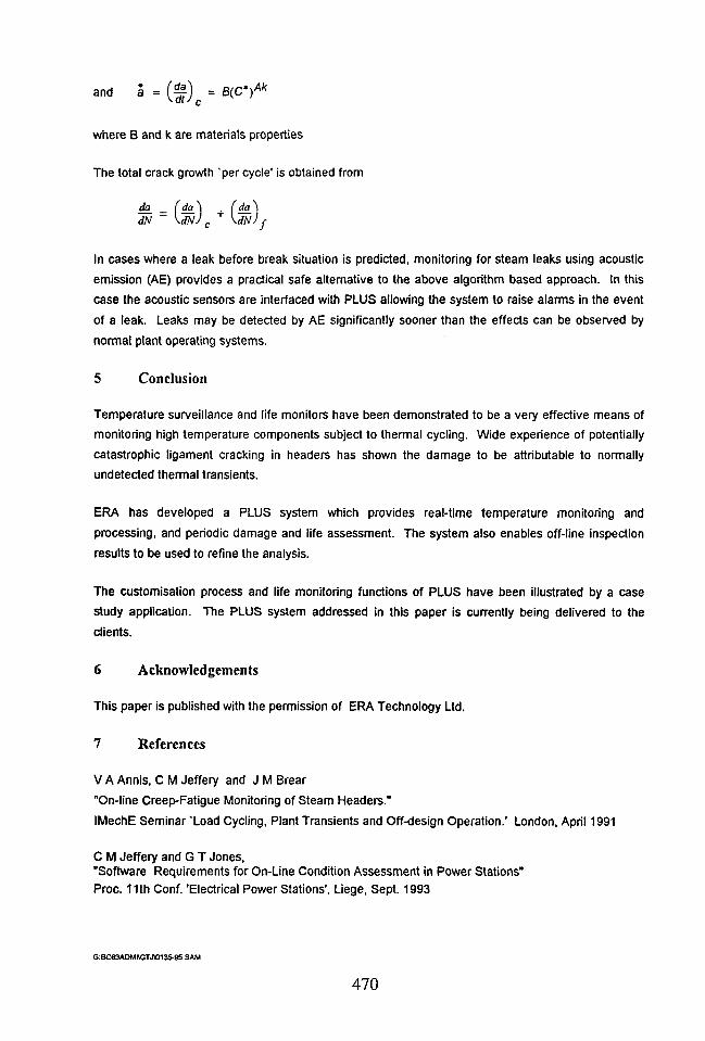
and Mi)c = e(c*)Mwhere B and k are materials properties

The total crack growth 'per cycle' is obtained from

da _ f do'i f da AdN ~ \dNJ c \dN) j-

In cases where a leak before break situation is predicted, monitoring for steam leaks using acoustic

emission (AE) provides a practical safe alternative to the above algorithm based approach. In this

case the acoustic sensors are interfaced with PLUS allowing the system to raise alarms in the event

of a leak. Leaks may be detected by AE significantly sooner than the effects can be observed by

normal plant operating systems.

5 Conclusion

Temperature surveillance and life monitors have been demonstrated to be a very effective means of

monitoring high temperature components subject to thermal cycling. Wide experience of potentially

catastrophic ligament cracking in headers has shown the damage to be attributable to normally

undetected thermal transients.

ERA has developed a PLUS system which provides real-time temperature monitoring and

processing, and periodic damage and life assessment. The system also enables off-line inspection

results to be used to refine the analysis.

The customisation process and life monitoring functions of PLUS have been illustrated by a case

study application. The PLUS system addressed in this paper is currently being delivered to the

clients.

6 Acknowledgements

This paper is published with the permission of ERA Technology Ltd.

7 References

V A Annis, C M Jeffery and J M Brear

"On-line Creep-Fatigue Monitoring of Steam Headers."

IMechE Seminar 'Load Cycling, Plant Transients and Off-design Operation.’ London, April 1991

C M Jeffery and G T Jones,"Software Requirements for On-Line Condition Assessment in Power Stations"

Proc. 11th Conf. ’Electrical Power Stations', Liege, Sept. 1993

G:BC63ADMI\GTJ\0135-95. SAM

470

R Viswanathan

"Life Assessment of High Temperature Components - Current concerns and research in the US"

ERA Report 93-0690, Conf. Proc ’Life Assessment of Industrial Components and Structures',

Cambridge, Sept 1993

EPRI Report

' An Integrated Approach to Life Assessment of Boiler Pressure Parts’, EPRI Project RP 2253 -10

G:BCS3ADMI\G™0135-95.SAM

Table 1Summary of Inspections for Ligament Cracking in a European Utility

Header Type NumberInspected

NumberCracked % Cracked

Maximum Depth, % wall

thicknessAll Superheater Outlet 80 33 41 100

Primary 9 3 33 100

Interstage 28 8 29 100

Secondary and Final 43 22 51 69

All Superheater Inlet 32 2 6 20

All Reheater 18 0 0 N/A

All Headers 130 35 27 100

Table 2Summary of Ligament Cracking Experience in the US

Header Type NumberInspected

Numbercracked

%Cracked

Secondary Superheater Outlet 157 44 28

11/4Cr 73 26 36

21/4 Or 76 17 22

Op.T > 1050C 14 6 43

Reheater Outlet 118 2 2

All Others 101 4 4

472

473

PLUS SYSTEM SHELL STRUCTURE

MONITORED LOCATIONS Fig.1:

PLUS OUTER SHELL UNIX

APPLICATIONS

BDE

ODM

RLA

TLA

CDU

TSU

PDU

DDD

SSC

GDD

HSD

TLD

OSD

BOILER DATA BASE EDITOR

ON-LINE DATA MANAGER— MANAGEMENT

REMANENT LIFE ASSESSMENT

TUBE LIFE ASSESSMENT

CREEP DAMAGE UPDATE

TUBE STATISTICS UPDATE

PERIODIC DAMAGE UPDATE

DUMP DAMAGE DATA

STEADY STATE CREEP

GRAPHIC DAMAGE DISPLAY

HISTORIC STRESS DISPLAY

TUBE LIFE DISPLAY

ON-LINE SURVEILLANCE DISPLAY

«- FUNCTIONS

SFW - SURVEILLANCE FILE WRITE (SIMULATOR)

Scope of PLUS

Fig.2: ’Classic' ligament cracking in a boiler header

at an advantage stage of development

474

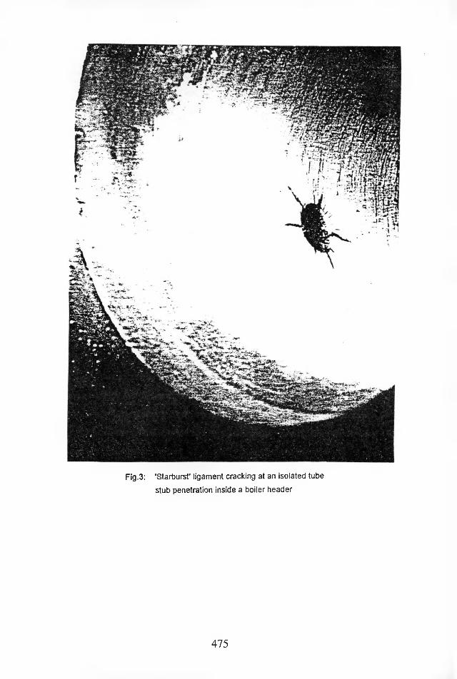
Fig.3: 'Starburst' ligament cracking at an isolated tube

stub penetration inside a boiler header

475

Max

. Dep

th o

f Cra

ckin

g, %

All Superheater Outlet Headers

*—m* •ThousaniS®

Number of Operating Hours

a Secondary and Final + Primary and Interstage

Fig.4: Susceptibility to ligament cracking as a function

of the number of operating hours

476

Max

. Dep

th of

Cra

ckin

g, %

All Superheater Outlet Headers

■*—*Thousands

Number of Starts

a Secondary and Final ^ Primary and Interstage

Fig.5: Susceptibility to ligament cracking as a function

of the number of starts

477

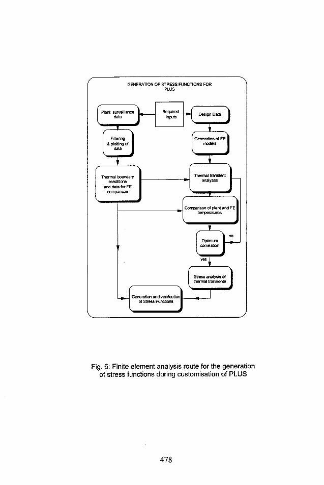
GENERATION OF STRESS FUNCTIONS FOR PLUS

Requiredinputs

Plant surveillance Design Data

Filtering & plotting of

data

Generation of FE models

Thermal transient analyses

Thermal boundary conditions

and data for FE comparison

Comparison of plant and FE temperatures

Optimumcorrelation

Stress analysis of thermal transients

Generation and verification of Stress Functions

Fig. 6: Finite element analysis route for the generation of stress functions during customisation of PLUS

478

Fig. 7: Comparison of FE Thermal analysis results and thermocouple datat - Reheater outlet manifold body

-j

FE manifold

Manifold t/c

Estimated steam

4000 5000 6000 7000 8000 9000 10000 11000 12000 13000 14000 15000

Time in seconds

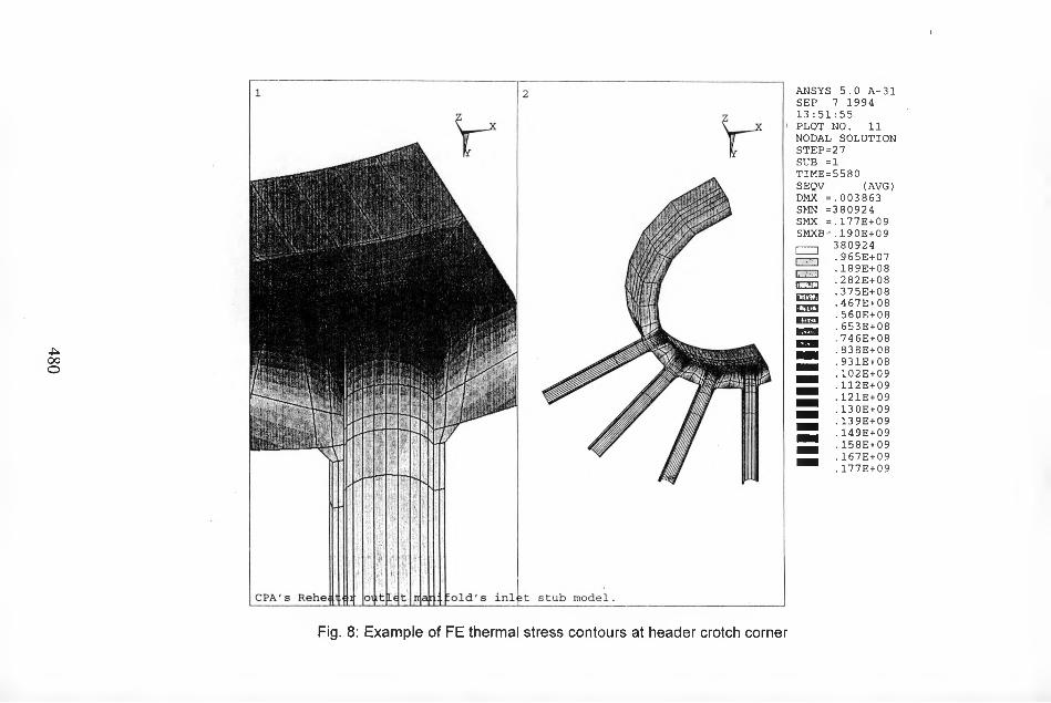
480

i

ANSYS 5.0 A-31 SEP 7 1994 13:51:55 PLOT NO. 11 NODAL SOLUTION STEP=27 SUB =1 TIME=5580 SEQV (AVG)DMX =.003863 SMN =380924 SMX =.177E+09

CZHl~~lr: • i .1

analB'? j I

SMXB=.190E+09 380924 .965E+07 .189E+08 .282E+08 .375E+08 .467E+08 .560E+08 .653E+08 .7 4 6E+08 .838E+08 .931E+08 .102E+09 .112E+09 .121E+09 .13 0E+09 .139E+09 .149E+09 .158E+09 .167E+09 .177E+09

Fig. 8: Example of FE thermal stress contours at header crotch corner

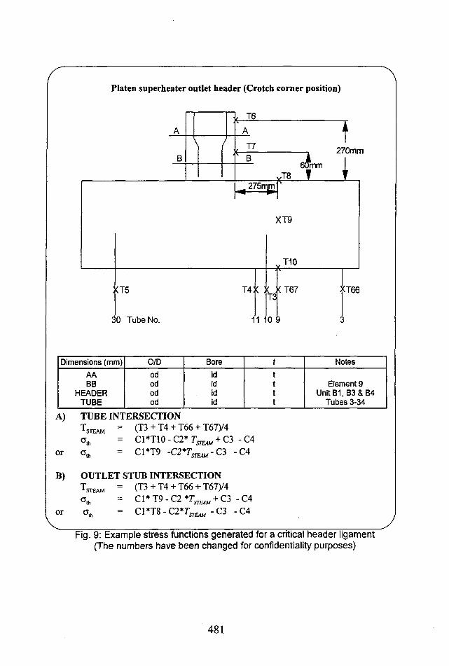
Platen superheater outlet header (Crotch corner position)

\ /

T6

T7

f

60rrjn L

270mm

^ 275rr|nrii

:(T5

30 Tube No.

T4X X

11

XT9

, T10

T3

0 9

( T67 XT66

Dimensions (mm) O/D Bore t Notes

AA od id tBB od id t Element 9

HEADER od id t Unit B1, B3 & B4TUBE od id t Tubes 3-34

A) TUBE INTERSECTIONTsteam = (T3 + T4 + 166 + T67)/4

a,, = CimO-CZT^+CS -C4or a* = C1*T9 -Cl'T^-Cl -C4

B) OUTLET STUB INTERSECTIONTsteam = (T3 + T4 + T66 + T67)/4a,- = 01*19-02*7^ + 03-04

or o* = 01*18-02*7^-03 -04

Fig. 9: Example stress functions generated for a critical header ligament(The numbers have been changed for confidentiality purposes)

481

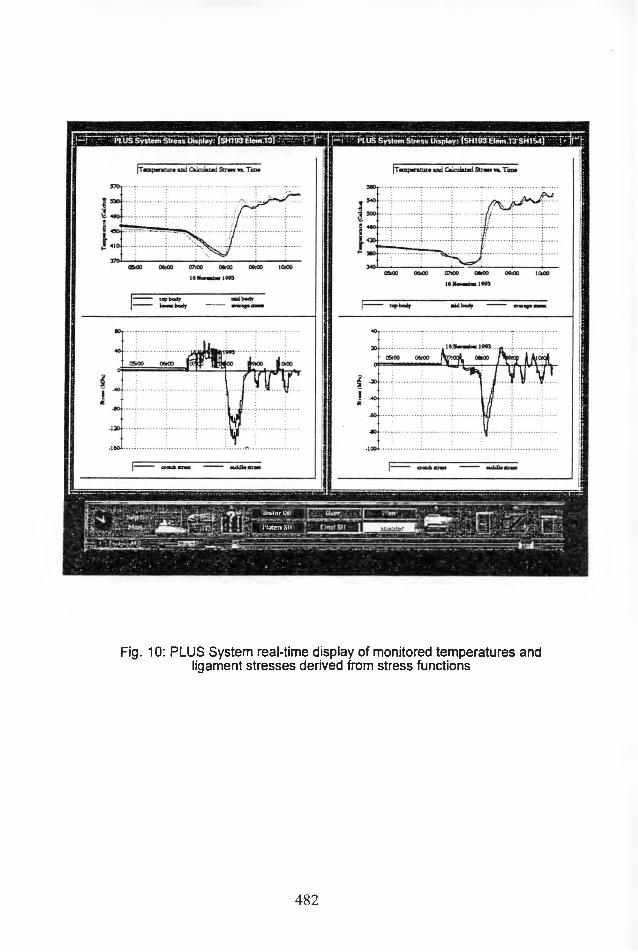
iimlcx Utl

IMjtrn SM abr

Fig. 10: PLUS System real-time display of monitored temperatures and ligament stresses derived from stress functions

23

FATIGUE CREEP

READ IN TEMPERATURE TIME AND ELASTIC

STRESSES

RESOLVE INTO SEQUENCE OF TENSILE/COMPRESSIVE

PEAKS AND DWELLS

CALCULATE FATIGUE DAMAGE FOR EACH

SET OF PEAKS

CALCULATE ELASTIC/ PLASTIC STRAIN

RANGE

SUM DAMAGE

PAIR COMPRESSIVE & TENSILE PEAKS IN DESCENDING ORDER

OF SIZE

DETERMINE THE RELAXED STRESS DURING THE PEAKS TAKING INTO ACCOUNT DWELLS

DETERMINE ELASTIC / PLASTIC CYCLIC

LOOPS USING NEUBER METHOD

CALCULATE CREEP DAMAGE USING A

DUCTILITY EXHAUSTION METHOD

Fig.11: Creep-fatigue damage assessment route

483

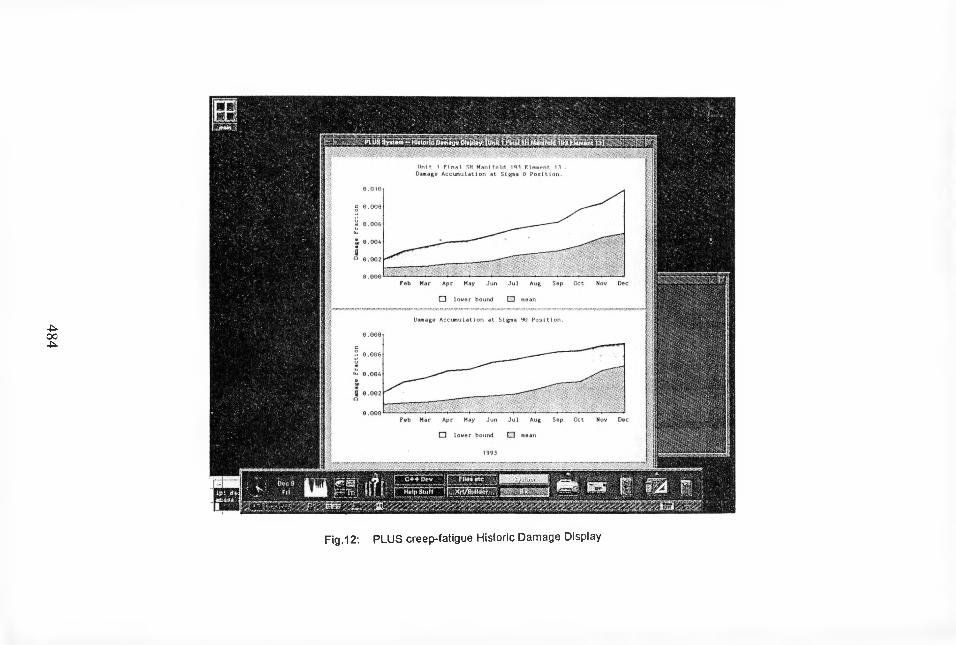
484

Fig.12: PLUS creep-fatigue Historic Damage Display

OPTIMISATION OF POWER PLANT COMPONENT LIFE ASSESSMENT RESULTING FROM THE SP249 PROJECT AND THE SP249 KNOWLEDGE-BASED SYSTEM

A. Jovanovic (MPA, Stuttgart, Germany)

AbstractThe paper presents main (“strategic”) results obtained in the first two years of the SP249 project, addressing the issue of optimisation of enhanced life assessment and life management of components in fossil-fuelled power plants in Europe. The enhancement is related to the achievement of two major issues of the project, namely through development of the set of SP249 Generic Guidelines for Component Life Assessment (CLA) and the corresponding knowledge-based system. The paper summarises the features of both issues, and gives somewhat more details on the knowledge-based system.

1. INTRODUCTION

Following a proposal of 13 European partners, namely: AZT Allianz

(Germany), EdF (France), EDP (Portugal), Endesa (Spain), ERA

Technology (UK), ESB (Ireland), GKM (Germany), ISQ (Portugal), I VO

(Finland), Laborelec (Belgium), MPA Stuttgart (Germany), Tecnatom

(Spain) and VTT (Finland), under the co-ordination of MPA Stuttgart, a

SPRINT Specific Project (designated SP249) has been approved and started

in 1993. At the and of 1994 the project has been extended until the end of

1996, involving Belgian inspection company AIB Vincotte (introducing its

visual inspection guidelines) and involving further FVO (and its FVONDT

database). Overall, main goal of SP249 has been to enhance the transfer of

component life assessment (CLA) technology for high-temperature com­

ponents of fossil fuel power plants, assuring diffusion of modem state-of-

the-art plant CLA technology among power plant utilities and research

organisations in Europe (Brear, Jovanovic, 1992).

485

2. MAIN ELEMENTS OF THE SP249 PROJECT

In order to achieve its main goal, the SP249 project has foreseen (Figure 1)

development and use of two main elements, namely of

a) a set of SP249 CLA Generic Guidelines (a "paper summary" of the

technology to be transferred), and

b) a knowledge-based system (SP249 KBS) for enhancing the transfer

of the CLA technology.

Figure 1: Two basic elements of SP249

The basic idea of the project organisation (Figure 1) is that the knowledge

coming from the power plant should be first summarised in the form of

guidelines (paper) and then transferred into the KBS. The CLA technology

coming from different sources will thus be "packed" into a framework

similar to the one used in MPA ESR system (Jovanovic, Maile, 1992). The

"KBS-supported" use of the guidelines and the corresponding training of

end-users personnel are major issues in the project.

486

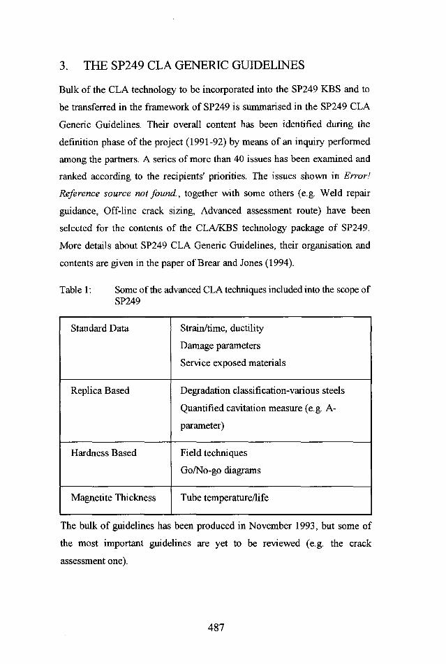
3. THE SP249 CLA GENERIC GUIDELINES

Bulk of the CLA technology to be incorporated into the SP249 KBS and to

be transferred in the framework of SP249 is summarised in the SP249 CLA

Generic Guidelines. Their overall content has been identified during the

definition phase of the project (1991-92) by means of an inquiry performed

among the partners. A series of more than 40 issues has been examined and

ranked according to the recipients' priorities. The issues shown in Error!

Reference source not found., together with some others (e.g. Weld repair

guidance, Off-line crack sizing, Advanced assessment route) have been

selected for the contents of the CLA/KBS technology package of SP249.

More details about SP249 CLA Generic Guidelines, their organisation and

contents are given in the paper of Brear and Jones (1994).

Table 1: Some of the advanced CLA techniques included into the scope ofSP249

Standard Data Strain/time, ductility

Damage parameters

Service exposed materials

Replica Based Degradation classification-various steels

Quantified cavitation measure (e.g. A-

parameter)

Hardness Based Field techniques

Go/No-go diagrams

Magnetite Thickness Tube temperature/life

The bulk of guidelines has been produced in November 1993, but some of

the most important guidelines are yet to be reviewed (e.g. the crack

assessment one).

487

4. THE SP249 KNOWLEDGE-BASED SYSTEM (KBS)

Exploitation of the KBSs within the CLA technology has been successfully

demonstrated in programs such as those of presented at the ACT

Conference (1992), and, in particular case of SP249 project, by the ESR

project of MPA Stuttgart (Jovanovic, Maile, 1992).

The KBS technology appears in the SP249 project at two levels:

a) as a part of the modem CLA technology

b) as the principal means or "vehicle" of the CLA technology

transfer.

SP249 CLA Generic Guidelines are being implemented in a knowledge-

based system (KBS), which serves as the main tool for transfer and

application of the target CLA technology. The system appears as a

conglomerate of single software modules controlled by an overview

module, based on the Advance Assessment Route Intelligent Flowchart. The

whole system is designed as an engineering "tool box", built on top of

commercially available software (a more detailed description is give in the

work of Jovanovic and Friemann, 1994).

The object oriented programming (OOP) appears both at the level of overall

SP249 KBS architecture (each part of the system is an object exchanging

messages with other ones) and at the level of its single parts. The

architecture allows to introduce new modules or to reorganise the existing

ones any time. The hypermedia based parts/modules "cover" the

background information built into the system: the CLA guidelines,

frequently used codes, standards and other documents, case studies. All

hypermedia-based modules and all other modules in SP249 KBS are

controlled by the expert system shell, based on the novel approach of

mirroring the contents of the hypermedia documentation bases in the expert

system shell (Jovanovic, Freimann, Kautz, 1992: Jovanovic, Friemann,

488

1994). The shell is thus "aware" of the contents of the documentation bases

as well of the relations among the single documents (and even parts of

single documents).

As the SP249 CLA Generic Guidelines, the SP249 KBS will cover:

a) Decision making according to SP249 CLA guidelines (decision

aid for making the "3R decision" (replace, repair, run). This

decision is based partly on the regulatory guidelines, partly on the

experience and heuristic knowledge incorporated into the CLA

guidelines.

b) Recommendation regarding the annual inspection (revision)

c) Damage analysis

Using the system the user is expected to be supported by an "intelligent

environment", helping him to calculate, retrieve data (about material,

component, etc.), retrieve necessary standards, obtain advice and, finally,

find an optimised solution for his problem (Figure 2).

5. STRATEGIC ACHIEVEMENT OF SP249 - A STEP TOWARDS EUROPEAN DE FACTO STANDARD FOR OPTIMISED COMPONENT LIFE ASSESSMENT

The KBS technology has been identified (Brear, Jovanovic, 1992) as a

modem and appropriate mean to achieve the consolidation of the CLA

technology necessary for a de facto standard. In other words, by bringing

the technology into the "computer digestible form", the technology itself has

been re-assessed and consolidated. This has been a considerable exercise,

needing frequent review to ensure success. But the results already achieved

show that the guidelines and the system do pave the way towards the de

facto European standard desired for plant life management (in terms of

CLA), leading to:

489

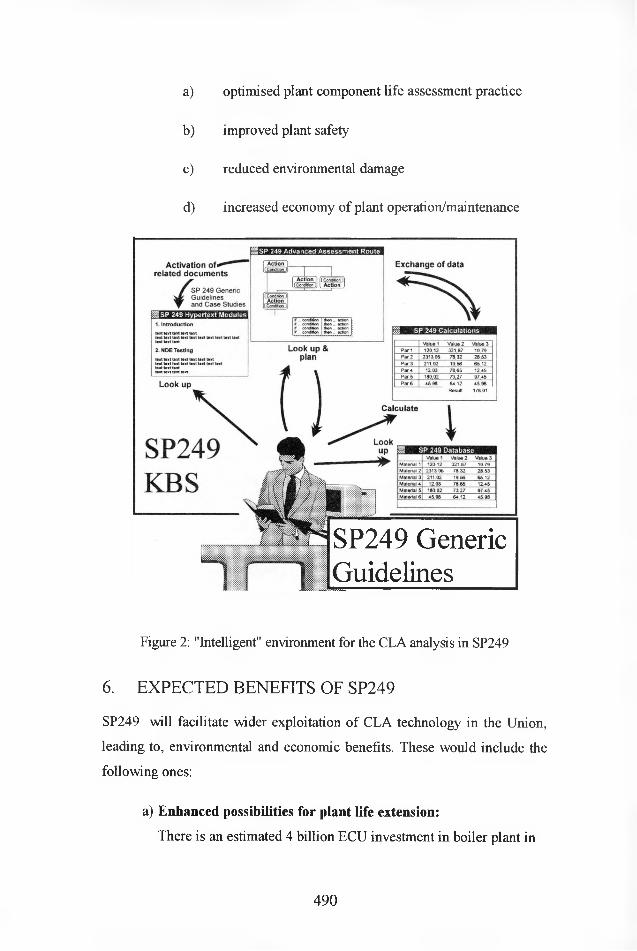
a) optimised plant component life assessment practice

b) improved plant safety

c) reduced environmental damage

d) increased economy of plant operation/maintenance

SP249 Generic Guidelines

Figure 2: "Intelligent" environment for the CLA analysis in SP249

6. EXPECTED BENEFITS OF SP249

SP249 will facilitate wider exploitation of CLA technology in the Union,

leading to, environmental and economic benefits. These would include the

following ones:

a) Enhanced possibilities for plant life extension:

There is an estimated 4 billion ECU investment in boiler plant in

490

Europe. Taking the significance of critical high temperature

components in retirement decisions, and assuming that 20% of

plant may have its life extended by 10 years a financial benefit to

European Industry of 200 million ECU's per year is estimated.

Further financial benefits accrue due to optimised replacement and

refurbishment planning, thereby maximising potential of capital

investment and reductions of forced outages, increasing plant

efficiency and reliability.

b) Enhanced predictive maintenance:

Experience in the USA has shown that predictive maintenance

can save 60% of the costs associated with maintenance (15 to

40% of operating costs) due to the savings by reducing

unscheduled down time, associated lost production/altemative

generation costs, reduced downtime and inspection resources,

optimised refurbishment schedules, and the ability to make

run/retire decisions without employing specialists. Drawing

parallels in Europe savings of 5.5 billion ECU's per year are

estimated.

For a single utility company and in the long-term, expected benefits depend

on local conditions, but for a utility operating say 1000 MWe, extending the

life of its plants for another 5 years would be a gain of over 400x106 ECU.

On the other hand, assuming that SP249 will induce the decrease of only

2% of the overall maintenance cost, it would achieve further savings

another 300,00 of more ECU/year.

Besides, individual utilities expect to benefit from simplified

maintenance/inspection planning resulting from higher precision component

life predictions and from an ability to deploy precious human resources

more effectively. Both are highlighted in utility questionnaire responses

(Brear, Jovanovic, 1992). Optimised component life assessment leads to

491

reduced risks - of both large scale catastrophic failures and of small scale

but extended duration environmental degradation (use of new sites for new

plant, higher emissions etc.). Such factors, though of great importance, are

not easy to quantify.

7. CURRENT ACHIEVEMENTS OF THE SP249 KBS

The first version of the system has been produced and distributed to

partners in May 1994. Partners' comments and wishes were implemented,

and bugs eliminated, during the remaining part of 1994 and a new version

released in April 1995. It contains the following modules:

• Object management modules

• Advance Assessment Route

• Case history management (with over 100 case histories)

• Documentation management (with all CLA Generic

Guidelines, with relevant DIN, TRD, ASME, VGB and

NT standards)

• Material database (with relevant ISO, DIN, BSI, ASTM

and other materials)

• A - Parameter Calculation

• Hardness Calculation

• TULIP (Tube Life Prediction)

• Case History Selection and Management

• Crack Dating

• SP249 Remnant Life Calculation

• Inclusion of oxidation effects

• SP249 Material Database

• Inverse Stress Calculation TRD (new version being

programmed)

492

• Creep and Fatigue Usage Calculation TRD (new version

being programmed)

• Cavity Density

• Linear extrapolation according to Generic Guidelines

003 and 004.

• Chemical Composition influence onto remaining life

• Defect Assessment

Despite the fact that the guidelines were still not finished and the KBS

lacked the full functionality, the first (generic) training has been performed

in June 1994. Main reason for the early start up of the training activity was

the need of direct interaction between the developers of the guidelines and

the system, on one side, and the end-users, in the other side. Further

training has been planned as per partner, on-site training.

An effort has been made to establish the maintenance structure of SP249

KBS, but there are no "clear" solutions so far.

Furthermore, an 'observer group' of over 25 European and world experts has

been established in order to ensure widespread dissemination of experience

gained within SP249.

8. PRACTICAL APPLICATION AND VERIFICATION - THE SP249 WORKED EXAMPLES

Both the SP249 guidelines and the KBS have to be verified in practice. It is

planned for 1995 and will take place within the so called SP249 Worked

Examples. In each of the cases approximately one working week is planned

for:

a) preparation of the necessary inputs

b) presentation of the guidelines and the system to the power plant

personnel involved

493

c) joint (MPA+ERA+partner) analysis of the selected real life

problem

d) direct application of the relevant and applicable parts of the

guidelines and the system, respectively, to the selected problem

e) consolidation of the application results and final discussions with

the power plant personnel.

As shown in Table 2, the series of SP249 Worked Examples will start with

GKM/Allianz in April 1995, with analysis of a main steam line (Figure 3).

Table 2: The “calendar” of the SP249 Worked Examples

One-week session: MPA+ERA+ Partner(s): Planned for

GKM / Allianz (GKM power plant in

Mannheim, main steam line)

April 1995

EDP/ISQ (Carregado power plant, header) Dec. 1995

EdF (power plant yet to be determined) Sept. 1995

Endesa/Tecnatom (Compostilla power plant) June 1995

ESB (power plant yet to be determined) Sept. 1995

Laborelec (power plant yet to be determined) Oct. 1995

IVO (power plant yet to be determined) Oct. 1995

9. DIFFICULTIES, LESSONS LEARNED

Even if it had had a more "conventional" and far less complex goals than

"producing a European de facto standard" and/or "consolidating technology

for component life assessment in power plants" and/or "producing an

494

integrated knowledge based system" for the "European standard" and for the

"consolidated technology", SP249 would have been, with its thirteen

partners, its intercultural gaps and its different philosophies, a project

difficult enough to run and manage. Strongly related to the software

technology which is currently "putting half of the universe upside down,

and making desperate the other half, the project has faced many of the

difficulties.

Figure 3: GKM piping to be used in the first SP249 Worked Example

Most of these difficulties are well known for the software projects in

general (O'Connell, 1994a) and some of them, like delays and insufficient

specificity of the initial planning for some tasks, appeared also in SP249

("An oft-quoted figure is that only 1% of software projects are delivered on

time, within budget and provide what the customer wanted", O'Connell,

1994b).

495

A particular SP249 specific difficulty is the definition of the user profile: it

came out that huge differences exist in the computer- and CLA-related

knowledge among different potential users. These differences led to

different understanding of (e.g.) user-friendliness, usability, etc.

10. CONCLUSIONS

The SP249 Project and the development of the SP249 knowledge-based

system and its future deployment in power plants should help in achieving a

series of economic and technical benefits: e.g. improved availability of

systems and plants, shorter and better utilised maintenance periods, reduced

costs of scheduled inspections due to the optimised inspection strategy-

reduced costs of daily operation (specialists called only when necessary),

reduced unplanned costs, or improved possibilities for the life extension of

the plants.

Joint effort of CEC and European industries (utility companies and

consulting and research organisations), based on the large scale European

application of KBS technology (the total value of SP249 project is about 2.5

MECU) mark a milestone for the KBS technology applications the area of

power plant operation and management in Europe. It opens the way for

further applications in the area and establishes the KBS technology both as

a part of the modem CLA technology and as a powerful vehicle for

technology transfer.

By combining efforts of the CEC and European industries (utility com­

panies and consulting and research organisations) SP249 will become a

milestone for large scale applications of the KBS technology, both as a part

of the modem CLA technology and as a powerful vehicle for technology

transfer.

496

11. ACKNOWLEDGEMENTS

The author wants to acknowledge herewith precious help and collaboration

of all partners in SP249 (see chapter 1) and in particular to the persons

involved in the project on behalf of their companies: Dr. L. Hagn, Allianz,

to Messrs. G. Thoraval and P. Rivron, EDF, to Mr. A. Batista, EdP, to Mr.

E. Santos Endesa, to Messrs. J. M. Brear and J. Jones, ERA, A. Bissell, to

Prof. H. R. Kautz, GKM, to Dr. C. de Araujo ISQ, to Mrs. U. McNiven and

Mr. J. Rantala, IVO, to Mrs. Verelst, Laborelec, to Mrs. M. Aguado

Tecnatom, to Mr. P. Auerkari VTT, to Mr. P. Lowe, SPRINT TAU, to Ms.

Stupka and Messrs. Friemann, Kluttig, Ober, Schwarzkopf, Sommer and

Wolf of MPA Stuttgart, and to all others who have in or the other form

contributed in the realisation of this large European project.

12. REFERENCES

ACT (1992). Advanced Computer Technology Conference 1992, held in Phoenix, Arizona, December 9-11, 1992, Proceedings, Vols 1 and 2, published by EPRI Palo Alto, US, December 1992

Brear, J. M., Jones, G. (1994). A consolidated approach to component life assessment in SP249, Proceeding of the 20th MPA Seminar, vol. 3, MPA Stuttgart

Brear, J. M., Jovanovic, A. (1992). SPRINT Specific Project SP249 "Implementation of Power Plant Component Life Assessment technology using a Knowledge-Based System", Phase I - Definition, Final report. May 1992, ERA technology, Leatherhead, UK, and MPA Stuttgart, FR Germany

Jovanovic, A., Friemann, M. (1994). Overall structure and use of SP249 knowledge based system, Proceeding of the 20th MPA Seminar, vol. 3, MPA Stuttgart

Jovanovic, A., Friemann, M., Kautz, H. R. (1992). Practical Realization of intelligent inter-process communication in integrated expert systems in materials and structural engineering. Proc. of the Avignon '92 Conference Expert Systems and their Applications (Vol. 2-Specialized Conferences). Avignon, pp 707-718.

497

Jovanovic, A., Maile, K. (1992). ESR-A Large Knowledge Based System Project of European Power Generation Industry. Expert Systems With Applications. Vol. 5: 465-477

O’Connell, F. (1994a). How to rate your software project. The Wall Street Journal, Jan. 4, 1994

O’Connell, F. (1994b). Why the domino effect should not be ignored. Computer Weekly, April 14, 1994

498

A CONSOLIDATED APPROACH TO COMPONENT LIFE ASSESSMENT IN SPRINT PROJECT SP249

J M Brear, G T Jones - ERA Technology Ltd, UK A S Jovanovic, M Friemann and Th Geyer - MPA Stuttgart, Germany

1 INTRODUCTION

The objective of the SPRINT Specific Project SP249 is the transfer of state-of-the-art component life assessment technology to a group of European Utilities by means of a knowledge based system. It is intended that this activity will contribute to a larger goal - the establishment of a de facto European Standard for plant life assessment.

These aims are ambitious, so - to impose a realistic constraint - the partners agreed to limit the scope, at this stage, to power plant (and similar) pressure parts operating predominantly in the creep range. Extensions to other industrial sectors and other components is a distinct future possibility.

The project activities have fallen into these broad areas:

Consolidation of existing knowledge, leading to the production of Generic Guidelines for Component Life Assessment - including an overall Advanced Assessment Route and supporting Materials Data

Training the end users in the practical use of the techniques - individually and as a integrated approach

Hands-on’ on plant and on computer

Establishment of a series of case-studies to demonstrate and validate the overall assessment process.

Future extension and dissemination.

Several contributions to this conference address different aspects of the project. The purpose of the present paper is to summarise the approach to Component Life Assessment.

2 PHILOSOPHY

Economic necessity drives the use of plant beyond its design envelope; similar constraints determine the degree of inspection, assessment and maintenance that is appropriate to ensure safe and reliable service. The overriding principle of the Advanced Assessment Route within the Project SP249 Guidelines is to proceed step by step, generating information as economically as possible, minimising disruption to plant function whilst maximising the data generated for immediate and future use. the route is thus essentially iterative, repeating calculations with more exact information as reserve margins decrease.

3 SCOPE AND FORM OF PRESENTATION

The Advanced Assessment Route provides a systematic approach to Component Life Assessment. In its present form it is applicable to high temperature boiler components and pipework. It covers all stages of a life assessment from initial plant prioritisation through conventional and advanced inspection techniques - including defect assessment methods - to the run/repair/retire decision.

499

The route is presented as a series of flow-charts, identical to those displayed on-screen when using the PC knowledge-based-system (KBS). These charts depict each step and sub-step of the main phases of the assessment route, in a strict hierarchical sequence. Facing each chart is an outline text description of each step, with reference to the point in the 'Generic Guidelines for Life Assessment' where the relevant technique or process is described in detail. These supporting documents can be referred to in paper form or via the ’Hypertext' links in the KBS. Where necessary, the logical path through the steps of the Advanced Assessment Route is also explained in the text.

Each Flow Chart has a title band (shaded) at the top which not only describes the activities covered, but also indicates numerically the position of the chart in the overall sequence. The title will be that of the phase, step or sub-step which the chart outlines. The number will be of the form:

Phase.Sub-phase - Step.Sub-step.Sub-sub-step

Each activity thus has a unique identifying number, related to the overall assessment logic. The document symbol:

appears in the top left of the title bar to indicate that the particular chart is a detailed sub-chart, expanding an activity presented as a single step on a higher level chart. ’Clicking' this symbol on the KBS version allows immediate access to the appropriate higher level chart.

Above the title bar, in some cases, is a statement describing the logical entry condition for that chart. These are explained in the text.

Each chart shows a series of boxes denoting the activities that comprise a phase or step of the assessment process. The activity title and reference number are given in the centre of each box. Above this is the logical entry condition to that activity, below it the logical exist condition, or outcome, is shown. The document symbol, shown in a box, indicates that a lower level sub-chart exists - providing a more detailed breakdown of the activity. Again, this sub-chart can be accessed directly via the KBS.

In implementing this route, some compromises have had to be made between three logical systems:

- what can be implemented in the software

- the ’ideal' assessment process

- the realities of hands-on plant access

The result cannot be perfect, particularly at the prototype stage. Its application will always require human intelligence and insight.

4 ACKNOWLEDGEMENTS

This route reflects much existing experience in Europe and further afield - the contributions of all to the science and practice of component life assessment is gratefully acknowledged by the authors and their colleagues in the project. The route was designed at ERA and programmed as an intelligent flowchart at MPA.

This paper is published with the permission of ERA Technology Ltd, MPA Stuttgart and the Project SP249 Steering Committee.

500

5 THE ADVANCED ASSESSMENT ROUTE

This top-level chart shows the overall relationship between the phases of the life assessment process. It commences with the decision to implement a plant life assessment strategy, provides methods of performing the assessment and ends with a run/repair/retire decision. The fundamental process is iterative, bringing in more detailed techniques only when appropriate. Whenever continued operation is allowed, appropriate monitoring and inspection criteria are set.

Phase 0 - Prioritisation

Prioritises progressively at the plant, unit, component and location levels to ensure that the assessment is economically optimised within the bounds of safety and operational requirements.

Phase 1 - General Calculation and Review of Operation

For each component/location identified in Phase 0, a code-based calculation of life consumption is performed and the operational history is reviewed.

Phase 1 - Step 6

If no critical points have been reached, then the component can be left in service under a defined monitoring strategy and the Phase 1 assessment process repeated at a defined future date.

Phase 2 - Inspection-Based Assessment

If the Phase 1 assessment results show that a critical point has been reached, then an inspection allowing access for NDE and metallography is required. Improved life assessment calculations are based on the results of these activities.

Advanced Assessment Route

Phase 1

General calculation Review of Operation

tesults of general calculation OK

Results of general calculation criticalPhase (1-6)

Continue Monitoring

Phase 2Inspection-based assessment

Access for NDE & Metallography

Tnspertioruesult^ntlcar

} Phase 3Repair / Replace / Refine assessment =fnspectionsresu!t?OK OR

NO replacement necessaryleplacement necessary

Phase 4Implement Monitoring &

Inspection Strategy

Phase 5Replacement / retirement Strategic

501

Phase 3 - Repair/Replace/Refine Assessment

If a defect is found during Phase 2 NDE, or if the results of Phase 2 assessment indicate that the component will not survive for two more operating periods, then repair options and the possibilities of refining the assessment are considered.

Phase 4 - Implement Monitoring and Inspection Strategy

If the results of a Phase 2 assessment or a Phase 3 refined assessment indicate a satisfactory remaining life, or after a successful Phase 3 repair, then the component may be returned to service. Appropriate monitoring is installed and reinspection intervals are set. If on-line life-calculation software is installed, then the re-entry point to the assessment route is at Phase 2, otherwise at Phase 1.

Phase 5 - Replacement/Retirement Strategy

If phase 3 indicates that no further refinement of the assessment is possible or that repair is either impossible or uneconomic, then a replace/retire decision is made. Controlled operation for a limited time may be allowed.

Separate papers in this conference address the defect assessment route (Phase 2.2) and demonstrate the general use of the assessment route by means of a worked example.

502

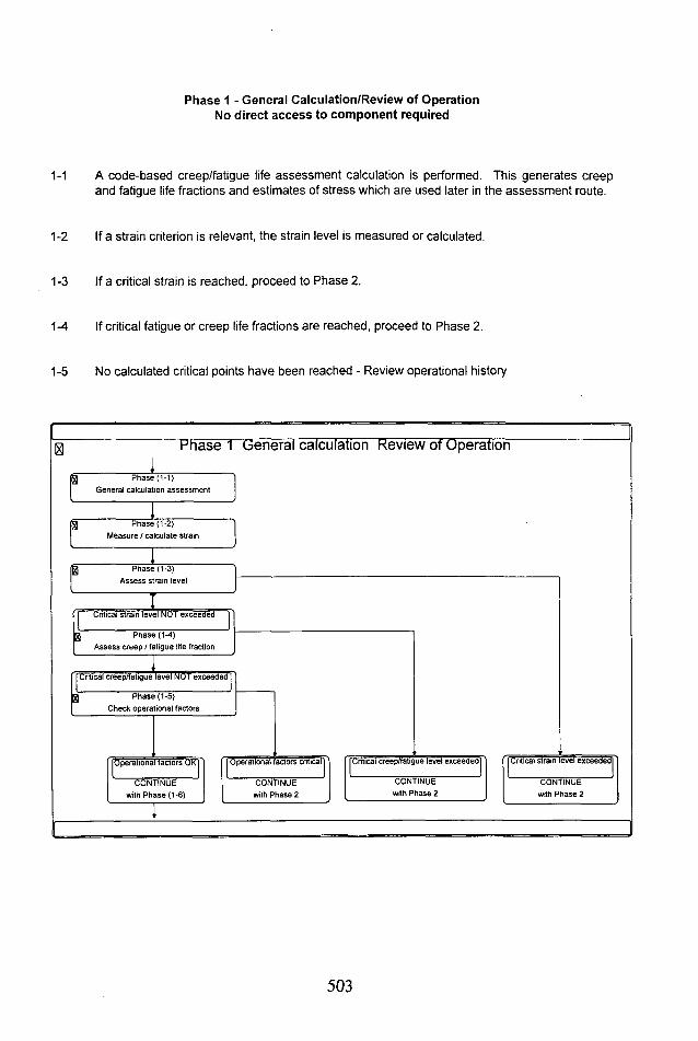
Phase 1 - General Calculation/Review of Operation No direct access to component required

1-1 A code-based creep/fatigue life assessment calculation is performed. This generates creep and fatigue life fractions and estimates of stress which are used later in the assessment route.

1-2 If a strain criterion is relevant, the strain level is measured or calculated.

1-3 If a critical strain is reached, proceed to Phase 2.

1-4 If critical fatigue or creep life fractions are reached, proceed to Phase 2.

1-5 No calculated critical points have been reached - Review operational history

Phase 1 General calculation Review of Operation

Phase {1-1)General calculation assessment

Phase (1-2)Measure / calculate strain

Phase (1-3) Assess strain level

Critical strain level NOT exceedet

Phase (1-4)Assess creep / fatigue life fraction

[ Critical creep/fatigue level NOT exceeded

Phase (1-5)Check operational factors

Critical strain level^xceededCritical creep/fatigue level exceedetOperational factors OK actors criticaliperational

CONTINUE with Phase 2

CONTINUE with Phase 2

CONTINUE with Phase 2

CONTINUE with Phase (1-6)

503

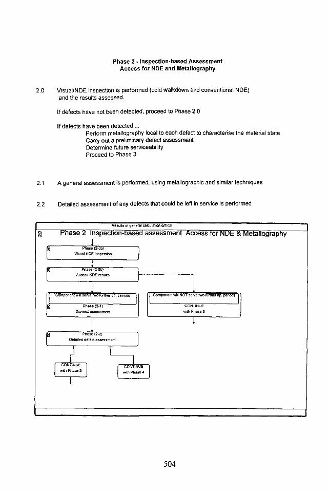
Phase 2 - Inspection-based Assessment Access for NDE and Metallography

2.0 Visual/NDE inspection is performed (cold walkdown and conventional NDE) and the results assessed.

If defects have not been detected, proceed to Phase 2.0

If defects have been detected ...Perform metallography local to each defect to characterise the material state Carry out a preliminary defect assessment Determine future serviceability Proceed to Phase 3

2.1 A general assessment is performed, using metallographic and similar techniques

2.2 Detailed assessment of any defects that could be left in service is performed

Results of general calculation critical

Phase 2 Inspection-based assessment Access for NDE & Metallography§

504

Phase 2.1 - General Assessment

2.1- 1 Apply metallographic assessment techniques

2.1- 2 Review available temperature data

2.1- 3 Generate life prediction using all data now available

A separate paper gives a worked example demontrating many of the methods relevant here

Component will serve two further op. periods

Phase (2-1) General assessment

CONTINUE with Phase (2.2)

Apply metallographic assessment techniquesPhase (2-1.1) (GG 1)

Check temperature dataPhase (2-1.2)

Generate life prediction using all available dataPhase (2-1.3)

1

Phase 2.2 - Detailed Defect Assessment

This covers ligament creep life, creep and creep/fatigue crack initiation and growth and final failure criteria [- described in a separate paper in this conference]

505

This phase is entered if a defect has been found or the assessed life is less than two operational periods.

3-1 Repair options are considered

3-2 If repair is possible, it is done and the life of the repaired component is re-appraised. If the life is acceptable, proceed to Phase 4.

3-3 If the assessed life of the repaired component is not adequate then a refined assessment is required

3-8 If the repair followed a preliminary defect assessment (Step 2.Ob-5), then proceed to Phase 2.1

3-4 If repair was not possible, or repair followed a full defect assessment (Phase 2.2) then consider the possibility of refining the assessment further

3-5 If refinement is not possible, proceed to Phase 5

If refinement is possible, then3.6 Refine input data3.7 Revise calculations using new data3.9 Return to Phase 2-3.3

Phase 3 - Repair/Replace/Retire/Refine Assessment

Inspection results critical

Phase 3 Repair / Replace / Refine assessment

506

Is the Repair Option Possible? (3-1)

3-1.1 Is the component life defect dominated?

If not, then repair is not a viable option - proceed to Step 3-4

3-1.2 Is a repair technically and economically possible?

If not, proceed to Step 3-4

If possible, proceed to step 3-2

Phase (3-1) Is repair option possible

Phase (3-1.2)Can a repair be made (technically / economically) ?

iepair is possible

CONTINUE with Phase (3*2)

Life defect dominated

Phase (3-1.1)Is life defect dominated ?

Life defect NOT dominaleTUTf

Repair is NOT possible

CONTINUE

with Phase (3-4)

507

Repair and Review (3-2)

3-2.1 Perform repair

3-2.2 Assess life of repaired component, using results already available from Phases 1,2.1

If life is acceptable, proceed to Phase 4

If not, proceed to Step 3-3

Repair is possible

Phase (3-2) Repair and review

Phase (3-2.1) (GG 5) Repair

Phase (3-2.2)Is life NOW adequate ?

adequate

Phase (3-2.3)CHECK : Has a full Phase (2.1 / 2.2) assessment been performed ?

j Phase (2.1 / 2.2 ) NOT performed on adequate!,2) performei

CONTINUE with Phase A

CONTINUE with Phase (2-1)

CONTINUE with Phase (3-4)

508

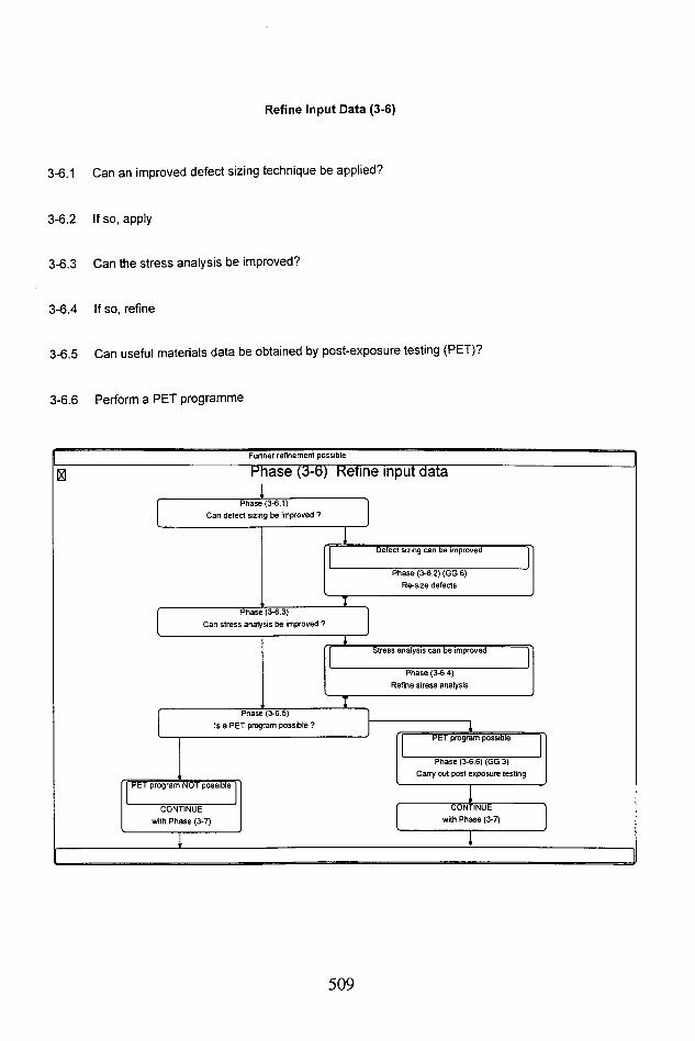
Refine Input Data (3-6)

3-6.1 Can an improved defect sizing technique be applied?

3-6.2 If so, apply

3-6.3 Can the stress analysis be improved?

3-6.4 If so, refine

3-6.5 Can useful materials data be obtained by post-exposure testing (PET)?

3-6.6 Perform a PET programme

Further refinement possible

Phase (3-6) Refine input data

tress analysis can be improved

Phase (3-6.4) Refine stress analysis

program possible

Phase (3-6.6) (GG 3) Carry out post exposure testing

CONTINUE with Phase (3-7)

Phase (3-6.1)Can defect sizing be improved ?

Phase (3-6.5)

is a PET program possible ?

Phase (3-6.3)Can stress analysis be improved ?

TETprogram NOT possible

CONTINUE with Phase (3-7)

Defect sizing can be improved

Phase (3-6.2) (GG 6) Re-size defects

509

Revise Calculations (3-7)

3-7.1 Repeat the general calculational assessment (as Step 1-1) using refined stresses and materials data

3-7.2 Repeat the defect assessment (Phase 2.2) using refined defect sizes, stresses and materials data

3-7.3 Re-appraise results of refined assessment

Phase (3-7) Revise Calculations

□

510

Phase 4 - Implement Monitoring and Inspection Strategy

If the results of the inspections and the calculated life are adequate (after repair if necessary), the component can be returned to service with appropriate strategies for monitoring and inspection in

place.

Monitoring Strategy (4-1)

4-1.1 Are growing cracks present?

4-1.2 If definitely or possibly, they should be monitored

4-1.3 If not, global loads and strains should be monitored

4-1.4 Temperature monitoring should be reviewed

Phase (4-1) Establish and implement further Monitoring strategy

| Growing c

Phase (4-1.2) Monitor defects

one of the previous actions finisl

Phase (4-1,4)Review temperature monitoring

CONTINUE with Phase (4.2)

Phase (4-1.1)Are growing cracks present ?

g Phase (4-1.3)Monitor global loads and strain

Growing cracks NOT present

J

511

Future Inspection Strategy (4-2)

4-2.1 On the basis of the assessed component life and likely degradation rate, establish a future reinspection interval

4-2.2 Is an on-line life calculation monitor is installed?

4-2.5 If so, then at the next inspection, re-enter the assessment route at Phase 2

4-2.3 If not, then consider installing such a monitor and ...

4-2.4 ... at the next inspection, re-enter the assessment route at Phase 1

This is the end point for a component which continues in service

"I Phase (4-2) Establish and implement further inspection strategy

monitored on-line

Phase (4-2.3)Consider installing an on-line monitor

ored on-line

Phase (4-2.4)At next inspection CONTINUE with Phase 2

Phase (4-2.1)Determine optimum inspection interval

Phase (4-2.2)Is an on-line monitoring system installed ?

Phase (4-2.4)At next inspection CONTINUE with Phase 1

512

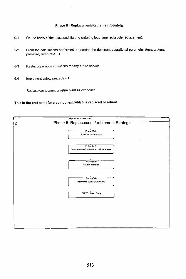
Phase 5 - Replacement/Retirement Strategy

5-1 On the basis of the assessed life and ordering lead-time, schedule replacement.

5-2 From the calculations performed, determine the dominant operational parameter (temperature, pressure, ramp-rate...)

5-3 Restrict operation conditions for any future service

5.4 Implement safety precautions

Replace component or retire plant as economic

This is the end point for a component which is replaced or retired

Replacement necessary

Phase 5 Replacement / retirement Strategie1

Phase (5-1)Schedule replacement

Phase (5-2)Determine dominant operational parameter

Phase (5-3)Restrict operation

Phase (5-4)Implement safety precautions

GO TO : Case Study

514

Structure and Use of the SP 249 Knowledge Based SystemA. Jovanovic, M. Friemann

Staatliche Materialprufungsanstalt (MPA) Universitat Stuttgart

Stuttgart, Germany

Abstract

The structure and use of the SP 249 software system developed within the

European SPRINT SP 249 project is described in this paper. The SP 249

software is built as an easy to use toolbox for advanced remaining life esti­

mation and management. It provides a series of calculation modules, full-

text documents of pertinent literature in the problem area, an intelligent

flowchart to guide the user during the assessment procedure and a support­

ing database with all relevant material properties. Besides, the system sup­

ports the assessment with a set of case studies.

1. INTRODUCTION

The SPRINT Specific Project (designated SP 249) has been approved to

enhance the transfer of component life assessment (CLA) technology for

high-temperature components operating in creep and creep-fatigue regime

in fossil fuel power plants [1].

The distinctive feature of the SP 249 project is the use of a knowledge-

based system (KBS) for enhancing the transfer of the CLA technology to

power plants. The KBS technology appears in the project at two levels:

• as a part of the modem CLA technology

• as the principal means or "vehicle" of the CLA technology transfer.

General aspects of the system are described in [2], The structure of this

paper is as follows: first the general use is described, then the single

modules are described and in section 7 the integrated use is described.

515

2. STRUCTURE OF THE SYSTEM

2.1 THE SP 249 SOFTWARE BASELINE

The system is built on the basis of five development tools1 2 3 in the MS Win-

dows 3. lx environment. The integration of these tools is realised via the

Windows system facilities DDE, OLE, DLL and launching with command

strings. Based on the experience with end-users the appearance and usage of

the software is similar to standard MS Windows applications.

In contrast to more conventional systems the user interface is not presented

by a single application. All the development tools were used to create sin­

gle modules and therefore are part of the user interface.

The SP 249 KBS is a modular object-oriented software. Single software

modules of the KBS are objects, as well as data, information and knowledge

in the system knowledge base are also handled and stored as objects.

2.2 SOFTWARE STRUCTURE

Table 1 Single modules and their tasks in SP 249 KBS

Module Task

Workbench overview/control of the modules, logging of the session

Advanced Assessment Route

advice for the next action to the user

DocumentationBase

for background information and on-line documentation

Case Studies background information for support in decision making

Single Calculations to calculate single results (as input for AAR)The SP 249 software system is organised as "conglomerate" of software

1 KAPPA-PC, Guide, MS C++, MS Visual Basic, MS Access. See [3] for details.2 MS, Microsoft and Windows are trademarks of Microsoft Corporation3 DDE = dynamic data exchange , OLE = abject linking and embedding, DLL = dynamic link library

516

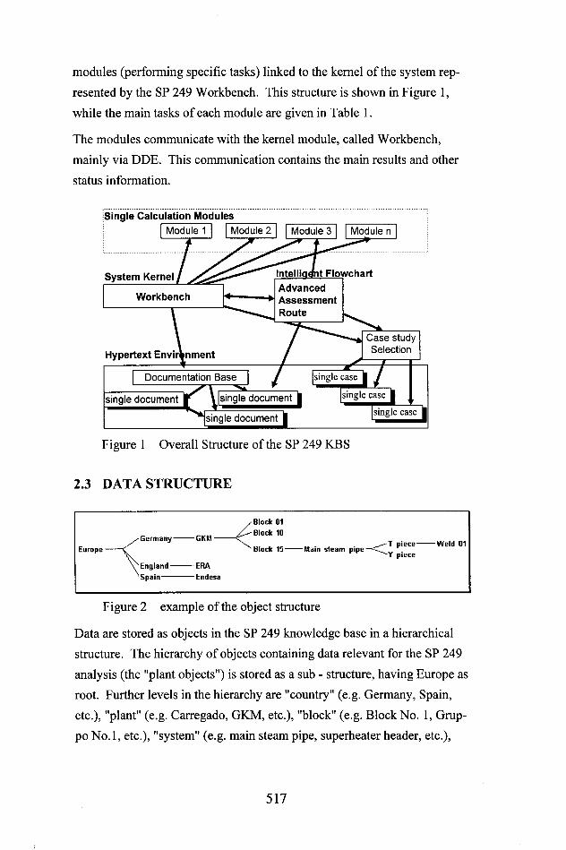
modules (performing specific tasks) linked to the kernel of the system rep­

resented by the SP 249 Workbench. This structure is shown in Figure 1,

while the main tasks of each module are given in Table 1.

The modules communicate with the kernel module, called Workbench,

mainly via DDE. This communication contains the main results and other

status information.

Single Calculation ModulesModule 1 Module 2 Module 3 Module n

System Kernel / ifiiemutfiii nutAdvanced

Workbench *------------- AssessmentRoute

Hypertext Envi^nment j Case studv Selection/

Documentation Base / single case l/single document \ single document | single case |

single document |single case |

Figure 1 Overall Structure of the SP 249 KBS

2.3 DATA STRUCTURE

EuropeGermany-------- GKM

England---------- ERASpain--------------Endesa

Block 01 Block 10

Block 15------- Main steam pipeT piece--------Weld 01Y piece

Figure 2 example of the object structure

Data are stored as objects in the SP 249 knowledge base in a hierarchical

structure. The hierarchy of objects containing data relevant for the SP 249

analysis (the "plant objects") is stored as a sub - structure, having Europe as

root. Further levels in the hierarchy are "country" (e.g. Germany, Spain,

etc.), "plant" (e.g. Carregado, GKM, etc.), "block" (e.g. Block No. 1, Grup-

po No.l, etc.), "system" (e.g. main steam pipe, superheater header, etc.).

517

"component" (e.g. elbow, T-piece, etc.), and "location" (e.g. location n,

weld x upper side, etc.). The hierarchy is schematically shown in Figure 2.

Inputs and outputs of the calculations/analyses performed are also handled

as objects. These "calculation/analysis objects" are then attached to various

“plant objects”. E.g. the remaining life calculation based on hardness

measurements can be performed on a location, the TRD calculation can be

performed on a component. A list of available analyses/calculations is

given in section 4.2.

The hierarchical structure of the "plant objects" simplifies their recovering.

Furthermore it allows to apply the principle of "inheritance" e.g. if one

defines a tubing to be built of material 13 Cr Mo 4 4, this will cause all parts

of this tubing to have this material property as a default. Applying inheri­

tance helps to avoid unnecessary user input and facilitates storing of data.

Furthermore the software system provides the means to store all relevant

data. The work done during a session is logged in a transcript, which can be

stored and printed out.

3. GENERAL USE OF THE SYSTEM

Use of the system is schematically shown in Figure 3. A SP 249 user (1)

would have to solve a problem related to a high temperature power plant

component (2). In order to solve it, the SP 249 project is offering him two

tools: the SP 249 Generic Guidelines for component life assessment (CLA)

in a "paper form" (3), and the computer software SP 249 KBS (4). The

structure and use of the Guidelines "on paper" is described in work of Brear

[5],

The software part offers essentially three types of support:

a) "Look up" (and store) type of support:

The user can look up (and store) information in the case study collection

(5) in the Advanced Assessment Route (AAR) (7) and in the calculation

part (6) of the system. He can also look up the guidelines and other

documents like standards, norms, etc. (5), as well as the material data (8).

518

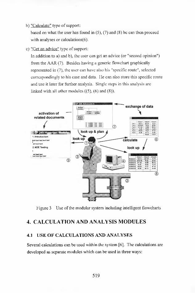
b) "Calculate" type of support:

based on what the user has found in (5), (7) and (8) he can then proceed

with analyses or calculations^).

c) "Get an advice" type of support:

In addition to a) and b), the user can get an advice (or "second opinion")

from the AAR (7). Besides having a generic flowchart graphically

represented in (7), the user can have also his "specific route", selected

correspondingly to his case and data. He can also store this specific route

and use it later for further analysis. Single steps in this analysis are

linked with all other modules ((5), (6) and (8)).

activation of related documents

— SP 249 Hypertext Modules

1. Introduction

text text text text text j t

ext text text

2. NDE Testing

ext text text text text text text

Figure 3 Use of the modular system including intelligent flowcharts

4. CALCULATION AND ANALYSIS MODULES

4.1 USE OF CALCULATIONS AND ANALYSES

Several calculations can be used within the system [6], The calculations are

developed as separate modules which can be used in three ways:

519

1. Started from the Windows Program-Manager or SP 249 System work­

bench (see Figure 8) as "unbound" (separate) application

• the user has to input all necessary data,

• the user needs to care about saving input and results in a file;

2. started from the SP 249 System as a so called "bound" calculation (see

Figure 10):

• the necessary basic data is passed to the calculation from the system

kernel,

• the user does not need to care about data storing,

• the result is returned to the kernel, which will use it for further

examination;

3. started from the AAR in the ExpertChart application as a "bound"

calculation (see Figure 12):

• like in the second way,

• in addition the result is also returned to the AAR module, which will

use it for further examination and advice.

The modular construction was based on the end-users requests to reflect the

way they work.

a) On one hand they have to deliver single calculation results. Therefore

they use the modules like pocket-calculators.

b) On the other hand, using the system as described in the introduction the

calculation modules serve for the higher goal to decide upon

"run/repair/replace". Therefore the coupling of all single modules has

been automated.

4.2 SINGLE CALCULATION/ANALYSIS MODULES

Based on the idea of the engineering ‘tool box’ the object-oriented architec­

ture allows to introduce single modules. The main task of these modules is

the integrated use with full integration of data and program start-up. The

520

calculation/analysis modules can also be used as single applications in the

MS Windows environment. The modules developed and integrated into the

system are:

• Creep and fatigue usage calculation according to German TRD-code,

including inverse stress calculation,

• SP249 remnant life calculation, including the influence of chemical

composition of material onto remaining life,

• life fraction based on ‘A’ - parameter,

• life fraction based on cavity density,

• life fraction based on hardness (life estimation via temperature),

• temperature calculation from oxide thickness, including oxidation ef­

fects and life prediction,

• Crack dating by oxide thickness and/or temperature measurement

• Extrapolation of remaining life from post exposure testing data

• Defect (Crack) Assessment and Life Prediction

In the following sections, the TRD inverse design calculation and the ‘A’-

parameter module are described as representative examples. Moreover the

SP 249 material data base as the supporting module for the calculations is

described.

4.2.1 TRD inverse design Calculation

The TRD calculation module calculates the life fraction based on inverse

design following the German TRD design code [4], Creep and fatigue are

taken into account. The stress calculation is possible for straight tube,

elbow, T-piece, Y-piece and header geometry. The module uses the SP 249

material data base (described in section 4.2.3) as an underlying module, p-

T tables can be imported from an on-line data retrieval system. The

calculation of the usage due to cyclic loading is possible in the three

different ways, as described in TRD code.

521

TRD INVERSE DESIGNFile Edit View Data input Calculation Results Window Help

I Bn

C:\SP249iEXAMPLESVrRD\TEST5NN.TRD

Component data sheet Component Type | T-Piece

Plant

Comp. Name

Location

Design piess

Working pre;

Operating ho

ComponeDIMENSIONS D

Inside diameter ol Wall thickness of Inside diameter of Wall thickness of Length of inward Out-of-roundness Design wall thickr

X

Total Usage Factor

Damage due to creepfx Sum for evaluated period (pi-matrix)

P Sum prior to evaluated period

3123 m

5 1M

Damage due to fatiguef-' Sum for evaluated period (Table 5)

Sum for evaluated period (Regime)

f” Sum for evaluated period (Table 4}

r" Sum prior to evaluated period

f 10.139 m

["24.466 IXi

i£

16.342 [XI

11*1

Total usage factor ’w 277589 [%]OK.

Cancel

Figure 4: The TRD inverse design calculation, Results window

4.2.2 ‘A’ - Parameter Calculation

Figure 5: The ‘A’-parameter calculation window.

The ‘A’-parameter is defined as the number of fractions of cavitating grain

boundaries encountered in a line parallel to the direction of maximum prin-

522

cipal stress [5]. After performing the measurements with an optical micro­

scope the values have to be typed in into the software. The software then

calculates the remaining life and necessary statistical data, which shows the

accuracy of the measurements. In the absence of a crack the Life fraction LF

is calculated, in the presence of a crack the residual ductility fraction, used

in the crack growth rate equation, is calculated. The parameter n, p and A

on which lifetime calculation is based are included as standard values in the

program. Figure 5 shows the appearance of the module on a large screen.

4.2.3 Supporting module - The Material Database

The SP249 material database comprises data for most of the today’s mate­

rials used for high temperature components in power plants, given by stan­

dards like ISO, DIN, AFNOR, ASTM, BS, DIN and others, as well as some

data from other sources.

Given that the users of the SP249 material database are subject to different

statutory requirements, the following approach has been adopted. The in­

formation from each relevant summary document has been included into a

common format, with blank fields where data are not provided/available.

Since the ISO data provide the closest existing approach to a consolidated

data set, blank fields in the ISO data sheets are filled, where possible, with

the best available data from elsewhere. For convenience and to help com­

parison, the materials are grouped into families, classes and subclasses

forming a hierarchical structure [8]. All data are stored in twelve data ta­

bles. The contents of the data tables are:

Title and description of the material, source specification, range for which

the data are expected to apply, tensile data, rupture parameters, stress de­

pendency of rupture life (parameters), stress dependency of rupture life

(explicit), rupture strength - creep strength relationship, average rupture

strengths, allowable rupture strengths, creep strengths, physical property

data

523

5. HYPERTEXT MODULES

The hypertext modules display documents from different sources for

different goals:

• frequently used codes and standards allow explanation of actions

performed in the SP 249 system

• CLA guidelines for advanced assessment, produced in this project, allow

explanation of actions performed in the AAR

• case studies - worked examples and failure cases - support the user in

decision making, where the system cannot decide on the basis of strict

rules.

5.1 DOCUMENTATION BASE

Documentation base

Call documents! □

? ;|VGB - Guidelines

r>>i 300>>;17155

R 509 L

rr~ifechn. Agreements and TS-Reports

SEE] 301 [Ml 508»j17175 >>|54150

Recurring Examinations of Pipe Line Systems

>"> (1983/6) Examination of Surface Microstructure » (1992) Guideline for the Assessment of Microstructure

and Damage Development of Creep Exposed Materials (draft)

iNordtest:

THASME:

!i»| NT 170 Reference Micrographs

] ASME B31.1-1989 Appendix D

? ] SP 249 specific » CLA GG 000»>>

>>»

CLA GG 002CLA GG 004 Egg 004 Annex 1 CLA GG 006 CLA GG 008CLA Advanced Assessment Route

»»

"IF»

CLA GG 001 CLA GG 003 CLA GG 005 CLA GG 007 CLA GG 009

j:>»j VTT Inspection criteria of hot pipework

Help Main Menu Case Study Matrix Quit

Figure 6 SP 249 Documentation base

The hypertext based environment allows the user to view documents on­

screen, easily navigating through the documents structure, expanding and

collapsing documents to display different levels of detail. Figure 6 shows

the main page with the hyperdocuments stored in the system, while Figure 7

524

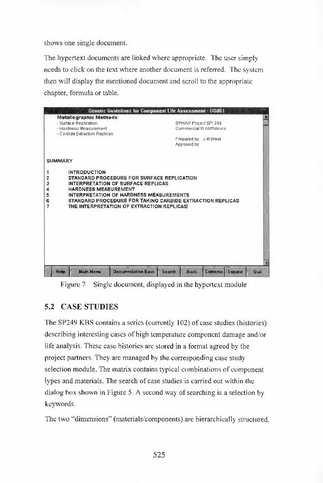
shows one single document.

The hypertext documents are linked where appropriate. The user simply

needs to click on the text where another document is referred. The system

then will display the mentioned document and scroll to the appropriate

chapter, formula or table.

Generic Guidelines for Component Life Assessment - GG001Metallographic Methods:- Surface Replication- Hardness Measurement- Carbide Extraction Replicas

SUMMARY

SPRINT Project SPI 249 Commercial in confidence

Prepared by: J M Brear Approved by:

1 INTRODUCTION2 STANDARD PROCEDURE FOR SURFACE REPLICATION3 INTERPRETATION OF SURFACE REPLICAS4 HARDNESS MEASUREMENT5 INTERPRETATION OF HARDNESS MEASUREMENTS6 STANDARD PROCEDURE FOR TAKING CARBIDE EXTRACTION REPLICAS7 THE INTERPRETATION OF EXTRACTION REPLICAS]

| Documentation Bare | Search |Help Main Menu Back Contents Expand j Quit

Figure 7 Single document, displayed in the hypertext module

5.2 CASE STUDIES

The SP249 KBS contains a series (currently 102) of case studies (histories)

describing interesting cases of high temperature component damage and/or

life analysis. These case histories are stored in a format agreed by the

project partners. They are managed by the corresponding case study

selection module. The matrix contains typical combinations of component

types and materials. The search of case studies is carried out within the

dialog box shown in Figure 5. A second way of searching is a selection by

keywords.

The two “dimensions” (materials/components) are hierarchically structured.

525

A search is started by selecting an item in the list of materials and another

on the list of components. All cases within the selected class and their sub­

structure will be found. The number of entries found is shown in the upper

right comer while the case names are listed there below. The user selects a

single case out of a range of the listed cases, which is then displayed in the

hypertext environment.

Figure 5: Dialog box of Case study matrix

The usefulness of the system was further enhanced by linking the case

studies with AAR. This is realised by means of keywords, attached to

single steps of AAR and keywords attached to the case studies. The case

studies are in this way used as an additional explanation how single steps in

the AAR have to be performed.

6. THE SP 249 WORKBENCH

6.1 GENERAL

After starting the SP 249 system from Program-Manager in Windows, the

'Workbench' window (Figure 8) appears.

The user can open an existing or create a new file. This file contains the

user defined structure of objects and their data, given by the user. Fie would

526

then probably edit the object structure, to add data or add new objects.

Figure 8 The start-up and main window

Next step would be to select the object to analyse. For the overall analysis

he would then start the Advanced Assessment Route.

In parallel to these steps the following parts of the system are accessible:

• the hypertext module to review documents and case studies

• auxiliary tools (e. g. report generator, transcript).

An on-line help using the Windows help facility is included in the system.

Each of the modules has also it's own help fde which explains how to use

the module (explanations for the assessment side are handled in the CLA

guidelines). The kernel help file explains how to use the overall system.

6.2 WORKING WITH SP 249 OBJECTS ("PLANT

OBJECTS")

As described previously, the system is working on the basis of an object

structure. Figure 9 shows the dialog for editing the object tree. The user

can add, rename, delete and edit objects.

If the user wants to analyse an object in the object base, he needs to select it

first. He would therefore use the 'Object Selection' dialog.

527

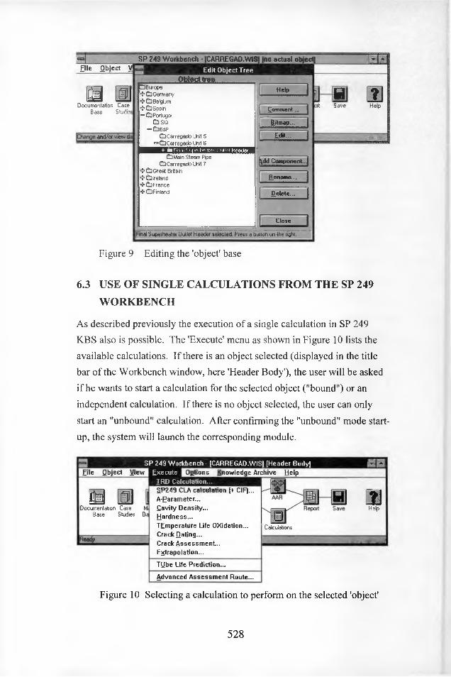
File Object V

Documentation Case Base Studies

[Change and/or view da

SP 249 Workbench - [CARREGAD.W1S] jno actual object]Edit Object Tree

-ObjecUreg-^Europe❖ CD Germany ‘v1 CD Belgium ■v1 CD Spain

CD Portugal CD ISO

•= CD EdPCDCarregado Unit 5 GCarregado Unit 6

CD Main Steam Pipe GCarregado Unit 7

❖ G Great Britain❖ G Ireland cu> G France❖ G Finland

Help

Comment... f

Bitmap ..

Edit ..

^dd Component.j

1 HUort Save

fiename...

delete..

Close

final Superheater Outlet Header selected Press a button on the right.

Figure 9 Editing the 'object' base

6.3 USE OF SINGLE CALCULATIONS FROM THE SP 249

WORKBENCH

As described previously the execution of a single calculation in SP 249

KBS also is possible. The 'Execute' menu as shown in Figure 10 lists the

available calculations. If there is an object selected (displayed in the title

bar of the Workbench window, here 'Header Body'), the user will be asked

if he wants to start a calculation for the selected object ("bound") or an

independent calculation. If there is no object selected, the user can only

start an "unbound" calculation. After confirming the "unbound" mode start­

up, the system will launch the corresponding module.

File Object ViewSP 249 Workbench - [CARREGAD.WISj (Header Body]

ExecuteTRD Calculation.

Documentation Case M Base Studies Dr

Ready

Options Knowledge Archive Help

SP249 CLA calculation (+ OF)... A-Parameter...Cavity Density...Hardness...TEmperature Life Oxidation... Crack Dating...Crack Assessment... Extrapolation...

TUbe Life Prediction-

Advanced Assessment Route..

Help

Calculations

Figure 10 Selecting a calculation to perform on the selected 'object'

528

7. THE SP 249 ADVANCED ASSESSMENT ROUTE

7.1 MODULE DESCRIPTION

The Advanced Assessment Route (AAR) module is the key module in the

SP 249 System. It combines all the calculation modules to an overall ad­

vanced assessment route. The AAR itself supports the user to decide upon

the basic goals of the SP 249 System application (run/repair/replace).

Advanced Assessment Route

Inspection results critical

iJ Phase 3Repair / Replace / Refine assessment

Results of general calculation OK

Inspection results OK OR NO replacement necessary

Phase 1General calculation

Review of Operation

Phase (1 -6) Continue Monitoring

Phase 5Replacement i retirement Strategic

Replacement necessaryPhase 4

Implement Monitoring & Inspection Strategy

Results of general calculation critical

Access for NDE & Metallography

Phase 2Inspection-based assessment

Figure 11 AAR: highest level of the flowchart

The AAR is implemented as an active flowchart [7]. Boxes are activities

which can have sub-activities (Figure 11). Facts coming as input during the

session are then combined with the rules stored within AAR, and a recom­

mendation is produced for each activity/subactivity.

Advantages of such an appearance are:

• Complex activities are divided into hierarchically ordered, small entities

of information. So one can limit the portion of details he wants to look at.

• AAR automatically layouts activities and the connections between them.

529

• AAR stores every user input and uses it for calculations about the possi­

ble next steps in the execution of one activity.

• Compared to rule based systems the process is presented in a very clear

way to the end-user.

Activities can be "started", "informed" and "ended". Information means the

entry of a value that describes the result of an activity. The "information"

can also be performed by a calculation module, executed through the start

of the activity.

Each of the boxes can be connected to a node in a hypertext document. De­

pendant on the user’s task, he can request for appropriate pieces of hyper­

text by clicking on the description area of an activity. By corresponding

keywords a list of supporting case studies (see section 5.2) can be reviewed.

7.2 INTEGRATED USE OF AAR

Figure 11 shows the main level of "Advanced Assessment Route" in

SP 249. The main level (activity) consists of 6 sub-activities. These

activities represent Phases (or ‘main’-activities) 1 to 5 of AAR.

The description of an activity includes an activity number and the CLA

guideline [5] attached to that activity. The user has to click on the green tri­

angle to start the corresponding activity. Activities that are finished can be

ended by a click on the green triangle in the lower left. Dependant on their

preconditions other activities can be started. After having started an activity

with sub-activities the first sub-activity can be started.

Figure 12 shows an example of AAR, in this particular case the interpre­

tation of surface replica. This is covered by sub-activity 1.1.4 of Phase 2.

The marked activity shows the coupling of the AAR and the calculation

modules. When "qualitative damage assessment is not possible or inspec­

tion interval not adequate" (activity 2-. 1.1.4.5) then the next step will be

performing the A-parameter method or cavity density method. Dependant

on the user's decision one of the methods will be performed. If that was A-

parameter, the user would then do the A-parameter measurements (activity

2-. 1.1.4.6) with the help of generic guideline on CLA (GG 1 chapter 3.2.1).

530

ExpertChart - |BAUT2.CHT]”1 Eile View Window Help

Phase (2-1.1.4) (GG 1.3) Interpretation of surface replica

Phase (2-1.1.4.5) (GG 1-32) Quantitative damage assessment

with Phase (2-1.1) with Phase (2-1.1) with Phase (2-1.1)

Phase (2-1.1.4.8) (GG 1 -32.2) Cavity density method

CONTINUE with Phase (2-1.2)

Phase (2-1.1.4.9) (GG 1-3.3.3) Calculate remaining life

te (2-1.1 4 6) (GG 1-3.2.1) A-Parameter method

Phase (2-1.1.4.7) (GG 1-3.3.2) Calculate remaining life

Phase (2.1.1.4.10) (GG 1-3.1.1) Qualitative state of degradation

Damage assessment NOT possible C Inspection intervall NOT adequate

Damage assessment possible

Phase (2-1.1.4.2) (GG 1-3.12)

Indicate microstructural zones containing creep damage

Phase (2-1.1.4.1) (GG 1-3.1)Identify the microstructural zones covered by the replica

Phase (2-1.1.4.3) (GG 1-3.3.4) Determine the inspection interval

Inspection intervall adequate

Phase (2-1.1.4.3) (GG 1-3.1.3) Determine the damage class for this zone

Figure 12 Detail view of the AAR (A-Parameter calculation)

The following step (activity 2-1.1.4.7) would then be performed with the

help of the SP 249 KBS calculation modules. The calculation of remaining

life based on A-parameter would be done. This calculation module is

started by the system, when the user starts the corresponding activity.

When the life fraction based on A-parameter measurement is calculated, the

result is sent to the SP 249 system kernel. The kernel then informs AAR

about the result and a "history" event is produced. The AAR then includes

the life fraction based on A-parameter into it's interpretation process.

8. CONCLUSIONS

The SP 249 knowledge-based system is designed as an engineering 'tool

box' built with a user friendly interface. The SP 249 system combines

intelligent interpretation, hypermedia, calculation modules and databases.

The hypermedia based modules "cover" the background information built

531

into the system: the CLA guidelines, frequently used codes, standards,

other documents and case studies. The key module is the Advances

Assessment Route based on an intelligent flowchart, which guides the user

during the assessment procedure. Overall control of the modules in SP 249

KBS is assured by the system kernel. The modules and their functionality

will be further developed and tested in the remaining part of the project.

REFERENCES

[1] Jovanovic, A.; The SP 249 Project and the SP 249 Knowledge-Based System as Steps Towards the de facto Standardisation of Power Plant Component Life Assessment Practice in Europe; SPRINT Dissemina­tion Workshop, Session 1 at 20. MPA Seminar, 1994

[2] Jovanovic, A.; Optimisation of power plant component life assessment resulting from the SP 249 project and SP 249 knowledge-based system; SPRINT Dissemination Workshop, at BALTICA III, Helsinki - Stockholm, June 6-9, 1995

[3] Jovanovic, A., Friemann, M.; Structure and Use of SP 249 Knowledge Based System; SPRINT Dissemination Workshop, Session 1 at 20. MPA Seminar, 1994

[4] Technical Rules for Steam Boilers; Deutscher Dampfkessel-AusschuB (DDA), Vereinigung der Technischen Uberwachungs-Vereine e.V. (VdTUV), Essen

[5] Brear, J., Jones, G.; A Consolidated Approach to Component Life Assessment in SP 249 Project; SPRINT Dissemination Workshop, Session 1 at 20. MPA Seminar, 1994

[6] Kluttig, B., Jovanovic, A., Friemann, M., Nothdurft, R., Krellmann, M., Schwarzkopf, C.; Single Analysis Modules in SP 249 Knowledge- Based System; SPRINT Dissemination Workshop, Session 2 at 20. MPA Seminar, Stuttgart, 1994

[7] Geyer, T.; Reimplementierung des ExpertBook-Kems und Model- lierung der Referenz-Prozedur des ESR-Systems, Studienarbeit; Universitat Erlangen-Numberg, 1994

[8] Standard Data Tables for SPRINT Specific Project SP249;1st. and 2nd. Six Monthly Report for SPRINT SP249 Project, MPA Stuttgart, Germany, 1993 - 1994.

532

SP249 GUIDELINES FOR DEFECT ASSESSMENT

John M Brear ERA Technology, UK Meinhard Ober MPA Stuttgart, Germany

1 INTRODUCTION

No material or structure is free from defects, nor immune to their formation. Ongoing improvements in

non-destructive examination techniques have provided the means to locate, characterize, size and

monitor defects such that it is now realistic to formulate rigorous procedures for their assessment.

Such procedures give a firm basis for run, repair, replace decisions and for defining inspection scope,

frequency and precision.

The overall assessment route defined within the SP249 Project Guideline provides such a procedure.

It is based upon current standards (Refs. 1-5) and ongoing research worldwide (Refs.6-8).

This procedure addresses the assessment of defects - either actual or postulated - in components

operating at elevated temperatures. It includes treatment of crack initiation and growth under creep,

fatigue and creep-fatigue.

The principles of each stage of the assessment process are outlined and detailed calculation

procedures are given. Throughout, the emphasis is on achieving an efficient compromise between

accuracy and simplicity.

2 SCOPE

The procedure covers the following aspects of defect analysis.

Failure Process

This guideline treats the following aspects of defect analysis:

Global deterioration

• embrittlement

• ageing

• creep damage

Crack initiation

• by creep, fatigue and creep-fatigue

• from manufacturing/fabrication defects

• from accumulated damage

533

Crack growth

• by creep, fatigue and creep fatigue

• interaction with ligament damage

Failure criteria

• global creep failure

• critical crack size

brittle fracture

plastic collapse

• leak-before-break

Materials

The procedure is applicable to ferritic and austenitic steels for which long term creep rupture and

ductility data are available, together with some fatigue data.

Components

The procedure covers components subject to steady mechanical and cyclic thermal or mechanical

loading, at elevated temperatures in or below the creep range.

At present it is restricted to components subject to 'global shakedown', that is, regions experiencing

cyclic plasticity are sufficiently small that the overall instantaneous load-deformation behaviour of the

structure is linear.

Acceptability and Limitations

Formal procedures for defect assessment are now in place in several countries. Some of these have

statutory force, others are for 'guidance' but appear to be legally acceptable as defining the 'state of the

art'. Though there are still some areas where the concept of leaving known defects in service is not

presently acceptable, developments in NDE techniques and assessment methods - together with

economic factors - are likely to change this.

The limits within which this procedure is valid are broadly those given above. Additionally, further

advice should be sought in applying this procedure in situations where stress corrosion or

environmentally assisted cracking are known or suspected factors. Care should also be taken with the

assessment of welds, particularly in the presence of stress-relief (reheat) damage.

534

3 DEFINITION OF SERVICE PARAMETERS

Cause of Cracking

Prior to performing the calculational defect assessment, the most likely cause of cracking should be

identified. This will be based upon the findings of conventional non-destructive examination (NDE),

which should indicate the size, form and location of the defect(s), local metallographic examination

(especially surface replication and hardness measurement), to characterize the general material

condition and any damage local to the cracking, and visual inspection - including dimensional checks - to define the general component conditions.

Particular situations that may be discovered include:-

• Evidence of stress corrosion or environmentally assisted cracking. In this case further advice

should be sought before proceeding.

• Evidence of overheating, e.g. distortion plus excessive material degradation. If this is local, then a

repair may be the most cost effective solution. In any case the cause should be rectified.

• Evidence of overstressing, e.g. distortion sometimes accompanied by creep damage. This should

be considered in the same way as overheating.

• Evidence of a general end-of-life situation, e.g. general degradation and/or damage in the

component, sometimes with excessive deformation. Care should be taken to use appropriate

materials data if proceeding with an assessment in such cases. Such components should only be

kept in service with cracks for a short time, until repair or replacement can be effected. This

procedure may be used to underwrite such operation.

• Evidence of a local end-of-life situation, e g. degradation and/or damage or fatigue cracking local to

a stress raising feature.

• Evidence of crack initiation and/or growth from a pre-existing defect.

Operating Conditions

Loading and temperature histories are required for the total assessment period, past and future.

Sensible assumptions regarding future operation should be made.

Normal temperature variation during operation can be accommodated by calculating an effective

temperature for the life limiting process. Cyclic operation and start-up transients are included in the

fatigue analysis. Major changes - of long term duration - in operating temperature can be dealt with by

noting that a general time-temperature equivalence can be established for creep dominated process.

All applied stresses should be categorized as either primary (in equilibrium with external loads - e.g.,

mechanical) or secondary (in internal equilibrium - e.g. thermal and residual).

Account should be taken of the results of previous code-based calculations which should generate

estimates of steady state stresses, transient stresses and life fractions consumed to date by creep and

fatigue.

535

Previous code-based calculations will have divided the service history into periods of steady-state

operation, each characterized by a stress and temperature, and identified distinct categories of service

cycle, each characterized by heating/cooling rates and pressure and thermal stress ranges. This

information can be used directly in the defect assessment.

Crack Parameters

Defects are classified as:

• known (or postulated) to be present at start of service

• known to have formed during service

• discovered during service

and, based on the NDE data, as:

• volumetric

• planar

• point

In general, defects found during service are conservatively assumed to have existed from the start of

service at the same size as when discovered.

An accurate measure of crack size - in terms of length and through thickness depth - is required

together with as much information on the position and geometry of the defect as is available.

The generally irregular shape of a defect is idealised to an ellipse of axes 2a, 2c, based upon the

information available from the NDE data. If the defect is not aligned with a plane of principal stress,

then it should be projected onto the three principal planes and the stress intensity factors and

reference stress calculated for each plane. The assessment should be based upon the projection onto

the plane giving the highest values for these parameters. Further advice should be sought if:

the defect is at an angle of >20° to this plane

there is less than 20% difference in either of these parameters between two planes

the highest stress intensity and the highest reference stress lie on different planes

one of the principal stresses is significantly compressive (i.e. the second in magnitude)

Interactions between defects should be accounted for. In general, the effective dimensions after

interaction are those of the overall containment rectangle.

If there are multiple defects, interactions may need to be considered iteratively.

536

Stress Analysis

The relevant stresses are those which would exist in the neighbourhood of the defect if the component

were uncracked. Stress intensification factors are calculated within the procedure itself.

Stresses should be classified as:

• Primary - due to loads which contribute to plastic collapse

in equilibrium with external forces

e.g. mechanical loads, internal pressure, Iona range thermal and residual

stresses

• Secondary - due to forces which do not contribute to plastic collapse

in internal equilibrium

e.g. short range thermal and residual stresses

• Peak - due to local stress raising features

Initially, code-derived stresses are used. When greater accuracy is needed, simplified inelastic

methods are used where possible, shakedown analysis being preferred.

Alternatively, elastic analysis may be performed, with the results corrected for plasticity. Neuber's

method is commonly applied.

Initial elastic and creep redistributed stresses are required - at the critical point(s) for initiation and

through the structure for crack growth. The timescale for redistribution should also be determined,

from creep/relaxation data.

For fatigue and creep-fatigue assessment, typical operational cycles should be analysed and - using

creep/relaxation and (cyclic) stress strain data - hysteresis loops derived. From these the stress and

strain ranges may be obtained.

4 MATERIALS DATA REQUIREMENTS

An understanding of materials behaviour improves, unified models of creep and plasticity are being

derived. This procedure is formulated to use these approaches where possible, thus allowing

consistent description of flow and creep strengths, rupture lives and ductilities, damage and hardening.

Potentially, complete integration of these with the fatigue models is possible. Such approaches have

great value where raw data are in short supply.

In the absence of data appropriate to such models, most of the information required for defect

assessment can be obtained or estimated from the project’s Standard Data Tables. Additional data,

specific to this procedure, are being collated for addition to those tables. In the present draft of this

procedure, these additional data are provided in the appropriate sections below.

537

In many cases, simple approximations are also given. These can be used if no better information is

currently available. They are also suitable for a preliminary, simplified defect assessment.

For consistency, all data are expressed in units consistent with:

time - hours - h

length - metres m

stress - MegaPascal - MPa

temperature - Kelvin - K

strain - absolute, NOT percentage

Creep Rate, Ductility and Life

Where possible, detailed creep data appropriate to continuum damage type models should be used.

Simple power law expressions can be used as a first approximation. Ductility data are required for

crack growth assessment.

Unified model

This is based on continuum damage mechanics and describes the accumulation of strain (e) and

damage (co) at a given stress (a) and temperature (T):

£=£0\\->i

(l-a,)-" _ exp(-g. IRT)

with the following materials properties:

(l-a>) ^|-j-1 exp(-QDIRT)

So {a! aj n exp(-g. / RT)

and

Eo'0*

fir> Qd

n, V, TJ,fJ

R

fundamental flow rate and strength

activation energies

exponents

the Gas Constant = 8.3143

Expressions for ductility and rupture life are also available.

538

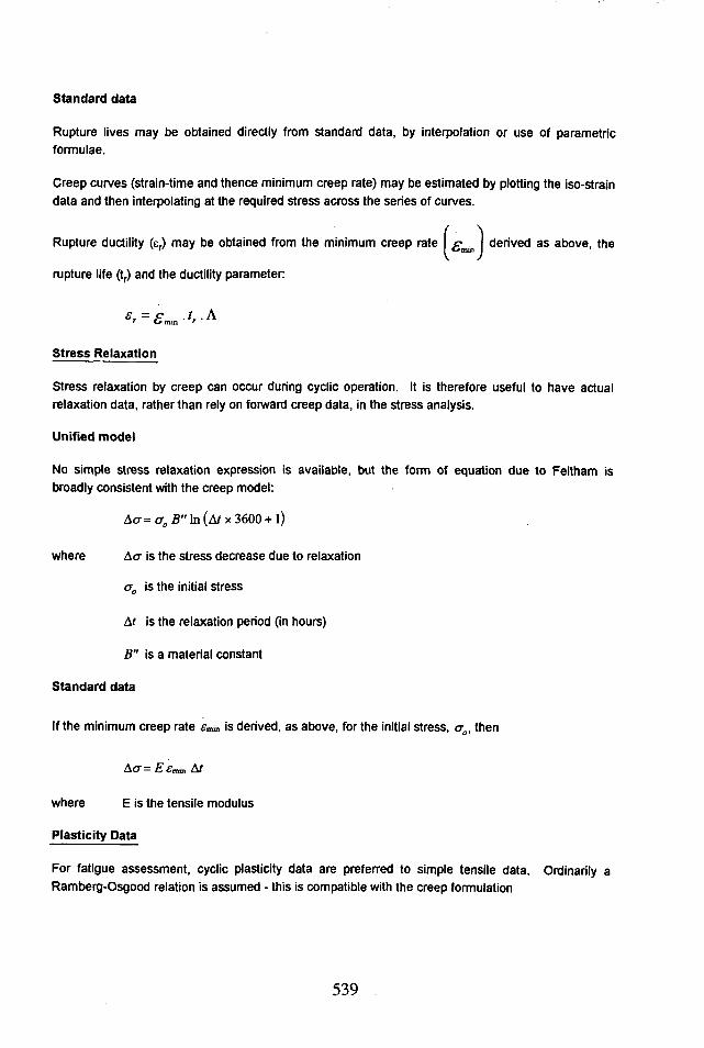
Standard data

Rupture lives may be obtained directly from standard data, by interpolation or use of parametric

formulae.

Creep curves (strain-time and thence minimum creep rate) may be estimated by plotting the iso-strain

data and then interpolating at the required stress across the series of curves.

Rupture ductility (er) may be obtained from the minimum creep rate ^£vn j derived as above, the

rupture life (tr) and the ductility parameter:

e,-p .tr.hr O min r

Stress Relaxation

Stress relaxation by creep can occur during cyclic operation. It is therefore useful to have actual

relaxation data, rather than rely on forward creep data, in the stress analysis.

Unified model

No simple stress relaxation expression is available, but the form of equation due to Feltham is

broadly consistent with the creep model:

Acr= cro 2?" In (A/x 3600 + l)

where A<r is the stress decrease due to relaxation

<j0 is the initial stress

A/ is the relaxation period (in hours)

B" is a material constant

Standard data

If the minimum creep rate e*m is derived, as above, for the initial stress, <j0, then

A<r= Eemn At

where E is the tensile modulus

Plasticity Data

For fatigue assessment, cyclic plasticity data are preferred to simple tensile data. Ordinarily a

Ramberg-Osgood relation is assumed - this is compatible with the creep formulation

539

Unified model

This is a simple inversion of the creep equation:

For load control:

e=£0

m-ti(l - <»)" exp (Q./ RT)

For strain control:

r v/i/ incr= <j0 (l- e I —I EoexpiQ./ RT)

where £* is the effective modulus

and £ is the applied strain rate

or <r is the applied loading rate

Standard data

Tensile data are directly obtainable from standard data which provide stress-strain data including

yield (or 0.2% proof stress) and ultimate tensile strength. These tables give minimum values. A

realistic estimate of the ultimate tensile strength may be obtained from the hardness of the material.

Fatigue Data

Endurance data are required for the initiation assessment, parametric relations between cycles to

failure and strain range are available for several materials. For creep-fatigue assessment, data from

tests with an appropriate dwell period are preferred.

Unified model

This is still at the development state.

Standard data

Information available in national codes is presently used.

Crack Growth

Creep crack growth data, in terms of the parameter C*, are required.

Fatigue crack growth data in terms of the parameter K, are required.

540

Unified model

The standard expression for creep crack growth rate (a) is directly related to the continuum damage

model for creep

a = A(C*Y

where A is a function of creep ductility

and <j> is related to creep stress sensitivity

If the creep ductility {er) at the appropriate conditions is known, then

A = 0.003/£,

(j> = n/(n+1)

where n is the stress dependency factor for creep.

The standard expression for fatigue crack growth (da/dN) has not yet been formally linked to the

unified model:

— = C{hK)m dN K '

where da/dN is the crack growth per cycle

AK is the range of stress intensity factor over the cycle

C, m are material constants

At present the conservative values

C = 8x10‘11 (consistent units)

m = 3

may be used for ferritic and austenitic steels.

541

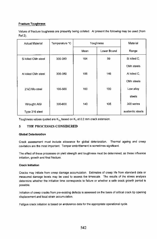
Fracture Toughness

Values of fracture toughness are presently being collated. At present the following may be used (from

Ref.2).

Actual Material Temperature °C Toughness Material

RangeMean Lower Bound

Si killed CMn steel 300-380 164 99 Si killed C,

CMn steels

Al killed CMn steel 300-380 196 146 Al killed C,

CMn steels

21/4CrMo steel 100-500 150 100 Low alloy

steels

Wrought AISI 300-600 140 105 300 series

Type 316 steel austenitic steels

Toughness values quoted are K1c based on at 0.2 mm crack extension.

5 THE PROCESSES CONSIDERED

Global Deterioration

Crack assessment must include allowance for global deterioration. Thermal ageing and creep

cavitation are the most important. Temper embrittlement is sometimes significant.

The effect of these processes on yield strength and toughness must be determined, as these influence

initiation, growth and final fracture.

Crack Initiation

Cracks may initiate from creep damage accumulation. Estimates of creep life from standard data or

measured damage levels may be used to assess the timescale. The results of the stress analysis

determine whether the initiation time corresponds to failure or whether a safe crack growth period is

possible.

Initiation of creep cracks from pre-existing defects is assessed on the basis of critical crack tip opening

displacement and local strain accumulation.

Fatigue crack initiation is based on endurance data for the appropriate operational cycle.

542

Creep-fatigue initiation is based on a linear summation of creep strain fraction and fatigue cycle

fraction. (Creep life fraction is a poor alternative to strain fraction).

Crack Growth

Standard solutions for reference stress and stress intensity are used.

Creep crack growth is predicted using C* correlations. If transient behaviour is expected, then Ct

calculations are used. Safety factors are applied to crack growth in the period before full stress

redistribution has occurred. For pure creep, crack growth is calculated on a time base. For creep

fatigue, the creep element is determined per cycle.

Fatigue crack growth is predicted using MT correlations, taking due account of crack closure.

For creep-fatigue, the total crack growth per cycle is obtained as the linear sum of the creep and

fatigue components.

In all cases, account must be taken of any deterioration in materials properties ahead of the crack.

The stress and temperature gradients ahead of the crack should also be considered and crack arrest

calculations performed where appropriate.

It is usually wise, in a full assessment, to calculate growth in both the through-thickness direction

(crack size a) and that perpendicular to it (crack size c), since these may differ. For a simple,

preliminary assessment, calculation of through-thickness behaviour is usually sufficient.

Failure Criteria

Failure by global creep processes should always be considered.

Critical crack sizes are determined by reference to a two-parameter failure assessment diagram. For a

given structure, load and material, regions may be plotted on this representing stable defects, initiating

defects and crack growth regimes, (Fig.1). It is believed that this form of presentation is novel to this

project.

The changes in toughness and collapse load with global deterioration should be included.

A leak before break analysis should be performed.

543

Two-parameter failure assessment diagram showing regimes for

(s) - stable defects (i) - initiating defects (g) - growing defects

Fig.1: Failure assessment diagram

544

6 LIFE PREDICTION

The time to failure by global deterioration is first calculated, as this may be life limiting. The total life

due to crack initiation and growth, to the fast fracture limit, is then determined. Comparison of these

timescales gives the overall life of the structure (Fig.2).

Consideration of the sensitivity of the defects to overloads is required, as this may impose the effective

limit to operation.

t=0 Initial sharp crack

Cracking blunting

j*17> Formation of a short crack

when the crack opening reaches a critical value

t>t Creep crack growth

Growth TimetIncubation

Relative timescales for:

(i) - crack initiation (g) - crack growth(c) - reduction in critical crack size with global deterioration(I) - remaining life ofthe ligament ahead of the crack,

as a function of crack size and material degradation(tf) - time to fa st fra dure

(t - time to failure by continuum damage cd

Fig.2: Life limiting processes associated with defects

545

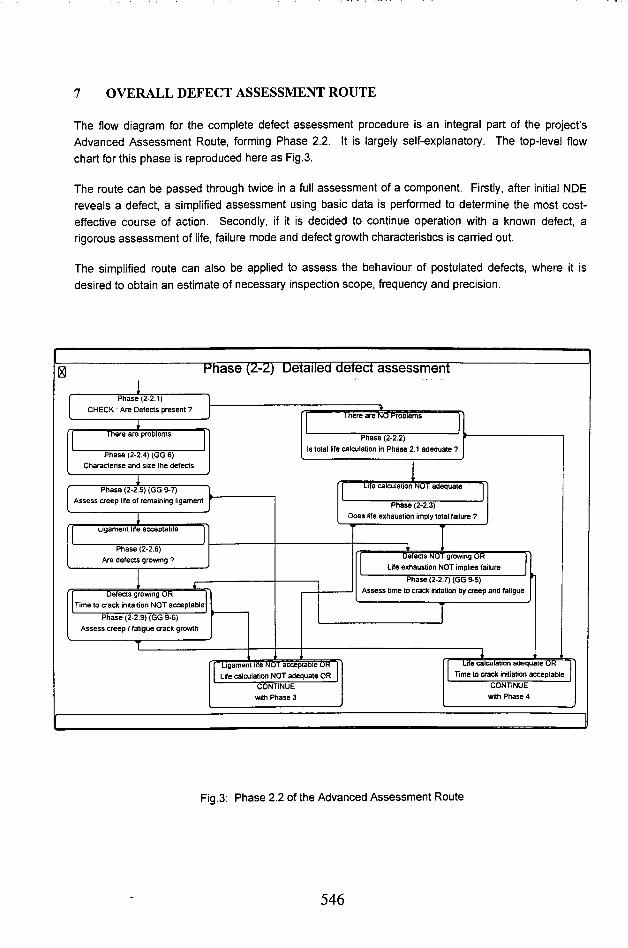
7 OVERALL DEFECT ASSESSMENT ROUTE

The flow diagram for the complete defect assessment procedure is an integral part of the project's

Advanced Assessment Route, forming Phase 2.2. It is largely self-explanatory. The top-level flow

chart for this phase is reproduced here as Fig.3.

The route can be passed through twice in a full assessment of a component. Firstly, after initial NDE

reveals a defect, a simplified assessment using basic data is performed to determine the most cost-

effective course of action. Secondly, if it is decided to continue operation with a known defect, a

rigorous assessment of life, failure mode and defect growth characteristics is carried out.

The simplified route can also be applied to assess the behaviour of postulated defects, where it is

desired to obtain an estimate of necessary inspection scope, frequency and precision.

Phase (2-2) Detailed detect assessment

Fig.3: Phase 2.2 of the Advanced Assessment Route

546

8 ACKNOWLEDGMENTS

This paper is published with the permission of ERA Technology Ltd, MPA Stuttgart and the Project SP249 Steering Committee. The authors are grateful to their colleagues in the project for their contributions to the development of this approach and to the many workers in the field of defect assessment whose publications have provided source material.

9 REFERENCES

1. British Standard Published Document

PD 6493 : 1991 Guidance on methods for assessment of the acceptability of flaws in fusion

welded structures

BSI London 1991

2. British Standard Published Document

PD 6539 : 1994 Methods for the assessment of the influence of crack growth on the

significance of defects in components operating at high temperature

BSI London 1994

3. Drubay B., Moulin D., Faidy C., Poette C., Bhandari S.,

Defect assessment procedure - a French approach for fast breeder reactors

SMiRT-12, MPA Stuttgart, August 1993

Paper FG15/1, Vol 12, pp139-144

pub Elsevier Science BV

4. Nuclear Electric Assessment Procedure R6

Assessment of the integrity of structures containing defects (Rev 3)

Nuclear Electric, Berkeley UK 1986

5. Nuclear Electric Assessment Procedure R5

An assessment procedure for the high temperature response of structures (Issue 2)

Nuclear Electric, Berkeley UK 1994

6. EPRI Project RP-2253-7

Remanent life of boiler pressure parts - crack growth

EPRI, Palo Alto USA, 1988

7. Riedel, H

Fracture at High Temperatures

Springer-Verlag, Berlin 1987

8. Piques R., Molinie E., Pineau A.,

Comparison between two assessment methods for defects in the creep range

Fatigue Fract. Eng. Mat. Struct., Vol 14, No 9, pp871-885,1991

547

548

A Worked Example Using the SP249 Advanced Assessment Route: - The Carregado Unit 6 Final Superheater Outlet Header

J. M. Brear, P. Jarvis, G. T. Jones - ERA Technology, UK A. S. Jovanovic, M. Friemann, B. Kluttig, M. Ober - MPA Stuttgart, Germany

A. Batista - EDP-PROET, Portugal C. L. de Araujo, A. Pires - ISQ, Portugal

Introduction

As a key part of its information resource, the SP249 Project contains a number of case studies, drawn from the collective experience of the partners and from the literature. The user of the system may search this data-base by component type and material or by assessment method, to find a practical example close to his own current problem. He can thus draw upon past experience as well as state-of-the-art knowledge to obtain advice. To facilitate this, a set of key-words has been defined to create links between the case studies and the overall assessment methodology. These relate to damage and failure types and causes as well as to techniques of investigation and assessment.

For demonstration, validation and didactic purposes, certain of these case studies - one per end- user utility in the project - have been chosen for full elaboration as ‘worked-examples’. These real component evaluations are worked through by an expert group from the project team so as to provide the utility staff with ‘hands-on’ training in both the practical techniques of component life assessment and the use of the knowledge based system. The exercise also provides valuable opportunity for feedback, allowing refinement of the technology package and the software. Amongst these worked examples, an assessment of EDP’s Carregado Unit 6 Final Superheater Outlet Header has been chosen for special attention - as the operators have kindly allowed direct access to the component during two outages. This has allowed certain techniques which require multiple interactions with the component to be included in the work programme.

This paper summarises the Carregado Case Study. It is intended to serve as a demonstration and guide as to how the Advanced Assessment Route (AAR) is used in practice. The actions performed and results obtained are summarised. In the normal working situation, the user would operate directly with the computer based system, though he could use the paper form of the AAR with the Generic Guidelines for Life Assessment (GG) and Standard Data Tables (SDT) to hand if preferred. Readers of this paper may follow the logic of the procedure in outline by making reference to an earlier paper in this conference (Ref. 1).

549

The example is structured to follow the AAR exactly, the route being traced by the standard numbering system: Phase . sub-phase - Step . sub-step.

Didactic and explanatory comments are in italics.

Keyword links between this case study and the AAR are bold and underlined.

The example now follows:

AAR Step: Activity/Result: Keyword:

Phase 0 Prioritisation Prioritisation

0-1 In line with EDP’s general philosophy,...

... Carregado. power station,...

.... Unit 6 (on account of its availability) was chosen for assessment

0-2

0-3

0-4

0-5

Given the history of cracking on a sister unit, the Final Superheater Outlet Header was selected as the critical component

Design ASMEMaterial ASTM SA 335 P22 (2.25CrMo ~ 9 CrMo 9 10)

Critical locations on the header were identified progressively on the basis of code calculations (Phase 1) and inspection results (Phase 2).

This demonstrates that some degree of iteration is inevitable in practical application the AAR

of

550

Phase 1 General Calculation - Review of Operation

1-1 General Calculation Code-based calculation

A TRD code-based calculation was performed, treating several key geometric positions on the header (Ref. 2). The tube-tube ligaments were found to be the most critical. Results for this location type may be summarised as:

• Service hours Cold starts Warm starts

• Steady state creep stress Most frequent temperature Creep life fraction consumed

lower bound properties mean material properties

100917230498

44.2 MPa 560-565° C

total creep life1.078 - 93615h0.334 - 302081h

• Fatigue stress ranges:cold start 293.0 MPawarm start 201.5 MPafatigue cycle fraction consumed 0.0013

The remainder of this example addresses the tube-tube ligaments

1-1.6 Additional Factors Composition Improvement Factor

No composition improvement factor is available for this material.

Oxidation Life Extension Factor

An oxidation life extension factor is available for materials of this group.Application yields:

Creep life fraction consumed - total creep life lower bound properties 0.690mean material properties 0.213

14621Ih 474267h

551

1-2 Measure/Calculate Strain

A strain criterion is relevant to this thick section component. No measurements are available. From the Standard Data Tables for similar materials (ISO 2.25CrMo N&T<750°C, DIN 10 CrMo 9 10) it is likely that 1% strain (or more) has been accumulated in 100917h at 565°C, 44.2 MPa)

1-3 Assess Strain Level Critical Strain

This estimated strain level is, in itself sufficient to generate a recommendation to proceed to Phase 2 of the assessment. However for confirmation of this decision and illustration, this example continues with Phase J.

1-4 Assess Creep/Fatigue Life Fraction Critical Creep/Fatigue Life Fraction

Consideration of the creep - fatigue interaction diagram using the conservative bound fatigue cycle fraction and the oxidation corrected mean and lower bound creep life fractions shows that:

Fatigue is insignificantCrack initiation by damage accumulation in the absence of a pre-existing defect is :

unlikely - considering mean materials properties possible - considering lower bound materials properties

Thus, the assessment should proceed to Phase 2.

However, for illustration,, ...

1-5 Check Operational Factors Operational Factors

Though no problems have been experienced with this component, the cracking on a sister unit and the service life in excess of lOOOOOh indicate that the assessment should proceed to Phase 2.

552

Phase 2 Inspection-based Assessment

2.0 Visual/NDE Inspection Visual/NDE Inspection

No defects or other abnormalities were found. Tube stub magnetite thicknesses were measured for subsequent assessment.

2.1 General Assessment

2.1-1.1 Check Critical locations

Critical locations for examination were verified

2.1-1.2 Select Metallographic Methods Metallographic AssessmentTechniques

Surface replication and hardness measurement were the techniques selected.

2.1-1.3 Surface replication Surface replication

Surface replicas were made of selected tube stub weld regions, following the recommended procedure.

2.1-1.4 Interpretation of Surface Replicas Surface replication

The general microstructure type and state of degradation for each region on each replica were recorded. No abnormalities were found and no damage (creep cavitation) was observed.On the basis of CEGB/EPRI data this information would imply a total life of

(1+7.33)* 100917 = 840639hA conservative limit, based upon Neubauer’s classification would give

5*8000+100917 = 140917h

553

2.1-1.5 Hardness Measurements Hardness

Hardness measurements were made on header base material, weld metal and tube base material, following the recommended procedure.

It should he noted that, to be consistent with the overall methodology, the header base material and tube base material must be considered as separate locations. The connecting weld metal can be considered as belonging to either - or both. At present, the ligaments are being assessed as a set, taking mean and extreme results. It may be necessary at a later stage or at a subsequent assessment to consider individual ligaments one by one.

2.1-1.6 Interpretation of Hardness Measurements Hardness

Base material

From the average and softest ligament position header base material hardnesses, temperatures were estimated and the remanent and total lives calculated.

The following figures shows the screen output observed when using the computer system

Fig. 1 Calculated Hardness:

Hardness-Test

j Comment: Comment: Comment:

Position: Hardness [HV1 Position: Hardness [HVJ Position: Hardness [HV] ♦1 143 1 137 1 02 149 2 137 2 03 139 3 8 3 04 138 4 0 4 05 138 5 0 5 06 148 G 0 6 07 143 7 0 7 0 _a 1T7 a n a n ♦

Average 141.7 Average 137.0 AverageOh-1 4.41 G CTn-1 0.000 <Jn-l

Correctionfactor

0 Correctionfactor

0 Correctionfactor

0

Averagecorrected

141,7 Averagecorrected

137,0 Averagecorrected

WeldMaterial: □ □ n

554

Fig 2. Estimated Temperature:

Temperature Estimation

Operating Time: ^00^17 [h]

Estimated Temperature Formula

[HrHssr3-(HQ-Hss)-:i

C0- t

ResultsCW3ABM River I ' r 557|[C*]

EW3AWM t T=r 588J [ C*]

CW3A BM Unit 1 r=r |tc*l

Close

Help I

3. Calculated Remaining Lifetime:

555

The results for the base material can be summarised as:

Hardness Temperature Remanent life Total life

Average 141.7 557 623524 724441

Softest 137.0 568 303971 404888

The mean total life is consistent with that derived from the replica-based damage assessment.

Weld MetalThe average (162/141.7 = 1.144) and softest (176/138 = 1.275) weld metal to base material hardness ratios are less than 1.423, thus implying that - in the absence of defects - failure will be expected in the weld metal or HAZ. Using appropriate weld metal data gives the following:

Hardness Temperature Remanent life Total life

Average 162 557 * 286619 387536

Softest 140 568 * 44738 145655

* Note that temperature cannot be estimated from the weld metal hardness, values derived from the base material are used here.

2.1- 2 Check Temperature Data Temperature Monitoring

2.1- 2.1 Review Available Temperature Data

Adequate Thermocouple coverage was installed prior to this case study. However, for demonstration purposes, the following actions were performed.

2.1- 2.2.1 Thermocouples Thermocouples

Sufficient - see above

2.1- 2.2.2 PETIT PETIT

For demonstration purposes, PETIT capsules were attached to several tube stubs in the dead space. These should be removed for examination after 10000 - 20000 h further service.

556

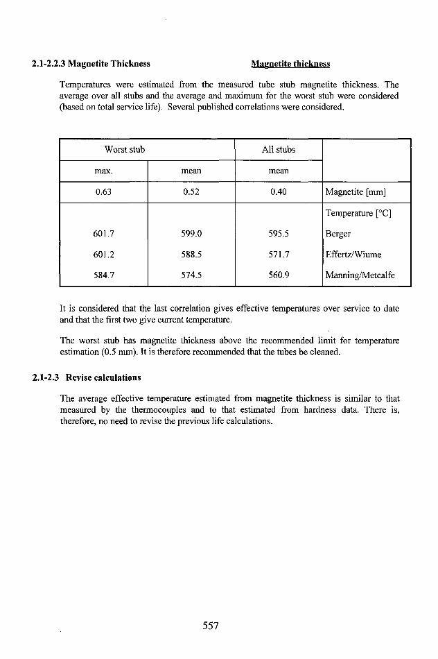
2.1-2.2.3 Magnetite Thickness Magnetite thickness

Temperatures were estimated from the measured tube stub magnetite thickness. The average over all stubs and the average and maximum for the worst stub were considered (based on total service life). Several published correlations were considered.

Worst stub All stubs

max. mean mean

0.63 0.52 0.40 Magnetite [mm]

Temperature [°C]

601.7 599.0 595.5 Berger

601.2 588.5 571.7 Effertz/Wiume

584.7 574.5 560.9 Manning/Metcalfe

It is considered that the last correlation gives effective temperatures over service to date and that the first two give current temperature.

The worst stub has magnetite thickness above the recommended limit for temperature estimation (0.5 mm). It is therefore recommended that the tubes be cleaned.

2.1-2.3 Revise calculations

The average effective temperature estimated from magnetite thickness is similar to that measured by the thermocouples and to that estimated from hardness data. There is, therefore, no need to revise the previous life calculations.

557

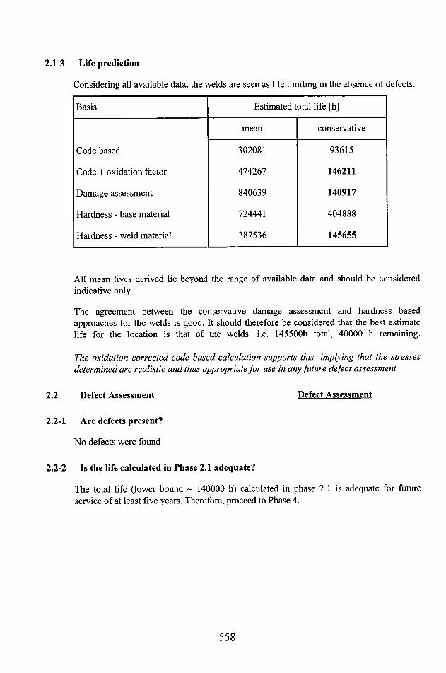
2.1-3 Life prediction

Considering all available data, the welds are seen as life limiting in the absence of defects.

Basis Estimated total life [h]

mean conservative

Code based 302081 93615

Code + oxidation factor 474267 146211

Damage assessment 840639 140917

Hardness - base material 724441 404888

Hardness - weld material 387536 145655

All mean lives derived lie beyond the range of available data and should be considered indicative only.

The agreement between the conservative damage assessment and hardness based approaches for the welds is good. It should therefore be considered that the best estimate life for the location is that of the welds: i.e. 145500h total, 40000 h remaining.

The oxidation corrected code based calculation supports this, implying that the stresses determined are realistic and thus appropriate for use in any future defect assessment

2.2 Defect Assessment Defect Assessment

2.2- 1 Are defects present?

No defects were found

2.2- 2 Is the life calculated in Phase 2.1 adequate?

The total life (lower bound ~ 140000 h) calculated in phase 2.1 is adequate for future service of at least five years. Therefore, proceed to Phase 4.

558

Phase 4 Inspection and Monitoring

4-1.1 Are growing cracks present?

No growing cracks are present.

4-1.3 Monitor global loads and strains Mechanical Monitoring

4-1.3.1 Is there a history of support problems?

There is no history of support problems.

4-1.3.3 Is global strain being monitored?

No strain monitoring is being performed

4-1.3.4 Install strain monitors Strain gauges

There is some argument for installing strain gauges across or close to the stub welds.

4-1.4 Are temperature data adequate?

This is adequate

Temperature Monitoring

4-2 Future Inspection Inspection Planing

4-2.1 Determine optimum inspection interval

The life of the tube/tube ligament is governed, in the absence of defects, by the stub welds.

There is conservatively 140000 total i.e. 40000 remanent.

Provided no other locations on the header prove more critical and operation does not change, a further inspection in 30000 h would be appropriate. However the PETIT capsules will require removal in -10000 h (no more than 20000h), therefore the opportunity to reinspect at that time should be taken and the life prediction reviewed. It would also be prudent to clean the tubes of internal scale at that time.

4-2.2 Is an on-line life monitor installed?

No on-line monitor is installed.

4-2.3 Consider installing an on-line life monitor.

On-line monitoring should be considered.

4-2.4 At next inspection, go to Phase 1

At the next inspection, the Phase 1 calculations should be revised in the light of additional service data, and Phase 2 inspections repeated.

END

The assessment has been successfully concluded with a future management plan for this location defined. Total planning for the component would depend on the results of similar assessments for other locations - however the results of the phase 1 calculations imply that the tube-tube stubs are the most critical positions and therefore will control overall component life.

560

Acknowledgments

This paper is published with the permission of ERA Technology Ltd, MPA Stuttgart, EDP, ISQ and the Project SP249 Steering Committee. The collaboration of all project partners has been most welcome but particular thanks are due to the staff of EDP, especially the Carregado Power Station personnel.

References

1 J.M. Brear and G. T. JonesA consolidated approach to component life assessment in Project SP249 This conference.

2 P. Jarvis, G. T. Jones, A. Batista and C. de AraujoLife assessment using codes and standard materials properties in SP249 Carregado case study.20 MPA Seminar, MPA Stuttgart, October 1994

561

562

DECISION SUPPORT SYSTEM FOR PLANNING OF INSPECTIONS IN POWER PLANTS.PART I - METHODOLOGY.

A. Jovanovic S.M. Psomas MPA Stuttgart Stuttgart, Germany

P. Auerkari VTTMPA Stuttgart

Stuttgart, Germany Espoo, Finland

Abstract

A system for computer-aided planning of forthcoming inspections of high temperature piping in fossil-fired power plants has been developed. Its use permits to model the whole inspection procedure and to concentrate on the most important decision-making issues. Final output from the system is the matrix "component inspection scope vs. year" showing what inspection technique and to what extent should be applied at a given location/ component during next inspection(s).

1 INTRODUCTION

The power plant components operating at high temperatures are important

targets in the in-service inspections and measurements. Apart from being

large and expensive and subjected to complex mechanical and thermal

(creep-fatigue) loading in service, these components can limit the

availability of the whole plant. Due to ageing, these components need

additional monitoring, repairs and replacements.

Such components include typically

• boiler tubing, superheaters and reheaters;

• headers, valves, T- and Y-pieces and the rest of the hot pipelines;

• hot parts of the steam and gas turbines.

563

The safety aspects of design impose that the nominal (design) life, e.g.

200,000 service hours and 1000 cold starts, is considerably shorter than the

true average life for these components at nominal (design) service loading

level. Reasons for this include e.g. using lower bound values for material

strength in design and upper bound dimensions in manufacturing. The

extent (or occurrence) of excess life potential is not certain. Furthermore,

overloading, overheating or other disturbance not accounted for in design,

can on the other hand, considerably shorten component life.

Whenever feasible, extension of life or inspection periods is to be

recommended, not only because of the direct cost impact but also because

any unnecessary maintenance compounds to a significant additional risk for

damage and failures. For example, excessive residual stresses,

embrittlement or cracking after unnecessary repair welding and local heat

treatments will occur at a non-zero (and high in case of susceptible

materials in stiff structures) probability. Nevertheless, timing of

maintenance is always an optimisation problem, since also too lax

maintenance or too long maintenance periods will lead to costly unexpected

shutdowns.

The amount of relevant background information, extent of data of the

service, inspection and maintenance history, number of locations of

potential interest in a large system, as well as needs for relatively long term

systematics and expert experience, all support the view that much of the

work would be ideally handled by an application-oriented decision support

system. Following the initial concept [7], such a system for computer-aided

planning on forthcoming inspections of high temperature piping in fossil-

fired power plants has been developed in the European Union research

project BE5935 [6], Initial concept for the part regarding the inspection

564

results interpretation has been given by Auerkari [1], in connection to the

recent guidelines of Nordtest [2] and VGB [11],

Input to the system are results of previous inspection (if available), data

about the piping component and strategic constraints resulting from the

importance of the component, the desired level of confidence, etc. Based on

the integration of several elements the system produces a final output in

form of a "component vs. year" matrix showing:

• what inspection technique (replica, ultrasonic, etc.) and

• to what extent (e.g. how percent of welded joint examined)

should be applied at a given location/component during the next inspection

(overhaul).

2 BASIC INSPECTIONS PRINCIPLES

The most important factors affecting the conclusions made from the

inspection results of the hot pipework are

• service history and its deviations from the expected (in design)

range;

• inspection history, i.e. the results from earlier measurements;

• materials and manufacturing / repairs / modifications; and

• expected consequences of failure (cost and safety aspects).

Very often the conclusion resulting from the inspections or other

measurements is a recommended time period to next inspection. In

principle, length of such a period is limited by

565

• extent and quality of the available information of details e.g. in the

service history and future service, as well as in the maintenance

history;

• optimum failure risk level for the plant and the component;

• inherent inaccuracies in the evaluation methods for limiting

failure; and

• limited systematics (holistics) in producing the final conclusions.

Many of these inadequacies are partly addressed by using an appropriate

decision support system, which hence should be useful in minimising the

economical impact of too frequent or extensive inspections. However, in the

beginning it is not possible in general to optimise exactly in this sense,

because only the accumulating inspection results provide means for

improving the accuracy of optimisation. Therefore, sets of experience-based

recommendations (e.g. [10]) have been devised for initial selection of the

methods and location of first inspections.

Experience suggests that in the straight pipes and most areas (possibly

excluding some bends and T-piece bodies) of hot steam pipings the nominal

design life is relatively easily exceeded, on average perhaps by a factor of 3

to 10. In the welds that are likely to fail first, this safety factor on life is

probably of the order 1.5 to 3 on average, when the steam temperature

exceeds the value of about 500°C. In the welded joints the variation of life

is also large, and hence while it is important to include the critical welds in

the inspection programs, it is equally relevant to use these programs for

finding those welds that determine overall life and possible corrective

actions.

566

In an ageing plant some weld damage and failures are very likely and can be

economically important events. Normal consequences of (circumferential)

weld failures are not catastrophic and do not require consideration of

personnel safety. Failures of bends can be sudden and catastrophic, but are

in general rare, and mainly limited to susceptible materials such as

14 MoV 6 3 (0.5Cr-0.5Mo-0.25V) after less than successful manufacturing.

As a consequence, the inspection programs tend to concentrate on welds

and treat bends (and some T-piece bodies) case by case. Straight pipes are

usually not included in the programs, and are of little interest before

attaining a very long service life (» 250,000 h), if even then.

In addition to experience-based general rules or earlier inspections,

naturally any indication of overloading or overheating, as well as

manufacturing or material defects, is useful in determining the locations of

interest. Local decrease and variation in life time is most common in welds,

nozzle joints and perhaps some bends. Particularly loading and thermal

transients tend to concentrate relative lifetime accumulation in thick-wall

components such as main valves of the boiler and turbine, critical headers

and turbine rotors. These components typically also determine the

manufacturers' recommended maximum rates in changing temperature and

pressure during startups and shutdowns.

3 LOCATIONS AND INSPECTION CRITERIA

The locations of interest are usually selected from components and areas

with

• earlier indications of defects or other deviations;

567

• substandard or clearly less than ideal design (e.g. seam welded

pipes);

• significant overloading (e.g. improper hanger supports) or

overheating;

• suspected material/manufacturing defects; and

• higher than average damage rates from general experience.

First inspections are recommended for quality purposes to be taken and

documented at the time of taking the plant / components into service. Apart

from the more frequent (max. period about 4 years) inspections for certain

components such as boiler drums, safety valves and other components

included in the usual periodical pressure vessel inspections, it is

recommended that the extended inspections targeting for life assessment of

the hot pipework are started by the time when 80 % of the nominal design

life has been consumed (max. 100,000 h), if there are no specific reasons to

deviate from this rule (such as earlier inspection results or damage /

failures).

Normally the extent of such a first inspection can be as shown in Table 1.

The timing and selection of locations after a given inspection are defined

according to the results. If then no deviations or defects are found, a new

evaluation is recommended not later than at the time of an additional 80 %

of the nominal life (max. 100,000 h); this applies only to the obvious

locations of interest according to Table 1. The extent of the first inspection

of this kind can often be reduced, when the steam temperature does not

exceed 480°C (e.g. recovery boilers), and replaced completely by ordinary

periodical inspections when the steam temperature does not exceed 400°C.

568

Table 1: Recommended locations, extent and methods of first inspections

for pipework operated for 80 % of the nominal design life (max. 100,000 h)

Locations Methods Extent

Header nozzles and welds

Endoscopy, MT/PT + RT,UT

End caps, welds in nozzles (20 %)

Safety valves, steam coolers

Check of operation (UT of int. surfaces or endoscopy)

Component internals

Main steam valves other heavy valves (at least one)

Check of operation, MT/PT+RT (welds), check of inside wear/cracks

MT/PT n. 100 mm wide of welds, RT according to findings

Bends near fixed points, bends of lengthy pipes curving up/down (min. one per line)

Bend MT/PT+RT minimum wall (UT) + ovality 1)

MT/PT from bend^) RT at least from extrados + acc. to MT/PT-results

T- and Y-pieces near fixed points (at least 2 + main branches)

MT/PT+RT, UT at welds, wall thickness 1) and strain^)

MT/PT of welds 100 mm wide, RT acc. to indications, UT for body

Deaeration/dewatering nozzles (spot test or by experience)

MT/PT+UT where water may be trapped^)

Inside of the joint

Flange joints near fixed points

MT/PT+RT, welds MT/PT externally

UT = ultrasonic testing; MT/PT = surface inspection; RT = replica testing. Visual inspection in all cases; according to crack indications additional UT. Surface quality requirements as in VGB R509L, except for RT as in SFS 3280.

1) +recalculation of stresses2) d < 300: MT/PT whole bend; d > 300: MT/PT of four zones ~ 200 mm wide3) especially near the boiler and when the nozzle dia ratio > 0.74) hoop measurement of the body and the nozzles; mark the measurement points

Note: consider internals where high fatigue life consumption is expected.

569

The above applies to most plants; however, there are indications that

significant service-induced damage can occur in some cases as early as after

40,000 service hours; these cases have been mainly associated with the

material type 14 MoV 6 3 (0.5Cr-0.5Mo-0.25V). Damage could be also

induced before attaining 80% of the nominal life, due to improper hanger

supports or other inadequacies related to design, operation or maintenance.

Indications of the possible early damage or service incidents of significance

can be checked by regular hot and cold walk downs, including noting of the

general condition of hangers and supports of the pipework.

4 DECISION PROBLEM FORMULATION AND

MODELING

4.1 GENERIC

Fig. 1 gives an understanding to the overall decision problem formulation

and modelling of the inspection planning of power plant components. As

may be seen, the process of inspection planning is divided into two levels:

1. „A11 component level14: Selection and prioritisation of the

components/locations for the actual inspection purposes.

2. „One component level44: Inspection and determination of the next

inspection time for each selected component/ location.

On each of these two levels the critical decision node is placed where a

multi criteria decision-making (ranking) problem with crisp, fuzzy and/or

random inputs has to be solved. Crisp inputs are e.g. certain crisp numbers

(e.g. number of operating hours). Fuzzy inputs are e.g. those involving

linguistic variables (e.g. "high risk") represented in terms of membership

570

functions. Random inputs are e.g. the stochastic input variables (e.g.

temperature) represented in terms of probability distributions.

Goal of the complete system represented in Fig. 1 is to provide a new

inspection plan for all selected components/locations.

All Component Level

One Component Level

Inspection Results

User's preliminary selection of inspec­tion items (systems, compon., locations)

I

Decision node:Ranking of inspection items acc. to ranking criteria

Selection of inspec­tion item acc. to position in ranking list

IDecision node:Determination of inspection strategy for inspection item

I

Criteria:Importance, Prev. results

Cost, Safety, Environment Past history,.

COMPONENT LOCATIONRANKING (COLOR)

Component/Location

Type Rank

# 2873 Header 2# 3987 T-piece 3M 127S Y-Piece 1

Criteria:Inspection cost, Diffi­culties, Risk, Priority

from COLOR

INSPECTION STRATEGY ADVISOR (1STRA)

InspectionStrategy

Extent for Y-Piece

Rank

zero attention VI 3low profile + TH 2standard + MT, FT 1

Performing of inspec­tions; determination of next inspection time and scope

I

New inspection plan for selected inspection items

RESULT: INSPECTION PLANComponent/Location

1994 1995 1996

# 2873 MT, PT VI UT# 3987 MT, PTU 1275 VI TH

Fig. 1: Generic flowchart of decision problem formulation

571

There are different problems that have to be handled when co-ordinating

complex actions like those in the decision making process for inspection

planning of power plant components. In order to cope with all of them, the

developed decision support system consists of the following elements:

1. A flowcharting part enabling to model the inspection/evaluation

procedure graphically;

2. a knowledge-based system part controlling the user's movement

through the procedure;

3. multi criteria decision analysis modules (COLOR, ISTRA) optimising

the selection of possible alternatives in each decision node;

4. a hypermedia part providing the explanation facility;

5. a numerical calculations part providing additional input (e.g.

calculation of consumed life according to standards, etc.).

4.2 INTELLIGENT FLOWCHARTING MODULE

The modelling of the problem domain is done with an "intelligent"

flowcharting program. The "intelligence" of the program refers to its

interaction with a knowledge-based system controlling all movements in the

flowchart. In that way, the resulting integrated module acts as a user-

advisor, assisting the user in facing the problem in a recommended way and

allowing him not only to obtain information and recommended actions from

the other modules (MCDA, Hypermedia) but also to input his personal

thinking and/or experience, where uncertainty exists. Finally, with the use

of the system the user avoids possible overlooking of significant aspects of

the procedure.

572

4.3 MULTI CRITERIA DECISION ANALYSIS (MCDA)

MODULES

The two modules, namely COLOR (COmponent/LOcation Ranking) and

ISTRA (Inspection STRategy Advisor), developed for the analysis of the

two decision nodes shown in Fig. 1, are both application-oriented and will

be described later on in detail. However, the underlying methodology is

very general and applicable also in other fields, where modelling of

uncertainties is mainly based on experience.

The applied methodology [8] is an extension of Saaty's AHP [9], as

amended by Buckley [3,4] in order to incorporate fuzzy comparison ratios.

In such a way, it is much easier to model uncertainties regarding

comparisons of criteria, on which the decision has to be based, as well as

ranking of alternatives with respect to each criterion.

Both modules can also handle crisp and stochastic inputs. In this way, they

model also situations where no or stochastic uncertainty exist.

4.4 HYPERMEDIA AND NUMERICAL CALCULATIONS

MODULES

Both modules are integrated in the decision support system in order to

provide related background information in each step of the overall process.

The related information, consisting mainly of experience-based

recommendations and/or guidelines, may be retrieved automatically.

Furthermore, numerical calculations based on them can provide additional

input.

573

5 COLOR MODULE

5.1 ALTERNATIVES

The alternatives for the ranking procedure are the different components of a

power plant. For each type of component there might be different locations.

In general the list of the alternatives may be like the following one:

• boiler tubing, location 1,

• boiler tubing, location 2,

• superheater, location 3,

• economiser, location 4, etc.

5.2 CRITERIA

To model the multi criteria decision of component/location ranking the

following criteria were defined:

1. Fundamental importance of the component for the present plant

(seriousness of failure/downtime)

2. Results of previous inspections

3. Cost of replacement of component

4. Safety aspects (including regulatory safety aspects)

5. Environmental aspects (including regulatory environmental aspects)

6. Qualitative past service history

7. Quantified past service history

8. Expected change in the operating conditions used for the analysis so

far

9. Alternative supply patterns (i.e. relative importance of the component

in comparison with existing alternatives).

574

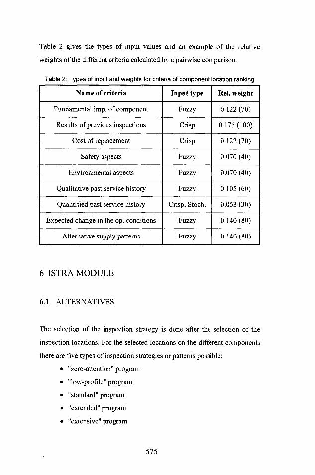
Table 2 gives the types of input values and an example of the relative

weights of the different criteria calculated by a pairwise comparison.

Table 2: Types of input and weights for criteria of component location ranking

Name of criteria Input type Rel. weight

Fundamental imp. of component Fuzzy 0.122 (70)

Results of previous inspections Crisp 0.175 (100)

Cost of replacement Crisp 0.122 (70)

Safety aspects Fuzzy 0.070 (40)

Environmental aspects Fuzzy 0.070 (40)

Qualitative past service history Fuzzy 0.105 (60)

Quantified past service history Crisp, Stoch. 0.053 (30)

Expected change in the op. conditions Fuzzy 0.140 (80)

Alternative supply patterns Fuzzy 0.140 (80)

6 ISTRA MODULE

6.1 ALTERNATIVES

The selection of the inspection strategy is done after the selection of the

inspection locations. For the selected locations on the different components

there are five types of inspection strategies or patterns possible:

• "zero-attention" program

• "low-profile" program

• "standard" program

• "extended" program

• "extensive" program

575

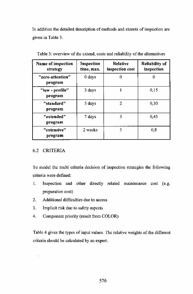
In addition the detailed description of methods and extents of inspection are

given in Table 3.

Table 3: overview of the extend, costs and reliability of the alternatives

Name of inspection strategy

Inspection time, max.

Relative inspection cost

Reliability of inspection

"zero-attention"program

0 days 0 0

"low - profile" program

3 days 1 0,15

"standard"program

5 days 2 0,30

"extended"program

7 days 3 0,45

"extensive"program

2 weeks 5 0,8

6.2 CRITERIA

To model the multi criteria decision of inspection strategies the following

criteria were defined:

1. Inspection and other directly related maintenance cost (e.g.

preparation cost)

2. Additional difficulties due to access

3. Implicit risk due to safety aspects

4. Component priority (result from COLOR)

Table 4 gives the types of input values. The relative weights of the different

criteria should be calculated by an expert.

576

Table 4: Types of input for criteria of component location ranking

Name of criteria Type of input values

Optimisation goal

Inspection and other related

maintenance cost

Fuzzy Minimise (for higher level inspection patterns cost are

increasing)

Additional difficulties due to

access

Fuzzy Minimise (more difficult access to inspection region

forces lower level inspection pattern)

Implicit risk due to safety aspects

Fuzzy Minimise (higher safety needs forces higher level inspection

patterns)

Component priority (result from COLOR)

Crisp Maximise (higher component priority forces higher level

inspection patterns)

7 CONCLUSIONS AND ACKNOWLEDGEMENTS

Practical examples in German and Finnish power plants will be reported in

another paper of this conference [5], In the future, the system will be

coupled with a NDT database and used primarily for preliminary screening

and "drafting" of the annual inspection plans. Experts' revision of these

drafts will remain a mandatory part of the overall procedure.

Some of the work presented in the paper has been accomplished within the

European Union research projects SPRINT SP249 and BRITE-EURAM

BE5935. In addition, some of the results have been achieved under the

Brite-Euram Fellowship Contract No. BRE-CT93-3039 (fellowship for the

stay and research of Mr. S. Psomas at MPA Stuttgart). This support is

gratefully acknowledged here.

577

8 REFERENCES

1. Auerkari, P., 1993, "Guidelines for Inspection criteria of Hot

Pipework", SPRINT SP249 Technical Report, VTT metals

Laboratory, Espoo

2. Auerkari, P., Borggreen, K., Salonen, J., 1992, "Reference

Micrographs for Evaluation of Creep Damage in replica Inspections",

NT Technical report 170, Nordtest, Espoo

3. Buckley, J. J., 1985a, "Ranking Alternatives Using Fuzzy Numbers,"

Fuzzy Sets and Systems 15, North-Holland, pp.21-31.

4. Buckley, J. J., 1985b, "Fuzzy Hierarchical Analysis," Fuzzy Sets and

Systems 17, North-Holland, pp. 233-247.

5. Jovanovic, A., Psomas, S., Ellingsen, H.P., Kautz, H.R., McNiven, U.,

Ronnberg, J., Auerkari, P., 1995, “Decision support system for

planning of inspections in power plants. Part II - Application in GKM

and IVO power plants”, to be presented at the Baltica Conference,

June 8, 1995.

6. Jovanovic, A., Psomas, S., Schwarzkopf, Ch., Auerkari, P., Bath, U.,

Weber, R., Kautz, H. R., Verelst, L., 1994, "Decision Making for

Power Plant Component inspection Scheduling" Report on Task

4.2/4.3 of BE-5935 Project RESTRUCT - Decision-Making for

Requalification of Structures, Document TEC-T4-01, MPA Stuttgart

7. Jovanovic, A., Zimmermann, H.-J., 1990, "Decision Making and

Uncertainty in Life Assessment and Management of Power Plant

Components", Document BE3088/89, MPA Stuttgart

578

8. Lieven, K., Weber, R., Bath U., Jovanovic, A., Psomas, S., De Witte,

M., Verelst, L., 1993, "Multi-Criteria Decision Making - Modelling

Technology" Report on Task 3.1 of BE-5935 Project RESTRUCT -

Decision-Making for Requalification of Structures, Document TEC-

T31-01, MPA Stuttgart

9. Saaty, R. W., 1987, "The Analytical Hierarchy Process - What it is and

how it is Used", Math. Modelling, Vol. 9. No. 3-5, pp. 161-176

10. VGB-R 509 L, 1984, "Wiederkehrende Priilungen an

Rohrleitungsanlagen in fossilbefeuerten Warmekraftwerken", VGB,

Essen

11. VGB-TW507e, 1992, "Guideline for the Assessment of Microstructure

and Damage Development of Creep Exposed Materials for Pipes and

Boiler Components", VGB, Essen

579

580

DECISION SUPPORT SYSTEM FOR PLANNING OF INSPECTIONS IN POWER PLANTS.PART II - APPLICATIONS

A. Jovanovic, S. Psomas, H.P. Ellingsen (MPA, Stuttgart, Germany),H.R. Kautz (GKM, Mannheim, Germany),U. McNiven & J. Ronnberg (IVO, Finland) & P. Auerkari (VTT, Finland)

AbstractThis paper describes two realistic applications of a decision support system regarding the inspection planning in power plants. The first application refers to a sample steam line of IVO in Finland and the second one deals with a piping of GKM in Germany. The decision support system ranks the candidate components by their priority for the inspection and selects, for each of them, the appropriate inspection strategy. Both ranking and selection decisions are based on a multicriteria analysis handling various types of input values (crisp, fuzzy, stochastic). The overall system represents a helpful tool for maintenance of power plant structures.

1. INTRODUCTION

A decision support system is used for solving sample inspection planning

problems in IVO and GKM power plants. IVO application refers to a

sample steam line, where GKM one refers to a whole piping.

The decision support system and the corresponding methodological issues

are described in detail in [6]. The general procedure consists of two major

decision making nodes (problems):

A. prioritising the candidate components/locations for the inspection needs;

B. choosing the appropriate inspection strategy for each component of

interest (i.e. component with high priority).

581

Two modules, namely COLOR (Component Location Ranking) and ISTRA

(Inspection Strategy Advisor) have been developed for solving these two

problems respectively.

In this paper the results of IVO and GKM applications will be presented.

IVO example is simplified and will concentrate on all methodological

issues, whilst GKM example is more detailed but will only concentrate on

the decision making node A and on the interaction with the system

databases.

2. PRACTICAL APPLICATIONS

2.1 IV O-EXAMPLE

The following (slightly modified) example works through a steam line. A

sketch of this piping including the component ID’s mentioned in the input

and output tables is given in Fig. 1. The material is 13CrMo44 with a

nominal temperature of 545°C, and the situation is given in 1993, after

110,000 service hours.

To support the complex decision making process a modelling tool, namely

ExpertChart, was developed and integrated to the decision support system.

ExpertChart is used to:

1. Model the problem domain

2. Lead the user through the problem

3. Provide background information

4. Perform analysis and calculations

For a more detailed description of ExpertChart features refer to [5, 8],

582

____ Z807

T-yhteesta Z301 IShtee linja 2RA14

2206 >UNJA2RA12

Fig. 1: Sketch of IVO sample steam line (including component ID)

The problem domain is modelled through a flowchart like the one in Fig. 2.

Activities are represented by boxes and their interconnections by lines and

arrows. Each activity may be detailed on a sublevel, which can be a

complete chart on his own (activated by the small checked rectangle in the

upper left comer of the box). Traditional if-boxes are translated into pre-

and post-conditions. These conditions are also needed for leading the user

through the flowchart.

Fig. 2: Modelling of the problem domain by a flow chart

583

The flowchart modelling the inspection planning problem for the IVO steam

line is shown in the following figures (Fig. 3 - Fig. 7).

Inspection Scheduling "All Component Level"

(1) First inspection? )

0 (3) Selection and priontisation of components and locations.

0 End analysis

End selection condition

No (Inspection results exist)

Begin selection condition

(^User's decision to take one component for determination

of the next insp e ction time

(6) Other components in the COLOR ranking

list available?

(2) Review results from previous inspection

(5) "One component level" Perform detailed analysis

for one selected component

Fig. 3: Inspection Scheduling "All Component Level"

(3.1) Prelinunary user's selection of components to be considered

(3.2) Run COLOR in order to obtain a ranked list

of components

Decision

(3) Selection and prioritisationBegin selection condition

Fig. 4: Selection and prioritisation of components and locations

584

L(5.1) Change in service conditions?

("Significant" observed or expected changes, fuzzy?)

(5) "One component level"

| Significant condition change |

(5.2) Recalculation necessary?

(5.5) Run ISTRA in order to choose inspection strategy

Begin testing condition

(5.6) Perform testing acc. to table “Methods and extents ..." Significant indications found?

■HBegin delete condition

(5.7) Delete this location from inspection programs but reconsider after 100000 h if there are damage indications nearby

X

(53) Recalculate remaining life for COLOR input

"Quantitive past history"(5 .4) Re-run COLOR in order

to obtain new value for "Component prionty" for ISTRA

Decision node"B"

Significant indications yes

(5.8) Macrocracks, nucrocracks, cavities.End damage condition

(5.9) Permanent strain. Micro­structure, hardness, oxidation

End strain condition

Showtime condition

(5.10) Show recommended time for next inspection. Add results

to inspection plan (matrix)

Fig. 5: One component level, perform detailed analysis

Significant indications yts

0 (5.8) Macrocracks,

(5.8.1) Maximum damage type?

(58.2) Repair/ remove, re- mspect any repairs within 10 kh

(58.11) Remspect within 20 kh, bends within 15 kh

(58 J) Repair / remove; reinspect any repairs within 10 kh, consider replacement particulary for bends

(58.8) Reinspect within 10 kh, for bends consider replacement

(58.4) Remove if abundant, small amount acceptable up to 50 kh

(58.9) If service (58.14) If service time > 100 kh and(58.5) Repair and reinspect within 10 kh, for bends consider replacement

10CrMo910, periods cenbe doubled 10CrMo910 penods

(58.10) Reinspect within 50 kh, bends within 20 kh

(58.13) Reinspect within 15 kh; bends within 10 kh

(58 6) Reinspect within20 kh, bends within 15 kh

(58.7) Reinspect within 15 kh, bends within 10 kh

(Nordtest)

End damage condition

Fig. 6: Macrocracks, microcracks, cavities

585

Fig. 7: Permanent strain, microstructure, hardness, oxidation

The inspection planning procedure for this example follows the steps below.

Step 1 [Fig. 3, Box (1)]

Is this the first inspection for this system? (Tes/Not. User selects "No" since

there are previous results from 1986-87.

Step 2 [Fig. 3, Box (2)]

Access to the database of previous inspections. User selects the appropriate

inspection data and reviews inspection results. According to "Results of

previous inspections" criterion, components with ID No. #813, #815, #507

are in a critical phase.

586

Step 3 [Fig. 4, Box (3.1)]

Initialisation of COLOR. User selects the above mentioned components as

well as five others for further analysis. He fills all related data in Table 1.

Step 4 [Fig. 4, Box (3.2)]

Running of COLOR. With the data from Table 1 and the relative weights of

each criterion, the system gives a priority to each selected component. The

ranked list in descending priority order is the following: (6, 8, 1, 7, 2, 4, 3,

5)

Step 5 [Fig. 3, Box (4)]

Which component should be analysed? Hast of components^ According to

his experience user selects component No. 8 to determine next inspection

time.

Step 6 [Fig. 5, Box (5.1)]

Change in service conditions? (Yes/NoT New temperature monitoring

results show a +5°C change in average temperature for the service

conditions of component No. 8. Therefore, user selects "Yes".

Step 7 [Fig. 5, Box (5.2)]

Is a recalculation of consumed/residual life necessary? fYes/NoV User

selects "Yes".

Step 8 [Fig. 5, Box (5.3)]

With use of the calculations part module and based on the new data the

system provides a new value for the criterion "Quantified past service

history" regarding component No. 8. Table 1 is also modified.

587

Step 9 [Fig. 5, Box (5.4)]

Running of COLOR. With the new data of Table 1, COLOR produces a

new output. The ranked list is now the following: (8, 6, 1,7, 2, 4, 3, 5).

Since the new priority of component No. 8 is even greater user proceeds

with the same component, in order to find out the best inspection strategy.

Step 10 [Fig. 5, Box (5.5)]

Initialisation of ISTRA. For component No.8 and for all possible strategies

user fills all related data in a table (Table 2).

Step 11 [Fig. 5, Box (5.5)]

Running of ISTRA. With the data from Table 2 and relative weights for

each criterion given from an on-line pairwise comparison, the system gives

a priority value to each inspection strategy/program. According to these

values, standard inspection program for component No. 8 is suggested.

Step 12 [Fig. 5, Box (5.6)]

The system retrieves the recommended actions related to the standard

program (tests and their extent). User performs the recommended tests.

Step 13 [Fig. 5, Box (5.6)]

Significant indications of damage found? (Tes/Nol. User selects "Yes"

since there exist some indications.

Step 14 [Fig. 6, Box (5.8.1)]

Maximum damage type found? (Several options). User selects the

appropriate option (Microcracks with cavities).

588

Step 15 [Fig. 6, Box (5.8.5)]

According to the recommendations [1,6], failures are repaired and reinspec­

tion is scheduled within 10,000 hours.

Step 16 [Fig. 7, Box (5.9.1)]

Permanent strain tel observed? fe>0.1%. e<0.1%. unknownt. The observed

permanent strain is less than 0.1% for this component.

Step 17 [Fig. 7, Box (5.9.2)]

Unexpected microstructure, hardness or oxidation? (Yes/Nof User selects

"No".

Step 18 [Fig. 7, Box (5.9.6)]

Since no other problems were found, next inspection time remains as it was.

Step 19 [Fig. 5, Box (5.10)]

Recommended time for next inspection is added in the inspection plan.

Step 20 [Fig. 3, Box (6)]

Since there are other components in the COLOR list available, i.e. 6, 1,7, 2,

4, 3, 5, system returns to step 5. The same procedure is then followed for

components No. 6, 1, and 7. The analysis is then stopped after user's

decision.

Step 21 [Fig. 3, Box (7)]

With the end of analysis the final output of the system is given in the form

of Table 3.

589

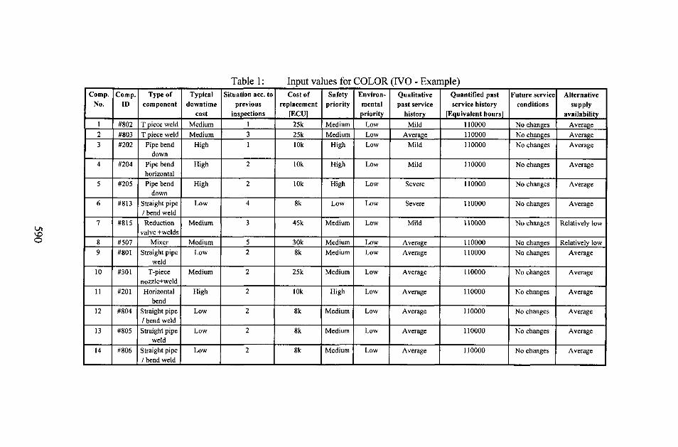
590

Table 1: Input values for COLOR (IVO - Example)Comp.

No.Comp.

IDType of

componentTypical

downtimecost

Situation acc. to previous

inspections

Cost of replacement

[ECU]

Safetypriority

Environ­mentalpriority

Qualitative past service

history

Quantified past service history

[Equivalent hours]

Future serviceconditions

Alternativesupply

availability1 #802 T piece weld Medium 1 25k Medium Low Mild 110000 No changes Average2 #803 T piece weld Medium 3 25k Medium Low Average 110000 No changes Average3 #202 Pipe bend

downHigh 1 10k High Low Mild 110000 No changes Average

4 #204 Pipe bend horizontal

High 2 10k High Low Mild 110000 No changes Average

5 #205 Pipe bend down

High 2 10k High Low Severe 110000 No changes Average

6 #813 Straight pipe / bend weld

Low 4 8k Low Low Severe 110000 No changes Average

7 #815 Reductionvalve +welds

Medium 3 45k Medium Low Mild 110000 No changes Relatively low

8 #507 Mixer Medium 5 30k Medium Low Average 110000 No changes Relatively low9 #801 Straight pipe

weldLow 2 8k Medium Low Average 110000 No changes Average

10 #301 T-piecenozzle+weld

Medium 2 25k Medium Low Average 110000 No changes Average

11 #201 Horizontalbend

High 2 10k High Low Average 110000 No changes Average

12 #804 Straight pipe / bend weld

Low 2 8k Medium Low Average 110000 No changes Average

13 #805 Straight pipe weld

Low 2 8k Medium Low Average 110000 No changes Average

14 #806 Straight pipe / bend weld

Low 2 8k Medium Low Average 110000 No changes Average

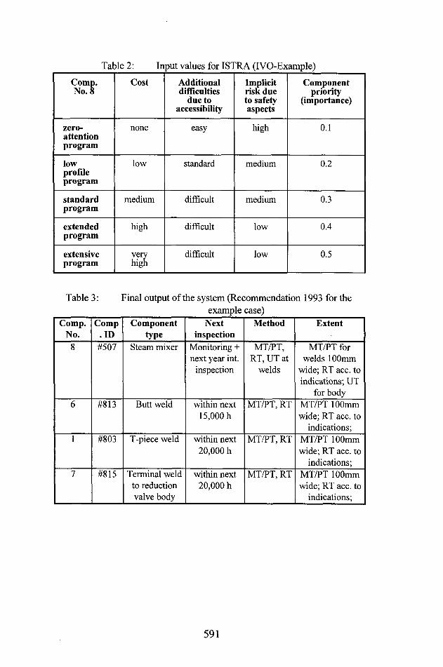
Table 2: Input values for ISTRA (IVO-Example)Comp.No. 8

Cost Additional difficulties

due to accessibility

Implicit risk due to safety aspects

Componentpriority

(importance)

zero-attentionprogram

none easy high 0.1

lowprofileprogram

low standard medium 0.2

standardprogram

medium difficult medium 0.3

extendedprogram

high difficult low 0.4

extensiveprogram

veryhigh

difficult low 0.5

Table 3: Final output of the system (Recommendation 1993 for theexample case)

Comp.No.

Comp.ID

Componenttype

Nextinspection

Method Extent

8 #507 Steam mixer Monitoring + next year int.

inspection

MT/PT, RT, UT at

welds

MT/PT for welds 100mm

wide; RT acc. to indications', UT

for body6 #813 Butt weld within next

15,000 hMT/PT, RT MT/PT 100mm

wide; RT acc. to indications;

1 #803 T-piece weld within next 20,000 h

MT/PT, RT MT/PT 100mm wide; RT acc. to

indications;7 #815 Terminal weld

to reduction valve body

within next 20,000 h

MT/PT, RT MT/PT 100mm wide; RT acc. to

indications;

591

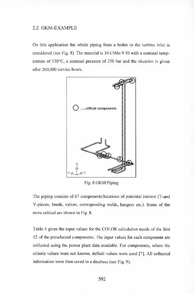
2.2 GKM-EXAMPLE

On this application the whole piping from a boiler to the turbine inlet is

considered (see Fig. 8). The material is 10 CrMo 9 10 with a nominal temp­

erature of 530°C, a nominal pressure of 250 bar and the situation is given

after 200,000 service hours.

critical components

Fig. 8 GKM Piping

The piping consists of 67 components/locations of potential interest (T-and

Y-pieces, bends, valves, corresponding welds, hangers etc.). Some of the

more critical are shown in Fig. 8.

Table 4 gives the input values for the COLOR calculation needs of the first

12 of the preselected components. The input values for each component are

collected using the power plant data available. For components, where the

criteria values were not known, default values were used [7], All collected

information were then saved in a database (see Fig. 9).

592

593

Table 4: Input values for COLOR (GKM-Example)Input data CRITERIACOMPONENTS Typical

downtimecost

Results of previous

inspections

Cost of replacement [1000 ECU]

Safetypriority

Environ­mentalpriority

Qualitative past service history

Quantified past [equivalent hours]

Futureservice

conditions

Alternativesupplypattern

kind of input data fuzzy crisp crisp fuzzy fuzzy fuzzy crisp fuzzy fuzzy

weight 70 100 70 40 40 60 30 80 80

No. Component No. - Name max max max max max max max max max

1 200 - Montagenaht am

Kesselaustritt

medium 6 15 high high average 111000 no changes relatively low

2 101 - Montagenaht low 4 15 medium high average 200000 no changes relatively low

3 B1-Bogen medium 4 75 high high average 200000 no changes relatively low

4 4 - Werkstattnaht low 2 15 medium high average 200000 no changes relatively low

S 201 - Montagenaht low 4 15 medium high average 200000 no changes relatively low

6 B2-Bogen medium 6 75 high high average 170000 no changes relatively low

7 202 - Montagenaht low 4 15 medium high average 200000 no changes relatively low

8 B3-Bogen medium 4 75 high high average 200000 no changes relatively low

9 109 - Werkstattnaht low 2 15 medium high average 200000 no changes relatively low

10 B4 - Bogen medium 4 75 high high average 200000 no changes relatively low

11 114 - Montagenaht low 4 15 medium high average 200000 no changes relatively low

12 203 - Montagenaht am

Kesselaustritt

medium 5 15 medium high average 0 no changes relatively low

Microsoft Access1Component/location specificationComp./location number: |.' I

File Edit View fiecords Window Help

Components

Comp./location name: jMonidgenaht am Kesselaustritt

Type of component: j straight pipe weld

-------- __11979: Mischnaht ausgebaut. Untersuchung bei MPA, MFI, I

VGB. Eisetzt dutch Ubetgangsstiick nach Zeichnung OM 55 754a Fa Votlandet R=1177 KE 270 832

I 2ttudjr fir ..............Cate study: |MPA 937 270 / 51

Picture:

Inspection planning input data:Domain expert selection: j r'es

Ranking: jTT"

••• ■-

Typical downtime cost: j medium

Results of previous insp.: jh

Cost of replacement: jl 5

Safety priority: [high

Environmental priority: [high

Qual. past service history: I average

Quantified past [eg. hours]: |111000

Future service conditions: jno changes

ARernative supply pattern: | relatively low

M 4 | Record jl [of 67 ITJh]

4- u I*

NuT.mef del Komponenle {ar^log Plan) 1 [Hum f ;

Fig. 9: Database interface for inspection input data

Apart of the inspection planning input data, the database contains

component/location specifications, including a detailed picture of the

respective location of the piping.

The type of the input values are either crisp or linguistic. For the COLOR

analysis, the linguistic statements must be transformed to fuzzy numbers

using appropriate membership functions [2, 3, 4, 10]. After this analysis, the

output is a list of components ranked by their priority for inspection. A

graphic illustration of COLOR results for GKM piping is shown in Fig. 10.

The result value , shown in this figure, corresponds to the priority of each

component, since it integrates all criteria inputs. In that way, the most

critical component achieves the highest result value. In the GKM example,

this component was the valve DH 14-la.

594

160.00

140.00

120.00

100.00a>3rtJ 80.003V)a“ 60.00

40.00

20.00

0.00

Fig. 10: Graphic illustration of the result of the ranking tool COLOR

As already shown in IVO example, the next step when using the decision

support system is to establish the appropriate inspection strategy using

ISTRA module, and to perform the recommended tests. The developed

database, interacts with the whole decision support system, enabling a

feedback of all the information gathered with the various techniques

applied. For example, for the component no. 200, shown in Fig. 9, the value

regarding the “results of previous inspections” criterion could be decreased

(e.g. from 6 to 3 or 4) if the damaged weld was repaired.

3. CONCLUSIONS

The applications of the decision support system in the IVO and GKM power

plants, confirmed the capability of the system to efficiently use the

experience of local domain experts and the service history to quickly make

a first draft of the inspection plan. The overall system represents a helpful

tool for maintenance of power plant structures.

595

4. REFERENCES

[1] Auerkari, P., Borggreen, K. & Salonen, J., Reference micrographs for

evaluation of creep damage in replica inspections. NORDTEST

Technical Report NT 170. NORDTEST, Espoo, 1992, 41 p.

[2] Buckley, J.J., Fuzzy Flierarchical Analysis, Fuzzy Sets and Systems

17, North-Holland, 1985, pp. 233-247.

[3] Buckley, J.J., Ranking Alternatives Using Fuzzy Numbers, Fuzzy Sets

and Systems 15, North-Holland, 1985, pp. 21-31.

[4] Chen, S.J., Hwang, C.L., Fuzzy Multiple Attribute Decision Making,

Springer, Germany, 1992, pp. 351-370.

[5] Geyer, T., Reimplementierung des ExpertBook-Kems und Model-

lierung der Referenz-Prozedur des ESR-Systems, Studienarbeit,

Universitat Erlangen-Niimberg, 1994

[6] Jovanovic, A., Psomas, S.M., Auerkari, P., Decision support system

for planning of inspections in power plants. Part I. Methodology, to be

presented at the Baltica Conference, June 8, 1995

[7] Jovanovic, A., Psomas, S.M., Scharzkopf, Ch., Auerkari, P., Kautz,

H.R., Ronnberg, J., KBS-Supported Planning of periodic Inspections

in Power Plants, 20th MPA Seminar, Oct. 6 and 7, 1984, pp. 5.4.1-

5.4.12

[8] Jovanovic, A., Psomas, S., Schwarzkopf, Ch, Auerkari, P., Ronnberg,

J., Bath, U., Weber, R., Kautz, H.R., Verelst, L., Decision Making for

Power Plant Component Inspection Scheduling, TEC-T4-01/REV-1,

RESTRUCT, Sep. 1994, 60 p.

[9] Kautz, H., Jovanovic, A., Schwarzkopf, C., Technical meeting at

GroBkraftwerk Mannheim (GKM), 6 Dec. 1994

[10] Zimmermann, H.J., Fuzzy Sets, Decision Making, and Expert

Systems, Boston, Kluwer Academic Publishers, 1987

596

HOW TO EVALUATE THE EFFECTIVENESS OF A MAINTENANCE PROGRAM ?

Kari Laakso, special research scientist VTT Automation, PL 1301, FIN-02044 VTT Seppo Hanninen, research scientist VTT Energy, PL 1606, FIN-02044 VTT Lennart Hallin, leader of operational planning Forsmarks Kraftgrupp Ab, S-74203 Osthammar.

Abstract

A model was developed for evaluation of the effectiveness of existing test and maintenance programs of technical systems. The model combines an analysis of the historical data on faults and repairs with an analysis of the history of functional testing and preventive maintenance. The periodic tests and preventive maintenance actions, where faults were detected, are pin­pointed by the method. The two parts of the analysis are combined by cal­culation of simple indicators on test and maintenance effectiveness.

The present model was developed in pilot analyses on maintenance effecti­veness of motor operated closing valves and automatic protection systems in Finnish and Swedish nuclear power plants. An application results in verification of the preventive action programs and justification of changes in them. The changes recommended are prolonging or shortening of the preventive action intervals and introduction of modified or new actions.

A further development of the usefullness of methods and integration of the model will continue in new applications. The model can also be adapted for other applications in different types of power plants and technical systems.

Keywords: Maintenance, experience feedback, reliability, power plants.

1 INTRODUCTION

The first developments of the model for maintenance analysis are based on

the earlier Finnish studies on experience based reliability centered mainte­

597

nance [1,2,3], Recently, maintenance related application studies were bom

from the co-operation within the indicator group of the Nordic research

project NKS/SIK-1 [4],

Maintenance in this paper is not defined as only condition monitoring, pre­

ventive maintenance and repairs. A broader systems approach to mainte­

nance is taken. Thus the ’’total” maintenance program consisting of preven­

tive and corrective actions is defined according to the Table 1.

Table 1. Maintenance actions.

Functional testing which can be periodic motioning of a valveNon destructive testing (NDT) which can be ultrasonic testing of a weldServicing such as cleaning and lubricationCalibration control and adjustments such as check of a limit switchPeriodic replacement such as rubber items in a solenoid valveCondition monitoring e.g. measurement of motor power by valve actuationRepairsModification work based on redesign.

The main goal of the maintenance studies was to develop a methodology

for systematic maintenance analysis and demonstrate its utilization on dif­

ferent equipment and technical systems. One important goal has thus been

to develop a good model for follow-up of reliability and maintenance ef­

fectiveness by analysis of historical data on faults and maintenance. Intro­

duction of quantitative measures for evaluation of test and maintenance ef­

fectiveness was also found important by the utilities. Components or items

which are weak from the reliability point of view should be identified. The

model should also provide prerequisities for management of component

ageing. Needs on reduction of excessive periodic testing and preventive

maintenance has recently arisen as a new issue and the potential opportuni­

ties for justified reductions should be identified. The main goal of the

598

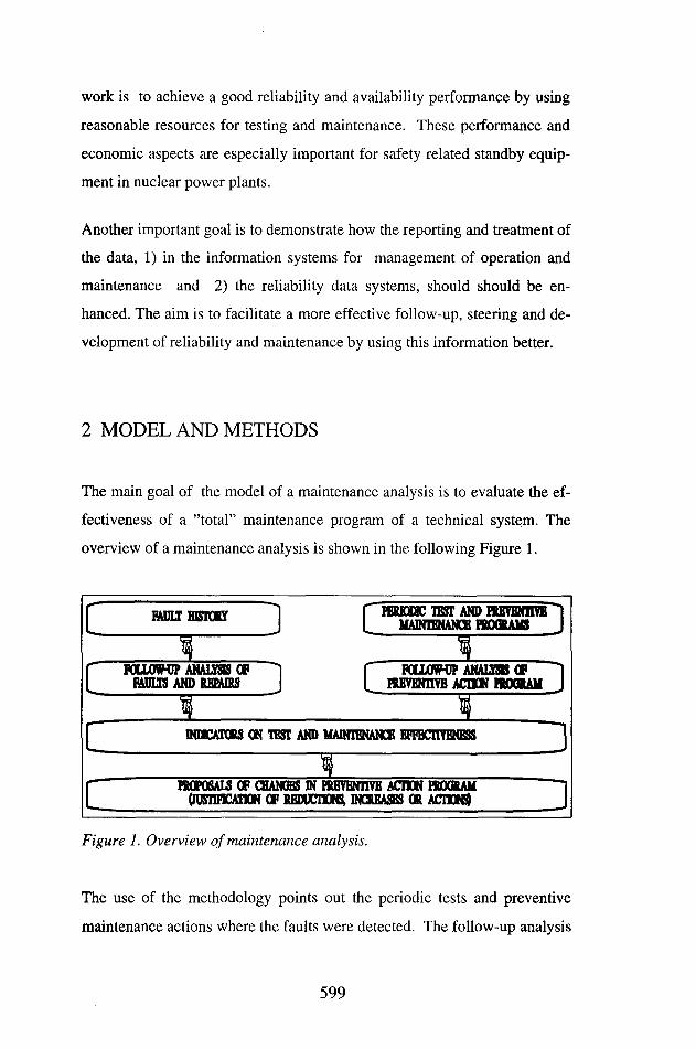
work is to achieve a good reliability and availability performance by using

reasonable resources for testing and maintenance. These performance and

economic aspects are especially important for safety related standby equip­

ment in nuclear power plants.

Another important goal is to demonstrate how the reporting and treatment of

the data, 1) in the information systems for management of operation and

maintenance and 2) the reliability data systems, should should be en­

hanced. The aim is to facilitate a more effective follow-up, steering and de­

velopment of reliability and maintenance by using this information better.

2 MODEL AND METHODS

The main goal of the model of a maintenance analysis is to evaluate the ef­

fectiveness of a ’’total” maintenance program of a technical system. The

overview of a maintenance analysis is shown in the following Figure 1.

PERIODIC TEST AND PREVEN1TVBMAINTENANCE R0GRA1B

PROPOSALS OF CHANGES IN PRETENTITE ACTON PROGRAMOusnncAnON op rbcucikni increases or actons)

FOLLOW? ANALHS OFRUMS AND REPAIRS

BfflKAIORS ON TEST AND MAINTENANCE EFFECTIVENESS

FOUOWP ANAU5B OFISEVENHTB ACnGN ROGKAM

Figure 1. Overview of maintenance analysis.

The use of the methodology points out the periodic tests and preventive

maintenance actions where the faults were detected. The follow-up analysis

599

of faults and repairs and the follow-up analysis of the preventive action

program are combined by calculation of simple indicators on the test and

maintenance effectiveness.

The qualitative methods of the follow-up analysis of fault and repair his­

tory are adaptations of the fault modes and effects analysis, FMEA, [5] and

maintenance effects analysis (MEA) described by Laakso & Bums in [6].

These qualitative methods are usually used for design review of equipment

during the definition and detailed design of technical systems. In a system­

atic maintenance analysis, the methods are applied for detailed analysis and

classification of operating experience. In our adaptation of FMEA, it is im­

portant to identify the procedure for fault detection in order to improve the

understanding of the effectiveness of the individual test and maintenance

types in fault detection. The analysis scheme, and the uses of the fault ex­

perience based assessment of the maintenance needs of equipment, is de­

scribed in detail by Hanninen & Laakso in [1], The analysis method helps

to rank the needs to strengthen the preventive action programs.

The additional reason to analyze the history of the test and preventive

maintenance programs has arisen from the need of the utilities to make the

preventive action programs more effective e.g. by reducing excessive

maintenance or testing recommended by the plant and equipment vendors.

The most important step in this analysis scheme, partially based on schemes

similar to FMEA and MEA, is the evaluation of the effects of testing and

preventive maintenance. The goal and the effects of the preventive actions

(PA) are defined. The preventive actions are usually done in order to detect

early the fault developments, eliminate the functional failures on real de­

mands and verify the condition and operability of the equipment. The

analysis of the preventive actions (PAEA) includes a study on how many

and which fault modes have been identified in the individual test and pre­

600

ventive maintenance types. The criticality analysis of PAEA contains an

analysis of the functional effects of the isolation of the maintenance object

from the operable system on the subsystem, system or plant level. One

quantitative result is the duration of the unavailability required by mainte­

nance including returning the system into an operable status after the main­

tenance actions [2,6]. The analysis method helps in ranking the potential

opportunities for reductions in the preventive action programs.

The indicators on test and maintenance effectiveness can be calculated at

different levels such as system, component group, component and item

level. The evaluation of the levels of the indicators should cover several

years of plant operational history, preferably not less than five years when

the trends [7] of fault occurrence are taken into account. The indicators

have been calculated for individual types of preventive and corrective ac­

tions covering redundant components, e.g. groups of four motor operated

closing valves. Typical indicators used are defined briefly in Table 2.

Table 2. Examples of indicators on test and maintenance effectiveness.

CM = Number of detected faults needing corrective actions RT = Total unavailability time due to corrective actions PA = Number of preventive actions PT = Total unavailability time due to preventive actions CM/PA = Ratio of the corrective and preventive action rates RT/PT = Ratio of the unavailability times due to corrective

and preventive actions.

It should be noticed that a part of the faults are detected in preventive ac­

tions and another part e.g. through alarm or in real demand situations. The

division of the faults into groups according to their detection method and

procedure will be done accordingly in the indicator calculations.

601

Candidates for reductions or reinforcements of the existing periodic test and

preventive maintenance programs can be identified, when deviating values

of the indicators are found. Conclusion can then be drawn from the underly­

ing data and its recent trends and from a functional judgement of the main­

tenance or testing practices to be preferred. This judgement includes search

of opportunities for timely and functional coordination of the tests, preven­

tive maintenance actions and condition monitoring tasks which are found

overlapping. Justification of the proposals of changes in the existing pre­

ventive action programs can then base on simple qualitative and quantitative

evaluation criteria. In order to facilitate economic evaluations of the main­

tenance effectiveness, the ratios of the corrective and preventive actions

could also be compiled for e.g. person-hours needed.

3 EXAMPLE OF PRESENTATION OF RESULTS

Candidates for reductions or reinforcements in the existing periodic test and

preventive maintenance programs are identified, when deviating values of

the indicators are found. The understanding of the conclusions, result pres­

entation and decision making is facilitated easier if a matrix of the preven­

tive actions is prepared. The matrix presents the potential opportunities to

make the preventive action program more effective. The example result is a

more balanced, simpler and less resource demanding program with the per­

spective to preserve or improve the reliability and availability of the system.

The example matrix shows how different periodic tests and preventive

maintenance actions cover an individual motor-operated closing valve

(MOV). An entire analysis and the results cover usually a larger group of

similar and different components belonging to one or several technical sys­

tems. The present intervals of the periodic preventive actions covering a

602

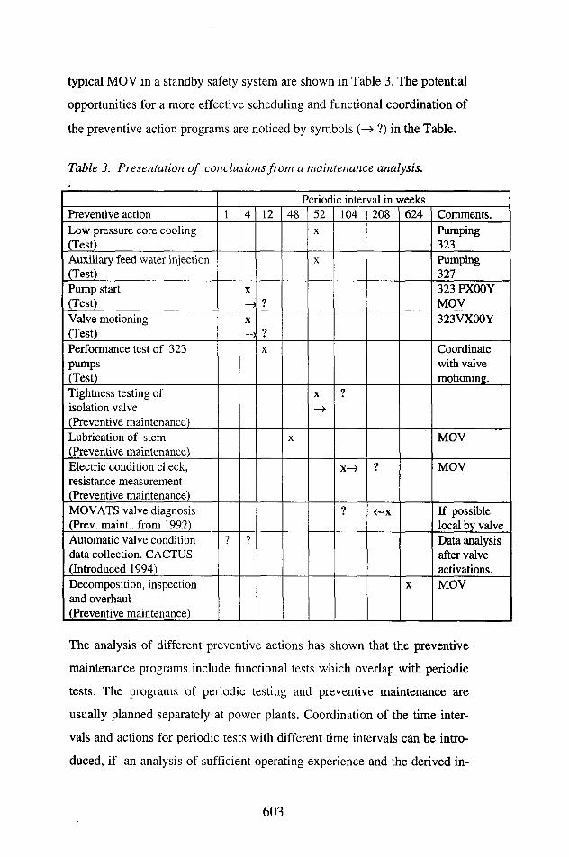
typical MOV in a standby safety system are shown in Table 3. The potential

opportunities for a more effective scheduling and functional coordination of

the preventive action programs are noticed by symbols (—» ?) in the Table.

Table 3. Presentation of conclusions from a maintenance analysis.

Periodic interval in weeksPreventive action 1 4 12 48 52 104 208 624 Comments.Low pressure core cooling (Test)

X Pumping323

Auxiliary feed water injection (Test)

X Pumping327

Pump start (Test)

X9

323 PX00Y MOV

Valve motioning (Test)

X7

323VXOOY

Performance test of 323pumps(Test)

X Coordinate with valve motioning.

Tightness testing of isolation valve (Preventive maintenance)

X

—»7

Lubrication of stem (Preventive maintenance)

X MOV

Electric condition check, resistance measurement (Preventive maintenance)

x—> 7 MOV

MOV ATS valve diagnosis (Prev. maint.. from 1992)

7 <-x If possible local by valve

Automatic valve condition data collection. CACTUS (Introduced 1994)

? ? Data analysis after valve activations.

Decomposition, inspection and overhaul (Preventive maintenance)

X MOV

The analysis of different preventive actions has shown that the preventive

maintenance programs include functional tests which overlap with periodic

tests. The programs of periodic testing and preventive maintenance are

usually planned separately at power plants. Coordination of the time inter­

vals and actions for periodic tests with different time intervals can be intro­

duced, if an analysis of sufficient operating experience and the derived in-

603

dicators on test and maintenance effectiveness and related conclusions jus­

tify the change. If e.g. the ratio of the corrective and preventive action rates

covering the electric condition check of the motor actuators of MOVs is low

or zero, it can be justified to study the opportunities to prolong the mainte­

nance interval or to make the corresponding preventive check more effec­

tive. The recently introduced automatic condition monitoring system, re­

cording actuations of motor operated closing valves, can be credited as an

effective preventive check and functional test in this case. Opportunities for

timely and functional coordination of the preventive actions of the mechani­

cal, electrical and instrumentation maintenance also exist.

4 DISCUSSION AND CONCLUSIONS

A vision supporting the need to develop the model of maintenance analysis

is the “total maintenance program”. This integrated program would include

periodic functional testing, preventive maintenance and servicing, calibra­

tion control and adjustments, condition monitoring and NDT in the same

program. One related long-term goal would be replacing the periodic testing

and maintenance tasks to an extent reasonable by justified condition based

tasks. A trial study on a protection system and connected electric drives,

covering a significant part of the analysis model, has been performed by

VTT together with a utility.

The information for the study was collected from different data sources, in­

cluding the maintenance history data system of the power plant. The data

was analyzed and utilized systematically in the study. Based on the analysis

experiences, practical recommendations were prepared on reporting, data

treatment and data presentation enhancements in the information system for

management of operation and maintenance. The application of the model

showed its usefullness by resulting in proposal of qualitatively and quanti­

604

tatively justified changes in the scheduling and coverage of the test and

maintenance programs of the technical systems studied.

A further development of the methods and integration of the model will

continue in future applications. The methods can be adapted for the use in

applications of different types of power plants and technical systems.

ACKNOWLEDGEMENTS

The method developments were performed in the research projects

’’Reliability assessment of maintenance in nuclear power plants, 1990-94”

and ’’Evaluation of maintenance strategies and reliability, 1995-98”. These

projects have been financed by the Ministry of Trade and Industry (KTM)

and the Technical Research Centre of Finland (VTT). The methods were

developed and tested in connection to practical application studies financed

by Forsmarks Kraftgrupp Ab (FKAB) in Sweden and the Finnish Centre for

Radiation Nuclear Safety (STUK) in co-operation with the utilities Teol-

lisuuden Voima Oy and Imatran Voima Oy.

We express especially our gratitudes to Mr. Pentti Koutaniemi, STUK, and

Mr. Lennart Hallin, FKAB, who acted as the coordinators of the two practi­

cal application studies.

REFERENCES

1. Hanninen, S. & Laakso, K. Experience based reliability centered maintenance - An application on motor operated valve drives. Hel­sinki: Finnish Centre for Radiation and Nuclear Safety. 1993. 51 p.+ app. 10 p. (STUK-YTO-TR 45). ISBN 951-47-7171-0.

2. Simola, K. & Laakso, K. Analysis of failure and maintenance experi­ences of motor operated valves in a Finnish nuclear power plant.

605

Espoo: Technical Research Centre of Finland. 1992. 57 p. + app. 140 p. (VTT Research Notes 1322). ISBN 951-38-4054-9.

3. Hanninen, S.Analysis of failure and maintenance experiences of large electrical motors. Helsinki University of Technology. Otanie- mi. 1991/31. 71 p. ISBN 951 - 22 - 0774 - 5.

4. Laakso, K (ed.). Safety evaluation by living probabilistic safety as­sessment and safety indicators. Final report of the Nordic nuclear safety research project SIK-1. The Nordic Council of Ministers, Co­penhagen: TemaNord 1994: 614. 45 p. + app. 5 p. (Prepared by a team consisting of Holmberg, J., Laakso, K., Lehtinen, E. & Johan- son, G.). ISBN 92 9120 540 0.

5. IEC 812. Analysis techniques for system reliability - procedure for failure mode and effects analysis (FMEA). International Electro­technical Commission. 1985. 40 p.

6. Laakso, K., Burns, D. A systematic maintainability review for plant design. Paper presented in 2nd European Logistics Symposium. Vaxjb. 11.-12. 6. 1985. 17 p. (Asea-Atom)

7. Huovinen, T. Estimation of some stochastic models used in reli­ability engineering. Espoo: Technical Research Centre of Finland. 1989. 144 p. (VTT Research Reports 598).

saved by kjl 31.3..95 as d:\seppo\toimi\balt3usl.doc

606

UNIT CONDITION ANALYSIS AT THE ISRAEL ELECTRIC CORPORATION

J. Rezek Ph.D., Manager, Materials Laboratory Israel Electric Corporation Haifa, Israel

Abstract

The electric system in Israel is unique; at the present time it is still isolated from any international grid. As a consequence, the need to supply adequate power necessitated, up to the mid 1980’s, the fullest use of all equipment as a primary requisite, irrespective of long term effects.

Condition analysis studies of 17 older units used under the above conditions were initiated in 1986 and completed in 1993. These studies, originally contracted to foreign companies, after a short learning period were performed locally. Today essentially all such studies are planned, performed and analyzed in-house.

Corporation policy is to subject all generating units to condition analysis according to a preset schedule. Older units are subjected to partial analysis every three years. Over two such shutdowns, all critical components are examined. The particular components examined are determined by their age, operating experience and previous examination results. Newer equipment is subject to examination determined by experience. After 12 years service new equipment is given a full condition assessment.

Units being brought on line are examined so as to determine base line conditions. Specifications for units being ordered for future delivery include requirements for base line data, information on critical locations and conservative material design.

607

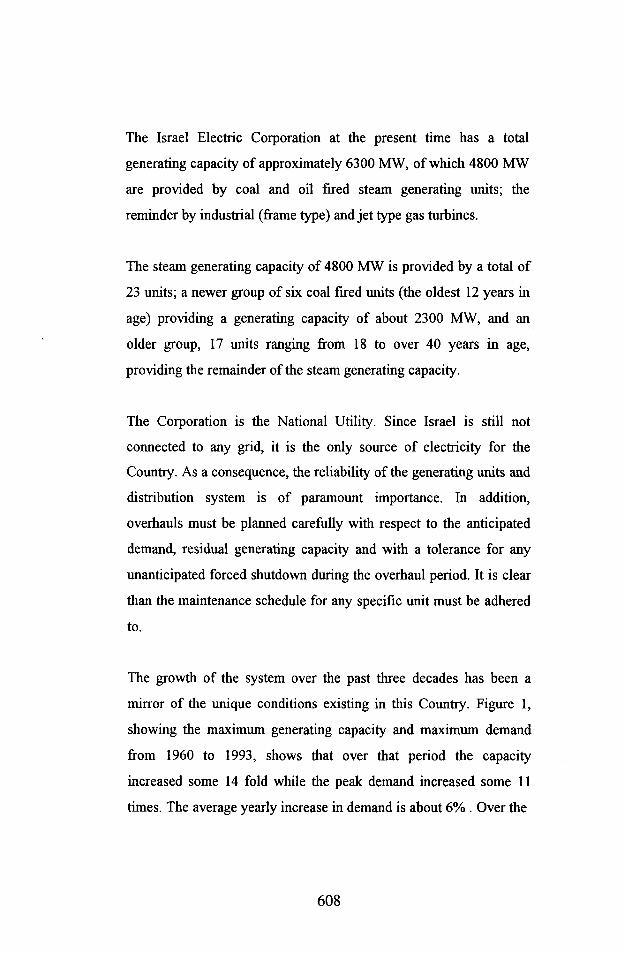
The Israel Electric Corporation at the present time has a total

generating capacity of approximately 6300 MW, of which 4800 MW

are provided by coal and oil fired steam generating units; the

reminder by industrial (frame type) and jet type gas turbines.

The steam generating capacity of 4800 MW is provided by a total of

23 units; a newer group of six coal fired units (the oldest 12 years in

age) providing a generating capacity of about 2300 MW, and an

older group, 17 units ranging from 18 to over 40 years in age,

providing the remainder of the steam generating capacity.

The Corporation is the National Utility. Since Israel is still not

connected to any grid, it is the only source of electricity for the

Country. As a consequence, the reliability of the generating units and

distribution system is of paramount importance. In addition,

overhauls must be planned carefully with respect to the anticipated

demand, residual generating capacity and with a tolerance for any

unanticipated forced shutdown during the overhaul period. It is clear

than the maintenance schedule for any specific unit must be adhered

to.

The growth of the system over the past three decades has been a

mirror of the unique conditions existing in this Country. Figure 1,

showing the maximum generating capacity and maximum demand

from 1960 to 1993, shows that over that period the capacity

increased some 14 fold while the peak demand increased some 11

times. The average yearly increase in demand is about 6% . Over the

608

Available pow

er vs. maxim

um demand 1960 - 1993

7

U1o3'

■ Capability (MW)

Wk Maximum Demand (MW)

5

4

3

1960 1962 1964 1966 1968 1970 1972 1974 1976 1978 1980 1982 1984 11961 1963 1965 1967 1969 1971 1973 1975 1977 1979 1981 1983 1985

Year

986 1988 1990 19921987 1989 1991 1993

years 1990-92, the peak, demand, as a result of accelerated

immigration, increased over 15% In the period 1960-93, the

population of the Country grew from 2.1 to 5.3 million; the number

of customers from 571,000 to 1,692,000.

Reference to Figure 1 shows that in the 60's and early 70's, peak

demand and capacity were almost identical. In some years peak

demand exceeded capacity. As a consequence of the lack of

generating capacity, up to the early 80's the need to produce

electricity far outweighed considerations concerning the long time

health of these units; most of the 17 older units mentioned above

were operated to their limits, if not beyond.

Not until the mid 80's, with increasing capacity and lower

immigration rates, was it possible to build up a sufficient power

reserve to have any kind of assurance that a routine maintance plan

could be implemented. At the same time, it was obvious to

management that those operational stresses imposed in the 60's,70's

and early 80's on units still active, could have caused safety related

damage in addtion to accelerated deterioration of the equipment.

As a consequence, in 1985 a policy decision was made to undertake

condition analyses of all 17 "older" units, as necessary repair or

replace components to bring them to a safe condition, and to upgrade

the units so as to improve their reliability. A decision was also made

to build "in-house" capability to perform condition analyses and to

perform routine examinations during overhaul. The Materials

Laboratory of the I.E.C. was given the responsibility of developing a

capability to perform a full condition analysis of the boiler and major

610

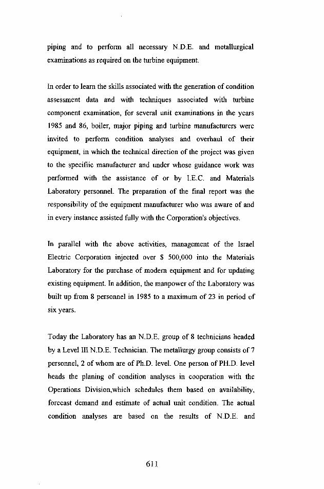
piping and to perform all necessary N.D.E. and metallurgical

examinations as required on the turbine equipment.

In order to learn the skills associated with the generation of condition

assessment data and with techniques associated with turbine

component examination, for several unit examinations in the years

1985 and 86, boiler, major piping and turbine manufacturers were

invited to perform condition analyses and overhaul of their

equipment, in which the technical direction of the project was given

to the specifiic manufacturer and under whose guidance work was

performed with the assistance of or by I.E.C. and Materials

Laboratory personnel. The preparation of the final report was the

responsibility of the equipment manufacturer who was aware of and

in every instance assisted fully with the Corporation's objectives.

In parallel with the above activities, management of the Israel

Electric Corporation injected over $ 500,000 into the Materials

Laboratory for the purchase of modem equipment and for updating

existing equipment. In addition, the manpower of the Laboratory was

built up from 8 personnel in 1985 to a maximum of 23 in period of

six years.

Today the Laboratory has an N.D.E. group of 8 technicians headed

by a Level III N.D.E. Technician. The metallurgy group consists of 7

personnel, 2 of whom are of Ph.D. level. One person of PH.D. level

heads the planing of condition analyses in cooperation with the

Operations Division,which schedules them based on availability,

forecast demand and estimate of actual unit condition. The actual

condition analyses are based on the results of N.D.E. and

611

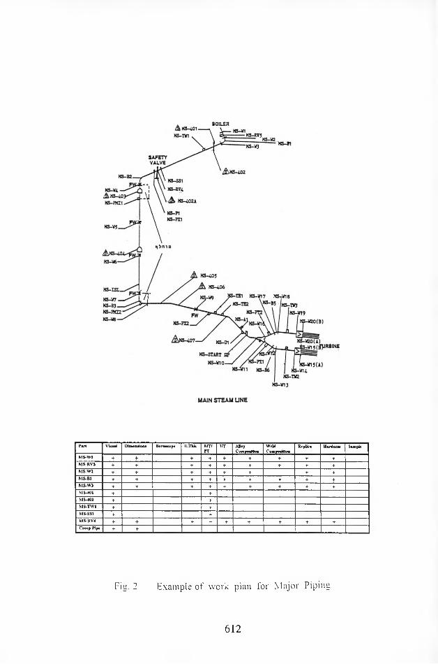
MS-W2

MS-PIMS-PI1

MS-PE MS-W1i

MS-START

MAIN STEAM LINE

Part Visual Dimensiocu Horoscope U.Thlc MTVPT

UT AlloyComposfckMi

WeUCompoaMoa

Replica

MS-W1 + + + + + + + + +

MS-RV5 + + + + + + + + +

MS-VV2 + +• + + + + + +

MS-B1 + + + + + + + + +MS-W3 + + + + + + + +

MS-401 + +

MS-402 + +

MS-TW1 + +

MS-SS1 + +

MS-RV4 + + + + + + + +

Creep Pip* + +

Fin. 2 Example of work plan for Major Piping

612

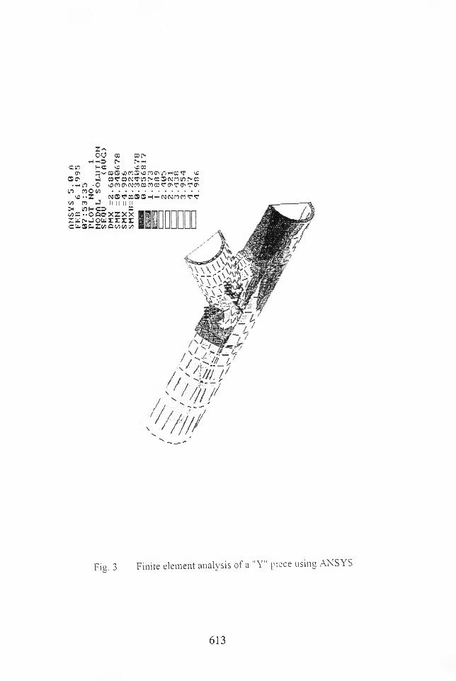
ftNSV

S

OC 05 05[>-

CUO HC kC CC5Ch D'w'C0O'J5 053or0CMn-i05^ U5

J esvesN'Twr'-ooSNciinr'-© • Hin *o ^co^Ne>5 05coco,J'0''j,o"?a'

m mOco>j5..Z05 J

inn c=> os a-.oootrxx ho-JowrrrrH S 0. Z(/) Cl 05 05 05

NOfOSOO-IHN N05 05 <? 5fII II II II

\'i \ y

/

//

/ \ ' / -r— w'/".iti !,s' m

.//

/s V

Fisi. 3 Finite element analysis of a " Y" piece using ANSY S

613

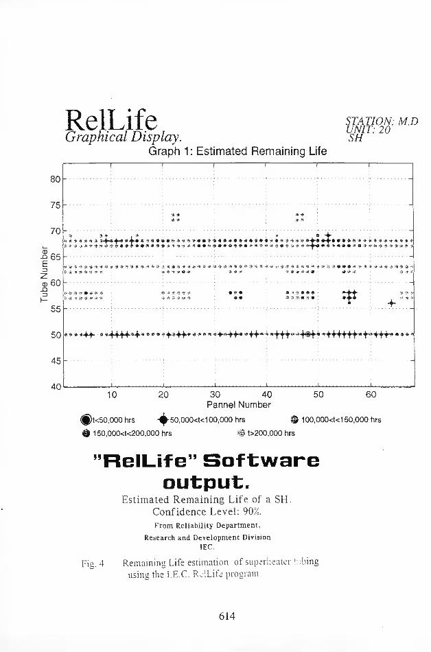
RelLifeGraphical Display.

Graph 1: Estimated Remaining Life

STATION: M.D UNIT: 20 SH

— ———

* a?S -■» -a ft n

* « * a * * ap ■3 '* * A T

4 O <»• * a 'a *•.**» 3 ^» ir a >•*©■**•**<»*■9 *l ■?» * <v a a i» a a-4-fli 4-4-»»•» a # -ft a a a # « > a a • a » » a »-a vl a ^ ^

? -a j v -vj rtj? V* ^ ^ ^ « * '> e i ^ a O -> :> '-V >\V 4 ^ »■.» pi ^ s «« a M« Sr »i ^ ♦ k * 51 ^ • M :*t»'>4P -> .a <> a 4 ftft =c

o y « ;» # rvCr -e* # ^ -J .V fj ■3 « ^.»> Vr o => • T* •<» • * •?. 4 K 4 ••V Ift ■{»

■4“

A « » ‘■-fs-ff* «-H”v * ** t i f *• *‘ ! 111 T T t ,,T'

.................... .................... ................... ................... .................... L..............

80

75

70

-Q 65 Ez

<d 60JD

55

50

45

4010 20 50 6030 40

Pannel Number@t<50,000 hrs -^■50,000<t<100,000 hrs © 100,000<t<150,000 hrs

© 150,000<t<200,000 hrs # t>200,000 hrs

’’RelLife” Software output.

Estimated Remaining Life of a SH. Confidence Level: 90%.From Reliability Department,

Research and Development Division IEC.

Fiu. 4 Remaining Life estimation of superheater tubing using the I.E.C. RelLife program

614

metallurgical examinations. This is augmented by stress analyses

developed by our Design Division and Computer Programs

developed by our Research and Development Division. The

integration of all the work and the preparation of a final report is the

responsibility of the person above, responsible for the planning of

the condition analyses.

Examples of the of type of work performed today by the group

combination above are shown as Figure 2, a work plan for

examinations to be performed on a section of major piping. Figure 3,

a stress analyses of a Y junction in which cracks were found and

Figure 4, a layout of .remaining life in a superheater section as

derived from ultrasonically measured internal oxide thickness.

Considering the work performed on the 17 older units, in the period

1985 to 1993 all units underwent a complete or partial condition

analysis. As the work progressed, it become evident that decisions

could be made ahead of time for replacement of components; thus, a

decision to replace all bat wing pipe supports with an alternative

design and all longitudinally welded bends in all units was made in

1985 during the first condition analysis study. Similarly, on the basis

of the results of an examination of a particular unit in which was

found damage to most bends on the major piping, it was deemed

more economical to replace the same components on another three

identical units constructed at the same time rather than bear the costs

(and risk of lack of generating power) during a long preliminary

condition analysis, possible temporary repairs, and a following

scheduled shutdown for replacement of the bends.

615

The consequences of the demanding conditions imposed on the older

units during the 60's, 70's and early 80's were apparent from the

operating history of each of the units and it was not necessary to

perform a full condition analysis in order to decide whether

replacement of boiler components was obligatory or not. Thus, for

many of the older units, prior to a condition analysis, decisions to

replace water walls, superheaters or economizers, for example, had

already been made and the actual condition analysis was performed

only on the residual pressure parts.

In the course of the examinations, it also become apparent that

equipment suffered damage as a result of specific design parameters

and not necessarily operating conditions. Thus, it was found that

virtually all dearators suffered stress corrosion cracking at most

welds because stress relief of welds when the dearators were built

was not a requirement of the standard. In this respect, all dearators

are now routinely spot examined each year and not only at times of

condition analyses. Although operating conditions may have some

part in the cause of damage, we have found cracks in many boiler

drums at the internal weld of the piping to the safety valves. This

location is also routinely examined each yearly shutdown. Similary,

condensate drains of major piping are another location at which

damage, as a result of thermal fatigue, is found. Y junctions,

generally welded, into wich steam enters form two headers is another

location at which damage which is often seen. This damage occurs as

a result of thermal stresses due to gross wall thickness differences at

the strengthening pads of junctions and/or because of restrictions to

the movement of the piping. Depending on the specific unit, this is

another location for which we perform yearly checking.

616

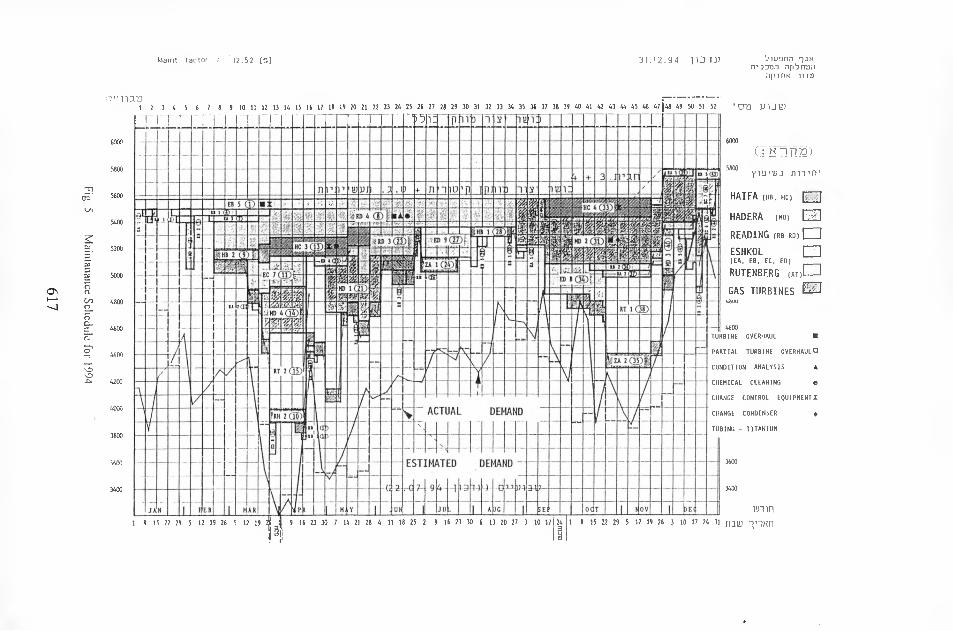
Fig. 5 M

aintanance Schedule for 1994

Maim factor : 12.5 2 [%] 31.12.94 111111) biuonn ^aKrrjDTDn np^rran

npmN htd

n-'iu-Q1 2 3 u 5 6 7 8 9 10 11 12 13 14 15 16 17 18 19 20 21 22 23 24 25 26 27 28 29 30 31 32 33 34 35 36 37 38 39 40 41 42 43 44 45 46 47 |48 49 50 51 52 ' D'Q U13U3

r^n6000

5800

5000

CTk-ifm)MOO

TID’BD nil’P'

HAIFA (no, hc)

HADERA mo)

READING (rb rd)

ESHKOL(EA. EB, EC. ED)

RUTENBERG (rt

GAS TURBINESoauu

4600TURBINE OVERHAUL ■

PARTIAL TURBINE OVERHAUL □

CONDITION ANALYSIS ▲

CHEMICAL CLEANING e

CHANGE CONTROL EQUIPMENT X

CHANGE CONDENSER +

TUBING - TITANIUM

unm1 8 15 22 29 5 12 19 26 5 12 19 2 i> I 9 16 23 30 7 14 21 28 4 11 18 25 2 9 16hi 23 30 6 13 20 27 3 10 17124 1 8 15 22 29 5 12 19 26 3 10 17 24 31 -piNn

I □□□

01

here damage to equipment has been attributed to operating

conditions, strain gauges and thermocouples have been attached to

components so as to identify those conditions and so to modify them.

Overall, in all the checking which has been performed on our units,

there has been no instance in which failure or potential failure of

headers or major piping can be attributed to pure hydrostatic steam

pressures. All the damage which has been determined has been

caused by design, construction, operating conditions, or material

factors affecting the component in addition to the pressure.

The philosophy of the Israel Electric Corporation with respect to

Condition Analyses is affected by its experience over the past ten

years; in practice, it is controlled by the same unique conditions

applicable to the system; i.e., its isolation and the necessity to

produce power to all consumers as required.

Figure 5 is a graph showing the actual maintenance, including

condition analyses, performed in 1994. This graph gives a much

better picture than the graph in Figure 1 since it shows the actual

power available during shutdowns and the peak demand at same

time. The figure clearly shows that deviations from expected demand

can cause concern. In mid December 1994, a "non scheduled" cold

spell put peak demand above the steam and industrial gas turbine

capacity. The result was that it was necessary to activate almost 80%

of the expensive jet turbine capacity over a short period in order to

maintain supply.

618

This condition is expected to continue for about another year when

extra industrial turbine capacity and an additional 575 MW of steam

capacity will be brought on line.

Irrespective of the above, it is the policy of the Israel Electric

Corporation to have all its units 12 years of age and over undergo a

series of condition analysis tests so that over a period of six years a

complete condition analysis of each unit is performed, generally over

two scheduled shutdowns three years apart. Since economic

conditions are now a potent factor in policy decisions, it is the

intention that the "in house" condition evaluation work will be no

more expensive than similar work performed by outside contractors.

The results of the examinations which have been performed to date,

including problems occuring in newer units, have had a direct effect

on our specifications for new units. Thus, our policy is to increase

the life of equipment by avoiding designs which contribute to its

degradation. On this basis we specify dearators and feedwater

storage tanks with postweld heat treatment, no longitudinal welds on

major piping and headers and no batwing hangers. In addition we

specify nil usage of T-1A tubing in superheater, reheater and

economizer components, P91 headers instead P-22, greater use of

T91 in superheaters and a more conservative limit to oxidation

temperatures of P22, and P11 including use of P12 in lieu of P11.

For purposes of future condition analyses of new units, we require

information on the zero condition of piping, tubing, headers and

turbine components as well as recommendations by suppliers of the

equipment, as to where they recommend locations of tests, and at

what intervals.

619

In summary, the overriding necessity to maintain electrical supply in

Israel was accomplished at the cost of the long term reliability of

some operating units. In 1985, with increasing power reserve, a

decision was made to implement condition analysis studies of these

units, to extend the concept to the whole system, and to build up in

house capability so as to plan, perform and analyze this work.

The results of the studies were to assure the safety of the units, and

to upgrade their reliability. Analysis of damage trends and causes of

them required that certain components undergo routine yearly

examination. Corporation policy is to avoid those parameters in

design which affect component life by specifying a conservative

approach to all design parameters. In addition, base line dimensional

and metallurgical data is requested so as to assist in future condition

studies

620

TRENDS IN LIFE MANAGEMENT OF “EESTI ENERGIA” POWER PLANTS

H. Tallermo1,1. Klevtsov1, V. Arras2, J. Gorohhov3

INTRODUCTION

The state enterprise “Eesti Energia” is monopoly company in Estonia, that

produces, transfers and distributes the electricity. The total installed

electrical capacity of power plants is 3370 MW and the heating capacity is

419 MW. Practically almost all electricity is produced at the two big power

plants: Baltic Power Plant (built in 1959-1965) and Estonian Power Plant

(built in 1969-1973). Both power plants fire the local fuel - Estonian oil

shale. The amount of fired oil shale is extremely great due to its enormously

low heat value, for example in 1994 was totally fired about 11,7-106 tons

and produced altogether 8,78 Twh of electricity.

The remaining life assessment of power plant units became to be very

important subject for “Eesti Energia”, because almost 50% of Baltic Power

Plant units have exceeded the design life for major number of high

temperature components. “Eesti Energia” approach to life management was

established in new rules for arrangement of diagnostic system. These rules

were co-ordinated with the Department of Technical Inspection of Estonia.

The comer stone of these mles is the safety of power plant units.

1 Senior Research Scientist, Tallinn Technical University, Tallinn, ESTONIA2 Engineer, State Enterprise “Eesti Energia”, Tallinn, ESTONIA3 Head of Central Laboratory of Metals and Welding, “Eesti Energoremont, Narva, ESTONIA

621

SUPERHEATER TUBING REMAINING LIFE ESTIMATION

The heating surfaces of oil shale fired boilers have very small reliability due

to high ash content of Estonian oil shale (up to 50%) and specific

composition of ash (contains alkaline, chloride and sulphur). The tubes of

heating surfaces of such boilers are covered with fireside sintered ash

deposits, that can accelerate the high temperature corrosion of tubes due to

the presence of above mentioned components in oil shale ash. The working

conditions of high temperature superheater surfaces are especially hard. The

periodical removing of deposits (soot-blowing or water lancing) allows

maintaining of steam temperature in the certain limits, but accelerates the

high temperature erosion of tubes because such soot-blowing can destroy

partly or entirely the oxide layer on the tubes surfaces. It should be also

mentioned that the deposits are extremely aggressive for tubes

manufactured from martensite and austenite steels.

The economiser tubes resource exhaustion is caused mainly by abrasive

erosion of metal due to high fly ash content in flue gas. The new methods of

cleaning of heating surfaces enable to improve the thermal efficiency of

power generating units and to reduce the requirements for repairs of heating

surfaces. Unfortunately total amount of repair works in such boilers is still

very large despite of using cleaning devices. For example, on the 200 MW

boiler (double unit 2x100 MW) the expenditures for heating surfaces repair

reach about 22% of total unit repair cost.

For the superheater tubes of oil shale fired boilers the typical creep damage

does not have practical importance thus the loss of wall thickness of tubes

due to high temperature erosion affects many times stronger on it’s resource

exhaustion. The high temperature corrosion intensity, was determined

622

several years ago on the basis of the laboratory tests so as the site tests for

different type of boiler steels used in oil shale fired boilers.

On the basis of above mentioned tests and operational experience standard

rules were established that allow the remaining life estimation for the

particular operational conditions and measured actual tube wall thickness.

Such kind of assessment is sufficiently precise. The total number of shut­

downs due to high temperature corrosion caused breakdown of superheater

tubes on the oil shale fired boiler does not exceed 1 for boiler per year.

DESIGN LIFE

The serious accidents of components working in the conditions of available

creep damage (piping, heaters, components of steam turbines, valves) did

not take place at the Baltic Power Plant though ca 50% of units (power

generating units with capacity 100 MW) have exceeded their design life. At

the Estonian Power Plant the design life of first unit will be achieved at

2005-2006 years. All equipment of Estonian power plants is manufactured

in former Soviet Union, and the design life their components must be in

accordance to the ORGRES norm RD 34.17.421-92. Some examples of

design life of power generating units document can be seen in the Table 1.

TECHNICAL DIAGNOSTIC SYSTEM

Diagnostic system is based on the three most important documents:

- rules of inspection of boilers, drums, headers, steam pipes, turbines and

valves;

- the data of operational history (temperature, pressure, vs. operational

time, number of start-shutdown cycles)

623

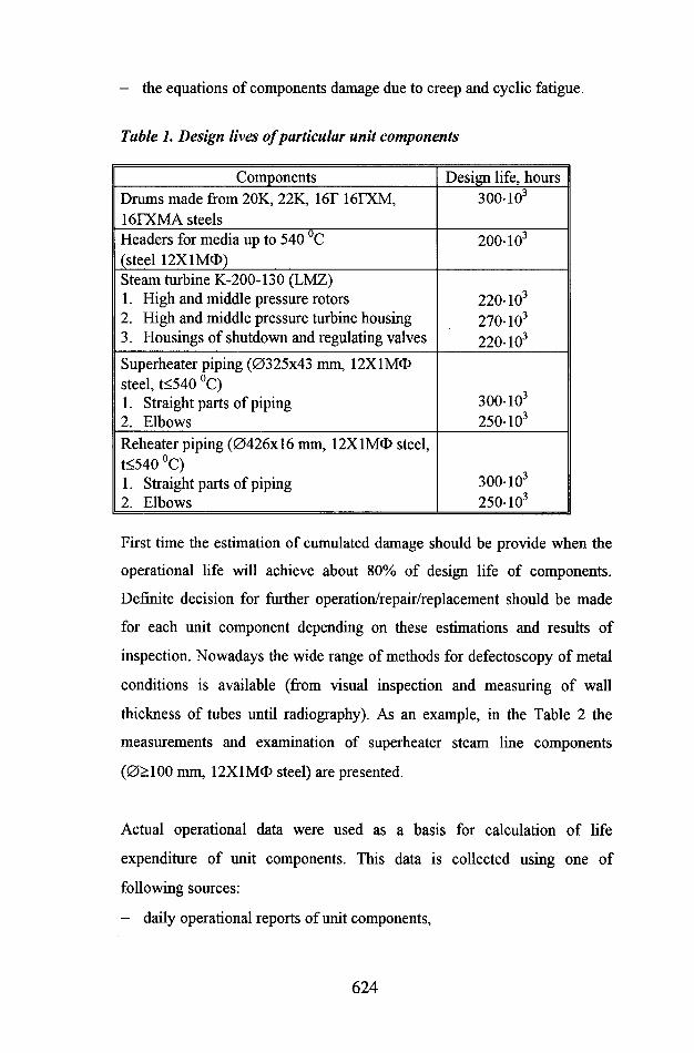
- the equations of components damage due to creep and cyclic fatigue.

Table 1. Design lives of particular unit components

Components Design life, hoursDrums made from 20K, 22K, 16T 16FXM, 300-10316FXMA steelsHeaders for media up to 540 °C 200-103(steel 12X1MO)Steam turbine K-200-130 (LMZ)1. High and middle pressure rotors 220-1032. High and middle pressure turbine housing 270-1033. Housings of shutdown and regulating valves 220-103

Superheater piping (0325x43 mm, 12XlM(t>steel, t<540 °C)1. Straight parts of piping 300-1032. Elbows 250-103

Reheater piping (0426x16 mm, 12X1 MO steel,t<540 °C)1. Straight parts of piping 300-1032. Elbows 250-103

First time the estimation of cumulated damage should be provide when the

operational life will achieve about 80% of design life of components.

Definite decision for further operation/repair/replacement should be made

for each unit component depending on these estimations and results of

inspection. Nowadays the wide range of methods for defectoscopy of metal

conditions is available (from visual inspection and measuring of wall

thickness of tubes until radiography). As an example, in the Table 2 the

measurements and examination of superheater steam line components

(0>1OO mm, 12X1MO steel) are presented.

Actual operational data were used as a basis for calculation of life

expenditure of unit components. This data is collected using one of

following sources:

- daily operational reports of unit components,

624

- automatic operational parameters measuring and registration system,

checking the registered parameters of unit components are pressure and

temperature vs. operational time, number of start-up-shutdown cycles

The data should be gathered for entire operational session that is under

consideration and appropriate estimations of cumulated resource exhaustion

should be made. This period of operational history should be divided into

intervals according to pressure and temperature deviations. The bank of data

for every piping system should include also the following information:

- all dimensions of straight parts and tube elbows, radius and bending

angle of tube elbows, type of steel;

- scheme of piping system including straight parts, tube elbows, welded

joints and placement of supports;

- actual wall thickness, ovality and creep of tube elbows;

- number and parameters of springs in hangers, type of hangers and their

height;

- thermal expansion of tubes;

- operational time and date of latest inspection.

METAL INSPECTION

The inspection and test of metal conditions in 5 electrical power plants and

6 boilerhouses of state enterprise “Eesti Energia” were provided accor­

dingly to above mentioned directives by Central Laboratory of Metals and

Welding which belongs to state enterprise “Eesti Energoremont” (Estonian

Energy Repairs). The total number of laboratory employees is 39, number

of specialists is 14. The laboratory is working in several different directions:

- the complete examination and testing of metal (extent determination of

stress-rupture strength) using the laboratory and site methods;

625

- non-destructive examination of welded joints;

- precise measuring and metrological certifying (this direction is being

assembled with two above mentioned directions);

- analyses of rupture accidents of pressure vessels and different type metal

constructions.

In addition to the test of metal conditions of power plants and boiler-houses

of state enterprise “Eesti Energia”, the Central Laboratory of Metals and

Welding is also fulfils orders for other Estonian enterprises and is also

certifying welders according to the requirements of EN-287. The cost of

metal inspections and examination carried out according to the above

mentioned rules is about 2,8-3,5% of total repairs cost for the boiler

equipment and about 6,7% for to turbines.

REPLACEMENT OF COMPONENTS

If the design life of unit components reaches 80% or the creep intensity is

more than 0,75-10'5 %, the further operation without metal examination is

forbidden. During such examination should be tested:

- presence (or absence) of internal defects;

- carbide content;

- microstructure;

- mechanical characteristics.

If any of examination results does not satisfy the criteria given in standard

rules, the unit component must be replaced. During the 35 year operation of

100 MW electricity generating units at the Baltic Power Plant have been

replaced 6 superheater headers, 4 steam coolers and about 60 pieces of large

valve (because of manufacture defects).

626

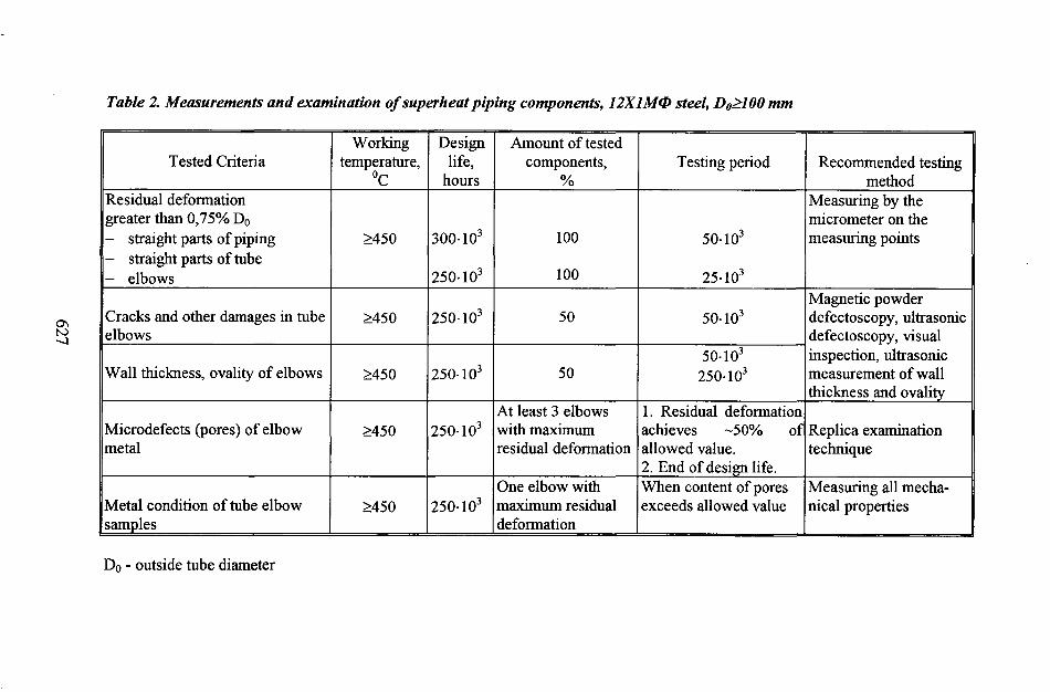
Table 2. Measurements and examination of superheat piping components, 12X1M0 steel, Dg>100 mm

Tested CriteriaWorking

temperature,°C

Designlife,

hours

Amount of tested components,

%Testing period Recommended testing

methodResidual deformation greater than 0,75% D0- straight parts of piping- straight parts of tube- elbows

>450 300-103

250-103

100

100

50-103

25-103

Measuring by the micrometer on the measuring points

Cracks and other damages in tube elbows

>450 250-103 50 50-103Magnetic powder defectoscopy, ultrasonic defectoscopy, visual inspection, ultrasonic measurement of wall thickness and ovality

Wall thickness, ovality of elbows >450 250-103 5050-103

250-103

Microdefects (pores) of elbow metal

>450 250-103At least 3 elbows with maximum residual deformation

1. Residual deformation achieves ~50% of allowed value.2. End of design life.

Replica examination technique

Metal condition of tube elbow samples

>450 250-103One elbow with maximum residual deformation

When content of pores exceeds allowed value

Measuring all mecha­nical properties

D0 - outside tube diameter

628

Creep Deformation and Rupture of Ferritic Tubular Components Subject to Complex

Stressing Conditions

J.M. Church* and R.C. Hurst

Institute for Advanced Materials, JRC Petten *Now at ERA Technology Ltd, Leatherhead, UK

ABSTRACT

Experimental observations for a 2‘ACr-lMo ferritic steel tested at 550°C and the application of a Continuum Damage Mechanics (CDM) model are utilised to examine the relationship between the creep deformation and rupture properties of uniaxial bar testpieces and those of model tubular components subjected to combinations of internal pressure and additional tensile end load. Rupture lifetime is observed to vary depending on specimen geometry, the applied stress state and the rate of monotonic stress increase as well as the nominally applied stress. Uniaxial constant stress data is used as the starting point for the CDM model which, when applied to the model component data, enables accurate predictions of both creep strain evolution and rupture lifetime to be made and which identifies a mixed Multiaxial Stress Rupture Criterion (MSRC) for the material over the range of rupture lifetimes considered. As part of the analysis a simple algorithm is presented which enables the MSRC to be derived analytically based upon measurements of creep strain evolution on tubular components. The results of the algorithmic approach are in good agreement with those of the CDM predictions.

1. INTRODUCTION

High temperature plant almost invariably operates under complex stressing conditions.

In spite of this fact, current design and remanent life estimation procedures rely

extensively upon uniaxial data to characterise material properties with regard to creep

deformation and fracture. Thereafter, empirically based formulae and tabulated, or

graphical, information are used to translate uniaxial property data into appropriate design

criteria. These relations aim to compensate for. amongst others, the effects of component

geometry and of material behaviour under multiaxial states of stress, and hence tend to

incorporate a conservative approach.

An alternative approach to high temperature analysis is to apply phenomenological

models of creep deformation and rupture to predict component response. Currently, the

practical application of such techniques, particularly in the area of remanent life

629

estimation involves a number of basic assumptions. In the first instance, the material

specific constants used in such models are generally derived from uniaxial constant load

data. Thereafter, it is assumed that the stress state in a component may be characterised

using reference stress techniques and further that long term creep failure occurs under

brittle conditions for which the applied stressing conditions may be assumed constant.

Brittle creep fracture is only one form of plant failure mechanism under creep conditions.

Alternatively, loss of functionality may occur, for example, as a consequence of

excessive creep deformation. The change in component shape and dimensions inherent

with the accumulation of strain may render the assumption of constant stressing

conditions inappropriate, in which case the effects of monotonic stress increase and

constant loading must be incorporated into the analysis. Furthermore, it is no longer

appropriate to characterise only rupture lifetime, or remaining life fraction during the

analysis, rather an accurate prediction of strain evolution is required as an integral part of

the analysis, to predict the limit of functionality in relation to operational lifetime.

This paper examines specifically the application of a continuum damage mechanics

(CDM) model to the prediction of creep strain evolution and rupture behaviour of tubular

2'/4Cr-lMo components which are subjected to internal pressure loading or a

combination of internal pressure and additional axial end loading. Uniaxial constant

stress creep data is used to derive the material parameters used in the constitutive model.

Subsequent application of the model to the component data enables the Multiaxial Stress

Rupture Criterion (MSRC) to be evaluated. As part of the analysis, a simple analytical

technique is presented which enables the MSRC to be derived by inspection from the

measurement of creep strain evolution on tubular component geometries.

2. EXPERIMENTAL DETAILS

The basic objective of this study is the examination of the creep behaviour of tubular

components with a view to predicting creep strain evolution and rupture lifetime in

relation to baseline uniaxial creep data. Testing was commissioned at 550°C on a

normalised and tempered ZViCr-lMo steel from the 60 mm wall thickness of a header

pipe manufactured for a boiler installation. The baseline uniaxial constant stress data

utilised as part of the study was obtained from work performed by partners in a BRITE

collaboration [1]. The material utilised during this work originated from two separate

batches, the first of which was utilised to generate a comprehensive uniaxial constant

stress database to aid initial model development, with the second material batch utilised

630

to undertake the model component testing, supported by limited uniaxial constant stress

and constant load testing for reference purposes.

The series of tubular component tests were conducted within the high pressure testing

facility at JRC Petten. Cylindrical blanks were first machined from the steam pipe wall

using electron discharge machining techniques. Tubular specimens were then machined

from these blanks to realise gauge length dimensions of 29mm internal diameter and

33mm external diameter. End caps, providing means for internal pressure inlet and axial

end load were then electron beam welded to the tubes to form testpieces. In all cases the

testpiece design and testing procedures used were in line with the guidelines of a Code of

Practice for internal pressure testing of tubular components at elevated temperatures [2].

As part of the model component test series, 4 internal pressure tests were performed at

pressures between 220 and 300 Bar together with one tensile loaded and three combined

tensile and internal pressure loaded experiments. Measurements of diametral and axial

strain, as a function of time, were made as appropriate using specially designed ceramic

extensometry [3]. Details of each test are given in Tables 1 and 2.

3. DEVELOPMENT OF A CONSTITUTIVE EQUATION SET

The parallelism between the CDM formulation and the mechanisms of constrained cavity

growth has been used extensively in developing methods of metallurgical condition

assessment and life prediction for low alloy creep resisting steels in particular [4]. In

their common form CDM models describe secondary and tertiary creep only, which

perhaps restricts their range of applicability. Primary creep may be introduced by

incorporating an Andrade type exponent into the constitutive equation set, which is

achieved following the works of Leckie and Hayhurst [5], and leads to the coupled

equations:

(1)

do) _ _(2)— = A

dt (l-o))"

where .1. K, m, n, tp and v are material specific constants. £ t and 0) denote strain, time

and the scalar damage state variable respectively, with the function rm introducing the

primary creep effect. For the current model, the chosen form of primary function has the

advantage of only introducing one additional parameter into the constitutive equation set

631

and is introduced into both rate equations on the assumption that strain and damage

evolve homogeneously with time.

3.1 Constant Stress Applications

The application of the model to the prediction of uniaxial constant stress behaviour

provides for a simple algebraic solution. Integration of the coupled equation set (1-2)

provides the normalised strain-time relation.

f r i l-m ^1- t

VTj.

)

l+l(3)

where the associated damage accumulation may be expressed in the form,

i<p+\

(4)<B = 1- i-40+i)<7vl-m

with the rupture lifetime, tf, and rupture strain, Ef, given by.

f A(<l)-n+l) K ’

It remains to assign values to the six material parameters used in the model. Parameter

optimisation for a standard Rabotnov-Kachanov CDM model often relies on making

basic assumptions regarding the exponents of stress within the coupled equation set,

which enables the constants to be reduced in number and to be evaluated based upon

experimental creep-rupture and minimum creep rate data. Assigning values to all six

constants within the above equation set should, in principle, provide a better description

of creep curve shape.

The optimisation of the material parameters in equations (1-2) requires the use of

numerical techniques. The method outlined below is based upon the procedure developed

by Evans, Parker and Wilshire [6], In principle, this method of parameter optimisation

may be employed to evaluate any number of constants. In practice, however, it has been

found that optimising all six parameters simultaneously leads to problems of

\-mA(<p + \)<JV

Ko"~v

0+1(5)

r&\

632

convergence and the procedure has required extensive modifications overcome this

problem.

In the first instance, a theoretical creep curve is supposed of the general form,

e =/(*/»') (7)

where xj denotes the set of material constants. Optimisation proceeds by minimising the

global error function, O, given by,

(8)

which may alternatively be written,

where f(xi ,tj) is the expected value of Sj , with k experimental data points available to

describe each creep curve. For the current model, the partial differential equations

df / dxl are non-linear and a guarded Gauss-Newton iterative procedure is used for their

solution. Iteration proceeds on the basis of a pre-determined convergence criterion for

the error function O, with the iteration step size and direction determined from the

gradient vector of the partial differential equations df / dxi. It is possible that the

solution will converge to a saddle point rather than at a local minimum. Upon

convergence, therefore, a grid search is performed to confirm that no improved solution

occurs in the immediate neighbourhood.

Practical implementation of the method requires experimental creep data normalised

with respect to failure time and strain, to correspond with the theoretical expression,

equation (3), which describes creep strain evolution in terms of the three material

constants, m, n and <p.

As with any iterative scheme, it is important to select initial values for each parameter

which are sufficiently close to the final solution to ensure convergence. Ideally, these

parameters should be determined from an individual creep curve. This has not been

achieved for the current model. Instead, n is taken as the Norton stress exponent for the

series of creep curves to be examined and 0 the stress exponent of rupture, with m taken

as the average proportion of lifetime expended at the onset of steady-state conditions.

The parameters m, n and 0 may then be optimised for any number of creep curves and

633

averaged to provide mean parameters for the database. Thereafter, re-arranging equation

(5) provides the expression,

log ^4 + V log O’= log l-w</> + ! 7 (10)

Given at least two complete creep curves, therefore, A and v may be determined using

regression analysis based upon inputs of the experimentally applied stress and failure

lifetime. K may then be found from the relation,

I ( , \i-»\1""/*+l-('-('/'/) )which enables K to be optimised for the whole database, based on the minimisation of

the residuals associated with predictions of all the experimental creep curves.

Figure 1 illustrates a series of 9 constant stress creep curves and their associated

optimised predictions of creep strain accumulation, for which the associated optimised

parameter set is :

m = 0.16754 n = 7.82641 0= 11.25006

v= 8.83061 = 2.43429 x 1 O'24 A'=3.5xl0-20

Visual inspection of the series, as a whole, suggests the analysis to provide a good

description of the data, particularly with regard to primary and secondary strain

evolution. Predictions of tertiary creep strain evolution provide examples of both

conservative and non-conservative estimates. The divergences observed are seen to be

non-systematic and are attributed to experimental scatter. These observations are

reflected in the predicted stress rupture response for the database. Figure 2, which infers

good interpolation capabilities over the range of stresses considered. Included on Figures

1 - 2 is an additional result (at 155 MPa) intended to examine the extrapolation potential

of the predictive methodology, albeit over a factor of only 5 in lifetime, and which is

well represented by the model. With the exception of the extrapolated prediction (155

MPa), values of failure ductility predicted by the model are below those observed in

practice. Nevertheless, rupture lifetime, which is well predicted by the model, is

inherently associated with a near infinite strain rate. Consequently, the onset of failure,

measured in terms of strain rate, is well predicted.

634

3.2 Constant Load Applications

Industrial components rarely experience constant stressing conditions. More typically,

the applied load is maintained constant such that stress increases monotonically with

strain. For uniaxial testpieces, this stress increase may be accounted for in terms of true

strain, e, such that the instantaneous stress is given by :

CT = (T0exp(e) (12)

where c0 is the initial applied stress. Partial solution of the constitutive equation set for

constant loading conditions provides the following :

fife~dt

KoT

1 - exp(v - ri)£ 1 - exp(v - ri)£f

n0-rt+l

(13)

t» = 1-,+ar lV-'')‘){exp((t,",,)c)''11 0-/I+!

(14)

£/ =v-n

-In KoTin-v)A(jp-n + l)

(15)

The above expression assumes an Andrade time hardening primary process. Whilst

providing a readily soluble equation, its physical realism may be open to question in

many cases. Treatments of primary-secondary creep identify both time and strain

hardening algorithms [7], which are generated by expressing creep strain rate explicitly

as a function of either time or strain respectively. The solutions are developed on the

assumption that the two algorithms are phenomenologically indistinguishable under

constant stress and temperature conditions. Leckie and Hayhurst [8] contest the use of

such algorithms in the presence of a state variable and prefer to maintain continuity of

the state variable when evaluating variable stress behaviour. In the context of the current

analysis this may be achieved by using the following time substitution in equation (13),

t = l-mA(</>-n + l)

1 r1-/M

* 1- 1-1 - exp((v - n)e)

l-exp((v-«)£/)

0+10-M+I

1l-m

(16)

For constant load applications, the constitutive equation (13) cannot be integrated to

formulate an algebraic expression for creep strain evolution with time and 4th order

635

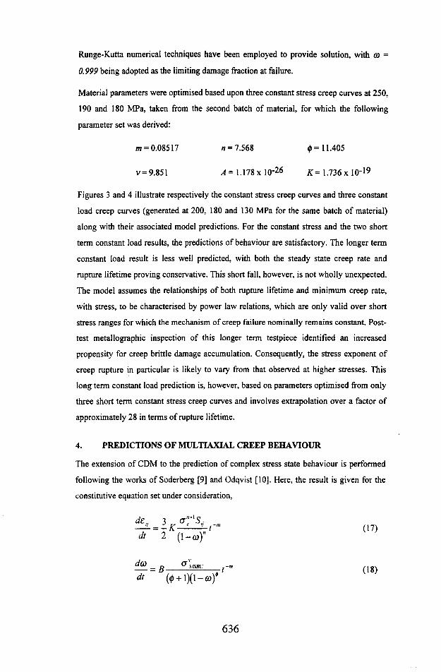
Runge-Kutta numerical techniques have been employed to provide solution, with ft) =

0.999 being adopted as the limiting damage fraction at failure.

Material parameters were optimised based upon three constant stress creep curves at 250,

190 and 180 MPa, taken from the second batch of material, for which the following

parameter set was derived:

m = 0.08517 /i = 7.568 0=11.405

v = 9.851 ^= 1.178 x lO'26 A> 1.736 x 10'19

Figures 3 and 4 illustrate respectively the constant stress creep curves and three constant

load creep curves (generated at 200, 180 and 130 MPa for the same batch of material)

along with their associated model predictions. For the constant stress and the two short

term constant load results, the predictions of behaviour are satisfactory. The longer term

constant load result is less well predicted, with both the steady state creep rate and

rupture lifetime proving conservative. This short fall, however, is not wholly unexpected.

The model assumes the relationships of both rupture lifetime and minimum creep rate,

with stress, to be characterised by power law relations, which are only valid over short

stress ranges for which the mechanism of creep failure nominally remains constant. Post­

test metallographic inspection of this longer term testpiece identified an increased

propensity for creep brittle damage accumulation. Consequently, the stress exponent of

creep rupture in particular is likely to vary from that observed at higher stresses. This

long term constant load prediction is, however, based on parameters optimised from only

three short term constant stress creep curves and involves extrapolation over a factor of

approximately 28 in terms of rupture lifetime.

4. PREDICTIONS OF MULTIAXIAL CREEP BEHAVIOUR

The extension of CDM to the prediction of complex stress state behaviour is performed

following the works of Soderberg [9] and Odqvist [10]. Here, the result is given for the

constitutive equation set under consideration.

d*, 3 gr'S,,

dt 2 (l-o,)"(17)

d(t> _ q G \tsRc fdt (tj) + l)(l - ©)*

(18)

636

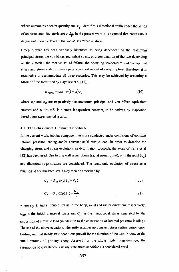
where co remains a scalar quantity and £jJ identifies a directional strain under the action

of an associated deviatoric stress S[j. In the present work it is assumed that creep rate is

dependent upon the level of the von Mises effective stress.

Creep rupture has been variously identified as being dependent on the maximum

principal stress, the von Mises equivalent stress, or a combination of the two depending

on the material, the mechanism of failure, the operating temperature and the applied

stress and stress state. In developing a general model of creep rupture, therefore, it is

reasonable to accommodate all three scenarios. This may be achieved by assuming a

MSRC of the form used by Hayhurst et al [11],

=a<71+(l-«K (19)

where Oj and ae are respectively the maximum principal and von Mises equivalent

stresses and a (0<a<l) is a stress independent constant, to be derived by inspection

based upon experimental results.

4.1 The Behaviour of Tubular Components

In the current work, tubular component tests are conducted under conditions of constant

internal pressure loading and/or constant axial tensile load. In order to describe the

changing stress and strain evolutions as deformation proceeds, the work of Taira et al

[12]-has been used. Due to thin wall assumptions (radial stress, or=0), only the axial (crz)

and diametral (cq) stresses are considered. The monotonic evolution of stress as a

function of accumulated strain may then be described by,

Oe =<7ft,exp(£8 -£r) (20)

=tf.-0exp(£.-) + — (21)

where Eq, £z and er denote strains in the hoop, axial and radial directions respectively,

<jq0 is the initial diametral stress and a:o is the initial axial stress generated by the

imposition of a tensile load (in addition to the contribution of internal pressure loading).

The use of the above equations inherently assumes no transient stress redistribution upon

loading and that steady state conditions prevail for the duration of the test. In view of the

small amount of primary creep observed for the alloys under consideration, the

assumption of instantaneous steady state stress conditions is considered valid.

637

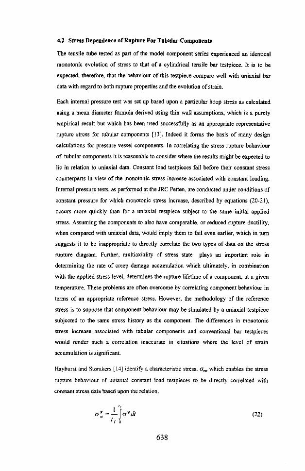
4.2 Stress Dependence of Rupture For Tubular Components

The tensile tube tested as part of the model component series experienced an identical

monotonic evolution of stress to that of a cylindrical tensile bar testpiece. It is to be

expected, therefore, that the behaviour of this testpiece compare well with uniaxial bar

data with regard to both rupture properties and the evolution of strain.

Each internal pressure test was set up based upon a particular hoop stress as calculated

using a mean diameter formula derived using thin wall assumptions, which is a purely

empirical result but which has been used successfully as an appropriate representative

rupture stress for tubular components [13]. Indeed it forms the basis of many design

calculations for pressure vessel components. In correlating the stress rupture behaviour

of tubular components it is reasonable to consider where the results might be expected to

lie in relation to uniaxial data. Constant load testpieces fail before their constant stress

counterparts in view of the monotonic stress increase associated with constant loading.

Internal pressure tests, as performed at the JRC Petten, are conducted under conditions of

constant pressure for which monotonic stress increase, described by equations (20-21),

occurs more quickly than for a uniaxial testpiece subject to the same initial applied

stress. Assuming the components to also have comparable, or reduced rupture ductility,

when compared with uniaxial data, would imply them to fail even earlier, which in turn

suggests it to be inappropriate to directly correlate the two types of data on the stress

rupture diagram. Further, multiaxiality of stress state plays an important role in

determining the rate of creep damage accumulation which ultimately, in combination

with the applied stress level, determines the rupture lifetime of a component, at a given

temperature. These problems are often overcome by correlating component behaviour in

terms of an appropriate reference stress. However, the methodology of the reference

stress is to suppose that component behaviour may be simulated by a uniaxial testpiece

subjected to the same stress history as the component. The differences in monotonic

stress increase associated with tubular components and conventional bar testpieces

would render such a correlation inaccurate in situations where the level of strain

accumulation is significant.

Hayhurst and Storakers [14] identify a characteristic stress, <7m, which enables the stress

rupture behaviour of uniaxial constant load testpieces to be directly correlated with

constant stress data based upon the relation.

/ o(22)

638

which effectively accommodates creep curve shape to identify an average operating

stress for the duration of creep life, \jf being the stress exponent of rupture. Assuming the

maximum principal and von Mises stress descriptors to provide nominal upper and lower

bounds to component stress rupture response the same procedure may be followed for

tubular components based upon each stress descriptor in turn and using equations (22-

23) to evaluate true stress increase. The MSRC may then be determined by comparison

with the constant stress datum and the true position of the results on the stress rupture

diagram subsequently discerned, Figures 5 and 6. Table 3 presents the values of a

derived for each test result. Based upon this methodology, for the internal pressure

results an average value of the MSRC is defined with am = 0.5 which implies 07 and <Je

to contribute equally to the failure mechanism. Previous work on low alloy ferritic

materials suggests an increased propensity for creep cavitation damage accumulation at

longer lifetimes, associated with an increased contribution from CT/ to the MSRC. The

current data does not accurately reflect this trend, although the shortest test does exhibit

the largest contribution of <7e to the rupture stress. The data is, however, relatively short

term, with little observed cavitation damage, for which it is anticipated that ae does

contribute to the MSRC. It is also to be expected that a remains essentially constant over

the stress range considered. Included on Figures 5 and 6 are the results of similar

analysis for the tensile tube and combined loading experiments which were all set up to

experience the same initial von Mises stress (201.5 MPa). For two of the results (at

biaxial stress ratios of Choop/°axiai=0 and crh00p/oaxial=l) the MSRC is not discernible in

view of the operational stress state. The remaining results do not show any systematic

variation in a as a function of stress state. It must be conceded, however, that the number

of test results is small and the influence of experimental scatter will, therefore, play a

role during the interpretation of results.

4.3 CDM Predictions of Component Behaviour

Figure. 7 compares the experimentally determined and CDM predictions of creep strain

evolution for each of the internal pressure tests based upon the material parameters

derived for the Batch 2 material. In each case, predictions of rupture behaviour are

presented based upon maximum principal and von Mises stress dependences of rupture

(a=/ and a=0 respectively) along with a prediction based upon a mixed rupture criterion

derived separately, by inspection, for each test result. In all cases the predicted secondary

creep rate is well described based upon the von Mises criterion, with rupture bounded by

the maximum principal and von Mises based predictions. The average value of a derived

639

for the internal pressure series, acm =0.55, agrees well with that derived using the

characteristic stress methodology.

In the case of the combined loading tests, Figure 8, behaviour is again well characterised

by the model, with an average MSRC for the series defined with Ocdm =0.71. Figure 9

illustrates, for the combined loading series, rupture lifetime as a function of the initial

biaxial stress ratio (o^/o^i). Included on the diagram are CDM predictions of rupture

lifetime based upon maximum principal and von Mises rupture criteria. Also included is

a prediction of behaviour based upon the average mixed rupture response derived for all

the model component data, with am=0.60. The figure demonstrates how lifetime

depends upon both the initial biaxial stress state and the operating MSRC, with the most

marked life reduction occurring for internally pressurised components experiencing a

maximum principal stress rupture criterion. For the current data, the figure confirms the

individual variations in a to be non-systematic and that the CDM model, based upon a

predicted mixed rupture response, generated using material parameters optimised from a

constant stress database, provides an accurate assessment of complex stress state creep

behaviour.

5. CONCLUSIONS

1. Continuum damage mechanics techniques have been applied successfully to

characterise uniaxial constant stress creep curves and extrapolated to describe

behaviour under uniaxial constant load conditions.

2. Complex benchmark creep experiments have been successfully carried out on

tubular 214Cr-lMo steel components conducted under tensile, internal pressure

and combined loading conditions.

3. Continuum damage mechanics based modelling has successfully been applied to

predict the strain evolution and stress rupture behaviour of plain tubular

components subject to complex loading conditions, based upon material

parameters derived from uniaxial data.

4. Multiaxial stress rupture criteria for plain tubular components subjected to

complex stress states have been established using a simple analytical technique

based upon characteristic stresses.

5. Application of the CDM model to the component data identifies both rupture

lifetime and the rate of strain evolution, for a particular testpiece, to depend

640

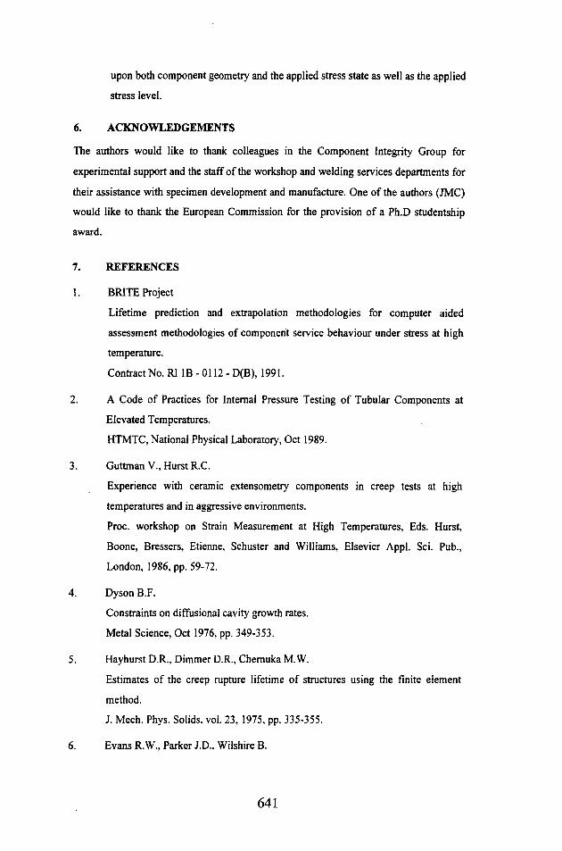
upon both component geometry and the applied stress state as well as the applied

stress level.

6. ACKNOWLEDGEMENTS

The authors would like to thank colleagues in the Component Integrity Group for

experimental support and the staff of the workshop and welding services departments for

their assistance with specimen development and manufacture. One of the authors (JMC)

would like to thank the European Commission for the provision of a Ph.D studentship

award.

7. REFERENCES

1. BRITE Project

Lifetime prediction and extrapolation methodologies for computer aided

assessment methodologies of component service behaviour under stress at high

temperature.

Contract No. R1 IB - 0112 - D(B), 1991.

2. A Code of Practices for Internal Pressure Testing of Tubular Components at

Elevated Temperatures.

HTMTC, National Physical Laboratory, Oct 1989.

3. Guttman V., Hurst R.C.

Experience with ceramic extensometry components in creep tests at high

temperatures and in aggressive environments.

Proc. workshop on Strain Measurement at High Temperatures, Eds. Hurst,

Boone, Bressers, Etienne, Schuster and Williams, Elsevier Appl. Sci. Pub.,

London, 1986, pp. 59-72.

4. Dyson B.F.

Constraints on diffusional cavity growth rates.

Metal Science, Oct 1976, pp. 349-353.

5. Hayhurst D.R., Dimmer D.R., Chemuka M.W.

Estimates of the creep rupture lifetime of structures using the finite element

method.

J. Mech. Phys. Solids, vol. 23, 1975, pp. 335-355.

6. Evans R.W., Parker J.D.. Wilshire B.

641

An extrapolation procedure for long-term creep strain and creep life prediction,

with special reference to 0.5Cr0.5Mo0.25V ferritic steels.

Recent advances in the creep and fracture of engineering materials and

structures, Eds. Wilshire and Owen, Pineridge Press, Swansea, 1982, pp. 135-

184.

7. Kraus H.

Creep analysis

Wiley and Sons, New York, 1980.

8. Leckie F.A., Hayhurst D.R.

The damage concept in creep mechanics.

Mech. Res. Comm., Pergamon Press, USA, vol. 2, 1975, pp. 23-26.

9. Soderberg C.R.

Interpretation of creep tests for machine design.

Trans. ASME, vol. 58, No.8,1936, pp. 733 -743.

10. Odqvist F.K.G.

Creep stresses in a rotating disk.

Proc. 4th Int. Cong. Appl. Mech.,Cambridge Univ. Press,, 1935, pp. 228-.

11. Hayhurst D.R., Leckie F.A., Morrison C.J.

Creep rupture of notched bars.

Proc. Roy. Soc., London. Ser. A, vol. 360, 1978, pp. 243-264.

12. Taira S., Ohtani R., Ishisaka A.

Creep and creep fracture of a low carbon steel under combined tension and

internal pressure

Proc. Japan Congr. Test. Mater., vol. 11, 1968, pp. 76-81.

13. Penny R.K., Marriot D.L.

Design for creep

McGraw-Hill, Maidenhead, chapter 4, 1971, pp. 100-155.

14. Hayhurst D.R., Storakers B.

Creep rupture of the Andrade shear disk.

Proc. Roy. Soc.. London, Ser. A, vol. 349, No. 1658. 1976, pp. 369-382.

642

Table 1 (a) Uniaxial Constant Stress Data - Batch 1

Stress Failure Strain Lifetime

(MPa) ef(%) (hr)

155 10.81 5636.18

180 21.94 1108.76

190 19.83 591.40

200 20.03 319.66

215 30.03 220.28

230 21.71 62.21

245 19.52 40.08

250 23.20 30.15

260 27.29 28.02

275 23.54 5.70

Table 1 (b) Uniaxial Constant Stress & Constant Load Data - Batch 2

Stress Failure Strain Lifetime

(MPa) e,(%) (hr)

180 32.96 598.75

190 24.75 415.45

250 26.53 18.92

130* 11.92 12924.5

180* 35.56 486.2

200* 38.3 144.9

* Constant Load Data

643

Table 2 Model Tubular Component Creep Test Data - Batch 2

Testpiece BiaxialStressRatio

Applied Stress

MPa

Failure Strain

(%)

RuptureLifetime

(Hr)

Ghoop/^axi*1

Oi ei(%) M%)

BP300.550 2 232.67 201.5 26.77 30.91 78.57

BP260.550 2 201.5 174.5 9.94 11.13 192.45

BP240.550 2 186.0 161.1 14.19 16.38 470.57

BP220.550 2 170.5 147.7 17.67 20.40 1360.97

BT39.550 0 201.5 201.5 35.44 35.44 122.16

BC150.550 0.5 232.67 201.5 10.71 12.36 69.72

BC260.550 1 201.5 201.5 13.62 27.24 101.88

BC295.550 1.5 228.48 201.5 12.16 6.93 44.58

Table 3 Multiaxial Stress Rupture Criteria for Model Tubular Components

Testpiece Biaxial Stress Ratio^hoop-^aiial

Values of the MSRC parameter a derived using the

characteristic stress analysis

BP300.550 2 0.26

BP260.550 2 0.68

BP240.550 2 0.63

BP220.550 2 0.47

BT39.550 0 -

BC150.550 0.5 0.40

BC260.550 1 -

BC295.550 1.5 0.79

644

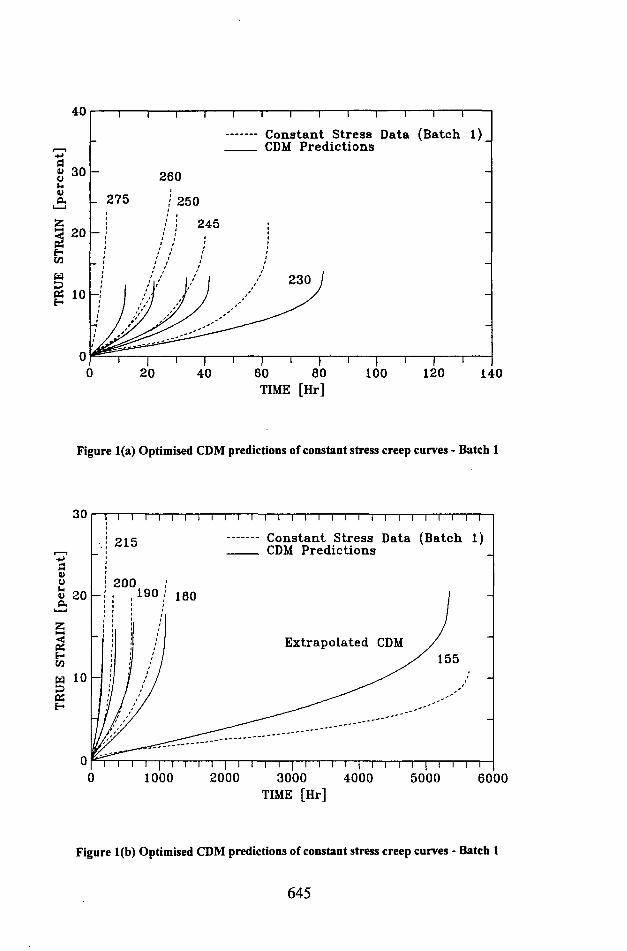
TRU

E STR

AIN

[perc

ent]

TRU

E STR

AIN

[perc

ent]

(Batch l)_Constant Stress Data CDM Predictions

0 20 40 60 80 100 120 140TIME [Hr]

Figure 1(a) Optimised CDM predictions of constant stress creep curves - Batch 1

l l l l lConstant Stress Data (Batch l) CDM Predictions

20 -

Extrapolated CDM

t—i—r i i i i I i i i—i r20001000 3000

TIME [Hr]4000 5000 6000

Figure 1(b) Optimised CDM predictions of constant stress creep curves - Batch 1

645

a)PU

COCOCdOSHCO

10

I I I 11 1—I I I ! I M| I I I I I lll| r i i 11111

I>iii Constant Stress (Batch 1) _____ CDM Prediction

t n 111 ii|T I I 1 11 ll| t r i 111 ii|1 10 102 103 104 10

LIFETIME [Hr]5

Figure 2 Actual and predicted constant stress rupture response - material Batch 1

oaaaa Constant Stress Data (Batch 2) _____ CDM Predictions

250MPa

CS 10

TIME [Hr]

Figure 3 Optimised CDM predictions of constant stress creep curves - Batch 2

646

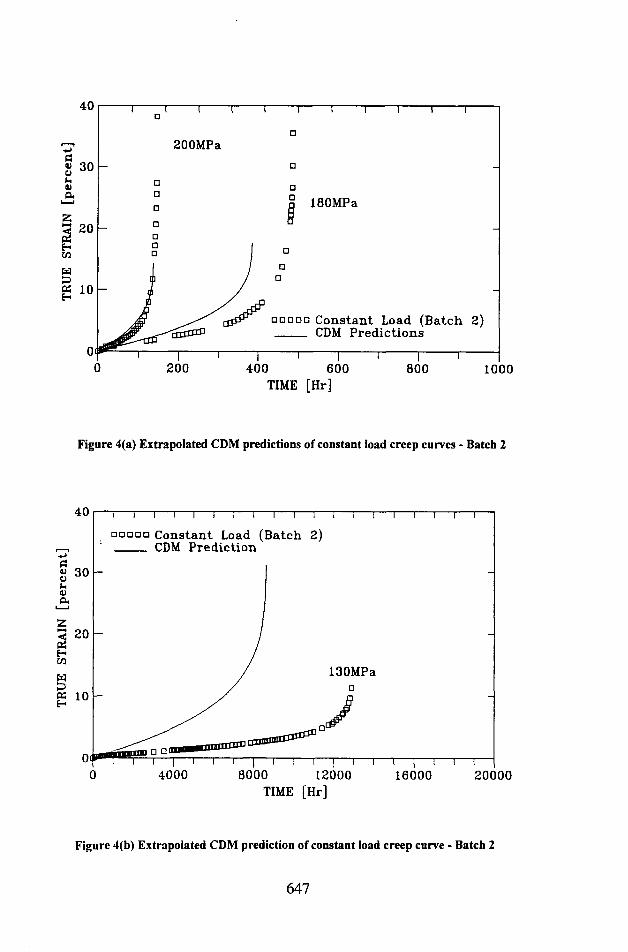
TRU

E STR

AIN

[perc

ent]

TRU

E STR

AIN

[perc

ent] 200MPa

□ □□□□ Constant Load (Batch 2) _____ CDM Predictions

1000TIME [Hr]

Figure 4(a) Extrapolated CDM predictions of constant load creep curves - Batch 2

□ □□□□ Constant Load (Batch 2) _____ CDM Prediction

130MPa

4000 12000 16000 20000TIME [Hr]

Figure 4(b) Extrapolated CDM prediction of constant load creep curve - Batch 2

647

STR

ESS [M

Pa]

STR

ESS [M

Pa]

3

10

z

2

l II i l ll| i i i i i

_____ Constant Stress (Batch 2)■■■■ Internal Pressure Characteristic MPS 11 J_i u Internal Pressure Characteristic VM AAAAA Combined Load Characteristic MPS AAAAA Combined Load Characteristic VM

1 10 10 2 10 3 10 4 10LIFETIME [Hr]

5

Figure 5 Characteristic stress rupture response of tubular components

------1—i miiq—i— n iiii|----- 1—rrmTTi----- 1—i i 111ii| n 1 1 1 1 III

\\

_ __ Constant Stress (Batch 2)XXXXX Constant Load

>5

A .

A' .

H®EE Internal Pressure MPS □■■■■■Internal Pressure MSRC i i i i i 1 Internal Pressure VM 'x-------- Int. Press. CDM (averaged prediction)

AAAAA Combined Load MPSIsAA/iA Combined Load MSRCAAAAA Combined Load VM

1 10 102 10 3 10 4 10LIFETIME [Hr]

5

Figure 6 True stress rupture response of tubular components

648

STR

AIN

[perc

ent]

STR

AIN

[perc

ent] □ □□□□ Experimental Data

_____ CDM Prediction

260 Bar v. Mises

Mixed

i i i Ii—i—rt i—| i i r200

TIME [Hr]

300 Bar

v. Mises

Mixed ^

60 I TIME [Hr]

220 Bar

v. Mises

Mixed

800 1200 1600 2000 TIME [Hr]

240 Bar

v. Mises

Mixed

iOO 600 TIME [Hr]

800 1000

Figure 7 CDM predictions of strain accumulation for internally pressurised tubular components

21

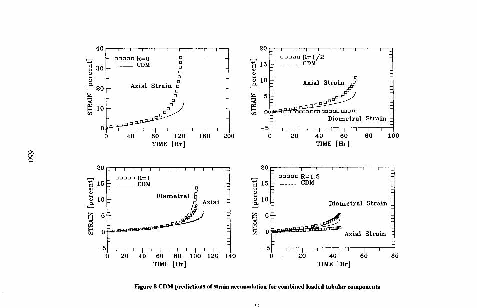
STR

AIN

[perc

ent]

STR

AIN

[perc

ent]

5 10 Axial Strain

TTnmn n m nnn nn mnDiametral Strain -

40 60TIME [Hr]

□ □□□□ R=0

Axial Strain □

80 120 TIME [Hr]

□ □□□□ Rrrl.5

Diametral Strain :

Axial Strain

40TIME [Hr]

- □□□□□ R=1

Diametral aAxial

20 40 60 80 100 120 140TIME [Hr]

Figure 8 CDM predictions of strain accumulation for combined loaded tubular components

10

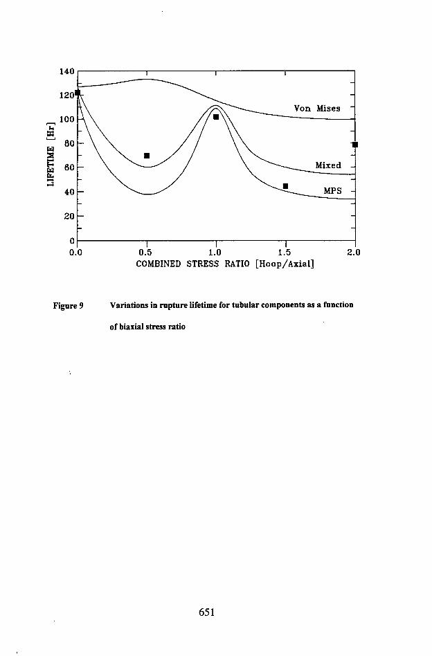
Mises

Mixed

0.5 1.0 1.5COMBINED STRESS RATIO [Hoop/Axial]

Figure 9 Variations in rupture lifetime for tubular components as a function

of biaxial stress ratio

651

652

STATISTICAL APPROACH TO THE LIFETIME ASSESSMENT

OF STEAM POWER PLANT COMPONENTS

J.K. Petrenja *

*The Polzunov Central Boiler and Turbine Institute Polytechnicheskaya, 24, St.-Petersburg, 194021, Russian Federation

As life time increases the accuracy of the determination of stress safety margin factors related to the lower allowable value of safety margin factors has to decrease. The scatter of creep properties as a main cause of the uncertainty of safety margin factors is considered. The experimental study of creep properties scatter of steels for long term service is extremely difficult.The modelling procedure of creep properties scatter by using the representation of Larson-Miller parametric approach as a random function is considered. The changes of safety margin factors against life time are analyzed taking into account their statistical nature. The use of the scatter modelling and statistical values of safety margin factors increase the reliability of remanent life prediction.

INTRODUCTION

Many power plants commissioned 30 or more years ago are approaching the limit of their expected design lives. However considerable attention is now being focused on life extension of steam power plant. For many high- temperature engineering components and structures especially for pipelines creep is a major life-limiting factor. Lifetime prediction is a critical issue in the design of structural components for reasons of safety and economy of operation of plant too.

To demonstrate that components operating under creep conditions have an adequate margin against creep failure during service period safety margin factors has traditionally been applied. The conventional safety concept has been usually formulated on the base of deterministic safety principle. The deterministic stress safety margin concept is formulated for design, production and service aspects. This paper deals with a probabilistic lifetime prediction approach by coupling statistical safety margin concept and the modelling of scatter of material properties.

653

DETERMINISTIC SAFETY MARGIN FACTORS

In deterministic lifetime prediction, material property scatter and variability in loading are accounted for by using lower and upper bound values respectively, and by introducing a safety margin between the lower limit on the material resistance and the upper limit on the load (Novozhilov et al (1), Bressers et al (2)). The deterministic stress safety margin factor n0 and the deterministic time safety margin factor nt are given as :

n a MKI (i)

where [a] = stress rupture strength corresponding to the appointed service life t;

[Go ] = design stress,

" M

where [t0 ] = the total rupture time at [a0 ]•

The resulting conservatism can be lifted by adopting a probabilistic lifetime prediction approach, which takes into account the statistical distribution of the material properties and of the loading parameters.

THE RELATIONSHIP BETWEEN STRESS AND TIME SAFETYMARGIN FACTORS

The long term properties of material are determined using small-scale uniaxially loaded specimens. The time - scale associated with laboratory test duration and industrial component life can differ by orders of magnitude. This raises the problem of establishing extrapolation rules and determination of application range in which these remain valid. Parametric methods for collapsing all the available data onto "master curves" are well known and here we consider Larson-Miller parametric approach which is widely used for Cr-Mo-V and 9 % Cr pipeline steels (Woodford (3), Wachter and Bendick (4), Peternja (5)).

The Larson-Miller parametric approach uses plots of log stress versus the parameter p = T (C + logt), where T is absolute temperature in K, t is rupture time in hours, C is a constant. Stress rupture strength of Cr-Mo-V steel (C = 0,12-0,15 wt.pct., Cr = 1,1-1,4 wt.pct., Mo = 0,9 - 1,1 wt.pct., etc.) against Larson-Miller parameter is shown in Fig.l.

654

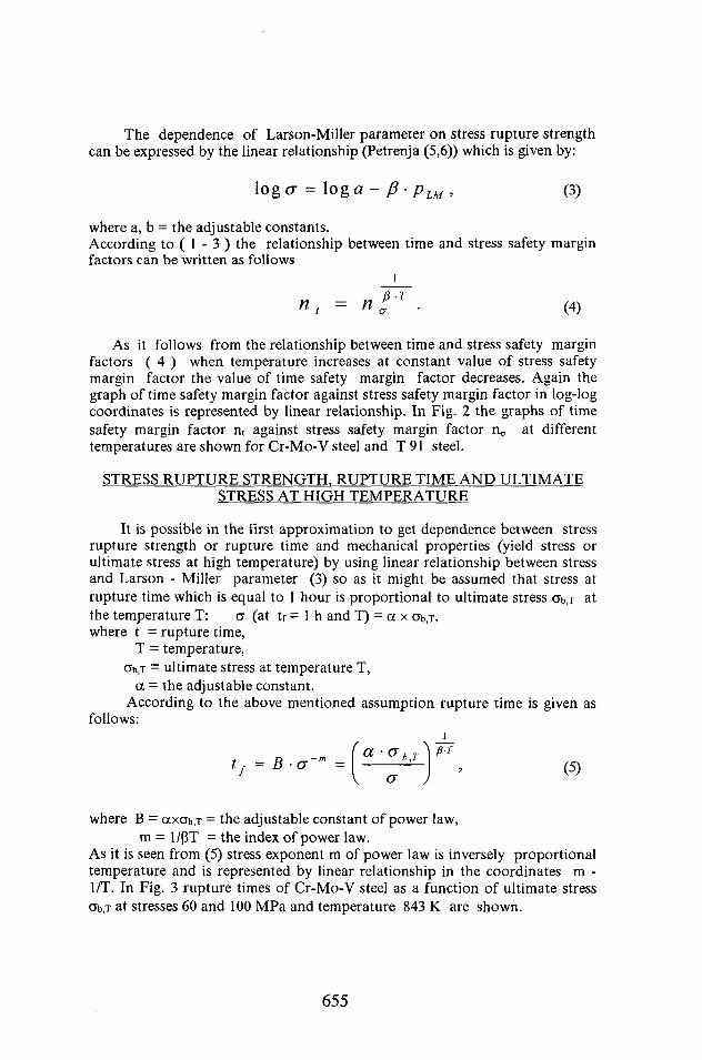
The dependence of Larson-Miller parameter on stress rupture strength can be expressed by the linear relationship (Petrenja (5,6)) which is given by:

loga = \oga - p ■ pLM, (3)

where a, b = the adjustable constants.According to ( 1 - 3 ) the relationship between time and stress safety margin factors can be written as follows

B Tn t = n £ (4)

As it follows from the relationship between time and stress safety margin factors ( 4 ) when temperature increases at constant value of stress safety margin factor the value of time safety margin factor decreases. Again the graph of time safety margin factor against stress safety margin factor in log-log coordinates is represented by linear relationship. In Fig. 2 the graphs of time safety margin factor nt against stress safety margin factor n„ at different temperatures are shown for Cr-Mo-V steel and T91 steel.

STRESS RUPTURE STRENGTH. RUPTURE TIME AND ULTIMATESTRESS AT HIGH TEMPERATURE

It is possible in the first approximation to get dependence between stress rupture strength or rupture time and mechanical properties (yield stress or ultimate stress at high temperature) by using linear relationship between stress and Larson - Miller parameter (3) so as it might be assumed that stress at rupture time which is equal to 1 hour is proportional to ultimate stress ab.x at the temperature T: o (at tf = 1 h and T) = a x Ob.x,where t = rupture time,

T - temperature,Ob,T = ultimate stress at temperature T,

a = the adjustable constant.According to the above mentioned assumption rupture time is given as

follows:

tf = B-a-ma ■ a b,T

1P-T

\ <J J(5)

where B = axab/r = the adjustable constant of power law, m = 1/(3T = the index of power law.

As it is seen from (5) stress exponent m of power law is inversely proportional temperature and is represented by linear relationship in the coordinates m - 1/T. In Fig. 3 rupture times of Cr-Mo-V steel as a function of ultimate stress Ob,x at stresses 60 and 100 MPa and temperature 843 K are shown.

655

MODELLING OF STRESS RUPTURE STRENGTH. AND RUPTURETIME SCATTER

It is well known that stress rupture strength and rupture time of commercial steels have considerable scatter which arises from a number of sources. Creep is highly sensitive to metallurgical structure, testing and service conditions. This factor together with immense expense of creep testing does not give satisfactory possibility for the experimental study of creep properties scatter. On the other hand the analytical expressions which have been used to describe stress rupture strength and rupture time can be used for the theoretical modelling of scatter (Bressers et al (2), Peterenja(5,6), Petrenja and Gusev (7)). The analytical expression (5) can be considered as function of random variables (stress a, ultimate stress Ob.x , temperature T, the adjustable constants a, (3). It means that this function is random too. It was pointed out (Petrenja (5,6)) that a rigorous analysis of statistical behavior of such functions is extremely difficult and practically impossible because the probability distribution of variables are unknown a priori.

The linearization of random function is an appropriate assumption to simplify calculations and to give an appropriate evaluation of statistical moments of arguments when probability distributions are unknown. If the function has necessary derivatives with respect to the arguments it may be suggested that the function can be represented by an expansion function in terms of series by Taylor where terms in second and higher orders have been omitted. Scatter of rupture time may be characterized by the variance vt of rupture time which is given by:

2

’ (6)v, =

1

p2 -Tf

+ Va + 'J11° ab.T P

2 (X ' (7 b j

1

V P-T-In-

a ■ a b.T +1 da b,T

p-a b.T dT

where vCT , v0ib,T, vT, vp = the variances of stress, ultimate stress, temperature and the adjustable constant p respectively.

Lower and upper values of rupture time tf are estimated by means of variance vt in the following way:

'/,» =b ■(1±9-v<)’ (7)

where tf = mean value of rupture time,q = coefficient which value depends on confidential level of

probability.In Fig. 4 95 % confidential limits of rupture time for Cr-Mo-V steel as afunction of ultimate stress at temperature 843 K and stresses 60 and 90 MPa

656

are presented at the following values of variances va = 0.005, v0,b,T = 0.003, vp = 0.001, vt = 0.001.

STATISTICAL SAFETY MARGIN FACTORS

Use of the representation of stress nCT and time nt safety margin factors as random ones gives the estimation of lower and upper levels of safety margin factors at different confidential levels of probability. Taking into account the expressions for deterministic safety margin factors (1-2) and linearization of a random function statistical stress and time safety margin factors can be written as:

and

nCF,q

= ncT-]\ + q\va+vao^

nt,q =H,-[l±0-(v,+V,jO)],

(8)

(9)

where n0 , nt = mean values of stress and time safety margin factors, v0 , vt , v„,0 , vt,o = the variances of stress rupture strength a corresponding to the appointed service life t, design stress o0, the total rupture time t0 at design stress respectively. The value of q coefficient depends on confidential level of probability.

In Fig. 5 statistical time safety margin factors with 95 % confidential limits against mean value of stress safety margin factor at ultimate stresses 350 MPa at temperature 843 K for Cr-Mo-Y pipeline steel and T91 are represented. The values of variances are equal to the ones in Fig. 4.

CONCLUSIONS

Statistical safety margin factors (8,9) coupling of statistical nature of properties and uncertainties of working stresses which control the life of pipelines or other structures under creep conditions are different from conventional lifetime prediction approach which is usually formulated in deterministic terms. A typical example of deterministic lifetime prediction model is well known scatter in stress rupture strength where the width of the accepted scatterband amounts to 20 % of the average stress rupture strength. The corresponding scatter in lifetime of pipeline steels spans a range up to an order of magnitude.

Whereas experimental study of scatter of stress rupture strength is extremely difficult modelling procedure which was proposed (Petrenja(5,6)) is improved in this paper by taking into account mechanical property at service temperature enables to predict scatter of creep rupture properties. Another reason for favouring a statistical lifetime prediction approach is related to the random nature of the level of the the service loading conditions, existing in all

657

load bearing applications. Both uncertainties associated with life controlling material property and working stress are estimated by using the above mentioned modelling procedure.

To provide an efficient design and life extension of creep loaded components it is necessary to develop advanced lifetime prediction methods coupling modelling and experiments with particular reference to statistical nature of life controlling material property and working stress.

REFERENCES

(1) Novozhilov V.V.,Tchizhik A.A., Petrenja J.K. Trans, of CKTI, vol. 246,1988.

(2) Bressers J., Steen M., Valles J.L. International Conference on Plant Life Management, Baltika II, Helsinki, 1992.

(3) Woodford D.A., Met. Trans., vol. 6A, 1975.

(4) Wachter O., Bendick W. VGB - Konferenz Werkstoffe und Schweiptechnik im Kraftwerke, 1991.

(5) Petrenja J.K. Trans, of CKTI, vol. 260, 1990.

(6) Petrenja J.K. The 5th International Conference on Creep and Fracture of Engineering Materials and Structures, Swansea, 1993.

(7) Petrenja J.K., Gusev V.V. The 4th European East - West Conference on Materials and Process, St.-Petersburg, 1993.

658

lOOOCf—Mo—V steel

95 % confidential limitsn

io-l------------------- .------------------- 1------------------- ,-------------------19 20 21 22 23

Larson —Miller parameter (Thousands)

Figure 1. Stress rupture strength of Cr-Mo-V steel with Larson - Miller parameter constant of 20

843 KT 91

Cr — Mo — V steel

1.3 1.4 1.5 l.istress safety margin factor

Figure!. Time safety margin factor versus stress safety margin factor for Cr-Mo-V steel and T 91 at 843 K.

659

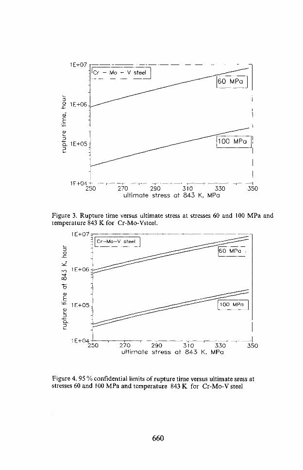
1E+077Cr-Mo-V steel

60 MPa

o 1E+06:.

100 MPaa 1E+05:

1E+0470 290 310 32ultimate stress at 843 K, MPa

Figure 3. Rupture time versus ultimate stress at stresses 60 and 100 MPa and temperature 843 K for Cr-Mo-Vsteel.

1 E+07 =rCr—Mo—V steel

60 MPa

1E+06 =

100 MPa1E+05.

1E+04270 290 310 33Cultimate stress at 843 K, MPa

Figure 4. 95 % confidential limits of rupture time versus ultimate sress at stresses 60 and 100 MPa and temperature 843 K for Cr-Mo-V steel

660

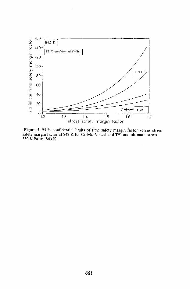
843 K140-

95 % confidential limits

Cr-Mo-V steel

stress safety margin factor

Figure 5. 95 % confidential limits of time safety margin factor versus stress safety margin factor at 843 K for Cr-Mo-V steel and T91 and ultimate stress 350 MPa at 843 K.

661

662

HIERARCHICAL RELIABILITY STUDY - A method for planning maintenance activities in the process industry

Arja Took, Ph.D.VTT Manufacturing Technology Safety Engineering P.O.Box 1701 FIN-33101 TAMPERE

Abstract

When the reliability of a plant is improved or ensured, a problem is to identify and prioritise the most profitable targets for investment. The whole plant has to be looked at to find those systems which have the greatest potential to jeopardise the planned production.

Systematic reliability analyses covering a whole plant are rare in the process industry. An analysis requires much work and involves a good deal of uncertainty; and furthermore, the results are of little use: the findings concerning critical components are quite often already known to the experienced plant personnel, and the failure rate figures for the plant or plant components provide little help in the planning of operation or maintenance.

An advantage of plant level reliability analysis is that it is able to model system aspects which are not covered if studies are focused directly on the chosen components. Such aspects include interdependencies, organisational aspects and information flows which affect reliability and lifetime. Another advantage is that a systematic analysis ensures that every aspect of production will be given equal consideration.

We have adopted a hierarchical qualitative approach to reliability studies. Its intent is to approach the plant from the plant level and to focus quickly on those areas of the plant where improvements and more detailed analyses would be productive. It is also possible to include non-technical aspects in the analysis. The approach utilises the expertise of the plant personnel as the main source of information. We applied the approach to a paper production line, which has been operating since 1960, to find ways to ensure its availability and efficiency in the future.

663

1. INTRODUCTION

Reliable process plants do not suffer from disruptions or unplanned stops,

and they produce high quality products at the intended utilisation rate.

Reliability affects the costs and profitability of systems. It is also an

important consideration as industrial equipment ages, because of the

general desire to prolong plant service life. A wide range of factors affects

reliability. Equipment is subject to malfunctioning and failure; the system

requires certain operational, control and maintenance actions to work

dependably; to prevent disruptions, assured quality of raw materials,

machinery, components and work is required. Environmental factors can

also disrupt operation: thunderstorms are a major cause of unavailability in

summer, and sub-zero winter weather must also be taken into account. In

improving and ensuring reliability, a problem is to find the most profitable

actions to take, i.e. to determine the parts and aspects of a system where

development or modernization is needed.

Reliability is a term which describes availability and other related

concepts in general when no specific feature is meant. Table 1 lists some

of the main terms and measures of reliability.

Reliability measures are used to look for ways to improve system

reliability, as well as to measure and compare the effect of the potential

improvements. The measures can be considered at different hierarchical

levels of the system: for single components, for subsystems and

production lines or for production units.

664

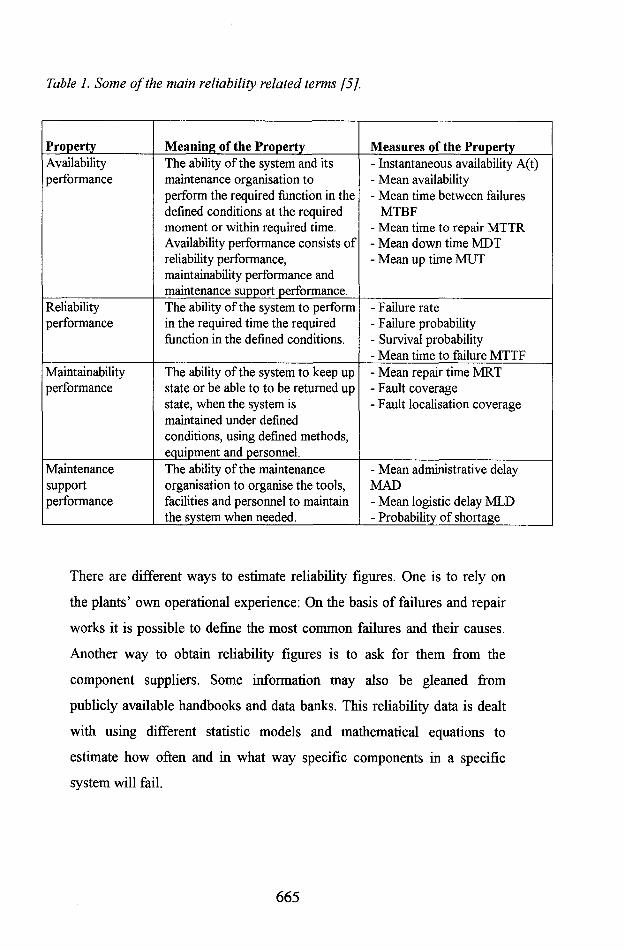
Table 1. Some of the main reliability related terms [5J.

Property Meaning of the Property Measures of the PropertyAvailabilityperformance

The ability of the system and its maintenance organisation to perform the required function in the defined conditions at the required moment or within required time. Availability performance consists of reliability performance, maintainability performance and maintenance support performance.

- Instantaneous availability A(t)- Mean availability- Mean time between failures

MTBF- Mean time to repair MTTR- Mean down time MDT- Mean up time MUT

Reliabilityperformance

The ability of the system to perform in the required time the required function in the defined conditions.

- Failure rate- Failure probability- Survival probability- Mean time to failure MTTF

Maintainabilityperformance

The ability of the system to keep up state or be able to to be returned up state, when the system is maintained under defined conditions, using defined methods, equipment and personnel.

- Mean repair time MRT- Fault coverage- Fault localisation coverage

Maintenancesupportperformance

The ability of the maintenance organisation to organise the tools, facilities and personnel to maintain the system when needed.

- Mean administrative delayMAD- Mean logistic delay MLD- Probability of shortage

There are different ways to estimate reliability figures. One is to rely on

the plants’ own operational experience: On the basis of failures and repair

works it is possible to define the most common failures and their causes.

Another way to obtain reliability figures is to ask for them from the

component suppliers. Some information may also be gleaned from

publicly available handbooks and data banks. This reliability data is dealt

with using different statistic models and mathematical equations to

estimate how often and in what way specific components in a specific

system will fail.

665

When the reliability of a larger system consisting of numerous components

is to be investigated, a reliability model is constructed. The models include

a simple sum-model, a block diagram model or a fault tree model [1,2,4],

A more sophisticated view of the system is obtained when its dynamics are

modelled and the system’s response to failures is simulated [6],

Quantifying reliability is a difficult task, and there are some software

packages on the market to help in quantitative calculations. These,

however, do not model the system automatically, and though they are a

help, they do not eliminate all of the problems. The reliability analyses are

still time consuming. They involve many uncertainties; and there are

problems in transferring the results to the design or operation of systems.

In practice, reliability related decisions are often based on expert opinions:

the bottle-necks are either known or predicted on the basis of operational

experience gained from the system or similar systems. There may even

exist collected information on failures and repair works in modem

maintenance support systems, so that the failure rates and weak points can

be estimated. It is also possible to organise a special condition monitoring,

either on-line or off-line, to facilitate the prediction of future failures.

Thus, in practice, reliability theory is quite a theoretical domain which

requires specialised reliability engineers, while the design, operation and

maintenance of process plants is based on good engineering judgements

and expert advice. There are reasonable grounds for not utilising reliability

assessments in everyday life: they require a lot of time and specific

mathematical methods; and the uncertainty of the results may be greater

than it would be if one use common sense. Furthermore, the results of all

this hard work do not necessarily assist in the decision making process.

666

This paper presents a case study in which a reliability study based on

engineering judgements and expert opinions is applied to an old paper

mill. However, the study is structured so as to combine the plant covering

description with detailed level studies when necessary, in an attempt to

avoid unneccessarity detailed discussion of potential failure modes which

are not critical to production under the prevailing operational and

maintenance practices. The reliability study is mainly qualitative,

identifying the critical process components on the basis of their

importance to production. Rough classifications are used to prioritise the

functions and components in order to enable us to focus the more detailed

discussion and analyses, such as those involving spare part decisions,

reliability assessments, lifetime predictions, etc., on the most critical parts

of the process.

2 HIERARCHICAL RELIABILITY STUDY

2.1 OVERVIEW

A hierarchical reliability model describes plant operation factors which

affect reliability. Potential disruptions inherent in these factors are studied

to find those which are the most critical. This is done by describing the

process functions as blocks. A general block is shown in Figure 1. The

hierarchical nature of the model means that the first description is very

general but covers the whole process, and that the model is then focused

on more detailed level in the areas where more detailed analyses are

needed, until the component level and the failure mode levels are reached.

667

The method consists of the system description and questions and

checklists to assist in the analysis. The results of discussions are reported

on tabular sheets. Roughly speaking, the method is divided into identifying

potential reliability problems and prioritising such problems. A more

detailed division of the way in which the reliability analysis proceeds is

shown in Figure 2. Two aspects are then studied in more detail when they

are applied to the paper production line: first, the system model

description (phases 2 and 3 in Figure 2); and second, the classification for

prioritising the risks (phase 5).

energy flows auxiliary systems

input flows

Function of the system- components- environment- chemicals

output flows: products,by-products,wastes

operative and control actions operation organisation maintenance actions maintenance organisation

Fig. 1. A general block of the block diagram

668

2. Divide the system into fuctional subsystems

3. Identify the dependencies

1. Define the system

6. Analyse in detail

4. Identify the potential problems

5. Define the risk

7. Propose measures to manage the risks

1.1 Define the scope of the system which is being analysed: process area, geographical area and functions whichare included.1.2 Define the types of risks which are looked for in unavailability, loss of capacity and loss of quality.

2.1 Draw a block diagram of the system: start from a general view and divide the system into "reasonable" subsystems. Draw the main flow of the production as inputs and outputs of the blocks.

3.1 Draw the other input and output flows into the blocks of the diagram.3.2 List the auxiliary systems and energies needed for the functions, as well as the operative, maintenance and control actions and organization.3.3 List the main components in the block

4.1 Identify the events and causes which results in the failure of the inputs, outputs or the components. Keyword list helps.4.2 Deepen the block diagram description into more detailed level for complex systems and for severe risks.4.3 Estimate the effects of the failures on system reliability.4.4 Write the events, causes and effects down on a tabular sheet.

5.1 Classify the events identified on the bases of probability and potential consequences.5.2 Make a list of the most severe risks

6.1 Choose the events and functions or components which need more detailed analyses.6.2 Make a decision on the analysis methods needed.6.3 Analyse.

7.1 Look for means to diminish the probability of unavailability or to shorten the unavailability periods.

Figure 2. The course of the reliability analysis [3],

669

2.2 DESCRIPTION OF THE PLANT

The United Paper Mill’s Jamsankoski Paper Mill has four paper machines.

The oldest of them, paper machine 3, is the machine we are studying. It

has been running since 1960, and despite its age, it is still considered as

profitable, because it is producing quite a specialised paper and involves

no investment costs. However, the machine is getting old and there are

growing needs for preventive maintenance and replacement of old

components with new ones. At the same time there are plans to increase

the net operating efficiency by several per cent in 1995.

Figure 3 shows a high level block diagram of the paper production line

with the main stream only. The paper mass is produced from pulp by

treating it mechanically and adding chemicals and water to get about 0.5%

mass in the wet head of the machine. A typical feature to the production is

that there is hardly any functional redundancy: only the most critical

components have either stand-by redundancy or spare parts in the store.

The vessels in the pulp and chemical treatment lines make buffers of about

zero to eight hours available. The quality and production of the paper is

very vulnerable to problems in the paper machine.

The hierarchical reliability analysis was a part of the net operating

efficiency project aimed at improving the availability of the plant by

reducing the number and length of unintended stops and the loss of

quality. The plant personnel aimed to use the reliability analysis to

identify and examine all important components and to check whether they

had spare parts or not. A ‘top ten’ list of components to be replaced or

systems to be redesigned was also desired. In addition, functional block

670

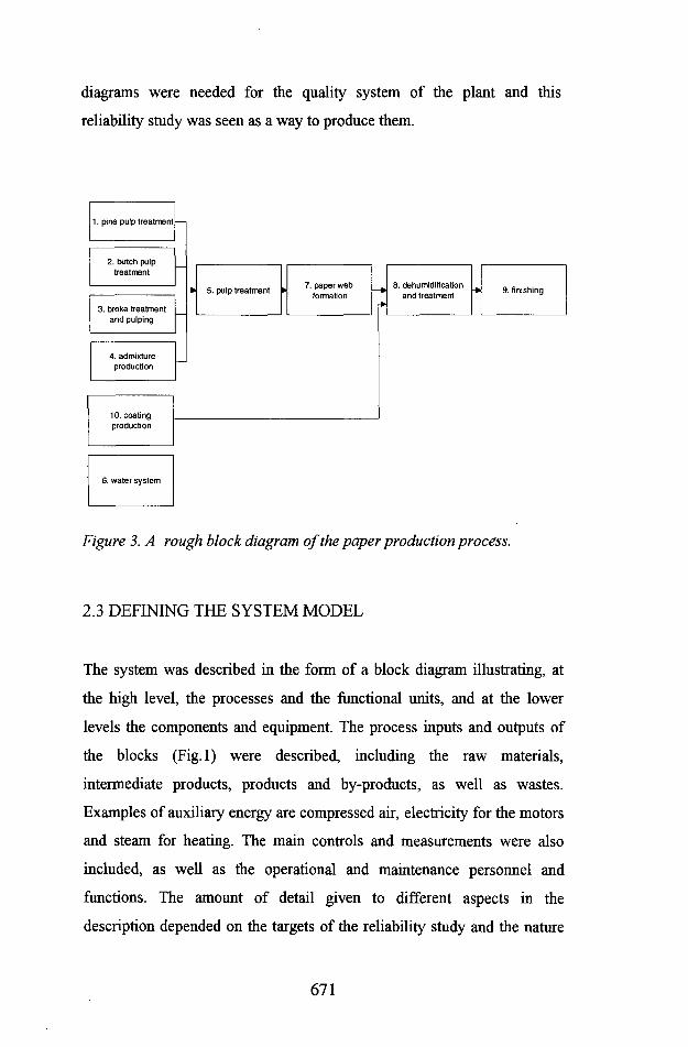
diagrams were needed for the quality system of the plant and this

reliability study was seen as a way to produce them.

Figure 3. A rough block diagram of the paper production process.

2.3 DEFINING THE SYSTEM MODEL

The system was described in the form of a block diagram illustrating, at

the high level, the processes and the functional units, and at the lower

levels the components and equipment. The process inputs and outputs of

the blocks (Fig.l) were described, including the raw materials,

intermediate products, products and by-products, as well as wastes.

Examples of auxiliary energy are compressed air, electricity for the motors

and steam for heating. The main controls and measurements were also

included, as well as the operational and maintenance personnel and

functions. The amount of detail given to different aspects in the

description depended on the targets of the reliability study and the nature

671

of the system. The main emphasis was given to identifying the critical

components and describing their potential failures.

Figure 4 shows the example of an intermediate level block diagram

describing the pine pulp treatment system (block 1 in Figure 3). The

blocks were further divided into more detailed descriptions.

electricity packing water

electricity packing water flushing

electricity packing water compressed air lubricating oil

maintenance

Fig. 4. A block diagram of the pulp treatment system.

2.4 CLASSIFYING AND PRIORITISING THE RISKS

After the risks related to the flows, functions and components had been

identified, they were classified according to the criticality and probability

of the undesired events.

First, to estimate the criticality, the consequences were determined:

whether the event is able to cause shutdown of the paper machine, an

672

interruption in production, or out of specification quality. Second, the

probabilities were estimated: The team concentrated on potential

component failures and other quite frequent or probable disturbances

recognised, for example, because of near-misses. Thus the probabilities

ranged from four times a year to once in ten years. Few rarer mishaps

were considered.

The classification of risks was based on the potential consequences rather

than frequencies. Class 1 included events which can cause shutdown of

the paper machine or a noticeable loss of quality. The latter problem will

in any case stop the process until the failures are repaired and specified

quality achieved. Class 2 included events which will interrupt production

for a while or cause difficulties in operating. Class 3 included events

which can be rectified within the time allowed before there are any effects

on production. For example, functions which have redundancy and

failures which do not immediately affect production were assigned to

Class 3.

2.5 RESULTS OF THE ANALYSES

Drawing of the block diagram took three sessions. This was more than we

has anticipated. One reason was that the personnel wanted to be more

thorough than us and describe the process to quite a detailed level right at

the outset, because they were going to use the descriptions for their quality

program. The analysis took four sessions, ranging in lenght from one-and-

a-half to four hours.

The block diagram description made it possible to see the important flows,

which often are common to several systems: redundant systems, for

example, may draw water from the same tank by means of a single pump.

673

Failures in electricity supply and automation systems are obviously

serious, but need a more detailed and focused study to determine if the

risks are acceptable and to find reasonable ways to improve the systems.

Most of the findings concerned spare part requirements, condition

monitoring requirements, requirements for component type modifications

because of the need for easy and quick repairs, and cases where it was

necessary to replace some of the old components with new ones simply

because of the age. At the time of writing of this paper the risk

classification to get the ‘top-ten’ list is not yet completed. Thus the

decisions which will be made on the basis of this study are not yet known.

3 DISCUSSION

The purpose of the study was firstly to improve the efficiency of

production. The aim was to achieve this by replacing components with

new ones and adding redundancy where needed to diminish the number of

failures disrupting production, and by improving maintenance procedures.

Our second aim was to test whether this plant level reliability study would

give a view of the most critical issues for decission making and unsolved

problems for further more detailed analyses and development work.

The results will be seen within a couple of years. However, there is a lot

of improvement work being done on paper machine 3, and it will be

difficult to judge which of the potential improvements in efficiency are

due to our study. However, the sessions were productive, at least as far as

the number of pages of paper is concerned. They systematically elicited

the plant personnel’s experiences and fears. The plant personnel also find

674

the analysis useful because they have already experienced some of the

identified risks after the identificatioin sessions.

At the time of writing of this paper, the study is still going on; thus the

method cannot be evaluated in detail. However, it is evident that the focus

and types of results of the analysis are closely associated with the reasons

for the analysis and motives of the team members. It can also be

considered as an advantage that a reliability study allows flexibility and

suitability in analysing many kinds of systems and problems.

Acknowledgements

This work is being carried out by the Operability and Risk Management

project, supported by the Technical Research Centre of Finland,

Department of Manufacturing Technology. United Paper Mills

Jamsankoski are providing working time, experience and technical

information to support this study. Their contribution is gratefully

acknowledged.

References

1. IEC 1025. Fault tree analysis. International Electrotechnical

Commission. 1990. 39 p.

2. Lees, F.P. Loss prevention in the process industries. London,

Butterworths. 1980. 1316p.

675

3. Nissila, M. & Rouhiainen, V. Keskeytysriskianalyysi laitoksen

haavoittuvuuden tarkasteluun. VTT Tiedotteita 1575. Espoo.

1994. 27 p + app. 25 p.

4. O’Connor, P.D.T. Practical Reliability Engineering. London,

Heyden & Son Ltd. 1981. 299 p.

5. SFS 3750. Luotettavuussanasto. Helsinki 1986.

6. Tiihonen, O., Hanninen, M. & Puska, E.K. APROS-based

Loviisa Nuclear Power Plant Analyzer. In: Miettinen, J. &

Holmstrom, H.(eds.) VTT Symposium 141 CSNI specialist

meeting on simulators and plant analyzers. Espoo. 1994. Pp.

510-525.

/

676

MANUAL ULTRASONIC INSPECTION OF AUSTENITIC AND DISSIMILAR WELDS

Pentti Kauppinen, Pauli Sarkiniemi and Harri Jeskanen VTT Manufacturing Technology P.O. Box 1704 FIN-02044 VTT, Finland

Abstract

In the third phase of the Programme for Inspection of Steel Components (PISCIII) several round robin tests with austenitic test samples and assemblies containing dissimilar welds were carried out. Based on the destructive analysis the performance of different inspection procedures and participating teams was evaluated. By using low recording level and a combination of conventional shear wave angle beam probes and mode conversion technique the team of VTT Manufacturing Technology detected all the flaws considered in the evaluation of the results of round robin tests. The majority of flaws in the austenitic test samples were stress corrosion cracks (IGSCC). The sizes (heights) of the flaws were mainly overestimated slightly by the team but the sizing capability clearly fiillfils the requirements of the latest ASME Code Appendix VIII. In the nozzle and dissimilar weld action the team detected all rejectable flaws in the assembly that was estimated to be the most difficult assembly of this action.

1 INTRODUCTION

The results of both nozzle and dissimilar metal weld (NOW) action and

austenitic steel testing (AST) action of the third phase of the Programme

for Inspection of Steel Components (PISCIII) show that the manual

inspection technique can be very effective in both detection and sizing of

flaws. The manual technique has been successfully used in the AST-

action by team DH and by team YR in the NDW-action. These are in fact

one team - the team of VTT, Finland. The reasons for the excellent

performance of this team in both actions will be discussed in this paper.

677

2 INSPECTION PROCEDURES USED IN MANUAL

INSPECTIONS

In both round robin exercises the main features of the procedure used by

the Finnish team are similar to the procedure applied in the inservice

inspections of nuclear power plants in Finland. The team employed

portable UT-equipment and transducers they normally use in the field

inspections. In the procedure, however, a wide selection of transducers

and techniques were included. The basic flaw detection technique based

on shear wave angle beam probes was complemented by mode conversion

technique, creeping waves and twin-crystal probes. The selection of

probes was carefully planned using the information available about the

geometry of the specimen to be inspected in the round robin exercises. In

NDW-action a special transducer (50°, 1.7 MHz) was designed and

manufactured by VTT.

The correct selection of probes was certainly one of the key-factors

leading to good performance. Application of several probes and

techniques in field inspections is impractical but the detailed analysis of

the teams result shows that this is not even necessary. Although a wide

selection of probes were used all the defects were in fact detected with

only a few probes. In the AST-action these were a mode conversion probe

(70°, 2 MHz) and a conventional shear wave probe (55°, 2 MHz). In

NDW-action the probe manufactured by VTT was most effective.

The recording level specified in the procedure was equal to noise level. In

fact all the signals exceeding noise level were analyzed and signals that

were suspected to be caused by a defect were recorded. In this analysis

the inspectors’ experience certainly played an important role.

678

3 PERSONNEL

Most of the team members have over 20 years experience in ultrasonic

testing and are certified according to the Nordtest certification to level 3

or 2 in ultrasonic testing. The team members regularly perform

inspections in the industry and most of them have been yearly involved in

the inservice inspections of Finnish nuclear power plants since 1976. For

detection of IGSCC the inspectors have had special training in Finland

and abroad. The first one-week training courses were held at Siemens-

KWU in Germany and since 1984 two-days training courses have been

yearly organized in Finland. Both lectures and practical training with

flawed specimen are included in the training course. The specimen used

in training are decontaminated pieces of pipes that have been removed

from nuclear power plants and contain both thermal fatigue cracks and

IGSCC. These specimen have been thoroughly analyzed with different

NDE-techniques and the dimensions of flaws are known. Thus inspectors

can get feed-back on their performance in flaw sizing during the training

course.

4 PERFORMANCE IN DETECTION OF FLAWS

The team DF1 has detected all the flaws in Assemblies 31-36 as can be

seen in Fig. 1 presenting the flaw detection frequencies of all teams for all

flaws and for rejectable flaws. DH has a false call rate in detection of

0.13 and in rejection 0.06 which are clearly less than the average values

0.2 and 0.13 of all participating teams. In the NDW-action the

performance of team YR varied in different assemblies. One example of

high performance is shown in Fig. 2. Team YR is the only team that has

679

detected all rejectable flaws in austenitic and dissimilar metal welds of

nozzles 21 and 22. In this assembly the false call rates of team YR were

0 both for detection and rejection.PKA952D

FDFR

Fig. 1. Performance of teams: detection of flaws in wrought-to-wrought Assemblies 31-36. FDF = flaw detection frequency, FDFR = flaw detecti­on frequency of rejectable flaws.

1.0

0.8

0.6

0.4

0.2

0

PKA952D

LOOcc>-

o>CMCM

LUQ_

>CC

T- tos o o>O o oS g ^

•r- in5 gcc hx 5

Fig. 2. Performance of teams: detection of flaws in assembly 20.

680

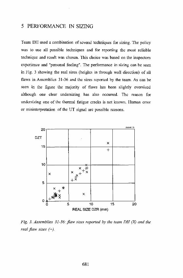
5 PERFORMANCE IN SIZING

Team DH used a combination of several techniques for sizing. The policy

was to use all possible techniques and for reporting the most reliable

technique and result was chosen. This choice was based on the inspectors

experience and "personal feeling". The performance in sizing can be seen

in Fig. 3 showing the real sizes (heights in through wall direction) of all

flaws in Assemblies 31-36 and the sizes reported by the team. As can be

seen in the figure the majority of flaws has been slightly oversized

although one clear undersizing has also occurred. The reason for

undersizing one of the thermal fatigue cracks is not known. Human error

or misinterpretation of the UT signal are possible reasons.

20

DZT

15

10

X

+

X

X -H- X ,'•'x

X

C_1______________

X

5 10 15REAL SIZE DZR (mm)

20

Fig. 3. Assemblies 31-36: flaw sizes reported by the team DH (X) and the

real flaw sizes (+).

681

6 PERFORMANCE DEMONSTRATION BASED ON

ASME

The Assemblies 31-36 used in the study were not made for performance

demonstration purposes and therefore the evaluation of teams’

performance can not be strictly based on the requirements of ASME

Appendix VIII. The Assemblies contained 26 defects from which 17 were

cracks. In this number also two axial cracks are included. The cracks are

divided into different depth categories which correspond the requirements

of ASME except that the number of deep cracks is slightly lower than

required.

In Assemblies 31-36 team DH has detected all the flaws and has made

only 4 false calls. Thus the requirements for detection and false calls are

fulfilled.

In Fig. 4 the 95% confidence levels and regression line for team data are

presented. In this figure only 17 cracks are included. The slope of the

regression line is 1.02 and correlation 0.93 which both clearly exceed the

values 0.6 and 0.7 required in ASME. The root mean square error

(RMSE) for the team data is 2.15 mm and thus is less than the maximum

value 3.175 mm accepted by ASME. In the new version of ASME this is

the only acceptance criterion.

682

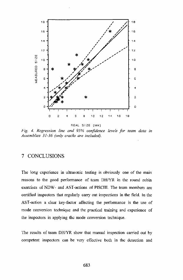
- 1818 -

- 16

14 -

12 -

REAL SIZE (MM)

Fig. 4. Regression line and 95% confidence levels for team data in Assemblies 31-36 (only cracks are included).

7 CONCLUSIONS

The long experience in ultrasonic testing is obviously one of the main

reasons to the good performance of team DH/YR in the round robin

exercises of NDW- and AST-actions of PISCIII. The team members are

certified inspectors that regularly carry out inspections in the field. In the

AST-action a clear key-factor affecting the performance is the use of

mode conversion technique and the practical training and experience of

the inspectors in applying the mode conversion technique.

The results of team DH/YR show that manual inspection carried out by

competent inspectors can be very effective both in the detection and

683

sizing of flaws. The requirements set in ASME Code for performance

demonstration are met and the slight oversizing of flaws leads to a

conservative assessment for structural safety.

REFERENCES

Draft report on the evaluation of the inspection results of the safe-end

areas of the PISCIII assembly No. 20. PISCDOC(90)40.

Draft (19.4.1994) of PISCIII report No. 33. Report on the evaluation of

the inspection results of the wrought-to-wrought PISCIII Assemblies No.

31, 32, 33, 34, 35 and 36. PISCDOC(93)21.

684

APPENDIX I

CONTENTS OF VOLUME IPage

Preface 3

Opening address 9M. Mannerkoski, VTT Director General

Session 1: Utility/industry view on condition and life management: present and future

On-line power plant condition monitoring 11A. Juusela

Strong thick section boiler steels for ultrasupercritical units 25E. Metcalfe & R. Blum

Increasing the efficiency of steam turbines by using improved9-10% Cr steels 45K.H. Mayer & H. Neft

Steam power plant with improved operating efficiency 59M. Staubli, C. Henry & R.B. Scarlin

Session 2a: Boilers and steam lines

Life prediction method for environmentally assisted cracking:An application for power plant components 77V. Bicego, A. Elli, G. Quaglia, G. Perboni & S. Tettamanti

Inspection and condition assessment of a retired superheater header 91H.C. Choi, H.K. Kim, J.S. Kim & J.J. Park

High temperature corrosion of boiler heating surfaces metal 105A. Ots

Creep damage development in weldments in a main steam pipe system made of 0.5Cr0.5Mo0.25V and 2.25CrlMo steels 119J. Storesund, R. Wu & R. Sandstrom

Properties and use of 10% Cr-steel for tubes of modem boilersand steam generators 135A.A. Tchizhik, T.A. Tchizhik & G.P. Alexeichuk

685

APPENDIX I

Properties and application of modified 9-Cr creep-resistant steels 143 F. Arav and J.C. van Wortel

The methodical aspects of steam pipe creep damage estimation 155I. Klevtsov, H. Tallermo & R.A. Crane

Session 3: Steam turbines

Life extension of a steam turbine 165F. Rotvel, L.B. Pedersen, J. Luotonen & P. Auerkari

Some considerations regarding the small punch testing ofimportant engineering components 179J. H. Bulloch & A. Fairman

Improved guidelines for determining the minimum service temperature 195K. Wallin

The influence of operational transients on the corrosion potential,C.P., of deaerator feedwater storage vessels 219J.H. Bulloch, E. Rochford & T.B. Healy

Improving service life of heat exchanger equipment for fossil and nuclear power plants by the use of duplex stainless steels and Ti-alloys 233TP. Lihareva, A.P. Shljiamnev, G.G. Poklonov & V.N. Jaskin

Life time prediction of Ip rotors from CrNiMoV steels for large steam turbines by criteria of brittle strength 241A.A. Tchizhik, LG. Ivanova & T.A. Tchizhik

Session 2b: Boilers and steam lines

Integrity of creep damaged components in power generation plants after repair welding without post weld heat treatment 255J.C. van Wortel, J.H. Heerings & F. Arav

Creep damage in boiler steels: classification for condition assessment 271J. Brear & P. Auerkari

Experiences of combined water chemistry of a supercriticalpower plant 281R. Andersson & R. Sonninen

686

APPENDIX I

Session 4: Gas turbines

Assessment of the degradation processes in gas turbine components during service 289N. Kasik

Coating service experience with a peak load power gas turbine 305A.I. Rybnikov, A.A. Tchizhik, L.B. Getsov, S.A. Leontiev,A.S. Osyka & I.S. Malashenko

The design for performance concept applied to life managementof gas turbine blades 319D.A. Woodford

Metallographical approach to turbine blade life time prediction 333S.-A. Karlsson, C. Persson & P.-O. Persson

APPENDIX I. Contents of Volume II 351

687

Published by

VttVuorimiehentie 5, P.O.Box 2000, FIN-02044 VTT, Finland Phone internat. + 358 0 4561 Telefax + 358 0 456 4374

Series title, number and report code of publication VTT Symposium 151 VTT-SYMP-151

DateMay 1995

Project number V5SU00418

Authors

Ed. bySeija Hietanen Pertti Auerkari

Name of project

Baltica III

Commissioned by

Title

BALTICA IIIInternational conference on plant condition & life management. Vol II

Abstract

The BALTICA III, International Conference on Plant Condition & Life Management will held on June 6 - 8, 1995 on board Silja Serenade on its cruise between Helsinki - Stockholm and at the Forest Lake Hotel Korpilampi in Espoo. BALTICA III provides forum for the transfer of technology from applied research to practice.

This is the second volume of the publications, which contain the presentations given at the BALTICA III, Plant Condition & Life Management. A total of 45 papers report recent experience in plant condition and life management. The conference focuses on recent ap­plications that have been demonstrated for the benefit of safe and economical operation of power plants. Practical approach is emphasised, including the presentations that aim to provide insight into new techniques, improvements in assessment methodologies as well as maintenance strategies. Compared to earlier occasions in the BALTICA series, a new aspect is in the applications of knowledge-based systems in the service of power plant life man­agement.

Activity unit y-p-p Manufacturing Technology, Materials and Structural Integrity Kemistintie 3, P.O. Box 1704, FIN-02044 VTT, Finland

ISSN and series title0357-9387 VTT SYMPOSIUM

ISBN951-38-4542-7

LanguageEnglish

Class (UDC)621.311.22:621.18:669.14 620.17/. 18:62-7:681.518

Keywordspower plants, maintenance, boilers, steel, condition monitoring, cracking, corrosion, service life, optimization, automation

Sold by VTT Information ServiceP.O. Box 2000, FIN-02044 VTT, Finland Phone internat. + 358 0 456 4404 Fax + 358 0 456 4374

Pages

334 p.

Price group

G