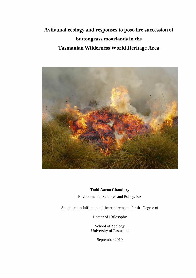
Avifaunal ecology and responses to post-fire succession of ...
293
Avifaunal ecology and responses to post-fire succession of buttongrass moorlands in the Tasmanian Wilderness World Heritage Area Todd Aaron Chaudhry Environmental Sciences and Policy, BA Submitted in fulfilment of the requirements for the Degree of Doctor of Philosophy School of Zoology University of Tasmania September 2010
-
Upload
khangminh22 -
Category
Documents
-
view
0 -
download
0
Transcript of Avifaunal ecology and responses to post-fire succession of ...
Avifaunal ecology and responses to post-fire succession of
buttongrass moorlands in the
Tasmanian Wilderness World Heritage Area
Todd Aaron Chaudhry
Environmental Sciences and Policy, BA
Submitted in fulfilment of the requirements for the Degree of
Doctor of Philosophy
School of Zoology
University of Tasmania
September 2010

ii
Declaration of originality
This thesis contains no material which has been accepted for a degree or diploma by the
University or any other institution, except by way of background information and duly
acknowledged in the thesis, and to the best of my knowledge and belief no material
previously published or written by another person, except where due acknowledgement is
made in the text of the thesis, nor does the thesis contain any material that infringes
copyright.
Signed: Date:
Todd A. Chaudhry
Authority of access
This thesis may be made available for loan and limited copying in accordance with the
Copyright Act 1968.
Signed: Date:
Todd A. Chaudhry
iii
Statement of ethical conduct
The research associated with this thesis abides by the international and Australian codes on
human and animal experimentation, the guidelines by the Australian Government’s Office of
the Gene Technology Regulator and the rulings of the Safety, Ethics and Institutional
Biosafety Committees of the University. This research was approved by the Animal Ethics Committee of the University of Tasmania
(Permit # A0007591 and # A0008676), and by the Biodiversity Conservation Branch to take
Wildlife (Permit # FA 03171 and # FA 05282) and Plants (Permit # FL 05036) for Scientific
Purposes.
Funding
This research was funded by the Birds Australia Stuart Leslie Bird Research Awards (2003-
2004) and the Biodiversity Conservation Branch, Department of Primary Industries, Parks,
Water and Environment, Tasmanian Wilderness World Heritage Area Fauna Conservation
Research Grants (2003-2006).
iv

Abstract
Fire management has become an increasingly critical issue in areas of high conservation value
such as the pyrogenic buttongrass moorlands in the Tasmanian Wilderness World Heritage
Area. The moorland avifauna is depauperate, comprised of only three cryptic, ground-
dwelling resident species that depend exclusively upon moorlands in the study area. These
include the Southern Emu-wren (Stipiturus malachurus), Striated Fieldwren (Calamanthus
fuliginosus), and Ground Parrot (Pezoporus wallicus), in addition to a small number of
species that are typically associated with adjacent forested habitats. This thesis is the first
comprehensive study of the buttongrass moorland avifauna and investigated responses to
post-fire succession primarily to help guide fire and conservation management. The
replicated space-for-time study included sites in low productivity, blanket moorlands at Lake
Pedder (n = 12; 2-54 years post-fire) and in moderate productivity, eastern moorlands at Lake
St Clair (n = 14; 1-44 years post-fire). Avifaunal diversity, density, and habitat use over three
seasons were quantified and analysed in relation to fire age, soil productivity and
composition, structure, and spatial characteristics of habitats at both locations. Observed
patterns of avifaunal diversity, density, and habitat use across the two chronosequences were
complex and revealed high levels of inter-specific and inter-site variation in relation to habitat
variables. Overall, mean densities of the resident species at Lake Pedder increased across the
chronosequence, whereas at Lake St Clair they peaked 2-8 years post-fire. Mean densities of
the non-resident species did not exhibit any consistent trends in relation to fire age.
Observations of habitat use demonstrated that the resident and non-resident species used
riparian and edge habitats disproportionately to their availability at both locations when
compared to the moorland matrix. Surveys of potential arthropod prey resources conducted in
matrix and riparian habitats at Lake St Clair indicated that mean abundance and mean energy
content across orders were greater in riparian habitats and mid-seral sites, respectively. Thus,
patterns of habitat selection by insectivorous species at Lake St Clair also appeared to reflect
the differing availabilities of potential arthropod prey. Lastly, a paired before-after-control-
impact study conducted at Lake St Clair (n = 4) indicated that hazard-reduction burning in
moorlands may result in overall reductions in resident avian densities and increases in non-
resident densities in the short-term (< 1.5 years post-fire). The implications of these findings
are discussed in relation to current fire management practices and recommendations are
provided to facilitate the conservation of critical resources for the moorland avifauna across
the landscape and over time.
v

Acknowledgements
Due to the multidisciplinary nature of this thesis there are many people whom I would like to
thank for their gracious advice, assistance, and support over the past few years. First of all, I
would like to thank my parents Asif and Melanie without whose love and unwavering
support I would have never been able to return to academia, and to my sister Serena for
always being there for me through thick and thin.
I wish to thank my supervisors, Assoc. Prof. Alastair Richardson at the University of
Tasmania and Michael Driessen at the Biodiversity Conservation Branch, who were always
there with open doors when I needed their help and who have been a real pleasure to work
with over the years. Special thanks to Michael who was instrumental in assisting me
throughout many aspects of my project.
I would like to thank the following people at the University of Tasmania for their assistance
and advice along the way including: Kit Williams, Sherrin Bowden, Wayne Kelly, Kate
Hamilton, Adam Stephens, Tom Sloane, Richard Holmes, and Randy Rose. Thanks to
Claire Lawrence, Ryan Downie, and Glenda for bumbling through buttongrass with me to
set-up the transects. I would like to thank John Osborne, Arko Lucieer, Rob Anders, Mick
Russell, Penny Atkinson, and Don Driscoll in the School of Geography and Environment
and Geoff Allen in the School of Agricultural Science. To all fellow students past and
present, especially Beth Strain, David Sinn, Kerryn Herman, John Gooderham, Glenn
Dunshea, Laura Parsley, Kevin Redd, Rodrigo Hamede, Alex Kabat, and Heidi Auman for
all the good times and commiserations. And to the rest of my friends in Hobart and
Melbourne- thanks for helping make Australia my home away from home.
The following staff from the Biodiversity Conservation Branch provided considerable
assistance throughout my project: Jayne Balmer, Colin Reed, Sib Corbett, John Corbett,
Chris Collins, Sally Bryant, Mark Holdsworth, and Julian Ward. Special thanks to Drew Lee
and Stephen Mallick for their assistance in the field. Thanks also goes out to John Ireson
and Wade Chatterton at the New Town lab for advice on vacuum sampling and graciously
lending me their equipment. Staff from Parks and Wildlife Service also provided invaluable
assistance with my project. Special thanks to Jon Marsden-Smedley for assistance with
identifying sites and providing me with data on fire histories, and to everyone at Lake St
Clair National Park without whose help, hospitality, and company I could not have
completed my research. I would like to thank Kent McConnell and Richard Hale for
facilitating my use of the Park as a home base for research and Tony Nichols for getting the
vacuum running when I needed it most. Thanks to Barry Batchelor, Maren Goerne, Ian
vi

Marmion, and Shawn for their assistance in conducting Ground Parrot surveys. I would like
to especially thank Trevor Norris for his willingness to share his knowledge of fire
management and otherwise helping throughout my project and Adam Scurra, Sam Tacey,
and Steve Locke for putting me up, putting up with me, and keeping me entertained.
I wish to thank the following people from a wide range of organisations whom provided me
with advice and assistance during the research process: Peter Brown formerly at the Nature
Conservation Branch; Marie Yee, Gab Warren, and Michael McDonald at Forestry
Tasmania; Eric Woehler and Colin Southwell at Australian Antarctic Division; members of
Birds Tasmania; Ray Brereton at Hydro Tasmania; Robert Driessen at Datavisions; Marcus
Pickett at Mt. Loft Ranges Southern Emu-wren Recovery Program; Jack Baker at NSW
Parks and Wildlife Service; David McFarland at QLD Environmental Protection Agency;
Mike Weston and Grainne Maguire at Birds Australia; Ken Chan at University of the
Sunshine Coast; Penny Greenslade at CSIRO; Owen Seeman at the Queensland Museum;
Greg Horrocks, Paul Bailey, and Sheila Hamilton-Brown at Monash University; and Rick
Redak at the University of California Riverside.
I am perhaps most indebted to those who provided me with much needed statistical advice
and assistance throughout my research. I would like to especially thank Gerry Quinn at
Deakin University who graciously volunteered his time and energy, Russell Thomson at the
Menzies Center, Leon Barmuta at the University of Tasmania, and Glenn McPherson of
Glenn McPherson Consulting. I would also like to especially thank Len Thomas who was
instrumental in helping me to conduct my Distance analyses and the other Distance folks at
the University of St. Andrews.
I would like to give special thanks to my mother-in-law Henriette Cooper Wessels for
graciously and meticulously proofreading all my final drafts.
I thank Birds Australia and the Biodiversity Conservation Branch for recognising the
importance of and providing funding for my research.
To Tarryn, Akuna, Tuk Tuk and other canids, for staying by my feet and keeping a smile on
my face like only friends of the four-legged variety can.
And last, but certainly not least, to my wife Karen- for her unwavering love and friendship,
extraordinary tolerance, continual support, ecological input, editing, and assisting me in
innumerable ways. I couldn’t have done it without you!
vii

viii
Table of contents
Declaration of originality and Authority of access iii
Statement of ethical conduct and Funding iv
Abstract v
Acknowledgements vi
Table of contents ix Chapter 1 - Introduction 1
Background 1
Buttongrass moorlands 4
Fire ecology of buttongrass moorlands 8
Habitat loss and degradation 15
The avifauna of buttongrass moorlands- a review 16
Thesis aims and structure 36 Chapter 2 - Study design, site descriptions, and fire regimes 39
Study design 39
Site descriptions and fire regimes 42 Chapter 3 - Avian habitat mapping in buttongrass moorlands and an accuracy assessment of the Tasmanian Wilderness World Heritage Area Vegetation Mapping 65
Introduction 65
Methods 69
Results 80
Discussion 97 Chapter 4- Avifaunal composition and densities in relation to post-fire succession of buttongrass moorlands in the Tasmanian Wilderness World Heritage Area 101
Introduction 101
Methods 105
Results 122
Discussion 147 Chapter 5- Avifaunal habitat use and potential availability of arthropod prey resources in relation to post-fire succession of buttongrass moorlands in the Tasmanian Wilderness World Heritage Area 163
Introduction 163
Methods 165
Results 178
Discussion 193
ix

Table of contents cont. Chapter 6- Short-term avifaunal composition and densities in relation to hazard-reduction burning of buttongrass moorlands in the Tasmanian Wilderness World Heritage Area 205
Introduction 205
Methods 208
Results 212
Discussion 218 Chapter 7- General discussion 225
Synthesis 225
Implications for fire and conservation management 235
Future directions 244 References 249
x
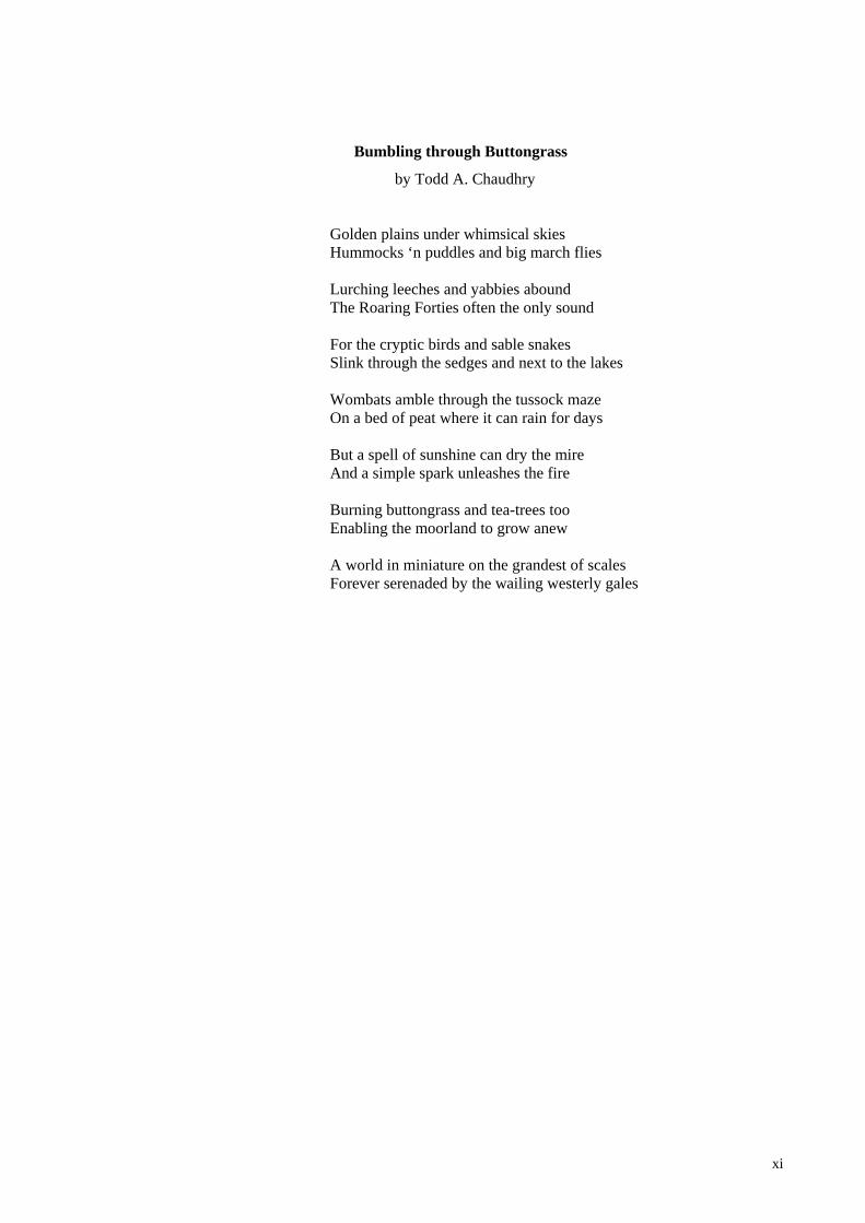
Bumbling through Buttongrass
by Todd A. Chaudhry
Golden plains under whimsical skies Hummocks ‘n puddles and big march flies Lurching leeches and yabbies abound The Roaring Forties often the only sound For the cryptic birds and sable snakes Slink through the sedges and next to the lakes Wombats amble through the tussock maze On a bed of peat where it can rain for days But a spell of sunshine can dry the mire And a simple spark unleashes the fire Burning buttongrass and tea-trees too Enabling the moorland to grow anew A world in miniature on the grandest of scales Forever serenaded by the wailing westerly gales
xi

xii
Chapter 1
Introduction
Background Fire is one of the primary abiotic agents in Australian ecosystems, as exemplified by the
mosaic of vegetation types with contrasting fire response patterns that characterise much of
the continent (Jackson 1968; Bowman 2000; Clark et al. 2002). Although recent evidence
indicates that climatic factors initiated extensive landscape-scale changes in vegetation
patterns, fire probably served to accelerate these trends (Kershaw et al. 2002).
Characteristics of fire regimes (e.g. time since fire, season, patchiness, extent, intensity,
frequency) influence the spatiotemporal patterns in plant communities, which affect faunal
species composition and abundance through subsequent changes in the biotic and abiotic
environment (e.g. habitat structure, food resources, microclimate) (Catling and Newsome
1981; Recher and Christensen 1981; Brown 1991; Whelan et al. 2002). Fire may cause
direct effects on the fauna during and after single events (e.g. mortality, natality,
emigration/immigration), and indirect cumulative effects due to habitat disturbance over time
(e.g. population density, composition, persistence) (Fox 1978; Russell and Rowley 1993;
Woinarski and Recher 1997; Whelan et al. 2002; Bradstock et al. 2005). The nature and
extent of these effects are influenced by complex interactions with environmental factors
such as landscape attributes (e.g. soils and topography) and pre- and post-fire climatic
conditions (Keith et al. 2002a; Whelan et al. 2002). Faunal responses will also largely
depend upon the specific life cycle attributes of the species of interest (Whelan et al. 2002),
and may range from null responses for some generalist species (e.g. Kotliar et al. 2002), to
temporary increases due to greater post-fire availability of food resources (e.g. Woinarski
1990), to reduction and recovery reflecting changes in habitat structure and suitability (e.g.
Baker 2000). However, such patterns and their underlying processes are often very complex,
and may only become apparent from long-term demographic studies (e.g. Brooker 1998).
Humans have used fire as a land management tool for millennia, varying from purposeful
ignition and, more recently, to outright suppression (Pyne 1994; Jackson 1999a; Kershaw et
al. 2002). Early Aboriginal changes in fire regimes during the Pleistocene have been
implicated in the megafaunal extinction that took place in Australia between 50,000 to
45,000 years ago (Miller et al. 2005). Although fire activity is believed to have been
relatively constant throughout the Holocene, there was a marked increase in anthropogenic
burning during early European colonisation, which was followed by a reduction to current
levels (Kershaw et al. 2002). Changes in fire regimes since European colonisation and the
1
Chapter 1 Introduction resulting direct or indirect mortality have similarly either been confirmed or implicated as
contributing to the extinction of at least two species and three subspecies of Australian birds
(Woinarski and Recher 1997). Currently, fire regimes that are outside of their historical
range of variation are a threat to at least 51 bird taxa, including many heathland species
(Garnett 1992; Woinarski 1999a, 1999b; Garnett and Crowley 2002; Olsen and Weston
2005). Short inter-fire intervals and increased fire frequency are considered to be the major
threats to many bird species, particularly for mid- to late-successional species that cannot
persist or reproduce in early successional habitats (Brooker and Rowley 1991; Mushinsky
and Gibson 1991; Woinarski and Recher 1997). Although many studies have been
conducted on the effects of fire on Australian birds (for a review see Woinarski 1999a,
1999b), it is generally recognised that due to the extremely wide range of observed responses
and complex interactions between a multitude of biotic and abiotic factors, ecosystem-
specific research is essential in order to help guide prudent conservation and fire
management activities (Wilson 1994; Woinarski and Recher 1997; Whelan et al. 2002).
Buttongrass moorlands form an ecosystem that exemplifies the complex interplay of fire,
soils, flora, and avifauna. They are comprised of sedgeland and graminoid heathland
communities typically dominated by the hummock-forming tussock sedge commonly named
buttongrass (Gymnoschoenus sphaerocephalus) (Specht 1979a; Jarman et al. 1988a).
Buttongrass moorlands are most extensive in the perhumid, oligotrophic peatlands of
western Tasmania where they are largely protected within the Tasmanian Wilderness World
Heritage Area (TWWHA) (Brown et al. 1993; Smith and Banks 1993). Buttongrass
moorlands are recognised as a World Heritage ecosystem as they are highly pyrogenic,
exemplify post-fire successional processes, occur in peatlands primarily formed by sedges as
opposed to Sphagnum moss as in the Northern Hemisphere, and are largely undisturbed by
development (Jarman et al. 1988a; Balmer et al. 2004). In part due to these unique
characteristics, buttongrass moorlands are a difficult environment to live in and support a
relatively depauperate fauna (Driessen 2006). In particular, the avian community consists of
only three cryptic, ground-dwelling resident species that are thought to depend exclusively
upon moorlands in the study area for survival and reproduction, namely the Southern Emu-
wren (Stipiturus malachurus), Striated Fieldwren (Calamanthus fuliginosus), and Ground
Parrot (Pezoporus wallicus). A small number of transient species that are typically
associated with adjacent woodlands and related habitats are also present (Brown et al. 1993;
Driessen 2006). Our knowledge of the moorland avifauna is very limited and primarily
based on qualitative observations (e.g. Brown et al. 1993; Driessen 2006), since no detailed,
community-level studies have been conducted to date. Bryant’s study (1991) on the density,
distribution, and conservation status of the Ground Parrot in Tasmania is the only significant
research to date that has focused on a moorland resident species; however, its scope in
2

Chapter 1 Introduction
relation to fire ecology was limited and it did not investigate any other members of the
avifauna (S. Bryant pers. comm. 2003). The rest of our knowledge of the resident species is
limited to either old observational studies conducted in non-moorland habitat in other
regions of the State (e.g. Legge 1908; Fletcher 1913a, 1913b, 1915a; Lord 1927; Sharland
1953), or more recent studies primarily on different subspecies on the Australian mainland
(McFarland 1991a, 1991b, 1991c; Gosper and Baker 1997; Burbidge et al. 2005; Maguire
2006a, 2006b). Accordingly, over the years a number of researchers have identified the need
to specifically study the Tasmanian moorland avifauna, particularly in relation to the effects
of fire on the resident species, in order to help guide conservation efforts (e.g. Gellie 1980,
Eberhard 1987; Bryant 1991).
Similar to many fire-adapted ecosystems around the world, there is considerable debate
concerning the most appropriate way to manage fire within the TWWHA to conserve its
biodiversity, particularly within buttongrass moorland ecosystems (DPIW 2007). The Parks
and Wildlife Service (PWS; Department of Primary Industries, Parks, Water and
Environment) is responsible for fire management within the TWWHA, and has mandates to
both conserve natural and cultural resources, and to protect life and property (PWS 1999).
The current strategy to meet these sometimes conflicting demands consists of limited, but
fairly frequent hazard-reduction burning of buttongrass moorlands (i.e. inter-fire interval ≤
10 years) along areas that pose the greatest risk for ignitions (e.g. roads); and suppression,
where and when it is feasible, throughout the rest of the landscape (Marsden-Smedley et al.
1999; PWS 1999). This fire regime has apparently caused changes in some of the plant and
animal communities; however, very little is actually known about these patterns and
processes. Nevertheless, some evidence suggests that current fire regimes represent a
significant shift from historical regimes (Brown 1999; PWS 1999; Marsden-Smedley and
Kirkpatrick 2000). Despite this relative lack of knowledge, there seems to be a growing
recognition that the current fire management strategy may need to be changed to more
closely mimic the historical disturbance regime characteristic of this ecosystem and to help
conserve the diversity of species that comprise and depend upon it (PWS 1999; Marsden-
Smedley and Kirkpatrick 2000; DPIW 2007). Accordingly, the Tasmanian Wilderness
World Heritage Area Management Plan has identified fire research as one of its Key Focus
Areas (PWS 1999). As part of this ongoing effort, the PWS and the Biodiversity
Conservation Branch (BCB; Department of Primary Industries, Parks, Water and
Environment) initiated a series of integrated research programs investigating the role of fire
with respect to fauna, flora, and soils in buttongrass moorlands. This program, focused on
assessing the impacts of fire on fauna, is a World Heritage Area Consultative Committee
Priority One Project; however, to date it has been limited to studies on invertebrates and
small mammals (e.g. Driessen 1999; Driessen and Greenslade 2004). Hence, in a recent
3
Chapter 1 Introduction report for the Committee, one of the research needs that was specifically identified was to
conduct a space-for-time project studying the effects of fire on birds in buttongrass
moorlands (Driessen 2001). This thesis directly addresses that research need and will
hopefully aid in the development of a better understanding of avian community ecology in
buttongrass moorlands, provide an indication of overall ecosystem health (Mac Nally et al.
2004), and serve as a foundation for the implementation of sound conservation practices by
fire and biodiversity managers. In addition, since this study has been developed and
implemented in close collaboration with the BCB and PWS, the collective results from our
research will be instrumental in developing a more holistic understanding of apparent
patterns in avian habitat relationships and the underlying ecological processes in buttongrass
moorlands. Furthermore, since some of the birds found in moorlands are migratory and/or
are closely related to similar taxa on the Australian mainland, the possible applications of
this research may reach well beyond the borders of the TWWHA itself. This is of particular
significance since some of these taxa are either threatened in other parts of Tasmania, closely
related to taxa that are threatened on the mainland, or otherwise potentially susceptible to
altered fire regimes (see below).
In this thesis I used an integrated approach towards studying post-fire habitat relationships of
the bird community in buttongrass moorlands by incorporating a range of disciplines
including ornithology, fire ecology, vegetation classification, geographic information
systems (GIS), entomology, dendrochronology, and pedology. Most of these disciplines, as
they pertain to buttongrass moorland ecosystems, have been discussed to varying degrees in
the literature. I have briefly described these below to provide a general framework for the
thesis and I discuss them in more detail in subsequent chapters. However, I have provided a
comprehensive literature review on the buttongrass moorland avifauna with an emphasis on
the three resident species that are the focus of this thesis, since no such reviews have been
conducted to date. I conclude this chapter by providing a description of the overall aims and
structure of my thesis.
Buttongrass moorlands Description
Buttongrass moorlands are extensive vegetation communities dominated to varying degrees
by shrub and graminoid species, and most notably by the hummock-forming tussock sedge
buttongrass (Gymnoschoenus sphaerocephalus) (Balmer 1991). Buttongrass has
sclerophyllous leaves that form tussocks up to 2 x 2 m atop large rhizomatous pedestals
(Brown 1999) (Figure1).
4

Chapter 1 Introduction
Fig. 1. Buttongrass (Gymnoschoenus sphaerocephalus) (Photo: M. Driessen).
Buttongrass moorlands are defined in the standard reference by Jarman et al. (1988a) as
being any treeless vegetation that typically contains buttongrass, or any vegetation in which
buttongrass is common, but may contain widely spaced emergent trees. Small recurring
islands (i.e. copses) or strips of vegetation along drainages (i.e. riparian zones) can be found
within this main moorland matrix that may not contain buttongrass and are otherwise
structurally and/or floristically distinct from the surrounding matrix (Jarman et al. 1988a;
Marsden-Smedley 1990). Excluding such emergent features, buttongrass moorland
vegetation is typically less than two metres in height (Balmer 1991). Moorlands are
considered to be intermediary between terrestrial and wetland systems since they are
waterlogged most of the year (Harris and Kitchener 2005).
Distribution
Buttongrass moorlands occur in isolated patches on mainland Australia including southeast
Queensland, New South Wales, Victoria, and South Australia, but are most extensive and
diverse in Tasmania (Keith 1995; Balmer et al. 2004). Buttongrass moorlands cover about
8% (0.55 million ha) of Tasmania and can be found throughout the State in a wide range of
climatic, topographical, geological, and edaphic conditions (Jarman et al. 1988a; Balmer et
al. 2004; TVMP 2004). However, they are most widespread in the perhumid, oligotrophic
peatlands of lowland and subalpine western and southwestern Tasmania where they have
likely dominated the landscape throughout the Holocene (Macphail 1979; Brown et al 1993;
Tye 2002; Bridle et al. 2003; Fletcher and Thomas 2007). They cover approximately 24%
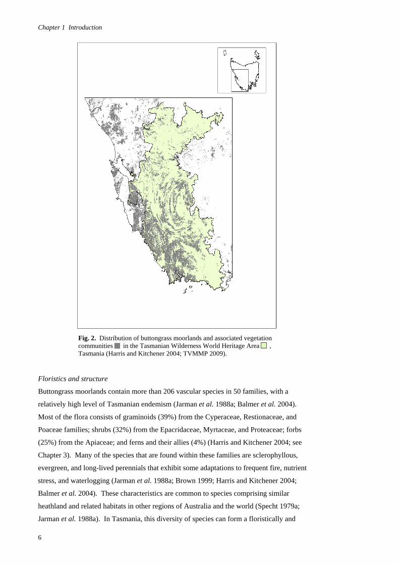
(335,000 ha) of the TWWHA (Figure 2), and they form part of a complex mosaic of
vegetation consisting of wet scrub, wet sclerophyll forest, and cool temperate rainforest
(TVMP 2004; Harris and Kitchener 2005).
5
Chapter 1 Introduction
Fig. 2. Distribution of buttongrass moorlands and associated vegetation communities in the Tasmanian Wilderness World Heritage Area , Tasmania (Harris and Kitchener 2004; TVMMP 2009).
Floristics and structure
Buttongrass moorlands contain more than 206 vascular species in 50 families, with a
relatively high level of Tasmanian endemism (Jarman et al. 1988a; Balmer et al. 2004).
Most of the flora consists of graminoids (39%) from the Cyperaceae, Restionaceae, and
Poaceae families; shrubs (32%) from the Epacridaceae, Myrtaceae, and Proteaceae; forbs
(25%) from the Apiaceae; and ferns and their allies (4%) (Harris and Kitchener 2004; see
Chapter 3). Many of the species that are found within these families are sclerophyllous,
evergreen, and long-lived perennials that exhibit some adaptations to frequent fire, nutrient
stress, and waterlogging (Jarman et al. 1988a; Brown 1999; Harris and Kitchener 2004;
Balmer et al. 2004). These characteristics are common to species comprising similar
heathland and related habitats in other regions of Australia and the world (Specht 1979a;
Jarman et al. 1988a). In Tasmania, this diversity of species can form a floristically and
6
Chapter 1 Introduction
structurally variable mosaic of sedgeland, heathland, graminoid heathland, and wet scrub
communities (Jarman and Crowden 1978; Jarman et al. 1982; Jarman et al. 1988a; Marsden-
Smedley 1990).
Classification
Jarman et al. (1988a) utilised these differences in floristic composition and structure, along
with climate, geography, and topography to develop a comprehensive classification system
for buttongrass moorlands. Over the years buttongrass moorlands have been referred to by a
range of names, such as hummock sedgelands (Jackson 1968), heathland/sedgelands (Jarman
and Crowden 1978); sedgeland-heaths (Brown and Podger 1982) and wet temperate heaths
(Keith et al. 2002a), but will be referred to as buttongrass moorlands throughout this thesis.
Buttongrass moorlands share floristic and structural similarities with other heathlands and
related communities that are typically (co-)dominated by woody plants less than two metres
tall, such as those found in mainland Australia and other regions of the world, including New
Zealand, South Africa, and northwestern Europe (Specht 1979a). The two major groups of
buttongrass moorland identified by Jarman et al. include blanket moorland and eastern
moorland, both of which have some lowland (~ 0-600 m asl) and highland (~ > 600 m asl)
forms (Figures 3 and 4; see Chapter 3). Although floristic composition is one of the primary
variables used to classify these groups, they share approximately 40% of their species in
common (Harris and Kitchener 2004). Blanket moorlands occur extensively in western and
notably in southwestern Tasmania, including the Lake Pedder region. They are primarily
found on peat soils overlying infertile siliceous substrates (e.g. quartzite) from sea level up to
approximately 1000 m asl and form a ‘blanket’ over a range of landscape features including
flats, slopes, plateaus, and ridges (Jarman et al.1988a; Harris and Kitchener 2005). Blanket
moorlands consist of 15 main communities, the majority of which are graminoid heathlands
(as defined by Specht 1979a), and a few peripheral communities and special habitats (Jarman
et al. 1988a). Their boundaries with adjacent vegetation communities (e.g. forests) are often
indistinct, creating ecotones in which floristics and structure intergrade (Jarman and
Crowden 1978). Eastern moorlands are less widespread and occur primarily in isolated
patches in eastern and central Tasmania. They are most extensive on poorly-drained peat
flats and gentle slopes overlying moderately fertile substrates (e.g. dolerite) above 600 m asl
on the Central Plateau, including the Lake St Clair region (Harris and Kitchener 2005).
Eastern moorlands consist of 10 main communities, the majority being sedgelands that often
contain scattered heath species, and a few peripheral communities and special habitats
(Jarman et al. 1988a). Unlike blanket moors, eastern moors form relatively distinct
boundaries with adjacent woodland communities that typically occur on the better-drained
mineral soils associated with glacial moraines (Jarman et al.1988a). Such minor hydrologic
and edaphic differences may also facilitate the development of habitat features such as
7
Chapter 1 Introduction copses and riparian vegetation zones within the primary moorland matrix (Jarman et al.
1982; Marsden-Smedley 1990). These factors are also at work in determining the nature of
the transitions between the primary plant communities, which may vary from indistinct
ecotones to distinct habitat edges (Jarman et al.1982; Bowman et al.1986; Balmer 1990),
depending on the scale and degree of changes in these abiotic and biotic variables. These
habitat edges and features may provide important microhabitats for birds, such as perching
sites in emergent vegetation and eucalypts (Balmer 1990). Repeated use of such sites over
time by birds and other vertebrates and the associated accumulation of excreta may also lead
to increases in local nutrient levels, and thus help to perpetuate these communities (Verbeek
1984; Balmer 1990; Hannan 1993).
Fire ecology of buttongrass moorlands Historical fire regimes
Fire has been part of the Tasmanian environment for approximately 30 million years
(Kirkpatrick et al. 1978). Archaeological evidence indicates that Aborigines occupied
southwestern Tasmania, although not necessarily continually, from approximately 35,000
years ago (Kee et al. 1993). However, recent palaeoecological research suggests that an
increase in fire frequency from approximately 40,000-70,000 years ago may possibly be
attributable to anthropogenic activities (Jackson 1999a; Kershaw et al. 2002), since this
period did not coincide with major climatic changes and large, lightning-caused fires have
been relatively infrequent in Tasmania until recent years (Jackson and Bowman 1982;
Marsden-Smedley 1998a; Kershaw et al. 2002; J. Marsden-Smedley pers. comm. 2007).
The following description of historical fire regimes in the study area is based on a
comprehensive review and assessment by Marsden-Smedley (1998a). Historical records
indicate that Tasmanian Aborigines actively burnt buttongrass moorlands throughout the
study regions at the time of early European settlement in the early 1800s, although their
actual time of occupation and initial use of fire as a management tool is debatable. They
probably used fire to aid in hunting and gathering of specific resources, creating and
maintaining travel corridors, communication, and warfare (Plomley 1966; Gammage 2008).
Marsden-Smedley speculated that Aborigines probably lit frequent fires (e.g. inter-fire
interval ≤ 20 years) under weather conditions that would result in low intensity burns that
were largely restricted to moorland vegetation. Such conditions are typically associated with
spring and autumn, but may also occur during dry periods in winter or after rain events in
summer. Aborigines probably employed such a fire regime until their extirpation during the
1830s, and their activities may have facilitated the maintenance and expansion of buttongrass
moorlands throughout western Tasmania prior to European colonisation (Jackson 1968;
8

Chapter 1 Introduction
Fig. 3. Blanket moorland, Lake Pedder region, Tasmania.
Fig. 4. Eastern moorland, Lake St Clair region, Tasmania.
9
Chapter 1 Introduction Marsden-Smedley 1998a). The phase of early European settlement from the 1830s to the
1930s was characterised by periods of few, relatively small fires, which caused fuels to
accumulate to levels that eventually led to high-intensity, landscape-scale fires. This regime
largely reflected shifting patterns of European resource utilisation. Of particular note are
fires during 1897/98 and 1933/44 that burnt large portions of the study area, including both
moorland and fire-sensitive vegetation such as rainforest and alpine communities (Marsden-
Smedley 1998b; Johnson and Marsden-Smedley 2002). Since the 1930s, fire has been
prevented or suppressed throughout most of the region except for about a dozen large fires,
and some habitat management and fuel reduction burns, particularly during the 1970s and
more regularly in recent years. These fires were of variable intensity and the majority of the
area burnt over this period was in moorland and wet scrub (Marsden-Smedley 1998b;
Marsden-Smedley and Kirkpatrick 2000). As of 2007, it was estimated that approximately
65% of buttongrass moorland in the TWWHA had succeeded to old-growth (> 35 years post-
fire), while only 23% was in a mature (15-35 years post-fire) and 12% in a regrowth seral
stage (< 15 years post-fire), due to this considerable reduction in the frequency, intensity,
and extent of fires (Marsden-Smedley 2007).
Post-fire succession
Although buttongrass moorlands have no direct commercial value, they have been the focus
of a considerable amount of research and management over the years due to their extreme
flammability and unique flora, fauna, and soils (e.g. Jackson 1968; Mount 1979; Bowman et
al. 1986; Jarman et al. 1988a; Marsden-Smedley 1998a; Balmer and Barnes 2000; Brown et
al. 2002; Bridle et al. 2003). Buttongrass moorlands are classified as having very high
flammability and they will readily burn throughout the year, except after recent precipitation,
but they have low fire sensitivity since many of the species are highly adapted to fire (Pyrke
and Marsden-Smedley 2005). Most commonly crown fires scorch or burn through the entire
above ground fuel array and typically have a moderate to high rate of spread and intensity,
while surface fires burn fuels directly on the ground and typically have a low to moderate
rate of spread and intensity (Gellie 1980; Jarman et al. 1988a; Marsden-Smedley 1993).
Most moorland species regenerate quickly after fire, typically by vegetative regeneration
through rootstock, but also by seed germination for some species (Jarman et al. 1988a;
Balmer 1991; Brown 1999). Since under typical conditions the majority of above-ground
vegetation is completely burnt, the age of most of the vegetation in a site will reflect the date
of the last major fire event (Bowman and Jackson 1981; Jarman et al. 1988b). However, if
prescribed burns are conducted under marginal conditions then some patches may remain
unburnt (e.g. riparian zones) and a significant amount of thatch (i.e. near-surface dead fuels)
may remain and pose a major fire hazard from several days up to approximately two years
after the burn (Gellie 1980; Marsden-Smedley 1993; Marsden-Smedley and Catchpole
10
Chapter 1 Introduction
1995a, PWS unpublished data). Although rare, under extremely dry conditions buttongrass
tussocks and other plants may be killed and peat fires may ignite (Marsden-Smedley 1993).
Peat fires are characterised by little or no flaming combustion below the ground surface and
very slow rates of spread, but are extremely difficult to extinguish (Gellie 1980; Marsden-
Smedley 1993). Post-fire recovery of moorland vegetation may depend on a range of factors
such as species composition, age, drainage, internal competition, external invasion, soil
fertility, and post-fire weather conditions (Gellie 1980; Jarman et al. 1982; Bowman et al.
1986).
Despite the fact that successional processes remain poorly understood (Balmer et al. 2004),
time since fire, fire frequency, and fire behaviour are considered to be the primary
determinants of both floristics and structure in many buttongrass moorlands (Jarman and
Crowden 1978; Brown and Podger 1982; Jarman et al. 1988a; Brown et al. 2002; Harris and
Kitchener 2005). The most widely accepted model developed to help explain the vegetation
patterns that characterise western Tasmania is ‘ecological drift’, as originally proposed by
Jackson (1968) (Brown and Podger 1982; Jarman et al. 1988a; Brown et al. 2002; Balmer et
al. 2004). This model is based on the concept that buttongrass moorlands are the first sere in
a successional pathway; in the absence of disturbance by fire moorlands gradually change
into wet scrub, then into wet sclerophyll forest, and ultimately climax as temperate rainforest
(Jackson 1968). Despite the fact that the environmental conditions in perhumid western
Tasmania appear to be suitable for the development of rainforest (e.g. precipitation > 1200
mm yr-1), both historical and current patterns in vegetation communities show a
disproportionate area covered by disclimax communities (i.e. buttongrass moorlands)
(Jackson 1968, 1999a; Gammage 2008). Thus, Jackson (1968) proposed that fire frequency
was the primary determinant of these vegetation patterns. Specifically, he stated that shorter
inter-fire intervals favoured the development and abundance of pyrogenic communities
across the landscape, and that longer inter-fire intervals favoured the development of fire-
sensitive communities. Since each seral stage differs in its relative flammability, fire
sensitivity, and productivity, each sere has a characteristic frequency distribution for fire-free
intervals and thus, along with other environmental factors (e.g. topography and prevailing
wind direction), helps to perpetuate the observed vegetation mosaic (Jackson 1968;
Marsden-Smedley and Kirkpatrick 2000; Brown et al. 2002; Pyrke and Marsden-Smedley
2005). Based on quantitative ageing of scrub and tree stems, Jackson suggested the average
fire-free intervals required to maintain the different communities were approximately 20-40
years for buttongrass moorland, 40-80 years for wet scrub, 80-150 years for wet sclerophyll
forest, and 150-300 years for rainforest (Jackson 1968, 1999a). Based on these estimates and
paleoecological data, Jackson (1968, 1981, 1999a) proposed that relatively frequent burning
by Aborigines throughout western Tasmania over the course of up to 70,000 years may have
11
Chapter 1 Introduction resulted in buttongrass moorland extending beyond its edaphic limits (i.e. a vegetation
disclimax), whereas in the absence of such frequent burning most of the region would be
covered in rainforest.
A number of studies have been conducted over the years to investigate the validity of
Jackson’s model. Consistent with Jackon’s model, the majority of moorlands (95%) studied
by Jarman et al. (1988b) supported vegetation less than 50 years old and anecdotal evidence
suggests that after approximately 65 years post-fire significant structural and floristic
changes may occur (Marsden-Smedley 2003). Brown and Podger’s (1982) study on a
vegetation sequence in the Southwest also provided general support for ecological drift, but
they suggested that there are numerous successional pathways that may also depend upon the
duration and intensity of fire. Henderson and Wilkin’s (1975) modelling based on Jackson’s
postulates accurately predicted the expected distribution of vegetation communities, with
early successional communities dominating the landscape. However, a number of
researchers have highlighted the importance of edaphic factors on vegetation dynamics. For
example, Brown and Podger (1982) found that if conditions result in the combustion of peat,
a single fire can change community composition and structure and may result in the
successional process being slowed or halted (Brown and Podger 1982). Bowman et al.
(1986) likewise suggested that the rate and extent of post-fire recovery is dependent on the
fertility of the remaining peat layer, and thus the time scales proposed by Jackson may only
be valid at sites with well developed and fertile peats. Brown et al.’s (2002) study that
examined vegetation change over a 20 year period in the Southwest found that there were
significant changes in both moorland structure and floristics, as well as shifts in vegetation
boundaries between moorland and scrub, that appeared to be influenced by the time since the
last fire. However, at some sites the effects of fire age were confounded with infection by
the plant pathogen Phytophthora cinnamomi (see below). Although there were clear
successional changes within the moorlands studied by Brown et al. (2002) (J. Balmer pers
comm. 2003), a period of 20 years was apparently not long enough to observe marked
changes from moorland to scrub, and they suggested that in areas with relatively infertile
soils moorland communities could be maintained with longer inter-fire intervals. In
addition, they suggested that although fire frequency affected the average species response to
disturbance over time, the extent and distribution of vegetation communities appeared to be
more a result of being topographically exposed to or protected from fire than fire frequency
per se. Furthermore, it has been conjectured by Pemberton (1986, 1989) and Jarman et al.
(1988a, 1988b) that edaphic factors such as waterlogging and severe frosts may result in
conditions that are only conducive to supporting moorlands in some areas, such as the
Central Plateau. In such areas moorlands may be able to persist even in the absence of fire,
and thus do not conform to the ecological drift model.
12

Chapter 1 Introduction
In summary, as with other communities, vegetation cover, height, and structural complexity
of moorlands are initially reduced by fire disturbance, and may then gradually increase to
pre-fire levels through regeneration and reproduction (Brown 1991; Driessen 1999; Brown et
al. 2002). The rate of post-fire recovery may be influenced by edaphic factors, and the
intervals between fires may influence which species and hence communities are able to
survive and perpetuate themselves (Marsden-Smedley 1990). Despite the ongoing debate
regarding the exact nature of post-fire changes in moorland vegetation, for the purposes of
this thesis these changes will generally be referred to as succession. This is in recognition of
the possibility that such changes in the moorlands that comprise the chronosequences
investigated in this thesis may be more due to changes in structure than in floristics per se, as
implied by the classic models of plant succession (Noble and Slatyer 1981; Jarman et al.
1982; Brown 1991; Begon et al. 1996; Brown et al. 2002).
Fire behaviour and fuel modelling
Fire in buttongrass moorlands often exhibits more extreme behaviours (e.g. higher intensities
and rates of spread) than would be expected under similar conditions in other vegetation
communities. This is in part due to their high proportion of fine and especially dead fuels,
open nature that allows rapid drying, high levels of volatile oils, and heterogeneous fuel
characteristics (Gellie 1980; Balmer 1991; Marsden-Smedley 1993; Marsden-Smedley and
Catchpole 1995b, 1995c). In fact, moorlands can burn at higher fuel moisture levels than
any other communities for which data have been reported (Marsden-Smedley and Catchpole
1995b, 1995c; Marsden-Smedley et al. 1999; Balmer et al. 2004). Accordingly, they can
sustain fires after only one or two rain/dewfall-free days and while in standing water
(Marsden-Smedley and Catchpole 1995c; Marsden-Smedley et al. 1999).
Given the importance of fire in buttongrass moorlands and recognising that existing fire
models did a poor job of predicting moorland fire behaviour, cooperative research on fuel
and fire dynamics was conducted since the early 1990s in order to develop a specific fire
behaviour prediction system for Tasmanian buttongrass moorlands (Marsden-Smedley et al.
1999). Research was focused on blanket moorlands, including sites at Lake Pedder, and
sedgey eastern moorlands, including sites at Lake St Clair. The former were chosen since
the majority of moorlands are classified as such, and the latter since significant fire
management problems occur in these communities (e.g. high fire spread rates and flame
heights) (Marsden-Smedley and Catchpole 1995b). Marsden-Smedley and Catchpole’s
results indicated that total and dead fuel loading could be reasonably predicted based on both
geology and vegetation age (i.e. time since last fire). Moorlands were categorised as either
low or moderate productivity sites, which is presumed to be a result of their associated
geologies, including Precambrian quartzite at Lake Pedder and Jurassic dolerite at Lake St
13

Chapter 1 Introduction Clair. Fuel loading was found to be positively correlated with site age. Fuel loading at the
low productivity sites, ranging in age from 3-41 years post-fire, increased steeply at first and
then stabilised beyond approximately 20 years. Fuel loading at medium productivity sites,
ranging in age from 1-20 years, increased even more rapidly, as expected. However, since
older moderate productivity sites were not available to sample, they could not confirm
whether fuel loading likewise stabilises beyond approximately 20 years, although they
considered such a trend to be ecologically reasonable. The primary factors that influenced
fire behaviour, including rate of spread and flame heights, were wind speed, vegetation age,
dead fuel moisture, and site productivity. Dead fuel moisture was, in turn, influenced by
recent and significant rain/dewfall, temperature, and humidity (Marsden-Smedley and
Catchpole 2001). Although sufficient data were not available, it is likely that slope has a
similar influence on moorland fire behaviour as in other vegetation communities (Marsden-
Smedley and Catchpole 1995b). The fuel and fire behaviour models that were the product of
these studies are currently being used by PWS to guide prescribed burning and wildfire
control operations in buttongrass moorlands, as outlined below.
Current fire management
Buttongrass moorlands are the focus of fire management activities in the TWWHA and
adjacent lands since they are highly pyrogenic, can burn throughout the year, and because
moorland fires can pose a risk to resources such as peat soils, fire sensitive vegetation
communities, life, and property (Hannan 1993; Marsden-Smedley et al. 2001). Although
Sphagnum bogs, rainforest, alpine, and plantation communities are classified as low to
moderately flammable, they can burn under dry conditions, are highly to extremely sensitive
to fire, and may take hundreds of years to recover (TVMP 2004; Pyrke and Marsden-
Smedley 2005). The likelihood of moorland fires threatening such adjacent resources is
purported to increase with higher fuel loads that are largely determined by the time since the
last fire and site productivity (Balmer 1991; Marsden-Smedley and Catchpole 1995b;
Marsden-Smedley and Kirkpatrick 2000). Therefore, fires in older moorlands have higher
rates of spread and intensities that may significantly limit effective fire control, and thus
result in resource damage or loss and enable the development of severe, landscape-scale
wildfires (Marsden-Smedley and Catchpole 1995b, 1995c; Marsden-Smedley et al. 1999;
Marsden-Smedley et al. 2001). Accordingly, most fire management activities in buttongrass
moorlands are focused on resource protection, and consist of wildfire suppression and
frequent tactical hazard-reduction burning in high-risk areas (Marsden-Smedley and
Kirkpatrick 2000; Marsden-Smedley et al. 2001). The primary objective of hazard-reduction
burning is to reduce > 70% of the fuel load across > 70% of the site being burnt, which is
typically contained by both natural (e.g. watercourses, wet scrub, forest) and constructed
boundaries (e.g. roads and fuel breaks) (PWS 1996; Marsden-Smedley et al. 1999, Marsden-
14
Chapter 1 Introduction
Smedley et al. 2001; Marsden-Smedley 2009). Hazard-reduction burns have been conducted
on a 5-8 year rotation at medium productivity sites at a high risk of accidental and arson
ignitions, such as along the Lyell Highway at Lake St Clair (PWS 1996; Marsden-Smedley
et al. 1999; Marsden-Smedley and Kirkpatrick 2000; see Chapter 2). However, it is
recognised that such high frequency fire regimes may adversely affect biodiversity and cause
long-term community changes (Jackson 1978; Marsden-Smedley and Kirkpatrick 2000;
Pyrke and Marsden-Smedley 2005). Currently, it is estimated that less than 2% of
moorlands throughout Tasmania is subjected to tactical hazard-reduction burning (Driessen
2006); however, recent fire modelling suggests that increased levels of burning (i.e. 5-10%)
may be required to reduce the incidence and extent of unplanned fires in southwestern
Tasmania (King et al. 2006, 2008). Only very limited habitat-management burns have been
conducted to maintain suitable foraging habitat for the migratory Orange-bellied Parrot at
Birchs Inlet and Melaleuca (Marsden-Smedley et al. 2001; J. Marsden-Smedley pers. comm.
2003).
Habitat loss and degradation Since the majority of the study area is within the TWWHA it has been largely protected from
anthropogenic disturbances other than fire. However, before its protection the study area
was dramatically affected by hydroelectric power generation schemes that created large
impoundments, including Lake Pedder (1972) and Lake Gordon (1974) in the Southwest and
Lake King William (1951) in the Central Plateau (Hydro Tasmania 2007). It has been
estimated that the total area of flat moorland vegetation inundated was 191 km2 and 117 km2
at Lakes Pedder and Gordon, respectively (Driessen et al. 2006). Other vegetation
communities that may have served as suitable habitat for the avifauna were also inundated
(e.g. wet scrub) at Lake Pedder (Balmer and Corbett 2001). This is probably the case at
Lake Gordon as well, and thus these figures may be conservative estimates of total habitat
loss. Although no similar assessment of pre-flooding vegetation has been conducted for
Lake King William, the total area currently inundated is approximately 44 km2; based on
topography and current vegetation it is probable that a sizeable proportion of this area was
also composed of suitable moorland and associated communities (LIST 2003; TVMP 2004).
While no studies have been conducted to date, the large loss of habitat due to inundation has
probably had an impact on both avian species abundance and metapopulation dynamics in
the study area, particularly for species such as the resident Southern Emu-wren that are
known to have limited flight capabilities and perceive large expanses of unsuitable habitats
(e.g. lakes) as barriers to dispersal (Littlely and Cutten 1994; Pickett 2000; Wilson and Paton
2004).
15

Chapter 1 Introduction The other potentially significant disturbance to buttongrass moorlands is the introduced
water mould, Phytophthora cinnamomi (Schahinger et al. 2003). It is a soil-borne plant
pathogen that moorland communities are highly susceptible to and it has caused significant
changes in moorland floristics and structure across extensive areas in Tasmania, notably in
the Southwest (Brown et al. 2002; Schahinger et al. 2003). These effects may potentially be
confounded or exacerbated by those of different fire regimes (Podger 1990; Brown et al.
2002). Despite the recognition that P. cinnamomi presents a significant threat to moorlands
in the TWWHA, no studies have examined the potential impacts on the moorland avifauna
(see Chapter 7).
The avifauna of buttongrass moorlands- a review Despite the fact that buttongrass moorlands cover approximately 8% of Tasmania (Balmer et
al. 2004; TVMP 2004), they support a relatively depauperate avifauna that largely consists
of widely distributed and opportunistic species, similar to the avifaunas of other heathlands
and related habitats found in mainland Australia, as well as other regions of the world such
as South Africa, Europe, and North and South America (Cody 1975; Bigalke 1979;
Gimingham et al. 1979; Kikkawa et al. 1979; Recher 1981; Specht 1994; Brown et al. 1993;
Wirtz et al. 1996; Keith et al. 2002a). This may be due to an overall lack of adequate food
resources in buttongrass moorlands, comparable to other cool and wet habitats in Tasmania
(Ridpath and Moreau 1966), or due to their relative structural uniformity (Brown et al.
1993). The depauperate state of the buttongrass moorland avifauna is discussed in relation to
other comparable communities and associated environmental factors in Chapter 7.
To date, no quantitative, comprehensive, and community-level avian surveys have been
conducted in Tasmanian buttongrass moorlands. Wilson (1950), Ridpath and Moreau
(1966), Rose (1978), Gellie (1980), Collins (1990), Brown et al. (1993), and Driessen (2006)
all provide some description of the avifauna found in buttongrass moorlands and associated
habitats (e.g. scrub). Overall, their descriptions were not based on formal surveys, did not
include clear habitat definitions, and did not specify criteria for species inclusion.
Accordingly, they should be interpreted with some caution and may not accurately reflect the
avifauna of the areas covered by this study (see Chapter 2). They reported a total of 55
species utilising buttongrass moorlands and associated habitats to varying degrees (Table 1).
A total of 15 species are common to at least five of the sources. According to Brown et al.
(1993), which is the most thorough and detailed source, the bird community of buttongrass
moorlands consists of approximately 18 species. For comparison, a total of 120 terrestrial
bird species have distributions within the TWWHA as a whole (Driessen and Mallick 2003).
Although the reported species assemblages may vary based on season, geography, and the
precise definitions of habitat (P. Brown pers. comm. 2005), these figures provide a rough
16

Chapter 1 Introduction
estimate of the relatively low species richness that is typical of buttongrass moorlands. All
sources agree that only three species appear to be common residents that depend exclusively
on moorlands for breeding, feeding, and other resource needs within the study area. These
specialist species are the Southern Emu-wren (Stipiturus malachurus), Striated Fieldwren
(Calamanthus fuliginosus), and Ground Parrot (Pezoporus wallicus), and are the primary
focus of this study. In addition, the Orange-bellied Parrot (Neophema chrysogaster) is
dependent upon buttongrass moorlands for foraging in its geographically restricted summer
breeding grounds in southwestern Tasmania (Brown and Wilson 1982). Although the
remainder of the species listed in Table 1 have been recorded using buttongrass moorlands or
associated habitats, none of them breed or permanently reside in the habitat. In this sense,
these species are only secondary or marginal members of the buttongrass moorland
community (i.e. non-residents of moorlands) and are either habitat generalists or more
commonly associated with ecotonal and adjacent habitats (e.g. scrub and woodland).
Relatively few detailed studies have been conducted on the resident species of buttongrass
moorlands in Tasmania or on the Australian mainland (refer to Higgins 1999; Higgins et al.
2001; Higgins and Peter 2002). Accordingly, some of the information presented below is
from studies conducted within other regions of each subspecies’ respective ranges or on
other subspecies. Whenever possible, information most relevant to this study and consistent
with personal observations has been presented. Since the non-resident species are not the
primary focus of this study they are not described in detail below, but references to them are
provided throughout this thesis as appropriate.
17
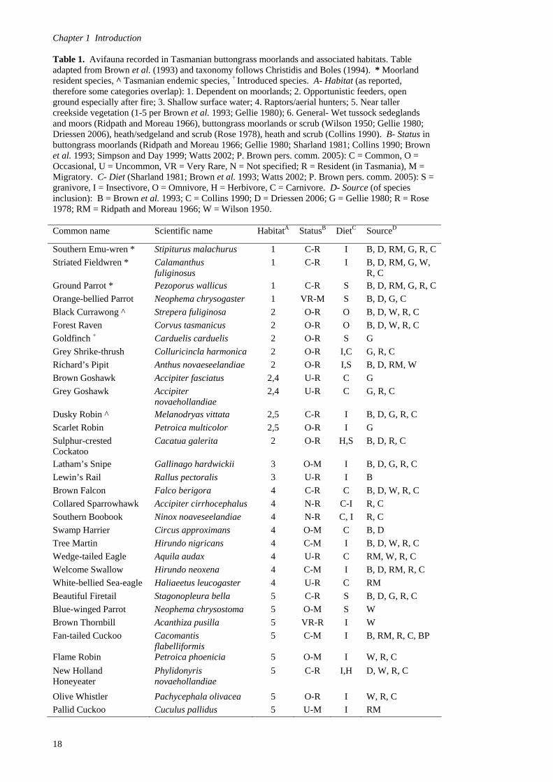
Chapter 1 Introduction Table 1. Avifauna recorded in Tasmanian buttongrass moorlands and associated habitats. Table adapted from Brown et al. (1993) and taxonomy follows Christidis and Boles (1994). * Moorland resident species, ^ Tasmanian endemic species, + Introduced species. A- Habitat (as reported, therefore some categories overlap): 1. Dependent on moorlands; 2. Opportunistic feeders, open ground especially after fire; 3. Shallow surface water; 4. Raptors/aerial hunters; 5. Near taller creekside vegetation (1-5 per Brown et al. 1993; Gellie 1980); 6. General- Wet tussock sedeglands and moors (Ridpath and Moreau 1966), buttongrass moorlands or scrub (Wilson 1950; Gellie 1980; Driessen 2006), heath/sedgeland and scrub (Rose 1978), heath and scrub (Collins 1990). B- Status in buttongrass moorlands (Ridpath and Moreau 1966; Gellie 1980; Sharland 1981; Collins 1990; Brown et al. 1993; Simpson and Day 1999; Watts 2002; P. Brown pers. comm. 2005): C = Common, O = Occasional, U = Uncommon, VR = Very Rare, N = Not specified; R = Resident (in Tasmania), M = Migratory. C- Diet (Sharland 1981; Brown et al. 1993; Watts 2002; P. Brown pers. comm. 2005): S = granivore, I = Insectivore, O = Omnivore, H = Herbivore, C = Carnivore. D- Source (of species inclusion): B = Brown et al. 1993; C = Collins 1990; D = Driessen 2006; G = Gellie 1980; R = Rose 1978; RM = Ridpath and Moreau 1966; W = Wilson 1950. Common name Scientific name HabitatA StatusB DietC SourceD
Southern Emu-wren * Stipiturus malachurus 1 C-R I B, D, RM, G, R, C
Striated Fieldwren * Calamanthus fuliginosus
1 C-R I B, D, RM, G, W, R, C
Ground Parrot * Pezoporus wallicus 1 C-R S B, D, RM, G, R, C
Orange-bellied Parrot Neophema chrysogaster 1 VR-M S B, D, G, C
Black Currawong ^ Strepera fuliginosa 2 O-R O B, D, W, R, C
Forest Raven Corvus tasmanicus 2 O-R O B, D, W, R, C
Goldfinch + Carduelis carduelis 2 O-R S G
Grey Shrike-thrush Colluricincla harmonica 2 O-R I,C G, R, C
Richard’s Pipit Anthus novaeseelandiae 2 O-R I,S B, D, RM, W
Brown Goshawk Accipiter fasciatus 2,4 U-R C G
Grey Goshawk Accipiter novaehollandiae
2,4 U-R C G, R, C
Dusky Robin ^ Melanodryas vittata 2,5 C-R I B, D, G, R, C
Scarlet Robin Petroica multicolor 2,5 O-R I G
Sulphur-crested Cockatoo
Cacatua galerita 2 O-R H,S B, D, R, C
Latham’s Snipe Gallinago hardwickii 3 O-M I B, D, G, R, C
Lewin’s Rail Rallus pectoralis 3 U-R I B
Brown Falcon Falco berigora 4 C-R C B, D, W, R, C
Collared Sparrowhawk Accipiter cirrhocephalus 4 N-R C-I R, C
Southern Boobook Ninox noaveseelandiae 4 N-R C, I R, C
Swamp Harrier Circus approximans 4 O-M C B, D
Tree Martin Hirundo nigricans 4 C-M I B, D, W, R, C
Wedge-tailed Eagle Aquila audax 4 U-R C RM, W, R, C
Welcome Swallow Hirundo neoxena 4 C-M I B, D, RM, R, C
White-bellied Sea-eagle Haliaeetus leucogaster 4 U-R C RM
Beautiful Firetail Stagonopleura bella 5 C-R S B, D, G, R, C
Blue-winged Parrot Neophema chrysostoma 5 O-M S W
Brown Thornbill Acanthiza pusilla 5 VR-R I W
Fan-tailed Cuckoo Cacomantis flabelliformis
5 C-M I B, RM, R, C, BP
Flame Robin Petroica phoenicia 5 O-M I W, R, C
New Holland Honeyeater
Phylidonyris novaehollandiae
5 C-R I,H D, W, R, C
Olive Whistler Pachycephala olivacea 5 O-R I W, R, C
Pallid Cuckoo Cuculus pallidus 5 U-M I RM
18

Chapter 1 Introduction
Table 1. cont.
Common name Scientific name HabitatA StatusB DietC SourceD
Superb Fairy-wren Malurus cyaneus 5 O-R I D, RM, W, R, C
Yellow-throated Honeyeater ^
Lichenostomus flavicollis
5 C-R I B, D, W, R, C
Silvereye Zosterops lateralis 5 C-M I,H W, R, C
Striated Pardalote Pardalotus striatus 5 U-M I W
Tasmanian Thornbill ^ Acanthiza ewingii 5 C-R I D, W, R, C
Yellow Wattlebird ^ Anthochaera paradoxa 5 U-R I, H W, R, C
Bassian Thrush Zoothera lunulata 6 N-R I, S R, C
Black-faced Cuckoo-shrike
Coracina novaehollanidiae
6 N-M I R, C
Brown Quail Coturnix ypsilophora 6 U-R S,I RM
Crescent Honeyeater Phylidonyris pyrrhoptera
6 C-M I,H D, G, W, R, C
Eastern Spinebill Acanthorrhyynchus tenuirostris
6 N-R H, I R, C
Golden Whistler Pachycephala pectoralis 6 N-R I R, C
Great Egret Ardea alba 6 N-M C, I C
Green Rosella Platycercus calydonicus 6 N-R S R, C
Grey Fantail Rhipidura fuliginosa 6 N-M I R, C
Masked Lapwing Vanellus miles 6 U-R I RM
Pink Robin Petroica rodinogaster 6 N-R I R, C
Scrubtit ^ Acanthornus magnus 6 N-R I R, C
Strong-billed Honeyeater ^
Melithreptus validirostris
6 N-R I R, C
Tasmanian Scrubwren ^ Sericornus humilis 6 N-R I R, C
White-throated Needletail
Hirundapus caudacutus 6 N-M I R, C
Yellow-tailed Black-cockatoo
Calyptorhynchus funereus
6 N-R S,I R, C
19
Chapter 1 Introduction Southern Emu-wren Description
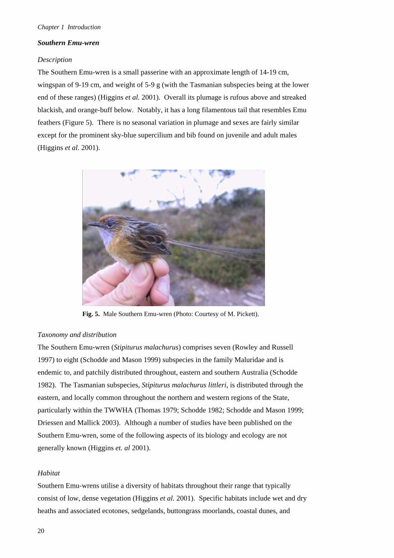
The Southern Emu-wren is a small passerine with an approximate length of 14-19 cm,
wingspan of 9-19 cm, and weight of 5-9 g (with the Tasmanian subspecies being at the lower
end of these ranges) (Higgins et al. 2001). Overall its plumage is rufous above and streaked
blackish, and orange-buff below. Notably, it has a long filamentous tail that resembles Emu
feathers (Figure 5). There is no seasonal variation in plumage and sexes are fairly similar
except for the prominent sky-blue supercilium and bib found on juvenile and adult males
(Higgins et al. 2001).
Fig. 5. Male Southern Emu-wren (Photo: Courtesy of M. Pickett).
Taxonomy and distribution
The Southern Emu-wren (Stipiturus malachurus) comprises seven (Rowley and Russell
1997) to eight (Schodde and Mason 1999) subspecies in the family Maluridae and is
endemic to, and patchily distributed throughout, eastern and southern Australia (Schodde
1982). The Tasmanian subspecies, Stipiturus malachurus littleri, is distributed through the
eastern, and locally common throughout the northern and western regions of the State,
particularly within the TWWHA (Thomas 1979; Schodde 1982; Schodde and Mason 1999;
Driessen and Mallick 2003). Although a number of studies have been published on the
Southern Emu-wren, some of the following aspects of its biology and ecology are not
generally known (Higgins et. al 2001).
Habitat
Southern Emu-wrens utilise a diversity of habitats throughout their range that typically
consist of low, dense vegetation (Higgins et al. 2001). Specific habitats include wet and dry
heaths and associated ecotones, sedgelands, buttongrass moorlands, coastal dunes, and
20
Chapter 1 Introduction
wetland areas such as bogs, fens, swampy gullies, and reedlands (Fletcher 1915a; Sharland
1981; McFarland 1988b; Pickett 2000). Although their habitat can be structurally diverse, it
is typically dense, ranging from 0.5-1.5 m tall, and has few trees (Wilson and Paton 2004).
Some research indicates that such structural parameters may be more important than
floristics in determining habitat suitability (i.e. able to support survival and reproduction)
(Pickett 2000; Wilson and Paton 2004; Maguire 2006a). Although in parts of their range
they are more commonly found in undisturbed natural habitats, they have been reported
using woodland regrowth 2-3 years post-logging (Wardell-Johnson and Williams 2000) and
sometimes utilise introduced vegetation (e.g. blackberry thickets) found in more developed
areas, particularly in autumn and winter in Tasmania (McNamara 1937). They have been
recorded from sea level to approximately 1000 m asl (Schodde 1982).
Populations
Southern Emu-wrens can be locally common in suitable habitat, but only a few studies have
provided estimates of home range sizes and densities (Sharland 1981). Fletcher (1915a)
estimated that one pair’s territory consisted of approximately 1 km of swampy creekside
habitat in Tasmania. Recent quantitative research conducted by Maguire and Mulder (2004)
in Victoria showed that pairs defended territories with a mean of 0.97 0.09 ha (range 0.30-
2.86 ha); however, territory boundaries were more variable during the winter. Pickett (2000)
reported similar estimates from the Mount Lofty Ranges of South Australia, with breeding
season mates having highly overlapping home ranges with a mean of 0.85 0.66 ha (range
0.34-2.61 ha), and non-breeding individual home ranges of 0.31-6.53 ha. Southern Emu-
wren densities have been estimated by Gosper and Baker (1997) who reported a minimum
density of 1.6 birds ha-1 in dry and wet heathlands in New South Wales, Maguire (2006b)
who reported a mean density of 2.3 birds ha-1 in wetlands and coastal heathlands in Victoria,
as well as by McFarland (1988b) and Jordan (1987a) (see below).
Behaviour
Southern Emu-wrens are cryptic, ground-dwelling birds and can be very elusive and difficult
to study (Pickett 2000). This is particularly true under windy conditions, in which they tend
to remain hidden in low cover (Rowley and Russell 1997). Maguire and Mulder (2004)
reported that birds were only visible for 6.6% of the total of 1434 person-hours of surveying
they conducted. They are sedentary residents that can be found individually, but more often
in pairs or small family groups, and can exhibit strong territoriality through interspecific
physical contests and song displays (Gosper and Baker 1997; Maguire 2006b). They creep
and run along the ground with ‘mouse-like’ movements and when disturbed they often seem
to prefer to hop away into denser cover where they can easily conceal themselves (North
1912; Fletcher 1913a; Schodde 1982). However, males in particular may sometimes move
21

Chapter 1 Introduction to a more prominent position in order to investigate the disturbance before retreating
(Sharland 1981; Pickett 2000). They are considered to be weak and reluctant fliers (Pringle
1982a), and when approached within close range they typically only flush up to 30 m, after
which they may be difficult to relocate (Corben 1973; Schodde 1982). Most individuals
seem to perceive large open areas that do not provide adequate cover (e.g. paddocks and
lakes) as barriers to dispersal (Littlely and Cutten 1994; Pickett 2000; Wilson and Paton
2004), but may disperse through otherwise unsuitable habitat (e.g. mature forest) (Wardell-
Johnson and Williams 2000). Juveniles have been recorded dispersing up to 1.2 km
(Maguire and Mulder 2004), and the longest recorded one-way movements of banded
Southern Emu-wrens were approximately 2.5 km (Pickett 2000).
Calls
Southern Emu-wren territorial songs are high-pitched (~ 5-12 kHz) and variable descending
trills composed of four to six rapid deedle notes (Pringle 1982a; Rowley and Russell 1997;
Higgins et al. 2001). Their songs, often issued from prominent perches, can be heard
throughout the year (Rowley and Russell 1997; Pickett 2000). Although both sexes have
been observed singing, it is most often done by males and during the breeding season
(Fletcher 1915a; Rowley and Russell 1997). Southern Emu-wrens also frequently issue soft
tsuuuh contact calls while foraging, and a buzzy trrrt alarm call when disturbed (Schodde
1982; Rowley and Russell 1997). Although they are often very difficult to hear, especially
when there is noise disturbance such as strong winds (Pickett 2000), they can be heard up to
approximately 50 m under good listening conditions (Schodde 1982).
Diet
Southern Emu-wrens are primarily insectivorous and only rarely consume plant material
(Barker and Vestjens 1989). They typically glean, and occasionally sally for invertebrates,
as they hop along the ground and particularly up and through shrubs (Fletcher 1915a; Littlely
and Cutten 1994; Rowley and Russell 1997). They have been observed foraging in both
open and dense vegetation, but appear to favour the latter, particularly when alarmed
(Littlely and Cutten 1994; Wilson and Paton 2004). They have also been observed picking
insects from spider webs, and preying on large insects during courtship feeding and the
provisioning of nestlings (Gosper and Baker 1997; Maguire and Mulder 2004; Maguire
2006b). They prey on species from a wide range of Insecta and Arachnida orders including
but not limited to the following: Araneae, Coleoptera, Diptera, Hemiptera, Hymenoptera,
Lepidoptera, Mantodea, Neuroptera, and Orthoptera (Lea and Gray 1936; Barker and
Vestjens 1989).
22

Chapter 1 Introduction
Breeding
Southern Emu-wrens have been recorded breeding from August to January in Tasmania
(Fletcher 1913a; Fletcher 1918). They make domed nests with side entrances, loosely
constructed from vegetation such as grass and moss, and lined with feathers and other soft
materials (Fletcher 1915a; Sharland 1981). The nests are often well concealed and placed in
a range of locations, from low dense vegetation to recently burnt areas, and from ground
level to the top of shrub patches (Fletcher 1915a). Southern Emu-wrens can have multiple
broods with two to four (although usually three) eggs each (Fletcher 1913a; Sharland 1981).
Young of the first brood are usually driven away before the second brood, the young of
which may then stay with their parents as late as mid-winter (Fletcher 1915a; pers. obs.).
Although considered uncommon, cooperative breeding by Southern Emu-wren males was
verified by Maguire and Mulder (2004). Breeding success is variable across their range, and
some populations have sustained significant losses due to high mortality and may be
vulnerable to local extinction (Fletcher 1915a; Jordan 1987a; Pickett 2000; Maguire and
Mulder 2004).
Fire ecology
Direct threats to Southern Emu-wrens as a result of fire include adult mortality, loss of
clutches, and partial or complete loss of populations (Fletcher 1913a; Fox 1978; Pickett
2005). Their limited flight capabilities may render them particularly vulnerable to extensive
wildfires (Cooper 1974; Pringle 1982a). However, a few accounts indicated that they are
able to actively avoid fire fronts (McNamara 1945; Gellie 1980; Schodde 1982). Although
fires during spring may interrupt breeding cycles, they have been observed surviving and re-
nesting after some fires, and are able to temporarily colonise habitats regenerating after
disturbance (Fletcher 1913a; Gellie 1980; Emison et al. 1987; Britton 2004). Small unburnt
or partially burnt patches of vegetation, such as along creeks, may be necessary for them to
persist in the post-fire environment (Recher and Christensen 1981; Pickett 2005). Gellie
(1980) stated that if adequate unburnt vegetation is not available, then breeding in
Tasmanian moorlands could be precluded 5-7 years post-fire; however, he did not provide
any substantiating data. Jordan (1987a) observed Southern Emu-wrens foraging along the
edges of recently burnt areas of Barren Grounds Nature Reserve, New South Wales, and
presumably recolonising from adjacent source populations within a year after the fire.
However, populations did not increase rapidly until a year after the fire and were most
abundant (~ 40 birds 10 ha-1) 2-3 years post-fire. The fluctuations observed in this
population coincided with seasonal changes in the post-fire insect populations. Loyn (1997)
similarly found that Southern Emu-wrens were common in their preferred heathy
understorey habitats before an extensive wildfire in eastern Victoria, but their numbers
declined steeply and remained at low levels until populations started to recover a couple
23
Chapter 1 Introduction years post-fire. After a severe wildfire in southwestern Victoria, Reilly (1991a) observed
some Southern Emu-wrens occasionally using a one hectare patch of heath that had burnt a
year prior. However, they did not return to the larger burnt heath/woodland and swamp
thicket site, and another heath/woodland site, until approximately 3 and 4.5 years post-fire,
respectively. McFarland (1988b) reported densities of 0.8 birds 10 ha-1 at 2.5 years post-fire,
1.2 birds 10 ha-1 at 5.5 years, and 0.4 birds 10 ha-1 at 6.5 years, while none were reported in
the 0 and 10.5 year old heathland sites in Cooloola National Park, Queensland. McFarland
(1994) also reported that their highest densities of 2.0-2.5 birds 10 ha-1 were at 6-8 year old
sites, and no nests were found in heathlands < 2 and > 10.5 years post-fire. Such apparent
delays in recolonisation, as noted above, may be partly attributed to Southern Emu-wrens
need for adequate vegetative cover for foraging and shelter (Gellie 1980; Schodde 1982;
MacHunter et al. 2009). High fire frequency from both wildfires and management burns,
extensive wildfires in fragmented habitat, and otherwise modified fire regimes have been
implicated in the local extinction of some populations, and have been identified as some of
the primary threats to extant populations (Pringle 1982a; MLRSERT 1998; Garnett 1992;
McFarland 1994; Maguire and Mulder 2004; Pickett 2005).
Threats and status
In addition to altered fire regimes, clearing, draining, and fragmentation of habitat have been
identified as some of the primary threats to extant populations and have already led to
declines and local extinctions is some areas (Schodde 1982; Rowley and Russell 1997).
Although they can persist in small, isolated patches of habitat in some parts of their range
(Schodde 1982), small subpopulations (e.g. < 30) are more prone to sudden population
declines (Maguire and Mulder 2004). Habitat fragementation in conjunction with altered fire
regimes are likely to have contributed to the local extinction of some populations, as well as
reduced the likelihood of recolonisation from potential isolated source populations (Garnett
1992; Littlely and Cutten 1994; McFarland 1994). Inbreeding suppression has also been
considered as a possible threat to small, isolated populations in parts of their range (Pickett
2000). Southern Emu-wren broods in Tasmania have been parasitised by Horsefield’s
Bronze and Fan-tailed Cuckoos, and potentially by Pallid Cuckoos as well (Fletcher 1915b).
Other threats include native predators such as rats, birds, and particularly snakes, introduced
foxes and cats, and invasion of habitat by both native and introduced weeds (Pringle 1982;
Maguire and Mulder 2004).
The Southern Emu-wren showed no significant change (< 20%) in national reporting rates
between The Atlas of Australian Birds (1977-81; Blakers et al. 1984) and The New Atlas of
Australian Birds (1998-2002; Barrett et al. 2003), but has decreased (> 20%) in portions of
its range on the Australian mainland (Barrett et al. 2003). Accordingly, the Southern Emu-
24
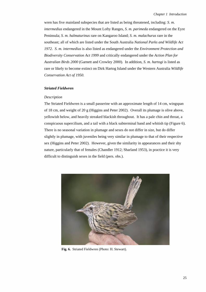
Chapter 1 Introduction
wren has five mainland subspecies that are listed as being threatened, including: S. m.
intermedius endangered in the Mount Lofty Ranges, S. m. parimeda endangered on the Eyre
Peninsula; S. m. halmaturinus rare on Kangaroo Island; S. m. malachurus rare in the
southeast; all of which are listed under the South Australia National Parks and Wildlife Act
1972. S. m. intermedius is also listed as endangered under the Environment Protection and
Biodiversity Conservation Act 1999 and critically endangered under the Action Plan for
Australian Birds 2000 (Garnett and Crowley 2000). In addition, S. m. hartogi is listed as
rare or likely to become extinct on Dirk Hartog Island under the Western Australia Wildlife
Conservation Act of 1950.
Striated Fieldwren Description
The Striated Fieldwren is a small passerine with an approximate length of 14 cm, wingspan
of 18 cm, and weight of 20 g (Higgins and Peter 2002). Overall its plumage is olive above,
yellowish below, and heavily streaked blackish throughout. It has a pale chin and throat, a
conspicuous supercilium, and a tail with a black subterminal band and whitish tip (Figure 6).
There is no seasonal variation in plumage and sexes do not differ in size, but do differ
slightly in plumage, with juveniles being very similar in plumage to that of their respective
sex (Higgins and Peter 2002). However, given the similarity in appearances and their shy
nature, particularly that of females (Chandler 1912; Sharland 1953), in practice it is very
difficult to distinguish sexes in the field (pers. obs.).
Fig. 6. Striated Fieldwren (Photo: H. Stewart).
25
Chapter 1 Introduction Taxonomy and distribution
The Striated Fieldwren (Calamanthus fuliginosus) comprises four subspecies in the family
Pardalotidae, is endemic to southeastern Australia, and is considered to be most common in
Tasmania (Pringle 1982b). The two Tasmanian subspecies only vary slightly in plumage
and size and include the nominate Calamanthus fuliginosus fuliginosus distributed
throughout the eastern half of the State, and Calamanthus fuliginosus diemenensis,
distributed throughout the western half of the State (Thomas 1979; Schodde and Mason
1999). In the absence of additional data needed to determine intergradation of the two
subspecies in central-south Tasmania, it is assumed that the latter subspecies is the focus of
this study as the majority of sites fall in the wetter western watershed of Tasmania (Schodde
and Mason 1999; Higgins and Peter 2002). Although a few studies have been published on
the Striated Fieldwren, many of the following aspects of its biology and ecology are
generally not known (Higgins and Peter 2002).
Habitat
Striated Fieldwrens utilise a diversity of habitats throughout their range that typically consist
of low, dense vegetation (Higgins and Peter 2002). Specific habitats include dry and wet
heathlands, sedgelands, tussock grasslands, alpine meadowlands, marshes, some dry and wet
sclerophyll forests and associated clearings, and particularly buttongrass moorlands in
Tasmania (Wilson 1950; Sharland 1953; Thomas 1979; Keast 1978; Gosper and Baker 1997;
Taylor et al. 1997; Schodde and Mason 1999). In some areas they seem to prefer shrubbier
sites with emergent shrubs (≤ 1 m) and may also utilise taller scrub edges (≤ 3 m) bordering
such sites (Recher 1981; Gosper and Baker 1997). They can also be found along the borders
of wetlands, such as marshes and creeks, and in introduced vegetation in more developed
areas, such as along roads, fences, and ditches (Legge 1908; Napier 1969; Keast 1978;
Sharland 1981). They have been recorded from sea level and occasionally up into subalpine
forest (~ 900-1100 m asl) and above tree-line in Tasmania (> 1100 m asl) (Sharland 1953;
Thomas 1979; MacDonald 2001).
Populations
Although their numbers can be hard to estimate (Watson 1955), some studies have reported
approximate home range sizes and densities of Striated Fieldwrens. Taylor et al. (1997)
estimated densities of 3.4 1.1 birds 10 ha-1 in young regrowth (0-6 years old) and 0.6 0.4
birds ha-1 in older regrowth (6-12 years old) and none in mature (> 12 years old) dry
sclerophyll forest with heathy and sedgey understories in southeast Tasmania. Based on
observations made in Victoria, Chandler (1912) estimated that home ranges were roughly
0.2-0.8 ha, and Keast (1978) observed that birds were spaced about 50 m apart where
populations were most dense. Gosper and Baker (1997) found that they were uncommon
26
Chapter 1 Introduction
overall, but had a relatively high average minimum density of 6.2 birds 10 ha-1 (range 4.0-9.0
birds 10ha-1) in their preferred habitat of low, dry heath in New South Wales.
Behaviour
Striated Fieldwrens are considered to be shy and secretive ground-dwelling birds, and are not
easily detected except by call (Legge 1908). Although they are resident and primarily
sedentary, they have been recorded up to 160 km from the nearest known population in New
South Wales (Higgins and Peter 2002). They are found singly, in pairs, and occasionally in
small groups and exhibit territorial behavior throughout the year (Keast 1978; Gosper and
Baker 1997). They typically run or creep along the ground and seem reluctant to fly unless
approached closely (Sharland 1981; Pringle 1982b). After being disturbed they may quickly
run away, drop into cover, or suddenly flush and fly up to approximately 20 m away (Littler
1904; Legge 1908; Sharland 1953; Keast 1978). They may be very difficult to relocate and
flush again, or may perch on top of emergent shrubs appearing to scan the area for the source
of the disturbance (Legge 1908; Chandler 1912; Gosper and Baker 1997). Despite their
overall shy nature, it has been noted that they can be less wary in developed areas where
their natural habitat has been modified (Legge 1908).
Calls
Striated Fieldwrens have complex, variable, and melodious territorial songs (~ 2-6 kHz)
thought to be sung by males (Legge 1908; Chandler 1912; Sharland 1953; Stewart 2001;
Higgins and Peters 2002). They typically sing from prominent perches, such as at the top of
emergent shrubs, with their head tilted back and tail cocked and flicking from side to side
(Legge 1908; Dove 1912; Keast 1978). They often start the song in a low key, seeming to
come from hundreds of metres away, which has a ventriloquial effect (Chandler 1912;
Sharland 1953). They then continue into a loud song that can be readily heard from up to
approximately 100 m away and last for 20 seconds ( Keast 1978; Gosper and Baker 1997).
A common form begins with two sharp whip, whip notes, followed by a pause, a single note,
another pause, and then 4-5 quick notes (Keast 1978). They will often cease singing if
approached within approximately 30 m and then plunge into cover (Chandler 1912). They
are known to sing at most times of the day and throughout the year, and particularly just
before sunset during the early breeding season of winter and during spring mornings and
afternoons (Sharland 1953; Watson 1955). In addition to their distinctive song, Striated
Fieldwrens also have a couple of other notable calls, including a rapid trill and a short churr
call, the latter typically issued during summer in Tasmania (Stewart 2001; T. Chaudhry
unpublished data).
27

Chapter 1 Introduction Diet
Striated Fieldwrens are primarily insectivorous, but do occasionally feed on seeds as well
(Pringle 1982b). They have been observed spending approximately two-thirds of their time
foraging in low or emergent shrubs, although they do not seem to prefer particular plant
species, and one-third on the ground (Keast 1978; Gosper and Baker 1997). They prey on
species from a wide range of Insecta, Arachnida, and Mollusca orders including but not
limited to the following: Araneae, Coleoptera, Gastropoda, Hemiptera, Hymenoptera,
Lepidoptera, Orthoptera, and Neuroptera (Lea and Gray 1936; Barker and Vestjens 1989).
Breeding
Striated Fieldwrens are one of the earliest breeders in Tasmania and have a long breeding
season, beginning as early as July and sometimes extending into early February (Legge
1908; Dove 1912; Sharland 1953; Napier 1969). They construct dome-shaped nests with
side or top entrances from vegetation such as dried grass, leaves, and moss, and line the
interior of the nest with feathers or hair (Dove 1912; Sharland 1981). The nests are well
concealed and located on or close to the ground and within or under tussocks or other low
vegetation (Sharland 1981; Dove 1916). They have at least two broods a year with three to
four eggs in each brood (Sharland 1981). Eggs have been found in nests from July to
October (Fletcher 1915b), and fledglings from September to December in western Tasmania
(Legge 1908; Dove 1912). Young have been observed in the nest as late as early February in
eastern Tasmania (Napier 1969).
Fire ecology
Only limited and mostly qualitative information is available on the fire ecology of Striated
Fieldwrens. Early records indicate the loss of natural habitat through ‘burning off’ (Legge
1908). Gellie (1980) stated that they are capable of finding sufficient food and cover almost
immediately after fire, and have been observed foraging on recently burnt moorlands in
Tasmania. He further stated that breeding cycles may be interrupted if fires occur during
spring, and breeding may not be successful for five to seven years post-fire unless adequate
unburnt patches are available; however, he provided no supporting data. Taylor et al.’s
(1997) study indicated that the Striated Fieldwren occurred in significantly higher densities
in young regrowth (0-6 years old) when compared to older regrowth coupes (6-12 years old)
following clearfall logging, regeneration burns, and portions of both coupes being
subsequently burnt in a wildfire; however, they were absent from mature forest (> 12 years
old). In southwestern Australia, Striated Fieldwrens are considered to be an early
successional species in heath, thus long-term fire exclusion may render some areas
unsuitable (Smith 1985, 1987). It has been recommended that a mosaic of fire ages should
28
Chapter 1 Introduction
be provided for such heathland species in order to maintain current population levels
(Woinarski 1999b).
Threats and status
Threats to the Striated Fieldwren, in addition to possible threats from fire, include extensive
land clearing and drainage of wetlands for agricultural development (Napier 1969; Sharland
1981). Such habitat loss may have significantly reduced populations in these areas and
possibly caused a shift in habitat utilisation toward some of these disturbed environments
that have developed elements of suitable habitat (Legge 1908; Sharland 1981). Natural
predators such as snakes have also been indicated as possible threats (Chandler 1912). In
addition, the Fan-tailed Cuckoo and potentially the Horsefield’s Bronze-Cuckoo and Pallid
Cuckoo are brood parasites of the Striated Fieldwren in Tasmania (Fletcher 1915b; Brown et
al. 1993).
The Striated Fieldwren showed no significant change (< 20%) in national reporting rates
between The Atlas of Australian Birds (1977-81; Blakers et al. 1984) and The New Atlas of
Australian Birds (1998-2002; Barrett et al. 2003), but decreased (> 20%) in western
Tasmania and portions of its range on the Australian mainland (Barrett et al. 2003). Due to
severe reductions in populations from some of the above threats (including broad-scale
vegetation clearing, exotic weeds, and grazing pressure; DEWHA 2007) C. f. albiloris is
listed as vulnerable under the New South Wales Threatened Species Conservation Act 1995.
However, it is recognised that there is inadequate information available regarding the current
status of this species (Lunney et al. 2000).
Ground Parrot
Description
The Ground Parrot is a psittaciforme and is one of only four ground-nesting parrots in the
world (Balmer et al. 2004). It has an approximate length of 30 cm, wingspan of 13 cm, and
weight of 80 g (Higgins 1999). Overall its plumage is bright green with black and yellow
streaks throughout. It has a red band across the forehead and yellow wing bars (Figure 7).
There is no seasonal variation and sexes of both adults and juveniles look similar, with
juveniles lacking the red forehead band and having bolder black streaks (Higgins 1999).
29
Chapter 1 Introduction
Fig. 7. Ground Parrot (Photo: Courtesy of PWS).
Taxonomy and distribution
The Ground Parrot (Pezoporus wallicus) comprises two subspecies in the family Psittacidae,
and is endemic in primarily coastal areas of eastern, southeastern, and western Australia.
The nominate Pezoporus wallicus wallicus is found in eastern Australia, and Tasmania is
considered to be its stronghold (Forshaw 1981). It is found throughout western and
southeastern Tasmania, and has the greatest numbers in the Southwest, particularly within
the TWWHA (Bryant 1991; Driessen and Mallick 2003). Unlike the Southern Emu-wren
and Striated Fieldwren described above, the Ground Parrot has been extensively studied
throughout its range (Higgins 1999).
Habitat
Ground Parrots primarily utilise patchily distributed heathland and sedgeland habitats within
their range, with such areas typically lacking tall shrubs or trees (Forshaw 1981; Meredith
1983; McFarland 1988a, 1988c). In Tasmania, Bryant (1991) reported that they
predominantly occur in graminoid heathlands (especially Standard and Layered Blanket
Moors, after Jarman et al. 1988a) and sedgelands, and on well to poorly drained soils. The
vegetation is typically 0.5 to 1.0 m tall (range 0.3-2.5 m). It is dense with a projective
foliage cover > 60% from 0-30 cm above ground level, and a highly variable overall
projective foliage cover of 30-90%. However, no significant correlation was found between
Ground Parrot densities and projective foliage cover or plant species richness. The apparent
importance of vegetation structure has also been noted in research conducted in New South
Wales (Wall 1989). Within their home ranges, they likely use a mosaic of different habitat
30
Chapter 1 Introduction
types, such as sedgey areas for foraging and heathy areas for nesting and roosting (Bryant
1991). Such use of different microhabitats can change throughout the year and may be
partly in response to seed abundance and accessibility (McFarland 1991a). Ground Parrots
are found from sea level to alpine areas over 1300 m asl, in the approximately 570,000 ha of
estimated potentially suitable habitat in Tasmania. However, most are found below 500 m
asl in perhumid southwestern Tasmania (Bryant 1991).
Populations
In Tasmania, Bryant (1991) reported Ground Parrot populations ranged from 0.2-5.3 birds 10
ha-1, with a mean density of 1.7 ± 1.0 10 ha-1. The smallest inhabited patch of moorland was
5 ha. These data, in conjunction with the estimated area of potentially suitable habitat, were
used to calculate a theoretical estimate of 97,000 birds. Some of her surveys were conducted
in the areas covered by this study. Near Lake St Clair a mean of 2.1 birds 10 ha-1 (range 1.5-
3.1 birds 10 ha-1) was reported for Burns Plains (3 years post-fire) and King William Plains
(8 years years post-fire). None were reported along Lake St Clair Road. Near Lake Pedder,
a mean of 1.2 birds10 ha-1 (range 0.3-2.1 birds10 ha-1) was reported for a number of sites
along Scotts Peak Dam Road (11-19 years post-fire). Consecutive year surveys conducted at
the latter sites indicated that densities remained fairly constant. Repeated surveys conducted
at Snug Tiers near Hobart showed that estimated densities fluctuated throughout the year,
with highest densities in March and November and lowest densities in June and July,
corresponding with the breeding season, dispersal of juveniles, and mid-winter, respectively.
No significant association was found between density and altitude (Bryant 1991). Extensive
research on the Ground Parrot has also been conducted in Cooloola National Park,
Queensland by McFarland (1991a, 1991b, 1991c). Birds maintained an average distance of
106 m from each other. Mean home ranges were 9.2 ha (mean 5.6 ha for adults and 13.9 ha
for subadults). There was considerable overlap of individual home ranges, but little in
foraging areas (McFarland 1991a). These figures are comparable to Meredith et al.’s (1984)
estimate that pairs require 8-20 ha of heath (depending on fire age). A study on Ground
Parrot vocalisations also conducted in Queensland indicated that sites 5.4 km apart supported
birds that were still considered to be from the same population or metapopulation (Chan and
Mudie 2004).
Behaviour
Ground parrots are ground-dwelling and both diurnal and crepuscular (Jordan 1987b).
Overall they are solitary and exhibit low intraspecific aggression (Courtney 1997); however,
adults are territorial during the breeding season (Jordan 1987b). Due to their camouflaged
plumage, preference for dense habitat, and shy and elusive nature, direct visual observations
on the ground are very difficult (Forshaw 1981, McFarland 1991d). They are not easily
31
Chapter 1 Introduction flushed even within close range (Burbidge 1989), and may simply remain motionless or
quickly run away (McFarland 1991d). They are usually flushed singly, and only rarely in
pairs (Bryant 1991). The mean bird-observer distance at flushing is 12.3 ± 0.5 m (range 2-50
m), and they typically fly in a zig-zag pattern into denser vegetation with a (straight-line)
mean distance of 76.8 ± 3.3 m (range 4-200 m) (McFarland 1991d). If pursued, they usually
only flush once or twice and then may resort to running away (Green and Mollison 1961;
McFarland 1991d). Ground Parrots are considered to be strong fliers and are capable of
flying long distances even over non-suitable habitat (e.g. woodland or water) (Forshaw
1981). By some accounts, they are considered to be primarily sedentary (Cooper 1974;
Bryant 1994). However, radio-telemetry data showed that they can be fairly mobile,
especially when young, with one bird moving a mean of 730 m over a 17 day period (Jordan
1987b). The longest recorded single flight was 700 m (McFarland 1991a) and others have
been recorded dispersing up to 220 km from the nearest known breeding area (Meredith et
al. 1984).
Calls
Ground Parrots are noted for having distinctive calling-flight sessions during dawn and dusk
(Higgins 1999), and do occasionally call during the day, especially in spring and summer in
some parts of their range (Jordan 1984; pers. obs.). Up to 11 calls types have been
recognised; however, their typical call issued during their calling-flight sessions can be
characterised as a high-pitched (~ 2-5 kHz) and ascending flute-like whistle consisting of
tsee notes (Watts 2002; Chan and Mudie 2004). The calls are issued by both sexes and most
birds (79%) may call while in flight (Jordan 1987b; McFarland 1991b). It has been assumed,
with some substantiating evidence, that all birds at a site call during each session, with the
possible exception of birds dispersing after the breeding season (Meredith et al. 1984). Calls
are sometimes issued simultaneously by different birds, but usually one call is followed by a
response by another bird (Forshaw 1981). A number of studies have indicated that these
calls can be heard for at least 400 m under still conditions with no rain, but only up to
approximately 200 m under windy conditions with heavy rain (Meredith and Isles 1980;
Bryant 1991). Light intensity is considered to be the primary influence on the beginning and
end of calling sessions (McFarland 1991b). In Tasmania, they call for a mean of 20.3 ± 0.8
minutes at dusk, with a mean of 4.8 ± 0.2 calls bird-1 and 0.3 ± 0.02 calls bird-1 minute-1
(Bryant 1991). These sessions were typically longer during the breeding season, and calling
duration, number of calls, and rate of calling were all significantly correlated with density of
Ground Parrots (Bryant 1991). They fly for approximately 10-15 minutes during the middle
of the session, with a mean flight length of 220 m during dusk sessions (Jordan 1987b;
McFarland 1991b). Although adults rarely fly more than 400 m, one young was recorded
flying 1.74 km from its daytime foraging area to nighttime roost site (Jordan 1987b).
32

Chapter 1 Introduction
Diet
Ground Parrots are primarily granivorous, but may occasionally feed on other plant matter
and insects (Sharland 1981). They usually feed on the ground, sometimes in low shrubs, and
may consume the order of 10,000 seeds per day (Meredith and Isles 1980; Forshaw 1981;
Jordan 1989). It has been estimated that males forage over an area of approximately 13 ha
around the nest to provision chicks during the breeding season (Jordan 1984). They are
considered to be opportunistic foragers, and likely choose seeds based on varying aspects of
availability and size (McFarland 1991a). In Tasmania, their known and potential food plants
come from 13 dicotyledon and 12 monocotyledon species from 9 families, with the majority
of their food probably from the Restionaceae and Cyperaceae families (Bryant 1994). The
wide variety of these species that can be found in graminoid heathlands and sedgelands may
help to explain Ground Parrots’ apparent preference for these habitats. However, as sites
become older they may become more dominated by shrub species. The associated floristic
and structural changes may result in a decrease in sedge seed abundance and accessibility
(Jordan 1989).
Breeding
Ground Parrots have been recorded breeding from mid-October to February in Tasmania, but
timing may vary depending on climatic conditions and food resources (McFarland 1988a;
Bryant 1991). Their nests can be located in dry or ecotonal microhabitats (McFarland
1991b). They consist of shallow depressions in the ground lined with buttongrass stems,
rushes or other plant material, and are well concealed under tussocks or small shrubs (Green
and Mollison 1961; Hodges 1961; Sharland 1981). They usually only have one brood with a
mean of 4.24 0.12 eggs (range 2-6 eggs) from October to as late as January in Cooloola
National Park, Queensland (McFarland 1988a; McFarland 1991b). Egg failure rates can be
high (22-31%), and pairs averaged 1.9 fledglings nest-1 (Meredith and Isles 1980; McFarland
1991b). Chicks are fledged from December onwards, and young may remain in the natal
area for a couple months before dispersing to new habitat (Meredith et al. 1984; Bryant
1991).
Fire ecology
Extensive research has been carried out on the fire ecology of the Ground Parrot throughout
its range (Woinarski 1999a). Although studying the effects of fire on Ground Parrots was
not considered to be the primary focus of her research in Tasmania (S. Bryant pers. comm.
2003), the majority of this section references Bryant (1991, 1992, 1994), with additional
references from mainland research as appropriate.
33
Chapter 1 Introduction Ground Parrots have been observed flying before fire fronts (Cooper 1975), but may
potentially lose clutches if fires take place during the breeding season (Gellie 1980), and may
die due to heat or asphyxiation during severe wildfires (Fox 1978). A Ground Parrot has
also been observed foraging on grains in a fowl-yard after presumably being displaced from
a nearby buttongrass plain by a bushfire (Fletcher 1946). Bryant (1991) identified Ground
Parrots across the full range of sites investigated in Tasmania, from 1-90 years (mean 13.4)
by flushing and from 2 months-35 years (mean 9.2) post-fire by call surveys. Recolonisation
occurred at sites approximately 1 year post-fire, when the estimated minimal projective
foliage cover of 30% was attained at most sites (Bryant 1994). However, Ground Parrots
have been noted using sites much sooner after fires (Gellie 1980). Such younger sites,
especially with small copses of older and denser vegetation, may provide adequate cover and
become temporarily crowded within larger burnt areas (Meredith et al. 1984; Bryant 1991).
Densities typically remained low until 4-7 years post-fire, when densities peaked above
approximately 2.2 birds 10 ha-1. Densities were then maintained above the mean of 1.7
birds10 ha-1 until approximately 13 years post-fire, after which densities declined but
remained good (density not specified) more than 30 years post-fire. The correlation between
densities and fire age was highly significant ( = 0.26, P < 0.001, n = 182), and may be
attributable to age related differences in flowering, seeding, and vegetation structure (Bryant
1991). Although fire frequency was not explicitly studied and no data were provided, she
attributed some local extinctions to ‘overfiring’ of moorlands, specifically along the Lyell
Highway corridor within the Lake St Clair study area (see Chapter 2).
Results from studies conducted on the mainland have shown similar correlations between
Ground Parrot densities and site age. In Queensland, McFarland (1991c) reported Ground
Parrots returned to subtropical heathland sites within one year post-fire, peaked at densities
of 4-5 10 ha-1 at 5-8 years post-fire, while none were recorded at sites > 14 years post-fire.
He attributed such long-term patterns to changes in vegetation structure and food resources,
and short-term fluctuations with seasonal effects on population dynamics. In New South
Wales, Jordan (1987b) similarly found that populations in a heathland peaked at 5-6 years
post-fire, but declined to zero by 12 years post-fire. However, a long-term study conducted
in the same area by Baker and Whelan (1994) and Whelan and Baker (1999) indicated that
populations reached maximum densities 13 years post-fire, and ongoing monitoring has
indicated that they are still present although apparently declining 20 years post-fire (Tasker
and Baker 2005). In Western Australia, Western Ground Parrots have likewise been
reported inhabiting older sites, and were considered to be relatively common in sites 20-40+
years post-fire, but can utilise recently burnt sites when directly adjoined to unburnt habitat
with established populations (Burbidge 1989; Burbidge et al. 2007). Such an apparent range
in the age of utilised habitats may reflect regional differences in rainfall and other factors,
34

Chapter 1 Introduction
which in turn affect the rate of vegetation regrowth. In this sense, vegetation structure (e.g.
cover) and floristics (e.g. seed production) may have a greater influence on Ground Parrot
densities than fire age per se (Meredith et al. 1984; Baker and Whelan 1994). Fire frequency
has also been identified as an important consideration in managing Ground Parrot habitat
(Meredith 1984a, 1984b; Bryant 1991; Burbidge et al. 2007). Short fire intervals (e.g. 6-8
years) may lead to declines and local extinctions due to a loss of plant species that Ground
Parrots rely on for food. After being subjected to such fire regimes, some sites may take a
long time to become suitable again (Meredith 1984a).
Clearly, fire plays a critical role in Ground Parrot densities, and some populations on the
mainland have become threatened or locally extinct due to detrimental fire regimes, ranging
from frequent prescribed burning to fire exclusion (Woinarski 1999b). However, fire is only
one factor in a complex set of interactions, with other factors including vegetation type,
habitat diversity, extent, and proximity to recolonisers (McFarland 1991c). Although Bryant
(1991) stated that prescribed burning specifically for the Ground Parrot was not required, she
provided some general guidelines in order to minimise adverse impacts and maintain
adequate suitable habitat across the landscape. Guidelines included conducting prescribed
burns between April and September in order to minimise impacts during the breeding
season, providing a mosaic of burnt and unburnt vegetation within sites, and not burning
more than 25% of an area over a 10 year rotation in order to maintain sustainable densities.
Threats and status
In addition to altered fire regimes, Ground Parrot populations are threatened by habitat loss,
fragmentation and degradation from development, agriculture, grazing, and the plant
pathogen Phytophthora cinnamomi (Forshaw 1981; Bryant 1991; Garnett 1992). Additional
threats may include avian diseases and predation by both native (e.g. snakes and raptors) and
feral animals (e.g. foxes and cats) (Lord 1927; Meredith 1984a; Jordan 1989; Bryant 1991).
Despite numerous studies citing predation as a major threat to Ground Parrot populations,
McFarland (1991c) considers the risks to Queensland populations to be minimal. In
Tasmania, Ground Parrots populations have declined and some populations have become
locally extinct, particularly in northern and eastern regions where suitable habitat was
historically limited (Bryant 1991). Such losses have been attributed to development,
grazing, and increased fire frequency. However, populations are considered to be secure in
southwestern Tasmania where they are free from most threats under the protection of the
Tasmanian Nature Conservation Act 2002 and the TWWHA (Bryant 1991).
Due to some of the threats identified above, Ground Parrot populations and distribution have
been severely reduced in parts of its range (Lunney et al. 2000). Accordingly, the Ground
Parrot is listed as vulnerable under the Action Plan for Australian Birds 2000 (Garnett and
35
Chapter 1 Introduction Crowley 2000), the Queensland Nature Conservation Act 1992, and the New South Wales
Threatened Species Conservation Act 1995. The Western Ground Parrot, P. w. flaviventris,
is listed as endangered under the Environment Protection and Biodiversity Conservation Act
1999 and the Action Plan for Australian Birds 2000 and rare or likely to become extinct
under the Western Australia Wildlife Conservation Act of 1950.
Orange-bellied Parrot The Orange-bellied Parrot (Neophema chrysogaster) is extremely rare and within Tasmania
is only found within the Macquarie and Bathurst Harbour basins in the Southwest. It is a
summer migrant from mainland Australia that depends on buttongrass moorlands for
foraging during the summer breeding season, and adjacent forests for nesting (Brown and
Wilson 1984). Appropriate fire regimes are thought to be an important factor in maintaining
optimal foraging and nesting habitat, but no rigourous fire ecology studies have been
conducted to date (Brown et al. 1993; M. Holdsworth pers. comm. 2007). Due to significant
habitat loss on the mainland and a very small population size, the Orange-bellied Parrot is
listed as critically endangered under the IUCN Red List of Threatened Species 2004, and
endangered under the Australia Environment Protection and Biodiversity Protection Act
1999, the Tasmania Threatened Species Protection Act 1995, and the South Australia
National Parks and Wildlife Act 1972. However, since the Orange-bellied Parrot breeds
outside of the range of this study (see Chapter 2), it is not considered any further herein.
Thesis aims and structure This is the first quantitative, community-level study of the avifauna of Tasmanian
buttongrass moorland and investigated the influence of a range of abiotic and biotic factors
on avifaunal composition and densities, particularly in relation to post-fire succession. The
primary aim of this thesis was to contribute information to help guide fire management and
conservation of the moorland avifauna in the TWWHA, with a focus on the three resident
species (i.e. Southern Emu-wren, Striated Fieldwren, Ground Parrot).
I wrote the primary Chapters (4-6) of this thesis in a format to facilitate publication in the
near future. Accordingly, there is some repetition, but I have attempted to limit this by
referring to other chapters, as appropriate. However, I have elaborated within some sections
(e.g. Methods) to enable a more critical review of my research and the replication of methods
for future research and monitoring. I am the principal contributor to all chapters in this
thesis and will be the primary author for all publications and presentations arising from it.
In Chapter 2, I provide a rationale for the study design and site selection process, background
information on the study locations and sites, and a critical evaluation of fire regime data for
36
Chapter 1 Introduction
37
the study sites. I rely upon this information for analyses and interpretation of results in
subsequent chapters.
In Chapter 3, I present methods for developing a fine-scale and high-resolution classified
avian habitat map for buttongrass moorlands and associated vegetation communities. I use
this map to quantify the composition, structure, and spatial characteristics of avian habitat in
the study area that are required for analyses and interpretation of results in subsequent
chapters. In addition, I present the results from a formal accuracy assessment of the
Tasmanian Wilderness World Heritage Area Vegetation Mapping (WHAveg) within the
study area.
In Chapter 4, I use a replicated space-for-time (SFT) design to investigate the short- to long-
term effects of fire (i.e. 1-54 years post-fire) and other environmental variables on avifaunal
composition and densities in low productivity blanket moorlands at Lake Pedder and
moderate productivity eastern moorlands at Lake St Clair, with an emphasis on the three
resident species.
In Chapter 5, I investigate whether the resident and non-resident avian species use habitats
disproportionately in relation to availability and fire age within low productivity blanket
moorlands at Lake Pedder and moderate productivity eastern moorlands at Lake St Clair. I
describe and compare the terrestrial arthropod community between moorland matrix and
riparian habitats in relation to fire age, and investigate whether patterns of habitat use of
insectivores reflect the patterns of potential availability of arthropod prey resources.
In Chapter 6, I opportunistically utilise prescribed burns conducted by Parks and Wildlife
Service at two study sites included in the SFT study in Chapter 4. I use a before-after-
control-impact design (BACI) to investigate the short-term responses of the moorland
avifauna to hazard-reduction burning in relation to unburnt control sites.
In Chapter 7, I conclude this thesis by synthesising the effects of fire and other
environmental factors on avian species composition, density, and habitat use in Tasmanian
buttongrass moorlands. I discuss my results in relation to similarly depauperate sedgeland
and heathland communities within a national and global context, as well as patterns in post-
fire faunal succession within a theoretical context. I discuss the implications of results from
previous chapters for fire and conservation management in Tasmanian moorlands, and
conclude this thesis by providing recommendations for future research.

38
Chapter 2
Study design, site descriptions, and fire regimes
Study design The ultimate aim of this thesis was to investigate the effects of post-fire succession on the
avifauna of Tasmanian buttongrass moorlands in order to provide recommendations for their
conservation to fire and wildlife managers. The literature is replete with studies
investigating the effects of fire on Australian fauna, and on birds in particular (for a review
see Woinarski 1999a, 1999b). However, since it is clear that reported patterns and their
underlying processes are both complex and highly variable in space and time (Whelan et al.
2002; Burbidge 2003; Gill and Bradstock 2003), it is critical to conduct site- and species-
specific research to develop appropriate management recommendations. There was a clear
management need for this study as no previous studies have explicitly focused on the fire
ecology of the Tasmanian moorland avifauna, and only one (Bryant 1992) has explored the
effects of fire age on the resident Ground Parrot. Accordingly, the primary aims of this
Chapter were: 1) to provide a rationale for the study and describe its design and the site
selection process; 2) to present background information on the study locations and sites; and
3) to collect, compile, and evaluate data on fire regimes for the study sites.
Studies with comparable aims to this one have been conducted both on the Australian
mainland and abroad. The inferences that can be drawn from many of these studies are
limited by a host of issues associated with study design, implementation, analyses, and
reporting. A number of different study designs are often used to assess the effects of fire on
birds, including designed experiments, before-after-control-impact (BACI), space-for-time
(SFT), and inferential studies (Stewart-Oaten et al. 1986; Pickett 1989; Loyn 1999; Block et
al. 2001), each of which has its pros and cons. Replicated manipulative field experiments
are considered to be the most desirable design since they make it possible to draw strong
inferences regarding responses to fire regime parameters per se and to develop a more
process-based understanding of population changes (Whelan et al. 2002). BACI studies that
include randomly allocated replicate burnt and control sites and adequate pre- and post-fire
surveying can likewise provide a basis for strong inferences (Whelan 1995; see Chapter 6).
Despite their obvious advantages, studies that employ such rigorous designs are exceedingly
rare (e.g. Loyn et al. 2003; Woinarski 1990) due to real-world constraints such as limited
time, personnel, and funding. Furthermore, it is often not feasible to impose the treatment
(i.e. fire) for designed experiments at the appropriate time, location, and scale (Whelan
1995). Thus, many studies must use sites that were either burnt in the past (e.g. Meredith et
39

Chapter 2 Study design and site descriptions al. 1984; McFarland 1988b) or opportunistically utilise previously surveyed sites subjected
to contemporaneous fire events and accept the associated compromises in study design and
applicability (e.g. Brooker and Rowley 1991; Recher 1997; Loyn 1997).
A SFT design was deemed the most appropriate and feasible option to utilise, considering
the primary aims and specific constraints imposed on this study. SFT designs are commonly
used within ecosystems that exhibit marked successional dynamics in relation to disturbance
events, such as buttongrass moorlands, and are based on the assumption that spatial and
temporal variations are homologous (Pickett 1989; Brown et al. 2002). In other words,
many researchers are interested in identifying temporal trends over the medium to long term
(i.e. ~ 10 to > 50 years) but do not have the ability to monitor sites over commensurate time
scales. For that reason, sites of different ages (i.e. time since the last fire) are ‘substituted’
for time to create a chronosequence of sites from which retrospective temporal trends can be
extrapolated (Pickett 1989). In this sense, SFT studies fall within the general class of
comparative mensurative experiments, as defined by Hurlbert (1984). In a comprehensive
review and annotated bibliography of Australian birds and fire by Woinarski (1999a, 1999b),
he noted that a large proportion of studies used SFT or similar designs. Perhaps the most
serious inherent limitation of SFT studies is the possibility of inter-site variability in abiotic
(e.g. geology, topography, climate) and biotic (e.g. vegetation, disease, predation) factors
confounding or compounding observed differences in populations from effects of fire
regimes per se (Loyn 1999; Woinarski 1999b). Another limitation is that both population
and fire regime differences may covary with these and other factors that may be either
unmeasured or unknown (Whelan 1995). Specific deficiencies that have been identified for
previous avian SFT studies in particular, and fire ecology studies in general, include failures
to:
- incorporate adequate (or any) replication, control sites, survey timespans, and
statistical analyses (Whelan 1995; Burbidge 2003);
- survey an adequate range of fire ages (Baker and Whelan 1994);
- clearly report and assess the quality of fire regime data and report the sizes and
specific locations of fires, sites, replicates, and sampling units (Parr and Chown
2003);
- investigate the impacts of fire regime parameters other than just time since last fire
on populations (Woinarski 1999b);
- quantify and investigate the impacts of other habitat variables (e.g. vegetation,
productivity, food resources) (Smith 2000);
- and form explicit collaborations between researchers and land management
authorities to facilitate the research process and implementation of management
recommendations (Whelan 1995).
40
Chapter 2 Study design and site descriptions
Despite some of these limitations and deficiencies, SFT and other mensurative studies are
still deemed to be valuable and pragmatic approaches to assess post-fire changes in faunal
communities, provided they are carefully designed, implemented, and interpreted (Twigg et
al. 1989; Whelan 1995; Loyn 1999). Furthermore, they are viewed as a necessary
prerequisite for much needed experimental research into ecosystems, such as buttongrass
moorlands, for which such baseline information does not currently exist (Saab and Powell
2005).
To address several of the above design deficiencies, this SFT study included two study
locations stratified by productivity and vegetation type, and comprising a broad
chronosequence of replicated fire ages. To the extent possible, sites were selected to
minimise inter-site variability in abiotic and biotic factors which have been described and
quantified in detail. This study was designed and implemented in close collaboration with
the Biodiversity Conservation Branch (BCB) and the Parks and Wildlife Service (PWS)
(Department of Primary Industries, Parks, Water and Environment), which are responsible
for fauna, flora, and fire management within the Tasmanian Wilderness World Heritage Area
(TWWHA). This multidisciplinary collaboration included a synchronous SFT study
conducted by BCB on the effects of fire on moorland invertebrates and was inclusive of all
sites used in this study except Gingerbread Track at Lake St Clair (GIT) and Airstrip West
(AIW) at Lake Pedder (Table 4) (M. Driessen unpublished data). To make the results from
these studies directly applicable to current fire management practices in buttongrass
moorlands, the design was based on two of the primary variables in the fuel and fire
behaviour models currently used by PWS and described by Marsden-Smedley et al. (1999)
(see Chapter 1). The first variable is vegetation age (i.e. years since fire). Although the
predictive models do not include other fire regime parameters such as frequency and season,
they are used in the prescription guidelines. As such, they are considered herein to the extent
that reliable data were available for inferences. The second variable is site productivity as it
pertains to fuel accumulation rates, loads, and spatial continuity. Sites are classified in the
models as either low or moderate productivity based on geological substrate. Investigating
productivity as it relates to intrinsic edaphic differences between sites appears to be a unique
approach for an avian fire ecology study as neither the literature review by Woinarski
(1999a, 1999b) nor that conducted for this thesis identified any such previous research (see
References). While not an explicit model variable, the blanket and eastern moor community
groups were also considered since they are closely associated with site productivity within
the study area (i.e. low and moderate, respectively), and the latter group presents major
issues for fire management (e.g. high fire spread rates and flame heights) (Marsden-Smedley
and Catchpole 1995b; Marsden-Smedley et al. 1999). Although productivity is obviously a
continuum and can vary over both time and space, and time since fire is likewise only one
41

Chapter 2 Study design and site descriptions factor in an extremely complex system, these variables have proven to be effective in
modelling and predicting fuel loads and fire behaviour in buttongrass moorlands. Therefore,
these two variables are used as part of the underlying paradigm of this study.
Site descriptions and fire regimes Study locations
The island state of Tasmania (excluding associated islands) is located between latitudes
40°6’-43°6’S and longitudes 144°6’-148°4’ E, approximately 200 km south of the Australian
mainland. Research was conducted in the Tasmanian Wilderness World Heritage Area,
associated National Parks and inholdings, and adjacent lands (e.g. State Forest and Hydro
Electric Commission lands). The TWWHA was established in 1982 and encompasses 1.38
million hectares in western Tasmania (~ 20% of the State) (Smith and Banks 1993). The
study comprises two locations, hereafter referred to as Lake Pedder (42°83’-43°05’S,
146°19’-146°38’E), primarily in Southwest National Park, and Lake St Clair (42°12’-
42°21’S, 146°10’-146°22’E) primarily in Cradle Mountain-Lake St Clair and Franklin-
Gordon Wild Rivers National Parks (Figure 1). These locations were chosen since sites near
Lake Pedder are considered to be representative of typical blanket moorlands found
throughout the low productivity quartzitic geologies of the Southwest, and sites near Lake St
Clair are representative of typical eastern moorlands found in the moderate productivity
doleritic geologies of the Central Plateau (Greenslade and Driessen 1999; Marsden-Smedley
2003). Furthermore, these regions are of high conservation concern (PWS 1999), are
relatively accessible, and have been the focus of past and ongoing fire management activities
and multidisciplinary fire ecology research (e.g. Marsden-Smedley 1993; PWS 1996;
Driessen 1999; Driessen and Greenslade 2004; Barnes and Balmer 2000; Balmer and Barnes
2000; Bridle et al. 2003).
42

Chapter 2 Study design and site descriptions
43
Australia
Tasmania
#Hobart
Lake St Clair
Lake Pedder
Tasmanian Wilderness World Heritage Area
SouthwestNational Park
Franklin-Gordon Wild RiversNational Park
Cradle Mountain -Lake St ClairNational Park
Lyell Highway
Gordon River Road
Lake St Clair
Lake King William
Lake Gordon
Lake Pedder
0 50 100 Kilometers
N
Fig. 1. Lake Pedder and Lake St Clair study locations, Tasmanian Wilderness World Heritage Area , Tasmania, Australia (AGD 66; LIST 2003). Note: King, Flinders, Macquarie, and associated islands not shown.
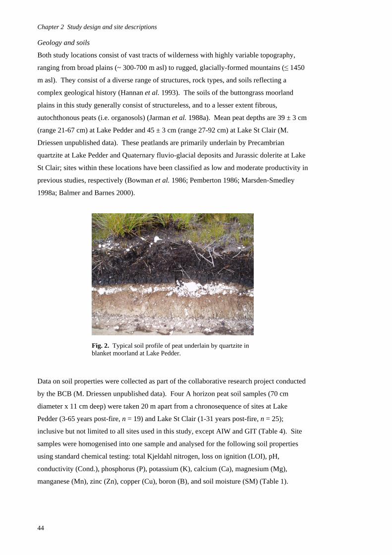
Chapter 2 Study design and site descriptions Geology and soils
Both study locations consist of vast tracts of wilderness with highly variable topography,
ranging from broad plains (~ 300-700 m asl) to rugged, glacially-formed mountains (≤ 1450
m asl). They consist of a diverse range of structures, rock types, and soils reflecting a
complex geological history (Hannan et al. 1993). The soils of the buttongrass moorland
plains in this study generally consist of structureless, and to a lesser extent fibrous,
autochthonous peats (i.e. organosols) (Jarman et al. 1988a). Mean peat depths are 39 ± 3 cm
(range 21-67 cm) at Lake Pedder and 45 ± 3 cm (range 27-92 cm) at Lake St Clair (M.
Driessen unpublished data). These peatlands are primarily underlain by Precambrian
quartzite at Lake Pedder and Quaternary fluvio-glacial deposits and Jurassic dolerite at Lake
St Clair; sites within these locations have been classified as low and moderate productivity in
previous studies, respectively (Bowman et al. 1986; Pemberton 1986; Marsden-Smedley
1998a; Balmer and Barnes 2000).
Fig. 2. Typical soil profile of peat underlain by quartzite in blanket moorland at Lake Pedder.
Data on soil properties were collected as part of the collaborative research project conducted
by the BCB (M. Driessen unpublished data). Four A horizon peat soil samples (70 cm
diameter x 11 cm deep) were taken 20 m apart from a chronosequence of sites at Lake
Pedder (3-65 years post-fire, n = 19) and Lake St Clair (1-31 years post-fire, n = 25);
inclusive but not limited to all sites used in this study, except AIW and GIT (Table 4). Site
samples were homogenised into one sample and analysed for the following soil properties
using standard chemical testing: total Kjeldahl nitrogen, loss on ignition (LOI), pH,
conductivity (Cond.), phosphorus (P), potassium (K), calcium (Ca), magnesium (Mg),
manganese (Mn), zinc (Zn), copper (Cu), boron (B), and soil moisture (SM) (Table 1).
44
Chapter 2 Study design and site descriptions
Table 1. Summary of peat soil properties across fire ages for sites at Lake Pedder (3-65 years post-fire, n = 19) and Lake St Clair (1-31 years post-fire, n = 25), Tasmania (M. Driessen unpublished data). Lake Pedder Lake St Clair Soil variables Mean SE Range Mean SE Range
Total Kjeldahl N (%) 0.73 ± 0.07 0.33 - 1.41 1.25 ± 0.06 0.42 - 1.73
LOI (%) 48 ± 5 8 - 93 63 ± 4 21 - 93
pH 3.8 ± 0.0 3.5 - 4.0 4.1 ± 0.0 3.8 - 4.7
Cond. (us/cm) 255 ± 14 160 - 340 324 ± 26 140 - 810
P (ppm) 8 ± 1 4 - 14 12 ± 1 6 - 32
K (ppm) 152 ± 14 54 - 270 209 ± 28 74 - 780
Ca (ppm) 357 ± 36 170 - 630 821 ± 101 300 - 2640
Mg (ppm) 532 ± 66 180 - 1040 444 ± 41 120 - 930
Mn (ppm) 6.7 ± 0.2 5.0 - 8.1 55.5 ± 24 8.3 - 520.0
Zn (ppm) 1.1 ± 0.1 0.6 - 2.0 6.2 ± 0.8 1.8 - 20.0
Cu (ppm) 0.4 ± 0.0 0.2 - 0.6 5.7 ± 0.9 1.4 - 15.0
B (ppm) 1.8 ± 0.1 1.4 - 3.2 2.9 ± 0.2 2.1 - 7.0
SM (%) 76.1 ± 1.4 59.2 - 84.4 79.7 ± 1.7 58.6 - 92.7
Principal Components Analysis (PCA) was used to identify overall differences in soil
properties between Lake Pedder and Lake St Clair using Primer 5.2.2 (Primer-E Ltd. 2001).
Data were normalised and log10-transformed, as appropriate (Table 2) (Clarke and Warwick
1994; Clarke and Gorley 2001). The first two Principal Components (PC1 and PC 2) had
eigenvalues > 1 (7.40 and 2.69, respectively) and accounted for 77.6% of the variation; thus,
the two-dimensional PCA plot (Figure 3) provided a parsimonious summary and showed a
clear difference in overall soil properties between Lake Pedder and Lake St Clair (Clarke and
Gorley 2001; Quinn and Keough 2002).
A dissimilarity matrix was calculated using normalised Euclidean distances and a one way
analysis of similarities routine (ANOSIM, with 999 permutations) was used to test for
significant differences in soil properties between locations as depicted in the PCA plot
(Clarke and Warwick 1994). The global ANOSIM test showed there were significant
differences in overall soil properties between locations (R = 0.498, P < 0.01) and the
moderate R value indicated there were clear, although overlapping differences (Clarke and
Gorley 2001).
Overall, these results demonstrated there was a significant difference in soil properties
between Lake Pedder and Lake St Clair. The sites at Lake Pedder generally have lower
levels of soil nutrients and hence lower fertility and productivity than those at Lake St Clair
and thus confirm their a priori classification as low and moderate productivity soils,
respectively. Results from Lake Pedder are consistent with previous research by Bowman et
al. (1986) that likewise concluded the soils in that region are extremely infertile.
45
Chapter 2 Study design and site descriptions Table 2. Principal Components Analysis eigenvectors of peat soil property values (log10-transformed* and normalised from Table 1) for sites at Lake Pedder and Lake St Clair, Tasmania.
Soil variables PC1 PC2
Total Kjeldahl N (%) -0.313 0.028
LOI (%) -0.283 0.250
pH* -0.208 -0.391
Cond. (us/cm)* -0.313 0.204
P (ppm)* -0.296 0.205
K (ppm)* -0.292 0.280
Ca (ppm)* -0.312 -0.084
Mg (ppm)* -0.206 0.398
Mn (ppm)* -0.296 -0.241
Zn (ppm)* -0.315 -0.241
Cu (ppm)* -0.276 -0.325
B (ppm)* -0.181 -0.437
SM (%) -0.269 0.208
PC
2
4
3
2
1
0
-1
-2
-3
-6 -4
-4 -2 0 2 4 6
PC1
Fig. 3. Two-dimensional PCA ordination of the 13 peat soil property variables (Table 2) for sites at Lake Pedder ( ; n = 19) and Lake St Clair ( ; n = 25), Tasmania (77.6% of variance explained).
46
Chapter 2 Study design and site descriptions
Climate
Tasmania is characterised as having a temperate maritime climate dominated by the westerly
‘Roaring Forties’ wind system (ABS 2000). The Lake Pedder and Lake St Clair regions
have cool to mild perhumid climates and are renowned for having extremely variable short-
term weather conditions (Gentilli 1972). Table 3 includes seasonal and annual averages for
climatic conditions obtained from the nearest and most representative weather stations for
the study regions (Bridle et al. 2003).
Table 3. Average seasonal (based on bird survey periods) and annual climatic conditions for Lake Pedder (Scotts Peak Dam Station # 97083, 1992-2004) and Lake St Clair (Lake St Clair National Park Station # 096071, 1989-2004) study locations, Tasmania (BOM 2004). Lake Pedder Lake St Clair
Conditions Feb. Jun. Oct. Annual Feb. Jun. Oct. Annual
Temperature- daily max. (°C) 21.0 9.7 13.8 14.7 19.3 7.7 12.5 13.1 Temperature- daily min. (°C) 9.6 4.4 4.8 6.2 5.9 0.3 1.9 2.7 Relative humidity- 9am (%) 82.0 90.5 84.0 85.2 84.0 88.0 82.0 84.0 Precipitation (mm) 62.0 250.6 170.4 1819.9 85.6 193.2 180.5 1906.0 Rain days 14.4 25.5 24.8 256.7 12.4 22.9 22.4 235.6 Wind speed- 9am (km h-1) 6.7* 7.0* 9.6* 8.1* 5.0 5.0 6.4 5.5
* Mean wind speed from Strathgordon Village Station (# 097053, 1968-2004) located west of the study region since data not available for Scotts Peak Dam.
Climates in both regions are broadly comparable. Temperatures are normally cool to mild
throughout the year, and range from an average daily maximum of approximately 19-21°C
during summer to a minimum of 0-4°C during winter. Consistent with its higher altitude,
minimum temperatures at Lake St Clair are typically a few degrees lower throughout the
year than at Lake Pedder. Precipitation is highest in spring and winter and lowest in
summer, though significant rain occurs throughout the year. Protracted periods without rain
(i.e. ~ 2 weeks) are rare (Marsden-Smedley 1993), and extreme fire conditions generally
occur for only up to a few days each summer (Jackson 1999a). A precipitation gradient
decreasing from west to east exists in both study regions due to the predominantly westerly
air flow and mountainous terrain (Nunez et al. 1996). Accordingly, mean precipitation
figures for Lake St Clair are likely higher than indicated above since the data are from a
station located in the eastern portion of the study area. Precipitation is sufficient to maintain
rainforest communities in both locations (Balmer and Barnes 2000; TVMP 2004) and results
in waterlogged conditions during most of the year in the poorly-drained peat flats in this
study. Prevailing winds are from the northwest to southwest, but can be highly variable in
speed, duration, and direction. Wind speeds are typically light (< 19 km h-1) with occasional
stronger gusts, but moderate to gale force winds (20-87 km h-1) are not uncommon,
particularly in winter and early spring (BOM 2004).
47
Chapter 2 Study design and site descriptions Site selection
The primary objective for the site selection process was to identify numerous replicate
buttongrass moorland sites within each location that spanned a wide range of fire ages (i.e.
chronosequences), encompassing the inter-fire interval range of 5 - ≥ 30 years proposed for
ecosystem-management burning in the TWWHA (Marsden-Smedley and Kirkpatrick 2000;
PWS 2004; Marsden-Smedley 2009). Additional objectives included ensuring that sites had
comparable abiotic and biotic characteristics, and that they were well interspersed within
each study location.
In order to reduce the potential confounding effects of abiotic and biotic variables other than
the primary treatment (i.e. fire age) both within and between sites, the following criteria were
utilised during the site selection process:
- Accessibility
Due to a range of logistical and safety considerations, sites were initially limited to
those that were either next to or within a reasonable walking distance of the
relatively limited road networks found within the study area.
- Site size
Based on the estimated home ranges reported in the literature, five hectares was
considered to be the minimum moorland patch size that could reasonably support at
least one breeding pair for each of the three resident bird species (see Chapter 1). To
ensure that each site could be surveyed in its entirety within a six hour survey period
and to maximise the number of sites that could be surveyed during the course of the
study the largest desirable site size was considered to be approximately 100 ha.
- Altitude
Altitude is known to affect a variety of abiotic factors that can, in turn, influence
vegetation. Sites were limited to altitudinal ranges that are not known to contain any
significant vegetation gradients (Jarman et al. 1988a; J. Marsden-Smedley pers.
comm. 2003).
- Topography
Sites were limited to those that were flat to gently rolling (slope ~ ≤ 5%) in order to
minimise the variability of site aspect and hydrology and their associated effects on
the behaviour of past fire events, vegetation structure and composition, and bird
habitat utilisation.
- Geology
Although the Lake Pedder and Lake St Clair study locations are characterised by
quartzitic and doleritic geologies, respectively, localised variability in geology and
associated productivity do occur (J. Marsden-Smedley pers. comm. 2003).
Accordingly, road-cuts, boulders, outcrops, and apparent fuel-loading (based on
48
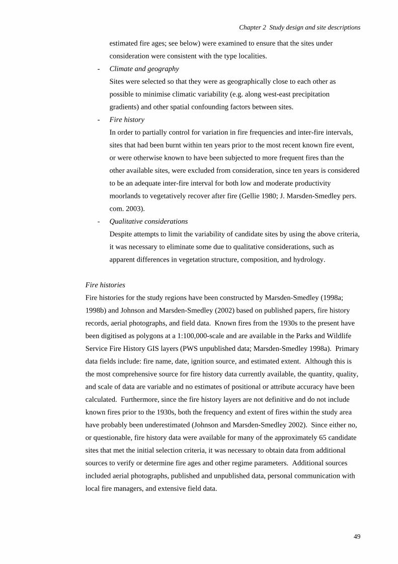
Chapter 2 Study design and site descriptions
estimated fire ages; see below) were examined to ensure that the sites under
consideration were consistent with the type localities.
- Climate and geography
Sites were selected so that they were as geographically close to each other as
possible to minimise climatic variability (e.g. along west-east precipitation
gradients) and other spatial confounding factors between sites.
- Fire history
In order to partially control for variation in fire frequencies and inter-fire intervals,
sites that had been burnt within ten years prior to the most recent known fire event,
or were otherwise known to have been subjected to more frequent fires than the
other available sites, were excluded from consideration, since ten years is considered
to be an adequate inter-fire interval for both low and moderate productivity
moorlands to vegetatively recover after fire (Gellie 1980; J. Marsden-Smedley pers.
com. 2003).
- Qualitative considerations
Despite attempts to limit the variability of candidate sites by using the above criteria,
it was necessary to eliminate some due to qualitative considerations, such as
apparent differences in vegetation structure, composition, and hydrology.
Fire histories
Fire histories for the study regions have been constructed by Marsden-Smedley (1998a;
1998b) and Johnson and Marsden-Smedley (2002) based on published papers, fire history
records, aerial photographs, and field data. Known fires from the 1930s to the present have
been digitised as polygons at a 1:100,000-scale and are available in the Parks and Wildlife
Service Fire History GIS layers (PWS unpublished data; Marsden-Smedley 1998a). Primary
data fields include: fire name, date, ignition source, and estimated extent. Although this is
the most comprehensive source for fire history data currently available, the quantity, quality,
and scale of data are variable and no estimates of positional or attribute accuracy have been
calculated. Furthermore, since the fire history layers are not definitive and do not include
known fires prior to the 1930s, both the frequency and extent of fires within the study area
have probably been underestimated (Johnson and Marsden-Smedley 2002). Since either no,
or questionable, fire history data were available for many of the approximately 65 candidate
sites that met the initial selection criteria, it was necessary to obtain data from additional
sources to verify or determine fire ages and other regime parameters. Additional sources
included aerial photographs, published and unpublished data, personal communication with
local fire managers, and extensive field data.
49
Chapter 2 Study design and site descriptions Fire seasons for this study were determined from reported dates or inferred from other data
and defined according to current fire management guidelines in Tasmania as follows: spring
(August - mid-October), summer (mid-October - March), and autumn (April - June) (PWS
1996; Marsden-Smedley et al. 1999). Data on season and intensity of fires (kW m-1) were
limited overall and unavailable for some of the older sites. Data on ignition were also
limited and typically only specified sources (e.g. planned or arson) and not actual methods
and patterns of ignition (e.g. hand or aerial; line or point, respectively). In general, most
planned burns over the past decade were conducted during the autumn and spring seasons
since they typically have conditions most suitable for planned burning, resulting in fires of
low to moderate intensity (Marsden-Smedley et al. 1999; T. Norris pers. comm. 2005). In
contrast, older fire events that occurred during summer months were likley during conditions
typically associated with more intense and extensive wildfires (Marsden-Smedley 1993).
Fire ageing
The age of buttongrass moorland sites is considered to be the time since the last major fire
event consumed most of the above ground biomass (Jarman et al. 1988a). After a fire event,
there is typically a pulse of vegetative and seed regeneration with the result that the aerial
parts of plants are even-aged within most sites less than approximately 60 years of age
(Jarman et al. 1988b; Marsden-Smedley 1990; Marsden-Smedley et al. 1999). Therefore,
the age of the majority of sites can be estimated by counting the annual growth nodes (i.e.
swelling at branch junctions) of Banksia marginata (Brown and Podger 1982) or the annual
growth rings of a number of shrub and tree species, notably Leptospermum spp. which
typically produce clear and countable rings (Jarman et al. 1988b) (Figure 4). The
approximate fire age of a site, and hence the year of the last major fire event, is usually
considered to be the modal count of samples plus one year (Marsden-Smedley et al. 1999).
Wills (2002) assessed the reliability of the Banksia node count method in relation to sites of
known fire ages in heathlands and demonstrated that it is an accurate (± 1 year) method to
estimate site ages under most conditions.
The age of each site was either determined or ground-truthed by following the ageing
method outlined by Marsden-Smedley et al. (1999). Preference was given to node counts
since they are easily conducted and non-destructive. Since Banksia marginata does not
occur within eastern moorlands at Lake St Clair, ring counts was the only available method.
Ring count samples were obtained by cutting cross-sections of stems just above ground level
with a hand saw. Due to the destructive nature of obtaining these samples and in
consideration of the fact that the study sites were located within the TWWHA, the number of
ring count samples that were collected for this study was necessarily limited (n = 130). At
least six node and/or ring counts were obtained from each site, as recommended, but for sites
50

Chapter 2 Study design and site descriptions
at Lake Pedder larger numbers of node counts were conducted (n > 230). Where possible,
samples were taken throughout the site to ensure node and ring counts were consistent,
particularly in areas where changes in vegetation patterns indicated possible fire boundaries.
Ring count samples were dried, polished with fine-grade sandpaper, and annual growth rings
were independently counted (by T. Chaudhry and M. Driessen) using a dissecting
microscope. The approximate fire age of each site was estimated by comparing counts and
calculating the mode plus one for these samples in conjunction with other available fire
history data. The range of site fire ages was examined, and sites were grouped into logical
fire age classes based on previous research that indicated significant differences in structure,
floristics, and fuel loads between certain fire ages (Bryant 1991; Marsden-Smedley 1998a;
Marsden-Smedley et al. 1999; Driessen 1999). Regardless of estimated age, most sites
contained microhabitats, such as copses and riparian zones (see Chapter 3), which are less
prone to burning than the surrounding moorland and thus may be older than indicated by the
site fire age (Marsden-Smedley 1990).
Fig. 4. Banksia marginata stem showing annual growth nodes at Lake Pedder (left) and an unsanded cross-section of a Leptospermum lanigerum stem showing annual growth rings at Lake St Clair (right).
1 year’s growth
Site mapping and data compilation
Sites were delineated using a number of methods and it was assumed that during the most
recent fire event the majority of the aboveground biomass within the buttongrass moorland
was scorched, partially burnt, or fully consumed within each site as defined. Younger sites
(~ ≤ 10 years since fire) could be delineated with a high level of accuracy due to the
availability of fire maps, the presence of fire-killed or scorched woody vegetation, and
regrowth at the sites (Figure 5), as well as personal communication with fire managers
1 year’s growth
51
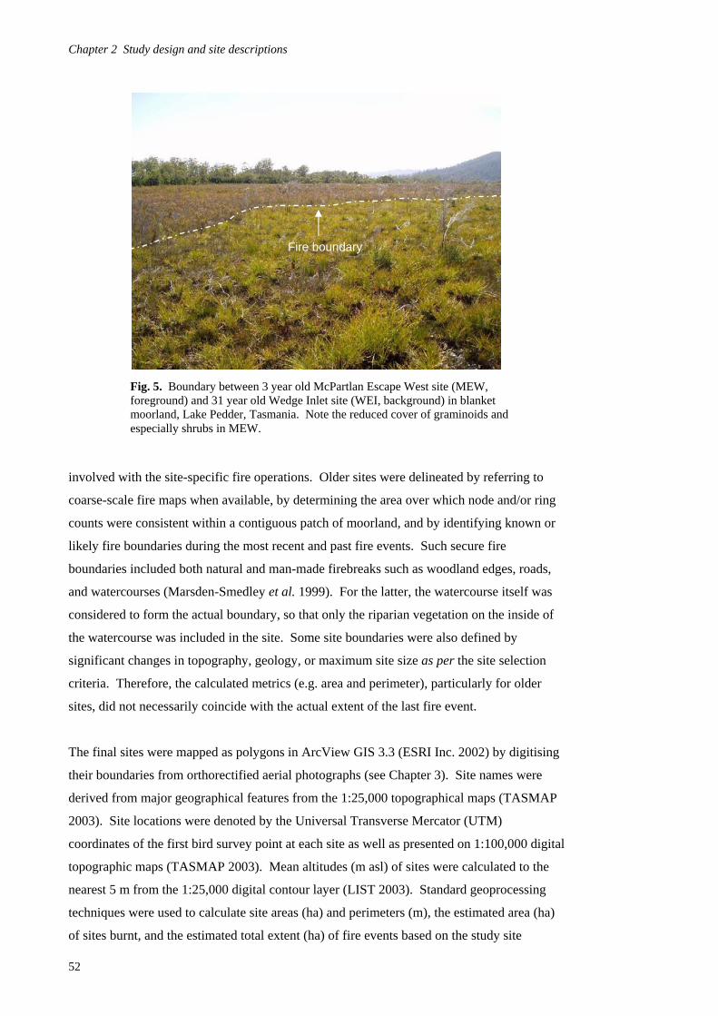
Chapter 2 Study design and site descriptions
Fire boundary
Fig. 5. Boundary between 3 year old McPartlan Escape West site (MEW, foreground) and 31 year old Wedge Inlet site (WEI, background) in blanket moorland, Lake Pedder, Tasmania. Note the reduced cover of graminoids and especially shrubs in MEW.
involved with the site-specific fire operations. Older sites were delineated by referring to
coarse-scale fire maps when available, by determining the area over which node and/or ring
counts were consistent within a contiguous patch of moorland, and by identifying known or
likely fire boundaries during the most recent and past fire events. Such secure fire
boundaries included both natural and man-made firebreaks such as woodland edges, roads,
and watercourses (Marsden-Smedley et al. 1999). For the latter, the watercourse itself was
considered to form the actual boundary, so that only the riparian vegetation on the inside of
the watercourse was included in the site. Some site boundaries were also defined by
significant changes in topography, geology, or maximum site size as per the site selection
criteria. Therefore, the calculated metrics (e.g. area and perimeter), particularly for older
sites, did not necessarily coincide with the actual extent of the last fire event.
The final sites were mapped as polygons in ArcView GIS 3.3 (ESRI Inc. 2002) by digitising
their boundaries from orthorectified aerial photographs (see Chapter 3). Site names were
derived from major geographical features from the 1:25,000 topographical maps (TASMAP
2003). Site locations were denoted by the Universal Transverse Mercator (UTM)
coordinates of the first bird survey point at each site as well as presented on 1:100,000 digital
topographic maps (TASMAP 2003). Mean altitudes (m asl) of sites were calculated to the
nearest 5 m from the 1:25,000 digital contour layer (LIST 2003). Standard geoprocessing
techniques were used to calculate site areas (ha) and perimeters (m), the estimated area (ha)
of sites burnt, and the estimated total extent (ha) of fire events based on the study site
52
Chapter 2 Study design and site descriptions
polygons and the fire polygons included in the Parks and Wildlife Service Fire History GIS
layers (PWS unpublished data; Marsden-Smedley 1998a). Fire names, dates, and ignition
sources were obtained from the PWS layers as well, except for sites that were solely aged in
this study from node and/or ring counts or from other sources. In such cases, the fire events
were named after the sites, ages were approximated to the nearest year, the estimated area of
the site burnt was assumed to be the same as the total area of the site as defined, and the
ignition sources and the total extent of these fire events were reported as unknown.
Study sites
A total of 26 sites were chosen based on the selection criteria and fire ageing data (Table 4,
Figures 6-8). The sites included 12 at Lake Pedder ranging in age from 3-54 years post-fire,
and 14 at Lake St Clair ranging from 1-44 years post-fire. These ages span the regrowth
(< 15 years), mature (15- 35 years), and old-growth (> 35 years) fire age classes identified by
Marsden-Smedley (1998a) for blanket moorlands. Classes at a finer resolution were
desirable for some of the subsequent analyses so the following eight classes were utilised
with the years since fire shown in parenthesis: 1 (1), 2 (2-3), 3 (5-8), 4 (12), 5 (14-16), 6 (22-
27), 7 (30-33), 8 (44-54). Detailed fire history data (from 1933-2005) for the study sites are
presented in Table 5. Replicate sites were identified for all fire age classes, except class 4 at
Lake Pedder, and classes 1 and 8 at Lake St Clair, due to a lack of availability. Replicates
were considered to be sites within the same fire age class that were either burnt during
different fire events (e.g. NPW and KWE) or were burnt on the same date but were spatially
separated at an appropriate scale in relation to the expected small home ranges and/or limited
dispersal capabilities of the resident species (e.g. > 2 km between MEW and MEE) (see
Chapter 1). Within a SFT context, the latter cases may be considered pseudoreplicates in the
strict sense of the term (Hurlbert 1984). However, fire events (i.e. treatments) in general are
inherently variable over space and time (Clark et al. 2002). Fire behaviour research and
personal observations confirm such spatiotemporal variability in buttongrass moorlands
(Marsden-Smedley 1993). In other words, both fire behaviour and site conditions are often
variable at relatively fine scales (i.e. metres or minutes) such that the scale of the sites (i.e.
hectares) and the separation between sites (i.e. kilometres) warranted treating them as
independent replicates.
Although data for all known fire events are presented in Table 5, fire frequencies were not
calculated due to a lack of adequate data and the inability to verify the mapping of historical
burns at the site scale. It was apparent that most sites have burnt at frequencies that are
consistent with the maintenance of moorland communities of the Southwest (Jackson 1968),
while it is assumed that this is likely the case for other sites for which no historical data were
available (e.g. SCS, SCN, TRR). However, other factors such as frost and hydrology may
53
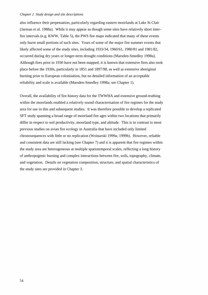
Chapter 2 Study design and site descriptions
54
also influence their perpetuation, particularly regarding eastern moorlands at Lake St Clair
(Jarman et al. 1988a). While it may appear as though some sites have relatively short inter-
fire intervals (e.g. KWW, Table 5), the PWS fire maps indicated that many of these events
only burnt small portions of such sites. Years of some of the major fire summer events that
likely affected some of the study sites, including 1933/34, 1960/61, 1980/81 and 1981/82,
occurred during dry years or longer-term drought conditions (Marsden-Smedley 1998a).
Although fires prior to 1930 have not been mapped, it is known that extensive fires also took
place before the 1930s, particularly in 1851 and 1897/98, as well as extensive aboriginal
burning prior to European colonisation, but no detailed information of an acceptable
reliability and scale is available (Marsden-Smedley 1998a; see Chapter 1).
Overall, the availability of fire history data for the TWWHA and extensive ground-truthing
within the moorlands enabled a relatively sound characterisation of fire regimes for the study
area for use in this and subsequent studies. It was therefore possible to develop a replicated
SFT study spanning a broad range of moorland fire ages within two locations that primarily
differ in respect to soil productivity, moorland type, and altitude. This is in contrast to most
previous studies on avian fire ecology in Australia that have included only limited
chronosequences with little or no replication (Woinarski 1999a; 1999b). However, reliable
and consistent data are still lacking (see Chapter 7) and it is apparent that fire regimes within
the study area are heterogeneous at multiple spatiotemporal scales, reflecting a long history
of anthropogenic burning and complex interactions between fire, soils, topography, climate,
and vegetation. Details on vegetation composition, structure, and spatial characteristics of
the study sites are provided in Chapter 3.
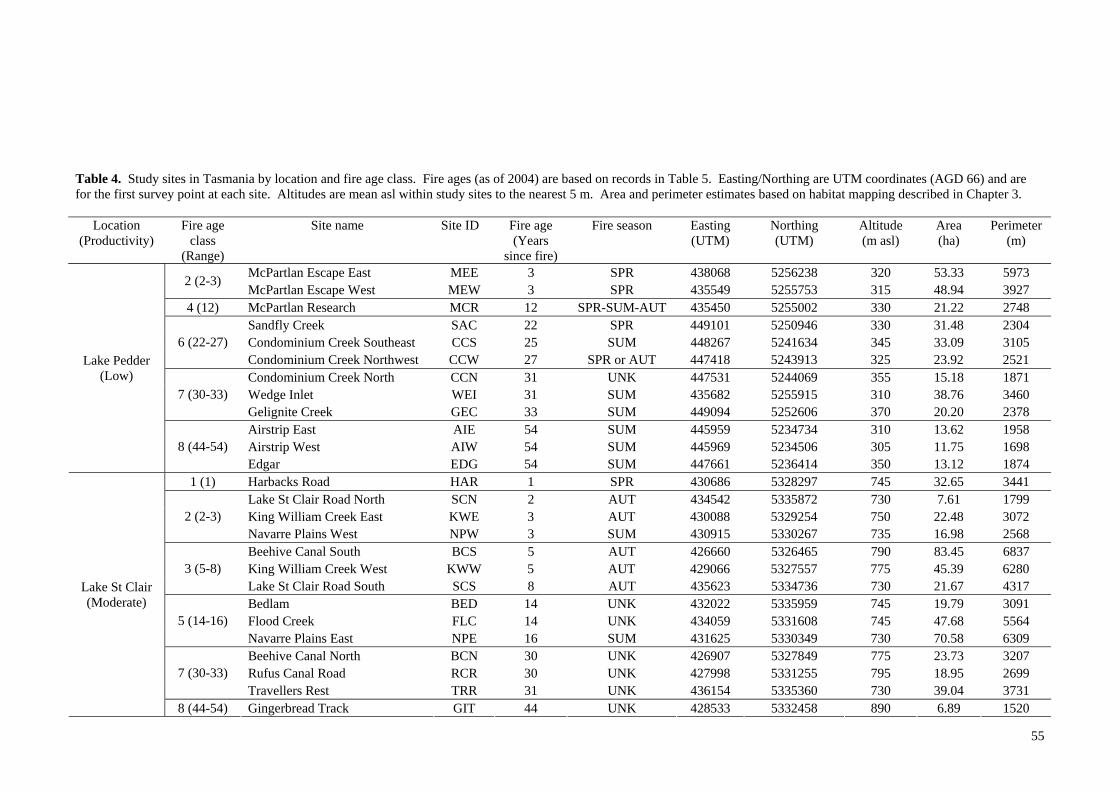
Table 4. Study sites in Tasmania by location and fire age class. Fire ages (as of 2004) are based on records in Table 5. Easting/Northing are UTM coordinates (AGD 66) and are for the first survey point at each site. Altitudes are mean asl within study sites to the nearest 5 m. Area and perimeter estimates based on habitat mapping described in Chapter 3.
Location (Productivity)
Fire age class
(Range)
Site name Site ID Fire age (Years
since fire)
Fire season Easting (UTM)
Northing (UTM)
Altitude (m asl)
Area (ha)
Perimeter (m)
McPartlan Escape East MEE 3 SPR 438068 5256238 320 53.33 5973 2 (2-3)
McPartlan Escape West MEW 3 SPR 435549 5255753 315 48.94 3927 4 (12) McPartlan Research MCR 12 SPR-SUM-AUT 435450 5255002 330 21.22 2748
Sandfly Creek SAC 22 SPR 449101 5250946 330 31.48 2304 Condominium Creek Southeast CCS 25 SUM 448267 5241634 345 33.09 3105 6 (22-27) Condominium Creek Northwest CCW 27 SPR or AUT 447418 5243913 325 23.92 2521 Condominium Creek North CCN 31 UNK 447531 5244069 355 15.18 1871 Wedge Inlet WEI 31 SUM 435682 5255915 310 38.76 3460 7 (30-33) Gelignite Creek GEC 33 SUM 449094 5252606 370 20.20 2378 Airstrip East AIE 54 SUM 445959 5234734 310 13.62 1958 Airstrip West AIW 54 SUM 445969 5234506 305 11.75 1698
Lake Pedder (Low)
8 (44-54) Edgar EDG 54 SUM 447661 5236414 350 13.12 1874
1 (1) Harbacks Road HAR 1 SPR 430686 5328297 745 32.65 3441 Lake St Clair Road North SCN 2 AUT 434542 5335872 730 7.61 1799 King William Creek East KWE 3 AUT 430088 5329254 750 22.48 3072 2 (2-3) Navarre Plains West NPW 3 SUM 430915 5330267 735 16.98 2568 Beehive Canal South BCS 5 AUT 426660 5326465 790 83.45 6837 King William Creek West KWW 5 AUT 429066 5327557 775 45.39 6280 3 (5-8) Lake St Clair Road South SCS 8 AUT 435623 5334736 730 21.67 4317 Bedlam BED 14 UNK 432022 5335959 745 19.79 3091 Flood Creek FLC 14 UNK 434059 5331608 745 47.68 5564 5 (14-16) Navarre Plains East NPE 16 SUM 431625 5330349 730 70.58 6309 Beehive Canal North BCN 30 UNK 426907 5327849 775 23.73 3207 Rufus Canal Road RCR 30 UNK 427998 5331255 795 18.95 2699 7 (30-33) Travellers Rest TRR 31 UNK 436154 5335360 730 39.04 3731
Lake St Clair (Moderate)
8 (44-54) Gingerbread Track GIT 44 UNK 428533 5332458 890 6.89 1520
55

Chapter 2 Study design and site descriptions
56
BED SCN TRR
SCS
FLC
NPWNPE
HAR
KWE
RCR
GIT
BCN
KWW
BCS
Lake St Clair
Lake King Willam
N
Fire Age Class (Years since fire)
1 (1)2 (2-3)3 (5-8)4 (12)5 (14-16)6 (22-27)7 (30-33)8 (44-54)
0 1 2 3 km
57
Fig. 6. Study sites by fire age class (as of 2004), Lake St Clair region, Tasmanian Wilderness World Heritage Area (1:100,000 Sheet #8113; AGD 66; TASMAP 2003). Note NPE and TRR were burnt by PWS in 2005 and were thus reclassified as fire age class 1 for the BACI study presented in Chapter 6.

Chapter 2 Study design and site descriptions
58
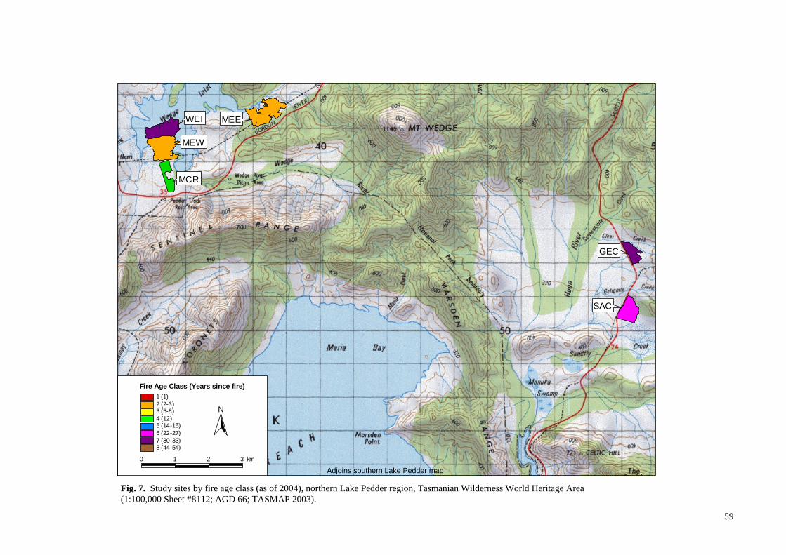
59
WEI MEE
MEW
MCR
GEC
SAC
N
Fire Age Class (Years since fire)
1 (1)2 (2-3)3 (5-8)4 (12)5 (14-16)6 (22-27)7 (30-33)8 (44-54)
0 1 2 3 km
Adjoins southern Lake Pedder map
Fig. 7. Study sites by fire age class (as of 2004), northern Lake Pedder region, Tasmanian Wilderness World Heritage Area (1:100,000 Sheet #8112; AGD 66; TASMAP 2003).

Chapter 2 Study design and site descriptions
60

61
CCW
CCN
CCS
EDG
AIW
AIE
Adjoins northern Lake Pedder map
N
Fire Age Class (Years since fire)
1 (1)2 (2-3)3 (5-8)4 (12)5 (14-16)6 (22-27)7 (30-33)8 (44-54)
0 1 2 3 km
Fig. 8. Study sites by fire age class (as of 2004), southern Lake Pedder region, Tasmanian Wilderness World Heritage Area (1:100,000 Sheets #8112/8111; AGD 66; TASMAP 2003).

Chapter 2 Study design and site descriptions
62
Table 5. Fire history records for study sites at Lake Pedder and Lake St Clair (1933-2005), Tasmania. Records are in chronological order and bold records are the most recent fire events used to define site ages for the SFT study (Chapters 4-5) and italics records are reburnt sites included in the BACI study (Chapter 6). Ignition source: PLA-Planned burn, ESC- Escaped, ARS- Arson, UNK- Unknown. Source: aThis study (based on ring/node counts and ground-truthing); bParks and Wildlife Service unpublished data; cMarsden-Smedley 1998a; dMarsden-Smedley 1993; eMarsden-Smedley 1990; fParks and Wildlife Service 1996; gDriessen and Greenslade 2004; hBalmer and Barnes 2000; iGellie 1980; jForestry Tasmania unpublished data.
Lake Pedder
Site ID
Fire name Date (dd/mm/yr or
est. yr)
Ignition source
Est. area (ha) of site
burnt
Est. area (ha) of fire event
Source
MEE Wedge Inlet 11/10/2001 ESC 53.34 666.54 a,b,c
Airstrip Road research burns 27/10/1992-16/11/1992
PLA 4.90 4.90 b,c,d
Lake Gordon (Starfish fire) 1972/73 UNK 52.71 30537.30 b,c
1933/34 fire 1933/34 UNK 52.10 573187.70 b,c
MEW Wedge Inlet 11/10/2001 ESC 48.94 666.54 a,b,c
Lake Gordon (Starfish fire) 1972/73 UNK 48.94 30537.30 b,c
1933/34 fire 1933/34 UNK 48.94 573187.70 b,c
MCR McPartlan Pass research burns 28/10/1991- 14/11/1992
PLA 21.22 21.22 a,d
Lake Gordon (Starfish fire) 1972/73 UNK 21.22 30537.30 b,c
1933/34 fire 1933/34 UNK 21.22 573187.70 b,c
SAC Sandfly Creek 9/1982 PLA 31.48 222.12 a,b,c
Upper Huon River 1/11/1971 PLA 31.48 2374.71 b,c
Sandfly Creek 16/12/1970 PLA 18.89 259.25 b,c
Lake Pedder 1950 UNK 31.48 27112.40 b,c
1933/34 fire 1933/34 UNK 31.48 573187.70 b,c
CCS Harlequin Hill 1978/79 UNK 33.06 673.40 a,b,c
Lake Pedder 1950 UNK 33.06 27112.40 b,c
1933/34 fire 1933/34 UNK 33.06 573187.70 b,c
CCW Harlequin Hill 1978/79 UNK 1.75 673.40 b,c
Condominium Creek 1977 PLA 23.92 135.16 a,b,c,i
Lake Pedder 1950 UNK 23.92 27112.40 b,c
1933/34 fire 1933/34 UNK 23.92 573187.70 b,c
CCN Harlequin Hill 1978/79 UNK 0.92 673.40 b,c
Condominium Creek 1977 PLA 2.00 135.16 b,c
Celtic Hill 24/06/1975 PLA 0.24 140.09 b,c
Condominium Creek North 1972/73 UNK 15.18 UNK a,b,c
Lake Pedder 1950 UNK 13.28 27112.40 b,c
1933/34 fire 1933/34 UNK 13.12 573187.70 b,c
WEI Lake Gordon (Starfish fire) 1972/73 UNK 38.77 30537.30 a,b,c
1933/34 fire 1933/34 UNK 38.77 573187.70 b,c
GEC Upper Huon River 1/11/1971 PLA 20.20 2374.71 a,e
Lake Pedder 1950 UNK 20.20 27112.40 b,c
1933/34 fire 1933/34 UNK 20.20 573187.70 b,c
AIE Edgar Pond 1971/72 UNK UNK 52.00 a,b,c
Lake Pedder 1950 UNK 13.62 27112.40 a,b,c
1933/34 fire 1933/34 UNK 13.62 573187.70 b,c
AIW Edgar Pond 1971/72 UNK 1.12 52.00 b,c
Lake Pedder 1950 UNK 11.75 27112.40 a,b,c
1933/34 fire 1933/34 UNK 11.75 573187.70 b,c
EDG Lake Pedder 1950 UNK 13.12 27112.40 a,b,c
1933/34 fire 1933/34 UNK 13.12 573187.70 b,c

Chapter 2 Study design and site descriptions
63
Table 5. cont.
Lake St Clair
Site ID Fire name Date (dd/mm/yr or est. yr)
Ignition source
Est. area (ha) of site
burnt
Est. area (ha) of fire event
Source
HAR Harbacks Road 14/10/2003 PLA 32.65 115.25 a,b,c
King William Plains 10/12/1989 ARS 4.71 94.86 b,c King William Plains 1979 UNK 5.12 2773.00 b,c
1933/34 fire 1933/34 UNK 32.65 573187.70 b,c
SCN Lake St Clair Road North 30/4/2002 PLA 7.61 7.61 b
KWE King William Creek 4/5/2001 PLA 22.48 22.48 b,c
King William Creek 1987 PLA 22.48 22.48 b,c
King William Plains 1979 UNK 13.87 2773.00 b,c
King William Creek 1977/78 UNK 0.09 11.30 b,c
1933/34 fire 1933/34 UNK 22.48 573187.70 b,c
NPW Lyell Hwy/Rufus Canal Road 5/2/2001 ARS 16.98 19.93 b,c
Little Navarre River 12/1/1997 UNK 0.20 462.71 b,c
Coates Creek 12/11/1988 UNK 16.98 152.82 b,c
1933/34 fire 1933/34 UNK 16.98 573187.70 b,c
BCS Beehive Canal 12/4/1999 PLA 83.45 313.00 b,c
Beehive Canal 1987 PLA 83.45 231.42 b,c
King William Plains 1979 UNK UNK 2773.00 b,c
1933/34 fire 1933/34 UNK 83.45 573187.70 b,c
KWW King William Creek 17/4/1999 PLA 44.64 44.64 b,h
Beehive Canal 4/1/1999 PLA 2.32 231.42 b,c
Beehive Canal 1987 PLA 45.39 146.00 f
King William Creek 9/3/1984 ARS 16.42 66.17 b,c,h
King William Plains 1979 UNK 42.88 2773.00 b,c
King William Creek 1977/78 UNK 11.46 176.40 b,c
1933/34 fire 1933/34 UNK 45.39 573187.70 b,c
SCS Lake St Clair Road South 26/9/1995- 4/5/1996
PLA 21.67 21.67 a,b
BED Bedlam 1990 UNK 19.79 UNK a
1933/34 fire 1933/34 UNK 19.79 573187.70 b,c
FLC Little Navarre River 1989/1990 UNK 47.68 UNK a,b,j
Coates Creek 1980 UNK 10.36 63.49 b,c
1933/34 fire 1933/34 UNK 41.49 573187.70 b,c
NPE Navarre Plains 9/21/2005 PLA 66.15 611.79 a,b
Little Navarre River 12/1/1997 UNK 0.50 462.71 b,c
Coates Creek 12/11/1988 UNK 70.58 152.82 a,b,c
1933/34 fire 1933/34 UNK 70.58 573187.70 b,c
BCN King William Saddle 1974 UNK 23.72 2773.00 a,b,c
1933/34 fire 1933/34 UNK 23.72 573187.70 b,c
RCR Rufus Canal Road 1974 UNK 18.95 UNK a,g
1933/34 fire 1933/34 UNK 18.13 573187.70 b,c
TRR Travellers Rest 4/21/2005 PLA 36.20 41.97 a,b
Travellers Rest 1973 UNK 39.04 UNK a
GIT Gingerbread Track 1960 UNK 6.89 UNK a

64
Chapter 3
Avian habitat mapping in buttongrass moorlands and an accuracy
assessment of the Tasmanian Wilderness World Heritage Area
Vegetation Mapping
Introduction The characteristic biotic and abiotic features of the environment in which a given species
lives define its habitat, and provide the proximate or ultimate resources required for survival
and reproduction. For birds in particular, it has long been recognised that both vegetation
structure (e.g. MacArthur 1958) and floristics (e.g. Rotenberry 1985) can play critical roles
in determining the composition and relative abundance of communities. This recognition
has guided much of the research on avian habitat relationships to date (for reviews see
Hildén 1965; Block and Brennan 1993; Jones 2001). The relative importance of vegetation
structure and floristics on avian communities has been the focus of much debate; however,
results may ultimately be dependent upon both the temporal and spatial scales at which a
given system is being studied (Wiens et al. 1987; Mac Nally 1990; Collins 2001).
Furthermore, it is important to recognise that habitat selection is a hierarchical process, such
that birds select habitat at scales ranging from the geographic or home range (i.e.
macrohabitat) to specific elements within their home range (i.e. microhabitat) (Hildén 1965;
Johnson 1980; Block and Brennan 1993). To determine actual preference for a particular
habitat, it is necessary to quantify both the relative usage (i.e. quantity utilised) and
spatiotemporal availability (i.e. accessibility) of habitats at the relevant scales of interest
(sensu Johnson 1980; see Chapter 5). Thus the objectives, design, and subsequent
conclusions of a study are not only contingent upon what variables are measured, but also on
the scales those measurements are made in relation to those of the underlying processes.
Relatively few studies to date, including those conducted on the Australian mainland, have
focused on the habitat relationships of the resident bird species found in Tasmanian
moorlands, namely the Southern Emu-wren, Striated Fieldwren, and Ground Parrot (see
Chapter 1). These studies have primarily centered on defining the microhabitat of these
species by identifying environmental features (e.g. vegetation floristics and structure) that
were used to meet (at least proximally) their resource needs. These studies typically
consisted of qualitative assessments of occupied habitat (e.g. Fletcher 1913a; Gosper and
Baker 1997) or quantitative vegetation surveys (e.g. Bryant 1991; McFarland 1991a). The
baseline information obtained from these studies is critical to understand the ecology of these
species. However, considering their methods, study locations, and scale, this information
65

Chapter 3 Avian habitat mapping cannot be readily applied to studies such as the present one that investigates the influence of
spatial heterogeneity and the underlying landscape-scale processes (e.g. fire regimes) on
avian communities. Since conservation and fire management decisions are increasingly
being made at the ecosystem level in the TWWHA (e.g. PWS 1999; Marsden-Smedley and
Kirkpatrick 2000), it is imperative to provide information to land managers on avian habitat
relationships that are location-specific and at a commensurate scale.
One way to bridge the gap between fine-scale, microhabitat and coarse-scale, macrohabitat
characterisations is to utilise remote sensing and geographic information systems (GIS) to
develop a habitat map. Although any map is essentially an imperfect model of reality
(Foody 2002), maps are spatially continuous and thus may be used to provide a more
comprehensive description of the environment than the sample-based vegetation surveys
described above. These technologies also allow for vegetation mapping to be conducted,
analysed, and displayed at varying spatial scales, and are increasingly relied upon in both
bird conservation (e.g. Buchanan et al. 2005) and fire management (e.g. Bobbe et al. 2001).
These methods are particularly powerful when used in conjunction with field-based avian
surveys since they provide a means of quantifying the relationships between birds and the
spatial heterogeneity of their habitats (i.e. composition, structure, spatial configuration)
(McGarigal and McComb 1995; Li and Reynolds 1995; Fuller et al. 2005). Provided that
both bird abundance and habitat usage data are collected, and mapping is at a fine enough
scale and of an acceptable accuracy, it is possible to gain a more holistic understanding of
avian habitat relationships and their underlying processes. These relationships can then
potentially be extrapolated to even larger scales, which is a critical step towards
understanding and managing natural systems (Bibby et al. 2000).
Despite the increasing use of remote sensing and GIS technologies reported in the wildlife
literature, a review by Glenn and Ripple (2004) revealed that most papers failed to report
important information regarding the digital maps that were used to assess wildlife habitat.
For example, 23% of studies (n = 44) did not cite their map data sources; 55% did not
specify the map scale, pixel size, or minimal mapping unit; 80% did not report map
accuracy; and 27% utilised ‘off-the-shelf’ map products developed by other parties. Without
adequate documentation it is difficult to interpret and assess the results of such studies,
particularly as they pertain to determining habitat use and selection.
To avoid potential biases associated with the unquestioning use of an existing map product
as the sole basis for classifying and quantifying vegetation within the study area, it was
considered desirable to assess the accuracy of the existing Tasmanian Wilderness World
Heritage Area Vegetation Mapping (hereafter WHAveg) (TVMP 2004) in relation to the
66
Chapter 3 Avian habitat mapping
overall aims of this study. A brief overview of WHAveg is presented below, while a formal
accuracy assessment is described herein.
WHAveg is a relatively coarse-scale, remote sensing, and polygon-based vegetation
classification and mapping project covering the 1.38 million ha of the TWWHA (as
compared to the less than 800 ha covered by this study) and was intended to provide detailed
regional information on vegetation communities for natural resource management and
research (ILS 2004; TVMP 2004). The WHAveg mapping methodology and classification
system has changed over time and across different locations within the TWWHA. The
following description is based on the metadata for WHAveg provided in the Tasmanian
Spatial Data Directory (ILS 2004; TVMP 2004). A complete 1:25,000 colour run of aerial
photographs was taken in 1988 on which most of the vegetation mapping has been based.
Prior to 2000, a more complex synusia-based (i.e. associations of distinct strata; n = 534)
classification scheme was used largely in the eastern TWWHA (including most of the study
area). Aerial photographs were interpreted and the different vegetation communities were
delineated with a grease pen onto transparencies overlain on each photograph. The resulting
vegetation class polygons were ocularly transferred onto topographic base maps, scanned,
imported into GenaMap GIS (Genaware Pty. Ltd. 1995), and labelled. This process included
extensive field verification. After 2000, a simpler community-based classification scheme
(i.e. vegetation types; n = 55) was developed for the more remote western TWWHA. The
photographic interpretation was similar to the above method; however, vegetation
communities were delineated with a fine marker onto transparencies. The resulting
vegetation polygons were then scanned and orthorectified using proprietary photogrammetry
PhotoFactory software (SonarData Pty. Ltd. 2005), including a Triangulated Interlaced
Network Elevation Model, and then imported into GenaMap. These have subsequently been
converted to shapefiles and stored in ArcView 9.0 (ESRI Inc. 2002). Only limited field
verification has been conducted. Accordingly, attribute accuracy reported in the metadata is
considered to be variable (and has not been quantified to date), with higher accuracy
assumed to be in areas classified under the former scheme. Positional accuracy is
qualitatively estimated at 50 m; however, the latter method is considered to be relatively
more accurate.
To make these different classification systems compatible across the TWWHA, a set of new,
mutually exclusive amalgamated classification codes was developed and is used as the base
for the classification used herein (TVMP 2004). As with many maps, it should be noted that
this system uses broad vegetation classes that represent communities that can be floristically
and structurally variable even within a given vegetation patch (Jarman and Crowden 1978).
For example, some copse communities were originally classified and delineated separately in
67

Chapter 3 Avian habitat mapping the synusia-based classification scheme, but were subsequently amalgamated into their
surrounding polygons and associated classes. Considering such simplifications inherent in
any coarse-scale map product, WHAveg and its derivatives should be interpreted with some
caution. After an initial assessment of the WHAveg GIS layer, it was obvious that
significant delineation, classification, and registration errors existed and that the scale of
mapping and level of classification would not entirely meet the needs of this study. For
example, polygons representing the various vegetation classes were often offset and
simplified (i.e. smoothed) so that the area covered by a given polygon and the shape of its
boundaries with adjacent polygons did not accurately reflect the boundaries on the
orthorectified aerial photographs or those known to exist on the ground. In addition, features
such as copses and riparian vegetation zones were not typically mapped since they were not
considered part of their overall mapping objectives, were not readily identified from the
aerial photos, or were below the minimal mapping unit (~ 0.5 ha within the study area).
Accordingly, a formal accuracy assessment was conducted on WHAveg, which to the
knowledge of the author is the first of its kind since neither the Tasmanian Vegetation
Mapping and Monitoring Program (BCB) nor any end users have conducted a formal
assessment to date. Knowing the potential limitations of the acquired layers a priori, it was
also deemed necessary to delineate site boundaries and habitat features at a finer scale and
greater resolution so that subsequent quantification of the habitat metrics would be more
inclusive, accurate (> 85% attribute accuracy; Congalton and Green 1999), and appropriate
for the aims of this study. Finally, it should be noted that this study was completed before
the recent publication of the State-wide TASVEG Version 2.0 mapping scheme that was, in
part, derived from the WHAveg mapping (TVMMP 2009). Consequently, the TASVEG
communities and associated codes are not explicitly referenced herein.
The primary aims of this study were: 1) to develop a fine-scale and high-resolution classified
avian habitat map for buttongrass moorlands and associated vegetation communities using
remote sensing and GIS techniques; 2) to perform an accuracy assessment of WHAveg
within the study area; 3) to quantify the composition, structure, and spatial characteristics of
avian habitat for use in the analyses presented in Chapters 4-6; and 4) to provide a
foundation for the potential future development of landscape-scale bird-habitat prediction
models in buttongrass moorlands.
68
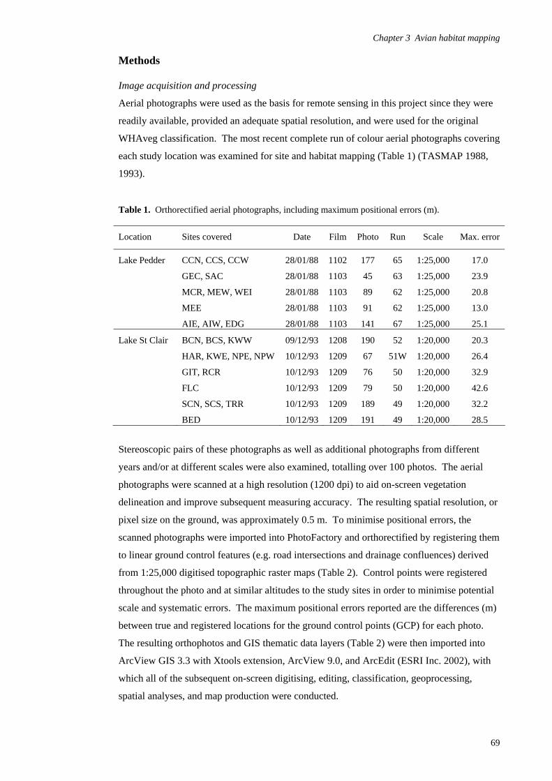
Chapter 3 Avian habitat mapping
Methods Image acquisition and processing
Aerial photographs were used as the basis for remote sensing in this project since they were
readily available, provided an adequate spatial resolution, and were used for the original
WHAveg classification. The most recent complete run of colour aerial photographs covering
each study location was examined for site and habitat mapping (Table 1) (TASMAP 1988,
1993).
Table 1. Orthorectified aerial photographs, including maximum positional errors (m).
Location Sites covered Date Film Photo Run Scale Max. error
Lake Pedder CCN, CCS, CCW 28/01/88 1102 177 65 1:25,000 17.0
GEC, SAC 28/01/88 1103 45 63 1:25,000 23.9
MCR, MEW, WEI 28/01/88 1103 89 62 1:25,000 20.8
MEE 28/01/88 1103 91 62 1:25,000 13.0
AIE, AIW, EDG 28/01/88 1103 141 67 1:25,000 25.1
Lake St Clair BCN, BCS, KWW 09/12/93 1208 190 52 1:20,000 20.3
HAR, KWE, NPE, NPW 10/12/93 1209 67 51W 1:20,000 26.4
GIT, RCR 10/12/93 1209 76 50 1:20,000 32.9
FLC 10/12/93 1209 79 50 1:20,000 42.6
SCN, SCS, TRR 10/12/93 1209 189 49 1:20,000 32.2
BED 10/12/93 1209 191 49 1:20,000 28.5
Stereoscopic pairs of these photographs as well as additional photographs from different
years and/or at different scales were also examined, totalling over 100 photos. The aerial
photographs were scanned at a high resolution (1200 dpi) to aid on-screen vegetation
delineation and improve subsequent measuring accuracy. The resulting spatial resolution, or
pixel size on the ground, was approximately 0.5 m. To minimise positional errors, the
scanned photographs were imported into PhotoFactory and orthorectified by registering them
to linear ground control features (e.g. road intersections and drainage confluences) derived
from 1:25,000 digitised topographic raster maps (Table 2). Control points were registered
throughout the photo and at similar altitudes to the study sites in order to minimise potential
scale and systematic errors. The maximum positional errors reported are the differences (m)
between true and registered locations for the ground control points (GCP) for each photo.
The resulting orthophotos and GIS thematic data layers (Table 2) were then imported into
ArcView GIS 3.3 with Xtools extension, ArcView 9.0, and ArcEdit (ESRI Inc. 2002), with
which all of the subsequent on-screen digitising, editing, classification, geoprocessing,
spatial analyses, and map production were conducted.
69
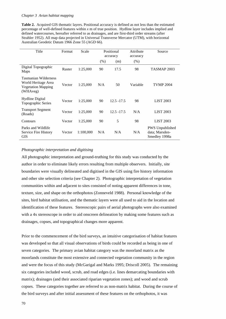
Chapter 3 Avian habitat mapping Table 2. Acquired GIS thematic layers. Positional accuracy is defined as not less than the estimated percentage of well-defined features within x m of true position. Hydline layer includes implied and defined watercourses, hereafter referred to as drainages, and are first-third order streams (after Strahler 1952). All map data projected in Universal Transverse Mercator (UTM), with horizontal Australian Geodetic Datum 1966 Zone 55 (AGD 66).
Format Scale Positional accuracy
Source Title
(%) (m)
Attribute accuracy
(%)
Digital Topographic Maps
Raster 1:25,000 90 17.5 98 TASMAP 2003
Tasmanian Wilderness World Heritage Area Vegetation Mapping (WHAveg)
Vector 1:25,000 N/A 50 Variable TVMP 2004
Hydline Digital Topographic Series
Vector 1:25,000 90 12.5 -17.5 98 LIST 2003
Transport Segment (Roads)
Vector 1:25,000 90 12.5 -17.5 N/A LIST 2003
Contours Vector 1:25,000 90 5 98 LIST 2003
Parks and Wildlife Service Fire History GIS
Vector 1:100,000 N/A N/A N/A PWS Unpublished data; Marsden-Smedley 1998a
Photographic interpretation and digitising
All photographic interpretation and ground-truthing for this study was conducted by the
author in order to eliminate likely errors resulting from multiple observers. Initially, site
boundaries were visually delineated and digitised in the GIS using fire history information
and other site selection criteria (see Chapter 2). Photographic interpretation of vegetation
communities within and adjacent to sites consisted of noting apparent differences in tone,
texture, size, and shape on the orthophotos (Zonneveld 1988). Personal knowledge of the
sites, bird habitat utilisation, and the thematic layers were all used to aid in the location and
identification of these features. Stereoscopic pairs of aerial photographs were also examined
with a 4x stereoscope in order to aid onscreen delineation by making some features such as
drainages, copses, and topographical changes more apparent.
Prior to the commencement of the bird surveys, an intuitive categorisation of habitat features
was developed so that all visual observations of birds could be recorded as being in one of
seven categories. The primary avian habitat category was the moorland matrix as the
moorlands constitute the most extensive and connected vegetation community in the region
and were the focus of this study (McGarigal and Marks 1995; Driscoll 2005). The remaining
six categories included wood, scrub, and road edges (i.e. lines demarcating boundaries with
matrix); drainages (and their associated riparian vegetation zones); and wood and scrub
copses. These categories together are referred to as non-matrix habitat. During the course of
the bird surveys and after initial assessment of these features on the orthophotos, it was
70

Chapter 3 Avian habitat mapping
apparent that the vegetation within the sites and along these edges was often ecotonal in
nature (after Risser 1993). This observation is consistent with that reported in the literature
(Jarman and Crowden 1978; Balmer 1990). Thus, in some areas floristics and structure were
highly variable, even within a relatively fine spatial scale (i.e. metres). For example,
although some scrub copses could be identified on the orthophotos and clearly delineated on
the ground, others graded almost imperceptibly into the surrounding matrix. Such variability
within and ‘fuzzy’ boundaries (Bobbe et al. 2001) between vegetation types was difficult to
define on the ground and even more difficult to delineate on the orthophotos. Any attempt to
consistently and accurately delineate such features across all study sites would have
necessitated a rigorous and resource-intensive classification, mapping, and assessment
system. Also, in consideration of the large area that would have to be surveyed, it was
determined that such an endeavour was beyond the scope of this study. Therefore, the final
mapping was based on the four structurally and floristically distinct avian habitat categories,
namely the matrix, riparian zones, wood copses, and edges (Figures 1-3); each of which was
composed of similar vegetation classes as described below and summarised in Tables 4, 6,
and 7.
Vectorised thematic layers were created for each habitat category based on the rasterised
orthophotos- polylines for drainage and edge classes, and polygons for the wood copse and
matrix classes. Each site was thoroughly examined for these features and was viewed at
varying scales in order to locate and identify site boundaries and other habitat features. Most
features were delineated and digitised on-screen at a consistent scale (~ 1:2,000) to ensure
comparability between sites. The minimum mapping unit for polygons was 0.02 ha, which
was small enough to produce a detailed map of the study area and large enough to
distinguish most significant habitat features both on the orthophotos and on the ground. It
should be noted that many sites contained scattered trees, but these were only mapped as
wood copses if they contained discrete clusters of trees ≥ 0.02 ha and were structurally and
floristically distinct from the surrounding matrix vegetation. The acquired drainage layer
was used as a base for drainages and associated riparian zones; however, some drainage
segments were either modified or added if indicated by prior site knowledge and the
photographic interpretation. In some cases, sites were adjacent to large drainages channels;
however, the actual vegetation bordering the site was often more characteristic of woodland
than riparian communities (typically when the distance between the site boundary and the
drainage itself was > 25 m). In these cases, the edge habitat was delineated and classified
accordingly.
71

Chapter 3 Avian habitat mapping
Fig. 1. Riparian zone through eastern moorland matrix habitat (approx. drainage centerline as marked); Beehive Canal North (BCN; 30 years post-fire), Lake St Clair, Tasmania.
Fig. 2. Woodland edge formed with eastern moorland matrix habitat; Flood Creek (FLC; 14 years post-fire), Lake St Clair, Tasmania.
72
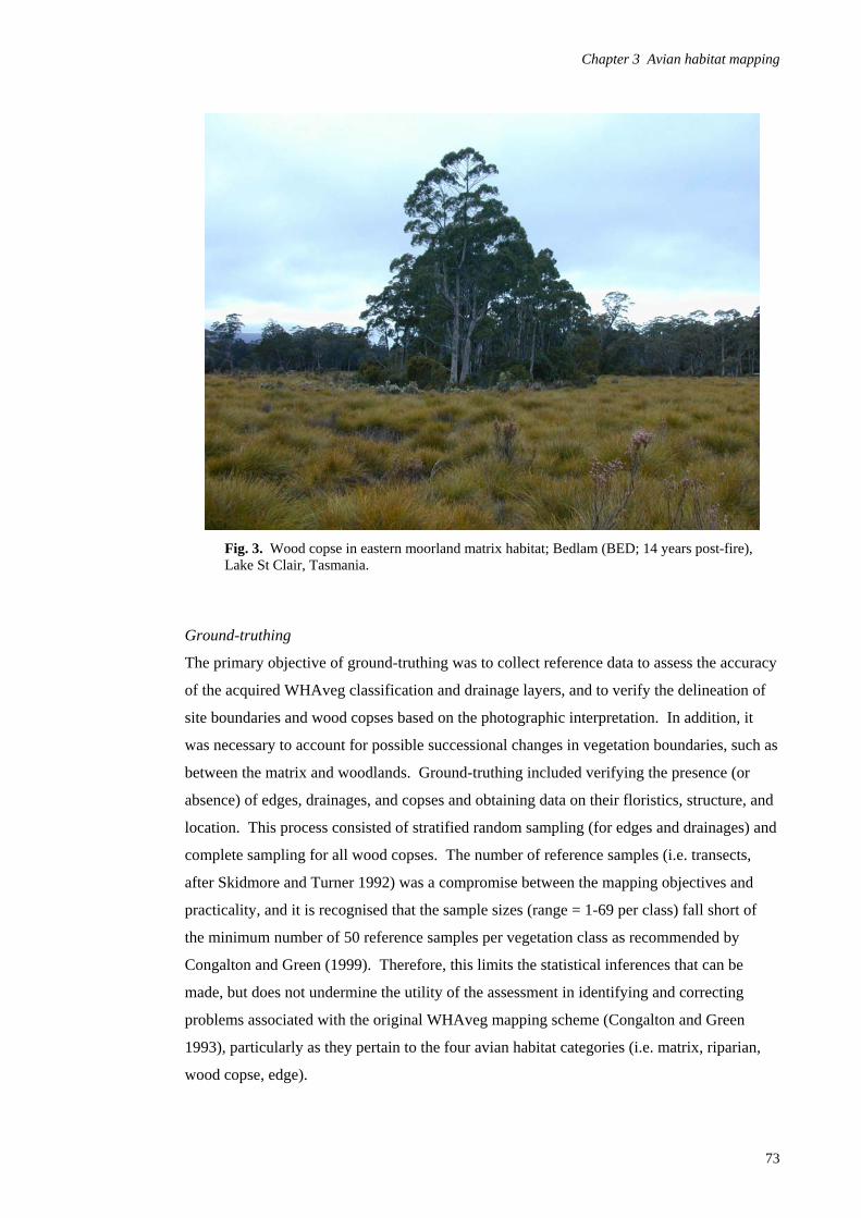
Chapter 3 Avian habitat mapping
Fig. 3. Wood copse in eastern moorland matrix habitat; Bedlam (BED; 14 years post-fire), Lake St Clair, Tasmania.
Ground-truthing
The primary objective of ground-truthing was to collect reference data to assess the accuracy
of the acquired WHAveg classification and drainage layers, and to verify the delineation of
site boundaries and wood copses based on the photographic interpretation. In addition, it
was necessary to account for possible successional changes in vegetation boundaries, such as
between the matrix and woodlands. Ground-truthing included verifying the presence (or
absence) of edges, drainages, and copses and obtaining data on their floristics, structure, and
location. This process consisted of stratified random sampling (for edges and drainages) and
complete sampling for all wood copses. The number of reference samples (i.e. transects,
after Skidmore and Turner 1992) was a compromise between the mapping objectives and
practicality, and it is recognised that the sample sizes (range = 1-69 per class) fall short of
the minimum number of 50 reference samples per vegetation class as recommended by
Congalton and Green (1999). Therefore, this limits the statistical inferences that can be
made, but does not undermine the utility of the assessment in identifying and correcting
problems associated with the original WHAveg mapping scheme (Congalton and Green
1993), particularly as they pertain to the four avian habitat categories (i.e. matrix, riparian,
wood copse, edge).
73

Chapter 3 Avian habitat mapping Ground-truthing was conducted March-April 2005. Sampling locations were determined by
one of the following methods for each site and were based off of the randomised bird survey
transects (see Chapter 4) to help reduce potential biases (e.g. autocorrelation between sample
locations; Congalton and Green 1999). For edges, the sampling location was the intersection
of closest approach from three randomly selected points at the ends of the transects for each
site (n = 222); for drainages, it was the intersection of riparian vegetation by the transects (n
= 79); and for wood copses (n = 33), it was the intersection of closest approach from the
nearest point along an adjacent transect. At each location a 20 m transect (or longer in the
case of wider riparian zones) was then walked perpendicular to the vegetation boundary,
such that vegetation in one matrix and one non-matrix polygon were both assessed along
approximately 10 m. The actual boundaries between the matrix and non-matrix vegetation
were primarily determined by apparent changes in vegetation floristics, structure, and
hydrology. The average height of the tallest non-tree stratum was estimated, since no bird
observations in the primary tree canopy were recorded for this study (see Chapters 4-6).
Heights were measured and assigned to one of four classes (< 1, 1-2, 2-3, 3-4 m). Floristics
were formally evaluated along the transect (and informally at the polygon/line scale) to
determine whether they were consistent with the classification codes assigned on the
WHAveg map. If the vegetation differed from, or was not included in, the original WHAveg
classification (i.e. drainages and wood copses), structurally- and/or cover-dominant species
that differentiated these habitats from the matrix were recorded. A GPS (Garmin eTrex, 12
parallel channels, accuracy ± 15 m) was used to record the UTM coordinates of the
intersection between the vegetation transect and the habitat boundary. The width of riparian
vegetation and the approximate dimensions of wood copses were measured in metres with a
laser rangefinder (Leica LRF 800 Rangemaster, accuracy ± 1 m, range 10-800 m) or
estimated by pacing (if < 10 m). In some cases features such as drainages or wood copses
were identified on the ground but were not mapped, or features such as wood edges were of a
different shape and/or location than indicated by the orthophoto map or WHAveg layer. In
these cases, the features were either sampled using the above method or were qualitatively
assessed and notes were taken accordingly. This was done to ensure that errors of
commission and/or omission were minimised at the polygon/line scale, and that the final
map would accurately represent features on the ground.
An index of vegetation cover (i.e. density) in matrix habitat was collected for all sites (except
AIW and GIT) as part of a collaborative SFT research project on terrestrial invertebrates
conducted by the BCB (M. Driessen unpublished data). Cover values were based on ocular
estimates of the number of 5 cm2 squares (out of 200) covered by vegetation on a gridded
site board (50 x 100 cm), as outlined in Driessen (1999), and mean values for each site (n =
7) were used in subsequent analyses. It is important to note that since sampling was limited
74

Chapter 3 Avian habitat mapping
to a relatively small area (~ 0.5 ha) of each site, the cover values may not accurately reflect
overall cover across each site.
Vegetation structure analyses
Vegetation height and overall sample sizes were small for many of the separate vegetation
classes as well as the wood copse avian habitat category largely due to a lack of availability;
therefore, those with similar structure and floristics were pooled into one of three habitat
categories (i.e. matrix, riparian zone, edge) for all subsequent analyses. The mean height (m
± SE) of vegetation (excluding mature tree species) for each habitat type was calculated by
using the mid-point values of each height class (0.5, 1.5, 2.5, 3.5 m). SPSS 14.0 statistical
software (SPSS Inc. 2005) was used to conduct a non-parametric Kruskal-Wallis test to
determine whether there were significant differences between mean height class ranks for all
habitat categories both within and between Lake Pedder and Lake St Clair. Mann-Whitney
U post hoc tests with Bonferroni adjusted P-values were used to identify any significant
differences between categories within each study location. The mean width (m ± SE) of
riparian zones for both locations was also calculated, and used to determine the width of
cartographic buffers applied to the drainage polylines in order to construct riparian zone
polygons and proportional area estimates used in the following GIS spatial analyses.
Regression was used to determine if there were significant relationships between the mean
index of vegetation cover for each site and fire age at Lake Pedder and Lake St Clair. An
initial examination of scatterplots as well as previous research modelling cover and fuel
loading in relation to fire age (Marsden-Smedley and Catchpole 1995b) indicated that there
was a curvilinear relationship between cover and fire age. Therefore, curve estimation
regression in SPSS 14.0 (SPSS Inc. 2005) was used to test the fit of alternative models. The
final regression was based on an S-curve model which provided a plausible fit since the
regression curve passed through the origin at zero years post-fire and plateaued at older sites,
as predicted based on previous research (see Chapter 1). Model adequacy regarding the
assumptions of normality and homogeneity of variance was checked by inspection of
residual plots, which did not indicate obvious issues with the models.
Vegetation composition and classification
The results of the ground-truthing were used to revise and update the original WHAveg
classification so that it more accurately reflected avian habitat used within the study area.
Since vegetation class descriptions have yet to be defined for all of the new amalgamated
WHAveg classification codes (S. Corbett pers. comm. 2005), a range of sources were used
as the basis for the class descriptions (Jarman et al.1988a; Marsden-Smedley 1993; Driessen
1999; Barnes and Balmer 2000; Balmer and Barnes 2000; Harris and Kitchener 2004; TVMP
75
Chapter 3 Avian habitat mapping 2004). It was apparent from the reference data that the flora within the study area differed
from some of these class descriptions in terms of both presence, absence, and dominance
(structural or cover). Therefore, the reference data were queried in order to identify
characteristic species and the class descriptions were modified accordingly. Since most
riparian vegetation and wood copses were not mapped as such in WHAveg, the reference
data formed the primary basis for these descriptions, with the recognition that these
communities shared similarities with some of those described under the various WHAveg
classification schemes, as well as by Jarman et al. (1988a).
The final classification codes and list of characteristic species identified during ground-
truthing were intended to provide a qualitative description of the overall composition and
structure of these communities (e.g. sedgeland/heathland vs. woodland), and are not
comprehensive species lists derived from rigorous floristic sampling methods. Therefore,
these descriptions should be considered accordingly and within the context of this study. A
more definitive classification system for buttongrass moorland communities was developed
by Jarman et al. (1988a) (see Chapter 1) and their comparable classifications are referenced
as appropriate herein.
Accuracy assessment
Although there is continuing debate in the remote sensing literature regarding the appropriate
methods for conducting an accuracy assessment and presentation of its results, the generation
of an error matrix and associated analyses are generally accepted as the standard approach
(Foody 2002). Therefore, an accuracy assessment as described by Congalton and Green
(1999) was conducted in order to increase the quality of the final habitat map by identifying
and correcting WHAveg mapping errors. This was accomplished by comparing the remotely
sensed WHAveg classification and habitat delineations with the reference data that were
collected during the ground-truthing survey, which are theoretically 100% accurate. A total
of 334 reference samples was collected and used for the WHAveg error assessment. The
UTM coordinates for the reference samples were mapped in the GIS and used to identify
each sample transect and vegetation boundary on the orthophotos. In conjunction with the
transect data, these were used to reveal any discrepancies in the classification and shape of
WHAveg polygons as compared to those communities and habitat features identified on the
ground.
Results of this assessment were recorded in an error (or ‘confusion’) matrix (after Congalton
and Green 1993) which shows the number of polygons assigned to a specific class in the
WHAveg classification relative to that determined by the reference dataset (n = 222). The
diagonal values show when the two classifications are in agreement. This probability, or
76

Chapter 3 Avian habitat mapping
overall accuracy (%), was calculated by dividing the sum of these values by the total number
of reference polygons. The off-diagonal values show errors of omission or commission by
the WHAveg classification. Accordingly, the producer’s accuracy is the probability of a
reference polygon being correctly classified as such on the map, measuring omission errors;
and conversely, the user’s accuracy is the probability of a classified polygon being confirmed
as such on the ground, measuring commission errors. A separate accuracy assessment was
conducted for the wood copses and riparian zones since these were not classified as such in
WHAveg. The 33 wood copses were assessed as to whether they were classified as or within
woodland polygons in the WHAveg layer, and the 79 drainages as to whether they were
included as polylines in the drainage layer.
The values from the error matrix were used to perform a Kappa analysis in program KAPPA,
as described by Congalton (1991), which is a discrete multivariate technique used to
determine whether the agreement between the classified and reference datasets is statistically
significant (assuming a multinomial sampling method). The result of the Kappa analysis is a
KHAT statistic (an estimate of Kappa), which is a comparable measure to the overall
accuracy reported in the error matrix. The KHAT accuracy represents the difference
between the actual agreement (diagonal values) and the row and column totals (of the off-
diagonal values), and thus indirectly incorporates errors of omission and commission
(Congalton and Green 1999). The Kappa analysis also includes confidence intervals for the
KHAT statistic, variance using the Delta method, and a Z statistic, indicating significance at
the 95% confidence level (Congalton et al. 1983 in Congalton 1991). The accuracy of
classification for both site areas and perimeters was determined by calculating the difference
in actual area/perimeter measured in the GIS for all classes that were originally used in the
WHAveg classification (i.e. not including the riparian and wood copse classes defined for
this study) and those on the final map produced for each study site. The sum of the
differences was then divided by the totals for all study sites to determine the percentage that
was correctly classified in the WHAveg layer (Skidmore and Turner 1992).
Final mapping and spatial analyses
The results from the ground-truthing and accuracy assessment were then used to guide, as
appropriate, the modification, addition, deletion, and labelling of habitat features with the
revised class descriptions. The resulting final habitat map served as the basis for all the
subsequent spatial analyses. Spatial analyses were conducted using standard GIS
geoprocessing techniques.
The spatial heterogeneity of landscapes can be measured by its complexity in both
composition (i.e. number and proportion of patch types) and configuration (i.e. patch shape,
77

Chapter 3 Avian habitat mapping spatial arrangement, contrast with adjacent patches) (Li and Reynolds 1994; 1995).
Although a plethora of different landscape metrics have been developed over the years, many
of these are highly correlated and oftentimes only a small subset of these are necessary to
capture a large amount of the spatial heterogeneity in categorical maps (O’Neill et al. 1988;
Riitters et al. 1995; Li and Reynolds et al. 1995; Gustafson 1998). The metrics chosen for
this study are among those identified in the above studies and are commonly used in
ecological research (e.g. McGarigal and McComb 1995; Helzer and Jelinski 1999; Lichstein
et al. 2002; Kearns et al. 2005). The metrics include the following as described by
McGarigal and Marks (1995): patch type, area, perimeter, shape index, and edge contrast
index. The site polygons were considered to form the habitat edges for the purpose of
calculating patch metrics, even though some polygons (e.g. matrix) continued beyond the
site boundaries (McGarigal and Marks 1995). Area (ha), perimeter (m), and the proportional
abundances (%) of vegetation classes by area and perimeter length were computed for the
study area, and are summarised by both locations and sites. Proportional areas of the three
habitat catgories (i.e. matrix, riparian zone, edge) pooled across vegetation classes were also
calculated for each site, although not reported separately herein, and used in subsequent
analyses (Chapters 4-5). The edge habitat areas were calculated by creating a 2 m buffer
around all edges, including wood copses and disturbed or cleared land (i.e. roadside
vegetation dominated by scrub and eucalypt species), as they had similar structure and
floristics to the adjacent woodlands and likewise formed distinct edges with the matrix. This
area was within the known or assumed fire-affected area and the maximum distance from the
matrix edge at which a bird was recorded as within the site. Metrics were calculated using
the equations of McGarigal and Marks (1995) as implemented in FRAGSTATS. The shape
index is the ratio of perimeter to area normalised to that of a circle; a low value indicates the
patch is circular (1.00) while a high value indicates the patch shape is highly irregular. The
edge contrast index (%) was calculated by weighting the length of each edge segment
(including site boundaries and wood copse perimeters) by the relative structural and floristic
contrast between the adjacent patches as derived from the reference dataset. Edge contrast
weights (i.e. dissimilarities) ranged from 0.00 for no-contrast boundaries formed by adjacent
vegetation patches of the same type (e.g. matrix vs. matrix) to 1.00 for high-contrast ‘true’
edges formed by vegetation classes that differed markedly in structure and floristics (e.g.
matrix vs. woodland). The total edge contrast length for each site was then divided by total
perimeter and multiplied by 100 to convert it to a percentage. It is believed that the use of
such weighting factors more accurately reflects the functional relationship between different
habitat edges and the fauna than treating all edges as functionally equivalent (McGarigal and
Marks 1995).
78
Chapter 3 Avian habitat mapping
Positional errors
Numerous sources of error may occur at any point during the mapping process, and can
contribute to a reduction in overall accuracy of any remote sensing based map. Some of
these errors can be controlled for, while others are an inherent part of the process. During
the image acquisition process, minor sources of error can arise from lens, film, atmospheric,
printing, and scanning distortions; yet, together these may only translate to on-the-ground
errors of a couple of metres and are typically ignored in GIS applications. During the
orthorectification process, registration errors may also occur, which may arise from human
error in registering fiducial and ground control points; however, with care these can be
minimised. More significant potential sources of positional errors were calculated for the
final habitat map in order to provide information on which to evaluate its accuracy. Relief
displacement resulting from photo geometry can be a significant source of error.
Displacement increases with increasing radial distance from the photo’s principal point and
elevation above datum (Wolf 1983). This has been partially controlled for by selecting flat
study sites and using photos in which the sites were as close to the principal point as
possible. To gain a sense of the scale of such errors for the final habitat map, the maximum
horizontal error (at the edge of a given photo) was calculated from the vertical error of the
contour layer, and the photo radius and focal length obtained from the specific cameras used
for both sets of aerial photos. An additional error may result from digitising; however, since
it was conducted on-screen it is difficult to quantify error associated with delineating habitat
features. A general rule of thumb is that digitising can be conducted to a tolerance of
approximately 0.5 mm, which was multiplied by the photoscale in order to estimate the
distance (m) of on-the-ground errors. Finally, accuracy estimates were obtained from the
GPS and averaged in order to gain a sense of potential errors associated with the UTM
coordinates for the vegetation boundary reference transects.
79
Chapter 3 Avian habitat mapping Results Vegetation structure, floristics, and classification
The Kruskal-Wallis test indicated that overall mean vegetation heights of the three avian
habitat categories were significantly taller at Lake Pedder than at Lake St Clair (Figure 4; χ2
= 34.135, df = 1, P < 0.001), largely due to the prominence of shrub species that typify
graminoid heathlands. The Kruskal-Wallis test also indicated that there were significant
differences in mean ranks of vegetation heights both within Lake Pedder (χ2 = 62.913, df = 2,
P < 0.001) and Lake St Clair (χ2 = 47.533, df = 2, P < 0.001). The results from post hoc
Mann-Whitney U tests with Bonferroni adjusted P = 0.025 (Table 3) indicated that moorland
matrix vegetation was significantly shorter than the other habitats as defined. These
differences in height and associated structure primarily appeared to be the result of a
transition in floristic dominance towards taller shrub (e.g. Leptospermum and Melaleuca
spp.), and to a lesser extent tree species (e.g. Eucalyptus spp.) in the non-matrix habitats. A
number of these species are the same as those found in the primary matrix classes (i.e.
BSW/BSR at Lake Pedder and BEA/ATG at Lake St Clair) as illustrated in the revised
WHAveg class descriptions (Table 4). However, some of these appeared to have more
robust growth forms in the non-matrix communities. The four new vegetation classes that
were developed for this study (Table 4) included Eastern and Southwestern Wood Copses
(WCE, WCS) and Eastern and Southwestern Buttongrass Riparian Zones (RIE, RIS).
Results from the curve estimation regression indicated that there was a significant
relationship between mean vegetation cover index and fire age at both Lake Pedder (F =
66.063; df = 1, 9; P < 0.001, R2 = 0.880) and Lake St Clair (F = 67.672; df = 1, 11; P <
0.001, R2 = 0.860), with cover increasing and then leveling-off with time since fire (Figure
5). The rate of recovery appeared to be faster in the moderate productivity eastern
moorlands at Lake St Clair compared to the low productivity blanket moorlands at Lake
Pedder. These findings are in agreement with previous research on cover and fuel loading at
these locations that showed a similar trend in post-fire vegetative recovery, such that at
comparable ages post-fire, cover and fuel loads were higher in moderate productivity sites
than in low productivity sites (Marsden-Smedley and Catchpole 1995b; see Chapter 1).
80

Chapter 3 Avian habitat mapping
3
2.5
Mea
n he
ight
(m
S
E)
2
1.5
1
0.5
0 Matrix Riparian zone Edge^
Habitat
Fig. 4. Mean height (± SE) of tallest non-tree vegetation stratum for each habitat category at Lake Pedder ( ) and Lake St Clair ( ), Tasmania. Means are based on mid-point values of the four height classes (i.e. 0.5, 1.5, 2.5, 3.5 m). ^ Edge habitat includes woodland, wood copse, forest, and roadside vegetation.
Table 3. Comparison of mean ranks of vegetation heights between habitat categories at Lake Pedder and Lake St Clair from post hoc Mann-Whitney U tests with Bonferroni adjusted P = 0.025. Location Habitat category comparison Z P Lake Pedder Matrix v Riparian zone -5.818 < 0.001 v Edge -5.664 < 0.001 Lake St Clair Matrix v Riparian zone -5.936 < 0.001 v Edge -7.844 < 0.001
(a) Lake Pedder
0
20
40
60
80
100
120
140
160
180
200
0 10 20 30 40 50 60
(b) Lake St Clair
Fig. 5. Mean vegetation cover index () versus site fire ages with fitted S-curve regression lines ( ) and 95% confidence intervals ( ) at (a) Lake Pedder (n = 11) and (b) Lake St Clair (n = 13), Tasmania.
Mea
n co
ver
inde
x
0 10 20 30 40
Fire age (years post-fire)
81
Chapter 3 Avian habitat mapping
82
Table 4. Vegetation classification legend for the study area. Height and cover data in parentheses are based on the original WHAveg descriptions and not the vegetation data reported above. Classes in italics developed for this study. Sources: This study; Jarman et al.1988a; Marsden-Smedley 1993; Driessen 1999; Barnes and Balmer 2000; Balmer and Barnes 2000; Harris and Kitchener 2004; TVMP 2004.
Code Class Description
ATG Subalpine Sedgeland – Similar to Eastern Buttongrass (see below), but somewhat more dominated by species typical of wet alpine/subalpine herbfields, including Astelia alpina, Restio australis, Gleichenia alpina, and Empodisma minus. Additional species may include Lepidosperma filiforme, Diplarrena latifolia, Poa spp., Epacris spp. as well as a range of other shrub species. Scattered Eucalyptus amygdalina and E. delegatensis may also be present. Similar to Jarman et al.’s (1988a) Highland Eastern Sedgey (E9), Highland Dry Sedgey (E10), and Pure Buttongrass (E7) communities. Small patches of Sphagnum Bogs (EP3) and Sedgey Fern Bogs (EP4) may also occur.
BEA Eastern Buttongrass Moorland – (< 2.0 m) Dominated by Gymnoschoenus sphaerocephalus (25-75% cover) and co-dominated by other graminoids including Restio australis, Lepidosperma filiforme, Lepyrodia tasmanica, and Leptocarpus tenax. Associates forming an emergent shrub layer include Sprengelia incarnata, Baeckea gunniana, Epacris gunnii or E. lanuginosa, Boronia citriodora, Almaleea subumbellata, Melaleuca squamea, and M. squarrosa. May also include other species from wet alpine herbfields, such as Gleichenia alpina, Astelia alpina, and Empodisma minus; and HGR and HHA (see below). May contain scattered Eucalyptus spp.. Similar to Jarman et al.’s (1988a) Layered Eastern Moor (E8) and Common Highland Sedgey (E9a) communities.
BML Buttongrass Scrubland – Gymnoschoenus sphaerocephalus significantly overtopped by Leptospermum and Melaleuca spp. and sometimes by Banksia marginata and other shrub species. May contain numerous thickets with these species and Eucalyptus nitida. Usually with BSW or BSR affinities (see below), and considered to be later sere between these and WNS.
BSR Sedgey Buttongrass Moorland – (0.5-1.0 m) Sedgelands low in Gymnoschoenus sphaerocephalus (< 10% cover) but rich in other sedges, particularly Restio spp.. Also Lepyrodia tasmanica, Leptocarpus tenax, Lepidosperma filiforme, Empodisma minus, and Gleichenia dicarpa. Sparse emergent shrub layer or thickets variable in composition, and may include Melaleuca squamea and M. squarrosa, Leptospermum scoparium and L. nitidum, Sprengelia incarnata, Epacris spp., Baeckea leptocaulis, Bauera rubioides, Allocasuarina monilifera, and Boronia spp.. Similar to Jarman et al.’s (1988a) Standard Blanket Moor (B1), Wet Standard (B2), and Southwestern Sedgey (B5) communities.
BSW Southwestern Buttongrass Moorland – (1.0-1.5 m) Dominated by Gymnoschoenus sphaerocephalus (20-60% cover) and includes other sedges such as Restio spp., Lepyrodia tasmanica, Leptocarpus tenax, Lepidosperma filiforme, and Empodisma minus. Contains a prominent but variable emergent shrub layer (0.6-2.0 m, 10-30% cover) composed of Leptospermum nitidum, Melaleuca squamea, Sprengelia incarnata, Bauera rubioides, Baeckea spp., Boronia spp. and Epacris spp. Wetter areas may form tall (1.0 to > 2.0 m) wet scrub and copses typically dominated by Banksia marginata and Leptospermum and Melaleuca spp., and may contain some of the above species, along with others such as Gahnia grandis and Agastachys odorata. Similar to Jarman et al.’s (1988a) Standard Blanket Moor (B1) and Layered Blanket Moor (B4) communities.
CLL Disturbed or Cleared Land – Typically found alongside roads and other areas with disturbed and often mounded soils. Variable floristics and structure, primarily composed of species found in adjacent moorlands or woodlands, but usually more robust growth forms and more dominated by shrub and tree species. Species may include Gymnoschoenus sphaerocephalus, Gahnia grandis, Leptospermum and Melaleuca spp., Allocasuarina monilifera, Banksia marginata, Bauera rubioides, Baeckea spp., Epacris spp., Acacia mucronata, and Eucalyptus spp.
Chapter 3 Avian habitat mapping
Table 4. cont.
Code Class Description
EAA
Eucalyptus amygdalina Woodland – Dry forests and woodlands often found on rocky dolerite moraines. Dominated by open and uneven-aged E. amygdalina, and may contain E. nitida, E. pauciflora, and E. delegatensis. Understory variable and may contain a wide range of species typical of BEA and HHA.
HGR Grassland - Tussock grassland dominated by Poa spp. and may also include graminoid species typical of BEA. Similar to Jarman et al.’s (1988a) Poa Grassland (EP1) community.
HHA Subalpine Heath – (≤ 2.0 m) Variable subalpine to lowland shrubbery dominated by one or more of Pultenaea spp., Oxylobium ellipticum, Cyathodes spp., and Epacris spp. May also contain Leptospermum spp., Callistemon viridflorus, Banksia marginata, Allocasuarina monilifera, Lomatia tinctoria, Bauera rubioides, Coprosma nitida, Hakea spp., Boronia spp., Poa spp., and Diplarrena latifolia. Often associated with the understory of Eucalyptus woodlands.
HWT Tall Wet Heath – (1.0-4.0 m) Dominated by Leptospermum spp. and includes one or more of Melaleuca spp., Banksia marginata, Epacris heteronema, Gleichenia dicarpa, Acacia mucronata, and Monotoca spp. Additional species include Bauera rubioides, Gahnia grandis, Agastachys odorata, Cenarrhenes nitida, Boronia spp., Blandfordia punicea, and Richea spp.
LST Tea Tree Scrub – (≤ 3.0 m) Dominated by Leptospermum spp. May also contain Melaleuca spp., Banksia marginata, Bauera rubioides, Boronia spp., Gymnoschoenus sphaerocephalus, and Eucalyptus spp.
MNF Eucalyptus nitida Mixed Forest – Forest dominated by E. nitida along with E. delegatensis. Understories are typically composed of thamnic Rainforest species (Note: MNF is included here since BSW vegetation at one site was misclassified as MNF by WHAveg).
MSH Eucalyptus subcrenulata Mixed Forest – Tall closed forest or subalpine woodlands/thickets dominated by E. subcrenulata. E. johnstonii, E. delegatensis, E. obliqua, and E. coccifera may also be present. Understories are typically composed of thamnic Rainforest species.
RFT Rainforest - Callidendrous and gallery forests dominated by Nothofagus cunninghamii. May also include Eucryphia lucida, Atherosperma moschatum, Phyllocladus aspleniifolius, Anodopetalum biglandulosum, Richea pandanifolia, and a range of other species.
RIE Eastern Buttongrass Riparian Zone – Found along drainages. Variable in floristics and structure, often composed of similar species found in adjacent BEA, ATG, and HHA communities; however, usually dominated by sedges that prefer wetter areas and shrub species with more robust growth forms. Typical species include Restio spp., Astelia alpina, Gleichenia spp., Lepidosperma filiforme, Empodisma minus, Diplarrena latifolia, Poa spp., and Gymnoschoenus sphaerocephalus. These species are typically overtopped by one or more of the following shrub species, including Leptospermum spp., Baeckea spp., Epacris spp., Ozothamnus hookeri, Callistemon viridiflorus, Tasmannia lanceolata, Sprengelia incarnata, Melaleuca spp., Olearia obcordata, and a range of other shrub species. Eucalyptus spp. may also be present to varying degrees.
RIS Southwestern Buttongrass Riparian Zone– Found along drainages. Variable in floristics and structure depending on age and extent. Often composed of similar species found in adjacent BSW, BSR, and related communities. However, usually dominated by shrub species with more robust growth forms, most notably Banksia marginata, as well as Melaleuca spp., Leptospermum spp., Allocasuarina moniflera, Boronia spp., Agastachys odorata, Hakea spp. and Acacia mucronata. Additional species include Gahnia grandis, Bauera rubioides, Calorphus elongatus, Restio spp., Gleichenia spp., as well as some Rainforest species. Eucalyptus spp. are often present to varying degrees. Similar to Jarman et al.’s (1988a) Creek Copses (B13a)
83

Chapter 3 Avian habitat mapping
84
Table 4. cont.
Code Class Description
SCW Eucalyptus coccifera Woodland – Dominated by E. coccifera but other Eucalyptus spp. may be present, forming an open subalpine woodland with a HHA understory.
SDH Eucalyptus delegatensis Woodland – Heathy woodland dominated by E. delegatensis, but may also contain E. pauciflora, E. dalrympleana, E. amygdalina, as well as other Eucalyptus spp. Understory includes species typical of HHA and to a lesser degree BEA.
SLE Leptocarpus Swamp – Sedgey moorland dominated by Leptocarpus tenax, with Sprengelia incarnata, Gleichenia dicarpa, sometimes Epacris lanuginosa, and Restio spp. May have emergent Hakea spp. and Leptospermum spp. Similar to Jarman et al.’s (1988a) Southwestern Sedgey (B5) community.
SSS Sphagnum Bogs – Dominated by S. cristatum, but also contains species typical of BEA. Similar to Jarman et al.’s (1988a) Sphagnum Bogs (EP3) community.
WAT Water – Lakes and impoundments. Edges may contain similar floristics and structure to CLL, BEA, BSW and BSR.
WCE Eastern Wood Copses – Often similar in floristics and structure to adjacent SDH and EAA. Understories are composed of some BEA and HHA species, typically with more robust growth forms for those shrub species that prefer better drained soils. Some species include Allocasuarina moniflera, Banksia marginata, Leptospermum spp., Acacia virticiallata, Lomatia spp., Monotoca linifolia, Epacris spp., Gahnia grandis, and Oxylobium ellipticum.
WCS Southwestern Wood Copses – Often similar in floristics and structure to adjacent WNF and WNS. Understories are heathy and composed of some BSW species, typically with more robust growth forms for those shrub species that prefer better drained soils. Some species include Banksia marginata, Melaleuca spp., Leptospermum spp., Boronia spp., Bauera rbioides, Gahnia grandis, Agastachys odorata, and Oxylobium ellipticum. Similar to Jarman et al.’s (1988a) Dry Copses (B12b/c) and Wet Copses (B13b/c) communities.
WDF Eucalyptus delegatensis Wet Forest – Closed tall forest or subalpine woodland dominated by E. delegatensis. Other species include E. pauciflora, E. dalrympleana, E. regnans, E. oblique, and E. coccifera. Understories dominated by Banksia marginata, along with Leptospermum spp. and Melaleuca spp. Additional species may include Bauera rubioides, Gahnia grandis, Boronia citriodora, and Agastachys odorata.
WNF Eucalyptus nitida Wet Forest –Medium to tall forest dominated by E. nitida and other Eucalyptus spp., including E. subcrenulata and E. delegatensis. Understories are wet shrubberies composed of some thamnic rainforest species including Leptospermum spp. (any of L. glaucescens, L. scoparium, L. nitidum) and sometimes Phebaleum squameum, Acacia mucronata, Cenarrhenes nitida, Nothofagus cunninghamii, Bauera rubioide,s and Gahnia grandis. Also forms tall thickets and creekline scrub with some of the above species, as well as Melaleuca spp., Agastachys odorata, Banksia marginata, Anopterus glandulosis, Phyllocladus aspleniifolius, and Calorophus erostris.
WNS Eucalyptus nitida Wet Scrub – (3.0-4.0 m) Wet scrub and copses dominated by any of Leptospermum glaucescens, L. scoparium, or L. nitidum, often with a few small emergent Eucalyptus nitida and sometimes other Eucalyptus spp. Acacia mucronata and Banksia marginata may be important, and additional species include Boronia citriodora, Blandfordia punicea, and Agastachys odorata. Wetter areas may have Melaleuca squarrosa, sometimes M. squamea, and Cenarrhenes nitida. Often dense and tangled, with Bauera rubioides, Sprengelia incarnata, Gahnia grandis, and Calorophus erostris.

Chapter 3 Avian habitat mapping
Accuracy assessment
Table 5 shows the error matrix that quantifies classification differences (i.e. attribute errors)
between WHAveg and the reference data collected during ground-truthing. The reference
data are theoretically considered to be 100% accurate, but in reality are subject to some
errors or differences in interpretation inherent in any classification system, particularly in
relation to delineating boundaries between contiguous vegetation communities (Harris and
Kitchener 2004). Any such errors may thus contribute to some of those reflected in the error
matrix and other accuracy figures reported below for WHAveg.
Two different analyses were conducted to assess the overall accuracy of WHAveg in the
study area. The first one was derived from the diagonal values in the error matrix, which
indicated where the two datasets agree, and were used to calculate the overall accuracy of
83%. This is just below 85%, which is considered to be the minimal, albeit arbitrary,
acceptable level of accuracy for a map product (Congalton and Green 1999). The result from
the Kappa analysis, which incorporates off-diagonal values, showed a lower KHAT accuracy
of 79% (KHAT 0.79, CI 0.72-0.85, Var. 0.001). Although the Z statistic is typically used to
compare two error matrices, the value of 25.0 affirmed, not surprisingly, that the WHAveg
classification itself was significantly better than random at the 95% confidence level.
Although these estimates indicated that WHAveg does not meet an acceptable level of
overall accuracy in the study area, these figures alone provide little insight into the source of
such biases. A closer inspection revealed that most of the off-diagonal values, also reflected
in the producer’s and user’s accuracies, were primarily the result of a few sources of error.
The first was between the mapping of matrix classes, such as BEA, and wood edge classes
such as SDH. Figure 6 shows the acquired WHAveg and drainage layers superimposed on
the orthophoto for an example site, Beehive Canal North (BCN) at Lake St Clair. From this,
it was apparent that there was an obvious difference between the two communities. The
delineation of their boundaries was subject to a number of factors, including: the scale of
mapping, the relative degree of ‘smoothing’ of irregular edges, the inclusion/exclusion of
small vegetation patches (e.g. wood copses) in larger polygons, and placement of boundary
lines within ecotonal edges. Therefore, such discrepancies in delineation likely accounted
for some of these errors. When they were examined at the polygon scale, it was apparent
that most of the vegetation communities themselves were classified correctly and their
general polygon shape was similar to that of their corresponding vegetation patches. Yet the
polygons were spatially offset from their true position (Figure 6), up to 100 m in some areas.
Thus, it was apparent that most of the ‘confusion’ indicated in the error matrix was not due
to misinterpretation between such easily discernable classes, but was largely the result of
registration errors. In light of the now somewhat dated method used to map most of the
85

Chapter 3 Avian habitat mapping
86
study area, such errors were not unexpected. The other major source of error seemed to stem
from differences in the interpretation and consistent utilisation of some classes. For
example, CLL was used to denote vegetation associated with cleared and disturbed land,
such as along roads, but had a producer’s accuracy of only 7% because it seemed to have
been used sparingly, inconsistently, and primarily in the Lake Pedder area. This was despite
the fact that in many areas the vegetation along roads not classified as such did show signs of
disturbance related to road-building and were structurally and floristically similar to those
classified as CLL in WHAveg. Furthermore, some portions along the same stretch of road
(i.e. within 2 km) were classified as CLL, while others were not, despite essentially
appearing the same on the photos and on-the-ground. When CLL was dropped from the
error matrix, then the overall accuracy was increased to 89%. This largely resulted from
interpretation differences within WHAveg, perhaps between different staff, and between
WHAveg and the classification of reference data, in which all road edges were classified as
CLL.
The four new vegetation classes describing wood copses and riparian vegetation for this
study (WCE, WCS, RIE, RIS) were not included in the error matrix since they were not
explicit classes used in the original WHAveg mapping. Nevertheless, it was still possible to
assess the accuracy of the WHAveg and drainage layers in identifying the presence of wood
copses and drainages identified in this study. A total of 33 wood copses were identified and
sampled for reference data, ranging in size from 0.02-1.31 ha. Of these, the five largest
wood copses were identified as woodland vegetation by WHAveg, three as distinct wood
copses, and two as parts of larger woodland polygons, for an overall accuracy of only 15%.
This low accuracy was largely a reflection of the estimated minimum mapping unit of 0.5 ha
in WHAveg. As for the drainages, a total of 79 were traversed and sampled for reference
data. Of these, 56 were identified in the drainage layer as either implied or defined
watercourses, for an overall accuracy of 71%. This less than acceptable level of accuracy
was seemingly the result of a combination of the methodology used to create the original
1:25,000 base maps from which the digital drainage layer was derived, differences in
interpretation, and scale.
Table 5. Error matrix comparing the WHAveg classified data to the ground-truthed reference data within the study area.
Ground-truthed reference data
Vegetation Class ATG BEA BML BSR BSW CLL EAA HGR HWT LST MNF SCW SDH SSS WAT Total User’s Accuracy (%)
ATG 12 2 1 15 80 BEA 69 1 1 6 77 90 BML 2 1 3 67 BSR 18 1 19 95 BSW 55 11 66 83 CLL 1 1 100 EAA 2 3 5 60 HGR 3 3 100 HW T 0 0 LST 3 3 100 MNF 1 1 0 SCW 1 1 2 50 SDH 7 14 21 67 SSS 1 3 4 75
`
WAT 1 1 2 50 Total 12 79 2 18 58 14 5 3 1 3 0 1 22 3 1 222 Producers's Accuracy (%)
100
87
100
100
95
7
60
100
0
100
0
100
64
100
100
Overall Accuracy = 83%
87

Chapter 3 Avian habitat mapping
88
SDH- Eucalyptus delegatensis Woodland
RFT- Rainforest
BEA- Eastern Buttongrass Moorland
ATG- Subalpine Sedgeland
LEGEND
Drainage
N
0 100 200 300 Meters
#
Drainage ommitted
#
Misregistration offset RFT misclassified as BEA
#
Irregular boundarysmoothed
# Misregistration offsetBEA misclassified as SDH
#Wood copse incl. in larger SDH polygon
#
Drainage ommitted #Riparian zone not
classified separately
#
Wood copse incl. inlarger BEA polygon
Fig. 6. Acquired WHAveg and drainage layers showing attribute and positional errors in relation to the orthorectified aerial photograph for Beehive Canal North (BCN), Lake St Clair, Tasmania.

Chapter 3 Avian habitat mapping
0 100 200 300 Meters
N
ATG- Subalpine Sedgeland
BEA- Eastern Buttongrass Moorland
RIE- Eastern Buttongrass Riparian
LEGEND
WCE- Eastern Wood Copse
RFT- Rainforest
SDH- Eucalyptus delegatensis Woodland
Fig. 7. Final avian habitat map in relation to the orthorectified aerial photograph for Beehive Canal North (BCN), Lake St Clair, Tasmania.
89
Chapter 3 Avian habitat mapping Another issue considered regarding the reported accuracy of WHAveg was temporal
differences between the image sources and ground-truthing, both for WHAveg and this
study. For example, successional processes may have accounted for some of the differences
between classified and reference data. This may be particularly relevant for those sites that
have been burnt since the dates of aerial photography, and for those at Lake St Clair since a
different run of photos was used herein (1993, 1:20,000) compared to that used for the
original WHAveg classification (1988, 1:25,000). However, in consideration of the presence
of mature eucalypts in the majority of wood copse and edge habitat (Figure 7), and the
relatively slow expected rate of succession (Brown et al. 2002), such changes were unlikely
to account for the identified scale of offset.
To assess the effects of some of the identified errors in WHAveg on the actual estimates for
patch metrics, the percentage of correctly mapped vegetation was calculated for both area
and perimeter throughout the study area based on the final area and perimeter figures (Tables
6-7). The accuracy of area estimates from WHAveg clipped by site polygons was only 84%,
excluding the RIE, RIS, WCE, and WCS vegetation classes created for this study. It was
also clear that WHAveg would have included non-habitat (e.g. woodland classes) within the
sites, creating an unacceptable discrepancy between these estimates and the actual habitats
surveyed for birds. The accuracy of perimeter estimates was only 6%, although
unacceptably low, was expected since boundary accuracy is a conservative measure of map
accuracy, meaning relatively small spatial discrepancies can dramatically reduce the
estimated accuracy (Skidmore and Turner 1992). Again, most of this error was associated
with the offset between the WHAveg polygons and the boundary of vegetation communities
as delineated on the orthophotos and confirmed on the ground. Finally, it is also important
to note that if one relied upon the WHAveg polygons to help delineate the boundaries of
buttongrass moorland patches used in this study, then the subsequent site polygons would
have been appreciably displaced and calculated metrics relatively inaccurate. Therefore,
within an applied framework the estimated accuracies for WHAveg (i.e. 83% and 79%) were
likely biased somewhat high. For reference, the final corrected habitat map for BCN is
provided in Figure 7.
Habitat composition and spatial configuration
It was apparent that there was considerable diversity in vegetation classes for both locations
based on the percentage of area and perimeter of vegetation classes measured from the final
habitat map by study location and site (Tables 6-7). The Lake Pedder area was primarily
composed of the two matrix classes, including BSW and BSR. The composition of
perimeter was more evenly distributed among the classes, with CLL and RIS contributing
the greatest proportions of total edge length. The Lake St Clair area was less diverse; with
90
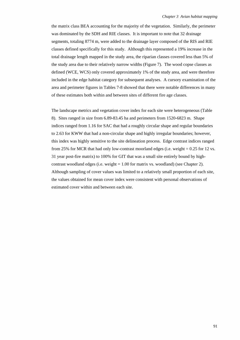
Chapter 3 Avian habitat mapping
the matrix class BEA accounting for the majority of the vegetation. Similarly, the perimeter
was dominated by the SDH and RIE classes. It is important to note that 32 drainage
segments, totaling 8774 m, were added to the drainage layer composed of the RIS and RIE
classes defined specifically for this study. Although this represented a 19% increase in the
total drainage length mapped in the study area, the riparian classes covered less than 5% of
the study area due to their relatively narrow widths (Figure 7). The wood copse classes as
defined (WCE, WCS) only covered approximately 1% of the study area, and were therefore
included in the edge habitat category for subsequent analyses. A cursory examination of the
area and perimeter figures in Tables 7-8 showed that there were notable differences in many
of these estimates both within and between sites of different fire age classes.
The landscape metrics and vegetation cover index for each site were heterogeneous (Table
8). Sites ranged in size from 6.89-83.45 ha and perimeters from 1520-6823 m. Shape
indices ranged from 1.16 for SAC that had a roughly circular shape and regular boundaries
to 2.63 for KWW that had a non-circular shape and highly irregular boundaries; however,
this index was highly sensitive to the site delineation process. Edge contrast indices ranged
from 25% for MCR that had only low-contrast moorland edges (i.e. weight = 0.25 for 12 vs.
31 year post-fire matrix) to 100% for GIT that was a small site entirely bound by high-
contrast woodland edges (i.e. weight = 1.00 for matrix vs. woodland) (see Chapter 2).
Although sampling of cover values was limited to a relatively small proportion of each site,
the values obtained for mean cover index were consistent with personal observations of
estimated cover within and between each site.
91

Chapter 3 Avian habitat mapping
92
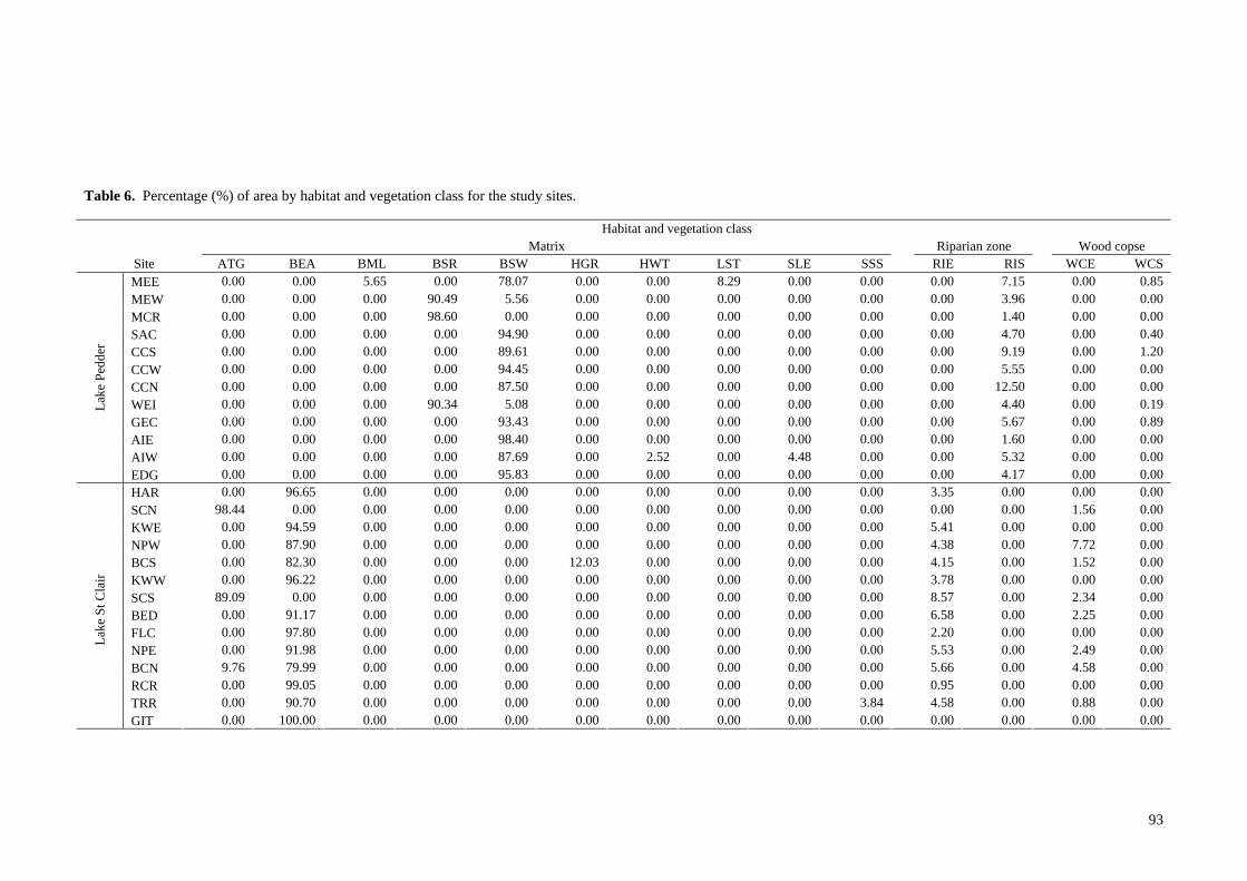
Table 6. Percentage (%) of area by habitat and vegetation class for the study sites.
Habitat and vegetation class Matrix Riparian zone Wood copse
Site ATG BEA BML BSR BSW HGR HWT LST SLE SSS RIE RIS WCE WCS MEE 0.00 0.00 5.65 0.00 78.07 0.00 0.00 8.29 0.00 0.00 0.00 7.15 0.00 0.85 MEW 0.00 0.00 0.00 90.49 5.56 0.00 0.00 0.00 0.00 0.00 0.00 3.96 0.00 0.00 MCR 0.00 0.00 0.00 98.60 0.00 0.00 0.00 0.00 0.00 0.00 0.00 1.40 0.00 0.00 SAC 0.00 0.00 0.00 0.00 94.90 0.00 0.00 0.00 0.00 0.00 0.00 4.70 0.00 0.40 CCS 0.00 0.00 0.00 0.00 89.61 0.00 0.00 0.00 0.00 0.00 0.00 9.19 0.00 1.20 CCW 0.00 0.00 0.00 0.00 94.45 0.00 0.00 0.00 0.00 0.00 0.00 5.55 0.00 0.00 CCN 0.00 0.00 0.00 0.00 87.50 0.00 0.00 0.00 0.00 0.00 0.00 12.50 0.00 0.00 WEI 0.00 0.00 0.00 90.34 5.08 0.00 0.00 0.00 0.00 0.00 0.00 4.40 0.00 0.19 GEC 0.00 0.00 0.00 0.00 93.43 0.00 0.00 0.00 0.00 0.00 0.00 5.67 0.00 0.89 AIE 0.00 0.00 0.00 0.00 98.40 0.00 0.00 0.00 0.00 0.00 0.00 1.60 0.00 0.00 AIW 0.00 0.00 0.00 0.00 87.69 0.00 2.52 0.00 4.48 0.00 0.00 5.32 0.00 0.00
Lak
e P
edde
r
EDG 0.00 0.00 0.00 0.00 95.83 0.00 0.00 0.00 0.00 0.00 0.00 4.17 0.00 0.00 HAR 0.00 96.65 0.00 0.00 0.00 0.00 0.00 0.00 0.00 0.00 3.35 0.00 0.00 0.00 SCN 98.44 0.00 0.00 0.00 0.00 0.00 0.00 0.00 0.00 0.00 0.00 0.00 1.56 0.00 KWE 0.00 94.59 0.00 0.00 0.00 0.00 0.00 0.00 0.00 0.00 5.41 0.00 0.00 0.00 NPW 0.00 87.90 0.00 0.00 0.00 0.00 0.00 0.00 0.00 0.00 4.38 0.00 7.72 0.00 BCS 0.00 82.30 0.00 0.00 0.00 12.03 0.00 0.00 0.00 0.00 4.15 0.00 1.52 0.00 KWW 0.00 96.22 0.00 0.00 0.00 0.00 0.00 0.00 0.00 0.00 3.78 0.00 0.00 0.00 SCS 89.09 0.00 0.00 0.00 0.00 0.00 0.00 0.00 0.00 0.00 8.57 0.00 2.34 0.00 BED 0.00 91.17 0.00 0.00 0.00 0.00 0.00 0.00 0.00 0.00 6.58 0.00 2.25 0.00 FLC 0.00 97.80 0.00 0.00 0.00 0.00 0.00 0.00 0.00 0.00 2.20 0.00 0.00 0.00 NPE 0.00 91.98 0.00 0.00 0.00 0.00 0.00 0.00 0.00 0.00 5.53 0.00 2.49 0.00 BCN 9.76 79.99 0.00 0.00 0.00 0.00 0.00 0.00 0.00 0.00 5.66 0.00 4.58 0.00 RCR 0.00 99.05 0.00 0.00 0.00 0.00 0.00 0.00 0.00 0.00 0.95 0.00 0.00 0.00 TRR 0.00 90.70 0.00 0.00 0.00 0.00 0.00 0.00 0.00 3.84 4.58 0.00 0.88 0.00
Lak
e St
Cla
ir
GIT 0.00 100.00 0.00 0.00 0.00 0.00 0.00 0.00 0.00 0.00 0.00 0.00 0.00 0.00
93

Chapter 3 Avian habitat mapping
94
Table 7. Percentage (%) of perimeter length (i.e. edge) by vegetation class for the study sites (excluding wood copses). Edge contrast weights relative to matrix, used to calculate edge contrast index.
Vegetation class (Edge contrast weights)
Site
ATG (0.00)
BEA (0.00)
BML (0.50)
BSR (0.25)
BSW (0.00)
CLL (0.25- 0.50)
EAA (1.00)
HHA (0.75)
HWT (0.75)
LST (0.75)
MSH (1.00)
RIE (0.50)
RIS (0.50)
RFT (1.00)
SCW (1.00)
SDH (1.00)
SSS (0.00)
WAT (0.00)
WDF (1.00)
WNF (1.00)
WNS (1.00)
MEE 0.00 0.00 23.72 0.00 10.87 15.24 0.00 0.00 0.00 41.07 0.00 0.00 8.32 0.00 0.00 0.00 0.00 0.00 0.00 0.00 0.79 MEW 0.00 0.00 0.00 21.31 0.00 18.18 0.00 0.00 0.00 0.00 0.00 0.00 18.18 0.00 0.00 0.00 0.00 0.00 0.00 0.00 42.32 MCR 0.00 0.00 0.00 100.00 0.00 0.00 0.00 0.00 0.00 0.00 0.00 0.00 0.00 0.00 0.00 0.00 0.00 0.00 0.00 0.00 0.00 SAC 0.00 0.00 0.00 0.00 47.66 34.38 0.00 0.00 0.00 0.00 0.00 0.00 15.84 0.00 0.00 0.00 0.00 0.00 2.13 0.00 0.00 CCS 0.00 0.00 0.00 0.00 11.14 42.83 0.00 0.00 0.00 0.00 0.00 0.00 23.86 0.00 0.00 0.00 0.00 0.00 0.00 0.00 22.16 CCW 0.00 0.00 0.00 0.00 31.54 27.89 0.00 0.00 0.00 0.00 0.00 0.00 36.02 0.00 0.00 0.00 0.00 0.00 0.00 0.00 4.56 CCN 0.00 0.00 0.00 0.00 8.28 19.51 0.00 0.00 0.00 0.00 0.00 0.00 72.21 0.00 0.00 0.00 0.00 0.00 0.00 0.00 0.00 WEI 0.00 0.00 0.00 30.46 0.00 0.00 0.00 0.00 0.00 0.00 0.00 0.00 9.05 0.00 0.00 0.00 0.00 0.00 0.00 33.24 27.25 GEC 0.00 0.00 0.00 0.00 15.18 32.42 0.00 0.00 0.00 0.00 0.00 0.00 32.59 0.00 0.00 0.00 0.00 0.00 0.00 0.00 19.81 AIE 0.00 0.00 0.00 0.00 20.28 57.10 0.00 0.00 0.00 0.00 0.00 0.00 10.62 0.00 0.00 0.00 0.00 7.15 0.00 0.00 4.85 AIW 0.00 0.00 0.00 0.00 8.60 51.59 0.00 0.00 1.24 0.00 0.00 0.00 32.86 0.00 0.00 0.00 0.00 0.00 0.00 0.00 5.71
Lak
e P
edde
r
EDG 0.00 0.00 0.00 0.00 19.80 40.13 0.00 0.00 0.00 0.00 0.00 0.00 30.84 0.00 0.00 0.00 0.00 0.00 0.00 9.23 0.00 HAR 0.00 7.88 0.00 0.00 0.00 6.42 0.00 0.00 0.00 0.00 0.00 7.59 0.00 0.00 0.00 78.12 0.00 0.00 0.00 0.00 0.00 SCN 10.34 0.00 0.00 0.00 0.00 0.00 85.88 0.00 0.00 0.00 0.00 0.00 0.00 0.00 0.00 3.78 0.00 0.00 0.00 0.00 0.00 KWE 0.00 1.63 0.00 0.00 0.00 4.20 0.00 4.59 0.00 0.00 0.00 50.39 0.00 0.00 0.00 39.19 0.00 0.00 0.00 0.00 0.00 NPW 0.00 18.50 0.00 0.00 0.00 22.43 0.00 0.00 0.00 0.00 0.00 0.00 0.00 0.00 0.00 59.07 0.00 0.00 0.00 0.00 0.00 BCS 0.00 10.87 0.00 0.00 0.00 5.03 0.00 7.25 0.00 0.00 2.84 20.39 0.00 11.06 0.00 34.25 0.00 0.00 0.00 8.31 0.00 KWW 0.00 2.63 0.00 0.00 0.00 3.73 0.00 0.00 4.82 0.00 0.00 22.17 0.00 0.00 0.00 66.66 0.00 0.00 0.00 0.00 0.00 SCS 0.00 0.00 0.00 0.00 0.00 0.00 22.31 0.00 0.00 0.00 0.00 32.87 0.00 0.00 0.00 44.82 0.00 0.00 0.00 0.00 0.00 BED 0.00 1.71 0.00 0.00 0.00 0.00 41.96 0.00 0.00 0.00 0.00 40.80 0.00 0.00 0.00 15.53 0.00 0.00 0.00 0.00 0.00 FLC 0.00 0.00 0.00 0.00 0.00 6.34 0.00 0.00 0.00 0.00 0.00 0.00 0.00 0.00 0.00 93.66 0.00 0.00 0.00 0.00 0.00 NPE 0.00 4.07 0.00 0.00 0.00 2.87 0.00 0.00 0.00 0.00 0.00 31.95 0.00 0.00 0.00 61.10 0.00 0.00 0.00 0.00 0.00 BCN 0.00 0.00 0.00 0.00 0.00 0.00 0.00 0.00 0.00 0.00 0.00 8.17 0.00 9.88 0.00 81.95 0.00 0.00 0.00 0.00 0.00 RCR 0.00 0.00 0.00 0.00 0.00 13.19 0.00 0.00 0.00 0.00 0.00 0.00 0.00 0.00 0.00 86.81 0.00 0.00 0.00 0.00 0.00 TRR 0.00 0.00 0.00 0.00 0.00 0.00 0.00 0.00 0.00 0.00 0.00 35.97 0.00 0.00 0.00 58.86 5.17 0.00 0.00 0.00 0.00
Lak
e St
Cla
ir
GIT 0.00 0.00 0.00 0.00 0.00 0.00 0.00 0.00 0.00 0.00 0.00 0.00 0.00 0.00 27.17 72.83 0.00 0.00 0.00 0.00 0.00
95

Chapter 3 Avian habitat mapping
Table 8. Landscape configuration metrics and vegetation cover for the study sites. *Actual cover not measured by BCB; therefore, based on personal observations it was considered to be the mean value of the adjacent 54 year old sites (AIE and EDG) so that AIW could be included in subsequent analyses.
Site Area
(ha) Perimeter
(m) Shape index Edge contrast
index (%) Mean cover
index MEE 53.34 5943 2.30 59.56 14.29 MEW 48.94 3927 1.58 61.29 20.71 MCR 21.22 2748 1.68 25.00 41.07 SAC 31.48 2300 1.16 34.16 103.57 CCS 33.06 3098 1.52 54.39 84.29 CCW 23.92 2525 1.46 36.45 102.86 CCN 15.18 1872 1.36 40.96 115.00 WEI 38.77 3460 1.57 66.05 87.86 GEC 20.20 2377 1.49 57.58 66.57 AIE 13.62 1957 1.50 38.74 83.57 AIW 11.75 1696 1.40 48.91 82.14*
Lak
e P
edde
r
EDG 13.12 1875 1.46 44.69 80.71 HAR 32.65 3432 1.69 83.73 12.14
SCN 7.61 1799 1.84 90.49 45.00 KWE 22.48 3077 1.83 68.78 32.14 NPW 16.98 2559 1.75 70.72 27.86 BCS 83.45 6823 2.11 77.36 57.14 KWW 45.39 6278 2.63 83.25 75.00 SCS 21.67 4317 2.62 85.16 73.21 BED 19.79 3091 1.96 81.46 63.57 FLC 47.68 5554 2.27 95.41 79.29 NPE 70.58 6304 2.12 80.54 94.29 BCN 23.72 3209 1.86 96.54 86.43 RCR 18.95 2699 1.75 90.10 91.43 TRR 39.04 3738 1.69 78.45 96.43
Lak
e S
t Cla
ir
GIT 6.89 1520 1.63 100.00 −
Positional errors
Perhaps the greatest potential sources of estimated positional errors of the final habitat map
(Table 9) during orthorectification arose from the (in)accuracy of the base layers, including
the acquired drainage and road layers used for visual registration and the contour layer used
as the base for the digital elevation model. The acquired layers can vary from ≤ 12.5-17.5 m
horizontal displacement depending on the specific image processing method used to map a
given feature, and ≤ 5 m vertical displacement. Based on the latter, and photo radius and
focal length of the cameras used for both sets of aerial photos, an additional error of 1.9-3.8
m may have occurred at sites that were located near the edge of the orthorectified photos.
Since photos were chosen in which sites were located as close to the photo’s principal point
as possible, the amount of error contributed from such distortions were likely to be less than
these figures indicate. Both of these potential sources of horizontal displacements were
largely reflected in the maximum positional errors reported in Table 1 for each orthorectified
96
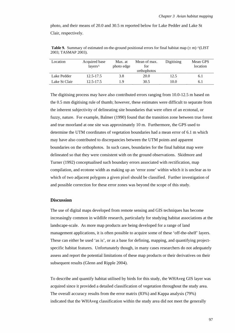
Chapter 3 Avian habitat mapping
photo, and their means of 20.0 and 30.5 m reported below for Lake Pedder and Lake St
Clair, respectively.
Table 9. Summary of estimated on-the-ground positional errors for final habitat map (± m) ^(LIST 2003; TASMAP 2003). Location Acquired base
layers^ Max. at
photo edge Mean of max.
for orthophotos
Digitising Mean GPS location
Lake Pedder 12.5-17.5 3.8 20.0 12.5 6.1
Lake St Clair 12.5-17.5 1.9 30.5 10.0 6.1
The digitising process may have also contributed errors ranging from 10.0-12.5 m based on
the 0.5 mm digitising rule of thumb; however, these estimates were difficult to separate from
the inherent subjectivity of delineating site boundaries that were often of an ecotonal, or
fuzzy, nature. For example, Balmer (1990) found that the transition zone between true forest
and true moorland at one site was approximately 10 m. Furthermore, the GPS used to
determine the UTM coordinates of vegetation boundaries had a mean error of 6.1 m which
may have also contributed to discrepancies between the UTM points and apparent
boundaries on the orthophotos. In such cases, boundaries for the final habitat map were
delineated so that they were consistent with on the ground observations. Skidmore and
Turner (1992) conceptualised such boundary errors associated with rectification, map
compilation, and ecotone width as making up an ‘error zone’ within which it is unclear as to
which of two adjacent polygons a given pixel should be classified. Further investigation of
and possible correction for these error zones was beyond the scope of this study.
Discussion The use of digital maps developed from remote sensing and GIS techniques has become
increasingly common in wildlife research, particularly for studying habitat associations at the
landscape-scale. As more map products are being developed for a range of land
management applications, it is often possible to acquire some of these ‘off-the-shelf’ layers.
These can either be used ‘as is’, or as a base for defining, mapping, and quantifying project-
specific habitat features. Unfortunately though, in many cases researchers do not adequately
assess and report the potential limitations of these map products or their derivatives on their
subsequent results (Glenn and Ripple 2004).
To describe and quantify habitat utilised by birds for this study, the WHAveg GIS layer was
acquired since it provided a detailed classification of vegetation throughout the study area.
The overall accuracy results from the error matrix (83%) and Kappa analysis (79%)
indicated that the WHAveg classification within the study area did not meet the generally
97
Chapter 3 Avian habitat mapping accepted accuracy standard of 85%. Additional analyses also indicated that important avian
habitat features, such as wood copses and riparian zones, were either inconsistently classified
or omitted altogether since they were not considered as part of their overall mapping
objectives, were not readily identified from aerial photos, or were below the minimal
mapping unit (~ 0.5 ha within the study area). These low accuracy estimates were largely
the result of a range of interpretation, classification, delineation, and registration errors that
are common to many mapping projects (Congalton and Green 1993). Since positional errors
such as those caused by misregistration tend to confound the sources of any attribute errors,
it is difficult to determine the extent to which each of these contributes to the overall
accuracy (Foody 2002). It has been shown that misclassification alone can cause significant
bias in area and perimeter estimates (Czaplewski 1992), and the accuracy estimates of 84%
and 6%, respectively, for WHAveg bring this to bear. Furthermore, the magnitude of the
underlying errors, such as the inclusion of non-habitat (e.g. woodland classes) within the
study sites, must be considered as well. Since the utility of a map is a function of its
accuracy relative to the scale and objectives of a study (Foody 2002), and the main objective
here was to classify and accurately quantify all avian habitat features in the study area, it was
apparent that the WHAveg and associated layers could not simply be used ‘as is’ Thus, the
results from the accuracy assessment were used to correct some of these errors to the extent
possible, and used as a base for creating a finer-scale and greater-resolution classified bird
habitat map that was more inclusive, accurate, and appropriate for the aims of this study.
As is the case with any map, there were numerous potential sources of attribute and
positional errors associated with the final habitat map produced for this study. However, the
quantification of such errors is considered to be a complex task, even for studies focused on
mapping in and of itself (Foody 2005). This is exacerbated by the fact that these errors tend
to accumulate through the mapping process (Congalton and Green 1999). Despite this being
the case, it is possible to provide some overall accuracy estimates in relation to those
reported for WHAveg and the other acquired layers. In consideration of the relative scale
and degree of ground-truthing conducted for this study, it is a reasonable assumption that
attribute accuracy was markedly higher than that estimated for WHAveg, but no greater than
that reported for the other base layers (e.g. drainages), and thus was likely close to 98%.
Positional accuracy is somewhat harder to quantify into one figure since numerous sources
of error may be at play and a more comprehensive assessment would have required methods
(e.g. surveying) that were beyond the scope of this study. Since the accuracy of a map
cannot surpass that of the base layers on which it is based (if uncorrected), it can be assumed
that the best case scenario was positional accuracies around 12.5 m (based on lowest
reported error for drainage and road layers) and a worse case scenario around 43 m (based on
largest maximum horizontal error for the orthophotos). In either case, these errors were less
98
Chapter 3 Avian habitat mapping
than the estimated positional accuracy of 50 m reported in the WHAveg metadata, and
considerably less than the actual maximum offsets (~ 100 m) measured for WHAveg in this
accuracy assessment. Therefore, in relation to the scale and objectives of this study, this
level of positional accuracy was considered to be acceptable. Moreover, since the same
image sources and methods were used for all sites within the study locations, the relative
accuracy was adequately high. The mapping methods used herein have ensured that the final
habitat map was both logically consistent (i.e. all features are labelled with only one class
and all polygons are closed) and complete (i.e. all sites were mapped in their entirety).
The results of this fine-scale mapping project demonstrated that there was a notable
improvement in both attribute and positional accuracies in the final habitat map, thus
minimising potential biases in the calculated habitat metrics and the possibility of spurious
avian habitat associations in subsequent analyses presented in Chapters 4-6. The process
necessary to thoroughly assess existing GIS layers and to modify and amend them
accordingly was both resource and time consuming. Thus, the development of project-
specific map products may not necessarily be worthwhile for all such wildlife research
projects and must be evaluated against the relative scales (i.e. mapping and ecological) and
objectives of a given study.
The significant differences identified in vegetation heights between the avian habitat
categories (i.e. matrix, riparian zone, and edge) and their characteristic floristics helped to
substantiate their a priori classification. These findings are in agreement with previous
research in blanket moorlands (Marsden-Smedley 1990; Brown and Podger 1982), and are
likely the result of interspecific competition that may be attributed to minor changes in
drainage as well as peat type (e.g. from muck to fibrous peat). These differences are also
manifested in their fire sensitivity and flammability attributes, with moorlands classified as
having low sensitivity and very high flammability, while the edge-forming wet sclerophyll
woodlands and forests have a high fire sensitivity and moderate flammability (Pyrke and
Marsden-Smedley 2005). In addition, the significant relationship between mean index cover
and time since fire is consistent with both previous research and current theory on post-fire
succession in Tasmanian buttongrass moorlands (see Chapter 1). However, results from the
vegetation analyses showed that despite attempts to minimise other abiotic and biotic
variables among the study sites as described in Chapter 2, there were notable differences in
vegetation composition, structure, and spatial configuration both within and between study
sites. Inter-site differences in landscape metrics are largely the result of varying, complex,
and long-term interactions between vegetation and factors such as soil conditions, hydrology,
and fire (Jarman et al.1988a; Marsden-Smedley 1990; Balmer 1991). However, these
differences were also partially artifacts of the site selection and delineation process (see
99

Chapter 3 Avian habitat mapping
100
Chapter 2). The relative influence of such spatial heterogeneity, in addition to fire age per
se, on avian habitat use, composition, and densities is explored in Chapters 4-6. Finally, this
avian habitat map, along with the results in subsequent chapters, may be used as a foundation
for the potential future development of landscape-scale bird-habitat prediction models in
buttongrass moorlands (see Chapter 7).
Chapter 4
Avifaunal composition and densities in relation to post-fire
succession of buttongrass moorlands in the Tasmanian Wilderness
World Heritage Area
Introduction Fire is perhaps the principal abiotic agent in Australian ecosystems (Jackson 1968; Bowman
2000; Clark et al. 2002) and avifaunal responses to disturbance by fire are complex, highly
variable, and species- and context-specific (for reviews see Woinarski and Recher 1997;
Woinarski 1999a, 1999b; Chapter 1). Paradoxically, many Australian vegetation
communities including sedgelands and heathlands are characterised by being both highly
flammable throughout much of the year (Specht 1979a; Keith et al. 2002a; Pyrke and
Marsden-Smedley 2005) and supporting resident bird species that possess a number of
attributes associated with fire-sensitivity, such as being ground-dwelling and cover-
dependent, and having limited dispersal capabilities and low fecundity (Kikkawa et al. 1979;
Baker 2000; Woinarski and Recher 1997; Burbidge et al. 2005). Since fires in heathlands
often burn much of the above-ground vegetation, species that exhibit one or more of these
attributes may be less likely to survive the fire, find adequate resources in the post-fire
environment, evade predators, recolonise from adjacent unburnt areas, or successfully
reproduce (Fox 1978; Baker 2000, 2002; Keith et al. 2002a; Whelan et al. 2002). The rate
and extent of the recovery of vegetation after fire may influence the relative suitability of
habitats for both resident and opportunistic species through changes in vegetation structure
and resource availability over time (Kikkawa et al. 1979; Brown 1991; Keith et al. 2002a;
Whelan et al. 2002). Numerous studies in Australian heathlands have demonstrated that bird
species composition and abundance may be affected by fire (e.g. Smith 1987; McFarland
1988b, 1994; Brooker and Rowley 1991; Recher 2005). However, bird populations do not
necessarily follow a predictable successional pathway and may be influenced by a range of
factors other than, or in addition to, habitat structure and fire age per se (Meredith et al.
1984; Woinarski and Recher 1997; Baker 2002). Although many Australian ecosystems and
their fauna are considered to exhibit adaptations to fire disturbance (Catling and Newsome
1981; Recher and Christensen 1981), changes in fire regimes (e.g. time since fire, season,
patchiness, extent, intensity, frequency) since European colonisation and the resulting direct
or indirect mortality have either been confirmed or implicated as contributing to the
extinction of at least two species and three subspecies of Australian birds (Woinarski and
Recher 1997). Currently, fire regimes that are outside of their historical range of variation
are a threat to at least 51 bird taxa, including many heathland species (Garnett 1992;
101
Chapter 4 Avifaunal responses to post-fire succession Woinarski 1999a, 1999b; Garnett and Crowley 2002; Olsen and Weston 2005). Short inter-
fire intervals and increased fire frequency are considered to be the major threats to many bird
species, particularly for mid- to late-successional heathland species that cannot persist and
reproduce in early-successional habitats (Brooker and Rowley 1991; Mushinsky and Gibson
1991; Woinarski and Recher 1997). These circumstances present a major challenge for fire
and conservation managers. It is generally recognised due to the extremely wide range of
observed avian responses to fire and the complexity of the underlying processes that sound
decision-making is contingent upon detailed, ecosystem-specific research (Wilson 1994;
Woinarski and Recher 1997; Baker 2002; Whelan et al. 2002; Paton et al. 2005; Recher
2005; Tasker and Baker 2005).
Buttongrass moorlands form an ecosystem that exemplifies the complex interplay of fire,
soils, flora, and avifauna. They are comprised of sedgeland and graminoid heathland
communities typically dominated by the hummock-forming tussock sedge commonly named
buttongrass (Gymnoschoenus sphaerocephalus) (Specht 1979a; Jarman et al. 1988a).
Buttongrass moorlands cover large areas in Tasmania (0.55 million ha) and are most
extensive in the perhumid, oligotrophic peatlands of western Tasmania where they are
largely protected within the Tasmanian Wilderness World Heritage Area (TWWHA;
335,000 ha) (Brown et al. 1993; Smith and Banks 1993; Balmer et al. 2004; TVMP 2004).
Buttongrass moorlands are highly pyrogenic, but are adapted to and have a low sensitivity to
fire, and exhibit post-fire changes in vegetation structure and composition that are
characteristic of secondary succession (Connell and Slatyer 1977; Brown et al. 2002; Balmer
et al. 2004; Pyrke and Marsden-Smedley 2005; see Chapter 1).
To date, knowledge of the Tasmanian moorland avifauna has been very limited and is
primarily based on qualitative descriptions (e.g. Gellie 1980; Brown et al. 1993; Driessen
2006). However, all sources report that the avifauna is depauperate and is comprised of only
three resident species that are known to depend exclusively upon moorlands in the study
area, namely the Southern Emu-wren (Stipiturus malachurus littleri), Striated Fieldwren
(Calamanthus fuliginosus diemenensis), and Ground Parrot (Pezoporus wallicus wallicus),
and a small number of transient species that are typically associated with adjacent
woodlands, forests, and related habitats (Brown et al. 1993; see Chapter 1). Bryant’s
research (1991, 1992, 1994) on the density, distribution, and conservation status of the
Ground Parrot is the only major work to date that has focused on a moorland resident species
in Tasmania; however, its scope in relation to fire ecology was limited and it did not
investigate any other members of the avifauna (S. Bryant pers. comm. 2003). Otherwise, our
knowledge of the resident species is limited to either old observational studies conducted in
non-moorland habitat in other regions of the State (e.g. Legge 1908; Fletcher 1913a,
102
Chapter 4 Avifaunal responses to post-fire succession
1913b,1915a; Lord 1927; Sharland 1953), or on more recent studies primarily on different
subspecies on the Australian mainland (e.g. Gosper and Baker 1997; Burbidge et al. 2005;
Maguire 2006a, 2006b). Although extensive research investigating the effects of fire on the
Ground Parrot has been conducted on the mainland, results have varied and their
implications for fire management have been equivocal (Meredith et al. 1984; McFarland
1991a, 1991b, 1991c; Woinarski 1999a, 1999b; Baker 2002; Tasker and Baker 2005;
Burbidge et al. 2007). To date, no detailed fire ecology studies either on the mainland or in
Tasmania have focused on the Southern Emu-wren or Striated Fieldwren (Woinarski 1999a,
1999b; Higgins et al. 2001; Higgins and Peter 2002). Accordingly, over the years a number
of researchers have identified the need to study the Tasmanian moorland avifauna,
particularly in relation to the effects of fire, in order to help guide fire management and
conservation efforts (e.g. Gellie 1980, Eberhard 1987; Bryant 1991; Driessen 2001).
Despite the lack of prior research on the Tasmanian resident avifauna, it is evident from the
literature that the Southern Emu-wren, Striated Fieldwren, and Ground Parrot all exhibit
some fire-sensitive attributes since they are habitat specialists, cryptic, ground-dwelling,
dependent on dense cover, and except for the latter, are poor fliers and are considered to
have limited dispersal capabilities (Meredith et al. 1984; Bryant 1990; Gosper and Baker
1997; Pickett 2000; Higgins and Peter 2002; Wilson and Paton 2004; Tasker and Baker
2005; Burbidge et al. 2007; see Chapter 1). Accordingly, extensive wildfires in increasingly
fragmented habitats, short inter-fire intervals, high fire frequencies, and otherwise modified
fire regimes have been implicated in the local extinction of some mainland populations, and
have been identified to be among the primary threats to extant populations (MLRSERT
1998; Garnett 1992; Woinarski 1999a; Garnett and Crowley 2000; Lunney et al. 2000). In
part due to such fire-induced impacts, five mainland subspecies of Southern Emu-wren are
listed as being threatened or endangered (S. m. hartogi, Western Australia Wildlife
Conservation Act of 1950; S. m. intermedius, S. m. parimeda, S. m. halmaturinus, and S. m.
malachurus, South Australia National Parks and Wildlife Act 1972 and Environment
Protection and Biodiversity Conservation Act 1999); a mainland subspecies of Striated
Fieldwren is listed as vulnerable (C. f. albiloris, New South Wales Threatened Species
Conservation Act 1995); and both subspecies of Ground Parrot are listed on the mainland as
either vulnerable (P. w. wallicus, Queensland Nature Conservation Act 1992 and New South
Wales Threatened Species Conservation Act 1995) or endangered (P. w. flaviventris,
Western Australia Wildlife Conservation Act of 1950 and Environment Protection and
Biodiversity Conservation Act 1999) (Garnett and Crowley 2000). None of the resident
species are currently listed in Tasmania; however, Ground Parrot populations have declined
and some populations have become locally extinct, particularly in northern and eastern
regions where suitable habitat was historically limited (Bryant 1991). Despite the historical
103
Chapter 4 Avifaunal responses to post-fire succession and ongoing threats posed by development, grazing, and increased fire frequency in some
parts of Tasmania, populations are considered to be secure in the southwest where they are
free from most threats under the protection of the Tasmanian Nature Conservation Act 2002
and the TWWHA (Bryant 1991). It has also been suggested that inappropriate fire regimes
may be a threat to populations of the Southern Emu-wren and Striated Fieldwren in
Tasmania (Legge 1908; Gellie 1980).
Currently, there is considerable debate concerning the most appropriate way to manage fire
within the TWWHA in order to protect life and property, and conserve its biodiversity,
particularly within buttongrass moorland ecosystems (PWS 1999; DPIW 2007; May and
Balmer 2008). Since inappropriate fire regimes are a demonstrated or proposed threat to
mainland populations of the Southern Emu-wren, Striated Fieldwren, and Ground Parrot, as
well as a number of other species known to use moorlands (Garnett 1992; Brown et al. 1993;
Garnett and Crowley 2000; see Chapter 1), it is imperative to investigate the ecological
attributes and responses of the moorland avifauna to fire in order to help guide management
across Tasmania. The research described here is the first community-level study of the
buttongrass moorland avifauna and was primarily focused on exploring the influence of site
fire age and productivity on the avifauna, since these are the primary variables in the fire
behaviour and prediction models currently used by the Parks and Wildlife Service to guide
prescribed burning and wildfire suppression operations in the TWWHA (Marsden-Smedley
et al. 1999; PWS 2004; Marsden-Smedley 2009). Distance sampling and variable circular-
plots were used within a replicated space-for-time (SFT) design to compare patterns in
avifaunal composition and density across three seasons and two chronosequences in low
productivity, blanket moorlands at Lake Pedder (3-54 years post-fire) and medium
productivity, eastern moorlands at Lake St Clair (1-44 years post-fire) in the TWWHA. The
primary aims of this study were 1) to quantitatively describe the avifauna of buttongrass
moorlands; 2) to investigate the short- to long-term effects of different times since fire and
other environmental attributes on avifaunal composition and densities; 3) to identify the seral
stages that provide suitable habitat for the resident species; and 4) to provide information to
help guide fire management and conservation of the buttongrass moorland avifauna.
104
Chapter 4 Avifaunal responses to post-fire succession
Methods Study area
Details of the study design, site descriptions, fire histories, vegetation configurations, and
floristics have been provided in Chapters 2-3 but a summary of the results as they pertain to
this study is provided below. The study area is largely within the TWWHA, as well as
adjacent land allocations, and is composed of a mosaic of buttongrass moorland, scrub, wet
sclerophyll woodland and forest, and temperate rainforest. The two study locations include
sites on the low productivity (i.e. infertile) quartzitic geologies at Lake Pedder (3-54 years
post-fire, n = 12; 305-370 m asl) and the moderate productivity doleritic geologies at Lake St
Clair (1-44 years post-fire, n = 14; 730-795 m asl). Within the study sites, buttongrass
moorland comprises the primary vegetation matrix and is mainly composed of Southwestern
Buttongrass Moorland and Sedgey Buttongrass Moorland (i.e. blanket moorlands) at Lake
Pedder and Eastern Buttongrass Moorland and Subalpine Sedgeland (i.e. eastern moorlands)
at Lake St Clair (for descriptions of these vegetation types see Chapter 3). The moorland
matrix is interspersed and bordered by typically small perennial watercourses (i.e. first-third
order streams; after Strahler 1952) and associated vegetation communities classified as
Southwestern Buttongrass Riparian Zones (mean width 12.5 ± 1.5 m, n = 28) and Eastern
Buttongrass Riparian Zones (mean width 9.2 ± 1.0 m, n = 51), respectively. The matrix is
also interspersed with wood copses (mean area 0.5 ± 0.1 ha, n = 14) classified as
Southwestern and Eastern Wood Copses, respectively. The woodland and forest vegetation
classes at Lake Pedder are variable, but are most commonly composed of Eucalyptus nitida
Wet Scrub and Forest, while at Lake St Clair are dominated by Eucalyptus delegatensis
Woodlands which form relatively distinct edges with the matrix.
Avian survey methods
A considerable portion of the ornithological literature to date has focused on examining
survey design and methods for counting birds in order to investigate a wide range of research
questions, particularly regarding avian habitat relationships (for reviews see Hewish and
Loyn 1989; Schwarz and Seber 1999; Bibby et al. 2000; Rosenstock et al. 2002; Watson
2004; Buckland 2006). A brief overview of these methods is provided below followed by a
detailed description of the methods used for this study.
Avian survey methods range from complete censuses, in which all (or at least most)
individuals within a population are counted to determine absolute abundance and/or density,
to relative indices, in which individuals and/or cues (e.g. calls) are counted and assumed to
represent a constant proportion of the true population size. Implicit in these methods is a
general recognition of both the likelihood and ability of observers to count all individuals or
cues that are present. A wide range of factors can contribute to a species’ (and individual’s)
105
Chapter 4 Avifaunal responses to post-fire succession detectability, including call type and frequency, sex, age, size, plumage, behaviour, and life
history, as well as environmental variables such as habitat, time of day, season, weather, and
background noise (Dawson 1981a; Robbins 1981a, 1981b; Craig and Roberts 2001; Simons
et al. 2007). In particular, disturbance by fire causes distinct changes in vegetation structure,
and therefore may directly or indirectly affect the conspicuousness of birds (Burbidge 2003).
The degree to which these factors influence counts must be considered within the context of
observer experience and visual and auditory acuity, as well as the probability that an
individual is available for detection at the moment that the observer is actively surveying
(Diefenbach et al. 2007). While some of these factors can be controlled through appropriate
study design and implementation, many of these variables are an unavoidable aspect of field
work in a natural environment (Thompson 2002).
Reliable abundance estimates are particularly difficult to obtain for cryptic species, such as
the three resident species of buttongrass moorlands. A number of alternative methods have
been proposed to increase the detectability of such cryptic species. One method is to utilise
call playback, which has been used in a number of avian studies (e.g. Marion et al. 1981;
Lynch 1995), including for the Southern Emu-wren (Pickett 2000). However, regular
playback may cause adverse impacts on the populations being studied and may result in
positive bias in density estimates since birds may be drawn in towards the observer from a
larger and unknown area (Buckland et al. 2001). Methods such as territory mapping (Bibby
et al. 2000), area searches (Loyn 1986), multiple observer approaches (Hutto and Mosconi
1981; Baker and Whelan 1994), and the use of dogs (Buckland et al. 2001), may likewise
increase the detectability of species by focusing search efforts in relatively small areas, yet
their resource-intensive nature, limited scale, and potentially adverse impacts within the
TWWHA prohibited their use in this study.
The vast majority of avian studies rely upon some form of index count, in spite of the fact
that the limitations of such methods have long been recognised (Rosenstock et al. 2002;
Diefenbach et al. 2003). However, since differences in detectability within a study are often
not accounted for and the assumption of constant proportionality is often not met, it is
difficult if not impossible to reliably estimate absolute bird abundance and density (Burnham
1981; Norvell et al. 2003). Low bias and high precision population estimates are necessary
in order to make valid inferences for most research applications (Thompson 2002).
Analytical methods that correct such differences in detectability are not new (e.g. Burnham
and Anderson 1976; Reynolds et al. 1980), but their use is still somewhat limited despite
their obvious advantages (Rosenstock et al. 2002). Of these methods, one of the most
widely used and broadly applicable is distance sampling, which is comprehensively
described in the standard references by Buckland et al. (2001, 2004) and summarised below.
106
Chapter 4 Avifaunal responses to post-fire succession
Distance sampling is an integrated method that includes study design, data collection, and
statistical analyses (Buckland et al. 2001; Rosenstock et al. 2002). It is essentially an
extension of quadrat sampling; however, instead of assuming that all birds are detected
within a given area, the observer measures the distance (y) from the line or point to each bird
that is detected. These distances, or distance categories, are then used to estimate the
detection function (g(y)), which is based on the premise that the probability of detection
decreases with increasing distance from the observer, assuming that all individuals are
available for detection (Buckland et al. 2001; Diefenbach et al. 2007). However, other
factors may also affect detectability, such as different survey methods (e.g. line or point),
modes of detection (e.g. audio or visual), type of objects (e.g. individuals or clusters),
species, locations, times, and survey conditions. Depending upon the particular research
objectives, study design, and sample sizes, a specific detection function can be determined
for such variables individually or in combination. Using conventional distance sampling
(CDS) analysis, the probability of detection based on these distances can then be modelled
using robust, semi-parametric methods (i.e. key function + series adjustment) in Distance 5.0
software (Buckland et al. 2001; Thomas et al. 2006). With multiple covariate distance
sampling (MCDS) analysis, additional covariates (e.g. time, season, habitat variables) can
also be included in the detection function model through a log link key function and thus can
influence the scale of the detection function (Thomas et al. 2006; Marques et al. 2007). In
the absence of sufficient data to model strata- or condition-specific detection functions, the
incorporation of covariates may account for variation in detection probability and thus
provide a means to increase the reliability and precision of density estimates as well as assess
the influence of the covariates themselves (Marques and Buckland 2004; Marques et al.
2007). One of the most notable features of these models is that they are ‘pooling robust’,
meaning that variables other than distance, including those that have not been measured or
modelled per se, are incorporated into the detections functions, and thus can affect
detectability without biasing density estimates (Burnham et al. 1980; Buckland et al. 2001;
Burnham et al. 2004). In other words, detection distance may serve as a proxy for a suite of
other factors that may influence the detection process (Alldredge et al. 2007). The model(s)
with the best fit are then used to correct the site specific encounter rates (i.e. raw counts) for
differences in detectability, and thus estimate absolute density and/or abundance. However,
a number of key assumptions must be met in order to obtain reliable estimates (Buckland et
al. 2001). These assumptions include:
1) all birds directly on the line or point are detected;
2) birds are detected prior to any responsive movement; and
3) distances are measured or distance categories are recorded accurately.
107

Chapter 4 Avifaunal responses to post-fire succession Although under some circumstances these assumptions can be relaxed and the method can be
robust to violations, proper survey design and field methods are essential to ensure they are
met to a reasonable degree (Buckland et al. 2001; Norvell et al. 2003). Distance sampling
has been assessed and validated in a number of studies (e.g. Nelson and Fancy 1999; Cassey
and McArdle 1999; Norvell et al. 2003) and is considered by many to be a more rigorous,
robust, and viable alternative to traditional avian survey methods (e.g. Bibby 2000; Buckland
et al. 2001; Rosenstock et al. 2002; Thompson 2002; Diefenbach et al. 2003; Ellingson and
Lukacs 2003; Royle et al. 2004; Buckland 2006; Buckland et al. 2008). However, it should
be noted that some researchers have questioned whether or not the underlying assumptions
of distance sampling can reasonably be met in most avian ecology studies and that the
resulting density estimates may not be as accurate as simple, unadjusted counts (Verner and
Ritter 1985; Raphael 1987; Hutto and Young 2003). On the other hand, others propose that
relative abundance methods (i.e. indices) often fail to meet the fundamental assumption of
constant proportionality (Ellingson and Lukacs 2003; Norvell et al. 2003). Thus, the relative
advantages and disadvantages of distance sampling are likely to be a source of continued
debate.
Since the three resident species of buttongrass moorlands are very cryptic, can often only be
detected by call, and vary in their overall detectability, a number of different survey
techniques were considered in order to ensure representative and adequate samples in this
study. Three common techniques are used to survey bird populations, including line and
point transects used in distance sampling, and point counts, which can be used as a type of
plot sampling (e.g. variable circular-plots; see below). Their relative advantages and
disadvantages have been extensively discussed in the literature (e.g. Ralph and Scott 1981;
Ralph et al. 1995; Buckland et al. 2001). All other things being equal, line transects are
considered to be the most efficient technique, and are particularly well suited for species in
low densities and detected through a flushing response (Casagrande and Beissinger 1997;
Buckland et al. 2001; Buckland 2006), such as Striated Fieldwrens (pers. obs.). However,
point transects are advantageous when uneven terrain (Dawson 1981b) or other conditions,
such as background noise generated from walking through scrubby vegetation, make it
difficult to fully concentrate on detecting and recording birds while moving (Reynolds et al.
1980). This is particularly relevant in buttongrass moorlands since they are difficult to
traverse quietly due to their hummocky and scrubby nature, and when surveying cryptic
species, such as the Southern Emu-wren, that are often only detected by their soft and high-
pitched calls (see Chapter 1). Point counts have similar advantages to point transects and
can be used to determine absolute densities if the radius of detection is either estimated (e.g.
based on maximum hearing distance; Bryant 1991) or fixed (Petit et al. 1995), and all birds
within that area are likely to be detected. Such point counts have typically been used for
108

Chapter 4 Avifaunal responses to post-fire succession
surveying Ground Parrots since their relatively loud and distinctive calls can consistently be
detected during their dawn and dusk calling-flight sessions and evidence indicates that most
individuals will call during these periods (Bryant 1991; McFarland 1991c; Meredith et al.
1984).
In consideration of the low expected densities for the three resident species, their differences
in detectability, and the large area that needed to be surveyed (782 ha), it was decided to
utilise a composite survey design (Casagrande and Beissinger 1997; Buckland et al. 2001).
This design consisted of line and point transect distance sampling for the avifauna as a whole
and variable circular-plot sampling for Ground Parrots in order to estimate bird densities
within each site. Ancillary data, including habitat use by birds, were also collected in order
to identify bird-habitat relationships both within and across sites of different fire ages (see
Chapter 5). A series of pilot studies were conducted in order to establish a standard survey
design and methods that were both feasible to implement and would enable the attainment of
the overall aims of this study.
Point and line transect distance surveys
An area-proportionate sampling scheme was chosen in order to maximise coverage and
hence sample size for the study area, and because area per se was one of the potential
explanatory factors to be used in subsequent analyses (Atkinson et al. 2006). A systematic
grid with spacing of 150 m between lines and points was chosen to maximise the detection
of the residents, and minimise overlap and potential double counting between points and
lines (Buckland et al. 2001). This distance was based on a compromise between the
expected maximum detection distances of the Southern Emu-wren (~ 50 m) and Striated
Fieldwren (~ 100 m), as determined from the literature (see Chapter 1) and the pilot surveys.
A random first point was located in each site based on 75 m buffers from the site boundaries
at the point of access (considered to be random in relation to theoretical bird distribution)
(Buckland et al. 2001; Diefenbach et al. 2003). The grid was then oriented to maximise
coverage probability for all portions of the sites and to strike a balance between maximising
line/point replication and survey efficiency within each site (Strindberg et al. 2004). Each
point was marked with a 1.2 m bamboo stake and survey flagging along the appropriate
bearing, and where necessary additional flagging was placed between stakes so that the line
could be clearly identified for distance measurements during the course of surveys
(Buckland et al. 2001). This type of ‘minus sampling’ survey design may result in under-
sampling of the edge and uneven coverage probability since the survey plots do not extend
beyond the site boundaries and the resulting detection functions reflect both detectability and
availability of birds (Strindberg et al. 2004; Thomas et al. 2006). However, potential biases
from these edge effects are considered to be minor and can reasonably be ignored for most
109
Chapter 4 Avifaunal responses to post-fire succession surveys (Buckland et al. 2001; Strindberg et al. 2004; Buckland 2006). A total of 116 points
and 32 transects (totalling 12.60 km) were established at the 12 sites at Lake Pedder and 181
points and 43 transects (totalling 20.28 km) at the 14 sites at Lake St Clair. It is important to
note that due to the limited size and configurations of some sites (see Chapter 2) fewer than
the ideal number of points/lines per site could be established in order to calculate reliable
variance estimates (~ 20; Buckland et al. 2001).
All point and line transect surveys were conducted by the author to eliminate the potentially
large biases and reduced precision that can result from inter-observer variability
(Cunningham et al. 1999; Diefenbach et al. 2003). Although seasonality per se was not of
specific interest, surveys were replicated over three seasons to account for within-site
variability and increase the sample sizes and hence reliability of estimates of the detection
functions and abundances (Link et al. 1994; Buckland et al. 2001). Surveys were conducted
during the summer (2 February - 9 March), winter (24 May 24 - 6 July), and spring (11
October - 27 November) of 2004, such that each site was surveyed three times. These
intervals were considered to be of sufficient length to reduce the dependency of stochastic
errors between successive surveys (Buckland et al. 2001). Surveys were started
approximately one hour after sunrise, based on previous research conducted on the resident
species (e.g. Maguire and Mulder 2004) and personal observations. They were conducted
for up to six hours each day, as determined by the approximate time taken to survey the
largest site in its entirety (BCS, 83.45 ha) and personal observations that indicated birds were
detectable by both auditory and visual cues throughout this time period. A survey schedule
was developed in which the time of day and order of sites were systematically rotated within
and across seasons to minimise temporal biases and maximize survey efficiency (Mac Nally
1996a; Campi and Mac Nally 2001). Although it would have been desirable to limit
surveying to calm and fine conditions, this was not feasible because of the highly variable
weather typical of the study regions (see Chapter 2) and the large area that needed to be
surveyed by a single observer. However, surveys were not conducted or were stopped if
unfavourable conditions prevailed, such as sustained moderate or stronger winds
(≥ 20 km h-1) and moderate rain, since these conditions can adversely influence bird
detectability (Robbins 1981a; Maguire 2005).
Surveys were conducted by using a combination of line and point transects as described by
Buckland et al. (2001) and the date, sunrise time, start time, and end times were recorded for
each survey. Even though distance methodology is considered to be robust to the influences
of environmental variables on density estimates (Buckland et al. 2001), weather conditions
that could affect bird behaviour and detectability were recorded for each survey since at
times surveying had to be conducted in sub-optimal conditions. Temperature (°C), humidity
110

Chapter 4 Avifaunal responses to post-fire succession
(%), and wind speed (km h-1) were recorded at breast height with an electronic weather
gauge (Skymate Plus SM-19, Speedtech Instruments; accuracy: wind ± 3%; rH ± 4%; ± 1°
C). Temperature and humidity were recorded at the start and end of each survey. Prevailing
wind speed was classified as calm (0 km h-1), light (< 19 km h-1), moderate (20-29 km h-1), or
fresh (30-39 km h-1) (after BOM 2004), and the prevailing direction was noted. Cloud cover
was estimated by eye and classified as clear (0%), mostly sunny (25%), partly cloudy (50%),
mostly cloudy (75%), or overcast (100%). Precipitation was classified as none, fog, light,
moderate, or heavy rain, or snow.
Each point was surveyed for four minutes, which is congruous with the standards
recommended for point counts (Ralph et al. 1995) as well as the amount of time it typically
takes to traverse each 150 m of transect. Counts did not start until approximately one minute
after the point was reached to allow for normal bird activity to resume (Pyke and Recher
1985). After the point count, the 150 m of line transect up to the next point was traversed at
a slow and consistent speed, and as quietly as possible. Periodic stops were made to listen
for auditory cues and to thoroughly scan the area for birds. Line transects were traversed at a
mean rate of travel of 1.86 km h-1, including the occasional stops, which is within the range
of what is considered to be a reasonable survey speed in open terrain (Baker 1997; Bibby et
al. 2000). Binoculars (Gerber Montana 8 x 42) were used to aid in identification, improve
detection distance, and to increase the chances of visual observations, particularly for the
cryptic resident species. While the surveys were being conducted, search effort was focused
on and near the point/line to ensure that the probability of detection at the point/line was
unity (i.e. g(0) = 1; Buckland et al. 2001). During the line survey or after the point was
completed, and if necessary, the immediate area (~ < 25 m) around the point/line was
searched for a brief period (up to a few minutes) to confirm species identification, group
size, or other data of any birds that were detected (particularly by call) during the survey
period. However, if there was reason to believe that the bird(s) moved in response to these
searches, an exact distance was not recorded even if there was subsequent visual
confirmation. Only birds using habitat within the site as defined were recorded. Therefore,
birds flying through the site that did not appear to be feeding or otherwise using the site as
habitat were not included. This included aerial feeders, such as White-throated Needletails,
if they were flying high above the ground and could not be directly associated with the site
itself. In addition, since mature trees in adjacent woodland edges and large wood copses are
not typically affected by the moorland surface fires (Marsden-Smedley et al. 1999; Pyrke
and Marsden-Smedley 2005), birds observed in the primary canopy were not recorded.
Conspecifics that were observed in close proximity to each other (~ < 10 m apart) and
exhibited behaviours consistent with those of a pair bond or family group were recorded as a
cluster. For each individual identified by call the following were recorded: time, species,
111
Chapter 4 Avifaunal responses to post-fire succession cluster size, location (left or right of point), call type (for residents, see Chapter 1), and
distance (within or beyond 25 m). In consideration of the limitations of binomial models it
would have been desirable to group distances into more than two categories; however, the
high-pitched and ventriloquistic calls of some of the species (e.g. Striated Fieldwren; see
Chapter 1) and results from the pilot surveys and other studies (e.g. Jarvinen and Vaisanen
1975; Bibby et al. 1985; Diefenbach et al. 2003; Alldredge et al. 2006) indicated that this
would have likely resulted in highly variable and unacceptable error rates, thus violating one
of the underlying assumptions of distance sampling (Buckland 1987; Alldredge et al. 2006).
For visual observations, the exact radial distance (m) between the point and bird or exact
perpendicular distance (m) between the line and bird was measured with a laser rangefinder
(Leica LRF 800 Rangemaster; accuracy ± 1 m, range 10-800 m) or paced if < 10 m (for
methods refer to Buckland et al. 2001). In most cases, the rangefinder was aimed at a
prominent object (e.g. tussock or shrub) nearest to the bird. If a bird was identified ahead or
behind of the observer, then the nearest prominent shrub or other landmark was noted and
the measurement was taken from the position on the line perpendicular to the observation.
In the relatively few cases in which the birds were a long distance from the observer, the
angle and bird-observer distance were recorded and were later used to calculate
perpendicular distances. Visual observations of aerial feeding species, such as Welcome
Swallows and Tree Martins, were only categorised as being within or beyond 25 m due to
the difficulty in accurately measuring their exact distance when initially observed.
In addition to the above information, sex (for dichromatic species), age (when discernible),
behaviour (flushed, feeding, flying, perching), and habitat type (see Chapter 5) were also
recorded for visual observations. If a bird was flushed while traversing the line, the bird-
observer distance and flight length were also measured or estimated by eye. Care was taken
to avoid double counting of individual birds (particularly at the same point or along the same
line) by noting their relative location (e.g. left or right of transect) and maintaining a mental
map of their locations. However, distance sampling is considered to be robust to double
counting between separate points and lines, and typically neither contributes much bias nor
violates any underlying assumptions of the method (Buckland et al. 2001; Buckland 2006).
The above process was repeated until all point and line transects had been surveyed once
within the site.
Variable circular-plot surveys
A variable circular-plot (VCP) survey method (i.e. point count), as outlined by Reynolds et
al. (1980) and modified by Bryant (1991), was used to survey sites for Ground Parrots
during each of the three seasons since they could not be reliably detected during the course
of the daytime distance surveys (see Chapter 1). Surveys were conducted during their dusk
112
Chapter 4 Avifaunal responses to post-fire succession
calling-flight sessions since they are considered to be most detectable during this period and
all birds at a site are thought to call during each session (Bevege 1968; Meredith et al. 1984;
Jordan 1989; McFarland 1991b; Burbidge et al. 2007). This method has proven to be both
reliable and effective due to the predictability of these calling sessions and the long distance
over which calls can typically be heard. Furthermore, results from a number of studies
utilising this and similar methods have been corroborated by a range of different techniques
including repeat surveys conducted over several consecutive days, thorough area searches,
and opportunistic observations (Meredith et al. 1984; Bryant 1991; McFarland 1991c). An
additional benefit is that Bryant (1991) utilised this method for surveying Ground Parrots in
Tasmania during 1989-90, thus results from this study should be directly comparable and
usable by fire and conservation managers. All surveys were conducted at the first point (i.e.
point #1) at each site, which by design was adjacent to site and habitat boundaries. Although
this limited the proportion of sites from which calls could be heard, it made it easier to
confirm whether a given call was ‘in’ or ‘out’ of the site. Surveys were started at sunset, and
weather conditions at the start of the survey were recorded as above. Based on the results of
previous research and a pilot study, surveys were conducted for 30-60 minutes, which
allowed for enough time to establish presence-absence and to count all calls issued during a
given session (Bryant 1991; McFarland 1991b; Burbidge et al. 2007). The survey area was
scanned in all directions while standing quietly at the point (Bryant 1991; Burbidge et al.
2007). The time and relative location of all calls and flight observations were noted on a
datasheet that included a basic map of the site. While it would have been desirable to
estimate the distance from the point to each observation to use in distance sampling, as
described above, results from a series of pilot studies indicated that distances to aural cues
could not be estimated with any acceptable level of accuracy. Volunteer observers were
used for repeat surveys at sites that had already been surveyed by the author and where
Ground Parrots were thought to be absent or unlikely to occur. All volunteers were trained
by accompanying the author on surveys where Ground Parrots were known to be present to
ensure that they could both hear and identify the calls, and were familiar with the site
boundaries, methodology, and overall objectives. In consideration of their limited use and
training, it is unlikely that they contributed significant variability to the results (Kepler and
Scott 1981).
Survey conditions
Weather conditions during the surveys were typical for the study area (see Chapter 2);
temperature and rainfall data for 2004 compared to historical climatic data (1961-1990)
indicated that there were no major anomalies at either location (BOM 2007; I. Barnes-
Keoghan pers. comm. 2007). The mean temperature was 10.8°C (range 2-23°C) during the
daytime surveys and 9.4°C (range 1-20°C) at dusk, while mean relative humidity was 74.7%
113
Chapter 4 Avifaunal responses to post-fire succession (range 40-100%) during the daytime and 80.8% (range 49-100 %) at dusk. During both
daytime and dusk surveys cloud cover and wind speeds were highly variable. Overall,
survey conditions were typically partly cloudy to overcast (65%; n = 156) with calm to light
winds (85%) and no precipitation (69%). The potential influence of survey-specific weather
conditions are incorporated into the density estimates and analyses, as described below.
Distance density estimates
Point and line transect data were analysed using Program Distance 5.0 (Thomas et al. 2010)
following the methods detailed by Buckland et al. (2001, 2004) and Thomas et al. (2006,
2010). Four separate sets of analyses were conducted, including for exact points, exact lines,
binomial points, and binomial lines. Although sample sizes were considerably larger for the
binomial datasets and hence generally more precise due to the inclusion of both auditory and
visual observations, for these datasets fewer than 50% of observations were within the first
distance bin, thus limiting the possibility of obtaining robust estimates (Buckland 1987).
Based on an assessment of preliminary analyses, the binomial density estimates are not
presented or discussed herein. However, since the binomial data contained fewer absences
overall, they were used to determine species occurrence in conjunction with the exact data,
such that a species was considered to be present if recorded at a site during any one of the
seasonal surveys and absent if not recorded during any survey. In the case of the resident
species, some off-survey observations indicated that they were present at a few sites in which
they were not detected during the course of the actual surveys. Thus, it was apparent that
they occasionally used more sites than indicated by the presence-absence data (i.e. detection-
nondetection; MacKenzie 2005). Nevertheless, since such opportunistic observations
indicate ‘use’ but not necessarily ‘occupancy’, they were not included in subsequent analyses
(MacKenzie 2005).
Exact data were pooled from the repeat seasonal visits to a single line or point since they
were originally intended to provide an overall estimate of density across the year. Thus,
survey effort was multiplied by three for points (total number of visits, K = 837) and lines
(total length, L = 96,810 m), accounting for points that fell near site boundaries or for lines
that passed through non-habitat (i.e. woodland). Since the points along transects were
spaced equidistant to lines (150 m), the individual points were taken as the sampling unit
(Buckland et al. 2001; Thomas et al. 2002). Distance analyses were conducted separately
for the resident Southern Emu-wren and Striated Fieldwren since they were the primary
focus of the distance surveys and both exploratory analyses and personal observations
indicated that their detectabilities differed.
114

Chapter 4 Avifaunal responses to post-fire succession
A number of non-resident aerial feeding and hunting species were excluded from the
distance analyses since they were only recorded as binomial observations. Furthermore, the
survey methods were subsequently determined to be poorly suited to obtaining reliable
density estimates (e.g. due to their high mobility) and their associations with the sites
themselves proved to be tenuous (Buckland et al. 2008). These included unspecified raptor
species, Tree Martin (Hirundo nigricans), Welcome Swallow (Hirundo neoxena), and
White-throated Needletail (Hirundapus caudacutus). Similar to these latter species, nine
others were present in less than 5% of point/line transect surveys across the year (n = 78),
thus the limited number and opportunistic nature of these observations did not warrant their
inclusion (McCune et al. 2002; see Results). The remaining 10 species (see Table 4),
comprising the non-resident group, were analysed together due to the small sample sizes and
the similarity in detectability for most of these species. For example, they are generally
conspicuous (e.g. maximum detection distances > 85 m), noisy, and associated with early
successional or edge habitats (Higgins 1999; Higgins et al. 2001; Higgins and Peter 2002;
Watts 2002; Higgins et al. 2006; pers. obs.). Alldredge et al. (2007) used a similar method
and concluded that such a parsimonious multi-species approach may produce more precise
density estimates without a substantial increase in bias.
The following methods were used to build, test, and select detection function models for
each set of exact point and line transect analyses. Histograms of the number of observations
in relation to distance (y m) for the Southern Emu-wren, Striated Fieldwren, and non-resident
species were inspected and data were right-truncated (at w m) for each analysis in order to
better model the detection functions and since outlier observations (i.e. > w m) typically do
not contribute much information towards their estimation (Buckland et al. 2001). All
detections were treated as clusters and cluster sizes (s) were estimated at the global level due
to small sample sizes. Size-biased regression (i.e. ln(s) vs. (y)) was used to correct for the
possibilities of size-biased detection and the underestimation of the size of detected clusters
(Buckland et al. 2001). The encounter rates of clusters (n K
g
-1 or n L-1) were estimated at the
stratum level while the detection functions were estimated at the global level (i.e. including
all sites at both locations) due to small sample sizes. A range of plausible detection function
models was assessed using the uniform, half-normal, and hazard-rate key functions with
cosine, simple polynomial, and hermite polynomial series expansions. The shape of the
fitted functions were assessed with either no constraints or with strictly or weakly
monotonically non-increasing constraints. All possible adjustment terms (≤ 5) were assessed
and selected using Akaike’s Information Criterion (AIC, see below) (Buckland et al. 2001;
Thomas et al. 2006). Using the MCDS engine, a range of covariates at the stratum and
observation layers were assessed that were considered a priori as most likely to affect
detectability in respect to, but independent of distance, including: location, fire age
115
Chapter 4 Avifaunal responses to post-fire succession (continuous and categorical), cover index, season, and time (Thomas et al. 2006; Marques et
al. 2007). Contrary to the Ground Parrot analysis, wind speed and precipitation were not
included as variables since detections were not solely dependent upon auditory cues. For the
MCDS analyses, detection functions were estimated at the global and stratum levels and only
the half-normal and hazard-rate key functions with no constraints were available for testing
(Thomas et al. 2006). Model fit was assessed using the Kolmogorov-Smirnov goodness-of-
fit test (GOF) and q-q plots of the fitted cumulative distribution function (cdf) against the
empirical distribution function (edf), and by visual inspection of the detection probability
plots and probability density plots (in the case of point transects) (Burnham et al. 2004;
Thomas et al. 2006). Although sample sizes were small, the relative fits of candidate models
were assessed using AIC instead of AICc since the former does not assume the data are
normally distributed (Buckland et al. 2001). The weight of evidence for each model was
assessed using the differences between AIC values (AIC = AIC - AICmin) and Akaike
weights (Burnham and Anderson 2002). In the case of the MCDS analyses the failure to
include model covariates may result in higher precision at the expense of substantial bias of
habitat-specific density estimates, since AIC attempts to strike a balance between decreasing
bias by adding more parameters and increasing precision by decreasing the number of
parameters (i.e. the principle of parsimony) (Buckland et al. 2001; Burnham and Anderson
2002; Marques and Buckland 2004; Marques et al. 2007). Therefore, histograms, GOF tests,
and other associated evidence were also evaluated for models with comparable AIC values to
determine whether another model was more plausible (Buckland 2006).
The best model for each set of analyses was used to estimate the probability ( ) of the
number of clusters detected within the surveyed area (a), effectively dealing with the issue of
constant proportionality, and thus allowing for estimates of population densities based on
site-specific encounter rates (Buckland et al. 2001; Norvell et al. 2003). Incorporating the
expected cluster sizes for the selected models, the density estimates (
aP
D ) were calculated at
the stratum level. In the case of the non-resident species, and the standard error (SE) of
were calculated for the shared-detection functions and then used as multipliers with a
uniform key function and no adjustment terms to calculate the density of each species for
each site for use in the multivariate analyses, as Distance is currently not capable of handling
multiple levels of stratification (Thomas et al. 2006).
aP
aP
Preliminary analyses indicated that the estimated detection functions and encounter rates
differed between the point and line transect surveys for the Southern Emu-wren, Striated
Fieldwren, and non-resident group. Furthermore, they were not consistently detected from
both the point and line transects for all sites. However, for all sites where they were
116
Chapter 4 Avifaunal responses to post-fire succession
recorded from both transects, the methods produced species- and group-specific density
estimates with 95% lognormal confidence intervals that overlapped. In part due to the small
sample sizes, it was difficult to determine from the detection functions and ancillary data
which of the methods best met their respective assumptions and thus provided the least
biased estimates of density. Due to these issues, the estimated species- and group-specific
densities derived from the point and line methods were averaged for each site (mean birds
ha-1) (Buckland et al. 2001). The variance of density estimates was approximated using the
delta method and included variance from the encounter rate, detection probability, and
cluster size estimation (Buckland et al. 2001). Estimates of encounter rate variance were
based on a Poisson distribution and each point and line was treated as a replicate (Buckland
et al. 2001; Thomas et al. 2002). Since a number of the sites were small and/or linearly-
shaped and only had one or a few line transects and few points (see Chapter 2), it was not
possible to obtain variance estimates for such sites. Furthermore, since count data are often
overdispersed (e.g. patchily distributed) due to a lack of complete independence and other
sources of heterogeneity, an overdispersion parameter (b; or variance inflation factor) was
calculated for each set of analyses following the method described by Buckland et al. (2001)
in order to provide more reliable variance estimates for all of the sites (Lebreton et al. 1992;
Burnham and Anderson 2002; Franklin et al. 2002). Estimates of detection probability and
cluster size variances were calculated in Distance using the methods of Buckland et al.
(2001). Estimates of variance for the final combined point and line density estimates for
each species and group by site were derived following the method of Steel and Torrie
(1980).
VCP density estimates
The number of individuals present at each site was estimated by plotting the number of
spatial and temporal clusters of calls recorded on the datasheets to calculate the occurrence
and relative densities of Ground Parrots. They were considered to be present if recorded at a
site during any one of the seasonal surveys and absent if not recorded during any survey.
Under some circumstances it was difficult to determine whether calls were being issued by
the same or different birds, particularly since they fly around during these sessions (Burbidge
et al. 2007); therefore, simultaneous (Chan and Mudie 2004) and responsive calls (Jordan
1987b) were relied upon to distinguish individuals. Standard hearing distances as estimated
by Bryant (1991) using call playback were used to determine the maximum call detection
distance in a range of weather conditions known to affect detectability (Table 1). This
approach has been utilised by other avian studies (e.g. Emlen and DeJong 1981) and the
distances reported, although crude, are consistent with personal observations and results
from previous studies of the Ground Parrot (Bevege 1968; Meredith and Isles 1980;
Meredith et al. 1984; Watkins 1985; K. Chan pers. comm. 2005; D. McFarland pers. comm.
117

Chapter 4 Avifaunal responses to post-fire succession 2005; Burbidge et al. 2007; Gibson et al. 2007). The weather data for each survey were used
to calculate the radius of each hearing circle, which was then plotted in ArcView GIS (ESRI
2002) and used to determine the estimated area surveyed within each site and for each
survey. The number of individuals for each survey was divided by these area estimates in
order to calculate an index of relative mean densities of Ground Parrots (birds ha-1). For
each site, these estimates were then averaged across seasons (including zero values) since
repeat surveys were originally intended to increase sample size and accuracy, and not to
provide insights into seasonality per se. As above, the variances of density estimates for the
sites were calculated from data pooled across seasons and based on a Poisson distribution
with b = 1, since preliminary analyses did not indicate the data were notably overdispersed.
Table 1. Standard hearing distances (m) for Ground Parrot calls in various weather conditions (after Bryant 1991). Wind speed (km h-1) No rain Light rain Medium rain
Calm (0) Light (< 19) Moderate-Fresh (29-39)
400 350 300
350 300 250
300 250 200
Univariate analyses of habitat associations
Avifaunal densities were analysed in relation to a range of site-specific environmental
variables as reported in Chapters 2-3. However, due to limited sample sizes and the
stratified study design, analyses were limited to a subset of variables identified a priori as
most likely to influence bird-habitat associations based on previous research, ecological
theory, and personal observations. These continuous variables included site fire age (years
post-fire), cover index, area (ha), edge contrast index (%), and riparian area (%). Other fire
regime parameters (e.g. intensity, frequency, season) were not included since verifiable data
were not available for all sites (see Chapter 2). Although categorical fire age classes are
used in some analyses in this thesis, fire age was treated as a continuous variable here due to
the limited degrees of freedom, and since as a continuous variable it is both more sensitive to
detecting significant effects and the results are easier to interpret (Quinn and Keough 2002).
Since preliminary analyses indicated that the cover index was an important explanatory
variable, one site (GIT) was excluded from the analyses reported herein since no cover data
were available and the value could not be reasonably extrapolated from other sites (M.
Driessen unpublished data). However, exploratory analyses indicated that its exclusion did
not have a prominent effect on the overall results. Fire age and cover were highly correlated
with each other (see Chapter 3); nevertheless, they were both included in the analyses since
previous research on the Ground Parrot and other ground-dwelling faunal species indicated
that the resident species may be more responsive to changes in cover than fire age per se
(e.g. Fox 1982; Meredith et al. 1984; Baker and Whelan 1994; Monamy and Fox 2000).
118

Chapter 4 Avifaunal responses to post-fire succession
Riparian area was not used in the Ground Parrot analyses since survey data and field
observations did not indicate that they rely upon riparian habitats and the majority of their
diet is considered to be comprised of graminoid species that are more dominant throughout
the moorland matrix (Bryant 1994; see Chapters 3 and 5). However, due to the patchy
distribution and relatively high mobility of Ground Parrots, analyses for the Ground Parrot
also included 400 m radius circular plots (based on maximum hearing distance; ~ 50 ha)
around each survey point and thus extending beyond the site boundaries (i.e. landscape
scale). The percentage of suitable habitat was calculated from the WHAveg GIS layer
(TVMP 2004) and included vegetation communities that consisted of suitable structural and
floristic attributes (e.g. sedgeland, heathland, and graminoid heathland communities; see
Chapter 3), as identified by Bryant (1991, 1994). This approach is commonly used in avian
research to calculate landscape-scale metrics, particularly for studies investigating factors
that influence species occurrence (e.g. Meyer and Miller 2002; Grand et al. 2004).
The influence of the above environmental variables on the estimated densities of the
Southern Emu-wren, Striated Fieldwren, Ground Parrot, and non-resident group was tested
using linear regression since examination of scatterplots and preliminary analyses did not
indicate the presence of nonlinear relationships (Quinn and Keough 2002). Consistent with
the design of this study, the survey data were pooled across seasons and analysed separately
at Lake Pedder and Lake St Clair (see Chapter 2). This set of analyses was restricted to
univariate tests since the limited dataset and low number of replicates for the two
chronosequences resulted in insufficient degrees of freedom to utilise multiple regression
and to explore the potential influence of all possible main and interaction effects. While the
Southern Emu-wren, Striated Fieldwren, and non-resident group occurred at most sites, the
Ground Parrot dataset contained a large number of zeros and was positively skewed since
over the course of the three survey seasons it occurred in low numbers (≤ 6 per survey) and
was only present at 7 out of 12 sites at Lake Pedder and 5 out of 14 sites at Lake St Clair.
Such multimodal distributions may reflect both the probability of occurrence and the level of
abundance in relation to species and environmental heterogeneity (Welsh et al. 1996; Quinn
and Keough 2002; Fletcher et al. 2005). Under such circumstances, Fletcher et al. (2005)
recommended creating two datasets; the first includes presence-absence data and is analysed
with logistic regression, and the second includes abundance data and is analysed with
ordinary linear regression, which they also concluded is more informative than using a
single-model approach. A similar approach is used herein for the Ground Parrot, but since
the ratio of replicates, where present, to explanatory variables was too low to obtain reliable
results, it was necessary to include the absences in the density dataset as well. Accordingly,
the logistic and ordinary models for the Ground Parrot are not independent, but the results
119

Chapter 4 Avifaunal responses to post-fire succession from the ordinary models should indicate which variables may be influencing Ground Parrot
density responses in lieu of or in addition to those identified in the logistic models.
All analyses were conducted in SPSS 14.0 (SPSS Inc. 2005). Both dependent and
explanatory variables were examined for normality, and densities for the Southern Emu-
wren, Striated Fieldwren, and non-resident group were subsequently square-root transformed
(√ ) and densities for the Ground Parrot log10-transformed by adding a small constant to all
values (y + 0.001) since zeros were included in the dataset. Preliminary analyses for the
Ground Parrot indicated that the overall results were consistent regardless of the constant
used. Adequacy of the ordinary regression models regarding the assumptions of normality
and homogeneity of variance was checked by inspection of residual plots, which indicated
no obvious issues with the models. High influence and high leverage outliers were identified
by examining Cook’s D statistic versus centred leverage values. In the case of the logistic
models, residuals were also examined to identify outlier sites and the Hosmer-Lemeshow test
was used to assess goodness-of-fit since all of the predictor variables were continuous
(Quinn and Keough 2002). In the few cases where it was warranted, analyses were also
conducted with outlier sites excluded.
Multivariate analyses of habitat associations
A notable issue that arises when using a set of univariate (or multivariate) tests is trying to
identify the most important explanatory variable(s) that may be inferred to have a causal
influence on the response variable (Mac Nally 2000; Quinn and Keough 2002). When the
primary interest is to help explain observed patterns as opposed to develop a predictive
model, it is necessary to concurrently consider all possible models (Mac Nally 2000). This
can be accomplished by using hierarchical partitioning (Chevan and Sutherland 1991; Mac
Nally 1996b). Hierarchical partitioning is used to examine the dataset within a multivariate
framework by using all possible model combinations from the hierarchy of regression
models (i.e. simplest to most complex) and partitions the proportions of both independent
and joint variance for each potential explanatory variable based on an appropriate goodness-
of-fit measure (Chevan and Sutherland 1991; Mac Nally 1996b, 2000). This method enables
the identification of the variable(s) with the greatest relative average independent influence
on the dependent variable (positive or negative), as well as their relative joint contributions
(i.e. correlations) with the other independent variables (Chevan and Sutherland 1991; Mac
Nally 1996b; Quinn and Keough 2002). Although multiple regression could not be used for
these datasets, the hierarchical partitioning approach holds advantages over other commonly
used multivariate model selection techniques (e.g. sequential) since it is less likely to
produce inconsistent and spurious results due to statistical anomalies, high Type I error rates,
and issues associated with collinearity (Mac Nally 1996b, 2000; Burnham and Anderson
120
Chapter 4 Avifaunal responses to post-fire succession
2002). Furthermore, hierarchical partitioning can be used to make direct comparisons
between results of different statistical methods (e.g. ordinary and logistic models), but it is
important to note that it does not test null hypotheses or attribute causality per se (Chevan
and Sutherland 1991; Mac Nally 1996b; Quinn and Keough 2002). Hierarchical partitioning
was conducted in R 2.5.0 (R Development Core Team 2006) with the hier.part package
(Walsh and Mac Nally 2007) using a Gaussian distribution and R2 for the density dataset and
binomial distribution and log-likelihood χ2 goodness-of-fit statistic for the Ground Parrot
presence dataset.
The influence of the environmental variables (i.e. site fire age, cover, total area, edge
contrast index, riparian area) on observed patterns in species composition and densities at the
community level was explored using multivariate techniques available in Primer 5.2.2
(Primer-E Ltd. 2001). The similarities of mean densities contributed by species between
sites were calculated using the Bray-Curtis measure as it ignores joint absences, while the
similarities of each environmental variable between sites were calculated using Euclidean
distances (Clarke and Gorley 2001; Quinn and Keough 2002; McCune et al. 2002). The
avifaunal data were square-root transformed in order to reduce the chances that the resident
species would obscure contributions from the less abundant non-resident species (Clarke and
Warwick 1994; McCune et al. 2002). The RELATE procedure (999 random permutations)
was used to test for significant relationships between the similarity matrix for the avifauna
and those for each environmental variable with the Spearman rank correlation coefficient
(rs), which is a Mantel-type test where rs ranges from 0 for no relationship to 1 for a perfect
correlation (Clarke and Gorley 2001). The BIO-ENV procedure was then used to determine
which environmental variables best matched the patterns in avifaunal composition and
densities for each location by identifying the subset of variables that maximised the rank
correlation value (Clarke and Warwick 1994). The similarity matrix for the full set of
environmental variables was calculated using normalised Euclidean distances since they
were measured on different scales (Clarke and Gorley 2001). Finally, the SIMPER
procedure (similarity percentages) was conducted to examine the mean one-way similarities
in square-root transformed density within Lake Pedder and Lake St Clair and thus determine
which species were contributing the most to the avifaunal patterns observed at each location
(Clarke and Gorley 2001).
121
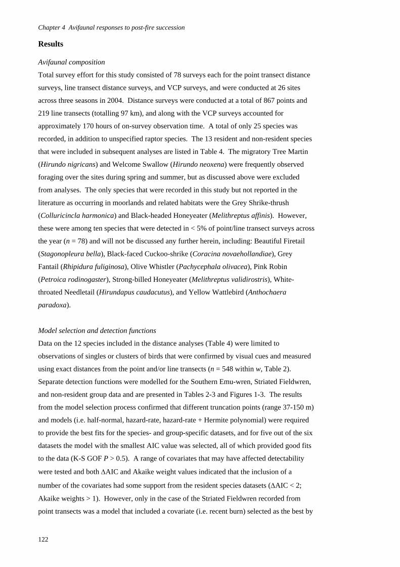
Chapter 4 Avifaunal responses to post-fire succession Results Avifaunal composition
Total survey effort for this study consisted of 78 surveys each for the point transect distance
surveys, line transect distance surveys, and VCP surveys, and were conducted at 26 sites
across three seasons in 2004. Distance surveys were conducted at a total of 867 points and
219 line transects (totalling 97 km), and along with the VCP surveys accounted for
approximately 170 hours of on-survey observation time. A total of only 25 species was
recorded, in addition to unspecified raptor species. The 13 resident and non-resident species
that were included in subsequent analyses are listed in Table 4. The migratory Tree Martin
(Hirundo nigricans) and Welcome Swallow (Hirundo neoxena) were frequently observed
foraging over the sites during spring and summer, but as discussed above were excluded
from analyses. The only species that were recorded in this study but not reported in the
literature as occurring in moorlands and related habitats were the Grey Shrike-thrush
(Colluricincla harmonica) and Black-headed Honeyeater (Melithreptus affinis). However,
these were among ten species that were detected in < 5% of point/line transect surveys across
the year (n = 78) and will not be discussed any further herein, including: Beautiful Firetail
(Stagonopleura bella), Black-faced Cuckoo-shrike (Coracina novaehollandiae), Grey
Fantail (Rhipidura fuliginosa), Olive Whistler (Pachycephala olivacea), Pink Robin
(Petroica rodinogaster), Strong-billed Honeyeater (Melithreptus validirostris), White-
throated Needletail (Hirundapus caudacutus), and Yellow Wattlebird (Anthochaera
paradoxa).
Model selection and detection functions
Data on the 12 species included in the distance analyses (Table 4) were limited to
observations of singles or clusters of birds that were confirmed by visual cues and measured
using exact distances from the point and/or line transects (n = 548 within w, Table 2).
Separate detection functions were modelled for the Southern Emu-wren, Striated Fieldwren,
and non-resident group data and are presented in Tables 2-3 and Figures 1-3. The results
from the model selection process confirmed that different truncation points (range 37-150 m)
and models (i.e. half-normal, hazard-rate, hazard-rate + Hermite polynomial) were required
to provide the best fits for the species- and group-specific datasets, and for five out of the six
datasets the model with the smallest AIC value was selected, all of which provided good fits
to the data (K-S GOF P > 0.5). A range of covariates that may have affected detectability
were tested and both AIC and Akaike weight values indicated that the inclusion of a
number of the covariates had some support from the resident species datasets (AIC < 2;
Akaike weights > 1). However, only in the case of the Striated Fieldwren recorded from
point transects was a model that included a covariate (i.e. recent burn) selected as the best by
122

Chapter 4 Avifaunal responses to post-fire succession
AIC (AIC = 0; Akaike weight = 0.760). Results for the Striated Fieldwren recorded from
line transects indicated that the no covariate model provided the best relative fit; however,
the density estimates for the recently burnt sites (i.e. MEE, MEW, HAR) appeared to be
positively biased since the model did not account for the higher detectability of the Striated
Fieldwren in the open, early successional habitat. Therefore, consistent with the point
transects the model that included the recent burn covariate was selected for the line transects
in order to provide a more plausible detection function and more accurate density estimates,
particularly since it similarly had substantial empirical support (AIC = 1.25, Akaike weight
= 0.18) and still provided a good overall fit to the data (K-S GOF Dn = 0.173, P = 0.161).
The estimated probabilities of detecting a cluster of Southern Emu-wrens, Striated
Fieldwrens, and non-resident species within the surveyed areas ( ) and the estimated
effective detection radii ( ) for points and effective strip half-widths ( ) for lines as
derived from the selected models are presented in Table 3. The probability of detecting
clusters varied due to inter-specific differences in detectability and the associated detection
functions, truncations widths, and differential responses to the method of detection. While
the detection probabilities for the Striated Fieldwren were similar between line and point
transects, those for the Southern Emu-wren were approximately three times higher and those
for the non-residents were approximately twice as high for line versus point transects. The
effective strip half-widths and effective detection radii were similar between lines and points
for both the Southern Emu-wren and non-residents, but the detection distance for the Striated
Fieldwren was substantially narrower for line versus point transects ( = 13.48 m, =
86.35 m). Larger values were expected for the point transects a priori since the area and
hence number of birds that can be detected increases linearly with distance from the point
(Buckland 2006). Nevertheless, the magnitude of the difference for the Striated Fieldwren
along with the fact that > 90% of observations within 14 m from line transects were
classified as flushing responses, while none were classified as flushing from points
regardless of distance, which suggested the species exhibited differential responses in
relation to a moving versus stationary observer.
aP
ρ μ
μ ρ
123

Chapter 4 Avifaunal responses to post-fire succession
124
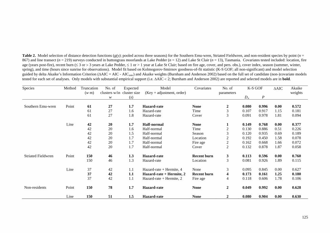
Table 2. Model selection of distance detection functions (g(y); pooled across three seasons) for the Southern Emu-wren, Striated Fieldwren, and non-resident species by point (n = 867) and line transect (n = 219) surveys conducted in buttongrass moorlands at Lake Pedder (n = 12) and Lake St Clair (n = 13), Tasmania. Covariates tested included: location, fire age (years post-fire), recent burn ( 3 or 3 years at Lake Pedder, 1 or > 1 year at Lake St Clair; based on fire age, cover, and pers. obs.), cover index, season (summer, winter, spring), and time (hours since sunrise for observations). Model fit based on Kolmogorov-Smirnov goodness-of-fit statistic (K-S GOF; all non-significant) and model selection guided by delta Akaike’s Information Criterion (AIC = AIC - AICmin) and Akaike weights (Burnham and Anderson 2002) based on the full set of candidate (non-)covariate models tested for each set of analyses. Only models with substantial empirical support (i.e. AIC 2; Burnham and Anderson 2002) are reported and selected models are in bold.
K-S GOF Species Method Truncation(w m)
No. of clusters w/in
w
Expected cluster size
(s)
Model (Key + adjustment, order)
Covariates No. of parameters
Dn P
AIC Akaike weights
Southern Emu-wren Point 61 27 1.7 Hazard-rate None 2 0.080 0.996 0.00 0.572 61 27 1.6 Hazard-rate Time 3 0.107 0.917 1.15 0.181 61 27 1.8 Hazard-rate Cover 3 0.091 0.978 1.81 0.094 Line 42 20 1.7 Half-normal None 1 0.149 0.768 0.00 0.377 42 20 1.6 Half-normal Time 2 0.130 0.886 0.51 0.226 42 20 1.5 Half-normal Season 3 0.120 0.935 0.69 0.189 42 20 1.7 Half-normal Location 2 0.192 0.450 1.58 0.078 42 20 1.7 Half-normal Fire age 2 0.162 0.668 1.66 0.072 42 20 1.7 Half-normal Cover 2 0.132 0.878 1.87 0.058 Striated Fieldwren Point 150 46 1.3 Hazard-rate Recent burn 3 0.113 0.596 0.00 0.760 150 46 1.3 Hazard-rate Location 3 0.081 0.926 1.89 0.115 Line 37 42 1.1 Hazard-rate + Hermite, 4 None 3 0.095 0.845 0.00 0.627 37 42 1.1 Hazard-rate + Hermite, 2 Recent burn 4 0.173 0.161 1.25 0.180 37 42 1.1 Hazard-rate + Hermite, 2 Fire age 4 0.118 0.606 1.78 0.106 Non-residents Point 150 78 1.7 Hazard-rate None 2 0.049 0.992 0.00 0.628 Line 150 51 1.5 Hazard-rate None 2 0.080 0.904 0.00 0.630
125
Chapter 4 Avifaunal responses to post-fire succession
Table 3. Estimated probability of clusters being detected within the surveyed area ( ), their effective detection radii (EDR, Points) and effective strip half-widths (ESW, Lines), and associated lognormal 95% confidence intervals (CI) from the selected models (see Table 2) by species and method. The EDR/ESW indicate the estimated distance from the point/line ( / ) at which as many
individuals or clusters are missed within / as detected beyond / (Buckland et al. 2001).
aP
ρ μ
ρ μ ρ μ
Method Detection probability EDR/ESW Species
aP 95% CI ρ / (m) μ 95% CI Southern Emu-wren Point 0.17 0.06 - 0.48 25.35 14.88 - 43.18 Line 0.60 0.41 - 0.88 25.23 17.15 - 37.12 Striated Fieldwren Point 0.33 0.25 - 0.44 86.35 75.20 - 99.15 Line 0.36 0.26 - 0.52 13.48 9.50 - 19.12 Non-residents Point 0.23 0.15 - 0.36 71.91 57.06 - 90.62 Line 0.52 0.42 - 0.64 77.42 62.72 - 95.57
126

Chapter 4 Avifaunal responses to post-fire succession
1.2 (a)
1.0
Det
ectio
n pr
obab
ility
0.8
0.6
0.4
0.2
0.0 10 20 30 40 50 600
Distance (m)
0.040 (b)
0.035
Pro
babi
lity
dens
ity
0.030
0.025
0.020
0.015
0.010
0.005
0.000 10 20 30 40 50 600
Distance (m)
1.6 (c)
1.4
1.2
Det
ectio
n pr
obab
ility
1.0
0.8
0.6
0.4
0.2
0.0 10 20 30 400
Distance (m)
Fig. 1. Southern Emu-wren: (a) The estimated detection probability function and corresponding (b) estimated probability density function from point transect surveys, and (c) estimated detection probability function from line transect surveys based on the selected models (Table 1) for Southern Emu-wren observations in buttongrass moorlands at Lake Pedder and Lake St Clair, Tasmania. The models are fitted to scaled histograms of observations as a function of distance (m) from the survey points/lines.
127

Chapter 4 Avifaunal responses to post-fire succession
1.2 (a)
1.0
Det
ectio
n pr
obab
ility
0.8
0.6
0.4
0.2
0.0 10 20 30 40 50 60 70 80 90 0 100 110 120 130 140 150
Distance (m)
0.016 (b)
0.014
0.012
Pro
babi
lity
dens
ity
0.010
0.008
0.006
0.004
0.002
0.000 10 20 30 40 50 60 70 80 90 0 100 110 120 130 140 150
Distance (m)
1.4 (c)
1.2
Det
ectio
n pr
obab
ility
1.0
0.8
0.6
0.4
0.2
0.0 10 20 0 30
Distance (m)
Fig. 2. Striated Fieldwren: (a) The estimated detection probability function and corresponding (b) estimated probability density function from point transect surveys, and (c) estimated detection probability function from line transect surveys based on the selected models (Table 1) and averaged over the recent burn covariate factors for Striated Fieldwren observations in buttongrass moorlands at Lake Pedder and Lake St Clair, Tasmania. The models are fitted to scaled histograms of observations as a function of distance (m) from the survey points/lines.
128

Chapter 4 Avifaunal responses to post-fire succession
1.2 (a)
1.0
Det
ectio
n pr
obab
ility
0.8
0.6
0.4
0.2
0.0 10 20 30 40 50 60 70 80 90 100 110 120 130 140 1500
Distance (m)
0.014 (b)
0.012
Pro
ba
bili
ty d
en
sity
0.010
0.008
0.006
0.004
0.002
0.000 10 20 30 40 50 60 70 80 90 100 110 120 130 140 1500
Distance (m)
(c)
0.0 908070605040 30 20 10 0
1.2
1.0
0.8
0.2
0.4
0.6
Det
ectio
n pr
obab
ility
100 110 120 130 140 150
Distance (m)
Fig. 3. Non-resident species: (a) The estimated detection probability function and corresponding (b) estimated probability density function from point transect surveys, and (c) estimated detection probability function from line transect surveys based on the selected models (Table 1) for non-resident species observations in buttongrass moorlands at Lake Pedder and Lake St Clair, Tasmania. The models are fitted to scaled histograms of observations as a function of distance (m) from the survey points/lines.
129

Chapter 4 Avifaunal responses to post-fire succession Species occurrence and density estimates
A summary of species occurrence and estimates of avian population density by species and
location are presented in Table 4 and general trends in relation to fire age are presented in
Figure 4. The Striated Fieldwren occurred at all but one site (96%; n = 25), while the
Southern Emu-wren was also widely distributed (88%). The Ground Parrot was patchily
distributed (48%), while the remaining species, except for the Tasmanian Thornbill, were
present in 50% of the sites. However, on-survey auditory observations as well as
occasional off-survey observations indicated that both use and occurrence at sites,
particularly for the resident species, may be somewhat higher than indicated by these figures.
The Southern Emu-wren had the highest estimated densities at both Lake Pedder and Lake St
Clair (1.83 and 1.64 birds 10 ha-1, respectively), followed by the Striated Fieldwren (1.08
and 1.05 birds 10 ha-1, respectively) and Ground Parrot (0.61 and 0.80 10 ha-1, respectively).
The Southern Emu-wren and Striated Fieldwren were detected across the full range of fire
ages at both Lake Pedder and Lake St Clair (3-54 and 1-32 years post-fire, respectively),
although were absent from some replicate sites within a few of the fire age classes. The only
exception is that neither was visually detected at the one 12 year post-fire site (MCR) at
Lake Pedder. However, a pair of Southern Emu-wrens were detected by call during one
survey, indicating occasional use but not occupancy. The Ground Parrot appeared to have a
more restricted distribution in relation to site fire ages at Lake Pedder and Lake St Clair (22-
54 and 3-16 years post-fire, respectively), and as with the other residents was not detected at
all replicate sites within these fire age classes. Overall, densities of the non-resident species
were higher at Lake St Clair compared to Lake Pedder, particularly in the younger age
classes (i.e. 1-3 years post-fire). Of these, the Tasmanian Thornbill, Crescent Honeyeater,
and Superb Fairy-wren occurred at the most sites and had the highest overall densities at
both locations (range 0.07-0.26 10 ha-1). The Black Currawong, Dusky Robin, and Flame
Robin were the only non-resident species included in the analyses that were only recorded at
Lake St Clair; however, off-survey observations indicated that they were present within the
Lake Pedder region. A number of the non-residents occurred across a broad range of fire
ages at Lake Pedder and/or Lake St Clair, albeit inconsistently and generally at low densities,
including the Tasmanian Thornbill, Superb Fairy-wren, Richard’s Pipit, Black Currawong,
Flame Robin, and Dusky Robin. However, the three Honeyeater species included in the
analyses appeared to primarily occur in mature to old-growth moorlands and associated edge
habitats at Lake Pedder and Lake St Clair (22-54 and 5-31 years post-fire, respectively; see
Chapters 5-6).
The survey methods that were employed for this study were primarily intended to provide
density estimates with low bias (Buckland et al. 2001); however, the moderate to large
coefficients of variation (range CV = 28-128%; Table 4) and overlapping confidence
130
Chapter 4 Avifaunal responses to post-fire succession
intervals for many of the species indicated the estimates only had moderate to low precision
at the location scale. In the case of the distance density estimates, the variability in
encounter rates and in the estimation of detection probability and cluster size all contributed
to the overall variability. For the encounter rates, the small sample sizes and limited number
of points/lines that could be established within many of the sites contributed to the high
variability (i.e. on average 82% of total variance) (Fewster and Buckland 2004).
Furthermore, no visual observations were recorded during any of the three seasons from 35%
of the points that were surveyed (n = 289), indicating that the populations were patchily
distributed both within and among sites. This was also reflected in the encounter rate
variance as well as the estimated overdispersion parameters (range b = 1-2.19), which were
nevertheless within the range identified as normal for patchily distributed biological
populations (i.e. 1 b 4, Burnham and Anderson 2002). Differences in detection
probability were also a notable source of variance (i.e. on average 17% of total variance),
while those in cluster sizes were only minor (i.e. on average 1% of total variance).
While the overall precision of the density estimates was lower than desirable, particularly at
the site scale (not reported), as is often the case for such studies, these variance estimates
provided a more honest and realistic assessment of uncertainty when compared to those
calculated by simple indices of abundance that do not take such sources of variance into
account (Casagrande and Beissinger 1997; Buckland et al. 2001; Burnham and Anderson
2002; Ellingson and Lukacs 2003; Diefenbach et al. 2007). These estimates of precision
indicated that the buttongrass moorland avifauna exhibited a high degree of variability both
within and among species, sites, and seasons; accordingly, these density estimates and
subsequent analyses should be interpreted with a degree of caution.
131

Chapter 4 Avifaunal responses to post-fire succession
132

Table 4. Summary of species occurrence and mean density estimates ( , birds 10 haD -1 ) from distance and VCP surveys conducted in buttongrass moorland sites at Lake Pedder (n = 12) and Lake St Clair (n = 13), Tasmania. Species included were present in 5% of point/line transect surveys across the year (n = 78) (excluding aerial foragers/hunters). Densities for each location were calculated as the mean of site densities weighted by site area, including sites with zero density (Buckland et al. 2001). Site densities were derived from a mean of exact point and line transect survey estimates for all species except the Ground Parrot which was only based on the VCP surveys. Variance estimates were based on a Poisson distribution with species- and group-specific overdispersion factors (range b = 1 - 2.19) and include the percent coefficient of variance (CV) and lognormal 95% confidence intervals (CI). Species are listed in decreasing order of occurrence across locations. * Denotes moorland residents.
Lake Pedder Lake St Clair
Occurrence Occurrence Species no. of 12
sites 3 - 54 yrs. post-fire
Mean D(birds 10 ha-1)
CV % Lognormal 95% CI
no. of 13 sites
1 - 31 yrs. post-fire
Mean D(birds 10 ha-1)
CV % Lognormal 95% CI
Striated Fieldwren* Calamanthus fuliginosus
11 3 - 54 1.08 28.26 0.63 - 1.86 13 1 - 31 1.05 28.76 0.61 - 1.83
Southern Emu-wren* Stipiturus malachurus
12 3 - 54 1.83 49.10 0.74 - 4.55 10 1 - 31 1.64 50.32 0.65 - 4.15
Tasmanian Thornbill Acanthiza ewingii
6 3 - 31 0.10 44.64 0.05 - 0.24 7 2 - 31 0.16 30.88 0.09 - 0.29
Crescent Honeyeater Phylidonyris pyrrhoptera
7 22 - 54 0.18 35.70 0.09 - 0.35 5 8 - 31 0.07 45.49 0.03 - 0.17
Ground Parrot* Pezoporus wallicus
7 22 - 54 0.61 128.00 0.09 - 4.21 5 3 - 16 0.80 111.72 0.14 - 4.68
Superb Fairy-wren Malurus cyaneus
3 3 - 33 0.10 44.08 0.04 - 0.23 7 1 - 31 0.26 25.71 0.16 - 0.42
New Holland Honeyeater Phylidonyris novaehollandiae
5 22 - 54 0.10 44.64 0.05 - 0.24 2 14 - 31 0.02 82.46 0.00 - 0.07
Richard's Pipit Anthus novaeseelandiae
2 3 - 31 0.06 57.01 0.02 - 0.17 5 1 - 3 0.06 43.91 0.03 - 0.14
Yellow-throated Honeyeater Lichenostomus flavicollis
2 22 - 54 0.03 79.06 0.01 - 0.11 4 5 - 30 0.06 47.55 0.02 - 0.14
Green Rosella Playcercus caledonicus
4 25 - 27 0.03 79.06 0.01 - 0.12 1 5 0.01 108.03 0.00 - 0.06
Black Currawong Strepera fuliginosa
0 0 0 0 0 4 1 - 30 0.08 41.89 0.04 - 0.17
Flame Robin Petroica phoenicea
0 0 0 0 0 4 3 - 31 0.06 48.26 0.02 - 0.15
Dusky Robin Melanodryas vittata
0 0 0 0 0 3 1 - 30 0.07 44.16 0.03 - 0.15
133
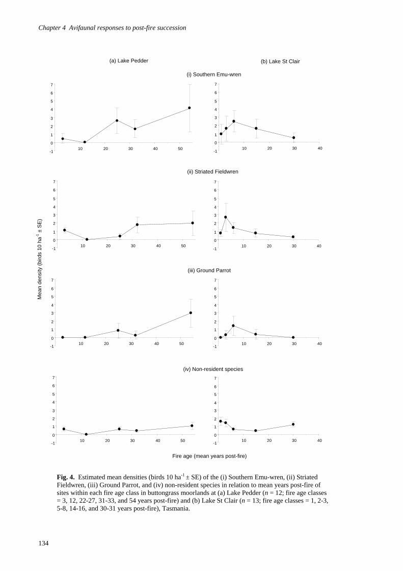
Chapter 4 Avifaunal responses to post-fire succession
(a) Lake Pedder (b) Lake St Clair
(i) Southern Emu-wren
7
Mea
n de
nsity
(bi
rds
10 h
a-1 ±
SE
)
Fig. 4. Estimated mean densities (birds 10 ha-1 ± SE) of the (i) Southern Emu-wren, (ii) Striated Fieldwren, (iii) Ground Parrot, and (iv) non-resident species in relation to mean years post-fire of sites within each fire age class in buttongrass moorlands at (a) Lake Pedder (n = 12; fire age classes = 3, 12, 22-27, 31-33, and 54 years post-fire) and (b) Lake St Clair (n = 13; fire age classes = 1, 2-3, 5-8, 14-16, and 30-31 years post-fire), Tasmania.
(ii) Striated Fieldwren
(iii) Ground Parrot
(iv) Non-resident species
Fire age (mean years post-fire)
-1
0
1
2
3
4
5
6
10 20 30
7
6
5
4
3
40-1
0
1
2
10 20 30 40 50
7
-1
0
1
2
3
4
5
6
7
10 20 30 40
6
5
4
3
2
1
0 10 20 30 40 50
-1
-1
0
1
2
3
4
5
6
7
10 20 30 40 50-1
0
1
2
3
4
5
6
7
10 20 30 40
-1
0
1
2
3
4
5
6
7
10 20 30 40 50-1
0
1
2
3
4
5
6
7
10 20 30 40
134
Chapter 4 Avifaunal responses to post-fire succession Species-habitat associations
Results from the univariate ordinary regression analyses of transformed mean avian densities
in relation to six environmental variables are presented in Table 5 and trends in mean
densities in relation to fire age classes are depicted in Figure 4. For simplicity, when
densities are subsequently referred to in relation to the univariate and multivariate analyses,
it is implied that they are transformed densities as specified in Table 5. Results from the
hierarchical partitioning analyses depicting the percentage of explained variance for both
independent and joint contributions from the full sets of environmental variables are
presented in Figures 5 and 6.
Southern Emu-wren
There was a general trend in Southern Emu-wren densities to increase with time since fire at
Lake Pedder (max. site 8.30 birds 10 ha-1), while at Lake St Clair they initially increased up
to approximately 5-8 years post-fire (max. site 4.69 birds 10 ha-1) and then gradually
decreased across the remainder of the chronosequence (Figure 4). Although fire age was not
a significant factor for the Southern Emu-wren when all of the sites were included in the
regression for Lake Pedder, an examination of residuals indicated that the site AIE had both
high influence and leverage. This is largely due to the fact that AIE was included in the
oldest fire age class at Lake Pedder and that the Southern Emu-wren was not identified by
sight during any of the surveys and hence was recorded as a density of zero based on the
exact distance analyses. However, results from the aural binomial surveys indicated that
they did occur at the site throughout the study period, but for reasons explained earlier those
data could not be incorporated into subsequent analyses. Accordingly, the regression was
conducted with the ‘false’ absence at AIE omitted, which not only improved the fit of the
correlation with fire age but also indicated that Southern Emu-wren densities significantly
increased with time since fire at Lake Pedder, explaining 66.3% of variance compared to
only 24.4% when the outlier AIE was included in the regression.
In contrast, there was no significant correlation between Southern Emu-wren densities and
fire age at Lake St Clair. As shown in Chapter 3, there was a positive although nonlinear
relationship between mean cover index and fire age at both Lake Pedder (F = 66.063; df = 1,
9; P < 0.001, R2 = 0.880) and Lake St Clair (F = 67.672; df = 1, 11; P < 0.001, R2 = 0.860).
Consequently, there was also a significant positive correlation between Southern Emu-wren
densities and cover at Lake Pedder (omitting AIE), explaining 39.6% of variance compared
to 28.3% with AIE included, while there was no apparent relationship at Lake St Clair.
There was also a significant negative correlation between densities and site area at Lake
Pedder (omitting AIE), explaining 40.7% of variance compared to 18.9% with AIE included.
135
Chapter 4 Avifaunal responses to post-fire succession Finally, site riparian area was significantly and positively correlated with densities of the
Southern Emu-wren at Lake St Clair, explaining 57.9% of variance.
In general, the results from the hierarchical partitioning for the Southern Emu-wren (Figure
5) were consistent with those from the univariate regressions. At Lake Pedder, the results
including the outlier site AIE indicated that cover made the greatest independent contribution
(29.1% explained variance), closely followed by fire age (26.2%), riparian area (21.1%), and
site area (19.3%). However, when AIE was excluded from the analysis, it was apparent that
the independent contribution from fire age amounted to more than twice that of the other
variables (49.5%) and also made the highest joint contribution (37.9%). Site area (23.3%)
and cover (20.2%) also made notable independent contributions, while that from riparian
area was substantially reduced (3.6%). In contrast, at Lake St Clair site riparian area was
clearly the most important variable (79.4%), while the other variables only had minor
independent influence (< 8%). Riparian area also had a much higher ratio of independent to
joint effects than any of the other variables, suggesting that interactions with the other
variables were relatively minor (Mac Nally 2000).
Striated Fieldwren
Overall, there was a moderate although inconsistent increase in Striated Fieldwren densities
across the chronosequence at Lake Pedder (max. site 3.95 birds 10 ha-1). At Lake St Clair
there was a marked increase in densities up to approximately 3 year post-fire (max. site 5.20
birds 10 ha-1) and then a gradual decrease across the chronosequence (Figure 4). Overall,
this resulted in a significant negative correlation with fire age at Lake St Clair, explaining
41.8% of variance. Similar to the trend in relation to fire age, Striated Fieldwren densities at
Lake St Clair were negatively correlated with cover; however, the relationship was relatively
weak and non-significant, explaining only 25.3% of variance. Correlations between Striated
Fieldwren densities and the remainder of the site variables were all non-significant, each
explaining < 12% of variance.
In general, the results from the hierarchical partitioning for the Striated Fieldwren (Fig. 5)
were consistent with those from the univariate regressions. Although there were no
significant results in relation to the variables at Lake Pedder, the hierarchical partitioning
indicated that fire age made substantially greater independent (44.5%) contributions than the
other variables, followed by site area (24.0%), while the other variables independently each
only explained < 18% of the total variance. The high joint contributions from both fire age
(44.0%) and site area (61.5%) suggested complex interrelationships with each other and the
other variables. At Lake St Clair, fire age provided the greatest independent (54.9%)
contribution, followed by cover (25.2%), while the other variables independently each only
136

Chapter 4 Avifaunal responses to post-fire succession explained < 11% of the total variance. The high joint contributions from both fire age
(42.8%) and cover (36.2%) suggested complex interrelationships with each other and the
other variables. Although the trends in densities as indicated by the univariate regressions
are opposite at Lake Pedder (positive) and Lake St Clair (negative), these results suggested
that fire age was the most important explanatory variable in relation to Striated Fieldwren
densities in buttongrass moorlands. Due to the lack of a strong correlation between densities
and fire age at Lake Pedder (R2 = 0.100), it was difficult to determine the actual direction of
the trend, if any exists.
Ground Parrot
Results from the univariate logistic regressions in relation to Ground Parrot occurrence are
presented in Table 6. At Lake Pedder, the probability of occurrence of Ground Parrots was
significantly and positively correlated with both fire age and cover, explaining 60.5% and
79.2% of variance, respectively. The results showed that Ground Parrots were more likely to
occur at older sites with higher cover values at Lake Pedder. In contrast, at Lake St Clair
there was a relatively weak and non-significant negative correlation with fire age, explaining
only 27.8% of variance, and no apparent association with cover. The Ground Parrot was the
only species for which edge contrast index was a significant factor. Similar to the analyses
for the Southern Emu-wren, one site (MCR) was identified as an outlier. This was largely
due to the fact that it was established as a relatively small research burn plot (21.22 ha)
(Marsden-Smedley 1993) within a much larger patch of moorland and thus had a very low
edge contrast index. Ground Parrots were not recorded there during any of the surveys,
although one off-survey observation indicated that some individuals may periodically use the
site. Accordingly, the regression was conducted with the outlier MCR omitted, which not
only improved the fit of the relationship but also indicated that the probability of Ground
Parrot occurrence at Lake Pedder significantly decreased at sites with high contrast edges
(e.g. a high proportion of forest edges), explaining 51.4% of variance compared to only
11.7% when the outlier MCR was included in the regression. These results indicated that
despite its low edge contrast index, MCR apparently did not provide good habitat relative to
portions of the surrounding moorlands due to its younger age and lower cover. At Lake St
Clair there was also a significant negative correlation between Ground Parrot occurrence and
edge contrast index, explaining 64.2% of variance. At Lake St Clair there was a significant
positive correlation between the probability of occurrence of Ground Parrots and the
percentage of suitable habitat found within a 400 m radius of the survey point at each site (~
50 ha), explaining 57.1% of variance. At Lake Pedder there was also a positive but non-
significant correlation (P = 0.053), explaining 36.0% of variance; however, at either location
Ground Parrots did not occur at sites with < 45% of suitable habitat within the 50 ha circles.
137

Chapter 4 Avifaunal responses to post-fire succession Results from the ordinary regressions in relation to Ground Parrot density were generally
consistent with those obtained above in relation to occurrence, largely due to the necessity to
include sites with no detections in the density dataset (see Methods). The Ground Parrot was
absent from sites < 13 years post-fire at Lake Pedder and then showed a general increase in
densities across the chronosequence (max. site 4.19 birds 10 ha-1) (Figure 4). At Lake St
Clair, it was absent from the one recently burnt site, gradually increased in density up to
approximately 5-8 years post-fire (max. site 3.19 birds 10 ha-1), and then gradually decreased
in density and was absent from the oldest sites. Similar to the above, there were significant
positive correlations between Ground Parrot densities and both fire age and cover at Lake
Pedder, explaining 56.9% and 48.9% of variance, respectively, and no significant
relationships with fire age and cover at Lake St Clair. Although Ground Parrot occurrence
did not appear to be influenced by site area, there was a significant negative correlation with
density and site area at Lake Pedder, explaining 37.4% of variance. The trend at Lake St
Clair was opposite, with densities increasing with site area, explaining 35.9% of variance.
Similar to the analyses above, there were significant negative correlations between Ground
Parrot densities and edge contrast index at Lake Pedder (excluding the high influence and
leverage MCR) and Lake St Clair, explaining 58.1% and 36.2% of variance, respectively.
Finally, the percentage of suitable habitat was also a significant factor, with densities being
higher at sites surrounded by a greater proportion of suitable habitat at Lake St Clair,
explaining 45.9% of variance, while at Lake Pedder the sites were typically found within
large, contiguous patches of moorland and hence there was a weak, non-significant
correlation, explaining only 20.5% of variance. These percentages of explained variance in
relation to density were likely to be lower than those in relation to occurrence since one
would expect that the proportions of suitable habitat beyond the sites and/or home ranges of
the more mobile Ground Parrots (i.e. at the landscape scale) would have a greater influence
on dispersal and hence occupancy than densities per se (i.e. at the site scale).
In general, the results from the hierarchical partitioning for the Ground Parrot (Fig. 6) were
consistent with those from the univariate regressions. Since the results between the
occurrence and density analyses were comparable, only the hierarchical partitioning graphs
in relation to Ground Parrot densities are presented. At Lake Pedder, the results including
the outlier site MCR indicated that fire age had the greatest independent contribution
(37.1%), followed by cover (22.7%), while those from the remainder of the variables were
all < 18%. However, when MCR was excluded from the analysis it was apparent that the
independent contribution from fire age was reduced (25.7%) while that from edge contrast
index was increased (28.0%), but those from the remainder were again < 18% and had
similar joint contributions (11-24%). At Lake St Clair, the percentage of suitable habitat had
the greatest independent (27.1%) and joint (41.8%) contribution, closely followed by the
138
Chapter 4 Avifaunal responses to post-fire succession independent contributions from edge contrast index (24.8%), area (21.8%), and fire age
(18.8%). The independent contribution from cover was only minor (7.6%) and offset by
negative joint effects (-7.5%), suggesting that the other variables may have been suppressing
the independent influence of cover (Chevan and Sutherland 1991; Mac Nally 1996b).
Non-resident species
There were no significant relationships between non-resident densities and fire age at either
Lake Pedder or Lake St Clair. The only notable pattern was a peak in non-resident mean
densities at the youngest site at Lake St Clair (i.e. 1 year post-fire), as well as a secondary
peak at the oldest sites (i.e. 30-31 years post-fire), which were the only two age classes at
either location in which mean densities exceeded those of all three resident species (Figure
4). The sole variable significantly correlated with non-resident densities was site area at
Lake St Clair, indicating decreasing densities with increasing site area and explaining 65.1%
of variance. Correlations between non-resident densities and the remainder of the site
variables were all non-significant, each explaining < 13% of variance.
In general, the results from the hierarchical partitioning for the non-resident species (Figure
6) were consistent with those from the univariate regressions. Although there were no
significant results in relation to the variables at Lake Pedder, the hierarchical partitioning
indicated that riparian area was the strongest independent correlate (36.4%), consistent with
their strong selection for riparian habitats compared to the matrix, as described in Chapter 5.
However, this was largely offset by joint negative interactions with the other variables (-
25.3%), suggesting that they may have been suppressing the independent influence of
riparian area. A similar pattern in independent contribution being offset by negative joint
interactions was also apparent for cover. Large positive joint contributions for fire age
(52.4%) and area (79.0%) suggested they had some influence on densities; however, overall
the results suggested that none of the variables had a strong independent influence on non-
resident densities, while the other variables had little independent and joint effects. At Lake
Pedder, site area clearly had the strongest independent (69.8%) and joint (151.3%)
contribution towards the overall variance, while those from the other variables were
relatively negligible. This strong contribution may have reflected the fact that they could be
more readily detected at smaller sites since a greater proportion of their preferred edge
habitats (see Chapter 5) were closer to the transects when compared to larger sites where
there was a negative bias towards detecting non-residents from the interior of the sites, as
well as a preference for such sites with a higher edge to area ratio. Furthermore, all sites at
Lake St Clair had higher edge contrast indices than any at Lake Pedder, which may have
accounted for the greater contribution of area towards variance at Lake St Clair versus Lake
Pedder. However, as stated above and indicated by the high joint contribution, area may be
139

Chapter 4 Avifaunal responses to post-fire succession
140
confounded with the influence of the other variables as well as its influence on the
calculation of bird densities.
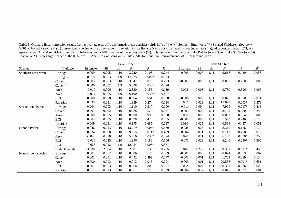
Table 5. Ordinary linear regression results from univariate tests of (transformed) mean densities (birds ha-1) of the (√ ) Southern Emu-wren, (√ ) Striated Fieldwren, (log10(y + 0.001)) Ground Parrot, and (√ ) non-resident species across three seasons in relation to site fire age (years post-fire), mean cover index, area (ha), edge contrast index (ECI, %), riparian area (%), and suitable Ground Parrot habitat within a 400 m radius of the survey point (%), in buttongrass moorlands at Lake Pedder (n = 12) and Lake St Clair (n = 13), Tasmania. * Denotes significance at the 0.05 level. ^ Analyses excluding outlier sites (AIE for Southern Emu-wren and MCR for Ground Parrot). Lake Pedder Lake St Clair Species Variable Estimate SE df F P R2 Estimate SE df F P R2 Southern Emu-wren Fire age 0.009 0.005 1,10 3.220 0.103 0.244 -0.005 0.007 1,11 0.617 0.449 0.053 Fire age ^ 0.014 0.003 1,9 17.675 0.002* 0.663 Cover 0.005 0.003 1,10 3.947 0.075 0.283 -0.001 0.003 1,11 0.090 0.770 0.008 Cover ^ 0.006 0.002 1,9 5.898 0.038* 0.396 Area -0.010 0.006 1,10 2.330 0.158 0.189 0.003 0.003 1,11 0.780 0.396 0.066 Area ^ -0.014 0.005 1,9 6.190 0.035* 0.407 ECI 0.000 0.008 1,10 0.004 0.951 0.000 -0.008 0.009 1,11 0.875 0.370 0.074 Riparian 0.035 0.031 1,10 1.339 0.274 0.118 0.089 0.023 1,11 15.099 0.003* 0.579 Striated Fieldwren Fire age 0.004 0.003 1,10 1.110 0.317 0.100 -0.011 0.004 1,11 7.909 0.017* 0.418 Cover 0.001 0.002 1,10 0.428 0.528 0.041 -0.003 0.002 1,11 3.731 0.080 0.253 Area 0.000 0.005 1,10 0.000 0.993 0.000 0.000 0.003 1,11 0.003 0.954 0.000 ECI 0.004 0.005 1,10 0.690 0.426 0.065 -0.008 0.006 1,11 1.500 0.246 0.120 Riparian 0.009 0.021 1,10 0.175 0.685 0.017 0.019 0.025 1,11 0.594 0.457 0.051 Ground Parrot Fire age 0.046 0.013 1,10 13.219 0.005* 0.569 -0.038 0.025 1,11 2.315 0.156 0.174 Cover 0.024 0.008 1,10 9.555 0.011* 0.489 -0.004 0.011 1,11 0.147 0.708 0.013 Area -0.048 0.020 1,10 5.976 0.035* 0.374 0.028 0.011 1,11 6.160 0.030* 0.359 ECI -0.036 0.025 1,10 1.996 0.188 0.166 -0.073 0.029 1,11 6.246 0.030* 0.362 ECI ^ -0.076 0.022 1,9 12.454 0.006* 0.581 Suitable habitat 3.830 2.384 1,10 2.581 0.139 0.205 3.818 1.250 1,11 9.331 0.011* 0.459 Non-resident species Fire age 0.001 0.002 1,10 0.086 0.776 0.009 -0.001 0.003 1,11 0.024 0.879 0.002 Cover 0.001 0.001 1,10 0.492 0.499 0.047 -0.002 0.001 1,11 1.703 0.219 0.134 Area 0.000 0.003 1,10 0.012 0.915 0.001 -0.005 0.001 1,11 20.556 0.001* 0.651 ECI 0.001 0.003 1,10 0.066 0.802 0.007 0.003 0.004 1,11 0.331 0.576 0.029 Riparian 0.012 0.013 1,10 0.861 0.375 0.079 -0.004 0.017 1,11 0.045 0.837 0.004
141
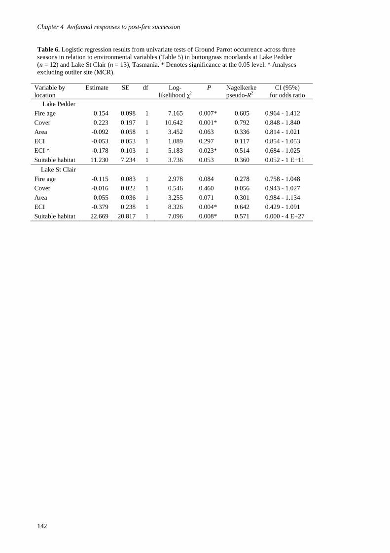
Chapter 4 Avifaunal responses to post-fire succession Table 6. Logistic regression results from univariate tests of Ground Parrot occurrence across three seasons in relation to environmental variables (Table 5) in buttongrass moorlands at Lake Pedder (n = 12) and Lake St Clair (n = 13), Tasmania. * Denotes significance at the 0.05 level. ^ Analyses excluding outlier site (MCR).
Variable by location
Estimate SE df Log-likelihood χ2
P Nagelkerke pseudo-R2
CI (95%) for odds ratio
Lake Pedder
Fire age 0.154 0.098 1 7.165 0.007* 0.605 0.964 - 1.412
Cover 0.223 0.197 1 10.642 0.001* 0.792 0.848 - 1.840
Area -0.092 0.058 1 3.452 0.063 0.336 0.814 - 1.021
ECI -0.053 0.053 1 1.089 0.297 0.117 0.854 - 1.053
ECI ^ -0.178 0.103 1 5.183 0.023* 0.514 0.684 - 1.025
Suitable habitat 11.230 7.234 1 3.736 0.053 0.360 0.052 - 1 E+11
Lake St Clair
Fire age -0.115 0.083 1 2.978 0.084 0.278 0.758 - 1.048
Cover -0.016 0.022 1 0.546 0.460 0.056 0.943 - 1.027
Area 0.055 0.036 1 3.255 0.071 0.301 0.984 - 1.134
ECI -0.379 0.238 1 8.326 0.004* 0.642 0.429 - 1.091
Suitable habitat 22.669 20.817 1 7.096 0.008* 0.571 0.000 - 4 E+27
142
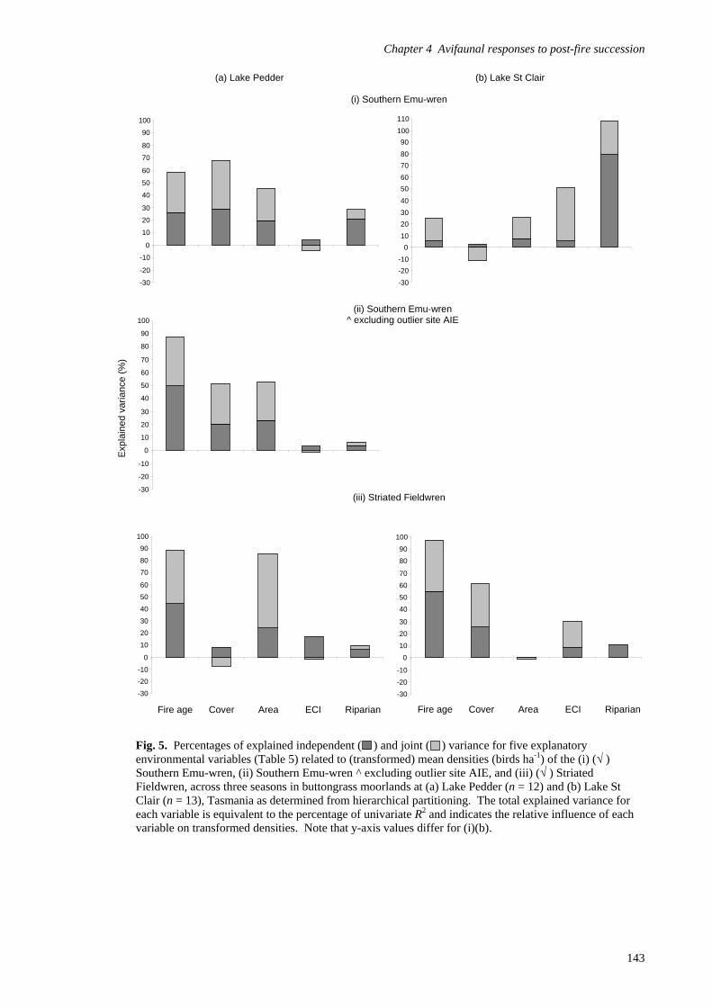
Chapter 4 Avifaunal responses to post-fire succession
(a) Lake Pedder (b) Lake St Clair
(i) Southern Emu-wren
110
Fig. 5. Percentages of explained independent ( ) and joint ( ) variance for five explanatory environmental variables (Table 5) related to (transformed) mean densities (birds ha-1) of the (i) (√ ) Southern Emu-wren, (ii) Southern Emu-wren ^ excluding outlier site AIE, and (iii) (√ ) Striated Fieldwren, across three seasons in buttongrass moorlands at (a) Lake Pedder (n = 12) and (b) Lake St Clair (n = 13), Tasmania as determined from hierarchical partitioning. The total explained variance for each variable is equivalent to the percentage of univariate R2 and indicates the relative influence of each variable on transformed densities. Note that y-axis values differ for (i)(b).
-30
-20
-10
0
10
20
30
40
50
60
70
80
90
100
100
10090 9080 8070 70
60
50
6050
40 40
30 30
20 2010 100 0
-10 -10
-20 -20
-30-30
(ii) Southern Emu-wren ^ excluding outlier site AIE
Exp
lain
ed v
aria
nce
(%)
(iii) Stri ed Fieldwrenat
90
100 100
-30
-20
-10
0
10
20
30
40
50
60
70
80
Fire age Cover Area ECI Riparian Fire age Cover Area ECI Riparian
90
80
70
60
50
40
30
20
10
0
-10
-20
-30
143

Chapter 4 Avifaunal responses to post-fire succession
144
(a) Lake Pedder (b) Lake St Clair
Fig. 6. Percentages of explained independent ( ) and joint ( ) variance for five explanatory environmental variables (Table 5) related to (transformed) mean densities (birds ha-1) of the (i) ((log10(y + 0.001)) Ground Parrot, (ii) Ground Parrot ^ excluding outlier site MCR, and (iii) (√ ) non-resident species, across three seasons in buttongrass moorlands at (a) Lake Pedder (n = 12) and (b) Lake St Clair (n = 13), Tasmania as determined from hierarchical partitioning. The total explained variance for each variable is equivalent to the percentage of univariate R2 and indicates the relative influence of each variable on transformed densities. Note that y-axis values differ for (iii)(b).
-40
-20 0
20 40
60
80100
120
140
160 180
200
220
240
-30
-20
-10
0
10
20
30
40
50
60
70
80
90
100
(i) Ground Parrot
-30
-20
-10
0
10
20
30
40
50
60
70
80
90
100
-20
-10
0
10
20
30
40
50
60
70
80
90
100
-30
100
90
80
70
60
50
40
30
20
10
0
-10
-20
(ii) Ground Parrot ^ excluding outlier site MCR
Exp
lain
ed v
aria
nce
(%)
-30
Fire age Cover Area ECI Suitable
Fire age Cover Area ECI Suitable habitat habitat
(iii) Non-resident species
Fire age Cover Area ECI Riparian Fire age Cover Area ECI Riparian
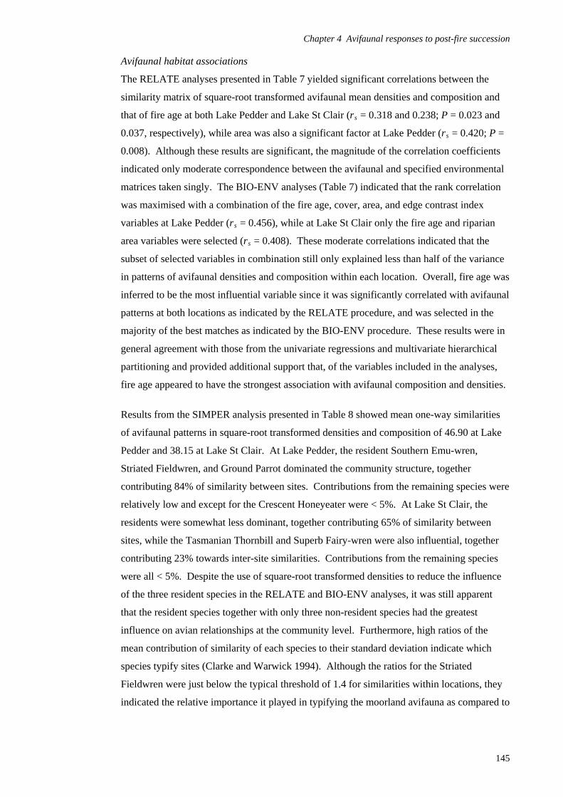
Chapter 4 Avifaunal responses to post-fire succession
Avifaunal habitat associations
The RELATE analyses presented in Table 7 yielded significant correlations between the
similarity matrix of square-root transformed avifaunal mean densities and composition and
that of fire age at both Lake Pedder and Lake St Clair (rs = 0.318 and 0.238; P = 0.023 and
0.037, respectively), while area was also a significant factor at Lake Pedder (rs = 0.420; P =
0.008). Although these results are significant, the magnitude of the correlation coefficients
indicated only moderate correspondence between the avifaunal and specified environmental
matrices taken singly. The BIO-ENV analyses (Table 7) indicated that the rank correlation
was maximised with a combination of the fire age, cover, area, and edge contrast index
variables at Lake Pedder (rs = 0.456), while at Lake St Clair only the fire age and riparian
area variables were selected (rs = 0.408). These moderate correlations indicated that the
subset of selected variables in combination still only explained less than half of the variance
in patterns of avifaunal densities and composition within each location. Overall, fire age was
inferred to be the most influential variable since it was significantly correlated with avifaunal
patterns at both locations as indicated by the RELATE procedure, and was selected in the
majority of the best matches as indicated by the BIO-ENV procedure. These results were in
general agreement with those from the univariate regressions and multivariate hierarchical
partitioning and provided additional support that, of the variables included in the analyses,
fire age appeared to have the strongest association with avifaunal composition and densities.
Results from the SIMPER analysis presented in Table 8 showed mean one-way similarities
of avifaunal patterns in square-root transformed densities and composition of 46.90 at Lake
Pedder and 38.15 at Lake St Clair. At Lake Pedder, the resident Southern Emu-wren,
Striated Fieldwren, and Ground Parrot dominated the community structure, together
contributing 84% of similarity between sites. Contributions from the remaining species were
relatively low and except for the Crescent Honeyeater were < 5%. At Lake St Clair, the
residents were somewhat less dominant, together contributing 65% of similarity between
sites, while the Tasmanian Thornbill and Superb Fairy-wren were also influential, together
contributing 23% towards inter-site similarities. Contributions from the remaining species
were all < 5%. Despite the use of square-root transformed densities to reduce the influence
of the three resident species in the RELATE and BIO-ENV analyses, it was still apparent
that the resident species together with only three non-resident species had the greatest
influence on avian relationships at the community level. Furthermore, high ratios of the
mean contribution of similarity of each species to their standard deviation indicate which
species typify sites (Clarke and Warwick 1994). Although the ratios for the Striated
Fieldwren were just below the typical threshold of 1.4 for similarities within locations, they
indicated the relative importance it played in typifying the moorland avifauna as compared to
145
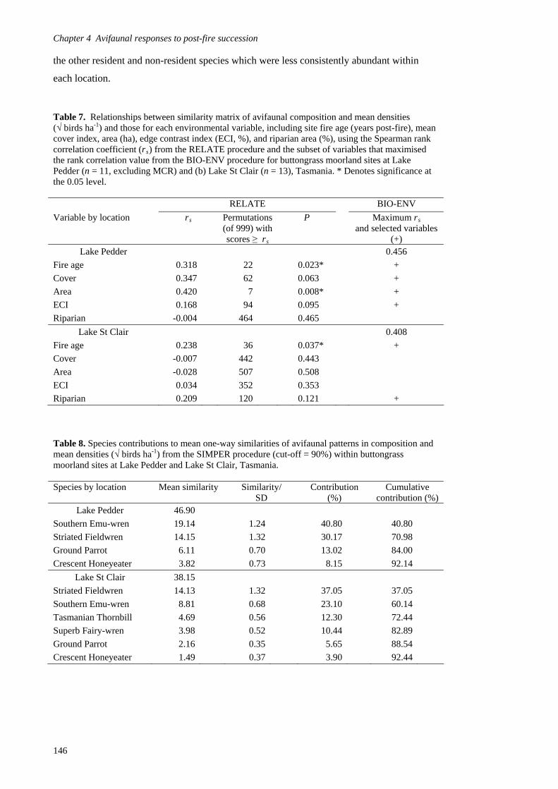
Chapter 4 Avifaunal responses to post-fire succession the other resident and non-resident species which were less consistently abundant within
each location.
Table 7. Relationships between similarity matrix of avifaunal composition and mean densities (√ birds ha-1) and those for each environmental variable, including site fire age (years post-fire), mean cover index, area (ha), edge contrast index (ECI, %), and riparian area (%), using the Spearman rank correlation coefficient (rs) from the RELATE procedure and the subset of variables that maximised the rank correlation value from the BIO-ENV procedure for buttongrass moorland sites at Lake Pedder (n = 11, excluding MCR) and (b) Lake St Clair (n = 13), Tasmania. * Denotes significance at the 0.05 level.
RELATE BIO-ENV
Variable by location rs Permutations (of 999) with scores ≥ rs
P Maximum rs
and selected variables (+)
Lake Pedder 0.456
Fire age 0.318 22 0.023* +
Cover 0.347 62 0.063 +
Area 0.420 7 0.008* +
ECI 0.168 94 0.095 +
Riparian -0.004 464 0.465
Lake St Clair 0.408
Fire age 0.238 36 0.037* +
Cover -0.007 442 0.443
Area -0.028 507 0.508
ECI 0.034 352 0.353
Riparian 0.209 120 0.121 + Table 8. Species contributions to mean one-way similarities of avifaunal patterns in composition and mean densities (√ birds ha-1) from the SIMPER procedure (cut-off = 90%) within buttongrass moorland sites at Lake Pedder and Lake St Clair, Tasmania. Species by location Mean similarity Similarity/
SD Contribution
(%) Cumulative
contribution (%) Lake Pedder 46.90
Southern Emu-wren 19.14 1.24 40.80 40.80
Striated Fieldwren 14.15 1.32 30.17 70.98
Ground Parrot 6.11 0.70 13.02 84.00
Crescent Honeyeater 3.82 0.73 8.15 92.14
Lake St Clair 38.15
Striated Fieldwren 14.13 1.32 37.05 37.05
Southern Emu-wren 8.81 0.68 23.10 60.14
Tasmanian Thornbill 4.69 0.56 12.30 72.44
Superb Fairy-wren 3.98 0.52 10.44 82.89
Ground Parrot 2.16 0.35 5.65 88.54
Crescent Honeyeater 1.49 0.37 3.90 92.44
146

Chapter 4 Avifaunal responses to post-fire succession
Discussion Overall patterns in avifaunal occurrence and densities
This is the first comprehensive and quantitative study of the avifauna of Tasmanian
buttongrass moorlands. During the course of surveys, a total of only 25 species were
recorded, in addition to unspecified raptor species, and amounted to 45% of the 55 species
reported in the literature as having been observed in buttongrass moorlands and associated
habitats in Tasmania (see Table 1, Chapter 1). Based on occurrence and relative density
data, this study provides the first quantitative evidence that the core avian community of
buttongrass moorlands is composed of only three year-round resident species within the
study area that depend exclusively on moorlands for breeding, feeding, and other resource
needs, namely the Southern Emu-wren, Striated Fieldwren, and Ground Parrot. Only 12
other species, in addition to unspecified raptors, occurred in more than 5% of all point/line
transect surveys. Since none of these species were continuously present and many of them
occurred in relatively low densities and were primarily associated with adjacent ecotonal,
scrub, woodland, and forest habitats (Watts 2002; see Chapter 5), they should be regarded as
marginal or periodic users of moorlands within the study area. The remaining 10 species
were rarely observed and are not species typically expected in moorlands. Thus, the results
from this study generally concur with previous qualitative accounts (e.g. Ridpath and
Moreau 1966; Brown et al. 1993; Driessen 2006; see Chapter 1) and demonstrate that the
avifauna of Tasmanian buttongrass moorlands has a relatively low species richness
characterised by only three year-round resident specialist species and approximately 12 non-
resident species in the study area, including those listed in Table 4 and the Welcome
Swallow and Tree Martin, both common summer migrants (pers. obs.; see Chapter 1).
However, the actual number of species and the community composition likely varies with
geography, site attributes, season, and the precise definitions of ‘moorland’ habitat and
‘characteristic’ species that have been used by various authors (P. Brown pers. comm. 2005;
see Chapter 1). For the purposes of this discussion, inferences from the distance sampling
surveys are limited to the study area, including sites at Lake Pedder and Lake St Clair, and
should not be extrapolated to the landscape as a whole (Buckland et al. 2008).
Overall, the observed patterns of avifaunal occurrence and density across the space-for-time
fire chronosequences at Lake Pedder and Lake St Clair were complex and revealed high
levels of variability within and among species, sites, and locations. Dissimilarities in
composition and densities were partially explained by differences in location (i.e. moorland
type, soil productivity, and altitude), fire age, cover, and habitat composition and
configuration. Measures of avian richness and density in particular are often implicitly
assumed to be positively correlated with habitat quality per se. Habitat quality is defined as
the relative suitability of an area to support a reproducing population of a given resident
147
Chapter 4 Avifaunal responses to post-fire succession species (i.e. carrying capacity) (Maurer 1986; Hobbs and Hanley 1990) and quantified as the
product of density, survival, and reproductive success (Van Horne 1983). However, this
assumption has often not been fully validated since it is necessary to obtain detailed
demographic data (e.g. survival, reproduction, dispersal) from the population(s) of interest to
make reliable inferences for management (Van Horne 1983; Hobbs and Hanley 1990;
Wheatley et al. 2002). In particular, species-specific factors such as territoriality, fecundity,
dispersal, and niche breadth, as well as environmental factors such as temporal (e.g.
disturbance related time-lags) and spatial (e.g. patchiness) heterogeneity of resources may
result in what are deemed low- or moderate-quality habitats supporting higher densities than
those considered high-quality habitats (Fretwell and Lucas 1969; Van Horne 1983; Vickery
et al. 1992; Hobbs and Hanley 1990; Vierling 1999; Wheatley et al. 2002). Furthermore, in
dynamic landscapes such as within the study area, the complex interrelationships of source
and sink habitats in both space and time make it even more difficult to solely explain the
observed patterns in densities with site-level attributes (Dunning et al. 1992; Brawn and
Robinson 1996). As was the case with this study, detailed demographic data are rarely
available due to the resource intensive nature of such studies, particularly for cryptic species
such as the moorland residents. In the absence of such data and for the purpose of this
discussion, it is necessary to assume that there is an as yet undetermined, although
presumably positive, relationship between species densities and habitat suitability. A
literature review by Bock and Jones (2004) indicated that this may be a reasonable
assumption in most cases. If detailed demographic and multi-year survey data become
available in the future, the results from this study should be reassessed in order to elucidate
the nature of these relationships and their underlying processes, particularly in relation to the
resident species. Given this limitation, it is currently difficult to make any definitive
statements concerning the habitat relationships of the moorland avifauna. Nevertheless,
some important patterns have emerged that provide a better understanding of this previously
little studied avian community and represents an important first step for more informed
management of buttongrass moorland ecosystems and future research on the avifauna.
The resident Southern Emu-wren, Striated Fieldwren, and Ground Parrot dominated the
avifauna in terms of site occupancy, estimated densities, and inter-site similarities in
community structure at Lake Pedder and Lake St Clair, consistent with expectations based
on previous accounts of the moorland avifauna (see Table 1, Chapter 1). Both the Striated
Fieldwren and Southern Emu-wren were nearly ubiquitous throughout the study area, while
the Ground Parrot was patchily distributed and occurred at just under half of the study sites.
The only non-resident species that notably contributed (i.e. > 5%) to avian relationships at
the community level are relatively common and widespread species (Watts 2002; pers. obs.),
including the Crescent Honeyeater at Lake Pedder and the Tasmanian Thornbill and Superb
148

Chapter 4 Avifaunal responses to post-fire succession
Fairy-wren at Lake St Clair. The remaining non-resident species occurred inconsistently
across the study area and were primarily associated with adjacent woodland and forest
habitats (see Chapter 5).
As with the avifaunas of other pyrogenic vegetation communities in Australia and abroad
(for reviews see Woinarski 1999a, 1999b; Saab and Powell 2005; and Chapter 7), the results
from this study suggest that fire is one of the primary factors that influence both the
composition and densities of bird species in Tasmanian buttongrass moorlands over the
course of successional time scales (i.e. ~ 1 to > 50 years post-fire). In particular, fire age
was identified as a significant independent factor in relation to the densities of the three
resident species at Lake Pedder and/or Lake St Clair, and in maximising rank correlations of
similarity matrices at the community level at both locations. In addition, there were notable
joint interactions between fire age and the other explanatory variables discussed below,
suggesting that some of the inter-site variability could be attributed to complex interactions
between the habitat variables included in the analyses. These results, along with those from
Chapters 5-6, are more thoroughly discussed in Chapter 7 in relation to similarly depauperate
sedgeland and heathland communities within a national and global context, as well as
models of post-fire faunal succession within a theoretical context.
Species occurrence in relation to post-fire succession
Overall, patterns in species occurrence in relation to time since last fire appeared to reflect
the relative suitability of different seral stages of post-fire vegetation in relation to the
specific niche breadths and habitat preferences of the resident and non-resident species in the
study area (see Chapters 1 and 3). The Southern Emu-wren and Striated Fieldwren were
detected across the full range of fire ages at both locations (3-54 at Lake Pedder, 1-32 years
post-fire at Lake St Clair; except MCR for the former, see below). Although to date no
formal studies have been conducted on either species in Tasmanian moorlands, the Lyell
Highway Fire Management Plan and references therein (PWS 1996, citing Gellie 1980 and
Brown et al. 1993) provided limited and principally qualitative information. In contrast to
the results from this study, it suggested that the Southern Emu-wren does not inhabit sites <
9 years post-fire, while it reported that it was unknown whether it inhabited sites > 15 years
post-fire. In the case of the Striated Fieldwren, it reported that it was known to inhabit sites
3-11 years post-fire, while it was unknown whether it inhabited younger or older sites.
Based on the present study, it is apparent that both younger and older sites can provide
suitable resources to enable use and/or occupancy by the Southern Emu-wren and Striated
Fieldwren.
149
Chapter 4 Avifaunal responses to post-fire succession The Ground Parrot appeared to have a more restricted distribution in relation to site fire ages
when compared to the other resident species (22-54 at Lake Pedder, 3-16 years post-fire at
Lake St Clair). While the Ground Parrot was absent at sites < 22 years post-fire at Lake
Pedder and < 3 and > 16 years post-fire at Lake St Clair, previous research on the Ground
Parrot in Tasmanian moorlands by Bryant (1991, 1992, 1994) identified Ground Parrots
across the full range of sites investigated in Tasmania (including blanket and eastern
moorlands), from 1-90 years post-fire by flushing and from 2 months to > 30 years post-fire
by call surveys. However, due to the fact that extensive surveys were conducted throughout
the state for her study, it is not surprising that the results from the present geographically
limited study indicated a more restricted occupancy of sites in relation to time since fire at
both Lake Pedder and Lake St Clair. It should be noted that no species were visually
detected at the one 12 year post-fire site (MCR) at Lake Pedder during the survey. This site
was considered to be an outlier since it was a relatively small research burn plot adjacent to
older moorlands with greater cover (see Chapter 2), and thus presumably provided a less
suitable habitat for the cover-dependent resident species. Nevertheless, both on-survey
auditory and off-survey visual detections of the Southern Emu-wren and Ground Parrot,
respectively, indicated occasional use, but not occupancy, of this site. Due to the lack of
availability and hence replication of sites between 3 and 22 years post-fire at Lake Pedder, it
is difficult to make any definitive inferences regarding possible trends between these fire
ages in blanket moorlands for any of the species. In particular, in the case of the Ground
Parrot, the limited representation of younger sites coupled with the slower rate of post-fire
vegetative recovery of these low productivity sites may have resulted in some bias towards
older blanket moorlands relative to patterns of occupancy in a statewide context (Bryant
1991).
Among the non-resident species, the Tasmanian Thornbill, Superb Fairy-wren, Richard’s
Pipit, Black Currawong, Flame Robin, and Dusky Robin occurred across a broad range of
fire ages at Lake Pedder and/or Lake St Clair, albeit inconsistently. However, the Crescent,
New Holland, and Yellow-throated Honeyeater species included in the analyses appeared to
primarily occur in mature to old-growth moorlands and associated edge habitats at Lake
Pedder and Lake St Clair (i.e. 22-54 and 5-31 years post-fire, respectively; see Chapter 5).
In contrast, results presented in Chapter 6 demonstrated that all three species utilised recently
burnt moorlands and that short-term densities may increase under some conditions. It should
be noted that the necessity of pooling the non-resident species into a single class may have
masked more definitive species-specific patterns of occurrence in relation to fire age.
150

Chapter 4 Avifaunal responses to post-fire succession
Species densities in relation to post-fire succession
All three resident species demonstrated qualitatively similar, although variable, patterns in
post-fire changes in densities. The Southern Emu-wren had the highest estimated mean
densities at both Lake Pedder and Lake St Clair (1.83 and 1.64 birds 10 ha-1, respectively),
followed by the Striated Fieldwren (1.08 and 1.05 birds 10 ha-1, respectively), and Ground
Parrot (0.61 and 0.80 10 ha-1, respectively). Intra-specific mean densities and inter-specific
ranks of densities across fire ages were remarkably similar between locations. These
densities are within the range of those reported in previous studies conducted in Tasmania
and/or on the mainland for the Southern Emu-wren, Striated Fieldwren, and Ground Parrot,
despite considerable differences in survey methods, analyses, and environmental variables in
comparison to this study (Table 9).
Table 9. Comparison of density ranges (birds 10 ha-1) of resident species of Tasmanian buttongrass moorlands reported in previous studies conducted in Australia. Species Density range
(birds 10 ha-1) Habitat, State, Reference
Southern Emu-wren 0.4-45.0 Heathland, NSW, Jordan 1987a; dry and wet heathland, QLD, McFarland 1988b, 1994; sedgeland, shrubland, banksia-eucalypt forest, NSW, Wood 1995; low heathland, NSW, Gosper and Baker 1997; heathland, VIC, Maguire 2006b
Striated Fieldwren 0.6-9.0 Samphire shrubland, VIC, Watson 1955; low heathland, NSW, Gosper and Baker 1997; regrowth dry sclerophyll forest, TAS, Taylor et al. 1997
Ground Parrot 0.2-6.5 Sedgleland and heathland, VIC, Meredith and Isles 1980; heathland, NSW, Jordan 1987b; dry and wet heathland, QLD, McFarland 1988b, 1991c; heathland, WA, Burbidge 1989; sedgeland and graminoid heathland (i.e. buttongrass moorland), TAS, Bryant 1991
The lowest mean densities of the residents generally occurred within the youngest sites
surveyed at Lake Pedder and Lake St Clair (i.e. 3 and 1 years post-fire, respectively). At
Lake Pedder, the resident species generally increased in densities across the chronosequence,
with the highest mean densities at the oldest sites surveyed (i.e. 54 years post-fire), which for
the Striated Fieldwren were at least two times the densities at the youngest sites, and for the
Southern Emu-wren up to over ten times. At Lake St Clair, the mean densities of the
residents peaked between 2-8 years post-fire, after which they all gradually declined to their
lowest densities at the oldest sites surveyed (i.e. 30-31 years post-fire). For the Ground
Parrot, the peaks in densities ranged from at least three times those at the oldest sites, and for
the Striated Fieldwren they were up to over ten times. Despite the apparent trends in mean
densities in relation to fire age (Figure 4), they were only statistically significant within a
linear model for the Southern Emu-wren and Ground Parrot at Lake Pedder (positive) and
the Striated Fieldwren at Lake St Clair (negative). Species-specific comparisons between
151

Chapter 4 Avifaunal responses to post-fire succession this study and previous research provide a broader context in which to assess these results
and are discussed below.
Although this is the first study to investigate the influence of fire on Southern Emu-wrens in
Tasmanian moorlands, studies conducted on the mainland have shown some comparable
post-fire trends in occupancy and densities (see Chapter 1). Studies to date likewise indicate
that Southern Emu-wrens were either absent or present in substantially reduced numbers
soon after disturbance by fire and did not start to increase until one to a few years post-fire
(Jordan 1987a; McFarland 1988b, 1994; Reilly 1991a; Loyn 1997). The relatively
fragmented nature of their habitats on the mainland may pose additional issues in relation to
post-fire recolonisation due to the limited dispersal capabilities of Southern Emu-wrens.
This is particularly the case for extensive wildfires, since the longest recorded movements to
date are only 1.2 km for juveniles (Maguire and Mulder 2004) and approximately 2.5 km for
adults (Pickett 2000). Although the trend of Southern Emu-wren densities in relation to fire
age at Lake St Clair was not significant, data indicated initially low post-fire densities,
followed by a rapid increase and peak at approximately 2-8 years, and then a gradual decline
to their lowest densities at the oldest sites sampled (i.e. 30-31 years post-fire). This trend of
post-fire reduction, recovery, and decline has also been reported in other studies. For
example, Jordan (1987a) observed Southern Emu-wrens populations did not increase rapidly
until a year after fire and were most abundant 2-3 years post-fire (~ 40 birds 10 ha-1).
McFarland (1988b) reported densities of 0.8 birds 10 ha-1 at 2.5 years post-fire, 1.2 birds 10
ha-1 at 5.5 years, and 0.4 birds 10 ha-1 at 6.5 years, while none were reported in the 0 and
10.5 year old heathland sites in southeastern Queensland. McFarland (1994) also reported
that their highest densities of 2.0-2.5 birds 10 ha-1 were at 6-8 year old sites, and that no nests
were found in heathlands < 2 and > 10.5 years post-fire. However, trends from these
mainland studies are in contrast to those at Lake Pedder, where Southern Emu-wrens
significantly increased in densities across the chronosequence (i.e. > 50 years post-fire).
This may be attributed to the less productive soils and associated slower post-fire recovery of
Tasmanian blanket moorlands when compared to some sites on the mainland. Nevertheless,
it is not possible to determine whether a similar trend exists in other portions of the Southern
Emu-wren’s range since previous studies on the mainland either included a limited range of
fire ages (i.e. 9 years post-fire; McFarland 1994) and/or did not provide site age data for
pre-fire surveys (Loyn 1997).
Only limited and mostly qualitative information is available on the fire ecology of Striated
Fieldwrens. Early records indicated the loss of natural habitat through ‘burning off’ (Legge
1908). Gellie (1980) stated that they are capable of finding sufficient food and cover almost
immediately after fire, and have been observed foraging on recently burnt moorlands in
152
Chapter 4 Avifaunal responses to post-fire succession
Tasmania. He further stated that breeding cycles may be interrupted if fires occur during
spring, and breeding may not be successful for 5-7 years post-fire unless adequate unburnt
patches are available; however, he provided no supporting data. Taylor et al.’s (1997) study
on changes in the avifauna of dry sclerophyll forests with sedgy and heathy understories in
southeast Tasmania indicated that the Striated Fieldwren occurred in significantly higher
densities in young regrowth (0-6 years old) when compared to older regrowth coupes (6-12
years old) following clearfall logging, regeneration burns, and portions of both coupes being
subsequently burnt by a wildfire; however, they were absent from mature forest (> 12 years
old). Observations of Striated Fieldwrens in southwestern Australia suggest that they
recolonise heath once sufficient post-fire cover is attained (Smith 1985; Hopkins and Smith
1996 in Woinarski 1999a, 1999b). Since they are considered to be an early successional
species in some portions of their range, it has been postulated that long-term fire exclusion
may render some heaths unsuitable for Striated Fieldwrens (Smith 1985, 1987; Woinarski
1999a). In support of this, results from Lake St Clair indicated that mean density peaked
within 2-3 years post-fire at Lake St Clair and overall, there was a significant decrease in
density across the full chronosequence when tested within a linear model. However, results
from Lake Pedder, although not statistically significant, indicated that longer inter-fire
intervals may be required for the Striated Fieldwren to reach maximum densities in lower
productivity, blanket moorlands in southwestern Tasmania, since the highest densities were
recorded in older sites (i.e. 31-54 years post-fire).
The only prior research focused on the Ground Parrot in Tasmania is that of Bryant (1991,
1992, 1994). Despite the fact that similar methods were used to survey Ground Parrots in
this study and Bryant’s, there are a number of issues that make it difficult to directly
compare results. In contrast to this study, Bryant excluded sites with zero density in her
analyses, and conducted global analyses across all statewide surveys and hence different
locations, moorland types, productivity levels, and altitudes (Bryant 1991). She also did not
differentiate between sites > 30 years post-fire for her fire age analysis, and did not clearly
delineate all site boundaries by fire age (Bryant 1991, S. Bryant pers. comm. 2003). The
latter may have resulted in density estimates being based upon observations of Ground
Parrots that occurred across areas of multiple fire ages. Such potential sources of variation
may have been exacerbated by the use of multiple observers who were probably less familiar
with the boundaries of sites within a given purported fire age.
Despite the issues associated with comparing the results of this study with Bryant’s, there are
still some important assessments that can be made. Where possible, results from this study
were re-analyzed (not reported in Results) using Bryant’s method (1991) to make findings
more comparable. She noted that recolonisation occurred at most sites approximately 1 year
153

Chapter 4 Avifaunal responses to post-fire succession post-fire (Bryant 1991, 1994), while results from this study indicated that Ground Parrots did
not occupy sites until at least 3 years post-fire at Lake St Clair and 22 years post-fire at Lake
Pedder. However, Ground Parrots have been noted to use sites soon after fires in Tasmania,
in conjunction with adjacent unburnt habitat (Gellie 1980). Such younger sites, especially
with small copses of older and denser vegetation, may provide adequate cover and become
temporarily crowded within larger burnt areas (Meredith et al. 1984; Bryant 1991). Bryant
(1991) found a significant positive correlation between Ground Parrot densities and fire age.
When results for this study were reanalyzed, there was likewise a significant positive
correlation between density and fire age across locations. Bryant reported that densities
typically remained low until 4-7 years post-fire, when they peaked at approximately 2.2 birds
10 ha-1. Densities were then maintained above the global mean of 1.7 birds10 ha-1
(compared to a mean 1.5 birds10 ha-1 for this study, excluding sites with zero density) until
approximately 13 years post-fire, after which densities declined but remained above
approximately 1.0 birds 10 ha-1 at sites 30 years post-fire and older. While the results from
Lake St Clair likewise indicated that peak densities (excluding zeros) occurred at sites
approximately 5 years post-fire and were then followed by a gradual decline, there was no
significant relationship between density and fire age (both with and without sites with zero
density). Similar to Bryant’s global analyses, there was a significant positive relationship
between density and fire age at Lake Pedder (both with and without sites with zero density).
However, peak mean densities occurred at sites over 50 years post-fire and exceeded those of
Bryant’s (i.e. > 2.2 birds 10 ha-1), though they were similar to the range of maximum
densities that she recorded across locations (i.e. ~ 5.3 birds 10 ha-1). Thus, this study
indicated that the relationships between Ground Parrot densities and fire age differed notably
between locations, namely low productivity, low altitude blanket moorland sites at Lake
Pedder and moderate productivity, moderate altitude eastern moorland sites at Lake St Clair.
Results from the majority of studies conducted on the mainland likewise show strong
associations between Ground Parrot densities and fire age and appear to reflect both the
patterns of post-fire changes in densities identified in this study. These include post-fire
reductions and gradual increases in densities with populations remaining present in long-
unburnt sites, such as in the graminoid heathlands of Lake Pedder, and post-fire reductions
followed by densities peaking and then declining toward local extinction at various ages
post-fire, such as in the sedgelands of Lake St Clair. As an example of a similar pattern to
that at Lake Pedder, research conducted in a heathland site at Barren Grounds Nature
Reserve, New South Wales indicated that the population peaked (~ 4.0 birds 10 ha-1) at 13
years post-fire (Baker and Whelan 1994, Whelan and Baker 1999) and ongoing monitoring
has indicated that they are still present, although unlike at Lake Pedder apparently declining
after more than 20 years post-fire (Baker 2002; Tasker and Baker 2005). Although the
154

Chapter 4 Avifaunal responses to post-fire succession
Western Ground Parrot of Western Australia is a different subspecies (P. w. flaviventris), as
at Lake Pedder they have been reported to reach their highest densities in long-unburnt
heathlands (i.e. > 40 years post-fire) (Burbidge 1996, 2003; Burbidge et al. 2007). They can
also utilise recently burnt sites (i.e. < 6 years post-fire) if they are directly adjoined by
unburnt habitat with established populations, and they appear to prefer areas with a mosaic
of vegetation ages (Burbidge 1996, 2003; Burbidge et al. 2007; Gibson et al. 2007). As an
example of a similar pattern to that at Lake St Clair, studies conducted in Victoria showed
that Ground Parrots recolonised graminoid heathlands within 3 years post-fire, gradually
increased to maximum density at 15 years post-fire (i.e. ~ 3.0 birds 10 ha-1), and then rapidly
declined to zero at sites over 20 years post-fire (Meredith and Isles 1980; Meredith et al.
1984). A similar, although shortened pattern also occurred in Queensland, where Ground
Parrots returned to subtropical heathland sites within 1 year post-fire, peaked at 5-8 years
post-fire (4.0-5.0 10 ha-1), while none were recorded at sites more than 14 years post-fire
(McFarland 1991c). These examples illustrate the array of patterns of post-fire changes in
densities that Ground Parrots exhibit across their range, possibly reflecting regional
differences in rainfall and other factors, which in turn affect the rate of vegetation regrowth.
In this sense, vegetation structure (e.g. cover) and floristics (e.g. seed production) may have
a greater influence on Ground Parrot densities than fire age per se (Meredith et al. 1984;
McFarland 1991c; Baker and Whelan 1994). This highlights the need for site-specific data
on which to base appropriate management recommendations, particularly in relation to inter-
fire intervals that will maximise likelihood of persistence over both space and time.
Overall, there were no consistent patterns in the densities of the non-resident group in
relation to time since fire at either Lake Pedder or Lake St Clair. However, the necessity of
pooling the non-resident species into a single group masked some species-specific patterns
of density in relation to fire age. In general, the use of moorlands by the non-resident species
appeared to reflect species-specific habitat and food requirements in relation to
characteristics of moorlands at different seral stages (see Chapter 1). Based upon species
occurrence, densities, and contributions toward community similarities at Lake Pedder and
Lake St Clair, the Tasmanian Thornbill, Superb Fairy-wren, and Crescent Honeyeater
dominated the non-resident group across the chronosequences. The limited information
available from previous studies on the fire ecology of the non-resident species found in
moorlands and adjacent vegetation communities was primarily focused on the short-term
effects of fire on habitat use in comparison to ‘unburnt’ habitat; additional details on these
effects are provided in Chapter 6. Survey data from this study indicated that there were five
relatively common non-resident species found in recently burnt sites (i.e. 1-3 years post-fire)
at both locations. These include Richard’s Pipit, Dusky Robin, Black Currawong, Superb
Fairy-wren, and Tasmanian Thornbill, although the latter two were more often recorded
155
Chapter 4 Avifaunal responses to post-fire succession utilising edge habitat (see Chapter 5). These five non-resident species primarily accounted
for the higher mean densities of non-resident species when compared to those of the resident
species at the youngest site surveyed at Lake St Clair (i.e. 1 year post-fire). Although the use
of recently burnt habitat by these species is supported by previous observations in Tasmania
and on the mainland, none appear to be restricted to early successional habitats (Green and
Mollison 1961; Ratkowsky 1978, 1985; Gellie 1980; Smith 1985; Brown et al. 1993; Loyn
1997; Woinarski and Recher 1997; Woinarski 1999b; Paton et al. 2005; Recher 2005). The
Crescent, New Holland and Yellow-throated Honeyeaters recorded in this study appeared to
prefer mature to old-growth moorlands, consistent with studies conducted in other habitats in
Tasmania (Ratkowsky 1979, 1985; Taylor et al. 1997). In contrast, results presented in
Chapter 6 demonstrated that all three species utilised recently burnt moorlands and that
short-term densities may increase under some conditions. Finally, although the Green
Rosella was relatively uncommon, previous research also indicates that it more typically
occurs in ‘unburnt’ forested habitats (Ratkowsky 1979, 1985).
Avifaunal habitat associations
Fire and its short- to long-term effects on buttongrass moorlands clearly play an important
role in the varying levels of use by the resident and, to a lesser degree, non-resident bird
species and subsequent patterns in densities across the fire chronosequences. However, a
number of the other possible explanatory environmental variables included in this study were
also found to both independently and jointly influence densities of the avifauna across the
chronosequences. These variables help to further explain the apparently patchy distribution
and variable densities of the avifauna, particularly the cover-dependent residents, both
between sites within the same fire age class and within different fire age classes at each
location.
Change in vegetation cover is the only environmental variable included in this study that is
significantly related to time since fire from both a statistical and ecological perspective (see
Chapters 1 and 3). The rate of vegetative recovery is determined by the respective peat soil
properties and hence productivity of the sites at Lake Pedder (i.e. low) and Lake St Clair (i.e.
moderate) (see Chapter 2). All three resident species are dependent on adequate vegetative
cover (Meredith et al. 1984; Gosper and Baker 1997; Wilson and Paton 2004; see Chapter
1); however, change in cover across the chronosequences was only a significant positive
factor in relation to the densities of the Southern Emu-wren and Ground Parrot at Lake
Pedder. The delay in recolonisation by Southern Emu-wrens may be partly attributed to their
need for adequate vegetative cover for foraging and shelter (Gellie 1980; Schodde 1982;
Pickett 2000; Wilson and Paton 2004; Maguire 2006a; MacHunter et al. 2009). In the case
of the Ground Parrot, Bryant (1991, 1994) did not find a significant correlation between
156
Chapter 4 Avifaunal responses to post-fire succession
densities and total percentage cover, although she noted that recolonisation occurred at most
sites approximately 1 year post-fire, when the estimated minimal projective foliage cover of
30% was typically attained. This apparent discrepancy with the results from this study at
Lake Pedder may be due to the fact that she measured foliage projective cover (after Specht
1981) as opposed to using an index of vegetation cover (after Driessen 1999; see Chapter 2)
and conducted her analyses across all moorland types and locations. As for the Striated
Fieldwren, the Ground Parrot has been noted to be less cover-dependent than the Southern
Emu-wren (Gellie 1980), presumably if adequate unburnt or partially burnt vegetation is
available at the territory scale. In contrast to the low productivity sites at Lake Pedder, cover
was not a significant influence on the resident or non-resident species at the moderate
productivity sites at Lake St Clair. This may be attributed to the relatively rapid rate of post-
fire vegetative recovery of these sites (i.e. ~ 20 vs. 5 years post-fire, respectively; see
Chapter 3). From a theoretical standpoint, these observations are consistent with Fox’s
(1982, 1990a, 1990b) habitat accommodation model for animal succession. Fox’s model
states that within some faunal communities species will appear, peak, and then may
disappear in a sequence that can be predicted based upon species-specific habitat
requirements (e.g. low vs. high cover) and the rate of vegetative recovery. The attributes of
a given fire regime (e.g. intensity, season, frequency, patchiness) may influence these
successional processes and patterns in both space and time. However, it is the continuum of
vegetational changes and associated habitat suitability thresholds or ranges that determines
the timing of faunal succession and not time since fire per se (Fox 1982, 1990a, 1990b;
Meredith et al. 1984; Baker and Whelan 1994; Monamy and Fox 2000). The differing
results between avifaunal responses at low productivity sites at Lake Pedder versus moderate
productivity sites at Lake St Clair and associated differences in post-fire vegetation
succession provide additional support for the habitat accommodation model (se Chapter 7).
Variations in vegetation cover are not only exhibited between sites of different fire ages and
locations, but also within sites due to finer-scale differences in both abiotic and biotic factors
that influence patterns in vegetation composition and structure, fire effects, and post-fire
recovery of buttongrass moorlands (Jarman et al. 1988a; see Chapter 1). The vegetation of
riparian zones along the numerous watercourses that intersect the moorland sites differ in
both composition and structure from the surrounding matrix and thus provide a relatively
discrete avian microhabitat that is dominated by emergent shrubs, particularly in the eastern
moorlands of Lake St Clair (see Chapters 1, 3, and 5). There was a significant, positive
relationship between mean densities of the Southern Emu-wren and the areal percentage of
riparian zones at Lake St Clair, which accounted for the highest independent contribution of
any variable for the Southern Emu-wren at either location. There were also positive,
although non-significant, relationships between mean densities of the Southern Emu-wren
157

Chapter 4 Avifaunal responses to post-fire succession and riparian area at Lake Pedder, as well as the Striated Fieldwren at both locations. The
higher fuel moisture levels associated with small drainages can limit or prevent combustion
with the result that unburnt or partially burnt riparian zones serve as ‘biological legacies’
(sensu Franklin et al. 2000) that both directly and indirectly contribute to post-fire recovery.
For example, in the case of the one recently burnt site at Lake St Clair (HAR, 1 year post-
fire), an area search the day after the fire (T. Chaudhry unpublished data) as well as data
from the distance surveys indicated that the unburnt riparian vegetation along the drainages
provided adequate cover to enable Southern Emu-wrens to at least periodically use the site
and enable Striated Fieldwrens to occupy it continuously post-fire. These results are
consistent with previous research on the Australian mainland and abroad that likewise
indicated that such small unburnt or partially burnt patches of vegetation in sedgeland and
heathland habitats, particularly if available at the territory scale, may enable Southern Emu-
wrens and other cover-dependent, territorial passerines to persist in the post-fire
environment, although often in reduced numbers (Recher 1981; Recher and Christensen
1981; Rowley and Brooker 1987; Reilly 1991a, 1991b; Beyers and Wirtz 1995; Pickett
2005; Bain et al. 2008).
Furthermore, even in highly fragmented habitats such as those found in the Mt Lofty Ranges
of South Australia, observations of Southern Emu-wrens indicate that they are capable of
persisting and possibly breeding in long and narrow or very small patches of high quality
swamp vegetation (Littely and Cutten 1996). Although Gellie’s (1980) observations of
Striated Fieldwrens in Tasmanian moorlands indicated that they can persist in recently burnt
moorlands, observations from this study suggested that such use may depend on the
availability of adequately sized and dispersed patches of unburnt or partially burnt post-fire
refugia that are often associated with riparian zones. In contrast to the Southern Emu-wren
and Striated Fieldwren, relationships between mean densities of the Ground Parrot and the
non-resident species with riparian area differed between locations. Along with fire age,
riparian area maximised the rank correlation between similarity matrices and avifaunal
composition and densities at Lake St Clair, indicating that both variables help to account for,
although they are not necessarily causal of, inter-site similarities at the community level
(Clarke and Gorley 2001). Overall differences in results between locations at the species and
community levels may be attributed to the greater structural and floristic diversity across fire
ages provided by riparian habitats at Lake St Clair compared to the sedge-dominated matrix
of these eastern moorlands, whereas such differences between habitats are less pronounced
in the scrub-dominated blanket moorlands at Lake Pedder (see Chapter 3).
Results from Chapter 5 indicated that the use, and hence value, of riparian zones for the
resident and non-resident bird species in both low and moderate productivity moorlands was
158
Chapter 4 Avifaunal responses to post-fire succession
disproportionately high compared to their extent in the moorland landscape (i.e. < 5% of
study area). Both the Southern Emu-wren and Striated Fieldwren used riparian habitats
significantly more than expected across the full range of fire ages at both locations and both
the resident and non-resident groups were more likely to select riparian habitat at Lake St
Clair when compared to Lake Pedder. In the case of moorlands of moderate productivity at
Lake St Clair, where the arthropod surveys were conducted, selection for these habitats by
insectivorous birds reflected the greater availability of potential arthropod prey across fire
ages. Furthermore, peak mean densities of the Southern Emu-wren and Striated Fieldwren
overlapped with those of mean abundance and energy content of arthropod prey resources in
relation to fire age. However, the discrepancy between years of sampling and fire ages
between the avian and arthropod surveys maked it difficult to provide any definitive
statements regarding their relationship and possible interaction with fire. Nevertheless, the
evidence suggested that sites with higher proportions of riparian zones, at least at Lake St
Clair, provide preferred riparian microhabitats that support higher carrying capacities and
thus densities of the two insectivorous resident species. At least in the case of the Southern
Emu-wren, this was associated with significantly higher densities at sites with greater
proportions of riparian areas. Possible mechanisms underlying the higher relative selection
probabilities for riparian zones in relation to matrix habitat are detailed in Chapter 5.
The spatial configuration of vegetation communities at the site to landscape scales were also
related to avifauna densities to varying degrees. Site area was a significant negative factor
for the Southern Emu-wren and Ground Parrot at Lake Pedder and non-resident species at
Lake St Clair, while it was a significant positive factor for the Ground Parrot at Lake St Clair
and in relation to inter-site similarities at the community level at Lake Pedder. However,
elucidating the effects of site area on densities is complicated by a number of factors,
including criteria used for the selection and delineation of sites (see Chapter 2), habitat use
(e.g. higher selection of edge habitats by non-resident species; see Chapter 5), the relatively
well-connected moorland matrix, especially at Lake Pedder, and the fact that site area is a
component of, and significantly correlated with, other spatial metrics (e.g. shape index) (see
Chapters 2-3). In this sense, site area as defined may not be commensurate with the
characteristics that influence individual and species-specific site selection (i.e. from an
‘organism’s perspective’ after McGarigal and Marks 1995) and hence densities.
Accordingly, the underlying mechanisms that contributed to the observed patterns are
unclear, but may be partly influenced by the independent and joint influence of other habitat
variables. Such locational variability in the influence of patch area on bird species
abundance and richness has been found in other studies and likewise attributed to scalar
issues and the influence of other location-specific habitat variables (e.g. McGarigal and
McComb 1995; Mac Nally and Watson 1997; Johnson and Igl 2001). In relation to the
159
Chapter 4 Avifaunal responses to post-fire succession Ground Parrot, it should be noted that although area was relatively weakly related to
densities at both locations, the logistic analysis indicated that area did not have a significant
influence on occupancy in either case. This may be attributed to the minimum moorland
patch size (i.e. 5 ha) used as a site selection criterion to ensure that sites were of an adequate
size to support at least one breeding pair of the three resident species (see Chapters 1-2). In
relation to edge contrast index and the percentage of suitable habitat, results indicated that
Ground Parrot occurrence and densities were significantly higher at sites with lower contrast
edges at both locations, and at sites at Lake St Clair with a higher percentage of suitable
habitat within a 400 m radius of survey points. There were weaker, although still positive
relationships between occurrence and densities with the percentage of suitable habitat at
Lake Pedder. On average, sites at Lake Pedder had notably lower edge contrast and a higher
percentage of adjacent suitable habitat, reflecting the characteristic ecological differences
and hence distribution of blanket versus eastern moorlands within the landscape mosaic (see
Chapter 1). Nevertheless, at either location Ground Parrots did not occur at sites with < 45%
of suitable habitat within the 50 ha circles, indicating a threshold response within the study
area. A study conducted in subtropical heathlands in New South Wales likewise indicated
that Ground Parrots required relatively large tracts of suitable habitat (i.e. > 300 ha) to enable
occupancy (Martin and Catterall 2001), with the higher threshold likely due to the highly
fragmented condition of heathlands on the mainland when compared to the relatively
extensive and contiguous tracts of suitable habitat found in the TWWHA (see Chapter 1).
Although Ground Parrots are relatively strong fliers, have been recorded dispersing over
long distances, and have been noted dispersing between suitable habitat patches separated by
non-habitat (Forshaw 1981; see Chapter 1), sites that are primarily bordered by high contrast
woodlands and forests and isolated from other moorlands possibly inhibit dispersal and
persistence, at least in the short-term. These relationships between Ground Parrot
occurrence and densities and the spatial configuration of moorlands may help to partially
explain the relatively patchy distribution of Ground Parrots throughout the study area, and
particularly at Lake St Clair, when compared to the widespread Southern Emu-wren and
Striated Fieldwren.
Limitations
The results from this study highlight the complexity of fire-adapted ecosystems and inherent
difficulties in elucidating patterns in avifaunal composition and densities and their
underlying processes. The limitations of space-for-time (SFT) study designs in particular,
and fire ecology studies in general, as well as the measures incorporated into this study to
help ameliorate them are detailed in Chapter 2 and herein. The primary limitation of SFT
studies is that inferences may be weakened due to the possibility of inter-site variability in
abiotic and biotic factors confounding or compounding observed differences in populations
160

Chapter 4 Avifaunal responses to post-fire succession
161
from any effects of fire per se (McFarland 1991c; Whelan 1995; Loyn 1999; Woinarski
1999b; Paton et al. 2005). Previous research on Australian heathland birds indicates that
populations may fluctuate greatly from year to year due to climatic and other factors,
highlighting the limitations of short-term studies such as this one (i.e. only 1 year of
observations), while some sites may support higher species richness irrespective of fire age
(Rowley and Brooker 1987; Maron et al. 2005; Paton et al. 2005). In addition, apparent
changes in species composition and densities after a given fire event may not be
representative of ‘typical’ responses due to differences in fire-specific and regime-specific
characteristics (Loyn 1999; Woinarski 1999b; Bradstock et al. 2005; Bain et al. 2008; see
Chapter 2). Furthermore, there may be time lags between a fire event (or events) and faunal
responses at the individual and population levels; thus, observed patterns may reflect
conditions of a younger age class as well as longer-term site history (Wiens 1985; Knick and
Rotenberry 2000). This wide range of potential explanatory spatiotemporal variables cannot
typically be measured and included in a given study due to resource constraints and
analytical limitations such as those resulting from highly stratified study designs and limited
sample sizes, as was the case for this study (Buckland et al. 2001; Marques et al. 2007).
Such limitations may also increase bias and the possibility of both Type I and Type II errors,
but can be partially addressed by the a priori incorporation of applicable theory and adequate
replication, as was attempted for this study (Whelan 1995; Anderson et al. 2001a, 2001b;
Buckland et al. 2001; Quinn and Keough 2002).
The results from this study are further discussed in Chapter 7, particularly in relation to the
persistence of the resident species through changes in fire regimes since European
colonisation despite exhibiting fire-sensitive attributes, and their overall implications for
avifaunal conservation and fire management of Tasmanian buttongrass moorlands.

162
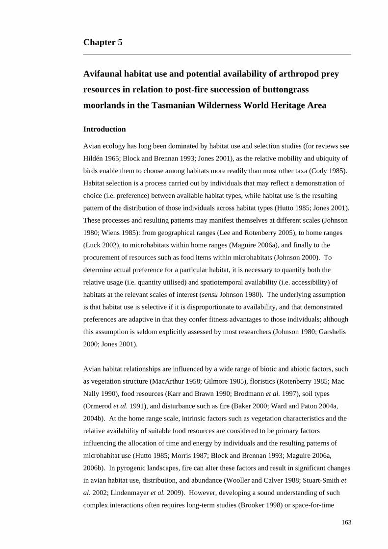
Chapter 5
Avifaunal habitat use and potential availability of arthropod prey
resources in relation to post-fire succession of buttongrass
moorlands in the Tasmanian Wilderness World Heritage Area
Introduction Avian ecology has long been dominated by habitat use and selection studies (for reviews see
Hildén 1965; Block and Brennan 1993; Jones 2001), as the relative mobility and ubiquity of
birds enable them to choose among habitats more readily than most other taxa (Cody 1985).
Habitat selection is a process carried out by individuals that may reflect a demonstration of
choice (i.e. preference) between available habitat types, while habitat use is the resulting
pattern of the distribution of those individuals across habitat types (Hutto 1985; Jones 2001).
These processes and resulting patterns may manifest themselves at different scales (Johnson
1980; Wiens 1985): from geographical ranges (Lee and Rotenberry 2005), to home ranges
(Luck 2002), to microhabitats within home ranges (Maguire 2006a), and finally to the
procurement of resources such as food items within microhabitats (Johnson 2000). To
determine actual preference for a particular habitat, it is necessary to quantify both the
relative usage (i.e. quantity utilised) and spatiotemporal availability (i.e. accessibility) of
habitats at the relevant scales of interest (sensu Johnson 1980). The underlying assumption
is that habitat use is selective if it is disproportionate to availability, and that demonstrated
preferences are adaptive in that they confer fitness advantages to those individuals; although
this assumption is seldom explicitly assessed by most researchers (Johnson 1980; Garshelis
2000; Jones 2001).
Avian habitat relationships are influenced by a wide range of biotic and abiotic factors, such
as vegetation structure (MacArthur 1958; Gilmore 1985), floristics (Rotenberry 1985; Mac
Nally 1990), food resources (Karr and Brawn 1990; Brodmann et al. 1997), soil types
(Ormerod et al. 1991), and disturbance such as fire (Baker 2000; Ward and Paton 2004a,
2004b). At the home range scale, intrinsic factors such as vegetation characteristics and the
relative availability of suitable food resources are considered to be primary factors
influencing the allocation of time and energy by individuals and the resulting patterns of
microhabitat use (Hutto 1985; Morris 1987; Block and Brennan 1993; Maguire 2006a,
2006b). In pyrogenic landscapes, fire can alter these factors and result in significant changes
in avian habitat use, distribution, and abundance (Wooller and Calver 1988; Stuart-Smith et
al. 2002; Lindenmayer et al. 2009). However, developing a sound understanding of such
complex interactions often requires long-term studies (Brooker 1998) or space-for-time
163

Chapter 5 Habitat use and prey resources
(SFT) substitutions when such studies are not feasible (Pickett 1989; Loyn 1999; Woinarski
1999b).
Buttongrass moorland is a globally unique and highly pyrogenic vegetation community
(Brown et al. 1993; Balmer et al. 2004; Harris and Kitchener 2005) that covers extensive
areas in Tasmania (0.55 million ha), and most notably in the Tasmanian Wilderness World
Heritage Area (TWWHA, 335,000 ha) (Balmer et al. 2004; TVMP 2004; see Chapter 1).
Despite such expanses, buttongrass moorlands support a relatively depauperate avifauna that
is comprised of only three cryptic ground-dwelling resident species that are known to depend
exclusively upon moorlands for survival and reproduction within the study area, namely the
Southern Emu-wren (Stipiturus malachurus), Striated Fieldwren (Calamanthus fuliginosus),
and Ground Parrot (Pezoporus wallicus), and a small number of transient species that are
typically associated with adjacent woodland and related habitats (Brown et al. 1993; see
Chapters 1, 4, and 6). Although buttongrass moorlands have been regarded as a structurally
uniform habitat for birds (Brown et al. 1993), they are comprised of a range of vegetation
communities that differ in both structure and floristics, particularly in response to fire
(Jarman et al. 1988a; see Chapters 1 and 3).
To date, only Bryant (1991, 1994) has conducted a study on habitat use and the diet of a
Tasmanian buttongrass moorland resident; however, this was limited to the granivorous
Ground Parrot and did not consider the effects of the availability of habitat or food resources
on habitat selection. The Southern Emu-wren, Striated Fieldwren, and the avian community
as a whole have not been studied in Tasmanian moorlands. On the Australian mainland,
only one detailed use versus resource availability study has been conducted by Maguire
(2006a) on the Southern Emu-wren in Victoria; however, this was on a different subspecies,
in an area with highly fragmented habitats unlike those found in the TWWHA, and did not
consider the effects of fire. Other studies on the mainland such as that by McFarland
(1991a) on the Ground Parrot in Queensland did not formally analyse use versus availability
and that by Gosper and Baker (1997) on the Striated Fieldwren in New South Wales only
provided a qualitative assessment of occupied habitat (Gosper and Baker 1997). Relatively
few studies in general have focused on the food resources available to insectivorous birds
(Poulin and Lefebvre 1997). Only one study by Maguire (2006b) has examined nestling
provisioning and arthropod availability of the Southern Emu-wren. Even fewer have
investigated the effects of fire on food resources of the Australian avifauna in any more than
a speculative manner (Woinarski 1999a), and no such studies have been attempted in
buttongrass moorlands. Previous research on terrestrial arthropods in buttongrass
moorlands, particularly in relation to fire, has been limited to studies conducted by
Greenslade (1997), Greenslade and Driessen (1999), Greenslade and Smith (1999) and
164

Chapter 5 Habitat use and prey resources
Driessen and Greenslade (2004), and a collaborative SFT research project (M. Driessen
unpublished data). Clearly, there is a significant need for multidisciplinary research on the
effects of fire on avian habitat use and food resources in order to provide more ecologically
sound and holistic guidelines to resource managers (Woinarski 1999b).
This study compares habitat selection by the buttongrass moorland avifauna between three
habitats at different stages of post-fire succession and attempts to relate that use to the
potential availability of arthropod prey. The primary aims of this study were 1) to
investigate whether the avifauna use habitats disproportionately in relation to availability and
fire age within low productivity blanket moorlands at Lake Pedder and moderate
productivity eastern moorlands at Lake St Clair in the TWWHA; 2) to investigate whether
patterns of habitat use of insectivores reflect the potential availability of arthropod prey
resources in relation to habitat type and fire age at Lake St Clair; 3) to describe and compare
the terrestrial arthropod community between moorland matrix and riparian habitats; and 4) to
provide information to assist with fire management and conservation of the buttongrass
moorland avifauna in the TWWHA.
Methods General rationale
Habitat use data were collected during the course of distance sampling surveys conducted
throughout 2004 for the space-for-time study presented in Chapter 4. Since distance
sampling was primarily intended to collect data on bird densities, behavioural observations
were limited to the initial visual observation to provide a general sense of the behavioural
cues eliciting an observation. After the completion of the 2004 SFT surveys, a pilot study
was conducted to assess the feasibility of conducting detailed behavioural surveys, with the
primary goal of obtaining data on foraging behaviour for the Southern Emu-wren and
Striated Fieldwren. Such quantitative measures of foraging behaviour have been
recommended by Hutto (1990) to provide a way of checking whether measures of food
availability are biologically meaningful. However, it was determined that such a study was
not feasible in consideration of the limited time and resources remaining for this thesis.
Furthermore, it should be noted that such comprehensive studies on the Southern Emu-wren
and Striated Fieldwren are inherently difficult due to their cryptic nature, in addition to the
other issues associated with obtaining detailed behavioural observations in the field. This
difficulty has been noted by other researchers (M. Pickett pers. comm. 2005; J. Baker pers.
comm. 2005; Maguire and Mulder 2004) and reflected in the lack of formal studies on
foraging behaviour in the literature (for reviews see Higgins et al. 2001; Higgins and Peter
2002), with the recent exception of Maguire (2006b). In the absence of adequate data on the
foraging behaviour of the target species in Australia in general, and Tasmanian moorlands in
165
Chapter 5 Habitat use and prey resources
particular, it is assumed that foraging time spent in the specified habitats is roughly
proportional to overall habitat use and is thus indicative of the relative importance of these
habitats to their feeding ecology (Morse 1971; Hutto 1985).
An initial assessment of the habitat use data indicated that the avifauna appeared to be
selecting both riparian and edge habitats disproportionately to their availability within both
study locations and that the strongest preference seemed to be for riparian habitats at Lake St
Clair. To investigate some of the potential factors that may have been contributing to these
observed patterns, a post hoc study of the availability of food resources was initiated but was
limited to comparing only matrix and riparian habitats at Lake St Clair due to resource and
time constraints. In addition, as over 95% of habitat use observations were of species that
are either entirely or partially insectivorous (see Chapter 1), the investigation of food
resources was limited to potential arthropod prey. Although it would have been desirable to
conduct this study synchronously with the habitat use surveys, the arthropod sampling could
not be conducted until the summer of 2006. This delay limits the strength of inferences that
can be drawn between the habitat use and prey resource data largely due to associated post-
fire successional changes in vegetation and, in turn, those of the arthropod and avian
communities. Furthermore, two of the study sites were burnt by PWS during 2005.
Therefore, site ages have been changed accordingly between the two datasets. Despite these
obvious limitations, these studies are presented together to preserve the original intent, but
the two datasets are not formally analysed together in recognition of these issues. Finally,
for simplicity the term ‘habitat’ is used throughout this paper, although according to some
definitions the vegetation communities identified in this study (i.e. matrix, riparian zone,
edge) can also be regarded as ‘microhabitats’ as they are the primary habitat components
within individual home ranges in the study area (Morris 1987; Block and Brennan 1993).
Study area
Details on the study design and area, and site descriptions, fire histories, vegetation
configurations, and floristics are provided in Chapters 2 and 3. Analyses were conducted
primarily in relation to site attributes including proportional habitat area (i.e. matrix, riparian
zone, edge) and fire age (years post-fire). The habitat use study included 10 of the 12 sites at
Lake Pedder (3-54 years post-fire) and 12 of the 14 sites at Lake St Clair (1-31 years post-
fire) primarily within the TWWHA as well as adjacent land allocations. The four sites
excluded from the analyses (i.e. MCR, CCN, SCN, GIT) did not contain all three habitat
types and their inclusion would have violated one of the underlying assumptions of the
habitat use analyses: all habitat types must be accessible to all birds at the appropriate scale
(Manly et al. 2002). The arthropod availability study was conducted at 11 sites at Lake St
Clair, also excluding SCS, as PWS conducted prescribed burns at the site during autumn
166

Chapter 5 Habitat use and prey resources
2005 and again in spring 2005 because the first burn failed to meet fuel reduction objectives
(T. Norris pers. comm. 2005). In addition, prescribed burns were conducted at TRR on April
21, 2005 and NPE on September 21, 2005 (see Chapter 6). Thus, these sites were
reclassified as (less than) one year old, while the remaining sites were reclassified as being
two years older than as defined in Chapter 2 and were analysed as exact ages (i.e. < 1-32
years post-fire).
Habitat use surveys
Habitat use data were collected through the course of distance sampling surveys conducted
during the summer (2 February - 9 March), winter (24 May 24 - 6 July), and spring (11
October - 27 November) of 2004. Details on the study design, fire histories, and survey
methods and conditions are provided in Chapters 2- 4. Only initial visual observations of
birds utilising habitats within the sites were recorded to determine proportional usage, as
recommended by Bell et al. (1990). This was also done to eliminate the potentially high bias
if auditory cues alone were used to estimate which habitats were being used. Birds observed
flying were only recorded if their subsequent movements indicated that they were using
specific habitat features on the ground. Thus, aerial feeders such as Welcome Swallows and
other birds that were observed flying above or across the site were excluded from
consideration. In addition, since mature trees in adjacent woodland edges and large wood
copses were not considered to be affected by the moorland surface fires, birds observed in
the primary canopy were likewise not recorded. Care was taken to avoid double counting of
individual birds by noting the observation time, their relative location (e.g. left or right of
transect), and maintaining a mental map of their locations. Conspecifics that were observed
in close proximity to each other (i.e. ~ < 10 m apart) and exhibited behaviours consistent
with those of a pair bond or family group were recorded as a cluster. All such visual
observations were recorded as occurring in either the matrix, riparian, or edge habitats along
with any details of the habitats being used (e.g. structure and location).
Species-specific habitat use could not be analysed due to limited sample sizes (see below);
therefore, all species recorded were classified into two groups based on their known habitat
associations (see Chapter 1). The resident group includes the three species that exclusively
depend upon and breed within the moorlands in the study area, namely the Striated
Fieldwren, Southern Emu-wren, and Ground Parrot (Brown et al. 1993). The non-resident
group is comprised of the remaining 18 species that are only marginal users of moorlands
and are all typically associated with and breed within adjacent woodland and other non-
moorland habitats. Non-residents of moorlands include: Beautiful Firetail, Black
Currawong, Black-faced Cuckoo-shrike, Black-headed Honeyeater, Crescent Honeyeater,
Dusky Robin, Flame Robin, Green Rosella, Grey Fantail, Grey Shrike-thrush, New Holland
167
Chapter 5 Habitat use and prey resources
Honeyeater, Pink Robin, Richard’s Pipit, Strong-billed Honeyeater, Superb Fairy-wren,
Tasmanian Thornbill, Yellow Wattlebird, and Yellow-throated Honeyeater (see Chapters 1
and 4).
Habitat use modelling
Habitat use versus availability studies are common throughout the wildlife literature and a
range of statistical techniques have been developed and debated over the years (e.g. Johnson
1980; Alldredge and Ratti 1986; Thomas and Taylor 1990; Alldredge and Ratti 1992;
Aebischer et al. 1993; Alldredge et al. 1998; Garshelis 2000; Jones 2001; Manly et al. 2002).
The underlying philosophy behind these studies is that use of different habitats is considered
to be selective if it is disproportionate to their availability, which is typically assumed to be
the proportional areas of habitats within a study area (Johnson 1980; Alldredge et al. 1998).
Following Manly et al. (2002), this study utilises a common sampling design and protocol in
which the available habitat types are mapped, used habitats are randomly sampled from the
populations in the study area, and individual animals are not uniquely identified. They
highlighted a number of key assumptions that are necessary for the valid application of
resource selection analyses that are outlined below as they pertain to this study:
- Bird habitat use was randomly sampled from the distance transects as described in
Chapter 4.
- Clusters (pairs or family groups) of birds, when present, were treated as independent
units of observation (Neu et al. 1974).
- Observations were recorded during three seasons to encompass seasonal variability
and separated by at least three months such that relocations of the same individuals
or clusters were assumed to be independent of each other.
- All habitats were assumed to be available to all birds at the site scale (i.e. within
whole or partial home ranges). However, it was necessary to pool habitat types
within fire age classes and locations in order to meet sample size requirements (see
below).
- Availability of habitats were known and derived from the fine-scale GIS habitat map
described in Chapter 3 and estimated locations of habitat use observations have been
cross-checked with the map to ensure they were classified correctly.
- Availability was constant as the boundaries between the moorland matrix and
adjacent habitat types were known to be stable over the study period (pers. obs.) and
intra- and inter-specific habitat selectivities were assumed to be constant over time.
- Birds were assumed to be detected with an equal probability in all the habitats.
Although detectability is addressed in Chapter 4 in relation to distance sampling
density estimates, Manly (2002) pointed out that when transects are used to collect
168
Chapter 5 Habitat use and prey resources
count data on used resource units the probability of detection may similarly depend
both on the distance from the line and the type of habitat. He proposed some logistic
regression models that would incorporate these potential confounding factors;
however, as these methods are still in development and require moderate sample
sizes they could not be readily applied to these data.
In consideration of the study design, validity of the above assumptions, and the nature of the
study questions, log-linear modelling was chosen to examine relative selection of the matrix,
riparian, and edge habitats in relation to fire age. As originally proposed by Heisey (1985)
and more recently described by Manly et al. (2002), log-linear modelling is used to develop
a resource selection function (w(x)) (McDonald et al. 1990) based on Manly’s selectivity
index, which is a weighting factor reflecting the non-random use of resources (Manly 1974;
Heisey 1985). The estimated value for a resource unit is proportional to the probability of its
use (Manly et al. 2002), thus resource selection functions provide a unified theoretical
framework for such resource selection studies (Heisey 1985; Alldredge et al. 1998).
A hierarchical log-linear model building process was used to determine the models of best fit
from which to calculate the resource selection function and relative selection probabilities
(Heisey 1985; Manly et al. 2002). Consistent with the design of this study, habitat use data
at Lake Pedder and Lake St Clair were analysed separately (see Chapter 2). The models
were programmed in R 2.0.1 (R Development Core Team 2006) with a log link function,
Poisson error distribution, and with base rates (i.e. offset terms) set as the proportional areas
of each habitat within the study area (Manly 1992), thus reflecting their differential
availabilities (Manly et al. 2002). Initial examination of residuals and Akaike Information
Criterion (AIC) values indicated that the limited sample size (n = 108 at Lake Pedder, n =
142 at Lake St Clair) and inclusion of all the factors (i.e. season, fire age, site, habitat, and
species) within a full model for each location did not provide adequate power or acceptable
error rates, as most of the cells did not have expected values > 5 and the total samples size
was not five times the number of cells in the table (Manly et al. 2002). Part of this
complication also resulted from the inherently small proportions and hence small expected
counts in riparian and edge habitats since each comprised < 10% of total area at the site scale
while the matrix comprised > 85%. However, pooling these habitats further did not make
any ecological sense and the issue of dealing with habitat classes that comprise such small
relative proportions is not otherwise dealt with in the literature. As a result of these
problems, separate two way models had to be developed to investigate the primary research
questions of interest at both study locations, namely if there was selection of habitat by
group across fire age classes and across the residents and non-residents within each fire age
class. Despite the fact that it is often necessary and justifiable to pool and limit factors to
169
Chapter 5 Habitat use and prey resources
meet statistical considerations in avian ecology studies (Noon and Block 1990), it is
recognised that some of the other possible explanatory variables that could not be included in
the models (e.g. season and species) probably do influence habitat selection to some
unknown degree. However, as the relative habitat proportions were fairly similar among
sites, pooling area estimates across sites and fire age classes probably had little effect on the
estimated habitat availabilities and overall results. Given such assumptions and limitations,
inferences are necessarily restricted to showing relative selection of the defined habitats and
populations (Thomas and Taylor 1990; Alldredge et al. 1998). Analysis of deviance tables
were calculated for these models based on the likelihood ratio chi-square goodness-of-fit
statistics and the models of best fit for each analysis were used to generate the associated
parameter estimates (Heisey 1985). The parameter estimates were then used to estimate the
resource selection functions and relative selection probabilities for each habitat based on a
standardised unit of 1.00 for the matrix, as described by Manly et al. (2002).
Arthropod prey sampling
To measure the availability of potential prey of insectivorous birds it is necessary to identify
the foraging methods of the target species over available microhabitats, their potential prey
taxa, and the abundance (relative or absolute) of those taxa in the relevant microhabitats
(Wolda 1990; Johnson 2000). Table 1 provides a summary of the foraging methods,
microhabitats, and arthropod prey orders identified from the literature and confirmed by
personal observations in the study area, as well as a summary of the relevant habitat use data
that are more fully described herein. Potential arthropod prey were identified from the
literature based on the insectivorous species that accounted for at least 5% of total habitat use
observations (n = 250). Information available on the diet of bird species that are found in
moorlands are very limited and are primarily based on observational data that have been
recorded in other vegetation types (e.g. Fletcher 1915a) and on limited stomach contents
analyses conducted on Australian mainland subspecies (e.g. Barker and Vestjens 1989; for
details refer to Higgins et al. 2001, Higgins and Peter 2002). Dietary data were only
consistently available at the ordinal level and it was considered to be overly restrictive to
only record the relatively few families and species for which data were reported. Therefore,
identification was limited to order and life form (larvae, nymph, or adult) to match the
taxonomic level available from the literature (Johnson 2000). Those orders not known to be
utilised as prey were excluded from analyses; however, it is recognised that some excluded
orders may serve as prey under some circumstances. Similarly, only very limited data were
available regarding the size of prey items utilised by any of the insectivorous species and no
minimum or maximum prey size thresholds could be determined from the literature (range <
2 - > 27 mm) (Paton 1982; Tullis et al. 1982; Maguire 2006b). Therefore, all arthropods
170

Chapter 5 Habitat use and prey resources
within the identified prey orders were included regardless of size, with the recognition that
size preferences probably do exist among the moorland avifauna.
Table 1. Foraging ecology and habitat use of insectivorous birds in buttongrass moorlands at Lake Pedder and Lake St Clair, Tasmania. Species included accounted for at least 5% of total habitat use observations (n = 250) that included but were not limited to foraging behaviours. Diet and foraging data are from the literature and confirmed by pers. obs. where noted* (North 1912; Fletcher 1915a; Lea and Gray 1936; Barker and Vestjens 1989; Gosper and Baker 1997; Higgins et al. 2001, Higgins and Peter 2002, and references therein; Maguire 2006b, see Chapter 1). Species Foraging
methods Foraging microhabitats
Arthropod prey orders Habitat use in study area
Southern Emu-wren
Gleaning and sallying*
Not well known; ground and litter; foliage and inner twigs of low, dense herbs and shrubs*
Araneae, Coleoptera (incl. larv.), Diptera (incl. larv.), Hemiptera, Hymenoptera, Lepidoptera (incl larv.), Mantodea, Neuroptera, Orthoptera*
Matrix 64%, Riparian 36% (n = 44)
Striated Fieldwren
Not well known, gleaning *
Not well known; ground and litter; foliage and branches of low herbs and shrubs*
Araneae, Coleoptera, Hemiptera, Hymenoptera, Lepidoptera (incl. larv.), Neuroptera, Orthoptera*
Matrix 74%, Riparian 19%, Edge 7% (n = 84)
Superb Fairy-wren
Gleaning and sallying*
Ground and litter; low understorey foliage and twigs of shrubs and trees*
Araneae, Chilopoda, Blattodea, Coleoptera (incl. larvae), Dermaptera, Diptera, Hemiptera, Hymenoptera, Lepidoptera (incl. larvae), Neuroptera, Orthoptera
Matrix 13%, Riparian 30%, Edge 57% (n = 23)
Tasmanian Thornbill
Not well known, gleaning and sallying*
Not well known; foliage and twigs of shrubs and trees*
Araneae, Coleoptera, Diptera, Hemiptera, Hymenoptera, Lepidoptera larvae
Matrix 25%, Riparian 25%, Edge 50% (n = 20)
Many methods are used to sample arthropods in ornithological studies. Sweep netting is
probably the most commonly used as it is simple and inexpensive; however, it is often of
limited value in making direct comparisons between habitats because it can only provide an
index of relative abundance (Cooper and Whitmore 1990). Furthermore, the efficiency of
sweeping can vary due to differences in vegetation structure (Ausden 1996), and sweep nets
are not able to penetrate into the interior and lower portions of shrubs (Osborne and Allen
1999). This is compounded by daily activity patterns of arthropods that may result in biased
samples depending on the time of day and height of vegetation being sampled (New 1998;
Southwood and Henderson 2000). Vacuum sampling is one alternative to sweep-netting that
enables the estimation of absolute abundance (or density) but it has not been broadly used in
avian research to date (Cooper and Whitmore 1990). Vacuum sampling has traditionally
been used in studies of arthropod pests in structurally homogenous agricultural systems (e.g.
Ellington et al. 1984; MacLeod et al. 1994); however, it is increasingly being used for
171

Chapter 5 Habitat use and prey resources
ecological research in structurally complex habitats such as coastal sage scrub (Bolger et al.
2000), chaparral (Osborne and Allen 1999), and forest understoreys (Moir et al. 2005), and
has been trialled in one prior study in buttongrass moorland (Greenslade 1997). Buffington
and Redak (1998) compared the effectiveness of sweep-netting and vacuum sampling in
coastal sage scrub in southern California and found that vacuum sampling was more efficient
overall, sampled greater species richness, and collected more individuals per order (most
notably for Diptera, Hemiptera, and Hymenoptera). Vacuuming can also be more effective
at capturing smaller arthropods (e.g. parasitic Hymenoptera) (Buffington and Redak 1998),
as well as those that inhabit the inner and lower portions of shrubs (e.g. Hemiptera) and the
ground litter (e.g. Coleoptera) (Stewart and Wright 1995; Brodmann and Reyer 1999):
representing orders that are known to be consumed by all of the target bird species.
However, vacuum sampling may under-sample some arthropods, such as those that may take
evasive action due to the disturbance caused by the vacuuming process (e.g. Orthoptera) or
that are firmly attached to vegetation (e.g. Lepidoptera larvae) (Ausden 1996). Additionally,
vacuums can also be susceptible to mechanical failures, which are not an issue with many
other methods. Despite limitations inherent with any sampling method, vacuum sampling is
considered to be less biased overall and has been recommended over other common
sampling techniques, and sweep-netting in particular (Cooper and Whitmore 1990; Ausden
1996; Buffington and Redak 1998; Southwood and Henderson 2000; Moir et al. 2005).
Based on the above attributes, it was determined that vacuum sampling was the most
appropriate method that would minimise biases between structurally diverse habitats (i.e.
matrix and riparian zones) and collect a broad range of both active (e.g. flying insects caught
by sallying) and inactive (e.g. sedentary insects caught by probing) potential prey taxa from
the primary microhabitats known to be used by the target species (see Table 1).
Vacuum sampling was conducted with a 25 cc, 2-stroke gas trimmer (Model PS-06152,
Ryobi) with vacuum attachment (Model RLV1100, Ryobi) and a modified suction tube
constructed from a 10 x 70 cm PVC pipe. Collection bags measuring ca 17 x 37 cm were
sewn from fine nylon voile (0.2 mm x 0.2 mm mesh size), and held inside the suction tube
by folding the hem back over the tube opening and securing it with a snug-fitting PVC
collar. Mean air intake velocities at full throttle and with an empty collection bag in place
were measured at the opening of the suction tube with a hand-held anemometer
(Skymate+Plus Model SM-19, Speedtech Instruments) every ten seconds over one minute.
The mean velocity of two trials was 41.2 m s-1, which is within the range of other vacuum
sampler velocities (e.g. 20 m s-1, Osborne and Allen 1999; 24.8 m s-1, Buffington and Redak
1998; 45.6 m s-1, Stewart and Wright 1995), and well exceeds the recommended minimal
velocity of 26.8 m s-1 (Southwood and Henderson 2000).
172

Chapter 5 Habitat use and prey resources
Vacuum sampling was performed at each of 11 sites at Lake St Clair from 14-17 February
2006, the month that is known to have peak arthropod abundance in moorlands (M. Driessen
unpublished data) and during which summer bird surveys were conducted in 2004 for the
SFT study. Site sampling order was determined systematically to reduce potential biases
between fire ages. Sampling was conducted during daylight hours and limited to fine
weather with calm to light winds and dry vegetation (Sutherland 1996; Ozanne 2005);
however, it should be noted that during sampling and most of the year the peat soils are
water-logged and the sites often have standing water. The mean temperature was 23.5°C
(range 19-27°C) and the mean relative humidity was 51.6% (range 38-76%) with variable
cloud cover. Although these are typical conditions for the study area in February (see
Chapter 2), multiple linear regression was used to explore potential sampling biases of time
of day, temperature, humidity, and cloud cover on mean arthropod energy content by habitat
and site (wind was excluded from the analysis as speeds were fairly consistent). No
significant relationships were found (F = 0.194; df = 4, 17; P = 0.938, R2 = 0.044) and
variance-inflation factors (all < 10) did not suggest any issues with collinearity of the
explanatory variables (Quinn and Keough 2002), indicating that these factors had limited
influence on the overall results. These findings are consistent with those of Greenslade and
Driessen (1999), which showed total epigaeic arthropod numbers collected by sweep-netting
in Tasmanian buttongrass moorlands were likewise not related to time of day or temperature.
Arthropods were sampled using a split-plot design, with factors including fire age, sites (i.e.
replicates) nested within fire age, and habitat (Quinn and Keough 2002). Three subsamples
consisting of 1 x 1 m quadrats were taken within each matrix and riparian habitat at each site
to provide a more accurate measure of food availability. This was deemed to be a reasonable
scale of measurement considering that the resident Southern Emu-wren and Striated
Fieldwren are known to thoroughly work their way through shrubs at this scale while
foraging (see Chapter 1) and due to the anticipated large sample sizes of arthropods (based
on results from a pilot study). Quadrats were located at 20 m intervals along a 40 m transect
randomly positioned and oriented within each habitat, with a minimum buffer of 20 m from
adjacent habitats using ArcView GIS 3.3 (ESRI Inc. 2002) and the random point generator
extension (Jenness 2005). For logistical and safety reasons, transects were limited to within
250 m of the point of access of each site, or the next nearest area. A total of 66 quadrats
were taken among the two habitats and 11 sites. A three-sided PVC quadrat was slid into
place to minimise disturbance to the plot. All vacuuming was conducted by the author to
eliminate inter-operator bias. The vacuum was started immediately prior to sampling with a
plastic plug in the nozzle to prevent sampling outside of the specified time and area. The
plug was then removed and vegetation within quadrats was thoroughly vacuumed by
sweeping the nozzle both vertically and horizontally at full throttle for one minute from
173
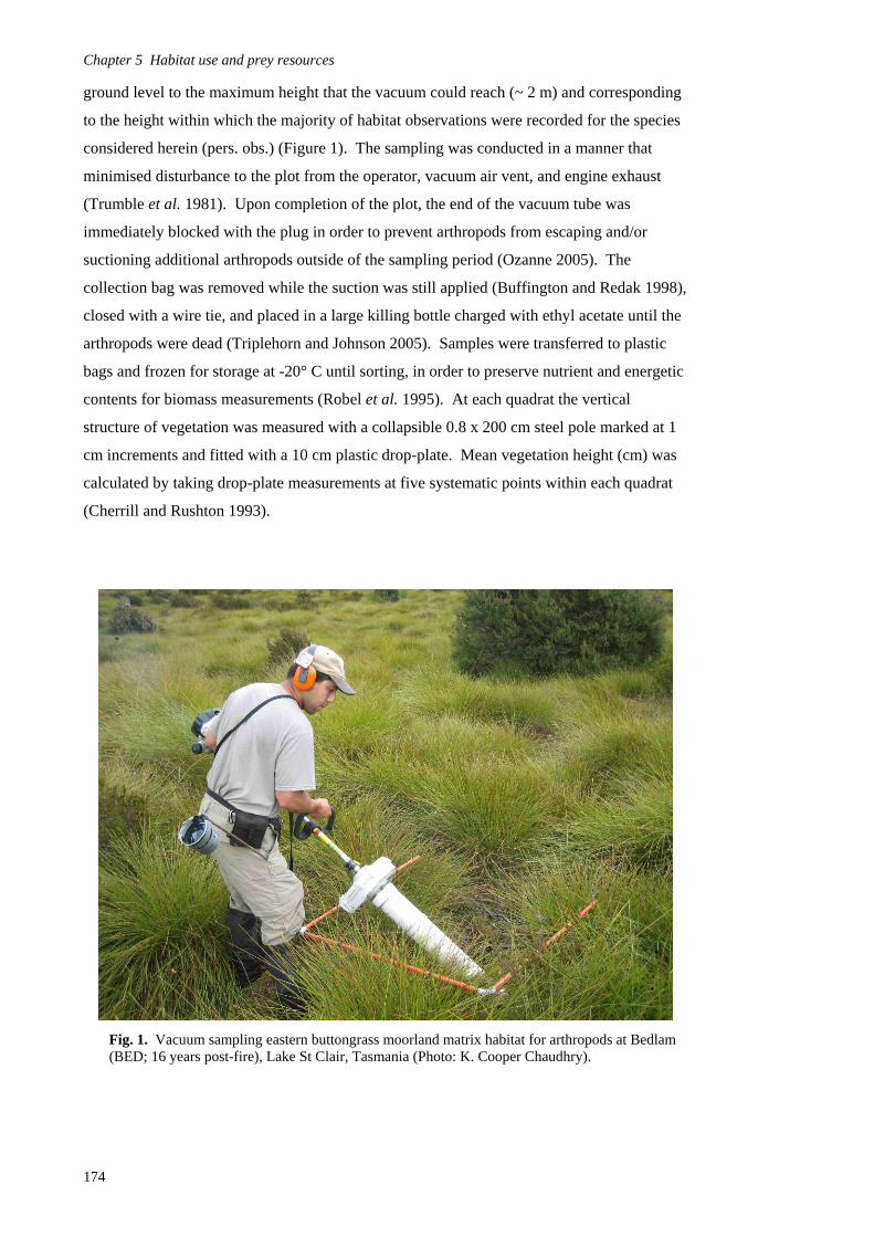
Chapter 5 Habitat use and prey resources
ground level to the maximum height that the vacuum could reach (~ 2 m) and corresponding
to the height within which the majority of habitat observations were recorded for the species
considered herein (pers. obs.) (Figure 1). The sampling was conducted in a manner that
minimised disturbance to the plot from the operator, vacuum air vent, and engine exhaust
(Trumble et al. 1981). Upon completion of the plot, the end of the vacuum tube was
immediately blocked with the plug in order to prevent arthropods from escaping and/or
suctioning additional arthropods outside of the sampling period (Ozanne 2005). The
collection bag was removed while the suction was still applied (Buffington and Redak 1998),
closed with a wire tie, and placed in a large killing bottle charged with ethyl acetate until the
arthropods were dead (Triplehorn and Johnson 2005). Samples were transferred to plastic
bags and frozen for storage at -20° C until sorting, in order to preserve nutrient and energetic
contents for biomass measurements (Robel et al. 1995). At each quadrat the vertical
structure of vegetation was measured with a collapsible 0.8 x 200 cm steel pole marked at 1
cm increments and fitted with a 10 cm plastic drop-plate. Mean vegetation height (cm) was
calculated by taking drop-plate measurements at five systematic points within each quadrat
(Cherrill and Rushton 1993).
Fig. 1. Vacuum sampling eastern buttongrass moorland matrix habitat for arthropods at Bedlam (BED; 16 years post-fire), Lake St Clair, Tasmania (Photo: K. Cooper Chaudhry).
174
Chapter 5 Habitat use and prey resources
A variety of different methods are often used to separate invertebrates samples from plant
and other material such as UV light extraction (Buffington and Redak 1998), sieving (Dennis
et al. 1998), flotation (Ausden 1996), and phase-separation techniques (Barmuta 1984).
Since vacuum sampling often results in large volumes of organic matter that can be very
time-consuming and tedious to sort through by hand (i.e. ~ ≤ 500 ml per quadrat for this
study), a number of pilot studies were conducted to evaluate the appropriateness and
effectiveness of live and dead extraction techniques for this study. A formal pilot was
conducted following the methods of Buffington and Redak (1998) and the extraction
efficiencies of four trials were determined by calculating the percentage of arthropods
extracted into the collection head based on the total number of dead specimens identified in
the sample by hand sorting. Extraction efficiencies ranged from only 13-26%, were biased
towards positively phototactic and flying insects, and showed notable intraorder and
interorder variability in extraction success. Informal trials were also conducted on the latter
methods which were unsuccessful in separating the arthropods from the organic material.
Accordingly, all samples were hand sorted by the author to maximise the recovery of
arthropods from the samples and minimise intersorter bias (Barmuta 1984). Despite the
potential unreliability of this method (Barmuta 1984), hand sorting is typically considered to
be less biased overall than other sorting techniques (Ausden 1996; Southwood and
Henderson 2000).
Frozen samples were allowed to thaw and were thoroughly examined with a dissecting
microscope at 10x magnification in a sorting tray. All specimens were identified to order
using the identification keys of Zborowski and Storey (1995), New (1996), Harvey and Yen
(1997), and Naumann (1991), and nymphs and larvae were recorded separately. Counting
was focused on bodies, and moults and specimens that had clearly died prior to sampling
were not recorded, although in practice this can sometimes be difficult to determine
(Southwood and Henderson 2000). Detached heads and appendages (i.e. of a reasonable
size, e.g. Orthoptera legs) that could be identified were included in vials of their respective
orders. Total and mean abundance (± SE) were calculated for each of the potential prey
orders for each sample.
Calculating food availability solely based on relative abundance can be misleading (Beaver
and Baldwin 1975; Johnson 2000; Buchanan et al. 2006). Therefore, individuals were
pooled by order within each sample and weighed within the microvials as the large sample
size prohibited weighing or measuring specimens individually. All vials were opened and
placed in drying racks in an oven at 50° C for 72 hours, after which point there was no
decrease in weights. Each vial was weighed to the nearest 0.1 mg using an analytical
balance (Mettler AE 200, ± 0.1 mg SD). The original vials were emptied, cleaned, and
175
Chapter 5 Habitat use and prey resources
weighed to determine the individual tare weights for each vial. Dry weight biomass (mg
DW m-2) was then converted to a more biologically meaningful estimate of gross energy
content (Joules m-2) by using published conversion factors for each order (Table 8).
Arthropod prey analyses
As there was no a priori ecological interest in variation at the quadrat scale, mean values (±
SE) of abundance (no. m-2), biomass (mg Dry Weight m-2) and energy content (J m-2) were
calculated by order (n = 242) and pooled across orders (n = 22) from the three quadrats
within each habitat and site. In the case of the former, although the mean number of
arthropods was based on 1 x 1 m quadrats and hence could be considered an estimate of
density, due the the different volumes of vegetation sampled within each quadrat, it is more
appropriately referred to as a (relative) estimate of abundance. Absences in abundance,
biomass, and energy within quadrats were treated as true zero values. Two-tailed Spearman
rank correlations indicated that both mean abundance (rs = 0.714; n = 22; P = 0.004) and
mean biomass (rs = 0.995; n = 22; P < 0.001) were correlated with mean energy content
when pooled across orders within each habitat and site. Therefore, mean biomass was
excluded from further univariate analysis; however, both mean abundance and mean energy
content were included as they are often considered to be complementary measures of prey
availability (e.g. Bryant 1973, Maguire 2006b). Similarly, two-tailed Spearman rank
correlations indicated that both mean abundance (rs = 0.906; n = 242; P < 0.001) and mean
biomass (rs = 0.998; n = 242; P < 0.001) were highly correlated with mean energy content
by order within each habitat and site and were therefore excluded from further multivariate
analyses. Total abundance and total energy content per order were used to estimate the mean
energy content per individual (J individual-1); although, as specimens were not weighed
individually no standard error terms are presented and these figures are only provided for
illustrative purposes.
A split-plot mixed model analysis of variance (ANOVA) was used to test for overall
significant differences in mean arthropod prey abundance (no. m-2) and mean energy content
(J m-2) of quadrats (pooled across orders) in response to habitat and fire age using SYSTAT
10 (SPSS Inc. 2000). Separate tests were conducted for the two dependent variables, with
habitat type and fire age as fixed factors, and the site replicates (nested within fire age)
treated as a random factor. Although the sites were chosen based on the selection criteria
described in Chapter 2, they are included as a random factor as they are considered to be
representative of their respective fire ages in eastern moorlands and as it is consistent with
the original intent of the study design and hypotheses (G. Quinn pers. comm. 2006). The
residual term (quadrats) was omitted from the models as the associated hypotheses were not
of interest. Fire age three (HAR, see Chapter 2) was excluded from these analyses as only
176

Chapter 5 Habitat use and prey resources
one site was available for sampling (i.e. no replication). The dependent variables were not
transformed as the assumptions of normality and homogeneity of variances were met.
Furthermore, examination of Studentised residuals did not indicate any issues of concern
regarding outliers and model fit. Post hoc tests using Tukey HSD were conducted to test for
significant differences between fire ages. Two-tailed Spearman rank correlations were
conducted to determine whether there were any significant correlations between mean
vegetation height and the dependent variables.
The influence of arthropod community structure on observed patterns in energy content and
distribution was explored using a range of multivariate techniques available in Primer 5.2.2
(Primer-E Ltd. 2001). The similarities of mean energy content contributed by orders
between different samples were calculated using the Bray-Curtis similarity measure as it
ignores joint absences and is often recommended for community data (Quinn and Keough
2002; McCune et al. 2002). The data were untransformed as there was no interest in
reducing the influence of the orders with the greatest biomass (i.e. energy content) (Clarke
and Gorley 2001). The similarity matrix was analysed with non-metric Multidimensional
Scaling (MDS) using two and three dimensions with 30 random restarts; however, for ease
of display and interpretation the best 2-dimensional configuration with its associated stress
was chosen (Clarke and Warwick 1994). The habitat and fire age factors were plotted on the
ordination plot to show any apparent patterns with the underlying similarities. A cluster
analysis (CLUSTER) using a group mean and ranked similarities was also performed on the
Bray-Curtis similarity matrix and five clusters (arbitrarily identified at the 120 rank level)
were superimposed on the MDS plot to assess the adequacy and consistency of the MDS and
CLUSTER methods (Clarke and Warwick 1994). The similarity percentages procedure
(SIMPER) was conducted to examine the mean one way similarities within and mean one
way dissimilarities between the habitat and fire age factors and thus determine which orders
were contributing the most to the patterns observed in the MDS plot (Clarke and Gorley
2001). As complex designs such as split-plots cannot be accommodated in analysis of
similarities (ANOSIM) procedures, one way ANOSIMs (999 random permutations) were
used to test for significant differences in the energy contributions of different arthropod
orders between habitats and between fire ages among the 11 sites as depicted in the MDS
plot (Clarke and Gorley 2001). Post hoc tests using a Bonferroni adjusted P-value were
conducted to test for significant differences between fire ages.
177
Chapter 5 Habitat use and prey resources
Results Habitat use
Observations of habitat use in the study area (n = 250) were dominated by the resident
Southern Emu-wren (17%) and Striated Fieldwren (34%), while the Ground Parrot was
rarely observed (2%). The 18 non-resident species together accounted for the remaining
47% of observations. The results of the log-linear modelling in relation to groups are
summarised in the analysis of deviance shown in Table 2 and their parameter estimates are
outlined in Table 3. The saturated models provided the best fit for the data at Lake Pedder
and Lake St Clair and demonstrated significantly non-random selection of habitats (P <
0.001) that depended on the availability of different habitats, group membership, and their
interactions. The estimated relative selection probabilities (Table 4) indicate the relative
expected use if habitats were available in equal proportions (Garshelis 2000). In all cases,
the birds used riparian and edge habitats more than expected (range ŵ = 1.57-42.00), with
the large values of these probabilities resulting from the extensive use (48%, n = 250) and
the very limited availabilities of these habitats (≤ 5% of total area each within either
location). Overall, the probabilities of selection for the non-matrix habitats were relatively
higher in the sedge-dominated eastern moorlands at Lake St Clair than the scrub-dominated
blanket moorlands at Lake Pedder. This was particularly the case in relation to the apparent
preference for riparian habitats demonstrated by both the resident and non-resident groups at
Lake St Clair (ŵ = 15.04 and 21.07, respectively). As expected, the residents accounted for
the majority (70%) of total observations in the moorland matrix (n = 133); however, 39% of
resident observations in the matrix (n = 92) were originally noted as being in scrub copses,
while 65% (n = 40) of non-resident observations were in scrub copses or isolated trees.
Residents also appeared to weakly select edge habitat over matrix at both locations, although
the effect appeared to be stronger at Lake Pedder (ŵ = 4.60 vs. 1.57). However, it should be
noted that of the three resident species, only the Striated Fieldwren was recorded using edge
habitat (n = 6), and in all of these cases the edge habitat was originally noted as being
primarily comprised of scrub species (e.g. Leptospermum and Melaleuca spp.) associated
with ecotones between the moorland and woodland or along road edges. In this sense, the
apparent selection of edge habitats by the residents was again largely an artefact of the
necessary scale of mapping and habitat classification (see Chapters 2-3), as opposed to a
demonstrated affinity for the typically Eucalyptus-dominated edges per se. Furthermore, a
lack of any off-survey observations within the woodlands helped to substantiate the
contention that the resident species do not utilise woodland habitats within the study area. In
contrast, the relatively large probabilities of non-resident species using edge habitat at Lake
Pedder and Lake St Clair (ŵ = 38.64 and 42.00, respectively) helped to confirm their a priori
categorisation. In other words, the non-resident group included species typically associated
with adjacent woodland habitats that primarily fall outside of the moorland sites as defined.
178
Chapter 5 Habitat use and prey resources
The results of the log-linear modelling in relation to fire age are summarised in the analysis
of deviance shown in Table 5 and the parameter estimates from the models of best fit are
outlined in Table 6. The results demonstrated significantly non-random selection of habitats
at both locations (P < 0.001). At Lake St Clair, the saturated model included a significant
interaction between habitat and fire age (P = 0.002) and therefore cannot be reduced any
further, indicating that availability of different habitats, fire age, and their interaction were
significantly related to habitat use. In contrast, at Lake Pedder the reduced model provides
the best fit (P < 0.001) indicating that fire age was not significantly related to habitat
selection. As in the group analysis (Table 4), the relative selection probabilities (Table 7)
indicated that the avifauna used riparian and edge habitats more than expected in all cases
(range ŵ = 5.02-79.48). When compared to all ages at Lake Pedder, the relative probabilities
for the riparian and edge habitats were notably higher across fire ages at Lake St Clair, with
the exception of the 3 year old sites. In this sense the models were somewhat redundant,
particularly for Lake Pedder as the reduced model necessitated the pooling of relative
selection probabilities across fire ages and essentially provided a community-level summary
of those presented in Table 4. However, as fire age was significantly related to habitat
selection at Lake St Clair some important inferences can be made. The most striking pattern
was at the one year old site (HAR), where there was a strong apparent preference for riparian
habitat (ŵ = 79.48), most of which was largely unburnt by the prescribed fire in October
2003 (pers. obs.; Figure 2). Although it was evident that the magnitude of this preference
was considerably reduced in older sites (range ŵ = 3.70-41.45), there was no clear linear
trend across the chronosequence as indicated by these probabilities and the coefficient
estimates.
179
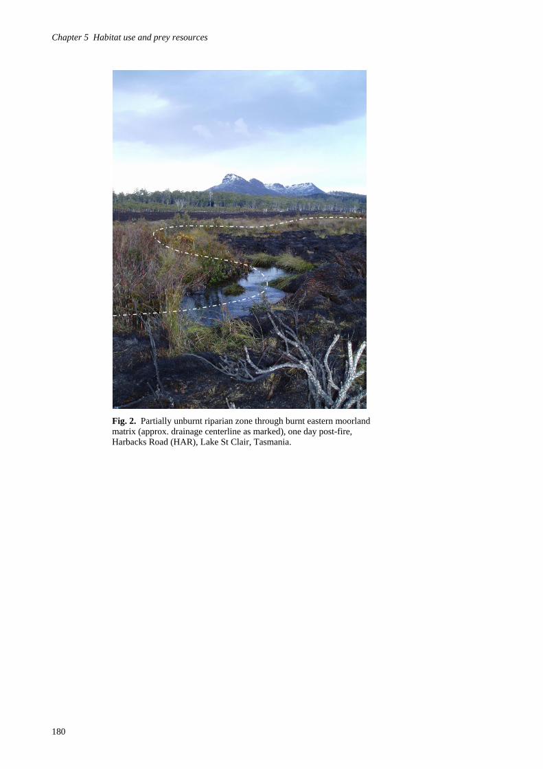
Chapter 5 Habitat use and prey resources
Fig. 2. Partially unburnt riparian zone through burnt eastern moorland matrix (approx. drainage centerline as marked), one day post-fire, Harbacks Road (HAR), Lake St Clair, Tasmania.
180

Chapter 5 Habitat use and prey resources
181
Table 2. Analysis of deviance table for the log-linear models of habitat selection in relation to the resident and non-resident birds of buttongrass moorlands at Lake Pedder (n = 108) and Lake St Clair (n = 142), Tasmania.* Denotes significance at the 0.05 and ** at the 0.01 level and ^ denotes model of best fit. Model by location df Deviance df Residual
deviance P
Lake Pedder No selection of habitat 5 96.025 Selection by habitat 2 69.685 3 26.341 < 0.001** Selection by habitat + group 1 4.513 2 21.828 0.034* Selection by habitat + group + habitat x group ^
2 21.828 0 < 0.001 < 0.001**
Lake St Clair No selection of habitat 5 276.789 Selection by habitat 2 241.301 3 35.488 < 0.001** Selection by habitat + group 1 0.451 2 35.037 0.502 Selection by habitat + group + habitat x group ^
2 35.037 0 < 0.001 < 0.001**
Table 3. Parameter estimates from the log-linear models of best fit for habitat selection in relation to the matrix habitat and resident bird group of buttongrass moorlands at Lake Pedder and Lake St Clair, Tasmania. * Denotes significance at the 0.05 and ** at the 0.01 level. Coefficient by location Estimate SE Z P
Lake Pedder Constant 4.079 0.135 30.249 < 0.001** Riparian 0.627 0.430 1.459 0.145 Edge 1.526 0.518 2.946 0.003** Non-residents -1.117 0.272 -4.113 < 0.001** Riparian x non-residents 1.964 0.558 3.518 < 0.001** Edge x non-residents 2.129 0.644 3.306 < 0.001**
Lake St Clair Constant 3.715 0.162 22.902 < 0.001** Riparian 2.711 0.252 10.770 < 0.001** Edge 0.450 0.726 0.621 0.535 Non-residents -0.547 0.268 -2.040 0.041* Riparian x non-residents 0.342 0.393 0.870 0.384 Edge x non-residents 3.287 0.777 4.230 < 0.001**
Table 4. Relative selection probabilities (ŵ) in relation to the resident and non-resident groups estimated from the resource selection functions for the avifauna of buttongrass moorlands at Lake Pedder and Lake St Clair, Tasmania. Availability of matrix habitat is standardised as 1.00. Habitat by location Group
Lake Pedder Residents Non-residents Matrix 1.00 1.00 Riparian 1.87 13.35 Edge 4.60 38.64
Lake St Clair Matrix 1.00 1.00 Riparian 15.04 21.17 Edge 1.57 42.00
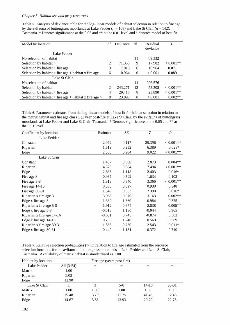
Chapter 5 Habitat use and prey resources
Table 5. Analysis of deviance table for the log-linear models of habitat selection in relation to fire age by the avifauna of buttongrass moorlands at Lake Pedder (n = 108) and Lake St Clair (n = 142), Tasmania. * Denotes significance at the 0.05 and ** at the 0.01 level and ^ denotes model of best fit. Model by location df Deviance df Residual
deviance P
Lake Pedder No selection of habitat 11 89.332 Selection by habitat ^ 2 71.350 9 17.982 < 0.001** Selection by habitat + fire age 3 7.018 6 10.964 0.071 Selection by habitat + fire age + habitat x fire age 6 10.964 0 < 0.001 0.089
Lake St Clair No selection of habitat 14 296.576 Selection by habitat 2 243.271 12 53.305 < 0.001** Selection by habitat + fire age 4 29.415 8 23.890 < 0.001** Selection by habitat + fire age + habitat x fire age ^ 8 23.890 0 < 0.001 0.002**
Table 6. Parameter estimates from the log-linear models of best fit for habitat selection in relation to the matrix habitat and fire age class 1 (1 year post-fire at Lake St Clair) by the avifauna of buttongrass moorlands at Lake Pedder and Lake St Clair, Tasmania. * Denotes significance at the 0.05 and ** at he 0.01 level. t
Coefficient by location Estimate SE Z P Lake Pedder
Constant 2.972 0.117 25.396 < 0.001** Riparian 1.613 0.252 6.389 0.028* Edge 2.558 0.284 9.022 < 0.001**
Lake St Clair Constant 1.437 0.500 2.873 0.004** Riparian 4.376 0.584 7.494 < 0.001** Edge 2.686 1.118 2.403 0.016* Fire age 3 0.967 0.592 1.634 0.102 Fire age 5-8 1.818 0.540 3.366 < 0.001** Fire age 14-16 0.588 0.627 0.938 0.348 Fire age 30-31 1.349 0.563 2.398 0.016* Riparian x fire age 3 -3.068 0.970 -3.163 0.002** Edge x fire age 3 -1.339 1.360 -0.984 0.325 Riparian x fire age 5-8 -1.912 0.674 -2.838 0.005** Edge x fire age 5-8 -0.518 1.180 -0.044 0.965 Riparian x fire age 14-16 -0.651 0.745 -0.874 0.382 Edge x fire age 14-16 0.706 1.240 0.569 0.569 Riparian x fire age 30-31 -1.856 0.730 -2.543 0.011* Edge x fire age 30-31 0.440 1.181 0.372 0.710
Table 7. Relative selection probabilities (ŵ) in relation to fire age estimated from the resource selection functions for the avifauna of buttongrass moorlands at Lake Pedder and Lake St Clair,
asmania. Availability of matrix habitat is standardised as 1.00. T Habitat by location Fire age (years post-fire)
Lake Pedder All (3-54) − − − − Matrix 1.00 Riparian 5.02 Edge 12.90
Lake St Clair 1 3 5-8 14-16 30-31 Matrix 1.00 1.00 1.00 1.00 1.00 Riparian 79.48 3.70 11.75 41.45 12.43 Edge 14.67 3.85 13.93 29.72 22.78
182
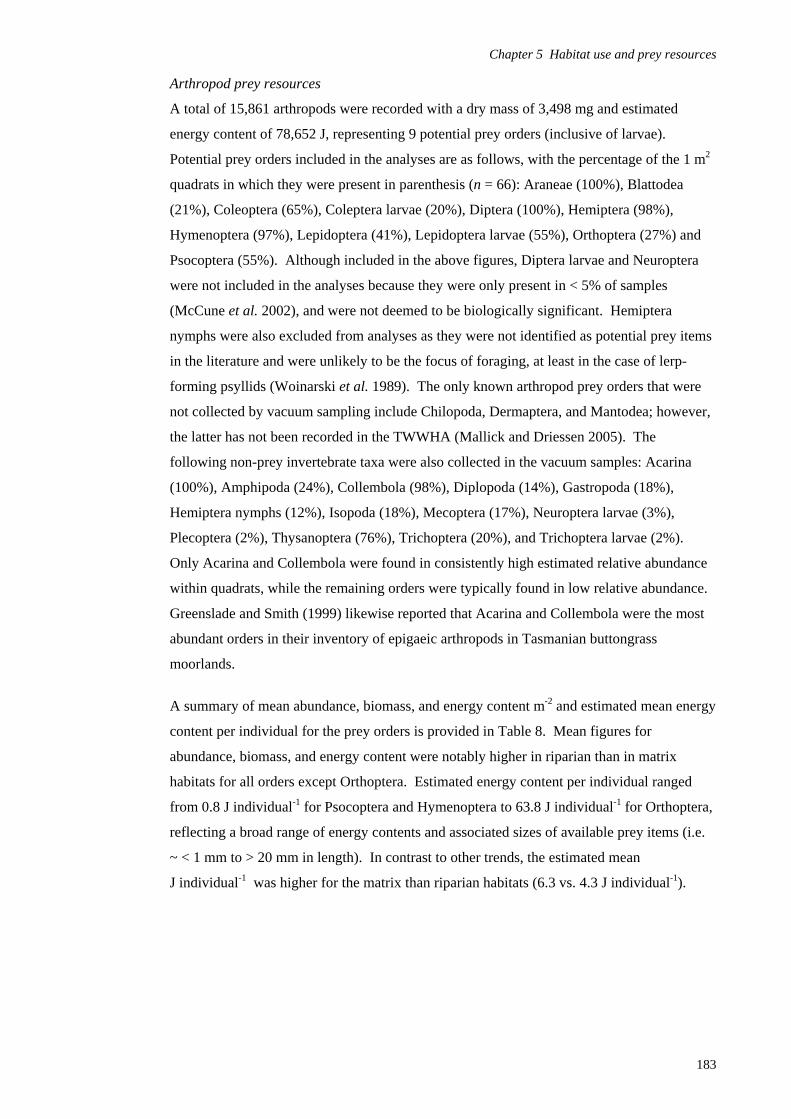
Chapter 5 Habitat use and prey resources
Arthropod prey resources
A total of 15,861 arthropods were recorded with a dry mass of 3,498 mg and estimated
energy content of 78,652 J, representing 9 potential prey orders (inclusive of larvae).
Potential prey orders included in the analyses are as follows, with the percentage of the 1 m2
quadrats in which they were present in parenthesis (n = 66): Araneae (100%), Blattodea
(21%), Coleoptera (65%), Coleptera larvae (20%), Diptera (100%), Hemiptera (98%),
Hymenoptera (97%), Lepidoptera (41%), Lepidoptera larvae (55%), Orthoptera (27%) and
Psocoptera (55%). Although included in the above figures, Diptera larvae and Neuroptera
were not included in the analyses because they were only present in < 5% of samples
(McCune et al. 2002), and were not deemed to be biologically significant. Hemiptera
nymphs were also excluded from analyses as they were not identified as potential prey items
in the literature and were unlikely to be the focus of foraging, at least in the case of lerp-
forming psyllids (Woinarski et al. 1989). The only known arthropod prey orders that were
not collected by vacuum sampling include Chilopoda, Dermaptera, and Mantodea; however,
the latter has not been recorded in the TWWHA (Mallick and Driessen 2005). The
following non-prey invertebrate taxa were also collected in the vacuum samples: Acarina
(100%), Amphipoda (24%), Collembola (98%), Diplopoda (14%), Gastropoda (18%),
Hemiptera nymphs (12%), Isopoda (18%), Mecoptera (17%), Neuroptera larvae (3%),
Plecoptera (2%), Thysanoptera (76%), Trichoptera (20%), and Trichoptera larvae (2%).
Only Acarina and Collembola were found in consistently high estimated relative abundance
within quadrats, while the remaining orders were typically found in low relative abundance.
Greenslade and Smith (1999) likewise reported that Acarina and Collembola were the most
abundant orders in their inventory of epigaeic arthropods in Tasmanian buttongrass
moorlands.
A summary of mean abundance, biomass, and energy content m-2 and estimated mean energy
content per individual for the prey orders is provided in Table 8. Mean figures for
abundance, biomass, and energy content were notably higher in riparian than in matrix
habitats for all orders except Orthoptera. Estimated energy content per individual ranged
from 0.8 J individual-1 for Psocoptera and Hymenoptera to 63.8 J individual-1 for Orthoptera,
reflecting a broad range of energy contents and associated sizes of available prey items (i.e.
~ < 1 mm to > 20 mm in length). In contrast to other trends, the estimated mean
J individual-1 was higher for the matrix than riparian habitats (6.3 vs. 4.3 J individual-1).
183

Chapter 5 Habitat use and prey resources
184
Table 8. Measures of potential arthropod prey orders of insectivorous birds in buttongrass moorlands at Lake St Clair, Tasmania. Mean (± SE) abundance, biomass (mg Dry Weight), and energy content (J) of arthropod prey orders m-2 vacuum sample (n = 33) and estimated mean energy content individual-1 in matrix (MTX) and riparian (RIP) habitats pooled across buttongrass moorland sites ranging from < 1-32 years post-fire. Energy content conversions factors are from the literature (aCummins and Wuycheck 1971, *excluding Stratiomyidae since rare in buttongrass moorlands (M. Driessen unpublished data); bO’Farrell et al. 1971 cited in Bell 1990; cBrodmann and Reyer 1999; dNorberg 1978). ^ Standard errors are not presented for J individual-1 as these figures are derived estimates and not based on individual DWs of specimens.
Order Habitat n
Total abundance
Mean abundance
Mean biomass (mg DW)
Mean energy content (J)
Est. individual energy content ^ (J individual-1 )
Energy conversions (J mg-1 DW)
Aranaeae MTX 33 1254 38.0 ± 4.2 10.7 ± 1.7 216.2 ± 34.8 5.7 20.19a RIP 33 1613 48.9 ± 7.0 11.3 ± 1.4 227.2 ± 28.6 4.6 Blattodea MTX 33 5 0.2 ± 0.1 0.0 ± 0.0 0.8 ± 0.4 5.4 22.58a RIP 33 14 0.4 ± 0.1 0.5 ± 0.3 11.5 ± 5.8 27.1 Coleoptera MTX 33 39 1.2 ± 0.3 1.8 ± 1.1 41.8 ± 25.8 35.4 23.25a RIP 33 146 4.4 ± 0.9 3.7 ± 0.9 87.1 ± 20.7 19.7 Coleoptera larvae MTX 33 1 0.0 ± 0.0 0.0 ± 0.0 0.2 ± 0.2 5.5 27.56b RIP 33 32 1.0 ± 0.4 0.2 ± 0.1 5.9 ± 2.7 6.1 Diptera MTX 33 1617 49.0 ± 13.0 8.1 ± 2.0 185.4 ± 44.9 3.8 22.78a* RIP 33 5040 152.7 ± 36.1 19.1 ± 4.1 434.3 ± 94.5 2.8 Hemiptera MTX 33 1538 46.6 ± 6.0 18.3 ± 2.2 432.1 ± 52.7 9.3 23.59a RIP 33 1805 54.7 ± 9.7 22.8 ± 3.9 537.3 ± 92.5 9.8 Hymenoptera MTX 33 431 13.1 ± 1.8 0.6 ± 0.1 12.1 ± 1.7 0.9 19.37a RIP 33 1405 42.6 ± 9.7 1.7 ± 0.3 32.9 ± 5.9 0.8 Lepidoptera MTX 33 16 0.5 ± 0.1 0.5 ± 0.4 10.9 ± 8.7 22.4 22.42c RIP 33 58 1.8 ± 0.7 1.2 ± 0.5 25.9 ± 10.7 14.7 Lepidoptera larvae MTX 33 37 1.1 ± 0.4 0.3 ± 0.1 7.0 ± 3.1 6.2 22.95c RIP 33 74 2.2 ± 0.5 1.4 ± 0.8 32.5 ± 19.0 14.5 Orthoptera MTX 33 33 1.0 ± 0.4 2.1 ± 0.9 47.7 ± 20.0 47.7 22.18a RIP 33 4 0.1 ± 0.1 0.3 ± 0.2 7.7 ± 4.6 63.8 Psocoptera MTX 33 31 0.9 ± 0.4 0.0 ± 0.0 0.8 ± 0.3 0.8 21.7d RIP 33 662 20.1 ± 7.3 1.2 ± 0.3 25.4 ± 5.6 1.3 Total Means MTX 363 5002 13.8 ± 1.7 3.9 ± 0.5 86.8 ± 10.2 6.3 RIP 363 10853 29.9 ± 4.3 5.8 ± 0.7 129.8 ± 15.6 4.3
185
Chapter 5 Habitat use and prey resources
A summary of mean arthropod abundance m-2 pooled across orders is presented in Figures 3
and 4 and the associated results from the split-plot ANOVA are presented in Table 9.
Results indicated that habitat was a significant factor (P = 0.004) while fire age was not a
significant factor (P = 0.219). There was no significant interaction between habitat and fire
age (P = 0.295). There was also no significant added component of variance from the nested
site factor (P = 0.219). Two-tailed Spearman rank correlations indicated that mean
abundance was significantly correlated with mean vegetation height (rs = 0.563; n = 22; P =
0.006).
A summary of mean arthropod energy content m-2 pooled across orders is presented in
Figures 5 and 6 and the associated results from the split-plot ANOVA are presented in Table
10. Results for the main effects were in contrast to those described for abundance, with
habitat identified as marginally non-significant (P = 0.051) and fire age as a significant
factor (P = 0.038). Post hoc tests revealed that there was a significant difference in mean
arthropod energy content between fire ages 1 and 16 (P = 0.049), with the next smallest P
values between 1 and 3 (P = 0.098) and 16 and 32 (P = 0.088). While habitat was
marginally non-significant, the relatively high F-ratio (F = 6.498) and low degrees of
freedom (df = 1) indicated that habitat appeared to have some ecological effect on the
response variable, with riparian habitats typically being higher in energy content than matrix
habitats across all fire ages. Similar to the results above, there was no significant interaction
between habitat and fire age (P = 0.445) and again the nested site factor was not significant
(P = 0.512), indicating the sites were serving as reasonable replicates of their respective fire
ages. Contrary to the above results, two-tailed Spearman rank correlations indicated that
mean energy content was not significantly correlated with mean vegetation height (rs =
0.256; n = 22; P = 0.251).
186

Chapter 5 Habitat use and prey resources
500
400
300
Fig. 3. Mean abundance (no. m-2 ± SE) of potential arthropod prey (pooled across orders and fire ages) in matrix and riparian habitats of buttongrass moorlands at Lake St Clair, Tasmania (n = 33).
Mea
n ab
unda
nce
(no.
m-2
± S
E)
Mea
n ab
unda
nce
(no.
m-2
± S
E)
100
200
0 Riparian Matrix
Habitat
500
400
300
200
100
0 < 1 16 3 5 7 32
Fire age (years post-fire)
Fig. 4. Mean abundance (no. m-2 ± SE) of potential arthropod prey (pooled across orders and habitats) in buttongrass moorlands ranging in age from < 1-32 years post-fire at Lake St Clair, Tasmania (n = 12 for all ages except age 3 where n = 6). Table 9. Split-plot ANOVA for mean arthropod abundance (no. m-2) in response to habitat type (matrix and riparian) and fire age (< 1, 5, 7, 16, 32 years post-fire) in buttongrass moorlands at Lake St Clair, Tasmania. * Denotes significance at the 0.05 level.
Variable SS df MS F P Habitat 1.548 E+05 1 1.548 E+05 23.954 0.004* Fire age 1.150 E+05 4 2.875 E+04 2.092 0.219 Habitat x fire age 4.272 E+04 4 1.068 E+04 1.652 0.295 Site (Fire age) 6.871 E+04 5 1.374 E+04 2.126 0.214 Error 3.232 E+04 5 6.463 E+03
187
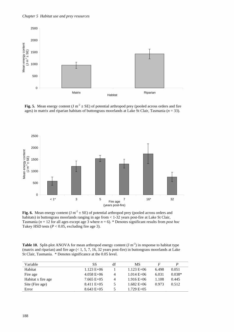
Chapter 5 Habitat use and prey resources
2500
2000 M
ean
ener
gy c
ont
ent
(J m
-2 ±
SE
)
1500
500
1000
0 Matrix Riparian
Habitat Fig. 5. Mean energy content (J m-2 ± SE) of potential arthropod prey (pooled across orders and fire
ages) in matrix and riparian habitats of buttongrass moorlands at Lake St Clair, Tasmania (n = 33).
2000
2500
Mea
n en
ergy
co
nten
t (J
m-2
± S
E)
1500
1000
500
0 16* 32 < 1* 3 5 7
Fire age (years post-fire)
Fig. 6. Mean energy content (J m-2 ± SE) of potential arthropod prey (pooled across orders and habitats) in buttongrass moorlands ranging in age from < 1-32 years post-fire at Lake St Clair, Tasmania (n = 12 for all ages except age 3 where n = 6). * Denotes significant results from post hoc Tukey HSD tests (P < 0.05, excluding fire age 3).
Table 10. Split-plot ANOVA for mean arthropod energy content (J m-2) in response to habitat type (matrix and riparian) and fire age (< 1, 5, 7, 16, 32 years post-fire) in buttongrass moorlands at Lake St Clair, Tasmania. * Denotes significance at the 0.05 level.
Variable SS df MS F P Habitat 1.123 E+06 1 1.123 E+06 6.498 0.051 Fire age 4.058 E+06 4 1.014 E+06 6.031 0.038* Habitat x fire age 7.665 E+05 4 1.916 E+06 1.108 0.445 Site (Fire age) 8.411 E+05 5 1.682 E+06 0.973 0.512 Error 8.643 E+05 5 1.729 E+05
188
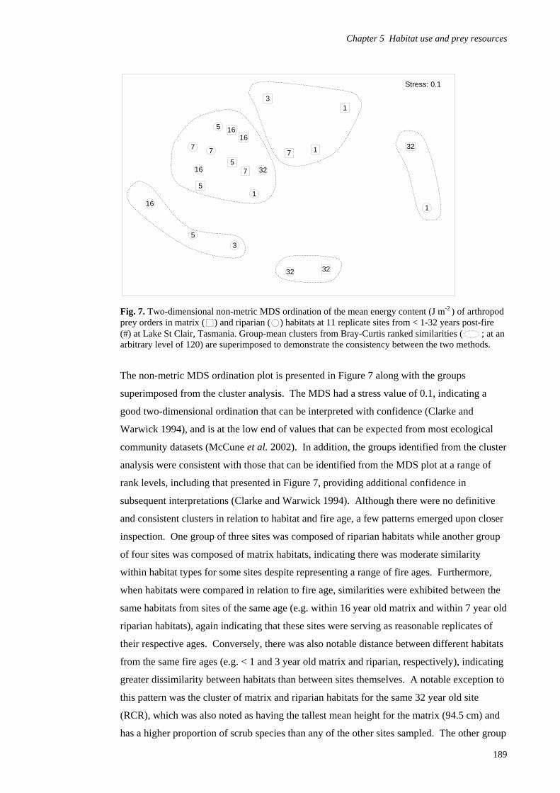
Chapter 5 Habitat use and prey resources
Fig. 7. Two-dimensional non-metric MDS ordination of the mean energy content (J m-2 ) of arthropod prey orders in matrix () and riparian () habitats at 11 replicate sites from < 1-32 years post-fire (#) at Lake St Clair, Tasmania. Group-mean clusters from Bray-Curtis ranked similarities ( ; at an arbitrary level of 120) are superimposed to demonstrate the consistency between the two methods.
32
32
77
16
16
16
16
3
3
5
5
7
7
1
1
5
5
3232
1
1
Stress: 0.1Stress: 0.1
The non-metric MDS ordination plot is presented in Figure 7 along with the groups
superimposed from the cluster analysis. The MDS had a stress value of 0.1, indicating a
good two-dimensional ordination that can be interpreted with confidence (Clarke and
Warwick 1994), and is at the low end of values that can be expected from most ecological
community datasets (McCune et al. 2002). In addition, the groups identified from the cluster
analysis were consistent with those that can be identified from the MDS plot at a range of
rank levels, including that presented in Figure 7, providing additional confidence in
subsequent interpretations (Clarke and Warwick 1994). Although there were no definitive
and consistent clusters in relation to habitat and fire age, a few patterns emerged upon closer
inspection. One group of three sites was composed of riparian habitats while another group
of four sites was composed of matrix habitats, indicating there was moderate similarity
within habitat types for some sites despite representing a range of fire ages. Furthermore,
when habitats were compared in relation to fire age, similarities were exhibited between the
same habitats from sites of the same age (e.g. within 16 year old matrix and within 7 year old
riparian habitats), again indicating that these sites were serving as reasonable replicates of
their respective ages. Conversely, there was also notable distance between different habitats
from the same fire ages (e.g. < 1 and 3 year old matrix and riparian, respectively), indicating
greater dissimilarity between habitats than between sites themselves. A notable exception to
this pattern was the cluster of matrix and riparian habitats for the same 32 year old site
(RCR), which was also noted as having the tallest mean height for the matrix (94.5 cm) and
has a higher proportion of scrub species than any of the other sites sampled. The other group
189
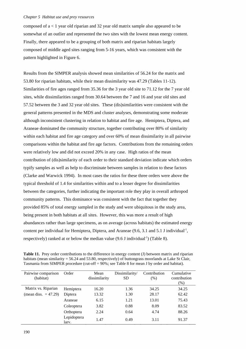
Chapter 5 Habitat use and prey resources
composed of a < 1 year old riparian and 32 year old matrix sample also appeared to be
somewhat of an outlier and represented the two sites with the lowest mean energy content.
Finally, there appeared to be a grouping of both matrix and riparian habitats largely
composed of middle aged sites ranging from 5-16 years, which was consistent with the
pattern highlighted in Figure 6.
Results from the SIMPER analysis showed mean similarities of 56.24 for the matrix and
53.80 for riparian habitats, while their mean dissimilarity was 47.29 (Tables 11-12).
Similarities of fire ages ranged from 35.36 for the 3 year old site to 71.12 for the 7 year old
sites, while dissimilarities ranged from 30.64 between the 7 and 16 and year old sites and
57.52 between the 3 and 32 year old sites. These (dis)similarities were consistent with the
general patterns presented in the MDS and cluster analyses, demonstrating some moderate
although inconsistent clustering in relation to habitat and fire age. Hemiptera, Diptera, and
Araneae dominated the community structure, together contributing over 80% of similarity
within each habitat and fire age category and over 60% of mean dissimilarity in all pairwise
comparisons within the habitat and fire age factors. Contributions from the remaining orders
were relatively low and did not exceed 20% in any case. High ratios of the mean
contribution of (dis)similarity of each order to their standard deviation indicate which orders
typify samples as well as help to discriminate between samples in relation to these factors
(Clarke and Warwick 1994). In most cases the ratios for these three orders were above the
typical threshold of 1.4 for similarities within and to a lesser degree for dissimilarities
between the categories, further indicating the important role they play in overall arthropod
community patterns. This dominance was consistent with the fact that together they
provided 85% of total energy sampled in the study and were ubiquitous in the study area,
being present in both habitats at all sites. However, this was more a result of high
abundances rather than large specimens, as on average (across habitats) the estimated energy
content per individual for Hemiptera, Diptera, and Araneae (9.6, 3.1 and 5.1 J individual-1,
respectively) ranked at or below the median value (9.6 J individual-1) (Table 8).
Table 11. Prey order contributions to the difference in energy content (J) between matrix and riparian habitats (mean similarity = 56.24 and 53.80, respectively) of buttongrass moorlands at Lake St Clair, Tasmania from SIMPER procedure (cut-off = 90%; see Table 8 for mean J by order and habitat). Pairwise comparison
(habitat)
Order Mean dissimilarity
Dissimilarity/ SD
Contribution (%)
Cumulative contribution
(%) Matrix vs. Riparian Hemiptera 16.20 1.36 34.25 34.25
(mean diss. = 47.29) Diptera 13.32 1.30 28.17 62.42
Araneae 6.15 1.21 13.01 75.43
Coleoptera 3.82 0.88 8.09 83.52
Orthoptera 2.24 0.64 4.74 88.26
Lepidoptera larv.
1.47 0.49 3.11 91.37
190

Chapter 5 Habitat use and prey resources
Table 12. Prey order contributions to the difference in energy content (J) between fire ages of buttongrass moorlands at Lake St Clair, Tasmania from SIMPER procedure (cut-off = 80%). Fire ages (years post-fire) followed by mean similarity in parenthesis: < 1 (50.48), 3 (35.36), 5 (66.41), 7 (71.12), 16 (66.58), 32 (46.94).
Pairwise comparison (years post-fire)
Order Mean dissimilarity
Dissimilarity/ SD
Contribution (%)
Cumulative contribution
(%) < 1 vs. 3 Diptera 15.06 1.18 29.96 29.96
(mean diss. = 50.28) Hemiptera 13.11 1.05 26.08 56.04 Orthoptera 8.13 1.01 16.18 72.22
Lepidoptera larv.
6.39 0.95 12.70 84.92
< 1 vs. 5 Hemiptera 19.97 1.95 36.10 36.10 (mean diss. = 55.31) Diptera 16.77 1.40 30.33 66.43
Araneae 8.85 1.56 15.99 82.42
< 1 vs. 7 Hemiptera 22.79 1.59 48.08 48.08 (mean diss. = 47.41) Diptera 9.76 1.97 20.59 68.66
Araneae 5.97 1.28 12.60 81.26
< 1 vs. 16 Hemiptera 27.17 2.17 48.95 48.95 (mean diss. = 55.51) Diptera 15.33 1.12 27.62 76.57
Araneae 6.26 0.93 11.28 87.85
< 1 vs. 32 Diptera 13.76 1.46 25.93 25.93 (mean diss. = 53.09) Hemiptera 13.47 1.71 25.37 51.29
Coleoptera 9.13 1.01 17.20 68.49
Araneae 8.57 1.39 16.14 84.63
3 vs. 5 Diptera 11.90 1.29 27.83 27.83 (mean diss. = 42.78) Hemiptera 9.25 1.68 21.63 49.46
Araneae 6.24 1.58 14.58 64.03 Orthoptera 4.99 0.97 11.67 75.70
Lepidoptera larv.
4.23 1.03 9.88 85.58
3 vs. 7 Hemiptera 12.70 1.62 30.59 30.59 (mean diss. = 41.53) Diptera 10.56 2.28 25.43 56.01
Orthoptera 5.41 1.23 13.03 69.04
Lepidoptera larv.
4.60 1.00 11.07 80.11
3 vs. 16 Hemiptera 14.56 2.28 31.45 31.45 (mean diss. = 46.30) Diptera 14.09 1.40 30.44 61.89
Orthoptera 4.84 0.95 10.46 72.35
Araneae 4.25 0.97 9.19 81.54
3 vs. 32 Hemiptera 15.02 1.28 26.12 26.12 (mean diss. = 57.52) Diptera 13.52 1.57 23.51 49.63
Orthoptera 7.44 0.98 12.93 62.56 Araneae 5.93 1.39 10.31 72.86
Coleoptera 5.91 1.03 10.27 83.13
5 vs. 7 Diptera 9.50 1.28 29.83 29.83 (mean diss. = 31.84) Hemiptera 8.92 2.02 28.00 57.83
Araneae 5.37 1.83 16.87 74.70 Coleoptera 2.70 1.11 8.46 83.17
191

Chapter 5 Habitat use and prey resources
Table 12. cont.
Pairwise comparison (years post-fire)
Order Mean dissimilarity
Dissimilarity/ SD
Contribution (%)
Cumulative contribution
(%) 5 vs. 16 Diptera 12.97 1.47 41.74 41.74
(mean diss. = 31.08) Hemiptera 6.16 1.60 19.84 61.57 Araneae 5.17 1.37 16.65 78.22
Coleoptera 3.34 1.35 10.76 88.99
5 vs. 32 Hemiptera 21.60 2.20 39.37 39.37 (mean diss. = 54.88) Diptera 12.92 1.32 23.55 62.92
Araneae 9.09 1.37 16.56 79.48
Coleoptera 5.04 1.14 9.19 88.67
7 vs. 16 Diptera 10.41 1.02 33.99 33.99 (mean diss. = 30.64) Hemiptera 9.48 1.24 30.96 64.95
Araneae 3.83 1.30 12.49 77.43
Coleoptera 2.22 0.79 7.25 84.69
7 vs. 32 Hemiptera 24.86 2.01 48.12 48.12 (mean diss. = 51.66) Araneae 7.60 1.39 14.72 62.84
Diptera 5.93 1.38 11.48 74.32
Coleoptera 5.38 1.08 10.41 84.73
16 vs. 32 Hemiptera 28.19 2.35 48.76 48.76 (mean diss. = 57.81) Diptera 12.90 1.05 22.31 71.07
Araneae 7.50 1.11 12.97 84.04
The global ANOSIM test showed there were borderline significant differences in arthropod
community energy contributions between matrix and riparian habitats (R = 0.089, P = 0.05);
however, the low R value indicateed that these did not form distinct groups (Clarke and
Gorley 2001). The global ANOSIM test showed there were significant differences between
fire ages (R = 0.22, P = 0.007). Using a Bonferroni adjusted value of P = 0.003 for the
pairwise tests there were no significant differences between fire ages, with the smallest P
values between fire ages < 1 and 5 (R = 0.448, P = 0.029), < 1 and 16 (R = 0.479, P = 0.029),
and 16 and 32 (R = 0.521, P = 0.029). However, the moderate R values indicated there were
clear, although overlapping differences between these fire ages (Clarke and Gorley 2001).
Overall, these results were consistent with the general patterns highlighted in the above
analyses.
192
Chapter 5 Habitat use and prey resources
Discussion Habitat use
The avifauna of buttongrass moorlands and adjacent habitats in Tasmania demonstrated
significantly non-random habitat use within the study area. Both the resident and non-
resident groups utilised riparian and edge habitats more than expected when compared to the
moorland matrix. These patterns were related, either directly or indirectly, to differences in
habitat type and availability, group membership, and their interactions. While the residents
comprised the majority of observations in the matrix, both the residents and non-residents
appeared to demonstrate fine-scaled selection of scrub copses and other emergent vegetation
within the matrix; however, this could not be analysed in relation to availability due to the
relatively coarse scale of mapping available (see Chapter 3). Such areas shared similar
structure and floristics to the riparian and edge habitats, suggesting that the reported relative
selection probabilities for non-matrix habitats may be underestimated in relation to those of
the matrix. Although the relative selection probabilities indicated that the residents show
some selection for edge habitats, especially at Lake Pedder, in all cases the Striated
Fieldwren used areas that were intermediary in structure and floristics between the matrix
and non-matrix habitats (i.e. ecotonal), and not the woodland edges per se. In addition, no
off-survey observations were made of any of the residents utilising habitat beyond the
moorland boundaries (i.e. woodland and forest). In a habitat mosaic in southeastern
Australia that is comparable to this study, Baker et al. (2002) investigated patterns of bird
density and species richness across heath-woodland edges. They classified the Southern
Emu-wren as a heath specialist and ecotone-shy at two locations and ecotone-neutral at one
location, although the Southern Emu-wren demonstrated limited use of the Eucalyptus
woodland and edge habitat. They did not have sufficient data to include the Ground Parrot
and Striated Fieldwren in their analyses; however, all records were limited to the heath.
These findings are in general agreement with the conclusions of this study in that all three
species are considered to be heath specialists. Nevertheless, some previous studies have
reported the Striated Fieldwren using dry regrowth (0-12 years post-logging) and wet
sclerophyll forests within some regions of Tasmania (Thomas 1979; Taylor et al. 1997) and
the Southern Emu-wren using low closed Eucalyptus woodlands in southeastern Australia
(Maguire 2006a) and regrowth Karri forests (2-3 years post-logging) in southwestern
Australia (Wardell-Johnson and Williams 2000). These disparities may be due to real
variation in relation to different subspecies and the relative availability and suitability of
habitats, or may likewise be partially a result of the scale and detail of vegetation
classification. Overall, it appears that within the study area the residents’ home ranges were
limited to the moorland itself and that within the moorland they used ecotonal areas and
showed strong preference for riparian habitats within and bordering the matrix. This is the
193
Chapter 5 Habitat use and prey resources
first time that moorland riparian zones have been identified as being important habitats for
the resident birds.
The non-residents demonstrated even stronger preference for the non-matrix habitats as
compared to the resident species. Their use of edge habitat is consistent with the known
habitat relationships for the non-residents. Despite the fact that it was expected they would
show limited use of the matrix and intra-matrix riparian habitats, the results highlight that
they demonstrated a strong selection for the riparian habitats. The association of some of the
non-resident species with riparian habitats within moorlands has only been suggested by
Brown et al. (1993) based on qualitative observations of the Dusky Robin, Beautiful Firetail,
and Yellow-throated Honeyeater using taller creekside vegetation. However, neither the
resident species nor numerous other non-resident species recorded in this study were
identified in this group, particularly the Superb Fairy-wren and Crescent Honeyeater that
both comprised large percentages of riparian observations. Baker et al.’s (2002) study
included many of the same species classified as non-residents for this study, including the
Crescent Honeyeater, which they classified as a wood specialist and ecotone-neutral, while
the Superb Fairy-wren and New Holland Honeyeater were both classified as habitat
generalists and ecotone-conspicuous. They found that species richness and density in the
woodland were twice those of the heath, which they attributed to greater habitat complexity,
and determined that none of the ecotone-conspicuous species were truly ecotonal. In this
sense, their findings are in general agreement with this study in that the non-resident species
may use heath and edge habitat, but are not solely reliant on the heath to meet all of their
resource requirements. Thus, unlike the resident species, inferences regarding apparent
habitat preferences by non-residents should be made with more caution as an unknown and
presumably large proportion of their home ranges lie outside of the moorland sites as
defined. Within the context of the moorlands and associated habitats, the non-residents
appeared to view the matrix primarily as non-habitat. They only seemed to show finer-
scaled selection for areas that contain suitable structure and floristics within the matrix (e.g.
riparian zones and ecotonal areas), especially at Lake St Clair. Considering the almost total
lack of prior research on the moorland avifauna, these findings helped to demonstrate the
relative contributions of the different classes to the overall observed patterns of avifaunal
habitat use versus availability. These results also demonstrated that the riparian zones within
and bounding the moorland matrix were viewed as suitable habitat for many species that are
more typically associated with woodland habitats.
At the community level, habitat selection was exhibited across moorlands at different stages
of post-fire succession. Time-since-fire and its interaction with habitat were significant at
Lake St Clair but not at Lake Pedder, which may be partly attributed to the latter
194
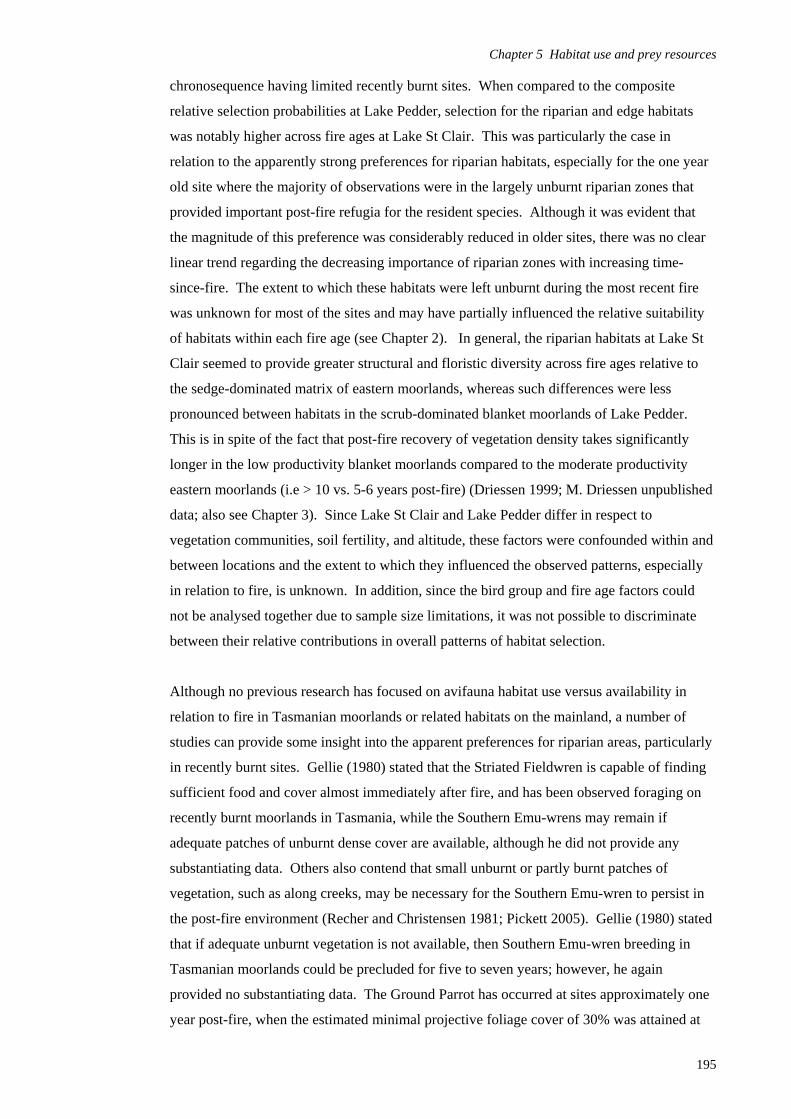
Chapter 5 Habitat use and prey resources
chronosequence having limited recently burnt sites. When compared to the composite
relative selection probabilities at Lake Pedder, selection for the riparian and edge habitats
was notably higher across fire ages at Lake St Clair. This was particularly the case in
relation to the apparently strong preferences for riparian habitats, especially for the one year
old site where the majority of observations were in the largely unburnt riparian zones that
provided important post-fire refugia for the resident species. Although it was evident that
the magnitude of this preference was considerably reduced in older sites, there was no clear
linear trend regarding the decreasing importance of riparian zones with increasing time-
since-fire. The extent to which these habitats were left unburnt during the most recent fire
was unknown for most of the sites and may have partially influenced the relative suitability
of habitats within each fire age (see Chapter 2). In general, the riparian habitats at Lake St
Clair seemed to provide greater structural and floristic diversity across fire ages relative to
the sedge-dominated matrix of eastern moorlands, whereas such differences were less
pronounced between habitats in the scrub-dominated blanket moorlands of Lake Pedder.
This is in spite of the fact that post-fire recovery of vegetation density takes significantly
longer in the low productivity blanket moorlands compared to the moderate productivity
eastern moorlands (i.e > 10 vs. 5-6 years post-fire) (Driessen 1999; M. Driessen unpublished
data; also see Chapter 3). Since Lake St Clair and Lake Pedder differ in respect to
vegetation communities, soil fertility, and altitude, these factors were confounded within and
between locations and the extent to which they influenced the observed patterns, especially
in relation to fire, is unknown. In addition, since the bird group and fire age factors could
not be analysed together due to sample size limitations, it was not possible to discriminate
between their relative contributions in overall patterns of habitat selection.
Although no previous research has focused on avifauna habitat use versus availability in
relation to fire in Tasmanian moorlands or related habitats on the mainland, a number of
studies can provide some insight into the apparent preferences for riparian areas, particularly
in recently burnt sites. Gellie (1980) stated that the Striated Fieldwren is capable of finding
sufficient food and cover almost immediately after fire, and has been observed foraging on
recently burnt moorlands in Tasmania, while the Southern Emu-wrens may remain if
adequate patches of unburnt dense cover are available, although he did not provide any
substantiating data. Others also contend that small unburnt or partly burnt patches of
vegetation, such as along creeks, may be necessary for the Southern Emu-wren to persist in
the post-fire environment (Recher and Christensen 1981; Pickett 2005). Gellie (1980) stated
that if adequate unburnt vegetation is not available, then Southern Emu-wren breeding in
Tasmanian moorlands could be precluded for five to seven years; however, he again
provided no substantiating data. The Ground Parrot has occurred at sites approximately one
year post-fire, when the estimated minimal projective foliage cover of 30% was attained at
195
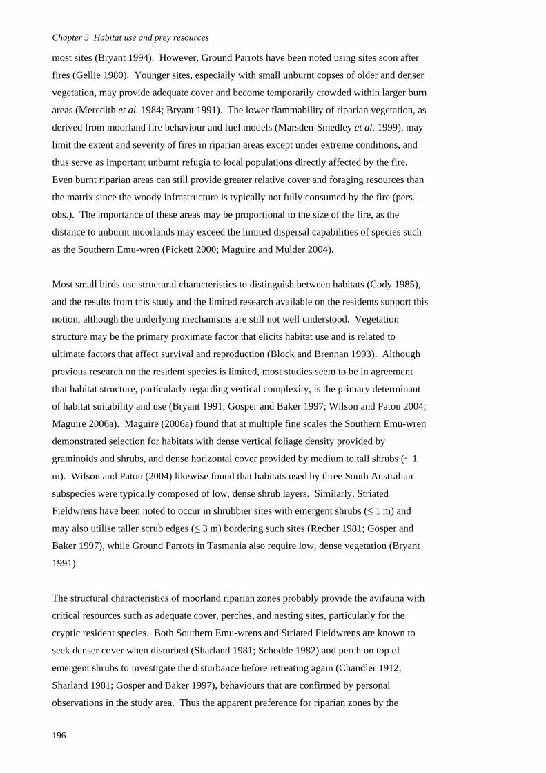
Chapter 5 Habitat use and prey resources
most sites (Bryant 1994). However, Ground Parrots have been noted using sites soon after
fires (Gellie 1980). Younger sites, especially with small unburnt copses of older and denser
vegetation, may provide adequate cover and become temporarily crowded within larger burn
areas (Meredith et al. 1984; Bryant 1991). The lower flammability of riparian vegetation, as
derived from moorland fire behaviour and fuel models (Marsden-Smedley et al. 1999), may
limit the extent and severity of fires in riparian areas except under extreme conditions, and
thus serve as important unburnt refugia to local populations directly affected by the fire.
Even burnt riparian areas can still provide greater relative cover and foraging resources than
the matrix since the woody infrastructure is typically not fully consumed by the fire (pers.
obs.). The importance of these areas may be proportional to the size of the fire, as the
distance to unburnt moorlands may exceed the limited dispersal capabilities of species such
as the Southern Emu-wren (Pickett 2000; Maguire and Mulder 2004).
Most small birds use structural characteristics to distinguish between habitats (Cody 1985),
and the results from this study and the limited research available on the residents support this
notion, although the underlying mechanisms are still not well understood. Vegetation
structure may be the primary proximate factor that elicits habitat use and is related to
ultimate factors that affect survival and reproduction (Block and Brennan 1993). Although
previous research on the resident species is limited, most studies seem to be in agreement
that habitat structure, particularly regarding vertical complexity, is the primary determinant
of habitat suitability and use (Bryant 1991; Gosper and Baker 1997; Wilson and Paton 2004;
Maguire 2006a). Maguire (2006a) found that at multiple fine scales the Southern Emu-wren
demonstrated selection for habitats with dense vertical foliage density provided by
graminoids and shrubs, and dense horizontal cover provided by medium to tall shrubs (~ 1
m). Wilson and Paton (2004) likewise found that habitats used by three South Australian
subspecies were typically composed of low, dense shrub layers. Similarly, Striated
Fieldwrens have been noted to occur in shrubbier sites with emergent shrubs (≤ 1 m) and
may also utilise taller scrub edges (≤ 3 m) bordering such sites (Recher 1981; Gosper and
Baker 1997), while Ground Parrots in Tasmania also require low, dense vegetation (Bryant
1991).
The structural characteristics of moorland riparian zones probably provide the avifauna with
critical resources such as adequate cover, perches, and nesting sites, particularly for the
cryptic resident species. Both Southern Emu-wrens and Striated Fieldwrens are known to
seek denser cover when disturbed (Sharland 1981; Schodde 1982) and perch on top of
emergent shrubs to investigate the disturbance before retreating again (Chandler 1912;
Sharland 1981; Gosper and Baker 1997), behaviours that are confirmed by personal
observations in the study area. Thus the apparent preference for riparian zones by the
196
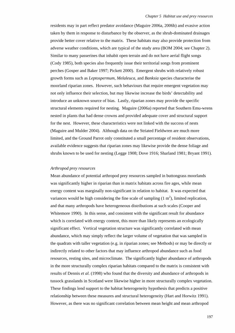
Chapter 5 Habitat use and prey resources
residents may in part reflect predator avoidance (Maguire 2006a, 2006b) and evasive action
taken by them in response to disturbance by the observer, as the shrub-dominated drainages
provide better cover relative to the matrix. These habitats may also provide protection from
adverse weather conditions, which are typical of the study area (BOM 2004; see Chapter 2).
Similar to many passerines that inhabit open terrain and do not have aerial flight songs
(Cody 1985), both species also frequently issue their territorial songs from prominent
perches (Gosper and Baker 1997; Pickett 2000). Emergent shrubs with relatively robust
growth forms such as Leptospermum, Melaleuca, and Banksia species characterise the
moorland riparian zones. However, such behaviours that require emergent vegetation may
not only influence their selection, but may likewise increase the birds’ detectability and
introduce an unknown source of bias. Lastly, riparian zones may provide the specific
structural elements required for nesting. Maguire (2006a) reported that Southern Emu-wrens
nested in plants that had dense crowns and provided adequate cover and structural support
for the nest. However, these characteristics were not linked with the success of nests
(Maguire and Mulder 2004). Although data on the Striated Fieldwren are much more
limited, and the Ground Parrot only constituted a small percentage of resident observations,
available evidence suggests that riparian zones may likewise provide the dense foliage and
shrubs known to be used for nesting (Legge 1908; Dove 1916; Sharland 1981; Bryant 1991).
Arthropod prey resources
Mean abundance of potential arthropod prey resources sampled in buttongrass moorlands
was significantly higher in riparian than in matrix habitats across fire ages, while mean
energy content was marginally non-significant in relation to habitat. It was expected that
variances would be high considering the fine scale of sampling (1 m2), limited replication,
and that many arthropods have heterogeneous distributions at such scales (Cooper and
Whitemore 1990). In this sense, and consistent with the significant result for abundance
which is correlated with energy content, this more than likely represents an ecologically
significant effect. Vertical vegetation structure was significantly correlated with mean
abundance, which may simply reflect the larger volume of vegetation that was sampled in
the quadrats with taller vegetation (e.g. in riparian zones; see Methods) or may be directly or
indirectly related to other factors that may influence arthropod abundance such as food
resources, resting sites, and microclimate. The significantly higher abundance of arthropods
in the more structurally complex riparian habitats compared to the matrix is consistent with
results of Dennis et al. (1998) who found that the diversity and abundance of arthropods in
tussock grasslands in Scotland were likewise higher in more structurally complex vegetation.
These findings lend support to the habitat heterogeneity hypothesis that predicts a positive
relationship between these measures and structural heterogeneity (Hart and Horwitz 1991).
However, as there was no significant correlation between mean height and mean arthropod
197
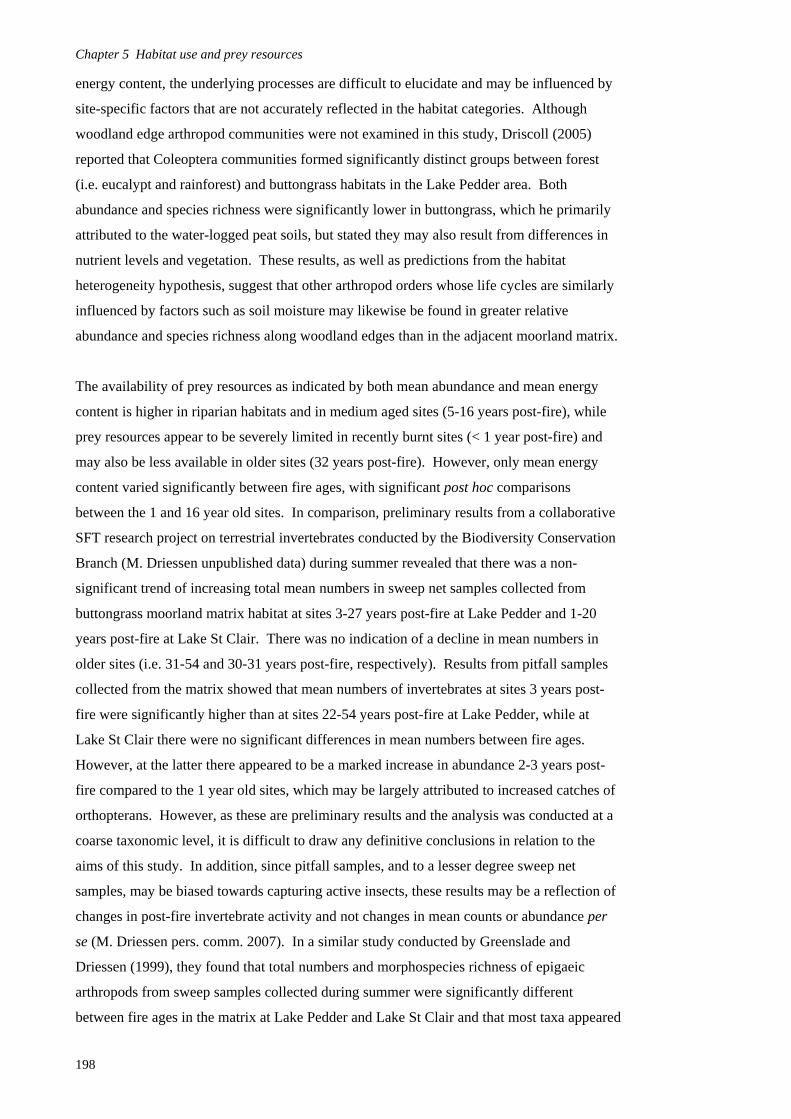
Chapter 5 Habitat use and prey resources
energy content, the underlying processes are difficult to elucidate and may be influenced by
site-specific factors that are not accurately reflected in the habitat categories. Although
woodland edge arthropod communities were not examined in this study, Driscoll (2005)
reported that Coleoptera communities formed significantly distinct groups between forest
(i.e. eucalypt and rainforest) and buttongrass habitats in the Lake Pedder area. Both
abundance and species richness were significantly lower in buttongrass, which he primarily
attributed to the water-logged peat soils, but stated they may also result from differences in
nutrient levels and vegetation. These results, as well as predictions from the habitat
heterogeneity hypothesis, suggest that other arthropod orders whose life cycles are similarly
influenced by factors such as soil moisture may likewise be found in greater relative
abundance and species richness along woodland edges than in the adjacent moorland matrix.
The availability of prey resources as indicated by both mean abundance and mean energy
content is higher in riparian habitats and in medium aged sites (5-16 years post-fire), while
prey resources appear to be severely limited in recently burnt sites (< 1 year post-fire) and
may also be less available in older sites (32 years post-fire). However, only mean energy
content varied significantly between fire ages, with significant post hoc comparisons
between the 1 and 16 year old sites. In comparison, preliminary results from a collaborative
SFT research project on terrestrial invertebrates conducted by the Biodiversity Conservation
Branch (M. Driessen unpublished data) during summer revealed that there was a non-
significant trend of increasing total mean numbers in sweep net samples collected from
buttongrass moorland matrix habitat at sites 3-27 years post-fire at Lake Pedder and 1-20
years post-fire at Lake St Clair. There was no indication of a decline in mean numbers in
older sites (i.e. 31-54 and 30-31 years post-fire, respectively). Results from pitfall samples
collected from the matrix showed that mean numbers of invertebrates at sites 3 years post-
fire were significantly higher than at sites 22-54 years post-fire at Lake Pedder, while at
Lake St Clair there were no significant differences in mean numbers between fire ages.
However, at the latter there appeared to be a marked increase in abundance 2-3 years post-
fire compared to the 1 year old sites, which may be largely attributed to increased catches of
orthopterans. However, as these are preliminary results and the analysis was conducted at a
coarse taxonomic level, it is difficult to draw any definitive conclusions in relation to the
aims of this study. In addition, since pitfall samples, and to a lesser degree sweep net
samples, may be biased towards capturing active insects, these results may be a reflection of
changes in post-fire invertebrate activity and not changes in mean counts or abundance per
se (M. Driessen pers. comm. 2007). In a similar study conducted by Greenslade and
Driessen (1999), they found that total numbers and morphospecies richness of epigaeic
arthropods from sweep samples collected during summer were significantly different
between fire ages in the matrix at Lake Pedder and Lake St Clair and that most taxa appeared
198
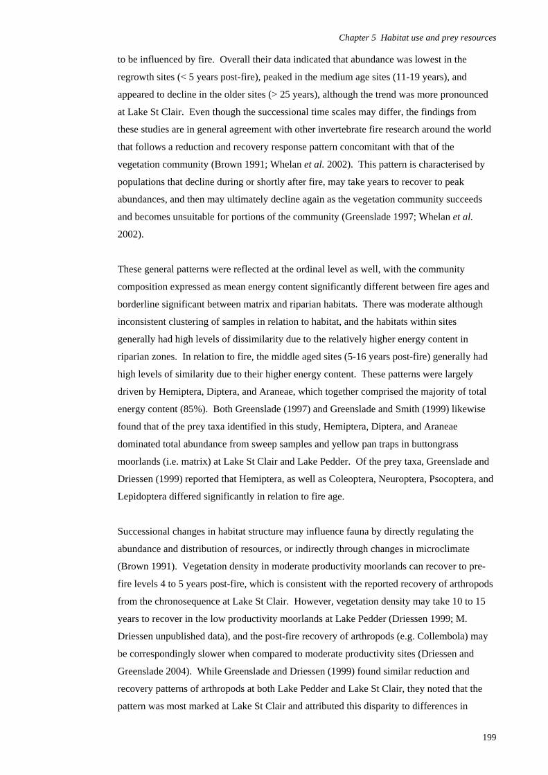
Chapter 5 Habitat use and prey resources
to be influenced by fire. Overall their data indicated that abundance was lowest in the
regrowth sites (< 5 years post-fire), peaked in the medium age sites (11-19 years), and
appeared to decline in the older sites (> 25 years), although the trend was more pronounced
at Lake St Clair. Even though the successional time scales may differ, the findings from
these studies are in general agreement with other invertebrate fire research around the world
that follows a reduction and recovery response pattern concomitant with that of the
vegetation community (Brown 1991; Whelan et al. 2002). This pattern is characterised by
populations that decline during or shortly after fire, may take years to recover to peak
abundances, and then may ultimately decline again as the vegetation community succeeds
and becomes unsuitable for portions of the community (Greenslade 1997; Whelan et al.
2002).
These general patterns were reflected at the ordinal level as well, with the community
composition expressed as mean energy content significantly different between fire ages and
borderline significant between matrix and riparian habitats. There was moderate although
inconsistent clustering of samples in relation to habitat, and the habitats within sites
generally had high levels of dissimilarity due to the relatively higher energy content in
riparian zones. In relation to fire, the middle aged sites (5-16 years post-fire) generally had
high levels of similarity due to their higher energy content. These patterns were largely
driven by Hemiptera, Diptera, and Araneae, which together comprised the majority of total
energy content (85%). Both Greenslade (1997) and Greenslade and Smith (1999) likewise
found that of the prey taxa identified in this study, Hemiptera, Diptera, and Araneae
dominated total abundance from sweep samples and yellow pan traps in buttongrass
moorlands (i.e. matrix) at Lake St Clair and Lake Pedder. Of the prey taxa, Greenslade and
Driessen (1999) reported that Hemiptera, as well as Coleoptera, Neuroptera, Psocoptera, and
Lepidoptera differed significantly in relation to fire age.
Successional changes in habitat structure may influence fauna by directly regulating the
abundance and distribution of resources, or indirectly through changes in microclimate
(Brown 1991). Vegetation density in moderate productivity moorlands can recover to pre-
fire levels 4 to 5 years post-fire, which is consistent with the reported recovery of arthropods
from the chronosequence at Lake St Clair. However, vegetation density may take 10 to 15
years to recover in the low productivity moorlands at Lake Pedder (Driessen 1999; M.
Driessen unpublished data), and the post-fire recovery of arthropods (e.g. Collembola) may
be correspondingly slower when compared to moderate productivity sites (Driessen and
Greenslade 2004). While Greenslade and Driessen (1999) found similar reduction and
recovery patterns of arthropods at both Lake Pedder and Lake St Clair, they noted that the
pattern was most marked at Lake St Clair and attributed this disparity to differences in
199
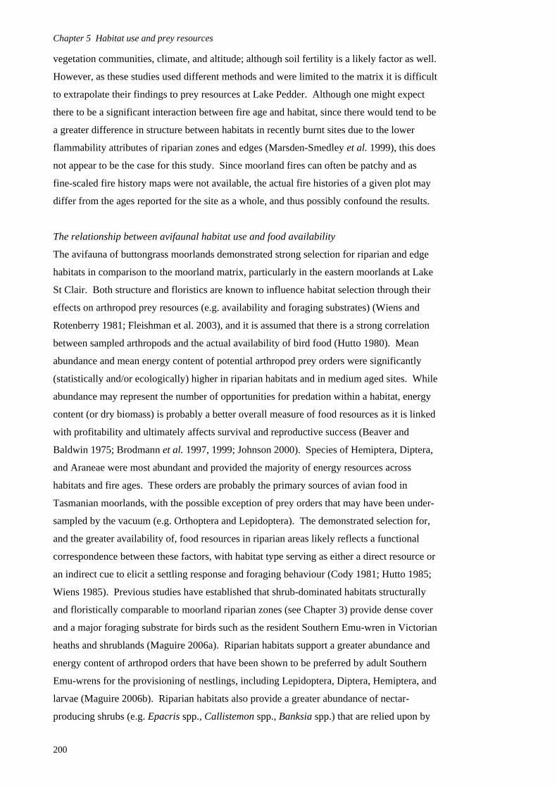
Chapter 5 Habitat use and prey resources
vegetation communities, climate, and altitude; although soil fertility is a likely factor as well.
However, as these studies used different methods and were limited to the matrix it is difficult
to extrapolate their findings to prey resources at Lake Pedder. Although one might expect
there to be a significant interaction between fire age and habitat, since there would tend to be
a greater difference in structure between habitats in recently burnt sites due to the lower
flammability attributes of riparian zones and edges (Marsden-Smedley et al. 1999), this does
not appear to be the case for this study. Since moorland fires can often be patchy and as
fine-scaled fire history maps were not available, the actual fire histories of a given plot may
differ from the ages reported for the site as a whole, and thus possibly confound the results.
The relationship between avifaunal habitat use and food availability
The avifauna of buttongrass moorlands demonstrated strong selection for riparian and edge
habitats in comparison to the moorland matrix, particularly in the eastern moorlands at Lake
St Clair. Both structure and floristics are known to influence habitat selection through their
effects on arthropod prey resources (e.g. availability and foraging substrates) (Wiens and
Rotenberry 1981; Fleishman et al. 2003), and it is assumed that there is a strong correlation
between sampled arthropods and the actual availability of bird food (Hutto 1980). Mean
abundance and mean energy content of potential arthropod prey orders were significantly
(statistically and/or ecologically) higher in riparian habitats and in medium aged sites. While
abundance may represent the number of opportunities for predation within a habitat, energy
content (or dry biomass) is probably a better overall measure of food resources as it is linked
with profitability and ultimately affects survival and reproductive success (Beaver and
Baldwin 1975; Brodmann et al. 1997, 1999; Johnson 2000). Species of Hemiptera, Diptera,
and Araneae were most abundant and provided the majority of energy resources across
habitats and fire ages. These orders are probably the primary sources of avian food in
Tasmanian moorlands, with the possible exception of prey orders that may have been under-
sampled by the vacuum (e.g. Orthoptera and Lepidoptera). The demonstrated selection for,
and the greater availability of, food resources in riparian areas likely reflects a functional
correspondence between these factors, with habitat type serving as either a direct resource or
an indirect cue to elicit a settling response and foraging behaviour (Cody 1981; Hutto 1985;
Wiens 1985). Previous studies have established that shrub-dominated habitats structurally
and floristically comparable to moorland riparian zones (see Chapter 3) provide dense cover
and a major foraging substrate for birds such as the resident Southern Emu-wren in Victorian
heaths and shrublands (Maguire 2006a). Riparian habitats support a greater abundance and
energy content of arthropod orders that have been shown to be preferred by adult Southern
Emu-wrens for the provisioning of nestlings, including Lepidoptera, Diptera, Hemiptera, and
larvae (Maguire 2006b). Riparian habitats also provide a greater abundance of nectar-
producing shrubs (e.g. Epacris spp., Callistemon spp., Banksia spp.) that are relied upon by
200
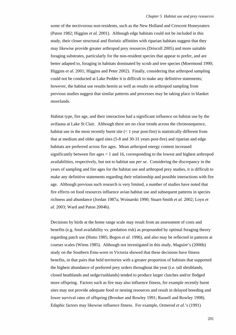
Chapter 5 Habitat use and prey resources
some of the nectivorous non-residents, such as the New Holland and Crescent Honeyeaters
(Paton 1982; Higgins et al. 2001). Although edge habitats could not be included in this
study, their closer structural and floristic affinities with riparian habitats suggest that they
may likewise provide greater arthropod prey resources (Driscoll 2005) and more suitable
foraging substrates, particularly for the non-resident species that appear to prefer, and are
better adapted to, foraging in habitats dominated by scrub and tree species (Moermond 1990;
Higgins et al. 2001; Higgins and Peter 2002). Finally, considering that arthropod sampling
could not be conducted at Lake Pedder it is difficult to make any definitive statements;
however, the habitat use results herein as well as results on arthropod sampling from
previous studies suggest that similar patterns and processes may be taking place in blanket
moorlands.
Habitat type, fire age, and their interaction had a significant influence on habitat use by the
avifauna at Lake St Clair. Although there are no clear trends across the chronosequence,
habitat use in the most recently burnt site (< 1 year post-fire) is statistically different from
that at medium and older aged sites (5-8 and 30-31 years post-fire) and riparian and edge
habitats are preferred across fire ages. Mean arthropod energy content increased
significantly between fire ages < 1 and 16, corresponding to the lowest and highest arthropod
availabilities, respectively, but not to habitat use per se. Considering the discrepancy in the
years of sampling and fire ages for the habitat use and arthropod prey studies, it is difficult to
make any definitive statements regarding their relationship and possible interactions with fire
age. Although previous such research is very limited, a number of studies have noted that
fire effects on food resources influence avian habitat use and subsequent patterns in species
richness and abundance (Jordan 1987a; Woinarski 1990; Stuart-Smith et al. 2002; Loyn et
al. 2003; Ward and Paton 2004b).
Decisions by birds at the home range scale may result from an assessment of costs and
benefits (e.g. food availability vs. predation risk) as propounded by optimal foraging theory
regarding patch use (Hutto 1985; Begon et al. 1996), and also may be reflected in patterns at
coarser scales (Wiens 1985). Although not investigated in this study, Maguire’s (2006b)
study on the Southern Emu-wren in Victoria showed that these decisions have fitness
benefits, in that pairs that held territories with a greater proportion of habitats that supported
the highest abundance of preferred prey orders throughout the year (i.e. tall shrublands,
closed heathlands and sedge/rushlands) tended to produce larger clutches and/or fledged
more offspring. Factors such as fire may also influence fitness, for example recently burnt
sites may not provide adequate food or nesting resources and result in delayed breeding and
lower survival rates of offspring (Brooker and Rowley 1991; Russell and Rowley 1998).
Edaphic factors may likewise influence fitness. For example, Ormerod et al.’s (1991)
201
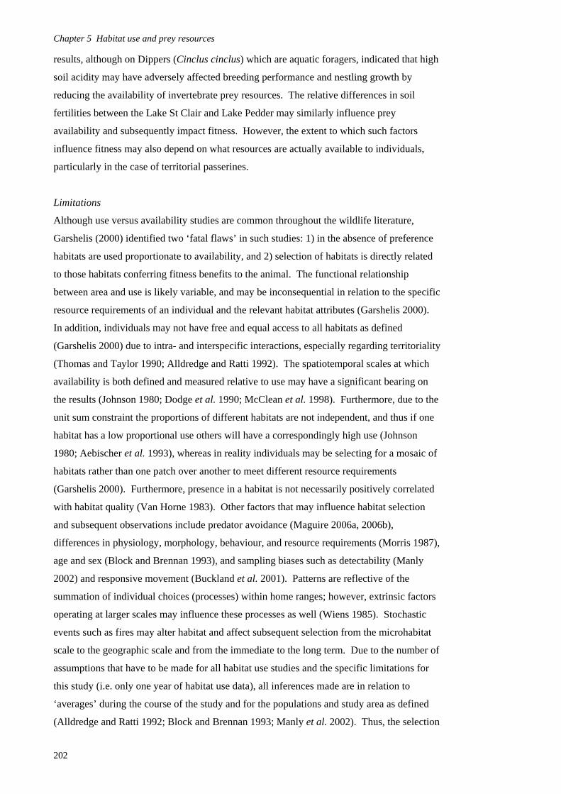
Chapter 5 Habitat use and prey resources
results, although on Dippers (Cinclus cinclus) which are aquatic foragers, indicated that high
soil acidity may have adversely affected breeding performance and nestling growth by
reducing the availability of invertebrate prey resources. The relative differences in soil
fertilities between the Lake St Clair and Lake Pedder may similarly influence prey
availability and subsequently impact fitness. However, the extent to which such factors
influence fitness may also depend on what resources are actually available to individuals,
particularly in the case of territorial passerines.
Limitations
Although use versus availability studies are common throughout the wildlife literature,
Garshelis (2000) identified two ‘fatal flaws’ in such studies: 1) in the absence of preference
habitats are used proportionate to availability, and 2) selection of habitats is directly related
to those habitats conferring fitness benefits to the animal. The functional relationship
between area and use is likely variable, and may be inconsequential in relation to the specific
resource requirements of an individual and the relevant habitat attributes (Garshelis 2000).
In addition, individuals may not have free and equal access to all habitats as defined
(Garshelis 2000) due to intra- and interspecific interactions, especially regarding territoriality
(Thomas and Taylor 1990; Alldredge and Ratti 1992). The spatiotemporal scales at which
availability is both defined and measured relative to use may have a significant bearing on
the results (Johnson 1980; Dodge et al. 1990; McClean et al. 1998). Furthermore, due to the
unit sum constraint the proportions of different habitats are not independent, and thus if one
habitat has a low proportional use others will have a correspondingly high use (Johnson
1980; Aebischer et al. 1993), whereas in reality individuals may be selecting for a mosaic of
habitats rather than one patch over another to meet different resource requirements
(Garshelis 2000). Furthermore, presence in a habitat is not necessarily positively correlated
with habitat quality (Van Horne 1983). Other factors that may influence habitat selection
and subsequent observations include predator avoidance (Maguire 2006a, 2006b),
differences in physiology, morphology, behaviour, and resource requirements (Morris 1987),
age and sex (Block and Brennan 1993), and sampling biases such as detectability (Manly
2002) and responsive movement (Buckland et al. 2001). Patterns are reflective of the
summation of individual choices (processes) within home ranges; however, extrinsic factors
operating at larger scales may influence these processes as well (Wiens 1985). Stochastic
events such as fires may alter habitat and affect subsequent selection from the microhabitat
scale to the geographic scale and from the immediate to the long term. Due to the number of
assumptions that have to be made for all habitat use studies and the specific limitations for
this study (i.e. only one year of habitat use data), all inferences made are in relation to
‘averages’ during the course of the study and for the populations and study area as defined
(Alldredge and Ratti 1992; Block and Brennan 1993; Manly et al. 2002). Thus, the selection
202
Chapter 5 Habitat use and prey resources
probabilities are still considered to be valid but the associated errors may not reflect the
actual variation in the populations being studied (Manly et al. 2002).
The primary issues with avian habitat use and food resource studies are biased sampling of
food resources and definitions of availability in both space and time (Block and Brennan
1993). As no sampling methods are considered to be capable of collecting all individuals
from all orders present in a plot (Southwood and Henderson 2000), these results may have
underestimated actual abundance and diversity. For example, during the course of vacuum
sampling two large orthopterans (~ 3 cm) and one large dipteran (~ 4 cm) were observed
within or adjacent to the quadrat but were able to escape collection, although such apparent
evasive action was expected (Ausden 1996). Overall extraction efficiency of vacuum
sampling under some conditions has been shown to be reduced in taller vegetation (~ > 50
cm; De Barro 1991; Brodmann and Reyer 1999; Hossain et al. 1999); therefore, differences
between riparian and matrix habitats may be greater than indicated by these results. It is also
important to note that these are measures of standing crop within matrix and riparian habitats
and not actual productivity, and that these figures essentially represent a snap-shot in both
space (i.e. 11 sites at Lake St Clair) and time (i.e. 4 days of sampling) and do not encompass
the spatial, seasonal, and annual variation that would be expected in arthropod communities
(Wiens 1984; Hutto 1990; Driessen and Greenslade 2004). For example, overall arthropod
catches in buttongrass moorlands are known to be significantly lower in winter (M. Driessen
unpublished data). Finally, measures of abundance and diversity may be confounded with
changes in arthropod activity, particularly in relation to post-fire succession (M. Driessen
pers. comm. 2007), although this is likely to be more of an issue with passive sampling
methods such as pitfall traps.
Although the prey orders included in this study were based on species-specific dietary data
from the literature, there are a range of factors that may influence which arthropods are
actually consumed by the avifauna. There can be a complex interaction between
interspecific foraging methods and arthropod size, conspicuousness, activity patterns,
mobility, abundance, microhabitats, and weather (Bryant 1973; Hutto 1980; Hutto 1981;
Cooper and Whitmore 1990; Wolda 1990). Some studies suggest that foraging choices are
ultimately based on profitability, particularly during the breeding season, such that birds will
pursue large and/or abundant prey that are easily captured in order to maximize net energy
gain per unit time (Bryant 1973; Brodmann and Reyer 1999). Such important patterns may
be masked by only identifying arthropods to the ordinal level, as there is a risk that nonprey
species may actually be driving the observed patterns in arthropod abundance and energy
content and obscure any relationships with avian habitat use (Wolda 1990). The scale of
measurement may also influence results if the sampling of prey resources it is not
203
Chapter 5 Habitat use and prey resources
204
commensurate with that of foraging (Hutto 1990). The extent to which seasonal differences
may affect arthropods is unknown, although community composition and energy content are
known to vary with seasons (Norberg 1978; Driessen and Greenslade 2004; M. Driessen
unpublished data; pers. obs.), which may, in turn, influence the relative use of these habitats
(Hutto 1980). Lastly, birds may directly and indirectly affect insect populations (Hutto
1985; Otvos 1979 cited in Block and Brennan 1993); thus, sampled areas may represent
depleted patches. When only measuring the standing crop, it must be assumed that values
are representative of the resources in that microhabitat both before and after the sampling
event (Hutto 1990). Ultimately, one must decide whether the chosen methods produce
reliable results regarding the use and actual availability of habitat and food resources (Hutto
1990). Despite some of these limitations, and particularly the fact that the arthropod surveys
were not conducted synchronously with the habitat use surveys, it is believed that these
results provided a reasonable first approximation of the relative availability of potential
arthropod prey resources between matrix and riparian habitats in buttongrass moorlands.
These results may help to explain, in part, the observed patterns in avian habitat selection in
moorlands.
The implications of the results from this study for avifaunal conservation and fire
management of Tasmanian buttongrass moorlands are summarised in Chapter 7.

Chapter 6 Short-term avifaunal composition and densities in relation to
hazard-reduction burning of buttongrass moorlands in the
Tasmanian Wilderness World Heritage Area
Introduction Fire has been part of the Tasmanian environment for millions of years and was probably
used as a land management tool by Tasmanian Aborigines since approximately 40,000-
70,000 years BP (Plomley 1966; Kirkpatrick et al. 1978; Kee et al. 1993; Jackson 1999a;
Kershaw et al. 2002; Gammage 2008; see Chapter 1). Historical records indicate that
Tasmanian Aborigines actively burnt buttongrass moorlands throughout western Tasmania at
the time of early-European settlement in the early 1800s (Plomley 1966; Gammage 2008). It
has been speculated that Aborigines probably lit recurrent fires (e.g. inter-fire interval ≤ 20
years) under weather conditions that would have resulted in low-intensity burns that were
largely restricted to moorland vegetation (Marsden-Smedley 1998a). Early European use of
fire was variable, but showed a notable departure from Aboriginal-style burning practices,
resulting in a number of high-intensity, landscape-scale fires that burnt large areas of both
moorland and fire-sensitive vegetation (e.g. rainforest and alpine communities) (Marsden-
Smedley 1998b; Johnson and Marsden-Smedley 2002; Pyrke and Marsden-Smedley 2005).
Currently, most fire management activities in buttongrass moorlands are focused on resource
protection and consist of limited wildfire suppression and frequent tactical hazard-reduction
burning (i.e. inter-fire interval ~5-8 years) in areas that are at a high risk of accidental and
arson ignitions, such as the medium productivity sites along the Lyell Highway near Lake St
Clair in, and adjacent to, the Tasmanian Wilderness World Heritage Area (TWWHA) (PWS
1996; Marsden-Smedley et al. 1999; Marsden-Smedley and Kirkpatrick 2000; Marsden-
Smedley et al. 2001; Marsden-Smedley 2009; PWS unpublished data; see Chapter 2). The
primary objective of hazard-reduction burning in buttongrass moorlands is to reduce > 70%
of the fuel load across > 70% of the site being burnt (PWS 1996; Marsden-Smedley et al.
1999). Reduced fuel loads help ensure that subsequent fires in intervening years will have
lower rates of spread and shorter flame heights, and thus increase the likelihood of successful
suppression (Marsden-Smedley and Catchpole 1995b; Marsden-Smedley et al. 1999). It is
estimated that less than 2% of moorlands throughout Tasmania is currently subjected to
tactical hazard-reduction burning (Driessen 2006). Although limited in scope, it is
recognised that high-frequency fire regimes may adversely affect biodiversity and cause
long-term community changes in the targeted areas (Jackson 1978; Marsden-Smedley and
205

Chapter 6 Short-term avifaunal responses to fire Kirkpatrick 2000; Pyrke and Marsden-Smedley 2005). Thus, fire management is arguably
the primary deterministic factor affecting Tasmanian buttongrass moorland ecosystems,
particularly in the TWWHA, where they are largely protected from other potential
anthropogenic threats.
Proposed future fire management strategies include an overall increase in the total area of
moorlands burnt on an annual basis (i.e. 5-10%), using a combination of broad-scale
ecosystem management burning and tactical hazard-reduction burning in high risk areas, as
well as wildfire suppression when and where appropriate (Marsden-Smedley and Kirkpatrick
2000; Marsden-Smedley et al. 2001; PWS 2004; King et al. 2006, 2008; Marsden-Smedley
2009). It is thought that such a strategy would mimic Aboriginal burning regimes and help
to conserve fire-adapted ecosystems (e.g. moorlands, wet sclerophyll woodlands and
forests), while limiting the incidence, extent, and severity of unplanned fires and their
adverse impacts on fire-sensitive resources (e.g. peat, temperate rainforests, alpine
communities) and other assets (Marsden-Smedley and Kirkpatrick 2000; Marsden-Smedley
et al. 2001; Pyrke and Marsden-Smedley 2005; PWS 2004; King et al. 2006, 2008; J.
Marsden-Smedley pers. comm. 2007). Treatment levels at the lower end of this range (i.e. ~
5%) would represent a fairly modest increase on current levels, but at the upper end (i.e. ~
10%) would result in higher fire frequencies than are believed to have characterised
Aboriginal and early-European fire regimes, and may adversely impact moorland ecosystems
(Marsden-Smedley 1998b; Marsden-Smedley and Kirkpatrick 2000; PWS 2004; Pyrke and
Marsden-Smedley 2005; King et al. 2006, 2008). Accordingly, both current fire
management practices and proposed future strategies have generated vigorous debate over
the potential short- to long-term effects of fire on biogeodiversity, including the moorland
avifauna, and a consensus on appropriate fire management both within and outside of the
TWWHA remains elusive (DPIW 2007; May and Balmer 2008; see Chapter 7).
Although many birds are probably able to survive low- to moderate-intensity fires typical of
hazard-reduction burns in buttongrass moorlands (Cowley et al. 1969; Recher and
Christensen 1981; Rowley and Brooker 1987; Wooller and Calver 1988; Marsden-Smedley
and Catchpole 1995c; Marsden-Smedley et al. 1999), their ability to persist and reproduce in
the post-fire environment is less certain and may be influenced by a wide range of species-,
site-, and fire-specific factors (Brooker and Rowley 1991; Keith et al. 2002a; Whelan et al.
2002; Bradstock et al. 2005; see Chapters 1, 4-5). Despite the pyrogenic nature of
buttongrass moorlands (Pyrke and Marsden-Smedley 2005), some fire-sensitive attributes
are exhibited by a number of the species that comprise the moorland avifauna, including the
resident Southern Emu-wren, Striated Fieldwren, and Ground Parrot (Meredith et al. 1984;
Bryant 1990; Gosper and Baker 1997; Pickett 2000; Higgins and Peter 2002; Wilson and
206
Chapter 6 Short-term avifaunal responses to fire
Paton 2004; Tasker and Baker 2005; see Chapter 4). Inappropriate fire regimes are a
demonstrated or speculated threat to mainland populations (Garnett 1992; Brown et al. 1993;
Garnett and Crowley 2000; see Chapters 1 and 4) and the space-for-time (SFT) studies
presented in Chapters 4 and 5 highlight some of the potential effects of fire on the resident
and non-resident species of Tasmanian moorlands over successional time scales (i.e. up to ~
50 years post-fire). However, the inferences that can be drawn from SFT studies are
somewhat limited due to the possibility of inter-site variability in abiotic and biotic factors
confounding or compounding observed differences in populations from any effects of fire
per se (Whelan 1995; Loyn 1999; Woinarski 1999b; Block et al. 2001; see Chapters 2 and
4). An alternative study design is before-after-control-impact (BACI) (Stewart-Oaten et al.
1986), that may include paired impact and control sites that are surveyed before and after the
impact (i.e. fire) (Smith 2002). This provides a basis for stronger inferences since any
observed changes in community composition and abundance can more reasonably be
attributed to the effects of fire per se (Whelan 1995; Loyn 1999; Parker and Wiens 2005).
During the autumn and spring of 2005, the Parks and Wildlife Service (PWS) conducted
hazard-reduction burns in the Lake St Clair area, including moderate productivity, eastern
moorlands at Travellers Rest (TRR, last burnt 1973) and Navarre Plains East (NPE, 1988),
respectively (see Chapter 2). Since these sites were surveyed during three seasons in 2004,
along with both Beehive Canal North (BCN, 1974) and Bedlam (BED, 1990) which
remained unburnt, a valuable opportunity was available to more rigorously assess the short-
term impacts of fire on the moorland avifauna within a paired BACI framework. Such
opportunistic studies conducted in other regions of Australia have provided important
guidance for avian conservation and fire management (e.g. Brooker and Rowley 1991;
Recher 1997; Loyn 1997). In this study, distance sampling and variable circular-plots were
used within a paired BACI design to quantify pre- and post-fire (i.e. before- and after-
impact) avifaunal diversity and density in paired unburnt (i.e. control during time of study)
and burnt (i.e. impact) medium productivity eastern moorlands at Lake St Clair, Tasmania.
The primary aims of this study were 1) to investigate the short-term impacts (5-18 months
post-fire) of low intensity hazard-reduction burns on avifaunal diversity and density, with a
focus on the Southern Emu-wren and Striated Fieldwren; 2) to asses the influence of site-
and fire-specific factors on species response patterns; and 3) to provide information to help
guide fire management and conservation of the buttongrass moorland avifauna.
207

Chapter 6 Short-term avifaunal responses to fire Methods Study area
Details of the site descriptions, fire histories, vegetation configurations, and floristics of the
study sites are provided in Chapters 2 and 3. This study was limited to four sites (i.e. BED,
NPE, BCN, TRR) on the moderate-productivity doleritic geologies at Lake St Clair,
Tasmania. The moorland matrix primarily consists of Eastern Buttongrass Moorland with a
small area of Subalpine Sedgeland at BCN (for vegetation classes see Table 4, Chapter 3).
The matrix is scattered with Eastern Wood Copses, interspersed and bordered by typically
small perennial watercourses (i.e. first - third order streams; after Strahler 1952) forming
Eastern Buttongrass Riparian Zones, and primarily bordered by Eucalyptus delegatensis
Woodlands and roadside vegetation (i.e. Cleared or Disturbed Land), all of which form
relatively distinct edges with the moorland matrix.
Hazard-reduction burns were conducted by PWS on 21 April 2005 at TRR and 21 September
2005 at NPE, thus eliminating the risk of pseudoreplication among treatment sites (sensu
Hurlbert 1984). At the time of the hazard-reduction burns the impact sites, NPE and TRR,
were approximately 18 and 33 years post-fire, respectively. The control sites, BED and
BCN, were chosen since they were the same approximate age as the impact sites at the time
of the hazard-reduction burns (i.e. 16 and 32 years post-fire, respectively; see Chapter 2).
The burn at NPE was ignited by both an aerial ‘Dragon’ driptorch and by hand driptorches
(ignition pattern not reported). It was of a low intensity (i.e. rate of spread < 4.5 m min-1 and
flame heights < 4.5 m), burnt approximately 94% of the site as defined in this study, and
covered a total of 612 ha, including extensive moorlands to the east and south of the site.
The burn at TRR was ignited by hand driptorches (ignition pattern not reported). It was of a
low intensity, burnt approximately 93% of the site as defined, and covered a total of 42 ha,
including small areas adjacent to the site (Marsden-Smedley and Catchpole 1995c; Marsden-
Smedley et al. 1999; J. Marsden-Smedley pers. comm. 2007; PWS unpublished data; this
study). The hazard-reduction burn objectives were met at both sites, with an estimated
average of 70% of aerial fuels burnt over 70% of the areas (PWS 1996; Marsden-Smedley et
al. 1999; PWS unpublished data; pers. obs.).
Avian survey methods
Survey methods consisted of point and line transect distance surveys conducted during the
day for the avifauna as a whole and variable circular plot (VCP) surveys conducted at dusk
for the Ground Parrot, as detailed for the SFT surveys in Chapter 4. Transects at each of the
four sites were re-established based on the GPS coordinates from the survey points used
during the pre-fire SFT surveys in 2004. The post-fire sampling was conducted during the
summer (3-6 February), winter (13-17 May), and spring (6-16 October) of 2006; therefore,
208

Chapter 6 Short-term avifaunal responses to fire
each site was surveyed three times and the burn sites (i.e. NPE and TRR) were 5-13 months
and 10-18 months post-fire, respectively, during the survey period. Thus, the study design
consisted of paired control and burn sites for two fire age classes and at the time of the burns
all four sites (i.e. BED-NPE, 16-18 years post-fire; and BCN-TRR, 32-33 years post-fire; see
Chapter 2) were considered to be mature moorlands in relation to vegetative cover and other
metrics of successional development (Marsden-Smedley and Catchpole 1995b; Marsden-
Smedley 1998a; see Chapters 1 and 3). A survey schedule was developed in which the time
of day and the order of the control and burn sites were systematically rotated within and
across seasons to minimise temporal biases (Mac Nally 1996a). Since the Ground Parrot
was absent from the four sites during all of the pre-fire and post-fire VCP surveys, it was
excluded from further consideration in this study.
Weather conditions during the surveys were fairly typical for the study area (see Chapter 2);
temperature and rainfall data for 2004-2006, when compared to historical climatic data
(1961-1990), indicated that there were no major temperature anomalies, while rainfall was
14% below normal during 2006 (BOM 2007). Weather conditions for the pre-fire surveys
are detailed in Chapter 4. For the post-fire surveys the mean temperature was 8.7°C (range
1-17°C) during the daytime surveys and 8.7°C (range 3-15°C) at dusk, while mean relative
humidity was 76.1% (range 54-100%) during the daytime and 76.3% (range 67-98%) at
dusk. During both daytime and dusk surveys cloud cover and wind speeds were highly
variable, but survey conditions were typically partly cloudy to overcast (83%; n = 24) with
calm to light winds (96%) and no precipitation (75%). As reported in Chapter 4, it is
unlikely that such weather conditions had a notable influence on the overall results.
Analyses
The resident and non-resident species included in this study and the methods for determining
species composition and densities of the control and burn sites during the pre-fire surveys are
outlined for the SFT study in Chapter 4. As for the pre-fire surveys, both auditory and visual
detections from the point and line transects were used to determine total species presence for
the four control and burn sites. Exact distance data (i.e. visual detections) for the post-fire
control and burn sites were analysed using Program Distance 5.0 to estimate species
densities (Thomas et al. 2010) following the methods detailed by Buckland et al. (2001,
2004) and Thomas et al. (2006, 2010). Separate sets of analyses were conducted for exact
point and exact line surveys. Due to the small sample sizes from the post-fire surveys,
probabilities ( ) and the standard error (± SE) of of the number of clusters detected
within the surveyed areas (a) (using the associated truncation widths (w) and expected
cluster sizes (s)) estimated for the Southern Emu-wren, Striated Fieldwren, and non-resident
group for the point and line transects in the SFT study were used as multipliers with a
aP aP
209
Chapter 6 Short-term avifaunal responses to fire uniform key function and no adjustment terms to estimate mean stratum-level densities ( D ,
birds 10-1) (pooled across the three seasons) for the post-fire control and burn sites. Data
were insufficient to obtain reliable results from multiple covariate distance sampling
(MCDS) analysis in order to determine whether the treatment covariate influenced
detectability for the post-fire surveys. However, based on the MCDS model selection
process from the larger pre-fire SFT dataset, the recent-burn covariate was only selected in
the case of the Striated Fieldwren and indicated that it had a higher probability of detection
in recently burnt sites compared to older sites (i.e. 1 or > 1 year post-fire at Lake St Clair,
respectively). Accordingly, the corresponding covariate-specific probabilities of detection
for the pre-fire sites were used to estimate stratum-specific densities for the Striated
Fieldwren at the post-fire control and burn sites.
The estimated species-specific mean densities (across seasons) derived from the point and
line methods were averaged for each site (Buckland et al. 2001; see Chapter 4). The
variance of density estimates by species and site was approximated using the delta method
and included variance from the encounter rate from the post-fire surveys, and detection
probability and cluster size estimation from the pre-fire surveys (Buckland et al. 2001; see
Chapter 4). Estimates of encounter rate variance were based on a Poisson distribution and
each point and line was treated as a replicate (Buckland et al. 2001; Thomas et al. 2002).
The overdispersion parameters (b; aka variance inflation factor) calculated for each set of
analyses in the SFT study following the method described by Buckland et al. (2001) were
used in order to provide more reliable variance estimates for all of the sites (Lebreton et al.
1992; Burnham and Anderson 2002; Franklin et al. 2002) and ensure comparability between
the pre- and post-fire estimates. Estimates of variance for the final combined point and line
density estimates for each species by site were derived following the general methods of
Steel and Torrie (1980).
A range of different methods for analysing BACI and related study designs have been
extensively discussed and debated in the literature (Hurlbert 1984; Stewart-Oaten et al. 1986;
Underwood 1994; Conquest 2000; McDonald et al. 2000; Murtaugh 2000, 2002, 2003;
Smith 2002; Stewart-Oaten 2003; Clarke et al. 2006; Buckland et al. 2009). In order to
address some of the inherent limitations of BACI designs and meet the underlying
assumptions of many of these proposed methods, it is necessary to have statistically
independent estimates based on large sample sizes, adequate replication within and between
sites, and numerous pre- and post-impact survey periods. Murtaugh (2002, 2003, 2007)
argued that, even under such ideal circumstances, it may be more appropriate to base
inferences on informed interpretation of graphical representations and overall weight of
evidence than to solely rely upon results from statistical tests. He demonstrated that
210
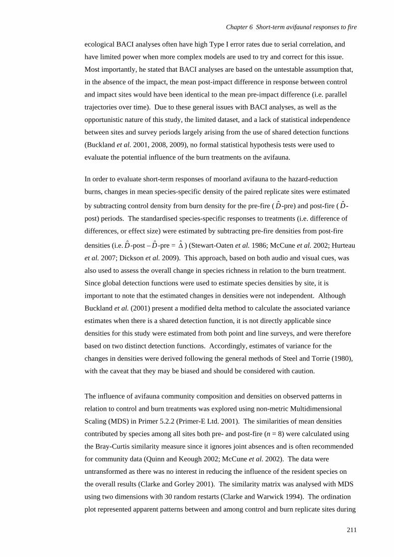
Chapter 6 Short-term avifaunal responses to fire
ecological BACI analyses often have high Type I error rates due to serial correlation, and
have limited power when more complex models are used to try and correct for this issue.
Most importantly, he stated that BACI analyses are based on the untestable assumption that,
in the absence of the impact, the mean post-impact difference in response between control
and impact sites would have been identical to the mean pre-impact difference (i.e. parallel
trajectories over time). Due to these general issues with BACI analyses, as well as the
opportunistic nature of this study, the limited dataset, and a lack of statistical independence
between sites and survey periods largely arising from the use of shared detection functions
(Buckland et al. 2001, 2008, 2009), no formal statistical hypothesis tests were used to
evaluate the potential influence of the burn treatments on the avifauna.
In order to evaluate short-term responses of moorland avifauna to the hazard-reduction
burns, changes in mean species-specific density of the paired replicate sites were estimated
by subtracting control density from burn density for the pre-fire ( D-pre) and post-fire ( D-
post) periods. The standardised species-specific responses to treatments (i.e. difference of
differences, or effect size) were estimated by subtracting pre-fire densities from post-fire
densities (i.e. D-post – D-pre = ) (Stewart-Oaten et al. 1986; McCune et al. 2002; Hurteau
et al. 2007; Dickson et al. 2009). This approach, based on both audio and visual cues, was
also used to assess the overall change in species richness in relation to the burn treatment.
Since global detection functions were used to estimate species densities by site, it is
important to note that the estimated changes in densities were not independent. Although
Buckland et al. (2001) present a modified delta method to calculate the associated variance
estimates when there is a shared detection function, it is not directly applicable since
densities for this study were estimated from both point and line surveys, and were therefore
based on two distinct detection functions. Accordingly, estimates of variance for the
changes in densities were derived following the general methods of Steel and Torrie (1980),
with the caveat that they may be biased and should be considered with caution.
The influence of avifauna community composition and densities on observed patterns in
relation to control and burn treatments was explored using non-metric Multidimensional
Scaling (MDS) in Primer 5.2.2 (Primer-E Ltd. 2001). The similarities of mean densities
contributed by species among all sites both pre- and post-fire (n = 8) were calculated using
the Bray-Curtis similarity measure since it ignores joint absences and is often recommended
for community data (Quinn and Keough 2002; McCune et al. 2002). The data were
untransformed as there was no interest in reducing the influence of the resident species on
the overall results (Clarke and Gorley 2001). The similarity matrix was analysed with MDS
using two dimensions with 30 random restarts (Clarke and Warwick 1994). The ordination
plot represented apparent patterns between and among control and burn replicate sites during
211

Chapter 6 Short-term avifaunal responses to fire the pre- and post-fire periods with the underlying similarities in community composition and
densities.
Results
Avifaunal responses to hazard-reduction burning
A total of only 20 bird species, in addition to unspecified raptor species, was recorded by
audio and/or visual cues during the course of both pre- and post-fire surveys at the four
control and burn sites included in this study. Of the 25 species listed for the SFT study in
Chapter 4, the only species not detected were the Ground Parrot (Pezoporus wallicus), Grey
Fantail (Rhipidura fuliginosa), Olive Whistler (Pachycephala olivacea), Pink Robin
(Petroica rodinogaster), Strong-billed Honeyeater (Melithreptus validirostris), and White-
throated Needletail (Hirundapus caudacutus), none of which were recorded at any of these
sites either pre- or post-fire. Latham’s Snipe (Gallinago hardwickii) was the only species
recorded that was not detected in the SFT study. Three species were only detected in
unburnt sites (i.e. pre-fire control and burn and post-fire control): the Beautiful Firetail
(Stagonopleura bella), Black-headed Honeyeater (Melithreptus affinis), and Grey Shrike-
thrush (Colluricincla harmonica), while two species were only detected at post-fire burn
sites, namely Latham’s Snipe (Gallinago hardwickii) and Black Currawong (Strepera
fuliginosa). Based on audio and visual cues, there was an overall mean increase of three
species in the burn treatments when compared to the controls from the pre- to post-fire
periods. Data on the 12 resident and non-resident species included in the following analyses
(Table 1) were limited to observations of singles or clusters of birds that were confirmed by
visual cues and measured using exact distances from the point and/or line transects (n = 168
within w, see Chapter 4).
A summary of estimated mean species densities (across seasons) for the pre- and post-fire
control and burn replicate sites is presented in Table 1, and the standardised differences of
mean densities (across replicates) between pre- and post-fire estimates for the burn
treatments relative to the controls are presented in Figure 1. Overall, the resident Striated
Fieldwren and Southern Emu-wren decreased in post-fire densities at burn sites relative to
controls, with mean differences of -0.68 ± 0.97 and -1.25 ± 2.96 birds 10 ha-1, respectively.
In contrast, all of the non-resident species, except for the Green Rosella, increased in
densities relative to controls, with a mean difference across all non-residents of 1.64 ± 0.82
birds 10 ha-1. Of these, the Flame Robin (0.58 ± 0.27 birds 10 ha-1), Superb Fairy-wren (0.56
± 0.43 birds 10 ha-1), and Richard’s Pipit (0.44 ± 0.18 birds 10 ha-1) demonstrated the
greatest relative increases in estimated densities.
212

Chapter 6 Short-term avifaunal responses to fire
The large standard errors were due to a number of factors (Table 1, Figure 1), including the
small sample sizes, high variability in intra- and inter-site estimated densities, and the
propagation of errors due to the series of calculations required to estimate the standardised
differences in pre- and post-fire densities (i.e. D-post – D-pre = ). Since the confidence
intervals included 0 for 7 out of the 12 species, including the two resident species, the data
were insufficient to demonstrate a clear treatment effect. For some species the sign and
magnitude of standardised differences in estimated densities differed between the paired
replicate control-burn sites (i.e. BED-NPE and BCN-TRR). For example, although the mean
difference across replicates for the Southern Emu-wren indicated an overall decrease in
density due to a relatively large post-fire decrease for BED-NPE (-3.19 ± 5.10 birds 10 ha-1),
the difference for BCN-TRR was positive (1.65 ± 3.01 birds 10 ha-1) since it was not
detected during the pre-fire surveys but was detected post-fire at TRR (Table 1). There was
a similar, although less pronounced, pattern for the Striated Fieldwren with a negative
difference for BED-NPE (-1.43 ± 1.49 birds 10 ha-1) and a positive difference for BCN-TRR
(0.09 ± 1.25 birds 10 ha-1), since it was likewise not recorded by visual observation during
the pre-fire surveys at TRR. However, it was recorded by audio cue in the pre-fire surveys
and thus at least utilised, and possibly occupied, the site before the burn (T. Chaudhry
unpublished data). Accordingly, the apparent post-fire increase in density of the Striated
Fieldwren at TRR may be overestimated (Table 1) and hence the standardised negative
difference underestimated (Figure 1). Due to the issues outlined above, these estimates and
subsequent inferences should be considered with a high degree of caution.
The non-metric MDS ordination plot of the four control and burn sites pre- and post-fire had
a stress value of 0.03 (Figure 2), indicating an excellent two-dimensional ordination that can
be interpreted with a high degree of confidence (Clarke and Warwick 1994). Although there
are no definitive clusters among the sites, some patterns in avifaunal composition and
densities were apparent. Both the control sites (BED and BCN) were more similar in
avifaunal composition and densities from the pre- to post-fire periods when compared to the
burn sites pre- and post-fire (NPE and TRR), particularly NPE which shows the highest level
of intra-site dissimilarity between periods. Although TRR also shows a relatively high level
of intra-site dissimilarity, it was apparent that the pre-fire community is the most dissimilar
among the pre-fire sites. One possible explanation for this, as noted above, is that the two
resident species were not recorded by visual observations during the pre-fire surveys at TRR,
but were recorded during the post-fire surveys. Hence, TRR shared greater post-fire
similarities with the other sites where these species were likewise recorded. However, since
the Striated Fieldwren was not recorded by visual observation in the pre-fire period but was
present at the site based on auditory cues, this apparent dissimilarity may be positively
biased.
213

Chapter 6 Short-term avifaunal responses to fire
214
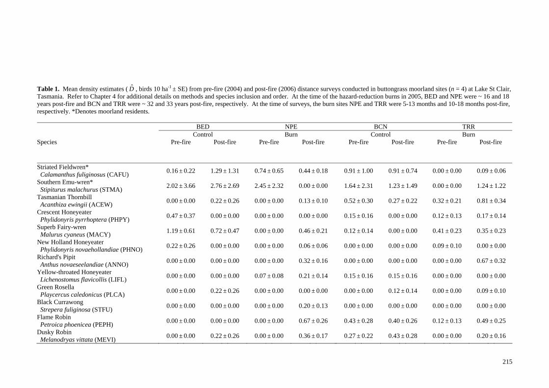
Table 1. Mean density estimates ( , birds 10 haD -1 ± SE) from pre-fire (2004) and post-fire (2006) distance surveys conducted in buttongrass moorland sites (n = 4) at Lake St Clair, Tasmania. Refer to Chapter 4 for additional details on methods and species inclusion and order. At the time of the hazard-reduction burns in 2005, BED and NPE were ~ 16 and 18 years post-fire and BCN and TRR were ~ 32 and 33 years post-fire, respectively. At the time of surveys, the burn sites NPE and TRR were 5-13 months and 10-18 months post-fire, respectively. *Denotes moorland residents.
BED NPE BCN TRR Control Burn Control Burn
Species
Pre-fire Post-fire Pre-fire Post-fire Pre-fire Post-fire Pre-fire Post-fire
Striated Fieldwren* Calamanthus fuliginosus (CAFU)
0.16 ± 0.22 1.29 ± 1.31 0.74 ± 0.65 0.44 ± 0.18 0.91 ± 1.00 0.91 ± 0.74 0.00 ± 0.00 0.09 ± 0.06
Southern Emu-wren* Stipiturus malachurus (STMA)
2.02 ± 3.66 2.76 ± 2.69 2.45 ± 2.32 0.00 ± 0.00 1.64 ± 2.31 1.23 ± 1.49 0.00 ± 0.00 1.24 ± 1.22
Tasmanian Thornbill Acanthiza ewingii (ACEW)
0.00 ± 0.00 0.22 ± 0.26 0.00 ± 0.00 0.13 ± 0.10 0.52 ± 0.30 0.27 ± 0.22 0.32 ± 0.21 0.81 ± 0.34
Crescent Honeyeater Phylidonyris pyrrhoptera (PHPY)
0.47 ± 0.37 0.00 ± 0.00 0.00 ± 0.00 0.00 ± 0.00 0.15 ± 0.16 0.00 ± 0.00 0.12 ± 0.13 0.17 ± 0.14
Superb Fairy-wren Malurus cyaneus (MACY)
1.19 ± 0.61 0.72 ± 0.47 0.00 ± 0.00 0.46 ± 0.21 0.12 ± 0.14 0.00 ± 0.00 0.41 ± 0.23 0.35 ± 0.23
New Holland Honeyeater Phylidonyris novaehollandiae (PHNO)
0.22 ± 0.26 0.00 ± 0.00 0.00 ± 0.00 0.06 ± 0.06 0.00 ± 0.00 0.00 ± 0.00 0.09 ± 0.10 0.00 ± 0.00
Richard's Pipit Anthus novaeseelandiae (ANNO)
0.00 ± 0.00 0.00 ± 0.00 0.00 ± 0.00 0.32 ± 0.16 0.00 ± 0.00 0.00 ± 0.00 0.00 ± 0.00 0.67 ± 0.32
Yellow-throated Honeyeater Lichenostomus flavicollis (LIFL)
0.00 ± 0.00 0.00 ± 0.00 0.07 ± 0.08 0.21 ± 0.14 0.15 ± 0.16 0.15 ± 0.16 0.00 ± 0.00 0.00 ± 0.00
Green Rosella Playcercus caledonicus (PLCA)
0.00 ± 0.00 0.22 ± 0.26 0.00 ± 0.00 0.00 ± 0.00 0.00 ± 0.00 0.12 ± 0.14 0.00 ± 0.00 0.09 ± 0.10
Black Currawong Strepera fuliginosa (STFU)
0.00 ± 0.00 0.00 ± 0.00 0.00 ± 0.00 0.20 ± 0.13 0.00 ± 0.00 0.00 ± 0.00 0.00 ± 0.00 0.00 ± 0.00
Flame Robin Petroica phoenicea (PEPH)
0.00 ± 0.00 0.00 ± 0.00 0.00 ± 0.00 0.67 ± 0.26 0.43 ± 0.28 0.40 ± 0.26 0.12 ± 0.13 0.49 ± 0.25
Dusky Robin Melanodryas vittata (MEVI)
0.00 ± 0.00 0.22 ± 0.26 0.00 ± 0.00 0.36 ± 0.17 0.27 ± 0.22 0.43 ± 0.28 0.00 ± 0.00 0.20 ± 0.16
215

Chapter 6 Short-term avifaunal responses to fire
2.5
Mea
n de
nsity
diff
eren
ces
(bird
s 10
ha
-1 ±
SE
)
1.5
0.5
-0.5
-1.5
-2.5
-3.5
-4.5 CAFU STMA ACEW PHPY MACY PHNO ANNO LIFL PLCA STFU PEPH MEVI
Species
Fig. 1. Standardised differences in estimated pre-fire (2004) and post-fire (2006) mean species densities ( birds 10 ha -1 ± SE) across paired control and burn replicate sites (n = 4) at Lake St Clair, Tasmania (for species codes see Table 1). Positive and negative density values represent an overall
positive or negative response to hazard-reduction burns, respectively (i.e. D -post – D -pre = ). ˆ
BED-06
BCN-06 NPE-06
TRR-06
BED-04
BCN-04
NPE-04
TRR-04
Stress: 0.03
Fig. 2. Two-dimensional non-metric MDS ordination of pre-fire (2004) and post-fire (2006) estimated mean densities (birds 10 ha-1) of 12 bird species at paired control (○) and burn (●) replicate sites (site code-year; trajectory of change pre- to post-fire) at Lake St Clair, Tasmania (see Table 1).
216

Chapter 6 Short-term avifaunal responses to fire
Fig. 3. A moderate-productivity eastern moorland at Travellers Rest (TRR), Lake St Clair, Tasmania in November 2003, approximately 31 years post-fire.
Fig. 4. TRR in February 2006, 10 months after a low-intensity, hazard-reduction burn conducted by PWS in April 2005. Although vegetative recovery is relatively rapid at such moderate productivity sites, it typically takes at least 4-6 years for cover to return to pre-fire levels (M. Driessen unpublished data; see Chapter 3).
217

Chapter 6 Short-term avifaunal responses to fire
Fig. 5. TRR in February 2006, 10 months after the hazard-reduction burn. A group of three Southern Emu-wrens was observed utilising this burnt matrix habitat during the course of the post-fire survey, despite low levels of cover. Unburnt matrix and riparian vegetation was approximately 100 m from this location within a contiguous patch of buttongrass moorland (see Chapter 2). Discussion Short-term avifaunal responses to hazard-reduction burning
This opportunistic BACI study provided insights into the short-term responses of the
avifauna to low-intensity hazard-reduction burns in eastern buttongrass moorlands at Lake St
Clair, Tasmania. The results from this study suggested that hazard-reduction burning was
associated with short-term overall decreases in estimated mean densities of resident species
and overall increases in non-resident species in comparison to control sites. The observed
patterns reflected the general short-term responses of birds to fire proposed by Pons (2002),
including disappearance, persistence, and colonisation. These responses are influenced by
both direct (e.g. mortality) and indirect (e.g. habitat modification) fire effects on the avifauna
and may vary at the individual level due to factors such as phenotypic plasticity and site
tenacity, and at the species level due to autoecological attributes (Pons 2002; Keith et al.
2002a; Whelan et al. 2002; MacHunter et al. 2009).
The observed changes in estimated mean densities of the resident Southern Emu-wren and
Striated Fieldwren from the pre-fire to post-fire periods in relation to the burn and control
sites were consistent with expectations based on previous research (see Chapters 4-5). Both
218

Chapter 6 Short-term avifaunal responses to fire
species demonstrated short-term overall reductions in estimated mean densities (across
seasons and replicates) in relation to hazard-reduction burning during the post-fire period.
Previous studies on the Southern Emu-wren and Striated Fieldwren likewise indicated that
they were absent, or present in substantially reduced numbers, soon after disturbance by fire
and did not start to increase until one to a few years post-fire, although data on the Striated
Fieldwren are very limited (Legge 1908; Gellie 1980; Jordan 1987a; McFarland 1988b,
1994; Reilly 1991a; Loyn 1997; MacHunter et al. 2009). Specific examples of fire response
patterns of the resident species are provided in Chapters 1 and 4. These patterns may be at
least partly attributed to their apparent dependence upon adequate cover (for foraging,
roosting and nesting), which is often absent or very limited in the post-fire environment
(Gellie 1980; Recher 1981; Schodde 1982; Smith 1985; Hopkins and Smith 1996 in
Woinarski 1999a, 1999b; Gosper and Baker 1997; Wilson and Paton 2004; Maguire 2006a;
MacHunter et al. 2009). Results presented in Chapter 4 were consistent with these observed
patterns, particularly in eastern moorlands at Lake St Clair, where mean densities of both
species were relatively low at the youngest site surveyed (i.e. HAR, 1 year post-fire) when
compared to mid-seral sites (i.e. 2-16 years post-fire). In addition, results in Chapter 5
indicated that mean abundance and energy content of potential arthropod prey resources
were also lower at the youngest sites (i.e. NPE and TRR, < 1 year post-fire) when compared
to older sites (i.e. ≥ 3 years post-fire), suggesting limited foraging opportunities for the
resident insectivores at recently burnt sites.
Overall differences in densities of the Southern Emu-wren and Striated Fieldwren suggested
a negative effect of hazard-reduction burning on these species; however, site-level patterns
highlighted the variability in their inferred responses to burning. Specifically, the sign and
magnitude of changes for both species differed between the two replicate burn sites (i.e. NPE
and TRR) in relation to their respective controls (i.e. BED and BCN), which can be
attributed to their autecological attributes and site- and fire-specific context (Keith et al.
2002a; Whelan et al. 2002; Bradstock et al. 2005; MacHunter et al. 2009; see Chapter 1).
Although both species were present at NPE during the pre-fire period, the Southern Emu-
wren was absent and the Striated Fieldwren had reduced densities during the post-fire period.
In contrast, the reported increases in densities at TRR were in relation to their apparent
absence during the pre-fire surveys. In the case of the Southern Emu-wren, there was no
evidence either on- or off-survey to indicate its presence at the site during the pre-fire period,
although it is likely they were inhabiting part of the adjacent moorland outside of the
surveyed area prior to the fire since it was the closest potential source habitat (~ 35 ha)
(Figure 5). In the case of the Striated Fieldwren, as discussed above, auditory observations
during the pre-fire surveys indicated that it was present at TRR; however, since density
estimates were only based on visual detections (see Chapter 4), the apparent slight increase
219
Chapter 6 Short-term avifaunal responses to fire in post-fire density may simply be due to a failure to visually detect it during the pre-fire
surveys. Overall, the magnitude of post-fire decreases in densities for both residents at NPE
was considerably greater relative to their increases at TRR.
Post-fire reductions in densities at NPE relative to TRR may have been caused by direct
mortality (i.e. heat or asphyxiation) including loss of clutches, indirect mortality (i.e. loss of
territory, starvation, predation), or dispersal to unburnt sites (Fletcher 1913a, 1946; Fox
1978; Gellie 1980; Bigalke and Willan 1984; Keith et al. 2002a; Pons 2002; Pickett 2005).
Many birds, including both resident species, are able to avoid fire fronts and survive low-
intensity fires, such as those reported in this study (Fletcher 1913a; McNamara 1945; Gellie
1980; Schodde 1982; Woinarski and Recher 1997; Burbidge 2003; pers. obs.). However,
different ignition methods were used at NPE (i.e. aerial ‘Dragon’ and hand driptorches) and
TRR (i.e hand driptorches) which may have influenced the likelihood of escape and
survivability due to the associated differences in fire behaviour (Parr and Chown 2003). For
example, the aerial ignition at NPE would have been more likely to involve line-ignition
patterns with multiple fire fronts converging, resulting in higher fire intensities and a lower
probability of escape. In addition, since the burn at NPE was conducted in September,
during the reported breeding seasons for both resident species (Legge 1908; Dove 1912;
Fletcher 1913a; Fletcher 1918; Sharland 1953; Napier 1969), it is possible that clutches were
lost, young may have been killed due to their limited mobility, and/or breeding adults may
have been killed due to a reluctance to leave nest sites in adequate time to escape (Gellie
1980). In contrast, the burn at TRR was conducted in April, outside of their breeding
seasons, and thus would have posed less of a threat to birds that may have colonised the site
during the period between the pre- and post-fire surveys. The burn at NPE was also more
extensive than the one at TRR (i.e. 612 ha vs. 42 ha), further from unburnt habitat (i.e. ~ 500
m vs. ~ 150 m from the site centroids to nearest habitat > 1 ha), and shared limited edge with
adjacent unburnt habitat (i.e. ~ 200 m vs. 1500 m) (Marsden-Smedley et al. 1999; J.
Marsden-Smedley pers. comm. 2007; PWS unpublished data; this study). Previous research
indicates that the likelihood of survival, persistence, and/or (re)colonisation by the residents
is dependent upon the availability of adequate fire refugia within or nearby territories due to
their dependence on adequate cover and limited flight capabilities (Fletcher 1913a; Cooper
1974; Gellie 1980; Recher and Christensen 1981; Pringle 1982a, 1982b; Emison et al. 1987;
Britton 2004; Pickett 2005). Results from Chapters 4 and 5 likewise indicated that the
persistence of the resident species at the most recently burnt site at Lake St Clair (i.e. HAR,
1 year-post fire) was dependent on the presence of unburnt or partially burnt riparian habitat
within and adjacent to the site. Accordingly, these differences in site- and fire-specific
factors at NPE and TRR helped to explain the respective differences in post-fire responses of
the residents in comparison to the controls.
220
Chapter 6 Short-term avifaunal responses to fire
These observations are also supported by research on the Eastern Bristlebird (Dasyornis
brachypterus), which is likewise a cryptic, ground-dwelling, insectivorous passerine with
limited flight capabilities that inhabits dense sedgelands and heathlands (Baker 1997, 2000,
2002). Recent studies on the Eastern Bristlebird by Bain et al. (2008) and Lindenmayer et
al. (2009) demonstrated that despite predictions based on such fire-sensitive attributes, it can
persist in and rapidly recolonise recently burnt habitat, provided that adequate unburnt
refugia is within or nearby occupied territories. This further highlights that short-term
responses of such species is highly dependent upon spatiotemporal context.
The non-resident species included in this study demonstrated short-term overall increases in
estimated mean densities (across seasons and replicates) in relation to hazard-reduction
burning during the post-fire period, in contrast to the patterns observed for the two resident
species. Although there was some variability in species-specific responses between the
replicate sites, the signs of the mean differences between the burn and control sites from the
pre- to post-fire periods were the same for all but two species (i.e. Tasmanian Thornbill and
New Holland Honeyeater). Of the non-resident species, the Flame Robin showed the
greatest positive mean difference at the burn sites relative to the controls from the pre- to
post-fire period, followed by the Superb Fairy-wren and Richard’s Pipit. Both the Flame
Robin and Richard’s Pipit are associated with open and early seral habitat and have been
shown to colonise and increase in abundance in recently burnt habitats, including buttongrass
moorlands in Tasmania and heathlands and associated habitats on the mainland (Loyn 1985,
1997; Ratkowsky 1985; Smith 1985; McFarland 1988b; Reilly 1991b; Brown et al. 1993;
Schulz and Kirstensen 1994; Woinarski and Recher 1997; Watts 2002; Loyn et al. 2003;
Paton et al. 2005; Recher 2005; MacHunter et al. 2009). Superb Fairy-wrens have been
recorded returning to burnt areas within a few weeks to a few months after fire, although
they generally require a mosaic of both open areas and those with adequate cover, as was the
case at both of the burn sites (Ratkowsky 1978; Recher 1981; Schodde 1982; Loyn 1997;
Rowley and Russell 1997; Taylor et al. 1997; Watts 2002; Loyn et al. 2003; see Chapter 3).
Both the Black Currawong and Dusky Robin have also previously been documented as being
common in, or opportunistically utilising, recently burnt moorlands and other open and early
seral habitats in Tasmania (Green and Mollison 1961; Gellie 1980; Ratkowsky 1984; Brown
et al. 1993; Schulz and Kirstensen 1994; Taylor et al. 1997). None of the above five species
was recorded at NPE during the pre-fire period, while the Richard’s Pipit and Dusky Robin
were also absent at TRR during the pre-fire period. This suggests that these species had
colonised, or at least opportunistically utilised, both sites during the post-fire period. They
also demonstrated greater use of the burnt matrix habitat at these sites when compared to the
riparian and edge habitats, whereas their use of the unburnt matrix at the post-fire control
sites was notably less (i.e. 59% vs. 14%, respectively) (This study; see Chapter 5). This may
221
Chapter 6 Short-term avifaunal responses to fire be in part due to the increased foraging opportunities for seeds and arthropods afforded by
the open, burnt ground (Gellie 1980; Brown et al. 1993; Higgins et al. 2001, 2006; Higgins
and Peter 2002; see Chapter 1). Results from the SFT study in Chapter 4 likewise
demonstrated that these five species were relatively common in recently burnt eastern
moorlands at Lake St Clair and blanket moorlands at Lake Pedder (i.e. 1-3 years post-fire).
In contrast, the other four non-resident species (i.e. Tasmanian Thornbill and Crescent, New
Holland, and Yellow-throated Honeyeaters) had increased densities at the post-fire burn sites
relative to the controls and are typically absent or occur in reduced numbers in recently burnt
habitat due to their preference for dense scrub and forested habitats (Ridpath and Moreau
1966; Thomas 1979; Ratkowsky 1978, 1979, 1985; Recher and Christensen 1981; Reilly
1991b; Loyn 1997; Taylor et al. 1997; Watts 2002; MacHunter et al. 2009). However, the
majority of observations of these species at the post-fire burn sites were in unburnt or
partially burnt riparian and edge habitats that share greater structural and floristic similarities
with their core habitats compared to the moorland matrix (T. Chaudhry, unpublished data;
see Chapter 3). This pattern of habitat use is consistent with results from Chapter 5, which
demonstrated that the non-resident species had higher relative selection probabilities for
riparian and edge habitats compared to the matrix, especially at the recently burnt site at
Lake St Clair (i.e. HAR, 1 year post-fire). Finally, the Green Rosella was the only non-
resident species that showed an overall decrease in density at the burn sites, consistent with
previous research where it was more commonly recorded in ‘unburnt’ forested habitats
(Ratkowsky 1979, 1985).
Community-level patterns in avian composition and densities varied between the control and
burn treatments and from the pre- to post-fire periods. These patterns partially reflected the
differing combinations of disappearance, persistence, and colonisation response patterns by
the resident and non-resident species at each site. Based on both audio and visual cues, there
was a slight overall increase in species richness in relation to the burn treatments, although
the particular composition of species varied among the sites. Based on the 12 species
included in the multivariate analysis, there were greater similarities in species composition
and densities among the control sites from the pre- to post-fire periods when compared to the
burn sites, in part due to the influence of early seral coloniser species at the latter. Post-fire
community-level patterns at NPE were most dissimilar among all of the sites, probably due
to the unique site- and fire-specific factors there when compared to TRR, as discussed above.
In contrast, post-fire patterns at TRR shared greater similarities with the other sites in
relation to pre-fire patterns, largely due to the presence of the two resident species, which
were not detected in the pre-fire period. These results further highlight that site-level
patterns of the avifauna are most likely influenced by numerous factors, in addition to those
222
Chapter 6 Short-term avifaunal responses to fire
223
inferred from the low-intensity hazard-reduction burns per se. Previous observations of
heathland avifauna likewise indicate that low-intensity burns may have less pronounced
influence on community composition and abundance when compared to more intense and
extensive wildfires (Burbidge 2003; Burbidge et al. 2005).
Limitations
Although before-after-control-impact (BACI) designs can provide a basis for stronger
inferences relative to other study designs, it is still difficult to demonstrate that any observed
changes are caused by the treatments per se (Whelan 1995; Loyn 1999; Murtaugh 2002,
2003; Smith 2002; Parker and Wiens 2005). This is especially true for such opportunistic
field studies as this one that often have limited (or no) replication, small sample sizes with
high variance, and are conducted over relatively short time frames that may confound the
observed patterns in relation to fire with those from natural annual variation and other factors
(Wardell-Johnson and Williams 2000; Hurteau et al. 2007; Bain et al. 2008; Dickson et al.
2009; Lindenmayer et al. 2009). Furthermore, as discussed above and shown in Chapters 4
and 5, there are numerous other species-, site-, and fire regime-specific factors (e.g.
autecology, habitat configuration, food resources, fire history) that appear to influence the
moorland avifauna that could not be quantitatively tested in this study due to the limited
dataset. Thus, these results may not be indicative of potential responses of the moorland
avifauna to burning beyond the specific species, sites, and pre- and post-fire conditions that
characterised this study. Despite such limitations, the observed responses were generally
consistent with expectations based on the results from previous research and those presented
in preceding chapters, and thus add to the body of knowledge regarding the fire ecology of
the buttongrass moorland avifauna.
The implications of the results from this study for avifaunal conservation and fire
management of Tasmanian buttongrass moorlands are summarised in Chapter 7.

224

Chapter 7
General discussion
Synthesis Overview
This is the first quantitative, community-level study of the Tasmanian buttongrass moorland
avifauna. The primary aim of this thesis was to investigate the ecology of the Tasmanian
buttongrass moorland avifauna and the influence of a range of abiotic and biotic factors on
diversity and density, particularly in relation to post-fire succession of blanket moorlands at
Lake Pedder and eastern moorlands at Lake St Clair. Below, I provide a synthesis of results
from this thesis and discuss them in relation to similarly depauperate sedgeland and
heathland communities within a national and global context, as well as models of post-fire
faunal succession within a theoretical context. I also discuss the implications of these
findings for fire and conservation management in Tasmanian moorlands and I conclude this
thesis by providing recommendations for future directions.
Since this constitutes the first major study on the buttongrass moorland avifauna in some
respects the results should be considered as preliminary. In particular, it should be noted that
sample sizes proved to be inadequate to conduct the full range of desired analyses, due to the
cryptic nature and low apparent densities of the resident species and the limited time and
resources that are characteristic of many doctoral studies. Accordingly, the strength of
inferences that I have been able to draw from my dataset are limited to some degree.
Nevertheless, the outcomes of this thesis and subsequent publications will hopefully serve as
an impetus for continued investigations into this fire-adapted, World Heritage ecosystem that
we are just beginning to understand and value.
The depauperate avifaunas of sedgelands and heathlands
During the course of the SFT and BACI surveys conducted for this study (n = 90) a total of
only 26 bird species were recorded, in addition to unspecified raptor species, and were
inclusive of almost half of the 55 species reported in the literature as having been observed
in buttongrass moorlands and associated habitats throughout Tasmania (see Chapters 1, 4,
and 6). This study provides the first quantitative evidence that the core avian community is
composed of only three resident species that depend exclusively on moorlands for breeding,
feeding, and other resource needs within the study area. The resident species are the
Southern Emu-wren and Striated Fieldwren, diminutive passerines that are nearly ubiquitous
in moorlands, and the Ground Parrot, one of only four ground-dwelling parrots in the world,
225
Chapter 7 General discussion which is more patchily distributed throughout the study area. Only 14 other species, in
addition to unspecified raptors, were detected in more than 5% of all point/line transect
surveys for both the SFT and BACI studies (including the 13 species specified in Chapter 4
and the Yellow Wattlebird). Since many of these occurred in relatively low densities and are
primarily associated with adjacent ecotonal, scrub, woodland, and forest habitats (Watts
2002), they should be regarded as marginal and/or periodic users of moorlands within the
study area. The remaining 10 species were essentially opportunistic observations, and are
not species typically expected in moorlands per se (see Chapters 4 and 6). Thus, the results
from this study were in general concurrence with previous qualitative accounts (e.g. Ridpath
and Moreau 1966; Brown et al. 1993; see Chapter 1) and demonstrated that the Tasmanian
buttongrass moorland avifauna is indeed depauperate, characterised by only three, year-
round resident species and approximately 13 non-resident species. However, the actual
number of species and community composition likely vary with geography, season, and the
precise definitions of ‘moorland’ habitat and ‘characteristic’ species. To put this into
context, despite the fact that buttongrass moorlands cover approximately 24% of the
TWWHA (i.e. 335,000 ha), the avifauna that characterises moorlands includes less than 14%
of the 120 terrestrial bird species that occur in this area (Driessen and Mallick 2003; TVMP
2004).
Buttongrass moorlands share floristic and structural similarities with other sedgeland and
heathland communities around the world, which are likewise typically found on relatively
infertile substrates, are (co-)dominated by sedges and sclerophyllous woody plants (< 2 m),
and contain only limited numbers of tall shrubs and trees (Specht 1979a; Jarman et al.
1988a; see Chapters 1 and 3). Although communities such as buttongrass moorlands in
Tasmania and heather moors in the British Isles occur in cool, temperate regions, many
comparable heathlands are found in ‘Mediterranean’ climate zones, such as some heaths of
mainland Australia, fynbos of South Africa, coastal sage scrub of California, and matorral of
Chile (Cody 1975; Specht 1979a).
Despite the fact that heathlands are widely distributed throughout Australia, from the
temperate southeast to the tropical north, all of their avifaunas are characterised by a small
proportion of specialist species that are dependent on this habitat throughout the year
(Kikkawa et al. 1979; McFarland 1988b). Similar patterns emerge when examining the
characteristics of sedgeland and heathland avifaunas globally (Table 1). Although these
estimates of species richness are obviously contingent upon survey methods and the exact
definitions of species-habitat associations (e.g. ‘specialist’, ‘common’, ‘characteristic’), the
consistent pattern is that heathland communities are depauperate in comparison to other
226

Chapter 7 General discussion
vegetation communities found within the same regions, and typically contain only a few
species that exclusively rely upon them.
Table 1. Approximate number of species that are specialists or closely associated with global sedgelands, heathlands, and related habitats. Habitat No. of
species Region, Country References
Heathlands and shrublands
4-6 Coastal NSW, Australia
Recher 1981; Martin and Catterall 2001
Graminoid heathlands
15 Southeast QLD, Australia
Dwyer et al. 1979; McFarland 1988b
Fynbos 6 South Africa Winterbottom 1966; Cody 1975; Bigalke 1979; Siegfried and Crowe 1983; Huntley 1984
Matorral 12 Chile Cody 1975
Coastal sage scrub
11-32 California, U.S.A.
Cody 1975; Wirtz et al. 1996
Moorlands 9-14 Great Britain Gimingham et al. 1979; Gimingham et al. 1981; Buchanan et al. 2006; Pearce-Higgins and Grant 2006
The similarities exhibited by heathland avifaunas around the world appear to be a result of a
range of shared ecological attributes, most notable of which is vegetation structure. Cody
(1975, 1983) examined patterns in species diversities over Mediterranean habitat gradients
by comparing the avifaunas of four continents, namely South Africa, South America, North
America, and Europe. He found that heathland communities that largely consisted of low
vegetation all supported relatively low species richness and diversity when compared to
taller and more complex vegetation types within each region. In fact, the overall differences
in species diversity along the habitat gradients within each region were greater than those of
structurally similar communities between each region. The positive correlation of species
diversity with habitat complexity (e.g. height, cover, number of strata) appears to be an
emergent theme in most of the studies that have investigated heathland avifaunas, including
those in Australia (e.g. Recher 1969; Bigalke 1979; Kikkawa et al. 1979; Recher 1981;
Brown et al. 1993; Pearce-Higgins and Grant 2006). This pattern not only exhibits itself at
coarse scales between broad vegetation communities, but also at finer scales within
sedgelands and heathlands themselves. For example, results from this study showed that
both resident and non-resident species selected the more structurally complex riparian and
edge habitats disproportionately to their availability when compared to the relatively simple
moorland matrix at Lake Pedder and Lake St Clair (see Chapter 5).
Considering the oligotrophic nature of sedgeland and heathland soils, overall productivity
also appears to limit the number of species that can persist solely in these habitats. The
infertile and often acidic soils restrict primary productivity, which is reflected throughout the
227

Chapter 7 General discussion trophic levels by the relatively limited food resources and consequently small numbers of
resident primary and secondary consumers (Ridpath and Moreau 1966; Bigalke 1979;
Kikkawa et al. 1979; Recher 1981; Milewski 1983; McFarland 1988b; Driessen 2006;
Pearce-Higgins and Grant 2006). However, results from this study indicated that
microhabitats, such as riparian zones, appear to serve as important resources for
insectivorous species, probably due to the greater availability of arthropod prey (i.e.
abundance and energy content) and more suitable foraging substrates (see Chapter 5). In
addition, riparian zones and edge habitats are often dominated by robust growth-forms of
nectar-producing plant species that may likewise serve to boost total productivity and hence
overall carrying capacity of these oligotrophic communities (see Chapters 2-3).
The ecological attributes of heathland habitats and surrounding vegetation communities
appear to impart a spatiotemporal structure on the avifauna, reflected by the degree of
adaptations to these habitats by a limited number of resident specialist species, and the often
seasonal associations of opportunistic members of the regional avifauna (Recher 1969;
Bigalke 1979; Dwyer et al. 1979). A number of resident heathland species from different
continents possess striking similarities in body size, morphology, colouration, diets, foraging
behaviour, and narrow habitat preferences that exemplify convergent evolution (Recher
1969; Cody 1975, 1983; Milewski 1983). For example, many heathland residents are small
wren-like birds that are cover-dependent and insectivorous, such as the Karoo Prinia (Prinia
maculosa) that inhabits South African fynbos, very similar to the Southern Emu-wren and
Striated Fieldwren (Cody 1975; Bigalke 1979; Kikkawa et al. 1979; see Chapter 1). The
Striated Fieldwren, as well as the Ground Parrot, are considered to be phylogenetically relict
heathland species and the Southern Emu-wren is likely to have radiated into heathlands at a
later stage in the evolutionary history of the Australian avifauna (Kikkawa et al. 1979;
Recher 1981; McFarland 1988b; Martin and Catterall 2001). In addition, many heathlands
are also used by often nomadic nectivorous and insectivorous birds, such as the Cape
Sugarbird (Promerops cafer) that utilises South African fynbos, similar to the Crescent, New
Holland, and Yellow-throated Honeyeaters observed in this study (Cody 1975; Bigalke
1979; Kikkawa et al. 1979). These opportunistic species primarily rely upon the more
complex vegetation communities in the surrounding landscape mosaic, but often exploit
heathlands when suitable food resources are readily available (Bell 1966; Bigalke 1979;
Dwyer et al. 1979; Gimingham et al. 1979; Kikkawa et al. 1979; Recher 1981; Specht 1994;
Keith et al. 2002a). Such honeyeater species from the family Meliphagidae may have
likewise coevolved with heathland vegetation, in particular with nectar-producing plants
(e.g. Banksia and Leptospermum spp.), but have subsequently developed traits that have
enabled them to exhibit more catholic habitat use (Kikkawa et al. 1979; Burbidge 2003).
228

Chapter 7 General discussion
In increasingly developed areas on the Australian mainland, the occurrence of heathland
specialists may be severely limited by the availability of adequately-sized patches of suitable
habitat (i.e. > 5-500 ha, depending on the species), while fragmentation may favour more
generalist species that can take advantage of the resulting mosaic of altered and natural
vegetation (Rowley and Russell 1997; Martin and Catterall 2001; Lunney et al. 2002).
Although the TWWHA is largely protected from the impacts of development, results from
this study indicated that the relatively ‘natural’ patterns of buttongrass moorland distribution
across the western Tasmanian landscape may also influence the distribution of species such
as the Ground Parrot, which was less likely to occur, and was found in lower densities, in
relatively isolated moors that formed high-contrast edges with adjacent forest communities
(see Chapter 4).
Thus, sedgeland and heathland communities must be examined within a landscape context,
with similarities in guild structure and species richness most likely reflecting broad
similarities in climate and vegetation structure, while differences in relative abundance may
be due to differing availabilities of suitable microhabitat, food, and breeding resources at
finer scales (Dwyer et al. 1979; Kikkawa et al. 1979; Specht 1979b; Cody 1983). Results
from this study revealed a similar pattern, with diversity being dominated by species that
opportunistically utilised Tasmanian moorlands, such as those typically associated with the
interspersed ecotonal, scrub, woodland, and forest habitats (e.g. Tasmanian Thornbill and
Superb Fairy-wren); nomadic honeyeater species, particularly during the summer flowering
season (e.g. Crescent Honeyeater and New Holland Honeyeater); and summer migrants (e.g.
Tree Martin and Welcome Swallow) (see Chapter 4). Habitat use by non-residents mainly
occurred in microhabitats (e.g. riparian zones, copses, edges) that shared structural and
floristic characteristics with their primary habitats. In contrast, use of the relatively simple
moorland matrix was primarily limited to the three resident species (see Chapter 5).
However, at both locations the Southern Emu-wren and Striated Fieldwren demonstrated
higher relative selection probabilities for riparian and edge habitats when compared to the
matrix. Sites with higher proportions of riparian habitat also supported higher densities of
both species, particularly the Southern Emu-wren at Lake St Clair (see Chapters 4-5). These
findings are in broad agreement with our long-standing understanding of the importance of
vegetation structure at varying spatiotemporal scales in determining the composition and
relative abundance of avian communities (e.g. MacArthur 1958; Cody 1981; Gilmore 1985;
Block and Brennan 1993).
Tasmanian buttongrass moorlands clearly share a number of important attributes with global
sedgelands and heathlands. However, the low species diversity found in Tasmanian
moorlands is not only a result of the relatively low structural diversity and productivity
229

Chapter 7 General discussion characteristic of such habitats, but also reflects an island avifauna (Ridpath and Moreau
1966). The Tasmanian avifauna is impoverished relative to comparably sized areas on the
Australian mainland, in part due to the partial geographic barrier caused by Bass Strait
during the current and past inter-glacial periods (Ridpath and Moreau 1966). In addition,
although Tasmania is the most southerly point along the East Asian-Australasian Flyway,
results from this and other studies indicated that either partially or fully migratorial landbirds
do not make a large contribution to the diversity of the local sedgeland and heathland
avifauna (Ridpath and Moreau 1966; Chan 2001; Watts 2002; see Chapters 4 and 6). Thus,
in some respects the characteristic history, geography, climate, and landscape features of
Tasmania have provided a template for a globally unique sedgeland and heathland avifauna.
Models of faunal responses to fire disturbance
The shared structural and floristic attributes of global sedgelands and heathlands also
contribute to their high flammability (Specht 1979a); therefore, any discussion of these
communities must consider the influence that fire has on ecosystem processes and patterns.
Fox (1982, 1990a, 1990b) developed the habitat accommodation model for small mammal
secondary succession in Australian coastal heathlands based on the principles that species
have specific thresholds for habitat colonisation (e.g. minimum % cover) and exhibit
differing competitive abilities through the course of succession. The habitat accommodation
model predicts that species will occur at a site once the suitability threshold is met, and reach
peak abundances as the habitat becomes optimal (i.e. habitat facilitation). Subsequently,
abundances may decline and some species may disappear as the habitat succeeds to an
unsuitable condition and reduces their competitive advantage over later colonists (i.e. habitat
tolerance). In other words, within some faunal communities species will appear, peak, and
then may disappear in a sequence that can be predicted based upon species-specific habitat
requirements (e.g. low vs. high cover) and the rate of vegetative recovery (Fretwell and
Lucas 1969; Fox 1982, 1990a, 1990b). The attributes of a given fire regime (e.g. intensity,
season, frequency) may thus influence these successional processes and patterns in both
space and time; therefore, it is the continuum of vegetational changes and associated habitat
suitability thresholds that determine the timing of faunal succession, and not time since fire
per se (Fox 1982, 1990a, 1990b; Baker and Whelan 1994; Monamy and Fox 2000).
Subsequent studies ranging from small mammal communities in heathlands to ant
communities in forests have served to validate the habitat accommodation model (e.g. Twigg
et al. 1989; Fox 1990a, 1990b; Monamy and Fox 2000; Fox et al. 2003).
Whelan et al. (2002) provided a broader and more explicitly process-oriented framework
within which to examine post-fire population changes in Australian communities. Keith et
al. (2002a) subsequently applied this framework to heathland ecosystems. They
230

Chapter 7 General discussion
conceptualise the processes underlying faunal fire response patterns as the interactions
between attributes of a species’ life cycle with those of the fire regime (e.g. fire behaviour,
season, time since last fire), landscape (e.g. slope, fire refugia), and climate (pre- and post-
fire). Specific life cycle attributes include behaviour, micro- and macro-scale habitat
associations and resource use (i.e. niche breadth), short- and long-distance dispersal
capabilities, susceptibility to competition and predation, and reproductive strategies. In
conjunction with the environmental attributes, these will have a bearing on a species’ ability
to survive the fire event, persist in or opportunistically utilise the post-fire environment,
(re)colonise from unburnt areas, and successfully reproduce (Recher and Christensen 1981;
Fox 1982; Bigalke and Willan 1984; Whelan 1995; Sutherland and Dickman 1999; Keith et
al. 2002a; Pons 2002; Whelan et al. 2002; Bradstock et al. 2005). Thus, faunal responses
may range from null responses for some generalist bird species (e.g. Kotliar et al. 2002), to
temporary increases due to greater post-fire availability of food resources (e.g. Woinarski
1990), to reduction and recovery reflecting successional changes in habitat structure and
suitability (e.g. Baker 2000) (Woinarski and Recher 1997; Pons 2002; MacHunter et al.
2009). However, these patterns are not universal and even intra-specific responses can be
highly variable and complex due to site- and fire-specific factors (Mushinsky and Gibson
1991; Fox 1990a, 1990b; Catling et al. 2001; Keith et al. 2002a; Whelan et al. 2002;
Burbidge 2003; Bradstock et al. 2005; Paton et al. 2005).
In view of the above, a logical question is whether or not the observed patterns in avifaunal
responses to fire disturbance in Tasmanian buttongrass moorlands can be explained within
the frameworks provided by the habitat accommodation and life cycle process models
described above. Although the role of fire in moorland avian community dynamics is
complex, a number of patterns in diversity, density, habitat use, and resources have emerged.
The results from this study suggested that fire is one of the primary factors that influences
the composition, densities, and habitat use of bird species in Tasmanian buttongrass
moorlands in both the short-term and over successional time scales (i.e. ~1 to > 50 years
post-fire; see Chapters 4-6). In particular, fire age was identified as a significant factor in
relation to the densities of the three resident species at Lake Pedder and/or Lake St Clair, and
at the community level at both locations. In the short term, the resident Southern Emu-wren
and Striated Fieldwren showed overall decreases, and the non-resident species overall
increases, in densities in relation to fire at Lake St Clair. Over the longer term, all three
resident species demonstrated qualitatively similar, although variable, patterns in post-fire
changes in densities within each location. The lowest mean densities of the residents
generally occurred within the youngest sites surveyed at both Lake Pedder and Lake St Clair
(i.e. 3 and 1 years post-fire, respectively). At Lake Pedder the resident species generally
increased in densities across the chronosequence, with the highest mean densities at the
231

Chapter 7 General discussion oldest sites surveyed (i.e. 54 years post-fire). At Lake St Clair, the mean densities of the
residents peaked between 2-8 years post-fire, after which they all gradually declined to their
lowest densities at the oldest sites surveyed (i.e. 30-31 years post-fire). In contrast, there
were no clear long-term trends in mean densities of the non-resident species in relation to
fire age at either location. Thus, both short- and long-term changes in species densities in
relation to time since last fire included a combination of the full range of potential patterns
identified in models of faunal responses to fire (e.g. persistence, disappearance, reduction
and recovery, colonisation, null). These patterns, in part, reflected the rate of vegetative
recovery and relative suitability of different seral stages of post-fire vegetation in relation to
the specific autecological attributes of the resident and non-resident species in the study area
(see Chapters 1, 3-6). Since these patterns would not have become apparent over shorter
chronosequences, these results underscore the need for SFT studies to include sites with fire
ages that span periods commensurate with successional time scales.
However, results from this study also highlighted that fire age alone cannot account for the
full range of variability observed in avifaunal composition, densities, and habitat use within
and between sites and across each chronosequence. Observed patterns were also associated
with differences in habitat structure, composition, and configuration, as well as the potential
availability of arthropod prey resources. In some cases a single variable appeared to have a
strong independent influence on estimated densities, such as the positive relationship
observed between Southern Emu-wren densities and the proportion of site-level riparian
habitat at Lake St Clair (see Chapter 4). However, results suggested that in most cases
observed patterns at both the species and community levels could be attributed to multiple
variables and their complex interactions (see Chapters 4-5). Numerous other studies in
Australian heathlands have demonstrated that bird species composition and abundance may
be affected by fire (e.g. Smith 1987; McFarland 1988b, 1994; Brooker and Rowley 1991;
Recher 2005), but do not necessarily follow a simple and predictable successional pathway
and may be influenced by a range of factors other than, or in combination with, habitat
structure and fire age per se (Meredith et al. 1984; Woinarski and Recher 1997; Baker 2002;
Paton et al. 2005).
The identified species- and community-level differences in the avifauna between the blanket
moorlands at Lake Pedder and eastern moorlands at Lake St Clair may also be attributed to a
range of factors that characterise each location. These include the specific structural,
floristic, and post-fire successional patterns and processes that typify blanket moorlands and
eastern moorlands (i.e. sedgelands vs. graminoid heathlands, respectively), as well as soil
productivity (i.e. low vs. moderate fertility), the rate of post-fire vegetative recovery (i.e.
slow vs. rapid), altitude (i.e. low vs. moderate), and food resources (see Chapters 4-5). Thus,
232
Chapter 7 General discussion
differences in post-fire avifaunal responses between the locations partially reflected the
differences identified for blanket and eastern moorlands in the fire management models in
current use in the TWWHA, particularly in relation to dissimilarities in site productivity and
post-fire recovery rates (Marsden-Smedley et al. 1999; Marsden-Smedley 2009; see
Chapters 1-2).
In summary, Tasmanian buttongrass moorlands are pyrogenic ecosystems; the flora and
fauna have adapted to fire over millenia (Kirkpatrick et al. 1978). However, fire regimes
have changed dramatically over time: from infrequent lightning-caused fire during pre-
human times, to frequent and widespread use of fire by Tasmanian Aborigines from the Late
Pleistocene throughout much of the Holocene, to relatively few but high-intensity,
landscape-scale fires since European settlement from the 1830s-1930s, to relatively limited
planned burns and wildfires in current times (Plomley 1966; Marsden-Smedley 1998a;
Marsden-Smedley 1998b; Jackson 1999a; Marsden-Smedley and Kirkpatrick 2000; Johnson
and Marsden-Smedley 2002; Kershaw et al. 2002; Driessen 2006; Fletcher and Thomas
2007; Gammage 2008; see Chapters 1 and 6). Although from an evolutionary perspective it
is uncertain approximately when the three moorland resident species may have first occurred
within their current range in western Tasmania, it is clear that sufficient time has passed to
subject them to a broad range of anthropogenic fire regimes (Ridpath and Moreau 1966).
Accordingly, a critical question is how the three resident species that exhibit some fire-
sensitive attributes (i.e. ground-dwelling, cover-dependent, limited dispersal capabilities)
have been able to continue to persist in an ecosystem that is both pyrogenic and has been
subjected to dramatically shifting fire regimes. Results from this study and previous
research indicated that the three resident species can persist in, or rapidly recolonise, some
recently burnt sites and occur across a broad range of fire ages and conditions in Tasmanian
moorland habitat, although specific patterns may vary in relation to fire age and other factors
(Bryant 1991, 1992; see Chapters 4-6). Accordingly, these species appear to possess a
degree of phenotypic plasticity and resilience to disturbance by fire that has enabled them to
maintain viable populations over time. These traits have similarly been demonstrated for
other heathland bird species in Australia and abroad and reflect long-term evolutionary
processes (Ridpath and Moreau 1966; Catling and Newsome 1981; Kikkawa et al. 1979;
Recher and Christensen 1981; Frost 1984; Brooker and Rowley 1991; Pons 2002; Keith et
al. 2002b; Recher 2005). Although mainland populations have similarly been subjected to
varying fire regimes, such changes since European colonisation have been implicated in the
local extinction of some mainland populations, and have been identified to be among the
primary threats to extant populations (MLRSERT 1998; Garnett 1992; Woinarski 1999a;
Garnett and Crowley 2000; Lunney et al. 2000; Barrett et al. 2003). In contrast, populations
233
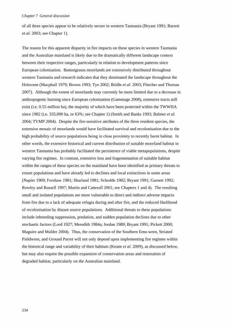
Chapter 7 General discussion of all three species appear to be relatively secure in western Tasmania (Bryant 1991; Barrett
et al. 2003; see Chapter 1).
The reason for this apparent disparity in fire impacts on these species in western Tasmania
and the Australian mainland is likely due to the dramatically different landscape context
between their respective ranges, particularly in relation to development patterns since
European colonisation. Buttongrasss moorlands are extensively distributed throughout
western Tasmania and research indicates that they dominated the landscape throughout the
Holocene (Macphail 1979; Brown 1993; Tye 2002; Bridle et al. 2003; Fletcher and Thomas
2007). Although the extent of moorlands may currently be more limited due to a decrease in
anthropogenic burning since European colonisation (Gammage 2008), extensive tracts still
exist (i.e. 0.55 million ha), the majority of which have been protected within the TWWHA
since 1982 (i.e. 335,000 ha, or 63%; see Chapter 1) (Smith and Banks 1993; Balmer et al.
2004; TVMP 2004). Despite the fire-sensitive attributes of the three resident species, the
extensive mosaic of moorlands would have facilitated survival and recolonisation due to the
high probability of source populations being in close proximity to recently burnt habitat. In
other words, the extensive historical and current distribution of suitable moorland habitat in
western Tasmania has probably facilitated the persistence of viable metapopulations, despite
varying fire regimes. In contrast, extensive loss and fragementation of suitable habitat
within the ranges of these species on the mainland have been identified as primary threats to
extant populations and have already led to declines and local extinctions in some areas
(Napier 1969; Forshaw 1981; Sharland 1981; Schodde 1982; Bryant 1991; Garnett 1992;
Rowley and Russell 1997; Martin and Catterall 2001; see Chapters 1 and 4). The resulting
small and isolated populations are more vulnerable to direct and indirect adverse impacts
from fire due to a lack of adequate refugia during and after fire, and the reduced likelihood
of recolonisation by distant source populations. Additional threats to these populations
include inbreeding suppression, predation, and sudden population declines due to other
stochastic factors (Lord 1927; Meredith 1984a; Jordan 1989; Bryant 1991; Pickett 2000;
Maguire and Mulder 2004). Thus, the conservation of the Southern Emu-wren, Striated
Fieldwren, and Ground Parrot will not only depend upon implementing fire regimes within
the historical range and variability of their habitats (Keane et al. 2009), as discussed below,
but may also require the possible expansion of conservation areas and restoration of
degraded habitat, particularly on the Australian mainland.
234

Chapter 7 General discussion
Implications for fire and conservation management In July 2007, the first Buttongrass Moorland Management Workshop was held in Hobart,
Tasmania (DPIW 2007). It was attended by scientists and land managers from a broad range
of disciplines and affiliated organisations (May and Balmer 2008). There appeared to be a
shared desire to develop and implement science-based, practical fire management strategies
to help conserve Tasmanian moorlands and protect surrounding assets and natural resources,
particularly from severe, landscape-scale wildfires. Although issues associated with
property protection are very limited in and adjacent to the TWWHA, there was nevertheless
a striking lack of consensus on the precise means to achieve this, even within a primarily
ecosystem-management context. Over the past decade we have greatly improved our
understanding of moorland ecosystems in general, and the role of fire in particular, as a
result of research in key fields such as soil science, botany, fire behaviour and fuel
modelling, and faunal ecology (see Chapter 1). We now have some of the key pieces to the
puzzle, but this workshop was only the first step in trying to put the pieces together. The
interdisciplinary and often contentious nature of fire ecology and management, and the all
too real risks associated with making poor decisions, render multi-stakeholder decision-
making and implementation a daunting task. A detailed discussion of, and possible
recommendations for, addressing such ‘big picture’ issues in Australia is well beyond the
scope of this thesis.
Aims
The primary aim of these management recommendations is to help ensure, based on the best
available science, that fire management strategies support the conservation of the avifauna in
Tasmanian buttongrass moorlands. These general guidelines are focused on maintaining
resilient populations of the Southern Emu-wren, Striated Fieldwren, and Ground Parrot
throughout their ranges since they are the only year-round residents of buttongrass
moorlands, are the only members of the avifauna that are entirely dependent upon moorlands
in the study area, and some of their populations on the Australian mainland are listed as
being threatened, at least in part, due to inappropriate fire regimes (see Chapters 1 and 4).
Furthermore, the populations of the Southern Emu-wren (S. m. littleri) and Striated
Fieldwren (C. f. diemenensis) that were the focus of this study are unique subspecies
restricted to western Tasmania and thus warrant special protection (Thomas 1979; Schodde
and Mason 1999). Since all of the non-resident species recorded in this study, as well as
those identified in the literature, are primarily associated with other habitats, their use of
moorlands at various post-fire seral stages is relatively opportunistic (see Chapters 1, 4-6).
Thus, based on current information, they do not appear to warrant specific management
guidelines within moorlands in order to help conserve their broader populations.
235

Chapter 7 General discussion While the literature is rife with studies that discuss fire management in relation to avian
conservation on mainland Australia (for a review see Woinarski 1999a, 1999b), it is almost
entirely devoid of ones on the Tasmanian avifauna, particularly in buttongrass moorlands.
Management recommendations in relation to the moorland avifauna only include Bryant’s
(1991) regarding the Ground Parrot, and Gellie’s (1980) on the avifauna as a whole,
although he did not provide any quantitative data to substantiate his recommendations.
Additional work has been conducted on the critically endangered Orange-bellied Parrot that
forages in moorlands areas during the summer breeding season, but this will not be explicitly
discussed herein since it occurs in a relatively small part of Tasmania’s moorlands, outside
the range of this study (Brown and Wilson 1984; Marsden-Smedley et al. 2001; M.
Holdsworth pers. comm. 2007). Nevertheless, these recommendations should be considered
when planning fire management activities within the Orange-bellied Parrot breeding grounds
in the Bathurst and Macquarie Harbour basins since these areas also support populations of
the three resident species (see Chapter 1; pers. obs.). Unfortunately, the few specific
recommendations that have been made regarding the minimisation of adverse fire effects on
the moorland avifauna by Bryant (1991) and Gellie (1980) are not explicitly incorporated in
current operational guidelines outlined in the Tasmanian Wilderness World Heritage Area
Tactical Fire Management Plan (PWS 2004) or Planned burning in Tasmania: operational
guidelines and review of current knowledge (Marsden-Smedley 2009), and are only briefly
touched-upon in other fire plans such as the Lyell Highway Fire Management Plan that
covers the Lake St Clair region (PWS 1996; see Chapters 1 and 6). However, the Draft
Ecological-management Burning Prescriptions (PWS 2004; Marsden-Smedley 2009)
contain a number of general ecological management guidelines that, if formally adopted and
implemented, should facilitate conservation of the moorland avifauna.
Guidelines for fire management are provided below based on the autecological attributes of
the resident bird species, results from this study, and recommendations from other
references, including those from mainland Australia. It should be noted that since additional
research is needed to better understand avifaunal dynamics in moorlands (see Future
directions), these should be regarded as preliminary recommendations. It is also recognised
that managers will need to balance these recommendations for the avifauna against those for
other resources, and that a particular regime will not favour all species and resources at a
given space and time (Burbidge 2003). Nevertheless, managers should explicitly consider
the avifauna in all phases of planning and implementation (e.g. MacHunter et al. 2009).
While it is expected that these conservative recommendations will likely benefit many faunal
species, including non-resident bird species, it is essential to recognise that any myopic and
inflexible approaches towards fire management and conservation may be to the detriment of
236

Chapter 7 General discussion
other taxa and the ecosystem as a whole (Chladil 1991; Agee 1999; Bradstock et al. 1995;
Kotliar et al. 2002; Burbidge 2003; Kotliar et al. 2005).
Fire season and intensity
Prescribed burns conducted during the breeding season may result in direct loss of clutches
and nestlings, delayed or unsuccessful breeding attempts, and increased predation,
particularly for ground-nesting birds such as the resident species (Fletcher 1913a; Gellie
1980; Rowley and Brooker 1987; Reilly 1991b; Maguire 2005; see Chapters 1 and 6). Since
identifying the breeding season of the resident and other moorland species was not an
objective of this study, these recommendations are primarily based on previous studies and
should be modified if additional information indicates that breeding periods differ from those
stated below, particularly in relation to climate change, as well as geography, altitude, and
site productivity (e.g. Lake Pedder vs. Lake St Clair). In Tasmania, the Southern Emu-wren
is known to breed from August through January (Fletcher 1913a, 1918; pers. obs.), the
Striated Fieldwren from as early as July through February (Dove 1912; Napier 1969), and
the Ground Parrot from October through February (Bryant 1991). Thus, the most
conservative approach is to limit both hazard-reduction and ecological-management burning
to March - June. This period is more restrictive than that recommended by Bryant (1991) for
the Ground Parrot (i.e. April - September), since the Striated Fieldwren starts breeding
earlier in Tasmania (Dove 1912). It is also more conservative than the guidelines for
ecological-management burning (i.e. Autumn, mid-April - June; Spring, August -
September) and hazard-reduction burning (i.e. Autumn, April - early May; Spring,
September - mid-October) (Marsden-Smedley et al. 1999; PWS 2004; A. Pyrke pers. comm.
2007; Marsden-Smedley 2009). The draft ecological burning guidelines also state that when
and where feasible, approximately 75% of ecological burns should be conducted in autumn
or winter and approximately 25% in spring (PWS 2004; Marsden-Smedley 2009). Based on
previous research that indicated birds in fire-adapted ecosystems demonstrated a degree of
resilience to a few prescribed burns during the breeding season (Loyn et al. 2003; Knapp et
al. 2009), these guidelines appear to allow for adequately long prescription windows to meet
other resource management objectives. However, if spring burns are necessary, adequate
areas of unburnt vegetation (i.e. > 30% of site) should be provided for refugia and to
facilitate post-fire dispersal (Gellie 1980; Bryant 1991, 1992; PWS 2004; Maguire 2005).
Although most prescribed burns in buttongrass moorlands are of a low intensity (Marsden-
Smedley et al. 1999; J. Marsden-Smedley pers. comm. 2007), these seasonal guidelines
should also help to ensure that fire intensities do not exceed a threshold beyond which
adverse direct and indirect effects on the avifauna are highly probable (Bain et al. 2008).
237

Chapter 7 General discussion Fire extent and patchiness
The specific impacts of extensive wildfires on the Tasmanian moorland avifauna are unclear
since most of the sites surveyed for this study were subjected to smaller prescribed burns or
much older wildfire events (see Chapter 2), which makes it difficult to draw inferences
regarding the impacts of large wildfires in the short to medium term. However, due to the
fire-sensitive attributes of the resident bird species, it is reasonable to assume that extensive
summer wildfires which consume most of the above ground vegetation may result in adverse
effects, including mortality, reductions in reproductive success, and local extinctions (Fox
1978; Recher and Christensen 1981; Bryant 1991; Garnett 1992; Loyn 1997; Garnett and
Crowley 2002; Pickett 2005; Burbidge et al. 2007).
Proposed future fire management strategies for moorlands include an overall increase in the
total area burnt on an annual basis (i.e. 5-10%), using a combination of broad-scale
ecosystem management burning and tactical hazard-reduction burning in high risk areas
(Marsden-Smedley and Kirkpatrick 2000; Marsden-Smedley et al. 2001; PWS 2004; King et
al. 2006, 2008; Marsden-Smedley 2009). This is considered necessary since a large
proportion of moorland is currently in an old-growth seral stage (i.e. > 35 years post-fire)
that poses a high fire risk and low probability of successful control (Marsden-Smedley
1998a, 1998b; Marsden-Smedley et al. 1999; PWS 2004; J. Marsden-Smedley pers. comm.
2007; A. Pyrke pers. comm. 2007; Marsden-Smedley 2009). It is thought that such a
strategy would mimic Aboriginal burning regimes characterised by more frequent, low-
intensity fires and help to conserve fire-adapted ecosystems, while limiting the incidence,
extent, and severity of unplanned fires and their adverse impact on fire-sensitive resources
and other assets (Marsden-Smedley and Kirkpatrick 2000; Marsden-Smedley et al. 2001;
Pyrke and Marsden-Smedley 2005; PWS 2004; King et al. 2006, 2008; Marsden-Smedley
pers. comm. 2007).
However, the risk and scale of both planned and unplanned fires should be evaluated on an
ongoing basis to help ensure that adequate areas remain unburnt (e.g. ~ 30-70%; Gellie
1980), allowing for the continuing development and availability of mature and old-growth
moorland vegetation (i.e. 15-35 and > 35 years post-fire, respectively) across the landscape
(Gellie 1980; McFarland 1988b; Woinarski and Recher 1997; Richards et al. 1999; Baker
2000; Marsden-Smedley et al. 2001; Ward and Paton 2004a; Buchanan et al. 2006). This is
particularly important for blanket moorlands in the Lake Pedder area, where old-growth sites
appear to support relatively high densities of the resident species (see Chapter 4). The
maintenance of such large source areas is critical for many heathland birds that are
characterised by low reproductive rates and poor dispersal capabilities (Woinarski 1999a,
1999b). Furthermore, by maintaining a greater proportion of the landscape in mid- to late-
238
Chapter 7 General discussion
successional phases, more options would remain available to fire managers (e.g. planned
burning) to implement strategies based on the current state of the system (Richards et al.
1999).
A large body of research to date, including results from this study (see Chapters 4-6), not
only indicates that the extent of fires should be limited in relation to total suitable habitat
area, but that burnt areas should also contain an adequate number, size, and interspersion of
unburnt patches to provide refugia during and after fire events; facilitate persistence,
dispersal, and post-fire recolonisation; and adequate reproduction over space and time
(McFarland 1998b; Bryant 1991; Reilly 1991b; Littley and Cutten 1996; Woinarski 1999b;
Bradstock et al. 1995; Baker 2002; Garnett and Crowley 2002; Maguire 2005; Paton et al.
2005; Tasker and Baker 2005; Burbidge et al. 2007; Gibson et al. 2007; Bain et al. 2008;
Lindenmayer et al. 2009). Such patches of unburnt or partially burnt habitat thus function as
‘biological legacies’ that facilitate persistence of pre-disturbance organisms, patterns, and
processes, and thus the recovery of the avifauna in the post-disturbance environment,
particularly in the case of large, intense fires (Franklin et al. 2000). The Draft Ecological-
management Burning Prescriptions (PWS 2004) also contain a number of guidelines that, if
implemented, should facilitate meeting some of these objectives; these should also be
incorporated into hazard-reduction burning when feasible and consistent with other
management objectives. These include burning < 90% of small sites (i.e. 100 ha) and <
50% of large sites (i.e. > 100 ha), maintaining unburnt patches (> 0.25 ha) no more than 500
m apart, and using a dispersed ignition pattern. However, results from this study suggested
that burning up to these thresholds may not ensure persistence of the resident species,
particularly at small sites and in the short-term (see Chapters 4 and 6).
The results from this study suggested that preservation of moorland riparian habitats is
particularly important since they provide greater relative cover and food resources, and may
serve as important post-fire refugia and dispersal corridors, particularly in the case of
extensive fires that may displace large portions of the resident populations (see Chapters 4-
6). The effects of prescribed burning operations on riparian zones have not been explicitly
addressed to date (Marsden-Smedley et al. 1999; Marsden-Smedley and Kirkpatrick 2000;
PWS 2004; Marsden-Smedley 2009). Parts of riparian areas may remain unburnt under
some conditions; however, riparian areas can be extensively burnt by a primary fire (see
Chapter 6), or may be hand-torched by fire crews if such areas of unburnt vegetation remain
after the initial ignition and fire front have passed (T. Norris pers. comm. 2003; pers. obs.).
Since burning such small patches of habitat is unlikely to significantly contribute to hazard-
reduction aims, it is recommended that fire crews are informed of the importance of ensuring
that portions of riparian habitats and other emergent vegetation (e.g. scrub copses) remain
239
Chapter 7 General discussion unburnt within each site to provide post-fire refugia for the fauna. These recommendations
should be considered in relation to back-burning operations when responding to wildfires as
well (Lindenmayer et al. 2009).
Inter-fire intervals and frequency
Although data for all known fire events in the study area were presented in Chapter 2, fire
frequencies were not calculated due to a lack of adequate data and the inability to verify the
mapping of historical burns at the site scale. However, it is apparent that most sites have
burnt at frequencies that are consistent with the maintenance of moorland communities, at
least for blanket moorlands in southwestern Tasmania (i.e. 20-40 year inter-fire intervals;
Jackson 1968, 1999a). Furthermore, part of the site selection process for this study included
control of variation in fire frequencies and inter-fire intervals (i.e. > 10 years), at least over
the past two fire events, to help minimise these variables from confounding the effects of
time since fire per se (see Chapter 2). Accordingly, there is some uncertainty as to the
potential effects of multiple, shorter inter-fire intervals of < 10 years on the resident species.
Current hazard-reduction prescriptions for moorlands suggest that the optimum interval
between burns is 7-10 years (range 5-15 years) for low productivity sites (e.g. Lake Pedder)
and 5-8 years (range 5-10 years) for medium productivity sites (e.g. Lake St Clair)
(Marsden-Smedley et al. 1999; Marsden-Smedley 2009). Recommendations for ecological-
management burning encompass a much broader range of inter-fire intervals, including short
intervals of 20-30 years and long intervals ≥ 30+ years for low productivity sites, and short
intervals of 5-12 years and long intervals > 12 years for medium productivity sites (Marsden-
Smedley and Kirkpatrick 2000; PWS 2004; Pyrke and Marsden-Smedley 2005; Marsden-
Smedley 2009). They also recommend that fire frequencies are varied, with a maximum of
two short or two long consecutive burn intervals. Since the highest mean densities of the
residents in low productivity moorlands were at the oldest sites surveyed (i.e. 54 years post-
fire), the guidelines, particularly for hazard-reduction burns, would likely not be sufficient
for resident populations to attain peak densities at some sites (see Chapter 4). Therefore, it is
recommended that the majority of burns should follow the ecological-management
guidelines, provided they include multiple burns of long intervals > 50 years. In contrast, the
highest mean densities of the residents in moderate productivity moorlands were in younger
sites (i.e. 2-8 years post-fire) (see Chapter 4). Therefore, guidelines for ecological-
management burns appear to be appropriate to maintain resident populations in moderate
productivity sites, provided that burns with short inter-fire intervals (i.e. < 10 years) are
limited in extent and include adequate areas of unburnt vegetation.
240
Chapter 7 General discussion
For conservation of the Ground Parrot, Bryant (1991) recommended not burning more than
25% of an area over a 10 year rotation in order to maintain suitable habitat and sustainable
densities across a landscape. This appears to be appropriate for eastern moorlands, but the
frequency may be too high for blanket moorlands in which habitat > 50 years post-fire is
likely needed to provide suitable conditions for populations to attain maximum densities
within portions of the region (see Chapter 4). She also cautioned against ‘overfiring’ of
moorlands in the Lake St Clair area since it represents an important eastern fringe of Ground
Parrot distribution in Tasmania (Bryant 1991). While repeated hazard-reduction burning in
some areas may cause adverse, although probably localised, impacts on the resident species
(Bryant 1991, 1992; Littley and Cutten 1996), this needs to be weighed against the reduced
risk of intense and extensive wildfires across the landscape, which may ultimately pose the
greatest threat to the avifauna (Brooker and Rowley 1991; Brooker 1998; Reilly 1991a; Loyn
1997; Marsden-Smedley and Kirkpatrick 2000; Burbidge 2003; PWS 2004; Burbidge et al.
2005; Pickett 2005; Marsden-Smedley 2009). King et al. (2006, 2008) recently modelled the
effects of different prescribed burning strategies in moorlands compared to the risk of
unplanned wildfires and assessed the potential impacts on ecological values in southwestern
Tasmania. Simulations indicated that prescribed burning treatment levels of between 5%
and 10% of total moorland area on an annual basis and consisting of small treatment units
(i.e. a ‘fine-scale fuel mosaic’) would reduce the mean extent and incidence of unplanned
fires and thus help to conserve fire-sensitive species and overall biodiversity. Treatment
levels at the lower end of this range would represent a fairly modest increase from the
current levels. However, the upper end would result in higher fire frequencies than were
believed to characterise Aboriginal and early European fire regimes, and may adversely
impact moorland ecosystems (Marsden-Smedley 1998b; Marsden-Smedley and Kirkpatrick
2000; PWS 2004; Pyrke and Marsden-Smedley 2005; Driessen 2006; King et al. 2006,
2008).
Relevant recommendations from the mainland concur that inter-fire intervals of at least
approximately 10 years and fire regimes of variable frequencies should benefit most bird
species, but that longer intervals (e.g. > 20 years) may be required for some cover-dependent
threatened species (Meredith et al. 1984; McFarland 1988b; Brooker and Rowley 1991;
Garnett 1992; Littley and Cutten 1996; Baker 1997; Woinarski and Recher 1997; Brooker
1998; Woinarski 1999a, 1999b; Garnet and Crowley 2002; Keith et al. 2002b; Burbidge
2003; Recher 2005; Tasker and Baker 2005; Burbidge et al. 2007). Furthermore, long
intervals (i.e. 20-30 years) may be necessary to conserve peat soils, particularly if trends in
global warming continue (Bridle et al. 2003). Although species associated with early
successional habitats in some regions may be disadvantaged by such a fire regime (e.g.
241
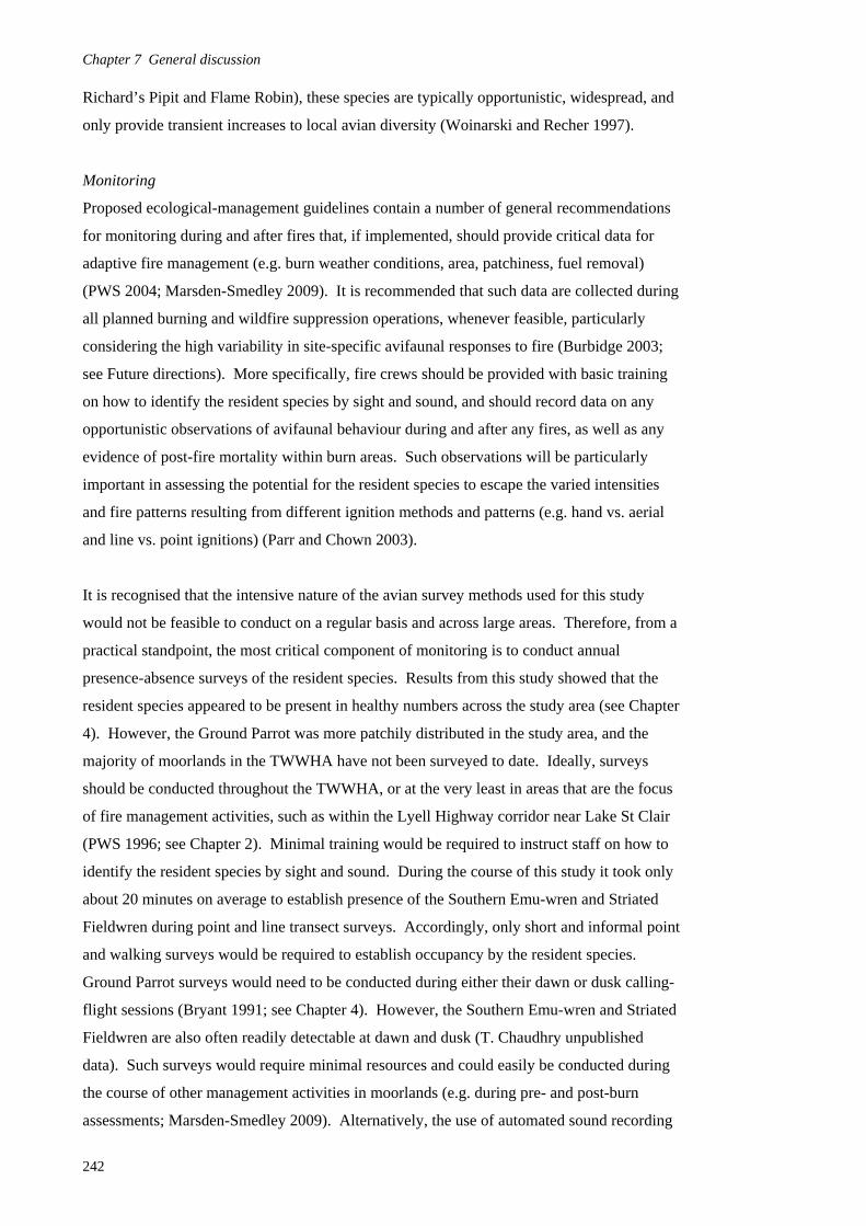
Chapter 7 General discussion Richard’s Pipit and Flame Robin), these species are typically opportunistic, widespread, and
only provide transient increases to local avian diversity (Woinarski and Recher 1997).
Monitoring
Proposed ecological-management guidelines contain a number of general recommendations
for monitoring during and after fires that, if implemented, should provide critical data for
adaptive fire management (e.g. burn weather conditions, area, patchiness, fuel removal)
(PWS 2004; Marsden-Smedley 2009). It is recommended that such data are collected during
all planned burning and wildfire suppression operations, whenever feasible, particularly
considering the high variability in site-specific avifaunal responses to fire (Burbidge 2003;
see Future directions). More specifically, fire crews should be provided with basic training
on how to identify the resident species by sight and sound, and should record data on any
opportunistic observations of avifaunal behaviour during and after any fires, as well as any
evidence of post-fire mortality within burn areas. Such observations will be particularly
important in assessing the potential for the resident species to escape the varied intensities
and fire patterns resulting from different ignition methods and patterns (e.g. hand vs. aerial
and line vs. point ignitions) (Parr and Chown 2003).
It is recognised that the intensive nature of the avian survey methods used for this study
would not be feasible to conduct on a regular basis and across large areas. Therefore, from a
practical standpoint, the most critical component of monitoring is to conduct annual
presence-absence surveys of the resident species. Results from this study showed that the
resident species appeared to be present in healthy numbers across the study area (see Chapter
4). However, the Ground Parrot was more patchily distributed in the study area, and the
majority of moorlands in the TWWHA have not been surveyed to date. Ideally, surveys
should be conducted throughout the TWWHA, or at the very least in areas that are the focus
of fire management activities, such as within the Lyell Highway corridor near Lake St Clair
(PWS 1996; see Chapter 2). Minimal training would be required to instruct staff on how to
identify the resident species by sight and sound. During the course of this study it took only
about 20 minutes on average to establish presence of the Southern Emu-wren and Striated
Fieldwren during point and line transect surveys. Accordingly, only short and informal point
and walking surveys would be required to establish occupancy by the resident species.
Ground Parrot surveys would need to be conducted during either their dawn or dusk calling-
flight sessions (Bryant 1991; see Chapter 4). However, the Southern Emu-wren and Striated
Fieldwren are also often readily detectable at dawn and dusk (T. Chaudhry unpublished
data). Such surveys would require minimal resources and could easily be conducted during
the course of other management activities in moorlands (e.g. during pre- and post-burn
assessments; Marsden-Smedley 2009). Alternatively, the use of automated sound recording
242

Chapter 7 General discussion
systems could also be considered (e.g. Cunningham et al. 2004). Although the information
provided by simple presence-absence surveys is somewhat limited compared to intensive
surveys such as distance sampling (see Chapters 4 and 6), considerable work has been
recently conducted to maximise the inferences that can be made from such datasets for the
purposes of wildlife management (e.g. Royle and Nichols 2003; Westphal et al. 2003;
Brotons et al. 2004; MacKenzie 2005). However, in some cases it may be necessary to
conduct repeated surveys over relatively short timeframes (i.e. a few within a season) in
order to establish ‘absence’ at a given site with certainty and thus obtain more reliable
parameter estimates (MacKenzie 2005). If the presence-absence surveys become standard
practice, these data could be used to determine if fire management activities are leading to
adverse effects, such as local extinctions, and then be used to adapt strategies accordingly
(e.g. reduce frequency and extent, increase fine-scale patchiness). Ideally, these data would
be used to build and validate models that would assist managers in predicting the potential
impacts of different management strategies on the avifauna (see Future directions).
Adaptive management
The above recommendations for the conservation of the avifauna of buttongrass moorlands
should be evaluated within an adaptive management framework, using a more flexible
approach towards fire management that will allow strategies to be adapted as both conditions
and understanding of fire ecology change (Bradstock et al. 1995; Gill et al. 2002; Keith et al.
2002b; Kotliar et al. 2005; Tasker and Baker 2005). This will necessitate the use of a more
systematic and ecosystem-oriented approach, which will need to include clear management
objectives based on the current state of the landscape and desired future conditions, sound
science, risk assessment, long-term monitoring, and ongoing formal evaluation (Richards et
al. 1999; Gill et al. 2002; Keith et al. 2002b; Bradstock et al. 2005; Collins 2006). This
entire process must be flexible enough to adapt to unexpected outcomes (e.g. on non-target
species and food resources), unplanned wildfires, and other possible disturbances (e.g.
climate change) (Bradstock et al. 1995; Keith et al. 2002b; Lindesay 2003). As far as
possible, indigenous knowledge of fire should also be incorporated into management
strategies. However, it should be recognised that such strategies were most likely spatially
and temporally variable, and that significant gaps in knowledge of the historical range and
variability of fire regimes will likely persist. Accordingly, information on historical range
and variability should only be used as a guide, and not to try and recreate an uncertain past in
the highly-altered and changing modern landscape (Marsden-Smedley and Kirkpatrick 2000;
Keith et al. 2002b; Burbidge 2003; Kotliar et al. 2005; Collins 2006).
The general strategy outlined above is based to some extent on the ‘mosaic paradigm’ and is
essentially a form of bet-hedging; the hope is that providing a range of habitat conditions
243
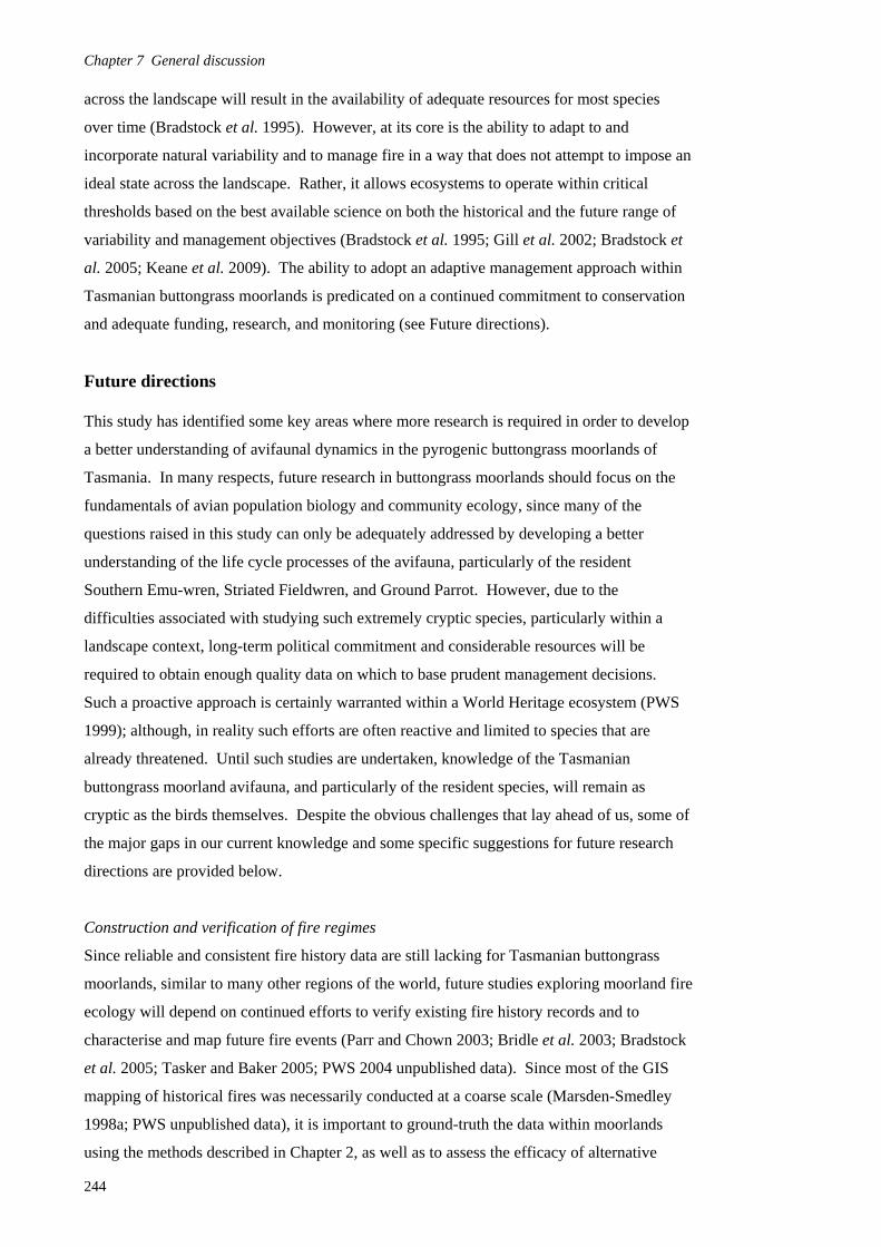
Chapter 7 General discussion across the landscape will result in the availability of adequate resources for most species
over time (Bradstock et al. 1995). However, at its core is the ability to adapt to and
incorporate natural variability and to manage fire in a way that does not attempt to impose an
ideal state across the landscape. Rather, it allows ecosystems to operate within critical
thresholds based on the best available science on both the historical and the future range of
variability and management objectives (Bradstock et al. 1995; Gill et al. 2002; Bradstock et
al. 2005; Keane et al. 2009). The ability to adopt an adaptive management approach within
Tasmanian buttongrass moorlands is predicated on a continued commitment to conservation
and adequate funding, research, and monitoring (see Future directions).
Future directions This study has identified some key areas where more research is required in order to develop
a better understanding of avifaunal dynamics in the pyrogenic buttongrass moorlands of
Tasmania. In many respects, future research in buttongrass moorlands should focus on the
fundamentals of avian population biology and community ecology, since many of the
questions raised in this study can only be adequately addressed by developing a better
understanding of the life cycle processes of the avifauna, particularly of the resident
Southern Emu-wren, Striated Fieldwren, and Ground Parrot. However, due to the
difficulties associated with studying such extremely cryptic species, particularly within a
landscape context, long-term political commitment and considerable resources will be
required to obtain enough quality data on which to base prudent management decisions.
Such a proactive approach is certainly warranted within a World Heritage ecosystem (PWS
1999); although, in reality such efforts are often reactive and limited to species that are
already threatened. Until such studies are undertaken, knowledge of the Tasmanian
buttongrass moorland avifauna, and particularly of the resident species, will remain as
cryptic as the birds themselves. Despite the obvious challenges that lay ahead of us, some of
the major gaps in our current knowledge and some specific suggestions for future research
directions are provided below.
Construction and verification of fire regimes
Since reliable and consistent fire history data are still lacking for Tasmanian buttongrass
moorlands, similar to many other regions of the world, future studies exploring moorland fire
ecology will depend on continued efforts to verify existing fire history records and to
characterise and map future fire events (Parr and Chown 2003; Bridle et al. 2003; Bradstock
et al. 2005; Tasker and Baker 2005; PWS 2004 unpublished data). Since most of the GIS
mapping of historical fires was necessarily conducted at a coarse scale (Marsden-Smedley
1998a; PWS unpublished data), it is important to ground-truth the data within moorlands
using the methods described in Chapter 2, as well as to assess the efficacy of alternative
244
Chapter 7 General discussion
methods for constructing long-term fire histories for the region (e.g. dendrochronological
studies in adjacent forests). In addition, although a greater emphasis has been placed on fire
record keeping in recent years, detailed data on ignition methods and patterns, fuel loads, fire
behaviour, and burn patchiness should be collected for all prescribed burning operations
conducted by Parks and Wildlife Service and Forestry Tasmania, as well as for wildfires
when feasible (PWS 2004; Marsden-Smedley 2009). Particularly if spatially-explicit (e.g.
based on remote sensing) and provided in a readily accessible format (e.g. online GIS
database), such data will not only be instrumental for continued fire ecology research, but
would also help to validate and refine the fuel and fire behaviour models in current use by
fire managers (i.e. Marsden-Smedley et al. 1999; Marsden-Smedley 2009). In the long-term,
detailed and accurate fire history records will be invaluable in investigating the potential
impact of different fire regimes on moorland ecosystems, particularly in relation to fire
behaviour, scale, and frequency.
Robust experimental design
During the planning and implementation stages of this study, considerable effort was
expended to ensure that the design was appropriate for addressing the primary research aims,
included an adequate range of fire ages and replication (Baker and Whelan 1994; Whelan
1995), and investigated the influence of key abiotic and biotic variables in addition to time
since fire per se (Woinarski 1999b; Smith 2000; see Chapter 2). However, this study was
limited by similar time and resource constraints as imposed on most doctoral research
projects. Although most fire ecology studies to date have not included any replication
(Whelan 1995; Whelan et al. 2002), the inclusion of more replicates in this study may have
increased power and provided additional insights into the dynamics of moorland ecosystems.
In order to develop a more process-oriented understanding of pyrogenic ecosystems, it will
be necessary to conduct long-term, manipulative experiments (Whelan et al. 2002; Ward and
Paton 2004a; Saab and Powell 2005). This will not only require ongoing commitment and
funding (e.g. Brooker 1998), but also close and flexible collaboration between researchers
and land management authorities, especially considering the often narrow windows during
which prescribed burns can be conducted (Whelan 1995; Marsden-Smedley et al. 1999;
Marsden-Smedley 2009).
Demographics
To date no formal demographic studies have been conducted on the three moorland resident
species in Tasmania and only limited research has been conducted on mainland populations.
Notable examples are Pickett’s (2000) and Maguire’s (2005) research on the Southern Emu-
wren in South Australia and Victoria, respectively. However, no similarly detailed
demographic studies have been conducted on the Ground Parrot or Striated Fieldwren (for
245

Chapter 7 General discussion reviews see Higgins 1999; Higgins and Peter 2002). This dearth of research is not surprising
given the resource-intensive nature of demographic studies, particularly for cryptic, ground-
dwelling species that are rarely seen, making colour-banding of limited utility. The task
becomes even more daunting when trying to examine demographic trends within a fire and
landscape ecology framework (e.g. Brooker 1998). Nevertheless, even obtaining baseline
demographic data on Tasmanian populations would help to provide a fitness framework
within which to consider the findings of this and subsequent studies, and would contribute to
a better understanding of the underlying processes (Morse 1990; Wolda 1990; Alldredge et
al. 1998; Jones 2001; Whelan et al. 2002; MacHunter et al. 2009). Ideally, such
information, along with that obtained during this study, will enable the development of
spatially-explicit, fitness-based models that will make it possible to predict species densities
and diversities across the landscape, and ultimately the potential risks of different
management regimes on the avifauna (e.g. Brooker and Brooker 1994; Littley and Cutten
1996; Richards et al. 1999; Westphal et al. 2003; Buchanan et al. 2005; Bradstock et al.
2005; MacHunter et al. 2009). An adequate amount of quality autecological data is needed
to parameterise accurate models since predicted outcomes are likely to be highly sensitive to
even small discrepancies between expected and observed attributes of species (Keith et al.
2002a; Whelan et al. 2002).
Accordingly, some areas of research of particular value include the identification of specific
breeding periods of the resident species in relation to climate change and investigating fire-
related mortality, site fidelity, territoriality, dispersal, recolonisation, reproduction, and
population levels (Whelan 1995; Gill et al. 2002; Keith et al. 2002b; Whelan et al. 2002;
Bradstock et al. 2005; Maguire 2005; Paton et al. 2005; MacHunter et al. 2009). Such
studies would undoubtedly be facilitated by the use of radio-telemetry, which has already
been successfully used on the Ground Parrot for at least short periods of time (Jordan 1987b;
McFarland 1991a). However, transmitters are yet to be developed that are small enough to
be used on diminutive birds such as the Southern Emu-wren and Striated Fieldwren
(Maguire 2006a).
Foraging behaviour and dietary preferences
Results reported in Chapter 5 indicated that potential arthropod prey resources (i.e. order-
level abundance and energy content) for insectivorous species varied in relation to both
habitat type and fire age in eastern moorlands at Lake St Clair, while related research
conducted on moorland invertebrates at Lake Pedder indicated that similar patterns may exist
in blanket moorlands (e.g. Greenslade and Driessen 1999; M. Driessen unpublished data; see
Chapter 5). However, information used in this study regarding the foraging behaviour and
dietary preferences of the insectivorous species was largely drawn from the literature and
246

Chapter 7 General discussion
based on studies conducted in other regions of Australia. Hence, it would be worthwhile to
conduct research in Tasmanian moorlands, across a chronosequence of sites if possible,
focused on identifying the foraging behaviour and dietary preferences of the Southern Emu-
wren and Striated Fieldwren. Given their cryptic nature, detailed behavioural observations
are extremely difficult to obtain (see Chapter 5), so they will probably need to be
supplemented with other methods such as remote viewing of food provisioning at nest sites
(e.g. Maguire 2006b), stomach content analyses (e.g. Lea and Gray 1936), and stable isotope
analyses (Hood-Novotny and Knols 2007). A component of this research should also
include obtaining additional food resource data (e.g. at Lake Pedder) of a finer taxonomic
resolution and encompassing multiple seasons. Additional avenues of research include the
identification of other factors that may influence habitat choice, such as site fidelity and
territoriality, sexual differences, competition, and predation (Cody 1981, 1985; Jones 2001).
Interspecific interactions and niche differentiation
Based on the results from this study it is clear that the insectivorous and ground-dwelling
Southern Emu-wren and Striated Fieldwren share very similar niches and are sympatric
throughout much of their ranges in western Tasmania, with the latter occurring in a
somewhat broader range of sites (see Chapters 4-6). Although such associations are not
uncommon, their’s is of particular interest since they are the only two resident insectivores
found in over 0.5 million hectares of Tasmanian moorlands. How are these species able to
coexist in a habitat characterised by limited structural diversity and overall productivity?
Although these species have been seen in close proximity to each other (i.e. < 2 m) while
showing no obvious agonistic behaviour (pers. obs.), essentially nothing is known about the
nature and extent of interspecific interactions between these species. Are niches
differentiated through the maintenance of spatially exclusive territories, or through fine-scale
differences in habitat selection and resource use? In particular, what role do interspecific
interactions and niche differentiation play in the competitive post-fire environment where
cover, food, and nesting resources are often in short supply? As with the other suggested
avenues of research, attempting to answer these questions will be extremely difficult. Some
possible approaches may include intensive behavioural observations, territory mapping, and
radio-telemetry, if and when feasible.
Potential threats
Although populations of the Southern Emu-wren, Striated Fieldwren, and Ground Parrot are
not currently listed as threatened in Tasmania, some of the lessons learned from research on
mainland populations indicate that potential threats, in addition to altered fire regimes, do
exist in Tasmania. The most likely direct threat comes from native predators (e.g. Tiger
Snakes, Notechis scutatus), and particularly from feral predators such as cats (Felis catus)
247
Chapter 7 General discussion
248
and Red Foxes (Vulpes vulpes), and from possible interactions between predation and fire
disturbance (Burbidge 2003). Feral cats have been sighted in both the Lake Pedder and Lake
St Clair areas and are known to prey on resident species in Tasmania (Bryant 1991; PWS
unpublished data; pers. obs.), as well as populations on the mainland (Pringle 1982a;
McFarland 1991c; Maguire and Mulder 2004; Maguire 2005). Recently, feral foxes were
illegally introduced into Tasmania and they may pose a significant threat to the moorland
avifauna (Saunders et al. 2006), particularly if they are able to expand into the TWWHA.
Although it would be interesting to investigate current and potential future impacts of feral
predators on the avifauna, resources would be better used to expand current eradication
efforts since the impacts of feral predators on the Australian fauna are well documented
(Dickman 1996).
Other potential threats to the moorland avifauna that should be examined include the impact
of the introduced water mould and plant pathogen, Phytophthora cinnamomi, on avian
habitat and food resources (Bryant 1991; Brown et al. 2002; Schahinger et al. 2003). These
effects may be confounded with or exacerbated by those of different fire regimes (Podger
1990; Brown et al. 2002), and should be explicitly considered when planning and
implementing fire management activities (PWS 2004). Finally, climate change predictions
indicate the possibility of adverse impacts on the Australian fauna, which may be
exacerbated by altered fire regimes (e.g. increased frequency and severity) (Watson et al.
1999; Cary 2002; Bridle et al. 2003; Lindesay 2003). The only way to assess the possible
effects of climate change on the Tasmanian moorland avifauna and to adapt fire and
conservation management strategies accordingly, is to conduct long-term monitoring of
avian populations and habitat (Bryant 1991; Whelan 1995; PWS 1999; Baker 2000; Tasker
and Baker 2005).
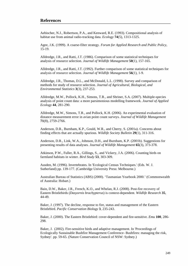
References Aebischer, N.J., Robertson, P.A., and Kenward, R.E. (1993). Compositional analysis of habitat use from animal radio-tracking data. Ecology 74(5), 1313-1325. Agee, J.K. (1999). A coarse-filter strategy. Forum for Applied Research and Public Policy, 15-19. Alldredge, J.R., and Ratti, J.T. (1986). Comparison of some statistical techniques for analysis of resource selection. Journal of Wildlife Management 50(1), 157-165. Alldredge, J.R., and Ratti, J.T. (1992). Further comparison of some statistical techniques for analysis of resource selection. Journal of Wildlife Management 56(1), 1-9. Alldredge, J.R., Thomas, D.L., and McDonald, L.L. (1998). Survey and comparison of methods for study of resource selection. Journal of Agricultural, Biological, and Environmental Statistics 3(3), 237-253. Alldredge, M.W., Pollock, K.H., Simons, T.R., and Shriner, S.A. (2007). Multiple-species analysis of point count data: a more parsimonious modelling framework. Journal of Applied Ecology 44, 281-290. Alldredge, M.W., Simons, T.R., and Pollock, K.H. (2006). An experimental evaluation of distance measurement error in avian point count surveys. Journal of Wildlife Management 71(8), 2759-2766. Anderson, D.R., Burnham, K.P., Gould, W.R., and Cherry, S. (2001a). Concerns about finding effects that are actually spurious. Wildlife Society Bulletin 29(1), 311-316. Anderson, D.R., Link, W.A., Johnson, D.H., and Burnham, K.P. (2001b). Suggestions for presenting results of data analyses. Journal of Wildlife Management 65(3), 373-378. Atkinson, P.W., Fuller, R.A., Gillings, S., and Vickery, J.A. (2006). Counting birds on farmland habitats in winter. Bird Study 53, 303-309. Ausden, M. (1996). Invertebrates. In 'Ecological Census Techniques.' (Eds. W. J. Sutherland) pp. 139-177. (Cambridge University Press: Melbourne.) Australian Bureau of Statistics (ABS) (2000). ‘Tasmanian Yearbook 2000.’ (Commonwealth of Australia: Hobart.) Bain, D.W., Baker, J.R., French, K.O., and Whelan, R.J. (2008). Post-fire recovery of Eastern Bristlebirds (Dasyornis brachypterus) is context-dependent. Wildlife Research 35, 44-49. Baker, J. (1997). The decline, response to fire, status and management of the Eastern Bristlebird. Pacific Conservation Biology 3, 235-243. Baker, J. (2000). The Eastern Bristlebird: cover-dependent and fire-sensitive. Emu 100, 286-298. Baker, J. (2002). Fire-sensitive birds and adaptive management. In 'Proceedings of Ecologically Sustainable Bushfire Management Conference- Bushfires: managing the risk, Sydney'. pp. 59-65. (Nature Conservation Council of NSW: Sydney.)
249
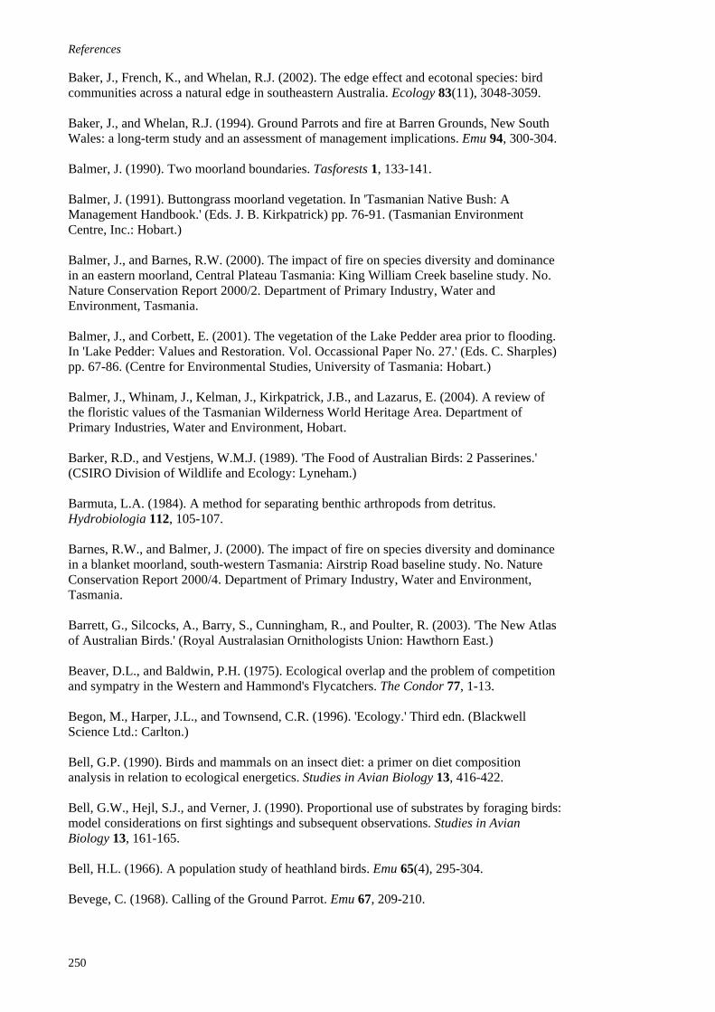
References Baker, J., French, K., and Whelan, R.J. (2002). The edge effect and ecotonal species: bird communities across a natural edge in southeastern Australia. Ecology 83(11), 3048-3059. Baker, J., and Whelan, R.J. (1994). Ground Parrots and fire at Barren Grounds, New South Wales: a long-term study and an assessment of management implications. Emu 94, 300-304. Balmer, J. (1990). Two moorland boundaries. Tasforests 1, 133-141. Balmer, J. (1991). Buttongrass moorland vegetation. In 'Tasmanian Native Bush: A Management Handbook.' (Eds. J. B. Kirkpatrick) pp. 76-91. (Tasmanian Environment Centre, Inc.: Hobart.) Balmer, J., and Barnes, R.W. (2000). The impact of fire on species diversity and dominance in an eastern moorland, Central Plateau Tasmania: King William Creek baseline study. No. Nature Conservation Report 2000/2. Department of Primary Industry, Water and Environment, Tasmania. Balmer, J., and Corbett, E. (2001). The vegetation of the Lake Pedder area prior to flooding. In 'Lake Pedder: Values and Restoration. Vol. Occassional Paper No. 27.' (Eds. C. Sharples) pp. 67-86. (Centre for Environmental Studies, University of Tasmania: Hobart.) Balmer, J., Whinam, J., Kelman, J., Kirkpatrick, J.B., and Lazarus, E. (2004). A review of the floristic values of the Tasmanian Wilderness World Heritage Area. Department of Primary Industries, Water and Environment, Hobart. Barker, R.D., and Vestjens, W.M.J. (1989). 'The Food of Australian Birds: 2 Passerines.' (CSIRO Division of Wildlife and Ecology: Lyneham.) Barmuta, L.A. (1984). A method for separating benthic arthropods from detritus. Hydrobiologia 112, 105-107. Barnes, R.W., and Balmer, J. (2000). The impact of fire on species diversity and dominance in a blanket moorland, south-western Tasmania: Airstrip Road baseline study. No. Nature Conservation Report 2000/4. Department of Primary Industry, Water and Environment, Tasmania. Barrett, G., Silcocks, A., Barry, S., Cunningham, R., and Poulter, R. (2003). 'The New Atlas of Australian Birds.' (Royal Australasian Ornithologists Union: Hawthorn East.) Beaver, D.L., and Baldwin, P.H. (1975). Ecological overlap and the problem of competition and sympatry in the Western and Hammond's Flycatchers. The Condor 77, 1-13. Begon, M., Harper, J.L., and Townsend, C.R. (1996). 'Ecology.' Third edn. (Blackwell Science Ltd.: Carlton.) Bell, G.P. (1990). Birds and mammals on an insect diet: a primer on diet composition analysis in relation to ecological energetics. Studies in Avian Biology 13, 416-422. Bell, G.W., Hejl, S.J., and Verner, J. (1990). Proportional use of substrates by foraging birds: model considerations on first sightings and subsequent observations. Studies in Avian Biology 13, 161-165. Bell, H.L. (1966). A population study of heathland birds. Emu 65(4), 295-304. Bevege, C. (1968). Calling of the Ground Parrot. Emu 67, 209-210.
250
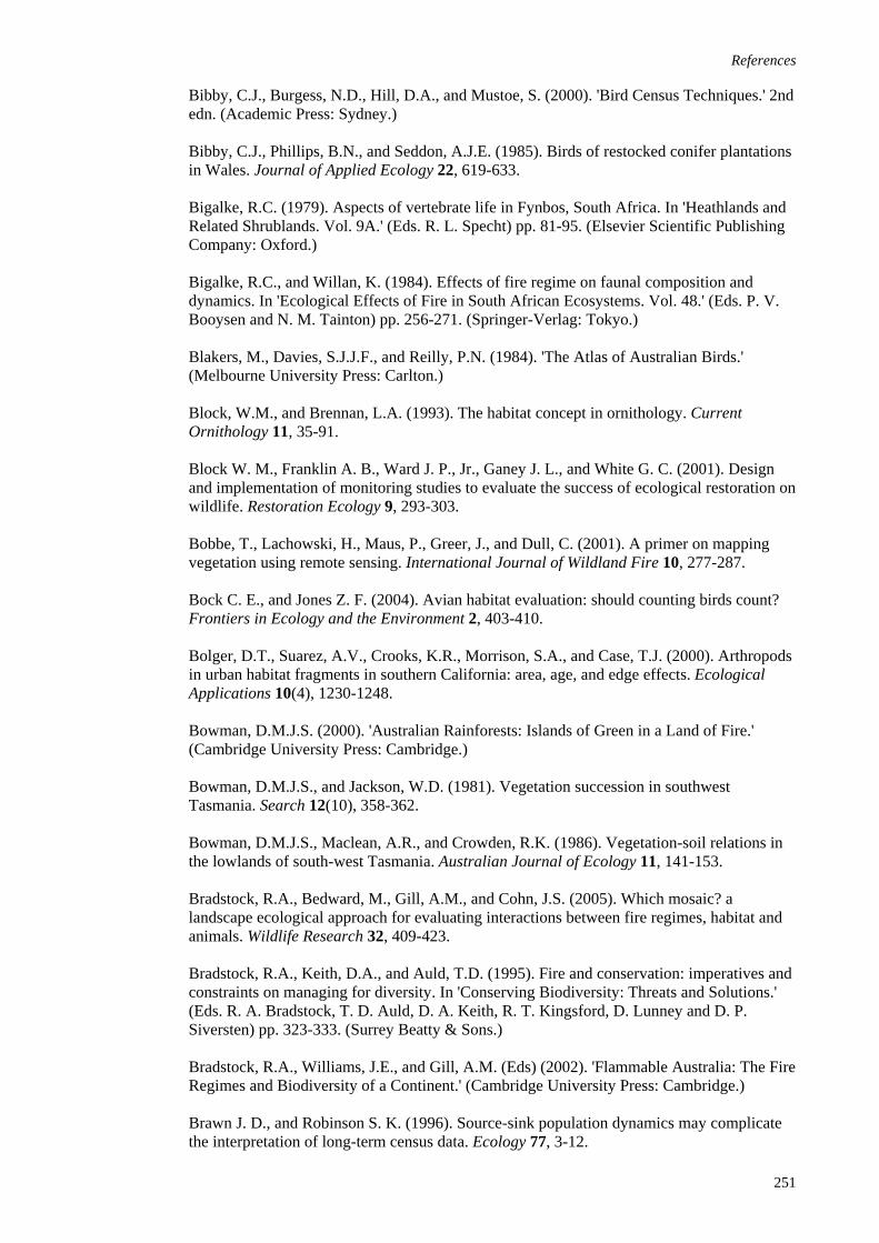
References
Bibby, C.J., Burgess, N.D., Hill, D.A., and Mustoe, S. (2000). 'Bird Census Techniques.' 2nd edn. (Academic Press: Sydney.) Bibby, C.J., Phillips, B.N., and Seddon, A.J.E. (1985). Birds of restocked conifer plantations in Wales. Journal of Applied Ecology 22, 619-633. Bigalke, R.C. (1979). Aspects of vertebrate life in Fynbos, South Africa. In 'Heathlands and Related Shrublands. Vol. 9A.' (Eds. R. L. Specht) pp. 81-95. (Elsevier Scientific Publishing Company: Oxford.) Bigalke, R.C., and Willan, K. (1984). Effects of fire regime on faunal composition and dynamics. In 'Ecological Effects of Fire in South African Ecosystems. Vol. 48.' (Eds. P. V. Booysen and N. M. Tainton) pp. 256-271. (Springer-Verlag: Tokyo.) Blakers, M., Davies, S.J.J.F., and Reilly, P.N. (1984). 'The Atlas of Australian Birds.' (Melbourne University Press: Carlton.) Block, W.M., and Brennan, L.A. (1993). The habitat concept in ornithology. Current Ornithology 11, 35-91. Block W. M., Franklin A. B., Ward J. P., Jr., Ganey J. L., and White G. C. (2001). Design and implementation of monitoring studies to evaluate the success of ecological restoration on wildlife. Restoration Ecology 9, 293-303. Bobbe, T., Lachowski, H., Maus, P., Greer, J., and Dull, C. (2001). A primer on mapping vegetation using remote sensing. International Journal of Wildland Fire 10, 277-287. Bock C. E., and Jones Z. F. (2004). Avian habitat evaluation: should counting birds count? Frontiers in Ecology and the Environment 2, 403-410. Bolger, D.T., Suarez, A.V., Crooks, K.R., Morrison, S.A., and Case, T.J. (2000). Arthropods in urban habitat fragments in southern California: area, age, and edge effects. Ecological Applications 10(4), 1230-1248. Bowman, D.M.J.S. (2000). 'Australian Rainforests: Islands of Green in a Land of Fire.' (Cambridge University Press: Cambridge.) Bowman, D.M.J.S., and Jackson, W.D. (1981). Vegetation succession in southwest Tasmania. Search 12(10), 358-362. Bowman, D.M.J.S., Maclean, A.R., and Crowden, R.K. (1986). Vegetation-soil relations in the lowlands of south-west Tasmania. Australian Journal of Ecology 11, 141-153. Bradstock, R.A., Bedward, M., Gill, A.M., and Cohn, J.S. (2005). Which mosaic? a landscape ecological approach for evaluating interactions between fire regimes, habitat and animals. Wildlife Research 32, 409-423. Bradstock, R.A., Keith, D.A., and Auld, T.D. (1995). Fire and conservation: imperatives and constraints on managing for diversity. In 'Conserving Biodiversity: Threats and Solutions.' (Eds. R. A. Bradstock, T. D. Auld, D. A. Keith, R. T. Kingsford, D. Lunney and D. P. Siversten) pp. 323-333. (Surrey Beatty & Sons.) Bradstock, R.A., Williams, J.E., and Gill, A.M. (Eds) (2002). 'Flammable Australia: The Fire Regimes and Biodiversity of a Continent.' (Cambridge University Press: Cambridge.) Brawn J. D., and Robinson S. K. (1996). Source-sink population dynamics may complicate the interpretation of long-term census data. Ecology 77, 3-12.
251

References Bridle, K., Cullen, P., and Russell, M. (2003). Peatland hydrology, fire management and Holocene fire regimes in southwest Tasmanian blanket bogs. No. 03/07. Earth Science Section, Department of Primary Industries, Water and Environment, Hobart. Britton, P. (2004). Tasmania Bird Report 30 for 2002. Birds Tasmania, Hobart. Brodmann, P.A. (1995). Relations between food conditions, foraging behaviour and reproductive performance in the Water Pipit (Anthus spinoletta). Ph.D. Thesis, University of Zurich, Zurich. Brodmann, P.A., and Reyer, H. (1999). Nestling provisioning in Water Pipits (Anthus spinoletta): do parents go for specific nutrients or profitable prey? Oecologia 120, 506-514. Brodmann, P.A., Reyer, H., Bollmann, K., Schlapfer, A.R., and Rauter, C. (1997). The importance of food quantity and quality for reproductive performance in alpine Water Pipits (Anthus spinoletta). Oecologia 109, 200-208. Brooker, L.C., and Brooker, M.G. (1994). A model for the effects of fire and fragmentation on the population viability of the splendid fairy-wren. Pacific Conservation Biology 1, 344-358. Brooker, M.G. (1998). Fire and birds in a Western Australian heathland. Emu 98, 276-287. Brooker, M.G., and Rowley, I. (1991). Impact of wildfire on the nesting-behaviour of birds in heathland. Wildlife Research 18(3), 249-263. Brotons, L., Thuiller, W., Araujo, M.B., and Hirzel, A.H. (2004). Presence-absence versus presence-only modelling methods for predicting bird habitat suitability. Ecography 27(4), 437-448. Brown, M.J. (1999). Buttongrass moorlands. In 'Vegetation of Tasmania.' (Eds. J. B. Reid, R. S. Hill, M. J. Brown and M. J. Hovenden) pp. 286-303. (Australian Biological Resources Study: Hobart.) Brown, M.J., Balmer, J., and Podger, F.D. (2002). Vegetation change over 20 years at Bathurst Harbour, Tasmania. Australian Journal of Botany 50(4), 499-510. Brown, M.J., Brown, P.B., Bryant, S.J., Horwitz, P.B., McQuillan, P.B., Nielsen, E., Rounsevell, D.E., Smith, S.J., and Richardson, A.M.M. (1993). Buttongrass moorland ecosystems. In 'Tasmanian Wilderness: World Heritage Values.' (Eds. S. J. Smith and M .R. Banks) pp. 101-108. (Royal Society of Tasmania: Hobart.) Brown, M.J., and Podger, F.D. (1982). Floristics and fire regimes of a vegetation sequence from sedgeland-heath to rainforest at Bathurst Harbour, Tasmania. Australian Journal of Botany 30, 659-676. Brown, P.B., and Wilson, R.I. (1982). The Orange-bellied Parrot. In 'Species at Risk: Research in Australia.' (Eds. R. H. Groves and W. D. C. Ride) pp. 106-115. (Australian Academy of Science: Canberra.) Brown, P.B., and Wilson, R.I. (1984). The Orange-bellied Parrot recovery plan. National Parks and Wildlife Service Tasmania, Hobart. Brown, V.K. (1991). The effects of changes in habitat structure during succession in terrestrial communities. In 'Habitat Structure: The Physical Arrangement of Objects in Space.' (Eds. S. S. Bell, E. D. McCoy and H. R. Mushinsky) pp. 141-168. (Chapman & Hall: Melbourne.)
252

References
Bryant, D.M. (1973). The factors influencing the selection of food by the House Martin (Delchion urbica (L.)). The Journal of Animal Ecology 42(3), 539-564. Bryant, S.L. (1990). Firing of King William Plains. Department of Parks, Wildlife and Heritage, Hobart. Bryant, S.L. (1991). The Ground Parrot, Pezoporus wallicus, in Tasmania: distribution, density and conservation status. No. Scientific Report 91/1. Department of Parks, Wildlife and Heritage, Tasmania. Bryant, S.L. (1992). The Ground Parrot and age of vegetation in Tasmania. In 'Issues in the conservation of parrots in Australasia and Oceania: Challenges to Conservation Biology.' (Eds. L. Joseph) pp. 42-45. (RAOU.) Bryant, S.L. (1994). Habitat and potential diet of the Ground Parrot in Tasmania. Emu 94, 166-171. Buchanan, G., Pearce-Higgins, J., Grant, M., Robertson, D., and Waterhouse, T. (2005). Characterization of moorland vegetation and the prediction of bird abundance using remote sensing. Journal of Biogeography 32, 697-707. Buchanan, G.M., Grant, M.C., Sanderson, R.A., and Pearce-Higgins, J.W. (2006). The contribution of invertebrate taxa to moorland bird diets and the potential implications of land-use management. Ibis 148, 615-628. Buckland, S.T. (1987). On the variable circular plot method of estimating animal density. Biometrics 43, 363-384. Buckland, S.T. (2006). Point transect surveys for songbirds: robust methodologies. The Auk 123, 345-357. Buckland, S.T., Anderson, D.R., Burnham, K.P., Laake, J.L., Borchers, D.L., and Thomas, L. (2001). 'Introduction to Distance Sampling.' (Oxford University Press: Oxford.) Buckland, S.T., Anderson, D.R., Burnham, K.P., Laake, J.L., Borchers, D.L., and Thomas, L. (Eds) (2004). 'Advanced Distance Sampling.' (Oxford University Press: London.) Buckland, S.T., Marsden, S.J., and Green, R.E. (2008). Estimating bird abundance: making methods work. Bird Conservation International 18, S91-S108. Buckland, S.T., Russell, R.E., Dickson, B.G., Saab, V.A., Gorman, D.N., and Block, W.M. (2009). Analysing designed experiments in distance sampling. Journal of Agricultural, Biological, and Environmental Statistics 14, 432-442. Buffington, M.L., and Redak, R.A. (1998). A comparison of vacuum sampling versus sweep-netting for arthropod biodiversity measurements in California coastal sage scrub. Journal of Insect Conservation 2, 99-106. Burbidge, A. (1996). Western Ground Parrot recovery efforts. Eclectus 1, 2-3. Burbidge, A., Comer, S., and Danks, A. (2005). Threatened birds and wildfire in south-west Western Australia. Wingspan (Supplement) 15(3), 18-20. Burbidge, A.H. (1989). Conservation of the Ground Parrot in Western Australia. Project 118: unpublished report to World Wildlife Fund (Australia).
253
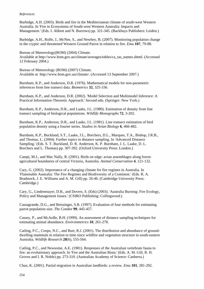
References Burbidge, A.H. (2003). Birds and fire in the Mediterranean climate of south-west Western Australia. In 'Fire in Ecosystems of South-west Western Australia: Impacts and Management.' (Eds. I. Abbott and N. Burrows) pp. 321-345. (Backhuys Publishers: Leiden.) Burbidge, A.H., Rolfe, J., McNee, S., and Newbey, B. (2007). Monitoring population change in the cryptic and threatened Western Ground Parrot in relation to fire. Emu 107, 79-88. Bureau of Meteorology(BOM) (2004) Climate. Available at http://www.bom.gov.au/climate/averages/tables/ca_tas_names.shtml. (Accessed 12 February 2004.) Bureau of Meteorology (BOM) (2007) Climate. Available at http://www.bom.gov.au/climate/. (Accessed 13 September 2007.) Burnham, K.P., and Anderson, D.R. (1976). Mathematical models for non-parametric inferences from line transect data. Biometrics 32, 325-336. Burnham, K.P., and Anderson, D.R. (2002). 'Model Selection and Multimodel Inference: A Practical Information-Theoretic Approach.' Second edn. (Springer: New York.) Burnham, K.P., Anderson, D.R., and Laake, J.L. (1980). Estimation of density from line transect sampling of biological populations. Wildlife Monographs 72, 3-202. Burnham, K.P., Anderson, D.R., and Laake, J.L. (1981). Line transect estimation of bird population density using a fourier series. Studies in Avian Biology 6, 466-482. Burnham, K.P., Buckland, S.T., Laake, J.L., Borchers, D.L., Marques, T.A., Bishop, J.R.B., and Thomas, L. (2004). Further topics in distance sampling. In 'Advanced Distance Sampling.' (Eds. S. T. Buckland, D. R. Anderson, K. P. Burnham, J. L. Laake, D. L. Borchers and L. Thomas) pp. 307-392. (Oxford University Press: London.) Campi, M.J., and Mac Nally, R. (2001). Birds on edge: avian assemblages along forest-agricultural boundaries of central Victoria, Australia. Animal Conservation 4, 121-132. Cary, G. (2002). Importance of a changing climate for fire regimes in Australia. In 'Flammable Australia: The Fire Regimes and Biodiversity of a Continent.' (Eds. R. A. Bradstock, J. E. Williams and A. M. Gill) pp. 26-46. (Cambridge University Press: Cambridge.) Cary, G., Lindenmayer, D.B., and Dovers, S. (Eds) (2003). 'Australia Burning: Fire Ecology, Policy and Management Issues.' (CSIRO Publishing: Collingwood.) Cassagrande, D.G., and Beissinger, S.R. (1997). Evaluation of four methods for estimating parrot population size. The Condor 99, 445-457. Cassey, P., and McArdle, B.H. (1999). An assessment of distance sampling techniques for estimating animal abundance. Environmetrics 10, 261-278. Catling, P.C., Coops, N.C., and Burt, R.J. (2001). The distribution and abundance of ground-dwelling mammals in relation to time since wildfire and vegetation structure in south-eastern Australia. Wildlife Research 28(6), 555-564. Catling, P.C., and Newsome, A.E. (1981). Responses of the Australian vertebrate fauna to fire: an evolutionary approach. In 'Fire and the Australian Biota.' (Eds. A. M. Gill, R. H. Groves and I. R. Noble) pp. 273-310. (Australian Academy of Science: Canberra.) Chan, K. (2001). Partial migration in Australian landbirds: a review. Emu 101, 281-292.
254

References
Chan, K., and Mudie, D. (2004). Variation in vocalisations of the Ground Parrot at its northern range. Australian Journal of Zoology 52, 147-158. Chandler, L.G. (1912). Field notes on the White-browed Field-wren (Calamanthus albiloris). Emu 11, 237-239. Cherrill, A.J., and Rushton, S.P. (1993). The Auchenorryncha of an unimproved moorland in northern England. Ecological Entomology 18, 95-103. Chevan, A., and Sutherland, M. (1991). Hierarchical partitioning. The American Statistician 45(2), 90-96. Chladil, M. (1991). Fire management for nature conservation. In 'Tasmanian Native Bush: A Management Handbook.' (Eds. J. B. Kirkpatrick) pp. 197-212. (Tasmanian Environment Centre, Inc.: Hobart.) Christidis, L., and Boles, W.E. (1994). 'The Taxonomy and Species of Birds of Australia and its Territories.' (RAOU: Melbourne.) Clark, J.S., Gill, A.M., and Kershaw, A.P. (2002). Spatial variability in fire regimes: its effects on recent and past vegetation. In 'Flammable Australia: The Fire Regimes and Biodiversity of a Continent.' (Eds. R. A. Bradstock, J. E. Williams and A. M. Gill) pp. 125-141. (Cambridge University Press: Cambridge.) Clarke, K.R., and Gorely, R.N. (2001). 'Primer v5: User Manual / Tutorial.' (Primer-E: Plymouth.) Clarke, K.R., Somerfield, P.J., Airoldi, L., and Warwick, R.M. (2006). Exploring interactions by second-stage community analyses. Journal of Experimental Marine Biology and Ecology 338, 179-192. Clarke, K.R., and Warwick, R.M. (1994). 'Change in Marine Communities: An Approach to Statistical Analysis and Interpretation.' (Plymouth Marine Laboratory: Plymouth.) Cody, M.L. (1975). Towards of theory of continental species diversities: bird distribution over Mediterranean habitat gradients. In 'Ecology and Evolution of Communities.' (Eds. M. L. Cody and J. M. Diamond) pp. 214-257. (Belknap Press: Cambridge.) Cody, M.L. (1981). Habitat selection in birds: the roles of vegetation structure, competitors, and productivity. Bioscience 31(2), 107-113. Cody, M.L. (1983). Continental diversity patterns and convergent evolution in bird communities. In 'Mediterranean-type Ecosystems: The Role of Nutrients.' (Eds. F. J. Kruger, D. T. Mitchell and J. U. M. Jarvis) pp. 355-402. (Springer-Verlag: Tokyo.) Cody, M.L. (1985). An introduction to habitat selection in birds. In 'Habitat Selection in Birds.' (Eds. M. L. Cody) pp. 3-56. (Academic Press: Orlando.) Collins, K. (1990). 'South-west Tasmania: A Natural History and Visitor's Guide.' (Heritage Books: Hobart.) Collins, P. (2006). 'Burn: The Epic Story of Bushfire in Australia.' (Allen and Unwin: Crows Nest.) Collins, S.L. (2001). Long-term research and the dynamics of bird populations and communities. The Auk 118(3), 583-588.
255

References Congalton, R.G. (1991). A review of assessing the accuracy of classifications of remotely sensed data. Remote Sensing of Environment 37, 35-46. Congalton, R.G., and Green, K. (1993). A practical look at the sources of confusion in error matrix generation. Photogrammetric Engineering and Remote Sensing 59(5), 641-644. Congalton, R.G., and Green, K. (1999). 'Assessing the Accuracy of Remotely Sensed Data: Principles and Practices.' (Lewis Publishers: London.) Congalton, R.G., Oderwald, R.G., and Mead, R.A. (1983). Assessing Landsat classification accuracy using discrete multivariate statistical techniques. Photogrammetric Engineering and Remote Sensing 49(12), 1671-1678. Connell, J.H., Noble, I.R., and Slatyer, R.O. (1987). On the mechanisms producing successional change. Oikos 50(1), 136-137. Connell, J.H., and Slatyer, R.O. (1977). Mechanisms of succession in natural communities and their role in community stability and organization. The American Naturalist 111(982), 1119-1144. Conquest, L.L. (2000). Analysis and interpretation of ecological field data using BACI designs: discussion. Journal of Agricultural, Biological, and Environmental Statistics 5(3), 293-296. Cooper, R.J., and Whitmore, R.C. (1990). Arthropod sampling methods in ornithology. Studies in Avian Biology 13, 29-37. Cooper, R.P. (1974). The avifauna of Wilson's Promontory. Bird Watcher 5(5), 137-174. Cooper, R.P. (1975). The avifauna of Wilson's Promontory. Bird Watcher 6(1), 17-34. Corben, C. (1973). The Southern Emu-wren in South-East Queensland. Sunbird 4(1), 5-7. Courtney, J. (1997). Age-related colour changes and behaviour in the Ground Parrot Pezoporus wallicus. Australian Bird Watcher 17, 185-191. Cowley, R.D., Heislers, A., and Easley, E.H.M. (1969). Effects of fire on wildlife. Victoria's Resources 11(3), 18-22. Craig, M.D., and Roberts, J.D. (2001). Evaluation of the impact of time of day, weather, vegetation density and bird movements on outcomes of area searches for birds in eucalypt forests of south-western Australia. Wildlife Research 28(1), 33-39. Cummins, K.W., and Wuycheck, J.C. (1971). Caloric equivalents for investigations in ecological energetics. Internationale Vereinigung Fur Theoretische Und Angewandte Limnologie 18, 1-158. Cunningham, R.B., Lindenmayer, D.B., and Lindenmayer, B.D. (2004). Sound recordings of bird vocalisations in forests. I. Relationships between bird vocalisations and point interval counts of bird numbers- a case study in statistical modeling. Wildlife Research 31, 195-207. Cunningham, R.B., Lindenmayer, D.B., Nix, H.A., and Lindenmayer, B.D. (1999). Quantifying observer heterogeneity in bird counts. Australian Journal of Ecology 24(3), 270-277. Czaplewski (1992). Misclassification bias in aerial estimates. Photogrammetric Engineering and Remote Sensing 58(2), 189-192.
256

References
Dawson, D.G. (1981a). Counting birds for a relative measure (index) of density. Studies in Avian Biology 6, 12-16. Dawson, D.K. (1981b). Sampling in rugged terrain. Studies in Avian Biology 6, 311-315. De Barro, P.J. (1991). A cheap lightweight efficient vacuum sampler. Journal of the Australian Entomological Society 30, 207-208. Dennis, P., Young, M.R., and Gordon, I.J. (1998). Distribution and abundance of small insects and arachnids in relation to structural heterogeneity of grazed, indigenous grasslands. Ecological Entomology 23, 253-264. Department of Primary Industries and Water (DPIW) (2007). Buttongrass moorland management workshop. Hobart, Tasmania. Department of the Environment, Water, Heritage and the Arts (DEWHA) (2007). Biodiversity assessment - south east corner: species at risk and the threatening process. In ‘Australian Natural Resources Atlas. Vol. 2008’ (Australian Government: Canberra.) Dickman, C.R. (1996). Impact of exotic generalist predators on the native fauna of Australia. Wildlife Biology 2(3), 185-195. Dickson, B.G., Noon, B.R., Flather, C.H., Jentsch, S., and Block, W.M. (2009). Quantifying the multi-scale response of avifauna to prescribed fire experiments in the southwest United States. Ecological Applications 19(3), 608-621. Diefenbach, D.R., Brauning, D.W., and Mattice, J.A. (2003). Variability in grassland bird counts related to observer differences and species detection rates. The Auk 120(4), 1168-1179. Diefenbach, D.R., Marshall, M.R., Mattice, J.A., and Brauning, D.W. (2007). Incorporating availability for detection in estimates of bird abundance. The Auk 124(1), 96-106. Dodge, K.M., Whitmore, R.C., and Harner, J. (1990). Analyzing foraging use versus availability using regression techniques. Studies in Avian Biology 13, 318-324. Dove, H.S. (1912). Striated Field-wren. Emu 12(1st July), 53-54. Dove, H.S. (1916). Some Tasmanian birds' nests. Emu 15, 234-243. Driessen, M. (1999). Effects of fire on the broad-toothed mouse, Mastacomys fuscus, and other small mammals in buttongrass moorlands of western Tasmania: preliminary findings. In 'Proceedings of the Australian Bushfire Conference - Bushfire 99, Albury, NSW'. (Eds. I. Lunt, D. G. Green and B Lord). (Albury, NSW.) Driessen, M. (2001). Impacts of fire on fauna. Department of Primary Industries, Water and Environment, Hobart. Driessen, M. (2006). The fauna of buttongrass moorland. The Tasmanian Naturalist 128, 37-51. Driessen, M., Mallick, S.A., Lee, A., and Thurstans, S. (2006). Loss of habitat through inundation and the conservation status of two endemic Tasmanian Syncarid crustaceans: Allanaspides hickmani and A. helonomus. Oryx 40(4), 464-467. Driessen, M.M., and Greenslade, P. (2004). Effect of season, location and fire on Collembola communities in buttongrass moorlands, Tasmania. Pedo biologia 48, 631-642.
257
References Driessen, M.M., and Mallick, S.A. (2003). The vertebrate fauna of the Tasmanian Wilderness World Heritage Area. Pacific Conservation Biology 9, 187-206. Driscoll, D.A. (2005). Is the matrix a sea? habitat specificity in a naturally fragmented landscape. Ecological Entomology 30, 8-16. Dunning J. B., Danielson B. J., and Pulliam H. R. (1992). Ecological processes that affect populations in complex landscapes. Oikos 65, 169-175. Dwyer, P.D., Kikkawa, J., and Ingram, G.J. (1979). Habitat relationships of vertebrates in subtropical heathlands of coastal southeastern Queensland. In 'Heathlands and Related Shrublands: Descriptive Studies. Vol. Vol. 9A.' (Eds. R. L. Specht) pp. 281-299. (Elsevier Scientific Publishing Company: Oxford.) Eberhard, I. (1987). Ecological research for better fire management in the Western Tasmania World Heritage Area. Hobart. Ellingson, A.R., and Lukacs, P.M. (2003). Improving methods for regional landbird monitoring: a reply to Hutto and Young. Wildlife Society Bulletin 31, 896-902. Ellington, J., Kiser, K., Ferguson, G., and Cardenas, M. (1984). A comparison of sweepnet, absolute, and Insectivac sampling methods in cotton ecosystems. Journal of Economic Entomology 77(3), 599-605. Emison, W.B., Beardsell, C.M., Norman, F.I., and Loyn, R.H. (1987). 'Atlas of Victorian Birds.' (Department of Conservation, Forests and Lands / RAOU: Melbourne.) Emlen, J.T., and DeJong, M.J. (1981). The application of song detection threshold distance to census operations. Studies in Avian Biology 6, 346-352. ESRI (2002). ArcView GIS 3.3. Redlands, California. ESRI (2004). ArcMap 9.0. Redlands, California. Fewster, R.M., and Buckland, S.T. (2004). Assessment of distance sampling estimators. In 'Advanced Distance Sampling.' (Eds. S. T. Buckland, D. R. Anderson, K. P. Burnham, J. L. Laake, D. L. Borchers and L. Thomas) pp. 281-306. (Oxford University Press: London.) Fleishman, E., McDonald, N., Mac Nally, R., Murphy, D.D., Walters, J., and Floyd, T. (2003). Effects of floristics, physiognomy and non-native vegetation on riparian bird communities in a Mojave Desert watershed. Journal of Animal Ecology 72, 484-490. Fletcher, D., MacKenzie, D., and Villouta, E. (2005). Modelling skewed data with many zeros: a simple approach combining ordinary and logistic regression. Environmental and Ecological Statistics 12, 45-54. Fletcher, J.A. (1913a). Field notes on the Emu-wren (Stipiturus malachurus). Emu 12, 168-170. Fletcher, J.A. (1913b). Springfield (Tasmania) notes. Emu 13, 49-51. Fletcher, J.A. (1915a). Further field notes on the Emu-wren (Stipiturus malachurus). Emu 14, 213-217. Fletcher, J.A. (1915b). Cuckoos in Tasmania. Emu 14, 166. Fletcher, J.A. (1918). Bird notes from the boat harbour (Tasmania) district. Emu 18, 96-101.
258

References
Fletcher, J.A. (1946). Tasmanian notes. Emu 46, 394-395. Fletcher, M., and Thomas, I. (2007). Holocene vegetation and climate change from near Lake Pedder, south-west Tasmania, Australia. Journal of Biogeography 34, 665-677. Foody, G.M. (2002). Status of land cover classification accuracy assessment. Remote Sensing of Environment 80, 185-201. Foody, G.M. (2005). Local characterization of thematic classification accuracy through spatially constrained confusion matrices. International Journal of Remote Sensing 26(6), 1217-1228. Forshaw, J.M. (1981). 'Australian Parrots.' 2nd edn. (Landsdowne Editions: Melbourne.) Fox, A. (1978). The '72 fires of Nadgee Nature Reserve. Parks and Wildlife 2, 5-24. Fox, B.J. (1982). Fire and mammalian secondary succession in an Australian coastal heath. Ecology 63(5), 1332-1341. Fox, B.J. (1990a). Changes in the structure of mammal communities over successional time scales. Oikos 59(3), 321-329. Fox, B.J. (1990b). Two hundred years of disturbance: how has it aided our understanding of succession in Australia? Proceedings of the Ecological Society of Australia 16, 521-529. Fox, B.J., Taylor, J.E., and Thompson, P.T. (2003). Experimental manipulation of habitat structure: a retrogression of the small mammal succession. Journal of Animal Ecology 72, 927-940. Franklin, A.B., Anderson, D.R., and Burnham, K.P. (2002). Estimation of long-term trends and variation in avian survival probabilities using random effects models. Journal of Applied Statistics 29(1-4), 267-287. Franklin, J.F., Lindenmayer, D.B., MacMahon, J.A., McKee, A., Magnuson, J., Perry, D.A., Waide, R., and Foster, D. (2000). Threads of continuity: ecosystem disturbances, biological legacies and ecosystem recovery. Conservation Biology in Practice 1, 8-16. Fretwell S. D., and Lucas H. L., Jr. (1969). On territorial behavior and other factors influencing habitat distribution in birds. Acta Biotheoretica 19, 16-36. Frost, P.G.H. (1984). The responses and survival of organisms in fire-prone environments. In 'Ecological Effects of Fire in South African Ecosystems. Vol. 48.' (Eds. P. V. Booysen and N. M. Tainton) pp. 274-309. (Springer-Verlag: Tokyo.) Fuller, R.M., Devereux, B.J., Gillings, S., Amable, G.S., and Hill, R.A. (2005). Indices of bird-habitat preference from field surveys and remote sensing of land cover: a study of south-eastern England with wider implications for conservation and biodiversity assessment. Global Ecology and Biogeography 14, 223-239. Gammage, B. (2008). Plain facts: Tasmania under aboriginal management. Landscape Research 33(2), 241-254. Garnett, S. (1992). Threatened and extinct birds of Australia. No. Report no. 82. RAOU, Melbourne. Garnett, S.T., and Crowley, G.M. (2002). 'The Action Plan for Australian Birds 2000.' (Environment Australia: Canberra.)
259

References Garshelis, D.L. (2000). Delusions in habitat evaluation: measuring use, selection, and importance. In 'Research Techniques in Animal Ecology: Controversies and Consequences.' (Eds. L. Boitani and T. K. Fuller) pp. 111-164. (Columbia University Press: New York.) Gellie, N.J.H. (1980). Fire ecology of buttongrass moorlands. No. Bulletin no. 6. Forestry Commission Tasmania, Hobart. Genaware Pty. Ltd. (1995). GenaMap. Sydney. Gentilli, J. (1972). 'Australian Climate Patterns.' (Thomas Nelson LTD: London.) Gibson, L., Barrett, B., and Burbidge, A. (2007). Dealing with uncertain absences in habitat modelling: a case study of a rare ground-dwelling parrot. Diversity and Distributions 13, 704-713. Gill, A.M., and Bradstock, R.A. (1995). Extinction of biota by fires. In 'Conserving Biodiversity: Threats and Solutions.' (Eds. R. A. Bradstock, T. D. Auld, D. A. Keith, R. T. Kingsford, D. Lunney and D. P. Siversten) pp. 309-322. (Surrey Beatty & Sons.) Gill, A.M., and Bradstock, R.A. (2003). Fire regimes and biodiversity: a set of postulates. In 'Australia Burning: Fire Ecology, Policy and Management Issues.' (Eds. G. Cary, D. B. Lindenmayer and S. Dovers) pp. 15-25. (CSIRO Publishing: Collingwood.) Gill, A.M., Bradstock, R.A., and Williams, J.E. (2002). Fire regimes and biodiversity: legacy and vision. In 'Flammable Australia: The Fire Regimes and Biodiversity of a Continent.' (Eds. R. A. Bradstock, J. E. Williams and A. M. Gill) pp. 429-446. (Cambridge University Press: Cambridge.) Gilmore, A.M. (1985). The influence of vegetation structure on the density of insectivorous birds. In 'Birds of Eucalypt Forests and Woodlands: Ecology, Conservation, and Management.' (Eds. A. Keast, H. F. Recher, H. Ford and D. Saunders) pp. 21-31. (Royal Australian Ornithological Union & Surrey Beatty: Sydney.) Gimingham, C.H., Chapman, S.B., and Webb, N.R. (1979). European heathlands. In 'Heathlands and Related Shrublands. Vol. 9A.' (Eds. R. L. Specht) pp. 365-413. (Elsevier Scientific Publishing Company: Oxford.) Gimingham, C.H., Hobbs, R.J., and Mallick, A.U. (1981). Community dynamics in relation to management of heathland vegetation in Scotland. In 'Vegetation Dynamics in Grasslands, Heathlands and Mediterranean Ligneous Formations. Vol. 4.' (Eds. P. Poissonet, F. Romane, M. A. Austin, E. van der Maarel and W. Schmidt) pp. 149-155. (Dr W. Junk Publishers: London.) Glenn, E.M., and Ripple, W.J. (2004). On using digital maps to assess wildlife habitat. Wildlife Society Bulletin 32(3), 852-860. Golley, F.B. (1961). Energy values of ecological materials. Ecology 42(3), 581-584. Gosper, C.R., and Baker, J. (1997). Notes on the birds of Nadgee, particularly the Striated Fieldwren, Calamanthus fuliginosus. Australian Bird Watcher 17(3), 111-125. Grand, J., Buonaccorsi, J., Cushman, S.A., Griffin, C.R., and Neel, M.C. (2004). A multiscale landscape approach to predicting bird and moth rarity hotspots in a threatened pitch pine-scrub oak community. Conservation Biology 18(4), 1063-1077. Green, R.H., and Mollison, B.C. (1961). Birds of Port Davey and South Coast of Tasmania. Emu 61, 223-236.
260
References
Greenslade, P. (1997). The effect of fire on invertebrates in buttongrass moorland in Southwest Tasmania. CSIRO, Canberra. Greenslade, P., and Driessen, M. (1999). The effect of fire on epigaeic arthropods in buttongrass moorland in Tasmania. In 'The Other 99%: The Conservation and Biodiversity of Invertebrates.' (Eds. W. Ponder and D. Lunney) pp. 82-89. (Royal Zoological Society of New South Wales: Mosman.) Greenslade, P., and Smith, D. (1999). The epigaeic arthropod fauna of buttongrass moorland in Tasmanian Wilderness World Heritage Area. In 'The Other 99%: The Conservation and Biodiversity of Invertebrates.' (Eds. W. Ponder and D. Lunney) pp. 90-94. (Royal Zoological Society of New South Wales: Mosman.) Gustafson, E.J. (1998). Quantifying landscape spatial pattern: what is the state of the art? Ecosystems 1, 143-156. Hannan, D.G., Banks, M.R., Kiernan, K., Pemberton, M., and Williams, E. (1993). Physical environment- geology, geomorphology and soils. In 'Tasmanian Wilderness: World Heritage Values.' (Eds. S. J. Smith and M. R. Banks) pp. 16-27. (Royal Society of Tasmania: Hobart.) Hargrove, W.W., and Pickering, J. (1992). Pseudoreplication: a sine qua non for regional ecology. Landscape Ecology 6(4), 251-258. Harris, S., and Kitchener, A. (2004). Tasmania's Vegetation: A technical manual for TASVEG: Tasmania's Vegetation Map. Version 1.0, draft. Department of Primary Industries, Water and Environment, Hobart. Harris, S., and Kitchener, A. (2005). 'From Forest to Fjaeldmark: Descriptions of Tasmania's Vegetation.' (Department of Primary Industries, Water and Environment, Printing Authority of Tasmania: Hobart.) Hart, D.D., and Horwitz, R.J. (1991). Habitat diversity and the species-area relationships: alternative models and tests. In 'Habitat Structure: The Physical Arrangement of Objects in Space.' (Eds. S. S. Bell, E. D. McCoy and H. R. Mushinsky) pp. 47-68. (Chapman & Hall: Melbourne.) Harvey, M.S., and Yen, A.L. (1997). 'Worms to Wasps: An Illustrated Guide to Australia's Terrestrial Invertebrates.' (Oxford University Press: Melbourne.) Heisey, D.M. (1985). Analyzing selection experiments with log-linear models. Ecology 66 (6), 1744-1748. Helzer, C.J., and Jelinski, D.E. (1999). The relative importance of patch area and perimeter-area ratio to grassland breeding birds. Ecological Applications 9(4), 1448-1458. Henderson, W., and Wilkins, C.W. (1975). The interaction of bushfires and vegetation. Search 6(4), 130-133. Hewish, M.J., and Loyn, R.H. (1989). Popularity and effectiveness of four survey methods for monitoring populations of Australian land birds. No. Report no. 55. RAOU. Higgins, P.J. (Ed.) (1999). 'Handbook of Australian, New Zealand and Antarctic Birds. Volume 4. Parrots to Dollarbird.' (Oxford University Press: Melbourne.) Higgins, P.J., and Peter, J.M. (Eds) (2002). 'Handbook of Australian, New Zealand and Antarctic Birds. Volume 6: Pardalotes to Shrike-thrushes.' (Oxford University Press: Melbourne.)
261
References Higgins, P.J., Peter, J.M., and Cowling, S.J. (Eds) (2006). 'Handbook of Australian, New Zealand and Antarctic Birds. Volume 7: Boatbill to Starlings.' (Oxford University Press: Melbourne.) Higgins, P.J., Peter, J.M., and Steele, W.K. (Eds) (2001). 'Handbook of Australian, New Zealand and Antarctic Birds. Volume 5: Tyrant-flycatchers to Chats.' (Oxford University Press: Melbourne.) Hildén O. (1965). Habitat selection in birds: a review. Annales Zoologici Fennici 2, 53-75. Hobbs, N.T., and Hanley, T.A. (1990). Habitat evaluation: do use/availability data reflect carrying capacity? Journal of Wildlife Management 54(4), 515-522. Hodges, M. (1961). Nesting of the Ground Parrot. Emu 61, 218-221. Holdaway, R.N. (1989). New Zealand's pre-human avifauna and its vulnerability. New Zealand Journal of Ecology 12, 11-25. Hood-Nowotny R., and Knols B. G. J. (2007). Stable isotope methods in biological and ecological studies of arthropods. Entomologia Experimentalis et Applicata 124, 3-16. Hopkins, A.J.M., and Smith, G.T. (1996). Fire: effects and management implications. In 'The Natural History of Two Peoples Bay Nature Reserve.' (Eds. A. J. M. Hopkins and G. T. Smith). (Department of Conservation and Land Management: Perth.) Hossain, Z., Gurr, G.M., and Wratten, S.D. (1999). Capture efficiency of insect natural enemies from tall and short vegetation using vacuum sampling. Annals of Applied Biology 135, 463-467. Huntley, B.J. (1984). Characteristics of South African biomes. In 'Ecological Effects of Fire in South African Ecosystems. Vol. 48.' (Eds. P. V. Booysen and N. M. Tainton) pp. 1-17. (Springer-Verlag: Tokyo.) Hurlbert, S.H. (1984). Pseudoreplication and the design of ecological field experiments. Ecological Monographs 54(2), 187-211. Hurteau, S.R., Sisk, T.D., Block, W.M., and Dickson, B.G. (2007). Fuel-reduction treatment effects on avian community structure and diversity. Journal of Wildlife Management 72(5), 1168-1174. Hutto, R.L. (1980). Winter habitat distribution of migratory land birds in western Mexico, with special reference to small foliage-gleaning insectivores. In 'Migrant Birds in the Neotropics: Ecology, Behavior, Distribution, and Conservation.' (Eds. A. Keast and E. S. Morton) pp. 181-199. (Random House (Smithsonian Inst. Press): New York.) Hutto, R.L. (1981). Temporal patterns of foraging activity in some wood warblers in relation to the availability of insect prey. Behavioral Ecology and Sociobiology 9, 195-198. Hutto, R.L. (1985). Habitat selection by nonbreeding, migratory land birds. In 'Habitat Selection in Birds.' (Eds. M. L. Cody) pp. 455-476. (Academic Press, Inc.: Sydney.) Hutto, R.L. (1990). Measuring the availability of food resources. Studies in Avian Biology 13, 20-28. Hutto, R.L., and Mosconi, S.L. (1981). Lateral detectability profiles for line transect bird censuses: some problems and an alternative. Studies in Avian Biology 6, 382-387.
262

References
Hutto, R.L., and Young, J.S. (2003). On the design of monitoring programs and the use of population indices: a reply to Ellingson and Lukacs. Wildlife Society Bulletin 31(3), 903-910. Hydro Tasmania (2007) Gordon and Derwent Catchments. Available at http://www.hydro.com.au/home/ (Accessed 29 April 2007.) Information Land Services (ILS)(2004) Tasmanian Spatial Data Directory. Available at http://www.thelist.tas.gov.au/thelistprod/list_metadata.contents?p_dummy=X (Accessed 12 August 2004.) Jackson, W.D. (1968). Fire, air, water and earth- an elemental ecology of Tasmania. Proceedings of the Ecological Society of Australia 3, 9-16. Jackson, W.D. (1978). Ecological drift- an argument against the continued practice of hazard reduction burning. In 'The South-West Book.' (Eds. H. Gee and J. Fenton) pp. 98-101. (Australian Conservation Foundation.) Jackson, W.D. (1981). Fire patterned vegetation. In 'The Vegetation of Tasmania.' (Eds. W. D. Jackson) pp. 17-35. (University of Tasmania: Hobart.) Jackson, W.D. (1999a). The Tasmanian legacy of man and fire. Papers and Proceedings of the Royal Society of Tasmania 133(1), 1-13. Jackson, W.D. (1999b). The Tasmanian Environment. In 'Vegetation of Tasmania.' (Eds. J. B. Reid, R. S. Hill, M. J. Brown and M. J. Hovenden) pp. 11-38. (Australian Biological Resources Study: Hobart.) Jackson, W.D., and Bowman, D.M.J.S. (1982). Reply: ecological drift or fire cycles in south-west Tasmania. Search 13(7-8), 175-176. Jarman, S.J., and Crowden, R.K. (1978). Lower Gordon River Scientific Survey: A survey of vegetation. The Hydro-Electric Commission, Hobart. Jarman, S.J., Crowden, R.K., and Brown, M.J. (1982). A descriptive ecology of the vegetation in the Lower Gordon River Basin, Tasmania. Papers and Proceedings of the Royal Society of Tasmania 116, 165-177. Jarman, S.J., Kantvilas, G., and Brown, M.J. (1988a). Buttongrass moorland in Tasmania. No. Research Report no. 2. Tasmanian Forest Research Council Inc., Hobart. Jarman, S.J., Kantvilas, G., and Brown, M.J. (1988b). A preliminary study of stem ages in buttongrass moorlands. No. Research Report no. 3. Tasmanian Forest Research Council Inc., Hobart. Jarvinen, O., and Vaisanen, R.A. (1975). Estimating relative densities of breeding birds by the line transect method. Oikos 26(3), 316-322. Jenness, J. (2005). Random point generator (randpts.avx) extension for ArcView 3.x, v. 1.3. Flagstaff. Johnson, D.H. (1980). The comparison of usage and availability measurements for evaluating resource preference. Ecology 61(1), 65-71. Johnson, D.H., and Igl, L.D. (2001). Area requirements of grassland birds: a regional perspective. The Auk 118(1), 24-34.
263
References Johnson, K.A., and Marsden-Smedley, J.B. (2002). Fire history of the northern part of the Tasmanian Wilderness World Heritage Area and its associated regions. Papers and Proceedings of the Royal Society of Tasmania 136, 145-151. Johnson, M.D. (2000). Evaluation of an arthropod sampling technique for measuring food availability for forest insectivorous birds. Journal of Field Ornithology 71(1), 88-109. Jones, J. (2001). Habitat selection studies in avian ecology: a critical review. The Auk 118 (2), 557-562. Jordan, R. (1984). The Ground Parrot: effect of fire on a population. No. Report no.11. RAOU. Jordan, R. (1987a). The Southern Emu-wren in Barren Grounds. No. Report no. 27. RAOU. Jordan, R. (1987b). The Ground Parrot in Barren Grounds Nature Reserve. No. Report no. 27. RAOU. Jordan, R. (1989). The Ground Parrot: out of the frying pan, into the fire. Geo 11(1), 83-86. Karr, J.R., and Brawn, J.D. (1990). Food resources of understorey birds in central Panama: quantifications and effects on avian populations. Studies in Avian Biology 13, 58-64. Keane, R.E., Hessburg, P.F., Landres, P.B., and Swanson, F.J. (2009). The use of historical range and variability (HRV) in landscape management. Forest Ecology and Management 258, 1025-1037. Kearns, F.R., Kelly, N.M., Carter, J.L., and Resh, V.H. (2005). A method for the use of landscape metrics in freshwater research and management. Landscape Ecology 20, 113-125. Keast, A. (1978). The relationships of the Fieldwren Calamanthus fuliginosus (Acanthizinae). Emu 78, 20-24. Kee, S., Prince, B., Dunnett, G., and Thomas, I. (1993). Holocene Aboriginal settlement patterns. In 'Tasmanian Wilderness: World Heritage Values.' (Eds. S. J. Smith and M. R. Banks) pp. 101-108. (Royal Society of Tasmania: Hobart.) Keith, D.A. (1995). How similar are geographically separated stands of the same vegetation formation? a moorland example from Tasmania and mainland Australia. Proceedings of the Linnaean Society of New South Wales 115, 61-75. Keith, D.A., McCaw, W.L., and Whelan, R.J. (2002a). Fire regimes and Australian heathlands and their effects on plants and animals. In 'Flammable Australia: The Fire Regimes and Biodiversity of a Continent.' (Eds. R. A. Bradstock, J. E. Williams and A. M. Gill) pp. 199-237. (Cambridge University Press: Cambridge.) Keith, D.A., Williams, J.E., and Woinarski, J.C.Z. (2002b). Fire management and biodiversity conservation: key approaches and principles. In 'Flammable Australia: The Fire Regimes and Biodiversity of a Continent.' (Eds. R. A. Bradstock, J. E. Williams and A. M. Gill) pp. 401-425. (Cambridge University Press: Cambridge.) Kepler, C.B., and Scott, J.M. (1981). Reducing bird count variability by training observers. Studies in Avian Biology 6, 366-371. Kershaw, A.P., Clark, J.S., Gill, A.M., and D'Costa, D.M. (2002). A history of fire in Australia. In 'Flammable Australia: The Fire Regimes and Biodiversity of a Continent.' (Eds.
264

References
R. A. Bradstock, J. E. Williams and A. M. Gill) pp. 1-25. (Cambridge University Press: Cambridge.) Kikkawa, J., Ingram, G.J., and Dwyer, P.D. (1979). The vertebrate fauna of Australian heathlands: an evolutionary perspective. In 'Heathlands and Related Shrublands: Descriptive Studies. Vol. Vol. 9A.' (Eds. R. L. Specht) pp. 231-279. (Elsevier Scientific Publishing Company: Oxford.) King, K.J., Bradstock, R.A., Cary, G.J., Chapman, J., and Marsden-Smedley, J.B. (2008). The relative importance of fine-scale fuel mosaics on reducing fire risk in south-west Tasmania, Australia. International Journal of Wildland Fire 17, 421-430. King, K.J., Cary, G.J., Bradstock, R.A., Chapman, J., Pyrke, A., and B., M.-S.J. (2006). Simulation of prescribed burning strategies in south-west Tasmania, Australia: effects on unplanned fires, fire regimes, and ecological management values. International Journal of Wildland Fire 15, 527-540. Kirkpatrick, J.B., Tyson, R.G., Hodge, G., and Jackson, W.D. (1978). Fire in the South-West. In 'The South-West Book.' (Eds. H. Gee and J. Fenton) pp. 93-101. (Australian Conservation Foundation: Melbourne.) Knapp, E.E., Estes, B.L., and Skinner, C.N. (2009). Ecological effects of prescribed fire season: a literature review and synthesis for managers. No. PSW-GTR-224. USDA Forest Service, Albany, CA. Knick, S.T., and Rotenberry, J.T. (2000). Ghosts of habitats past: contribution of landscape change to current habitats used by shrubland birds. Ecology 81(1), 220-227. Kotliar, N.B., Hejl, S.J., Hutto, R.L., Saab, V.A., Melcher, C.P., and McFadzen, M.E. (2002). Effects of fire and post-fire salvage logging on avian communities in conifer-dominated forests of the western United States. Studies in Avian Biology 25, 49-64. Kotliar, N.B., Saab, V.A., and Hutto, R.L. (2005). Fire on the mountain: burns and birds in the Rocky Mountains. No. General Technical Report PSW-GTR-191. USDA Forest Service, Bozeman. Land Information Systems Tasmania (LIST) (2003) LIST hydarea, hydline, contours, and transport segment metadata. (Department of Primary Industries, Water and Environment: Hobart.) Lea, A.H., and Gray, J.T. (1936). The food of Australian birds: an analysis of stomach contents. Emu 35, 335-347. Lebreton, J.D., Burnham, K.P., Clobert, J., and Anderson, D.R. (1992). Modeling survival and testing biological hypotheses using marked animals: a unified approach with case studies. Ecological Monographs 62(1), 67-118. Lee, P., and Rotenberry, J.T. (2005). Relationships between bird species and tree species assemblages in forested habitats of eastern North America. Journal of Biogeography 32, 1139-1150. Legge, W.V. (1908). Some notes on the location of birds in the vicinity of homesteads, Break-o'-Day District, Tasmania. Emu 7, 142-152. Li, H., and Reynolds, J.F. (1994). A simulation experiment to quantify spatial heterogeneity in categorical maps. Ecology 75(8), 2446-2455.
265
References Li, H., and Reynolds, J.F. (1995). On definition and quantification of heterogeneity. Oikos 73(2), 280-284. Lichstein, J.W., Simons, T.R., and Franzreb, K.E. (2002). Landscape effects on breeding songbird abundance in managed forests. Ecological Applications 12(3), 836-857. Lindenmayer, D.B., MacGregor, C., Wood, J.T., Cunningham, R.B., Crane, M., Michael, D., Montague-Drake, R., Brown, D., Fortescue, M., Dexter, N., Hudson, M., and Gill, A.M. (2009). What factors influence rapid post-fire site re-occupancy? A case study of the endangered Eastern Bristlebird in eastern Australia. International Journal of Wildland Fire 18, 84-95. Lindesay, J.A. (2003). Fire and climate in Australia. In 'Australia Burning: Fire Ecology, Policy and Management Issues.' (Eds. G. Cary, D. B. Lindenmayer and S. Dovers) pp. 32-40. (CSIRO Publishing: Collingwood.) Littlely, T., and Cutten, J. (1994). Draft recovery plan for the Mt Lofty Ranges Southern Emu-wren (Stipiturus malachurus intermedius). Conservation Council of South Australia Inc., Adelaide. Littlely, T., and Cutten, J. (1996). Population modelling and the definition and management of threats to the Mt Lofty Ranges Southern Emu-wren (Stipiturus malachurus intermedius). Conservation Council of South Australia, Adelaide. Littler, F.M. (1904). From a Tasmanian notebook. Emu 3, 213-217. Lord, C. (1927). The "button-grass" parrot. Emu 27, 42-43. Loyn, R.H. (1985). Bird populations in successional forests of Mountain Ash Eucalyptus Regnans in central Victoria. Emu 85(4), 213-230. Loyn, R.H. (1986). The 20 minute search - a simple method for counting forest birds. Corella 10(2), 58-60. Loyn, R.H. (1997). Effects of an extensive wildfire on birds in far eastern Victoria. Pacific Conservation Biology 3(3), 221-234. Loyn, R.H. (1999). Assessing effects of fire regimes on birds in forest landscapes. In 'Proceedings of the Australian Bushfire Conference - Bushfire 99, Albury, NSW'. (Eds. I Lunt, DG Green and B Lord). pp. 137-141. (Albury, NSW.) Loyn, R.H., Cunningham, R.B., and Connelly, C. (2003). Effects of repeated low-intensity fire on bird abundance in a mixed eucalypt foothill forest in south-eastern Australia. Arthur Rylah Institute, Department of Sustainability and Environment, East Melbourne. Luck, G.W. (2002). The habitat requirements of the Rufous Treecreeper (Climacteris rufa). 1. Preferential habitat use demonstrated at multiple spatial scales. Biological Conservation 105, 383-394. Lunney, D., Curtin, A.L., Ayers, D., Cogger, H.G., Dickman, C.R., Maitz, W., Law, B., and Fisher, D. (2000). The threatened and non-threatened native vertebrate fauna of New South Wales: status and ecological attributes. NSW National Parks and Wildlife Service, Hurtsville. Lynch, J.F. (1995). Effects of point count duration, time-of-day, and aural stimuli on detectability of migratory and resident bird species in Quintana Roo, Mexico. No. General Technical Report PSW-GTR-149. USDA Forest Service, Albany.
266

References
Mac Nally, R. (1990). The roles of floristics and physiognomy in avian community composition. Australian Journal of Ecology 15, 321-327. Mac Nally, R. (1996a). A winter's tale: among-year variation in bird community structure in a southeastern Australian forest. Australian Journal of Ecology 21, 280-291. Mac Nally, R. (1996b). Hierarchical partitioning as an interpretive tool in multivariate inference. Australian Journal of Ecology 21, 224-228. Mac Nally, R. (2000). Regression and model-building in conservation biology, biogeography and ecology: the distinction between- and reconciliation of- 'predictive' and 'explanatory' models. Biodiversity and Conservation 9, 655-671. Mac Nally, R., Ellis, M., and Barrett, G. (2004). Avian biodiversity monitoring in Australian rangelands. Austral Ecology 29, 93-99. Mac Nally, R., and Watson, D.M. (1997). Distinguishing area and habitat heterogeneity effects on species richness: birds in Victorina buloke remnants. Australian Journal of Ecology 22, 227-232. MacArthur, R.H. (1958). Population ecology of some warblers of northeastern coniferous forests. Ecology 39, 599-619. MacDonald, M.A. (2001). Altitudinal distribution of birds at the Warra LTER Site, southern Tasmania: a preliminary study. Tasforests 13(1), 87-100. MacHunter, J., Menkhorst, P., and Loyn, R.H. (2009). Towards a process for integrating vertebrate fauna into fire management planning. No. No. 192. Department of Sustainability and Environment, Heidelberg. MacKenzie, D.I. (2005). What are the issues for presence-absence data with wildlife managers? Journal of Wildlife Management 69(3), 849-860. MacLeod, A., Wratten, S.D., and Harwood, R.W.J. (1994). The efficiency of a new lightweight suction sampler for sampling aphids and their predators in arable land. Annals of Applied Biology 124, 11-17. Macphail, M.K. (1979). Vegetation and climates in southern Tasmania since the last glaciation. Quaternary Research 11, 306-341. Maguire, G.S. (2005). Behavioural ecology of the Southern Emu-wren. Ph.D. Thesis, University of Melbourne, Melbourne. Maguire, G.S. (2006a). Fine-scale habitat use by the Southern Emu-wren (Stipiturus malachurus). Wildlife Research 33, 137-148. Maguire, G.S. (2006b). Territory quality, survival and reproductive success in Southern Emu-wrens Stipiturus malachurus. Journal of Avian Biology 37(6), 579-593. Maguire, G.S., and Mulder, R.A. (2004). Breeding biology and demography of the Southern Emu-wren (Stipiturus malachurus). Australian Journal of Zoology 52, 583-604. Mallick, S.A., and Driessen, M.M. (2005). An inventory of the invertebrates of the Tasmanian Wilderness World Heritage Area. Pacific Conservation Biology 11(3), 198-211. Manly, B.F.J. (1974). A model for certain types of selection experiments. Biometrics 30, 281-294.
267
References Manly, B.F.J. (1992). 'The Design and Analysis of Research Studies.' (Cambridge University Press: Cambridge.) Manly, B.F.J. (2002). Estimating a resource selection function with line transect sampling. Journal of Applied Mathematics and Decision Sciences 6(4), 213-228. Manly, B.F.J., McDonald, L.L., Thomas, D.L., McDonald, T.L., and Erickson, W.P. (2002). 'Resource Selection by Animals: Statistical Design and Analysis for Field Studies.' Second edn. (Kluwer Academic Publishers: London.) Marion, W.R., O'Meara, T.E., and Maehr, D.S. (1981). Use of playback recordings in sampling elusive or secretive birds. Studies in Avian Biology 6, 81-85. Maron, M., Lill, A., Watson, D.M., and Mac Nally, R. (2005). Temporal variation in bird assemblages: how representative is a one-year snapshot? Austral Ecology 30, 383-394. Marques, F.F.C., and Buckland, S.T. (2004). Covariate models for the detection function. In 'Advanced Distance Sampling.' (Eds. S. T. Buckland, D. R. Anderson, K. P. Burnham, J. L. Laake, D. L. Borchers and L. Thomas) pp. 31-47. (Oxford University Press: London.) Marques, T.A., Thomas, L., Fancy, S.G., and Buckland, S.T. (2007). Improving estimates of bird density using multiple-covariate distance sampling. The Auk 124(4), 1229-1243. Marsden-Smedley, J.B. (1990). The ecology of moorland-copse boundaries in southwest Tasmanian oligotrophic environments. Honours Thesis, University of Tasmania, Hobart. Marsden-Smedley, J.B. (1993). Fuel characteristics and fire behaviour in Tasmanian buttongrass moorlands. Parks and Wildlife Service Department of Environment and Land Management, Hobart. Marsden-Smedley, J.B. (1998a). Fire and fuel in Tasmanian buttongrass moorlands: regimes, characteristics, behaviour and management. Ph.D. Thesis, University of Tasmania, Hobart. Marsden-Smedley, J.B. (1998b). Changes in southwestern Tasmanian fire regimes since the early 1800s. Papers and proceedings of the Royal Society of Tasmania 132, 15-29. Marsden-Smedley, J.B. (2003). Long unburnt buttongrass moorlands in central southwest Tasmania. Parks and Wildlife Service. Marsden-Smedley, J.B. (2007). Fire management in the Tasmanian Wilderness World Heritage Area: report for the World Heritage Committee. Parks and Wildlife Service, Hobart, Tasmania. Marsden-Smedley, J.B. (2009). Planned burning in Tasmania: operational guidelines and review of current knowledge. Fire Management Section, Parks and Wildlife Service, Department of Primary Industries, Parks, Water and the Environment, Hobart. Marsden-Smedley, J.B., and Catchpole, W.R. (1995a). Fire behaviour modelling in Tasmanian buttongrass moorlands. In 'Proceedings of Australian Bushfire Conference - Bushfire 95, Hobart, Tasmania'. (Hobart, Tasmania.) Marsden-Smedley, J.B., and Catchpole, W.R. (1995b). Fire behaviour modelling in Tasmanian buttongrass moorlands. I. fuel characteristics. International Journal of Wildland Fire 5(4), 203-214.
268

References
Marsden-Smedley, J.B., and Catchpole, W.R. (1995c). Fire behaviour modelling in Tasmanian buttongrass moorlands. II. fire behaviour. International Journal of Wildland Fire 5(4), 215-228. Marsden-Smedley, J.B., and Catchpole, W.R. (2001). Fire modelling in Tasmanian buttongrass moorlands. III. dead fuel moisture. International Journal of Wildland Fire 10(2), 241-253. Marsden-Smedley, J.B., Catchpole, W.R., and Pyrke, A. (2001). Fire modelling in Tasmanian buttongrass moorlands. IV. sustaining versus non-sustaining fires. International Journal of Wildland Fire 10(2), 255-262. Marsden-Smedley, J.B., and Kirkpatrick, J.B. (2000). Fire management in Tasmania's Wilderness World Heritage Area: ecosystem restoration using Indigenous-style fire regimes? Ecological Management and Restoration 1(3), 195-203. Marsden-Smedley, J.B., Rudman, T., Pyrke, A., and Catchpole, W.R. (1999). Buttongrass moorland fire-behaviour prediction and management. Tasforests 11, 87-107. Martin, T.G., and Catterall, C.P. (2001). Do fragmented coastal heathlands have habitat value to birds in eastern Australia? Wildlife Research 28, 17-31. Maurer, B.A. (1986). Predicting habitat quality for grassland birds using density-habitat correlations. Journal of Wildlife Management 50(4), 556-566. May, T., and Balmer, J. (Eds) (2008). 'Australasian Plant Conservation.' (Australasian Network for Plant Conservation: Canberra.) McClean, S.A., Rumble, M.A., King, R.M., and Baker, W.L. (1998). Evaluation of resource selection methods with different definitions of availability. Journal of Wildlife Management 62(2), 793-801. McCune, B., Grace, J.B., and Urban, D.L. (2002). 'Analysis of Ecological Communities.' (MJM Software Design: Gleneden Beach.) McDonald, L.L., Manly, B.F.J., and Raley, C.M. (1990). Analyzing foraging and habitat use through selection functions. Studies in Avian Biology 13, 325-331. McDonald, T.L., Erickson, W.P., and McDonald, L.L. (2000). Analysis of count data from before-after control-impact studies. Journal of Agricultural, Biological, and Environmental Statistics 5(3), 262-279. McFarland, D.C. (1988a). Geographical variation in the clutch size and breeding season of the Ground Parrot Pezoporus wallicus. Australian Bird Watcher 12, 247-250. McFarland, D.C. (1988b). The composition, microhabitat use and response to fire of the avifauna of subtropical heathlands in Cooloola National Park, Queensland. Emu 88, 249-257. McFarland, D.C. (1988c). Fire and the vegetation composition and structure of subtropical heathlands in south-eastern Queensland. Australian Journal of Botany 36, 533-546. McFarland, D.C. (1991a). The biology of the Ground Parrot, Pezoporus wallicus, in Queensland.1. microhabitat use, activity cycle and diet. Wildlife Research 18(2), 169-184. McFarland, D.C. (1991b). The biology of the Ground Parrot, Pezoporus wallicus, in Queensland. 2. spacing, calling and breeding-behavior. Wildlife Research 18(2), 185-197.
269
References McFarland, D.C. (1991c). The biology of the Ground Parrot, Pezoporus wallicus, in Queensland. 3. distribution and abundance. Wildlife Research 18(2), 199-213. McFarland, D.C. (1991d). Flush behaviour, catchability and morphometrics of the Ground Parrot Pezoporus wallicus in south-eastern Queensland. Corella 15(5), 143-149. McFarland, D.C. (1994). Notes on the Brush Bronzewing Phaps elegans and Southern Emu-wren Stipiturus malachurus in Cooloola National Park. Sunbird 24(1), 14-17. McGarigal, K., and Marks, B.J. (1995). FRAGSTATS: spatial pattern analysis program for quantifying landscape structure. No. PNW-GTR-351. USDA Forest Service, Pacific Northwest Research Station, Portland. McGarigal, K., and McComb, W.C. (1995). Relationships between landscape structure and breeding birds in the Oregon Coast Range. Ecological Monographs 65(3), 235-260. McNamara, E. (1937). Birds of the blackberries. Emu 37, 99-102. McNamara, E. (1945). Birds and Bushfires. Emu 45, 92. Meredith, C.W. (1983). The Ground Parrot. No. Report no. 10. RAOU, Melbourne. Meredith, C.W. (1984a). The Ground Parrot Pezoporus wallicus Kerr. No. Conservation Statement no. 1. RAOU, Maryborough. Meredith, C.W. (1984b). Fire and birds - the results of two studies and their relevance to fuel reduction burning. In 'Fighting Fire with Fire.' (Eds. E.H.M. Ealey) pp. 6. (Graduate School Environmental Science, Monash University: Melbourne.) Meredith, C.W., Gilmore, A.M., and Isles, A.C. (1984). The Ground Parrot (Pezoporus wallicus Kerr) in south-eastern Australia: a fire-adapted species? Australian Journal of Ecology 9, 367-380. Meredith, C.W., and Isles, A.C. (1980). A study of the Ground Parrot (Pezoporus wallicus) in Victoria. No. Publication 304. The Arthur Rylah Institute for Environmental Research, Fisheries and Wildlife Division, Melbourne. Meyer, C.B., and Miller, S.L. (2002). Use of fragmented landscapes by Marbled Murrelets for nesting in southern Oregon. Conservation Biology 16(3), 755-766. Milewski, A.V. (1983). A comparison of ecosystems in Mediterranean Australia and South Africa: nutrient-poor sites at the Barrens and the Caledon Coast. Annual Review of Ecology and Systematics 14, 57-76. Miller, G.H., Fogel, M.L., Magee, J.W., Gagan, M.K., Clarke, S.J., and Johnson, B.J. (2005). Ecosystem collapse in Pleistocene Australia and a human role in megafaunal extinction. Science 309(5732), 287-290. Moermond, T.C. (1990). A functional approach to foraging: morphology, behavior, and the capacity to exploit. Studies in Avian Biology 13, 427-430. Moir, M.L., Brennan, K.E.C., Majer, J.D., Fletcher, M.J., and Koch, J.M. (2005). Toward an optimal sampling protocol for Hemiptera on understorey plants. Journal of Insect Conservation 9, 3-20. Monamy, V., and Fox, B.J. (2000). Small mammal succession is determined by vegetation density rather than time elapsed since disturbance. Austral Ecology 25, 580-587.
270
References
Morris, D.W. (1987). Ecological scale and habitat use. Ecology 68(2), 362-369. Morse D. H. (1971). The insectivorous bird as an adaptive strategy. Annual Review of Ecology and Systematics 2, 177-200. Morse, D.H. (1990). Food exploitation by birds: some current problems and future goals. Studies in Avian Biology 13, 134-143. Mount, A.B. (1979). Natural regeneration processes in Tasmanian forest. Search 10(5), 180-186. Mount Lofty Ranges Southern Emu-wren Recovery team (MLRSERT) (1998) Recovery plan for the Mt Lofty Ranges Southern Emu-wren (Stipiturus malachurus intermedius) 1999-2003, (Conservation Council of South Australia: Adelaide.) Murtaugh, P.A. (2000). Paired intervention analysis in ecology. Journal of Agricultural, Biological, and Environmental Statistics 5(3), 280-292. Murtaugh, P.A. (2002). On rejection rates of paired intervention analysis. Ecology 83(6), 1752-1761. Murtaugh, P.A. (2003). On rejection rates of paired intervention analysis: reply. Ecology 84(10), 2799-2802. Murtaugh, P.A. (2007). Simplicity and complexity in ecological data analysis. Ecology 88(1), 56-62. Mushinsky, H.R., and Gibson, D.J. (1991). The influence of fire periodicity on habitat structure. In 'Habitat Structure: The Physical Arrangement of Objects in Space.' (Eds. S. S. Bell, E. D. McCoy and H. R. Mushinsky) pp. 237-259. (Chapman & Hall: Melbourne.) Napier, J.R. (1969). Birds of Break O'Day Valley. Tasmanian Bird Watcher 3 (6), 179-192. Naumann, I.D. (Ed.) (1991). 'The Insects of Australia: A Textbook for Students and Research Workers (Second edn).' (Melbourne University Press: Melbourne.) Nelson, J.T., and Fancy, S.G. (1999). A test of the variable circular-plot method where exact density of a bird population was known. Pacific Conservation Biology 5, 139-143. Neu, C.W., Byers, C.R., and Peek, J.M. (1974). A technique for analysis of utilization-availability data. Journal of Wildlife Management 38(3), 541-545. New, T.R. (1996). 'Name that Insect: A Guide to the Insects of Southeastern Australia.' (Oxford University Press: Melbourne.) New, T.R. (1998). 'Invertebrate Surveys for Conservation.' (Oxford University Press: Oxford.) Noble, I.R., and Slatyer, R.O. (1981). Concepts and models of succession in vascular plant communities subject to recurrent fire. In 'Fire and the Australian Biota.' (Eds. A. M. Gill, R. H. Groves and I. R. Noble) pp. 311-335. (Australian Academy of Science: Canberra.) Noon, B.R., and Block, W.M. (1990). Analytical considerations for study design. Studies in Avian Biology 13, 126-133. Norberg, R.A. (1978). Energy content of some spiders and insects on branches of spruce (Picea abies) in winter; prey of certain passerine birds. Oikos 31, 222-229.
271

References North, A.J. (1912). 'Nests and Eggs of Birds Found in Australia and Tasmania.' (Australian Museum: Sydney.) Norvell, R.E., Howe, F.P., and Parrish, J.R. (2003). A seven-year comparison of relative abundance and distance sampling methods. The Auk 120(4), 1013-1029. Nunez, M., Kirkpatrick, J.B., and Nilsson, C. (1996). Rainfall estimation in south-west Tasmania using satellite images and phytosociological calibration. International Journal of Remote Sensing 17(8), 1583-1600. O'Farrell, M.J., Studier, E.H., and Ewing, W.G. (1971). Energy utilization and water requirements of captive Myotis thysanodes and Myotis lucifugus (Chiroptera). Comparative Biochemistry and Physiology 39A, 549-552. Oksanen, L. (2001). Logic of experiments in ecology: is pseudoreplication a pseudoissue? Oikos 94(1), 27-38. Olsen, P., and Weston, M. (2005). Fire and birds: fire management for biodiversity. Wingspan (Supplement) 15(3), 31. O'Neill, R.V., Krummel, J.R., Gardner, R.H., Sugihara, G., Jackson, B., DeAngelis, D.I., Milne, B.T., Turner, M.G., Zygmunt, B., Christensen, S.W., Dale, V.H., and Graham, R.L. (1988). Indices of landscape pattern. Landscape Ecology 1(3), 153-162. Ormerod, S.J., O'Halloran, J., Gribbin, S.D., and Tyler, S.J. (1991). The ecology of Dippers Cinclus cinclus in relation to stream acidity in upland Wales: breeding performance, calcium physiology and nestling growth. Journal of Applied Ecology 28(2), 419-433. Osborne, K.H., and Allen, W.W. (1999). Allen-Vac: an internal collection bag retainer allows for snag-free arthropod sampling in woody scrub. Environmental Entomology 28(4), 594-596. Otvos, I.S. (1979). The effects of insectivorous bird activities in forest ecosystems: an evaluation. In 'The Role of Insectivrous Birds in Forest Ecosystems.' (Eds. J. G. Dickson, R. N. Conner, R. R. Fleet, J. A. Jackson and J. C. Kroll) pp. 341-374. (Academic Press: New York.) Ozanne, C.M.P. (2005). Sampling methods for forest understorey vegetation. In 'Insect Sampling in Forest Ecosystems.' (Eds. S. Leather) pp. 58-76. (Blackwell Publishing: Carlton.) Parker, K.R., and Wiens, J.A. (2005). Assessing recovery following environmental accidents: environmental variation, ecological assumptions, and strategies. Ecological Applications 15(6), 2037-2051. Parks and Wildlife Service (PWS) (1996) Lyell Highway fire management plan, (Department of Environment and Land Management: Hobart.) Parks and Wildlife Service (PWS) (1999) Tasmanian Wilderness World Heritage Area Management Plan 1999, (Department of Primary Industries, Water and Environment: Hobart.) Parks and Wildlife Service (PWS) (2003) Complete Lists of Tasmanian Birds, (Department of Parks, Heritage and the Arts: Hobart.)
272

References
Parks and Wildlife Service (PWS) (2004). Tasmanian Wilderness World Heritage Area tactical fire management plan, version 4. (Department of Tourism. Parks, Heritage, and the Arts, Hobart.) Parr, C.L., and Chown, S.L. (2003). Burning issues for conservation: a critique of faunal fire research in southern Africa. Austral Ecology 28, 384-395. Paton, D.C. (1982). The diet of the New Holland Honeyeater, Phylidonyris novaehollandiae. Australian Journal of Ecology 7, 279-298. Paton, D.C., Rogers, D.J., Ward, M.J., and Gates, J.A. (2005). Birds and fire in the mallee heathlands of Ngarkat. Wingspan (Supplement) 15(3), 21-24. Pearce-Higgins, J.W., and Grant, M.C. (2006). Relationships between bird abundance and the composition and structure of moorland vegetation. Bird Study 53, 112-125. Pemberton, M. (1986). Land systems of Tasmania Region 5- Central Plateau. Department of Agriculture, Hobart. Pemberton, M. (1989). Land systems of Tasmania Region 7- South West. Department of Agriculture, Hobart. Petit, D.R., Petit, L.J., Saab, V.A., and Martin, T.E. (1995). Fixed-radius point counts in forests: factors influencing effectiveness and efficiency. No. PSW-GTR-149. USDA Forest Service, Albany. Pickett, M. (2000). The Mount Lofty Ranges Southern Emu-wren Stipiturus malachurus intermedius recovery program: banding and monitoring 1994-1999. Conservation Council of South Australia, Adelaide. Pickett, M. (2005). Eyre Peninsula Southern Emu-wren 2005 post-fire survey. Department for Environment and Heritage, Port Lincoln. Pickett, S.T.A. (1989). Space-for-time substitution as an alternative to long-term studies. In 'Long-term Studies in Ecology: Approaches and Alternatives.' (Eds. G. E. Liken) pp. 110-135. (Springer Verlag: New York.) Plomley, N.J.B. (Ed.) (1966). 'Friendly Mission: The Tasmanian Journals and Papers of George Augustus Robinson 1829-1834.' (Tasmanian Historical Research Association: Hobart.) Podger, F.D. (1990). Phytophthora, fire and change in vegetation. Tasforests 1, 125-128. Pons, P. (2002). The population responses of birds to fire in Mediterranean ecosystems. In 'Fire, Landscape and Biodiversity: An Appraisal of the Effects and Effectiveness. Vol. 29.' (Eds. G. Pardini and J. Pinto) pp. 57-68. (Servei de Publicacions de la Universitat de Girona: Girona.) Poulin, B., and Lefebvre, G. (1997). Estimation of arthropods available to birds: effect of trapping technique, distribution, and bird diet. Journal of Field Ornithology 68(3), 426-442. Primer-E Ltd. (2001). Primer 5.2.2. Plymouth. Pringle, J.D. (1982a). Southern Emu-wren Stipiturus malachurus. In 'The Wrens and Warblers of Australia.' (Eds. V. Serventy) pp. 343. (Angus & Robertson: London.)
273
References Pringle, J.D. (1982b). Striated Field-wren Calamanthus fuliginosus. In 'The Wrens and Warblers of Australia.' (Eds. V. Serventy) pp. 343. (Angus & Robertson: London.) Pyke, G.H. (1985). Seasonal patterns of abundance of insectivorous birds and flying insects. Emu 85, 34-39. Pyne, S.J. (1994). Maintaining focus: an introduction to anthropogenic fire. Chemosphere 29(5), 889-911. Pyrke, A.F., and Marsden-Smedley, J.B. (2005). Fire-attributes categories, fire sensitivity, and flammability of Tasmanian vegetation communities. Tasforests 16(December), 35-46. Quinn, G.P., and Keough, M.J. (2002). 'Experimental Design and Data Analysis for Biologists.' (Cambridge University Press: Cambridge.) R Development Core Team (2006). R: A language and environment for statistical computing. Vienna. Ralph, C.J., Droege, S., and Sauer, J.R. (1995). Managing and monitoring birds using point counts: standards and applications. No. PSW-GTR-149. USDA Forest Service, Albany. Raphael M. G. (1987). Estimating relative abundance of forest birds: simple versus adjusted counts. Wilson Bulletin 99, 125-131. Ratkowsky, A.V. (1978). The effect of a spring fire on the number of bird species. Tasmanian Naturalist 53, 11-12. Ratkowsky, A.V. (1979). The bird species of Mt. Nelson in relation to microhabitat and recent bushfires. Tasmanian Naturalist 57, 12-18. Ratkowsky, A.V. (1984). Some notes on the Dusky Robin (Melanodryas vittata). The Tasmanian Naturalist 76(6), 6. Ratkowsky, A.V. (1985). The effect of a severe fire on the number of bird species in a wet sclerophyll environment. Tasmanian Naturalist 80, 8-9. Recher, H.F. (1969). Bird species diversity and habitat diversity in Australia and North America. The American Naturalist 103(929), 75-80. Recher, H.F. (1981). Bird communities of heath and their management and conservation requirements. In 'Heaths in New South Wales.' (Eds. C. Haigh) pp. 27-40. (National Parks and Wildlife Service: Sydney.) Recher, H.F. (1997). Impact of wildfire on the avifauna of Kings Park, Perth, Western Australia. Wildlife Research 24(6), 745-761. Recher, H.F. (2005). Birds, fire and Nadgee. Wingspan (Supplement) 15(3), 24-25. Recher, H.F., and Christensen, P.E.S. (1981). Fire and the evolution of the Australian biota. In 'Ecological Biogeography of Australia. Vol. 41.' (Eds. A. Keast) pp. 137-164. (Dr W Junk Publishers: The Hague.) Reilly, P. (1991a). The effect of wildfire on bush bird populations in six Victorian coastal habitats. Corella 15(5), 134-142. Reilly, P. (1991b). The effect of wildfire on bird populations in a Victorian coastal habitat. Emu 91, 100-106.
274
References
Reynolds, R.T., Scott, J.M., and Nussbaum, R.A. (1980). A variable circular-plot method for estimating bird numbers. Condor 82, 309-313. Richards, S.A., Possingham, H.P., and Tizard, J. (1999). Optimal fire management for maintaining community diversity. Ecological Applications 9(3), 880-892. Ridpath, M.G., and Moreau, R.E. (1966). The birds of Tasmania: ecology and evolution. Ibis 108, 348-393. Riitters, K.H., O'Neill, R.V., Hunsaker, C.T., Wickham, J.D., Yankee, D.H., Timmins, S.P., Jones, K.B., and Jackson, B.L. (1995). A factor analysis of landscape pattern and structure metrics. Landscape Ecology 10(1), 23-39. Risser, P.G. (1993). Ecotones at local to regional scales from around the world. Ecological Applications 3(3), 367-368. Robbins, C.S. (1981a). Bird activity levels related to weather. Studies in Avian Biology 6, 301-310. Robbins, C.S. (1981b). Effect of time of day on bird activity. Studies in Avian Biology 6, 275-286. Robel, R.J., Press, B.M., Henning, B.L., Johnson, K.W., Blocker, H.D., and Kemp, K.E. (1995). Nutrient and energetic characteristics of sweepnet-collected invertebrates. Journal of Field Ornithology 66(1), 44-53. Rose, R.W. (1978). Lower Gordon scientific survey- the birds. The Hydro-Electric Commission, Hobart. Rosenstock, S.S., Anderson, D.R., Giesen, K.M., Leukering, T., and Carter, M.F. (2002). Landbird counting techniques: current practices and an alternative. The Auk 119(1), 46-53. Rotenberry, J.T. (1985). The role of habitat in avian community composition: physiognomy or floristics? Oecologica 67, 213-217. Rowley, I., and Brooker, M. (1987). The response of a small insectivorous bird to fire in heathlands. In 'Nature Conservation: The Role of Remnants of Native Vegetation.' (Eds. D. A. Saunders, G. W. Arnold, A. A. Burbidge and A. J. M. Hopkins) pp. 211-218. (Surrey Beatty and Sons Pty Limited.) Rowley, I., and Russell, E. (1997). 'Fairy-wrens and Grasswrens: Maluridae.' (Oxford University Press: New York.) Royle, J.A., Dawson, D.K., and Bates, S. (2004). Modeling abundance effects in distance sampling. Ecology 85(6), 1591-1597. Royle, J.A., and Nichols, J.D. (2003). Estimating abundance from repeated presence-absence data or point counts. Ecology 84(3), 777-790. Russell, E., and Rowley, I. (1998). The effects of fire on a population of Red-winged Fairy-wrens Malurus elegans in karri forest in southwestern Australia. Pacific Conservation Biology 4(3), 196-208. Russell, E.M., and Rowley, I. (1993). Demography of the cooperatively breeding Splendid Fairy-Wren, Malurus splendens (Maluridae). Australian Journal of Zoology 41(5), 475-505.
275
References Saab, V.A., and Powell, H.D.W. (2005). Fire and avian ecology in North America: process influencing pattern. Studies in Avian Biology 30, 1-13. Samu, F., Nemeth, J., and Kiss, B. (1997). Assessment of the efficiency of a hand-held suction device for sampling spiders: improved density estimation or oversampling? Annals of Applied Biology 130, 371-378. Saunders, G., Lane, C., Harris, S., and Dickman, C. (2006). Foxes in Tasmania: a report on the incursion of an invasive species. Invasive Animals Cooperative Research Centre, Canberra. Schahinger, R., Rudman, T., and Wardlaw, T. (2003). Conservation of Tasmanian plant species and communities threatened by Phytophthora cinnamomi. No. Nature Conservation Report 2003/03. Department of Primary Industries, Water and Environment, Hobart. Schodde, R. (1982). 'The Fairy-wrens: A Monograph of the Maluridae.' (Landsdowne Editions: Melbourne.) Schodde, R., and Mason, I.J. (1999). 'The Directory of Australian Birds: Passerines.' (CSIRO: Canberra.) Schulz, M., and Kristensen, K. (1994). Notes on selected bird species on the south-western coast of Tasmania between Port Davey and Cape Sorell. Australian Bird Watcher 15, 265-272. Schwarz, C.J., and Seber, G.A.F. (1999). Estimating animal abundance: Review III. Statistical Science 14(4), 427-456. Sharland, M. (1953). Field-wren's habitat. Emu 53, 92-93. Sharland, M. (1981). 'A Guide to the Birds of Tasmania.' (Drinkwater publishing: Hobart.) Siegfried, W.R., and Crowe, T.M. (1983). Distribution and species diversity of birds and plants in fynbos vegetation of Mediterranean-climate zone, South Africa. In 'Mediterranean-type Ecosystems: The Role of Nutrients.' (Eds. F. J. Kruger, D. T. Mitchell and J. U. M. Jarvis) pp. 403-416. (Springer-Verlag: Tokyo.) Simons, T.R., Alldredge, M.W., Pollock, K.H., and Wettroth, J.M. (2007). Experimental analysis of the auditory detection process on avian point counts. The Auk 124(3), 986-999. Simpson, K., and Day, N. (1999). 'Field Guide to the Birds of Australia.' (Penguin Books Australia Ltd: Camberwell.) Skidmore, A.K., and Turner, B.J. (1992). Map accuracy assessment using line intersect sampling. Photogrammetric Engineering and Remote Sensing 58(10), 1453-1457. Smith, E.P. (2002). BACI designs. In 'Encyclopedia of Environmetrics. Vol. 1.' (Eds. A. H. El-Shaarawi and W. W. Piegorsch) pp. 141-148. (John Wiley & Sons, Ltd.: Chichester.) Smith, G.T. (1985). Fire effects on populations of the Noisy Scrub-bird (Atrichornis clamosus), Western Bristle-bird (Dasyornis longirostris) and Western Whip-bird (Psophodes nigrogularis). In 'Proceedings of Fire Ecology and Management in Western Australian Ecosystems Conference, Perth'. (Ed. J. R. Ford). pp. 95-102. (Western Australian Institute of Technology: Perth.) Smith, G.T. (1987). The changing environment for birds in south-west of Western Australia; some management implications. In 'Nature Conservation: The Role of Remnants of Native
276

References
Vegetation.' (Eds. D. A. Saunders, G. W. Arnold, A. A. Burbidge and A. J. M. Hopkins) pp. 269-277. (Surrey Beatty and Sons Pty Ltd: Chipping Norton.) Smith, J.K. (2000). Wildland fire in ecosystems: effects of fire on fauna. No. RMRS-GTR-42. USDA Forest Service, Rocky Mountain Research Station, Ogden. Smith, S.J., and Banks, M.R. (Eds) (1993). 'Tasmanian Wilderness- World Heritage Values.' (Royal Society of Tasmania: Hobart.) SonarData Pty. Ltd. (2005). PhotoFactory. Hobart. Southwood, T.R.E., and Henderson, P.A. (2000). 'Ecological Methods.' (Blackwell Science: Carlton.) Specht, R.L. (1979a). Heathlands and related shrublands of the world. In 'Heathlands and Related Shrublands: Descriptive Studies. Vol. 9A.' (Eds. R. L. Specht) pp. 1-18. (Elsevier Scientific Publishing Company: Oxford.) Specht, R.L. (1979b). The sclerophyllus (heath) vegetation of Australia: the eastern and central states. In 'Heathlands and Related Shrublands: Descriptive Studies. Vol. 9A.' (Eds. R. L. Specht) pp. 125-210. (Elsevier Scientific Publishing Company: Oxford.) Specht, R.L. (1994). Heathlands. In 'Australian Vegetation.' Second edn. (Eds. R. H. Groves) pp. 321-344. (Cambridge University Press: Oakleigh.) SPSS Inc. (2000). SYSTAT 10. Chicago. SPSS Inc. (2005). SPSS for Windows graduate student version 14.0. Chicago. Steel, R.G.D., and Torrie, J.H. (1980). 'Principles and Procedures of Statistics: A Biometrical Approach.' Second edn. (McGraw-Hill Book Company: Sydney.) Stewart, A.J.A., and Wright, A.F. (1995). A new inexpensive suction apparatus for sampling arthropods from grasslands. Ecological Entomology 20, 98-102. Stewart, D. (2001). Australian Bird Calls Tasmania. Nature Sound, Mullumbimby. Stewart-Oaten, A. (2003). On rejection rates of paired intervention analysis: comment. Ecology 84(10), 2795-2799. Stewart-Oaten, A., Murdoch, W.W., and Parker, K.R. (1986). Environmental impact assessment: "pseudoreplication" in time? Ecology 67(4), 929-940. Strahler, A.N. (1952). Dynamic basis of geomorphology. Geological Society of America Bulletin 63, 923-938. Strindberg, S., Buckland, S.T., and Thomas, L. (2004). Design of distance sampling surveys and geographic information systems. In 'Advanced Distance Sampling.' (Eds. S. T. Buckland, D. R. Anderson, K. P. Burnham, J. L. Laake, D. L. Borchers and L. Thomas) pp. 191-228. (Oxford University Press: London.) Stuart-Smith, K., Adams, I.T., and Larsen, K.W. (2002). Songbird communities in a pyrogenic habitat mosaic. International Journal of Wildland Fire 11(1), 75-84. Sutherland, E.F., and Dickman, C.R. (1999). Mechanisms of recovery after fire by rodents in the Australian environment: a review. Wildlife Research 26, 405-419.
277

References Sutherland, W.J. (1996). 'Ecological Census Techniques.' (Cambridge University Press: Melbourne.) Tasker, E., and Baker, J. (2005). Fire and feathers: managing fire-sensitive birds on a flammable continent. Wingspan (Supplement) 15(3), 28-30. Tasmanian Vegetation Mapping Program (TVMP) (2004). Western Tasmanian Wilderness World Heritage Area Vegetation Mapping (WHAveg). (Department of Primary Industries, Water and Environment: Hobart.) Tasmanian Vegetation Mapping and Monitoring Program (TVMMP) (2009). TASVEG 2.0. (Department of Primary Industries and Water: Hobart.) TASMAP (1988). 1:25,000 colour aerial photographs, Films 1102 and 1103. (Department of Primary Industries, Water and Environment: Hobart.) TASMAP (1993). 1:20,000 colour aerial photographs, Films 1208 and 1209. (Department of Primary Industries, Water and Environment: Hobart.) TASMAP (2003). 1:25,000 Raster Maps. (Department of Primary Industries, Water and Environment: Hobart.) Taylor, R., Duckworth, P., Johns, T., and Warren, B. (1997). Succession in bird assemblages over a seven-year period in regrowth dry sclerophyll forest in south-east Tasmania. Emu 97, 220-230. Thomas, D. (1979). 'Tasmanian Bird Atlas.' (University of Tasmania: Hobart.) Thomas, D.L., and Taylor, E.J. (1990). Study designs and tests for comparing resource use and availability. Journal of Wildlife Management 54(2), 322-330. Thomas, L., Buckland, S.T., Burnham, K.P., Anderson, D.R., Laake, J.L., Borchers, D.L., and Strindberg, S. (2002). Distance sampling. In 'Encyclopedia of Environmetrics. Vol. 1.' (Eds. A. H. El-Shaarawi and W. W. Piegorsch) pp. 544-552. (John Wiley & Sons, Ltd: Chichester.) Thomas, L., Buckland, S.T., Rexstad, E., Laake, J.L., Strindberg, S., Hedley, S.L., Bishop, J.R.B., Marques, T.A., and Burnham, K.P. (2010). Distance software: design and analysis of distance sampling surveys for estimating population size. Journal of Applied Ecology 47, 5-14. Thomas, L., Laake, J.L., Strindberg, S., Marques, F.F.C., Buckland, S.T., Borchers, D.L., Anderson, D.R., Burnham, K.P., Hedley, S.L., Pollard, J.H., Bishop, J.R.B., and Marques, T.A. (2006). Distance 5.0 Release 2. Research Unit for Wildlife Population Assessment, University of St. Andrews, UK. Thompson, W.L. (2002). Towards reliable bird surveys: accounting for individuals present but not detected. The Auk 119(1), 18-25. Triplehorn, C.A., and Johnson, N.F. (2005). 'Borror and Delong's Introduction to the Study of Insects.' 7th edn. (Thomson, Brooks/Cole: Southbank.) Trumble, J.T., Cartwright, B., and Kok, L.T. (1981). Efficiency of suction sampling for Rhinocyllus conicus and a comparison of suction sampling and visual sampling techniques. Environmental Entomology 10(5), 787-792.
278
References
Tullis, K.J., Calver, M.C., and Wooller, R.D. (1982). The invertebrate diets of small birds in Banksia woodland near Perth, W. A. during winter. Australian Wildlife Research 9, 303-309. Twigg, L.E., Fox, B.J., and Jia, L. (1989). The modified primary succession following sand mining: a validation of the use of chronosequence analysis. Australian Journal of Ecology 14, 441-447. Tye, A.W. (2002). Fire and the Late Holocene development of buttongrass plains in SW Tasmania. Honours Thesis, University of Melbourne, Melbourne. Underwood, A.J. (1994). On beyond BACI: sampling designs that might reliably detect environmental disturbances. Ecological Applications 4(1), 4-15. Van Horne, B. (1983). Density as a misleading indicator of habitat quality. Journal of Wildlife Management 47(4), 893-901. Verbeek, N.A.M., and Boasson, R. (1984). Local alteration of alpine calcicolous vegetation by birds: do the birds create hummocks? Arctic and Alpine Research 16(3), 337-341. Verner J., and Ritter L. V. (1985). A comparison of transects and point counts in oak-pine woodlands of California. The Condor 87, 47-68. Vickery, P.D., Hunter, M.L., and Wells, J.V. (1992). Is density an indicator of breeding success? The Auk 109(4), 706-710. Vierling, K.T. (1999). Habitat quality, population density and habitat-specific productivity of Red-winged Blackbirds (Agelaius phoeniceus) in Boulder County, Colorado. American Midland Naturalist 142(2), 401-409. Wall, C.A. (1989). Post-fire dynamics of the vegetation habitat and population of the Ground Parrot at Barren Grounds Nature Reserve, New South Wales. Honours Thesis, University of New South Wales, Sydney. Walsh, C., and Mac Nally, R. (2007). Hierarchical partitioning (hier.part package for R). Clayton. Ward, M.J., and Paton, D.C. (2004a). Responses to fire of Slender-billed Thornbills, Acanthiza iredalei hedleyi, in Ngarkat Conservation Park, South Australia. I. densities, group sizes, distribution and management issues. Emu 104, 157-167. Ward, M.J., and Paton, D.C. (2004b). Responses to fire of Slender-billed Thornbills, Acanthiza iredalei hedleyi, in Ngarkat Conservation Park, South Australia. II. foraging behaviour. Emu 104, 169-175. Wardell-Johnson, G., and Williams, M. (2000). Edges and gaps in mature karri forest, south-western Australia: logging effects on birds species abundance and diversity. Forest Ecology and Management 131, 1-21. Watkins, D. (1985). Report on the RAOU Ground Parrot survey in Western Australia. No. Report no. 15. RAOU, Melbourne. Watson, I.M. (1955). Birds of Laverton Saltworks. Emu 55(3), 224-248. Watson, P., and Wardell-Johnson, G. (2004). Fire frequency and time-since-fire effects on the open-forest and woodland flora of Girraween National Park, south-east Queensland, Australia. Austral Ecology 29, 225-236.
279
References Watson, R.T., Zinyowera, M.C., and Moss, R.H. (Eds) (1999). 'Australasian Impacts of Climate Change: An Assessment of Vulnerability.' (Panther Publishing and Printing: Canberra.) Watts, D. (2002). 'Field Guide to Tasmanian Birds.' 2nd edn. (Reed New Holland: Sydney.) Welsh, A.H., Cunningham, R.B., Donnelly, C.F., and Lindenmayer, D.B. (1996). Modelling the abundance of rare species: statistical models for counts with extra zeros. Ecological Modelling 88(1-3), 297-308. Westphal, M.I., Pickett, M., Getz, W.M., and Possingham, H.P. (2003). The use of stochastic dynamic programming in optimal landscape reconstruction for metapopulations. Ecological Applications 13(2), 543-555. Wheatley, M., Larsen, K.W., and Boutin, S. (2002). Does density reflect habitat quality for North American Red Squirrels during a spruce-cone failure? Journal of Mammalogy 83(8), 716-727. Whelan, R.J. (1995). 'The Ecology of Fire.' (Cambridge University Press: Cambridge.) Whelan, R.J., and Baker, J. (1999). Fire in Australia: coping with variation in ecological effects of fire. In 'Proceedings of Protecting the Environment, Land, Life and Property Conference, Sydney'. (Eds. F. Sutton, J. Keats, J. Dowling and C. Doig). pp. 71-79. (NSW Nature Conservation Council: Sydney.) Whelan, R.J., Rodgerson, L., Dickman, C.R., and Sutherland, E.F. (2002). Critical life cycles of plants and animals: developing a process-based understanding of population changes in fire-prone landscapes. In 'Flammable Australia: The Fire Regimes and Biodiversity of a Continent.' (Eds. R. A. Bradstock, J. E. Williams and A. M. Gill) pp. 94-124. (Cambridge University Press: Cambridge.) Wiens, J.A. (1984). Resource systems, populations, and communities. In 'A New Ecology: Novel Approaches to Interactive Systems.' (Eds. P. W. Price, C. N. Slobodchikoff and W. S. Gaud) pp. 397-436. (John Wiley and Sons: Brisbane.) Wiens, J.A. (1985). Habitat selection in variable environments: shrub-steppe birds. In 'Habitat Selection in Birds.' (Eds. M. L. Cody) pp. 227-251. (Academic Press, Inc.: Sydney.) Wiens, J.A., and Rotenberry, J.T. (1981). Censusing and the evaluation of avian habitat occupancy. Studies in Avian Biology 6, 522-532. Wiens, J.A., Rotenberry, J.T., and Van Horne, B. (1987). Habitat occupancy patterns of North American shrubsteppe birds: the effects of spatial scale. Oikos 48, 132-147. Wills, T.J. (2002). Succession in sand heathland at Loch Sport, Victoria: changes in vegetation, soil seed banks, and species traits. Ph.D. Thesis, Monash University, Clayton. Wilson, B.A. (1994). Fire effects on vertebrate fauna and implications for fire management and conservation. In 'Proceedings of Fire and biodiversity: the Effects and Effectiveness of Fire Management Conference, Melbourne, Vic'. (Biodiversity Series, Paper No. 8, Chapter 11: Melbourne, Vic.) Wilson, D., and Paton, D.C. (2004). Habitat use by the Southern Emu-wren, Stipiturus malachurus (Aves: Maluridae), in South Australia, and evaluation of vegetation at a potential translocation site for S. m. intermedius. Emu 104, 37-43. Wilson, H. (1950). The RAOU camp-out at Lake St Clair, November, 1949. Emu 50, 41-51.
280

References
281
Winterbottom, J.M. (1966). Ecological distribution of birds in the indigenous vegetation of the South-west Cape. The Ostrich June, 76-91. Wirtz, W.O., Mayer, A.L., and Raney, M.M. (1996). Research progress report for 1 February 1995 - 31 January 1996. Department of Biology, Pomona College, Claremont. Woinarski, J.C.Z. (1990). Effects of fire on the bird communities of tropical woodlands and open forests in northern Australia. Australian Journal of Ecology 15, 1-22. Woinarski, J.C.Z. (1999a). Fire and Australian birds: an annotated bibliography. In 'Australia's Biodiversity- Responses to Fire: Plants, Birds and Invertebrates. Vol. Biodiversity Technical Paper, No. 1.' (Eds. A. M. Gill, J. C. Z. Woinarski and A. York) pp. 113-180. (Commonwealth of Australia: Canberra.) Woinarski, J.C.Z. (1999b). Fire and Australian birds: a review. In 'Australia's Biodiversity- Responses to Fire: Plants, Birds and Invertebrates. Vol. Biodiversity Technical Paper, No. 1.' (Eds. A. M. Gill, J. C. Z. Woinarski and A. York) pp. 55-111. (Commonwealth of Australia: Canberra.) Woinarski, J.C.Z., Cullen, J.M., Hull, C., and Nayudu, R. (1989). Lerp-feeding in birds: A smorgasbord experiment. Australian Journal of Ecology 14, 227-234. Woinarski, J.C.Z., and Recher, H.F. (1997). Impact and response: a review of the effects of fire on the Australian avifauna. Pacific Conservation Biology 3(3), 183-205. Wolda, H. (1990). Food availability for an insectivore and how to measure it. Studies in Avian Biology 13, 38-43. Wolf, P.R. (1983). 'Elements of Photogrammetry with GIS.' (McGraw Hill: Singapore.) Wood, K.A. (1995). Temporal and spatial variations in density of landbirds at an urban bushland reserve. Corella 19(1), 7-11. Wooller, R.D., and Calver, M.C. (1988). Changes in an assemblage of small birds in the understorey of dry sclerophyll forest in south-western Australia after fire. Australian Wildlife Research 15, 331-338. Zborowski, P., and Storey, R. (1995). 'A Field Guide to Insects in Australia.' (Reed Books Australia: Chatswood.) Zonneveld, I.S. (1988). Interpretation of remote sensing images. In 'Vegetation Mapping. Vol. 10.' (Eds. AW Kuchler and I. S. Zonneveld) pp. 265-268. (Kluwer Academic Publishers: Dordrecht.)