Avery 76.pdf - Newcastle University Theses

•

UNIVERSITY OF NEWCASTLE UPON TYNE

DEPARTMENT OF CIVIL ENGINEERING

THE TRANSFER OF OXYGEN FROM AIR ENTRAINED

BY JETS ENTERING A FREE WATER RECIPIENT

by

S.T. AVERY, B.Sc •

A thesis submitted for the Degree of Doctor

of Philosophy, 1976

ACKNOWLEDGEMENTS

ABSTRACT

CONTENTS

LIST OF FIGURES AND PLATES

LIST OF TABLES

LIST OF PRINCIPAL SYMBOLS WITH DIMENSIONS

INTRODUCTION

CHAPTER 1: THE PROCESSES OF GAS TRANSFER

1.1 OXYGENATION OF WATER - GENERAL 1.2 MOLECULAR DIFFUSION 1.3 EDDY DIFFUSION 1.4 TOTAL DIFFUSION 1.5 THEORIES OF GAS TRANSFER

1.5.1 Film Theory - LEWIS and WHITMAN (1924) 1.5.2 Penetration Theory - HIGBIE (1935) 1.5.3 Surface Renewal Theory - DANCKWERTS (1951) 1.5.4 Film/Surface Renewal Theory - DOBBINS (1962) 1.5.5 Relative Merits of the Gas Transfer Theories

1.6 FACTORS AFFECTING THE GAS TRANSFER COEFFICIENT 1.6.1 Temperature 1.6.2 Surface Active Agents 1.6.3 Suspended Solids

1.7 A GENERAL EQUATION OF GAS TRANSFER 1.8 THE APPLICATION OF GAS TRANSFER EQUATIONS 1.9 THE SOLUBILITY OF OXYGEN IN WATER

1.9.1 The Effects of Temperature and Pressure 1.9.2 The Effect of Added Salts 1.9.3 The Effect of Suspended Solids

1.10 THE EFFECTS OF TURBULENCE ON TEMPERATURE INFLUENCE

CHAPTER 2: THE AERATION OF FLOWING WATERS

2.1 • 2.2

2.3

2.4-

2.5

INTRODUCTION NATURAL REAERATION THROUGH A STREAM SURFACE SUPPLEMENTAL REAERATION 2.3.1 Diffused Air Aeration 2.3.2 Mechanical Aeration 2.3.3 Turbine Aeration 2.3.4 U-Tube Aeration 2.3.5 Weir Aeration NATURAL REAERATION THROUGH AIR ENTRAINMENT 2.4.1 Introduction 2.4.2 Similarity and Aerated Flows 2.4.3 Air Entrained by Hydraulic Jumps 2.4.4 Air Entrained by Liquid Jets 2.4.5 Oxygen Uptake in an Hydraulic Jump 2.4.6 Oxyge.n Uptake at Weirs 2.4.7 Further Attempts to Establish Modelling

Laws for Oxygen Transfer at Hydraulic Structures .

THE OXYGEN BALANCE IN A RIVER SYSTEM

Page No.

i

ii

iii

vii viii

xii

1

1 1 4 5 6 6 7 9

10 11 12 12 13 14 15 18 19 19 20 22 22

25

25 26 29 29 29 30 30 31 32 32 32 34 36 40 42 53

55

CHAPTER 3: THE HYDRAULIC JUMP - HYDRAULIC EQUATIONS AND 57 CHARACTERISTICS, AND AN INVESTIGATION OF THE DOWN-STREAM VELOCITY COEFFICIENTS

3.1 A DEFINITION OF THE HYDRAULIC JUMP 57 3.2 EQUATIONS DESCRIBING THE HYDRAULIC JUMP 57 3.3 VELOCITY COEFFICIENTS 58

3.3.1 Velocity Coefficients Defined 58 3.3.2 Reasons for Attempting to Measure a 59 3.3.3 The Computation of a 60 '

3.4 EXPERIMENTAL APPARATUS 61 3.4.1 The Flume and Water Supply System 61 3.4.2 The Measurement of Velocity 61

(a) Pitot-Static Tube 62 (b) Miniature Current Meter - Wallingford 62

3.5 EXPERIMENTAL TECHNIQUE 63 3.6 RESULTS 64 3.7 AN EXPLANATION OF THE DISCREPANCIES REPORTED BY 68

APTED 3.8 SUMMARY 73

CHAPTER 4: AN ELUCIDATION OF THE 'FACTORS CONTROLLING THE OXYGEN 74 TRANSFER IN AN HYDRAULIC JUMP

4.1 OBJECTIVES 74 4.2 A DESCRIPTION OF THE APPARATUS 74

4.2.1 The Flume and Water Supply System 74 4.2.2 Hydraulic Measurements 74 4.2.3 Measurement of Oxygen Levels 75

4.3 THE QUALITY OF THE LABORATORY WATER 75 4.4 AN APPRAISAL OF TUE PARAMETERS CONTROLLING THE 76

GAS TRANSFER IN AN HYDRAULIC JUMP 4.5 ADJUSTMENT FOR TEMPERATURE VARIATIONS 78 4.6 THE EFFECT OF DISCHARGE ON OXYGEN TRANSFER - RESULTS 82 4.7 THE EFFECT OF DISSOLVED SALTS 84

4.7.1 Further Experiments 84 4.7.2 Results 85 4.7.3 An Explanation of the Observed Effect of 86

Sodium Nitrite 4.7.4 Implications of the Observed Effect of 90

Dissolved Salts • 4.8 A FURTHER TEST OF THE CORRELATION EQUATIONS 91 4.9 RELATIONSHIP BETWEEN AIR UPTAKE AND OXYGEN TRANSFER 92 4.10 SIMILARITY CONSIDERATIONS 93 4. 11 SUMMARY 95

CHAPTER 5: A DETAILED STUDY OF BUBBLE SIZE AND CONTACT TIME IN 97 THE HYDRAULIC JUMP WITH SUBSEQUENT APPLICATION TO THE ESTIMATION OF THE GAS TRANSFER COEFFICIENT

5.1 OBJECTIVES 97 5.2 A PHOTOGRAPHIC STUDY OF THE BUBBLE SIZE DISTRIBUTION 97

IN THE HYDRAULIC JUMP 5.2.1 A Justification for Further Measurement 97 5.2.2 A Means of Measuring the Bubble Size 98

Distribution 5.2.3 The Effect of Scale 98 5.2.4 The Effect ,of Dissolved Salts 99

5.3

5.4

5.5

AN ATTEMPT TO MEASURE THE CONTACT TIME 5.3.1 Description of the Technique and Apparatus

Utilised 5.3.2 Length of the Zone of Aeration 5.3.3 Results AN ESTIMATE OF THE TRANSFER COEFFICIENT 5.4.1 Computation of the Liquid Film

Coefficient 5.4.2 Implications for Similarity of ~ SUMMARY

100 100

101 102 103 103

106 106

CHAPTER 6: THE EFFECT ON OXYGEN UPTAKE OF DOWNSTREAM POOL GEOMETRY 108 AND JET DISCHARGE FOR A PARTICULAR WEIR NOTCH

6.1 6.2 6.3

6.4

6.5

INTRODUCTION AIMS DESCRIPTION AND USE OF APPARATUS 6.3.1 General 6.3.2 The Weir Apparatus 6.3.3 Test Procedure 6.3.4 The Measurement of Oxygen Uptake EFFECTS OF VARYING DISCHARGE - RESULTS 6.4.1 Variations in Optimum Depth 6.4.2 Variations in Oxygen Uptake 6.4.3 The Contrasting Results of APTED (1975) THE EFFECT OF REDUCING THE DOWNSTREAM POOL WIDTH 6.5.1 Introduction 6.5.2 Results of Experimental Work 6.5.3 Results Contrasted with those of JARVIS

and APTED 6.6 SUMMARY

CHAPTER 7: THE EFFECTS OF JET SHAPE AND DISSOLVED SALTS ON THE OXYGEN UPTAKE - NEW CORRELATIONS INTRODUCING A JET FROUDE NUMBER

..

7.1 THE EFFECT OF JET SHAPE - AIMS 7.1.1 Results

7.1.1.1 The Effect of Jet Shape on Optimum Depth I

7.1.1.2 The Effect of Jet Shape on the Aeration Achieved

7.1.2 The Concept of a Jet Froude Number 7.1.2. 1 General '-Approach 7.1.2.2 The Definition of a Jet Froude

Number 7.1.3 A Correlation of Results in the Jet Froude

Number 7.1.3.1 The Measurement of Jet Perimeters 7.1.3.2 Application to Test Results 7.1.3.3 A Correlation of Optimum Depth

with Height of Fall and Jet Froude Number

7.1.3.4 A Correlation of Oxygen Uptake with Height of Fall and Jet Froude Number

108 108 108 108 109 110 111 112 112 115 118 119 119 121 122

123

125

125 125 125

126

127 127 127

128

128 130 132

133

7.2 THE EFFECT OF DISSOLVED SALTS 135 7.2.1 Further Tests 135 7.2.2 Results for Different Salt Concentrations 136 7.2.3 Reasons for the Observed Effects of 138

Sodium Nitrite 7.3 FINAL CORRELATIONS WITH JET FROUDE NUMBER 138 7.4 APPLICATION TO MULTI-CRESTED WEIRS 141

7.4.1 General i 141 7.4.2 Some Tests with a Twin-Crested Weir 142

7.5 APPLICATION TO A CASCADE WEIR 143 7.6 SIMILARITY CONSIDERATIONS 144 7.7 SUMMARY 146

CHAPTER 8: CORRELATION WITH PUBLISHED LABORATORY AND PROTOTYPE FREE OVERFALL MEASUREMENTS AND AN ASSESSMENt OF AERATION EFFICIENCIES

8.1 INTRODUCTION 8.2 CORRELATION WITH PUBLISHED LABORATORY RESULTS

8.2.1 DEPARTMENT OF ENVIRONMENT (1973) 8.2.2 HOLLER (1971) 8.2.3 VAN DER KROON and SCHRAM (1969) 8.2.4 JARVIS (1970)

8.3 CORRELATION WITH PROTOTYPE DATA 8.4 A COMPARATIVE EVALUATION OF AERATION EFFICIENCIES

8.4.1 A Measure of Aeration Efficiency 8.4.2 Efficiency of a Number of Supplemental

Aerators Compared to Weirs 8.4.3 A Comparison of the Aeration Efficiency

of the Hydraulic Jump and Free Overfall 8.4.4 Aeration Efficiency of a Cascade

8.5 A COMPARISON OF PREVIOUSLY PUBLISHED PREDICTION EQUATIONS WITH EQUATION 7.20

8.6 SUMMARY

CHAPTER 9: SUMMARY, SUGGESTIONS FOR FURTHER RESEARCH, AND CONCLUSIONS

9.1 SUMMARY 9.1.1 Background to the Reported Research 9.1.2 The Reported Research

• 9.1.2.1 The Hydraulic Jump 9.1.2.2 The Free Falling Jet

9.2 SUGGESTIONS FOR FURTHER RESEARCH 9~3 CONCLUSIONS

148

148 148 148 150 152 154 154 159 159 160

162

165 166

167

169

169 169 170 170 172 176 178

APPENDIX A: THE MEASUREMENT OF OXYGEN DISSOLVED IN WATER 181

A.I Standard }Iethods of Measurement 182 A.2 The Selection of a Suitable Means of Measuring 183

Dissolved Oxygen A.3 Description of Dissolved Oxygen Meters and Electrodes 183 A.4 Accuracy of Oxygen Measurement 184 A.5 Calibration of Dissolved Oxygen Meters 185 A.6 A Linearity Check on the Dissolved Oxygen Meters 186 A.7 The Effect of Flow Velocity on Readings Indicated 187

by the DO meters A.8 A Technique to Eliminate Oxygen Depletion 189 A.9 SUlIIIlary 189

, APPENDIX B: THE DEOXYGENATION OF TIlE LABORATORY WATER

B.I Introduction B.2 Various Means of Removing Oxygen from Water B.3 The Technique and Equipment Used B.4 Calculation of Dosing Rate B.5 A Check for Sulphite Residuals

APPENDIX C: FREE OVERFALL DATA - 100mm WIDE RECTANGULAR NOTCH

APPENDIX D: FREE OVERF ALL DATA - 220mm WIDE RECTANGULAR NOTCH ,

APPENDIX E: FREE OVERFALL DATA - 300mm WIDE RECTANGULAR NOTCH I

APPENDIX F: FREE OVERF ALL DATA - A TWIN CRESTED NOTCH

REFERENCES

•

191

192 192 193 194 195

196

197.

198

199

200

• - ~ -

ACKNOWLEDGEMENTS

• The author wishes to express appreciation to all whose assis-

tance has led to the production of this thesis.

Particular thanks are due to:

Professor P. Novak for the many hours spent in discussion and,

thankfully, for his patience. The technical staff of the Department

of Civil Engineering, both for their technical assistance and welcome

company during the many months spent in the laboratory. To mention

but a few: Alan Jefferson, Dave Innes, John Cuthbert, John Hamilton,

Vic Henderson, Neil Baldridge, John Allen and Mr. E. Armstrong.

The following individuals and organisations for their cooperation

and kind provision of supplementary data without which this project

would have been incomplete: Mr. A.L.H. Gameson of the Water Research

Centre, Mr. A.G. Holler of the U.S. Corps of Engineers, the firm of

Lawler, Matusky and Skelly of New York, the Minnesota Power and Light

Company, U.S.A., Mr. J.J. McKeown of the NCASI, New York, and Bauassessor

K.R. Imhoff of the Ruhrverband and Ruhrtalsperrenverein, West Germany.

Miss Kathy Gray for performing the arduous task of producing a

typed draft from my notes and Mrs. Dorreen Moran for typing the final •

script.

The Science Research Council for the award of a research

studentship.

Messrs. Waterhouse and Partners, Consulting Engineers,. for provi

sion of financial assistance by way of part-time employment.

The University for the remission of fees for the session 1974/75.

My fellow research students for their occasionally inspiring

company.

And finally, my parents, for their moral support throughout.

•• - 11 -

ABSTRACT

A detailed study has been made of the oxygen transfer resulting

from the air entrained into a free water recipient by water jets.

Particular attention has been paid to various free falling jets entering

a pool for a variety of conditions of this pool, also to a guided jet

terminating in the formation of an hydraulic jump. These features are

common to a number of hydraulic structures.

An extensive laboratory programme has been conducted, the effect

of all important hydraulic variables has been investigated together

with water quality effects, in particular the effect of dissolved salts.

Dimensionless correlation equations have been developed and some

success has been achieved in determining the modelling laws governing

the oxygen transfer in an air entrainment situation. Modelling

according to the Froude law of similarity has shown that the oxygen

transfer expressed as a deficit ratio varied as a simplified function

of the scale. For the first time, the laboratory measurements of

oxygen transfer due to a free falling jet entering a free water

recipient have been successfully correlated with data received for a

• number of prototype dam and weir structures. Similar success has been

achieved in correlation with published laboratory work on free overfall

weirs, and a wider range of applicability to multi crested and cascade

weirs has been shown subject to certain conditions.

I • I

1.2 1.3 1.4

1.5

1.6

3.la 3.lb 3.2 3.3 3.4

3.5

4.1 4.2 4.3

4.4

4.5 4.6 4.7 4.8 4.9 4.10 4.11 4.12

4.13 4.14 4.15

4.16

4.17 4.18

5.1

5.2

5.3

5.4

••• - 111 -

LIST OF FIGURES AND PLATES

Gas concentration in liquid due to molecular diffusion at various time intervals since exposure Gas/liquid interface - two film model Steady and unsteady state diffusion through a liquid film Relationship between oxygen levels above and below a weir system Nomogram to calculate dissolved oxygen content (mg/l) from dissolved oxygen (% saturation) at temperature TOC and atmospheric pressure P mm Hg. The effect of temperature on the relative dissolved oxygen transfer

The hydraulic jump Channel cross section - typical velocity measuring grid Mean velocity distributions downstream of an hydraulic jump Discharge calculated from velocity measurements Variation in the Coriolis coefficient with distance downstream of an hydraulic jump Recorded deviations from the hydraulic jump conjugate depth equation of Belanger'.

Laboratory circuit - hydraulic jump experiments An approximate velocity profile through the hydraulic jump The effect of temperature on deficit ratio at two weir systems Relative DO transfer v initial DO for various temperatures at two weir systems ~E/YJ v deficit ratio for various discharges. Deficit ratio v Froude No. for various discharges ~E/YI v rJ5-1 for various discharges Frl v r15-1 for various discharges kJ and k2 (Equations 4.J5 and 4.16) v q/345 Energy loss v deficit ratio for various discharges Relationship between Froude No. and ~E/YI ~E/YJ v deficit ratio for various discharges - the effect of dissolved salts on the oxygen transfer ~E/YI v r 15-1 - additional tests Frl v [r 15-U - additional tests Energy loss v deficit ratio for various discharges - the effect of dissolved salts on the oxygen transfer kil' kJ2 , kJ3 ~Equations 4.24, 4.25, 4.26) v concentration o sodlum nlfrlte Correlation of data with Equation 4.24 Correlation of data with Equation 4.25

The effect of model scale on bubble size distribution in an hydraulic jump The effect of dissolved salt (sodium nitrite) on the bubble size distribution in an hydraulic jump Schematic-apparatus to determine contact time in an hydraulic jump Ultraviolet trace

Followin2 Page

3

3 8

17

20

24

57 57 64 64 66

69

74 77

'80

80

82 82 82 82 82 83 83 85

85 85 85

86

86 86

98

99

100

101

5.5

5.6

5.7 5.8

5.9

6.1 6.2 6.3

6.4

6.5

6.6

6.7

6.8

7.1

7.2

7.3 7.4

7.5 7.6

7.7 7.8 7.9 7. 10 7.11 7.12

7.13 7.14

7.15

7.16

7.17

• - lV -

Different interpretations of the length of the hydraulic jump The variation in contact time with scale of hydraulic jump Verification of Equation 4.10 A comparison of liquid film coefficients for the hydraulic jump and published values for free rising bubbles Q.AE/ A'V v Sherwood No.

Deficit ratio v height of fall - various published results Laboratory circuit - free overfa1l experiments Effect of varying the pool depth on the deficit ratio for various elevations of the lower weir pool The effect on optimum depth of varying discharge for a particular rectangular notch The effect of discharge on oxygen transfer for a particular rectangular notch discharging into a pool of width • I.Om and depth ~ the optimum depth Discharge effects observed during current experiments compared with the observations of APTED for an identical notch of width 100mm The effect of reducing the pool width for a fixed discharge and various elevations of the lower weir pool The effect of varying pool width reported by JARVIS and APTED contrasted with current tests.

The effect of jet shape on optimum depth for constant discharge The effect of jet shape on oxygen transfer for constant discharge and optimum pool depth conditions Variation in jet width with height of fall - 100mm notch Variation in jet width with height of fall - 100, 220mm notches Variation in jet width with height of fall - 300mm notch Deficit ratio v jet Froude number for solid jets and optimum pool depth conditions Optimum depth v jet Froude number (solid jets only) Ratio d'/h v jet Froude number d' /h v jet Froude number' Kd v h/hQ 6 Correlat1on of data with Equation 7.13 r15-1 v jet Froude number (solid jets and optimum pool depth conditions) KJ (Equation 7.15) as a function of scale Equation 7.18 tested against measured results (optimum depth conditions) The effect of dissolved salt (NaN03) on the oxygen transfer for fixed specific discharge and pool bed elevation but varying pool depth Effect of dissolved salt (NaNO~) on oxygen transfer for fixed specific discharge, vary1ng height of fall and optimum pool depth conditions. Deficit ratio v jet Froude number for solid jets and optimum pool depth conditions - additional tests with tap water, also tap water + 0.6% sodium nitrite

101

102

102 105

105

108 109 113

114

115

118

121

122

125

126

129 129

129 130

130 132 132 132 133 133

134 134

136

137

139

7.18

7.19 7.20

7.21

7.22

8.1

8.2

8.3

8.4

8.S 8.6

A.I

A.2

B.I

C 1. I

CI.2

CI.3

CI.4

CI.S

CI.6

CI.7

C2.1

C2.2

C2.3

C2.4

C2.S

C2.6

C2.7

C3.1

C3.2

C3.3

C3.4

C3.S

C3.6

- v -

rlS-1 v jet Froude number - additional tests with tap water, , a so tap water + 0.6% NaN03 (solid jets and optimum pool

depth conditions) Correlation of data with Equation 7.20 Variation of Ks in Equation 7.20 with dissolved salt (NaN03) concentration The effect of splitting the flow over a weir for a constant total discharge The effect of splitting the flow over a weir for a constant specific discharge

rlS v h, a comparison of D.O.E. (1973) results with current tests for an identical notch Deficit ratio/jet Froude number correlation for various published results A comparison of deficit ratios predicted by Equation 7.20 and measured values The aeration efficiency of a free overfall and an hydraulic jump Air entrainment by jets and hydraulic jumps A comparison of various prediction equations for the determination of oxygen transfer at free overfalls

A check on the linearity of a dissolved oxygen meter

The effect of flow velocity past a dissolved oxygen electrode on the indicated dissolved oxygen level

Mixing tank and deoxygenation system

r lS v d (Q a 0.6 L/s, tap water + 0.6% NaN03)

r l5 v d (Q - 0.8 L/s, tap water + 0.6% NaN03)

r l5 v d (Q - 1.0 L/s, tap water + 0.6% NaN03)

r lS v d (Q - 1.5 L/s, tap water + 0.6% NaN03)


r lS v d (Q - 2.S L/s, tap water + 0.6% NaN03)

r lS v d (Q - 5.8 L/s" tap water + 0.6% NaN03)

.15 v d (Q - 0.6 L/s, tap water + 0.3% NaN03)

r l5 v d (Q • 0.8 L/s t tap water + 0.3% NaN03)

r lS v d (Q • 1.0 L/s, tap water + 0.3% NaN03)

r 15 v d (Q - I.S L/s, tap water + 0.3% NaN03)


r lS v d (Q - 2.S L/s, tap water + 0.3% NaN03)

r 15 v d (Q - S.O L/s t tap water + 0.3% NaN03)

r 1S v d (Q • 0.6 L/s, tap water)

r 1S v d (Q - 0.8 L/s, tap water)

r 15 v d (Q - 1.0 L/s, tap water)

r lS v d (Q • I.S L/s, tap water)

r 1S v d (Q • 2.0 L/s, tap water)

r 15 v d (Q • 2.S L/s, tap water)

139

140 140

142

142

149

149

149

163

163 166

187

188

193

196

196

196

196

, 196

196

196

196

196

196

196

196

196

196

196

196

196

196

196

196

D 1. I

DI.2

D1.3

D1.4

D2.1

D2.2

D2.3

E I. I

EI.2

EI.3

EI.4

E2.1

FI

F2

F3

4.1

5.1

5.2a 5.2b 5.3

6.1 6.2 6.3 6.4 7.1

A.I A.2

B.I

• - Vl -

r l5 v d (Q • 1.0 LIs, tap water + 0.3% NaN03)

r l5 v d (Q • 1.82 Lls,tap water + 0.3% NaN03)

r 15 v d (Q • 2.5 LIs, tap water + 0.3% NaN03)


r l5 v d (Q • 1.0 LIs, tap water)



r lS v d (Q • 1.5 L/s, tap water + 0.3% NaN03)


r 15 v d (Q • 2.5 L/s, tap water + 0.3% NaN03)


r 15 v d (Q • 2.0 L/s, tap water)

r 15 v d (Q • 1.2 L/s, tap water + 0.3% NaN03)

r l5 v d (Q • 2.0 L/s, tap water + 0.3% NaN03)


LIST OF PLATES

The operational flume with hydraulic jump

Entrained air bubbles in the hydraulic jump (tap water + 0.37. NaN03) Entrained air bubbles in the hydraulic jump (tap water) Entrained air bubbles in the hydraulic jump (tap water)1 Wheatstone Bridge, conductivity probes and UltraViolet recorder

Weir stilling pool and rotnmeters Operational weir apparatus A disintegrating jet viewed head-on A disintegrating-jet viewed from the side

A solid jet viewed head-on

Dissolved oxygen meters with probes and pcrspex cells Dissolved oxygen meter undergoing calibration

Flow-inducer used for dosing sodium sulphite solution

197

197

197

197

197

197

197

198

198

198

198

198

199

199

199

74

98

98 98

104

109 110 115 115

129

183 186

193

2.1

3.1 3.2 3.3

4.1 4.2 4.3

4.4

5.1 5.2

6.1

7.1

7.2

8.1

8.2

8.3

8.4 8.5 8.6

8.7

8.8

8.9 8.10

•• - Vll -

LIST OF TABLES

Various Equations Relating the Surface Reaeration Rate Coefficient to Hydraulic Parameters .

Calculated Values of Coriolis Coefficient APTED's Hydraulic Jump Data and Calculated Energy Losses Hydraulic Jump - Depths and Calculated Energy Levels

Energy Expenditure at Two Weir Systems Energy Expenditure During Hydraulic Jump Tests Var~atio~ 0: the Constant~, kJI , kJ2 and kJ3 with Dissolved Sodlum Nltrlte Concentratlon Some Hydraulic Jump Measurements by HOLLER (private communication 26/11/74)

The Effect of Scale on Average Entrained Air Bubble Size A Computation of Liquid Film Coefficient for the Hydraulic Jump Studied

A Typical Sample of the Data Collected for one Notch and Constant Discharge

The Effect of Dissolved Salt on Aeration for Constant Hydraulic Conditions The variation in K (Equation 7.20) with Change in Sodium Nitrite Con~entration

The Prediction of the D.O.E. (1973) Measurements by Equation 7.20 HOLLER (1971) - Laboratory Data for 30.5cm Wide Rectansular Notch VAN DER KROON and SCHRAM (1969) - Laboratory Data for Three Multi-Crested Rectangular Notches Identification and Source of the Prototype Data Collected Aeration Measurements at Six Prototype Weir Systems The Energy Expenditure per Unit Volume of Tailwater for the Prototype Structures . The Aeration Efficiency Achieved by a Variety of Aerators and Structures A Comparison of the Aeration Efficiency of a Free Overfall and Hydraulic Jump 2 The Efficiency Variation Through a Cascade, q - 150~ /s A Comparison of Various Prediction Equations

Page

27

65 69 71

79 81 86

91

99 104

113

137

140

149

151

153

155 156 157

161

162

165 166

• •• - Vlll -

LIST OF PRINCIPAL SYMBOLS WITH DIMENSIONS

a water quality index, Equation 2.11

A area of gas/liquid interface, (L2)

Ac cross sectional area of flow, (L2)

c

river structure parameter, Equation 2.11

channel or weir crest width (L)

jet width, (L)

constant (y - cx2) constant, Equation 2.41

aeration capacity, Equation 1.34

gas c~ncentration_~n liquid film at gas/liquid interface, Equatl0n 1.9, (ML )

gas concentration in the body of liquid beyond the liquid film, Equation 1.9, (ML-3) constant, Equation 2.41

gas saturation concentration, (ML-3)

gas saturation concentration in saline water, (ML-3)

gas concentration at time t, (ML-3) gas concentration at time t and distance x from the gas/liquid interface, (ML-3)

gas concentration at time t - 0, (ML-3) •• • (ML-3) oxygen concentratl0n prl0r to aeratlon,

oxygen concentration after aeration, (ML-3)

stilling pool depth, (L)

optimum depth of ,stilling pool, (L)

~ubble diameter, (L)

thickness of gas film, (L)

thickness of liquid film, (L)

depth of flow over weir crest, (L)

jet diameter, (L)

coefficient of eddy diffusion, (L2T- I)

longitudinal mixing coefficient, Equation 4 Table 2.1, (L2~1)

coefficient of molecular diffusion, (L2T- I)

overall coefficient of diffusion, (L2T-l )

specific energy (y + av2/2g), (L)

energy dissipation per unit mass of fluid, Equation 5 Table 2.1

f

g

6h

h

H

kg k.

J

- ix -

specific energy upstream of sluice gate (y + Q v 2/2g), (L) 000

specific energy at the initial hydraulic jump conjugate depth section (Yl + QIVI2/2g), (L) specific energy at the sequent hydraulic jump conjugate depth section (Y2 + Q2V22/2g), (L)

friction factor, Equation 1.3

Froude number (v/~)

Froude number at the initial hydraulic jump conjugate depth section (vl/lgYI) jet Froude number, Equation 7.4

acceleration due to gravity, (LT-2)

change in water surface elevation, Equation 13 Table 2.1, (L)

height of fall (difference between upstream and downstream water surface elevations), (L) height of fall (difference between the pool crest and stilling pool bed elevations), (L)

gas film diffusion coefficient, (LT-l )

constant, Equation 4.5

kJl kJ2 kJ3 functions of specific discharge, Equations

~ liquid film diffusion coefficient. (LI-l )

4.24, 4.25, 4.26

k r

kl k2 K

Kd

Kr

~ ~ ~a K m

K p

K s K sa

1

L. J

L o


functions of specific discharge, Equations 4.15, 4.16

constant, Equation 1.30 also Equation 2.1

constant, Equation 1.4 also Equation 7.10

deoxygenation rate constant, Equation 2.44


overall film coefficient, (LT-l )

overall gas transfer coefficient (~A/V). (I-I)

·constant, Equation 2.17




Prandtl mixing length, (L)

length of aerated zone of hydraulic jump, (L)

distance to point of total jet disintegration measured along jet centre line, Equation 2.7, (L)

length of roller zone of hydraulic jump, (L) BOD at time t, (ML-3)

initial BOD (Biochemical Oxygen Demand), (ML-3)

- x -

m depth exponent, Equation 2.36

M mass of gas transferred. (M)

n

P. 1.

energy loss scale

liquid film coefficient scale

length scale

rate of gas transfer, (MT-l )

r-l scale «r-l)1/(r-l)2)

time scale

number of steps in a cascade

exponent, Equation 2.37

«Kx,) f(~) ) 1 2

number of jets discharged from a notch

Avogadro's number

jet perimeter •. (L)

concentration (partial pressure) of solute in main body of gas, (ML-1T-2)

concentration (partial pressure) of solute in gas at gas/ liquid interface, (ML- I I-2)

barometric pressure, (ML-II-2)

saturated water vapour pressure at TOe, (ML-II-2)

water discharge per unit notch or channel width, (L2I-

l)

air discharge per unit channel width, (L2I-l)

d'· h ° 0 • (L2I-l ) water 1.SC arge per un1.t Jet per1.meter,

water discharge, (L3I-l )

waser discharge computed from channel velocity traverse, (L T-l)

• dO h (' 3 -1) a1.r 1.SC arge, L I

r deficit ratio (Cs-C2/Cs-C 1) at IOC

r constant rate of surface renewal, (I-1) c r'lS -deficit ratio at150 c R hydraulic radius (A /P), (L) c R Reynolds number, Equation 2.5 e Ro universal gas constant

s rate of surface production. Equation 1.20 (T-1)

S channel slope

Sa salinity

S Schmid t number c

t time of contact, (I)

t' time of bubble rise, (T)

til time of bubble descent, (T)

.' t c t f tJ

I

I 0

u~

u

U U e

v

v n • v1,v2

V

V a

x

y

Ye

Yo

Y1' !2

a

a 0

a1,a2

a aB

~ aos)s2

1

11 A

n e ~

v

n

p

~s ~v

• - Xl -

constant time of exposure of fluid elements, (T)

time of flow, (I)

jet thickness, (L)

temperature, (oC)

absolute temperature, (oK)

shear velocity, Equation 11 Iable 2.1, (LI-l )

average velocity with respect to time, (LI-l )

velocity of free falling jet, (LI-l )

minimum jet velocity for the entrainment of air, (LI-1)

channel velocity, (LT- l ) -1 mean velocity in segmental area dA, (LT )

velocity at initial sequent hydraulic jump conjugate depth sections (LT-l)

volume of body of liquid, (L3)

volume of entrained air, (L3)

horizontal distance coordinate, (L) perpendicular distance from a point in the fluid to the air/water interface, (L)

mean depth of stream, (L) vertical distance coordinate, (L)

effective depth of flow (surface area/surface width), (L)

depth of flow in channel upstream of sluice gate, (L)

initial sequent conjugate depth of the hydraulic jump, (L)

Coriolis coefficient, Equation 3.7

Coriolis coefficient upstream of sluice gate

Coriolis coefficients at the initial sequent conjugate depth sections of the hydraulic jump

ratio of air/liquid discharge (Q /Q) , a

Boussinesq coefficient, Equation 3.8

~ maximum ratio of air/liquid discharge, Equation 2.3

constants, Equations 2.36, 2.38, 2.39

surface tension, (M/T2)


increment of or change in

efficiency of oxygen transfer (M/ML2I 3)

temperature coefficient

dynamic viscosity, (ML-lT-l )

k " "" " (2T-l) lnematlc V1SCOSlty, L

circle circumference/diameter ratio

fluid density, (ML-3)

a function of channel geometry, Equation 10 Iable 2.1 I

a function of surface velocity, Equation 10 Iable 2.1

•• - Xll -

INTRODUCTION

Pollution has recently become an emotive term symbolising man's

interference with the delicate balance otherwise efficiently maintained

by nature. A healthy stream will contain a great number of species

of flora and fauna with none predominant, pollution will become appa-

rent by a reduction in the number of species with an increasing

abundance of individual species among those surviving. Various

biological and chemical indices of pollution have been developed requir

ing considerable time and expertise in analysis and evaluation. Whilst

highly polluted streams have been observed with no oxygen sag, and,

although oxygen is only one of many stream resources susceptible to

depletion, it is generally regarded as the most important. The main-

tenance of oxygen levels in a stream is essential for the aerobic

breakdown of organic matter into simple inorganic compounds containing

oxygen (e.g. H20, CO2, N03, S04' P20S). In the absence of oxygen,

decomposition is taken over by anaerobic bacteria resulting in the

production of compounds which are toxic to life (e.g. CH4, NH3 , H2S).

Any effluent can be rendered harmless by suitable treatment, but

the cost of doing so will add to the price of the article being manu-•

factured, a factor which might render impossible the sale of that

article due to competition from some country in which there is less

concern about natural amenities. The choice between clean and polluted

rivers is thus essentially a political and social one.

In the meantime, more efficient management of wate~courses, for

instance in more efficient utilisation of head losses to aerate water,

can add significantly to the assimilative capacity of a river at

little extra cost.

· · i - Xl1 -

The studies reported herein are aimed at identifying the para-

meters controlling the oxygen transfer occurring at two features common

to a large number of hydraulic structures. the hydraulic jump and free

falling jet. These studies thus aim at providing general equations

describing the mechanics of the transfer processes and thus a tool

with which predictions may be made as to the oxygen that will be trans-

ferred as a result of air entrainment at an hydraulic structure. and.

also to assist in identifying suitable modifications to optimise such

a situation.

An extensive literature review has been presente4 to permit an

understanding of the principles of gas transfer and subsequent attempts

to apply these to practical situations such as free overfall weirs.

The limitations of these attempts have been recognised and a suitable

progfamme of laboratory work devised.

CHAPTER 1

THE PROCESSES OF GAS TRANSFER

- 1 -

1.1 OXYGENATION OF WATER - GENERAL

The oxygenation of turbulent water is a purely physical process

involving the entry of oxygen molecules at an air/water interface

followed by the distribution of this oxygen throughout the volume of the

liquid. The air/water interface may be at the exposed water surface

or may be created by the entrainment of air.

Two distinct processes are identified above, that of molecular

diffusion and that of the physical mixing. Diffusion of gas from one

medium.to another will only occur if there is a difference between the

active partial pressures of the gas in the two mediums. The actual

process of diffusion will always occur in a direction such that it

tends to reduce the partial pressure gradient. In other words, if water

is oxygen deficient then oxygen will diffuse into it. If the active

parti~l pressure gradient between air and the liquid is zero then the

liquid is said to be saturated. This state of affairs is the ultimate

state of equilibrium, but, it does not mean that diffusion ceases. The

movement of molecules in both directions is equalised. The process of

diffusion into quiescent water is very slow since it relies only on the

inherent energy of the gas molecules themselves, but the whole process

is speedeU up by the application of some external force to cause rapid

mixing of the oxygen saturated elements and dispersion into the main

body of the fluid.

1.2 MOLECULAR DIFFUSION

If a quiescent body of liquid has an air/water contact area then

the rate of mass transfer can be quantified by FICK's first Law of

Diffusion:

- 2 -

aM ac - • - D A - (g/s) at m ax

where D • coefficient of Molecular Diffusion (m2/s)

m

x - distance from air/water Interface

- -ac ax concentration gradient

A • air/water contact area

(1.1)

The equation is expressed as a partial differential equation since the

concentration gradient varies during the diffusion. The minus sign

indicates that the diffusion proceeds in a direction such that it offsets

the concentration gradient. Clearly, for a particular gas, the law of

diffusion states that the rate of diffusion per unit area is solely

governed by the concentration gradient.

An equation to evaluate the molecular diffusion coefficient was

developed by Albert EINSTEIN from his studies of Brownian motion:

D m

R T o 0 . -N f o

R - Universal Gas constant o

To - Absolute Temperature

No· • Avogadro's Number

(1.2)

f • friction factor (related to the ability of the surrounding

medium to impede the progress of the diffusing molecule)

A little later on, the friction factor f was re-defined by ~TOKES.

Spherical particles falling freely through water were considered and

STOKES showed that:

(1.3)

- 3 -

~ - viscosity of the medium

r b • radius of the falling sphere

Thus combining Equations 1.2 and 1.3 it is seen that the coefficient

of molecular diffusion of the diffusing matter is a function of the

viscosity of the fluid, the absolute temperature and the size of the

diffusing particle. II

A solution by a Fourier Series (POPEL) to Equation 1.1 enables

the concentration of a diffusing gas to be obtained at a depth x below

the gas liquid interface. Thus:

C _ C -0.811 Kd 1 Kd 1 25Kd

tx s (Cs - Co)·(e + 9 e + 25 e + •••• ) (1.4)

C - gas concentration at time t • 0 o

C • gas concentration at time t and distance x from the tx

gas/liquid interface

C • saturation concentration of gas in liquid s

Kd • n2

Dm t/4x2

For very short times of exposure (a matter of seconds), the concentra!

tion Ctx ~an be approximated by:

C - C -a s C - c s 0

in D t m

(1.5)

This approximate solution is indicated by the dotted lines fn Figure 1.1 \

along with the curves given by Equation 1.4.

During an exposure time t, the amount of gas absorbed through

the gas/liquid interfacial area'is given by:

t100 t=co

c 0 -a '-::J - 50 ~ o· ~

X -U

0 distance from surface --...

llgJJ. gas concentration in liquid due to molecular diffusion at various time intervals since exposure (reproduc~d - HIGBIE (1935))

,

gas

liquid film , "... ~ . .---: ......

liquid

concentrati on ...

lig·1.2 gas/liquid interface - two film model

- 4 -

~.t

M - 2A(C - C) ~ s 0 1T (g) (1.6)

This process is very slow, stagnant water will absorb in one hour a

quantity of gas equivalent to a saturated water layer only 2mm thick

(DANCKWERTS) •

1.3 EDDY DIFFUSION

In dealing with molecular diffusion a quiescent body of fluid

and gas was assumed. Furthermore, no reaction between the gas and

liquid is assumed. This situation is analogous to laminar flow in

which no eddies are present in the body of liquid and no renewal of the

gas interface occurs.

Turbulent flow is characterised by a motion of particles,

totally random with respect to time, direction or magnitude. The

-PRANDTL theory assumes that eddies move with a mean velocity u perpen-

dicular to the net flow over a mean distance given by the Prandtl mixing

length. The means are measured with respect to time.

The interchange of fluid particles associated with these turbu-

lent eddies aids the distribution of solute throughout a solution, a

process started by the molecular diffusion of solute • •

The process of solute distribution or mixing by eddies is known

as eddy diffusion and a simp~y defined coefficient of eddy diffusion

in terms of the Prandtl mixing length and mean velocity is:

1 - Prandtl mixing length

DE is thus a function of the hydrodynamic conditions

existing.

- 5 -

1.4 TOTAL DIFFUSION

The effects of molecular diffusion and eddy diffusion are

additive and therefore an overall diffusion coefficient can be

expressed as:

I The effect of eddy diffusion has one other important effect. It will

aid the distribution of gas molecules throughout the liquid mass, but,

in so doing it speeds up the process of molecular diffusion. The rate

of molecular diffusion falls as the concentration gradient falls, but,

if eddies are present then it is probable that bodies of fluid with

high concentrations of solute are "whisked" away from the surface and

replaced with solute deficient fluid bodies. Thus, the more eddies

there are, or, the more turbulent the body of the fluid. the greater

will be the tendency to maintain homogeneity within the fluid and there

fore to maintain the maximum concentration gradient. The tendency is

therefore to fully exploit the molecular diffusion capability.

A distinction is made between the two effects of turbulence.

namely, it aids the diffusion of gas through the body of the liquid

• and secondly it maintains a high transfer across the gas/liquid inter-

face by keeping high the concentration gradient across the interface • . '

Conversely, the highe~ the turbulence the shorter will be the

exposure time of an element of fluid.

- 6 -

1 .5 THEORIES OF GAS TRANSFER

1.5.1 Film Theory - LEWIS and WHITMAN (1924)

LEWIS and WHITMAN visualised a model of contact between liquid

and gas consisting of two stagnant films of gas and liquid on either

side of the gas/liquid interface. The transfer of gas must therefore

be effected by the relatively slow process of diffusion through these

films. The quantity of diffusion occurring may be given by: .

k • diffusion coefficient through gas film g

~ • diffusion coefficient through liquid film

P • concentration of solute in gas (mm. Hg)

C - concentration of solute in liquid (ppm)

Subscript g applies to conditions in main body of gas

(1.9)

Subscript i applies to conditions at gas/liquid interface

Subscript L applies to conditions in main body of liquid

This film model is illustrated in Figure 1.2.

In the case of insoluble gases, such as oxygen, the gas film

resistan~e is 'generally held to be insignificant compared to the liquid

film resistance. Therefore it can be stated that P. • P and therefore 1 g

that Ci is equal to the concentration for a liquid saturated with the

diffusing gas i.e. c. • C. Equation 1.9 becomes: 1 s

(1.10)

~ represents the overall film coefficient, referred to as the Liquid

Film Coefficient (m/s) •

•

- 7 -

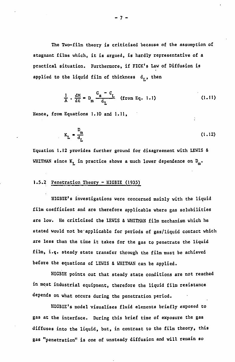
The Two-film theory is criticised because of the assumption of

stagnant films which, it is argued, is hardly representative of a

practical situation. Furthermore, if FICK's Law of Diffusion i,s

applied to the liquid film of thickness dL, then

1 dM Cs - CL - • - • D (from Eq. 1. I) A dt m dL

Hence, from Equations 1.10 and 1.11,

D m

~.~

(1.11)

(1.12)

Equation 1.12 provides further ground for disagreement with LEWIS &

WHITMAN since ~ in practice shows a much lower dependence on Dm.

1.5.2 Penetration Theory - HIGBIE (1935)

HIGBIE" s iiwestigations were concerned mainly with the liquid

film coefficient and are therefore applicable where gas solubilities

are low. He criticised the LEWIS & WHITMAN film mechanism which he

stated would not be'applicable for periods of gaS/liquid contact which

are less than the time it takes for the gas to penetrate the liquid

film, i.~. steady state transfer through the film must be achieved

before the equations of LEWIS & WHITMAN can be applied.

HIGBIE points out that steady state conditions are not reached

in m~st industrial equipment. therefore the liquid film resistance

depends on what occurs during the penetration period.

HIGBIE's model visualises fluid elements briefly exposed to

gas at the interface. During this brief time of exposure the gas

diffuses into the liquid, but, in contrast to the film theory, this

gas "penetration" is one of unsteady diffusion and will remain so

- 8 -

unless the time of exposure becomes great enough to permit achieve-

ment of the steady state. Fig. 1.3 depicts HIGBIE's model of gas

penetration. The initial gas concentration in the liquid element is

that in the main body of the fluid Co • CL• The gas film is assumed

non-existent (by using a pure gas) and the element interface is thus

instantaneously saturated with the gas, c. • C. The history of the 1 s

penetration of the liquid film by dissolved gas is shown by dashed

lines in Figure 1.3. If penetration is uninterrupted then the condi-

. tion indicated by the full line is attained. This line represents the

state of steady state diffusion upon which the theory of LEWIS &

WHITMAN was based.

The time of exposure is small so the approximate solution to

Fick's Law (Equation 1.5) may be applied. whence the depth of penetra-

tion:

x • {,f'i)"'t m

The concentration gradient is:

c - C s L

IiiD"t m

and by applying Fick's Law. Equation 1.1:

(g/s)

which gives the unsteady gas transfer rate during the time of

exposure.

(1.13)

(1.14)

The penetration theory assumes a constant time of exposure for

all fluid elements. t • t the amount of gas transferred to the fluid c·

element in time tc is thus:

fig. 1.3

QJ o c c ~

(/) .--c

t

gas

liquid

gas/liquid interface

/ • . ~

state diffusion

concentration ,..

,

steady and unsteady state diffusion

through a liquid film (after HIGBIE)

- 9 -

W·t • 2A (C - C) m c s L 11

(g)

The mean rate of transfer during this time tc is give9 bYJ.

M Mo· -.

tc 2ff A (C - C ) n.tc s L

The penetration theory leads to:

Kz. • 2t'!t c

(g/s)

(1.15)

(1.16)

(1.17)

(1. 18)

Since a constant time of exposure t has been assumed then the rate c

of surface renewal rc has also been assumed constant. Equation 1.18

can be re-written:

(1. 19)

1.5.~ Surface'Renewal Theory - DANCKWERTS (1951)

In common with HIGBIE, DANCKWERTS abandoned the concept of a

stagnant film stating the improbability of the existence of such a •

film in a turbulent fluid. He does however refer to this as a

"harmless and convenient usage" as measured absorption rates do indeed

conform to relationships of the form of Equation 1.10 with the liquid

film mass transfer coefficient being constant for a given liquid under

given conditions.

DANCKWERTS supposes the liquid surface to be continually

replaced with fresh liquid. This is a case of unsteady diffusion of

gas into the liquid element and DANCKWERTS assumes the rate of gas

- 10 -

absorption to be as given by Equation 1.14.

The average rate of production of surface s is constant, and

the chance of a surface element being replaced within a given time is

assumed to be independent of its age. The possible time of exposure

may vary from zero to infinity - in this respect the theory differs

from HIGBIE's assumption of constant time of exposure. The fraction

of the surface having ages between t and t + dt is assumed to be

f(t).dt - se~st.dt. The rate of absorption into those surface elements -st

of age t and of fraction se ~dt of the area is found from

Equation 1.14 to be:

dM -at jDm - - A se - (Cs - CL) .dt dt nt

c

whence the average absorption rate will be:

• ••

00 -st M Ho - f A se . ~ (C

s - C

L) d t

o ntc

The surface renewal theory predicts that

1.5.4 Film/Surface Renewal Theory - DOBBINS (1962)

(1.20)

(1.21)

(1.22)

(1.23)

This theory combines the film and surface renewal theories into

one equation.

For conditions of very low turbulence such as a slow flowing

river, the exposure of surface elements may be long enough to permit

the attainment of steady state diffusion. Also, during unsteady

.. .

- 11 -

diffusion under these conditions the depth of penetration may reach

beyond the surface element and into the main body of the fluid and

thus into the region of molecular and eddy diffusion, i.e. the film

theory vill apply.

The theory applies the concept of surface reneval and the gas

transfer coefficient is expressed as a function of the average rate of

surface renewal s and maximum depth of penetration (film thickness),

(1.24)

Note for low turbulence, s tends to zero, the film theory (~ - Dm/dL -

Equation 1.12) vill apply. For high turbulence the coth te~ in

Equation 1.24 tends to unity and ~ becomes governed by surface renewal

theory, Equation 1.~3.

1.5.~ Relative merits of the Gas Transfer Theories

The assumption of steady state diffusion and of stagnant

surface films by the film theory makes this an unrealistic theory since

the periods of exposure usually occurring in practice are too short •

to enable a steady state of diffusion to be attained. Further, the

existence of a stagnant film is a convenient but unrealistic one in

view of the conditions of turbulence usually prevailing. Also, the

dependence of KL on Dm as predicted by Equation 1.12 is not borne out

by practical experience.

The first three theories discussed all have one unknown and

the fourth has two. Of the first three theories, one has been discrediI

ted, vhich leaves the penetration theory (unknown constant time of

- 12 -

exposure, t c) and the surface renewal theory (unknown average rate of

surface renewal, s). Of these two, t is more readily measured in c

practice, but s can only be obtained by measurements of ~ and substi-

tution into Equation 1.23.

It is generally accepted that ~ is a function of turbulence,

the more turbulent the body of fluid the higher will ~ be, (a parti

cular gas is assumed).

This effect is readily explained by the various theories

discussed: The effect of increasing turbulence is to reduce the

thickness dL of the liquid film, to reduce the time of exposure to gas

of the fluid elements, t , to increase the rate of surface renewal, s, c

and in the last theory dL is decreased and s is increased.

All the theories can therefore be said to satisfactorily explain

the effect of turbulence on the gas transfer coefficient.

In contrast to the above theories, KISHINEVSKI (1955) has con

cluded that the value of ~~ independent of the gas idiffusion

coefficient being solely dependent on the turbulence intensi~y at the

interface.

1.6 FACTORS AFFECTING THE GAS TRANSFER COEFFICIENT

• 1.6.1 Temperature

In keeping with EINSTEIN's equation, Equation 1.2, the coeffi-

cient of molecular diffusion will increase as the temperature rises and

thus will increase the value of ~ given by the various gas transfer

theories. The viscosity of the water will be decreased by a temperature

rise and this will enable the bubbles in an air entrainment situation

to rise more rapidly with consequent reduction in the time of exposure

tc (assume ~ given by HIGBIE's model - Equation 1.18). Tbis reduction

in tc will result in a higher value of ~.

- 13 -

Two other quite separate temperature effects must be noted. A

rise in temperature results in a drop in the solubility of a gas in a

liquid (Section 1.9.J), the saturation concentration C is reduced, the s

concentration gradient is therefore reduced with a consequent lowering

of the rate of gas transfer. Secondly, a rise of temperature in a

situation of air entrainment results in a reduction of the surface

tension of the liquid. The bubbles will thus tend to expand and in so

doing they create a larger air/water interface which should promote

aeration. Conversely, the expansion of the bubble will result in a

fall in the partial pressure of gas within the bubble with consequent

lowering of the driving force.

The effects of temperature are generally taken into account by

a temperature function, this will be discussed later (Section 1.10).

1.6.2 Surface Active Agents

These agents are seen to have a variety of conflicting effects.

Generally they are visualised as forming a diffusion inhibiting film

at interfacial surfaces although there is evidence to suggest that in

highly turbulent situations this film is effectively destroyed and

thus no effect on the aeration performance is noted, (MANCY & OKUN, •

1965).

However, if a film is forme~ then the surface active agent

will not only lower the surface tension of the fluid but it will also

" modify the hydrodynamic properties of the surface layer (~OPEL). The

normal random motion is reduced to one of surface stagnation or to a

viscous layer with a lowering of the rate of surface renewal.

Two conflicting effects of surface active agents are possible.

On the one hand they form inhibiting films at gas transfer interfaces

- 14 -

and on the other they reduce surface tension and thus increase the

gas/liquid interface. The resultant effect cannot be predicted since

it must depend on the concentrations involved and on the dynamics of

the aerating system. Hence it is not surprising that a literature

review will reveal that surfactants may have no effect or they may

increase or decrease aeration.

Under highly turbulent conditions, the surface active agents

will probably have no effect on the liquid film coefficient ~ and

thus the oyerall effect will be governed by the effect on the air/water

interface. MANCY & OKUN's (1960) studies on bubble aeration showed

A a reduced ~ but increased ~V. Similarly the experiments of

ZIEMINSKI, GOODWIN & HILL (1960) showed that the addition of alcohols

and carboxylic acids can increase the aeration efficiency by up to

100%, this effect increased progressively as the length of the carbon

chain. Tests on anionic commercial surface active agents revealed a

lesser improvement in aeration efficiency but two non-ionic surface

active agents tested resulted in a marked decrease in absorption effic-

iency. In this latter case the advantage offered by the ,reduced size

of air bubbles was more than offset by the decreased transfer or

liquid film coefficient ~.

It is clearly useless to attempt a generalisation.

1.6.3 Suspended Solids

VAN DER KROON (1968) has shown that the rate of oxygen transfer

.in a mixed liquor and an aluminium hydroxide suspension depends on the

concentration of suspended solids and decreases with increase in

suspended solids concentration.

MANey & OKUN (1968) attributed this effect to an increase in

the liquid viscosity and the fact that turbulent eddies will tend to

- 15 -

be dissipated by the presence of suspended solids. The increase in

viscosity will of course tend to decrease the oxygen diffusivity

coefficient. The dissipation of the kinetic energy of liquid eddies

will tend to result in a thicker boundary layer, larger values of dif

fusion time, smaller frequency of surface renewal - the resultant

conclusion in the light of the various transfer theories already discussed

is a net reduction in the transfer coefficient~. For most practical

applications it is believed that the main effect of suspended solids is

the interference with the liquid hydrodynamics rather than the reduction

in oxygen diffusivity coefficient.

However, the effect of suspended solids is reduced by mechanical

agitation or highly turbulent situations (BOWERS 1955, also BRIERLEY &

STEEL 1959) and there will be some critical degree of turbulence beyond

which the effect of solids on the rate of aeration will become negligible.

The parallel turbulence dependent behaviour displayed by tempera-

ture, surface active agents, suspended solids is interesting and it is

probable that for a turbulent air entrainment situation the detrimental

effects of contaminants may safely be assumed negligible. The tempera-

ture effects are discussed in Section 1.10 •

• 1.7 A GENERAL EQUATION OF GAS TRANSFER

All the theories of gas transfer discussed earlier have taken

FICK's Law as the basic equation describing the transfer of oxygen

from the gas to the liquid phase. The differences between the individual

theories lie in the different approaches to predicting the liquid film

gas transfer coefficient, (the physical presence of a liquid film is not

being implied).

•

- 16 -

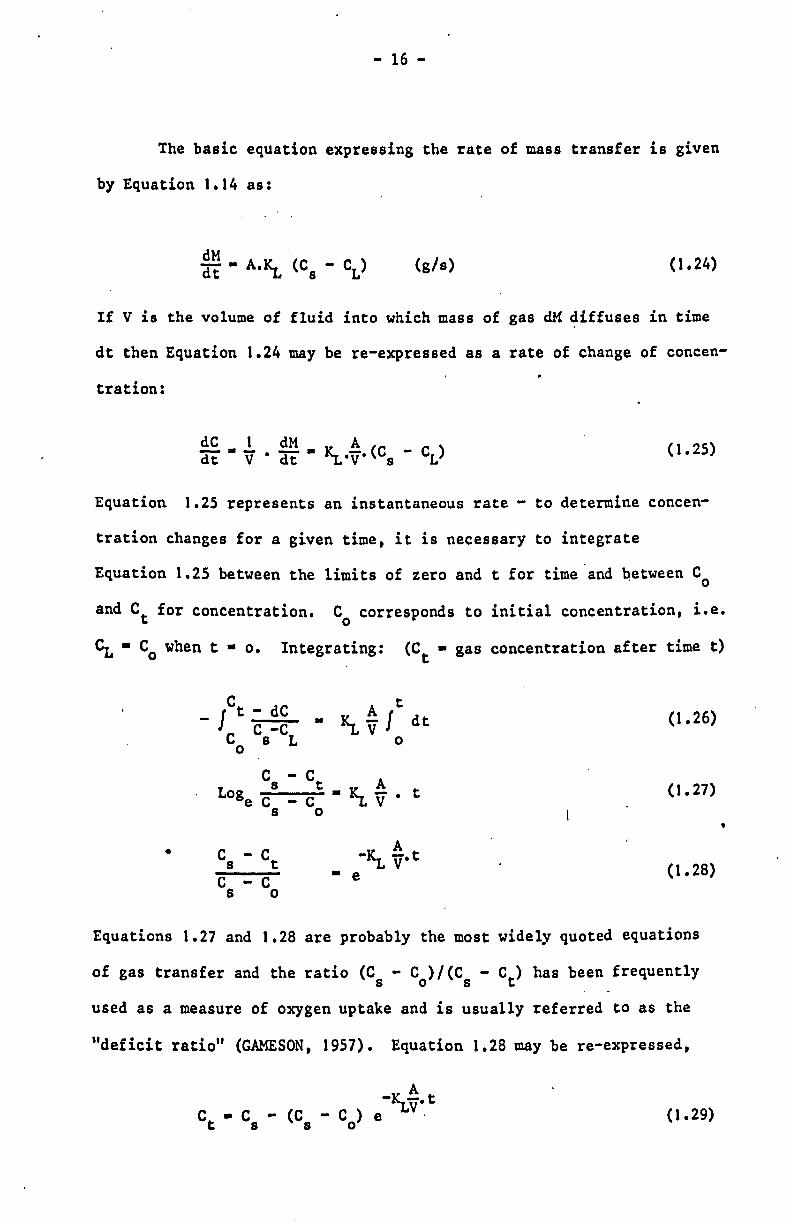
The basic equation expressing the rate of mass transfer is given

by Equation 1.14 as:

(g/s) (1.24)

If V is the volume of fluid into which mass of gas dM diffuses in time

dt then Equation 1.24 may be re-expressed as a rate of change of concen-

tration:

dC 1 ---dt V dM . --dt (1.25)

Equation 1.25 represents an instantaneous rate - to determine concen-

tration changes for a given time, it is necessary to integrate

Equation 1.25 between the limits of zero and t for time and ~etween C o

and Ct for concentration. Co corresponds to initial concentration, i.e.

CL - Co when t • o. Integrating: (C • gas concentration after time t) t

•

t

• ~ ~ I dt o

A -~ V· t

• e

(1.26)

(1.27)

(1.28)

Equations 1.27 and 1.28 are probably the most widely quoted equations

of gas transfer and the ratio (C - C )/(C - Ct ) has been frequently s 0 s

used as a measure of oxygen uptake and is usually referred to as the

"deficit ratio" (GAMESON, 1957). Equation 1.28 may be re-expressed,

C • C - (C - C ) t s s 0 (1.29)

•

- 17 -

and in this form it is essentially the same as the relationship of

ADENEY & BECKER (1919 and 1920) derived from experiments on the rate of

gas transfer from bubbles.

VAN DER KROON & SCHRAM (1969) expressed the oxygen uptake in

terms of what' they termed the "aeration capacity", C • ac

Assuming that for a particular aeration situation:

A -Ktvt e • Constant • 1 - K (1.30)

and the oxygen levels above and below the aeration system are Cl and

C2' then Equation 1.28 may be re-expressed:

C - C Cl - C2 s 2 1 1 - K • + C - C • C - C s 1 s 1

or C (I - K)

C2 • KC + C1

s (1.31) s C s

C2 • C1 + KC (1

C1 (1.32) or --) s C s

C2 • CI + Cac (I C1 (1.33) or --) C s

The aeration capacity, C , is expressed in Equation 1.33 and expressed ac

in words the aeration capacity of a particular system is defined as th~

oxygen level that would be achieved by the system if the oxygen level in

the water arriving at the system were zero (See Figure 1.4).

The aeration capacity is related to the deficit ratio by

Equa tion 1.34:

(1.34)

t Cs ~-------~ Cs - C1 -E

a. 0. -c

.0 .-~ a 'Q) c

c OJ Ol ~ X o

""C Q)

~ o Vl Vl .-

""C

..

.1 Cae

o a dissolved oxygen prior to aeration (ppm) ".

fig. 1.4 relationship between oxygen levels above

'and below a weir system

- 18 -

Both the deficit ratio and aeration capacity are presented graphically

in Figure 1.4 which depicts the relationship between oxygen levels above

and below a particular weir system for constant hydraulic conditions.

1.8 THE APPLICATION OF GAS TRANSFER EQUATIONS

The reciprocal of the deficit ratio could be predicted for a

particular system of aeration by the application of Equation 1.28.

This would require an accurate knowledge of the oxygen solubility which

depends on prevailing conditions of temperature and pressure and on the

presence of dissolved salts (Section 1.9). According to gas theories

(except that of KISHINEVSKI) the liquid film coefficient dep~nds on the

diffusion coefficient of the gas, the time of exposure or rate ,of

surface renewal and on the presence of surface active agents~ The

volume of fluid and the time over which aeration occurs can be stated

but the interfacial area would require an estimation based on air flow,

bubble size, bubble velocity etc.

Clearly, for practical purposes such as aeration at a weir the

precise application of Equation 1.28 is impossible and it is for this

reason that recourse is made to experiment to estimate the aeration

possibilJties of a particular situation.

In general, an overall gas transfer coefficient ~ is used,

re-writing Equation 1.28:

or

C - C s 2 C - C s 1

A 1 -IL-vt -~ t -1. -1.a· ---e -e (1.35) r

(J .36)

- 19 -

In all the experimental work reported in this thesis, the oxygen uptake

has been expressed as the deficit ratio and attempts have been made to

correlate the deficit ratio with the hydraulic parameters controlling

the values of ~a and t. The success of such correlations would have to

be tested outside the laboratory and can only be expected to be success-

ful if all parameters that influence ~a and t appear in the correlation.

All the theories discussed so far relate to gas transfer in

general. In these studies interest is focused on oxygen transfer and

the factors affecting it in a situation of air entrainment.

1.9 THE SOLUBILITY OF OXYGEN IN WATER

1.9.1 The Effects of Temperature and Pressure

A liquid can be said to be saturated with a gas when ~quilibrium

is reached between the concentration of gas dissolved in the liquid and

the partial pressure of the gas above the liquid. This is a statement

of HENRY's Law.

Sparingly soluble gases are generally held to obey the gas laws

and KLOTS and BENSON (1963) have confirmed this by observing no devia-

tiona from HENRY's Law for the solubility of oxygen. nitrogen and argon

at partial pressures up to 1 atmosphere. Furthermore BENSON & PARKER •

(1961) have shown that oxygen and nitrogen conform to DALTON's Law at

I at~sphere.

For a given atmospheric pressure. the oxygen partial pressure in

air will vary with temperature because of the increase in the saturated

water vapour pressure:

(1.37)

- 20 -

where Pg - oxygen partial pressure in air

P - atmospheric pressure o

P • vp saturated water vapour pressure at temperature TOe

0.21 • proportion by volume of oxygen in air

The partial pressure of oxygen and therefore also the solubility of

oxygen in water will both vary with changes in temperature and

pressures.

For temperatures ranging from oOe to 350 e HATFIELD (1941)

expressed the solubility of atmospheric oxygen in water by the equation:

0.678 (P - P ) o vp Cs - T + 35

Cs - solubility of oxygen (ppm)

(1.38)

Much work has been carried out to determine the solubility of

• oxygen ln water. Among the most recent work, the results of MONTGOMERY.

THOM & COCKBURN (1964) are in good agreement with KLOTS & BENSON (1963).

Doubts nave been expressed (GREEN) about the accuracies of the results

of TRUESDALE, DOWNING & LOWDEN (1955). A convenient nomogram which

enables the calculation of dissolved oxygen contents in water has been

presenteQ by HART (1967) based on the saturation valves of MONTGOMERY

and co-workers. This nomogram, reproduced in Figure 1.5, gives values

of Cs in agreement with those calculated from Equation 1.38.

The reduction in solubility with increase in temperature is con-

sistent with the principle of LE CHATELIER since the dissolving of a

gas is associated generally with an evolution of heat.

1.9.2 The Effect of Added Salts

The solubilities of most gases in water are reduced by adding

salts to the'water. This salting out effect of an electrolyte is

connect T and P to give intersection on R, connect

point of int ersection and % Cs ,read C

c T R

30

40

.

z w ~ ~ Cl

~-20 :::.J o Vl ~ Cl

p

780

770

-760~ .

E E

!SO-w 0:: :J

740 ~ w 0:: a.

730 0 0:: w

7205: If) o ~ r::

710 «

]9. 1.5 nomogram to calculate dissolved oxygen content

(mg/l) from dissolved oxygen (0,{) saturation)

at temperature Toe and atmospheric

pressure P mm. Hg - after' HART (1967)

- 21 -

attributed to the congregation of dipolar molecules of the polarizable

solvent, for instance water, around the ions of the added electrolyte.

The net effect is a reduction in the amount of free water available

to the solution of gas.

It has been generally accepted that solubility changes linearly

with salinity (FOX 1909, TRUE5DAlEand others, 1955), although GREEN's

results (1965) were best fitted by a relationship proposed by SETSCHENOW

in' 1875:

C s

Log.c;- - - Ksa (T).5a (1.39)

5 is the salt concentration and C ' is the solubility in this solution. a s

Ksa is a constant.

The equation proposed by TRUESDALE and co-workers (1955) for

sea water is given by Equation 1.40:

c ' • 14.161 - 0.3943 T + 0.007714 T2 - 0.0000646 T3 -s

Sa (0.0841 - 0.00256 T + 0.0000374 T2)

, with C in ppm and salinity S in parts per thousand. s a

(1.40)

Equation 1.40 is very cumbersome to apply and this resulted in a •

simpler equation being produced by GAMESON & ROBERTSON (1955):

s

475 - 2.65 Sa .-~~-~-33.5 + T

(1.41) C·

In the range 0 - 300 this equation is stated to fit the experimental

data of TRUESDALE and others with the same precision as Equation 1.40.

For pure water Equation 1.41 reduces to:

475 C • ---:--~ S 33.5 + T

(1.42)

- 22 -

which is of the same form as Equation 1.38 - Note that the experiments

of TRUESDALE and others were carried out at a pressure 760 mm. Hg.,

also that GREEN suggested that these results were about 3% too low.

1.9.3 The Effect of Suspended Solids

A drop of less than 5% in the oxygen saturation value has been

found by VAN DER KROON (1968) for a mixed liquor and a l suspension of

aluminium hydroxide. MANCY & OKUN (1968) questioned this finding and

suggested that perhaps salting out effects had been ignored. In any

event, there is no other evidence to support this finding.

1.10 THE EFFECTS OF TURBULENCE ON TEMPERATURE INFLUENCE

The effects of temperature on the interfacial area and on the

liquid film coefficient have already been discussed in Section 1.6.1.

The temperature dependence of Equation 1.36 is generally described by

a temperature function of the form:

or •

T -T (~!) • (~!) .a 2 1

-"1. V T -"1. V T 2 1

(1 .43)

(1.44)

A survey of the literature will reveal a variety of values for the

"constant" a. These vary from 1.00 to 1.047 and this variation has

been shown to be due to different degrees of turbulence. GAMESON,

VANDYKE & OGDEN (1958) suggested a coefficient of e • 1.018 for an

experimental weir system and they also found that this coefficient was

not affected by the presence of surface active agents. TRUESDALE and

VANDYKE (1958) found a value of 1.015 for flowing water. The results

- 23 -

of CHURCHILL (1961)' are those generally applied to surface aeration:

(~a) 0 • (~a) x 1.0241(T-20) -~ T -~ 200

(1.45)

In common with but prior to CIWRCHILL, DOWNING and TRUESDALE (1955)

carried. out experiments in a stirred vessel and reported e • 1.0212

which is similar to CHURCHILL's reported value. They also indicated

lower values of e for higher stirring rates and reported no evidence.

to suggest a different coefficient for saline water.

The reduction in e with increase in turbulence was further

reported by DRESNACK and METZGER (1968). It is therefore conceivable

that extrapolation to high degrees of turbulence or mixing will result

in e tending to unity and thus it follows from Equations 1.43 and 1.35

that the oxygen transfer expressed as deficit ratio would theoretically

become independent of the temperature.

The varying temperature effects can best be understood by . visualising the following model describing the two phases of gas transfer.

(a) On exposure to an air interface, the water molecular boundary layer

is instantaneously saturated with oxygen whatever the initial ~eficit

(PASVEER, 1955 (ii)} (b) The dispersal of this oxygen throughout the

fluid cart be effected either by diffusion into the fluid body, or by •

the intensive mixing of. the oxygen saturated particles with oxygen

deficient water, or by a combination of these latter two processes~ In

phase (a), the temperature is important in that it determines the sat

uration value. In phase (b) the diffusion processes will be accelerated

by temperature increases whereas the mixing process is not believed to

change with temperature (IMHOFF & ALBRECHT 1972). Therefore it is the

degree of mixing (or turbulence) in the fluid body which will determine

- 24 -

the relative temperature influence in phase (b), since, the greater the

mixing, the lower will be the dependence on diffusion for the distribution

of oxygen throughout the fluid and thus the lower the temperature

influence.

This is illustrated in Figure 1.6 where the oxygen transfer (mg)

at various temperatures is expressed as a ratio of the oxygen transfer

at IOoC and plotted against the temperature. For surface aeration

(Curve A - CHURCHILL) and an increased temperature, the increased

diffusion rate outweighs the reduced solubility, for diffused aeration

or low turbulence systems (Curve B - PASVEER, also BEWTRA, NICHOLAS &

POLOKOWSKI) the reduction in oxygen solubility with increased tempera-

ture is almost equally compensated by the increased diffusion. For

higher turbulence systems, as illustrated by the experimental weir

studies of GAMESON, VANDYKE & OGDEN (1958), the influence of the diffu-

sion processes on the oxygen movement becomes progressively less

significant, an overall reduction in relative oxygen transfer being felt

as a result of the relative reduction in solubility. Curve C depicts

the relative oxygen saturation variation with temperature (1.0 at

100C) and this curve represents the limit at which the contribution to

oxygen distribution by the diffusion processes becomes negligible.

IMHOFF & ALBRECHT (1972) believed that the prototype structures

they studied (a weir, two turbine aerators, two surface rotary aerators)

exhihited the temperature dependence displayed by curve C. They also

suggested that an energy expenditure of 20 watt/m3 represented the .

lowest limit for temperature dependence described by Curve C. This

view is not consistent with the results of GAMESON, VANDYKE & OGDEN,

and will be discussed in more detail in Section 4.5.

1.5r----.----~----~--~----~---------~

A. CHURCHILL (1961) -'-'-

1.4 B. PASVEER (1955) ------

1.3

11.2

& 1.1 ~

U I N

~ 10 '" . 0 t--is I 0.9 N

u -...... 0.8

0.7

0.6

0.5 0

C. Oxygen saturation values --

..... .. ~ .. ........... ....... ~~.-. ----.. :.:..~ ......... , ... :~~

..,,' .' ","'" .'"

./

." ."

.,,' ;,' ."

,tI' ," "

/A

-'''''' ~.~ B .-.... ---~.. ...---

"...........; .. ..:::.---- ------., ---.. ----.:-~-----.-----............. ' .................. '.. "-, .-., ..

.......... ........ .. -_JJ1 ........ ..........

......... . ................... .. ~ "

............ ........·· .................. 02 ......., ..........

... ....... .. '· ....... 03

D. GAMESON, VANDYKE & OGDEN (1958) 1 h=0.61 m 2 h= 1.ft9m _e_ .. _ 3 h=3.28m -----

5 10 15 20 25 30 35

- te mperature °C ,.

.flg.1.6 the effect of temperature on the relative dissolved

oxygen transfe r (1.0 at 10°C). [partly reproduced from IMHOFF & ALBRECHT (1972)]

CHAPTER 2

THE AERATION OF FLOWING WATERS

•

- 25 -. ..' ~.. ,

2.1 INTRODUCTION

The assimilative capacity of a river has been the subject of

research since the early work of BLACK & PHELPS (1911) when first

attempts were made to predict reaeration capacity.

The oxygen balance of a river system depends on a number of

variables some of which are noted in Section 2.5. The use of a river

as a convenient recipient for human and industrial wastes places con-

siderable strains on the river's natural assimilative capacity and

times of low flow are critical since the dilution ratio is low. Simi-

larly during high temperature periods when the gas solubility in water

is reduced and the bacterial growth stimulated. At such times a need ,

for supplemental aeration is realised, preferably at the lowest point

on the oxygen sag curve. The location of such facilities is however

usually dictated by the adaptability of existing structures (usually

those involving a head loss e.g. turbines) or by the availability of

either power or supervisory personnel. An oxygen level of 40% satura-

tion .has been suggested as an upper limit for economical supplemental

aeration (THACKSTON & SPEECE, 1966).

A review is presented of means of estimating the reaeration •

capacity of 'a river and various ways of supplementing river oxygen

levels are noted.

Particular attention has been paid to two air entraining

phenomena common to many hydraulic structures, namely the hydraulic jump

and free falling water jet.

- 26 -

2.2 NATURAL REAERATION THROUGH A STREAM SURFACE

The aeration equation developed by STREETER & PHELPS (1925)

(basically Equation 1.25) has formed the basis of all studies of stream

assimilative capacity and numerous formulations have been proposed to

enable estimates of the reaeration rate coefficient ~~ or ~a for gas

transfer through the surface of a stream. Table 2.1 summarises most of

the major contributions in this field.

In their early work STREETER & PHELPS proposed that ~ depended

upon many variables such as mean stream velocity v , depth y, slope S, m

and channel irregularity. This is reflected in Equation 1 of Table 2.1

where C and n are constants for a particular river stretch whose values

depend in part on the channel slope and roughness. STREETER & PHELPS

indicated that wide variations in the empirical coefficients are to be

expected and indeed this has been amply demonstrated by most of the

subsequently developed models in Table 2.1, almost all of which follow

the form of the original equation of STREETER & PHELPS. Of the two

equations developed by O'CONNOR & DOBBINS, Equation 2 of Table 2.1

applies to streams exhibiting a pronounced vertical velocity gradient,

a condition of non-isotropic turbulence (Chezy Coefficient

vm/liRS < 20), whilst the second equation is relevant to comparatively •

deep channels where a condition of isotropic turbulence may be approached

(Chezy Coefficient> 20).

ISAACS & MAAG (1969) introduced additional empirical factors for

channel shape ~ and surface velocity ~. From the data of CHURCHILL, s v ELMORE & BUCKINGHAM (1962). they obtained mean values ~ • 1.078 and s

~v • 1.16.

KRENKEL & ORLOB (1962) attempted to explain reaeration in terms

of a longitudinal mixing coefficient DL whilst in the second ~odel

Equation 5, Table 2.1, the energy dissipation per unit mass of fluid

1\

I: It

I

TABLE 2.1

Various ~quations Relating the Surface Reaeration Rate Coefficient

AUTHOR(S)'

STREETER & PHELPS (1925)

O'CONNOR & DOBBINS (1956)

• to Hydraulic Parameters

REAERATION RATE COEFFICIENT

~ _ Cv n -2 m Y

~a - 480 Dm1s!y-S/4

~ ... D Iv ly-3/2 2 -1 a m m .31

.(1)

(2)

(3)

KRENKEL & ORLOB (1962)

~a(20oC) - 0.00004302 DLI • 15y-l.915, (4)

~a(20oC) a 0.000141 EdO.408y-0.66

OWENS, EDWARDS ,~ (200C) ... 9 41 0.67 -1.85 & GIBBS (1964) -La • vm y

CHURCHILL, EL~ORE Ii K- (OoC) a 5 026 0.969 -1.673 & BUCKINGHAM (1962) -La 2 • vm Y

ISAACS J (J967) ~ a cVm (1.0241)T-20y-l.S

LANGBEIN & DURUM ,. Ie ... 3 3 -1.33 (1967) -La • vmY

ISAACS & MAAG (1969)

THACKSTON & KRENKEL (1969)

NEGULESCU (1969)

TSIVOGLOU (t 972)

& ROJk~SKI

& WALLACE

.• K- ... 2.98 ~ ~ v·y-J.5 -La s v m

r-- -1 ~a ... 0.000125 (I + vm/rgy)u*y

~a a 0.0153 D v 1.63y-l.63 m m

KLa(2SoC) ... 0.054 6h/t f

(5)

(6)

(7)

(8)

(9)

(10)

(11)

(12)

(13)

UNITS

-1 ~ day ,v ft/s, Y ft -"La m

-1 ~a day ,S ft/ft, Y ft

2 D ft /day, v ft/s m m

~ min-I, D ft2/min. y ft -La m

v ft/s. y ft m -1

~ day , vm ft/s, y ft

-1 Ie day , v ft/s, Y ft -"La m

-I ~ day ,v ft/s, y ft -""La m

2 Dm cm /s,vm mIs, ym

-1 ~a hr , 6h ft, t f hr

N

"

- 28 -

was introduced where Ed • vmSg. THACKSTON & KRENKEL (1969) produced

another modified form of the STREETER & PHELPS model when they intro

duced the Froude number vm/lgy and a shear velocity u*. The studies

of CHURCHILL and co-workers (1962) are among the most extensive carried

out. They produced nineteen models involving some eight to ten hydrau-

lic parameters and all exhibited similar correlation. The model

recommended was the simplest but gave equally good correlation of the.

data.

TSIVOGLOU & WALLACE (1972) utilised a recently developed field

tracer procedure for measuring stream reaeration, a radioactive form of

the noble gas krypton serving as a tracer for oxygen. The field results

collected encompassed a wide variety of conditions and were considered

as representative of most non tidal fresh water streams. The early

predictive models given by Equations (3), (7), (9), (11) and (6) in

Table 2.1 were tested against observed results. None proved capable

of prediction within acceptable limits the differences between predicted

and observed values of ~a proving to be consistently large for highly

turbulent stream reaches where flow was not uniform.

The change in water surface elevation 6h and time of flow t f were

demonstrat~d to be primary hydraulic properties related to reaeration • •

The mean forward flow velocity and stream depth were not found to be

related to stream reaeration in a primary way and similarly the stream

bottom roughness and longitudinal dispersion were not found to serve as

useful indicators of stream reaeration capacity.

The constant 0.054 in Equation 13 Table 2.1, referred to as the

escape coefficient, is affected by pollution as indeed are all the

models in Table 2.1. The value given is for a typical stream, reasonably

well mixed and'moderately polluted (5 day BOD approximately 15 mg/l).

- 29 -

2.3 SUPPLEMENTAL REAERATION

2.3.1 Diffused Air Aeration

The injection of air into a body of water through diffusers is

an important constituent of the activated sludge waste treatment process

(BEWTRA & NICHOLAS 1964) and as a result has provoked much research.

particularly with regard to the suitable design of diffusers. The tech

nique has also been employed to aerate streams (TYLER. 1946; PALLADINO.

1961) but reported efficiencies were low and the costs. both capital and

operating. were high. However. the technique has been recommended

(SPEECE & RAYYAN. 1973) for the aeration of the hypol.imnion(cold water

layer) of stratified impounded waters since this could be achieved

without disturbance of the stratification. De-stratification by

pumping hypolimnion waters to the surface is a method commonly used to

aerate the hypolimnion. but. this involves pumping huge quantities of

water and the distribution of nutrients from the hypolimnion with

undesirable increases in algal activity.

2.3.2 Mechanical Aeration

This is another system used where no head losses are available.

The water surface is churned up by a series of rotating vanes. or

alternatively a system whereby water is pumped from the river and sub

sequently sprayed out by the turbines was tested by KAPLOVS~.

WALTERS & SOSEWITZ (1964). The system has an advantage of mobility

since the aerators can be mounted on readily movable pontoons. However.

the capital costs involved are probably greater than any other system

whilst the running costs are comparable to those encountered with

diffused air aeration (THACKSTON & SPEECE. 1966).

- 30 -

2.3.3 Turbine Aeration

This is a case where existing structures have been modified in

favour of supplementing aertation. Many power turbines set above tail-

water level are fitted with spring loaded air vents to alleviate the

vibration and cavitation which develop in the turbine draft tubes as a

. result of high vacuums at low flows. The wisdom of permanent venting

was initially doubted because of possible increases irt cavitation and

corrosion together with the destruction of tailwater vacuum. However,

the damage feared did not materialise and power losses of only 5% for

heads 6 to 9m were reported (THACKSTON & SPEECE) whilst significant

aeration was achieved. Alternative techniques such as the injection of I.

compressed air immediately before the turbine impeller have been

reported (IMHOFF & ALBRECHT, 1972).

2.3.4 U-Tube Aeration

A more recent development, this is a conceptually sim?le system,

consisting of two basic elements - a device for introducing air to a

flowing water stream (an aspirator, or a compressor linked t~ a

diffuser) followed by a vertical u-shaped flow path to provi~e co~tact

time under conditions of above atmospheric pressure thus providing a

favourable driving force for the transfer of oxygen. The u-shaped

flow path may take various forms, possibly a pair of vertical pipes

connected at the bottom by a 1800 bend, or, a pair of concentric pipes

with flow down one passage and up the other.

The U-Tube, first reported by BRIUZN & TUINZAAD in 1958, is a

highly attractive aerator requiring little maintenance, minimal operat

ing labour, and offering considerable flexibility in the choice of

- 31 -

configurations. In cases where a head loss was available, MITCHELL

(1973) demonstrated that the cost per unit oxygen dissolved was very

significantly less than for mechanical or diffused air aeration. Even

when the head had to be created by pumping, the U-Tube proved the most

economical at a discharge 10 mgd whilst for a higher discharge 100 mgd

it proved comparable to mechanical aeration whilst slightly less

economical than diffused air aeration.

2.3.5 Weir Aeration'

Since weirs are rarely constructed specifically for aeration

purposes, they must constitute the cheapest most effective and most

reliable source· of oxygen available. The superior oxygen transfer

capability of a weir compared to a turbine was noted by THACKSTON &

SPEECE together with the possibility of improving the aeration perform-

ance by breaking a single fall into a number of steps. The value of a

weir as a source of oxygen for ice-bound rivers was stated by LE BOSQUET.

Aeration is achieved by the weir in addition to breaking the ice cover

over the stream below the weir and thus promoting the surface aeration

possible.

The aeration at weirs, either by a free falling jet or by a •

spil~way controlled jet culminating in an hydraulic jump, forms the

basis of this thesis and will shortly be discu'ssed in some detail.

,.

- 32 -

2.4 NATURAL REAERATION THROUGH AIR ENTRAINMENT

2.4.1 Introduction

The capability of free surface flows to entrain air is very much

in evidence in nature and because of the engineering problems associated

with this phenomenon, it has already provoked much research. An under-

standing of the mechanics of air entrainment is necessary before

attempting to comprehend and quantify the processes governing the trans-

fer of gases from the air to the water.

2.4.2 Similarity and Aerated Flows

The difficulties encountered in the modelling of air entraining

flows stem from the well proven fact (HAINDL, 1958; RAO & KOBUS.1975)

that irrespective of model scale the size of air bubble entrained remains

relatively constant. This means that the conditions of geometric and

kinematic similarity cannot be satisfied.

The conditions required for perfect similarity of geometrically

sLnilar air/water flows have been demonstrated by RAO & KOBUS (1975)

from a dimensional analysis. Perfect similarity is achieved if the

Froude number, Reynolds number and Weber number are simultaneously equal

• in the model and prototype. As it is usual to use the same fluid in

both model and prototype and also keep the gravitational acceleration

constant, then only one of the numbers can be kept constant at anyone

time. Under these conditions perfect similarity is theoretically not

possible and the success of modelling air entrainment situations will

depend on the relative influence of the conditions not satisfied.

The Reynolds number describes the viscous forces associated with

the flow of a real fluid and these forces are most prominent when the

- JJ -

velocities are low or if the flow section is restricted. For relatively

high velocity water flows and relatively large flow sections the viscous

forces are insignificant in comparison with other forces.

The effects of surface tension at fluid interfaces are described

by the Weber number. These effects are similarly only significant for

low velocities and narrowed flow sections. Thus, for fully turbulent

flow conditions, the effects described by the Reynolds and Weber numbers

become relatively insignificant and therefore model similarity may be

achieved directly by keeping the Froude number (the ratio of inertial to

gravitational forces) constant.

A.review of various investigations into the entrainment of air

by free surface flows led RAO i KOBUS to conclude that the process of

air entrainment could be described very well by similarity according to

Froude's law. It was also suggested that those cases where scale effects

were observed had in common the fact that the process of air entrainment

was being influenced by the limitations in the transport cap~city of the

flow.

Evidence for the two air entraining situations relevant specifi-

cally to this thesis will be reviewed, namely, for an hydraulic jump and

free falling jet. The air entraining capability of other free surface

flow~ is· not reviewed here.

A most comprehensive review recently edited by RAO & ~OBUS,

refeFence to which has already been made, deals more broadly with air !

entraining free surface flows.

An excellent review of various air entrainment studies involving

shaft spillways, plunging jets, hydraulic jumps etc. is provided by

RENNER (1973).

- 34 -

2.4.3 Air entrained by Hydraulic Jumps

If an air pocket is formed, for instance, in a pipeline, then an

hydraulic jump will form at the end of the air pocket thus entraining air

and ultimately removing the air pocket. It was this phenomenon which

prompted the studies of KALINSKE & ROBERTSON (1942).

From studies they carried out on a laboratory scale circular

pipeline they found the ratio at of air discharge Qa to water discharge

Q to be a function of the Froude Number as follows:

a • ~ • K (Fr - 1) 1 .4 Q 1 (2.1 )

where Fr 1 ,. v1/{gYe is the Froude number of the supercritical flow

Ye • effective approach depth (water area divided by ~urface width)

K • 0.0066 for these tests

With a view to improving the existing design criteria for air

vents CAMPBELL & GUYTON (1953) studied the air demand resulting from

hydraulic jumps formed in pressure conducts downstream of dam outlet

gates for'Fr 1 < 30. The air discharge ratios they obtained we~e

consistently higher than those predicted by Equation 2.1 and they sug

gested t~is coul4 be due to: (1) entrainment of air into the stream

before reaching the jump; (2) entrainment of air by the intensely

fluctuating turbulent front of the jump; (3) the higher velocities

downstream facilitating more efficient removal of air.

The equation describing the results of CAMPBELL & GUYTON is:

\,

a • 0.04 (Fr - 1)°·65 1

(2.2)

- 35 -

FASSO (1956) on the other hand arrived at air quantities consider-

ably less than predicted by Equation 2.1.

However, Equation 2.1 was verified by the laboratory experiments

of HAINDL and SOTORNIK (1957) in a closed rectangular conduit. Their

flow section was approximately three times larger than that employed by

KALINSKE $ ROBERTSON and they concluded that this therefore indicated a

wide range of applicability of Equation 2.1. Taking into account the

scatter of his points HAINDL (1958) noted a maximum value K • q.012 in

Equation 2.1.

WISNER (1965) further compared the field measurements of

YUKIO (1959), GUYTON (1958), PETRIKAT (1958), and concluded that these

results were in good agreement with the model of KALINSKE & ROBERTSON

with a maximum value of K • 0.014. This is in good agreement with the

maximum K noted by HAINDL (1958) for his model tests. 'These results

confirmed WISNER's supposition that it is possible to model air entrain-. ment according to the Froude criterion in locally turbulent ~ituations

only. WISNER stated a lower limit of validity for the prototype to be

satisfactorily modelled according to ~odel results, namely, for hydrau

lic jumps, Fr 1 > 8. WISNER states that Equation 2.2 gives values of a erring on the low side for Fr 1 > 8 •

• In contrast, RAJARATNAM (1962) investigated the aeration

characteri~tics of jumps formed in open conduits and noted that the

air is entrained at the toe of the jump. The mean air concentration

in a vertical section was observed to attain a maximum value within a

very short distance of the toe of the jump and thereafter it was seen

to decrease as air was lost to atmosphere through the surface roller.

Similar results were noted by others and most recently by RESCH &

LEUTHEUSSER {1971~, also LEUTHEUSSER, RESCH & ALEMU (1973).

- 36 -

RAJARATNAM showed a similar dependence on Froude number thus:

B - 0.018 (Fr - 1)1.245 m I'

where B is the maximum relative air discharge which was recorded m

close to the toe of the jump.

(2.3)

RENNER (1973) compared the measurements of RESCH & LEUTHEUSSER

(1972) in an open conduit with those of RAJARATNAM and showed them to

be higher. However, RESCH & LEUTHEUSSER used an anemometric technique

which produced results of dubious accuracy as discussed in Section 5.2.4.

2.4.4 Air Entrained by Liquid Jets

SHIRLEY (1950) was possibly the first to quantify the air

entrained by a plunging liquid jet. He investigated the air entrained

by an inclined circular jet issuing from five different nozzle sizes.

SHIRLEY reported a separate relationship between air entrained and jet

velocity for each jet diameter studied.

TONG JOE LIN & DONNELLY (1966) principally studied plunging

laminar jets, namely, those jets having a flat velocity profile at the

point of entry into the fluid. Al though such laminar jets .are not •

likely to occur in·practical situations, some interesting conclusions

are made and these will be reviewed.

In contrast to the mechanical bubble trapping device of SHIRLEY,

LIN & DONNELLY employed high speed cine photography. The volumetric ;

gas flow rate was thu~ determined from the bubble size distribution

data and frequency of bubble occurrence data obtained from photographic

analysis. Spherical bubbles were assumed. A minimum entrainment

velocity was defined as the minim~ jet velocity, based on the jet

- 37 -

diamete,r at plunging point, required to entrain bubbles in a given

system. This was expressed by the correlation:

0.794 Ue • 6.22 Do.206Y 0.206 0.587

P lJ

(m/s) (2.4)

A minimum velocity U is required to entrain air and this is shown to e

be a function of fluid density p, viscosity lJ. and surface tension Y,

and, also of the diameter D of the jet at the plunging point.

Equation 2.4 is applicable in the laminar region up to a

REYNOLD's number (defined in Equation 2.5 below) 1500. Above this value

the jet becomes unstable and the entrainment mechanism chang~s.

R • pUD e lJ

where U is the ~et velocity.

(2.5)

Entrainment by laminar jets is effected by a thin fil~ of gas

formed around the jet. The jet and film enter into the liquid intact.

As the jet penetrates further into the liquid, oscillations develop

and this subsequently leads to the breakup of the gas film into bubbles.

In contrast, the turbulent jet, occurring for R > 1500, is character-e .

ised by~nstability in the gas phase with visible disturbances on the

jet surfaces. These disturbances are responsible for the entrainment

of air, visual observations showed that in contrast to the laminar jet

no gas film was entrained intact into the liquid body. The addition

of a surface active agent was observed to reduce the minimum entraining

velocity. This is due to the lowering of the solution surface tension. \

The presence of more than 0.2% surface active agents did not produce any

further effect on U or surface tension, while the initial addition of :. e

0.02% had the most dramatic effect.

- 38 -

The dominant factor affecting both bubble size and bubble

frequency was the jet velocity. The average bubble size decreased and

the bubble frequency increased sharply as the jet velocity was increased

above the minimum entraining velocity. An increase in the jet diameter

has a lesser effect, but, it resulted in increases in both bubble size

and frequency with a more pronounced effect on the latter. The addition

of 0.02% surface active agent resulted in reduced bubble size but

increased frequency at minimum entrainment velocity.

WISNER (1965) was mainly concerned with the design of venting

orifices to provide adequate ventilation behind the jet falling from a

weir. WISNER demonstrated for prototype and model situations that the

relative air entrainment was a function of the Froude number of the jet

at impact. It is worth noting that the air uptake measured by WISNER

was that due to the underside of the jet (i.e. the venting required). I

The total relative air entrainment into the tailwater will thus be far

greater, or, approximately twice as much.

More recently, ERVINE & ELSAWY (1975) reported experiments on the

air entrained by rectangular nappes falling freely to a downstream

pool. They produced an empirical relationship between the maximum

ratio air to water discharge and the nappe parameters width BJ

• peri

meter P; thickness tJ

, vela: ity ~ .tl nd impacting with a pool after

fall h.

Qa BJ - - 0.26 (-) Q p

U (1 - ...!. ) u

(2.6)

where Ue was the minimum velocity to entrain air (approximately 1.1 m/s).

For low values « 10) of Froude number (UI/gtJ). the ra:tio Qa/Q

was not constant but varied as the jet thickness varied. This was

- 39 -

attributed to noticeable surface tension and viscous effects in the

thinnest jets giving a reduced rate of entrainment. This is possible, \

but the design of the apparatus was such that entrained air may not have

been readily removed and thus scale effects introduced. The apparatus

as illustrated by ERVINE & ELSAWY provided that the water left the

pool at the same end as the inclined jet entered, in other words, the

horizontal velocity components of the inclined jet and the mass of fluid

in the pool were opposed. The comments of RAO & KOBUS on scale effects

mentioned in Section 2.2 might therefore apply. It is interesting to

add that for the thinnest jets, ERVINE & ELSAWY obtained values of B

as high as unity which is surprising since this represents the upper

limit of B which is in general physically possible. A value of B • I

corresponds to the maximum possible air concentration of approximately

50% (the ratio of air volume to the total volume of air and water)

(RAO & KOBUS), the exact maximum being dependent on the distribution . I

of bubble sizes.

For values of Froude number> 10, ERVINE & ELSAWY stat~d that the

ratio air to water discharge tended to a maximum as given by Equation

2.6.

The work of CHARLTON (1970) was also mentioned. CHARLTON found a

clear correlation between the Froude number and the air water discharge

ratio of a circular jet plunging into a pool of water and he similarly

recorded a tendency towards a constant ratio air to water discharge

for higher values of Froude number (> 10).

In all the work ~iscussed so far, only LIN & DONNELLY classified

the nature of their jets. In their case a distinction was made

between laminar and turbulent jets, but no one has distinguished between

solid and disintegrated jets which is surprising since this must

radically alter the air entrainment process.

- 40 -

The behaviour in air of free falling jets formed by rectangular

crests was studied in detail by HORENI (1956). The co-ordinates of the

passage of these jets through air were shown to be expressed by a

parabola of the second order, i.e. y • cx2, and for these experiments

the coefficients of velocity at the exit section were found to 'vary

between 0.93 and 0.98. At the point at which disintegration occurred

in the whole width of the jet, a distinct change in the jet outlines

was observed. Horeni conveniently expressed this point of disintegra

tion as a function of the specific discharge at the crest:

L - 31 19 0.319 o • q (2.7)

q - specific discharge (cm2/s)

Lo - distance measured along the jet centre line to the point

of total disintegration (cm)

2.4.5 Oxygen Uptake in an Hydraulic Jump

As already discussed, the air entrainment qualities of the

hydraulic jump have long been recognised with much work being done to

quantify the air uptake.

Very little has been done to record the oxygen uptake which is

clearly one of the major attributes of the hydraulic jump. JARVIS (1970)

recognised this need during his field survey of weirs which included

Crump weirs and sloping aprons. In such cases the quantity of oxygen

absorbed depended on whether or not an hydraulic jump was formed.

JARVIS demonstrated in the laboratory the significant aeration achieved

by an hydraulic jump by comparing the aeration achieved by a sloping

apron without an hydraulic jump to that with an hydraulic jump. Further-

more, detailed work was recommended and a possible correlation with

- 41 -

Froude number was suggested.

APTED (1975) followed on and carried out experiments with an

hydraulic jump formed in the narrowed section of a flume (10 cm wide)

downstream of an underflow sluice gate. Downstream of the jump the

narrowed section expanded abruptly to the full width of the flume

(30.5 cm).

APTED's experiments were for one discharge (approximately 4 lis)

and he suggested it was not possible to express the relationship

between the oxygen uptake (expressed as the deficit ratio (defined in

Section 1.7. Equation 1.35) adjusted to l50 C by use of Equation 2.13).

and the upstream Froude number by a simple mathematical equation.

Instead, he proposed a correlation with the measured energy

loss llE:

or

lOO.0024AE r 15 •

Log r lS • 0.0024 AE

. (AE cm) (2.8)

(AE cm) (2.9)

The hydraulic jump was also studied by, HOLLER (1971) using a

discharge of 1.2 cfs (33.98 lis) in a 15 inch (38.lcm) wide channel

(Private·Communication. 1974), HOLLER correlated the deficit ratio

corrected to 200 C with Av the difference in measured velocities before

and after the jump:

2 r 20 • 1 + 0.0043 llv (Av ft/s) (2.10)

The information· available on the oxygen transfer within an

hydraulic jump is obviously limited and inconclusive with more work

being called for.

- 42 -

2.4.6 Oxygen Uptake at Weirs

GAMESON (1957) made the first serious attempt to provide a means

of predicting the aeration occurring at a weir system. GAMESON expres-

sed the oxygen change in terms of the deficit ratio (Equation 1.35). A

survey of various prototype weir systems led to an approximate relation

between deficit ratio and height of fall (difference between water

levels).

r - 1 +~ 2 (h in metres) (2.11)

'a' is an arbitrary measure of water quality with suggested

values 1.25, 1.00, 0.85 respectively for slightly,

moderately and grossly polluted waters.

'b' is a function of the type of weir being 1.0, 1.3 respec

tively for a free overfall and cascade (step weir).

GAMESON also expressed the degree of aeration in terms of a

weir coefficient r-l/h for comparison of different weir systems since

this coefficient was apparently independent of h. It was also reported

that despite changes in discharge, water temperature and concentration

of surface active agents at a particular weir system, there was no •

recorded ch~nge in the degree of aeration. Tests on an experimental·

weir system verified that the rate of escape of oxygen from 6uper-. \

saturated water is equal to the rate of entry of oxygen into water

which is less than saturated with oxygen.

The effect of temperature was further studied by GAME~ON,

VANDYKE & OGDEN (1958) and found to be significant at an experimental

weir system. As a result the following equation was suggest~d to I

replace Equation 2.11:

- 43 -

r • 1 + 0.11 abel + 0.046T)h (2.12)

where r is the deficit ratio at TOe.

The equation used for adjusting data to a standard value at 150 e

was

r - 1 r l5 • 1 + 1 + 0.027 (T-15) (2.13)

Additional tests indicated that the temperature coefficient was

not affected by the presence of surface active agents.

Further work by BARRETT, GAMESON & OGDEN (1960) at four weir

systems confirmed the equality of rates of invasion and evasion of \

oxygen. In studies at Teddington weir on the River Thames, observed

values of r-l were 17% greater than those predicted by Equation 2.12.

The need to investigate the effects of discharge and depth of receiving

water was acknowledged, although the omission of these effects was not

considered to greatly affect the validity of Equation 2.12 • . OWENS & EDWARDS (1963) studied three free overfall weirs in the

River Lark and concluded that the oxygen transfer is essentially

predictable in a manner described by Equation 2.12. Close examination

of their.data shows that an increase in deficit ratio was recorded for

a reduction in discharge. At another weir, the opposite effect was

indicated by their data, although, at this weir considerable leakage

occurred through the boards forming the weir on the occasion of the I

lower discharge. The height of fall at these weirs was small I

(approximately 0.6m).

The effect of discharge was also noted separately by NATERMAN

(1952) and LONDONG (1967) - a reduction in aeration with increasing

discharge being observed.

- 44 -

GANNON (1967) illustrated the significance of a~ration at waste

treatment plant overfall structures and compared observations with

predictions from Equation 2.12.

In one free overfall, observed values of r-l were only 6%

higher than predicted while in another the predicted r-l was 58% too

high.

MASTROPIETRO (1968) reported a technique credited to QUIRK,

LAWLER & MATUSKY (1966) which was developed to predict aeration at the

Upper Gate House on the St. Louis River. Discharge Q was considered an

•• • d· dC 0 lmportant varlable, steady state conditlons were assume l.e.de •

and the mixing was assumed complete. i.e. Cs - Ct • Cs - C2•

A mass balance of dissolved oxygen at the dam was considered:

(2.14)

Cl ,C2 are dissolved oxygen concentrations above, below the dam.

For constant volume V of system, K- will vary with Q. thus: -~a '

(2.15)

or • C1 f(Q).Cs

C2 • 1 + f(Q) + 1, + f(Q) (2.16)

The second method review by MASTROPIETRO assumed a linear rela-

tionship between per cent saturation above and below the dam and that

this relationship is independent of discharge, i.e.:

, C1 100 • K x 100 + K 'e- x 100

m p s (2.17)

or

C2 • K C + K C m 8 p 1 (2.18)

-

- 45 -

Equation 2.17 was verified for dams of height 7 and 15 feet and

K and K were tentatively shown to vary linearly with the dam height: m p

K • O.037h and K • 1 - O.043h (h ft) m p (2.19)

A comparison with the deficit~ratio is interesting. Re-arranging

the deficit ratio yields:

and

whence

Equations 2.20, 2.18 and 2.16 are identical if

!.K .~_l~~ r p 1 + f(Q)

1 - ! . K. f(Q) r m 1 + £(Q)

1 + (1 1) 1 r - r • ~l-+~f (~Q~) + f(Q)

1 + f(Q)

(2.20)

(2.21)

(2.22)

(2.23)

If f(Q) is constant for a given dam height then K + K • 1 and m p

Equations 2.21 and 2.22 hold true.

The experimental results as indicated in Equation 2.19 indicate •

an approximate validity. Note that temperatures effects were ignored,

the equations were developed for temperatures in the range 2o-2SoC.

The prediction equations were derived for use with specific

structures and were not intended for general use, but, the principles

embodied could be applied elsewhere.

JARVIS (1970) showed that the values of 'a' given by GAMESON

(1957) for use with Equation 2.11 were incorrectly derived and should

be 1.52, 1.04, 0.68 respectively. From his own field survey of weirs,

- 46 -

JARVIS derived the following values of a - 1.23, 0.91, 0.59 for slight,

moderate and gross degrees of pollution.

JARVIS also experimented using a 221 0 V-Notch discharging at

the rate of 0.65 lIs into a 6lcm square downstream pool. He related

the deficit ratio to the height of fall (difference between water levels)

by the equation:

r 15 - 2.05 hO•434 (h m) (2.24)

Deficit ratios were corrected to l50 C by Equation 2.13. JARVIS, and

earlier the DEPARTMENT OF SCIENTIFIC & INDUSTRIAL RESEARCH (1958).

showed that as the depth of downstream pool increases (for constant

height of fall, h) then the deficit ratio increases until an optimum

value of depth is reached beyond which the deficit ratio is independent

of depth. This depth is approximately the depth to which bubbles

penetrate (D.S.I.R., 1958) and is termed the optimum depth. JARVIS

reported a relationship between the optimum depth d' and the distance H

between the upstream water surface and the bed of the downstream pool:

d' - 8.46 loge (H/l4.l4) (em) (2.25)

• with H in em.

For optimum depth conditions:

r 15 - 0.009H + 1.00 (H cm) (2.26)

JARVIS also obtained an increase in aeration for a reduction

in his downstream pool width.

VAN DER'KROON & SCHRAM (1969) experimented with a variety of

notches. They demonstrated partitioning of a weir nappe could lead

- 47 -

to considerable increases in the aeration occurring with an optimal

result being achieved with about six jets per metre width of weir crest.

Their results also showed that an increase in discharge was accompanied

by a small reduction in aeration. It is worth noting that the depth of

water in their downstream pool was 0.6m for the majority of their

experiments. In one experiment at a bight of fall 0.9m the depth was

reduced to 0.4m, in this case a slight reduction in aeration was obtained

for notches consisting of up to three partitions but for greater than

three partitions no change was observed. The width of the downstream

pool was 0.75m and the length was reduced to 0.5m without influencing

the aeration occurring. The discharge used in most of the tests was

8.33 lIs with a maximum notch width of 0.75m.

An almost direct proportionality was observed between the

aeration capacity (see Equation 1.34 and Figure 1.4 for definition)

and the height of fall. This constant of proportionality decreased

abruptly irrespective of the weir type at a height of fall 0.7 to 0.8m.

These studies made no attempt to provide prediction equations.

A reduction in aeration with increased discharge was observed

by TEBBUTT (1972) during studies on a laboratory cascade weir.

HOLLER (1971) experimented with sharp crested weirs in a 15 inch •

(38 em) wide channel over a height of fall range 8 inch (20.3cm) to

22.5 inches (57.l5cm), (details obtained by private communication).

The water jet impacted on the bed of the channel, and, the aeration

was expressed in terms of the deficit ratio corrected to 200e standard

and the impact 'velocity of the jet:

(2.27)

where U • impact velocity after height of fall h.

- 48 -

and

r 20 • 1 + 0.0043 U2 (U ft/s) (2.28)

Using Equation 2.27, Equation 2.28 may be expressed in terms of h:

r 20 • 1 + 0.0091 h (h cm) (2.29)

The similarity between Equations 2.26 and 2.29 is somewhat fortui

tous since H • h+d' in Equation 2.26. HOLLER's experiments did not

consider the effect of depth below the weir. Furthermore, the implied

linear variation between deficit ratio and height of fall is contrary

to that given by Equation 2.24 or Equation 2.33. The discharge used

in HOLLER's experiments was 0.2 cfs (5.66 l/s). For one height of fall

(36.8cm) the effect of discharge ranging from 2.7 to 7.25 l/s was

tested with no significant effect on the oxygen uptake (details by

private communication). HOLLBR also obtained aeration measurements for

three prototype weir structures involving heights of fall 12, 27.5 and ,

35 feet and tai1water depths up to 16 feet. The aeration achieved by

these structures was expressed by:

• r 20 • 1 + 0.0010 U2 (U ft/s) (2.30)

This can be're-expre~sed in terms of the height of fall:

r 20 • 1 + 0.0021 h (h cm) (2.31)

The ieduction in the coefficient 0.0043 in Equation 2.28 to

0.001 in Equation 2.30 was suggested to be due to the cushioning effect,

of tai1water below th~ prototype structures. The ratio prototype to

- 49 -

model for values of r-l is 0.23 and is approximately half the same ratio

observed by the D.O.E. (1973) (to be discussed shortly). In the latter's

work the ratio 0.55 was attributed to difference in water quality, but,

it is probable that neither reasoning is correct.

The DEPARTMENT OF THE ENVIRONMENT (1973) published further data

on the deficit ratio "achieved with optimum depth of receiving ~ater for

their experimental 'weir. For these experiments (for falls up to 3m):

r 15 ·"1 + 1.17h (1 - 0.11 h) (h m) (2.32)

or, if the temperature coefficient is incorporated (Equation 2.13):

r • 1 + 0.69 h (1 - 0.11 h) (1 + 0.046 T) (h m) (2.33)

This experimental weir utilised a 0.22m wide rectangular notch , I

and a 30cm square lower pool'. Oxygen levels were determined by titra-

tion and the discharge employed was about 1.82 lIs (private

communication).

Additions of synthetic anionic detergents were shown to signif-

icantly reduce r - 1 by up to 16% at the experimental weir. The D.O.E.

then toak the results of 12 weirs previously observed in moderately

polluted rivers as well as 5 studied by JARVIS, and on the a~sumption

of optimum depth conditions, these observations were compared with

those predicted by Equation 2.33. An average ratio of observed to

predicted r-1 of 0.55 was obtained, and as a result an amended eq~a-

tion was recommended:

r • 1 + 0.38 ah (1 - 0.11 h)(l + 0.046 T) (2.34)

- 50 -

in which h is in metres and 'a' has the values 1.8, 1.6, 1.0, 0065

for clean, slightly polluted, moderately, grossly polluted water.

The effect of discharge was further studied by APTED (1975)

who used a 100mm wide notch with a downstream pool of width 1.OOm,

length 1.5m and variable depth up to a maximum 005m. For a fixed posi-

tion of the receiving basin greater aeration was observed at the lower

discharges for shallow pool depths. The peak values of deficit ratio

achieved at different discharges did not differ significantly. These

peaks were attained at the optimum depth which for this set of experi-

ments was related to the discharge (Q l/s) by the expression:

, d • 25 log Q + 24.2 (cm) (2035)

Among the most recent work on weir aeration is that of NAKASONE (1975)

in Japan. Experiments were conducted using weir notches 0.14, 0.2,

0028m wide approximately, with a range of discharges from 2.5 to 10 lIs

discharging into a pool 300cm long and 20 cm wide. The pool depth was

varied between 13.6 and 43.6cm and the height of fall between 40 and

110cm.

The model developed by ECKENFELDER (1959) for diffused aeration

was adapted to describe the aeration occurring at a weir:

dC. de

Cs-CL

Qa • Gas flow rate

Sc • Schmidt number relating diffusivity and kinematic viscosity

V - Volume of fluid being aerated

d - Depth of fluid

~ - bubble diameter

Bo • constant m - depth exponent

(2.36)

- 51 -

For highair-f1ow rates ECKENFELDER states that

(2.37)

where the exponent n1 relates to the variation of bubble size with air

flow rate and also to turbulence as dictated by tank geometry. Hence

Equation 2.36 becomes: "

1-n B Q 1dl -m

1 a lLa .--~~--L. V S 0.5

\ .'. (2.38)

c

a1 iJ a combination of the constants from Equations 2.36 and 2.37.

NAKASONE assumed that for air entrainment by a jet that:

(2.39)

u • {2gh • -.Q... • !L-Et:. t.

(2.40) 'J J

where U • tjare the jet velocity and thickness at impact. The jet

width appears to have been assumed equal to the weir crest width B at

all heights of fall •.

• Substituting into Equation 2.38:

where a a (1-n1) C • 1 2 (2g)a n S 0.5

c

a • (O.5x-y)(1-n)

Y1 • (l-m) j'

. \

(2.41)

- 52 -

From his experiments, NAKASONE obtained values for the exponents

and the constant in Equation 2.41: (all results were corrected to 200 C

using the temperature correction given by Equation 2.13),

(2.42)

where ~a.V has units m3/h.m, d and h metres, q m2/h.

Equation 2.42 're-expressed in terms of the deficit ratio at 200 C:

Loge r20

• 0.0675hl •28 qO.62 dO. 439 (2.43)

None of the equations so far discussed is dimensionless. The

choice of ECKENFELDER's general diffused aeration equation a~ a basis

for developing the Equation 2.42 proposed by NAKASONE is surprising as

ECKENFELDER states clearly that the exponents n1 and m in Equation 2.38

are variables affected by pool geometry etc. The exponents derived by

NAKASONE from his experiments therefore relate solely to his experimental

apparatus and Equation 2.42 will certainly not be a general equation of

oxygen uptake at free overfalls as claimed.

Furthermore, Equation 2.43 predicts that the natural logarithm •

of the deficit ratio will vary as the depth to the power 0.439 provid-

ing all other conditions are kept constant. This is physically

possible only over a limited range as it is well established LD.O.E.

(1973). JARVIS (1970). AFTED (197517 that once the pool depth exceeds

the depth of bubble penetration (i.e. the optimum depth) then the oxygen

uptake becomes independent of the pool depth for constant height of

fall.

Despite the limitations of NAKASONE's work, -his experimental

results are of interest. An increase in 'aeration is recorded with

- 53 -

increase in discharge which contrasts with the findings of VAN DER KROON

& SCHRAM.

Much work has clearly been done to provide a clearer picture of

the mechanics of oxygen transfer at a weir situation, but, as yet, it

has not proved possible to bring together all this research or to

provide a generally applicable model describing the transfer processes.

2.4.7 Further Attempts to Establish Modelling Laws for Oxygen Transfer

at Hydraulic Structures

Recent attempts to determine the model/prototype laws governing

the gas transfer at hydraulic structures have not met with much success

as evidenced by the efforts of WILHELMS (1975). WILHELMS recommended

continued efforts to correlate model and prototype data but concluded

that at present, it is still quicker to define the aeration character-

is tics by large scale collection of prototype data.

This approach was used by JOHNSON and KING (1975), who working

from the basic aeration equation, Equation 1.29, suggested means of

d "A 'h d l' eterm1n1ng Cs ' ~v and t as a result of stud1es at prototype y rau 1C

structures. The results they quoted, indicated good estimat~s of

dissolved nitrogen levels after aeration but dissolved oxygen levels •

observed were in several cases as low as 85% of the predicte~ levels.

Errors such as these would result in dramatic errors in the peficit

ratio. Several assumptions were necessary to determine values of

Cs ' ~~ and t and these will be briefly mentioned. In evaluating Cs '

JOHNSON and KING rightly allowed for the depth of water in the aeration

basin, a value of barometric pressure and two-thirds of the basin

depth being assumed. The contact time was determined (k) by considering

the tailwater depth and assuming the bubbles to rise at a terminal

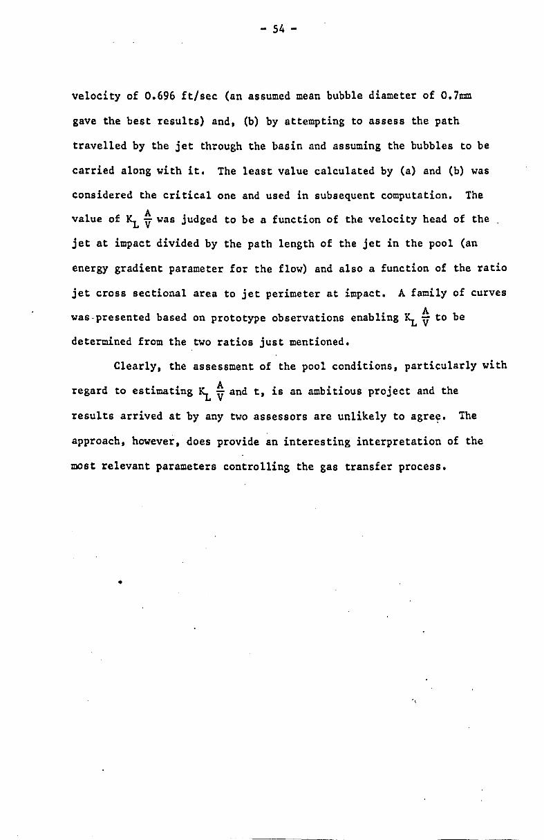
- 54 -

velocity of 0.696 ft/sec (an assumed mean bubble diameter of 0.7mm

gave the best results) and, (b) by attempting to assess the path

travelled by the jet through the basin and assuming the bubbles to be

carried along with it. The least value calculated by (a) and (b) was

considered the critical one and used in subsequent computation. The

value of ~ ~ was judged to be a function of the velocity head of the

jet at impact divided by the path length of the jet in the pool (an

energy gradient parameter for the flow) and also a function of the ratio

jet cross sectional area to jet perimeter at impact. A family of curves

was-presented based on prototype observations enabling ~ $ to be

determined from the two ratios just mentioned.

Clearly, the assessment of the pool conditions, particularly with

d •• 1<... Ad· b· • • d h regar to est1mat1ng _~ V an t, 1S an am 1t10US project an t e

results arrived at by any two assessors are unlikely to agree. The

approach, however, does provide an interesting interpretation of the

most relevant parameters controlling the gas transfer process •

•

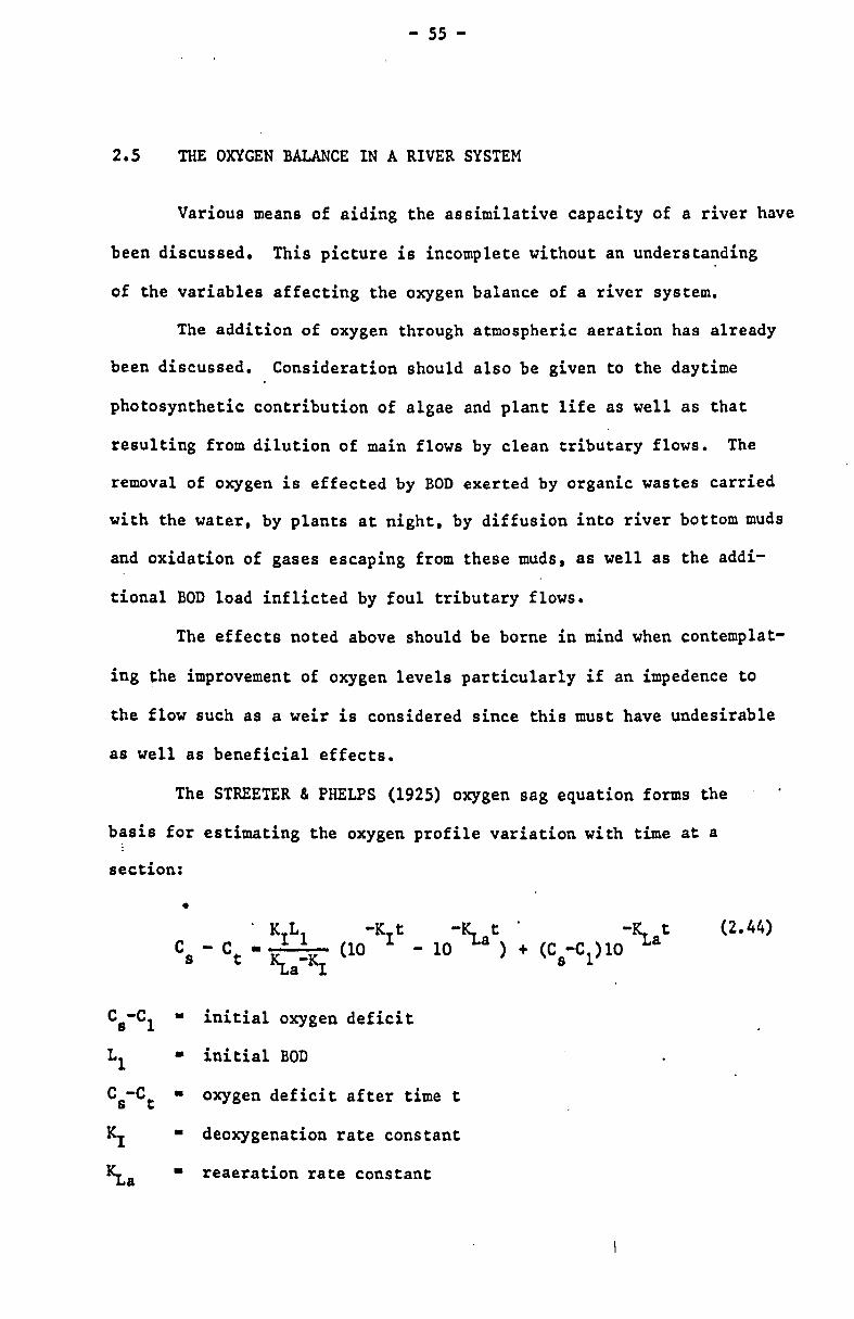
- 55 -

2.5 THE OXYGEN BALANCE IN A RIVER SYSTEM

Various means of aiding the assimilative capacity of a river have

been discussed. This picture is incomplete without an understa~ding

of the variables affecting the oxygen balance of a river system.

The addition of oxygen through atmospheric aeration has already

been discussed. Consideration should also be given to the daytime

photosynthetic contribution of algae and plant life as well as that

resulting from dilution of main flows by clean tributary flows. The

removal of oxygen is effected by BOD exerted by organic wastes carried

with the water, by plants at night, by diffusion into river bottom muds

and oxidation of gases escaping from these muds, as well as the addi-

tional BOD load inflicted by foul tributary flows.

The effects noted above should be borne in mind when contemplat-

ing ~he improvement of oxygen levels particularly if an impedence to

the flow such as a weir is considered since this must have undesirable

as well as beneficial effects.

The STREETER & PHELPS (1925) oxygen sag equation forms the

basis for estimating the oxygen profile variation with time at a

section:

•

Cs-Cl • initial oxygen deficit

Ll • initial BOD

Cs-Ct • oxygen deficit after time t

KI • deoxygenation rate constant

~ • reaeration rate constant -"La

(2.44)

- 56 -

The BOD change follows the relation

L • L lo-Kt t 1

(2.45)

The use of the STREETER-PHELPS equation will provide an over

simplified solution to the oxygen situation in a river. A complete

consideration of the effective factors noted above together with stream

characteristics poses a difficult problem and much work is still being

done using the basic oxygen sag equation (TEBBUTT, 1971) •

•

•

CHAPTER 3

THE HYDRAULIC JUMP - HYDRAULIC EQUATIONS

AND CHARACTERISTICS. AND AN INVESTIGATION

OF THE DOWNSTREAM VELOCITY COEFFICIENTS

----- ----~~

- 57 -

3.1 A DEFINITION OF THE HYDRAULIC JUMP

It is established in hydraulics that subcritical flow is produced

by a downstream control (e.g. weirs) and supercritical flow by an upstream

control (e.g. underflow sluice gate).

If two such controls are present in a channel, the one downstream

creating subcritical flow in the channel upstream of itself and the one

upstream creating supercritical flow downstream of itself, then, a con-

flict arises between the influence of the two controls. Such a conflict

can only be resolved by a transition from supercritical to subcritical

flow. This transition which is characterised by considerable turbulence,

air entrainment and loss of energy is the feature known as the hydraulic

jump.

The formation of an hydraulic ~ump is illustrated in Figure 3.la.

3.2 EQUATIONS DESCRIBING THE HYDRAULIC JUMP

The application to an hydraulic jump situation (illustrated in

Figure 3.1a)of the simplified equations of continuity,·momentum and

energy for an homogeneous liquid flowing through a horizontal. resistance-

free channel of rectangular cross section will lead to the following . . well-known equations of the hydraulic jump:

Y2 1 - • - (-1 + 11 + 8 Fr 2 ) Yl 2 1

(3.1)

where Fr1 is the Froude No. of the supercritical flow at the toe of the

jump:

(3.2)

energy tine --- ------- -------.... -,

sluice gate

-'--, .... .......

/1/ L 4 \\.....:.--".

sluice gate loss

............ en~rgy loss across "-, . ,

I .... JUIP "'-. i A ........

"'- ...- ------------------current meter

-.---. ~ )1 r=~

. n ............

Y2

downstream control

YO ------ ¥J ~ 1 t II -~~, " ,~-.--.-, 'r ' 'L.-'" ':j" < 'I' < , """

x ·1 L-Soo A

figure 3.10 the hydraulic juonp

, section A-A

f-' t-t-@ P @~., Q) ___ I I

I --: I l -~---~-- -t-- ----i- - ___ ,-_____ 1-_

@-:pl v3·trf€Oi·~-1-=i---~4"~

@ ~ 1-"3.t~AZi--- ----l. ®

I I ,'l..t I ...; ,,<, i I l t" (Ie < ( . i"'i"'l ,

figure 3.1b channel cross section - typical

. vetocity measuring grid

- 58 -

and Y1' Y2 are the conjugate depths of the hydraulic jump (suffices

1. 2 refer to the cross sections before and after the hydraulic jump).

V is the mean velocity (q/y). q is the specific discharge flowing.

The Energy Loss AE in the hydraulic jump is: .

2 2 v 1 v 2

AE - (y 1 + 2g ) - ~ 2 + 28) (3. 3)

or.

AE - (y - y ) + 1 2

substituting for q:

AE -

3.3 VELOCITY COEFFICIENTS

2 2 2 92 ~ (y 2 - y 1)

2g y 1 Y 2

3.3.1 Velocity Coefficients Defined

(3.4)

(3.5)

In all the above equations it has been assumed that the mean

velocity head across a section. (v2/2g) • is equal to v2/2g where v is m m m

the mean velocity across the section.

This can never be true because viscous drag reduces velocities •

at boundaries below those in the main fluid body.

The true mean velocity head is thus obtained by multiplication i

by a correction factor.

: The mean velocity head, or kinetic energy per unit weight of

fluid is equal to:

v m

2

.-2g

where A is the cross sectional area of flow. e

(3.6)

- 59 -

The correction coefficient a is sometimes known as the Corlolis

Coefficient. a is a correction coefficient to be applied to the velocity

head as calculated from the mean velocity i.e.:

/v3.dA a • ~3---

v .A m c

(3.7)

Similarly, a correction coefficient, the Boussinesq coefficient a ,is B

employed to correct the momentum term which has been computed using

the mean velocity, v , thus: m

(3.8)

The coefficients a and ~are never less than unity and are bpth equal

to unity when the flow is uniform across the cross section. The further

the flow departs from being uniform, the greater become the coefficients

a and aBo It follows from Equations 3.7 and 3.8 that a is more sensi

tive to velocity variations and thus, for a given channel section,

3.3.2 Reasons for Attempting to Measure a

~t was suggested by APTED that the assumption a - aB • 1 was

inv~lid for the hydraulic jump he studied. APTED came to t9is conclu

sioq because he found that the energy loss as given by Equation 3.3 did

not agree with that calculated from Equation 3.5. These equations are

of course the same assuming that a • aB • 1. Following from APTED's

supposition. one of the first objectives of this research was to attempt

to quantify the magnitude of the velocity coefficients. APTED calcula

ted aB to be as high as 3.01 at his downstream conjugate depth section.

- 60 -

3.3.3 The Computation of a

To calculate a from Equation 3.7 it is necessary to obtain a grid

of velocity measurements over the whole cross section under considera-

tion.

For simplicity of illustration, consider a cross section of flow,

depicted in Figure 3.1b, divided into n segments of flow each of equal

area dA by a system of grid lines as shown. Velocity measurements are

taken at all the intersection points of the grid lines.

Considering the typical segmental area of flow dA in Figure J.lb,

the mean velocity of flow of the segment is approximately:

(3.9)

Thus, considering all segmental areas constituting the whole area

(3.10)

Also,

(3.11) •

The Coriolis coefficient may be estimated: Ii

n I (v 3.dA)

n a· --3~--v .A m c

(3.12)

where vm - Q/Ac - q/Y2' Q is the recorded discharge and Q' is the

discharge as calculated from the velocity traverse. Obviously, the

more concentrated the grid pattern, the more accurate will be the

estimate of a and Q' •

- 61 -

3.4 EXPERIMENTAL APPARATUS

3.4.1 The Flume and Water Supply System

The hydraulic jump studied was formed downstream of a variable

opening underflow sluice gate in a glass walled flume, 3 metre long by

lOcm wide.

The water is supplied under constant head from the header tank

of the laboratory's re-circulating water system. Water is contained

in a 22,000 gallon capacity sump from which it is pumped to the header

tank. This header tank supplies all hydraulic apparatus in the labora

tory, the available head being approximately 11 metres. After passing

through the flume, the water is returned to the sump.

The flume and water circulating system are illustrated in

Figure 4.1 and Plate 4.1.

The measurement of flow through the flume was effected by an

orifice plate connected to a differential mercury manometer and

calibrated to British Standard.

The flume is fitted with a downstream control with which the

depth of flow may be regulated. The slope of the channel may be varied,

but, for all hydraulic jump experiments the flume was maintained in a

horizont~l position.

Depth measurements were obtained by means of point gauges

mounted on carriages which could be moved along the length of the flume

on rails.

3.4.2 The Measurement of Velocity

Some difficulty was experienced in finding a suitable means of

accurately measuring velocities.

- 62 -

(a) Pitot - Static Tube

In view of the anticipated fluctuating nature of velocities at a

point, the pitot-Static tube was first tested as it was thought that

the velocity oscillations might be effectively damped in the manometer

tubes, thus providing an easily read mean velocity at that point.

After numerous tests, the use of the Pitot-Static tube was

abandoned and an alternative method sought.

The first objection to the use of the pitot-Static tube was its

interference with the flow. This highlighted one of the disadvantages

of working in such a small flume, the obstruction to flow offered by

the tube being quite significant relative to the actual cross section

of flow. As the pitot-static tube was lowered deeper into the flow, the

hydraulic jump was visibly observed to advance towards the sluice gate.

An interference of this scale was unacceptable. Secondly, measurements

collected and computed, revealed values of the Corioli~ Coefficient less

than unity, an impossible result. It was established that the pitot

Static tube was sensitive to boundary conditions and that the calibration

could only be applied with confidence when the tube was positioned

in the centre of the flow section and thus free from boundary effects.

(b) }liniature Current meter - Wallingford

The miniature Wallingford current meter with a 3mm diafeter

propeller proved to be the solution required. It provided accurate

measurement and retained its calibration near boundaries. By virtue of

its small size, it was therefore possible to take measurements within

2mm of the boundary walls and the channel bed, and, no interference with

the flow was observed.

The rotation of the meter's propeller was recorded by a counter, I

and, by measuring the number of rotations over a known period of time,

- 63 -

the mean number of cycles per second recorded at the particular point of

measurement could then be translated to the mean velocity via the

calibration curve. The meter was calibrated in a towing tank 30 metres

in length.

One of the main difficulties encountered with this current meter

was the meter's inability to differentiate between forward and reverse

velocities. Consequently, if the ~urrent meter is placed in a region

of reversible flow, such as occurs in the roller region of the hydraulic

jump, then, the forward and reverse velocities will be added positively

reSUlting in an over-estimate of the velocity at that point. It was'

necessary, therefore, to ensure that there were no flow reversals in any

selected measuring section. It was thus not possible to take measure-

menta too close to the roller region of ,the jump.

3.5 EXPERIMENTAL TECHNIQUE

The discharge through the flume was kept constant at 3.45 lIs (as

recorded by the orifice plate).

For various openings of the sluice gate, an hydraulic jump was

formed just downstream of the sluice gate by suitable adjustment of

the gate regulating the tail-water depth • •

Depths at the toe of the jump and downstream of the roller were

recorded.

Three cross sections were arbitrarily selected (in two cases,

only two were studied), the sections all being downstream o~ the roller

of the hydraulic jump. The location of the chosen section was recorded

as the horizontal distance x measured from the toe of the jump. (See

Figure 3.1a.)

The measurement of velocities was carried out on a 2cm square

grid except at the boundaries where measurements were taken within lOmm

- 64 -

and 2mm of the boundary. At each measuring point, the rotation of the

• current meter propeller was measured over 50 seconds.

3.6 RESULTS

The results collected have been summarised in Table 3.1. The

velocity measurements collected were read into a computer progr~m, and,

as a check on the accuracy of the qata, the discharge was computed

(Equation 3.11) and compared with the discharge recorded by the orifice-

plate meter. The latter discharge Q was a constant 3.45 lIs and the

computed discharges Q' tabulated in Table 3.1 are also plotted in

Figure 3.2 against the ratio x/Y2. The bulk of the data indicate that

the calculated discharges lie within! 1% of the recorded discharge,

but, deviations of up to -2% are exhibited by five other points with

four further points deviating by 3% and slightly more. It must be

concluded that the agreement between recorded and measured flow rate

is very good and therefore the velocity measurements were confidently

applied for further computation.

The mean velocity distributions across the width of the channel

are presented in Figure 3.3. The distributions displayed are fairly

typical for turbulent flow, and, as would be expected, the flow is not •

uniform within the range of these tests. Flow is said to be uniform

if the velocity profile does not change in the direction of motion

(HENDERSON). The limit between non uniform and uniform flow,downstream

of a jump was shown by LEUTHEUSSER and KARTHA (1972) to be p~actically

independent of upstream Froude number (for Frl

> 4) and, for an

hydraulic jump formed close to the sluice gate they showed the inflow

to the hydraulic jump to be undeveloped, i.e. the boundary layer is

still predominant. The experiments reported here were probably conducted

.{

3.50

t 3.48 3.1.5 + 1% --------- -------------- -- ----- ---------- ---------------------

V

-U)

" 3.46 --11I 3.41. Ol

V 01l§ t::l

t'ill-® 0/ Q

A ~:------- ® 3.45 A

L-

a ..c. 3.42 3.1.5 -1% u (/)

-------------------- ---- ------ ------- ----------- ----- - ---o =-0 3.1.0

-g 3.38 El ~ ~ 3.45 - 2%

------------------------------------------ ----"<9------ --------a ~ 3.36 lJ -B 3.34

6. 3.45-3% ---------------------------------------------------------------------

o 3.32

4 5 6 7 8 9 10 11

--x/Y2 •

figure 3.2 discharge calculated fro~ velocity measurements

(manometer discharge = 3.45 lIs)

RUN No. G 1

x 2

A 3

c.4

® 5

v·6

~ 7

?8 l

12

I.P.

"E .g

" I...l v CI >

I I

I RJN 1

50 F'1 = 6.5

l x/Y2 I " 5.70

"0 I 111 0.08 . f IA 9.67

301 J ...... tT----~-""~ L .,- .. ----~I._ /0 --, I ./ -"f

20 ~/. I ••• ~ ]

a 2

l.O .... 5.69 • 9.05

1

- <9 5./.8

I. 6

RUN 5

I 30 b-'''/tc-:==.· ..

8

20\ ~'~--1--_' o 8 2 4 6

10

I I J

10

llgure 3.3

RUN 2 F'1 = 2.6

~-- '~

~

xlY2

• 5.02 I( 6.42 J. 8.l.5

RUN 3 F, = 5.2

RUN I. ~~ - 3.9 I r, _

150

1.0 ~~-""--' ...... I '.

. O~ ..... "&

'. -'. xlY2

8 1..22 I.. 7.17

• ~~-~.-t•• - r~.: ...... ~ , .... ~ ...... ,-

.,. .-- --- ..... &7"'- "". . , .... ,~ . . ~.' '"

I t(·· .. - ~ ......... :' ... ' J30 - . '.. .J xlY2 .....

o 5.20 . ',] f • 7.06 1

20

o 2

x/Y2 e 5.61 6 6.0 I\: 7.71.

L 6

R!;~l t .- r .. :" 6.:i

I

• J- --.-

8 10

I Y

__ -t~:=:-:-i==:::-~ ." ..... c -:a..

-~

o 2 4 6 8 10

o 2

x/Y2

a 5.26 A 6.81

4 6

RUN 7 Fr1 = 1..8

o 10

/-:~I~ t- ".6 '" . .

.. ,-_. ' ....... ~ ...... #' .....

e~

o 2 4 6 8 10

------ distance from channel walt (em) ..

" 9.13

I' S 10 024

RUN 8 Fr1 = 3.1

50

~:~ J40 ",,;,~-;~----"---- '~{.~:-~-." ]'

x/yo EO .... .:~.

2 " . "":1 30

It ~ ~~~ '\ 1 J( 9.1.2 ,

20 ~ ____ L-__ ~ ____ ~ ___ ~ ___ ~

o 2 L 6 8 10

MEAN VELOCITY D!STRI BUT IONS DOWNSTREAM OF AN HYDRAULIC JUMP

Q = 3.1.5 lis

- 65 -

TABLE 3.1

Calculated Values of Corio1is Coefficient

RUN Q x Q' x Q' x Q' (LiS) - a

(LIS) - a (LIS) - a (LIS) NO. 12 12 Y2 J

I ,

I

1 I 3.45, 5.70 1.15 3.33 8.08 1.03 3.41 9.87 1.02 3.38

2 3.45 4.22 1.24 3.32 7.17 1.03 3.45 - - -I I

I 3 3.45 5.02 1.16 3.36 6.42 1.06 3.44 8.46 1.04 3.44

I 4 3.45 I 5.20 1.20 3.39 7.06 1.05 I 3.47 9.13 1.02 3.46 I

5 3.45 : 5.48 1.05 3.45 6.69 1.02 \ 3.47 9.05 1.02 3.45 i I

6 3.45 I 5.61 1.06 3.47 6.43 1.04 . 3.48 7.74 1.03 3.46

7 3.45 5.26 1.13 3.45 6.81 1.04 3.47 - - -8 3.45 4.77 1.21 3.32 7.53 1.03 3.39 9.42 1.02 3.39

• I.

- 66 -

for a condition of undeveloped inflow and for this condition LEUTllliUSSER

and KARTHA showed that the flow becomes uniform at a distance down-

stream of the toe of the jump given by x/Y2 ~ 12. The non-uniformity

of flow displayed by Figure 3.3 is consistent with this, and, velocity

coefficients greater than unity are anticipated. A skewed velocity

distribution is present in a number of cases, but as one travels

downstream of the jump the influence of the channel begins to predominate

over the influence of the jump and the distribution tends to a symmetri-

cal one. The reason for the skew is not clear, but, it can probably be

attributed to a variation in the sluice gate opening with width due to

imperfections in construction.

It is worth recording here that one run was repeated with an

obstruction placed in the water downstream of the measuring section.

This was done to investigate the effects on the characteristics of the

jump due to the presence of a dissolved oxygen measuring electrode in

the flow downstream of the jump. An electrode was inserted, the back

ing up of flow resulting was compensated for by opening the tailwater

control gate until the jump returned to the position it occupied prior

to insertion of the electrode. A complete velocity traverse was con

ducted and to conclude. no significant variation in the velocity •

distribution due to the obstruction was observed.

The values of Corio lis coefficient computed for these experiments

by means of Equation 3.12 are tabulated in Table 3.1 and p10~ted

against the ratio x/Y2 in Figure 3.4. Extrapolation of the results

shows that the flow becomes uniform (i.e. a - 1) for x/Y2 = 12 which is

in agreement with the limit shown by the experiments of LEUTHEUSSER

and KARTHA (discussed above).

1.36 RUN "No. i 1.32 (;) 1

1.28 length of roller length of jump x 2

\ A 3 = 6Y2 (LEUTHEUSSER (, a 4 C 1.24 ~ (PETERKA) KARTHA • 1972 ) ® 5 OJ -

\ / ~ v 6

~ 1.20 ~ 7 -..-(]J ¢ 8 8 1.16 II

0 •

~ 1.12 L ~ • . •

0 -L-

8 1.08 A

1.0L.r ~ a "if r&'l - J( -9'7-0 ':'" A

® ~-¢ 1.00

4 5 6 7 8 9 10 11 12 . xlY2 •

!igure 3.4 variation in the Coriol is coefficient with distance downstream of an hyd rau lie ju mp

- 67 -

The transition point indicated on Figure 3.4 is consistent with

the end of the roller of the hydraulic jump defined by PETERKA (1963),

Lj ~ 6Y2 •. It would appear from these measurements that the Coriolis

coefficient for the downstream conjugate depth section is unlikely to

exceed 1.05, and, further, this value of a is considerably smaller

than the value anticipated by APTED to explain his discrepancy between

measured and calculated energy losses.

As confirmation of the above results, the classic air model

results of ROUSE, SIAIO & NAGARATNAM (1959) are cited. These revealed

that at the end of the hydraulic jump transition, a was within 5% of

unity in every case, i.e. a ~ 1.05; the agreement is remarkable. I

Although the tests reported above were not conducted i~ the same

apparatus as those of APTED, the results obtained here do not support

APTED's supposition regarding his discrepancies, and the reasons for

these will be sought elsewhere and discussed in Section 3.7 •

•

- 68 -

3.7 AN EXPLANATION OF THE DISCREPANCIES REPORTED BY APTED

The data supplied by APTED have been reproduced in Table 3.2.

Also presented in columns 8 and 9 of this Table are the energy losses

in the jump as computed from Equations 3.3 and 3.5 respectively.

Comparison of columns 8 and 9 reveal the discrepancy noted by

APTED and it can be seen to be very significant. It appears that~E

computed from Equation 3.3 is consistently higher than that calculated

from Equation 3.5. APTED attributed this to the geometry of his flume

and an incorrect assumption of velocity coefficients equal to unity.

Whilst measurements in Section 3.6 do not support this view, it should

be remembered that these were conducted in a different flume. However,

close examination of Table 3.2 reveals an impossible situation described

by columns 5 and 6. It would appear that a large proportion o~ APTED's

data suggest an increase in the specific energy function across the

sluice gate; this is clearly ridiculous and can only be attributed to

inaccuracies in the measurement of the depth of super-critical flow

below the sluice gate. The larger depths above the sluice gate and

downstream of the hydraulic jump are less sensitive to inaccuracies in

the depth measurement since the velocity hend term in the energy func

tion i~ relatively small compared to the static head. For the super

critical flow region, even very slight errors in the depth measurement

are reflected in very significant changes in the calculated velocity

head, which, for this flow regime. constitutes the largest portion

of the energy function. To illustrate the extent of the errors

in Yl' the ratio Y2{YI has been plotted in Figure 3.5 against the

Froude number of the supercritica1 flow. For comparison. the law of

Belanger, Equation 3.1. relating the conjugate depths, is also shown.

Yo (em)

42.48

38.68

38.60

35.56

35.32

35.29

35.02

33.73

32.00

30.93

28.65

27.14

25.47

24.59"

24.04

23.96

22.14

20.19

17.40

17.90

15.82

15.54

1

- 69 -

TABLE 3.2

APTED's Hydraulic Jump Data and Calculated

Energy Losses

I El Yl Y2 Q E E2 E1-E2 a (em) (em) (l/s) (em) , (em) (em) (em)

I

I

1.43 12.8 4.16 42.53 I 44.53 13.34 31.19

1.41 11.9 3.94 38.73 41.21 12.46 28.75

1.42 12.1 3.95 38.65 40.86 12.64 28.22

1.51 12.0 4.08 35.63 38.72 12.59 26.13

1.53 12.1 3.97 35.38 35.85 12.65 23.20

1.54 11.5 4.06 35.36 36.96 12.13 24.83

1.52 12.1 4.01 35.09 36.99 12.66 24.33 ,

1.50 11.3 3.90 33.80 135.95 11.91 24.04

1.58 12.0 4.04 32.08 I 34.90 12.58 I 22.32

1.61 11.5 3.98 31.01 32.76 12.11 20.65 , I

1.70 11.2 4.01 28.75 30.06 11.85 118.21 I

111.67115.30 1.80 11.0 4.00 27.25 26.97

1.85 10.8 4.00 25.59 25.68 11.5 ;14.18

1.90 10.8 4.00 24.72 24.49 11.5 112.99

11.32 ! 11.87 1.96 10.6 4.00 24.18 23.19

2.00 10.6 4.04 24.10 22.79 11.34 11.45

2.17 10.3 4.01 22.31 19.57 11.07 8.50

2.19 10.0 4.00 20.39 19.19 10.81 8.38

2.50 9.5 4.06 17.68 I

15.94 10.43 . 5.51

2.39 9.6 4.01 18.15 16.74 10.49 6.25

2.55 8.9 4.00 16.14 15.09 9.93 5.16

2.65 8.6 4.01 15.88 14.32 9.71 4.61

2 3 4 5 6 7 8

(Y2-Yl) 3

4 Y2Y1

20.07

17.20

17.72

15.93

25.95

13.95

116

•10

1 13 •88 I I 114.92 I I I 113.06 I

111.26

9.83

8.97

8.69 I I

7.76

7.50

6.01

5.44

3.61

4.08

2.82

2.31

9

..-~

...... N ~

0 .--C &.0

.c -a. (II

"0

41 ..... a .~ .. c:: 0 u

10r-----r---~~--~----~----~-----,___---·r---~

9 0

~

8 , BELANGER Equation -

,...,~

[ Equation 3.1 ] ~ e l( a 7 Q

)( Ao 6

/~ . 0 Q

0

5 Ite ~ 4 0

/~0 ~ G>

G> 3

2

1

1 2 3 t. 5 6 7 8 upstream Froud~ number Fr1

<:) APTED (1975) - Table 3.2 A HOLLER (1971) - Table I..t. x. these studies - Table 3.3 - Y1 measured in the centre

of the channel.

¢ these studies - Y1 = mean depth lI,easured across channel wi dth •

.!i.gure 3.~ - recorded deviations from the hydraulic jump conjugatc! df!pth

equation of BELANGER.

•

- 70 -

Deviations from the B~langer law have been shown to occur by

LEUTHEUSSER & KARTHA (1972) but these have been for a situation where

the inflow into the hydraulic jump is fully developed. For the inflow

to fully develop, the hydraulic jump must be formed a long way downstream

from the sluice gate. LEUTHEUSSER & KARTHA referred to a previous

finding by KARTHA (1968) indicating that the distance required for

inflow ,to fully develop must be greater than or equal to two hundred times

(200 x) the sluice gate opening.

The experiments of this research and those of APTED were conducted

for conditions of undeveloped inflow and for such a condition,

LEUTHEUSSER & KARTHA concluded from their results that the ratio of

conjugate depths is essentially that given by the Belanger equation,

Equation 3.1. RESCH & LEUTHEUSSER (1971) showed this was so since for

this inflow condition the energy of turbulence upstream of the jump was

negligible. ,

The deviations from the Belanger law exhibited by APTED's data in

Figure 3.5 are significant particularly as the range of Froude nUmber

tested was relatively small.

Also plotted in Figure 3.5 are some data supplied by HOLLER

which display similar inaccuracies in the depth measurements • •

As a matter of interest, the data discussed in Section 3.6 was

treated in the same way as APTED's data resulting in Table 3.3.

Curiously, exactly the same observations can be made with regard to this

data except to a lesser degree. An increase in specific energy across

the sluice gate was similarly implied and discrepancies were revealed

between the calculated and measured energy losses. There is a deviation

of the conjugate depth ratio from the law of Belanger (Figure 3.5), but

to a much lesser degree than suggested by the data of APTED and HOLLER.

- 71 -

TABLE 3.3

Hydraulic Jump - Depths and Calculated

Energy Levels

3 RUN Yo Y1 Y2 Eo E1 E2 E1-E2 (Y2-Y1) NO. (em) (em) (em) (em), (em) (em) (em) 4Y2Y1

1 30.75 1.39 11.7S 1 30•81 32.79 12.19 20.60 17.02

2 11.94 2.54 8.30 12.36 11.94 9.18 I

I 2.76 2.26

3 23.70 1.63 10.75 23.81 24.46 I 11.27 \13.19 10.82

4 16.94 1,99 9.42 17.15 17.31 10.10 7.21 5.47 I

5 25.44 1.53 11.05 25.53 27.44 11.55 15.89 12.76

6 28.53 1.44 11.50 28.60 30.69 11.96 18.73 15.37

7 21.87 1. 74 10.65 22.00 21.78 11.18 10.60 9.54

8 14.0 2.33 8.70 14.31 13.50 9.50 4.00 3.19

•

• •

- 72 -

The belief that these deviations were entirely due to slight

errors in Yl is reinforced by the excellent agreement obtained (Section

3.6) between recorded discharges and the discharge calculated from

velocity measurements and the measured downstream depth Y2. If signifi

cant errors arose in measuring Y2' then these would have been reflected

in the calculated discharges.

, Great care was taken in the measurement of depth, but, it must

be admitted that the design of the point-gauges precluded any depth

measurement other, than in the middle of the channel. A special carriage

was therefore constructed which enabled the point-gauge to be traversed

across the width of the channel as well as along the length of it.

The measurements of Yl subsequently collected across the channel

width, revealed a concave water surface such that the depths near the

boundaries were anything up to 25% higher than the minimum depth which

generally occurred in the centre of the channel. For five different

Froude numbers, the mean supercritica1 depth across the channel width

Y1 was measured along with the corresponding downstream depth Y2. The

results, plotted in Figure 3.5, display almost total agreement with the

law of Belanger. This is consistent with the conclusions of LEUTHEUSSER

and KARTHA • •

It would seem reasonable to suggest that Y1 in APrED's experi

ments was similarly underestimated, thus explaining the discrepancies

he observed.

It is interesting to record here that MOORE (1941) similarly

noted the sensitivity of the specific energy of the supercritica1 flow

at the base of a free overfa11 to small changes in the 8upercritical

depth, and MOORE referred to errors exceeding 25%.

- 73 -

3.8 SUMMARY

An investigation of the velocity coefficients in the flow down

stream of an hydraulic jump did not reveal any significant departure

of the coefficients from unity. This was shown to be consistent with

the findings of ROUSE, SIAIO & NAGARATNAM.

Subsequent tests showed that the conjugate depth ratio was

closely described by the law of Belanger, and that departures from this

law observed by APTED, HOLLER, and also by the author of this thesis in

earlier tests, were entirely due to inaccurately measured depths in the

supercritical region downstream of the sluice gate and just prior to

formation of an hydraulic jump. The validity of the law of Belanger

was also demonstrated by LEUTHEUSSER and KARTHA for an hydraulic jump

formed just downstream of a sluice gate •

•

, t

•

•

. . CHAPTER 4

AN ELUCIDATION OF THE FACTORS CONTROLLING'

THE OXYGEN TRANSFER IN AN HYDRAULIC

JUMP

- 74 -

4.1 OBJECTIVES

(a) In view of the inaccuracies in APIED's hydraulic measure-

ments, identified in Chapter 3. it has been considered expedient to

repeat all his tests and

(b) to expand on the work begun by APTED by investigating as

wide a range of discharges as possible,

(c) to achieve a generally applicable correlation between

oxygen transfer and hydraulic characteristics of the hydraulic jump.

4.2 A DESCRIPTION OF THE APPARATUS

4.2.1 The Flume and Water Supply System

This has already been described in Section 3.4.1. However, in

addition to the water supply from the main laboratory header tank used

in the experiments conducted in Chapter 3, an additional supply line was

installed to provide deoxygenated water from the mixing tank on the

floor above. the deoxygenation of the water is explained in detail in

Appendix B and a schematic layout of the experimental system is detailed

in Figure 4.1.

the availability of two water supply lines proved useful in •

providing ~igher discharges than were possible from the mixing tank

alone. This was effected by mixing deoxygenated water with oxygena~ed

water from the main laboratory header tank.

The operational flume is shown in Plate 4.1.

4.2.2 Hydraulic Measurements

Discharge measurement was effected by a differential water

manometer connected to an orifice plate meter in the deoxygenated water

supply line~ The main water supply from the laboratory header tank was

._n_~

~--.----__ ~_ =_~L----'----------------------------~, " ' !cbcrctory hl?od~r tank

.....

flow inducer ~

E I dosing -1i1 ltll I . ..,.;=sa t ~ i.

soluti on [!~ _~ xing ~~. _ _ GROUN 0 .--.-1..... <, <" , < < , ~ , < \ < ,-I -",\.c-;.~~ " < 'IIt----r.~~

FLOOH J «<''\~

supply to free overta!l:1 (fig. 6.2) r

orifice plate 1--------1.----, - ,/' ~ tappings to mercury '- - - • tappings to water -----. manometer ~ manometer

dissdved a<ygen

depth point gluge .... sluice gate ____ ............. : -... .

~ .... -

.... ,-\

\

'~ ttow disperser

3 m~tre

re-circulating plimp

flume

outlet control-.. -

overflow. to

sump

./-+---

., ....... , , I-y" L._---'

I \'

I ~-, I BASEMENT l

--I-~~~--ot"'-1- ----.. --.. --------------- ---- ---- ---- -- - "',--- ~

------~-

covered laboratory sump

-If , ( ( ( \ < , ( \; < c ( C

* signifies a flow 'control valve

figure 4.1 LABOHATOHY CIHCUIT - HYDHf\ULIC JUr-lP EXPERIMENTS

- 75 -

similarly fitted with an orifice plate meter but connected to a mercury

manometer.

Depth measurements upstream of the hydraulic jump were effected

by a point gauge mounted on a carriage which enabled the gauge to be

traversed both longitudinally and laterally across the channel. The

fluctuating water surface downstream of the jump made accurate point

gauge depth measurement difficult. During these tests~ the oscillations

were damped and the depth measured by connecting single limb manometers

of internal diameter IOmm to several tappings in the bed of the channel.

These manometers were calibrated against the point gauges for water

flowing freely in the channel for various depths.

4.2.3 Measurement of Oxygen Levels

The equipment used to monitor dissolved oxygen levels has been

. " fully described and tested in Appendix A. The electrodes were immersed

in the flow immediately upstream of the sluice gate and in the flow

downstream of the hydraulic jump. In all tests the hydraulic jump was

formed immediately downstream of the sluice gate by suitable adjustment

of the tailwater depth. It was established in Section 3.6 that the

presence of the electrode in the tailwater did not alter the velocity •

distribution in the flow upstream of the electrode.

4.3 THE QUALITY OF THE LABORATORY WATER

The water of the hydraulics laboratory re-circulatory system is

treated with quantities of Sodium Nitrite NaN03

to prevent the corro

sion of pipes and other equipment in contact with this water.

For the experiments of JARVIS & APIED the concentration of sodium

nitrite in the laboratory water is likely to have been maintained at

- 76 -

approximately 0.6%. Similarly for earlier experiments carried out by

the author of this thesis.

During the course of experimental work the concentration of sodium

nitrite was reduced to a more economic level of 0.3% and this presented

an ideal opportunity to investigate the effects of sodium nitrite on

aeration characteristics (Section 4.7 and 7.2). Neither JARVIS nor

APTED suspected any effects due to the presence of this salt.

The properties of corrosion inhibition displayed by the nitrite

ion NO; are discussed by WEST (1970) and will be reviewed here.

The nitrite ion acts as a powerful oxidising agent of ferrous ions and

this oxidation gives rise to a stable protective film which inhibits

further dissolution. It is classed as an anodic inhibitor since the

passivating oxide film is formed primarily at those parts of the metal

surface where metal cations are formed, i.e. at the anodes. This type

of inhibitor is positively dangerous if used in insufficient quantities

as it can then enhance the rate of corrosion. WEST mentions concentra-

tions of nitrite ion of less than 0.05 Molar as deficient.

4.4 AN APPRAISAL OF THE PARAMETERS CONTROLLING THE GAS TRANSFER

IN AN HYDRAULIC JUMP

• Reference is made to the equation of gas transfer, Equation 1.36.

Three controlling factors are apparent for constant temperature and

water quality, the liquid film coefficient, the contact time and the

ratio air/water interfacial area to volume.

From Equation 2.1:

(4.1)

- 77 -

the mean bubble diameter db is re,lative1y constant (HAINDL)

• •• (4.2)

Kt is assumed to be a function of the energy loss ~E which from

Equation 3.5 can be re-expressed:

• • •

(4.3)

(4.4)

An estimate can be made of the contact time, t. An approximate model

of the variation in mean velocity through the hydraulic jump is shown

in Figure 4.2. Lr represents the length of the roller zone of the

hydraulic jump whilst L. represents the length of the aerated zone which J

will extend beyond the roller zone. It is shown in Section 5.3.2 that

L - k y , r r 2 (4.5)

where k and k. are relatively constant irrespective of Froude number. r. J

The time of contact will be given by:

•

+ L.-L

J r v2

2L LJ• - Lr __________ ~r~_______ + ____ ~_~~~ __ __

!cl (-1 + {1+8Fr1

2 ) Y1

(4.6)

(4.7)

roller

L~I-<------- J

1---" ------ Lr .. d

. . .1...· , • • I • • I.

aerated zone downstream of roller

zone :: : : • .. 1* : -. ~... ; .-;-•• • • I. • ... I

. __ =:====:=~ _____ ~::::::::~2~:::i~:...;i~i-:"'i-'::'"!~~ - ••••• • • •• ... I .,-- •••• * •••• • • I· I 2 I ... I I

jL -.- ; ! i ! A " A Sf :, J( )( x x : I ~ x it .1 a K ' I ~ le, X X X )1(-

..

V1

profile

~ - c c c { V2 ~--JC ~

figure 4.2 an approximate velocity profile through the hyd raulic JU m p

- 78 -

• (4.8)

c. (k.-k ) (-1 + Il+8Fr12 j + J r (4.9)

4(-1 + 11+8Fr 2 ) 1

• IYi" Frlli

k (-1 + {1+8Fr12 ) r '+

1 + 2(-1 + Il+8Fr12)

(k.-k )(-1 + {1+8Fr12 )j J r (4.10)

4 (-1 + 11 + 8Fr 1 2 :

(4.11)

For constant Froude number, the time of contact varies as the

squar~ root of the scale. It is clear from Equations 4.2, 4.4 and 4.11

that

(4.12)

i.e. for a constant Froude number, an increase in discharge which

results in an increase in energy loss and time of contact will there-

fore result in an increase in the oxygen transfer according to some

• • functlon of the length scale Yl'

4.5 ADJUSTMENT FOR TEMPERATURE VARIATIONS

The influence of temperature on oxygen transfer in water was

discussed in Section 1.10 and the influence of the degree of mixing was

illustrated in Figure 1.6. The experiments of GAMESON, VANDYKE and

OGDEN at an experimental weir clearly indicated an increase in the

deficit ratio with increase in temperature whereas IMHOFF & ALBRECHT

- 79 -

suggested, for a prototype weir they studied, that the deficit ratio

was independent of temperature. If this latter observation was in fact

true. then it would jeopardise the validity of modelling an oxygen

transfer situation since the modes of transfer would be different in

both situations. In the model the diffusion transfer processes are

apparent. whereas in the prototype the effect of these is suggested by

IMHOFF & ALBRECHT to be absent.

The inconsistency between the results of GAMESON, VANDYKE.

OGDEN and IMHOFF & ALBRECHT is highlighted if the energy expended in

the former's experiments is compared with that cited by IMHOFF &

ALBRECHT for their prototype weir; (see Table 4.1 below).

TABLE 4.1

Energy Expenditure at Two Weir Systems

POOL DIMENSIONS (m) HEIGHT OF ENERGY SOURCE EXPEND3TURE

Length Width Depth FALL (m) watt/m

GAMESON. VANDYKE 0.3 0.3' 0.089 3.28 7316 & OGDEN (1958) . 1.49 3323

0.61 1360

IMHOFF, ALBRECHT Spillenburg weir (Ruhr River) 1200 • (1972)

The energy available was computed from the expression: (MKS units)

p Q g h 1000 Kw

and the energy expenditure (watt/m3) quoted by IMHOFF/ALBRECHT was

(4.13)

assumed to refer 'to the energy being expended per unit volume of the

stilling pool.

- 80 -

Clearly, the energy expended in the model stilling pool exceeds

that quoted by IMHOFF/ALBRECHT for their prototype. Therefore if the

latter's observations were correct, then the oxygen transfer dependence

on temperature in the model should have been described by curve' C in

Figure 1.6.

The model tests were carefully controlled, whilst during the

measurements of IMHOFF & ALBRECHT the discharge varied between 12 and

28 m3/s (ALBRECHT, 1968) and therefore the height of fall also varied.

The measurements of IMHOFF/ALBRECHT have been recalculated in terms of

deficit ratio and plotted in Figure 4.3 along with the model tests of

GAMESON & co-workers for three heights of fall and a cons tan; discharge.

The scatter displayed by the data of IMHOFF/ALBRECHT is remarkable and

not surprising in view of the discharge range of their tests, The

original presentation of results by IMHOFF & ALBRECHT has been repro

duced in Figure 4.4 along with the data of GAMESON & co-workers for

one height of fall (1.49m). The oxygen transfer as a percentage of the

initial oxygen level is plotted against the initial oxygen level as a

percentage of saturation. Temperature has been marked alongside each

point. It is easy to see how IMHOFF & ALBRECHT came to their conclusion

from this plot and also to see that for the same temperature range

(13-260 )-a similar conclusion might have been drawn from the data of

GAMESON, VANDYKE and OGDEN.

It is felt therefore, that IMHOFF & ALBRECHT's recommendation on

. the influence of temperature in highly turbulent systems (> 20 watt/m3)

is not substantiated and that the measure of oxygen transfer used to

present their data was particularly insensitive to changes in oxygen

transfer especially when small initial oxygen deficits existed.

Successful modelling of oxygen transfer systems is anticipated

and the temperature correction of GAMESON, VANDYKE & OGDEN will apply

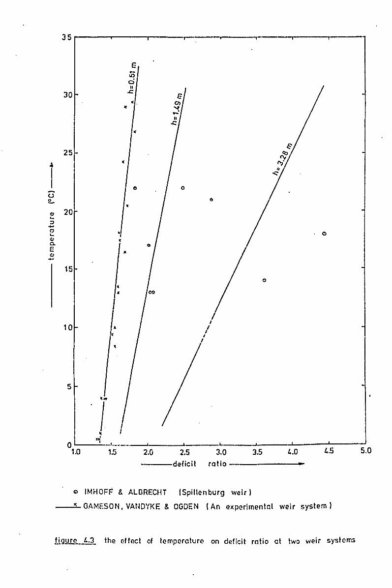
1 -u 0 ~ ...

QJ '-:l -C '-QJ a. E (!J -

35------~------r-----~-

E .-U)

ci " 30 .c I(

Jf

25 I(

0 0

II

20

• II

I(

15

" I(

10 .. I(

5 It .... .

I It .

0 ~ _1 ___ -

1.0 1.5 2.0 2.5 daficit

I

/ I

I

L

3.0

ratio

Q IMHOFF & ALDRECHT (Spillenburg weir)

1-

3.5 i..0 4.5

_......;:1C:.,. GAMESON, VANDYKE & OGDEN (An experimental weir system)

!lgure i..3 the offect of temperaturo on deficit rntio at two weir systems

5.0

100T-----------r-------------·--·-··-.----.~ ..... --------_r--.... ·-------1

... ... , , , , \ , - ' 't' \ , , , , , \ , ,

\ \ , \ , \ \ ' \ \ . '

• \ J .. , ' \ \ \ \ , -, \ \ '. '. I

\ \ \ \ \ \8(\\ \ \ \ ,\ '\ \ \

\ \ \' '. \ 13\ '\ (!) ,

',\ \ \ '\ \ \ \ \ \' " ,\ \, ,\

"', 0\ ',\ 17 \

\ \ ~

" \' \ ' \' , ' " .. ' "', " \,' .. \ " ", 0, ,

" ,11 , " I,', "', 14

" '" " "",', "',', ,,, .. " ... ,: .. , '~,,22

, ...... 21' ' .... ' ... ','" ~ ' ..... ' ... ,~,

','~~,':..." "'-.'::~'

"~" ......... ~~ ....... ~ ~ ..... I o ~ ____ , ___________ ~~ _______________ L-_________________ L-________________ ~ ______________ ~.

o 20 40 60 80 100

-~-

-initial dissolved oxyg~n (% saluru~ion)-..

IMHOFF & ALBRECHT (Spillenburg weir. temp~r~ltures rOC) indicated beside each point)

GAMESON. VANDYKE & OGDEN shown on each curv~)

(Experimental wair. h:;1.49 rn , temperature! lOC]

!i.gure 4.4- relative 00 transfer v initial DO for various tempp.llltures

at two weir systems

- 81 -

broadly to a variety of model and prototype situations.

The application of the temperature correction of GAMESON &

co-workers to the current hydraulic jump experiments is justified by

the comparable energy expenditure demonstrated in Table 4.2 over most

of the range of the tests.

The volume of tailwater has been taken as the volume of the

roller region, i.e. between sections (1) and (2) in Figure 4.2. The

length of the roller is taken as 6Y2 (PETERKA) and a linear variation

in depth between sections (1) and (2) is assumed. This volume is the

volume of air and water, therefore the energy expenditure per unit

volume of water will be higher than that shown in Table 4.2.

Whilst the energy expenditure per cubic metre for the low values

of Froude number is smaller than the lowest value for the tepts of \ •

GAMESON & Co-workers (Table 4.1), significant errors in temperature

correction are not anticipated.

TABLE 4.2

Energy Expenditure During Hydraulic Jump Tests

• Q Yl Y2 6E Energy

Fr1 Expenditure (l/s) (em) (em) (em) (w/m3)

i 1.45 0.64 7.85 9.0 18.5 1316

0.94 6.3 5.1 6.5 676

3.46 1.35 12.78 7.0 21.6 1353

2.39 8.98 3.0 3.3 366

6.75 2.61 17.6 5.1 18.3 1136

- 82 -

4.6 THE EFFECT OF DISCHARGE ON OXYGEN TRANSFER-RESULTS

Oxygen transfer has been expressed as the deficit ratio (Equation

1.35) and the temperature correction equation of GAMESON, VANDYKE &

OGDEN (Equation 2.13) was used to correct deficit ratios to a standard

value at l50 C.

The deficit ratio results have been presented in Figure 4.5

against the dimensionle~s ratio AE/Yl. The separate relationship for

each discharge is consistent with comments made in Section 4.4.

AE i.e. Y1, - f (Frl ) whereas r - f(Y1' Fr1) (4.14)

Similar comments apply to Figure 4.6, the relationship between deficit

ratio and supercritica1 Froude number. It is apparent from both these

graphs that the deficit ratio is independent of the initial oxygen

deficit as would be expected,from the law of ADENEY and BECKER (1919).

From Figures 4.7 and 4.8:

(4.15)

d 1 k (Fr'l)2.l a~ r 15 - • 2 (4.16)

and k1 and k2 are functions of q.

To test the variation of r-1 with scale for constant Froude

number, the scale ratio has been expressed as a specific d~scharge

ratio q/345 and plotted against k1 and k2 from Equations 4.15, 4.16.

(q • 345 cm2/s was chosen for comparison since the largest quantity of

data was available at this discharge.) See Figure 4.9. It is now

possible to express the results by the following two equations:

t ~E

Y,

30 q

\cm~ 14$

145

.. .. 2-:-..0 :.. 2;)0 ::

345

'is ~~

345

Clb

513

t\

e Q

e II: ..

c. (oIoSGt)

43

20 41

IS

S! .. , 31

12 42 $1

~~ * . .. 4 6~

71,j

].4S

-0-

1ft

Q

67 U 20

'\.\~

<-,CJ4$' ,,>y;

~/ A .&1.

Q

II:

m

o

/

/t... A

A/a

/.~ = ~~~~ G) ~.~'?>~

&I " C\:/"': til Q,/' 0

/ • /0

• .. u '" • ' • .,.?'" 8 • /iO'I III ~·o /" ,. ~/S 10

I c .. /..,·· o· • ",~1oG

I

. -~..::>--A •• .'. 0. -'~ / .... e ~"~ •• • ~ y~S <-11'

5 ~ /. D. • ·"1·--- ." ~.. ..;..--- .. h' ./ •. 0 eO ,.~~ •• .:--.....-----.---9- ===----------~ ~~61SC{'f\'1/S ft./' ----~'

r J-..----" .",_.:'ti.~~"-:::""""--::;~ 3-- /,> -G- • /O.£--.~Q' • -L~ < • ..,. a ~~~:r-~.--!!-\~" -<> ~ -- ---.-~~.- ~ "

1.00 - _L __

__J ____ _

Tap water + 0.6% NaNO,

105

.!lgure 4.5 tE/Yl v

. :'0 1\15 deficit ratio r150

deficit ratio for various discharges

1.20 1.25

I

1

1

<11 "'0 :::J o '-U.

I.

3

2

Tap w::lter + 0.6% NaN03

13 ;./ CIa .&. iii

/

:,Y/a-;;--a 'I II 'l·S c.~ ~

_ • go.. ,. /. . .~ .

• / J' •• 0 ~ , }?'. ..~' 2. rot ~ ~. ~~ 8' .n~ c .... t; /' /0... .. • •• .' ~ ••• u

/

/ ---". . .~

/

• : ./' 0" '" y.~ ••• ~~ • ,e.--.:.a' •• ~-" ----:::;-c~1'i____ /./~ -%/0""; _ 0, .~.~.-;---" ~~ /~;/ . ~~/ J/..l~ ~ ~ ~~ ~ 0 e .o~ .~~Q./':9~ j--. q C • • ,/.0 - 4 ' I ~/;/ V-~ . .& ~ ~ 4 Ie",,!;) I%sat)

• .,/ .~. / -0- '" • ~_: ~-<'.;hY./ -0- ;::, • ~ t:

:. . zoo : :~

(#'/(I?~~ ~:~ : :: ,7/ ,n. . '" "

e 11 47& • sa ., 545 9 ~ .0-

710 .. 14S Q

41

S3 44

f.7

6& :0

1 ;:.... .... ______ --1..

1.00 1.05 1.10

fi gurL':.£ d~ficit ratio v

1.15 1.20 r15° deficit ratio

Frcude No. for various discharges

1.25

100

80 q 70 (cm2;s) 60

145 50 145

1 40

200 200 34S

30 14S 6E 14S

Y1 145 20 47&

51] S4S bSO 710

10 34S

8 7 6 5

I.

3

2

~ (% sat.)

6 43 A 20

• 41 ~ ·15 ,.. 51 I) 41 tap water i' 11

+ e 12 Q 42 0.6°/0 NaND, '( 53

«I 44 e /;)7

a> b& e 20

002 0.03 0.04 0.06

( r15 - 1 )

0.1 0.2

figure 1..7 (6E/Y1) v (r15 -1) for various discharges

0.3 0.4

10. 9 8 7

. 6

t 5 Fr1

4

3

2

1 0.01

I

Tap water + 0.6% NaNOl

0.02 OD3 0.04 ODS 0.07 0.1 0.2 0.3 ( r15 -1 )

llgure 4.8 Fr1 v r15 -1 for various discharges

q (cm'ls)

145 145 200

200

'45 '45 '45 ]45-476

513 545

650

7.0 l4S

0.4 0.5

~. (0/0 sat.)

4 4]

~ 20

0 41 181 .5

C> 53

0 4.

• 31

e .2

• 42 ,. 5' ,. 44 -e- 67 5 66 Q 20

0.7 1

0.10 r--j --~---r----r----'r--r---1--r-Y-----"-----'---r---'

t 0.09 0.08

I< _ • r -1 . 0.07 I - (l~E/Ya f.& 0.06

[Eq 4.15] 0.05

0.04

0.03

0.02

o k. ----(I) k2 --

/~

e/ ,,' /

" " ,," 0'

/'

,,~

"~",, " ~/

," c;) ,,/

~~

,,"

,,' ,,0

Q/

c;) ,," , ,,"

,," ~"

0.010 0.009

f 0.008 0.007 . r-1

k--0.006 2- Fr,2J

0.005 [Eq 4.16]

0.004

.0.003

0.002 I

0.01 I I 0.001 0.2 0.3 0.4 0.5 0.6 0.8 1.0 2.0 3.0 f..0

(q/345) ~

figure 4.9 k. (,. k2 (Eq 4.15 t, 4.16) v q/34S.

__ ~.o...tl.b _"'Wte~-..,.;

- 83 -

f1E 0.8 0.75 r 15 - 1 • 0.023 <Yi> (325) (4.17)

2 (q cm Is) (4.18)

Now

(4.19)

Equation 4.18 can therefore be re-expressed:

(4.20)

which confirms the theoretically derived supposition,. Equatipn 4.12, , :

that r is a function of Fr1 and Y1'

The energy loss f1E is also a function of Fr1 and Y1 and this has

been plotted against deficit ratio in Figure 4.10 leading to the

relationship:

r 15 • 1 + 0.01 f1E • (f1E cm)

or (4.21)

• r 15 • 1 + f1E (f1E m)

The relationship between f1E, Y1 and Fr1 is given by Equation 4.3

but in this form it is not easily utilised. From Figure 4.11, derived

from Equation 4.3, the following equation is approximately valid for

the limits shown:

!! • 0.098 Fr 2.6 y 1

1 10 ~ Fr1 ~ 4 (4.22)

--

figure 4.10 energy loss v deficit ratio for various discharges.

25 •• --------------.---------------r-------------~--------------~------------__

1 20 -E u

W <J 15

(J) (J) 0

~ ·.10 L... OJ C OJ

5

tap water + 0.6% NaND] <

te.o a~~.~

.r§JA d'e A. • (S) Q ~ ~ E) ~0l'T 0 G

o i ~~dI • ~c;:a ~~a.\~$ ~')./.~I

/?-,O • a./~ a Y if' -.

• • Qe G eoG• e & .~ WA"'t:

• C . Q/OI II., l'

G> e II IiQ ~£!~~ ~ G 6"""""'- •

C. o~......... 0 • ..'l" A·e> e 3 !.-JT..

CD ~ ........ '\CjlIII yO • • "i .. -<>-

• :\T~e. B ~" ~. ~ .J..~ -0-

~~p 0-.

Y ~ C> -o-~ 0<)-

C)

-0-

011 C C) Gl

q C1 (cm'is) (% sat.) . 145 A 43

145 £. 20 200 c 41 200 ~ IS

345 C 53 345 (;) 41 ]45 • 31 ]4.5 8 12 47& • 42 51l ~ .5] 545 ~ 44

&SO -0- 67 710 $ 66 345 Q 20

o ~v ______________ _L ______________ ~--------------~--------------~--------------~

1.00 1.05 1.10 1.15 1.20 1.25 defici t rat io, r150

f 20

Fr1

10~-9 8 7 6 5

4

3

2

1 1

,

0----.. - " .. -,"

2

..

----Q----e-- actual relationship [Eq 4.3]

approx. relationship 10 ~ Frt;' 4

3 4 5 6 7 8 910 20 30 L.O 50 60 80 100 ~E/Y1

.!.igure 4.11 relationship between Froude No. and ~E/Y1

- 84 -

This relationship could equally well be derived from Equations

4.17 and 4.18.

Substituting Equation 4.22 into 4.21:

which is very similar to Equation 4.20. In view of the small range of

6E tested. the use of Equation 4.21 is not recommended. either of the

two non dimensional expressions, Equations 4.17 and 4.18. being

preferable.

4.7 THE EFFECT OF DISSOLVED SALTS

4.7.1 Further Experiments

The experiments reported so far were carried 'out using the

laboratory water which contained approximately 0.6% of sodium nitrite

for reasons discussed in Section 4.3.

Two further sets of tests were conducted (a) for laboratory

water containing 0.3% NaN03 and (b) for tap water piped directly from

the mains water supply. The range of discharges for (a) was similar.

to those already presented in Figure 4.5 while for (b) only two dis-•

charges were possible, 1.45 and 2.00 l/s.

The experiments were conducted similarly to those already repor-

ted except that the tap water was not permitted to enter the laboratory

sump. This was necessary to avoid dilution of the laborato~y water con

taining sodium nitrite. therefore the tap water was intercepted at

outlet from the flume and pumped directly to the sewers.

- 85 -

4.7.2 Results

The presence of dissolved salts in water is seen in Figure 4.12

to enhance the aeration achieved. The ratio AEIY1' is plotted against

deficit ratio for three discharges, 145, 345 and 675 cm2/s. The curves

corresponding to water containing 0.6% sodium nitrite have been repro-

duced from Figure 4.5. The data in Figure 4.12 have been replotted,

together with some additional data, in Figure 4.13. All these results

for tap water and water containing 0.3% sodium nitrite have also been

plotted against Froude number in Figure 4.14.

A comparison of Figures 4.7 and 4.13, also 4.8 and 4.14, indi

cates a similar dependence on hydraulic characteristics as indicated

previously by Equations 4.17 and 4.18 except that the constants in

these latter equations become functions of dissolved salt level.

Similar conclusions may be drawn from Figure 4.15 - a plot of deficit

.ratio against energy loss.

From Figures 4.13, 4.14 and 4.15:

AE 0.8 0.75 2 r ls - 1 • kJ1 (-) (325) (q cm Is) Y1

(4.24)

F 2.1 0.75 2 ,rls - 1 • kJ2 r 1 (325) (q cm Is) (4.25)

•

(AE m) (4.26)

with kJ1' kJ2' kJ3 constants which varied with dissolved salt level

as shown in Table 4.3.

If)

~--------r---------r---------r---------r---------r---------~------~~

L I

I I

I f , .. 1

tn M

I 0 M

-~I~

I If) 0 III 0 N N .- ...

~ N

E u

II) t-- iii 1.0_

Lf} Ill..., ..., • Q

Mel

If)

III

f Y": ....

Ih .:-0 -0 I--.-O.~

Y":_ .... 111

"0

lol -S "0 ev ;. (\

~ :.::i -0

-U III --ev ell .c -I ~ tn I-0

-5 .~ ,J

§ 'i: ~ L. 0 .... 0 -0 .... ~ ... QI -:Q ~ - 0 lJJ '0 '--> C

III ~O)

" >. ~ M <11 .c

~l -c 0

~~I :-. c' ._' _I

~ !

if i. \'

I;

i' i' i, " r " I I I, 11 I I'

I I, I I:

, I

100

t 6E -Y1

80

60

40

20

10

8

6

2

1 0.01

\

I

q C1 ,

~

cm'is 010 sat. t

.45 A 31 200 ... l& 345 ... 27 tap water 475 e 41 +

475 • 4b 0.30/0 NaN 0, b75 <> 55

"'~ eoa (;) 51 c.~

145 V ~D tap. w~~er 200 E9

0.02 0.03 0.04 0.06 0.1 0.2 0.3 ( r15 - 1 )

tigure 4.13 6E/Y1 v r15-1 - additional tests

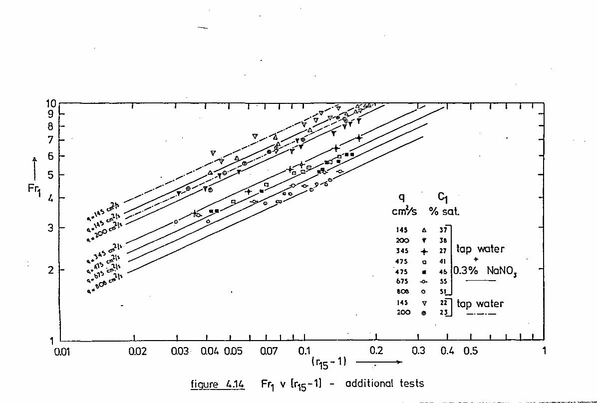
1

~o~ 7

6

5

Fr1 l.

3

2

1 0.01 0.02 Q03· 0.04 0.05

figure 4.14

q C1 cmYs % sat.

-145 6 37

200 • la l4S + 27 tap water 475 a 41 +

47S • 4b 0.30/0 NaND, b7S ~ S5 tOO 0 5L 145 v ~~ tap .w~ter ~oo e

0.07 0.1 0.2 0.3 0.4 0.5 1 (r15 - 1)

Fr1 v [r15 -1] - additional tes ts

--- -- .,,- --~ .... ,~*~ --- ,,-- ,--- ~ - ':. --: ._-::.. _':: .• .:.::=-, .• ~~", ~._.~'!"l-:~~~,'L-«;::_~A;o~

LO N

\ \

\ \

\

\ , \ ,

\ \

\ \

.q \ .., \ ~ \ ,

\ . ~ \ ~ \

~ N

0" . E o

<0 \

o z o Z -~~ lD~ . o

"OJ -~ E o o.~ 0-~

o N

, \

\ \

LO o ~ or-

(W::» 3V ' 5501 ,.{5Jaua

c5' z :£

LO

"OJI ~. 0, ~i c.j o ~

o C"t or-

Lf) q or-

o

o q ~

o lfl ~ .. o

~

'u .-.... OJ

"'C

c o Vl --o Vl

"'C OJ > -o Vl Vl .-

"'0

.... o -to) OJ .... .... OJ

OJ ..c -I Vl OJ 0\ L-

a ..c u (J) .-

"'0

(J)

:::J o L-

a > Lo .. -o

.-to)

> u; c

(J) a Vl Lo ......

~ c Ol OJ L- rn OJ ~ C x Q) 0

GJ Lf) ..c. ~ -~

•

- 86 -

TABLE 4.3

Variation of the Constants kJ1 , kJ2 and kJ3 with

Dissolved Sodium Nitrite Concentration

Sodium Nitrite ~1 kJ2 kJJ Concentration % (Eq. 4.24) Eq. 4.25) (Eq. 4.26)

0 0.0158 0.002JO 0.0064

0.3 0.0186 0.00285 0.0075

0.6 0.0230 0.00355 0.0100 ,

The variation of the constants with sodium nitrite concentration

is shown to be approximately linear in Figure 4.16 within the range

tested. Extrapolation beyond the limits tested is not recommended

for reasons discussed in Section 4.7.4.

The correlation of all the data with Equations 4.24 and 4.25 is

demonstr~ted in Figures 4.17 and 4.18. The results are therefore

expressed by Equations 4.24, 4.25 and 4.26 with constants appropriately

chosen from Table 4.3 according to the concentration of sodium nitrite

• pres~nt.

4.7.3 An Explanation of the Observed Effect of Sodium Nitrite

The observed increases in aeration with increases in sodium

nitrite concentration are at first surprising since it is well esta

blished that increases in salinity levels will lead to a decrease in

the solubility of oxygen in water as shown by Equation 1.41. Further

more, experiments by OGDEN, GIBBS and GAMESON (1959) on the surface

aeration of water flowing in experimental channels sh6wed that there

i --- 0--- ~1

-~-~2

_._.-8._. - kJ3

" '" /'

/ ®

0'

'kJ1 '<J2 . kJ3

0.028 - 0.0035 - 0.013

0.026 .l.. 0.0033 - 0.012 f

0.024 - 0.0031 - 0.011

./" ,~~o.022 - 0.0029 - 0.010 ./ ",.

./ /'

./

", ", '" ./" ", ,," '" ./" " " ./ "

'" '" ,./ ",-'" "," " ,," '" " ./ " ./ ."

./ 0 "" ./ ."

./ " ./ " ", .

./ ".'" /'

./ ",

./ ","

" . ,," ,,"

",.

" . ",.

A

'/./ /,'

6 ". ,/ " .

./ 0/0 NaNG3 ~

0.020 - 0.0027 - 0.cXJ9

0.018 - 0.0025 - 0.008

0.016 - 0.0023 - 0.007

o .!lgure 1..16'

0.3 0.60.011. - 0.0021 - 0.006

':11 ' ~2' ~3 ;". (Eq 1..21.,1..25,1..26) v concentration of sodium nitrite

11

10

9

8

1

6

5

L

3

2

/ I 4-

~ .-/ /'

.I c;),'

+- / + ' / " / • • .. 0

[hEJO-al," -.9....]c.n [>j 3L5

;" +.. • ",' / .. ,,; s ,1>'. ,.' ,. it. &I ,. II / y+ III • ,,,0.

OJ.-' • • .0,' .. , ~. ba." v .. ,; A ~ 6 ~ , «I • ,,' ella • 4, G

'" • lit- IIJ ~;r' (,I:l 1:3

,'" 4 ~ .. ".. t/ '" 7 II 0 ,r.P C .... , a $' ,

,. • , Q

~" " ~ ..... 6' , • ~-¥+ +/ ~ G r;,Jy,' e ,. t ' Q

.. ..t' ~. .." Q' Y lof b

'" e" .. a

•

q cm~'s + .f Y " " ... · e it ,. Il ~fV to

t ." • '. • ~... -+ •• ~_ O. •

~' ~ / 0" '"'IiI Q .. ,'a Q

,,/_ 0·'-• , ,,' w

/"t " .. ~r.J-" itl 0

;a. of- / / 1-,a-'/'/'" e,~ 1. ~ 3 / ,"

(9. a 1; ,.: & ~ U

_ t .. .;:--6~'t dl~/r:4 ·

A

14)

:zoo HS

475

$1}

$-45

bU 710

;1 t.:p wc!er

}.6%+ ~NO, ,. 0.." GI

,l& • & C,c ID IiIIil ,/ ~ e,' Ill" • ~. _ oi fIII,"eaa •

.A.,.. :?cll ' (SJ0 Y " •

//" " tI. / CL .SI

145 •

200 ~ 145

tap water

" + 47S

67S :10.3% N.JNOl

/ . .,u ,s;;,..~ a-

m 0,' / ~~ o ••

ac. ... 14$ :} zoo tap water -_.-

1 / ",'~ G

//'1° : #,' 'b v.' ,,"

o 1.00 1.05

deficit ratio • r1SO ~

1.10 1.15 1.20 1.25

figur(:) [,.17

corr~lction of data with

Eq. 4.2-'

70

60

50

1.0

30

20

10

/" /'

/' .J.... ,/ T

, ", .,

1 F r,2J [~]O.7S

I 345

,/ /

/ ~/ '* ,~. ./* • ./'" ~ u' ,.' ././ --ft,," & &&/ •• ",.0

". .1; /"f' ~ • .' )/f -0. t' +~ . .. ~ • eo .~".,. : ..

./ ,," P aV o. .. ,/' · ~ ... ." ..... J./ Q/ B .. /./:;/:r IIb.B:lP:.d •.

/,. , ." ",,& ~ • -1 \ u ... Q' • .T ~.... A --.; Q ..

-<,>;..1' &/ II.., " .... -- • B·

•

tap water +

Q

q cm2/s

145 A

200 a H5 • 47S s

*~/ ~/ q, Q .,. __ VV i • _./~ ~./-?' .. ,: .. ,,/ A '\,.. .. .~ ~.:At'" ~G V \!I ,0 - D ./ /:r .... "0. • - .. CO

t/ • ,0 ,.." J ./ I> ./0' .... s.. ~y.." '" .. .-

0.6% NaND] 51] V

S45

lf ,. /' ~ ~ ~NI' lIu" ..,..!-o- ~/ / •. ~ ~:''''J e e

,. .LJ.,;' koo~ • +... ~" o~ .... __ .. 0 }& /o~ Q ~fRiP ~ ...

'" I "" (,I Cg t:>," 0 V _",' o.J\ll) & A ,,' C!»

i"" .... "" ~:"~ .". " 'eo' V-~ ,~ ..

/O.f!n/'<li. ' • . o ~.~" •

#.,,~ .... ,e't

,,0 ... ~' "",,,,~ . . ". ..... ", "" ~

tap water +

• 0.3% NaNO]

-_._- tap water

C)

b4S e 710 •

45 , 200 + 14S , 47S ~

bU t _10& ..

Jl45 .. LXX) ..

01.00 1.05 1.10 1.15 1.20 deficit ratio, r1SO ...

!i.gure 4.18 correlation of data with Eq. 4.25

"

125

- 87 -

is a pronounced lowering of the rate of aeration in saline water. A

linear relationship was found between the square root of the salinity

and the percentage reduction in the aeration exchange coefficient. This

reduction is of course consistent with the reduced gas solubility.

Conversely, DOWNING (1958) stated that under conditions of very

high turbulence in combination with entrainment of air, the presence of

dissolved salts can increase the mass transfer coefficient which agrees

with the findings reported in this thesis. Unfortunately neither

reasons nor experimental evidence were submitted to support this obser-

vation.

The presence of dissolved salts will naturally alter the density

and viscosity of the fluid which in turn governs the coefficient of

molecular diffusivity, but, these effects will be relatively small. In

any case, the liquid film coefficient ~ is unlikely to be a major fac

tor cpntrolling the rate of gas transfer since the degree of turbulence

or mixing will generally be high in an air entrainment situation.

The relative quantities of air entrained are unlikely to be

affected by the salt content of the water since these are generally

acknowledged to be governed by the supercritical Froude number only.

Referring to the general gas transfer equation, Equation 1.36.

two possibilities remain, namely, the contact time and the surface area

offered by the entrained air. The contact time is unlikely to be affec

ted by the presence of dissolved salts since this is basicallr dependent

on the velocity distribution through the jump, i.e. an hydraulic

dependent characteristic. If constant volumes of air are entrained then

the only parameter governing the entrained air/water interfacial area

will be the mean diameter of air bubble entrained. The size of bubble

entrained into'hydraulic jumps is a matter which has received much

attention (Chapter 5) but no effects due to the presence of dissolved

- 88-

salts or other contaminants have been noted.

It is interesting at this stage to refer in detail to the work

of VERSCHOOR (1950) in which the effect of lowering the liquid phase -

surface tension was investigated. SEELIGER (1949) found that if the

surface tension of water was reduced by adding ethanol, and air was

bubbled into the liquid, then the swarm of gas bubbles was found to be

composed of very much smaller bubbles. VERSCHOOR noted however that

bubbling air through separate volumes of water and methanol resulted in

more or less equal bubble sizes in each case despite the fact that the

surface tension of the methanol was approximately one third that of the

water. The kinematic viscosity of the two liquids was approximately

the same. However the reduction of the surface tension of water by the

addition of Teepol did result in the formation of smaller bubbles, a

similar observation to that by SEELIGER. More recently, ECKENFELDER and

BARNHART (1961) observed a reduction in the mean size of bubbles

produced by diffusers in the presence of surface active agents.

VERSCHOOR explained the contrasting effects resulting from

reduced surface tension by recourse to the work of FOULK and MILLER

(1931).

FOULK and MILLER discovered that in liquids containing dissolved

matter, i resistance was present which prevented two bubbles from

coalescing. This resistance was absent in the case of pure liquids.

Furthermore, the presence of certain inorganic salts was observed to

result in considerable foaming thus further indicating the presence of

a coalescence inhibiting film on the bubbles. This film or resistance

exists as a result of a difference between the dissolved salt concen-

tration at the bubble/liquid interface and the concentration in the

- 89 -

main body of the liquid. This concentration difference has been

experimentally demonstrated.

SCRIVEN and PIGFORD (1958) came to a similar conclusion from

their experiments - the accumulation of contaminants on the liquid film

surface was visualised as forming a rigid or semi-rigid surface struc-

ture which drastically impedes liquid flow close to the surface. HISE

(1975) similarly referred to the concentration of surfactants at the

bubble surface thus creating tangential shear stresses resulting from

surface tension gradients which in turn are caused by surfactant con-

centration gradients around the bubble's surface.

HABERMAN and MORTON (1956) observed an increased drag on free

rising bubbles (ranging in diameter from O.6mm to 6mm) in the presence

of surface active agents and a certain critical concentration of these

surfactants was identified beyond which further concentration increases

had no further effect on the bubble drag. HISE likened this critical

concentration to a state at which the shear stress equals that of a

solid wall and at which the liquid velocity at the bubble surface is

effectively zero. Similarly, HOLROYD and PARKER (1949) demo~strated the

production of smaller bubbles and reduced velocities in the presence of

detergents.

Tqe presence of the inhibiting films as a result of surfactants

does of course reduce the liquid film coefficient, but, the production

of smaller bubbles for a given air volume results in a significantly

larger air/water interface and hence the increased overall transfer . . A

coefficient ~V observed by MANCY and OKUN (1960) and also by

ECKENFELDER and BARNHART (1961). In an air entrainment situation

accompanied by vigorous mixing, the disadvantages of the film formed . .

on the surface of the bubbles become virtually non existent since this

- 90 -

film will be rapidly removed by the turbulent water anyway. The

advantage of a reduced bubble rise velocity, i.e. increased contact time, I

together with the greater air/water interface offered results in a

significant increase in the gas transfer as observed with the current

experiments.

The relevance of the above reasoning to the results observed here , I

with the hydraulic jump, was validated by the'measurement of the size

of bubble entrained by an hydraulic jump. These tests are reported in

Section 5.2.4. It is clear from these measurements (Figure 5.2) that

the mean bubble size was reduced by the presence of sodium nitrite, a

reduction in the mean bubble diameter from 2.53mm to 1.57mm being noted

from tap water to tap water with 0.6% added sodium nitrite. The tendency

for the bubbles to coalesce in the absence of dissolved salts is well

illustrated by comparison of Plates 5.1 and 5.2b.

4.7.4 Implications of the Observed Effect of Dissolved Salts

If the enhanced aeration recorded above in the presence of

dissolved sodium'nitrite could be taken as representative of the effect

of dissolved inorganic salts in general then the implication with

regard to saline waters is very significant. This is especially so since •

the maximum salinity of 6 parts per thousand in the above experiments is

relatively small in comparison with sea water salinity levels which would

be of the order of 30 parts per thousand.

Whilst Table 4.3 illustrates the variation in the constants in

Equations 4.24, 4.25 and 4.26 with dissolved sodium nitrite over the

range tested, extrapolation is inadvisable since there will be a

critical salinity level beyond which there will be no further reduction

in bubble size. i.e. the coalescence is fully prevented and the bubble

•

- 91 -

size will be governed solely by the size at inception. This critical

salinity is in accordance with the observations HABERMAN and MORTON

and others noted in Section 4.7.3. Furthermore any increases in

salinity beyond this critical point may in fact result in a reduction

in oxygen transfer due to the reduction in solubility.

4.8 A FURTHER TEST OF THE CORRELATION EQUATIONS

HOLLER (1971) measured the reaeration of a discharge of 33.9 lIs

in a 38cm wide open channel.

Summarised in Table 4.4 are some of the data supplied by HOLLER

for an initial oxygen deficit of 50%. Deficit ratios have been correc

ted to l50 C, and energy losses computed from Equation 3.3. The deficit

ratios have been predicted from Equations 4.24, 4.25 and 4.26, assuming

tap water was used, with constants appropriately selected from Table 4.3.

TABLE 4.4

Some Hydraulic Jump Measurements by HOLLER (private communication 26/11/74)

D E F I CIT RAT I 0 r 15 Yl Y2 ~E

(em) Fr l p red . t e d , (em) (em) (Eq. 3.3) 1 C

Measured • (Eq. 4.24)

I (Eq. 4.25) (Eq. 4.26)

I

I

3.14 19.38 23.74 6.12 1.223 1.162 1.21 1.152

3.38 17.37 20.05 4.58 1.117 1.134 1.114 1.128

3.42 16.79, 6.95 3.06 "i ~ 1.056 1.057 1.049 1.044

- 92 -

The predictions are remarkably good, particularly with Equation

4.25. The assumption of tap water is therefore validated. Note: The ,

different results given by Equations 4.24, 4.25 and 4.26 result

from the fact that HOLLER's conjugate depth measurements do not satisfy

the equation of Belanger. This has already been demonstrated in

Figure 3.5 and discussed in Section 3.7.

A wider range of validity of the prediction Equations 4.24 and

4.25 is therefore suggested with constants chosen appropriately accord

ing to Table 4.3-;· The further application of Equation 4.26 was discussed

in Section 4.6.

4.9 RELATIONSHIP BETWEEN AIR UPTAKE AND OXYGEN TRANSFER

The ratio of air to water discharge is known to be dep~ndent

solely on the supercritical Froude number - Equations 2.1, 2.2, 2.3, I '!

whilst the oxygen transfer expressed as the deficit ratio was shown to

be a function of Froude number, discharge and mean bubble siz~ -

Equation 4.25.

Equation 2.1 was expressed in terms ~f (Frl-l) simply because

a~ hydraulic jump does not form if Frl-l. The ratio a could equally

well have been expressed in terms of Frl as follows: •

(4.27)

This form is as valid as the origin,al, Equation 2.1.

From Equations 4.27 and 4.25:

(4.28)

•

- 93 -

Equation,4.28 may be simplified:

1.34 qa

r 15 - 1 • 22.66 kJ2 0 59 q • (4.29)

q being the air discharge per unit channel width (cm2/s) and with a

• 2/ q 1n cm s.

Equation 4.29 shows the deficit ratio dependence on air discharge

for the hydraulic jump studied assuming the air discharge' ratio to be as

given by the equation of KALINSKE and ROBERTSON, Equation 2.1.

4.10 SIMILARITY CONSIDERATIONS

In Section 4.4 it was suggested that for a constant Frpude number,

~ is constant and the time of contact varies as the square ropt of the

scale.

i.e •

Also from Equation 4.24 or 4.25:

•

(r-l) 1 9/8 Mr- l • (r-l)2 • Mt

The basic equation of gas transfer (Equation 1.35) states that , ,

which when expanded into a series gives

n n r - 1 + L (Kr.~ t)

1 i n.

(4.30)

(4.31)

(4.32)

• l..e.

- 94 -

A III k(1). V t)

From Equations 4.30, 4.31 and 4.33:

M - Mv • M - M 9/8 r-l "L t L

(4.33)

5/8 The scale of the liquid film coefficient is' therefore, III Mt

subject to confirmation that Mt - MLI. ' Whilst the scale of contact

'time'for the hydraulic jump may be MLI, the scale of contact time in the

aerated zone downstream of the jump may be bigger than indicated by the

length scale since for an unchanged bubble size this zone may extend

'further beyond the bigger j~mp than indicated by the length scale.

Possibly, therefore, Mt > ~I and, < ~5/8.

The limit of validity of Equations 4.24 and 4.25 in terms of q

remains to be seen, but, the contribution to oxygen transfer of the

aerated zone downstream of the jump will be relatively small compared

to the highly mixed roller regime.

Also, the supposition by WISNER that there is a lower limit

(Fr. > 8) for satisfactory modelling of air entrainment in a prototype

hydraulic jump situation (Section 2.4.3) remains to be similarly con

firmed for the modelling of gas transfer. Also, for the very low Froude •

numbers tested here, the energy expenditure per unit volume was not very

high (Table 4.2) and therefore the slower diffusion processes may have

been more predominant in' the model than in a prototype situation of the

same Froude number.', Again, this remains to be seen.

There will also be some upper, limit beyond which the scale of the

liquid film coefficient will tend to unity i.e. , III 1. 'Ihis follows,

- 95 -

since there will be some degree of mixing above which any increased

mixing will not result in any. change in the value of~, (llICBIE) and

is therefore a waste of time.

4.11 SUMMARY

Some observations of temperature effects on gas transfer by

IMHOFF and ALBRECHT have been discussed in relation to work by GAMESON,

VANDYKE and OGDEN. The former worker's results were shown to be based

on an insensitive measure of oxygen transfer and incompatible with the

latter's results. The temperature correction of GAMESON, VANDYKE and

OGDEN was considered to be applicable to a variety of model and proto-

type situations.

The oxygen transfer in an hydraulic jump was shown th~oretically

to be a function of the Froude number and the scale, and this was con-

firmed by a series of tests conducted for various discharges. Whilst

the ratio of air to water discharge was constant for constant Froude

number, an increase in discharge was shown to result in increased energy

loss and time 9f contact and hence a greater oxygen transfer.

An enhanced aeration was observed for water containing quantities

of sodium nitrite. This was attributed to the formation of smaller •

bubbles in the presence of sodium nitrite and thus, for a constant volume

of air, the creation of a larger air/water interfacial area. The

presence of dissolved salt prevented the coalescence of bubbles, a

supposition which was confirmed by measurements of bubble size reported

in Chapter 5.

Two general equations expressing the oxygen transfer in terms of

the measurable hydraulic characteristics of an hydraulic jump have been

recommended, Equations 4.24 and 4.25. A wider range of applicability of

- 96 -

these is suggested although this has only been tentatively confirmed by

successful prediction of some measurements by HOLLER (1971). The

appropriate choice of the constants for this equation is made by

reference to Table 4.3.

A discussion of similarity considerations suggested that the time

of contact scale varied as the square root of the length scale, i.e.

Mt • MLl, also that the liquid film coe~ficient scale ~ ~ Mt5/ 8• The

experimental results led to the conclusion that the scale of

r -1 -~ 9/8 for· the range tested 15 -~ •

•

, .

CHAPTER 5

A DETAILED STUDY OF BUBBLE SIZE AND CONTACT

TIME IN THE HYDRAULIC JUMP

WITH SUBSEQUENT APPLICATION TO THE

ESTIMATION OF THE GAS TRANSFER COEFFICIENT

- 97 -

5.1 OBJECTIVES.

(a) To confirm that bubble size is independent of scale.

(b) To test the effect of dissolved salts on the size of air

bubble entrained.

(c) To attempt to measure the time of contact and thereby con-

firm that the time of contact can ~e estimated by an .

expression of the form Equation 4.10.

(d) To estimate the transfer coefficient and thus test the

dependence of ~ on energy loss.

5.2 A PHOTOGRAPHIC STUDY OF THE BUBBLE SIZE DISTRIBUTION IN THE

HYDRAULIC JUMP

5.2.1 A Justification for Further Measurements

It has been demonstrated by a number of research workers,

notably HAINDL (1958) and WISNER (1965), that the size of entrained air

bubble remains constant irrespective of scale.

The mean diameter of bubble has been measured by various workers

producing generally similar results - HAINDL (1958) 2 to 3mm, WISNER (1965)

3 to 5mm,whilst bubble diameters ranging from 2 to 5mm were referred to •

by ALBRECHT (1968). APTED (1975) quoted a median bubble diameter of

1.25mm in an hydraulic ju~p whilst LEUTHEUSSER, RESCH and ALEMU (1973)

referred to an average bubble size of the order of lOmm for their

hydraulic jump.

Both HAINDL and APTED photographed the entrained air bubbles

whilst LEUTHEUSSER and co-workers employed hot film anemometry using

conical probes assuming that (i) all bubbles are intercepted by the probe

along their diameters and (ii) that the bubble velocity is equal to the

98

water velocity at the instant of bubble arrival at the probe.

The measurements of LEUTHEUSSER and co-workers also indicated

that the hydraulic jump with fully developed inflow entrained signifi-

cantly larger bubbles than its counterpart with undeveloped inflow. The

contrasting measurements of APTED and LEUTHEUSSER and others merit fur-

ther investigation.

Furthermore, in Chapter 4 an enhanced aeration has been observed

with increasing quantities of dissolved salt. In Section 4.7.3 it was

shown thar this could only be due to the creation of a larger air/water .

interface as a result of the formation of smaller air bubbles in the

presence of dissolved salts. This hypothesis requires substantiation.'

~.2.2 A Means of Measuring the Bubble Size Distribution

Use was made of the apparatus described in Chapters 3 ~nd 4.

The hydraulic jump was formed in a glass walled flume thus enabling

high speed photography of the air water mixture. The use of 1/1000 sec

electronic flash successfully froze the bubbles against a scale thus

allowing for accurate measurement of the bubble size distribution.

Plate 5.1 is an example of one of the photographs used for analysis.

LEUTHEUSSER and co-workers indicated that the bubble size distribution

is the s~e in all regions of the jump, thus it was unimportant which

particular grid within the zone of aeration was analysed.

5.2.3 The Effect of Scale

Figure 5.1 summarises results obtained here over a small range

of discharges for a relatively constant range of Froude number. Data

have been presented as the percentage of the total number of bubbles

whose measured diameters fell within! 0.25mm of the plotted point. A

PLATE 5.1 Entrained air bubbles in the hydraulic jump (tap w + 0.3% NaN03)

~~--~- ---~--==~

PLATE 5.2 !)

ntr ined ir bubbl s in th I.../ U ....,

v \J

hydr ulic jump ( p wat ) ...

.. I

t

PLATE 5 . 2b Entrain d ir bubbl iu tb ic jump (t p at r)

-- (.I v ...., . IJ

, \.j

• I

\.) UU U .J

U I'

,J

, .J V

50

t q cm2/s Fr1

~ 40 I 0 HS 6.q ~ l4S / c 200 8.2

~ 475 7.b

i 30 I 6- -<>- . 475 q.b ~

tap water I /-()-+ 0.3 % NaND]

::J c 20 ~

c -0 .....

'0 10 I C(> '\. A 'T

'Cf!. /A a ~

:~A V

o . ..........- I ~,_

0 0.5 :.0 1.5 2.0 2.5 3.0 3.5 4.0 bubble diameter (mm) ~

fiqure 5.1 the effect of model scale on bubble size distribution in an hydraulic

Jump

50

1 tJ) 40 a1

..0

..0 :J

..0 30

"-0 c... (lJ

..0

E 20 :J c:

-0 --.B 10 ~

0

~ 0

0 0 0.5. 1.0

tap water + 0.6% NaND, (APTED, 1975)

tap water + 0.3 % NaND] (fi gure 5.1)

I LEUTHEUSSER. RESCH, ALEMU (1973)'.

[undeveloped inflow]

/

~-~o_._ 1.5 2.0 2.5 3.0 3.5 4.0 4.5 5.0 5.5

bubble diameter (mm) .. 6.0

figure 5.2 the effect of dissolved salt (sodium nitrite) on the bubble size distribution i"n an

hydraulic jump.

- 100 -

are to be found in Section 4.7.3. The larger bubbles obtained with tap

water can be visually appreciated by comparison of Plate 5.1 (0.3%

and Plates 5.2a and 5.2b (tap water). \

The range of bubble diameters obtained with tap water is in

agreement with those quoted separately by HAINDL, WISNER and ALBRECHT -

presumably therefore, these latter researchers obtained their values

in waters low in dissolved salt concentration. The predominance of

large bubbles suggested by the data of LEUTHEUSSER, RESCH and ALEMU

reproduced in Figure 5.2 is inexplicable with regard to water quality.

This casts some doubt on their anemometric technique, it is possible

that the physical obstruction afforded by the conical probe on inter-•

cepting the bubble resulted in a reduction in the bubble velocity

relative to the main flow and a consequent overestimate of the size.

5.3 AN ATTEMPT TO ~IEASURE THE CONTACT TIME

5.3.J Description of the Technique and Apparatus Utilised

The objective was to measure the time taken by a typical fluid

element to pass through the aerated zone and thus give a measure of

contact time. This was achieved by timing the passage of a ~racer

through the hydraulic jump. The tracer usedwas a concentrat~d solu-•

tion'of sodium nitrite and this was "gUlp" injected into the flow

upstteam of the jump. The progress of the tracer was regist~red by a ,

Wheatstone Bridge to which two conductivity probes were conn~cted. I '

1be probes were suitably positioned in the water upstream ~f the jump

and at the end of the zone of aeration downstream of the jump. The

change in conductivity on passage of the tracer pulse was registered

by the Wheatstone Bridge and recorded on Ultra Violet paper. The Ultra

- 101 -

Violet recorder was capable of accurately recording time lapses as

small as 0.01 sees. The layout of the equipment is shown in Figure

5.3 whilst the conductivity probes and Ultra Violet recorder are

illustrated in Plate 5.3.

One of the main difficulties anticipated was the loss of the

salt pulse as a result of intense mixing and dispersion by the hydraulic

jump. In fact strong pulses were generally recorded with clearly dis

cernible peaks. This is illustrated by a typical trace in Figure 5.4.

The pre-selected time intervals of 0.1 sec are marked along the base of

the trace thus enabling ready analysis of time elapsed between the

recording of the upstream and downstream pulses. This time is taken

to be the measure of time of contact for a fluid element.

5.3.2 Length of the Zone of Aeration

The correct positioning of the downstream conductivity probe is

of obvious importance. Two definitions of the length of hydraulic jump

are indicated in Figure 5.5. The definition of PETERKA (1963) is the

conventional length of the roller (see Figure 3.1a) whilst LEUTHEUSSER

and KARTHA (1972) defined the length as that measured from the toe of

the jump 'to the point downstream where the influence of the jump has •

become nigligible and the flow characteristics are governed ~y the

channel alone. The length utilised for these tests, i.e. the distance

between the conductivity probes, required visual observation of the end

of the main zone of aeration. As shown in Figure 5.5 this criterion

lies between the two discussed above as is to be expected. The length

of the aerated zone is similarly a function of the downstream conjugate

depth alone over the range tested, i.e. Lj/Y2 is constant. The

scatter displayed in Figure 5.5. is perfectly acceptable in ,view of the

Wayne-Kerr

Univ,~rs:::l Bridge

~

conductivity

~ ...

... , \ ... ---~------,,-~ ...

syring~ for SUlp salt ~ injection

~ .... -e-+ ' e /" " --(~----, . • • • I I · • • • • I .... ---. I • · , • . I '-------------41 I •

Ult ra - Violet ~ recorder

u-v trace

figure 5.3 Schematic - apparatus to determine contact tim~ in an hydraulic jump

PLATE 5.3 Wheatstone Bridge, conductivity probes and Ultra-Violet recorder

0J •

0'1

0 <U

'" W 0

U cS <{

0:: .... - tI1

N E

....t t-O

t.() W Lf') If)

-' . Q) 0 to (Y) L..

:J Ol

II II

~I a::: 0- La

-1

t q cm2/s.

13 A '''~ ; 200 LEUTHEUSSER 8. KARTHA (1972) L' • lSO / [undeveloped inflow] -L

Y2 II 47S

II s·a 12

r ~ b7S

11

10

9 I!) aerated zone

t, Ii1 . /. 8

dl'¥ ~'¥ y

'" 8 Q D,. ,&~~V~-~IiJ;---:Q~0~--~~---

~'/)( K

s A. III

~ x • e

11

7

6 G1l

--............ PETERKA (1963)

5

Fr1 ~ L._ ! .!

o 1 2 3 4 5 6 7 8 9 10 11 12 13

.!lgure 5.5 different interpretations of the length of the hydrou1ic jump

- 102 -

insensitivity of visually determining the end of the aeration zone.

The data of LEUTHEUSSER and KARTHA in Figure 5.5 is for a condition of

undeveloped inflow, for developed inflow they showed that Lj m 16Y2'

i.e. larger for this latter condition.

5.3.3 Results

It was earlier suggested in Section 4.4 from an approximately

derived model of contact time in the aerated zone of the hydraulic

jump (Equation 4.10), that

trg _ f(Fr ) . Iy 1 I

i.e. for a constant Froude number, the contact time varies as the

square root of the length scale. The current tests for a variety of

discharges are summarised in Figure 5.6, these results are quite con-

sistent with the observations made from the model. Furthermore, the

validity of the approximate model is successfully tested in the dimen

sionless plot Figure 5.7, from which the following expression for the

time of contact may be stated:

• (sec) (5.1)

The variation of contact time scale with the square root of the length

scale is validated by the measurements over the range of scale

encompassed by the oxygen transfer tests.

The technique just described has proved a most useful means of

determining contact times of fluid elements. Furthermore, the nature

of the pulse observed downstream indicates the degree of recirculation

10

9

f : or

L. I.L

~ 6 r J c 5 <11 "0 J o L. I

lJ.. ...

3

2

,

q cm2;s & 145 El 200

o lSO

Ie 47S

• 54S

~ 67S

0.6 0.8 1.0

.flgur~ 5.6

•

1.2 1.1.

Q A

...,cf

/"

1.6

... \' ~

1! u

.~ ,~

I '"

1.8 2.0

time of contact (sec)

~

l.

2.2 2.1. 2.6

~\' ,. ~O ~ ..

2.8

the variation in contact ti me with scale of hyc!rouUc jump

'\.\, .. #>

,:." ~\'\ ,. ~" . . .," ,.

'0 .. ., )\'

....

3.0

I -

.,

j .. J(

l 1

e

.'

~--~----~--~~ __ ~ ____ ~_--L. ____ L-__ -L __ --~--~ M N o

-.. --~ u.

o 1'0

1.0 L/")

0 1.0

1.0 ~

0 ~

In M

0 M

In 1-"

0 N

III -o -III

o

0 ~

~

M ~

c 0 .... . § -~ ell >

r--t.n

C1J ~

:::J

-

- 103 -

occurring. In the experiments reported above, a rapid rise in conduc-

tivity to a peak value was generally followed by rapid re-attainment

of background levels (Figure 5.4). The technique is versatile, and

could be refined to quantify the degree of dispersion or recirculation

occurring.

5.4 AN ESTIMATE OF THE TRANSFER COEFFICIENT

5.4.1 Computation of the Liquid Film Coefficient

where

From Equation 1.36:

Log r L _ e -l" ! t

V

A Qa - - - X 4'11' V Q

(5.2)

(5.3)

The ratio Qa/Q is readily determined from Equation 2.1, twa? measured

in Section 5.3 (Equation 5.1), db was measured in Section 5.2 whilst

measurements of deficit ratio were reported in Chapter 4. A realis

tic estimate of the liquid film coefficient is therefore possible.

Table 5.2 contains the liquid film coefficients computed for a range

of discHarges, for three Froude numbers in each case and for the three

different water types tested. The contribution to the surface area

of the upper water surface is considered negligible since this is

largely occupied by air bubbles .(see Plate 5.1).

- 104 -

TABLE 5.2

A Computation of Liquid Film Coefficient for the

Hydraulic Jump Studied

Specific Upstream Energy LIQUID FILM COEFFICIENT

Discharge Froude Loss ~ cm/hr

(cm~/s) No. ~E Fr 1 (em) Water Water Water

Type A Type B Type C

* ** *** I 1 I

,

145 8.37 17.67 60.1 53.9 68.1

. 6.53 10.58 68.8 61.7 77

3.73 3.29 78.5 70.2 89.3

345 7.10 22.01 90.8 81.9 103.7

5.59 . 14.04 90.9 114.5 101.1

3.22 4.08 118.3 100.8 129.6

710 4.85 16.95 139.6 127.2 158.6 I

3.51 8.20 152.9 136.2 172.5

2.50 3.20 157.9 139.9 173.2 •

* Water Type A - Tap water + 0.6% NaN03 d ·O.157cm b .

** Water Type B - Tap water + 0.3% NaN03 db. O.172cm

*** Water Type C - Tap water db • 0.253cm

- 105 -

The values of ~ computed have been plotted in Figure 5.8

together with numerous published data for various bubble sizes

reproduced from BARNHART (1969) for freely rising bubbles.

The orders of magnitude of ~ for the hydraulic jump are compar-

able.

For a constant discharge an increase in Froude number results

in greater energy loss, air entrainment and gas transfer but also a

reduced liquid film coefficient. This similarly follows from Figure

4.10 where a constant oxygen transfer was recorded for constant energy

loss irrespective of discharge. From Equations 4.21 and 4.33 it

follows that for constant deficit ratio:

(5.4)

i.e. ~. is a function of the energy loss per unit time per u~it inter

facial area to volume ratio.' In addition ~ is a function of the

molecular diffusivity Dm of oxygen in water, and of the kinematic vis

cosity of the water. ~ also varies with bubble size. These parameters

have all been incorporated in the dimensionless correlation depicted in

Figure 5.9 from which

• d_ V AE 1. 2 1 • 2

~ B! -0.266 (A~U v) - 0.266 (t. 6vE)

db where I).'n is the Sherwood number.

m

(5.5)

In producing Figure 5.9, the molecular diffusivity of oxygen in

water at 15°C was determined from the INTERNATIONAL CRITICAL TABLES to

be 0.07 cm2/h, a figure which is approximately equal to that determined

• COPPOCK. MEIKLJOHN (1951) 260 reproduced • IPPEN. CARVER (195L)

from • PHILPOTT (1952) 240 BARNHART (19S9) A BARNHART

r ~ PASVEER (1955)

220

- • ..c "- 200 E

·f u --l 180 ~

1 * • .... c • ClI 160 - • 0 ~ u

~[: 00-00-Q,/ 0 u 140 ~ • E

.,. . , . A -- · r· \ ..

120 ., • "0 ",,6 '5 • A • ". • cr \.

e. , 100

• • • $ • C!)

80 * -e- til • • -+ 6) •

60 +~

4-" • 40

cm2/s q 145 345 710"

20 -Go ~ ~ tap water + 0.6% NaNQ, 4- • " tap water + 0.3% NaNOJ • .. + tap water

0 0 0.1 0.2 0.3 0.4 0.5 0.6 0.7 0.8 0.9

bubble diameter (em) •

!igure 5.8 a comparison of liquid film copfficient3 for the hydraulic jump and published values for free rising bubbles

700_ q cm2/s

1 600 t ~5 3~5 7~0

4\ A A 500 s ~' +

Q8E

A" 400

300

200

150' =v=

100

+

"

tap water + 0.6% NaND] tap water + 0.30/0 NaND] tap water

4

A/ 9

A c;> / ~ ci>

A &. /lA 9 0A

0(1).

db K - ~ L Om

200 300 400 500 600 700

figure 5.9

[Q8E/A~] v Sherwood No.

- 106 -

more recently by BAIRD and DAVIDSON (1962). The kinematic viscosity

of water at 150 C was taken to be 0.01143 cm2/s, the changes in this

value due to the presence of dissolved salts being ignored.

5.4.2 Implications for Similarity of ~

For a constant water quality, db is constant, and for a constant

temperature D and v are constant. m

if the gas transfer situation is modelled according to the

Froude law of similarity then ~ is constant and the time scale Mt - MLI from Equation 5.1. Also, according to Equation 4.3 M~E • ML whence

from Equation 5.5:

0.6 - ~ The liquid film coefficient therefore varies as the 1.67 root of the

length scale or Mt°. 6• This is indicated in Section 4.10 where it

was suggested that ~ a MLO. 625 • A caution about limits of validity

was expressed in Section 4.10.

5.5 SpMMARY

The size of bubble entrained by an hydraulic jump was studied.

The results confirmed HAINDL's statement that a constant size of air

bubble is entrained irrespective of scale. The distribution of

bubble sizes indicated a slight positive skew, i.e. a predominance of

bubble sizes larger than the median. The presence of dissolved salts

was observed to result in a reduced bubble size thus confirming the

reasons expressed in Section 4.7.3 for the enhanced aeration observed

- 107 -

in Section 4.7.2. Some comments were made regarding the extremely

large bubble sizes recorded by.LEUTHEUSSER, RESCH & ALEMU as these

contrasted markedly with the observations of other published measure-

ments.

A technique for estimating the time of passage of a fluid ele

ment through the hydraulic jump was reported and the results provided

confirmation of an approximately derived time of contact model presen-

ted in Section 4.4. The suggestion made in Section 4.10, that the

scale of time of contact varied as the square root of the length scale,

was validated, i.e. Mt - MLi .

An estimate was made of the liquid film coefficient fqr the

hydraulic jump studied. The values calculated were shown to be co~

parable to others published in the literature. A dimensionless

correlation equation (Equation 5.5) was presented which related ~ to

the Energy loss per unit time per unit ratio of air interface to

volume. The scale of the liquid film coefficient was shown to vary

as the 1.67 root of the length scale over the range of the current

tests for constant Froude number, a similar conclusion to one reached

in Section 4.10, namely that ~ a MLO. 625 •

•

•

CHAPTER 6

THE EFFECT ON OXYGEN UPTAKE OF DOWNSTREAM

POOL GEOMETRY AND JET DISCHARGE FOR

A PARTICULAR WEIR NOTCH

- 108 -

6.1 INTRODUCTION

Although much useful work has been published on the oxygen

uptake at weirs this has largely proved inconclusive. Figure 6.1

serves to summarise much of this work, and, with the exception of

NAKASONE, all the workers mentioned have attempted to relate the

oxygen uptake solely to the height of fall although VAN DER KROON and

SCHRAM did note that discharge variations are also effective. The

inconclusiveness of previously published work is further illustrated

by the inability of both the WATER POLLUTION RESEARCH LABORATORY

(D.O.E. 1973) and-HOLLER to relate their laboratory correlat~ons

directly to prototype measurements although reasons for this were

advanced.

It was intended therefore to exhaustively study the e~fect of

all important variables in the hope of clarifying the differ~n~ effects

displayed in Figure 6.1.

6.2 AIMS

The experiments reported in this chapter represent a continua

tion of work begun by APTED. The effect of varying the jet discharge

and the geometry of the downstream pool for a particular weir crest

and a constant water quality is investigated.

6.3 DESCRIPTION AND USE OF APPARATUS

6.3.1 General

The laboratory re-circulatory system has already been discussed

(Section 3.4.1) as has the supply of de-oxygenated water from the

mixing tank (Appendix B). The weir apparatus was set up immediately

1

I LO .:-

0 -0 '--.::! -QJ "0

4.5

1..0

3.5

3.0

2.5

2.0

1.5 r

.!igure 6.1 deficit ratio v height of fall - various published results

VAN [ER KROON & SCHRAM (1969)

weir width of shape' each

notch terra 65

f=I'-=i 33

f=A=Y 21 i

~ 145

~

fl-'lJWI..1

10

8

fJUWV-lli 6

{O = 8.33 tIs)

curve No.

.1-

2

3

I.'

NAKASONE (1975) curve Equation

discharge curve No. No.

(lIs) No. 9 2.29 (HOLLER.1971. taboratory weir)

2.5 5 10 2.31 (HOLLER.1971. prototype weirsJ

5.0 6 11 2.24 UARVIS.1970. laboratory weir)

7.5 7 12 2.11· (GAMESON.1957. field survey)

10.0 8 13 2.32 (O.C.E, 1973. laboratory weir) • a= b=1

Note deficit ratios adjusted to 150C where necessary with Eq.2.13

.... 'l.~--,...' -_ .. , .. '" ..,,' -' ......

~ ...

_-------10

~'l

,,'2.

I I ') I 250 300 I - _. I 1C:0 .. 00 ( _, 1.0~ 50 100 - !leig."1 of feU. h. c,,"

- 109 -

beneath the mixing tank, on the floor below, and connected to the

mixing tank as shown in Figure 6.2.

6.3.2 The Weir Apparatus

After deoxygenation in the mixing tank water flowed under gravity

to the upper weir pool. This pool consisted of a galvanised mild

steel tank O.92m x O.65m x O.6Om fitted with a system of baffles to

stabilize the flow prior to discharging over a sharp crested weir.

The water then fell freely to the pool below. The rate of flow was

metered by passage through a pair of rotameters illustrated in Plate

6.1, and placed in parallel in the supply line between the mixing tank

and weir stilling pool. Sensitive control of the flow rate was

effected by a pair of valves, one placed prior to each rotameter. The

weir notch was readily removable thus permitting the substitution of

alternative notches as required.

The downstream pool was constructed of timber and was fitted

with a wicket-type outflow gate which enabled the depth in the pool

to be varied up to the maximum of O.5m. The length of the pool remained

constant at 1.5m while the width of the pool could be reduced at will

from I.Onby the insertion of a pair of timber baffles placed appropriately

• but parallel to the sides of the tank. With the baffles in position

it was necessary to line the pool with a plastic sheet to prevent

water from escaping under the baffles.

For all the tests conducted at the maximum pool width it ~as

possible to observe the behaviour of the jet underwater through a

glass inspection window built into one side of the lower pool.

The water discharging from the lower weir pool was returned

down a shute to the laboratory sump whence it was again available

for re-circu1ation to the header tank.

dosing solution

~:: -.-laboratory head~r tank

mixing tank

, I I } r=r 7 7· , I , , , ,,-7 ~R~l{.N~ flfJO,R.,3.,- -,', ,._ su~ply line to _--------.1..-*"---. 3 met~ flume

rota meter_ --.

depth control slats

inspection window~

lower weir pool--"

"---4-1----'

[tig. 1..11

J~dePth manometer

I I I I , ,

I t i

laborptory water /e,-clrcurating p.1mp , .

. J-~------..:J-E-n-II'!IPf"---------------------------------------_-_-_-... -r--_-_-_--'----1"BASEt~E~.::t! covered laboratory sump ,

-K signifies a flow control valve

figure 6.2, LABORATORY CIRCUIT - FREE OVERFALL EXPERIMErnS

PLATE 6.1 Weir tilling pool and otameter

I

- 110 -

The measurement of water levels in both the stilling pool and

downstream pool was effected by a calibrated single limb manometer in

each case tapped into the bed of each pool.

'The height through which the jet fell was varied simply by

either raising or lowering the downstream pool. At all times the

upper weir pool was fixed in position and the whole apparatus was

rigidly supported by scaffolding tubes.

The layout described above is illustrated by the flow diagram

set out in Figure 6.2 and the weir apparatus is depicted under operat-

ing conditions in Plate 6.2.

6.3.3 Test Procedure

This set of experiments was conducted with a sharp cr~sted rec-

tangular notch of width lOOmm for a variety of discharges.

For various positions of the lower pool and for various dis-

charges over the weir the depth of water in the lower pool 'was varied.

Tests were similarly conducted for reduced widths of the lower pool.

After any adjustment to any of the variables discharge, pool

depth, pool width, height of fall, etc., it was essential to allow Buf-

ficient time for the attainment of both stable hydraulic conditions

• and steady oxygen levels. These were continuously monitored and were

recorded only when equilibrium was judged to have been achieved.

The sequence of operations discussed below was arrived at through

experience and although somewhat wasteful in chemicals it was most

efficient with regard to time.

With the pool position and width fixed, the discharge was set

to 2.5 lIs and the downstream pool wicket gate adjusted to provide the,

maximum depth in the pool. A series of tests was now conducted altering

- 111 -

only the discharge. As with the previously reported hydraulic jump

tests, the inflow to: the mixing tank was fixed, in this case at .

Q - 2.5 lIs, with the result that as the discharge through the weir

apparatus was reduced, then the excess flow was removed by the overflow

weir in the mixing tank. It was found that to alter the inflow to the \

mixing tank each time a new discharge was selected, and thus the chemi-

cal dosing as well, was far too time consuming because of the large •

retention time of the mixing tank and the consequent length of time

to re-attain stability.

Th~s, with all other variables constant, the discharge in the

weir apparatus was gradually reduced. On completing recordings at

the minimum discharge 0.6 lIs, the discharge was again set at 2.5 lIs, ,

the depth in the downstream pool set to a new level and the procedure ,

repeated.

The tests were conducted over a range of the variables as limi-

ted by the physical size of the apparatus. In addition to the discharge

range 0.6 to 2.5 l/s, an extra experiment was conducted for one higher

discharge 5.0 l/s.

Throughout these experiments the levels of sodium nitrite in the

water were monitored and remained constant at a concentration of 0.3%.

6.3.4 The Measurement of Oxygen Uptake

'As discussed in Appendix A.3, oxygen levels recorded were

expressed as percentage saturation.

Th~ measure of oxygen uptake selected was the deficit ratio

(Equation 1.35) and all deficit ratios were corrected to a standard

o value at 15 C by means of the temperature correction of GAMESON,

VANDYKE & OGDEN (Equation 2.13).

- 112 -

In contrast to the hydraulic jump tests the dissolved oxygen

electrode was placed in a perspex cell and not slspended freely in the

water. The reasons for this are discussed more fully in Appendix A.

Suffice to mention here that this was designed to avoid the dangers of

oxygen depletion in the vicinity of the electrode. The validity of this

technique is also discussed in detail in Appendix A.

6.4 EFFECTS OF VARYING DISCHARGE-RESULTS

6.4.1 Variations in Optimum Depth

The results of the experiments for various discharges are plotted

in Figures C2.1 to C2.7 (See Appendix C). A typical sample of the

data collected is given in Table 6.1 together with the defiqit ratios

computed. This data is reproduced in Figure 6.3 in the typtcal form

of presentation of Appendix C. For a particular discharge, water

quality and notch type, the deficit ratio adjusted to ISoC has been

plotted against the lower pool depth for the various elevations of the

lower pool tested.

The behaviour displayed in Figure 6.3 confirms the observations

of JARVIS, the D.O.E., and also APTED, in that for any fixed pool posi-

tion, an increase in deficit ratio is observed for an increase in pool

depth u~ to a critical value of depth beyond which a decrease in the

deficit ratio becomes apparent. This critical depth, being the depth

at which optimum aeration is achieved, is henceforth referred to as the

optimum depth, d'. It has already been established (see Section 2.4.6)

thar this is the depth to which the jet or bubble plume would

penetrate into the pool if unimpeded. For lesser depths the bubble

plume would strike and be deflected off the bed of the pool and this

reduced contact time is reflected by the reduced oxygen uptak~ observed

- 113 -

TABLE 6.1

A Typical Sample of the Data Collected for one Notch and

Constant Discharge

Notch Type • Rectangular, sharp crested, 100mm wide

Discharge - 2.0 lIs

Pool width • 1.0Om

Water • Tap water treated with 0.3% sodium nitrite

DISTANCE LOWER WATER DISSOLVED OXYGEN DEFICIT OF POOL POOL TEMP. % SATURATION

BED BELOW DEPTH ABOVE BELOW NOTCH (CM) (CM) (oC) WEIR WEIR r

,~OiS 31.0 14.8 40.1 62.1 1.58 37.4 15.0 39.8 60.1 1.51 24.3 15.1 37.8 61.2 1.60 17.3 15.2 38.2 60.0 . 1.55

126 45.8 17. 1 36.3 68.4 2.02 37~0 17.2 39.0 71.0 2.10 28.6 17.0 35.7 69.0 2.07 19.2 16.9 42.5 70.2 1.93 24.0 16.8 40.6 70.4 2.01 31.6 13.8 47.0 72.4 1.92 I

27.4 16.6 41.6 70.8 2.00 33.8 . 16.7 38.2 69.7 2.04 40.2 16.8 39.5 69.8 2.00 23.1 16.9 39.0 68.7 1.95

• 14.3 17.0 38.8 I 65.0 1.75

157 45·7 ! 16.7 36.0 72.3 2.31 35.6 16.9 34.6 73.0 2.42 30.5 17. 1 34.5 73.0 I

2.43 24.5 17. 1 34.8 71.6 2.30 17.3 17.2 34.7 69.0 : 2. 11

\ 200 45.6 2.84 . 19.0 43.0 79.9

32.0 19.0 43.5 80.5 2.90 25.8 19.1 43.3 79.6 2.78 26.8 19.2 42.6 80.0 2.87 11.1 19.3 43.2 74.7 2.25

245 42.7 20.2 42.0 83.7 3.56 33.7 20.3 39.9 83.5 3.64 27.0 20.4 40.5 82.8 3.46 15.1 20.4 38.4 77.7 2.76 38.0 20.5 40.9 83.9 3.67

RATIO

r l5

1.58 1 .51 1.60 1.54

1.96 2.04 2.02 1.88 1.96 1.95 1.96 1.99 1.96 1.90 1.71

2.25 2.35 2.35 2.23 2.04

I i 2.66 I 2.71

2.60 2.68 2.12

3.24 3.31 3.15 2.54 3.33

4.0 distance from wei r crest to po<? 1 bed

(cm) 3.5 ~ 80.5 <:>

1300

126 ? 157 -&

200 6 245. -4r

l.l) ~

L.

o· .- 2.5 -0 '--0

-.-OJ v 2.0

15

1.00 5

figure 6.3

weir type - 10cm wide, rectangular, sharp crested width of lower pool = 100 cm discharge = 2.0 lis tap water + 0.3% sodium nitrite ,/ optimum depth

,~ curve

/0

10

,../4t /'

I

______ .. _ .A.

~--------- ,'" I

, , , , I

I , / ~-----

b -- -6 / -6 '0,' ___ I , , , -e- ' -e- - _____ _ ------ /,- -~

~ I ~

~ .1 9 ~ ~ - q /!J 9 Q ·--9 _9 __

9~ , ~ /' ~~. /'

~ _----0 " 0-___ 0---- , ~-----------0 ______

/ .

/

depth of lower pool, d (cm)

15 20 25 30 35 40 45

effect of varying the pool depth on the deficit ratio for various elevations of the lower weir poot

50

- 114 -

for the lower pool fixed in position; an increase in depth beyond the

optimum depth provides no further increase in bubble contact time and

the reduced aeration experienced is as a result of the reduction in

the available height of fall. For depths leading up to the optimum

depth, the increase in aeration due to increasing contact time clearly

outweighs the drop in aeration due to the reduction in height of fall.

For a particular weir situation the maintenance of optimum

depth conditions is desirable for both reasons of oxygen uptake and in

order to avoid excessive scour on the river or stilling pool bed.

The optimum depths observed in Figures C2.t to C2.7 (Appendix C)

have been plotted in Figure 6.4 against the height of fall. The

general trend for a constant height of fall is an increase in d' for

an increase in discharge. The plunging jet can be visualised as

losing part of its energy at impact with the water surface and the

rest through the process of entraining large quantities of air into

the pool. The higher the discharge then the larger the cross

sectional area presented at impact, but, the observations in Figure

6.4 show the lower discharge jets requiring a smaller entrainment

depth due, possibly, to their capacity to entrain relatively larger

quantities of air. The ratio of surface area to volume of the jet is

• clearly a controlling factor in the air entraining process.

This discussion is confined to the jets tending to a circular

cross section (0.6 < Q < 2.5 l/s) - the contrasting behaviour shown by

the jet Q - 5 lIs in Figure 6.4 illustrates the effect of jet shape.

This jet was essentially a broad flat jet and these are treated in

more detail in Chapter 7.

The attainment of a constant value of d' at high heights of fall

noted with the lower discharges (Q < 2.0 lIs) is undoubtedly due to the

45

1 -~ 40 --"'C

... .c 0. 35 OJ

"'C

E ':J E :;: 30 a. 0

25

20

15

10

5

00

flgure

Q (/s .

(!) O.b

)( o.e. A r.o a r.S tA 2.0 (I) l.S ... S.O

50

--~~-

point of jet disintegration according to v HORENI, 1956 (Eq. 2.7)

Notch w~dth = 100 mm ,

Tap water + 0..3 % NaN~]

100 150 200 height of fall. h (em)

250 ~

300 .

6.4 the effect on optimum depth of . discharge varying

for a particular rectangular notch

- 115 -

disintegration of these jets. The point of disintegration of the

various jets as determined from the equation of HORENI (Equation 2.7)

, has been marked in Figure 6.4. The application of this equation was

generally validated by visual observation of these jets. The point of

disintegration was identified as the point at which the jets were seen

to have expanded in cross sectional area and broken up across the

width of the jet - an observation which is quite consistent with those

of HORENI. The disintegration of the jets will be accompanied by a

loss of jet energy which is reflected by no significant increase in

penetration depth for falls in excess of that at which disintegration

occurs. The process of disintegration is progressive and therefore not

instantaneous and the height of fall at which the optimum depth ceases

to increase with height of fall will not necessarily be specifically

described by HORENI's equation. This is illustrated by the higher 1

discparges 2.0 and 2.5 lIs in Figure 6.4. '

The disintegration of a jet is illustrated in Plate 6.3 (facing

the weir) and also in Plate 6.4 (the jet viewed from the sid~). The

development of oscillation and subsequent break up of the jet is

plain to see and can be further appreciated if Plate 6.3 is compared

with' Plate 7.1. This latter plate shows a different but solid jet

photographed shortly after disch~rge from the notch.

,6.4.2 Variations in Oxygen Uptake

I For all the discharges studied and for pool depths greater

'\\ than or equal to the optimum, the deficit ratio has been plotted against

the height of fall, h (difference between water levels), in Figure 6.5.

The data for each discharge fall clearly on separate curves

with a reduction in oxygen uptake apparent for any increase in discharge I

PLATE 6.3 A disintegrating jet viewed head-on

PLATE 6 . 4 A disintegrating jet viewed from the side

4.0 , Q lis I) O.b

'If O.S

3.5 A 1.0

o 1.5

LO • 2.0 ~

~ 2.:S .0 • 5.0 -e 3.0 ...-0 \I-

ClJ "0

2.51

2.0

1.5

1.00

Notch wid th = 100 mm Vo

Tap water + 0.3 010 NaND,

(j) (!)

. .,p'-/ /v/' /'.Jil £ ................ .. - • •• /'\1_.10>':" Y /' /'

50 100

..- a

point of jet disintegration according v to HORENI, 1956 (see Eq. 2.7)

height of faU, h (em)

150 -. 200

figure 6.5 the effect of discharge on oxygen transfer for a particular '.rectangular notch discharging into a pool of width =1.0 m and depth ~ the optimum depth.

250

- 116 -

between 0.6 and 2.5 lIs. This agrees with the findings of VAN DER KROON

and SCHRAM although NAKASONE recorded a completely opposi'te effect.

For an increase in discharge from 2.5 to 5.0 lIs there is no further

reduction in oxygen transfer. in fact. the curves for these two dischar

ges are practically coincident. This is attributed to the shape of the

free falling jet. 'For discharges 0.6 to 2.5 lIs the jet was observed

to contract during t~e free fall showing a tendency towards a circular

cross section. VAN DER KROON and SCHRAM recorded a similar tendency.

However, the jet for discharge 5.0 lIs was observed to expand in

width after passing through the notch and thereafter showed no

tendency to contract. In fact this jet proved very unstable,

oscillating markedly during its free fall. In view of the high

specific discharges tested ,by NAKASONE it is possible i that his jets

behaved similarly to this jet. The specific discharge 500 cm2/s

tested here might indicate a turning point in the oxygen uptake varia

tion with specific discharge towards a similar trend to that observed

by NAKASONE. It would have been interesting to test this by further

experiments ,with higher specific discharges. Unfortunately it was not

feasible to pass a higher discharge through the apparatus though a

separa~e set of tests with an even narrower notch might have been

considered.

The points of disintegration of the various jets have been

marked in Figure 6.5 (according to equation of HORENI, Equation 2.7)

but there is no apparent change in the rates of aeration thereafter.

The disintegration of the jet will result in a more" significant

oxygen absorption by the jet prior to impact with the pool due to the

larger air/water interface created. Plate 6.3 illustrates the

disintegration of a jet into water droplets. However, as seen in

- 117 -

Figure 6.4. the depth of jet penetration will be adversely affected.

although from the results in Figure 6.5 it is clear that the disinte

grated jets continue to entrain large volumes of air. I

The varying effects of discharge are apparent from the results

in Figures 6.5 and 6.1 but are also somewhat confusing. Apart from the

effects of changing the discharge itself they serve to illustrate the

importance of the jet shape and the effects of changing it. The

influence of the jet shape is not surprising since this determines

the perimeter of the jet and thus will regulate the quantities of

air entrained into the pool. The depth to which air will be entrained

into the pool will also be affected by the jet shape as was pointed out

with Figure 6.4.

Effects of varying jet shape for constant discharge are dis

cussed in detail in Chapter 7.

The variation in deficit ratio with height of fall displayed in

Figure 6.5 follows the same pattern as the experiments of the p.O.E.

(1973). The magnitude of the values of deficit ratio obtained in the

current studies is generally higher than the curve produced by the

D.O.E., although the curve for the highest discharges studied is only

slightly above the D.O.E. curve. The D.O.E. experiments were conducted

using a~2Omm wide notch passing a discharge of 1.82 lIs. (Details by

private communication.) This jet similarly contracted rapidly during

its free fall, but, the downstream pool being only 30cm square, the

retention' time was substantially lower than in the current experiments.

The effect of retention time is tested and discussed fully in Section

6.5.

- 118 -

6.4.3 The Contrasting Results of APTEO (1975)

APTEO reported on similar experiments to test the effect of

discharge for a single height of fall. Although the tests reported

in this chapter were obtained from the same apparatus with only minor

modifications, the contrasting results obtained were unexpected.

Figure 6.6 contains the results of APTEO for the bed of the

downstream pool 1.15m below the weir crest together with those

obtained during these studies for the pool bed 1.26m below the notch.

First, it is noticeable that the optimum depths are similar in both

graphs but that the peak deficit ratios for APTEO's lower discharges

are in fact lower than those for the highest discharges. The

experience of the current studies contradicts this. Whereas at

shallow pool depths the variation displayed by APTEO's data with

discharge is similar to that shown by these current studies it is •

clear that as the pool depth increases,'APTED's data begins to show a

reversal of this trend - a trend which is in no way apparent from the

current studies.

The reasons for this became certain during early tests for

which the dissolved oxygen electrode was placed directly in the weir

pools and as close to the outflow sections as possible. This tech-•

nique was the same as employed by APTED and also JARVIS, and indeed

similar results to those of APTED were initially collected until it

was noticed that agitation of the electrodes resulted in a rise in

the indicated oxygen level. Despite attempts to place the electrodes

in regions of highest velocity, these were apparently insufficient to

eliminate the oxygen depletion which was occurring in the electrode

vicinity. This source of error was eliminated by the enclosure of the

electrode in a perspex cell (See Appendix A.8. also Plate A.l) and

t 2.4 Q 1/. r15 e 2.07 c 1.7S

2.2 A I.U I( 0.87

Ii) 0.b2

2.0

1.8

4 e

1.6 I'l 5 10 15 20

d cm ....

'f 2.4

r15 Q II.

e 2.0

c I.S 2.2 A 1.0

)( 06

(j) Qb

2.0

1.8

1.6 current tests, H = 1.26 m

pool width = 1.0 m

20 25 30 35 d em ~

i!gure 6.6 discharge effects observed during· current experiments c9mpared with the observations of

APT ED for an identical notch of width 100 mm.

50

50

- 119 -

the subsequent passage of siphoned sample water through the cell.

The belief that APTED's data was affected by inadequate flow

velocities passing his measuring electrodes is consistent with the

trends displayed by his data in Figure 6.6. For shallower depths

of pool (i.e. higher flow velocities) APTED's data does not contrast

with the currently reported experiments. However, for a deeper pool

and low discharges (i.e. low flow velocities) the deficit ratios .

indicated by APTED are depressed compared to the data for ~is higher

discharge. Again. this is considered to be indicative of the occur

rence of oxygen depletion. It is also believed that JARVIS's data is

equally suspect and further evidence to support this argument is

presented in Section 6.5.

The deficit ratios for the current studies are generatly not

significantlYcdifferent from those of APTED portrayed in Fig~re 6.6 -

this does not invalidate the above argument. The laboratory water

contained approximately 0.6% sodium nitrite at the time of APTED's

experiments, which is double that in the current studies. It is demon

strated in Chapter 4 that increasing the concentration of sodium

nitrite results in a significant increase in deficit ratio - this is

not apparent when APTED's data are compared to the current studies and

is furth~r evidence of the dissolved oxygen starvation discussed above.

In the light of the above findings, it was clearly necessary

to repeat all APTED's experimental work as well as to expand on it.

6.5 THE EFFECT OF REDUCING THE DOWNSTREAM POOL WIDTH

6.5.1 Introduction

The experiments reported so far were carried out for the maximum

pool width of I.OOm. In this case the sides of the pool were judged to

•

- 120 -

exert no influence on the behaviour of the bubbles. It might be

argued that this was an unrealistic model since the width of pool

beneath a prototype weir will generally be the same as the width of

weir above it. Indeed. the experiments of VAN DER KROON. NAKASONE. and

the DEPARTMENT OF THE ENVIRONMENT (Water Pollution Research Laboratory)

all employed a downstream channel of similar width to the weir crest.

but. it was felt that if the walls of the channel did exert an

influence then in a prototype situation the influence would probably

not extend far from the boundaries. whereas in the very much smaller

model situation such side influences, if indeed they did exist, would

probably then be felt across the full width of the channel.

The influence of the sides of the channel will certainly affect

hydraulic conditions in the pool but should not alter the quantities

of air being entrained by the jet.

A significant reduction in the width of the pool will restrict

the sideways spread of the bubbles thus perhaps adversely affecting the

bubble contact time. On the other hand. this reduction will increase

the velocity of flow along the length of the channel thus perhaps

increasing the contact time by increasing the path le~gth travelled

by the bubbles in their rise to the surface. Again, the reduced pool

width results in the more rapid removal of water from the pool. The

water is therefore available for further contact with entrained air

for a shorter length of time. This will apply also to the contribu~

tion to aeration through the pool water surface.

Recourse was made, therefore, to experiment to investigate

what effect, if any, there was on the oxygen transfer. For all

previously investigated elevations of the lower pool. the width was

reduced successively from 1.00 to 0.44m and finally to O.15m. The

- 121 -

experimental technique was as earlier described in this chapter.

6.5.2 Results of Experimental Work

Reference is made again to Figures C2.l to C2.6 which also

contain the data for the additional two pool widths studied. A

typical representation of this data is provided in Figure 6.7 - the

deficit ratio variation with pool depth for various elevations of the

pool and a constant discharge of 0.8 lIs.

It is clear from Figure 6.7 that for the two highest pool bed

elevations, namely 0.80 and I.26m below the weir crest, that there is

no apparent effect from reducin$ the pool width.

As the pool is dropped further, however, an effect becomes \

apparent, becoming more noticeable the further the lower pool is

lowered. This is not surprising in view of the greater energy losses

occurring in the pool for the greater heights of fall~ It is at these

greater heights that the side influences should be greatest.

The results for the channel reduced to width O.44m show a

slightly reduced deficit ratio but otherwise follow closely the

. pattern displayed at the maximum width I.OOm. There is no significant

change in the depth at which optimum aeration is achieved. For the

channel~educed further to 0.15m there is a further reduction in the

values of deficit ratio achieved and the optimum deficit ratio is

reached at substantially the same depth as in the two wider pools.

For depths greater than the optimum, however, there is no i~dication

of any falloff in the values of deficit ratio attained suc~ that for

depths in excess of the optimum the deficit ratio recorded is

substantially the same whatever the pool width. ~

It would seem that comments made in Section 6.5.1, concerning

a loss of contact time when the pool width is significantly reduced

L..0r--1 ----r------a----.-----,------,------.----.----.---.---I pool width (em) I H

(cm)

tJ')

~

3.5J-

3.0

.~ 2.5 -e -.5:! ...OJ "0 2.0

1.5

I

1.00

100

0

~ ~

6 -¢-

014

g

9 ~

Q

+ -----

IS

• • ... • -+-

80,~

12b IS7

200 24S

k>-

-~~!.-~-Q-, .... ---- ,~ --.--....... , ---...... ..,...-' +' ..1. '-'-,,- - =---"""----- ...... ------_.-............ Q ,,- __ -, • - ..... _ -," ...1. . - -- ... .~ .""",. "..,. I • -, -----. ,,/ _. , /~ ",.",,- ,: ~ -~ptimum depth curve

/" /' , /' /' ,

• "" .1. ' // /"" .-------to)--~:------------__ _ ". "" 1 ___ ---______ 1~J.. tap water + 0.3% NaND] / / ~ _~-o_w-o,-_ ---.----_-.S:J __ . ~ ----............, ....... --.--- ------

"" _.- , -. - -- - 1 , / I' _0 _ I -'- Q ---- __ '// / /0_ ......... ~·_",-~-o-, ____ :- '-_

:/ / /.",.-- -"~ ! "" _~ -./" ,,- -Q- --0-'--0 '-'-_ ..-0-

-J;T ::;"-Q/ _"" ~._o_ _ __ ~---=::=-::.--- ..... ~-_-_ £; / -" ,- -~--, .-~-. --~-.'/ ./.---- __ ~.- I -.-~

-V ./ ". -- I --.1" ,,' - ' • • '_'" I /~", , _~~ I

-Q: I

~ rR' / Q __ ~ tj):"-,,',s-,--~ ~ r~-~T /"

~, " ~ " ~/ . "

~ g c:> "

Notch width = 100 mm

a = 0.8 lis

o

.~~

~_---.. I -.-GL.... ______ --Q- ". Q ~-~-G)

--Q " -------~ / ---, ,

depth of lower pool, d (em) .-

5 10 15 20 25 30 35 40 45 fiQure __ 6.7 the effect of reducing the pool width for a fixed discharge and

various elevations of the lower weir pool.

50

- 122 -

were correct, though, for practical purposes the reductions in deficit

ratio recorded are not very significant. Also, the fact that such

effects were noticeable only at the greater heights of fall indicates

that the retention time of water in the pool is not a significant

factor and that surface aeration is negligible. Undoubtedly this is

because the water jet is substantially saturated with oxygen immediately

after entry into the pool with the effect that any subsequent exposure

to air, either entrained or at the surface, contributes negligibly to

the oxygen transfer.

6.5.3 Results Contrasted with those of JARVIS and APTED

The conclusion from the experiment above is that a re9uction in

the pool width will result in a reduction in deficit ratio. In contrast

JARVIS reduced his pool width from 0.600 to 0.305m for one height of

fall and recorded an increase in the deficit ratio at all depths of

pool. APTED's results similarly indicated a general tendency for the

deficit ratio to increase with reduction in pool width. JARVIS's data,

together with some of APTED's (for optimum depth of pool) are reproduced

in Figure 6.8 and contrasted with some results reproduced from Figure

6.7.

These contrasting results confirm the suggestions in Section

6.4.3 concerning the occurrence of oxygen depletion in the water in

the immediate vicinity of the oxygen measuring electrodes. This con

dition occurs when these electrodes are placed in flows of insuf

ficient velocities and as a result the indicated oxygen levels are

too low. The effect of reducing the pool width during the experiments

of both APTED and JARVIS was to increase the flow velocities and this

probably led to a reduction in the condition of oxygen depletion in the

water in contact with their electrodes, and, hence the higher oxygen

readings they obtained on reduction of pool width. Coupled with the

2.9,1 ---'~-.------r---.-----r--,---,----y---r----®

Note: optimum depth conditions prevuil.

If)

~ .. o

2.8

2.7

2.6

2.5

-E 2.4

-o -<II -c 2.3

\ APTED (1975) , .Q = 0·.62 lis. H = 1.57 m

\'-e/ ,~ ®

® " ", -, ® ~ "

-@

0=0.8 lis. H=1.57 m .. (fig. 6.7) ~

....... .......... .

" x, x

,..--------- ® ----------------------------\41 ®

, , 8" ______ JARViS (1970) , Q=0.62 Vs. H=1.36 m

, ''', _ APTED (1975) , Q= 2.07 lis, H = 1.32 m , ,

, , .... ,

)('. " .. / .... X, , .... , "

"'.. ){ '" 0=0.8 lis, H= 1.26 m )C.

x ............ ' ... ........ 'A

X -__ l;)..

)( ...................... x x '.......... (fig. 6.7) ~

---- ' ... . 2.21::. .. "--- " ____ . -f ---.~--------------------V/idth of lower pool (em) •

2.10 10 20. 30 40 50 60 7.0. 80 90 100

figure 6.8 the effect of varying pool. width reported bj JARVIS and APTED contrasted with current tests

- 123 -

evid~nce in Section 6.4.3, serious doubts must be expressed nbout the

accuracy of the oxygen measurements of both APT ED and JARVIS.

6.6 SUMMARY

The experiments have confirmed the existence of an optimum

depth - the depth at which, for a constant stilling pool bed elevation,

optimal aeration is achieved. This depth corresponds to the depth to

which the entrained air will penetrate if unimpeded (D.S.I.R., 1958).

For depths less than this optimum there was a loss of contact time and

thus of aeration also. For depths greater than this optimum (for

fixed pool bed) there was no further gain in contact time and thus a

loss in aeration as a result of the associated reduction in height of

fall. These results are consistent with those of the D.O.E. and JARVIS.

The optimum depth was shown to increase with increasing height of fall

although the disintegration of the jet was shown to affect this

increase. For the jets which contracted and tended to a circular

cross section, an increase in the optimum depth for constant height of

fall was observed with increasing discharge. This was similarly

demonstrated by APTED for one height of fall. The effect of jet shape

has been recognised and is dealt with in Chapter 7 • •

An increasing discharge has been shown to result in a reduction

in oxygen uptake which is consistent with the findings of V~ DER KROON I

and SCHRAM. These results have emphasised the importance of the jet

perimeter since this affects the quantities of air entrained. The dis

integration of the jets did not appear to result in any noticeable

change in the rate of oxygen transfer.

The reduction in the downstream pool width resulted in small but

practically insignificant reductions in the aeration achieved. This

,

·-~~------------------"------

- 124 -

contrasted with the observations of JARVIS and APTED. However, doubts

have been expressed as to the accuracy of oxygen measurement during

both the latter researcher's experimental work and evidence has been

presented to support these doubts.

The studies in this section have been confined to a series of

jets which contracted rapidly during their free fall thus tending to a

circular cross section and which were discharged from a sharp crested

rectangular notch of width 10Omm. The water during these tests con

tained 0.3% sodium nitrite for reasons already discussed in Section 4.3.

•

. ..

•

CHAPTER 7

THE EFFECTS OF JET SHAPE AND DISSOLVED

SALTS ON THE OXYGEN UPTAKE - NEW

CORRELATIONS INTRODUCING A JET

FROUDE NUMBER

- 125 -"

7.1 THE EFFECT OF JET SHAPE - AIMS AND TEST PROCEDURE

The importance of the ratio of jet perimeter to cross sectional

area was demonstrated in Chapter 6. By reducing the discharge of a

circular jet, a greater ratio of the jet interfacial area to volume

was produced, thus greater relative quantities of air were entrained

as reflected by the larger oxygen uptake recorded.

The aim of the following tests was to encourage the formation

of a broad flat jet, i.e. to vary the hydraulic radius of the jet for

any particular discharge. Two similar sharp crested rectangular

notches were selected, with 220mm and 300mm crest lengths, and a simi

lar set of tests to those reported in Chapter 6 was carried out with

each notch. As in Chapter 6, the laboratory water contained 0.3%

sodium nitrite during these tests.'

The range of discharges tested was 1.0, 1.82, 2,5, 5.0 lIs for

the 220mm notch and 1.0, 1.5, 2.0, 2.5, 5.0 lIs for the 30~ hatch.

7.1.1 Results

7.1.1.1 The Effect of Jet Shape on Optimum Depth

This data was initially treated in the same fashio~ as that

reporte~ in Chapter 6. The deficit ratio was plotted for th~ two

notches against the downstream pool depth - Appendices Dl and EI. The

general observations made in Section 6.4.1 apply to this data also.

In Section 6.4.1 the flat jet for Q ~ 5.0 lIs was shown (in ~igure 6.4)

to contrast with the trend set by the other rapidly contrasting jets.

The effect of this jet shape is confirmed by the optimum depth

data collected from Appendices DI and EI. For one discharge, Q - 2.5 l/s,

the optimum depths have been plotted against the height of fall in

Figure 7.1. Also shown are the data for this discharge from Figure 6.4.

4S~----~------~----~~------------~----~

40

3S

30

-E u -- 2S -0

.. .c -a.

ClJ "0 20 E :J E .-0. 0

1S

5

notch width (mm)

CD 100 (t 220 e 300

50

•

Q = 2.5 lis

Tap water + 0.3 % NaND]

100 150 200 250 300 height of fall , h (em) --~ ..

iigure 7.1 the effect of jet shape on optimum depth for constant! discharge.' !

- 126 -

The conclusion to be drawn is that for constant discharge and

height of fall, the effect of altering the jet shape from one of cir-

cular cross section to one which is broadly rectangular is to reduce

the depth to which air is entrained. This is possibly as a result of

greater energy losses due to larger quantities of air being drawn into

the pool. This is obviously desirable but the red~ced contact time

resulting might offset this advantage.

It should be borne in mind that changes in the depth of penetra-

tion affect the contact time during two phases, namely, during the

forced descent of the bubbles and during the subsequent buoyant rise

of the bubbles.

7.1.1.2 The Effect of Jet Shape on the Aeration Achieved

To illustrate the effects of a change in jet shape on the

oxygen uptake, the deficit ratio for depths of pool greater than or

equal to the optimum have been plotted against height of fall for the

two notches along with data for the same discharge (2.5 l/s) from

Figure 6.5. See Figure 7.2.

Despite the apparent reduction in contact time for the broader

jets (noted in Section 7.1.1.1), there was a noticeable increase in the •

oxygen uptake recorded.

This implies that there are indeed greater quantities of air

entrained by the wider flat jets and that this advantage offsets the

disadvantage of a possibly reduced contact time. This greater air

entrainment is consistent with the larger air/water interface offered

by this type of jet.

~~~~~~~~~~~~~I 4.0.

notch width (mm)

3.5

.3.0

Ln ~

.2 2.5 -o '--u -Cl1

"'0 2.0

1.5

1.00

CD 100 .A 220 o 300

(1)

,<c~. • . ~., ~

~/

1

50

A·. :,-!/

~ ••• ...........-CD

~ .... P' ~ ,4; A"",.·

~ .~/fs," .- . ./\ . . ./ / .. ' .// .. . ~ .. .:;/" .~< .• t:J~ ~

.~ .. :~Jm/' CD ~: a> ~

a = 2.5 lis

ifop water + 0.3 % NaND)

height of fat I • h (em)

100 150 200 figure 7.2 the effect of jet shape on oxygen transfer for constant discharge and optimum pool

depth condit ions.

250

- 127 -

7.1.2 The Concept of a Jet Froude Number

7.1.2.1 General Approach

Because of the conflicting effects of bubble contact time and

the quantities of air entrained, a need was felt to separate these two

components and to attempt to quantify their separate effects.

To do this, it was decided to attempt to correlate the oxygen

uptake with some form of jet Froude number. It was earlier (Section

2.4.2) noted that modelling air entrainment on the Froude number

criterion was indeed possible and that this has been validated by a

number of workers (RENNER, WISNER). The general concept shown to be

true was that for a constant Froude number the ratio of air discharge

to water discharge will be constant. One advantage for analrsis pur

poses, is that this immediately fixes one of the two conflicting

factors (noted earlier) contributing to the oxygen transfer, and,

further, it offers the possibility of correlating oxygen transfer in

some non-dimensional form. In fact this has yet to be achieved, being

a major drawback with most work published to date.

7.1.2.2 The Definition of a Jet Froude Number

-For a circular jet of diameter D and velocity U, the jet

Frou~e number is defined here as :

Fr -J (7. 1)

Further, for a circular jet and assuming a unit coefficient of velocity

of tpe jet, we can write:

(7.2)

I I: ,I , I

il , . II

; : , I

, I : I ·1 1-:

'I 11

11

- 128 -

whence

(7.3)

where Q. qJ are respectively the discharge. specif~c discharge of the

jet, h is the height fallen.

Equation 7.1 may now be re-expressed:

Fr • [<2gh) 3/2J I J 4qJg

(7.4)

For non circular jets, Equation 7.4 is also applicable:

where R is the hydraulic radius of the jet. D· 4R is an equivalent

jet diameter and for qJ in Equation 7.4, qJ • Q/P must be supstituted

where P is the perimeter of the jet at impact.

Equation 7.4 is therefore a general expression of Froude

number for any solid jet for which the vertical height of fall and the

discharge per unit jet perimeter, qJ' are known •

• 7.1.3 A Correlation of Results with Jet Froude Number

7.1.3.1 The Measurement of Jet Perimeters

The application of Equation 7.4 to the data requires a

knowledge of the geometry of the various jets at various heights of

fall.

The direct measurement of the widths or diameters of the jets

generally proved difficult and inaccurate on account of their oscillatory

- 129 -

nature. Therefore it was decided to employ high speed photography to

freeze each jet against a fixed calibrated scale and by taking several

photographs at each position a sensible mean jet width was arrived at.

A typical photograph is shown in Plate 7.1.

This photographic technique was used for all the jets studied

with the 220 and 300mm notches, but the jets formed by the lOOmm

notch for discharges 0.6 to 2.5 lis inclusive and 5.8 lis were directly

observed without recourse to photographs. For Q ~ 2.5 lIs these jets

were seen to rapidly tend to a circular cross section.. The point at

which each jet became circular was judged as the point at which the

measured jet width equalled the diameter satisfying Equation 7.3.

i.e. (7.6)

Thereafter the observed jet diameters were found to be described i

by Equation 7.6.

The resultant jet width variations with height are summarised

in Figures 7.3, 7.4 and 7.5. The behaviour of the jets for Q ~ 5.0 lIs

formed by the 100mm notch was exceptional. On passing through the

notch these jets were seen to expand into a curved cross section, the

upper surface of the jet being convex and the lower edge concave. As

the jet fell progressively further this cross section tended to flatten

with the consequent increase in jet width displayed in Figure 7.4. For

these two jets it was difficult to obtain a good estimate of jer peri-

meter. All the other jets were broadly flat and permitted accurate

measurement.

The perimeter of the jets was calculated assuming the flat

jets to be rectangular.

----",.".".

10

9

1 -~ 6 -

:E 5 "0

-OJ .-- 3

2

1

00

,/

-- flat jet ------- ci rcular jet

T

1:l~'0 ,o~ ~ 'd'_~ ,

a lis E) O.b

e 0.& A 1.0

c I.S ~ 2.0 T 2.S

~;~A"" ' ~----- -------------

'A ------__ ---------------- -----------------~ U_ .. __ ___ (!) -----------_________________ ---------------------- ____ _

.---.:-.::::--:.:.~::;=-----:::--=-=-:-=.:-:..:--~::=-=-:==-:..-:::==-:.-:-~~-=~~-;~~~~=-~~~;i:~=~_;:~~;.;~~~;~~~~

50 100 150 200 height of fal I ~ h (c m) ~

figure 7.3 variation in jet width '/lith height of fall -100 mm notch_

250

30

28.

26f-

24~

22

20

18

-J::. -:0 12 :: a; 10 .~

8

6

'-+

2

00

."A ~ 'A Al "0" . ~

Q tIs o 1.0

~ 2.0 A 2.S A 5.0

A

A

--flat jet

--- --circular jet

A

~o #.Js '0

-- - -- ----- -------- ------- -------------I ___ ~

50 100 150 200 250 height of fall, h (c m) ..

figure 7.5 variation in jet width with height of fall- 300 mm notch.

. "'

- 130 -I. ,..If ",1.1 I , •• 1' I •• t .. " ' '''''''

Thus

where BJ and t J are the width and thickness of the jet. t J was

estimated by using measured values of BJ

and by assuming the velocity

of the jet after falling through a height h to be {2gh.

whence (7.8)

Similarly, for jets of assumed circular cross section and

diameter D:

P • '7I'D

where D is estimated from Equation 7.6.

7.1.3.2 Application to Test Results

The calculation of the jet Froude number will of course be

restricted to solid jets only, An analysis for disintegrated jets . i

lies beyond the scope of this thesis.

For the data with depths ~ the optimum depth for all ~hree

notches the Froude number has been determined from Equation 7.4 with . .'

perimeters determined as detailed in Section 7.1.3.1. The Froude

numbers thus calculated are plotted against the deficit ratio in

Figure 7.6. Also plotted against the Froude number, in Figure 7.7,

are the optimum depths for solid jets. In Figure 7.6 no attempt has

been'made to separate the individual curves for all the discharges

between 0.6 and 2.5 l/s for the 100mm notch. For a constant Froude

3.0 I

a lIs -Q 0-6

v 0.1

~ 1.0

a I.S ~ 100 mm notch (A) " 20 ~" 1.5

r5r g s.~ _LJ

.... 1.12 • l.S 220 mm notch (8)

t!') ~5.0

~ ;4 1.0"

! 2"O~ ~ I.S

~ Z.O ~3CO mm notch (e) ~ l.5

~ 5.0 0 -(].I -0

1.5

1.°0 5

~ .. .,9 .' Jl' ., ,

. .. .1}" I' ~,. .JJt 0 .,.," , .$I .,., l~

~~~t j>-,". I ~ l;ra" . ~: t$ •• jI$ t~

"f " L .'-~

~I

rI

Tap water + 0.3% NaNOJ

10 15 20

jet Froude number. Frj .. figure 7.5 deficit ratio v jet Froude number for sclid jets and optimum pool depth conditicns

401r----------------r------~~------r_--------------_r----------------~--------------~

135

E .g 30 -"'0

..c -0.

~ 25 ,-C ::J E -a. o 20

15

100

Q l/s o O.b·

v 0.8

A 1.0

[:J I.S

 2.0

Q 2.S

SI 5.0

-e- 2.S

-{r

¢ 1.0

~ I.S

cp 2.0

lil 2.5

• 5.0

100 mm notch (A)

220 mm notch (B)

300 mm notch (C)

5

figure 7.7

~ .. o ;".~ ~ ..

/~., ., . '\. "'. / ~ .. ,,-

.. 7f#/~ "/ /.... c. • ~p \1' ./ ,...... ~ / (I) .... /. ...

/

",. ., • I!J •• / ,,'

//-¥/;j ~ //A/////' o.,,\I~ .. '~·O\I'/ c,-

........--- .... / (I) .m

Y \\' o.b

m~

/ ~.v .,.,., (;)

~

." --,,/'

~

/ jet Froude numb~r, Frj

10 15

II /~

~

20 opti mum depth v jet Froude numbet- {solid jets only)

~ .... ., ,.

25

- 131 -10 ' ••• "

number, the relative quantities of air entrained are assumed the same

but a very significant variation in amount of oxygen transferred is

indicated in Figure 7.6. This is in part due to the differing depths

of jet penetration associated with the different jet shapes. This is

well illustrated in Figure 7.7. For a constant discharge and Froude •

number the penetration depth associated with the flat jet formed by the

300mm notch is much less than that with the equivalent jet formed by the

lOOmm notch and this is reflected by the reduced oxygen levels observed

in Figure 7.6 for the former notch. However the different oxygen

levels recorded for constant FrJ are due not only to different contact

times but also to different heights of fall and thus different energy

losses in the downstream pool. This follows from Equation 7.4. In

order to keep FrJ constant for a change in discharge or jet perimeter,

a change in h is required. A practical example is provided by dischar-

ges 0.8 lIs and 5.0 lIs for the lOOmm notch. In Figure 7.7 the depth

of penetration for these jets is the same for constant Froude number

but as seen in Figure 7.6 the oxygen transfer is lower for the higher

discharge. The importance of the relative heights of fall lies in

the relative levels of pool turbulence. The more vigorous the mixing

in the pool the more rapidly is the film of oxygen saturated:water in

contact vith bubbles replaced by unsaturated water with cons~quent more \

efficient oxygenation.

To summarise, for a constant Froude number, but for a variety

of jets of differing perimeter and discharge, the oxygen transfer will

differ according to differences in the height of fall, jet 'shape, and

therefore depth of penetration.

- 132

7.1.3.3 A Correlation of Optimum Depth with Height of Fall and Jet

Froude Number

The optimum depths presented in Figure 7.7 have been rendered

non dimensional by division by the height of fall and this ratio has

been plotted against FrJ in Figures 7.8 and 7.9. The available data

for solid jets is limited, but, from Figure 7.9 it is reasonable to

suppose that

d' _ K Fr -1.2 h d J

(7.9)

and that Kd will be some function of the height of fall or scale.

test this, the height of fall for each jet has been expressed as a

ratio of the height of fall for a circular jet with the same Froude

number and disc?arge 0.6 l/s, i.e. as a scale ratio, h/hO•6• The

To

choice of this 0.6 l/s jet was largely a matter of convenience since

this jet was circular over the whole height of fall with the diameter

being conveniently calculated from Equation 7.6.

In Figure 7.10, Kd has been shown to be a function of this

scale ratio, i.e. that

• ., h -0.42' Kd - f (-)

hO•6 (7.10)

From Equations 7.4 and 7.6

(h cm) (7.11)

The resulting correlation may be expressed as

d' --h 5 9 h -0.42 . (-) Fr 1.2 hO•6 J

(7. ) 2)

~4~. ,~ (J c, ~~_ ~~ ~~8.~

~

'---...)f~ ~ ~cp---

o b 5 1·0 1'5 20 is jet Froude number, Frj ~

ligure 7.8 ratio d~ h v jet Froude number.

Q lIs

0.7l- 0 0.6-V 0.8

0.5 A 1.0

. 1 0.5 ~ I. s 1100 mm notch .m 2.0 (A)

I 0.1. G} 2.S d e s.o -h

03 I -G>- r.82 I

220 mm notch (B) L 4 ~:~.I 02 .Rf r.o

& I.S

4> 2.0 ~300 mm notch (C) ~ 2.S

• s.o

L 0.12 3 4 5 5 7 8 9 10

-" ·0 ~

-~ .J ~

20 30 1.0 jet Froude number. Frj ~

.figure 7.9 d~h v jet Froude number

N

.... .c..: _, • L-""" "ell..

II

~

0"''''000 . . . . . . -NN"'N'" ,'II"'"

q1 N .

cq o

> "'0 ~

.--

- 133 -

Thus

d' 7.5 (h em) ...... -h 0.53 hO.42 FrJ

(7.13)

or

d' 7.S hO•s8 ~~ - F 0.53 r J

(7.14)

This correlation has been tested against the data in Figure 7.11 where

good agreement has been exhibited. Also plotted is the data co1lec-

ted by the D.O.E. (1973) together with that of !PIED (1975). For these

latter data, the jet perimeters have been determined from measurements

tabulated in Figures 7.3 and 7.4 and only solid jets as determined by

the equation of HOREN I (Equation 2.7) have been considered.

A wider range of validity of Equations 7.13 and 7.14 is there

fore suggested though it has not yet proved possible to test this in a

prototype situation.

7.1.3.4 A Correlation of Oxygen Uptake with Height of Fall and Jet

Froude Number

The data in Figure 7.6 have been re-plotted in logarithmic

form in Figure 7.12 • •

From Figure 7.12 it appears' that for a particular jet:

(7.15)

As already discussed in Section 7.1.3.2.for a constant Froude

number, the oxygen uptake will vary according to the contact time and

energy loss in the pool. It is therefore probable that KJ in

O.B· Q lIs

<:> 0.6

0.7 v o.e b 1.0

1 0.6

o loS 100 mm notch to 2.0

4l 2.S

d' m S.O -

/ h -<:> I.

0.5 220 mm notch

-{> • 0-9-

0.4 J?J

~ I. S

4> 300 mm notch ~ 2.S

0.3

0.2 e DOE (1973)

0.1 ~ APTED (1975)

a 0 0.1 0.2 0.3 0.4 0.5 0.6 7.5 ~

F~O.Sl h 0.42

llgure 7.11

correlation of data with Eq. 7.13

5.0~--~~~~~~~--------'-----'---'

4.0

3.0

2.0

.-a U")

~

1.0 0.9 0.8 0.7 0.6

0.5

0.4

0.3

Q .t/s o 0.6

v 0.8

A 1.0

El 1.5

~ 2.0

$ 2.S A S.O

.(;)0 I.

C2I 1.82

IB 2.S

+ 2.0

~ 2.$

100 mm notch (A)

Tap water + 0.3% NaND]

:$ o .,.

(/

4 5 6 7 8 9 10 20 30

figure 7.12 r15 -1 v jet Froude number

(solid jets and optimum pool depth conditions)

- 134 -

Equation 7.15 will be some function of the scale. This is shown to

be possible in Figure 7.13 from which:

h 0.8 KJ - 0.008 (h

O•6) (7.16)

As in Section 7.1.3.3,scale comparisons have been made as a scale

ratio relative to a 0.6 lIs circular jet.

:. From Equations 7.11, 7.15 and 7.16:

h 0.8 2 r 15-1 - 0.008 ( 1 6) FrJ (h em)

1.794 Fr • J

(7.17)

or

(h em) (7. 18)

The correlation given in Equation 7.15 with KJ

given by Equation 7.16

is the first non dimensional correlation describing oxygen uptake at

a free overfall. but. the form given in Equation 7.18 is not quite

complete as will;be discussed in Section 7.3. A comparison of observed

• to predicted (Equation 7.18) values of r1S

-l is presented in Figure 7.14

and on the whole, good agreement is displayed. The biggest divergences

occur for the thinnest jets and high values of Froude number. This is

close to the points of total disintegration described by the Equation

of H~RENI. i.e. the divergences noted are attributed to partial disin

tegration of the jets.

Also a factor which has not been considered is the energy loss

by a jet during its free fall. This will be greater for the jet

, "

3.0

A. 1.0 v •

. 12.0 ,A , 2.0 II.

~ , 1.821A

h 8 , 2.~ II.

ho.b ,8. S.OIl.

C, 2.~ II.

C. S.O II.

1.0 0.9 0.8 0.7

0.6

0.5

0.4

0.3 --------..I~-"__'____Ii._.L_'__'__'_ ____ __'

0.002 0.005 0.010 0.020 K' _ rl~-1 ~-: F~2

figure 7.13

KJ (Eq. 7.15) as a' function of scale

2.9 -----...----

2.5

2.1

1.4

1.3

1.2

1.1

0 .--0 '--'0

0-

0+-

ClJ "'C

"'0 ClJ '-:::J til 0 C1I

E

Tap water + 0.3% NaND]

•

• line of

~

.ll

•

Q lis (;) O.b

V 0.8

h 1.0

100 mm notch C I. 5 <n 2.0

220 mm notch

300 mm note

$ 2.5

m ~.O

1.01.0 11 12 3 2 23 2 I 2 5 2 6 2 7 . 1. 1.4 1.5 1.6 1.7 1.8 1.9 2.0 2.1' 2. . I-t • • •

pre dieted deficit ratio (Eq. 7:18) ~

figure 7.14 Equation 7.18 tested against measured re·sult~ (optimum depth conditions)

- 135 -

presenting the largest air water interface and for a constant height

of fall this jet would then have less energy available during the air

entraining process. The significance of this is difficult to gauge, but

this reasoning would be consistent with the divergence of the broadest

and thinnest jets as displayed in Figure 7.14.

However for practical purposes, Equation 7.18 provides a good

correlation for the data with optimum lower pool depths.

7.2 THE EFFECT OF DISSOLVED SALTS

7.2.1 Further Tests

The addition of sodium nitrite to the laboratory re-circu1atory

water system has already been discussed in Section 4.3.

The experimental work reported in Chapter 6 and Section 7.1 of

the current chapter refers to tests with sodium nitrite levels of 0.3%.

Additional tests are shortly reported:

(a) Experiments with the 100mm wide rectangular notch, for a

range of discharges 0.6 to 5.8 lIs over the same range of heights

of fall and depths of pool already reported but with a singie pool

width of 10Omm. This set of experiments was carried out prior to

those already reported and with sodium nitrite levels in the water

estimated to be 0.6%. This data has already been published (AVERY and

NOV~, 1975).

(b) Experiments with sharp crested rectangular notches, 100,

220 and 300mm wide respectively, for a range of discharges'up to

2.5 lIs over the same range of heights of fall and depths of pool

already reported, but with a single pool width of 0.44m. For these,

the laboratory water supply to the mixing tank was substituted by a

supply taken directly from the tap water mains. A discharge of 2.5 lIs

- 136 -

was the maximum possible from the available mains supply. The only

other modification to the apparatus, in these tests only, was to

intercept the water discharging from the lower weir pool and thence to

pump this water directly into the main sewers. This was wasteful but

necessary to avoid dilution of the laboratory water treated with sod-

ium nitrite.

7.2.2 Results for Different Salt Concentrations

The data for the tests with tap water and the laboratory water

containing 0.6% sodium nitrite are presented in Appendices CI, C3, D2

and E2 as the deficit ratio adjusted to 150 C plotted against the depth

in the lower pool for various elevations of the latter pool.

A typical example of the effect of sodium nitrite on oxygen

transfer is shown in Figure 7.15.

This figure shows the deficit ratio plotted against the pool

deptll for a discharge of 2.0 lIs over the 100mm wide notch and for the

downstream pool fixed in position with the bed 1.57m below the weir

crest.

The presence of sodium nitrite does not appear to alter the

pattern of deficit ratio change with pool depth and the optimum depth

is not sIgnificantly altered. There is, however, a very significant

effect on the oxygen transfer as previously noted with tests on the

hydraulic jump. This is further illustrated in Table 7.1 which has

been constructed by reading from Figure 7.15 the respective values of

deficit ratio for a pool depth of 32cm. A 60% initial oxygen deficit

has been presumed.

3.5 I .

pool width (em)

100 44 15 e " ,/ tap water + 0.6 % NaND]

3.0' . tap water + 0.3% NaND] ~ 0 • ca • (l) 10)

~Q

" A " tap water 0 ______

2.5 • • lJ")

~ $ ()

.. o .-E 2.0

o G)/

. ~ ~ _______ 11 15. -A __

~Q ___ A

.-o -OJ

'"0

/

1.5 Q = 2.0 lis

H = 1.57 m

Notch width = 100 mm

1.00 5 10 15 20 25 30 35 lower pool depth. d (em) ~

figure 7.15 the effect of dissolved salt (NaND]) on the oxygen transfer for and pool bed elevation but varying pool depth.

1.0 1.5 50

fixe d specific discharge

- 137 -

TABLE 7.1

THE EFFECT OF DISSOLVED SALT ON AERATION FOR CONSTANT

HYDRAULIC CONDITIONS

Sodium Deficit Dissolved Oxygen C2 - C1 Nitrite Ratio % Saturation Cs content

% rlSo C1 C2 %

0 2.12 40 72 32 0.3 2.42 40 75 35 0.6 2.82 40 79 39

The addition of sodium nitrite to a concentration of 0.6%

results in a 7% increase in the relative oxygen transfer and a 33%

increase in the deficit ratio. This represents a very significant

change.

The effect noted in Figure 7.15 is similarly described by the

data for the other discharges and notches tested. The results of

deficit ratio, for the 100mm notch and a discharge of 0.6 lIs with

pool depths in excess of or equal to the optimum depth, are ~lotted

against the height of fall in Figure 7.16. This figure is similarly

typical in displaying the effect of sodium nitrite on the oxygen

tran~fer.

In conclusion it would seem that the general comments made in

Chap~er 6 and earlier in this chapter in Section 7.1 apply irrespective

of s~linity levels but that the relative levels of aeration achieved

are very significantly affected by the relative salinity levels

present.

4.5. -,--------0 ~

• ,"Cd wi d:h (c~"! • ~ o 0 100 44 15 ~

4.01-" " tap water + 0.6 % NaND, G

G.

Q 0 • tap water + 0.3% NaNO,

13

0sr " Ii. " tap water • C>

• • •

3.0 til • a:-

0 -E 2.5

-·0 -C1I

"0 2.0 I / ./ ../.'

100 mm wide notch

a = 0.6 lis I / -' .. ~

1.5

50 100 i50 200 250 height of fall. h (em) •

!igure 7.15 effect cf dissolved salt (NoNO:) on oxygen transfer for fixed specific discharge. varying

height of fall and optimum pooi depth conditions

- 138 -

7.2.3 Reasons for the Observed Effects of Sodium Nitrite

These have already.been discussed in. detail in Section

4.7.3

It was suggested that the quantities of air entrained by an

hydraulic jump are unlikely to be affected by the presence of dissol

ved salts. This is similarly true here since the quantity of air

entrained by a jet is a function of the jet velocity and the air/water

interface of the jet. It was also suggested that the contact time

is also unlikely to be significantly affected. This is consistent

with observations in Section 7.2.2 that the optimum depth remained con

stant irrespective of dissolved salt level.

The observations in this chapter are therefore consis~ent with

the argument presented in Section 4.7.3. The enhanced aeration recor

ded in the presence of sodium nitrite is due to the formation of

smaller bubbles and thus the creation of a larger air/water inter

facial area for a given volume of air. As previously noted in

Section 4.7.3, this was confirmed by measurements of bubble size

reported in Section 5.2.4.

7.3 FINAL CORRELATIONS WITH JET FROUDE NUMBER

• The presence of dissolved sodium nitrite in water has been

showr to enhance the quantities of oxygen transferred at a ffee over

fall, the degree of enhancement depending on the quantities of salt

dissolved.

The data collected with tap water and for laboratory water with

0.6% sodium nitrite concentration have been similarly treated as

detailed in Section 7.1.3. The resultant relationships betWeen deficit

- 139 -

ratio and jet Froude number for optimum pool depth conditions are

illustrated in Figure 7.17 with linear scales and Figure 7.18 with

logarithmic scales. Comparison with Figures 7.6 and 7.12 for sodium

nitrite levels of 0.3%, indicates that the dependence of the deficit

ratio on the jet Froude number is similar irrespective of the dissolved

salt levels in the water, i.e. for a particular jet:

r-I - f (FrJ

2) as shown in Section 7.1.3.4.

This in fact follows from the argument presented in Section

4.7.3 which suggested that the only factor to change markedly as a

result of the presence of dissolved salts was the bubble diameter and

hence the ratio air/water interfacial area. It is possible to con-

ceive that the dependence on the various controlling parameters is

similarly the same here irrespective of dissolved salt concentrations,

i.e. that the transfer rate per unit air/water interface is the same

(govFrned solely by hydraulic conditions) and therefore that the

total oxygen transfer occurring differs solely according to the differ-

ent air/water interfacial areas offered.

If this were so, then Equation 7.18 would apply, but with a

differe~t constant KS' KS being dependent on the quantities of

dissolved salt present,

i.e. J2

h 0.4 r -1· K Fr

15 S [ J(lo794 Fr/o6) (h em)

or

(h cm)

(7. 19)

(7.20)

a Vs

~ ~

m 1.5

o 1.0

() 1.5

tap water +

0.5% NaND)

tap water

100 mm [AI notch

CI 1.U1 .:-L 220 mm II 1.J tap wate~ notch 18]

10

,~

IC ., I •

A Of

jet Froude number. FrJ

15 20

!igur~ 7.1Z deficit ratio v j~t FroJdo number for solid jets and optimum pool depth

conditions - additicr.al tests ',vith tap woter. also ·tap water + 0.6% sodium nitrite.

3.0

2.0

-..

® 2.0

V l.S

.l s.a

CP 0.8

4. 1.0

m I.S tap water

100 mm [A] notch

1.0 C) 1.0

0.9 (J 1 .• S 0.8-0.7 0.6

0.5

0.4-

p.3 -

0.2

$ 1.8iL tap waterL 220 mm [8] ~ l.U ~ ·notch

~ J-300mm w l.~ tap water notch [el

0.11~· ----21.---...L.-3

-[.'---....JSL--..L..

6 --l..7 --18L--L-9-1.10-----L20--~30

llgure 7.1B r15 -1 v jet F.roude number - additional tests wi t h tap wat e r , al so tap water + 0.6 °10. NaND 3 ,(so\ i d jets

. and opt imum pool depth conditions)

- 140 -

Equation 7.20 is tested with all the data in Figure 7.19. Also

plotted is the best straight line for the data collected for sodium

nitrite levels of 0.3% (from Equation 7.18) • .

Equation 7.20 is seen to accurately describe the aeration due to

a jet plunging into a pool whose depth exceeds or equals the optimum

(described by Equation 7.14), with constants ~ as tabulated in

Table 7.2 below.

TABLE 7.2

The Variation in Ks (Equation 7.20) with Change in

Sodium Nitrite Concentration

NaN03 concentration Ks . 1n tap water (Eq. 7.20) %

0 0.0057 0.3 0.0079 0.6 0.0113

The variation of Ka with % sodium nitrite is also displayed

in Figure 7.20, an approximately linear variation exists over the •

range of these experiments as given by the equation:

K • 0.0054 + 0.009 S (S %) s a a

(7.21 )

It must be emphasised that Equation 7.21 is only applicable

over the range tested and that extrapolation to higher salinity

levels will probably result in an over estimate in the value of K • s

Reasons for this have been discussed in Section 4.7.4.

1

M lO d -

100 mm notch

tap water +

0.6% NaNO]

II "

1

f

~~: ~1 '., o.a A 1.0

o t. S .'

c

tap water to. 1.0 I Q1 ,.~ .,

C) z.o , It 2.) 1

220 mm rotch rtap water _r I.U ~ L~ 1.~ ~

3pO rnm __ ~ ___ ~~ __ ~ __ ~~ __ ~ __ ~~I_ I

O~ 1n 1~

!not~h-qap rat~I'-=2.2.~J 2.0

1.i.gur~. '1.19 correlalion ot data with Equation 7,20.

0.012r---r-----------r---------r---,.

1 0.010

Ks

0.008

0.006

, 0.004 ........ .1----------'---------.1-----'

0.6 o 0.3 0/0 Sodium Nitrite ..

!Lgure 7.20 variation of Ks in Eq.7.20 with dissolve d salt (NaNOl ) concentrat ion

- 141 -

7.4 APPLICATION TO MULTI-CRESTED WEIRS

7.4.1 General

Consider a single circular jet of diameter D. and discharge Q

falling through a height h.

The Froude number of this jet will be as given by Equation 7.4

with (qJ)1 - Q/nD.

This jet is divided into N circular jets of equal discharge by

partitioning the notch. The diameter of each jet will be D/i.N and the

Froude number of these jets will still be given by Equation 7.4 except

that

(7.22)

Thus if one jet of Froude number FrJ is split into N jets of equal

diam~ter, the resultant Froude number will be VN,FrJ

,

The advantage afforded is obvious, a higher Froude number can

be achieved for the same discharge and height of fall by splitting the

jet and therefore greater aeration is anticipated. The more the jet is

split, the greater the advantage offered. This is in fact confirmed by

the ~xperiments of VAN DER KROON & SCHRAM (1969) • • It is proposed therefore that' the aeration achieved by multiple

crested weirs would be described by Equation 7.20 subject to two con

ditions: 1. that the jets did not interact during their free fall,

and 2. that the air entrainment and mixing process due to ~ny jet was

not unduly influenced by that of any neighbouring jets, Any inter

action between the jets is likely to result in a greater aeration than

indicated by Equation 7.20.

- 142 -

7.4.2 Some Tests with a Twin-Crested Weir

To test the suggestions made in Section 7.4.1 some experiments

were conducted with a weir crest consisting of a pair of notches each

of width 10Omm. Three discharges were selected, 1.2, 2.0 and 2.5 lIs

and a range of tests, identical to those for the previously discussed

notches, is summarised in Appendix F.

The advantageous effects of splitting the flow demonstrated by

VAN DER KROON have been similarly shown here. Figure 7.21 illustrates

the increased aeration achieved for a constant flow by partitioning

the flow. This confirms comments made in Section 7.4.1, i.e. the

splitting of the jet results in a larger air entraining jet perimeter.

a larger Froude number and thus greater aeration. The lower optimum

dept~s required for the twin jets (see Figure 7.21) are consistent

with the smaller diameter jet entraining larger relative quantities of

air. Interaction between the jets in the pool may also be contributing

to reduced optimum depths.

The validity of application of Equation 7.20 to describe the

aeration achieved by a multiple crested weir is confirmed in Figure

7.22. The twin notch is discharging 1.2 lIs, i.e. 0.6 lIs per crest,

and comparison has been made with the discharge of 0.6 lIs from the •

single notch. Therefore, for a constant height of fall, the Froude

number will be the same for both notches. Figure 7.22 shows that

constant aeration has been achieved for constant Froude number.

A similar comparison for a higher discharge of 1.0 l/s per

crest, (see Appendices C2.3 and F2). indicates a slightly higher

aeration achieved for constant Froude number with the twin notch than

with the single notch - clearly, there was interference between the

jets in the pool.

. ...,

~ o N II

C

E '" ~-

... a :z ~ :if!. M d + L. C1I .... o ~ a. o ....

o In M N

SLJ • 01 'OJ 'I t t.~uap

• \

.c 10 0. N III

'"0

... _ 0 C1I N

~ -

'0

"0 (5 .... .... Co .... ~ 8 o L. o -'-.-C1I :: o L. <11

is ~ o --Q)

..c

-o .... u OJ --<11

l'J .c ....

r-----~------~------r-----~------~------~----~~

~ ~ .J~ .c -:2 ; ~

...... +

I tI

1 t'~ • II

I [J

I

It~\

"\ \

(J

\ \, \

o

-c o -~ o I,)

L.. o -o

~ o --en c: .---

- 143 -

VAN DER KROON & SCHRAM reported that at their lowest height of

fall (0.25m) optimal aeration was achieved by partition to the maximum

number of jets studied whereas for greater heights of fall the optimal

result was attained by progressively fewer jets. They observed that

having attained an optimal aeration result, further partitioning did

not result in any change in the aeration. This may indicate a stage

at which advantages due to increases in air entrainment become offset

by detrimental interference of the jets. This detrimental interference

of jets is similar to the slight detrimental effects observed in

Section 6.5 as a result of reduced pool widths.

7.5 APPLICATION TO A CASCADE WEIR

Since a cascade weir consists basically of a series of free

overfalls strung together, then use can of course be made of Equation

7.20 provided the jet does not cling to the face of each step and also

that the depth of water on each step is greater than or equal to the

optimum. The calculation would be slightly tedious since it would be

necessary to calculate the deficit ratio for each step from Equation

7.20. Then, from these deficit ratios and knowing the initial dissolved

oxygen level above the cascade, it would be possible to trac~ the dis-I

• solv~d oxygen profile through the cascade. Hence the dissolved oxygen

level at the end of the cascade and hence the overall deficit ratio may

be computed.

The process would be simplified, however, if the cascade con-

sisted of a series of equal steps. If the deficit ratio r for one

step was determined, then for a cascade of n equal steps, the overall

deficit ratio would be rn (demonstrated in Section 8.4.4).

- 144 -

7.6 SIMILARITY CONSIDERATIONS

Reference is made to the gas transfer equation, Equation 1.35,

which is reproduced here &

and which when expanded into a series becomes:

• • •

r • 1

'n n (Kt~t)

+l----1 nl

(7.23)

For a constant Froude number, the ratio air to water ~ischarge

is a~sumed constant. It is an acknowledged fact that whatev~r the

model scale, the mean entrained air bubble size remains unaltered.

Ther~fore ~ is constant for constant Froude number.

The time of contact in a jet air entrainment situation is best

considered in two phases, namely plunging bubbles and free rising

bubbles. Unfortunately, analysis is complicated since unless the jet

is markedly inclined then the plunging bubbles will interfere with the

rising bubbles and vice versa. An analysis will be attempted by •

ignoring this.

The depth of penetration is assumed to be the optimum depth d'

as given by Equation 7.14. The velocity of free rise of a bubble in

wate~ of a particular quality depends on the bubble size only

(HAB~RMAN & MORTON) and is therefore constant irrespective of scale.

For bubbles rising freely from the optimum depth:

, tl d1 -----t' d' 2 2

(7.24)

- 145 -

ML is the length scale more conveniently expressed.

For plunging bubbles, initial velocity v - {2gh at the Yater . 0

surface and vt - 0 at the optimum depth:

d' - {2gh tit - 1. at,,2 . 2

v - v - at" t 0

for v t - 0 , a • {~~h and d' • t til (2gh

t" d' --L _ ...L M-1 _ M.- 0.6 .~O.s _ M.- 0.1 t" d' L -1. -1. -1. 2 2

Comparing overall contact times for tyO situations:

t • + t " 2 2 -t ' + t " 1 1

t'+t" I I

Mt being the time scale.

(7.25)

(7.26)

The limits of the time scale are (from Equatio~s 7.24 and 7.25):

M 0.1 < Mt

< M 0.6 L L·

•

From Equation 7.20:

(rIS-l)I

(r1S-I)2

(7.27) •

(7.28)

From the statement made in Equation 7.23, it is possible to

esticate the scale of the liquid film coefficient ~ for the limits

give~ by Equation 7.27 above:

then

- 146 -

A Assuming that r-l • K (~vt)

M 0.2 t

< M 0.7 L

(7.29)

(7.30)

The limits are broad but are the best attainable in the circum-

stances. It is interesting to note that the scale ~ determined from

hydraulic jump measurements falls between the limits given by

Equation 7.30.

7.7 SUMMARY

The importance of jet shape has been demonstrated. Whilst the

subsFitution of_ a flat jet for a round jet at the same discharge and

height of fall resulted in a reduction in optimum depth, an increased I

aeration, was observed which was consistent with the flat jet present

ing a larger air/water interface and thus entraining larger quantities

of air.

On the assumption that a similarity of air entrainment is pos-

sible ac~ording to the Froude criterion (Section 2.4.2), it was

considered logical to define a jet Froude number (Equation 7.4) which

incorporated the parameters jet velocity and discharge per unit jet

perimeter at impact with the downstream pool.

Correlations between this Froude number and the optimum depth

and also the oxygen uptake have been demonstrated. In both cases, for I

4 constant Froude number, the optimum depth and oxygen transfer were

shown to vary according to simplified functions of the scale.

- 147 -

A significant enhancement in the oxygen transfer in the presence

of dissolved sodium nitrite was recorded. Similar observations were

made in Chapter 4 and explanations for this effect have already been

presented in Section 4.7.3.

A general equation (Equation 7.14) has been presented which

enables estimates to be made of the minimum depth required for optimum

oxygen transfer in the pool below a weir. A similarly general equa-

tion has been presented de~cribing the oxygen uptake (Equation 7.20) as

a result of a free falling jet entering a pool with optimum depth

conditions. Equation 7.20 incorporates a constant whose value depends

on the concentration of dissolved salts present as shown in ~able 7.2.

Equation 7.20 has also 'been shown to be applicable to a cascade and

also to a multi-crested weir subject to certain conditions.

Tentative suggestions have been made with regard to similarity , '

considerations with limits being suggested for the scales of the time

of contact (Equation 7.27) and liquid film coefficient (Equation 7.30)

at a f~ee overfall situation •

•

CHAPTER 8

CORRELATION WITH PUBLISHED LABORATORY AND

PROTOTYPE FREE OVERF ALL MEASUREMENTS

AND AN ASSESSMENT OF AERATION EFFICIENCIES

•

- ---------~~----

I I I I I :

- 148 -

8.1 INTRODUCTION

A final equation, Equation 7.20, was presented in Chapter 7 \

which successfully correlated all the experimental results reported

in this thesis for a free falling jet entering a free water recipient

with depth equal to or in excess of the depth required for optimal

oxygen transfer.

While successful correlation was exhibited in Figure 7.19, the

general applicability of Equation 7.20 can only be ascertained by

application to a variety of model and prototype situations. The collec

tion of the necessary prototype data was beyond the scope of these

studies, therefore recourse was made to published work. In ~st cases

the hydraulic measurements required were not published. but. 'in a

number of cases these were kindly supplied as a result of private

correspondence.

Since no mention has been found in all the published ~ork of the

presence of dissolved salts in the water used, it has been assumed here

that the waters were non-saline.

8.2 CORRELATION WITH PUBLISHED LABORATORY RESULTS

• 8.2.1 Department of Environment (1973)

Direct comparison is possible with the tap water experiments

carried out at the Water Pollution Research Laboratory (D.O.E., 1973)

since an identical jet was tested during the current studies. The

equation describing the aeration measured by the D.O.E. has already

been presented (See Equation 2.32 and Figure 6.1). The line describ-

ing the D.O.E. deficit ratio measurements is plotted in Figure 8.1

•

- 149 -

against the height of fall alongside the experimental points for the

equivalent tap water jet studied here (Appendix D, Figure D2.2). All

data refer to optimum depth conditions. Similarly, Figure 8.2 shows

the deficit ratio/Froude number relationship. The agreement indicated

in Figure 8.1 is gratifying since it provides independent confirmation

of the accuracy of the polarographic oxygen measuring technique employed

for the current studies. The D.O.E. used the more precise and well

proven WINKLER chemical titration method.

It follows from Figures 8.1 and 8.2 that the D.O.E. measurements

could be predicted accurately by means of Equation 7.20 with the

appropriate value of K for tap water (Table 7.2). To illustrate this, s

three points in the solid jet region as determined by the equation of

HOREN I , Equation 2.7, have been selected a~ random. the jet Froude

numbers determined from Equation 7.4 with the aid of the jet widths given

in Figure 7.4, and the deficit ratio calculated from Equation 2.32.

The results are tabulated in Table 8.1 together with the deficit ratio

predi~ted by Equation 7.20 (Ks - 0.0057). Further comparison with the

predicted deficit ratio is afforded by the D.O.E. deficit ratios plotted

in Figur~ 8.3. I.

• TABLE 8.1

The Prediction of the D.O.E. (1973) Measurements by Equation 7.20

Height of Jet Froude DEFICIT RATIO r 15 No. fall D.O.E. Predicted

h (m) Fr (Eq. 2.32) (Eq. J.20) (Eq. 7.4)

0.54 11.27 1.59 \1.50 0.89 14.06 1.94 1.88 1.17 14.72 2.19 2.12

j

lJ)

c .

0 -E -'u 'to-<l1

"'0

,

1.5

4--220-+ o ~ Q = 1.82 lis

Tap water tests I optimum depth conditions

o

co <:>

o

c---- rls = 1 + 1.17h{1- 0.11 h) [D.o.E. , 1973]

1.0~~~--~~--L-~~--~~~~~~--~~~

a 50 100 150 heig ht of fall, h (em) ---til

llgure ·8.1 r15 v h , a comparison' of D.O.E. (1973)

results with current tests for an identical notch

3.0 " --"---'--'---'---,-'-'--'--r--,---Y---r---r-r-.-'-...-~--r-'--"'-r-1r-r-Ot,E- ~ OWENS t, EDWARDS (prototype)

QLM ~ OJIRK t,co. (Upper Gate House)

H5 % HOLLER [Hastings Dam)

HOLLER (1971) : model

H5 ~ HOLLER (Meldchl Dam)

DCE -- D,O.E. (model)

125

~

H1 (;) 2.73 lis

H2 A. 4.02 lis

H3 Ii' 5.66 lis

H4 El 7.25 lis s:1 /

.f .... >0

" I·! I ;:1'" ! L'l ~

o -o

• I· I (fj/!

I

I &<r/ I

L. 2.0 , r"/' / J. I

I ~ I

I . / i • . 1 I fa I I j / I!».i lUi -o -Q1 "0

e" I /lil I .' "

"

I /! , I (t, i ! /.' Curr.nt 10 i e!,'.' . p water test

I ' I a - 1 82 s: • ! i / I -. I/s .. 22 ,. i / '" Q = 0 mm nol

. ! .! ,"/ 0 mm $ I. 'I '" ,i /' notch

~4 <D / ~ . /.'J~' U' ~ .//

~ Z"/ ",. ~ yr:J

/.,I!f':' /. ~~/

l /~;)!!j/~/~ ~~:;/ .?: _ .. _/ Vl (\) (l

1

,. -.--~ .'. ~ •. -.0-' .,' ... ,.-... ,.-' .. ,.- ~ o " I jot Fr V2 <Yl f1--11-I1 5 ..L........I. I cud. number. Fr ......t:::::'] 10 "II V3 e !l-flAAlUUUJ 15 I 20

1.5 VAN DER KROON c. SQ-lRAM (1969)

model studies:

figure 8.2 deficit ratio I jet Froude number correlation for various published results -..

25

3~r' -''-'--'~r-.--r-.'-.--r-''-.--r-,,-~-.-.--.--r-.--~-r~--~~~--

-0-

12

°T r

line of perfect prediction ~

/ ::

MODEL WEIRS

• o :!I

r 1'3 D.O.E. (1973) - Table 8.1

r:l / ~ HOLLER (1971) - Table 8.2

-e ..... o

Q; 2.0 = 2-notch weir VAN DER KROON "U

"U (11 L..

:::J Ul o C\;

E

a

I 13

105~ A· /~% [

J,. /c ~~}~

I ~ A.A = L a/

:

Q 't

IC 3 -notch weir

Jl 5-notch weir

, SCHRAfv1 (1969)

Table 8:3

PROTOTYPE STRUCTURES

l. Lock Weir

f). Oucksluice Farm

¢ Hastings Dam

<> Meldahl Dam

Tables 8-', 8.5

~.El

• . ...J.. -1 I , , 1 0 !. __ L--l. '_ l..--L_...1_ -.J_~ - 2.5 3.0 3.5

. 1.0 1.:, 2..... .. . predicted aeflClt ratIo ~

figure 8.3 a comparison of deficit ratios predicted by Equation 7.20 cnd measured vclues

- 150-

8.2.2 HOLLER (1971)

HOLLER (1971) published the results of aeration experiments and

precise details of these tests were subsequently received (private

communication, 1974). HOLLER conducted experiments with a sharp

crested weir placed in a 12 inch (30.48 cm) wide open channel. The

jets did not fall to a pool of water but were made to impact on the bed

of the downstream channel.

However, similar work by the D.O.E. (1973) revealed, for heights

of fall up to 0.61m, that their jet provided the same aeration (for

constant h) whether it splashed on to the pool bed or whether it fell

to a pool with optimum depth conditions prevailing. On the basis of

these results, it has been considered valid to compare the experiments ,

of HOLLER with the current studies for optimum depth conditions.

A very similar weir was studied in the current studies (30Omm

wide rectangular notch). Thus, with the aid of Figure 7.5, it has been

possible to 'accurately assess the width of HOLLER's jets at impact.

The resultant Froude numbers together with data supplied by HOLLER are

tabulated in Table 8.2. Deficit ratios have been adjusted to ISoC, and

compared.with the values predicted by Equation 7.20 assuming tap water,

(K .. 0.0057). s

I I

- 151 -

TABLE 8.2

HOLLER (1971) - Laboratory Data for 30.5cm Wide Rectangular Notch

Deficit Ratio Discharge Height of Froude No. Measured Predicted

Q fall Fr., l/s cm (Eq. .4) r 15

r 15 (Eq. 7.201

2.73 36.8 9.52 ] .33 1.33 4.02 36.8 8.02 . 1.33 ].29 7.25 36.8 6. ]8 ].33 1.24 5.66 20.3 4.53 1.14 1 • 12 5.66 22.8 4.90 1.27 1.14 5.66 36.8 6.87 1.33 1.26 5.66 57.1 9.26 1.46 1.45

The variation of deficit ratio with Froude number is shown in

Figure 8.2, the behaviour displayed being similar to that shown for the

current studies by Figur~ 7.17. The tap water results of the current

studIes for the 300mm notch and discharge 2.5 lIs are reproduced in

Figure 8.2 and these are seen to extrapolate approximately from the

similar jet studied by HOLLER (Q • 2.73 l/s).

The excellent correlation between HOLLER's experiments and the

current studies is further illustrated in Figure 8.3 and tends to con-

firm the assumption of clean water K • 0.0057 used in calculating • s

the predicted deficit ratios in Table 8.2 from Equation 7.20.

The independence of the deficit ratio on discharge, displayed

by HOLLER's results for constant height of fall, is interesting. This

might have occurred simply because the height of fall involved was so

small, alternatively, it raises the question whether the effects of

discharge observed in the current studies for optimum pool depth .

conditions would similarly have been noted if the jet was a~lowed to

splash directly on to the pool bed.

- 152 -

8.2.3 VAN DER KROON and SCHRAM (1969)

VAN DER KROON and SCHRAM investigated the aeration due to

various weir configurations. They devoted much attention to the

effect of splitting the weir nappe to produce several jets and increa-

ses in oxygen uptake were demonstrated. This is consistent with the

increased Froude number demonstrated in Section 7.4.1. For the

purposes of comparison with the current studies. three weir configura-

tions have been selected with individual notch widths comparable to those

investigated in the current studies. It should thus be possible to

assess the individual jet width from Figures 7.3, 7.4 and 7.5.

" . VAN DER KROON and SCHRAM expressed the oxygen uptake as the aerat10n

capacity" (Equation 1.34) and this they determined to be relatively

insensitive to temperature within the range of temperature for their

experiments (180 > T > 12oC). Table 8.3 summarises the data for the

three notches, the deficit ratio was determined from measured aeration

capacity by Equation 1.34 and assuming Cs

- 10ppm. and, the predicted

deficit ratio assumes tap water was used. i.e. K • 0.0057 in Equation s

7.20.

The variation of deficit ratio with Froude number is graphically

presented in Figure 8.2. The twin-jet'weir displays similar ~haracter-•

is tics to all the other lets discussed so far and good agreement

between measured and predicted deficit ratio is indicated in Figure

8.3. The assumption of tap water is therefore validated.

The two other notches, producing 3 and 5 jets respectively, are

seen in Figure 8.2 (for heights of fall> 0.5) to display dramatic

increases in deficit ratio for small changes in the Froude number.

This is more pronounced in the case of the notch producing 5 jets, and

is indicative of interference between the jets either during the free

- 153 -

TABLE S.3

VAN DER KROON & SCHRAM (1969) - Laboratory Data for Three

Multi-crested Rectangular Notches

: ' ,

NUMBER OF

NOTCHES

2

3

5

Total Discharge • S.33 lIs, pool depth • 0.6m,

temperature range • 12-ISoC.

DEFICIT RATIO WIDTH HEIGHT FROUDE NO.

OF EACH OF FrJ NOTCH FALL Measured Predicted (m) h (m) (Eq. 7.4) r . (Eq. 7.20)

r 15

0.25 6.17 1 • II 1 • 17 0.50 9.85 1.25 1.43

0.33 0.65 11.65 1.47 1.59 0.90 14.00 1.80 1,88 1.35 16.73 2.41 2,38

0.25 6.09 1. 16 I • 17 0.50 9.19 1.38 1.40

0.21 0.65 10.42 1.66 1.55 0.90 12.23 2.11 1. SO 1.35 13.96 2.99 2.21

0.25 5.15 1.22 1 • 15 0.50 7.50 1.52 1.35

0.10 0.65 • 7.73 1.82 1.44 0.90 7.96 2.27 1.58

fall or more probably in the pool itself. This interference in the

pool ~ill lead to more intense mixing with consequent higher degrees \

of aeration. As mentioned in Section 7.4, it is not possible to

predi~t the aeration occurring under these conditions, the use of

Equation 7.20 of course leading to an underestimate of the aeration

occurring as illustrated in Figure 8.3. Further research is required

in order to specify the limiting jet spacing required for .successful

application of" Equation 7.20.

•

- 154 -

8.2.4 JARVIS (1970)

In view of the doubts expressed in Sections 6.4.3 and 6.5.3

with regard to the accuracy of the oxygen measurements of JARVIS, no

attempts have been made at predictions from Equation 7.20.

It must also be recorded that the similarity between the results

of JARVIS and the D.O.E. (Figure 6.1) is believed to have been pure

coincidence. The discharge used by JARVIS, 0.62 lIs, was approximately

one third that used by the D.O.E' t and, from findings reported in

Section 6.4.2, JARVIS's aeration results might be expected to be higher.

This of course ignores effective factors such as jet shape, however.

the dissolved sodium nitrite level during JARVIS's experiments was

high. approximately 0.6%. Therefore it is to be expected from findings

in this thesis with regard to dissolved salts (Sections 4.7, 7.'2), that

the aeration recorded by JARVIS should have been considerably higher than

those obtained by the D.O.E. with tap water.

8.3 CORRELATION WITH PROTOTYPE DATA

Although many research workers have measured the oxygen transfer

at prototype weir systems, very few chose to record the discharge

"flowing at the time or the geometry of the weirs studied.

Wherever possible, supplementary data for free falling jets has

been accumulated by private correspondence.

In all the prototype situations discussed shortly, it has been

necessary to assume the width of the jet at impact to be approximately

equal to the length of the weir crest. To allow for any contraction

in the jet. the jet perimeter at impact has been taken to be twice the

weir crest length only. Table 8.4 summarises the prototype structures

studied together with the various sources of information.

- 155 -

TABLE 8.4

Identification and Source of the Prototype Data Collected

WEIR WEIR OR REFERENCE RIVER SOURCE OF INFORMATION LETTER DAM NAME

A Lock Lark (U.K. ) OWENS & EDWARDS (1963) * Anglian Water Authority

B Ducksluice Lark (U.K.) OWENS & EDWARDS (1963) . Farm * Anglian Water Authority

C Hastings Mississippi HOLLER (1971 ) (USA)

I

D Meldahl Ohio (USA) HOLLER (1971 )

E Marklands Ohio (USA) HOLLER (1971 )

F" Upper Gate St. Louis (USA) QUIRK, LAWLER, MATUSKY House + Minnesota Power & Light

Co.

* weir geometry

+ weir geometry and discharge data

. . The data collected have been summarised in Table 8.5. The jet Froude

number is calculated according to Equation 7.4 and the measured values

of deficit ratio have been adjusted to 150 C. This adjusted deficit

ratio has. been compared with the predicted deficit ratio obtained from

Equation 7.20. A value of Ks • 0.0057 (non-saline water) has been

taken when using Equation"7.20.

- 156 -

TABLE 8.5

Aeration Measurements at six Prototype Weir Systems (See Table 8.6)

WEIR CREST HEIGHT LOWER DISCHARGE FROUDE WATER DEFICIT RATIO REFERENCE OF POOL NO. TEMP.

LETTER LENGTH FALL DEPTH Q FrJ T Measured Predicted

h (m) (m) (m) (m3/s) (Eq. 7.4) (oC) I (Eq.7 • 20)

IrIS r r 15 I

A 3.5 0.61 - 0.42 4.18 14 I 1. 25 1.26 1.27

A 3.5 0.61 - 0.31 4.89 14 1.33 1.34 1.30

B 3.5 0.66 - 0.42 4.44 14 1.49 1.50 1.30

B 3.5 0.66 - 0.31 5.19 14 1.25 1.26 1.33

c 18.3 3.72 1.83 56.30 3.21 0 1.44 1.74 1.95

D 30.5 8.41 4.57 308.60 3.27 20 2.72 2.63 2.84

E 33.5 10.67 4.57 9.43 * 25 4.04 3.39 *

F 7.3 I 4.57 3.23 45.90 2.62 20 1.80 1.70 1.96 \

*indicates disintegrated jet

The correction of the deficit ratios to a standard value at 150 C by use

of Equation 2.13 was justified since the mixing levels or degree of

turbulen~e in the model used by GAMESON, VANDYKE & OGDEN to derive

Equation 2.13 were comparable to those estimated for the various proto-

types. Energy losses per unit volume of stilling pool were calculated

in Section 4.5 for the experiments of GAMESON & Co-workers - Table 4.1.

These have been similarly calculated for the prototype structures in

Table 8.6. The data in Table 8.5 was utilised and the stilling basin

width was assumed to equal the crest width. The length of stilling

pool over which the jet power is dissipated was assumed to be equal to

approximately six times (6 x) the tailwater depth.

«

- 157 -

TABLE 8.6

The Energy Expenditure per Unit Volume of Tailwater for the

Prototype Structures

WEIR REFERENCE

LETTER

A

B

C

D

E

F

POWER TAl LWATER AVAILABLE VOLUME POWER EXPENDED IN TAILWATER

Kw (m3)

*

*

2054 368

25460 3763

'+ +

2048 457

*Insufficient data available

+Disintegrated jet

(w/m3)

* . .

*

5581

6766

+

4481

The raw data supplied for weirs C and F consisted of a large

number of measurements over a range of discharges. The resultant varia-

tions in the jet Froude number calculated were small so the data

presented in Table 8.5 represents a mean of all the data. The stilling •

pool depths, where given in Table 8.5, were assumed to be sufficient

to ensure optimum oxygen transfer. For weirs A and B, the height of

fall was small so the assumption of optimum depth conditions was con-

sider~d valid.

The deficit ratio variation with Froude number indicated in

Figure 8.2 is consistent with the observations made with regard to scale

in Chapter 7.

- 158 -

The correlation of the prototype data with predicted deficit

ratios illustrated in Figure 8.3 is remarkable, especially in view of

the vast range of heights of fall and discharge encompassed. The

assumption of K • 0.0057 (non-saline water) appears to be validated. s

The pollution load of the water flowing over the various proto-

type systems is not known. However, the data supplied for Hastings dam

indicated initial oxygen levels as low as Oppm. At Lock and Ducksluice

Farm Weirs initial oxygen levels as low as 3ppm were present, and,

similarly, zero initial oxygen levels were frequently recorded at the

Upper Gate House. It would be reasonable to suggest that a spectrum

of pollution loads is described by the prototype data. The fact that

despite this pollution, good correlation is obtained with the laboratory

clean water experiments, is confirmation of observations made in

Section 1.7 suggesting no effect of pollutants on the transfer ,

coefficient because of the high turbulence prevailing. This would also

invalidate the use of arbitrary water quality constants as suggested by

the D.O.E. (1973) (Equation 2.34).

The original introduction of these constants by GAMESON (1957) was

not based on an assessment of pollution loads as a result of chemical

analysis, but was a broad classification based "mainly on local knowledge

and generAl appearance". In only one case was an undiluted sewage

effluent encountered. Furthermore, this field survey did not consider

such characteristics as jet shape, discharge etc. These are all factors

which will contribute to causing the scatter of points which was origin

ally attributed to various pollution loads.

Distinction must be made between the depressive effects suggested

by the D.O.E. water quality constant and the enhanced aeration observed

in the current studies in the presence of dissolved salts. The sugges-

tion by the D.O.E. is a reduced transfer coefficient whilst the

dissolved salts increased the air/water interfacial area.

- 159 -

If the correlation of the form given by Equation 7.20 is further

validated by other prototype measurements, then the non dimensional

correlation Equation 7.20 will represent the first successful model/

prototype correlation at a free overfall weir. This correlation has

already been shown in Figure B.3 to describe accurately the measure\

ments of all model aeration studies published to date (those for

which sufficient information was available), again for the first time.

B.4 A COMPARATIVE EVALUATION OF AERATION EFFICIENCIES

8.4.1 A Measure of Aeration Efficiency

The efficiency of aerators is generally gauged as the quantity

of oxygen transferred relative to the power expended (kg 02 per Kw h).

Consider a situation where CI and C2 mg/l are the oxygen levels

before and after aeration. The expression of deficit ratio, r - Cs-C 1/

(Cs-C2) , may be re-expressed to give the change in oxygen concentration,

thus:

C -C - C -c (r-l) 2 1 sIr (mg/l) (B. 1)

where Cs~l is the initial oxygen deficit (mg/l). If the dis~harge,

Q m3/s, is known, then the mass of oxygen transferred per hour can be

computed: ,

(B.2)

and thus the efficiency n for height of fall h:

- 160 -

Tl -

3 6 (C C) (r-l) • s- 1 r

gh (Kg/Kw h) (8.3)

Clearly the efficiency is a function of the initial oxygen

deficit (as well as Froude number and height of fall) and this should

therefore be specified when efficiencies are quoted.

8.4.2 Efficiency of a Number of Supplemental Aerators Compared to

Weirs

Table 8.7 summarises the aeration efficiency achieved by a

number of aeration systems (See Section 2.3 for discussion of these

systems). Wherever possible, the efficiencies are quoted as published

whilst the others were calculated from available oxygen data using

Equation 8.3 and assumed 50% initial oxygen deficit for a temperature

of ISoC.

The potential of a weir as a cheap source of oxygen is confirmed

but underestimated by the sample of free overfal1s quoted. Significant

improvements are possible involving capital costs but no additional

operating costs if the single free fall were converted to a series of

smaller falls • • In fact, ALBRECHT (1968) quotes ECKOLDT (1962) as referring to

the aeration of modern dams with a head of 6 to 7m by a single fall as

a "wasteful aeration method", the same effect being obtainable with a

lower head.

- 161 -

TABLE 8.7

The Aeration Efficiency Achieved by a Variety of Aerators and Structures

DATA SOURCE AERATOR

IMHOFF & ALBRECHT (1972) Turbine

INITIAL EFFICIENCY DEFICIT Kg0 2/Kw h

50% 0.45-1.41 * WILEY. LUECK, SCOTT. WISNIEWSKI(1960, Turbine 0.82-2.46 * WAGNER (1958)

PADDADINO (1961)

WILEY & LUECK (1960)

PALLADINO (1961)

Turbine

Turbine

Air Diffuser

Air Diffuser

1.50-1.79 * 0.91

2-3mg/l 0.99

0.23

*

* KAPLOVSKY, WALTERS & SOSEWITZ (1964) Surface Aerator 0.79-2.00 * MITCHELL (1973)

I '

SPEECE, ADAMS & WOOLDRIDGE (1969)

BRIUZN & TUINZAAD (1958)

OWENS & EDWARDS (1963)

OWENS & EDWARDS (1963)

HOLLER (1971)

HOLLER (1971)

• HOLLER (1971)

QUIRK, LAWLER & MATUSKY (1966)

ALBRECHT (1968)

ALBRECHT (1968)

U-Tube

U-Tube

U-Tube

o 0.30-4.1 * p.2mg/l 0.61-2.13 * (21°C)

1.00-1.50

Lock Weir + 50% 0.61-0.75

Ducksluice + 50% 0.56-0.91

Hastings + 50% 0.21

Meldahl + 50% 0.13

Marklands + 50% 0.12

Upper Gate House" 50% 0.16

Free Overfall 50% 0.92

Shooting Weir 50% 0.43

+Free overfa11 weirs (Tables 8.4 and 8.5)

*Values as published

..

- 162 -

8.4.3 A Comparison of the Aeration Efficiency of the Hydraulic Jump

and Free Overfall

Assuming a particular available head loss, an available discharge

of approximately 145 cm2/s and a channel width of 10cm, a comparison

has been made between the aeration efficiencies achieved by a free

overfall and an hydraulic jump formed downstream of a sluice gate.

Table 8.8 contains the efficiencies calculated for four different

head losses. . - '

TABLE 8.8

A Comparison of the Aeration Efficiency of a Free Overfall and

Hydraulic Jump

ENERGY LOSS (em)

•

21.1

34.3

57.1

107.4

HYDRAULIC JUMP + FREE OVERFALL + 2

q - 145 cm /s q - 150 cm2/s

Froude No. Efficiency Tailwater Froude No. Efficiency

•

'Ie Depth FrJ Frl

(Kg/Kwh) (cm) (Eq. 7.4)

9.72 1.596 8.08 4.64

13.10 1.495 9.02 6.19

18.3Q 1.317 10.15 7.67

28.20 1.004 11.80 10.35

*50% Initial oxygen deficit assumed

+Water containing 0.3% sodium nitrite

'Ie

Kg/Kwh

1.646

1.498

1.252 ,

0.93

Tailwater Depth (em)

18.1

21.3

25.0

29.1

Since the range of head losses studied with the hydraulic jump was

limited, extrapolation has been necessary and use was made of Equation

4.25 to determine the oxygen transfer. Figure 6.5 is the source of I

oxygen measurements for the free overfall.

- 163 -

The data in Table 8.8 has been reproduced in Figure 8.4 together

with two other specific discharges for the free overfall. The hydraulic

jump did not display any significant change in efficiency with discharge

over the range tested. As well as being an efficient aerator over the

range tested, the hydraulic jump system had the advantage of requiring

a smaller tailwater depth as shown in Table 8.8, i.e. the required fall

between upstream water surface and the channel bed downstream was

significantly less. The tailwater depths quoted for the free overfall

are the optimum depths, (Figure 6.4): in practice the depth required

to prevent scour might be greater.

The high efficiencies of free overfall noted for small heights

of fall indicate why a cascade weir provides better aeration than a

single free fall. An increase in head loss, although resulting in an

increased oxygen input, resulted in the fall in rate of increase of

oxygen ,input illustrated in Figure 8.4. Similar observations are to

be found elseWhere, notably ALBRECHT (1968). The reasons for this

differ for the free overfall and hydraulic jump and it is necessary to

compare the relative quantities of air entrained by the two structures.

Figure 8.5 summarises the air entrainment characteristics of the

hydraulic jump according to KANLINSKE & ROBERTSON (1942) and also

RAJARATN~ (1962) with the relative air discharge, a - Qa/Q, plotted

against (Fr1-l). Also plotted are the turbulent jet data of SHIRLEY

(1950) and the laminar jet data of LIN & DONNELLY (1966), in both cases

the original data have been recalculated and presented in terms of tpe

jet Froude number FrJ

(Equation 7.4). The representation of the data

of SHIRLEY by a single relationship in Figure 8.5~ an improvement on

SHIRLEY's original presentation of separate relationships with velocity

for each jet diameter, and is consistent with comments in Section 2.4.2

1 ~ ~ ~

" ... 0

~

~ u c cu u --cu

c 0 -0 '-cu 0

2.0r---------~------~~--------·---------

1.5

1.4

c

1.3

1.2

1.1

1.0 -

0.9 -

0.8 -

0.7

0.6 -

hydraul ic jump

free overfall

step(j). 0.2 m

step <2,) 0.2 m

Q) 0.2m

III'} '7"-- J t

O.S '--____ ..I-____ -L-____ ..J-------'-----~

50 1S0 200 250 o 100 head loss, h (em) ~

tlgur£' 8.4, the aeration efficiency of a free overfall and an hydraulic jump

0.8

0.6

0.4

0.2

0.1

1

0.08

0.06

0.04 c ...... c o ~ 0.02

0.01

O.t)0C

o.c') (3

0.002 I

probable practicel limit to ~

----------- --------. -------~ ----------------_ .. -KALINSKE (. ROBERTSON (19/.2) /

Equation 2.1 (?) /' .I

RAJARATNAM (1962) Equation 2.3 <D

, / / . . / / . o I / . . /

/. / o / / . . .I

.I I .I /l

/ . . / //

.I / // //

/ .I " /' /1 <t

ufO //

I I

". /" I 7-1 /rf i

/~ t:J 4

LIN f, DONNELLY (1966) rio 9 jet diameter = 0.5 em

Re < 2000 (I aminur)

-I I

-~

® SHIRl.EY

(1950) turbulent

jets

'J

It

,~

::l

0

<0

jet R~noldso No. diem (ern) max min

3.81 127,500 75,000 1.92 15Q900 61.3 00 0.96 178,800 66,000 0.43 12£0,500 39,00~

0.2!. 56,900 45,000

i d

I

I I

--! I I

I • I

70 0.001 L--__ ~_'__..J_..J_..L...1--'-J....I_ __ .......I_--'---'---.......J-~~---J

2m 1 2 3 20 30 50 100

Fr1-1 -Joo

figure 8.5 air entrainment by jets end hydraulic jumps

- 164 -

concerning similarity of air entrainment according to Froude's law. The

separate relationship for laminar and turbulent jets is consistent with

the different entrainment mechanisms observed by LIN & DONNELLY.

• I l' It is apparent from Table 8.8 and F1gure 8.5 that the re at1ve

quantities of air entrained by the hydraulic jump for a given head loss

are far higher and this no doubt explains the greater oxygen transfer

efficiency noted with the jump especially as the contact time in an

hydraulic jump is likely to be significantly less than for an equivalent

jet plunging into a pool with optimum depth conditions prevailing.

MOORE (1941) demonstrated that the ratio of energy loss at the

base of a free overfall to available height of fall (6E/h) increased

as the height of fall increased for constant discharge, i.e. for

increasing fall a greater proportion of the available jet energy is

lost during free fall and at impact. The proportion of the total head

which is lost during the air entrainment process is therefore reduced

for increasing fall. This must therefore explain the reduction in

aeration efficiency which results for increasing fall despite the grea

ter relative quantities of air entrained. In the case of the hydraulic

jump, greater energy losses occur through the sluice gate opening for

larger available heads, but, a state of "water saturated with air" is

more rapidly reached which will result in losses in the potential airl

water interface because of the increased tendency for air bubbles to

make contact with each other.

For greater head losses than those tested in Table 8.8 for this

specific discharge, the free overfall will probably become the more

efficient aerator since the hydraulic jump will have attained the

"water saturated with air" condition (RAO & KOBUS, Qa/(Qa + Q) • 50%,

i.e. a • 1).

•

- 165 -

8.4.4 Aeration Efficiency of a Cascade

To enable comparison with the free overfall and hydraulic jump

discussed in Section 8.4.3, a cascade has been visualised which' fits

into a 10cm wide channel and consists of a series of five free over-

falls, h - 0.2m each, depth of pool on each step 0.2m (this provides

optimum depth conditions, see Figure 6.4) - for illustration of this

cascade see Figure 8.4.

The oxygen deficit is traced through this cascade in Table 8.9

below together with the transfer efficiency for each step.

TABLE 8.9

The Efficiency Variation Through a Cascade, 2

q - ISO cm /s

STEP (Cs -C I) (C

s-C2) Efficiency Deficit Ratio

'Ie % Saturation % Saturation Kg/Kwh r l5

1 50 40.65 1.68 1.23

2 40.65 33.05 1.37 1.23

3 33.05 26.87 1 • II 1.23

4 26.87 21.84 0.90 1.23

5 • 21.84 17.76 , 1.23 I 0.73

'leFigure, 6.5 (tap water containing 0.3% sodium nitrite)

OVERALL DEFICIT RATIO • 2.815 • (1.23)5

OVERALL EFFICIENCY • 1. 159 Kg/Kwh

The reduction in transfer efficiency through the cascade is to

be expected from the reduction in oxygen deficit through the cascade.

It is clear from this that an optimal number of steps will exist ,.for a

- 166 -

given height of fall and discharge. Comparison with Table 8.8 shows

the improved aeration efficiency attained by this cascade.

8.5 A COMPARISON OF PREVIOUSLY ~UBLISHED PREDICTION EQUATIONS WITH

EQUATION 7.20

As a final confirmation of the wide range of applicability of

Equation 7.20, the measured deficit ratios for the prototype data intro-

duced in Tables 8.4 and 8.5 have been compared in Table 8.10 below with

the predicted values using the various prediction equations discussed

in Chapter 2 together with Equation 7.20. These results are also

plotted in Figure 8.6.

TABLE 8.10

A Comparison of Various Prediction Equations

WEIR REFERENCE MEASURED

LETTER r 15 ****

A 1.26

A 1.34 •

B 1.50

B 1.26

C 1.74

D 2.63

E 3.39

F 1.70

PREDICTED DEFICIT RATIO

Eq. Eq. Eq. Eq. Eq. Eq. 2.11 2.24 2.31 2.34 2.43 7.20 * **

1.30 1.65 1.11 1.36 - 1.27

1.30 1.65 1.11 1.36 - J .30

1.33 1 .71 1.12 1.39 - 1.30

1.33 1. 71 1 • 12 1.39 - 1.33 -, l (

2.86 3.62 1.89 2.41 GO J .95 -4.21 5.16 2.S6v 1.40 GO 2.84

1 . !I. -0.19 *** 5.33 5.73 2.97 GO

-2.28 3.96,/ 1. 8S v' 2.46 00 J .96

v

*=~ : ~ · 1 ***disintegrated jet

****for data refer to Tables 8/6) and 8.7' l/- -- 'S

•

3.0

1 IJ')

~

0 -2.5 tj ....

-.~ -Cl1 "'0

'0 QI .... :J 1/'1 @ E

l.S I(

®

A

x.. l( 0

0

o

o

~ line of perfect correllation

o Equation 2.11

A Eql1Jtion 2.24

)( Equation 2.31

~ Equation 2.34

• Equation 7,,20

A

i .r

-.&.--'-'""-'-".....L...1-l-J.-I--1._l_. :..1 -11--L.1 ...11-1.' ..J'i-J,.' _tL-J.'_'L....J.'-L.1 ..11--,-, -11--'-' ..J1--f..'..,I'L-.,L' ...J'L-I.' _IL..-L'_~' ..... ,~' ..... I--&.., -,I--&..' -"'1.--'-1_, ........ _,

1.5 2.0 2.5 3.0 3.5 1..0 1..5 5.0 5.5

predicted deficit ratio r15 - ..

figure 8.5 a comparison of various prediction equations for the determinution

ot oxygen transfer at free overfalls.

- 167 -

When viewing the results in Table 8.10 it should be borne in

mind that Equation 2.31 was developed by HOLLER from the data for

weirs c, D and E so the prediction of these should be perfect. As

expected, Equation 2.43 is inapplicable except to the specific appara-

tus from which it was derived, and the limitations of the other

prediction equations are apparent, particularly for large heights of

fall.

Equation 7.20 is the only equation giving consistently reliable

predictions.

8.6 SUMMARY

A general equation, describing the oxygen transfer resulting

from a jet entering a free water recipient with optimum depth condi-

tions prevailing, was developed from model studies and presented in

Chapter 7, Equation 7.20.

This equation has been further validated by successful correla-

tion with laboratory data collected from various publications.

Furthermore, satisfactory correlation was achieved without exception

with a number of prototype situations encompassing a wide variety of

discharges, heights of fall and degrees of' pollution (Figure 8.3). A . .

comparison with various other prediction equations has further con-

firmed the wide range of applicability of Equation 7.20 (Figure 8.6).

If this success can be confirmed by further prototype measure

ments, then it will establish Equation 7.20 as the first successful

correlation of laboratory and prototype data at a free overfall weir.

A comparison of aeration efficiencies of various aerators has

been made. While the recently developed U-Tube aerator represents the

most efficient and economic aeration system currently av~ilable, the

- 168 -

. free overfall Yeir, particularly in the form of a series of falls or

cascade, also ranks highly as a cheap efficient means of oxygen trans

fer. In addition it has the advantage of being a structure yhich in

most cases is not installed for aeration purposes (therefore no capital

costs) and yhich is relatively trouble free being unaffected by floating

debris etc.

Similarly, ~he high efficiency of oxygen transfer in an

hydraulic jump has been demonstrated. The efficiency achieved yas

similar to that yith a free overfall for a particular availabl~ head,

and the hydraulic jump yas shown to have an advantage of requiring a

smaller tailYater depth than the free overfall •

•

•

CHAPTER 9

SUMMARY" SUGGESTIONS FOR FURTHER

RESEARCH, AND CONCLUSIONS

..

",

- 169 -

9.1 SUMMARY

9.1.1 Background to the Reported Research

1. The processes of gas transfer are generally described by

the gas transfer equation. Equation 1.35.

2. Equation 1.35 indicates that the oxygen transfer at a

particular aeration system is predictable from a knowledge of the

following factors:

(i) the oxygen solubility in the liquid phase which is dependent

on the prevailing conditions of temperature and pressure and on

the presence of dissolved salts.

(ii) the volume of the liquid phase;

(iii) the air/water interfacial area yhich may be estimated

from a knowledge of gas flow rate. bubble size and contact

time; .

(iv) the time over which the water volume is aerated;

(v) the liquid film gas t.ransfer coefficient which is dependent

on the oxygen diffusion coefficient, the time of exposure or

r~te of surface renewal. and also in some cases on the presence

of surface active agents.

For practical purposes, the application of Equation 1.35 is not

possible.

3. ·Recourse has therefore usually been made to experiment to

attempt to relate the oxygen transfer expressed as a deficit ratio (an

expression of Equation 1.35) to the measurable hydraulic characteris

tics of an aeration syst~m.

..

- 170 -

4. The air entraining capability of many hydraulic features

is relatively well understood and successful modelling according the

Froude law of similarity has been achieved •

5. Little work has been done to quantify the oxygen transfer

in an hydraulic jump.

6. The free overfall weir has been extensively studied,

however, the available oxygen transfer prediction equations are

generally severely limited in application. Also, attempts at modell

prototype correlation have not proved successful and therefore it is

clear that all the effective parameters controlling the oxygen trans-

fer at a free overfall weir have yet to be identified.

7. Most research workers have attempted to relate t~e oxygen

tran~fer at a free overfa11 weir to the height of fall only, although

the importance of the downstream pool conditions and the effect of

discharge have been recognised by several workers.

9.1.2 The Reported Research

9.1.2.1 The Hydraulic Jump

• 1. A study of the velocity coefficients of the flow down-

stream of an hydraulic jump did not indicate any significant

departure of these from unity.

2. Departures in the conjugate depth ratio from the law of ,

Belanger as indicated by measurements of APTED (and hence the discrep-

ancies between energy losses given by Equation 3.4 and 3.5), and

similarly by some measurements of HOLLER, are due to inaccurately

measured supercritical depths.

- 171 -

3. The time of contact in an hydraulic jump was both

theoretically and experimentally demonstrated to vary as the square

root of the length scale over the range tested.

4. The liquid film coefficient was reasoned to be a function

of the energy loss and therefore to be a function of Froude number

and depth Yl or Y2 (i.e. the scale).

5. It is established that the relative quantity of air

entrained is a function of Froude number only. It was reasoned, and

experimentally verified, that the oxygen transfer in an hydraulic jump

should therefore be a function of the supercritical Froude number and

the scale (and therefore discharge).

6. The presence of dissolved inorganic salts in the form of

sodium nitrite was found to significantly enhance the oxygen transfer

at this situation of air entrainment.

7. The mean size of air bubble entrained into an hydraulic

jump was recorded photographically. Results were in general agree

ment with the results of a variety of workers, but, it was shown that

this size, whilst independent of scale, was substantially reduced in

the presence of dissolved sodium nitrite.

8. A positively skewed distribution of bubble sizes was

observed. A mean diameter of 2.5mm was observed in tap water, of

1.7mm in tap water containing 0.3% sodium nitrite and of 1.5mm in

APTED's measurements in tap water containing 0.6% sodium nitrite •.

9. The presence of sodium nitrite is believed to have

resulted in the concentration of dissolved matter at the bubble liquid

interface, thus creating a resistance which prevented the coalescence

of bubbles.

- 172 -

10. The anemometric determination of bubble sizes by

LEUTHEUSSER, RESCH and ALEMU was queried as otherwise inexplicably

large bubble diameters of the order of lOmm were recorded.

11. For an unchanged quantity of air entrainment, the reduced

mean bubble size in the presence of dissolved salt resulted in a larger

gas/liquid interface and thus a greatly enhanced aeration.

12. There will be some limiting salinity beyond which no fur-

ther' reduction in bubble size will be observed and a reduction in

aeration may follow due to the reduced solubility.

13. Two general equations describing the oxygen transf~r in an

hydraulic jump have been presented, Equations 4.24 and 4.25 (non

dimensional, q/345 is a specific discharge ratio with q in cm2/s).

14. A non dimensional expression, Equation 5.5, has been

presented describing the dependence of the liquid film coefficient on

various factors •.

. 9.1.2.2 The Free Falling Jet

1. The oxygen transfer due to a free falling jet entering a

free water, recipient has been fully investigated • •

2. For a fixed lower pool bed, there was an optimum depth

for maximum oxygen transfer as similarly observed by others. \

3. The optimum depth, and therefore bubble contact time, was

dependent on the jet discharge, and therefore the shape of the jet,

also on the height of fall and therefore whether the jet was solid

or disintegrated.

- 173 -

4. The reduction of the pool width resulted in slight losses

of contact time and thus of oxygen transfer also, but did not alter

the optimum depth required.

5. Serious reservations have been expressed concerning the

accuracy of oxygen measurements of both JARVIS and APIED.

6. The oxygen transfer as a result of air entrainment by a

jet has been shown to depend on the height of fall and discharge as

similarly demonstrated by others.

7. For a constant height of fall, an increase in the ratio

of jet perimeter to jet cross sectional area (reduced hydraulic radius)

resulted in an increased relative air entrainment, a reduced optimum .

dept~ requirement and an enhanced oxygen transfer.

8. A reduction in hydraulic radius c~n be effected for a

particular discharge and height of fall by partitioning the flow to

produce a series of jets of lesser discharge, or, by inducing the

formation of a wider jet.

9. Disintegrated jets may require a lesser optimum depth,

however they continue to entrain large quantities of air as ~videnced •

by the fact that no falloff in the rate of aeration was recorded.

10. A jet Froude number, applicable to solid jets only, has

been defined (Equation 7.4) in terms of the important factors control

ling the air entrainment - the jet velocity (i.e. height of fall) and

the discharge per unit jet perimeter.

11. The optimum depth has been shown to vary according to some

function of the height of fall (or the length scale of the model) for

Constant jet Froude number.

- 174 -

12. A correlation equation, Equation 7.13 or 7.14, has been

presented which describes the relationship between optimum depth,

Froude number and the height of fall (or the model length scale).

13. Equation 7.14 has been shown to provide sensible predic

tions of the optimum depths observed by the D.O.E. (1973) and also

APTED (1975).

14. For pool depths equal to or in excess of the optimum,

the oxygen transfer has been shown to vary as a function of the height

of fall or scale for constant Froude number. This has been justified

since for a constant Froude number, the relative quantities of air

entrained are assumed constant whilst the contact time in the pool and

also the energy loss in the pool (and hence the liquid film coefficient)

will be functions of the height of fall or model length scale.

IS. For optimum depth conditions prevailing, a correlation

equation, Equation 7.20, has been submitted which describes the rela

tionship between oxygen transfer, jet Froude number and the model

length scale.

16. Equation 7.20 accurately correlates all the data from

experimertts conducted by the author of this thesis for a variety of

solid jets of varying discharge and shape as well as for varying

heights of fall. The enhancing effects of dissolved salts on aeration

have been taken into account with the appropriate value of the con

stant being selected from Table 7.2.

17. Equation 7.20 correlates well, for the first time, with

all available published laboratory measurements at free overfalls.

- 175 -

18. Equation 7.20 has been shown to describe the aeration

occurring at a cascade weir and also that due to multi-crested weirs

subject to certain conditions.

19. Furthermore, Equation 7.20 has correlated ~e11 and without

exception with data received for a number of prototype free overfal1

weirs and dams encompassing a wide variation in heights of fall, jet

discharge, and also in degrees of pollution as evidenced by the

initial oxygen deficits recorded at these structures.

20. Equation 7.20 therefore represents the first Isuccessfu1

correlation of laboratory and prototype oxygen measurements at a free

overfall.

21. It has therefore been suggested that the presence of

poll~tants may influence the size of bubble entrained, but that the

effeGt on the liquid film transfer coefficient will be minimal in a

situation of highly turbulent air entrainment, since the degree of

mixing will be such as to rapidly replenish liquid films with ~resh ,

fluid elements and thus prevent the stifling effects of a congregation

of surface active agents surrounding the bubbles.

2%. A comparison of predictions by Equation 7.20 and all the

previously available equations with measured deficit ratio at a number

of prototype structures, confirmed Equation 7.20 as consistently

reliable whilst the others displayed a1a~ing discrepancies in several

instances. Equation 7.20 therefore takes into account all' the

important variables.

23. A weir represents an efficient and cheap source of oxygen

when compared to various commercial aerators.

- 176 -

24. A free overfall weir and hydraulic jump displayed similar

aeration efficiencies at laboratory scale whilst the hydraulic jump

had the advantage of requiring a smaller tailwater depth.

25. The efficiency of a weir as an aerator decreases with

increasing heights of fall, hence a more efficient use may be made of

a large height of fall by constructing a cascade of small falls, thus

exploiting the greater efficiency of the smaller falls.

26. The efficiency of a weir as an aerator for a given height

of fall may be promoted by ensuring optimum depth conditions in the

pool below and by forming a jet with as large a jet Froude number as

possible. This may be achieved for a given fall by increasing the

crest width or by 'partitioning of the crest. The increased Froude

number also results in a reduced optimum depth requirement (Equation

7.l4).

9.2 SUGGESTIONS FOR FURTHER RESEARCH

I. Initially, it is necessary to fully test the prediction

equations submitted in this thesis, namely Equations 4.24 and 4.25 for

the hydraulic jump and Equations 7.14 and 7.20 for the free falling •

From these tests the direction of further research will be water jet.

more obvious.

2. It is clear that the lower limit (Frl

> 8) indicated by

WISNER for successful modelling of air entrainment in an hydraulic jump,

requires investigation with regard to oxygen transfer since the tests

reported in this thesis generally fell below this limit. Even with

regar~ to air entrainment, the limit has yet to be fully confirmed.

- 177 -

3. An effect of inflow condition of the hydraulic jump on the

air entrainment has been indicated by LEUTHEUSSER, RESCH and ALEMU.

There will therefore be a separate relationship describing the oxygen

transfer which needs determination. I

4. Equation 7.20 could easily be expanded from the data in

this thesis to describe the deficit ratio for depths less than the . .

optimum. The deficit ratio may well vary as some function of the

ratio of actual depth to optimum depth for constant Frou4e number and

height of fall.

5. Consideration needs also to be given to disintegrated jets

since these doubtless display different characteristics of air

entrainment whilst creating a large air/water interface during the free

fall.

6. The application of Equation 7.20 to multi-crested weirs

requires that there be no jet interaction and that the air entr~inment

processes of one jet should not be unduly altered by those of a neigh-

bouring jet. The effect of jet spacing requires investigation with a

view to assessing limits to the application of Equation 7.20 •

• 7. The effects on entrained air bubble size observed with

sodium nitrite require to be similarly tested with other inorganic

dissolved salts. The range of salinity investigated here requires to

be extended with a view to determining the limiting salt concentration

anticipated f~r full prevention of bubble coalescence.

8. The dependence of the oxygen transfer processes on the

Froude number and the model length scale as demonstrated with the

- 178 -

hydraulic jump and free overfall weir could similarly be extended to

air entraining situations encountered with other hydraulic structures

such as morning glory spillways.

9. Further work is required on the effect of temperature to

establish the range of' applicability of Equation 2.13 in terms of

energy levels. The importance of comparable levels of energy expendi-

ture in both model and prototype is obvious in order to equalise the

influence of diffusion effects. In this respect, the hydraulic jump

tests in this thesis require further substantiation since relatively

low energy expenditure levels were encountered in a number"of cases.

9.3 CONCLUSIONS

1. If an hydraulic jump is modelled according to the Froude

law of similarity, then the oxygen transfer expressed as a deficit

ratiq will vary as a simplified function of the length scale of the

model as described by Equations 4.24 and 4.25.

2. Equations 4.24 and 4.25 may therefore be used to determine

the oxygen transferred as a result of air entrainment by an hydraulic

jump. •

3. ,~Hitherto available prediction equations for application at

free overfall weirs are severely limited in application since they do

not consider all effective factors governing the oxygen transfer.

4. The oxygen measurements of JARVIS and also APTED were shown

to be in. error.

, I , '

~ - I

I, , '

- 179 -

5. The importance of maintaining optimum depth conditions in

the pool below a weir was confirmed, but the width of the pool did not

exert any significant influence on the oxygen transfer from entrained

air.

6. A jet Froude number, Equation 7.4, has been defined in

terms of the jet velocity and the hydraulic radius of the jet.

7. If a free overfa11 is modelled according to the Froude

law of similarity, then the oxygen transfer, resulting from a solid

jet entr~ining air into a pool with optimum depth conditions prevailing,

will vary as a simplified function of the scale as described in

Equation 7.20.

8. Equation 7.20 for the first time successfully correlates

all hitherto published laboratory data together with the currently

reported data at a free overfa11 for a variety of weir types, dischar-

ges and heights of fall.

9. Equation 7.20 successfully correlates the aforementioned

model studies with data received for a number of prototype free over-

fall situations encompassing a very wide range of discharges, crest

widths, ~eights of fall and also pollution levels. This represents the

first successful model/prototype correlation for a free overfall.

10. The presence of dissolved inorganic salts in the form of

sodium nitrite resulted in a reduction in the mean size of air bubble

entrained, an increase in the air/water interface and hence an

enhancement of the oxygen transfer resulting.

, I

'I

,

- 180 -

11. The presence of pollutants or surface active agents in

water is not likely to inhibit the oxygen transfer rate per unit

area in a highly mixed situation of air entrainment although it may

influence the size of bubble entrained and thus the air/water inter-

facial area.

•

J ;! I'

•

- 181 -

APPENDIX A

THE MEASUREMENT OF OXYGEN

DISSOLVED IN WATER

- 182 -

A. 1 STANDARD METHODS OF MEASUREMENT

The standard means of determining the quantities of oxygen

dissolved in water remains that due to WINKLER (J888).

The method makes use of the fact that under alkaline conditions,

oxygen will oxidise Mn++ to a higher state of valence and that on

addition of acid, the manganese in a higher state of valence is capable

of oxidising 1- to free 12

• The amount of liberated iodine is equiva

lent to .the amount of dissolved oxygen initially present and this

amount is measured by titration with a standard sodium thiosulphate

solution.

There are a number of modifications of this method designed to

cope with various interfering substances. (See SAWYER and McCARTY for

details):

(I) Alsterberg (Azide) Method - in the presence of ni~rites.

(2) Rideal-Stewart (Permanganate) Method - in the presence of

ferrous iron but not in the presence of organic matter.

(3) Pomeroy-Kirshman-Alsterberg Method - in the presence of

high organic content or for water supersaturated with

oxygen •

• The most recent development in dissolved oxygen determination is

the Polarographic method. A galvanic cell capable of reducing oxygen

is constructed using a basic electrolyte with a lead anode and silver

cathode. The electrode is surrounded by a selective semi-permeable

membrane which permits the diffusion of oxygen and shields the anode and

cathode from contamination. Oxygen diffusing into the electrode is

rapidly reduced and a current produced whose magnitude is dependent on

- 183 -

the partial pressure of oxygen in the water. Hence a useful means of

measuring dissolved oxygen.

A.2 THE SELECTION OF A SUITABLE MEANS OF MEASURING DISSOLVED OXYGEN

The laboratory water system is treated with quantities of sodium

nitrite as a rust inhibitor (Section 4.3).

The concentrations of nitrite ion present unfortunately proved

excessive even for the Alsterberg modification of the WINKLER method

of dissolved oxygen determination. This factor together with the need I

for continuous monitoring of dissolved oxygen levels made t~e choice of

the Polarographic technique an obvious one.

A.3 DESCRIPTION OF DISSOLVED OXYGEN METERS AND ELECTRODES

The model ISA Dissolved Oxygen Meter coupled with the Model AISA

Mackereth Oxygen Electrode and Model TISA resistance thermo~eter and

temperature compensator as manufactured by Electronic Instruments Ltd. t

Surrey, is illustrated in Plate A.I. Two such meters were used.

The meters are provided with two scales, the first indicating the

partial pressure of oxygen in solution expressed as percentage satura-

tion, with two available scale ranges 0-100% and 0-200%, anq the o ~

second scale indicating temperature over a range -5 to 30 C., In I

common with other electrodes which permit gaseous but not liquid or

ionic diffusion, the AISA electrode has a high temperature coefficient

of approximately 6% per °c change in temperature, compensation for

this being provided by the TISA combined resistance thermometer and

temperature compensator.

PLATE A.I Dissolved oxygen meters with probes and perspex cells

""""_,,,,;lU G.. ,.,D

~,-[

- 184 -

Apart from the obvious convenience of this type of equipment, a

major advantage is offered by the measurement of partial pressure. If

solutions of varying ionic content are equilibrated with air, then

the oxygen saturation concentration in the various solutions will vary

according to the ionic content, but the oxygen partial pressure will

be the same in the various solutions since this is a function of

temperature and pressure only. This type of equipment can therefore

be used to record oxygen levels as a percentage of saturation without

prior knowledge of salinity levels, the ionic content will only be

required should it be necessary to convert from percentage saturation

to oxygen concentration in ppm.

A limitation with this equipment was that a minimum flow velocity

of I~cm/s was specified to prevent the occurrence of oxygen depletion

in the vicinity of the electrode. The relatively sluggish response

time is a further limitation. The manufacturers quote the response

as the time taken to attain 90% of the final reading: 75 seconds for

oxygen, 90 seconds for temperature. However it is worth noting that

the last 10%, which was not referred to in the specification, takes a

significant time as the rate of approach to the final reading was

observed to decrease as the final reading was approached. Hence some

difficufty could be encountered in deciding when the final reading had

been attained.

A.4 ACCURACY OF OXYGEN MEASUREMENT

The following accuracy limits are quoted by the manufacturers: o

Temperature: .:!: 1.5 e

Temperature compensation: automatic in the range -5°C to 300 C

Oxygen: ! 5% of scale reading for temperatures within 100e of a

previously selected temperature.

I: , I I, : i

- 185 -

In fact the equipment performed within the maker's limits as

shown by the following example taken from the laboratory log book:

TABLE A.I

Date of Calibration: 9 June 1975 Tap Water

Meter Readings WINKLER Test oxygen content Meter error as % of

Temperature Oxygen WINKLER determination mg/l % Sat. °c % Saturation

23.7 94.3 8.17 95 -0.7

. 13.9 88.9 9.62 94 -5.4

A.S CALIBRATION OF DISSOLVED OXYGEN METERS

The errors indicated in Table A.I demonstrate inadequate

temperature compensation and were not acceptable in view of the accur-

acy required for these experiments. Thus the meters were always

calibrated at the operating temperature in order to reduce the depen-

dence on temperature compensation and under these conditions were

observed to perform accurately • •

The manufacturers recommend that the meters be calibrated to

indicate the ratio (expressed as a percentage) of the parti~l pressure (;. l"r o.-l,~,~. , r, I. , ,h.

at prevailing temperature and pressure to partial pressure at prevail-. ~

ing temperature and 760mm pressure. During the current studies it was

preferred to calibrate the meters to indicate partial pressure as a

percentage of saturation at prevailing conditions of temperature and

pressure, since this is a more correct definition.

- 186 -

To calibrate the meters, the electrodes were immersed in a , 10 litre vessel of air-equilbrated tap water at the same temperature

as the laboratory water - a small air pump with a diffuser stone was

used (See Plate A.2). The oxygen electrode was vigorously agitated

to prevent the occurrence of oxygen starvation in the vicinity of the

electrode, the dissolved oxygen level (mg/l) of the water was deter-

mined by the Azide modification of the WINKLER method. Accurate

readings of atmospheric pressure were obtained from a mercury barometer

(manufactured by Negretti & Zambra, London) and hence the oxygen

concentration could be expressed as a percentage of saturation by

means of the nomogram of HART (1967) - Figure 1.5. The reading

indicated by the meter was set to this value.

It is worth recording here that on a number of occasions the

oxygen concentration in the air equilibrated water was some 3 to 4%

below saturation. The chemical titration method was very precise, and

similarly the determination of pressure and temperature. This occur-

renee was attributed to differences between air and water temperature,

the former generally being higher than the latter.

A.6 A LINEARITY CHECK ON THE DISSOLVED OXYGEN METERS

The daily calibration procedure provided a check on the reading

of the Dissolved Oxygen Meter at the top end of its scale and by

immersing the oxygen electrode in a 5% solution of sodium sulphite the

zero reading was also checked. In addition it was deemed worthwhile

to check on the performance at intermediate oxygen levels.

A large vessel of water was de-oxygenated to the required oxygen

level by bubbling nitrogen gas' into the water. Water was siphoned

from this vessel, passed over the oxygen electrode contained in a

PLATE •• 2 Dissolved oxygen meter undergoing calibration

- 1S7 -

perspex cell (Section A.S) and the indicated reading compared with

that obtained from a sample collected and tested by the WINKLER

method.

A typical comparison of indicated and chemically analysed

dissolved oxygen levels is illustrated in Figure A.I from which it

was clear that the equipment performed accurately over its whole scale

range. Also shown in Figure A.I is a schematic sketch of the test

described above.

A.7 THE EFFECT OF FLOW VELOCITY ON READINGS INDICATED BY THE DO METERS

During early experiments with this equipment the dangers of the

occurrence of oxygen depletion in the vicinity of the oxygen electrodes

and the subsequent underestimate of oxygen levels became apparent.

This was particularly so during experiments with the free overfsl1

wher~ relatively low velocities were obviously present at outflow from

the lower pool. A detailed examination of the behaviour of the elec

trode under various flow conditions was considered beneficial.

A series of tests was conducted in the 3 metre flume (Section

4.2.1) to establish the effect of flow velocity on the indicated

reading.- Various velocities were obtained by appropriately altering

the depth of flow in the channel for a range of discharges between 1.0

and ~.O l/s. The reading of oxygen level indicated with the electrode

placed vertically in the flow was compared with the true reading

obtained with the electrode in its perspex cell with ~ater·siphoning

from the channel through the cell. This latter technique is validated

in Section A.S.

,

@ temperature probe @ D.O. electrode © deoxygenated water @ perspex cell

'.

100 TYPICAL RESULT

ARril 3 1974

t 80

~ Q) ..... Q) 60 E

0 0 ...... ~ 40 c (/)

~ 0

d

TEST SET UP

""',\'1'

@ siphon tube @ sample for WINKLER test (!) D.O. meter

." .

d 20 "-r correllat i on I ne of perfect •

20 1.0 60 80 100 D.O. %sat. [WINKLER test] --..

!lgure A.1 'a check on the linearity of a dissolved oxygen (O.Q) meter

•

- 188 -

The results have been expressed in Figure A.2 where the mean

velocity in the channel (Q/A) has been plotted against ~DO (% satura

tion), ~DO being "the oxygen reading indicated by the meter with the

electrode in the channel" minus "the true oxygen reading obtained

with the same electrode in the perspex cell~

To obtain steady background oxygen levels, the water was allowed

to stand overnight in the header tank and thus attain uniform oxygen

concentration throughout. This water was then drained from the header

tank through the flume. One experiment is reported for which the

water was deoxygenated chemically to 44% saturation, however this

technique was abandoned since it was impossible to attain the absolute

constancy of background oxygen levels required.

From Figure A.2 it can be seen for the minimum flow velocity of

IDcm/s recommended by the manufacturers that the electrode is still

experiencing an oxygen deficiency in its vicinity. While the 1.7%

error is not great in view of the specification accuracy limits of

! 5%, such errors must be eliminated to enable the accuracy of measure

ment required here. The extent of errors possible for smaller flow

velocities is very significant as shown in Figure A.2. Disappearance

of oxygen depletion was not apparent until velocities in excess of

30cm/s were flowing,

It is interesting to record that RYDER (1972) quoted a minimum

flow velocity of 0.3 m/s (identical to the limit indicated in Figure

A.2) in order to prevent inaccuracies due to oxygen depletion at the

electrode membrane and electrode polarization.

o

-1

-2

-3

-4

600

o ------

mean channel velocity (cm/s) .,...

5 10 15 20 25 30 35 40 45

-----------------t;,.- ----w -- E9 - - --~--A ID ------- 11. ~ ~ ---

~w E& <9 -0--Q '" . . Q" - - -0 --

<> /'" (;). <> '" w -- -<>--.;""Ol> Oi> El - - -

m 2~(J{ 0 '" IDA II> -0-<ll

mID /~o E9

ED ~ CB/ A i --- I· a- - Ine ~ III indO cqrrect DO Icatlon ..

~ D.Q = (indicated - actual) dissolved oxygen (% saturation)

D.O. (% saturation)

o

e A

86 101 44

50

!-SL. ~-L __ ~ __ ~ __ ~~ __ ~ __ ~ __ ~ __ ~ __ ~ __ ~

figure A2 the effect of flow velocity past a dissolved oxygen elect rode on the indicated dissolved oxygen level

•

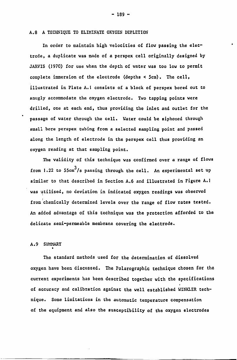
- 189 -

A.8 A TECHNIQUE TO ELIMINATE OXYGEN DEPLETION

In order to maintain high velocities of flow passing the elec

trode, a duplicate was made of a perspex cell originally designed by

JARVIS (1970) for use when the depth of water was too low to permit

complete immersion of the electrode (depths < Scm). The cell,

illustrated in Plate A.I consists of a block of perspex bored out to

snugly accommodate the oxygen electrode. Two tapping points were

drilled, one at each end, thus providing the inlet and outlet for the

passage of water through the cell. Water could be siphoned through

small bore perspex tubing from a selected sampling point and passed

along the length of electrode in the perspex cell thus providing an

oxygen reading at that sampling point.

The validity of this technique was confirmed over a range of flows

from 1.22 to 55cm3/s passing through the cell. An experimental set up

similar to that described in Section A.6 and illustrated in Figure A.I

was ~tilised, no deviation in indicated oxygen readings was observed

from'chemically determined levels over the range of flow rates tested.

An added advantage of this technique was the protection afforded to the

delicate semi-permeable membrane covering the electrode.

A.9 SUMMARY •

The standard methods used for the determination of dissolved

oxygen have been discussed. The Polarographic technique chosen for the

current experiments has been described together with the specifications

of accuracy and calibration against the well established WINKLER tech-

nique. Some limitations in the automatic temperature compensation

of the equipment and also the susceptibility of the oxygen electrodes

•

- 190 -

to oxygen depletion have been highlighted together with

recommendations to overcome these •

•

•

•

- 191 -

A P PEN D I X B

THE DEOXYGENATION OF THE

LABORATORY WATER

- 192 -

B.I INTRODUCTION

since the laboratory water was generally maintained in an oxygen

saturated condition by the recirculatory pump, it was necessary to

reduce the oxygen concentration of inflowing water such that even

after aeration the dissolved oxygen level was still significantly

below saturation.

B.2 VARIOUS MEANS OF REMOVING OXYGEN FROM WATER

The removal of oxygen from water in industrial processes for the

prevention of corrosion is usually effected by such processes as vacuum

deaeration whereby the water is induced to boil by application of

reduced pressures. Oxygen solubility is zero in boiling water, ho~ever,

absolute oxygen removal is required,andJit is after this stage that

chemical scavengers such as hydrazine and sodium sulphite may be

employed to remove remaining traces of oxygen. The respective reactions

of hydrazine and sodium sulphite with oxygen are as follows:

•

N2H4 + O2 -. 2H20 + N2

2Na2SOJ + O2 -. 2Na2So4

Hydrazine is generally used in waters of high temperature an~ has

adva?tages over the sodium sulphite in that it is volatile apd does

not affect the concentration of dissolved salts. Also it ha~ been

claimed to be a corrosion inhibitor (SHREIR. 1963). There is evidence

to suggest that the sodium sulphite reaction may have undesirable side

effects at high temperature such as production of S02 (Sl~IR) and

thus acidifying the water.

- 193 -

However a side reaction,whereby hydrazine is decomposed,yielda

ammonia - an undesirable smell to have in any laboratory. Sodium

sulphite was therefore used in the current studies.

The reaction between the sulphite ion and oxygen is extremely

slow at normal temperatures, but tests by PYE (1~47) showed that in

the presence of 0.01 ppm cobalt as a catalyst the water was completely

deoxygenated from saturation within IS to 20 seconds. In the absence

of a catalyst barely 0.2% of the total oxygen would have been removed.

B.l THE TECHNIQUE AND EQUIPMENT USED

Contact time between water and sodium sulphite was provided by

passage of water through a galvanised steel tank 1.51m x 0.9m x 0.75m

whence it flowed under constant head to the free overfall apparatus or

3 metre flume located on the floor below. This tank was fitted with a

baffle system to prevent short circuiting of flow between the inlet

and outlet sections (Figure B.l). The volume of this mixing tank

would therefore enable a total flow of SO lIs to be satisfactorily

deoxygenated according to PYE's findings above.

Both JARVIS and APTED used Mariotte vessels to provide a constant

dosing ~ate of sodium sulphite and cobalt chloride. However this

technique was abandoned here due to the inadequate capacity of the . vessels and difficulty encountered in maintaining a constant dosing

rate.

An efficient system was evolved utilising a 90 litre vessel in

which the measured quantities of sodium sUlphite and cobalt chloride

catalyst were dissolved with water. This solution was pumped by a

variable capacity Watson-Marlow Flow-Inducer (See Plate B.I) and

FlO 8.1 r-1!XING Tt,~IK tdlD Of:~;<'·GENI\TIi.Jtl SYSr('},1 .. --~ ... - ... _ ... __ .......... ~._.--... _______ ,. w~ ... -. ...... _",*,~ __ • ___ ._ ......... "-___ .l.o,i. ..... "._

f II • .... fC) ;t ~

II J, .

~ 1[------------ Ii __ JD o ---------=-::J::I3G , , \ , \~ \ ..(:; , " ' <.~ " ; ~ ,~ " ~ '" , ~ .• ::; \~~_:_\-~-r

ELEVATION -

~-~

- 1

PLAN --

@ floVi inducer ® d~oxYgenated Vloter supply pip~

@ Inlet from header tank aD nacdle va\v(!

@ overflow tank <D gate volvo

@ sodiurn sulphite solution (j) bafft~ plate

® siphon tub(: ® wire m~~h floY! dbporscr

CD mixlnu tank CD 90 titre v05:.nt

A

- 194 -

injected into the inlet pipe. Whilst the dosing rate could be regula-

ted by a rheostat control on the pump, a fine control needle valve was

installed on the suction side of the pump. The efficient mixing of water and

sodium sulphite solution was aided by a wire mesh flow disperser fitted

over the inlet to the mixing tank. To maintain a continuous supply of

sodium sulphite, a second 90 litre vessel was used for mixing the new

solution and this solution was then siphoned into the vessel from

which sulphite was already being extracted.

The system described above is illustrated in Figure B.I.

B.4 CALCULATION OF DOSING.RATE

The quantities of cobalt chloride added were always in excess of

O.Olppm. The stoichiometric requirement for the fixation of oxygen

is 7.88 ppm of sodium sulphite per ppm of oxygen.

Therefore if a discharge of Q lIs is to be deoxygenated from

saturation to an oxygen deficit D. then the quantity of sulphite

required is:

mgls of NaNO)

where the required oxygen deficit D is expressed as a:percentage of the •

saturation concentration C (mg/l) of oxygen in water. C will depend s s

on the conditions of water temperature and barometric pressure

prevailing and also on the dissolved salt level in the water - see

Equations 1.38 and 1.41 for estimates of C. Various oxyg~n deficits s

were used during tests.

- 195 -

B.5 A CHECK FOR SULPHITE RESIDUALS

In view of the rapidity of sulphite reaction and the large con

tact time provided by the mixing tank, sulphite ,residuals were not

anticipated.

The presence of sulphite is easily identified by iodide in acid

solution with a starch indicator. Sulphite present reduces iodide to

iodine which gives a blue colour with the starch. In the absence of

sulphite no colour is produced when the reagents are added to a

sample.

Recourse to this test did not prove necessary. iSulphite resi

duals were checked for during hydraulic jump tests by measuring

dissolved oxygen levels along the length of the flume. If sulphite

was present then the dissolved oxygen profile would have indicated a

drop in oxygen level along the length of the flume. No such drop was

found. Similarly, during a free overfall experiment, the lower pool

was maintained at maximum depth. The oxygen levels in the pool were

continuously monitored and when steady, the water supply to the weir

apparatus was shut off and the outlet from the lower pool was closed.

The oxygen level in the water held in the pool was then monitored for

several minutes. As with the hydraulic jump tests, no fall in the

oxygen level was observed thus confirming the absence of sulphite.

- 196 -

APPENDIX C

FREE OVERF ALL DATA - 100MM WIDE RECTANGULAR NOTCH

100 I J

Figutes CI.t to.Ct.7 Tests with tap water + 0.6% NaN03

Figures C2.t to C2.7 Tests with tap water + 0.3% NaN03

Figures C3.1 to C3.6 Tests with tap water

•

..

4 ..

4.5 . ~

H pool width / ___ e~. (em) 100

80 . E)

4.0 I- 100 + V ~d, , -0- "-... 125 157 ~

3.5 I 200 0 ,

/' --- ~ .J".

-0-~ ~

3.0 I / / /~~' ~~<t .u '~ 1.O ~

0 .--c 2.5 L. - /' /~

~- ~-~ 9 -+-~ u ~ / .--<!J

-0

2.0 ~ / :7~e~ ------\----It? /: c>

<:)

~

1.5l FIGURE C1.1

Q = 0.6 tIs

\ 1.0 0 5 10 15 20 25 30 35 40 45 50

downstream depth (em) -

4.5 H

(em) , 80

4.0 f.: 100

125 200

3.5

3.0 u

. -Ln

C

0

~ 2.5 I '-- I e-

O e-o.&-

W "'0

2.0

I 1,5

pool width ~ 100 ~ a

+ , 0 0/

/

~

b

/ , \\- -;

0

~ /

/9~ /4>

-------_ .. ---.. ---.. ----....... e ---------FIG U R E C 1.2

Q = 0.8 lis

-b ____ o

"Q

"

o

1.0 o. 5 1 '0 1'5. 2'0 2'5 3'0 3'5 ~'O ~'5 510

downstream depth (em) -,

4.5 I r

H pool width (em) 100 80 (!)

4.0 100 ; 125 , 157 -e-

3.5 200 0

3.0 u

.LJ')

,::-

~2.5 r /0 -u .--C!J '"0

2.0

1.5

1.0 0 5 10

~---~

-<!>-- --0-_________ _ -...,... ~

'1/.r;"-''1·~- -'a..'1~ . ~

{+..----* ---

15

-~-+--+-q---,-o 0 ____________ ~--__ __

---Q~----- 0 ---

FIG U R E C1.3

Q = 1.0 lis

20 25 30 35 downstream depth (em) ..

40

b"

45 50

..

4.5 ,

H poot width (em) 100 80 e

i..0 100 + 125 ~

3.5

157 .. 200. 0 o 4 ____ & .........

/ ~, o

-<;>-- ~

3.0

.~ c ~ o l, .--0 2.5 L--o

-& w ~~_ 9 ~

 ~ T T-fl-'i'

.--OJ -0

2.0 ,~-~- -9 ----c(>-T

o

-0

1.5 cb El , FIG U R E C 1.1.

Q = 1.5 lis

1.0 0 5 10 1S 20 ·25 30 35 1.0 45 50 downstream depth (em)

.0 Lf) ~

'-

0 .--0 '--u .--ClJ

"'0

4.0 .-, --r---r----.------,------,---~-._-_r_-__,_-I

H pool width ..

3.5

3.0

2.5

2.0

1.5

~ ... (em) 100 80 a

cbQ 0 J, 0 - ----6_ .r~

100 + .0

125 , 157 ..0-

200 d,

-& ~ -<!)-

/0 .~-&--&-

~-~ --~-------. ---r /-<>- ~ __ ~ __ ~ ol>~~ c!>_+ __ _ ~ ~ -+-

+-----;~(i)- e e" _CC)

~0

F t G U R E C 1.5

Q = 2.0 lis

G __

1.0 .~------~----~~----~------~------~----~------~------~----~------~ o 5 10 15 20 25 30 35 1.0 1.5 50 downstream depth (em)

4.5 H pool width

(em)' 100 80 f)

4.0 t- 1 00 ~ 125 ~.

157 -e-

3.5 200 . cl>

3.0 .u ({)

~

0 .--E 2.5 :!:: 0 .--QJ

'"'0

2.0

I ~

1.5

1.0 0 5 10

G . 0

-"----0 __ d.- <>

/1. -G-~ ------- . -----.... ~ .............. ~.

~ cp ~

~-- -~~9 , _____ . ----9 ,:,..-- • ~~_~ + 66 I;" ............. ~ ~ ~ + .,.~ 9T

____

fl

+~ " n~ ______ - Q--+~ '" '6 ?-

15

FIG U R E C1.6

Q = 2.5 lis

20 25 30

Q--------

35 downstream depth (em) ,.

o ---------8 L.O 45 50

.u If)

~

o 0-

1..5

H pool wid th (em) 100 80 c::>

4.0 1- 100 + 125 ~

157- .4).

3.5 I- 200· ~

245- +

3.0

"0 2.5 '--0-u ~

Q) "'0

2.0

1.5

1.0 0 5

~---+- -~- +----4:. / +

/¥ + ~ ~ .

+'" / y :; I . If' I. -e-/0 _

. -~ -Go-

-0, -----~ }...~ --------- b /T CQ (!) 0 -e _ .... .

~ e-~~ G ~ e _____ ~& ,0 Q~

-4>---

FIGURE C1.7

Q = 5.8 \/s

10 15 20 25 30 35 [,0 [,5 50 downstream depth (em) ~.

• I . , ...

; . , I , . I -fl. . I

1/ . I .

Ii ~!

I . I -¢=' I ; . i 1-4> . ,

.i. . I I I i . I

~ . I

~ -e¢ , \

...., \ -e

\ \

. \ \ •

'-0 ~ . \ \ \ . \

\ \

- I ELO • .. + -- +1 ~..- I

.c -t-....:

• Q- + ... +1 "0 ._ ....r ~ I

0 0 ~ -G -{>- I 00 Q E>-a:...-

-LnlDt""-O It)

:J:EONLOO -..t .gCO..- ..... N N

a L() 0 • • • ....: M M

-41 ~oSLJ i

I • (J

Q .. I. Q"

To-I

tq.e-

~ 0-

, <t

0

~ \ \ e •

L() 0 L()

• • • N N .....

onOJ l!~!!ap

/ G

..-. N U

~ -'

UJ lO

0:: • 0 ::> II

C!) 0'

LL

0 • ~

a tn

If') ....r

0 ....:

If') M

0-M E

.g

.c -+J 0. C!J

If') -0

N E 0 <V ..... ..... l/) C

0 ~ N 0

"'0

Ln' ~

0 ~

0

. ,

, , , ... , 4-I, . /,

/ i I I , .q. i ,

. I I , i I I I ; ... -¢-t :

+ i :

-

i I . I , , \-+& \ ' . \ \ \

\ \ . \

-9: 0', 0\ . \ \ \ . \ \ \

\ \ \ \ . , , \

" .

~~ ... + ... + -.c ~j(J~~-4+1 --'

00 I 0 0 C) 0- ¢.a-t c. ......

-I/) to ...... 01.0 E·· ~~ J:uONI.OO...t

_CO ........... NN

o M

rl I . I !

" +t* I

~" I, II . I I I I I

;... 1.1 'i' i<r I

I , . , ~ \

I

Q

()

•

\ \ 0-

~ e\ 11'-\ 4

\

t.n • .....

N •

N U

UJ 0::

:J (!)

u..

cD • o

II

a

o • .....

o If)

tIl M

O-M E o

I/)

-.c. ~ c. ~

N E c Q) '--til C

o ~ N 0

"'0

an ..-

o

I ~

I

. .f I .I I

:j 'i' I. I ,

/1 • I I, . I

1+ . , I I

j4 ~ . I . . I ,

I , l-t \ \ \ \

\ \ . \ \ \ . ,

\. \ \ \

, \ \. , '-t\

, \

\. \ , , , \ '. , , ,

" \\

" ~ " I, '~ ,

IJ) o IJ) . M •

M •

N

~

/ J 9

..

o • 9 0

./

M . N U .

\ . , l.L.

'\ 't

o . IJ) • ......

o • ......

II

cr

o • ......

o LO

LO M

0-cYl E

c.,) -.c ...., 0-Q)

10-0 N E

c QJ L. ...., Vl C

o ~ N.g

o ......

o

, .Jfi w

jYI I . II 1.1

'I! I

I~

LI /il

, -0

-Ii- i1 i I ; I.... , ; II I . , I , , I

+ I 1 . , ~ , I

I, .... ' \ I

~ ~

I

, I

\ \ \ _~ \ -a\~,,\ ~\ \

\ \ . \ \. , ~ \

+

\ , \ \

\\ '\ -(;l\'\ \.' \ ., \ ... ~ \ -e \ \.~ .,~ \

I

+ -0 + : I

.~ \ ~ \ ~

~\

*

-'0

[~ 0 ~ c} ~ 1- I .-Lf)lOr;-..,.OLf) :r:EONLf)O~ ~CX)"-"-NN

l.l) o • . ('t') M

4

an •

N

-0

\

o •

N

o

t.n • .-

~ •

N U

u.

•

LO •

or-

II

o

o • .....

o U')

LO M

0-ME u

LO

-.J::. ~ 0-OJ

-C

NE . 0

OJ l-

t) c

03: N.g

LO .....

o .....

o

,

-

f , ; ; . I + ,

't H H)

I ,

i ' .0-' I ,

i \ . \ I , .... \ I

ILL • \

7f \ \ + . \ \ . \

\ \

\ \ \ \ . \ \ \ ++ \ \ \

\ \ -0

\ \ -~ . \ \ \ . \ '. \ \ \ \ \ \ \ \ ~ \ '"'f,...C)

. \ \. ,

\ \

" -+-

~~ ... +-..,--

LO o L() 0 • • • M N ('oJ

• M

.... ~.S~J OnOJ l!::lUuP

•

LO • .....

•

t.() •

N U

W 0::

~

(!)

\

-o

• N II

C1

g ..-

o Ln

o ...:

LO M

o-M E

,g

..c ....... ~

LO"C

N E o Q.I '-

"til c

o ~ N.g

o .....

o

4.0

• I·

3.5

3.0 U

-LO ~

0 - 2.5 a '--.-u .-

"I-(1J

"'0 2.0·

1.5

1.0 o

H pool width (em) (em) 100 44 15 BO.5 Q Q • 126 9 t , 157 -Q.- .Q. ---200

..b- f

~ • • • -<?--0- f

21.5 -~ .0- f :.9-- -'t' -e- _-0--,.. .I. .~ ______ • _iir -lr · • , •

- -- ----- -Q. ,

~

~.~-A-J, -:~

e .,.

~

~ . ~ ~r;r~r -o=-<r

- e-

~ ~-& _Q- -0-

.0-

y~'i'_'J. . " 'i' f 'i't-,-'- ,,-7 ,-'w. ---cr_

~,. --- . Q_O- 0 ---------.-0---Q-----~~--~.Q---~--__ _ _____ Gfi) G E)

~------ -----Q--o. --. FIG U R E C2.6 c:;p--

5 10 15

Q = 2.5 lis

20 25 30 downstream depth (em)

35 40 45 50

1..0

H pool widt h (em) (em) 100 .44 15

, 80.5 G) Q • 3.5 126 ., . , ,

157 ..Q- -0- -... .200 A, ~ •

3.0 U

21.5 ~- -+- -+-..... _.-. ----- -{>- -9-

-tn ~.

o

C 2.5 '- . -u -<l1 '"C

2.0

~

,~+_cb_---<"'" -+- b<}:

./ _k ...----- 4'" '+' /+ r . b~-~o-~- + -:.<io}-_ ~~ 0-

...--~---~--.."...? ~ -------9 __

o~ CO)

_0 0 0 __ 0-

1.5 FIG U R E C2.7

Q = 5.0 lis 1.0

0 5 10 . 15 20 ·25 30 35 40 45 50 downstream depth (em)

U -1.0 or'-

o .-

4.0 H

(em)

80 3.5 J- 126

157 200

3.0

o 2.5 '--·u ..-Q)

-c 2.0

1.5 l-

I 1.0

0

pool width 44 g

~ ~

e

/-

5 10

FI GURE C 3.1

Q = 0.6 lIs

---------~----------~ -------~--

~ ---- -Q-- _o-Q- ____

--,,- ,."

"_ G-= Q-g

II' -------- .CIi) ----15 20 25 30 35 40 1.5 50

downstream depth (em) '"

4.0 H pool width

(em) 44 80 (i)

3.5 I- 126" 1> 157 ~

200 6

3.0 .u

L{)

~

0 .-o 2.5 '--u ~

OJ -0

2.0

1.5

1.0 o 5

FIG U R E C32

Q = 0.8 lis

~--------e------________ ~

~ / e ='>: -e-. --------- ~ ---

~4r ~-----, ~

_______ , - -Cf ---

-

_Q Q Q 0

~

10 15 20 25 30 35 40 downstream depth (em)

-$--

45 50

:

4.0 H

(em)

80 3.5 ~ 126

157' 200

3.0 u

.Lf) ~

L-

0 .-o 2.5 '-

..... u -(lJ

"0

2.0

1.5

1.0 o

pool width' ,," Q'

~

-e-

e

/~

5 10

FIG U R E C3.3

Q = 1.0 lis

___ -4--------'---Q-------------------

15 20 25 . 30 downstream depth (em)

~ ---

35 1.0 1.5 50

1.0 o 5 . 10 15

FIG U R E C3.4

Q = 1.5 lIs

.;- e 6_

---- ---------------~g~---------------:-Q- . --Q--

-----1l-' -'TT __

~-Q - Q----------Q-

20 25 30 35 40 1.5 downstream depth (em)

50

, 4.0

H (em)

80 3.5 l- 126

.0 U')

~

o .-

3.0

o 2.5 '-..-u -CJ

"'C

2.0

1.5

1.0

•

157 200

o

pool width. 44

Q

~.

-Q-

~

~6

5 10 15

FIG U R E C3.5

Q = 2.0 lIs

·e ~ e

-~ ------........ - -Q---

---- ~~ -- 'j'-, 'i'T

a 8 Q -l'\ ~ _________ _

-- • -1;)-

20 25 30 35 40 45 50 downstream depth (em)

4.0

3.5

3.0 .u

LO ~

0 -a 2.5 '--u 0--(!J

"0

2.0

1.5 f

1.0 o

..

H pool width (em) l. 4 157 ~

200 e

5 10

FIG U R E C3.6

Q = 2.5 lIs

. . e _______ e- e A----~e~- ~- -- ~ ~ e-~ ~ ~

15 20 25 30 downstream depth (em)

35 1.0 45 50

- 197 -

APPENDIX D

FREE OVERF ALL DATA - 220MM WIDE RECTANGULAR NOTCH

220

Figures DI.I to DI.4 Tests with tap water + 0.3% NaN03

Figures D).I to D2.3 Tests with tap water

, .

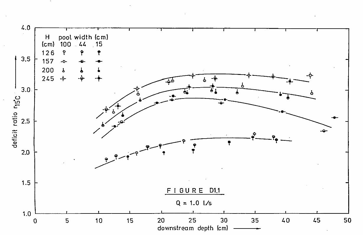
o ·LO ~

'-

o

4.0

3.5

3.0·

a 2.5 '---<.) .--QJ

-0

2.0

1.5

1.0 o

H pool width (em) (em) 100 . 44 15

126 f ~ t 157 ~ 200 J,

245 -~

-Q-

~

-/r-

... ~

+ ~ <f--;----:l---

. +....- '... + . / ",,,,~.. &' b -~ -~/ ~ ... -.... - .\ / b */ :;.. -.~ $ ~ / /___ -e-

5

. _'_'T--~ ... .-7' _,-'i' , ; ,''T, -:..

10 15 20

FIG U R E D1.1

Q = 1 .. 0 1/5-

25 30 downstrea m depth (em)

35 40 1.5

----Q-

50

4.0 H pooL wi dth (em)

(em), 100 lJ. 15

,126 '" " 1'. 3.5 I 157 -&- -Q- ...

200 o. I 1>, 8"

21.5 ..0- ..Q.. + , ,

3.0

.u LO ~

0

=c 2.5 '-...-.-u "'-OJ

"'0 2.0

1.5

-tr ~---------=-=-= -+=

/

+,-- --------~---~~- --",;or

-0- ,.,'" . ",'"

" ,," ,,/

~// ~ ,

,,'" ","

..,

Q "b-~_-,----e. • -.. I -e- ::e ____

.;-

., T ---'1'-(0)-------' f~

FIG U R E D1~2

Q = 1 .82 lIs

1.0 ~l ________ ~ ________ ~ _____ ~L_ _____ ~ ______ _L _______ ~ _______ L_ ____ ~ ______ _L ________ ~

a 5 10 15 20 25 30 35 1.0 1.5 50 downstream depth (em) ..

0 ~ t.n

-J,- ~I ./ +' ~ -4)

~~ + 7 t.n ... ....:

+ • I I

~

G 0 ....: ,

... -e •

-0- ..... I -t+. ... t.n

M

1 0

0-I ... ME ... M U I -. ~ .r::. 0 Ul +J

"- 0-- Q)

UJ t.n "0

a= . ~E C'J ::::> II

0 OJ

C!) CJ

L.. +J Ul c

LL O~ C'J-o

t.n -4) ~

\ -ELO .. + ... -+-

0 O~ ~ -.c :o~ -- 0 -e + .- ~ ~ •

-0 go e- ; 4>';-a.~

- to t""- O t.n :r: E N t.n 0 ....: u

~ ~ N N -0

0 to 0 to 0 to 0 • . • • • . .

-....t M M N N ~ or-

.... ~.S~J OllOJ l!:l!Jap "

4.0 H pool width (em)

(em) 100 44 15 80.5 G e •

3.5 ~ 126 , , , 157 .'

-0.. -Q- .. -200 ~ • •

u 3.0 r 245 + ..0- + . ,

4 ~ ~-·tn <or- • +-- . '-

=+-~ ~ 2.5 ~ b_ .t~ -I.-

~-- --o4J

u #~~..,.-

--Go-

:& 2.0 l .0-o-~

G -0"

~ (j> 9 ~~9-- ------i'_

", Q --0 &-

1.5 i-I) Q __ e--

FIG U R E Ott.

Q = 5.0 lIs I

1.0 0 5 10 15 20 25 30 35 1.0 1.5 50

downstream depth (em)

4.0 H

(em)

J. 3.5 ~ 157

L) eU)

~

o

3.0

C 2.5 L..

...... u .--C!J

-c 2.0

1.5

1.0

200

o

pool width

1 5 --e-

44 •

5

FIGURE 02.1

Q = 1.0 lis

--e e ~

..e- -. _______ _ ----- ---:.-~ ~ . -e-__ ___ --- --

10 15 20 25 30 35 40 45 50 downstre a m depth (em)

4.0 I

H pool wi-dth (em) 44 15 80 e

3.5 I- 157 ~ FIGURE 02.2 .....

200 • Q = 1.82 lis

u 3.0 I e

"l,{)

~

_0

J,$ - e - 2.5 ~

0

~ .---'--lJ --- ---• :.0- ...-- .. ---

:;:: - -e-

--0-QJ

-0- ---'"0

~~~ -0-0-2.0 -G-

...Q-.".,

1.5 ~ Q ~ Q-

Q -

Q

1.0 o 5 10 15 20 25 30 35 40 [,5 50

downstream depth (em) r

U etJ')

~

o

4.0 H

(em)

3.5 t- 80 157

3.0

-0 2.5 '-..... u

:;:: (lJ

"'0

2.0

1.5

1.0 o

pool width 44

Q

-Q-

5

FIGURE D2.3

Q = 2.5 lis

----Q- -..Q~

~-o-

_Q Q 8 ___ _

Q- -g

10 15 20 25 30 35 40 45 50 dov/nstream depth (em) )0

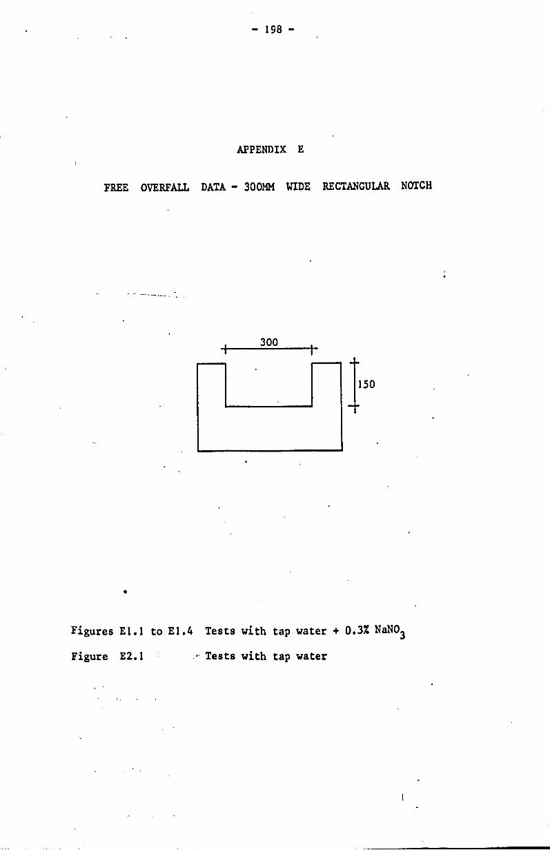
- 198 -

APPENDIX E

FREE OVERFALL DATA - 300MM WIDE RECTANGULAR NOTCH

300

•

Figures EI.I to EI.4 Tests with tap water + 0.3% NaN03

Figure E2.1 ,.' Tests with tap water

4.0

3.5

3.0 U

-m ~

o ~ e 2.5 ~

o -C!J -0

2.0

1.5

H pool width (em) 100 44 80.5 126 157 200 245

G Q , , ..0- -Q-

d, • -+ + ~+--,--~- :& - -"1[:--

I

b ~

• ~ --=-----~.----~/~e~

____ of /.!. ~ .. t-g /' /'/ T-1L- ,

~

--.s;r~

'--/' .,,/'

Q'-------g Q------------Q-

FIG U R E E1.1:-------------Q

Q = 1.5 lis

~

1.0 1'--__ ---1-__ -----IL--__ ..l.--__ -L-----L-----L-_--IL-__ l-__ ...!-__ ..l

o 5 10 15 20 25 30 35 1.0 1.5 50 downst rea m depth (em)

I

~

-0

-9-

...

+\ ~

\ " , . , .t: =O....t . - ~ ... ~ -e -; . ~ -0

+ go 0- -G + 0.'-- lD t'- 0 tn

:I: E N tn 0 ~ U N N - or- ...-

0 tn 0 LO . • . • ~ ("I") ("I") N ... 8.S~J O!lDJ

/ 0-

N or-'W

Vl "--W 0 a: • N

:::> II (!)

0

u...

\

0 LO • •

N ...-

U:>!lap

...

0 • .-

o Ln

0 ...:

Ln ("I")

0 M

Ln N

0 N

LO .-

0 .-

0

-E .,g

.t: ~

0. OJ

-0

E 0 CJJ '-o4J

~ ~ 0

"0

U elf)

~

o

4.0

3.5

3.0

a 2.5 L.. -U -QJ

"'0

2.0

1.5

H pool wi dth (em) 100 44 80.5 e e

126 9 , 157 -0- -Q-

200 c!> ~

245 -+- -+- ~

c!>~ _~....- ~ e ¥ ~e ____ / ~~~~ - ~ 4'./' ____ 'i'- _t. ----/~.........-- 'P -e-__

~-...

Q Q ~Q- -1;>-

.----------Q--------- .

FIG U R E E1.3

Q = 2.5 lis

1.0 'r------~----~------L-----~--~--~----~------~----~------~----~ o 5 10 15 20 25 30

downstream depth (em) 35 40 45 50

4.0

3.5

3.0

.~ ~

o C 2.5 '-..-.-o -OJ -0

2.0

1.5

1.0 o

H pool width (em)' 100 80.5 e

126 157 200 245

, -0..

b

+

5

-b-•

______ -6--9-~~ -9-..___4 · .. --- =-.Jkfr-• ___ c!.- I. · - - · ".___ -'r-

----6 ----&. -0. ~~

-9 __________ 9_

"",,;<>

~9~~'

~o- 0 Q.--~ __ ~ 0

10 15 20

FIG U R E E1.4

Q = 5.0 lis

25 30 35 downstream dept h (em) •

40 45 50

~ • N W

~ -W a: LJ")

• N

::> II

(,!) 0-

LL

- ,

. .. ..... ..c. -"0 .-~~ ca (J.. cp-t> -~ 0 0 a. - to t'-- 0

':I: E 0 N LO 0 oro ~ .- N -

0 1.0 0 • • • ~ (Y) M ...

I

~

c) ,

-4)

'-

~~\. \ \

().

\

LO q • N C'I

8.S~J O!lDJ l!:l!Jt>P

()

()

()

LO 0 • • ~ ~

o LJ")

o ...r

LJ") (Y)

0-(Y) E

0 -.c. -a. (!J

"0 LO N E

C Q) L--til c

o ~ N"O

LO ~

0 ~

0

- 199 -

APPENDIX F

FREE OVERFALL DATA - TWIN CRESTED NOTCH

. I 100,SO, 100 I

r---

,

•

Figures Fl to F3 Tests with tap water·

I .

4.0 i.

.u If)

~

o

3.5

3.0

C 2.5 '--.-o .--(I)

"0

2.0

1.5

1.0 o

H pool width (em) 100 44 8f G &

126 y. , 157 --&- -Q-

200 b ~ d>

-Q-__________ I

++ · .. ~":c?:~

245 + -~ .J,- ~:-------

-Q-

~'i'-? ' f

~~ /"t Q gQ Q_

----- "-------5 10 15

FIG U R E F1

Q = 1.2 tIs

20 25 30 35 downstream depth (em) ;

b

~--

1.0 1.5 50

1..0 H

(em)

81 3.5 126

157 200

3.0 21.5

.u It)

~

0 .-- 2.5 0 '--u .--OJ

"0 2.0

1.5

1.0 o

pool width 100 1.1.

el 8

f , -<:>- -0-

0 • .~ +

~9

5 10

.+ :-~ -4-

b G • ~ $

8-:

,,-" 9

, _______ IP ______ 9 .

Q- -0 g-----OQ-~OZ!---__ g _____

--- Q--

15

FIG U R E F2

Q = 2.0 lis

20 25 30 dOY/nstream depth (em)

35 1.0

9---0.. '--..

e_

----------cr __

1.5 50

U -to c-

'0 .-

4.0

3.5

3.0

15 2.5 '--.-o -OJ

"'0 2.0

1.5 r

, 1·0

'0

H pool width (em) 100 44

81 0 8

126 1> , 157 -60 -g.

200 J, J. 245 + +

5

c

.. Ir - ~ -+~A _~.; -9- _~ ..0-• ,+-~~

~

~~--$-~~ ~ b~ -a- -[, -b-

/' _______ IF ----..: -ffF

-----'(----~fIl-- -? ____

F I 'G U R E F3

Q = 2.5 lis

10 15 20 25 30 35 l.0 45 50 downstream depth (em)

- 200 .:.

REFERENCES

•

• - 201 -

ADENEY, W.E. and BECKER, H.G. (19J9). The determination of the rate of solution atmospheric nitrogen and oxygen by water. Part I. Phil. Mag. ~, 225, 317-337.

ADENEY, W.E. and BECKER, H.G. (1920). The determination of the rate of solution of atmospheric nitrogen and oxygen by water. Part II. Phil. Mag. ~, 232, 385-404.

ALBRECHT, D. (1968). Beluftung des Ruhrwassers am wehr Spillenburg. Die Wasserwirtschaft 11, 317-321.

APTED, R.W. (1975). The mechanics of aeration at weirs with special reference to river quality. M.Sc. thesis, University of Newcastle upon Tyne.

APTED, R.W. and NOVAK, P. (1973). Some studies of oxygen uptake at weirs. Proc. XV Congress I.A.H.R., Paper B23, 177-186.

AVERY, S. and NOVAK, P. (1975). Oxygen uptake in hydraulic jumps and at overfalls. Proc. XVI Congress I.A.H.R., Paper C38, 329-337.

BAIRD, M.H.I. and DAVIDSON, J.F. (1962). Annular jets. II Gas absorption. Chem. Engng Sci. 11, 473-480.

BARNHART, E.L. (1969). Transfer of oxygen in aqueous solutions. Proc. A.S.C.E. ~, SA3, 645-661.

BARRETT, M.J. and GAMESON, A.L.H. and OGDEN, C.G. (1960). Aeration studies at four weir systems. J. Watt Watt Engng~, 207-213 •

• BENSON, B.B. and PARKER, P.D.N. (1961). Relations among the solu-bilities of nitrogen, argon, and oxygen in distilled water. J. Phys. Chem. ~, 1489-1496.

BEWTRA, J.K. and NICHOLAS, W.R. (1964). Oxygenation from diffused air in aeration tanks. J. WPCF 36, 10, 1195-1224. -BEWTRA, J.K. and NICHOLAS, W.R. and POLOKOWSKI, L.B. (1970). Effect of temperature on oxygen transfer in water. Watt Research~, 115-123.

- 202. -

BLACK, W.M. and PHELPS, E.B. (1911). The discharge of sewage into New York harbour. Report made to the Board of Estimate and Appointment, New York City.

BOWERS, R.H. (1955). The mechanics of bubble formation. J. appl. Chem. 2,. 542-8.

BRIERLEY, M.R. and STEEL. R. (1959). Agitation-Aeration in 8ubmerged fermentation. II Effect of solid disperse phase on oxygen absorption in a fermentor. Appl. Microbio. 1, 57-61.

BRIUZN, J. and TUINZAAD. H. (1958). The relationship between depth of U-Tubes and the aeration process. J. Am. Watt Wks Assn 2Q. 879.

CAMPBELL, F.B. and GUYTON, B. (1953). Air demand in gated outlet works. Proc. Minnesota Int. Hydraulics Convention, 529-532 •

• CHARLTON, J.A. (1970). The air control of self priming siphon spillways. Ph.D thesis, King's College, London.

CHURCHILL, M. (1961). Effect of water temperature on stre~ reaerationa 31. Progress Report on sanitary engineering research. Proc. A.S.'C.E. !l, SA6, 59-71.

CHU~CHILL, M.A. and ELMORE, H.L. and BUCKINGHAM, R.A. (1962). The prediction of stream reaeration rates. Proc. A.S.C.E. 88, SA4,

-i

1-46.

COPPOCK, P.P. and MEIKLEJOHN, G.T. (1951). The behaviour of gas bubbles in relation to mass transfer. Trans. Inst. Chem. Engrs 29, 75-86. -

• DANCKWERTS, P.V. (1951). Significance of liquid film coefficients in gas absorption. Ind. Engng Chem. 43, 1460-7. -DEPARTMENT OF THE ENVIRONMENT (1973). Notes on water pollution, No. 61.

DEPARTMENT OF SCIENTIFIC AND INDUSTRIAL RESEARCH (1958). Water pollution research, 1957. H.M.S.O •• 15-16.

DOBBINS, W.E. (1962). Mechanisms of gas absorption by turbulent liquids. Advances in Watt Poll. Research 1. -

- 203 -

DOWNING, A.L. (1958). Aeration in relation to water treatment. Proc. Soc. Watt Treatm. Exam. I. 66-101.

DOWNING, A.L. and TRUESDALE, G.A. (1955). Some factors affecting the rate of solution of oxygen in water. J. apple Chem. ~. 570-581.

DRESNACK. R. and METZGER I. (1968). Oxygen response and aeration in streams. Proc. 23rd Ind. Waste Conf •• Purdue Univ •• Part I, 262-274.

ECKENFELDER. W.W. (1959). Factors affecting the aeration efficiency of sewage and industrial wastes. Sew. Ind. Wastes 31. 1. 60-70. . -ECKENFELD~R, W.W. and BARNHART, E.L. (1961). Effect of organic substances on the .transfer of oxygen from air bubbles in water. J. Amer. Inst. Chem. Engng I. 631-4.

ECKOLDT, M. (1962). "Die Kunstliche beluftung der fluBse. Deutsche Gewasserkundliche Mitteilungen. No.1. p.l.

ERVINE. D.A. and ELSAWY, E.M. (1975). The effect of a falling nappe on river aeration. Proc. XVI Congress I.A.H.R., Paper C45, 390-398.

FASSO (1956). outlet works.

Experimental ,research on air entrainment in gates Milano.

FOX, C.J.J. (1909). On the coefficients of absorption of nitrogen and oxygen in distilled water and sea water. and of atmospheric carbonic acid in sea water. Trans. Far. Soc. ~. 68-87.

FOULK, C.W. and MILLER. J.N. (1931). Ind. Engng Chem. 12. 1283.

•

GAMES ON , A.L.H. (1957). Weirs and the aeration of rivers. J. Inst. Watt Engrs, 11. 477-490. -GAME SON , A.L.H. and ROBERTSON. K.G. (1955). The solubility of oxygen in pure water and sea water. J. apple Chem. 5, 502. " -GAMESON, A.L.H., VANDYKE, K.G. and OGDEN. C.G. (1958). The effect of temperature on aeration at weirs. Watt Watt Engng 62, 489-492. -

1 ,

- 204 -

GANNON, J. (1967). Aeration of waste treatment plant outfall structures. J. Wat. Wastes Engng i, 4, 62-65.

GREEN, E.J. (1965). A redetermination of the solubility of oxygen in sea water and some thermodynamic implications of the solubility relations. D.S.R. 9337, Contract GP-486 Nat.Sci. Foundation, Dept. Geol. Geoph., Mass. Inst." Tech.

GUYTON, B. (1958). Field investigation of spillways and outlet works. Proc. A.S.C.E. ~, BYl, Paper 1532.

HABERMAN, W.L. and MORTON, D.K. (1956). Experimental study of bubbles moving in liquids. Trans. A.S.C.E. l!l, 227-250.

HAINDL, K. (1958). Theory of the hydraulic jump in closed conduits and its use in practice. Vyzkumny ustav vodohospodirsky prace a studie. SeBit 98, Praha-Podbaba.

BAINDL, K. and SOTORNIK, V. (1957). Quantity of air drawn into a cond~it by the hydraulic jump and its measurement by gamma radiation. Proc. VII Congress I.A.H.R., Paper 031, 1-7.

HART, I.C. (1967). Nomograms to calculate the dissolved oxy~en contents and exchange coefficients. Water Research!, 391-5,

HATFIELD, W.O. (1941). Sew. Wks. J. 11, 557.

HENDERSON, F.M. (1967). Open Channel Flow. MacMillan, New York.

HIGBIE,.R. (1935). The rate of absorption of a pure gas into a still liquid during short periods of exposure. Trans. Amer. Inst. Chem. Engrs 11, 365-389.

HISE, R.E. (1975). A model of gas dissolution in water. S~p. on Reaeration Research. A.S.e.E. Hyd. Div., Glenstone Lodge, Gatlinburg, Tennessee.

HOLLER, A.G. (1970). Reaeration of discharge through hydraulic structures. U.s. Army Corps of Engineers.

- 205 -

HOLLER, A.G. (1971). The mechanism describing oxygen tranlf~r from the atmosphere to discharge through hydraulic structures. Proc. XIV Congress I.A.H.R., Paper A45. 373-382.

HOLROYD. A. and PARKER, H.B. (1949). Investigations on the dynamic. of aeration. J. and Proc. Inst. Sew. Purif., Part 3, 292-323.

HORENI, P. (1956). Disintegration of a free jet of water in air. Vyzkumny ustav vodohospodarsky price a studie. Seait 93, PrahaPodbaba.

IMHOFF, K.R. and ALBRECHT, D. (1972). Influence of temperature and turbulence on the oxygen transfer in water. Advances in Watt Poll. Research, Jerusalem.

INTERNATIONAL CRITICAL TABLES (1925). McGraw-Hill Book Co., New York.

IPPEN, A.T. and CARVER, C.E. (1954). Basic factors of oxygen transfer in aeration systems. Sew. Ind. Wastes, 26, 7, 813-827. . -ISAACS, W.P. (1967). Atmospheric oxygenation and biological deoxygenation in an idealised stream1low model. Ph.D. thesis, Oklahoma State University.

ISAACS, W.P. and MAAG. J.A. (1968). Investigation of the effects of channel geometry and surface velocity on the reaeration rate coefficient. Proc. 23rd Ind. Waste Conf., Purdue Univ., 619·639.

JARVIS, P.J. (1970). A study in the mechanics of aeration at weirs. M.Sc. thesis, University of Newcastle upon Tyne •

• JOHNSON, P.L. and KING, D.L. (1975). Prediction of dissolved gas at hydraulic structures. Symp. on Reaeration Research, A.S.C.E. Hyd. Div., Glenstone Lodge, Gatlinburg, Tennessee.

KALINSKE, A.A. and ROBERTSON, J.M. (1942). Entrainment of air in flowing water - closed conduit flow. Proc. A.S.C.E. ~. 1141-1153.

KAPLOVSKY, WALTERS and SOSEWITZ (1964). Artificial aeration of canals in Chicago. J. WPCF 36, 463-474. -

- 206. -

KARTHA, C.V. (1968). Effects of inflow conditions on the hydraulic jump. Master of Applied Science thesis, University of Toronto.

KISHINEVSKI, M. (1955). Two approaches to the theorotical aspect. of gas absorption. J. Appl. Chem. Russia.

KLOTS, C.E. and BENSON, B.B. (1963). oxygen and argon in distilled water.

Solubilities of nitrogen. J. Mar. Research 21.48-57. -

KRENKEL, P.A. and ORLOB, G.T. (1962). Turbulent diffusion and the reaeration coefficient. P·roc. A.S.C.E. ~. SA2. 53-83.

LEUTHEUSSER, H.J. and KARTHA, V.C. (1972). Effects of inflow condition on hydraulic jump. Proc. A.S.C.E. 2!. HY8. 1367-85.

LEUTHEUSSER, H.J., RESCH, F.J. and ALEMU, S. (1973). Water quality enhancement through hydraulic aeration. Proc. XV Congress I~A.H.R. 1, · Paper B22, 167-175.

LEWIS, W.K. and WHITMAN, W.G. (1924). Principles of gas absorption. Ind. Engng Chem. li, 1215-1220.

LE BOSQUET, M. Discus'sion of "The oxygen sag and DO relationships in streams" by H.W. STREETER in "Oxygen relationships in streams" Tech. Rept W58-2, Robert A. Taft Sanitary Engng Centre. U.S. Public Health Service. '

LIN, T.J. and DONNELLY, H.G. (1966). Gas bubble entrainment by plunging laminar jets. A.I. Chi E. Journal 11. 3. 563-571.

LONDONG,'D. (1967). Flusswasserbeluftung an der Lippe. Lecture given in the "Haus der Technik", Meeting No. 104, May 17 & 18, Essen.

MANCY, K.H. and OKUN, D.A. (1960). Effects of surface active agents on bubble aeration. J. WPCF ~. 4, 351.

MANCY, K.H. and OKUN, D.A. (1965). The effects of surface active agents on aeration. J. WFCF 37, 212-227. -MANCY, K.H. and OKUN, D.A. (1968). Discussion of a paper by VAN DER KROON (1968). 4th Int. Conf. on Wat. Poll. Research, 231-239.

- 207. -

MASTROPIETRO, M.A. (1968). Effects of d~ reaeration on waIte assimilative capacities of the Mohawk river. Proc. 23rd Ind. Waite Conf., Purdue University, 754-765.

MITCHELL, R.C. (1973). U-Tube aeration. EPA-670/2-73-03I, Environmental Protection Techn. Series Project No. 17050 DVT, U.S. Covt. Printing Office, Washington D.C.

MONTGOMERY, H.A.C., THOM, N.S. and COCKBURN, A. (1964). Determination of dissolved oxygen by the Winkler method and the solubility of oxygen in pure water and sea water. J. apple Chem. 14, 280. -MOORE, W.L. (1941). Energy loss at the base of a free overfall. Proc.- A.S.C.E. 21., 1697-1714.

NAKASONE, H. (1975). Derivation of aeration equation and its verification - Study on the aeration at falls and spillways (I). Trans. J.S.I.D.R.E., 42-48.

NATERMAN, E. (1952). Eine neue berechnungsweise des sauerstoffhaushaltes veruntreinigter flusse nebst einigen folgerungen. C.W.F., No 16.

NEGULESCU, M. and ROJANSKI, V. (1969). Recent research to determine reaeration coefficient. Water Research 1, 189-202.

O'CONNOR, D.J. and DOBBINS, W.E. (1956). Mechanics of reaeration in natural streams. Proc. A.S.C.E. 82, SA6, Paper 1115.

, -OGDEN, C.G., GIBBS, J.W. and GAMESON, A.L.H. (1959). Some factors affecting the aeration of flowing saline water. Watt Waste Treatm. Journal 1, 392-6 •

•

OWENS, M. and EDWARDS, R.W. (1963). Some oxygen studies in the river Lark. Proc. Soc. Watt Treatm. Exam. 12, 126-145. -OWENS, M., EDWARDS, R.V. and GIBBS, J.W. (1964). Some reaeration studies in streams. Int. Jour. Air and Water Poll. 8, 469-486. -PALLADINO, A.J. (1961). Investigations of methods of stream improvement. Ind. Water and Wastes i, 3, 87.

PASVEER, A. (1955(i». Research on activated sludge. VI Oxygenation of water with air bubbles. Sew. Ind. Wastes 27, 10, 1130. -

- '208 -

PASVEER, A. (1955(ii». Untersuchungen uber das bclebt schlammverfahren fur die reinigung von abwasser. Ces.-1ng., P. 332.

PETERKA, A.J. (1963). Hydraulic design of stilling basins and energy dis·sipators. Engng. Monograph No. 25, U.S.B.R., u.s. Covt. Printing Office, Washington D.C.

PETRIKAT (1958). Vibration tests on weirs and bottom gates. Watt Power.

PHILPOTT, J.A. (1952). Ph.D. thesis, University of London •

.. POPEL, H.J. (1972). Aeration and gas transfer. Delft Univ. of Techn. Depart. of Civ. Engng, Div. of San. Engng. '

PYE, D.J. (1947). Chemical fixation of oxygen. J. Am. Watt Wks Assn 2i, 1121-7.

QUIRK, LAWLER and MATUSKY (1966). Study of the assimilatioq capacity of the St. Louis river from Cloquet, Minnesota to Lake Superior. Report to Northwest Paper and Wood Conversion Comp~ny.

RAO, N.S.L. and KOBUS, H.E. (1975). Characteristics of lelf-aerated free surface flows. Water and Waste Water Current Research and Practice, Vol. 10.

ROUSE, H.T., SIAIO, T.T., and NAGARATNAM, S. (1959). Turbulence characteristics of the hydraulic jump. Trans. A.S.C.E. 124, 926-950. -RAJARATNAM, N. (1962). An experimental study of air entrainment characteristics of the hydraulic jump. J. Inst. Engrs of India 42, -No.7. .'

RENNER, J. (1973). L~fteinmischung beim aufprall eines cbencn wasserstrahls auf eine wand. Doktor-Ingenieurs dissertation, Universitat Karlsruhe.

RESCH, F.J. and LEUTHEUSSER, H.J. (1971). Mesures de turbulence dans le ressaut hydraulique. La Houille Blanche, No.1, 17-32.

RESCH, F.J. and LEUTHEUSSER, H.J. (1972). Le rcssaut bydraulique: .mesures de turbulence dans la region diphasique. La 1I0uille Blanche, No.4, 279-294.

- 209: -

RYDER, R.A. (1972). Dissolved oxygen ~ontrol of activated sludge aeration. Water Research, i. pp 441-445.

SAWYER, C.N. and McCARTY, P.L. Chemistry for Sanitary Engineers. McGraw Hill Book Co., New York.

SCRIVEN, L.E. and PIGFORD, R.L. (1958). gas-liquid interface during absorption. 439-444.'

On phase equilibrium at the A.I.Ch.E. Journal 4, -

SEELIGER, R. (1949). Die Naturwissenschaften~, 41.

SETSCHENOW, J. (1875). Memoirs Acad. Imperial Sci. St. Petersburg B. No.6.

SHIRLEY, R.W. (1950). Entrainment of air by liquid jets. M.Sc. thesis, University of Iowa.

SHREIR, L.L. (1963). Corrosion. Vol. I - Corrosion of metals and alloys. George Newnes Ltd., London.

SPEECE. R.E., ADAMS, J.L. and WOOLDRIDGE (1969). U-Tube aeration operating characteristics. J. A.S.C.E., SA3. 563-574.

SPEECE, R.E. and RAYYAN, F. (1973). Hyplomnion aeration with commercial oxygen. Vol. 1 Dynamics of bubble plume. EPA - 660/2 -73 - 025a. Environmental Protection Techn. Series Project 16080 FW, U.S. Govt. Printing Office, Washington D.C.

STREETER, H.W. and PHELPS, E.B. (1925). A study of the pollution and natural purification of the Ohio river. Public Health Bull. 146, U.S. P.H. Service, Washington D.C.

TEBBUTT, T.H.Y. (1971). Dissolved oxygen - its significance in effluents. Effl. and Watt Treabn. J., 39-44.

TEBBUTT, T.H.Y. (1972). Some studies on reaeration in cascades. Watt Research!, 297-304.

THACKSTON, E.G. and KRENKEL, P.A. (1969. Reaeration prediction in natural streams. J. A.S.C.E. 95, SAl, 65. -

- 210-

THACKSTON, E.L. and SPEECE, R.E. (1966). Review of Supplemental reaeration of flowing streams. J. WPCF 38, 1614-1622.

TRUESDALE, G.A., DOWNING, A.L., LOWDEN, G.F. (1955). The solubIlity of oxygen in pure water and sea-water. J. apple Chem. d, 53-62.

TRUESDALE, G.A. and VANDYKE, K.G. (1958). The effect of temperature on the aeration of flowing water. Watt Waste Treatm. J. 1, 9-11.

TSIVOGLOU, E.C. and WALLACE, J.R. (1972). Characterisation of stream reaeration capacity. EPA-R3-72-012, U.S. Environmental Protection Agency Ecological Research Series, Project No. 16050 EDT. Washington D.C.

TYLER, R.G. (1946). Polluted streams cleared up by aeration. Civil Eng • ..!i, 348.

VAN DER KROON, G.T.M. (1968). The influence of suspended solids on the rate of oxygen transfer in aqueous solutions. 4th Int. Conf. on Watt Poll. Research, 219-229.

VAN DER KROON, G.T.M. and SCHRAM A.H. (1969). Weir aeration - Part 1: Single free fall. H20(2), No. 22, 528-537.

VERSCHOOR, H. (1950). Some aspects of the motion of a swarm of gas bubbles rising through a vertical liquid column. Conference on formation and properties of gas bubbles. Trans. Inst. Chem. Eng. 1!, 52-57.

WAGNER, H. (1958). Versuche mit der kunstlichen flubwasserbeluftung. Deutsche Gewasserkundliche Mitteilungen II, 4, 73 •

• WEST. J.M. (1970). Electrodeposition and Corrosion Processes. Van Nostrand Reinhold Co., London.

WILEY, A.J. and LUECK, B.F. (1960). Turbine aeration and other methods of aerating streams. Tapp!~, 241.

WILEY, A.J., LUECK, B.F., SCOTT, R.H. and WISNIEWSKI. T.F. (1960). Commercial scale operation of turbine aeration on Wisconsin rivers. J. WPCF ~. 2, 186.

- 211 -

WILHELMS, S.C. (1975). Reaeration through hydraulic structures. Symp. on Reaeration Research, A.S.C.E. Hyd. Div., Glenstone Lodge, Gatlinburg, Tennessee.

WINKLER, R.W. (1888) Ber. dtsch. chem. Ges. 21, 2843. -WISNER, P. (1965). On the role of the Froude number in the air entrainment by higb velocity flow. Froc. XI Congress I.A.H.R., Paper 1.15.

YUKlO, M., ILGININ, S. and NAKAGAUR (1959). Air demand in conduits partly filled with flowing water. Proc. VIII Congress I.A.H.R.

ZIEMINSKI, S.A., GOODWIN, C.C. and HILL, R.L. (1960). The effect of some organic substances on oxygen absorption in bubble aeration. Tappi!1. 12, 1029-34 •

•

Reprint from XVllh Congress, InlernalionallssDcialion for Hr~raulic Research, Sao Paulo, 1~15

INTERNATIONAL ASSOCIATION FOR HYDRAULIC RESEARCH

OXYGEN UPTAKE IN HYDRAULIC JUMpS

AND AT OVERFALLS (Subject C. )

BY S. AVERY Research Student

P. NOVAK Professor of Civil & Hydraulic Engineering

Department of civil Engineering, University of Newcastle upon Tyne,

Great Britain

SYNOPSIS

This paper presents results of a continuation of oxygen uptake studies first reported at the XVth IAHR Congress in 1973. Experiments on hydraulic jumps have now been completed and the effects of discharge and upstream oxygen deficit have been taken into account; the results are presented in a dimensionless form and conclusions about similarity of oxygen uptake are drawn. The previous studies of oxygen uptake at a free overfall have been extended over a wide range of discharges and height of fall; the results for the deficit ratio for solid jets and" optimum downstream depth are again expressed in a dimensionless generally applicable form and the validity of the derived relationship is tested against other published results. The study of oxygen uptake at overfalls is continuing.

I ,

RESUME

Le bulletin contient les r~sultats de la continuation des ~tudes de l'augmentation d'oxygene pr~sentes pour la premiere fois au XVie Congres AIHR en 1973. Les experiences sur le ressant hydraulique ont ~t~ complet~es et tiennent compte des effets du debit et du deficit d'oxygene en amont. Les '1 " . li resu tats sont presentes dans une forme sans dimenslon, et les cone us ons

rapportant sur la similitude de l'augmentation d'oxyg~ne. Les ~tudes pr~alables sur l'augmentation d'oxygJne dans un deversoir libre ont ete etendues pour embrasser une grande etendue de debits"d'eau et hauteurs de chute. Les resultats du rapport des deficits d'oxygene pour jetssolides et de profondeur optimale en aval sont de nouveau exprimes en forme sans dimension et generalement applicable et la validite de la relation d~rivee a ete verifiee contre les r~sultats deja publiJs. Les etudes sur l'augmentation d'oxygene quise passe en barrages, continuent.

1. OXYGEN UPtAKE IN A llYDRAUUC JUMP

1.1 Theory and previously reported experiments

Previously reported experiments on the oxygen uptake in a hydraulic jump{l} based on preliminary experiments with one discharge (4.0 lIs) and one upstream oxygen deficit (Cl • 55%) expressed the results as a correlation between the def-

i i i ( 100 - Cl • h . c t rat 0 r r· 100 _ C ' where Cl 1S t e upstream oxygen concentrat10n

expressed as % of saturat~on concentration Cs and C2 the downstream concentration) and the energy loss in the hydraulic jump ~ (em):

100.0024toE r • ; (1)

this is within the tested range of 0.02 < ~ < 0.3Om and up to toE ~ 1.Om approximately equal to (toEmm):

r - 1 + 0.70 ~ (2)

HOller {2} conducted experiments on OXIgen uptake in a hydraulic jump using a 380mm wide flume and a discharge of 890c~/s; Cl was 35 < Cl < 80%. Holler summarised his results by the equation:

2 r20 -1 • 0.0043 tov (3)

where !::.V is the difference in measured velocities before and after the jJmp (!::.v in ft/s).

Equations 1 to 3 have of course the disadvantage of not being expressed in a dilOOnsionless form throughout.

The dir entrainment in a hydraulic jump is well documented and has been proved to be a function of Froude number. Kalinske and Robertson {3} established (for a hydraulic jump in an open channel) the following equation for air entrainment:

a - Qa • K (Fr _ 1)1.4 Q 1

(4)

(where Qa is the air discharge and Q the water discharge and K a coefficient given by the a~thors as K • 0.0066. Haindl {4} verified equation 4 for a jump in a closed conduit and found k to vary between 0.0066 and 0.012.

The basic equation for oxygen transfer can be expressed as:

V ~ - k A(C - C) (5) dt . s

where V is the volume of liquid :~ the rate of change of oxygen concentration C,

k the liquid film coefficient and A the area of air-liquid interface. Eq. 5 can be rewd t ten as

{I} APIED R.W., NOVAK P. (1973). Some studies of oxygen uptake at weirs, XV Congress IAHR, Paper B23.

{2} HOLLER A.G. (1971). The mechanism describing oxygen transfer from the atmosphere to discharge through hydraulic structures, XIV Congress IAHR, Paper M5.

{3} KALINSKE A.A., ROBERTSON J.M. (1943). Closed conduit flow. Trans. A.S.C.E., 108, 1435-1516.

{4} HAINDL K. (1958). Theory of the hydraulic jump in closed conduits and its use in practice, Vyzkumny ustav Vodohospodarsky Prace a Studie, 98, Prague.

C38 330

100 - Cl A ln 100 _ C - ln r - k V t

2

where t is the time of contact.

Substituting for ln r a series and taking the first two terms only we get:

r - 1 - k ~ t (6)

Neglecting the free water surface the contact area for n spherical bubbles radius R can be expressed as A - n/4nR2 and n -Qat - Thus 4/3nR3 •

From 6:

A - -V 3 --6 R

1.2 Experimental procedure and results

(7)

A comprehensive study of the oxygen uptake in a hydraulic jump with variable parameters Cl and Yl (upstream supercritical depth) was carried out. The experiments were carried out in a glass walled flume 3000mm long and lOOmm wide with a sluice gate near the flume inlet. By adjusting the gate position and tail water level a hydraulic jump was created in the flume close to the gate. Oxygen saturated water was supplied from the laboratory circuit; upstream of the flume inlet the water was deoxygenated to the required level by controlled dosing with sodium Sulphite and cobalt chloride in a mixing tank. Care was taken to ensure adequate reaction. The discharge was measured by an orifice meter in the flume supply line and the oxygen concentration by E.I.L. Dissolved Oxygen Meters which recorded the oxygen concentration as a percentage of saturated levels automatically compensating for temperature and which were calibrated against the standard Winkler chemical titration method.

VI g The range of Froude numbers Frl - --- - 3/2 1/2 was 2 < Frl < 9, the

{gYl bYl g range of upstream oxygen content was 10% < Cl < 70% (of saturation concentration Ca) and the range of discharges was 1.45 < Q < 7.10 lIs or expressed in terms of

specific discharge (q -~) 145 < q < 710 cm2/s.

The temperature range of the water Twas 140 < T < 180 C.

The full experimental results (includinf those used in {I} for the derivation of eq. 1) are plotted in fig. 1, in terms o~ against r for various values of Cl and q. The advantage of this plot is that itlis dimensionless and that both axes are functions of Froude number as (for both the Boussinesque and Coriolis coefficients 6 - a-I):

(_ 3 + ;1. + 8 Frl2 )3

(8)

331 C38

and r is clearly a function of e which is a function of Froude number. All experimental results have been corrected to a temperature lSOC using a previously reported {S} temperature correction:

rT - 1 • (r1S -1) LI + a (T-1527 where a· 0.0271 (9)

It can be seen from Fig.1 that the results are practically independent of the upstream concentration C1 but vary substantially with q as would be expected from equation 7 as both r and t will vary with q. All the results can be expressed by a single relationship:

-9....: 3/4 r lS • 1.00 + 0.023 (345)

(with q in cm2/s)

(10)

If the jump is close to the vena contracta then q - vl Y1 = 12gh Y1 where h is the difference between the upstream water level and Yl. Equation 10 then results in:

In our experiments h varied between the limits 0.17 < h < 0.46m, and Y1 between the 1i~ts 0.013 < Y1 < 0.03m. Using the mean values h = 0.30m and Yl - 0.022m the results can approximately be expressed by a simple expression (which is not dimensionless with ~E in m):

r = 1 + 0.54 ~E4/5 (2a)

which is quite close to equation 2; the difference in the coefficients can be explained by an extension of Froude numbers in the presently reported experiments.

For comparison Holler's results (obtained by private correspondence) were recalculated for a temperature of lSoC and compared with equation 10. The results are summarised in the table on Fig.1; the resultant correlation is very good.

1.3 Similarity considerations

Hydraulic jumps are of course modelled according to the Froude law of similarity and for a constant value of Froude number,~~ is constant (eq. 8).

According to eq. 10 for two cases I and II

r I - 1.00 - M'-_l)-r II - 1.00 ~

3/4 [ ] 3/4 (s!....) .. (M )3/2 _ M 9/8 qII 1 1 (11)

• 11 where MR, is the length scale (r--).

II

Comparing equations 10 and 7 we can draw further tentative conclusions about the scale of the liquid film coefficient k:

{S} GAMESON A.L.H., VANDYKE K.G., OGDEN C.G. (1958). The effect of temperature on aeration at weirs. Wat. & Wat. Eng., 62, 489-492.

C38 332

3 3/4 ~E 4/5 R kBt II 0.023 (325) ~l)

For constant Froude numbers ~ and B are constant (eq. 4) and R is also Yl

practically constant i.e. the size of air bubbles entrained in the hydraulic jump is constant and independent of scale M1 {4}.

The scale 0f/~he time of contact Mt can be assumed to be approximately g1ven by Mt - M1 •

Thus:

M. M 1/2 II M 9/S -It R, 1

The scale of the liquid film coefficient is therefore approximately Mk II MR,5/S• This result is only approximate as actually Mt ; MR,1/2. The scale of contact time for the actual hydraulic jump may be given by MR,1/2, but the scale for the contact time in the aerated zone beyond the hydraulic jump will be bigger than MR.l/2 as for an unchanged bubble size this zone will extend further beyond the bigger i~~ than indicated by the length scale. Thus it is likely that Mt > MR. and Mk < MR,5/8. It is important to realise that the largest discharge used in the experiments on which equations 10 and 11 are based was 7l0cm2/s. Although the authors are confident that these equations can be safely used for substantially bigger discharges there may be an upper lindt of their validity (in terms of q). For a constant value of Yl the energy loss ~E increases with q; this in turn results in an increase of macroturbulence and may lead to a situation where the value of the liquid film coefficient k is likely to I converge to a constant. The consequence of this would be Mk II 1 and ~_~II MR. 1 2.

2. OXYGEN UPTAKE AT OVERFALLS

2.1 Previous Studies

Results of previous experiments in Newcastle, as well as of some other studies, were briefly reported in 1973 {l}. Since then the WPRL {6} published additional results,incorporating their previously reported results, which could be expressed as:

rT • 1 + 0.38 a h (l-O.llh) (1 + 0.046T) (12)

Equation 12isapplicable for jets from rectangular notches falling over height hem) (difference of upstream and downstream water levels) into a pool where the depth d ia ,equal to or greater than that required for maximum oxygen transfer {l}. The range of h tested was 0.15 < h < 3.05m. The parameter a is a function of water quality and is approximately 1.S, 1.6, 1.0, 0.65 respectively for clean, slightly pOlluted, moderately polluted and grossly pOlluted water (sewage effluent). The discharge used was about 1.S lIs flowing over a 0.22m wide notch into a pool 0.30 x 0.30m2•

Jarvis {7} reported for a jet falling from a 22.50 notch into a pool 0.61 x 0.61m2 and discharge 0.65 lIs (clean laboratory water) the equation:

{6}

{7}

r 15 • 2.05 hO•434 (13)

WATER POLLUnON RESEARCH LABORATORY (England). Aeration at weirs. Notes on Water Pollution, No.6l, June 1973. JARVIS P.J. (1970). A study in the mechanics of aeration at weirs, M.Sc. Thesis, University of Newcastle upon Tyne, England.

333 C38

which over the tested range of 0.40 < h < 108m gives practically the satOO result as equation 12 with a - 1.8. Previous experiments conducted at Newcastle {l} have further shown that the oxygen uptake at a free overfall is dependent on the discharge and downstream depth as well as the height of fall; it was shown qualitatively and only in a very limited way quantitatively that the optimum downstream pool depth required for maximum oxygen transfer increased with the height of fall h and also with the discharge Q. Some of these findings agreed with conclusions reached by Van der Kroon {a}. These studies have now been extended over a wide range of variables to enable a comprehensive analysis.

2.2 Experimental procedure and results

Experiments were conducted in the laboratory using the satOO process for creating oxygen deficit and the same instrumentation for measuring the oxygen concentrations as reported in par. 1.2. From the mixing tank the deoxygenated water flowed through a rotameter measuring the discharge to the "upstream" pool: from there the jet fell from a lOOmm wide rectangular notch to a "downstream" pool, whose length, depth, width and distance below the notch could be varied. In the presently discussed experiments the pool length and width were kept constant at length 1.5m and width 1.00m; the mode of jet entry was also not controlled in any way and corresponded to that of a solid or disintegrated jet; the depth was 0.10 < d < 0.50m and the height of fall 0.40 < h < 2.10m. The discharge was 0.6 < Q < 2.5 lIs. One experiment was also conducted with a discharge 5.8 lIs. The upstream oxygen concentration was 40% < Cl < 50%.

Fig. 2 shows the measured values of r (for the depth ~ the optimum depth d') as a function of h and Q. For comparison equations 12, 13 and Van der Kroon's data for seven notches have also been plotted in fig. 2. Fig. 2 contains results both for solid and disintegrated jets: the point of disintegration is indic,ted on each curve and was obtained by using an equation given by Horenl {9}:

(14)

where L is the length of passage of the jet from a rectangular notch and q - ~ is the discharge per unit length of crest of the notch). This agreed well with results obtained by visual observation.

Concentrating on solid jets it was observed that for Q ! 1.5 lIs these rapidly contracted into an approximately circular cross-section with diameter D. Analysing the "optimum" depth d' (the limiting depth beyond which the entrained air is permitted to penetrate unobstructed deep into the pool and for which thus the deficit ratio is a maximum) as a function of height of fall h and the jet Froude No.

v Fr --, DIgD where v is the velocity of the jet at impact with the downstream pool,.fig. 3 was obtained resulting in the equation:

{a}

{9}

C38

d' 5.39 it - FrD 1.24 (15)

VAN der KROON G.T.M., SCHRAM A.H. (1969). ,Weir Aeration - part 1: Single free fall, H20 (2), nr. 22, 528-537. HOREN I P. (1956). Disintegration of a free jet of water in air. Vyzkumny ustav Vodohospodarsky Prace a Studie,'93, Prague.

334

The use of the jet Froude number FrD in these studies is justified by the fact that the air entrainment by the jet into the downstream pool will depend on the solid jet circumference at the point of impact. For a circular jet we could

write Q • qnD; since v • 12gh (assuming the coefficient of velocity Cv to be

unity for small heights of fall) and Q - rD2 12gh. Then:

Fr _ ~ _ (1I1l) IghS • 2-1/4 ~ 1/4 ( ) 1/4 ( )1/4

D IgD Q q2 (16)

For non-circular jets (in our case Q > 1.5 l/s) and for q • R/2gh equation 16 in

the form FrD - (:: !) 1/4 is .1.0 .pp li cab le l in thi. ea.e D - 4R is an e qui v.lent jet diameter and for q we must substitute q • g where p is the perimeter p of the jet. Using equation 16, equation 15 can be rewritten:

. ~. - 3.39(~hiJ31 - 6.68 (::jy.31 (17)

For solid jets the results shown on fig. 2 have been recalculated in terms of FrD' plotted on fig. 4, and expressed by the equation:

(IS)

As can be seen.from fig. 4 Van der Kroon's results agree quite well with equation lS (the number of notches must of course be taken into account as FrD for two

notches is Vi" FrD for one notch at the same discharge); further , circular jets have been assumed which is reasonably correct only for the case of mUltiple notches. The jet from a V notch disintegrates quickly and only one point for a small height of fall (assuming a circular section) has been included in the figure, again with reasonable agreement.

The results f~r the higher values of FrD for the bigger discharge 5.S lIs deviate somewhat from the others; for this discharge the solid jet remained flat throughout the height of fall before disintegration and considerable uncertainty persisted about the actual perimeter at higher values of h (high FrD)' although an attempt was made to establish this from preliminary measurement.

The WPRL results are on a quite different curve; apart from the fact that these refer again to a flat jet (this was taken into account by measuring the jet width and estimating q), this difference is attributed to the retention and contact time in downstream pool which was substantially lower in the WPRL experiments than in the authors' or Van der Kroon's work. An overall analysis must thus - apart from the depth of the downstream pool - take into account the shape and volume of the pool as well as the mode of entry of the jet. These factors, as well as an analysis of the disintegrated jet, form the basis of further work at Newcas tie.

335 C38

,II.' '\ 14. • 145 • 100 Q 200 • sa t 1411 II 1411 0 10 .!1

" 141 • 141 e II

411 • I'll ! 145 ISO -0

II

14

rio • S45 lit U

10

" I.

1111

II

10

• • III

•

4·4 t 4'. '"" N° 01'

4·0 JUI

"., I

I·. a I

1·111 4 , ... • , • .0

I"

•• • ·111

••• .'0

I·.

I-I

1'4

I·a

CI~

4J 20 41 IS IS 41 .. II 42 IS 44 11 .. ao

WIDTH 0' lACH

NOTC .. \.", IS IS II 14" 10

• I

.. OUIII , • 110 ""''I' !!.. DUICIT RATIO (",)

'I IlIA'UIIED MEDlcnD (MUN) (!:till III' '1(,) (I,,,, 10)

"11 I'US I· all 1·1.

I· "' 1·0.4

I'" I·OU 1·0111

+ Af'nD, NOVAK (I)

•• 11100 ,,,,'1, FIG. I

lOt .!O 1-11 1-11 liS HIlI ... 11 .... Ii' 1-. 1·11 .20 .21 I-U.23 1-24

I)

".., 0 001 tI, v 001 fl. A '·0 1.1. a u tI, • ZoO tl' • ... l/' • "1 tll-.

FIG. 2 h (cm)-

C38 336

• 0 10Clllf'

• O.OOCIIIY, • •• 'KJcIll·/ • • o200C~/' • • acc"'/. • • &eO_'ll

• WPItL (II) •• 13cm!'.

• AI'Tto.NOVAI( (II

0,2

.~.~--------~----~--~--~~~~~~--------~--~~----~~--------~ I 2 .. , II 7 •• 10

FIG. 3

VAN DEli K"OON ", OlSCHAIiGE o ",U/. N° or WI~"OI' ~n.

NOTC" ( .. ,

I as 1·1 z II

I II 4 14,' , 10 , • l' • 0- .rlli. ,.)

.'. 0<)0 ~"VI' ,T)

.'4 U

II

201

1,0

I,'

I,'

I,'

1,1

1,4

1,1

II

,.,

kiT

• • • • • • 0

•

•

•

FIG. 4

337

20 40 150

KEY

• • 0",/1 • I·Ot/o a '·Itt. • I·Ot/. • •. ,1I. Ii ",'/.

9

I" f .. 0'.0-004 FrD

9 9

Ii

0-

0-

0-

0-

C38

ERRATA

The following substitutions should be noted

Figure 5.4

Figure 7.13

"0.1 sec" for "0.01 sec"

Legend

0 A, 1.0 lIs

A A, 2.0 lIs

e B, 1.82 lIs

en B, 2.5 1/s

a B, 5.0 l/s

m c, 2.5 lIs

8 c, 5.0 1/s

Table 8.5 "See Table 8.4" for "See Table

Table,8.l0, Column Eq. 2.11 ,"5.21" for "4.21"

"6.33" for "5.33"

"3.28 " for "2.28 "

Table 8.10, Column Eq. 2.31 "2.31" for "1.89"

"2.76" for "2.97

8.6"

Table 8.10 "Tables 8.4 and 8.5" for "Tables 8.6 and,8.7"

Page 199 "tap water + o. 3~~ Na N03 " for "tap \'1ater"

Avery 76.pdf - Newcastle University Theses

Documents

Transcript of Avery 76.pdf - Newcastle University Theses