Automatic Verification of Safety Rules for a Subway Control ...

Automatic Verification of Safety Rules for a

Subway Control Software

Nelson Guimaraes Ferreira and Paulo Sergio Muniz Silva1 ,2

Departamento de Engenharia de Computacao e Sistemas DigitaisEscola Politecnica da Universidade de Sao Paulo

Av. Prof. Luciano Gualberto, trav. 3, n.158 05508-900 Sao Paulo SP Brazil

Abstract

This paper proposes the introduction of an automatic verification phase for a subway controlsoftware development process in which bounded model checking (BMC) and induction proof wouldbe used to anticipate error discovery and increase the quality of the final product. We report thetests we developed for some safety rules of two actual sections of a subway track and the resultswe achieved. We conclude that the technique seems feasible for the problem domain, but the issuerequires extensive research to allow an exact understanding of which requirements the use of theBMC meets, and actual benefits this approach might bring to the project.

Keywords: Bounded model checking, safety requirements model checking, subway controlsoftware model checking.

1 Introduction

Computer-controlled systems had a boost in the last few years, as much asthe problems that may arise due to software errors. The problem is even moreserious when we consider that the systems to be controlled are becoming moreand more complex, whereas the delivery times are the same as before, if notshorter. While software correctness may be a very important issue for non-safety-related systems, it is critical for systems controlling devices that canput human lives as well as expensive equipment and installation at risk.

1 Email: [email protected] Email: [email protected]

Electronic Notes in Theoretical Computer Science 130 (2005) 323–343

1571-0661/$ – see front matter © 2005 Elsevier B.V. All rights reserved.

www.elsevier.com/locate/entcs

doi:10.1016/j.entcs.2005.03.017

mailto:[email protected]

mailto:[email protected]

http://www.elsevier.com/locate/entcs

This paper describes an effort to assess the feasibility of model checkingthe software controlling a section of an actual subway system. A subway trackmay be large enough to make it necessary to divide it into many sections andto assign to each section a controller running its own specific (safety-related)software. A section normally encompasses a small number of stations, whichmeans that the software controlling it may be relatively complex. In order tomitigate the risks of delivering an implementation with errors, the companydeveloping the controller defines a verification and validation (V&V) processwith inspection and test activities in well-defined phases.

We believe that there are some solid reasons for implementing an automaticverification process for that kind of development. Firstly, it is a well-knownfact that fixing a software error becomes more and more expensive as theproject progresses. The use of model checking immediately after the softwareis ready for release to the inspection phase may anticipate error discovery,thereby generating savings. Secondly, it may also contribute to an improve-ment in the quality of the final product, because an automatic verificationmay uncover subtle errors that would not be uncovered otherwise. Thirdly,the verification activities presented here may represent reduced man-hourswhen compared to other activities in the development process. Finally, mostof the work done for the first software release may be reused during the de-velopment of the next releases.

There is some research on the automatic verification of railway controlsoftware. Since, in general, the controlled railway and its associated softwarecan be easily and automatically reduced to a Finite State Machine (FSM), itis natural that model checking and other techniques exploiting that kind offormalism have been used to tackle the problem. Examples in the literatureare [8], [7], [6], [9], [11], and [12].

Our approach is close to [8], [7] and [6]. The first common point between allthe works is the problem domain: railway control software written in languagesthat are close to each other. [8] describes the verification of some safety rulesof a relatively simple Dutch station. The tool that was used is the Stalmarcktheorem prover. The second work uses a Binary Decision Diagram (BDD)based model checker to verify both the same station that [8] verified as wellas a more complex one. Both works are related to ours because, althoughthey used different techniques than us, they intended to verify safety rules forrailway control software using an exhaustive state-space exploration. Anothershared point is that the techniques they used allow the verification of ruleswhich may exhibit very general patterns.

[6] uses bounded model checking (BMC) to verify some safety invariantsand proposes using it at the end of the implementation phase of the develop-

N.G. Ferreira, P.S. Muniz Silva / Electron. Notes Theor. Comput. Sci. 130 (2005) 323–343324

ment process. It is also concerned with implementing the verification phasewith both low impact on the process and no requirement for personnel train-ing. Although we intend to verify rules that exhibit more general patternsthan [6], our work is close to it for two main reasons. First, and in spite ofsome different points of view, both works are concerned with the developmentprocess and the impact caused by an automatic verification phase. Second,we use the same kind of technique (SAT-based bounded model checking).

Hence, we think we are contributing to [8] and [7] by discussing the use ofa verification phase in the development process and to [6] by proposing a moregeneral way of verifying the safety rules, as well as by proposing some differentways of executing the activities associated with the automatic verificationphase. As a further contribution, this paper intends to draw the attention tothe influence of the software structure in the format of the specification to beverified.

The remainder of this paper is structured as follows: section 2 describes thesystem to be verified and discusses the benefits of our proposal that includes anautomatic verification activity. Section 3 introduces the formalisms associatedwith BMC and explains how we implemented the use of induction proofs.Section 4 describes the experiments that we developed and shows their results.Section 5 discusses some issues and compares our results and proposals withothers. Finally, section 6 concludes the paper and shows some future steps.

2 System description

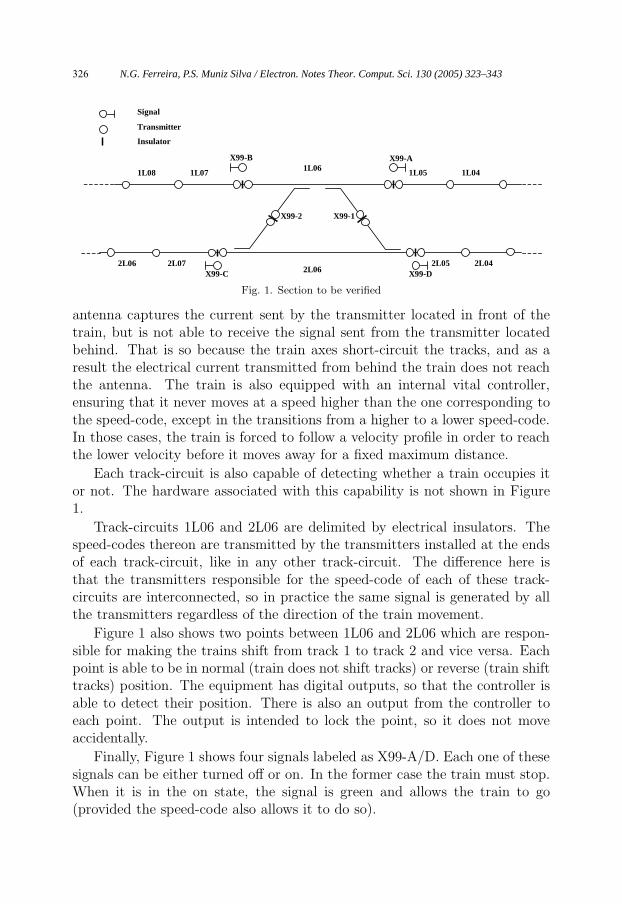
The software to be verified implements the control of a track section that ispartially represented in Figure 1. The figure shows two tracks labeled 1 and2 that can be merged by two points labeled X99-1 and X99-2. The tracks aredivided into about 40 track segments called track-circuits, each one labeledeither as 1Lnn or 2Lnn, depending on the track in which they are located.Figure 1 shows only ten of the available track-circuits.

Except for 1L06 and 2L06, two transmitters delimit each track-circuit.Each transmitter is able to send a speed-code to a train occupying one ofthe track-circuits delimited by it. The speed-code informs the train of themaximum speed it is allowed to move on that track-circuit and it is transmittedby outputting a modulated electrical current throughout the tracks. Thereare speed-codes corresponding to 10, 35, 50, 60, and 68 km/h. Not all thetransmitters are able to transmit all the codes. By construction, it is notpossible that the signal transmitted by one transmitter reaches a track-circuitnot delimited by it.

Each train running on the track is equipped with a front antenna. The

N.G. Ferreira, P.S. Muniz Silva / Electron. Notes Theor. Comput. Sci. 130 (2005) 323–343 325

Signal

Transmitter

Insulator

1L06

2L06

1L05 1L04

2L05 2L04

1L071L08

2L06 2L07

X99-B

X99-C

X99-A

X99-D

X99-2 X99-1

Fig. 1. Section to be verified

antenna captures the current sent by the transmitter located in front of thetrain, but is not able to receive the signal sent from the transmitter locatedbehind. That is so because the train axes short-circuit the tracks, and as aresult the electrical current transmitted from behind the train does not reachthe antenna. The train is also equipped with an internal vital controller,ensuring that it never moves at a speed higher than the one corresponding tothe speed-code, except in the transitions from a higher to a lower speed-code.In those cases, the train is forced to follow a velocity profile in order to reachthe lower velocity before it moves away for a fixed maximum distance.

Each track-circuit is also capable of detecting whether a train occupies itor not. The hardware associated with this capability is not shown in Figure1.

Track-circuits 1L06 and 2L06 are delimited by electrical insulators. Thespeed-codes thereon are transmitted by the transmitters installed at the endsof each track-circuit, like in any other track-circuit. The difference here isthat the transmitters responsible for the speed-code of each of these track-circuits are interconnected, so in practice the same signal is generated by allthe transmitters regardless of the direction of the train movement.

Figure 1 also shows two points between 1L06 and 2L06 which are respon-sible for making the trains shift from track 1 to track 2 and vice versa. Eachpoint is able to be in normal (train does not shift tracks) or reverse (train shifttracks) position. The equipment has digital outputs, so that the controller isable to detect their position. There is also an output from the controller toeach point. The output is intended to lock the point, so it does not moveaccidentally.

Finally, Figure 1 shows four signals labeled as X99-A/D. Each one of thesesignals can be either turned off or on. In the former case the train must stop.When it is in the on state, the signal is green and allows the train to go(provided the speed-code also allows it to do so).


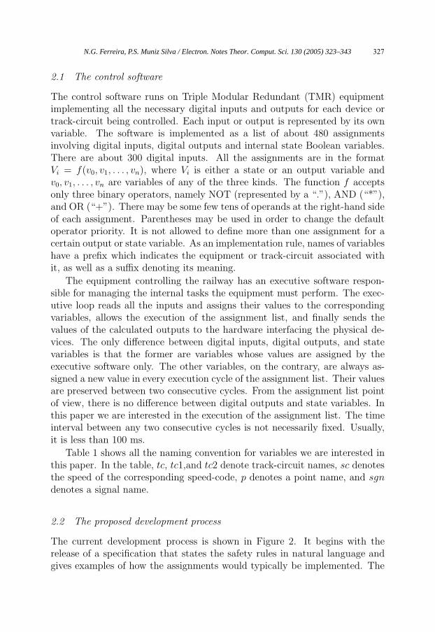
2.1 The control software

The control software runs on Triple Modular Redundant (TMR) equipmentimplementing all the necessary digital inputs and outputs for each device ortrack-circuit being controlled. Each input or output is represented by its ownvariable. The software is implemented as a list of about 480 assignmentsinvolving digital inputs, digital outputs and internal state Boolean variables.There are about 300 digital inputs. All the assignments are in the formatVi = f(v0, v1, . . . , vn), where Vi is either a state or an output variable andv0, v1, . . . , vn are variables of any of the three kinds. The function f acceptsonly three binary operators, namely NOT (represented by a “.”), AND (“*”),and OR (“+”). There may be some few tens of operands at the right-hand sideof each assignment. Parentheses may be used in order to change the defaultoperator priority. It is not allowed to define more than one assignment for acertain output or state variable. As an implementation rule, names of variableshave a prefix which indicates the equipment or track-circuit associated withit, as well as a suffix denoting its meaning.

The equipment controlling the railway has an executive software respon-sible for managing the internal tasks the equipment must perform. The exec-utive loop reads all the inputs and assigns their values to the correspondingvariables, allows the execution of the assignment list, and finally sends thevalues of the calculated outputs to the hardware interfacing the physical de-vices. The only difference between digital inputs, digital outputs, and statevariables is that the former are variables whose values are assigned by theexecutive software only. The other variables, on the contrary, are always as-signed a new value in every execution cycle of the assignment list. Their valuesare preserved between two consecutive cycles. From the assignment list pointof view, there is no difference between digital outputs and state variables. Inthis paper we are interested in the execution of the assignment list. The timeinterval between any two consecutive cycles is not necessarily fixed. Usually,it is less than 100 ms.

Table 1 shows all the naming convention for variables we are interested inthis paper. In the table, tc, tc1,and tc2 denote track-circuit names, sc denotesthe speed of the corresponding speed-code, p denotes a point name, and sgn

denotes a signal name.

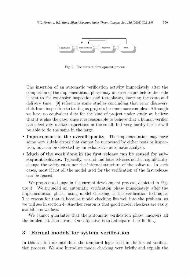
2.2 The proposed development process

The current development process is shown in Figure 2. It begins with therelease of a specification that states the safety rules in natural language andgives examples of how the assignments would typically be implemented. The


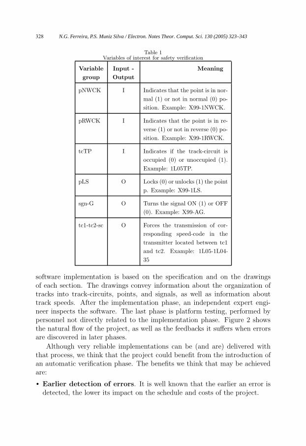
Table 1Variables of interest for safety verification

Variable

group

Input -

Output

Meaning

pNWCK I Indicates that the point is in nor-

mal (1) or not in normal (0) po-

sition. Example: X99-1NWCK.

pRWCK I Indicates that the point is in re-

verse (1) or not in reverse (0) po-

sition. Example: X99-1RWCK.

tcTP I Indicates if the track-circuit is

occupied (0) or unoccupied (1).

Example: 1L05TP.

pLS O Locks (0) or unlocks (1) the point

p. Example: X99-1LS.

sgn-G O Turns the signal ON (1) or OFF

(0). Example: X99-AG.

tc1-tc2-sc O Forces the transmission of cor-

responding speed-code in the

transmitter located between tc1

and tc2. Example: 1L05-1L04-

35

software implementation is based on the specification and on the drawingsof each section. The drawings convey information about the organization oftracks into track-circuits, points, and signals, as well as information abouttrack speeds. After the implementation phase, an independent expert engi-neer inspects the software. The last phase is platform testing, performed bypersonnel not directly related to the implementation phase. Figure 2 showsthe natural flow of the project, as well as the feedbacks it suffers when errorsare discovered in later phases.

Although very reliable implementations can be (and are) delivered withthat process, we think that the project could benefit from the introduction ofan automatic verification phase. The benefits we think that may be achievedare:

• Earlier detection of errors. It is well known that the earlier an error isdetected, the lower its impact on the schedule and costs of the project.


SpecificationSpecification

ImplementationImplementation

InspectionInspection

TestsTests

Fig. 2. The current development process

The insertion of an automatic verification activity immediately after thecompletion of the implementation phase may uncover errors before the codeis sent to the expensive inspection and test phases, lowering the costs anddelivery time. [9] references some studies concluding that error discoveryshift from inspection to testing as projects become more complex. Althoughwe have no equivalent data for the kind of project under study we believethat it is also the case, since it is reasonable to believe that a human verifiercan effectively realize inspections in the small, but very hardly he/she willbe able to do the same in the large.

• Improvement in the overall quality. The implementation may havesome very subtle errors that cannot be uncovered by either tests or inspec-tion, but can be detected by an exhaustive automatic analysis.

• Much of the work done in the first release can be reused for sub-

sequent releases. Typically, second and later releases neither significantlychange the safety rules nor the internal structure of the software. In suchcases, most if not all the model used for the verification of the first releasecan be reused.

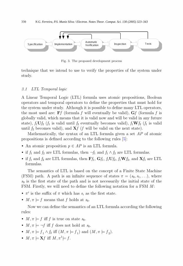
We propose a change in the current development process, depicted in Fig-ure 3. We included an automatic verification phase immediately after theimplementation phase, using model checking as the verification technique.The reason for that is because model checking fits well into the problem, aswe will see in section 4. Another reason is that good model checkers are easilyavailable nowadays.

We cannot guarantee that the automatic verification phase uncovers allthe implementation errors. Our objective is to anticipate their finding.

3 Formal models for system verification

In this section we introduce the temporal logic used in the formal verifica-tion process. We also introduce model checking very briefly and explain the


SpecificationSpecification

ImplementationImplementation

Inspection

AutomaticVerification Tests

Inspection Tests

Fig. 3. The proposed development process

technique that we intend to use to verify the properties of the system understudy.

3.1 LTL Temporal logic

A Linear Temporal Logic (LTL) formula uses atomic propositions, Booleanoperators and temporal operators to define the properties that must hold forthe system under study. Although it is possible to define many LTL operators,the most used are: Ff (formula f will eventually be valid), Gf (formula f isglobally valid, which means that it is valid now and will be valid in any futurestate), f1Uf2 (f1 is valid until f2 eventually becomes valid), f1Wf2 (f1 is validuntil f2 becomes valid), and Xf (f will be valid on the next state).

Mathematically, the syntax of an LTL formula given a set AP of atomicpropositions is defined according to the following rules [5]:

• An atomic proposition p ∈ AP is an LTL formula.

• if f1 and f2 are LTL formulas, then ¬f1 and f1 ∧ f2 are LTL formulas.

• if f1 and f2 are LTL formulas, then Ff1, Gf1, f1Uf2, f1Wf2, and Xf1 are LTLformulas.

The semantics of LTL is based on the concept of a Finite State Machine(FSM) path. A path is an infinite sequence of states π = (s0, s1, . . .), wheres0 is the first state of the path and is not necessarily the initial state of theFSM. Firstly, we will need to define the following notation for a FSM M :

• πi is the suffix of π which has si as the first state.

• M , π |= f means that f holds at s0.

Now we can define the semantics of an LTL formula according the followingrules:

• M , π |= f iff f is true on state s0.

• M , π |= ¬f iff f does not hold at s0.

• M , π |= f1∧ f2 iff (M , π |= f

1) and (M , π |= f

2).

• M , π |=Xf iff M , π1|= f .


• M , π |= f1Uf2 iff there is a k ≥ 0 such that M , πk|= f

2and M , πi|= f

1for

any 0 ≤ i < k .

As an abbreviation, we may write M |= f whenever it is implicit that thefirst state of the path is one of the initial states of the model. Obviously, othercommon Boolean operators like ∨, → and ←→ can be defined from ¬ and ∧.The operators F, G, and W may be defined respectively as Ff ≡ (trueUf ),Gf ≡ ¬F¬f , and f1Wf2 ≡ (f1Uf2) ∨Gf1.

3.2 Model checking

Model checking is a set of techniques used to verify some temporal logic spec-ification of a system modeled into an FSM by exhaustively analyzing all itsstates and transitions. We usually have a set AP of atomic propositions, anFSM M = (S , S0,R,L) and a specification f stated in some temporal logic,where S is a finite set of states, S0 ⊆ S is the set of initial states, R ⊆ S × S

is the total transition relation (i.e., any state has at least one successor) andL : S → 2AP is a function that labels each state with the atomic propositionsthat are true in that state [5]. The model checker tries to verify if M |= f forall the paths starting from the initial states of the model and, if it does not,it usually issues a counter-example which can be used to debug the system.

The most common challenge when using model checking is to deal withthe state explosion problem created by the combination of all possible valuesof the system variables. Sometimes it is necessary to abstract some systembehavior in order to enable the verification of a given specification with asimplified model. This approach has some drawbacks, namely that it maydemand a manual interference in the process and cause some errors in theverification. If possible, we would like to avoid any kind of abstraction whentrying to verify the control software we are interested in.

There are many model checking techniques which are intended to be usedin different kinds of applications. They can be divided into two main groups:the group of techniques using an explicit representation for the states of theFSM and the group using a symbolic representation for them. In the firstgroup, each state is individually analyzed and stored into the computer mainmemory, while the second group uses propositional formulas describing sets ofstates as well as transition relations. The explicit representation methods areusually used when the system can be modeled by an FSM limited in its sizeby some few million states. That limit is usually given by the amount of mainmemory available on the computers in use nowadays. Since we are dealingwith systems with a number of states much larger than that limit, explicitrepresentation techniques would not be our first choice.


Typically, symbolic model checkers use a technique by which they representsets of states complying with some propositional formula, instead of workingwith individual states. One of the most used methods is based on fixpointscalculation. In its basic form, a model checker based on this technique startswith a set representing either all or none of the states of the model, dependingon the kind of specification under analysis. That set is iteratively updated bythe application of the transition relation until a fixpoint is eventually reached.The model checker then verifies if all the initial states belong to that fixpoint.If that is the case, the specification holds. Most of the model checkers usingthis kind of technique employ a BDD [3] library for creating Boolean formulasrepresenting the state sets and the transition relations. This technique worksfine for some models with few hundreds Boolean variables, but fails whenthe models are larger than that. The main reason for that is the significantamount of memory and CPU time needed to deal with the state sets andtransition relations when the model becomes larger. Even when BDD-basedmodel checking works, it is sometimes necessary to carefully set up the modelchecker framework, because some parameters like variable orderings and thealgorithm used for calculating the fixpoints may be critical to the success ofthe method. The limitations and difficulties for medium to large-sized modelsdo not make BDD-based model checkers ideal candidates to the systems thatwe want to verify if we do not consider using abstraction.

The limitations of the BDD solution and the progress that was achieved inrecent years with the invention of faster algorithms for the satisfiability (SAT)of propositional formulas problem created the conditions for the introductionof bounded model checking [2]. In BMC, both the transition relations andthe set of states are still represented by propositional formulas. Initially, themodel checker builds a formula that is the conjunction of the initial states ofthe system and the negation of the specification under analysis. The formulais then analyzed by a SAT solver which tries to find a valuation that makesit true. If there is such a valuation, it is used as a counter-example for thespecification. If there is no such valuation, nothing can be said about thetruth of the specification and the model checker starts a new cycle. In thenew cycle, the formula to be analyzed is: a disjunction of the initial states, thetransition relation, and the negation of the specification. The model checkertries to find a counter-example for the specification, taking into account theinitial states as well as their successors. Again, the formula is sent to theSAT solver. The process continues until either a counter-example is found,the maximum configured number of iterations k is reached or the formula tobe analyzed becomes large enough to make its analysis infeasible.

Compared to the classical unbounded model checking, BMC has some


disadvantages and advantages. The main disadvantage is that it is not able,in general, to say something about the truth of the required specification incase it either holds or the counter-example is large enough to be handled bythe SAT solver. Thus, BMC is primarily an error-finder tool.

The advantages of BMC over unbounded model checking are manyfold.First, the user does not need to set up the environment manually. Usually, thedefault parameters will suffice. Second, the model checker is able to deal withthousands of variables instead of hundreds and, in doing so, it uses much lessmemory and spends much less computer time. Third, the generated counter-example is guaranteed to be minimum, simplifying the analysis of the problem.The first and second features will be of great value for us in our verificationprocess.

3.3 Robust systems and induction proofs

A model is defined in [7] as robust with respect to a specification f if f holdsfor all possible states of the model, even if they are not reachable from theinitial states. Mathematically, an FSM model M = (S , S0,R,L) is robust withrespect to f if, given M ′ = (S , S ,R,L), M |= f → M

′|= f .

A robust model with respect to the specification f has an interesting fea-ture, namely that if f = f (p0, p1, . . . ,Xp0,Xp1, . . . ,X

kp0,Xkp1, . . .) holds for

all finite sequence of k+1 states starting from the initial states s0, then Gf alsoholds. In other words, we can say that M ′ |= f → M |=Gf . In fact, any finitestate sequence for which f holds ends at some final state sk which belongs,itself, to the set of the initial states of the modified model M ′. Therefore, thestate sk is the initial state of a new finite sequence for which f also holds,and inductively M |=Gf . We define the depth of a formula as the maximumnumber k of nested X operators.

For example, in the subway system under consideration we can expectthat signal X99-A must be turned off whenever point X99-1 is in reverse. Thisrule could be specified as G(X99-1RWCK → F(¬X99-AG W¬X99-1RWCK)).The sentence says that it is always true (G) that if X99-1 is in reverse thensignal X99-A will be eventually (F) turned off and stay at that state until (W)X99-1 is not reversed. This sentence format has two drawbacks. The first oneis that we have no information about the number of cycles the software takesto respond to the new condition. It is a sensible issue because if we keepthe LTL specification as stated above, we are theoretically accepting longresponse times that could turn the implementation unable to quickly respondto an emergency situation, making it unsafe. Moreover, in order to use theinductive proof scheme we need to have a bound k on the number of softwarecycles and the sentence, as stated above, does not carry any information about


that.

We worked this problem out by analyzing the source code for the complete-ness of the proof. Rather than trying to use a sentence like the one above,we start looking for a specification that could be stated as (X99-1RWCK→ Xk¬X99-AG), which means that the signal X99-AG is turned off k cyclesafter point X99-1 is in reverse. If the sentence can be proved true for a givenk and a generic initial condition, the safety rule we are interesting in wouldbe verified if k is to be considered small enough. In fact, it would be proventhat if the point is in reverse at any state si , then the signal is off at anysuccessor state si+k . It also means that the signal will stay off while the pointkeeps its reverse state because if the point is still in reverse at s i+1 then thesignal will be off at s i+k+1 and so on. In our example, we concluded after aquick source code analysis that the specification to be proved is (X99-1RWCK→ XX¬X99-AG), and that a bound k = 2 would be enough to prove it.

4 Verification and experiments

In this section we describe the tools we used, the safety rules we wantedto verify, their translations into LTL, and the results we obtained from twoexperiments.

4.1 Tools

We chose to use NuSMV [4] as the bounded model checker. It is a re-implementation that extends the Symbolic Model Verifier (SMV) [10], de-veloped at the Carnegie Mellon University 3 . NuSMV accepts as input a filewhich describes the model of the system to be verified. The input languageis basically the same language as defined by SMV (the “SMV language”).Therefore, we needed a program to automatically translate the original sourcecode into the SMV language. The translator we implemented creates a singleSMV input file declaring all the variables and the complete set of assignmentsdefined by the original source code. There is a one to one correspondencebetween the assignments in the original source code and the SMV input lan-guage.

The translator is responsible for the following tasks:

• The assignment, and the operators and, or and not are represented bydifferent symbols in both languages, so the original representation has to be

3 We used the NuSMV version 2.1.2, running under Cygwin and Windows XP. The versionimplements both bounded and unbounded BDD-based model checking and is freely availableat http://nusmv.irst.itc.it/.


http://nusmv.irst.itc.it/

converted according to the SMV language rules.

• The SMV language does not accept variables with a digit as the first char-acter, so the translator always includes an underscore ( ) at the beginningof every variable.

• The SMV operator next is attached to any variable at the left-hand sideof an assignment. In doing so, we specify that the next state value of thevariable being assigned will be the result of the formula at the right-handside.

• The translator has to decide how it translates any variable var at the right-hand side of an assignment. It can translate it just as “var” or it cantranslate it as “next (var)”. The former case is used when, starting thetranslation from the first assignment, var has not already been used at theleft-hand side of an assignment. The later case is used otherwise.

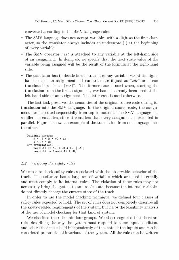
The last task preserves the semantics of the original source code during itstranslation into the SMV language. In the original source code, the assign-ments are executed sequentially from top to bottom. The SMV language hasa different semantics, since it considers that every assignment is executed inparallel. Figure 4 shows an example of the translation from one language intothe other.

Original program:A = .B * D * (C + A);B = .A * D;

SMV translation:next( A) := ! B & D & ( C | A);next( B) := !next( A) & D;

4.2 Verifying the safety rules

We chose to check safety rules associated with the observable behavior of thetrack. The software has a large set of variables which are used internallyand must comply to its internal rules. The violation of these rules may notnecessarily bring the system to an unsafe state, because the internal variablesdo not directly change the current state of the track.

In order to use the model checking technique, we defined four classes ofsafety rules expected to hold. The set of rules does not completely describe allthe safety-related requirements of the system, but helps the feasibility analysisof the use of model checking for that kind of system.

We classified the rules into four groups. We also recognized that there arerules describing the way the system must respond to some input condition,and others that must hold independently of the state of the inputs and can beconsidered propositional invariants of the system. All the rules can be written


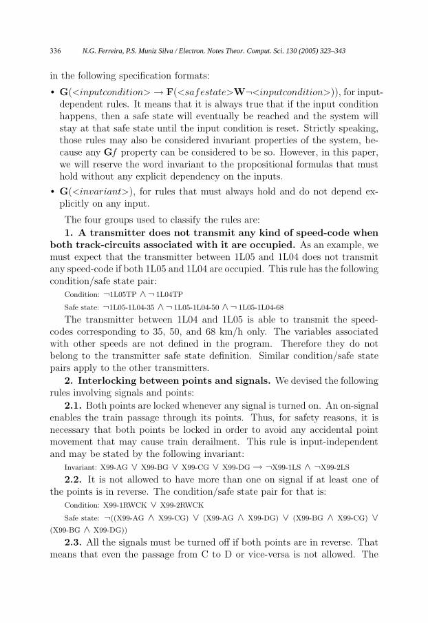
in the following specification formats:

• G(<inputcondition> → F(<safestate>W¬<inputcondition>)), for input-dependent rules. It means that it is always true that if the input conditionhappens, then a safe state will eventually be reached and the system willstay at that safe state until the input condition is reset. Strictly speaking,those rules may also be considered invariant properties of the system, be-cause any Gf property can be considered to be so. However, in this paper,we will reserve the word invariant to the propositional formulas that musthold without any explicit dependency on the inputs.

• G(<invariant>), for rules that must always hold and do not depend ex-plicitly on any input.

The four groups used to classify the rules are:

1. A transmitter does not transmit any kind of speed-code when

both track-circuits associated with it are occupied. As an example, wemust expect that the transmitter between 1L05 and 1L04 does not transmitany speed-code if both 1L05 and 1L04 are occupied. This rule has the followingcondition/safe state pair:

Condition: ¬1L05TP ∧¬ 1L04TP

Safe state: ¬1L05-1L04-35 ∧¬ 1L05-1L04-50 ∧¬ 1L05-1L04-68

The transmitter between 1L04 and 1L05 is able to transmit the speed-codes corresponding to 35, 50, and 68 km/h only. The variables associatedwith other speeds are not defined in the program. Therefore they do notbelong to the transmitter safe state definition. Similar condition/safe statepairs apply to the other transmitters.

2. Interlocking between points and signals. We devised the followingrules involving signals and points:

2.1. Both points are locked whenever any signal is turned on. An on-signalenables the train passage through its points. Thus, for safety reasons, it isnecessary that both points be locked in order to avoid any accidental pointmovement that may cause train derailment. This rule is input-independentand may be stated by the following invariant:

Invariant: X99-AG ∨ X99-BG ∨ X99-CG ∨ X99-DG → ¬X99-1LS ∧ ¬X99-2LS

2.2. It is not allowed to have more than one on signal if at least one ofthe points is in reverse. The condition/safe state pair for that is:

Condition: X99-1RWCK ∨ X99-2RWCK

Safe state: ¬((X99-AG ∧ X99-CG) ∨ (X99-AG ∧ X99-DG) ∨ (X99-BG ∧ X99-CG) ∨(X99-BG ∧ X99-DG))

2.3. All the signals must be turned off if both points are in reverse. Thatmeans that even the passage from C to D or vice-versa is not allowed. The


condition/safe state pair is:

Condition: X99-1RWCK ∧ X99-2RWCK

Safe state: ¬(X99-AG ∨ X99-BG ∨ X99-CG ∨ X99-DG)

2.4. Signals A and C must be turned off whenever point 1 is in reverse.By the same token, signals B and D must also be turned off whenever point 2is in reverse. The condition/safe state pairs of both rules are:

Condition 1: X99-1RWCK

Safe state 1: ¬(X99-AG ∨ X99-CG)

Condition 2: X99-2RWCK

Safe state 2: ¬(X99-BG ∨ X99-DG)

2.5. Both points must be in normal position whenever we have one onsignal at each track. The condition/safe state pair is:

Condition: ¬(X99-1NWCK ∧ X99-2NWCK)

Safe state: ¬((X99-AG ∧ X99-CG) ∨ (X99-AG ∧ X99-DG) ∨ (X99-BG ∧ X99-CG) ∨(X99-BG ∧ X99-DG))

3. Opposite signals must never be on at the same time. We definedtwo invariants for that rule, which are listed below.

Invariant 1: ¬(X99-AG ∧ X99-BG)

Invariant 2: ¬(X99-CG ∧ X99-DG)

4. The speed-code, transmitted when a train is approaching an

off–signal, should always correspond to low speed. As an example, wemust expect that the speed-code is transmitted to the train that is approachingsignal A must not correspond to either 50 or 68 km/h. The condition/safepair for the example is given below. There are equivalent rules for the othersignals.

Invariant: ¬X99-AG → ¬1L05-1L06-50 ∧ ¬1L05-1L06-68

4.3 Creating the LTL specifications

In order to prove the rules using the inductive procedure described above, wehave to create LTL specifications for those rules. The specifications may beprovable true after a finite number of cycles of the software being analyzed. Wehave already given an example in which we found that the software needs twocycles to turn signal X99-A off after point X99-1 is in reverse. Obviously, wecould expect that at least one cycle would be necessary, because the softwareneeds to be executed at least once before it can respond to any input change.However, we do not have any means to know the necessary number of cycles a

priori without recurring to analysis. It could well be the case that the softwareneeded three or four cycles to respond.

In practice, analyzing the software is a matter of observing the sequence of


assignments of the variables used by the rule to be verified and of the interme-diary variables that may affect them. After the analysis, the LTL formula iswritten and checked. If the model checker indicates that the specification doesnot hold, it may be either because the LTL specification was incorrectly statedor because the software has some error. In both cases we have to re-analyzethe program with the help of the model checker counter-example.

Another way of creating an LTL specification is assuming that the softwareis correct and starting from a tentative specification. If the model checkerstates that the specification holds, the process ends. Otherwise, we can createa new tentative specification until either we prove the rule or we give upand consider analyzing the source code. Although we may have to run sometentative specifications before we reach a valid one, we may save some timeand effort because the model checker response time is short compared to thetime needed to analyze the source code. In the example given above, we couldstart from the tentative specification (X99-1RWCK → X ¬X99-AG). Sincethe model checker would say that the specification does not hold, we couldtry (X99-1RWCK → XX ¬X99-AG). That specification holds, so we wouldhave successfully saved time and effort on not analyzing the code.

In brief, we spent only few hours writing the correct LTL specificationsfor the problem at hand. Table 2 shows the results of that work. The secondcolumn shows the LTL specification used for checking the rules and the thirdcolumn gives the bound for model checking, i.e. the number of cycles thesoftware has to run in order to either go to the safe state or to be compliantwith the invariant.

One interesting point is the origin of the X operator used at the beginningof specifications of groups 2.1, 3, and 4. These groups are responsible forchecking the input-independent invariants. It means that the LTL specifica-tions depend only on the variables calculated by the software. According tothe model we are using, the values of those variables are completely undefinedbefore the first software cycle. Therefore, it is not possible to guarantee anyrule concerning their values before the first iteration. The X operator in frontof the formula reflects this argument. The LTL specification of group 2.1 hasanother X operator at the right-hand side of the → operator. It expressesthe fact that the software is written in a way that the assignments of the lockcommands (LS variables) are executed before the assignments of the signals(G variables). Hence, the state of the signals will be reflected at the lockcommand only at the next cycle.


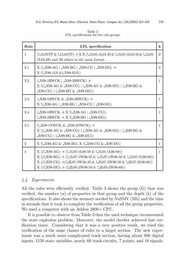
Table 2LTL specifications for the rule groups

Rule LTL specification k

1 (! 1L05TP & ! 1L04TP) -> X X (! 1L05-1L04-35 & ! 1L05-1L04-50 & ! 1L05-

1L04-68) and 39 others in the same format.

2

2.1 X (( X99-AG | X99-BG | X99-CG | X99-DG) ->

X (! X99-1LS &! X99-2LS))

2

2.2 ( X99-1RWCK | X99-2RWCK) ->

X !(( X99-AG & X99-CG) | ( X99-AG & X99-DG) | ( X99-BG &

X99-CG) | ( X99-BG & X99-DG))

1

2.3 ( X99-1RWCK & X99-2RWCK) ->

X !( X99-AG | X99-BG | X99-CG | X99-DG)

1

2.4 ( X99-1RWCK -> X !( X99-AG | X99-CG))

( X99-2RWCK -> X !( X99-BG | X99-DG))

1

2.5 !( X99-1NWCK & X99-2NWCK) ->

X !(( X99-AG & X99-CG) | ( X99-AG & X99-DG) | ( X99-BG &

X99-CG) | ( X99-BG & X99-DG))

1

3 X !( X99-AG & X99-BG) X !( X99-CG & X99-DG) 1

4 X ((! X99-AG) -> (! 1L05-1L06-50 & ! 1L05-1L06-68))

X ((! X99-BG) -> (! 1L07-1W06-35 & ! 1L07-1W06-50 & ! 1L07-1L06-68))

X ((! X99-CG) ->(! 2L07-2W06-35 & ! 2L07-2W06-50 & ! 2L07-2L06-68))

X ((! X99-DG) -> (! 2L05-2W06-50 & ! 2L05-2W06-68))

1

4.4 Experiments

All the rules were efficiently verified. Table 3 shows the group (G) that wasverified, the number (n) of properties in that group and the depth (k) of thespecifications. It also shows the memory needed by NuSMV (Mb) and the timein seconds that it took to complete the verification of all the group properties.We used a computer with an Athlon 2800+ CPU.

It is possible to observe from Table 3 that the used technique circumventedthe state explosion problem. Moreover, the model checker achieved fast ver-ification times. Considering that it was a very positive result, we tried theverification of the same classes of rules to a larger section. The new exper-iment was a much more complicated track section, having about 800 digitalinputs, 1150 state variables, nearly 60 track-circuits, 7 points, and 18 signals.


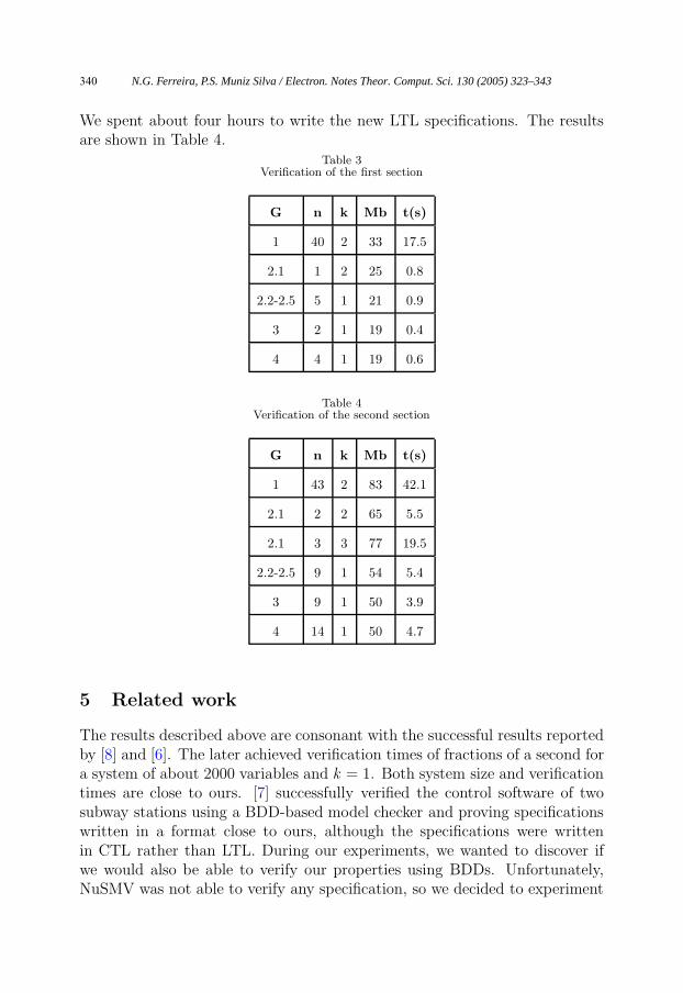
We spent about four hours to write the new LTL specifications. The resultsare shown in Table 4.

Table 3Verification of the first section

G n k Mb t(s)

1 40 2 33 17.5

2.1 1 2 25 0.8

2.2-2.5 5 1 21 0.9

3 2 1 19 0.4

4 4 1 19 0.6

Table 4Verification of the second section

G n k Mb t(s)

1 43 2 83 42.1

2.1 2 2 65 5.5

2.1 3 3 77 19.5

2.2-2.5 9 1 54 5.4

3 9 1 50 3.9

4 14 1 50 4.7

5 Related work

The results described above are consonant with the successful results reportedby [8] and [6]. The later achieved verification times of fractions of a second fora system of about 2000 variables and k = 1. Both system size and verificationtimes are close to ours. [7] successfully verified the control software of twosubway stations using a BDD-based model checker and proving specificationswritten in a format close to ours, although the specifications were writtenin CTL rather than LTL. During our experiments, we wanted to discover ifwe would also be able to verify our properties using BDDs. Unfortunately,NuSMV was not able to verify any specification, so we decided to experiment


with another easily available SMV implementation called Cadence SMV [1],trying to verify one property of each of the four groups defined above. Theresults for the simpler section ranged from 25 seconds of execution time and65 Mbytes of memory for verifying a property of group 1 to a failure in theverification of the property of group 4, due to lack of memory. No specificationof the larger section could be verified. Hence, although the good results re-ported by [7] with BDD-based model checking, we concluded that SAT-basedBMC seems to be much more promising for our domain.

Like us, [6] was not able to verify its system with BDDs and proposedBMC. However, it suggests a different way of verifying the safety properties:instead of writing a specification using temporal logic, it proposes the defini-tion of new variables that are appended to the end of the program. Thosevariables represent system invariants and the value of each one is a function ofthe current and next values of other variables. The domain expert engineersshould create the invariants based on their interpretation of the safety require-ments. The rationale for this approach is that the authors believe that using alanguage familiar to the expert domain engineers is crucial for their proposalto be useful. We dispute that. Firstly, this approach limits the propertiesthat can be verified to depth 0 or 1 formulas, unless the developer creates newintermediary variables to store older values (entangling the verification andbringing unwanted manual intervention). Secondly, we concluded that it iseasy to write down LTL specifications for the properties to be verified, sincewe only need the X LTL operator as well as the traditional Boolean operators.Thirdly, we are afraid that the chance of common mode errors increases withthat approach, because the expert domain engineers are responsible for manytasks: interpreting the specification stated in natural language, implementingthe program, and defining the invariants in the same language of the controlsoftware. The verification may fail if either the interpretation of the require-ments is incorrect or the wrongly implemented code is used somehow in thedefinition of the invariants. Another drawback is that it makes it difficult forothers to check whether the invariants are correctly stated. Thus, we thinkthat a better approach would be stating the safety properties either as condi-tion/safety pairs or as invariants in the specification document. The developerwould have to write the LTL formulas and run the model checker in order toverify the properties. The LTL formulas would be implementation-dependent,but could be easily assessed by independent reviewers.


6 Conclusion and future work

We have presented the results of model checking two different actual sectionsof a subway track. The main problem that we could have faced was the stateexplosion problem. However, experience showed that we were able to verifyall the rules in relatively short time, with no need for further abstractions,which would demand more manual interference on the process as well as thepossibility of inserting errors into the verification. An interesting point is thatalthough we used a model checker, we actually did not need one. A SAT solverwould suffice, because it is not possible to verify a temporal formula of depthk in less than k applications of the transition relation. Hence, there is nouse in trying to find a counter-example smaller than k . However, we decidedto use NuSMV because it easily represents the model to be verified and isfreely available. Another point in favor of the model checker is that the timespent on finding counter-examples smaller than the depth of the formulas isnot a problem, given its fast response time. We conclude that, for the specifickind of subway control software that was examined, an automatic verificationprocess based on model checking and on the described approach seems to befeasible.

This work opens some paths for future works. One of them is the automaticverification of software functional requirements on this particular domain. Ex-amples of functional requirements are the conditions for a route approval, theconditions for cancelling a route, and how the system must depict a pointposition while it is moving. Another essential point to be studied is to under-stand the coverage degree that can be achieved with that kind of verification,its costs, and benefits to the project.

References

[1] Cadence SMV. Cadence SMV and its documentation can be downloaded fromhttp://www-cad.eecs.berkeley.edu/∼kenmcmil/smv/.

[2] A. Biere, A. Cimatti, E. Clarke, and Y. Zhu. Symbolic model checking without BDDs. InProceedings of TACAS 1999, number 1579 in LNCS, page 193. Springer-Verlag, 1999.

[3] R. Bryant. Graph-based algorithms for boolean function manipulation. IEEE Transactionson Computers, C35(8):677–691, 1986.

[4] A. Cimatti, E. Clarke, F. Giunchiglia, and M. Roveri. NuSMV: a new symbolic model checker.International Journal on Software Tools for Technology Transfer, 2(4):410–425, 2000.

[5] E. Clarke, O. Grumberg, and D. A. Peled. Model Checking. MIT Press, Cambridge, MA, 1999.

[6] G. Dipoppa, G. D’Alessandro, R. Semprini, and E. Tronci. Integrating automatic verificationof safety requirements in railway interlocking system design. In Proceedings of HASE 2001,pages 209–219. IEEE Computer Society, 2001.


http://www-cad.eecs.berkeley.edu/~kenmcmil/smv/

[7] C. Eisner. Using symbolic model checking to verify the railway stations of Hoorn-Kersenboogerd and Heerhugowaard. In Proceedings of CHARME 1999, number 1703 in LNCS,pages 97–109. Springer-Verlag, 1999.

[8] W. Fokkink. Safety criteria for Hoorn-Kersenboogerd railway station. Logic Group PreprintSeries 135, Utrecht University, 1995.

[9] M. Huber and S. King. Towards an integrated model checker for railway signalling data. InProceedings of FME 2002, number 2391 in LNCS, page 204. Springer-Verlag, 2002.

[10] K. McMillan. Symbolic Model Checking: An Approach to the State Explosian Problem. KluwerAcademic Publishers, Norwell, MA, USA, 1993.

[11] K. Winter. Model checking railway interlocking systems. In M. Oudshoorn, editor, Proceedingsof Australian Computer Science Conference (ACSC 2002), number 24(1), pages 303–310.Australian Computer Science Communications, 2002.

[12] K. Winter and N. Robinson. Modelling large railway interlockings and model checkingsmall ones. In M. Oudshoorn, editor, Proceedings of the 26th Australian Computer ScienceConference (ACSC 2003), pages 309–316, 2003.


Automatic Verification of Safety Rules for a Subway Control ...

Documents

Transcript of Automatic Verification of Safety Rules for a Subway Control ...