AUTHOR: TITLE - OpenAIR@RGU

AUTHOR:

TITLE:

YEAR: OpenAIR citation:

OpenAIR takedown statement:

This work is made freely available under open access.

This ǘƘŜǎƛǎ is distributed under a CC ____________ license.

____________________________________________________

Section 6 of the “Repository policy for OpenAIR @ RGU” (available from http://www.rgu.ac.uk/staff-and-current-students/library/library-policies/repository-policies) provides guidance on the criteria under which RGU will consider withdrawing material from OpenAIR. If you believe that this item is subject to any of these criteria, or for any other reason should not be held on OpenAIR, then please contact [email protected] with the details of the item and the nature of your complaint.

This work was submitted to- and approved by Robert Gordon University in partial fulfilment of the following degree: _______________________________________________________________________________________________

COMPUTATIONAL FLUID

DYNAMICS MODELLING OF

PIPELINE ON-BOTTOM STABILITY

IBIYEKARIWARIPIRIBO IYALLA

A thesis submitted in partial fulfilment of the

requirements of the Robert Gordon University

for the degree of Doctor of Philosophy

October 2017

i

ACKNOWLEDGEMENTS

I must first express my profound gratitude to Dr Mamdud Hossain, my principal

supervisor, who patiently supported me through the period of this research,

constructively critiquing the work, and helping with developing CFD models. His

invaluable contribution has led to the successful completion of this thesis.

I would also like thank my wife Dr Ibifaa Iyalla, my uncle Prof Kelsey Harrison,

my father-in-law Mr Emmanuel Ngoye for their consistent encouragement and

push for me to complete this research. And to my dear children, David and

Dorothy for their cooperation and support.

My thanks also go to my friends and work colleagues, Dr Omowunmi Omole, Dr

Shiekh Islam, Dr Jesse Andrawus, Dr Eben Adom, Dr Miki Sun, George Kidd and

Prof Babs Oyeneyin for their moral support. Thanks to Roma Boulton for

formatting tips and Steve Button for reading through my initial draft. Thanks Dr

Mark & Mrs Alero Igiehon for their prayers.

Above all I am grateful to God who began the work in me and has brought it to

a perfect end.

ii

DEDICATION

This thesis is dedicated to the memory of my late mother Mrs Basoene Obuba

Iyalla who did not live long enough to see the fruits of her labour.

iii

ABSTRACT

Subsea pipelines are subjected to wave and steady current loads which cause

pipeline stability problems. Current knowledge and understanding on the

pipeline on-bottom stability is based on the research programmes from the

1980’s such as the Pipeline Stability Design Project (PIPESTAB) and American

Gas Association (AGA) in Joint Industry Project. These projects have mainly

provided information regarding hydrodynamic loads on pipeline and soil

resistance in isolation. In reality, the pipeline stability problem is much more

complex involving hydrodynamic loadings, pipeline response, soil resistance,

embedment and pipe-soil-fluid interaction.

In this thesis Computational Fluid Dynamics (CFD) modelling is used to

investigate and establish the interrelationship between fluid (hydrodynamics),

pipe (subsea pipeline), and soil (seabed). The effect of soil types, soil

resistance, soil porosity and soil unit weight on embedment was examined. The

overall pipeline stability alongside pipeline diameter and weight and

hydrodynamic effect on both soil (resulting in scouring) and pipeline was also

investigated. The use of CFD provided a better understanding of the complex

physical processes of fluid-pipe-soil interaction.

The results show that the magnitude of passive resistance is on the average

eight times that of lateral resistance. Thus passive resistance is of greater

significance for subsea pipeline stability design hence the reason why

Coulomb’s friction theory is considered as conservative for stability design

analysis, as it ignores passive resistance and underestimates lateral resistance.

iv

Previous works (such as that carried out by Lyons and DNV) concluded that soil

resistance should be determined by considering Coulomb’s friction based on

lateral resistance and passive resistance due to pipeline embedment, but the

significance of passive resistance in pipeline stability and its variation in sand

and clay soils have not be established as shown in this thesis. The results for soil

porosity show that increase in pipeline stability with increasing porosity is due to

increased soil liquefaction which increases soil resistance. The pipe-soil

interaction model by Wagner et al. established the effect of soil porosity on

lateral soil resistance but did not attribute it to soil liquefaction. Results showed

that the effect of pipeline diameter and weight vary with soil type; for sand,

pipeline diameter showed a greater influence on embedment with a 110%

increase in embedment (considering combined effect of diameter and weight)

and a 65% decrease in embedment when normalised with diameter. While

pipeline weight showed a greater influence on embedment in clay with a 410%

increase.

The work of Gao et al. did not completely establish the combined effect of

pipeline diameter and weight and soil type on stability. Results also show that

pipeline instability is due to a combination of pipeline displacement due to

vortex shedding and scouring effect with increasing velocity. As scoring

progresses, maximum embedment is reached at the point of highest velocity.

The conclusion of this thesis is that designing for optimum subsea pipeline

stability without adopting an overly conservative approach requires taking into

consideration the following; combined effect of hydrodynamics of fluid flow on

soil type and properties, and the pipeline, and the resultant scour effect leading

v

to pipeline embedment. These results were validated against previous

experimental and analytical work of Gao et al, Brennodden et al and Griffiths.

Keywords: Drag, Embedment, Hydrodynamic Force, Lateral Resistance, Lift,

Passive Resistance, Pipeline, Pressure Coefficient, Scour, Stability.

vi

TABLE OF CONTENTS

Acknowledgements ........................................................................ i

Dedication ..................................................................................... ii

Abstract ....................................................................................... iii

Table of Contents ......................................................................... vi

List of Figures .............................................................................. xi

List of Tables .............................................................................. xvi

Nomenclature ............................................................................ xvii

Chapter 1: Introduction ................................................................ 1

1.1 Research Aim ..................................................................... 3

1.2 Research Objectives ........................................................... 5

1.3 Thesis Outline .................................................................... 5

Chapter 2: Literature Review ........................................................ 8

2.1 Potential Flow Phenomena on a Cylinder ........................... 9

2.2 Viscous Fluid .................................................................... 10

2.3 Drag Forces ...................................................................... 13

2.4 Lift Force .......................................................................... 14

2.5 Inertia Force .................................................................... 14

2.6 Wave Loading .................................................................. 16

2.7 Hydrodynamic Forces ....................................................... 17

2.8 Morison’s Equation ........................................................... 18

2.9 Wake Force Model ............................................................ 19

2.9.1 Wake I Model ........................................................... 20

2.9.2 Wake II Model ......................................................... 24

2.10 Soil Resistance: Coulomb’s Friction Theory .................... 26

vii

2.11 Seabed Soil Properties ................................................... 28

2.11.1 Soil Classification .................................................. 29

2.11.2 Soil Behaviour ....................................................... 30

2.11.3 Sediment Mobility .................................................. 30

2.11.4 Soil Liquefaction .................................................... 34

2.12 Past and Current Stability Analysis Methods ................. 39

2.12.1 Pipe-Soil Interaction Stability Design Methods ...... 40

2.12.2 Fluid-Pipe-Soil Interaction Stability Design Methods48

Chapter 3: Methodology ............................................................. 56

3.1 Governing Equations ....................................................... 59

3.1.1 Reynolds-averaged Navier-Stokes (RANS) equations60

3.2 Calculation of soil resistance ........................................... 61

Chapter 4: Modelling the Effect of Soil Resistance on Subsea Pipeline

Stability ...................................................................................... 66

4.2 Results of the Effect of Soil Types on Lateral Resistance . 73

4.3 Results of the Effect of Hydrodynamic Load and Embedment on

Soil Resistance ...................................................................... 77

4.4 Model Validation .............................................................. 80

4.5 Results Summary ............................................................ 81

Chapter 5: Pipeline Stability Analysis ......................................... 82

5.1 Model Validation .............................................................. 85

5.2 Results of Pipeline Stability Analysis ............................... 87

5.2.1 Results of the Effect of Soil Embedment on Pipeline

Lateral Stability ................................................................ 89

5.2.2 Results of the Effect of Seabed Porosity on Pipeline

Lateral Stability ................................................................ 90

viii

5.3 Results Summary ............................................................. 91

Chapter 6: Modelling Pipeline Embedment for On Bottom Stability

Optimisation ............................................................................... 92

6.1 Results of the Effect of Pipe Diameter and Pipe Weight on

Pipeline Embedment .............................................................. 96

6.2 Results of the effect of unit weight of soil on pipeline

embedment .......................................................................... 101

6.3 Results of the effect of hydrodynamic forces on pipeline

embedment .......................................................................... 102

6.4 Model Validation ............................................................ 105

6.5 Results Summary ........................................................... 106

Chapter 7: Modelling Scouring Effect ........................................ 107

7.1 Results on Scouring Effect on Velocity ........................... 111

7.2 Results for Scouring Effect on Wall Shear Stress and Pressure

Coefficient ........................................................................... 119

7.3 Model Validation ............................................................ 128

7.4 Results Summary ........................................................... 129

Chapter 8: Conclusion and Recommendation ............................ 131

8.1 Future work ................................................................... 134

REFERENCES ............................................................................. 136

BIBLIOGRAPHY ......................................................................... 145

APPENDIX A .............................................................................. 151

Flowchart of Matlab Program for Embedment Calculation for

varying Pipeline Diameter .................................................... 151

APPENDIX A(i) .......................................................................... 152

ix

Embedment Calculation for each Pipeline Diameter on Sand Matlab

Code ..................................................................................... 152

APPENDIX A(II) ........................................................................ 153

Embedment Calculation for each Pipeline Diameter on Clay Matlab

Code ..................................................................................... 153

APPENDIX B .............................................................................. 154


varying Pipeline Weight ....................................................... 154

APPENDIX B(i) .......................................................................... 155

Embedment Calculation for each Pipeline Weight on Sand Matlab

Code ..................................................................................... 155

APPENDIX B(ii) ......................................................................... 156

Embedment Calculation for each Pipeline Weight on Clay Matlab

Code ..................................................................................... 156

APPENDIX C .............................................................................. 157


combined Pipeline Diameter and Weight .............................. 157

APPENDIX C(i) .......................................................................... 158

Embedment Calculation for combined Pipeline Diameter and

Weight on Sand Matlab Code ................................................ 158

APPENDIX C(II) ........................................................................ 159

Embedment Calculation for combined Pipeline Diameter and

Weight on Clay Matlab Code ................................................. 159

APPENDIX D .............................................................................. 160


varying unit Weight of Soil ................................................... 160

x

APPENDIX D(i) .......................................................................... 161

Embedment Calculation for each unit Weight of Soil (Sand) Matlab

Code ..................................................................................... 161

APPENDIX D(II) ........................................................................ 162

Embedment Calculation for each unit Weight of Soil (Clay) Matlab

Code ..................................................................................... 162

APPENDIX E .............................................................................. 163

Embedment Calculation due to Scouring Matlab Code .......... 163

APPENDIX F .............................................................................. 165

Publications .............................................................................. 168

xi

LIST OF FIGURES

Figure 1.1 Fluid-pipe-soil (F-P-S) interaction mode….………………………………..4

Figure 2.1 On-bottom pipeline stability (Soedigbo, Lambrakos and Edge

1998)……………………………………………………………………………………………………………8

Figure 2.2 Potential flow around a circular cylinder (Marbus 2007) ….……..10

Figure 2.3 Flow around a cylinder with wake (Groh 2016)…………………………11

Figure 2.4 Flow regimes (Sumer and Fredsoe 2006)……..…………….………….12

Figure 2.5 Hydrodynamic forces on a pipeline (Mousselli 1981)….………….17

Figure 2.6 Wake velocity effect on effective velocity (Lambrakos et al

1987)………………………………………………………………………………………………………….22

Figure 2.7 Pipeline embedment conditions (Bransby et al. 2014)….…………32

Figure 2.8 Tunnel erosion (Scour) (Sumer and Fredsoe 2002)…………………33

Figure 2.9 Seabed sediment motion due to vortex (Sumer and Fredsoe

2002)……………………………………………………………………………………………………………34

Figure 2.10 Lee-wake effect (Sumer and Fredsoe 2002)…………………………..34

Figure 2.11 Seabed soil deformation (Sumer 2014)…………………………….…..36

Figure 2.12 Excess pore pressure time series (Sumer 2014)……………………37

Figure 2.13 Build-Up pore pressure and liquefaction (Sumer 2014)…………38

Figure 2.14 Surface stresses on a small soil element (Sumer 2014)……….39

Figure 2.15 Soil passive resistance (Ryan et al 2011)………………………………48

Figure 2.16 Onset of sand scour (Gao, Jeng and Wu 2006)………………………50

Figure 2.17 Pipeline rocks (Gao, Jeng and Wu 2006)………………………………51

Figure 2.18 Pipeline breakout (Gao, Jeng and Wu 2006)………………………….51

Figure 2.19 Sweep area (Griffiths 2012)……………………………………………………54

Figure 2.20 Suck area (Griffiths 2012)………………………………………………………54

xii

Figure 3.1 Interconnectivity of the main elements of CFD codes (Tu, Yeoh and

Liu 2013)…………………………………………………………………………………………….58

Figure 3.2 Solver process (Tu, Yeoh and Liu 2013)……………………………………59

Figure 4.1 Pipeline displacement ( mm 510 )………………………………..……….….65

Figure 4.2 mmmm 5050 Mesh Mesh…………….……………………………………………65

Figure 4.3 Geometry and boundaries.………….……………………………………………67

Figure 4.4 Pipe-soil interaction (Ren and Liu 2013)………………………………...67

Figure 4.5 Passive Resistance on sand with 5%, 10%, 15% and 20%

embedment……………………………………………………………..………………………………..69

Figure 4.6 Passive Resistance on clay with 5%, 10%, 15% and 20%

embedment………………………………………………………………………………..……………..69

Figure 4.7 Maximum passive resistance on sand and clay…………………………70

Figure 4.8 Soil resistance versus lateral displacement plot (Brennoddden et al

1989)…………………………………………………………………………..…………………………71

Figure 4.9 Soil Friction on sand with 0%, 5% and 10% embedment

……………………………………………….….…………………………………..…………………………73

Figure 4.10 Soil Friction on clay with 0%, 5% and 10%

embedment……………………………….….………………………………..…………………………73

Figure 4.11 Maximum lateral resistance on sand and clay………………………74

Figure 4.12 Relationship between hydrodynamic loading and soil friction on

Sand……………………….………………………………………………………………………………….77


clay.……………………………………………………………………………………………………………77

Figure 4.14 Horizontal force comparison with CFD model…..……………………78

Figure 5.1 Interior volume of mesh ( mmm 0.25.110 )...........………………..79

Figure 5.2 Geometry and boundaries………………………………………………………..80

xiii

Figure 5.3 Lift coefficient with start-up effect ………………………………………….83

Figure 5.4 Drag coefficient with start-up effect ……………………………………….83

Figure 5.5 Pipeline stability criteria for 0.5m diameter pipeline with 5%

embedment……………………………………………………………………………………………….84

Figure 5.6 Effect of weight increase on 0.5m diameter pipeline (submerged

weight 1 = N415 , submerged weight 2 = N440 and submerged weight 3

= N465 ) …………………………………………………………………………………………………….85

Figure 5.7 Effect of soil embedment on pipeline lateral stability ……………86

Figure 5.8 Effect of porosity on pipeline lateral stability ………………………..87

Figure 6.1 Mesh with applied inflation on pipeline wall ……………………………90

Figure 6.2 Fluid-pipe-soil boundary conditions ………………………………………..91

Figure 6.3 Effect of increasing diameter on initial embedment (sand) …..93

Figure 6.4 Effect of increasing diameter on initial embedment (clay) ……..94

Figure 6.5 Effect of submerged pipe weight on embedment (sand) ………..95

Figure 6.6 Effect of submerged pipe weight on embedment (clay) ………….95

Figure 6.7 Combined effect of pipe diameter and weight on embedment (sand)

……………………………………………………………………………………………………….96

Figure 6.8 Effect of normalised pipe diameter on embedment (sand) ……96

Figure 6.9 Combined effect of pipe diameter and weight on embedment (clay)

……………………………………………………………………………………………………97

Figure 6.10 Effect of normalised pipe diameter with embedment (clay) …97

Figure 6.11 Effect of unit weight of soil on embedment (sand).………………98

Figure 6.12 Effect of unit weight of soil on embedment (clay) ………………99

Figure 6.13 Effect of current velocity on embedment (0.5m pipe on loose sand)

……………………………………………………………………………………………………….100

xiv

Figure 6.14 Effect of current velocity on embedment (1m pipe on loose sand)

……………………………………………………………………………………………………100

Figure 7.1 Mesh with applied inflation on pipeline wall …………………………103

Figure 7.2 Boundary regions (A- inlet; B- outlet; C- symmetry top; D- wall left;

E- wall right; F- wall bottom; G- wall Cylinder) ………………………………104

Figure 7.3 Pipeline positions from onset of scour to breakout…………………106

Figure 7.4 Pipeline position at reference point 0.0 …………………………………106

Figure 7.5a Vector of pipeline at position -0.7 ………………………………………..108

Figure 7.5b Contour of pipeline at position -0.7 ………………………………………108

Figure 7.6a Vector of pipeline at position -0.3 ………………………………………..109

Figure 7.6b Contour of pipeline at position -0.3 ………………………………………109

Figure 7.7a Vector of pipeline at position 0.0 ………………………………………….110

Figure 7.7b Contour of pipeline at position 0.0. …………………………………….110


Figure 7.8b Contour of pipeline at position 0.5 ……………………………………….111


Figure 7.9b Contour of pipeline at position 1.0 ……………………………………….112

Figure 7.10a Vector of pipeline at position 1.2 ……………………………………….113

Figure 7.10b Vector of pipeline at position 1.2 ……………………………………….113

Figure 7.11 Vorticity plot for the mechanism of scour under pipeline……..114

Figure 7.12a Wall shear stress of pipeline at position -0.7 ……………………..116

Figure 7.12b Pressure coefficient of pipeline at position -0.7 …………………117

Figure 7.13a Wall shear stress of pipeline at position -0.5 ……………………..117

Figure 7.13b Pressure coefficient of pipeline at position -0.5 …………………118

Figure 7.14a Wall shear stress of pipeline at position 0.0 ……………………….118

Figure 7.14b Pressure coefficient of pipeline at position 0.0 ………………….119

xv







Figure 7.18 CD and CL plot at pipeline positions …………………………………….123

Figure 7.19 Influence of a fixed boundary on drag coefficient of a circular

cylinder (DNV-RP-C205, 2010) ………………………………………………………………123


cylinder as generated by CFD model ……………………………………………………125

xvi

LIST OF TABLES

Table 2.1 Flow regimes around a circular cylinder (Sumer and Fredsoe

2006)………………………………………………………………………………………………………….13

Table 4.1 Boundary conditions ………………………………………………………………..66

Table 4.2 Selected parameters ………………………………………………………………..66

Table 4.3 Maximum passive resistance on sand and clay ……………………..70

Table 4.4 Maximum lateral resistance on sand and clay ……………………….74

Table 4.5 Effect of submerged weight on maximum lateral resistance on sand

…………………………………………………………………………………………………….…..75

Table 4.6 Effect of submerged weight on maximum lateral resistance on clay

……………………………………………………………………………………………………………76

Table 5.1 Boundary conditions ………………………………………………………………..80

Table 5.2 Selected parameters …………………………………………………………………81

Table 6.1 Boundary conditions ………………………………………………………………….91

Table 6.2 Selected parameters …………………………………………………………………92

Table 6.3 Initial embedment in loose sand (18400 N/m3 bulk unit

weight)…………………………………………………………………………………………………….102

Table 6.4 Initial embedment in dense sand (19400 N/m3 bulk unit

weight)…………………………………………………………………………………………………….102

Table 6.5 Initial embedment in clay (17300 N/m3 bulk unit weight) ………102

Table 7.1 Boundary conditions ……………………………………………………………….104

Table 7.2 Selected parameters ……………………………………………………………….105

Table 7.3 CD and CL values……………………………………………………………………….120

xvii

NOMENCLATURE

a acceleration (m/s2)

A area (m2)

aC added mass coefficient

AWC added mass coefficient with wake flow

DC drag Coefficient

DSC steady current drag coefficient

SC steady flow force coefficient

LC lift coefficient

MC coefficient of inertia

1C , 2C wake velocity correction parameters in periodic flow

d average sediment particle diameter (m)

D diameter (m)

DF drag force (N)

FF sliding resistance (N/m)

HF total lateral resistance (N/m)

RF soil lateral resistance (N/m)

IF inertia force (N)

LF lift force (N)

essureFPr Froude-Krylov force (N)

g acceleration due to gravity (m/s2)

G shear modulus (Pa)

sG specific gravity soil

xviii

H wave height (m)

k coefficient of soil permeability

K apparent bulk modulus of elasticity of water

KC Keulegan-Carpenter number

P pressure (Pa)

Re Reynolds number

t time (s)

T wave period (s)

wu wake velocity correction (m/s)

U velocity (m/s)

cU critical velocity (m/s)

eU effective velocity (m/s)

mU Peak Velocity (m/s)

tU total free stream velocity of steady current (m/s)

WU wake velocity (m/s)

sW submerged weight (N)

Greek

' buoyant unit weight of sand (N/m3)

coefficient of passive soil resistance

coefficient of sliding resistance

c critical Shields Number

density (kg/m3)

kinematic viscosity (m2/s)

xix

phase angle (˚)

Poisson’s ratio

p pore-water pressure (Pa)

Shields number

soil porosity (%)

w specific weight of water (N/m3)

volume expansion per unit volume of soil.

wave frequency (Hz)

wavelength (m)

1

CHAPTER 1: INTRODUCTION

Petroleum reserves located under the seabed have resulted in the development

of offshore structures and facilities to support the activities of the oil and gas

industry which include exploration, drilling, storage, and transportation of oil

and gas. Offshore structures constructed on or above the continental shelve

and on adjacent continental slopes take many forms including pipeline system

for transporting reservoir fluids from wells to tieback installations or onshore

location, and platforms (Wilson 2002). Producing oil and gas from offshore and

deepwater wells by means of subsea pipelines has proven to be the most

convenient, efficient, reliable and economic means of large scale continuous

transportation to existing offshore installation or onshore location on a regular

basis (Guo et al 2005).

A pipeline on the seabed has to be stable to avoid possible breakage and

eventual spill of hydrocarbons. If the pipeline is too light, it will move (i.e.

become unstable) under the action of currents and waves. On the other hand,

if it is too heavy, it will be difficult and expensive to construct (Palmer and King

2011). To accurately design systems or design operations at sea, an

understanding of the working environment is necessary, that is, an

understanding of the principal environmental factors which will influence the

design. The process of subsea pipeline stability design incorporates wave and

current prediction, determination of hydrodynamic loads due to current, and

soil lateral resistance analysis. The loads acting on the pipeline due to wave and

current are drag, lift and inertia forces. To ensure stability, the friction due to

the effective weight of pipeline on the seabed must balance these forces. Where

2

the weight of pipeline and contents alone is insufficient in achieving stability,

other stabilization techniques such as trenching, mattresses, concrete coating,

etc, have to be used (Palmer and King 2011, Bai and Bai 2005).

To evaluate the wave-induced forces acting on a subsea pipeline, the

surrounding hydrodynamic loads must be known. Hydrodynamic loads are

flow-induced loads caused by the relative motion between pipeline and the

surrounding water. To assess the structural integrity and stability of subsea

pipelines at the design stage, the environmental loads and structural responses

must be calculated and evaluated. Both the static and dynamic response of a

subsea pipeline can be reasonably predicted at the design stage. To determine

the dynamic behaviour of a subsea pipeline, it is important to acquire realistic

data on environmental conditions such as wave, current, soil, etc., and to

properly account for them in the calculations (Marbus 2007).

Pipeline stability is affected by the interaction between the sea waves and

currents and the pipeline (fluid-pipe), the interaction between the pipeline and

the seabed (pipe-soil) and the interaction between the sea waves and currents

and the seabed (fluid-soil). Fluid-pipe interaction results in hydrodynamic

loading on pipeline, pipe-soil interaction results in soil lateral and passive

resistance, while fluid-soil interaction results in seabed mobility or liquefaction.

There is a complex relationship between these interactions; fluid-soil

interaction in the form of seabed liquefaction affects the degree of pipeline

embedment, which in turn affects the hydrodynamic loading on the pipeline

(fluid-pipe interaction) and the soil passive resistance (pipe-soil interaction)

(Ryan et al. 2011). The approach to pipeline stability design is to limit the lateral

3

movement of the pipeline under wave loading by establishing a balance

between wave loading, the submerged weight of pipeline and soil resistance.

This is done by determining the submerged weight required to produce a large

enough soil lateral resistance that will hold the pipeline in equilibrium against

the combination of weight and hydrodynamic loads. Without sufficient

resistance from the soil, the pipeline will loose on-bottom stability which may

result in the breaking of pipeline. Conventionally, to avoid the occurrence of

such instability, the pipeline has to be given a heavy weight coating or

alternatively be anchored or trenched into the soil to avoid the occurrence of

pipeline instability. However, both methodologies are considered expensive and

complicated in terms of design and construction. Thus a better understanding of

on-bottom pipeline stability is of utmost importance in subsea pipeline design

(Palmer and King 2011; Gao et al. 2006; Gao and Jeng 2005; Gao et al. 2002).

1.1 Research Aim

Current knowledge and understanding of pipeline on-bottom stability is based

on research programmes from the 1980’s such as the Pipeline Stability Design

Project (PIPESTAB) and American Gas Association (AGA) in Joint Industry

Project. These projects have mainly provided information regarding

hydrodynamic loads on pipeline and soil resistance in isolation. In reality, the

pipeline stability problem is much more complex involving cyclic hydrodynamic

loadings, pipeline response, soil resistance, embedment and pipe-soil-fluid

interaction. Zeitoun et al. (2008) provided a detailed overview of the currently

available knowledge on the pipeline stability and concluded that many aspects

of the complex interaction of hydrodynamic loads and structural response is not

currently fully understood. As a result of the limitations of the current design

4

methods, there is a need for an on-bottom stability design method that will

consider the interdependency between fluid-pipe, pipe-soil and fluid-soil

interactions to give an overall fluid-pipe-soil (F-P-S) interaction model as

depicted by the Venn diagram in Figure 1.1 below.

Figure 1.1 Fluid-Pipe-Soil (F-P-S) interaction model

This new approach will reduce the uncertainty in design and thus minimise

over-conservatism. This will eliminate the use of costly stabilisation techniques

by reducing the uncertainty on the effect of pipe embedment on pipeline

stability, and the effect of pipe embedment on the seabed as a result of pipeline

self-burial, sediment transport and hydrodynamic loading on pipeline.

This research is thus intended to investigate subsea pipeline on-bottom stability

under hydrodynamic loading and soil interaction with a view to further improve

the present knowledge of subsea pipeline on-bottom stability and provide a

Computational Fluid Dynamics (CFD) model for optimum stability design of

subsea pipelines.

5

1.2 Research Objectives

The main aim of the research is to provide a better understanding of the

complex interaction of pipe, seabed and the fluid flow, with specific objectives

as follows;

1. To determine the effect of soil resistance on subsea pipeline stability by

investigating;

a) The effect of soil types (sand and clay) on passive resistance

b) The effect of soil types (sand and clay) on lateral resistance

c) The effect of hydrodynamic load and embedment on soil resistance

2. To investigate the effect of pipeline embedment and seabed porosity on

subsea pipeline stability.

3. To determine degree of pipeline embedment by investigating;

a) The effect of pipeline diameter and weight on pipeline embedment

b) The effect of unit weight of soil on pipeline embedment

c) The effect of hydrodynamic forces on pipeline embedment

4. To investigate the effect of scouring on subsea pipeline embedment by

considering velocity, wall shear stress, and pressure coefficient effect.

1.3 Thesis Outline

The thesis is structured as follows;

Chapter 1: Provides an introduction to the concept of subsea pipeline

on-bottom stability. The rationale for the research is discussed, and the aim and

objectives of the thesis also described.

6

Chapter 2: Provides a brief description of the factors that influence subsea

pipeline on-bottom stability. It also provides review of past and current

approaches to on-bottom stability design.

Chapter 3: Computational Fluid Dynamics modelling is a very useful computer

based modelling tool for solving a wide range of fluid flow and associated

problems. In this chapter the governing equations and supplementary

equations used in developing the models described in this thesis is presented.

Chapter 4: Describes the FEA/CFD model created to analyse effect of soil

resistance on pipeline stability and presents the results for the effect of soil

types on passive and lateral resistance, and effect of hydrodynamic load on

embedment and soil resistance.

Chapter 5: Describes the CFD model created to analyse pipeline stability and

presents the results for the effect of soil embedment on seabed porosity on

pipeline lateral stability

Chapter 6: Describes the CFD model created to analyse pipeline embedment

for pipeline stability optimisation and presents the results for the effect of pipe

diameter, pipe weight, unit weight of soil, and hydrodynamic forces on pipeline

embedment.

Chapter 7: Decribes the CFD model created to analyse seabed scouring effect

and presents the results for velocity effect on scouring and scouring effect on

wall shear stress and pressure coefficient.

7

Chapter 8: Final chapter of thesis summarising findings and presenting

recommendations for future work.

8

CHAPTER 2: LITERATURE REVIEW

To accurately design subsea systems or plan subsea operations, an

understanding of the working environment is necessary, that is, an

understanding of the principal environmental factors which will influence the

design and operation. The process of subsea pipeline stability design

incorporates wave and current prediction, determination of hydrodynamic loads

due to current, and soil lateral resistance analysis. The loads acting on the

pipeline due to wave and current are drag, lift and inertia forces. To ensure

stability, the friction due to the effective weight of pipeline on the seabed must

balance these forces (Figure 1.1) (Palmer and King 2011; Bai and Bai 2005).

Figure 2.1 On-bottom pipeline stability (Soedigbo, Lambrakos and Edge 1998)

When a pipeline is installed subsea, the presence of the pipe will change the flow

pattern in its immediate neighbourhood. The flow condition around the pipeline

does not only affect the wave force acting on the pipe, but can also induce sea

floor instability. The occurrence of seabed instability is a widespread

phenomenon in ocean environments. There is evidence of ocean floor instability

in a wide variety of offshore regions, from shallow water, near-shore zones,

continental slopes, and beyond to deep ocean floors (Dong 2003).

9

Analytical study of on-bottom pipeline begins with calculating the wave and

current loadings. The widely used load calculation methods are reviewed in the

following sections.

2.1 Potential Flow Phenomena on a Cylinder

Pipelines are cylindrical structures, to calculate the forces on these structures, a

view of the theory of forces on a cylinder due to wave and current has to be

obtained.

The steady flow of a potentially incompressible fluid yields a relationship called

the Bernoulli equation. The equation relates the kinetic energy and the work

done on a water particle, and is expressed as:

Hg

U

g

p

2

2

(2.1)

P - Pressure, U – Velocity, ρ – Density, g – Acceleration due to gravity, and H is

a constant.

This formula states that the sum of the piezometric and kinetic pressure is

constant along a streamline for the steady flow of an incompressible,

non-viscous fluid. If a non-viscous and incompressible fluid is considered, then

Bernoulli’s equation will apply everywhere in the flow field around a circular

cylinder as shown in figure 2.2 below (Marbus 2007; Sumer and Fredsoe 2006).

10

Figure 2.2 Potential flow around a circular cylinder (Marbus 2007)

Point A is considered as 0 and point C as 180 . In a vertical and horizontal sense,

the flow is symmetrical through the centre of the cylinder. The cylinder is

assumed to be a slender cylinder that is the diameter of the cylinder is relatively

small when compared with the wavelength. Point A is referred to as a stagnation

point (with normal and tangential component of velocity zero) (Marbus 2007;

Sumer and Fredsoe 2006).

2.2 Viscous Fluid

In general, fluids have viscous characteristics. This will have a significant effect

on the flow pattern around a cylinder. The viscous nature of the fluid will cause

a zero velocity of the fluid at the surface of the cylinder. This viscous effect

produces a thin layer called a boundary layer (figure 2.3). The velocity in this

11

layer changes from zero to the free stream velocity, and the flow in this layer

can be either laminar or turbulent. It is relatively stable in front of the cylinder,

but once it moves around the cylinder it produces eddies/vortices which are

shed from the cylinder. These eddies are shed alternatively from side to side.

Figure 2.3 Flow around a cylinder with wake (Groh 2016)

The different states of flow around a cylinder described from low velocity to high

velocity are shown in figure 2.4 (a-f), and the characteristics of the different

states are described in table 2.1.

12

Figure 2.4a Laminar Figure 2.4b Transition

Figure 2.4c Subcritical Figure 2.4d Critical

Figure 2.4e Supercritical Figure 2.4f Transcritical

Figure 2.4 Flow regimes (Sumer and Fredsoe 2006)

13

Table 2.1 Flow regimes around a circular cylinder (Sumer and Fredsoe 2006)

Flow definition Characteristics Reynolds Number

Laminar Laminar vortex Re < 5

Transition wake Transition to turbulence

wake

200 < Re < 300

Subcritical Wake completely

turbulent

Laminar boundary layer

separation

300 < Re < 3*105

Critical Laminar boundary layer

separation

Start of turbulent

boundary layer

separation

3*105 < Re < 3.5*105

Supercritical Turbulent boundary

layer separation; partly

laminar, partly turbulent

3.5*105 < Re < 1.5*106

Transcritical Boundary layer

completely turbulent

4*106 < Re

2.3 Drag Forces

With reference to figure 2.3, the pressure increases with distance along the

surface downstream of the midsection. The velocity decreases along the

surface in the boundary layer, while the pressure increases in the reverse

direction. At a point called the separation point, the pressure gradient forces the

14

fluid to go roundabout the surface. The circular flow behind the cylinder is

referred to as the wake.

The wake is thus a low pressure region. This pressure gradient over the cylinder

results in a pressure force on the cylinder which is referred to as the drag force

( DF ) and is expressed as (Sumer and Fredsoe 2006):

UUDCF DD 2

1 (2.2)

DC - drag coefficient, D - diameter of cylinder (m), - density of water

(kg/m3), UU - same as velocity squared ( 2U ) ([m/s]2) but shows that drag

force is in the direction of velocity.

2.4 Lift Force

Lift is produced in the same way as a flow over an airfoil. The presence of the

seabed introduces an asymmetry between the flow over the top of the pipe and

the flow underneath. This causes slower flow (or no flow) underneath the

pipeline (high pressure) and higher velocities over the top (low pressure),

resulting in lift (Sumer and Fredsoe 2006).

Lift force ( LF ) is expressed as follows:

2

2

1UDCF LL (2.3)

LC - coefficient of lift

2.5 Inertia Force

For oscillatory flow, two additional forces contribute to the total in-line force.

The flow acceleration is of interest for the inertia forces.

15

A cylinder inserted within the pressure gradient field of accelerating water

particles will experience a force referred to as the pressure gradient force or the

Froude-Krylov force ( pressureF ). It is the product of the mass of the water ( A ),

which is replaced by the cylinder and the acceleration ( a ) present in the water

(Sumer and Fredsoe 2006).

AaFpressure (2.4)

- density of water, A - cross-sectional area of cylinder

The cylinder geometry forces the fluid to go around it and thus the velocities

and accelerations are modified. The mass of the fluid around the cylinder which

is accelerated due to the cylinder causing pressure is referred to as the

hydrodynamic mass. This is a result of the force from the cylinder. This force is

referred to as the disturbance force ( ichydrodynamF ) and is expressed as follows:

AaCF aichydrodynam (2.5)

aC - added mass coefficient

These two forces result in the total inertia force expressed as:

aDCF MI

2

4

(2.6)

Where:

aM CC 1

MC is the experimental inertia coefficient, which consists of the coefficient of the

two forces. The pressure gradient force is always 1, but the coefficient

disturbance force varies for every stream condition and the characteristics of

the element (Sumer and Fredsoe 2006).

16

2.6 Wave Loading

Waves represent the dominant force mechanism acting upon offshore

structures such as pipelines. The wave forces are generally periodic, however,

non-linearity may result in mean and low frequency steady drift forces.

Non-linearity can also induce super harmonic high frequency forces; these are

loading frequencies considerably higher than the wave generated frequencies.

All forms of wave forces can be significant if they can excite the system

resonance. Offshore structures tend to be relatively strained; therefore any

stimulation of resonance upon that structure can have an impact on the

behaviour of that structure (Faltinsen 1993).

Wave loading for the offshore industry has been applied to developing methods

to calculate forces on structural elements such as pipelines and risers. The

analysis and interpretation of wave forces have been directed towards the

influence of the wave height, diameter of the structural element, and

wavelength. Equivalent ratios for wave loading result in a series of

non-dimensional coefficients. Wave loading ratios are characterized using the

following non-dimensional parameters (Det Norske Veritas 2011):

Keulegan-Carpenter numberD

TUKC M (2.7)

Reynolds number

DU MRe (2.8)

Roughness ratio D

k (2.9)

Froude number 5.0gD

UFr m (2.10)

MU - maximum flow velocity; T - wave period; - kinematic viscosity; k - pipe

roughness; g - acceleration due to gravity

17

2.7 Hydrodynamic Forces

A pipeline on the seabed is subjected to a combined effect of waves and

currents which results in a pressure difference between the upstream and

downstream of the pipeline. This pressure difference creates a hydrodynamic

force. Hydrodynamic force is divided into two main components; a horizontal

force (drag and inertia) and a vertical force (lift). Figure 2.5 shows a free body

diagram of these forces acting on a cross section of a pipeline (Palmer and King

2011; Bai and Bai 2005).

Figure 2.5 Hydrodynamic forces on a pipeline (Mousselli 1981)

Generally, hydrodynamic forces are determined by using the conventional

Morison equation with suitable drag, inertia and lift coefficient and pipeline

diameter, pipeline roughness and current velocity and acceleration. The steady

current and wave induced flow are used for this analysis. The wave and current

data used are for extreme conditions such as, wave occurrence probability of

one in hundred years used for operational lifetime design and a wave of one

18

year or five years applied for installation design (Sumer and Fredsoe 2002;

Mousselli 1981).

2.8 Morison’s Equation

Morison’s equation was first proposed in the 1950’s (Wade and Dwyer 1978)

and has been used to calculate hydrodynamic loads on cylindrical bodies such

as pipelines. The drag ( DF ), inertia ( IF ), and lift ( LF ) forces traditionally are

calculated using an adaptation of Morison’s equation (Evans 1970).

Morrison equation specifies that the horizontal force ( HF ) and lift force ( LF )

acting on a subsea pipeline with diameter D can be written as:

tMttDH UCD

UUDCtF ...4

......

2

1 2

(2.11)

2....

2

1tLL UDCtF (2.12)

tU - total free stream velocity of steady current and wave component

The flow kinematics tU and hydrodynamic coefficients to apply to a wide range

of flow conditions must be known in order to predict the hydrodynamic loads

acting on a subsea pipeline (Zietoun et al 2008). However, it has been found

that Morison’s equation does not describe with accuracy the forces for

combined flow as it applies mainly to small objects where wave kinematics do

not change appreciably over a distance equivalent to the width of the structural

element (Evans 1970). The measured forces especially for lift forces differ from

the calculated forces for regular waves, as lift forces depend on flow history

effects (due to wake). In the case of regular waves with current component,

Morison’s equation gives substantial errors in magnitude, phase relative to

velocity, and shape of the lift forces (Det Norske Veritas 2010). This has

19

resulted in the postulation of better design models (Wake II Model) that will

best predict the hydrodynamic loads acting on a pipeline on the seabed. One of

the difficulties in the calculation of the hydrodynamic forces is the determination

of the drag, inertia, and lift coefficients. Extensive measurements have been

made in order to define the coefficients as a function of Reynolds number, pipe

roughness, and Keulegan-Carpenter number. One of the main sources used for

the coefficients is the Norwegian rules Det Norske Veritas (Det Norske Veritas

2010; Marbus 2007).

2.9 Wake Force Model

To assess the adequacy of existing hydrodynamic force models for pipeline

design and to provide a reference base for testing improvements to these force

models, Exxon operated a field program called Pipeline Field Measurement

Program (PFMP) in Washington State. The program lasted six months over the

winter of 1980-1981. The objective was to measure design-level forces on a full

scale pipe section, and the corresponding flow kinematics (Lambrakos 1982).

The PFMP measurements correspond to a wide range of flow conditions.

Keulegan-Carpenter numbers, ( KC range up to 40), and Reynolds numbers,

( Re up to 5108 ). Water velocity varied from pure steady to pure wave (with

velocity ratio ranging from 0.5 to 1.5), and the two pipes relative roughness

tested (mean roughness height/pipe diameter) were 410

(smooth) and

2102 (rough) (Lambrakos et al. 1987). The PFMP measurements were in

agreement with that predicted by the Wake Force Model, which is an indication

of the accuracy of the model with reference to general force characteristics and

maximum force values. Pipeline motions determined from predicted forces

20

using the Wake Force Model was also in agreement with motions calculated

from PFMP measured forces (Verley, Lambrakos and Reed 1987).

2.9.1 Wake I Model

Lambrakos et al (1987) proposed the Wake I Force Model, based on the data

obtained from the Exxon’s Pipeline Field Measurement Program (PFMP). This

model was intended to incorporate in the Morison’s equation the wake velocity

behind the cylinder and time dependent hydrodynamic coefficients. The primary

difference between the Wake I Model and Morison’s equation is that the velocity

in the Wake I Model is modified to include the pipe’s encounter with the wake

flow when the velocity reverses. The effective velocity acting on the pipe is then

determined by superimposing the wake generated by the presence of the pipe

onto the ambient flow. Time-dependent drag and lift coefficients are also used

for this model; this dependence is referred to as a start-up effect (Soedigbo,

Lambrakos and Edge 1998).

The basic equations for the drag and lift forces are assumed to be the same as

that of Morison’s equation. The drag and lift coefficients in the Wake I Model are

time dependent (accounting for start-up effect), the effective flow velocity ( eU )

is taken to be equal to the sum of the ambient velocity (U), which accounts for

the boundary layer of the steady component in the flow, and the wake velocity

( WU ). Time dependence for the lift coefficient is particularly important as the

relative occurrences of velocity zero-crossings, minimum lift forces, maximum

lift forces, and maximum velocities cannot be matched with simple phase

shifting of velocities, or the introduction of an internal term.

21

The Wake I Model expression for the drag ( DF ), lift ( LF ) and inertial ( IF ) forces

are:

eeDD UUtDCF 5.0 (2.13)

25.0 eLL UtDCF (2.14)

dt

dUC

dt

dUC

DF W

AWMI

4

2

(2.15)

Where:

tCD - time-dependent coefficient of drag

tCL - time-dependent coefficient of lift

AWC - added mass coefficient with wake flow passing the pipe

The horizontal force is the sum of DF and IF .

Figure 2.6 shows the effect of wake velocity (represented as W which is same as

WU ) correction in oscillatory pipe motion on the effective velocity encountered

by the pipe. The mean wake flow behind the moving pipe is in the same

direction as the pipe motion. The wake still flows in the same direction when

pipe direction is reversed. The effective velocity is thus equal to the sum of the

wake velocity and pipe velocity.

22

Figure 2.6 Wake velocity effect on effective velocity (Lambrakos et al 1987)

Considering figure 2.6 and using the Prantl’s mixing length hypotheses (using

eddy viscosity to describe momentum transfer by turbulence Reynolds

stresses), far wake velocity (represented as w which is same as wU ) is as

follows (Lambrakos et al. 1987);

22/3

1

b

y

x

DC

U

U DSw (2.16)

DSC - steady flow drag coefficient; x - distance from pipe along direction of

motion; b - wake width; y - distance from x in a direction transverse to the

motion.

The average far-wake velocity over the pipe diameter approximates to the

wake velocity variation behind the pipe. The wake velocity ( WU ) is thus

expressed as follows;

kUx

DCUU DS

W for 2k

DCx DS (2.17)

k is assumed constant with a value less than or equal to 1.

23

The wake and start-up effect though empirically determined, preserve and

reflect theoretical considerations to the extent possible. In developing the Wake

I Model, the following assumptions (Lambrakos et al. 1987):

1) The effect of the boundary layer on forces can be represented by the

plane of symmetry containing the line of contact between two free pipes

whose lines of centre are in a plane normal to the flow (that is,

representing the vortex fields and boundary layer effects). To model a

pipe on a boundary, the diameter of the pipe ( D ) in equation (2.17) is

taken to be twice the diameter of the pipe ( D2 ) to approximate to the

two pipes of diameter D .

2) The magnitude of the wake flow for a pipe on a boundary (represented by

two free pipes in contact) is similar to the wake flow for a free pipe of

twice the diameter.

3) A fixed pipe exposed to wave flow is similar to a pipe in oscillatory motion

in still water (Sabag 1999).

The basic findings from the Exxon Pipeline Field Measurement Program (PFMP)

and Wake I Model that are not accounted for by Morison’s equation are as

follows:

1) The lift force shows a large phase difference relative to the velocity.

2) The hydrodynamic forces in a given velocity half cycle is very dependent

on the magnitude of the velocity in the preceding half cycle (a velocity

half cycle is defined by the consecutive zero crossings).

3) The drag and lift force coefficients from Morison’s equation for oscillatory

flow are larger than expected; PFMP data range from 0.6 to 1.0 as

opposed to 1.0 to 3.0 range for Morison’s equation.

24

4) The mean horizontal forces are very small and practically independent of

the presence of current for current to wave velocity ratios less than 0.5

(Sabag 1999).

2.9.2 Wake II Model

The Wake II Model is an improvement of the Wake I Model. The Wake II Model

is based upon a closed form correction by solving the linearized Navier-Stokes

equation for oscillatory flow. The eddy vorticity in the wake is assumed to be

only time-dependent and of a harmonic sinusoidal form (Sabag 1999).

The derivation of the force model expression for the drag, lift, and inertial forces

for pipelines is the same as the force model for a cylinder as expressed in

equations (2.12), (2.13), and (2.14), except the drag and lift coefficients are

based on the start-up effects (Soedigbo, Lambrakos and Edge 1998).

The Wake II Model differs from the Wake 1 Model in that it assumes only a time

dependent eddy vorticity in the wake, and the eddy vorticity is of a harmonic

sinusoidal form. Thus results in a wake correction with a better analytical basis.

The wake correction is described in the following section (2.2.2.1) (Soedigbo,

Lambrakos and Edge 1998).

2.9.2.1 The Wake Flow Effect

The Navier-Stokes equations for non-steady state boundary layer are used to

solve the wake flow effect for a cylinder in periodic flow. The simplified

Navier-Stokes equation for the outer flow of the boundary layer (free stream) is

expressed as follows (Soedigbo, Lambrakos and Edge 1998):

x

p

x

UU

t

U

1 (2.18)

25

p - internal pressure; x - distance measured in the flow direction.

The Navier-Stokes equations can also be simplified to what is known as

Prandtl’s boundary layer equations for wake expressed as:

2

21

y

u

x

p

y

uv

x

uu

t

u

(2.19)

u - horizontal wake velocity; v - vertical wake velocity; - kinematic viscosity

The solution to the wake flow effect is derived by following Lin’s method for

boundary layer solution as applied by Schlichting (1979) for flows of the form;

)(10 tUUtU (2.20)

Where:

tU - total ambient velocity

0U - steady velocity

tUtU m sin1 - oscillatory velocity

mU - peak velocity

The wake velocity correction to the free stream velocity in Morison’s equation is

thus expressed as follows:

dyetCUuD

tCy

n

mw

n

222

2 sin

1 sin (2.21)

2

12 sin2

1

C

CUtCerf

U

m

n

W

(2.22)

Where

wu - wake velocity correction with respect to pipe

26

WU - wake velocity correction affecting pipe in periodic flow

1C and 2C are constants that determine the rise and decay of the wake velocity

correction

- phase angle

n - exponent which determines the sharpness of the wake velocity correction.

The value of the parameters 1C , 2C , and n were estimated on the basis of

predicted Wake II Force Model for KC numbers 10, 20, 30, 40, 50, 60 and 70.

1C was found to be 0.50, 95.02 C and 3n for all values of KC . The value of

varied for different KC numbers; decreasing exponentially from 170 (at

10KC ) to 150 (at 40KC ) and then increasing exponentially to 190 (at

70KC ) (Soedigbo, Lambrakos and Edge 1998). This shows that is the only

parameter affected by KC number ( 1C , 2C and n are all independent of KC

number).

Overall the Wake II Model showed an improvement of a 40%-50% increase in

the magnitude of lift force predicted over the conventional Morison’s equation.

The prediction of the model was in line with measured forces. The Wake II

Model for pipeline stability design is best suited for regular wave conditions

(without current). Adjustments will have to be for all parameters in the model

for other sea conditions, and also the boundary condition of the pipeline will

have to be taken into account (Soedigbo, Lambrakos and Edge 1998).

2.10 Soil Resistance: Coulomb’s Friction Theory

Soil resistance is an important part of subsea pipeline stability design. Friction

which depends on the seabed soils and submerged weight of pipeline provide

the equilibrium required for stability. Before the 1970’s, Coulomb’s friction

27

theory was applied in the estimation of the frictional force between submarine

pipeline and the seabed under the influence of ocean waves (Gao, Gu and Jeng

2002). Coulomb’s friction theory is the simplest method used to estimate lateral

resistance of subsea pipelines on the seabed. This theory assumes a constant

friction between the subsea pipeline and the seabed, and does not consider any

loading history or passive resistance due to pipeline embedment. Coulomb’s

friction theory is applicable in both static and dynamic analysis, and usually

offers a conservative estimate of the lateral resistance. This theory offers an

easy solution to model lateral resistance, and is perfectly adequate for subsea

pipelines lying on hard rocky seabed, stiff clay or cemented sand. Coulomb’s

friction theory however underestimates the soil lateral resistance if passive

resistance is ignored, and does not model accurately the pipe-soil-interaction in

most geotechnical conditions (Zietoun et al. 2008; Bai and Bai 2005).

Lyons (1973) examined the soil resistance to lateral sliding of marine pipelines

experimentally and concluded that the Coulomb friction theory is unsuitable for

explaining the wave-induced interaction between pipeline and soil particularly

when the soil is adhesive clay because the lateral friction between pipeline and

soil is a function of pipe, wave and soil properties.

In practice the expression for soil resistance is much more complex than the

simple Coulomb’s friction theory. This complexity is caused by embedment of

pipeline, loading history effect on lateral resistance, and pipe-soil-interaction.

Soil resistance should thus be determined by determining the pure Coulomb

friction and passive resistance due to soil penetration of pipeline (Det Norske

Veritas 2010). The governing equations are as follows;

LSf FWF (2.23)

28

Where fF , is the frictional force between the pipeline and the soil, is the

coefficient of friction, SW is the submerged weight of pipeline and LF is the

hydrodynamic lift force.

The submerged weight of the pipeline is given by:

LgDLgDDW owiosS

222

44

(2.24)

Where s and w are densities of steel pipe and seawater respectively, oD is

outer diameter of pipe, iD is internal diameter of pipe, L is length of pipeline

and g is acceleration due to gravity.

Traditionally, the frictional resistance must be greater than the total horizontal

force ( TF ) for the pipeline to be stable (Soedigdo, Lambrakos and Edge 1998).

That is;

1

T

LS

F

FW (2.25)

RFH FFF (2.26)

Where HF is total lateral soil resistance, FF is sliding resistance and RF is

lateral soil passive resistance

2.11 Seabed Soil Properties

When a structure is installed in a marine environment, the presence of the

structure will change the flow pattern in its immediate neighbourhood. The flow

condition around the structure does not only affect the wave force acting on the

structure, but also can induce sea floor instability. The former has been the

main concern in the design of marine structures, which has been intensively

studied by marine and structural engineers. However, the latter involves the

29

foundations of the structure, which has attracted attention from marine

geotechnical engineers in recent years. In the past few decades, considerable

effort has been devoted to the wave-soil-structure interaction phenomenon.

The major reason for the growing interest is that many marine structures such

as vertical walls, caissons, pipelines, etc. have been damaged by the

wave-induced seabed response, rather than from construction deficiencies. It is

common to observe that concrete armour blocks at the toes of many marine

structures have been found to subside into the seabed.

Seabed instability is a widespread phenomenon in subsea environments; there

is evidence of ocean floor instability in a wide variety of offshore regions, from

shallow water, near-shore zones, continental slopes, and beyond to deep ocean

floors. Seabed instability has been responsible for the damage and destruction

of offshore structures. Recently, significant progress has been made towards

the development of both analytical and numerical approaches for some simple

modes of instability in the vicinity of marine structures (Dong 2003). An

understanding of the seabed soil properties is thus essential for optimising

subsea pipeline design.

2.11.1 Soil Classification

Soil classification is used to predict soil behaviour and define design parameters

for subsea pipeline. Soil classification is based on particle size and plasticity.

Generally, fine grained soil is described as a clay or silt and course grained soil

is defined as sand or gravel. BS5930, ISO 14688 and ASTM D-2487 are some

of the standards that define soil classification. These standards specify different

boundary definition for percentage particle size. ASTM defines a fine soil as

having 50% or more of the particles less than 0.075mm in size, while BS 5930

30

specifies 35% to be less than 0.063mm. The variation in classification boundary

(based on different standards) can lead to difficulties as the same soil can be

classified differently if the particle size distribution is close to the boundaries

(Thusyanthan 2012).

2.11.2 Soil Behaviour

Soil behaviour can be categorised as drained or undrained depending on the

rate of loading on the soil and its permeability. If the rate of loading exceeds

the rate at which the pore water is able to move out of the soil, it is defined as

behaving in an undrained manner. If the rate of loading is lower it behaves in a

drained manner. The strength of a soil acting in an undrained manner is given

as ‘undrained shear strength’, measured in kilopascals, and the strength of a

drained soil is given in terms of friction angle. Generally, clay behaves in an

undrained manner and sand behaves in a drained manner due to the

permeability of each. However, it is important to note that if the rate of loading

is very low a clay soil can act in a drained manner and rapid loading on a sandy

soil can cause it to act in an undrained manner (Thusyanthan 2012).

2.11.3 Sediment Mobility

Increase in local fluid velocity due to the presence of pipeline on the seabed

results in sediment mobility and scouring. Scouring is the process by which

sediment (soil) is removed from beneath the pipeline as result of pressure

difference between the upstream and downstream sides of the pipeline. This

leads to the removal of soil in areas on the downstream side of the pipeline, and

continues through to the upstream side forming a tunnel. The water velocity

through this tunnel is accelerated causing the gap under the pipeline to grow,

31

eventually allowing the pipeline to sag into the gap. (Bransby et al. 2014).

Sediment mobility and scouring result in pipeline embedment, and thus affect

the overall pipeline stability. Figure 2.7a, b, c and d shows a representation of

the different geometries that a subsea pipeline may assume from the initial time

of laying (a) to (b) which is a result of motions during laying process to (c) result

of scouring and (d) result of sediment build up.

Figure 2.7 Pipeline embedment conditions (Bransby et al. 2014)

Shields’ Criteria is used to determine the onset of sediment motion using

equation (2.27); Sediment particles will become mobile when Shields Number

( ) is greater than the Critical Shields Number ( c ).

dGg

U

s

c

1

2

(2.27)

Where cU is critical velocity (when sediment particles begin to move), sG is the

specific gravity of the soil and d is average sediment particle diameter.

When a subsea pipeline is laid on the seabed, there is an initial embedment into

32

the soil due to subsea environmental loads which result in scouring. Scouring

underneath pipelines occurs when there is an induced seepage flow in the soil

under the pipeline. This is as a result of the pressure difference between the

upstream and downstream of the pipeline (Luo and Gao 2008). The pipeline

profile also changes the flow pattern a r ound the pipeline which increases

the seabed shear stress and flow turbulence. Scouring underneath a pipeline

affects the hydrodynamic forces acting on the pipeline and thus its stability

(Sumer and Fredsoe 1999). The mechanism for the onset of scour is also known

as tunnel erosion (Figure 2.8); where a considerable amount of water is

directed towards the gap between the pipeline and the seabed resulting to a

very high velocity in the gap and high shear stress on the seabed below the

pipeline. Tunnel erosion is calmed as the gap-flow velocity decreases with

increasing gap between pipeline and seabed due to scour (Sumer and Fredsoe

2002).

Figure 2.8 Tunnel erosion (Scour) (Sumer and Fredsoe 2002)

There is a rapid increase in scouring with increasing seabed shear stress,

resulting in vortex shedding due to increase in gap between pipeline and seabed

as shown in Figure 2.9.

33

Figure 2.9 Seabed sediment motion due to vortex (Sumer and Fredsoe 2002)

Vortex shedding results in lee-wake erosion (Figure 2.10). Lee-wake erosion

occurs when sediment transport at the lee side (shielded side) of the pipeline

increases great due to vortices shed from the seabed side of the pipe sweeping

the seabed as they are transported downstream. The Shields number ( ) in the

period of lee-wake erosion is found to be raised up to 4 (Sumer and Fredsoe

2002).

Figure 2.10 Lee-wake effect (Sumer and Fredsoe 2002)

34

2.11.4 Soil Liquefaction

Liquefaction is a state of the soil where there is a loss of confinement and shear

strength between the individual grains of the soil, resulting in the water-soil

mixture acting as a fluid. Subsea soils affected by liquefaction under wave

action are fine soils (fine sand and silt) and composite soils (silty sand and

clayey sand). Wave induced liquefaction can be categorised based on wave

mechanism into residual liquefaction (build-up of pore-water pressure) and

momentary liquefaction (upward-directed vertical pressure in the soil during

passage of wave trough) (Sumer 2014).

2.11.4.1 Residual Liquefaction

A loose soil is susceptible to liquefaction under wave action due to pore-water

pressure build-up, this is referred to as residual liquefaction. In this form of

liquefaction, the hydrodynamic pressure on the seabed undergo periodic

variation due to increased bed pressure under the wave crest and opposite

effect under the wave trough as illustrated in Figure 2.11. This results in cyclic

shear stresses and deformation of the soil as it compresses under wave crest

and expands under wave trough. As pore-water pressure builds up, it may

exceed the value of overburden pressure with soil particles becoming

unbounded and free resulting in soil liquefaction, that is soil beginning to act like

a liquid (Sumer 2014).

35

Figure 2.11 Seabed soil deformation (Sumer 2014)

The stages of residual liquefaction is as illustrated in Figure 2.12; pore pressure

build-up begins at point A with the introduction of waves, resulting in an

increase in pressure gradient. Point B is the onset of liquefaction as increase in

pressure gradient drives the water in the liquefied soil upward with soil particles

settling through the water until they begin to come in contact with each other.

36

Figure 2.12 Excess pore pressure time series (Sumer 2014)

The onset of liquefaction begins at the surface of the seabed and progresses

downwards. This is followed by the compaction process where pore water at the

deepest layer moves out of the soil and travels upward (until all of the excess

pore-water pressure is dissipated), allowing soil particles to compact and settle

in a non-liquefied state (point C to G). Compaction causes the mean seabed

level to shift downwards.

Kirca, Sumer, and Fredsoe (2012) carried out a series of controlled liquefaction

experiments using video recordings of soil behaviour and pore pressure ( p ) to

study the onset of liquefaction. The results showed that liquefaction occurred

when the pore pressure ( p ) reached a value referred to as the critical pore

pressure ( crp ) which is equal to the initial mean normal effective shear stress

( 0 ); this formed the basis of the onset of liquefaction criterion given as;

Liquefaction occurs when 0 p or 10

p

37

This finding was contrary to the perception that liquefaction occurs at the time

when maximum pore pressure ( maxp ) is reached. Rather liquefaction occurs

when p reaches 0 crp which is much less than maxp as shown in Figure 2.13

(Sumer 2014).

Figure 2.13 Build-up pore pressure and liquefaction (Sumer 2014)

2.11.4.2 Momentary Liquefaction

Momentary liquefaction is related to phase resolved components of the waves

and occurs during the passage of wave trough. As shown in figure 2.8b, the

pore pressure in the soil beneath the trough (having a negative sign) is less

than the hydrostatic pressure due to the calm water height. In unsaturated

soils this leads to a high pore pressure gradient at the top layer of the soil which

is dissipated at a very fast rate due to soil containing some gas in the pore

spaces. The high pressure gradient can generate a lift force which may exceed

the submerged weight of the soil. If this happens the soil will fail and

momentary period of liquefaction will occur during the passage of the wave

trough (Sumer 2014; Sumer and Fredsoe 2006).

38

2.11.4.3 Biot Equations for Soil Shear Stresses

Wave induced shear stresses in the soil, pore pressure, and ground-water flow

which are essential components of soil liquefaction are governed by Biot’s

equations. Figure 2.14 shows equilibrium condition for a stress field, with shear

stresses denoted as normal forces as .

Figure 2.14 Surface stresses on a small soil element (Sumer 2014)

Sumer (2014) gives a detailed derivation of the equations, where the soil is

treated as a poro-elastic material. The equilibrium conditions for a stress field,

stress-strain relationships, equilibrium equations for a poro-elastic soil and

Darcy’s law are used along with the conservation of mass equation of pore

water to obtain equation 2.28.

tt

p

Kp

k

w

2 (2.28)

Where k is the coefficient of permeability of the soil, w is the specific weight of

water, p is the pore-water pressure, is the porosity of the soil, K is the

apparent bulk modulus of elasticity of water, is the volume expansion per unit

39

volume of soil. and 2 are represented by equation 2.29 and 2.30

respectively.

z

w

y

v

x

u

(2.29)

2

2

2

2

2

22

zyx

(2.30)

Where u , v and w are components of soil displacement in the x , y and z

directions respectively.

Equation 2.16 is referred to as the storage equation and can be used along with

Biot Consolidation Equations (2.31 to 2.33) to find the individual components of

soil displacement and the pore pressure. This information can also be used to

find the stresses in the soil.

x

p

x

GuG

21

2 (2.32)

y

p

y

GvG

21

2 (2.32)

z

p

z

GwG

21

2 (2.33)

Where G is the shear modulus and is Poisson’s ratio.

2.12 Past and Current Stability Analysis Methods

There has been much interest and research over the past few decades to

understand the dynamics of the complex interaction of fluid-pipe-soil in pipeline

on-bottom stability. Current application of pipeline stability design is based on

pipe-soil interaction models proposed following Joint Industry Projects such as

the Pipeline Stability Design Project (PIPESTAB), American Gas Association

AGA) and Danish Hydraulic Institute (DHI) project (Zeitoun et al. 2008; Gao et

40

al. 2006). The following sections give an overview of the various approaches to

subsea pipeline stability design.

2.12.1 Pipe-Soil Interaction Stability Design Methods

The conventional approach for pipeline stability design was the static stability

(static analysis) approach based on a force balance calculation (equation 2.34)

in which the submerged weight required to give a large enough lateral

resistance to prevent pipeline movement against the combination of submerged

weight pipeline and hydrodynamic force (horizontal and lift forces) is

determined (Palmer and King 2011; Knut et al. 2009; Zeitoun et al. 2008).

LsHs FWF (2.34)

DIH FFF (2.35)

Where s is safety factor (typically taken as 1.1 (Det Norske Veritas 2000)),

HF is horizontal force, IF is inertia force, DF is drag force, is Coulomb

friction factor, sW is submerged weight of pipeline, and LF is lift force.

This approach does not allow for horizontal pipeline movement when exposed

to extreme environmental conditions. Pipeline movement is assumed as a

failure criteria, which is not the case for most design conditions, and thus leads

to costly stabilisation requirements (Zeitoun et al. 2008).

To improve on the conventional design method, extensive research work was

carried out to further investigate the physical phenomena of pipeline on-bottom

stability. The research work involved two joint industry projects (JIPs); Pipeline

Stability Design (PIPESTAB) and the Pipeline Research Committee of the

American Gas Association (AGA) which were run concurrently between 1983

and 1987(Knut et al. 2009; Allen et al. 1989).

41

2.12.1.1 PIPESTAB Project (Wolfram, Getz and Verley 1987)

The PIPESTAB project was aimed at investigating the physical phenomenon

involved in predicting subsea pipeline lateral stability with a view to provide a

better application for on-bottom pipeline stability analysis. The project included

an experimental investigation from which analytical models were developed for

predicting hydrodynamic forces and soil resistance forces acting on a pipeline

on the seabed (Wolfram, Getz and Verley 1987). The project involved

developing a computer program (PONDUS) to model pipeline response (predict

pipeline movement and strain) under applied hydrodynamic loads. The

program was validated with a structural response model and a finite element

model. The results showed a high degree of accuracy and a reduction in

computing time. The project was also aimed at verifying the Wake Force Model

proposed by Lambrakos et al. (1987) by carrying out a large-scale test.

Measured forces from the test were in agreement with predicted forces using

Wake Force Model, confirming a much improved maximum force prediction of

the Wake Force Model when compared to the conventional approach using

Morison’s equation. Another part of the project was to develop a pipe-soil

interaction model to account for load history effect and its impact on soil

resistance. A soil test flume was used to measure soil resistance for coarse sand,

silty fine sand, soft clay and stiff clay. The results showed a higher total soil

resistance when compared to the simple Coulomb friction theory. The empirical

model developed included a frictional term and a passive resistance term which

is dependent on soil load history but independent of pipeline weight (Wolfram,

Getz, and Verley 1987).

42

2.12.1.2 The AGA project (Allen et al. 1989)

The AGA project had similar objectives as the PIPESTAB project, to obtain

accurate assessment and verification of forces associated with pipeline stability,

produced an analytical procedure and software program (Pipeline Research

Council International (PRCI)) that can predict hydrodynamic forces and their

effect on pipeline stability. As with the PIPESTAB project, the AGA project was

carried out in various parts; a large-scale test of about 1000 tests (with varying

conditions of current only, regular or irregular wave only, combination of

current and either regular or irregular waves, and varying non-dimensional

parameters such as KC , Re , pipe and seabed roughness, and current to

wave ratio) was carried out and an analytical model (New Force Model)

developed to accurately predict hydrodynamic forces. A pipe-soil interaction

test was also carried out in a soil test flume and the measured data used to

develop an empirical pipe-soil interaction model implemented into the PRCI

software program. The AGA project showed that pipelines designed using the

conventional method were more than sufficiently weighted to withstand

movement. However in very hard soils with no pipe seabed penetration the new

design procedure from this project showed that conventionally designed pipes

may move. The general conclusion from the AGA project is as follows;

A pipeline designed to be stable using the conventional approach,

I. will be stable in clay (with undrained shear strength < 80psf) and sand

(with relative density < 50%) with little pipeline movement;

II. gives a conservative result in soft clay and loose sand;

III. shows pipeline movement in harder clay and denser sand (Allen et al.

1989).

43

2.12.1.3 Summary of PIPESTAB and AGA Projects

Both PIPESTAB and AGA projects resulted in the development of special

purpose dynamic finite element model programs; PRCI for AGA and PONDUS

for PIPESTAB, which made allowance for pipeline movement within defined

limits of lateral displacements and is thus referred to as dynamic stability

approach. This dynamic stability approach provided a better understanding of

pipeline response and displacement patterns, and thus resulted in much less

requirement for pipeline stabilization compared to the static stability approach.

The finite element programs were initially developed as three dimensional

models, but due to the time requirement for simulations, a simple two

dimensional model was developed in order to improve computational efficiency

(Knut et al. 2009; Zeitoun et al. 2008; Allen et al. 1989).

The complexity and time requirement of the dynamic stability approach led to

the development of calibrated (or empirical) methods (Simplified Method and

Generalized Method) which involves calibrating the static stability method with

results from the finite element simulations of the dynamic stability method. This

approach is applied using simple finite element models or spreadsheets, and

provides less conservative results compared to the static stability approach

(Knut et al. 2009; Zeitoun et al. 2008).

The simplified method is an empirical approach, as used in AGA Level II, which

applies hydrodynamic loading, spectral representation of sea state, and a more

complex form of pipe-soil interaction. This approach is still considered to be

conservative. The generalized method was developed by Lambrakos (Knut et al.

2009; Zeitoun et al. 2008) based on the dynamic finite element analysis using

the PIPESTAB PONDUS software. It involves using a set of design response

curves to determine the submerged pipeline weight requirement for

44

stabilization (for a specified displacement). This generalized approach forms the

basis of the Generalized Stability design methodology as presented in the Det

Norske Veritas (DNV) guideline RP-F109 (Zeitoun et al. 2008).

The AGA and PIPESTAB projects showed that there is a significant increase in

lateral soil resistance (which is not considered in the conventional stability

analysis approach) as pipeline is embedded in seabed as a result of pipeline

displacement due to oscillation (Allen et al. 1989).

An important difference between the PIPESTAB and AGA pipe-soil models is

based on how the soil resistance is determined; while PIPESTAB model uses

volume soil displaced to determine soil resistance, the AGA model uses the work

done on the soil by the pipeline to determine embedment and soil resistance.

Thus the PIPESTAB model gives less embedment and soil resistance. Both

models however underestimates actual soil resistance when compared to

experimental tests on which they are based (Hale, Lammert and Allen 1991).

All the design methods discussed above assume a stationary and immovable

seabed in the analysis of pipeline response, and so does not take into account

seabed mobility and liquefaction (Palmer 1996). Seabed movement occurs in

response to hydrodynamic forces (fluid soil interaction), thus pipeline

movement and sediment transport occur together. In reality seabed instability

and mobility occur before the design conditions for pipeline on-bottom stability

are reached (Palmer and King 2011). Damgaard and Palmer (2001) proposed

an approach which takes into account seabed liquefaction when assessing

requirements for pipeline stabilization. This approach is based on research and

observation that pipeline embedment or floatation depends on the specific

gravity of the pipeline; the seabed liquefaction potential is assessed and a

45

design pipeline embedment is specified, which is then used to determine the

required pipeline specific gravity. The challenge with this method is specifying

the extent of seabed mobility and liquefaction with some degree of certainty,

and also applying it to larger diameter (36”– 42”) pipelines which normally have

low specific gravity which reduces the likelihood of embedment (Zeitoun et al.

2008).

2.12.1.4 Energy-Based Pipe-Soil Interaction Method

Brennodden et al. (1989) describes and presents the results for the full scale

pipe-soil interaction tests carried out for loose medium sand, dense sand

medium sand and soft clay following a research project carried out by SINTEF

(sponsored by AGA). The aim of this project was to investigate the interaction

between an unburied subsea pipeline and the seabed with the pipeline exposed

to hydrodynamic loading. The test parameters included pipeline diameter,

pipeline weight and soil properties. The results showed that soil resistance is to

a greater extent determined by pipeline embedment; in both sand and clay soil

resistance increased with increasing degree of pipeline embedment. It was

observed that any load condition (e.g. pipeline weight) that causes an increase

in pipeline embedment, increases soil resistance. Generally, soil resistance in

loose soils (that is, soils with relatively low load bearing capacity), was greater

than in dense soils as a result of greater pipeline embedment in loose soil; soil

resistance increased from 0.18kN/m to 0.80kN/m for a test case of pipe

diameter 0.5m and submerged weight of 0.25kN/m with corresponding

embedment increasing from 0.7cm to 5.5cm.

As with previous research work, a much higher lateral soil resistance than

predicted by Coulomb’s friction model was also observed in this project.

46

2.12.1.5 Det Norske Veritas (DNV) Recommended Practice

The current on-bottom stability design method is based on modelling fluid-pipe

and pipe-soil interactions interdependently without fluid-soil interaction. There

are three design methods currently recommended by DNV for lateral on-bottom

stability design. These methods are; Dynamic Lateral Stability Analysis,

Generalised Lateral Stability Analysis, and Absolute Lateral Static Stability

Design (Ryan et al. 2011).

The dynamic lateral stability method determines the lateral displacement of a

pipeline due to hydrodynamic loads from a given combination of waves and

current during a design sea state by analysing the pipeline response to applied

hydrodynamic loads and time domain simulation of soil resistance for the given

design sea condition. DNV RP F109 (2010) specifies a soil resistance consisting

of a Coulomb’s friction component and a passive resistance (FR) due to soil

embedment with pipeline lateral displacement. The soil passive resistance

versus lateral displacement relationship (Figure 2.15) shows an elastic region

with very little pipeline lateral displacement, a region with significant lateral

displacement which increases pipeline embedment, a breakout region where

there is a decrease in soil resistance and pipeline embedment, and a very high

lateral region after breakout where soil passive resistance and embedment

remain fairly constant. This is in agreement with the wave-pipe-soil interaction

model proposed by Gao, Gu and Jeng (2003) with the characteristic times

corresponding to the regions specified in DNV RP F109 (2010).

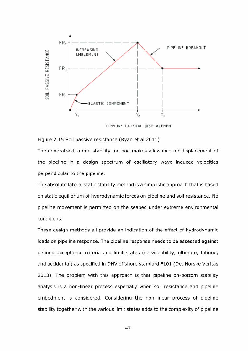
47

Figure 2.15 Soil passive resistance (Ryan et al 2011)

The generalised lateral stability method makes allowance for displacement of

the pipeline in a design spectrum of oscillatory wave induced velocities

perpendicular to the pipeline.

The absolute lateral static stability method is a simplistic approach that is based

on static equilibrium of hydrodynamic forces on pipeline and soil resistance. No

pipeline movement is permitted on the seabed under extreme environmental

conditions.

These design methods all provide an indication of the effect of hydrodynamic

loads on pipeline response. The pipeline response needs to be assessed against

defined acceptance criteria and limit states (serviceability, ultimate, fatigue,

and accidental) as specified in DNV offshore standard F101 (Det Norske Veritas

2013). The problem with this approach is that pipeline on-bottom stability

analysis is a non-linear process especially when soil resistance and pipeline

embedment is considered. Considering the non-linear process of pipeline

stability together with the various limit states adds to the complexity of pipeline

48

response assessment. It is thus necessary to seek an alternative design

approach that will allow for the assessment of the different factors (soil

resistance, pipeline displacement, pipeline embedment, etc.) that influence

pipeline on-bottom stability (Zeitoun et al. 2008).

2.12.2 Fluid-Pipe-Soil Interaction Stability Design Methods

Pipe-soil interaction tests carried out by both the Pipeline Stability Design

Project (PIPESTAB) and American Gas Association (AGA) show that the process

of pipeline instability was either displacement controlled or force controlled.

Both experiments show that in the process of lateral instability, the pipe pushes

the nearby soil back and forth, and sand scouring was not involved. The

PIPESTAB and AGA experiments have generally showed that any loading history

causing additional pipeline penetration would result in an increase of lateral

resistance (Wolfram, Getz and Verley 1987). It is also noteworthy that in the

pipe-soil methods discussed, wave loads were modelled with mechanical

actuators rather than hydrodynamic methods. Thus, wave induced scour

around the pipeline was not considered.

Some of the attempts made to improve upon the pipe-soil interaction is

discussed as follows.

2.12.2.1 Wave-Pipe-Soil Interaction Model

Gao, Gu and Jeng (2003) investigated the mechanism of wave induced pipeline

on-bottom stability using a U-shaped oscillatory flow tunnel in which the critical

conditions for pipeline instability was investigated by varying submerged weight

and diameter of pipeline, soil parameters and loading histories. The experiment

showed that an increase in the oscillatory flow amplitude results in three

49

characteristic times, stt , rtt and btt during pipe losing on-bottom

stability.

Onset of scour ( stt ) (see figure 2.16): Sand ripples gradually form in the

vicinity of the pipe as a result of increasing water particle velocity thus

triggering local scouring. In the process of local scouring, the sands in front of

the pipe move towards the pipe, and the sands behind the pipe are scoured

away from the pipe. The sand scour zone enlarges as the flow velocity

increases.

Figure 2.16 Onset of sand scour (Gao, Jeng and Wu 2006)

Pipe rocking ( rtt ) (see figure 2.17): At a certain flow velocity the pipe rocks

slightly periodically at its original location with approximately same frequency of

oscillatory flow. The pipe pushes the soil with a noticeable horizontal

displacement, accompanied by pipe rolling. Local scouring is also involved in

this phase and later phases.

50

Figure 2.17 Pipeline rocks (Gao, Jeng and Wu 2006)

Pipe breakout ( btt ) (see figure 2.18): As the flow velocity further increases

after a period of slight pipe rocking, the pipe is displaced from its original

location losing on-bottom stability. That is, the pipe breaks out suddenly from

its original location with a large lateral displacement (Gao, Jeng and Wu 2006).

Figure 2.18 Pipeline breakout (Gao, Jeng and Wu 2006)

The experiment showed a correlation between the dimensionless pipeline

weight (2D

WG s

where sW is submerged weight of pipeline, is buoyant

weight of soil, and D is pipeline diameter) and KC number for the constraint

conditions of freely laid pipeline and anti-rolling pipeline. For both constraint

51

conditions there is a linear relationship between G and KC as pipeline loses

stability for same diameter, but different for different diameters. This shows the

significance of pipeline diameter in stability analysis. Similarly, a correlation

between Fr and G was also established; for the same soil type with different

pipeline diameters there is a linear relationship between Fr and G , but results

differ with different soil types which is an indication of the influence of soil type

on pipeline stability. These relationships have been used as stability criteria for

subsea pipelines (Gao, Jeng and Wu 2006; Gao, Gu and Jeng 2003).

Comparing the physical phenomena of pipe instability in the pipe-soil

interaction experiment and that of wave-pipe-soil interaction shows an

additional penetration of pipeline into soil bed under cyclical preloadings which

increases the ultimate lateral resistance (Gao, Jeng and Wu 2006; Gao et al.

2006). The wave-pipe-soil interaction experiment showed that sand scouring

occurred around pipe and sediment transport had significant influence on pipe

on-bottom stability. The wave-pipe-soil interaction model thus provides a

better understanding of the pipeline on-bottom stability (Gao et al. 2005).

2.12.2.2 Conceptual Fluid-Pipe-Soil Stability Design Approach

Ryan et al (2011) proposed a fluid-pipe-soil interaction approach which includes

physical model testing and numerical stability analysis that will allow for the

combination of fluid-soil, pipe-soil and fluid-pipe effects to be investigated. The

physical model testing is intended to provide a better understanding of changes

in pipeline embedment, soil strength and soil resistance with time, and the

changes in hydrodynamic loading on pipeline with changes in pipeline

embedment. The pipe-soil model can then be updated taking into account the

52

combined effect of scouring, pipe-soil interaction, and soil liquefaction on the

overall pipeline response. This is intended to reduce design uncertainty by

minimising over-conservatism and also reduce potential under-conservatism in

the current design method.

2.12.2.3 2D Pipe-Soil-Fluid Interaction Model

Griffiths (2012) developed a pipe-soil-fluid (PSF) interaction model aimed at

accurate modelling of soil scouring and liquefaction at a minimal computational

cost (compared to the continuum soil Finite Element Analysis (FEA) approach).

A number of seabed shear stress profiles were generated as a function of

seabed and pipe geometry under various wave and current flow conditions

using 2D CFD models. The PSF model based on Shield’s criteria replicates the

CFD results and incorporates sediment suspension and transport into a pipe-soil

interaction model without requiring the solution of the Navier Stokes equations

in a CFD model. The key elements of the PSF model is as follows;

1. Determine soil deformation by first calculating the swept area of soil in front

of the pipe (as shown in figure 2.19) considering a D2.0 initial pipe

embedment with a D5.0 and D05.0 horizontal (to the right) and downward

displacement respectively.

53

Figure 2.19 Sweep area (Griffiths 2012)

2. The second step is then to calculate the suck area (void created behind the

pipe following pipe displacement) as shown in Figure 2.20. The suck area is

able to draw in water and sediment to fill the void as pipe is embeded.

Figure 2.20 Suck area (Griffiths 2012)

3. Determine soil reaction forces using modified equations from DNV RP F109

(2010) to calculate vertical soil reaction force and Verley’s theoretical model

(Verley , Sortberg and Brennodden 1990) to calculate soil horizontal

reaction force.

54

4. Determine hydrodynamic forces by generating wave velocity time and force

time history taking into account force reduction factors such as embedment

and pipe movement using DNV RP F109 (2010).

5. Soil-fluid interaction is then modelled by considering sediment transport and

deposition and applying Shield’s criteria to predict onset of sediment motion.

The PSF model results when compared to results obtained from Brennodden et

al (1989)’s Energy-Based Pipe-Soil Interaction model show a similar general

behaviour. The limitation with this model is in describing the fluid domain

accurately considering turbulence and fluid-soil interaction and its resultant

pipeline embedment since CFD is not used. Another limitation is that the PSF

fluid-soil interaction algorithm does not account for soil liquefaction. The PSF

model is undergoing further refinement, verification and validation with a view

to improve current pipeline stability design methodology which makes for costly

stabilisation techniques.

This project thus seeks to improve the current methodology for subsea pipeline

on-bottom stability design by providing a better understanding of fluid-pipe-soil

interaction using CFD modelling to incorporate the effect of seabed scouring

and liquefaction which are not presently correctly accounted for. The use of CFD

capability to accurately model fluid flow and sediment transport around subsea

pipelines have been proven; for example, Zhao et al. (2007) applied a

Computational Fluid Dynamics (CFD) model to investigate the flow dynamics

around a piggyback pipeline and found that the relative position of the smaller

pipe has significant effects on the vortex shedding characteristic and the

subsequent hydrodynamic loads on the pipeline. Kamarudin (2005) has shown

55

using a CFD modelling technique that the current practice of using an equivalent

diameter approach for piggyback pipelines underestimates the drag coefficient.

56

CHAPTER 3: METHODOLOGY

Computational Fluid Dynamics (CFD) is an advanced computer based modelling

tool for solving fluid dynamics (fluid flow, heat transfer and associated

phenomena) problems (Contantinides, Oakley and Holmes 2005). Experimental

works are expensive to perform and time consuming, sometimes there are risks

and environmental issues involved in designing test facilities, and thus

computer modelling technique is a very efficient and useful tool to carry out

stability analysis of submarine pipelines. With the progress in the development

of computational technology, CFD is becoming the most available and useful

tool for simulating a wide range of flow, mass, momentum and energy

problems. The use of CFD presents the opportunity to simulate different flow

conditions and environment faster and without the difficulty and expenses

required for experiments (Versteeg and Malalsekera 2007). This will benefit the

industry in the understanding of the behaviour of subsea pipelines under

various conditions.

CFD codes are based on numerical algorithms that can solve fluid flow related

problems. The codes comprises of a pre-processor, solver, and post-processor

(figure 3.1).

57

Figure 3.1 Interconnectivity of the main elements of CFD codes (Tu, Yeoh and

Liu 2013)

Versteeg and Malalsekera (2007) describe these three elements as follows;

Pre-processor - This is the input element of the code where key parameters are

defined. Parameters defined include geometry and computational domain, fluid

properties, boundary conditions, and mesh (grid) generation.

Solver - This integrates governing equations of fluid flow (such as continuity

Navier Stokes equations) over the computational domain, converting the

resulting integral equations into algebraic equations and generating a solution

by an iterative method (figure 3.2).

58

Figure 3.2 Solver process (Tu, Yeoh and Liu 2013)

Post-processor – This is the graphics output element of the code providing data

visualisation in the form of geometry and grid display, vector and surface

(two-dimensional and three-dimensional) plots, contour plots etc.

This research work is focussed on developing a fluid-pipe-soil model by

combining the effect of fluid-pipe, fluid-soil and pipe-soil interaction and using

computational fluid dynamics code to solve the model.

This chapter provides an explanation of the governing equations and

supplementary equations used in developing the model.

59

3.1 Governing Equations

CFD modelling for fluid flow is governed by equations of the laws of

conservation of physics; continuity equation (equation 3.1) which accounts for

mass conservation, momentum equation (equation 3.2 and equation 3.3) which

accounts for the force balance between rate of change of momentum and the

sum of forces on a fluid particle.

0)(

t (3.1)

2

2

2

21

y

uv

x

uv

x

p

y

uv

x

uu

t

u

(3.2)

2

2

2

21

y

vv

x

vv

y

p

y

vv

x

vu

t

v

(3.3)

2

2

2

2

y

T

C

k

x

T

C

k

y

Tv

x

Tu

t

T

PP

(3.4)

Where is the fluid density, u and v are velocity vectors, p is the pressure,

is the vector gradient, T is the temperature, PC is specific heat capacity and

k is thermal conductivity (Tu, Yeoh and Liu 2013).

Many attempts have been made to solve separated flow around marine

structures numerically, Navier-Stokes equations (equation 3.5) govern the

motion of a fluid around a body (Sumer and Fredsoe 2006).

upuut

u 2.

(3.5)

Navier-Stokes equations (equation 3.5) representing the conservation of

momentum are solved together with the continuity equation (equation 3.6)

which represents conservation of mass.

0. u (3.6)

Where p is the pressure, 2 is the Laplacian operator and is the fluid

viscosity.

The Navier-Stokes equations (equation 3.5) and the continuity equation

(equation 3.6) for a two dimensional flow in a Cartesian coordinate system are

presented as follows;

60

2

2

2

2

y

u

x

uv

x

p

y

uv

x

uu

t

u (3.7)

2

2

2

2

y

v

x

vv

y

p

y

vv

x

vu

t

v (3.8)

0

y

v

x

u (3.9)

Where u and v are the components of the velocity along the x and y directions

respectively.

It is more convenient to write the Navier-Stokes equations in terms of the

stream function, and the vorticity function, defined by:

yu

(3.10)

xv

(3.11)

y

u

x

v

(3.12)

The continuity equation (equation 3.9) is satisfied by equation 3.10 and

equation 3.11. Eliminating the pressure from equation 3.7 and equation 3.8,

and making use of equation 3.10, equation 3.11 and equation 3.12, the

following equation is obtained:

2

2

2

2

yxv

yv

xu

t

(3.13)

This equation is known as the vorticity-transport equation (Sumer and Fredsoe

2006).

3.1.1 Reynolds-averaged Navier-Stokes (RANS) equations

RANS equations solve the unsteady Navier-Stokes equations by introducing

averaged and fluctuating components. For incompressible flow with no change

in viscosity, the RANS equation are supplemented with turbulence model. The

RANS models offer a cost effective approach for computing turbulent flows. In

this thesis, the two-equation standard k turbulence model has been used

61

with the following key equations (equation 3.14 and equation 3.15). The choice

of standard k model was based on its accuracy for turbulent flow and good

convergence, and is widely used for turbulence modelling in industrial

applications.

Turbulence kinetic energy k :

k

jk

t

j

i

i

Gx

k

xku

xk

t (3.14)

Energy dissipation rate, ε:

k

CGk

Cxx

uxt

k

j

t

j

i

i

2

21

(3.15)

kG represents the generation of turbulence kinetic energy due to the mean

velocity gradients, 1C (1.44) and 2C (1.92) are constants, k (1) and

(1.3) are the turbulent Prandtl numbers for k and respectively (Ansys

Fluent 2015).

3.2 Calculation of soil resistance

Passive resistance ( RF ) on sand and clay is determined as shown in equation

3.16, equation 3.17, and equation 3.18 as follows (Det Norske Veritas 2010);

25.1

215.05

D

zkk

Fw

F p

ss

Ls

R for 7.26sk (3.16)

25.1

D

zk

Fw

F p

s

Ls

R for sk >26.7 (3.17)

31.1

39.0

1.4

D

z

G

k

Fw

F p

C

c

Ls

R (3.18)

62

Where

pmpip zzz Ls

s

sFw

Dk

2

Ls

u

cFw

Dsk

s

u

cD

sG

D - pipeline diameter,

piz - initial embedment

pmz - embedment due to movement

s - buoyant weight of soil

s - dry weight of soil

sw - submerged weight of pipeline

LF - lift force

us - undrained shear strength

When pipeline is laid on the seabed, the initial embedment ( piz ) which is due to

its own weight is determined by equation 3.19 for sand and equation

3.20 for clay (Det Norske Veritas 2010).

(3.19)

7.03.0

2.33.0

0062.00071.0

c

c

c

cpi

k

G

k

G

D

z (3.20)

For initial embedment LF is assumed to be zero.

Initial embedment is determined by using the submerged unit weight of soil

( ) which is determined from the bulk unit weight of soil ( bulk ) as follows;

e

eSGs

wbulk1

(3.21)

67.0037.0

s

pik

D

z

63

Where w unit weight of water is, sG is specific gravity of soil, S is the degree

of saturation and

1e is the voids ratio (where is soil porosity).

When the degree of saturation S =1 indicating that the voids are filled with

water (as in dense sands), the bulk unit weight of soil ( bulk ) = saturated unit

weight of soil ( sat ) which is written as;

e

eGs

wsat1

(3.22)

When the degree of saturation S =0 indicating that the voids are filled with air,

the bulk unit weight of soil ( bulk ) = dry unit weight of soil ( dry ) which is written

as;

e

Gs

wdry1

(3.23)

The submerged unit weight of soil ( ) is then determined as;

wsat

Seabed was modelled as porous media to ensure flow through the soil. This was

done by inputting porosity and inertial resistance values in the seabed region.

Porosity values used are as shown in the following chapters. Inertial resistance

is the inverse of the coefficient of permeability ( k ) of the soil. Assuming an

average soil particle diameter ( d ) of 0.6mm, equation 3.24 (Yang 2010) was

used to determine the coefficient of permeability ( k ).

2

22

)1(

)(

dck (3.24)

is the porosity and c is 0.003.

64

In this research work Computational Fluid Dynamics (CFD) software in

combination of analytical formulations has been used to model hydrodynamic

loadings, pipeline response, soil resistance, pipeline embedment and

pipe-soil-wave interaction. ABAQUS was initially used to model pipe-soil

interaction (chapter 4) as it able to simulate motion, deformation and fluid flow

using continuous function. ANSYS Fluent was used to model fluid-pipe-soil

interaction (chapters 5, 6, and 7) as its architecture enables efficient simulation

and control, flexible mesh capabilities to solve fluid flow using unstructured

meshes generated about complex generates.

Models created were used to analyse; the effect of soil types on passive and

lateral resistance and the effect of hydrodynamic loads on total soil resistance;

the effect of soil embedment and soil porosity on pipeline lateral stability; the

degree of embedment taking into consideration combined effect of pipeline

diameter and weight, unit weight of soil, and hydrodynamic forces; the scour

phenomenon and its effect on pipeline embedment. Models were created in 2D

to represent a finite section of pipeline to gain a better understanding of the

fluid-pipe-soil interaction which can be replicated across the pipeline length.

Considering the analysis to be carried out are mostly nonlinear, 2D simulation

will provide faster and more accurate results allowing for design iterations and

optimisation.

All models were created using dimensions from previous work carried out by

Gao et al (2007) in the wave-pipe-soil interaction model (discussed in section

1.12.2.1), Brennodden et al (1989) in the energy-based pipe-soil interaction

method (discussed in section 2.12.1.4), and Griffiths (2012) in the 2D

65

pipe-soil-fluid interaction model ( discussed in section 2.12.2.3). The results

from the work were also validated by results from these models.

66

CHAPTER 4: MODELLING THE EFFECT OF SOIL

RESISTANCE ON SUBSEA PIPELINE STABILITY

ABAQUS CFD was used to simulate pipe-soil interaction with a view to

investigating the effect of soil types (sand and clay) on passive and lateral

resistance and the effect of hydrodynamic loading and pipe embedment on soil

resistance. A 2D pipeline model with length to diameter ratio (20) of a typical

cross-section of full scale pipeline was created (Wang et al 2010). A 0.5m

diameter pipe (typical pipeline diameter vary from 2in (0.05m) to 72in (1.8m))

was created with the seabed soil represented as a relatively finite space. To

analyse the relationship between passive resistance and displacement and

lateral resistance and displacement, the pipeline is assumed to move between a

lateral displacement boundary of x=0 to x=0.5m (Figure 4.1).

The soil was modelled as elastic since pipe self-embedment and soil resistance

due to soil deformation was not considered. Also as the pipe’s Young’s Modulus

is much greater than that of the soil, the pipe was modelled as non-deformable

analytical rigid. As nonlinear deformation of soil is not considered, a tetrahedral

4-node bilinear plane mesh with cell size mmmm 5050 was generated is as

shown in Figure 4.2.

67

Figure 4.1 Pipeline displacement ( mm 510 )

Figure 4.2 mmmm 5050 Mesh

68

The boundary conditions (Figure 4.3) defines a series of physical behaviour for

the fluid flow process, such as pressure, temperature, and velocity. The

boundary names and types, and selected parameters were set as shown in

Table 4.1 and Table 4.2 respectively.

Table 4.1 Boundary conditions

Table 4.2 Selected parameters

Parameter Value

Density H2O 1025 kg/m3

Viscosity of H2O 0.001002 Pa-s

Reference Gravity 0, 0, -9.81 m2/s

Young’s Modulus Sand 1.034 × 107 Pa

Clay 6.894 × 105 Pa

Poisson’s Ratio Sand 0.3

Clay 0.3

Friction Coefficient Sand 0.6

Clay 0.2

Inlet Velocity 0.2 - 1.6 m/s

Pipeline weight 400 N

Boundary Name Boundary Type

Inlet Velocity Inlet

Outlet Pressure Outlet

Side wall 1 Symmetry Plane


Top wall Symmetry Plane

Bottom wall No-Slip Wall

Pipe wall No-Slip Wall

69

Figure 4.3 Geometry and boundaries

Simulation was carried out for various penetration depth ( e ) to outer diameter

( D ) ratio i.e. embedment as illustrated in Figure 4.4; D

e= 5%, 10%, 15% and

20%.

Figure 4.4 Pipe-soil interaction (Ren and Liu 2013)

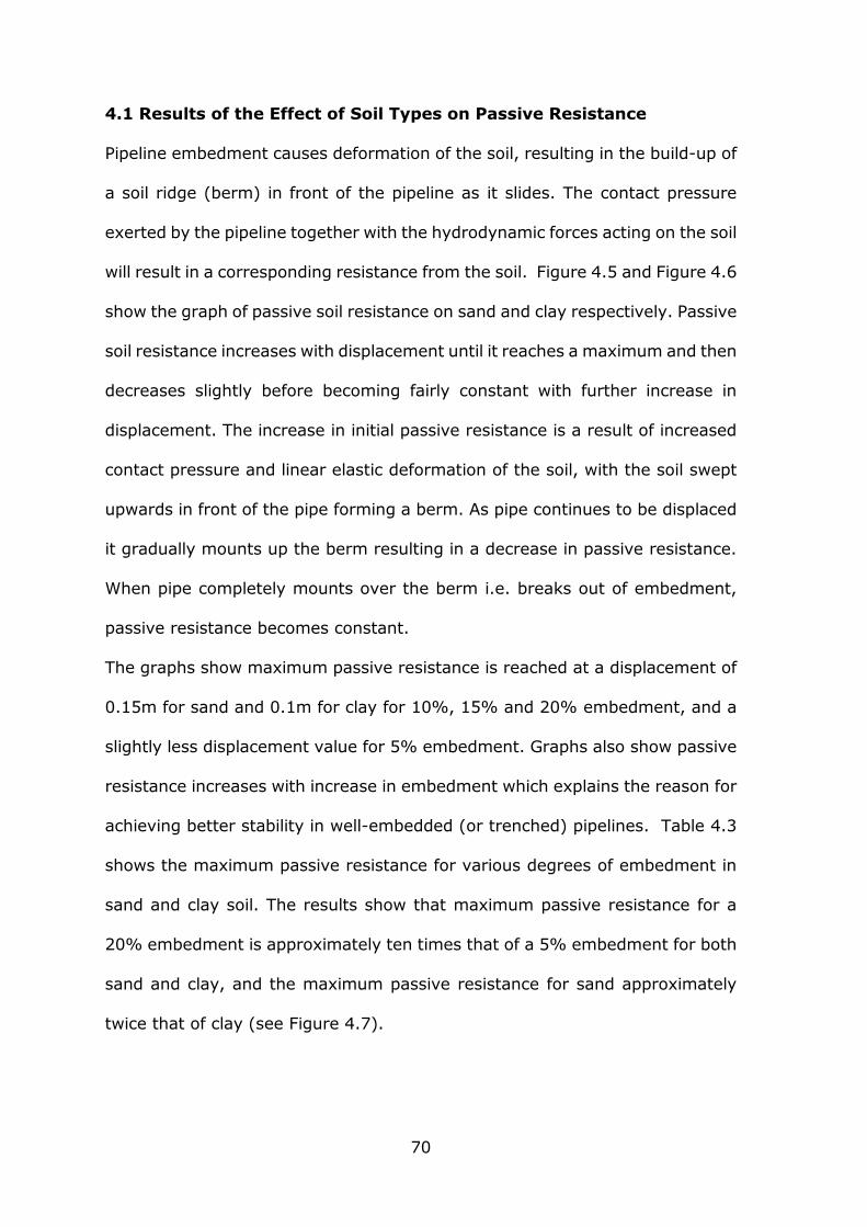
70

4.1 Results of the Effect of Soil Types on Passive Resistance

Pipeline embedment causes deformation of the soil, resulting in the build-up of

a soil ridge (berm) in front of the pipeline as it slides. The contact pressure

exerted by the pipeline together with the hydrodynamic forces acting on the soil

will result in a corresponding resistance from the soil. Figure 4.5 and Figure 4.6

show the graph of passive soil resistance on sand and clay respectively. Passive

soil resistance increases with displacement until it reaches a maximum and then

decreases slightly before becoming fairly constant with further increase in

displacement. The increase in initial passive resistance is a result of increased

contact pressure and linear elastic deformation of the soil, with the soil swept

upwards in front of the pipe forming a berm. As pipe continues to be displaced

it gradually mounts up the berm resulting in a decrease in passive resistance.

When pipe completely mounts over the berm i.e. breaks out of embedment,

passive resistance becomes constant.

The graphs show maximum passive resistance is reached at a displacement of

0.15m for sand and 0.1m for clay for 10%, 15% and 20% embedment, and a

slightly less displacement value for 5% embedment. Graphs also show passive

resistance increases with increase in embedment which explains the reason for

achieving better stability in well-embedded (or trenched) pipelines. Table 4.3

shows the maximum passive resistance for various degrees of embedment in

sand and clay soil. The results show that maximum passive resistance for a

20% embedment is approximately ten times that of a 5% embedment for both

sand and clay, and the maximum passive resistance for sand approximately

twice that of clay (see Figure 4.7).

71

Figure 4.5 Passive resistance on sand with 5%, 10%, 15% and 20%

embedment

Figure 4.6 Passive resistance on clay at 5%, 10%, 15% and 20% embedment

72

Table 4.3 Maximum passive resistance on sand and clay

Embedment

Maximum Passive Soil Resistance (kN/m)

Sand Clay

5% 2.87 1.32

10% 8.55 4.04

15% 12.77 6.39

20% 21.89 10.31

0

5

10

15

20

25

0 5 10 15 20 25

Penetration (%)

Max Passive Friction (kN)

Sand

Clay

Figure 4.7 Maximum passive resistance on sand and clay

These results are in agreement with the DNV recommended practice (Det

Norske Veritas 2010) model (figure 4.8) which specifies four regions for passive

resistance; a) an elastic region with very little lateral displacement, b) a region

with significant increase in displacement and increased passive resistance as a

73

result of increased pipe embedment which is due to pipe soil interaction, c) a

region of with decreased passive resistance and embedment signifying pipe

breakout, and d) a region with very high displacement where passive resistance

and embedment are fairly constant. The predicted results conform well with the

experimental work (an energy-based pipe-soil interaction model) carried out by

Brennoddden et al (1989) as part of research project conducted by SINTEF on

behalf of AGA (see Figure 4.8 shown below).

Figure 4.8 Soil resistance versus lateral displacement plot (Brennoddden et al

1989)

4.2 Results of the Effect of Soil Types on Lateral Resistance

Unlike passive soil resistance which is dependent on submerged weight of

pipeline, diameter of pipeline, height of berm in front of pipeline and

74

hydrodynamic loading, lateral soil resistance relates to soil resistance against

sliding friction only (that is the ability of soil to resist lateral forces exerted by

pipeline). Figure 4.9 and Figure 4.10 show the graph of soil friction variation

with displacement at various embedment for sand and clay respectively. As pipe

is displaced, soil friction increases for the partially embedded pipe and

maintains as a result of elastic deformation of the soil and build-up of mound.

This results in an increase of lateral soil resistance. After the breakout of pipe

(i.e. pipe going over berm), soil friction remains constant. The total soil friction

then becomes equal to the Coulomb’s friction. The graphs show that for a

pipeline with NWs 400 at 0% embedment, the sliding friction on sand and clay

is 240N and 80N respectively which is same as calculated using the Coulomb’s

friction equation FF = sW .

On Sand: NNWF sF 2404006.0

On Clay: NNWF sF 804002.0

75

Figure 4.9 Soil friction on sand at 0%, 5% and 10% embedment

Figure 4.10 Soil friction on clay at 0%, 5% and 10% embedment

76

The maximum lateral resistance for sand and clay is calculated as shown in

Table 4.4 and plotted as shown in Figure 4.11.

Table 4.4 Maximum lateral resistance on sand and clay

Embedment

Maximum lateral resistance (N/m)

Sand Clay

0% 238 80

5% 377 175

10% 845 412

0

100

200

300

400

500

600

700

800

900

0 2 4 6 8 10 12

Penetration (%)

Max Soil Resistance

Sand

clay

Figure 4.11 Maximum lateral resistance on sand and clay

77

Table 4.4 and Figure 4.11 show that maximum lateral resistance on sand is

greater (approximately twice) than on clay. Clay is more easily yielded and

deformed making it easier for pipeline to breakout of embedment. Thus for clay

soil a greater degree of embedment is required to maintain pipeline on-bottom

stability.

Overall passive resistance is by far greater than lateral resistance, thus passive

resistance is of greater significance for pipeline on-bottom stability analysis.

4.3 Results of the Effect of Hydrodynamic Load and Embedment on

Soil Resistance

To investigate the effect of hydrodynamic force and pipeline embedment on soil

resistance, the maximum lateral resistance was determined for various pipeline

submerged weight as shown in Table 4.5 and Table 4.6. Table 4.5 and Table 4.6

show that as submerged weight decreases the maximum lateral resistance also

decreases but increases with increasing embedment.

Table 4.5 Effect of submerged weight on maximum lateral resistance on sand

Submerged

weight (N/m)

Maximum lateral resistance on Sand (N/m)

0% 5% 10%

400 240 377 845

300 180 283 637

200 120 189 441

100 60 95 226

50 30 47 115

78

Table 4.6 Effect of submerged weight on maximum lateral resistance on clay

Submerged

weight (N/m)

Maximum lateral resistance on Clay (N/m)

0% 5% 10%

400 80 175 412

300 60 132 312

200 40 88 209

100 20 38 106

50 10 22 54

As the submerged weight of pipeline decreases, lift force increases resulting in

a corresponding decrease in lateral soil resistance due to reduced contact

pressure. When the lift force becomes equal or exceeds the submerged weight

of pipeline, there will be no contact pressure between soil and pipeline, thus soil

resistance becomes zero. This is illustrated as shown in the plots of Figure 4.12

and Figure 4.13 for sand and clay respectively.

79

0

100

200

300

400

500

600

700

800

900

0 0.2 0.4 0.6 0.8 1 1.2 1.4

Current Velocity (m/s)

Soil Friction (N/m)

0%

5%

10%


sand

0

50

100

150

200

250

300

350

400

450

0 0.2 0.4 0.6 0.8 1 1.2 1.4


Soil Friction (N/m) 0%

5%

10%

Figure 4.13 Relationship between hydrodynamic loading and soil friction on clay

80

4.4 Model Validation

The model developed was used to determine the horizontal force acting on the

pipeline and the results compared with that calculated from Morison’s equation

and Wake II Model (applied in DNV code) based on Lambrakos et al (1987) and

Chao, Lambrakos and Verley (1989) comparison of Wake Model predictions

with measured forces from Exxon’s PFMP. The results (Figure 4.14) show that

the CFD model predicts a 25% increase when compared to the Wake Model, and

the Morison equation values are much higher. Though the CFD and Wake II

models both account for wake effect as flow goes past pipeline and velocity

reverses resulting in an upstream region of low pressure (hence the closeness

of predicted result), the CFD model more accurately accounts for the pipeline

boundary conditions and varying sea conditions.

Figure 4.14 Horizontal force comparison with CFD model

81

4.5 Results Summary

The results from modelling the effect of soil resistance on pipeline stability show

that overall soil resistance is a combination of passive and lateral soil

resistance. While passive resistance is a function of pipeline weight and height,

and hydrodynamic forces, lateral resistance on the other hand is a function of

the pipeline’s contact with the soil (that is, sliding friction). The results also

show that passive resistance is on the average 10 times the value of lateral

resistance for both sand and clay soils, which implies that passive resistance is

more critical for pipeline on-bottom stability analysis. This confirms the

limitation of the Coulomb’s friction theory (discussed in section 2:10) which

estimates soil resistance based on lateral resistance.

82

CHAPTER 5: PIPELINE STABILITY ANALYSIS

CFD model was developed to represent a typical pipeline installed on a seabed,

with the inlet in the direction of the positive x-axis and the direction of flow

perpendicular to the axis of the pipeline using a scale of mmm 0.25.110 . Figure

5.1 shows the generated mesh near the pipe-seabed. The geometry of the

imported mesh is considered to be a control volume of a pipeline installed on the

seabed (Figure 5.2). A polyhedral mesh (with a relative size of 1.5% of model

size) was chosen as it uses less memory, gives faster solution and greater

accuracy. The boundary names and types, and selected parameters were set as

shown in Table 5.1 and Table 5.2 respectively.

Figure 5.1 Interior volume of mesh ( mmm 0.25.110 )

83

Figure 5.2 Geometry and boundaries


REGION

Fluid Porous

Boundary

Name

Boundary Type Boundary Name Boundary Type

Fluid-Porous

Interface

No-Slip

Wall

Porous 1 No-Slip Wall

Inlet Velocity Inlet Porous 2 No-Slip Wall

Outlet Pressure Outlet Porous 3 No-Slip Wall

No-Slip Wall Porous-Fluid Interface No-Slip Wall



Top wall Symmetry Plane

84


An unsteady, incompressible and turbulent segregated flow model was chosen

to solve the flow equations. Segregated flow model solves equations separately

and sequentially as opposed to coupled flow model which solves equations

together at the same time thus requires more memory space. Considering that

the flow is turbulent, the flow was modelled based on RANS equation derived

from the Reynolds decomposition of the Navier Stokes equation using the

standard k-ε model as described in section 3.1.1.

Parameter Value

Density of H2O 1025 kg/m3


Reference Gravity 0, 0, -9.81m2/s

Reference Temperature 273K

Reference Pressure 101325 Pa

Static Temperature 280K

Turbulence Dissipation Rate 0.1 J/kg-s

Turbulence Kinetic Energy 0.001 J/kg

Inlet Velocity 0.2 to 1.5 m/s

Porous Inertial Resistance 50 kg/m4

Porous Viscous Resistance 3000 kg/m3-s

Time Step 0.05 seconds

Maximum Inner Iteration 5

Maximum Physical Time 90 seconds

85

Hydrodynamic force was simulated by considering a constant flow amplitude of

0.3m/s at varying KC number (40, 50, 60, and 70) based on Soedigbo,

Lambrakos and Edge (1998) Wake II Model. Series of simulations were

performed by varying inlet flow velocity from 0.2 m/s to 1.5 m/s, to determine

the hydrodynamic forces acting on the pipeline. The embedment of the pipeline

and the porous resistance of the seabed were also varied in order to determine

their effect on pipeline stability. As seabed was modelled as static, the pressure

loads and distribution on the pipe wall was used to analyse the pipeline stability.


The CFD model was validated by comparing its start-up effect with that

observed by Soedigbo, Lambrakos and Edge (1998) in the analysis of field work

carried out by Exxon Production Research Company (EPRC) to improve the

prediction of hydrodynamic forces on subsea pipelines. The start-up effect

(discussed in section 2.9.1) for the CFD model and work based on EPRC show

that as the relative velocity between pipeline and sea (water) changes, the lift

force varied more rapidly compared to the drag force which is the effect of

varying time dependent force coefficients as shown in Figure 5.3 (lift

coefficient) and Figure 5.4 (drag coefficient). This also in agreement with the

results from the full-scale laboratory and field investigation of hydrodynamic

force characteristics by Verley, Lambrakos and Reed (1987) which also

established that lift coefficient has a stronger start-up effect than the drag

coefficient.

86

Figure 5.3 Lift coefficient with start-up effect

Figure 5.4 Drag coefficient with start-up effect

87

5.2 Results of Pipeline Stability Analysis

The lateral stability of the pipeline in currents can be achieved by maintaining a

balance between the horizontal forces acting on the pipeline and the total lateral

soil resistance. Figure 5.5 shows the graph for stability criteria for 0.5m

diameter pipeline with 5% embedment. The pipeline will be unstable if the

horizontal force becomes greater than the total lateral soil resistance. At the

point of intersection between the horizontal force and total lateral soil

resistance, the critical velocity of the current CU above which the pipeline

becomes unstable is determined (in figure 5.5 CU is 0.94m/s). This implies at

any current velocity below CU the pipe will be stable and any current velocity

above CU will result in lateral instability of the pipeline.

Figure 5.5 Pipeline stability criteria for 0.5m diameter pipeline with 5%

embedment

88

Reducing the diameter to thickness ratio of the pipeline will increase the

thickness as well as the submerged weight of the pipeline thus increasing the

total lateral soil resistance which will cause the pipeline to be more stable. Any

small proportional increase in submerged weight results in a proportional

increase in the total lateral soil resistance and the critical velocity that will cause

pipeline instability. In Figure 5.6 any submerged weight above weight 1 will

keep the pipeline stable in a sea state with critical velocity 1CU or less.

Figure 5.6 Effect of weight increase on 0.5 m diameter pipeline (submerged

weight 1 = N415 , submerged weight 2 = N440 and submerged weight 3

= N465 )

89

5.2.1 Results of the Effect of Soil Embedment on Pipeline Lateral

Stability

The submerged weight of an installed pipeline induces some degree of

embedment of the pipeline. The degree of embedment also depends on the

properties of the seabed soil. Figure 5.7 shows that a slight reduction (2% i.e.

decrease from 5% to 3%) in pipeline embedment reduces the total lateral soil

resistance by approximately 23%. This is due to the reduced pipe-soil contact.

The effect of reduced embedment on horizontal force was insignificant (as there

was no notable difference as can been see in figure 5.7) when compared with

the effect on the total lateral soil resistance. This implies that the higher the

degree of embedment the more stable the pipeline and vice versa.

Figure 5.7 Effect of soil embedment on pipeline lateral stability

90

5.2.2 Results of the Effect of Seabed Porosity on Pipeline Lateral

Stability

Increasing the porous inertial resistance and porous viscous resistance by

100% and 67% respectively results in a corresponding reduction in the porosity

of the seabed. Figure 5.8 shows that this reduction in porosity results in a slight

reduction (5%) in the lateral stability of the pipeline. There is a higher rate of

decrease in total lateral soil resistance of the less porous seabed with flow

velocity when compared with the higher porous seabed.

Figure 5.8 Effect of porosity on pipeline lateral stability

A very slight rate of increase in the horizontal force was observed with the less

91

porous seabed as flow velocity increased. This is due to the reduced fluid-soil

interaction; the less porous seabed reduces the ease with which the fluid flows

through the soil, thus increasing the pressure acting on the pipeline. As

discussed in section 2.11 (sediment mobility), wave induced shear stresses on

subsea soils causes pore-water pressure build-up which results in soil

liquefaction. Thus, the higher the pore-water pressure build-up, the higher the

soil porosity and hence greater soil liquefaction.

5.3 Results Summary

The results from this chapter show the effect of seabed porosity on lateral soil

resistance; increasing seabed porosity increases lateral soil resistance. This

explains the reason for the decrease in pipeline stability in less porous seabed

as higher porosity results in greater soil liquefaction which increases soil

resistance and hence pipeline stability. The results obtained are in agreement

with the conclusion of Wagner et al. (1987) pipe-soil interaction model, which

established that pipeline embedment as a result of soil porosity have a

significant effect on lateral soil resistance and thus overall lateral stability of

subsea pipelines.

92

CHAPTER 6: MODELLING PIPELINE

EMBEDMENT FOR ON BOTTOM STABILITY

OPTIMISATION

The experimental work by Gao et al. (2007) on ocean currents-induced pipeline

lateral stability on sandy seabed showed a linear correlation between the

Froude number and dimensionless submerged weight of pipeline for various

pipeline diameters. The result gave an indication of the influence of pipeline

diameter on stability. However the combined effect of change in diameter and

submerged weight of pipeline on stability was not fully established. This section

seeks to establish the relationship of this combined effect on pipeline stability in

sand and clay soils.

CFD model was developed to represent a pipeline on a seabed, with the seabed

created as a porous media using dimensions from experimental work on

pipeline stability carried out by Gao et al. discussed in section 2.12.2.1 (Gao et

al. 2007; Gao, Gu and Jeng 2003; Gao et al. 2002).

To ensure good resolving of boundary layer as the flow is wall bounded, a

410000 cell mesh (Figure 6.1) was generated with inflation applied to

accurately calculate effects of non-slip condition on pipe wall. Inflation layer

results in correct prediction of hydrodynamic coefficients (drag and lift), wake,

turbulence and other surface losses. Considering turbulent conditions, the

standard k-ε turbulence model was selected as discussed in section 3.1.1.

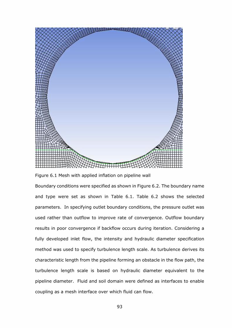
93

Figure 6.1 Mesh with applied inflation on pipeline wall

Boundary conditions were specified as shown in Figure 6.2. The boundary name

and type were set as shown in Table 6.1. Table 6.2 shows the selected

parameters. In specifying outlet boundary conditions, the pressure outlet was

used rather than outflow to improve rate of convergence. Outflow boundary

results in poor convergence if backflow occurs during iteration. Considering a

fully developed inlet flow, the intensity and hydraulic diameter specification

method was used to specify turbulence length scale. As turbulence derives its

characteristic length from the pipeline forming an obstacle in the flow path, the

turbulence length scale is based on hydraulic diameter equivalent to the

pipeline diameter. Fluid and soil domain were defined as interfaces to enable

coupling as a mesh interface over which fluid can flow.

94

Figure 6.2 Fluid-pipe-soil boundary conditions





Symmetry 1 Symmetry Plane

Symmetry 2 Symmetry Plane

Pipe wall No-Slip Wall

Interface 1 Mesh Interface

Interface 2 Mesh Interface

95


Simulation was carried out for various penetration depth ( e ) to outer diameter

( D ) ratio i.e. embedment D

e= 5%, 10%, 15%, 20% and 25%.

Three sets (0.5m and 1m diameter pipeline on loose sand and 0.5m diameter

pipeline on dense sand) of thirty-six simulations were carried out for six current

velocities at six embedment conditions with varying pipeline submerged weight

Parameter Value

Inlet Velocity 0.25 to 1.5 m/s

Pipeline Diameter 0.5m, 1m

Unit Weight of Soil

Loose Sand 18400 N/m3

Dense Sand 19400 N/m3

Soft Clay 17300 N/m3

Unit Weight of Dry Soil

Loose Sand 13900 N/m3

Dense Sand 15100 N/m3

Soft Clay 11500 N/m3

Saturation

Loose Sand 94.8%

Dense Sand 100%

Soft Clay 100%

Porosity

Loose Sand 48.3

Dense Sand 43.9

Undrained Shear Strength Soft Clay 1400 Pa

Static Friction Coefficient

Sand 0.6

Clay 0.2

96

per unit length. Matlab code (see appendix A (I and II), B (I and II), C (I and II),

D (I and II), E) was used to determine embedment.

6.1 Results of the Effect of Pipe Diameter and Pipe Weight on Pipeline

Embedment

Figures 6.3 (for sand) and 6.4 (for clay) show the relationship between

increasing pipe diameter and pipeline embedment (at a fixed weight submerged

weight of 1000N/m3). The graph shows a decrease in pipeline embedment with

increasing diameter, which is due to the increased pipe-soil contact area

resulting in increased resistance to embedment, and increase in lift force with

increasing diameter. The plots (Figures 6.3 and 6.4) show that the percentage

decrease in embedment with increasing diameter (0.2m to 1.2m) is similar for

both sand (86%) and clay (83%) with clay having a higher degree of

embedment.

0.2 0.3 0.4 0.5 0.6 0.7 0.8 0.9 1 1.1 1.20

0.01

0.02

0.03

0.04

0.05

0.06

0.07

0.08

Pipe Outer Diameter (m)

Initia

l E

mbedm

ent

(Norm

alis

ed w

ith D

iam

ete

r)

Figure 6.3 Effect of increasing diameter on initial embedment (sand)

97

0.2 0.3 0.4 0.5 0.6 0.7 0.8 0.9 1 1.1 1.20

0.05

0.1

0.15

0.2

0.25

0.3

0.35


Initi

al E

mbe

dmen

t (N

orm

alis

ed w

ith D

iam

eter

)

Figure 6.4 Effect of increasing diameter on initial embedment (clay)

Figures 6.5 and 6.6 show the variation of embedment for a 0.5m diameter pipe

with increasing weight of pipeline. The plots show that for both sand and clay,

as pipe weight increases embedment also increases, with sand having a

percentage increase in embedment of approximately 78% and 81% for clay for

pipe weight 200N/m to 1200N/m.

To investigate the combined effect of pipe diameter and weight on pipeline

embedment, a submerged weight per unit length was assigned to each

diameter on the basis of calculated volume per unit length (resulting in a

proportional increase in weight as diameter increases). The result for sand

(Figure 6.7) show that there is an increase in pipeline embedment with

increasing diameter as a result of increasing weight and build-up of a soil ridge.

However, when embedment is normalised with diameter (Figure 6.8), there is a

decrease in embedment with increasing diameter which is in line with Figures

6.3 and 6.4. This is a result of increased lift force on larger diameter pipelines

due to a greater fluid-pipe contact area resulting in a reduced soil ridge and

98

hence reduced embedment. This implies that pipe diameter has a greater

influence on pipeline embedment than pipe weight.

200 400 600 800 1000 1200 1400 1600 1800 20000.002

0.004

0.006

0.008

0.01

0.012

0.014

0.016

0.018

Pipe Weight per Unit Length (N/m)

Initia

l E

mbedm

ent

(m)

Figure 6.5 Effect of submerged pipe weight on embedment (sand)

200 400 600 800 1000 1200 1400 1600 1800 20002

3

4

5

6

7

8

9

10

11x 10

-3

Pipe Weight per Unit Length (N/m)

Initi

al E

mbe

dmen

t (m

)

Figure 6.6 Effect of submerged pipe weight on embedment (clay)

99

0.2 0.4 0.6 0.8 1 1.20.005

0.01

0.015


Initia

l E

mbedm

ent

(m)

a

0.2 0.4 0.6 0.8 1 1.20.01

0.015

0.02

0.025

0.03

0.035


Initia

l E

mbedm

ent

(Norm

alised w

ith D

iam

ete

r) b

Figure 6.7 Combined effect of pipe diameter and weight on embedment (sand)

Figure 6.8 Effect of normalised pipe diameter on embedment (sand)

100

The result for clay show that both actual (Figure 6.9) and normalised

embedment (Figure 6.10) increase with increasing diameter, this implies for

clay soil, pipe weight has a greater influence on embedment than in sand.

0.2 0.4 0.6 0.8 1 1.20

0.01

0.02

0.03

0.04

0.05


Initia

l E

mbedm

ent

(m)

a

0.2 0.4 0.6 0.8 1 1.20.026

0.028

0.03

0.032

0.034

0.036

0.038


Initia

l E

mbedm

ent

(Norm

alised w

ith D

iam

ete

r) b

Figure 6.9 Combined effect of pipe diameter and weight on embedment (clay)

Figure 6.10 Effect of normalised pipe diameter with embedment (clay)

101

6.2 Results of the effect of unit weight of soil on pipeline embedment

Figure 6.11 and Figure 6.12 show the effect of increasing unit weight of soil on

pipeline embedment for sand and clay respectively. Both plots show a decrease

in embedment with increasing unit weight of soil. This is a result of decrease in

porosity as density (weight and particle size) increases. As discussed in chapter

5 section 5.1.2 a reduction in soil porosity will reduce embedment as the less

porous soil reduces the ease with which fluid flows through the soil, thus

increasing the upward force on the pipeline. The rate of decrease in embedment

with increasing unit weight is greater in sand (≈33%) than in clay (≈7%) as

sand has a lower porosity than clay and thus lower degree of embedment.

1.6 1.7 1.8 1.9 2 2.1 2.2 2.3 2.4

x 104

0.007

0.008

0.009

0.01

0.011

0.012

0.013

Unit Weight of Soil (N/m3)

Initia

l E

mbedm

ent

(m)

Figure 6.11 Effect of unit weight of soil on embedment (sand)

102

1 1.2 1.4 1.6 1.8 2 2.2 2.4

x 104

5.6

5.8

6

6.2

6.4

6.6

6.8

7x 10

-3

Dry Unit Weight of Soil (N/m3)

Initia

l E

mbedm

ent

(m)

Figure 6.12 Effect of unit weight of soil on embedment (clay)

6.3 Results of the effect of hydrodynamic forces on pipeline

embedment

The method used to compute the scour depth was first to determine if scour

would occur based on results from initial embedment conditions, then the

equilibrium depth was calculated in one step. This reduced the need for a

lengthy iterative process. Figures 6.13 and 6.14 show the effect of increasing

current velocity on embedment (in loose sand) for a 0.5m and 0.1m diameter

pipe respectively.

103

Figure 6.13 Effect of current velocity on embedment (0.5m pipe on loose sand)

0 0.5 1 1.50

0.1

0.2

0.3

0.4

0.5

0.6

0.7


Pip

e E

mbedm

ent

(Norm

alis

ed w

ith D

iam

ete

r)

Ws=1500N/m3

Ws=2000N/m3

Ws=3000N/m3

Ws=4500N/m3

Figure 6.14 Effect of current velocity on embedment (1m pipe on loose sand)

104

The plots show that other than the initial embedment as a result of pipe weight,

there is no change in embedment with initial increase in velocity until the onset

of scouring. As scouring progresses with increasing velocity, embedment

increases until pipeline breakouts of embedment signifying a decrease in

embedment to zero. The results also show that the velocity at which pipe

breakout occurs increases with increasing submerged weight of pipe that is the

heavier the pipe the higher the velocity required to cause breakout.

Comparing Figures 6.13 (0.5m pipe) and 6.14 (1m pipe) it can be seen that a

larger pipe weight is required to prevent pipe breakout at a lower degree of

embedment for a 1m diameter pipe than for a 0.5m diameter pipe. This is

because hydrodynamic force is proportional to diameter thus the higher

diameter pipe has a greater hydrodynamic force acting on it and will require a

heavier weight to prevent movement.

Gao et al. (2007), in the experiment on ocean currents-induced pipeline lateral

stability on sandy seabed concluded that there is a linear relationship between

submerged weight of pipeline and the ratio of inertia force to gravitational force

(Froude number) for the lateral stability of pipelines. However, the experiment

did not completely verify the combined effect of diameter and submerged

weight on pipeline stability. This model has shown the combined effect of

pipeline diameter and submerged weight on pipeline embedment which

reflects pipeline stability.

105


The model was validated by comparing the results of varying pipeline diameter

and weight, and soil type on the initial of embedment with the results from

experimental work on energy based pipe-soil interaction carried out by

Brennodden et al. (1989) as discussed in section 2.12.1.4 and Griffitts et al.

(2012) pipe-soil-fluid model (not based on CFD) discussed in section 2.12.2.3

as shown in Table 6.3, Table 6.4 and Table 6.5.

Table 6.3 Initial embedment in loose sand (18400 N/m3 bulk unit weight)

Diameter

(m)

Submerged

weight

(N/m)

Initial Embedment (m)

CFD Model Brennodden et al Griffiths et al

0.5 250 0.004 0.004 0.004

0.5 500 0.007 0.006 0.006

1.0 1000 0.009 0.016 0.012

1.0 2000 0.014 0.018 0.018

Table 6.4 Initial embedment in dense sand (19400 N/m3 bulk unit weight)

Diameter

(m)

Submerged

weight

(N/m)


CFD Model Brennodden et al Griffiths et al

1.0 1000 0.008 0.003 0.010

1.0 2000 0.013 0.004 0.012

Table 6.5 Initial embedment in clay (17300 N/m3 bulk unit weight)

Diameter

(m)

Submerged

weight

(N/m)


CFD Model Brennodden et al

0.5 250 0.011 0.009

1.0 1000 0.032 0.021

1.0 2000 0.043 0.030

106

The results show that the CFD model is in more in agreement with Griffiths et al.

(2012) than Brennodden et al. (1989). CFD model shows a higher degree of

initial embedment compared to Brennodden et al. (1989) as the later only

considered pipe-soil interaction without the effect of fluid. In the case of

Griffiths et al. (2012) which is a pipe-soil-fluid model, the results are almost

same as that of the CFD model.

6.5 Results Summary

The results show that pipeline embedment decreases with increasing diameter

(a 27% embedment decrease for diameter increase from 0.5m to 1m). This is

inverse to the effect of pipeline weight on embedment (embedment increases

with increasing weight). The results from the combined effect of pipeline

diameter and weight show a variation in embedment based on soil type.

Embedment decreased with increasing diameter for sand and remained the

same for clay. These results establish that pipeline diameter has a greater

influence on embedment in sand while pipeline weight has more influence on

embedment in clay. Experimental work by Gao et al. (Gao et al. 2007; Gao, Gu

and Jeng 2003; Gao et al. 2002) gave an indication of the influence of diameter

in pipeline stability but this was not really established. This work has

demonstrated the effect of pipeline diameter and its combined effect with

pipeline weight on embedment.

107

CHAPTER 7: MODELLING SCOURING EFFECT

Model was created as a 2D model representing 0.4m pipeline on a seabed, with

seabed scouring effect and eventual breakout of pipe in an unbounded flow. A

383612 node mesh (Figure 7.1) was generated with inflation applied to

accurately capture the effect of no-slip condition on the boundary layer region

for turbulent flow. Considering turbulent conditions, the k-ε turbulence model

was used.

Figure 7.1 Mesh with applied inflation on pipeline wall

Boundary conditions were specified as shown in Figure 7.2. The boundary name

and type were set as shown in Table 7.1. Table 7.2 shows the selected

parameters.

108

Figure 7.2 Boundary regions (A- inlet; B- outlet; C- symmetry top; D- wall left;

E- wall right; F- wall bottom; G- wall Cylinder)





Symmetry Top Symmetry

Wall Cylinder No-Slip Wall

Wall Part Body Surface Wall

Wall Part Body Surface 1 Wall

Wall Part Body Surface Shadow Wall

109


Simulation was carried out for various pipeline positions (-0.7, -0.3, 0.0, 0.5,

1.0, 1.2) representing pipe movement on the scoured seabed (Figure 7.3).

Position -0.7 represents the initial pipeline position before any movement, at

position -0.3 embedment is beginning to occur with pipeline gradually be

displaced downwards. Position 0.0 represents pipeline at maximum

embedment, any further displacement from this position moves pipeline out

berm resulting in eventual pipeline breakout. Positions 0.5 and 1.0 represent

pipeline movement out of embedment, and position 1.2 represents pipeline at

breakout position (i.e. total displacement from embedment).

Parameter Value

Density of H2O 998.2 kg/m3

Density of Pipe 2719


Specific Heat of H2O 4182 J/kg-K

Specific Heat of Pipe 871 J/kg-K

Inlet Velocity 1.5 m/s

Temperature 288.16 K

Time Step 0.001s

Maximum Inner Iteration 20

110

Figure 7.3 Pipeline positions from onset of scour to breakout

Position is with reference to point 0.0 the centre of hydrodynamic scour (see

Figure 7.4; arrow shows direction of pipe movement). Simulations were done at

0.001s time step for 10000 time steps at a maximum iteration of 20 per time

step with a reporting interval of 1. The seabed scour was modelled as fixed and

pipeline position was moved along the scour path as illustrated in figure 7.3.

Figure 7.4 Pipeline position at reference point 0.0

111

7.1 Results on Scouring Effect on Velocity

Figures 7.5a 7.6a, 7.7a, 7.8a, 7.9a and 7.10a show the velocity vector and

corresponding contour diagrams (Figures 7.5b, 7.6b, 7.7b, 7.8b, 7.9b and

7.10b) of pipeline from position at -0.7 to position 1.2. At position -0.7 (Figures

7.5a and 7.5b) scouring is yet to occur but a region of high velocity can be seen

between the bottom of pipe and seabed. The high velocity combined with the

action of vortices (see vorticity plot Figures 7.11a-f) at the downstream side of

the pipeline induces seabed erosion (scour). As scouring progresses the region

of high velocity is seen at the top of the pipe (Figure 7.6a) indicating negative

lift (as shown in the pressure coefficient plot in Figure 7.13b) which signifies

pipe embedment. This position (-0.3) also shows an increase in vortex strength.

The highest velocity vector is reached at the point (0.0) where maximum

scouring (that is maximum embedment) is achieved. Further pipe movement

after this position (0.0) causes the pipe to breakout of embedment (Figures

7.8a and 7.8b; 7.9a and 7.9b; 7.10a and 7.10b). These results are in

agreement with the wave-pipe-soil interaction experiment by Gao, Gu and Jeng

(2006) which showed that there is an increase in the oscillatory flow amplitude

(from the onset of scour to pipe rocking and eventual breakout of pipe) during

process of pipe losing on-bottom stability. These results are contrary to the

conclusion of the PIPESTAB and AGA pipe-soil interaction tests that scouring is

not involved in the process of lateral pipeline instability, which is one of the

limitations of the study (PIPESTAB and AGA). These results prove that scouring

(seabed erosion) is a result of seabed particle movement induced by high

velocity region (between pipe and seabed) and vortex formation due to wake

effect.

112

Figure 7.5a Vector of pipeline at position -0.7

Figure 7.5b Contour of pipeline at position -0.7

113

Figure 7.6a Vector of pipeline at position -0.3

Figure 7.6b Contour of pipeline at position -0.3

114

Figure 7.7a Vector of pipeline at position 0.0

Figure 7.7b Contour of pipeline at position 0.0

115



116



117



118

Figure 7.11a -0.7 Figure 7.11b -0.3

Figure 7.11c 0.0 Figure 7.11d 0.5

Figure 7.11e 1.0 Figure 7.11f 1.2

Figure 7.11 Vorticity plot for the mechanism of scour under pipeline

119

7.2 Results for Scouring Effect on Wall Shear Stress and Pressure

Coefficient

Figures 7.12a, 7.13a, 7.14a, 7.15a, 7.16a and 7.17a show the wall shear stress

plots (that is, shear stress in the layer of the fluid in contact with the pipe wall)

and corresponding pressure coefficient plots Figure 7.12b, 7.13b, 7.14b, 7.15b,

7.16b and 7.17b (that is the relative pressure at each point across the pipe wall)

for pipeline position -0.7, -0.3, 0.0, 0.5, 1.0 and 1.2. Pressure coefficient plot

round circumferential position theta is as shown in Appendix F. Maximum wall

shear stress decreases from position -0.7 (≈34 Pa) to position -0.3 (≈15 Pa) as

pipeline embedment increases and then increases slightly at position 0.0 (≈20

Pa) maximum embedment. As pipeline breaks out from position 0.5, 1.0 and

1.2 there is an increase in maximum shear stress to ≈30 Pa. The point of

maximum shear stress which is around the midsection of the pipeline

corresponds to the point of highest velocity as shown in the velocity vector plots

in Figures 7.5a 7.6a, 7.7a, 7.8a, 7.9a and 7.10a. The plots also generally show

that maximum wall shear stress corresponds to a minimum pressure

coefficient. This is because the point of maximum shear stress represents the

point in the fluid-pipe-soil interface where scouring effect is at its greatest. As

shown on the velocity vector plots, the highest velocity is also at the midsection

of the pipeline corresponding to the area of scouring. The lift force at the point

of maximum shear stress represented by the pressure coefficient is at its

minimum as pipeline is at maximum embedment. This is so for all positions

except position -0.3 and 1.0 where the maximum wall shear stress is at the top

of the pipe as it gets embedded at position -0.3 and breaks out at position 1.0.

At both these positions pipeline instability is a result of displacement rather

scouring which explains the effect that was observed in the PIPESTAB and AGA

120

pipe-soil interaction projects. The points of maximum wall shear stress and

minimum pressure coefficient also correspond with the point of maximum

velocity vector and velocity contour as shown in Figures 7.5a and 7.5b; 7.6a

and 7.6b; 7.7a and 7.7b; 7.8a and 7.8b; 7.9a and 7.9b; 7.10a and 7.10b. The

highest maximum wall shear stress and lowest minimum pressure coefficient is

observed to be at position -0.7. As explained in section 7.1 this is the position

where scouring effect is induced.

-5

0

5

10

15

20

25

30

35

-2.5 -2 -1.5 -1 -0.5 0 0.5 1 1.5 2 2.5

Wall Shear

Stress [Pa]

Position

Figure 7.12a Wall shear stress of pipeline at position -0.7

121

Figure 7.12b Pressure coefficient of pipeline at position -0.7

-5

0

5

10

15

20

25

30

35

-2.5 -2 -1.5 -1 -0.5 0 0.5 1 1.5 2 2.5

Wall Shear

Stress [Pa]

Position

Figure 7.13a Wall shear stress of pipeline at position -0.3

122

Figure 7.13b Pressure coefficient of pipeline at position -0.3

Figure 7.14a Wall shear stress of pipeline at position 0.0

123

Figure 7.14b Pressure coefficient of pipeline at position 0.0


124



125



126


Table 7.3 and corresponding plot Figure 7.18 below shows the CD and CL values

at the various pipeline positions 1(-0.7), 2(-0.5), 3(0.0), 4(0.5), 5(1.0) and

6(1.2). The plot shows that CL increases with decreasing CD from pipeline initial

embedment progressing to the onset of scouring and peaks at position 0.0

(position of maximum embedment) where CD is at its minimum. This confirms

the results of the Pipe-Soil Interaction Model presented by Wagner et al (1987)

which showed that there is substantial soil resistance even under high lift forces

as there is an increase in pipeline embedment.

127

Table 7.3 CD and CL values

Pipeline Position CD CL

-0.7 2.58 0.57

-0.5 2.03 0.63

0.0 1.83 1.32

0.5 2.10 1.11

1.0 2.52 1.02

1.2 2.47 1.47

0

0.5

1

1.5

2

2.5

3

0 2 4 6 8

Coefficent of Drag (CD) and Coefficeint of Lift (CL) Plot

CD

CL

Figure 7.18 CD and CL plot at pipeline positions

128


This model was validated by comparing the wall interaction effects plot (d

d

C

C

versus D

H) as stated in DNV Recommended Practice C205 (Figure 7.19)

(DNV-RP-C205 2010) with that generated by the model considering unbounded

flow as shown in Figure 7.20.


cylinder (DNV-RP-C205, 2010)

129


cylinder as generated by CFD model

7.4 Results Summary

The results from modelling scour effect shows maximum embedment (scour) is

reached at the point of highest velocity vector, maximum wall shear stress

(point of greatest scour effect) corresponds to minimum pressure coefficient

(lift force). The model shows that embedment is a result of displacement (initial

pipe position before scouring) and scouring. The displacement effect as shown

in the results is in agreement with that observed in the PIPESTAB and AGA

pipe-soil interaction tests, however the effect of scouring as demonstrated in

the results disproves conclusion of the PIPESTAB and AGA pipe-soil interaction

tests that scouring is not involved in the process of lateral pipeline instability.

130

The results also show CL increases (with maximum at point of maximum

embedment) as CD decreases which confirms previous results that show that

soil resistance increases with high lift forces due to increased pipe embedment.

131

CHAPTER 8: CONCLUSION AND

RECOMMENDATION

This thesis presents a numerical study of hydrodynamics loading of a

submerged pipe under embedment, passive resistance, porous sea-bed and

scoured sea-bed. The computational fluid dynamics (CFD) technique applied in

this research took into account the boundary layer effects, wake flow effects,

vortex fields, the fluid interaction with both pipeline and seabed, and the

interaction between pipeline and seabed. The boundary layer specifications

used in this research included pressure outlet in place of pressure outflow to

improve convergence, turbulence length scale specified using the intensity and

hydraulic method, and inflation applied to ensure accurate prediction of

hydrodynamic coefficients.

Wake effect which induces vortex shedding at boundary layer causes an initial

reduction in lift force and increase in drag force. Vortex shedding as a result of

wake effect induces further interaction between fluid and the seabed (tunnel

erosion) leading to sediment mobility which results in scouring of the seabed. As

hydrodynamic forces increase, scouring increases resulting in increased

pipeline embedment until the break-out point is reached. Hydrodynamic forces

also induce pore pressure build-up and vertical pressure on the seabed which

results in liquefaction. The CFD model showed an accurate combined effect of

fluid flow around a pipeline and on the seabed (considering scouring and

liquefaction) when compared with previous work by Gao et al (2007) on

wave-pipe-soil interaction model, Brennodden et al (1989) on energy-based

132

pipe-soil interaction method and Griffiths’ (2012) 2D pipe-soil-fluid interaction

model.

The simulation results obtained in this research are validated with past

experimental and analytical results as stated above. The findings of this

research work are summarised as follows;

Passive soil resistance increases as pipe is displaced and becomes

embedded, and decreases as further pipe displacement causes pipe to

mount up from embedment. The results show a similar trend for both

sand and clay but is approximately twice as much in sand compared to

clay for the same lateral displacement.

Lateral soil resistance increases initially as pipe is displaced then remains

fairly constant as pipe displacement increases during period of

embedment. Lateral soil resistance then decreases as pipe moves out of

embedment and becomes constant after pipe breakout. Passive soil

resistance on the other hand increases through the period of embedment

until maximum embedment is reached and pipe begins to move out of

embedment. As with passive resistance, lateral resistance in both sand

and clay show similar trend with sand having the greater (approximately

twice) value for the same lateral displacement.

Overall, passive resistance is of greater significance for on-bottom

stability analysis of subsea pipelines as it is by far greater than lateral

resistance (passive resistance is about 8-10 times lateral resistance for

sand and 10-16 times for clay).

There is a critical velocity (when horizontal force equals total lateral soil

resistance) above which pipe becomes unstable (that is, when horizontal

force becomes greater than total lateral soil resistance). Results show

133

that increasing pipe weight (which induces pipe embedment) increases

the critical velocity and thus ensures pipeline stability. The results also

show that increasing seabed porosity increases lateral soil resistance

(which increases pipe stability). Thus validating the fact that porous

seabed provides more stability compared to solid seabed.

Pipeline embedment decreases with increasing diameter (with sand

having a lower degree of embedment than clay), which is the converse

for pipe weight. The results from the combined effect of pipe diameter

and weight shows that pipe diameter has a greater influence on

embedment in sand; decrease in embedment with increasing diameter

when normalised diameter. Without normalising increasing diameter will

show a corresponding increase in embedment (in sand) due to increase

in weight. Embedment in clay remained the same for a normalised and

non-normalised case, showing increased embedment with increase in

diameter. Thus pipe weight appears to have a greater influence on

embedment in clay. The results also show that initial pipe embedment is

due to pipe weight, increasing velocity initiates soil scouring which

progresses and results in further pipe embedment until pipe moves out of

embedment. Thus, a greater degree of embedment is required to

maintain on-bottom stability of subsea pipeline in clay than sand.

Maximum embedment is reached at the point of maximum wall shear

stress in the fluid-pipe-soil interface which corresponds to minimum lift

force (negative lift coefficient) and represents the point of maximum

scour effect. The findings also show that embedment is a result of the

combination of displacement (initial pipe position before scouring) and

scouring.

134

CL increases as CD decreases, and reaches maximum at the point of

maximum embedment. This further validates the reason for high soil

resistance and lift forces as pipeline embedment increases.

The findings of this research have further shown the weakness of the

current approach to pipeline on-bottom stability analysis and its inherent

over-conservatism leading to the use of costly stabilisation techniques.

8.1 Future work

Computational fluid dynamics (CFD) model have been developed in this

research work to study the complex interaction of fluid, pipeline and soil in the

analysis of subsea pipeline on-bottom stability, and the observed results

compared with past experimental and analytical results. The findings in this

thesis can however be better validated and model refined by carrying out

experimental work in line with the practical method for design approach

proposed Ryan et al (2011) which is a combination of physical testing and

numerical analysis, but with numerical analysis based on CFD rather than FEA

as proposed. The future work thus recommended is as follows;

Experimental study to investigate the combined effect of fluid, soil

behaviour and pipeline (weight and diameter effect) on pipeline stability.

As discussed in the literature review chapter of this thesis, previous

experimental studies were based on modelling wave loads using

mechanical actuators (with no water) rather than hydrodynamic

methods. Thus an experimental study that will model wave-induced

seabed scour and liquefaction and the overall effect on pipeline stability

will help validate the findings of this thesis and help optimise the current

approach to subsea pipeline stability.

135

Conventionally hydrodynamic coefficients of CD=0.7, CL=0.9 CI=3.29 are

used in stability analysis calculations. However a large uncertainty is

encountered in the application of these coefficients due to varying

ambient water conditions, current velocity, Reynolds number effects,

fluctuations of pressure fields near pipeline and variations in the

geometric layout. These factors are mostly time dependent. Thus an

experimental study to investigate the time dependence of hydrodynamic

coefficients will also improve widely accepted DNV code for subsea

pipeline stability design.

136

REFERENCES

ALLEN, D.W. et al., 1989. Submarine pipeline on-bottom stability: recent AGA

research. Offshore Technology Conference. 1-4 May 1989. Texas: Offshore

Technology Conference. pp. 121-132.

ANSYS FLUENT [computer program] 2015. Release 16.2. Pennsylvania, PA:

ANSYS Inc.

BAI, Y. and BAI, Q., 2005. Pipelines and risers. Oxford: Elsevier. pp. 129-136.

BRANSBY, F. et al., 2014. Sediment mobility effects on seabed resistance for

unburied pipelines. Offshore Technology Conference. 5-8 May 2014. Texas:

Offshore Technology Conference. pp. 2205-2221.

BRENNODDEN, H. et al., 1989. An energy based pipe-soil interaction Model.

Offshore Technology Conference. May 1-4, 1989. Texas: Offshore Technology

Conference. pp. 147-158.

CHAO, J.C., LAMBRAKOS, K.F. and VERLEY, R.L.P., 1989. Hydrodynamic force

characteristics for submarine pipelines. Offshore Technology Conference. 1-4

May 1989. Texas: Offshore Technology Conference. pp. 181-188.

CONSTANTINIDES, Y., OAKLEY, O. and HOLMES, S., 2005. Modelling GBS

hydrodynamics with CFD. Offshore Technology Conference. 2-5 May 2005.

Texas: Offshore Technology Conference. pp. 1-6.

137

DAMGAARD, J.S. and PALMER, A.C., 2001. Pipeline stability on a mobile and

liquefied seabed: a discussion of magnitudes and engineering implications. 20TH

International Conference of Offshore Mechanics and Artic Engineering. 3-8 June

2001. Rio de Janeiro: Polar and Arctic Pipeline Technology. pp. 195-204

DET NORSKE VERITAS, 2000. Offshore standard DNV-OS-F101: Submarine

pipeline systems. Det Norske Veritas.

DET NORSKE VERITAS, 2010. Recommended practice DNV-RP-C205:

Environmental conditions and environmental loads. Det Norske Veritas.

DET NORSKE VERITAS, 2011. Recommended practice DNV-RP-H103: Modelling

and analysis of marine operations. Det Norske Veritas. pp. 25

DET NORSKE VERITAS, 2010. Recommended practice DNV-RP-F109:

On-bottom stability design of submarine pipelines. Det Norske Veritas. pp.

17-19.

DET NORSKE VERITAS, 2013. Offshore standard DNV-OS-F101: Submarine

pipeline systems. Det Norske Veritas.

EVANS, D.J., 1970. Analysis of wave force data. Journal of Petroleum

Technology, pp. 347-358.

138

FALTINSEN, O.M., 1993. Sea loads on ships and offshore structures.

Cambridge: Cambridge University Press. pp. 223-252.

GAO, F. and JENG, D., 2005. A new design method for wave-induced pipeline

stability on a sandy seabed. [online]. The University of Sydney. Available from:

http://www.civil.usyd.edu.au/publications/r860.pdf [Accessed 30 June 2009].

GAO, F. et al., 2002. An experimental study for wave-induced instability of

pipelines: the breakout of pipelines. Journal of Applied Ocean Research, 24(2),

pp. 83-90.

GAO, F. et al., 2005. Wave-Induced pipeline on-bottom stability: comparison

between pipe-soil and wave-pipe-soil interaction models. In: Proceedings of the

fifteenth International Offshore and Polar Engineering Conference. 19-24 June

2005. Seoul: The International Society of Offshore and Polar Engineers. pp.

109-114.

GAO, F. et al., 2006. Experimental study of pipeline stability on sandy seabed

under the influence of ocean currents. In: Proceedings of the Seventh

International Society of Offshore and Polar Engineers Pacific/Asia Offshore

Mechanics Symposium. 17-21 September 2006. Dalian: International Society

of Offshore and Polar Engineers. pp. 152-156.

GAO, F. et al., 2007. Ocean currents-induced pipeline lateral stability on sandy

seabed. Journal of Engineering Mechanics, 133(10), pp. 1086-1092.

http://www.civil.usyd.edu.au/publications/r860.pdf

139

GAO, F.P., GU, X.Y. and JENG, D.S., 2003. Physical modelling of untrenched

submarine pipeline instability. Journal of Ocean Engineering, 30(10), pp.

1283-1304.

GAO, F., JENG, D.S. and WU, Y., 2006. Improved analysis method for

wave-induced pipeline stability on sandy seabed. Journal of Transportation

Engineering, 132(7), pp. 590-595

GRIFFITHS, T., 2012. Development of a novel 2D pipe-soil-fluid interaction

model for subsea pipeline stability design. Proceedings of the 22nd International

Offshore and Polar Engineering Conference. 17-22 June 2012. Rhodes:

International Society of Offshore and Polar Engineers. pp. 327-336.

GROH, R., 2016. Boundary layer separation and pressure drag [online]. 15

October 2016. Available from:

http://aerospaceengineeringblog.com/boundary-layer-separation-and-pressur

e-drag/ [Accessed 24 February 2017].

HALE, J.R., LAMMERT, W.F. and ALLEN, D.W., 1991. Pipeline on-bottom

stability calculations: comparison of two state-of-the-art methods and pipe-soil

model verification. Offshore Technology Conference. 6-9 May 1991. Texas:


KAMARUDIN, M.H., 2005. Numerical Modelling of Hydrodynamics Coefficients

for Piggyback Pipelines. Thesis, UWA.

http://aerospaceengineeringblog.com/boundary-layer-separation-and-pressure-drag/

http://aerospaceengineeringblog.com/boundary-layer-separation-and-pressure-drag/

140

KIRCA, O., SUMER, B.M. and FREDSOE, J., 2012. Wave liquefaction in soils with

clay content. Proceedings of the 8th International Conference on Coastal and

Port Engineering in Developing Countries. 20 -24 Feb. Chennai, India: pp.

395-402

KNUT, T. et al., 2009. A stability design rationale – a review of present design

approaches. Proceedings of the ASME 28th International Conference on Ocean,

Offshore and Artic Engineering. 31 May-5 June 2009. Hawaii: ASME. pp.

717-729.

LAMBRAKOS, K.F., 1982. Seabed wave boundary layer measurements and

analysis. Journal of Geophysics, 87(C6), pp. 4171-4189.

LAMBRAKOS, K.F., et al., 1987. Wake Model of hydrodynamic forces on

pipelines. Journal of Ocean Engineering, 14(2). pp. 117-136

LUO, C. and GAO, F., 2008. Numerical investigation on the onset of tunnel

erosion underneath a submarine pipeline in currents. Proceedings of the Fourth

International Conference on Scour and Erosion. 5-7 November 2008. Tokyo.

pp. 214-219.

LYONS, C.G., 1973. Soil Resistance to lateral sliding of marine pipelines.

Offshore Technology Conference. 29 April-2 May1973. Texas: Offshore


http://orbit.dtu.dk/en/persons/b-mutlu-sumer%28565d9ed3-47e0-41a2-8c95-f09839524f1d%29.html

http://orbit.dtu.dk/en/persons/joergen-fredsoee%28033cdf7f-f3a8-48e2-91ef-95fb2ff82ef9%29.html

http://orbit.dtu.dk/en/publications/wave-liquefaction-in-soils-with-clay-content%28b1ba3639-5a11-471a-9dfb-0b4cc8910f58%29.html

http://orbit.dtu.dk/en/publications/wave-liquefaction-in-soils-with-clay-content%28b1ba3639-5a11-471a-9dfb-0b4cc8910f58%29.html

141

MARBUS, G.D., 2007. Verification of the water forces on stinger of Allseas’

Solitaire. Delft: Allseas Engineering BV. pp. 7-12.

MOUSSELLI, A.H., 1981. Offshore pipeline design, analysis, and methods.

Tulsa: Pennwell. pp. 33-69.

PALMER, A.C., 1996. A flaw in the conventional approach to stability design of

pipelines. Proceedings of the 19th Annual Offshore Pipeline Technology

Conference. 15-16 February 1996. Amsterdam: Offshore Pipeline Technology.

pp. 1-10.

PALMER, A.C. and KING, R.A., 2011. Subsea Pipeline Engineering. 2nd ed. Tulsa:

Pennwell. pp. 361-389.

REN, Y. and LIU, Y., 2013. The analysis of pipeline’s penetration laid on the

elastic-plastic seabed based on the ABAQUS software. Journal of Advanced

Materials Research, 748, pp. 416-420.

RYAN, J. et al., 2011. A fluid-pipe-soil approach to stability design of submarine

pipelines. Offshore Technology Conference. 2-5 May 2011. Texas: Offshore

Technology Conference. pp. 1-13

SABAG, R., 1999. Wake II Model for hydrodynamic forces on marine pipelines

for the wave plus current case. Texas: Texas A & M University.

142

SABAG, S.R., EDGE, B.L. and SOEDIGDO, I., 2000. Wake II Model for

hydrodynamic forces on marine pipelines including waves and currents. Journal

of Ocean Engineering, 27(12), pp. 1295-1319.

SCHLICHTING, H., 1979. Boundary-layer theory. 7th ed. New York:

McGraw-Hill. pp. 1-17.

SOEDIGDO, I.R., LAMBRAKOS, K.F. and EDGE, B.L., 1998. Prediction of

hydrodynamic forces on submarine pipelines using an improved Wake II Model.

Journal of Ocean Engineering, 26(5), pp. 431-462.

SUMER, B.M. and FREDSOE, J., 1999. Wave scour around structure. In: LUI,

P.L.F., ed. Advances in Coastal and Ocean Engineering. Vol. 4. New Jersey:

World Scientific Publishing Company. pp. 191-249.

SUMER, B.M. and FREDSOE, J., 2002. The mechanics of scour in the marine

environment. Vol 17. London: World Scientific Publishing Co. Pte. Ltd. pp.

15-66

SUMER, B.M. and FREDSOE, J., 2006. Hydrodynamics around cylindrical

structures. Revised Ed. Singapore; London: World Scientific Publishing. pp.

1-120.

SUMER, B.M., 2014. Liquefaction around marine structures. Singapore;

London: World Scientific Publishing. pp. 6-150

143

THUSYANTHAN, N.I., 2012. Seabed soil classification, soil behaviour and

pipeline design. Proceedings of the Offshore Technology Conference. 30 April–3

May. Houston, Texas: Offshore Technology Conference. pp. 1793-1803.

TU, J., YEOH, G. and LIU, C., 2013. Computational fluid dynamics a practical

approach. 2nd ed. Amsterdam; Boston: Elsevier/Butterworth-Heinemann.

UNIVERSITY OF CAMPINAS. FACULTY OF MECHANICAL ENGINEERING. Flow

around a cylinder in steady current. [online]. Campinas, Sao Paulo Brasil:

University of Campinas. Available from:

http://www.fem.unicamp.br/~phoenics/SITE_PHOENICS/AULAS/GRADE%20

&%20MALHA/wake%20of%20bodies%206248_chap01.pdf [Accessed 18

September 2015]

VERLEY, R.L.P., LAMBRAKOS, K.F. and REED, K., 1987. Prediction of

hydrodynamic forces on seabed pipelines. Offshore Technology Conference.

27-30 April 1987. Texas: Offshore Technology Conference. pp. 171-180.

VERSTEEG, H.K. and MALALSEKERA, W., 2007. An introduction to

computational fluid dynamics: the finite element method. Essex: Longman

Scientific & technical. pp. 1-20

WADE, B.G. and DWYER, M., 1978. Application of Morison’s equation to fixed

offshore platforms. Journal of Petroleum Technology, pp. 447-454.

http://www.fem.unicamp.br/~phoenics/SITE_PHOENICS/AULAS/GRADE%20&%20MALHA/wake%20of%20bodies%206248_chap01.pdf

http://www.fem.unicamp.br/~phoenics/SITE_PHOENICS/AULAS/GRADE%20&%20MALHA/wake%20of%20bodies%206248_chap01.pdf

144

WAGNER, D.A. et al., 1987. Pipe-Soil interaction model. Offshore Technology

Conference. 27-30 April 1987. Texas: Offshore Technology Conference. pp.

181-190.

WANG, J. et al., 2010. Uplift resistance of buried pipelines at low

cover-diameter ratios. Offshore Technology Conference. 3-6 May 2010. Texas:


WILSON, J.F., 2002. Dynamics of offshore structures. New Jersey: John Wiley &

Sons Inc.

WOLFRAM, W.R., GETZ, J.R. and VERLEY, R.L.P., 1987. PIPESTAB project:

improved design basis for submarine pipeline stability. Offshore Technology


153-158.

ZHAO, M. et al., 2007. Hydrodynamics Forces on Dual Cylinders of Different

Diameters in Steady Currents. Journal of Fluid and Structures, 23, pp. 59-83.

ZIETOUN, H.O. et al., 2008. Pipeline stability-state of the art. Proceedings of

the ASME 27th International Conference on Offshore Mechanics and Artic

Engineering. 15-20 June 2008. Estoril: ASME. pp. 213-228.

145

BIBLIOGRAPHY

ABEELE, V.F. and VOORDE, V.J., 2011. Stability of offshore pipelines in close

proximity to the seabed. 6TH Pipeline Technology Conference. 4-5 April 2011.

Hannover: Pipeline Technology Conference.

BEATTIE, J.F., BROWN, L.P. and WEBB, B., 1971. Lift and drag forces on a

submerged circular cylinder. Offshore Technology Conference. 19-21 April

1971. Texas: Offshore Technology Conference. pp. 319-328.

BRAESTRUP, M.W. et al., 2005. Design and Installation of Marine Pipelines. First

Edition Oxford: Blackwell Publishing Co. pp. 107-108.

BRYNDUM, M.R. and JACOBSEN, V.B., 1983. Hydrodynamic forces from wave

and current loads on marine pipelines. Offshore Technology Conference. 2-5


CARDOSO, C.O. and SILVEIRA, R.M.S., 2010. Pipe-soil interaction behavior for

pipelines under large displacements on clay soils - a model for lateral residual

friction factor. Offshore Technology Conference. 3-6 May 2010. Texas: Offshore


CHEUK, C.Y. and BOLTON, M.D., 2006. A technique for modelling the lateral

stability of on-bottom pipelines in a small drum centrifuge. In: NG,

https://www.onepetro.org/search?q=dc_creator%3A%28%22Jacobsen%2C+Vagner+B.%22%29

146

C.W.W., ZHANG, L.M. and WANG, Y.H., ed. Physical modelling in geotechnics.

Proceedings of the sixth International Conference of Physical Modelling in

Geotechnics. 4-6 August 2006. Hong Kong: ICPMG. pp. 715-721.

FODA, M.A., CHANG, J. and LAW, A., 1990. Wave-induced breakout of

half-buried marine pipes. Journal of Waterways, Port, Coastal Ocean

Engineering, 116(2), pp. 267-286.

GAO, F.P., JENG, D.S. and SEKIGUCHI, K., 2003. Numerical study on the

interaction between non-linear wave, buried pipeline and non-homogenous

porous seabed. Journal of Computers and Geotechnics Engineering, 30(6), pp.

535-547.

GRIFFITHS, T.J., WHITE, D.J. and CHENG, L., 2010. Progress in investigating

pipe-soil-fluid interaction: the STABLEpipe JIP. Proceedings of the 20th

International Offshore and Polar Engineering Conference. 20-25 June 2010.

Beijing: International Society of Offshore and Polar Engineers. Pp. 115-122.

GUO, B. et al., 2005. Offshore pipelines. Oxford: Elsevier Inc.

HELFINSTINE, R.A. and SHUPE, J.W., 1972. Lift and drag on a model offshore

pipeline. Offshore Technology Conference. 1-3 May 1972. Texas: Offshore


147

HUSE, E. and MUREN, P., 1987. Drag in oscillatory flow interpreted from wake

considerations. Offshore Technology Conference. 27-30 April 1987. Texas:


JAS, E. et al., 2012. Pipeline stability revisited. The Journal of Pipeline

Engineering, 4th Quarter, pp. 259-269.

JENG, D.S. and CHENG, L., 2000. Wave-induced seabed instability around a

buried pipeline in a poro-elastic seabed. Journal of Ocean Engineering, 27(2),

pp. 127-146.

JO, C.H., KIM, K. and HONG, S.G., 2000. Subsea pipeline stability in various

trench sections. Proceedings of the 10th International Offshore and Polar

Engineering Conference. 28 May-2 June 2000. Seattle: International Society of

Offshore and Polar Engineers. pp. 218-225.

LAM, K.Y., WANG, Q.X. and ZONG, Z., 2002. A nonlinear fluid–structure

interaction analysis of a near-bed submarine pipeline in a current. Journal of

Fluids and Structures, 16(8), pp. 1177-1191.

LAMBRAKO, K.F., 1985. Marine pipeline soil friction coefficients from in-situ

testing. Journal of Ocean Engineering, 12(2), pp. 131-150.

LAMMERT, W.F. and HALE, J.R., 1989. Dynamic response of submarine

pipelines exposed to combined wave and current action. Offshore Technology

148

Conference. 1-4 May 1989. Texas: Offshore Technology Conference. pp.

159-170.

LIANG, D. and CHENG, L., 2005. Numerical modeling of flow and scour below a

pipeline in currents: Part I. flow simulation. Journal of Coastal Engineering,

52(1), pp. 25-42.

LIANG, D., CHENG, L. and LI, F., 2005. Numerical modeling of flow and scour

below a pipeline in currents: Part I. scour simulation. Journal of Coastal

Engineering, 52(1), pp. 43-62.

ONG, C.M. et al., 2011. Near-Bed flow mechanisms around a circular marine

pipeline close to a flat seabed in the subcritical flow regime using a k-ɛ model.

Journal of Offshore Mechanics and Arctic Engineering, 134(2), pp.

021803-021803-11

RANDOLPH, M.F. and WHITE, D.J., 2008. Pipeline embedment in deep water:

processes and quantitative assessment. Offshore Technology Conference. 5-8


SHEN, W.O et al., 2013. 2D and 3D CFD investigation of seabed and shear

stresses around subsea pipelines. Proceedings of the ASME 32nd International

Conference on Ocean, Offshore and Artic Engineering. 9-14 June 2013. Nantes:

ASME. pp. 1-15.

149

TEH, T.C. et al., 2006. Stability of submarine pipelines on liquefied seabeds.

Journal of Waterway, Port, Coastal and Ocean Engineering, 132(4), pp.

244-251.

TEH, T.C., PALMER, A.C. and DAMGAARD, J.S., 2003. Experimental study of

marine pipelines on unstable and liquefied seabed. Journal of Coastal

Engineering, 50(1-2), pp. 1-17.

TIAN, Y. and CASSIDY, M.J., 2008. A practical approach to numerical modeling

of pipe-soil interaction. Proceedings of the 18th International Offshore and Polar

Engineering Conference. 6-11 July 2008. Vancouver: International Society of

Offshore and Polar Engineers. pp. 533-538.

YANG, B. et al., 2008. Forces acting on the seabed around a pipeline in

unidirectional ocean currents. The Open Civil Engineering Journal, (2), pp.

148-155.

YANG, L., et al., 2010. A study in motion on seabed with submarine pipeline. In:

Proceedings of the 20th (2010) International Offshore and Polar Engineering

Conference. 20-25 June 2010. Beijing: International Society of Offshore and

Polar Engineers. pp. 98-103.

TRYGGESTAD, S., KOLLSTAD, T. and SELANGER, K.A., 1987. Measuring

technique and field data for pipeline stability studies. Offshore Technology


199-210.

150

ZANG, Z. et al., 2009. A numerical model for onset of scour below offshore

pipelines. Journal of Coastal Engineering, 56(4), pp. 458-466.

ZHAO, M. and CHENG, L., 2009. Numerical investigation of local scour below a

vibrating pipeline under steady currents. Journal of Coastal Engineering, 57(4),

pp. 397-406.

ZIETOUN, H.O. et al., 2009. Advanced dynamic stability analysis. Proceedings

of the ASME 28th International Conference on Ocean, Offshore and Artic

Engineering. 31 May-5 June 2009. Hawaii: ASME. pp. 661-673.

http://www.sciencedirect.com/science/article/pii/S0378383909001872

http://www.sciencedirect.com/science/article/pii/S0378383909001872

151

APPENDIX A

Flowchart of Matlab Program for Embedment Calculation for varying

Pipeline Diameter

152

APPENDIX A(I)

Embedment Calculation for each Pipeline Diameter on Sand Matlab

Code

clear all clf

ga = input('Bulk Unit Weight of Sand (N/m3) = '); S = input('Saturation of Sand (%) = '); p = input('Porosity of Sand (%) = '); gaw = 9810; % Unit Weight of Water

e = p/(1-p); % Voids Ratio Gs = ((ga*(1+e))/gaw)-(e*S); % Specific Gravity of Soil gas = (gaw*(Gs+e))/(1+e); % Saturated Unit Weight of Soil gad = gas - gaw; % Submerged Unit Weight of Soil

D = 0.2:0.1:1.2; % Pipe Diameter Range W = 1000; % Submerged Weight per Unit Length of Pipe zp = zeros(1,11); zpn = zeros(1,11); % Storage Matrices

for i = 1:11

zp(i) = 0.037*D(i)*((gad*(D(i))^2)/W)^-0.67; zpn(i) = zp(i)/D(i); % Embedment Calculation for Each Diameter end

figure(1) plot(D,zpn) xlabel('Pipe Outer Diameter (m)') ylabel('Initial Embedment (Normalised with Diameter)')

153

APPENDIX A(II)

Embedment Calculation for each Pipeline Diameter on Clay Matlab

Code

clear all clf

Ga = 11500; % Dry unit soil weight Su = 30000; % Undrained shear strength D = 0.2:0.1:1.2; % Pipe Diameter Range W = 1000; % Submerged Weight per Unit Length of Pipe zp = zeros(1,11); zpn = zeros(1,11); % Storage Matrices

for i = 1:11

Gc = Su/(D(i)*Ga); Kc = (Su*D(i))/W;

zp(i) = D(i)*(0.0071*(((Gc^0.3)/Kc)^3.2) +

0.062*(((Gc^0.3)/Kc)^0.7));

zpn(i) = zp(i)/D(i); % Embedment Calculation for Each Diameter end

figure(1) plot(D,zpn) xlabel('Pipe Outer Diameter (m)') ylabel('Initial Embedment (Normalised with Diameter)')

154

APPENDIX B


Pipeline Weight

155

APPENDIX B(I)

Embedment Calculation for each Pipeline Weight on Sand Matlab Code

clear all clf

D = input('Diametr (m) = '); ga = input('Bulk Unit Weight of Sand (N/m3) = '); S = input('Saturation of Sand (%) = '); p = input('Porosity of Sand (%) = '); gaw = 9810; % Unit Weight of Water

e = p/(1-p); % Voids Ratio Gs = ((ga*(1+e))/gaw)-(e*S); % Specific Gravity of Soil gas = (gaw*(Gs+e))/(1+e); % Saturated Unit Weight of Soil gad = gas - gaw; % Submerged Unit Weight of Soil

Ws = 200:50:2000; % Pipe Submerged Unit Weight Range zp = zeros(1,37); % Storage Matrix

for i = 1:37

zp(i) = 0.037*D*((Ga*D^2)/Ws(i))^-0.67; % Embedment Calculation for Each Weight end

156

APPENDIX B(II)

Embedment Calculation for each Pipeline Weight on Clay Matlab Code

clear all clf

Ga = 11500; % Dry unit soil weight Su = 30000; % Undrained shear strength D =input('Diameter (m) = ');

W = 200:50:2000; % Pipe Submerged Unit Weight Range zp = zeros(1,37); % Storage Matrix

for i = 1:37

Gc = Su/(D*Ga); Kc = (Su*D)/W(i);

zp(i) = D*(0.0071*(((Gc^0.3)/Kc)^3.2) + 0.062*(((Gc^0.3)/Kc)^0.7)); % Embedment Calculation for Each Weight end

157

APPENDIX C

Flowchart of Matlab Program for Embedment Calculation for combined

Pipeline Diameter and Weight

158

APPENDIX C(I)

Embedment Calculation for combined Pipeline Diameter and Weight

on Sand Matlab Code

clear all clf

Ga = 8836; % Submerged Unit Weight of Soil D = 0.2:0.1:1.2; % Pipe Diameter Range zp = zeros(1,11); zpn = zeros(1,11); % Storage Matrices

for i = 1:11

Xd = [0.1016, 0.1143, 0.1413, 0.1683, 0.2191, 0.273, 0.3238, 0.66, 0.965,

1.219]; Ywt = [0.00574, 0.00602, 0.00655, 0.00711, 0.00818, 0.00927, 0.00953,

0.00953, 0.00953, 0.00953]; % Range of Standard Pipe Diameters and Wall Thicknesses

wt = interp1(Xd, Ywt, D(i)); % Wall thickness for Diameter

Vp = (pi*(D(i)^2 - (D(i)-(wt*2))^2))/4; % Volume of Pipe W = Vp*7600*9.81; % Weight of Pipe Ws = W - Vp*1025*9.81; % Submerged Weight of Pipe

zp(i) = 0.037*D(i)*((Ga*(D(i))^2)/Ws)^-0.67; zpn(i) = zp(i)/D(i); % Embedment Calculation for Each Diameter end

159

APPENDIX C(II)

Embedment Calculation for combined Pipeline Diameter and Weight

on Clay Matlab Code

clear all clf

Ga = 18000; % Dry Unit Weight of Soil Su = 30000; % Undrained Shear Strength D = 0.2:0.1:1.2; % Pipe Diameter zp = zeros(1,11); zpn = zeros(1,11); % Storage Matrices

for i = 1:11

Xd = [0.1016, 0.1143, 0.1413, 0.1683, 0.2191, 0.273, 0.3238, 0.66, 0.965,

1.219]; Ywt = [0.00574, 0.00602, 0.00655, 0.00711, 0.00818, 0.00927, 0.00953,




Gc = Su/(D(i)*Ga); Kc = (Su*D(i))/Ws;

zp(i) = D(i)*(0.0071*(((Gc^0.3)/Kc)^3.2) + 0.062*(((Gc^0.3)/Kc)^0.7)); zpn(i) = zp(i)/D(i); % Embedment Calculation for Each Diameter end

160

APPENDIX D


unit Weight of Soil

161

APPENDIX D(I)

Embedment Calculation for each unit Weight of Soil (Sand) Matlab

Code

clear all clf

Gad = 7000:500:13500; % Submerged Unit Weight of Soil Range Ga = Gad+9810; % Unit Weight of Soil Range D = input('Pipe Diameter (m) - '); zp = zeros(1,14); zpn = zeros(1,14); % Storage Matrices

Xd = [0.1016, 0.1143, 0.1413, 0.1683, 0.2191, 0.273, 0.3238, 0.66, 0.965,

1.219]; Ywt = [0.00574, 0.00602, 0.00655, 0.00711, 0.00818, 0.00927, 0.00953,




for i = 1:14

zp(i) = 0.037*D*((Gad(i)*D^2)/(Ws))^-0.67; % Embedment Calculation for Each Unit Weight of Soil end

162

APPENDIX D(II)

Embedment Calculation for each unit Weight of Soil (Clay) Matlab

Code

clear all clf

Ga = 10000:1000:24000; % Dry unit soil weight Su = 30000; % Undrained shear strength

D = input('Pipe Diameter (m) - '); zp = zeros(1,14); zpn = zeros(1,14); % Storage Matrices

Xd = [0.1016, 0.1143, 0.1413, 0.1683, 0.2191, 0.273, 0.3238, 0.66, 0.965,

1.219]; Ywt = [0.00574, 0.00602, 0.00655, 0.00711, 0.00818, 0.00927, 0.00953,




for i = 1:15

Gc = Su/(D*Ga(i)); Kc = (Su*D)/W;

zp(i) = D*(0.0071*(((Gc^0.3)/Kc)^3.2) + 0.062*(((Gc^0.3)/Kc)^0.7)) % Embedment Calculation for Each Unit Weight of Soil end

163

APPENDIX E

Embedment Calculation due to Scouring Matlab Code

clear all clf

D = 0.5; % Pipe Diameter gad = 8836; % Submerged Weight of Soil mu = 0.6; % Pipe/Soil Friction Coefficient ph = 9*(pi/180); % Soil Response Angle

Fl = zeros(1,7); Fd = zeros(1,7); Fc = zeros(1,7); Ff = zeros(1,7); Ks = zeros(1,7); Fr = zeros(1,7); Fx = zeros(1,7); P1 = zeros(1,7); P2 = zeros(1,7); Fln = zeros(1,7); Fcn = zeros(1,7); Zp = zeros(1,7); ZP = zeros(4,7); % Storage Matrices

zpR = 0:0.05:0.25; % Embedment Range Uc = 0:0.25:1.5; % Current Velocity Range Ws = 500:500:2000; % Pipe Submerged Weight

FlR = [0 0 0 0 0 0; 40.77 37.92 32.11 29.84 25.99 22.96; 171.32 158.34 155.7

124.11 105.5 86.33; 394.41 364.73 346.11 286.25 242.55 197.76; 665.36 655.02

597.6 511.34 436.75 350; 1094.7 1031.7 1027.3 727.74 675.17 543; 1593.6

1512.3 1493.1 1183.7 1105.5 808.4];

FdR = [0 0 0 0 0 0; 26.28 21.98 18.65 17.1 14.82 12.59; 99.25 82.49 80.68

64.16 54.87 46.26; 216.2 178.62 157.86 139.56 119.07 100.68; 353.72 306.28

271.34 240.83 205.24 173.74; 598.55 468.92 460.95 342.5 312.4 265.77; 848.28

671.63 651.92 527.06 468.26 383];

P1R = [0 0 0 0 0 0; 32.14 32.79 33.17 32.1 30.58 27.86; 126.87 130.35 118.61

127.6 126.27 124.32; 283.83 292.17 276.62 284.86 283.58 279.22; 522.04 541.13

526.93 529.53 353.77 509.09; 773.02 823.96 717.31 861.95 778.37 782.37;

1110.6 1162.1 1030.1 1131.7 979.06 1114.7];

P2R = [0 0 0 0 0 0; -23.1 -19.99 -16.21 -14.73 -12.34 -10.44; -88.48 -75.56

-87.86 -54.58 -40.11 -27.11; -192.02 -163.68 -145.93 -118.67 -84.39 -56.59;

-286.72 -254.35 -232.58 -178.12 -151.1 -84.41; -624.57 -413.21 -501.05

-207.01 -219.81 -137.35; -885.56 -613 -705.4 -437.99 -430.33 -198.64]; % Ansys Results

for n = 1:4 % Sets Up Loop for 4 Pipe Weights

zpin = 0.037*D*((gad*D^2)/Ws(n))^-0.67; % Initial Embedment

for j=2:7 % Sets Up Loop for 6 Current Velocities Fl(j) = interp1(zpR, FlR(j,:), zpin); Fd(j) = interp1(zpR, FdR(j,:), zpin); % Lift and Drag Forces at Initial Embedment

164

Fc(j) = Ws(n)-Fl(j); % Contact Force Ff(j) = mu*Fc(j); % Friction Force

Ks(j) = (gad*D^2)/Fc(j);

if Ks(j) > 26.7 Fr(j) = Fc(j)*Ks(j)*(zpin/D)^1.25; else Fr(j) = Fc(j)*(5*Ks(j)-0.15*Ks(j)^2)*(zpin/D)^1.25; end % Passive Reaction Force Calculation

Fx(j) = Fr(j) + Ff(j); % Total Reaction Force

if (Fx(j) > Fd(j)) % Condition for Pipe Break-Out

Zp(1) = zpin; % Sets First Element in Embedment

Storage Matrix to Initial Embedment

P1(j) = interp1(zpR, P1R(j,:), zpin); P2(j) = interp1(zpR, P2R(j,:), zpin); % Pressures at Initial Embedment

Fln(j) = interp1(zpR, FlR(j,:), zpin); Fcn(j) = Ws(n)-Fln(j); % New Lift and Contact Force with Current Flowing

al = acos(1-((2*zpin)/D)); Pdc = gad*(al*D*tan(ph))/(cos(al)+(sin(al)*tan(ph)));

if P1(j)-P2(j) >= Pdc;

% Condition for Onset of Scour

Zp(j) = 0.972*((((Uc(j))^2)/(2*9.81))^0.2)*(D^0.8); % Equilibrium Scour Hole Depth else Zp(j) = 0.037*D*((gad*D^2)/Fcn(j))^-0.67; % Embedment with New Contact Force end else display('Pipe will break out of embedment') end end

ZP(n,:) = Zp; % Stores Embedment Values for Each Pipe Weight end ZPN = ZP./D; % Normalised Embedment Results

165

APPENDIX F

Pressure coefficient as a function of Theta for pipeline at position -0.7

Pressure coefficient as a function of Theta for pipeline at position -0.7

166

Pressure coefficient as a function of Theta for pipeline at position 0.0


167



168

PUBLICATIONS

1. I Iyalla, K Umah and M Hossain. Computational Fluid Dynamics Modelling of

Pipe-Soil Interaction in Current. Proceedings of the IAENG World Congress

on Engineering. 2010 June 30- August 2. London: IAENG, 2010. Vol II p.

1539-1543.

2. Ibiye Iyalla, Mamdud Hossain and Jesse Andrawus. Calculating

Hydrodynamic Loads on Pipelines and Risers: Practical Alternative to

Morison’s Equation. Proceedings of the 3rd International Conference of

Engineering Research and Development (ICERD). 2010 September 7-9.

Benin. ICERD10101.

3. Iyalla I, Hossain M, Andrawus J. Calculating hydrodynamic loads in

pipelines and risers: practical alternative to Morison’s equation. Advanced

Materials Research. 2012; 367.

AUTHOR: TITLE - OpenAIR@RGU

Documents

Transcript of AUTHOR: TITLE - OpenAIR@RGU