Atomic Physics lectures University of Amsterdam
497
Atomic Physics lectures University of Amsterdam J.T.M. Walraven December 1, 2018
-
Upload
khangminh22 -
Category
Documents
-
view
0 -
download
0
Transcript of Atomic Physics lectures University of Amsterdam

Atomic Physics
lectures
University of Amsterdam
J.T.M. Walraven
December 1, 2018

ii

Contents
Fundamental constants xiii
1 Quantum motion in a central potential field 11.1 Hamiltonian . . . . . . . . . . . . . . . . . . . . . . . . . . . . . . . . . . . . . . . . . 1
1.1.1 Quantization of the hamiltonian - basic commutation relations . . . . . . . . 21.1.2 Angular momentum operator L . . . . . . . . . . . . . . . . . . . . . . . . . . 51.1.3 The operator Lz . . . . . . . . . . . . . . . . . . . . . . . . . . . . . . . . . . 61.1.4 Commutation relations for Lx, Ly, Lz and L2 . . . . . . . . . . . . . . . . . . 71.1.5 The operators L± . . . . . . . . . . . . . . . . . . . . . . . . . . . . . . . . . 81.1.6 The operator L2 . . . . . . . . . . . . . . . . . . . . . . . . . . . . . . . . . . 81.1.7 Orbital angular momentum in Dirac notation . . . . . . . . . . . . . . . . . . 101.1.8 Radial momentum operator pr . . . . . . . . . . . . . . . . . . . . . . . . . . 11
1.2 Schrodinger equation . . . . . . . . . . . . . . . . . . . . . . . . . . . . . . . . . . . . 121.2.1 Schrodinger equation in spherical coordinates . . . . . . . . . . . . . . . . . . 121.2.2 Schrodinger equation in cylindrical coordinates . . . . . . . . . . . . . . . . . 14
1.3 Symmetry properties, conserved quantities and good quantum numbers . . . . . . . 15
2 Hydrogenic atoms 172.1 Hydrogenic atoms . . . . . . . . . . . . . . . . . . . . . . . . . . . . . . . . . . . . . 17
2.1.1 Atomic units . . . . . . . . . . . . . . . . . . . . . . . . . . . . . . . . . . . . 192.1.2 Solving the radial wave equation . . . . . . . . . . . . . . . . . . . . . . . . . 20
2.2 Energy levels and degeneracy . . . . . . . . . . . . . . . . . . . . . . . . . . . . . . . 222.3 Eigenfunctions of the bound states . . . . . . . . . . . . . . . . . . . . . . . . . . . . 23
2.3.1 Dirac notation . . . . . . . . . . . . . . . . . . . . . . . . . . . . . . . . . . . 252.4 Diagonal matrix elements . . . . . . . . . . . . . . . . . . . . . . . . . . . . . . . . . 25
2.4.1 Radial averages . . . . . . . . . . . . . . . . . . . . . . . . . . . . . . . . . . 252.4.2 Angular averages . . . . . . . . . . . . . . . . . . . . . . . . . . . . . . . . . 28
2.5 Off-diagonal matrix elements . . . . . . . . . . . . . . . . . . . . . . . . . . . . . . . 282.5.1 Transition dipole matrix elements . . . . . . . . . . . . . . . . . . . . . . . . 282.5.2 Angular matrix element - spherical basis . . . . . . . . . . . . . . . . . . . . 292.5.3 Transition dipole and transition strength . . . . . . . . . . . . . . . . . . . . 302.5.4 Selection rules for electric-dipole transitions - spin of the photon . . . . . . . 312.5.5 Examples of electric-dipole transitions in hydrogen: . . . . . . . . . . . . . . 31
3 Angular Momentum 353.1 Angular momentum algebra . . . . . . . . . . . . . . . . . . . . . . . . . . . . . . . 35
3.1.1 Shift operators versus standard components of vector operators . . . . . . . 383.2 Matrix representation of angular momentum . . . . . . . . . . . . . . . . . . . . . . 39
3.2.1 Example: the case l = 1 - spherical basis . . . . . . . . . . . . . . . . . . . . 393.2.2 Example: the case l = 1 - cartesian basis . . . . . . . . . . . . . . . . . . . . 40
iii

iv CONTENTS
3.2.3 Example: the case s = 12 - Pauli spin matrices . . . . . . . . . . . . . . . . . 41
3.3 Vector model and polarization . . . . . . . . . . . . . . . . . . . . . . . . . . . . . . 423.3.1 Ensemble average and density matrix . . . . . . . . . . . . . . . . . . . . . . 433.3.2 Two-level system (s = 1
2 ) . . . . . . . . . . . . . . . . . . . . . . . . . . . . . 453.3.3 Two level system (s = 1
2 ) in the density matrix formalism . . . . . . . . . . . 463.4 Addition of two angular momenta . . . . . . . . . . . . . . . . . . . . . . . . . . . . 47
3.4.1 The uncoupled basis . . . . . . . . . . . . . . . . . . . . . . . . . . . . . . . . 473.4.2 The coupled basis . . . . . . . . . . . . . . . . . . . . . . . . . . . . . . . . . 483.4.3 Clebsch-Gordan basis transformation . . . . . . . . . . . . . . . . . . . . . . 503.4.4 Addition in the presence of coupling - conservation rules . . . . . . . . . . . 51
3.5 Angular momentum and infinitesimal rotations . . . . . . . . . . . . . . . . . . . . . 533.5.1 Rotations versus unitary transformations . . . . . . . . . . . . . . . . . . . . 533.5.2 Rotation in the euclidean space - Euler angles . . . . . . . . . . . . . . . . . 553.5.3 Unitary transformation in Hilbert space for the case s = 1
2 . . . . . . . . . . 573.5.4 Infinitesimal rotation operators - the case s = 1
2 . . . . . . . . . . . . . . . . 603.5.5 Infinitesimal rotation operators - generalization . . . . . . . . . . . . . . . . 61
3.6 Angular momentum . . . . . . . . . . . . . . . . . . . . . . . . . . . . . . . . . . . . 623.6.1 Introduction . . . . . . . . . . . . . . . . . . . . . . . . . . . . . . . . . . . . 623.6.2 Differential operators - formal definition of angular momentum operators . . 633.6.3 Integral versus half-integral angular momentum . . . . . . . . . . . . . . . . 653.6.4 Physical rotation of angular momentum systems - general case . . . . . . . . 663.6.5 Spherical tensor operators - irreducible tensor operators . . . . . . . . . . . . 67
3.7 Composition and reduction of tensor operators . . . . . . . . . . . . . . . . . . . . . 683.7.1 Composition of tensor operators . . . . . . . . . . . . . . . . . . . . . . . . . 683.7.2 Reduction of products of tensor operators . . . . . . . . . . . . . . . . . . . . 693.7.3 Composition of spherical tensor operators from vector operators . . . . . . . 693.7.4 Composition of cartesian tensor operators from vector operators . . . . . . . 70
3.8 Generating angular momentum representations . . . . . . . . . . . . . . . . . . . . . 723.8.1 Example - the case j = 1
2 . . . . . . . . . . . . . . . . . . . . . . . . . . . . . 723.8.2 Example: l = 1 orbital angular momentum . . . . . . . . . . . . . . . . . . . 76
4 Fine Structure 794.1 Relativistic and radiative shifts . . . . . . . . . . . . . . . . . . . . . . . . . . . . . . 80
4.1.1 Relativistic mass correction . . . . . . . . . . . . . . . . . . . . . . . . . . . . 804.1.2 Darwin term . . . . . . . . . . . . . . . . . . . . . . . . . . . . . . . . . . . . 824.1.3 Lamb shift . . . . . . . . . . . . . . . . . . . . . . . . . . . . . . . . . . . . . 84
4.2 Hamiltonian for electronic motion in magnetic fields . . . . . . . . . . . . . . . . . . 854.3 Hydrogen-like atom in an external magnetic field . . . . . . . . . . . . . . . . . . . . 87
4.3.1 Effective magnetic moment . . . . . . . . . . . . . . . . . . . . . . . . . . . . 874.3.2 Diamagnetic coupling . . . . . . . . . . . . . . . . . . . . . . . . . . . . . . . 894.3.3 Orbital Zeeman coupling . . . . . . . . . . . . . . . . . . . . . . . . . . . . . 894.3.4 Larmor precession . . . . . . . . . . . . . . . . . . . . . . . . . . . . . . . . . 914.3.5 Spin . . . . . . . . . . . . . . . . . . . . . . . . . . . . . . . . . . . . . . . . . 924.3.6 Spin Zeeman coupling . . . . . . . . . . . . . . . . . . . . . . . . . . . . . . . 934.3.7 Zeeman hamiltonian for the electron . . . . . . . . . . . . . . . . . . . . . . . 94
4.4 Fine-structure hamiltonian . . . . . . . . . . . . . . . . . . . . . . . . . . . . . . . . 944.4.1 Addition of orbital angular momentum and spin . . . . . . . . . . . . . . . . 944.4.2 Velocity-induced magnetic field . . . . . . . . . . . . . . . . . . . . . . . . . 964.4.3 Thomas precession . . . . . . . . . . . . . . . . . . . . . . . . . . . . . . . . 984.4.4 Spin-orbit interaction . . . . . . . . . . . . . . . . . . . . . . . . . . . . . . . 994.4.5 Fine structure hamiltonian for hydrogen-like atoms . . . . . . . . . . . . . . 99

CONTENTS v
4.5 Fine structure in zero field . . . . . . . . . . . . . . . . . . . . . . . . . . . . . . . . 1004.5.1 Effective hamiltonian and spin-orbit splitting . . . . . . . . . . . . . . . . . . 1004.5.2 Shift rules for spin-orbit coupling in zero field . . . . . . . . . . . . . . . . . 1014.5.3 Fine structure of hydrogenic atoms . . . . . . . . . . . . . . . . . . . . . . . 102
4.6 Fine structure of alkali-like atoms in zero field . . . . . . . . . . . . . . . . . . . . . 1034.6.1 Introduction . . . . . . . . . . . . . . . . . . . . . . . . . . . . . . . . . . . . 1034.6.2 Screening by core electrons - effect on principal structure . . . . . . . . . . . 1044.6.3 Quantum defects . . . . . . . . . . . . . . . . . . . . . . . . . . . . . . . . . 1044.6.4 Effective nuclear charge - screening efficiency . . . . . . . . . . . . . . . . . . 1064.6.5 Preferential binding of s electrons . . . . . . . . . . . . . . . . . . . . . . . . 1074.6.6 Isoelectronic pairs . . . . . . . . . . . . . . . . . . . . . . . . . . . . . . . . . 1084.6.7 Screening by core electrons - effect on fine structure . . . . . . . . . . . . . . 1104.6.8 Transition dipole moments in the presence of spin-orbit coupling . . . . . . . 112
4.7 Fine structure in an applied magnetic field . . . . . . . . . . . . . . . . . . . . . . . 1144.7.1 Introduction . . . . . . . . . . . . . . . . . . . . . . . . . . . . . . . . . . . . 1144.7.2 Matrix element in the uncoupled basis . . . . . . . . . . . . . . . . . . . . . 1154.7.3 Diagonalization of the perturbation matrix for hydrogen-like atoms . . . . . 1164.7.4 High-field limit - Paschen-Back effect . . . . . . . . . . . . . . . . . . . . . . 1194.7.5 Low-field limit - Lande factor gJ . . . . . . . . . . . . . . . . . . . . . . . . . 1204.7.6 Example for hydrogen-like atoms . . . . . . . . . . . . . . . . . . . . . . . . 123
5 Magnetic hyperfine structure 1255.1 Nuclear magnetic coupling . . . . . . . . . . . . . . . . . . . . . . . . . . . . . . . . . 126
5.1.1 Nuclear Zeeman coupling . . . . . . . . . . . . . . . . . . . . . . . . . . . . . 1265.1.2 Total atomic angular momentum . . . . . . . . . . . . . . . . . . . . . . . . 128
5.2 Magnetic hyperfine interaction . . . . . . . . . . . . . . . . . . . . . . . . . . . . . . 1295.2.1 Introduction . . . . . . . . . . . . . . . . . . . . . . . . . . . . . . . . . . . . 1295.2.2 Three contributions to the magnetic hyperfine interaction in zero field . . . . 1315.2.3 Magnetic dipole-dipole interaction using spherical tensor operators . . . . . 131
5.3 Hyperfine interaction in zero field . . . . . . . . . . . . . . . . . . . . . . . . . . . . 1325.3.1 Introduction - effective hamiltonian . . . . . . . . . . . . . . . . . . . . . . . 1325.3.2 Zero-field hyperfine shift in hydrogen-like atoms - the case l = 0 . . . . . . . 1345.3.3 Zero-field hyperfine shift in hydrogen-like atoms - the case l > 0 . . . . . . . 1355.3.4 Magnetic hyperfine structure of hydrogen-like atoms . . . . . . . . . . . . . . 1385.3.5 Shift rules for the magnetic hyperfine coupling in zero field . . . . . . . . . . 1395.3.6 Magnetic hyperfine structure of hydrogenic atoms in zero field . . . . . . . . 1395.3.7 Transition dipole moments in the presence of hyperfine coupling . . . . . . . 140
5.4 Hyperfine structure in an applied magnetic field . . . . . . . . . . . . . . . . . . . . 1425.4.1 Matrix elements in the uncoupled basis . . . . . . . . . . . . . . . . . . . . . 1435.4.2 Hydrogen-like atoms with j = 1
2 . . . . . . . . . . . . . . . . . . . . . . . . . 1445.4.3 High-field limit . . . . . . . . . . . . . . . . . . . . . . . . . . . . . . . . . . . 1475.4.4 Low-field limit - linear Zeeman shift and hyperfine g factor (gF ) . . . . . . . 1495.4.5 Low-field limit - quadratic Zeeman shift . . . . . . . . . . . . . . . . . . . . . 151
5.5 Ground state hyperfine structure of hydrogen-like atoms . . . . . . . . . . . . . . . 1525.5.1 Hydrogen (1H) in the electronic ground state 2S1/2 (I = 1
2 ) . . . . . . . . . . 1525.5.2 Deuterium (2H) and 6Li in the electronic ground state 2S1/2 (I = 1) . . . . . 1535.5.3 The alkali atoms 7Li, 23Na, 39K, 41K and 87Rb in the electronic ground state
2S1/2
(I = 3
2
). . . . . . . . . . . . . . . . . . . . . . . . . . . . . . . . . . . 154
5.5.4 Potassium-40 in the electronic ground state 2S1/2 (I = 4) - negative hyperfineshift . . . . . . . . . . . . . . . . . . . . . . . . . . . . . . . . . . . . . . . . . 155

vi CONTENTS
6 Electric hyperfine structure 157
6.1 Electrostatic interaction between an electron and a classical nucleus . . . . . . . . . 157
6.1.1 Nuclear quadrupole moment in quantum mechanics . . . . . . . . . . . . . . 160
6.1.2 Electric quadrupole interaction for l = 0 . . . . . . . . . . . . . . . . . . . . . 162
7 Helium-like atoms 163
7.1 Atoms with exactly two electrons . . . . . . . . . . . . . . . . . . . . . . . . . . . . 164
7.1.1 Electrostatic repulsion versus screening . . . . . . . . . . . . . . . . . . . . . 166
7.1.2 Variational calculation . . . . . . . . . . . . . . . . . . . . . . . . . . . . . . 168
7.1.3 The hydrogen negative ion H− . . . . . . . . . . . . . . . . . . . . . . . . . . 169
7.1.4 Effective potential and self-consistent mean field . . . . . . . . . . . . . . . . 170
7.2 The helium ground state in a magnetic field . . . . . . . . . . . . . . . . . . . . . . 172
7.3 Exchange degeneracy and Pauli principle . . . . . . . . . . . . . . . . . . . . . . . . 172
7.4 Expressions for the Coulomb integrals . . . . . . . . . . . . . . . . . . . . . . . . . . 174
7.4.1 Angular integrals . . . . . . . . . . . . . . . . . . . . . . . . . . . . . . . . . 175
7.4.2 Radial integrals . . . . . . . . . . . . . . . . . . . . . . . . . . . . . . . . . . 178
7.4.3 The ground state of helium 1S0 . . . . . . . . . . . . . . . . . . . . . . . . . 180
7.4.4 The ground state of metastable triplet helium 3S1 . . . . . . . . . . . . . . . 181
7.4.5 Helium-like atoms - energy levels . . . . . . . . . . . . . . . . . . . . . . . . 182
8 Central field approximation for many-electron atoms 185
8.1 Hamiltonian . . . . . . . . . . . . . . . . . . . . . . . . . . . . . . . . . . . . . . . . 186
8.1.1 Central field approximation . . . . . . . . . . . . . . . . . . . . . . . . . . . . 186
8.2 Non-interacting electron atoms . . . . . . . . . . . . . . . . . . . . . . . . . . . . . . 187
8.3 The statistical atom . . . . . . . . . . . . . . . . . . . . . . . . . . . . . . . . . . . . 188
8.3.1 Thomas-Fermi central field . . . . . . . . . . . . . . . . . . . . . . . . . . . . 188
8.3.2 Thomas-Fermi model . . . . . . . . . . . . . . . . . . . . . . . . . . . . . . . 189
8.3.3 Schrodinger equation for one-electron in the presence of screening . . . . . . 191
8.4 Hartree equations . . . . . . . . . . . . . . . . . . . . . . . . . . . . . . . . . . . . . 192
8.5 Quantum defects for alkali-like atoms . . . . . . . . . . . . . . . . . . . . . . . . . . 196
8.5.1 Radial averages . . . . . . . . . . . . . . . . . . . . . . . . . . . . . . . . . . 197
9 Many-electron wavefunctions 199
9.1 Introduction - identical particles and exchange operator . . . . . . . . . . . . . . . . 199
9.1.1 Pauli principle . . . . . . . . . . . . . . . . . . . . . . . . . . . . . . . . . . . 200
9.1.2 Spinorbitals and Slater determinants . . . . . . . . . . . . . . . . . . . . . . 201
9.1.3 Slater determinants - notations and ordering convention . . . . . . . . . . . . 203
9.2 Matrix elements of operators between Slater determinants . . . . . . . . . . . . . . 205
9.2.1 One-body operators . . . . . . . . . . . . . . . . . . . . . . . . . . . . . . . . 205
9.2.2 Two-body operators . . . . . . . . . . . . . . . . . . . . . . . . . . . . . . . . 206
9.3 Occupation number representation . . . . . . . . . . . . . . . . . . . . . . . . . . . . 208
9.3.1 Introduction . . . . . . . . . . . . . . . . . . . . . . . . . . . . . . . . . . . . 208
9.3.2 Number states in the N -body Hilbert space . . . . . . . . . . . . . . . . . . 209
9.3.3 Number states in Grand Hilbert space - construction operators . . . . . . . . 209
9.3.4 Operators in the occupation number representation . . . . . . . . . . . . . . 211
9.4 Angular momentum of N -electron Slater determinants . . . . . . . . . . . . . . . . 214
9.4.1 Total orbital angular momentum L . . . . . . . . . . . . . . . . . . . . . . . 214
9.4.2 Total electronic spin S . . . . . . . . . . . . . . . . . . . . . . . . . . . . . . 218
9.4.3 Total electronic angular momentum J . . . . . . . . . . . . . . . . . . . . . . 218

CONTENTS vii
10 Ground states of many-electron atoms 21910.1 Aufbau principle and Hund’s rules . . . . . . . . . . . . . . . . . . . . . . . . . . . . 22010.2 Hartree-Fock method . . . . . . . . . . . . . . . . . . . . . . . . . . . . . . . . . . . 221
10.2.1 Hamiltonian . . . . . . . . . . . . . . . . . . . . . . . . . . . . . . . . . . . . 22110.2.2 Configuration mixing . . . . . . . . . . . . . . . . . . . . . . . . . . . . . . . 22210.2.3 Hartree-Fock equations . . . . . . . . . . . . . . . . . . . . . . . . . . . . . . 22210.2.4 Koopmans’ theorem . . . . . . . . . . . . . . . . . . . . . . . . . . . . . . . . 22410.2.5 Fock operators - direct and exchange contributions . . . . . . . . . . . . . . 22510.2.6 Energy functionals for valence electrons . . . . . . . . . . . . . . . . . . . . . 227
10.3 Atoms with zero orbital angular momentum . . . . . . . . . . . . . . . . . . . . . . 23010.3.1 Closed shell atoms - 1S0 . . . . . . . . . . . . . . . . . . . . . . . . . . . . . . 23010.3.2 Atoms with half-filled shells - 2J+1SJ . . . . . . . . . . . . . . . . . . . . . . 231
10.4 Atoms with one valence electron . . . . . . . . . . . . . . . . . . . . . . . . . . . . . 23210.4.1 Competition between electron configurations . . . . . . . . . . . . . . . . . . 23210.4.2 Core polarization - unrestricted Hartree-Fock method . . . . . . . . . . . . . 233
10.5 Atoms with more than one valence electron - Hund’s Rule 1 & 2 . . . . . . . . . . . 23410.5.1 Introduction . . . . . . . . . . . . . . . . . . . . . . . . . . . . . . . . . . . . 23410.5.2 Partially filled shells with np2 configuration . . . . . . . . . . . . . . . . . . 23510.5.3 Partially filled shells with nd2 configuration . . . . . . . . . . . . . . . . . . 24110.5.4 Metastable excited state configurations . . . . . . . . . . . . . . . . . . . . . 245
10.6 Fine structure - Hund’s rule 3 . . . . . . . . . . . . . . . . . . . . . . . . . . . . . . 24710.6.1 Zeeman interaction . . . . . . . . . . . . . . . . . . . . . . . . . . . . . . . . 24710.6.2 Spin-orbit interaction . . . . . . . . . . . . . . . . . . . . . . . . . . . . . . . 24710.6.3 Coupling schemes: LS coupling versus jj coupling . . . . . . . . . . . . . . . 24810.6.4 Russell-Saunders coupling . . . . . . . . . . . . . . . . . . . . . . . . . . . . 24910.6.5 Equivalence of electrons and holes . . . . . . . . . . . . . . . . . . . . . . . . 25110.6.6 Third Hund rule . . . . . . . . . . . . . . . . . . . . . . . . . . . . . . . . . . 252
10.7 Zeeman effect in the presence of spin-orbit interaction . . . . . . . . . . . . . . . . . 25410.7.1 Hamiltonian . . . . . . . . . . . . . . . . . . . . . . . . . . . . . . . . . . . . . 25410.7.2 Description in the uncoupled basis . . . . . . . . . . . . . . . . . . . . . . . . 25510.7.3 High-field limit - Paschen-Back effect . . . . . . . . . . . . . . . . . . . . . . . 25510.7.4 Low-field limit - Lande factor . . . . . . . . . . . . . . . . . . . . . . . . . . . 25510.7.5 Low-field limit - quadratic Zeeman shift . . . . . . . . . . . . . . . . . . . . . 257
10.8 jj coupling . . . . . . . . . . . . . . . . . . . . . . . . . . . . . . . . . . . . . . . . . 25810.8.1 Introduction . . . . . . . . . . . . . . . . . . . . . . . . . . . . . . . . . . . . 25810.8.2 Partially filled shells with np2 configuration . . . . . . . . . . . . . . . . . . 25910.8.3 Coulomb shift of the jj-coupled states . . . . . . . . . . . . . . . . . . . . . 261
11 The free electromagnetic field 26311.1 Classical free wave in vacuum - description in Coulomb gauge . . . . . . . . . . . . 264
11.1.1 Maxwell equations . . . . . . . . . . . . . . . . . . . . . . . . . . . . . . . . . 26411.1.2 Scalar and vector potentials and gauge freedom . . . . . . . . . . . . . . . . . 26411.1.3 Fourier decomposition into spatial modes . . . . . . . . . . . . . . . . . . . . 26511.1.4 Discrete modes - periodic boundary conditions . . . . . . . . . . . . . . . . . 26611.1.5 Fourier decomposition into temporal modes - dispersion relation . . . . . . . 26811.1.6 Expressions for the E and B fields . . . . . . . . . . . . . . . . . . . . . . . . 269
11.2 Quantization of the electromagnetic field . . . . . . . . . . . . . . . . . . . . . . . . 27011.2.1 Hamiltonian . . . . . . . . . . . . . . . . . . . . . . . . . . . . . . . . . . . . . 27011.2.2 Canonical field variables . . . . . . . . . . . . . . . . . . . . . . . . . . . . . . 27111.2.3 Quantization - analogy with the harmonic oscillator . . . . . . . . . . . . . . 27311.2.4 Number operator and construction operators . . . . . . . . . . . . . . . . . . 274

viii CONTENTS
11.2.5 Photons and Fock space . . . . . . . . . . . . . . . . . . . . . . . . . . . . . . 275
11.2.6 Occupation number representation of the full radiation field . . . . . . . . . . 276
11.2.7 Momentum of the photon . . . . . . . . . . . . . . . . . . . . . . . . . . . . . 277
11.2.8 Poynting’s vector and the intensity operator . . . . . . . . . . . . . . . . . . 278
11.3 Properties of the quantized electromagnetic field . . . . . . . . . . . . . . . . . . . . 279
11.3.1 Introduction - quadrature operators and the phase space representation . . . 279
11.3.2 Number states . . . . . . . . . . . . . . . . . . . . . . . . . . . . . . . . . . . 281
11.3.3 Coherent states . . . . . . . . . . . . . . . . . . . . . . . . . . . . . . . . . . 282
11.3.4 Quasi-classical behavior of coherent states . . . . . . . . . . . . . . . . . . . . 284
11.3.5 Statistical properties of single-mode coherent light . . . . . . . . . . . . . . . 285
11.4 Polarization . . . . . . . . . . . . . . . . . . . . . . . . . . . . . . . . . . . . . . . . 289
11.4.1 Linear polarization and the Loudon convention . . . . . . . . . . . . . . . . . 289
11.4.2 Helical polarization . . . . . . . . . . . . . . . . . . . . . . . . . . . . . . . . . 290
11.4.3 Spherical basis - decomposition of polarization along the z direction . . . . . 292
11.5 Single-mode polarized light . . . . . . . . . . . . . . . . . . . . . . . . . . . . . . . . 292
11.5.1 Polarized light in the helical basis . . . . . . . . . . . . . . . . . . . . . . . . 294
12 Interaction of atoms with light 299
12.1 Hamiltonian . . . . . . . . . . . . . . . . . . . . . . . . . . . . . . . . . . . . . . . . . 299
12.2 Electric-dipole and magnetic-dipole hamiltonians . . . . . . . . . . . . . . . . . . . . 300
12.2.1 Matrix elements of electric-dipole transitions . . . . . . . . . . . . . . . . . . 302
12.2.2 Matrix elements for magnetic-dipole transitions . . . . . . . . . . . . . . . . 303
12.3 Electric-dipole hamiltonian . . . . . . . . . . . . . . . . . . . . . . . . . . . . . . . . 306
12.3.1 Polarization convention . . . . . . . . . . . . . . . . . . . . . . . . . . . . . . 307
12.4 Electric-dipole transitions . . . . . . . . . . . . . . . . . . . . . . . . . . . . . . . . . 308
12.4.1 Introduction . . . . . . . . . . . . . . . . . . . . . . . . . . . . . . . . . . . . 308
12.4.2 Selection rules . . . . . . . . . . . . . . . . . . . . . . . . . . . . . . . . . . . 309
12.4.3 Polarization dependence . . . . . . . . . . . . . . . . . . . . . . . . . . . . . . 309
12.5 Electric-dipole transitions in real atoms . . . . . . . . . . . . . . . . . . . . . . . . . 312
12.5.1 Atoms with only orbital structure . . . . . . . . . . . . . . . . . . . . . . . . 312
12.5.2 Atoms with fine structure . . . . . . . . . . . . . . . . . . . . . . . . . . . . . 312
12.5.3 Atoms with hyperfine structure . . . . . . . . . . . . . . . . . . . . . . . . . . 314
12.5.4 Atoms in a magnetic field . . . . . . . . . . . . . . . . . . . . . . . . . . . . . 315
13 Spontaneous emission 317
13.1 Introduction . . . . . . . . . . . . . . . . . . . . . . . . . . . . . . . . . . . . . . . . . 317
13.2 Linewidth and lifetime of two-level atom . . . . . . . . . . . . . . . . . . . . . . . . . 317
13.3 Lifetime of hydrogen-like atoms with only orbital structure . . . . . . . . . . . . . . 319
13.3.1 Thomas-Reiche-Kuhn sum rule (f-sum rule) . . . . . . . . . . . . . . . . . . . 320
13.3.2 Oscillator strength, f-sum rule and closed transitions . . . . . . . . . . . . . . 322
13.3.3 Example: 2P → 1S transitions in hydrogen-like atoms . . . . . . . . . . . . . 322
13.4 Lifetime of hydrogen-like atoms with fine structure . . . . . . . . . . . . . . . . . . 323
13.5 Lifetime of hydrogen-like atom with hyperfine structure . . . . . . . . . . . . . . . . 324
A Periodic table of the elements 327
B Properties of atomic isotopes 329
C Properties of the elements 331

CONTENTS ix
D Classical Mechanics 335D.1 Introduction . . . . . . . . . . . . . . . . . . . . . . . . . . . . . . . . . . . . . . . . . 335D.2 Kinematic evolution of holonomous systems . . . . . . . . . . . . . . . . . . . . . . . 336
D.2.1 Virtual displacements - principle of d’Alembert . . . . . . . . . . . . . . . . 336D.3 Lagrange equations . . . . . . . . . . . . . . . . . . . . . . . . . . . . . . . . . . . . 338
D.3.1 Absence of constraining forces . . . . . . . . . . . . . . . . . . . . . . . . . . . 339D.3.2 Presence of constraining forces . . . . . . . . . . . . . . . . . . . . . . . . . . 339D.3.3 Example: friction force . . . . . . . . . . . . . . . . . . . . . . . . . . . . . . . 341D.3.4 Example: Lorentz force . . . . . . . . . . . . . . . . . . . . . . . . . . . . . . 341
D.4 The Lagrange formalism . . . . . . . . . . . . . . . . . . . . . . . . . . . . . . . . . 342D.4.1 Principle of Hamilton . . . . . . . . . . . . . . . . . . . . . . . . . . . . . . . 342D.4.2 Lagrangian of a free particle . . . . . . . . . . . . . . . . . . . . . . . . . . . . 344D.4.3 Lagrangian of a single particle in a potential field . . . . . . . . . . . . . . . . 345
D.5 Many-particle systems . . . . . . . . . . . . . . . . . . . . . . . . . . . . . . . . . . . 347D.5.1 Lagrangian . . . . . . . . . . . . . . . . . . . . . . . . . . . . . . . . . . . . . 347D.5.2 Energy conservation . . . . . . . . . . . . . . . . . . . . . . . . . . . . . . . . 348D.5.3 Momentum conservation in closed systems . . . . . . . . . . . . . . . . . . . . 349D.5.4 Conservation of angular momentum in closed systems . . . . . . . . . . . . . 350
D.6 The Hamilton formalism . . . . . . . . . . . . . . . . . . . . . . . . . . . . . . . . . . 351D.6.1 Legendre transformation of lagrangian - hamiltonian . . . . . . . . . . . . . . 351
D.7 Center of mass and relative coordinates . . . . . . . . . . . . . . . . . . . . . . . . . 353D.7.1 Center of mass motion of a closed system . . . . . . . . . . . . . . . . . . . . 353D.7.2 Relative motion in a closed system of two atoms . . . . . . . . . . . . . . . . 354D.7.3 Kinematics of scattering . . . . . . . . . . . . . . . . . . . . . . . . . . . . . . 355
E Classical electrodynamics 357E.1 Maxwell equations . . . . . . . . . . . . . . . . . . . . . . . . . . . . . . . . . . . . . 357
E.1.1 Linear media . . . . . . . . . . . . . . . . . . . . . . . . . . . . . . . . . . . . 357E.1.2 Scalar and vector potentials and gauge freedom . . . . . . . . . . . . . . . . . 358
E.2 Transformation formulas for moving objects . . . . . . . . . . . . . . . . . . . . . . . 359E.3 Current-charge distributions in the quasi-static approximation . . . . . . . . . . . . 359
E.3.1 Introduction . . . . . . . . . . . . . . . . . . . . . . . . . . . . . . . . . . . . 359E.3.2 Expansion of the scalar potential . . . . . . . . . . . . . . . . . . . . . . . . . 361E.3.3 Expansion of the Vector potential . . . . . . . . . . . . . . . . . . . . . . . . 362
F Various concepts from Quantum Mechanics 363F.1 Dirac formalism . . . . . . . . . . . . . . . . . . . . . . . . . . . . . . . . . . . . . . 363
F.1.1 Introduction . . . . . . . . . . . . . . . . . . . . . . . . . . . . . . . . . . . . 363F.1.2 Continuous bases - position and momentum representation . . . . . . . . . . 365F.1.3 Discrete basis - orbital angular momentum . . . . . . . . . . . . . . . . . . . 366F.1.4 Spin coordinates, spinor states and spinorbitals . . . . . . . . . . . . . . . . 367
F.2 The Schrodinger and Heisenberg pictures of time evolution . . . . . . . . . . . . . . 368F.2.1 Schrodinger picture . . . . . . . . . . . . . . . . . . . . . . . . . . . . . . . . . 370F.2.2 Heisenberg picture . . . . . . . . . . . . . . . . . . . . . . . . . . . . . . . . . 371F.2.3 Interaction picture . . . . . . . . . . . . . . . . . . . . . . . . . . . . . . . . . 372F.2.4 Constants of the motion and “good” quantum numbers . . . . . . . . . . . . 374F.2.5 Translation as an example of a symmetry operation . . . . . . . . . . . . . . 376
F.3 Density matrix formalism . . . . . . . . . . . . . . . . . . . . . . . . . . . . . . . . . 376F.3.1 Density operators for pure states . . . . . . . . . . . . . . . . . . . . . . . . . 376F.3.2 Density operators for mixed ensembles of states . . . . . . . . . . . . . . . . 378F.3.3 Density matrices for quantum-statistical mixtures . . . . . . . . . . . . . . . 379

x CONTENTS
F.4 Conservation of normalization and current density . . . . . . . . . . . . . . . . . . . 382
G Time-independent perturbation theory 383G.1 Introduction . . . . . . . . . . . . . . . . . . . . . . . . . . . . . . . . . . . . . . . . 383G.2 Perturbation theory for non-degenerate levels . . . . . . . . . . . . . . . . . . . . . . 384
G.2.1 Renormalization of the wavefunction . . . . . . . . . . . . . . . . . . . . . . 388G.3 Perturbation theory for degenerate levels . . . . . . . . . . . . . . . . . . . . . . . . 389
G.3.1 Reduction to ordinary first-order perturbation theory . . . . . . . . . . . . . 393G.4 Example: the two-fold degenerate case . . . . . . . . . . . . . . . . . . . . . . . . . 394
G.4.1 Weak versus strong coupling . . . . . . . . . . . . . . . . . . . . . . . . . . . 396
H Time-dependent perturbation theory 399H.1 Introduction . . . . . . . . . . . . . . . . . . . . . . . . . . . . . . . . . . . . . . . . . 399H.2 Perturbation expansion in powers of λ . . . . . . . . . . . . . . . . . . . . . . . . . . 400H.3 Transition amplitudes and probabilities for stationary or harmonic perturbations . . 403
H.3.1 The delta function representations F [t, ω] and G[t, ω] . . . . . . . . . . . . . 405H.4 Transition rate and Fermi’s golden rule . . . . . . . . . . . . . . . . . . . . . . . . . . 406H.5 Time evolution in the intermediate picture . . . . . . . . . . . . . . . . . . . . . . . 406
H.5.1 Transition rates . . . . . . . . . . . . . . . . . . . . . . . . . . . . . . . . . . . 408
I Variational Methods 409I.1 Introduction . . . . . . . . . . . . . . . . . . . . . . . . . . . . . . . . . . . . . . . . . 409
I.1.1 Fundamental theorem . . . . . . . . . . . . . . . . . . . . . . . . . . . . . . . 409I.1.2 Extremal values of a continuous function . . . . . . . . . . . . . . . . . . . . 409I.1.3 Extremal values of a function in the presence of constraints - Lagrange mul-
tipliers . . . . . . . . . . . . . . . . . . . . . . . . . . . . . . . . . . . . . . . 409I.2 Rayleigh-Ritz variational principle . . . . . . . . . . . . . . . . . . . . . . . . . . . . 410
I.2.1 Estimating the ground state energy . . . . . . . . . . . . . . . . . . . . . . . 411I.3 Variational method for degenerate states . . . . . . . . . . . . . . . . . . . . . . . . 412
I.3.1 Lifting of degeneracy by a small symmetry-breaking term . . . . . . . . . . . 413I.3.2 Variation method applied to two degenerate states . . . . . . . . . . . . . . . 414
J Clebsch-Gordan coefficients 415J.1 Relation with the Wigner 3j symbols . . . . . . . . . . . . . . . . . . . . . . . . . . 415
J.1.1 Special cases for given values of J . . . . . . . . . . . . . . . . . . . . . . . . 417J.1.2 Special cases for integer values of l . . . . . . . . . . . . . . . . . . . . . . . . 418
J.2 Relation with the Wigner 6j symbols . . . . . . . . . . . . . . . . . . . . . . . . . . . 419J.3 Tables of Clebsch-Gordan coefficients . . . . . . . . . . . . . . . . . . . . . . . . . . 424
K Irreducible tensor operators 425K.1 Definition . . . . . . . . . . . . . . . . . . . . . . . . . . . . . . . . . . . . . . . . . . 425
K.1.1 Spherical tensor operators of rank zero - scalar operators . . . . . . . . . . . 426K.1.2 Spherical tensor operators of rank 1 - vector operators . . . . . . . . . . . . 426K.1.3 Generalization - spherical tensor operators of rank 2 . . . . . . . . . . . . . . 428
K.2 Wigner-Eckart theorem . . . . . . . . . . . . . . . . . . . . . . . . . . . . . . . . . . 428K.2.1 Reduction of matrix elements . . . . . . . . . . . . . . . . . . . . . . . . . . 429K.2.2 Proof of Wigner-Eckart theorem . . . . . . . . . . . . . . . . . . . . . . . . . 429
K.3 Examples . . . . . . . . . . . . . . . . . . . . . . . . . . . . . . . . . . . . . . . . . . 432K.3.1 Reduced matrix elements and hermitian conjugation of spherical tensor oper-
ators . . . . . . . . . . . . . . . . . . . . . . . . . . . . . . . . . . . . . . . . . 432K.3.2 Reduced matrix elements for angular momentum operators . . . . . . . . . . 432K.3.3 Reduced matrix elements for the spherical harmonics . . . . . . . . . . . . . . 433

CONTENTS xi
K.3.4 Reduction of matrix elements of vector operators . . . . . . . . . . . . . . . 433K.3.5 Calculation of reduced matrix elements in coupled basis . . . . . . . . . . . . 434
L Properties of functions, series and integrals 437L.1 Finite sums of powers . . . . . . . . . . . . . . . . . . . . . . . . . . . . . . . . . . . 437L.2 Gamma function . . . . . . . . . . . . . . . . . . . . . . . . . . . . . . . . . . . . . . 438L.3 Polylogarithm . . . . . . . . . . . . . . . . . . . . . . . . . . . . . . . . . . . . . . . . 438L.4 Bose-Einstein function . . . . . . . . . . . . . . . . . . . . . . . . . . . . . . . . . . . 439L.5 Fermi-Dirac function . . . . . . . . . . . . . . . . . . . . . . . . . . . . . . . . . . . . 439L.6 Riemann zeta function . . . . . . . . . . . . . . . . . . . . . . . . . . . . . . . . . . . 439L.7 Selected integrals and rules . . . . . . . . . . . . . . . . . . . . . . . . . . . . . . . . 440L.8 Commutator algebra . . . . . . . . . . . . . . . . . . . . . . . . . . . . . . . . . . . 440L.9 Legendre polynomials . . . . . . . . . . . . . . . . . . . . . . . . . . . . . . . . . . . 441
L.9.1 Spherical harmonics Y ml (θ, ϕ) . . . . . . . . . . . . . . . . . . . . . . . . . . . 442L.10 Hermite polynomials . . . . . . . . . . . . . . . . . . . . . . . . . . . . . . . . . . . . 444L.11 Laguerre polynomials . . . . . . . . . . . . . . . . . . . . . . . . . . . . . . . . . . . . 445L.12 Bessel functions . . . . . . . . . . . . . . . . . . . . . . . . . . . . . . . . . . . . . . . 446
L.12.1 Spherical Bessel functions and Hankel functions . . . . . . . . . . . . . . . . . 446L.12.2 Bessel functions . . . . . . . . . . . . . . . . . . . . . . . . . . . . . . . . . . . 448L.12.3 Jacobi-Anger expansion and related expressions . . . . . . . . . . . . . . . . . 450
L.13 The Wronskian and Wronskian Theorem . . . . . . . . . . . . . . . . . . . . . . . . . 451L.14 Total differentials and partial derivatives . . . . . . . . . . . . . . . . . . . . . . . . . 452
L.14.1 Total differential . . . . . . . . . . . . . . . . . . . . . . . . . . . . . . . . . . 452
M Square matrices 455M.1 Nomenclature and notation . . . . . . . . . . . . . . . . . . . . . . . . . . . . . . . . 455M.2 Properties . . . . . . . . . . . . . . . . . . . . . . . . . . . . . . . . . . . . . . . . . . 456
M.2.1 Unitary matrices . . . . . . . . . . . . . . . . . . . . . . . . . . . . . . . . . . 458
N Vector relations 459N.1 Inner and outer products . . . . . . . . . . . . . . . . . . . . . . . . . . . . . . . . . 459N.2 Gradient, divergence and curl . . . . . . . . . . . . . . . . . . . . . . . . . . . . . . . 459
N.2.1 Helmholtz theorem . . . . . . . . . . . . . . . . . . . . . . . . . . . . . . . . . 459N.2.2 Vector identities with a single vector differential operator . . . . . . . . . . . 459N.2.3 Expressions with second derivatives . . . . . . . . . . . . . . . . . . . . . . . 460
Bibliography 461
Index 467

xii CONTENTS

Fundamental constants
The values given below for the fundamental physical constants correspond to the recommendedvalues (CODATA-2014 [73]).
~ = 1.054 571 800(13)× 10−34 J s Planck constant (reduced) ~ = h/2πc = 299 792 458 m s−1 speed of light in vacuum defµ0 = 4π × 10−7 N A−2 magnetic constant defε0 = 8.854 187 817...× 10−12 F m−1 electric constant ε0 = 1/µ0c
2
e = 1.602 176 6208(98)× 10−19 C elementary chargeα = 7.297 352 5664(17)× 10−3 fine-structure constant α = e2/4πε0~c
α−1 = 137.035 999 139(31) inverse fine-structure constant α−1 = 4πε0~c/e2
a0 = 0.529 177 210 92(17)× 10−10 m Bohr radius a0 = α/4πR∞me = 9.109 38356(11)× 10−31 kg electron massR∞ = 1.097 373 156 8508(65)× 107 m−1 Rydberg constant R∞ = α2mec/2hRy = 3.289 841 960 355(19)× 1015 Hz Rydberg frequency R∞cλC = 386.159 267 64(18)× 10−15 m Compton wavelength (reduced) λC = ~/mec = αa0
µB = 927.400 9994(57)× 10−26 J T−1 Bohr magneton µB = e~/2me
ge = 2.002 319 304 361 82(52) electron g factor 1 ge = 2(1 + ae)ae = 1.159 652 180 91(26)× 10−3 electron magnetic moment anomaly ae = |µe|/µB − 1mp = 1.007 276 466 879(91) mu proton massmd = 2.013 553 212 745(40) mu deuteron massµN = 5.050 783 699(31)× 10−27 J T−1 nuclear magneton µN = e~/2mp
gp = 5.585 694 702(17) proton g factor gp = 2µp/µNgd = 0.857 438 2311(48) deuteron g factor gd = 2µd/µNrp = 0.87 51(61)× 10−15 m proton rms charge radiusmu = 1.660 539 040(20)× 10−27 kg atomic mass constant mu = 1
12m(12C)1 Here we deviate from the CODATA recommendation in which ge is defined as a negative number.
xiii

xiv CONTENTS

1
Quantum motion in a central potential field
The motion of particles in a central potential plays an important role in atomic and molecularphysics. To understand the properties of the hydrogen atom we rely on careful analysis of themotion of the electron in the Coulomb field of the nucleus. Similarly, many properties related tointeractions between atoms, like collisional properties, can be understood by analyzing the relativeatomic motion under the influence of central forces.
In view of the importance of central forces we summarize in this chapter the derivation of theSchrodinger equation for the motion of two particles, say of masses m1 and m2, interacting througha central potential V(r), r = |r1 − r2| being the radial distance between the particles. For suchpotentials, purly depending on the relative distance between the particles, it is (in the absence ofexternally applied fields) practical to eliminate the center of mass motion of the pair and representthe relative motion by a single particle of reduced mass mr = m1m2/(m1 + m2) in the samepotential field (see Appendix D.7). To further exploit the symmetry we can separate the radialmotion from the rotational motion, obtaining the radial and angular momentum operators as wellas the hamiltonian operator in spherical coordinates (Section 1.1). Knowing the hamiltonian we canwrite down the Schrodinger equation (Section 1.2) and specializing to specific angular momentumvalues we obtain the radial wave equation. The radial wave equation is the central equation for thedescription of the radial motion associated with specific angular momentum states.
The approach just described amounts mathematically to the method of separation of variablesfor solving differential equations. This suggests to extend the discussion to cylindrical coordinates,as this opens - with little additional effort - a window onto related problems like quantization ofelectronic orbitals into Landau levels as well as the description of the flow fields of quantized vortices.In these cases the central potential is absent but the solutions are rotational in character; hence,show a form of central symmetry.
1.1 Hamiltonian
The classical hamiltonian for the motion of a particle of (reduced) mass mr in the central potentialV(r) is given by the sum of the kinetic and potential energy,
H = 12mrv
2 + V(r), (1.1)
where v = r is the velocity of the particle with r its position relative to the potential center. Inthe absence of externally applied fields p = mrv is the canonical momentum of the particle and thehamiltonian can be written as1
H0 =p2
2mr+ V(r). (1.2)
1In the presence of an external electromagnetic field the non-relativistic momentum of a charged particle of massm and charge q is given by p = mv + qA, with mv its kinetic momentum and qA its electromagnetic momentum.
1

2 CHAPTER 1. QUANTUM MOTION IN A CENTRAL POTENTIAL FIELD
To exploit the central symmetry we separate the radial motion from the angular motion by writingthe hamiltonian in the form (see Problem 1.1)
H0 =1
2mr
(p2r +
L2
r2
)+ V(r) (r 6= 0). (1.3)
Here pr = r·p (see Fig. 1.1) is the radial momentum, with r = r/r the unit vector in radial direction,and L = r × p the orbital angular momentum with respect to the potential center. As Eq. (1.3)is well-defined only outside the origin any result based on this expression should be tested for itsvalidity at the origin.
Problem 1.1. Derive the vector relation (see also Appendix N).
(r · p)2
+ (r× p)2
= p2. (1.4)
Solution. In the Einstein notation with summation over repeating indices the cartesian componentsof r× p are given by (r× p)i = εijkrjpk, where i, j, k ∈ x, y, z and εijk is the Levi-Civita tensor
εijk =
1 for even permutations of x, y, z
0 for i = j or i = k or j = k
−1 for odd permutations of x, y, z.
(1.5)
Using the summation convention, the contraction of the Levi-Civita tensor is given by
εijkεilm = δjlδkm − δjmδkl.
Since L2 = LiLi we obtain
(r× p)2
= (εijkrjpk) (εilmrlpm) = (δjlδkm − δjmδkl) rjpkrlpm
= (rj rj) (pkpk)− rjpj rkpk = p2 − (r · p)2. 2
1.1.1 Quantization of the hamiltonian - basic commutation relations
The transition from classical mechanics to quantum mechanics is made by postulating that the dy-namical variables for position and momentum correspond to the following hermitian operators in theposition representation, p → −i~∇ and r → r.1 This is known as quantization by correspondence.With this quantization rule, Eq. (1.2) becomes the quantum mechanical hamiltonian and takes thefamiliar form of the Schrodinger hamiltonian for a particle in a central field,
H0 = − ~2
2mr∆ + V(r). (1.6)
Although the quantization went smoothly in this case, in general we should watch out for ambiguitiesin the application of the correspondence rules. For instance, whereas in classical mechanics theexpressions pr = r · p and pr = p · r are equivalent this does not hold for pr = −i~ (∇ · r) andpr = −i~ (r ·∇) because r = r/r and −i~∇ do not commute.
Up to this point we did not make any choice of coordinate system (metric). To deal with non-commutativity for a given coordinate system the operator algebra has to be completed with commu-tation relations for the operators. In arbitrary orthogonal curvilinear coordinates r = r(r1, · · · rd)of a d-dimensional euclidean vector space the gradient vector is given by
∇ = h−11 ∂1, · · · , h−1
d ∂d = e1h−11 ∂1 + · · ·+ edh
−1d ∂d, (1.7)
1Here we emphasized in the notation that r is the position operator rather than the position r. As this distinctionrarely leads to confusion the underscore will be omitted in most of the text.

1.1. HAMILTONIAN 3
where the unit vectors are defined by u ≡ eu = ∂ur/|∂ur| and the scale factors by hu ≡ |∂ur|, withu ∈ r1, · · · rd. Here ∂u ≡ ∂/∂ru is a shorthand notation for the partial derivative operator. Notethat ∂ur = huu.
In cartesian coordinates we have r = (r1, · · · rd) = (x, y, z). As the radius vector is given byr = xx + yy + zz it follows that ∂xr = x, ∂yr = y, ∂zr = z and hx = hy = hz = 1. Note that theproperty hi = 1, with i ∈ 1, · · · , d, is valid for an euclidean vector space of arbitrary dimensiond. The commutation relations for the components of the operators ri and pj = −i~∂j are obtainedby evaluating the action of the operator [ri, pj ] on a smooth test function of position φ(rx, ry, rz),
[ri, pj ]φ = −i~ (ri∂j − ∂jri)φ = −i~ (ri∂jφ− ri∂jφ− φδij) = i~δijφ. (1.8)
Thus we derived the commutation relations
[ri, pj ] = i~δij . (1.9)
These commutation relations hold for cartesian coordinates. In general, the direction of the unitvectors depends on position (hi 6= 1) and the commutation relations do not have this simple form.
A consequence of the commutation relations (1.9) is that r and p do not commute with thehamiltonian H0: for p we have [pi,H0] = [pi,V(r)] 6= 0, for r we find an important relation betweenp and r
[ri,H0] =[ri,p
2/2mr
]= i(~/mr)pi, (1.10)
which can be written in the formp = −i (mr/~) [r,H0] . (1.11)
Laplacian in spherical coordinates
To explore the central symmetry of our problem we wish to write the laplacian from the Schrodingerhamiltonian in spherical coordinates r, θ, φ. The relation between the cartesian coordinates andthe spherical coordinates of a point P = P(x, y, z) = P (r, θ, φ) is given by (see Fig. 1.1)
x = r sin θ cosφ, y = r sin θ sinφ, z = r cos θ. (1.12)
Using ∂aP = haa, with a ∈ (r, θ, φ, the angular dependence of the unit vectors is given by1
r = x sin θ cosφ+ y sin θ sinφ+ z cos θ (1.13a)
θ = x cos θ cosφ+ y cos θ sinφ− z sin θ (1.13b)
φ = −x sinφ+ y cosφ. (1.13c)
Using P = rr = r we calculate hr = |∂r/∂r| = 1, hφ = |∂r/∂φ| = r(sin2 θ sin2 φ+ sin2 θ cos2 φ)1/2 =r sin θ and hθ = |∂r/∂θ| = r(cos2 θ cos2 φ+ cos2 θ sin2 φ+ sin2 θ)1/2 = r.
Hence, in spherical coordinates the gradient operator (1.7) becomes
∇ = r ∂r + θ1
r∂θ + φ
1
r sin θ∂φ. (1.14)
Evaluating the inner product ∇ ·∇ we obtain for the Laplace operator (see Problem 1.2)
∆ =∂2
∂r2+
2
r
∂
∂r+
1
r2 sin θ
∂
∂θsin θ
∂
∂θ+
1
r2 sin2 θ
∂2
∂φ2. (1.15)
1In these lecture notes we use interchangeable notations for the radial unit vector: r ≡ Ω ≡ (θ, φ).

4 CHAPTER 1. QUANTUM MOTION IN A CENTRAL POTENTIAL FIELD
z
x
θ
z
x
yφ
p = mv
rp
r
(b)(a)
θ
yφ
r
r
φ
(a)
φ
r
r
),(r, φθ
θ
φ
Pz),(x, yz
x
θ
z
x
yφ
p = mv
rp
r
(b)(a)
θ
yφ
r
r
φ
(a)
φ
r
r
),(r, φθ
θ
φ
Pz),(x, y
Figure 1.1: Illustration of spherical coordinates of a point P = P(x, y, z) = P (r, θ, φ): (a) unit vectorconvention; (b) vector diagram indicating the direction r and amplitude pr of the radial momentum vector.
Problem 1.2. Derive the expression (1.15) for the laplacian in spherical coordinates.
Solution. Starting from the vector expression (1.14) for the gradient operator the laplacian isobtained by evaluating the inner product
∇ · ∇ψ = r ·(∂r r ∂r + [∂rθ]
1
r∂θ + [∂rφ]
1
r sin θ∂φ
)ψ
+1
rθ ·(
[∂θ r]∂r + ∂θθ1
r∂θ + [∂θφ]
1
r sin θ∂φ
)ψ
+1
r sin θφ ·(
[∂φr]∂r + [∂φθ]1
r∂θ + ∂φφ
1
r sin θ∂φ
)ψ.
Here we dismissed many terms that yield zero due to the orthogonality of the unit operators. Using∂r r = ∂rθ = ∂rφ = 0 and ∂θ r = θ, ∂θθ = −r, ∂θφ = 0 and ∂φr = φ sin θ, ∂φθ = φ cos θ,
∂φφ = − r sin θ − θ cos θ the expression further simplifies to
∇ · ∇ψ = ∂2rψ +
1
r
(∂r +
1
r∂2θ
)ψ +
1
r sin θ
(sin θ∂r + cos θ
1
r∂θ +
1
r sin θ∂2φ
)ψ.
Collecting the terms we obtain for the Laplace operator
∆ = ∂2r +
2
r∂r +
1
r2∂2θ +
cos θ
r2 sin θ∂θ +
1
r2 sin2 θ∂2φ,
which can be written in the form (1.15). 2
Laplacian in cylindrical coordinates
To describe central symmetry in two-dimensional systems or systems with cylindrical symmetry it isimportant to be aware of the expression for the laplacian in cylindrical coordinates P = P(x, y, z) =P (r⊥, φ, z). As illustrated in Fig. 1.2 the relation between the cartesian coordinates and the cylin-drical coordinates is given by the expressions
x = r⊥ cosφ, y = r⊥ sinφ, z = z. (1.16)
Using ∂aP = haa, with a ∈ r⊥, φ, z, the angular dependence of the unit vectors is given by
r⊥ = +x cosφ+ y sinφ (1.17a)
φ = −x sinφ+ y cosφ (1.17b)
z = z. (1.17c)

1.1. HAMILTONIAN 5
z
x
yφ ⊥r
φ
z
z
⊥r
P z ),,( r φ⊥
z ),( x , yz
x
yφ ⊥r
φ
z
z
⊥r
P z ),,( r φ⊥
z ),( x , y
Figure 1.2: Illustration of cylindrical coordinates of a point P = P(x, y, z) = P (r⊥, φ, z) with unit vectorconvention.
Using P = r⊥ r⊥ + z z we have P2 = r2⊥ + z2 and calculate hr⊥ = |∂P/∂r⊥| = 1, hφ = |∂P/∂φ| =
r⊥(sin2 φ+ cos2 φ)1/2 = r⊥ and hz = |∂P/∂z| = 1.Hence, in cylindrical coordinates the gradient operator (1.7) is given by
∇ = r⊥ ∂r⊥ + φ1
r⊥∂φ + z ∂z. (1.18)
Evaluating the inner product we obtain for the laplacian (see Problem 1.3)
∆ =∂2
∂r2⊥
+1
r⊥
∂
∂r⊥+
1
r2⊥
∂2
∂φ2+
∂2
∂z2. (1.19)
Fixing the value of z this expression also serves to describe two-dimensional systems. In the form(1.19) the laplacian is used to describe the flow field of quantized vortices in superfluids.
Problem 1.3. Derive the expression (1.19) for the laplacian in cylindrical coordinates.
Solution. Starting from the vector expression (1.18) for the gradient operator the laplacian isobtained by evaluating the inner product (here we set r⊥→ r for compactness of notation)
∇ · ∇ψ = r ·(∂r r ∂r + [∂rφ]
1
r∂φ + [∂rz]∂z
)ψ
+1
rφ ·(
[∂φr]∂r + ∂φφ1
r∂φ + [∂φz]∂z
)ψ
+ z ·(
[∂zr] ∂r + [∂zφ]1
r∂φ + ∂z z ∂z
)ψ.
Here we dismissed the many terms that yield zero due to the orthogonality of the unit operators.Using ∂r r = ∂rφ = ∂rz = ∂z r = ∂zφ = ∂z z = 0 and ∂φr = φ , ∂φφ = −r + z z, ∂φz = 0 theexpression for ∆ψ further simplifies to
∇ · ∇ψ = ∂2rψ +
1
r
(∂r + ∂φ
1
r∂φ
)ψ + ∂2
zψ.
Thus, the Laplace operator can be written in the form (1.19). 2
1.1.2 Angular momentum operator L
To obtain the operator expression for the angular momentum L = r×p in the position representationwe use the correspondence rules p → −i~∇ and r → r. Importantly, although r and p do notcommute the transition to the quantum mechanical expression,
L = −i~ (r×∇) , (1.20)

6 CHAPTER 1. QUANTUM MOTION IN A CENTRAL POTENTIAL FIELD
can be made without ambiguity because the correspondence rules yield the same result for L = r×pand for L = −p× r. This is easily verified by using the cartesian vector components of r and p andtheir commutation relations,
− (p× r)i = −εijkpjrk = −εijkrkpj = εikjrkpj = εijkrjpk = (r× p)i . (1.21)
Note that for j 6= k the operators rj and pk commute and for j = k one has εijk = 0.Having identified Eq. (1.20) as the proper operator expression for the orbital angular momen-
tum we can turn to arbitrary orthogonal curvilinear coordinates r = r(u, v, w). In this case thegradient vector is given by ∇ = h−1
u ∂u, h−1v ∂v, h
−1w ∂w and the angular momentum operator can
be decomposed in the following form
L =− i~ (r×∇) =− i~
∣∣∣∣∣∣u v wru rv rw
h−1u ∂u h−1
v ∂v h−1w ∂w
∣∣∣∣∣∣ . (1.22)
For spherical coordinates the components of the radius vector are rr = r and rθ = rφ = 0. Workingout the determinant in Eq. (1.22), while respecting the order of the vector components ru and h−1
u ∂u,we find for the angular momentum operator in spherical coordinates
L = −i~ (r×∇) = i~(θ
1
sin θ
∂
∂φ− φ ∂
∂θ
). (1.23)
Importantly, as was to be expected for a rotation operator in a spherical coordinate system, Ldepends only on the angles θ and φ and not on the radial distance r.
1.1.3 The operator Lz
The operator for the angular momentum along the z direction is a differential operator obtained bytaking the inner product of L with the unit vector along the z direction, Lz = z ·L. From Eq. (1.23)we see that
Lz = i~(
(z · θ)1
sin θ
∂
∂φ− (z · φ)
∂
∂θ
). (1.24)
Because the unit vector φ = −x sinφ + y cosφ has no z component, only the θ component ofL will give a contribution to Lz. Substituting the unit vector decomposition θ = x cos θ cosφ +y cos θ sinφ− z sin θ we obtain
Lz = −i~ ∂
∂φ. (1.25)
The eigenvalues and eigenfunctions of Lz are obtained by solving the equation
− i~ ∂
∂φΦm(φ) = m~ Φm(φ). (1.26)
Here, the eigenvalue m is called the magnetic quantum number for the projection of the angularmomentum L on the z axis.1 The eigenfunctions are
Φm(φ) = ameimφ. (1.27)
Because solutions of the Schrodinger equation must be single valued functions of position, the wave-function must be invariant under rotation over 2π about the z axis; i.e., we have to impose the bound-ary condition eimφ = eim(φ+2π). Thus we require eim2π = 1, which implies m ∈ 0, ±1, ±2, . . ..
1In this chapter we use the shorthand notation m for the magnetic quantum numbers ml corresponding to stateswith orbital quantum number l. When other forms of angular momentum appear we will use the subscript notationto discriminate between the different magnetic quantum numbers; e.g., lml, sms, jmj , etc..

1.1. HAMILTONIAN 7
In other words we quantized the rotation about the z axis. As the orientation of the coordinatesystem was not defined up to this point, the chosen z direction is called the quantization axis. Withthe normalization ˆ 2π
0
|Φm(φ)|2 dφ = 1 (1.28)
we find the same normalization coefficient for all values of the m quantum number, am = (2π)−1/2
.
1.1.4 Commutation relations for Lx, Ly, Lz and L2
The three cartesian components of the angular momentum operator are differential operators satis-fying the following commutation relations
[Li, Lj ] = i~εijkLk ⇔ [Lx, Ly] = i~Lz, [Ly, Lz] = i~Lx and [Lz, Lx] = i~Ly. (1.29)
These expressions are readily derived with the help of some elementary commutator algebra (seeAppendix L.8). We derive the relation [Lx, Ly] = i~Lz explicitly; the other commutators areobtained by cyclic permutation of x, y and z. Starting from the definition Li = εijkrjpk we usesubsequently the distributive rule (L.29b), the multiplicative rule (L.29d) and the commutationrelation (1.9),
[Lx, Ly] = [ypz − zpy, zpx − xpz] = [ypz, zpx] + [zpy, xpz]
= y [pz, z] px − x [pz, z] py = i~(xpy − ypx) = i~Lz. (1.30)
A scalar operator always commutes with itself. This well-known commutation rule does not holdfor vector operators. Two vector operators A and B only commute if all components of A commutewith all components of B.1 Hence, L does not commute with itself (see Problem 1.4).
The components of L commute with L2,
[Lx,L2] = 0, [Ly,L
2] = 0, [Lz,L2] = 0. (1.31)
We verify this explicitly for Lz. Using the relation
L2 = L · L = L2x + L2
y + L2z (1.32)
we obtain with the aid of the multiplicative rule (L.29c)
[Lz, L2z] = 0
[Lz, L2y] = [Lz, Ly]Ly + Ly[Lz, Ly] = −i~(LxLy + LyLx)
[Lz, L2x] = [Lz, Lx]Lx + Lx[Lz, Lx] = +i~(LyLx + LxLy).
By adding these terms we find [Lz,L2] = 0 as well as [Lz, L
2x + L2
y] = 0.
Problem 1.4. Vector operators differ from classical vectors. Show that
L× L = i~L, [L,L] 6= 0,[L2,L2
]= 0.
1The commutator of two vectors is a second order tensor. This becomes evident in the Einstein notation [A,B]⇔[Ai, Bj ] = AiBj −BjAi ⇔ ABT − (BAT )T , where ()T represents matrix transposition.

8 CHAPTER 1. QUANTUM MOTION IN A CENTRAL POTENTIAL FIELD
1.1.5 The operators L±
The operatorsL± = Lx ± iLy (1.33)
are obtained by taking the inner products of L with the unit vectors along the x and y direction,L± = (x · L)± i (y · L). In spherical coordinates this results in
L± = i~([
(x · θ)± i(y · θ)] 1
sin θ
∂
∂φ−[(x · φ)± i(y · φ)
] ∂∂θ
), (1.34)
as follows directly with Eq. (1.23). Substituting the unit vector decompositions φ = −x sinφ+y cosφand θ = x cos θ cosφ+ y cos θ sinφ− z sin θ we obtain
L± = ~e±iφ(i cot θ
∂
∂φ± ∂
∂θ
). (1.35)
These operators are known as shift operators and more specifically as raising (L+) and lowering (L−)operators because their action is to raise or to lower the angular momentum along the quantizationaxis by one quantum of angular momentum (see Section 1.1.6).
Several useful relations for L± follow straightforwardly. Using the commutation relations (1.29)we obtain
[Lz, L±] = [Lz, Lx]± i [Lz, Ly] = i~Ly ± ~Lx = ±~L±. (1.36)
Further we have
L+L− = L2x + L2
y − i [Lx, Ly] = L2x + L2
y + ~Lz = L2 − L2z + ~Lz (1.37a)
L−L+ = L2x + L2
y + i [Lx, Ly] = L2x + L2
y − ~Lz = L2 − L2z − ~Lz, (1.37b)
where we used again one of the commutation relations (1.29). Subtracting these equations we obtain
[L+, L−] = 2~Lz (1.38)
and by adding Eqs. (1.37) we find
L2 = L2z + 1
2 (L+L− + L−L+) . (1.39)
1.1.6 The operator L2
To derive an expression for the operator L2 we use the operator relation (1.39). SubstitutingEqs. (1.25) and (1.35) we obtain after some straightforward manipulation
L2 = −~2
[1
sin2 θ
∂2
∂φ2+
1
sin θ
∂
∂θsin θ
∂
∂θ
]. (1.40)
The eigenfunctions and eigenvalues of L2 are obtained by solving the equation
− ~2
[1
sin2 θ
∂2
∂φ2+
1
sin θ
∂
∂θsin θ
∂
∂θ
]Y (θ, φ) = λ~2Y (θ, φ). (1.41)
Because the operators L2 and Lz commute they share a complete set of eigenstates (see ProblemF.1); i.e., the shared eigenfunctions Y (θ, φ) must be of the form Y (θ, φ) = P (θ, φ)Φm(φ), wherethe function Φm(φ) is an eigenfunction of the Lz operator. Because of Eq. (1.26) this implies thatLzP (θ, φ) ≡ 0, which can only be satisfied for arbitrary value of θ if the variables θ and φ separate:

1.1. HAMILTONIAN 9
P (θ, φ) = P (θ)Q(φ). In turn this requires LzQ(φ) ≡ 0, which can only be satisfied if Q(φ) is aconstant. Thus, we conclude that the shared eigenfunctions Y (θ, φ) must be of the form
Y (θ, φ) = P (θ)Φm(φ). (1.42)
Evaluating the second order derivative ∂2/∂φ2 in Eq. (1.41) we obtain[1
sin θ
∂
∂θsin θ
∂
∂θ− m2
sin2 θ+ λ
]P (θ) = 0. (1.43)
As this equation is real its solutions are real functions of the variable θ. Introducing the notationλ = l(l+ 1) and u ≡ cos θ (with θ restricted to the interval 0 ≤ θ ≤ π) this equation takes the formof the associated Legendre differential equation (L.36),[(
1− u2) d2
du2− 2u
d
du+ l(l + 1)− m2
1− u2
]Pml (u) = 0. (1.44)
Since 0 ≤ θ ≤ π we have sin θ =√
1− u2 ≥ 0. The solutions are determined up to a constant factor,which has to be fixed by convention. For m = 0 the Eq. (1.44) reduces to the Legendre differentialequation and its normalized solutions are the Legendre polynomials, defined by
Pl(u) =1
2ll!
dl
dul(u2 − 1)l. (1.45)
The solution Pl(u) is a real polynomial of degree l ∈ 0, 1, 2 · · · with l zeros in the interval −1 ≤u ≤ 1. The Legendre polynomials of lowest degree are
P0(u) = 1, P1(u) = u, P2(u) = 12 (3u2 − 1). (1.46)
Note that the sign of the highest power term is chosen to be positive. For m 6= 0 the solutions arethe associated Legendre functions Pml (u), real functions which can be written as the product of apositive function (1−u2)m/2 and a polynomial of degree (l−m), parity (−1)l−m with (l−m) zerosin the interval −1 ≤ u ≤ 1. For m = 0 we define P 0
l (u) ≡ Pl(u). For m > 0 the Pml (u) are obtainedby differentiation of the Legendre polynomials,1
Pml (u) = (−1)m(1− u2)m/2dm
dumPl(u). (1.47)
The parity of the Pml (u) is given by
Pml (−u) = (−1)l−mPml (u) (1.48)
and the above definitions fix the normalization,ˆ 1
−1
[Pml (u)]2du =
2
2l + 1
(l +m)!
(l −m)!. (1.49)
As Eq. (1.44) depends on m2 we also can define solutions for m < 0. Obviously, P−ml (u) andPml (u) are in essence the same but for the P−ml (u) we still have to define sign and normalization.Unfortunately, several competing conventions can be found in the literature. In this course we usea positive sign and adhere to the convention in which the normalization (1.49) is valid for bothpositive and negative m. This is realized by extending the Pml (u) to negative m by the relation
P−ml (u) ≡ (−1)m(l −m)!
(l +m)!Pml (u), (1.50)
where 0 ≤ m ≤ l. The inclusion of the phase factor (−1)m
in both Eq. (1.47) and (1.50) is referred toas the Condon and Shortley phase convention [27]. It implies that the phase factor (−1)m is presentfor positive m but absent for negative m. Note that the Pml (u) are nonzero only for −l ≤ m ≤ l;i.e., the index m can assume 2l + 1 possible values for a given value of l.
1Beware of other phase conventions for the Pml (u), they affect the recurrence relations.

10 CHAPTER 1. QUANTUM MOTION IN A CENTRAL POTENTIAL FIELD
Spherical harmonics - Condon and Shortley phase convention
At this point we define the spherical harmonics (cf. Section L.9.1)
Y ml (θ, φ) = AmPml (cos θ)eimφ (1.51)
as the joint eigenfunctions of L2 and Lz in the position representation,
L2 Y ml (θ, φ) = l(l + 1)~2 Y ml (θ, φ) (1.52)
Lz Yml (θ, φ) = m~Y ml (θ, φ). (1.53)
The prefactor Am is a normalization constant. Combining the normalization integrals (1.28) and(L.46) we obtain
Y ml (θ, φ) =
√2l + 1
4π
(l −m)!
(l +m)!Pml (cos θ)eimφ, (1.54)
with −l ≤ m ≤ l. The Condon and Shortley phase convention assures that the shift operatorssatisfy the following relations
L±Yml (θ, φ) =
√(l ∓m) (l ±m+ 1) ~Y m±1
l (θ, φ)
=√l (l + 1)−m(m± 1) ~Y m±1
l (θ, φ), (1.55)
with a positive sign in front of the square root for all values of l and m. Eqs. (1.55) are readilyobtained with the aid of Eqs. (1.35) and the recurrence relations (L.49). The parity of the Y ml (θ, φ)under inversion in 3D, r = (θ, φ)→ −r = (π − θ, φ+ π), is independent of m and given by
Y ml (−r) = (−1)lY ml (r) (1.56)
as follows with Eqs. (1.54) and (1.48); i.e., the parity is even for l even and odd for l odd. Thisparity rule is important as selection rule for electric-dipole transitions in atomic systems.
1.1.7 Orbital angular momentum in Dirac notation
The observables of the orbital angular momentum are represented by the operators L2 and Lz. InDirac notation (cf. Appendix F.1.1) their shared basis is defined by
L2 |l,m〉 = l(l + 1)~2 |l,m〉 (1.57a)
Lz |l,m〉 = m~ |l,m〉 , (1.57b)
where the |l,m〉 are abstract state vectors in Hilbert space, with l and m the rotational quantumnumbers. The spherical harmonics
Y ml (θ, φ) ≡ Y ml (r) = 〈r|l,m〉 (1.58)
are the corresponding wavefunctions in the position representation using spherical coordinates. Theaction of the shift operators L± is given by
L± |l,m〉 =√l (l + 1)−m(m± 1) ~ |l,m± 1〉 , (1.59)
with a positive sign in front of the square root for all values of l and m. The latter requirementconstitutes the Condon and Shortley phase convention for the eigenstates |l,m〉 (cf. Section 1.1.6).

1.1. HAMILTONIAN 11
1.1.8 Radial momentum operator pr
Thus far we succeeded in quantizing the Schrodinger hamiltonian H0 and the angular momentumL. Let us now turn to the radial momentum pr = r · p. Here we have a difficulty because thecorrespondence rules are not unambiguous in this case. In classical mechanics the expressionspr = r · p and pr = p · r are identities but since r = r/r and −i~∇ do not commute this is not thecase for pr = −i~ (∇ · r) and pr = −i~ (r ·∇). There is a way around this problem. Since we know
how to quantize p2 and (r× p)2, we infer with the aid of Eq. (1.4) that the radial momentum must
be given byp2r = (r · p)
2= p2 − (r× p)
2= −~2∆− L2/r2. (1.60)
Substituting Eqs. (1.15) and (1.40) this yields
p2rψ = −~2
(∂2
∂r2+
2
r
∂
∂r
)ψ = −~2
(∂
∂r+
1
r
)2
ψ = −~2 1
r
∂2
∂r2(rψ) . (1.61)
Hence, up to a sign, the radial momentum in spherical coordinates is given by
prψ = −i~(∂
∂r+
1
r
)ψ = −i~1
r
∂
∂r(rψ). (1.62)
We shall use the sign convention of Eq. (1.62). This implies the commutation relation
[r, pr] = i~. (1.63)
Importantly, since L is independent of r and pr is independent of θ and φ, we find that p2r commutes
with both Lz and L2, [p2r, Lz
]= 0 and
[p2r,L
2]
= 0. (1.64)
In Problem 1.5 it is shown that pr is only hermitian if one restricts oneself to the sub-class ofnormalizable wavefunctions which are regular in the origin; i.e.,
limr→0
rψ(r) = 0.
This additional condition is essential to select physically relevant solutions for the (radial) wave-function. Here we mean by physically relevant that the wavefunction satisfies not only the laplacianin spherical coordinates (which is not defined in the origin) but also the laplacian in cartesiancoordinates (which is defined throughout space).
Problem 1.5. Show that pr is hermitian for square-integrable functions ψ(r) only if they are regularat the origin, i.e. limr→0 rψ(r) = 0.
Solution. For pr to be hermitian we require the following expression to be zero for any wavefunctionψ within its Hilbert space:
〈ψ, prψ〉 − 〈ψ, prψ〉∗ = −i~ˆ [
ψ∗1
r
∂
∂r(rψ) +
1
rψ∂
∂r(rψ∗)
]r2drdΩ
= −i~ˆ [
rψ∗∂
∂r(rψ) + rψ
∂
∂r(rψ∗)
]drdΩ
= −i~ˆ
∂
∂r|rψ|2 drdΩ.
For this to be zero we requireˆ
∂
∂r|rψ|2 dr =
[|rψ|2
]∞0
= 0.

12 CHAPTER 1. QUANTUM MOTION IN A CENTRAL POTENTIAL FIELD
Because ψ(r) is taken to be a square-integrable function; i.e.,´|rψ|2 dr = N with N finite, we
have limr→∞ rψ(r) = 0 and limr→0 rψ(r) = χ0, where χ0 is (in general) finite. Thus, for pr to behermitian we require ψ(r) to be regular in the origin (χ0 = 0) on top of being square-integrable.However, square-integrable eigenfunctions of pr can also be irregular at the origin and have complexeigenvalues, e.g.
prexp[−αr]
r= − i~
r
∂
∂rr
exp[−αr]r
= i~αexp[−αr]
r. 2
Problem 1.6. Show that the radial momentum operator can be written in the form
pr = 12 (r · p + p · r) = − i~
2
[rr·∇+∇ ·
(r
r
)]. (1.65)
Verify that in two dimensions pr cannot be written in the form given on the r.h.s..
1.2 Schrodinger equation
1.2.1 Schrodinger equation in spherical coordinates
We are now in a position to write down the Schrodinger equation of a (reduced) mass mr movingat energy E in a central potential field V(r)[
1
2mr
(p2r +
L2
r2
)+ V(r)
]ψ(r, θ, φ) = Eψ(r, θ, φ). (1.66)
Because the operators L2 and Lz commute with the hamiltonian1 they share a complete set ofeigenstates with that hamiltonian (See Problem F.1); i.e., the shared eigenfunctions ψ(r, θ, φ) mustbe of the form ψ = R(r, θ, φ)Y ml (θ, φ), which implies L2R(r, θ, φ) ≡ 0 in view of Eq. (1.52). This canonly be satisfied for arbitrary values of r if the radial variable can be separated from the angularvariables, R(r, θ, φ) = R(r)X(θ, φ). In turn this requires L2X(θ, φ) ≡ 0, which implies that X(θ, φ)must be a constant. Thus, we conclude that the shared eigenfunctions ψ(r, θ, φ) must be of the form
ψ(r, θ, φ) = Rnl(r)Yml (θ, φ), (1.67)
where the quantum number n appears to allow for more than one solution of given l. Hence, usingEq. (1.52) and substituting Eqs. (1.61) and (1.67) into Eq. (1.66) we obtain[
~2
2mr
(− ∂2
∂r2− 2
r
∂
∂r+l(l + 1)
r2
)+ V(r)
]Rnl(r)Y
ml (θ, φ) = ERnl(r)Y
ml (θ, φ). (1.68)
Here the term
Vrot(r) ≡l(l + 1)~2
2mrr2(1.69)
is called the rotational energy barrier and represents the centrifugal energy at a given distance fromthe origin and for a given value of the angular momentum. Because the operator on the left ofEq. (1.68) is independent of θ and φ we can eliminate the functions Y ml (θ, φ) from this equation.The remaining equation takes the form of the radial wave equation.[
~2
2mr
(− d2
dr2− 2
r
d
dr+l(l + 1)
r2
)+ V(r)
]Rnl(r) = ERnl(r), (1.70)
where the solutions Rnl(r) must depend on r but be independent of θ and φ. Note that the solutionsdo not depend on m because the hamiltonian does not depend on Lz. This is a property of centralpotentials.
1Note that Lz commutes with L2 (see Section 1.1.6); Lz and L2 commute with r and pr (see Section 1.1.8).

1.2. SCHRODINGER EQUATION 13
Reduction to one-dimensional Schrodinger equation
Eq. (1.70) is the starting point for the description of the relative radial motion of any particle in acentral potential field. Introducing the quantities
ε = 2mrE/~2 and U(r) = 2mrV(r)/~2, (1.71)
Suppressing the quantum number n, Eq. (1.70) can be written in the compact form
R′′l +2
rR′l +
[ε− U(r)− l(l + 1)
r2
]Rl = 0, (1.72)
where the prime refers to a derivative with respect to r. Eq. (1.61) suggests to introduce so-calledreduced radial wavefunctions
χl(r) = rRl(r), (1.73)
which allows us to reduce the radial wave equation (1.70) to the form of a one-dimensional Schrodingerequation
χ′′l +
[2mr
~2(E − V)− l(l + 1)
r2
]χl = 0. (1.74)
The 1D-Schrodinger equation is a second-order differential equation of the following general form
χ′′ + F (r)χ = 0. (1.75)
Equations of this type satisfy some general properties. These are related to the Wronskian theorem,which is derived and discussed in appendix L.13.
Not all solutions of the 1D Schrodinger equation are physically acceptable. The physical solutionsmust be normalizable; i.e., for bound statesˆ
r2 |R(r)|2 dr =
ˆ|χ(r)|2 dr = N , (1.76)
where N is a finite number. However, there is an additional requirement. Because the hamiltonian(1.3) is only valid outside the origin (r 6= 0) the solutions of the radial wave equation are notnecessarily valid at the origin. To be valid for all values of r the solutions must, in addition to bebeing normalizable, also be regular in the origin; i.e., limr→0 rR(r) = limr→0 χ(r) = 0. Althoughthis is stated without proof we demonstrate in Problem 1.7 that normalizable wavefunctions ψ(r)scaling like R(r) ∼ 1/r near the origin do not satisfy the Schrodinger equation in the origin. Allthis being said, only wavefunctions based on the regular solutions of Eqs. (1.70) and (1.74) can bevalid solutions for all values of r, including the origin.
Problem 1.7. Show that a normalizable radial wavefunction scaling like R(r) ∼ 1/r for r → 0 doesnot satisfy the Schrodinger equation in the origin.
Solution. Next we turn to solutions ψ(r) = Rl(r)Yml (θ, φ) of the Schrodinger equation for the
motion of a particle in a central field. We presume that the wavefunction is well behaved everywherebut diverges like Rl(r) ∼ 1/r for r → 0. We ask ourselves whether this is a problem because - after all- the wavefunction is normalizable. However, the divergent wavefunction Rl(r) is defined everywhereexcept in the origin. This is more than a technicality because it implies that the Schrodinger equationis not satisfied in the origin. Using Problem 1.9 we find(
− ~2
2mr∆ + V(r)− E
)ψ(r) = −4π~2
2mrδ (r) ,
which is zero everywhere except in the origin. Apparently, by solving the Schrodinger equation afterseparation in radial and angular variables we have generated a solution that does not satisfy theoriginal equation (which is valid everywhere in space - including the origin). 2

14 CHAPTER 1. QUANTUM MOTION IN A CENTRAL POTENTIAL FIELD
Problem 1.8. Show that for a normalizable radial wavefunction scaling like R(r) ∼ 1/r for r → 0the kinetic energy diverges in the origin.
Solution. We first write the radial wavefunction in the form R0(r) = (χ0(r)/r), where χ0(r) isnonzero in the origin, limr→0 χ0(r) = χ0(0) 6= 0. Calculating the kinetic energy we find
−ˆR0(r)Y 0
0 (θ, φ)~2
2mr∆R0(r)Y 0
0 (θ, φ) dr > − ~2
2mrχ2
0(0) limε→0
ˆV
1
4πr∆
1
rdr
=− ~2
2mrχ2
0(0) limε→0
ˆV
1
rδ (r) dr→∞. 2
Problem 1.9. Use the Gauss theorem to demonstrate the relation ∆ (1/r) = −4πδ (r) .
Solution. We first integrate this expression on both sides over a small sphere V of radius ε centeredat the origin, ˆ
V
∆1
rdr = −4π.
Here we used´Vδ (r) dr = 1 for an arbitrarily small sphere at the origin. The l.h.s. also yields −4π
as follows with the divergence theorem (Gauss theorem)
limε→0
ˆV
∆1
rdr = lim
ε→0
˛S
dS ·∇1
r= limε→0
˛S
dS · r(− 1
r2
)= limε→0
4πε2(− 1
ε2
)= −4π. 2
1.2.2 Schrodinger equation in cylindrical coordinates
In systems with cylindrical symmetry about the z axis (see Fig. 1.2) the motion separates into motionparallel to the z axis and motion in planes orthogonal to the z axis,
p2 = (z · p)2
+ (r⊥ · p⊥)2
+ (r⊥ × p⊥)2, (1.77)
where r⊥ is defined in Eq. (1.17a) and z is independent of position; p⊥ is the momentum in thexy plane. The quantization rule for the linear momentum in the z direction, pzφ = z · pφ →−i~z ·∇φ = −i~∂zφ, can be applied without ambiguity and we have for the p2
z operator
p2z = (z · p)
2= −~2∂2/∂z2. (1.78)
With regard to the motion in planes orthogonal to the z axis we run into the same dilemma aswe encountered with spherical coordinates. The quantization rules for r⊥ · p⊥ = p⊥ · r⊥ are notunambiguous since r⊥ ·∇⊥φ 6=∇⊥ · r⊥φ (the direction of the unit vector r⊥ depends on position).This dilemma can be circumvented in the same way as we did for pr in Section 1.1.8. By rewritingEq. (1.77) in the form
p2r⊥
= (r⊥ · p⊥)2
= p2 − (r⊥ × p⊥)2 − (z · p)
2(1.79)
we obtain an expression where pr⊥ is expressed in quantities for which the correspondence rules canbe applied without ambiguity: p2 → −~2∆ and r⊥ × p⊥ → −i~r⊥ ×∇⊥. Note that for cylindricalcoordinates the angular momentum along the symmetry axis, L⊥ = r⊥ × p⊥, satisfies the property
L⊥ = −i~ ∂
∂φ= Lz. (1.80)
Replacing the dynamical variables by their operators Eq. (1.79) takes the form
p2r⊥
= −~2
(∆− 1
r2⊥
∂2
∂φ2− ∂2
∂z2
). (1.81)

1.3. SYMMETRY PROPERTIES, CONSERVEDQUANTITIES ANDGOODQUANTUMNUMBERS 15
Substituting Eq. (1.19) for the laplacian we obtain
p2r⊥
= −~2
(∂2
∂r2⊥
+1
r⊥
∂
∂r⊥
). (1.82)
At this point we can quantize the hamiltonian and starting from Eq. (1.77) the Schrodinger equationtakes the form[
− ~2
2mr
(∂2
∂r2⊥
+1
r⊥
∂
∂r⊥+
∂2
∂z2
)+
L2z
2mrr2⊥
+ V(r⊥, φ, z)
]ψ(r⊥, φ, z) = Eψ(r⊥, φ, z). (1.83)
If the potential only depends on the r⊥ variable, V(r⊥, φ, z) = V(r⊥), we have separation of variablesfor the axial, radial and angular motion and we find for the radial Schrodinger equation in this case
~2
2mr
(− d2
dr2⊥− 1
r⊥
d
dr⊥+l2
r2⊥
+ V(r⊥)
)Rnl(r⊥) = ERnl(r⊥). (1.84)
Reduction to one-dimensional Schrodinger equation
Suppressing the quantum number n and using the definitions (1.71) the radial wave equation (1.84)takes the compact form
R′′l +1
r⊥R′l +
[ε− U(r⊥)− m2
r2⊥
]Rl = 0, (1.85)
where the prime refers to a derivative with respect to r⊥. Introducing the functions
yl(r⊥) = r1/2⊥ Rl(r⊥), (1.86)
also in this case the radial wave equation is reduced to the form of a one-dimensional Schrodingerequation,
y′′l +
[2mr
~2(E − V) +
1/4−m2
r2⊥
]yl = 0. (1.87)
1.3 Symmetry properties, conserved quantities and good quantum numbers
To conclude this chapter we return to the Schrodinger hamiltonian,
H0 = − ~2
2mr∆ + V(r), (1.88)
and discuss the main findings of the chapter against the background of the symmetry propertiesof this hamiltonian. In general, the symmetries of a physical quantity are defined by the set ofcoordinate transformations that leave this quantity invariant. With each symmetry we associate anoperator that generates the corresponding coordinate transformation. The transformations may becontinuous (e.g., translation and rotation) or discrete (e.g., reflection and inversion). For instance,an equilateral triangle is invariant under rotation over 120 about an axis through the center of massand perpendicular to the plane of the triangle; this reveals a three-fold symmetry under rotation (afinite rotation symmetry in this case). The mathematical discipline for the investigation of symmetryproperties is called Group theory [106].
What are the symmetries of the Schrodinger hamiltonian? For the potential energy term this isself evident from the notation because the central potential V(r) depends only on the radial distancer = |r| to the atomic center of mass. This manifestly being the case, V(r) is said to be manifestlyinvariant under any transformation that does not affect |r|. This is the case for all rotations aboutthe origin, all reflections about a plane through the origin and for inversion about the origin. For

16 CHAPTER 1. QUANTUM MOTION IN A CENTRAL POTENTIAL FIELD
the kinetic energy term the symmetry under such operations is certainly not manifest and we needto have a closer look.
As an example we consider the space inversion by the parity operator P. This operator transformsthe position r into position −r, which is equivalent to sign reversal of the cartesian coordinates(x→ −x, y → −y, z → −z). As this operation conserves |r|, the potential energy is invariant underspace inversion. To determine the inversion symmetry of the kinetic energy operator we write thelaplacian in cartesian coordinates,
∆ =∂2
∂x2+
∂2
∂y2+
∂2
∂z2. (1.89)
As this expression only contains second derivatives with regard to position it also is invariant undersign reversal. In other words the Schrodinger hamiltonian conserves parity for any interaction thatconserves parity. Note that by inverting twice we obtain the unit operator, P 2 = 1. In group theoryP and P 2 are said to be the elements of a group of order 2: the inversion group (P 2 is the identityelement). In the language of quantum mechanics we say that P commutes with the hamiltonian.This implies that P is a hermitian operator; hence, its eigenvalues are real. As P 2 = 1 theseeigenvalues are 1 (even parity) or −1 (odd parity). The radius vector is odd under parity (suchvectors are called polar vectors). Angular momentum is even under parity (such vectors are calledaxial vectors or pseudovectors). As P commutes with H0, also the energy eigenstates must be parityeigenstates. This property was already noticed in Section 1.1.6.
What about rotational symmetry? From the commutation of Lz with H0 we find by using theproduct rule for differentiation(
∂
∂φH0 −H0
∂
∂φ
)ψ(r, θ, φ) =
(∂H0
∂φ
)ψ
ψ(r, θ, φ) = 0. (1.90)
Because this relation is valid for any function ψ(r, θ, φ) it implies the invariance of H0 under aninfinitesimal rotation about the z axis,
∂H0
∂φ= 0. (1.91)
As the quantization axis was chosen in an arbitrary direction, this invariance of H0 holds for anyinfinitesimal rotation about the origin. Inversely, it is this invariance that makes Lz commute withH0, which implies that Lz is a conserved quantity (see Appendix F.2.4). The operator Lz can beidentified with the operator for an infinitesimal rotation about the z axis as introduced above. Thehamiltonian is also invariant under any finite rotation about the origin because any such rotationcan be realized by an infinite sequence of infinitesimal rotations about the origin. The infinite setof all rotations about the origin constitutes the elements of a continuous group: the full rotationgroup.
In this course we raise awareness for the symmetry properties but do not enter into the sys-tematics of group theory. With regard to rotation we emphasize that for the hamiltonian H0 theexpectation values of L2 and Lz are conserved whatever the radial motion, showing that L2 and Lzare observables (observable constants of the motion). This means that the corresponding eigenvaluesand eigenstates can be measured simultaneously to arbitrary precision and are uniquely determinedby the quantum numbers l and ml. Whenever a quantum number is conserved, it is called a goodquantum number of the hamiltonian under consideration. As a counter example we consider p2
r. Asp2r does not commute with r (see Section 1.1.8), it does not commute with the hamiltonian. This
means that p2r is not a conserved quantity and no good quantum number can be identified with the
radial kinetic energy. This is no surprise from the physical point of view because the radial motionis oscillatory.

2
Hydrogenic atoms
The term hydrogenic is used for atomic systems in which exactly one elementary charge is orbitingthe nucleus [12]. Aside from the hydrogen isotopes hydrogen (H), deuterium (D) and tritium (T), ionslike singly ionized helium (He+), doubly ionized lithium (Li2+) and exotic atoms like positroniumand muonic hydrogen belong to this class. Hydrogen-like behavior is more common. It occurs inone-electron atoms. This is the class of atoms in which a single electron dominates the atomicproperties. This class includes of course the hydrogenic atoms but more typically involves many-electron atoms with one distinct outer electron, the valence electron. Many-electron atoms behaveat best hydrogen-like because the nuclear charge is partially screened by one or more shells of coreelectrons. For instance, hydrogen-like behavior is observed in one-electron Rydberg atoms. Theseare atoms in which the valence electron is excited to a weakly bound state. Other examples are thealkali-like atoms. Aside from the alkali (group I) atoms lithium (Li), sodium (Na), potassium (K),rubidium (Rb) and cesium (Cs) also the singly charged ions of “two-electron” atoms (group II) suchas the ions of magnesium (Mg+), calcium (Ca+), strontium (Sr+) and barium (Ba+) are alkali-like.
In the present chapter we focus on the non-relativistic theory of hydrogenic atoms. We analyzethe electronic motion under influence of the Coulomb interaction with a point-like nucleus; i.e., forthe so-called Bohr atom. We obtain the principal structure of the atom. The typical energy levelseparation turns out to be a factor α2 smaller than the electron rest mass energy, which justifiesthe non-relativistic Ansatz (α ' 1/137 is the fine-structure constant).
The subsequent task will be to include relativistic corrections. This is the subject of Chapter 4.Relativistic effects give rise to the atomic fine structure and manifest themselves most prominentlyas magnetic forces. As these forces are much weaker than Coulomb forces they may be neglected indescribing the principal structure. Importantly, being weak does not mean unimportant. Magnetismis crucial for the understanding of many physical phenomena and of seminal importance for majortechnological applications. As we show in Chapter 4 the weakness of the magnetic interaction isconvenient from the theoretical point of view because it allows an analytic description of manymagnetic properties with the aid of perturbation theory. As magnetism is intimately related toangular momentum, the properties of angular momentum in its quantum mechanical context aresummarized in Chapter 3. Before turning to Chapter 4, also a refreshment of the operational skillson perturbation theory (Appendix G) may prove well invested.
2.1 Hydrogenic atoms
Hydrogenic atoms consist of a single electronic charge orbiting a positively charged nucleus. It wasdemonstrated by Ernest Rutherford in 1911 that the nucleus is orders of magnitude smaller thanthe size of the atom [92]. After this discovery the atom was visualized as a miniature planetarysystem in which the nucleus could be approximated by a point charge. The conceptual step to themodern atom was made by Niels Bohr in 1913 [16, 17, 18]. By quantization of the planetary motion
17

18 CHAPTER 2. HYDROGENIC ATOMS
Bohr formulated the famous Bohr model for the atom which explains the optical spectrum of atomichydrogen and defines the principal structure of the atom. In this section we solve the Bohr atomwith the method developed by Erwin Schrodinger in 1926 [96]. To start the discussion we note thatthe Coulomb interaction between electron and nucleus gives rise to a central potential. Hence, thehamiltonian operator to calculate the energy eigenvalues in the absence of externally applied fieldsis of the general form (1.6) and will be referred to as the Schrodinger hamiltonian for the atom,
H0 =p2
2mr+ V(r) = − ~2
2mr∆− Ze2
4πε0r. (2.1)
Here r is the electron-nuclear radial distance and mr the reduced mass,
mr = me/(1 +me/M), (2.2)
with me ' 9.1× 10⁻³¹ Kg the electronic and M the nuclear rest mass. The quantity
V(r) = −eϕ(r) = − Ze2
4πε0r(2.3)
is the electrostatic energy ; i.e., the potential energy of the electronic charge, −e, in the electromag-netic scalar potential (Coulomb potential) of the nucleus
ϕ(r) =Ze
4πε0r, (2.4)
where Ze is the nuclear charge, with e being the elementary charge; Z is called the atomic numberor the nuclear charge number. Furthermore, ε0 = 1/µ0c
2 is the electric constant,1 µ0 = 4π × 10−7
N A−2 the magnetic constant and c = 299 792 458 m s−1 the defined value of the speed of light invacuum. The reduced mass has has typically a value close to the mass of the free electron but canbe substantially smaller for exotic atoms like positronium.
As V(r) represents a central potential energy field, the motion of the electron can be describedby a Schrodinger equation of the type (1.66)[
1
2mr
(p2r +
L2
r2
)+ V(r)
]ψ(r, θ, φ) = Eψ(r, θ, φ), (2.5)
where pr is the radial momentum operator, L the angular momentum operator and E the totalenergy of the system (see Section 1.1). The Hamiltonian commutes simultaneously with L2 and Lz.Therefore, these operators share a complete set of eigenfunctions with the full hamiltonian and, asdiscussed in Section 1.1, can be written in the form of a product of the type
ψnlm(r, θ, φ) = Rnl(r)Yml (θ, φ), (2.6)
where n is the principal quantum number for the radial motion to be determined later in this chapter.The wavefunctions (2.6) are called atomic orbitals. Substituting this expression in Eq. (2.5) we obtainthe radial wave equation[
~2
2mr
(− d2
dr2− 2
r
d
dr+l(l + 1)
r2
)+ V(r)
]Rnl(r) = ERnl(r). (2.7)
The term l(l + 1)/r2 represents the centrifugal energy in electronic motion (see Section 1.1) andRnl(r) is called the radial wave function. There is a standard convention to refer to the value of theorbital quantum number l
l = 0 1 2 3 4 5 6 7 8 9 10 11 12 13 14 15 · · ·s p d f g h i k l m n o q r t u · · · (2.8)
1The traditional names vacuum permeability (for µ0) and vacuum permittivity (for ε0) have been abandoned bythe standards laboratories in favor of the names magnetic constant and electric constant, respectively.

2.1. HYDROGENIC ATOMS 19
Table 2.1: Summary of Hartree atomic units.
SI Hartree†
length unit: m a =4πε0~2
mre2
energy unit: J EH =~2
mra2= 2hcRM
length: r ρ = r/a
energy: E ε = E/EH
V(r): − Ze2
4πε0rU(ρ) = −Z
ρ
Vrot(r)~2
2mr
l(l + 1)
r2Urot(ρ) =
l(l + 1)
2ρ2
Hrad(r) − ~2
2mr
(d2
dr2+
2
r
d
dr
)Hrad(ρ) = − 1
2ρ
d2
dρ2ρ
†Hartree a.u. correspond to setting mr = e = ~ = 1/4πε0 = 1; this implies a = EH = 1.
In this convention one refers to s orbitals (l = 0), p orbitals (l = 1), d orbitals (l = 2), etc.. Thisnomenclature has its origin in atomic spectroscopy, with the first four orbital labels referring to theterms sharp, principal, diffuse, and fundamental. When it adds to the readability of equations onesometimes writes Rns(r), Rnp(r), Rnd(r), · · · , rather than Rn0(r), Rn1(r), Rn2(r), · · · .
2.1.1 Atomic units
The 1D Schrodinger equation is made dimensionless by turning to atomic units (a.u.). For thispurpose Eq. (1.74) is multiplied by a2, where a is a characteristic length to be determined. If wechoose a such that
mra2
~2V(r) = −mra
~2
Ze2a
4πε0r= −Z
ρ≡ U(ρ), (2.9)
where ρ = r/a is the dimensionless radius, we find that
a =4πε0~2
mre2= (me/mr)a0 = (1 +me/M)a0. (2.10)
where a0 = 4πε0~2/mee2 (= α/4πR∞) ' 5.2 × 10⁻¹¹ m is the Bohr radius. Note that the proton
charge radius, rp ' 8.8×10⁻¹⁶ m, is almost 5 orders of magnitude smaller. The characteristic lengtha obtained with this procedure is called the atomic unit of length. The corresponding Hartree atomicunit of energy is defined as
EH =~2
mra2=
1
4πε0
e2
a= α2mrc
2 = 2hcRM =2hcR∞
1 +me/M, (2.11)
with α = e2/4πε0~c = ~/meca0 ' 1/137 being the fine-structure constant, and RM = R∞/(1 +me/M) and R∞ = α2mec/2h the finite-mass/infinite-mass Rydberg constants, respectively. Notethat 4πα2a = µ0e
2/mr. The Hartree energy is defined as Eh = α2mec2 ' 4.36×10⁻¹⁸ J ' 27.2 eV.1
1Note the difference between the Hartree a.u., EH = ~2/µa2 = Eh/(1 +me/M), and the Hartee energy, Eh.

20 CHAPTER 2. HYDROGENIC ATOMS
This shows that the characteristic energy scale of the atom is α2 times smaller the rest mass energyof the electron. In other words, relativistic phenomena play a minor role in the description of theorbital motion of the electron. Sometimes the Rydberg atomic unit is used,1 1Ry ' 13.6 eV, twiceas small as the Hartree and corresponding to the ionization energy of the hydrogen ground state.Hartree atomic units are summarized in Table 2.1. The operator for the dimensionless radial kineticenergy Hrad(r) is given by
mra2
~2Hrad(r) =
mra2
~2
~2
2mr
(− d2
dr2− 2
r
d
dr
)= − 1
2ρ
d2
dρ2ρ. (2.12)
Defining the energy of bound states as negative, ε = −κ2 (with κ > 0), we find for the energy inthe dimensionless form
ε = −κ2 =mra
2
~2E. (2.13)
Hence, in Hartree atomic units the radial wave equation can be written compactly as
R′′l /2 + R′l/ρ+ [Z/ρ− l(l + 1)/2ρ2 − κ2]Rl = 0, (2.14)
where we suppressed (for the time being) the quantum number n and write
Rl(ρ) = Rl(r/a) ≡ a3/2Rl(r) = a3/2Rl(ρa) (2.15)
for the radial wavefunctions redefined as unit-normalized dimensionless functions of ρ,
ˆR2l (r)r
2dr =
ˆR2l (ρ)ρ2dρ = 1. (2.16)
The primes in Eq. (2.14) represent derivatives with respect to the variable ρ. Note that in Hartreeatomic units (a→ 1, ρ = r/a→ r) the expressions for Rl(r) and Rl(ρ) coincide. A similar equationcan be based on the Rydberg atomic unit of energy, 1Ry = hcRM .
Problem 2.1. Show that in Hartree atomic units a = 1, EH = 1, c = 1/α, RM = α/4π.
2.1.2 Solving the radial wave equation
In this section we shall solve the radial wave equation (2.14) in dimensionless form using Hartreeatomic units. Recalling the substitution
χl(ρ) = ρRl(ρ), (2.17)
we first reformulate Eq. (2.14) into the form of a 1D Schrodinger equation,
χ′′l + 2[Z/ρ− l(l + 1)/2ρ2 − κ2
l
]χl = 0. (2.18)
For ρ→ 0 and l > 0 this expression may be approximated by
χ′′l +[−l(l + 1)/ρ2
]χl = 0, (2.19)
with solutions χl(ρ) ∼ ρl+1, regular in the origin for all values of l. Similarly, for ρ → ∞ we mayneglect the Z/ρ and l(l + 1)/ρ2 terms and obtain (for all values of l)
χ′′l − 2κ2l χl = 0, (2.20)
1Typically we use the Hartree a.u.; when occasionally using the Rydberg a.u. this is explicitly indicated.

2.1. HYDROGENIC ATOMS 21
with solutions χl(ρ) ∼ e−κlρ√
2, which are finite for large ρ. This suggest to write
χl(ρ) = ρl+1e−κlρ√
2wl(ρ) (2.21)
and search for a function wl(ρ) that allows us to connect the short-range expression of the wavefunction to the long-range one. The desired function must satisfy the condition wl(0) = 1 and bealgebraic for r → ∞. Substituting the expression for χl(ρ) into Eq. (2.18) we obtain the followingdifferential equation for wl(ρ),
ρw′′l + 2[(l + 1)−√
2κlρ]w′l + 2[Z − (l + 1)√
2κl]wl = 0. (2.22)
Hence, the condition wl(0) = 1 implies w′l(0) =√
2κlγ/(l + 1), where γ ≡ (l + 1) − Z/(√
2κl).Dividing Eq. (2.22) by 2
√2κl and turning to new variables, wl → wl and ρ→ x, where
wl(x) = wl(ρ) and x = 2√
2κlρ, (2.23)
we obtain the Kummer equation,
xw′′l + [β − x]w′l − γwl = 0, (2.24)
where β ≡ 2(l + 1). The derivatives are now with respect to the variable x and the boundaryconditions become wl(0) = 1 and w′l(0) = γ/β. For non-positive values of γ the solutions ofEq. (2.24) are confluent hypergeometric series (Kummer functions) [1]
wl(x) = 1F1(γ|β|x) =
∞∑p=0
Γ(γ + p)Γ(β)
Γ(γ)Γ(β + p)
xp
p!= 1 +
γ
β
x
1!+γ(γ + 1)
β(β + 1)
x2
2!+ · · · . (2.25)
If γ is a non-positive integer, γ(κn′l) = −n′, this series turns into a polynomial of degree n′ ≥ 0
wl(x) = 1F1(−n′|β|x) =
n′∑p=0
Γ(p− n′)Γ(β)
Γ(−n′)Γ(β + p)
xp
p!. (2.26)
For non-integer values of γ the series is not truncated and has an essential singularity for x→∞. Aswe are only interested in normalizable wave functions it is conventional to use Laguerre polynomialsof degree n′ (see Appendix L.11) rather than Kummer functions,
wl(x) =Γ(n′ + 1)Γ(β)
Γ(β + n′)Lβ−1n′ (x). (2.27)
The truncation condition for the series, γ(κn′l) = −n′ ≤ 0, allows us to normalize the radialwave function and provides us with the quantization condition
γ(κn′l) = (l + 1)− Z√2κn′l
= −n′ ≤ 0 ⇔√
2κn′l =Z
n′ + l + 1. (2.28)
Note that the energy eigenvalues depend on two quantum numbers, n′ and l. The integer n′ isknown as the radial quantum number. Its value corresponds to the number of zeros of the Laguerrepolynomial; i.e., the number of nodes in the radial wavefunction outside the origin. In view of theexperimental practice since the discovery of the Balmer formula in 1885 and the prominent roleof the Bohr theory [16, 17, 18] since 1913, the radial quantum number is not used in the commonscientific literature; preference is given to the principal quantum number, a historical mix of thequantum numbers n′ and l,
n ≡ n′ + l + 1. (2.29)

22 CHAPTER 2. HYDROGENIC ATOMS
Recalling the definitions (2.23) we find with the aid of Eq. (2.28) x = 2Zρ/n. The radial wavefunctioncorresponding corresponding to the quantum numbers n and l is of the form
Rnl(ρ) = Anlρle−Zρ/nwl(2Zρ/n), (2.30)
where Anl is a normalization constant. As wl(x) is a polynomial of degree n′ = n − l − 1 ≥ 0, theorbital angular momentum quantum number satisfies the condition
l ≤ n− 1. (2.31)
Since the formulation of the Bohr theory, electrons with the same principal quantum number aresaid to belong to the same electron shell. The shells are labeled K,L,M,N,O, P,Q, · · · in order ofincreasing principal quantum number n = 1, 2, 3, · · · . Electrons sharing the same quantum numbersfor n and l are called equivalent electrons and occupy a (sub)shell. Specifying the number of electronsper subshell one obtains the electron configuration. For example, with one electron in the 1s shellthe configuration of hydrogenic atoms in their ground state is (1s)
1, usually abbreviated to 1s.
2.2 Energy levels and degeneracy
In terms of the principal quantum number the quantization condition (2.28) takes the famous formof the Bohr formula [16],
ε = − Z2
2n2Hartree, (2.32)
with n ≥ 1. Restoring the dimensions we obtain for the energy eigenvalues
En = −α2mrc2 Z
2
2n2= −α
2mec2Z2
1 +me/M
1
2n2= −hcRM
Z2
n2= −Z
2
n2Ry. (2.33)
Note that the atom has an infinite number of bound states. Writing En ' 12me
⟨v2⟩
we infer that
α2Z2 '⟨(v/c)2
⟩. States with a large principal quantum number are called Rydberg states and
atoms excited to those states are called Rydberg atoms. Eq. (2.33) defines the complete spectrum ofthe hydrogen atom according to the Schrodinger theory. It shows degeneracy of the energy levels,which means that different states have the same energy. For states of given l the degeneracy is 2l+1because the energy eigenvalues are independent of the the quantum number ml. Degeneracies ofthis type are called essential. In contrast, degeneracies of states with different quantum numbers(e.g., states of given n but differing in l) are called accidental. With the condition l ≤ n − 1 thedegeneracy of the level En is given by the arithmetic series
n−1∑l=0
(2l + 1) = 12 [1 + (2n− 1)]n = n2. (2.34)
The atomic energy levels are illustrated in Fig. 2.1a along with the names of some well-knownatomic transitions between hydrogenic levels: Lyman α (Lα) and Balmer-α (Hα). In the case of op-tically induced transitions the change in state of the atom is accompanied by a simultaneous changeof the light field. This happens through exchange of a photon between the atom and field in sucha way that the total energy and momentum are conserved. Energy-level diagrams discriminatingbetween various quantum numbers (like in Fig. 2.1a) are often referred to as Term diagrams.1 Thispractice finds its origin in the assignment of the energy levels in optical spectroscopy (see Fig. 2.1b)in which spectral lines are assigned to terms in a series of transitions sharing the same final (or
1Term diagrams were introduced by the astrophysicist Walter Grotrian in 1928. The formal definition of thenotion Term is given in Section 4.6.2.

2.3. EIGENFUNCTIONS OF THE BOUND STATES 23
Figure 2.1: (a) Atomic energy level diagram (Term diagram) of hydrogen. Indicated are the first transitionsof both the Lyman series (Lα) and the Balmer series (Hα). (b) Balmer spectrum of hydrogen observed inabsorption (upper) and emission (lower).
initial) state. The first series of this type was discovered empirically by Balmer in 1885 for thespectral lines of hydrogen in the visible part of the spectrum. The Balmer series is defined byall optical excitations from (or decay to) the n = 2 level. Analogously, the Lyman series involvesthe transitions to (or from) the hydrogen ground state (n = 1). In 1888 Rydberg generalized theexpression for the Balmer series into the Rydberg formula, which yields the wavelength (in vacuum)of any transition between two hydrogenic energy levels,
1
λn= −RM
[(1
n
)2
−(
1
n0
)2], (2.35)
where n > n0, with n0 being the principal quantum number of the common and lowest level in alltransitions considered; i.e., the defining level of the series. The corresponding energy splitting isgiven by
∆En = En − E0 = hc/λn. (2.36)
If n0 refers to an initial state, the atom is excited from the common level E0 ≡ En0 to one of thelevels En under absorption of a photon of energy ~ωn = En − E0.1 In astronomy, such transitionsare observed as dark lines in the spectrum of stellar light (see Fig. 2.1b-upper) and demonstrate thepresence of cold (dark) interstellar gas between the observer and a distant star. Inversely, if n0 refersto a final state, the atom is de-excited from one of the levels En to the level E0 under emissionof a photon of energy ~ωn = En − E0. This is observed in spectroscopic studies of glowing hotinterstellar clouds (in regions of star formation), where the emission appears as bright lines againsta dark background in the spectrum of the glow (see Fig. 2.1b-lower).
2.3 Eigenfunctions of the bound states
Combining Eqs. (2.30) and (2.27) we find for the radial wavefunctions
Rnl(ρ) = N−1/2nl (2Z/n)l+3/2ρle−Zρ/nL2l+1
n−l−1(2Zρ/n). (2.37)
Note that the normalization factor Anl used in Eq. (2.30) has been replaced by the normalization
factor N−1/2nl . Substituting this expression into Eq. (2.16) and changing to the variable x = 2Zρ/n
1Here we neglect the recoil shift, a small shift of the optical transition frequency with respect to the value ωn. Itresults from the conservation of linear momentum in the emission of a photon.

24 CHAPTER 2. HYDROGENIC ATOMS
Figure 2.2: The lowest order hydrogenic radial wavefunctions plotted in atomic units as a function of radialdistance. Note that for a given value of the orbital quantum number l the number of nodes increases withthe principal quantum number n.
we find with the aid of Eq. (L.83)
Nnl =
ˆ ∞0
x2l+2e−x[L2l+1n−l−1(x)
]2dx = J1(n− l − 1, 2l + 1) =
2nΓ(n+ l + 1)
Γ(n− l). (2.38)
A few important cases are N1s = 2, N2p = 24, N3d = 720 and N4f = 40320. The integralJ1(n − l − 1, 2l + 1) is a generalized normalization integral as defined by Eq. (L.81). Inspectingthe solution Eq. (2.37), we find that χl(ρ) ∼ ρne−Zρ/n for ρ → ∞. This is independent of lbecause asymptotically the Coulomb term, 2Z/ρ , always dominates over the −l(l + 1)/ρ2 termin the hamiltonian (all radial wave functions behave asymptotically as s waves). For ρ → 0 theradial wavefunction vanishes for all values l > 0. For the case l = 0 the probability density (seeAppendix F.1.1) of the radial wavefunction at the origin is
R2ns(0) = 4(Z/n)3. (2.39)
As an example we calculate the lowest hydrogenic radial wavefunctions for the cases n = 1, 2, 3 andarbitrary Z. The results for the hydrogen atom are obtained by setting Z = 1. Substituting thequantum numbers n and l into Eqs. (2.37) and (2.38) we find
R1s(ρ) = Z3/22e−Zρ (2.40a)
R2s(ρ) = (Z/2)3/2
(1− Zρ/2)2e−Zρ/2 (2.40b)
R2p(ρ) = (Z/2)3/2√
1/3(Zρ/2)2e−Zρ/2 (2.40c)
R3s(ρ) = (Z/3)3/2 [
1− 2(Zρ/3) + 23 (Zρ/3)2
]2e−Zρ/3 (2.40d)
R3p(ρ) = (Z/3)3/2√
8/9[1− 1
2 (Zρ/3)]
2e−Zρ/3 (2.40e)
R3d(ρ) = (Z/3)3/2√
2/45(Zρ/3)22e−Zρ/3 (2.40f)
In all cases´R2nl(ρ)ρ2dρ = 1. Some examples are shown (for Z = 1) in Fig. 2.2.

2.4. DIAGONAL MATRIX ELEMENTS 25
2.3.1 Dirac notation
In many cases it is convenient to adopt the Dirac notation |nlm〉 for the electronic orbital eigenstatesof hydrogenic atoms. In this notation the Schrodinger equation (2.5) takes the compact form
H0 |nlm〉 = En |nlm〉 . (2.41)
The relation with the eigenfunctions in the position representation is given by
ψnlm(r) = 〈r |nlm〉 = 〈r |nl〉 〈r |lm〉 , (2.42)
with 〈r |nl〉 = rRnl(r) and 〈r |lm〉 = Y ml (r).
2.4 Diagonal matrix elements
2.4.1 Radial averages
The expectation value of an operator A for an atom in eigenstate |nlm〉 is given by
〈A〉 ≡ 〈nlm|A|nlm〉 . (2.43)
In many cases of practical importance the operator A depends analytically on the radial distanceto the nucleus, A = A(ρ). Operators of this type are diagonal in the representation |nlm〉.Importantly, 〈A〉 separates into the product of a radial and an angular integral,1
〈A〉nlm =
ˆdρ ρ2Rnl(ρ)A(ρ)Rnl(ρ)
ˆ|Y ml (Ω)|2 dΩ, (2.44)
which reduces, given the normalization of the spherical harmonics, to a purely radial integral,
〈A〉nlm =
ˆdρA(ρ)χ2
nl(ρ) = 〈A〉nl. (2.45)
Here χnl(ρ) is a reduced radial wavefunction as introduced in Section 1.2.1. By separating the radialfrom the angular integral we obtain a reduced matrix element ; i.e., it depends on n and l but noton m (see Problem 2.2). Like an ordinary matrix element it is an integral over the radial variablebut differs by the presence of the additional weight factor ρ2. The function
χ2nl(ρ) = ρ2R2
nl(ρ) (2.46)
is called the radial distribution function of the state |nl〉 and expresses the radial distribution ofthe probability density to find the electron at distance ρ from the origin. For the lowest radialwavefunctions these are shown in Fig. 2.3.
Atomic size
As a first example we calculate the average radius of the hydrogen ground state |1s〉 with the aid ofEq. (2.40a),
〈ρ〉1s =
ˆρ[2ρe−ρ]2dρ = 4
ˆρ3e−2ρdρ = 1
4
ˆx3e−xdx = 1
4Γ(4) = 32 . (2.47)
Comparing with Eq. (2.10) we find that 〈r〉1s = 32a, which is 50% larger than the Bohr radius,
a0 ' 5.2 × 10⁻¹¹ m. As the proton size is orders of magnitude smaller, rp ' 8.8 × 10⁻¹⁶ m, this
1In these lecture notes we use interchangeable notations for the radial unit vector: r ≡ Ω ≡ (θ, φ).

26 CHAPTER 2. HYDROGENIC ATOMS
Figure 2.3: Radial distribution functions for the lowest hydrogenic wavefunctions. For the 1s wavefunctionthe radial distribution reaches a maximum at the Bohr radius (ρ = 1).
justifies in hindsight our Ansatz of treating the nucleus as a point charge. Compact relations forthe radial averages
⟨ρk⟩nl
in atomic units can be obtained by expressing Eq. (2.44) in terms of theintegrals Jν(n′, 2l + 1) defined in Eq. (L.81),
⟨ρk⟩nl
=1
Nnl
( n
2Z
)k ˆ ∞0
x2l+2+ke−x[L2l+1n−l−1(x)
]2dx
=( n
2Z
)k Jk+1(n− l − 1, 2l + 1)
J1(n− l − 1, 2l + 1). (2.48)
In particular we obtain for a number of important special cases with the aid of Eqs. (L.82)-(L.85)
〈ρ〉nl =1
2Z[3n2 − l(l + 1)] 〈ρ−1〉nl =
Z
n2(2.49a)
〈ρ2〉nl =1
2Z2n2[5n2 + 1− 3l(l + 1)] 〈ρ−2〉nl =
Z2
n3
1
l + 1/2(2.49b)
〈ρ−3〉nl =Z3
n3
1
(l + 1) (l + 1/2) l. (2.49c)
By substituting n = 1, l = 0, Z = 1 we regain the result 〈r〉 = 3/2a for the average radius of thehydrogen ground state in atomic units. With Eqs. (2.49a) and (2.49b) the variance in the radialposition is calculated to be
〈(ρ− 〈ρ〉)2〉nl = 〈ρ2〉nl − 〈ρ〉2nl =1
4Z2
[n2(n2 + 2)− l2(l + 1)2
]. (2.50)
As another example of a radial average we calculate the average radial kinetic energy for thehydrogen ground state |100〉 in Hartree atomic units
⟨− 1
2ρ
∂2
∂ρ2ρ
⟩1s
= −2
ˆdρ ρe−ρ
d2
dρ2(ρe−ρ)
= 4
ˆρe−2ρdρ− 2
ˆρ2e−2ρdρ = Γ(2)− 1
4Γ(3) = 12 . (2.51)
This expression may be generalized for arbitrary hydrogenic eigenstates (see Problem 2.3).

2.4. DIAGONAL MATRIX ELEMENTS 27
Problem 2.2. Show that Eq. (2.45) is a reduced matrix element in the sense of the Wigner-Eckarttheorem (cf. Appendix K.2).
Solution. The scalar operator A(ρ) is an irreducible tensor operator of rank zero. Using the sumrule of Appendix K.2.1 the reduced matrix element is given by
|〈nl||A||nl〉|2 =
l∑m=−l
|〈nlm|A|nlm〉|2.
Substituting Eq. (2.45) we have 2l + 1 equal terms and obtain
〈A〉2nl = |〈nl||A||nl〉|2/(2l + 1),
which is independent m and, as such, a reduced matrix element in the sense of the Wigner-Eckarttheorem. For zero-order tensors the use of this theorem is overkill because the angular integral notonly factors out of the integral but evaluates to unity - see derivation of Eq. (2.45). 2
Problem 2.3. Show that the radial kinetic energy of the state |nlm〉 is given by⟨− 1
2ρ
∂2
∂ρ2ρ
⟩nl
=Z2
n2
[1
2− l (l + 1)
n (2l + 1)
]a.u.. (2.52)
Solution. Changing to the variable x = 2Zρ/n we have
R2nl(ρ)ρ2dρ = N−1
nl x2l+2e−x
[L2l+1n−l−1(x)
]2dx
and after angular integration we are left with the radial average,⟨− 1
2ρ
∂2
∂ρ2ρ
⟩nl
= − 1
2Nnl
(2Z
n
)2 ˆ ∞0
xl+1e−x/2L2l+1n−l−1(x)
d2
dx2[xl+1e−x/2L2l+1
n−l−1(x)]dx.
In view of the orthogonality relation (L.76) we have to retain only those derivatives which are
proportional to[L2l+1n−l−1(x)
]2,
[L2l+1n−l−1(x)
]2xl+1e−x/2 d2
dx2xl+1e−x/2 = x2l+1e−x
(l(l + 1)x−1 − (l + 1) + 1
4x) [L2l+1n−l−1(x)
]2−L2l+1
n−l−1(x)∑n−l−2m=0 L2l+1
m (x)[2xl+1e−x/2 d
dxxl+1e−x/2
]→ −x2l+1e−x (n− l − 1)
[L2l+1n−l−1(x)
]2L2l+1n−l−1(x)
∑n−l−2m=0 lL2l+1
m (x)(xl+1e−x/2
)2 → 0.
Here we used the expansions (L.80b) and (L.80c). Collecting the selected terms we obtain⟨− 1
2ρ
∂2
∂ρ2ρ
⟩nl
= − 2
NnlZ2
n2
ˆ ∞0
x2l+1e−x[L2l+1n−l−1(x)
]2(l(l + 1)x−1 − n+
1
4x
)dx
=Z2
n2
−2l(l + 1)
J−1(n− l − 1, 2l + 1)
J1(n− l − 1, 2l + 1)+ 2n
J0(n− l − 1, 2l + 1)
J1(n− l − 1, 2l + 1)− 1
2
.
Substituting the expressions for the Jν(m,α) from Appendix L.11 we find Eq. (2.52). 2

28 CHAPTER 2. HYDROGENIC ATOMS
2.4.2 Angular averages
Angular distributions can be written as an expansion over spherical harmonics Y qk (r) for which theangular averages are easily calculated using the Gaunt integral (L.59),
〈Y qk (r)〉lm ≡ 〈lm|Y qk (r)|lm〉
=
ˆY qk (r) |Y ml (r)|2 dr (2.53)
= (−1)m (2l + 1)
√(2k + 1)
4π
(l k l
0 0 0
)(l k l
−m q m
). (2.54)
This average is non-zero only for q = 0 and k = even in the interval 0 ≤ k ≤ 2l. See Eq. (J.19) andthe selection rules for 3j symbols.
Examples
The angular averages of the lowest-order spherical harmonics are found by using the expressions forthe Wigner 3j symbols - see Eq. (L.59),
〈lm|Y 00 (r)|lm〉 =
√1
4π(2.55a)
〈lm|Y 01 (r)|lm〉 = 0 (2.55b)
〈lm|Y 02 (r)|lm〉 =
l (l + 1)− 3m2
(2l + 3)(2l − 1)
√5
4π. (2.55c)
Problem 2.4. Show that for s orbitals 〈lm|Y qk (r)|lm〉 is non-zero only for k = q = 0.
Solution. To calculate the angular average of Y qk (r) we use Eq. (2.54). The angular average isnonzero if the 3j symbols are nonzero; i.e., for 0 ≤ k ≤ 2l. For s orbitals (l = 0) this implies0 ≤ k ≤ 0. Hence, for k > 0 the angular averages all vanish. For k = 0 we find
〈00|Y 00 (r)|00〉 =
√1/4π〈00|00〉 =
√1/4π. 2
Problem 2.5. Show that the s-wave angular average of sin2 θ is 〈00| sin2 θ|00〉 = 2/3.
Solution. First we express sin2 θ in spherical harmonics
sin2 θ =2
3− 2
3
√4π
5Y 0
2 (θ, φ)
Then the angular average follows with Eq. (2.55c),
〈lm| sin2 θ|lm〉 =2
3− 2
3
l (l + 1)− 3m2
(2l + 3)(2l − 1).
For s waves (l = m = 0) this yields 2/3. It may speak for itself that there are simpler ways toaverage sin2 θ over a sphere. This problem merely serves to demonstrate the general case. 2
2.5 Off-diagonal matrix elements
2.5.1 Transition dipole matrix elements
In this section we investigate the matrix elements 〈n′l′m′|d |nlm〉 of the electric-dipole operator
d =− er =− eaρ r (2.56)

2.5. OFF-DIAGONAL MATRIX ELEMENTS 29
between eigenstates of the Schrodinger hamiltonian. The electric-dipole operator has odd parity ; i.e.,the operator changes sign when replacing the radius vector r by −r. Since the electronic eigenstatescarry the parity of the Y ml (r) - see Eq. (L.53) - the expectation value of the electric-dipole operatoraverages to zero, 〈nlm|d|nlm〉 = 0. This reflects the absence of a permanent electric-dipole momentfor hydogenic eigenstates.1 Hence, the atomic-dipole matrix is off-diagonal.
The off-diagonal matrix element
Deg = 〈e|d |g〉 (2.57)
is called the transition-dipole moment of the e ↔ g transition between atomic states. As Deg isgenerally a complex vector it may be written as the product of a generally complex unit vector uand a real prefactor Deg,
Deg = Degu. (2.58)
Because the dipole operator is hermitian,2 Deg = D∗ge, we have
|Deg|2 = |Dge|2 = D2eg. (2.59)
With regard to the eigenstates |g〉 = |nlm〉 and |e〉 = |n′l′m′〉 of hydrogenic atoms, the transitiondipole moment is given by
Dn′l′m′,nlm = −ea〈n′l′m′|ρ r |nlm〉 . (2.60)
Decomposing the hydrogenic wavefunctions into the product of radial and angular states, ψg(r) =Rnl(r)Y
ml (r), the matrix elements of the transition dipole separate into a radial and an angular
contribution,
Dn′l′m′,nlm = −eaRn′l′,nl 〈l′m′| r |lm〉 . (2.61)
The radial contribution is given by the integral - compare with Eq. (2.45)
Rn′l′,nl ≡ˆ ∞
0
χn′l′ρχnl(ρ)dρ. (2.62)
Note the property
Rn′l′,nl = Rnl,n′l′ . (2.63)
The angular contribution is given by
〈l′m′| r |lm〉 =
ˆY m
′∗l′ (r) rY ml (r)dr. (2.64)
Note that this integral is zero if the parity of the integrand is odd. This immediately reveals theparity selection rule
l′ = l ± 1. (2.65)
2.5.2 Angular matrix element - spherical basis
To find an explicit expression for the angular matrix element we decompose the radial unit vectorr, as defined in Eq. (1.13a), in the spherical basis 3
r =√
4π/3[u∗+1Y
11 (r) + u∗−1Y
−11 (r) + u∗0Y
01 (r)
], (2.66)
1States sharing the same principal quantum number but differing in orbital angular momentum are degeneratein the case of the Schrodinger hamiltonian. Linear combinations of such states do have a permanent electric dipolemoment. This moment becomes nonstationary when the degeneracy is lifted by some perturbation.
2Note that 〈r|r|r′〉∗ = r′δ(r′ − r) = rδ(r− r′) = 〈r′|r|r〉.3This is readily verified: u±1 · r = ∓
√1/2 [(x · r)± i(y · r)] = ∓r
√1/2 e±iφ sin θ; u0 · r = z · r = r cos θ.

30 CHAPTER 2. HYDROGENIC ATOMS
where the spherical unit vectors are defined by
u+1 = −√
12 (x + iy), u−1 = +
√12 (x− iy), u0 = z. (2.67)
The decomposition (2.66) is called the standard decomposition or spherical decomposition of theradial unit vector r. Substituting Eqs. (2.67) into Eq. (2.66) we regain the cartesian decompositionof r as given in Eq. (1.13a). The orthonormality relations for the spherical unit vectors are
u∗i · uj = δij (2.68)
with i, j ∈ −1, 0, 1. Note that u+1 = −u∗−1, u−1 = −u∗+1 and u0 = u∗0, which is summarized bythe expression
uq = (−1)qu∗−q. (2.69)
The reverse transformation is given by
x = −√
12 (u+1 − u−1), y = +
√12 (u+1 + u−1) i, z = u0. (2.70)
The angular matrix element is readily evaluated in the spherical decomposition. Using the integralfor the product of three spherical harmonics, see Eq. (L.59), we obtain
〈l′m′| r |lm〉 =∑1q=−1u
∗q 〈l′m′|
√4π/3Y q1 (r) |lm〉
=∑1q=−1u
∗q (−1)m
′+max(l,l′)√
max(l, l′)
(l′ 1 l
−m′ q m
)δl′,l±1
= u∗m′−mAl′m′,lm, (2.71)
where the prefactor of the angular integral and given by
Al′m′,lm = (−1)m′+max(l,l′)
√max(l, l′)
(l′ 1 l
−m′ m′ −m m
)δl′,l±1. (2.72)
Note the propertyAl′m′,lm = (−1)m
′−mAlm,l′m′ . (2.73)
The last step in Eq. (2.71) follows from the projection rule of 3j symbols, q + m −m′ = 0, whichimplies that only one of the three terms of the spherical decomposition gives a nonzero contribu-tion to the matrix element 〈l′m′| r |lm〉. This selection rule expresses the conservation of angularmomentum along the quantization axis. The factor δl′,l±1 expresses the parity selection rule (2.65).
2.5.3 Transition dipole and transition strength
Thus we established that the transition dipole can be written in the general form (2.58),
Dn′l′m′,nlm = Dn′l′m′,nlmu∗m′−m, (2.74)
where u∗m′−m is a spherical unit vector and
Dn′l′m′,nlm = −eaRn′l′,nlAl′m′,lm. (2.75)
The quantity|Dn′l′m′,nlm|2 = D2
n′l′m′,nlm = e2a2R2n′l′,nlA2
l′m′,lm (2.76)
is called the n′l′m′ ↔ nlm (atomic-dipole) transition strength. Note that Dn′l′m′,nlm can be writtenin the form
Dn′l′m′,nlm = −ea 〈n′l′m′|√
4π/3 ρY(m′−m)1 (r) |nlm〉 . (2.77)

2.5. OFF-DIAGONAL MATRIX ELEMENTS 31
Figure 2.4: Depending on the change in magnetic quantum number of the atom, electric-dipole transitionsare referred to as sigma-plus (∆m = 1), sigma-minus (∆m = −1) or pi (∆m = 0) transitions.
As the operator√
4π/3 rY(m′−m)1 (r) is a standard component of the irreducible vector operator r
(cf. Section 2.5.2 and Appendix K.1.2) we can apply the Wigner-Eckart theorem (K.24),
Dn′l′m′,nlm = −ea(−1)l′−m′〈n′l′||
√4π/3 ρY1(r)||nl〉
(l′ 1 l
−m′ m′ −m m
). (2.78)
Comparing Eqs. (2.78) with (2.75) and (2.72) we obtain once and for all the expression for thereduced matrix element in the standard representation L2, Lz
〈n′l′||√
4π/3 ρY1(r)||nl〉 = ±√
max(l, l′) δl′,l±1Rn′l′,nl. (2.79)
2.5.4 Selection rules for electric-dipole transitions - spin of the photon
Since e2a2R2n′l′,nl is positive-definite, the transition-dipole is only non-zero if Al′m′,lm is non-zero;
i.e., if the condition (l′ 1 l
−m′ m′ −m m
)δl′,l±1 6= 0 (2.80)
is satisfied. The parity selection rule (2.65) is enforced by the Kronecker symbol δl′,l±1. Togetherwith the properties of the 3j symbol Eq. (2.80) yields the selection rules for electric-dipole transitions
∆l = ±1, ∆m = 0,±1, (2.81)
where ∆l = l′− l and ∆m = m′−m. Transitions in which the magnetic quantum number increases(decreases) are called σ+ (σ−) transitions; transitions with ∆m = 0 are called π transitions (seeFig. 2.4).
If the transition is induced by the electromagnetic field, the change in angular momentum of theatom is compensated by a change in angular momentum of the field (to conserve the total angularmomentum). This happens in the exchange of a photon between atom and field. From the selectionrule ∆l = ±1 we infer that the emitted (or absorbed) photon always carries a single unit of angularmomentum. This angular momentum is called the spin of the photon (s = 1). From the selectionrule ∆m = 0,±1 we infer that the quantum number ms for the projection of the photon spin onthe quantization axis of the atom is given by ms = ∆m = 0,±1. The probability to observe thephoton as a particle with polarization unit vector ε is given by |ε · u∗m′−m|2. Further discussion ofoptical transitions is best given after the interaction of atoms with the electromagnetic field hasbeen introduced.
2.5.5 Examples of electric-dipole transitions in hydrogen:
Lyman transitions:
Let us calculate the radial and angular integrals for a couple of important cases. First we considerexcitation from (or decay to) the electronic ground state (np ↔ 1s). These transitions define the

32 CHAPTER 2. HYDROGENIC ATOMS
Figure 2.5: Angular contribution to the transition strength for: (a) sp transitions; (b) pd transitions. Thesquared angular matrix element of the reference transition (the weakest of the set) is 1/3 (for sp) and 1/15(for dp). Note that the sum of the transition probabilities is the same for all upper (or lower) levels.
Lyman series. Setting l = 0 in Eq. (2.80) the selection rule for these transitions becomes(l′ 1 0
−m′m′ 0
)6= 0. (2.82)
In other words we require l′ = 1 and m′ = −1, 0, 1.
Substituting the expressions for R1s(ρ) and Rnp(ρ) from Eq. (2.37) into the radial integral (2.62)and changing to the variable x = 2Zρ/n the radial integral becomes
Rnp,1s ≡1
Z
√(n− 2)!
(n+ 1)!
(n2
)2ˆx4e−(n+1)x/2L3
n−2(x)dx. (2.83)
This integral is evaluated by repetitive use (3×) of the recurrence relation (L.80a),
ˆx4e−(n+1)x/2L3
n−2(x)dx =
n−2∑n′=0
n′∑n′′=0
n′′∑k=0
ˆx4e−(n+1)x/2Lk(x)dx. (2.84)
Note that the number of recurrences required is equal to the upper index of the Laguerre polynomial.Evaluating the integral and summations we obtain
Rnp,1s = (1/Z)24n7/2 (n− 1)n−5/2
(n+ 1)n+5/2n ≥ 2. (2.85)
The angular integral yields (see also Fig. 2.5-a)
A1m′,00 = (−1)m′+1
(1 1 0
−m′m′ 0
)=√
13 . (2.86)
In particular we find for n = 2 the 1s↔ 2p (Lyman α) transition strength,
D22p,1s = 0.554 93 e2a2/Z2. (2.87)
Balmer transitions:
The second example is the Balmer series, which is defined by excitation from (or decay to) the firstexcited electronic state (n = 2 level).

2.5. OFF-DIAGONAL MATRIX ELEMENTS 33
np↔ 2s transitions (n ≥ 2)Substituting the expressions for R2s(ρ) and Rnp(ρ) from Eq. (2.37) into the radial integral (2.62)and changing to the variable x = 2Zρ/n the radial integral becomes
Rnp,2s ≡1
2Z√
2
√(n− 2)!
(n+ 1)!
(n2
)2ˆx4(1− nx/4)e−(n+2)x/4L3
n−2(x)dx. (2.88)
The integral is evaluated by repetitive use (3×) of the recurrence relation (L.80a),
ˆx4(1− nx/4)e−(n+2)x/4L3
n−2(x)dx =
n−2∑n′=0
n′∑n′′=0
n′′∑k=0
ˆx4(1− nx/4)e−(n+2)x/4Lk(x)dx. (2.89)
Evaluating the integral and summations we obtain
Rnp,2s =
−(1/Z)3√
3 n = 2
+(1/Z)28√
2n7/2(n2 − 1)1/2 (n− 2)n−3
(n+ 2)n+3n > 2.
(2.90)
The angular integral yields for all sp transitions (see also Fig. 2.5-a)
A1m′,00 = (−1)m′+1
(1 1 0
−m′m′ 0
)=√
13 . (2.91)
In particular we find for n = 3 the 2s↔ 3p contribution to the Balmer-α transition strength,
D23p,2s = 3.131 e2a2/Z2. (2.92)
ns↔ 2p transitionsSubstituting the expressions for R2p(ρ) and Rns(ρ) from Eq. (2.37) into the radial integral (2.62)and changing to the variable x = 2Zρ/n the radial integral becomes
Rns,2p ≡1
32Z√
6n5/2
ˆx4e−(n+2)x/4L1
n−1(x)dx. (2.93)
The integral is evaluated with the aid of the recurrence relation (L.80a)
ˆx4e−(n+2)x/4L1
n−1(x)dx =
n−1∑k=0
ˆx4e−(n+2)x/4Lk(x)dx. (2.94)
Evaluating the integral and summations we obtain 1
Rns,2p =
−(1/Z)3√
3 n = 2
+(1/Z)27√
2/3n9/2 (n− 2)n−3
(n+ 2)n+3n 6= 2.
(2.95)
The angular integral yields for all sp transitions (see also Fig. 2.5-a)
A00,1m = (−1)m+1
(0 1 1
0−mm
)=√
13 . (2.96)
1For n = 1 the transition is part of the Lyman series - compare with Eq. (2.85).

34 CHAPTER 2. HYDROGENIC ATOMS
Note that for n = 1 we regain the 1s ↔ 2p (Lyman α) transition strength as given by Eq. (2.87).Furthermore, we find for n = 3 the 3s↔ 2p contribution to the Balmer-α transition strength,
D23s,2p = R2
3s,2pe2a2
1∑m=−1
A200,1m = 0.880 60 e2a2/Z2. (2.97)
nd↔ 2p transitionsSubstituting the expressions for R2p(ρ) and Rnd(ρ) from Eq. (2.37) into the radial integral (2.62)and changing to the variable x = 2Zρ/n the radial integral becomes
Rnd,2p ≡ (1/Z)1
32√
6
√(n− 3)!
(n+ 2)!n3
ˆx6e−(n+2)x/4L5
n−3(x)dx. (2.98)
The integral is evaluated by repetitive use (5×) of the recurrence relation (L.80a)
ˆx6e−(n+2)x/4L5
n−3(x)dx =
n−3∑n′=0
n′∑n′′=0
n′′∑n′′′=0
n′′′∑n′′′′=0
n′′′′∑k=0
ˆx6e−(n+2)x/4Lk(x)dx. (2.99)
Evaluating the integral and summation we obtain
Rnd,2p = (1/Z)29√
2/3n5(n2 − 1)(n− 2)n−3
(n+ 2)n+3
√(n− 3)!
(n+ 2)!n > 2. (2.100)
The angular integral yields for d↔ p transitions
A2m′,10 = (−1)−m′√
2
(1 1 2
0m′ −m′
)= (−1)−m
′
√4−m′2
15, (2.101a)
A2m′,1±1 = (−1)−m′√
2
(1 1 2
±1m′ ∓ 1m′
)= (−1)−m
′
√
2+3m′+m′2
30 0 ≤ m′ ≤ 2√2−3m′+m′2
30 −2 ≤ m′ ≤ 0.(2.101b)
Summing over the magnetic quantum numbers of the p level we obtain
1∑m=−1
A22m′,1m = 2
5 . (2.102)
Note that this result is independent of m′; i.e., the sum is same for all values of the magnetic quantumnumber of the d level (see Fig. 2.5-b). For the case n = 3 we find for the 3d↔ 2p contributions tothe Balmer-α transition strength
D23d,2p = R2
3d,2pe2a2
1∑m=−1
A22m′,1m = 9.0172 e2a2/Z2. (2.103)
Problem 2.6. Verify the general expressions for 1s ↔ np, 2s ↔ np and 2p ↔ nd transitions bydirect substitution of Eqs. (2.40) into Eq. (2.62) for the 1s ↔ 2p (Lyman α), the 2s ↔ 2p and2p↔ 3d transitions in hydrogen.
Solution. By direct substitution of Eqs. (2.40) into Eq. (2.62) we calculate
R2p,1s ≡ˆ ∞
0
ρ3R2p(ρ)R1s(ρ)dρ = +1.29027/Z
R2p,2s ≡ˆ ∞
0
ρ3R2p(ρ)R2s(ρ)dρ = −5.19616/Z
R2p,3d ≡ˆ ∞
0
ρ3R3d(ρ)R2p(ρ)dρ = +4.74799/Z.
These values also follow from the formulas for 1s↔ np, 2s↔ np and 2p↔ nd transitions. 2

3
Angular Momentum
In Chapter 1 we solved the Schrodinger equation for the motion of a particle in a central potentialfield. Exploiting the central symmetry we found separate equations of motion as a function ofr, θ and φ and established that the radial and angular motions are quantized. For the angularmotion this was expressed by the eigenvalue equations for the operators L2 and Lz. In the presentchapter we develop another line of reasoning. We start by demonstrating that the properties ofquantized angular momentum follow directly from the commutation relations (1.29). In particular,the eigenvalues of L2 and Lz and the properties of L+ and L− are obtained without solving theSchrodinger equation. This leads us to generalize the discussion: whenever we meet a vector operatorJ of which the cartesian components, Jx, Jy and Jz, are hermitian operators satisfying commutationrelations of the type (1.29), the quantization properties of its observables are immediately known.We shall find that these commutation rules define an algebra that not only reproduces the propertiesobtained in Chapter 1 but also allows for different (non-classical) kinds of angular momentum. InSection 3.2 we introduce the matrix representation for angular momentum operators in vector spacesof arbitrary dimension. For the two-dimensional case we obtain the Pauli matrices, identifying spinas a s = 1
2 form of angular momentum. In Section 3.4 we introduce the vector addition of twoangular momenta to form a total angular momentum. We define the coupled and the uncoupledrepresentation and introduce the Clebsch-Gordan transformation between these two. In Section 3.5we investigate the relation between rotations in real space and unitary transformations in Hilbertspaces. We find for the spin s = 1
2 case that the angular momentum operators Sx, Sy and Sz canbe written as differential operators representing infinitesimal rotations about the x, y and z axis,respectively.
In Section 3.6 we arrive at the formal definition of the angular momentum operator Ja asan infinitesimal rotation about the direction a. From this definition all properties of quantizedangular momentum follow in a few steps. We find that half-integral angular momenta have rotationproperties that do not exist in classical physics.
Introductions in the theory of quantized angular momentum are given by Albert Messiah [71, 72]and in dedicated books on Angular Momentum by Morris E. Rose [91] and A.R. Edmonds [34]. Theclassics by Ugo Fano and Giulio Racah on Irreducible Tensorial Sets [36] and by Eugene P. Wigneron Group Theory [114] put emphasis on the mathematical basis of the theory.
3.1 Angular momentum algebra
In this section we demonstrate that the vector operator J has the properties of an angular momentumoperator if its cartesian components (Jx, Jy and Jz in some frame of reference S) are hermitianoperators satisfying the commutation relations
[Jx, Jy] = i~Jz, [Jy, Jz] = i~Jx and [Jz, Jx] = i~Jy. (3.1)
35

36 CHAPTER 3. ANGULAR MOMENTUM
Using the inner product ruleJ2 = J2
x + J2y + J2
z , (3.2)
it is straightforward to show that J2 commutes with Jz - see Eq. (1.31). Therefore, J2 and Jz sharea complete set of eigenstates (see Problem F.1). Adopting the Dirac notation we denote this jointbasis by |λ,m〉 and the corresponding eigenvalue equations take the form
J2 |λ,m〉 = λ~2 |λ,m〉 and Jz |λ,m〉 = m~ |λ,m〉 , (3.3)
where the eigenvalues λ and m are real numbers still to be determined. Note that, equally well wecould have chosen the joint basis of J2 and Jx (or J2 and Jy). By selecting J2 and Jz we adopted thez axis of our coordinate system S as the quantization axis in the real space of observation; the basis|λ,m〉 that diagonalizes J2 and Jz simultaneously defines the standard representation J2, Jz.
Like in the case of orbital angular momentum we proceed by introducing shift operators
J± ≡ Jx ± iJy. (3.4)
For convenience of reference we also give the inverse relations
Jx = 12 (J+ + J−) and Jy = −i 1
2 (J+ − J−). (3.5)
Note that J+ and J− are hermitian conjugates, as follows from the hermiticity of Jx and Jy,
〈χ′| J+ |χ〉 = 〈χ′| Jx |χ〉+ 〈χ′| iJy |χ〉= 〈χ| Jx |χ′〉
∗ − i 〈χ| Jy |χ′〉∗
= 〈χ| J− |χ′〉∗, (3.6)
where |χ〉 and |χ′〉 represent arbitrary angular momentum states. With the aid of the commutationrelations (3.1) it is straightforward to derive commutation relations for the shift operators - compareEqs. (1.36) and (1.38),
[Jz, J±] = ±~J± and [J+, J−] = 2~Jz. (3.7)
Furthermore, we can derive the following operator identities - cf. Eqs. (1.37),
J−J+ = J2 − J2z − ~Jz (3.8a)
J+J− = J2 − J2z + ~Jz. (3.8b)
Adding these equations we obtain the inner product rule
J2 = J2z + 1
2 [J+J− + J−J+]. (3.9)
The shift operators are introduced because they enable us to construct the subspace Vλ of theangular momentum Hilbert space corresponding to the eigenvalue λ. To elucidate this point we notethat J+ is an operator that raises the eigenvalue m~ by one unit of angular momentum about thequantization axis; i.e., if |λ,m〉 is an eigenstate of Jz with the eigenvalue m~ also J+ |λ,m〉 will bean eigenstate of Jz but with eigenvalue (m+ 1)~,
JzJ+ |λ,m〉 = (J+m~ + ~J+) |λ,m〉 = (m+ 1)~J+ |λ,m〉 . (3.10)
This follows directly from the commutation relations (3.7). Comparing Eq. (3.10) with the genericeigenvalue relation (3.3) we find
J+ |λ,m〉 = c+ (λ,m) ~ |λ,m+ 1〉 , (3.11)
where c+ (λ,m) is a (generally complex) constant to be determined. Similarly we find that J− is anoperator that lowers the eigenvalue by ~,
J− |λ,m〉 = c− (λ,m) ~ |λ,m− 1〉 . (3.12)

3.1. ANGULAR MOMENTUM ALGEBRA 37
Thus we established that for a given eigenvalue λ the operators J± act as construction operators bywhich new angular momentum eigenstates of the subspace Vλ can be generated.
We are now in a position to determine the constants c± (λ,m). As we shall see this leads usto the quantized spectrum of λ and m. First we derive a relation between c+ and c− using theproperty that J+ and J− are hermitian conjugates,
c+ (λ,m) = 〈j,m+ 1| (J+/~) |j,m〉 = 〈j,m| (J−/~) |j,m+ 1〉∗ = c∗− (λ,m+ 1) . (3.13)
We proceed by deriving two expressions for the expectation value 〈λ,m| J−J+ |λ,m〉. Using Eqs.(3.11), (3.12) and (3.13) we obtain
〈λ,m| J−J+ |λ,m〉 = c− (λ,m+ 1) c+ (λ,m) ~2 = |c+ (λ,m) |2~2. (3.14)
On the other hand from Eq. (3.8a) it follows that
〈λ,m| J−J+ |λ,m〉 = 〈λ,m|J2 − J2z − ~Jz |λ,m〉 = [λ−m(m+ 1)] ~2. (3.15)
Equating Eqs. (3.14) and (3.15) we find the condition
0 ≤ |c+ (λ,m) |2 = λ−m(m+ 1). (3.16)
Repeating the derivation starting from J+J− we obtain in a similar way
0 ≤ |c− (λ,m) |2 = λ−m(m− 1). (3.17)
To assure that the conditions (3.16) and (3.17) are not violated, the construction of the subspace Vλby the operators J± has to be terminated at some point; i.e., we require the existence of a maximumand a minimum value of m, −j ≤ m ≤ j. The only way in which these bounds follow logicallyfrom the algebra is if the conditions c+ (λ, j) = 0 and c− (λ,−j) = 0 are simultaneously satisfied.Together with Eqs. (3.16) and (3.17) this leads to the condition
λ = j(j + 1) = j(j + 1). (3.18)
Hence, we find j = j and since m has to vary in integral steps, the condition −j ≤ m ≤ j impliesthat j and m have to be either both integers (0, 1, 2, · · · ) or half-integers ( 1
2 ,32 , · · · ). Other values of
j and m are not allowed because the construction procedure would not be truncated by the algebraand result in violation of the conditions (3.16) and (3.17). For the coefficients we find the relation
|c± (j(j + 1),m) |2 = j(j + 1)−m(m± 1). (3.19)
Choosing the phases of c± (j(j + 1),m) such that these coefficients represent positive real numberswe obtain the coefficients in the Condon and Shortley phase convention [27],
c± (j(j + 1),m) =√j(j + 1)−m(m± 1). (3.20)
This represents a generalization of the phase convention introduced in Section 1.1.6 to the case ofarbitrary angular momenta.

38 CHAPTER 3. ANGULAR MOMENTUM
Summary:
A vector operator J is called angular momentum operator if its cartesian components (Jx, Jy and Jzin some frame of reference S) are hermitian operators satisfying the following commutation relations
[Ji, Jj ] = i~εijkJk, (3.21)
with i, j, k ∈ x, y, z. Choosing the quantization axis along the z direction of a cartesian coordinatesystem in the euclidean space of observation, the eigenvalue equations of an arbitrary angularmomentum operator J can be written in the form,
J2 |j,m〉 = j(j + 1)~2 |j,m〉 (3.22a)
Jz |j,m〉 = m~ |j,m〉 . (3.22b)
The quantum numbers j and m are called rotational quantum numbers. They are either both integralor half-integral. The quantum number m is often referred to as the magnetic quantum number andis restricted to the interval
− j ≤ m ≤ j. (3.23)
The kets |j,m〉 correspond to the basis vectors in the standard representation J2, Jz of a d = 2j+1dimensional subspace V d of Hilbert space, with d = 1, 2, 3, · · · . Using the Condon and Shortley phaseconvention the shift relations (3.11) and (3.12) become
J± |j,m〉 =√
(j ∓m) (j ±m+ 1)~ |j,m± 1〉 (3.24a)
=√j (j + 1)−m(m± 1)~ |j,m± 1〉 . (3.24b)
Any sublevel |j,m〉 can be constructed starting from |j, j〉 by repeated action of the lowering oper-ator,
|j,m〉 =
√(j +m)!
(2j)! (j −m)!
(J−~
)j−m|j, j〉 . (3.25)
This expression is readily verified by induction.
3.1.1 Shift operators versus standard components of vector operators
With respect to the cartesian basis the angular momentum operator J can be written as
J = xJx + yJy + zJz, (3.26)
where Jx, Jy, Jz are the cartesian components. An inconvenience of the cartesian decomposition isthat the properties of the angular momentum are best accessed by the operators Jz, J+ and J−.Thus we are lead to reexpress Jx and Jy in terms of the shift operators. Substituting Eqs. (3.5) into(3.26) we find
J = 12 (x− iy) J+ + 1
2 (x + iy) J− + zJz. (3.27)
Here we recognize the spherical unit vectors,
J = −√
12 u∗+1J+ + u∗0Jz +
√12 u∗−1J−. (3.28)
Rewriting this expression in the form
J = u∗+1J+1 + u∗0J0 + u∗−1J−1 (3.29)

3.2. MATRIX REPRESENTATION OF ANGULAR MOMENTUM 39
we obtain the standard decomposition of J. The standard components J+1, J0, J−1 are defined by 1
J0 = Jz; J±1 = ∓√
12 (Jx ± iJy) = ∓
√12J±. (3.30)
As the decomposition of J maps uniquely onto that of the radius vector r, the standard compo-nents have the same transformation properties as the Y m1 (r). This implies that, with the standarddecomposition we adopt the Condon and Shortley phase convention. Operators that transform likethe Y ml (r) are called spherical tensor operators [90]. For l = 1 the tensor operator is called vectoroperator, for l = 0 scalar operator. The standard decomposition can be applied to any vector oper-ator and is used in unified approaches for the calculation of matrix elements in systems with angularmomentum (see Appendix K). We return to the transformation properties of J in Section 3.5.
3.2 Matrix representation of angular momentum
The dimension of a d = 2j + 1 dimensional subspace V d becomes most explicit in the matrixnotation, where an arbitrary state of angular momentum is represented by a normalized columnvector of dimension d and the angular momentum operators by d × d matrices. In the case oforbital angular momentum this dimension is an odd number because the quantum number j is aninteger. In general, the dimension of the vector space can be odd (integral angular momentum) oreven (half-integral angular momentum). In the present section we shall determine these matricesstarting from the eigenvalue equations (3.22). In Section 3.6 they will be rederived using a formalgenerating procedure.
3.2.1 Example: the case l = 1 - spherical basis
First we discuss an example of integral angular momentum. We shall use the spherical basis |l,ml〉,well known from the eigenstates of orbital angular momentum. In the matrix representation thestates are represented by column vectors of odd dimension d = 2l+ 1. The example is given for thecase l = 1 where the basis vectors correspond to ml ∈ −1, 0, 1 and are given by
|1, 1〉 =
1
0
0
, |1, 0〉 =
0
1
0
, |1,−1〉 =
0
0
1
. (3.31)
The angular momentum operators L+, L−, Lz are represented by 3 × 3 matrices which can bedetermined with the aid of Eqs. (3.22b) and (3.24). Using Eq. (3.22b) we find for the Lz operator
Lz = ~
1 0 0
0 0 0
0 0 −1
. (3.32)
As the Lz operator is diagonal in this representation, the spherical representation is called thediagonal representation. Using the same approach we find with Eqs. (3.24) for the shift operators
L+ =√
2 ~
0 1 0
0 0 1
0 0 0
, L− =√
2 ~
0 0 0
1 0 0
0 1 0
. (3.33)
The expressions for Lx and Ly follow from the definitions of the shift operators,
Lx =~√2
0 1 0
1 0 1
0 1 0
, Ly =~√2
0 −i 0
i 0 −i0 i 0
. (3.34)
1Beware of the subtle difference between J±1 and J±

40 CHAPTER 3. ANGULAR MOMENTUM
It is readily verified that these 3× 3 matrices indeed satisfy the commutation relations (3.1), (1.36)and (1.38). Note that the operators Lu are traceless, trLu = 0, with u ∈ x, y, z, where the traceof the matrix is defined by Eq. (M.5). Furthermore, it is straightforward to show with Eq. (1.39)that L2 = 2~21, where 1 is the unit matrix. Hence, also Eq. (1.57a) is satisfied; note that L2 andLz are both diagonal.
3.2.2 Example: the case l = 1 - cartesian basis
Of course we are free to choose any set of three orthogonal unit vectors to span the l = 1 angularmomentum Hilbert space. For the case l = 1 the cartesian basis deserves our attention,1
|x〉 =
1
0
0
, |y〉 =
0
1
0
, |z〉 =
0
0
1
.
This basis is obtained from spherical basis by the same unitary transformation as the one thatseparates the spherical harmonic Y m1 (r) into its real and imaginary part - see also Eq. (L.55)
|x〉 ≡ − 1√2
(|1, 1〉 − |1,−1〉), |y〉 ≡ i√2
(|1, 1〉+ |1,−1〉), |z〉 ≡ |1, 0〉. (3.35)
Note that these vectors are normalized and orthogonal. The angular momentum operators L+, L−, Lzare again represented by 3× 3 matrices. These matrices have to satisfy the properties of the opera-tors. Using Eq. (3.22b) we find the following properties of the Lz operator:
Lz|x〉 = i|y〉, Lz|y〉 = −i|x〉, Lz|z〉 = 0. (3.36)
Having these relations it is straightforward to determine Lz operator in the cartesian representation
Lz = ~
0 −i 0
i 0 0
0 0 0
. (3.37)
Note that the representation is no longer diagonal. Similarly, using Eqs. (3.24) we find the followingproperties for the shift operators
L+|x〉 = +|z〉, L+|y〉 = i|z〉, L+|z〉 =√
2|1, 1〉 = −|x〉 − i|y〉 (3.38a)
L−|x〉 = −|z〉, L−|y〉 = i|z〉, L−|z〉 =√
2|1, 1〉 = +|x〉 − i|y〉. (3.38b)
From these relations we find for the shift operators in the cartesian representation
L+ = ~
0 0 −1
0 0 −i1 i 0
, L− = ~
0 0 1
0 0 −i−1 i 0
. (3.39)
Using the definitions of the shift operators we obtain the matrix representations of Lx and Ly,
Lx = ~
0 0 0
0 0 −i0 i 0
, Ly = ~
0 0 i
0 0 0
−i 0 0
. (3.40)
It is readily verified that these 3× 3 matrices indeed satisfy the commutation relations (3.1), (1.36)and (1.38). Furthermore, using Eq. (1.32) it is straightforward to demonstrate the operator identityL2 = 2~21, where 1 is the unit matrix. Hence, also Eq. (1.57a) is satisfied. Note that the matricesLu are again traceless, trLu = 0, with u ∈ x, y, z, as they should be because the trace of a matrixis invariant under unitary transformation.
1Beware that these three unit vectors represent a basis of Hilbert space and have nothing to do with the cartesianbasis of the real space (e.g. the laboratory-fixed frame) in which the angular momentum is observed.

3.2. MATRIX REPRESENTATION OF ANGULAR MOMENTUM 41
3.2.3 Example: the case s = 12 - Pauli spin matrices
For the case of half-integral angular momentum we shall use (in this example) the notation |s,ms〉. Inthe matrix representation the states are represented by column vectors of even dimension d = 2s+1.In particular, for the case s = 1
2 the basis vectors correspond to ms ∈ − 12 ,
12. We shall meet this
case when discussing the intrinsic angular momentum of the electron, the electron spin S. It is goodto emphasize already at this point that the case s = 1
2 is of more general importance because it canbe used to describe any quantum mechanical two-level system. The basis vectors are 1
|+〉 = |↑〉 ≡ | 12 ,12 〉 =
(1
0
), |−〉 = |↓〉 ≡ | 12 ,−
12 〉 =
(0
1
). (3.41)
The operators S+, S− and Sz are given by 2 × 2 matrices, which are easy to determine usingEqs. (3.22b) and (3.24) in accordance with the phase convention (3.20)
Sz = ~(
1/2 0
0 −1/2
), S+ = ~
(0 1
0 0
), S− = ~
(0 0
1 0
). (3.42)
DefiningS = 1
2~σ, (3.43)
the corresponding matrices for the cartesian components of σ are given by
σx =
(0 1
1 0
), σy =
(0 −ii 0
), σz =
(1 0
0 −1
). (3.44)
These matrices are called the Pauli spin matrices. They are traceless, trσu = 0, idempotent, σ2u = 1,
have negative determinant, detσu = −1, and satisfy the relation
σuσv = 1 δuv + iεuvwσw, with u, v, w ∈ x, y, z). (3.45)
This combination is unique for s = 12 . We can also decompose the Pauli matrix σ along a quanti-
zation axis in the arbitrary direction r = (θ, φ) = (x, y, z),
σr ≡ r · σ = xσx + yσy + zσz, (3.46)
where x = sin θ cosφ, y = sin θ sinφ and z = cos θ are the cartesian components of the unit vectorr, cf. Eq. (1.13a). The operator σr is said to measure the angular momentum of the s = 1
2 system inthe direction r. Note that with the substitution r→ z we have x = y = 0 and z = 1, regaining σzas we should. In terms of the spherical components σ+, σ− and σz the component σr can be writtenin the form
σr = 12 (x− iy)σ+ + 1
2 (x+ iy)σ− + zσz. (3.47)
In matrix notation σr becomes
σr =
(z x− iy
x+ iy −z
)=
(cos θ sin θ e−iφ
sin θ eiφ − cos θ
), (3.48)
as follows immediately by substitution of the Pauli matrices into Eq. (3.46). Note that
σ2r = 1. (3.49)
This does not come as a surprise because by choosing the quantization axis along the direction r wehave σr → σz and Eq. (3.45). Another expression that will turn out valuable is
(σ ·A)(σ ·B) = A ·B + i σ· (A×B) , (3.50)
where A and B are vector operators that commute with σ.
1In quantum information science one uses the notation |0〉 ≡ |↑〉 and |1〉 ≡ |↓〉 for the basis vectors that definethe possible superposition states of the qubit.

42 CHAPTER 3. ANGULAR MOMENTUM
Problem 3.1. Prove the relation (3.50)
Solution. Since A and B commute with σ we have in Einstein notation
(σ ·A)(σ ·B) = σuσvAuBv.
Using the property (3.45) this becomes
(σ ·A)(σ ·B) = 1δuvAuBv + iσwεuvwAuBv = 1AuBu + iσw (A×B)w ,
which can be rewritten in the desired form. 2
3.3 Vector model and polarization
In this section we elaborate on the measurement of angular momentum. We already establishedthat the angular momentum of a physical system is a vector quantity, which, in a cartesian frameof reference, can be written in the form
J = xJx + yJy + zJz. (3.51)
In classical physics the state of angular momentum can be determined to arbitrary precision bymeasuring the magnitude, direction and sense of the vector J. For closed mechanical systems thisquantity is conserved in time (cf. Appendix D.5.4). In quantum mechanics, the best we can do isprepare the system in an eigenstate, |j,m〉, where j defines the magnitude and m the projection(including sense) of the angular momentum with respect to the quantization axis. The directionremains undetermined in this process. Formally, it makes no sense to ask for the direction becausethe components of J do not commute. This makes Jx, Jy and Jz into incompatible operators,which means that (by lack of a common basis) the components of the vector operator J cannot bedetermined simultaneously to arbitrary precision (cf. Appendix F.1.1).
A way to visualize the difference between angular momentum in classical physics and in quantummechanics is the semi-classical vector model illustrated in Fig. 3.1a. In this model, the angularmomentum is represented by a semi-classical vector of quantized magnitude,
√〈J2〉 =
√j(j + 1)~,
and quantized projection on the z axis, 〈Jz〉 = m~. Importantly, the same projection is obtained forall vectors on the cone of possibilities shown in Fig. 3.1b. This indicates that, whereas any vector onthe cone corresponds to a classically distinguishable state, quantum mechanically the direction onthe cone is undetermined (all directions are equally probable). One may argue that it makes littlesense to draw a vector for a direction that cannot be determined. However, as we shall see later, theoperator J transforms under rotation exactly like the classical angular momentum vector. Althoughthe direction itself has no observable meaning, changes in the direction (e.g., caused by precession ofJ about the quantization axis) can be (and have been) observed experimentally (cf. Section 3.6.2).Moreover, we shall find that also the addition of angular momentum operators proceeds as in thecase of classical vectors (under the constraint of quantization - see Section 3.4.2). All this beingsaid, vector diagrams offer a valuable geometric tool for visualizing the addition and rotation ofangular momenta under the constraint of quantization.
In a typical (state-selective) measurement, the state in which a system is prepared is destroyed byprojection on the state of observation. So, to gain more information about the state of a system, thebest we can do with a state-selective detector (a detector that discriminates between the eigenstates)is repeat the measurement with identically prepared systems until the desired precision is reached. Inthis way we can determine the expectation values 〈Jx〉, 〈Jy〉 and 〈Jz〉, which define the componentsof the polarization vector of the angular momentum state prepared,
P = 〈J/j~〉 ≡ (〈Jx/j~〉, 〈Jy/j~〉, 〈Jz/j~〉) . (3.52)

3.3. VECTOR MODEL AND POLARIZATION 43
Figure 3.1: (a) Vector model for a system with angular momentum J for the case j = 2; (b) Preparing thesystem in the state |2, 2〉 the direction of the vector J is restricted to a cone of possible values, all sharingthe same quantized projection onto the z axis. The quantum numbers j and m are conserved - the directionon the cone is uncertain. (c) The polarization of the state |2, 2〉 is given by P = 〈J/j~〉 = z.
If the operators Jx, Jy and Jz commute with the hamiltonian of the system the polarization isconserved in time (cf. Appendix F.2).
Let us have a look at a few examples. For particles prepared in the state |2, 2〉 with respect to thequantization axis z, we calculate P = (0, 0, 1) = z and the particles are said to be fully polarized inthe z direction (see Fig. 3.1c). When prepared in the state |2, 1〉 we find P = (0, 0, 1
2 ) = 12 z; i.e., the
particles are partially polarized in the z direction. For the state |2, 0〉 we calculate P = (0, 0, 0) = 0.In this case the particles are called unpolarized.
Problem 3.2. Calculate for the angular momentum state |j,m〉 the following quantities:
〈J2x〉, 〈J2
y 〉, 〈J2z 〉, 〈Jx〉, 〈Jy〉 and 〈Jz〉.
Discuss the relation 〈J2x〉+ 〈J2
z 〉 = 〈J2〉 in the context of the semi-classical vector model. 2
3.3.1 Ensemble average and density matrix
Next we have a closer look at the measurement of the polarization vector. Typically one creates abeam of particles, for the above example all prepared in the state |ψ〉 = |2, 2〉. Ideally, the particlesare prepared one by one and observed sequentially using a detector that discriminates between theeigenstates |j,m〉 with respect to the quantization axis z. To determine 〈Jz/j~〉 we measure theprobability density to observe the particle in the eigenstate |j,m〉,
Pm = |〈j,m|ψ〉|2, (3.53)
subject to the Parseval relation ∑m
Pm = 1. (3.54)
This type of measurement is called a state-selective measurement (or filtration). Repeating themeasurement many times we find the polarization from the ensemble average, which is the statisticalaverage over a lot of quantum measurements,
P = 〈〈J/j~〉〉 ≡ (〈〈Jx/j~〉〉, 〈〈Jy/j~〉〉, 〈〈Jz/j~〉〉) . (3.55)
If all particles are prepared in the same state (as in the above example) we speak of a pure ensemble.Pure ensembles satisfy the property 〈〈J/j~〉〉 = 〈J/j~〉. The magnitude of the polarization vector iscalled the degree of polarization,
p =√〈〈Jx/j~〉〉2 + 〈〈Jy/j~〉〉2 + 〈〈Jz/j~〉〉2. (3.56)

44 CHAPTER 3. ANGULAR MOMENTUM
This degree can vary between zero and unity, 0 ≤ p ≤ 1. For a pure ensemble prepared in the state|ψ〉 = |2, q〉 the detector will only measure particles in the channel |2, q〉; i.e., Pm = δm,q, whichimplies 〈〈Jz/j~〉〉 = q/2 and 〈〈Jx/j~〉〉 = 〈〈Jy/j~〉〉 = 0, which confirms the values calculated at theend of the previous subsection. The degree of polarization is given by p = q/2.
More generally one can create beams with a mixture of particles in various angular momentumstates. In this case we speak of a mixed ensemble. The mixture may contain a bias towards certainstates or be completely random. The state may vary from particle to particle but (for a givenmixture) the statistical average remains well defined. For random ensembles all states are equallyprobable, which implies 〈〈Jx/j~〉〉 = 〈〈Jy/j~〉〉 = 〈〈Jz/j~〉〉 = 0, whatever the quantization axis. Inthis case the degree of polarization is zero, p = 0, and the beam is called unpolarized.
Density matrix and statistical operator
The density matrix formalism provides an alternative method for calculating the polarization ofangular momentum systems (cf. Appendix F.3). For a pure ensemble of particles prepared in thestate |ψ〉 the probability density for observing a particle in the eigenstate |j,m〉 is given by
Pm = |〈j,m|ψ〉|2 = 〈ρm〉, (3.57)
where ρm = |j,m〉〈j,m| is the density operator subject to the closure relation 1 =∑m ρm and
Parseval relation (cf. Appendix F.3),
tr ρ = 1. (3.58)
For the eigenstate |ψ〉 = |j, j〉 the expectation value 〈Jz〉 is given by
〈Jz〉 = tr ρJz =∑m
〈ψ|j,m〉〈jm|Jz|ψ〉 = j~.
When dealing with a mixed ensemble of angular momentum eigenstates, the density operator isreplaced by the statistical operator of the ensemble |j,m〉
% =∑m
wmρm, (3.59)
where wm is the statistical weight of the state |j,m〉 from the ensemble. Without active preparationof a specific state the ensemble is random and wm has the same value for all m in the interval−j < m < j. For ensemble averages the Parseval relation relation is replaced by the trace over thestatistical operator,
tr % = 1. (3.60)
For a random ensemble of angular momentum states the degree of polarization is zero, p = 0 (seeProblem 3.3).
Problem 3.3. Show that for a random ensemble of angular momentum states the degree of polar-ization is zero, p = 0.
Solution. Consider a random ensemble of angular momentum states. Since the ensemble is random,the probability to observe the system in the state |j,m〉 is the same for any quantization axis andfor all values of m, wm = 1/(2j + 1). Then, the degree of polarization is zero because the ensembleaverage of Jz vanishes for any quantization axis,
〈〈Jz〉〉 = tr %Jz = wm∑m,q
〈j, q|j,m〉〈jm|Jz|j, q〉 = wm∑m
m = 0.

3.3. VECTOR MODEL AND POLARIZATION 45
Figure 3.2: Bloch sphere for the state of polarization of a s = 12
system. An arbitrary state of polarization isrepresented by a unit vector P pointing to a point on the surface of the sphere. Note that for the polarizationangle (θ) changing from 0 to 180, the coupling angle (θ/2) changes from 0 to 90. Note also that the relativephase of the two components depends on the definition of the coordinate system (the components are inphase in the x direction).
3.3.2 Two-level system (s = 12 )
Two-level systems play an important role as the simplest among the discrete quantum systems. Forangular momentum a two-level system means s = 1
2 . In this section we keep the notation generaland denote the basis states by |+〉 and |−〉, which means that an arbitrary state can be written asa linear superposition of these states,
|χ〉 = α+ |+〉+ α− |−〉 . (3.61)
Here α+ = 〈+|χ〉 and α− = 〈−|χ〉 are complex coefficients, subject to the constraint of the Parsevalrelation (see Appendix F.1.1), which for unit normalized states is given by
|α+|2 + |α−|2 = 1. (3.62)
Note that P+ = |α+|2 and P− = |α−|2 represent the probability densities to observe the system inthe state |+〉 and |−〉, respectively. As only two states are involved, knowledge of the occupation ofone also determines the occupation of the other - a unique property of two-level systems. As complexnumbers are defined by their real and imaginary parts, the arbitrary state |χ〉 is fully determinedby four parameters, three of which correspond to observable quantities. Denoting these by θ, φ andnormalization N = 1 the state |χ〉 can be written in the form
|χ〉 = cos (θ/2) |+〉+ eiφ sin (θ/2) |−〉 =
(cos (θ/2)
eiφ sin (θ/2)
). (3.63)
In this convention the fourth parameter (the global phase) is taken to be unity; φ represents therelative phase of the two states. Together with N the angles θ and φ define a vector in a three-dimensional space, which (for given N ) can be represented by a point on a sphere, with θ and φbeing the polar and azimuthal angles, respectively. This sphere is called the Bloch sphere and weshall find that the vector corresponds to the polarization vector P, which defines a direction inreal space as shown in Fig. 3.2. In optics the sphere is called the Poincare sphere and the vectoris defined in an abstract three-dimensional vector space and corresponds to an arbitrary state ofpolarized light (elliptical polarization). Importantly, for a given quantization axis, the choice ofxy-coordinate system defines the relative phase between the components.

46 CHAPTER 3. ANGULAR MOMENTUM
Bloch sphere
To demonstrate how the angles θ and φ correspond to the direction of P we calculate the polarizationvector, Pi = 〈2Si/~〉 = 〈σi〉 with i ∈ x, y, z,
Px = 〈σx〉 = 12 〈χ|σ− + σ+|χ〉 = 2 Re[α∗+α−] (3.64a)
Py = 〈σy〉 = i 12 〈χ|σ− − σ+|χ〉 = 2 Im[α∗+α−] (3.64b)
Pz = 〈σz〉 = 〈χ|σz|χ〉 = |α+|2 − |α−|2. (3.64c)
Substituting α+ = cos θ/2 and α− = (cosφ+ i sinφ) sin θ/2 we find
P = (sin θ cosφ, sin θ sinφ, cos θ) = r. (3.65)
Hence, the vector P indeed corresponds to a point on a sphere, the unit sphere because the statewas unit normalized. In this context the polarization vector is called the Bloch vector.
3.3.3 Two level system (s = 12 ) in the density matrix formalism
Let us start with the pure state |χ〉 defined by Eq. (3.63). This state can be used to represent anarbitrary state of a two-level system. The density operator for |χ〉 is given by the 2× 2 matrix
ρ = |χ〉〈χ| = 1
2
(1 + cos θ sin θ e−iφ
sin θ eiφ 1− cos θ
). (3.66)
Note that 〈χ|ρ|χ〉 = 1. This reflects the normalization of the state. It is evident that this matrixcan be separated into a unit matrix and a traceless part,
ρ = |χ〉〈χ| = 1
2
[(1 0
0 1
)+
(+ cos θ sin θ e−iφ
sin θ eiφ − cos θ
)]. (3.67)
Recalling Eq. (3.48) we find that the density operator can be written in the compact form
ρ = 12 (1 + r · σ) . (3.68)
Using the vector relation (3.50) we findρ2 = ρ. (3.69)
This idempotence of the density operator is a property of pure states (see Appendix F.3). Thecomponents of the polarization vector are given by the trace
〈Pi〉 = tr (ρσi) = 〈+|ρσi|+〉+ 〈−|ρσi|−〉, (3.70)
where i ∈ x, y, z. Substituting the density and Pauli matrices we regain Eq. (3.65) for the polar-ization vector of |χ〉. Eq. (3.68) is the general form for the density matrix of a two-level system.
To illustrate the use of the expression (3.68) we recalculate P+ for the arbitrary spin state(3.61). For this we need the density matrix ρ+ of the state |+〉, for which the polarization is givenby P = (0, 0, 1) = z, which means that
ρ+ = 12 (1 + σz) . (3.71)
Using this operator we calculate with the aid of Eqs. (3.62) and (3.64c)
P+ = 〈χ|ρ+ |χ〉 = 12 (1 + 〈σz〉) = 1
2
(1 + |α+|2 − |α−|2
)= |α+|2. (3.72)
Indeed this result coincides with that of Eq. (3.76), as it should.

3.4. ADDITION OF TWO ANGULAR MOMENTA 47
Specializing Eq. (3.63) to the following special directions on the Bloch sphere, x, y,−x,−y ↔(θ = π/2, φ = 0, π/2, π, 3π/2) we obtain (see Fig. 3.2)
|↑〉x = 1√2(|↑〉+ |↓〉) and |↑〉−x = 1√
2(|↑〉 − |↓〉)
|↑〉y = 1√2(|↑〉+ i |↓〉) and |↑〉−y = 1√
2(|↑〉 − i |↓〉).
(3.73)
For the negative z direction the result depends on the angle φ chosen for the plane of rotation.Rotating about the positive y axis we have −z ↔ (θ = π, φ = 0) and obtain
|↑〉−z ≡ |↓〉 . (3.74)
The density matrices ρx↑ and ρy↑ follow directly from Eqs. (3.73) and are given by
ρx↑ =1
2
(1 1
1 1
)and ρy↑ =
1
2
(1 −ii 1
). (3.75)
Note that these density matrices are idempotent and have unit trace as required for pure states.The probability P+ can be expressed as the expectation values of the density operators ρ+ =
|+〉 〈+|,P+ = |α+|2 = 〈χ|ρ+|χ〉 = 〈ρ+〉, (3.76)
and a similar relation holds for P−.
Problem 3.4. Consider the state |χ〉 of a s = 12 angular momentum system with polarization vector
P. Show that |χ〉 is an eigenstate of the operator σr,
σr|χ〉 = |χ〉,
where σr = P · σ is the operator measuring the angular momentum in the direction r = P.
Solution. Rewriting Eq. (3.68) we have
P · σ = 2ρχ − 1⇒ σr = 2|χ〉〈χ| − 1.
Hence, σr|χ〉 = (2|χ〉〈χ| − 1) |χ〉 = |χ〉. 2
3.4 Addition of two angular momenta
In many cases of practical importance quantum mechanical systems are characterized by more thanone kind of angular momentum. To analyze such cases we consider a closed mechanical system withtwo angular momenta, j1 and j2, acting in orthogonal sectors of Hilbert space,
[j1, j2] = 0. (3.77)
As an example one can think of the two orbital angular momenta of a two electron atom like atomlike helium, or of a single electron carrying both orbital and spin angular momentum.
3.4.1 The uncoupled basis
Since j1 and j2 commute, also the operators j21, j1z and j2
2, j2z commute and define a joint basis(see Problem F.1),
j2i |j1m1; j2m2) = ji(ji + 1)~2|j1m1; j2m2) (3.78a)
jiz |j1m1; j2m2) = mi~ |j1m1; j2m2), (3.78b)

48 CHAPTER 3. ANGULAR MOMENTUM
Figure 3.3: Vector addition of quantized angular momenta. The quantization condition limits the numberof possible resulting vectors. This is illustrated for the example of the angular momenta j1 = 2 and j2 = 1(compare with Fig. 3.3). The state with m1 = j1 and m2 = j2 (i.e., M = j1 + j2 = 3) is called thestate of parallel coupling or the stretched state as it represents the largest angular momentum that can beconstructed by quantized vector addition.
with i ∈ 1, 2. This shared basis is called the uncoupled basis of the Hilbert space of the systemand consists of product states of the type
|j1m1; j2m2) ≡ |j1m1〉 ⊗ |j2m2〉. (3.79)
We used curved brackets to distinguish product states from symmetrized product states, for whichwe shall later use angled brackets. For given values of j1 and j2 the uncoupled basis |j1m1; j2m2)spans a (2j1 + 1)(2j2 + 1)-dimensional space, which is called the product space of the tensor j1⊗j2.We say that in the uncoupled representation j1, m1, j2 and m2 are good quantum numbers.
3.4.2 The coupled basis
Knowing that j1 and j2 satisfy commutation relations of the type (3.1) and commute with eachother it is straightforward to show also that the total angular momentum, given by the vector sum
J = j1 + j2, (3.80)
satisfies the commutation relations (3.1). This implies that J satisfies all properties of quantizedangular momentum as summarized in Section 3.1. In particular we have
J2|JM〉 = J(J + 1)~2|JM〉 (3.81a)
Jz|JM〉 = M~ |JM〉, (3.81b)
with M restricted to the interval− J ≤M ≤ J. (3.82)
At this point we have established that the vector addition is subject to the constraint that also theresultant vector be quantized. This is illustrated in Fig. 3.3.
Since j21 and j2
2 commute with both J2 and Jz (see Problem 4.3) we infer that j1, j2, J and Mare compatible quantum numbers. For given values of j1, j2 and J, the operator J acts in a (2J + 1)-dimensional subspace of the product space of j1⊗ j2, with the quantum number J restricted to theinterval (see Problem 3.5),
|j1 − j2| ≤ J ≤ j1 + j2. (3.83)
Denoting the lesser of j1 and j2 by j< ≡ minj1, j2, the quantum number J can take 2j<+1 values(see Problem 3.6). The direct sum of the subspaces corresponding to these 2j< + 1 possible valuesof J is a vector space spanned by the basis |j1j2; JM〉, which is called the coupled basis of thestandard representation J2, Jz for given values of j1 and j2. Since angular momentum states of

3.4. ADDITION OF TWO ANGULAR MOMENTA 49
different J are orthogonal, the dimension of the direct sum of the subspaces equals the sum of thedimensions of these spaces, which add up to (2j1 + 1)(2j2 + 1) as is demonstrated in Problem 3.6.
The product space of j1 ⊗ j2, represented by the uncoupled basis, |j1m1; j2m2), is calledreducible because it can be decomposed as the direct sum of 2j< + 1 irreducible subspaces. Theseare the subspaces corresponding to one of the allowed values of J. Note that the eigenstates of theuncoupled basis are also eigenstates of Jz, with eigenvalue
M = m1 +m2. (3.84)
As we shall find in Section 3.5 the irreducible subspaces of the coupled representation are invariantunder rotations about a point. Importantly, the coupled basis and the uncoupled basis are definedirrespective of the presence (or absence) of a coupling mechanism.
Triangle inequality
The principle of quantized vector addition is illustrated in Fig. 3.3. The quantum numbers of thevector J satisfy the triangle inequality. The largest possible value of J ,
Jmax = j1 + j2, (3.85)
is the result of so-called parallel coupling of the angular momenta, pictorially referred to as the stateof stretched angular momentum. Similarly, the smallest possible value,
Jmin = |j1 − j2|, (3.86)
corresponds to the state of antiparallel coupling. Hence, the allowed total angular momenta differin the level of stretching. Antiparallel coupling corresponds to minimal stretching (which implieszero total angular momentum for j1 = j2). Parallel coupling corresponds to maximal stretching.Complete stretching is ruled out by the quantization condition, it is only possible in the classicallimit. If either j1 or j2 (not both) are half-integral, J also has to be half-integral and, therefore,nonzero. In all other cases J can also take the value zero. Note that j1 + j2 + J is always integral.
Problem 3.5. Let j1 and j2 be two commuting angular momentum operators and J = j1 + j2 theresulting total angular momentum operator. Show that the 2j< + 1 allowed values of J satisfy theinequality
|j1 − j2| ≤ J ≤ j1 + j2.
Solution. In view of the property (3.84) we find that the maximum occurring value of M is j1 + j2;i.e., M ≤ J = j1 + j2. Next we search for the minimum value of J . Without loss of generality wepresume that j1 ≥ j2. Considering first the case of integral M , we know that for any allowed valueof J the minimal value of |M | must be zero. Hence, the degeneracy of the value M = m1 +m2 = 0gives us 2j2 possible vector additions consistent with the quantization rules. Hence the value M = 0can only be realized for J ≥ (j1 + j2)− 2j2 = j1 − j2. The same result is obtained in a similar wayfor half-integral M . Together, the upper and lower limits provide the inequality. Subtracting thehighest and lowest value of J the number of allowed J values is found to be
N(J) = (j1 + j2)− (j1 − j2) + 1 = 2j2 + 1 = 2j< + 1.
Problem 3.6. Show that the coupled basis and uncoupled basis have the same dimension.
Solution. The uncoupled basis |j1m1; j2m2) spans a product space of dimension d = (2j1 +1)(2j2 + 1). For a given value of J the coupled basis |j1j2; J,M〉 spans a (2J + 1)-dimensionalsubspace of this product space. Without loss of generality we presume that j1 ≥ j2. Summing overthe 2j2 + 1 subspaces of this type we regain
d =
2j2∑n=0
[2(j1 + j2 − n) + 1] = (2j2 + 1)× [2(j1 + j2) + 1]−2j2∑n=0
n = (2j2 + 1)(2j1 + 1). 2

50 CHAPTER 3. ANGULAR MOMENTUM
3.4.3 Clebsch-Gordan basis transformation
The coupled basis and the uncoupled basis are related by a basis transformation known as theClebsch-Gordan transformation. For a system of two spin- 1
2 particles this is demonstrated in Prob-lem 3.7. For arbitrary angular momenta this transformation is defined by the Clebsch-Gordandecomposition
|JM〉 =
j1∑m1=−j1
j2∑m2=−j2
|j1m1; j2m2)(j1m1; j2m2 |JM〉 . (3.87)
This relation follows immediately from the closure relation for the coupled basis. The coefficients(j1m1; j2m2 |JM〉 are called Clebsch-Gordan coefficients. The inverse transformation is given by
|j1m1; j2m2) =
j1+j2∑J=|j1−j2|
J∑M=−J
|JM〉 〈JM |j1m1; j2m2). (3.88)
From the inner products of Eqs. (3.87) and (3.88) with their hermitian conjugates we obtain
j1∑m1=−j1
j2∑m2=−j2
〈J ′M ′|j1m1; j2m2)(j1m1; j2m2 |JM〉 = δJ′JδM ′M (3.89)
j1+j2∑J=|j1−j2|
J∑M=−J
(j1m′1; j2m
′2 |JM〉 〈JM |j1m1; j2m2) = δm′1m1
δm′2m2. (3.90)
These orthonormality relations determine the Clebsch-Gordan coefficients up to a phase factor.By convention they are chosen to be real. To fix the sign we use the Condon and Shortley phaseconvention. In this convention the Clebsch-Gordan coefficients with M = J are positive:
(j1j1; j2(J − j1)|JJ〉 > 0, (3.91)
where |j1 − j2| ≤ J ≤ j1 + j2, with j1 ≥ j2. For the stretched state with M = J = j1 + j2 thisconvention has the consequence that the Clebsch-Gordan coefficient is unity,
(j1j1; j2j2|JJ〉 = 1. (3.92)
The case j1 = j2 = j deserves special attention in view of its importance for the exchange sym-metry of identical particles. The state |JM〉 is symmetric under exchange of m1 and m2 forJ = Jmax, Jmax − 2, Jmax − 4, · · · and antisymmetric for J = Jmax − 1, Jmax − 3, · · · . Impor-tantly, this symmetry is independent of the value of MJ (see Problem J.1). For coupling of integerspins Jmax = 2j is always even, whereas for half-integer spins it is always odd. Therefore, for integerspins the even (odd) total spin states are symmetric (antisymmetric) whereas for half-integer spinsthis is the case for odd (even) total spin.
Problem 3.7. Find the unitary matrix U transforming the uncoupled basis |j1m1; j2m2) intothe coupled basis |j1j2; JM〉 for a system of two spin- 1
2 particles. By this transformation the4-dimensional subspace spanned by the uncoupled representation is reduced to two irreducible sub-spaces corresponding to the quantum numbers J = 1 and J = 0.
Solution. Starting from the Clebsch-Gordan transformation (3.87) and using Table J.2 we find theunitary matrix (UU† = 1 - see Appendix M.2.1)
|1, 1〉|1, 0〉|1,−1〉|0, 0〉
= U
|↑↑〉|↑↓〉|↓↑〉|↓↓〉
where U =
1 0 0 0
0√
1/2√
1/2 0
0 0 0 1
0√
1/2 −√
1/2 0
.

3.4. ADDITION OF TWO ANGULAR MOMENTA 51
Figure 3.4: Graphical representation of 3j symbols with j1 = 2, j2 = 1: a.) J = 3; b.) J = 2; c.) J = 1.The 3j symbol is valid (i.e., not manifestly zero) if the triangle is closed and the projections onto the z axisare quantized in integer values. This implies that the triangle inequality is satisfied, j1 + j2 + J is integral,and the projections onto the z axis add up to zero, m1 +m2 +M = 0. The phase rules are not captured inthese diagrams.
Wigner 3j symbols
An inconvenience of Clebsch-Gordan coefficients are its non-intuitive symmetry properties, not tospeak of the forest of competing notations in the literature. This spoils the joy of rapid manipulationand assessment. An important simplifying factor in this context is the transformation to Wigner 3jsymbols,
(j1m1; j2m2 |JM〉 = (−)j1−j2+M√
2J + 1
(j1 j2 J
m1 m2 −M
). (3.93)
The 3j symbols satisfy easy-to-memorize symmetry rules that enable swift manipulation. These aregiven in Appendix J.1. Clebsch-Gordan coefficients are manifestly zero for nonphysical combinationsof the indices. The latter can be rapidly established using the vector addition diagram shown inFig. 3.4. As most combinations of the indices turn out to be nonphysical, rapid disposal of thesecombinations greatly enhances the efficiency of calculations. Only if a 3j symbol is not manifestlyzero it has to be evaluated. Beware that not being manifestly zero does not exclude being zero.This happens rarely and can be understood from the symmetry rules (unfortunately, these are notcaptured by the vector diagram). Many properties of 3j symbols are summarized in Appendix J.
3.4.4 Addition in the presence of coupling - conservation rules
Let us continue with the closed mechanical system of two angular momenta introduced above.Let j1 and j2, with [j1, j2] = 0, be these angular momenta and H1 and H2 the hamiltonians ofthe orthogonal subsystems. As discussed in Appendix F.2.4 the angular momenta are conservedquantities if they commute with their hamiltonian,
[j1,H1] = 0 and [j2,H2] = 0. (3.94)
When H0 = H1 +H2 is the hamiltonian of the combined system, it follows from the commutationrelations (3.94) that also the total angular momentum J = j1 + j2 is a conserved quantity,
[J,H0] = 0. (3.95)
This is no surprise: given the homogeneity and isotropy of free space, the linear and angular momentaof a closed mechanical system are always conserved. Importantly, note that j1 and j2 commute witheach other, [j1, j2] = 0, but not with J (only the components along the quantization axis do). Thisshows that the three conserved quantities j1, j2 and J do not share a joint basis. For this reason

52 CHAPTER 3. ANGULAR MOMENTUM
the properties of j1 and j2 are most conveniently evaluated in the uncoupled basis, |j1m1; j2m2),whereas the coupled basis, |j1j2JM〉, is the preferred basis to analyze J.
In typical situations, the simultaneous conservation of j1, j2 and J is broken when a so-calledcoupling term, H′, enters the hamiltonian
H = H1 +H2 +H′. (3.96)
Let us analyze two examples. First we consider a case of mutual coupling,
H′ = α j1 · j2. (3.97)
Being mutual, this coupling is internal and the system remains mechanically closed, so we knowthat J has to remain conserved. This is confirmed by the commutation relation [J,H] = 0, which isvalid because J commutes with j1 ·j2, although, individually, j1 and j2 do not commute with j1 ·j2
(see Problem 4.7). This shows that j1 and j2 are no longer conserved, although the magnitude ofthese vectors (i.e., the quantum numbers j1 and j2) as well as their vector sum, J, still are. This isexpressed by the commutation relations
[j2i , j1 · j2] = 0, [Jz, j1 · j2] = 0, [J2, j1 · j2] = 0 and [j2
i ,J2] = 0, (3.98)
with i ∈ 1, 2 (see Problems 4.3-4.6). Hence this coupling is best analyzed in the coupled basis,|j1j2JM〉. The behavior of the physical system is sketched in Fig. 3.5a: j1 and j2 precess aboutJ. In the semi-classical picture, the angle between j1 and j2 is conserved because the system cannotlower its interaction energy (hamiltonian evolution is dissipation free).
As a second example we consider a coupling term of the Zeeman type (see Section 4.3.3),
H′ = α1j1 ·B + α2j2 ·B. (3.99)
In this case the angular momenta are individually coupled to the external magnetic field B. Theexternal field breaks the spherical symmetry of free space and by choosing the quantization axisalong B we find that only the z components of j1 and j2 remain conserved,
[j1z,H] = 0 and [j2z,H] = 0. (3.100)
The physical system is sketched in Fig. 3.5b: the angular momenta j1 and j2 precess individuallyabout the B field. Since j1 and j2 are no longer conserved also J is no longer conserved. In this caseonly the magnitude of the vectors j1 and j2 (i.e., the quantum numbers j1 and j2) as well as theirprojections (i.e., the quantum numbers m1 and m2) are constants of the motion. This behavior isbest captured by the uncoupled basis, |j1m1; j2m2).
In summary, for H′ = 0 (i.e., in the absence of any coupling) all three angular momenta j1,j2 and J are simultaneously conserved; i.e., j1, m1, j2, m2 as well as J and M are good quantumnumbers - whatever the quantization axis. In the presence of pure j1 · j2 coupling both J and Jzare conserved; i.e., J and M are good quantum numbers - whatever the quantization axis. In thepresence of pure Zeeman coupling only j1z, j2z and J are conserved; i.e., m1, m2 and M = m1 +m2
are good quantum numbers with respect to the direction of the symmetry-breaking field.
Coupling of the J levels
Note that in both of the above coupling cases the commutation relation [Jz,H] holds. So, also inthe simultaneous presence of both couplings,
H′ = α1j1 ·B + α2j2 ·B + α j1 · j2, (3.101)
the operator Jz = j1z + j2z corresponds to a conserved quantity; i.e., M is a good quantum number.For B → 0 the eigenstates are given by the coupled representation, |j1j2JM〉, whereas for B →∞

3.5. ANGULAR MOMENTUM AND INFINITESIMAL ROTATIONS 53
Figure 3.5: Two examples of coupling of the angular momenta j1 and j2 : (a) In the presence of the mutualcoupling mechanism H′ = α j1 · j2, the angular momenta j1 and j2 precess about J = j1 + j2. This givesrise to time-varying projections of j1 and j2 on the z-axis but J as well as the projections j1 · J and j2 · Jremain conserved. In other words: j1, j2, J and M are good quantum numbers; (b) In the presence ofcoupling to an external field in the z-direction, H′ = α1j1 ·B + α2j2 ·B, the angular momenta j1 and j2precess individually about the z-axis. Since the projections j1z and j2z remain conserved, j1, m1, j2 andm2 are good quantum numbers. Note that only in the absence of any coupling the three angular momentaj1, j2 and J are simultaneously conserved.
this becomes the uncoupled representation, |j1m1; j2m2), with M = m1 + m2. For intermediatefields the basis can be denoted by |j1j2jm〉, whereH′|j1j2jm〉 = εjm(B)|j1j2jm〉 and the definitionof |j1j2jm〉 depends on the field. Decomposing |j1j2jm〉 with respect to the coupled basis we find
|j1j2jm〉 =∑J,M
|j1j2JM〉〈j1j2JM |j1j2jm〉 =∑J
αJ(B) |j1j2Jm〉, (3.102)
where the αJ(B) = 〈j1j2JM |j1j2jm〉 are field-dependent coefficients. This shows that for interme-diate fields |j1j2jm〉 can be written as a linear combination of all coupled states |j1j2JM〉 for whichM = m. This is called mixing of the J levels by the Zeeman coupling.
Problem 3.8. Let us denote two angular momenta by j1 = L and j2 = S, and their vector sumby J = L + S. Derive the following three inner product rules,
L · S = LxSx + LySy + LzSz (3.103a)
L · S = LzSz + 12 (L+S− + L−S+) (3.103b)
L · S = 12 (J2 − L2 − S2). (3.103c)
Solution. Rule (a) is simply the definition of the inner product in cartesian coordinates. Using thedefinitions for the shift operators we have
L+S− = (Lx + iLy) (Sx − iSy) = LxSx + LySy + i (LySx − LxSy)
L−S+ = (Lx − iLy) (Sx + iSy) = LxSx + LySy − i (LySx − LxSy) .
Adding these expressions and using rule (a) we obtain after rearrangement of terms rule (b). Notethat the LzSz operator as well as the operators L+S− and L−S+ conserve the total angular mo-mentum along the quantization axis mj = ml + ms. Rule (c) follows straightforwardly from theinner product J2 = (L + S)2 = L2 + S2 + 2L · S. 2
3.5 Angular momentum and infinitesimal rotations
3.5.1 Rotations versus unitary transformations
In Section 3.1.1 we found that the decomposition of the angular momentum operator J mapsuniquely onto that of the radius vector r. To further explore the properties of J we ask our-

54 CHAPTER 3. ANGULAR MOMENTUM
selves how this vector operator transforms into an operator J′ by changing from one quantizationaxis to another. Such a change can be implemented by a proper rotation of the coordinate systemabout the origin. This is a rotation in which the handedness of the coordinate system is conserved.1
A rotation of the coordinate system is called a passive rotation to distinguish it from physical ro-tations, in which the physical system is rotated (i.e., the “contours” of the wavefunction) and thecoordinate system is fixed.
So let us consider the proper rotation R by which the right-handed cartesian coordinate systemS transforms into S ′; i.e., the direction r = (x, y, z) of a vector with respect to S changes intor′ = (x′, y′, z′) with respect to S ′ under conservation of the handedness of the coordinate system,
r′ = R r. (3.104)
This transformation holds, in particular, for the quantization axis. Equivalently, we can fix thecoordinate system S and apply the inverse rotation to J,
J′ = R−1J. (3.105)
The existence of the inverse is evident from a physical point of view. Mathematically, it followsfrom the nonzero determinant (detR = 1 for proper rotations) - see Appendix M. Comparing thetwo approaches we find the relation
J · r′ = J′ · r. (3.106)
Before we analyze the equality of these two inner products we discuss the effect of a change ofquantization axis on the angular momentum states. The new quantization axis comes with a newset of basis states, |j,m〉′. These are the joint eigenstates of J′2 and J ′z and are related to theoriginal basis of the operators J2 and Jz, |j,m〉, by a norm-conserving basis transformation,
|χ〉′ = u|χ〉. (3.107)
Here |χ〉 is an arbitrary angular momentum state within the invariant subspace V 2j+1 of the oper-ators J′ and J. The transformation u has to be norm conserving because |χ〉 and |χ〉′ represent thesame state with respect to two different bases,
〈χ|χ〉 = 〈χ|χ〉′ = 〈χ|u†u|χ〉 → u†u = 1. (3.108)
This identity shows that the transformation must be unitary, u† = u−1, which implies that theinverse transformation is given by
|χ〉 = u†|χ〉′. (3.109)
Furthermore, as |χ〉 and |χ〉′ represent the same state (the rotation is passive) we require
〈χ|J′|χ〉′ = 〈χ|J|χ〉. (3.110)
In other words, we require that the expectation value of the operator be invariant under rotation ofthe coordinate system. In particular, this should hold for observables. Substituting Eq. (3.109) inthe r.h.s. of Eq. (3.110) we obtain
〈χ|J′|χ〉′ = 〈χ|uJu†|χ〉′. (3.111)
As this expression holds for arbitrary |χ〉 we find that under the rotation (3.104) the transformationof the operator J involves the same unitary operator as used for the states |χ〉,
J′ = uJu†. (3.112)
1A proper rotation, R, is an orthogonal transformation (R−1 = RT ) with unit determinant (detR = 1) - seeAppendix M.

3.5. ANGULAR MOMENTUM AND INFINITESIMAL ROTATIONS 55
Figure 3.6: (a) an arbitrary passive rotation can be decomposed into three subsequent positive rotations ofa coordinate system over the Euler angles α, β and γ called yaw, pitch and roll in aviation; (b) the samethree Euler rotations shown for a coordinate system attached to an imaginary ball for clarity of illustration.All figures show the orientation after rotation over the angle indicated by the arrow. The combination ofthe right-handed coordinate system, right-handed sense of rotation and definition of the Euler angles areaccording to the convention of Rose [91] (z−y−z convention - beware of other conventions in the literature).
We now return to the two inner products of Eq. (3.106). Substituting Eq. (3.104) into the l.h.s. ofEq. (3.106) and Eq. (3.112) into the r.h.s., we arrive at an expression relating the rotation R of thecartesian coordinate system S (in real space) to the corresponding unitary transformation u (inHilbert space),
J·R r = uJu† ·r. (3.113)
For two subsequent rotations this expression becomes
J·R2(R1 r) = u2(u1 Ju†1)u†2 ·r. (3.114)
So, once we have an expression for R (see Section 3.5.2), Eqs. (3.113) and (3.114) can serve todetermine u. This is the subject of Section 3.5.3.
Transformation of the cartesian components
Combining Eqs. (3.112) and (3.105) we obtain for the cartesian components of J′
J ′j = uJj u† =
∑i
[R−1]jiJi =∑i
[R]ijJi, (3.115)
with i, j ∈ x, y, z, where we used the property (M.13) of orthogonal matrices, R−1 = RT .Eq. (3.115) shows that the components of J′ (i.e., with respect to the rotated frame) can be ex-pressed in two ways:
• as a unitary transformation of the cartesian components of J (in Hilbert space)
• as a decomposition in terms of the cartesian components of J (in real space).
In the latter case the coefficients of the decomposition are matrix elements of the rotation matrixR. In Section 3.6.5 we shall present a similar transformation for the spherical components.
3.5.2 Rotation in the euclidean space - Euler angles
First we discuss rotations of the coordinate system about the origin as expressed by Eq. (3.104). Inmatrix notation this passive rotation takes the formx′y′
z′
= R
xyz
, (3.116)

56 CHAPTER 3. ANGULAR MOMENTUM
where x, y, z and x′, y′, z′ are the cartesian coordinates of the position vector before and after thetransformation, respectively. According to the Euler rotation theorem any proper rotation of thecoordinate system S can be decomposed into three subsequent proper rotations about specifiedangles and axes, as illustrated in Fig. 3.6. Throughout these lectures we shall adopt the z − y − zrotation convention of Rose [91] (see Fig. 3.6). First, a positive rotation Rz(α) of S to S ′ over theangle α about the positive z direction is given by1
Rz(α) =
cosα sinα 0
−sinα cosα 0
0 0 1
. (3.117)
In aviation this rotation is called yaw and corresponds to a change of heading. Second, a positiverotation Ry′(β) of S ′ to S ′′ over the angle β about the y′ axis (the y axis of S ′) is given by
Ry′(β) =
cosβ 0− sinβ
0 1 0
sinβ 0 cosβ
. (3.118)
In aviation β is called the pitch angle. Finally, a rotation Rz′′(γ) of S ′′ to S ′′′ over the angle γabout the z′′ axis (the z axis of S ′′) is, similarly to Rz(α), given by
Rz′′(γ) =
cos γ sin γ 0
− sin γ cos γ 0
0 0 1
. (3.119)
In aviation γ is called the roll angle. Note that Rz(α), Ry′(β) and Rz′′(γ) are orthogonal matriceswith determinant +1 (see Appendix M). Hence, in using the Euler angles, the rotations are specifiedwith respect to the coordinate system fixed to an observer (the pilot) experiencing the rotations,
r′ = R(α, β, γ) r = Rz′′(γ)Ry′(β)Rz(α) r. (3.120)
Evaluating the matrix product we find
R =
− sinα sin γ + cosα cosβ cos γ cosα sin γ + sinα cosβ cos γ − sinβ cos γ
− sinα cos γ − cosα cosβ sin γ cosα cos γ − sinα cosβ sin γ sinβ sin γ
cosα sinβ sinα sinβ cosβ
. (3.121)
Interestingly, a pure pitch β about the y′ axis can be decomposed into three subsequent rotationsin the laboratory-fixed frame S (see Fig. 3.7a),
Ry′(β) = Rz(α)Ry(β)Rz(−α). (3.122)
Similarly, a pure roll γ about the z′′ axis can be decomposed into three subsequent rotations in theframe S ′ (see Fig. 3.7b),
Rz′′(γ) = Ry′(β)Rz′(γ)Ry′(−β). (3.123)
Substituting Eqs. (3.122) and (3.123) into Eq. (3.120) and using the commutation of Rz(α) andRz′(γ) (note that the z axis coincides with the z′ axis) we find that the rotation R can also berealized by three subsequent rotations about laboratory-fixed axes,
R(α, β, γ) = Rz(α)Ry(β)Rz(γ). (3.124)
1The sense of rotation in the direction r is called positive if the coordinate system, S, rotates in the same way asa right-handed screw advances in the direction r. By convention, the rotation angle increases for a positive rotation.

3.5. ANGULAR MOMENTUM AND INFINITESIMAL ROTATIONS 57
Figure 3.7: (a) the Euler rotation R(β, y′), i.e., pure pitch of the coordinate system S ′ = (x′, y′, z′), isequivalent with three subsequent rotations of the frame S = (x, y, z); (b) the Euler rotation R(γ, z′′), i.e.,pure roll of the coordinate system S ′′ = (x′′, y′′, z′′), is equivalent with three subsequent rotations of theframe S ′. All figures show the orientation after rotation over the angle indicated by the arrow.
Comparing Eqs. (3.124) and (3.120) we note that the same angles appear (α, β, γ) but in reverseorder.
To conclude this section we point out that the set of all passive rotations in real space of a sphereabout its center constitutes a group. If the general element of this group is given by R(α, β, γ), wefind that R(−γ,−β,−α) is its inverse and R(0, 0, 0) is the unit element. Furthermore, the set isclosed under the group operation and successive operations are associative. This group is called thespecial orthogonal group SO(3); i.e., the group of all orthogonal coordinate transformations withdeterminant +1 in the three-dimensional real space.
3.5.3 Unitary transformation in Hilbert space for the case s = 12
Let us now leave real space and turn to the unitary transformations (3.107) and (3.112) in Hilbertspace corresponding to the rotations R (the z axis being the quantization axis). In view of thespecial importance of two-level systems we demonstrate this for the case s = 1
2 . In Section 3.6.1 ourfindings will be generalized to the case of arbitrary angular momentum. For s = 1
2 Eq. (3.113) canbe written as a transformation of the Pauli matrices,
σ·R r = uσ u† ·r. (3.125)
To start the discussion we point out that the most general unitary 2× 2 matrix is of the form (seeProblem 3.9)
u ≡√
∆U = ±√
∆
(a b
−b∗ a∗
), (3.126)
where aa∗ + bb∗ = 1 and ∆ ≡ detu can be expressed in the form of a phase factor (∆ = eiξ). Thematrix U , with detU = 1, is called the special unitary matrix. It is fully defined by the parametersa and b (Cayley-Klein parameters). Substituting Eq. (3.126) into the r.h.s. of Eq. (3.125) we obtain

58 CHAPTER 3. ANGULAR MOMENTUM
an expression for the most general unitary transformation of σr = σ · r,
uσ u† · r =
(Axx+Ayy +Azz Bxx+Byy +Bzz
(Bxx+Byy +Bzz)∗ −(Axx+Ayy +Azz)
), (3.127)
where the coefficients Ai and Bi, with i ∈ x, y, z, are defined in terms of the matrix elements aand b by the following fundamental expressions
Ax = ab∗ + ba∗ Ay = −i (ab∗ − ba∗) Az = aa∗ − bb∗
Bx = a2 − b2 By = −i(a2 + b2
)Bz = −2ab.
(3.128)
Note from Eq. (3.127) that the phase factor ∆ = eiξ has dropped out of the analysis. This meansthat we are free to choose ∆. The obvious choice is ∆ = 1, which means that the analysis can berestricted to the special unitary matrix U .
To determine the Uz(α) corresponding to the Euler rotation Rz(α) we substitute Eq. (3.117) intothe matrix equation (3.125) and obtain after some matrix manipulation
σ ·Rz(α)r =
(z eiαx− ieiαy
e−iαx+ ie−iαy −z
). (3.129)
It is instructive to compare this expression with the non-rotated form of σr as given in Eq. (3.48).Equating the matrices (3.129) and (3.127) gives Ax = Ay = 0, Az = 1 en Bx = eiα, By =−ieiα, Bz = 0. Further comparison with the fundamental expression for Az in (3.128) yieldsAz = aa∗ − bb∗ = 1. In combination with the property aa∗ + bb∗ = 1 we find b = 0. Substi-tuting this result into the fundamental expression for Bx we find Bx = a2 = eiα. Thus, we arrive ata = eiα/2 and obtain for the special unitary matrix corresponding to Rz(α)
Uz(α) = ±(eiα/2 0
0 e−iα/2
). (3.130)
Note that the positive and negative solution are connected by a rotation over 2π,
− Uz(α) = Uz(2π)Uz(α) = Uz(α+ 2π) = U−z(−α− 2π). (3.131)
Apparently, after rotating over 2π we evolve from one solution to the other.Similarly, for the Euler rotation Ry(β) we obtain Ax = sinβ, Ay = 0, Az = cosβ and Bx = cosβ,
By = −i, Bz = − sinβ. Comparing the result for Bx and By with the fundamental expressions in(3.128) we find cosβ = 2a2−1, which implies a = cos(β/2). The comparison of Ax and Ay with thefundamental expressions in (3.128) yields sinβ = 2ab∗, which after the substitution of the result fora leads to b = sin(β/2). Thus we obtain for the special unitary matrix corresponding to Ry(β)
Uy(β) = ±(
cos(β/2) sin(β/2)
− sin(β/2) cos(β/2)
), (3.132)
which satisfies the same rotation property as Eq. (3.131),
− Uy(β) = Uy(2π)U(2π) = Uy(β + 2π) = U−y(−β − 2π). (3.133)
Next we turn to the general case. From Eq. (3.124) we know that an arbitrary rotation of thecoordinate system can be written as the product of three proper rotations over the Euler angles α,β and γ,
R(α, β, γ) = Rz(α)Ry(β)Rz(γ). (3.134)

3.5. ANGULAR MOMENTUM AND INFINITESIMAL ROTATIONS 59
The corresponding unitary transformation is found by applying the product rule (3.114) to Eq. (3.125),
U(α, β, γ) = Uz(α)Uy(β)Uz(γ) (3.135)
= ±(eiα/2 0
0 e−iα/2
)(cos(β/2) sin(β/2)
− sin(β/2) cos(β/2)
)(eiγ/2 0
0 e−iγ/2
). (3.136)
The set of all 2×2 unitary matrices with determinant +1 constitutes a group: the special unitarygroup, SU(2). Writing the general element of this group as ±U(α, β, γ), we find for U(α, β, γ)that U(−γ,−β,−α) is its inverse and U(0, 0, 0) is the unit element; for −U(α, β, γ) the inverse is−U(−γ,−β,−α) and −U(2π, 2π, 2π) the unit element. For both branches, the set is closed underthe group operation and successive operations are associative. As the unitary operators U(α, β, γ)and −U(α, β, γ) are connected by Euler rotations over 2π we can equally well work with one branch,using either U(α, β, γ) or −U(α, β, γ) to represent the rotation, provided we double the domain of theEuler angles from an interval of 2π to an interval of 4π. This is sometimes compared to transforminga circular band into a Mobius band. From here on we shall use +U(α, β, γ) along with the 4π domain.One may argue that there is a certain elegance in using U(α, β, γ) rather than −U(α, β, γ) becausethe former connects to the unit matrix for α, β, γ → 0 (rather than for α, β, γ → 2π) but this isalready a matter of taste.
Eq. (3.125) defines a double-valued map from SO(3) to SU(2),
R(α, β, γ) 7→ ±U(α, β, γ).
Both branches of the map conserve the group structure of SO(3). Mathematically, there exists atwo-to-one homomorphism from SU(2) onto SO(3).1 The group SO(3) is said to be doubly coveredby SU(2). The double cover can be reduced to a single cover by extending the domain of the Eulerangles to 4π. We return to the physical significance of this double covering in Section 3.6.3.
Problem 3.9. Show that any unitary 2× 2 matrix u can be written in the form
u = ±√
∆
(a b
−b∗ a∗
),
where aa∗ + bb∗ = 1 and ∆ ≡ detu = eiξ with ξ an arbitrary phase factor.
Solution. Since u is unitary the determinant of u∗ can be expressed as ∆∗ = detu∗ = detu† =detu−1 = ∆−1. This implies |∆|2 = 1 and, hence ∆ = eiξ, generally an arbitrary phase factor. Todemonstrate that the most general unitary 2× 2 matrix can be expressed in the given form we startfrom
u =
(a b
c d
).
Using Eq. (M.23) for the inverse we can equate u† and u−1(a∗ c∗
b∗ d∗
)= u† = u−1 =
1
∆
(d −b−c a
).
Thus we find d = a∗∆ and c = −b∗∆ and
u =
(a b
−b∗∆ a∗∆
)= ±√
∆
(±a∆−1/2 ±b∆−1/2
∓b∗∆1/2 ±a∗∆1/2
).
Redefining ±a∆−1/2 → a and ±b∆−1/2 → b we obtain the desired result. 21A homomorphism is a map from one space to another in which the algebraic structure is conserved.

60 CHAPTER 3. ANGULAR MOMENTUM
3.5.4 Infinitesimal rotation operators - the case s = 12
Let us have a closer look at the unitary transformation (3.130) corresponding to a passive rotationover the angle α about the z axis,
Uz(α) =
(eiα/2 0
0 e−iα/2
). (3.137)
Using the well-known relation e±iϕ = cosϕ± i sinϕ we can write Uz(α) in the form
Uz(α) = 1 cos (α/2) + iσz sin (α/2) . (3.138)
Note the appearance of the Pauli matrix σz. The change of Uz(α) by an infinitesimal passiverotation about the z axis is given by the partial derivative with respect to α and evaluates to
∂Uz(α)
∂α= (iσz/2)Uz(α). (3.139)
Since Uz(0) = 1 the above expression shows that σz satisfies the relation
iσz/2 =∂Uz(α)
∂α
∣∣∣∣α=0
. (3.140)
Hence, the Pauli matrix σz can be obtained from the unitary transformation Uz(α) in the limitα→ 0. For arbitrary α the differential equation (3.139) is solved by the exponential operator
Uz(α) = eiασz/2. (3.141)
In other words, to determine Uz(α) for an arbitrary angle α all we need to know is the operatoriσz/2. For this reason iσz/2 is called the generator of rotation about the z axis. In the language ofgroup theory iσz/2 is one of the generators of the group SU(2) and Uz(α) is a representation of oneof the elements of this group.
Since our choice of quantization axis was arbitrary Eq. (3.141) suggests the generalization
Ur(ϕ) = eiϕσr/2, (3.142)
where Ur(ϕ) is the unitary transformation for a passive rotation (of the s = 12 system) over the
angle ϕ about the direction r, with σr ≡ r · σ. The correctness of this generalization follows in afew steps by expansion of the exponential operator - see Problem 3.10,
Ur(ϕ) = ei(ϕ/2)σr = 1 cos (ϕ/2) + iσr sin (ϕ/2) . (3.143)
Note that by specializing (3.143) to r → z and r → y we immediately regain the unitary matrices(3.130) and (3.132), respectively. For other directions the matrices are more complicated becauseσr only has a simple form along the x, y and z axes. In any case, the half-angle notation nicelyreminds us of the domain doubling of the Euler angles.
Problem 3.10. Show that the unitary operator Ur(ϕ) for the passive rotation of a s = 12 system
over the angle α about the direction r can be written in the form
ei(α/2)σr = 1 cos (α/2) + iσr sin (α/2) .
Solution. For s = 12 we have
Ur(α) = eiαSr/~ = ei(α/2)σr =∑n
in (α/2)nσnr
n!

3.5. ANGULAR MOMENTUM AND INFINITESIMAL ROTATIONS 61
Since σ2r = 1, see Eq. (3.49), we have σ2n
r = 1 and σ2n+1r = σr and the expansion can be separated
into its even and odd terms,
ei(α/2)σr = 1∑n
(−1)n (α/2)2n
(2n)!+ iσr
∑n
(−1)n (α/2)2n+1
(2n+ 1)!.
Recognizing the expansions for the sine and the cosine, this expression takes the desired form. 2
3.5.5 Infinitesimal rotation operators - generalization
Let us return to Eq. (3.143). This expression holds for unitary transformations corresponding topassive rotations over a finite angle. Its validity is restricted to the case s = 1
2 because the sine/cosinedecomposition relies on the property σ2
r = 1 of the Pauli matrix (see Problem 3.10). Interestingly,this restriction does not hold for infinitesimal rotations. As we shall see below, an infinite productof infinitesimal rotations also leads to the exponential relation (3.142), even if the condition σ2
r = 1is not imposed.
To demonstrate this generalization, we analyze Ur(ϕ) as the product of n subsequent rotationsover the angle ϕ/n (about the direction r). For n→∞ this product becomes an infinite product ofinfinitesimal rotations,
Ur(ϕ) = limn→∞
[Ur(ϕ/n)]n. (3.144)
For infinitesimal angles Eq. (3.143) reduces to
Ur(ϕ/n)|n→∞ = 1 + (iϕ/2n)|n→∞σr. (3.145)
Recalling Eq. (3.43) we substitute iσr/2 = iSr/~. Evaluating the infinite product (3.144) we find
Ur(ϕ) = limn→∞
(1 + i
ϕ
nSr/~
)n= eiϕSr/~. (3.146)
This result is obtained without imposing the condition σ2r = 1 (see Problem 3.11). Rearranging
Eq. (3.145) we find that any operator iSr/~ that satisfies the relation (3.145) can be interpreted asthe operator for an infinitesimal small rotation about the r direction,
iSr/~ = limn→∞
Ur(ϕ/n)− 1
ϕ/n=∂Ur(ϕ)
∂ϕ
∣∣∣∣ϕ=0
. (3.147)
Problem 3.11. Show that the unitary operator Ur(ϕ), corresponding to a passive rotation overthe angle ϕ about the direction r, can be written as an exponential operator of Sr ≡ r · S
Ur(ϕ) = limn→∞
(1 + i
ϕ
nSr/~
)n= eiϕSr/~,
irrespective of the value of the quantum number s.
Solution. The unitary operator for an infinitesimally small (but nonzero) passive rotation over theangle (ϕ/n)|n→∞ about the direction r, is given by
Ur(ϕ/n)|n→∞ = 1 + (iϕ
nSr/~)|n→∞.
Substituting this expression into (3.144) we obtain
Ur(ϕ) = limn→∞
(1 + i
ϕ
nSr/~
)n= limn→∞
n∑k=0
(n
k
)(iϕSr/~)
kwith
(n
k
)=
n!
k!(n− k)!.

62 CHAPTER 3. ANGULAR MOMENTUM
Substituting the values for the binomial coefficients we obtain
Ur(ϕ) = limn→∞
[(1 + iϕSr/~ +
n(n− 1)
2!
1
n2(iϕSr/~)
2+n(n− 1)(n− 2)
3!
1
n3(iϕSr/~)
3+ · · ·
· · ·+ n1
nn−1(iϕSr/~)
n−1+
1
nn(iϕSr/~)
n
).
Rewriting this expression as an expansion in powers of (1/n) it becomes
Ur(ϕ) = limn→∞
(1 + iϕSr/~ +
1
2!(1− 1
n) (iϕSr/~)
2+
1
3!(1− 3
n+
2
n2) (iϕSr/~)
3+ · · ·
)= 1 + iϕSr/~ +
1
2!(iϕSr/~)
2+
1
3!(iϕSr/~)
3+ · · · ,
where all terms depending on n have vanished. In the last line we recognize the expansion of theexponential operator - see Eq. (L.31). As no presumptions are made with respect to the actual valueof the spin, this result holds for any value of s. 2
3.6 Angular momentum
3.6.1 Introduction
In Section 3.1 we established that a vector operator J caries the properties of angular momentum(as introduced in Chapter 1) if its cartesian components Jx, Jy and Jz are hermitian operators thatsatisfy the commutation relations (3.1). In the present section we shall make a fresh start and defineangular momentum as an infinitesimal rotation imposed on a physical system. As we shall see, thisdefinition leads in a few steps to conditions of Section 3.1.
To set the stage, we consider a stationary state of the Schrodinger hamiltonian, ψnlm (r), wherer = (r, θ, φ) is the position with respect to the center of rotation (in spherical coordinates). Weintroduce an operator Uz (∆φ) to impose on ψnlm a passive rotation over the angle ∆φ about the zaxis. At this point Uz (∆φ) is unknown but has to be unitary in order to conserve the normalizationof the state under rotation. Then, the change of ψnlm by an infinitesimal passive rotation aboutthe z axis can be expressed in terms of Uz (∆φ) by evaluating the partial derivative of ψnlm withrespect to φ,
∂ψnlm (r, θ, φ)
∂φ≡ lim
∆φ→0
ψnlm (r, θ, φ+ ∆φ)− ψnlm (r, θ, φ)
∆φ
= lim∆φ→0
Uz (∆φ)ψnlm (r, θ, φ)− ψnlm (r, θ, φ)
∆φ
= lim∆φ→0
Uz (∆φ)− 1
∆φψnlm (r, θ, φ) . (3.148)
As this expression holds for arbitrary ψnlm (r) the partial derivative can be expressed in the form
∂
∂φ= limn→∞
Uz (φ/n)− 1
φ/n=∂Uz(φ)
∂φ
∣∣∣∣φ=0
. (3.149)
Here we defined ∆φ ≡ φ/n, with integer n. In this notation, the (unknown) unitary operatorUz (φ/n) |n→∞ corresponds to a passive rotation over the infinitesimal angle δφ = (φ/n) |n→∞about the z axis.
At this point we leave the mathematical convention of passive rotations to give preference tophysical rotations of the system. In this way we conform ourselves to the convention of Chapter 1

3.6. ANGULAR MOMENTUM 63
in which the orbital angular momentum, L = r × p, is defined as a right-handed rotation of thephysical system. This change of convention is simple to implement because a physical rotation overthe angle α about the arbitrary direction a is equivalent to a passive rotation over the angle −αabout the same axis. Then, the unitary operator Pa (α) corresponding to a physical rotation overthe angle α about the direction a is defined as
Pa (α) ≡ Ua (−α) . (3.150)
As an aside we mention that by inverting the direction of a we have
P−a (α) = Pa (−α) = Ua (α) . (3.151)
Recalling Eq. (1.25) we find that the operator for orbital angular momentum about the z axis isgiven by
Lz = −i~ ∂
∂φ= i~ lim
n→∞
Pz(φ/n)− 1
φ/n= i~
∂Pz(φ)
∂φ
∣∣∣∣φ=0
, (3.152)
where an explicit expression for Pz(φ) remains to be obtained. Note that Lz is hermitian.
3.6.2 Differential operators - formal definition of angular momentum operators
In the previous section we found that orbital angular momentum can be represented by a unitaryoperator which imposes an infinitesimal rotation on the wavefunction of a physical system. Theexpressions (3.147) and (3.152) suggest to define any type of angular momentum in terms of adifferential operator,
− iJa/~ ≡ limn→∞
Pa(ϕ/n)− 1
ϕ/n=∂Pa(ϕ)
∂ϕ
∣∣∣∣ϕ=0
. (3.153)
Here Pa (ϕ/n) |n→∞ is the unitary operator corresponding to the physical rotation over the infinites-imal angle δϕ = ϕ/n|n→∞ about the direction a and 1 is the unit operator. Inverting Eq. (3.153)we obtain for Pa(δϕ) the operator identity
Pa (ϕ/n) |n→∞ = 1− (iϕ/n)|n→∞Ja/~. (3.154)
Note that this expression is unitary (P †a = P−1a ) provided the operator
Ja ≡ a · J (3.155)
is hermitian (J†a = Ja). The unitary operator for a rotation over the finite angle ϕ about thedirection a is given by the following infinite product of infinitesimal operators (see Problem 3.11),
Pa(ϕ) ≡ limn→∞
(1− iϕ
nJa/~
)n= e−iϕJa/~. (3.156)
The significance of Eqs. (3.153)-(3.156) can hardly be over-emphasized because the propertiesof angular momentum follow in a few lines from the definition (3.153). To convince ourselves,all we need to do is show that the criteria for angular momentum operators (as introduced inSection 3.1) are satisfied; i.e., Ja has to be hermitian (as we already established above) and thecartesian components Jx, Jy and Jz have to satisfy the commutation relations (3.1). As we willmake no assumption about the type of system under rotation such as the dimension of the subspacein which Pa(ϕ) operates, our definition holds for any type of angular momentum. To obtain thecommutation relations (3.1) we use a geometrical argument by noting that infinitesimal rotationsdo not commute. This is illustrated in Fig. 3.8. In the upper part of the figure (a1) we first rotate aball over the angle δy = ϕy/n about the y axis and (a2) subsequently δx = ϕx/n about the x axis.In the lower part (b1) we first rotate over the angle δx about the x axis and (b2) subsequently δy

64 CHAPTER 3. ANGULAR MOMENTUM
Figure 3.8: Infinitesimal rotations do not commute. Upper part: (a1) rotation of a ball about the y axis;(a2) rotation about the x axis. Lower part: (b1) rotation of the ball about the x axis; (b2) rotation abouty axis; (b3) additional rotation required to obtain the same orientation as shown in (a2). All figures showthe orientation of the ball after rotation over the angle indicated by the arrow.
about the y axis. Comparing (a2) and (b2) we find that in the latter case it takes a small additionalrotation δyδx = ϕxϕy/n
2 to realize the orientation of (a2). In the limit n → ∞ this additionalrotation is about the z axis as indicated in (b3),
limn→∞
[Px(ϕx/n)Py(ϕy/n)− Pz(ϕxϕy/n2)Py(ϕy/n)Px(ϕx/n)
]= 0. (3.157)
Expanding the exponential operators to lowest non-vanishing order in 1/n we obtain(ϕxϕy/n
2)
(JyJx − JxJy)/~2 − i(ϕxϕy/n
2)Jz/~ = 0 ⇔ [Jx, Jy] = i~Jz (3.158)
and by cyclic permutation we find also the other commutation relations of the set (3.1). From thispoint on all properties of angular momentum follow from the algebra developed in Section 3.1.
Example 1 - hydrogenic wavefunctions
At this point we are in the position to calculate actual rotations. First, we demonstrate this for arotation of the orbital wavefunction ψnlm (r, θ, φ) about the z axis. Specializing to orbital angularmomentum we calculate
Pz(ϕ)ψnlm (r, θ, φ) = e−iϕLz/~ψnlm (r, θ, φ) = e−imϕ/~ψnlm (r, θ, φ) , (3.159)
where we used Lzψnlm = −i~∂φψnlm = m~ψnlm (see Section 1.1.3). In particular, we havePz(2π)ψnlm (r, θ, φ) = ψnlm (r, θ, φ).
Example 2 - angular momentum states in Dirac notation
Turning to the general case, we consider the eigenstates |j,m〉 of the angular momentum operatorsJ2 and Jz. In this case the effect of an arbitrary rotation about the direction a is given by
Pa(ϕ)|j,m〉 =∑m′
|j,m′〉〈j,m′|e−iϕJa/~|j,m〉. (3.160)
The unitary matrix[Pa(ϕ)]m′m ≡ 〈j,m
′|e−iϕJa/~|j,m〉, (3.161)

3.6. ANGULAR MOMENTUM 65
is called a linear representation of the rotation operator, Pa(ϕ). In principle, the operators Pa(ϕ),1 and Ja operate on vectors of the full Hilbert space of J2 and Jz but as the Pa(ϕ) do not mixstates differing in j we can restrict ourselves - for given j - to the corresponding d = 2j + 1dimensional subspace V d of Hilbert space. This block-diagonal form of the matrix (3.161) is calledthe irreducible form of the angular momentum representation. In particular, the eigenstates |j,m〉transform in accordance with one of the irreducible representations of the full rotation group (theone corresponding to the value j). Recalling the identity (3.150), we note that by specializing thematrix (3.161) to the case j = 1
2 we regain the Eqs. (3.130) and (3.132).For a given basis |j,m〉 the unitary transformations Pa(ϕ) (corresponding to proper rotations
about the direction a in real space) can be generated with the aid of Eq. (3.161). The set of allPa(ϕ) constitutes a group, the group SU(2). The general element of this group is Pa(ϕ), Pa(−ϕ)is its inverse and for ϕ = 0 we obtain the unit element. Moreover, the set is closed under thegroup operation. The operators Ja are called the generators of the group. The rotation matrices[Pa(ϕ)]m′m are called representations of the group. Depending on the dimension d = 2j + 1 of thebasis |j,m〉 the operators Pz(ϕ) generate d = 1, 2, 3, · · · dimensional irreducible representations ofthe group SU(2). Note that in Section 3.5.3 the above was already established for the special cases = 1
2 without introducing differential operators. This case is called the fundamental representationof the group SU(2).
3.6.3 Integral versus half-integral angular momentum
We are now equipped to analyze the effect of a physical rotation on a system of arbitrary angularmomentum. This will lead us to an important insight in the difference between integer and half-integer angular momenta. We consider for this purpose a system of angular momentum j, with|j,m〉 being the basis defined by the operators J2 and Jz. An arbitrary state |χ〉 of this systemcan be decomposed in the form
|χ〉 =
j∑m=−j
|j,m〉〈j,m|χ〉. (3.162)
Now we apply a physical rotation of this system over 2π about the z axis. Setting a → z andϕ→ 2π in Eq. (3.156) we find for the corresponding unitary transformation
Pz(2π)|χ〉 = e−i2πJz/~|χ〉 =
j∑m=−j
e−i2πm|j,m〉〈j,m|χ〉. (3.163)
Note that each term contains the same phase factor, +1 for integral j and −1 for half-integral j.Thus we obtain
Pz(2π)|χ〉 =
|χ〉 for integral j
−|χ〉 for half-integral j.(3.164)
Note that for integral j the rotation properties are regular; i.e., all eigenfunctions of the decom-position are in phase after rotation of the physical system over 2π. This is readily verified for thespherical harmonics derived from the Schrodinger equation in Section 1.1.3. In contrast, for half-integral angular momentum we find Pz(2π+ϕ) = −Pz(ϕ) and we have to rotate over an additional2π (4π in total) to recover the original state |χ〉. This was first demonstrated in 1975 in famousneutron interferometry experiments [87, 113]. Obviously, in the real space of the laboratory therange of angles 0 ≤ ϕ < 2π is not distinguishable from the range 2π ≤ ϕ < 4π. Therefore, theunitary transformations of the group SU(2) capture a property of half-integral angular momentathat is absent in the real space rotation matrices of the group SO(3) - spin differs from classicalrotation. For a given physical rotation over the angle ϕ (about the z axis) we can equally well choosePz(ϕ) or −Pz(ϕ) to describe the corresponding unitary transformation. Recall that we arrived at

66 CHAPTER 3. ANGULAR MOMENTUM
same conclusion in Section 3.5.3. Apparently, the “wavefunctions” of half-integral spin systems aredouble-valued functions as was first noticed by Wolfgang Pauli [78]. These wavefunctions are calledspinors to distinguish their rotation properties from those of the (single-valued) states of integerangular momenta (the spherical harmonics). Experimentally this double valuedness is of no conse-quence because the global phase of the state does not affect the expectation values of the angularmomentum operators. In Section 3.8 we discuss how to generate matrix representations for unitarytransformations of arbitrary angular momenta and illustrate this for the examples s = 1
2 and s = 1.
Importantly, the double covering is of no consequence for unitary transformations of the operatorsbecause the transformation (3.112) involves U and U† symmetrically. This causes the sign of U todrop out of the transformation; i.e., it does not affect expectation values - as expected for observables.In contrast, the double covering has important consequences for the states as these become doublevalued as expressed by Eqs. (3.131) and (3.133). So, whereas the operators transform like classicalangular momentum operators, the transformation properties of the states have no classical analogue.
3.6.4 Physical rotation of angular momentum systems - general case
Our next task is to generalize the discussion to include rotations about arbitrary axes. Accordingto the Euler rotation theorem, any passive rotation R can be written as three subsequent coordi-nate rotations over the Euler angles α, β and γ: R(α, β, γ) = Rz′′(γ)Ry′(β)Rz(α). To obtain thecorresponding physical rotation RP (α, β, γ) we invert the subsequent Euler rotations,
RP (α, β, γ) = Rz′′(−γ)Ry′(−β)Rz(−α) = R(−α,−β,−γ). (3.165)
Note that RP (α, β, γ) 6= R−1(α, β, γ) = R(−γ,−β,−α). Next, the physical rotation is expressed interms of rotations about laboratory-fixed axes with the aid of Eq. (3.124),
RP (α, β, γ) = R(−α,−β,−γ) = Rz(−α)Ry(−β)Rz(−γ). (3.166)
Changing to the corresponding unitary transformation (see Sections 3.5.4 and 3.6.1) we arrive at
PR ≡ P (α, β, γ) = U(−α,−β,−γ) = Pz(α)Py(β)Pz(γ) = e−iαJz/~e−iβJy/~e−iγJz/~. (3.167)
The rotation matrices Djm′m
Knowing the unitary matrices corresponding to the Euler rotations we can write the unitary trans-formations corresponding to an arbitrary physical rotation as
|χ〉′ = PR|χ〉 =
+j∑m,m′=−j
|j,m′〉〈j,m′|PR|j,m〉〈j,m|χ〉. (3.168)
The rotation matrix element is commonly denoted by
Djm′m(α, β, γ) ≡ 〈j,m′|PR(α, β, γ)|j,m〉. (3.169)
In view of the diagonality of Pz the rotation matrix simplifies to
Djm′m(α, β, γ) = 〈j,m′|e−iαJz/~Py(β)e−iγJz/~|j,m〉 = e−im
′αdjm′m(β)e−imγ , (3.170)
where the matrix djm′m(β) is given by
djm′m(β) ≡ 〈j,m′|e−iβJy/~|j,m〉. (3.171)

3.6. ANGULAR MOMENTUM 67
It is straightforward to evaluate this matrix for any integral or half-integral value of j (see Prob-lems 3.14 and 3.15 for the case j = 1
2 ). A general formula for the matrix elements djm′m(β) wasderived by Wigner [114]
djm′m(β) =∑κ
(−1)κ√
(j +m′)!(j −m′)!(j +m)!(j −m)!
(j +m′ − κ)!(j −m− κ)!κ!(κ−m′ +m)!
× [cos (β/2)]2j+m′−m−2κ
[sin (β/2)]2κ−m′+m
, (3.172)
where the summation runs over all values of κ for which the factorials are meaningful. Note thatthe djm′m(β) are real, which explains, in hindsight, the preference for the z − y − z convention ofRose. The Wigner formula is easily embedded in computer algebra to manipulate angular momentaof arbitrary size on their generalized Bloch sphere.
Problem 3.12. Show that pure rotations about the x, y and z directions are given by
Pz(α) = P (α, 0, 0), Py(β) = P (0, β, 0), Px(β) = P (− 12π, β,
12π).
3.6.5 Spherical tensor operators - irreducible tensor operators
Substituting an eigenstate into Eq. (3.168), |χ〉 → |k, q〉, we obtain an expression for the transfor-mation of eigenstates under rotation
|k, q〉′ =∑q′
|k, q′〉Dkq′q(α, β, γ). (3.173)
Turning to the position representation, 〈r|k, q〉 = Y qk (r), we obtain the transformation properties ofthe Y qk (r),
Y qk (r′) =∑q′
Y q′
k (r)Dkq′q(α, β, γ). (3.174)
In Section 3.1.1 we established that the standard components of J transform like the Y q1 (r). So,replacing in Eq. (3.174) Y q1 (r) by Jq ∈ J−1, J0, J+1 we find for the transformation properties ofthe standard components of J
J ′q =
+1∑q′=−1
Jq′D1q′q(α, β, γ). (3.175)
Combining this expression with Eq. (3.112) we obtain
J ′q = PR(α, β, γ)JqP†R(α, β, γ) =
+1∑q′=−1
Jq′D1q′q(α, β, γ). (3.176)
The above procedure can be generalized by introducing spherical tensor operators T(k) as oper-ators with standard components that transform like Y qk (r) [90]. This restricts the rank of the tensorto integer values, k ∈ 0, 1, · · · . Replacing in Eq. (3.174) the Y qk (r) by the standard componentsTk,q ∈ Tk,−k, · · · , Tk,k we obtain
T ′kq = PRTkqP†R =
+k∑q′=−k
Tkq′Dkq′q. (3.177)
As was first demonstrated by Giulio Racah [83] these transformation properties are valid for anytensor operator Tkq that satisfies the following commutation relations (see Problem K.1):
[Jz, Tk,q] = q ~Tk,q (3.178a)
[J±, Tk,q] =√k (k + 1)− q (q ± 1) ~Tk,q±1. (3.178b)

68 CHAPTER 3. ANGULAR MOMENTUM
Operators satisfying these commutation relations are called irreducible tensor operators. They actwithin the invariant subspace of a pure angular momentum state (for given j, the subspace spannedby the basis |j,m〉, with −j ≤ m ≤ j - see Section 3.1). Angular momentum operators areirreducible tensor operators of rank 1 (T1,q → Jq). For these operators the commutation relations(3.178) reduce to those of angular momentum (cf. Appendix K.1.2). The simplest class of irreducibletensor operators are the spherical tensor operators of rank 0. They have a single component, T00,which is invariant under rotation (D0
00 = 1),
T ′00 = PRT00P†R = T00. (3.179)
The hamiltonian of systems of identical particles can only involve irreducible tensor operators ofintegral rank since half-integral ranks would give rise to transitions between bosonic and fermionicstates, which contradicts the experimental observation that the statistical nature of particles isrigorously conserved (cf. Section 3.4.3).
3.7 Composition and reduction of tensor operators
3.7.1 Composition of tensor operators
Let us return to the Clebsch-Gordan transformation
|k, q〉 =
j1∑m=−j1
j2∑m=−j2
|j1,m1; j2,m2)(j1,m1; j2,m2|k, q〉. (3.180)
We recall from Section 3.6.5 that the standard components Tl,m of the spherical tensor operatorT(l) transform under rotation like the Y ml (r) = 〈r|l,m〉. Generalizing the transformation propertiesto tensors of arbitrary rank, we find that starting from two irreducible tensor operators, T(j1) andT(j2), we can construct irreducible operators of rank k with the aid of the transformation
[T(j1) ⊗ T(j2)]kq =
j1∑m=−j1
j2∑m=−j2
Tj1,m1Tj2,m2(j1,m1; j2,m2|k, q〉. (3.181)
Here, the [T(j1)⊗T(j2)]kq represent the (2k+1) standard components of the irreducible tensor operator
[T(j1)⊗T(j2)](k). In matrix notation, the operator T(j) is represented by a (2j+1)× (2j+1) matrix;i.e., it acts in a (2j + 1)-dimensional space. Turning to 3j symbols and using the projection rule(J.3) the decomposition (3.181) takes the form
[T(j1) ⊗ T(j2)]kq =
j1∑m=−j1
Tj1,mTj2,(q−m)(−1)j1−j2+q√
2k + 1
(j1 j2 k
m q −m −q
). (3.182)
Note that the triangle inequality for 3j symbols restricts the rank of [Tj1 ⊗ Tj2 ](k) to the interval
|j1 − j2| ≤ k ≤ j1 + j2. (3.183)
Specializing to the case j1 = j2 = j we find that for every irreducible tensor operator T (j) wecan construct a scalar operator (k = q = 0), which, like Y 0
0 (r), is invariant under pure rotations,
[T(j) ⊗ T(j)]00 =
j∑m=−j
Tj,mTj,−m
(j j 0
m −m 0
)=
j∑m=−j
Tj,mTj,−m(−1)j−m√
2j + 1. (3.184)
This operator is called the Casimir invariant of [T(j) ⊗ T(j)]. The operator [T(j1) ⊗ T(j2)] is calledthe direct product of the operators T(j1) and T(j2). It acts in a (2j1 + 1)(2j2 + 1)-dimensional spaceand is represented by a (2j1 + 1)(2j2 + 1) × (2j1 + 1)(2j2 + 1) matrix, which is in index notationgiven by Tj1,m1Tj2,m2 .

3.7. COMPOSITION AND REDUCTION OF TENSOR OPERATORS 69
3.7.2 Reduction of products of tensor operators
Starting from the inverse Clebsch-Gordan transformation,
|j1,m1; j2,m2) =
j1+j2∑k=|j1−j2|
k∑q=−k
|k, q〉〈k, q|j1,m1; j2,m2), (3.185)
we find by following an analogous procedure that the tensor product of two irreducible tensoroperators of rank j1 and j2 can be written as the sum of irreducible tensor operators of rank k, withk again restricted to the interval (3.183),
Tj1m1Tj2m2
=
j1+j2∑k=|j1−j2|
Tk,q(−1)j1−j2+q√
2k + 1
(j1 j2 k
m1 m2 −q
)δq,(m1+m2). (3.186)
The Tj1m1Tj2m2
are the (2j1 + 1)(2j2 + 1) tensor components of the tensor operator [Tj1 ⊗ Tj2 ],which is the direct product of the operators This operator corresponds to the direct product of Inthe matrix representation this operator Eq. (3.186) shows that [Tj1 ⊗ Tj2 ] can written as the directsum of irreducible tensor operators,1
[Tj1 ⊗ Tj2 ] = [Tj1 ⊗ Tj2 ]|j1−j2| ⊕ · · · ⊕ [Tj1 ⊗ Tj2 ]|j+j2 . (3.187)
This decomposition is called reduction of the (2j1 + 1)(2j2 + 1) tensor components of [Tj1 ⊗Tj2 ] intothe direct sum of the standard components of all irreducible tensor operators [Tj1 ⊗ Tj2 ](k),
(2j1 + 1)(2j2 + 1) =
j1+j2∑k=|j1−j2|
(2k + 1). (3.188)
In the matrix representation this implies that the (2j1 + 1)(2j2 + 1) × (2j1 + 1)(2j2 + 1) matrixrepresenting the operator [Tj1⊗Tj2 ] is transformed into a block-diagonal form with (2k+1)×(2k+1)matrices along the diagonal, each representing one of the irreducible operators [Tj1⊗Tj2 ]k. The latterare called irreducible because they cannot be reduced into blocks of lower dimension.
3.7.3 Composition of spherical tensor operators from vector operators
Specializing Eq. (3.182) to the case j1 = j2 = j = 1 we can construct spherical tensor operators ofrank 0, 1 and 2,
Tk,q ≡ [Tj ⊗ Tj ]kq = (−1)q√
(2k + 1)
1∑m=−1
T1,mT1,(q−m)
(1 1 k
m q −m −q
). (3.189)
This expression provides the algebraic underpinning of the vector model for the addition of angularmomenta as introduced in Section 3.4.1. Denoting the two rank 1 spherical tensor operators (vectoroperators) by U and V we can express the standard components of the spherical tensor operatorsT(0) (rank 0), T(1) (rank 1) and T(2) (rank 2) in terms of the standard components of U and V:
• standard component of T(0) in terms of the standard components of U and V
T0,0 =√
13 (U+1V−1 − U0V0 + U−1V+1). (3.190)
1The sum of non-intersecting maps is called the direct sum of these maps.

70 CHAPTER 3. ANGULAR MOMENTUM
• standard components of T(1) in terms of the standard components of U and V
T1,0 =√
12 (U+1V−1 − U−1V+1) (3.191a)
T1,± = ±√
12 (U±1V0 − U0V±1). (3.191b)
• standard components of T(2) in terms of the standard components of U and V
T2,0 =√
16 (U+1V−1 + 2U0V0 + U−1V+1) (3.192a)
T2,±1 =√
12 (U±1V0 + U0V±) (3.192b)
T2,±2 = U±1V±1. (3.192c)
Alternatively, using Eq. (3.30) we can express the standard components of U and V in terms ofthe cartesian components of U and V. Using this transformation we obtain an expression for thestandard components of the spherical tensor operators T(0), T(1) and T(2) in terms of the cartesiancomponents of U and V:
• standard component of T(0) in terms of the cartesian components of U and V
T0,0 = −√
13 (UxVx + UyVy + UzVz). (3.193)
• standard components of T(1) in terms of the cartesian components of U and V
T1,0 = i√
12 (UxVy − UyVx) (3.194a)
T1,±1 = 12 [(UzVx − UxVz)± i(UzVy − UyVz)]. (3.194b)
• standard components of T(2) in terms of the cartesian components of U and V
T2,0 =√
16 (2UzVz − UxVx − UyVy) (3.195a)
T2,±1 = ∓ 12 [(UxVz + UzVx)± i(UyVz + UzVy)] (3.195b)
T2,±2 = 12 [UxVx − UyVy ± i(UxVy + UyVx)]. (3.195c)
3.7.4 Composition of cartesian tensor operators from vector operators
Next we turn to the cartesian components of the cartesian tensors T(0), T(1) and T(2) in terms ofthe cartesian components of U and V. This offers the possibility to write these tensor componentsin vector notation
• cartesian component of T(0) in terms of the cartesian components of U and V
T0 = −√
13 (UxVx + UyVy + UzVz). (3.196)
This shows that, in vecttor notation, T(0) can be written as a dot product (i.e., remainsinvariant under rotation),
T(0) = −√
13 U ·V. (3.197)

3.7. COMPOSITION AND REDUCTION OF TENSOR OPERATORS 71
• cartesian components of T(1) in terms of the cartesian components of U and V. InvertingEqs. (3.194), using Eqs. (K.8), the cartesian components become
Tx = i√
12 (UyVz − UzVy) (3.198a)
Ty = −i√
12 (UxVz − UzVx) (3.198b)
Tz = i√
12 (UxVy − UyVx). (3.198c)
Using the index notation the can be compactly written in the form
Ti = i√
12εijkUjUk (3.199)
which shows that, in vector notation, T(1) represents a cross product and transforms like avector,
T(1) = i√
12
∣∣∣∣∣∣x y z
Ux Uy UzVx Vy Vz
∣∣∣∣∣∣ = i√
12 (U×V). (3.200)
• cartesian components of T (2) in terms of the cartesian components of U and V. In the indexnotation the reduction of the cartesian components Tij becomes - see Problem 3.13
Tij = UiVj = 13U ·Vδij + 1
2 (UiVj − UjVi) + 12 (UiVj + UjVi)− 1
3U ·Vδij . (3.201)
This expression shows that Tij (i.e., any 3×3 matrix) can be written as the sum of a diagonalmatrix,
13U ·Vδij (3.202)
(fixed by the trace of the matrix), an antisymmetric matrix,
Ai,j = 12 (UiVj − UjVi) (3.203)
(fixed by 3 matrix elements: UxVy, UxVz and UyVz), and a symmetric matrix of zero trace,
Si,j = 12 (UiVj + UjVi)− 1
3U ·Vδij (3.204)
(fixed by 5 matrix elements, UxVy, UxVz, UyVz, UxUy and UyUy, with UzUz following fromthe constraint of zero trace).
Problem 3.13. Derive Eq. (3.201), which shows that any 3× 3 matrix can be written as the sumof a diagonal matrix, an antisymmetric matrix and a zero-trace diagonal matrix.
Solution. We start from the inverse decomposition (3.186) for the case j1 = j2 = j = 1,
T1,m1T1,m2 =
2∑k=0
Tk,q(−1)q√
2k + 1
(1 1 k
m1 m2 −q
)δq,(m1+m2). (3.205)
From this expression we obtain (most conveniently with computer algebra) the reduction of thespherical tensor components T1,m1T1,m2 = Um1Vm2 :
Um1Vm2 V+1 V0 V−1
U+1 T2,+2
√12
(T2,+1 + T1,+1)√
16
(T2,0 +√
3T1,0 +√
2T0,0)
U0
√12
(T2,+1 − T1,+1)√
13
(T2,0 −√
2T0,0)√
12
(T2,−1 + T1,−1)
U−1
√16
(T2,0 −√
3T1,0 +√
2T0,0)√
12
(T2,−1 − T1,−1) T2,−2

72 CHAPTER 3. ANGULAR MOMENTUM
To obtain the reduction of the cartesian tensor components UiVj , with i, j ∈ x, y, z, we the expressthe UiVj in terms of the Um1Um2 with the aid of Eqs. (K.8). Subsequently, we substitute for theTk,q, the decomposition in terms of the cartesian components of U and V. We demonstrate thisexplicitly for Txx, Txy and Txz :
Txx = UxVx = −√
13 T0,0 + 1
2T2,−2 −√
16 T2,0 + 1
2T2,2 = 13U ·V + UxUx − 1
3U ·V
Txy = UxVy = −i(√
12 T1,0 − 1
2T2,−2 + 12T2,2) = 1
2 (UxVy − UyVx) + 12 (UxVy + UyVx)
Txz = UxVz = − 12 (T1,−1 + T1,1 − T2,−1 + T2,1) = 1
2 (UxVz − UzVx) + 12 (UxVz + UVx).
These results all satisfy the desired expression. 2
3.8 Generating angular momentum representations
To demonstrate the procedure for generating representations we discuss a few examples. The unitarymatrix Pz(ϕ) for a rotation over an angle ϕ about the z direction is generated by the operatore−iϕJz/~. The matrix representation follows with Eq. (3.161). For the diagonal representation thistakes a minimal effort,
[Pz(ϕ)]m′,m ≡ 〈j,m′|e−iϕJz/~|j,m〉 = e−iϕmδm′,m (3.206)
and using the definition (3.153),
Jz = i~∂Pz(ϕ)
∂ϕ
∣∣∣∣ϕ=0
, (3.207)
we obtain[Jz]m′,m = m~δm′,me−iϕm|ϕ=0 = m~δm′,m. (3.208)
This could have been written down immediately since
[Jz]m′,m ≡ 〈j,m′|Jz|j,m〉 = m~δm′,m. (3.209)
The added value of the formalism becomes evident when asking for the matrix representation ofnon-diagonal angular momentum operators. For instance, the unitary operator Py(θ) correspondsto a physical rotation over an angle θ about the y direction. In this case the matrix representationfollows with the Wigner formula,
[Py(θ)]m′,m = 〈j,m′|e−iθJy/~|j,m〉 = djm′m(θ). (3.210)
and
〈j,m′|Jy|j,m〉 = i~∂djm′m(θ)
∂θ
∣∣∣∣∣θ=0
. (3.211)
3.8.1 Example - the case j = 12
To demonstrate the procedure for generating representations we first consider the example of angularmomentum j = 1
2 and rederive the results of Section 3.2.3. The unitary matrix Pz(ϕ) for a rotationover an angle ϕ about the z direction follows with Eq. (3.206). For j = 1
2 we find
Pz(ϕ) =
e−iϕ/2 0
0 eiϕ/2
. (3.212)

3.8. GENERATING ANGULAR MOMENTUM REPRESENTATIONS 73
To determine Jz we turn to the definition (3.153). First, we calculate the derivative of Pz(ϕ),
∂Pz(ϕ)
∂ϕ
∣∣∣∣ϕ=0
=
−(i/2)e−iϕ/2|ϕ=0 0
0 (i/2)eiϕ/2|ϕ=0
= −i
1/2 0
0 −1/2
. (3.213)
Substituting this result into Eq. (3.153) we obtain for the angular momentum operator
Jz = i~∂Pz(ϕ)
∂ϕ
∣∣∣∣ϕ=0
= 12~
1 0
0 −1
. (3.214)
The corresponding eigenvectors are
|↑〉 =
1
0
, |↓〉 =
0
1
. (3.215)
There are various equivalent ways to proceed. First of all we can use again the method demon-strated for Jz. To determine Jy we start from the unitary operator Py(θ), representing a physicalrotation over an angle θ about the y direction. For j = 1
2 the operator Py(θ) follows with Eq. (3.210)
Py(θ) = d1/2m′m(θ) =
cos (θ/2) − sin (θ/2)
sin (θ/2) cos (θ/2)
. (3.216)
Using the definition (3.153) we calculate the derivative of Pz(ϕ),
∂Py(θ)
∂θ
∣∣∣∣θ=0
= 12
− sin (θ/2) |θ=0 − cos (θ/2) |θ=0
cos (θ/2) |θ=0 − sin (θ/2) |θ=0
= 12
0 −1
1 0
. (3.217)
Substituting this result into Eq. (3.153) we obtain for the angular momentum operator
Jy = i~∂Py(ϕ)
∂ϕ
∣∣∣∣ϕ=0
= 12~
0 −i
i 0
. (3.218)
Transformation of the cartesian components of J
An alternative approach to obtain Jx and Jy is by unitary transformation of Jz and Jx,
Jx = Py(π/2)JzP†y (π/2) (3.219a)
Jy = Pz(π/2)JxP†z (π/2). (3.219b)
The unitary operator Pz(ϕ) corresponds to a physical rotation over an angle ϕ about the z direction -see Eq. (3.206); for j = 1
2 it is given by Eq. (3.212). Similarly, the unitary operator Py(θ) correspondsto a physical rotation over an angle θ about the y direction - see Eq. (3.210); for j = 1
2 it is givenby Eq. (3.216). Using ϕ = π/2 in Pz(ϕ) and θ = π/2 in Py(θ) the unitary operators become
Pz(π/2) =√
12
1− i 0
0 1 + i
, Py(π/2) =√
12
1 −1
1 1
. (3.220)

74 CHAPTER 3. ANGULAR MOMENTUM
Substituting these expressions into Eqs. (3.219) we find
Jx = 12~
0 1
1 0
, Jy = 12~
0 −i
i 0
. (3.221)
The shift operators follow from the definitions (3.4),
J+ = ~
0 1
0 0
and J− = ~
0 0
1 0
. (3.222)
With these expressions we generated the results of Section 3.2.3. The commutation relations (3.1)and (3.7) as well as the shift relations (3.24) are satisfied. Using Eq. (3.9) we calculate J2 = 3
4~21,
where 1 is the unit matrix. This not only shows that Eq. (3.22a) is satisfied but also that J2 isinvariant under rotation - like any scalar operator (cf. Appendix K). This is not surprising because√〈J2〉 is a measure for the magnitude of J. Once the matrices for Jy and Jz are known the matrix
expressions for Pz(ϕ) = Uz(−ϕ) = e−iϕJz/~ and Py(ϕ) = Uy(−ϕ) = e−iϕJy/~ can also be derivedby expansion of the exponential operators. This is demonstrated in Problems 3.14 and 3.15.
Transformation of the angular momentum eigenstates
As an example we derive some expressions for the eigenstates of the s = 12 system with respect an
arbitrary quantization axis starting from the states |↑〉 and |↓〉 defined in Eqs. (3.41). A change ofthe quantization axis from z = (0, 0) to r = (θ, φ) is realized by a rotation of the coordinate systemover the Euler angles γ = 0, β = −θ and α = −φ. The corresponding unitary transformation isgiven by
D1/2(α, β, γ) = Pz(φ)Py(θ)Pz(0). (3.223)
Substituting Eqs. (3.212) and (3.216) we obtain
D1/2(φ, θ, 0) =
e−iφ/2 cos (θ/2) −e−iφ/2 sin (θ/2)
eiφ/2 sin (θ/2) eiφ/2 cos (θ/2)
. (3.224)
Thus, the spin-up and spin-down states with respect to an arbitrary quantization axis in the rdirection are given by
|↑〉r = D1/2(φ, θ, 0) |↑〉 = e−iφ/2
cos (θ/2)
eiφ sin (θ/2)
(3.225a)
|↓〉r = D1/2(φ, θ, 0) |↓〉 = e−iφ/2
− sin (θ/2)
eiφ cos (θ/2)
. (3.225b)
Note that with Eq. (3.225a) we regained Eq. (3.63).
Problem 3.14. Show by expansion of the exponential operator eiαSz/~ that the two-dimensionalunitary transformation corresponding to a rotation over an angle α about the z axis is given by
Uz(α) =
eiα/2 0
0 e−iα/2
.

3.8. GENERATING ANGULAR MOMENTUM REPRESENTATIONS 75
Solution. We start with the expansion of the exponential operator,
Uz(α) = eiαSz/~ = 1 + iαSz/~ +1
2!(iαSz/~)
2+
1
3!(iαSz/~)
3+ · · · .
The even and the odd terms can be factorized in a form containing a common matrix,
(iαSz/~)2n
= (iα/2)2n
1 0
0 1
; (iαSz/~)2n+1
= (iα/2)2n+1
1 0
0 −1
.
Next we recall the expansions of the sine and the cosine,
cosϕ =
∞∑n=0
(−1)n
2n!ϕ2n =
∞∑n=0
(iϕ)2n
2n!
i sinϕ =
∞∑n=0
i (−1)n
(2n+ 1)!ϕ2n+1 =
∞∑n=0
(iϕ)2n+1
(2n+ 1)!.
Summing the even and odd terms separately we obtain
Uz(α) = cos(α/2)
1 0
0 1
+ i sin(α/2)
1 0
0 −1
.
Using the relation eiϕ = cosϕ+ i sinϕ we arrive at the desired expression. 2
Problem 3.15. Show by expansion of the exponential operator eiβSy/~ that the two-dimensionalunitary transformation corresponding to a rotation over an angle β about the y axis is given by
Uy(β) =
cos (β/2) sin (β/2)
− sin (β/2) cos (β/2)
.
Solution. The proof goes along the same lines as in Problem 3.10. We start with the expansionof the exponential operator. In the present case the even and the odd terms factorize differently inthe following way,
(iβSy/~)2n
= (iβ/2)2n
1 0
0 1
; (iβSy/~)2n+1
= (iβ/2)2n+1
0 −i
i 0
.
Recalling the expansions of the sine and cosine we obtain after summing over the even and oddterms
Uy(β) = cosβ/2
1 0
0 1
+ sinβ/2
0 1
−1 0
.
Adding the two contributions we arrive at the desired expression. 2

76 CHAPTER 3. ANGULAR MOMENTUM
3.8.2 Example: l = 1 orbital angular momentum
To demonstrate the procedure for generating representations we consider the example of l = 1orbital angular momentum and rederive Eq. (3.32). The unitary matrix Pz(ϕ) is generated by theoperator e−iϕLz/~. The matrix elements follow with Eq. (3.161),
[Pz(ϕ)]m′,m = 〈l,m′|e−iϕLz/~|l,m〉 =
e−iϕm/~ for m′ = m
0 for m′ 6= m.(3.226)
For l = 1 we obtain
Pz(ϕ) =
e−iϕ 0 0
0 1 0
0 0 eiϕ
. (3.227)
To determine Lz we turn to the definition (3.153). First, we calculate the derivative of Pz(ϕ),
∂Pz(ϕ)
∂ϕ
∣∣∣∣ϕ=0
=
−ie−iϕ|ϕ=0 0 0
0 0 0
0 0 ieiϕ|ϕ=0
= −i
1 0 0
0 0 0
0 0 −1
. (3.228)
Substituting this result into Eq. (3.153) we obtain for the angular momentum operator
Lz = i~∂Pz(ϕ)
∂ϕ
∣∣∣∣ϕ=0
= ~
1 0 0
0 0 0
0 0 −1
. (3.229)
This is indeed the expression given by Eq. (3.32).
The unitary matrix Py(ϕ) is generated by the operator e−iϕLy/~. The matrix elements followwith Eq. (3.161),
[Py(θ)]m′,m = 〈j,m′|e−iθJy/~|j,m〉 = djm′m(θ). (3.230)
For l = 1 we obtain
Py(θ) =
12 (1 + cosθ) −
√12 sinθ 1
2 (1− cosθ)√12 sinθ cosθ −
√12 sinθ
12 (1− cosθ)
√12 sinθ 1
2 (1 + cosθ)
. (3.231)
To determine Ly we use the definition (3.153). First, we calculate the derivative of Py(θ),
∂Py(θ)
∂θ
∣∣∣∣θ=0
=
− 1
2 sinθ|θ=0 −√
12cosθ|θ=0
12 sinθ|θ=0√
12cosθ|θ=0 −sinθ|θ=0 −
√12cosθ|θ=0
12 sinθ|θ=0
√12cosθ|θ=0 − 1
2 sinθ|θ=0
=√
12
0 −1 0
1 0 −1
0 1 0
. (3.232)

3.8. GENERATING ANGULAR MOMENTUM REPRESENTATIONS 77
Substituting this result into Eq. (3.153) we obtain for the angular momentum operator
Ly = i~∂Py(θ)
∂θ
∣∣∣∣θ=0
=√
12~
0 −i 0
i 0 −i
0 i 0
. (3.233)
Note that this is the expression given in Eq. (3.34).
Transformation of the angular momentum eigenstates
As an example we derive some expressions for the eigenstates of the l = 1 system with respect anarbitrary quantization axis starting from the state |1, 1〉 ≡ |1, 1〉z defined in Eqs. (3.31). A change ofthe quantization axis from z = (0, 0) to r = (θ, φ) is realized by a rotation of the coordinate systemover the Euler angles γ = 0, β = −θ and α = −φ. The corresponding unitary transformation isgiven by
D1(α, β, γ) = Pz(φ)Py(θ)Pz(0). (3.234)
Substituting Eqs. (3.227) and (3.231) we obtain
D1(φ, θ, 0) =
12 (1 + cosθ)e−iϕ −
√12 sinθe−iϕ 1
2 (1− cosθ)e−iϕ√12 sinθ cosθ −
√12 sinθ
12 (1− cosθ)eiϕ
√12 sinθeiϕ 1
2 (1 + cosθ)eiϕ
. (3.235)
Hence, by unitary transformation we find |1, 1〉x and |1, 1〉y
|1, 1〉x = D1(0, π/2, 0 |1, 1〉 =1
2
1 −
√2 1
√2 0 −
√2
1√
2 1
1
0
0
=1
2
1√
2
1
(3.236a)
|1, 1〉y = D1(π/2, π/2, 0) |1, 1〉 =1
2
−i i√
2 −i√
2 0 −√
2
i i√
2 i
1
0
0
=1
2
−i√
2
i
. (3.236b)
The corresponding density matrices are ρ|1,1〉xand ρ|1,1〉y follow directly from these expressions
ρ|1,1〉x =1
4
1√
2 1√
2 2√
2
1√
2 1
and ρ|1,1〉y =1
4
i1 −i
√2 −1
√2 2 −i
√2
−1 i√
2 1
. (3.237)
Note that these density matrices are idempotent and have unit trace as required for pure states.

78 CHAPTER 3. ANGULAR MOMENTUM
Transformation of the cartesian components of J
An alternative approach to obtain Jx and Jy is by unitary transformation of Jz and Jx,
Jx = Py(π/2)JzP†y (π/2) (3.238a)
Jy = Pz(π/2)JxP†z (π/2). (3.238b)
The unitary operator Pz(ϕ) corresponds to a physical rotation over an angle ϕ about the z direction -see Eq. (3.206); for j = 1 it is given by Eq. (3.227). Similarly, the unitary operator Py(θ) correspondsto a physical rotation over an angle θ about the y direction - see Eq. (3.230); for j = 1 it is givenby Eq. (3.231). Using ϕ = π/2 in Pz(ϕ) and θ = π/2 in Py(θ) the unitary operators become
Pz(π/2) =
−i 0 0
0 1 0
0 0 i
, Py(π/2) =1
2
1 −
√2 1
√2 0 −
√2
1√
2 1
. (3.239)
Substituting these expressions into Eqs. (3.238) we find
Jx =√
12~
0 1 0
1 0 1
0 1 0
, Jy =√
12~
0 −i 0
i 0 −i
0 i 0
. (3.240)
The shift operators follow from the definitions (3.4),
J+ =√
2~
0 1 0
0 0 1
0 0 0
and J− =√
2~
0 0 0
1 0 0
0 1 0
. (3.241)
With these expressions we generated the results of Section 3.2.1.

4
Fine Structure
In Chapter 2 we introduced the term fine structure for small deviations from the principal atomicstructure. The deviation from the Bohr formula can be a small shift or involve the splitting of anenergy level. A common feature is that the shift or splitting is much smaller than the separationfrom adjacent Bohr levels. Interestingly, fine-structure splittings were already recorded a centurybefore the Bohr formula was derived. In 1814 Joseph von Fraunhofer studied the solar spectrumand noted the famous doublet splitting of the D lines of sodium (Na) at 589.5 nm [40]. We shallfind that in the alkali elements this splitting arises from slight differences in screening of the nuclearcharge by the core electrons (see Section 4.5).
The fine structure of atomic hydrogen has a completely different origin. Revealing this originhas been one of the great puzzles of modern physics - competing phenomena had to be unraveledand important new physics had to be discovered. The first step was made by Arnold Sommerfeld,who showed in 1916 that relativistic correction of the kinetic energy gives rise to a doublet splittingof the correct order of magnitude [101]. A rigorous relativistic description was possible only afterPaul Dirac formulated his relativistic quantum theory for the electron in 1928 [32]. In this theorythe appearance of spin and the associated magnetic moment were identified as intrinsic relativisticphenomena. Aside from relativistic corrections also radiative corrections are essential to explain thedetailed fine structure of the hydrogen atom. In 1947 Willis Lamb and Robert Retherford measureda small shift between the 2s and 2p level in hydrogen that could not be explained by the Diractheory [64]. In the same year Hans Bethe demonstrated that this so-called Lamb shift arises fromthe zero-point fluctuations of the quantized electromagnetic field [13]. This has been one of thekey ingredients that led to the formulation of modern quantum electrodynamics (QED) in whichrelativistic quantum mechanics and electrodynamics are unified in a single theory.
Unfortunately, both the Dirac theory and QED fall outside the scope of this introductory course.We adopt the phenomenological point of view in which the consequences of the Dirac theory (likespin) are postulated. This has the advantage that the elements of atomic spectroscopy can beintroduced without facing the full complexity of the atom at once. Following the historical sequenceof events we introduce the relativistic corrections to the kinetic and potential energy of the electronsand discuss the properties of spin as well as the origin of spin-orbit coupling. This phenomenologicalapproach can be justified as being a mapping of the Dirac theory onto an effective hamiltonian whichcan be evaluated with perturbation theory.
Atoms consist of orbiting and spinning charges. Therefore, it is not surprising that these ingredi-ents affect the atomic structure at the fundamental level. They manifest themselves as classical andnon-classical forms of magnetism. The best known magnetic phenomenon is the splitting of spectrallines by an applied magnetic field. This was discovered by Pieter Zeeman in 1897 and known as theZeeman effect [117]. In zero field, the electronic magnetism manifests itself in spin-orbit splitting.The importance of magnetic interactions reaches far beyond atomic physics into condensed mat-ter physics and chemistry. Magnetic interactions between atoms are crucial for the understanding
79

80 CHAPTER 4. FINE STRUCTURE
of molecular binding and cohesion in solids and find important applications, for instance in med-ical imaging. Interestingly, although decisive for major applications, in atomic physics magneticinteractions appear as weak perturbations of the principal atomic structure.
In the coming sections we introduce the atomic fine structure of one-electron atoms.. We startwith hydrogenic atoms and identify four contributions to the level shift (see Fig. 4.1). We distinguishbetween orbital- and spin-related coupling to magnetic fields (Sections 4.1-4.2). The spin and orbitaldynamics are combined in spin-orbit coupling (Section 4.5). This is a velocity-induced phenomenonand embodies the central issue of the chapter. We discuss how, in hydrogenic atoms, the variousshifts enter on equal footing (Section4.5), whereas in alkali-like atoms the spin-orbit shift dominatesthe physics (Section 4.6). This is explained by the role of core electrons which effectively screen thevalence electron from the nuclear charge. The last section of the chapter deals with the competitionbetween spin-orbit and Zeeman coupling (Section 4.7).
4.1 Relativistic and radiative shifts
4.1.1 Relativistic mass correction
Close to the nucleus the electrons are accelerated to relativistic velocities. This gives rise to liftingof the degeneracy of energy levels of different l but equal n. The relativistic shifts are small butcomparable to the Zeeman splitting. The relativistic Hamiltonian of a spinless particle of rest massm moving in a central field V(r) is given by
H =√c2p2 +m2c4 + V(r). (4.1)
Subtracting the rest energy mc2 and the potential energy V(r) we obtain the kinetic energy T, whichcan be expanded in even powers of v/c,
T =√c2p2 +m2c4 −mc2 = mc2
√1 + (
v
c)2 −mc2
=[1 + 1
2 (v
c)2 − 1
8 (v
c)4 + · · · − 1
]mc2
=p2
2m− 1
2mc2
(p2
2m
)2
+ · · · ]. (4.2)
The second line shows how the mass of the moving body depends on v/c. For weakly relativisticvelocities the expansion (4.2) can be used to calculate the relativistic correction to the kinetic energyby perturbation theory. In particular, using the reduced mass mr of the electron in a hydrogenicatom we can write the atomic hamiltonian in the form (G.1)
H−mrc2 = T + V(r) =
p2
2mr+ V(r) +Hmass
r = H0 +Hmassr , (4.3)
where H0 is the (non-relativistic) Schrodinger hamiltonian (2.1) with eigenstates Rnl (r) given byEq. (2.37). The perturbation Hmass
r can be expressed in terms of H0 and V(r)
Hmassr = − 1
2mrc2
(p2
2mr
)2
= − 1
2mrc2
(p2r
2mr+
L2
2mrr2
)2
= − 1
2mrc2[H0 − V(r)]
2. (4.4)
We now calculate the splitting of the Bohr level n by the relativistic mass correction. Since Hmassr
commutes with L2 and Lz, the relativistic mass correction is diagonal in the rotational basis |lml〉;i.e., l and ml are “good” quantum numbers. This makes explicit diagonalization of the perturbationmatrix superfluous and reveals the rotational basis as the optimal basis to evaluate the perturbation

4.1. RELATIVISTIC AND RADIATIVE SHIFTS 81
Figure 4.1: Fine-structure effects in hydrogenic atoms. From left to right are shown the unperturbed levelat E2 = − 1
4RM and the cumulative effects of subsequently the relativistic mass correction shift ∆Emass
2 ,the Darwin shift ∆ED
2 , the spin-orbit shifts ∆ELS2,j for j = l ± 12
and the Lamb shift. The latter cannot beunderstood with classical fields but requires quantum electrodynamics (QED). On the far right the Balmertransitions are shown. The dashed line is forbidden as a single photon electric-dipole transition.
(see Appendix G.3). Although states of different n are coupled by the perturbation (Hmassr does not
commute with H0) this is of no consequence as long as the second order correction is negligible (nis a “good quantum number to first order in perturbation theory”). The latter is satisfied as longas the first-order shifts are small in comparison to the level separation of the principal structure.Under these conditions the level shifts can be calculated in hydrogenic basis, |nlml〉, using thewell-known expression from ordinary first-order perturbation theory - see Appendix G.3.1
∆Emassnlm = 〈nlml|Hmass
r |nlml〉. (4.5)
Using the hermiticity of H0 as well as the eigenvalues of the Schrodinger hamiltonian we obtain
∆Emassnlml
= − 1
2mrc2〈nlml| [H0 − V(r)]
2 |nlml〉 (4.6)
= − 1
2mrc2[E2n − 2En〈nlml|V(r)|nlml〉+ 〈nlml|V2(r)|nlml〉]. (4.7)
Let us evaluate the relativistic shift ∆Emassnlml
for hydrogenic atoms. Using the radial wavefunc-tions given in Section 2.3 we find that the shift is independent of the quantum number ml. Afterintegration over the angles θ and φ it takes the form
∆Emassnl = − 1
2mrc2
[E2n − 2En
ˆ ∞0
V(r)R2nl(r)r
2dr +
ˆ ∞0
V2(r)R2nl(r)r
2dr
]. (4.8)
Before evaluating the integral we note that the electrostatic interaction can be expressed in termsof the fine-structure constant α, V(r) = −(e2/4πε0)Z/r = −α2mrc
2Za/r. Then, using Eq. (2.33)for En and Eqs. (2.49) for 〈1/ρ〉 and
⟨1/ρ2
⟩we obtain
∆Emassn = −En
En2mrc2
[1 + 2α2mrc2Z/En 〈1/ρ〉+
(α2mrc
2Z/En)2 ⟨
1/ρ2⟩]
= Enα2Z2
4n2
[1− 2
2n2
Z
Z
n2+
(2n2
Z
)2Z2
n3
1
l + 1/2
]
= −Enα2Z2
n2
(3
4− n
l + 1/2
). (4.9)

82 CHAPTER 4. FINE STRUCTURE
This is a celebrated result - obtained by Arnold Sommerfeld in 1916 [101]. Note that it validates ouruse of first-order perturbation theory because the shifts are small compared to the level spacing of theprincipal structure, ∆Emass
n /En ≈ α2. More interestingly, it shows that the relativistic correctionsdepend on the orbital angular momentum quantum number l and are biggest for states with lowl. This l dependence lifts the accidental degeneracy of states with different angular momentum(see Fig. 4.1). Physically this is to be expected: the smaller the value of l, the closer the electronapproaches the nucleus, the faster the motion and the larger the relativistic shift.
4.1.2 Darwin term
The relativistic velocity of the electron close to the nucleus also affects the Coulomb interaction.It turns out that under weakly relativistic conditions the Dirac equation can be reduced to aSchrodinger-type equation in which the effective Coulomb interaction is weaker. This is expressedby a correction term in the effective hamiltonian known as the Darwin term,
HDarwinr =
e~2
8m2ec
2divE. (4.10)
The Darwin term has no classical analogue but it can be made plausible. The Dirac theory has theproperty that relativistic electrons exhibit a rapid quiver motion called Zitterbewegung [97, 45] overdistances of the order of the (reduced) Compton wavelength, λC = ~/mec = αa0 ' 3.86× 10⁻¹³ m.This length is a factor α smaller than the Bohr radius, a0 ' 5.29× 10⁻¹¹ m, but much larger thanthe proton rms charge radius rp ' 8.78 × 10⁻¹⁶ m. If we postulate this Zitterbewegung we canestimate the magnitude of the Darwin term by heuristically delocalizing the electron presuming acentrally symmetric charge distribution %(r′) of size of the Compton wavelength and normalizedto the total charge,
´%(r′)dr′ = −e. In this model an effective electrostatic energy is obtained by
averaging over the charge distribution. For a nucleus of charge Ze at position r the average is givenby
V(r) = Ze
ˆ%(r′)ϕ(r− r′)dr′. (4.11)
Here
ϕ(r− r′) =1
4πε0
1
|r− r′|(4.12)
is a nonlocal scalar potential, nonlocal because the electron is delocalized as is accounted for byintegrating over the dummy variable r′. Obviously, the model cannot provide more than an order ofmagnitude estimate. So, we simply model the nucleus as a homogeneously charged sphere of radiusR, with the charge density given by
%(r′) = %0 = − 3e
4πR3. (4.13)
To evaluate the integral we choose r and r′ relative to the center of the charge distribution asillustrated in Fig. 4.2. Using the multipole expansion (L.41) we find with the aid of the orthogonalityrelation for Legendre polynomials (L.45) that for a spherical charge distribution only the l = 0contribution is nonvanishing and obtain for the electrostatic potential (see Problem 4.1)1
ϕ(r) = − 1
4πε0
e
r− 1
4πε0
e
2R
[3−
( rR
)2
− 2R
r
]r<R
. (4.14)
To obtain the Darwin term we rewrite the potential energy in a form introducing a short-rangecorrection to the pure Coulomb law
V(r) = Zeϕ(r) = − Ze2
4πε0
1
r+ V ′(r). (4.15)
1Nonspherical nuclei are discussed in Chapter 6.

4.1. RELATIVISTIC AND RADIATIVE SHIFTS 83
Figure 4.2: Electrostatic scalar potential (see a) and electric field (see c) of a homogeneously charged solidsphere of total charge q and radius R (see c). The dashed vertical arrow shows how the electrostatic potentialcan be obtained by correcting the Coulomb law for distances r ≤ R.
Comparing Eqs. (4.14) and (4.15) we find that the correction is given by
V ′(r) = − Ze2
4πε0
1
2R
(3− r2
R2− 2R
r
)for r ≤ R. (4.16)
We calculate the Darwin correction of the Bohr level n in the same way as the relativistic masscorrection. We use ordinary first-order perturbation theory in the hydrogenic basis |nlml〉,
∆EDarwinn = 〈nlml|V ′(r)|nlml〉. (4.17)
Since V ′(r) commutes with L2 and Lz this perturbation is diagonal in the rotational basis |lml〉;i.e., l and ml are “good” quantum numbers. Since V ′(r) does not commute with H0, states ofdifferent n are coupled by the perturbation but this is of no consequence as long as the second-order shift is negligible (n is a “good quantum number to first order in perturbation theory” - seeAppendix G.3). In the position representation we find
∆EDarwin ' − Ze2
4πε0
1
2R
ˆ (3− r2
R2− 2R
r
)R2nl(r)|Y
mll (r)|2dr with r ≤ R. (4.18)
Since V ′(r) has central symmetry the angular part evaluates to unity. Since r ≤ R a0 the radialwavefunction can be replaced by its value in the origin and the Darwin correction is given by
∆EDarwin ' − Ze2
4πε0
1
2RR2nl(0)
ˆ R
0
(3− r2
R2− 2R
r
)r2dr =
Ze2
4πε0
R2
10R2nl(0). (4.19)
Importantly, this expression shows that the Darwin shift only affects s states because for nonzeroangular momentum the radial wavefunction vanishes in the origin (see Fig. 2.2). The result (4.19)can also be obtained by using the concept of a contact interaction; i.e., an interaction for whichthe strength scales with the probability density of the electronic wavefunction at the position of thenucleus. Note that by including the following contact interaction directly into the hamiltonian
HDarwinr ' Ze2
ε0
R2
10δ(r) (4.20)
we regain the Darwin shift (4.19) after averaging over the electronic wavefunction.1 With insiderknowledge of Eq. (4.10) we choose R2/10 = λ2
C/8 and obtain
HDarwinr =
Ze2
ε0
~2
8m2ec
2δ(r). (4.21)
1Note the relation δ(r) = 4πδ(r)r2.

84 CHAPTER 4. FINE STRUCTURE
This results also follows directly from Eq. (4.10). In the Dirac theory the electron is point like andits Coulomb potential in the field of the nuclear charge given by ϕ(r) = Ze/4πε0r. Since E = −∇ϕand ∆1/r = −4πδ(r) the Darwin term (4.10) takes the form (4.21).
To conclude the section we calculate the total relativistic correction. For the Darwin correctionwe use ~/mec = αa0 and recalling Eq. (2.39) for the radial wavefunction in the origin we obtain
∆EDarwin =1
4πε0
e2
a0
Z2
2n2
α2Z2
n2n = −En
α2Z2
n2n. (4.22)
Combining the two relativistic corrections
Hr = Hmassr +HDarwin
r , (4.23)
we obtain the total relativistic shift
∆Ereln = ∆Emass
n + ∆EDarwinn =
−En
α2Z2
n2
(3
4− n
l + 1/2
)for l > 0
−Enα2Z2
n2
(3
4− n
)for l = 0.
(4.24)
As we shall see in the coming sections the relativistic corrections discussed here are of the sameorder of magnitude as typical magnetic corrections.
Problem 4.1. Show that for a homogeneously charged sphere of radius R and total charge q theelectrostatic potential can be written as the sum of a pure Coulomb potential plus a correction termfor distances r < R,
ϕ(r) =1
4πε0
q
r+
1
4πε0
q
2R
[3−
( rR
)2
− 2R
r
]r<R
.
Solution. The electrostatic potential is given by
ϕ(r) =1
4πε0
ˆ%(r′)
|r− r′|dr′,
where r> = maxr, r′. For a homogeneously charged sphere of total charge q the charge densityis %0 = 3q/4πR3. As the charge distribution is spherical we can evaluate the integral by restrictingourselves to the first term of the multipole expansion (L.41). Thus, we obtain
ˆ%(r′)
r>
dr′ =
%0
r
ˆ r
0
4πr′2dr′ + %04πr′dr′ =q
2R
[3−
( rR
)2]r < R
%0
r
ˆ R
0
4πr′2dr′ =q
rr ≥ R.
Adding and subtracting q/r for distances r < R we obtain after putting the prefactor the desiredexpression (see Fig. 4.2). 2
4.1.3 Lamb shift
Quantum electrodynamics (QED) is outside the scope of this introductory text but a flavor of itsorigin can be obtained from Welton’s picture for the Lamb shift. Welton argued that the zero-pointfluctuations of the quantized electromagnetic field will give rise to quiver motion of the electronsrelative to the nucleus. This quiver motion will reduce the Coulomb interaction of the electronswith the nucleus because, like the Zitterbewegung in the case of the Darwin correction, the zero-point motion will tend to delocalize the electron. Thus, also in the present case we shall represent

4.2. HAMILTONIAN FOR ELECTRONIC MOTION IN MAGNETIC FIELDS 85
the electron by a centrally symmetric charge distribution %(r′) normalized to the total charge,´%(r′)dr′ = −e. Therefore, we simply presume the charge to be homogeneously distributed over a
sphere of radius RL. Hence, the Lamb shift can be estimated in the same way as the Darwin shift,which leads to the result
∆ELamb =Ze2
4πε0
R2L
10R2nl(0). (4.25)
This means that the Lamb shift only affects the s states. Without further explanation we state thatthe radius can be estimated to be RL '
√3αλC , which means that the Lamb shift is a few percent
of the Darwin shift.
4.2 Hamiltonian for electronic motion in magnetic fields
In the presence of an externally applied magnetic field B the motion of a charged particle is affectedby the Lorentz force, F = q(v×B), with q the charge of the particle and v = r its velocity. Unlikethe electrical force F = qE, the Lorentz force is a velocity dependent force. It is an example of ageneralized force for which a generalized potential function may be defined such that the canonicaldescription of classical mechanics remains valid (see Problem 4.2). The generalized potential functionfor a particle of charge q is given by
U(r,v, t) = q(ϕ− v ·A). (4.26)
Here ϕ(r, t) is the scalar potential and A(r, t) the vector potential of the electromagnetic field, withB =∇×A and E = −∇ϕ− ∂A/∂t expressions for the magnetic and electric fields, respectively.1
Like the force, also the momentum of charged particles is affected by the B field. The generalizedmomentum is given by the canonical expression pj = ∂L/∂vj , where L = T − U is the lagrangian,with T the kinetic energy and U the generalized potential function of a system. SubstitutingT = 1
2mv2 for the kinetic energy and Eq. (4.26) for the generalized potential energy we obtain forthe canonical momentum
p = mv + qA, (4.27)
which shows that a particle of mass m and charge q does not carry only kinetic momentum mv butalso electromagnetic momentum qA.
To calculate the energy eigenstates of the atom in the presence of magnetic fields we have toquantize the classical hamiltonian
H = p · v − L. (4.28)
Substituting the lagrangian we obtain
H = mv2 + qA · v − 1
2mv2 + q(ϕ− v ·A) =
1
2mv2 + qϕ (r) , (4.29)
which is seen to coincide with the familiar expression (1.1). To prepare for quantization we rewritethe classical hamiltonian in terms of the canonical momentum
H =1
2m(p− qA)2 + qϕ (r) . (4.30)
With the identification p → −i~∇ we obtain the quantum mechanical hamiltonian for a chargedparticle in a classical electromagnetic field
H =1
2m(−i~∇− qA)2 + qϕ (r) . (4.31)
1Note that the expressions for the fields indeed satisfy the Maxwell equations ∇ ·B = 0 and ∇× E = −∂B/∂tbecause ∇ · (∇×A) = 0 for any vector A and ∇×∇ϕ = 0 for any scalar ϕ.

86 CHAPTER 4. FINE STRUCTURE
To obtain the well-known Zeeman hamiltonian we write Eq. (4.31) in the form1
H = − ~2
2m∆ +
i~q2m
[(∇ ·A) + (A ·∇)] +q2
2mA2 + qϕ (r) . (4.32)
This expression may be simplified using the gauge freedom: A is not uniquely defined. Because wehave ∇ ×∇χ = 0 for any choice of scalar potential χ, any vector potential A = A′+∇χ resultswith B =∇×A in the same magnetic field. Hence, by choosing ∆χ = −∇ ·A′ the vector potentialcan be made divergence-free
∇ ·A = 0. (4.33)
This choice for the vector potential is called the Coulomb gauge, also known under the name radiationgauge. It is the preferred gauge for atomic physics [26]. In the Coulomb gauge, the hamiltonian(4.32) takes the form
H = − ~2
2m∆ + V (r) +
i~qm
A ·∇+q2
2mA2, (4.34)
where V (r) = qϕ (r) is the Coulomb energy of the charge q.Specializing further to a homogeneous magnetic field the vector potential can be written as2
A = 12B× r. (4.35)
This relation is readily verified by direct substitution in B = ∇ ×A. Substituting Eq. (4.35) intoEq. (4.34) we obtain3
H = H0 −q
2mL ·B +
q2
8mr2⊥B2, (4.36)
where H0 is the Schrodinger hamiltonian, the second term stands for the orbital Zeeman coupling(cf. Section 4.3.3) and the third term for the atomic diamagnetism (cf. Section 4.3.2). The operatorr⊥ = r sin θ represents the component of the radius vector perpendicular to the direction of B.
Problem 4.2. Show that the force F = q(E + v ×B) acting on a charge q, moving at velocity vin an electromagnetic field given by E (t) and B (t), may be described as arising from a generalizedpotential function U(r,v, t) = q (ϕ− v ·A), where ϕ (r) is the scalar potential (Coulomb potential)and A(r, t) the vector potential of the electromagnetic field.
Solution. In order to satisfy the laws of classical mechanics a system should satisfy the Lagrangeequations,
d
dt
∂L
∂qi− ∂L
∂qi= 0, (4.37)
where L(qi, qi, t) ≡ T (qi, qi, t)−U(qi, qi, t) is the lagrangian and qi, qi, t the generalized coordinates,with i ∈ 1, 2, · · · , l the coordinate index and l the number of degrees of freedom of the system.Substituting the lagrangian into Eq. (4.37) the Lagrange equations take the form
d
dt
∂T
∂qi− ∂T
∂qi= −∂U
∂qi+d
dt
(∂U
∂qi
)≡ Qi(qi, qi, t). (4.38)
To solve our problem we turn to the case of a single body of mass m. In cartesian coordinates, thekinetic energy of the body is given by T = 1
2mr2i where ri represents its position, with i ∈ x, y, z,
and ri its velocity. Evaluating the l.h.s. of Eq. (4.38) the Lagrange equations for the motion becomemri = Qi(ri, ri, t), which is just the Newton equation of motion if Qi is interpreted as a generalized
1Note that, in general, ∇ and A do not commute, (∇ ·A)φ = φ (∇ ·A) + (A · ∇)φ.2Note that ∇ · r = 3 and (B · ∇)r = B.3With Eq.(1.22) we obtain 2i~A · ∇ = i~(B× r) · ∇ = B · (r× i~∇) = −B · L.
Note that (r×B)2 = r2 sin2 θ B2 = r2⊥B ·B.

4.3. HYDROGEN-LIKE ATOM IN AN EXTERNAL MAGNETIC FIELD 87
force. Thus our task is reduced to demonstrating that the Lorentz force is obtained by evaluatingthe generalized force
Qi(ri, vi, t) = −∂U∂ri
+d
dt
(∂U
∂vi
), (4.39)
starting from the generalized potential function U(r,v, t) = q (ϕ− v ·A), which with the summationconvention takes the form U = q [ϕ (r)− vjAj (r, t)]. The first term of Eq. (4.39) yields
− ∂iU = q [−∂iϕ+ vj∂iAj (r, t)] . (4.40)
and the second term can be written as
d
dt
(∂U
∂vi
)= q
d
dt
(∂ϕ (r, t)
∂vi− ∂vjAj (r, t)
∂vi
)= −q d
dtAi (r, t)
= −q(∂Ai (r, t)
∂t+∂Ai (r, t)
∂rj
drjdt
)= q [−∂tAi (r, t)− rj∂jAi (r, t)] . (4.41)
Combining Eqs. (4.40) and (4.41) we obtain for the generalized force
Qi = q [−∂iϕ− ∂tAi + vj∂iAj − vj∂jAi] . (4.42)
Recalling the expression for the E field in terms of the scalar and vector potentials, E = −∇ϕ −∂A/∂t, we recognize in the first two terms within the brackets of Eq. (4.42) the Ei-component ofthe E field,
Ei = −∂iϕ− ∂tAi. (4.43)
Similarly, using B = ∇ × A, we recognize in the last two terms the component (v ×B)i of thev ×B field,
(v ×B)i = εijkvj(∇×A)k = εijkεklmvj∂lAm = vj∂iAj − vj∂jAi. (4.44)
Hence, Eq. (4.42) can be rewritten as Qi = q [Ei + (v ×B)i], which is indeed the expression for theLorentz force as had to be proved. 2
4.3 Hydrogen-like atom in an external magnetic field
4.3.1 Effective magnetic moment
Let us consider a hydrogen-like atom at position r passing through an inhomogeneous magnetic fieldB(r) as is sketched for a cloud of atoms in Fig. 4.3. Suppose that the atom is in eigenstate |nlm〉with respect to the quantization axis defined by the direction of B. If this direction does not changealong the trajectory of the atom (or changes adiabatically; i.e., sufficiently slowly), the atom staysin the same eigenstate and its energy can be regarded as a state-dependent effective potential,
U(r) = 〈H0〉nlm +e
2mr〈L ·B(r)〉nlm +
e2
8mr〈r2⊥〉nlmB2(r). (4.45)
To obtain this expression we substituted the charge q = −e and the reduced mass mr of the electroninto the hamiltonian (4.36). The use of ordinary first-order perturbation theory in this context isjustified in Section 4.3.3. The presence of the field gradient results in a force on the atom,
F = − gradU(r) = − ∂U∂B
gradB = µeff gradB. (4.46)
Hence, the force depends on the gradient of the absolute value B(r) = |B(r)| and can be used tomeasure µeff , the effective magnetic moment. This method is called the Stern-Gerlach method [102].The effective magnetic moment is given by the first derivative of the effective potential
µeff = − ∂U∂B
= −(e~/2mr)ml −(e2/4mr
)〈r2⊥〉B. (4.47)

88 CHAPTER 4. FINE STRUCTURE
Figure 4.3: Stern-Gerlach apparatus for determining the magnetic moment of atoms by measuring themagnetic force induced by the gradient of |B(r)|: (a) for atoms with unit total electronic angular momentum(J = 1) three spots are observed. Note that γJ < 0; i.e., atoms with magnetic moment polarized parallelto the magnetic field are deflected towards high field (high-field seekers); those with magnetic moment anti-parallel towards low field (low-field seekers); without a magnetic moment the atoms are not deflected; (b)magnet configuration with a constant magnetic field gradient along the vertical direction in the symmetryplane.
The second derivative
αM =∂2U∂B2
=(e2/4mr
)〈r2⊥〉 (4.48)
is known as the magnetic polarizability (magnetizability). To obtain these results we approximatedthe field as homogeneous over the size of the atom. Eqs. (4.45) and (4.47) suggests to rewritethe hamiltonian (4.36) in the form of an effective hamiltonian for a classical magnetic dipole in amagnetic field,
H = H0 − µL ·B− 12µdia ·B, (4.49)
whereµL = −(e/2mr)L (4.50)
represents the operator of a permanent magnetic moment and is called the orbital magnetic moment,and
µdia = −(e2/4mr
)r2 sin2 θB ≡ −αMB, (4.51)
is the operator for an induced magnetic moment known as the diamagnetic moment. As expectedfor an induced moment, µdia opposes the direction of the applied magnetic field B; also µL and Lpoint in opposite directions, in this case caused by the negative electron charge.
The relation between the magnetic moment µL and the angular momentum L will be written inthe form 1
µL = γLL ≡ −gLµB (L/~) , (4.52)
where L/~ is the dimensionless angular momentum operator (L in units of ~). The coefficient
γL = −e/2mr ≡ −gLµB/~, (4.53)
relating the magnetic moment µL to the angular momentum L in Eq. (4.50), is called the gyromag-netic ratio of the orbiting electron. Its value coincides with that of an orbiting classical body ofcharge −e and mass mr. The quantity
µB = e~/2me (4.54)
is the Bohr magneton (µB ' 9.27 × 10⁻²⁴ J/T). The prefactor gL is called the orbital g factor.Note that gL is defined as a positive dimensionless number. Specification of the g factor is theconventional way to compare small differences in orbital magnetic moment between the elements.The orbital g factor can be expressed in terms of the electron-to-nucleus mass ratio
gL = me/mr = (1 +me/M) ' 1. (4.55)1In these lectures we define gyromagnetic ratios always in the same way: positive if the magnetic moment is
parallel to the angular momentum. The electron g factors (gL and ge) are (traditionally) defined as positive numbers.In contrast, the nuclear g factors will be defined to have the same sign as the nuclear gyromagnetic ratio.

4.3. HYDROGEN-LIKE ATOM IN AN EXTERNAL MAGNETIC FIELD 89
4.3.2 Diamagnetic coupling
Atomic diamagnetism finds its origin in the third term of the hamiltonian (4.49),
Hdia = − 12µdia ·B = 1
2αMB2. (4.56)
For hydrogenic atoms in s states, |nlml〉 = |n00〉 ≡ |ns〉, which are eigenstates of the Schrodingerhamiltonian H0, the magnetic polarizability can be calculated with the expression for ordinaryfirst-order perturbation theory
α(ns)M = 〈ns|αM |ns〉 = (e2/4mr)〈00| sin2 θ|00〉〈r2〉ns. (4.57)
The angular average evaluates to 〈00| sin2 θ|00〉 = 2/3 (see Problem 2.5); the reduced matrix elementfor the radial average follows with Eq. (2.49). For l = 0 we obtain
α(1s)M =
n2
Z2
e2a2
12mr(5n2 + 1). (4.58)
Note that the diamagnetism of the hydrogen ground state is extremely small ; for a 1T applied fieldthe induced moment is only µdia = (ea2/~)glµBB ' 4 × 10⁻⁶µB . However, it is important forhigh-n Rydberg atoms (n & 50) because the polarizability scales with n4.
For materials, the magnetic polarizability is related to the diamagnetic susceptibility χdiam , whichis a dimensionless number determining the diamagnetic magnetization (magnetic moment per unitvolume) for a given applied field, Mdia = χdiam H. For dilute systems (in which the mutual interactionbetween the atoms may be neglected) the magnetization at position r is simply the product of thediamagnetic moment and the atomic (number) density n(r),
Mdia = n(r)µdia. (4.59)
Using Eq. (4.51) and B = µ0H we find for the diamagnetic susceptibility of dilute systems
χdiam = −µ0αM n(r). (4.60)
4.3.3 Orbital Zeeman coupling
The orbital Zeeman effect finds its origin in the second term of the effective hamiltonian (4.49)which is known as the orbital Zeeman hamiltonian
HZ = −µL ·B, (4.61)
where µL is the orbital magnetic momentum operator (4.52). Note that Eq. (4.61) coincides withthe expression for the energy of a classical magnetic dipole moment in a magnetic field.
Let us analyze how the degeneracy of the magnetic sublevels is lifted by applying a magneticfield.1 Since L2 and Lz commute with H0 the orbital Zeeman hamiltonian is diagonal in thehydrogenic basis, |nlml〉; i.e., the orbital Zeeman shift is given by
∆EZ = 〈nlml|HZ |nlml〉 = 〈lml|HZ |lml〉. (4.62)
Hence, l and ml are good quantum numbers and, for given l, the Zeeman operator acts in a (2l+1)-dimensional sector of Hilbert space. The relativistic corrections do not affect the magnetic shiftsand diamagnetic corrections may be neglected as long as the magnetic field is sufficiently small.Substituting Eq. (4.52) into (4.61) the Zeeman hamiltonian becomes
1Pure orbital Zeeman splitting is not observed in atomic systems. It always comes in combination with spin-orbitinteraction (see Section 4.5.1).

90 CHAPTER 4. FINE STRUCTURE
Figure 4.4: (a) Semi-classical vector model of angular momentum for the case l = 2. The diagram showsthe 2l+1 projections of the semi-classical vector L along the direction of the magnetic field (z-direction); (b)The (2l + 1)-fold degeneracy of the energy-levels is lifted when applying a magnetic field (Zeeman effect-inthe absence of electronic spin). For 1 Bohr magneton the splitting amounts 1.4 MHz/Gauss (67 µK/Gauss);(c) The projections stay constant in time, also in the presence of Larmor precession which has the sameangular frequency (ωL) for all ml values.
HZ = −γLL ·B = gLµBB (Lz/~) , (4.63)
where the z direction is again chosen along the direction of the B field. This hamiltonian expressesthe coupling of L to the B field (orbital Zeeman coupling). In this notation the Zeeman shifts ofthe 2l + 1 magnetic sublevels are given by
∆EZ = −γLB 〈lml|Lz |lml〉 = gLµBBml. (4.64)
Comparing Eqs. (4.66) and (4.64) we note that, classically spoken, µL is never parallel to B (seeFig. 4.4a). The quantity referred to as the magnitude of the orbital magnetic moment (short: theorbital moment) is defined as
µL ≡ gL(e/2me) 〈ll|Lz |ll〉 = gLµBl. (4.65)
It corresponds to the maximum observable magnetic moment (for given l) and should not be confusedwith the operator µL or with the semi-classical magnitude of the orbital moment,
√〈µ2
L〉 =√〈lml|µL · µL |lml〉 = gL(e/2me)
√〈lml|L2 |lml〉 = gLµB
√l(l + 1). (4.66)
As mentioned in Section 4.3.1 the effective magnetic moment of a given magnetic sublevel is definedas the derivative of the Zeeman energy with respect to magnetic field. With Eq. (4.64) we find
µeff = −∂[∆EZ(B)]/∂B = −gLµBml. (4.67)
For the purely orbital Zeeman coupling µeff is a constant for given value of ml but in more generalcases of magnetic coupling it will depend on magnetic field (cf. Section 4.7). For an effectivemagnetic moment of 1 Bohr magneton, µeff = µB ' 9.27× 10⁻²⁴ J/T, the level shift corresponds to1.4 MHz/Gauss (67 µK/Gauss). With Eq. (4.64) we have established that in a magnetic field the(2l + 1)-fold orbital degeneracy is lifted, with the lowest energy corresponding to the lowest valueof the magnetic quantum number (ml = −l). This is illustrated in Fig. 4.4b.

4.3. HYDROGEN-LIKE ATOM IN AN EXTERNAL MAGNETIC FIELD 91
4.3.4 Larmor precession
In a semi-classical picture, the Zeeman hamiltonian (4.61) gives rise to a torque,
dL(t)/dt = µL ×B, (4.68)
tending to line up the magnetic moment with the magnetic field giving rise to precession about Bbecause hamiltonian evolution is dissipation free. This is known as Larmor precession. Substitut-ing Eq. (4.50) into Eq. (4.68) the expression for the torque describes the precession of the angularmomentum vector L about the field direction,
dL(t)/dt = γLL×B. (4.69)
Rewriting this expression in the form
dL/dt = ωL × L (4.70)
we find that the angular momentum L precesses about B at angular frequency
ωL = γLB. (4.71)
This is illustrated in Fig. 4.4c. The precession frequency is known as the Larmor frequency,
ωL ≡ |ωL| = gLµBB/~. (4.72)
In terms of the Larmor frequency the Zeeman energy can be written as
∆EZ = −~γLBml = gLµBBml = ~ωLml. (4.73)
Quantum mechanically, the precession follows from the Heisenberg equations of motion. In thisapproach all time-dependence is contained in the Heisenberg operator L(t) ≡ U†(t, t0)LU(t, t0),where U(t, t0) = exp[−i(t− t0)HZ/~] is the evolution operator (see Appendix F.2). As the Zeemanhamiltonian is time independent, the precession of L(t) is described by
dL(t)/dt = − (i/~) [L(t),HZ ]. (4.74)
Writing the Zeeman hamiltonian in the form HZ = −γL L ·B the equation of motion becomes
dL(t)/dt = (i/~) γL[L(t),L(t) ·B]. (4.75)
To evaluate this expression we consider the time evolution of the angular momentum componentsLi(t). With the aid of the commutation relations (1.29) and using the Einstein summation conven-tion we have [Li, Lk] = −εijki~Lj and Eq. (4.75) becomes
dLi/dt = (i/~) γL[Li, LkBk] = (i/~) γL[Li, Lk]Bk = γLεijkLjBk. (4.76)
Returning to the vector notation this becomes
dL(t)/dt = γL [L(t)×B] . (4.77)
This expression may be rewritten in two equivalent forms
dL/dt = µL ×B and dL/dt = ωL × L. (4.78)
Here the operator L is found to be described by the well-known equation of motion (4.70) fromclassical mechanics describing the precession (at angular frequency ωL about the direction n =ωL/|ωL|) of a spinning top of angular momentum L under the influence of the torque µL ×B.

92 CHAPTER 4. FINE STRUCTURE
Figure 4.5: Observation of half-integral angular momentum atoms by the Stern-Gerlach method.
4.3.5 Spin
Spin was postulated by Goudsmit and Uhlenbeck in 1925 to provide a physical interpretation for theappearance of half-integral quantum numbers in the analysis of the atomic spectra [108, 109]. Atthe time of the proposal spectroscopic evidence for the existence of half integral quantum numberswas available and particularly elegantly demonstrated in the atomic beam experiment of Stern andGerlach with silver atoms - see Fig. 4.5 [44]. Building on the spectroscopic evidence Pauli had alreadyestablished the double-valuedness of the electronic wavefunction (see Appendix F.1.4) which pointsto the presence of an additional quantum number for the electron (a fourth degree of freedom) buthe refrained from giving an interpretation. In his words the double-valuedness was “not describableclassically” [78]. In their postulate Uhlenbeck and Goudsmit attribute this degree of freedom toself-rotation of the electron with angular momentum 1/2 in units of ~ and a gyromagnetic ratiotwice as large as the orbital value −e/2me.
Superficially, the presence of electron spin may not come as a surprise because it is well knownfrom classical mechanics that an orbiting satellite will generally show solid body rotation. However,in 1925 the modeling of the electron as some rotating cloud of charge had a two decade history ofdisappointment. It was not clear what was holding the charge together and to generate the requiredmagnetic moment special relativity had to be violated; i.e., the cloud had to rotate so fast thatlocally the speed of light was exceeded. A difficulty of all mechanical models was that they evenfailed to provide a self-consistent description for the gyromagnetic ratio. The postulate of Goudsmitand Uhlenbeck was no exception in this respect: on the one hand the g factor of the electron hadto have the value 2 (to describe the Zeeman effect in high fields - see Section 4.7.4); on the otherhand using this value to estimate the zero-field splitting the calculated value was a factor of 2 toolarge (by itself this would imply a g factor of 4). Therefore, it is not surprising that the postulateonly started to gain acceptance after it was demonstrated by Thomas that the proper relativisticanalysis yields the value 2 in both cases (see Section 4.4.2) [103, 105]. However, it remained to beexplained why spin represents a fixed quantity of angular momentum (called the intrinsic angularmomentum) rather than variable amounts as observed for classical bodies.
In 1928 the mentioned properties were captured in the famous Dirac theory for the electron [32].In this theory the spinning electron emerges as a manifestly non-classical object. It represents thefirst example of an elementary particle on which the standard model is based. In this respect thepostulate marks the beginning of particle physics. The electron is an elementary particle of massme, elementary charge q = −e and spin s = 1
2 . Within experimental error the particle is of zero size[41] and without electric dipole moment [53]. The particle spin, together with its magnetic quantumnumber ms = ± 1
2 defines the spin state of the electron. A difficulty of the Dirac theory is that theenergy contained in the electric field of a point charge diverges. It took until 1948 before this problemwas resolved with the development of quantum electrodynamics (QED) by Tomonaga, Schwinger andFeynman. Close to the singularity the electromagnetic energy density becomes so large that virtualexcitation (see Appendix G.2) of electron-positron pairs becomes substantial. These virtual pairsconstitute electric dipoles that live only briefly but long enough to be polarized by the electric field.This is known as vacuum polarization. The induced electric field counteracts the Coulomb field ofthe electron in such a way that the divergence can be eliminated and the experimental values of the

4.3. HYDROGEN-LIKE ATOM IN AN EXTERNAL MAGNETIC FIELD 93
electron charge and mass are obtained.In view of the above it is evident that we should not think simplistically about the electron.
This being said, the essential atomic physics can be explained without entering in the origin of spinand so we shall do; after all, the spin was postulated to successfully represent the properties of theatom. An exceptionally lucent account of the early developments that led to our current notion ofspin is given in the book The Story of Spin by Tomonaga [107].
4.3.6 Spin Zeeman coupling
The spin manifests itself by its magnetic moment
µs = γeS ≡ −geµB (S/~) , (4.79)
where S is the electron-spin operator and
γe ≡ −geµB/~ (4.80)
the electron gyromagnetic ratio, γe/2π ' −2.8025 MHz/Gauss, with µB the Bohr magneton andge the electron g factor defined as a positive number. Hence, like µL and L also µs and S point inopposite directions. In analogy to the orbital case (4.65) the magnitude of the intrinsic magneticmoment (short: the intrinsic moment) is defined as the maximum observable moment,
µe ≡ 12geµB . (4.81)
Advanced analysis based on the Dirac theory for the electron predicts ge = 2. Experimentshows ge to be slightly larger, ge ' 2.002 319. Therefore, the electron is said to have an anomalousmagnetic moment [63],
ge = 2(1 + ae). (4.82)
The deviation is known as the electron anomaly , ae ≡ (ge − 2) /2 ' α/2π, with numerical valueae ' 1.159 65 × 10−3 [75]. The electron anomaly finds its origin in the zero-point fluctuations ofthe electromagnetic field. The free-electron value differs slightly from that of electrons bound inatoms. It continues to be subject of intensive experimental and theoretical research as it providesan important test of quantum electrodynamics (QED). In contemporary experiments the spin stateof a single electron is measured without destroying the state by observing spin-flip events of atrapped electron in real time [75, 41, 49]. This is an example of a Quantum Non Demolition (QND)experiment. It has demolished old wisdom [80] that it is fundamentally impossible to observe themagnetic moment of an electron by a Stern-Gerlach-like experiment [28].
Knowing the magnetic moment, the spin Zeeman hamiltonian takes the generic form
HZ = −µs ·B. (4.83)
Substituting Eq. (4.79) we obtain
HZ = (geµB/~) S ·B = geµBB (Sz/~) , (4.84)
where the z direction is again chosen along the direction of the B field. This hamiltonian expressesthe coupling of S to the B field (spin Zeeman coupling). The Zeeman hamiltonian (4.83) gives riseto a torque, which can be written in two equivalent forms
dS/dt = µs ×B and dS/dt = ωe × S, (4.85)
where ωe = γeB is the angular frequency vector. The torque tends to line up the magnetic momentwith the magnetic field but (in view of the absence of dissipation) this gives rise to precession aboutB at frequency
ωe = |ωe| = geµBB/~ = (ge/gL)ωL, (4.86)

94 CHAPTER 4. FINE STRUCTURE
where ωL is the Larmor frequency (4.72) and gL the orbital angular momentum g factor.
We analyze the level splitting by the spin Zeeman coupling in the same way as we did for theorbital Zeeman coupling.1 Since S2 and Sz commute with H0, L
2 and Lz, the spin Zeeman operatoris diagonal in the hydrogenic basis extended by a spin sector |nlml〉 → |nlmlsms〉,
∆EZ = 〈nlmlsms|HZ |nlmlsms〉 = 〈sms|HZ |sms〉. (4.87)
Hence, s and ms are good quantum numbers, with s = 12 for one-electron atoms. In general, the
spin Zeeman operator acts in a (2S + 1)-dimensional sector of Hilbert space. Substituting Eq. (4.84for HZ the spin Zeeman shift becomes
∆EZ = −γeB〈sms|Sz|sms〉 = geµBmsB = (ge/gL)ms~ωL. (4.88)
Like the orbital Zeeman energy, also the spin Zeeman energy can be expressed in a form containingeither the Bohr magneton µB or the Larmor frequency ωL. For a spin-up electron (ge ' 2 andms = 1
2 ) the effective magnetic moment equals 1 Bohr magneton, just like in the case of theorbital Zeeman coupling. Thus, in this case the Zeeman shift is 1.4 MHz/Gauss.2 To observe thecharacteristic two spot Stern-Gerlach image of a spin- 1
2 system (see Fig. 4.5) the effective magneticmoment must be close to 1 Bohr magneton along the semi-classical trajectory of the atoms (inSection 5.4.2 we show that this condition is satisfied for B > Bhfs, where Bhfs is called is thehyperfine crossover field).
4.3.7 Zeeman hamiltonian for the electron
At this point we can formulate the Zeeman hamiltonian for the electron, which describes the inter-action of the electron with an externally applied static magnetic field. Combining Eqs. (4.83), (4.61)and (4.56) we find,
HZ = −(µs + µL) ·B + 12αMB
2. (4.89)
Later, in Chapter 5, a nuclear contribution will be added to obtain the Zeeman hamiltonian forthe complete atom. The Zeeman hamiltonian is an effective hamiltonian. It can be used withperturbation theory as long as the electronic wavefunctions are not substantially distorted by theapplied field. This is the case for a large class of experiments in atomic physics laboratories. Itbreaks down under extreme conditions. Near neutron stars the magnetic field can be millions oftimes stronger than the strongest fields, 100-1000 T, that can be achieved in laboratories on earth.In these lectures we restrict ourselves to perturbative conditions.
4.4 Fine-structure hamiltonian
4.4.1 Addition of orbital angular momentum and spin
As long as we may neglect the interaction with the environment the atom represents a closedmechanical system and the total angular momentum is a conserved quantity. In general, this totalangular momentum is the result of several contributions. In the description of the atomic finestructure we restrict ourselves to orbital angular momentum (L) and spin (S). The total angularmomentum is given by the vector sum
J = L + S. (4.90)
1Pure electron spin Zeeman splitting is observed in isotopes of chromium, Cr, and molybdenum, Mo (see Sec-tion 10.3.2). In one-electron atoms spin Zeeman coupling does not occur without hyperfine interaction (see Chapter 5).
2Note that we are dealing here with level shifts, not to be confused with the Zeeman shift of spin-flip transitionfrequencies, which are twice as big (for spin 1/2).

4.4. FINE-STRUCTURE HAMILTONIAN 95
Figure 4.6: Addition of angular momenta allowing for L · S coupling. The states (so-called LS Terms),are written in the spectroscopic notation (Term notation) as n (2s+1)Lj , where n is the principal quantumnumber, s the quantum number for the electronic spin, and j the quantum number for the total electronicangular momentum J (which is a conserved quantity in the absence of coupling to the environment). Thesymbol L stands for the total orbital angular momentum L = S, P,D, F · · · for l = 0, 1, 2, · · · , respectively.Note that the angular momentum projections Lz and Sz are proportional to Jz. This provides the geometricfoundation of the Wigner-Eckart theorem as applied to vector operators.
Starting from the commutation relations for L and S separately it is straightforward to show thatalso J obeys commutation relations of the type (1.29),
[Jx, Jy] = i~Jz, [Jy, Jz] = i~Jx and [Jz, Jx] = i~Jy. (4.91)
Recalling Section 3.1 this implies that J satisfies all properties of quantized angular momenta,
J2 |lsj,mj〉 = j(j + 1)~2 |lsj,mj〉 (4.92)
Jz |lsj,mj〉 = mj~ |lsj,mj〉 , (4.93)
with mj restricted to the interval− j ≤ mj ≤ j. (4.94)
In many cases the values of l and s are irrelevant or obvious from the context. In such cases thesequantum numbers are usually omitted from the notation, writing simply |j,mj〉 rather than |lsj,mj〉.As shown in Section 3.10 the value of j is restricted by the values of l and s; j can take all valuesdiffering by one unit of angular momentum in the interval as expressed by the triangle inequality
|l − s| ≤ j ≤ l + s. (4.95)
Note that j is positive definite for half-integral spin (the vector sum can only become zero if the twoangular momenta are equal in magnitude and opposite in sense). The action of the shift operatorsJ± are given by (see Eq. 3.20)
J± |j,mj〉 =√j (j + 1)−mj(mj ± 1)~ |j,mj ± 1〉 . (4.96)
Since the components of J commute with the Schrodinger hamiltonian, the total electronicangular momentum is a conserved quantity. Also, when extending the hamiltonian by a so-calledinternal coupling term of the type H′ ∝ L · S the total angular momentum J remains conserved(just as we expect for a closed mechanical system). In the latter case, L and S exert a torqueon each other, which results (given the absence of dissipation) in a joint precession of L and Sabout J as is illustrated in Fig. 4.6. This is expressed by the commutation relations demonstratedin Problems 4.3-4.6 (see also Section 3.4.4).

96 CHAPTER 4. FINE STRUCTURE
For given value of j the operator J acts in a (2j + 1)-dimensional subspace of the (2l + 1) (2s+ 1)-dimensional product space defined by the so-called uncoupled basis |lmlsms〉 ≡ |lml〉⊗|sms〉. Thesum of the (2j + 1)-dimensional subspaces of all values of j allowed by the triangular inequality canalso be represented by the so-called coupled basis |lsjmj〉. The coupled and the uncoupled basisare related by a unitary transformation (see Problem 3.7).
Problem 4.3. Prove the following commutation relations [L2,L · S] = [S2,L · S] = 0.
Solution. Decomposing L ·S we find [L2,L ·S] = [L2, LxSx] + [L2, LySy] + [L2, LzSz] = 0 because[L2, LiSi] = Li[L
2, Si] + [L2, Li]Si = 0 for i ∈ x, y, z. [S2,L · S] = 0: Idem replacing L2 by S2. 2
Problem 4.4. Prove the commutation relation [Jz,L · S] = 0.
Solution. Decomposing L · S we find [Jz,L · S] = 12 [Jz,J
2] − 12 [Jz,L
2] − 12 [Jz,S
2] = 0 because[Jz,J
2] = 0, [Jz,L2] = [Lz + Sz,L
2] = 0 and [Jz,S2] = [Lz + Sz,S
2] = 0. 2
Problem 4.5. Prove the commutation relation [J2,L · S] = 0.
Solution. Decomposing J2 we find [J2,L · S] = [L2,L · S] + [S2,L · S] + 2[L · S,L · S] = 0 because
[L2,L · S] = [S2,L · S] = 0 (see Problem 4.3) and [L · S,L · S] = (L · S)2 − (L · S)
2= 0. 2
Problem 4.6. Prove the commutation relations [J2,L2] = [J2,S2] = 0, where J = L + S.
Solution. Decomposing J2 we find [J2,L2] = [L2,L2]+[S2,L2]+2[L ·S,L2] = 0 since [L ·S,L2] = 0(see Problem 4.3); further [L2,L2] = 0 (any scalar operator commutes with itself) and [S2,L2] = 0because S and L operate in orthogonal vector spaces. [J2,S2] = 0: Idem replacing L2 by S2. 2
Problem 4.7. Show that [Lz,L · S] 6= 0 and [Sz,L · S] 6= 0 although [Jz,L · S] = 0.
Solution. Decomposing L · S we find (using the summation convention) [Lz,L · S] = [Lz, LνSν ] =Lν [Lz, Sν ]+[Lz, Lν ]Sν = [Lz, Lν ]Sν . Because [Lz, Lν ] = 0 for ν = z we have [Lz,L·S] = [Lz, Lx]Sx+[Lz, Ly]Sy = i~(LySx − LxSy) 6= 0. Similarly, we find [Sz,L · S] = i~(LxSy − LySx) 6= 0. 2
4.4.2 Velocity-induced magnetic field
As is well-known from classical electrodynamics, a particle moving at velocity v in the presence ofan electric field E experiences a velocity-induced magnetic field, which is given by
B = (E× v)/c2, (4.97)
where c is the speed of light. This follows from a special-relativistic analysis in the limit whereLorentz contraction can be neglected (cf. Appendix E). Classically, this result can also be obtainedwith the aid of the Biot and Savart law by considering the current resulting from the relative motionof the nucleus with respect to the electron. Taking the relativistic point of view, an electron orbitingat velocity v in the electric field E of a nucleus will experience the velocity-induced field and itsspin magnetic moment will couple to it. This coupling is similar to the spin Zeeman coupling and isknown as spin-orbit coupling. To estimate this coupling we note that the electric field of the nucleusat the position of the electron is given by
E = −∇ϕ(r) = −r
r
dϕ(r)
dr, (4.98)
where ϕ(r) is the electromagnetic scalar potential of the nucleus. Substituting L = mr(r × v) forthe orbital angular momentum, the velocity-induced magnetic field can be written as
BL = − 1
mrc21
r
dϕ(r)
drL. (4.99)

4.4. FINE-STRUCTURE HAMILTONIAN 97
This expression holds for all hydrogen-like atoms. For hydrogenic atoms ϕ(r) is a simple Coulombpotential. For alkali-like atoms the nuclear charge is screened by a spherical shell of core electrons(see Section 4.6 for a phenomenological introduction of screening phenomena). A way to accountfor the screening is to replace the Coulomb potential by a screened Coulomb potential 1
ϕ(r) =e
4πε0
Znl(r)
r, (4.100)
where eZnl(r) is called the effective nuclear charge for an electron (the spectator electron) in thenl shell at distance r from the nucleus. Close to the nucleus screening is absent, at large distancescreening by the core electrons is maximal,
limr→0
Znl(r) = Z and limr→∞
Znl(r) = Zc. (4.101)
Here eZc is called the Rydberg charge of the atom or ion. It is defined as the effective nuclearcharge in the limit of perfect screening by the core electrons and is used for the description of atomsexcited to Rydberg states. For neutral atoms Zc = 1, for a singly charged ion Zc = 2, etc.. In thehydrogenic case screening is absent at all distances; i.e., Znl(r) ≡ Z = Zc. Since the derivative ofthe scalar potential determines BL it is convenient to introduce the spin-orbit screening functionZnl(r),
dϕ(r)
dr=
e
4πε0
1
r2
(rdZnl(r)
dr− Znl(r)
)≡ − e
4πε0
Znl(r)r2
. (4.102)
As long as Znl(r) decreases monotonically with increasing r we have
Znl(r) ≡ Znl(r)− rdZnl(r)/dr > 0, (4.103)
with Znl(r) ≡ Z in the hydrogenic case (for any state |κ〉 of the electron).
Treating the nucleus heuristically as a homogeneously charged sphere of radius rn and totalcharge Ze, the electric field E(r) corresponds to a Coulomb field, for r ≤ rn attenuated proportion-ally to r (see Fig. 4.2). Hence, the velocity-induced magnetic field can be written as
BL =
Znl(r)
µ0
4π
e
mr
L
r3for r > rn
Zµ0
4π
e
mr
L
r3n
for r ≤ rn,(4.104)
where µ0 is the magnetic constant. Note that the finite core size prevents the divergence of the Eand B fields for r → 0. Classically, the field experienced by the electron as a result of its orbitalmotion at nuclear distance r = a0 is large, as follows from the prefactor
µ0
4π
e
me
~a3
0
' 12.517 T. (4.105)
Quantum mechanically we have to average over the orbital wavefunction, which results in a reduc-tion of this field. Calculating the modulus of the velocity-induced magnetic field using first-orderperturbation theory we obtain for an electron in the state |κ〉 = |nlml〉
BL =√〈nlml|B2
L|nlml〉 =µ0
4π
e~mr〈Z(r)/r3〉nl
√〈lml| (L/~)
2 |lml〉. (4.106)
1We restrict ourselves to centrally symmetric screening potentials.

98 CHAPTER 4. FINE STRUCTURE
Figure 4.7: Vector diagram showing the precession cone of the electron spin S in the velocity induced fieldBL. Since the electron spin precesses in the same direction as the orbital motion L a reduced precessionfrequency is observed in the electron rest frame.
Turning to dimensionless quantities L/~ and ρ = r/a, with a = (me/mr) a0, and neglecting thefinite size of the nucleus we obtain by substitution of Eqs. (2.49c) and (1.52) for the hydrogenic case
BL =
µ0
4π
e
mr
~a3
Z4
n3
√l(l + 1)
(l + 1) (l + 1/2) lfor l > 0
0 for l = 0.
(4.107)
For l > 0 Eq. (4.107) is well-behaved. For instance, for the 2P level of hydrogen (Z = 1, n = 2, l = 1)we calculate BL ' 0.74 T. For l = 0 the internal field tends to diverge but taking into account thenonzero nuclear size this divergence turns out to be an artifact of the pure Coulomb field. UsingEq. (4.104) (for r < rn) the divergence is avoided and BL turns out to be zero as a result of the
angular averaging, 〈00| (L/~)2 |00〉 = 0.
4.4.3 Thomas precession
The velocity-induced field BL results from the rectilinear motion of the electron and causes theelectron spin to precess in its non-rotating rest frame,
(dS/dt)nonrot = µs ×BL = −ge(e/2me)S×BL. (4.108)
In view of Eq. (4.99) this precession proceeds about the direction of L (see Fig. 4.7). However, in thepresence of angular momentum, the frame in which the linear motion is observed rotates at angularvelocity ωT . For weakly relativistic velocities this angular velocity is given by
ωT =v × a
2c2, (4.109)
where a is the acceleration and v the velocity in the laboratory-fixed frame. In the rest frame ofthe electron this manifests itself as Thomas precession [103, 105]. It is a purely kinematical effect,existing completely independently of other effects such as the Zeeman precession in a magneticfield. To account for the Thomas precession we have to transform to the rotating rest frame of theelectron,
(dS/dt)rest = (dS/dt)nonrot − ωT × S. (4.110)
Substituting Eq. (4.108) we can write the precession rate in the form
(dS/dt)rest = −ge(e/2me)S×BL + S× ωT = −ge(e/2me)S×BLS , (4.111)
whereBLS = BL −
ωTge(e/2me)
(4.112)

4.4. FINE-STRUCTURE HAMILTONIAN 99
is the effective internal field, the spin-orbit field as experienced by the electron spin.In the atom the acceleration is in radial direction,
a = − 1
mr∇V(r) =
e
mr
r
r
dϕ(r)
dr. (4.113)
Hence, the Thomas precession is given by
ωT = − e
2m2rc
2
1
r
dϕ(r)
drL. (4.114)
For the spin-orbit field we find using Eqs. (4.112), (4.99), and (4.114)
BLS = −(
1− 1
ge
me
mr
)1
mrc21
r
dϕ(r)
drL. (4.115)
Approximating gemr/me ' 2 we notice that the Thomas precession reduces the spin-orbit field byas much as 50%.
4.4.4 Spin-orbit interaction
Substituting the expression for the spin-orbit field (4.115) into the spin-Zeeman hamiltonian (4.83)we obtain the hamiltonian describing the spin-orbit interaction
HLS = −µs ·BLS = ge(e/2me)S ·BLS = ξ(r)L · S. (4.116)
This hamiltonian expresses the coupling between L and S (spin-orbit coupling). The function ξ(r)is the coupling strength,
ξ(r) = − (g′e − 1)
2m2rc
2
e
r
dϕ(r)
dr=
ξ0Znl(r)r3
for r > rn
ξ0Z
r3n
for r ≤ rn,(4.117)
where the prefactor can be written in various equivalent forms,
ξ0 '1
2m2rc
2
e2
4πε0=µ0
4π2γ2L =
1
2α4mrc
2 a3
~2, (4.118)
as follows by approximating g′e = gemr/me ' 2 and the use of Eqs. (4.53), (2.11) and (2.13).Importantly, we note that ξ(r) > 0 if Znl(r) > 0.
4.4.5 Fine structure hamiltonian for hydrogen-like atoms
We are now in a position to write down the hamiltonian for the magnetic fine structure of hydrogen-like atoms; i.e., for an electron, of charge q = −e and intrinsic magnetic moment µs, moving in thecentral field of the atomic nucleus and in the presence (or absence) of an externally applied magneticfield,
H = − ~2
2mr∆ + V (r) +Hr −
i~emr
(A ·∇) +e2
2mrA2 − µs · (B + BLS). (4.119)
This expression holds in the Coulomb gauge, ∇ ·A = 0. From left to right we recognize first theSchrodinger hamiltonian H0 and its relativistic correction Hr, the A ·∇ term describes the motionof the electron in the vector potential of an externally applied magnetic field B (for a homogeneousfield A = 1
2B× r). The last term is the spin Zeeman coupling, involving both the external field Band the spin-orbit field BLS . We start by considering the atom in the absence of an external field(B = 0); i.e., for a vanishing vector potential (A = 0). In Section 4.7 we discuss fine structure inthe presence of an external field (B 6= 0).

100 CHAPTER 4. FINE STRUCTURE
4.5 Fine structure in zero field
4.5.1 Effective hamiltonian and spin-orbit splitting
In the absence of external fields the fine-structure hamiltonian (4.119) reduces to the form
H = H0 +Hr + ξ(r)L · S, (4.120)
where H0 is the Schrodinger hamiltonian and Hr stands for the relativistic correction. The spin-orbit interaction causes the n2-fold degeneracy of the principal atomic structure to be lifted in zerofield. This is called spin-orbit splitting and is illustrated for 2P terms in Fig. 4.8. Since ξ(r) does notcommute with H0 and Hr, the spin-orbit interaction couples states of different principal quantumnumber. Hence, to calculate the splitting, we have to turn to perturbation theory (of a degeneratelevel). Fortunately, both ξ(r) and L · S commute with L2, S2, J2 and Jz (see Problems 4.3, 4.4,4.5 and 4.6). This makes the spin-orbit interaction diagonal in the coupled angular momentumbasis, |lsjmj〉; i.e., l, s, j and mj are good quantum numbers. Since l remains a good quantumnumber, the parity of the angular momentum state is not affected by the spin-orbit interaction. Fora manifolds of given n, the spin-orbit shift can be calculated using the well-known expression (G.56)from ordinary first-order perturbation theory,1
∆ELSn,j = 〈nlsjmj |HLS |nlsjmj〉 = (ζnl/~2)〈lsjmj |L · S|lsjmj〉, (4.121)
where ζnl is a radial integral known as the spin-orbit coupling constant,
ζnl = 〈ξ(r)〉nl~2 =
12α
4mrc2a3〈Z(r)/r3〉nl for l > 0
finite for l = 0.
(4.122)
The divergence expected for the l = 0 radial integral is avoided (ζnl = finite) provided we accountfor the nonzero nuclear size. The coupling constant has the properties of a so-called reduced matrixelement: it depends on the quantum numbers n and l but not on ml (see Problem 2.2). Its numericalvalue is always positive (ζnl > 0) in hydrogenic atoms. In many-electron atoms the coupling constantcan also become negative (see Section 10.6.5). The radial integral 〈Z(r)/r3〉nl can be determinednumerically but generally not without a substantial effort because the determination of Znl(r)requires knowledge of the effective charge distribution and this in turn depends on the screening.On the other hand, using the spin-orbit shift rules (see Section 4.5.2 below), it is straightforwardto determine the integral experimentally from a measurement of the spin-orbit splitting in zeromagnetic field. In view of the discussion above it is convenient to write the atomic hamiltonian inthe following approximate form,
H = H0 +Hr + (ζnl/~2)L · S, (4.123)
where the numerical constant ζnl is defined by Eq. (4.122). Eq. (4.123) is an effective fine-structurehamiltonian that holds for given values of the quantum numbers n and l. It has the advantageover Eq. (4.120) that it offers the possibility to determine ζnl experimentally as a phenomenologicalconstant. Importantly, for the last term of the hamiltonian (4.123) not only l but also n is a goodquantum number. This is an approximation: calculations based on Eq. (4.123) are equivalent withcalculations based on the actual hamiltonian (4.120) as long as the principal structure of the atomis accounted for only to first order in perturbation theory. This is a good approximation as long thefine-structure splitting of a level of given n is small compared to the principal-level splitting, whichis the case for ζnl En+1 −En. As this condition is satisfied in many practical cases, we shall usethe effective hamiltonian (4.123) to describe the fine structure of hydrogen-like atoms.
1The coupling to different n levels enters only to second or higher order in pertubation theory. In first order onlythe states within the manifold of given n contribute (n is a good quantum number to first order in perturbationtheory - see Appendix G.3).

4.5. FINE STRUCTURE IN ZERO FIELD 101
Figure 4.8: Fine-structure splitting for a n 2P Term (l = 1, s = 12). Shown are the unperturbed level as
well as the spin-orbit splitting into the n 2P3/2 (stretched) and 2P1/2 manifolds. The splitting is drawn forthe regular (hydrogen-like) case (ζnp > 0). Note that the center-of-gravity of the levels is conserved in thesplitting. The magnitude of the splitting, ∆Wj , satisfies with the Lande interval rule.
4.5.2 Shift rules for spin-orbit coupling in zero field
Using the operator identityL · S = 1
2 (J2 − L2 − S2) (4.124)
the spin-orbit shift of the LS manifold with quantum number j evaluates to
∆ELSn,j = 12ζnl [j(j + 1)− l(l + 1)− s(s+ 1)] . (4.125)
Note that for positive coupling constant (ζnl > 0) the energy of the LS manifolds increases with j.This is called regular (i.e., hydrogen-like) ordering of the j levels; for ζnl < 0 the order of the jlevels is called inverted. The manifold of highest multiplicity (j = jmax = l + s) corresponds to theso called stretched state of the LS coupling scheme. From Eq. (4.125) we derive three shift rules forthe spin-orbit manifolds of given j, l and s (see Fig. 4.8):
• the shift of the stretched state (j = jmax = l + s) is given by
∆ELSn,jmax= ζnlls. (4.126)
• the relative shift of two adjacent j manifolds follows the Lande interval rule:
∆Wj = ∆ELSn,j −∆ELSn,j−1 = ζnlj>, (4.127)
where j> is the quantum number of the manifold with the highest multiplicity of adjacentpairs, j> = max(j, j − 1).
• the weighted mean of the energies of all j manifolds of a given LS coupling scheme coincideswith the energy of the (2l + 1) (2s+ 1)-fold degenerate unperturbed level (see Problem 4.8),
1
(2l + 1) (2s+ 1)
l+s∑j=|l−s|
(2j + 1) ∆ELSn,j = 0. (4.128)
This is called the center-of-gravity rule.
The fine structure of all hydrogen-like atoms is determined by the angular momentum properties ofa single electron. Hence, the electronic states are electron spin doublets (s = 1
2 ) of varying orbitalangular momentum. To facilitate verbal discussion the manifolds are usually referred to in the Termnotation; e.g., 1 2S, 2 2P, 3 2D, etc..1 In doublet terms the coupling of the spin to the orbital angular
1In the most general context a Term is defined as a manifold of states spanning the angular momentum subspaceof given L and S; for hydrogen-like atoms L = l and S = s = 1
2.

102 CHAPTER 4. FINE STRUCTURE
momentum can result in only two values of total angular momentum: j = l + 12 (parallel coupling,
e.g. n 2P3/2) and j′ = l − 12 (anti-parallel coupling, e.g. n 2P1/2). For these two cases we have
∆ELSn,j =
+ 12ζnll
(j = l + 1
2
)− 1
2ζnl(l + 1)(j = l − 1
2
) for l > 0
0 for l = 0.
(4.129)
Note in this example that for hydrogen-like atoms (ζnl > 0) the state with the highest multiplicityhas indeed the highest energy (as mentioned above). Note further that the interval rule holds,
∆Wl+1/2 = ∆ELSn,l+1/2 −∆ELSn,l−1/2 = ζnl(l + 12 ). (4.130)
The sum of the level shifts is given by
∆ELSn,l+1/2 + ∆ELSn,l−1/2 = −ζnl/2 (4.131)
and the center of gravity of the levels is indeed zero,
(2l + 2) ζnll/2− 2lζnl (l + 1) /2 = 0. (4.132)
Problem 4.8. Show that the center of gravity of the fine-structure manifold coincides with theenergy of the unperturbed level.
Solution. Note that the trace is independent of the choice of representation,
tr (H′
LS) = tr(U−1HLSU
)= tr
(UU−1HLS
)= tr (HLS) ,
where U is a unitary transformation between the two bases and we used (in the second step) thematrix property (M.26) that the trace of a product of operators is invariant under cyclic permutationof the operators. Rather than working in the coupled basis |nlsjmj〉 we choose the uncoupledbasis |nlmlsms) to calculate the trace (4.128),
tr (HLS) =
s∑ms=−s
l∑ml=−l
(ζnl/~2)(lmlsms|L · S|lmlsms).
Using the inner product rule (3.103b) and noting that only the LzSz terms are diagonal we find
tr (HLS) =
s∑ms=−s
l∑ml=−l
ζnlmlms = 0.
For the center of gravity we have to normalize on the (2l + 1) (2s+ 1)-fold degeneracy of the unper-turbed level but obviously this does not change the result if the center of gravity is zero. 2
4.5.3 Fine structure of hydrogenic atoms
For the special case of hydrogenic atoms the orbital integrals can be solved analytically. SettingZnl(r) ≡ Z in Eq. (4.117) we obtain for the coupling strength
ξ(r) = 12α
4mrc2 a
3
r3
Z
~2. (4.133)

4.6. FINE STRUCTURE OF ALKALI-LIKE ATOMS IN ZERO FIELD 103
Hence, the coupling constant follows from Eq. (4.122)
ζnl =
12α
4mrc2Z 〈ρ−3〉nl for l > 0
finite for l = 0.
(4.134)
Evaluating the radial integral, see Eqs. (2.49), this becomes
ζnl =
12α
4mrc2Z
4
n3
1
l(l + 1/2)(l + 1)= −α
2Z2
nEn
1
l(l + 1/2)(l + 1)for l > 0
finite for l = 0,
(4.135)
where En is the zero-order energy given by Eq. (2.33); for l = 0 we took into account the finitenuclear size. Thus, using Eq. (4.130) we find for the fine structure splitting
∆Wl+1/2 = −α2Z2
nEn
1
l(l + 1)=α2Z4
2n3
1
l(l + 1)Hartree for l > 0. (4.136)
The numerical value of the splitting is 10 GHz. Using Eqs. (4.129) we find for the level shifts
∆ELSn,j =
−α2Z2
n2En
n
(l + 1/2)(l + 1)
1
2
(j = l + 1
2
)+α2Z2
n2En
n
l(l + 1/2)
1
2
(j = l − 1
2
) for l > 0
0 for l = 0.
(4.137)
Interestingly, adding Eqs. (4.24) and (4.137) brings us a single expression for the fine-structureshift of both j values in which the explicit dependence on the quantum number l happens to havedisappeared,
∆En,j = ∆Ereln + ∆ELSn = −En
α2Z2
n2
(3
4− n
j + 1/2
). (4.138)
This expression is also valid for the case l = 0.
4.6 Fine structure of alkali-like atoms in zero field
4.6.1 Introduction
We found that the exact coincidence of the (relativistic) shift of the 2 2S1/2 level and the (spin-orbit) shift of the 2 2P1/2 level in hydrogen gives rise to an accidental degeneracy of these levels (notconsidering the small Lamb shift). Fig. 4.9 shows that this degeneracy occurs in hydrogen but notin alkali atoms. Note that in hydrogen the centers of gravity of the 2 2S and 2 2P terms are separatedby only 10 GHz, whereas in the alkalies this splitting is roughly 2 eV; i.e., more than four ordersof magnitude larger. In the theoretical description of the fine structure in hydrogen the mentioneddegeneracy has the effect of eliminating the quantum number l from the expression for the energyshift, see Eq. (4.138). This has led to one of the great puzzles in understanding one-electron atomsthat had to be solved before the electron spin could be postulated [107]: why do we need only twoquantum numbers (n, j) to describe hydrogen but three (n and l and s) for the alkali atoms?
It is now our task to understand these phenomena. We search for answers in the physics of thecore electrons. These affect the properties of the alkali atoms but are simply absent in the hydrogenic

104 CHAPTER 4. FINE STRUCTURE
Figure 4.9: Term diagram showing the difference in fine structure between hydrogen and alkali-like atoms:(a) without spin-orbit splitting, (b) with spin-orbit splitting. In hydrogen the splitting is small (10 GHz)and caused by a difference in relativistic shift between the 2 2P and 2 2S terms (which happens to be equalto the spin-orbit shift of the 2P1/2 level). The small splitting between the 2S1/2 and 2P1/2 levels is the Lambshift. In alkali-like atoms the separation of the n 2P and n 2S levels is much larger (∼ 2 eV) and results froma difference in screening of the nuclear charge by core electrons (which is less effective for s electrons thanfor p electron).
case. First we shall analyze the enormous impact of the core on the principal structure of the atom(Section 4.6.2). In Section 4.6.7 we study how the core electrons affect the spin-orbit coupling.The discussion will be mostly phenomenological and relies heavily on the well-known electron shellmodel and the periodic system of the elements. This means that we shall temporarily jump ahead,using features from the physics of many-electron atoms for which the theoretical underpinning willbe presented in Chapters 7 through 10.
4.6.2 Screening by core electrons - effect on principal structure
As mentioned above, alkali-like atoms differ from hydrogenic atoms by the presence of core electrons.So, how does the core affect the behavior of the valence electron? Interestingly, the rotationalstructure is not affected because the core is spherical, so the central symmetry remains conserved.In contrast, the binding energy changes dramatically. To introduce this phenomenon we show inFig. 4.10a the energy levels of the valence electron in the alkali atoms (labeled by the principalquantum number) next to those of hydrogen.1 Note that the alkali levels cover roughly the samerange of energies as those of hydrogen in spite of the enormous difference in atomic number, whichranges from Z = 1 in hydrogen (H) to Z = 87 in francium (Fr). This points to efficient screening ofthe nuclear charge by the core electrons. As will be discussed below, the levels become hydrogenicfor large values of l and/or n, which indicates that the screening has reached its maximum value.
4.6.3 Quantum defects
A valuable approach in the analysis of screening is a change of variable which turns the principalquantum number, the integer n, into an effective principal quantum number, the real number,
n∗l = n− δnl. (4.139)
The quantity δnl is an empirical correction of the principal quantum number known as the quantumdefect or Rydberg correction. The immediate advantage of this approach is that it provides a simplebut accurate procedure for obtaining the energy levels of one-electron atoms using the quantumdefects as a set of empirical parameters. At the advanced level, the quantum defect is a key elementin the theory of Rydberg atoms [42]. A list of quantum defects is given in Table 4.1. Note that δnl
1Beware that we focus on the similarities between the behavior of the valence electron in the alkalies and thehydrogenic electron of the Bohr atom. Core electron levels are not included in this diagram.

4.6. FINE STRUCTURE OF ALKALI-LIKE ATOMS IN ZERO FIELD 105
Figure 4.10: (a) Energy levels of the alkali atoms for different states of the valence electron next to thoseof hydrogen. The data are taken from the NIST Atomic Spectra Database Levels Data [62]. Note that thebinding energies in the alkali atoms remain close to that of the hydrogenic electron in spite of enormousdifferences in nuclear charge. In particular, for l → ∞ and/or n → ∞ the levels converge to those of H.This similarity is the result of nuclear screening by the core electrons. In the Rb, Cs and Fr data the fine-structure splitting of the 5 2P , 6 2P and 7 2P terms becomes resolved on the eV energy scale of the diagram.(b) Quantum defect plot of the same data [27]. Note that for l > 2 the alkali atoms behave hydrogenic; i.e.,the screening by the core electrons is maximal.
decreases with increasing l (as illustrated in Fig. 4.10b) but shows little dependence on the principalquantum number; i.e., δnl ' δl. This means that by measuring a few quantum defects (δs, δp, δd, · · · )the whole level diagram can be reconstructed using the Bohr formula for the binding energies butwith n∗l replacing n. In Hartree atomic units this formula takes the form
εnl = − Z2c
2n∗2l= − Z2
c
2(n− δnl)2= − Z2
c
2n2
1
(1− δnl/n)2. (4.140)
Here Zc is the Rydberg charge number introduced in Section 4.4.2; for neutral atoms Zc = 1, forsingly charged ions Zc = 2, etc..
Since δnl decreases with l the binding energy of the valence electron (εnl) becomes hydrogenicfor l 1; i.e., for large l the screening of the nucleus by the core electrons becomes maximal andthe energy levels can be calculated by replacing Z with Zc in the Bohr formula. As illustrated inFig. 4.10, for alkali atoms (Zc = 1) the levels are hydrogenic already for l > 2. For comparison thehydrogenic levels are included in the plot. Also for n 1 the binding energies become hydrogenicas is evident from Eq. (4.140). More precisely, for n 1 the ratio of the level shift (with respect tothe hydrogenic value) over the level separation value goes to a constant. This is called the Rydberglimit. To determine the limiting value we expand Eq. (4.140) to leading order in powers of δnl/nand calculate the level shift
δεnl =Z2c
n3δnl + · · · , (4.141)
as well as the level separation
∆εnl =Z2c
2(n− δnl)2− Z2
c
2(n+ 1− δnl)2=Z2c
n3+ · · · . (4.142)
Hence, for n 1 this ratio indeed goes to a constant (equal to the quantum defect),
δεnl∆εnl
= δnl + · · · . (4.143)

106 CHAPTER 4. FINE STRUCTURE
Table 4.1: Fine-structure-avaraged quantum defects for selected atomic energy levels. The table is basedon the NIST Atomic Spectra Database Levels Data [62]. Metastable helium (He∗) will be discussed inSection 7.4.4.
El. ns n∗s δs σs np n∗p δp σp nd n∗d δd σd
H 1 1.000 0.000 1 − − − − − − − −He∗ 2 1.689 0.311 0.82 2 1.938 0.062 0.97 − − − −Li 2 1.589 0.411 0.87 2 1.959 0.041 0.99 − − − −
3 2.596 0.404 0.92 3 2.956 0.044 0.99 3 2.999 0.001 1
Na 3 1.627 1.373 0.92 3 2.117 0.883 0.96 3 2.990 0.010 1
4 2.643 1.357 0.95 4 3.133 0.867 0.97 4 3.988 0.012 1
K 4 1.770 2.230 0.93 4 2.234 1.766 0.96 3 2.854 0.146 1
5 2.801 2.199 0.96 5 3.265 1.735 0.97 4 3.797 0.203 1
Rb 5 1.805 3.195 0.95 5 2.288 2.712 0.97 4 2.767 1.233 0.99
6 2.845 3.155 0.97 6 3.325 2.675 0.98 5 3.706 1.294 0.99
Cs 6 1.869 4.131 0.96 6 2.351 3.649 0.97 5 2.553 2.447 0.98
7 2.920 4.080 0.97 7 3.395 3.605 0.98 6 3.534 2.466 0.99
4.6.4 Effective nuclear charge - screening efficiency
An alternative way of comparing the alkalies with hydrogen is to determine the effective nuclearcharge number Znl,
Znl ≡ Z − σnl, (4.144)
where the parameter σnl is called the screening constant. In the limit of maximal screening by thecore electrons (also called perfect screening) the effective nuclear charge equals the Rydberg charge,Znl = Zc. Hence, we have Znl ≥ Zc and σnl ≤ Z − Zc ≡ σmax
nl . A measure for the screening is thescreening efficiency , defined as
σnl ≡ σnl/σmaxnl = σnl/(Z − Zc), (4.145)
which varies from 0 in the absence of screening to 1 for perfect screening. The effective nuclearcharge is related to the effective principal quantum number through the identity
Z2c
n∗2l≡ Z2
nl
n2. (4.146)
Combining this expression with Eq. (4.140) we find the relation between Znl and the quantum defect,
Znl ≡ Zc/(1− δnl/n). (4.147)
From the screening perspective, the position of a level in the diagram 4.10 can be attributed to adeviation from Zc. The screening efficiency can be expressed as an expansion in powers of δnl/n,
σnl = 1− ZcZ − Zc
[δnl/n+ (δnl/n)2 + · · · ]. (4.148)
This expression shows that the screening becomes perfect both for l 1 and/or n 1. Furthermore,for given Z, Zc and n, a smaller quantum defect is equivalent with larger screening. In general, thelatter is not the case (see Section 4.6.6 and Problem 4.9).
The screening efficiencies for the valence electron of the alkali atoms are included in Table 4.1.For the ground state of lithium (Li) with only two screening electrons it is 87%. For all other alkali

4.6. FINE STRUCTURE OF ALKALI-LIKE ATOMS IN ZERO FIELD 107
Figure 4.11: Radial distribution functions of hydrogenic wavefunctions give an impression of the electroniccharge distribution in the lithium atom (Li). The 1s orbital is a core orbital and is drawn for the unscreenednuclear charge (Z = 3). We compare two valence electrons, both drawn for Z = Zc = 1: (a) the 2s electronpenetrates deeply into the core which points to poor screening from the nucleus; (b) the 2p electron hardlypenetrates into the core. This points to close to perfect screening. Note that screening corrections givingrise to deviations from the hydrogenic shape are not accounted for in this plot.
states analyzed in the table the screening is over 90% and increases with increasing values of n and l.The latter is expected because for large n and l the valence electron resides less in close proximity tothe nucleus. Accordingly, the charge overlap of this electron with the core decreases for increasingn and l until the Rydberg limit is reached.
4.6.5 Preferential binding of s electrons
At this point we are ready to present the physical picture of screening. The basic idea is that theelectron core acts as a cloud of negative charge in-between the nucleus and the valence electron. Inclassical electrodynamics such a charge distribution is called space charge. In quantum mechanicsthe space charge arises as a mean field of charge distributed according to the probability density ofthe electronic orbitals. This mean field of negative charge lowers the electrostatic potential aroundthe nucleus, thus giving rise a screened Coulomb potential.
To illustrate the mean field concept we show in Fig. 4.11 the example of lithium (Li). In thiscase we have Z = 3 and the valence electron is screened from the nucleus by the 1s2 core. Hence, weexpect for the effective nuclear charge number Znl ' Z−2 = Zc = 1. The experimental values followfrom Table 4.1 with the aid of Eq. (4.147): Z2s = 1.2587, Z2p = 1.0209, Z3s = 1.1587, Z3p = 1.0149and Z3d = 1.0003. Apparently, the screening is close to perfect for the 2p, 3p and 3d orbitals butis incomplete for the 2s and 3s orbitals. This is consistent with the mean field picture becauses orbitals extend all the way to the nucleus (where screening is negligible), whereas orbitals withhigher angular momenta (p, d, f, · · · ) have a characteristic node at this point (see Section 2.3). Notefurther in Fig. 4.11b that the radial distribution of the 2p electron surrounds the 1s core like a halo,whereas the 2s electron electron has a sizable overlap with the core (see Fig. 4.11a). This pointsto incomplete screening for the 2s electron which shows up as stronger binding in Fig. 4.10a. Thisdifference in binding is typically 2 eV in the alkalies as emphasized in Fig. 4.9.
Another interesting observation is the deviation from hydrogenic ordering of the levels. Inhydrogenic atoms the binding energy decreases with increasing principal quantum number but thisordering is lost in the alkalies. For instance, in Na we have E4s < E3d, for K this becomes E4s, E4p <E3d and even E5s < E3d. It is important to be aware of these anomalies because they have importantconsequences for the ground state configurations of the alkali atoms and the structure of the periodicsystem more in general (cf. Chapter 10).

108 CHAPTER 4. FINE STRUCTURE
Figure 4.12: (a) Energy levels of the alkaline-earth ions for different states of the valence electron. Thedata are taken from the NIST Atomic Spectra Database Levels Data [62]. Note that the binding energiesremain close to that of the hydrogenic electron in He+ as the result of screening by the core electrons. Inparticular, for l → ∞ and/or n → ∞ the levels converge to those of He+; (b) Quantum defect plot of thesame data. For l > 2 the ions behave hydrogenic; i.e., the screening by the core electrons is maximal. Notethe close similarity with Fig. 4.10; i.e., the alkaline-earth ions behave alkali like. A qualitative differencewith the alkali atoms is the appearance of the metastable 2D levels in Ca+, Sr+ and Ba+ which can be usedto create optical qubits for quantum information processing [95].
4.6.6 Isoelectronic pairs
To deepen our insight in the physics of screening we ask ourselves what happens if we increase thenuclear charge from Z to Z + 1 elementary charges. It may speak for itself that by increasing Zthe atom has to contract. The effect on the energy levels is shown in Fig. 4.12. This is the leveldiagram of the singly ionized alkaline-earth ions, which are isoelectronic (i.e., have the same numberof electrons) with the adjacent alkali atom in the periodic system. Along with the increase in Zalso the value of Zc increases (Z → Z + 1, Zc → Zc + 1). Hence, for the alkaline-earth ions we haveZc = 2, like in hydrogenic helium, He+. This means that Zc has doubled with respect to the neutralatom; i.e., without changes in screening the binding energy of the valence electron has to increase bya factor of four. This is confirmed by Fig. 4.12. For comparison the levels of the He+ ion are includedin the figure. Apart from the larger binding energies, the level diagram is quite similar to that ofthe alkali atoms. For the l dependence this becomes evident by comparing Figs. 4.10b and 4.12b).The hydrogenic-helium limiting behavior is implicit in Eq. (4.140) because it is independent of theZc value: δnl → 0 for l → ∞ and δnl/n → 0 for n → ∞. A numerical comparison between atomsand ions (see Table 4.2) shows that in all cases the screening efficiency, as defined by Eq. (4.148), isslightly smaller in the ions. This is consistent with a picture in which the valence orbital contractswith respect to the core, as this tends to increase the overlap between valence and core electrons(i.e., decreases the screening).
σnl ' 1− ZcZ − Zc
δnln→ σ+
nl ' 1− ZcZ − Zc
2δ+nl
n. (4.149)
Closer inspection of Table 4.2 reveals some interesting differences between atoms and ions. For thelowest d levels the quantum defect increases (i.e., the ion is less hydrogenic) but for the lowest sand p levels the opposite occurs. So, aside from the tendency of pulling the valence electron fromthe outside into the electron core another physical mechanism comes into play. This mechanism hasto be substantial because for the heavy ions calcium (Ca+), strontium (Sr+) and barium (Ba+) the

4.6. FINE STRUCTURE OF ALKALI-LIKE ATOMS IN ZERO FIELD 109
Table 4.2: Fine structure averaged quantum defects for isoelectronic pairs. The table is based on the NISTAtomic Spectra Database Levels Data [62].
El. ns n∗s δs σs np n∗p δp σp nd n∗d δd σd
Li 2 1.589 0.411 0.87 2 1.959 0.041 0.99 − − −Be+ 2 1.728 0.272 0.84 2 1.954 0.046 0.99
Na 3 1.627 1.373 0.92 3 2.117 0.883 0.96 3 2.990 0.010 0.999
Mg+ 3 1.902 1.098 0.89 3 2.265 0.735 0.94 3 2.969 0.031 0.998
K 4 1.770 2.230 0.93 4 2.234 1.766 0.97 3 2.854 0.146 0.997
Ca+ 4 2.141 1.859 0.90 4 2.469 1.504 0.93 3 2.312 0.688 0.97
Rb 5 1.805 3.195 0.95 5 2.288 2.712 0.97 4 2.767 1.233 0.99
Sr+ 5 2.221 2.779 0.93 5 2.604 2.396 0.95 4 2.431 1.569 0.96
Cs 6 1.869 4.131 0.96 6 2.351 3.649 0.97 5 2.553 2.447 0.98
Ba+ 6 2.332 3.668 0.94 6 2.720 3.280 0.96 5 2.414 2.586 0.96
energy of the lowest d level drops below that of the lowest p level.1 For the light ions, beryllium(Be+) and magnesium (Mg+), this is not the case. As we shall see this points to differences inscreening properties between the inner core (1s2, 2s2, 2p6) and outer core electrons (3s2, 3p6, etc.)which leads to a redistribution of the valence charge away from the vicinity of the nucleus. Weillustrate this phenomenon with a few examples:
• In the case of lithium (Li) and Be+ only the 1s2 core is present. The 1s core electrons areexposed to a practically unscreened nucleus (Z1s ' Z). So, for these electrons, the nuclearcharge number increases from Z = 3 to Z = 4 when turning from the atom to the ion.Recalling Eq. (2.39), we infer that the charge density of the 1s core at the nucleus more thandoubles. Table 4.2 reveals improved screening for the 2s valence orbital (δ2s decreases by0.139). This suggests a redistribution of the 2s valence charge density in which some valencecharge is expelled away from the nuclear region. In contrast, the increase in effective nuclearcharge close to the nucleus does not affect the 2p orbital. For the latter the screening is closeto perfect in both Li (Z2p ' Zc = 1; δ2p = 0.041) and Be+ (Z2p ' Zc = 2; δ2p = 0.046). Thisis plausible because the radial distribution function of the 1s core has little overlap with thatof the 2p orbital as shown in Fig. 4.11b.
• Also for sodium (Na) and Mg+ the outer core is absent. The inner core consists in this caseof closed 1s2, 2s2 and 2p6 shells. The nuclear charge number increases from 11 to 12 (increaseby 9%). Since Z1s ' Z the charge density of the 1s2 core at the nucleus increases by 25%.For the 2s2 and 2p6 shells the increase in effective nuclear charge is larger, Z2s ' Z − 2(increase by 11%) and Z2p ' Z − 4 (increase by 13%). Table 4.2 shows that this (andadditional contributions provided by the 2s2 and 2p6 shells) tends to enhance the screeningof the 3s valence orbital (δ3s decreases by 0.275 ) and to a lesser extent of the 3p orbital(δ3p decreases by 0.148 ) but does not affect the screening of the valence electron in the 3dorbital. The latter is close to perfect for both Na (Z2p ' Zc = 1; δ3d = 0.010) and Mg+
(Z2p ' Zc = 2; δ3d = 0.031). This is again plausible when comparing the radial distributionfunction (2.46) for the 2p orbital with Zc = Z − 4 = 8 with that of the 3s, 3p and 3d orbitalsfor which Zc = 2. For the 3s and 3p orbitals the overlap is substantial, for the 3d orbital it issmall.
• The perfect screening of the 3d orbital in Na and Mg+ is lost when turning to potassium (K)and Ca+. This has to do with the presence of the outer core (3s2 and 3p6 shells). The outer
1For doubly ionized scandium (Sc2+), which is isoelectronic with singly ionized calcium (Ca+) and with potasium(K), the lowest d level becomes the ground state (see Section 10.4).

110 CHAPTER 4. FINE STRUCTURE
core contracts with respect to the inner core because the increase in effective nuclear charge islargest for the outer shells. Increasing Z from 19 in K to 20 in Ca+, the 1s2 core contractionis small because Z1s ' Z and increases by only 5%. Also for the 2s2 and 2p the increase issmall: Z2s ' Z − 2 (increase by 6%) and Z2p ' Z − 4 (increase by 7%). These estimatescorrespond to maximal screening by the inner-lying shells. For the outer core electrons theeffective charges are much smaller, Z3s ' Z − 10 and Z3p ' Z − 12. So, Z3s roughly changesfrom 9 in K to 10 in Ca+, which corresponds to an increase of 11%. The increase of Z3p is14%. Table 4.2 shows that the contraction of the core increases the screening (decreases thebinding) of the 4s orbital (δ4s decreases by 0.371 ) and to a lesser extent of the 4p orbital(δ4p decreases by 0.262 ). As the 3d orbital has much less overlap with the core electrons theincrease in Zc leads to a reduction in screening (δ3d increases by 0.542). Hence, the bindingof the 3d electron grows relative to that of the 4s and 4p electrons. Further increasing Zcby turning to doubly ionized scandium (Sc2+) the 3d orbital contracts even further and itsenergy even drops below that of the 4s level, thus restoring the hydrogenic ordering of thelevels. The contraction of the 3d orbital with growing nuclear charge is sometimes referred toas the collapse of the 3d shell. We return to this feature in Chapter 10.
Thus we identified two opposing mechanisms that affect the screening of the valence electron. Theincrease in Z pulls the valence electron towards the nucleus, which always results in increasedbinding (Zc doubles). In the presence of an outer core, the valence electron is pulled into the coreelectron cloud which further increases the binding by a decrease of screening. On the other hand,the same increase in Z results in a contraction of the electron core. This decreases the binding ofa valence electrons if it penetrates sufficiently deeply into the core; i.e., for valence electrons in sorbitals and (to a lesser extent) p orbitals.
Problem 4.9. Consider a hydrogen-like isoelectronic pair of an atom and a singly charged ion instates with the same quantum numbers n and l. Show that the screening efficiency of the valenceelectron in atom and ion are equal if the following condition is satisfied:
δ+nl = 1
2δnl,
where δnl and δ+nl are the quantum defects of the atom and ion, respectively, and δnl/n 1. The
relation shows that in a general comparison between two isoelectronic states with equal n and l, asmaller quantum defect is not always equivalent with better screening.
Solution. For δnl/n 1 the screening efficiency is given by Eq. (4.148). For the atom Zc = 1 andZ −Zc = Z − 1; for the isoelectronic singly charge ion Zc = 2 and Z + 1−Zc = Z − 1. Substitutingthis into Eq. (4.148) for atom and ion we find the condition for equal screening:
1− 2
Z − 1
δ+nl
n= 1− 1
Z − 1
δnln.
This condition is equivalent with the desired form. 2
4.6.7 Screening by core electrons - effect on fine structure
An alternative view on screening can be obtained by analyzing the influence of core electrons onthe magnitude of the spin-orbit splitting. To introduce this alternative we present in Table 4.3 thespin-orbit splitting of the (lowest-n) 2P term, ∆W3/2, as observed in the alkali atoms together withthe Lyman α splitting in hydrogen (H) and deuterium (D). This 2P splitting is usually referred to asthe doublet splitting in hydrogen-like atoms. Included in the table are further the binding energiesof the (lowest-n) 2P1/2 and 2P3/2 levels (represented by their effective principal quantum number aswell as in Ry atomic units) along with the corresponding wavelength of the optical transitions to

4.6. FINE STRUCTURE OF ALKALI-LIKE ATOMS IN ZERO FIELD 111
Table 4.3: Fine structure splitting of hydrogen and alkali atoms. The hydrogen and deuterium data aretaken from [57]; those of lithium from [23, 94]; the rest of the table is based on the NIST Atomic SpectraDatabase Levels Data [62].
E(n 2S) E(n 2P ) λvac(D2) λvac(D1) ∆W3/2
n n∗s (Ry) n∗p (Ry) (nm) (nm) (GHz) (Ry) Z Zi
H 2 2.000 −0.25 2.000 −0.25 121.567 121.567 10.969 0 3.3× 10⁻⁶ 1 1
D 2 2.000 −0.25 2.000 −0.25 121.534 121.534 10.972 0 3.3× 10⁻⁶ 1 16Li 2 1.590 −0.40 1.961 −0.26 670.977 670.992 10.052 8 3.1× 10⁻⁶ 3 17Li 2 1.589 −0.40 1.959 −0.26 670.962 670.977 10.053 4 3.1× 10⁻⁶ 3 1
Na 3 1.627 −0.38 2.117 −0.22 589.158 589.756 515.521 1.6× 10⁻⁴ 11 7
K 4 1.770 −0.32 2.234 −0.20 766.700 770.108 1 730.11 5.3× 10⁻⁴ 19 15
Rb 5 1.805 −0.31 2.293 −0.19 780.241 794.979 7 122.92 2.3× 10⁻³ 37 31
Cs 6 1.869 −0.29 2.362 −0.18 852.347 894.593 16 609.67 5.1× 10⁻³ 55 49
Fr 7 1.828 −0.30 2.373 −0.18 718.185 817.166 50 562.67 15.4× 10⁻³ 87 84
D1 : n 2P1/2 − n 2S1/2; D2 : n 2P3/2 − n 2S1/2; ∆W3/2 = E(n 2P3/2)− E(n 2P1/2)
the 2S1/2 ground states. For the alkalies these transitions are referred to as the D1 and D2 lines,respectively (see Fig. 4.13). The D1, D2 doublet shows up as a characteristic feature in the opticalwindow of the alkali spectra.
Note that the magnitude of the doublet splitting grows by orders of magnitude when the atomicnumber increases from Z = 1 in hydrogen to Z = 87 in francium (Fr) but in all cases this splittingremains much smaller than the n 2S − n 2P splitting (which is roughly 2 eV as we discussed above).The increase of the doublet splitting with Z may be large in absolute terms, it does not match theenormous increase predicted by the Z4 scaling of the hydrogenic formula (4.136). As we are awareof the screening by core electrons this does not come as a surprise. Heuristically, the core electronsreduce the effective nuclear charge, which leads to a reduction of the velocity-induced magneticfield and the spin-orbit coupling accordingly. An impression of the influence of screening on thespin-orbit interaction can be obtained using a semi-empirical expression discovered by Lande [66].This expression follows by substituting the observed binding energies, as given by Eq. (4.140), intoEq. (4.136) for the doublet splitting,
∆Wl+1/2 = α2 Z2cZ
2i
2n∗3l l(l + 1)Hartree. (4.150)
Here Zc is the Rydberg charge, Zi is called the internal charge and n∗l is the doublet-averagedeffective principal quantum number of the 2P doublet. In hydrogen Zi = Z and n∗l = n. For the 2Pdoublets in the alkalies, Zi can be calculated with Eq. (4.150) using the experimental values for l, n∗land ∆Wl+1/2; the results are listed in Table 4.3. Note that (Z − Zi) increases only modestly from∼ 2 in Li to ∼ 6 in Cs with Z increasing from 3 to 58. This suggests that only the innermost coreelectrons are effective in suppressing the spin-orbit field. Roughly speaking, we have Zi ' Z − 4 forp electrons. Francium differs because relativistic effects dominate. We return to these issues whendiscussing many-electron atoms.
Note that the D1 and D2 transition frequencies depend slightly on the isotope under consider-ation. In Table 4.3 this is demonstrated for the light isotopes, hydrogen, deuterium and lithium(6Li and 7Li). For sodium (Na) and the heavier alkalies this isotope shift is too small to be visibleat the wavelength resolution presented. The origin of the isotope shift is found in two isotope-dependent phenomena that affect the binding energy: (a) the reduced mass correction, introducedin Section 2.1; (b) the nuclear volume correction to be discussed in Section 6.1. For the hydrogenisotopes the nuclear volumes are small and the reduced mass correction large; i.e., the latter com-

112 CHAPTER 4. FINE STRUCTURE
Section
Figure 4.13: Fine structure and electric-dipole transitions in hydrogen-like atoms. Left: Lyman-α andBalmer-α transitions in atomic hydrogen; Middle and Right : The D1, D2 doublet structure observed in thespectra of alkali atoms is closely related to the rotational structure of the Lyman-α doublet in hydrogen.The fine structure of the 2D3/2,5/2 levels is regular (hydrogen-like) in lithium but anomalous (inverted) inrubidium. Such anomalies arise from kinematic correlations between the electrons (see Chapter 8) but donot affect the selection rules.
pletely dominates the shift (see Problem 4.10). For the lithium isotopes the two corrections come inon equal footing. Knowledge of the mass related corrections are essential for the determination ofthe Lamb shift; hence, crucial for precision tests of quantum electrodynamics. Note that, aside fromthe isotope effect on the binding energy of the 2P1/2 and 2P3/2 levels, there is also a small isotopeeffect of the doublet splitting itself. The latter has to be small because the mentioned correctionsare predominantly common to the 2P1/2 and 2P3/2 levels. It is a challenge for theoreticians andexperimentalists alike to attain the required precision for a consistent determination of the isotopeeffects on the D1 and D2 lines as well as that on the spin-orbit splitting [94].
Problem 4.10. The Lyman-α isotope shift between hydrogen and deuterium is ∆λ = 0.033 nm(see Table 4.3). Show that this shift is (mostly) explained by the reduced mass correction.
Solution. Using the Rydberg formula (2.35) we find that the Lyman-α wavelength ratio is inverselyproportional to the ratio of Rydberg constants
λHλD
=RDRH
=1 +me/mp
1 +me/md' 1.000272,
where mp = 1.007276466812 amu is the proton mass and md = 2.013553212712 amu the deuteronmass. Hence, we calculate λH to be 0.0272% larger than that of deuterium, which corresponds to areduced mass correction of 0.0330 57 nm and explains the observed isotope shift. 2
4.6.8 Transition dipole moments in the presence of spin-orbit coupling
In the presence of spin-orbit coupling the ml is no longer a good quantum number and this hasconsequences for the calculation of the transition-dipole elements of the electric-dipole operator. Inthis case the states are written as |nlsjmj〉 and the transition dipole is of the form
Deg = Degu∗q (4.151)
where e = |n′l′s′j′m′〉, g = |nlsjm〉 and
Deg = −ea 〈n′l′s′j′m′|√
4π/3ρY q1 (r) |nlsjm〉 (4.152)

4.6. FINE STRUCTURE OF ALKALI-LIKE ATOMS IN ZERO FIELD 113
is the transition dipole moment, with q = m′−m. In this case we immediately turn to the canonicalapproach. Because the operators
√4π/3 erY q1 (r) are irreducible vector operators we can apply the
Wigner-Eckart theorem (K.24) and obtain
Deg = −ea(−1)j′−m′〈n′l′s′j′||
√4π/3ρY1(r)||nlsj〉
(j′ 1 j
−m′ q m
).
In this case the reduced matrix element can be further reduced to the standard representationL2, Lz,S
2, Sz. For this we use the repeated reduction formula (K.62),
〈n′l′s′j′||√
4π/3ρY1(r)||nlsj〉 = (−1)j+l′+s+1δs,s′
× 〈n′l′||√
4π/3ρY1(r)||nl〉√
(2j + 1) (2j′ + 1)
l′ j′ s
j l 1
. (4.153)
Substituting Eq. (2.79) this becomes
〈n′l′s′j′||√
4π/3ρY1(r)||nlsj〉 = (−1)j+s+1+max(l,l′)δs,s′δl′,l±1Rn′l′,nl×
×√
max(l, l′)√
(2j + 1) (2j′ + 1)
l′ j′ s
j l 1
. (4.154)
Writing the transition dipole moment in the form
Dn′l′s′j′m′↔nlsjm = −eaRn′l′,nlAl′lsj′m′jmδs,s′δl′,l±1, (4.155)
we find for the angular contribution (after reordering the 3j symbol)
Al′lsj′m′jm = (−1)−m
′+s+max(l,l′)√
max(l, l′)√
(2j + 1) (2j′ + 1)
l′ j′ s
j l 1
(j 1 j′
m q −m′
). (4.156)
The selection rules for fine-structure transitions (determined by the 3j symbol) are:
∆m = 0,±1 for π, σ± − transitions (4.157a)
∆j = 0,±1 (excluding j = 0↔ j′ = 0). (4.157b)
These selection rules come on top of the parity selection rule of the principal structure,
∆l = ±1 ∆s = 0 . (4.158)
In addition also the triangular inequalities ∆ (l, s, j) and ∆ (l′sj′) must be satisfied. Note that thecase j = j′ = 0 is excluded because the triangular inequality ∆ (j, j′, 1) cannot be satisfied. Therule ∆s = 0 is trivial because in one-electron atoms the total spin is s = 1
2 , which is the intrinsicspin of the electron and cannot change. The allowed electric-dipole transitions between lower levelsof hydrogen-like atoms are sketched in Fig. 4.13.
Example: sp transitions in hydrogen-like atoms (s = 12 )
The result for the angular matrix elements of p → s transitions in the presence of fine-structurecoupling
(j′ = 1
2 ,32 → j = 1
2
)depends, for given j′, on m′ ≡ mj′ ,
Al′ls32m′, 12±
12
= (−)32−m
′√8
1 3/2 1/2
1/2 0 1
(1/2 1 3/2
±1/2 m′ ∓ 1/2 −m′
)= (−)
32−m
′ 13
√3/2±m′, (4.159a)
Al′ls12m′, 12±
12
= (−)32−m
′√8
1 1/2 1/2
1/2 0 1
(1/2 1 1/2
±1/2 m′ ∓ 1/2 −m′
)= (−)
32−3m′ 1
3
√3/2∓m′. (4.159b)

114 CHAPTER 4. FINE STRUCTURE
Figure 4.14: The angular contributions to the transition strength between two angular momentum levels (l′
and l) is independent of the presence (or absence) of fine structure. This is illustrated for p→ s transitionsin hydrogen-like atoms with fine structure: (a) in principal structure (see Fig. 4.14); (b) from j′ = 1
2level;
(c) from j′ = 32
level. Note that the sum of the probabilities starting from any of the mj′ levels, alwaysyields the same value (unity, not counting the common prefactor 1/3).
Summing over the magnetic quantum numbers of the j = 12 level (which is the only s level) we
obtain1/2∑
m=−1/2
A2j′m′, 12m
= 13 . (4.160)
Note that (for given l′, l, and s) this sum is independent of j′ and m′; i.e., the sum is same for allvalues of the magnetic quantum number of the p level. This is illustrated in Fig. 4.14. This sumrule can be understood from the physical point of view when considering electric-dipole transitions.Since the electric-dipole operator does not couple to the spin (it acts in a different sector of Hilbertspace), the spin cannot affect the total electric dipole transition rate. It only distributes the rateover the available final states in the form of σ+, σ− and π contributions.
4.7 Fine structure in an applied magnetic field
4.7.1 Introduction
In the presence of an externally applied magnetic field B the vector potential is nonzero, A = 12B×r
(presuming the field to be homogeneous across the atom), and using the results of Sections 4.2 and4.3, the hamiltonian for the magnetic fine structure (4.119) can be written in the form of an effectivehamiltonian valid to first order in perturbation theory for given values of n and l - compare withEq. (4.123).
H = H0 +Hr + (ζnl/~2)L · S− (µs + µL) ·B. (4.161)
HereH0 is the Schrodinger hamiltonian (2.1) andHr is the relativistic correction given by Eq. (4.23).Substituting Eqs. (4.52) and (4.79) for the magnetic moments the hamiltonian takes the form
H = H0 +Hr + (ζnl/~2)L · S + (gLµBL + geµBS) ·B/~. (4.162)
We write this as H = H0 +Hr +H′, where
H′ = HLS +HZ (4.163)
is the perturbation to be considered, with
HLS = (ζnl/~2)L · S and HZ = (gLµBLz + geµBSz)B/~. (4.164)
representing the spin orbit coupling and the orbital and Zeeman terms, respectively, with the quan-tization axis (z axis) chosen along the magnetic field direction.

4.7. FINE STRUCTURE IN AN APPLIED MAGNETIC FIELD 115
We calculate the splitting of a fine-structure level of given n and l using first-order perturbationtheory for a degenerate level. Unlike the zero-field case, for finite fields the perturbation theory doesnot reduce to ordinary first-order perturbation theory. Although L · S and HZ commute separatelywith H0 +Hr, they do not commute mutually (see Problem 4.7). Therefore, the operators do notshare a basis. Physically, there is competition between the mutual coupling between L and S andthe coupling of L and S individually with the external B field. In low fields the L · S coupling isdominant, whereas in high fields it is replaced by the L ·B and S ·B couplings. This crossover fromlow-field to high-field behavior is known as the Paschen-Back effect [76]. In intermediate fields thehamiltonian is neither diagonal in the |nlsjmj〉 (coupled) representation nor in the |nlmlsms〉(uncoupled) representation and to calculate the level shifts to first order we have to diagonalize theperturbation matrix. This is equivalent to solving the secular equation (I.24),
|H′i,j − εδi,j | = 0, (4.165)
where H′i,j are the matrix elements of the perturbation H′ in the representation of choice.Also for many-electron atoms, with total orbital angular momentum L and total spin S, the
above diagonalization procedure can be used to describe the fine structure. This is the case if theperturbation can be written in the form (4.163) and is known as LS coupling or Russell-Saunderscoupling.
4.7.2 Matrix element in the uncoupled basis
To solve the secular equation in the uncoupled representation we use the inner product rule (3.103b)to write the perturbation in the form
H′ = (ζnl/~2)[LzSz + 1
2 (L+S− + L−S+)]
+ (gLµBLz + geµBSz)B/~. (4.166)
Note that this hamiltonian conserves the total angular momentum along the z axis; i.e., ml +ms isa good quantum number (Jz commutes with the hamiltonian) for all values of the magnetic field.This quantum number will be denoted by mj . The diagonal matrix elements of the perturbationH′ in the uncoupled basis |nlmlsms) and for given values of mj = ml +ms are given by
(nlmlsms|H′|nlmlsms) = (nl (mj −ms) sms|H′|nl (mj −ms) sms)
= ζnl (mj −ms)ms + [gLmj + (ge − gL)ms]µBB
≡ (mjms|H′|mjms) ≡ H′mjmsms , (4.167)
with ζnl the spin-orbit coupling constant. Note that in these matrix elements the states |nlmlsms)share fixed values for the quantum numbers n, l and s; only the values of ml and ms vary. Usingthe relation ml = mj −ms we gave preference to specification of mj and ms rather than ml andms. Turning to the shorthand notation |nlmlsms) → |mjms) the matrix elements take the form(mjm
′s|H′|mjms). Since mj is conserved by H′ the notation can be condensed to H′mjm′sms . The
terms 12 (ζnl/~2) (L+S− + L−S+) give rise to off-diagonal elements and are calculated using the shift
operators (1.59) and the conservation of mj ,
〈nlm′lsm′s|H′|nlmlsms) = (nl (mj −ms ± 1) s (ms ∓ 1) |H′|nl (mj −ms) sms)
= 12ζnl
√l (l + 1)− (mj −ms) (mj −ms ± 1)
√s (s+ 1)−ms(ms ∓ 1)
≡ H′mj(ms∓1)ms.
(4.168)
Hence, the perturbation couples states differing in ms such that ∆ms = ±1 while ml + ms = mj
remains conserved. For the coupled basis |nlsjmj〉 this implies that the perturbation couplesstates differing in j such that ∆j = ±1 while mj remains conserved. In the description of the field

116 CHAPTER 4. FINE STRUCTURE
dependence preference will be given to expressing coupled states in terms of uncoupled states, ratherthan the other way around, because in the uncoupled representation the expressions for the limitingcases of low and high field remain intuitively transparent. In the coupled representation the latteris only the case for the low-field limit.
4.7.3 Diagonalization of the perturbation matrix for hydrogen-like atoms
For hydrogen-like atoms the solution of the secular equation (4.165) can be obtained analytically forarbitrary magnetic fields because the electronic states are electron spin doublets
(s = 1
2
). As shown
in Section 4.5 the spin-orbit shifts in zero field can be expressed as
∆ELSn,j =
+ 1
2ζnll(j = l + 1
2
)− 1
2ζnl(l + 1)(j = l − 1
2
) for l 6= 0, (4.169)
where the manifold with the highest (lowest) multiplicity has the highest (lowest) energy. In theabsence of orbital angular momentum (l = 0) this shift is absent. For l > 0 the perturbation matrixtakes the form
H′ =
H′M↑↑ 0 0 · · · 0 0 0
0 H′(M−1)↑↑ H′(M−1)↑↓ · · · 0 0 0
0 H′(M−1)↓↑ H′(M−1)↓↓ · · · 0 0 0
......
......
......
0 0 0 · · · H′(−M+1)↑↑ H′(−M+1)↑↓ 0
0 0 0 · · · H′(−M+1)↓↑ H′(−M+1)↓↓ 0
0 0 0 · · · 0 0 H′−M↓↓
, (4.170)
where M ≡ l + 12 and ↑ is the usual short hand notation for ms = 1
2 (and ↓ for ms = − 12 ). The
quantum number mj varies within the range −M ≤ mj ≤ M . Note that the matrix is a d × dmatrix, where d = (2l + 1)(2s + 1) is the dimension of the angular momentum subspace in whichL and S operate. The characteristic equation is of the asymmetric type (cf. Appendix G.3) andfactorizes into a product of two determinants of size (1×1) and 2l determinants of size (2× 2), eachcharacterized by its own value of mj = ml +ms, with −M ≤ mj ≤M . With the aid of Eqs. (4.167)and (4.168) the matrix elements are found to be
H′mj↑↑ = + 12ζnl
(mj − 1
2
)+ gLµBmjB + 1
2µ′BB (4.171a)
H′mj↓↓ = − 12ζnl
(mj + 1
2
)+ gLµBmjB − 1
2µ′BB (4.171b)
H′mj↓↑ = + 12ζnl(l + 1
2 )√
1− m2j = H′mj↑↓, (4.171c)
where
µ′B ≡ (ge − gL)µB ' µB (4.172a)
mj ≡ mj/(l + 12 ) with − 1 ≤ mj ≤ 1. (4.172b)
Pure states
Note that for mj = ±(l+ 12 ), the coupling term vanishes, H′mj↓↑ = 0. Therefore, the corresponding
states are called pure states. They are also known under the name stretched states because theorbital and spin angular momentum spins are coupled “parallel” and have maximum projectionalong the quantization axis,
|jmax,±(l + 12 )〉 =
∣∣l,±l; s,± 12
⟩. (4.173)

4.7. FINE STRUCTURE IN AN APPLIED MAGNETIC FIELD 117
The corresponding energies are
E± = 12ζnll ± (µL + µe)B for mj = ±(l + 1
2 ). (4.174)
Here µL ≡ gLµBl and µe ≡ geµBs are, respectively, the orbital and intrinsic magnetic moment ofthe electron (cf. Sections 4.3.3 and 4.3.5).
Mixed states
The other states, mj 6= ±(l + 12 ), are called mixed states because they involve linear combinations
of the uncoupled basis states,
|jmax,mj〉 = + cosα|l,(mj − 1
2
); s, ↑) + sinα|l,
(mj + 1
2
); s, ↓) (4.175a)
|jmin ,mj〉 = − sinα|l,(mj − 1
2
); s, ↑) + cosα|l,
(mj + 1
2
); s, ↓). (4.175b)
With this choice of coefficients the states |jmax,mj〉 and |jmin,mj〉 form an orthonormal pair. Thestates labeled jmax (jmin) are taken to be part of the manifold with highest (lowest) multiplicity.In the limit B → 0 the Zeeman energy vanishes and j becomes a good quantum number, jmax →j = l + 1
2 and jmin → j = l − 12 . In this limit the Eqs. (4.175) take the form of the Clebsch-
Gordan decomposition (J.42), where the phase factors satisfy the Clebsch-Gordan phase conventionintroduced in Section 4.4.1. We have chosen the phase factors also for non-zero fields in accordancewith this convention. Because Eq. (4.175a) corresponds in the limit B → 0 to a state of maximalj (parallel coupling) the phase factors are unity. The energies of the mixed states are given bysolutions of the secular equation for given value of mj ,
W±(mj) = 12
(H′mj↑↑ +H′mj↓↓
)± 1
2
√(H′mj↑↑ −H
′mj↓↓)
2 + 4|H′mj↓↑|2. (4.176)
This equation can be written in the form of the Breit-Rabi formula,1
ε± = gLµBmjB − 14ζnl ±
12ζnl(l + 1
2 )
√1 + 2mjB/Bfs + (B/Bfs)
2. (4.177)
The characteristic magnetic fieldBfs ≡ ζnl(l + 1
2 )/µ′B (4.178)
is called the fine-structure crossover field with µ′B defined by Eq. (4.172a). It is a measure for thestrength of the spin-orbit coupling and corresponds to the intersection point of the low-field andhigh-field expressions for the field dependence of the spin-orbit shift. For the 2p level of atomichydrogen Bfs ' 0.8 T (see Problem 4.11). With Eq. (4.177) we have obtained an expression forthe magnetic field dependence of the spin-orbit shift of atomic states with given values of l andmj = ml+ms 6= ±(l+ 1
2 ). It describes the crossover from zero field to the high magnetic field limit.In Fig. 4.15 this is illustrated for 2P3/2 and 2P1/2 atomic states with the magnetic field given in unitsof the crossover field Bfs.
To obtain the eigenstates corresponding to the energies ε+ and ε− we have to determine thecoefficients in Eqs. (4.175). This is done by the procedure described in Appendix G.3. For hydrogen-like atoms (ζnl > 0) we have ε+ > ε−; i.e., ε+ (ε−) corresponds to the upper (lower) branch of thedoublet. From the limit B → 0 analyzed in Section 4.5 we know that ε+ corresponds to |jmax ,mj〉and ε− to |jmin ,mj〉. The amplitudes of the coefficients, A+ ≡ cosα and A− ≡ sinα, follow bysubstitution of the matrix elements (4.171a)-(4.171c) into Eq. (G.87)
A2± =
1− m2j(
mj +B/Bfs ∓√
1 + 2mjB/Bfs + (B/Bfs)2)2
+ 1− m2j
(4.179)
with mj ≡ mj/(l + 12 ).
1An expression of this type was first published in relation to the hyperfine structure of atomic hydrogen [21].

118 CHAPTER 4. FINE STRUCTURE
Figure 4.15: Fine structure diagram for the 2P3/2 and 2P1/2 electronic states and magnetic energy of thevarious magnetic sublevels from zero field to the Paschen-Back regime as calculated with Eqs. (4.177). Themagnetic energy is given in units of the spin-orbit coupling constant ζnl and the magnetic field in units ofthe fine-structure field Bfs. The dashed lines correspond to the high-field approximations - see Eq. (4.188).The dotted lines correspond to the low-field approximation - see Eq. (4.197). The states of equal mJ are LScoupled. The limiting behavior is: (a) B →∞ : sinα, sinβ → 0; (b) B → 0 : cos2 α→ 2/3, cos2 β → 1/3.
High-field limit (B Bfs): In high magnetic fields we can expand the Breit-Rabi formula (4.177)in powers of Bfs/B. Retaining only the terms up to first order in Bfs/B we obtain
ε± = gLµBmjB − 14ζnl ±
12ζnl(l + 1
2 ) (B/Bfs) [1 + mj (Bfs/B)]. (4.180)
The leading terms of this expression corresponds to the high-field asymptotes indicated by the dashedlines in Fig. 4.15. Using a similar expansion Eq. (4.179) takes the form
A2− = sin2 α ' 1
4
[1−m2
j/(l + 12 )2]
(Bfs/B)2 → 0. (4.181)
This is an example of weak coupling (strong asymmetry) as defined in Appendix G.4.1.
Low-field limit (B Bfs): For low magnetic fields we can expand Eq. (4.177) in powers of B/Bfs.Retaining only the terms up to second order in B/Bfs we obtain
ε± = gLµBmjB − 14ζnl ±
12ζnl(l + 1
2 )[1 + mj (B/Bfs) + 12 (1− m2
j ) (B/Bfs)2
+ · · · ]. (4.182)
The linear and quadratic contributions are referred to as linear and quadratic Zeeman effects. Thelinear terms correspond to the low-field tangents indicated by the dotted lines in Fig. 4.15. Similarlyexpanding Eq. (4.179) to first order in B/Bfs we obtain
A2± ' 1
2 (1± mj) [1± (B/Bfs) (1∓ mj) + · · · ] . (4.183)
Note that this is not an example of the strong coupling limit (weak asymmetry) as defined inAppendix G.3. This would be the case for mj = 0 but this value does not occur in hydrogen-likeatoms.
Crossover field (B = Bfs): Equating the expressions for the high- and low-field tangents weobtain an expression for the intersection point,
(B/Bfs) [1 + mj (Bfs/B)] = 1 + mj (B/Bfs)⇔ B = Bfs. (4.184)

4.7. FINE STRUCTURE IN AN APPLIED MAGNETIC FIELD 119
This intersection point represents the crossover field separating the low-field from the high-fieldregime. Note that the value of the crossover field does not depend on mj .
Problem 4.11. Calculate the fine-structure field Bfs for the 2p level of hydrogen.
Solution. Using Eqs. (4.178), (4.135) and (2.33) we obtain the following expression for the fine-structure field in hydrogenic atoms
Bfs ' α2Z4
n4
hcRMµB
(l + 1/2)n
l(l + 1/2)(l + 1).
For the 2p state of hydrogen (n = 2, l = 1 and Z = 1) this implies 116α
2hcRM/µB ' 0.8 T. 2
4.7.4 High-field limit - Paschen-Back effect
For magnetic fields much higher than the fine-structure field (B Bfs) the spin-orbit coupling isweak as compared to the Zeeman interaction. This causes the Zeeman coupling of L and S individ-ually to the external field to dominate over the spin-orbit coupling between L and S - see Fig. 4.16.For increasing magnetic field, this manifests itself as a crossover from spin-orbit coupling of L andS (B Bfs) to Zeeman coupling of L and S individually to the magnetic field (B Bfs). Thiscrossover is known as the Paschen-Back effect. Therefore, in the high-field limit the atomic hamil-tonian
H = (H0 +Hr +HZ) +HLS (4.185)
is best analyzed in the uncoupled representation |nlmlsms〉, where HZ is diagonal and HLS actsas the perturbation. In this basis and for given value of n, l, s the perturbation matrix is given by
HLSm′lm′s;mlms = (ζnl/~2)(lm′lsm′s|L · S|lmlsms), (4.186)
which can be written in the form
HLSm′lm′s;mlms = (ζnl/~2)(lm′lsm′s|LzSz + 1
2 (L+S− + L−S+) |lmlsms). (4.187)
As only the diagonal matrix elements of a weak perturbation contribute to first order in pertur-bation theory (see Appendix G.4.1 - weak coupling), in high fields the spin-orbit shift is givenby ∆ELSn;mlms
= ζnlmlms and the asymptotic field dependence (dashed lines in Fig. 4.15) can beexpressed as
∆En;mlms = (gLml + gems)µBB + ζnlmlms. (4.188)
Note that the derivation of this expression is valid for arbitrary values of l and s. Moreover,Eq. (4.188) may be generalized to the case of many-electron atoms under conditions of Russell-Saunders coupling using the arguments presented in Section 4.7.1 (cf. Section 10.6.4).
Hydrogen-like atoms
For hydrogen-like atoms the high-field limit is illustrated in Fig. 4.15 for the case l = 1, s = 12 ,
assuming gL = 1 and ge = 2. The stretched cases ml = 1, ms = 12 and ml = −1, ms = − 1
2correspond to
∆En;±ml±ms = 12ζnl ± 2µBB (4.189)
and coincide with the straight solid lines in Fig. 4.15. The ml = 0 cases ms = ± 12 correspond to
∆En;±ml±ms = ±µBB (4.190)
and are represented by the inclined dashed lines in Fig. 4.15. The antiparallel cases ml = −1,ms = 1
2 and ml = 1, ms = − 12 correspond to
∆En;±ml±ms = − 12ζnl (4.191)
and are shown as the horizontal dashed line in Fig. 4.15.

120 CHAPTER 4. FINE STRUCTURE
Figure 4.16: Precession of angular momenta in an externally applied magnetic field for the example l = 1,s = 1
2. In low fields L and S are strongly spin-orbit coupled (by HLS) to form the total electronic angular
momentum J = L+S, which precesses slowly about the field direction as a result of a weak Zeeman coupling,HZ = −µJ ·B; this is most conveniently described in the coupled basis |j,mj〉. In high fields L and S arepredominantly Zeeman coupled to the external field, HZ = −(µL+µS) ·B, and precess independently aboutthe field direction; this is best described in the uncoupled basis |l,ml, s,ms). Note that mj = ml +ms isa good quantum number in both limits.
4.7.5 Low-field limit - Lande factor gJ
For magnetic fields much lower than the fine-structure field (B Bfs) the angular momenta Land S are spin-orbit coupled (by HLS) to form the total electronic angular momentum J = L + S(see Fig. 4.16). Under these conditions the atomic hamiltonian
H = (H0 +Hr +HLS) +HZ (4.192)
is best analyzed in the coupled representation, |nlsjmj〉, where L · S is diagonal and HZ acts asthe perturbation. In this basis and for given values of n, l, s, j the perturbation matrix is given by
HZj′mj′ ;jmj = 〈j′mj′ |gLLz + geSz |jmj〉µBB/~. (4.193)
Limiting ourselves to the diagonal terms, we obtain the following expression for the energy shift(Zeeman shift)
∆EZj,mj = 〈jmj |gLLz + geSz |jmj〉µBB/~. (4.194)
This expression is valid to only first order in perturbation theory because HZ is in not diagonal inthe coupled representation: only the diagonal matrix elements of a weak perturbation contributeto first order (see Appendix G.4.1 - weak coupling). Interestingly, the operators Lz and Sz cannotchange ml and ms and, therefore, have to conserve mj . This is a consequence of the mj selectionrule (3.84), mj = ml +ms. However, Lz and Sz do not conserve j (see Problem 4.12). Only in lowfields the perturbation can be made sufficiently weak to neglect the off-diagonal terms; i.e., to regardboth j and mj as good quantum numbers of the atomic hamiltonian (4.192).. Furthermore, usingthe arguments given in Section 4.7.1, also the analysis of the low-field limit may be generalized tothe case of many-electron atoms under conditions of Russell-Saunders coupling (cf. Section 10.6.4).
Intuitively the situation is also clear: for sufficiently low fields the magnetic moment of the atomwill scale with the total electronic angular momentum J,
µJ ≡ γJJ ≡ −gJµB (J/~) for B → 0. (4.195)
Note that γJ and gJ are defined with opposite sign, just as we did for γL and γe. The value of gJwill turn out to be positive. In terms of µJ the Zeeman energy can be described by the effectivehamiltonian
HZ = −(µL + µs) ·B = −µJ ·B for B → 0. (4.196)

4.7. FINE STRUCTURE IN AN APPLIED MAGNETIC FIELD 121
This hamiltonian yields a Zeeman shift on top of the zero-field spin-orbit shift ∆ELSnj (for givenvalues of n, l, s, j):
∆EZj,mj = gJµBB〈jmj |(Jz/~) |jmj〉 = gJµBmjB for B → 0. (4.197)
This expression corresponds to the low-field tangents indicated by the dotted lines in Fig. 4.15. Aswas to be expected, also the effective hamiltonian (4.196) is diagonal in the |nlsjmj〉 basis if thequantization axis is chosen along the direction of the B field. Our task is of course to determine thevalue of gJ .
Problem 4.12. Show that the fine-structure levels of a one-electron atom are coupled by theZeeman interaction.
Solution. We show this for the orbital Zeeman interaction. Since Lz conserves mj = ml +ms, wehave to show 〈j′m|Lz|jm〉 6= 0 for j′ 6= j, where m = mj′ = mj . First we do a Clebsch-Gordandecomposition to the uncoupled representation using the triangle inequality l − 1
2 ≤ j ≤ l + 12 as
well as the projection conservation rule (J.3),
|jm〉 = |l(m− 12 ); 1
212 〉〈l(m−
12 ); 1
212 |jm〉+ |l(m+ 1
2 ); 12 −
12 〉〈l(m+ 1
2 ); 12 −
12 |jm〉.
Using this decomposition we obtain for the matrix element
〈j′m|Lz|jm〉 = (m− 12 )〈j′m|l(m− 1
2 ); 12
12 〉〈l(m−
12 ); 1
212 |jm〉
+ (m+ 12 )〈j′m|l(m+ 1
2 ); 12 −
12 〉〈l(m+ 1
2 ); 12 −
12 |jm〉,
which is nonzero if j′ = l ± 12 for j = l ∓ 1
2 , with m = ±j or m = ∓j′. 2
Wigner-Eckart theorem
To understand the relation between Eqs. (4.194) and (4.197) we recall the vector diagram in Fig. 4.6.The slow precession of J = L + S about the direction of a weak probe field (just serving to define aquantization axis) does not affect the projections of the angular momentum operators. As Lz andSz commute with Jz these operators are invariant under rotation about the z axis; i.e., diagonal inthe |nlsjmj〉 basis. The matrix elements of Lz and Sz can be written in the form
〈nlsjmj |Lz |nlsjmj〉 = 〈lsj ‖L‖ lsj〉 〈jmj | Jz |jmj〉 (4.198a)
〈nlsjmj |Sz |nlsjmj〉 = 〈lsj ‖S‖ lsj〉 〈jmj | Jz |jmj〉 , (4.198b)
where the proportionality constants 〈lsj ‖L‖ lsj〉 and 〈lsj ‖S‖ lsj〉 are known as reduced matrixelements. They deserve special attention because they turn out to be independent of mj . SinceJz = Lz + Sz we find by adding Eqs. (4.198a) and (4.198b) that the reduced matrix elements addup to unity,
〈lsj ‖L‖ lsj〉+ 〈lsj ‖S‖ lsj〉 = 1 = 〈lsj ‖J‖ lsj〉. (4.199)
The above is intuitively clear from the vector diagram in Fig. 4.6. The projections of L and S alongthe total angular momentum vector J, i.e. L · J and S · J, are conserved while J precesses about B,
〈nlsjmj |Lz |nlsjmj〉 =〈lsjmj | (L · J) Jz |lsjmj〉〈lsjmj |J2 |lsjmj〉
. (4.200)
Since L·J is diagonal in the low-field basis (see Problem 4.13) we find by comparison with Eq. (4.198a)
〈lsj ‖L‖ lsj〉 =〈lsjmj |L · J |lsjmj〉〈lsjmj |J2 |lsjmj〉
=j(j + 1) + l(l + 1)− s(s+ 1)
2j(j + 1), (4.201)

122 CHAPTER 4. FINE STRUCTURE
which is indeed independent of mj . An alternative derivation of this expression (not relying on thegeometric argument presented here) is given in Problem 4.14. Eqs. (4.198) and similar expressions forthe other vector components (including the shift operators) follow from the Wigner-Eckart theoremof group theory for the case of vector operators (cf. Appendix K.3.4). Importantly, the threecomponents of the vector operators share the same reduced matrix element,
〈nlsjmj |Lz |nlsjmj〉 = 〈lsj ‖L‖ lsj〉 〈jmj | Jz |jmj〉 (4.202a)
〈nlsj (mj ± 1)|L± |nlsjmj〉 = 〈lsj ‖L‖ lsj〉 〈j (mj ± 1)| J± |jmj〉 . (4.202b)
These expressions embody the vector projection rule of coupled angular momenta.
Lande factor gJ
In search for gJ we return to Eqs. (4.194) and (4.197). With the aid of the Wigner-Eckart theorem(4.198) as well as the relation (4.199) we obtain the expression
gJ = gL〈lsj ‖L‖ lsj〉+ ge〈lsj ‖S‖ lsj〉= 1
2 (gL + ge) + 12 (gL − ge) [〈lsj ‖L‖ lsj〉 − 〈lsj ‖S‖ lsj〉] . (4.203)
Substituting the expressions for the reduced matrix elements (see above or Problem 4.14)
〈lsj ‖L‖ lsj〉 =j(j + 1) + l(l + 1)− s(s+ 1)
2j(j + 1)(4.204a)
〈lsj ‖S‖ lsj〉 =j(j + 1) + s(s+ 1)− l(l + 1)
2j(j + 1)(4.204b)
we obtain for the gJ factor,
gJ = 12 (gL + ge) + 1
2 (gL − ge)l(l + 1)− s(s+ 1)
j(j + 1). (4.205)
Approximating gL = 1 and ge = 2 we find that gJ takes the form
gJ = 1 +j(j + 1) + s(s+ 1)− l(l + 1)
2j(j + 1). (4.206)
This expression is called the Lande factor. Note that just like the expressions for the high-field limitalso the derivation of the expressions for the low-field limit is valid for arbitrary values of l and s.For the hydrogen-like atoms we have s = 1
2 and the Lande factor reduces to the compact form
gJ =
1± 1
2l + 1
(j = l ± 1
2
)for l > 0
2 for l = 0.(4.207)
Note that in this important case the gJ factor is always positive (gJ > 0) and largest for the statewith the largest multiplicity (highest j).
In the important case of electronic s states Eq. (4.205) reduces to gJ = ge as expected for theabsence of an orbital moment. However, due to confinement of the electron inside the atom, gJdiffers slightly from the free-electron ge value. These deviations are summarized for hydrogen-likeatoms in Table 4.4. For the hydrogen atom gJ(H)/ge − 1 = −17.4(1.0) × 10−6, which means thatin hydrogen the electron g factor is reduced by 17.4 ppm [7]. The value of gJ cannot be determinedwithout consideration of the nuclear properties because of coupling of the electronic and nuclearmagnetic moments (see Chapter 5). Therefore, precision measurement of gJ requires analysis of theatomic hyperfine structure [11].

4.7. FINE STRUCTURE IN AN APPLIED MAGNETIC FIELD 123
Table 4.4: Relative deviation from the free-electron g-value for hydrogen-like atoms; differences betweenisotopes of a given atom are at the ppb level [11, 4].
H Li Na K Rb Cs units
gJ/ge − 1 −17.4 −20.9(1) −23.4(1) −24.3(1) 5.9(1) 98.5(1) ppm
Problem 4.13. Derive the operator identity
L · J = 12 [J2 + L2 − S2].
Solution. Since J = L + S we find
L · J = L2 + L · S = L2 + 12 [J2 − L2 − S2] = 1
2 [J2 + L2 − S2]. 2
Problem 4.14. Derive the relation
〈lsj ‖L‖ lsj〉 =j(j + 1) + l(l + 1)− s(s+ 1)
2j(j + 1).
Solution. To determine 〈lsj ‖L‖ lsj〉 we evaluate the operator S2 = (J− L)2
= J2 + L2 − 2J · L(note that J · L = L · J) in the coupled representation,
〈lsjmj |S2 |lsjmj〉 = 〈lsjmj |J2 + L2 − 2L · J |lsjmj〉 .
Comparing the left-hand with the right-hand side we obtain
s(s+ 1) = j(j + 1) + l(l + 1)− 2 〈lsjmj |L · J |lsjmj〉 /~2.
With the aid of the inner-product rule (3.103b) and using Wigner-Eckart theorem (4.202) thisrelation becomes
s(s+ 1) = j(j + 1) + l(l + 1)− 2 〈lsjmj |LzJz + 12 [L+J− + L−J+] |lsjmj〉 /~2
= j(j + 1) + l(l + 1)− 2〈lsj ‖L‖ lsj〉〈lsjmj |J2z + 1
2 [J+J− + J−J+] |lsjmj〉 /~2
= j(j + 1) + l(l + 1)− 2〈lsj ‖L‖ lsj〉〈lsjmj |J2 |lsjmj〉 /~2
= j(j + 1) + l(l + 1)− 2〈lsj ‖L‖ lsj〉j(j + 1).
Solving for 〈lsj ‖L‖ lsj〉 we obtain the desired relation. 2
4.7.6 Example for hydrogen-like atoms
In Fig. 4.15 the low-field limit can be recognized for the case l = 1, s = 12 , assuming gL = 1 and
ge = 2. For j = l − s = 12 we calculate the Lande result gJ = 2/3; for j = l + s = 3
2 we havegJ = 4/3. As shown by the solid lines in Fig. 4.15, in low field (B → 0) we note that
• the 4-fold degeneracy of the 2P3/2 level is lifted in accordance with
∆En,j=3/2,mj ' ∆En,3/2 + 43µBmjB, (4.208)
where mj = ± 12 ,±
32 . Decomposing |j,mj〉 =
∑mlms
|lml; sms)(lml; sms|jmj〉 the corre-sponding eigenstates can be written as
| 32 ,±32 〉 = |1,±1; 1
2 ,±12 〉 (4.209)
| 32 ,±12 〉 =
√2/3|1, 0; 1
2 ,±12 〉+
√1/3|1,±1; 1
2 ,∓12 〉, (4.210)

124 CHAPTER 4. FINE STRUCTURE
where the Clebsch-Gordan coefficients (lml; sms|jmj〉 are taken from Appendix J.3 for thecase of (1× 1/2) coupling. Here the phase factors are unity because this is a case of maximalj. Note that the correct amplitudes of the coefficients are also obtained using Eq. (4.183) inthe limit B → 0. Hence, as we now have also established the sign, the full field dependence ofthe coefficients is known.
• the two-fold degeneracy of the 2P1/2 level is lifted like
∆En,j=1/2,mj ' ∆En,1/2 + 23µBmjB, (4.211)
with mj = ± 12 . In this case the eigenstates are
| 12 ,±12 〉 = ∓
√1/3|1, 0; 1
2 ,±12 〉 ±
√2/3|1,±1; 1
2 ,∓12 〉, (4.212)
where the Clebsch-Gordan coefficients (lmlsms|jmj〉 are again taken from Appendix J.3 forthe case of (1× 1/2) coupling. Also in this case the amplitude of the coefficients are obtainedusing Eq. (4.183) in the limit B → 0.

5
Magnetic hyperfine structure
The term hyperfine structure is reserved for features of the atomic structure that arise from prop-erties of the nucleus. From Chapter 1 we recall the effective mass correction, which accounts forthe influence of the nuclear mass on the size of the electronic orbits. Similarly, the nuclear vol-ume correction corrects for the non-zero nuclear volume (see Problem 4.1). The most prominenthyperfine features result from the magnetic dipole moment and electric quadrupole moment of thenucleus. The magnetic dipole moment, µI , is related to the nuclear spin, I, and gives rise to themagnetic hyperfine structure. The electric quadrupole moment, Q, arises from the nuclear shapeand contributes to the electric hyperfine structure.
The existence of nuclear spin was conjectured by Wolfgang Pauli in 1924 in relation to observa-tions of hyperfine structure in optical spectra [77]. The related phenomenology was demonstratedby Back and Goudsmit in 1928 [6]. However, as hyperfine shifts and splittings can be as muchas a factor 1000 smaller than those of the fine structure, spectral resolution becomes an issue forprecision measurements. Therefore, it took the invention of radio-frequency spectroscopy in atomicbeams by Isodor Rabi in 1939 [82] before the hyperfine structure could be fully explored. TheRabi method was turned into a modern precision method by Norman Ramsey in 1949 [85, 84]. Forthe alkali atoms the experimental status was reviewed in 1977 [4]. Since the invention of opticalfrequency combs by Theodore Hansch [50] and John Hall [48], hyperfine structure is studied withhigh-resolution optical spectroscopy (see e.g. [94]).
Although the nuclear properties are determined by the constituent particles (nucleons - protonsand neutrons) and their orbits inside the nucleus, remarkably little detailed knowledge of nuclearand high-energy physics is required to understand a lot of the atomic hyperfine structure. For atomicspectroscopy it is important to know that the forces between the nucleons conserve parity in almostall practical cases. In exceptional cases the weak interaction (which does not conserve parity) playsa role. In any case, we do not have to deal with many other challenging issues of the nucleus. Forinstance, the structure of the nucleons is highly non-trivial because the interactions between thequarks (the building blocks of the nucleons) cannot be treated perturbatively. In this respect, thename proton spin puzzle of quantum chromodynamics (QCD) speaks for itself [2]: why is the spinof the proton 1/2 ? The quark spins (each spin- 1
2 ) turn out to account for only some 30% of itsvalue, and the largest contribution is attributed to a combination of the gluon spin (spin-1) and theorbital motion of quarks and gluons.
In this chapter we introduce the magnetic hyperfine structure of one-electron atoms. As forthe fine structure we focus on atomic systems in which a single electron dominates the electronicangular momentum properties. Hence, the electronic states remain electron spin doublets (s = 1
2 )of varying orbital angular momentum. However, also non-hydrogen-like features arise. Aside fromthe spin of the valence electron, also the spin of the core electrons (core polarization - see Section10.4.2) as well as the nuclear spin (this chapter) and shape (next chapter) play a role.
In view of the above we introduce the atomic hyperfine structure in two rounds. In the present
125

126 CHAPTER 5. MAGNETIC HYPERFINE STRUCTURE
chapter we focus on the magnetic hyperfine structure as observed in the hydrogen atom and in theground states of the alkali elements. In the former case the core does not have to be addressedbecause core electrons are simply absent, in the latter the core may affect the results quantitativelybut qualitatively the hyperfine structure remains hydrogen like. Further we comment on cases inwhich the core cannot be neglected such as for the l > 0 excited states (2P , 2D terms) of thealkali elements. In Chapter 6 we shall focus on the electric hyperfine structure. As we shall find,in hydrogen (I = 1
2 ) the electric hyperfine structure is absent because the nucleus is spherical. ForI > 1
2 (as is the case for many alkali atoms) the nuclei are nonspherical. This affects the hyperfinestructure but is of no consequence for the electronic ground states of the alkali atoms because theelectronic charge distribution is spherical (2S terms) and the coupling to electric multipole momentsaverages to zero.
Thus the present chapter serves to introduce the principal features of the magnetic hyperfinestructure, including the Zeeman effect. We emphasize the formal similarity with the phenomenologyof the fine structure. In Chapter 6 we turn to the electric hyperfine structure. These two chapterscover the backbone of the non-relativistic theory for the hyperfine structure of free atoms. Thisbeing said we should be aware that interesting anomalies immediately arise once we deviate fromthe elementary picture of a non-relativistic one-electron atom with a homogeneously charged classicalnucleus. A comprehensive introduction falls outside the scope of this introductory text but can befound in the book by Lloyd Armstrong [5].
5.1 Nuclear magnetic coupling
5.1.1 Nuclear Zeeman coupling
Any charged particle with angular momentum gives rise to a magnetic moment and the atomicnucleus is no exception to this rule. Therefore, just as we associated the electronic spin Zeemanenergy to the electron spin, the nuclear spin gives rise to a nuclear spin Zeeman contribution. Writingthe hamiltonian for the magnetic energy in the generic form of a Zeeman interaction we have
HZ = −µI ·B, (5.1)
whereµI = γII ≡ gIµN (I/~) (5.2)
is the nuclear magnetic moment, with I the nuclear spin, γI the gyromagnetic ratio of the nucleus,gI the nuclear g factor and
µN ≡ e~/2mp = (me/mp)µB (5.3)
the nuclear magneton, µN ' 5×10⁻²⁷ J/T. Note that e~/2mp is the gyromagnetic ratio of a classicalrotating body of charge e and mass equal to the proton mass mp. The gI can be positive or negative,which is an important indicator that the nucleus is more than a simple rotating cloud of positivecharge; aside from the rotational motion, also the intrinsic spins of the nucleons contribute to themoment. The quantum numbers I and mI define the nuclear spin state. In analogy to the orbitalcase (4.65) the magnitude of the nuclear magnetic moment (short: the nuclear moment) is definedas the maximum observable nuclear moment (i.e., the value obtained for mI = I),
µI ≡ gIµNI. (5.4)
For the nuclear spin quantum number I we shall use capitals rather than the lower-case notationused for the angular momentum quantum numbers of a single electron (s, l and j). The g factor isrelated to the gyromagnetic ratio of the nucleus,
γI ≡ gIµN/~. (5.5)

5.1. NUCLEAR MAGNETIC COUPLING 127
Table 5.1: Nuclear spin, nuclear moments and ground-state hyperfine constant and crossover field for selectedisotopes [4]. In this reference the authors avoid the nuclear magneton and use a different sign conventionfor the nuclear g factor: g′I = −gI(me/mp).
I gI µI γI/2π Q ahfs gJ Bhfs
(µN ) (MHz/T) (barn) (MHz) (Gauss)
H 1/2 5.5857 2.79285 42.578 - 1420.405 752 2.002284 5072H 1 0.8574 0.85744 6.536 0.0029 327.384 353 2.002284 175
3He 1/2 4.2550 2.12750 -32.434 - - -4He 0 - - - - - -6Li 1 0.8226 0.82257 6.270 −0.0008 152.136 841 2.002301 827Li 3/2 2.1710 3.25646 16.548 −0.041 401.752 043 2.002301 2879Be 3/2 0.7852 −1.1778 −5.985 3 0.053 - -
20,22Ne 0 - - - - - -21Ne 3/2 0.4412 −0.66180 −3.363 1 0.103 - -23Na 3/2 1.4784 2.21766 11.270 0.101 885.813 064 2.002296 633
24,26Mg 0 - - - - - -25Mg 5/2 0.3422 −0.85545 −2.608 3 0.201 - -
36,38,40Ar 0 - - - - - -39K 3/2 0.2601 0.39147 1.989 0.049 230.859 860 2.002294 16540K 4 0.3245 −1.29810 −2.474 −0.061 −285.730 800 2.002294 45941K 3/2 0.1433 0.21489 1.092 0.060 127.006 935 2.002294 90
40,··· ,48even Ca 0 - - - - - -
43Ca 7/2 0.3765 −1.31764 −2.869 7 −0.049 - -78,··· ,86even Kr 0 - - - - - -
83Kr 9/2 0.215 7 −0.97067 −1.644 2 0.253 - -85Rb 5/2 0.5413 1.35335 4.126 0.23 1011.910 813 2.002331 108487Rb 3/2 1.8345 2.75182 13.984 0.127 3417.341 306 2.002331 2441
84,86,88Sr 0 - - - - - -87Sr 9/2 0.2430 −.09360 −1.852 4 0.335 - -
133Cs 7/2 0.7380 2.58291 5.625 −0.004 2298.157 943 2.002540 3284130,··· ,138even Ba 0 - - - - - -
135Ba 3/2 0.5586 0.837943 4. 258 2 0.160 - -137Ba 3/2 0.6249 0.937365 4. 63 4 0.245 - -
As we do not enter into the internal structure of the nucleus we simply treat γI as an empiricalvalue. Recalling the discussion of Section 4.3.4 we infer that the torque on the nuclear spin is givenby
dI(t)/dt = µI ×B. (5.6)
This torque gives rise to precession of I about B at angular frequency
ωI = γIB. (5.7)
For a free proton the gyromagnetic ratio is given by γp = gp(e/2mp) = gpµN/~, with γp/2π '4.26 kHz/Gauss and gp ' 5.5857 being the proton g factor. Similarly, for the deuteron gd ' 0.8574and we calculate with γd = gdµN/~ for the gyromagnetic ratio γd/2π ' 0.653 59 kHz/Gauss. Forsome selected isotopes the values are tabulated in Table 5.1. Note that the nuclear magneton isa factor µB/µN = mp/me ' 1836.2 smaller than the Bohr magneton. Therefore, the nuclear-spinZeeman coupling is typically three orders of magnitude weaker than the electronic-spin Zeemancoupling introduced in Section 4.3.5. As a result this coupling only weakly perturbs the atomicfine structure discussed in Chapter 4. Substituting Eq. (5.2) into the Zeeman hamiltonian (5.1) the

128 CHAPTER 5. MAGNETIC HYPERFINE STRUCTURE
nuclear Zeeman term takes the form
HZ = −γII ·B = −gIµNB (Iz/~) , (5.8)
where the z direction is again chosen along the direction of the B field. This hamiltonian expressesthe coupling of I to the B field (nuclear Zeeman coupling).
We analyze the level splitting by the nulear spin Zeeman coupling in the same way as we didfor the electron spin Zeeman coupling using ordinary first-order perturbation theory.1 For thenuclear spin Zeeman term this is done in the hydrogenic basis further extended by a spin sector|nlmlsms〉 → |nlmlsmsImI〉, ∆EZ = 〈nlmlsmsImI |HZ |nlmlsmsImI〉. Since I2 and Iz com-mute with H0, L2, Lz, S2 and Sz the nuclear spin Zeeman operator acts in a 2I + 1 dimensionalsector of Hilbert space and is diagonal in the spin basis |ImI〉; i.e., I and mI are good quantumnumbers. The nuclear-Zeeman energy shift is given by
∆EZ = −γIB〈I,mI |Iz|I,mI〉 = −gIµNmIB. (5.9)
5.1.2 Total atomic angular momentum
As long as we may neglect the interaction with the environment (i.e., in zero field) the atom repre-sents a closed mechanical system and the total angular momentum is a conserved quantity. In thepresence of hyperfine interaction this quantity is denoted by F. In hydrogen-like atoms it resultsfrom the contribution of three angular momenta,
F = L + S + I. (5.10)
Since the addition of three angular momenta can be done in different ways it is an importantsimplifying factor that the coupling of the nuclear spin to the other angular momenta is weak, muchweaker than the coupling between L and S. Therefore, we may (and shall) presume that the nuclearspin couples only to the total electronic angular momentum J = L + S rather than to L and Sseparately. In this way the hyperfine structure of the atom can be obtained by considering thecoupling of only two angular momenta,2
F = J + I. (5.11)
Starting from this expression it is straightforward to show that F obeys commutation relations ofthe type (1.29),
[Fx, Fy] = i~Fz, [Fy, Fz] = i~Fx and [Fz, Fx] = i~Fy. (5.12)
Therefore, F satisfies all properties of quantized angular momenta,
F2 |jIF,mF 〉 = F (F + 1)~2 |jIF,mF 〉 (5.13)
Fz |jIF,mF 〉 = mF~ |jIF,mF 〉 , (5.14)
with mF restricted to the interval− F ≤ mF ≤ F. (5.15)
In many cases the specification of j and I is irrelevant because their value is obvious from thecontext. In such cases these quantum numbers are usually omitted in the notation, writing simply|F,mF 〉 rather than |jIF,mF 〉. For given values of j and I the value of F can vary from |j − I| toj + I in steps of unit angular momentum in accordance with the triangle inequality
|j − I| ≤ F ≤ j + I. (5.16)
1Pure nuclear spin Zeeman splitting is observed in isotopes of closed shell atoms (e.g. the inert gases). In one-electron atoms nuclear spin Zeeman coupling does not occur without hyperfine interaction (see later in this chapter).
2In heavy many-electron atoms the identity J = L+S is not satisfied (see jj coupling - Section 10.6.3). However,irrespective of the detailed coupling scheme, J remains well defined and Eq. (5.11) remains valid in zero field.

5.2. MAGNETIC HYPERFINE INTERACTION 129
Figure 5.1: Addition of angular momenta in the presence of nuclear spin, presuming L · S coupling at thefine-structure level. The precession along the z axis occurs when the symmetry is broken by a non-zeromagnetic field in this direction.
Note that F can become zero (unlike j in the case of the fine structure of hydrogen-like atoms).This happens for j = I. The actions of the shift operators F± are given by Eq. (3.24),
F± |F,mF 〉 =√F (F + 1)−mF (mF ± 1)~ |F,mF ± 1〉 . (5.17)
Since j, I and F are quantized the coupling of I and J cannot exist without their joint precessionabout F as is illustrated in Fig. 5.1. In view of this precession I and J are clearly not conserved.The conservation of F is lost when a nonzero magnetic field B breaks the symmetry. This gives riseto a precession of F about the field direction as is also indicated in Fig. 5.1. The operator F actsin a (2F + 1)-dimensional subspace of the full (2j + 1) (2I + 1)-dimensional product space definedby the so-called uncoupled basis |jmjImI〉 ≡ |jmj〉 ⊗ |ImI〉. Together the (2F + 1)-dimensionalsubspaces of all possible values of F allowed by the triangular inequality provide the so-called coupledbasis |jIFmF 〉 of the same (2j + 1) (2I + 1)-dimensional product space. Since Fz commutes withboth Jz and Iz we know that these operators are diagonal in both bases and, since Fz = Jz + Iz,the magnetic quantum numbers are related by
mF = mj +mI . (5.18)
Note that this is the selection rule (3.84).
5.2 Magnetic hyperfine interaction
5.2.1 Introduction
The magnetic hyperfine interaction finds its origin in the coupling of the magnetic moment of thenucleus to the degrees of freedom of the electron and to the external magnetic field B. Approximatingthe nucleus by a point dipole, µI , its contribution to the vector potential is given by
AI (r) =µ0
4π
µI × r
r3, (5.19)
where r is the usual operator for the position of the electron relative to the nucleus (see Fig. 5.2).The corresponding magnetic field is the nuclear magnetic dipole field (see Problem 5.1),
BI (r) = ∇×AI (r) =µ0
4π
1
r3[3 (µI · r) r− µI ] + 2
3µ0µIδ (r) . (5.20)
This field consists of two contributions: the first term is the ordinary nuclear dipole field, observableoutside the nucleus; the second term accounts for the field inside the nucleus.

130 CHAPTER 5. MAGNETIC HYPERFINE STRUCTURE
In the Coulomb gauge (∇·A = 0) the atomic hamiltonian, including hyperfine interaction, takesthe form
H = − ~2
2mr∆ + V (r) +Hr −
i~emr
A ·∇+e2
2mrA2 − µs · (BLS + BI + B)− µI ·B. (5.21)
The latter terms represent the interaction of µs with the spin-orbit field (BLS), the nuclear dipolefield (BI) and the external field (spin Zeeman term), and further the interaction of µI with theexternal field (nuclear Zeeman term). The A ·∇ term represents the sum of the orbital Zeemancoupling (coupling of the orbital motion of the electron to the external field B - see Section 4.2) andthe nuclear-spin-orbit coupling (coupling of the orbital motion to the nuclear field BI). Separatingthe principal structure and fine-structure terms from the rest of the hamiltonian, Eq. (5.21) can beexpressed as the sum of 5 contributions
H = H0 +Hr +HLS +Hhfs +HZ , (5.22)
where H0 is the Schrodinger hamiltonian, Hr the relativistic correction term, HLS the spin-orbithamiltonian (4.116),
HZ = −(µL + µs + µI) ·B (5.23)
the Zeeman hamiltonian and
Hhfs = − i~emr
AI ·∇+e2
2mrA2I − µs ·BI (5.24)
the magnetic hyperfine contribution. The A2I term may be neglected because its contribution is
much smaller than the contribution of the terms linear in AI . A similar approximation was madein the case of the fine structure; at a distance of the Bohr radius from the nucleus the nuclear fieldin hydrogen is far too weak to induce any appreciable magnetic polarization, BI (a0) ' 10−2 T.
Problem 5.1. The magnetic field of a point dipole is given by
BI =µ0
4π
1
r3[3 (µI · r) r− µI ] + 2
3µ0µIδ(r).
Derive this expression starting from the expression for the vector potential of the dipole field outside ahomogeneous magnetized sphere, AI = (µ0/4π) (µI × r) /r3, and the vector potential A = 1
2 (B×r)of a homogeneous field inside the sphere (see Fig.5.2).
Solution. (a) Using Eq. (N.9) the magnetic field BI = ∇ ×AI of the nuclear magnetic momentoutside the nucleus can be written as
(4π/µ0) BI =∇× (µI × r) /r3 = −(µI ·∇)r/r3 + µI(∇ · r/r3).
This can be reformulated in the form
(4π/µ0) BI = −r−3(µI ·∇)r− r(µI ·∇r−3
)+ r−3µI(∇ · r) + µI
(r ·∇r−3
).
Using Eqs. (N.13), (N.11) and (N.18) we obtain after collecting terms the first two terms of theexpression for the dipole field.(b) At the surface of a homogeneously magnetized sphere of radius R the vector potential becomes
A|r=R = 12 (B× r)|r=R = (µ0/4π) (µI × r) /r3|r=R,
which implies B = (µ0/2π)µ0µI/R3. Integrating the field over the volume of the sphere we obtain
ˆ (4/3)πR3
0
B(r)dr = 23µ0µI .
The same result is obtained for a point dipole by choosing B = 23µ0µIδ(r). 2

5.2. MAGNETIC HYPERFINE INTERACTION 131
Figure 5.2: Left : Electron moving in the magnetic field of the nuclear magnetic dipole. Right : Not only thedipole field outside the nucleus but also the field inside the nucleus contributes to the hyperfine interaction.The latter contribution is estimated in the text by treating the nucleus as a homogeneously magnetizedsphere of vanishing size (point dipole).
5.2.2 Three contributions to the magnetic hyperfine interaction in zero field
Substituting Eq. (5.19) into the hamiltonian (5.24) we find that the magnetic hyperfine interactioncan be written as the sum of three terms,
Hhfs = HIL +Hdd +HFermi , (5.25)
which are sufficient to calculate the level shifts in hydrogen-like atoms.
• the first term follows from HIL = −(i~e/mr)AI ·∇ and represents the nuclear-spin-orbit in-teraction of the moving electron with the magnetic field of the nucleus. Substituting Eq. (5.19)and using Eqs. (N.1), (4.53), (4.80) and (5.2) this term takes the form 1
HIL = 2gLge
µ0
4π
γI |γe|r3
I · L ' µ0
4π
γI |γe|r3
I · L, (5.26)
where we recalled that 2gL/ge ' 1.
• the second and third term both follow from −µs · BI(r). Substituting Eq. (5.20) and usingEqs. (4.79) and (5.2) we obtain the magnetic dipole-dipole interaction
Hdd =µ0
4π
γI |γe|r3
[3 (I · r) (S · r)− I · S] (5.27a)
• as well as the Fermi contact interaction
HFermi = 23µ0γI |γe|δ (r) I · S. (5.28)
5.2.3 Magnetic dipole-dipole interaction using spherical tensor operators
Note that the operatorsHdd andHFermi are symmetric in the role of the nuclear spin and the electronspin. In other words, we can equally well can say that the electron spin probes the magnetic fieldof the nucleus or that the nucleus probes the magnetic field of the electron spin. In view of theimportance of the interaction between two magnetic dipoles we derive - as an intermezzo - anexpression for this interaction in which the central symmetry of the atom is optimally exploited.For two magnetic dipoles, denoted by µI = γII and µS = γSS, the dipole-dipole interaction takesthe following well-known form
Hdd =µ0
4π
1
r3[3 (µI · r) (µS · r)− µI · µS ] . (5.29)
1Note that −i~ (µI × r) ·∇ = −i~µI · (r×∇) = µI · L.

132 CHAPTER 5. MAGNETIC HYPERFINE STRUCTURE
The difficulty in evaluating this operator is related to the inner products of the dipoles with the radialdirection operator. These inner products complicate the separation of the position dependence fromthe dependence on angular momentum. For a system of central symmetry this separation is bestachieved by decomposition of Hdd in terms of the standard components Tm2 of a rank 2 sphericaltensor (see Problem 5.2),
Hdd =µ0
4π
γSγIr3
√4π
5
2∑m=−2
(−1)mY −m2 (r)Tm2 . (5.30)
The operators Tm2 can be expressed in terms of the standard components I±1, I0 and S±1, S0 of theconstituent rank 1 tensors (the vector operators I and S). Actually, in order to facilitate evaluationof the matrix elements of Hdd in the |sms, ImI〉 representation, we do not use the standardcomponents I±1, I0 and S±1, S0 but rather Iz and Sz and the shift operators I± and S±,
T 02 = 2IzSz − 1
2 (I−S+ + I+S−) , (5.31a)
T±12 = ∓ (I±Sz + IzS±)
√3/2, (5.31b)
T±22 = I±S±
√3/2. (5.31c)
Note that the Tm2 satisfy the commutation relations (K.3), as required for spherical tensor operators.The inclusion of the phase factor (−1)m in Eq. (5.30) assures that the Tm2 transform like the Y m2 ,hence satisfy the Condon and Shortley phase convention.
Problem 5.2. Verify the tensor decomposition (5.30).
Solution. We first we express the inner products I · r and S · r in spherical coordinates (θ and φ):
I · r = Iz cos θ + Ix sin θ cosφ+ Iy sin θ sinφ = Iz cos θ + 12I− sin θeiφ + 1
2I+ sin θe−iφ.
Replacing I by S we obtain S · r. For the product of these inner products we find
(I · r) (S · r) = IzSz cos2 θ + 14 (I−S+ + I+S−) sin2 θ
+ 12 (IzS− + I−Sz) sin θ cos θ eiφ + 1
2 (IzS+ + I+Sz) sin θ cos θ e−iφ
+ 14I−S− sin2 θe2iφ + 1
4I+S+ sin2 θe−2iφ.
Recalling the inner product rule (3.103b) we have I · S = IzSz + 12 (I+S− + I−S+) and recognizing
the spherical harmonics Y ±12 (r) and Y ±1
2 (r) we obtain
3 (I · r) (S · r)− I · S = IzSz(3 cos2 θ − 1) + 14 (I+S− + I−S+) (3 sin2 θ − 2)
+√
4π/5[− (IzS− + I−Sz)Y
12 (r) + (IzS+ + I+Sz)Y
−12 (r)
]√3/2
+√
4π/5[I−S−Y
22 (r) + I+S+Y
−22 (r)
]√3/2.
At this point we identify the (−1)qT q2 with the prefactors of Y −q2 (r) for q = ±1,±2. Since 2 −3 sin2 θ = 3 cos2 θ − 1 = 2
√4π/5Y 0
2 (r) we finally identify T 02 with the prefactor of Y 0
2 (r). 2
5.3 Hyperfine interaction in zero field
5.3.1 Introduction - effective hamiltonian
In the previous section we identified three mechanisms through which the angular momentum of theelectron can couple to that of the nucleus. Before continuing with the derivation of the associated

5.3. HYPERFINE INTERACTION IN ZERO FIELD 133
coupling coefficients and hyperfine shifts we summarize the main results to be obtained later in thischapter. We shall establish that the three contributions of the magnetic hyperfine interaction addup to a single effective hamiltonian,
Hhfs = (Ahfs/~2) I · J, (5.32)
where Ahfs is called the hyperfine coupling constant. Note that this hamiltonian is of the samegeneral form as the spin-orbit hamiltonian. Within the framework of first-order perturbation theoryHhfs acts in the (2j + 1)(2I + 1)-degenerate subspace of the fine-structure level n 2s+1Lj . Withinthis approximation j, I, F and mF are good quantum numbers, with −F ≤ mF ≤ F (note that J2,I2, F2 and Fz commute with Hhfs). For the electronic ground state the approximation is excellentbecause the hyperfine splitting is small as compared to the splitting of the principal structure. Forthe electronically excited states the approximation is only good as long as the fine-structure splittingis sufficiently large. For the time being we distinguish two cases:
• Hydrogen-like atoms: For zero orbital angular momentum (l = 0) only the Fermi contactinteraction contributes. In this case we have J = S and one uses the lower case notation forthe coupling constant, Ahfs → ahfs. In this notation Eq. (5.32) takes the form
Hhfs = (ahfs/~2) I · S, (5.33)
where the coupling constant for the n 2s+1Lj fine-structure level is given by
ahfs
(n 2s+1Lj
)=µ0
4π
2
3γI |γe|
~2
a3R2ns(0) (l = 0) . (5.34)
• Hydrogenic atoms: For l > 0 the Fermi contact interaction does not contribute and the form(5.32) follows from the addition of HIL and Hdd. In this case the coupling constant is writtenin the upper case notation. For the n 2s+1Lj fine-structure level it is given by
Ahfs
(n 2s+1Lj
)=µ0
4πγI |γe|
~2
a3〈nl||ρ−3||nl〉 l(l + 1)
j(j + 1)(l > 0) , (5.35)
where ρ = r/a is the reduced distance to the nucleus, a = (me/mr)a0 being the atomic unitof length and mr the reduced mass of the electron.
Note that Hhfs is an effective hamiltonian because the radial dependence of the hyperfine interactionis averaged over the orbital wavefunction, thus neglecting the coupling to other manifolds withdifferent principal quantum number. Therefore, it is valid only to first-order in perturbation theory.For reasons of compactness of notation in most cases we do not specify the fine-structure Termbut simply write Ahfs (for l > 0) or ahfs (for l = 0) for the coupling constant. Importantly, theexpressions for Ahfs and ahfs are both proportional to γI . As all other quantities in the definitionof the coupling constant are positive the hyperfine shift is positive for atoms with positive nucleargyromagnetic ratio and negative for atoms where this ratio is negative.1 For selected isotopes theobserved ground state coupling constants ahfs are listed in Table 5.1.
To finish this introduction we compare the hyperfine coupling with fine-structure coupling inhydrogenic atoms. Rewriting Eq. (4.134) with the aid of Eq. (4.118) the fine-structure couplingtakes the form
ζnl =µ0
4π2γ2L
~2
a3Z 〈nl||ρ−3||nl〉. (5.36)
1In many-electron atoms Ahfs can become negative for positive gI (see Fig. 5.3). This arises as a result ofpolarization of the electron core (see Section 10.4.2). Core polarization also affects the value of the ground statehyperfine splitting of alkali atoms but is not strong enough to affect its sign. Hence, the ground state hyperfinesplitting of the alkali atoms is hydrogen like. For this reason these ground states are discussed in the context of thepresent chapter.

134 CHAPTER 5. MAGNETIC HYPERFINE STRUCTURE
Comparing this expression with Eq. (5.35) we find for the ratio of the coupling constants
Ahfs
(n 2s+1Lj
)ζnl
' γI|γL|
l(l + 1)
j(j + 1)
1
Z(l > 0) . (5.37)
Here we approximated γe ' 2γL. Since γI/|γL| ' gIme/mp we find that the hyperfine couplingconstant is typically a factor 1000 smaller than the corresponding constant for the fine structure.
5.3.2 Zero-field hyperfine shift in hydrogen-like atoms - the case l = 0
We start the derivation of magnetic hyperfine shifts with hydrogen-like atoms of zero orbital angularmomentum (s states) in the absence of external fields. This case is of considerable importancebecause all hydrogen-like atoms have l = 0 ground states. Note that in the absence of orbitalangular momentum also the spin-orbit coupling is absent, which means that only the electronic andnuclear spins contribute to the total angular momentum,
F = S + I. (5.38)
As the Schrodinger hamiltonian, H0, commutes with I · S the orbital wavefunctions separate fromthe spin part, suggesting the basis |nlml; sIFmF 〉 to calculate the perturbation. Interestingly,as we shall see, to obtain Eq. (5.34) the Fermi contact term (5.28) suffices: ∆Ehfs = ∆EFermi.Factoring out the orbital matrix element 〈nlml|δ (r) |nlml〉 = 〈n00|δ (r) |n00〉 and recalling therelation δ(r) = 4πδ(r)r2, we obtain to first order in perturbation theory
∆Ehfs(n2s+1S1/2) = (ahfs/~2)〈sIFmF |I · S|sIFmF 〉, (5.39)
where the hyperfine coupling constant is given by
ahfs(n2s+1S1/2) = 2
3µ0γI |γe|~2〈n00|δ (r) |n00〉
=µ0γI |γe|~2
a3
2
3
ˆδ (ρ) R2
ns(ρ)∣∣Y 0
0 (ρ)∣∣2 dρ
=µ0
4π
γI |γe|~2
a3
2
3R2ns(0) (l = 0) (5.40)
with ρ = r/a being the radial distance in atomic units a = (me/mr)a0 (see Section 2.1). Thiscompletes the derivation of Eq. (5.34). A special feature of the delta function is that it does notcouple states with different principal quantum number. Hence, with regard to contact interactionsn is a good quantum number.
Fermi contact suffices for l = 0
What about the other terms of the hyperfine hamiltonian? They turn out to vanish. We shalldemonstrate that for s states neither HIL nor Hdd contribute to the hyperfine shift. For thispurpose we choose the basis |nlml; sIFmF 〉 in which L is decoupled from F = S + I. Note thatthis choice of basis is both possible and logical for subspaces in which orbital angular momentum isabsent; i.e., for l = ml = 0. In this basis the absence of an energy shift is straightforward for thenuclear-spin-orbit interaction HIL,
∆EIL(n 2s+1Lj) = 2gLge
µ0
4πγI |γe|〈n00; sIFmF |
I · Lr3|n00; sIFmF 〉 = 0, (5.41)
because all components of L yield zero when acting on a state of zero orbital angular momentum.

5.3. HYPERFINE INTERACTION IN ZERO FIELD 135
A bit more effort is required to show that the magnetic dipole-dipole operator (Hdd) does not con-tribute to the l = 0 hyperfine shift. We shall find that its contribution averages to zero for sphericalorbitals. For this purpose we consider the first-order shift in the |n00; sIFmF 〉 representation,
∆Edd(n2s+1Lj) =
µ0
4πγI |γe|〈n00; sIFmF |
1
r3[3 (I · r) (S · r)− I · S] |n00; sIFmF 〉. (5.42)
To separate the position dependence from the spin dependence we express the Hdd in terms ofsecond-order spherical harmonics - see Eq. (5.30)
Hdd =µ0
4π
γeγIr3
2∑m=−2
Tm2 Y −m2 (r), (5.43)
where the tensor components Tm2 are defined by Eqs. (5.31). Thus we obtain
∆Edd(n2s+1Lj) =
µ0
4πγIγe
2∑m=−2
〈n00|Y −m2 (r)/r3|n00〉〈sIFmF |Tm2 |sIFmF 〉. (5.44)
Note that because the Tm2 are independent of r we could factor out the r dependent matrix element
〈n00|Y m2 (r)/r3|n00〉 =
ˆ[Rns(r)]
2
r3Y m2 (r)|Y 0
0 (r)|2dr. (5.45)
This integral vanishes as follows by evaluating the angular part. Rather than using direct integration,which is straightforward, we demonstrate this with the aid of the general formula (L.58),
ˆY m2 (r)|Y 0
0 (r)|2dr =
√5
4π
(0 2 0
0 0 0
)(0 2 0
0m 0
)= 0. (5.46)
Here the 3j symbols are zero because the triangle inequality is violated. Hence, there is no need forany further integration, all matrix elements of Hdd vanish in the |n00; sIFmF 〉 representation.Note that this holds not only for the diagonal matrix elements but also for the off-diagonal matrixelements of the Tm2 . Actually, along the same lines of reasoning also the coupling to s states withdifferent principal quantum number vanishes. This shows that also in second order a dipole-dipolecontribution to the hyperfine shift of s levels is absent. Although we set out to show that ∆Edd = 0to first order in perturbation theory we found that this equation holds quite rigorously. Only whenthe spherical shape of the s orbitals is lost (e.g., in an external electric field) the dipole-dipole shiftno longer vanishes.
5.3.3 Zero-field hyperfine shift in hydrogen-like atoms - the case l > 0
For electrons of non-zero orbital angular momentum the Fermi contact contribution is absent becauseany radial wavefunction with l > 0 is zero at the origin: Rnl(0) = 0 for l > 0. Unfortunately, thisdoes not mean that we can forget about the contact interaction for all valence electrons in non-spherical orbital states. As it turns out, in many-electron atoms, polarization of the electron coreby the valence electrons give rise to an induced Fermi contact interaction which can be so strongthat it affects even the sign of Ahfs, in particular for alkali atoms in electronically excited states.The phenomenon of core polarization is discussed in Section 10.4.2. In hydrogen, core electronsare absent and the simple rule holds: for electrons with nonzero orbital angular momentum thecontact interaction vanishes and HIL and Hdd fully determine the hyperfine shift. For this reason,the results to be obtained in the current section apply to the hydrogenic case.

136 CHAPTER 5. MAGNETIC HYPERFINE STRUCTURE
So let us focus on the contributions of HIL and Hdd to the hyperfine shift. Rather than consid-ering these contributions independently we calculate their sum,
HIL +Hdd =µ0
4π
γI |γe|r3
[3 (I · r) (S · r) + I · (L− S)]. (5.47)
Actually, we approximated 2gL/ge ' 1, which is a good approximation since (ge − 2)me/M ' 10−6.The shift follows with
∆Ehfs(n2s+1Lj) =
µ0
4πγI |γe|〈nlsjIFmF |
1
r3[3 (I · r) (S · r) + I · (L− S)]|nlsjIFmF 〉. (5.48)
To calculate the matrix elements we rewrite the equation in the form
∆Ehfs(n2s+1Lj) = γI〈nlsjIFmF |I ·BJ |nlsjIFmF 〉, (5.49)
where
BJ =µ0
4π
|γe|r3
[3r (S · r) + (L− S)] (5.50)
may be interpreted as the effective magnetic field generated by the electron at the position of thenucleus. Since BJ is a vector operator acting in the space spanned by the spin-orbit basis |nlsjmj〉,we can apply the Wigner-Eckart theorem to its components,
〈nlsjmj |BJz |nlsjmj〉 = 〈nlsj||BJ ||nlsj〉〈jmj |Jz |jmj〉 (5.51a)
〈nlsj (mj ± 1) |BJ± |nlsjmj〉 = 〈nlsj||BJ ||nlsj〉〈j (mj ± 1) |J± |jmj〉 . (5.51b)
Here we have written both the diagonal and the off-diagonal matrix elements of BJ to emphasizethat the same reduced matrix element applies to both cases (reduced matrix elements do not dependon magnetic quantum numbers). This property gives us the freedom to determine 〈nlsj||BJ ||nlsj〉by considering only diagonal matrix elements (irrespective of the operator being diagonal or not).To determine 〈nlsj||BJ ||nlsj〉 we choose to use the diagonal matrix elements of the operator J ·BJ ,
〈nlsjmj |J ·BJ |nlsjmj〉 = 〈nlsj||BJ ||nlsj〉〈jmj |J2 |jmj〉 . (5.52)
As shown in Problem 5.3 the evaluation of the matrix elements yields for hydrogen-like atoms (s = 12 )
〈nlsj||BJ ||nlsj〉 =µ0
4π|γe|〈nl||r−3||nl〉 l(l + 1)
j(j + 1). (5.53)
The expression for the hyperfine shift is obtained by returning to Eq. (5.48). We temporarily de-compose the matrix elements for the hyperfine shift in the |ImIjmj) basis. This enables us toapply Eqs. (5.51),
∆Ehfs = γI∑
m′Im′j ,mImj
〈FmF |jm′jIm′I)(nlsjm′jIm′I |I ·BJ |nlsjmjImI)(jmjImI |FmF 〉
= γI〈nlsj||BJ ||nlsj〉∑
m′Im′j ,mImj
〈FmF |jm′jIm′I)(jm′jIm′I |I · J|jmjImI)(jmjImI |FmF 〉
= γI〈nlsj||BJ ||nlsj〉〈nlsjIFmF |I · J|nlsjIFmF 〉. (5.54)
Substituting the reduced matrix element (5.53) we obtain
∆Ehfs(n2s+1Lj) = (Ahfs/~2)〈jIFmF |I · J|jIFmF 〉, (5.55)

5.3. HYPERFINE INTERACTION IN ZERO FIELD 137
where the coupling constant is given by
Ahfs(n2s+1Lj) =
µ0
4πγI |γe|~2〈nl||r−3||nl〉 l(l + 1)
j(j + 1). (5.56)
Writing the radial matrix element in dimensionless form using ρ = r/a, with a = (me/mr)a0
being the atomic unit of length, we see that Eq. (5.56) coincides exactly with the expression forthe hyperfine coupling constant announced in Eq. (5.35). Since I · J is diagonal in the |jIFmF 〉basis the perturbation theory has been reduced to ordinary perturbation theory. This makes theanalysis of the hyperfine structure into a straightforward exercise (as we demonstrate later in thischapter). This being said it should be remembered that the result is based on the assumption thatthe hyperfine coupling is much weaker than the spin-orbit interaction. If this is not satisfied theprimary coupling of L and S into J cannot be justified. Furthermore, since the radius operator doesnot commute with the Schrodinger hamiltonian we should be aware that states of different principalquantum number contribute in second order.
Problem 5.3. Show that for s = 12 the reduced matrix element of the electronic field at the nucleus
is given by
〈nlsj||BJ ||nlsj〉 =µ0
4π|γe|〈nl||r−3||nl〉 l(l + 1)
j(j + 1).
Solution. Starting from Eq. (5.52) we have
〈nlsj||BJ ||nlsj〉 =〈nlsjmj |J ·BJ |nlsjmj〉
〈jmj |J2 |jmj〉
=µ0
4π
|γe|j(j + 1)~2
〈nlsjmj |1
r33 (J · r) (S · r) + J · (L− S)|nlsjmj〉.
Noting that J · r = S · r because L · r = (r × p) · r = 0 we obtain, using the tensor decomposition(5.30) and retaining only the terms conserving mj ,
〈nlsj||BJ ||nlsj〉 =µ0
4π
|γe|j(j + 1)~2
〈nlsjmj |1
r3[3 (S · r)
2 − S2] + L2|nlsjmj〉
=µ0
4π
|γe|j(j + 1)~2
〈nlsjmj |1
r3
[4S2
z − (S−S+ + S+S−)]Y 0
2 (r) + L2|nlsjmj〉
=µ0
4π
|γe|j(j + 1)~2
〈nlsjmj |1
r3
(6S2
z − 2S2)Y 02 (r) + L2
|nlsjmj〉.
Decomposing the states |nlsjmj〉 to the uncoupled basis |lmlsms) we find, using s = 12 , that the
electron-spin contribution vanishes
〈lsjmj |6S2z − 2S2|lsjmj〉 =
∑mlms
(lmlsms|6S2z − 2S2|lmlsms)(lmlsms|lsjmj〉2 = 0.
Hence, factoring out the angular-independent part we obtain
〈nlsj||BJ ||nlsj〉 =µ0
4π
|γe|j(j + 1)~2
〈nl||r−3||nl〉〈lsjmj |L2|lsjmj〉,
which results in the requested expression when substituting 〈lsjmj |L2|lsjmj〉 = l(l + 1)~2. 2

138 CHAPTER 5. MAGNETIC HYPERFINE STRUCTURE
Figure 5.3: Zero-field hyperfine splittings of the lowest electronic states of 7Li [11, 22] and 87Rb [14, 116, 8].As both species have the same nuclear spin
(I = 3
2
)the level diagrams are similar. Note that 87Rb behaves
like hydrogen whereas 7Li does not (inversion of the hyperfine structure of the 2P3/2 level; cf. Section 10.4.2).
5.3.4 Magnetic hyperfine structure of hydrogen-like atoms
At this point we formulate the effective spin hamiltonian for hydrogen-like atoms including magnetichyperfine interaction (5.32),
H = H0 +Hr + (ζnl/~2) L · S + (Ahfs/~2) I · J. (5.57)
This hamiltonian suffices to calculate magnetic hyperfine shifts for hydrogen-like atoms of given n,l and j. For hydrogenic atoms the constants ζnl and Ahfs can be calculated from first principles.For alkali-like atoms in their electronic ground state ζnl and Ahfs can be regarded as empirical. Forthe excited states of alkali-like atoms they become non-hydrogen-like because the Ahfs coefficientscan become negative (cf. Section 10.4.2). As examples we show in Fig. 5.3 the hyperfine splitting ofn 2S1/2, n 2P1/2 and n 2P3/2 terms of 7Li and 87Rb.
To calculate the hyperfine splitting we use perturbation theory for degenerate levels. After split-ting off the perturbation H′ = Hhfs we calculate the energy shifts relative to the fine-structure levelsn 2s+1Lj , characterized by n, l, s and j. As long as the hyperfine shifts remain small compared to thefine-structure splitting the quantum numbers n, l and j may be considered as “good quantum num-bers to first-order in perturbation theory of a degenerate level” - see Eq. (G.56). The mathematicaljustification for this is that the second-order contribution to the energy shift (G.63) is negligiblysmall because the energy denominator of Eq. (G.63) is large. Physically, the quantum number jremains a good quantum number because the fine-structure coupling is much stronger than thehyperfine couplings. The fine-structure hamiltonian (4.123) commutes with both J2 and I2 andbecause these operators also commute with I · J we know that j and I are good quantum numberof the full hamiltonian (5.57). Furthermore, as F = J + I and F2 = J2 + I2 + 2I · J we find that F2
and Fz = Jz + Iz commute with both the fine-structure and the hyperfine hamiltonian. Therefore,also F and mF are good quantum numbers and Hhfs is diagonal in the joint basis |n(ls)jIFmF 〉of L · S, F2 and Fz; i.e., for given values of n, l and j the quantum numbers F and mF are goodquantum numbers (s and I are always good quantum numbers in atomic physics because theserepresent intrinsic properties of the electron and the nucleus, respectively). The level shift causedby the hyperfine interaction depends on F and is then given by
∆EIJF (n 2s+1Lj) =(Ahfs/~2
)〈jIFmF |I · J|jIFmF 〉, (5.58)
where Ahfs is the hyperfine coupling constant for given quantum numbers n, l and j.

5.3. HYPERFINE INTERACTION IN ZERO FIELD 139
5.3.5 Shift rules for the magnetic hyperfine coupling in zero field
Using the operator identityI · J = 1
2 (F2 − I2 − J2) (5.59)
the hyperfine shift of the manifold with quantum number F takes the form
∆EIJF (n 2s+1Lj) = 12Ahfs [F (F + 1)− j(j + 1)− I(I + 1)] . (5.60)
Importantly, for negative Ahfs the multiplet structure is inverted. As the form of Eq. (5.60) isidentical to that of Eq. (4.125) derived for the fine-structure splitting this leads again to three shiftrules of the type introduced in Section 4.5.2:
• the shift of the stretched state is given by
∆EIJFmax(n 2s+1Lj) = Ahfs jI. (5.61)
Recall that the stretched state corresponds to the F manifold with the largest multiplicity,F = Fmax = j + I.
• the relative shift of two adjacent F manifolds follows an interval rule of the Lande type:
∆WF = ∆EIJF (n 2s+1Lj)−∆EIJF−1(n 2s+1Lj) = AhfsF>, (5.62)
where F> is the quantum number of the manifold with the highest multiplicity of adjacentpairs, F> = max(F, F − 1).
• the hyperfine manifolds satisfy the center-of-gravity rule:
1
(2I + 1) (2j + 1)
j+I∑F=|j−I|
(2F + 1) ∆EIJF (n 2s+1Lj) = 0, (5.63)
where (2I + 1) (2j + 1) is the degeneracy of the unperturbed n 2s+1Lj level.
5.3.6 Magnetic hyperfine structure of hydrogenic atoms in zero field
For hydrogenic atoms the orbital parts in Eqs. (5.35) and (5.34) can be expressed analytically; usingEqs. (2.37) and (2.49c) we obtain
ahfs =µ0
4π
8
3
γI |γe|~2
[(1 +me/mp)a0]3Z3
n3(l = 0) (5.64a)
Ahfs =µ0
4π
γI |γe|~2
[(1 +me/mp)a0]3Z3
n3
1
j(j + 1)(l + 1/2)(l > 0). (5.64b)
For all hydrogen-like atoms in s levels the hyperfine states are spin doublets(j = 1
2
). In such systems
coupling of the nuclear spin I to the total electronic angular momentum J can result in only twovalues of total angular momentum: F = I + 1
2 (parallel coupling) and F ′ = I − 12 (anti-parallel
coupling). For these two cases we have
∆EIJF (n 2s+1L1/2) =
+ 1
2ahfsI(F = I + 1
2
)− 1
2ahfs(I + 1)(F = I − 1
2
)
for F > 0
0 for F = 0.
(5.65)
For γI > 0 (γI < 0) the state with the highest multiplicity has the highest (lowest) energy.

140 CHAPTER 5. MAGNETIC HYPERFINE STRUCTURE
Hydrogen in its electronic ground state 1 2S1/2
The electronic ground state of atomic hydrogen is the 1 2S1/2 state. With nuclear spin I = 12 the
hyperfine levels correspond to F = 0, 1. Starting from Eq. (5.64) the hyperfine splitting may berewritten in terms of fundamental constants,
∆νhfs = ahfs/h = 43gp(1 + ae)α
4me
mp
mec2/h
(1 +me/mp)3, (5.66)
where ae = (ge − 2) /2 = 1.159 652 180 91(26) × 10−3 is the electron anomaly (see Section 4.3.6),gp = 5.585 694 702(17) the proton g factor, α = 7.297 352 5664(17)×10−3 the fine-structure constant,me = 9.109 383 56(11) × 10−31 kg the electron rest mass me/mp = 5.446 170 213 52(52) × 10−4 theelectron-proton mass ratio and c = 299 792 458 m s−1 the defined value for the speed of light in vac-uum. With the quoted values for the fundamental constants we calculate ∆νhfs ' 1.420 49 GHz. Theexperimental value is [111]
∆νhfs = 1 420 405 751.770(3) Hz. (5.67)
Remarkably, the simple theory presented here already gives agreement at the level 1 : 104. Withthe most advanced theories one, possibly two additional digits can be accounted for. When notaccounting for the electron anomaly agreement is worse, about 1 : 103. Historically, this discrepancygave rise to the suggestion of the existence of the electron anomaly and its relevance in relation toquantum electrodynamics [20]. The experimental precision became possible with the developmentof the hydrogen maser, the first example of an atomic clock [86]. The precision of the hydrogenmaser is better than the actual accuracy, which is limited by collisions of the hydrogen atoms in theclock. Beware that the hyperfine structure of deuterium (nuclear spin I = 1) is complicated by thepresence of a nuclear electric quadrupole moment (see Chapter 6).
Hyperfine transitions in ground state hydrogen are also well-known from radio astronomy asthey give rise to electromagnetic radiation at 1.420 GHz, (wavelength 21 cm). This wavelength isnot absorbed in the earth atmosphere. The 21 cm radiation of cosmic origin is famous because itwas used to reveal, for the first time, the spiral structure of our galaxy [54].
5.3.7 Transition dipole moments in the presence of hyperfine coupling
In the presence of hyperfine coupling mj is no longer a good quantum number and this has con-sequences for the calculation of the transition-dipole moment of the electric-dipole operator. Theeigenstates of the hamiltonian are given by the basis |nlsjIFM〉 and the transition dipole is of theform
Deg = Degu∗q , (5.68)
where e = |n′l′s′j′I ′F ′M ′〉, g = |nlsjIFM〉 and
Deg = −ea 〈n′l′s′j′I ′F ′M ′|√
4π/3ρY q1 (r) |nlsjIFM〉 (5.69)
is the transition dipole moment, with q = M ′−M . Starting again with the Wigner-Eckart theoremwe have
Deg = −ea(−1)F′−M ′〈n′l′s′j′I ′F ′||
√4π/3ρY1(r)||nlsjIF 〉
(F ′ 1 F
−M ′ q M
). (5.70)
In this case the reduced matrix element 〈n′l′s′j′I ′F ′||√
4π/3ρY1(r)||nlsjIF 〉 can be further reduced.Therefore, we turn to the reduction formula (K.62),
〈n′l′s′j′I ′F ′||√
4π/3ρY1(r)||nlsjIF 〉 = (−1)F+j′+I+1δI,I′×
× 〈n′l′s′j′||√
4π/3ρY1(r)||nlsj〉√
(2F + 1) (2F ′ + 1)
j′ F ′ I
F j 1
. (5.71)

5.3. HYPERFINE INTERACTION IN ZERO FIELD 141
Substituting Eq. (4.154) this becomes
〈n′l′s′j′I ′F ′||√
4π/3ρY1(r)||nlsjIF 〉 = (−1)F+j′+I+j+s+max(l,l′)Rn′l′,nlδl′,l±1δs,s′δI,I′
×√
max(l, l′) (2j + 1) (2j′ + 1) (2F + 1) (2F ′ + 1)
l j′ s
j l 1
j′ F ′ I
F j 1
. (5.72)
Writing the transition dipole moment in the form
Deg = −eaRn′l′,nlAl′lsj′IF ′M ′,jIFMδl′,l±1δs,s′δI,I′ , (5.73)
we find for the angular contribution (after reordering the 3j symbol)
Al′lsj′IF ′M ′,jIFM = (−1)−M
′+j′+j+I+s+1+max(l,l′)
×√
max(l, l′) (2j + 1) (2j′ + 1) (2F + 1) (2F ′ + 1)
l j′ s
j l 1
j′ F ′ I
F j 1
(F 1 F ′
M q −M ′
). (5.74)
The selection rules for hyperfine transitions (determined by the 3j symbol) are:
∆M = 0,±1 for π, σ± − transitions (5.75a)
∆F = 0,±1 (excluding F = 0↔ F ′ = 0) (5.75b)
These selection rules come on top of those of the fine structure
∆j = 0,±1 (excluding j = 0↔ j′ = 0) (5.76a)
∆l=±1 ∆s = 0 ∆I = 0. (5.76b)
In addition also the triangular inequalities ∆ (l, s, j), ∆ (l′sj′), ∆ (I, j, F ) and ∆ (I, j′, F ′) must besatisfied. Note that the cases F = F ′ = 0 and j = j′ = 0 are excluded because the triangularinequalities ∆ (F, F ′, 1) and ∆ (j, j′, 1) cannot be satisfied.
Example: sp transitions in hydrogen-like atoms (s = 12 ) with I = 3
2
The result for the angular contributions to the strength of p → s transitions between two fine-structure levels (j′ → j) and in the presence of hyperfine coupling (F ′ = 4, 3, 2, 1, 0→ F = 2, 1)depends, for given I, F ′, on F and M ′ ≡ MF ′ . Summing over the magnetic quantum numbers ofthe F = 1, 2 levels (which are the only two s levels) we obtain
2∑F=1
F∑M=−F
A232 IF
′M ′, 12 IFM= 1
3 . (5.77)
Note that (for given I) this sum is independent of F ′ and M ′; i.e., the sum is same for all valuesof the magnetic quantum number of the p level. This is illustrated in Fig. 4.14. The sum rule canbe understood from the physical point of view by considering electric-dipole transitions. Since theelectric-dipole operator does not couple to spin degrees of freedom (it acts in a different sector ofHilbert space), the spins cannot affect the total electric dipole transition rate. It only distributesthe rate over the available final states in the form of σ+, σ− and π contributions. For transitionsfrom the F ′ = 2 level 50 % passes through the F ′ = 2 → F = 2 channel and 50 % passes throughthe F ′ = 2 → F = 1 channel. Similarly, for transitions from the F ′ = 1 level 1/6 passes throughthe F ′ = 1→ F = 2 channel and 5/6 passes through the F ′ = 1→ F = 1 channel.

142 CHAPTER 5. MAGNETIC HYPERFINE STRUCTURE
Figure 5.4: The angular contributions to the transition strength between two angular momentum levels(l′ and l) is independent of the presence (or absence) of hyperfine structure. This is illustrated for p → stransitions in hydrogen-like atoms with both fine structure and hyperfine structure (the example of 87Rb):(a) in principal structure (see Fig. 4.14); (b) from F ′ = 3 level; (c) and (d) from F ′ = 2 level; (e) and (f)from F ′ = 1 level and (g) from F ′ = 0 level. Note that the sum of the probabilities starting from any of theMF ′ levels, always yields the same value (unity, not counting the common prefactor 1/3).
5.4 Hyperfine structure in an applied magnetic field
Adding to the hamiltonian (5.57) the Zeeman hamiltonian (5.23) we obtain the effective hamiltonianfor the hyperfine-structure of hydrogen-like atoms in an externally applied magnetic field,
H = H0 +Hr + (ζnl/~2) L · S + (Ahfs/~2) I · J− (µL + µs + µI) ·B, (5.78)
which can be written in the form
H = Hfs + (Ahfs/~2) I · J + [gJ(e/2me)J− gI(e/2mp)I] ·B , (5.79)
where Hfs represents the zero field fine-structure hamiltonian (see Section 4.5.1),
Hfs = H0 +Hr + (ζnl/~2) L · S. (5.80)
Eq. (5.79) is a suitable hamiltonian for use in “first-order in perturbation theory of a degeneratelevel” as long as n, l and j are good quantum numbers; i.e., for magnetic fields much smaller than thefine-structure crossover field (B Bfs). Choosing the quantization axis (z axis) along the magneticfield direction Eq. (5.79) can be written in the form
H = Hfs + (Ahfs/~2) I · J + (gJµBJz − gIµNIz)B/~. (5.81)
In analogy with Eq. (4.162) we write the hamiltonian in the form H = Hfs +H′, where
H′ = Hhfs +HZ , (5.82)

5.4. HYPERFINE STRUCTURE IN AN APPLIED MAGNETIC FIELD 143
is the perturbation to be considered, with
Hhfs = (Ahfs/~2) I · J and HZ = (gJµBJz − gIµNIz)B/~ (5.83)
representing the hyperfine coupling and the (electronic plus nuclear) Zeeman terms, respectively.Although both I·J andHZ commute separately withHfs, mutually they do not commute. Physically,there is competition between the mutual coupling of J and I and the coupling of J and I individuallywith the external B field. In low fields the hyperfine coupling is dominant, whereas in the high fieldlimit it may be neglected (better: gives a field-independent contribution). This is called the Back-Goudsmit effect [6], the exact analogue of the Paschen-Back effect [76] in the atomic fine structure inwhich L and S decouple (see also [77]). As the fine-structure coupling is stronger than the hyperfinecoupling, the Paschen-Back decoupling typically takes place at higher fields than the hyperfinedecoupling. In intermediate fields the perturbation H′ is neither diagonal in the |nlsjIFmF 〉(coupled) representation nor in the |nlsjmjImI) (uncoupled) representation and we have to solvea secular equation of the type (I.24) just as in the case of the atomic fine structure (Section 4.7).
5.4.1 Matrix elements in the uncoupled basis
To solve the secular equation in the uncoupled representation we use the inner product rule (3.103b)to write the perturbation in the form
H′ = (ahfs/~2)[IzJz + 1
2 (I+J− + I−J+)]
+ (gJµBJz − gIµNIz)B/~. (5.84)
Note that this hamiltonian conserves the total angular momentum along the z axis; i.e., mj +mI =mF is a good quantum number (Fz commutes with the hamiltonian) for all values of the magneticfield. The diagonal matrix elements are for a given value of mF
(nImIjmj |H′|nImIjmj) = (nI (mF −mj) jmj |H′|nI (mF −mj) jmj)
= ahfs (mF −mj)mj − gIµNmFB + (gJµB + gIµN )mjB
≡ 〈mFmj |H′ |mFmj〉 ≡ H′mFmjmj , (5.85)
with me/mp = µN/µB being the electron-proton mass ratio. Note that in these matrix elements thestates |nlsjmjImI) share fixed values for the quantum numbers n, l, s, j and I; only the valuesof mj and mI vary. Using the relation mI = mF −mj we gave preference to specification of mF
and mj rather than mj and mI . Turning to the shorthand notation |nlsjmjImI) → |mFmj) thematrix elements take the form (mFm
′j |H′|mFmj). Since mF is conserved by H′ the notation can
be condensed to H′mFmjmj . The terms 12
(ahfs/~2
)(I+J− + I−J+) give rise to off-diagonal elements
and are calculated using the shift operators (1.59) and the conservation of mF ,
(nIm′Ijm′j |H′|nImIjmj) = (nI (mF −mj ± 1) j (mj ∓ 1) |H′|nI (mF −mj) jmj)
= 12ahfs
√I (I + 1)− (mF −mj) (mF −mj ± 1)
√j (j + 1)−mj(mj ∓ 1)
≡ 〈(m (mj ∓ 1) |H′|mFmj) ≡ H′mF (mj∓1)mj.
(5.86)
Hence, the perturbation couples states differing in mj such that ∆mj = ±1 while mI + mj = mF
remains conserved. For the coupled basis |nIjFmF 〉 this implies that the perturbation couplesstates differing in F such that ∆F = ±1 while mF remains conserved. In the description of thefield dependence preference will be given to expressing coupled states in terms of uncoupled states,rather than the other way around, because in the uncoupled representation the expressions for thelimiting cases of low and high field remain intuitively transparent. In the coupled representationthe latter is only the case for the low-field limit.

144 CHAPTER 5. MAGNETIC HYPERFINE STRUCTURE
5.4.2 Hydrogen-like atoms with j = 12
For hydrogen-like atoms in states with j = 12 and F = I ± 1
2 the solution of the secular equationcan be obtained analytically for arbitrary magnetic field. This case applies to the electronic groundstates of hydrogen (1 2S1/2) and all the alkali atoms (n 2S1/2 with n = 2 − 7). As we are dealingwith s orbitals the orbital magnetic moment is zero and gJ coincides with the free-electron g value,gJ = ge. The 2S1/2 states behave like the spin doublets discussed in Section 4.7.3. The hyperfineshifts in zero field were obtained in Section 5.3.4,
∆EI1/2I±1/2(n 2S1/2) =
+ 1
2ahfsI forF = I + 12
− 12ahfs (I + 1) for F = I − 1
2 .for F > 0. (5.87)
However, unlike the spin doublets discussed in Section 4.7.3 the state with the lowest multiplicity isnot necessarily the state with the lowest energy but this depends on the sign of ahfs and thereforeon the sign of the nuclear gyromagnetic ratio γI . For γI > 0 (γI < 0) the state of lowest multiplicityhas the lowest (highest) energy, as illustrated in Fig. 5.5. In the absence of nuclear spin (I = 0) thisshift is absent. For I > 0 the perturbation matrix takes the form
H′ =
H′M↑↑ 0 0 · · · 0 0 0
0 H′(M−1)↑↑H′(M−1)↑↓ · · · 0 0 0
0 H′(M−1)↓↑H′(M−1)↓↓ · · · 0 0 0
......
......
......
0 0 0 · · · H′(−M+1)↑↑H′(−M+1)↑↓ 0
0 0 0 · · · H′(−M+1)↓↑H′(−M+1)↓↓ 0
0 0 0 · · · 0 0 H′−M↓↓
, (5.88)
where M ≡ I + 12 and ↑ is the short hand notation for mj = 1
2 (and ↓ for mj = − 12 ). The quantum
number mF varies within the range −M ≤ mF ≤M . Note that the matrix is a d× d matrix, whered = (2I + 1)(2j+ 1) is the dimension of the angular momentum subspace in which I and J operate.The secular equation is of the asymmetric type (cf. Appendix G.3) and factorizes into a product oftwo (1× 1) and I + 1 (2× 2) determinants, each characterized by its value of mF = mj +mI . Withthe aid of Eqs. (5.85) and (5.86) the matrix elements are found to be
H′mF ↑↑ = + 12ahfs
(mF − 1
2
)− gIµNmFB + 1
2µ+B (5.89a)
H′mF ↓↓ = − 12ahfs
(mF + 1
2
)− gIµNmFB − 1
2µ+B (5.89b)
H′mF ↓↑ = + 12ahfs(I + 1
2 )√
1−m2F /(I + 1
2 )2 = H′mF ↑↓, (5.89c)
where1
µ± ≡ gJµB ± gIµN . (5.90)
Pure states
For mF = ±(I+ 12 ) the coupling term vanishes, H′mF ↓↑ = 0. These cases correspond to the stretched
states,|Fmax,±(I + 1
2 )〉 =∣∣s,± 1
2 ; I,±I⟩. (5.91)
The corresponding energies are
ε±(I+1/2) = 12ahfsI ∓ gIµN (I + 1
2 )B ± 12µ+B. (5.92)
Note that the last term dominates the field dependence.
1Note that µ− is defined at this point only for future convenience.

5.4. HYPERFINE STRUCTURE IN AN APPLIED MAGNETIC FIELD 145
Figure 5.5: Magnetic energy versus magnetic field in units of the hyperfine field Bhfs. Left: positive hyperfineshift. Right: negative hyperfine shift. We adopt the convention sinα→ 0 for B Bhfs. The dashed (dotted)lines correspond to the high-field (low-field) tangents of the energy curves.
Mixed states
The other states, mF 6= ±(I + 12 ), are mixed states because they involve linear combinations of the
uncoupled basis states. Depending on the sign of γI we write this linear combination in the form(see Fig. 5.5)
γI > 0
|Fmax,mF 〉 = + cosα| ↑, I,
(mF − 1
2
)) + sinα | ↓, I,
(mF + 1
2
))
|Fmin ,mF 〉 = − sinα | ↑, I,(mF − 1
2
)) + cosα| ↓, I,
(mF + 1
2
))
(5.93a)
γI < 0
|Fmin ,mF 〉 = − cosα| ↑, I,
(mF − 1
2
)) + sinα | ↓, I,
(mF + 1
2
))
|Fmax,mF 〉 = + sinα | ↑, I,(mF − 1
2
)) + cosα| ↓, I,
(mF + 1
2
)).
(5.93b)
In both cases the states |Fmax,mF 〉 and |Fmin,mF 〉 are seen to form an orthonormal pair. Thedifference in notation between the two cases is introduced solely to improve the readability of theexpressions (5.93a) and (5.93b); it implies that sinα ' α → 0 in the limit of high magnetic fields,irrespective of the value of γI . This notation offers the convenience of indicating which uncoupledstate can be neglected in high magnetic fields. From the limit B → 0 we know that for γI > 0 theupper branch of the spin doublets must correspond to the Fmax manifold; similarly, for γI < 0 thelower branch of the spin doublets must correspond to the Fmin. In the B → 0 limit the Zeemanenergy vanishes and F becomes a good quantum number
(Fmax → F = I + 1
2 , Fmin → F = I − 12
)and the Eqs. (5.93a) and (5.93b) take the form of a Clebsch-Gordan decomposition - compare withEq. (J.42). The phase factors are chosen in accordance with the Condon and Shortley phase con-vention, where the phase factors are unity for the branch of maximal F and mF = F (parallelcoupling).
The energies of the mixed states are given by solutions of the secular equation for given value ofmF ,
W± = 12
(H′mF ↑↑ +H′mF ↓↓
)± 1
2
√(H′mF ↑↑ −H
′mF ↓↓)
2 + 4|H′mF ↓↑|2. (5.94)
This equation can be expressed in the form of the Breit-Rabi formula [21],
γI > 0 : ε±γI < 0 : ε∓
= −gIµNmFB − 1
4ahfs ± 12ahfs(I + 1
2 )
√1 + 2mFB/Bhfs + (B/Bhfs)
2, (5.95)
wheremF ≡ mF /(I + 1
2 ) with − 1 ≤ mF ≤ 1. (5.96)

146 CHAPTER 5. MAGNETIC HYPERFINE STRUCTURE
Note that ε+ ≥ ε− for any value of γI ; i.e., ε+ always represents the upper branch of the doublet.Eq. (5.95) expresses the magnetic field dependence of the hyperfine shift for hydrogen-like atomswith j = 1
2 and for given values of F and mF = mI +mj 6= ±(I + 12 ). The characteristic field
Bhfs = ahfs(I + 12 )/µ+ (5.97)
is called the hyperfine crossover field with µ+ defined by Eq. (5.90). It can be positive or negative,depending on the sign of γI . As shown below its absolute value corresponds to the intersectionpoint of the low-field and high-field asymptotic expressions for the hyperfine energy. For the groundstate of atomic hydrogen the crossover field is Bhfs ' 50.7 mT, much smaller than the fine-structurecrossover field estimated in Section 4.7.3. Thus, in many cases of practical interest the high-field limitis reached for the hyperfine coupling when the atom is still in the low-field limit for the fine structure(|Bhfs| Bfs). If this comfortable separation of energy scales is absent one has to diagonalize thecombined secular equations for the fine structure and the hyperfine structure, which is already a taskfor which computers are best suited. Actually, some will say: why bother about analytic solutionsat all when computer diagonalizations are swift and flawless even in complicated cases! In thisrespect it is good to be aware that the proper assignment of the basis vectors and a consistent phaseconvention remains an issue for which analytic understanding remains indispensable.
To obtain the eigenstates corresponding to the energies ε+ and ε− we have to determine thecoefficients in Eqs. (4.175). This is done by the procedure described in Appendix G.3. The ampli-tudes of the coefficients, A+ ≡ cosα and A− ≡ sinα, follow by substitution of the matrix elements(4.171a)-(4.171c) into Eq. (G.87) and using the short-hand notation (5.96),
A2± =
1− m2F(
mF +B/Bhfs ∓√
1 + 2mFB/Bhfs + (B/Bhfs)2)2
+ 1− m2F
. (5.98)
Clock states (mF = 0): A special class of mixed hyperfine states are the states with mF = 0.These states are called clock states in view of their importance for precision time and frequencymeasurements. The Breit-Rabi formula takes the form
γI > 0 : ε±γI < 0 : ε∓
= − 1
4ahfs ± 12ahfs(I + 1
2 )
√1 + (B/Bhfs)
2. (5.99)
The amplitudes are given by
A2± =
(B/Bhfs ∓
√1 + (B/Bhfs)
2)−2
. (5.100)
High-field limit (B |Bhfs|): In high magnetic fields we can expand the Breit-Rabi formula(5.95) in powers of Bhfs/B. Retaining only the terms up to first order in Bhfs/B we obtain
γI > 0 : ε±γI < 0 : ε∓
= −gIµNmFB − 1
4ahfs ± 12ahfs(I + 1
2 ) (B/Bhfs) [1 + mF (Bhfs/B)]. (5.101)
This expression corresponds to the high-field asymptotes indicated by the dashed lines in Fig. 5.5.Using a similar expansion Eq. (5.98) takes the form
A2− = sin2 α ' 1
4
[1−m2
F /(I + 12 )2]
(Bhfs/B)2 → 0. (5.102)
This is an example of weak coupling (strong asymmetry) as defined in Appendix G.4.1.

5.4. HYPERFINE STRUCTURE IN AN APPLIED MAGNETIC FIELD 147
Low-field limit (B |Bhfs|): For low magnetic fields we can expand Eq. (5.95) in powers ofB/Bhfs. Retaining the terms up to second order in B/Bhfs we obtain
γI > 0 : ε±γI < 0 : ε∓
= −gIµNmFB − 1
4ahfs
± 12ahfs(I + 1
2 )[1 + mF (B/Bhfs) + 12 (1− m2
F ) (B/Bhfs)2
+ · · · ]. (5.103)
The linear and quadratic contributions are referred to as linear and quadratic Zeeman effects. Thelinear terms correspond to the low-field tangents indicated by the dotted lines in Fig. 5.5. Notethat the quadratic shift is strongest for small |mF |, in particular for mF = 0. The quadratic shift isalways positive for the upper (+) and negative for the lower (−) manifold as is evident from Fig. 5.5.Restricting ourselves to the leading terms we distinguish two cases:
a.) 0 < |mF | < I + 12 : In this case the linear terms are dominant,
γI > 0 : ε±γI < 0 : ε∓
= −gIµNmFB − 1
4ahfs ± 12ahfs(I + 1
2 )[1 + mF (B/Bhfs)] + · · · . (5.104)
This expression corresponds to the low-field tangents indicated by the dotted lines in Fig. 5.9.Similarly expanding Eq. (5.98) to first order in B/Bhfswe find
A2± '
1
2
(1± mF
I + 12
)[1±B/Bhfs
(1∓ mF
I + 12
)+ · · ·
]. (5.105)
b.) mF = 0 : Clock states correspond to the case of strong coupling (weak asymmetry) as definedin Appendix G.3. The Breit-Rabi formula takes a quadratic field dependence
γI > 0 : ε±γI < 0 : ε∓
= − 1
4ahfs ± 12ahfs(I + 1
2 )± 14ahfs(I + 1
2 )(B/Bhfs)2 + · · · . (5.106)
The absence of a linear field dependence in the limit B −→ 0 makes these levels insensitiveto small magnetic fields, which explains their importance for application in atomic clocks.Expanding Eq. (5.100) in powers of B/Bhfs we note that the linear term is absent and theamplitudes of the coefficients can be approximated by
A2± ' 1
2
[1± (B/Bhfs)
2+ · · ·
]. (5.107)
Crossover field (B = Bhfs): Equating the expressions for the high- and low-field tangents weobtain an expression for the intersection point,
(B/Bhfs) [1 + mF (Bhfs/B)] = 1 + mF (B/Bhfs)⇔ B = Bhfs. (5.108)
This intersection point represents the crossover field separating the low-field from the high-fieldregime. Note that the value of the crossover field does not depend on mF .
5.4.3 High-field limit
For magnetic fields much higher than the hyperfine field but much lower than the fine-structurefield (Bhfs B Bfs) the hyperfine coupling is weak compared to the Zeeman interaction whereasthe fine-structure coupling is still strong. For increasing magnetic field, this manifests itself as acrossover from the hyperfine coupling between J and I (B Bhfs) to Zeeman coupling of J and I

148 CHAPTER 5. MAGNETIC HYPERFINE STRUCTURE
Figure 5.6: Crossing of the nuclear Zeeman levels at at B ' 16.7 T in hydrogen. This happens when thenuclear Zeeman shift equals the hyperfine spitting. Note that the figure is not to scale (the nuclear momentwas chosen to be artificially large to show both the hyperfine splitting and the crossing in one plot).
individually to the magnetic field (B Bhfs) - see Fig. 5.7. This crossover is known as the Back-Goudsmit effect and is similar to the Paschen-Back effect in the fine structure. Therefore, in thehigh-field limit the atomic hamiltonian
H = (Hfs +HZ) +HIJ (5.109)
is best analyzed in the uncoupled hyperfine representation |nlsjmjImI) in which HZ is diagonaland HIJ is the perturbation. In this basis and for given values of n, l, s, j the perturbation matrixis given by
HIJm′jm′I ;mjmI= (ahfs/~2)(jm′jIm
′I |I · J|jmjImI), (5.110)
which can be written in the form
HIJm′jm′I ;mjmI= (ahfs/~2)(jm′jIm
′I |IzJz + 1
2 (I+J− + I−J+) |jmjImI). (5.111)
As only the diagonal matrix elements of a weak perturbation contribute to first order in pertur-bation theory (see Appendix G.4.1 - weak coupling), in high fields the hyperfine shift is given by∆EIJmjmI
(n 2s+1Lj
)= ahfsmImj and the asymptotic field dependence (dashed lines in Fig. 5.5) can
be expressed as
∆EmjmI(n 2s+1Lj
)= ahfsmImj + (gJµBmj − gIµNmI)B. (5.112)
Note that this expression is valid for arbitrary values of j and I.
Very-high-field limit (B > ahfsmj/gIµN )
The levels in the hyperfine manifold with the largest multiplicity will cross when the nuclear Zeemanshift becomes larger than the zero-field hyperfine splitting (see Fig. 5.6). This happens for gIµNB >ahfsmj > 0 (presuming j to be a good quantum number). Beyond the crossing the ordering of thenuclear sublevels is the same in the lower and upper manifold, as is to be expected in sufficientlyhigh field. Interestingly, at B = ahfsmj/gIµN the overall hyperfine shift is independent of mI ,∆EmjmI
(n 2s+1Lj
)= gJµBmjB. This means that all mI levels of a manifold with mj > 0 coincide,
which is an example of accidental degeneracy. For the ground states of atomic hydrogen, deuteriumand tritium this happens in the manifolds with ms = 1
2 at B ' 16.7 T.

5.4. HYPERFINE STRUCTURE IN AN APPLIED MAGNETIC FIELD 149
Figure 5.7: Precession of angular momenta in an externally applied magnetic field for the example j = 2, I =1. In low fields J and I are hyperfine coupled to form the total atomic angular momentum F = J+ I, whichprecesses slowly about the field direction as a result of a weak Zeeman coupling, HZ , to the magnetic field;this is most conveniently described in the coupled basis |F,mF 〉. In high fields J and I are predominantlyZeeman coupled to the external field and precess mostly independently about the field direction; this is bestdescribed in the uncoupled basis |j,mj , I,mI). Note that mF = mj + mI is a good quantum number inboth limits.
5.4.4 Low-field limit - linear Zeeman shift and hyperfine g factor (gF )
For magnetic fields much lower than the hyperfine field (B Bhfs) the angular momenta J and Iare strongly hyperfine coupled (by HIJ) to form the total electronic angular momentum F = J + I(see Fig. 5.7). Under these conditions the atomic hamiltonian
H = (Hfs +HIJ) +HZ (5.113)
is best analyzed in the coupled representation |nlsjIFmF 〉, where L ·S and J · I are diagonal andHZ is the perturbation. In this basis and for given values of n, l, s, j, I, F the perturbation matrixis given by
HZF ′mF ′ ;FmF = 〈F ′mF ′ |gJµBJz − gIµNIz |FmF 〉B/~. (5.114)
Expressing the nuclear magneton into the Bohr magneton, µN ≡ (me/mp)µB , and limiting ourselvesto the diagonal terms, we obtain the following expression for the energy shift (Zeeman shift)
∆EZF,mF(n 2s+1Lj
)= 〈jIFmF |gJJz − gIIz(me/mp) |jIFmF 〉µBB/~, (5.115)
This expression is valid to only first order in perturbation theory because HZ is in not diagonal inthe coupled representation: only the diagonal matrix elements of a weak perturbation contribute tofirst order (see Appendix G.4.1 - weak coupling). As the operators Jz and Iz cannot change mj
and mI , the quantum number mF has to be conserved. This is a consequence of the mF selectionrule (3.84), mF = mj +mI . However, Jz and Iz do not conserve F (compare Problem 4.12). Onlyin low fields the perturbation can be made sufficiently weak to neglect the off-diagonal terms andtreat both F and mF as good quantum numbers of the atomic hamiltonian (4.192).
The physics in low field is completely analogous to the low-field limit of the fine-structure: insufficiently low fields the magnetic moment of the atom will scale proportionally to the total atomicangular momentum F,
µF ≡ γFF ≡ −gFµB (F/~) for B → 0 and F > 0. (5.116)
Note that γF and gF are defined with opposite sign, just as we did for γL, γe and γJ ; as will beshown the sign of gF can be positive or negative depending on F . We only have to address the caseF > 0 because for F = 0 the magnetic moment must be absent. Hence, the Zeeman energy can bedescribed by the effective hamiltonian HZ = −µF ·B. This hamiltonian yields a Zeeman shift ontop of the fine- and hyperfine structure shifts determined by the quantum numbers n, l, s, j, I, F :
∆EZF,mF = gFµBB〈FmF |(Fz/~) |FmF 〉 = gFµBmFB for B → 0 . (5.117)

150 CHAPTER 5. MAGNETIC HYPERFINE STRUCTURE
This expression corresponds to the low-field tangents indicated by the dotted lines in Fig. 5.5. Notethat the effective hamiltonian is diagonal in the |nlsjIFmF 〉 basis.
In search for gF we compare Eqs. (5.115) and (5.117) and obtain for F > 0
gF = gJ〈jIF ||J ||jIF 〉 − gI(me/mp)〈jIF ||I||jIF 〉. (5.118)
To arrive at this result we applied the Wigner-Eckart theorem. As Jz, Iz and Fz are diagonal in the|nlsjIFmF 〉 basis, the matrix elements of Jz and Iz become for F > 0
〈nlsjIFmF | Jz |nlsjIFmF 〉 = 〈jIF ‖J‖ jIF 〉 〈FmF |Fz |FmF 〉 (5.119a)
〈nlsjIFmF | Iz|nlsjIFmF 〉 = 〈jIF ‖I‖ jIF 〉 〈FmF |Fz |FmF 〉 , (5.119b)
where the proportionality constants 〈jIF ‖J‖ jIF 〉 and 〈jIF ‖I‖ jIF 〉 are reduced matrix elementsand independent of mF . Note that since Fz = Jz + Iz we find by adding Eqs. (5.119a) and (5.119b)that the reduced matrix elements add up to unity,
〈jIF ||J ||jIF 〉+ 〈jIF ||I||jIF 〉 = 1 = 〈lsj ‖F‖ lsj〉 (for F > 0). (5.120)
With the aid of this expression we obtain for F > 0
gF =
−gI(me/mp) + [gJ + gI(me/mp)]〈jIF ||J ||jIF 〉 ' gJ〈jIF ||J ||jIF 〉 for j 6= 0
−gI(me/mp) for j = 0.(5.121)
Note that the derivation is valid for arbitrary values of J and I. For hydrogen-like atoms thecondition j 6= 0 is always satisfied. The projections of I and J along the total angular momentumvector F, i.e. I · F and J · F, are conserved while F precesses about B,
〈nlsjIFmF | Jz |nlsjIFmF 〉 =〈jIFmF | (J · F)Fz |jIFmF 〉〈jIFmF |F2 |jIFmF 〉
. (5.122)
Since J · F is diagonal in the low-field basis,
J · F = J2 + J · I = J2 + 12 [F2 − J2 − I2] = 1
2 [F2 + J2 − I2],
we find by comparison with Eq. (5.119a)
〈jIF ‖J‖ jIF 〉 =〈jIFmF |J · F |jIFmF 〉〈jIFmF |F2 |jIFmF 〉
=F (F + 1) + j(j + 1)− I(I + 1)
2F (F + 1)for F > 0. (5.123)
which is independent of mF , as it should for a reduced matrix element. The same result can beobtained with the algebraic procedure demonstrated in Problem 4.14.
For the important special case j = 12 the expression (5.121) reduces to the form
gF ' ±gJ1
2I + 1(F = I ± 1
2 ; j = 12 ; F > 0). (5.124)
For F = 0 also mF = 0 and gF has no meaning. Note that gF is always negative for the statewith the smallest multiplicity
(F = I − 1
2 > 0), i.e. for electronic and nuclear spins coupled in
opposite directions. This is intuitively clear because for I ≥ 1 the nuclear spin dominates theangular momentum of the j = 1
2 atom whereas the electron determines the magnetic moment.Hence the atoms behave like a classically spinning ball of positive charge. For similar reasons, gFis always positive for the state with the highest multiplicity
(F = I + 1
2
). The sign of the nuclear
gyromagnetic ratio is irrelevant in this context because the contribution of the nuclear magneticmoment is negligibly small anyhow.

5.4. HYPERFINE STRUCTURE IN AN APPLIED MAGNETIC FIELD 151
5.4.5 Low-field limit - quadratic Zeeman shift
In the expansion (5.103) we obtained the expression for the quadratic Zeeman shift for the specialcase j = 1
2 .1 For arbitrary value of j the quadratic shift can be calculated with the aid of second-order perturbation theory,
∆E(2)ZF,mF
(n 2s+1Lj
)=∑F ′
|〈IjF ′mF |gJµBJz − gIµNIz|IjFmF 〉B/~|2
EF,mF − EF ′,mF. (5.125)
Note that this contribution indeed scales like B2. As Jz and Iz conserve mF the Zeeman operatorcouples states of different F ′ ∈ |I − j|, · · · , I + j for given value of mF .
We demonstrate the procedure for the special case j = 12 , in which only two hyperfine levels are
coupled and the result is already known from Eq. (5.103). The energy splitting may be approximatedby its zero-field value; i.e., by the interval rule (5.62), ∆WF = ahfsF = ahfs(I + 1
2 ); note that theenergy splitting also has a field dependence but as this leads to a cubic shift it is not included here.The quadratic shifts of the upper (F = I + 1
2 ) and lower (F = I − 12 ) hyperfine levels (of given mF )
only differ in the sign, with the quadratic shifts of the upper manifold all positive and those of thelower manifold all negative. For the upper/lower manifold the quadratic shift becomes
∆E(2)ZF,mF
(n 2s+1Lj
)= ±|〈IjF
′mF |gJµBJz − gIµNIz|IjFmF 〉B/~|2
ahfs(I + 12 )
. (5.126)
where F ′ = I + 12 refers to the upper and F = I − 1
2 to the lower manifold. Adding and subtractinggIµNJz and using the orthogonality relation 〈IjF ′mF |IjFmF 〉 = 0 as well as the definitions (5.90)and (5.96) the Eq. (5.126) can be reduced to
∆E(2)ZF,mF
(n 2s+1Lj
)= ±ahfs(I + 1
2 ) (B/Bhfs)2 |〈IjF ′mF |Jz/~|IjFmF 〉|2. (5.127)
The matrix element follows by Clebsch-Gordan decomposition
〈IjF ′mF |Jz/~|IjFmF 〉 =∑mj ,mI
mj〈F ′mF |ImIjmj)(ImIjmj |FmF 〉. (5.128)
Noting that mI = mF −mj and turning to 3j symbols (using the property that 2I+ 1 +F +F ′ and2I − 2mF are always even) we find
〈IjF ′mF |Jz/~|IjFmF 〉 =∑
mj=±1/2
mj
√2(I + 1)2I
(I I + 1
212
(mF −mj)−mF mj
)(I I − 1
212
(mF −mj)−mF mj
).
(5.129)Using Eqs. (J.15) this becomes
〈IjF ′mF |Jz/~|IjFmF 〉 =∑
mj=±1/2
(−1)mj−32
1
2
√I + 1± (mF −mj)
(2I + 1)
√I ∓ (mF −mj)
(2I + 1). (5.130)
Both the mj = − 12 and the mj = 1
2 contribution yield the same result and adding these we obtain
〈IjF ′mF |Jz/~|IjFmF 〉 = 12
√1− m2
F . (5.131)
Substituting this expression into Eq. (5.127) we arrive at
∆E(2)ZF,mF
(n 2s+1Lj
)= ± 1
4ahfs(I + 12 ) (B/Bhfs)
2(1− m2
F ). (5.132)
Note that we indeed regained the quadratic term of Eq. (5.103). Since m2F ≤ 1 we re-established that
the quadratic Zeeman shift is largest for the state of smallest |mF |. This is important in particularfor phenomena which are insensitive for the linear Zeeman effect (see e.g. [56]).
1This quadratic shift is not to be confused with the diamagnetic contribution, which is much weaker but quadraticin B at the level of the hamiltonian.

152 CHAPTER 5. MAGNETIC HYPERFINE STRUCTURE
Figure 5.8: Breit-Rabi diagram for the hyperfine structure of atomic hydrogen in its ground state 12S1/2.Indicated is the clock transition (λ = 21 cm) on which the hydrogen maser is based and famous for itsastrophysical importance. The dotted lines correspond to the high-field asymptotes - see Eq. (5.112). Themagnetic field is given in units of the hyperfine splitting ahfs/µ+ = 507 Gauss. Note that the upper(lower) branches correspond in high fields with electron spin up (down). The zero-field hyperfine splittingis calculated to an accuracy of 1 : 104 in Section 5.3.6. The limiting behavior is: a) B →∞ : sinα→ 0; b)B → 0 : cos2 α→ 1/2. The upper two levels cross at B ≈ 16.7 T.
5.5 Ground state hyperfine structure of hydrogen-like atoms
5.5.1 Hydrogen (1H) in the electronic ground state 2S1/2 (I = 12 )
The electronic ground state of atomic hydrogen is the 1 2S1/2 state. In Fig. 5.8 the low-field limit
can be recognized for the case of the ground state of atomic hydrogen ( j = s = I = 12 ; l = 0).
Because l = 0 there is no orbital magnetic moment and gJ = ge ' 2. For F = I + s = 1 we observethe splitting into a triplet and using Eq. (5.121) we calculate for the effective g factor gF ' 1. Forthe stretched spin state mF = 1 the Zeeman shift is given by ∆EZ
F,mF' µBB, which is exactly
what we expect because neglecting the nuclear spin we are left with the contribution of the electronspin, ∆EZ
s,ms = geµBmsB ' µBB. Accurate expressions for the field dependence of the hyperfine
levels are obtained with Eqs. (5.92) and (5.106). For nuclear spin I = 12 and electronic spin s = 1
2we obtain (see Fig. 5.8)
ε± =
+ 1
4ahfs ± 12µ−B mF = ±1
− 14ahfs ± 1
2ahfs
√1 + (B/Bhfs)2 mF = 0 ,
(5.133)
The hyperfine field is Bhfs = ahfs/µ+ ' 507 Gauss. For mF = 0 the coupled eigenstates are givenby1
|Fmax, 0〉 = + cosα| ↑↓-) + sinα | ↓↑-), (5.134a)
|Fmin , 0〉 = − sinα | ↑↓-) + cosα| ↓↑-). (5.134b)
The phase factors determining the sign of the coefficients are chosen in accordance with the phaseconvention for the (I = 1
2 × S = 12 ) Clebsch-Gordan decomposition of Appendix J.3. The field
1In this notation |↑〉 =∣∣s,+ 1
2
⟩and |↓〉 =
∣∣s,− 12
⟩refer to the electron spin and |↑-〉 =
∣∣I,+ 12
⟩and |↓-〉 =
∣∣I,− 12
⟩,
to the proton spin.

5.5. GROUND STATE HYPERFINE STRUCTURE OF HYDROGEN-LIKE ATOMS 153
Figure 5.9: Hyperfine structure of the 2S1/2 electronic ground states of deuterium (D) and 6Li. The magneticfield is given in units of the hyperfine splitting, 175 Gauss for D and 81.4 Gauss for 6Li. The dotted linescorrespond to the high-field asymptotes - see Eq. (5.112). Note that the lower manifold (F = 1
2) is inverted
because its g-factor is negative (gF = −2/3). The limiting behavior is: a) B → ∞ : sinα, sinβ → 0; b)B → 0 : cos2 α, cos2 β → 2/3, 1/3.
dependence of the coefficients is given by Eq. (5.100), which reduces for small magnetic fields to
A2± ' 1
2
[1± (B/Bhfs)
2+ · · ·
](B Bhfs). (5.135)
Using this procedure we find for the coupled states |a〉, |b〉, |c〉 and |d〉 (in order of increasing energy)
|d〉= | ↑↑-)|c〉 = + cosα| ↑↓-) + sinα| ↓↑-)|b〉 = | ↓↓-)|a〉= − sinα| ↑↓-) + cosα| ↓↑-).
(5.136)
For B → 0 : α = π/4, i.e. sin2 α = cos2 α = 1/2 and |a〉 = |0, 0〉, |b〉 = |1,−1〉, |c〉 = |1, 0〉 and|d〉 = |1,+1〉. For B →∞ : α→ 0, i.e. sinα ' α ' 0 and cosα ' 1.
5.5.2 Deuterium (2H) and 6Li in the electronic ground state 2S1/2 (I = 1)
The heavy hydrogen isotope deuterium (2H) has one electron. Like hydrogen the ground stateconfiguration is 1s and the spin-orbit type is 1 2S1/2. The 6Li atom in its electronic ground statehas configuration 1s22s and is of the spin-orbit type 2 2S1/2. With orbital angular momentum
L = 0, electronic spin s = 12 and nuclear spin I = 1 the quantum number for the total angular
momentum can have the values F = I ± 12 = 3
2 ,12 . Both elements have a positive gyromagnetic
ratio. Hence, the Fermi contact interaction is positive (ahfs > 0) and the hyperfine structure regular;i.e., the manifold with the highest multiplicity
(F = 3
2
)has the highest energy. In terms of the field
parameter x = B/Bhfs the energies of the states are given by
ε± =
−gIµNmFB − 14ahfs + 3
4ahfs(1±B/Bhfs) mF = ± 32
−gIµNmFB − 14ahfs ± 3
4ahfs
√1 + 4
3mFB/Bhfs + (B/Bhfs)2mF = ± 1
2 .(5.137)

154 CHAPTER 5. MAGNETIC HYPERFINE STRUCTURE
Figure 5.10: Hyperfine structure of 2S1/2 electronic ground states with I = 32. The magnetic field is given
in units of the hyperfine splitting, 287 G for 7Li, 633 G for 23Na, 165 G for 39K, 90 G for 41K and 2.44kG for 87Rb. The dotted lines correspond to the high-field asymptotes - see Eq. (5.112). Note that thelower manifold (F = 1) is inverted because its g-factor is negative, gF = − 1
2. The limiting behavior is: a)
B →∞ : sinα, sinβ, sin γ → 0; b) B → 0 : cos2 α, cos2 β, cos2 γ → 3/4, 2/4, 1/4.
The hyperfine crossover field Bhfs = (I + 12 )ahfs/µ+ ' 175 Gauss in the case of deuterium and
81.4 Gauss in the case of 6Li (see Table 5.1). The Breit-Rabi diagram for this case is shown inFig. 5.9. The upper manifold is regular (gF = 2/3). The lower manifold (F = 1
2 ) is inverted becauseits g factor is negative (gF = −2/3). The phase factors determining the sign of the coefficientsare in accordance with the (1 × 1/2) Clebsch-Gordan decomposition of Appendix J.3. BecausemF = mI +ms is a good quantum number the eigenstates can be expressed for any field in the form
|Fmax,mF 〉 = + cosα| ↑; 1,(mF − 1
2
)) + sinα | ↓; 1,
(mF + 1
2
)) (5.138a)
|Fmin ,mF 〉 = − sinα | ↑; 1,(mF − 1
2
)) + cosα| ↓; 1,
(mF + 1
2
)). (5.138b)
Here we use the notation of Eq. (5.93a). The field dependence of the coefficients is given by Eq.(5.98), which reduces for small magnetic fields to
A2± '
1
2
(1± 2
3mF
) [1±B/Bhfs
(1∓ 2
3mF
)+ · · ·
](B Bhfs) . (5.139)
5.5.3 The alkali atoms 7Li, 23Na, 39K, 41K and 87Rb in the electronic ground state 2S1/2(I = 3
2
)The electronic ground state configuration of these alkali atoms is [He]2s for 7Li, [Ne]3s for 23Na,[Ar]4s for 39K and 41K, and [Kr]5s for 87Rb. In all cases the term type is 2S1/2. With orbital
angular momentum L = 0, electronic spin s = 12 and nuclear spin I = 3
2 the quantum number forthe total angular momentum can have the values F = I ± 1
2 = 2, 1. All elements mentioned havea positive gyromagnetic ratio. Hence, the Fermi contact interaction is positive (ahfs > 0) and thehyperfine structure regular; i.e., the manifold with the highest multiplicity (F = 2) has the highestenergy. For states with nuclear spin I = 3
2 and electronic spin s = 12 the energies of the coupled

5.5. GROUND STATE HYPERFINE STRUCTURE OF HYDROGEN-LIKE ATOMS 155
Figure 5.11: Example of an inverted hyperfine structure: the electronic ground state 2S1/2 of 40K(I = 4, γN < 0). The magnetic field is given in units of the hyperfine splitting, 459 G for 40K. Note that themanifold with the smallest multiplicity (F = 7
2) is also inverted because its g-factor is negative, gF = −2/9.
The limiting behavior is: a) B →∞ : sinα, · · · , sin ζ → 0; b) B → 0 : cosα, · · · , cos ζ → 8/9, · · · , 1/9.
states are given by
ε± =
−gIµNmFB − 1
4ahfs + ahfs(1±B/Bhfs), mF = ±2
−gIµNmFB − 14ahfs ± ahfs
√1 +mFB/Bhfs + (B/Bhfs)
2, mF = ±1
−gIµNmFB − 14ahfs ± ahfs
√1 + (B/Bhfs)
2, mF = 0 .
(5.140)
The hyperfine crossover field Bhfs = (I + 12 )ahfs/µ+ ' 287 G in the case of 7Li, 633 G in the
case of 23Na, 165 G in the case of 39K, 90 G in the case of 41K and 2.44 kG in the case of 87Rb(see Table 5.1). The Breit-Rabi diagram for this case is shown in Fig. 5.10. The upper manifold(F = 2) is regular
(gF = 1
2
). The lower manifold (F = 1) is inverted because its g factor is negative(
gF = − 12
). The phase factors determining the sign of the coefficients are in accordance with the
(3/2 × 1/2) Clebsch-Gordan decomposition of Appendix J.3. Because mF = mI + ms is a goodquantum number the eigenstates can be expressed for any field in the form
|Fmax,mF 〉 = + cosα+| ↑; 32 ,(mF − 1
2
)) + sinα+| ↓; 3
2 ,(mF + 1
2
)) (5.141a)
|Fmin ,mF 〉 = − sinα+| ↑; 32 ,(mF − 1
2
)) + cosα+| ↓; 3
2 ,(mF + 1
2
)). (5.141b)
Here we use the notation of Eq. (5.93a). For 0 < |mF | < 2 the field dependence of the coefficients isgiven by Eq. (5.98), which reduces for small magnetic fields to
A2± ' 1
2
(1± 1
2mF
) [1±B/Bhfs
(1∓ 1
2mF
)+ · · ·
](B Bhfs) . (5.142)
For mF = 0 the coefficients are given by Eq. (5.100) and become in low field
A2± ' 1
2
[1± (B/Bhfs)
2+ · · ·
](B Bhfs) . (5.143)
5.5.4 Potassium-40 in the electronic ground state 2S1/2 (I = 4) - negative hyperfine shift
The final example to be discussed in this section on the hyperfine interaction in hydrogen-like systemsis the electronic ground state of 40K. This case is special because the 40K nucleus has a negative

156 CHAPTER 5. MAGNETIC HYPERFINE STRUCTURE
Figure 5.12: Stern-Gerlach imaging of the hyperfine states of 40K. From left to right the atoms are firsttransferred (using radiowaves) from the upper half to the lower half of the lower hyperfine manifold (F = 9
2
- see Fig. 5.11). Subsequently, the atoms are removed from the | 92,− 7
2〉 state in two steps: first they are
transferred from the state | 92,− 7
2〉 to the state | 7
2,− 5
2〉 of the upper hyperfine manifold from which they are
“blown away” with resonant light on the 4S → 4P transition.
gyromagnetic ratio, which implies that also the Fermi contact interaction is negative (ahfs < 0). Likethe other atomic isotopes of potassium the electronic ground-state configuration is [Ar]4s with termtype 2S1/2. With orbital angular momentum L = 0, electronic spin s = 1
2 and nuclear spin I = 4
the quantum number for the total angular momentum can have the values F = I ± 12 = 9
2 ,72 . The
manifold with the lowest multiplicity(F = 7
2
)has the highest energy because the hyperfine shift
is negative (ahfs < 0). This is called an inverted hyperfine structure. For states with nuclear spinI = 4 and electronic spin s = 1
2 the energies are given by
ε± =
−gIµNmFB − 14ahfs + 9
4ahfs(1∓B/Bhfs), mF = ± 92
−gIµNmFB − 14ahfs ∓ 9
4ahfs
√1 + 4
9mFB/Bhfs + (B/Bhfs)2 |mF | = 12 , · · ·
72 .
(5.144)
The hyperfine crossover field Bhfs = (I + 12 )ahfs/µ+ ' −459 G (see Table 5.1). The Breit-Rabi
diagram for this case is shown in Fig. 5.11. An example of a corresponding Stern-Gerlach imageis shown in Fig. 5.12. The upper manifold (F = 7
2 ) is inverted because its g factor is negative(gF = −2/9). The lower manifold (F = 9
2 ) is regular (gF = 2/9). The phase factors determiningthe sign of the coefficients are in accordance with the (4 × 1/2) Clebsch-Gordan decomposition ofAppendix J.3. Because mF = mI +ms is a good quantum number the eigenstates can be expressedfor any field in the form
|Fmin ,mF 〉 = − cosα| ↑; 4,(mF − 1
2
)) + sinα | ↓; 4,
(mF + 1
2
)) (5.145a)
|Fmax,mF 〉 = + sinα | ↑; 4,(mF − 1
2
)) + cosα| ↓; 4,
(mF + 1
2
)). (5.145b)
Here we use the notation of Eq. (5.93b). The field dependence of the coefficients is given by Eq.(5.98), which reduces for small magnetic fields to
A2± ' 1
2
(1 + 2
9mF
) [1 +B/Bhfs
(1 + 2
9mF
)+ · · ·
](B Bhfs) . (5.146)

6
Electric hyperfine structure
6.1 Electrostatic interaction between an electron and a classical nucleus
The electrostatic interaction between the nucleus and the electron in one-electron atoms does notonly depend on the charge of the nucleus but also on its size and shape. To discuss this dependence weintroduce the unit-normalized nuclear charge-density distribution n(r′); i.e., we have
´n(r′)dr′ = 1,
where the position r′ is defined with respect to the nuclear center. In terms of n(r′) the electrostaticpotential at position r (also relative to the nuclear center) is given by (see Appendix E.3)
ϕ(r) =Ze
4πε0
ˆn(r′)
|r− r′|dr′. (6.1)
Then, the corresponding potential energy of an electron at position r in the electric field of thenucleus becomes
V(r) = − Ze2
4πε0
w n(r′)
|r− r′|dr′. (6.2)
To evaluate integrals of the type appearing in Eqs. (6.1) and (6.2), we apply the cosine rule toexpress the relative distance |r − r′| in terms of the radial distances r and r′ with respect to thenuclear center
1
|r− r′|=
1√r′2 + r2 − 2r′r cos θ
. (6.3)
Here θ is the angle enclosed by the directions r and r′ as illustrated in Fig. 6.1. We first expandEq. (6.3) in powers of the ratio (r</r>), where r
<= minr, r′ is the lesser and r
>= maxr, r′
the greater of r and r′
1
|r− r′|=
1
r>
∞∑k=0
(r<
r>
)kPk(cos θ). (6.4)
The expansion is called the multipole expansion, with the subsequent terms referred to as themonopole (k = 0), dipole (k = 1), quadrupole (k = 2), in general 2k-pole contribution to theexpansion. The expansion coefficients Pk(u) are Legendre polynomials of order k (cf. AppendixL.9). Only the monopole contribution is centrally symmetric. As only s electrons substantiallypenetrate the nucleus, only for s orbitals we meet conditions in which r < r′. For all other orbitalsthe penetration is negligible we may assume r′ ≪ r; i.e., r
>= r and r
<= r′. In view of the
orthogonality of the Legendre polynomials the s orbitals only sample the k = 0 term and theexpansion can be written in the form
1
|r− r′|=
1
r>
+r′
r2P1(cos θ) +
r′2
r3P2(cos θ) + · · · . (6.5)
157

158 CHAPTER 6. ELECTRIC HYPERFINE STRUCTURE
Figure 6.1: Nuclear charge distribution ρ(r′) and definition of the electron position r and nucleon positionr′ relative to the nuclear center.
Using this expression the potential energy of an electron in the electric field of the nucleus can bewritten as the sum of a pure Coulomb contribution (point charge Ze at the position of the nucleus)plus a series of correction terms,
V(r) = − Ze2
4πε0
1
r+HNV +HED +HEQ + · · · , (6.6)
where the correction terms are
• the nuclear volume correction,
HNV = − Ze2
4πε0
ˆ rn n(r′)
r>dr′ +
Ze2
4πε0
1
r, (6.7)
with r> = r for r′ ≤ r and r> = r′ for r′ > r. This correction accounts for the deviationfrom the pure Coulomb field inside the nucleus. To estimate its importance we use the sameapproach as used in Section 4.1.2 for estimating the Darwin correction. We replace the nucleusby a homogeneously charged sphere of radius rn and charge density %0 = 3Ze/4πr3
n. Then,the integral evaluates to (see Problem 4.1)
HNV = − Ze2
4πε0
1
2rn
[3−
(r
rn
)2
− 2rnr
]r<rn
. (6.8)
In calculating the correction for a given electronic orbital, ∆ENV = 〈nlm|HNV|nlm〉, we notethat rn a0. Therefore, the radial wavefunction can be replaced by its value in the originand the correction becomes
∆ENV ' −Ze2
4πε0
1
2rnR2nl(0)
ˆ rn
0
(3− r2
r2n
− 2rnr
)r2dr =
1
4πε0
Z
10
e2r2n
a3R2nl(0). (6.9)
• the electric-dipole interaction can be calculated under the assumption r′ ≪ r. This meansthat the relative distance |r− r′| can be approximated by the average distance of the electronto the nucleus, |r− r′| ' r and factored out of the integral,
HED = − Ze2
4πε0
1
r2
ˆr′P1(cos θ)n(r′)dr′.
The electric-dipole interaction has odd parity - see Eq. (L.38). Since pure rotational statescarry the parity of the Y ml (r) - see Eq. (L.53) - the expectation value of HED averages tozero, 〈nlm|HED|nlm〉 = 0. This reflects the absence of a permanent electric-dipole momentfor these states.1 The same holds for the nucleus. As the nucleus consists of nucleons confinedby the strong interaction (which is parity conserving like the electromagnetic interaction),the nuclear states have well-defined parity (to the extent that the weak interaction may beneglected). This implies a vanishing permanent nuclear dipole moment.
1The argument can be generalized to show that all odd-k multipole interactions average to zero.

6.1. ELECTROSTATIC INTERACTION BETWEENAN ELECTRONANDA CLASSICAL NUCLEUS159
Figure 6.2: Nuclei with spins I > 1/2 can have an electric quadrupole moment: a.) sketch of a classical chargedistribution spinning along the direction of axial symmetry. The quadrupole moment Q can be determinedby measuring the aspect ratio of the principal axes. Spherical nuclei have no quadrupole moment (Q = 0).The quadrupole moment is defined as positive (Q > 0) for shapes elongated along the axial direction(prolate); it is negative (Q < 0) for pancake-like (oblate) deformations. b.) Quantum mechanically nucleihave angular momentum in their ground state (the nuclear spin I) and it is impossible to fully align thespin along the quantization axis. To measure the quadrupole moment we have to polarize the nucleus in thestate of maximum spin projection mI = I and determine the expectation value of the quadrupole operator.
• the electric quadrupole interaction can also be calculated under assumption r′≪ r,
HEQ = − Ze2
4πε0
1
r3
ˆr′2P2(cos θ)n(r′)dr′. (6.10)
As the atomic orbitals can be represented by a single spherical harmonic depending on r, weexpress the Pk(cos θ) in terms of spherical harmonics depending on r and r′ using the sphericalharmonic addition theorem (L.56),
Pk(cos θ) =4π
2k + 1
k∑q=−k
(−1)qY −qk (r)Y qk (r′). (6.11)
Then, the expression for the quadupole interaction can be written in the form
HEQ = − Ze2
4πε0
1
r3
√4π
5
2∑q=−2
(−1)qY −q2 (r)Qq2.
Here the Qq2 represent the spherical components of a rank 2 tensor, the nuclear quadrupoletensor. For a (unit-normalized) classical charge distribution n(r) the component Qq2 is of form
Qq2 ≡√
4π/5
ˆr2Y q2 (r)n(r)dr. (6.12)
The quadrupole moment of such a classical distribution n(r) is defined as
Q ≡ˆr2(3 cos2 θ − 1)n(r)dr, (6.13)
where the angle θ is defined with respect to the direction of axial symmetry; note that thedimension of Q is area. Comparing Eqs. (6.12) and (6.13) we find
Q02 = 1
2Q. (6.14)
In Fig. 6.2a we show three examples of classical bodies, two with and one without a quadrupolardeformation. In all three cases the axis of axial symmetry is chosen along the z direction. Thequadrupole moment is positive for shapes elongated along the axial direction; i.e., for cigar-like(prolate) shapes. It is negative for axially compressed spheres; i.e., for pancake-like (oblate)shapes. Spherical bodies have no (i.e., zero) quadrupole moment.

160 CHAPTER 6. ELECTRIC HYPERFINE STRUCTURE
6.1.1 Nuclear quadrupole moment in quantum mechanics
The quantization of the Coulomb interaction was straightforward, we simply had to replace thedynamical variable r by the operator r. This enabled us to obtain the nuclear volume correction(6.9) without using any information about the internal structure of the nucleus. The quantization ofelectric quadrupole interaction is more demanding in this respect because the quadrupole momentcannot be observed without at least orienting the nucleus and for this we need information aboutthe nuclear state. Fortunately, in atomic physics we are dealing with nuclei in their ground state andto understand the electronic structure all we need to know is the state of the nuclear spin I; withoutcontrol over the spin we cannot orient the nucleus and the observable quadrupole moment is zero.The nuclear spin represents the total angular momentum of the nucleus. Therefore, without address-ing the nuclear structure it will be impossible to trace down the origin of this spin. Interestingly,this lack of information does not prevent us from establishing the nuclear quadrupole moment (orhigher multipole moments) because the total angular momentum offers the only reference directionof the nucleus which can be conserved in time (for a free nucleus). Although it is impossible to fullyalign the vector I along the z direction (see Fig. 6.2b), we can polarize the nucleus in the state ofmaximum spin projection, |α; I,mI〉 = |α; I, I〉, and use the quantization axis as the only availablereference axis to define the nuclear moments. Here α stands for all “other” quantum numbers of thenucleus. As these have to be invariant under rotation of the nucleus about the quantization axis,they have to correspond to the quantum mechanical eigenvalues of operators that commute withboth I2 and Iz. For the electric quadrupole moment this leads us to search for a spherical tensoroperator of rank 2, the quadrupole operator Q2, of which the standard components Qq2 transform likethe Y q2 (r) and satisfy the commutation relations (K.3) with respect to the standard components ofI. In particular, the q = 0 standard component Q0
2 matches our criteria for the quadrupole momentoperator
Q02 ≡
√4π/5r2Y 0
2 (r) (6.15)
because it commutes with both I2 and Iz. By analogy with Eq. (6.12) the nuclear quadrupole momentQ is defined by
〈α; I, I|Q02|α; I, I〉 ≡ 1
2Q. (6.16)
Some numerical values are listed in Table 5.1. The prefactor 12 serves to conform to the convention
(6.13) used for the classical quadrupole moment. Interestingly, although we did not introduce explicitexpressions for the components Qq2, we can already find out a lot about their properties because weknow that they have to transform like one of the standard components of a rank 2 spherical tensoroperator; i.e., they have to satisfy the Wigner-Eckart theorem (K.23),
〈αIm′I |Qq2|αImI〉 = (−1)I+m
′I 〈αI||Q2||αI〉
(I 2 I
0 0 0
)(I 2 I
mI q −m′I
). (6.17)
This theorem holds for any value of mI and m′I , and (in view of our current interest in the quadrupolemoment) in particular for the case mI = m′I = I and q = 0. Using Eq. (J.17a), we obtain
12Q = 〈α, I, I|Q0
2|α, I, I〉 = (−1)2I〈αI||Q2||αI〉(I 2 I
0 0 0
)√I(2I − 1)
(I + 1)(2I + 3) (2I + 1). (6.18)
Interestingly, since we have (I 2 I
0 0 0
)= 0 for I ≤ 1
2 (6.19)
we immediately establish that Q = 0 unless I ≥ 1; i.e., nuclei with spin I = 0 or I = 12 cannot have a
quadrupole moment in quantum mechanics. Solving Eq. (6.17) for 〈αI||Q2||αI〉 and substituting the

6.1. ELECTROSTATIC INTERACTION BETWEENAN ELECTRONANDA CLASSICAL NUCLEUS161
result into Eq. (6.18) we obtain a closed expression for the standard components of the quadrupolemoment,
〈αIm′I |Qq2|αImI〉 = (−1)−I+m
′I 1
2Q
√(I + 1)(2I + 3) (2I + 1)
I(2I − 1)
(I 2 I
mI q −m′I
), (6.20)
with
Q = 0 for I < 1. (6.21)
Note that the unknown reduced matrix element 〈αI||Q2||αI〉 has been eliminated from the expres-sion. Actually, it has been replaced by another unknown quantity: the quadrupole moment Q, whichcovers all nuclear properties except those related to the nuclear spin (in particular it contains theradial integral over the nuclear charge distribution). The strategy is clear: even if we do not havea theory at hand for the nuclear quadrupole moment we can search for its signature in experimentsand determine Q empirically.
At this point we can calculate all matrix elements of the type (6.20) and it should be possible todistill from this expressions for the operators Qq2. As a first example we focus again on the operatorQ0
2 for which the matrix elements are only nonzero if mI = m′I . Using Eq. (J.17a) we obtain
〈ImI |Q02|ImI〉 = Q
3m2I − I (I + 1)
2I(2I − 1), (6.22)
with Q/2I(2I − 1) = 0 for I ≤ 12 . The operator that satisfies this property is easily recognized; for
a spin-I nucleus we have
Q02 =
Q
2I(2I − 1)(3I2
z − I2). (6.23)
with Q/2I(2I − 1) = 0 for I ≤ 12 . It is readily verified that Q0
2 commutes with I2 and satisfiesthe commutation relations (K.3); i.e., Q0
2 indeed represents a standard component of the sphericaltensor operator Q2. Note further that Q0
2 is hermitian and since Iz and I2 commute with the finestructure hamiltonian it is also an observable. With Eq. (6.23) we established that the operator Q0
2
can be expressed in terms of the components of the vector operator I. The rank 2 tensor operatorsQq2 transform like the Y m2 , just like vector operators (rank 1 tensors) transform like Y m1 . Thus,comparing with Eqs. (L.55) or (5.31) we immediately find relations for Q±1
2 and Q±22 ,
Q±12 = ∓ Q
2I(2I − 1)(I±Iz + IzI±)
√3/2 (6.24)
Q±22 =
Q
2I(2I − 1)I±I±
√3/2, (6.25)
with Q/2I(2I − 1) = 0 for I ≤ 12 . These expressions also satisfy the commutation relations (K.3)
and we easily verify that Qq2 and Q−q2 are hermitian conjugates. Note the similarity with Eqs. (5.31).Using the quadrupole operators the electric quadrupole interaction (6.10) is replaced by
HEQ = − Ze2
4πε0
1
r3
√4π
5
2∑q=−2
(−1)qY −q2 (r)Qq2. (6.26)
Thus, using first order perturbation theory for a hyperfine state of given nlsjIF , the quadrupoleshift is given by
∆EEQ(n 2s+1Lj) = 〈nlsjIFMF |HEQ|nlsjIFMF 〉. (6.27)

162 CHAPTER 6. ELECTRIC HYPERFINE STRUCTURE
6.1.2 Electric quadrupole interaction for l = 0
The electric quadrupole interaction is given by
HEQ = − Ze2
4πε0
1
r3
√4π
5
2∑q=−2
(−1)qY −q2 (r)Qq2. (6.28)
Thus, using first order perturbation theory for a hyperfine state of given nlsjIF , the quadrupoleshift is given by
∆EEQ(n 2s+1Lj) = 〈nlsjIFMF |HEQ|nlsjIFMF 〉. (6.29)
∆EEQ(n 2s+1Lj) =1
4Bhfs
3K(K + 1)− 4I(I + 1)j(j + 1)
2I(2I − 1)j(2j − 1), (6.30)
where K ≡ F (F + 1)− j(j + 1)− I(I + 1) is a shorthand notation and
Bhfs = −2j − 1
2j + 2
e2
4πε0a3Q〈ρ−3〉nl. (6.31)
asd
〈nlsjIFMF |ρ−3Y −q2 (r)Qq2|nlsjIFMF 〉 = 〈nl|ρ−3Y −q2 (r)|nl〉〈jIFMF |Qq2|jIFMF 〉
asd
〈nl|ρ−3Y −q2 (r)|nl〉 = 〈ρ−3〉nlˆY −q2 (r)|Y ml (r)|2dr =
l(l + 1)− 3m2
(2l + 3)(2l − 1)
• q = 0 jlhlh
〈j′IF ′M ′|Qq2|jIFM〉 = (−1)F′−M ′〈j′IF ′||Q2||lIF 〉
(F ′ k F
−M ′ q M
)
〈j′IF ′||Tk||jIF 〉 = (−1)F+k+j′+I〈I||Tk||I〉√
(2F + 1) (2F ′ + 1)
j′ F ′ I
F j k
. (6.32)
HEQ = − Ze2
4πε0a3〈ρ−3〉nl
√4π
5
Q
2I(2I − 1)
√3/2[√
2/3Y 02 (r)(3I2
z − I2) + Y −12 (r) (I+Iz + IzI+)− Y 1
2 (r) (I−Iz + IzI−) + Y −22 (r)I+I+ + Y 2
2 (r)I−I−
]〈jIF ′M ′|Qq2|jIFM〉 =
∑m,m′I ,mI
〈J ′M ′|jmIm′I)〈Im′I |Qq2|ImI〉(jmImI |FM〉 .
〈jIF ′M ′|Q02|jIFM〉 =
∑m,mI
|(jmImI |FM〉 |2[3m2I − I(I + 1)].

7
Helium-like atoms
Once we have more than one electron around the nucleus the hamiltonian for the electronic motionrapidly becomes more complicated. Aside from the attraction by the nuclear charge we have toaccount for the electrostatic repulsion among the electrons. At a more refined level we not only haveto deal with the spin-orbit interaction between the spin and the orbit of the individual electrons butalso with the interaction of the spin of one electron with the orbit of the other electrons; i.e., thespin-other-orbit interaction. Likewise we have magnetic-dipole interaction between the spins of thevarious electrons and magnetic-orbit-orbit interaction between the orbital moments of the electrons.Needless to say that even a glance at the hamiltonian shows that we are facing a formidable task.
Fortunately a lot can be learned about many-electron atoms without pursuing the precisionpossible for hydrogen. Actually, bearing in mind that the electrostatic interaction is by far thestrongest interaction in the atom, it is pointless to consider refinements before we have a theory athand in which the electronic charge is distributed over the atom in the best possible way. If theelectronic wavefunction is known this requirement is of course implicitly satisfied but, unfortunately,for atoms with more than one electron exact analytical solutions cannot be obtained. We shall findthat at a given stage we have to rely on some semiclassical approximation to obtain a result for theelectrostatic energy. Furthermore, the distribution of the charge is strongly affected by a quantumphenomenon completely absent in hydrogenic atoms: exchange. The exchange phenomenon is notcaptured in the hamiltonian but has to be added to the theory as a completely new element. Itstrongly affects all many-electron systems. In atoms it tends to align the electron spins in a parallelfashion, in molecules anti-parallel, in many-body systems like gases and solids it gives rise to variousforms of magnetism.
Exchange emerges as an effective electrostatic interaction resulting from kinematic correlationsbetween the electrons. These correlations have a purely quantum mechanical origin and only occurbetween identical particles. As these are indistinguishable the hamiltonian is manifestly invariantunder exchange of two of these particles [30]. In other words the exchange operator commutes withthe hamiltonian and the symmetry under exchange is a conserved quantity (see Appendix F.2.4).The eigenstates of the exchange operator are either symmetric or antisymmetric [30]. Importantly,linear combinations of these (so called mixed statistics) are not observed. To distinguish between thetwo cases the particles are referred to as bosons (symmetric) or fermions (antisymmetric) [30]. As thecorrelations affect the probability of occupation of the single particle states, their presence demandsnew statistics, quantum statistics, different for boson and fermions [30]. Electrons behave likefermions. This was discovered by Wolfgang Pauli, when he realized that the magnetic fine structureof the optical spectra of the elements could be explained by excluding atomic states in which morethan one electron in a given spin state would occupy a given atomic orbital. He formulated thisobservation in his famous exclusion principle: double occupation of a given single-electron statehas to be excluded [79]. At a more abstract level this is a consequence of Fermi-Dirac statistics(short: Fermi statistics) [30]. In contrast, in Bose-Einstein statistics (short: Bose statistics) double
163

164 CHAPTER 7. HELIUM-LIKE ATOMS
occupation of a given state is favored. Bose statistics plays no role in theoretical descriptions ofatoms simply because the electrons are fermions and the atom only has a single nucleus. By studyingthe helium atom we meet the essential phenomenology at the origin of the Pauli principle.
7.1 Atoms with exactly two electrons
To start the discussion of atoms with more than one electron we consider the case of helium atomsand helium-like ions. These atoms consist of exactly two electrons in the central field of a Z-foldpositively charged nucleus. These systems include the helium isotopes 3He and 4He, the negative ionof hydrogen, H−, and the positive ions Li+, Be++, etc.. To calculate the principal structure of theseatoms we start with the hamiltonian for the orbital electronic motion including the electrostaticrepulsion between the electrons,
H =∑i=1,2
(− ~2
2me∇2i −
Ze2
4πε0ri
)+
e2
4πε0r12. (7.1)
Here the first term represents the summation over the Schrodinger hamiltonians of the two electronsmoving in the Coulomb field of a nucleus of charge Ze. The second term represents the electrostaticrepulsion, where ε0 is the electric constant , me the rest mass of the electron, ri the position ofelectron i relative to the atomic nucleus and r12 = |r1 − r2| the interelectronic distance. Smallcorrections, giving rise to fine structure and hyperfine structure, are not considered for the timebeing.
Before starting the actual work we have a look at the symmetry properties of H. Like theSchrodinger hamiltonian, H is invariant under space inversion, which means that the parity of theelectronic states is conserved in time (see Section 1.3). Since H is also invariant under rotation ofthe spatial coordinates about the origin, also the total orbital angular momentum L = l1 + l2 andits projection Lz are conserved quantities,
[L2,H] = 0 and [Lz,H] = 0. (7.2)
In other words, L and ML are good quantum numbers, also in the presence of the repulsion termin the hamiltonian. The commutation of L2 and Lz with the latter is demonstrated explicitly withthe methods of Chapter 4 in Problem 7.1.
To calculate the energy levels of the atom we start by crudely neglecting the electrostatic repul-sion term of Eq. (7.1). In this way we regain a structure similar to that of the hydrogen atom. Weobtain the hydrogenic eigenstates |nlml〉 and the eigenvalues are given by
En = −α2mec2 Z
2
2n2= −hcR∞
Z2
n2. (7.3)
Here n, l,ml are the quantum numbers of the principal atomic structure and R∞ is the Rydbergconstant for an electron bound to a nucleus of infinite mass. In the given approximation thehamiltonian for the electron pair does not contain electrostatic coupling between the orbital motionsof the electrons. Therefore, the pair wavefunction ψa(r1, r2) = (r1, r2|u, v) can be represented byproducts of two hydrogenic states |u〉 = |nlml〉 and |v〉 = |n′l′ml′〉,
ψa (r1, r2) = ϕu (r1)ϕv (r2) . (7.4)
The corresponding energy of the non-interacting electronic pair follows from solving the Schrodingerequation
H0 =∑i=1,2
(− ~2
2me∇2i −
Ze2
4πε0ri
)(7.5)

7.1. ATOMS WITH EXACTLY TWO ELECTRONS 165
Figure 7.1: Effective central field potential UCF(ρ) = Z1s(ρ)/ρ and screening potential U1s(ρ) for the heliumatom (Z = 2) in its ground state. For comparison also the −1/ρ hydrogenic Coulomb potential is shown(short dash) as well as the −2/ρ potential of the unscreened helium nucleus (long dash), demonstratingthat for an electron at distances ρ 1 a full elementary charge of the nucleus is screened by “the other”electron.
and is given by
E(0)a = Enu + Env = −hcR∞
(Z2
n2u
+Z2
n2v
), (7.6)
simply the sum of the energies of the individual electrons in the Coulomb field of the bare nucleus.For example, the helium atom in its electronic ground state consists of a doubly charged nucleus(Z = 2) and two equivalent electrons in the configuration 1s2, both occupying the |u〉 = |nlm〉 =|100〉 orbital of hydrogenic helium shown as the solid line in Fig. 7.3. With Eq. (7.6) we calculate forthe total energy of the electronic ground state
E(0)1s2 = −8hcR∞ (Z = 2, n = 1) , (7.7)
which is twice the energy of hydrogenic helium.
Problem 7.1. Show that for the orbital angular momentum L = l1 + l2, where lν = −i~ (rν ×∇ν)with ν ∈ 1, 2, the following commutation relations hold:
[Lz, 1/r12] = 0 and [L2, 1/r12] = 0,
where r12 = |r1 − r2| is the interelectronic distance.
Solution. The first commutation relation will be derived for the more general case of an arbitrarycartesian component, [Li, 1/r12] = 0 with i ∈ x, y, z; i.e., [L, 1/r12] = 0. Since L is a lineardifferential operator acting on the variables r and r′ we find
[L, 1/r12]ψ = L(ψ/r12)− (1/r12)Lψ = ψL(1/r12) = ψ (l1 + l2) (1/r12) = 0,
where we used l1(1/r12) = −l2(1/r12) as follows with Eq. (N.21). The second commutation relationfollows with the aid of the first relation. Using the Einstein summation convention we find
[L2, 1/r12] = [LiLi, 1/r12] = [Li, 1/r12]Li + Li[Li, 1/r12] = 0. 2

166 CHAPTER 7. HELIUM-LIKE ATOMS
7.1.1 Electrostatic repulsion versus screening
Not surprisingly the approximation of non-interacting electrons is rather poor. Electrostatic repul-sion tends to inflate the 1s orbitals, which reduces the binding energy of the electrons because theaverage distance to the nucleus increases. Another way to look at this is that one electron willpartly screen the nuclear charge for the other electron. This effectively reduces the nuclear chargeZe, which also results in a reduction of the binding energy. Using Eq. (7.6), i.e., without the inter-action term, we calculate for the first ionization energy of the atom 54.4 eV (4 Rydberg), whereasthe measured value is only 24.6 eV.
To better estimate the effect of screening we turn to perturbation theory; it may be that for thispurpose the repulsive term is not sufficiently small but at least it will reveal the trend. We first makethe hamiltonian dimensionless by multiplying Eq. (7.1) with mea
20/~2 = 1/ (2hcR∞), thus switching
to Hartree atomic units,
H =∑i=1,2
h(i)0 +
1
ρ12, (7.8)
where
h(i)0 = − 1
2∇2i −
Z
ρi(7.9)
is the Schrodinger hamiltonian of electron i in the Coulomb field of the bare nucleus, ρi = ri/a0
being the distance to the nucleus measured in Bohr radii and ∇i ≡ ∂/∂ρi the gradient operator.Next we regard the first term as the unperturbed hamiltonian H0, representing two non-interactingelectrons in the Coulomb field of the nucleus; the last term,
H′ =1
ρ12, (7.10)
represents the perturbation by the electrostatic repulsion.
To first-order in perturbation theory, ∆ε1s = ∆ε(1)1s , the energy shift is given by
∆ε1s = 〈1s, 1s|H′|1s, 1s〉. (7.11)
Let us postpone the actual evaluation of this expression until Section 7.4.3 and simply use the result,
∆ε1s =
ˆ ∞0
U1s(ρ)R21s(ρ)ρ2dρ, (7.12)
where R1s(ρ) = Z3/22e−Zρ is the 1s radial wavefunction and
U1s(ρ) = (1/ρ)[1− (1 + Zρ)e−2Zρ
], (7.13)
is the potential energy obtained by calculating the expectation value of the Coulomb repulsionbetween the electrons - see Eq. (7.71). Interestingly, the form (7.12) suggest to interpret U1s(ρ)semiclassically as some mean potential for one of the 1s electrons (the spectator electron) in theelectrostatic field of the other 1s electron (the screening electron),
∆ε1s = 〈1s|U1s(ρ)|1s〉. (7.14)
This mean field potential is called the potential energy of screening (short: screening potential), aconcept well known from classical electrostatics to account for the field associated with a charge-density distribution. The charge density relevant in the present context corresponds to a semiclassi-cal approximation in which the charge of the 1s electron, −e, is distributed in space proportional tothe probability density of the wavefunction. In the upper panel of Fig. 7.1 the screening potential isplotted for the helium ground state. Note that far from the nucleus (ρ 1) the function U1s(ρ) falls

7.1. ATOMS WITH EXACTLY TWO ELECTRONS 167
off like 1/ρ. Apparently, for the spectator at large distance a full elementary charge of the nucleusis screened by the other electron, which is intuitively correct. Close to the nucleus the screeningpotential reaches the constant value Z,
U1s(ρ) = Z − 23Z
3ρ2 + · · · for ρ 1. (7.15)
The constant Z represents the mean electrostatic repulsion energy of the spectator electron closeto the nucleus. The leading term being a constant means that the screening is negligible close tothe nucleus because the Coulomb energy diverges as −Z/ρ. At intermediate distances the spectatorelectron moves in the effective field of the partially screened nucleus.
Combining U1s(ρ) with the potential energy of the spectator electron in the Coulomb field ofthe nucleus we obtain an effective potential of the form
UCF(ρ) = −Zρ
+ U1s(ρ) ≡ −Z1s(ρ)/ρ. (7.16)
This potential is called a central-field potential for the 1s electrons in the helium ground state. Thefunction Z1s(ρ) is the effective nuclear charge for a 1s electron at distance r from the nucleus asintroduced in Section 4.4.2. Related quantities are the screening ratio
Φ1s(ρ) = Z1s(ρ)/Z (7.17)
and its complement, the screening efficiency
σ1s(ρ) ≡ 1− Φ1s(ρ). (7.18)
Expressing the screening ratio in terms of the screening potential, we find with the aid of theexpansion (7.15)
Φ1s(ρ) = 1− ρU1s(ρ)/Z =
1− ρ+ 2
3Z2ρ3 + · · · for ρ 1
(Z − 1)/Z + · · · for ρ 1.(7.19)
Hence, close to the nucleus, the screening ratio approaches unity, while the screening efficiencyincreases from zero linearly with ρ,
σ1s(ρ) = ρU1s(ρ)/Z =
ρ− 2
3Z2ρ3 + · · · for ρ 1
1/Z + · · · for ρ 1.(7.20)
Importantly, the screening conserves the central symmetry (and with this also the rotationalstructure derived in Chapter1 for central potentials). UCF(ρ) is the first example of a class ofelectrostatic potentials which are central but do not have the familiar 1/ρ dependence of the Coulombpotential. Although the concept of an effective potential is attractive from the computational point ofview it should be remembered that it represents a semiclassical approximation in which correlationsin the relative motion of the electrons are neglected. Such correlations have to be present in viewof the strong Coulomb repulsion between electrons at short distance.1 The concept of the centralelectrostatic potential is the stepping stone toward the description of many-electron atoms and wereturn to this concept in Chapter 8.
Resuming the evaluating of the screening integral (7.12) we obtain
∆ε1s =
ˆ ∞0
[1− (1 + Zρ)e−2Zρ
] [Z3/22e−Zρ
]2ρdρ = 5
8Z. (7.21)
Hence, the total energy of a helium-like atom is found to be
E(1)1s2 = E
(0)1s2 + ∆E1s = hcR∞
[−2Z2 + 5
4Z]. (7.22)

168 CHAPTER 7. HELIUM-LIKE ATOMS
Figure 7.2: Energy level diagram for the ground state of helium showing the effect of electrostatic screening:(a) 1s2 configuration without the electrostatic interaction between the electrons; (b) 1s2 configuration withelectrostatic screening calculated by first-order perturbation theory (E∗m is the binding energy of the secondelectron); (c) diagram experimental values; (d) 1s configuration of the He+ ion. Comparison with theexperimental value for the helium ground state shows that even first-order perturbation theory gives areasonable estimate for the electrostatic screening. Also the energy of He∗ (metastable triplet helium) isindicated.
Here we restored the dimension by multiplying with the Hartree, EH = 2hcR∞. For the helium
ground state (Z = 2) this implies E(1)1s2 = −(11/2)hcR∞ = −74.8 eV. The energy shift ∆E1s of
the ground state level is illustrated in the Term diagrams of Fig. 7.2. Adding the perturbationreduces the binding by 34.4 eV, which is the screening effect we are looking for. Comparing theenergy obtained for the ground state of He with the energy of the ground state of the He+ ion,E1s = −4hcR∞ = −54.4 eV, we see that according to first-order perturbation theory the secondelectron is bound with respect to the ion by 20.4 eV, less than the measured value 24.6 eV butmuch better than the 54.4 eV obtained in zero order (without screening). Apparently the screeningcorrection of 34.4 eV overestimates the experimental value (29.8 eV) by 4.2 eV (14%), actually notbad at all for a first try but of course poor as compared to the results obtained for hydrogen.
7.1.2 Variational calculation
At this point we have established that first order perturbation theory is inadequate to provide asatisfactory description of even the simplest many-electron atom. We could proceed by calculatingthe second order terms but this turns out to make little sense because the convergence of theperturbation series is too slow. Apparently, the effective potential U1s(ρ) in combination with the1s wavefunction of the unperturbed atom does not properly represent the actual charge distributionin the atom. This observation suggests to try a different approach and use Eq. (7.11) as an Ansatz tominimize the energy using the variational procedure of Appendix I.2.1. We vary the 1s wavefunction,
R1s(ρ) = Z3/22e−Zρ,
treating Z as the variational parameter. Interestingly, note that in this variational procedure boththe 1s shape and the normalization remain conserved. To avoid confusion with the variational
1Note that we tacitly assume that the Pauli principle is satisfied.

7.1. ATOMS WITH EXACTLY TWO ELECTRONS 169
Figure 7.3: Radial distribution function for the electrons in the ground state of the helium atom. The drawnline corresponds to a 1s2 configuration without interaction. The dashed line shows the effect of inflationof the charge distribution caused by the Coulomb repulsion. The curve corresponds to an effective atomicnumber Z1s = 27/16.
parameter (Z) the nuclear charge number is denoted by Z. Using Eqs. (2.52) and (2.49) we obtain
E(0)1s2 = 2〈1s| − 1
2ρ
∂2
∂ρ2ρ+
l (l + 1)
2ρ2− Zρ|1s〉 = 2
(Z2 − 2ZZ
)hcR∞. (7.23)
Adding to this the screening energy as given by Eq. (7.21) we find for the total energy
E(1)1s2 = E
(0)1s2 + ∆E1s = 2
[Z2 + (5/8− 2Z)Z
]hcR∞. (7.24)
Taking the derivative with respect to Z we find that the energy E(1)1s2 reaches its minimum value for
Z = Zeff ≡ Z − 5/16. Substituting this result into Eq. (7.24) we obtain
E(1)1s2 = −2 (Z − 5/16)
2hcR∞. (7.25)
For the helium ground state (Z = 2) we find E(1)1s2 = −2(27/16)2hcR∞ = −77.4 eV, which corre-
sponds to a binding energy of 23.0 eV and Z1s = 27/16 = 1.69. The corresponding wavefunctionis shown as the dashed line in Fig. 7.3. As expected the 1s orbitals are inflated in comparison tothe unscreened states. This variational result still deviates from the experimental value by 1.6 eVbut is clearly better than the 4.2 eV discrepancy obtained by first-order perturbation theory. Thescreening correction is reduced to 31. 4 eV, still overestimating the experimental value by 5.4%.
7.1.3 The hydrogen negative ion H−
The substantial improvement in binding energy obtained with the variational method is encouraging,in particular since there is no reason why the 1s shape of the wavefunction would be the best. Hence,further improvement is to be expected with more sophisticated variational wavefunctions. We discussthis for the hydrogen negative ion, H−, which is a negatively charged helium-like atom consistingof two electrons bound to a proton. In chemistry the H− ion is sometimes called the hydride ion.Experimentally, H− is found to be weakly bound with a binding energy
E(exp)1s2 ≈ −1.055hcR∞, (7.26)
i.e., the second electron is bound by 0.75 eV to the neutral atom. As hydrogen is the most abundantatom in the universe the existence of a stable negative ion of hydrogen is of obvious astrophysicalsignificance [24]. In theoretical physics the ion is not of less significance because its existence cannotbe demonstrated without taking into account the electronic correlations.

170 CHAPTER 7. HELIUM-LIKE ATOMS
Neglecting the correlations, we regain (by first-order perturbation theory) the result (7.22) forthe binding energy of the ground state of helium-like atoms,
E(1)1s2 = hcR∞
[−2Z2 + 5
4Z]. (7.27)
For the H− ion (Z = 1) this implies E(1)1s2 = − 3
4 hcR∞, which is larger than E1s = −hcR∞ of theneutral hydrogen atom. Hence, according to first-order perturbation theory the proton cannot bind
two electrons. To have binding of two electrons one requires E(1)1s2 < E1s = −hcR∞ (which is the
case for Z > 1.08). With the variational principle we can do better than first-order perturbationtheory; with Eq. (7.25) we find for Z = 1
E(1)1s2 = −2 (11/16)
2hcR∞ = −0.945 31hcR∞. (7.28)
Although this variational result is better it is still not good enough to bind the ion.To achieve binding the calculation has to account for the presence of correlations in the electron
motion because these tend to increase the average distance between the electrons. This obviouslylowers the electrostatic repulsion and, therefore increases the binding energy. The key idea ofaccounting for such correlations (even without the sacrificing the central symmetry) was publishedin a famous paper by Chandrasekhar [24]. The average distance between the electrons can beincreased by writing the two-electron wavefunction as the product state of two s electrons withdifferent Bohr radius,
ψ(ρ1, ρ2) = e−aρ1−bρ2 + e−bρ1−aρ2 . (7.29)
Using the variational principle (see Appendix I.2.1) the lowest energy for the ground state is obtainedfor a = 1.03925 and b = 0.28309 and the binding energy is
E(var)1s2 ≈ −1.026 6hcR∞. (7.30)
The actual calculation represents a substantial two-dimensional variational problem, which is notreproduced here. The result is quite intuitive. One electron remains almost hydrogenic with its Bohrradius only slightly compressed. The other electron is largely inflated (the Bohr radius increases bya factor 3.5). This is exactly what we expect. As the nuclear charge is strongly shielded by the firstelectron, the second electron has its largest probability far from the nucleus and has to be weaklybound. It may speak for itself that by choosing a still more sophisticated variational wavefunctionthe ground state energy can be further lowered. In this way high precision can be obtained forhelium-like atoms [33].
7.1.4 Effective potential and self-consistent mean field
The success of the variational method calls for a systematic approach to optimize the shape ofthe ground state wavefunction in the presence of screening. What is the best shape? To answerthis question, let us suppose that the ground state is a product state of s orbitals of the form|u1, u2) = |u1〉1 ⊗ |u2〉2, where the particle indices and state indices are chosen to coincide; i.e., forthe time being the electrons are treated as distinguishable. In this notation the energy of the state|u1, u2) is given by the expectation value of the hamiltonian (7.8),
ε = (u1, u2|H|u1, u2) =
2∑i=1
〈ui|h0|ui〉+ (u1, u2|1
ρ12|u1, u2). (7.31)
Note that we dropped the particle index on the Schrodinger operators, h(i)0 → h0, because there can
be no confusion about the integral to be evaluated. Since |u1〉 and |u2〉 are still to be determinedthe expectation value ε can be regarded as a functional of the s orbitals u1 and u2, where ui(r) =

7.1. ATOMS WITH EXACTLY TWO ELECTRONS 171
〈r|u1〉 = R1s(r)Y00 (r), with i ∈ 1, 2. To optimize the orbitals ui we minimize the energy functional
(7.31)
Hi(u1, u2) = 〈ui|h0|ui〉+ (u1, u2|1
ρ12|u1, u2) (7.32)
by variation of 〈ui| using the variational procedure of Appendix I.1.3. Introducing the effectivepotential of screening of electron i by electron j, with i 6= j ∈ 1, 2,
Uscr(ρi) = 〈uj |1/ρij |uj〉 (7.33)
the functional Hi(u1, u2) can be written in the form
Hi(u1, u2) = 〈ui|h(ρi)|ui〉, (7.34)
whereh(ρi) = h
(i)0 + Uscr(ρi). (7.35)
For s orbitals Uscr(ρi) is a central potential as will be shown in Section 7.4.3. To conserve thenormalization of the states, Hi has to be minimized under the constraint 〈ui|ui〉 = 1, with i ∈ 1, 2.Hence, the lagrangian for the variation of |ui〉 is
Li(u1, u2, λi) = 〈ui|h(ρi)|ui〉+ λi [〈ui|ui〉 − 1] , (7.36)
where λi is the Lagrange multiplier for the constraint 〈ui|ui〉 = 1, with i ∈ 1, 2.1 As discussed inAppendix I.1.3, after minimization of the lagrangian (8.49) under variation of 〈ui| the state |ui〉 isfound as the solution with eigenvalue εi = −λi of an effective single-electron Schrodinger equation,
hui(ρ) = εiui(ρ). (7.37)
This expression corresponds to a set of 2 integro-differential equations, one for each electron andcoupled by the screening integrals Uscr(ρ1) and Uscr(ρ2).
Note that the ground state energy is not simply the sum of the optimized single electron energiesε 6= ε1 + ε2 because the functionals H1 and H2 both contain the same repulsion term. Comparingwith Eq. (7.31) we find that the energy of the ground state follows from
ε = ε1 + ε2 − (u1, u2|1/ρ12|u1, u2). (7.38)
To solve Eqs. (7.37) we start with hydrogenic 1s wavefunctions and calculate the screening po-tentials. With these potentials we can solve Eqs. (7.37) numerically and obtain improved expressionsfor the wavefunctions. This, of course, gives rise to an inconsistency because the new wavefunctionsimply different screening, modifying the effective single-electron Schrodinger equation to be solved.Thus the procedure has to be repeated until a self-consistent solution is reached for the mean field.The principal drawback of this approach is that by constructing the semiclassical effective field,correlations in the relative motion of the electrons are neglected. This approximation is best suitedto describe large atoms because the concept of a local charge density becomes exact in the classicallimit. Mean field methods based on variation of the wavefunction are known as Hartree (see Chapter8) or Hartree-Fock (see Chapter 10) theories.
Actually, the observation that the Coulomb interaction is the dominant interaction in the atomsuggests a semiclassical approach in which the wavefunction does not appear at all but a quantumstatistical model is used to calculate the distribution of the electronic charge (or, equivalently, theelectrostatic potential). Statistical methods for these semiclassical quantities are called densityfunctional or potential functional methods. They work best for atoms with a large number ofelectrons because in this case the concept of a local charge density is best justified. We return tosemiclassical approaches in Chapter 8. Whatever the quantity being varied (wavefunction, densitydistribution or effective potential), the general idea is that the calculation of the atomic energy levelscan be strongly improved by the proper optimization procedure.
1Note that for this lagrangian the normalization of the orbitals is enforced but their orthogonality is not.

172 CHAPTER 7. HELIUM-LIKE ATOMS
7.2 The helium ground state in a magnetic field
A lot can be learned by analyzing the behavior of the 4He atom in an externally applied magneticfield B. Remarkably, this is because little happens! A small diamagnetic shift may be observed butno Zeeman splitting, in spite of the presence of two electrons each carrying a Bohr magneton. Apriori this is surprising. As we are dealing with s orbitals the orbital angular momentum of theatom is zero. Because the nuclear spin of 4He is also zero all angular momentum has to come fromthe electronic spin. The conserved quantity is the total angular momentum S = s1 + s2. Becauses1 = s2 = 1/2 we have two possibilities for coupling of these spins, parallel (S = 1) or anti-parallel(S = 0). In a sufficiently weak probe field we expect a spin-Zeeman effect, in accordance with theWigner-Eckart theorem described by the hamiltonian
HZ = gSµBB (Sz/~) , (7.39)
where gS is the g factor for the total spin S. The Zeeman shifts are obtained with first-orderperturbation theory, just as in the case of the low-field limit of the fine- or hyperfine structure,
Ez = gSµBMSB. (7.40)
Hence for S = 1 we expect the ground state to split into a triplet. For S = 0 we expect a singlet,no splitting and no Zeeman shift. As mentioned above only the singlet is observed. Apparently thetriplet option, in which both electrons are in the same (orbital + spin) state, has to be excluded.Also in strong magnetic fields the degeneracy is not lifted, which points to s1 · s2 coupling becausefor this type of coupling MS = ms1 +ms2 is conserved in accordance with the commutation relation[Sz, s1 · s2] = 0. Pauli generalized similar observations from atomic spectroscopy into the exclusionprinciple stating that apparently two electrons cannot occupy the same (orbital + spin) single-particle state.
7.3 Exchange degeneracy and Pauli principle
When the two electrons are in different orbitals, |u〉 = |nlml〉 and |v〉 = |n′l′ml′〉, the same pairenergy is obtained irrespective of which of the two electrons is in state |u〉 and which in state |v〉,
(u, v|H0|u, v) = Enu + Env (7.41a)
(v, u|H0|v, u) = Env + Enu . (7.41b)
This phenomenon is called exchange degeneracy. It implies that any linear combination of the type
ψuv (r1, r2) =1√
|c1|2 + |c2|2c1ϕu (r1)ϕv (r2) + c2ϕv (r1)ϕu (r2) (7.42)
represents a properly normalized energy eigenstate of the pair; hence, for any choice of c1 and c2 wecan construct an orthogonal pair state with the same energy.
Note that if the electrons would have a slightly different mass their hydrogenic energies would bedifferent, Enu1 6= Enu2, and the exchange degeneracy would be absent, Enu1 +Env2 6= Env1 +Enu2.More generally formulated, exchange degeneracy arises when the particles to be exchanged cannotbe distinguished. For the hamiltonian (7.1) this is clearly the case as it is invariant under interchangeof the electrons.
Let us analyze how the exchange degeneracy (7.41) is lifted by the Coulomb term (7.10) usingperturbation theory for a doubly degenerate level (see Appendix G.3). Like in Section 7.1 we splitthe hamiltonian (7.1) in the form
H = H0 +H′, (7.43)

7.3. EXCHANGE DEGENERACY AND PAULI PRINCIPLE 173
Figure 7.4: Exchange tends to “align” the electron spins in atoms. The energy level diagram shows thedirect and exchange shifts for helium atoms with two nonequivalent electrons. Because K is always positivethe antisymmetric orbital has always the lowest energy. Experiments show that the lowest pair state isalways a spin triplet and the highest pair state a spin singlet.
where H0 acts again as the unperturbed hamiltonian and H′ is the perturbation (7.10) representingthe electrostatic repulsion. For each pair of hydrogenic states |u〉 and |v〉 an exchange degeneratepair can be defined, |a) = |u, v) and |b) = |v, u). It is straightforward to show that H′aa = (a|H′|a) =(b|H′|b) = H′bb ≡ J . Furthermore we have H′ab = (a|H′|b) = (b|H′|a) = H′ba ≡ K, as follows fromthe hermiticity of H′. The overlap integrals Sab introduced in Appendix G.3 are zero because thehydrogenic eigenstates are orthogonal, Sab = (a|b) = (b|a) = Sba = 0. Solving the secular equation(G.70) we find the result of first order perturbation theory of a 2-fold degenerate level (symmetriccase of strong coupling),
E(1)± = E(0)
uv + ∆E±, (7.44)
where ∆E± can be written in the form of Eqs. (G.91) and (G.99),
∆E± = J ±K. (7.45)
The ∆E± represent the energy level shifts caused by the electrostatic repulsion. The integrals
J (u, v) = (u, v|H′|u, v) (7.46a)
K(u, v) = (u, v|H′|v, u) (7.46b)
are called the direct (J ) and the exchange (K) contribution to the energy shift. Note the properties
J (u, v) = J (v, u) and K(u, v) = K(v, u). (7.47)
The eigenstates corresponding to the shifts (7.45) are
ψ±u,v (r1, r2) =√
1/2 ϕu (r1)ϕv (r2)± ϕv (r1)ϕu (r2) , (7.48)
which correspond to the symmetric (+) and antisymmetric (−) linear combinations of the pair states|u, v) and |v, u), |ψ±〉 = 2−1/2 |u, v)± |v, u). The situation is sketched in Fig. 7.4. The matrixelements J and K are called the Coulomb integrals of the electrostatic repulsion.
Two important features should be pointed out for the antisymmetric pair state |ψ−〉. First wenote that |ψ−〉 has the lowest energy. This is intuitively clear because the electrostatic repulsionis largest when the electrons come close to each other and precisely this probability is excluded bythe antisymmetric form. The probability of finding two electrons at the same position is identicallyzero. This follows directly for any position r by writing the antisymmetric pair wavefunction in theform (7.42),
ψ−u,v (r, r) =√
1/2 ϕu (r)ϕv (r)− ϕv (r)ϕu (r) ≡ 0. (7.49)
Hence the electrostatic repulsion is smallest in the antisymmetric case. This increases the bindingenergy of the electron pair and lowers the total energy of atoms in antisymmetric states with respectto atoms in the corresponding symmetric states.

174 CHAPTER 7. HELIUM-LIKE ATOMS
A second point to note holds for two electrons in the same orbital, |u〉 = |v〉, for instance the 1s2
configuration of the helium ground state discussed in Section 7.1. In this case the antisymmetricwavefunction is also identically zero,
ψ−u,u (r1, r2) =√
1/2 ϕu (r1)ϕu (r2)− ϕu (r1)ϕu (r2) ≡ 0, (7.50)
whatever the positions of the two electrons. Not surprisingly, for two electrons in the same orbitalonly the symmetric state is an option,
ψu,u (r1, r2) = ϕu (r1)ϕu (r2) . (7.51)
Note that this wavefunction is both symmetrized and normalized to start with. Actually, the explicitsymmetrization (7.48) yields the wrong normalization as ψ± were derived for the case u 6= v; i.e.,for the presence of exchange degeneracy. For electrons in the same orbital exchange degeneracy isabsent and the energy shift caused by electrostatic repulsion between the electrons is given by thedirect shift only
∆Escr = J = (u, u|H′|u, u). (7.52)
Thus we arrived at two important conclusions: (a) two electrons in an antisymmetric orbitalpair state have zero probability to be found at the same position; (b) two electrons in the sameorbital state are represented by the simple product state (7.51) and not by Eq. (7.42). Pauli noticedthat in two-electron atoms (Pauli studied the alkaline-earth elements) the antisymmetric orbital isalways a spin triplet (S = 1) whereas the symmetric orbital always a spin singlet (S = 0). Thisis illustrated in Fig. 7.4. Pauli generalized these and other observations into his famous exclusionprinciple: no two electrons can occupy the same (orbital + spin) state. The symmetric spin stateis energetically favored over the antisymmetric spin state. Phenomenologically, one is tempted toattribute this to some effective magnetic interaction which tends to align the spins in atoms. Thisinteraction is referred to as exchange interaction (cf. Section 10.2.5) and is much stronger than atruly magnetic interaction because its origin is electrostatic and not magnetic at all.
7.4 Expressions for the Coulomb integrals
Rather than evaluating a special case we derive in this section general expressions for the diagonaland off-diagonal matrix elements of the electrostatic repulsion between atomic orbitals. In Hartreeatomic units the electrostatic repulsion between two electrons is given by
H′(ρ12) =1
ρ12=
1
(ρ21 + ρ2
2 − 2ρ1ρ2 cos θ12)1/2. (7.53)
Here the cosine rule is used to express the relative distance between the electrons, ρ12 = |ρ1 − ρ2|,in terms of the absolute positions ρ1 and ρ2 relative to the nucleus and the angle θ12 enclosed by thedirections r1 and r2 (see Fig. 7.5). This is important for the calculation of matrix elements becausethe electronic wavefunctions are defined in terms of the variables ρ1 and ρ2. Recalling the radialaverages (2.49) we expand Eq. (7.53) in powers of the ratio (ρ</ρ>), where ρ< = minρ1, ρ2 is thelesser and ρ> = maxρ1, ρ2 the greater of ρ1 and ρ2,
H′(ρ12) =1
ρ>
∞∑k=0
(ρ<ρ>
)kPk(cos θ12). (7.54)
The functions Pk(u) are Legendre polynomials of order k (see Appendix L.9). What remains to bedone is to express the relative angle θ12 into absolute position angles r1 and r2 of the individualelectrons. This is done with the aid of the spherical harmonic addition theorem (L.56),
Pk(cos θ12) =4π
2k + 1
k∑m=−k
Y m∗k (r1)Y mk (r2). (7.55)

7.4. EXPRESSIONS FOR THE COULOMB INTEGRALS 175
Figure 7.5: Doubly-charged nucleus with electrons at positions indicated by the vectors r1 and r2 (enclosingthe angles θ12) as well as the vector for the relative position r12.
Substituting this expression into the expansion (7.54) the perturbation takes the form of a multipoleexpansion, which is suited for evaluation with hydrogenic wavefunctions,
H′(ρ12) =1
ρ>
∞∑k=0
(ρ<ρ>
)k4π
2k + 1
k∑m=−k
Y m∗k (r1)Y mk (r2). (7.56)
This form is optimal for the evaluation of the Coulomb integrals (7.46). Using the multipole expan-sion the integrals J and K can be expressed in the form
J = (nlml;n′l′ml′ |
1
ρ12|nlml;n
′l′ml′) =∞∑k=0
ak(lml; l′ml′)F
k(nl;n′l′) (7.57a)
K = (nlml;n′l′ml′ |
1
ρ12|n′l′ml′ ;nlml) =
∞∑k=0
bk(lml; l′ml′)G
k(nl;n′l′), (7.57b)
The coefficients ak(lml; l′ml′) and bk(lml; l
′ml′) represent the angular parts and F k(nl;n′l′) andGk(nl;n′l′) the radial parts of the direct (J ) and exchange (K) contribution to the energy shift.
7.4.1 Angular integrals
The angular integrals can be expressed in 3j symbols (see Problem 7.2),
ak(lml; l′ml′) =
4π
2k + 1
k∑m=−k
〈lml|Y m∗k (r1)|lml〉〈l′ml′ |Y mk (r2)|l′ml′〉
= (−)ml+ml′ (2l + 1)(2l′ + 1)
(l k l
0 0 0
)(l k l
−ml 0ml
)(l′ k l′
0 0 0
)(l′ k l′
−ml′ 0ml′
)(7.58a)
bk(lml; l′ml′) =
4π
2k + 1
k∑m=−k
〈l′ml′ |Y m∗k (r1)|lml〉〈lml|Y mk (r2)|l′ml′〉
= (2l + 1)(2l′ + 1)
(l k l′
0 0 0
)2(l k l′
−ml (ml −ml′)ml′
)2
≥ 0 (7.58b)
where, in view of the properties of the 3j symbols,
ak(lml; l′ml′) = 0 unless k = even and 0 ≤ k ≤ 2l
<(7.59)
bk(lml; l′ml′) = 0 unless k + l + l′ = even and |l − l′| ≤ k ≤ l + l′, (7.60)
with l<
= minl, l′ (the lesser of l and l′). The ak coefficients can be positive, negative or zero. Thebk coefficients are positive or zero. Note that ak and bk coincide for electrons in the same state of

176 CHAPTER 7. HELIUM-LIKE ATOMS
angular momentum: ak(lml; lml) = bk(lml; lml). Note further the symmetry under state reversal:ak(lml; l
′ml′) = ak(l′ml′ ; lml) and bk(lml; l′ml′) = bk(l′ml′ ; lml). The ak and bk coefficients are
readily calculated with a symbolic manipulation program like Mathematica. For the configurationss2, sp, p2, sd, pd, d2 and f2 the results are given in Table 7.1. The special cases ak(00; lml) andbk(00; lml) are discussed in Problems 7.9 and 7.10.
Problem 7.2. Derive equation 7.58a:
ak(lml; l′ml′) = (−)ml+ml′ (2l + 1)(2l′ + 1)
(l k l
0 0 0
)(l k l
−ml 0ml
)(l′ k l′
0 0 0
)(l′ k l′
−ml′ 0ml′
).
Solution. Using Eq. (L.53) and Eq. (L.59) for the integral over three spherical harmonics we obtain
〈lml|Y m∗k (r1)|lml〉 = (−1)ml+m(2l + 1)
√(2k + 1)
4π
(l k l
0 0 0
)(l k l
−ml −mml
)〈l′ml′ |Y mk (r2)|l′ml′〉 = (−1)ml′ (2l′ + 1)
√(2k + 1)
4π
(l′ k l′
0 0 0
)(l′ k l′
−ml′ mml′
).
Multiplying these two expressions we find
4π
2k + 1〈lml|Y m∗k (r1)|lml〉〈l′ml′ |Y mk (r2)|l′ml′〉 =
= (−1)ml+ml′+m(2l + 1)(2l′ + 1)
(l k l
0 0 0
)(l k l
−ml −mml
)(l′ k l′
0 0 0
)(l′ k l′
−ml′ mml′
).
which is only nonzero for 0 ≤ k ≤ 2l< and m = 0 because
(j1 j2 j3m1 m2 m3
)= 0 unless |j1 − j3| ≤ j2 ≤
j1 + j3 and m1 +m2 +m3 = 0 (see Appendix J). 2
Problem 7.3. Show thata0(lml; l
′ml′) = 1.
Solution. Using Eq. (J.14) we have
(−)ml(2l + 1)
(l 0 l
0 0 0
)(l 0 l
−ml 0ml
)= 1.
Using this relation twice in Eq. (7.58a) we obtain a0(lml; l′ml′) = 1. 2
Problem 7.4. Show thatl∑
m=−l
ak(lm; l′m′) = 0 for k 6= 0.
Solution. This result follows immediately by applying the shell-summation formula (J.18) toEq. (J.14) (
l k l
0 0 0
) l∑m=−l
(−)m(
l k l
−m 0m
)= 0. 2
Problem 7.5. Show that
l∑m=−l
bk(lm; l′m′) = (2l + 1)
(l k l′
0 0 0
)2
.

7.4. EXPRESSIONS FOR THE COULOMB INTEGRALS 177
Table 7.1: List of ak and bk coefficients for the ss, sp, pp, sd, pd, dd and ff configurations. For reasonsof transparency the common denominators of the elements of the table are only printed at the top of thecolumns (of more than 3 rows); ml,ml′ = ±a,∓b stands for ml,ml′ = +a,−b or −a,+b.
ak(lml; l′ml′) = ak(l′ml′ ; lml) bk(lml; l
′ml′) = bk(l′ml′ ; lml)
ml m′l k = 0 k = 2 k = 4 k = 6 k = 0 k = 2 k = 4 k = 6
ss 0 0 1 1
±1 ±1 1 1/25 1 1/25
pp ±1 0 1 −2 0 3
±1 ∓1 1 1 0 6
0 0 1 4 1 4
0 ±2 1 0 1/5
sd 0 ±1 1 0 1/5
0 0 1 0 1/5
±2 ±2 1 4/49 1/441 1 4/49 1/441
dd ±2 ±1 1 −2 −4 0 6 5
±2 0 1 −4 6 0 4 15
±2 ∓1 1 −2 −4 0 0 35
±2 ∓2 1 4 1 0 0 70
±1 ±1 1 1 16 1 1 16
±1 0 1 2 −24 0 1 30
±1 ∓1 1 1 16 0 6 40
0 0 1 4 36 1 4 36
±3 ±3 1 25/225 9/1089 25/184041 1 25/225 9/1089 25/184041
ff ±3 ±2 1 0 −21 −150 0 25 30 175
±3 ±1 1 −15 3 375 0 10 54 700
±3 0 1 −20 18 −500 0 0 63 2100
±3 ∓1 1 −15 3 375 0 0 42 5250
±3 ∓2 1 0 −21 −150 0 0 0 11550
±3 ∓3 1 25 9 25 0 0 0 23100
±2 ±2 1 0 49 900 1 0 49 900
±2 ±1 1 0 −7 −2250 0 15 32 2625
±2 0 1 0 −42 3000 0 20 3 5600
±2 ∓1 1 0 −7 −2250 0 0 14 9450
±2 ∓2 1 0 49 900 0 0 70 12600
±1 ±1 1 9 1 5625 1 9 1 5625
±1 0 1 12 6 −7500 0 2 15 8750
±1 ∓1 1 9 1 5625 0 24 40 10500
0 0 1 16 36 10000 1 16 36 10000
ml m′l k = 0 k = 2 k = 4 k = 1 k = 3 k = 5
sp 0 ±1 1 1/3
0 0 1 1/3
±1 ±2 1 2/35 6/15 3/245
±1 ±1 1 −1 3 9
pd ±1 0 1 −2 1 18
±1 ∓1 1 −1 0 30
±1 ∓2 1 2 0 45
0 ±2 1 −4 0 15
0 ±1 1 2 3 24
0 0 1 4 4 27

178 CHAPTER 7. HELIUM-LIKE ATOMS
7.4.2 Radial integrals
The direct(F k)
and exchange(Gk)
radial integrals are given by
F k(nl;n′l′) =
ˆ ∞0
1
ρk+11
ˆ ρ1
0
ρk2
[Rnl(ρ2)
]2ρ2
2dρ2 +
+ ρk1
ˆ ∞ρ1
1
ρk+12
[Rnl(ρ2)]2ρ22dρ2
[Rn′l′(ρ1)
]2ρ2
1dρ1 (7.61a)
Gk(nl;n′l′) =
ˆ ∞0
1
ρk+11
ˆ ρ1
0
ρk2Rnl(ρ2)Rn′l′(ρ2)ρ22dρ2 +
+ ρk1
ˆ ∞ρ1
1
ρk+12
Rnl(ρ2)Rn′l′(ρ2)ρ22dρ2
Rnl(ρ1)Rn′l′(ρ1)ρ2
1dρ1. (7.61b)
Note that the radial integrals coincide for equivalent electrons, F k(nl;nl) = Gk(nl;nl). Furthermore,it is important to note that (like the ak and bk coefficients) the radial integrals are symmetric understate reversal, F k(nl;n′l′) = F k(n′l′;nl) and Gk(nl;n′l′) = Gk(n′l′;nl). The integrals can bereformulated in a more convenient and insightful form by introducing two screening potentials,
UkF (ρ) =1
ρk+1
ˆ ρ
0
%k[Rnl(%)
]2%2d%+ ρk
ˆ ∞ρ
1
%k+1
[Rnl(%)
]2%2d% (7.62a)
UkG(ρ) =1
ρk+1
ˆ ρ
0
%kRnl(%)Rn′l′(%) %2d%+ ρkˆ ∞ρ
1
%k+1Rnl(%)Rn′l′(%) %2d%, (7.62b)
where UkF (ρ) is called the potential for direct screening and UkG(ρ) the potential for exchange screen-ing (note the change of notation: ρ1 → ρ ; ρ2 → %). With the aid of these potentials the radialintegrals take the convenient form
F k(nl;n′l′) =
ˆ ∞0
UkF (ρ)[Rn′l′(ρ)
]2ρ2dρ, (7.63a)
Gk(nl;n′l′) =
ˆ ∞0
UkG(ρ)Rnl(ρ)Rn′l′(ρ)ρ2dρ. (7.63b)
For hydrogenic wavefunctions these integrals are conveniently calculated with a symbolic manipu-lation program like Mathematica.
Equivalent electrons
Some valuable exact solutions can be obtained for equivalent electrons. These are interesting intheir own right but also prove valuable as bench marks for numerical calculations. For equivalentelectrons the integrals (7.63) coincide and simplify to the form (see Problem 7.6)
F k(nl;nl) = 2
ˆ ∞0
dρ
ˆ ρ
0
d%%k+2
ρk−1[Rnl(%)Rnl(ρ)]2. (7.64)
Note that this expression is positive definite, F k(nl;nl) > 0. Changing to the variables x = 2Zρ/nand y = 2Zρ%/n this can be rewritten as
F k(nl;nl) = (2Z/n)2
N 2nl
ˆ ∞0
dxx2l+1−ke−x[L2l+1n−l−1(x)]2
ˆ x
0
dy y2l+2+ke−y[L2l+1n−l−1(y)]2. (7.65)
Since L2l+10 (x) ≡ 1 further simplification occurs for the case l = n − 1; i.e., for the configurations
1s2, 2p2, 3d2 and 4f2. In these cases the Coulomb integrals further simplify to
F k(nl;nl) = (2Z/n)2
N 2nl
ˆ ∞0
dxx2l+1−ke−xˆ x
0
dy y2l+2+ke−y. (7.66)

7.4. EXPRESSIONS FOR THE COULOMB INTEGRALS 179
Table 7.2: Coulomb integrals for orbitals corresponding to a zero-order Laguerre polynomial.
F k(nl2)/Z k = 0 k = 2 k = 4 k = 6
1s2 58
2p2 93512
45512
3d2 396546 080
209346 080
136546 080
4f2 1843313670016
1032753670016
690033670016
510513670016
These integrals are easily evaluated in Mathematica. For the configurations 1s2, 2p2, 3d2 and 4f2
the results are summarized in Table 7.2. Note that the following inequality is satisfied:
F k(nl2) < F k−2(nl2). (7.67)
Importantly, this inequality holds for any radial wavefunction; i.e., also in the non-hydrogenic case.Note that Problem 7.7 is helpful in this context.
Problem 7.6. Derive Eq. (7.64).
Solution. Starting from Eq. (7.63a) we find for equivalent electrons
F k(nl;nl) =
ˆ ∞0
dρ
ˆ ρ
0
d%%k
ρk+1[χnl(%)χnl(ρ)]2 +
ˆ ∞0
dρ
ˆ ∞ρ
d%ρk
%k+1[χnl(%)χnl(ρ)]2,
where χnl(ρ) = ρRnl(ρ). Next we change the order of integration of the second term
ˆ ∞0
dρ
ˆ ∞ρ
d%ρk
%k+1[χnl(%)χnl(ρ)]2 =
ˆ ∞0
d%
ˆ %
0
dρρk
%k+1[χnl(%)χnl(ρ)]2.
This leads to the desired result by a change of dummy indices, ρ→ % and vice versa. 2
Problem 7.7. Show that UkF (ρ) > Uk+1F (ρ).
Solution. We rewrite UkF (ρ)− Uk+1F (ρ) using the substitution z = x/ρ:
UkF (ρ)− Uk+1F (ρ) = ρ2
ˆ 1
0
[Rnl(ρz)
]2zk+2 (1− z) dz + ρ2
ˆ ∞1
[Rnl(ρz)
]2(1
z
)k(z − 1) dz > 0
This is positive definite because[Rnl(ρz)
]2zk+2 (1− z) ≥ 0 for 0 ≤ z ≤ 1[
Rnl(ρz)]2
(1/z)k
(z − 1) ≥ 0 for z ≥ 1. 2
Problem 7.8. Show that for equivalent electrons the exchange integral is positive definite, K > 0.
Solution. For equivalent electrons we have Gk(nl;nl) = F k(nl;nl) and Eq. (7.57b) can be rewrittenin the form
K(nlml;nlm′l) =
∞∑k=0
bk(lml; lm′l)F
k(nl;nl).
Since bk(lml; l′ml′) ≥ 0 and F k(nl;nl) > 0 for all values of k, we have K(nlml;nlm
′l) > 0. 2

180 CHAPTER 7. HELIUM-LIKE ATOMS
Figure 7.6: Energy-level diagram of the 1snl excited state configurations of helium. Left : singlet levels(S = 0) also known as parahelium; Right : triplet levels (S = 1) also known as orthohelium. Note that thehighly-excited states give rise to hydrogenic energy levels, which means the screened nuclear charge is unity.
7.4.3 The ground state of helium 1S0
As a first example we analyze the ground state of 4He, which consists of two electrons in the 1s2
configuration and Z = 2. The energy shift caused by the repulsion between the electrons in thesame state is to first order in perturbation theory given by
∆ε1s ' 〈1s, 1s|H′|1s, 1s〉 = J . (7.68)
Using Eq. (7.57a) this can be written in the form
∆ε1s = a0(00; 00)F 0(1s; 1s). (7.69)
Since a0(00; 00) = 1, as follows directly with Eq. (7.77), we find for the energy shift of one 1s electronby the other 1s electron
∆ε1s = F 0(1s; 1s) = 〈1s|U0F (ρ)|1s〉. (7.70)
Here UkF (ρ) is the potential of direct screening of one of the 1s electrons by the other; i.e., U0F (ρ) =
U1s(ρ) in the notation of Section 7.1.1. Substituting R1s(ρ) = Z3/22e−Zρ in Eq. (7.62a) for thewavefunction of the screening electron in a helium-like atom with nuclear charge Ze, we find withk = 0,
U0F (ρ) =
1
ρ
ˆ ρ
0
[R1s(%)
]2%2d%+
ˆ ∞ρ
1
%
[R1s(%)
]2%2d% =
1
ρ
[1− e−2Zρ(1 + Zρ)
]= U1s(ρ). (7.71)
Substituting this expression into Eq. (7.63a) we obtain with Z = 2 for the direct integral
∆ε1s = F 0(1s; 1s) = 32
ˆ ∞0
[1− e−4ρ(1 + 2ρ)
]e−4ρρdρ = 5
4 . (7.72)
Note that this result also can be obtained directly from Table 7.2 because the 1s2 configurationinvolves only zero-order Laguerre polynomials. Restoring the dimension the energy shift is found tobe ∆E1s ' 5
2hcR∞ = 34.0 eV, to be compared with the value 29.8 eV based on experiment. Thisshows that the perturbation theory overestimates the screening by 14% as was discussed in Section7.1.1. It is straightforward to show with the aid of the closure approximation (see Section G.2) thatthe second order correction overshoots the proper value, which means that the multipole expansion(7.56) converges too slowly for an accurate determination of the screening.

7.4. EXPRESSIONS FOR THE COULOMB INTEGRALS 181
7.4.4 The ground state of metastable triplet helium 3S1
The level diagram of the 1snl excited state configurations of helium is sketched in Fig. 7.6. Ourspecial interest concerns the 1s2s configuration, a typical example of a lifted exchange degeneracyin a system with two non-equivalent electrons. The 3S1 excited state of this configuration with totalspin S = 1 is famous because it is metastable against de-excitation to the 1S0 ground state witha radiative lifetime of 8000 s. The atom is called metastable triplet helium with the notation He∗.Neglecting the electrostatic repulsion between the electrons the energy of the system is given by
E(0)1s 2s = −hcR∞
(Z2
n2+Z2
n′2
)= −5hcR∞ (Z = 2, n = 1, n′ = 2) . (7.73)
The radial distribution functions of the R1s(ρ) and R2s(ρ) radial wavefunctions are shown as thedrawn lines in Fig. 7.7. The 2s orbital appears as a charged halo enclosing the 1s orbital with littleoverlap in the charge distribution. Therefore, in view of the discussion of electrostatic screeningin Section 7.1.1 we expect this screening to be more or less maximal for the 2s outer electron(Z2s ' Z − 1) and minimal for the 1s inner electron (Z1s ' Z). The 2s charge distribution for thecase Z2s = 1 is shown as the dashed line.
The energy shift caused by the repulsion between the electrons is to first order in perturbationtheory given by Eq. (7.45), ∆E− = J − K, where in view of Eq. (7.58) only the k = 0 termscontribute to the direct and exchange integrals,
J = (2hcR∞) a0(00; 00)F 0(1s; 2s) (7.74a)
K = (2hcR∞) b0(00; 00)G0(1s; 2s). (7.74b)
With Eqs. (7.77) and (7.78) we obtain a0(00; 00) = b0(00; 00) = 1. Substituting the expressions forthe R1s(ρ) and R2s(ρ) hydrogenic wavefunctions we find, using Eqs. (7.62) with k = 0, for the 1sdirect screening and the 1s2s exchange screening potentials
U0F (ρ) = (1/ρ)
[1− e−2Zρ(1 + Zρ)
]= U1s(ρ) (7.75a)
U0G(ρ) = (2/27)
√2Ze−3Zρ/2 [2 + 3Zρ] = X1s2s(ρ). (7.75b)
Substituting these expressions into Eqs. (7.63) we obtain with Z = 2 for the direct and exchangeradial integrals of the He∗ atom
F 0(1s; 2s) =
ˆ ∞0
U0F (ρ)
[R2s(ρ)
]2ρ2dρ = 34/81 (7.76a)
G0(1s; 2s) =
ˆ ∞0
U0G(ρ)R1s(ρ)R2s(ρ)ρ2dρ = 32/729. (7.76b)
Hence, the energy shift is found to be ∆ε2s = F 0(1s; 2s) − G0(1s; 2s). Restoring the units thisbecomes ∆E2s = (548/729)hcR∞ = 10.2 eV and the estimate for the energy of the state to first
order in perturbation theory is E(1)1s 2s = E
(0)1s 2s + ∆Escr = −57.8 eV. The experimental value is
E1s 2s = −59.2 eV. Comparing to the energy −54.4 eV of the He+ ion the state is calculated tobe bound with an ionization energy of 3.4 eV. The experimental value for the ionization energyof 4He∗ is 4.8 eV (see Fig. 7.6). Thus, like for the 1s2 configuration, also in the 1s2s case theperturbation theory underestimates the screening, 15.9% of 8.8 eV for 4He∗. For the singlet-tripletsplitting we calculate 2K = (64/729) 2hcR∞ = 2.39 eV, to be compared with the experimental value2K = 0.80 eV. The modest agreement is not surprising since the R2s(ρ) wavefunction does not havethe long-range behavior corresponding to an effective nuclear charge Z2s = 1. Obviously, this leavesroom for a lot of improvement but this falls outside the scope of the course.

182 CHAPTER 7. HELIUM-LIKE ATOMS
Figure 7.7: Radial distribution function for the 1s2s excited state configuration of the helium atom. In thiscase the effect of inflation is small because the 1s and 2s orbitals show little overlap. The dominant effectis screening, which reduces the effective charge of the nucleus for the 2s electron to the value Z ≈ 1. In thiscase the 2s orbital inflates to more or less its value in the hydrogen atom.
Problem 7.9. Show that for the configuration nsn′l the ak coefficient is given by
ak(00; lml) =
1 for k = 0
0 for k > 0. (7.77)
Solution. In view of Eqs. (7.58) ak(00, lml) = 0 for k > 0. For k = 0 we have
ak(00; lml) = (2l + 1)
(0 0 0
0 0 0
)2(l 0 l
0 0 0
)(l 0 l
−ml 0ml
)= 1
because (see Appendix J)(0 0 0
0 0 0
)= 1 and
√2l + 1
(l 0 l
−ml 0ml
)= (−1)−1. 2
Problem 7.10. Show that for the configuration nsn′l the bk coefficient is given by
(2l + 1)bk(00; lml) =
1 for k = l
0 for k 6= l. (7.78)
Solution. In view of Eqs. (7.58) bk(00, lml) = 0 for k 6= l. For k = l we have
bk(00; lml) = (2l + 1)
(0 l l
0 0 0
)2(0 l l
0−mlml
)2
=1
(2l + 1),
because (see Appendix J)√
2l + 1
(0 l l
0−mlml
)= (−1)
l−ml . 2
7.4.5 Helium-like atoms - energy levels
It is instructive to compare the energy-level diagram of helium with those of other helium-like atoms.In Fig. 7.8 this is done for the alkaline-earth elements. The level energies are determined by opticalspectroscopy. Note that the helium-like behavior is evident; in all cases we have a n 1S0 electronicground state and a similar structure of excited states featuring only singlet and triplet terms. Thelatter points to effective two-electron behavior. Apparently, the principal effect of the core electrons

7.4. EXPRESSIONS FOR THE COULOMB INTEGRALS 183
Figure 7.8: Energy levels of helium and helium-like atoms (the alkaline earth elements) for nl excitationof one of the s electrons from the 1S0 ground state. The data are taken from the NIST Atomic SpectraDatabase Levels Data [62]. In the Sr data the fine-structure splitting of the 5 3P term is just visible in theplot; for Ba this is the case for both the 6 3P and 5 3D terms. Levels associated with two-electron excitationsare not included in the diagram.
is to screen the nucleus. This shows up as a reduction of the ground-state binding energy withincreasing Z. Aside from the strong similarities there are also important differences. For instance,only in the helium case (n = 1) we find a metastable (n + 1) 3S1 level (He∗). In all other casesthe lowest triplet term is n 3P or even n 3D. The exceptional case of helium can be traced back tothe non-existence of 1p orbitals. Optical transitions between singlet and triplet terms are referredto as intercombination lines. These lines are weak because the transitions are spin forbidden. Thehelium 2 3S1 state is special because the 1 1S0 ↔ 2 3S1 transition is doubly forbidden (spin as wellas dipole forbidden). With increasing Z some of the intercombination lines become weakly allowed.This has to do with the increasing importance of spin-orbit coupling as will be explained in Section10.6 (crossover from LS coupling to jj coupling). The growing importance of fine-structure effectsare even visible on the rough energy scale of Fig. 7.8, where the fine-structure splitting becomes justvisible in the strontium (Z = 38) and barium (Z = 56) data.

184 CHAPTER 7. HELIUM-LIKE ATOMS
8
Central field approximation for many-electron atoms
The description of atoms with more than two electrons builds on the concepts introduced for thehelium atom in Chapter 7: central symmetry, nuclear screening, Pauli principle and exchange. Justas in the case of helium, the hamiltonian for the orbital motion is invariant under space inversionas well as under rotation of the spatial coordinates about the origin; i.e., the parity of the electronicwavefunction as well as the total orbital angular momentum are conserved in time. Recalling fromthe helium discussion the concept of electrostatic screening of the nuclear charge and the convenienceof the centrally symmetric mean field, we shall start the discussion of many-electron atoms by simplypresuming that also in that case central forces dominate the motion of the individual electrons. Thiscentral field approximation allows the separation of variables, which makes it possible to continuethe practice of describing the atoms in terms of single electron orbitals with quantum numbers n andl. This means that the atomic state can be characterized by specifying the electron configuration.The configuration with the lowest energy (strongest binding) corresponds to the ground state. Forhydrogenic atoms the possible configurations are: 1s, 2s, 2p, 3s, 3p, · · · . For atoms with morethan one electron the Pauli principle limits the occupation of the orbitals. In this way the heliumconfigurations can be identified as 1s2, 1s2s, 1s2p, 2s2, · · · ; for lithium we have 1s22s22p, 1s22s22d,etc.. Two electrons are said to be equivalent if they carry the same quantum numbers n and l(irrespective of the magnetic quantum numbers ml and ms). When a shell contains the maximumnumber of electrons consistent with the Pauli principle it is called closed or fully filled.
As was established before, the Coulomb interaction dominates by orders of magnitude over allother terms in the atomic hamiltonian (α2 ≈ 5 × 10⁻⁵). Therefore, to calculate the ground stateenergy the electronic charge has to be distributed across the atom as accurately as possible. Inatomic systems this is best done with the self-consistent mean method (Hartree method) introducedin the previous chapter. Other approaches to search for the optimal charge distribution are density-functional theory and potential-functional theory [35]. These are variational methods in which thevariation is not done at the level of the wavefunction but by varying the probability charge densityor its potential field, respectively. The archetype of such statistical theories is the Thomas-Fermimethod, introduced in the present chapter. Density functional theory plays an important role inchemistry and condensed matter physics, more in general in the physics of many-body systems whichare too big for an ab initio quantum mechanical approach like the self-consistent mean field method[60]. Interestingly, the evolution of the density-functional and potential-functional methods into afundamental theory was remarkably slow. It took half a century before it became main stream inthe 1980’s (in particular for the modeling of heavy molecules) which may explain its modest role (ifnot absence) in traditional atomic physics textbooks.
In this chapter we explore the concept of a central field screening the nucleus and introducethe central field approximation. In Section 4.7 we already discussed how this concept can be usedto describe alkali-like atoms, where a single valence electron surrounds the electronic core. In thepresent chapter we discuss four examples of central field approximations: the non-interacting electron
185

186 CHAPTER 8. CENTRAL FIELD APPROXIMATION FOR MANY-ELECTRON ATOMS
atom, the Thomas-Fermi model, the Hartree mean field method and the quantum-defect approachof Bates and Damgaard. The central field approximation provides - in hindsight - the justificationfor treating the alkali atoms as hydrogen-like atoms as was done in previous chapters, in particularin discussing the hyperfine structure (Chapter 5).
8.1 Hamiltonian
The hamiltonian for the principal structure of a N -electron atom is given by
H =
N∑i=1
(− ~2
2me∇2i −
Ze2
4πε0r
)+
1
2
N∑i,j
′ e2
4πε0rij, (8.1)
where the first term is the Schrodinger hamiltonian (2.1) for the electrons i ∈ 1, · · · , N, with rithe position of electron i relative to the atomic nucleus and rij = |ri − rj | the distance between theelectrons i and j and ε0 is the electric constant. The factor 1/2 in front of the double summation isto correct for double counting and the prime indicates that the case i = j is excluded. For neutralatoms we have N = Z.
8.1.1 Central field approximation
Recalling the concept of screening of the nuclear charge as discussed for the helium atom we rewritethe hamiltonian (8.1) in the form
H =
N∑i=1
(− ~2
2me∇2i −
Ze2
4πε0ri+ Vscr(ri)
)+
1
2
N∑i,j
′ e2
4πε0rij−
N∑i=1
Vscr(ri), (8.2)
where for each electron i we both added and subtracted a centrally symmetric potential energy termVscr(ri) to represent the screening. By this procedure the hamiltonian separates into two parts,H = HCF +H′. The first term,
HCF ≡N∑i=1
(− ~2
2me∇2i + VCF(ri)
), (8.3)
is called the central field hamiltonian. It is the sum of N one-electron hamiltonians which accountfor the motion of the individual electrons in the screened Coulomb field of the nucleus. The quantity
VCF(ri) = − Ze2
4πε0ri+ Vscr(ri) = − e2
4πε0
Zeff(ri)
ri(8.4)
is the potential energy of electron i in the (centrally symmetric) electrostatic potential of the nucleusscreened by the other electrons. The quantity Zeff(ri) is the effective nuclear charge for electron iat distance ri from the nucleus. Close to the nucleus the screening is negligible and VCF(r) mustapproach the potential energy of an electron in the unscreened nuclear charge Ze. Far from thenucleus all but one elementary charge is shielded. This imposes (for neutral atoms) onto the Zeff(r)the boundary conditions limr→0 Zeff(r) = Z and limr→∞ Zeff(r) = 1.
The second term of Eq. (8.2),
H′ ≡ 1
2
N∑i,j=1
′ e2
4πε0rij−
N∑i=1
Vscr(ri), (8.5)
represents the residual Coulomb interactions that cannot be included in the centrally symmetricscreening field. This term can be regarded as a (non-central) perturbation on HCF and accounts forCoulomb correlations in the relative motion of the electrons. Neglecting this perturbation we obtainthe central field approximation: H = HCF. A first estimate for the importance of the Coulombcorrelations can be obtained by perturbation theory with respect to the central field solutions.

8.2. NON-INTERACTING ELECTRON ATOMS 187
8.2 Non-interacting electron atoms
A lot can already be said about many-electron atoms by simply ignoring the interaction betweenthe electrons. In this approximation only the Coulomb interaction with the nucleus remains andthe atoms can be constructed using configurations of hydrogenic wavefunctions. For non-interactingelectron atoms the energies of the configurations is determined by the energies of the single-electronhydrogenic levels using the Pauli principle to assure that no level is occupied more than twice. Manyof the configurations will be degenerate but adding (for increasing Z) electrons in order of increasingorbital angular momentum the energy of the configuration increased in the following way:
[H] = 1s [He] = 1s2
[Li] = [He]2s [Be] = [He]2s2 [Bo] = [He]2s22p1 · · · [Ne] = [He]2s22p6
[Na] = [Ne]3s [Na] = [Ne]3s2 [Al] = [Ne]3s23p1 [Ar] = [Ne]3s23p6 .
This is a agreement with the periodic system of Mendeleev (see Table A.1) but this is where it ends.The next elements would have the configurations
[Ne]3s23p63d, · · · , [Ne]3s23p63d10,
whereas in the periodic system we find [K] = [Ar]4s. In this respect only the first three rows ofthe periodic table show the character of non-interacting electron atoms. Of course we could tryto add fine structure corrections but such refinements makes no sense because even the dominantcorrections (electrostatic repulsion and exchange) are not included.
Despite the obvious shortcomings, non-interacting electron atoms provide valuable informationabout the scaling of atomic properties with Z. Since the degeneracy of states of given principalquantum number is n2 - see Eq. (2.34) - the total number of electrons in closed shells N can beexpressed in terms of nmax, which is the principal quantum number of the highest occupied shell,
N =
nmax∑n=1
2n2 = 13nmax(nmax + 1)(2nmax + 1). (8.6)
Neutral atoms satisfy the conditionN = Z. (8.7)
Along similar lines we can obtain an expression for the total binding energy of closed shell atoms.Using Hartree atomic units we calculate
− ε =
nmax∑n=1
2n2 Z2
2n2= Z2nmax. (8.8)
Eliminating nmax = ε/Z2 from Eqs. (8.6) and (8.8) we can express ε as a function of N and Z (seeProblem 8.1)
− ε/Z2 = − 12 + (3N/2)
1/3+ 1
12 (3N/2)−1/3
+ · · · . (8.9)
If we compare this expression with a numerical inversion of Eq. (8.6) we find that approximatingε/Z2 by the first three terms of the expansion is accurate to the ppm level for N ≥ 2; i.e., the three-term approximation holds for all many-electron atoms or ions of the periodic system. We recall thatEq. (8.9) was derived for closed shell atoms but, as nmax is eliminated from the expressions, it alsooffers an interpolation procedure to interpolate for half-filled shells. For neutral atoms (N = Z)Eq. (8.9) becomes
− ε = − 12Z
2 + c7/3 Z7/3 + c5/3 Z
5/3 + · · · , (8.10)
where c7/3 = (3/2)1/3 ≈ 1.145 and c5/3 = (3/2)
−1/3/12 ≈ 7.280 × 10⁻². For instance, for the
ground state of 4He we calculate ε = −4.00012 Hartree, which is already an excellent approximationof the exact value (−4 Hartree for non-interacting electrons). It only gets better for larger Z.

188 CHAPTER 8. CENTRAL FIELD APPROXIMATION FOR MANY-ELECTRON ATOMS
Problem 8.1. Derive the expansion (8.9).
Solution. We first rewrite the sum (8.6) in the form
N = 23 (nmax + 1
2 )3 − 16 (nmax + 1
2 ),
which is equivalent to nmax + 12 = (3N/2)
1/3 [1 + 1
4 (nmax + 12 )/ (3N/2)
]1/3. Expanding the cubic
root we obtainnmax = − 1
2 + (3N/2)1/3
+ 112 (nmax + 1
2 ) (3N/2)−2/3
+ · · · .Iterating nmax we obtain the desired expression. 2
8.3 The statistical atom
8.3.1 Thomas-Fermi central field
The concept of a screened Coulomb potential may be self evident from the physical point of view,expressing it mathematically is another matter. A source of inspiration in this context is the meanfield approach introduced for two-electron atoms in Chapter 7. For two-electron atoms the centralpotential is given (in SI units) by
ϕCF(r) =1
4πε0
e
r
[(Z − 1) + (1 + Zρ)e−2Zρ
], (8.11)
with ρ = r/a0 and Z = 2 for helium. Recall that this expression is obtained in Section 7.1.4 byputting one 1s electron in the Coulomb potential of the nucleus screened by the other 1s electron.
To learn more about the phenomenology of screening, we write the central field potential as theproduct of a pure Coulomb potential and a monotonically decreasing screening function,
ϕCF(r) =1
4πε0
Ze
rΦ(r). (8.12)
Note that that the screening function is dimensionless and can be expressed in the form Φ(r) =Zeff(r)/Z. For neutral atoms the limiting behavior of the screening factor is given by limr→0 Φ(r) = 1(no screening) and limr→∞ Φ(r) = 1/Z (full screening by Z − 1 electrons). Although Eq. (8.11) hasthe proper limiting behavior for screening by a single 1s electron (note that 1/Z = [Z − 1] /Z forZ = 2) there is no reason to presume that the charge distribution of the 1s orbital is necessarily thebest to describe screening in general.
To account for screening in atoms with an arbitrary number of electrons Thomas and Fermiimposed the condition that the distribution of charge within the atom be in accordance with thePoisson equation of classical electrostatics [104, 37],
∆ϕCF(r) = −%e(r)/ε0 r 6= 0. (8.13)
Here %e(r) is the charge density of the electron cloud surrounding the nucleus, %e(r) = −en(r), withn(r) being the Thomas-Fermi number density of electrons. For neutral atoms we require
´n(r)dr =
Z and ϕCF(r) represents the Coulomb potential of the nucleus screened by all Z electrons. In viewof the central symmetry, %e(r) = %e(ρ)/4π, it is advantageous to turn to spherical coordinates andto remove the angular dependence by integrating both sides of the Poisson equation over θ and φ.In this way we obtain (cf. Sections 1.2.1 and 1.1.8)
1
r
∂2
∂r2rϕCF(r) = −%e(r)/ε0 r 6= 0. (8.14)
The idea of calculating screening by distributing the electronic charge according to a probabilitydistribution is well known from classical physics (space charge distribution). It is expected to work

8.3. THE STATISTICAL ATOM 189
best for many electron atoms in which n(r) can be obtained as the average density of electrons atposition r. Interestingly, again the helium atom provides us with an indication that this approachcan be stretched to atoms with a small number of electrons because the effective electrostaticpotential (8.11), derived for screening by only a single 1s electron, turns out to satisfy the Poissonequation if one uses for the average density the probability density of the electronic wavefunction,n(r) = |ψ1s(r)|2 - see Problem 8.2.
Problem 8.2. Show that the effective electrostatic potential
ϕCF(ρ) = (1/ρ)[(Z − 1) + (1 + Zρ)e−2Zρ
]derived for a 1s electron and a nuclear charge Ze satisfies the Poisson equation of electrostatics.
Solution. In atomic units, the Poisson equation is given by ∆ϕCF = −4π%e, where ∆ is thelaplacian with respect to ρ, ϕCF(ρ) the scalar potential and %e(ρ) the charge density, in atomicunits. In particular, the charge density of the electron cloud is given by %e(ρ) = −a3
0n(r) atomicunits. For the 1s electron the charge distribution is spherically symmetric and in atomic units givenby %e(ρ) = −R2
1s(ρ)/4π = −4e−2ZρZ3/4π, where ρ = r/a0. In view of the spherical symmetry theangular and radial variables separate and (using the same approach as taken for the derivation ofthe 1D Schrodinger equation) the Poisson equation becomes
O2ϕCF =∂2ϕCF
∂ρ2+
2
ρ
∂ϕCF
∂ρ=
1
ρ
∂2
∂ρ2ρϕCF = 4e−2ZρZ3.
Integrating twice and putting the boundary condition limρ→0 ρϕCF(ρ) = Z (no screening near thenucleus) and limρ→∞ ρϕCF(ρ) = Z − 1 (full screening by Z − 1 electrons) we obtain the givenexpression for the electrostatic potential ϕCF(ρ). 2
8.3.2 Thomas-Fermi model
Thomas and Fermi applied the central field concept in the Thomas-Fermi model for the atom[104, 37]. One may argue that this model is merely of historical interest because it does not offerthe precision that can be obtained by advanced variational methods like the Hartree-Fock method(cf. Section 10.2.3) or modern density functional theory. However, aside from being the first exampleof a density functional method, the Thomas-Fermi model continues to be educationally valuable forat least three reasons: (a) it points to the existence of Madelung ordering in the periodic systemof the elements, often emphasized in elementary texts on chemistry; (b) it offers an Ansatz formore advanced variational methods; (c) it attracts renewed interest in view of the application of theThomas-Fermi approximation in the mean-field description of ultracold atomic gases [81].
The Thomas-Fermi model is the simplest model that accounts for the quantum-statistical cor-relations of the electrons in many-electron atoms. It is a semi-classical model in which the electroncloud is represented by a degenerate Fermi gas at zero temperature. The cloud is supposed to becentrally symmetric and to have a well-defined local density n(r), distributed in accordance withthe Poisson equation (8.13). The use of quantum statistics in combination with a local densityapproximation is known as the Thomas-Fermi approximation. Because the electron gas is fully de-generate its compressibility is determined by the Pauli exclusion principle. Together with the spacecharge of the electron cloud this fixes the total number of electrons that can be contained in theCoulomb potential of the nucleus. Being fully degenerate the phase-space density is 2 electrons perunit volume of phase space - (2π~)3; i.e., wherever the density in configuration space is high thedensity in momentum space has to be low and vice versa. For instance, as close to the nucleus theelectron density is high, the density in momentum space has to be low. This means that the mo-mentum spread has to be large, which is possible without ionization because (close to the nucleus)the ionization energy is high. On the other hand, far from the nucleus the ionization energy is small

190 CHAPTER 8. CENTRAL FIELD APPROXIMATION FOR MANY-ELECTRON ATOMS
and because the electrons are bound also the uncertainty in momentum has to be small. This meansthat the density in momentum space has to be high, which is possible because (far from the core)the electron density is small.
The screening factor Φ(r) can be related to n(r) through the chemical potential of the atom, µ,This is the energy required to add one electron to the electron cloud at zero temperature. In theThomas-Fermi approximation the chemical potential is taken to be constant across the atom andcan be expressed as the sum of a local kinetic energy and potential energy contribution,
µ =~2
2me
[3π2n(r)
]2/3 − eϕCF(r). (8.15)
The kinetic energy of the least-bound electron at distance r from the nucleus is approximated bythe Fermi energy of a degenerate Fermi gas of density n(r); the potential energy of this electron isdetermined by the screening of the nucleus by the centrally symmetric charge distribution
%e(r) = −en(r). (8.16)
Starting from a bare nucleus of charge Ze we can supply electrons to the electron cloud until µ = 0.Hence, the electronic density distribution of a neutral atom follows from Eq. (8.15) by setting µ = 0,
n(r) =1
3π2
[2me
~2eϕCF(r)
]3/2
. (8.17)
At this point we impose the Poisson equation for the centrally symmetric case - see Eq. (8.14)
1
r
∂2
∂r2rϕCF(r) = en(r)/ε0. (8.18)
To assure the absence of screening near the nucleus we require limr→0 rϕCF(r) = Z; for neutral atomswe require full screening of the nucleus at large distance, limr→∞ rϕCF(r) = 0. By substitutingEq. (8.12) into Eqs. (8.18) and (8.17) we obtain two relations between the screening factor and thelocal density,
Z
r
∂2
∂r2Φ(r) = 4πn(r) and n(r) =
1
3π2a30
[2a0
Z
rΦ(r)
]3/2
. (8.19)
Eliminating n(r) from these equations and changing to new variables (Φ → F , r → x) we obtainthe Thomas-Fermi equation for screening,
F ′′ = x−1/2F 3/2. (8.20)
Here F (x) = Φ(r) is called the Thomas-Fermi function and x = bZ1/3ρ the Thomas-Fermi variable,with b = 2(4/3π)2/3 ' 1.13. The function F (x) has to satisfy the boundary conditions limx→0F (x) =1 (no screening near nucleus) and limx→∞xF (x) = 0 (normalizable density distribution). Thenormalization condition implies that for x→∞ the screening function decays sufficiently fast. Thisrequirement is stronger than the condition of full screening at large distance. Setting F = 1 in ther.h.s. of Eq. (8.20) we find the following functional behavior near the nucleus (x 0):
F (x) = 1−Bx+ Cx3/2 + · · · . (8.21)
The Thomas-Fermi equation is a non-linear second-order differential equation. As it cannot besolved analytically F (x) has to determined numerically, which is a simple task in Mathematica. Theboundary conditions are satisfied for B = 1.58807097266316554. The full numerical result is shownin Fig. 8.1. Note that F (x) is monotonically decreasing, as it should be for a screening function. TheThomas-Fermi function represents a universal scaling solution. The function is universal because

8.3. THE STATISTICAL ATOM 191
Figure 8.1: The Thomas-Fermi function (left) and the corresponding radial distribution function (right).
F (x) is independent of Z; i.e., the shape of the function is the same for all atoms. It is a scalingsolution because the variable x depends on Z1/3; i.e., the radial profile of the effective charge,Zeff(x) = ZF (x), scales with the atomic size. In atomic units this expression becomes
Φ(r) = Φ(ρ) = 1− bB Z1/3ρ+ C Z1/2(bρ)3/2 + · · · . (8.22)
The corresponding radial distribution function is (see Fig. 8.1)
ρ2n(ρ) =ρ2
3π2a30
[2Z
ρΦ(ρ)
]3/2
∼ Z4/3x2 [F (x)/x]3/2
. (8.23)
Calculating the screening potential with the aid of Eq. (7.17) we find for ρ 1
Uscr(ρ) =Z
ρ[bB Z1/3ρ+ C Z1/2(bρ)3/2 + · · · ] = 1.79Z4/3 + b3/2C Z3/2ρ1/2 + · · · . (8.24)
Like in the case of the self-consistent mean field (derived in Chapter 7 for the helium atom in itsground state) the leading term is a constant which represents the electrostatic repulsion energyof an electron close to the nucleus with the surrounding negative charge distribution of the otherelectrons. Comparing Eqs. (8.24) and (7.15) we note that in the Thomas-Fermi case the electrostaticrepulsion energy for a position in the electron cloud close to the nucleus is larger, 1.79Z4/3 > Z.
8.3.3 Schrodinger equation for one-electron in the presence of screening
It is of particular interest to analyze how the motion of an electron changes when we add isotropicscreening to a Coulomb potential. As the potential remains central all we have to do is replace Zby Zeff(ρ) in Eq. (2.18); i.e., in Hartree atomic units the 1D-Schrodinger equation becomes
χ′′l + 2[Zeff(ρ)/ρ− l(l + 1)/2ρ2 − εl
]χl = 0. (8.25)
For the limiting behavior of the effective charge we require limρ→∞ Zeff(ρ) = 1 and limρ→0 Zeff(ρ) =Z. These conditions lead to the same limiting expressions for the radial wave equation as in thecase of hydrogenic atoms. Thus, using the procedure of Section 2.1.2, we introduce a function wl(ρ)to connect the short-range tail to the long-range tail of the hydrogenic wavefunction,
χl(ρ) = ρl+1e−ρ√
2εlwl(ρ), (8.26)
with the condition that wl(0) = 1 and χl(ρ) be algebraic for ρ → ∞. Substituting this expressioninto Eq. (8.25) we find
ρw′′l + 2[(l + 1)−√
2εlρ]w′l + 2[Zeff(ρ)− (l + 1)√
2εl]wl = 0. (8.27)

192 CHAPTER 8. CENTRAL FIELD APPROXIMATION FOR MANY-ELECTRON ATOMS
This is just Eq. (2.22) with Z replaced by Zeff(ρ). In the present case the screening by the Z − 1“other” electrons of the atom is accounted for by the functional dependence of Zeff(ρ). Of course, theart is to find the best expression for Zeff(ρ). The price to pay is that the 1D-Schrodinger equationcan no longer be solved analytically.
Fortunately, already a lot can be learned by analyzing the effective potential energy
Ul(ρ) = −ZρZeff(ρ)/Z +
l(l + 1)
2ρ2, (8.28)
which should at least have a single bound state. The simplest one is to choose for Zeff(ρ)/Z simplythe universal (Z independent) Thomas-Fermi screening function Φ(ρ),
Ul(ρ) = −Zρ
Φ(ρ) +l(l + 1)
2ρ2. (8.29)
This expression has the obvious flaw of overestimating the screening because it includes self-screening(note that Zeff(ρ) → 0 for ρ → ∞). However, this error will decrease with increasing Z, so theapproximation is useful at least for large atoms. For l > 0 this potential energy curve is alwayspositive unless Z is sufficiently large. So we can determine the value of Z at which the curve startsto run negative by setting Ul(ρ) = 0. Changing to the Thomas-Fermi variable x = bZ1/3ρ, withb ' 1.13, the potential energy curve has a local minimum which touches on the zero energy axis at
Z(x) =4
3π
[l(l + 1)
xΦ(x)
]3/2
. (8.30)
This function has a universal (l independent) minimum at x ≈ 2.14; i.e., xΦ(x) ≈ 0.486. For l =1, 2, 3, 4 we calculate Z = 3.5, 18.4, 52, 112, respectively. These values represent lower bounds, foractual binding Z has to be somewhat larger. From the periodic table we know that the experimentalZ values at which the first p, d and f appear are Z = 5, 21, 58. Further, g electrons do not appearat all in the range of elements shown in the periodic system. Hence, already with this simple modelthe trend emerges satisfactorily. Solving the radial equation numerically we find Z = 6.6, 26, 66,134. In other words the model overestimates the charge required for binding, which is not surprisingbecause the model overestimates the screening. Moreover the model also neglects the exchange,which also implies an overestimate of the screening. In any case the model exposes the relevantphysics and is rewarding in the sense that it shows the Madelung order in the appearance of angularmomentum in the periodic system.
8.4 Hartree equations
Another way to deal with screening of the nuclear charge by the core electrons is the self-consistentmean field method introduced by Hartree in 1928 [51, 52]. In this section we derive the Hartreeequations with the aid of the variational principle as was first demonstrated by Fock and by Slaterin 1930 [99, 38]. We turn to (Hartree) atomic units by setting me = e = ~ = 1/4πε0 = 1 in thehamiltonian (8.1),
H =
N∑i=1
h(i)0 + 1
2
N∑k,l=1
′ 1
ρkl. (8.31)
Here we adopted the notation introduced for helium in which
h(i)0 = − 1
2∇2i −
Z
ρi(8.32)
represents the Schrodinger hamiltonian of electron i in the bare field of the nucleus - see Eq. (7.9).Recalling the use of product wavefunctions for the description of the ground state of the helium

8.4. HARTREE EQUATIONS 193
atom we again look for ground state solutions of the Schrodinger equation in the form of a productstate of single-electron orbitals. This is the approach of Hartree [51, 52]. In Dirac notation theproduct state is written as
|ψu) = |u1, · · ·uN ) ≡ |u1〉1 ⊗ |u2〉2 ⊗ · · · |uN 〉N , (8.33)
where particle 1 is in state u1, particle 2 in state u2, etc.; by convention the state of particle 1 alwaysappears at the first (most left) position, the state of particle 2 always at the second position, etc..Sometimes, when addressing a subset of the particles, we cannot use this implicit convention andattach the particle index and ordering explicitly,
|uκ, uν)i,j ≡ |uκ〉i ⊗ |uν〉j . (8.34)
The indices κ and ν are called state indices, and i and j particle indices. In the product state(8.33) each electron is assigned a particular orbital in accordance with the electron configuration.Exchange effects are left out of consideration. This is of course an approximation but irrelevant forour goal of introducing the Hartree method. To first order in perturbation theory the energy of theN -electron state |ψu) is given by
ε(u1, · · ·uN ) = (ψu|H|ψu) =
N∑i=1
〈ui|h(i)0 |ui〉i + 1
2
N∑k,l=1
′(ukul|1
ρkl|ukul)kl. (8.35)
Since the outcome of the integrals only depends on the orbitals involved we can drop the particleindices and write the expression in the form
ε(u1, · · ·uN ) =
N∑κ=1
〈uκ|h0|uκ〉+ 12
N∑κ,ν=1
′(uκuν |1
ρ12|uκuν). (8.36)
Applying the variational procedure of Appendix I.1.3 we require that the energy be stationary underarbitrary norm-conserving variations of any of the orbitals uκ while keeping the other orbitals fixed[99, 38]. For this purpose we consider the energy ε(u1, · · ·uN ) as a functional of the electronicorbitals. For the orbital uκ this functional is
Hκ(u1, · · · , uN ) = 〈uκ|h0|uκ〉+ 12
N∑ν=1
′[(uκuν |
1
ρ12|uκuν) + (uνuκ|
1
ρ12|uνuκ)
], (8.37)
where the prime indicates ν 6= κ. Using the equality (uκuν |1/ρ12|uκuν) = (uνuκ|1/ρ12|uνuκ) thefunctional becomes
Hκ(u1, · · · , uN ) = 〈uκ|h0|uκ〉+
N∑ν=1
′(uκuν |1
ρ12|uκuν), (8.38)
which represents the sum of the unscreened one-electron contribution plus the pair contributionof the Coulomb interaction between the uκ electron and all other electrons. The total energyε(u1, · · ·uN ) is stationary if the functionals Hκ(u1, · · · , uN ) are simultaneously stationary undervariation of the uκ. The optimized values are denoted by
ε = ε(u1, · · · , uN )|opt and εκ = Hκ(u1, · · · , uN )|opt. (8.39)
Importantly, the total energy is not simply sum of the Hκ(u1, · · · , uN )|opt,
ε 6=N∑κ=1
εκ =
N∑κ=1
〈uκ|h0|uκ〉+
N∑κ,ν=1
′(uκuν |1
ρ12|uκuν), (8.40)

194 CHAPTER 8. CENTRAL FIELD APPROXIMATION FOR MANY-ELECTRON ATOMS
because this would amount to double counting of the interactions. The proper expression is foundby subtracting the interaction energy,
ε =
N∑κ=1
εκ − 12
N∑µ,ν=1
′(uµuν |1
ρ12|uµuν). (8.41)
This expression also follows from a comparison of Eqs. (8.36) and (8.38).Adopting the notation of Eq. (7.46a) we can write Eq. (8.41) in the form
ε =
N∑κ=1
εκ − 12
N∑µ,ν=1
′J (uκ, uν) (8.42)
and the optimized form of Eq. (8.38) becomes
εκ = 〈uκ|h0|uκ〉+
N∑ν=1
′J (uκ, uν). (8.43)
Substituting this expression into Eq. (8.42) we regain Eq. (8.36) but now in the form
ε =
N∑κ=1
〈uκ|h0|uκ〉+ 12
N∑κ,ν=1
′J (uκ, uν). (8.44)
At this point we could use the procedure of Section 7.4 to evaluate the integrals J (uκ, uν)using hydrogenic wavefunctions and even obtain analytic expressions. However, there is no reasonwhy hydrogenic orbitals would be the optimal choice in many-electron atoms. On the contrary.Therefore, we proceed with the derivation of the Hartree equations. First we write Hκ(u1, · · · , uN )as the expectation value of the one-electron hamiltonian hκ for an electron in the state |uκ〉,
Hκ(u1, · · · , uN ) = 〈uκ|hκ|uκ〉, (8.45)
where
hκ = − 12∇
2 − Z
ρ+ Jκ(ρ). (8.46)
Here Jκ(ρ) represents the potential energy of screening at position ρ approximated by an average ofthe Coulomb energy over the orbitals of all other electrons (i.e., skipping the one in the orbital κ),
Jκ(ρ1) =
N∑ν=1
′〈uν |1
ρ12|uν〉. (8.47)
This is a generalization of the screening function (7.14) derived for the screening of one s electron bythe other s electron in helium. The average amounts to a local density approximation in which theeffects of correlations in the relative motion of the electrons are neglected. In view of this averagethe Uκ(ρ) are called a mean fields or effective fields.
〈uκ|Jκ|uκ〉 =
N∑ν=1
′J (uκ, uν). (8.48)
We are now prepared to determine the mean-field energy for the ground state with the aid ofthe variational principle. The lagrangian for the variation of Hκ under the constraint 〈uκ|uκ〉 = 1is given by
Lκ(u1, · · · , uN , λκ) = 〈uκ|hκ|uκ〉+ λκ [〈uκ|uκ〉 − 1] , (8.49)

8.4. HARTREE EQUATIONS 195
where λκ is the Lagrange multiplier. Note that in this lagrangian the orthogonality of the orbitalsis not enforced by a constraint. As discussed in Appendix I.1.3, for hermitian operators it sufficesto minimize the lagrangian (8.49) through variation of 〈uκ|,
δLκ = 〈δuκ|hκ|uκ〉+ λκ〈δuκ|uκ〉 = 0. (8.50)
With this procedure the orbital uκ is found as the stationary solution corresponding to the eigenvalueεκ = −λκ of the effective single-electron Schrodinger equation
hκ|uκ〉 = εκ|uκ〉. (8.51)
This expression represents a set of N differential equations known as the Hartree equations, one foreach orbital uκ, and coupled through the mean field potentials. This result is quite intuitive. TheSchrodinger equation for electronic motion in the bare nuclear field (as used for hydrogenic atoms) isreplaced by a set of Hartree equation for electrons moving in the mean field of the nucleus screenedby the other electrons, [
− 12∇
2 − Z
ρ+ Jκ(ρ)
]uκ(ρ) = εκuκ(ρ). (8.52)
These equations have to be solved iteratively by numerical integration until self-consistency isreached between the orbitals uκ and the corresponding screening functions 8.47. The energy εκcan be interpreted as the energy (in atomic units) required for the instant removal of an electron inthe orbital |uκ〉. In experiments the observed ionization energy will generally be different becausethe removal of one electron will also affect the screening of the other electrons. We return to theinterpretation of εκ in Section 10.2.3 when discussing Koopmans’ theorem in the context of theHartree-Fock equations.
Example: Because the central field hamiltonian is invariant under rotations, n, l and ml remaingood quantum numbers and, like in the case of hydrogen, the orbital wavefunctions must be of thegeneral form
ψnlm(ρ) = Pnl(ρ)Y ml (r). (8.53)
The Hartree wavefunctions Pnl(ρ) satisfy the radial wave equation[1
2
(− d2
dρ2− 2
ρ
d
dρ+l(l + 1)
ρ2
)− Z
ρ+ Jnl(ρ)
]Pnl(ρ) = εnlPnl(ρ) (8.54)
and differ of course from the hydrogenic one because the screening distorts the electrostatic potentialinto a non-Coulombic form. The set of N equations (8.51) are called the Hartree equations, one foreach electron. They have to be solved iteratively using numerical integration. Starting from thehydrogenic wavefunctions Rnl(ρ) of the electron configuration we obtain an educated guess for thepotential energy of screening Uscr(ρ) of the electron under consideration in the screened field of thenucleus. Then we can solve the Hartree equations and obtain new radial wavefunctions Pnl(ρ) forthe electrons and recalculate the screening integral. This procedure is repeated until self consistencyis reached.
The Hartree method has been used a lot in the past in spite of the neglect of exchange. Thepractical importance of the method has essentially vanished because the relative simplicity of theHartree wavefunctions is no longer important from the computational point of view. Without muchadditional effort one can replace the Hartree wavefunctions by Hartree-Fock wavefunctions, whichproperly take into account the required antisymmetry of the many-electron wavefunction underinterchange of two electrons. We return to the many-electron wavefunctions in Chapter 9.

196 CHAPTER 8. CENTRAL FIELD APPROXIMATION FOR MANY-ELECTRON ATOMS
8.5 Quantum defects for alkali-like atoms
For another example of a central field approximation we consider many-electron atoms with a singleouter electron such as the alkali atoms or singly charged ions of “two-electron” atoms, like Ba+.Also all atoms with a single highly excited electron, called Rydberg atoms, fall in this class. In thesecases it still is possible to use the formalism developed for hydrogen because at large distances fromthe core the outer electron will observe a core charge equal to the elementary charge, just like inthe case of hydrogen. Obviously, within the cloud of core electrons screening of the nuclear chargemust be taken into account. For this purpose we introduce an effective nuclear charge Zeff(ρ), whichis a function of the distance to the nucleus. The radial wave equation can be written in the form(8.54) and, introducing the reduced radial wavefunction χnl(ρ) = ρRnl(ρ), also in the form of a1D-Schrodinger equation
χ′′nl + 2[Zeff(ρ)/ρ− l(l + 1)/2ρ2 − εnl
]χnl = 0. (8.55)
In view of the limiting behavior of the effective charge, limρ→∞ Zeff(ρ) = 1 and limρ→0 Zeff(ρ) = Z,we expect the same limiting expressions for the radial wave equation as in the case of hydrogenicatoms. For ρ→∞ the Eq. (8.55) may be approximated by
χ′′nl − 2εnlχnl = 0, (8.56)
with solution χnl(ρ) ∼ e−ρ√
2ε. For ρ→ 0 the limiting expression is
χ′′nl −[l(l + 1)/ρ2
]χnl = 0, (8.57)
with solution χnl(ρ) ∼ ρl+1e−ρ√
2ε. Thus, like in the case of hydrogen, the wavefunction is of theform
χnl(ρ) = ρl+1e−ρ√
2εnlwnl(ρ), (8.58)
where wnl(ρ) is some crossover function between the expression of the wavefunction at short rangeand at large range. The remaining difficulty is that the binding energies εnl are not known. At thispoint we cannot calculate these values because the electrostatic potential of the central field is notknown.
Interestingly, Bates and Damgaard found a semi-empirical approach by which we can bootstrapourselves to an approximate solution in which detailed knowledge of the central field is not necessary[9]. Rather than calculating the energy levels the experimental values are used. As long as the levelsare only shifted slightly, the number of nodes in the radial wavefunction remains unaffected; i.e.,n′ = n− l − 1 remains unchanged.
To represent a proper set of eigenfunctions the wavefunctions must be orthonormal and this isthe case for Eq. (2.37). Bates and Damgaard found that a normalized wave function with the correctasymptotic behavior for ρ→∞ is obtained by using hydrogenic wavefunctions (2.37) in which theprincipal quantum number n is replaced by n∗ and the angular momentum quantum number l byl∗,
Rn∗,l∗(ρ) = N−1/2(2Z/n∗)l∗+3/2ρl
∗e−Zρ/n
∗iL2l∗+1
n∗−l∗−1 (2Zρ/n∗) , (8.59)
with normalization constant
N =2n∗Γ(n∗ + l∗ + 1)
Γ(n∗ − l∗). (8.60)
Note that n∗ − l∗ = n − l. Inspecting the solution Eq. (8.59), we find that the wave functionremained normalized because the boundary condition near the origin was properly adjusted, χl(ρ) 'ρl+1−δl for r → 0. This means that close the origin the wavefunctions are inaccurate but for many

8.5. QUANTUM DEFECTS FOR ALKALI-LIKE ATOMS 197
Table 8.1: Transition dipole moments and transition strengths for hydrogen, metastable helium and thealkali atoms.
El. Transition
|g〉 → |e〉 n∗s n∗p Deg(a.u.) D2eg(a.u.)
H 1s→ 2p 1.000 2.000 0.745 0.555
He∗ 2s→ 2p 1.689 1.938 2.59 6.452
Li 2s→ 2p 1.589 1.959 2.40 5.532
Na 3s→ 3p 1.627 2.117 2.29 5.978
K 4s→ 4p 1.770 2.235 2.71 8.077
Rb 5s→ 5p 1.805 2.293 2.77 8.509
Cs 6s→ 6p 1.869 2.362 2.95 9.567
applications this is not important. For instance, for the valence electron in alkali atoms the radialintegrals with ν ≥ 1 are given to good approximation by
〈ρν〉 =
ˆρ2+ν [Rn∗l∗(ρ)]2dρ. (8.61)
Although this integral cannot be evaluated analytically like in the case of hydrogen straightforwardnumerical calculation is possible. Importantly, wavefunctions of the type Eq. (8.59) offer a good ap-proximation to calculate optical transition strength for the alkali atoms on the basis of the quantumdefects tabulated above.
8.5.1 Radial averages
In the case of the alkali atoms the radial integrals cannot be evaluated analytically because thequantum defects give rise to non-integer values of the quantum numbers,
〈ρν〉 =
ˆρ2+ν [Rn∗l∗(ρ)]2dρ. (8.62)
However, the eigenfunctions given in Section 2.4 still allow straightforward numerical evaluationwith Mathematica, at least as long as the principal quantum numbers are not too large.
For s-p transitions we have with Eq. (8.59)
Rni0(ρ) = N−1/2i (2Z/n∗)−δs+3/2ρ−δse−ρ/n
∗iL1−2δs
n∗i+δs−1(2ρ/n∗i ) (8.63)
Rnf1(ρ) = N−1/2f (2Z/n∗f )−δp+5/2ρ1−δpe−ρ/n
∗fL
3−2δpn∗f+δp
(2ρ/n∗f ), (8.64)
where the normalizations are given by Eq. (8.60). In Table 8.1 we give the results for the firstoptically allowed transitions (s-p transitions) of some atomic systems from their ground state.

198 CHAPTER 8. CENTRAL FIELD APPROXIMATION FOR MANY-ELECTRON ATOMS

9
Many-electron wavefunctions
9.1 Introduction - identical particles and exchange operator
To introduce the subject of many-electron wavefunctions, we first recall the consequences of theindistinguishability of identical particles in quantum mechanics. Two particles are called identicalif there is no physical way to establish whether or not they particles have been exchanged. Thiscondition is satisfied for particles with identical internal structure because, in quantum mechanics,it is fundamentally impossible to label a particle by tracking its motion along an orbit. The latteris only possible in classical mechanics as it requires the simultaneous determination of position andmomentum. The state of the pair is represented by the pair wavefunction
ψ (r1, σ1; r2, σ2) , (9.1)
where r1 and r2 are the position coordinates and σ1 and σ2 the spin coordinates, respectively (seeAppendix F.1.4). The squared modulus of the wavefunction,
|ψ (r1, σ1; r2, σ2) |2, (9.2)
corresponds to the probability of observing one particle (say particle 1) at position r1 in spin state σ1
with the other particle (say particle 2) at position r2 in spin state σ2. With this procedure we labeledthe particles by the position of observation. It does not mean that we observe a labeled particle.The latter is only possible for particles with a difference in internal structure (the “label”) whichis absent for identical particles. Next we interchange the particles before doing the measurement.This can be done, also when the particles are identical. Formally this is realized by introducing theexchange operator P,
Pψ (r1, σ1; r2, σ2) ≡ ψ (r2, σ2; r1, σ1) . (9.3)
As “tracking” is impossible in quantum mechanics, we have no physical means to determine whetheror not two identical particles have been exchanged. This means that the probability to observeparticle 2 at position r1 in spin state σ1 with particle 1 at position r2 in spin state σ2 is equal tothat of observing particle 1 at position r1 in spin state σ1 with particle 2 at position r2 in spin stateσ2 :
|ψ (r1, σ1; r2, σ2) |2 = |ψ (r2, σ2; r1, σ1) |2. (9.4)
This shows that P has to be norm-conserving,
〈ψ|P†P|ψ〉 = 〈ψ|ψ〉 = 1, (9.5)
but also that the actual labels 1 and 2 have no physical significance.Let us have a closer look at the exchange operator. Because P is norm-conserving, we have
P†P = 1 (9.6)
199

200 CHAPTER 9. MANY-ELECTRON WAVEFUNCTIONS
andP|ψ〉 = e−iθ|ψ〉. (9.7)
Furthermore, exchanging the particles twice must leave the pair state unchanged. Rewriting thephase angle in the form θ = nπ + ϕ (which can be done without loss of generality) we find fromEq. (9.7)
P2|ψ〉 = e−i2ϕ|ψ〉. (9.8)
So the question arises for what value of ϕ the pair state is invariant under all possible ways toexchange the particles twice. For 3D systems (and in the absence of topological excitations)1 thisis the case only for ϕ = 0; i.e., for
P2 = 1. (9.9)
Writing P† = P†P2 = P we see that P is hermitian; i.e., the eigenvalues of P are real an take thevalues ±1. In view of the definition (9.3) these eigenvalues correspond to pair wavefunctions whichare either symmetric (+1) or antisymmetric (−1) under exchange of the particles.
As, by definition, the pair hamiltonian H is invariant under exchange of identical particles, Pcommutes with H, which implies that P and H share a complete set of eigenstates. Therefore, theeigenstates of P span the full Hilbert space of the pair and P is not only hermitian but also anobservable. Remarkably, in nature. particles of a given species are always found in states showingthe same symmetry under exchange, corresponding to only one of the eigenvalues of P. Apparently,for identical particles the pair wavefunction has to be an eigenfunction of the exchange operator; i.e.,the exchange symmetry is conserved in time. If the wavefunction is symmetric under exchange oftwo particles the particles are called bosons, if antisymmetric they are called fermions. The divisionof particles into bosons and fermions points to a rigorously enforced underlying principle, which isfound in relativistic quantum field theory in the form of the spin-statistics theorem. The relationbetween spin and statistics falls outside the scope of these lectures, except from mentioning thatbosons always have integral total spin and fermions half-integral total spin. Taking into accountthe spin-statistics theorem, the action of the exchange operator is summarized by the expression
Pψ (r1, σ1; r2, σ2) = e−i2πsψ (r1, σ1; r2, σ2) , (9.10)
where s is the (integral or half-integral) spin of the particle.
Problem 9.1. Show that any pair wavefunction can be written as the sum of a part symmetricunder exchange and a part antisymmetric under exchange of the pair.
Solution. For any pair state we have |ψ〉 = 12 (1 + P) |ψ〉+ 1
2 (1− P) |ψ〉, where P is the exchangeoperator, P2 = 1. The first term is symmetric, P (1 + P) |ψ〉 =
(P + P2
)|ψ〉 = (1 + P) |ψ〉, and the
second term is antisymmetric, P (1− P) |ψ〉 =(P − P2
)|ψ〉 = − (1− P) |ψ〉. 2
9.1.1 Pauli principle
Let us turn to the case of two electrons in the pair state ψ (r1, σ1; r2, σ2). As we are dealing withs = 1/2 fermions we find with Eq. (9.10)
Pψ (r1, σ1; r2, σ2) = −ψ (r1, σ1; r2, σ2) . (9.11)
Combining with the definition (9.3) we obtain the condition
ψ (r2, σ2; r1, σ1) = −ψ (r1, σ1; r2, σ2) . (9.12)
1The general case was analyzed by Jon Leinaas and Jan Myrheim in 1977 [67]. In 2D (or 3D in the presence ofvorticity), the phase angle θ corresponds to a rotation angle, with θ1 = nπ + ϕ being equivalent to θ2 = −(nπ − ϕ).This implies that exchange with θ1 + θ2 = 2ϕ 6= 0 is a physical option. It gives rise to quantum statistics with itsown type of identical particle called anyon (with fractional spin defined by θ = 2πs) [115].

9.1. INTRODUCTION - IDENTICAL PARTICLES AND EXCHANGE OPERATOR 201
For fermions in the same spin state (σ2 = σ1 = σ) and at the same position r1 = r2 = r thiscondition can only be satisfied if ψ (r, σ; r, σ) = −ψ (r, σ; r, σ). Hence, two fermions in the samespin state have zero probability to be found at the same position. Therefore, the fermions showcorrelated motion. Importantly, these kinematic correlations occur irrespective of the presence orabsence of forces between the particles.
As the electrons are identical particles the pair hamiltonian H is invariant under exchange ofthe two particles; i.e., the exchange operator P commutes with the hamiltonian and P and Hshare a complete set of eigenstates. Thus also the eigenfunctions (7.42) of the hamiltonian must beantisymmetric under exchange of the fermions.
We first look at the symmetry of the spin states. With a (s1×s1) Clebsch-Gordan decomposition
|S,MS〉 =∑m1,m2
|s1,ms1 ; s2,ms2)(s1,ms1 ; s2,ms2 |S,MS〉 (9.13)
and using Table J.3 we find for the case (1/2× 1/2); i.e., for two s = 1/2 fermions the spin states
|1,+1〉|1, 0〉|1,−1〉
= |↑↑)=√
1/2 |↑↓) + |↓↑)= |↓↓)
(S = 1)
|0, 0〉 =√
1/2 |↑↓)− |↓↑) (S = 0) .
(9.14)
Hence, presuming the electron to be in a symmetric spin state, for instance the state |1, 1〉, theorbital wavefunction must be antisymmetric,
ψ−u,v (r1, r2) |1, 1〉 =√
1/2 ϕu (r1)ϕv (r2)− ϕv (r1)ϕu (r2) |↑↑). (9.15)
If the electrons are in different orbital states (u 6= v) this gives rise to the above mentioned kinematiccorrelations. For two electrons in the same orbital state (u = v) Eq. (9.15) yields identically zero,
ψu,u (r1, r2) |↑↑) ≡ 0. (9.16)
Thus, also its norm |ψu,u (r1, r2)|2 is zero. Apparently two (identical) fermions cannot occupythe same state; such a coincidence is entirely destroyed by interference. Hence, the Pauli exclusionprinciple, holds for all fermionic particles and not only for electrons. Starting from an anti-symmetricspin state the orbital part should symmetric. An example is given by the state
ψu,u (r1, r2) |0, 0〉 = ϕu (r1)ϕu (r2)√
1/2 |↑↓)− |↓↑) . (9.17)
In this case no restriction is found for positions of the fermions.
We found that the quantum mechanical indistinguishability of identical particles affects thedistribution of particles over the single-particle states. For fermions this is made explicit by thePauli principle. Also the distribution in configuration space is affected. Remarkably, these kinematiccorrelations happen in the complete absence of forces between the particles: it is a purely quantumstatistical effect.
9.1.2 Spinorbitals and Slater determinants
Eq. (9.15) can be written in the form of a determinant,
ψ−u,v (r1, r2) |1, 1〉 =
√1
2
∣∣∣∣ϕu↑ (1) ϕv↑ (1)
ϕu↑ (2) ϕv↑ (2)
∣∣∣∣ , (9.18)

202 CHAPTER 9. MANY-ELECTRON WAVEFUNCTIONS
where ϕu↑(i) = ϕu (ri)χ↑ (σi) and ϕv↑ (i) = ϕv (ri)χ↑ (σi) with i ∈ 1, 2 are called spinor-bitals. Similarly, the symmetric spin state |1, 0〉 in combination with the antisymmetric orbitalstate ψ−u,v (r1, r2) can be written as the sum of two determinants
ψ−u,v (r1, r2) |1, 0〉 =1
2
∣∣∣∣ϕu↑ (1) ϕv↓ (1)
ϕu↑ (2) ϕv↓ (2)
∣∣∣∣+1
2
∣∣∣∣ϕu↓ (1) ϕv↑ (1)
ϕu↓ (2) ϕv↑ (2)
∣∣∣∣ , (9.19)
where ϕv↓ (i) = ϕv (ri)χ↓ (σi) with i ∈ 1, 2. The two-body state (9.17) consisting of an anti-symmetric spin state and a symmetric orbital state (u = v) takes the form
ψu,u (r1, r2) |0, 0〉 =
√1
2
∣∣∣∣ϕu↑ (1) ϕu↓ (1)
ϕu↑ (2) ϕu↓ (2)
∣∣∣∣ . (9.20)
Indeed, the property of determinants to vanish when two columns or two rows are equal assures thatthe wavefunction vanishes when two electrons are in the same state α or share the same (positionand spin) coordinates (i) = (ri, σi), while exchanging two rows or two columns yields the minus signrequired for anti-symmetric wavefunctions. One can easily show that any two-body fermion statecan be expressed as a linear combination of determinantal spin-orbital states.
Slater generalized this approach to antisymmetrize N -electron systems,
ψα (r1, σ1; · · · ; rN , σN ) =
√1
N !
∣∣∣∣∣∣∣ϕα1 (r1, σ1) · · · ϕαN (r1, σ1)
... · · ·...
ϕα1(rN , σN ) · · · ϕαN (rN , σN )
∣∣∣∣∣∣∣ . (9.21)
In this form the determinant is called a Slater determinant [98]. It is the simplest generalizationof the product wavefunction with the proper symmetry under interchange of any two electrons andconsistent the Pauli principle. It is a true milestone in many-body physics. In Dirac notation theantisymmetrized form of N fermions in states α1, · · · , αN is given by
|ψα〉 ≡ |α1, · · · , αN 〉 ≡√
1
N !
∑P
(−1)pP |α1, · · ·αN ), (9.22)
where
|α1, · · ·αN ) ≡ |α1〉1 ⊗ |α2〉2 ⊗ · · · |αN 〉N ≡ |ψα) (9.23)
is theN -body product state of the single-particle states |ακ〉i, where κ ∈ 1, · · · , N is the state indexand i ∈ 1, · · · , N the particle index. The sum runs over all permutations P of the particles, p beingthe parity (number of transpositions; i.e., binary interchanges) required to realize the permutationstarting from an initial ordering fixed by convention. As the sum runs over all permutations, itmakes no difference whether we permute all particles or permute all states of the particles. Wechoose the permutation operator P to act on the state index (κ) and not on the particle index (i).With this choice, the interchange of the states of particles 1 and 2 is written as
P |α1, α2, · · ·αN ) = |α2, α1, · · ·αN ) = |α2〉1 ⊗ |α1〉2 ⊗ · · · |αN 〉N . (9.24)
To assure a uniquely defined sign of the Slater determinants we shall adopt the standard orderingconvention of atomic configurations (see below). The state labeling α1, · · · , αN represents both theorbital and the spin quantum numbers, e.g. ϕακ (ri, σi) = ϕu↑ (ri, σi). These functions are calledspinorbitals.

9.1. INTRODUCTION - IDENTICAL PARTICLES AND EXCHANGE OPERATOR 203
9.1.3 Slater determinants - notations and ordering convention
The rows of the Slater determinant (9.21) differ only in the particle index and the columns only inthe state index. Note that is a matter of convention because determinants are invariant under trans-position - see property M.21. Whatever our preference and without loss of information, Eq. (9.21)can be written in the short-hand form
ψα (r1, σ1; · · · ; rN , σN ) = det(α1, · · · , αN ). (9.25)
We will use the Dirac notation, in which the N -electron state |ψα〉 = |α1, · · · , αN 〉 is constructedfrom one-electron spinorbitals
|ακ〉 = |nκlκmκl sκmκ
s 〉 = |uκ〉 ⊗ |sκmκs 〉, (9.26)
where κ ∈ 1, · · ·N is the state index. Using the arrow notation for spin, the N -electron state forthe spinorbitals |u↑〉, |v↑〉, · · · |w↓〉 can be written as (again without loss of information)
|ψα〉 = |u↑, v↑, , · · · , w↓〉 ≡ |u, v, · · · , w〉, (9.27)
where the spin is presumed to be “up” unless indicated as being “down” by putting a bar.For equivalent electrons the states differ in the magnetic quantum numbers,
|ακ〉 = |mκl m
κs 〉nl. (9.28)
For two equivalent s electrons the only possible determinant consistent with the Pauli principle is|0, 0〉ns2 ≡ |−〉ns2 , e.g. the ground state of the helium atom is
|ψHe〉 = |1s, 1s〉 ≡ |0, 0〉1s2 ≡ |−〉1s2 . (9.29)
If we have more than one occupied shell consisting the full state is represented by a joined determi-nant of order equal to the total number of electrons. Thus we obtain for beryllium
|ψBe〉 = |1s, 1s, 2s, 2s〉 ≡ |(0, 0)1s2(0, 0)2s2〉 = |(−)1s2(−)2s2〉 (9.30)
and for neon
|ψNe〉 = |1s, 1s; 2s, 2s; 2p1, 2p1, 2p0, 2p0, 2p−1, 2p−1〉 (9.31a)
= |(0, 0)1s2(0, 0)2s2(1, 1, 0, 0,−1,−1)2p6〉 ≡ |(−)1s2(−)2s2(− − −)2p6〉. (9.31b)
In this way we can write the state of any closed shell configuration in the form of a single Slaterdeterminant: the only Slater determinant for which the states satisfy the exclusion principle (thismeans that the determinant is non-zero) The example of Strontium is given in Fig. 9.1. Note thatthe notation with the arrows is the most compact and used in the well-known configuration plotsfor the various elements. The state notation
|2p1, 2p1, 2p0, 2p0, 2p−1, 2p−1〉 = |1, 1, 0, 0,−1,−1〉2p6 (9.32)
is written conform the standard ordering convention for the sign of the determinant: high ML pre-cedes low ML and spin up precedes spin down in the non-permuted product state |1, 1, 0, 0,−1,−1).With partially filled shells the situation is more complicated because - in general - they cannotbe represented by a single Slater determinant. In the case of two-electron atoms we are dealingwith two valence electrons in ns2, np2, nd2 or nf2 configurations orbiting about an atomic corepresenting at large distance from the nucleus a net positive charge 2e. For the ns2 configurationsone distinguishes helium-like atoms and alkaline-earth-like atoms.1 The helium-like atoms were
1The alkaline-earth elements are to be distinguished from the alkaline earths, which are the oxides of the elements.Historically, the notion earths was used for water-insoluble substances that do not burn in fire.

204 CHAPTER 9. MANY-ELECTRON WAVEFUNCTIONS
Figure 9.1: Configuration plot for the ground state of Strontium. Note that the arrow notation is a short-hand notation for Slater determinants as explained in the text.
discussed in Chapter 7. Alkaline-earth-like atoms are many-electron atoms consisting of two outerelectrons in a ns2 configuration and a doubly charged central core, thus resembling a two-electronatom like helium. Aside from the alkaline-earth elements (group II) atoms Be, Mg, Ca, Sr and Bathis class also includes the ions of the “three electron atoms” (group III atoms), B+, Al+, Ga+,In+ and Ti+. The group IV atoms have configuration np2 (C, Si, Ge, Sn, Pb). The nd2 atoms (Ti,Zr, Hf, Rf) are transition metals. For each electron in a nl2 configuration there are ν = 2(2l + 1)possible states |nlmlsms〉. For non-equivalent electrons this implies ν2 possible pair states; i.e., eachelectron can be paired with an electron in any of the ν possible states. For equivalent electrons wehave to exclude the occurrence of two electrons in the same state. This leaves
1
2ν(ν − 1) =
ν!
2!(ν − 2)!=
(ν
2
)(9.33)
combinations consistent with the Pauli principle. This procedure is readily generalized to x equiv-alent electrons in a nlx configuration. To avoid identical pairs we have to choose x out of ν, whichcan be done in (
ν
x
)=
ν!
x!(ν − x)!(9.34)
different ways as is well known from combinatorics. Thus, Eq. (9.34) provides the total number ofdifferent x-body states consistent with the Pauli principle in nlx configurations. We return to thesecases in Chapter 10.
Problem 9.2. Show that Slater determinants are invariant under unitary transformations.
Solution. To demonstrate this property we write the Slater determinant |ψα′〉 in the form
|ψα′〉 =
√1
N !
∣∣∣∣∣∣∣|α′1〉1 · · · |α′1〉N
... · · ·...
|α′N 〉1 · · · |α′N 〉N
∣∣∣∣∣∣∣ =
√1
N !det(α′).
Next we consider the subspace defined by the spinorbitals |α′1〉, · · · |α′N 〉. Let |α1〉, · · · |αN 〉 be analternative basis for the same subspace. Using the closure relation we define the basis transformationbetween both bases
|α′j〉 =
N∑i=1
|αi〉〈αi|α′j〉 =
N∑i=1
Uij |αi〉.
Since 〈α′j |αi〉 = 〈αi|α′j〉∗ this is a unitary transformation. Applying this transformation to the

9.2. MATRIX ELEMENTS OF OPERATORS BETWEEN SLATER DETERMINANTS 205
matrix α′ we have
α′ = Uα =
〈α1|α′1〉 · · · 〈αN |α′1〉... · · ·
...
〈α1|α′N 〉 · · · 〈αN |α′N 〉
|α1〉1 · · · |α1〉N
... · · ·...
|αN 〉1 · · · |αN 〉N
.
Using the properties of determinants (see Appendix M.2) we find
det(α′) = det(Uα) = det(U) det(α) = eiξ det(α),
where ξ is a real number. This expression shows that (up to a phase factor) the Slater determinantis invariant under unitary transformation, |ψα′〉 = eiξ|ψα〉; the phase factor is of no consequencebecause it does not affect the expectation values. 2
9.2 Matrix elements of operators between Slater determinants
Dealing with systems of more than one electron means dealing with many-body operators andantisymmetrized N -body states. At first sight it may seem a complicating factor to deal withwavefunctions in the form of Slater determinants and in a way it is, but fortunately a numberof simplifying expressions may be derived relating the properties of N -body states to those ofsingle electrons, pairs, triples, etc.. It is the purpose of the present section to derive a number ofsuch expressions for future use. We consider the matrix elements for common operator types incombination with antisymmetric N -electron basis states |ψα〉 = |α1, · · · , αN 〉, where the ακ, withκ ∈ 1, · · · , N, correspond to one-electron spinorbitals.
9.2.1 One-body operators
First we consider the matrix elements of a sum of one-body operators,
Q1 =
N∑i=1
qi, (9.35)
where the operator qi acts only on the electron with index i ∈ 1, · · · , N. A good example ofan operator of this type is the Schrodinger hamiltonian for electrons in the unscreened Coulombfield of the nucleus. Using Eq. (9.22) the most general matrix element of Q1 with determinantalwavefunctions is of the form
〈ψα′ |Q1|ψα〉 =1
N !
N∑i=1
∑P,P ′
(−1)p+p′(ψα′ |P ′qiP |ψα), (9.36)
where |ψα) ≡ |α1, · · · , αN ) is the non-symmetrized product state in standard order; p and p′ are theparities of the permutations P and P ′, respectively. In view of the orthogonality of the spinorbitals|ακ〉 the matrix elements (ψα′ |P ′qiP |ψα) ≡ (α1, · · · , ακ′ , · · ·αN |P ′qiP |α1, · · · , ακ, · · ·αN ) are zerofor all possible permutations P and P ′ whenever |ψα〉 and |ψα′〉 differ in more than one pair ofspinorbitals.
• Off-diagonal matrix elements differing in one pair. Let |ψα〉 and |ψα′〉 differ in one pair of spinorbitals, ακ and ακ′ . Then, for every value of i ∈ 1, · · · , N there are (N − 1)! permutationsP ′|α1, · · · , ακ′ , · · ·αN ) for which ακ′ appears on position i. For each of these permutationsthere is exactly one permutation P |α1, · · · , ακ, · · ·αN ) for which also ακ appears on positioni while, in addition, (ψα′ |P ′qiP |ψα) 6= 0. For this permutation the N -body matrix elements(ψα′ |P ′qiP |ψα) reduce to a one-body matrix element involving only electron i,
(ψα′ |P ′qiP |ψα) = 〈ακ′ |qi|ακ〉i. (9.37)

206 CHAPTER 9. MANY-ELECTRON WAVEFUNCTIONS
Importantly, the sign (−1)p+p′
corresponding to P and P ′ has the same value for all values of i,+1 or −1 depending on the ordering convention. Further, also the matrix elements 〈ακ′ |qi|ακ〉iare the same for all electrons; hence, without loss of generality we can drop the particle indexand write1
〈ακ′ |qi|ακ〉i = 〈ακ′ |q|ακ〉. (9.38)
Summing (ψα′ |P ′qiP |ψα) over i ∈ 1, · · · , N and over all permutations P, P ′ we arrive atN(N−1)! = N ! nonzero contributions of equal value (−1)p+p
′〈ακ′ |q|ακ〉 and Eq. (9.36) reducesto a single one-body matrix element,
〈ψα′ |Q1|ψα〉 = 〈ακ′ |q|ακ〉1
N !
N∑i=1
∑P
′(−1)p+p′
= ±〈ακ′ |q|ακ〉, (9.39)
where the sign depends on the ordering convention. The prime indicates that the permutationsum excludes, for a given value of i, all permutations P in which ακ appears on position ibut (ψα′ |P ′qiP |ψα) = 0. We thus established that an operator of the type Q1 can coupletwo one-electron states. Note that the corresponding matrix element does not depend on theparticle index. This reflects the indistinguishability of identical particles.
• Diagonal matrix elements. In this case |ψα〉 = |ψα′〉. Adopting the same approach as forthe off-diagonal elements we note that in the diagonal case the N -body matrix elementsare only nonzero if P ′ = P . Again we find that for every value of i ∈ 1, · · · , N thereare (N − 1)! permutations P |α1, · · · , ακ, · · ·αN ) for which ακ appears on position i while(ψα|PqiP |ψα) 6= 0 but in the present case this is possible for each value of κ ∈ 1, · · · , N.For each set of (N − 1)! permutations the N -body matrix elements reduce to the same one-body matrix element, (ψα|PqiP |ψα) = (−1)2p〈ακ|q|ακ〉 = 〈ακ|q|ακ〉. Summing (ψα|PqiP |ψα)over i ∈ 1, · · · , N and over all permutations P we have this time for each κ ∈ 1, · · · , Nagain N(N − 1)! = N ! nonzero terms of equal value 〈ακ|q|ακ〉 and Eq. (9.39) is replaced by
〈ψα|Q1|ψα〉 =
N∑κ=1
〈ακ|q|ακ〉. (9.40)
This result is intuitively clear: the expectation value of the operator Q1 represents the sum ofthe contributions of all spin-orbitals contained in the many-body state |α1, · · · , αN 〉. Againthe result is independent of the particle indices as expected for identical particles.
9.2.2 Two-body operators
Next we consider the matrix elements of a sum of two-body operators,
Q2 = 12
N∑i,j=1
′qij , (9.41)
where the operator qij acts only on the electrons with indices i, j ∈ 1, · · · , N. The prime meansthat the case i = j is excluded and the factor 1/2 corrects for double counting of pairs. A goodexample of such an operator is the electrostatic repulsion (7.10) between electrons in an atom. UsingEq. (9.22) the most general matrix element of Q2 with determinantal wavefunctions is of the form
〈ψα′ |Q2|ψα〉 =1
N !
1
2
N∑i,j=1
′∑P,P ′
(−1)p+p′(ψα′ |P ′qijP |ψα), (9.42)
1For example for the hydrogenic ns orbitals we calculate 〈ns|Z/ρi|ns〉 =´|φns(ρi)|2ρidρi = Z2/n2.

9.2. MATRIX ELEMENTS OF OPERATORS BETWEEN SLATER DETERMINANTS 207
where |ψα) ≡ |α1, · · · , αN ) is the N -body product state in standard order. In view of the orthog-onality of the spin-orbitals we have (ψα′ |P ′qijP |ψα) = 0 for all possible permutations P and P ′
whenever |ψα〉 and |ψα′〉 differ in more than two pairs of spin orbitals.
• Off-diagonal matrix elements differing in two pairs. Let |ψα〉 and |ψα′〉 differ by two pairsof spinorbitals, ακ, αν and ακ′ , αν′ , respectively. For each pair of indices i, j ∈ 1, · · · , Nwith i 6= j, there are 2 (N − 2)! permutations |α1, · · · , ακ, αν , · · ·αN ) = P |α1, · · ·αN ) forwhich ακ appears on the position i and αν on j (those we call P1) or vice versa (those wecall P2). For each of these permutations there is exactly one permutation, P ′1 or P ′2, forwhich ακ′ and αν′ appear, respectively, on the position i and j in (ψα′ |P ′, while in addition,(ψα′ |P ′qijP |ψα) 6= 0. With these two permutations the N -body matrix element reduces totwo two-body matrix element for the electrons i and j. The first is
(ψα′ |P ′1qijP1|ψα) = (−1)p+p1 (ακ′ , αν′ |qij |ακ, αν)i,j
= (−1)p+p1(ακ′ , αν′ |q12|ακ, aν). (9.43)
The permutation P2 gives (−1)p+p2(ακ′ , αν′ |q12|αν , aκ). The sign (−1)p+p2 = −(−1)p+p1 hasthe same value for all values of i. Summing (ψα′ |P ′qijP |ψα) over the 1
2N(N − 1) differentpairs i, j ∈ 1, · · · , N and over all permutations P, P ′ we obtain 1
2N (N − 1) 2(N − 2)! = N !equal nonzero terms and Eq. (9.42) becomes
〈ψα′ |Q2|ψα〉 = [(ακ′ , αν′ |q12|ακ, αν)− (ακ′ , αν′ |q12|αν , ακ)]1
N !
1
2
N∑i,j=1
′∑P
′(−1)p+p′1 (9.44)
= ± [(ακ′ , αν′ |q12|ακ, αν)− (ακ′ , αν′ |q12|αν , ακ)] , (9.45)
with the overall sign depending on the ordering convention. The prime on the permutationsum indicates that the sum excludes, for given values of i and j, all permutations P in whichακ and αν appear on the positions i or j but (ψα′ |P ′qiP |ψα) = 0. We thus found that anoperator of the type Q2 can couple two pairs of spinorbitals and that the corresponding matrixelements do not depend on the particle indices of the electrons involved.
• Off-diagonal matrix elements differing in one pair. Let |ψα〉 and |ψα′〉 differ by one pair ofspin orbitals, αν and αν′ . For each pair i, j ∈ 1, · · · , N with i 6= j and each κ ∈ 1, · · · , Nwe have, like in the previous case, 2 (N − 2)! permutations |α1, · · · , ακ, αν , · · ·αN ) = P |ψα)for which ακ appears on the position i and αν on j (those we call again P1) or vice versa(those we call again P2). For each of these permutations there is exactly one permutation,P ′1 or P ′2, for which ακ and αν′ appear, respectively, on the position i and j in (ψα′ |P ′,while in addition, (ψα′ |P ′qijP |ψα) 6= 0. The corresponding two two-body matrix elements are(ψα′ |P ′qijP |ψα) = (−1)p+p1(ακ, αν′ |q12|ακ, αν) and −(−1)p+p1(ακ, αν′ |q12|αν , ακ). Summing(ψα′ |P ′qijP |ψα) over the 1
2N(N − 1) different electron pairs (i, j) and over all permutationsP, P ′ we have this time for each κ ∈ 1, · · · , N again 1
2N (N − 1) 2(N−2)! = N ! equal termsand Eq. (9.45) is replaced by
〈ψα′ |Q2|ψα〉 = ±N∑κ=1
[(ακ, αν′ |q12|ακ, αν)− (ακ, αν′ |q12|αν , ακ)] , (9.46)
with the overall sign depending again on the ordering convention. We found that an operatorof the type Q2 can also give rise to the coupling of one pair of spinorbitals.
• Diagonal matrix elements. In this case |ψα〉 = |ψα′〉. Continuing with the approach adoptedabove we note that for each pair of electron indices i, j ∈ 1, · · · , N with i 6= j and each pairof state indices κ, ν ∈ 1, · · · , N there are 2 (N − 2)! permutations |α1, · · · , ακ, αν , · · ·αN ) =

208 CHAPTER 9. MANY-ELECTRON WAVEFUNCTIONS
P |ψα) for which ακ appears on the position i and αν on j (those we call again P1) or vice versa(those we call again P2). For each of these permutations there is exactly one permutation,P ′1 or P ′2, for which ακ and αν appear, respectively, on the position i and j in (ψα′ |P ′, whilein addition, (ψα′ |P ′qijP |ψα) 6= 0. The corresponding two two-body matrix elements give riseto a direct and an exchange contribution, given by (ψα|P ′qijP |ψα) = (ακ, αν |q12|ακ, αν) and−(ακ, αν |q12|ακ, αν), respectively. Summing (ψα|P ′qijP |ψα) over the 1
2N(N−1) different elec-tron pairs (i, j) and over all permutations P, P ′ we have this time for each κ, ν ∈ 1, · · · , N,with κ 6= ν, again 1
2N (N − 1) 2(N − 2)! = N ! equal contributions and obtain
〈ψα|Q2|ψα〉 =1
2
N∑κ,ν=1
[(ακ, αν |q12|ακ, αν)− (ακ, αν |q12|αν , ακ)] . (9.47)
Interestingly, for ν = κ the direct and exchange terms are equal. Therefore, the terms withν = κ can be excluded from the summation,
〈ψα|Q2|ψα〉 =1
2
N∑κ,ν=1
′ [(ακ, αν |q12|ακ, αν)− (ακ, αν |q12|αν , ακ)] , (9.48)
which shows that the expectation value of the operator Q2 represents the sum of the contri-butions of the 1
2N(N − 1) possible pairs of states.
Problem 9.3. Show that for paired spins the exchange terms cancel for a spin-independent two-body interaction,
(ακ, αν |q12|αν , ακ) = 0 for mκs 6= mν
s .
Solution. For a spin-independent two-body interaction the spin dependence factors out,
(ακ, αν |q12|αν , ακ) = (uκ, uν |q12|uν , uκ)δmκs ,mνs .
Hence, for paired spins (mκs 6= mν
s ) the matrix element vanishes. 2
9.3 Occupation number representation
9.3.1 Introduction
The notation of the previous section calls for simplification. This is realized by introducing construc-tion operators which satisfy an algebra that enforces the quantum statistics. The first constructionoperators were introduced by Paul Dirac in 1927 [31]. Starting from Maxwell’s equations, Diracquantized the electromagnetic field by treating the eigenmodes of the field as independent harmonicoscillators. The excitation level of the oscillator represents the mode occupation of the field. Theraising (lowering) operators of the oscillator serve to construct the field by creation (annihilation)of photons, the quanta of the radiation field, which occupy the modes. The commutation relationsbetween the operators define the algebra that enforces the Bose statistics of the field. This marksthe start of quantum field theory. In the same year Pascual Jordan and Oskar Klein showed thatthe method could be extended to describe quantum many-body systems of bosons satisfying theSchrodinger equation [58]. Adapting the algebra, Jordan and Wigner further extended the methodto describe quantum many-body systems of interacting fermionic particles [59]. The above sequenceof seminal papers is not complete without the name of Vladimir Fock, who emphasized in 1932the use of field operators (construction operators for configuration space) [39]. This approach leadsto an operator identity resembling the Schrodinger equation, which explains the unfortunate namesecond quantization for the construction operator formalism. In following sections we give a conciseintroduction into the construction operator formalism for quantum many-body systems. As elec-trons are fermions, we focus on the fermionic case. For a systematic introduction the lecture notesof Jan de Boer are recommended [15].

9.3. OCCUPATION NUMBER REPRESENTATION 209
9.3.2 Number states in the N-body Hilbert space
We start by introducing a new representation, the occupation number representation. In this repre-sentation we keep track of the occupation of the spinorbitals. To introduce this notation we startwith a seemingly innocent change in notation of the Slater determinants,
|ψα〉 ≡ |αr, · · · , αs, · · · , αt〉 = |1r, · · · , 1s, · · · , 1t〉, (9.49)
where by 1r, · · · we indicate that we have 1 electron in the spinorbitals |αr〉, · · · , given in standardorder. If we have N electrons we have
1r + · · ·+ 1s + · · ·+ 1t = N. (9.50)
If the state |αν〉 is not occupied we are of course free to write 0ν to indicate an empty orbital. Atfirst sight this may not appear as particularly useful but, as we shall see, an enormous simplificationof notation can be realized by introducing a representation in which we specify the occupationnumbers of all possible spinorbitals (given in standard order). In this representation an arbitraryN -electron Slater determinant |ψγ〉 is written as
|ψγ〉 ≡ |n1, n2, · · · 〉, (9.51)
where ns ∈ 0, 1 is the occupation number of the state |αs〉, with nr + ns + · · ·+ nt = N . In thisnotation the states are called number states, which are the basis states of the occupation numberrepresentation (see next section). The N -electron number states have normalization
〈n′1, n′2, · · · |n1, n1, · · · 〉 = δn1,n′1δn2,n′2
· · · (9.52)
and closure ∑n1,n2···
′ |n1, n2, · · · 〉 〈n1, n2, · · · | = 1, (9.53)
where n1, n2, · · · is either 0 or 1 and the prime indicates that the sum over all occupations equalsthe total number of particles, n1 + n2 + · · · = N . This is called closure within HN .
9.3.3 Number states in Grand Hilbert space - construction operators
An important generalization of number states is obtained by interpreting the occupation numbersn1, n2, · · · as the eigenvalues of the number operators n1, n2, · · · ,
ns|n1, n2, · · · , ns, · · · 〉 = ns|n1, n2, · · · , ns, · · · 〉, (9.54)
where n1, n2, · · · is either 0 or 1. The eigenstates |n1, n2, · · · , ns, · · · 〉 form the basis of the occupationnumber representation. With this definition the expectation value of ns is exclusively determinedby the occupation number ns of the state |s〉; it is independent of the occupation of all other states;i.e., independent of N . Therefore, the number operators may be interpreted as acting in a GrandHilbert space, also known as Fock space, which is the direct sum of the Hilbert spaces of all possibleatom number states of a gas cloud, including the vacuum,
HGr = H0 ⊕H1 ⊕ · · · ⊕HN ⊕ · · · .
By adding an atom we shift from HN to HN+1, analogously we shift from HN to HN−1 by removingan atom. As long as this does not affect the occupation of the single-particle state |s〉 the operator nsyields the same result. Hence, the number states from HN may be reinterpreted as number states|n1, n2, · · · 〉 within HGr by specifying the occupations of all single-particle states. For example, forthe N -electron state |ψα〉 ≡ |αr, · · · , αs, · · · , αt〉 we have nr = 1, ns = 1, · · · , nt = 1 and all otheroccupation numbers are zero.

210 CHAPTER 9. MANY-ELECTRON WAVEFUNCTIONS
The basic operators in Grand Hilbert space are the construction operators. In particular theoperator a†s is called a creation operator and defined by
a†s|1r, · · · , 0s, · · · , 1t〉 = |1s, 1r, · · · , 0s, · · · , 1t〉 = (−1)p |1r, · · · , 1s, · · · , 1t〉 (9.55a)
a†s|1r, · · · , 1s, · · · , 1t〉 = 0, (9.55b)
where (−)p yields +1 or −1 depending on whether it takes an even or an odd permutation Pbetween occupied states to bring the occupation number 1s to the empty position in the normalorder of states; with the second line we assure that the state |αs〉 cannot be occupied more thanonce. Similarly the operator as is called an annihilation operator and defined by
as |1r, · · · , 1s, · · · , 1t〉 = (−1)pas |1s, 1r, · · · , 0s, · · · , 1t〉 = (−1)
p |1r, · · · , 0s, · · · , 1t〉 (9.56a)
as |1r, · · · , 0s, · · · , 1t〉 = 0, (9.56b)
where (−)p yields +1 or −1 depending on whether it takes an even or an odd permutation P betweenoccupied states to bring the occupation number 1s the first position in the Slater determinant(without changing the order of the other states); the second line assures that an electron cannotbe cannot be removed from the state |αs〉 more than once. Let us have a look at a few examples:with the creation operators we obtain a†s |0q, 0s, · · · 〉 = + |0q, 1s, · · · 〉, a†s |1q, 0s, · · · 〉 = − |1q, 1s, · · · 〉,where we used the alphabetic order to represent the normal order. Analogously, we obtain with theannihilation operators as |0q, 1s, · · · 〉 = |0q, 0s, · · · 〉 and as |1q, 1s, · · · 〉 = − |1q, 0s, · · · 〉.
The basic actions of the construction operators can be summarized as
a†s|ns, · · · 〉 ≡√ns + 1|ns + 1, · · · 〉 (9.57a)
as|ns, · · · 〉 ≡√ns|ns − 1, · · · 〉, (9.57b)
with ns ∈ 0, 1. The creation operators transform an antisymmetrized N -body eigenstate in HN
into an antisymmetrized N + 1 body eigenstate in HN+1. Analogously, the annihilation operatorstransform an antisymmetrized N -body eigenstate in HN into an antisymmetrized N − 1 bodyeigenstate in HN−1. Further, we introduce the commutation relations 1
ar, a†s = δrs ; ar, as = a†r, a†s = 0, (9.58)
which serve to enforce the Pauli principle as embodied by Eq. (9.55b) and reflect the antisymme-try of the Slater determinants. From Eqs. (9.57) and (9.58) follow the following properties of theconstruction operators and the number states:
• the construction operators a†s and as are hermitian conjugates,
〈ns + 1|a†s|ns〉 = 〈ns|as|ns + 1〉∗ =√ns + 1. (9.59)
Hence, when acting on the bra side a†s and as change their role, a†s becomes the annihilationoperator and as the creation operator. Note that Eq. (9.59) only has physical significance forns = 0 because double occupation of electronic states violates the Pauli principle.
• the number operator is given by ns = a†sas,
ns|ns, · · · 〉 = a†sas|ns, · · · 〉 ≡√nsa†s|ns − 1, · · · 〉 = ns|ns, · · · 〉. (9.60)
• an absent particle cannot be annihilated. This is embodied by Eq. (9.56b),
as|ns, · · · 〉 ≡√ns|ns − 1, · · · 〉 = 0 for ns = 0. (9.61)
1Note that we use the curly bracket convention for the anti-commutator: a, b = ab+ ba.

9.3. OCCUPATION NUMBER REPRESENTATION 211
• the Pauli principle is satisfied. This is embodied by Eq. (9.55b),
asa†s|ns, · · · 〉 = (1− a†sas)|ns, · · · 〉 = (1− ns)|ns, · · · 〉 = 0 for ns = 1. (9.62)
• any N -body state |ψγ〉 = |1r, · · · , 1s, · · · , 1t〉 can be constructed by repetitive use of a set ofcreation operators
|ψγ〉 =∏s∈γ
a†s |0〉 , (9.63)
where the index s ∈ γ = q, · · · , r, · · · , t points to the set of one-body states to be populatedin normal order and |0〉 ≡ |01, 02, · · · 〉 is called the vacuum state.
• also the vacuum state is unit normalized,
〈0|0〉 =⟨1s|a†sas|1s
⟩= 〈1s|ns|1s〉 = 〈s|s〉 = 1, (9.64)
where αs is an arbitrary orbital.
• the number states created from the vacuum are antisymmetric. This follows from the commu-tation relation a†r, a†s = 0,
|1r, 1s〉 = a†ra†s |0〉 = −a†sa†r |0〉 = −|1s, 1r〉. (9.65)
Thus we have obtained the occupation number representation. By extending HN to HGr the defini-tion of the number states and their normalization has remained unchanged,
〈n′1, n′2, · · · |n1, n2, · · · 〉 = δn1,n′1δn2,n′2
· · · . (9.66)
Importantly, by turning to HGr the condition on particle conservation is lost. This has the veryconvenient consequence that in the closure relation (9.53) the restricted sum may be replaced by anunrestricted sum, thus allowing for all possible values of N ,∑
n1,n2···|n1, n2, · · · 〉 〈n1, n2, · · · | = 1, (9.67)
where n1, n2, · · · can take the values 0 or 1. This is called closure within HGr.
Problem 9.4. Show that the following commutation relations hold[nq, a
†s
]= +a†sδqs and [nq, as] = −asδqs . (9.68)
9.3.4 Operators in the occupation number representation
The real added value of the occupation number representation is in the calculation of the interactionterms of the atomic hamiltonian. In the present section we show that the extension of one-bodyoperators into Grand Hilbert space is given by
Q1 =∑i
qi → Q1 =∑s,s′
〈s′|q|s〉a†s′ as, (9.69)
where the sum in the expression for Q1 runs over the particle index and the sums in the expressionfor Q1 run over the state index of all one-body states (occupied or not) and a†s and as are theconstruction operators that change the occupation of the state |αs〉. Similarly the extension oftwo-body operators is given by
Q2 = 12
∑i,j
′qij → Q2 = 12
∑t,t′
∑s,s′
(s′, t′|q12|s, t)a†s′ a†t′ atas. (9.70)

212 CHAPTER 9. MANY-ELECTRON WAVEFUNCTIONS
To demonstrate the validity of these simple expressions we rederive the expression of Sections 9.2.1and 9.2.2. As we shall see, in the occupation representation these expressions are obtained with aminimal effort by straightforward application of the operator algebra. The key idea is based on theorthonormality relation
〈ψα′ |ψα〉 = 〈n′1, n′2, · · · |n1, n2, · · · 〉 = δn1,n′1δn2,n′2
· · · . (9.71)
In the language of the occupation number representation for N -electron atoms this means that theinner product is zero unless every state that is created on the ket side is annihilated on the bra side,
〈α1, · · ·αN |α1, · · ·αN 〉 = 〈0|aN · · · a1a†1 · · · a
†N |0〉 = 1. (9.72)
One-body operators:
• Diagonal matrix elements.
〈ψα|Q1|ψα〉 =∑s,s′
〈s′|q|s〉〈0|aN · · · a1a†s′ asa
†1 · · · a
†N |0〉.
In view of the diagonality any one-body state that is destroyed has to be recreated, otherwisethe matrix element will be zero by orthonormality of the one-body states. This means thatonly the following terms contribute:
Q1 =∑s
〈s|q|s〉a†sas =∑s
〈s|q|s〉ns, (9.73)
which is readily evaluated by summing the contributions of the occupied states |κ〉,
〈ψα|Q1|ψα〉 =∑κ
〈ακ|q|ακ〉. (9.74)
Here we regained Eq. (9.40).
• Off-diagonal matrix elements differing in one pair of states (the pair 〈κ′| and |κ〉). The onlyway in which such matrix elements can be nonzero is if we destroy the state |κ〉 and createthe state |κ′〉. This means that only one term contributes,
Q1 = 〈κ′|q|κ〉a†κ′ aκ, (9.75)
which is readily evaluated to yield,
〈ψα′ |Q1|ψα〉 = (−)pκ+pκ′ 〈ακ′ |q|ακ〉, (9.76)
which coincides with the result (9.39) with pκ and pκ′ representing the orders of the permu-tations that bring the states |ακ〉 and |ακ′〉 to the first position in the Slater determinant.
• Off-diagonal matrix elements differing in more than one pair of states. In this case we alwayshave
〈ψα′ |Q1|ψα〉 = 0 (9.77)
because the operator Q1 can at most replace one state by an other.

9.3. OCCUPATION NUMBER REPRESENTATION 213
Two-body operators:
• Diagonal matrix elements 〈ψα|Q2|ψα〉. In view of the diagonality, any one-body state thatis destroyed has to be recreated. If we annihilate two one-body states, we have two options,first annihilate |s〉 and then |t〉 or vice versa (note that asat|ψα〉 6= 0 implies atas|ψα〉 6= 0).Exploiting this symmetry we obtain the sum of two terms, which leaves us with a single optionto recreate the states. We implement this option by first recreating 〈t| and subsequently 〈s|(the inverse order yields the same result by renaming s↔ t). Summing over all different pairss and t we obtain
Q2 = 12
∑t,s
′[(s, t|q12|s, t)a†sa†t atas + (s, t|q12|t, s)a†sa
†t asat], (9.78)
where the prime on the summation stands for t 6= s. Switching to the number operators,nt = a†t at, and using the fermionic commutation relations as, a†t = 0 and at, as = 0 we
have a†sa†t atas = a†sasa
†t at = nsnt and a†sa
†t asat = −a†sasa
†t at = nsnt the expression for Q2
becomesQ2 = 1
2
∑t,s
′ [(s, t|q12|s, t)− (s, t|q12|t, s)] nsnt. (9.79)
This operator is readily evaluated by summing the contributions of the occupied pairs of states|ακ〉, |αν〉,
〈ψα|Q2|ψα〉 = 12
∑κ,ν
′ [(ακ, αν |q12|ακ, αν)− (ακ, αν |q12|αν , ακ)] . (9.80)
Here we regained Eq. (9.48).
• Off-diagonal matrix elements differing in one pair of states (the pair 〈ν′| and |ν〉). If weannihilate two occupied one-body states, we have two options, first |κ〉 and then |ν〉 or viceversa, before creating the state 〈ν′| and recreating 〈κ|. This means that for each value of κonly two terms contribute:
Q2 =∑κ
′[(κ, ν′|q12|κ, ν)a†κa†ν′ aν aκ + (κ, ν′|q12|ν, κ)a†κa
†ν′ aκaν ]. (9.81)
Switching to the number operators, ns = a†sas, and using the commutation relations a†κ, a†ν′ =
a†κ, aν = 0 (note that ν′ 6= κ and ν 6= κ) we have a†κa†ν′ aν aκ = a†ν′ aν nκ and a†κa
†ν′ aκaν =
−a†ν′ aν nκ this becomes
〈ψα′ |Q2|ψα〉 = (−)pκ+pν∑κ
[(ακ, αν |q12|ακ, αν)− (ακ, αν |q12|αν , ακ)] , (9.82)
which coincides with the result (9.46) with pν and pν′ representing the orders of the permu-tations that bring the states |αν〉 and |ακ〉, respectively, to the first column position in theSlater determinant.
• Off-diagonal matrix elements differing in two pairs of states (the pairs 〈κ′|, |κ〉 and 〈ν′|, |ν〉).If we annihilate two occupied one-body states, we have two option, first |κ〉 and then |ν〉 orvice versa, before creating the states 〈ν′| and 〈κ′|. This means that only two terms contribute:
Q2 = (κ′, ν′|q12|κ, ν)a†κ′ a†ν′ aν aκ + (κ′, ν′|q12|ν, κ)a†κ′ a
†ν′ aκaν . (9.83)
Switching to the number operators, ns = a†sas, and using the commutation relations a†κ′ , a†ν′ =
a†κ′ , aν = 0 (note that ν′ 6= κ′ and ν 6= κ′) we have a†κ′ a†ν′ aν aκ = a†ν′ aν a
†κ′ aκ and a†κ′ a
†ν′ aκaν =
−a†ν′ aν a†κ′ aκ this becomes
〈ψα′ |Q2|ψα〉 = (−)pκ+pν [(ακ, αν |q12|ακ, αν)− (ακ, αν |q12|αν , ακ)] , (9.84)

214 CHAPTER 9. MANY-ELECTRON WAVEFUNCTIONS
which coincides with the result (9.45) with pν and pν′ representing the orders of the permu-tations that bring the states |αν〉 and |ακ′〉, respectively, to the first column position in theSlater determinant.
• Off-diagonal matrix elements differing in more than two pairs of states. In this case we alwayshave
〈ψα′ |Q2|ψα〉 = 0 (9.85)
because the operator Q2 can annihilate and create at most replace two states.
9.4 Angular momentum of N-electron Slater determinants
9.4.1 Total orbital angular momentum L
Having established a procedure to calculate the matrix elements of one-body and two-body operatorsfor properly symmetrized N -electron basis states |ψα〉 = |α1, · · · , αN 〉, where |ακ〉 = |nκlκmκ
l smκs 〉
with κ ∈ 1, · · ·N and s = 1/2 being one-electron eigenstates of the spin-orbital type, we are in aposition to determine the properties of the total orbital angular momentum operator
L =
N∑i=1
li (9.86)
on the basis |ψα〉. Obvious questions involve the action of the operators Lz, L± and L2 on a givenmany-body basis state |ψα〉. Using the closure relation the action of any operator G can be writtenin the form of an expansion in the basis functions
G|ψα〉 =∑α′
|ψα′〉〈ψα′ |G|ψα〉 (9.87)
and we shall use this relation to investigate Lz, L± and L2. Importantly, we shall find that Slaterdeterminants are not necessarily eigenstates of the operators L± and L2.
• The operator Lz. The operator Lz =∑i l
(i)z is of the diagonal one-body type. It conserves the
angular momentum and its projection along the z axis is diagonal in the |ψα〉 representation.Thus, the expansion (9.87) reduces to a single term
Lz|ψα〉 = |ψα〉〈ψα|Lz|ψα〉 = |ψα〉N∑κ=1
〈lκmκl |lz|lκmκ
l 〉〈smκs |smκ
s 〉 = MαL~ |ψα〉, (9.88)
where we factored out the spin part, 〈smκs |smκ
s 〉 = 1, and where
MαL =
N∑κ=1
mκl (9.89)
is the magnetic quantum number of the total orbital angular momentum of the state |ψα〉.
• The operator L±. The operator L± =∑i l
(i)± is of the off-diagonal one-body type. It raises
or lowers the mκl of one of the electrons of the state |ψα〉 by one unit of angular momentum.
Thus, if |ψγ〉 represents the subset (of N elements) of |ψα′〉 for which mκl (and Mα
L ) changeby one, we have 〈ψγ |L±|ψγ〉 = 〈ψα|L±|ψα〉 ± ~ and the expansion (9.87) reduces to
L±|ψα〉 =∑γ
|ψγ〉〈ψγ |L±|ψα〉 =
N∑κ=1
|ψα(mκl ± 1)〉〈lκ(mκ
l ± 1)|l±|lκmκl 〉
=N∑κ=1
√lκ(lκ + 1)−mκ
l (mκl ± 1) ~ |ψα(mκ
l ± 1)〉. (9.90)

9.4. ANGULAR MOMENTUM OF N -ELECTRON SLATER DETERMINANTS 215
Again the spin part has been factored out, 〈smκs |smκ
s 〉 = 1. With the notation |ψγ〉 = |ψα(mκl ±
1)〉, with κ ∈ 1, · · ·N, we mean that the state |ακ〉 = |nκlκmκl sm
κs 〉 has been replaced by
|α′κ〉 = |nκlκ(mκl ± 1)smκ
s 〉. With this choice of ordering of the many-body state the phasefactor is always unity, (−1)2p = 1. The meaning of |ψα(mκ
l ± 1)〉 = |α′κ〉 is best expressed inthe occupation number representation
|α′κ〉 = a†α′κ aακ |ακ〉. (9.91)
• The operator L2. This operator L2 = (∑i li)
2 can be written in the form
L2 =∑i
l2i +∑i,j
′li · lj =∑i
l2i +1
2
∑i,j
′[2l(i)z l(j)z + (l(i)+ l
(j)− + l
(i)− l
(j)+ )]. (9.92)
Since l(i)− and l
(j)+ commute for i 6= j and the indices run over the same set of values, i, j ∈
1, · · ·N, the expression for L2 reduces to
L2 =∑i
l2i +∑i,j
′[l(i)z l(j)z + l(i)+ l
(j)− ]. (9.93)
The first term is of the diagonal one-body type and the second of the diagonal two-body type.The remaining term is of the off-diagonal two-body type with differences in two pairs. In view
of the off-diagonality of the l(i)+ l
(j)− operator, the direct terms vanish. Along the same lines as
above the action of the operator L2 is given by
L2|ψα〉 =
N∑κ=1
lκ(lκ + 1) +N∑
κ,κ′=1
′mκl m
κ′
l
~2 |ψα〉+
+
N∑κ,κ′=1
′√lκ(lκ + 1)−mκ
l (mκl + 1)
√lκ′(lκ′ + 1)−mκ′
l (mκ′l − 1) ~2 |ψα(mκ
l + 1)(mκ′
l − 1)〉,
(9.94)
where the notation
|ψγ〉 = |ψα(mκl + 1)(mκ′
l − 1)〉 ≡ |ψα(mκ′
l − 1)(mκl + 1)〉, (9.95)
with κ, κ′ ∈ 1, · · ·N, indicates that the state |ακ〉 = |nκlκmκl sm
κs 〉 has been replaced by
|α′κ〉 = |nκlκ(mκl + 1)smκ
s 〉 and the state |ακ′〉 = |nκ′ lκ′mκ′
l smκ′s 〉 by |α′κ′〉 = |nκ′ lκ′(mκ′
l −1)smκ′
s 〉. Note that
|ψα(mκl + 1)(mκ′
l − 1)〉 = −|ψα〉 for mκ′
l −mκl = 1. (9.96)
The meaning of |ψα(mκl + 1)(mκ′
l − 1)〉 is best expressed in the occupation number represen-tation
|ψα(mκl + 1)(mκ′
l − 1)〉 = |α′κ, α′κ′〉 = a†α′κ a†α′κ′aακ′ aακ |ακ, ακ′〉. (9.97)
There are(N2
)different states of this type and these correspond to all different pair combina-
tions of κ, κ′ ∈ 1, · · ·N with κ 6= κ′. Note that for these states 〈ψγ |Lz|ψγ〉 = 〈ψα|Lz|ψα〉.As demonstrated in Problem 9.6 Eq. (9.94) can be strongly simplified for stretched states ofN equal angular momenta l, where both the total angular momentum and its projection aremaximized (L = ML = Nl).

216 CHAPTER 9. MANY-ELECTRON WAVEFUNCTIONS
Example:
Let us further clarify the notation |ψα(mκl + 1)(mκ′
l − 1)〉. For the state
|ψα〉 = |ακ, ακ′〉 = |mκl ,m
κ′
l 〉nd2 = |1, 0〉nd2 (9.98)
we have |ακ〉 = |nκlκmκl sm
κs 〉 = |n, 1, 1, 1
2 ,12 〉 and |ακ′〉 = |nκ′ lκ′mκ′
l smκ′s 〉 = |n, 1, 0, 1
2 ,12 〉. The
states
|ψγ〉 = |ψα(mκl + 1)(mκ′
l − 1)〉 = |α′κ, α′κ′〉 = |2,−1〉nd2 (9.99a)
|ψ′γ〉 = |ψα(mκl − 1)(mκ′
l + 1)〉 = |α′κ, α′κ′〉 = |0, 1〉nd2 = −|1, 0〉nd2 (9.99b)
correspond to, respectively
|α′κ〉 = |nκlκ(mκl + 1)smκ
s 〉 = |n, 2, 2, 12 ,
12 〉
|α′κ′〉 = |nκ′ lκ′(mκ′
l − 1)smκ′s 〉 = |n, 2,−1, 1
2 ,12 〉
(9.100a)
|α′κ〉 = |nκlκ(mκl − 1)smκ
s 〉 = |n, 2, 0, 12 ,
12 〉
|α′κ′〉 = |nκ′ lκ′(mκ′
l + 1)smκ′s 〉 = |n, 2,+1, 1
2 ,12 〉
. (9.100b)
Problem 9.5. Calculate the total orbital angular momentum of the Slater determinant |1, 0〉np2 .
Solution. For two equivalent electrons we have N = 2 and the expression for L2 becomes
L2|1, 0〉np2 =
2l(l + 1) + 2m(1)l m
(2)l
~2 |1, 0〉np2
+
√l(l + 1)−m(1)
l (m(1)l + 1)
√l(l + 1)−m(2)
l (m(2)l − 1) ~2 |ψα(m
(1)l + 1)(m
(2)l − 1)〉
+
√l(l + 1)−m(2)
l (m(2)l + 1)
√l(l + 1)−m(1)
l (m(1)l − 1) ~2 |ψα(m
(2)l + 1)(m
(1)l − 1)〉
Substituting l(1) = l(2) = l = 1, m(1)l = 1 and m
(2)l = 0 we calculate m
(1)l m
(2)l = 0 and
m(1)l (m
(1)l + 1) = 2 m
(2)l (m
(2)l − 1) = 0 |ψα(m
(1)l + 1)(m
(2)l − 1)〉 = |2,−1〉np2
m(2)l (m
(2)l + 1) = 0 m
(1)l (m
(1)l − 1) = 0 |ψα(m
(2)l + 1)(m
(1)l − 1)〉 = −|1, 0〉np2
Thus we obtain
L2|1, 0〉np2 = 2l(l + 1)− 2~2 |1, 0〉np2 = 2~2 |1, 0〉np2
and with L(L+ 1) = 2 we calculate L = 1. 2
Problem 9.6. Show that eigenstates with L = ML = Nl, i.e. with stretched total orbital angularmomentum, can be represented by a single N -body Slater determinant |ψllα〉 = |α1, · · · , αN 〉 ofspin-orbitals |ακ〉 = |nκllsmκ
s 〉 with κ ∈ 1, · · ·N. For N > 2 the spin-orbitals must differ in thequantum numbers nκ and/or mκ
s .
Solution. Setting lκ = mκl = l in Eq. (9.88) and (9.94) these expression evaluate to
Lz|ψllα〉 = Nl~ |ψllα〉L2|ψllα〉 =
[N l(l + 1) +N(N − 1)l2
]~2|ψllα〉 = Nl(Nl + 1)~2|ψllα〉,
where Nl = L = ML and |ψllα〉 is the Slater determinant we are looking for. Analogous expressionscan be derived for stretched spin states. 2

9.4. ANGULAR MOMENTUM OF N -ELECTRON SLATER DETERMINANTS 217
Commutation relations
Starting from L =∑Ni=1 li and Lz =
∑Ni=1 l
(i)z it is straightforward to derive the following commu-
tation relations (see Problems 9.7 and 9.8)
[L2, l2i ] = 0 and [Lz, l2i ] = 0 (9.102a)
[L2, l(i)z ] 6= 0 but [L2, Lz] = 0. (9.102b)
Problem 9.7. Prove the commutation relations (9.102b)
[L2, l(i)ν ] 6= 0 but [L2, Lν ] = 0 for i ∈ 1, · · ·N and ν ∈ x, y, z.
Note that this is a generalization of the commutation relation (4.8).
Solution. Let us choose ν = z (proof analogous for ν ∈ x, y). Using Eq. (9.93) we find
[L2, l(i)z ] =∑j
[l2j , l(i)z ] +
∑j,k
′(
[l(j)x l(k)x , l(i)z ] + [l(j)y l(k)
y , l(i)z ] + [l(j)z l(k)z , l(i)z ]
)= [l2i , l
(i)z ] +
∑j
′(l(j)x [l(i)x , l(i)z ] + l(j)y [l(i)y , l(i)z ]
)+∑k
′(
[l(i)x , l(i)z ]l(k)x + [l(i)y , l(i)z ]l(k)
y
),
where the prime indicates that j 6= i 6= k. Changing dummy index k → j and using the commutationrelation (1.36) this results in [
[L2, l(i)z ] = 2∑j
′(l(j)x [l(i)x , l(i)z ] + l(j)y [l(i)y , l(i)z ] + l(j)z [l(i)z , l(i)z ]
)= 2~
∑j
′(−l(j)x l(i)y + l(j)y l(i)x
)6= 0.
This shows that L2 and l(i)z do not commute. Summing the l
(i)z to Lz we obtain
[L2, Lz] =∑i
[L2, l(i)z ] = 2~∑i,j
′(l(j)y l(i)x − l(j)x l(i)y
)= 0
because i and j run over the same range of values i, j ∈ 1, · · ·N. 2
Problem 9.8. Prove the commutation relations (9.102a)
[L2, l2i ] = 0 and [Lν , l2i ] = 0 for i ∈ 1, · · ·N and ν ∈ x, y, z.
Note that this is a generalization of the commutation relation (4.7).
Solution. Using Eq. (9.92) we have
[L2, l2i ] =∑j
[l2j , l2i ] +
∑j,k
′[lj · lk, l2i ]
The first term vanishes because∑j [l
2j , l
2i ] = [l2i , l
2i ] = 0. Also the second term is zero because∑
j,k
′[lj · lk, l2i ] =∑
ν=x,y,z
∑j,k
′(
[l(j)ν , l2i ]l(k)ν + l(j)ν [l(k)
ν , l2i ]),
=∑
ν=x,y,z
∑k
′[l(i)ν , l2i ]l(k)ν +
∑ν=x,y,z
∑j
′l(j)ν [l(i)ν , l2i ] = 0
because [l(i)ν , l2i ] = 0 for ν ∈ x, y, z; the prime indicates that j 6= i 6= k. Hence, L2 and l2i indeed
commute. In view of the definition of Lν we have
[Lν , l2i ] =
∑j
[l(j)ν , l2i ] = [l(i)ν , l2i ] = 0. 2

218 CHAPTER 9. MANY-ELECTRON WAVEFUNCTIONS
9.4.2 Total electronic spin S
The properties of the total spin angular momentum operator
S =∑isi (9.103)
acting on the basis |ψα〉 is rapidly derived from the expressions for the orbital angular momentumderived above. The spin case is somewhat simpler because the spin of the individual electrons isalways s = 1/2 and the magnetic quantum number can only take the values ms = ±1/2. Thus weobtain
• The operator Sz =∑i s
(i)z . In analogy with Eq. (9.88) we find
Sz|ψα〉 = MαS ~ |ψα〉, (9.104)
where MαS =
∑κm
κs is the total magnetic quantum number of the state |ψα〉.
• The operator S± =∑i s
(i)± . In analogy with Eq. (9.90) we find
S±|ψα〉 =∑κ
√s(s+ 1)−mκ
s (mκs ± 1) ~ |ψα(mκ
s ± 1)〉. (9.105)
• The operator S2 = (∑i si)
2. In analogy with Eq. (9.94) we find
S2|ψα〉 =
∑κ
s(s+ 1) +∑κ,κ′
′mκsm
κ′
s
~2 |ψα〉+
+∑κ,κ′
′√s(s+ 1)−mκ
s (mκs + 1)
√s(s+ 1)−mκ′
s (mκ′s − 1) ~2 |ψα(mκ
s + 1)(mκ′
s − 1)〉.
(9.106)
Commutation relations
Analogous to the commutation relations for the orbital angular momentum it is straightforward toderive the following commutation relations for the total electronic spin
[S2, s2i ] = 0 and [Sz, s
2i ] = 0; [S2, s(i)
z ] 6= 0 but [S2, Sz] = 0. (9.107)
9.4.3 Total electronic angular momentum J
To conclude this chapter we also consider the total electronic angular momentum,
J =∑i(li + si). (9.108)
Since J = L + S we can derive the following commutation relations,
[J2, l2i ] = 0 and [Jz, l2i ] = 0. (9.109)
Problem 9.9. Prove the commutation relations (9.109)
[J2, l2i ] = 0 and [Jz, l2i ] = 0 for i ∈ 1, · · ·N.
Solution. Using the first commutation relation (9.102a) we obtain
[J2, l2i ] = [L2 + S2 + L · S, l2i ] = [L · S, l2i ]
and using the second commutation relation (9.102a) we find
[L · S, l2i ] = [LxSx + LySy + LzSz), l2i ]
= [Lx, l2i ]Sx + [Ly, l
2i ]Sy + [Lz, l
2i ]Sz = 0. 2

10
Ground states of many-electron atoms
The structure of the electronic ground state of all atomic elements can be predicted by a set ofrules, commonly referred to under the name Aufbau principle and first formulated by Niels Bohrin the beginning of the 1920’s [19]. It was known since the work of Dimitry Mendeleev in 1869that the elements can be grouped systematically in the form of a periodic table [69]. The Aufbauprinciple explains the periodic structure of the table and provides us with the electron configurationof the atomic ground state as well as with the angular momentum properties of the elements. Theinterpretation of the table evolved over the years but its periodic structure remained a definingfeature. As shown in Table A.1 the elements are collected in seven periods (rows) subdivided ingroups (columns). The periods correspond to shells of electrons with the period number defining theprincipal quantum number of the least bound s shell. Within a period, the group number reflectsthe filling of the shells. For instance, the 1s2 configuration of the helium ground state consists of twoequivalent s electrons with ml = 0 and ms = ± 1
2 and represents the fully filled 1s shell. Similarly,the 1s22s22p6 configuration of the neon ground state consists of closed shells, with two equivalents electrons in the 1s and the 2s shells with ml = 0 and ms = ± 1
2 and six equivalent p electronsin the 2p shell with ml = 0,±1 and ms = ± 1
2 . One distinguishes between short periods (group Ithrough VIII), long periods (group 1 through 18, which include 10 groups of transition elements)and extra-long periods (which include an additional 14 groups of rare-earth elements - lanthanidesand actinides).1 The transition elements involve filling of the d shells and the rare-earth elementsfilling of the f shells.
Together, the shells of equivalent electrons provide the atomic shell structure of the atom, which isthe backbone of the Aufbau principle. In X-ray spectroscopy one uses the shell notation K,L,M, · · ·for the principal quantum numbers n = 1, 2, 3, · · · . The rotational substructure is represented byan index; e.g., L1, L2, L3. Although this notation is valuable for the innermost shells it is notpractical for the outer shells of large atoms. In the latter case shells of different n can have similarbinding energy. Therefore, we shall refer to shells by specifying always both n and l. When n andl no longer represent good quantum numbers the picture of a single relevant electron configurationbreaks down. This happens when two configurations are approximately degenerate and a mixedconfiguration results in stronger binding. This being said, for most elements, a single electronconfiguration is a good starting point.
In ground state atoms the closed shells form a spherically symmetric core of electrons surroundedby typically one or two incomplete shells of valence electrons. In Section 4.6 we found that the coregives rise to substantial screening of the nuclear charge, in such a way that at large distance thevalence electrons behave similar to the electrons of one-, two-, three-,· · · electron atoms with asingly-, doubly-, triply-,· · · charged nucleus, respectively. The success of describing atoms in termsof electron configurations points to the presence of a mostly central effective field similar to the
1The rare-earth elements are often referred to with the plural rare earths. Strictly speaking this term is reservedfor the oxides of these elements.
219

220 CHAPTER 10. GROUND STATES OF MANY-ELECTRON ATOMS
Hartree self-consistent field introduced in Section 8.5. The Pauli principle and exchange phenomenacan be incorporated into the Hartree method by representing the electron configuration by a Slaterdeterminant. This is known as the Hartree-Fock approach (Section 10.2).
10.1 Aufbau principle and Hund’s rules
The valence electrons are of special importance for the Aufbau principle because their configurationdetermines the atomic ground state. The name valence points to the number of electrons partici-pating in chemical bonding. This context also explains the names donor shell (for shells with lessthan half filling) and acceptor shell (for shells with more than half filling). As the binding energyof the valence electrons increases with shell filling, closed shells are least favorable for chemicalbonding. Almost filled shells carry the angular momentum of the vacant electron(s). Such vacan-cies behave like electrons of positive charge and negative mass and are referred to as holes in theclosed shell. Neglecting spin-orbit coupling, we can use the angular momentum addition rules todetermine all possible values of the total orbital angular momentum and the total spin of a givenelectron configuration,
L =∑
li and S =∑
si. (10.1)
Thus we identify one or more so called LS terms, each consisting of (2L + 1)(2S + 1) degenerateenergy levels sharing the quantum numbers L and S. The energy of the LS terms depends on theelectrostatic repulsion between the spinorbitals. For this reason we speak of electrostatic couplingof the single-electron orbital angular momenta li and of the single-electron spins si into statesof well-defined L and S.
Closed shells can be represented by a single non-degenerate LS term (L = 0, S = 0). This meansthat only the valence electrons determine the atomic angular momentum; i.e., the valence electronssuffice to determine the LS term of the electronic ground state. The latter can be established bya sequence of three semi-empirical rules of thumb, the Hund rules, for which we shall establishthe physical origin. The first two Hund rules are designed to select the LS term with smallestelectrostatic repulsion between the spinorbitals:
Rule 1 Choose the maximum value of S consistent with the Pauli principle
Rule 2 Choose the maximum value of L consistent with the Pauli principle.
For a given LS term we can still have several possible values of the total electronic angular momen-tum J , which is the conserved quantity of the electron cloud (neglecting the hyperfine interactionwith the nuclear spin) and ranges in integer steps from |L − S| to L + S, thus adding up to theabove mentioned (2L + 1)(2S + 1) degenerate levels. The third Hund rule discriminates betweenthese values:
Rule 3 Choose J =
Jmin = |L− S| for shells less than half-filled
Jmax = L+ S for shells more than half-filled.
To appreciate the third Hund rule we have to understand how the degeneracy of the LS terms islifted by the spin-orbit interaction. In one-electron atoms this results from the coupling of the spins of the electron with its own orbital angular momentum l into the total angular momentum j. Inmany-electron atoms we have to deal with competition between the electrostatic coupling and thespin-orbit coupling. This results in different coupling schemes depending on Z.

10.2. HARTREE-FOCK METHOD 221
10.2 Hartree-Fock method
10.2.1 Hamiltonian
The Hund rules offer a simple procedure to predict the electronic ground state of the elements, atleast in most cases. Therefore, it is important for our understanding of the periodic system to beaware of the general principles behind these rules. To identify these principles we shall introducethe Hartree-Fock method, which is a self-consistent field method that captures most of the physicsdetermining the atomic ground state. It differs from the Hartree method because it accounts forexchange. It also provides insight in the limitations of the Hund rules.
We start from the Hartree hamiltonian (8.31) for N electrons with mutual repulsion and movingin the electrostatic field of the nucleus of charge Ze,
H =
N∑i=1
h(i)0 + 1
2
N∑i,j=1
′ 1
ρij. (10.2)
We recall from Chapters 7 and 8 that the repulsion term can be interpreted as giving rise to amostly centrally symmetric screening potential about the nucleus. Following up on this result westart the discussion by simply presuming that also in the present case central symmetry dominatesthe motion of the individual electrons. This enables us to use separation of variables, which impliesthat the individual electrons occupy spinorbitals of well-defined angular momentum (just as in thehydrogenic wavefunctions). Importantly, H is invariant under rotation of the spatial coordinatesabout the origin. Therefore, the total orbital angular momentum (L) is a conserved quantity (i.e.,L and ML are good quantum numbers - see also Problem 7.1). Moreover, as H is spin independent,also the total spin (S) is conserved and S and MS are good quantum numbers. In other words,the hamiltonian H is diagonal in the |LML, SMS〉 representation. Later we shall analyze how thespin-orbit interaction breaks this symmetry.
Knowing the number of electrons we use the periodic system to guess the electron configuration.To assure orthogonality of the single-electron wavefunctions the N -electron state |ψα〉 is constructedin the form of a Slater determinant
|ψα〉 = |α1, · · ·αN 〉 (10.3)
of one-electron spinorbitals
|ακ〉 = |nκlκmκl sm
κs 〉 = |uκ〉 ⊗ |smκ
s 〉, (10.4)
with κ ∈ 1, · · ·N being the state index. As the electron configuration of partially filled shells leavesfreedom in choosing the magnetic quantum numbers ml and ms usually several Slater determinantsqualify for our purpose and the ground state will generally be a linear combination of those.
The Hartree-Fock method is a mean-field method in which a single Slater determinant of spinorbitals, |ψα〉, is used as a variational trial function to search for the electronic ground-state energyof many-electron atoms [99, 38]. In Hartree atomic units the energy of the state |ψα〉 is given by
ε = ε(α1, · · ·αN ) = 〈ψα|H|ψα〉 =
N∑i=1
〈ψα|h(i)0 |ψα〉+ 1
2
N∑i,j=1
′〈ψα|1
ρij|ψα〉. (10.5)
This expression is valid to first order in perturbation theory. The Schrodinger hamiltonians h(i)0 in
the first summation are operators of the one-body diagonal type and the Coulomb repulsions 1/ρijin the second summation are of the two-body type. To first order in perturbation theory we are onlyinterested in the diagonal matrix elements of the latter. Thus, it follows with the aid of Eqs. (9.40)and (9.48) that the energy of the state |ψα〉 can be written as summations over the state indices,
ε =
N∑κ=1
〈uκ|h0|uκ〉+ 12
N∑κ,ν=1
′[(uκ, uν |
1
ρ12|uκ, uν)− (uκ, uν |
1
ρ12|uν , uκ) δmκs ,mνs
]. (10.6)

222 CHAPTER 10. GROUND STATES OF MANY-ELECTRON ATOMS
Note that the spinorbitals are separated in their spin and orbital parts, |ακ〉 = |uκ〉 ⊗ |smκs 〉. The
last term of Eq. (10.6) is the exchange term and shows that the Coulomb repulsion is reduced forelectrons in the same spin state because these cannot be at the same position; they avoid closeproximity as a result of the quantum correlations of Fermi-Dirac statistics.
10.2.2 Configuration mixing
Importantly, the Coulomb repulsions 1/ρij can also couple the Slater determinant |ψα〉 of the con-figuration α to Slater determinants |ψβ〉 of the configurations β as long as these configurations differin not more than two spinorbitals. Thus, the configurations become coupled in accordance withEq. (G.28) of second-order time-independent perturbation theory,
|ψn〉 ' |ψα〉+∑β
′|φβ〉〈ψβ | 12
∑′i,j ρ
−1ij |ψα〉
E0α − E0
β
. (10.7)
Fortunately, in many cases the configuration energies E0α and E0
β differ sufficiently to render thesecond-order admixture negligible. Therefore we shall restrict the discussion to first order.
10.2.3 Hartree-Fock equations
To best approximate the energy of the ground state we search for the set ακ of N spinorbitals thatminimize 〈ψα|H|ψα〉 under the constraints 〈ακ|ακ〉 = 1 and 〈ακ|αν〉 = 0 for κ 6= ν; i.e., in additionto the conservation of normalization (as required for the Hartree equations) we also enforce theorthogonality of all orbitals in order to maintain the structure of the Slater determinants [99, 38].For this purpose we consider the energy ε(α1, · · ·αN ), see Eqs. (10.5) and (10.6), as a functional of thespinorbitals α1, · · ·αN . For the spinorbital ακ the functional dependence on the other spinorbitals(αν , with ν 6= κ) is of the form
Hκ(α1, · · ·αN ) ≡ 〈uκ|h0|uκ〉+
N∑ν=1
′[(uκ, uν |
1
ρ12|uκ, uν)− (uκ, uν |
1
ρ12|uν , uκ) δmκs ,mνs
], (10.8)
where the prime indicates ν 6= κ. Repeating the procedure of Section 8.5 the double summation inEq. (10.6) has been reduced to a single summation Eq. (10.8) and the factor 1/2 disappears; i.e., wesum over all pairs of orbitals involving one electron in the spinorbital |ακ〉. The result is the sumof the unscreened one-electron contribution plus the pair contribution of the Coulomb interactionbetween the electron in state |ακ〉 and all other electrons while taking into account the exchangecorrelations. Note that the latter only play a role for mκ
s = mνs ; i.e., among electrons in the same
spin state (cf. Problem 9.3).
To optimize the state |uκ〉 we construct the lagrangian for the variation of Hκ(α1, · · ·αN ) un-der the constraints 〈ακ|ακ〉 = 〈uκ|uκ〉 = 1 and 〈αν |ακ〉 = 〈uν |uκ〉〈mν
s |mκs 〉 = 0, where uν , uκ ∈
u1, · · ·uN,
Lκ(α1, · · ·αN , λκ1, · · ·λκN ) = Hκ(α1, · · ·αN ) +∑ν
λκν [〈uν |uκ〉〈mνs |mκ
s 〉 − δν,κ] . (10.9)
Here λκκ is the Lagrange multiplier for the normalization constraint 〈uκ|uκ〉 = 1 and λνκ, with ν 6= κ,is the Lagrange multiplier for the orthogonality constraint 〈uν |uκ〉〈mν
s |mκs 〉 = 0 . Furthermore,
comparing Eq. (10.9) with its hermitian conjugate we find that λνκ = λ∗κν , which means that thematrix (λνκ) is hermitian. Applying the procedure of Appendix I.1.3 it suffices to minimize the

10.2. HARTREE-FOCK METHOD 223
lagrangian (10.9) with respect to 〈uκ|,
δLκ = 〈δuκ|h0|uκ〉
+∑ν
′[(δuκ, uν |
1
ρ12|uκ, uν)− (δuκ, uν |
1
ρ12|uν , uκ) δmκs ,mνs
]+∑ν
λκν [〈δuν |uκ〉〈mνs |mκ
s 〉 − δν,κ]. (10.10)
With this procedure the orbital uκ is found as the solution of a set of N coupled integro-differentialequations, the Hartree-Fock equations,
h0uκ(ρ1) +∑ν
′[〈uν |
1
ρ12|uν〉uκ(ρ1)− 〈uν |
1
ρ12|uκ〉 δmκs ,mνs uν(ρ1)
]= −
∑ν
λνκ〈mνs |mκ
s 〉uκ(ρ1).
(10.11)Just like the Hartree equations, the Hartree-Fock equations have to be solved iteratively until self-consistency is reached between the orbitals uκ and their screening potentials. The solution is notunique because the determinant |ψα〉 = |α1, · · ·αN 〉 is invariant under a unitary transformation U ofthe spinorbitals (see Problem 9.2). This freedom can be exploited to diagonalize the matrix (λκν),which is always possible because it is hermitian. If we suppose that this goal is realized by theoperator U and results in the states |uκ〉 = U |uκ〉, with κ ∈ 1, · · ·N, Eq. (10.11) is replaced by
h0uκ(ρ1) +∑ν
′[〈uν |
1
ρ12|uν〉uκ(ρ1)− 〈uν |
1
ρ12|uκ〉 δmκs ,mνs uν(ρ1)
]= εκuκ(ρ1), (10.12)
where we defined εκ ≡ −λκ. Since 〈uν |ρ−112 |uν〉 = 〈uν |ρ−1
12 |uν〉 this set of equations reduces to theHartree equations (8.52) by omitting the exchange terms. Since we can drop the tilde in Eqs. (10.12)we shall continue from this point on (without loss of generality) by using the symbol uκ also for thediagonalized equations. In hindsight we come to the conclusion that the orthogonality condition isnot an intrinsic requirement of the Hartree-Fock method but could have been omitted by a cleverchoice of basis in the first place.
The total energy ε(α1, · · ·αN ) is stationary if the functionals Hκ(α1, · · ·αN ) are simultaneouslystationary under variation of the uκ. The optimized values are denoted by
ε = ε(α1, · · ·αN )|opt and εκ = Hκ(α1, · · ·αN )|opt. (10.13)
Importantly, the total energy is not simply the sum of the Hκ(α1, · · ·αN )|opt,
ε 6=N∑κ=1
εκ =
N∑κ=1
〈uκ|h0|uκ〉+
N∑κ,ν=1
′[(uκ, uν |
1
ρ12|uκ, uν)− (uκ, uν |
1
ρ12|uν , uκ) δmκs ,mνs
], (10.14)
because this would amount to double counting of the interactions. Hence, the proper expression isobtained by subtracting the interaction energy,
ε =
N∑κ=1
εκ − 12
N∑κ,ν=1
′ [J (uκ, uν)−K(uκ, uν) δmκs ,mνs]. (10.15)
In this notation, the optimized form of Eq. (10.8) becomes
εκ = 〈uκ|h0|uκ〉+
N∑ν=1
′ [J (uκ, uν)−K(uκ, uν) δmκs ,mνs]. (10.16)

224 CHAPTER 10. GROUND STATES OF MANY-ELECTRON ATOMS
Eliminating εκ we regain Eq. (10.6) for the total energy,
ε =
N∑κ=1
〈uκ|h0|uκ〉+ 12
N∑κ,ν=1
′ [J (uκ, uν)−K(uκ, uν) δmκs ,mνs]. (10.17)
Recalling Problem 7.8 we know that (for equivalent electrons) the exchange integral is positivedefinite, K(uκ, uν) > 0. Therefore, the energy is minimal if S is maximized, just as phrased in Hund’sfirst rule. Phenomenologically the exchange terms manifest themselves as a strong interaction thattends to align the spins. This is called ferromagnetic exchange. It is much stronger than typicalmagnetic interactions as it originates from spin-dependent differences in electrostatic screening ofthe nuclear charge.
10.2.4 Koopmans’ theorem
The energy εκ of an electron in the spinorbital |ακ〉 of a many-electron atom represents the totalenergy of this electron when taking into account the Coulomb field of the nucleus and the screeningby all other electrons of the atom (in the mean field approximation). Note that this is the energyfor instant removal of an electron from this state. This equals the ionization energy of the electronprovided rearrangement of the remaining charge (during removal of the electron) may be neglected,
εκ = (εatom − εion) + · · · . (10.18)
This conjecture is known as Koopmans’ theorem [61]. The theorem is best satisfied for ionization ofinner core electrons in large atoms.
Koopmans’ theorem is important because it enables a comparison between Hartree-Fock theoryand experiment. To obtain the theorem in a more formal way we consider the total energy εN ofan N -electron atom. The energy of the ion created by removal of one electron is denoted by εN−1.We presume the central field approximation to be well justified in both cases. In the Hartree-Fockapproximation the energies of atom and ion can be expressed, respectively, as
εN =
N∑µ=1
〈uµ|h0|uµ〉+ 12
N∑µ,ν=1
′ [J (uµ, uν)−K(uµ, uν)δmµs ,mνs]
(10.19)
εN−1 =
N−1∑µ=1
〈uµ|h0|uµ〉+ 12
N−1∑µ,ν=1
′ [J (uµ, uν)−K(uµ, uν)δmµs ,mνs]. (10.20)
In this notation it is the electron in state |uN 〉 that is removed. Subtracting the two expressions weobtain
εN − εN−1 = 〈uN |h0|uN 〉+ 12
N−1∑ν=1
[J (uN , uν)−K(uN , uν)δmNs ,mνs
]+ 1
2
N−1∑µ=1
[J (uµ, uN )−K(uµ, uN )δmNs ,mνs
]. (10.21)
This result is obtained without loss of generality because any of the occupied orbitals |uκ〉, withκ ∈ 1, · · ·N, can be labeled |uN 〉. However, in writing these expressions we assume that theCoulomb integrals between two orbitals uµ and uν are not affected by the removal of an electronfrom the orbital uκ. This is known as the frozen frozen orbital approximation. It is only partiallysatisfied because the removal affects the nuclear screening for all other electrons and therefore the

10.2. HARTREE-FOCK METHOD 225
radial distributions of their orbitals. Using the properties of the Coulomb integrals the differencebecomes - see Eq. (7.47)
εN − εN−1 = 〈uκ|h0|uκ〉+
N−1∑ν=1
[J (uκ, uν)−K(uκ, uν)δmNs ,mνs
]= εκ, (10.22)
which confirms the conjecture for the case of instant removal.
10.2.5 Fock operators - direct and exchange contributions
The notation of the Hartree-Fock equations can be simplified to the form[− 1
2∇2 − Z
ρ+ Jκ(ρ)−Kκ(ρ)
]uκ(ρ) = εκuκ(ρ). (10.23)
With this expression we regained the familiar form of the Hartree equations but have the advan-tage that the Pauli principle is implicitly satisfied. The expression has the appearance of a setof Schrodinger equations for electrons in the orbitals uκ but formally this is not the case becausethe operators are not one-electron hamiltonians but give rise to coupling between the equations.By comparison with Eq. (10.12) we find that the operators Jκ(ρ) and Kκ(ρ) are defined by theexpressions
Jκ(ρ)|uκ〉 = |uκ〉∑ν
′〈uν |1
ρ12|uν〉 (10.24a)
Kκ(ρ)|uκ〉 =∑ν
′|uν〉〈uν |1
ρ12|uκ〉δmκs ,mνs . (10.24b)
The operators Jκ(ρ) andKκ(ρ) represent effective operators for, respectively, the direct and exchangecontributions to the Coulomb repulsion energy of an electron in the orbital uκ. Importantly, onlyelectrons in the same spin state as the electron under consideration contribute to the exchange. InDirac notation the Hartree-Fock equations takes the form
Fκ|uκ〉 = εκ|uκ〉, (10.25)
where Fκ ≡ h0 + Jκ(ρ) − Kκ(ρ). The operators Fκ are called Fock operators. Their expectationvalue, εκ = 〈uκ|Fκ|uκ〉, is given by Eq. (10.16).
Hartree-Fock-Slater approximation
Slater discovered an approximation of the Hartree-Fock method that is particularly valuable to gainphysical insight in the meaning of the exchange terms [100]. For two electrons in the same state(κ = ν) the difference of the direct and the exchange terms vanishes,
(uκ, uν |1
ρ12|uκ, uν)− (uκ, uν |
1
ρ12|uν , uκ) δmκs ,mνs = 0 for κ = ν. (10.26)
This has the interesting consequence that we can drop the prime in the derivation of the Hartree-Fock equations as the omitted term yields zero anyhow. In the position representation Eqs. (10.24)become
Jκ(ρ)uκ(ρ1) = uκ(ρ1)∑ν
〈uν |1
ρ12|uν〉 = uκ(ρ1)UD(ρ1) (10.27a)
Kκ(ρ)uκ(ρ1) =∑ν
uν(ρ1)〈uν |1
ρ12|uκ〉δmκs ,mνs = uκ(ρ1)UX(ρ1). (10.27b)

226 CHAPTER 10. GROUND STATES OF MANY-ELECTRON ATOMS
where UD(ρ1) represents an effective interaction potential, called the direct screening potential ,
UD(ρ1) =∑ν
ˆ1
ρ12u∗ν(ρ2)uν(ρ2)dρ2 (10.28)
and UX(ρ) is another effective interaction potential, known as the exchange interaction
UX(ρ1) =∑ν
δmκs ,mνsu∗κ(ρ1)uν(ρ1)
|uκ(ρ1)|2
ˆ1
ρ12u∗ν(ρ2)uκ(ρ2)dρ2. (10.29)
In terms of these potentials the Hartree-Fock equations turn into the Hartree-Fock-Slater equations,[− 1
2∇2 − Z
ρ+ UD(ρ)− UX(ρ)
]uκ(ρ) = εκuκ(ρ), (10.30)
where both UD(ρ) and UX(ρ) vanish at large distance from the nucleus. With this expression weregained the familiar form of the Hartree equations but with the advantage that the Pauli principleis implicitly satisfied.
To elucidate the significance of the effective energy potentials UD(ρ) and UX(ρ) we start bynoting that the number density of electrons at position r is obtained by summing over the probabilitydensities of all occupied orbitals at position r,
n(r) =∑ν
|uν(r)|2. (10.31)
This is the total electron density at position r. Integrating over this distribution we obtain thetotal number of electrons,
´n(r)dr = N . Thus, the direct contribution to the potential energy of
an electronic charge at position ρ1 in the Coulomb field of all electrons (including the one underconsideration; i.e., the one in the orbital uκ) can be written as
UD(ρ1) =∑ν
〈uν |1
ρ12|uν〉 =
ˆ1
ρ12n(ρ2)dρ2. (10.32)
Clearly, by summing over all orbitals we overestimate the Coulomb repulsion because we includethe repulsion of the probe electron in the state |uκ〉 with its own mean field. This is called the selfenergy contribution to UD(ρ1) and is of course unphysical.
Next we show that the mentioned overestimate is exactly compensated by the exchange terms.For this purpose we start from the orthonormality of the electronic orbitals,
´u∗ν(r)uκ(r)dr = δν,κ.
Summing over all occupied orbitals (including the one under consideration) we find exactly unity,∑ν
ˆu∗ν(r)uκ(r)dr = 1. (10.33)
This is not surprising because all orbitals with ν 6= κ are orthogonal. The expression (10.33)suggest to switch summation and integration and to introduce a quantity which is called the electronexchange density at position r2 for electrons in the spinorbital ακ and at position r1,
nex(r1, r2) =∑ν
u∗ν(r2)u∗κ(r1)uκ(r2)uν(r1)
|uκ(r1)|2δmκs ,mνs . (10.34)
For electrons in different spin states (mκs 6= mν
s ) the exchange density vanishes, nex(r1, r2) ≡ 0. Forelectrons in the same spin state (mκ
s = mνs ) the exchange density is
nex(r, r) =∑ν
u∗ν(r)uν(r)δmκs ,mνs = n(r). (10.35)

10.2. HARTREE-FOCK METHOD 227
Figure 10.1: Schematic diagram of the separation into core and valence electrons: (a) inter-shell interactionbetween the valence orbital |κ〉 and the core orbitals µ; (b) intra-shell interaction between the valenceorbitals |κ〉 and |κ′〉 in a partially filled shell.
Note that n(r)/n(r) is the fraction of the electron density with the same spin and at the sameposition r as a probe electron in the spinorbital under consideration, ακ(r). In view of Eq. (10.33)the exchange density satisfies the property
ˆnex(r1, r2)dr2 = δmκs ,mνs
u∗κ(r1)uν(r1)
|uκ(r1)|2∑ν
ˆu∗ν(r2)uκ(r2)dr2 = δmκs ,mνs . (10.36)
For ν 6= κ the integral over r2 yields zero; for ν = κ the integral yields unity and the prefactorequals 1 provided the two electrons are in the same spin state. In other words, with this integralover the position of the second electron (which can be in any of the occupied states - including theone under consideration) we extract in total exactly one electron with spin parallel to that of thespinorbital under consideration). This is as it should be because two electrons in the same spinstate cannot be found at the same position. Thus, in Slater’s picture each electron of the atom issurrounded by an exchange hole (also called Fermi hole) in which electrons in the same spin stateare excluded. The exchange contribution to the potential energy of an electronic charge at positionr1 in the Coulomb field of all electrons can be written as
UX(ρ1) =∑ν
〈uν |1
ρ12|uκ〉
u∗κ(ρ1)uν(ρ1)
|uκ(ρ1)|2δmκs ,mνs =
ˆ1
ρ12nex(ρ1,ρ2)dρ2. (10.37)
10.2.6 Energy functionals for valence electrons
In this section we have a special look at the valence electrons; i.e., the electrons in one or morepartially filled shells ακ. Let ακ be the spinorbital of one of these valence electrons. This electronwill interact with the other valence electrons ακ′ as well as with the core electrons αµ; i.e., theenergy functional (10.8) can be written in the form (see Fig. 10.1)
Hκ(u1, · · ·uN ) ≡ 〈uκ|h0|uκ〉+
core∑µ
E(ακ, αµ) +
valence∑κ′
′E(ακ, ακ′). (10.38)
Here E(ακ, αµ) is the Coulomb repulsion energy between the spinorbitals ακ and αµ. In terms ofthe direct and exchange integrals (7.46) this energy becomes
E(ακ, αµ) =[J (uκ, uµ)−K(uκ, uµ)δmκs ,m
µs
]. (10.39)
Let us calculate the contribution to the core summation of a single fully filled shell, the shell nl(see Fig. 10.1a),
Enl2(2l+1)(ακ) ≡nl shell∑µ
E(ακ, αµ). (10.40)

228 CHAPTER 10. GROUND STATES OF MANY-ELECTRON ATOMS
The spinorbitals of this shell are |αµ〉 = |nlmlsms〉, with −l ≤ ml ≤ l and ms = ± 12 , so the
summation can be written as
Enl2(2l+1)(ακ) =
1/2∑ms=−1/2
l∑ml=−l
[J (nlml, nκlκmlκ)−K(nlml, n
κlκmlκ)δmsmκs ] (10.41)
=
l∑ml=−l
[2J (nlml, nκlκmlκ)−K(nlml, n
κlκmlκ)]. (10.42)
With the aid of Eqs. (7.57) the Coulomb integrals J and K can be expressed in terms of theangular integrals ak and bk and the radial integrals F k and Gk. Using the properties of ak andbk (see Problems 7.3, 7.4 and 7.5) the summation over ml can be evaluated and turns out to beindependent of ml and ms,
Enl2(2l+1)(ακ) =∑k
l∑ml=−l
[2ak(lml, lκmlκ)F k(nl, nκlκ)− bk(ml,mlκ)Gk(nl, nκlκ)]
=∑k
2(2l + 1)F k(nl, nκlκ)− (2l + 1)
(l k lκ
0 0 0
)2
Gk(nl, nκlκ)
. (10.43)
This expression can be written in the form of a potential energy integral using Eqs. (7.61a),
Enl2(2l+1)(ακ) =
ˆ ∞0
U(κ)nl (ρ)
[Rnκlκ(ρ)
]2ρ2dρ, (10.44)
where
U(κ)nl (ρ) ≡
∑k
2(2l + 1)UkF (ρ)− (2l + 1)
(l k lκ
0 0 0
)2Rnl(ρ)UkG(ρ)Rnκlκ(ρ)
Rnl(ρ)Rnl(ρ)
(10.45)
is the screening potential of the shell nl for valence electrons in the shell nκlκ.
Repeating the above procedure for all shells of the core we can write the energy functional inthe form
Hκ(u1, · · ·uN ) ≡∑nl
〈uκ|h0 + U(κ)nl (ρ)|uκ〉+
valence∑κ′
′E(ακ, ακ′), (10.46)
where the sum runs over all closed shells of the atom. This is an important result. Although twoequivalent valence electrons of nonzero angular momentum can have different charge distributions,as expressed by |Y ml (θ, φ)|2, the screening by the electronic core is the same; i.e., independent ofthe magnetic quantum number mlκ . In Problem 10.1 this is explicitly verified for the electrostaticinteraction of p valence electrons with a closed d shell. This result becomes intuitively clear if werealize (cf. Section 10.3) that the electronic core has a spherical charge distribution and all sphericalharmonics have the same normalization.
An important consequence of the screening by the core being independent of the magneticquantum numbers mlκ and msκ of the valence electrons is that only the interactions within a valenceshell determine which valence state has the lowest energy. The core electrons affect the binding ofthe valence electrons through screening of the nuclear charge and this can favor one valence shellover another but among equivalent electrons the core has no influence on the actual valence statewith the lowest energy. The latter (i.e., the ground state) is determined by the Coulomb repulsion

10.2. HARTREE-FOCK METHOD 229
Table 10.1: Coulomb repulsion energies of closed shells and of closed shells with a single valence electron.
Ens2 = F0(ns2)
Enp6 = 15F0(np2)− 30F2(np2) F2 = F 2/25
End10 = 45F0(nd2)− 70F2(nd2)− 630F4(nd2) F2 = F 2/49 F4 = F 4/441
Ens2(n′s) = 2F0(ns, n′s)−G0(ns, n′s)
Ens2(n′p) = 2F0(ns, n′p)−G1(ns, n′p) G1 = G1/3
Ens2(n′d) = 2F0(ns, n′d)−G2(ns, n′d) G2 = G2/5
End10(n′p) = 10F0(nd, n′p)− 10G1(nd, n′p)− 105G3(nd, n′p) G1 = G1/15 G3 = G3/245
between the valence electrons (see Fig. 10.1b). The contribution of the valence electrons to thebinding energy of the atom can be written in the form
Eval =∑κ
I(ακ) +∑κ,µ
E(ακ, αµ) + 12
∑κ,κ′
′E(ακ, ακ′), (10.47)
where I(ακ) = 〈uκ|h0|uκ〉 is the hydrogenic energy of the valence electron in spinorbital αµ and thesummations represent the sum over all valence (κ) and core (µ) electrons. The core contribution tothe binding energy is
Ecore =∑µ
I(αµ) + 12
∑µ,µ′
′E(αµ, αµ′). (10.48)
By summing over the angular integrals the Coulomb repulsion energy on entire configurations can beexpressed in terms of a small set of Coulomb integrals, which can be evaluated numerically startingfrom the Hartree-Fock solutions. Some of these compact expressions are presented in Table 10.1.Once the Coulomb integrals are known it is straightforward to calculate the binding energy of theelements. For a one-electron atom (boron) this is demonstrated in Problem 10.2.
Problem 10.1. Show by explicit calculation that the electrostatic interaction of one p valenceelectron with a closed d shell is independent of the magnetic quantum numbers ml and ms of the pelectron and given by
End10(n′p) = 10F0(nd, n′p)− 10G1(nd, n′p)− 105G3(nd, n′p).
Solution. Since the d shell is closed we have End10(pu) = End10(pu) = End10(pu), with u ∈1, 0,−1. Let us first calculate the electrostatic repulsion energy for a p1 electron:
End10(p1) = E(p1, d2) + E(p1, d1) + E(p1, d0) + E(p1, d−1) + E(p1, d−2)
+ E(p1, d2) + E(p1, d1) + E(p1, d0) + E(p1, d−1) + E(p1, d−2).
Using Table 7.1 we have
E(p1, d2) + E(p1, d2) = 2J (p1, d2)−K(p1, d2) = 2F0 + 4F2 − 6G1 − 3G3
E(p1, d1) + E(p1, d1) = 2J (p1, d1)−K(p1, d1) = 2F0 − 2F2 − 3G1 − 9G3
E(p1, d0) + E(p1, d0) = 2J (p1, d0)−K(p1, d0) = 2F0 − 4F2 −G1 − 18G3
E(p1, d−1) + E(p1, d−1) = 2J (p1, d−1)−K(p1, d−1) = 2F0 − 2F2 − 30G3
E(p1, d−2) + E(p1, d−2) = 2J (p1, d−2)−K(p1, d−2) = 2F0 + 4F2 − 45G3.

230 CHAPTER 10. GROUND STATES OF MANY-ELECTRON ATOMS
Adding up these contribution we find End10(p1) = 10F0−10G1−105G3, where F0 = F 0, F2 = F 2/35,G1 = G1/15 and G3 = G3/245. The same result is obtained for End10(p−1). What remains to beshown is that this result is also obtained for End10(p0). For this purpose we calculate
E(p0, d−2) + E(p0, d−2) + E(p0, d2) + E(p0, d2) = 4F0 − 16F2 − 30G3
E(p0, d−1) + E(p0, d−1) + E(p0, d1) + E(p0, d1) = 4F0 + 8F2 − 6G1 − 48G3
E(p0, d0) + E(p0, d0) = 2F0 + 8F2 − 4G1 − 27G3.
Adding up these contribution we indeed find again End10(p0) = 10F0 − 10G1 − 105G3. 2
Problem 10.2. Derive an expression for the ground state energy of boron (B).
Solution. Boron is a group III atom with electron configuration 1s22s22p; i.e., with the 2p electronas the only valence electron. The Coulomb energy of the ground state can be written as
E(1s22s22p) = 2I(1s) + 2I(2s) + I(2p) + E1s2 + E2s2 + E1s2,2s2 + E1s2(2p) + E2s2(2p),
where I(nl) = 〈nl|h0|nl〉 is the hydrogenic energy of a single electron. The Coulomb repulsionenergies are found with Table 7.1: E1s2 = E(1s, 1s) = F0(1s2), E2s2 = F0(2s2), E1s2,2s2 =E1s2(2s)+E1s2(2s) = 4F0(2s, 1s)−2G0(2s, 1s), E1s2(2p) = 2F0(2p, 1s)−G1(2p, 1s) and E2s2(2p) =2F0(2p, 2s) − G1(2p, 2s), with F0 = F 0, G0 = G0 and G1 = G1/3. Adding the various terms theCoulomb energy becomes
E(1s22s22p) = 2I(1s) + 2I(2s) + I(2p) + F0(1s2) + F0(2s2)
+ 4F0(2s, 1s)− 2G0(2s, 1s) + 2F0(2p, 1s)−G1(2p, 1s) + 2F0(2p, 2s)−G1(2p, 2s). 2
10.3 Atoms with zero orbital angular momentum
At this point we can start the search for the physics underlying the Hund rules. It will be our goal topredict the angular momentum of the ground state of an arbitrary element of the periodic system.The period and group of the element provides an Ansatz for the atomic ground state configuration,adequate in most cases but with some interesting exceptions. To determine the state of angularmomentum of the ground states we proceed in steps. First we consider atoms with a ground-stateconfiguration of only closed shells. Then we look at half-filled shells. In subsequent sections we addnew aspects to the analysis until we can handle the most general case. The Hund rules turn out notto be of general validity but nevertheless provide valuable guidance to sharpen our understandingof the physics that determines the ground states of atomic systems.
10.3.1 Closed shell atoms - 1S0
We start with atoms composed of only closed (sub)shells. For closed shells of given values of n andl, only a single nonzero Slater determinant can represent the angular momentum state of the atom,
|l, l, · · · , 0, 0, · · · ,−l,−l〉nl2(2l+1) . (10.49)
Moreover, the magnetic quantum numbers of the spinorbitals add up to zero,
ML = 2∑ml
ml = 0 and MS = 0. (10.50)
Hence, the angular momentum Hilbert space is one-dimensional, which means that the total orbitaland the total spin angular momentum have to be zero (L = 0, S = 0); i.e., closed-shell atoms are

10.3. ATOMS WITH ZERO ORBITAL ANGULAR MOMENTUM 231
Figure 10.2: Ionization energies and electron affinities of the elements.
characterized by a 1S0 term. The charge distribution is spherical as can be made explicit with theaid of the addition theorem (L.56) for the case r = r′,
2
l∑m=−l
|Y ml (r)|2 = 2(2l + 1)
4π. (10.51)
This is known as Unsold’s theorem [110].There are several types of neutral atoms with only closed shells. Best known are of course
the inert gases (group VIII) helium (He), neon (Ne), argon (Ar), krypton (Kr), xenon (Xe) andradon (Rn). Secondly, the two-electron atoms. These include the alkaline-earth elements (groupII) beryllium (Be), magnesium (Mg), calcium (Ca), strontium (Sr), barium (Ba) and radium (Ra).Further, the transition elements zinc (Zn), cadmium (Cd) and mercury (Hg) (group 12) and therare-earth elements ytterbium (Yb) and nobelium (No). In all these cases the electron affinity (i.e.,the ionization energy of the negative ion with the strongest binding energy) is either zero or smallas is shown in the upper panel of Fig. 10.2 (cf. Appendix C). The difference is in the ionizationenergies, which are largest for the inert gases as can be seen in the lower panel of Fig. 10.2. Thisdifference arises from the difference in occupation of the shells. For the alkaline-earth elements onlytwo electrons in ns shells share the Coulomb attraction of the nucleus, whereas the filled 2p shell(Ne) contains 6 electrons, the filled 3d shell (Zn) 10, etc.. For a growing number of electrons in agiven shell, the binding increases because for neutral atoms the nuclear charge increases with theshell occupation; hence also the ionization energy. So, it takes more energy to pull an electron froma shell of 6 than from a shell of 2 electrons. This effect is counteracted by the electrostatic repulsionof the electrons within a shell, which is large in small shells and small in large shells. As the relativeincrease in binding is largest for small Z, the differences in ionization energy are most pronouncedin the first few rows of the periodic system.
For the inert gases Ne and Ar both the s shell and the p shell are closed; for Kr and Xe this holdsfor the s, p and d shells; for Rn for the s, p, d and f shells. As the screening efficiency by the coreelectrons increases with increasing Z the ionization energy of the inert gases decreases accordingly;i.e., Rn is much less inert than He.
10.3.2 Atoms with half-filled shells - 2J+1SJ
Let us next turn to atoms with a ground-state configuration of closed shells plus one half-filled shellof given values of n and l. In this case again only a single nonzero Slater determinant can represent

232 CHAPTER 10. GROUND STATES OF MANY-ELECTRON ATOMS
the angular momentum state of the atom. This is the fully symmetric spin state, which can only becombined with an antisymmetric orbital state for the Pauli principle to be satisfied,
|l, · · · , 0, · · · ,−l〉nl(2l+1) . (10.52)
As discussed for the helium atom, antisymmetric orbital states minimize the Coulomb repulsionbetween the electrons, exactly as we require for atomic ground states. In other words, the total spinis maximized by quantum correlations since alignment of the spins minimizes the Coulomb repulsionwithin the shell. The magnetic quantum numbers of the state (10.52) add up to
ML =∑ml
ml = 0 and MS = 12 (2l + 1) = S. (10.53)
Hence, also in the case of half-filled shells the orbital angular momentum subspace is one-dimensionaland the total orbital angular momentum has to be zero (L = 0). As a consequence also the chargedistribution is spherical. The ground-state terms are of the type 2J+1SJ , with J = S = l + 1
2 .Let us look at a few examples: all ground states with three equivalent p electrons are of the
type 4S3/2. This holds for nitrogen (N), phosphorus (P), arsenic (As), antimony (Sb) and bismuth(Bi). Similarly, we have for five equivalent d electrons 6S5/2. This holds for manganese (Mn),technetium (Tc) and rhenium (Re). For the seven equivalent f electrons of europium (Eu) we have8S7/2 (cf. Appendix C). Chromium (Cr) and molybdenum (Mo) are special because in these casesboth an s shell and a d shell are half filled.
10.4 Atoms with one valence electron
10.4.1 Competition between electron configurations
We found that in closed shells both L and S are zero. This immediately implies that for all one-electron atoms the total angular momentum is equal to the angular momentum of the valenceelectron. Interestingly, in potassium (K) the 4s shell starts to be populated rather than the 3dshell. The same preference holds for the 5s shell over the both the 4d and 4f shells. This is thecase of rubidium (Rb). In indium (In) the occupation of the 5p shell is preferred over the 4f shell.These preferences originate in differences of penetration of the various nl orbitals of the valenceselectrons into the closed shells of core electrons. The Rns(ρ) wavefunctions penetrate all the wayto the nucleus. Therefore, the electron core is less effective in screening the nucleus for s electronsthan for p, d, f electrons.
Anomalies occur in the periodic table when two configurations have approximately the sameenergy. This holds for instance for the [Ar]3d54s1 and [Ar]3d44s2 configurations of chromium (Cr)and for the [Ar]3d104s1 and [Ar]3d94s2 configurations of copper (Cu). In both cases the occupationof the 3d shell is marginally favored over that of the 4s shell (cf. Appendix C). Other examplesare the [Kr]4p64d45s and [Kr]4p64d35s2 configurations of niobium (Nb) and the [Xe]4f145d96s and[Xe]4f145d86s2 configurations of platinum (Pt). In such cases it is more difficult to estimate theground state energy because the electronic wavefunction cannot be properly approximated by a singleconfiguration. This phenomenon is referred to as configuration interaction. In theories it is accountedfor by using a linear combination of configurations for the electronic state (cf. Section 10.2.2).
As an example of the arguments that come into play when discussing configuration interactionwe compare the configuration of potassium (K) with that of copper (Cu). Starting from the closedshell configuration [Ar] we note that the 4s electron is favored over the 3d electron. However, startingfrom the closed shell configuration [Zn], we note that the 4s hole is favored over the 3d hole. Howcan this be if the 4s electron state is preferentially bound? This paradox shows that, apparently, thepreferred binding of the 4s electron observed in K is lost in the case of Cu. This can be understoodby considering the strong increase in nuclear charge along the 4th period, from ZK = 19 to ZCu = 29.

10.4. ATOMS WITH ONE VALENCE ELECTRON 233
Figure 10.3: Example of three isoelectronic systems (K , Ca+ and Sc++) with one valence electron outsidethe core configuration of argon. With increasing nuclear charge the screening of the 4s electron by the 3delectron becomes more effective up to the point that the 3d electron is energetically favored; i.e., the groundstate is no longer alkali like.
As screening is always incomplete, the increase in Z tends to increase the binding of all electronsbut the actual increase depends on screening details of the individual orbitals:
• Screening by the core: As the core electrons of potassium (1s, 2s, 2p, 3s) are least screened,the increase in binding energy with increasing Z is strongest for these electrons. This resultsin core contraction. The contraction of the 3d orbital (and to a lesser extent the 4p orbital)is more pronounced than that of the 4s orbital (because the 4s electron always probes thenucleus). This phenomenon is sometimes referred to as the collapse of the 3d shell. We canconvince ourselves about this effect by comparing the energy levels of potassium (K), singlyionized calcium (Ca+) and doubly ionized scandium (Sc2+), which are isoelectronic (i.e., havethe same number of electrons) but differ in the nuclear charge - see Fig. 10.3. Actually, theelectronic ground state configurations of the transition-metal ions Sc2+, Ti3+, V4+, etc., are all[Ar]3d1. This shows that even a modest increase in nuclear charge from ZK = 19 to ZSc = 21is sufficient to remove the penetration advantage of the 4s electron and favor the 3d electron.
• Screening by the valence electrons: The collapsed 3d shell acts as an additional screening layerfor the 4s electrons. Therefore, with growing 3d occupation (along the 4th period) the bindingof the 4s electron erodes by 3d screening up to the point that a 3d electron is favored. Thisfirst happens for chromium (Cr) and later in the period for copper (Cu). Beyond Cr the 4selectron is again favored because all 3d orbitals are already occupied once and screening ofan additional 3d electron by the others is more effective at double occupation (not reducedby quantum correlations). Yet, as the increase in Z continues along the 4th period the storyrepeats itself: with the 4s shell closed the 3d occupation resumes and the 4s binding erodesuntil the 3d electron is again favored at Z = 29. This manifests itself as the 4s hole in theconfiguration of Cu.
10.4.2 Core polarization - unrestricted Hartree-Fock method
Thus far in calculating Coulomb repulsion we presumed that all electrons of a closed shell have thesame radial wavefunction. In Section 7.1.3 we briefly abandoned this restriction and found that toachieve binding of H− the two electrons of the 1s shell should have different Bohr radii; i.e., halfof the shell is compressed and the other half is inflated. In the case of H− this arises from thecorrelation in the electron motion, which tends to keep the inter-electronic separation as large aspossible. We now consider a similar phenomenon but with quantum correlations at its origin. The

234 CHAPTER 10. GROUND STATES OF MANY-ELECTRON ATOMS
Figure 10.4: Principle of core polarization by a spin-up valence electron. The Coulomb repulsion by the coreshell differs for spin-up and spin-down core electrons due to the presence (spin-up) or absence (spin-down)of the exchange contribution. In the diagram this is illustrated by splitting the 2p6 core shell into two shellsof slightly different diameter.
principle is illustrated in Fig. 10.4 where we show a schematic diagram in which the 3s electron ofsodium (Na) interacts with the 2p6 core shell. The Coulomb repulsion energy between the valenceelectron and the 2p6 shell is given by a part which includes exchange
E(3s, 2p1) + E(3s, 2p0) + E(3s, 2p−1) = 3F0 − 3G1, (10.54)
where G1 = G1/3 and a part which does not include exchange (see Problem 9.3 and Problem 10.3)
E(3s, 2p1) + E(3s, 2p0) + E(3s, 2p−1) = 3F0. (10.55)
As the Coulomb repulsion is less in the former case, the up-spin part of the core will be lesscompressed by the valence electron than the down-spin part. To allow for this effect one has to usedifferent orbitals for spin-up and spin-down in the Hartree-Fock optimization. This is known as theunrestricted Hartree-Fock method. This approach requires the use of twice as many core orbitals asin the ordinary Hartree-Fock method introduced in Section 10.2.3. The latter is called the restrictedHartree-Fock method because all electrons within a closed shell are forced to have the same radialwavefunction, irrespective of the spin state. An important consequence of the separation of the coreshells in a spin-up and a spin-down part is the appearance of a spin density which is globally balancedbut locally not. This is called local polarization of the electron core. Of particular importance iscore polarization of s shells as this gives rise to a nonzero electron spin density at the nucleus, whichis rigorously absent in the restricted Hartree-Fock picture. This gives rise to an induced Fermicontact interaction. This contact interaction can also be induced by valence electrons with l 6= 0.As the induced spin at the nucleus is opposite to the spin of the polarizing valence electron it tendsto suppress the hyperfine splitting for parallel coupling (j = l + s) and to enhance the splitting forantiparallel coupling (j = l − s). This can give rise to a level inversion of the hyperfine levels as isillustrated for the 2 2P1/2 and 2 2P3/2 fine-structure doublet of 7Li in Fig. 5.3.
10.5 Atoms with more than one valence electron - Hund’s Rule 1 & 2
10.5.1 Introduction
Thus far we have been dealing with an unambiguous angular momentum state of the atom. Once wehave more than one valence electron in a partially filled shell (but not half filled) matters complicateconsiderably because by coupling of angular momenta more than one angular momentum state canbe associated with a given electron configuration. So, it takes an additional effort to determinewhich angular momentum state (LS term) corresponds to the electronic ground state of a givenelectron configuration. The first two Hund rules provide us with a rapid assessment of the LS termcorresponding to the electronic ground state.

10.5. ATOMS WITH MORE THAN ONE VALENCE ELECTRON - HUND’S RULE 1 & 2 235
Table 10.2: Example np2 configuration: (top) uncoupled representation - the 15 linearly independent pairstates consistent with the Pauli principle; (bottom) coupled representation - all LS terms (including degen-eracy these yield 36 linearly independent states).
np2 MS deg.
uncoupled 1 0 -1 15
2 |1, 1〉 1
1 |1, 0〉 |1, 0〉|1, 0〉 |1, 0〉 4
ML 0 |1,−1〉 |1,−1〉|0, 0〉|1,−1〉 |1,−1〉 5
-1 |0,−1〉 |0,−1〉|0,−1〉 |0,−1〉 4
-2 | − 1,−1〉 1
np2 L deg.
coupled 0 1 2 36
S 0 1S01P1
1D2 9
1 3S13P2,
3P1,3P0
3D3,3D2,
3D1 27
In the present section we determine for a given electron configuration which LS terms areconsistent with Fermi-Dirac statistics; i.e., can be expressed as a linear combination of (nonzero)Slater determinants. Once we know the relevant LS terms we calculate their electrostatic energiesand demonstrate that the first two Hund rules correctly predict (in practically all cases) the LS termof lowest electrostatic repulsion between the valence electrons, which corresponds to the electronicground state of a given electron configuration.
10.5.2 Partially filled shells with np2 configuration
As the first case of a partially filled shell with two electrons we consider the np2 configuration. Thisis the case of the group IV atoms C, Si, Ge, Sn and Pb. In the absence of the Pauli principle theelectronic pair state |ψ12〉 can be expressed as a linear combination of the (2l + 1)2(2s + 1)2 = 36basis states of the uncoupled representation |nlml1sms1〉 ⊗ |nlml2sms2〉 with l = 1 and s = 1
2 .Using a basis transformation this basis can be reexpressed into a basis of(
6
2
)= 15 (10.56)
fully antisymmetric and 21 partly or fully symmetric linearly independent states. For equivalentelectrons the 21 partly or fully symmetric basis states have to be excluded on the basis of the Pauliprinciple. The leaves a 15-dimensional Hilbert space consistent with the Pauli principle. The 15linearly independent antisymmetric states are readily identified in the Slater determinant notation.In Table 10.2 they are grouped by the values of ML = ml1 +ml2 and MS = ms1 +ms2 .
Further insight into the role of the Pauli principle for partially filled shells is obtained by analyzingthe np2 configuration in the coupled representation of the total orbital angular momentum L = l1+l2coupled with the total spin S = s1 + s2 into the total angular momentum J = L + S. In a potentialfield of central symmetry J is a good quantum number. For the np2 configuration the total orbitalangular quantum number can take the values L = 0, 1, 2 with possible total spin S = 0, 1. In thecoupled representation |JMJ〉 we have 9 singlet states (S = 0) and 27 triplet states (S = 1); i.e.,together again 36 atomic states can be identified. In the absence of spin-orbit coupling these are alldegenerate. In the LS-term notation these 36 states are also given in Table 10.2. Three questions

236 CHAPTER 10. GROUND STATES OF MANY-ELECTRON ATOMS
immediately arise:
a.) which of these LS terms are consistent with the Pauli principle?
b.) what is the relation between the LS terms and the Slater determinants?
c.) which term has the lowest energy?
a.) Determination of LS terms consistent with Pauli principle
To answer the first question we are guided by the knowledge that the dimension of the anti-symmetricsubspace is independent of the choice of basis. Hence we search for 15 basis states in the coupledrepresentation. This is done with the aid of a decision table. For the np2 configurations this is Table10.3.
We start with the angular momentum state of the largest multiplicity, i.e., the 3D sector of thecoupled representation. This sector is not contained in the anti-symmetric subspace because forL = 2 and S = 1 the 3D sector must include the Slater determinant |1, 1〉, which corresponds toML = ml1 + ml2 = 2 and MS = ms1 + ms2 = 1. But this determinant violates the Pauli principleand therefore has to be excluded.
Continuing with the triplet manifolds, we turn to the 3P sector, which is the largest of theremaining sectors. Since L = 1 and S = 1, the 3P sector must include the Slater determinant|1, 0〉, which corresponds to ML = ml1 + ml2 = 1 and MS = ms1 + ms2 = 1. Hence, we identify:|1, 0〉 = |3P ;ML = 1,MS = 1〉. In Problem 9.5 we calculated L with the algebraic method of Eq. 9.94(which requires a larger effort than the dimensional analysis of the present section). Because thedeterminant |1, 0〉 is consistent with the Pauli principle it must be within the anti-symmetric partof the Hilbert space. Actually, this must hold for the whole 3P sector because all eigenstates ofthis sector can be generated from |1, 0〉 with the shift operators L± and S± and these preservethe antisymmetric symmetry - see Eq. (9.90) and question b.). Furthermore, because the 3P sectorrepresents a 3 × 3-fold degenerate manifold, also 9 linearly independent determinants are requiredto represent the 3P sector for all combinations of MS = 1, 0,−1 and ML = 1, 0,−1. These 9possibilities are collected in Table 10.4 along with the basis states of the 1D and 1S sectors, whichare also Pauli-allowed (compare with Table 10.4-top).
Next we turn to the 3S1 sector, for which L = 0 and S = 1. It has to be excluded because thereis only a single Slater determinant with MS = 1 and ML = 0 consistent with the Pauli principle butthis one was already assigned as part of the 3P manifold. Hence, the 3S1 sector has to be excluded.
We proceed with the singlet sectors. First 1D (L = 2;S = 0), this 1 × 5-fold degenerate sectorincludes the Slater determinant |1, 1〉, which is allowed by the Pauli principle. Thus the 1D sectormust be part of the subspace spanned by 5 linearly independent Slater determinants corresponding
Table 10.3: Decision table for np2 configurations using the known LS-term degeneracy to determine thespin-orbit Terms consistent with the Pauli principle for two equivalent p-electrons.
MS ML Slater determinants LS terms
Pauli allowed: options accept excl.
2 −−− 0 3D - 3D
1 1 − −− 1 3P 3P -
0 −− −,− −− 1 3P,3S - 3S
2 −−− 1 1D 1D -
0 1 − −− (2×) 2 3P,1D,1P - 1P
0 −− − (2×),− −− 3 3P,1D,1S 1S -

10.5. ATOMS WITH MORE THAN ONE VALENCE ELECTRON - HUND’S RULE 1 & 2 237
to all combinations of MS = 0 and ML = 2, 1, 0,−1,−2 (these 5 possibilities are collected Table10.4).
At this point we assigned 9 + 5 = 14 of the 15 basis states, which leaves only a single non-degenerate sector; i.e., a 1S0 term (also collected in Table 10.4). The same result is also obtained bycontinuing the procedure of Table 10.3 until we decided on all LS terms. Note that in view of thesymmetry either the non-positive (or the non-negative) MJ = ML +MS states suffice to assign allLS terms. We found that only the 3P , 1D2 and 1S0 sectors are consistent with the Pauli principle.In the coupled representation this implies the terms 3P2, 3P1, 3P0, 1D2 and 1S0. Including theirdegeneracies we recover again the 5 + 3 + 1 + 5 + 1 = 15-dimensional subspace of antisymmetricstates identified at the beginning of this section (see Table 10.5).
b.) The LS terms decomposed as linear combinations of Slater determinants
Let us turn to the second question. At this point we have identified all LS terms of the np2
configurations consistent with the Pauli principle. It would be nice if a unique mapping wouldexist onto the Slater determinants. Unfortunately this is generally not the case. Exceptions are theLS-term states |LML, SMS〉 ≡ |2S+1L;ML,MS〉 for which a single LS term combines with a singledeterminant in Table 10.3,
|3P ; 1, 1〉 = |1, 0〉np2 (10.57)
|1D; 2, 0〉 = |1, 1〉np2 . (10.58)
The first example corresponds to a stretched spin state (MS = S = 2s = 1), the second witha stretched orbital angular momentum state (ML = L = 2l = 2). Being stretched states theseexamples represent eigenstates of the total spin and the total angular momentum, respectively(see Problem 9.6). To find the other basis states of the 3P sector in the Hilbert space of the np2
configuration we compare the action of the spin lowering operator S− in both representations,
S±|ψα〉 =
√S(S + 1)−MS(MS ± 1) ~ |ψα(MS ± 1)〉∑κ
√s(s+ 1)−mκ
s (mκs ± 1) ~ |ψα(mκ
s ± 1)〉.(10.59)
Starting from the stretched spin state (10.57) we calculate
S−|3P ; 1, 1〉=√
2 ~ |3P ; 1, 0〉
S−|1, 0〉np2 = ~ |1, 0〉np2 + ~ |1, 0〉np2
→ |3P ; 1, 0〉 =√
12
[|1, 0〉np2 + |1, 0〉np2
]. (10.60)
Although it is a bit laborious we may convince ourselves explicitly with Eqs. (9.94), (9.88), (9.106)and (9.104) that the r.h.s. of Eq. (10.60) is indeed an eigenstate of L2, Lz,S
2 and Sz. To find the
Table 10.4: Multiplicity analysis of Table 10.2 (top) to identify the 15 linearly independent LS terms of thenp2 configuration consistent with the Pauli principle. Note the 3× 3 block of the 3P sector, the 1× 5 blockof the 1D sector and the 1× 1 block of the 1S sector.
|2S+1L;ML,MS〉 MS
(coupled) 1 0 -1
2 |1D; 2, 0〉1 |3P ; 1, 1〉 |3P ; 1, 0〉|1D; 1, 0〉 |3P ; 1,−1〉
ML 0 |3P ; 0, 1〉 |3P ; 0, 0〉|1S; 0, 0〉|1D; 0, 0〉 |3P ; 0,−1〉-1 |3P ;−1, 1〉 |3P ;−1, 0〉|1D;−1, 0〉 |3P ;−1,−1〉-2 |1D;−2, 0〉

238 CHAPTER 10. GROUND STATES OF MANY-ELECTRON ATOMS
basis of the 1D sector in the Hilbert space of the np2 configuration we compare the action of theorbital lowering operator L− on both representations
L±|ψα〉 =
√L(L+ 1)−ML(ML ± 1) ~ |ψα(ML ± 1)〉∑κ
√lκ(lκ + 1)−mκ
l (mκl ± 1) ~ |ψα(mκ
l ± 1)〉.(10.61)
Starting from the stretched orbital angular momentum state (10.58) we obtain
L−|1D; 2, 0〉= 2~ |1D; 1, 0〉
L−|1, 1〉np2 =√
2 ~ |0, 1〉np2 +√
2 ~ |1, 0〉np2
→ |1D; 1, 0〉 =√
12
[|1, 0〉np2 − |1, 0〉np2
]. (10.62)
The minus sign appeared when the determinantal state |0, 1〉np2 was brought to standard order.Note that the states |3P ; 1, 0〉 and |1D; 1, 0〉 are orthogonal eigenstates of L2, Lz,S
2 and Sz, bothcomposed of the same Slater determinants.
To express the basis state |1S; 0, 0〉 of the 1S sector in Slater determinants we have to take adifferent approach because this sector does not contain a stretched state. However, we can usethe L− operator to construct the states |3P ; 0, 0〉 and |1D; 0, 0〉, which both must be orthogonal to|1S; 0, 0〉. For the state |3P ; 0, 0〉 we find with the aid of Eqs. (10.60) and (9.90)
L−|3P ; 1, 0〉=√
2 ~ |3P ; 0, 0〉
L−
√12
[|1, 0〉np2 + |1, 0〉np2
]= ~ |1,−1〉np2 + ~ |1,−1〉np2
→→ |3P ; 0, 0〉 =
√12
[|1,−1〉np2 + |1,−1〉np2
]. (10.63)
Analogously we find with the aid of Eq. (10.62) for the state |1D; 0, 0〉
L−|1D; 1, 0〉=√
6 ~ |1D; 0, 0〉
L−
√12
[|1, 0〉np2 − |1, 0〉np2
]= 2~ |0, 0〉np2 + ~ |1,−1〉np2 − ~ |1,−1〉np2
→→ |1D; 0, 0〉 =
√16
[2|0, 0〉np2 + |1,−1〉np2 − |1,−1〉np2
]. (10.64)
What remains to be done is to find the coefficients that orthonormalize the linear combination|1S; 0, 0〉 = a|0, 0〉np2 + b|1,−1〉np2 + c|1,−1〉np2 with respect to both |3P ; 0, 0〉 and |1D; 0, 0〉. To
be orthogonal to |3P ; 0, 0〉 we require√
1/2b +√
1/2c = 0 ⇒ b = −c. To be also orthogonal to
Table 10.5: Coupled and uncoupled basis states for np2 configurations. In both cases we can identify 15linearly independent pair states spanning the antisymmetric subspace in which the Pauli principle is satisfied.
uncoupled coupled
ML |J,MJ〉2 1 0 -1 -2 1D2
3P23P1
3P01S0
|1, 1〉 |1, 0〉 |2, 2〉 |2, 2〉|1, 0〉|1, 0〉 |1,−1〉 |2, 1〉 |2, 1〉 |1, 1〉|1, 0〉 |1,−1〉|0, 0〉|1,−1〉 |0,−1〉 |2, 0〉 |2, 0〉 |1, 0〉 |0, 0〉 |0, 0〉
|1,−1〉 |0,−1〉|0,−1〉 |2,−1〉 |2,−1〉 |1,−1〉|0,−1〉 | − 1,−1〉 |2,−2〉 |2,−2〉

10.5. ATOMS WITH MORE THAN ONE VALENCE ELECTRON - HUND’S RULE 1 & 2 239
|1D; 0, 0〉 the coefficients should satisfy the relation√
2/3a −√
1/6c −√
1/6c = 0 ⇒ a = c. Thus,the normalized linear combination is
|1S; 0, 0〉 =√
13
[|0, 0〉np2 − |1,−1〉np2 + |1,−1〉np2
]. (10.65)
c.) The first Hund rule
The remaining question concerns the energies of the LS terms. First of all we note that all theterms identified in Table 10.3 have the same energy in the screened Coulomb field of the nucleus,
Enp2 = −2hcR∞Z2eff/n
2, (10.66)
where Zeff has to be determined experimentally, or theoretically by numerical integration of theradial Schrodinger equation for a p-electron (l = 1) in the screened Coulomb field of the nucleus.Therefore, the electrostatic repulsion between the electrons determines which LS term has the lowestenergy and this repulsion is smallest for the largest average separation between the electrons. Inview of Pauli exclusion of close approach of identical fermions, we may argue that the symmetricspin states (the states with the largest total spin S) are energetically most favorable (like in thehelium ground state). This insight provides the physics behind the first Hund rule:
The Coulomb repulsion between the valence electrons of an atomic ground state config-uration is minimal for the maximum (Pauli-allowed) value of the total spin, S.
For the np2 configuration the terms with the largest spin (S = 1) are the triplet terms 3P2,1,0. Theground state of carbon is indeed a 3P term: 3P0 (cf. Appendix C). To decide among the terms 3P2,3P1 and 3P0 we need the third Hund rule. This rule originates in the spin-orbit interaction and willbe discussed in Section 10.6.
Calculation of Term energies: Let us explicitly verify the validity of the first Hund rule bycalculating the energy of the three LS terms identified above. Because in zero field the energy isindependent of the magnetic quantum numbers it can be determined for any value of ML and MS .First we calculate the energy for the stretched states. In Hartree atomic units the electrostaticrepulsion energy of the 3P term is given by
E(3P ) = 〈1, 0| 1
ρ12|1, 0〉np2 . (10.67)
This is a diagonal matrix element of a two-body operator and using Eq. (9.48) we find
E(3P ) = (p1, p0|1
ρ12|p1, p0)− (p0, p1|
1
ρ12|p1, p0) = J −K, (10.68)
where J = (p1, p0|ρ−112 |p1, p0) and K = (p0, p1|ρ−1
12 |p1, p0) are the Coulomb integrals defined byEqs. (7.46). For two p electrons Eq. (10.68) reduces to
E(3P ) =∑k=0,2
[ak(p1, p0)F k(np2)− bk(p1, p0)Gk(np2)
]. (10.69)
Substituting the values for ak(p1, p0) and bk(p1, p0) for k = 0, 2 from Table 7.1 the electrostaticrepulsion can be written as the sum of two F integrals (note that F k = Gk for equivalent electrons),
E(3P ) = F0 − 2F2 − 3G2 = F0 − 5F2. (10.70)
In accordance with convention the common denominators of the ak and bk coefficients were elimi-nated by redefining the F integrals: F0 ≡ F 0, F2 ≡ F 2/25.

240 CHAPTER 10. GROUND STATES OF MANY-ELECTRON ATOMS
Figure 10.5: Fine-structure diagram of atoms from the carbon group (group 14) as an example of a np2
valence configuration.
Also the 1D term represents a stretched angular momentum state (orbital angular momentumin this case),
E(1D) = 〈1, 1| 1
ρ12|1, 1〉np2 . (10.71)
This case is even simpler than the 3P term because the exchange term vanishes; as the orbital part isstretched it is manifestly symmetric - note also the antisymmetric spin part. Looking up ak(p1, p1)for k = 0, 2 from Table 7.1 the expression for the electrostatic repulsion takes the form
E(1D) =∑k=0,2
ak(p1, p1)F k(np2) = F0 + F2. (10.72)
Note that E(1D) > E(3P ), in accordance with the first Hund rule.
Slater sum rule
The electrostatic repulsion energy is more difficult to calculate for the 1S term because it does notrepresent a stretched angular momentum state. In such cases the direct and exchange integrals donot suffice to calculate the energy with the straightforward way used above. Slater formulated asum rule that enables to work around this complication. It is based on the invariance of the traceof the matrix of an operator H under a unitary transformation, H′ = U−1HU , from the coupled tothe uncoupled representation,
tr (H′) = tr (U−1HU) = tr (UU−1H) = tr (H). (10.73)
This invariance follows from property (M.26) of square matrices. Secondly, the sum rule is based onthe degeneracy of all magnetic sublevels MS and ML of a given LS term in zero field. Together withthe states |3P ; 0, 0〉 and |1D; 0, 0〉 the state |1S; 0, 0〉 spans a 3 dimensional subspace. The electrostaticrepulsion is diagonal in this basis and summing the diagonal matrix elements we obtain for the traceof the 3× 3 matrix
tr (3× 3) = E(3P ) + E(1D) + E(1S) = 2F0 − F2 − 3G2 + E(1S), (10.74)

10.5. ATOMS WITH MORE THAN ONE VALENCE ELECTRON - HUND’S RULE 1 & 2 241
where we used the MS and ML independence of the LS term energies. The same subspace is spannedby the determinantal states |0, 0〉np2 , |1,−1〉np2 and |1,−1〉np2 . The trace of the correspondingmatrix is given by
tr (3× 3) = 〈0, 0| 1
ρ12|0, 0〉np2 + 〈1,−1| 1
ρ12|1,−1〉np2 + 〈1,−1| 1
ρ12|1,−1〉np2
= (F0 + 4F2) + (F0 + F2) + (F0 + F2) = 3F0 + 6F2. (10.75)
Here the three matrix elements were calculated by looking up the ak terms with the aid of Table 7.1.Note that the exchange terms do not contribute - see Problem 9.3 and Problem 10.3). ComparingEqs. (10.74) and (10.75), we find
E(1S) = F0 + 7F2 + 3G2 = F0 + 10F2. (10.76)
Note that E(1S) > E(3P ), again in accordance with the first Hund rule.
Problem 10.3. Show by explicit calculation that for the matrix element 〈u, v|ρ−112 |u, v〉 the exchange
terms vanish (see also Problem 9.3).
Solution. Expressing the determinantal state in terms of non-symmetrized states we have
|u, v〉 =1√2
∣∣∣∣∣ |u↑〉1 |v↓〉1|u↑〉2 |v↓〉2
∣∣∣∣∣ =1√2
[|uv) |↑↓)− |vu) |↓↑)] .
Using this expression to calculate the matrix element we obtain
〈u, v|ρ−112 |u, v〉 = 1
2
[(uv|ρ−1
12 |uv)(↑↓|↑↓) + (vu|ρ−112 |vu)(↓↑|↓↑)−(uv|ρ−1
12 |vu)(↑↓|↓↑)− (vu|ρ−112 |uv)(↓↑|↑↓)
].
Since (uv|ρ−112 |uv) = (vu|ρ−1
12 |vu), (↑↓ |↑↓) = (↓↑ |↓↑) = 1 and (↑↓ |↓↑) = (↓↑ |↑↓) = 0, the matrixelement reduces to
〈u, v|ρ−112 |u, v〉 = (uv|ρ−1
12 |uv),
in which the exchange term has vanished. 2
10.5.3 Partially filled shells with nd2 configuration
As a second example of a partially filled shell we consider the nd2 configuration. This is the caseof Ti, Zr, Hf and Rf. In the absence of the Pauli principle the electronic pair state |ψ12〉 can beexpressed as a linear combination of the (2l + 1)2(2s + 1)2 = 100 basis states of the uncoupledrepresentation |nlml1sms1〉 ⊗ |nlml2sms2〉, with l = 2 and s = 1
2 . In this case we obtain(10
2
)= 45 (10.77)
linearly independent antisymmetric states consistent with the Pauli principle. In Table 10.6 theyare grouped by the values of ML = ml1 + ml2 and MS = ms1 + ms2 . Like in the case of the np2
configuration we proceed by analyzing the nd2 configuration in the coupled representation of thetotal orbital angular momentum L = l1 + l2 coupled with the total spin S = s1 + s2 into the totalangular momentum J = L+S. In a potential field of central symmetry J is a good quantum number.For the nd2 configuration the orbital angular quantum number can take the values L = 0, 1, 2, 3, 4with possible spin S = 0, 1. In the coupled representation |JMJ〉 again a total of 100 atomicstates can be identified. In the LS-term notation these 100 states are also given in Table 10.6.

242 CHAPTER 10. GROUND STATES OF MANY-ELECTRON ATOMS
Table 10.6: Example nd2 configuration: (top) uncoupled representation - pair states consistent with thePauli principle; (bottom) coupled representation - all LS terms.
nd2 MS deg.
uncoupled 1 0 -1 45
4 |2, 2〉 1
3 |2, 1〉 |2, 1〉|2, 1〉 |2, 1〉 4
2 |2, 0〉 |2, 0〉|1, 1〉|2, 0〉 |2, 0〉 5
1 |2,−1〉|1, 0〉 |2,−1〉|1, 0〉|1, 0〉|2,−1〉 |2,−1〉|1, 0〉 8
ML 0 |2,−2〉|1,−1〉 |2,−2〉|1,−1〉|0, 0〉|1,−1〉|2,−2〉 |2,−2〉|1,−1〉 9
-1 |1,−2〉|0,−1〉 |1,−2〉|0,−1〉|0,−1〉|1,−2〉 |1,−2〉|0,−1〉 8
-2 |0,−2〉 |0,−2〉| − 1,−1〉|0,−2〉 |0,−2〉 5
-3 | − 1,−2〉 | − 1,−2〉|1,−2〉 | − 1,−2〉 4
-4 | − 2,−2〉 1
nd2 L deg.
coupled 0 1 2 3 4 100
S 0 1S01P1
1D21F3
1G4 25
1 3S13P2,
3P1,3P0
3D3,3D2,
3D13F4,
3F3,3F2
3G5,3G4,
3G3 75
Determination of LS terms consistent with Pauli principle
Next we have to select the LS terms consistent with the Pauli principle. We start again withthe terms of the highest multiplicity; i.e., with 3G. Since L = 4 and S = 1 the 3G manifoldmust include the Slater determinant |2, 2〉, which corresponds to ML = 4 and MS = 1. But thisdeterminant violates the Pauli principle and therefore has to be excluded. Continuing with thetriplet manifolds, we turn to the 3F terms, where L = 3 and S = 1. Therefore, the 3F manifoldmust include the Slater determinant |2, 1〉, which corresponds to ML = 3 and MS = 1. Because thisdeterminant is consistent with the Pauli principle it must be within the fully anti-symmetric partof the Hilbert space. Further, because the 3F terms represent a 21-fold degenerate manifold, also21 linearly independent determinants are required to represent the 3F sector of Hilbert space for allcombinations of MS = 1, 0,−1 and ML = 2, 1, 0,−1,−2.
In Table 10.7 the determinants are assigned. Next we proceed with the 3D term, where L = 2and S = 1. It has to be excluded because there is only one linearly independent Slater determinantwith MS = 1 and ML = 2 consistent with the Pauli principle and this one has to be assigned to the3F manifold. The next manifold is 3P , which can be accepted because it must include the Slaterdeterminant |1, 0〉 and we have two determinants with MS = 1 and ML = 1 consistent with thePauli principle, one was already assigned to the 3F manifold, but the other serves our purpose.To represent the full 3P manifold 9 linearly independent determinants are required. The 3S has tobe excluded because only two Slater determinants with MS = 1 and ML = 0 are consistent withthe Pauli principle and these have to be assigned to the 3F and the 3P manifolds. We proceed byturning to the singlet manifolds, first the 1G term (L = 4;S = 0). This 9-fold degenerate manifoldmust include the Slater determinant |2, 2〉, which is allowed by the Pauli principle. Thus the 1Gsector must be part of the anti-symmetric part of Hilbert space spanned by 9 linearly independentSlater determinants corresponding to all combinations of MS = 0 and ML = 2, 1, 0,−1,−2. Thisprocedure is continued until we decided on all LS terms. As illustrated in Table 10.7 only the terms3F4,3,2, 3P2,1,0, 1G4, 1D2 and 1S0 are consistent with the Pauli principle. Adding their degeneracies

10.5. ATOMS WITH MORE THAN ONE VALENCE ELECTRON - HUND’S RULE 1 & 2 243
Table 10.7: Decision table using the known LS-term degeneracy to determine the spin-orbit Terms consistentwith the Pauli principle for two equivalent d-electrons .
MS ML Slater determinants LS terms
Pauli allowed: options accept excl.
4 −−−−− 0 3G - 3G
3 − −−−− 1 3F 3F -
1 2 −− −−−,− −−−− 1 3F, 3D - 3D
1 −−− −−,− − −−− 2 3F, 3P 3P -
0 −−−− −,− −− −−,−− −−− 2 3F, 3P,3S - 3S
4 −−−−− 1 1G 1G -
3 − −−−− (2×) 2 3F, 1G, 1F - 1F
0 2 −− −−− (2×),− −−−− 3 3F, 1G, 1D 1D -
1 −−− −− (2×),− − −−− (2×) 4 3F, 3P, 1G, 1D, 1P - 1P
0 −−−− − (2×),− −− −− (2×),−− −−− 5 3F, 3P, 1G, 1D, 1S 1S -
we recover the 45-dimensional Hilbert space of antisymmetric states identified above.
The second Hund rule
The relative energies of the LS terms of the nd2 configuration may be estimated using the guidelinesgiven for the np2 configuration. All terms identified in Table 10.3 have the same energy in thescreened Coulomb field of the nucleus
End2 = −2hcR∞Z2eff/n
2, (10.78)
where Zeff is to be determined experimentally, or theoretically by numerical integration of theradial Schrodinger equation for a d-electron (l = 2) in the screened Coulomb field of the nucleus.The electrostatic repulsion between the electrons is lowest for the state with the largest averageseparation. In view of Pauli exclusion of close approach this is the case for terms of maximum S(Hund’s first rule).
The decision procedure of Table 10.7 resulted for the nd2 configuration in two terms with S = 1:3F and 3P . These terms differ in the coupling of the orbital angular momenta of the d electrons,parallel for the 3F4,3,2 terms and antiparallel for the 3P2,1,0 terms. If the angular momenta are inthe same direction the electrons meet less than if they rotate in opposite direction. Therefore, theelectrostatic repulsion is less in the state of maximum L. This exposes the physics behind the secondHund rule:
The Coulomb repulsion between the valence electrons of an atomic ground state config-uration (of maximal Pauli-allowed S) is minimal for the maximal (Pauli-allowed) valueof the total orbital angular momentum, L.
Thus, the symmetric spin state with the largest angular momentum has the lowest energy. Forthe nd2 configuration this corresponds to one of the triplet terms 3F4,3,2. The ground state of Tiis indeed a 3F term: 3F2 (cf. Appendix C). To decide among the terms 3F4, 3F3 and 3F2 we needHund’s third rule, which will be discussed in Section 10.6.
Calculation of Term energies: To conclude this section we verify that also the second Hund ruleis confirmed by explicit calculation of the energy. Because in zero field the energy is independent of

244 CHAPTER 10. GROUND STATES OF MANY-ELECTRON ATOMS
Figure 10.6: Fine-structure diagram of atoms from the titanium group (group 4) as an example of a nd2
valence configuration.
the magnetic quantum numbers we calculate the energy starting from the stretched spin states withthe largest L, which can be written as a single nonzero Slater determinant, |3F ; 3, 1〉 = |2, 1〉nd2 . InHartree atomic units the energy shift caused by electrostatic repulsion of this 3F term is given by
E(3F ) = 〈2, 1| 1
ρ12|2, 1〉nd2 . (10.79)
This is a diagonal matrix element of a two-body operator and using Eq. (9.48) we find
E(3F ) = (d2, d1|ρ−112 |d2, d1)− (d1, d2|ρ−1
12 |d2, d1) = J −K, (10.80)
where J = (d2, d1|ρ−112 |d2, d1) and K = (d1, d2|ρ−1
12 |d2, d1) are the Coulomb integrals defined byEqs. (7.46). As we are dealing with equivalent electrons we have F k = Gk and Eq. (10.79) reducesto
E(3F ) =∑
k=0,2,4
[ak(d2, d1)F k(nd2)− bk(d2, d1)Gk(nd2)
]. (10.81)
Substituting the values for ak(d2, d1) and bk(d2, d1) for k = 0, 2, 4 from Table 7.1 the electrostaticrepulsion can be written as the sum of three F integrals (note that F k = Gk for equivalent electrons),
E(3F ) = F0 − 2F2 − 4F4 − 6G2 − 5G4 = F0 − 8F2 − 9F4. (10.82)
Here, the common denominators of the ak and bk coefficients where eliminated by redefining theF integrals: F0 ≡ F 0, F2 ≡ F 2/49 and F4 ≡ F 4/441. The |3P ; 1, 1〉 term cannot be written as asingle determinant. Thus we turn to the Slater sum rule and using the degeneracy of all magneticsublevels MS and ML of a given LS term in zero field we obtain
tr (2× 2) = E(3F ) + E(3P ) = F0 − 8F2 − 9F4 + E(3P )
tr (2× 2) = 〈2,−1|ρ−112 |2,−1〉nd2 + 〈1, 0|ρ−1
12 |1, 0〉nd2 = 2F0 − F2 − 93F4
→→ E(3P ) = F0 + 7F2 − 84F4. (10.83)

10.5. ATOMS WITH MORE THAN ONE VALENCE ELECTRON - HUND’S RULE 1 & 2 245
Table 10.8: Example nsn′s configuration: (top) uncoupled representation - the 4 linearly independent pairstates consistent with the Pauli principle.
nsn′s MS deg.
uncoupled 1 0 -1
ML 0 |ns, n′s〉 |ns, n′s〉 |ns, n′s〉 |ns, n′s〉 4
Thus E(3P )− E(3F ) = 15F2 − 75F4 and the second Hund rule is satisfied if
E(3P ) > E(3F ) ⇔ 5F4/F2 = (245/441)F 4/F 2 < 1. (10.84)
This is the case because F 4 < F 2 for a given screened potential - see Eq. (7.67).
10.5.4 Metastable excited state configurations
Before proceeding to the Hund’s rule 3 we first have a look at some examples of excited states.Although the focus of the present chapter is on the determination of the electronic ground statesthe general formalism introduced in Chapter 9 can be applied to calculate the LS term energiesof any electron configuration; i.e., also the energies of excited state configurations. In this sectionwe shall demonstrate this for the nsn′s and nsn′p configurations. In this way we can practicethe procedure of Section 10.5 to calculate the Coulomb integrals for many-electron configurations.Thus, we consider the low-lying states of helium-like atoms; in particular, the 1S0 and 3S1 states ofhelium and the 1P1 and 3P0,1,2 states of the alkaline-earth atoms. The triplets terms are of specialsignificance because they can represent metastable atomic states.
Metastable helium (He∗)
Let us first convince ourselves that the general formalism leads to the same results as derived inChapter 7 for the excited states of helium. The configuration of the ground state is 1s2. Excitingone of the 1s electrons to the 2s level we obtain the 1s2s configuration, which is compatible with 1S0
(non-degenerate) and 3S1 (three-fold degenerate) angular momentum terms, which are both Pauliallowed (because the electrons are non-equivalent). To calculate the electrostatic repulsion energywe turn to the uncoupled representation for which the 1s2s subspace can represented by the Slaterdeterminants given in Table 10.8. As all 3S1 levels are degenerate we can calculate the electrostaticrepulsion energy in the 3S1 term by choosing the most convenient determinant; i.e., |ns, n′s〉, wherens stands for |nlm〉 = |100〉 and n′s stands for |n′l′m′〉 = |200〉:
E(3S) = 〈ns, n′s|ρ−112 |ns, n′s〉 = F0 −G0, (10.85)
with F0 = F 0 and G0 = G0/3. The electrostatic repulsion energy in the 1S0 term follows mostconveniently with the Slater sum rule,
E(3S) + E(1S) = tr (2× 2) = 〈ns, n′s|ρ−112 |ns, n′s〉+ 〈ns, n′s|ρ−1
12 |ns, n′s〉 = 2F0. (10.86)
Thus, the electrostatic repulsion energy in the 1S0 term is
E(1S) = tr (2× 2)− E(3S) = F0 +G0. (10.87)
Comparing this result with the result of Section 7.3 we identify J = F0 and K = G0 (see Fig. 7.4).The average energy of the 1S0 - 3S1 manifold is
E(1s, 2s) = [3(F0 −G0) + (F0 +G0)]/4 = F0 −G0/2. (10.88)

246 CHAPTER 10. GROUND STATES OF MANY-ELECTRON ATOMS
Alkaline earth elements - lowest energy P manifolds
To discuss the low-lying excited states of the alkaline-earth elements we consider in particular thegroup 2 atoms, which all have a ground state configuration [inertgas]ns2. The lowest-exited stateconfiguration is [inertgas]nsnp, which is compatible with 1P1 (three-fold degenerate) and 3P0,1,2
(nine-fold degenerate) angular momentum terms, which are all Pauli allowed. The calculation ofthe term energies goes analogously to the case of helium. First we do the decomposition into Slaterdeterminants, see Table 10.9. As all 3P levels are degenerate we can calculate the electrostaticrepulsion energy in the 3P term by choosing the most convenient determinant; i.e., |ns, np1〉, wherens stands for |nlm〉 = |n00〉 and np1 stands for |nlm〉 = |n11〉:
E(3P ) = 〈ns, np1|ρ−112 |ns, np1〉 = F0 −G1, (10.89)
with F0 = F 0 and G1 = G1/3. Using the Slater sum rule,
E(3P ) + E(1P ) = tr (2× 2) = 〈ns, np0|ρ−112 |ns, np0〉+ 〈ns, np0|ρ−1
12 |ns, np0〉 = 2F0, (10.90)
we find for the electrostatic repulsion in the 1S term
E(1S) = tr (2× 2)− E(3S) = F0 +G1. (10.91)
Hence, the structure of the shift diagram is like that of helium but the exchange integral is a differentone, G1 rather than G0 (see Fig. 10.7). The average energy of the 1P1 - 3P0,1,2 manifold is
E(np, ns) = [9(F0 −G1) + 3(F0 +G1)]/12 = F0 −G1/2. (10.92)
Since the Coulomb splitting is 2G1, the value of G1 can be readily determined by atomic spec-troscopy. From the data used for the level diagram 7.8 we can immediately determine the exchangeintegrals for the alkaline earth elements: Be: G1(2s, 2p) = 1.28 eV, Mg: G1(3s, 3p) = 0.82 eV, Ca:G1(4s, 4p) = 0.52 eV, Sr: G1(5s, 5p) = 0.43 eV, Ba: G1(6s, 6p) = 0.31 eV. Note that the valuedrops by a factor 4 along the series which reflects the decreasing importance of the electrostaticinteraction between the outer orbitals for growing atomic size (see also Table 10.10).
Problem 10.4. Show that the central field contribution to the electrostatic energy of the 1s22s2pexcited state configuration of beryllium (see Fig. 10.7) is given by
Ec(1s22s2p) = 2I(1s) + I(2s) + I(2p) + F0(1s, 1s) + 2F0(2s, 1s)−G0(2s, 1s)
+ 2F0(2p, 1s)−G1(2p, 1s) + E(2p, 2s).
Solution. The energy of the 1s22s2p excited state configuration of beryllium can be written as
Ec(1s22s2p) = 2I(1s) + I(2s) + I(2p) + E1s2 + E1s2(2s) + E1s2(2p) + E(2p, 2s),
where E(np, ns) is energy average (10.92). Further we have E1s2 = F0(1s2), E1s2(2s) = 2F0(2s, 1s)−G0(2s, 1s) and E1s2(2p) = 2F0(2p, 1s) − G1(2p, 1s), where F0 = F 0, G0 = G0 and G1 = G1/3.Collecting the terms we obtain the desired expression. 2
Table 10.9: Example nsnp configuration: in the uncoupled representation we have 12 linearly independentpair states, all consistent with the Pauli principle
nsnp MS deg.
uncoupled 1 0 -1 12
1 |ns, np1〉 |ns, np1〉 |ns, np1〉 |ns, np1〉 4
ML 0 |ns, np0〉 |ns, np0〉 |ns, np0〉 |ns, np0〉 4
−1 |ns, np−1〉 |ns, np−1〉 |ns, np−1〉 |ns, np−1〉 4

10.6. FINE STRUCTURE - HUND’S RULE 3 247
Figure 10.7: Coulomb splitting of nsnp excited-state configuration of the alkaline-earth atoms (comparewith Fig. 7.8).
10.6 Fine structure - Hund’s rule 3
10.6.1 Zeeman interaction
The Zeeman hamiltonian of a many-electron atom is given by the sum of the Zeeman contributionsof the individual electrons,
HZ =∑
i[gL(e/2me)li + ge(e/2me)si] ·B, (10.93)
where gL ' 1 is the effective g factor of the orbital motion and ge ' 2 the anomalous g factor ofthe electron spin. In the absence of spin-orbit coupling the total orbital and spin angular momenta
L =∑
ili and S =
∑isi (10.94)
are conserved quantities. Using the definition of the Bohr magneton µB = e~/2me = 9.274 0154(31)×10−24 J/T the Zeeman hamiltonian can be written in the form
HZ = [gLµB (L/~) + geµB (S/~)] ·B. (10.95)
Choosing the quantization axis (z axis) along the magnetic field direction this expression becomes
HZ = [gLLz + geSz]µBB/~. (10.96)
This hamiltonian is diagonal in the uncoupled representation |nLMLSMS〉. The Zeeman shift isgiven by
∆EZ = 〈nLMLSMS |HZ |nLMLSMS〉 = [gLML + geMS ]µBB. (10.97)
10.6.2 Spin-orbit interaction
In this section we return to spin-orbit coupling, introduced in Section 4.4 for hydrogen-like atoms.Now it is our task is to generalize this subject to the case of many-electron atoms. The analysis startswith the presence of a velocity-induced magnetic field whenever a particles is moving transversely toan electric field. In particular, electrons orbiting at velocity v in the electric field E of the partiallyshielded nucleus experience such a velocity-induced magnetic field, B = (E × v)/c2, where c is

248 CHAPTER 10. GROUND STATES OF MANY-ELECTRON ATOMS
the speed of light (cf. Appendix E). The spin-orbit coupling is the coupling of the spin magneticmoment of the electron to this magnetic field. In the central-field approximation the electric fieldat the position of the electron is given by
E = −∇ϕCF(r) = −r
r
dϕCF(r)
dr, (10.98)
where ϕCF(r) is the central-field scalar potential. Including the Thomas precession the spin-orbitfield takes the form
BLS ' −1
2mec21
r
dϕCF(r)
drl, (10.99)
where l = me(r × v) is the orbital angular momentum operator of the electron. The hamiltoniandescribing the spin-orbit interaction of an individual electron is
Hls = ge(e/2me)s ·BLS = ξ(r)l · s. (10.100)
The function ξ(r) is the coupling strength,
ξ(r) ' − 1
2m2ec
2
e
r
dϕCF(r)
dr. (10.101)
As long as the screened Coulomb potential, ϕCF(r), is a monotonically decreasing function of r, thecoupling strength has to be positive,
ξ(ρ) ' − 1
2m2ec
2
e2
a2
1
ρ
d[Zscr(ρ)/ρ]
dρ≡ 1
2m2ec
2
e2
a3
Z(ρ)
ρ3> 0 , (10.102)
where Z(ρ) ≡ Zscr(ρ)−ρdZscr(ρ)/dρ is the spin-orbit screening function introduced in Section 4.4.2.Summing the contributions of individual electrons we arrive at the hamiltonian for the total
spin-orbit interaction of the atom
HLS =
N∑i=1
ξi(r)li · si, (10.103)
where i ∈ 1, · · ·N is the particle index of a system of N electrons.
10.6.3 Coupling schemes: LS coupling versus jj coupling
Adding the spin-orbit interaction to the central field hamiltonian (8.3) we obtain the hamiltonian
H = HCF +HLS ,
which suffices to calculate the ground states of most many-electron atoms. Recalling that closedsubshells of equivalent electrons contribute zero angular momentum to the atom, the spin-orbitcontribution can be calculated by restricting the particle-index summation in Eq. (10.103) to thevalence electrons. In one-electron atoms this is particularly simple. The spin-orbit coupling resultsfrom the coupling of the spin s of the only valence electron with its own orbital angular momentum,l. In Section 4.5.3 we found that the strength of this coupling scales with Z4 for hydrogenic atomsin the weakly relativistic limit; for the alkalies we found it to increase by more than three ordersof magnitude (in spite of the screening) when comparing cesium with lithium (see Section 4.6, inparticular Table 4.3). It is straightforward to extend this analysis to one-electron atoms with one pelectron (group III) or one d electron (group 3) in the ground state. Matters change when turningto two-electron atoms, two p electrons (group IV) or two d electrons (group 4) or to three-electronatoms, three d electrons (group 5) or three f electrons (praseodymium). In these cases not only thecoupling strength but also the coupling scheme depends on Z but, whatever the coupling scheme,the total electronic angular momentum J is conserved (neglecting hyperfine structure).

10.6. FINE STRUCTURE - HUND’S RULE 3 249
• For small Z the electrostatic splitting between the LS terms is larger than the fine-structuresplitting within the terms. In this case the various li couple into a total orbital angularmomentum L and the si into a total spin S, and these couple into the total electronic angularmomentum
J = L + S. (10.104)
This coupling is known as LS coupling or Russell-Saunders coupling. In the presence ofstrong Russell-Saunders coupling the degeneracy of the LS terms is lifted by the spin-orbitinteraction into levels differing in J . As long as this splitting remains small it can be calculatedby perturbation theory with respect to the desired LS term. The Russell-Saunders couplingscheme applies typically to the atoms in the upper part of the periodic system.
• For large Z the spin-orbit interaction of the individual electrons dominates over the elec-trostatic coupling. This gives rise to a primary coupling into total angular momenta of theindividual electrons, ji = li + si, and a subsequent coupling into the total electronic angularmomentum of the atom,
J =∑i
ji.
This coupling scheme is known as jj coupling. The jj coupled levels differ in spin-orbitcoupling energy. As long as the electrostatic interaction energy is small as compared to thesplitting of the J levels it can be calculated by perturbation theory with respect to the jjcoupled level. This coupling tends to reduce the spin-orbit splitting until the Russell-Saunderslimit is reached in which all J levels are degenerate. The jj coupling scheme applies to theheaviest atoms of the periodic table.
• For the middle part of the periodic system the coupling is said to be intermediate between LSand jj coupling.
10.6.4 Russell-Saunders coupling
In this course we mostly restrict ourselves to LS coupling and calculate the spin-orbit shift in thecoupled representation with first-order perturbation theory. This is allowed as long as the spin-orbitsplitting is much smaller than the LS-term splitting. This approximation is valid except in cases ofconfiguration interaction. For a given LS term, |LSJMJ〉, the spin-orbit shift is given by
∆ELSn,J = 〈nLSJMJ |HLS |nLSJMJ〉, (10.105)
where it remains to be shown that the matrix is diagonal. Decomposing the LS term to the uncoupledrepresentation we obtain
∆ELSn,J =∑
ML,M ′L
∑MS ,M ′S
〈nLSJMJ |nLM ′LSM ′S〉
〈nLM ′LSM ′S |HLS |nLMLSMS〉〈nLMLSMS |nLSJMJ〉. (10.106)
Because the operators li operate on the orbital states and si on the spin states we can factor outthe spin part from the orbital part, and the matrix elements take the form
〈nLM ′LSM ′S |HLS |nLMLSMS〉 =∑i
〈nLM ′LSM ′S |ξi(r)li · si|nLMLSMS〉 (10.107)
= (ζnl/~2)∑i
〈LM ′L|li|LML〉 · 〈SM ′S |si|SMS〉, (10.108)

250 CHAPTER 10. GROUND STATES OF MANY-ELECTRON ATOMS
Table 10.10: Fine-structure splitting ratio ∆W2/∆W1 of 3P terms for increasing value of Z. For pureRussell-Saunders coupling this ratio is 2. Deviations from this value point to the presence of other couplingmechanisms. In the absence of nuclear spin (I = 0) and for large Z this points to a crossover to jj-coupling.This is confirmed by comparing the decrease in Coulomb integral G1 (see Section ) with the increase infine-structure splitting ∆W1.
element Be Mg Ca Sr Ba Ra unit
Z 4 12 20 38 56 88
G1 1.28 0.82 0.52 0.43 0.31 0.33 eV
∆W1 8× 10⁻⁵ 0.002 0.006 0.023 0.046 0.114 eV
∆W2/∆W1 3.6357 2.0297 2.0298 2.1100 2.3695 2.9200
where the summation runs over all equivalent electrons in the partially filled shell and ζnl is thespin-orbit coupling constant of the electrons in the shell under consideration. Recalling the Wigner-Eckart theorem we know that the components of li and si are proportional to the correspondingcomponents of L and S,
〈LM ′L|li|LML〉 = 〈L||li||L〉〈LM ′L|L|LML〉 (10.109a)
〈SM ′S |si|SMS〉 = 〈S||si||S〉〈SM ′S |S|SMS〉. (10.109b)
Introducing the Russell-Saunders coupling constant,
ζnLS = ζnl∑i
〈L||li||L〉〈S||si||S〉, (10.110)
the Russell-Saunders matrix element becomes
〈nLM ′LSM ′S |HLS |nLMLSMS〉 = ζnLS/~2〈LM ′LSM ′S |L · S|LMLSMS〉. (10.111)
With the aid of the projection theorem the reduced matrix element 〈L||li||L〉 can be written in theform
〈L||li||L〉 =〈LML|li · L|LML〉〈LML|L2|LML〉
. (10.112)
A similar expression for 〈S||si||S〉 follows analogously. Returning to Eq. (10.111) and substitutingthis expression into Eq. (10.106) we obtain (after transforming back to the coupled representation)the following expression for the spin-orbit shift
∆ELSn,J =(ζnLS/~2
)〈LSJMJ |L · S|LSJMJ〉. (10.113)
Here we used the inner product rule (3.103a) to establish that, in Russell-Saunders coupling, thespin-orbit interaction is indeed diagonal in the coupled representation. For the spin-orbit shift wefind,
∆ELSn,J = 12ζnLS [J(J + 1)− L(L+ 1)− S(S + 1)] . (10.114)
For positive coupling constant (ζnLS > 0) the LS term with the lowest J has the lowest energy.Similarly, for negative coupling constant (ζnLS < 0) the lowest energy is obtained for the highestvalue of J . With Eq. (10.114) we have obtained for the case of many-electron atoms the sameexpression for the spin-orbit shift as derived in Chapter 4 for hydrogen-like atoms. In the presentcontext this expression is valid for the case of LS coupling of arbitrary L and S.

10.6. FINE STRUCTURE - HUND’S RULE 3 251
Figure 10.8: The shift rules for spin-orbit coupling in the Russell-Saunders limit plotted for the exampleL = 1, S = 1. Triplets of this type are observed in the ground state of low-Z group-12 atoms like carbonand in ns→ np excited states of low-Z helium-like atoms like calcium.
Shift rules for Russell-Saunders coupled angular momenta
As introduced in Section 4.5.2 expressions of the type (10.114) imply three shift rules for the spin-orbit manifolds of given J , L and S:
• the shift of the stretched state (J = Jmax = L+ S) is given by
∆ELSn,Jmax= ζnLSLS. (10.115)
• the relative shift of two adjacent LS-coupled manifolds follows the Lande interval rule:
∆WJ = ∆ELSn,J −∆ELSn,J−1 = ζnLSJ, (10.116)
where J is the quantum number of the manifold with the highest multiplicity of the pair.
• the weighted mean of the energies of all manifolds of a given LS coupling scheme satisfies thecenter-of-gravity rule:
1
(2L+ 1) (2S + 1)
L+S∑J=|L−S|
(2J + 1) ∆ELSn,J = 0, (10.117)
where (2L+ 1) (2S + 1) is the degeneracy of the unperturbed level.
The shift rules are illustrated for the case L = 1, S = 1 in Fig. 10.8. In the absence of hyperfineinteraction (I = 0), breakdown of the interval rule is an indicator for the breakdown of pure LScoupling. For 3P terms this shows up as a deviation of the pure LS splitting ratio ∆W2/∆W1 = 2.In Table 10.10 this is illustrated for the Z dependence of ∆W2/∆W1 for the lowest 3P terms of thealkaline-earth elements (see also Fig. 7.8).
10.6.5 Equivalence of electrons and holes
Let us consider a closed nl shell and remove one of the electrons. This leaves us with a partiallyfilled shell occupied by 2(2l+ 1)− 1 electrons, total orbital angular momentum L and total spin S.As closed shells have zero angular momentum, we know that the angular momenta of the partiallyfilled shell and that of the vacant electron have to add up to zero, L + l = 0 and S + s = 0. Inother words, the angular momenta of the partially filled shell are opposite to those of the electronremoved,
L = −l and S = −s. (10.118)

252 CHAPTER 10. GROUND STATES OF MANY-ELECTRON ATOMS
This simple result of what could have been a serious calculation (see Section 10.5) suggests to assignproperties to a lacking electron. The configuration behaves like a closed shell in which an imaginaryparticle, called the hole, cancels all properties of the electron filling the vacancy. So, rather thanremoving an electron from the shell we add a hole. The hole has to be always at the position ofthe vacancy filling electron (i.e., move at the same velocity) and have opposite charge (q = +e) andmass (mh = −me). Apparently the hole has orbital angular momentum lh ≡ L = −l and spinsh ≡ S = −s. In search for more properties of the hole we return to the nl shell with one vacancy.Rewriting Eq. (10.113) with the aid of Eq. (10.110) we obtain for the spin-orbit shift
∆ELSn,J = ζnl
2(2l+1)−1∑i=1
〈L||li||L〉〈S||si||S〉〈nLSJMJ |L · S|nLSJMJ〉, (10.119)
Adding and subtracting the contribution of the lacking electron and using Eqs. (10.118) we find forthe spin-orbit shift of a shell with a single hole
∆ELSn,J = −(ζnl/~2
)〈nLSJMJ |l · s|nLSJMJ〉 = −
(ζnl/~2
)〈nLSJMJ |L · S|nLSJMJ〉, (10.120)
where
ζnl = 〈nl||ξ(r)||nl〉~2 > 0 (10.121)
is the spin-orbit coupling constant of a single nl electron moving in the shielded nuclear potential.Comparing Eqs. (10.120) and (10.113) we find
ζnLS = −ζnl = −〈nl||ξ(r)||nl〉~2. (10.122)
In view of Eq. (10.101) this expression represents the coupling constant of a single positive chargeq = +e moving in a nl orbital through the shielded field of the nuclear charge. For the intrinsicmagnetic moment we require
µh = gh(e/2mh)sh = ge(e/2me)s = −µs, (10.123)
which implies gh = ge. Since the electron and hole are at the same position r and move with thesame velocity v (i.e., have opposite momentum) we find
lh = −l = −me(r× v) = mh(r× v). (10.124)
10.6.6 Third Hund rule
Eq. (10.122) may be generalized to hold for the ground state of a partially filled shell of configurationnlx. Let us suppose that we are interested in the Russell-Saunders coupling constant ζnLS of a givenLS term of this configuration. Since the coupling constant is independent of J we are free to selectthe most convenient J manifold to find a relation between ζnLS and ζnl. This turns out to be themanifold of the stretched state, J = Jmax = L+ S, because in this case the shift rule is particularlysimple - see Eq. (10.115),
∆ELSn,Jmax= 〈nLSJmaxMJ |HLS |nLSJmaxMJ〉 = ζnLSLS. (10.125)
Moreover, this is the manifold which contains the pure state, which is the state with MJ = J .It is called pure because it maps uniquely onto the ML = L, MS = S sublevel of the uncoupledrepresentation (see Section 4.7.3). In other words, we can equally well calculate the matrix element
∆ELSn,Jmax= 〈nLLSS|HLS |nLLSS〉. (10.126)

10.6. FINE STRUCTURE - HUND’S RULE 3 253
As this matrix element is diagonal we only have to evaluate the diagonal part of HLS as is confirmedby the actual calculation,
∆ELSn,Jmax= 〈nLLSS|ζnLSLzSz|nLLSS〉 = ζnLSLS. (10.127)
Next we make the connection with the spin-orbit terms of the individual electrons. For theground state we know that the first two Hund rules are satisfied. This means that the LS term ofthe ground state carries the largest values of S and L consistent with the Pauli principle. For suchterms the subspace with MS = S and ML = L can be represented by a single Slater determinant(corresponding to the stretched electron - or hole - spin state)
|nLLSS〉 = |m1lm
1s, · · ·mx
lmxs 〉nl, (10.128)
where
MS =
x∑κ=1
mκs = S and ML =
x∑κ=1
mκl = L. (10.129)
In terms of the Slater determinants the spin-orbit shift takes the form
∆ELSn,Jmax= 〈m1
lm1s, · · ·mx
lmxs |HLS |m1
lm1s, · · ·mx
lmxs 〉nl
=
x∑i=1
〈m1lm
1s, · · ·mx
lmxs |ξi(r)li · si|m1
lm1s, · · ·mx
lmxs 〉nl. (10.130)
Hence, we have to evaluate the diagonal matrix elements of the one-body operators ξi(r)li ·si. Withthe aid of Eq. (9.40) we obtain
∆ELSn,Jmax= ζnl/~2
x∑κ=1
〈lmκl sm
κs |l · s|lmκ
l smκs 〉 = ζnl
x∑κ=1
mκl m
κs . (10.131)
Comparing the expressions (10.125) and (10.131) we find the following expression for the couplingconstant,
ζnLS =ζnlLS
N∑κ=1
mκl m
κs . (10.132)
At this point we distinguish between two cases:
a.) Shells less than half full. In this case we have MS = S = x/2 (Hund’s rule 1), ML = L (Hund’srule 2), with mκ
s = 12 for κ ∈ 1, · · ·N. Substituting these quantum numbers into Eq. (10.132)
we obtain
ζnLS =1
2
ζnlLS
N∑κ=1
mκl =
1
2
ζnlLS
ML = +ζnl2S
. (10.133)
b.) Shells more than half full. In this case we have MS = S = (2l+1)−x/2 (Hund’s rule 1), ML = L(Hund’s rule 2), with mκ
s = 12 for κ ∈ 1, · · · 2l + 1 and mκ
s = − 12 for κ ∈ 2l + 2, · · ·N
ζnLS =1
2
ζnlLS
2l+1∑κ=1
mκl −
1
2
ζnlLS
N∑κ=2l+2
mκl = −1
2
ζnlLS
ML = −ζnl2S
. (10.134)
The first summation yields zero because L = 0 for half-filled shells. The second summationyields ML = L.
Together with Eq. (10.114) the expressions (10.133) and (10.134) provide the scientific underpinningof the third Hund rule:

254 CHAPTER 10. GROUND STATES OF MANY-ELECTRON ATOMS
Figure 10.9: Magnetic energy versus magnetic field in units of the fine-structure field Bfs. Left: positivespin-orbit shift (one p electron - ground state of Indium). Right: negative spin-orbit shift (one p hole -ground state of Iodine).
The most negative spin-orbit shift is obtained for the valence electrons of an atomicground state configuration (of maximal Pauli-allowed S and L) if the total electronicangular momentum, J, is (a) minimal for less-than-half-filled shells; (b) maximal formore-than-half-filled shells.
In Fig. 10.9 the two cases are illustrated by the ground-state fine-structure diagrams of Indium andIodine. Note that the third Hund rule plays no role in the case of half-filled shells because in thiscase only a single J value (J = S) needs to be considered.
10.7 Zeeman effect in the presence of spin-orbit interaction
10.7.1 Hamiltonian
The hamiltonian describing the fine-structure of many-electron atoms is given by
H = HCF +HLS +HZ , (10.135)
where HCF is the central-field hamiltonian (8.3), HZ the Zeeman hamiltonian (10.93) and HLS thespin-orbit hamiltonian (10.103). We write this as H = H0 +H′, where
H′ = HLS +HZ (10.136)
is the perturbation to be considered. Because in weak magnetic fields 〈H′〉 〈HCF〉 we look fora perturbative solution using perturbation theory for degenerate levels. The hamiltonian HLS isdiagonal in the |nLSJMJ〉 (coupled) representation and HZ in the |nLMLSMS〉 (uncoupled)representation. Physically, there is competition between the mutual coupling of L and S and thecoupling of L and S individually with the external B field. In low fields the spin-orbit coupling isdominant, whereas in the high field limit it may be neglected. Thus, also for many electron atomswe have a Paschen-Back effect. In intermediate fields the hamiltonian is neither diagonal in thecoupled nor in the uncoupled representation and we have to solve the secular equation (I.24),
|H′µ,ν −Wn| = 0, (10.137)
where H′µ,ν are the matrix elements of the perturbation in the representation of choice. Note thatthe overlap integral in Eq. (I.24) vanishes when using orthonormal basis states.

10.7. ZEEMAN EFFECT IN THE PRESENCE OF SPIN-ORBIT INTERACTION 255
10.7.2 Description in the uncoupled basis
To solve the secular equation in the uncoupled representation within a given LS term we use one ofthe inner product rules to write the perturbation in the form
H′ = ζnLS[LzSz + 1
2 (L+S− + L−S+)]
+ (gLµBLz + gSµBSz)B/~. (10.138)
Note that this hamiltonian conserves the total angular momentum along the z axis; i.e., Ml+MS isa ‘good’ quantum number (Jz commutes with the hamiltonian) for all values of the magnetic field.This quantum number will be denoted by MJ . The diagonal matrix elements for given values ofMJ = Ml +MS are given by
H′MJMSMS= 〈L (MJ −MS)SMS |ζnLSLzSz + (gLµBLz + gSµBSz)B/~|L (MJ −MS)SMS〉= ζnLS (MJ −MS)MS + [gLMJ + (gS − gL)MS ]µBB, (10.139)
where ζnLS is the spin-orbit energy given by Eq. (10.133) or (10.133). The off-diagonal elements arefound using the shift operators (1.59) and the conservation of MJ ,
H′MJ (MS∓1)MS= 1
2ζnLS〈L (MJ −MS ± 1)S (MS ∓ 1) |L±S∓|L (MJ −MS)SMS〉
= 12ζnLS
√L (L+ 1)− (MJ −MS) (MJ −MS ± 1)
√S (S + 1)−MS(MS ∓ 1).
(10.140)
As demonstrated in Section 4.7 for hydrogen-like atoms, the solution of the secular equation(10.137) can be obtained analytically for arbitrary magnetic fields because the electronic states areelectron spin doublets S = s = 1
2 ) and J = j = l ± 12 . In this case, the characteristic equation is of
the asymmetric type (cf. Appendix G.3) and factorizes into a product of two (1×1) and l+1 (2× 2)determinants, each characterized by its own value of MJ = Ml+MS . In Fig. 10.9 the magnetic fielddependence based on these solutions is plotted for both positive and negative coupling constants.
For many-electron atoms the factorization of the secular equation into (d×d) determinants will ingeneral also contain determinants with d > 2, for which the diagonalization is best done numericallywith Mathematica. For the
10.7.3 High-field limit - Paschen-Back effect
In high magnetic fields the spin-orbit coupling is weak as compared to the Zeeman interaction. This isknown as the Paschen-Back effect and best analyzed in the uncoupled representation |nLMLSMS〉in which case the atomic hamiltonian including the Zeeman interaction, H0 +HZ , is diagonal. Inthis basis the spin-orbit matrix elements are given by
HLSM ′LM ′S ;MLMS= ζnLS〈LM ′LSM ′S |LzSz + 1
2 (L+S− + L−S+) |LMLSMS〉 . (10.141)
As only the diagonal matrix elements of a weak perturbation contribute to leading order in pertur-bation theory, in high fields the spin-orbit shift is given by ∆ELSn;MLMS
= ζnLSMLMS and the fielddependence can be expressed as
∆En;MLMS= ζnLSMLMS + (gLML + gSMS)µBB. (10.142)
Note that this expression is valid for arbitrary values of L and S.
10.7.4 Low-field limit - Lande factor
For magnetic fields much lower than the fine-structure field (B Bfs) the angular momenta L andS are coupled into the total electronic angular momentum J = L + S. Under these conditions theatomic hamiltonian
H = (HCF +HLS) +HZ (10.143)

256 CHAPTER 10. GROUND STATES OF MANY-ELECTRON ATOMS
is best analyzed in the coupled representation |nLSJMJ〉, where the first two terms of Eq. (10.143)are diagonal and HZ acts as the perturbation. In this basis and for given values of n,L, S, J theperturbation gives rise to an energy shift
∆EZJ,MJ= 〈JMJ |gLLz + geSz |JMJ〉µBB/~ (10.144)
Note that the operators LZ and SZ are diagonal in the |nLSJMJ〉 basis because they conserveML and MS and, in view of the MJ selection rule (3.84), also ML+MS = MJ . Hence, in sufficientlylow fields J and MJ are ‘good’ quantum numbers for the atomic hamiltonian (10.143).
Intuitively this situation is also clear: for sufficiently low fields the magnetic moment of the atomwill scale with the total electronic angular momentum J,
µJ = −gJµB (J/~) for B → 0. (10.145)
Hence, the Zeeman energy can be described by the effective hamiltonian HZ = −µJ · B. Thishamiltonian yields a Zeeman shift on top of the zero-field spin-orbit shift ∆ELSnJ (for given values ofn,L, S, J):
∆EZJ,MJ= gJµBB〈JmJ |(Jz/~) |JMJ〉 = gJµBMJB for B → 0. (10.146)
As was to be expected, also this effective hamiltonian is diagonal in the |nLSJMJ〉 basis if thequantization axis is chosen along the direction of the B field. Our task is of course to determine thevalue of gJ .
Wigner-Eckart theorem
To understand the relation between Eqs. (10.144) and (10.146) we recall the vector diagram inFig. ??. The slow precession of J = L + S about the direction of a weak probe field (just servingto define a quantization axis) does not affect the projections of the angular momentum operatorsLz, Sz and Jz. In other words these operators are invariant under rotation about the z axis. As allthree are diagonal in the |nLSJMJ〉 basis, the matrix elements of Lz and Sz can be written inthe form
〈nLSJMJ |Lz |nLSJMJ〉 = 〈lsJ ‖L‖ lsJ〉 〈JMJ | Jz |JMJ〉 (10.147a)
〈nLSJMJ |Sz |nLSJMJ〉 = 〈lsJ ‖S‖ lsJ〉 〈JMJ | Jz |JMJ〉 , (10.147b)
where the proportionality constants 〈LSJ ‖L‖LSJ〉 and 〈LSJ ‖S‖LSJ〉 are known as reduced ma-trix elements and are independent of MJ . Since Jz = Lz +Sz we find by adding Eqs. (10.147a) and(10.147b) that the reduced matrix elements add up to unity,
〈LSJ ‖L‖LSJ〉+ 〈LSJ ‖S‖LSJ〉 = 1 = 〈LSJ ‖J‖LSJ〉. (10.148)
The above is intuitively clear from the vector diagram in Fig. ??. The projections of L and S alongthe total angular momentum vector J, i.e. L · J and S · J, are conserved while J precesses about B,
〈nLSJMJ |Lz |nLSJMJ〉 =〈LSJMJ | (L · J) Jz |LSJMJ〉〈LSJMJ |J2 |LSJMJ〉
. (10.149)
comparing with Eq. (10.147a) we find
〈LSJ ‖L‖LSJ〉 =〈LSJMJ |L · J |LSJMJ〉〈LSJMJ |J2 |LSJMJ〉
=J(J + 1) + L(L+ 1)− S(S + 1)
2J(J + 1), (10.150)
which is indeed independent of MJ . Analogously we find
〈LSJ ‖S‖LSJ〉 =〈LSJMJ |S · J |LSJMJ〉〈LSJMJ |J2 |LSJMJ〉
=J(J + 1) + S(S + 1)− L(L+ 1)
2J(J + 1). (10.151)

10.7. ZEEMAN EFFECT IN THE PRESENCE OF SPIN-ORBIT INTERACTION 257
Lande factor gJ
In search for gJ we return to Eqs. (10.144) and (10.146). With the aid of the Wigner-Eckart theorem(10.147) as well as the relation (10.148) we obtain the expression
gJ = gL〈LSJ ‖L‖LSJ〉+ ge〈LSJ ‖S‖LSJ〉= 1
2 (gL + ge) + 12 (gL − ge) [〈LSJ ‖L‖LSJ〉 − 〈LSJ ‖S‖LSJ〉] . (10.152)
Substituting the expressions for the reduced matrix elements (10.150) and (10.151) we obtain forthe gJ factor,
gJ = 12 (gL + ge) + 1
2 (gL − ge)L(L+ 1)− S(S + 1)
J(J + 1). (10.153)
In the important case of S terms gJ = ge as is intuitively clear for the absence of an orbitalmoment. Approximating gL = 1 and ge = 2 we find that gJ takes the form of the Lande factor
gJ = 1 +[J(J + 1) + S(S + 1)− L(L+ 1)]
2J(J + 1). (10.154)
Note that just like the expressions for the high-field limit also the expressions for the low-field limitare valid for arbitrary values of L and S.
10.7.5 Low-field limit - quadratic Zeeman shift
For arbitrary value of S the quadratic shift can be calculated with the aid of second-order pertur-bation theory,
∆E(2)ZJ,M
(n 2s+1LJ
)=∑J′
|〈LSJ ′M |gLµBLz + gSµBSz|LSJM〉B/~|2
EJ,M − EJ′,M. (10.155)
Note that this contribution indeed scales like B2. As Lz and Sz conserve M , the Zeeman operatorcouples states of different J ∈ |J − S|, · · · , J + S for given value of M .
We demonstrate the procedure for the special case in which two fine-structure levels, J ′ andJ = J ′ − 1, are coupledby the spin-orbit interaction. At sufficiently low fields, the energy splittingmay be approximated by its zero-field value; i.e., by the interval rule (4.127), ∆WJ = ζnLSJ
′. Theenergy splitting also has a field dependence but if gJ = gJ′ the associated shift contributes in thirdor higher order. In any case, this field dependence is not included here. The quadratic shifts of theupper, J ′, and lower, J = J ′ − 1, fine-structure levels (of given M) only differ in the sign, with thequadratic shifts of the upper manifold positive and those of the lower manifold negative. For theupper/lower manifold the quadratic shift becomes
∆E(2)ZJ′/J,M
(n 2s+1LJ′/J
)= ±|〈LSJ
′M |gLLz + gSSz|LSJM〉µBB/~|2
ζnLSJ ′. (10.156)
Adding and subtracting gLµBSz and using the orthogonality relation 〈LSJ ′M |LSJM〉 = 0 as wellas the definitions (4.172a) and (4.178) the Eq. (10.156) can be reduced to
∆E(2)ZJ′/J,M
(n 2s+1Lj
)= ±ζnLSJ ′ (B/Bfs)
2 |〈LSJ ′M |Sz/~|LSJM〉|2, (10.157)
whereBfs ≡ ζnLSJ ′/µ′B , (10.158)
with µ′B ≡ (gS − gL)µB , is the fine-structure crossover field. Evaluating the matrix element we find(see Problem 10.5)
∆E(2)ZJ′/J,M
(n 2s+1Lj
)= ± 1
4ζnLSJ′ (B/Bfs)
2(
1− M2)R(LSJ ′) (10.159)

258 CHAPTER 10. GROUND STATES OF MANY-ELECTRON ATOMS
where M = M/J ′ and
R(LSJ ′) ≡ (L+ S + 1 + J ′)(J ′ − L+ S)(J ′ + L− S)(L+ S + 1− J ′)(2J ′ − 1)(2J ′ + 1)
. (10.160)
For L = 1 and S = 1/2 with J ′ = L+ S = 32 and J = L− S = 1
2 we calculate R(LSJ ′) = 1 and weregain the result from Eq. (4.182). Note that we indeed regained the quadratic term of Eq. (5.103).
Since M2 ≤ 1 we note that the quadratic Zeeman shift is largest for the state of smallest |M |.
Problem 10.5. Derive the expression for the matrix element
〈LSJ ′M |Sz/~|LSJM〉 =
√(1− M2
) (L+ S + 1 + J ′)(J ′ − L+ S)(J ′ + L− S)(L+ S + 1− J ′)4(2J ′ − 1)(2J ′ + 1)
.
Solution. The matrix element is evaluated for arbitrary J ′ and J = J ′−1 using the Wigner-Eckarttheorem - see Eq. (K.24),
〈LSJ ′M |Sz/~|LSJM〉 = (−1)J′−M 〈LSJ ′||S||LSJ〉
(J ′ 1 J
−M 0M
),
where, in analogy with Eq. (K.62),
〈LSJ ′||S||LSJ〉 = (−1)J+L+S〈S||S||S〉√
(2J + 1) (2J ′ + 1)
S J ′ L
J S 1
,
with 〈S||S||S〉 =√S(S + 1)(2S + 1) - see Eq. (K.50). Combining these expressions we find
〈LSJ ′M |Sz/~|LSJM〉 =
(−1)J+J′+L+S−M√S(S + 1)(2S + 1) (2J + 1) (2J ′ + 1)
(J ′ 1 J
−M 0M
)S J ′ L
J S 1
.
Since J ′ = J + 1 we can use the special case (J.11) to evaluate the 3j-symbol,(J ′ 1 J ′ − 1
−M 0 M
)= (−1)−J
′+M
√(J ′ +M) (J ′ −M)
J ′(2J ′ + 1)(2J ′ − 1),
and special case (J.31b) to evaluate the 6j-symbol,S J ′ L
J ′ − 1 S 1
= (−1)J+L+S
√2(L+ S + 1 + J ′)(J ′ − L+ S)(J ′ + L− S)(L+ S + 1− J ′)
2S(2S − 1)(2S + 1)(2J ′ − 1)2J ′(2J ′ + 1).
Substituting the Wigner symbols we obtain the desired expression. 2
10.8 jj coupling
10.8.1 Introduction
To discuss the limit of jj coupling we start from electron configurations of l · s coupled spinorbitals
|β1〉 = |nlsjmj〉, (10.161)

10.8. JJ COUPLING 259
which can be combined into Slater determinants of the type
|ψβ〉 = |β1, · · ·βN 〉 (10.162)
in order to satisfy Fermi-Dirac statistics. On the other hand we can use the angular momentumaddition rules to determine all possible values of the total angular momentum
J =∑i
ji
In the case of jj-coupled configurations it is our task to determine for a given electron configurationwhich jj-coupled states are consistent with Fermi-Dirac statistics; i.e., can be expressed as a linearcombination of (nonzero) Slater determinants. Once we know the relevant jj-coupled states we cancalculate their spin-orbit splitting.
10.8.2 Partially filled shells with np2 configuration
As the first example of jj-coupled states we return to the np2 configuration; i.e., we return to theHilbert space of dimension (2l+ 1)2(2s+ 1)2 = 36 for pairs of electrons. In the present context thepair states have to be expressed in terms of the basis of the ls-coupled representation |nlsj1mj1〉⊗|nlsj2mj2〉 with j1, j2 ∈ 1
2 ,32 since l = 1 and s = 1
2 . Using a unitary transformation this basis canbe reexpressed in terms of a basis of 15 fully antisymmetric and 21 partly or fully symmetric linearlyindependent states. The 15 linearly independent antisymmetric states are readily identified byapplying the Pauli principle on Slater determinants of ls-coupled orbitals, |β1, β2〉 = |j1mj1 , j2mj2〉.In the upper part of Table 10.11 they are grouped by the values of j1, j2 and MJ = mj1 +mj2 .
In a potential field of central symmetry the total electronic angular momentum J = j1 + j2
is a conserved quantity; i.e., J is a good quantum number. So, let us have a closer look at thejj-coupled representation. For the np2 configuration the total orbital angular quantum number cantake the values J = 0(2×), 1(4×), 2(3×), 3(1×); i.e., together again 36 angular momentum statescan be identified, which we denote by
(j1, j2)J = ( 12 ,
12 )0, (
12 ,
12 )1, (
12 ,
32 )1, (
12 ,
32 )2, (
32 ,
12 )1, (
32 ,
12 )2, (
32 ,
32 )0, (
32 ,
32 )1, (
32 ,
32 )2, (
32 ,
32 )3. (10.163)
These 36 jj-coupled states replace the 36 LS-coupled states of the Russell-Saunders limit: 1S0, 3S1,1P1, 3P0,1,2, 1D2 and 3D1,2,3; 15 of these states are consistent with the Pauli principle and can beidentified with a decision table analogously as we did for the LS terms. The Pauli-consistent termsare given in the lower part of Table 10.11.
To calculate the energy of electronic pair states we rely on the many-body formalism of Chapter9 by which we can calculate matrix elements between determinantal states. Thus we use the sameapproach as we did for the LS terms and search for the determinant within a given degeneratemanifold that can be evaluated most conveniently. For instance, the jj manifold np2( 3
2 ,32 )2 contains
the sublevel |j1, j2; JMJ〉 = | 32 ,32 ; 2, 2〉np2 which can be represented by the single Slater determinant
|n1l1sj1mj1 ;n2l2sj2mj2〉 = | 32 ,32 ; 3
2 ,12 〉np2 . This can be done for several manifolds and these can be
identified with the aid of Table 10.3,
np2( 32 ,
32 )2 → | 32 ,
32 ; 2, 2〉np2 = | 32 ,
32 ; 3
2 ,12 〉np2 (10.164)
np2( 32 ,
12 )2 → | 32 ,
12 ; 2, 2〉np2 = | 32 ,
32 ; 1
2 ,12 〉np2 (10.165)
np2( 32 ,
12 )0 → | 12 ,
12 ; 0, 0〉np2 = | 12 ,
12 ; 1
2 ,−12 〉np2 . (10.166)
Once the energy of these manifolds is known the energy of the remaining manifolds, np2( 32 ,
32 )0 and
np2( 32 ,
12 )1, can be determined using the Slater sum rule.
Let us apply this strategy to calculate the spin-orbit energy of the 5 Pauli-consistent jj manifolds
(j1, j2)J = ( 12 ,
12 )0, ( 3
2 ,12 )1, ( 3
2 ,12 )2, ( 3
2 ,32 )0 and ( 3
2 ,32 )2

260 CHAPTER 10. GROUND STATES OF MANY-ELECTRON ATOMS
Table 10.11: Example np2 configuration: (top) uncoupled representation - the 15 linearly independent pairstates consistent with the Pauli principle; (bottom) coupled representation - all jj-coupled angular momentaconsistent with the Pauli principle (again 15 linearly independent states - including degeneracy).
np2 j, j′ deg.
uncoupled 32 ,
32
32 ,
12
12 ,
12 15
|mj ,mj′〉2 | 32 ,
12 〉 | 32 ,
12 〉 2
1 | 32 ,−12 〉 | 32 ,−
12 〉|
12 ,
12 〉 3
MJ 0 | 32 ,−32 〉|
12 ,−
12 〉 | 12 ,−
12 〉| −
12 ,
12 〉 | 12 ,−
12 〉 5
-1 | − 32 ,
12 〉 | − 3
2 ,12 〉| −
12 ,−
12 〉 3
-2 | − 32 ,−
12 〉 | − 3
2 ,−12 〉 2
np2 deg.
coupled (j, j′)J 15
0 ( 32 ,
32 )0 ( 1
2 ,12 )0 2
J 1 ( 32 ,
12 )1 3
2 ( 32 ,
32 )2 ( 3
2 ,12 )2 10
of the np2 configuration. For this purpose we write the spin-orbit hamiltonian in the form
HLS =∑i
ξi(r)li · si =1
2
∑i
ξi(r)[j2i − l
2i − s2
i ], (10.167)
where we recognize a sum over one-body operators which are diagonal in the |jimji〉 representa-tion. For the determinantal state |j1mj1 , j2mj2〉np2 the spin-orbit shift is given by
∆Enp2(j1, j2)J = 〈j1mj1 , j2mj2 |HLS |j1mj1 , j2mj2〉np2
= 12
∑i
〈j1mj1 , j2mj2 |ξi(r)[j2i − l
2i − s2
i ]|j1mj1 , j2mj2〉np2 . (10.168)
Changing from summation over particle index to summation over state index, see Eq. (9.40), weobtain
∆Enp2(j1, j2)J = 12ζnp
∑κ
〈jκmκj |j
2 − l2 − s2|jκmκj 〉np
= 12ζnp
∑κ
[jκ(jκ + 1)− l(l + 1)− s(s+ 1)], (10.169)
where l = 1 and s = 12 . Note that this result is independent of the magnetic quantum numbers,
which make the application of the Slater sum rule particularly simple in this case. After evaluation

10.8. JJ COUPLING 261
we obtain for the 5 Pauli-consistent jj terms
∆Enp2( 32 ,
32 )0
∆Enp2( 32 ,
32 )2
= ζnp (10.170)
∆Enp2( 32 ,
12 )2
∆Enp2( 32 ,
12 )1
= − 1
2ζnp (10.171)
∆Enp2( 12 ,
12 )0 = −2ζnp, (10.172)
where the Slater sum rule was used to calculate ∆Enp2( 32 ,
32 )0 and ∆Enp2( 3
2 ,12 )1.
10.8.3 Coulomb shift of the jj-coupled states
In this section we consider the Coulomb interaction between the electrons as a perturbation ofthe jj-coupled manifolds. The calculation proceeds in a few steps. We demonstrate this for thenp2( 3
2 ,32 )2 term,
∆E[np2( 3
2 ,32 )2
]= 〈 32
32 ,
32
12 |ρ−112 | 32
32 ,
32
12 〉np2
= ( 32
32 ,
32
12 |ρ−112 | 32
32 ,
32
12 )np2 − ( 3
232 ,
32
12 |ρ−112 | 32
12 ,
32
32 )np2 . (10.173)
To evaluate the Coulomb integrals we have to turn from the |nlsjmj〉 to the |nlmlsms〉 repre-sentation using the Clebsch-Gordan decomposition
|j1mj1〉 =∑ml,ms
|lmlsms〉〈lmlsms|j1mj1〉. (10.174)
We demonstrate this for |j1mj1〉 = | 32 ,32 〉np and |j1mj1〉 = | 32 ,
12 〉np; using the Clebsch-Gordan
Table J.3 (1× 1/2) we obtain
| 32 ,32 〉np = |p1〉 (10.175)
| 32 ,12 〉np =
√2/3|p0〉+
√1/3|p1〉. (10.176)
The corresponding unsymmetrized pair states are
| 32 ,12 ; 3
2 ,32 )np2 =
√2/3|p0, p1) +
√1/3|p1, p1) (10.177)
| 32 ,32 ; 3
2 ,12 )np2 =
√2/3|p1, p0) +
√1/3|p1, p1). (10.178)
Using these expressions the Coulomb shift ∆Enp(32 ,
32 )2 is expressed in the form
∆E( 32 ,
32 )np
2
2 = 2/3(p1, p0|ρ−112 |p1, p0)− 2/3(p1, p0|ρ−1
12 |p0, p1)
+ 1/3(p1, p1|ρ−112 |p1, p1)− 1/3(p1, p1|ρ−1
12 |p1, p1)
+√
2/3(p1, p0|ρ−112 |p1, p1)−
√2/3(p1, p0|ρ−1
12 |p1, p1)
+√
2/3(p1, p1|ρ−112 |p1, p0)−
√2/3(p1, p1|ρ−1
12 |p0, p1). (10.179)
Note that only the first three terms give a nonzero contribution; the others vanish by spin orthogo-nality. With the aid of Table 7.1 these evaluate to,
∆E( 32 ,
32 )np
2
2 = 2/3J (p1, p0)− 2/3K(p1, p0) + 1/3J (p1, p1)
= 2/3 (F0 − 2F2)− 2/3 (3G2) + 1/3 (F0 + F2) = F0 − 3F2. (10.180)

262 CHAPTER 10. GROUND STATES OF MANY-ELECTRON ATOMS

11
The free electromagnetic field
In this chapter we turn to the electromagnetic field in vacuum. In the previous chapters the radiationfield played a minor role because we focused on the leading principles of the atomic structure. How-ever, as is well known, optical spectroscopy has been crucial for unraveling the physics of the atom.In the 19th century and the early 20th century this was done using broadband instruments such asdischarge lamps and grating spectrometers. Since the middle of the 20th century the spectroscopicstudies were mostly done with narrow-band radiation sources, first using radio-frequency (rf) coilsand microwave resonators but, after the invention of the laser in 1960, also in the optical part ofthe spectrum. By scanning the frequency of the radiation source we can measure the excitationspectrum of the atoms through observation of the absorption or emission of radiation. The locationof the spectral lines provides insight in the atomic structure. The shape of the absorption linesinforms us about the properties of ensembles of atoms such as the density and velocity distribution.The dielectric behavior of such ensembles can be investigated by studying the non-resonant opticalproperties. In modern atomic physics the internal and external degrees of freedom of the atoms aretreated on equal footing. This enables the kinetic manipulation of atoms, in particular the use ofoptical cooling and trapping methods.
In view of the importance of electromagnetic fields for the investigation and manipulation ofatoms we introduce in this chapter the properties of electromagnetic radiation in vacuum. Werecall from Chapter 4 the use of the vector potential in the Coulomb gauge as a convenient tool fordescribing the interaction between atoms and externally applied fields. For this reason the Coulombgauge is also called the radiation gauge. This approach can be justified for non- or weakly-relativisticconditions (where retardation effects may be neglected) [26].
Our starting point will be the Maxwell equations in a source-free vacuum and the derivation ofthe free-wave equation for the vector potential in the Coulomb gauge. In Sections 11.1.3 and 11.1.4we introduce the decomposition of the vector potential into its spatial modes and two linearly-independent polarization modes. From the vector potential we obtain in Section 11.1.6 the physicalfields E and B. We then turn to quantization of the field (Section 11.2). First we derive an expressionfor the hamiltonian. Then, we quantize the field by mapping the field mode onto a harmonicoscillator model. The excitation level of the oscillator modes is used to introduce in Section 11.2.4 thenumber operator and in Section 11.2.5 the photon as the particle of the quantized electromagneticfield (enabling the quantized energy exchange between matter and field). After introducing inSection 11.2.6 the occupation number representation we demonstrate that the properties of thequantized field can vary from manifestly non-classical to quasi-classical. In this way we meet theelectromagnetic vacuum (enabling spontaneous emission) as an example of the former and coherentstates (typically used in laser excitation of atoms) as an example of the latter.
263

264 CHAPTER 11. THE FREE ELECTROMAGNETIC FIELD
11.1 Classical free wave in vacuum - description in Coulomb gauge
11.1.1 Maxwell equations
We start from the Maxwell equations as summarized in Appendix E.1. Specializing to vacuumconditions we have µrel = 1, εrel = 1 and c = (µ0ε0)−1/2. Presuming currents and charges tobe absent we set J = 0 and ρ = 0 in Eqs. (E.6) and find the Maxwell equations for the freeelectromagnetic field in vacuum,
∇×B =∂E
c2∂t(11.1a)
∇×E = −∂B
∂t(11.1b)
∇ ·B = 0 and ∇ ·E = 0. (11.1c)
The upper two equations represent a coupled set of first-order linear differential equations, showingthat the changing E field induces the B field and vice-versa. If the fields are known at t = 0 theseequations fully determine their value at a later time t. The coupled set of first-order equations canbe separated into two uncoupled second-order linear differential equations by taking the rotation ofEqs. (11.1a) and (11.1b),
∇×∇×B− ∂2B
c2∂t2= 0 and ∇×∇×E− ∂2E
c2∂t2= 0. (11.2)
These are homogeneous wave equations for the B(r, t) field and the E(r, t) field in vacuum. Sincethe free fields are divergence-free, these equations can be written, with the aid of Eq. (N.24), in theform
−∇2B +∂2B
c2∂t2= 0 and −∇2E +
∂2E
c2∂t2= 0. (11.3)
These equations are referred to as the free wave equations for the B and E fields.
11.1.2 Scalar and vector potentials and gauge freedom
Using the vector identity (N.23) and the Maxwell equation div B = 0 the B field can be derivedfrom a vector potential A by requiring
B =∇×A. (11.4)
Substituting this expression into the Maxwell equation (11.1b) we obtain
∇× (E + ∂A/∂t) = 0. (11.5)
Thus, in view of the vector identity (N.22) we infer that the E field can be derived from the equation
E = −∇ϕ− ∂A/∂t. (11.6)
The potentials A(r, t) and ϕ(r, t) are not uniquely defined. Eq. (11.4) remains satisfied underthe transformation
A′ → A = A′ +∇χ, (11.7)
where χ(r, t) is an arbitrary scalar field because rot gradχ = 0 for all scalar fields χ. Furthermore,under the simultaneous transformation
ϕ→ ϕ′ − ∂χ/∂t (11.8)

11.1. CLASSICAL FREE WAVE IN VACUUM - DESCRIPTION IN COULOMB GAUGE 265
also Eq. (11.6) remains satisfied. This is known as gauge freedom. The transformation
(A′, ϕ′)→ (A, ϕ) (11.9)
is called a gauge transformation and the field χ(r, t) the gauge field. The invariance of Eqs. (11.4)and (11.6) under gauge transformations is called gauge invariance. In this sense the fields B and Eare said to be gauge invariant.
Expressing Eq. (11.2) for the B field in terms the vector potential, B = rot A, we find
∇×(∇×∇×A +
∂2A
c2∂t2
)= 0. (11.10)
Note that this expression holds irrespective of the gauge of choice. Therefore, A(r, t) has to satisfythe following homogeneous equation
∇×∇×A +∂2A
c2∂t2= 0. (11.11)
At this point we use the gauge freedom to choose the vector potential divergence-free,
∇ ·A = 0. (11.12)
To convince ourselves that this choice does not affect the electromagnetic field we recall the Helmholtztheorem (N.5), which states that any vector field A(r, t) can be separated into a solenoidal ordivergence-free part (denoted by A⊥), and a irrotational or rotation-free part (denoted by A‖),
A = A⊥ + A‖, with ∇ ·A⊥ = 0 and ∇×A‖ = 0. (11.13)
Hence we have B = rot A = rot A⊥, which means that B (thus also E) is invariant under changesin A‖. Similarly, we have div A = div A‖, which means that the choice div A = 0 corresponds toA‖ = 0 (and vice versa). In other words, for a divergence-free vector potential the field is transverse(A = A⊥). This gauge is called the Coulomb gauge or radiation gauge of the electromagnetic field.In this gauge Eq. (11.11) reduces to the free wave equation for the vector potential
−∇2A +∂2A
c2∂t2= 0. (11.14)
The physical solutions A(r, t) of this equation are real vector functions of position and time; i.e.,waves. As we are interested in the propagation of these waves in vacuum free of charges (div E = 0)the scalar potential must be independent of position and may conveniently be chosen to be zero,ϕ(r, t) = 0. Hence, for our conditions the E field is given by
E = −∂A/∂t. (11.15)
11.1.3 Fourier decomposition into spatial modes
To elucidate the transversality condition we apply spatial Fourier decomposition to the reciprocalspace (k space)
A(r, t) = (1/2π)3/2ˆ
~A(k, t)eik·rdk. (11.16)
From the divergence of this expression we obtain in the Coulomb gauge the condition
k · ~A(k, t) = 0. (11.17)
This shows that (in the Coulomb gauge) the Fourier components ~A(k, t) are (generally complex)vector functions (in k space) pointing transversely to k. Hence, A(r, t) represents a transverse

266 CHAPTER 11. THE FREE ELECTROMAGNETIC FIELD
wave. The vector k is called the wavevector and defines the propagation direction k of the wave.The wavelength λ is defined as the distance ∆r in the propagation direction over which the phaseϕ = k · r = k∆r increases by 2π; i.e., kλ ≡ 2π. This also defines the modulus of the wavevector,also called the wavenumber of the wave,
k ≡ 2π/λ. (11.18)
Similarly, as both B and E are divergence free (in vacuum) also these fields must be transverse.For B and E this holds irrespective of the gauge chosen because the Maxwell equations are gaugeinvariant. For the vector potential A(r, t) the transversality is only present in the Coulomb gauge.
11.1.4 Discrete modes - periodic boundary conditions
Each Fourier component ~A(k, t) corresponds to a plane wave
(1/2π)3/2 ~A(k, t)eik·r (11.19)
that we shall normalize on a cubic quantization volume V = L3 using periodic boundary conditions,
1
V
ˆV
ei(k′·r−k·r)dr = δk,k′ . (11.20)
For L→∞ the wavevector k becomes a quasi-continuous variable and the orthonormality relationcan be written in the form
δk,k′ = (2π/L)3F [L,k− k′], (11.21)
where F [L, 0] = (L/2π)3
and
limL→∞
F [L,k− k′] = (1/2π)3ˆei(k·r−k
′·r)dr = δ(k− k′). (11.22)
The function F [L,k− k′] is a representation of the delta function. As it is defined by its limitingbehavior for L → ∞ there is not a unique expression for F [L,k− k′]. In the one-dimensionalexample of Fig. 11.1 the delta function δ(k−k′) is represented by a simple block function F [L, k−k′](note that the dimension - length - is conserved by choosing the height of the block function equalto the inverse mode spacing). In three dimensions the delta function δ(k− k′) is of dimension cubiclength. Mathematically, the change from quasi-continuum to continuum is realized by replacing thediscrete summation over states by an integral over k space,∑
k
→(L
2π
)3 ˆdk, (11.23)
where (2π/L)3 is the volume per point in k space. In terms of the discrete modes Eq. (11.16) takesthe form of a discrete Fourier transform
A(r, t) =(2π)
3/2
V
∑k
~Ak(t)eik·r, (11.24)
or, equivalently,
A(r, t) =(2π)
3/2
V
∑k
12
[~Ak(t)eik·r + ~A−k(t)e−ik·r
]. (11.25)
Since the vector potential is a real quantity, it must equal its complex conjugate (A∗ = A) whichleads to the condition
~A−k(t) = ~A∗k(t). (11.26)
At this point we have decomposed the field into a set of orthogonal spatial modes (in the form ofplane waves), in which the modes k and −k are coupled by the realty condition for A(r, t).

11.1. CLASSICAL FREE WAVE IN VACUUM - DESCRIPTION IN COULOMB GAUGE 267
Figure 11.1: Left : periodic boundary conditions illustrated for the one–dimensional case. Right : Periodicboundary conditions give rise to a discrete spectrum of momentum states, which may be approximatedby a quasi-continuous distribution; i.e., the deltafunction is represented by the block-shaped distributionF [L, k − k′] of width ∆ = 2π/L and height ∆ = L/2π.
Polarization of the mode
The direction of the vector ~Ak(t) is called the polarization direction of the mode and can be decom-posed in three orthogonal vector components,
~Ak(t) = e1Ak,1(t) + e2Ak,2(t) + e3Ak,3(t). (11.27)
The standard choice is the cartesian basis e1 → x, e2 → y and e3 → z. However, in view of thetransversality condition (11.17) the polarization direction is restricted to a plane transverse to thepropagation direction k. Hence, the decomposition (11.27) can be reduced to a form involving onlytwo orthogonal unit vectors, e1 → εk,1, e2 → εk,2, by choosing the third one in the propagation
direction of the mode, e3 → εk,3 ≡ k,
~Ak(t) = εk,1Ak,1(t) + εk,2Ak,2(t), (11.28)
where
εk,1 × εk,2 = k, ε∗k,λ · εk,λ′ = δλ,λ′ (11.29)
with i ∈ 1, 2. The (generally complex) unit vectors εk,1 and εk,2 define a polarization basis for the
mode ~Ak(t) in k space. The (generally complex) functions Ak,1(t) and Ak,2(t) represent independent
time variations of the (generally complex) amplitudes of the mode ~Ak(t) in the directions εk,1 andεk,2, respectively. In view of the transversality condition (11.17) the amplitude in the direction εk,3is identically zero,
Ak,3(t) ≡ 0. (11.30)
Thus we establish that ~Ak(t) is a complex vector with temporal variations in both amplitude andorientation but restricted to a plane transverse to the propagation direction; it can be decomposedwith respect to the orthogonal directions εk,λ with time dependent amplitudes Ak,λ(t),
~Ak,λ(t) ≡ εk,λAk,λ(t). (11.31)
It is straightforward to show that the amplitudes satisfy the relation
|Ak|2 = |Ak,1|2 + |Ak,2|2. (11.32)
At this point we complete the spatial decomposition by accounting for the two polarizations modes,replacing Eq. (11.24) by
A(r, t) =(2π)
3/2
V
∑k,λ
~Ak,λ(t)eik·r. (11.33)

268 CHAPTER 11. THE FREE ELECTROMAGNETIC FIELD
Writing this expression in the form
A(r, t) =(2π)
3/2
V
∑k,λ
12
[~Ak,λ(t)eik·r + ~A−k,λ(t)e−ik·r
](11.34)
we establish that the realty condition (11.26) can be extended to the components ~Ak,λ individually,
~A−k,λ(t) = ~A∗k,λ(t). (11.35)
11.1.5 Fourier decomposition into temporal modes - dispersion relation
In the Coulomb gauge the modes (k, λ) satisfy the free-wave equation, as follows by substitutingEq. (11.33) into Eq. (11.14),
k2 ~Ak,λ(t) +∂2 ~Ak,λ(t)
c2∂t2= 0. (11.36)
This expression demonstrates a major result of the normal-mode decomposition: the time depen-dence of one mode does not affect that of the others (which is not obvious at the level of theMaxwell equations). To gain insight in the temporal structure of these modes we again apply aFourier transformation,
~Ak,λ(t) = (1/2π)1/2ˆ
ak,λ(ω)e−iωtdω, (11.37)
where ak,λ(ω) is the Fourier coefficient of the mode (k, λ) at angular frequency ω. SubstitutingEq. (11.37) into Eq. (11.36) we find for both k and −k(
k2 − ω2/c2)a±k,λ(ω) = 0. (11.38)
This equation has two solutions, at frequencies ω = ±ck
a±k,λ(ω) =V
4πA±k,λδ(ω − ck) +
V
4πA′±k,λδ(ω + ck). (11.39)
The prefactor V/4π is included for future convenience. Substituting this expression into Eq. (11.37)we obtain
~A±k,λ(t) = V/ (2π)3/2 1
2
[A±k,λe
−iωkt + A′±k,λe+iωkt
], (11.40)
where the relation between frequency and wavevector,
ωk = ck, (11.41)
is called the dispersion relation of the wave; it determines how the propagation speed depends onthe frequency, c = dωk/dk. Note that ωk is independent of the direction of the wavevector. Invacuum light is called dispersion free because its speed is independent of the wavelength. In viewof the realty relation (11.35) we equate ~Ak,λ(t) with ~A∗−k,λ(t),
~A+k,λ(t) = V/ (2π)3/2 1
2
[A+k,λe
−iωkt + A′+k,λe+iωkt
](11.42)
~A∗−k,λ(t) = V/ (2π)3/2 1
2
[A∗−k,λe
+iωkt + A′∗−k,λe−iωkt
]. (11.43)
These two expressions coincide if
A′±k,λ = A∗∓k,λ. (11.44)

11.1. CLASSICAL FREE WAVE IN VACUUM - DESCRIPTION IN COULOMB GAUGE 269
This means that A+k,λe−iωkt and (A−k,λe
−iωkt)∗ contribute independently to ~Ak,λ(t). Substituting~Ak,λ(t) into Eq. (11.33) we arrive at the following expression for the vector potential
A(r, t) =∑k,λ
12
[Ak,λe
i(k·r−ωkt) + A∗k,λe−i(k·r−ωkt)
], (11.45)
or, equivalently,
A(r, t) =∑k,λ
Re[Ak,λei(k·r−ωkt)]. (11.46)
Note that the prefactor V/ (2π)3/2
was eliminated in this procedure. The vector potential hastaken the form of a summation over independent modes (k, λ); the amplitudes Ak,λ are complexvector constants, all different in the most general case. Hence, to construct a vector potential thecoefficients Ak,λ can be chosen independently. For instance, for single-mode fields we can have
Ak,λ 6= 0 and A−k,λ = 0.
Polarization convention
In particular, A−k,λ can be chosen independently from Ak,λ. However, without loss of generalitywe can adopt a polarization convention that keeps the orthonormality of all modes as transparent aspossible. This is achieved by defining the polarization unit vectors εk,λ and ε−k,λ′ as an orthogonalset,
εk,λ · ε−k,λ′ = ±δλ,λ′ , (11.47)
with λ, λ′ ∈ 1, 2. The ± sign leaves freedom for an additional phase convention in a later stage.In this notation the vectorial amplitude Ak,λ is separated into the polarization unit vector εk,λ and
a scalar amplitude Ak,λ. Introducing a short-hand notation for the normal mode s = (k, λ) the
amplitudes Ak,λ take the compact form
As = εsAs, (11.48)
where As = Aseiφs is the complex scalar amplitude, with modulus As ≡ |As| and phase φk,λ. In
this notation the vector potential can be expressed as
A(r, t) =∑s
As Re[εs] cos(k · r−ωkt+ φs)− Im[εs] sin(k · r−ωkt+ φs) . (11.49)
11.1.6 Expressions for the E and B fields
Knowing the vector potential it is straightforward to derive expressions for the E and B fields.Starting from Eq. (11.45) the E field follows from the time derivative and the B field from the curl,1
E(r, t) =∑s
12 i[ωkAse
i(k·r−ωkt) − c.c.], (11.50a)
B(r, t) =∑s
12 i[k(k× As)e
i(k·r−ωkt) − c.c.], (11.50b)
where c.c. stands for the complex conjugate of the other term within the brackets. As these expres-sions are both derived from the same vector potential they provide information about the relative
1Here we use ∇× As (k · r) = −As×∇(k · r) = k× As. Note that ∇ (k · r) = k, as follows with the vector rulesEqs. (N.6) and (N.11).

270 CHAPTER 11. THE FREE ELECTROMAGNETIC FIELD
phase of the vector amplitudes Es and Bs, which are defined by the normal mode decompositionsof the E and B fields in vacuum - compare with Eq. (11.45),
E(r, t) =∑s
12
[Ese
i(k·r−ωkt) + c.c.], (11.51a)
B(r, t) =∑s
12
[Bse
i(k·r−ωkt) + c.c.]. (11.51b)
Equating the latter expressions with those of Eqs. (11.50) we obtain
Es = iωkAs and Bs = ik(k× As). (11.52)
Note that Es and As have the same polarization properties; i.e., the polarization of the radiationfield corresponds to the direction of the E field components. Eqs. (11.52) show that E and B are inphase and by eliminating As we establish that Es and Bs are orthogonal to each other,
Bs =1
c(k× Es). (11.53)
For future reference we note that Eq. (11.50a) can be written in the form
E(r, t) = −∑s
ωkIm[Asei(k·r−ωkt)] (11.54)
and can be expanded with the aid of Eq. (11.48) as
E(r, t) = −∑s
ωkAs Re[εs] sin(k · r−ωkt+ φs) + Im[εs] cos(k · r−ωkt+ φs) . (11.55)
This expression is also recognized as the (negative) time derivative of Eq. (11.49).
11.2 Quantization of the electromagnetic field
11.2.1 Hamiltonian
Let us now turn to the energy content of the wave. As is well-know from classical electrodynamics,the electromagnetic energy contained within the quantization volume V is given by the hamiltonianof the radiation field [55]
HR = 12ε0
ˆV
dr[E2(r, t) + c2B2(r, t)
]. (11.56)
This hamiltonian can be reduced to an expression containing only the normal mode amplitudes ofthe vector potential. This follows in a few steps. First, we note that the integral over the E fieldcan be written in the form (see Problem 11.1)
ˆV
dr E2(r, t) = 14V∑k,λ
[(Ek,λ · E−k,λ)e−2iωkt + (Ek,λ · E∗k,λ) + c.c.
]. (11.57)
Combining this expression with the analogous expression for the B field we obtain for the electro-magnetic energy within the quantization volume
HR = 18ε0V
∑k,λ
[(Ek,λ · E−k,λ + c2Bk,λ · B−k,λ)e−2iωkt + (Ek,λ · E∗k,λ + c2Bk,λ · B∗k,λ) + c.c.
].
(11.58)

11.2. QUANTIZATION OF THE ELECTROMAGNETIC FIELD 271
This expression consists of time-dependent terms and time-independent terms. Only the lattersurvive because the two terms in the prefactor of the time dependent term add up to zero.1 So whatremains are the time-independent terms,
HR = 18ε0V
∑s
[(Es · E∗s + E∗s · Es) + c.c.
], (11.59)
where we used the short-hand notation s = (k, λ) . Using Eqs. (11.52), (11.48) and (11.29) thisexpression can be expressed in the form
HR = 14ε0V
∑s
ω2k
[AsA
∗s + A∗sAs
]. (11.60)
Note that for a classical field we have AsA∗s = A∗sAs = |As|2. However, for later convenience
when quantizing the field we have kept the symmetrized form obtained by treating As = εsAs andA∗s = ε∗sA
∗s as noncommuting variables.
Problem 11.1. Show thatˆV
dr E2(r, t) = 14V∑k,λ
[(Ek,λ · E−k,λ)e−2iωkt + (Ek,λ · E∗k,λ) + c.c.
].
Solution. We start with Eq. (11.51a) and find by substitution
E2(r, t) = 14
∑k,λ
[Ek,λe
i(k·r−ωt) + E∗k,λe−i(k·r−ωt)
]·∑k′,λ′
[Ek′,λ′e
i(k′·r−ωk′t) + E∗k′,λ′e−i(k′·r−ωk′t)
]= 1
4
∑k,λ;k′,λ′
[(Ek,λ · Ek′,λ′)e
i(k+k′)·re−i(ωk+ωk′)t + (Ek,λ · E∗k′,λ′)ei(k−k′)·re−i(ωk−ωk′)t + c.c.
].
This expression is readily integrated over the normalization volume with the aid of Eq. (11.20),
ˆV
dr E2(r, t) = 14V
∑k,λ;k′,λ′
[(Ek,λ · Ek′,λ′)δk′,−ke
−i(ωk+ωk′)t
+(Ek,λ · E∗k′,λ′)δk′,ke−i(ωk−ωk′)t + c.c.].
As ωk is independent of the direction of k, we obtain after summation over k′
ˆV
dr E2(r, t) = 14V
∑k,λ,λ′
[(Ek,λ · E−k,λ′)e−2iωkt + (Ek,λ · E∗k,λ′) + c.c.
].
Using the polarization conventions (11.29) and (11.47) we have Ek,λ ·E∗k,λ′ = 0 and Ek,λ ·E−k,λ′ = 0for λ 6= λ′. Thus, summing over λ′ we obtain the desired expression. 2
11.2.2 Canonical field variables
To proceed towards quantization we simplify the notation in two steps. First, the classical hamilto-nian (11.60) of the radiation field is written in the form,
HR =∑s
Hs, (11.61)
1Note that c2Bk,λ · B−k,λ = (k × Ek,λ) · (−k × E−k,λ) = − Ek,λ · E−k,λ and c2Bk,λ · B∗k,λ = Ek,λ · E∗k,λ as
follows with Eqs. (11.53) and (N.1).

272 CHAPTER 11. THE FREE ELECTROMAGNETIC FIELD
where the summation runs over the modes s = (k, λ) and Hs is a shorthand notation for thecontribution of mode s,
Hs = ~ωk(ε0ωkV/2~) 12
[AsA
∗s + A∗sAs
]. (11.62)
Secondly, the notation for the mode amplitudes is brought in a dimensionless form,
as =√ε0ωkV/2~ As, (11.63)
which can be broken up into its modulus |as| and its phase φs,
as = |as|eiφs . (11.64)
In this compact notation the hamiltonian per mode becomes
Hs = 12 [asa
∗s + a∗s as] ~ωk (11.65)
and vector potential (11.45) takes the form
A(r, t) =√~/2ε0ωkV
∑s
[εsase
i(k·r−ωkt) + c.c.]. (11.66)
The ~ is introduced in these equations as an arbitrary constant with the proper dimension tomake as dimensionless. The symbol is of course chosen with insider knowledge of the result of thequantization process but at this point its value can be chosen freely. How do we find the quantummechanical hamiltonian and the operators for the fields? For this a further transformation step isneeded, in which Hs is mapped onto the canonical form of a one-dimensional classical harmonicoscillator,
Hs =p2s
2m+ 1
2mω2kq
2s = 1
2ωk(P 2s +Q2
s), (11.67)
where
Ps =
√1
mωkps and Qs =
√mωk qs (11.68)
are generalized dynamical variables of the oscillator mode s. The variables Ps and Qs are preferredover ps and qs because they eliminate the mass from the expressions and bring the hamiltonian intoa symmetrized form. Keeping in mind the time dependence of the position and momentum of aone-dimensional harmonic oscillator we parametrize Ps and Qs as real functions of time, oscillatingπ/2 out of phase,
Qs(t) =√
2~ |as| cos(φs − ωkt) =√
~/2(ase−iωkt + a∗se
iωkt) (11.69a)
Ps(t) =√
2~ |as| sin(φs − ωkt) = −i√
~/2(ase−iωkt − a∗seiωkt). (11.69b)
The harmonic oscillation is commonly represented by a phase vector (phasor) rotating at constantangular velocity −ωk in the two-dimensional phase plane defined by Ps and Qs as illustrated inFig. 11.2. Note that the modulus of the phase vector has to be chosen as
√2~ |as| in order to reproduce
the hamiltonian (11.65).To elucidate the role of the time dependence we write Eqs. (11.69) in the form
Qs(t) =√~/2 [as(t) + a∗s(t)] and Ps(t) = −
√~/2 [as(t)− a∗s(t)] , (11.70)
whereas(t) = ase
−iωkt. (11.71)
Substituting Eqs. (11.70) into Eq. (11.67) we find
Hs = 12 [as(t)a
∗s(t) + a∗s(t)as(t)] ~ωk = 1
2 [asa∗s + a∗s as] ~ωk. (11.72)
In this way the time dependence drops out of the hamiltonian, as it should.

11.2. QUANTIZATION OF THE ELECTROMAGNETIC FIELD 273
Figure 11.2: Plot of the trajectory in phase space of the generalized coordinates of a one-dimensional(classical) harmonic oscillator (phasor diagram).
Canonical equations of motion
To justify that Ps and Qs are proper canonical variables for the oscillator we have to demonstratethat they satisfy the canonical equations of motion (Hamilton equations). First we calculate thetime derivatives,
Qs = −iωk√~/2(ase
−iωkt − a∗seiωkt) = ωkPs (11.73a)
Ps = −ωk√~/2(ase
−iωkt + a∗seiωkt) = −ωkQs. (11.73b)
Comparing these expressions with the partial derivatives of the hamiltonian (11.67) we find thatthe Hamilton equations are indeed satisfied,
Qs =∂Hs
∂Psand Ps = −∂Hs
∂Qs. (11.74)
11.2.3 Quantization - analogy with the harmonic oscillator
The quantization is now straightforward, we replace the canonical field variables Ps(t) and Qs(t) bythe hermitian operators Ps(t) and Qs(t),
Qs → Qs ≡√~/2(a†s + as) and Ps → Ps ≡ i
√~/2(a†s − as), (11.75)
where the time dependence has been suppressed in the notation. The inverse relations are
as =√
1/2~(Qs + iPs) and a†s =√
1/2~(Qs − iPs). (11.76)
To assure that Ps and Qs are hermitian (i.e., observables) we require that as and a†s be hermitianconjugates. In Section 11.2.4 we shall establish that this condition can be satisfied - see Eq. (11.94).The Eqs. (11.69) and (11.75) imply the following field quantization rules for the dimensionless fieldamplitudes:
as(t) = ase−iωkt → ase
−iωkt and a∗s(t) = a∗seiωkt → a†se
iωkt, (11.77)
which is equivalent to quantization of the amplitudes
as → as and a∗s → a†s. (11.78)
The operators as and a†s are called construction operators for reasons that become clear in Section11.2.4. The commutation relations for the construction operators follow from the analogy with theharmonic oscillator. For the latter case we know that ps and qs must satisfy the familiar commutationrelations (cf. Section 1.1.1)
[Qs, Ps] = [qs, ps] = i~ and [Qs, Qs] = [Ps, Ps] = 0. (11.79)

274 CHAPTER 11. THE FREE ELECTROMAGNETIC FIELD
At this point we identify 2π~ with the Planck constant. Eqs. (11.79) immediately lead to thecommutation relation for bosonic field operators
[as, a†s] = 1 and [as, as] = [a†s, a
†s] = 0. (11.80)
Applying the quantization rules (11.78) to Eq. (11.65) we obtain the quantized hamiltonian,
Hs = 12 [asa
†s + a†sas]~ωk. (11.81)
Using the first of the commutation relations (11.80) this hamiltonian takes the form
Hs = (a†sas + 12 )~ωk. (11.82)
Field operators
Applying the field quantization rules to Eq. (11.66) we obtain the field operator for the electromag-netic vector potential,
A(r, t) =∑s
√~/2ε0ωkV [εsas e
i(k·r−ωkt) + h.c.] (11.83)
where h.c. stands for hermitian conjugate. From Eq. (11.83) we derive the quantization rule for themode amplitude As
As =√
2~/ε0ωkV εsas → As =√
2~/ε0ωkV εsas = εsAs. (11.84)
For real polarizations we have εs = ε∗s and Eq. (11.83) simplifies to
A(r, t) =∑s
εs√
~/2ε0ωkV [as ei(k·r−ωkt) + h.c.]. (11.85)
Using Eqs. (11.50) as well as the dispersion relation ωk = ck similar operators can be derived forthe E and B fields,
E(r, t) =∑s
i√~ωk/2ε0V [εsas e
i(k·r−ωkt) − h.c.] (11.86)
B(r, t) =∑s
i√~ωk/2ε0V
1
c[(k× εs)as ei(k·r−ωkt) − h.c.]. (11.87)
11.2.4 Number operator and construction operators
In Dirac notation the eigenstates of the harmonic oscillator hamiltonian Hs of the mode s = (k, λ)are denoted by |ns〉, with 〈ms|ns〉 = δnsms and closure relation
1 =
∞∑ns=0
|ns〉〈ns|. (11.88)
Here, the quantum number ns represents the level of excitation of the oscillator. The correspondingeigenvalues are well-known from elementary quantum mechanics,
Hs|ns〉 = (ns + 12 )~ωs|ns〉. (11.89)
Combining Eqs. (11.82) and (11.89) we find
(a†sas + 12 )~ωs|ns〉 = (ns + 1
2 )~ωs|ns〉. (11.90)

11.2. QUANTIZATION OF THE ELECTROMAGNETIC FIELD 275
This expression suggests to define the number operator
ns ≡ a†sas (11.91)
by which we can determine the level of excitation of the oscillator mode,
ns|ns〉 = ns|ns〉. (11.92)
In this context the states |ns〉 are called number states.What can be said about the operators a†s and as? As they must satisfy Eq. (11.92) as well as the
commutation relations (11.80) we infer that the action of the operators a†s and as is given by
a†s|ns〉 =√ns + 1 |ns + 1〉 (11.93a)
as|ns〉 =√ns |ns − 1〉. (11.93b)
It is straightforward to show that a†s and as are indeed hermitian conjugates (as required in Section11.2.3),
〈ns|as|ns + 1〉 = 〈ns + 1|a†s|ns〉∗. (11.94)
Thus we established that a†s and as create or annihilate an excitation of the oscillator mode s; theoperator a†s is called a creation operator and a†s an annihilation operator. Although the annihilationoperator lowers the excitation level from ns to ns − 1, it does not become negative for as acting onthe oscillator ground state |0s〉 ≡ |ns = 0〉; with Eq. (11.93b) we calculate
as|0s〉 = 0.
Further, we note that any level of excitation can be constructed by repeated action of the creationoperator starting from the oscillator ground state,
|ns〉 =
(a†s)ns
√ns!|0〉 . (11.95)
In view of their application for the construction or destruction of arbitrary eigenstates of the hamil-tonian, the operators a†s and as are called construction operators (other names are shift operators,ladder operators).
11.2.5 Photons and Fock space
At this point we interpret the excitation/de-excitation of the oscillator mode s = (k, λ) as thecreation/annihilation of photons in this mode. The photon was introduced as a particle-like object byEinstein in 1905 to describe the quantized energy exchange between matter and the electromagneticfield. In the present context it emerges from the formal analogy between the excitation of a harmonicoscillator and the addition of identical bosonic particles to a quantum many-body system. Both forharmonic oscillator states and for bosonic many-body states the normalization condition dependson ns and leads to the factor
√ns + 1 rather than
√ns in Eq. (11.93a), which expresses that a†s and
as do not commute for identical particles.The ground state of the mode s is called the vacuum state |0s〉 and its energy is
εs = 12~ωs. (11.96)
For this state the quantization volume is said to have zero occupation in the mode s. The action ofa†s on the vacuum state |0s〉 raises the excitation level of the mode s by one (the energy increasesby ~ωs) and the quantization volume is said to be occupied by a single photon in the mode s. By

276 CHAPTER 11. THE FREE ELECTROMAGNETIC FIELD
repeated action of the creation operator the quantization volume can be occupied by an arbitrarynumber of photons ns and the electromagnetic energy in the mode s is given by
εs = (ns + 12 )~ωs. (11.97)
The closure relation (11.88) is straightforward in the context of the oscillator. As a diversiontowards quantum many-body systems we point out that this relation is less obvious for massiveparticles, for which Hilbert spaces with a fixed number of particles are the usual starting point. Theclosure relation (11.88) combines subspaces of different particle number,
HGr = H0 + H1 + · · ·+ HN + · · · , (11.98)
where HN stands for a N -body Hilbert space and HGr is called the Grand Hilbert space of thesystem. This additive structure is of no consequence for the hamiltonian Hs because this quantityconserves the number of photons, it is an observable operating in one of the Hilbert spaces HN .However, the construction operators are not hermitian and their action pushes the system from onesubspace into another (differing in the number of photons). Although it may take some time to getused to the idea, this Grand Hilbert space (in which the number of particles is not conserved) isperfectly well defined by the mapping onto the harmonic oscillator. It is also called the Fock spaceof the many-body system and the number states are called Fock states.
As we shall see below the interpretation of Fock states of a given mode k, λ deserves attentionbecause they differ fundamentally from the familiar classical plane waves. This is remarkable inview of the prominent role of the classical plane-wave modes that were used in the quantization ofthe electromagnetic field. Further, it is important to realize that the specific choice of the modedecomposition of the free radiation field used for the introduction of the photon is by no meansunique. Our choice is convenient for the goal of describing the absorption and emission of light byfree atoms in space but is certainly not the only one. In other cases one may prefer to introducethe photon as the excitation of an optical cavity mode or as a quantized wave packet. With theseoptions we enter the domain of quantum optics, which is a fascinating field of modern physics butfalls largely outside the scope of these lectures (for an introduction see e.g. [68] [47]).
11.2.6 Occupation number representation of the full radiation field
Before entering into a discussion of the properties of the photon, we continue the analysis of Section11.2.4 with a generalization of the hamiltonian in order to describe the full radiation field we includeall modes s = (k, λ) into a single hamiltonian
HR =∑s
(ns + 12 )~ωk.
As the modes s are linearly independent, their number operators commute and the eigenstates ofHR are given by the tensor product of the oscillator states of all modes
|n1, n2, · · · , ns, · · · 〉 = |n1〉 ⊗ |ns〉 ⊗ · · · ⊗ |ns〉 ⊗ · · · . (11.99)
The energy eigenvalues are given by
ER =∑s
(ns + 12 )~ωk. (11.100)
Note that the generalization immediately gives rise to a conceptual difficulty. The number of modesis infinite and this causes the ground state energy to diverge! Although this is evidently a sourceof concern, it is of no consequence for the description of optical transitions because these are onlyaffected by a finite set of modes - those which couple to the atom. Hence, within the scope of these

11.2. QUANTIZATION OF THE ELECTROMAGNETIC FIELD 277
lectures there is no need to enter into the issue of the divergence and this is left for advanced coursesin quantum field theory (see [26]).
The action of the construction operators a†s and as of the mode s is independent of the excitationof all other modes (q 6= s),
a†s| · · · , nq, · · · , ns, · · · 〉 =√ns + 1 | · · · , nq, · · · , ns + 1, · · · 〉 (11.101a)
as| · · · , nq, · · · , ns, · · · 〉 =√ns | · · · , nq, · · · , ns − 1, · · · 〉. (11.101b)
From these expressions it is straightforward to derive the commutation relations
[as, a†q] = δsq and [as, aq] = [a†s, a
†q] = 0 (11.102)
as well as[ns, a
†q] = +a†qδsq and [ns, aq] = −aqδsq. (11.103)
The full radiation field is said to be in its vacuum state when none of the oscillator modes is excited.This state is denoted by |0〉. Any level of excitation can be constructed by repeated action of thecreation operators starting from the vacuum state,
|n1, n2, · · · , ns, · · · 〉 =(a†1)n1(a†2)n2 · · ·
(a†s)ns · · ·
√n1!n2! · · ·ns! · · ·
|0〉 . (11.104)
The orthonormal basis set |n1, n2, · · · , ns, · · · 〉 and the closure relation
1 =
∞∑n1,n2,···=0
|n1, n2, · · · 〉〈n1, n2, · · · |. (11.105)
define the occupation number representation of the quantized radiation field.
11.2.7 Momentum of the photon
It is also instructive to calculate the linear momentum PR of the quantized electromagnetic field.To calculate this quantity we use the same procedure as used for calculating the hamiltonian HR bystarting from classical electrodynamics where the linear momentum of the radiation field is givenby (see [55])
PR = ε0
ˆV
dr (E×B) . (11.106)
Aiming for quantization by the correspondence rule (11.84) the strategy is to reduce this expressionto a form containing only the field amplitudes of the vector potential. First we substitute thenormal mode expansions for the fields and after integration over the quantization volume we obtainin complete analogy with the derivation of Problem 11.1
PR = 14ε0V
∑k,λ
[(Ek,λ × B−k,λ)e−2iωkt + (Ek,λ × B∗k,λ) + c.c.]. (11.107)
Next we substitute Eqs. (11.52) for Ek,λ and Bk,λ. As k is real and the fields transverse we canderive with Eq. (N.2) the following vector relation
Ak,λ × (−k× A−k,λ) = −(Ak,λ · A−k,λ)k . (11.108)
Similarly we find Ak,λ × (k × A∗k,λ) = (Ak,λ · A∗k,λ)k. Using these vector relations Eq. (11.107)becomes
PR = 12
∑k,λ
(ε0ωkV/2~)[−(Ak,λ · A−k,λ)e−2iωkt + (Ak,λ · A∗k,λ) + c.c.]~k . (11.109)

278 CHAPTER 11. THE FREE ELECTROMAGNETIC FIELD
Next we note that Ak,λ · A−k,λ = A−k,λ · Ak,λ. Therefore, by summing over all k values, thetime-dependent terms cancel two by two (~k against −~k), which results in
PR = 12
∑s
(ε0ωkV/2~)[AsA∗s + A∗sAs]~k . (11.110)
Here we returned to the shorthand notation s = (k, λ). Applying the quantization rule (11.84) weobtain after some rearrangement,
PR =∑s
(ns + 12 )~k =
∑s
ns ~k , (11.111)
where p = ~k is the well-known result for the momentum of the photon. Eq. (11.111) shows thatthe momentum of the field is determined by the imbalance in photon occupation of modes withopposite momentum; the vacuum term yields exactly zero.
Massless particles
When collecting properties of the photon we certainly should not omit to point out that the photonis a massless particle. This follows from the hamiltonian (4.1) for relativistic particles. Substituting~ωk for the energy and ~k for the momentum we find for a free photon
~ωk =√c2~2k2 −m2c4. (11.112)
When comparing this expression with the dispersion relation ωk = ck we identify the photon as amassless relativistic particle moving at the speed of light.
11.2.8 Poynting’s vector and the intensity operator
As is well known from classical electrodynamics the energy-flux density at any point in the freeradiation field is given by the Poynting vector (see [55])
S =1
µ0(E×B) . (11.113)
This means that S satisfies the continuity relation for the energy density for the radiation field insource-free vacuum (see Problem 11.2). A closely related quantity is the intensity of a light beam,which is the power per unit area transported by an electromagnetic wave. For a single-mode lightbeam in the mode s = (k, λ) the intensity operator is defined as
I(r, t) =1
µ0
[Es (r, t)× Bs (r, t)
]. (11.114)
Substituting the expressions (11.86) and (11.87) for Es (r, t) and Bs (r, t) and using twice the vectorrelation (N.2) the intensity operator can be reexpressed in the form
I(r, t) = 2ε0(~ωk/2ε0V )ck[a†sas + 1
2 −12 (a2
sε2s e
2i(k·r−ωkt) + h.c.)]. (11.115)
A beam light emerging from a laser propagates as a Gaussian wave, which has a number of at-tractive features. For light beams focused in space the intensity in the focal plane depends on themode in which the laser operates and the beam propagates. The transverse optical modes describethe intensity distribution of the light in space. The fundamental mode has a transverse intensitydistribution of gaussian shape,
I(r) = I0 exp(−2r2/w2). (11.116)

11.3. PROPERTIES OF THE QUANTIZED ELECTROMAGNETIC FIELD 279
Hence, the half-width w is defined in terms of the 1/e points of the modulus E0 of the electric fieldamplitude. Integrating over the transverse profile, the intensity on the beam axis is found to be
I0 = 12ε0E0
2c, (11.117)
where E0 = |E0| is the modulus of the electric field. The relation between the total beam power Pand I0 is given by
P = 12I0πw
2. (11.118)
Problem 11.2. Show that the Poynting vector S = (E×B) /µ0 satisfies the continuity equationfor the energy density u = HR/V of the radiation field in a source-free vacuum
∂u
∂t+∇ · S = 0.
Solution. With the vector relation (N.8) we find
∇ · S =1
µ0E · (∇×B)− 1
µ0B · (∇×E) .
Using the Maxwell equations (11.1a) and (11.1b) this becomes
∇ · S =1
µ0c2E∂E
∂t+
1
µ0B∂B
∂t= 1
2
∂
∂t
[ε0E
2 +1
µ0B2
]=∂u
∂t. 2
Problem 11.3. A 10 W cw laser at wavelength λ = 500 nm emits a collimated beam of half-widthw = 1 mm. What is the intensity I0 of the light on the beam axis and what is the correspondingvalue of the modulus of the electric field amplitude? Show that ea0A0/~ 2π.
Solution. The intensity on the beam axis is given by I0 = 2P/(πw2
)= 6.4 × 10⁶ Wm−2. This
corresponds to E0 =√
2I0/ (cε0) = 6.9 × 10⁴ Vm−1. For λ = 500 nm we have ~ω = 2π~c/λ =7.2× 10⁻¹⁸ J and ea0A0/~ = ea0E0/~ω = 1.1× 10⁻⁶, which is indeed much smaller than 2π. 2
11.3 Properties of the quantized electromagnetic field
11.3.1 Introduction - quadrature operators and the phase space representation
The properties of the photon are certainly among the most striking features of the quantized elec-tromagnetic field but the coherence properties of the field are at least as intriguing and important.To reveal these properties and to appreciate the differences with the classical field we turn to thephase space representation which is well-known from the elementary theory of the classical harmonicoscillator. Aside from using the construction operators as and a†s we express the field in terms ofthe hermitian operator Qs and Ps introduced in Section 11.2.3. In quantum optics the operatorsQs and Ps are called the quadrature operators of the field. They offer a convenient way to visualizethe coherence properties of light; being hermitian they represent observables and as such they arevaluable for testing the quantum theory of light in the laboratory. Some of the properties of thequadrature operators for number states are summarized in Tables 11.1 and 11.2. For a single modes = (k, λ) with a complex polarization εs we have:
• the operator for the electric field of the mode s is - see Eq. (11.86):
Es(r, t) = i√
~ωk/2ε0V[asεs e
i(k·r−ωkt) − h.c.]. (11.119)
Since the quadrature operators are hermitian this can be rewritten in the form
Es(r, t) = −√~ωk/2ε0V
√2/~ Im
[(Qs + iPs)εs e
i(k·r−ωkt)], (11.120)

280 CHAPTER 11. THE FREE ELECTROMAGNETIC FIELD
which corresponds to
Es(r, t) = −√~ωk/2ε0V
√2/~
[Qs sin(k · r−ωkt) + Ps cos(k · r−ωkt)
]Re[εs]
+[Qs cos(k · r−ωkt)− Ps sin(k · r−ωkt)
]Im[εs]
. (11.121)
• the operator for the squared modulus of the electric field of the mode s is:
E2s (r, t) = 2(~ωk/2ε0V )
[a†sas + 1
2 −12 (a2
sε2s e
2i(k·r−ωkt) + h.c.)]. (11.122)
Expressing this in terms of the quadrature operators we obtain
E2s (r, t) = (2/~)(~ωk/2ε0V )
[(a†sas + 1
2 )~− 12Re[(Qs + iPs)
2ε2s e
2i(k·r−ωkt)]], (11.123)
which can be rewritten as
E2s (r, t) = (2/~)(~ωk/2ε0V )
(a†sas + 1
2 )~
+ [(QsPs + PsQs)(Re[εs] · Im[εs])− 12 (Q2
s − P 2s )(Re[εs]
2 − Im[εs]2)] cos 2(k · r−ωkt)
+[(Q2s − P 2
s )(Re[εs] · Im[εs]) + 12 (QsPs + PsQs)(Re[εs]
2 − Im[εs]2)] sin 2(k · r−ωkt)
.
(11.124)
• the operator for the intensity of light in the mode s is given by Eq. (11.115). Comparing thatexpression with Eq. (11.122) we find that the intensity operator can be written in the compactform
I(r, t) = ε0E2s (r, t)ck. (11.125)
Note that the above expressions simplify considerable for real polarization vectors because in thiscase Im[εs] = 0.
Average and standard deviation
To analyze the time dependence of a single mode s = (k, λ) the quantized electromagnetic field inthe state |ψs〉 we ask for the time dependence of the expectation value of the electromagnetic fieldoperator Es(r, t) in this state,
〈Es〉 = 〈ψs|Es(r, t)|ψs〉. (11.126)
The modulus of this field is given by the expectation value
〈E2s 〉 = 〈ψs|E2
s (r, t)|ψs〉. (11.127)
The quantum mechanical uncertainty gives rise to quantum noise around the average expectationvalue. This noise can be quantified by the expectation value of the variance, which is the square ofthe standard deviation ∆Es from the average
(∆Es)2
= 〈ψ|(Es(r, t)− 〈Es〉)2|ψ〉.= 〈ψ|E2
s (r, t)− 2Es(r, t)〈Es〉+ 〈Es〉2|ψ〉 = 〈E2s (r, t)〉 − 〈Es〉2. (11.128)

11.3. PROPERTIES OF THE QUANTIZED ELECTROMAGNETIC FIELD 281
Table 11.1: Properties of the quadrature operators for number states.
O 〈ns|O|ns〉ns = a†sas 〈ns|a†sas|ns〉 = ns
Qs =√
12~(a†s + as)
√12~〈ns|a
†s + as|ns〉 = 0
Ps = i√
12~(a†s − as)
√12~〈ns|a
†s − as|ns〉 = 0
Q2s = + 1
2~(a†s + as)2 1
2~〈ns|1 + 2a†sas + a†sa†s + asas|ns〉 = (ns + 1
2 )~
P 2s = − 1
2~(a†s − as)2 12~〈ns|1 + 2a†sas − a†sa†s − asas|ns〉 = (ns + 1
2 )~
QsPs = i 12~(a†s + as)(a
†s − as) −i 1
2~〈ns|1 + 2a†sas − a†sa†s + asas|ns〉 = −i(ns + 12 )~
PsQs = i 12~(a†s − as)(a†s + as) +i 1
2~〈ns|1 + 2a†sas + a†sa†s − asas|ns〉 = +i(ns + 1
2 )~
Phase space analysis
A good method to gain insight in the quantum mechanical properties of the electromagnetic field isto compare the expectation values 〈Qs〉 and 〈Ps〉 of the quadrature operators operators Qs and Pswith the dynamical variables Qs and Ps of a classical oscillator. As illustrated in Fig. 11.3a the state(Qs, Ps) of the classical oscillator can be represented by a point in the phase plane; the angle φ(t)represents the phase of the oscillation. In this representation the time dependence of the oscillatoris described a trajectory in the phase plane corresponding to a point rotating at constant angularvelocity ωk about the origin. To determine for the quantum mechanical oscillator the deviation fromthe classical dynamical evolution we have to analyze the time dependences of 〈Qs〉 and 〈Ps〉 as wellas the standard deviations from these average values,
∆Qs =
√〈Q2
s〉 − 〈Qs〉2 and ∆Ps =
√〈P 2s 〉 − 〈Ps〉2. (11.129)
In the coming sections this will be done for number states and for coherent states.
11.3.2 Number states
As a first example of single mode radiation we analyze the time dependence of the electric field ofthe mode s = (k, λ) in the number state |ns〉. Using Eq. (11.119) we find that the expectation valueof the electric field is zero,
〈Es〉 = 〈ns|Es(r, t)|ns〉 = 0, (11.130)
because as and a†s are off-diagonal in the number representation and the number states are orthog-onal. Similarly, we calculate the expectation value of the squared modulus
〈E2s (r, t)〉 = 〈ns|E2
s (r, t)|ns〉. (11.131)
This is done by substituting Eq. (11.122). Retaining only the diagonal terms we find
〈E2s (r, t)〉 = (2ns + 1)~ωk/2ε0V. (11.132)
In this section we established that the expectation value of the field is zero and its modulus nonzeroand time independent. This implies that the phase of the field has to fluctuate randomly (i.e.,without a preferred value), which shows that the properties of the number states of the mode differdramatically from the familiar monochromatic classical wave used in the definition of the modebefore quantization for which the phase development is deterministic.

282 CHAPTER 11. THE FREE ELECTROMAGNETIC FIELD
Phase space analysis of number states
The properties of the number states can be further elucidated by analyzing the expectation valuesof the quadrature operators. From Table 11.1 we learn that the expectation values of Qs and Ps areboth zero, 〈Qs〉 = 〈Ps〉 = 0. The uncertainty of the randomly fluctuating field can be quantified bycalculating the standard deviations ∆Qs and ∆Ps. With the aid of Eqs. (11.129) we calculate
∆Qs =√
(ns + 12 )~ and ∆Ps =
√(ns + 1
2 )~. (11.133)
Here we used 〈Qs〉 = 〈Ps〉 = 0 and 〈Q2s〉 = (ns + 1
2 )~ and 〈P 2s 〉 = (ns + 1
2 )~ as given in Table 11.1.Thus, the Heisenberg uncertainty relation for the oscillator state is given by
∆Qs∆Ps = (ns + 12 )~ ≥ 1
2~. (11.134)
This uncertainty is represented by the gray area in Fig. 11.2b, where the dark gray area correspondsto the minimum uncertainty condition. Eq. (11.134) shows that the quantum mechanical uncertaintygrows linearly with the occupation of the mode. Although pure number states are the first to emergefrom the theory it should be emphasized that their experimental creation is actually quite difficultand requires advanced methods of experimental quantum optics.
Vacuum fluctuations
Importantly, above we revealed that in any number state the modulus of the electromagnetic fieldis nonzero and time independent. This holds, in particular, for the vacuum state |0s〉. The electro-magnetic vacuum is fluctuating, with the standard deviation of the electric field being equal to itsmodulus,
∆Es =
√〈E2
s (r, t)〉 =√
~ωk/ε02V . (11.135)
For the wavelength of 1 µm and a quantization volume of 1 m3 we calculate ∆Es ' 10−4 V/m. Thisvalue corresponds to the minimum Heisenberg uncertainty of the oscillator (see dark gray area inFig. 11.2b),
∆Qs∆Ps = 12~. (11.136)
As we show in Chapter 13 the nonzero modulus of the vacuum fluctuations is responsible for oneof the most familiar optical processes, spontaneous emission, in which excited atoms decay sponta-neously (i.e., without externally applied fields) under emission of light. For processes described byfirst-order perturbation theory this emission involves a single photon. The presence of the vacuumfield is also demonstrated by the Lamb shift. However, the calculation of this shift falls outside thescope of these lectures.
11.3.3 Coherent states
Thus far we only considered eigenstates of the field hamiltonian but a general state of the electro-magnetic field consists of a linear superposition of eigenstates of the number operator. For a singlemode the most general state |ψs〉 can be expressed in the form
|ψs〉 =
∞∑ns=0
|ns〉〈ns|ψs〉. (11.137)
Let us consider in particular the state 1
|αs〉 = e−12 |αs|
2∞∑
ns=0
αns√ns!|ns〉, (11.138)
1R.J. Glauber, Coherent and incoherent states of the radiation field, Phys. Rev. 131, 2766 (1963).

11.3. PROPERTIES OF THE QUANTIZED ELECTROMAGNETIC FIELD 283
Figure 11.3: Plot of the trajectory in phase space of a one-dimensional harmonic oscillator (phasor diagram):(a) classical phase vector; (b) uncertainty in measurements of number states - the vacuum state (dark grayspot) corresponds to minimum Heisenberg uncertainty; (c) uncertainty of measurements of coherent states- this type of state behaves quasi-classically and its uncertainty corresponds to the minimum Heisenberguncertainty condition. (Note that in a quantum mechanical measurement one either measures Ps or Qs -the plot shows the result of many of such measurements on identically prepared states.)
where αs is some complex number, which we can separate into its modulus |αs| and phase φs,
αs = |αs|eiφs . (11.139)
The state |αs〉 is called a coherent state of the mode s = (k, λ) and in the present section we exploreits properties. Note that the state is normalized; using the orthonormality of the number states wefind
〈αs|αs〉 = e−|αs|2∞∑
ns=0
|αs|2n
ns!= 1. (11.140)
However, two different coherent states are not orthogonal
〈αs|αs′〉 = e−12 (|αs|2+|αs′ |
2)∞∑
ns=0
(α∗sαs′)2
ns!= e−
12 (|αs|2+|αs′ |
2+2α∗sαs′ ). (11.141)
Interestingly, since
|〈αs|αs′〉|2 = e−|αs−αs′ |2
(11.142)
we find that two coherent states become approximately orthogonal for |αs−αs′ |2 1. Further, thecoherent states are right eigenstates of the annihilation operator
as|αs〉 = e−12 |αs|
2∞∑
ns=0
αns√ns!
√ns|ns − 1〉 = αs|αs〉. (11.143)
Thus, we established that |αs〉 is an eigenstate of as with eigenvalue αs. Interestingly, |αs〉 is notan eigenstate of the creation operator a†s because it is not possible to rearrange the terms of thesummation in such a way that |αs〉 can be factored out. As as and a†s are hermitian conjugates wehave
〈αs|a†s = 〈αs|α∗s . (11.144)
Using Eq. (11.95) the coherent state |αs〉 can be constructed from the vacuum state
|αs〉 = e−12 |αs|
2∞∑
ns=0
(αsa†s)n
ns!|0〉 = eαsa
†s− 1
2 |αs|2
|0〉. (11.145)
This expression defines the displacement operator D for the state coherent |αs〉
|αs〉 = D(αs)|0〉, with D(αs) ≡ eαsa†s− 1
2 |αs|2
. (11.146)

284 CHAPTER 11. THE FREE ELECTROMAGNETIC FIELD
This displacement operator allows us to create the coherent state |αs〉 from the vacuum.Although |αs〉 is an eigenstate of as it is not a stationary state because as is not hermitian; i.e.,
it is not an eigenstate of the hamiltonian but a linear combination of eigenstates. Therefore, thecoherent state carries a time dependence,
|αs(t)〉 = e−12 |αs|
2∞∑
ns=0
αnss√ns!
e−i(ns+12 )ωkt|ns〉. (11.147)
It is easily verified that this expression indeed satisfies the time-dependent Schrodinger equation,
i~∂
∂t|αs(t)〉 = e−
12 |αs|
2∞∑
ns=0
(ns +1
2)~ωk
αnss√ns!
e−i(ns+12 )ωkt|ns〉 = Hs|αs(t)〉. (11.148)
Writing Eq. (11.147) in the form
|αs(t)〉 = e−i12ωkte−
12 |αs|
2∞∑
ns=0
(αse−iωkt)ns√ns!
e−i(ns+12 )ωkt|ns〉 (11.149)
and comparing this expression with Eq. (11.149) we find
as|αs(t)〉 = αs(t)|αs(t)〉, (11.150)
whereαs(t) = αse
−iωkt, (11.151)
with αs = αs(0). Hence, recalling Eq. (11.139) the time development of the phase is given by
φ(t) = φs − ωkt. (11.152)
11.3.4 Quasi-classical behavior of coherent states
Let us now analyze single mode radiation in the coherent state |αs〉. Using Eq. (11.121) we find thatthe expectation value of the electric field is given by
〈Es〉 = 〈αs|Es(r, t)|αs〉. (11.153)
Substituting Eq. (11.119) and using the relations as|αs〉 = αs|αs〉 and 〈αs|a†s = 〈αs|α∗s we calculate
〈Es〉 = i√
~ωk/2ε0V αsεs ei(k·r−ωkt) − c.c..
Comparing this expression with Eq. (11.50a) we find that the expectation value of the E field of themode s behaves just like the classical field mode with modulus
Es = ωkAs =√
2〈ns〉ωk/ε0V . (11.154)
The explains the name quasi-classical state. The square of the expectation value can be written inthe form
〈Es〉2 = − (~ωk/2ε0V )[α2s ε
2s e
2i(k·r−ωkt) − 2|αs|2 + α∗2s ε∗2s e−2i(k·r−ωkt)
]. (11.155)
Similarly, we have to calculate the expectation value of the squared modulus
〈E2s 〉 = 〈ns|E2
s (r, t)|ns〉. (11.156)

11.3. PROPERTIES OF THE QUANTIZED ELECTROMAGNETIC FIELD 285
Table 11.2: Properties of the quadrature operators for coherent states.
O 〈αs|O|αs〉ns = a†sas 〈αs|a†sas|αs〉 = |αs|2
Qs =√
12~(a†s + as)
√12~〈αs|a
†s + as|αs〉 =
√2~Re[αs]
Ps = i√
12~(a†s − as) i
√12~〈αs|a
†s − as|αs〉 =
√2~ Im[αs]
Q2s = + 1
2~(a†s + as)2 1
2~〈αs|1 + 2a†sas + a†sa†s + asas|αs〉 = (|αs|2 + 1
2 )~ + ~Re[α2s]‡
P 2s = − 1
2~(a†s − as)2 12~〈αs|1 + 2a†sas − a†sa†s − asas|αs〉 = (|αs|2 + 1
2 )~− ~Re[α2s]
QsPs = i 12~(a†s + as)(a
†s − as) −i 1
2~〈αs|1 + 2a†sas − a†sa†s + asas|αs〉 = −i(|αs|2 + 12 )~ + ~ Im[α2
s]
PsQs = i 12~(a†s − as)(a†s + as) +i 1
2~〈αs|1 + 2a†sas + a†sa†s − asas|αs〉 = +i(|αs|2 + 1
2 )~ + ~ Im[α2s]
‡ Note the difference between Re[α2]= cos 2φ and Re [α]2= cos2φ.
This is done by substituting Eq. (11.123) and results in
〈E2s 〉 = (~ωk/2ε0V )
[2|αs|2 + 1− (α2
s ε2s e
2i(k·r−ωkt) + c.c.)]. (11.157)
Using Eq. (11.128) the variance is obtained by subtracting Eq. (11.155) from Eq. (11.157),
(∆Es)2
= ~ωk/2ε0V. (11.158)
With this result we established that the quantum noise of the single-mode coherent state is equal tothat of the vacuum state of that mode. As the average field behaves like a classical monochromaticwave this means that the coherent state is a quasi-classical state which approaches the classical limitfor |αs|2 →∞. Quasi-classical light is of great practical importance as this is the type of light thatis typically emitted by lasers and used in laser spectroscopy of atoms.
Phase space analysis of quasi-classical states
Let us further analyze the coherent states by studying the expectation values of the quadratureoperators. From Table 11.2 we find 〈Qs〉 =
√2~Re[αs(t)] =
√2~ |αs| cos(φs − ωkt) and 〈Ps〉 =√
2~ Im[αs] =√
2~ |αs| sin(φs − ωkt), and their squared moduli 〈Q2s〉 = (|αs|2 + 1
2 + Re[α2s])~ and
〈P 2s 〉 = (|αs|2 + 1
2 − Re[α2s])~, with |αs|2 = 〈ns〉. The uncertainty of the randomly fluctuating
field can be quantified by calculating the standard deviations ∆Qs and ∆Ps. Thus, the standarddeviations are
∆Qs =
√〈Q2
s〉 − 〈Qs〉2 =√
12~ and ∆Ps =
√〈P 2s 〉 − 〈Ps〉2 =
√12~, (11.159)
where we used Re[α2s] + 2Im[αs]
2 = 2Re[αs] − Re[α2s] = |αs|2, which is independent of the phase
evolution. From this we find that the coherent states is a state of minimum Heisenberg uncertainty,
∆Qs∆Ps = 12~. (11.160)
This case is illustrated in Fig. 11.2c. Note that except for the quantum noise the time dependenceof the coherent state coincides with that of the classical oscillator.
11.3.5 Statistical properties of single-mode coherent light
For the single-mode coherent state |αs〉 we calculate the following properties:

286 CHAPTER 11. THE FREE ELECTROMAGNETIC FIELD
Figure 11.4: Poisson distributions P (ns) for four values of 〈ns〉.
• the expectation value of the number operator is
〈ns〉 = 〈αs|a†sas|αs〉 = |αs|2 (11.161)
• the expectation value of the square of the number operator is
〈n2s〉 = 〈αs|a†sasa†sas|αs〉 (11.162)
= 〈αs|a†s(1 + a†sas)as|αs〉 = |αs|2 + |αs|4 = 〈ns〉+ 〈ns〉2 (11.163)
• the variance of the number operator is equal to its average
(∆ns)2 = 〈(ns − 〈ns〉)2〉 = 〈n2
s〉 − 〈ns〉2 = 〈ns〉 (11.164)
• the relative uncertainty in photon number vanishes for 〈ns〉 → ∞,
∆ns〈ns〉
=1√〈ns〉
=1
|αs|. (11.165)
These quantities were calculated as expectation values for the single-mode coherent state |αs〉. Toget a better insight in the statistics we calculate the probability of finding ns photons in the modes,
P (ns) = |〈ns|αs〉|2 = e−|αs|2 |αs|2ns
ns!=〈ns〉nsns!
e−〈ns〉. (11.166)
Here we recognize the Poisson distribution for measuring an average of 〈ns〉 photons within the timeinterval of observation τ . Poisson statistics gives rise to fluctuations in the photon count rate knownas Poisson noise. In Fig. 11.4 the distribution is shown for four values of 〈ns〉.Notice that the average (11.161) and the variance (11.164) of ns can also be obtained from the
Poisson distribution (see Problems 11.4 and 11.5)
∞∑ns=0
nsP (ns) = 〈ns〉. (11.167)
and
(∆ns)2 ≡
∞∑x=0
(ns − 〈ns〉)2P (ns) = 〈ns〉. (11.168)
The quantity ∆ns is the standard deviation of the distribution. Hence, for a Poisson distribution, thevariance of the measurements equals the average and corresponds to the average number of events

11.3. PROPERTIES OF THE QUANTIZED ELECTROMAGNETIC FIELD 287
Figure 11.5: (a.) Poisson noise as observed by pulse counting in bins of 1 s. The noise increases by a factor√10 when the signal increases by a factor 10; (b.) Histogram of the same data binned in 1000 samples with
varying number of counts. These date represent the theoretically best signal to noise ratios that can beachieved with coherent light at the given count rates.
in the observation time τ . In the form (11.166) the distribution P is called a parent distribution.It is the hypothetical distribution obtained with an infinite number of measurements. In practice,quantities can only be determined from samples of N measurements. Sample quantities approachthe parent value in the limit N →∞.
A measure for the observability of a signal is the condition of unity signal to noise (S/N = 1).Identifying, as above, the average with "the signal" and the standard deviation with "the noise" wefind for the S/N ratio
SN
=〈ns〉∆ns
=√〈ns〉. (11.169)
Since 〈ns〉 is estimated by the total number of counts N in a measurement time τ (see above) theS/N ratio is given by
SN
=√N, (11.170)
which reveals that the S/N ratio increases proportional to the square root of the sample size andhence, for constant count rate also proportional to
√τ .
Example: Poisson noise in photon counting
As an example we discuss photon counting. Single-mode coherent light incident on the photo cathodeof a photomultiplier (PM) will liberate electrons with a quantum efficiency η per incident photon.The liberated electrons are accelerated and collide sequentially with an array of dynodes giving riseto a cascade of secondary electrons that is observed as a short (5-10 ns) current pulse at the collectorof the PM tube. These pulses are amplified and transformed into standard pulses which are countedduring a fixed time interval. By digital to analogue (D/A) conversion the signal can be written ona display. The result may look like Fig. 11.5a.
During the first 500 s the intensity of the light signal is low, with an average of 5 counts persecond. Then a slit is slightly opened, increasing the light intensity from the same light source onthe photo cathode by a factor 10. Although the noise increases by a factor
√10 in accordance with
Eq. (11.170), the signal to noise shows an overall improvement by a factor√
10.
Number-phase analysis of coherent states
The quasi-classical phase vector of a coherent state (see Fig. 11.2c) cannot be represented by a her-mitian operator. However, the operators as and a†s become "almost" hermitian for large occupations

288 CHAPTER 11. THE FREE ELECTROMAGNETIC FIELD
Figure 11.6: (a) Phase-space representation of coherent state of modulus Rs and phase φ - the gray shaderepresents the Heisenberg uncertainty; (b) same coherent state but emphasizing the uncertainty in phase∆φ = ∆Rs/Rs.
of the mode s because√ns + 1 ' √ns for ns → ∞. This suggest to introduce a phase vector Rs
for quasi-classical states,
Rs = 〈αs|Qs|αs〉+ i〈αs|Ps|αs〉 =√
2~〈αs|as|αs〉 =√
2~ |αs|eiφs .
The quasi-classical modulus of this phase vector is
Rs =
√〈Qs〉2 + 〈Ps〉2 =
√2~〈ns〉 (11.171)
and its quasi-classical uncertainty
∆Rs =√
(∆Qs)2 + (∆Ps)2 =√
~/2. (11.172)
The latter two equations enable us to estimate the quasi-classical uncertainty of the phase of Rs bythe expression
∆φs =∆RsRs
=1
2√〈ns〉
. (11.173)
Combining this uncertainty with that of the number operator - see Eq. (11.164),
∆ns =√〈ns〉, (11.174)
we obtain an effective number-phase uncertainty relation
∆ns∆φs = 12 . (11.175)
Thus we found that the phase fluctuations of the modes of a quasi-classical field decrease inverselyproportional to the uncertainty in the occupation of that mode. Note that this relation only holdsfor the quasi-classical limit; it does not represent an uncertainty relation in the Heisenberg sense,which involves the uncertainty of two non-commuting observables.
Problem 11.4. Show that for Poisson statistics the average of ns is given by
∞∑ns=0
nsP (ns) = 〈ns〉.
Solution. By rearranging the terms of the series we find
∞∑ns=0
nsP (ns) = 〈ns〉∞∑
ns=1
〈ns〉ns−1
(ns − 1)!e−〈ns〉 = 〈ns〉. 2

11.4. POLARIZATION 289
Problem 11.5. Show that for Poisson statistics the variance of ns is given by
(∆ns)2 ≡
∞∑ns=0
(ns − 〈ns〉)2P (ns) = 〈ns〉.
Solution. First we expand the square,
(∆ns)2 ≡
∞∑ns=0
(ns − 〈ns〉)2P (ns) =
∞∑ns=0
(n2s − 2ns〈ns〉+ 〈ns〉2)P (ns).
Using Problem 11.4 and the normalization of the distribution this becomes
(∆ns)2 =
∞∑ns=0
n2sP (ns)− 〈ns〉2. (11.176)
By rearranging the terms of the series we find
∞∑ns=0
n2sP (ns) = 〈ns〉
∞∑ns=1
ns〈ns〉ns−1
(ns − 1)!e−〈ns〉
= 〈ns〉∞∑
ns=1
(ns − 1) 〈ns〉ns−1
(ns − 1)!e−〈ns〉 + 〈ns〉
∞∑ns=1
〈ns〉ns−1
(ns − 1)!e−〈ns〉
= 〈ns〉2 + 〈ns〉.
In combination with Eq. (11.176) this leads to the desired result. 2
11.4 Polarization
11.4.1 Linear polarization and the Loudon convention
From the introduction in Section 11.1.4 it is evident that there is an infinite choice of basis vectorsfor the linear basis. Here we will follow the convention of Loudon (see Fig. 11.7a) in which onepolarization basis vector is chosen to be parallel to the xy plane (see [68]),
εk,α = k× z/|k× z|, (11.177)
and the other is defined byεk,β = k× εk,α. (11.178)
In optics the xy plane is often used to position an optical interface. With respect to this interface εk,αis called p polarization (where p stands for parallel) and εk,β is called s polarization (where s stands
for the German senkrecht) and is perpendicular to the plane defined by k and εk,α (i.e., tangentialto the meridian unit circle in the kz plane). If the xy plane is horizontal and the wavevector is inthe xy plane p polarization becomes horizontal and s polarization vertical. In cartesian componentsthe direction of the wavevector is given by
k = sin θ cosφ, sin θ sinφ, cos θ ≡ εk,0, (11.179)
where θ is the polar angle (with respect to the z axis) and φ the azimuthal angle (with respect tothe x axis). It is readily verified that in the Loudon convention the cartesian coordinates of the twolinear-polarization basis vectors become
εk,α = sinφ,− cosφ, 0 (11.180a)
εk,β = cos θ cosφ, cos θ sinφ,− sin θ. (11.180b)

290 CHAPTER 11. THE FREE ELECTROMAGNETIC FIELD
Figure 11.7: (a) Wavevector k of a free electromagnetic wave with the linear polarization vectors εk,α andεk,β chosen in the convention of Loudon. Note that εk,α is always horizontal ; i.e., parallel to the xy plane; (b)Plot of two linear bases for (θ, φ) = (0, π/2): the axial basis εα, εβ and the diagonal basis ε+π/4, ε−π/4.
For (θ, φ) = (0, π/2) this corresponds to εk,α = x and εk,β = y. Note that the unit vectors k,
εk,α and εk,β are indeed real and orthogonal and εk,α × εk,β = k. By inverting the direction of thewavevector, k→ −k⇔ (θ → π − θ; φ = φ+ π), the basis vectors become
ε−k,α = −εk,α and ε−k,β = εk,β . (11.181)
The Loudon convention is a convenient choice for describing the polarization of monochromaticlight emerging from a laser light source. It provides the transformation of the polarization vectorfor a typical change in orientation of the laser (yaw and pitch angle but not the roll - see Fig. 3.6).However, the polarizations of two monochromatic waves of opposite wavevector are not specifiedwith respect to the same polarization basis. This must be taken into account when discussinginterference in standing waves.
Axial versus diagonal basis
Other (right-handed) linear bases can be generated by rotating the axial basis εα, εβ about the
k direction. Rotating the axial basis over π/4 we obtain the diagonal basis ε+π/4, ε−π/4,
εk,±π/4 ≡ ±√
12 (εk,α ± εk,β), (11.182)
where εk,+π/4 is called diagonal and εk,−π/4 anti-diagonal (see Fig. 11.7b). The inverse relationsare
εk,α =√
12 (εk,+π/4 − εk,−π/4) (11.183a)
εk,β =√
12 (εk,+π/4 + εk,−π/4). (11.183b)
11.4.2 Helical polarization
The helical polarization basis εk,+, εk,− is obtained by a linear transformation of the axial polar-ization basis εα, εβ,
εk,+ = −√
12 (εk,α + iεk,β) = −ε∗k,− (11.184a)
εk,− = +√
12 (εk,α − iεk,β) = −ε∗k,+, (11.184b)

11.4. POLARIZATION 291
where εk,+ and εk,− are referred to as positive and negative helicity, respectively. These helicitiessatisfy the orthonormality relations
εk,± · ε∗k,± = 1 and εk,± · ε∗k,∓ = 0. (11.185)
By inverting the direction of the wavevector, k → −k ⇔ (θ → π − θ; φ = φ + π), the helical basisvectors become
ε−k,± = εk,∓. (11.186)
As in the case of the linear basis, the polarizations of two monochromatic waves of opposite wavevec-tor are not specified with respect to the same polarization basis vectors. This must be taken intoaccount when discussing interference in standing waves. Comparing the definition of the helicalbasis (11.184) with Eqs. (2.67) and the standard decomposition (3.29) we recognize the Condon andShortley phase convention for systems of unit angular momentum (cf. Sections 3.1.1 and 2.5.2).
The helical polarization basis εk,+, εk,− can also be expressed in terms of the diagonal polar-ization basis ε+π/4, ε−π/4
εk,+ = −√
12 (εk,+π/4 + iεk,−π/4)eiπ/4 (11.187a)
εk,− = +√
12 (εk,+π/4 − iεk,−π/4)e−iπ/4. (11.187b)
This expression follows by substituting Eqs. (11.183) into (11.184). Note that the transformations(11.184) and (11.187) have a similar structure but the latter contain an additional global phasefactor, which originates in the rotation of the diagonal basis with respect to the axial basis alongthe wavevector. In these transformations the third basis vector εk,0 ≡ k remains unchanged. Forfuture convenience of reference also the inverse transformations are given. For the axial basis wehave
εk,α = −√
12 (εk,+ − εk,−) (11.188a)
εk,β = +i√
12 (εk,+ + εk,−) . (11.188b)
For the diagonal basis the inverse relation is
εk,+π/4 = −√
12 (εk,+ − iεk,−) e−iπ/4 (11.189)
εk,−π/4 = +i√
12 (εk,+ + iεk,−) e−iπ/4. (11.190)
Later we shall identify εk,+ and εk,− with left-handed and right-handed-circularly polarized light(LHCP and RHCP), respectively. By left-handed (right-handed) circular we mean that the polar-ization vector rotates anti-clockwise (clockwise) when looking against the propagation direction ofthe light. It is straightforward to verify that k, εk,+ and εk,− are orthogonal, with εk,+× εk,− = k.In the Condon and Shortly convention the mathematical properties of εk,+ map exactly onto thoseof the angular momentum eigenstate |1, 1〉 (as presented in Chapter 3) and εk,− onto |1,−1〉 pro-vided the quantization axis is chosen along the propagation direction of the light. In view of thetransversality of the wave the polarization εk,0, corresponding to eigenstate |1, 0〉, does not occurand the circular polarization is recognized as an intrinsic spin-1 phenomenon but with only twodegrees of freedom. Upon reflection at normal incidence from a perfect mirror the rotation of theplane of polarization is conserved but the direction of propagation is inverted. This means that thehelicity changes sign.

292 CHAPTER 11. THE FREE ELECTROMAGNETIC FIELD
11.4.3 Spherical basis - decomposition of polarization along the z direction
As discussed above, the linear and helical bases are convenient for the description of the polarizationof monochromatic light emerging from a laser light source. However, often one is dealing with afluorescence light source (e.g. a lamp) in which the radiation is freely emitted by atoms as the resultof some spontaneous process in a direction which is completely arbitrary. In such cases the measuredpolarization depends on the direction of observation and it is advantageous to use a polarizationbasis fixed to the reference frame of the atomic wavefunctions, with the quantization axis chosen inthe z direction. The proper basis for this purpose is the spherical basis introduced in Section 2.5.2)and defined by a linear transformation of the cartesian basis x, y and z,
u+ = −√
1/2(x + iy) = −u∗− = −√
1/2,−i√
1/2, 0 (11.191a)
u− = +√
1/2(x− iy) = −u∗+ = +√
1/2,−i√
1/2, 0 (11.191b)
u0 = z = 0, 0, 1. (11.191c)
The basis vectors of the spherical basis are called σ+ (u+ ≡ u+1), σ− (u− ≡ u−1) and π (u0). Notethat the direction of the k vector does not appear in the definition.
In the spherical basis the decomposition of the radial unit vector r is given by
r =√
4π/3[u∗+Y
11 (r) + u∗−Y
−11 (r) + u∗0Y
01 (r)
], (11.192)
where the spherical harmonics appear as the projection of r onto the unit vectors
uq · r =√
4π/3Y q1 (r), (11.193)
where q ∈ 0,±1. Combining these expressions we obtain
1 = r · r =
1∑q=−1
(r · u∗q)(uq · r) =
1∑q=−1
|r · u∗q |2. (11.194)
This relation expresses the completeness of the decomposition into σ+, π and σ− polarization.Writing Eq. (11.194) in the form
1 = r · r =
√4π
3
1∑q=−1
|Y q1 (r)|2 =
√4π
3
1∑m=−1
〈r|1m〉〈1m|r〉 (11.195)
we recognize the spin-1 closure relation, revealing the spin-1 character of the polarization of light.Eq. (11.194) also implies the relation
1 =
1∑q=−1
u∗quq, (11.196)
Using this relation we can decompose an arbitrary polarization unit vector ε with respect to thespherical basis
ε =
1∑q=−1
(ε · u∗q) uq. (11.197)
11.5 Single-mode polarized light
Let us now return to the expression for the field operator E(r, t).
E(r, t) = i√
~ωk/2ε0V∑s
[εsasei(k·r−ωkt) − h.c.] (11.198)

11.5. SINGLE-MODE POLARIZED LIGHT 293
In this section we discuss the polarization properties of a single mode,
Es(r, t) = i√
~ωk/2ε0V [εsasei(k·r−ωkt) − h.c.] (11.199)
From the quantization procedure we know how to calculate the amplitude and it is good to sum-marize the other mode properties. For this purpose we consider a monochromatic wave A(r, t)consisting of a single k mode of the radiation field. The amplitude of this mode is denoted by A0
and its polarization by ε. For this wave Eq. (11.45) is written in the form
A(r, t) = 12 [A0e
i(k·r−ωt) + A∗0e−i(k·r−ωt)]. (11.200)
Here we changed notation, Ak → A0/2, but there can be no confusion about the mode underconsideration because the wavevector k still appears in the plane wave exponent. Note that A(r, t)is written as the average of two complex conjugate vector fields of amplitude A0,
A(r, t) = A0ei(k·r−ωt) and A∗(r, t) = A∗0e
−i(k·r−ωt), (11.201)
which are counter propagating and interfere in such a way that the imaginary parts exactly cancel.As the real parts of A(r, t) and A∗(r, t) coincide the vector potential is given by
A(r, t) = Re[A(r, t)]. (11.202)
Being a complex vector, A0 can be written in the form
A0 = εA0eiϕ0 , (11.203)
where ε = Re[ε] + iIm[ε] is a (generally complex) unit vector defining the polarization plane of thewave, A0 is the modulus |A0|, and eiϕ0 a global phase factor that has to be chosen in accordancewith some initial condition; e.g., ϕ0 = 0 at t = 0. The relations between the vector amplitudes ofthe E and B fields and the vector amplitude A0 are given by
E0 = iωkA0 and B0 = ik(k× A0). (11.204)
Note that the factor i amounts to a shift in global phase for both E0 and B0 and is, as such, withoutconsequence in one-beam experiments.
Let us now obtain expressions for ε and A0 for given ϕ0. As follows from Eq. (11.28) the complexamplitude A0 can be written in the form
A0 = ε1A1 + ε2A2, (11.205)
where the ελ are unit vectors representing either the linear or the helical basis. Note that we droppedthe spatial mode index, Ak,λ → Aλ. Expressing the complex coefficients Aλ as the product of amodulus times a phase factor,
Aλ = Aλeiϕi with Aλ = |Aλ|, (11.206)
the complex amplitude takes the form
A0 = (ε1A1 + ε2A2eiϕ)eiϕ1 = εA0e
iϕ0 , (11.207)
where ϕ = ϕ2−ϕ1 is the difference in phase of the two polarization components and ϕ1 acts as theglobal phase: ϕ1 = ϕ0. In a final step we write an arbitrary normalized linear combination of ε1
and ε2 in the formε = ε1 cosϑ/2 + ε2 sinϑ/2 eiϕ, (11.208)

294 CHAPTER 11. THE FREE ELECTROMAGNETIC FIELD
Figure 11.8: Polarization states of light illustrated for the vector potential A(r, t) for global phase ϕ0 = 0:(a) linearly polarized waves - |H〉 horizontal polarization; |V 〉 vertical polarization; (b) circularly polarizedwaves - |L〉 left-circular polarization; |R〉 right-circular polarization. Note that the sense of rotation isdefined for an observer looking into the light beam. Note that time runs in the direction opposite to thatof the wavevector.
which implies for the modulusA0 ≡ |A0| = (A2
1 +A22)1/2. (11.209)
Note that the modulus A0 is independent of the choice of basis - see Eq. (11.207). The angleϑ/2 = tan−1(A2/A1) is called the polarization mixing angle, with
cosϑ/2 =A1
(A21 +A2
2)1/2and sinϑ/2 =
A2
(A21 +A2
2)1/2. (11.210)
By defining the mixing angle as ϑ/2 rather than ϑ we can interpret any state of polarization as apoint on a sphere; note that Eq. (11.208) is of the same form as Eq. (3.63) for a general state of as = 1/2 system. For the s = 1/2 system this sphere is called the Bloch sphere (see Fig. 3.2) for thestate of polarization this sphere is known under the name Poincare sphere (see Fig. 11.9).
In summary, in the convention ϕ0 = 0 the field A(r, t) can be expressed in terms of the amplitude(11.209) and polarization (11.208) defined above,
A(r, t) = 12A0[εei(k·r−ωt) + ε∗e−i(k·r−ωt)]. (11.211)
In terms of only real quantities this expression becomes a linear combination of a sine and a cosine,
A(r, t) = Re[ε]A0 cos(k · r−ωt)− Im[ε]A0 sin(k · r−ωt). (11.212)
11.5.1 Polarized light in the helical basis
For many applications it is advantageous to decompose the polarization ε with respect to the helicalbasis, which we denote for a single mode compactly by ε+, ε−. Since ε, ε+ as well as ε− are unitvectors ε can be expressed in the form
ε = α+ε+ + α−ε−, (11.213)
where α+ and α− are complex constants subject to the normalization constraint
|α+|2 + |α−|2 = 1. (11.214)
It is straightforward to express the helical basis into the linear bases; using Eqs. (11.184) we find
α± = ∓√
12 (aα ∓ iaβ) and α± = ∓
√12
(a+iπ/4 ∓ ia−iπ/4
)e∓iπ/4. (11.215)

11.5. SINGLE-MODE POLARIZED LIGHT 295
Table 11.3: Polarization vectors for given ϕ along the equator of the Poincare sphere (ϑ = π/2)
ϕ P ε |ϕ/2〉0 (1, 0, 0)
√12 (ε+ + ε−) = εβ |H〉
12π (0, 1, 0)
√12 (ε+ + iε−) = ε+π/4 |D〉
12π (−1, 0, 0)
√12 (ε+ − ε−) = −εα |V 〉
32π (0,−1, 0)
√12 (ε+ − iε−) = ε−π/4 |A〉
Returning to Eqs. (11.213) and (11.214) we note that these are formally identical to the definingexpressions of a quantum mechanical two-level system (see Section 3.4.1). Hence, the polarizationcan be parametrized as
ε = ε+ cos(ϑ/2) + ε− sin(ϑ/2)eiϕ, (11.216)
where α+ = cos(ϑ/2) and α− = (cosϕ+ i sinϕ) sin(ϑ/2). Geometrically, the angles ϑ and ϕ definethe direction of a Bloch vector P = (P1, P2, P3) in the (abstract) three-dimensional vector space ofall possible polarizations of light - cf. Eqs. (3.64)
P1 = 2Re[α+α∗−] = sinϑ cosϕ (11.217a)
P2 = 2Im[α+α∗−] = sinϑ sinϕ (11.217b)
P3 = |α+|2 − |α−|2 = cosϑ. (11.217c)
In Fig. 11.9a the Bloch vector is represented by a point on a unit sphere, the Poincare sphere, withϑ and ϕ being the polar and azimuthal angles, respectively (compare with Fig. 3.2).1 On the polesof the sphere the light is circularly polarized. For ϑ = 0 the polarization is ε+ and looking into thelight beam is seen to be left-handed circularly polarized (LHCP); for ϑ = π the polarization is ε−and the light is right-handed circularly polarized (RHCP). Along the equator of the sphere the lightis linearly polarized and the polarization plane rotates as ϕ/2 over an angle of π (for 0 ≤ ϕ ≤ 2π).The latter is summarized for a few values of ϕ in Table 11.3.
Measuring the Bloch vector
Thus far the discussion of the Bloch vector and Poincare sphere provides a rather abstract way ofrepresenting all possible states of polarization of light. The obvious question is: how can we measurethe Bloch vector? As is turns out this can be done rather simply with the aid of a set of linear andcircular polarization analyzers but before we describe the procedure we express the components P1
and P2 in a more suitable form. P1 is expressed in axial linear basis; with Eq. (11.184) we obtain
P1 = −Re[(aα − iaβ)2] = |aβ |2 − |aα|2. (11.218)
P2 is expressed in diagonal linear basis; with Eq. (11.187) we find
P2 = −Im[−i(a+π/4 − ia−π/4
)2] = |a+π/4|2 − |a−π/4|2. (11.219)
Note that this procedure brings P1, P2 and P3 in the same general form but with respect to theaxial, diagonal and circular basis, respectively. This form represents the difference in probability toobserve the light in one of two orthogonal polarization states, the sum of these probabilities being
1Here we use for the spherical coordinates the symbols ϑ and ϕ to distinguish these coordinates from θ and φ,which have been reserved for the direction of the k vector.

296 CHAPTER 11. THE FREE ELECTROMAGNETIC FIELD
Figure 11.9: Poincare sphere for arbitrary states of polarization of light drawn for the helical polarizationbasis. (a) parametrization using spherical coordinates; (b) Stokes parametrization. The polarization isalways defined with respect to the propagation plane defined by εα and k (see Fig. 11.8). Along the equatorof the sphere the polarization is always linear, with the polarization plane inclined by an angle ψ = ϕ/2with respect to the propagation plane.
unity. As these probabilities are proportional to the intensity of the light measured with the twopolarizations we can define the Bloch vector in terms of the following four parameters
S0 = Iα + Iβ = I0 (11.220a)
S1 = Iβ − Iα (11.220b)
S2 = I+π/4 − I−π/4 (11.220c)
S3 = I+ − I−. (11.220d)
These parameters are called the Stokes parameters and define the Stokes vector S = (S1, S2, S3)
S1 = (Iβ − Iα) /I0 (11.221a)
S2 = (I+π/4 − I−π/4)/I0 (11.221b)
S3 = (I+ − I−)/I0, (11.221c)
where
p =√S2
1 + S22 + S2
3
the called the degree of polarization of the light - cf. Section 3.4. For unpolarized light p = 0. Inthis case the same transmission is measured (50%) whatever polarization analyzer is used. Hence,the intensity of the light can be high but the polarization low. For fully-polarized light p = 1; inthis case 100% transmission is measure with the proper analyzer (e.g., for I+ = I0, I− = 0 andIβ = Iα = I+π/4 = I−π/4 = 0.5I0, which corresponds to S3 = 1, S1 = S2 = 0).
Polarization ellipse
As it turns out in optics, rather than using the Bloch parametrization of polar angle ϑ and azimuthalangles ϕ, preference is given to the Stokes parametrization,
ε = ε+ cos(π/4− χ) + ε− sin(π/4− χ)ei2ψ, (11.222)
where α+ = cos(π/4 − χ) and α− = (cos 2ψ + i sin 2ψ) sin(π/4 − χ) and the angles 2χ = π/2 − ϑand 2ψ define the direction of the Stokes vector S = (S1, S2, S3), with 2χ and 2ψ being the latitude

11.5. SINGLE-MODE POLARIZED LIGHT 297
and longitude of a point on the Poincare sphere.
S1 = p cos 2χ sin 2ψ (11.223a)
S2 = p cos 2χ cos 2ψ (11.223b)
S3 = p sin 2χ. (11.223c)
What remains to be done is relate the position on the Poincare sphere with a given state of ellipticalpolarization of light. In this notation the real and imaginary parts of ε are given by
Re[ε] =√
12 [εα(sin (π/4− χ) cos 2ψ − cos (π/4− χ)) + εβ sin (π/4− χ) sin 2ψ] (11.224a)
Im[ε] =√
12 [εα sin (π/4− χ) sin 2ψ − εβ(cos (π/4− χ) + sin (π/4− χ) cos 2ψ)]. (11.224b)
Substituting these into (11.212) we obtain
A(r, t) =√
1/2A0εα[sin (π/4− χ) cos 2ψ − cos (ϑ/2)] + εβ sin (π/4− χ) sin 2ψ cos(k · r−ωt)
−√
1/2A0εα sin (π/4− χ) sin 2ψ − εβ [cos (π/4− χ) + sin (π/4− χ) cos 2ψ] sin(kr−ωt).(11.225)
The angles ϑ, ϕ define the elliptical polarization vector in space. Geometrically Eq. (11.213) corre-sponds to a point on the Poincare sphere as shown in Fig. 11.9(b). On the poles of the sphere thelight is circularly polarized. For ϑc = 0 the polarization is ε+ and looking into the light beam isseen to be left-handed circularly polarized (LHCP); for ϑc = π the polarization is ε− and the lightis right-handed circularly polarized (RHCP). Along the equator of the sphere the light is linearlypolarized and the polarization plane rotates with ϕ over an angle of π. We single out two importantcases:
• linear polarization - for polarizations in the equatorial plane (2χ = 0) we find with sometrigonometry
A(r, t) = −A0 [εα sinψ − εβ cosψ] sin(k · r−ωt+ ψ), (11.226)
where ψ defines the plane of linear polarization. In particular, ψ = 0, ψ = π/4, ψ = π/2and ε = 3π/4 refer to horizontal |H〉, diagonal |D〉 ≡
√1/2 (|H〉+ |V 〉), vertical |V 〉 and
anti-diagonal |A〉 ≡ −√
1/2 (|H〉 − |V 〉), respectively.
• circular polarization - for polarizations in the polar directions we find for ϕ = 0
A(r, t) =√
1/2A0
εα cos(k · r−ωt)− εβ sin(k · r−ωt) 2χ = π/2 (LHCP)
εα cos(k · r−ωt) + εβ sin(k · r−ωt) 2χ = −π/2. (RHCP).(11.227)

298 CHAPTER 11. THE FREE ELECTROMAGNETIC FIELD

12
Interaction of atoms with light
In this chapter we introduce the coupling of one-electron atoms to the electromagnetic field. Thiscoupling is responsible for the excitation/de-excitation of atoms under absorption/emission of elec-tromagnetic radiation. To discuss the coupling we distinguish three basic types of interaction.The electric-dipole interaction is responsible for the well-known optical transitions in the infrared(3× 10¹² − 4× 10¹⁴ Hz), visible (4− 8× 10¹⁴ Hz) and ultraviolet (8× 10¹⁴ − 3× 10¹⁷ Hz) part ofthe spectrum and arises from the coupling of the electric dipole moment of the atom to the electricfield component of the radiation. The magnetic-dipole interaction is responsible for magnetic transi-tions; i.e., transitions between states differing in angular momentum but sharing the same principalquantum number. This interaction arises from the coupling of the magnetic field component of theradiation to the electronic or nuclear magnetic moment. The magnetic moment of the electron givesrise to electron spin resonances (ESR) in the microwave part of the spectrum (3×10⁹−3×10¹² Hz).Similarly, one observes nuclear magnetic resonances (NMR) at radio frequencies (< 3× 10⁹ Hz) asa result of coupling to the nuclear spin. The latter resonances are employed in magnetic resonanceimaging (MRI). The third type of coupling is the electric-quadrupole interaction but this interactionis not discussed in this text.
Once we have the coupling hamiltonian for the electromagnetic field we can calculate the tran-sition matrix elements between atomic states. Both electric-dipole and magnetic dipole transitionswill be considered (Sections 12.2.1 and 12.2.2). These matrix elements serve in Chapter 13 as inputfor the calculation of transition rates using time-dependent perturbation theory. In preparation wehave a closer look at the polarization dependence of the transition matrix elements and at differentlevels of sophistication of the atomic states. We shall start with a simple atom with only principalstructure. Adding the spin-orbit coupling and subsequently the hyperfine coupling we calculate thetransition matrix elements first for the presence of fine structure also hyperfine structure.
12.1 Hamiltonian
To discuss the interaction of an atom with the electromagnetic field we write the hamiltonian in theform
H = HR +HE +HM, (12.1)
where HR is the hamiltonian of the quantized electromagnetic field, HE the coupling of the electroniccharge to the field and HM coupling of the electronic and nuclear magnetic moments to the field.
We start with HE and restrict the discussion to the non-relativistic approximation, in which thehamiltonian for the electronic charge orbiting about the nucleus in the presence of an externallyapplied electromagnetic field is given by
HE =1
2mr(−i~∇+ eA)2 + V (r) . (12.2)
299

300 CHAPTER 12. INTERACTION OF ATOMS WITH LIGHT
Here A is the vector potential of the field and V (r) = −eϕ (r) is the potential energy (with ϕ (r)the scalar potential) of the electronic charge in the electric field of the nucleus. In the Coulombgauge this hamiltonian reduces to the form - cf. Chapter 4,
HE = − ~2
2mr∆ + V (r)− i~e
mr(A ·∇) +
e2
2mrA2. (12.3)
This expression is decomposed in the form
HE = H0 +HA (12.4)
where H0 is the Schrodinger hamiltonian and, restricting ourselves to weak electromagnetic fields,
HA = − i~emr
(A ·∇) +e2
2mrA2 ' − i~e
mr(A ·∇). (12.5)
The hamiltonian HM was derived in Chapters 4 and 5 and represents the perturbation of H0 bythe coupling of the electronic (µS) and nuclear (µI) spin magnetic moments to internal and externalmagnetic fields,
HM = −µS · (B + BLS + BI)− µI · (B + BLI) . (12.6)
Here B is the external magnetic field; the fields BLS and BLI are the electronic and nuclear spin-orbit fields, respectively. The nuclear dipole field BI is responsible for the magnetic dipole-dipoleand the Fermi contact interaction between electron and nucleus. In principle B could also have beenexpressed in terms of the vector potential but this offers no added value.
In terms of the quantities introduced the hamiltonian we recognize four contributions,
H = HR +H0 +HA +HM. (12.7)
The first two terms represent the free radiation field and the principal atomic structure. Togetherthese terms will be regarded as the unperturbed hamiltonian. The last two terms play the role ofthe perturbations through which external fields can couple the unperturbed states. In the previouschapters we only considered static applied fields. In the present context our task is to deal withthe time dependence of the applied field. The magnetic component of this field in HM is denotedby B(r, t). Similarly, the vector potential of the radiation field in HA is denoted by A(r, t). Thetime-dependent electric and magnetic fields follow from
E = −∂A/∂t ; B =∇×A. (12.8)
12.2 Electric-dipole and magnetic-dipole hamiltonians
Before we have a closer look at the perturbations we introduce an important approximation of thevector potential. We describe A(r, t) with respect to a Cartesian coordinate system with its originlocated at the center of mass of the atom to be studied and with its z axis representing the atomicquantization axis. In this coordinate system the vector potential of a monochromatic plane wave ofwavevector k is given by
A(r, t) = 12 [A0e
i(k·r−ωt) + A∗0e−i(k·r−ωt)] (12.9)
and r is the position vector with respect to the origin. As long as the atomic size is much smallerthan the optical wavelength (k · r 1) the plane wave may be expanded around the atomic position(center of mass)
eik·r = 1 + i (k · r) + · · · (12.10)
and the vector potential (12.9) reduces to
A(r, t) = 12 [A0e
−iωt + i (k · r) A0e−iωt + c.c.] + · · · . (12.11)
Let us discuss the first two terms of the expansion in more detail:

12.2. ELECTRIC-DIPOLE AND MAGNETIC-DIPOLE HAMILTONIANS 301
• The first-order contribution is independent of position,
A1(t) = 12 [A0e
−iωt + c.c.]. (12.12)
This means that the fields are treated as homogeneous across the atom. This approximation issatisfied for optical transitions in ground-state atoms but breaks down in exotic cases; e.g., forRydberg atoms (where the atoms are large) or in Rontgen excitation (where the wavelength issmall). Substituting Eq. (12.12) in (12.5) we obtain the electric-dipole approximation
HA1(t)→ HED =e
mrA(t) · p, (12.13)
which can be put in the form - see Eq. 1.11
HED =i
~A(t) · [d, H0] , (12.14)
where d = −er is the electric dipole moment of the electronic charge at position r with respectto the nucleus.
• The second-order contribution is given by
A2(r, t) = 12 [i (k · r) A0e
−iωt + c.c.]. (12.15)
Using this expression in (12.5) we obtain
HA2(t) =e
2mr[i (k · r) (A0 · p)e−iωt + c.c.]. (12.16)
Using the definitions L = r× p and B0 = ik× A0 this becomes (see Problem 12.1)
HA2(t) = gLµBL ·B(t)e−iωt +HEQ. (12.17)
In the first term we recognize the coupling of the orbital magnetic moment of the electron tothe magnetic field. Adding this term to the spin-dipole interactions from Eq. (12.6) we obtainthe magnetic dipole hamiltonian
HMD = (gLµBL+geµBS−gIµBI) ·B(t). (12.18)
The second term of Eq. (12.17) corresponds to the electric quadrupole interaction
HEQ = 12gLµBi
[(r · k) (p · A0) + (r · A0) (p · k)
]e−iωt + c.c.. (12.19)
This interaction can be expressed in terms of the electric quadrupole moment but this fallsoutside the scope of this course.
Problem 12.1. Show that HA2 can be expressed in the form
HA2(t) =e
2mr[i (k · r) (A0 · p)e−iωt + c.c.] = gLµBL ·B(t)e−iωt +HEQ.
Solution. Since k · r = r · k and p · A0 = A0 · p (in the Coulomb gauge)
HA2(t) = 12gLµBi[(r · k) (p · A0)− (r · A0) (p · k)]e−iωt
+ 12gLµBi[(r · k) (p · A0) + (r · A0) (p · k)]e−iωt + c.c..
With the aid of Eq. (N.2) this becomes
HA2(t) = 12gLµB [(r× p) · (ik× A0)]e−iωt
+ 12gLµBi[(r · k) (p · A0) + (r · A0) (p · k)]e−iωt + c.c..
Using the definitions L = r× p and B0 = ik× A0 we find the desired expression. 2

302 CHAPTER 12. INTERACTION OF ATOMS WITH LIGHT
12.2.1 Matrix elements of electric-dipole transitions
In this section we consider the approximate hamiltonian
H ' HR +H0︸ ︷︷ ︸bare hamiltonian
+HED, (12.20)
where the bare hamiltonian provides the unperturbed states |s, nk,λ〉 for the perturbation theory.In this notation |nk,λ〉 represents a given number state of the free electromagnetic field and |s〉 is anelectronic orbital of the free atom; i.e., eigenstate of H0. Let us presume that at t = 0 the systemis in state |1〉. Then, to first order in perturbation theory, the transition amplitude to detect theatom at time t in state |2〉 is given by - see Eq. (H.26)
a(1)2 (t)eiE
02t/~ = − i
~
ˆ t
0
dt′eiω21t′〈f |HED(t′) |i〉 . (12.21)
Here the matrix element can be written in the form
〈f |HED |i〉 = − i~e〈2, n′k,λ|A(t) · [r, H0] |1, nk,λ〉
= iω21〈2, n′k,λ|A(t) · d |1, nk,λ〉 , (12.22)
where ω21 = (E2 −E1)/~ is the transition frequency and the vector potential is represented by thefield operator
A(t) =∑k,λ
√~/2ε0ωkV
[εk,λak,λ e
−iωkt + ε∗k,λa†k,λe
+iωkt]. (12.23)
To first order in perturbation theory usually only the creation terms or the annihilation termscontribute and we distinguish two cases (see Fig. 12.1):
(a) E1 > E2 : This case corresponds to decay under creation of a photon, which is called anemission process. As illustrated in Fig. 12.1a with a two-level system, the initial state corre-sponds to the excited state, |1〉 = |e〉, and the final state to the ground state, |2〉 = |g〉. For|ωk − ω12| ω12 we may approximate ω12 ' ωk and the transition amplitude becomes
a(1)2 (t)eiE
02t/~ = −iω12
∑k,λ
√~/2ε0ωkV 〈g, (nk,λ + 1) |(ε∗k,λ · d)a†k,λ |e, nk,λ〉A (ω21 + ωk, t)
' −i∑k,λ
√(nk,λ + 1)~ωk/2ε0V 〈g|ε∗k,λ · d|e〉A (ω21 + ωk, t) , (12.24)
where A (ω, t) is the spectral function (H.42).
(b) E1 < E2 : This case corresponds to excitation under annihilation of a photon, which is calledan absorption process. As illustrated in Fig. 12.1b for a two-level system, the initial statecorresponds to the ground state, |1〉 = |g〉, and the final state to the excited state, |2〉 = |e〉.For |ωk − ω21| ω21 we may approximate ω21 ' ωk and the transition amplitude becomes
a(1)2 (t)eiE
02t/~ = i
∑k,λ
√~ωk/2ε0V 〈e, (nk,λ − 1) |(εk,λ · d)ak,λ |g, nk,λ〉A (ω12 − ωk, t)
= i∑k,λ
√nk,λ~ωk/2ε0V 〈e|εk,λ · d|g〉A (ω12 − ωk, t) . (12.25)
In both cases analyzed above we recognize in the matrix elements the transition-dipole moment Deg,
〈g|ε∗k,λ · d|e〉∗ = 〈e|εk,λ · d|g〉 = εk,λ ·Deg. (12.26)

12.2. ELECTRIC-DIPOLE AND MAGNETIC-DIPOLE HAMILTONIANS 303
Figure 12.1: Three graphical representations for: (a) atomic decay under emission of a photon; (b) atomicexcitation under absorption of a photon. For atoms in the electromagnetic vacuum we have nk,λ = 0, whichmeans that decay is still possible (under spontaneous emission of a photon) but absorption is ruled out.
The transition dipole moment was introduced in Section 2.5.3 for atoms with only orbital structure(i.e., eigenstates of H0). To conclude this section we establish the condition for validity of theperturbation theory for a monochromatic wave in the semi-classical limit (nk,λ 1), where thetransition amplitude is given by
a(1)2 (t)eiE
02t/~ =
12E0ε
∗λ ·DegA (ω21 + ω, t) for |ω − ω12| ω12 (de-excitation)
12E0ελ ·DegA (ω21 − ω, t) for |ω − ω21| ω21 (excitation),
(12.27)
withE0 =
√2nλ~ω/ε0V =
√2I/cε0 (12.28)
being the amplitude of the oscillatory electric field of a light beam of intensity I as defined in Section11.2.8. Using Eq. (H.46) the condition for validity of the perturbation theory is
ωt ~ωE0ελ ·D12
. (12.29)
In is instructive to consider the validity of this criterion for the familiar picture of optical excitationfollowed by spontaneous emission. This picture only makes sense if the stimulated emission isnegligible compared to the spontaneous emission, which means that the transition amplitude for thestimulated processes (absorption and stimulated emission) has to be much smaller than unity onthe time scale of spontaneous emission τ . Hence, perturbation theory can be used if the condition(12.29) remains satisfied up to t ' τ . As the spontaneous lifetime of the excited state is much longerthan the period of oscillation of the emitted light (ωτ 1), the condition (12.29) shows that (forgiven optical frequency) we are in the perturbative limit only for sufficiently low intensity. For foratomic transitions in the visible part of the spectrum this condition is easily satisfied.
12.2.2 Matrix elements for magnetic-dipole transitions
To introduce the magnetic dipole transitions we consider the following approximate hamiltonian
H ' HR +H0 + (ahfs/~2)I · S + (geµB/~)S ·B− (gIµN/~)I ·B︸ ︷︷ ︸bare hamiltonian
+HMD(t), (12.30)
where the bare hamiltonian provides the unperturbed states |s, nk,λ〉 for the perturbation theory.In this notation |nk,λ〉 represents a given number state of the free electromagnetic field and |s〉corresponds to a hyperfine level of the free atom in its electronic ground state, i.e., an eigenstate ofH0 plus the given hyperfine coupling and Zeeman terms. We presume again that at t = 0 the system

304 CHAPTER 12. INTERACTION OF ATOMS WITH LIGHT
is in state |1〉. Then, to first order in perturbation theory, the probability amplitude to observe theatom at time t in state |2〉 is given by - see Eq. (H.26)
a(1)2 (t)eiE
02t/~ = − i
~
ˆ t
0
dt′eiω21t′〈f |HMD(t′) |i〉 . (12.31)
Rather than dealing with all three contributions to HMD at the same time, see Eq. (12.18), we focuson the electron-spin transitions, which are induced by the electron-spin-resonance perturbation,
HESR = (geµB/~)S · B(t). (12.32)
These are of the type |↑〉 → |↓〉. For the other contributions a similar analysis can be made. Beforeturning to the transition matrix elements we use the definitions of the shift operators and introduceanalogous definitions for the field operators,
S± = Sx ± iSy and B± = Bx ± iBy, (12.33)
to rewrite HESR in the form
HESR = (geµB/~)[SzBz + 1
2 (S+B− + 12S−B+)
], (12.34)
where we used the inner product rule (3.103b) and suppressed the explicit indication of the timedependence Bi(t)→ Bi, with i ∈ x, y, z. Thus the transition matrix element takes the form
〈f |HESR|i〉 = (geµB/~)〈2, n′k,λ|SzBz + 12 (S+B− + 1
2S−B+) |1, nk,λ〉 . (12.35)
The magnetic field operator is given by
B(t) = ik∑k,λ
√~/2ε0ωkV
[(k×εk,λ)ak,λ e
−iωkt − (k×ε∗k,λ)a†k,λe+iωkt
], (12.36)
The ± and z components of the (generally complex) polarizations are given by
b±k,λ = (k×εk,λ) · (x± iy) and bzk,λ = (k×εk,λ) · z. (12.37)
To first order in perturbation theory only the angular momentum conserving terms contribute andwe distinguish two cases (see Fig. 12.1):
(a) E1 > E2 : This case corresponds to an electron-spin-flip process under creation of a photon(emission process). In the two-level picture the initial state is the excited state, |1〉 = |e〉,and the final state the ground state, |2〉 = |g〉. For ωk − ω12 ω12 we may approximateω12 ' ωk = ck and the transition amplitude becomes
a(1)2 (t)eiE
02t/~ = −i(geµB/~)
∑k,λ
√~ωkµ0/2V
×〈g, (nk,λ + 1) |[bzk,λSz + 12 (b+k,λS− + b−k,λS+)]a†k,λ|e, nk,λ〉. (12.38)
Evaluating the field part of the equations we obtain
a(1)2 (t)eiE
02t/~ = −i(geµB/~)
∑k,λ
√(nk,λ + 1)~ωkµ0/2V
×〈g|bzk,λSz + 12 (b+k,λS− + b−k,λ)S+|e〉A (ω12 − ωk, t) . (12.39)
where A (ω, t) is the spectral function (H.42).

12.2. ELECTRIC-DIPOLE AND MAGNETIC-DIPOLE HAMILTONIANS 305
(b) E1 < E2 : This case corresponds to an electron-spin-flip process under annihilation of a photon(absorption process). In the two-level picture the initial state is the ground state, |1〉 = |g〉,and the final state the excited state, |2〉 = |e〉. For ωk − ω21 ω21 we may approximateω21 ' ωk = ck and the transition amplitude becomes becomes
a(1)2 (t)eiE
02t/~ = i(geµB/~)
∑k,λ
√nk,λ~ωkµ0/2V
×〈g|bzk,λSz + 12 (b+k,λS− + b−k,λ)S+|e〉A (ω21 − ωk, t) . (12.40)
To conclude this section we establish the condition for validity of the perturbation theory for amonochromatic wave in the semi-classical limit (nk,λ 1). In the radio-frequency part of thespectrum such a field is produced by an oscillating current in a simple coil,
B(t) = B0b cosωt, (12.41)
where
B0 =√
2nk,λ~ωkµ0/V . (12.42)
is the amplitude of the oscillating field and the ± and z components of the polarization in the bdirection are given by
b± = b · (x± iy) and bz = b · z. (12.43)
The transition amplitude is given by
a(1)2 (t)eiE
02t/~ = 1
2geµBB0〈g|bzSz + 12 (b+S− + b−S+)|e〉
×
A (ω21 + ω, t) /~ for |ω − ω12| ω12 (de-excitation)
A (ω21 − ω, t) /~ for |ω − ω21| ω21 (excitation),(12.44)
Using Eq. (H.46) the condition for validity of the perturbation theory is
ωt ~ωgeµBB0
. (12.45)
We demonstrate this for hydrogen electronic ground state where the hyperfine-coupled states aredenoted by |a〉, |b〉, |c〉 and |d〉 (in order of increasing energy)
|d〉= |↑↑-〉|c〉 = + cosα |↑↓-〉+ sinα |↓↑-〉|b〉 = |↓↓-〉|a〉= − sinα |↑↓-〉+ cosα |↓↑-〉 .
(12.46)
This was derived in Section 5.5.1. The dependence on the (static) magnetic field is shown inFig. 12.2. We found that for B → 0 : α = π/4, i.e. sin2 α = cos2 α = 1/2 and |a〉 = |0, 0〉,|b〉 = |1,−1〉, |c〉 = |1, 0〉 and |d〉 = |1,+1〉; for B → ∞ : α → 0, i.e. sinα ' α ' 0 and cosα ' 1.It is straightforward to show that only the transitions indicated in Fig. 12.2 can be driven with anoscillatory magnetic field.
We illustrate this for the a→ d and a→ c transitions.For the a→ d transition we calculate withthe aid of Eq. (3.24)
〈d|S+/~|a〉 = − sinα 〈↑↑-|S+/~ |↑↓-〉+ cosα 〈↑↑-|S+/~ |↓↑-〉 =√
3/2 cosα (12.47)
and transition matrix element becomes
a(1)2 (t)eiE
02t/~ = geµBB0
√3/2 cosα 1
2 b−k,λA (ω12 − ωk, t) /~. (12.48)

306 CHAPTER 12. INTERACTION OF ATOMS WITH LIGHT
Figure 12.2: Hyperfine structure of the electronic ground state of atomic hydrogen. Indicated are the allowedelectron-spin-dipole transitions and the corresponding spin operators. Note that the S+ and S− operatorsonly enable excitation or de-excitation. The Sz operator enables both excitation and de-excitation. The 5transitions indicated at the left of the figure are allowed in low magnetic field but forbidden in high fields(their amplitude is suppressed like sinα→ 0 for B →∞).
Since bxk,λ and ibyk,λ are 90 out of phase in 12 b−k,λ this expression shows that the transition is driven by
a magnetic field component rotating anti-clockwise in the xy plane. Similarly, the d→ a transitionis driven by a magnetic field rotating clockwise in the xy plane. Note that the z component of thefield does not contribute to the transition.
For the a→ c transition the spin matrix element is found to be
〈c|Sz/~|a〉 = − sinα cosα 〈↑↓-|Sz/~ |↑↓-〉+ cosα sinα 〈↓↑-|Sz/~ |↓↑-〉 = − sinα cosα (12.49)
and transition matrix element becomes
a(1)2 (t)eiE
02t/~ = −geµBB0 sinα cosα bzk,λA (ω12 − ωk, t) /~. (12.50)
This expression shows that the transition is driven by the z component of the magnetic field. Thisis called a parallel transition because the direction of the oscillatory magnetic field must be parallelto the quantization axis (defined by the direction of the Zeeman field).
12.3 Electric-dipole hamiltonian
In this section we present an alternative derivation of the electric-dipole hamiltonian. In view of thetime dependence of the radiation field we have to turn to the time-dependent Schrodinger equationfor the electric-dipole hamiltonian,[
− ~2
2mr∆ + V (r)− i~e
mrA ·∇
]|Ψ (t)〉 = i~
∂
∂t|Ψ (t)〉 , (12.51)
where |Ψ (0)〉 is the state of the system at time t = 0. In the electric-dipole approximation the vectorpotential depends only on time (and not on position - it is constant across the atom) as expressedby Eq. (12.12). Therefore, we can identify a unitary operator
U(t) = e−ier·A(t)/~eiφ. (12.52)
This operator is unitary because A(t) is a real vector and r a hermitian operator. The phaseφ can chosen such that U(0) = 1. Therefore, U(t) has the properties of an evolution operator ,

12.3. ELECTRIC-DIPOLE HAMILTONIAN 307
|ΨU (t)〉 = U(t) |Ψ (0)〉. Because A(t) oscillates in time also the evolution will be oscillatory and theaverage phase evolution zero. Using U(t) we can rewrite Eq. (12.51) in the form (see Problem 12.3)
[H0 +HED] |ΨU (t)〉 = i~∂
∂t|ΨU (t)〉 , (12.53)
where |ΨU (t)〉 ≡ U† |Ψ (t)〉 with |ΨU (0)〉 ≡ |Ψ (0)〉, H0 is the Schrodinger hamiltonian and HED
the hamiltonian for an electric dipole in an electric field,
HED = E · d, (12.54)
This hamiltonian is called the electric-dipole hamiltonian. The electric-dipole interaction is respon-sible for the usual one-photon optical transitions in atoms. Therefore, these are referred to aselectric-dipole transitions. For typical electromagnetic fields the phase jitter induced by U (t) issmall (see Problem 11.3),
er ·A(t)/~ 2π. (12.55)
Therefore we may approximate |ΨU (t)〉 ' |Ψ (t)〉 and for times much longer period of the lightfrequency (ωt 1) the time-evolution of |Ψ (t)〉 is governed by the time-dependent Schrodingerequation
[H0 +HED] |Ψ (t)〉 = i~∂
∂t|Ψ (t)〉 . (12.56)
To conclude this section we raise an interesting issue pointed out by Loudon. In the unitarytransformation to the form (12.53) the A2 term was retained, whereas it was dropped to obtainEq. (12.5). This paradox disappears at the level of quantum electrodynamics when realizing thatthe A2 term does not contribute to one-photon transitions.
Problem 12.2. Show the equivalence of the Schrodinger equations (12.51) and (12.53).
Solution. Eq. (12.51) can be rewritten in the form
U†HU |ΨU (t)〉 = i~U†∂
∂tU |ΨU (t)〉 , (12.57)
where |ΨU (t)〉 ≡ U† |Ψ (t)〉 with |ΨU (0)〉 = |Ψ (0)〉. Evaluating the l.h.s. and r.h.s we obtain
r.h.s. i~U†∂
∂tU |ΨU (t)〉 = i~
∂
∂t|ΨU (t)〉+ er · [∂A/∂t] |ΨU (t)〉 (12.58)
= i~∂
∂t|ΨU (t)〉 −E · d |ΨU (t)〉 (12.59)
l.h.s. U†HU |ΨU (t)〉 =1
2mU†(−i~∇+ eA)UU†(−i~∇+ eA)U + V (r) |ΨU (t)〉
= H0 |ΨU (t)〉 , (12.60)
Note that −i~U†∇Uψ = −i~∇ψ− i~ψU†∇U = −i~∇ψ−ψe∇ (r ·A) = (−i~∇− eA)ψ as followswith Eq. (N.15), since grad A = 0 and curl A = 0 in the dipole approximation. Thus, combiningEqs. (12.59) and (12.60) the Eq. (12.51) takes the form (12.53). 2
12.3.1 Polarization convention
Adopting the angle convention of Loudon, the direction of wavevector is denoted by (see Fig. 11.7)
k = sin θ cosφ, sin θ sinφ, cos θ. (12.61)

308 CHAPTER 12. INTERACTION OF ATOMS WITH LIGHT
Similarly, the direction of the position vector is denoted by (see Fig. 1.1)
r = sin Θ cos Φ, sin Θ sin Φ, cos Θ. (12.62)
Here θ,Θ are the polar angles (with respect to the z axis) and ϕ,Φ the azimuthal angles with respectto the x axis. As HED depends on the inner product ε · r it suffices to define the φ angle relative tothe Φ plane of the transition dipole of the atom. It is convenient to recognize two cases:
• Φ = 0: This case is practical to describe spontaneous emission from a given state. Firstspecifying the atom gives us the freedom to choose the radius vector of the electron in the xzplane, r = sin Θ, 0, cos Θ. Subsequently, the spontaneous emission in any possible directioncan be calculated.
• φ = 0: This case is practical for processes stimulated by light. First specifying the light givesus the freedom to choose the wavevector in the xz plane, k = sin θ, 0, cos θ. Subsequently,the absorption or stimulated emission can be calculated for any orientation of the atom.
We derive some useful expressions for the inner products εα · r and εβ · r. For the choices Φ = 0 andφ = 0 these become
εα · r = sinφ sin Θ
εβ · r = cos θ cosφ sin Θ− sin θ cos Θ
Φ = 0, (12.63a)
εα · r = − sin Φ sin Θ
εβ · r = cos θ cos Φ sin Θ− sin θ cos Θ
φ = 0. (12.63b)
Further we find∑λ(ελ · r)2 = (εα · r)2 + (εβ · r)2
= sin2 Θ + sin2 θ(cos2 Θ− cos2 ϕ sin2 Θ)− 2 sin θ cos θ cosϕ sin Θ cos Θ, (12.64)
where ϕ = φ for the choice Φ = 0 (starting from the atom) and ϕ = Φ for the choice φ = 0 (startingfrom the field).
12.4 Electric-dipole transitions
12.4.1 Introduction
At this point we resume the discussion of Section 2.5.3, in which we introduced the transition-dipolemoment for single-electron atoms in the absence of any fine- and/or hyperfine structure. Usingthe standard representation of the orbital angular momentum l2, lz, we consider transitions fromthe eigenstate |nlm〉 to eigenstate |n′l′m′〉 of the Schrodinger hamiltonian. For this transition thetransition matrix elements (12.26) are given by
ε ·Dn′l′m′,nlm = 〈n′l′m′|ε · d|nlm〉 = −ea 〈n′l′m′| ρ(ε · r) |nlm〉 , (12.65)
which is the inner product of the polarization vector ε with the transition-dipole moment Dn′l′m′,nlm.The transition dipole moment determines whether a transition is possible, with non-zero transitiondipoles corresponding to allowed transitions. The formulation of selection rules helps us to identifythese transitions. Obviously, the mere fact that a transition is allowed does not mean that itactually will occur. For monochromatic light the transition probability depends on the amplitudeand direction of the wavevector k as well as on the polarization ε of the light mode. The innerproduct of the direction of Dn′l′m′,nlm with ε determines the efficiency of the excitation; i.e., the
optimal direction k for a given polarization ε of the light mode.

12.4. ELECTRIC-DIPOLE TRANSITIONS 309
12.4.2 Selection rules
First we review how the transition-dipole moment leads to the selection rules and three character-istic types of electric-dipole transitions. In the position representation the transition-dipole matrixelements separate into the product of radial and angular contributions,
Dn′l′m′,nlm = −eaRn′l′,nl 〈l′m′| r |lm〉 , (12.66)
where Rn′l′,nl is the radial integral (2.62) and
〈l′m′| r |lm〉 =
ˆY m
′∗l′ (r)rY ml (r)dr (12.67)
the angular integral (2.64). Since |Y ml (r)|2 is even the angular integral imposes the parity selectionrule (2.65). In the present context the angular integral is most relevant because it contains theorientation of the transition dipole. Decomposing the radial unit vector r in the spherical basis
r =√
4π/3[u∗+Y
11 (r) + u∗−Y
−11 (r) + u∗0Y
01 (r)
]. (12.68)
we can express the angular integral as a sum over three Gaunt integrals - see Eq. (L.59). Importantly,only one of the three terms contributes to the transition dipole,
〈l′m′| r |lm〉 = Al′m′,lmu∗m′−m
where Al′m′,lm = (−1)m′−mAlm,l′m′ is the modulus of the angular integral,
Al′m′,lm = 〈l′m′|√
4π/3Y(m′−m)1 (r) |lm〉
= (−1)m′+max(l,l′)
√max(l, l′)
(l′ 1 l
−m′m′ −mm
)δl′,l±1. (12.69)
The Kronecker symbol δl′,l±1 enforces the parity selection rule. Together with the 3j symbol itdetermines the selection rules for electric-dipole transitions:
∆l = ±1, ∆m = 0,±1, (12.70)
where ∆l = l′ − l and ∆m = m′ −m.The change in magnetic quantum number is used to label optical transitions,
• σ+ transitions(u∗+1 : m→ m+ 1 = m′
): In these transitions the magnetic quantum number
(of the atom) increases by one unit of angular momentum.
• σ− transitions(u∗−1 : m→ m− 1 = m′
): In these transitions the magnetic quantum number
(of the atom) decreases by one unit of angular momentum.
• π transitions (u∗0 : m′ = m): In these transitions the magnetic quantum number (of the atom)is conserved.
For s↔ p transitions this is illustrated in Fig. 12.3.
12.4.3 Polarization dependence
In this section we analyze how the light polarization affects electric-dipole transitions. Our goal is towrite an arbitrary polarization vector ε into a form that allows decomposition into pure σ+, π and σ−
transitions for atoms in eigenstates with respect to quantization along the z axis (cf. Section 2.5.1).

310 CHAPTER 12. INTERACTION OF ATOMS WITH LIGHT
Figure 12.3: Three types of optical transitions depending on the change of magnetic quantum number (+~,−~ and 0 for σ+, σ− and π) for the example of s↔ p transitions.
For this purpose we consider the operator ε · r from Eq. (12.65). Using the spherical decomposition(12.68) we obtain
ε · r =
1∑q=−1
(ε · u∗q)√
4π/3Y q1 (r). (12.71a)
Recalling the closure relation for the spherical basis (11.196) the normalization of the polarizationunit vector can be expressed in the form
1 = ε · ε∗ =
1∑q=−1
(ε · u∗q
)(uq · ε∗) =
1∑q=−1
|ε · u∗q |2. (12.72)
This expression reveals that the terms |ε·u∗+|2, |ε·u∗0|2 and |ε·u∗−|2 represent the relative probabilitiesfor inducing σ+, π and σ− transitions, respectively; i.e., the fraction of the resonant light intensityavailable for driving σ+, π or σ− transitions. The actual occurrence of a transition depends on theselection rules.
Examples:
Let us consider a laser emitting monochromatic light of polarization ε in the direction k = (θ, φ).The relative probability amplitudes for inducing σ+, π and σ− transitions are given by
(ε · u∗+
),
(ε · u∗0) and(ε · u∗−
), respectively, and are tabulated in Table 12.1 for 10 typical choices of ε. In
the last four rows of the table we list the linear polarizations εα and εβ and helical polarizations
ε+ and ε− defined in the Loudon convention with respect to the general direction k = (θ, φ) of thewavevector (cf. Section 11.4). In the cartesian basis the wave vector is given by
k = sin θ cosφ, sin θ sinφ, cos θ ≡ εk,0, (12.73)
where θ is the polar angle (with respect to the z axis) and ϕ the azimuthal angle (with respect tothe x axis). Two orthogonal linear polarization unit vectors, x and y, are obtained for the specialcases of a εα beam with k in the yz plane and a εβ beam with k in the xz plane, respectively,
εα → x = 1, 0, 0 (12.74a)
εβ → y = 0, 1, 0. (12.74b)
With these unit vectors we defined in Section 11.4 two circular polarization unit vectors,
u+ = −√
1/2(x + iy) = −u∗− = −√
1/2,−i√
1/2, 0 (12.75a)
u− = +√
1/2(x− iy) = −u∗+ = +√
1/2,−i√
1/2, 0. (12.75b)

12.4. ELECTRIC-DIPOLE TRANSITIONS 311
Table 12.1: Decomposition of the polarization vector with regard to σ+, σ− and π-transitions. The anglesθ and φ define the direction of the wavevector with respect to the quantization axis (z-axis).
σ+ σ− π
ε (ε · u+) (ε · u−) (ε · u0) k
x −√
1/2√
1/2 0 (θ, π/2)
y i√
1/2 i√
1/2 0 (θ, 0)
z 0 0 1 (π/2, φ)
u+ 1 0 0 (0;π, φ)
u− 0 1 0 (0;π, φ)
u0 0 0 1 (π/2, φ)
εα −i√
1/2e−iφ −i√
1/2eiφ 0 (θ, φ)
εβ −√
1/2 cos θe−iφ√
1/2 cos θeiφ − sin θ (θ, φ)
ε+ + 12ie−iφ (1 + cos θ) + 1
2ieiφ (1− cos θ) i
√1/2 sin θ (θ, φ)
ε− − 12ie−iφ (1− cos θ) − 1
2ieiφ (1 + cos θ) i
√1/2 sin θ (θ, φ)
Note that u+ is obtained with a ε+ beam propagating in the positive z direction or with a ε− beammoving in the negative z direction (vice versa for u−). Together with
u0 = 0, 0, 1 = z (12.76)
these unit vectors define the spherical basis. Note that z polarized light is created with a εβ beampropagating in the xy plane. Note further that in all cases the polarization is transverse with respectto the propagation direction, as it should for light in vacuum.
Having defined the polarization choices we shall discuss the use of the table:
• laser in resonance with a σ+ transition. The table shows that this transition can be drivenby x or y polarized light, with 50% efficiency, or by u+ circularly polarized light with 100%efficiency. Choosing the linear polarization εα (horizontal) the efficiency is again 50%, forpolarization εβ the efficiency scales with 1
2 cos2 θ and and becomes zero for θ = π/2 (i.e., notransitions induced by vertically polarized light); for the helical polarizations ε+ and ε− wefind an efficiency of 1
4 (1± cos θ)2.
• laser in resonance with both a σ+ and a σ− transition. Driving the excitation with x or ypolarized light we coherently excite both transitions simultaneously, each with 50% efficiency.Choosing u+ circularly polarized light we only excite the σ+ transition and the efficiency is100%.
• laser in resonance with a π transition. The table shows that this transition can only beexcited when the polarization vector has a non-zero z component. The happens with 100%efficiency for z polarized light (this is called vertically polarized light), with efficiency sin2θfor εβ polarized light, and with efficiency 1
2 sin2θ for both ε+ and ε− polarized light.
• spontaneous emission on a σ+ transition. The atom can emit the photon in all directions exceptwith k vector in the xy plane; i.e., vertically polarized light cannot be emitted. Analyzing thepolarization of the emitted light perpendicular to the direction of emission we notice that theprobability of observing horizontally polarized light (εα) is 50%; the probability of observingεβ polarization scales like 1
2 cos2 θ and and becomes zero for vertical polarization (θ = π/2).The probability of observing ε+ or ε− polarization is 1
4 (1± cos θ)2; i.e., all photons emitted in

312 CHAPTER 12. INTERACTION OF ATOMS WITH LIGHT
the positive z direction have ε+ polarization and those emitted in the negative z direction areof the ε− type.
• spontaneous emission on a π transition. The atom can emit the photon in all directionsexcept along the z axis; i.e., horizontally polarized light cannot be emitted. Analyzing thepolarization of the emitted light perpendicular to the direction of emission we notice that alllight will show εβ polarization. The emission efficiency scales like sin2θ, which is indeed zeroalong the z axis. In accordance we can measure ε+ or ε−, both with probability 1
2 sin2θ.
12.5 Electric-dipole transitions in real atoms
12.5.1 Atoms with only orbital structure
To prepare ourselves for atoms with fine structure and/or hyperfine structure we return to Eq. (12.79)for a more general approach. First we separate the transition-dipole matrix elements in its modulusand vectorial part,
Dn′l′m′,nlm = Dn′l′m′,nlmu∗m′−m, (12.77)
The modulusDn′l′m′,nlm = −eaRn′l′,nlAl′m′,lm (12.78)
can be written in the form
Dn′l′m′,nlm = −ea 〈n′l′m′|√
4π/3ρY(m′−m)1 (r) |nlm〉 . (12.79)
Because the spherical harmonics transform like irreducible vector operators we can apply the Wigner-Eckart theorem (K.22) and obtain the following canonical expression for the transition dipole mo-ment,
〈n′l′m′|√
4π/3ρY(m′−m)1 (r) |nlm〉 = (−1)l−1+m′〈n′l′||
√4π/3ρY1(r)||nl〉
(l 1 l′
m q −m′
). (12.80)
To establish the value of the reduced matrix element we compare Eq. (12.80) with the expressions forRn′l′,nl and Al′m′,lm and obtain - once and for all - the expression for the reduced matrix elementsof the standard components of the electric-dipole operator in the standard representation l2, lz,
〈n′l′||√
4π/3ρY1(r)||nl〉 = Rn′l′,nl(−1)−l′+max(l,l′)
√max(l, l′)δl′,l±1. (12.81)
This expression will serve in subsequent sections as the final step in the reduction of more complexmatrix elements.
12.5.2 Atoms with fine structure
As a second case we consider single-electron atoms with fine structure but in the absence of externallyapplied fields using the standard representation J2, Jz, where J = l + s. In this case the statesare written as |nlsJM〉 and the electric-dipole matrix elements are of the form
ε ·Dn′l′s′J′M ′↔nlsJM = (ε · u∗q)Dn′l′s′J′M ′↔nlsJM (12.82)
whereDn′l′s′J′M ′↔nlsJM = −ea 〈n′l′s′J ′M ′|
√4π/3ρY q1 (r) |nlsJM〉 (12.83)
is the transition dipole moment and q = M ′−M . In this case we immediately turn to the canonicalapproach. Because the operators
√4π/3 erY q1 (r) are irreducible vector operators we can apply the
Wigner-Eckart theorem and obtain
Dn′l′s′J′M ′↔nlsJM = −ea(−1)J−1+M ′〈n′l′s′J ′||√
4π/3ρY1(r)||nlsJ〉(J 1 J ′
M q −M ′
). (12.84)

12.5. ELECTRIC-DIPOLE TRANSITIONS IN REAL ATOMS 313
../2015-version/graphics/Hydrogen-ED-transitions__4.pdf
Figure 12.4: Lyman-α and Balmer-α transitions in atomic hydrogen. The allowed electric-dipole transitionare indicated by solid lines. The dashed line is forbidden because more than one unit of angular momentumis exchanged. Note that ∆l = 0 transitions do not occur (parity forbidden) but ∆J = 0 is observed.
In this case the reduced matrix element can be further reduced to the standard representationl2, lz, s2, sz. For this we turn to the reduction formula (K.62),
〈n′l′s′J ′||√
4π/3ρY1(r)||nlsJ〉 = (−)J+l′+s−1δs,s′×
× 〈n′l′||√
4π/3ρY1(r)||nl〉√
(2J + 1) (2J ′ + 1)
l′ J ′ s
J l 1
. (12.85)
Recalling Eq. (12.81) and using the sign rule (−)2J+2M ′ = 1 we find that the transition dipolemoment can be written in the form
Dn′l′s′J′M ′↔nlsJM = −eaRn′l′,nlAl′lsJ′M ′JMδs,s′δl′,l±1, (12.86)
where
Al′lsJ′M ′JM = (−)l
′−M ′+s√
max(l, l′)√
(2J + 1) (2J ′ + 1)
l′ J ′ s
J l 1
(J 1 J ′
M q −M ′
).
In this case the selection rules become:
∆J = 0,±1 J + J ′ > 0 ∆M = 0,±1 for π, σ± − transitions
∆l = ±1
∆s = 0.
(12.87)
In addition also the triangular inequalities ∆ (l, s, J) and ∆ (l′sJ ′) must be satisfied. Note that thecase J = J ′ = 0 is excluded because the triangular inequality ∆ (J, J ′, 1) cannot be satisfied. InThe allowed electric-dipole transitions between lower levels of the hydrogen atom are sketched inFig. 12.4.

314 CHAPTER 12. INTERACTION OF ATOMS WITH LIGHT
Example: sp transitions in hydrogen-like atoms
The result for the angular matrix elements of sp transitions in the presence of fine-structure coupling(J = 1/2↔ J ′ = 3/2) is q dependent,
Al′ls32m′, 12m
= (−)12−m
′√8
1 3/2 1/2
1/2 0 1
(1 1/2 3/2
1 m −m′
)= (−)
12−m
′
√1
3
√(3/2 +m′)!
3(m′ + 1− q)!(12.88)
12.5.3 Atoms with hyperfine structure
As the third case we consider single-electron atoms with hyperfine structure in the absence ofexternally applied fields, using the standard representation F 2, Fz, where F = J + I. In this casethe states are written as |nlsJIFM〉 and the electric-dipole matrix elements are of the form
ε ·Dn′l′s′J′F ′M ′↔nlsJIFM = (ε · u∗q)Dn′l′s′J′F ′M ′↔nlsJIFM (12.89)
where
Dn′l′s′J′F ′M ′↔nlsJIFM = −ea 〈n′l′s′J ′I ′F ′M ′|√
4π/3ρY q1 (r) |nlsJIFM〉 (12.90)
is the transition dipole moment and q = M ′ −M . Starting again with the Wigner-Eckart theoremwe have
Dn′l′s′J′F ′M ′↔nlsJIFM = −ea(−1)F−1+M ′〈n′l′s′J ′I ′F ′||√
4π/3ρY1(r)||nlsJIF 〉(F 1 F ′
M q −M ′
).
(12.91)In this case the reduced matrix element 〈n′l′s′J ′I ′F ′||
√4π/3ρY1(r)||nlsJIF 〉 can be further reduced.
Therefore, we turn to the reduction formula (K.62),
〈n′l′s′J ′I ′F ′||√
4π/3ρY1(r)||nlsJIF 〉 = (−)F+J′+I−1δI,I′×
× 〈n′l′s′J ′||√
4π/3ρY1(r)||nlsJ〉√
(2F + 1) (2F ′ + 1)
J ′ F ′ I
F J 1
.1/2 (12.92)
For the reduced matrix element 〈n′l′s′J ′||√
4π/3ρY1(r)||nlsJ〉 we can substitute Eq. (12.85). Re-
calling Eq. (12.81) and using the sign rule (−)2F+2M ′ = 1 we find that the transition dipole momentcan be written in the form
Dn′l′s′J′F ′M ′↔nlsJIFM = −eaRn′l′,nlAl′lsJ′IF ′M ′,JIFMδl′,l±1δs,s′δI,I′ , (12.93)
where
Al′lsJ′IF ′M ′,JIFM = (−1)1+l′+s+J+J′+I−M ′
√max(l, l′)×
×√
(2J + 1) (2J ′ + 1) (2F + 1) (2F ′ + 1)
l′ J ′ s
J l 1
J ′ F ′ I
F J 1
(F 1 F ′
M q −M ′
). (12.94)
In this case the selection rules for hyperfine transitions become:
∆F = 0,±1 F + F ′ > 0 ∆MF = 0,±1 for π, σ± − transitions
∆J = 0,±1 J + J ′ > 0
∆l = ±1
∆s = 0, ∆I = 0.
(12.95)
In addition also the triangular inequalities ∆ (l, s, J), ∆ (l′sJ ′), ∆ (I, J, F ) and ∆ (I, J ′, F ) must besatisfied. Note that the cases F = F ′ = 0 and J = J ′ = 0 are excluded because the triangularinequalities ∆ (F, F ′, 1) and ∆ (J, J ′, 1) cannot be satisfied.

12.5. ELECTRIC-DIPOLE TRANSITIONS IN REAL ATOMS 315
12.5.4 Atoms in a magnetic field
In very high magnetic fields the atoms are best described in the uncoupled representation |nlmlsmsImI〉and the electric-dipole matrix elements are of the form
ε ·Dn′l′ml′s′ms′ImI′↔nlmlsmsImI = (ε · u∗q)Dn′l′ml′s
′ms′ImI′↔nlmlsmsImI (12.96)
where
Dn′l′ml′s′ms′ImI′↔nlmlsmsImI = −eaδs,s′δms,ms′ δI,I′δmI ,mI′ 〈n
′l′m′|√
4π/3ρY q1 (r) |nlm〉 (12.97)
is the transition dipole moment and q = m′ −m. Substituting Eq. (12.80) we obtain
Dn′l′ml′s′ms′ImI′↔nlmlsmsImI = −eaδs,s′δms,ms′ δI,I′δmI ,mI′Rn′l′,nlAl′m′,lm (12.98)
This means that in this case the selection rules
∆l = ±1 ∆ml = 0,±1 for π, σ± − transitions (12.99)
hold for ∆s = 0, ∆I = 0, ∆ms = 0, ∆mI = 0 and further the triangular inequalities ∆ (l, s, J)and ∆ (l′sJ ′) must be satisfied. These selection rules are so strict that all transitions become closedtransitions.
An important case concerns s→ p electric-dipole transitions from electronic ground state |g〉 =|nlsJIFMF 〉 of hydrogen-like atoms in magnetic fields less than the hyperfine crossover field to anexcited state |e〉 = |n′l′s′J ′M ′I ′mI′〉 larger than the crossover field of the excited state,
ε ·Dn′l′s′J′mJ′I′mI′↔nlsJIFM = (ε · u∗q)Dn′l′s′J′mJ′I
′mI′↔nlsJIFM (12.100)
where the transition dipole moment is given by
Dn′l′s′J′mJ′I′mI′↔nlsJIFM = −ea 〈n′l′s′J ′M ′I ′mI′ |
√4π/3ρY q1 (r) |nlsJIFMF 〉 . (12.101)
In this case we decompose the ground state to the same basis as the excited state and obtain (cf.Problem 12.3)
Dn′l′s′J′mJ′I′mI′↔nlsJIFM = −eaRn′l′,nl
∑M
Al′lsJ′M ′JM 〈JMI (MF −M) |JIFMF 〉 δI,I′δmI ,mI′ δs,s′ .
(12.102)Because hydrogen-like atoms have J = 1/2 ground states the expansion consists of never more thantwo terms. For each of these terms the fine-structure selection rules (12.87) hold with the additionalrequirement ∆I = 0, ∆mI = 0.
Problem 12.3. Show that the transition dipole moment Dn′l′s′J′mJ′I′mI′↔nlsJIFM can be decom-
posed into the form
Dn′l′s′J′mJ′I′mI′↔nlsJIFM = −eaRn′l′,nl
∑M
Al′lsJ′M ′JM 〈JMI (MF −M) |JIFMF 〉 δI,I′δmI ,mI′ δs,s′ .
Solution. First we decompose onto the |nlsJMImI〉 basis,
Dn′l′s′J′mJ′I′mI′↔nlsJIFM = −ea 〈n′l′s′J ′M ′I ′mI′ |
√4π/3ρY q1 (r) |nlsJIFMF 〉 . (12.103)
= −ea∑MmI
〈n′l′s′J ′M ′I ′mI′ |√
4π/3ρY q1 (r)|nlsJMImI〉〈JmJImI |JIFMF 〉
(12.104)

316 CHAPTER 12. INTERACTION OF ATOMS WITH LIGHT
Noting that the matrix element is diagonal in I and mI we obtain
Dn′l′s′J′mJ′I′mI′↔nlsJIFM = −ea
∑M
〈n′l′s′J ′M ′|√
4π/3ρY q1 (r)|nlsJM〉〈JMImI |JIFMF 〉 δI,I′δmI ,mI′
(12.105)
= −ea∑M
Dn′l′s′J′M ′↔nlsJM 〈JMImI |JIFMF 〉 δI,I′δmI ,mI′ . 2

13
Spontaneous emission
13.1 Introduction
In this section we start the application of our knowledge of optical transitions by calculating thespontaneous emission rate of hydrogen-like atoms. This will be done in a sequence of steps. Firstwe strip the problem to its bare essence by approximating the atom by a two-level system. Next,we make the atoms stepwise more realistic by including the rotational structure, the fine structureand the hyperfine structure. This provides insight in the effect of the degeneracy associated withthe angular momentum of the atom. As a milestone we shall find that the lifetime is not affected.All sublevels of (near) degenerate excited manifold show exactly the same spontaneous emissionrate as the simple excited two-level atom! The difference between the various cases is illustratedin Fig. 13.1. A given sublevel of the upper manifold can generally decay to one or more of thesublevels of the lower manifold. This connection is determined by the selection rules. Of particularimportance are closed transitions, in which a single level of the upper manifold is connected to singlelevel of the lower manifold. For these transitions the two-level approximation becomes exact andthis provides the simplest way to calculate the lifetime of the states of the excited manifold.
13.2 Linewidth and lifetime of two-level atom
Let us consider a two-level atom, as sketched in Fig. 13.1a, with the atom initially (at t = 0) in theelectronically excited state |e〉. Using the expression for the transition probability from first-ordertime-dependent perturbation theory, see Eq. (H.28), we can calculate the probability to find theatom at some later time t in the ground state |g〉 as a result of an electric-dipole transition,
We→g(t) ' |a(1)g (t)|2 =
1
~2
∣∣∣∣ˆ t
0
dt′eiωegt′〈f |HED(t′) |i〉
∣∣∣∣2 . (13.1)
The amplitude a(1)g (t) was already calculated in Section 12.2.1 and substituting Eq. (12.24) into
(13.1) we find
We→g(t) '1
~2
∑k,λ
(nk,λ + 1)~ωk/2ε0V |〈g|ε∗k,λ · d|e〉|2|A (ωge + ωk, t) |2. (13.2)
To arrive at this result we presumed the orthogonality of the modes k, λ. Restricting ourselves tothe spontaneous processes the transition probability becomes
We→g(t) =π
~2
∑k,λ
(~ωk/2ε0V )|ε∗k,λ ·Deg|2tF [t, (ωk − ωeg)/2], (13.3)
317

318 CHAPTER 13. SPONTANEOUS EMISSION
Figure 13.1: Four cases relevant for atoms with s/~ = 1/2 and I/~ = 1/2: (a) 2-level system; (b) onlyorbital structure; (c) fine structure; (d) hyperfine structure. For all excited states shown the lifetime is thesame (up to a small wavelength correction); hence, equal to the value obtained for the closed transitionsindicated by the dashed arrows.
where Deg is the transition dipole moment introduced in Section 2.5.1; further we introduced thefunction F [t, ω], which is a representation of the Dirac deltafunction - see Appendix H.3.1. Note thatwe can equally well drop the complex conjugation on the polarization; for the linear polarizationunit vectors εk,α and εk,β this is trivial because they are real; for the helical unit vectors εk,+and εk,− this is of no consequence in the modulus of the matrix element because ε∗k,+ = −εk,−,see Eqs. (11.184), and the sum runs with equal weight over both polarizations. Taking the timederivative of We→g(t) we obtain the transition rate
Γe→g =dWe→g(t)
dt=
π
~2
∑k,λ
~ωk2ε0V
|εk,λ ·Deg|2G[t, (ωk − ωeg)/2], (13.4)
where the function G[t, ω] is again a representation of the Dirac deltafunction - see Appendix H.3.1.In a final step we take the limit of long times (t→∞) and obtain the famous Fermi’s Golden ruleexpression for the spontaneous emission rate
1
τ=
2π
~∑k,λ
ωk2ε0V
|εk,λ ·Deg|2δ(ωk − ωeg). (13.5)
The lifetime τ is related to the Einstein A coefficient and the half-linewidth γ through
1/τ ≡ A = 2γ. (13.6)
As the k modes of the electromagnetic vacuum represent a continuum we return from the discretesummation to the integral (11.23)
1
τ=
2π
~∑λ
V
(2π)3
ˆdk
ωk2ε0V
|εk,λ ·Deg|2δ(ωk − ωeg), (13.7)
where (2π)3/V is the volume per point of the discretized k space. We evaluate this integral inspherical coordinates (r, θ, φ) (with respect to the atomic quantization axis) for a given directionreg = (Θ,Φ) of the radiating atomic dipole Deg = Deg reg,
1
τ=
1
8~ε0
ˆωkπ2
(|εk,α ·Deg|2 + |εk,β ·Deg|2)δ(ωk − ωeg) sin θ dθ dφ k2dk. (13.8)
The angular integral yields (see Problem 13.1)ˆ(|εk,α · reg|2 + |εk,β · reg|2) sin θ dθ dφ = 8π/3 (13.9)

13.3. LIFETIME OF HYDROGEN-LIKE ATOMS WITH ONLY ORBITAL STRUCTURE 319
and using the dispersion relation ωk = ck = 2πc/λ the transition rate becomes after integrationover ωk
1
τ= A = 2γ =
8π2
3~ε0
D2eg
λ3. (13.10)
With a bit of rearrangement this expression can be written in a form useful for future reference
ωD2eg = ε0c~γσ0, (13.11)
where
σ0 =3λ2
2π(13.12)
is to be identified later as the largest optical cross section for a transition of a given wavelength λ.
Problem 13.1. Show that the photon emission angular integral is given by
M =
ˆ(|εα · reg|2 + |εβ · reg|2) sin θ dθ dφ = 8π/3.
Solution. We the aid of Eq. (12.64) we obtain with choice Φ = 0
M =
ˆsin θ sin2 Θ + sin3 θ(cos2 Θ− cos2 φ sin2 Θ)dθ dφ.
Integrating over θ and φ this becomes
M = 4π sin2 Θ + 8π/3 cos2 Θ− 4π/3 sin2 Θ = 8π/3,
where we used´ 2π
0cos2 φdφ = π and
´ π0
sin3 θdθ = 4/3. Note that the Θ-dependence only dropsafter summing over the two polarizations. 2
13.3 Lifetime of hydrogen-like atoms with only orbital structure
In this section we shall demonstrate that the same lifetime is obtained for all excited state levels|e〉 = |n′l′m′〉 with the same principal quantum number n′ and orbital quantum number l′; i.e., thelifetime is independent of the specific magnetic sublevel in which the atom initially is. For the proofwe return to Eq. (13.8) and write the contribution to the lifetime by decay to states |g〉 = |nlm〉with principal quantum number n < n′ and orbital quantum l,
1
τnl=
1
8~ε0
ω3n,n′
π2c3
∑lm
ˆ(|εα ·Dn′l′m′,nlm|2 + |εβ ·Dn′l′m′,nlm|2) sin θ dθ dφ. (13.13)
Here ωn,n′ = 2πc/λn,n′ is the angular frequency of the n′l′ → nl transition at wavelength λn,n′ .Because the lower levels |nlm〉 can be degenerate, like in for 4p→ 3s, 3d decay, we included a sumover the orbital and magnetic quantum numbers l and m. Using Eqs. (2.74) and (2.75) we obtain
1
τnl=
π
~ε0
1
λ3n′,n
∑m
D2n′l′m′,nlm
ˆ(|εα · u∗q |2 + |εβ · u∗q |2) sin θ dθ dφ, (13.14)
where q = m′ −m andD2n′l′m′,nlm = e2a2R2
n′l′,nlA2l′m′,lm (13.15)
is the n′l′m′ ↔ nlm atomic transition strength introduced in Section 2.5.1 with Rn′l′,nl and Al′m′,lmgiven by Eqs. (2.62) and (2.72), respectively.

320 CHAPTER 13. SPONTANEOUS EMISSION
First we show that the angular integral of emission is independent of the quantum number m′
of the initial state. This follows by direct integration over the emission angles (θ, φ) using theexpressions for the σ± and π components of the polarization vectors εα and εβ given in Table 12.1,
´(|εα · u∗±|2 + |εβ · u∗±|2) sin θ dθ dφ = 1/2
´(1 + cos2 θ) sin θ dθ dφ = 8π/3 (13.16a)´
(|εα · u∗0|2 + |εβ · u∗0|2) sin θ dθ dφ =´
sin3 θ dθ dφ = 8π/3. (13.16b)
Indeed the same result is obtained, irrespective of the value of q ∈ 0,±1.What further remains to be shown is that for all transitions starting from a given initial state
|n′l′m′〉 in the n′l′ manifold, the sum over all electric-dipole transition strengths D2n′l′m′,nlm to final
states |nlm〉 of the nl manifold is also independent of the quantum number m′ of the initial state,
l∑m=−l
D2n′l′m′,nlm = e2a2R2
n′l′,nl
l∑m=−l
A2l′m′,lm, (13.17)
withl∑
m=−l
A2l′m′,lm = max(l, l′)
l∑m=−l
(l′
−m′1
m′ −ml
m
)2
=max(l, l′)
2l′ + 1, (13.18)
which follows by using Eq. (2.72) and the orthonormality relation (J.6). Note that the result ofthe summation is indeed independent of m′. Substituting this sum into Eq. (13.17) we obtain forthe combined transition strengths from any of the magnetic sublevels m′ of the n′l′ manifold to allallowed magnetic sublevels m of the nl manifold
l∑m=−l
D2n′l′m′,nlm = e2a2R2
n′l′,nl
max(l, l′)
2l′ + 1≡ D2
n′l′,nl. (13.19)
Note that this sum over the final levels is inversely proportional to the degeneracy (2l′ + 1) of theinitial level. For closed transitions the sum (13.19) consists of a single nonzero term. The angularsum rule is illustrated in Fig. 13.2, with the probabilities of the individual transitions specifiedrelative to the lowest non-zero contribution. The rule is based on the completeness of the degeneratemanifold of magnetic sublevels corresponding to the quantum number l and is closely related to theThomas-Reiche-Kuhn sum rule or f-sum rule (Section 13.3.1).
By summing the partial contributions to the decay rate we arrive at the expression for thelifetime,
1
τ=∑nl
1
τnlwith
1
τnl=
8π2
3~ε0
D2n′l′,nl
λ3n′,n
, (13.20)
which is again independent of m′. At this point we identify
D2n′l′,nl = e2a2R2
n′l′,nl
max(l, l′)
2l′ + 1(13.21)
with the two-level quantity D2eg used in Eq. (13.10).
13.3.1 Thomas-Reiche-Kuhn sum rule (f-sum rule)
The f-sum rule is based on the completeness of the basis set of all eigenstates of the atom, i.e.,on the closure relation 1 =
∑nlm |nlm〉〈nlm|. Its derivation is straightforward but needs some
preparation. First we recall from Section 1.1.1 the commutation relation
p = −i (µ/~) [r,H0] . (13.22)

13.3. LIFETIME OF HYDROGEN-LIKE ATOMS WITH ONLY ORBITAL STRUCTURE 321
Figure 13.2: Relative transition strengths between all magnetic sublevels of l = 2 and l = 1 manifolds asexpressed by the squared angular integralA2
l′m′,lm = A2lm,l′m′ . The number 1/15 is the common denominator
for all transitions. The sum of coefficients starting from the upper (lower) levels always add up to the value2/5 (2/3). This is expresses the angular sum rule. Note that these sums are inversely proportional to thedegeneracy of the (initial) level under consideration.
This operator expression implies an important relation between the off-diagonal matrix elements ofthe operators p and r,
〈n′l′m′|p|nlm〉 = i (µ/~)En′l′→nl〈n′l′m′|r|nlm〉, (13.23)
where En′l′→nl = (En′l′m′−Enlm) is the angular transition frequency between the manifolds En′l′m′
and Enlm, which is positive for En′l′m′ > Enlm.The f-sum rule follows from the operator identity
1 =1
3i~(r · p− p · r), (13.24)
which is a direct consequence of the commutation relations [ri, pj ] = i~δij . Using Eq. (13.23) andthe closure relation of all atomic eigenstates we obtain for the matrix element 〈n′l′m′|1|n′l′m′〉
1 =1
3i~∑nlm
〈n′l′m′|r|nlm〉 · 〈nlm|p|n′l′m′〉 − 〈n′l′m′|p|nlm〉 · 〈nlm|r|n′l′m′〉
= −2
3
µ
~2
∑nlm
En′l′→nl〈n′l′m′|r|nlm〉〈nlm|r|n′l′m′〉
=∑nlm
fn′l′m′→nlm, (13.25)
wherefn′l′m′→nlm = − 2
3 (µa2/~2)En′l′→nlR2n′l′,nlA2
l′m′,lm (13.26)
is called the oscillator strength of the n′l′m′ → nlm transition, with εn′l′→nl = (µa2/~2)En′l′→nlbeing the level separation in atomic units. Note further that the oscillator strength fi→f is negativefor Ei > Ef (emission) and positive for Ei < Ef (absorption). With the angular sum rule we findfor the total n′l′ → nl oscillator strength from a given magnetic sublevel m′
fn′l′→nl =∑m
fn′l′m′→nlm = − 1
(2l′ + 1)23εn′l′→nlR
2n′l′,nl max(l, l′) (13.27)
and for the total nl→ n′l′ oscillator strength from a given magnetic sublevel m,
fnl→n′l′ =∑m′
fnlm→n′l′m′ = +1
(2l + 1)23εn′l′→nlR
2n′l′,nl max(l, l′). (13.28)
The oscillator strength enters in expressions for the absorption and emission rates of electromag-netic radiation and its value expresses the absorption or emission efficiency of a quantum oscillatorrelative to that of a classical oscillator at the same frequency. As this comparison requires a discus-sion of the coupling of the atom to the electromagnetic field its description falls outside the topic ofthe present chapter.

322 CHAPTER 13. SPONTANEOUS EMISSION
13.3.2 Oscillator strength, f-sum rule and closed transitions
The fractional contribution fn′l′m′,nlm to the full decay rate τ−1 is given by
fn′l′m′,nlm =D2n′l′m′,nlm∑
nlm
D2n′l′m′,nlm
. (13.29)
The quantity fn′l′m′,nlm is called the oscillator strength of the transition. The property∑nlm
fn′l′m′,nlm = 1 (13.30)
is called the f-sum rule for one-electron atoms, also known as the Thomas-Reiche-Kuhn sum rule.When restricted to manifolds of states n′l′m′ and nlm, where the D2
n′l′m′,nlm coefficients share
the same radial integral R2n′l′,nl, the oscillator strengths can be expressed in terms of a single
Clebsch-Gordan coefficient,
fn′l′m′,nlm =D2n′l′m′,nlm∑
mD2n′l′m′,nlm
= |〈l1(m′ −m)m|l′m′〉|2 ≤ 1. (13.31)
To obtain this result we substituted the definition (13.15), the sum rule (13.17) with (13.18) anddefinition (J.1) for the Clebsch-Gordan coefficient. In the form (13.31) the sum rule enables a rapidrelative comparison of the oscillator strengths of the transitions between the manifolds.
In the special case where the Clebsch-Gordan coefficient is unity we are dealing with a so calledclosed transition, in which the initial and final states are not connected to any other magneticsublevel (by the electric-dipole operator), i.e. the summation over final states contains no morethan a single non-zero term
D2n′l′m′,nlm =
∑mD2n′l′m′,nlm =
∑m′D2n′l′m′,nlm ≡ D2
n′l′,nl. (13.32)
Closed transitions are easily identified because the Clebsch-Gordan coefficients are unity only forσ± transitions connecting to stretched states, i.e. states in which all angular momenta are coupledto the maximum value and also the corresponding angular momentum projection is maximal. Forthe present section, in which only orbital structure is considered, this means transitions of the typen′l′l′ ↔ nll, with min(l, l′) = max(l, l′)− 1.
As closed transitions represent effective two-level systems, the f-sum rule expresses the physicalpicture that the decay rate of excited states by electric dipole transitions is not effected by themagnetic sub-structure of the atoms and corresponds to the value expected for the correspondingtwo-level atom.
13.3.3 Example: 2P → 1S transitions in hydrogen-like atoms
As an example we consider the lifetime of an arbitrary 2P magnetic sublevel |n′l′m′〉 = |21m′〉 of ahydrogen-like atom. All three 2P levels m′ = −1, 0, 1 can decay only through a single electric-dipolechannel channel (q = m′ −m = m′). Thus the oscillator strength is given by
D221m′,100 = e2R2
21,10
(0
0
1
m′1
−m′
)2
= 13e
2R221,10, (13.33)
notably independent of m′. Alternatively, the same result is obtained with the sum rule (13.18),notably without calculating even a single 3j symbol.

13.4. LIFETIME OF HYDROGEN-LIKE ATOMS WITH FINE STRUCTURE 323
13.4 Lifetime of hydrogen-like atoms with fine structure
In this section we consider atoms with fine structure and in the absence of external fields. Weshall show that the expression for the lifetime of the fine-structure level |n′l′s′j′m′〉 coincides withEq. (13.20), obtained by neglecting the fine structure. The contribution to the lifetime of the decaychannel n′l′ → nl is given by
1
τnl=
π
~ε0
1
λ3n′,n
∑Jm
D2l′sJ′m′,lsJm
ˆ(|εα · u∗q |2 + |εβ · u∗q |2) sin θ dθ dφ, (13.34)
where q = m′ −m. Here, we have neglected the small differences in transition frequency caused bythe fine structure. Since R2
n′J′,nJ = R2n′l′,nl the transition strength is given by
D2l′sJ′m′,lsJm = e2R2
n′l′,nlA2l′sJ′m′,lsJm. (13.35)
Integrating Eq. (13.34) over the emission angles (θ, φ), just like in the previous section, the expressionfor the partial decay rate becomes
1
τnl' 8π2
3~ε0
1
λ3n′,n
∑Jm
D2l′sJ′m′,lsJm. (13.36)
Next we shall show that∑JmD
2l′sJ′m′,lsJm = D2
n′l′,nl, where D2n′l′,nl is defined as in Eq. (13.18).
Substituting Eq. (4.156) forAJ′m′,Jm we have∑Jm
D2l′sJ′m′,lsJm = e2R2
n′l′,nl max(l, l′)×
×∑J
(2J + 1) (2J ′ + 1)
l′
J
J ′
l
s
1
2∑m
(J ′
−m′1
q
J
m
)2
, (13.37)
where we used (−)2l′ = 1 and (−)2l′−2M ′+2s = 1. Then we apply the orthogonality relation (J.6)for 3j symbols, ∑
Jm
D2l′sJ′m′,lsJm = e2R2
n′l′,nl max(l, l′)∑J
(2J + 1)
l′
J
J ′
l
s
1
2
. (13.38)
Using the orthogonality relation (J.29) for 6j symbols to sum over J we obtain∑Jm
D2l′sJ′m′,lsJm = e2R2
n′l′,nl
max(l, l′)
2l′ + 1= D2
n′l′,nl (13.39)
and substituting this result into Eq. (13.36) the partial decay rate is given by
1
τnl' 8π2
3~ε0
D2n′l′,nl
λ3n′,n
. (13.40)
With Eq. (13.39) we have regained the result (13.20). Hence, the (electric-dipole) lifetime of elec-tronically excited states is independent of the fine-structure of the atoms, not surprisingly becausethe electric dipole operator does not couple to the electronic spin. The fine-structure summation(13.39) has replaced the sum rule (13.19). The oscillator strengths of fine-structure transitions canbe expressed in a form analogous to Eq. (13.31), emphasizing their relative strength,
fl′sJ′m′,lsJm =D2l′sJ′m′,lsJm∑
Jm
D2l′sJ′m′,lsJm
= (2l′ + 1) (2J + 1)
l′
J
J ′
l
s
1
2
|〈J1mq|J ′m′〉|2 ≤ 1. (13.41)

324 CHAPTER 13. SPONTANEOUS EMISSION
For the oscillator strength to be unity, not only the Clebsch-Gordan coefficient should be moststretched but also the 6j symbol. This implies that in the presence of fine-structure the closedtransitions are characterized by n′J ′J ′ ↔ n′JJ , with min(J, J ′) = max(J, J ′) − 1 and max(J, J ′)corresponds to the stretched state (max(J, J ′) = max(l, l′) + s).
13.5 Lifetime of hydrogen-like atom with hyperfine structure
In this section we turn to atoms with hyperfine structure in the absence of external fields. Weshall show that, also in the presence of hyperfine interaction, the contribution of the decay channeln′l′ → nl to the lifetime of an atomic state with quantum numbers n′l′ is given by Eq. (13.20). Forthe initial state |n′l′s′j′I ′F ′m′〉 the contribution to the lifetime of the decay channel n′l′ → nl isgiven by
1
τnl=
π
~ε0
1
λ3n′,n
∑Fm
D2J′I′F ′m′,JIFm
ˆ(|εα · u∗q |2 + |εβ · u∗q |2) sin θ dθ dφ, (13.42)
where q = m′ −m. Note that we neglected the small differences in transition frequency caused bythe fine and hyperfine structure. Since R2
n′F ′,nF = R2n′J′,nJ = R2
n′l′,nl the transition dipole momentis given by
D2J′I′F ′m′,JIFm = e2R2
n′l′,nlA2J′IF ′m′,JIFm. (13.43)
Integrating Eq. (13.42) over the emission angles (θ, φ), just like in the previous section, the expressionfor the decay rate to final states with quantum numbers n and l becomes
1
τnl' 8π2
3~ε0
1
λ3n′,n
∑JFm
D2J′IF ′m′,JIFm. (13.44)
Decomposing the A2J′I′F ′m′,JIFm coefficients using Eq. (12.94) we obtain∑
JFm
D2J′I′F ′m′,JIFm = (−)2s+2J+2J′+2I−2m′e2R2
n′l′,nl max(l, l′)×
×∑JF
(2J + 1) (2J ′ + 1) (2F + 1) (2F ′ + 1)
l′
J
J ′
l
s
1
2J ′
F
F ′
J
I
1
2∑m
(F
m
1
q
F ′
−m′
)2
. (13.45)
Noting that (−)2s+2J = 1 and (−)2J′+2I−2m′ = (−)2F ′−2m′ = 1 and using the orthogonality relationEq. (J.4) for 3j symbols this expression reduces to∑
JFm
D2J′I′F ′m′,JIFm = e2R2
n′l′,nl max(l, l′)×
×∑J
(2J + 1) (2J ′ + 1)
l′
J
J ′
l
s
1
2∑F
(2F + 1)
J ′
F
F ′
J
I
1
2
. (13.46)
Then using twice the orthogonality relation (J.29) for 6j symbols we arrive at∑JFm
D2J′I′F ′m′,JIFm = e2R2
n′l′,nl
max(l, l′)
2l′ + 1= D2
n′l′,nl, (13.47)
the same result as obtained with the orbital summation (13.19) and the fine-structure summation(13.39). Hence, also in the presence of hyperfine structure the partial decay rate is given by
1
τnl' 8π2
3~ε0
D2n′l′,nl
λ3n′,n
. (13.48)

13.5. LIFETIME OF HYDROGEN-LIKE ATOM WITH HYPERFINE STRUCTURE 325
Table 13.1: Transition dipole moments for alkali-like atoms.
El. Transition Theory Experiment
|g〉 → |e〉 n∗s n∗p Deg(a.u.) Deg(a.u.) Γ(MHz) Γ(MHz)
H 1s→ 2p 1.000 2.000 0.745 0.745 99.52 99.47
He∗ 2s→ 2p 1.689 1.938 2.59 2.540 1.64 1.62
Li 2s→ 2p 1.589 1.959 2.40 2.352 5.93 5.92
Na 3s→ 3p 1.627 2.117 2.29 2.445 9.43 10.01
K 4s→ 4p 1.770 2.235 2.71 2.842 5.78 6.09
Rb 5s→ 5p 1.805 2.293 2.77 2.917 5.78 5.56
Cs 6s→ 6p 1.869 2.362 2.95 3.093 4.99 5.18
With Eq. (13.47) we have regained the result (13.20), like in section 13.4. Hence, the (electric-dipole) lifetime of electronically excited states is also independent of the hyperfine-structure of theatoms. As mentioned before the electric dipole operator does not couple to the electronic and nuclearspins. The hyperfine-structure summation (13.47) has replaced the sum rules (13.19) and (13.39).As in the case of fine-structure, also in the case of hyperfine structure the oscillator strengths canbe expressed in a form analogous to Eq. (13.31), emphasizing their relative strength,
fJ′I′F ′m′,JIFm =D2J′I′F ′m′,JIFm∑
JFmD2J′I′F ′m′,JIFm
(13.49)
= (2l′ + 1) (2J + 1) (2J ′ + 1) (2F + 1)
l′
J
J ′
l
s
1
2
(13.50)J ′
F
F ′
J
I
1
2
|〈F1mq|F ′m′〉|2 ≤ 1. (13.51)
For the oscillator strength to be unity in this case, not only the Clebsch-Gordan coefficient shouldbe most stretched but also both 6j symbols. This implies that in the presence of hyperfine-structurethe closed transitions correspond to n′J ′J ′ ↔ n′JJ with the added requirements that also J , J ′, Fand F ′ are most stretched (J ′ = l′ + s, J = l + s, F ′ = J ′ + I and F = J + I).
Problem 13.2. Calculate the lifetime of the 2P level in hydrogen (Lyman-α)
Solution. This concerns the transition∣∣22P3/2, F = 2,MF = 2
⟩→∣∣12S1/2, F = 1,MF = 1
⟩in hy-
drogen. This is a pure σ− transition with
D221m′,100 = e2R2
21,10
(0
0
1
m′1
−1
)2
= 13e
2R221,10
With the value Deg = 0.745 ea0 in table 13.1 and λ = 121.57 nm we calculate with Eq. (13.10)τ = 1.578 ns. 2
Problem 13.3. Calculate the lifetime of the 5P level in 87Rb.
Solution. This concerns the transition∣∣52P3/2, F = 3,MF = 3
⟩→∣∣52S1/2, F = 2,MF = 2
⟩in ru-
bidium, again a pure σ− transition. With the value Deg = 2.917 ea0 in table 13.1 and λ = 780.24nm we calculate with Eq. (13.10) τ = 27.70 ns and A = 5.777 MHz. 2
Problem 13.4. Explain the difference in lifetime between the D1 and the D2 transitions in 87Rb(τD2 = 26.24(4) ns and τD1 = 27.70(4) ns [112].

326 CHAPTER 13. SPONTANEOUS EMISSION
Solution. Both transitions share the same Deg = 2.917 ea0 but differ in transition wavelength,
λD2 = 780.241 nm and λD1 = 794.979 nm. Using τD2 = 26.24 ns, we calculate τD1 = τD2 (λD1/λD2)3
=27. 76 ns, which explains reasonably well the measured lifetime of τD1 = 27.70(4) ns. 2

A
Periodic table of the elements
Table A.1: Eight primary groups cover the filling of s and p shells. The secondary groups 3-13 are thetransition metals and correspond to the filling of d shells. The rare-earth elements (lanthanides and actinides)correspond to filling of the f shells.
I II III IV V VI VII VIII
1 2 3 4 5 6 7 8 9 10 11 12 13 14 15 16 17 18
1
H (np shells)2
He
3
Li4
Be5
B6
C7
N8
O9
F10
Ne
11
Na12
Mg transition elements (nd shells)13
Al14
Si15
P16
S17
Cl18
Ar
19
K20
Ca21
Sc22
Ti23
V24
Cr25
Mn26
Fe27
Co28
Ni29
Cu30
Zn31
Ga32
Ge33
As34
Se35
Br36
Kr
37
Rb38
Sr39
Y40
Zr41
Nb42
Mo43
Tc44
Ru45
Rh46
Pd47
Ag48
Cd49
In50
Sn51
Sb52
Te53
I54
Xe
55
Cs56
Ba57−70∗
71
Lu72
Hf73
Ta74
W75
Re76
Os77
Ir78
Pt79
Au80
Hg81
Tl82
Pb83
Bi84
Po85
At86
Rn
87
Fr88
Ra89−102∗∗
103
Lr104
Rf105
Db106
Sg107
Bh108
Hs109
Mt110
Ds111
Rg
rare-earth elements (nf shells)
*lanthanides (4f)57
La58
Ce59
Pr60
Nd61
Pm62
Sm63
Eu64
Gd65
Tb66
Dy67
Ho68
Er69
Tm70
Yb
**actinides (5f)89
Ac90
Th91
Pa92
U93
Np94
Pu95
Am96
Cm97
Bk98
Cf99
Es100
Fm101
Md102
No
327

328 APPENDIX A. PERIODIC TABLE OF THE ELEMENTS

B
Properties of atomic isotopes
Figure B.1: Nuclear properties of atomic isotopes.
Z Element ground N A mass I gI µI Q
term (mu) (µN ) (barn)
0 neutron 1 1 1.008 664 916 1/2 −1.913 043
1 Hydrogen H 2S1/2 0 1 1.007 825 032 1/2 +2.792 847
Deuterium 1 2 2.014 101 778 1 +0.857 438
Tritium 2 3∗ 3.016 049 282 1/2 +2.978 962
2 Helium He 1S0 1 3 3.016 029 323 1/2 −2.127 498
2 4 4.002 603 254 0 -
3 Lithium Li 2S1/2 3 6 6.015 122 887 1 +0.822 047
4 7 7.016 003 437 3/2 +3.256 427
4 Beryllium Be 1S0 5 9 9.012 183 070 3/2 −1.177 432
5 Boron B 2P1/2 5 10 10.012936.862 3 +1.800 645
6 11 11.009305.167 3/2 +2.688 649
6 Carbon C 3P0 6 12 12.000 000 000 0 -
7 13 13.003 354 835 1/2 +0.702 412
8 14∗ 14.003 241 988 0 -
7 Nitrogen N 4S3/2 7 14 14.003 074 004 1 +0.403 761
8 15 15.000 108 899 1/2 −0.283 189
8 Oxygen O 3P2 8 16 15.994914.620 0 -
9 17 16.999131 757 5/2 −1.893 790
10 18∗ 17.999 159 613 0 -
9 Fluorine F 2P3/2 10 19 18.998 403 163 1/2 +2.628 868
10 Neon Ne 1S0 10 20 19.992 440 176 0 -
11 21 20.993 846 690 3/2 −0.661 797
12 22 21.991 385 110 0 -
∗radioactive
329

330 APPENDIX B. PROPERTIES OF ATOMIC ISOTOPES
Table B.1: Configuration, Ground term, Ionization energy (IE) and Electron affinity (EA) of the fourth andfifth row of the periodic table. This includes the filling of the 3d and 4d shells (transition metals). The tableis based on the NIST Atomic Spectra Database [62]. The Electron Affinities (EA) are from T. Andersen,H.K. Haugen, H. Hotop [3].
Z Element ground N A mass I gI µI Q
term (mu) (µN ) (barn)
11 Sodium Na 2S1/2 12 23 22.989 769 282 3/2 1.478348 +2.217 522 0.55
12 Magnesium Mg 1S0 12 24 23.985 041 697 0 - - < 0
13 25 24.985 836 960 2 -0.34218 −0.855 450
14 26 25.982 592 970 0 - -
13 Aluminium Al 2P1/2 14 27 26.981 538 410 5/2 1.4566028 +3.641 507 0.43
14 Silicon Si 3P0 14 28 27.976 926 535 0 - 0 1.39
15 29 28.976 494 665 1/2 -1.11058 −0.555 290
16 30 29.973 770 137 0 - 0
15 Phosphorus P 4S3/2 16 31 30.973 761 999 1/2 2.26320 +1.131 600 0.75
16 Sulphur S 3P2 16 32 31.972 071 174 0 - 0 2.08
17 33 32.971 458 910 3/2 0.429214 +0.643 821
18 34 33.967 867 010 0 - 0
20 36 35.967 080 700 0 - 0
17 Chlorine Cl 2P3/2 18 35 34.968 852 690 3/2 0.5479162 +0.821 874 3.61
20 37 36.965 902 580 3/2 0.4560824 +0.684 124
18 Argon Ar 1S0 18 36 36.965 902 580 0 - 0 < 0
20 38 37 962732.100 0 - 0
22 40 39 .962 383 124 0 - 0

C
Properties of the elements
Table C.1: Configuration, Ground term, Ionization Energy (IE) and Electron Affinity (EA) of the first threerows of the periodic table. Note that all half-filled and fully-filled shells have an S term ground state andthat the electron affinity of fully-filled shells vanishes. The table is based on the NIST Atomic SpectraDatabase [62]. The Electron Affinities (EA) are from T. Andersen, H.K. Haugen, H. Hotop [3].
ground IE in eV EA in eV
Z Element configuration term 1s 2s 2p 3s 3p 3d
1 Hydrogen H 1s 2S1/2 13.60 0.75
2 Helium He 1s2 1S0 24.59 < 0
3 Lithium Li [He]2s 2S1/2 5.39 0.62
4 Beryllium Be [He]2s2 1S0 9.32 < 0
5 Boron B [He]2s22p 2P1/2 8.30 0.28
6 Carbon C [He]2s22p2 3P0 11.26 1.26
7 Nitrogen N [He]2s22p3 4S3/2 14.53 -0.07
8 Oxygen O [He]2s22p4 3P2 13.62 1.46
9 Fluorine F [He]2s22p5 2P3/2 17.42 3.40
10 Ne Ne [He]2s22p6 1S0 21.56 < 0
11 Sodium Na [Ne]3s 2S1/2 5.14 0.55
12 Magnesium Mg [Ne]3s2 1S0 7.65 < 0
13 Aluminium Al [Ne]3s23p 2P1/2 5.99 0.43
14 Silicon Si [Ne]3s23p2 3P0 8.15 1.39
15 Phosphorus P [Ne]3s23p3 4S3/2 10.49 0.75
16 Sulphur S [Ne]3s23p4 3P2 10.36 2.08
17 Chlorine Cl [Ne]3s23p5 2P3/2 12.97 3.61
18 Argon Ar [Ne]3s23p6 1S0 15.76 < 0
331

332 APPENDIX C. PROPERTIES OF THE ELEMENTS
Table C.2: Configuration, Ground term, Ionization energy (IE) and Electron affinity (EA) of the fourth andfifth row of the periodic table. This includes the filling of the 3d and 4d shells (transition metals). The tableis based on the NIST Atomic Spectra Database [62]. The Electron Affinities (EA) are from T. Andersen,H.K. Haugen, H. Hotop [3].
ground IE in eV EA in eV
Z Element configuration term 3d 4s 4p 4d 5s 5p
19 Potassium K [Ar]4s1 2S1/2 4.34 0.50
20 Calcium Ca [Ar]4s2 1S0 6.11 0.02
21 Scandium Sc [Ar]3d4s2 2D3/2 6.56 0.19
22 Titanium Ti [Ar]3d24s2 3F2 6.83 0.08
23 Vanadium Va [Ar]3d34s2 4F3/2 6.75 0.53
24 Chromium Cr [Ar]3d54s1 7S3 6.77 0.67
25 Manganese Mn [Ar]3d54s2 6S5/2 7.43 < 0
26 Iron Fe [Ar]3d64s2 5D4 7.90 0.16
27 Cobalt Co [Ar]3d74s2 4F9/2 7.88 0.66
28 Nickel Ni [Ar]3d84s2 3F4 7.64 1.16
29 Copper Cu [Ar]3d104s1 2S1/2 7.73 1.23
30 Zinc Zn [Ar]3d104s2 1S0 9.39 < 0
31 Gallium Ga [Ar]3d104s24p 2P1/2 6.00 0.30
32 Germanium Ge [Ar]3d104s24p2 3P0 7.90 1.22
33 Arsenic As [Ar]3d104s24p3 4S3/2 9.79 0.81
34 Selenium Se [Ar]3d104s24p4 3P2 9.75 2.02
35 Bromine Br [Ar]3d104s24p5 2P3/2 11.81 3.37
36 Krypton Kr [Ar]3d104s24p6 1S0 14.00 < 0
37 Rubidium Rb [Kr]5s 2S1/2 4.18 0.49
38 Strontium Sr [Kr]5s2 1S0 5.69 0.05
39 Yttrium Y [Kr]4d5s2 2D3/2 6.22 0.31
40 Zirconium Zr [Kr]4d25s2 3F2 6.63 0.43
41 Niobium Nb [Kr]4d45s1 6D1/2 6.76 0.67
42 Molybdenium Mo [Kr]4d55s1 7S3 7.09 0.75
43 Technetium Tc [Kr]4d55s2 6S5/2 7.28 0.55
44 Ruthenium Ru [Kr]4d75s1 5F5 7.36 1.05
45 Rhodium Rh [Kr]4d85s1 4F9/2 7.46 1.14
46 Palladium Pd [Kr]4d10 1S0 8.34 0.56
47 Silver Ag [Kr]4d105s1 2S1/2 7.58 1.30
48 Cadmium Cd [Kr]4d105s2 1S0 8.99 < 0
49 Indium In [Kr]4d105s25p 2P1/2 5.79 0.4
50 Tin Sn [Kr]4d105s25p2 3P0 7.34 1.11
51 Antimony Sb [Kr]4d105s25p3 4S3/2 8.61 1.05
52 Tellurium Te [Kr]4d105s25p4 3P2 9.01 1.97
53 Iodine I [Kr]4d105s25p5 2P3/2 10.45 3.06
54 Xenon Xe [Kr]4d105s25p6 1S0 12.13 < 0
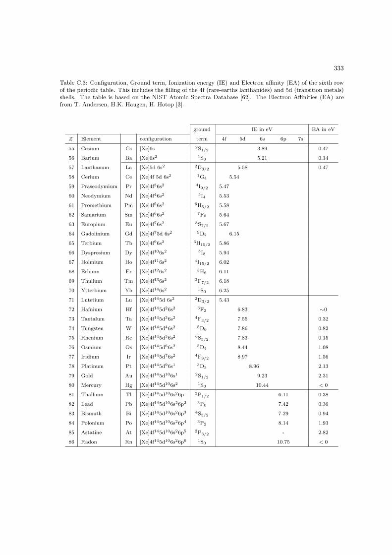
333
Table C.3: Configuration, Ground term, Ionization energy (IE) and Electron affinity (EA) of the sixth rowof the periodic table. This includes the filling of the 4f (rare-earths lanthanides) and 5d (transition metals)shells. The table is based on the NIST Atomic Spectra Database [62]. The Electron Affinities (EA) arefrom T. Andersen, H.K. Haugen, H. Hotop [3].
ground IE in eV EA in eV
Z Element configuration term 4f 5d 6s 6p 7s
55 Cesium Cs [Xe]6s 2S1/2 3.89 0.47
56 Barium Ba [Xe]6s2 1S0 5.21 0.14
57 Lanthanum La [Xe]5d 6s2 2D3/2 5.58 0.47
58 Cerium Ce [Xe]4f 5d 6s2 1G4 5.54
59 Praseodymium Pr [Xe]4f36s2 4I9/2 5.47
60 Neodymium Nd [Xe]4f46s2 5I4 5.53
61 Promethium Pm [Xe]4f56s2 6H5/2 5.58
62 Samarium Sm [Xe]4f66s2 7F0 5.64
63 Europium Eu [Xe]4f76s2 8S7/2 5.67
64 Gadolinium Gd [Xe]4f75d 6s2 9D2 6.15
65 Terbium Tb [Xe]4f96s2 6H15/2 5.86
66 Dysprosium Dy [Xe]4f106s2 5I8 5.94
67 Holmium Ho [Xe]4f116s2 4I15/2 6.02
68 Erbium Er [Xe]4f126s2 3H6 6.11
69 Thulium Tm [Xe]4f136s2 2F7/2 6.18
70 Ytterbium Yb [Xe]4f146s2 1S0 6.25
71 Lutetium Lu [Xe]4f145d 6s2 2D3/2 5.43
72 Hafnium Hf [Xe]4f145d26s2 3F2 6.83 ∼0
73 Tantalum Ta [Xe]4f145d36s2 4F3/2 7.55 0.32
74 Tungsten W [Xe]4f145d46s2 5D0 7.86 0.82
75 Rhenium Re [Xe]4f145d56s2 6S5/2 7.83 0.15
76 Osmium Os [Xe]4f145d66s2 5D4 8.44 1.08
77 Iridium Ir [Xe]4f145d76s2 4F9/2 8.97 1.56
78 Platinum Pt [Xe]4f145d96s1 3D3 8.96 2.13
79 Gold Au [Xe]4f145d106s1 2S1/2 9.23 2.31
80 Mercury Hg [Xe]4f145d106s2 1S0 10.44 < 0
81 Thallium Tl [Xe]4f145d106s26p 2P1/2 6.11 0.38
82 Lead Pb [Xe]4f145d106s26p2 3P0 7.42 0.36
83 Bismuth Bi [Xe]4f145d106s26p3 4S3/2 7.29 0.94
84 Polonium Po [Xe]4f145d106s26p4 3P2 8.14 1.93
85 Astatine At [Xe]4f145d106s26p5 2P3/2 - 2.82
86 Radon Rn [Xe]4f145d106s26p6 1S0 10.75 < 0

334 APPENDIX C. PROPERTIES OF THE ELEMENTS
Table C.4: Configuration, Ground term, Ionization energy (IE) and Electron affinity (EA) of the seventhrow of the periodic table up through the 5f shell (rare-earth actinides). The table is based on the NISTAtomic Spectra Database [62].
ground IE in eV EA in eV
Z Element configuration term 5f 6d 7s
87 Francium Fr [Rn]7s 2S1/2 4.07
88 Radium Ra [Ra]7s2 1S0 5.28
89 Actinium Ac [Ra]6d 7s2 2D3/2 5.38
90 Thorium Th [Ra]6d27s2 3F2 6.31
91 Protactinium Pa [Ra]5f26d 7s2 4K11/2 5.89
92 Uranium U [Ra]5f36d 7s2 5L6 6.19
93 Neptunium Np [Ra]5f46d 7s2 6L11/2 6.27
94 Plutonium Pu [Ra]5f67s2 7F0 6.03
95 Americium Am [Ra]5f77s2 8S7/2 5.97
96 Curium Cm [Ra]5f76d 7s2 9D2 5.99
97 Berkelium Bk [Ra]5f97s2 6H15/2 6.20
98 Californium Cf [Ra]5f107s2 5I8 6.28
99 Einsteinium Es [Ra]5f117s2 4I15/2 6.37
100 Fermium Fm [Ra]5f127s2 3H6 6.50
101 Mendelevium Md [Ra]5f137s2 2F7/2 6.58
102 Nobelium No [Ra]5f147s2 1S0 6.65

D
Classical Mechanics
D.1 Introduction
The goal of classical mechanics is to describe the time evolution of systems of point-like particles,called classical particles, subject to Newton’s laws of motion. To introduce the subject we considera mechanical system of N classical particles labeled by the particle index α. The position of particleα is denoted by the vector rα. The first derivative with respect to time t, rα ≡ drα/dt, is called thevelocity of the particle and the second derivative, rα ≡ d2rα/dt
2, its acceleration.We suppose that for a given state of the system the evolution does not depend on the instant
that we choose to follow it in time; i.e., time is homogeneous. Space is taken to be both homogeneousand isotropic; i.e., it is possible to choose a frame of reference in which the evolution of the systemis independent of position and orientation. Such a reference frame is called an inertial frame. Inan inertial frame a free particle either stays at rest or moves at constant velocity. This is Newton’sfirst law : the law of inertia.
A system of N classical particles has at most 3N degrees of freedom; i.e., 3N independent waysto change in time. For free particles this motion can be described by 3N coordinates, for instancethe cartesian coordinates xα, yα and zα, with α ∈ 1, · · ·N. However, in many cases the motionis not free but subject to constraints. These can be time independent (scleronomous) or havean explicit time dependence (rheonomous). An example of a scleronomous constraint is the fixeddistance between two particles in a rotating rigid body. A ball rolling on the deck of a ship is anexample of a system (the ball) with a rheonomous constraint (confinement to the deck of the ship).The system is called holonomic if the constraining relations reduce the 3N degrees of freedom thesystem. This holds for constraint equalities, for instance the above mentioned fixed distance betweentwo particles in a rotating rigid body. If the constraints do not affect the 3N degrees of freedomthe system is called nonholonomic. An example of the latter is the confinement of particles withina vessel. Nonholonomic constraints can sometimes be avoided by idealizations of the theory.
The field of classical mechanics is subdivided into three subjects: (a) statics, which is the theoryof mechanical equilibrium between forces; (b) kinematics, which is the theory of motion withoutentering in the origin of this motion; (c) dynamics, which is the theory of motion under the influenceof forces. This appendix cannot be more than a summary. For a proper introduction the reader isreferred to volume 1 of the Landau-Lifshitz series [65] and the book by Herbert Goldstein [46].
Dynamical evolution - Newton’s equation of motion
The time development of a system of N particles under the influence of external forces is calledthe dynamical evolution of that system. In classical mechanics the dynamical evolution of a singleparticle is described by Newton’s second law, which states that the total force Fα acting on particleα is proportional to the acceleration of that particle, with the proportionality constant mα being
335

336 APPENDIX D. CLASSICAL MECHANICS
its inertial mass,Fα = mαrα. (D.1)
For a system of N particles the force Fα is given by the resultant of all external forces, Fextα , and
the sum of the interaction forces Fαβ of particle α with all other particles of the system,
Fextα +
N∑β=1
′Fαβ = mαrα, (D.2)
where the prime indicates the condition β 6= α. This expression represents a set of N coupleddifferential equations which is impossible to solve for a macroscopic number of particles. However,as we shall see below, in many cases excellent approximations can be obtained by replacing theinterparticle forces by one or more relations acting as constraints on the motion of particle α.
D.2 Kinematic evolution of holonomous systems
For a holonomic system of N particles at positions rα with l constraints we can introduce f = 3N−lindependent coordinates qi(t) known as the generalized coordinates, with i ∈ 1, · · · f being thecoordinate index. Together these define the evolution of the system as a function of time in thef -dimensional configuration space of the system. The time derivatives qi(t) are called the generalizedvelocities.1
• The rheonomous constraints of a N -particle system with f = 3N − l degrees of freedomconstitute a set of l time-dependent relations fk(r1, · · · , rN , t) = 0, where k ∈ 1, · · · l iscalled the constraint index. In this case the position of particle α may be expressed as afunction of the f coordinates qi plus time,
rα = rα(q1, · · · , qf , t). (D.3)
The velocities follow with
rα =
f∑i=1
∂rα∂qi
qi +∂rα∂t
, (D.4)
which shows that the velocity of particle α is (in general) a function of qi, qi and t,
rα = rα(q1, · · · , qf , q1, · · · , qf , t). (D.5)
Hence, in rheonomous systems rα and rα depend explicitly on time.
• For scleronomous constraints the l constraining relations do not contain an explicit timedependence: fk(r1, · · · , rN ) = 0, with k ∈ 1, · · · l. This makes it is possible to choose thef coordinates qi in such a way that the position of the particles does not depend explicitlyon time. For instance, for a rolling sphere on a fixed surface we can choose the generalizedcoordinate system such that the entire sphere remains at rest.
D.2.1 Virtual displacements - principle of d’Alembert
The force Fα acting on particle α is the superposition of all forces acting on that particle. Theseforces can be separated into known forces Fext
α , like gravity or externally applied forces, and unknownforces Kα,
Fα = Fextα + Kα. (D.6)
1Throughout this appendix we adhere to the convention α ∈ 1, · · ·N for the particle index, i ∈ 1, · · · f for thecoordinate index and k ∈ 1, · · · l. for the constraint index.

D.2. KINEMATIC EVOLUTION OF HOLONOMOUS SYSTEMS 337
The unknown forces are called forces of constraint. These unknown forces are reaction forces thatreduce the freedom of motion of the particles. Their actual value is unknown but always such thatthe constraints remain satisfied, for instance to assure that a train stays in the rails.
The explicit appearance of the reaction forces can be eliminated from the formalism. To demon-strate this we first consider mechanical equilibrium. This is the state in which all particles are atrest in their equilibrium position; i.e., Fα = 0 and Kα = −Fext
α for all particles. By pulling on oneof the particles we expect to perform work against the restoring force of the system but as long asthe displacements δrα remain small (i.e., close to the equilibrium position) we find that this workvanishes because the forces Fα remain vanishingly small,∑
α
Fα · δrα =∑α
(Fextα + Kα) · δrα = 0. (D.7)
In other words, in equilibrium the restoring force is zero. This implies that in the absence of externalforces the reaction forces have to be zero, Fα = Kα = 0.
Now suppose that the system is pulled out of equilibrium. In this case we have forces acting on(in general) all the particles; i.e., Fα = mαrα 6= 0 and Kα = −Fext
α + Fα 6= 0. Shifting the externalforces to the l.h.s. of (D.7) this equation takes the form∑
α
(mαrα − Fextα ) · δrα =
∑α
Kα · δrα 6= 0. (D.8)
The dot product leads us to distinguish between the component of δrα along Kα and the componentperpendicular to Kα. A parallel displacement would require work but is not in accordance withthe constraints; a perpendicular displacement is in accordance with the constraints but does notresult in work (as long as the displacements remain sufficiently small). This insight leads us to theprinciple of d’Alembert : under virtual displacements δrα (in accordance with the constraints) nowork is done by the reaction forces,
δW =∑α
Kα · δrα = 0. (D.9)
This important principle allows us to derive the central equations of classical mechanics: the equa-tions of Lagrange (see Section D.3). By analyzing virtual displacement we can eliminate the reactionforces from (D.8) and the principle of d’Alembert takes the form
δW =∑α
(mαrα − Fextα ) · δrα = 0. (D.10)
As this expression also holds outside equilibrium, we have obtained a condition for the dynamicalevolution of the system in which the constraints are satisfied implicitly.
Let us have a closer look at the virtual displacements. These can be thought of as instantlybeing present at any desired point in time just to analyze how they would affect the system; i.e.,unlike real displacements, which are based on (D.3), virtual displacements have no (explicit) timedependence. To be relevant, they have to be in accordance with the constraints; i.e., δrα has to beperpendicular to Kα. This leads to the practical difficulty that (in principle) the virtual displacementof one particle affects the virtual reaction forces of all other particles; i.e., the δrα cannot be chosenindependently. This difficulty can be eliminated by decomposing the virtual displacements in termsof the generalized coordinates defined by the constraints,
δrα =
f∑i=1
∂rα∂qi
δqi. (D.11)

338 APPENDIX D. CLASSICAL MECHANICS
Note the absence of the time variable. Substituting this expression into (D.10) we obtain
δW =
f∑i=1
[N∑α=1
(mαrα − Fextα ) · ∂rα
∂qi
]δqi = 0 (D.12)
and since the qi are independent variables the principle of d’Alembert takes the form of a set of fcoupled differential equations∑
α
(mαrα − Fextα ) · ∂rα
∂qi= 0, with i ∈ 1, · · · , f. (D.13)
Inversely, it is easily verified that (D.10) is always valid provided the equations (D.13) are simulta-neously satisfied.
In the absence of dynamical evolution (the static case - rα = 0) the principle of d’Alembertreduces to the Bernoulli principle of virtual displacements :
δW =∑α
Fextα · δrα = 0. (D.14)
As an example of Bernoulli’s principle without constraints we consider a system of N = 2 identicalparticles subject to a force Fext
α = −∇αU(r1, r2), where U(r1, r2) is a potential function whichdepends on the position of all the particles. This is an example of a conservative force (see SectionD.5.2). The expression for the virtual work is δW = Fext
1 · δr1 + Fext2 · δr2 = 0. For two free
particles confined by a harmonic potential the condition δW = 0 is satisfied at the minimum ofthe potential. For two repulsive particles we have Fext
1 = −Fext2 and the condition δW = 0 is
satisfied for δr1 = −δr2 perpendicular to Fext1 . Note the correlation between δr1 and δr2 (these
are not independent). The virtual displacements correspond to a rotation of the pair about thepotential center. The latter case shows that the virtual variation does not automatically correspondto minimum of δW but can also represent a degenerate case.
Kinetic energy relations
Introducing the kinetic energy,
T ≡ 12
∑α
mαr2α, (D.15)
we note that, in view of (D.5), the kinetic energy of particle α is in the most general case a functionof qi(t), qi(t) and t,
T = T (q1, · · · , qf , q1, · · · , qf , t). (D.16)
For the partial derivatives with respect to qi and qi we derive for future use
∂T
∂qi=∑α
mαrα ·∂rα∂qi
(D.17a)
∂T
∂qi=∑α
mαrα ·∂rα∂qi
. (D.17b)
Here we used the relation ∂rα/∂qi = ∂rα/∂qi, which follows immediately from (D.4) and (D.3).
D.3 Lagrange equations
In this section we derive the Lagrange equations, which are the equations of motion of classicalmechanics. The Lagrange equations are equally valid for conservative and non-conservative forces.

D.3. LAGRANGE EQUATIONS 339
Examples of conservative forces are the gravitational force and the Lorentz force. The friction forceis an example of a non-conservative force. The Lagrange equations offer an important simplificationwith respect to Newton’s equation of motion because forces of constraint are eliminated from theformalism by the introduction of the generalized coordinates. We shall use the vector notation inwhich the position and velocity of the particles of a mechanical system are represented by vectorsin the configuration space and velocity space, respectively
q ≡ (q1, · · · , qf ) (D.18a)
q ≡ (q1, · · · , qf ). (D.18b)
The vectors q and q are called dynamical variables because their evolution in represents the dynam-ical evolution of the system. This time dependence is obtained by solving the Lagrange equations.In the present section the Lagrange equations are obtained from the principle of d’Alembert. InSection D.4 they follow the principle of least action of Hamilton.
D.3.1 Absence of constraining forces
First we show how the Lagrange equations are obtained form Newton’s second law. In the absence offorces of constraint the particles are called free and the equations of motion (D.1) suffice to describethe motion of the particles. Using Eq. (D.15) for the kinetic energy, we find that a force acting onparticle α can be written in the form
Fα =d
dt
∂T
∂rα. (D.19)
Now we restrict ourselves to forces that can be expressed as the negative gradient of a potentialfunction U = U(r1, · · · , rN , t),
Fextα = − ∂U
∂rα. (D.20)
In the special case of a time-independent potential function the force field is called conservative andpotential function can be interpreted as the potential energy U = V (r1, · · · , rN ). We return to theconcept of potential energy in the context of the conservation laws (see Section D.5.2). Combining(D.19) and (D.20) we find
− ∂U
∂rα=
d
dt
∂T
∂rα. (D.21)
At this point we introduce the Lagrangian L(rα, rα, t) as the difference between the kinetic energyand the potential function,
L(rα, rα, t) ≡ T (rα)− U(rα, t). (D.22)
Because the potential function U(r1, · · · , rN , t) does not depend explicitly on rα, and T (r1, · · · , rN )not explicitly on rα, (D.21) we arrive at the so-called Lagrange equations for particle α,
d
dt
∂L∂rα− ∂L∂rα
= 0, with α ∈ 1, · · · , N. (D.23)
D.3.2 Presence of constraining forces
Lagrange equations can also be derived for systems with holonomic constraints. So let us turn toa system of N particles in which holonomic constraints add up to the reaction forces Kα. How dothese constraints affect the evolution of the system? To answer this question we apply the principleof d’Alembert. Rewriting (D.13) in the form∑
α
Fextα ·
∂rα∂qi
=∑α
mαrα ·∂rα∂qi
, with i ∈ 1, · · · , f, (D.24)

340 APPENDIX D. CLASSICAL MECHANICS
we can introduce a generalized force defined by f components, one for every degree of freedom ofthe system,
Qi ≡∑α
Fextα ·
∂rα∂qi
, with i ∈ 1, · · · , f. (D.25)
Using the r.h.s. of (D.24) the Qi can be expressed as
Qi =d
dt
(∑α
mαrα ·∂rα∂qi
)−∑α
mαrα ·∂rα∂qi
, (D.26)
and after substitution of (D.17) this becomes
Qi =d
dt
(∂T
∂qi
)− ∂T
∂qi, with i ∈ 1, · · · , f. (D.27)
This expression holds for any holonomic system. It has the structure of a Lagrange equation but theforces have not been specified. Below we derive the Lagrange equation for three types of forces: (a)conservative or non-conservative potential forces; (b) generalized potential forces; (c) non-potentialforces.
(a) If the components of the generalized force can be expressed as the gradients of the potentialfunction U = U(r1, · · · , rN , t) we can substitute (D.20) into (D.25) and obtain
Qi ≡ −∑α
∂U
∂rα· ∂rα∂qi
= −∂U∂qi
. (D.28)
Substituting this equation into (D.27) and taking into account ∂U/∂qi = 0 (because U doesnot depend explicitly on the qi), the equations of motion takes the form
d
dt
∂L∂qi− ∂L∂qi
= 0, with i ∈ 1, · · · , f, (D.29)
whereL(q, q, t) ≡ T (q, q, t)− U(q, t). (D.30)
The set of equations (D.29) will be referred to as the Lagrange equations. Note that in thenonholonomic case we have f = 3N and the set of generalized coordinates qi coincides withthe full set of cartesian coordinates rα; i.e., (D.29) coincides with (D.23).
(b) The derivation of Eq. (D.29) breaks down in cases where ∂U/∂qi 6= 0; i.e., for velocity-dependent forces. However, by construction, the Lagrange equations will still be obtainedif the generalized forces can be written the form
Qi = −∂U∂qi
+d
dt
(∂U
∂qi
), with i ∈ 1, · · · , f. (D.31)
Substituting this expression into (D.27) we find
d
dt
∂L∂qi− ∂L∂qi
= 0, with i ∈ 1, · · · , f. (D.32)
Here the lagrangian is defined as.
L(q, q, t) ≡ T (q, q, t)− U(q, q, t). (D.33)
In the presence of a velocity dependence the function U = U(q, q, t) is called a generalizedpotential function.

D.3. LAGRANGE EQUATIONS 341
(c) Not all forces can be derived from a potential function. However, also for non-potential forces(for instance friction forces) the equation (D.27) is valid. In the most general case, when bothpotential and non-potential forces are present, the Lagrange equations can be written in theform
d
dt
∂L∂qi− ∂L∂qi
= Qi, with i ∈ 1, · · · , f. (D.34)
Here Qi are the components of the non-potential force. Forces that can be derived from apotential function are presumed to be contained in the lagrangian.
D.3.3 Example: friction force
In this example we ask for the steady-state velocity of particle falling in a gravitational field in thepresence of friction. For a gravitational field along the z axis the potential is V = αz. This is aconservative potential field. The friction force is a velocity dependent force,
F = −βz. (D.35)
This is a non-Newtonian force. The lagrangian is determined only by the kinetic energy and thepotential fields (in this case only the gravitational potential),
L = 12 z
2 − αz. (D.36)
Substituting the friction force into the r.h.s. of the Lagrange equation (D.29) we obtain
d
dt
∂L∂z− ∂L∂z
= −βz. (D.37)
Substituting the lagrangian (D.36) we obtain
z + βz − α = 0. (D.38)
The steady-state condition is z = 0; hence, we find for the steady-state velocity
z = −α/β. (D.39)
D.3.4 Example: Lorentz force
The celebrated example of a velocity-dependent force for which a generalized potential can bedefined is the Lorentz force. This force governs the motion of a charged particle moving through anelectromagnetic field in vacuum. The Lorentz force is given by
F = q(E + v ×B), (D.40)
where q is the electric charge and v = r the velocity of the particle. The generalized electromagneticpotential from which the Lorentz force may be derived has the form,
U(r,v, t) = q(ϕ− v ·A), (D.41)
where ϕ(r, t) and A(r, t) are the scalar and vector potentials of the electromagnetic field. Todemonstrate this assertion we start from (D.31) and find in the vector notation 1
F(r, r, t) = −∂rU +d
dt∂rU = −q[∂rϕ− ∂r(r ·A) +
d
dt∂r(r ·A)]. (D.42)
1In this example we use the short-hand notation ∂q ≡ ∂/∂q ≡ (∂/∂qx, ∂/∂qy , ∂/∂qz) and ∂t ≡ ∂/∂t.

342 APPENDIX D. CLASSICAL MECHANICS
Because A(r, t) does not depend explicitly on r and in view of the vector rule (N.17) the last termof (D.42) can be rewritten as
d
dt∂r(r ·A) =
dA
dt= ∂tA + (r · ∂r)A. (D.43)
Substitution of this expression into (D.42) we obtain
F = −q[∂rϕ+ ∂tA + (r · ∂r)A− ∂r(r ·A)], (D.44)
which yields with (N.16) the expression for the Lorentz force
F = −q(∂rϕ+ ∂tA− r× ∂r ×A) = q(E + v ×B). (D.45)
D.4 The Lagrange formalism
In Appendix D.3 the Lagrange equations were derived from the Newton equations of motion togetherwith the principle of d’Alembert. An alternative approach is to derive the Lagrange equations fromthe principle of Hamilton. In this approach we start by noting that the time evolution of the systemcorresponds to a unique path of the vector q ≡ (q1, · · · , qf ) in the f -dimensional configurationspace. As these generalized coordinates are mutually independent, this path can be predicted overan infinitesimal time interval from t to t+ δt by the relation
q(t+ δt) = q(t) + q(t)δt. (D.46)
Hence, to predict the continuation of the path at time t, both q(t) and q(t) have to be known. Inother words, together q and q fully determine the classical state of the system (often representedby a point in the so-called phase space of position and momentum).
D.4.1 Principle of Hamilton
Let us consider the case where the actual path q(t) runs from the starting point q(t0) to the endpoint q(t1) during the time interval (t0, t1), and let q′(t) be some adjacent path, slightly differingfrom the actual path but with the same starting point and end point. The key idea behind theprinciple of Hamilton is that any continuous deviation from the actual path,
δq(t) = q′(t)− q(t), (D.47)
with boundary conditionsδq(t0) = 0 and δq(t1) = 0, (D.48)
has to be unfavorable in some respect. Thus we search for a functional of q and q (the cost functionalof the variational problem) which is minimal for the actual path from q(t0) to q(t1). Minimizingthis functional with respect to the path provides us with criteria that have to be satisfied along theactual path (for instance conservation laws). This cost functional is called the action integral andis given by the integral of a lagrangian function L(q, q, t) over the time interval (t0, t1),
S =
ˆ t1
t0
L(q, q, t)dt. (D.49)
Whatever this “lagrangian” may turn out to be, the expression for the action is plausible; at eachpoint in time t within the interval (t0, t1), knowledge of q and q suffice to determine the actual pathfrom q(t0) to q(t1). So if the lagrangian is to be deterministic for the actual path, it can only bea function of the variables q, q and t. This minimization procedure is called the principle of leastaction or the principle of Hamilton.

D.4. THE LAGRANGE FORMALISM 343
The principle of Hamilton enables us to derive properties of the lagrangian for systems in whichthe function L(q, q, t) is at least twice differentiable; i.e., smooth with respect to the variables q,q and t. Fortunately, many systems fall in this class and we shall study some examples. Let usconsider the change in action of such a system over the time interval (t0, t1) when deforming thepath defined by q(t) and q(t) into an adjacent smooth continuous path q′(t) and q′(t) given byq′ = q + δq and q′ = q + δq,
δS =
ˆ t1
t0
[L(q + δq, q + δq, t)− L(q, q, t)]dt. (D.50)
As the lagrangian is smooth we can use a Taylor expansion with respect to δq and δq,1
L(q + δq, q + δq, t) = L(q, q, t) +∂L∂q· δq +
∂L∂q· δq + · · · , (D.51)
and the change of action takes the form
δS =
ˆ t1
t0
∑i
(∂L∂qi
δqi +∂L∂qi
δqi
)dt. (D.52)
By partial integration of the second term this integral becomes
δS =∑i
[∂L∂qi
δqi
]t1t0
+
ˆ t1
t0
∑i
(∂L∂qi− d
dt
∂L∂qi
)δqidt. (D.53)
Since the variation is zero at the boundaries of the path, see (D.48), this expression reduces to
δS =
ˆ t1
t0
∑i
(∂L∂qi− d
dt
∂L∂qi
)δqidt. (D.54)
At this point we can formulate a necessary condition for minimal action: the functional must bestationary (δS = 0) under arbitrary variations of the path,2
ˆ t1
t0
∑i
(∂L∂qi− d
dt
∂L∂qi
)δqidt = 0. (D.55)
Since the variations δqi are independent this condition is only satisfied if all terms of the summationvanish simultaneously,
∂L∂qi− d
dt
∂L∂qi
= 0, with i ∈ 1, · · · , f. (D.56)
These equations are called the Euler-Lagrange equations of the variational problem in which werecognize the Lagrange equations of classical mechanics. In Appendix D.3 these were obtainedstarting from the principle of d’Alembert.
Properties of the lagrangian
Above the lagrangian L(q, q, t) is introduced as a smooth (at least twice differentiable) function ofthe variables, q, q and t for which the action is stationary under the condition that the Lagrangeequations (D.56) are satisfied. Lagrangians have the following properties:
1Note the following equivalent notations for the gradient operator, ∂q ≡ ∂/∂q ≡ (∂/∂q1, · · · , ∂/∂qf ).2Note that the inverse is not generally true: being stationary does not mean that this action is minimal.

344 APPENDIX D. CLASSICAL MECHANICS
(a) Additive property : The lagrangian L of a system consisting of two non-interacting subsystemscan be written as the sum of the lagrangians L1 and L2 of the two subsystems,
L = L1 + L2. (D.57)
This has to be the case because the paths of the subsystems in configuration space can bevaried independently. Hence, the least action of the total system must coincide with the sumof the least actions of the two subsystems.
(b) Definition up to a multiplicative factor : The path of least action is invariant under multipli-cation of the lagrangian by an arbitrary constant. For L′ = αL we find
S′ = α
ˆ t1
t0
L(q, q, t)dt = αS. (D.58)
Hence, δS′ = αδS, which implies that the condition δS′ = 0 is equivalent to δS = 0. Thismeans that the multiplication by α does not affect the stationarity condition and leads to thesame Euler-Lagrange equation.
(c) Definition up to a total time derivative: The path of least action is invariant under additionof a total time derivative to the lagrangian. For L′ = L+ df/dt we find
S′ =
ˆ t1
t0
L(q, q, t)dt+
ˆ t1
t0
df
dtdt = S + f(t1)− f(t0). (D.59)
Hence, S′ and S differ by a constant and this does not affect the variation, δS′ = δS. Thus,the addition of dα/dt does not change the stationarity condition and leads to the same Euler-Lagrange equation.
D.4.2 Lagrangian of a free particle
To gain insight in the functional form of the lagrangian we consider a free particle. As in classicalmechanics space and time are postulated to be homogeneous we know that its lagrangian (whichdetermines the time evolution of the system) must be independent of position r and time t, whichleaves the velocity v = r as the only variable, L = L(v). Since L is independent of r we have∂L/∂r = 0 and the Lagrange equation (D.56) becomes
d
dt
∂L∂v
= 0. (D.60)
Hence, ∂L/∂v must be a constant and since v is the only variable of L the velocity must be constant,v(t) = v0. Thus we found Newton’s law of inertia.
Space is postulated to be isotropic. Thus, the lagrangian may only depend on the absolute valueof the velocity, v; i.e., it has to be some function of the velocity squared,
L = L(v2). (D.61)
This observation immediately implies that the lagrangian is invariant under time reversal; i.e., time isisotropic in newtonian mechanics. To get more precise information about the functional dependenceof L on v2 we turn to Galileo’s principle of relativity, which is also based on the homogeneity andisotropy of space and time. According to this principle the equations of motion (hence also thelagrangian) must be invariant under a Galilean transformation, which is a transformation of oneinertial frame to another (from the inertial frame S to the frame S ′)
r′ = r + Vt; t′ = t, (D.62)

D.4. THE LAGRANGE FORMALISM 345
where V is the relative velocity of the frame S ′ with respect to the frame S. Thus we are led tocompare two lagrangians, L(v′2) and L(v2), defined with respect to two inertial frames which movewith an infinitesimally small but constant velocity w = v′ − v with respect to each other. Usingthe relation v′2 = v2 + 2v ·w + w2 we find
L(v′2) = L(v2) +∂L∂v2
(2v + w) ·w+∂2L∂(v2)2
[(2v + w) ·w]2
+ · · · . (D.63)
Because the time evolution of the system must be independent of the choice of inertial frame, thetwo lagrangians must be equivalent. In view of property (D.59) this means that they cannot differ bymore than a total time derivative. Since v is by definition a total time derivative and w a constant,∂L/∂v2 has to be a constant; i.e., the function L has to be a linear function of v2,
L = L0 + αv2. (D.64)
For any other functional dependence on v2 the lagrangian is either trivially zero or differs from Lby more than a total time derivative. Once we accept that L has to be a linear function of v2 wefind that all higher order terms of the expansion vanish. As the constant L0 can also be regardedas a total time derivative we may write the lagrangian as simply proportional to v2,
L = 12mv
2 = T. (D.65)
The proportionality constant m is called the mass of the particle and serves to calibrate the la-grangian. This calibration is possible in view of property (D.58). The chosen calibration yields thekinetic energy of the particle, T = 1
2mv2.
For a free particle the principle of least action is very intuitive. The particle has to follow astraight path in configuration space (which coincides in this case with real space) because for aconstant lagrangian any deviation from a straight path leads to an increase of the action integral.The example also shows that the mass must be positive (m > 0) because otherwise the action couldbe reduced by deviating from the straight path, which contradicts experimental observation.
D.4.3 Lagrangian of a single particle in a potential field
Let us now add to the kinetic energy of the particle a (smooth) function of position and time (i.e.,a time-dependent field),
L(r, r, t) = 12mv
2 − U(r, t). (D.66)
Being a function of r, r and t, the new expression is again a lagrangian if the Lagrange equationsare satisfied:
∂L∂r
=d
dt
∂L∂v
. (D.67)
When will this be the case? Since U(r, t) is independent of v and T = 12mv2 is independent of r
and t, substitution of (D.66) into the Lagrange equations (D.67) leads to the following condition
− ∂U
∂r=
d
dt
∂T
∂v= m
dv
dt. (D.68)
Interpreting the negative gradient of U(r, t) as a force,
F = −∂U∂r
(D.69)
we recognize in (D.68) Newton’s second law, F = mr. Hence, the Lagrange equations are satisfied ifthe particle moves in accordance with the Newton equations of motion; i.e., under non-relativisticconditions. The function U(r, t) is called the potential field of the system. If this field does notdepend on position, U(r, t) = U(t), it is called uniform. If it does not depend on time, U(r, t) = U(r),the field is called conservative.

346 APPENDIX D. CLASSICAL MECHANICS
Generalized potential functions
The above discussion can be generalized to include velocity-dependent potentials, called generalizedpotential functions. For this purpose we add to the kinetic energy a (smooth) function of r, r and t,
L(r, r, t) = 12mv
2 − U(r, r, t). (D.70)
This function is a lagrangian if it satisfies the Lagrange equations. Substituting L(r, r, t) into (D.67),we find that the condition (D.68) is replaced by
− ∂U
∂r+d
dt
∂U
∂v=
d
dt
∂T
∂v. (D.71)
In other words, the Lagrange equations are satisfied for generalized forces of the type
Q = −∂U∂r
+d
dt
∂U
∂v. (D.72)
Note that (D.72) reduces to (D.69) for velocity-independent potentials; hence, the class of generalizedforces includes gradient forces as a subclass. Although any generalized potential function gives riseto a generalized force, the inverse is not true. For instance, friction forces, F = −αv, cannot beexpressed in the form (D.72). On the other hand, the Lorentz force is an example of a generalizedforce because we can define a generalized potential function for which (D.72) is satisfied (see ProblemD.1).
Problem D.1. Show, using the Einstein notation, that the Lorentz force, Fi = q[Ei + (v × B)i],is the generalized force resulting from the generalized potential function U = q(ϕ− vj · Aj), whereϕ(r, t) is the scalar and A (r, t) the vector potential. Further, Ei = −∂iϕ− ∂tAi and Bi = εijk∂jAkare the cartesian components of the (generally time dependent) E and B fields, respectively. Usethe short-hand notation ∂i ≡ ∂/∂ri and ∂t ≡ ∂/∂t.
Solution. The first term of (D.72) yields
− ∂iU = q [−∂iϕ− vj∂iAj (r, t)] (a)
and the second term can be written as
d
dt
(∂U
∂vi
)= q
d
dt
(∂ϕ (r, t)
∂vi− ∂vjAj (r, t)
∂vi
)= −q d
dtAi (r, t) = q [−∂jAi (r, t) rj − ∂tAi (r, t)] . (b)
Combining (a) and (b) we obtain for the generalized force
Qi = q [−∂iϕ− ∂tAi + vj∂iAj − vj∂jAi] . (c)
In the first two terms within the brackets we recognize the Ei-component of the E field. Similarly,recalling B =∇×A, we recognize in the last two terms the component (v ×B)i of the v×B field 1
(v ×B)i = εijkvj(∇×A)k = εijkεklmvj∂lAm = vj∂iAj − vj∂jAi.
Hence, Eq. (c) can be rewritten as Qi = q [Ei + (v ×B)i], which is indeed the expression for theLorentz force. 2
1In the Einstein notation the contraction of the Levi-Civita tensor is given by εijkεklm = δilδjm − δimδjl.

D.5. MANY-PARTICLE SYSTEMS 347
D.5 Many-particle systems
D.5.1 Lagrangian
At this point we return to many-particle systems. In view of property (D.57) we know that thelagrangian of a system of N non-interacting particles is given by
L = 12
∑α
mαv2α, (D.73)
where α ∈ 1, · · ·N. In search for the lagrangian in the presence of interactions between the parti-cles as well as interactions with the environment we use a procedure similar to the one introducedfor the single particle: we add to the lagrangian (D.73) a generalized potential function
L(· · · , rα, rα, · · · , t) = 12
∑α
mαr2α − U(· · · , rα, rα, · · · , t). (D.74)
The potential function depends in principle on the position and velocities of all the particles as wellas on time
U(· · · , rα, rα, · · · , t) = U int(· · · , rα, rα, · · · ) + Uext(· · · , rα, rα, · · · , t). (D.75)
The function U int is called the internal generalized potential function and represents the interactionbetween all particles of the system; e.g., the Van der Waals interaction between the atoms in aclassical gas. The function Uext is called the external generalized potential function and representsexternally applied fields; e.g., the electromagnetic potential of a light field.
The function (D.74) is a lagrangian if it satisfies the Lagrange equations,
∂L∂rα
=d
dt
∂L∂vα
, with α ∈ 1, · · ·N. (D.76)
Since the first term on the r.h.s. of (D.74) is independent of rα we find that the condition (D.76)can be written in the form
− ∂U
∂rα+d
dt
∂U
∂vα=
d
dt
∂T
∂vα= mαrα, with α ∈ 1, · · ·N. (D.77)
Hence, the quantity
Qα = − ∂U∂rα
+d
dt
∂U
∂vα, with α ∈ 1, · · ·N, (D.78)
can be interpreted as the generalized force acting on particle α as the result of its interaction withall other particles in the system.
Generalization to the presence of scleronomous constraints
It is straightforward to generalize the formalism to holonomic systems with scleronomous con-straints. In this case the positions rα and velocities rα of the particles can be expressed in terms off = 3N − l generalized coordinates q1, · · · , qf and velocities q1, · · · , qf ,
rα = rα(q1, · · · , qf ) (D.79a)
rα =
f∑i=1
∂rα∂qi
qi. (D.79b)

348 APPENDIX D. CLASSICAL MECHANICS
Substituting these expressions into (D.74) we obtain
L(q, q) = 12
f∑i,j=1
aij(q)qiqj − U(q, q). (D.80)
Here we use the vector notation (D.18); the coefficient aij(q) is given by
aij(q) =∑α
mα∂rα∂qi
∂rα∂qj
. (D.81)
In terms of the generalized coordinates and velocities the Lagrange equation take the form
∂L∂qi
=d
dt
∂L∂qi
, with i ∈ 1, · · · f, (D.82)
and the components of the generalized force become
Qi = −∂U∂qi
+d
dt
∂U
∂qi, with i ∈ 1, · · · f. (D.83)
Note that in the absence of constraints we have f = 3N and the generalized coordinates turn intothe cartesian coordinates of the particles, (q1, · · · , qf )→ (x1, y1, z1, · · · , xN , yN , zN ), and we regain(D.76) and (D.78).
Open and closed systems
A mechanical system is called closed if it does not interact with its environment; i.e., the potentialfunction can be written as U = U int(· · · , rα, rα, · · · ). Hence, for closed systems both the potentialfunction and the lagrangian are time independent. An example of a closed mechanical system is anatom in field-free space. If the system is not closed it is called open. An example of an open systemis a cloud of interacting particles confined by an external potential.
D.5.2 Energy conservation
In the absence of time-dependent external forces the evolution of a mechanical system only dependson the state of that system and not on the instant that this state is created in time. In view ofthis homogeneity of time the lagrangian of such a system cannot depend explicitly on time; i.e., thetotal time derivative of (D.74) can be written in the form
dLdt
=∑α
∂L∂rα· rα +
∑α
∂L∂rα· rα. (D.84)
With the aid of the Lagrange equation (D.76) this becomes
dLdt
=∑α
rα ·d
dt
∂L∂rα
+∑α
rα ·∂L∂rα
=∑α
d
dt
(rα ·
∂L∂rα
). (D.85)
Rewriting this expression in the form
d
dt
(∑α
rα ·∂L∂rα− L
)= 0 (D.86)
we find that the quantity
E =∑α
rα ·∂L∂rα− L (D.87)

D.5. MANY-PARTICLE SYSTEMS 349
is a constant of the motion; i.e., it is conserved along the path from t0 to t1. This quantityis called the energy of the system. Mechanical systems for which the energy is conserved arecalled conservative systems. It is straightforward to generalize (D.87) to holonomic systems withscleronomous constraints,
E(q, q) =∑i
qi∂L∂ri− L. (D.88)
Potential energy
The energy of a conservative system can always be written as the sum of a kinetic energy and apotential energy contribution. This can be seen as follows. The kinetic energy is uniquely determinedby the velocities of the particles,
T (r1, · · · , rN ) = 12
∑α
mαv2α.
In general this quantity will change in time under the influence of inter-particle forces but (since thesystem is conservative) the (total) energy has to remain constant, E(r1, · · · , rN , r1, · · · , rN ) = E.Since the same kinetic energy can be obtained for different distributions of velocity over the particlesthe difference of E and T has to be a function of the positions only. This difference is called thepotential energy V (r1, · · · , rN ) of the system,
V (r1, · · · , rN ) = E(r1, · · · , rN , r1, · · · , rN )− T (r1, · · · , rN ). (D.89)
Beware of the difference between the potential energy V (r1, · · · , rN ) and the generalized potentialfunction U(r1, · · · , rN , r1, · · · , rN ); the former determines the kinetic energy of a conservative system(also in the presence of generalized forces between the particles); the latter determines the force onall particles, both for conservative and non-conservative systems.
Open and closed systems
When discussing energy conservation we should distinguish between open and closed mechanicalsystems. An open system is conservative if the external potential is constant in time.
D.5.3 Momentum conservation in closed systems
The evolution of a closed mechanical system only depends on the internal state of that system andnot on the absolute position where this state is created in space. In view of this homogeneity ofspace the lagrangian of a closed system must be independent of the absolute position of that system;i.e., (D.74) must be invariant under a translation of the system over a distance R,
r′α = rα + R. (D.90)
Thus we are led to compare two lagrangians, defined with respect to two inertial frames shiftedwith respect to each other over an infinitesimally small distance δrα = r′α − rα = δR. For thisdisplacement the change change in lagrangian is given by
δL =∑α
∂L∂rα· δR + · · · . (D.91)
Hence, a necessary condition that the lagrangian be invariant under an arbitrary small shift δR is∑α
∂L∂rα
= 0. (D.92)

350 APPENDIX D. CLASSICAL MECHANICS
Note that also the sum over all higher order terms has to vanish but this has no relevance in thepresent context. Using the Lagrange equation (D.77) the condition (D.92) becomes∑
α
d
dt
∂L∂vα
=d
dt
∑α
∂L∂vα
= 0. (D.93)
Apparently, in a closed system the quantity
P =∑α
pα (D.94)
with
pα =∂L∂rα
(D.95)
is a constant of the motion. The quantity P is called the canonical momentum of the system and pαis the canonical momentum of particle α. Hence, for closed systems the canonical momenta of theindividual particles always add up to the total momentum of the system, irrespective of the absenceor presence of generalized forces between the particles. With (D.76) it immediately follows that
pα =∂L∂rα
. (D.96)
It is straightforward to generalize (D.95) and (D.96) to holonomic systems with scleronomous con-straints,
pi =∂L∂qi
(D.97a)
pi =∂L∂qi
(D.97b)
with i ∈ 1, · · · f.
Example: velocity-independent potential functions
In the special case of systems with only velocity-independent interactions between the particles (e.g.,gravitational forces) the canonical momentum only depends on the kinetic energy and we find thewell-known expression
pα = mαvα. (D.98)
The hamiltonian is given by
E =∑α
mαv2α − L, (D.99)
which becomes after substitution of the lagrangian (D.74)
E = T + V. (D.100)
D.5.4 Conservation of angular momentum in closed systems
In view of the isotropy of space the lagrangian of a closed system must be independent of theabsolute orientation of that system; i.e., (D.74) must be invariant under rotation of the system overan angle Ω about an axis in direction Ω through the origin of the inertial frame of observation,
r′α = rα + Ω× rα. (D.101)

D.6. THE HAMILTON FORMALISM 351
Under such a rotation also the velocity vector changes direction
v′α = vα + Ω× vα. (D.102)
Thus we are led to compare two lagrangians, defined with respect to two inertial frames rotatedwith respect to each other over an infinitesimally small angle δΩ so that δrα = r′α − rα = δΩ× rαand δvα = v′α − vα = δΩ× vα. For this rotation we have
δL =∑α
∂L∂rα· δΩ× rα +
∑α
∂L∂rα· δΩ× rα + · · · . (D.103)
Hence, a necessary condition that the lagrangian be invariant under an arbitrary rotation (aboutan axis through the origin) is ∑
α
(rα ×
∂L∂rα
+ rα ×∂L∂rα
)= 0. (D.104)
Here we used the permutation rules for the vector products (see Appendix N). Turning to canonicalvariables the condition becomes∑
α
(rα × pα + rα × pα) =d
dt
∑α
(rα × pα) = 0. (D.105)
Apparently, in a closed system the quantity
L =∑α
(rα × pα) , (D.106)
withLα ≡ rα × pα, (D.107)
is a constant of the motion. The quantity L is called the angular momentum of the system andLα is the angular momentum of particle α, both with respect to the origin of the inertial system.Although the value of L depends on the choice of origin, the conservation holds irrespective of thischoice.
D.6 The Hamilton formalism
In the Lagrange formalism the dynamical evolution of mechanical systems is expressed in termsof the dynamical variables q ≡ (q1, · · · , qf ) and q ≡ (q1, · · · , qf ) with the aid of the lagrangianL(q, q, t) and the Lagrange equations. With this approach we identified the sum over the canonicalmomenta p ≡ (p1, · · · , pf ) as a conserved quantity of a closed mechanical system. In the Hamiltonformalism the dynamical evolution is described in terms of the dynamical variables q and p; i.e.,the dependence on q is eliminated from the formalism and replaced by a dependence on p.
D.6.1 Legendre transformation of lagrangian - hamiltonian
To replace the dependence on q by a dependence on p we use a Legendre transformation of thefunction L(q, q, t) into the function
H(q,p, t) = p · q− L(q, q, t). (D.108)
The function H(q,p, t) is called the function of Hamilton or hamiltonian of the system. Note thatwith the sign convention of (D.108) the hamiltonian represents the energy of the system
E = H(q,p, t). (D.109)

352 APPENDIX D. CLASSICAL MECHANICS
To convince ourselves that the hamiltonian has the desired properties we consider the total differ-ential
dH = −dL+ d(∑i
piqi). (D.110)
For the total differential of the lagrangian L(q, q, t) we have with the aid of (D.97a) and (D.97b)
dL =∑i
∂L∂qi
dqi +∑i
∂L∂qi
dqi +∂L∂tdt =
∑i
pidqi +∑i
pidqi +∂L∂tdt. (D.111)
The total differential of the transformation term is
d(∑i
piqi) =∑i
qidpi +∑i
pidqi. (D.112)
Substituting (D.111) and (D.112) into (D.110) we obtain
dH = −∑i
pidqi +∑i
qidpi +∂L∂tdt. (D.113)
Thus we have verified that H is indeed a function of q and p. From the total differential we obtain
pi = −∂H∂qi
(D.114a)
qi = +∂H
∂pi(D.114b)
with i ∈ 1, · · · f. These equations are called the Hamilton equations of motion. In view of theirsymmetrical form they are called the canonical equations of motion.
Energy conservation
From (D.113) we further infer∂H
∂t=∂L∂t. (D.115)
Together with (D.109) this shows that the energy is conserved if the lagrangian (hence, also thehamiltonian) do not depend explicitly on time; i.e., for ∂H/∂t = 0.
Example: charged particle in an electromagnetic field
As an example of a system with a time-independent generalized potential function U(r, r) we considerthe motion of a charged particle in a static electromagnetic field. As we showed in Example D.3.4the force on a charged particle can be written as the gradient of a generalized potential function
U(r, r) = q[ϕ(r)− v ·A(r)] (D.116)
and the lagrangian is of the form (D.33). As the kinetic energy is given by
T (r) = 12mv2, (D.117)
the lagrangian becomesL(r, r) ≡ 1
2mv2 − q[ϕ− v ·A]. (D.118)
From this we calculate the canonical momentum
p ≡ ∂L∂v
= mv + qA. (D.119)

D.7. CENTER OF MASS AND RELATIVE COORDINATES 353
Thus we found that the canonical momentum consists in this case of two contributions; the firstterm is called the kinetic momentum and the second term the electromagnetic momentum. Thehamiltonian is given by
H = v · p− L = mv2 + qA · v − 12mv2 + q(ϕ− v ·A) = 1
2mv2 + qϕ. (D.120)
The potential energy is given byV (r) = H − T = qϕ(r). (D.121)
Expressing (D.120) in terms of the canonical variables r and p we obtain with the aid of (D.119)the hamiltonian of the system,
H =1
2m(p− qA)
2+ qϕ. (D.122)
D.7 Center of mass and relative coordinates
D.7.1 Center of mass motion of a closed system
In Section D.5.3 we found that the momentum of a closed mechanical system with velocity-independentinterparticle forces,
P =∑α
mαrα, (D.123)
is conserved in time. However, this quantity is not conserved when changing from one inertial frameto another. Obviously, the velocity of the particles depends on the inertial system in which thevelocity is measured. Hence, also the kinetic momentum depends on the inertial system. To analyzethis dependence we change from the inertial frame S to a new inertial frame S ′ in which the originof old frame is moving at velocity V. This change of inertial system is described by a galileantransformation,
r′α = rα −Vt (D.124a)
r′α = rα −V. (D.124b)
The observed difference in momentum between both inertial systems is given by
P′ = P−∑α
mαV. (D.125)
This expression reveals the existence of an inertial frame in which the momentum is zero, P′ = 0.Thus we find for the momentum in an inertial system moving with velocity V with respect to thezero-momentum frame,
P =∑α
mαV. (D.126)
In other words, the momentum of the entire system behaves like that of a single particle with mass
M =∑α
mα. (D.127)
This quantity is called the total mass of the system. Introducing the position vector
R =∑α
mαrα/∑α
mα (D.128)
we find the relationP = MR = MV. (D.129)

354 APPENDIX D. CLASSICAL MECHANICS
The vector R is called the center of mass of the system. Hence, in the zero-momentum frame thecenter of mass is at rest.
It is also instructive to compare the total angular momentum in the frame S ′ with that in theframe S. Using Eq. (D.124a) the total angular momentum in the frame S ′ can be expressed as
L′ =∑α
(rα × p′α)−Vt×∑α
p′α, (D.130)
where Vt is the position of the origin of S as observed in S ′. The second term vanishes if we choosefor S ′ the zero-momentum frame. To proceed we multiply both sides of Eq. (D.124b) by the particlesmass,
p′α = pα −mαV. (D.131)
Substituting this expression into Eq. (D.130) we find
L′ = L−∑α
(mαrα ×V) . (D.132)
In terms of the position and momentum of the center of mass this becomes
L = L′ + R×P. (D.133)
Thus we recognize two contributions to the angular momentum of the system: L′ is called theintrinsic angular momentum, which is the angular momentum with the center of mass at rest, andR ×P is the angular momentum resulting from the center of mass motion in the inertial frame ofreference.
D.7.2 Relative motion in a closed system of two atoms
To deal with interatomic interactions and collisions between particles one introduces relative coor-dinates. The position of particle 1 relative to particle 2 is given by
r = r1 − r2. (D.134)
Taking the derivative with respect to time we find for the relative velocity of particle 1 with respectto particle 2
v = v1 − v2. (D.135)
Let us analyze in some detail the case of a system of two particles. The total momentum of the pair(the center of mass momentum) is a conserved quantity and given by
P = p1 + p2 = m1v1 +m2v2 = m1r1 +m2r2. (D.136)
The total mass is given by the sum of the two particles masses, M = m1 + m2. With the relationP = MV, where V = R is the center of mass velocity, we find for the position of the center of mass
R = (m1r1 +m2r2)/(m1 +m2). (D.137)
Adding and subtracting (D.136) and (D.135) allows us to express v1 and v2 in terms of P and v,
P +m2v = (m1 +m2) v1 (D.138a)
P−m1v = (m1 +m2) v2. (D.138b)
With these expressions the total kinetic energy of the pair, E = ε1 +ε2, can be split in a contributionof the center of mass and a contribution of the relative motion
E =1
2m1v
21 +
1
2m2v
22 =
1
2m1
(P +m2v)2
(m1 +m2)2 +
1
2m2
(P−m1v)2
(m1 +m2)2 =
P2
2M+
p2
2mr, (D.139)

D.7. CENTER OF MASS AND RELATIVE COORDINATES 355
P = p1 + p2p1
p2
p
p
p'
m1P/M p'
m2P/MP = p1 + p2p1
p2
p
P/2p' p'
p
P = p1 + p2p1
p2
p
p
p'
m1P/M p'
m2P/MP = p1 + p2p1
p2
p
P/2p' p'
p
Figure D.1: Center of mass and relative momenta for two colliding atoms: left : equal mass; right : unequalmass with m1/m2 = 1/3.
wherep = mrv = mr r =
mr
m1p1 −
mr
m2p2 (D.140)
is the relative momentum withmr = m1m2/(m1 +m2) (D.141)
representing the reduced mass of the pair. Because both P and E are conserved quantities in elasticcollisions also p2 must be conserved. This implies that in elastic collisions the relative momentump = |p| is conserved, but not its direction. Adding and subtracting (D.134) and (D.137) we canexpress r1 and r2 in terms of R and r,
r1 = R +m2
Mr and r2 = R− m1
Mr. (D.142)
Similarly combining (D.136) and (D.140) we can express p1 and p2 in terms of P and p,
p1 =m1
MP + p and p2 =
m2
MP− p. (D.143)
The vector diagram is shown in Fig. D.1.
Problem D.2. Show that the Jacobian of the transformation dr1dr2 =∣∣∣∂(r1,r2)∂(R,r)
∣∣∣ dRdr is −1.
Solution. Because the x, y and z directions separate we can write the Jacobian as the product ofthree 1D Jacobians.∣∣∣∣∂ (r1, r2)
∂ (R, r)
∣∣∣∣ =∏
i=x,y,z
∣∣∣∣∂ (r1i, r2i)
∂ (Ri, ri)
∣∣∣∣ =∏
i=x,y,z
∣∣∣∣1 m1/M
1−m2/M
∣∣∣∣ = −1. 2
Problem D.3. Show that the Jacobian of the transformation dp1dp2 =∣∣∣∂(p1,p2)∂(P,p)
∣∣∣ dPdp is −1.
Solution. Because the x, y and z directions separate we can write the Jacobian as the product ofthree 1D Jacobians.∣∣∣∣∂ (p1,p2)
∂ (P,p)
∣∣∣∣ =∏
i=x,y,z
∣∣∣∣∂ (p1i, p2i)
∂ (Pi, pi)
∣∣∣∣ =∏
i=x,y,z
∣∣∣∣m1/M 1
m2/M −1
∣∣∣∣ = −1. 2
D.7.3 Kinematics of scattering
In any collision the momentum P is conserved. Thus, also the center of mass energy P2/2M isconserved and since also the total energy must be conserved also the relative kinetic energy p2/2mr
is conserved in elastic collisions, be it in general not during the collision. In this section we considerthe consequence of the conservation laws for the momentum transfer between particles in elasticcollisions in which the relative momentum changes from p to p′, with q = p′ − p. Because the

356 APPENDIX D. CLASSICAL MECHANICS
relative energy is conserved, also the modulus of the relative momentum will be conserved, |p| = |p′|,and the only effect of the collision is to change the direction of the relative momentum over an angleθ. Hence, the scattering angle θ fully determines the energy and momentum transfer in the collision.Using (D.138) the momenta of the particles before and after the collision (see Fig. D.1) are given by
p1 = m1P/M + p −→ p′1 = m1P/M + p′ (D.144a)
p2 = m2P/M − p −→ p′2 = m2P/M − p′. (D.144b)
Hence, the momentum transfer is
∆p1 = p′1 − p1 = p′ − p = q (D.145a)
∆p2 = p′2 − p2 = p− p′ = −q. (D.145b)
The energy transfer is
∆E1 =p′212m1
− p21
2m1=
(m1P/M + p′)2
2m1− (m1P/M + p)
2
2m1=
P · qM
(D.146a)
∆E2 =p′222m2
− p22
2m2=
(m2P/M − p′)2
2m2− (m2P/M − p)
2
2m2= −P · q
M. (D.146b)
In the special case p1 = 0 we have
P = p2 =−p
1−m2/M= −M
m1p (D.147)
orp = −mrv2. (D.148)
The momentum transfer becomes
q =√
q2 =
√(p′ − p)
2=√
2p2 − 2p′ · p = p√
2− 2 cosϑ. (D.149)
For small angles this impliesϑ = q/p. (D.150)
The energy transfer becomes
∆E1 =P · qM
= −p· (p′ − p)
m1=
p2
m1(1− cosϑ) =
m2r
m1v2
2 (1− cosϑ) , (D.151)
where θ is the scattering angle. This can be written in the form
∆E1 = 14ξm2v
22 (1− cosϑ) , (D.152)
where
ξ =4m2
r
m1m2=
4m1m2
(m1 +m2)2 = 4
mr
M. (D.153)
is the thermalization efficiency parameter. For m1 = m2 this parameter reaches its maximum value(ξ = 1) and we obtain
∆E1 = 12E2 (1− cos θ) . (D.154)
For m1 m2 the efficiency parameter is given by ξ ' 4m1/m2.

E
Classical electrodynamics
E.1 Maxwell equations
The central equations of classical electrodynamics are the four equations of Maxwell. In the presenceof a free charge density %e and free current density J the macroscopic Maxwell equations can bewritten in the form1
∇ ·D = %e (Gauss) (E.1a)
∇×H− ∂D
∂t= J (Ampere/Maxwell) (E.1b)
∇ ·B = 0 (E.1c)
∇×E +∂B
∂t= 0 (Faraday). (E.1d)
Here E is the electric field strength and B is the magnetic induction. These are the fields thatdetermine the forces acting on charges and currents, respectively. H is the magnetic field strengthand D the dielectric displacement. These fields are important for describing the response of matter.The relation between the two pairs of fields, B versus H and E versus D, is given by the materialsequations
B = µ0(H + M) E = ε−10 (D−P) , (E.2)
where M is called the magnetization and P the polarization of the medium under consideration;µ0 = 4π × 10−7 N A−2 and ε0 = 1/µ0c
2 = 8.854187817...× 10−12 Fm−1 are fundamental constantswith defined values, µ0 is called the magnetic constant and ε0 the electric constant.
E.1.1 Linear media
In linear media the magnetization M (the magnetic moment per unit volume) and polarization P(the electric dipole moment per unit volume) are given by
M = χmH P = ε0χeE, (E.3)
where χm is the magnetic susceptibility and χe the electric susceptibility of the material. Dividingthe susceptibilities by the atomic density N/V one obtains (for dilute systems) the magnetic andelectric polarizabilities αM and αE ,
χm = µ0 (N/V )αM (E.4a)
χe = (N/V )αE . (E.4b)
1See for instance: J.D. Jackson, Classical electrodynamics, John Wiley & Sons, 3rd edition, New York 1998.
357

358 APPENDIX E. CLASSICAL ELECTRODYNAMICS
Substituting these expressions into the materials equations they become
B = µ0(1 + χm)H = µH (E.5a)
D = ε0(1 + χe)E = εE, (E.5b)
where µ = µ0(1 + χm) = µ0µrel is the permeability and ε = ε0(1 + χm) = ε0εrel the permittivity ofthe material. In these media the D and H fields can be eliminated and the Maxwell equations canbe written in the form
∇ ·E = %e/ε (Gauss) (E.6a)
∇×B− ∂E
c2∂t= µJ (Ampere/Maxwell) (E.6b)
∇ ·B = 0 (E.6c)
∇×E +∂B
∂t= 0 (Faraday), (E.6d)
where c = (µε)−1/2 is the speed of light in the medium. Combining equations we obtain, with theaid of Eq. (N.24), for the E and B fields separately
−∇2B +∂2B
c2∂t2= µ∇× J (E.7)
−∇2E +∂2E
c2∂t2= −µJ−1
ε∇%e. (E.8)
In vacuum µrel = 1 and εrel = 1 and c = (µ0ε0)−1/2 and including all charges and currents (alsothose inside atoms) the Maxwell equations are referred to as the microscopic Maxwell equations orMaxwell-Lorentz equations.
E.1.2 Scalar and vector potentials and gauge freedom
Using the vector identity (N.23) and the Maxwell equation (E.6c) the B field can be derived froma vector potential A by requiring
B =∇×A. (E.9)
Substituting this expression into the Maxwell equation (E.6d) we obtain
∇× (E + ∂A/∂t) = 0. (E.10)
Thus, in view of the vector identity (N.22) we infer that the E field can be derived from the equation
E = −∇ϕ− ∂A/∂t. (E.11)
In view of the Helmholtz theorem (N.5) the vector potential A can be separated in a solenoidal ordivergence-free part, A⊥, and a irrotational or rotation-free part, A‖,
A = A⊥ + A‖ with ∇ ·A⊥ = 0 and ∇×A‖ = 0. (E.12)
The potentials A and ϕ are not uniquely defined. Eq. (E.9) remains satisfied under the trans-formation A′ → A = A′+∇χ, where χ(r, t) is an arbitrary scalar field because ∇×∇χ = 0 for allscalar fields χ. Furthermore, under the simultaneous transformation ϕ = ϕ′−∂χ/∂t also Eq. (E.11)remains satisfied. This is known as gauge freedom. The transformation (A′, ϕ′) → (A, ϕ) is calleda gauge transformation and the field χ(r, t) the gauge field. The invariance of Eqs. (E.9) and (E.11)under gauge transformations is called gauge invariance. Also the fields B and E are gauge invariant.In view of the Helmholtz theorem (E.12), the gauge invariance of Eq. (E.9) always allows us to freelychoose A‖.
For the electromagnetic field we mention two important gauges:

E.2. TRANSFORMATION FORMULAS FOR MOVING OBJECTS 359
• In the Coulomb gauge the gauge freedom is used to make the vector potential divergence-free,
∇ ·A =∇ · (A′ +∇χ) = 0. (E.13)
This condition is satisfied if the gauge field satisfies the relation ∇2χ = −∇ ·A′. This gaugeimplies A‖ = 0 as follows by using the Helmholtz relation∇ ·A⊥ = 0. In this sense the vectorpotential can be called transverse. More precisely, by spatial Fourier transformation
A(r, t) =1
(2π)3/2
ˆ~A(k, t)eik·rdk (E.14)
the Eq. (E.13) turns into
k · ~A(k, t) = 0. (E.15)
Hence, the Fourier components of the vector potential are transverse with respect to the vectork in reciprocal space.
• In the Lorenz gauge the gauge freedom is used to satisfy the Lorenz condition,
∇ ·A +1
c2∂ϕ
∂t=∇ · (A′ +∇χ) +
1
c2∂
∂t(ϕ′ − ∂χ/∂t)
=∇ ·A′ +∇2χ+1
c2∂ϕ′
∂t− 1
c2∂2χ
∂t2= 0.
This condition is satisfied if the gauge field satisfies the relation ∇2χ = −∇ ·A′− c−2∂ϕ/∂t+c−2∂2χ/∂2t.
E.2 Transformation formulas for moving objects
An observer moving in an static electromagnetic field experiences a velocity-induced electromagneticfield given by
E′⊥ = γ (E⊥ + v ×B⊥) B′⊥ = γ(B⊥ −
v
c2×E⊥
)E′‖ = E‖ B′‖ = B‖,
(E.16)
where γ = (1 − v2/c2)−1/2 is the Lorentz contraction factor. For an observer moving at a non-relativistic velocity in a static magnetic field B this reduces to
E′⊥ ' v ×B⊥ B′⊥ ' B⊥E′‖ = 0 B′‖ = B‖.
(E.17)
Similarly, for an observer moving at a non-relativistic velocity in a static electric field E we have
B′⊥ ' −v
c2×E⊥ E′⊥ ' E⊥
B′‖ = 0 E′‖ = E‖.(E.18)
For an observer moving orthogonally to the direction of a static electric or magnetic field this isillustrated in Fig. E.1.
E.3 Current-charge distributions in the quasi-static approximation
E.3.1 Introduction
Let us consider a current-charge distribution in vacuum, localized at the origin of a coordinate systemas illustrated in Fig. E.1. The current-charge distribution is defined by the charge-density distribu-tion %e(r, t) and the current-density distribution J(r, t), which are coupled through the continuity

360 APPENDIX E. CLASSICAL ELECTRODYNAMICS
Figure E.1: An observer moving perpendicularly to the direction of a static electric field experiences avelocity-induced magnetic field; an observer moving orthogonally to the direction of a static electric fieldexperiences a velocity-induced electric field. The formulas are valid in the weakly-relativistic limit (v c).
equation∂%e∂t
+∇ · J = 0. (E.19)
The charge-density distribution is normalized on the total free charge q of the system under consid-eration, ˆ
%e(r, t)dr = q. (E.20)
Rather than using charge densities and current densities we give preference to work with neutraldensities n and neutral currents j,
%e(r, t) = q n(r, t) (E.21a)
J(r, t) = q j(r, t), (E.21b)
where ˆn(r, t)dr = 1. (E.22)
Under quasi-static conditions (no retardation), the electromagnetic potentials of this current-chargedistribution are given by
ϕ(r, t) =q
4πε0
ˆ1
|r− r′|n(r′, t)dr′ (E.23a)
A(r, t) =µ0
4πq
ˆ1
|r− r′|j(r′, t) · dr′ (E.23b)
Note that by using for n(r, t) a delta-function distribution centered at the origin Eq. (E.23a) reducesto the well-known expression for the Coulomb potential of an electric point charge q,
ϕ(r, t) =
ˆqδ3(r′, t)
4πε0|r− r′|dr′ =
q
4πε0|r|. (E.24)
Hence, the integrand of Eq. (E.23a) represents the contribution of a point-charge density at positionr′ to the scalar potential. Similarly, the integrand of Eq. (E.23a) represents the contribution of thecurrent density at position r′ to the vector potential.
For a point r far from the current-charge distribution we can expand 1/|r − r′| in terms of aTaylor series in r′ about the origin. For r′/r < 1 the expansion is given by,
1
|r− r′|=∞∑n=0
1
n!(r′ ·∇′)n 1
|r− r′|
∣∣∣∣r′=0
(E.25)

E.3. CURRENT-CHARGE DISTRIBUTIONS IN THE QUASI-STATIC APPROXIMATION 361
Since ∇′|r− r′| = −∇|r− r′| (as is easily verified in cartesian coordinates) the Taylor series can bewritten in the form
1
|r− r′|=∞∑n=0
(−1)n
n!(r′ ·∇)n
1
|r|. (E.26)
The function 1/|r − r′| is called a generating function for the Legendre polynomials because theexpansion can be written in the form
1
|r− r′|=
1
r
∑l
(r′
r
)lPl(cos θ′) for r′/r < 1, (E.27)
where r = |r| and u = r · r′ = cos θ, with θ the angle included by the unit vectors r and r′. This isreadily verified order for order,
• zero order1
rP0(cos θ′) =
1
r(E.28)
• in first order we obtain with the aid of Eq. (N.18)
r′
r2P1(cos θ′) = −(r′ ·∇)
1
r=
1
r3(r′ · r) =
r′
r2cos θ′ (E.29)
• in second order we obtain with the aid of Eq. (N.18)
r′2
r3P2(cos θ′) =
1
2(r′ ·∇)(r′ ·∇)
1
r
= −1
2(r′ ·∇)
1
r3(r′ · r)
= −1
2
[(r′ · r)(r′ ·∇)
1
r3+
1
r3(r′ ·∇)(r′ · r)
]=
1
2
[3
r5(r′ · r)(r′ · r)− 1
r3(r′ · r′)
]=r′2
r312
[3 cos2 θ′ − 1
]. (E.30)
E.3.2 Expansion of the scalar potential
Substituting Eq. (E.27) into Eq. (E.23a) we obtain for the scalar potential
ϕ(r, t) =q
4πε0r
∑l
(r′
r
)lPl(cos θ′)n(r′, t)dr′ for r′/r < 1. (E.31)
Limiting the expansion to power n = 2,
ϕ(r, t) =q
4πε0
[ˆn(r′, t)
rdr′ +
ˆP1(cos θ′)
r2r′n(r′, t)dr′ +
ˆP2(cos θ′)
r3r′2n(r′, t)dr′ + · · ·
].
(E.32)Evaluating these terms order for order we obtain:
• zero order
ϕ(0)(r, t) =q
4πε0r
ˆn(r′, t)dr′ =
q
4πε0r(E.33)

362 APPENDIX E. CLASSICAL ELECTRODYNAMICS
• first order
ϕ(1)(r, t) =q
4πε0r2
ˆP1(cos θ′)r′n(r′, t)dr′ =
q
4πε0
d · rr3
, (E.34)
where the dipole moment of the charge distribution is defined as
d = q
ˆr′n(r′, t)dr′. (E.35)
• second order
ϕ(2)(r, t) =q
4πε0r3
ˆP2(cos θ′)r′2n(r′, t)dr′
=q
4πε0
1
2r3
ˆ [3(r′ · r)2 − r′ · r′
]n(r′, t)dr′
=q
4πε0
1
2r5
ˆ [3(∑ix′ixi)(
∑jx′jxj)− r′2
]n(r′, t)dr′
=q
4πε0
1
2
∑i,j
Qijxixjr5
, (E.36)
where xi are the cartesian components of r and Qij the components of the quadrupole momenttensor
Qij =
ˆ [3x′ix
′j − r′2δij
]n(r′, t)dr′. (E.37)
E.3.3 Expansion of the Vector potential
Substituting Eq. (E.27) into Eq. (E.23b) we obtain for the vector potential
A(r, t) =µ0
4πrq∑l
(r′
r
)lPl(cos θ′)j(r′, t)dr′ for r′/r < 1. (E.38)
Limiting the expansion to power n = 2,
A(r, t) =µ0
4πrq
ˆj(r′, t)dr′ +
µ0
4πr2q
ˆP1(cos θ′)r′j(r′, t)dr′ +
µ0
4πr3
ˆP2(cos θ′)r′2j(r′, t)dr′ + · · · .
(E.39)Let us write the current density of a moving point charge in the form
j(r′) = q r′δ(r′) (E.40)
and evaluate the terms of the expansion order for order we obtain:
• zero order
A(0)(r, t) =µ0
4π
q
r
ˆr′δ(r′)dr′ =
µ0
4πrqv
r(E.41)
• first order
A(1)(r, t) =µ0
4π
q
r2
ˆP1(cos θ′)r′r′δ(r′)dr′ (E.42)
• second order
A(2)(r, t) =µ0
4π
q
r3
ˆP2(cos θ′)r′2j(r′, t)dr′
=µ0
4π
q
2r3
ˆ [3(r′ · r)2 − r′ · r′
]j(r′, t)dr′
=µ0
4π
q
2r5
ˆ [3(∑ix′ixi)(
∑jx′jxj)− r′2
]r′δ(r′)dr′. (E.43)

F
Various concepts from Quantum Mechanics
In this appendix we give a summary of formal quantum mechanics for purposes of internal reference.For a proper introduction the reader is referred to one of the major textbooks on quantum mechan-ics, such as those by Paul Dirac [29], Albert Messiah [71, 72], Gordon Baym [10], Claude CohenTannoudji, Bernard Diu and Franck Laloe [25], Eugen Merzbacher [70], and Jun John Sakurai [93].
F.1 Dirac formalism
F.1.1 Introduction
In the formulation of Dirac, the dynamical state of a physical system is established by observation ofits dynamical variables (e.g., the position of a particle, its translational momentum, orbital angularmomentum with respect to a point of reference, spin, energy, . . . ). Each dynamical variable Acorresponds to a hermitian operator A which defines a complete orthonormal set of eigenstates|ai〉 called kets, representing the basis vectors of a complex vector space, the Hilbert space of thedynamical system. A hermitian operator with the mentioned properties is called an observable.The set of eigenstates |ai〉 is called a representation of the Hilbert space, often referred to as therepresentation A. The representation A serves to describe measurements of the observable A.The measurement is expressed by the eigenvalue relation
A|ai〉 = ai|ai〉, (F.1)
where ai is the eigenvalue corresponding to the eigenstate |ai〉. Observables are characterized by aspectrum of real eigenvalues. The kets are abstract state vectors which provide a representation-freenotation for the states. In this introduction we focus on discrete representations (e.g., the standardrepresentation L2, Lz of orbital angular momentum - cf. Appendix F.1.3). The discussion can beextended to continuous representations in which summations are replaced by integrations and in theorthonormality condition the Kronecker symbol becomes a Dirac delta function - cf. Appendix F.1.2.
By completeness we mean that an arbitrary state |ψ〉 of the system can be represented by thelinear superposition,
|ψ〉 =∑i
|ai〉〈ai|ψ〉, (F.2)
where 〈ai|ψ〉 is the inner product of the vectors |ψ〉 and |ai〉; i.e., the projection of |ψ〉 onto |ai〉.This is called the superposition principle. In matrix notation 〈ai| is written as a row vector and|ψ〉 as a column vector. In the Dirac formalism, the vectors 〈ai| are called bras. They are relatedto the kets by hermitian conjugation (antilinear transposition - in matrix notation the columnvector is transformed into a row vector with the coordinates replaced by their complex conjugates;i.e., 〈φ|ψ〉∗ = 〈ψ|φ〉). The orthonormality of the basis is expressed by the property 〈aj |ai〉 = δij .
363

364 APPENDIX F. VARIOUS CONCEPTS FROM QUANTUM MECHANICS
The inner product 〈ai|ψ〉 represents the amplitude, short for probability amplitude, to observe theeigenstate |ai〉 when the system prepared in the state |ψ〉. The corresponding density, short forprobability density or occupation density, is given by
Pi = |〈ai|ψ〉|2. (F.3)
The completeness of the representation A is expressed by the Parseval relation (which is a prob-ability sum rule), ∑
i
Pi =∑i
|〈ai|ψ〉|2 = 1 (F.4)
and the closure relation (which is a decomposition sum rule),
1 =∑i
|ai〉〈ai|. (F.5)
Here 1 is the identity operator.Presuming |ψ〉 to be normalized, 〈ψ|ψ〉 = 1, the quantity
〈A〉 = 〈ψ|A|ψ〉 (F.6)
is called the expectation value of the operator A. For |φ〉 = A|ψ〉 we write 〈ψ|A† = 〈φ|, where A† iscalled the hermitian conjugate of A. This implies the relation
〈ψ|A|ψ〉∗ = 〈ψ|A†|ψ〉, (F.7)
which is real for hermitian operators (A† = A). If the matrix elements 〈bi|A|bj〉 of the operator Aare known in some representation B, the expectation value is given by
〈A〉 =∑i,j
〈ψ|bj〉〈bj |A|bi〉〈bi|ψ〉. (F.8)
For the representation A, defined above, the matrix is diagonal, 〈ai|A|aj〉 = aiδi,j , and Eq. (F.8)reduces to
〈A〉 =∑i
〈ψ|ai〉ai〈ai|ψ〉 =∑i
aiPi. (F.9)
This result is also intuitively correct: the expectation value corresponds to the sum of the eigenvaluesweighted by the probability to have that eigenvalue.
Two dynamical variables A and B are called compatible if they can be measured simultaneouslyto arbitrary precision; i.e., share a complete set of eigenstates. This is the case if and only if thecorresponding operators A and B commute. Operators that do not commute are called incompati-ble. In general, the shared basis is not uniquely defined, because two eigenstates can have the sameeigenvalues. This is called degeneracy. To obtain a unique basis a complete set of commuting ob-servables A,B,C, · · · is required, together providing all quantum numbers of the dynamical system.This is called the representation A,B,C, · · · .
Problem F.1. Show that two commuting observables A and B share a complete set of eigenstates.
Solution. Consider the eigenvalue equations for the operators A and B,
A |α, k〉 = α |α, k〉 and B |β, l〉 = β |β, l〉 ,
where |α, k〉 is a complete set of kα-fold degenerate states corresponding to the operator A and|β, l〉 a complete set of lβ-fold degenerate states corresponding to the operator B. In search for ajoint basis we know that the eigenstates of A can be expressed in the eigenstates of B
|α, k〉 =∑β
lβ∑l=1
|β, l〉 〈β, l|α, k〉 =∑β
|β〉 ,

F.1. DIRAC FORMALISM 365
where
|β〉 ≡lβ∑l=1
|β, l〉 〈β, l|α, k〉 .
Note that |β〉 is a linear combination of degenerate eigenstates of B, all with eigenvalue β. Thisimplies that |β〉 itself is an eigenstate of B with eigenvalue β as follows from
B |β〉 ≡lβ∑l=1
B |β, l〉 〈β, l|α, k〉 =
lβ∑l=1
β |β, l〉 〈β, l|α, k〉 = β |β〉 .
Next we show that |β〉 is also an eigenstate of A. Since [A,B] = 0 we have
B(A |β〉) = AB |β〉 = Aβ |β〉 = β(A |β〉).
Hence A |β〉 is also an eigenstate of B with eigenvalue β. Having the eigenvalue β this eigenstate hasto be of the form, A |β〉 = λ |β〉. This shows that |β〉 is also an eigenstate of A. The correspondingeigenvalue λ has to be equal to α as follows from∑
β
A |β〉 = A |α, k〉 = α |α, k〉 =∑β
α |β〉 .
F.1.2 Continuous bases - position and momentum representation
For a particle in the arbitrary state |ψ〉 the wavefunction ψ(r) represents the probability amplitudeto observe the particle at position r. The ψ(r) defines the state |ψ〉 in the position representationand r stands for the position coordinates. In the Dirac formalism the same probability amplitude isobtained by projecting the state vector |ψ〉 onto the eigenstate |r〉 of the position operator r,
ψ(r) = 〈r|ψ〉. (F.10)
The set |r〉 forms a basis of the Hilbert space of the particle because |ψ〉 is completely defined byspecifying the probability amplitude ψ(r) for all values of r,
|ψ〉 =
ˆdr |r〉〈r|ψ〉. (F.11)
This shows that the closure relation is given by
1 =
ˆdr |r〉〈r| (F.12)
and the Parseval relation takes the form of the normalization integral,
1 =
ˆdr|〈r|ψ〉|2 =
ˆ|ψ(r)|2dr. (F.13)
To find the orthogonality relation for the position representation we note that the probability am-plitude to observe the particle at position r′ is given by
ψ(r′) =
ˆdr 〈r′|r〉ψ(r). (F.14)
Since |ψ〉 was chosen arbitrary this implies
〈r′|r〉 = δ(r− r′), (F.15)

366 APPENDIX F. VARIOUS CONCEPTS FROM QUANTUM MECHANICS
which is the Dirac deltafunction in three dimensions.In search for the momentum representation we consider the Fourier transform
ψ(p) =
ˆdr e−ip·r/~ψ(r). (F.16)
The inverse transform is given by
ψ(r) = (2π~)−3
ˆdp eip·r/~ψ(p). (F.17)
In the plane wave eip·r/~ we recognize the wavefunction of a free particle in state |p〉,
〈r|p〉 = eip·r/~. (F.18)
Substituting this expression into the Fourier transform (F.16) we find with the aid of the closurerelation (F.12)
ψ(p) =
ˆdr 〈p|r〉〈r|ψ〉 = 〈p|ψ〉. (F.19)
Substituting this expression into the inverse transform we obtain
|ψ〉 = (2π~)−3
ˆdp |p〉〈p|ψ〉. (F.20)
Since |ψ〉 was chosen arbitrarily, this shows that the set |p〉 forms the basis of the momentumrepresentation for the Hilbert of the particle. The wavefunction ψ(p) = 〈p|ψ〉 represents the prob-ability amplitude that the particle is measured with momentum p. The closure relation is givenby
1 = (2π~)−3
ˆdp |p〉〈p| (F.21)
and the Parseval relation becomes,
1 = (2π~)−3
ˆdp|〈p|ψ〉|2 = (2π~)−3
ˆ|ψ(p)|2dp. (F.22)
To find the orthogonality relation we note that the probability amplitude to find the particle withmomentum p′ is given by
ψ(p′) = (2π~)−3
ˆdp 〈p′|p〉ψ(p). (F.23)
Since |ψ〉 was chosen arbitrary we obtain
〈p′|p〉 = (2π~)3δ(p− p′). (F.24)
Using the closure relation (F.12) as well as Eq. (F.18) we find the expression
ˆdr〈p′|r〉〈r|p〉 =
ˆdr ei(p−p
′)·r/~ = (2π~)3δ(p− p′). (F.25)
F.1.3 Discrete basis - orbital angular momentum
As an example of a discrete basis, we discuss the case of orbital angular momentum. The threecartesian components of the angular momentum operator L satisfy the commutation relations
[Lx, Ly] = i~Lz, [Ly, Lz] = i~Lx and [Lz, Lx] = i~Ly. (F.26)

F.1. DIRAC FORMALISM 367
These are the generic commutation relations for any type of angular momentum. The Hermitianoperators that uniquely define the state of orbital angular momentum are the operators L2 and Lz.Their shared basis |l,ml〉 is defined by
L2 |l,ml〉 = l(l + 1)~2 |l,ml〉 (F.27a)
Lz |l,ml〉 = ml~ |l,ml〉 , (F.27b)
where the |l,ml〉 are abstract (i.e., representation-free) state vectors in Hilbert space, with l and ml
the rotational quantum numbers. The basis |l,ml〉 is called the standard representation L2, Lzof angular momentum. The spherical harmonics
Y mll (θ, φ) ≡ Y mll (r) = 〈r|l,ml〉 (F.28)
are the corresponding wavefunctions in the position representation of spherical coordinates.
F.1.4 Spin coordinates, spinor states and spinorbitals
The “wavefunction” χ(σ) of the spin of a particle in the angular momentum state |χ〉 is obtainedby projection of |χ〉 onto one of the eigenstates |σ〉 of the sz operator,
χ(σ) = 〈σ|χ〉 =
s∑ms=−s
〈σ|s,ms〉〈s,ms|χ〉, (F.29)
where σ assumes discrete values in the interval s ≤ σ ≤ s. Hence, the function χ(σ) is a function ofthe discrete variable σ, the spin coordinate. For a particle in spin state χ the spinor χ(σ) representsthe probability amplitude to detect the particle in the eigenstate σ. For s being half-integral itis called a 2s + 1 component spinor (to distinguish its rotation properties from scalar and vectorfunctions). The basis states are denoted by the unit spinors
χms(σ) ≡ 〈σ|s,ms〉 = δms,σ, (F.30)
where ms assumes discrete values in the interval s ≤ ms ≤ s. For the special case of s = 12 the
eigenstates are often written in the arrow notation, χ+1/2(σ) ≡ χ↑(σ) and χ−1/2(σ) ≡ χ↓(σ).
As an example we consider the case s = 12 , where the summation runs over the values ms ∈
− 12 ,+
12,
χ(σ) = χ↑(σ)〈+ 12 |χ〉+ χ↓(σ)〈− 1
2 |χ〉. (F.31)
Note that χ(σ) = 〈± 12 |χ〉 for σ = ± 1
2 . In the matrix representation the s = 12 spinors take the form
of a column vector,
χ(σ) =
(〈+ 1
2 |χ〉〈− 1
2 |χ〉
)= 〈+ 1
2 |χ〉(
1
0
)+ 〈− 1
2 |χ〉(
0
1
). (F.32)
and the basis vectors take the form (up to a not observable phase factor)
χ↑(σ) =
(1
0
)and χ↓(σ) =
(0
1
). (F.33)
The spinor concept is readily extended from discrete spinor functions to spinor fields. Suchan extension is essential to describe particles with both motional and spin degrees of freedom (forexample the electron). Since s and r are commuting observables they must share a complete set ofbasis functions, obtained as the tensor product of their eigenstates
|r, σ〉 ≡ |r〉 ⊗ |σ〉. (F.34)

368 APPENDIX F. VARIOUS CONCEPTS FROM QUANTUM MECHANICS
The tensor product assures that for every eigenvalue of one operator the state can assume alleigenvalues of the other operator. An arbitrary state can be written in the form
ψ (r, σ) = 〈r, σ|ψ〉 = ϕ (r)χ(σ), (F.35)
where ϕ (r) = 〈r|ϕ〉 is the wavefunction in the position representation and χ(σ) = 〈σ|χ〉 a discretespinor.
For the case s = 12 this implies
ψ (r, σ) = ϕ (r) 〈+ 12 |χ〉χ↑(σ) + ϕ (r) 〈− 1
2 |χ〉χ↓(σ). (F.36)
In matrix form this becomes
ψ (r, σ) =
(ψ (r,+1/2)
ψ (r,−1/2)
)= ψ (r,+1/2)
(1
0
)+ ψ (r,−1/2)
(0
1
), (F.37)
where ψ (r,±1/2) is a double-valued function representing the probability amplitude to observe theparticle at position r in spin state | ± 1
2 〉.If a particle is prepared in the motional state |ϕ〉 = |k〉 and spin state |χ〉 = |↑〉 the Eq. (F.36)
takes the form of a spinorbital
ψk↑ (r, σ) = ϕk (r)χ↑(σ). (F.38)
In terms of spinorbitals the spinor field becomes
ψ (r, σ) = ψk↑ (r, σ)χ(+ 12 ) + ψk↓ (r, σ)χ(− 1
2 ), (F.39)
where χ(± 12 ) is the probability amplitude to observe the particle in spin state
∣∣± 12
⟩.
F.2 The Schrodinger and Heisenberg pictures of time evolution
In this section we discuss two alternative views on the time evolution in non-relativistic quantummechanics. These are known as the Schrodinger and the Heisenberg picture. To introduce thesepictures, we start by recalling that the state of a quantum mechanical system is postulated to beuniquely defined by a state vector in Hilbert space (see Appendix F.1.1). At any point in time aquantum mechanical state can be written as a linear superposition of eigenstates. This superpositionis (in general) not stationary but evolves in time. In the Schrodinger picture we postulate that thetime evolution is uniquely defined by a linear transformation,
|ψS(t)〉 = U(t, t0)|ψS(t0)〉, (F.40)
where |ψS(t)〉 is the state of the system at time t. The linearity implies that |ψS(t)〉 is given by alinear superposition of independently evolving eigenstates; i.e., the superposition is conserved butthe coefficients vary in time. The operator U(t, t0) is called the evolution operator of the system andaccounts for the time dependence of the states over the interval t0 → t. By definition U(t0, t0) = 1.To assure the postulated uniqueness of the state evolution, the transformation has to be normconserving,
〈ψS(t)|ψS(t)〉 = 〈ψS(t0)|ψS(t0)〉. (F.41)
Only in this way we can be sure that a system, initially in state |ψS(t0)〉, arrives with unit probabilityat time t in the state |ψS(t)〉. Substituting the transformation (F.40) into (F.41), we find that thenorm is conserved if and only if U†U = 1; i.e., the evolution has to be unitary,
U†(t, t0) = U−1(t, t0) = U(t0, t). (F.42)

F.2. THE SCHRODINGER AND HEISENBERG PICTURES OF TIME EVOLUTION 369
In view of the uniqueness of the time evolution, U(t, t0) can be written as a product of unitaryoperators,
U(t, t0) = U(t, tn)U(tn, tn−1) · · ·U(t2, t1)U(t1, t0). (F.43)
This shows that the set U(t, t′) forms a group under multiplication, with unit element U(t, t) andinverse U(t′, t). In particular, as t is a continuous variable, U(t, t0) can be written as an infiniteproduct of infinitesimal evolution operators U(t + δt, t). Infinitesimal unitary operators with theproperty U(t, t) = 1 can be expressed in the form
U(t+ δt, t) = 1− (i/~)H(t)δt = e−iH(t)δt/~ for δt→ 0, (F.44)
where H(t) has to be a hermitian operator to assure the unitarity of U. The factor 1/~ has beenincluded for future convenience. Note that (for any point in time) the evolution operator commuteswith the hamiltonian,
[U(t+ δt, t),H(t)] = 0. (F.45)
Using U(t, t) = 1, we rewrite Eq. (F.44) in the form
limδt→0
U(t+ δt, t)− U(t, t)
δt= −(i/~)H(t). (F.46)
Multiplying both sides with U(t, t0) we obtain the differential equation 1
i~∂
∂tU(t, t0) = H(t)U(t, t0), (F.47)
subject to the boundary condition U = 1 for t = t0. This equation can be rewritten in the form ofan integral equation by integration over the finite time interval t0 → t,
U(t, t0) = 1− (i/~)
tˆ
t0
dt′H(t′)U(t′, t0). (F.48)
This form for the evolution operator is particularly suited for generating iterative solutions forapplication in time-dependent perturbation theory.
As the time dependences of U(t, t0) and |ψS(t)〉 are related by the equation
i~∂
∂t|ψS(t)〉 =
[i~∂
∂tU(t, t0)
]|ψS(t0)〉 (F.49)
we find for the time dependence of the state vector
i~∂
∂t|ψS(t)〉 = H(t)|ψS(t)〉, (F.50)
with the boundary condition that at t = t0 the system is in the state |ψS(t0)〉. In this differentialequation we recognize the familiar form of the time-dependent Schrodinger equation. In view of thisformal similarity the hermitian operator H is called the hamiltonian of the quantum mechanicalsystem. In hindsight this explains the factor 1/~ included in Eq. (F.44). This being said, it should beemphasized that Eq. (F.50) was obtained from the postulates without any reference to the Hamiltonformalism of classical mechanics. It shows that the hamiltonian can be defined, also in the absenceof any correspondence to a classical system, as the hermitian operator that assures unitary evolutionof the system.
Recalling that U(t, t0) can be written as an infinite product of infinitesimal operators we distin-guish three cases
1The time derivative of the operator U(t, t′) is defined as
∂
∂tU(t, t′) ≡ lim
δt→0
U(t+ δt, t′)− U(t, t′)
δt.

370 APPENDIX F. VARIOUS CONCEPTS FROM QUANTUM MECHANICS
• Time-dependent hamiltonian with the property [H(t),H(t′)] 6= 0.
U(t, t0) ≡ limδt→0
e−iH(t−δt)δt/~ · · · e−iH(t0)δt/~ (F.51)
• Time-dependent hamiltonian with the property [H(t),H(t′)] = 0. Using the properties ofexponential operators (see Appendix L.8)
U(t, t0) ≡ limδt→0
e−iH(t−δt)δt/~ · · · e−iH(t0)δt/~ = e−(i/~)
´ tt0H(t′)dt′
(F.52)
• Time-independent hamiltonian H = H0 (conservative system). In this case we write δt ≡(t− t0)/n and obtain with the aid of Eq. (L.33a)
U(t, t0) ≡ limn→∞
[e−(i/~)H0(t−t0)/n
]n= e−iH(t−t0)/~. (F.53)
F.2.1 Schrodinger picture
In this section we summarize the primary features of the Schrodinger picture. The evolution of thephysical system is contained in the time dependence of the state vector,
|ψS(t)〉 = U(t, t0)|ψS(t0)〉, (F.54)
where |ψS(t)〉 is the Schrodinger state of the system at time t. In the Schrodinger picture we writeAS for the operator that represents the dynamical variable A. Similarly, we shall write AH whenturning to the Heisenberg picture. An exception is made for the hamiltonian because, as we shallsee, this operator is the same in both pictures. For this reason we simply write H rather than HSor HH . The time dependence of the state vectors is governed by the Schrodinger equation,
i~∂
∂t|ψS(t)〉 = H(t)|ψS(t)〉, (F.55)
subject to the boundary condition that at t = t0 the system is in the state |ψS(t0)〉. Accordingto the postulate of quantum measurement (see Appendix F.1.1), the expectation value of AS(t) isgiven by
〈AS(t)〉 =〈ψS(t)|AS(t)|ψS(t)〉〈ψS(t)|ψS(t)〉
. (F.56)
As the evolution is norm conserving, the time derivative of the expectation value is given by - seeProblem F.2
i~d
dt〈AS(t)〉 = 〈[AS(t),H(t)]〉+ i~〈 ∂
∂tAS(t)〉. (F.57)
Here the first term arises from the time development of the state and the second one from that ofthe operator. Note that the latter is only nonzero if the operator depends explicitly on time.
Problem F.2. Show that the equation of motion for the expectation value of a (generally time-dependent) operator AS(t) is given by
i~d
dt〈AS(t)〉 = 〈[AS(t),H(t)]〉+ i~〈 ∂
∂tAS(t)〉.
Solution. The answer is obtained by differentiation of (F.56) using the Leibniz integral rule (L.28).Since the norm of the state is conserved we obtain the following three terms,
d
dt〈AS(t)〉 =
[∂
∂t〈ψS(t)|
]AS(t)|ψS(t)〉+ 〈ψS(t)|
[∂
∂tAS(t)
]|ψS(t)〉+ 〈ψS (t) |AS(t)
[∂
∂t|ψS(t)〉
].

F.2. THE SCHRODINGER AND HEISENBERG PICTURES OF TIME EVOLUTION 371
The first and the third term are evaluated using the Schrodinger equation (F.55) and its hermitianconjugate. The second term is zero unless the operator has an explicit time dependence. Thus weobtain
i~d
dt〈AS(t)|〉 = −〈ψS(t)| [H(t)AS(t)−AS(t)H(t)] |ψS(t)〉+ i~〈ψS(t)|
[∂
∂tAS(t)
]|ψS(t)〉,
which can be rewritten in the form of the desired expression. 2
F.2.2 Heisenberg picture
The Heisenberg picture is obtained by a unitary transformation of the Schrodinger states and oper-ators in the Hilbert space. This unitary transformation is chosen such that it exactly removes thetime dependence from the Schrodinger state |ψS(t)〉 by evolving it back to t = t0,
|ψH〉 ≡ U†(t, t0)|ψS(t)〉 = |ψS(t0)〉. (F.58)
The same unitary transformation puts a time dependence on the operators,
AH(t) = U†(t, t0)AS(t)U(t, t0). (F.59)
Note that with this transformation the Heisenberg and Schrodinger pictures coincide at t = t0,
AH(t0) = AS(t0) and |ψH〉 = |ψS(t0)〉. (F.60)
Importantly, since U(t, t0) commutes with the hamiltonian H(t), the transformation to the Heisen-berg picture leaves the hamiltonian invariant. For this reason we omit the subscript and simply writeH(t). It is straightforward to show, using Eq. (F.56), that the expectation value 〈AH〉 coincides with〈AS〉 at any time t and is given by
〈AH(t)〉 =〈ψH |AH(t)|ψH〉〈ψH |ψH〉
=〈ψH |U†(t, t0)AS(t)U(t, t0)|ψH〉〈ψH |U†(t, t0)U(t, t0)|ψH〉
= 〈AS(t)〉. (F.61)
As, by construction, |ψH〉 does not depend on time, the time dependence of 〈AH (t)〉 is fully de-termined by the time dependence of AH (t). The latter is known as the the Heisenberg equation ofmotion. By differentiation of (F.59) we obtain - see Problem F.3
i~d
dtAH(t) = [AH(t),H(t)] + i~
∂
∂tAH(t), (F.62)
where∂
∂tAH(t) ≡
(∂
∂tAS(t)
)H
= U†(t)
[∂
∂tAS(t)
]U(t). (F.63)
The correspondence (F.61) shows that the Heisenberg equation of motion is completely equivalentto the Schrodinger equation.
Problem F.3. Consider the Heisenberg operator AH(t) = U†(t)AS(t)U(t). Show that the equationof motion of this operator is given by
i~d
dtAH(t) = [AH(t),H(t)] + i~
∂
∂tAH(t).
Solution. By differentiation of 〈AH(t)〉 we obtain three terms using the Leibniz integral rule (L.28)
d
dt〈AH(t)〉 = 〈
[∂
∂tU†(t)
]AS(t)U(t) + U†(t)
[∂
∂tAS(t)
]U(t) + U†(t)AS(t)
[∂
∂tU(t)
]〉.

372 APPENDIX F. VARIOUS CONCEPTS FROM QUANTUM MECHANICS
The first and the third term are evaluated using the differential equation (F.47) and its hermitianconjugate. The second term is zero unless the operator has an explicit time dependence. Asthe Heisenberg states are time independent we can assign all time dependence to the Heisenbergoperators,
i~d
dtAH(t) ≡ −U†(t) [H(t)AS(t)−AS(t)H(t)]U(t) + i~U†(t)
∂
∂tAS(t)U(t).
As H(t) commutes with the evolution operator this expression simplifies to
i~d
dtAH(t) = [AH(t),H(t)] + i~U†(t)
∂
∂tAS(t)U(t).
Defining∂
∂tAH(t) ≡
(∂
∂tAS(t)
)H
≡ U†(t)[∂
∂tAS(t)
]U(t)
we arrive at the desired expression. 2
F.2.3 Interaction picture
Rather than removing the full time dependence, we can also use a unitary transformation thatremoves only part of it. It may speak for itself that this can be done in many ways. A particularlyvaluable variant arises when the hamiltonian of the system can be separated into two parts,
H(t) = H0 +H1(t), (F.64)
where H0 is the time-independent hamiltonian of a closed system and H1(t) is a (generally time-dependent) perturbation representing some interaction with an external field. To analyze this case,we consider the unitary transformations
|ψI(t)〉 = U†0 (t)|ψS(t)〉, (F.65)
andAI(t) = U†0 (t)AS(t)U0(t). (F.66)
Here U0(t) is the evolution operator corresponding to H0,
U0(t) = e−iH0(t−t1)/~, (F.67)
which is the solution of the differential equation
i~∂
∂tU0(t) = H0U0(t), (F.68)
under the boundary condition U0(t) = 1 for t = t1. With this definition, the state |ψI(t1)〉 coincideswith the Schrodinger state |ψS(t)〉 for t = t1. As we are free to choose the time t1, we convenientlychoose t0 = 0.
The above transformations define the interaction picture and the states |ψI(t)〉 are called theintermediate states. The operator AI(t) is called the intermediate operator. Note that U0(t) removesall H0-related evolution from the state but leaves the part related to H1(t). For small H1(t) thismeans that |ψI(t)〉 is “almost” stationary. It follows with the aid of Eqs. (F.65) and (F.56) that theexpectation values 〈AI〉 and 〈AS〉 coincide at all times,
〈AI (t)〉 =〈ψI(t)|AI(t)|ψI(t)〉〈ψI(t)|ψI(t)〉
=〈ψI(t)|U†0 (t)AS(t)U0(t)|ψI(t)〉〈ψI(t)|U†0 (t)U0(t)|ψI(t)〉
= 〈AS(t)〉. (F.69)

F.2. THE SCHRODINGER AND HEISENBERG PICTURES OF TIME EVOLUTION 373
The time dependence of the intermediate states can be obtained by differentiation of Eq. (F.65) -see Problem F.4,
i~∂
∂t|ψI(t)〉 = HI(t)|ψI(t)〉, (F.70)
where HI(t) is defined by
HI(t) ≡ U†0 (t)H1(t)U0(t), (F.71)
which is consistent with the general case (F.66). In complete analogy with the derivation of theHeisenberg equation of motion we obtain by differentiation of (F.66) the intermediate equation ofmotion,
i~d
dtAI(t) = [AI(t),H0] + i~
∂
∂tAI(t), (F.72)
where∂
∂tAI(t) ≡
(∂
∂tAS(t)
)I
= U†0 (t)
[∂
∂tAS(t)
]U0(t). (F.73)
Hence, just like the time evolution of AH follows from the full hamiltonian, the time dependence ofAI follows from the partial hamiltonian H0.
As also the time evolution driven by HI(t) has to be uniquely defined the evolution of theintermediate state over the interval t0 → t can be written in the form
|ψI(t)〉 = UI(t, t0)|ψI(t0)〉, (F.74)
where UI(t, t0) is a unitary operator and the solution of the differential equation
i~∂
∂tUI(t, t0) = HI(t)UI(t, t0), (F.75)
under the boundary condition UI(t0, t0) = 1. This differential equation can be rewritten in the formof an integral equation,
UI(t, t0) = 1− i
~
ˆ t
t0
dt1HI(t1)UI(t1, t0). (F.76)
In search for a relation between UI(t, t0) and U(t, t0) we write, with the aid of Eqs. (F.65) and(F.54), the intermediate state in the form
|ψI(t)〉 = U†0 (t)|ψS(t)〉 = U†0 (t)U(t, t0)|ψS(t0)〉 = U†0 (t)U(t, t0)U0(t0)|ψI(t0)〉. (F.77)
Comparing this expression with Eq. (F.65) we obtain the following relation between the full and theintermediate evolution operator,
UI(t, t0) = eiH0t/~U(t, t0)e−iH0t/~. (F.78)
Note that in the intermediate picture the time dependence is divided between the states andthe operators. Its operators resemble the Heisenberg operators - compare Eqs. (F.62) and (F.72),whereas its states resemble the Schrodinger states - compare Eqs. (F.55) and (F.70).
Problem F.4. Show that the equation of motion for the expectation value of a (generally time-dependent) intermediate operator AI(t) is given by
i~∂
∂t|ψI(t)〉 = HI(t)|ψI(t)〉.

374 APPENDIX F. VARIOUS CONCEPTS FROM QUANTUM MECHANICS
Solution. Differentiating (F.65) we obtain with the aid of Eqs. (F.68) and (F.55)
i~∂
∂t|ψI(t)〉 =
[∂
∂tU†0 (t)
]|ψS(t)〉+ i~U†0 (t)
∂
∂t|ψS(t)〉
= −H0U†0 (t)|ψS(t)〉+ U†0 (t)H(t)|ψS(t)〉.
Using Eq. (F.65) and its inverse, this becomes
i~∂
∂t|ψI(t)〉 = −H0|ψI(t)〉+ U†0 (t)H(t)U0(t)|ψI(t)〉.
Since H0 = U†0 (t)H0U0(t) and H1(t) = H(t)−H0 this corresponds to
i~∂
∂t|ψI(t)〉 = U†0 (t)H1(t)U0(t)|ψI(t)〉.
Defining HI(t) ≡ U†0 (t)H1(t)U0(t) we arrive at the desired form. 2
F.2.4 Constants of the motion and “good” quantum numbers
The dynamical variable A of a quantum mechanical system is called a constant of the motion if theexpectation value 〈AS〉 is independent of time, whatever the state of the system. This implies thatthe Heisenberg operator AH is stationary as follows by differentiation of (F.61),
d
dt〈AS〉 = 〈 d
dtAH〉 ≡ 0 ⇒ d
dtAH = 0. (F.79)
Furthermore, expressing the Heisenberg equation of motion for the operator AH in terms of thecorresponding Schrodinger operator AS we find with the aid of Eqs. (F.62) and (F.45)
i~d
dtAH = U†(t, t0)[AS ,H]U(t, t0) + i~U†(t) [∂AS(t)/∂t]U(t). (F.80)
This shows that the dynamical variable A is a constant of the motion if AS does not depend explicitlyon time, ∂AS(t)/∂t = 0, and commutes with the hamiltonian, [AS ,H] = 0.
In particular, suppose that at t = t0 the system is in the eigenstate |a〉 of AS with eigenvalue a.In this case we have 〈AS〉 = a and a is called a “good” quantum number if this expectation value isconserved in time. This invariance is satisfied if |a〉 is also an eigenstate of H (i.e., if [AS ,H] = 0).If a is a good quantum number the time development of the state is given by
|ψ(t)〉 = exp[−(i/~)εa(t− t0)] |a〉 , (F.81)
where exp[−(i/~)εa(t − t0)] is called the dynamical phase of the state. This shows explicitly thateigenstates are stationary up to the development of the dynamical phase.
Example: To illustrate these concepts we consider a system at t = 0 in the state
|ψ0〉 = |a〉 =√
1/2 (|α〉+ |β〉) , (F.82)
which is itself not an eigenstate ofH but a linear combination of the (normalized) eigenstates |α〉 and|β〉 of H with eigenvalues εa and εb, respectively. By integrating the time-dependent Schrodingerequation we obtain for the time dependence of the state
|ψ(t)〉 = e−(i/~)Ht |a〉 =√
1/2[e−(i/~)εαt |α〉+ e−(i/~)εβt |β〉
]. (F.83)

F.2. THE SCHRODINGER AND HEISENBERG PICTURES OF TIME EVOLUTION 375
Note that for t = 0 we regain Eq. (F.82). Projecting |ψ(t)〉 onto the state |a〉 we find that theoccupation of |a〉 will oscillate in time between 1 and 0 at the frequency corresponding to the energysplitting εa − εb between the levels,
|〈a |ψ(t)〉 |2 = 12 + 1
2 cos[(εα − εβ) t/~]. (F.84)
Note that the hamiltonian is an example of a constant of the motion,
〈ψ(t)|H |ψ(t)〉 = 12 (εα + εβ) . (F.85)
Let us now turn to the operator A, with |a〉 representing the eigenstate corresponding to the eigen-value a,
A |a〉 = a |a〉 . (F.86)
When is A is constant of the motion (and a a good quantum number)?
• If [A,H] = 0 we find with the aid of Eq. (F.83),
〈ψ(t)|A |ψ(t)〉 = a. (F.87)
Hence, in this case A is a constant of the motion (and a is a good quantum number).
• If [A,H] = −B 6= 0 we find with the aid of Eq. (L.33b)
〈ψ(t)|A |ψ(t)〉 = 〈a| e(i/~)HtAe−(i/~)Ht |a〉= a+ 1
2! (i/~) 〈a|B |a〉 t+ 13! (i/~)2 〈a| [H, B] |a〉 t2 + · · · . (F.88)
Hence, in this case A is not a constant of the motion (and a not a good quantum number).
Problem F.5. Show by explicit calculation the equivalence of the Heisenberg equation of motionand the Schrodinger equation for the example of a particle of mass m moving in the conservativepotential energy field V(r).
Solution. At t = 0 the particle is in the state |ψH〉. As the hamiltonian does not depend ontime and the position operator r does not depend explicitly on time, the time development of theHeisenberg position operator r(t) = rH(t) is given by Eq. (F.80) in the form
i~d
dtr(t) = [r(t),H], with H = −
p2
2m+ V(r).
Using r(t) = U†(t, t0)rU(t, t0) and recalling Eqs. (F.45) and (F.47) we have
i~d
dtU†(t, t0)rU(t, t0) |ψH〉 = U†(t, t0)[r,H]U(t, t0) |ψH〉 .
Multiplying from the left with U(t, t0) and turning to Schrodinger states this becomes
i~U(t, t0)d
dtU†(t, t0)r |ψ(t)〉 = [r,H] |ψ(t)〉
With the aid of the differential equation (F.47) this becomes
−Hr |ψ(t)〉+ i~d
dtr |ψ(t)〉 = [r,H] |ψ(t)〉 .
Turning to the position representation this becomes the Schrodinger equation,
i~d
dt〈r |ψ(t)〉 = H0〈r |ψ(t)〉 , with H0 = 〈r|H|r〉 = − ~2
2m∆ + V(r).

376 APPENDIX F. VARIOUS CONCEPTS FROM QUANTUM MECHANICS
F.2.5 Translation as an example of a symmetry operation
In Appendix D.5.3 we introduced the homogeneity of space in relation to conservation laws. Theevolution of a closed mechanical system only depends on the internal state of that system and noton the inertial frame in which the state is observed in space and time. Now let us suppose that thequantum mechanical state of the system is given by de wavefunction
ψ(r) = 〈r|ψ〉,
where r is the position with respect to a cartesian coordinate system S. We now consider a passivetranslation T of the cartesian coordinate system S defined by the displacement vector d. Denotingthe translated coordinate system by S ′ = TS, the position r = (x, y, z) with respect to S changesinto r′ = (x′, y′, z′) with respect to S ′, where
r′ = T r = r− d. (F.89)
As the translation is passive the physical state of the system is not affected by the translation, werequire
ψ′(r′) ≡ ψ(r), (F.90)
or, equivalently,
ψ′(r) = ψ(r + d). (F.91)
The appearance of the new state ψ′ does not come as a surprise. From general quantum me-chanics we know that a new coordinate system comes with a new linear combination of eigenstates,|ψ′〉, which is related to the original linear combination of eigenstates, |ψ〉, by a norm-conservingbasis transformation,
|ψ′〉 = u|ψ〉. (F.92)
The transformation u has to be norm conserving because |ψ〉 and |ψ′〉 represent the same state withrespect to two different bases,
〈ψ|ψ〉 = 〈ψ′|ψ′〉 = 〈ψ|u†u|ψ〉 → u†u = 1. (F.93)
This identity shows that the transformation must be unitary, u† = u−1, which implies that theinverse transformation is given by
|ψ〉 = u†|ψ′〉. (F.94)
So let us consider the wavefunction of a free particle,
ψ′(x) = u(∆x)ψ(x)
ψ′(x) = ψ(x+ ∆x)
= ψ(x) + ∆x∂xψ(x) + 12!∆x
2∂2xψ(x) + · · ·
= e∆x∂xψ(x)
F.3 Density matrix formalism
F.3.1 Density operators for pure states
The density matrix formalism provides an alternative for the familiar representation of quantummechanical states by linear combinations of eigenvectors spanning a Hilbert space. The central

F.3. DENSITY MATRIX FORMALISM 377
quantity of the density matrix formalism is the density operator. For a quantum mechanicalsystem in the state |ψ(t)〉 the density operator is defined as
ρ(t) ≡ |ψ(t)〉〈ψ(t)|. (F.95)
Note that this operator is hermitian, ρ† = ρ, as well as idempotent, ρ2 = ρ. The operator ρ can berepresented by a (in general nondiagonal) square matrix, ρij = 〈i|ρ|j〉, which explains the use ofthe names density operator and density matrix. Being hermitian, ρ is free of the phase ambiguityof the state vectors; i.e., a quantum mechanical state is fully defined by its density matrix. As thestate kets satisfy the Schrodinger equation (F.50) and the state bras its complex conjugate we havefor a time-independent hamiltonian
i~∂ρ(t)
∂t= H|ψ(t)〉〈ψ(t)| − |ψ(t)〉〈ψ(t)|H = −[ρ(t),H]. (F.96)
Apparently, the density matrix is stationary, ∂ρ(t)/∂t = 0, if it commutes with the hamiltonian. Thishas the important consequence that a stationary density matrix is diagonal in the representation ofH. Furthermore, by diagonalization of a given density matrix we obtain the state of the system andits eigenvalue is unity; i.e., the state of the system is the solution of the eigenvalue equation
ρ|ψ〉 = ρ0|ψ〉 (F.97)
with eigenvalue ρ0 = 1. In this state, the expectation value of the density operator is unity,
〈ρ〉 = 〈ψ|ρ|ψ〉 = 1. (F.98)
To demonstrate the calculation of properties of the system in state |ψ〉, we ask for the expectationvalue of an arbitrary operator A,
〈A〉 = 〈ψ|A|ψ〉. (F.99)
In some arbitrarily chosen alternative representation B, this expectation value can be rewritten(using the closure relation) in the form
〈A〉 =∑i
〈ψ|A|bi〉〈bi|ψ〉 =∑i
〈bi|ψ〉〈ψ|A|bi〉. (F.100)
Recognizing the density operator ρ = |ψ〉〈ψ| we find that the expectation value of A for the systemin the state |ψ〉 is given by
〈A〉 =∑i
〈bi|ρA|bi〉 = tr ρA. (F.101)
Note that tr ρA = trAρ. As the representation B was chosen arbitrarily, the trace is invariantunder unitary transformation (a property ofsquare matrices - see Appendix M.2.1). This is expressedby the representation-free form of Eq. (F.101).
To compare the two formalisms a bit further, we reconsider the Parseval relation for the state|ψ〉 in the representation B,
1 =∑i
|〈bi|ψ〉|2 =∑i
Pi, (F.102)
where1 =
∑i
|bi〉〈bi| =∑i
ρi (F.103)
is the closure relation in the representation B and Pi represents the probability density to observethe system in the eigenstate |bi〉. In the state formalism we write
Pi = 〈ψ|bi〉〈bi|ψ〉 = 〈ψ|ρi|ψ〉, (F.104)

378 APPENDIX F. VARIOUS CONCEPTS FROM QUANTUM MECHANICS
which is interpreted as the expectation value of the projection operator ρi = |bi〉〈bi|. In the densitymatrix formalism, Pi is interpreted as the expectation value of the density operator,1
Pi = 〈bi|ψ〉〈ψ|bi〉 = 〈bi|ρ|bi〉 = ρii. (F.105)
The representation B being arbitrary, the Parseval relation takes the representation-free form
tr ρ = 1. (F.106)
F.3.2 Density operators for mixed ensembles of states
The importance of the density matrix formalism finds its origin in the probabilistic nature of quan-tum mechanical measurement. A single state-selective measurement (state filtration) on a quantummechanical system is of little value. It tells us whether or not the selected state was observed butnothing more. Only by repeating the measurement many times we can determine the probability ofobserving that state. If the measurements are done on an ensemble of identically prepared systems,say a beam of particles all prepared in the state |ψ〉, the probability density of observing this state,Ps = |〈s|ψ〉|2, is obtained by averaging over the set of measurements. This procedure is called theensemble-averaging . As was shown at the end of the previous section, formally Ps can be expressedas the expectation value of the density operator for the system in state |s〉, Ps = 〈s|ρ|s〉. Such anensemble of identically prepared systems is called a pure ensemble, to distinguish it from mixedensembles, in which the state preparation may vary or is even absent.2 It may speak for itself thatwhatever the ensemble we can always determine ensemble averages. Therefore, to refer to an arbi-trary type of ensemble averaging we use a different notation for the density matrix, ρ→ %, denotingthe ensemble-averaged probality to detect the state |s〉 by 〈s|%|s〉. If there is no state preparationwhatsoever one speaks of a random ensemble and 〈s|%|s〉 = 1/n, where n is the order of the densitymatrix. The value of n cannot exceed the number of measurements but it can be smaller. Forinstance, measuring spin “up” or “down” on a beam of particles we can do many measurements butn = 2.
The relative probability of occurrence of one of the states of a mixed ensemble |s〉 is givenby the statistical weight ws, a number between zero and one (0 ≤ ws ≤ 1), and subject to thenormalization condition ∑
s
ws = 1. (F.107)
Here, the probability is defined for a discrete ensemble but can be generalized to the continuouscase. Note that orthogonality is neither mentioned nor required for the states of the ensemble |s〉.
Let us analyze ensemble averaging in more detail. Knowing the probabilities ws, we cancalculate the quantum statistical average for an arbitrary operator A,
A ≡ 〈〈A〉〉 =∑s
ws〈s|A|s〉. (F.108)
Note that this is the ensemble average of the expectation values 〈A〉s = 〈s|A|s〉 = Ass. Choosingan arbitrary representation B, we can use its closure relation to write the quantum-statisticalaverage in the form
A =∑s
ws∑i
〈s|A|bi〉〈bi|s〉 =∑i
∑s
ws〈bi|s〉〈s|A|bi〉 =∑i
〈bi|%A|bi〉, (F.109)
1Notice the difference between the density operator ρi and the diagonal matrix element of the density matrix,ρii. In our notation Pi = 〈ψ|ρi|ψ〉 = 〈ψ|bi〉〈bi|ψ〉 = 〈bi|ψ〉〈ψ|bi〉 = 〈bi|ρ|bi〉 = ρii.
2We distinguish between a mixed ensemble, which consists of a statistical mixture of states, and a mixed state,which is a coherent superposition of states. Beware that some authors use mixed state as an abbreviation for“statistical mixture of states”.

F.3. DENSITY MATRIX FORMALISM 379
where% ≡
∑s
ws|s〉〈s| =∑s
wsρs (F.110)
defines the statistical operator of the ensemble defined by the weights ws, which represents the (byconstruction diagonal) density matrix of a statistical mixture of states. Importantly, as for a time-independent mixture the weights ws are conserved, it follows in the same way as demonstratedfor Eq. F.96 that the time dependence of its density matrix is given by
i~∂%(t)
∂t= −[%(t),H]. (F.111)
Thus we established that (also) for mixed ensembles a stationary density matrix is diagonal in therepresentation of H.
Using the statistical operator the quantum statistical average can be written in the representation-free form
A ≡ 〈〈A〉〉 = tr %A. (F.112)
Substituting A→ 1 we find that for mixed ensembles the Parseval relation (F.106) is replaced by
tr % = 1. (F.113)
Substituting A→ ρs ≡ |s〉〈s| we obtain the probability to observe the (pure) state |s〉 in a measure-ment on the ensemble,
ρs = tr %ρs =∑i
〈bi|%|s〉〈s|bi〉 = 〈s|%|s〉 = %ss = ws. (F.114)
Thus, using the density matrix for mixed ensembles of states, we can calculate quantum statisticalaverages using the same methods as used for the density matrix of pure states - see Eq. (F.101).1
The density matrix of a pure state is in general nondiagonal, whereas that of mixed states is byconstruction diagonal. Furthermore, an important difference is revealed when calculating tr %2. Forpure states the density matrix is idempotent, ρ2 = ρ, and we have
tr ρ2 = tr ρ = 1. (F.115)
For mixed states this is replaced by the inequalities.
0 ≤ tr %2 ≤ (tr %)2 = 1. (F.116)
F.3.3 Density matrices for quantum-statistical mixtures
Thus far we emphasized ensemble averaging for a real set of measurements; e.g., of the spin statesof particles in a beam. Such ensembles of experimental data are called real ensembles. Interestingly,density matrices based on fictitious ensembles are at least as important. In many-body systemsit is simply impossible to measure all particles individually but, as is well known from statisticalphysics, often this is not necessary. For instance, to calculate the pressure of an ideal gas, all weneed to know is the probability of occupation of the single-particle states and this information canbe provided by a fictitious ensemble such as the canonical distribution over the energy eigenstatesof a physical system.
To start the discussion of quantum statistical ensembles we define the entropy of a physicalsystem in terms of its density matrix
S/kB = −tr % ln%. (F.117)
1Many authors do not distinguish between 〈〈A〉〉 and 〈A〉 as all relevant information is contained in the form of %.

380 APPENDIX F. VARIOUS CONCEPTS FROM QUANTUM MECHANICS
To explore the plausibility of this definition as a measure for the disorder in the system we choosethe representation of H (in which % is diagonal - see Section F.3.2). Denoting the basis of thisrepresentation by |s〉 the expression for the entropy can be written in the form
S/kB = −∑s,s′
〈s|%|s′〉〈s′|ln%|s〉 = −∑s
〈s|%|s〉ln〈s|%|s〉 = −∑s
%ss ln %ss. (F.118)
From classical statistical mechanics we recall that zero entropy corresponds to the system beingin a single microstate. In quantum statistics this translates to the system being in a pure state.Denoting this pure state by |ψ〉, its density operator is given by % = ρ = |ψ〉〈ψ| and
%ss = 〈s|%|s〉 = |〈s|ψ〉|2. (F.119)
To avoid the complications of entanglement we restrict ourselves to a single eigenstate of the repre-sentation |s〉 , |ψ〉 → |t〉 ∈ |s〉. In this case we have %ss = δs,t and calculate zero entropy, S = 0,because either %ss = 0 or ln %ss = 0. On the other hand, for a completely random ensemble (whereall energy eigenstates have the same probability), the density matrix is given by % = 1/n, where nis the size of the ensemble (the order of the density matrix),
S/kB = −tr1
nln
1
n= lnn. (F.120)
For example, the maximum entropy of a two-level system is ln 2.In general a statistical mixture will not have maximum entropy. We know from the statistical
principle for ergodic systems that only states of equal energy have to be equally probable. This limitsthe entropy because, at finite temperature, high-energy states will be less probable. In statisticalphysics the entropy is determined by a maximization procedure in which one or more constraintsare enforced. In a canonical ensemble we search for the maximum entropy under the constraints ofgiven total total energy E = 〈H〉 = tr %H and unit normalization, N = tr % = 1. To describe theprocedure, we turn to the representation of H, denoted by |s〉 = |1〉, · · · , |n〉, because in thisrepresentation the density matrix is diagonal. For the sake of the argument we restrict ourselvesto discrete systems with a finite-dimensional Hilbert space. The lagrangian for the variation of thediagonal elements of the density matrix %ss, and the multipliers β (for total energy) and γ (fornormalization) is stationary if the following conditions are satisfied - see Problem F.6
δL =
n∑s=1
δ%ss [−(ln %ss + 1)− βEs − γ] = 0, (F.121a)
δE =
n∑s=1
%ssEs − E = 0, (F.121b)
δN =
n∑s=1
%ss − 1 = 0, (F.121c)
where Es = 〈s|H|s〉 is the energy of the eigenstate |s〉. To assure that Eq. (F.121a) be valid forarbitrary variations of δ%ss, we require
[(ln %ss + 1) + βEs + γ] = 0. (F.122)
Renaming the lagrange multiplier γ → −(1 + βF ) we obtain
ln %ss = −β(Es − F ), (F.123)
which can be written in the form
%ss = e−β(Es−F ) =1
Ze−βEs . (F.124)

F.3. DENSITY MATRIX FORMALISM 381
Hence, the corresponding density matrix can be defined in the form of a statistical operator,
% =1
Ze−βH. (F.125)
Imposing the normalization condition (F.121c) we find
Z = e−βF =
n∑s=1
e−βEs . (F.126)
By identifying β ≡ 1/kBT , we recognize the well-known expression for the canonical partition sum.Note that in the high-temperature limit (β → 0) we obtain Z = n and %ss = 1/n, which shows thatthe limiting value for the entropy is that of a random ensemble, S = lnn.
For finite temperature we find for the entropy
S/kB = −n∑s=1
%ssln %ss = β
n∑s=1
%ss(Es − F ) = β(E − F ), (F.127)
where we used Eq. (F.121b). Identifying F with the Helmholtz free energy and E with the internalenergy U we obtain the thermodynamic relation
F = U − TS. (F.128)
Problem F.6. Show that the deviation of the lagrangian of the canonical ensemble of size n vanishesunder variation of the %ss, with s ∈ 1, · · ·n if
δL =
n∑s=1
δ%ss [−(ln %ss + 1)− βEs − γ] = 0.
Solution. The lagrangian for the variation of the %ss of the canonical ensemble under the con-straints of fixed total total energy E = 〈H〉 = tr %H and normalization, tr % = 1, is given by
L(%ssn, β, γ) =
n∑s=1
[−%ss ln %ss + β(E − %ssEs) + γ(1− %ss)] .
Hence, L is stationary under partial variation of %ss provided
δL
δ%ss= −(ln %ss + 1)− βEs − γ = 0
and also stationary under partial variation of β and γ provided
δL
δβ= E −
n∑s=1
%ssEs = 0 andδL
δγ= 1−
n∑s=1
%ss = 0.
Hence, L is stationary under simultaneous variation of of %ssn, β and γ if
δL =
n∑s=1
[−(ln %ss + 1)− βEs − γ] δ%ss = 0,
n∑s=1
%ssEs = E and
n∑s=1
%ss = 1.

382 APPENDIX F. VARIOUS CONCEPTS FROM QUANTUM MECHANICS
F.4 Conservation of normalization and current density
The rate of change of normalization of a wave function can be written as a continuity equation
∂
∂t|Ψ(r, t)|2 +∇ · j = 0, (F.129)
which defines j as the probability current density of the wave function. With the time-dependentSchrodinger equation
i~∂
∂tΨ(r, t) = H Ψ(r, t) (F.130a)
−i~ ∂∂t
Ψ∗(r, t) = H Ψ∗(r, t) (F.130b)
we find
∂
∂t|Ψ(r, t)|2 = Ψ∗(r, t)
∂
∂tΨ(r, t) + Ψ(r, t)
∂
∂tΨ∗(r, t)
=1
i~[Ψ∗(HΨ)−Ψ(HΨ∗)] . (F.131)
Hence,
∇ · j =i
~[Ψ∗(HΨ)−Ψ(HΨ∗)] . (F.132)
Hence, together with the continuity equation this equation shows that the normalization of a sta-tionary state is conserved if the hamiltonian is hermitian.
For a Hamiltonian of the type
H = − ~2
2m∆ + V (r) (F.133)
the Eq. (F.132) takes the form
∇ · j = − i~2m
[ψ∗(∇2ψ)− (∇2ψ∗)ψ
]= − i~
2m∇ · [ψ∗(∇ψ)− (∇ψ∗)ψ] . (F.134)
Hence, the continuity equation is satisfied by defining the probability current density as
j = − i~2m
(ψ∗∇ψ − ψ∇ψ∗) . (F.135)
The probability current density is a real quantity,
j = Re
[−i~m
ψ∗∇ψ]
= Re [ψ∗vψ] , (F.136)
where v = p/m = (−i~/m)∇ is the velocity operator , in which we recognize the well-knowncorrespondence rule p→− i~∇.
Writing ψ as the product of a position-independent amplitude |ψ| and a position-dependent phasefactor, ψ = |ψ|eiφ, we have
j =i~2m
(ψ∇ψ∗ − ψ∗∇ψ) =i~2m|ψ|2
(eiφ∇e−iφ − e−iφ∇eiφ
)= |ψ|2 (~/m)∇φ. (F.137)
Keeping in mind the flux relation j = nv, we identify n = |ψ|2 as the probability density and
v = (~/m)∇φ (F.138)
as the probability-flow velocity.

G
Time-independent perturbation theory
G.1 Introduction
In most cases of practical importance physical systems cannot be studied without approximationand quantum mechanical systems are no exception to this rule. Unfortunately, exact solutionsof the Schrodinger equation can only be obtained for a hand full of simple systems. Therefore,methods of approximation play a crucial role in the application of quantum mechanics. Obviously,in the computer era with massive calculational power at our disposal, approximate solutions of highprecision are available using numerical methods. However, these methods constitute a field in itselfand are better introduced in the context of mathematics. In this course we follow the tradition offocusing on analytical approaches as these offer structured insight in the physics of the quantummechanical system under consideration. Importantly, although the approximate methods to bediscussed are often intuitively convincing and appealing one should be aware that their foundationis generally non-trivial and forms an important subject of mathematical physics.1 In this appendixwe discuss analytical approximations for time-independent phenomena in systems with discreteenergy levels resulting from a time-independent hamiltonian. Time-dependent phenomena form atopic in itself and are best discussed separately.
In time-independent perturbation theory we consider physical systems in which the eigenstatesand eigenvalues of the hamiltonian H of the system are known, except for the effects of a small andstationary perturbing term H1. Typically this gives rise to level shifts and/or level splittings. Todevelop the theory the hamiltonian H is broken up in two hermitian parts,
H = H0 +H1, (G.1)
where H0 is called the unperturbed part and H1 the perturbation. We shall consider systems wherethe Schrodinger equation for the unperturbed hamiltonian
H0 |φn〉 = E0n |φn〉 . (G.2)
defines a discrete set of (known) eigenvalues E0n corresponding to an orthonormal set of (known)
eigenstates |φn〉, for instance corresponding to the bound states of a system. The presence ofan additional continuum of states is not considered here but can be included in the closure of theHilbert space. The Schrodinger equation for the full hamiltonian
H|ψn〉 = En|ψn〉 (G.3)
defines a discrete set of (unknown) eigenvalues En corresponding to an orthonormal set of (un-known) eigenstates |ψn〉. Because the perturbation is small we expect only a small shift of the
1See P.M. Morse and H. Feshbach, Methods of Theoretical Physics, McGraw-Hill Book Company, Boston 1953.
383

384 APPENDIX G. TIME-INDEPENDENT PERTURBATION THEORY
energy level En with respect to the value E0n. Projecting both sides of the Schrodinger equation
(G.3) on an arbitrary unperturbed state |φν〉 we obtain, after splitting off the perturbation andusing the hermiticity of H0,
En〈φν |ψn〉 = 〈φν |H0 +H1|ψn〉 = E0ν〈φν |ψn〉+ 〈φν |H1|ψn〉. (G.4)
Thus we found a set of expressions relating the energy of the perturbed level En with the energiesE0ν of all the eigenstates |φn〉 of the unperturbed hamiltonian H0,
En = E0ν +〈φν |H1|ψn〉〈φν |ψn〉
. (G.5)
For the special case ν = n this relation corresponds to an expression for the energy shift,
∆En = En − E0n =〈φn|H1|ψn〉〈φn|ψn〉
. (G.6)
It will be our approach to derive an approximate solution for the level shift with a method ofsuccessive approximation starting from Eq. (G.6). This method is called Rayleigh-Schrodinger per-turbation theory Schrodinger [96]. We distinguish between perturbation theory for non-degeneratelevels (ordinary perturbation theory - see Section G.2) and that for degenerate levels (see SectionG.3). It will be shown that the ordinary theory embodies a method of successive approximationdescribing the level shift (G.6); for the degenerate case the method amounts to the diagonalizationof the degenerate subspace and describes the lifting of degeneracy by splitting into nondegeneratesublevels.
G.2 Perturbation theory for non-degenerate levels
We start with the case of a non-degenerate energy level En. To develop the perturbation theory weintroduce a parametrized hamiltonian
H(λ) = H0 + λH1, (G.7)
with a set of (unknown) orthonormal eigenstates |ψn(λ)〉 satisfying the Schrodinger equation
H(λ) |ψn(λ)〉 = En(λ) |ψn(λ)〉 . (G.8)
The parameter λ enables us to vary the strength of the perturbation and is introduced solelyto keep track of the order at which the perturbation contributes; for λ → 0 the H(λ) reducesto the unperturbed hamiltonian, limλ→0H(λ) = H0; for λ → 1 we obtain the full hamiltonian,limλ→1H(λ) = H0 +H1. Using the hamiltonian (G.7) the expression (G.5) changes into
En(λ) = E0ν + λ
〈φν |H1 |ψn(λ)〉〈φν |ψn(λ)〉
. (G.9)
The denominator of the second term plays an important role in the perturbation theory and will bedenoted by
aν(λ) ≡ 〈φν |ψn(λ)〉. (G.10)
Eq. (G.9) is the starting point to obtain approximate solutions for the levels En(λ) and thecoefficients aν(λ). This is done with an iterative procedure in which Eq. (G.9) is expressed in theform of an hierarchy of equations of increasing power of λ obtained from the Ansatz
|ψn(λ)〉 ≡ |φn〉+ λ|ψ1n〉+ λ2|ψ2
n〉+ · · · , (G.11)

G.2. PERTURBATION THEORY FOR NON-DEGENERATE LEVELS 385
where |ψpn〉 corresponds to the pth-order correction to the wavefunction, with p ∈ 0, 1, · · · and|ψ0n〉 ≡ |φn〉. As will be shown below the corrections |ψpn〉 can be chosen orthogonal to the un-
perturbed state, 〈φn|ψpn〉 = 0, and we will do so in a later stage. The Ansatz (G.11) implies anexpansion in powers of λ for the function aν(λ),
aν(λ) = 〈φν |ψn(λ)〉 = δνn + λa(1)ν + λ2a(2)
ν + · · · , (G.12)
where the coefficients are defined by a(p)ν = 〈φν |ψpn〉. For weak perturbations the Ansatz assures
that the coefficients aν(λ) will change regularly with λ over the full interval 0 ≤ λ ≤ 1 (in particular
at the end points) and differ little, aν(λ)− a(0)ν 1, from the unperturbed value a
(0)ν given by
a(0)ν ≡ lim
λ→0aν(λ) = lim
λ→0〈φν |ψn(λ)〉 = 〈φν |φn〉 = δνn. (G.13)
The norm of the parametrized wavefunction is given by
〈ψn(λ)|ψn(λ)〉 = 1 + λ(a(1)n + a(1)∗
n ) + λ2(a(2)n + a(2)∗
n + 〈ψ1n|ψ1
n〉) + · · · . (G.14)
Substituting the Ansatz (G.11) and the expansion (G.12) into Eq. (G.9) we obtain for the specialcase ν = n
En(λ) = E0n +
λ〈φn|H1|φn〉+ λ2〈φn|H1|ψ1n〉+ · · ·
1 + λa(1)n + λ2a
(2)n + · · ·
. (G.15)
Expanding this expression in powers of λ we obtain
En(λ) = E0n + λ〈φn|H1|φn〉
+ λ2[〈φn|H1|ψ1n〉 − 〈φn|H1|φn〉a(1)
n ]
+ λ3[〈φn|H1|ψ2n〉 − 〈φn|H1|ψ1
n〉a(1)n − 〈φn|H1|φn〉a(2)
n ] + · · · . (G.16)
This expansion defines the energy shift order by order,
En(λ) ≡ E0n + λ∆E(1)
n + λ2∆E(2)n + λ3∆E(3)
n + · · · , (G.17)
where ∆E(p)n represents the pth-order contribution to the energy shift. With regard to the eigenstate
|ψn(λ)〉, the perturbation can be regarded as giving rise to an admixture of all other states (m 6= n)as follows with the aid of the closure relation under the assumption 〈φn|ψ1
n〉 = 0,
|ψn(λ)〉 ≡ |φn〉+ λ∑m
′|φm〉〈φm|ψ1n〉+ λ2
∑m
′|φm〉〈φm|ψ2n〉+ · · · . (G.18)
Here the prime on the summation indicates m 6= n (i.e., the term m = n is skipped in the sum-
mation). In terms of the coefficients a(p)m the corrections to the wavefunction can be expressed as
as|ψn(λ)〉 ≡ |φn〉+ λ
∑m
′a(1)m |φm〉+ λ2
∑m
′a(2)m |ψm〉+ · · · . (G.19)
Note that to calculate the energy shift to order p ≥ 1 we need to know the wavefunction |ψqn〉 to orderq ≤ p − 1. It is good to emphasize that there is no guarantee that the expansion (G.16) actuallyconverges for λ → 1. We will simply presume convergence, as is the case in many applicationsof practical interest. Convergence criteria and alternative perturbation methods can be found inadvanced texts.
Before proceeding to the calculation of the energy shifts ∆E(p)n we return to Eq. (G.9) and derive
a set of equations for the coefficients a(p)ν , this time for the case ν = m 6= n. Substituting Eqs. (G.11)
and (G.12) for the case ν = m 6= n into Eq. (G.9) we obtain
En(λ) = E0m +
λ〈φm|H1|φn〉+ λ2〈φm|H1|ψ1n〉+ · · ·
λa(1)m + λ2a
(2)m + · · ·
. (G.20)

386 APPENDIX G. TIME-INDEPENDENT PERTURBATION THEORY
Replacing the l.h.s. by the expansion (G.17) and collecting the terms of equal power in λ we have
(E0n − E0
m)a(1)m = 〈φm|H1|φn〉 first order (G.21a)
∆E(1)n a(1)
m + (E0n − E0
m)a(2)m = 〈φm|H1|ψ1
n〉 second order (G.21b)
∆E(2)n a(1)
m + ∆E(1)n a(2)
m + (E0n − E0
m)a(3)m = 〈φm|H1|ψ2
n〉 third order (G.21c)
· · · = · · · .
These equations are valid for m 6= n. Extension to any order in λ is straightforward. Note thatthe parameter λ has dropped out of the expressions; it only served to identify the orders of the
perturbation expansion. Note further that to calculate a(p)m to order p ≥ 1 we need to know the
correction to the wavefunction |ψqn〉 as well as the energy shift ∆E(q)n to order q ≤ p− 1.
Zeroth order
We are now prepared to calculate the energy shifts ∆E(p)n . To zeroth order we have En ' E0
n
and a(0)m ' 〈φm|ψ0
n〉 = 〈φm|φn〉 = δmn. Note that the approximate wavefunction |ψn〉 ' |φn〉 isnormalized.
First order
Proceeding to first order we compare Eqs. (G.17) and (G.16) to obtain
∆E(1)n = 〈φn|H1|φn〉. (G.22)
With this result we expressed the first-order energy shifts in terms of the (known) unperturbedstates |φn〉. Eq. (G.22) is of enormous practical importance. It shows that in the presence of theperturbation H1 the first-order contribution to the energy is obtained by calculating the expectationvalue of H1 under the assumption that the wavefunctions remain unchanged. Also from the intuitivepoint of view this is plausible: we expect
∆En =〈φn|H1|ψn〉〈φn|ψn〉
' 〈φn|H1|φn〉〈φn|φn〉
= 〈φn|H1|φn〉 (G.23)
because replacing in Eq. (G.6) the exact (but unknown) state |ψn〉 by the only slightly different (butknown) state |φn〉 will hardly affect the result.
Second order
Comparing Eq. (G.16) with (G.17), and using the closure relation the second-order contribution tothe energy shift takes the form
∆E(2)n =
∑m
〈φn|H1|φm〉〈φm|ψ1n〉 − 〈φn|H1|φn〉a(1)
n . (G.24)
Separating the term m = n from the summation it cancels against the second term on the r.h.s.and Eq. (G.24) reduces to
∆E(2)n =
∑m
′a(1)m 〈φn|H1|φm〉, (G.25)
where the prime indicates the constraint m 6= n. Interestingly, the result for ∆E(2)n is independent
of a(1)n . This leaves us the freedom to choose the value of a
(1)n to best serve our purpose. The obvious
choice is a(1)n = 0. This not only assures the normalization of the wavefunction to first order in λ,

G.2. PERTURBATION THEORY FOR NON-DEGENERATE LEVELS 387
see Eq. (G.14), but also has the advantage that the expression for the third-order shift simplifies,see Eq. (G.16). Eq. (G.25) shows that the second-order correction to the energy follows from thefirst-order correction to the state - see Eq. (G.19),
|ψn(λ)〉 ' |φn〉+ λ∑m
′a(1)m |φm〉. (G.26)
To obtain the coefficient a(1)m we rewrite Eq. (G.21a) in the form
a(1)m =
〈φm|H1 |φn〉E0n − E0
m
with m 6= n. (G.27)
As this expression is not defined for E0n = E0
m it is only valid in the absence of degeneracy. Substi-tuting Eq. (G.27) into Eq. (G.26) the first-order expression for the state is given by
|ψn〉 ' |φn〉+∑m
′|φm〉〈φm|H1 |φn〉E0n − E0
m
. (G.28)
Substituting Eq. (G.27) into Eq. (G.25) the second-order correction to the energy is found to be
∆E(2)n =
∑m
′ | 〈φn|H1 |φm〉 |2
E0n − E0
m
. (G.29)
Note that this second-order contribution to the energy shift consists of a summation over all states|φm〉 except the state |φn〉 under consideration. This feature of second-order perturbation theory iscalled summation over virtual excitations or virtual transitions to excited states.
Closure approximation: It is possible to set limits on |∆E(2)n | by over-estimating or under-
estimating all terms of the summation (G.29). We illustrate this for the ground state (n = 0). Since∣∣E01 − E0
0
∣∣ ≤ ∣∣E0m − E0
0
∣∣ ≤ ∣∣E00
∣∣ the following inequality holds:
1
|E00 |∑m
′| 〈φ0|H1 |φm〉 |2 ≤ |∆E(2)0 | ≤
1
|E01 − E0
0 |∑m
′| 〈φ0|H1 |φm〉 |2 (G.30)
Using the closure relation the summation can be rewritten in the form∑m
′ |φm〉 〈φm| = 1− |φn〉 〈φn| (G.31)
and the inequality becomes
〈φ0|H21 |φ0〉 − |〈φ0|H1 |φ0〉|2
|E00 |
≤ |∆E(2)0 | ≤
〈φ0|H21 |φ0〉 − |〈φ0|H1 |φ0〉|2
|E01 − E0
0 |, (G.32)
The quantity
(∆H1)2
= 〈φ0|H21 |φ0〉 − |〈φ0|H1 |φ0〉|2
is the variance of the perturbing term H1 in the state |φ0〉. This approximation is known as theclosure approximation.

388 APPENDIX G. TIME-INDEPENDENT PERTURBATION THEORY
Third order
In many cases the determination of the first-order contribution ∆E(1)n is already adequate for a good
estimate of the level shift, with ∆E(2)n serving as a tool to get an impression of the convergence of
the perturbation expansion. When the first-order shift happens to be zero, ∆E(1)n = 0, the second
order contribution may still be nonzero and provide the leading contribution to the shift of theenergy levels. Rarely we will need the third-order contribution. The reason to proceed anyhowand calculate the third order is that a new element enters the discussion with consequences for thenormalization of the wavefunction to second order in λ. Comparing Eqs. (G.17) and (G.16) and
using the choice a(1)n = 0 the third-order contribution to the energy shift can be written in the form
∆E(3)n =
∑m
〈φn|H1|φm〉〈φm|ψ2n〉 − 〈φn|H1|φn〉a(2)
n . (G.33)
As the term m = n from the summation cancels against the second term on the r.h.s. the expression
for ∆E(3)n becomes
∆E(3)n =
∑m
′a(2)m 〈φn|H1|φm〉. (G.34)
The result for ∆E(3)n is independent of a
(2)n . Thus, like for a
(1)n we have the freedom to choose
a(2)n . Choosing a
(2)n = 0 has the advantage that the expression for the fourth-order term simplifies.
However, unlike in the second-order case this choice does not conserve the normalization as is
evident from Eq. (G.14). Normalization requires a(2)n + a
(2)∗n + 〈ψ1
n|ψ1n〉 = 0. Hence, we have the
choice between unit normalization or a simplified hierarchy of equations of higher order. To keep
the procedure simple we choose for the latter (a(2)n = 0) and correct for the loss of normalization by
renormalizing the final result. We return to this renormalization below. To determine the coefficient
a(2)m for m 6= n we use the closure relation to rewrite Eq. (G.21b) in the form
(E0n − E0
m)a(2)m =
∑ν
′〈φm|H1|φν〉〈φν |ψ(1)n 〉 −∆E(1)
n a(1)m with m 6= n, (G.35)
where the term ν = n could be excluded because a(1)n was previously chosen to be zero. Substituting
the first-order results (G.22) and (G.27) the expression for the second-order coefficient becomes
a(2)m =
∑ν
′ 〈φm|H1|φν〉〈φν |H1|φn〉(E0
n − E0ν) (E0
n − E0m)− 〈φm|H1|φn〉〈φn|H1|φn〉
(E0n − E0
m)2with m 6= n. (G.36)
Substituting this result into Eq. (G.34) we find for the third-order shift
∆E(3)n =
∑m,ν
′ 〈φn|H1|φm〉〈φm|H1|φν〉〈φν |H1|φn〉(E0
n − E0ν) (E0
n − E0m)
− 〈φn|H1|φn〉∑m
′ |〈φm|H1|φn〉|2
(E0n − E0
m)2. (G.37)
G.2.1 Renormalization of the wavefunction
It is straightforward to show by induction that Eq. (G.25) can be generalized to arbitrary order by
choosing a(p)n = 0 for all orders p ≥ 1. With this convention we have an(λ) = 1 and the expression
for the energy shifts (G.15) reduces to
∆En(λ) = λ〈φn|H1|φn〉+ λ2〈φn|H1|ψ1n〉+ · · · = λ〈φn|H1|ψn(λ)〉. (G.38)
Here we recognize a conveniently simplified form of Eq. (G.6). However, as mentioned above, withthis convention the normalization differs from unity,
〈ψn(λ)|ψn(λ)〉 = 1 + λ2〈ψ1n|ψ1
n〉+ λ3[〈ψ1n|ψ2
n〉+ 〈ψ2n|ψ1
n〉] + · · · . (G.39)

G.3. PERTURBATION THEORY FOR DEGENERATE LEVELS 389
As the result (G.38) depends on the norm of |ψn(λ)〉 we have to correct for the normalization errorby multiplying with a renormalization factor,
∆En(λ) =λ〈φn|H1|ψn(λ)〉〈ψn(λ)|ψn(λ)〉1/2
= λ〈φn|H1|ψn(λ)〉Z1/2. (G.40)
The quantity
Z =1
〈ψn(λ)|ψn(λ)〉= 1− λ2〈ψ(1)
n |ψ(1)n 〉+ · · · (G.41)
is called the renormalization constant. Note that the renormalization correction enters as a second-order correction in λ. Using the closure relation as well as Eq. (G.27) the renormalization constantbecomes
Z = 1− λ2∑m
′ | 〈φn|H1 |φm〉 |2
(E0n − E0
m)2+ · · · . (G.42)
G.3 Perturbation theory for degenerate levels
In this section we turn to the perturbation theory for a g-fold degenerate energy level E0n of the
unperturbed hamiltonian H0, corresponding to bound states |φn,k〉, with k ∈ 1, · · · , g, where thevalue of g will generally depend on the primary quantum number n. In this case the Schrodingerequation of H0 takes the form
H0 |φn,k〉 = E0n |φn,k〉 with k ∈ 1, · · · , g, (G.43)
where the manifold of normalized eigenstates |φn,k〉, with k ∈ 1, · · · , g, span the degeneratesubspace of level E0
n but are not necessarily orthogonal,
Sik = 〈φn,i|φn,k〉 6= δik. (G.44)
The quantity Sik represents the overlap matrix for the eigenstates |φn,k〉 of the degenerate subspace.The set |φn,k〉, with k ∈ 1, · · · , g, can of course always be orthogonalized to provide a completeset of orthonormal eigenstates. Implicitly, we suppose that this orthogonalization has been done
〈φn,i|φn,k〉 = δik. (G.45)
As we will see this diagonalization, although convenient, is not sufficient to deal with the degeneratecase.
Ordinary perturbation theory fails in the degenerate case by divergence at the level of Eqs. (G.27)and (G.29) because E0
n,k = E0n,l for k 6= l ∈ 1, · · · , g. As will appear, for a degenerate manifold of
states, the effect of the perturbation is not so much an over-all shift of the manifold but a relativeshift of the degenerate sublevels with respect to each other. This is called lifting of the degeneracyby level splitting. To approximate the perturbed basis states |ψn,k〉 we reconsider the hamiltonian(G.7) with corresponding Schrodinger equation
H(λ) |ψn,k(λ)〉 = En,k(λ) |ψn,k(λ)〉 . (G.46)
For this case the expression (G.9) takes the form
En,k(λ) = E0ν + λ
〈φν,i|H1 |ψn,k(λ)〉〈φν,i|ψn,k(λ)〉
. (G.47)
To obtain approximate expressions for the levels En,k(λ) we start, in analogy with Eq. (G.11), withthe Ansatz
|ψn,k(λ)〉 ≡ |φn,k〉+ λ|ψ1n,k〉+ λ2|ψ2
n,k〉+ · · · . (G.48)

390 APPENDIX G. TIME-INDEPENDENT PERTURBATION THEORY
Figure G.1: Heuristic diagram for the selection of the optimal basis for perturbation theory of a degeneratelevel. The perturbation removes the ambiguity in the choice of basis vectors and this imposes a constraintin the choice of the unperturbed basis.
However, in the present case immediately an ambiguity arises. It is not obvious which of theunperturbed states from the degenerate manifold |φn,k〉 of energy E0
n should be chosen in theexpansion. Actually, any normalized linear combination of states from the degenerate the manifold|φn,k〉 will also be an eigenstate of H0 of energy E0
n. Therefore, it is not a priori clear how tochoose an orthonormal set |χn,k〉 within the degenerate subspace of the manifold n such that the|ψpn,k〉 with p ≥ 1 represent a small correction with respect to |χn,k〉 for λ→ 1. This becomes clearonly after we know how the symmetry of H0 is broken by the perturbation H1. Let us presume that|χn,i〉 is the (unknown) orthonormal set of the manifold n that we are looking for and |φm,k〉 isthe subset of the basis |φn,k〉 for which m 6= n, (see Fig. G.1). The selection of the optimal basisis illustrated in Fig. G.1. For the optimal basis the following closure relation holds
1 =∑i
|χn,i〉〈χn,i|+∑m,k
′|φm,k〉〈φm,k| ≡∑ν,µ
|ψ0ν,µ〉〈ψ0
ν,µ|, (G.49)
where the prime indicates m 6= n and
|ψ0ν,µ〉 =
|χn,µ〉 for ν = n
|φν,µ〉 for ν 6= n.(G.50)
For this new set of eigenstates the Ansatz (G.48) takes the form
|ψn,k(λ)〉 ≡ |χn,k〉+ λ|ψ1n,k〉+ λ2|ψ2
n,k〉+ · · · . (G.51)
This implies for the function aνµ,nk(λ) the following expansion in powers of λ:
aνµ,nk(λ) = 〈ψ0ν,µ|ψn,k(λ)〉 = δνµ,nk + λa
(1)νµ,nk + λ2a
(2)νµ,nk + · · · , (G.52)
where the coefficients are defined by a(p)νµ,nk = 〈ψ0
ν,µ|ψpn,k〉. Substituting this expansion into Eq. (G.47)
we obtain for the special case ν = n, µ = k
En,k(λ) = E0n +
λ〈χn,k|H1|χn,k〉+ λ2〈χn,k|H1|ψ1n,k〉+ · · ·
1 + λa(1)nk,nk + λ2a
(2)nk,nk + · · ·
. (G.53)
Expanding Eq. (G.53) in powers of λ we obtain
En,k(λ) = E0n + λ〈χn,k|H1|χn,k〉+ λ2[〈χn,k|H1|ψ1
n,k〉 − 〈χn,k|H1|χn,k〉a(1)nk,nk] + · · · . (G.54)
This expression defines the energy shifts order by order,
En,k(λ) ≡ E0n + λ∆E
(1)n,k + λ2∆E
(2)n,k + λ3∆E
(3)n,k + · · · . (G.55)

G.3. PERTURBATION THEORY FOR DEGENERATE LEVELS 391
First order
Comparing Eqs. (G.54) and (G.55) we obtain for the first-order shift,
∆E(1)n,k = 〈χn,k|H1|χn,k〉. (G.56)
Note that this expression coincides with the expression for the first-order energy shift given byEq. (G.22) from non-degenerate perturbation theory. The coupling to other manifolds does notenter the expression; only matrix elements diagonal in the quantum number n appear. In this sense,the quantum number n is always conserved to first order in perturbation theory and n is be calleda “good quantum number to first order in perturbation theory”.
Second order
Proceeding to second order we obtain with the aid of Eq. (G.49)
∆E(2)n,k =
∑m,l
〈χn,k|H1|ψ0m,l〉〈ψ0
m,l|ψ1n,k〉 − 〈χn,k|H1|χn,k〉a(1)
nk,nk. (G.57)
This is the analogue of (G.24). Separating the term with (m = n, l = k) from the summation itcancels against the subtracted term and we obtain
∆E(2)n,k =
∑m,l
′〈χn,k|H1|φm,l〉a(1)ml,nk, (G.58)
where the prime indicates the summation constraint (m 6= n, l 6= k) , which implies |ψ0m,l〉 = |φm,l〉
as follows from (G.50). As Eq. (G.58) does not depend on a(1)nk,nk we may choose a
(1)nk,nk = 0.
To determine the other coefficients a(1)ml,nk we consider Eq. (G.47) for (ν, µ) = (m, l) 6= (n, k)
En,k(λ) = E0m +
λ〈ψ0m,l|H1|χn,k〉+ λ2〈ψ0
m,l|H1|ψ1n,k〉+ · · ·
λa(1)ml,nk + λ2a
(2)ml,nk + · · ·
. (G.59)
Replacing the l.h.s. by the expansion (G.55) and collecting the terms of first order in λ we obtain
(E0n − E0
m)a(1)ml,nk = 〈ψ0
m,l|H1|χn,k〉. (G.60)
Here we distinguish two cases:
• for (m = n, l 6= k) we have〈χn,l|H1|χn,k〉 = 0, (G.61)
independent of the value of a(1)nl,nk; this provides us with the freedom to choose a
(1)nl,nk = 0 for
given n, k and all values of l.
• for m 6= n we obtain, irrespective of the values of l and k,
a(1)ml,nk =
〈φm,l|H1|χn,k〉E0n − E0
m
. (G.62)
Substituting these expressions for a(1)ml,nk the expression for the second order shift reduces to
∆E(2)n,k =
∑m,l
′ |〈φm,l|H1|χn,k〉|2
E0n − E0
m
, (G.63)
where the prime indicates the summation constraint m 6= n. Note that Eq. (G.63) is formallyidentical to the result (G.29) obtained with ordinary perturbation theory because summing overboth m and l represents the summation over all states non-degenerate with the manifold χn,k.

392 APPENDIX G. TIME-INDEPENDENT PERTURBATION THEORY
Relation with the unperturbed eigenstates
What remains to be done is to express the orthonormal set |χn,k〉 in terms of the (known) set|φn,k〉. From Eqs. (G.56) and (G.61) we find that this set diagonalizes the degenerate subspace,
〈χn,l|H1|χn,k〉 = ∆E(1)n,kδkl, (G.64)
but in general not the rest of the Hilbert space - see (G.62),
〈φm,l|H1|χn,k〉 = (E0n − E0
m)a(1)ml,nk 6= 0 for m 6= n. (G.65)
Hence, the orthonormal set |χn,k〉 represents a basis for the degenerate subspace. Only whenthe operators H0 and H1 commute they can share a complete basis for the full Hilbert space (seeProblem F.1). Thus, restricting ourselves to the degenerate subspace we may write
H1|χn,k〉 = εk|χn,k〉 for k ∈ 1, · · · , g, (G.66)
where we use the shorthand notation εk ≡ ∆E(1)n,k. The eigenstates of the (unknown) set |χn,k〉
and the (known) set |φn,k〉 are related by a basis transformation,
|χn,k〉 =∑j
cjk|φn,j〉 with∑j
|cjk|2 = 1, (G.67)
where the coefficients cjk ≡ 〈φn,j |χn,k〉 are yet to be determined. These coefficients follow in threesteps. First we project both sides of the Schrodinger equation for the degenerate subspace as givenby Eq. (G.66) onto an arbitrary state |φn,i〉 from the (known) set |φn,k〉,
〈φn,i|H1|χn,k〉 = εk〈φn,i|χn,k〉. (G.68)
In the second step we replace |χn,k〉 in Eq. (G.68) by the superposition (G.67) and obtain a set of gequations with g unknowns, one for each possible choice of i ∈ 1, · · · , g,∑
j
cjk[〈φn,i|H1|φn,j〉 − εkδij ] = 0. (G.69)
The third step is to solve these equations, which is possible if and only if the secular equation issatisfied,
det∣∣H ′ij − ε δij∣∣ = 0, (G.70)
where
H ′ij = 〈φn,i|H1|φn,j〉 (G.71)
is the coupling matrix. Eq. (G.70) represents a polynomial of order g in powers of ε and is calledthe characteristic polynomial (secular equation) of the set of equations. The set of equations hasg solutions for the set of coefficients c1k, · · · cgk, each corresponding to one of the roots εk ∈ε1, · · · , εg of the characteristic polynomial. Finding these solutions amounts to the diagonalizationof a g × g matrix eigenvalue problem, well-known from linear algebra. The roots correspond tothe eigenvalues εk and the corresponding eigenvectors define the coefficients c1k, · · · cgk. Thiscompletes our task of expressing |χn,k〉 in terms of the (known) eigenstates |φn,i〉 of the degeneratesubspace of level n.

G.3. PERTURBATION THEORY FOR DEGENERATE LEVELS 393
G.3.1 Reduction to ordinary first-order perturbation theory
Interestingly, in many practical cases involving degenerate levels we can calculate the perturbationshifts using the simple first-order expression form ordinary perturbation theory. In such cases it issaid that “perturbation theory for degenerate levels reduces to ordinary perturbation theory”. Tointroduce this topic we consider the special case in which we can select a basis |φn,k〉 in which notonly H0 but also H1 is diagonal,
H0|φn,k〉 = E0n|φn,k〉 (G.72a)
H1|φn,k〉 = ∆En,k|φn,k〉. (G.72b)
The existence of a basis |φn,k〉 with the given properties is assured if the operators H0 and H1
commute (see Problem F.1). Obviously, in this case there is no need for explicit diagonalizationbecause the full hamiltonian is already diagonal, with the quantum number n associated with H0
and k with H1. This situation arises when, in the modeling of a physical system, a new feature isintroduced; e.g., an external field. When the new feature involves a new degree of freedom (e.g., spin)the Hilbert space has to be expanded accordingly, turning the eigenstates |φn〉 of H0 into degeneratemanifolds |φn,k〉 of H0. The energy shifts associated with the new feature are captured by theterm H1 in the hamiltonian. As the new hamiltonian H = H0 +H1 is already diagonal in the basis|φn,k〉 we can restrict ourselves to calculating the energy shifts caused by the term H1,
∆En,k = ∆E(1)n,k + ∆E
(2)n,k + · · · for k ∈ 1, · · · , g, (G.73)
where∆E
(1)n,k = 〈φn,k|H1|φn,k〉 (G.74)
and
∆E(2)n,k =
∑m,l
′ |〈φm,l|H1|φn,k〉|2
E0n − E0
m
= 0. (G.75)
Thus, the shift is given by the expression for “ordinary” first order perturbation theory because all
terms of higher order (∆E(2)n,k, ∆E
(3)n,k, · · · ) vanish by orthogonality of the basis states |φn,k〉, as
follows directly by substituting (G.72b) into (G.75). This is of course as it should be because if thefull hamiltonian is already diagonal, we have the exact solution at our disposal and there is nothingthat perturbation theory can add to this.
In view of the above, it is good practice to first check the commutation properties of H0 andH1 and search (in case [H0,H1] = 0) for a basis that is diagonal for all quantum numbers. Onlyif this search is unsuccessful we have to turn to perturbation theory for degenerate levels anddiagonalize the perturbation matrix explicitly. Interestingly, in important cases (e.g., spin-orbitcoupling) the commutation of the operators H0 and H1, although not exact, is close to perfect.In these cases we can take advantage of the rule that n is always a “good quantum number tofirst order in perturbation theory” and use the basis (G.50) for which H1 is only diagonal in themanifold of interest; i.e., H1|χn,k〉 = ∆En,k|χn,k〉. Whether first-order perturbation theory yieldsa sufficiently good approximation can only be justified by verifying that the higher-order shifts aresufficiently small. Fortunately, in many cases a rough estimate suffices to convince ourselves thatthis requirement is satisfied.
Comment A: the level splitting by the orbital Zeeman interaction HZ is an example that canbe analyzed with first-order perturbation theory in the basis of the Schrodinger hamiltonian H0.This is possible because [H0,HZ ] = 0. In this case the exact result coincides with the first-orderexpression from ordinary perturbation theory.
Comment B : the level shifts by the relativistic mass correction, the spin-orbit interaction and thehyperfine interaction are examples of cases where full commutation with the perturbation is absentbut the hamiltonian is close to diagonal in the basis of the subspace of interest because the principal

394 APPENDIX G. TIME-INDEPENDENT PERTURBATION THEORY
quantum number is always a “good quantum number to first order in perturbation theory”. Hence,this is a good approximation as long as the second- and higher-order contributions are negligible.
G.4 Example: the two-fold degenerate case
In this section we turn to the special case of a 2-fold degenerate manifold of two bound states |a〉and |b〉 with primary quantum number n, unperturbed energy E0
n and satisfying the Schrodingerequation
H0 |φn,i〉 = E0n |φn,i〉 with |φn,i〉 ∈ |a〉 , |b〉. (G.76)
For simplicity the unperturbed states states |a〉 and |b〉 are presumed to be orthonormal. The fullhamiltonian H = H0 +H1 satisfies the Schrodinger equation
H |ψn,k〉 = En,k |ψn,k〉 , (G.77)
where En,k = E0n + ∆Ek, with ∆Ek the energy shift of level k ∈ 1, 2. In the perturbation theory
for degenerate levels the first-order approximation to the level shift, ∆Ek ' εk, is obtained bydiagonalization of the degenerate subspace with respect to the perturbation H1. In other words welook for the states |χk〉 that satisfy the Schrodinger equation
H1|χ〉 = ε|χ〉 with |χ〉 ∈ |χ1〉 , |χ2〉, (G.78)
where |χ〉 can be represented by a normalized linear combination of the unperturbed states |a〉 and|b〉,
|χ〉 = a |a〉+ b |b〉 with 〈a|b〉 = δab, (G.79)
with a = 〈a|χ〉 and b = 〈b|χ〉, and normalization condition
|a|2 + |b|2 = 1. (G.80)
Here we suppressed the primary quantum number n because the coupling to other primary levelsdoes not enter the expressions of first order in perturbation theory. In view of the normalizationcondition (G.80) it is convenient to introduce the concept of the coupling angle α by defining
a = eiφa cosα and b = eiφb sinα. (G.81)
For α = 0 we have a = eiφa and b = 0; i.e., the states are called pure (zero coupling). In thisapproach the phases φ = φa and φ = φb are chosen in the interval −π < φ ≤ π and have to bechosen according to some phase convention. For linear combination of angular momentum statesthis is preferably the Clebsch-Gordan phase convention given in Appendix J. Projecting both sidesof Eq. (G.78) onto the unperturbed states |a〉 and |b〉 we obtain a set of two equations,
〈a|H1 |χ〉 = ε 〈a|χ〉 and 〈b|H1 |χ〉 = ε 〈b|χ〉 , (G.82)
which by substitution of Eq. (G.79) become the secular equations for the coefficients a and b,
aH ′aa + bH ′ab = ε a (G.83a)
aH ′ba + bH ′bb = ε b, (G.83b)
where the matrix elements H ′aa, H ′bb, H′ab en H ′ba are matrix elements of the perturbation defined
byH ′ij = 〈i|H1|j〉, (G.84)
with i, j ∈ a, b. In matrix form Eq. (G.83) becomes(H ′aa H
′ab
H ′ba H′bb
)(a
b
)= ε
(a
b
). (G.85)

G.4. EXAMPLE: THE TWO-FOLD DEGENERATE CASE 395
Note that H ′ji = H ′∗ij because H ′ is hermitian. The matrix is called the coupling matrix, H ′ab andH ′ba the coupling matrix elements. Note that the diagonal elements do not give rise to coupling.We shall presume H ′aa ≥ H ′bb, which may be done without loss of generality. From Eq. (G.83a) weobtain
cot2 α =|a|2
|b|2=
|H ′ab|2
(H ′aa − ε)2 . (G.86)
Substituting the normalization condition |b|2 = 1− |a|2 and solving for |a|2 we obtain
cos2 α ≡ |a|2 =|H ′ab|
2
(H ′aa − ε)2 + |H ′ab|2 . (G.87)
The equations (G.83) are solvable if and only if their secular determinant is zero,∣∣∣∣H ′aa − ε H ′abH ′∗ab H ′bb − ε
∣∣∣∣ = 0. (G.88)
Thus by solving this equation we find the eigenvalues ε. For this purpose the equation is written inthe form (H ′aa − ε) (H ′bb − ε) = |H ′ab|
2, which is called the characteristic equation (secular equation)
of the two-level system. The eigenvalues are given by the roots ε+ and ε− of the characteristicequation,
ε± = 12 (H ′aa +H ′bb)± 1
2
√(H ′aa −H ′bb)
2+ 4 |H ′ab|
2, (G.89)
To analyze this expression we introduce the quantity
tan 2α′ =2 |H ′ab|
H ′aa −H ′bb, (G.90)
which can take only positive values, tan 2α′ ≥ 0, in view of our choice H ′aa > H ′bb. With each valuewe associate an angle α′ in the interval 0 ≤ α′ ≤ π/4. For |H ′ab| H ′aa − H ′bb (tan 2α′ 0) theoff-diagonal coupling is called weak; for |H ′ab| H ′aa −H ′bb (cot 2α′ 0) the off-diagonal couplingis called strong. Note that in the absence of asymmetry (H ′aa = H ′bb) any off-diagonal coupling isstrong.
Eigenvalues
Before showing that α′ = α, we first have a closer look at Eq. (G.89). This equation can be rewrittenin one of the following equivalent forms
ε± = 12 (H ′aa +H ′bb)± 1
2 (H ′aa −H ′bb)√
1 + tan2 2α′ (G.91a)
ε± = 12 (H ′aa +H ′bb)± |H ′ab|
√1 + cot2 2α′, (G.91b)
where the labeling of the energy levels is chosen such that ε+ → H ′aa and ε− → H ′bb in the limit ofweak coupling (α′ → 0), thus underlining our earlier convention H ′aa > H ′bb. Note that there is no
ambiguity in the sign of the square root√
1 + tan2 2α′ because tan 2α′ ≥ 0. The upper form is bestsuited to approximate cases of weak off-diagonal coupling (tan 2α′ 0); the lower form is used toapproximate strong off-diagonal coupling (cot 2α′ 0).
Level repulsion The shift of the energy levels is symmetric with respect to the average value12 (H ′aa + H ′bb). More precisely, the levels repel each other [74]. This is illustrated in Fig. G.2. Therepulsion is easily verified after rewriting Eq. (G.91a) in the form
ε+ = H ′aa + 12 (H ′aa −H ′bb)(
√1 + tan2 2α′ − 1) (G.92a)
ε− = H ′bb − 12 (H ′aa −H ′bb)(
√1 + tan2 2α′ − 1). (G.92b)

396 APPENDIX G. TIME-INDEPENDENT PERTURBATION THEORY
Figure G.2: Level shifts and level repulsion of a doubly degenerate level: (a) no perturbation; (b) diagonalperturbation without asymmetry - H ′aa = H ′bb; (c) diagonal perturbation with asymmetry - H ′aa 6= H ′bb; (d)weak repulsion of the perturbed levels by a small coupling matrix element H ′ab; (e) strong repulsion of theperturbed levels by a large coupling matrix element H ′ab.
Eigenstates
Substituting the solutions ε+ and ε− into Eq. (G.87) we obtain for the coefficients
|a±|2 =1
2
tan2 2α′
1 + tan2 2α′ ∓√
1 + tan2 2α′=
cos2 α′
sin2 α′, (G.93)
with |a±|2 = |b∓|2 ≡ A2±. With this result we established that the angle α′ introduced in Eq. (G.90)
represents indeed the coupling angle α as was announced above, α′ = α. Interestingly, since α′ isdefined on the interval 0 ≤ α′ ≤ π/4, also α is restricted to this interval, which implies A2
+ ≥ 1/2and A2
− ≤ 1/2. Hence, the eigenstates are given by
|ε+〉 = eiφ+a cosα |a〉+ eiφ
+b sinα |b〉 (G.94a)
|ε−〉 = eiφ−a sinα |a〉+ eiφ
−b cosα |b〉 . (G.94b)
These states can be made orthogonal by choosing the phases
ei(φ+a−φ
−a ) = −ei(φ
+b −φ
−b ) ⇒ (φ+
b − φ−b ) = (φ+
a − φ−a )± π. (G.95)
The phase factor can be made real by choosing φ+a and φ+
b to be either 0 or π.
G.4.1 Weak versus strong coupling
Depending on the relative strength of the off-diagonal terms H ′ab in comparison to the diagonalterms H ′aa and H ′bb we recognize two coupling regimes as illustrated in Fig. G.2:
• Weak coupling (strong asymmetry), |H ′ab|2 (H ′aa −H ′bb)
2 → α2 ' 14 tan2 2α 1. In this
regime Eq. (G.91a) reduces to
ε+ = H ′aa + α2 (H ′aa −H ′bb) + · · · = H ′aa + α |H ′ab|+ · · · , (G.96a)
ε− = H ′bb − α2 (H ′aa −H ′bb) + · · · = H ′bb − α |H ′ab|+ · · · . (G.96b)

G.4. EXAMPLE: THE TWO-FOLD DEGENERATE CASE 397
Here we used the expansion√
1 + tan2 2α = 1 + 12 tan2 2α+ · · · = 1 + 2α2 + · · · . Note that the
contribution of the off-diagonal matrix elements H ′ab is suppressed by a factor α in comparisonto the diagonal contributions H ′aa and H ′bb. In other words, the diagonal elements contributein first order, cf. Eq. (G.56), whereas the off-diagonal elements contribute in second-order,cf. Eq. (G.63). The corresponding basis coefficients satisfy the relations
A2+ = cos2 α = 1− α2 + · · · (G.97a)
A2− = sin2 α = α2 + · · · . (G.97b)
In the limit H ′ab → 0 we obtain the case of no coupling, in which
ε+ = H ′aa and ε− = H ′bb, with A2+ = 1 and A2
− = 0. (G.98)
• Strong coupling (weak asymmetry), (H ′aa −H ′bb)2 |H ′ab|
2 ⇔ cot2 2α 1. In this caseEq. (G.91b) reduces to
ε± = 12 (H ′aa +H ′bb)± |H ′ab| (1 + 1
2 cot2 2α+ · · · ). (G.99)
Here we used the expansion√
1 + cot2 2α = 1 + 12 cot2 2α + · · · . In this limit the basis
coefficients satisfy the relations
A2± = 1
2 (1± cot2 2α+ · · · ). (G.100)
In the limit H ′aa → H ′bb we obtain the symmetric case, in which
ε± = H ′aa ± |H ′ab| and A2± = 1
2 . (G.101)
• Crossover regime. In case we are neither weakly nor strongly coupled we are dealing withcrossover behavior between the two limits. In this case the shifts cannot be approximated andwe have to apply the exact expression; i.e., Eq. (G.89).
Comment A: The two-level case is used to calculate the zero-field fine-structure splitting in hydrogen-like atoms and the zero-field hyperfine splitting of hydrogen-like atoms in the electronic ground state.
Comment B : The exchange splitting in the helium atom can be estimate by first-order perturba-tion theory of a two-fold degenerate level and corresponds to the symmetric case of strong coupling.

398 APPENDIX G. TIME-INDEPENDENT PERTURBATION THEORY

H
Time-dependent perturbation theory
H.1 Introduction
In this appendix we analyze the effect of a small perturbation on the time evolution of a quantummechanical state. Both static and dynamic perturbations are considered. In many cases of practicalinterest the hamiltonian H of the system can be broken up in two hermitian parts,
H = H0 +H1(t), (H.1)
where the unperturbed part H0 is stationary but the perturbation H1(t) may carry a time dependence.The Schrodinger equation for the unperturbed hamiltonian
H0 |φn〉 = E0n |φn〉 (H.2)
defines a set of (possibly degenerate) eigenvalues E0n corresponding to a (known) orthonormal set
of eigenstates |φn〉 of H0. Although we use the notation for discrete states the continuum case isnot excluded.
Let us presume that the system is initially (t = 0) in the eigenstate |φi〉 of H0. Then, the stateof the system at time t > 0 is obtained by solving the time-dependent Schrodinger equation
i~d
dt|ψ(t)〉 = H |ψ(t)〉 (H.3)
using the initial condition |ψ(0)〉 ≡ |φi〉. In the absence of the perturbation the system will remainin this state. Our interest concerns the probability to observe the system at time t > 0 in anothereigenstate |φn〉 of H0,
Wn(t) = |〈φn|ψ(t)〉|2. (H.4)
With respect to the initial state |φi〉 this quantity represents the transition probability Wi→n(t) tothe final state |φn〉. Using the superposition principle the state of the system can be written in theform
|ψ(t)〉 =∑n
|φn〉 〈φn|ψ(t)〉 =∑n
an(t) |φn〉 , (H.5)
where the coefficientan(t) ≡ 〈φn|ψ(t)〉 (H.6)
represents the probability amplitude to observe the system at time t in the eigenstate |φn〉 and iscalled the transition amplitude to the state |φn〉. As the initial state |φi〉 is not an eigenstate of thefull hamiltonianH, the coefficients an(t) will depend on time and it is our task to determine this timedependence. For this purpose we substitute Eq. (H.5) into Eq. (H.3) and, using the orthogonality
399

400 APPENDIX H. TIME-DEPENDENT PERTURBATION THEORY
of the eigenstates |φn〉 and the hermiticity of H0, we find that the transition amplitude an(t) isgiven by a set of coupled differential equations,
i~d
dtan(t) = E0
nan(t) +∑m
〈φn|H1(t) |φm〉 am(t), (H.7)
where 〈φn|H1(t) |φm〉 is called the transition matrix element for the transition n→ m. As at t = 0the system is in state |φi〉, the initial condition for the amplitudes is
an(0) = 〈φn|ψ(0)〉 = 〈φn|φi〉 = δni. (H.8)
H.2 Perturbation expansion in powers of λ
To solve the set of coupled equations (H.7) we develop a perturbation theory by considering therelated hamiltonian
H(t, λ) = H0 + λH1(t), (H.9)
where parameter λ is a real number in the range 0 < λ ≤ 1 by which we can vary the strength ofthe perturbation. For this parametrized hamiltonian Eq. (H.7) takes the form
i~d
dtan(t, λ) = E0
nan(t, λ) + λ∑m
am(t, λ)〈φm|H1(t) |φn〉 , (H.10)
where an(t, λ) ≡ 〈φn|ψ(t, λ)〉. As long as the perturbation is weak most of the time-dependence ofthe coefficients an(t, λ) is covered by the hamiltonianH0. This suggests to search for an approximatesolution by expansion in powers of λ starting from the Ansatz
|ψ(t, λ)〉 = |ψ0(t)〉+ λ|ψ1(t)〉+ λ2|ψ2(t)〉+ · · · , (H.11)
where |ψp(t)〉 corresponds to the pth-order correction to the wavefunction, with p ∈ 0, 1, · · · and|ψ0(0)〉 ≡ |φi〉. This Ansatz implies an expansion in powers of λ for the parametrized transitionamplitude,
〈φn|ψ(t, λ)〉 ≡ an(t, λ) = a(0)n (t) + λa(1)
n (t) + λ2a(2)n (t) + · · · , (H.12)
where a(p)n (t) ≡ 〈φn|ψ0(t)〉. As the system is in state |φi〉 at t = 0 the initial conditions are
an(0, λ) = a(0)n (0) = δni and a(p)
n (0) = 0 for p = 0, 1, · · · . (H.13)
The transition amplitude an(t) is obtained by setting λ equal to unity,
an(t) = limλ→1
an(t, λ) = a(0)n (t) + a(1)
n (t) + a(2)n (t) + · · · . (H.14)
It is our task to determine the coefficients a(p)n (t). For this we substitute the expansion (H.12)
into Eq. (H.10). Collecting the terms of equal powers in λ we obtain
i~d
dta(0)n (t) = E0
na(0)n (t) zeroth order (H.15a)
i~d
dta(1)n (t) = E0
na(1)n (t) +
∑ma(0)m (t)〈φn|H1(t) |φm〉 first order (H.15b)
i~d
dta(2)n (t) = E0
na(2)n (t) +
∑ma(1)m (t)〈φn|H1(t) |φm〉 second order. (H.15c)
An approximate solution for the amplitude an(t) is obtained by solving the expressions for a(p)n (t)
order by order (p = 0, 1, · · · ). As the value for a(p)n (t) does not depend on λ, this parameter has

H.2. PERTURBATION EXPANSION IN POWERS OF λ 401
dropped out of the analysis; it only serves to identify the orders of the perturbation expansion. Thevalidity of the procedure depends on the properties of the perturbation H1; i.e., on the specifics ofthe physical problem under consideration. Because the Ansatz (H.11) is not automatically normconserving the probability to observe the system at time t > 0 in the state |φn〉, Eq. (H.4), has tobe replaced by the expression,
Wn(t) = limλ→1
|〈φn|ψ(t, λ)〉|2
〈ψ(t, λ)|ψ(t, λ)〉. (H.16)
Zeroth order
To zeroth order in λ the time-dependence of the probability amplitude to be at time t in the state|φn〉 is given by
i~d
dta(0)n (t) = E0
na(0)n (t). (H.17)
Integrating this equation using the boundary conditions (H.13) we obtain as the zeroth-order result
an(t) ' a(0)n (t) = e−iE
0nt/~a(0)
n (0) = e−iE0i t/~δni. (H.18)
Not surprisingly, the zero-order solution only carries the trivial time dependence governed by H0.Accounting explicitly for this time dependence the Ansatz (H.11) can be written in the form
|ψ(t, λ)〉 = e−iE0i t/~ |φi〉+ λ|ψ1(t)〉+ λ2|ψ2(t)〉+ · · · . (H.19)
Hence, the norm of the parametrized wavefunction is given by
〈ψ(t, λ)|ψ(t, λ)〉 = 1 + λ(a(1)i (t)eiE
0i t/~ + a
(1)∗i (t)e−iE
0i t/~) + · · · (H.20)
and Eq. (H.14) can be replaced by
〈φn |ψ(t)〉 ≡ an(t) = e−iE0i t/~δni + a(1)
n (t) + a(2)n (t) + · · · . (H.21)
Substituting this result into Eq. (H.16) we find for the transition probability to the state n 6= i
Wi→n(t) = |a(1)n (t) + a(2)
n (t) + · · · |2. (H.22)
This important expression enables us to calculate the transition probability Wi→n to any desiredorder in perturbation theory. As will be shown below, for weak harmonic perturbations we have
|a(1)i (t)| 1, which means that, at least to first order, renormalization is not required.
First order
The first-order expression (H.15b) only depends on the zeroth-order coefficients a(0)m (t) and, since
a(0)m (t) = δmi, this means that only the term m = i contributes to the state summation. Thus,
Eq. (H.15b) takes the form,
i~d
dta(1)n (t) = E0
na(1)n (t) + e−iE
0i t/~〈φn|H1(t) |φi〉 , (H.23)
where |φi〉 is the initial state. Multiplying this equation on both sides with eiE0nt/~ it becomes
i~d
dta(1)n (t)eiE
0nt/~ = eiωnit〈φn|H1(t) |φi〉 , (H.24)

402 APPENDIX H. TIME-DEPENDENT PERTURBATION THEORY
where
~ωni ≡ E0n − E0
i (H.25)
is called the transition energy. For E0n − E0
i = 0 the transition is called elastic; for E0n − E0
i 6= 0 itis called inelastic. Integrating Eq. (H.24) we obtain the first-order contribution for the probabilityamplitude to observe the system at time t in the eigenstate |φn〉
a(1)n (t)eiE
0nt/~ = − i
~
ˆ t
0
dt′eiωnit′〈φn|H1(t′) |φi〉 . (H.26)
Substituting a(1)n (t) into Eq. (H.21) we obtain the first-order result for the transition amplitude
an(t)eiE0nt/~ = δni −
i
~
ˆ t
0
dt′eiωnit′〈φn|H1(t′) |φi〉 . (H.27)
Substituting a(1)n (t) into Eq. (H.22) we find for the transition probability to the state n 6= i
Wi→n(t) ' |a(1)n (t)|2 =
1
~2
∣∣∣∣ˆ t
0
dt′eiωnit′〈φn|H1(t′) |φi〉
∣∣∣∣2 . (H.28)
Of special interest are harmonic perturbations
H1(t) = V0 cosωt = 12V0
(eiωt + e−iωt
). (H.29)
Without loss of generality we choose ω ≥ 0 and distinguish two special cases:
• Weak harmonic perturbation H1(t) = V0 cosωt with 〈φi|V0 |φi〉 ~ω.In this case the first-order correction to the amplitude to remain in the initial state is givenby
a(1)i (t)eiE
0i t/~ = − i
~〈φi|V0 |φi〉
ˆ t
0
cosωt′ dt′ = − i
~ω〈φi|V0 |φi〉 sinωt. (H.30)
Since the sinus is bounded this quantity remains small, |a(1)i (t)| 1, which means that only a
small fraction is lost from the initial state. In the limit V0 → 0 this case can be approximatedby
ai(t)eiE0i t/~ = 1 and a
(1)i (t) = 0. (H.31)
• Static perturbation H1(t) = V0.In this case the first-order correction to the amplitude to remain in the initial state growslinearly in time
a(1)i (t)eiE
0i t/~ = − i
~〈φi|V0 |φi〉 t. (H.32)
Second-order correction for a weak harmonic perturbation
The second-order expression (H.15c) only depends on the first-order coefficients a(1)m (t). For a weak
harmonic perturbation we found limV0→0 a(1)i (t) = 0. This means that for small V0 the term m = i
does not contribute appreciably to the state summation and can be excluded from the first-orderexpression (as is indicated by the prime),
i~d
dta(2)n (t) = E0
na(2)n (t) +
∑m
′a(1)m (t)〈φn|H1(t) |φm〉 . (H.33)

H.3. TRANSITION AMPLITUDES AND PROBABILITIES FOR STATIONARYORHARMONIC PERTURBATIONS403
Substituting Eq. (H.26) this becomes
i~d
dta(2)n (t) = E0
na(2)n (t)− i
~e−iE
0nt/~
∑m
′ˆ t
0
dt′eiωmit′〈φn|H1(t) |φm〉 〈φm|H1(t′) |φi〉 , (H.34)
After multiplication by eiE0nt/~ this equation can be written in the form
i~d
dta(2)n (t)eiE
0nt/~ = − i
~∑m
′ˆ t
0
dt′eiωmit′〈φn|H1(t) |φm〉 〈φm|H1(t′) |φi〉 . (H.35)
Solving this differential equation by integration, the second-order contribution to the probabilityamplitude becomes
a(2)n (t)eiE
0nt/~ = − 1
~2
∑m
′ˆ t
0
dt′〈φn|H1(t′) |φm〉ˆ t′
0
dt′′eiωmit′′〈φm|H1(t′′) |φi〉 . (H.36)
As long as H1(t) is a weak harmonic perturbation the term m = n from the summation is negligiblysmall,
1
~
ˆ t
0
dt′〈φn|H1(t′) |φm〉 =1
~ω〈φi|V0 |φi〉 sinωt 1, (H.37)
and may be excluded from the summation (like the term m = i). The exclusion of both terms isindicated by a double prime on the summation. Substituting the first- and second order contributionsinto Eq. (H.21) we find for n 6= i and m 6= i, n
an(t)eiE0nt/~ ' − i
~
ˆ t
0
dt′eiωnit′〈φn|H1(t′) |φi〉
− 1
~2
∑m
′′ˆ t
0
dt′ˆ t′
0
dt′′eiωmit′′〈φn|H1(t′) |φm〉 〈φm|H1(t′′) |φi〉 . (H.38)
In the special case of a two level system it turns out that the approximation a(1)i (t) = 0 becomes
exact. As (for this reason) in the state summation of Eq. (H.38) both the initial (m = i) and final(m = n) states may be rigorously excluded, we find that for a two-level system the second-orderresult for an(t) coincides with the first-order result given in Eq. (H.26).
H.3 Transition amplitudes and probabilities for stationary or harmonic perturbations
Substituting Eq. (H.29) into the first-order expression (H.26) we obtain for the transition amplitudeto the state n 6= i
a(1)n (t)eiE
0nt/~ = − i
2~〈φn|V0 |φi〉
ˆ t
0
eiωnit′(eiωt
′+ e−iωt
′)dt′. (H.39)
This result consists of the sum of two contributions. After integration the expression can be writtenin the form
a(1)n (t)eiE
0nt/~ =
1
2~〈φn|V0 |φi〉
(1− ei(ω+ωni)t
ω + ωni− 1− e−i(ω−ωni)t
ω − ωni
). (H.40)
Note that the denominators of the two contributions give rise to resonant enhancement of thetransition amplitude. Retaining only the dominant terms we distinguish three cases,
a(1)n (t)eiE
0nt/~ ' 1
2~〈φn|V0 |φi〉
A(ωni − ω, t) for |ω − ωni| |ωni| excitation
2A(ωni, t) for ω = 0 constant perturbation
A(ωni + ω, t) for |ω − ωin| |ωni| de-excitation,
(H.41)

404 APPENDIX H. TIME-DEPENDENT PERTURBATION THEORY
Figure H.1: Transition probability for a given time t after switching on a harmonic perturbation at frequencyω ≥ 0. For ω = |ωni| a resonance is observed. For ωni > 0 the transition is called an excitation process(right inset) and for ωni < 1 de-excitation process (left inset).
where we introduced the function
A($, t) ≡ (1− ei$t)/$ = −iei$t/2 sin($t/2)
$/2. (H.42)
The variable $ is defined by
$ =
ωni − ω for |ω − ωni| |ωni|ωni for ω = 0
ωni + ω for |ω − ωin| |ωni|(H.43)
with ωni given by Eq.(H.25). The perturbation may be considered to be weak if
|a(1)n (t)| 1→ 〈φn|V0 |φi〉 |~$|. (H.44)
Note that exactly on resonance ($ = 0) the amplitude grows linearly in time,
lim$→0
|a(1)n (t)| = 1
2~〈φn|V0 |φi〉 t, (H.45)
which means that the perturbation may only be considered weak for a brief time after applying theperturbation,
t ~/|〈φn|V0 |φi〉 |. (H.46)
To obtain the first-order expression for the transition probability to the state |φn〉 we substitute
the first-order expression for the amplitude a(1)n (t) from Eq. (H.40) into Eq. (H.28),
Wi→n(t) =1
4~2|〈φn|V0 |φi〉|2
∣∣∣∣1− ei(ωni+ω)t
ωni + ω+
1− ei(ωni−ω)t
ωni − ω
∣∣∣∣2 . (H.47)
For the three cases distinguished in Eq. (H.41) this expression takes the form - see Fig. H.1
Wi→n(t) =1
4~2|〈φn|V0 |φi〉|2
|A(ωni − ω, t)|2 for |ω − ωni| |ωni| excitation
|2A(ωni, t)|2 for ω = 0 constant perturbation
|A(ωni + ω, t)|2 for |ω − ωin| |ωni| de-excitation.
(H.48)

H.3. TRANSITION AMPLITUDES AND PROBABILITIES FOR STATIONARYORHARMONIC PERTURBATIONS405
Figure H.2: (a) The distribution F [(t, ω] as a function of ω for a fixed value of t; (b) the function F (t, ω) tas a function of t for a fixed value of ω - note that the initial time dependence is quadratic as indicated bythe dashed line.
Next we represent |A($, t)|2 by a function of t and $,
|A($, t)|2 ≡ πt F [t,$/2]. (H.49)
Properties of this function are discussed in Section H.3.1. Using F [t,$/2] the transition probabilitytakes the form
Wi→n(t) ' π
~2|〈φn|αV0 |φi〉 |2F [t,$/2] t where
α = 1 for ω = 0
α = 1/2 for ω > 1/t.(H.50)
H.3.1 The delta function representations F [t, ω] and G[t, ω]
Using Eq. (H.42) we find for the distribution function
F [t, ω] =1
π
sin2 ωt
ω2t∼
t for ωt 1
1/t for ωt 1. (H.51)
Note that F [t, ω] = F [t,−ω]. This function is plotted in Fig. H.2. For a given value of t the functionF [ω, t] satisfies the normalizationˆ ∞
−∞F [t, ω]dω =
1
π
ˆ ∞−∞
sin2 ξ
ξ2dξ = 1. (H.52)
In the last step we introduced the dummy variable ξ = ωt. In F [t, ω] we recognize a representationof the delta function: it diverges like t for ω → 0 and vanishes like 1/t for ω 6= 0,
limt→∞
F [t, ω] = δ(ω). (H.53)
A related quantity of importance is the time derivative of F [t, ω] multiplied by t,
G[t, ω] =∂F [t, ω] t
∂t=
1
π
sin 2ωt
ω. (H.54)
Note that G[t, ω] = G[t,−ω]. For a given value of t this function satisfies the normalizationˆ ∞−∞
G[t, ω]dω =1
π
ˆ ∞−∞
sin ξ
ξdξ = 1, (H.55)
where we introduced the dummy variable ξ = 2ωt. Also in G[t, ω] we recognize a representation ofthe delta function: it diverges like t for ω → 0 and averages to zero for angular frequencies ω > 1/t,
limt→∞
G[t, ω] = δ(ω). (H.56)

406 APPENDIX H. TIME-DEPENDENT PERTURBATION THEORY
H.4 Transition rate and Fermi’s golden rule
Let us return to Eq. (H.50) and consider its time derivative to obtain the transition rate, which isthe transition probability per unit time,
Γi→n(t) =dWi→n(t)
dt=
π
~2|〈φn|αV0 |φi〉 |2G[t,$/2]. (H.57)
For a systems with discrete energy levels this expression only has meaning for a short time afterswitching-on the perturbation. However consider a quantum mechanical system that is not onlycharacterized by an internal state |φi〉 but also by a continuum of external states k. A goodexample is a particle in motion. In this case there are many competing channels from the initialstate |φi〉 to the final states |φn〉 with given external state of motion k and for t→∞ the functionG[t,$] can be replaced by the delta function
Γi→n = limt→∞
dWi→n(t)
dt=
π
~2
∑k
|〈φn,k|αV0 |φi〉 |2δ($/2), (H.58)
where we summed over all final states of motion. Using the delta function property δ($/2) = 2δ($)the transition rate takes the form
Γi→n =2π
~2
∑k
|〈φn,k|αV0 |φi〉 |2δ(ω − ωni). (H.59)
This expression is called Fermi’s golden rule. The delta function assures that energy is conserved inthe process.
Γi→n =
(L
2π
)32π
~2
ˆ|〈φn,k|αV0 |φi〉 |2δ(ω − ωni)dk (H.60)
=
(L
2π
)32π
~2
ˆ|〈φn,k|αV0 |φi〉 |2δ(ω − ωni)4πk2dk. (H.61)
To evaluate this expression we need to use the dispersion relation
• for wave-like dispersion (ω = ck) the transition rate becomes
Γi→n =
(L
2π
)38π2ω2
ni
c3~2|〈φn, ωk|V0 |φi〉 |2 (H.62)
• for particle-like dispersion(ω = ~k2/2m
)the transition rate becomes
Γi→n =
(L
2π
)316π2mωnic3~3
|〈φn, ωk|V0 |φi〉 |2. (H.63)
two-level system the second-order result for an(t) coincides with the first-order result given inEq. (H.26).
H.5 Time evolution in the intermediate picture
In Appendix F.2 we introduced the Schrodinger picture, the Heisenberg picture and the Interactionpicture as three equivalent formalisms to describe the dynamical evolution of quantum mechanical

H.5. TIME EVOLUTION IN THE INTERMEDIATE PICTURE 407
systems. In the present section we look for perturbative solutions of time-dependent hamiltoniansof the type
H(t) = H0 +H1(t), (H.64)
where H0 is the time-independent hamiltonian of a closed system and H1(t) is a time-dependentperturbation representing some interaction with an extenal field. We analyze this system in theinteraction picture, which means that the evolution of the intermediate state over the intervalt0 → t can be written in the form
|ψI(t)〉 = UI(t, t0)|ψI(t0)〉, (H.65)
where UI(t, t0) is a unitary operator and the solution of the differential equation
i~∂
∂tUI(t, t0) = HI(t)UI(t, t0), (H.66)
under the boundary condition UI(t0, t0) = 1. This differential equation can be rewritten in the formof an integral equation,
UI(t, t0) = 1− i
~
ˆ t
t0
dt1HI(t1)UI(t1, t0). (H.67)
The operator UI(t, t0) is related to the operator for the full evolution by the expression
U(t, t0) = e−iH0t/~UI(t, t0)eiH0t/~. (H.68)
We now search for an iterative solution of (H.67). After one iteration we have
UI(t, t0) = 1− i
~
ˆ t
t0
dt1HI(t1) + (− i~
)2
ˆ t
t0
dt1
ˆ t1
t0
dt2HI(t1)HI(t2)UI(t2, t0). (H.69)
After two iterations this becomes
UI(t, t0) = 1− i
~
ˆ t
t0
dt1HI(t1)
+ (− i~
)2
ˆ t
t0
dt1
ˆ t1
t0
dt2HI(t1)HI(t2) (H.70)
+ (− i~
)3
ˆ t
t0
dt1
ˆ t1
t0
dt2
ˆ t2
t0
dt3HI(t1)HI(t2)HI(t3)
+ (− i~
)4
ˆ t
t0
dt1
ˆ t1
t0
dt2
ˆ t2
t0
dt3
ˆ t3
t0
dt4HI(t1)HI(t2)HI(t3)HI(t4)UI(t4, t0). (H.71)
This expansion is known as the Dyson series,
UI(t, t0) = 1 +
∞∑i=1
U(n)I (t, t0), (H.72)
where
U(n)I (t, t0) = (− i
~)nˆ t
t0
dt1
ˆ t1
t0
dt2 · · ·ˆ tn
t0
dt3HI(t1)HI(tn) · · ·HI(tn). (H.73)
The convergence of this series is not obvious but fortunately satisfied in important cases. For atime-independent hamiltonian this is demonstrated in Problem H.1.

408 APPENDIX H. TIME-DEPENDENT PERTURBATION THEORY
Problem H.1. Show that for a time-independent hamiltonian V0 the dyson series converges andis given by
UI(t, t0) = e−(i/~)V0(t−t0).
Solution. Denoting the time-independent hamiltonian by V0 the dyson series becomes
UI(t, t0) = 1− i
~V0
ˆ t
t0
dt1 + (− i~V0)2
ˆ t
t0
dt1
ˆ t1
t0
dt2 + (− i~V0)3
ˆ t
t0
dt1
ˆ t1
t0
dt2
ˆ t2
t0
dt3 + · · ·
= 1− i
~V0(t− t0) +
1
2![− i
~V0(t− t0)]2 +
1
3![− i
~V0(t− t0)]3 + · · · .
Here we recognize the expansion (L.31), which brings UI(t, t0) in the desired form. 2
H.5.1 Transition rates
Let us return to the system that is initially , at time t = t0, in the eigenstate |φi〉 of H0. Then, thestate of the system at time t > t0 is given by
|ψS(t)〉 = U(t, t0)|φi〉.
The probability amplitude to observe the system at time t in the eigenstate |φn〉 of H0 is given by
〈φn|ψS(t)〉 = 〈φn|U(t, t0)|φi〉 = e−iεnt/~〈φn|UI(t, t0)|φi〉eiεit/~ = e−i(εn−εi)t/~〈φn|ψI(t)〉.
The transition probability is given by
Wi→n(t) = |〈φn|ψS(t)〉|2 = |〈φn|ψI(t)〉|2.
This important expression shows that the transition probability is completely determined by theinteraction, which is of course not surprising because initially the system was in an eigenstate ofH0. We regain the expression for the transition probability to the state n 6= i
Wi→n(t) = |a(1)n (t) + a(2)
n (t) + · · · |2, (H.74)
witha(n)n (t) = 〈φn|U (n)
I (t, t0)|φi〉.

I
Variational Methods
I.1 Introduction
I.1.1 Fundamental theorem
The fundamental theorem of variational calculus states that the equation M(x) = 0 holds if the
integral I =´ baM(x)h(x)dx vanishes for any smooth function h(x). By smooth we mean in this
context that h(x), h′(x) and h′′(x) are continuous.
I.1.2 Extremal values of a continuous function
In physics we often have to search for a maximum or minimum (i.e., extremum) of some function.So, let f(v) be a continuous function of n variables, represented by the real vector v = (v1, · · · , vn),defined on the domain v ∈ V . In general f(v) will not be bounded; i.e., have no extreme points.Therefore, we shall suppose that f(v) has an extreme value at the point v0. Three types of extremacan be distinguished: (a) critical points (if ∂vf(v)|v=v0 = 0); (b) singular points (if ∂vf(v) doesnot exist at v0); (c) boundary points (if v0 is a point at the boundary of the domain V ). Here∂v represents the gradient with respect to the variables v1, · · · , vn. Inversely, if we have identifieda critical, singular or boundary point, this is not automatically an extreme point. The point canalso be a local rather than a global extremum or some kind of saddle point. In such cases furtherinspection will be necessary and may be labor intensive.
I.1.3 Extremal values of a function in the presence of constraints - Lagrange multipliers
In important cases we have to search for the extrema of the function f(v) in the presence of one ormore constraints. Such a constraint can be an inequality (e.g., restricting the domain of definitionof the function) or an equality (e.g., a normalization condition). In the latter case the numberof independent variables is reduced, which means that in principle one of the variables could beeliminated but for many types of constraints this turns out to be impractical.
For smooth functions we can turn to the method of Lagrange multipliers. To introduce thismethod we consider again the function f(v) of n variables, represented by the real vector v =(v1, · · · , vn), defined on the domain v ∈ V and subject to m ≤ n− 1 equality constraints
gj(v) = 0, (1 ≤ j ≤ m) . (I.1)
If f(v) has a critical point at v0 we can define a function of n+m variables,
L(v, λ1, · · ·λm) = f(v) + λ1g1(v) + · · ·+ λmgm(v), (I.2)
409

410 APPENDIX I. VARIATIONAL METHODS
with the property that L(v, λ1, · · ·λm) has a critical point at (v0, λ1, · · ·λm) provided ∂vgj(v0) 6= 0for 1 ≤ j ≤ m. The function L(v, λ1, · · ·λm) is called the lagrangian of the function f(v) under theconstraints gj(v) = 0 and λ1, · · ·λm are called Lagrange multipliers. Any critical point must satisfythe set of n+m equations
∂L
∂vi= 0, (1 ≤ i ≤ n) (I.3)
∂L
∂λj= 0, (1 ≤ j ≤ m) . (I.4)
I.2 Rayleigh-Ritz variational principle
In this section we introduce the variational principle for the determination of eigenvalues and eigen-functions of a quantum mechanical system. According to this principle any state |ψ〉 in the Hilbertspace of the hamiltonian H for which the expectation value
E[ψ] =〈ψ|H|ψ〉〈ψ|ψ〉
(I.5)
is stationary under arbitrary functional variations of the state |ψ〉, is an eigenstate of H witheigenvalue E[ψ].
To derive this theorem we consider the change of the energy functional E[ψ] = 〈ψ|H|ψ〉 underan arbitrary variation ψ → ψ + δψ
δE = E[ψ + δψ]− E[ψ] =〈ψ + δψ|H|ψ + δψ〉 − E〈ψ + δψ|ψ + δψ〉
〈ψ + δψ|ψ + δψ〉. (I.6)
Expanding this expression up to lowest order in the variation we obtain with the aid of Eq. (I.5)
〈ψ|ψ〉δE + · · · = 〈ψ|H|ψ〉+ 〈δψ|H|ψ〉+ 〈ψ|H|δψ〉 − E〈ψ|ψ〉 − E〈δψ|ψ〉 − E〈ψ|δψ〉+ · · ·= 〈δψ|H − E|ψ〉+ 〈ψ|H − E|δψ〉+ · · · . (I.7)
Hence, for E[ψ] to be stationary (δE = 0) under real variations of the state vector we require
〈ψ|ψ〉δE = 〈δψ|H − E|ψ〉+ 〈ψ|H − E|δψ〉 = 0. (I.8)
As H is an hermitian operator this condition can be written in the form
〈δψ|H − E|ψ〉+ 〈δψ|H − E|ψ〉∗ = 0. (I.9)
This shows that the variation of the bra 〈ψ| gives rise to a term which is the complex conjugateof the term arising from the variation of the ket |ψ〉, which has the convenient consequence that ifthe energy is stationary under variation of 〈ψ|, the condition for being stationary under variationof |ψ〉 is simultaneously satisfied. Hence, we can restrict the variational procedure to the variationof either 〈ψ| or |ψ〉. To complete the derivation we note that the condition
〈δψ|H − E|ψ〉 = 0 under arbitrary variation of ψ (I.10)
can only be satisfied if |ψ〉 is a stationary state of the system with eigenvalue E,
H|ψ〉 = E|ψ〉. (I.11)
Eq. (I.5) is sometimes referred to as the Rayleigh ratio as it can be identified with the Lagrangemultiplier for the normalization constraint 〈ψ|ψ〉 = N in the lagrangian variation of the functionalf [ψ] = 〈ψ|H|ψ〉 - see Problem I.1. The variational principle was introduced by Rayleigh in 1873 [88]for the identification of the eigenmodes of acoustical systems. The method was further developedby Ritz in 1909 [89].

I.2. RAYLEIGH-RITZ VARIATIONAL PRINCIPLE 411
Problem I.1. Show that the Rayleigh ratio (I.5) can be identified with the Lagrange multiplier for thenormalization constraint 〈ψ|ψ〉 = N of the functional f [ψ] = 〈ψ|H|ψ〉.
Solution. The lagrangian for the variation of f [ψ] = 〈ψ|H|ψ〉 under the constraint 〈ψ|ψ〉 = 1 is given by
L = 〈ψ|H|ψ〉+ λ(〈ψ|ψ〉 − N ).
This lagrangian is stationary if
δL = 〈ψ + δψ|H|ψ + δψ〉+ λ〈ψ + δψ|ψ + δψ〉 = 0,
which is satisfied for
−λ =〈ψ + δψ|H|ψ + δψ〉〈ψ + δψ|ψ + δψ〉 =
δψ→0
〈ψ|H|ψ〉〈ψ|ψ〉 = E[ψ]. 2
I.2.1 Estimating the ground state energy
The “arbitrary” variations considered in the variational principle remain meaningless unless theeigenmodes of the system are known. So what to do if the eigenstates of a quantum mechanicalsystem are unknown? In the present section we show that the ground state energy of a quantummechanical system can be found or at least approximated by cleverly choosing a trial wavefunction inwhich we try to include all our knowledge (or intuition) about the system, for instance by imposinga known symmetry. To demonstrate the procedure we consider a physical system described by thehamiltonian H, for which a complete set of (unknown) eigenstates |ψn〉 satisfy the Schrodingerequation
H|ψn〉 = En|ψn〉. (I.12)
Here E0, E1, E2, · · · are the eigenvalues in order of growing energy, E0 being the energy of the (non-degenerate) ground state |ψ0〉. Let us denote the trial state of the system by |χ〉. The correspondingtrial wavefunction χ (r) is given a functional form (preferably norm conserving) involving on oneor more coefficients α, β, γ, · · · which serve as variational parameters. In general |χ〉 will not be aneigenstate of H and is not necessarily normalized. Expressing |χ〉 as a linear combination of thebasis states |ψn〉 we have
|χ (α, β, γ, · · · )〉 =∑n
an (α, β, γ, · · · ) |ψn〉. (I.13)
Since En > E0, with n > 0, we can derive the following inequality for the expectation value of H,
〈χ|H|χ〉 =∑mn
a∗man〈ψm|H|ψn〉 =∑n
|an|2En ≥ E0
∑n
|an|2. (I.14)
With the aid of this inequality we obtain for the energy of the system
E (α, β, γ, · · · ) =〈χ|H|χ〉〈χ|χ〉
≥ E0. (I.15)
This expression is intuitively clear: an arbitrary state will in general not be the ground state andtherefore have an energy larger than E0. The better we succeed in capturing the properties of theground state in the trial state the lower will be the energy and the better will be our estimate of E0.Hence, this important theorem can be used to derive an upper bound for the ground-state energyof the system. By variation of the parameters α, β, γ, · · · we can minimize the energy of our trialstate. The minimum is obtained if the following equations are satisfied
∂E (α, β, γ, · · · )∂α
=∂E (α, β, γ, · · · )
∂β=∂E (α, β, γ, · · · )
∂γ= · · · = 0. (I.16)

412 APPENDIX I. VARIATIONAL METHODS
In view of the inequality (I.15) the minimal value must be larger or equal than E0. Accordingly,simultaneously imposing the conditions (I.16) is not equivalent to an arbitrary variation of |ψ0〉.In other words, minimizing the energy by variation of the trial wavefunction does not lead usnecessarily to the exact state. However, the procedure neither excludes this possibility. In ProblemI.2 we demonstrate the method by obtaining an upper bound for the ground state energy of aharmonic oscillator.
Problem I.2. The hamiltonian of the 1D harmonic oscillator is given by
H = − ~2
2m
d2
dx2+
1
2mω2x2.
Determine an upper bound for the ground state energy of the 1D harmonic oscillator using the variationaltrial function χ(x) = exp[− 1
2αx2]. Compare this value with the exact value.
Solution. Applying the inequality (I.15) the energy of the trial state χ(x) satisfies the relation
E(α) =
´exp[− 1
2αx2]H exp[− 1
2αx2]dx´
exp[−αx2]dx≥ E0.
Substituting the expression for H and evaluating the integrals we obtain
E(α) = − ~2
2mα
´∞0
exp[− 12x2] d
2
dx2exp[− 1
2x2]dx´∞
0exp[−x2]dx
+ 12mω2α
´∞0x2 exp[−x2]dx´∞
0exp[−x2]dx
=~2
4mα+ 1
4mω2α ≥ E0.
In this case we have only one variational parameter. Varying E(α) with respect to α the stationary value isreached for
∂E
∂α= − ~2
4mα2+ 1
4mω2 = 0,
which implies α = ~/mω. It is easily verified that the stationary value corresponds to the minimum of thefunction E(α) and substituting the value α = ~/mω we obtain
E = 12~ω.
This happens to the be the exact value because our trial function is of the same form as the true groundstate. Any other choice of trial function will yield E(α) > 1
2~ω. 2
I.3 Variational method for degenerate states
In many cases we have to deal with the phenomenon of lifting of a degeneracy by some form ofsymmetry breaking in the hamiltonian H. To discuss this phenomenon we consider a set with gdegenerate states which we shall denote by |χi〉, with i ∈ 1, · · · , g. The states |χi〉 need not beorthogonal or normalized. Because the states are degenerate we have
E0 =〈χi|H0 |χi〉〈χi|χi〉
for i ∈ 1, · · · , g, (I.17)
where H0 is the hamiltonian without symmetry breaking. To analyze how the degeneracy of thestates |χi〉 is lifted we choose a trial wavefunction in which g variational parameters c1, c2, · · · , cgare chosen as the coefficients of a linear combination of the type
|ψk〉 =
g∑i=1
ci |χi〉 . (I.18)
The energy of the trial wave function is given by
Ek =〈ψk|H |ψk〉〈ψk|ψk〉
=
∑i
∑j c∗i cj 〈χi|H |χj〉∑
i
∑j c∗i cj 〈χi|χj〉
. (I.19)

I.3. VARIATIONAL METHOD FOR DEGENERATE STATES 413
Using the rule that it suffices to vary either the state vector or its adjoint (see Section I.2) wedifferentiate this expression with respect to c∗i and obtain
∂Ek∂c∗i
=
(∑i
∑j c∗i cj
)∑j cjHi,j −
(∑i
∑j c∗i cjHij
)∑j cjSij(∑
i,j c∗i cjSij
)2 =
∑j cj(Hij − ESij)∑
i,j c∗i cjSij
. (I.20)
Here we definedHij = 〈χi|H |χj〉 (I.21)
as well as the quantitySij = 〈χi |χj〉 , (I.22)
called the overlap integral . The energy Ek is stationary under variation of c∗i when ∂E/∂c∗i = 0,which is the case for ∑
j
cj(Hij − ESi,j) = 0. (I.23)
Repeating this procedure for all c∗i with i ∈ 1, · · · , g we obtain g simultaneous equations for the gunknown variables cj . This set of equations only has non-trivial solutions when the so-called seculardeterminant vanishes,
det |Hij − ESij | = 0. (I.24)
This expression is called the secular equation and represents a polynomial of power g. The solutionsdefine g energy levels, Ei with i ∈ 1, · · · , g, which are stationary with respect to small variationsof the coefficients of the corresponding trial states.
I.3.1 Lifting of degeneracy by a small symmetry-breaking term
As a first special case we discuss the situation where the hamiltonian H can be broken up in twohermitian parts,
H = H0 +H1, (I.25)
where the Schrodinger equation H0 |φi〉 = E0 |φi〉, with i ∈ 1, · · · , g, defines a g-fold degeneratemanifold of levels corresponding to an orthonormal set of g eigenstates |φi〉. The term H1 ispresumed to break the symmetry and is here taken to be small.
Using the formalism introduced above we set |χi〉 = |φi〉 and since the |φi〉 are eigenstates ofH0 we have zero overlap between different states,
Sij = 〈φi |φj〉 = δi,j . (I.26)
Further, we haveHi,j = 〈φi|H0 |φj〉+ 〈φi|H1 |φj〉 = E0δij +H′ij , (I.27)
where we definedH′i,j = 〈φi|H1 |φj〉 . (I.28)
Substituting Eqs. (I.26) and (I.27) into the secular equation (I.24) we obtain
det∣∣H′i,j − ε1δi,j
∣∣ = 0, (I.29)
where ε1 = E −E0. This equation has g solutions, ε1 = ∆Ei with i ∈ 1, · · · , g, which correspondto the energy shifts of the levels Ei with respect to the degenerate value E0,
Ei = E0 + ∆Ei with i ∈ 1, · · · , g. (I.30)
Comment : This result coincides with first-order perturbation theory for a degenerate level andis further discussed in Section G.3.

414 APPENDIX I. VARIATIONAL METHODS
I.3.2 Variation method applied to two degenerate states
As a second special case we discuss the situation of two normalized real states |a〉 and |b〉, notnecessarily orthogonal, and of the same energy.
• Because the states are degenerate we have
H00 ≡ Haa = 〈a|H |a〉 = 〈b|H |b〉 = Hbb. (I.31)
• Because the states are real and H is hermitian
V ≡ Hab = 〈a|H |b〉 = 〈b|H† |a〉∗ = 〈b|H |a〉 = Hba
• Because the states are not necessarily orthogonal we have in general
S ≡ Sab = 〈a|b〉 = 〈b|a〉 = Sba 6= 0
In search for a state of lower energy we construct a trial state
|χ〉 = a |a〉+ b |b〉 . (I.32)
Applying the variational principle to the coefficients a and b we obtain the secular equation∣∣∣∣H00 − E V − ESV − ES H00 − E
∣∣∣∣ = 0, (I.33)
which can be written as (H00 − E)2
= (V − ES)2. Solving the quadratic equation yields for the
eigenvalues
E± =(H00 ± V )
(1± S). (I.34)
The coefficients fixing the eigenstates are found from
〈a|H |χ〉 = E± 〈a|χ〉 ⇔ a±H00 + b±V = E± (a± + b±S) , (I.35)
which can be written asa±b±
=E±S − VH00 − E±
= ±1. (I.36)
As the overlap is non-zero the normalization condition is
1 = 〈χ|χ〉 = |a|2 + |b|2 + 2abS (I.37)
Hence, setting |a|2 = |b|2 = |c|2 we find for the coefficients
|c±|2 =1
2(1± S). (I.38)
Comment : This variational method is used to calculate the exchange splitting in two-electronatoms (in this case S = 0). It is also the basis for the description of bonding and anti-bondingorbitals in quantum chemistry (in this case S 6= 0).

J
Clebsch-Gordan coefficients
J.1 Relation with the Wigner 3j symbols
The Clebsch-Gordan coefficients (jm1j2m2|JM〉 for the coupling (j1 × j2) of two quantized angularmomenta j1 and j2 into the total quantized angular momentum J are related to the Wigner 3jsymbols,
(j1m1j2m2|JM〉 ≡ (−1)j1−j2+M√
2J + 1
(j1 j2 J
m1 m2 −M
), (J.1)
where |JM〉 is a state of definite symmetry (edged bracket) and |j1m1j2m2) ≡ |j1m1〉1⊗ |j2m2〉2 isa product state (unsymmetrized - curved bracket). Note that (−1)j1−j2+M = (−1)j2−j1−M becausej1 − j2 +M is always an integer.
The Wigner 3j symbols can be visualized by the vector diagram shown in Fig. J.1. The properties
are listed below for the 3j symbol
(j1 j2 j3m1 m2 m3
):
Reality:
• 3j symbols are real
Selection rules:
• 3j symbols are zero unless the triangle inequality ∆ (j1j2j3) holds; this is the case if
|ja − jb| ≤ jc ≤ ja + jb (J.2)
with a, b, c representing any cyclic permutation of 1, 2, 3.
• 3j symbols are zero unless j1 + j2 + j3 is integral and the angular momentum projection isconserved,
j1 + j2 + j3 ∈ 0, 1, · · · and m1 +m2 +m3 = 0 (J.3)
Symmetries:
• invariant under cyclic permutation
• multiplied by (−1)j1+j2+j3 under interchange of two columns
• multiplied by (−1)j1+j2+j3 under simultaneous change of sign, m1,m2,m3 → −m1,−m2,−m3
415

416 APPENDIX J. CLEBSCH-GORDAN COEFFICIENTS
Figure J.1: To establish whether a 3j symbol is manifestly zero one can use a vector diagram, shown herefor the example j1 = j2 = 1, j3 = 2. The given 3j symbol is valid (i.e., not manifestly zero) because thetriangle is closed and the projections onto the z axis are quantized in integer values. This immediatelyimplies that the triangle inequality is satisfied, j1 + j2 + j3 is integral and the projections onto the z axisadd up to zero.
Orthonormality: ∑m1m2
(2j3 + 1)
(j1 j2 j3m1 m2 m3
)(j1 j2 j′3m1 m2 m
′3
)= δj3,j′3δm3,m′3
(J.4)
j1+j2∑j3=|j1−j2|
j3∑m3=−j3
(2j3 + 1)
(j1 j2 j3m1 m2 m3
)(j1 j2 j3m′1 m
′2 m3
)= δm1,m′1
δm2,m′2(J.5)
In particular: ∑m1
(2j3 + 1)
(j1 j2 j3m1 (m3 −m1)−m3
)2
= 1 (J.6)
2j∑J=0
J∑M=−J
(2J + 1)
(j j J
m1 m2 M
)2
= 1 (J.7)
Even and odd summations:
2j∑J=even
J∑M=−J
(2J + 1)
(j j J
m1 m2 M
)2
=1
2(J.8a)
2j∑J=odd
J∑M=−J
(2J + 1)
(j j J
m1 m2 M
)2
=1
2(J.8b)
Racah formula(j1 j2 J
m1 m2 −M
)= (−1)j1−j2+M
√∆(j1j2J)
×√
(j1 +m1)! (j1 −m1)! (j2 +m2)! (j2 −m2)! (J +M)! (J −M)!
×∑t
(−)t
t!(J − j2 + t+m1)!(J − j1 + t−m2)!(j1 + j2 − J − t)!(j1 − t−m1)!(j2 − t+m2)!(J.9)
where t = 0, 1, · · · and
∆(abc) ≡ (a+ b− c)!(b+ c− a)!(c+ a− b)!(a+ b+ c+ 1)!
(J.10)

J.1. RELATION WITH THE WIGNER 3J SYMBOLS 417
is called the triangle coefficient. It reduces to the triangle inequalities when defined as a logicalfunction, which is satisfied for ∆(abc) > 0 and violated for ∆(abc) = 0; e.g., if one of the factorialsis undefined.
J.1.1 Special cases for given values of J
• J taking its maximum value J = j1 + j2(j1 j2 J
m1 m2 −M
)=
(−1)j1−j2+M
√2J + 1
√(2j1)!(2j2)!
(2J)!
√(J +M)! (J −M)!
(j1 +m1)! (j1 −m1)! (j2 +m2)! (j2 −m2)!
(J.11)
• the stretched case (J,M maximal); this implies J = j1 + j2 and M = J , with m1 = j1 andm2 = j2, (
j1 j2 j1 + j2m1 m2 −(j1 + j2)
)=
(−1)2j1√2(j1 + j2) + 1
δm1,j1δm2,j2 . (J.12)
Since 2j1 is always integral, the corresponding Clebsch-Gordan coefficient is always unity,
(j1j1j2j2|(j1 + j2)(j1 + j2)〉 = 1. (J.13)
• J = 0 : (j j 0
m−m 0
)= (−1)j−m
1√2j + 1
⇔ 〈jm00|j,m〉 = 1 (J.14)
• J = 1/2 (note that j +m is always an integer):(j j + 1
212
m −m′ ± 12
)= (−1)j−m
′−1/2
√j + 1±m
2 (j + 1) (2j + 1)δm′,m± 1
2(J.15a)
(j j − 1
212
m −m′ ± 12
)= (−1)j−m−1
√j ∓m
2j (2j + 1)δm′,m± 1
2(J.15b)
• J = 1 (note that m = 0 can only occur for integral j and in this case 2j + 1 = odd):(j j 1
m−m 0
)= (−1)j−m
m√j (j + 1) (2j + 1)
(J.16a)
(j j 1
m−m′ ±1
)= (−1)j−min(m,m′)
√j(j + 1)−mm′
2j(j + 1)(2j + 1)δm′,m±1 (J.16b)
• J = 2 :(j j 2
m−m 0
)= (−1)j−m
3m2 − j (j + 1)√j(j + 1)(2j + 3) (2j + 1) (2j − 1)
(J.17a)
(j j 2
m−m′ ±1
)= (−1)j−m (1± 2m)
√3
2
j(j + 1)−mm′j(j + 1)(2j + 3) (2j + 1) (2j − 1)
δm′,m±1 (J.17b)
(j j 2
m−m′ ±2
)= (−1)j−m
√3
2
(j2 − 1−mm′) (j(j + 2)−mm′)j(j + 1)(2j + 3) (2j + 1) (2j − 1)
δm′,m±2 (J.17c)
• Shell summation: (l k l
0 0 0
) l∑m=−l
(−1)m(
l k l
−m 0m
)= δk,0 (J.18)

418 APPENDIX J. CLEBSCH-GORDAN COEFFICIENTS
J.1.2 Special cases for integer values of l
• m1 = m2 = m3 = 0 and l1 + l2 + l3 is odd(l1 l2 l30 0 0
)= 0 (J.19)
• m1 = m2 = m3 = 0 and l1 + l2 + l3 is even (including zero)(l1 l2 l30 0 0
)=
(−1)pp!√
∆(l1l2l3)
(p− l1)!(p− l2)!(p− l3)!, (J.20)
where p ≡ (l1 + l2 + l3)/2 and ∆(l1l2l3) is given by Eq. (J.10).
• l3 = 0 and l, l′ = integer , only nonzero if l+ l′ is even; this implies l′ = l and p ≡ (l+ l′)/2 = l(l l′ 0
0 0 0
)= (−1)l
1√2l + 1
δl′,l (J.21)
• l3 = 1 and l, l′ = integer , only nonzero if l + l′ + 1 is even; this implies l′ = l ± 1 andp ≡ (l + l′ + 1)/2 = max(l, l′)(
l l′ 1
0 0 0
)= (−1)max(l,l′)
√max(l, l′)
(2l + 1)(2l′ + 1)δl′,l±1 (J.22)
• l3 = 2 and l, l′ = integer , only nonzero if l + l′ + 2 is even; this implies l′ = l, l ± 2 andp ≡ (l + l′ + 2)/2 = max(l, l′)
(l l′ 2
0 0 0
)=
(−1)l+1
√l (l + 1)
(2l + 3) (2l + 1) (2l − 1)l′ = l
(−1)l
√max(l, l′)
(2l + 1)(2l′ + 1)
(3
4
l + l′
l + l′ + 1
)l′ = l ± 2.
(J.23)
Problem J.1. Using the exchange rule for 3j symbols to show that the symmetry of Clebsch-Gordancoefficients under exchange of the coupled angular momenta is given by
(jm1j2m2|JM〉 = (−1)J−(j1+j2)(j2m2j1m1|JM〉.
Solution. The relation between the Clebsch-Gordan coefficients and the 3j symbols is given by
(j1m1j2m2|JM〉 ≡ (−1)j1−j2+M√
2J + 1
(j1 j2 J
m1 m2 −M
).
Using the exchange rule for 3j symbols,(j1 j2 J
m1 m2 −M
)= (−1)j1+j2+J
(j2 j1 J
m2 m1 −M
),
we find(j1m1j2m2|JM〉 = (−1)3j2−j1+J(j2m2j1m1|JM〉.
Since (−1)4j2 ≡ 1 for all allowed values of j2 this results in the desired expression for exchange. 2

J.2. RELATION WITH THE WIGNER 6J SYMBOLS 419
J.2 Relation with the Wigner 6j symbols
The Wigner 6j symbols are defined by the relation
〈j′, (jj′′) g2; JM | (j′j) g1, j′′; J ′M ′〉 = (−)j+j
′+j′′+J√
(2g1 + 1) (2g2 + 1)
j′ j g1
j′′ J g2
δJJ ′δMM ′
(J.24)and can be expressed as a sum over a product of four 3j symbols
j1 j2 j3J1 J2 J3
=
∑m1,m2,m3M1,M2,M3
(−1)σ(j1 j2 j3m1 m2 m3
)(J2 J3 j1M2 −M3 m1
)(J3 J1 j2M3 −M1 m2
)(J1 J2 j3M1 −M2 m3
)(J.25)
where σ = J1 + J2 + J3 +M1 +M2 +M3.
The Wigner 6j symbols
j1 j2 j3J1 J2 J3
have the following properties:
Reality:The 6j symbols are all real.Selection rules:
j1 j2 j3J1 J2 J3
= 0 unless the triads (j1, j2, j3) (j1, J2, J3) (J1, j2, J3) (J1, J2, j3) (J.26)
• satisfy the triangular inequalities
• have an integral sum
Symmetry:
• invariant under column permutation,j1 j2 j3J1 J2 J3
=
j2 j1 j3J2 J1 J3
(J.27)
• invariant under simultaneous exchange of two elements from the first line with the correspond-ing elements from the second line,
j1 j2 j3J1 J2 J3
=
J1 J2 j3j1 j2 J3
(J.28)
Orthogonality: ∑j
(2j + 1)
j1 j2 j
J1 J2 J
j1 j2 j
J1 J2 J′
=
δJ′J(2J + 1)
(J.29)
• Special cases [34]l j s
j l 0
= (−1)
l+s+j 1√(2l + 1) (2j + 1)
, (J.30a)l j s
j l 1
= 1
2 (−1)l+s+j+1 X√
l(2l + 1)(l + 1)j(2j + 1)(j + 1),(J.30b)
l j s
j l 2
= 1
2 (−1)l+s+j 3X (X − 1)− 4j (j + 1) l (l + 1)√
(2j − 1) (2j + 1) (2j + 3) (2l − 1) (2l + 3) j (j + 1) l (l + 1), (J.30c)
where X = j(j + 1) + l(l + 1)− s(s+ 1).

420 APPENDIX J. CLEBSCH-GORDAN COEFFICIENTS
l j s
j − 1 l − 1 1
= (−1)l+s+j
√(l + s+ j)(l + s+ 1 + j)(l − s− 1 + j)(l − s+ j)
4(2l − 1)l(2l + 1)(2j − 1)j(2j + 1), (J.31a)
l j s
j − 1 l 1
= (−1)l+s+j
√(l + s+ 1 + j)(l − s+ j)(s− l + j)(l + s+ 1− j)
4l(2l + 1)(l + 1)(2j − 1)j(2j + 1), (J.31b)
l j s
j − 1 l + 1 1
= (−1)l+s+j
√(s− l − 1 + j)(s− l + j)(l + s+ 1− j)(l + s+ 2− j)
4(2l + 1)(l + 1)(2l + 3)(2j − 1)j(2j + 1).
(J.31c)
Fundamental relations:
• summation over product of four 3j symbols
∑q
∑m1m2
m′1,m′2
(−1)σ(j1 j2 J
m1 m2 M
)(j′2 j′1 J ′
m′2 m′1 M
′
)(j1 j′1 k
−m1 m′1 q
)(j2 j′2 k
−m2 −m′2 q
)=
= δJ,J ′δM,M ′1
2J + 1
j1 j2 J
j′2 j′1 k
, (J.32)
where σ = j′1 + j′2 + J +m1 +m2 + q.
• summation over the product of three 3j symbols
∑m1m2m3
(−1)σ(j1 j2 j
m1 −m2 m
)(j2 j3 j′
m2 −m3 m′
)(j3 j1 J
m3 −m1 M
)=
=
j′ J j
j1 j2 j3
(j′ J j
m′M m
), (J.33)
where σ = j1 + j2 + j3 +m1 +m2 +m3. Note that m1 = m2−m and m3 = m2 +m′; i.e., thesum runs over a single independent index (m2).
• summation over product of two 3j symbols
∑m
(−1)j+m(j1 j2 j
m1 m2 −m
)(j′1 j′2 j
m′1 m′2 m
)= (−1)−j2−j
′1−j−J
∑J,M
(−1)J+M (2J + 1)
j1 j′1 J
j′2 j2 j
(j1 j′1 J
m1 m′1 −M
)(j2 j′2 J
m2 m′2 M
)(J.34)
Note that M = m1 +m′1 = −m2 −m′2 and m = m1 +m2 = −m′1 −m′2; i.e., the summationsover m and M both consist only of a single nonzero term.
Determination of Clebsch-Gordan coefficients - recurrence relations
The values of the Clebsch-Gordan coefficients can be determined using recurrence relations. In thissection we derive two of such relations. Their use is demonstrated in Problem J.2. As you willsee the procedure is labor intensive. Therefore, it makes little sense to rederive these values everytime we need them. Once we understand the procedure, it suffices to determine the values withMathematica. For reference purposes some old-fashioned look-up tables are included in Appendix J.These are derived from the vector sum identity (3.80). For more information the books Elementarytheory of Angular Momentum by Morris Rose [91] and Angular Momentum in Quantum Mechanicsby A.R. Edmonds [34] are highly recommended.

J.2. RELATION WITH THE WIGNER 6J SYMBOLS 421
• ∆J = 0; ∆M = +1 : To relate the Clebsch-Gordan coefficient (j1m1; j2m2 |J(M − 1)〉 withcoefficients in which M is raised by one unit of angular momentum we use the operator identityJ− = j1− + j2− and start from the equation
(j1m1; j2m2 |J−|JM〉 = (j1m1; j2m2 |j1− + j2−|JM〉 . (J.35)
As the raising and lowering operators are hermitian conjugates we obtain a recurrence relationfor Clebsch-Gordan coefficients√
J (J + 1)−M(M − 1)(j1m1; j2m2 |J(M − 1)〉 =
=√j1 (j1 + 1)−m1(m1 + 1)(j1(m1 + 1); j2m2 |JM〉
+√j2 (j2 + 1)−m2(m2 + 1)(j1m1; j2(m2 + 1) |JM〉 . (J.36)
Specializing to the case M = J and m1 = j1, the selection rule (3.84) implies m2 = J − j1− 1and the recurrence relation simplifies to
(j1j1; j2(J − j1 − 1) |J(J − 1)〉 =
√j2 (j2 + 1)− (J − j1 − 1)(J − j1)
2J(j1j1; j2(J − j1) |JJ〉 .
(J.37)
• ∆J = 0; ∆M = −1 : To relate the Clebsch-Gordan coefficient (j1m1; j2m2 |J(M + 1)〉 withcoefficients in which M is lowered by one unit of angular momentum we use the operatoridentity J+ = j1+ + j2+ and start from the equation
(j1m1; j2m2 |J+|J(M − 1)〉 = (j1m1; j2m2 |j1+ + j2+|J(M − 1)〉 . (J.38)
As the raising and lowering operators are hermitian conjugates we obtain the recurrence rela-tion√
J (J + 1)−M(M + 1)(j1m1; j2m2 |J(M + 1)〉 =
=√j1 (j1 + 1)−m1(m1 − 1)(j1(m1 − 1); j2m2 |JM〉
+√j2 (j2 + 1)−m2(m2 − 1)(j1m1; j2(m2 − 1) |JM〉 . (J.39)
Specializing to the case M = J − 1 and m1 = j1, the selection rule (3.84) implies m2 = J − j1and the recurrence relation becomes
√2J(j1j1; j2(J − j1) |JJ〉 =
√2j1(j1(j1 − 1); j2(J − j1) |J(J − 1)〉
+√j2 (j2 + 1)− (J − j1)(J − j1 − 1)(j1j1; j2(J − j1 − 1) |J(J − 1)〉 .
(J.40)
Substituting Eq. (J.37) we find an expression for the next Clebsch-Gordan coefficient,
(j1(j1−1); j2(J−j1) |J(J − 1)〉 =2J − j2 (j2 + 1) + (J − j1)(J − j1 − 1)
2√j1J
(j1j1; j2(J−j1) |JJ〉 .
(J.41)
With these recurrence relations it is possible to express Clebsch-Gordan coefficients in terms of thecoefficient(j1j1; j2(J − j1) |JJ〉 , which is positive under the convention (3.91). The procedure isdemonstrated in Problem J.2. An example of a complete Clebsch-Gordan table for the addition ofj1 = 3/2 and j2 = 1/2 is given in Table J.1.

422 APPENDIX J. CLEBSCH-GORDAN COEFFICIENTS
Table J.1: Clebsch-Gordan coefficients for coupling of the angular momenta j1 = 32
and j2 = 12. Only the
non-zero coefficients are indicated. Note the selection rule M = m1 +m2.
(j1j2,m1,m2|JM〉 |2,+2〉 |2,+1〉 |1,+1〉 |2, 0〉 |1, 0〉 |1,−1〉 |2,−1〉 |2,−2〉(j1j2,+
32,+ 1
2
∣∣ 1(j1j2,+
32,− 1
2
∣∣ √1/4
√3/4(
j1j2,+12,+ 1
2
∣∣ √3/4 −
√1/4(
j1j2,+12,− 1
2
∣∣ √1/2
√1/2(
j1j2,− 12,+ 1
2
∣∣ √1/2 −
√1/2(
j1j2,− 12,− 1
2
∣∣ √1/4
√3/4(
j1j2,− 32,+ 1
2
∣∣ −√
3/4√
1/4(j1j2,− 3
2,− 1
2
∣∣ 1
M = m1 +m2 2 1 0 -1 -2
Example: Spin-doublet system with half-integral total angular momentum
The case of coupling a spin s = 12 to orbital angular momentum l is special since only two J values
can emerge, j = l± 12 . This implies that j and mJ have half-integral values. Using the mJ selection
rule (3.84) the Clebsch-Gordan decomposition (3.87) reduces to two terms,
|(l ± 12 ),mJ〉 =
−1/2∑ms=+1/2
|l(mJ −ms), sms〉(l(mJ −ms), sms|(l ± 12 ),mJ〉. (J.42)
This expression can be written in the form
|(l + 12 ),mJ〉 = a+|l(mJ −ms);
12 ,
12 〉+ a−|l(mJ −ms);
12 ,−
12 〉 (J.43)
|(l − 12 ),mJ〉 = b+|l(mJ −ms);
12 ,
12 〉+ b−|l(mJ −ms);
12 ,−
12 〉. (J.44)
where the Clebsch-Gordan coefficients,
a± = (l(mJ ∓ 12 ); 1
2 ,±12 |(l + 1
2 ),mJ〉
= (−)−(1/2−l−mJ )√
2(l + 1)
(l 1/2 l + 1/2
mJ ∓ 1/2 ±1/2 −mJ
)=
√l + 1/2±mJ
(2l + 1)(J.45)
b± = (l(mJ ∓ 12 ); 1
2 ,±12 |(l −
12 ),mJ〉
= (−)−(1/2−l−mJ )√
2l
(l 1/2 l − 1/2
mJ ∓ 1/2 ±1/2 −mJ
)= ∓
√l + 1/2∓mJ
(2l + 1). (J.46)
are readily determined with the aid of Eqs. (J.15a) and (J.15b).It is important to understand this spin-doublet system also from a more general point of view.
As the states |(l+ 12 ),mJ〉 and |(l− 1
2 ),mJ〉 form an orthonormal pair, the coefficients must satisfythe normalization condition
a2± + a2
∓ = 1 (J.47)
as well as the orthogonality condition
a+b+ + a−b− = 0. (J.48)
Note that both conditions are satisfied if we define an angle 0 ≤ α ≤ π/2 such that a+ = cosα,b+ = sinα and a− = − sinα, b− = cosα. Note that b± = ∓a∓, which implies
a2± + b2± = 1. (J.49)

J.2. RELATION WITH THE WIGNER 6J SYMBOLS 423
The angle α is called the coupling angle. This choice of phases for the coefficients is in accordancewith the Condon and Shortly phase convention for this two-level system of an angular momenta land s,
|(l + 12 ),mJ〉 = + cosα|l(mJ −ms), ↑〉+ sinα|l(mJ −ms), ↓〉 (J.50)
|(l − 12 ),mJ〉 = − sinα|l(mJ −ms), ↑〉+ cosα|l(mJ −ms), ↓〉. (J.51)
In this convention the coefficients of the state of maximal J (parallel coupling) are chosen to bepositive.
Problem J.2. Derive the Clebsch-Gordan coefficients for coupling of the angular momenta j1 = 32
and j2 = 12 (see Table J.1). Note that this is an example of a doublet system with integral total
angular momentum.
Solution. First the case J = 2. We start from the stretched state. Recalling Eq. (3.92) we have
( 32
32 ; 1
212 |22〉 = 1. (a)
Applying Eq. (J.37) we obtain( 3
232 ; 1
2 −12 |21〉 = 1
2 . (b)
Next we use the recurrence relation (J.39) with the values m1 = 32 , m2 = 1
2 and M = 1. Substituting(a) and (b) we find
2 ( 32
32 ; 1
212 |22〉 =
√3 ( 3
212 ; 1
212 |21〉+ ( 3
232 ; 1
2 −12 |21〉 ⇒ ( 3
212 ; 1
212 |21〉 =
√3/4. (c)
Next we use the recurrence relation (J.39) with the values m1 = 32 , m2 = − 1
2 and M = 0. Substi-tuting (b) and (c) we find
√6 ( 3
232 ; 1
2 −12 |21〉 =
√3 ( 3
212 ; 1
2 −12 |20〉 ⇒ ( 3
212 ; 1
2 −12 |20〉 =
√1/2. (d)
Next we use the recurrence relation (J.39) with the values m1 = 32 , m2 = 1
2 and M = 0. Substituting(c) and (d) we find
√6 ( 3
212 ; 1
212 |21〉 = 2 ( 3
2 −12 ; 1
212 |20〉+ ( 3
212 ; 1
2 −12 |20〉 ⇒ ( 3
2 −12 ; 1
212 |20〉 =
√1/2.
Continuing this procedure we obtain all Clebsch-Gordan coefficients for J = 2.We turn to the case J = 1. In this case we have no stretched state, so we have to determine
the starting value in a different way. We start with the recurrence relation (J.39) with the valuesm1 = 3
2 , m2 = 12 and M = 1,
0 =√
3 ( 32
12 ; 1
212 |11〉+ ( 3
232 ; 1
2 −12 |11〉 ⇒ ( 3
212 ; 1
212 |11〉 = −
√1/3 ( 3
232 ; 1
2 −12 |11〉 . (e)
Using the orthonormality relation
|( 32
12 ; 1
212 |11〉 |2 + |( 3
232 ; 1
2 −12 |11〉 |2 = 1
we find, using Eq. (e) and the convention (3.91),
( 32
32 ; 1
2 −12 |11〉 =
√3/4 and ( 3
212 ; 1
212 |11〉 = −
√1/4.
From here on we can continue with the recurrence procedure as discussed for J = 2 until all valuesare determined. 2

424 APPENDIX J. CLEBSCH-GORDAN COEFFICIENTS
J.3 Tables of Clebsch-Gordan coefficients
Table J.2: The Clebsch-Gordan coefficients (j1j2m1m2|JM〉 for the coupling of two angular momenta j1and j2 to the total angular momentum J = j1 + j2 for the cases: (j1×j2) = ( 1
2× 1
2), (1× 1
2), ( 3
2× 1
2), (2× 1
2).
|m| = 1 |1, 1〉 |1,−1〉 m = 0 |1, 0〉 |0, 0〉(j1j2,
12 ,
12 | 1 0 (j1j2,
12 ,−
12 |√
1/2√
1/2 ( 12 ×
12 )
(j1j2,− 12 ,−
12 | 0 1 (j1j2,− 1
2 ,12 |√
1/2 −√
1/2
|m| = 32 |
32 ,
32 〉 |
32 ,−
32 〉
(j1j2, 1,12 | 1 0
(j1j2,−1,− 12 | 0 1
(1× 12 )
m = 12 |
32 ,
12 〉 |
12 ,
12 〉 m = − 1
2 |32 ,−
12 〉 |
12 ,−
12 〉
(j1j2, 1,− 12 |√
1/3√
2/3 (j1j2, 0,− 12 |√
2/3√
1/3
(j1j2, 0,12 |√
2/3 −√
1/3 (j1j2,−1, 12 |√
1/3 −√
2/3
|m| = 2 |2, 2〉 |2,−2〉(j1j2,
32 ,
12 | 1 0
(j1j2,− 32 ,−
12 | 0 1
m = 1 |2, 1〉 |1, 1〉 m = −1 |2,−1〉 |1,−1〉(j1j2,
32 ,−
12 |√
1/4√
3/4 (j1j2,− 12 ,−
12 |√
3/4√
1/4 ( 32 ×
12 )
(j1j2,12 ,
12 |√
3/4 −√
1/4 (j1j2,− 32 ,
12 |√
1/4 −√
3/4
m = 0 |2, 0〉 |1, 0〉(j1j2,
12 ,−
12 |√
1/2√
1/2
(j1j2,− 12 ,
12 |√
1/2 −√
1/2
|m| = 52 |
52 ,
52 〉 |
52 ,−
52 〉
(j1j2, 2,12 | 1 0
(j1j2,−2,− 12 | 0 1
m = 32 |
52 ,
32 〉 |
32 ,
32 〉 m = − 3
2 |52 ,−
32 〉 |
32 ,−
32 〉
(j1j2, 1,− 12 |√
1/5√
4/5 (j1j2, 0,− 12 |√
4/5√
1/5 (2× 12 )
(j1j2, 0,12 |√
4/5 −√
1/5 (j1j2,−1, 12 |√
1/5 −√
4/5
m = 12 |
52 ,
12 〉 |
32 ,
12 〉 m = − 1
2 |52 ,−
12 〉 |
32 ,−
12 〉
(j1j2, 1,− 12 |√
2/5√
3/5 (j1j2, 0,− 12 |√
3/5√
2/5
(j1j2, 0,12 |√
3/5 −√
2/5 (j1j2,−1, 12 |√
2/5 −√
3/5
K
Irreducible tensor operators
K.1 Definition
An irreducible tensor operator of rank k, denoted by T(k), is defined as a set of 2k+ 1 components,Tk,q ∈ Tk,−k, · · · , Tk,k, which transform according to the (2k + 1)-dimensional representationDkq′q(α, β, γ) of the full rotation group (see Section 3.6.4),
T ′kq = PRTkqP†R =
+k∑q′=−k
Tkq′Dkq′q, (K.1)
wherePR ≡ P (α, β, γ) = Pz(α)Py(β)Pz(γ) = e−iαJz/~e−iβJy/~e−iγJz/~. (K.2)
is the operator for a rotation of the physical system over the Euler angles α, β, γ (see Section 3.6.3).The components Tk,q act in a (2k + 1)-dimensional subspace of the basis |αJM〉 of the standardrepresentation J2, Jz. The symbol α points to all other (i.e., non-angular momentum) quantumnumbers of the system. Alternatively, irreducible tensor operators can be defined by the followingcommutation relations of their standard components (see Problem K.1) [83],
[Jz, Tk,q] = q ~Tk,q (K.3a)
[J±, Tk,q] =√
(k ∓ q) (k ± q + 1) ~Tk,q±1 =√k (k + 1)− q (q ± 1) ~Tk,q±1. (K.3b)
The Tk,q of integral rank are called spherical tensor operators [90] because they transform like thespherical harmonics Y qk (r). For this reason the hermitian conjugate of Tk,q is given by
T †k,q = (−1)qTk,−q for k = 0, 1, 2, · · · . (K.4)
This can be verified with the aid of the commutation relations (K.3).
Problem K.1. Derive the commutation relations K.3 from the transformation properties K.1
Solution. To deal with Ja we consider an infinitesimal rotation δϕ about the direction a,
Pa(δϕ)Tk,qP†a (δϕ) =
∑q′
Tk,q′〈k, q′|Pa(δφ)|k, q〉.
Using Eq. (3.154) we have PR → Pa(δϕ) = 1− iδϕJa/~ and the l.h.s. becomes
Pa(δϕ)Tk,qP†a (δϕ) = Tk,q −
i
~δϕJaTk,q +
i
~δϕTk,qJa +
1
~2(δϕ)2JaTk,qJa.
425

426 APPENDIX K. IRREDUCIBLE TENSOR OPERATORS
On the r.h.s. the rotation matrix becomes
〈k, q′|Pa(δφ)|k, q〉 = δq,q′ −i
~δϕ〈k, q′|Ja|k, q〉.
Thus we obtain
Tk,q −i
~δϕJaTk,q +
i
~δϕTk,qJa +
1
~2(δϕ)2JaTk,qJa = Tk,q −
i
~δϕ∑q′
〈k, q′|Ja|k, q〉.
Subtracting Tk,q from both sides and dividing by iδϕ/~ this expression reduces in the limit δϕ→ 0to the form
[Ja, Tk,q] =∑q′
〈k, q′|Ja|k, q〉Tk,q.
In particular, this holds for a→ x, a→ y and a→ z. For a→ z the sum reduces to
[Jz, Tk,q] = q ~Tk,q.
Since J± = Jx ± iJy we find
[J±, Tk,q] =√k (k + 1)− q (q ± 1) ~Tk,q±1.
K.1.1 Spherical tensor operators of rank zero - scalar operators
The simplest class of irreducible tensor operators are scalar operators T0,0. These are irreducibletensor operator of rank 0; i.e., k = 0 and q = 0, which means that scalar operators only have asingle component. Any operator that commutes with J+, J− and Jz is a scalar operator in thevector space spanned by the basis |αJM〉,
[Jz, T0,0] = 0 (K.5a)
[J±, T0,0] = 0. (K.5b)
In other words, scalar operators are invariant under arbitrary rotations of the vector space in whichthey operate. An example of a scalar operator is the operator L2 in the vector space |LM〉.Operators like pr and r or any function f(r) of r are scalar operators within the vector space|nlm〉 of hydrogenic atoms with only principal structure.
K.1.2 Spherical tensor operators of rank 1 - vector operators
Vector operators are defined as operators with the same transformation properties as the radiusvector r under proper rotations; i.e., rotations in which the handedness of the coordinate system isconserved. In the cartesian basis an arbitrary real vector operator T can be written as
T = xTx + yTy + zTz =
TxTyTz
, (K.6)
where Tx, Ty, Tz are called the cartesian components. Vector operators are irreducible tensor oper-ators of rank 1; i.e., k = 1 and q = 0,±1. In the standard phase convention (Condon and Shortley)the standard components of T are defined in terms of the cartesian components by the relations
T1,0 = Tz, T1,±1 = ∓√
12 (Tx ± iTy). (K.7)

K.1. DEFINITION 427
Substituting the inverse relations
Tx = −√
12 (T1,+1 − T1,−1) and Ty = i
√12 (T1,+1 + T1,−1) (K.8)
into Eq. (K.6) the standard decomposition takes the form
T = u∗+1T1,+1 + u0T1,0 + u∗−1T1,−1, (K.9)
where the uq, with q = 0,±1, are the spherical unit vectors
u+1 = −√
12 (x + iy), u−1 = +
√12 (x− iy), u0 = z. (K.10)
The commutation relations (K.3) become
[Jz, T1,0] = 0 [Jz, T1,±1] = ±~T1,±1
[J±, T1,0] =√
2 ~T1,±1 [J±, T1,∓1] =√
2 ~T1,0.(K.11)
In particular, the standard components J+1, J0, J−1 of the angular momentum operator J are definedas
J0 = Jz; J±1 = ∓√
12 (Jx ± iJy) = ∓
√12J±. (K.12)
Using these relations the commutations take the form
[T1,0, T1,0] = 0 [T1,0, T1,±1] = ±~T1,±1
[T1,±1, T1,0] = ∓~T1,±1 [T1,±1, T1,∓1] = ∓~T1,0.(K.13)
Example K.1. The simplest example of a vector operator is the radius vector operator r withcartesian components x, y, z and standard components
T1,0 = z, T1,±1 = ∓√
12 (x± iy), (K.14)
which can be rewritten in the form
T1,0 = r cos θ =√
4π/3 rY 01 (r), (K.15a)
T1,±1 = ∓√
12 r(sin θ cosφ± i sin θ sinφ) =
√4π/3 rY ±1
1 (r), (K.15b)
where r = |r| and r is the operator for the direction unit vector. Note that these standard compo-nents transform like the spherical harmonics,
T1,m =√
4π/3 rY m1 (r). (K.16)
Substituting these quantities into the commutation relations (K.11) we find
[Lz, Y01 (r)] = 0 [Lz, Y
±11 (r)] = ±~Y ±1
1 (r)
[L±, Y01 (r)] =
√2~Y ±1
1 (r) [L±, Y∓11 (r)] =
√2~Y 0
1 (r).(K.17)
Using the relations (1.53) and (1.55) we readily verify (with the aid of a test function) that thesecommutation relations are indeed satisfied.1
1Note that a test function ϕ(r) is a function of r = x, y, z. The operator r acting on this test function yieldsthe variable r.

428 APPENDIX K. IRREDUCIBLE TENSOR OPERATORS
Example K.2. A second example of an irreducible vector operator is the angular momentum oper-ator L, which acts in the vector space spanned by the basis |LM〉 of the standard representationL2, LZ. The operator L is a (pseudo) vector with cartesian components Lx, Ly, Lz and standardcomponents
T1,0 = Lz, T1,±1 = ∓√
12 (Lx ± iLy) = ∓
√12L±. (K.18)
Substituting these definitions into the commutation relations (K.11) we find
[Lz, Lz] = 0 [Lz, L±] = ±~L±[L±, Lz] = ∓~L± [L±, L∓] = ±2~Lz,
(K.19)
which coincide with the commutation relations derived in Chapter 1, as it should be.
K.1.3 Generalization - spherical tensor operators of rank 2
We now generalize the vector concept by introducing tensors in the cartesian space. The simplesttensor is a tensor of rank 0. This is a quantity which is invariant under proper rotations oboutthe origin of the cartesian space. A tensor of rank 1 is a quantity with the same transformationproperties under proper rotations as the fundamental vector
r = xx+ yy + zz =
xyz
,
where u = ∂ur, with u ∈ x, y, z. A tensor of rank 2 is defined as a quantity with the sametransformation properties under proper rotations as the fundamental tensor
↔r = xxxx+ xyxy + xzxz + yxyx+ yyyy + yzyz + zxzx+ zyzy + zzzz =
xx xy xzyx yy yz
zx zy zz
,
where uv = ∂uv←→r , with u, v ∈ x, y, z. It is straightforward to generalize this concept and define
tensors of higher rank. The uq, with q = 0,±1, are the spherical unit vectors
u+1 = −√
12 (x + iy), u−1 = +
√12 (x− iy), u0 = z. (K.20)
Vector operators are irreducible tensor operators of rank 1; i.e., k = 1 and q = 0,±1 and wewrite T for T(1). In the standard phase convention (Condon and Shortley) the standard componentsof T are defined by
T1,0 = Tz, T1,±1 = ∓√
12 (Tx ± iTy). (K.21)
K.2 Wigner-Eckart theorem
Let Tk,q be the standard components of an irreducible tensor operator in the angular momentumvector space defined by the basis |JM〉 of the standard representation J2, Jz. The Wigner-Eckart theorem states:1
〈J ′M ′|Tk,q|JM〉 =1√
2J ′ + 1〈J ′||Tk||J〉(J,M ; k, q|J ′M ′〉, (K.22)
1The presence of the prefactor 1/√
2J ′ + 1 is a matter of taste. Being independent of M, M ′ and q, this prefactorcan equally well be included in 〈J ′||Tk||J〉 (as some authors do).

K.2. WIGNER-ECKART THEOREM 429
where (JM, kq|J ′M ′〉 is a Clebsch-Gordan coefficient. In terms of 3j symbols, the theorem takesthe form
〈J ′M ′|Tk,q|JM〉 = (−1)J−k+M ′〈J ′||Tk||J〉
(J k J ′
M q −M ′
). (K.23)
For integral k this is equivalent to
〈J ′M ′|Tk,q|JM〉 = (−1)J′−M ′〈J ′||Tk||J〉
(J ′ k J
−M ′ q M
). (K.24)
To arrive at this result we used the permutation rule for 3j symbols. Furthermore, since J ′ + M ′
is always integral, we have (−1)J′+M ′ = (−1)−J
′−M ′ . As k was taken to be integral also J − J ′ isintegral and (−1)J−J
′= (−1)−J+J′ .
The quantity 〈J ′||Tk||J〉 is called the reduced matrix element of the tensor for given J , J ′ and k.It represents a common factor shared by all matrix elements 〈J ′M ′|Tk,q|JM〉 whatever the valuesof M , M ′ and q. Actually, the notation 〈J ′||Tk||J〉 suggests more than it actually delivers becauseit only points to the existence of the common factor. Its value has to be determined on a case bycase basis by explicit calculation of one of the matrix elements 〈J ′M ′|Tk,q|JM〉. Since 〈J ′||Tk||J〉is independent of M , M ′ and q we can use the most convenient matrix element for this purpose.Some key examples are given in Section K.3.
K.2.1 Reduction of matrix elements
Formally, the reduced matrix elements can be expressed in the form of a sum rule. We first sumboth sides of the Wigner-Eckart theorem (K.22) over M and q,∑
M,q
|〈J ′M ′|Tk,q|JM〉|2 =1
2J ′ + 1|〈J ′||Tk||J〉|2
∑M,q
〈J ′M ′|JM, k, q)(JM, k, q|J ′M ′〉
=1
2J ′ + 1|〈J ′||Tk||J〉|2. (K.25)
Next we sum over all 2J ′ + 1 possible values of M ′ and arrive at∑M ′,M,q
|〈J ′M ′|Tk,q|JM〉|2 = |〈J ′||Tk||J〉|2, (K.26)
which is manifestly independent of M, M ′ and q.
K.2.2 Proof of Wigner-Eckart theorem
The proof proceeds in four steps
1. First we show that the matrix elements satisfy the projection rule (J.3) of the 3j symbols.Using the commutation relation (K.3a) we have
q~〈J ′M ′|Tk,q|JM〉 = 〈J ′M ′|[Jz, Tk,q]|JM〉. (K.27)
Expanding the commutator and using the hermiticity of Jz this becomes
q〈J ′M ′|Tk,q|JM〉 = (M ′ −M) 〈J ′M ′|Tk,q|JM〉. (K.28)
Thus we obtained the projection rule (J.3): 〈J ′M ′|Tk,q|JM〉 = 0 unless q = M ′ −M , whichcan be expressed as
〈J ′M ′|Tk,q|JM〉 = λ〈J ′M ′|Jq|JM〉 (K.29)

430 APPENDIX K. IRREDUCIBLE TENSOR OPERATORS
because also 〈J ′M ′|Jq|JM〉 is zero unless q = M ′ −M . Our conjecture is that the propor-tionality constant λ corresponds to the reduced matrix element that we are looking for,
λ = (2J ′ + 1)−1/2 〈J ′||Tk||J〉. (K.30)
However, for the time being it remains to be shown that in Eq. (K.29) the same value for λcan be used for any combination of M , M ′ and q; in other words, we have to show that thevalue of λ is independent of M , M ′ and q. For the special case of vector operators (k = 1)we recognize in Eq. (K.29) the structure of the vector projection rule used in the addition ofangular momenta; e.g., for J = L + S we find for T1,q = Lq
〈J ′M ′|Lq|JM〉 = λ〈J ′M ′|Jq|JM〉. (K.31)
2. To prove the Wigner-Eckart theorem we have to show that
〈J ′M ′|Tk,q|JM〉 = λ〈JM, k, q|J ′M ′〉, (K.32)
where the differences between different combinations of M , M ′ and q are contained in theClebsch-Gordan coefficient 〈JM, k, q|J ′M ′〉 and the prefactor λ is independent of these values.This suggests the strategy to search for two equivalent recurrence relations for given values ofJ , J ′ and k, one for the matrix elements 〈J ′M ′|Tk,q|JM〉 and the other for the correspondingClebsch-Gordan coefficients 〈JM, k, q|J ′M ′〉, both relating terms with different combinationsof M , M ′ and q. For the matrix elements such a relation follows from the commutation relation(K.3b), √
k (k + 1)− q (q ± 1)~〈J ′M ′|Tk,q±1|JM〉 = 〈J ′M ′|[J±, Tk,q]|JM〉 (K.33)
Expanding the commutator and using the property that J+ and J− are hermitian conjugateswe find√
k (k + 1)− q (q ± 1)〈J ′M ′|Tk,q±1|JM〉 =
=√J ′ (J ′ + 1)−M ′ (M ′ ∓ 1)〈J ′ (M ′ ∓ 1) |Tk,q|JM〉−
−√J (J + 1)−M (M ± 1)〈J ′M ′|Tk,q|J (M ± 1)〉. (K.34)
3. To find the equivalent recurrence relation for the Clebsch-Gordan coefficients we use the ad-dition of two angular momenta J′ = J + k and apply Clebsch-Gordan decomposition of thecoupled states |J ′M ′〉 onto the uncoupled basis |JM, kq〉. The properties of the couplingvector, k, is determined by the rank, k, of the tensor Tk,q. If Tk,q represents a vector operatorJ and J′ can differ by at most one unit of angular momentum (k = 1 and −1 ≤ q ≤ 1); forsecond-rank tensors by at most two units of angular momentum (k = 2 and −2 ≤ q ≤ 2), etc..To obtain the recurrence relation we use the operator identity
λJ ′± = λJ± + λk±, (K.35)
where λ can be any constant. First, we operate the l.h.s. onto the state |J ′M ′〉 and find
λJ ′∓|J ′M ′〉 = λ√J ′ (J ′ + 1)−M ′ (M ′ ∓ 1)~|J ′ (M ′ ∓ 1)〉 (K.36)
and subsequently, after decomposition of |J ′ (M ′ ∓ 1)〉 with respect to the basis |JM, kq〉,this becomes
λJ ′∓|J ′M ′〉 = λ√J ′ (J ′ + 1)−M ′ (M ′ ∓ 1)~
∑Mq
|JM, kq〉〈JM, kq|J ′ (M ′ ∓ 1)〉. (K.37)

K.2. WIGNER-ECKART THEOREM 431
Note that at this point we already obtained an expression that carries the same prefactor andquantum numbers as the first term on the r.h.s. of Eq. (K.34). Second, we start with thedecomposition
|J ′M ′〉 =∑Mq
|JM, kq〉〈JM, kq|J ′M ′〉 (K.38)
and subsequently operate the r.h.s. of the identity (K.35) onto the states |JM, kq〉,
λJ ′∓|J ′M ′〉 =∑Mq
λ√J (J + 1)−M (M ∓ 1)~|J (M ∓ 1) , kq〉〈JM, kq|J ′M ′〉
+∑Mq
λ√k (k + 1)− q (q ∓ 1)~|JM, k (q ∓ 1)〉〈JM, kq|J ′M ′〉. (K.39)
Note that we can bring λ under the summation as long as it is independent of M , M ′ andq. Comparing this expression with the recurrence relation (K.34) we note that the Clebsch-Gordan coefficients have to be shifted to serve our purpose. This is easily realized by relabelingof quantum numbers (M →M ′′±1 and q → q′′±1) and summing over the new dummy indices(M ′′ or q′′) which is allowed because the projection rule (J.3) assures that the summation totalis not affected,
λJ ′∓|J ′M ′〉 =∑M ′′q
λ√J (J + 1)−M ′′ (M ′′ ± 1)~|JM ′′, kq〉〈J(M ′′ ± 1), kq|J ′M ′〉
+∑Mq′′
λ√k (k + 1)− q′′ (q′′ ± 1)~|JM, kq′′〉〈JM, k(q′′ ± 1)|J ′M ′〉. (K.40)
After again renaming the dummy indices, M ′′ → M and q′′ → q, we equate the expansions(K.37) and (K.40) term by term and obtain the relation
λ√k (k + 1)− q (q ± 1)〈JM, k (q ± 1) |J ′M ′〉 =
= λ√J ′ (J ′ + 1)−M ′ (M ′ ∓ 1)〈JM, kq|J ′ (M ′ ∓ 1)〉−
− λ√J (J + 1)−M (M ± 1)〈J (M ± 1) , kq|J ′M ′〉, (K.41)
where we know that λ can depend on J , J ′ and k but certainly does not depend on M , M ′
and q; i.e., this recurrence relation holds for any value of of M , M ′ and q. Note that allsquare root prefactors coincide with those of Eq. (K.34). So, with Eq. (K.41), we succeeded inour goal to relate the matrix elements of Eq. (K.34) to Clebsch-Gordan coefficients multipliedby a coefficient λ which does not depend on the combination of M ′, M and q; comparingEqs. (K.34) and (K.41) we identify
〈J ′M ′|Tk,q±1|JM〉 = λ〈JM, k (q ± 1) |J ′M ′〉〈J ′ (M ′ ∓ 1) |Tk,q|JM〉 = λ〈JM, kq|J ′ (M ′ ∓ 1)〉〈J ′M ′|Tk,q|J (M ± 1)〉 = λ〈J (M ± 1) , kq|J ′M ′〉
(K.42)
Using the appropriate change of the dummy indices (q ± 1→ q, M ′ ∓ 1→M ′, M ± 1→M)these three equations all reduce to a single relation,
〈J ′M ′|Tk,q|JM〉 = λ〈JM, kq|J ′M ′〉. (K.43)
4. As this relation holds with the same value of λ for any combination of M , M ′ and q, wehave proved the existence of a prefactor with the properties of the reduced matrix elementintroduced in Eq. (K.22) and we may adopt the notation
λ = (2J ′ + 1)−1/2 〈J ′||Tk||J〉, (K.44)
which completes the proof.

432 APPENDIX K. IRREDUCIBLE TENSOR OPERATORS
K.3 Examples
K.3.1 Reduced matrix elements and hermitian conjugation of spherical tensor operators
Consider the following two expressions based on the Wigner-Eckart theorem:
〈J ′M ′|T †k,q|JM〉= 〈JM |Tk,q|J′M ′〉∗ = (−1)J
′−k+M 〈J ||Tk||J ′〉∗(J ′ k J
M ′ q −M
)(K.45a)
〈J ′M ′|Tk,−q|JM〉= (−1)J−k+M ′〈J ′||Tk||J〉
(J k J ′
M −q −M ′
). (K.45b)
Eliminating the 3j symbols and using the condition q = M −M ′ these expressions combine to
〈J ′M ′|T †k,q|JM〉 =(−1)J−J
′+q〈J ||Tk||J ′〉∗
〈J ′||Tk||J〉〈J ′M ′|Tk,−q|JM〉. (K.46)
Since 〈J ′||Tk||J〉 is independent of M , M ′ and q we can determine the relation between 〈J ′||Tk||J〉and 〈J ||Tk||J ′〉∗ by choosing the most convenient matrix element for this purpose. For integer rankwe can choose q = 0 and obtain
〈J ′M ′|T †k,0|JM〉 =(−1)J−J
′〈J ||Tk||J ′〉∗
〈J ′||Tk||J〉〈J ′M ′|Tk,0|JM〉. (K.47)
Since, for integer rank, Tk,0 is invariant under rotation, we have T †k,0 = Tk,0 and the above equationreduces to
〈J ′||Tk||J〉 = (−1)J−J′〈J ||Tk||J ′〉∗. (K.48)
K.3.2 Reduced matrix elements for angular momentum operators
To determine the reduced matrix element 〈J ′||J ||J〉 the Wigner-Eckart theorem is written in theform
〈J ′||J ||J〉 = (−1)J′−M ′〈J ′M ′|Jq|JM〉
(J ′ 1 J
−M ′ q M
)−1
. (K.49)
Since 〈J ′||Tk||J〉 is independent of M , M ′ and q we can use the most convenient matrix element todetermine its value. We demonstrate this by choosing q = 0 and M = M ′ = J and obtain with theaid of Eq. (J.16a)
〈J ′||J ||J〉 = 〈J ′J ′|J0|JJ〉
(J ′ 1 J
−J ′ 0 J
)−1
=√J (J + 1) (2J + 1) δJ,J ′ . (K.50)
Hence, for arbitrary q, M and M ′ the angular momentum matrix elements can be written in theform
〈J ′M ′|Jq|JM〉 = (−1)J+M ′−1√J (J + 1) (2J + 1)
(J 1 J
M q −M ′
)δJ,J ′ . (K.51)
Using Eqs. (J.16) it is readily verified that this one equation is equivalent to the set of Eqs. (3.22b)and (3.24b).

K.3. EXAMPLES 433
K.3.3 Reduced matrix elements for the spherical harmonics
As a second example we discuss the determination of the reduced matrix elements of tensor operatorsof the spherical harmonic type. This is done by comparing the expression obtained by applying theWigner-Eckart theorem with the result of the Gaunt integral (L.59).
〈l′m′|Y qk (r)|lm〉 =
(−1)m
′+l′〈l′||Yk(r)||l〉
(l′ k l
−m′ q m
)
(−1)m′
√(2l′ + 1)(2k + 1)(2l + 1)
4π
(l′ k l
0 0 0
)(l′ k l
−m′ q m
).
(K.52)
This comparison yields
〈l′||Yk(r)||l〉 = (−1)−l′
√(2l′ + 1)(2k + 1)(2l + 1)
4π
(l′ k l
0 0 0
), (K.53)
which is only nonzero for even values of k + l + l′.
Some special cases are:
• k = 0: Substituting the 3j symbol (J.21) we find
〈l′||√
4πY0(r)||l〉 =√
2l + 1 δl,l′ . (K.54)
• k = 1: Substituting the 3j symbol (J.22) we find
〈l′||√
4π/3Y1(r)||l〉 = (−1)−l′+max(l,l′)
√max(l, l′) δl′,l±1 = ±
√max(l, l′) δl′,l±1. (K.55)
• k = 2: Substituting the 3j symbol (J.23) we find
〈l′||√
4π/5Y2(r)||l〉 =
−
√l (l + 1) (2l + 1)
(2l + 3)(2l − 1)l′ = l
+
√max(l, l′)
(3
4
l + l′
l + l′ + 1
)l′ = l ± 2.
(K.56)
K.3.4 Reduction of matrix elements of vector operators
As a first example we consider the reduction of the matrix elements 〈lsJ ′M ′|Lq |lsJM〉 of theorbital angular momentum operator L expressed in the basis |JM〉 of the standard representationJ2, Jz of the total angular momentum operator J = L + S. Our aim is to show that
〈lsJ (M ± q)|Lq |lsJM〉 = 〈lsJ ||L||lsJ〉 〈lsJ (M ± q)| Jq |lsJM〉 for q = 0,±1, (K.57)
where Lq and Jq are the standard components of the vector operators L and J, respectively, and〈lsJ ||L||lsJ〉 is a proportionality constant independent of M and q.
We start by applying the Wigner-Eckart theorem (K.24) to the standard components Lq of therank 1 tensor L,
〈lsJM ′|Lq |lsJM〉 = (−)J′−M ′〈lsJ ||L||lsJ〉
(J 1 J
−M ′ q M
)with q = 0,±1. (K.58)

434 APPENDIX K. IRREDUCIBLE TENSOR OPERATORS
These matrix elements are only non-zero for M ′ = M + q. We evaluate subsequently the casesq = 0,±1 using the expressions (J.16a) and (J.16b) for 3j symbols,
〈lsJM |Lz |lsJM〉 = (−)J−M 〈lsJ ||L||lsJ〉
(J 1 J
−M 0 M
)
=〈lsJ ||L||lsJ〉√
J (J + 1) (2J + 1)M ~ (K.59a)
〈lsJ (M ± 1)|L± |lsJM〉 = (−)J−M∓1〈lsJ ||L||lsJ〉√
2 ~
(J 1 J
−(M ± 1) ±1 M
)
=〈lsJ ||L||lsJ〉√
J (J + 1) (2J + 1)
√J(J + 1)−M(M ± 1) ~. (K.59b)
Absorbing the joint prefactor√J (J + 1) (2J + 1) into the reduced matrix element (it is independent
of M , M ′ and q) and using the definitions of the Jz and J± operators we can rewrite Eqs. (K.59a)and (K.59b) in the form
〈lsJM |Lz |lsJM〉 = 〈lsJ ||L||lsJ〉 〈lsJM | Jz |lsJM〉 (K.60a)
〈lsJ (M ± 1)|L± |lsJM〉 = 〈lsJ ||L||lsJ〉 〈lsJ (M ± 1)| J± |lsJM〉 . (K.60b)
Here we recognize the vector projection rule used for describing the atomic fine structure in thelow-field limit. Using the definitions J0 = (Jz/~) and J±1 =
√1/2 (J±/~) these equations reduce
to Eq. (K.57).
K.3.5 Calculation of reduced matrix elements in coupled basis
The Wigner-Eckart theorem allows the reduction of matrix elements involving coupled angularmomenta. In this section we illustrate this for two angular momentum operators, j and s, actingin two orthogonal subspaces of the representations j2, jz and s2, jz, respectively, and togetherspanning the angular momentum space J2, Jz, where J = j+s is the coupled angular momentum.Let us consider matrix elements of the type 〈j′sJ ′M ′|Tk,q|jsJM〉, where Tk,q is a spherical tensoroperator acting in one of the subspaces, say the subspace defined by the basis |j,mj, but thematrix element is expressed in the basis |JM〉 of the standard representation J2, Jz. Applyingthe Wigner-Eckart theorem we obtain
〈j′sJ ′M ′|Tk,q|jsJM〉 = (−1)J′−M ′〈j′s′J ′||Tk||jsJ〉
(J ′ k J
−M ′ q M
). (K.61)
In view of the properties of the 3j symbols this matrix element is nonzero only for q = M ′ −M . Inother words, for given values of M and M ′ only a single component of the tensor Tk,q is nonzero.Further, as Tk,q operates within the subspace |j,mj it leaves the quantum numbers s and ms
unaffected. Hence, only the matrix elements diagonal in s and ms are nonzero and it is our task isto determine reduced matrix elements of the type 〈j′sJ ′||Tk||jsJ〉. In Problem K.2 we show thatthese are given by the expression for repeated reduction
〈j′sJ ′||Tk||jsJ〉 = (−1)J+j′+s+k〈j′||Tk||j〉√
(2J + 1) (2J ′ + 1)
j′ J ′ s
J j k
, (K.62)
where 〈j′||Tk||j〉 is the reduced matrix element of Tk within the subspace j2, jz as given by (K.50).Note that the red as uced matrix element is independent of magnetic quantum numbers

K.3. EXAMPLES 435
Example K.3. As a first example we consider the coupling of the orbital angular momentum Lwith the spin S, to form the total electronic angular momentum J = L + S. Let us consider matrixelements of the type 〈l′sj′M ′|Tk,q |lsjM〉 , where Tk,q is a spherical tensor operator operating in thesubspace L2, Lz of the orbital angular momentum but the matrix element is expressed in the basis|jM〉 of the total electronic angular momentum standard representation J2, Jz. With 〈l′||Tk||l〉given by (K.50), the expression for the repeated reduction is
〈l′sj′||Tk||lsj〉 = (−1)j+k+l′+s〈l′||Tk||l〉√
(2j + 1) (2j′ + 1)
l′ j′ s
j l k
. (K.63)
Example K.4. As a second example we consider the coupling of the total electronic angular mo-mentum J with the nuclear spin I, to form the total angular momentum F = J + I. Let us considermatrix elements of the type 〈j′IF ′M ′|Tk,q |jIFM〉 , where Tk,q is a spherical operator operating inthe subspace J2, Jz of the orbital angular momentum but the matrix element is expressed in thebasis |FM〉 of the total electronic angular momentum standard representation F2, Fz. With〈j′||Tk||j〉 given by (K.50), the expression for the repeated reduction is
〈j′IF ||Tk||jIF 〉 = (−1)F+k+j′+I〈j′||Tk||j〉√
(2F + 1) (2F ′ + 1)
j′ F ′ I
F j k
. (K.64)
Example K.5. Actually, in the previous example the total electronic angular momentum is itselfcomposed of two angular momenta, J = L+S. If the spherical tensor operator Tk only acts in one ofthe subspaces, say the subspace of L2, Lz we can repeat the reduction by substituting Eq. (K.63)into Eq. (K.64). In this way we reduce the matrix element from the standard representation F2, Fzto the standard representation L2, Lz. Using the relation (−1)2k = 1 we find
〈j′IF ||Tk||jIF 〉 = (−1)F+j′+j+l′+s+I〈l′||Tk||l〉
×√
(2j + 1) (2j′ + 1) (2F + 1) (2F ′ + 1)
l′ j′ s
j l k
j′ F ′ I
F j k
. (K.65)
Problem K.2. Derive Eq. (K.62).
Solution. We start by decomposing Eq. (K.61) with respect to the uncoupled basis |jmsms),
〈j′sJ ′M ′|Tk,q |jsJM〉 =∑
m,m′,ms
〈J ′M ′|j′m′sms)〈j′m′|Tk,q|jm〉(jmsms |JM〉 . (K.66)
Expressing the Clebsch-Gordan coefficients in terms of Wigner 3-j symbols using Eq. (J.1) we have
(jmsms|JM〉 = (−1)j−s+M√
2J + 1
(j s J
m ms −M
)(K.67a)
(j′m′sms|J ′M ′〉 = (−1)j′−s+M ′√2J ′ + 1
(j′ s J ′
m′ ms −M ′
). (K.67b)
To evaluate 〈j′m′|Tk,q|jm〉 we use the Wigner-Eckart theorem,
〈j′m′|Tk,q|jm〉 = (−1)j′−m′〈j′||Tk||j〉
(j′ k j
−m′ q m
). (K.68)
If the reduced matrix element 〈j′||Tk||j〉 cannot be reduced any further (i.e., j is not a compositeangular momentum itself) it can be determined by direct evaluation of the l.h.s. of Eq. (K.68),

436 APPENDIX K. IRREDUCIBLE TENSOR OPERATORS
as was demonstrated for the 〈j′||Yk(r)||j〉 in Section K.3.3. To evaluate Eq. (K.66) we substituteEqs. (K.67a), (K.67b) and (K.68). Collecting the phase factors we obtain
(−1)2j′+j−2s+M ′+M−m′ . (K.69)
Using the properties of the 3j symbols we know that M = ms + m and M ′ = ms + m′; hence,M ′ + M −m′ = 2ms + m = −M ′ + 4ms + m −ms + m′. Furthermore, since 4ms is even we have(−1)4ms = 1. Similarly (−1)−2s = (−1)2s because 2s is an integer. Hence, Eq. (K.66) can be writtenin the form
〈j′sJ ′M ′|Tk,q |jsJM〉 = 〈j′||Tk||j〉√
(2J + 1) (2J ′ + 1)∑
m,m′,ms
(−1)2j′+j−2s−M ′+m−ms+m′
×
(j s J
m ms −M
)(j′ s J ′
m′ ms −M ′
)(j′ k j
−m′ q m
). (K.70)
Next we bring the triple product of the 3j symbols in the order of triple-product summation formula(J.33). For this we first reorder the second and third 3j symbols,
〈j′sJ ′M ′|Tk,q |jsJM〉 = 〈j′||Tk||j〉√
(2J + 1) (2J ′ + 1)∑
m,m′,ms
(−1)2j′+j+2s−M ′+m+ms+m′
×
(j s J
m −ms −M
)(s j′ J ′
ms −m′ M ′
)(j′ j k
m′ −m −q
). (K.71)
Note that we have replaced ms by −ms, which is allowed because we sum over all values of ms. Atthis point we can apply the 3j triple-product summation formula and obtain (after using the signrule for 3j symbols)
〈j′sJ ′M ′|Tk,q |jsJM〉 = (−1)J′+J+k(−1)j
′+s−M ′〈j′||Tk||j〉
×√
(2J + 1) (2J ′ + 1)
J ′ k J
j s j′
(J ′ k J
−M ′ q M
). (K.72)
Comparing Eq. (K.72) with Eq. (K.61) we find
〈j′sJ ′||Tk||jsJ〉 = (−1)J+k+j′+s〈j′||Tk||j〉√
(2J + 1) (2J ′ + 1)
J ′ k J
j s j′
. (K.73)
Rearranging the 6j symbols using the symmetry relations (J.27) and (J.28) we arrive at Eq. (K.62).2

L
Properties of functions, series and integrals
L.1 Finite sums of powers
The best known example is the arithmetic series:
n∑k=1
ak = 12n(an + a1), with an+1 = an + v, (L.1)
where v is called the difference between successive terms. In particular, for ak = k this becomes
n∑k=1
k = 12n(n+ 1). (L.2)
Related finite sums are
n∑k=1
k2 = 16n(n+ 1)(2n+ 1) (L.3)
n∑k=1
k3 = 14n
2(n+ 1)2. (L.4)
Sums of powers of (generally complex) numbers:
n∑k=1
knzk =
(zd
dz
)nz − zn+1
1− z. (L.5)
The best known example is the geometric series
n∑k=1
ak = a11− rn
1− r, with an+1 = ran. (L.6)
The factor r is called the ratio of the series; i.e., the ratio of two subsequent terms. Other examplesof summations of this type are
n∑k=1
kzk = z1− (n+ 1)zn + nzn+1
(1− z)2(L.7)
n∑k=1
k2zk = z1 + z − (n+ 1)2zn + (2n2 + 2n− 1)zn+1 − n2zn+2
(1− z)3. (L.8)
437

438 APPENDIX L. PROPERTIES OF FUNCTIONS, SERIES AND INTEGRALS
L.2 Gamma function
The gamma function is defined for the complex z plane excluding the non-positive integers
ˆ ∞0
e−xxz−1dx = Γ (z) . (L.9)
For integer values z − 1 = n = 0, 1, 2, · · · the gamma function coincides with the factorial function,
ˆ ∞0
e−xxndx = Γ (n+ 1) = n! (L.10)
Some special values are:
Γ (−1/2) = −2√π = −3.545, Γ (1/2) =
√π = 1.772, Γ (1) = 1
Γ (−3/2) = 43
√π = 2.363, Γ (3/2) = 1
2
√π = 0.886, Γ (2) = 1
Γ (5/2) = 34
√π = 1.329, Γ (3) = 2
Γ (7/2) = 158
√π = 3.323, Γ (4) = 6.
(L.11)
Some related integrals are
ˆ ∞0
e−x2
x2n+1dx =1
2n! (L.12)
ˆ ∞0
e−x2
x2ndx =(2n− 1)!!
2n+1
√π. (L.13)
A useful integral relation is
ˆ ∞0
e−`xn
xmdx =1
`(m+1)/n
ˆ ∞0
e−xn
xmdx. (L.14)
L.3 Polylogarithm
The polylogarithm Liα(z) is a special function defined over the unit disk in the complex plane bythe series expansion
Liα(z) = PolyLog[α, z] ≡∞∑`=1
z`
`α(|z| < 1), (L.15)
where α is an arbitrary complex number. By analytic continuation the polylogarithm can be definedover a larger range of z. For z and α on the real axis and for α > 1 the polylogarithm are given bythe Bose-Einstein integrals
FBEα (z) =
1
Γ (α)
ˆ ∞0
xα−1
z−1ex − 1dx (z < 1) (L.16)
and the Fermi-Dirac integrals
FFDα (z) =
1
Γ (α)
ˆ ∞0
xα−1
z−1ex + 1dx (z ≥ −1). (L.17)
Recurrence relations:
FBE/FDα (z) = z
d
dzF
BE/FDα+1 (z) ⇔ FBE/FD
α (eu) =d
duF
BE/FDα+1 (eu). (L.18)

L.4. BOSE-EINSTEIN FUNCTION 439
L.4 Bose-Einstein function
The Bose-Einstein (BE) integrals are defined for real z and α > 1 as
FBEα (z) =
1
Γ (α)
ˆ ∞0
xα−1
z−1ex − 1dx (z < 1). (L.19)
The integrals can be expanded in powers of z on the interval 0 < z < 1,
FBEα (z) =
1
Γ (α)
∞∑`=1
ˆ ∞0
xα−1z`e−`xdx =
∞∑`=1
z`
`α= gα (z) = Liα(z), (L.20)
where Liα(z) is the polylogarithm. For non-integer values of α the BE-integrals can also be expandedin the form1
FBEα (e−u) = Γ (1− α)uα−1 +
∞∑n=0
(−1)n
n!ζ(α− n)un, (L.21)
where the expansion in powers of u = − ln z is valid on the interval 0 < u < 2π. For integer valuesα = m ∈ 2, 3, 4, · · · the BE-integrals the expansion is
FBEm (e−u) =
(−u)m−1
(m− 1)!
(1 +
1
2+
1
3+ · · ·+ 1
m− 1− lnu
)um−1 +
∞∑n=06=m−1
ζ(m− n)
n!un, (L.22)
with convergence for 0 < u ≤ 2π.
L.5 Fermi-Dirac function
The Fermi-Dirac (FD) integrals are defined for real z and α > 1 as
FFDα (z) =
1
Γ (α)
ˆ ∞0
xα−1
z−1ex + 1dx (z ≥ −1). (L.23)
The integrals can be expanded in powers of z on the interval 0 < z ≤ 1,
FFDα (z) =
−1
Γ (α)
∞∑`=1
ˆ ∞0
xα−1 (−z)` e−`xdx = −∞∑`=1
(−z)`
`α= fα (z) = −Liα(−z), (L.24)
where Liα(z) is the polylogarithm.
L.6 Riemann zeta function
The Riemann zeta function is defined as a Dirichlet series
limz→1
gα (z) = ζ (α) =
∞∑`=1
1
`α. (L.25)
Some special values are:
ζ (1/2) = −1.460, ζ (3/2) = 2.612, ζ (5/2) = 1.341, ζ (7/2) = 1.127,
ζ (1)→∞, ζ (2) = π2/6 = 1.645, ζ (3) = 1.202, ζ (4) = π4/90 = 1.082.
1For a derivation see J.E. Robinson, Phys. Rev. 83, 678 (1951).

440 APPENDIX L. PROPERTIES OF FUNCTIONS, SERIES AND INTEGRALS
L.7 Selected integrals and rules
For γ > 0 and ε > 0 ˆ ε
0
√x (ε− x)
γ−1dx =
√πΓ(γ)
2 Γ (3/2 + γ)ε1/2+γ (L.26)
The Leibniz integral rule for moving boundaries is given by
d
dt
ˆ b(t)
a(t)
f(x, t)dx =
ˆ b(t)
a(t)
∂
∂tf(x, t)dx+ f(x, t)
d
dtb(t)− f(x, t)
d
dta(t) (L.27)
In particular, for definite integrals with fixed boundaries this integration rule becomes
d
dt
ˆf(x, t)dx =
ˆ∂
∂tf(x, t)dx. (L.28)
L.8 Commutator algebra
If A,B,C and D are four arbitrary linear operators the following relations hold:
[A,B] = − [B,A] (L.29a)
[A,B + C] = [A,B] + [A,C] (L.29b)
[A,BC] = [A,B]C +B [A,C] (L.29c)
[AB,CD] = A[B,C]D +AC[B,D] + [A,C]DB + C[A,D]B (L.29d)
0 = [A, [B,C]] + [B, [C,A]] + [C, [A,B]] . (L.29e)
Commutators containing Bn:
[A,Bn] =
n−1∑s=0
Bs [A,B]Bn−s−1 (L.30a)
[A,Bn] = nBn−1 [A,B] if B commutes with [A,B]. (L.30b)
The exponential operator is defined as:
eA ≡∞∑n=0
An
n!. (L.31)
Baker-Campbell-Hausdorff formula:eAeB = eC , (L.32)
whereC = A+B + 1
2 [A,B] + 112 ([A, [A,B]] + [[A,B], B]) + · · · .
Special cases:
eAeB = eA+B+ 12 [A,B] if A and B commute with [A,B] (L.33a)
eABe−A = B + [A,B] + 12! [A, [A,B]] + 1
3! [A, [A, [A,B]]] + · · · (L.33b)
eABe−A = B + [A,B] if A commutes with [A,B] (L.33c)
eABe−A = eγB if [A,B] = γB, with γ a constant. (L.33d)
Trotter formula:eA+B = lim
N→∞(eA/NeB/N )N . (L.34)

L.9. LEGENDRE POLYNOMIALS 441
Zassenhaus formula:
eA+B = eAeB∞∏n=2
eCn , (L.35)
whereC2 = − 1
2 [A,B]; C3 = 16 (2[A, [A,B]]− [[A,B], B]).
L.9 Legendre polynomials
The associated Legendre differential equation is given by,[(1− u2
) d2
du2− 2u
d
du− m2
1− u2+ l(l + 1)
]Pml (u) = 0 (L.36)
For m = 0 this equation is called the Legendre differential equation and its solutions are the Legendrepolynomials, defined by the Rodrigues formula:
Pl(u) =1
2ll!
dl
dul(u2 − 1)l. (L.37)
Pl(u) is a real polynomial of degree l ∈ 0, 1, 2 · · · , parity
Pl(−u) = (−1)lPl(u) (L.38)
and having l zeros in the interval −1 ≤ u ≤ 1. The Legendre polynomials of lowest degree are
P0(u) = 1, P1(u) = u, P2(u) = 12 (3u2 − 1) (L.39)
P3(u) = 12 (5u3 − 3u), P4(u) = 1
8 (35u4 − 30u2 + 3). (L.40)
The Legendre polynomials are generated by expansion of the function
1
|r− r′|=
1√r2 − 2urr′ + r′2
=1
r>
∑l
(r<r>
)lPl(u), (L.41)
where r> = maxr, r′ and r< = minr, r′ with r = |r| and r′ = |r′|; further u = r · r′ = cos θ,with θ the angle included by the unit vectors r and r′. The expansion (L.41) is called the multipoleexpansion.
For m 6= 0 the solutions of Eq. (L.36) are called the associated Legendre functions Pml (u). Form = 0 they coincide with the Legendre polynomials. For m > 0 the Pml (u) are obtained bydifferentiation of the Pl(u),1
Pml (u) = (−1)m(1− u2)m/2dm
dumPl(u). (L.42)
Note that P 0l (u) ≡ Pl(u). The differentiation fixes the relative sign of the polynomials of different
power. These functions consist of the product of a function (−1)m(1− u2)m/2 and a polynomial ofdegree (l −m), parity (−1)l−m with (l −m) zeros in the interval −1 ≤ u ≤ 1. For crossing frompositive to negative m the sign and normalization are fixed by convention,2
P−ml (u) = (−1)m(l −m)!
(l +m)!Pml (u), (L.43)
1Here the phase factor (−1)m is introduced to simplify the definition of the spherical harmonics. This conventionis implemented in Mathematica but deviates from the convention used in most texts on quantum mechanics. Bewarethat differences in phase convention affect the recurrence relations (L.48) and (L.49).
2Note that the phase factor oscillates like (−1)m for m > 0 · · · but is always 1 for m ≤ 0. This is the signatureof the Condon and Shortley phase convention [27].

442 APPENDIX L. PROPERTIES OF FUNCTIONS, SERIES AND INTEGRALS
where 0 ≤ m ≤ l. The Pml (u) are nonzero only for −l ≤ m ≤ l; i.e., the index m can assume 2l + 1possible values for a given value of l. Particular cases are
P 0l (u) = Pl(u), P ll (u) = (−1)−l(2l − 1)!!(1− u2)l/2. (L.44)
The orthogonality of the Pml is expressed by
ˆ 1
−1
Pml (u)Pml′ (u)du = 0 (l 6= l′) (L.45a)
ˆ 1
−1
Pml (u)Pm′
l (u)du = 0 (m 6= m′). (L.45b)
The normalization of the Pml is expressed by
ˆ 1
−1
[Pml (u)]2du = 2
ˆ 1
0
[Pml (u)]2du =
2
2l + 1
(l +m)!
(l −m)!. (L.46)
The following recurrence relations hold for −l ≤ m ≤ l:
(2l + 1)uPml (u) = (l −m+ 1)Pml+1(u) + (l +m)Pml−1(u) (L.47)√1− u2Pm+1
l (u) = −(l −m+ 1)(l +m)√
1− u2Pm−1l (u)− 2muPml (u) (L.48)
and
(1− u2)d
duPml (u) = −luPml (u) + (l +m)Pml−1(u) (L.49a)
= (l + 1)uPml (u)− (l −m+ 1)Pml+1(u) (L.49b)
= −muPml (u)−√
1− u2Pm+1l (u) (L.49c)
= +muPml (u) + (l −m+ 1)(l +m)√
1− u2Pm−1l (u). (L.49d)
L.9.1 Spherical harmonics Y ml (θ, ϕ)
The spherical harmonics are defined as the joint, normalized eigenfunctions of L2 and Lz. Theirrelation to the associated Legendre polynomials is given by
Y ml (θ, ϕ) =
√2l + 1
4π
(l −m)!
(l +m)!Pml (cos θ)eimϕ, (L.50)
with −l ≤ m ≤ l. The orthogonality relation is
ˆY m∗l (r)Y m
′
l′ (r)dr = δl′lδm′m. (L.51)
Using Eq. (L.43) we find that the complex conjugation is given by
Y m∗l (r) = (−1)mY −ml (r). (L.52)
The parity under space inversion, r = (θ, ϕ)→ −r = (π − θ, ϕ+ π), is given by
Y ml (−r) = (−1)lY ml (r). (L.53)

L.9. LEGENDRE POLYNOMIALS 443
Alternatively, the spherical harmonics can be defined using only associated Legendre functions ofpositive m ,1
Y ml (θ, ϕ) = ε
√2l + 1
4π
(l − |m|)!(l + |m|)!
P|m|l (cos θ)eimϕ with ε =
(−1)
mfor m ≥ 0
1 for m < 0.(L.54)
Note that the spherical harmonics with even l have even parity and those with odd l have odd parity.The lowest order spherical harmonics are:√
4π2l+1Y
ml (θ, ϕ)− spherical
√4π
2l+1Yml (x, y, z)− cartesian
Y 00 = 1 ⇔ 1
Y 01 = cos θ ⇔ z/r
Y ±11 = ∓
√12 sin θ e±iϕ ⇔ ∓
√12 (x± iy) /r
Y 02 = 1
2
(3 cos2 θ − 1
)⇔ 1
2
(3z2 − r2
)/r
Y ±12 =
√32 sin θ cos θ e±iϕ ⇔
√32 (x± iy) z/r2
Y ±22 =
√32
12 sin2 θ e±2iϕ ⇔
√32
12 (x± iy)
2/r2
Y 03 = 1
2
(2 cos3 θ − 3 cos θ sin2 θ
)⇔ 1
2
(5z2 − 3r2
)z/r3
Y ±13 = ∓
√316
(4 cos2 θ sin θ − sin3 θ
)e±iϕ ⇔ ∓
√316 (x± iy)
(5z2 − r2
)/r3
Y ±23 =
√152
12 cos θ sin2 θ e±2iϕ ⇔
√152
12 (x± iy)
2z/r3
Y ±33 = ∓
√52
√18 sin3 θ e±3iϕ ⇔ ∓
√52
√18 (x± iy)
3/r3.
(L.55)
Note that the phase factor oscillates like (−1)m for m = 1, 3, 5, · · · 0 but is always 1 for m < 0; thisis the signature of the Condon and Shortley phase convention.
The addition theorem relates the angle θ12 between two directions r1 = (θ1, ϕ1) and r2 = (θ2, ϕ2)relative to a coordinate system of choice,
2l + 1
4πPl(cos θ12) =
l∑m=−l
Y m∗l (r1)Y ml (r2). (L.56)
The product of two spherical harmonics can be expressed in terms of Wigner 3j symbols
Y ml (r)Y m′
l′ (r) =
l+l′∑L=|l−l′|
L∑M=−L
(−1)M√
(2l + 1)(2l′ + 1)(2L+ 1)
4π
×(l l′ L
0 0 0
)(l l′ L
mm′M
)Y −ML (r), (L.57)
1Note that the phase factor (−1)m is only included for positive m. This is the signature of the Condon andShortley phase convention [27].

444 APPENDIX L. PROPERTIES OF FUNCTIONS, SERIES AND INTEGRALS
An important relation is the integral over three spherical harmonics [43]
ˆY m1
l1(r)Y m2
l2(r)Y m3
l3(r)dr =
√(2l1 + 1)(2l2 + 1)(2l3 + 1)
4π
(l1 l2 l30 0 0
)(l1 l2 l3m1 m2 m3
). (L.58)
In Dirac notation we have
〈l′m′|Y qk (r) |lm〉 = (−1)m′
√(2l′ + 1)(2k + 1)(2l + 1)
4π
(l′ k l
0 0 0
)(l′ k l
−m′ q m
). (L.59)
Some special cases are:
• k = 0: The 3j symbols are zero unless l′ = l and m′ = m; hence, we find
〈l′m′|√
4π Y 00 (r) |lm〉 = δl′,lδm′,m (L.60)
• k = 1: The first 3j symbol is zero unless l′ = l ± 1; hence, we find
〈l′m′|√
4π/3Y q1 (r) |lm〉 = (−1)m′+max(l,l′)
√max(l, l′)
(l′ 1 l
−m′ q m
)δl′,l±1 (L.61)
• k = 2: The first 3j symbol is zero unless l′ = l, l ± 2; hence, we find
〈l′m′|√
4π/5Y q2 (r) |lm〉 =
(−1)m
′+l+1
√l (l + 1) (2l + 1)
(2l + 3)(2l − 1)
(l 2 l
−m′ q m
)l′ = l
(−1)m′+l
√3
4
l + l′
l + l′ + 1
√max(l, l′)
(l′ 2 l
−m′ q m
)l′ = l ± 2.
(L.62)
L.10 Hermite polynomials
The Hermite differential equation is given by
y′′ − 2xy′ + 2ny = 0. (L.63)
For n = 0, 1, 2, . . . the solutions satisfy the Rodrigues formula
Hn(x) = (−1)nex2 dn
dxn(e−x
2
). (L.64)
These solutions are polynomials of degree n known as Hermite polynomials. Examples:
H0 (x) = 1 H4 (x) = 16x4 − 48x2 + 12
H1 (x) = 2x H5 (x) = 32x5 − 160x3 + 120x
H2 (x) = 4x2 − 2 H6 (x) = 64x6 − 480x4 + 720x2 − 120
H3 (x) = 8x3 − 12x H7 (x) = 128x7 − 1344x5 + 3360x3 − 1680x .
(L.65)
The generating function is
e2tx−t2 =
∞∑n=0
Hn (x)tn
n!. (L.66)
Useful recurrence relations are
Hn+1 (x) = 2xHn (x)− 2nHn−1 (x) (L.67)
H ′n (x) = 2nHn−1 (x) (L.68)
and the orthogonality relation is given byˆ ∞−∞
e−x2
Hm (x)Hn (x) = 2nn!√πδmn . (L.69)

L.11. LAGUERRE POLYNOMIALS 445
L.11 Laguerre polynomials
Generalized Laguerre polynomials satisfy the following differential equation
xy′′ + (α+ 1− x)y′ + 2ny = 0. (L.70)
For n = 0, 1, 2, . . . the solutions satisfy the Rodrigues formula1
Lαn(x) =1
n!exx−α
dn
dxn(e−xxn+α) (L.71)
=
n∑m=0
(−1)m(n+ α
n−m
)xm
m!
=
n∑m=0
Γ(α+ n+ 1)
Γ(α+m+ 1)
(−1)m
(n−m)!
xm
m!(L.72)
These polynomials are well-defined also for real α > −1 because the ratio of two gamma functionsdiffering by an integer is well-defined, (β)n = β(β + 1)(β + 2) · · · (β + n− 1) = Γ(β + n)/Γ(β). TheLaguerre polynomials of lowest degree are given by
Lα0 (x) = 1, Lα1 (x) = α+ 1− x, Lα2 (x) = 12 (α+ 1)(α+ 2)− (α+ 2)x+ 1
2x2. (L.73)
Some special cases for α = 0 and α = −n are
L0(x) = 1, L1(x) = 1− x, L2(x) = 1− 2x+ 12x
2, L−nn (x) = (−1)nxn
n!. (L.74)
The generating function is
(−1)mtm
(1− t)m+1 e−x/(1−t) =
∞∑n=m
Lmn (x)tn
n!. (L.75)
The generalized Laguerre polynomials satisfy the orthogonality relationˆ ∞0
xαe−xLαn(x)Lαm(x)dx = 0 for m 6= n (orthogonality relation) (L.76)
ˆ ∞0
xαe−xLαn(x)dx = Γ(α+ 1)δ0,n . (L.77)
Useful recurrence relations are:
xLαn(x) = (2n+ α+ 1)Lαn(x)− (n+ α)Lαn−1(x)− (n+ 1)Lαn+1 (L.78)
d
dxLαn(x) = −Lα+1
n−1(x) = −[1 + Lα1 (x) + · · ·+ Lαn−1(x)]. (L.79)
Series expansions:
Lα+1n (x) =
n∑m=0
Lαm(x) (L.80a)
d
dxLαn(x) = −
n−1∑m=0
Lαm(x) (L.80b)
d2
dx2Lαn(x) =
n−2∑m=0
(n−m− 1)Lαm(x). (L.80c)
1Different definitions can be found in the literature. Here we adhere to the definition of the generalized La-guerre polynomials as used in the Handbook of Mathematical functions by Abramowitz and Stegun (Eds.), DoverPublications, New York 1965. This definition is also used by Mathematica.

446 APPENDIX L. PROPERTIES OF FUNCTIONS, SERIES AND INTEGRALS
Further, it is practical to introduce a generalized normalization integral
Jν(m,α) =
ˆ ∞0
xα+νe−x[Lαm(x)]2dx. (L.81)
Some special cases are given by
J0(m,α) =
ˆ ∞0
xαe−x[Lαm(x)]2dx =Γ(α+m+ 1)
m!(L.82)
J1(m,α) =
ˆ ∞0
xα+1e−x[Lαm(x)]2dx =Γ(α+m+ 1)
m!(2m+ α+ 1) (L.83)
J2(m,α) =
ˆ ∞0
xα+2e−x[Lαm(x)]2dx =Γ(α+m+ 1)
m![6m(m+ α+ 1) + α2 + 3α+ 2] (L.84)
J−1(m,α) =
ˆ ∞0
xα−1e−x[Lαm(x)]2dx =1
α
ˆ ∞0
xαe−x[Lαm(x)]2dx =Γ(α+m+ 1)
m!
1
α(L.85)
The integrals Jν(m,α) with ν > 0 are obtained from Eq. (L.82) by repetitive use of the recurrencerelation (L.78) and orthogonality relation (L.76); integrals Jν(m,α) with ν < 0 are obtained fromEq. (L.82) by partial integration and use of the recurrence relation (L.79), the orthogonality relation(L.76) and the special integral (L.77).Selected ratios for m = n− l − 1 and α = 2l + 1 :
J4/J1 =1
n[35n2(n2 − 1)− 30n2(l + 2)(l − 1) + 3(l + 2)(l + 1)l(l − 1)] (L.86)
J3/J1 = 2[5n2 + 1− 3l(l + 1)
](L.87)
J2/J1 =1
n
[3n2 − l(l + 1)
](L.88)
J1/J1 = 1 (L.89)
J0/J1 =1
2n(L.90)
J−1/J1 =1
2n
1
2l + 1(L.91)
J−2/J1 =1
8
1
(l + 1)(l + 1/2)l(L.92)
J−3/J1 =1
32n
3n2 − l(l + 1)
(l + 3/2)(l + 1)(l + 1/2)l(l − 1/2). (L.93)
L.12 Bessel functions
L.12.1 Spherical Bessel functions and Hankel functions
The spherical Bessel differential equation is given by
x2y′′ + 2xy′ +[x2 − l(l + 1)
]y = 0. (L.94)
The general solution is a linear combination of two particular solutions, solutions jl (x), regular(as xl) at the origin and known as spherical Bessel functions of the first kind, and solutions nl(x), irregular at the origin and known as spherical Bessel function of the second kind (also calledNeumann functions). The spherical Bessel functions and the Neumann functions are real. Thegeneral solution can also be written as a linear combination of two complex functions called Hankelfunctions of the first (+) and second (−) type,
h±l (x) = nl (x)± ijl (x) (L.95)

L.12. BESSEL FUNCTIONS 447
or, vice versa
jl (x) =1
2i[h−l (x)− h+
l (x)]
(L.96a)
nl (x) =1
2
[h−l (x) + h+
l (x)]. (L.96b)
The spherical Bessel functions and Neumann functions are real and Hankel functions can be ex-pressed in the form
jl (x) = Rlsinx
x+ Sl
cosx
x(L.97)
nl (x) = Rlsinx
x− Sl
cosx
x(L.98)
h±l (x) = (Rl ± iSl)e±ix
x, (L.99)
where Rl and Sl are polynomials in 1/x with real coefficients. In the case of Rl the polynomial isof degree l and has parity (−1)l; the polynomial Sl is of degree l − 1 and has parity (−1)l−1. Forreal x the polynomial (Rl ± iSl) is of the form
Rl ± iSl =
l∑s=0
(±i)s−l
2ss!
(l + s)!
(l − s)!
(1
x
)s. (L.100)
For real argument x the functions jl (x) and nl (x) are real and the Hankel functions satisfy therelation
h±l (x) = h∓l (x)∗.
The parity relations for the spherical Bessel, spherical Neumann and spherical Hankel functions are
jl(−z) = (−1)ljl(z) (L.101)
nl(−z) = (−1)l−1nl(z) (L.102)
h±l (−z) = (−1)l−1h∓l (z). (L.103)
An integral representation of the spherical Bessel function is
jl (kr) = 12 (−1)l
ˆ 1
−1
eikr cos θPl(cos θ)d cos θ (L.104)
Some special cases are given by
• Lowest orders:
j0 (x) =sinx
x, n0 (x) =
cosx
x, h±0 (x) =
e±ix
x,
j1 (x) =sinx
x2− cosx
x, n1 (x) =
cosx
x2+
sinx
x, h±1 (x) =
(1
x2∓ i 1
x
)e±ix
x.
(L.105a)
• Asymptotic forms for x→∞
jl (x) ∼x→∞
1
xsin(x− 1
2 lπ) (L.106a)
nl (x) ∼x→∞
1
xcos(x− 1
2 lπ) (L.106b)
h±l (x) ∼x→∞
e±i(x−12 lπ)
x
[1± i l(l + 1)
2x
]. (L.106c)

448 APPENDIX L. PROPERTIES OF FUNCTIONS, SERIES AND INTEGRALS
• Asymptotic forms for x→ 0
jl (x) ∼x→0
xl
(2l + 1)!!
[1− x2
2(2l + 3)+ · · ·
](L.107a)
nl (x) ∼x→0
(2l + 1)!!
(2l + 1)
(1
x
)l+1 [1 +
x2
2(2l − 1)+ · · ·
]. (L.107b)
• Orthogonality relationsˆ ∞
0
jl (k1r) jl (k2r) r2dr =
π
2k21
δ(k1 − k2) (L.108)
ˆ ∞−∞
jl (x) jl′ (x) dx =π
2l + 1δl′l. (L.109)
Relation to Ricatti functions
The Ricatti functions l (x), nl (x) and h±l (x) are defined as
l (x) = xjl (x) (L.110a)
nl (x) = xnl (x) (L.110b)
h±l (x) = xh±l (x). (L.110c)
Relation to Bessel functions
The spherical Bessel functions are related to half-integer Bessel functions
jl (x) =
√π
2xJl+ 1
2(x) for l = 0, 1, 2, . . . (L.111)
nl(x) = (−)l√
π
2xJ−l− 1
2(x) for l = 0, 1, 2, . . . (L.112)
L.12.2 Bessel functions
The Bessel differential equation is given by
x2y′′ + xy′ +(x2 − n2
)y = 0. (L.113)
The general solution is a linear combination of two particular solutions
y = AJn(x) +BJ−n(x) for n 6= 0, 1, 2, · · · (L.114a)
y = AJn(x) +BYn(x) for all integer n (L.114b)
where A and B are arbitrary constants and J±n(x) are Bessel functions, which are defined by
J±n(x) =
∞∑p=0
(−1)p
(x/2)2p±n
p!Γ (1 + p± n). (L.115)
The Yn(x) are Neumann functions and are defined by
Yn (x) =Jn(x) cosnπ − J−n(x)
sinnπfor n 6= 0, 1, 2, · · · (L.116)
Yn (x) = limp→n
Jn(x) cos pπ − J−n(x)
sin pπfor n = 0, 1, 2, · · · . (L.117)

L.12. BESSEL FUNCTIONS 449
Extracting the leading term from the Bessel expansion (L.115) results in
J±n(x) =(x/2)±n
Γ (1± n)
(1− (x/2)2
(1± n)+ · · ·
). (L.118)
The generating function is of the form
ex(z−1/z)/2 =
∞∑n=−∞
Jn(x)zn, (L.119)
in particular for z = 1∞∑
n=−∞Jn(x) = 1.
Some differential recurrence relations are for any n ∈ Z
2J ′n(x) = Jn−1(x)− Jn+1(x) (L.120a)
2n
xJn(x) = Jn+1(x) + Jn−1(x) (L.120b)
d
dx[xnJn(x)] = xnJn−1(x). (L.120c)
Some integral recurrence relations are for any n ∈ Zˆxn+1Jn(x)dx = xn+1Jn+1(x) (L.121)
ˆx−n+1Jn(x)dx = −x−n+1Jn+1(x). (L.122)
Completeness relations for any m 6= 0
J20 (x) + 2
∞∑n=1
J2n(x) = 1 (L.123)
∞∑n=−∞
Jn+m(x)Jn(x) = 0. (L.124)
Addition relation
Jn(x+ y)
∞∑m=−∞
Jm(x)Jn−m(y) (L.125)
Special cases:Bessel functions with negative integer index
J−n(x) = (−1)nJn(x) for n = 0, 1, 2, · · ·Y−n(x) = (−1)nYn(x) for n = 0, 1, 2, · · · .
Bessel function of n = 1/4
J1/4(x) =(x/2)1/4
Γ (5/4)(1− (x/2)2Γ (5/4)
Γ (9/4)+ · · · ) (L.126)
J−1/4(x) =(x/2)−1/4
Γ (3/4)(1− (x/2)2Γ (3/4)
Γ (7/4)+ · · · ) (L.127)

450 APPENDIX L. PROPERTIES OF FUNCTIONS, SERIES AND INTEGRALS
Asymptotic expansions:
Jn(x) 'x→∞
√2
π
1
xcos(x− nπ
2− π
4
)(L.128)
Yn(x) 'x→∞
√2
π
1
xsin(x− nπ
2− π
4
)(L.129)
Integral expressions for µ+ ν + 1 > λ > 0
ˆ ∞0
1
rλJµ(kr)Jν(kr)dr =
kλ−1Γ (λ) Γ(µ+ν−λ+1
2
)2λΓ
(µ−ν+λ+1
2
)Γ(µ+ν+λ+1
2
)Γ(ν−µ+λ+1
2
) . (L.130)
Special cases 2µ+ 1 > λ > 0
ˆ ∞0
1
rλ[Jµ(kr)]
2dr =
kλ−1Γ (λ) Γ(
2µ−λ+12
)2λ[Γ(λ+1
2
)]2Γ(
2µ+λ+12
) . (L.131)
L.12.3 Jacobi-Anger expansion and related expressions
The Jacobi-Anger expansions are is given by
eiz cos θ =
n=∞∑n=−∞
inJn(z)einθ (L.132)
eiz sin θ =
n=∞∑n=−∞
inJn(z)ein(θ−π/2) =
n=∞∑n=−∞
Jn(z)einθ, (L.133)
where n assumes only integer values. Using´ π−π e
inαdα = δn,0 this leads to the following integralrepresentation of the Bessel function
ˆ π
−πeiz sin θe−imθdθ =
n=∞∑n=−∞
Jn(z)
ˆ π
−πeinθe−imθdθ = Jn(z), (L.134)
in particular
J0(z) =
ˆ π
−πeiz sin θdθ =
ˆ π
−πeiz cos θ′dθ′. (L.135)
This relation can be rewritten in several closely related forms
eiz sin θ = J0(z) +
n=∞∑n=1
Jn(z)[einθ + (−1)ne−inθ] (L.136)
cos(z sin θ) = <(eiz sin θ) = J0(z) + 2
n=∞∑n=2,4,···
Jn(z) cos(nθ) (L.137)
sin(z sin θ) = =(eiz sin θ) = 2
n=∞∑n=1,3,···
Jn(z) sin(nθ). (L.138)

L.13. THE WRONSKIAN AND WRONSKIAN THEOREM 451
L.13 The Wronskian and Wronskian Theorem
Let us consider a second-order differential equation of the following general form
χ′′ + F (r)χ = 0 (L.139)
and look for some general properties of this eigenvalue equation. The only restrictions will be thatF (r) is bounded from below and continuous over the entire interval (−∞,+∞). To compare fullsolutions of Eq. (L.139) with approximate solutions the analysis of their Wronskian is an importanttool. The Wronskian of two functions χ1(r) and χ2(r) is defined as
W (χ1, χ2) ≡ χ1χ′2 − χ′1χ2. (L.140)
Problem L.1. If the Wronskian of two functions χ1(r) and χ2(r) is vanishing at a given value ofr, then the logarithmic derivative of these two functions are equal at that value of r.
Solution. The Wronskian W (χ1, χ2) is vanishing at position r if χ1χ′2 − χ′1χ2 = 0. This can be
rewritten asd lnχ1
dr=χ′1χ1
=χ′2χ2
=d lnχ2
dr.
Hence, the logarithmic derivatives are equal. 2
Problem L.2. Show that the derivative of the Wronskian of two functions χ1(r) and χ2(r), whichare (over an interval a < r < b) solutions of two differential equations χ′′1 + F1(r)χ1 = 0 andχ′′2 + F2(r)χ2 = 0, is given by
dW (χ1, χ2)/dr = [F1(r)− F2(r)]χ1χ2.
This is the differential form of the Wronskian theorem.
Solution. The two functions χ1(r) and χ2(r) are solutions (over an interval a < r < b) of theequations
χ′′1 + F1(r)χ1 = 0 (L.141)
χ′′2 + F2(r)χ2 = 0, (L.142)
Multiplying the upper equation by χ2 and the lower one by χ1, we obtain after subtracting the twoequations
dW (χ1, χ2)/dr = χ1χ′′2 − χ2χ
′′1 = [F1(r)− F2(r)]χ1χ2.
In integral form this expression is known as the Wronskian theorem,
W (χ1, χ2)|ba =
ˆ b
a
[F1(r)− F2(r)]χ1(r)χ2(r)dr. (L.143)
The Wronskian theorem expresses the overall variation of the Wronskian of two functions over agiven interval of their joint variable. 2
Problem L.3. Show that the derivative of the Wronskian of two functions χ1(r) and χ2(r), whichare (over an interval a < r < b) solutions of two differential equations χ′′1 +F1(r)χ1 + f1(r) = 0 andχ′′2 + F2(r)χ2 + f2(r) = 0, is given by
dW (χ1, χ2)/dr = [F1(r)− F2(r)]χ1χ2 + f1(r)χ2 − f2(r)χ1.

452 APPENDIX L. PROPERTIES OF FUNCTIONS, SERIES AND INTEGRALS
Solution. The two functions χ1(r) and χ2(r) are solutions (over an interval a < r < b) of theequations
χ′′1 + F1(r)χ1 + f1(r) = 0 (L.144)
χ′′2 + F2(r)χ2 + f2(r) = 0, (L.145)
Multiplying the upper equation by χ2 and the lower one by χ1, we obtain after subtracting the twoequations
dW (χ1, χ2)/dr = [F1(r)− F2(r)]χ1χ2 + f1(r)χ2 − f2(r)χ1.
In integral form this expression becomes
W (χ1, χ2)|ba =
ˆ b
a
[F1(r)− F2(r)]χ1χ2dr +
ˆ b
a
[f1(r)χ2 − f2(r)]χ1dr. (L.146)
The Wronskian theorem expresses the overall variation of the Wronskian of two functions over agiven interval of their joint variable. 2
For two functions χ1(r, ε1) and χ2(r, ε2), which are solutions of the 1D-Schrodinger equation(L.139) on the interval a < r < b for energies ε1 and ε2, the Wronskian Theorem takes the form
W (χ1, χ2)|ba = (ε1 − ε2)
ˆ b
a
χ1(r)χ2(r)dr. (L.147)
Similarly, for two functions χ1(r) and χ2(r), which are (on the interval a < r < b) solutions forenergy ε of the 1D-Schrodinger equation (L.139) with potential U1(r) and U2(r), respectively, theWronskian Theorem takes the form
W (χ1, χ2)|ba =
ˆ b
a
[U2(r)− U1(r)]χ1(r)χ2(r)dr. (L.148)
L.14 Total differentials and partial derivatives
In this section we consider the function u, which is function of the variables x, y and z,
u = u(x, y, z) (L.149)
in the presence of a single constraintg(x, y, z) = 0. (L.150)
In thermodynamics the constraint is given by the equation of state of the system under consideration.In view of the constraint we can express x, y, z and u in terms of (y, z), (y, z) or (x, y), respectively,
z = z(x, y) or y = y(x, z) or x = x(y, z) (L.151)
u = u(x, y) or u = u(x, z) or u = x(y, z). (L.152)
L.14.1 Total differential
The total differential (also called exact differential),
dz =
(∂z
∂x
)y
dx+
(∂z
∂y
)x
dy (L.153)
can always be written in the form
dz = A(x, y)dx+B(x, y)dy, (L.154)

L.14. TOTAL DIFFERENTIALS AND PARTIAL DERIVATIVES 453
where
A(x, y) ≡(∂z
∂x
)y
and B(x, y) ≡(∂z
∂y
)x
, (L.155)
which implies (∂A
∂y
)x
=
(∂B
∂x
)y
=∂2z
∂x∂y. (L.156)
Properties:Path invariance: The integral
´A(x, y)dx +
´B(x, y)dy is independent of the integration path in
the x, y plane but only depends on the value of the function z at the beginning and the end point,ˆ x2,y2
x1,y1
A(x, y)dx+
ˆ x2,y2
x1,y1
B(x, y)dy =
ˆ z2
z1
dz = z2 − z1, (L.157)
where z1 = z(x1, y1) and z2 = z(x2, y2).Minus 1 rule: The variables x, y, z satisfy the relation (see Problem L.4)(
∂x
∂y
)z
(∂y
∂z
)x
(∂z
∂x
)y
= −1. (L.158)
Problem L.4. Derive the minus 1 rule.
Solution. This rule follows by substituting the total differential
dy =
(∂y
∂x
)z
dx+
(∂y
∂z
)x
dz (L.159)
into Eq. (L.153)
dz =
(∂z
∂x
)y
dx+
(∂z
∂y
)x
(∂y
∂x
)z
dx+
(∂z
∂y
)x
(∂y
∂z
)x
dz. (L.160)
Since (∂z
∂y
)x
(∂y
∂z
)x
= 1 (L.161)
the differential is only satisfied if (∂z
∂x
)y
+
(∂z
∂y
)x
(∂y
∂x
)z
= 0, (L.162)
which can be rewritten in the form of the minus 1 rule. 2Inversely, the expression (L.154) is in general not a total differential. Interpreting A(x, y) and
B(x, y) as partial derivatives,
A(x, y) ≡(∂zA∂x
)y
and B(x, y) ≡(∂zB∂y
)x
, (L.163)
we find that in general (∂A
∂y
)x
6=(∂B
∂x
)y
. (L.164)
For this case we use the notation:
d&z = A(x, y)dx+B(x, y)dy. (L.165)
Only if the condition (L.156) holds the functions zA(x, y) and zB(x, y) are equal (up to a constant)and Eq. (L.154) becomes a total differential.

454 APPENDIX L. PROPERTIES OF FUNCTIONS, SERIES AND INTEGRALS

M
Square matrices
M.1 Nomenclature and notation
In this section we summarize the nomenclature and properties of complex square matrices of ordern. An arbitrary n× n matrix A and its inverse are written as
A ≡ (aij) and A−1 ≡ (aij)−1 ≡ (aij), (M.1)
where aij and aij represent the elements of these matrices with the convention that the upper orcontravariant index is the row index and the lower or covariant index is the column index. Wedefine the index order, upper precedes lower. Conforming to the standard matrix notation, the firstindex is the row index of the matrix (aij) and the second index the column index. The transposedmatrix
AT ≡ A ≡ (aij) = (aji ) (M.2)
is obtained by exchanging rows and columns, the complex conjugate
A∗ ≡ (aij)∗ = (ai∗j ) (M.3)
by taking the complex conjugate of all elements, and the hermitian conjugate or conjugate transpose
A† ≡ (aij)† = (aj∗i ) = A∗ (M.4)
is obtained by complex conjugation of the transposed matrix. The trace of the matrix A is definedas
trA =
n∑i=1
aii. (M.5)
The determinant of the matrix A is defined by the Leibniz expansion
|A| ≡ detA = det(aij) =∑P
(−1)pai11· · · ain
n= εi1,···ina
i11· · · ain
n, (M.6)
where the summation runs over all permutations P of the indices (i1, · · · in) = (1, · · ·n) and p ∈even, odd is the order of the permutation; εi1,···in is a generalized Levi-Civita symbol.
With each element aij of the matrix we can associate a cofactor , cofactor(aij), which is defined as
the minor (sub-determinant) detAij corresponding to the sub-matrix Aij of that element, including
its sign (−1)i+j . The determinant detA can be expanded in terms of its minors detAij , c.q. cofactors,with respect to row i,
detA =
n∑i=1
(−1)i+jaij detA =
n∑i=1
aijcofactor(aij). (M.7)
455

456 APPENDIX M. SQUARE MATRICES
This is called the Laplace expansion. Replacing the elements of the transposed matrix by theircofactors we obtain the adjoint matrix, in which the elements are the cofactors of the transposedmatrix
Adj(aij) = cofactor(aji ) = (−1)i+j detAji . (M.8)
For square matrices we define the following special cases:
complex : hermitian A = A† ⇔ aij = aj∗i (M.9)
unitary A−1 = A† ⇔ aij = aj∗i (M.10)
real A = A∗ ⇔ aij = ai∗j (M.11)
real : symmetrical A = A ⇔ aij = aji (M.12)
orthogonal A−1 = A ⇔ aij = aji (M.13)
M.2 Properties
If the inverse exists, the matrix A satisfies the following properties:
• The determinant of an n × n matrix (aji ) is invariant under addition to a given column (orrow) a scalar multiple of another column (or rows)∣∣∣∣∣∣∣
a11 · · · an1...
...
a1n · · · ann
∣∣∣∣∣∣∣ =
∣∣∣∣∣∣∣a1
1 + kaj1 · · · an1...
...
a1n + kaj1 · · · ann
∣∣∣∣∣∣∣ =
∣∣∣∣∣∣∣a1
1 · · · an1...
...
a1n + ka1
i · · · ann + kani
∣∣∣∣∣∣∣ . (M.14)
• The determinant of a triangular n× n matrix (aji ), i.e. aji = 0 for i > j (or j > i), is equal tothe product of the diagonal elements,∣∣∣∣∣∣∣
a11 · · · an1
0. . .
...
0 0 ann
∣∣∣∣∣∣∣ =
n∏i=1
aii . (M.15)
This follows from the Leibniz expansion because the only nonzero product of n matrix elementsis the diagonal one.
• The determinant of the blockdiagonal (n+m) × (n+m) matrix of the n × n matrix A andthe m×m matrix B is equal to the product of the determinants of the matrices A and B,
∣∣∣∣AC0 B
∣∣∣∣ =
∣∣∣∣∣∣∣∣∣∣∣∣∣∣∣
a11 · · · an1 c11 · · · cm1...
......
...
a1n · · · ann c1n · · · cmm
b11 · · · bm10
......
b1m · · · bmm
∣∣∣∣∣∣∣∣∣∣∣∣∣∣∣= detAdetB. (M.16)
This follows from the Leibniz expansion because the only nonzero product of n + m matrixelements are the ones containing only elements of the submatrices A and B. Note that ther.h.s. is independent of C because the elements of the submatrix C appear in the determinantonly in combination with elements of the zero block.

M.2. PROPERTIES 457
• The product rule for the determinants of two n× n matrices, A and B,
det AB = detA detB. (M.17)
• The determinant of A is non-zero
detA = det(aij) = ∆ 6= 0. (M.18)
Proof: Because the inverse exists, (aij) = (aij)−1, we have (aij)(a
ij) = 1. Thus we obtain with
the aid of the product rule 1 = det[(aij)(aij)] = ∆ det(aij). This implies ∆ 6= 0.
• The determinant of A−1 equals the inverse of the determinant of A,
detA−1 = det(aij) = ∆−1. (M.19)
Proof: Because the inverse exists we have (with the aid of the product rule) 1 = det[(aij)(aij)] =
∆ det(aij) with ∆ 6= 0. This can be rewritten in the form (M.19).
• The determinant of A∗ equals the complex conjugate of detA,
detA∗ = det(ai∗j ) = det(aij)∗ = ∆∗. (M.20)
Proof: det(ai∗j ) = εi1,···inai1∗1· · · ain∗
n= (εi1,···ina
i11· · · ain
n)∗ = [det(aij)]
∗.
• The determinant of A is invariant under transposition
det A = detA. (M.21)
Proof: det(aij) = εi1,···inai1∗1· · · ain∗
n= εi1,···ina
1i1· · · anin = det(aji ).
• Kronecker property:
aikakj = δij and aii′a
i′
j = δij (M.22)
Proof:1 1 = (aij)(aij) = (aika
kj )⇒ (aika
kj ) = δij and 1 = (aij)(a
ij) = (aika
kj )⇒ aika
kj = δij .
• The elements of the inverse matrix are given by
aij = ∆−1Adj(aij), (M.23)
where Adj(aij) is the adjoint matrix of (aij), i.e. Adj(aij) = cofactor(aji ) = (−1)i+j det(Aji ).
Proof: Let B = (αij) = Adj(aij) be the adjoint matrix of (aij). Then, the product of thematrices A and B is given by
AB = (aij)(αij) = (aikα
kj ) =
n∑i=1
aikcofactor(ajk) = (δij) detA = 1 ∆. (M.24)
To arrive at the result we used Eq. (M.7) and further∑ni=1 a
ikcofactor(ajk) = 0 for i 6= j.2
Rewriting Eq. (M.24) we obtain at A−1 = B/∆, which had to be proven.
1Note that aikbkj 6= aki b
jk. Therefore we need a convention. In matrix multiplication we use the column on row
summation convention (cij) = (aij)(bij) = (aikb
kj ). This means that we sum over the column index of the left matrix
and the row index of the right matrix.2Note that this expression corresponds to a determinant with two identical columns.

458 APPENDIX M. SQUARE MATRICES
• The trace of the commutator of two (n× n) matrices, A and B, is zero,
tr [A,B] = 0 (M.25)
Proof: The trace trAB of the product of the matrices A and B is given by
trAB = tr(aikbkj ) =
n∑i,k=1
aikbki =
n∑i,k=1
bki aik = tr(bki a
il) = trBA.
Since [A,B] = AB −BA and tr (A+B) = trA+ trB this completes the proof.
• The trace of the product of three (n× n) matrices A, B and C is invariant under cyclicpermutation of these matrices,
trABC = trCAB = trBCA (M.26)
Proof: This follows by direct application of property M.25.
M.2.1 Unitary matrices
Let U = (ui′
i ) be a unitary n × n matrix, U−1 = U† ≡ U∗ ⇔ uii′ = ui′∗i . The unitarity implies the
following properties:
• Kronecker property: The Kronecker property takes the following form
ui′∗i uij′ = δi
′
j′ and uii′ui′∗j = δij . (M.27)
Proof: Substituting the unitarity condition uii′ = ui′∗i in Eq. (M.22) yields the desired result.
• Determinant - The determinant of a unitary n×n matrix U equals a complex number of unitnorm,
∆ ≡ detU = eiϕ. (M.28)
where ϕ ∈ R. For the special case ϕ = 0 the matrix U is called the special unitary matrix.Proof: Using the properties M.20, M.30 and M.19 we find ∆∗ = detU∗ = detU† = detU−1 =1/∆→ |∆|2 = 1, which implies (M.28).
• Matrix inversion rule: The elements of the inverse matrix are given by
ui∗i′ = e−iϕcofactor(ui′
i ), (M.29)
Proof: This follows from Eq. (M.23) by substitution of ∆ = eiϕ.
• Determinant of hermitian conjugate: The determinant of U† follows with Eq. (M.21),
detU† = det U∗ = detU∗ = e−iϕ. (M.30)
Proof: This follows from Eq. (M.21) and substitution of ∆ = eiϕ.
• Invariance of determinant under unitary transformation: The determinant of an arbitraryn× n matrix A is invariant under unitary transformation
detUAU† = detA. (M.31)
Proof: Using the properties M.17 and M.28 we find det UAU†) = detU detA detU† =eiϕ detAe−iϕ = detA.
• Invariance of trace under unitary transformation: The trace of an arbitrary n × n matrix Ais invariant under unitary transformation
trUAU† = trA. (M.32)
Proof: Using the properties M.26 and M.10 we find trUAU† = trU†UA = trU−1UA = trA.

N
Vector relations
N.1 Inner and outer products
(u,v,w) = u · (v ×w) = v · (w × u) = w · (u× v) (N.1)
u× (v ×w) = (u ·w)v − (u · v)w (N.2)
u× (v ×w) = − (v ×w)×u (N.3)
(u× v) · (w × z) = (u ·w)(v · z)− (u · z)(v ·w) (N.4)
N.2 Gradient, divergence and curl
N.2.1 Helmholtz theorem
Any vector A can be separated in an irrotational part A‖ and a rotational (solenoidal) part A⊥,defined by
A = A⊥ + A‖ with ∇ ·A⊥ = 0 and ∇×A‖ = 0. (N.5)
N.2.2 Vector identities with a single vector differential operator
∇ · (Aφ) = (A ·∇φ) + φ(∇ ·A) (N.6)
∇× (Aφ) = −(A×∇φ) + φ(∇×A) (N.7)
∇ · (A×B) = B · (∇×A) + A · (∇×B) (N.8)
∇× (A×B) = (B ·∇)A−B(∇ ·A)− (A ·∇)B + A(∇ ·B) (N.9)
∇(A ·B) = (B ·∇)A + (A ·∇)B + B× (∇×A) + A× (∇×B) (N.10)
Examples:
∇ · r = 3⇔ ∂iri = 3 (N.11)
∇× r = 0⇔ εijk∂jrk = 0 (N.12)
(A ·∇)r = A⇔Ai∇irk = Ak (N.13)
∇ · r =∇× r = (A ·∇)r = 0 (N.14)
Combining Eqs. (N.10), (N.12) and (N.13) we find
∇(r ·A) = A + (r ·∇)A + r× (∇×A). (N.15)
459

460 APPENDIX N. VECTOR RELATIONS
Similarly we find by combining Eqs. (N.10) with Eq. (N.9)
∇(r ·A) = (r ·∇)A + r× (∇×A) (N.16)
d
dtA =
∂
∂tA + (r · ∇)A. (N.17)
Special case:∇rn = nrn−1 (r/r) = nrn−1r. (N.18)
For n ≥ 0 this expression is valid everywhere, including the origin. For n < 0 the expression isirregular in the origin. In particular we have
∇1
r= − r
r3. (N.19)
Since
∇|r− r′| = r− r′
|r− r′|= −∇′|r− r′| (N.20)
(as is easily verified in cartesian coordinates) we can generalize Eq. (N.18) to
∇|r− r′|n = n|r− r′|n−1 r− r′
|r− r′|= −∇′|r− r′|n. (N.21)
N.2.3 Expressions with second derivatives
∇× (∇φ) = 0 (N.22)
∇ · (∇×A) = 0 (N.23)
∇× (∇×A) =∇(∇ ·A)−∇2A (N.24)
Expressions for the laplacian:
∆rn =∇ ·∇rn = nrn−2 (∇ · r) + nr·∇rn−2 = 3nrn−2 + n(n− 2)rn−2. (N.25)
We distinguish three cases:
∆rn = n(n+ 1)rn−2 is regular everywhere
for n ≥ 0 also at the origin
for n < 0 outside at the origin(N.26)
Note that for n = −1 this expression yields ∇2(1/r) = 0 everywhere outside the origin. The casen = −1 is special at the origin because the laplacian produces a flux out of any sphere centeredaround the origin. With the Gauss divergence theorem we calculate for this flux
−ˆ∇(1/r3
)r · dr = −
¸ (1/r3
)r · rdS = −4π. (N.27)
Thus, ∆r−1 can be regarded as a distribution and we write
∇2(1/r) = −4πδ(r). (N.28)

Bibliography
[1] Abramowitz, M., and I. Stegun (1965), Handbook of Mathematical Functions: with Formulas,Graphs, and Mathematical Tables (Dover Publications, New York).
[2] Aidala, C. A., S. D. Bass, D. Hasch, and G. K. Mallot (2013), Rev. Mod. Phys. 85, 655.
[3] Andersen, T., H. K. Haugen, and H. Hotop (1999), Journal of Physical and Chemical Refer-ence Data 28 (6), 1511.
[4] Arimondo, E., M. Inguscio, and P. Violino (1977), Rev. Mod. Phys. 49, 31.
[5] Armstrong, L. (1971), Theory of the Hyperfine Structure of Free Atoms (Wiley-Interscience,New York).
[6] Back, E., and S. Goudsmit (1928), Zeitschrift fur Physik 47 (3-4), 174.
[7] Balling, L. C., and F. M. Pipkin (1965), Phys. Rev. 139, A19.
[8] Banerjee, A., D. Das, and V. Natarajan (2004), EPL (Europhysics Letters) 65 (2), 172.
[9] Bates, D., and A. Damgaard (1949), Phil. Trans. R. Soc. Lond. A 242, 101.
[10] Baym, G. (1969), Lectures on Quantum Mechanics (Benjamin/Cummings Publishing Corpo-ration, New York).
[11] Beckmann, A., K. Boklen, and D. Elke (1974), Zeitschrift fur Physik 270 (3), 173.
[12] Bethe, H., and E. Salpeter (1977), Quantum Mechanics of One and Two-Electron Atoms(Plenum Publishing Corporation, New York).
[13] Bethe, H. A. (1947), Phys. Rev. 72, 339.
[14] Bize, S., Y. Sortais, M. S. Santos, C. Mandache, A. Clairon, and C. Salomon (1999), EPL(Europhysics Letters) 45 (5), 558.
[15] de Boer, J. (1965), in Studies in Statistical Mechanics, J. de Boer and G.E. Uhlenbeck (Eds.),Vol. III (North Holland) p. 212.
[16] Bohr, N. (1913), Philosophical Magazine Series 6 26 (151), 1.
[17] Bohr, N. (1913), Philosophical Magazine Series 6 26 (153), 476.
[18] Bohr, N. (1913), Philosophical Magazine Series 6 26 (155), 857.
[19] Bohr, N. (1922), Zeitschrift fur Physik 9 (1), 1.
[20] Breit, G. (1947), Phys. Rev. 72, 984.
461

462 BIBLIOGRAPHY
[21] Breit, G., and I. I. Rabi (1931), Phys. Rev. 38, 2082.
[22] Brown, R. C., S. Wu, J. V. Porto, C. J. Sansonetti, C. E. Simien, S. M. Brewer, J. N. Tan,and J. D. Gillaspy (2013), Phys. Rev. A 87, 032504.
[23] Bushaw, B. A., W. Nortershauser, G. W. F. Drake, and H.-J. Kluge (2007), Phys. Rev. A75, 052503.
[24] Chandrasekhar, S. (1944), Astrophysical Journal 100, 176.
[25] Cohen-Tannoudji, C., B. Diu, and F. Laloe (1977), Quantum Mechanics (John Wiley & Sons,New York).
[26] Cohen-Tannoudji, C., J. Dupont-Roc, and G. Grynberg (1989), Introduction to QuantumElectrodynamics (John Wiley & Sons, New York).
[27] Condon, E., and G. Shortley (1951), The Theory of Atomic Spectra (Cambridge UniversityPress, Cambridge).
[28] Dehmelt, H. (1988), Zeitschrift fur Physik D Atoms, Molecules and Clusters 10 (2), 127.
[29] Dirac, P. (1958), The Priciples of Quantum Mechanics (Oxford University Press, Oxford).
[30] Dirac, P. A. M. (1926), Proceedings of the Royal Society of London A: Mathematical, Physicaland Engineering Sciences 112 (762), 661.
[31] Dirac, P. A. M. (1927), Proceedings of the Royal Society of London A: Mathematical, Physicaland Engineering Sciences 114 (767), 243.
[32] Dirac, P. A. M. (1928), Proceedings of the Royal Society of London. Series A 117 (778), 610.
[33] Drake, G. W. F. (1999), Physica Scripta T83, 83.
[34] Edmonds, A. (1996), Angular Momentum in Quantum Mechanics (Princeton University Press,Princeton).
[35] Englert, B.-G. (1988), The Semiclassical Atom (Springer Verlag, Heidelberg).
[36] Fano, U., and G. Racah (1959), Irreducible Tensorial Sets (Acdemic Press, New York).
[37] Fermi, E. (1928), Zeitschrift fur Physik 48 (1-2), 73.
[38] Fock, V. (1930), Zeitschrift fur Physik 61 (1-2), 126.
[39] Fock, V. (1932), Zeitschrift fur Physik 75 (9-10), 622.
[40] Fraunhofer, J. (1814-1815), Denkschriften der Koniglichen Akademie der Wissenschaften zuMunchen 5, 193.
[41] Gabrielse, G., D. Hanneke, T. Kinoshita, M. Nio, and B. Odom (2006), Phys. Rev. Lett. 97,030802.
[42] Gallagher, T. (1994), Rydberg Atoms, Cambridge New Art History and Criticism (CambridgeUniversity Press).
[43] Gaunt, J. (1928), Phil. Trans. R. Soc. London. Series A 228, 151.
[44] Gerlach, W., and O. Stern (1922), Zeitschrift fur Physik 9 (1), 353.

BIBLIOGRAPHY 463
[45] Gerritsma, R., G. Kirchmair, F. Zahringer, E. Solano, R. Blatt, and C. Roos (2010), Nature463, 68.
[46] Goldstein, H. (1974), Classical Mechanics (Addison-Wesley Publishing Company, Amster-dam).
[47] Grynberg, G., A. Aspect, and C. Fabre (2010), Introduction in Quantum Optics (CambridgeUniversity Press, Cambridge).
[48] Hall, J. L. (2006), Rev. Mod. Phys. 78, 1279.
[49] Hanneke, D., S. Fogwell, and G. Gabrielse (2008), Phys. Rev. Lett. 100, 120801.
[50] Hansch, T. W. (2006), Rev. Mod. Phys. 78, 1297.
[51] Hartree, D. R. (1928), Mathematical Proceedings of the Cambridge Philosophical Society 24,89.
[52] Hartree, D. R. (1928), Mathematical Proceedings of the Cambridge Philosophical Society 24,111.
[53] Hudson, J. J., D. M. Kara, I. J. Smallman, B. E. Sauer, M. R. Tarbutt, and E. A. Hinds(2011), Nature 473, 493.
[54] van de Hulst, H. C., C. A. Muller, and J. H. Oort (1954), Bull. Astr. Inst. Neth. 12, 117.
[55] Jackson, J. (1999), Classical Electrodynamics (John Wiley & Sons, New York).
[56] Jacob, D., L. Shao, V. Corre, T. Zibold, L. De Sarlo, E. Mimoun, J. Dalibard, and F. Gerbier(2012), Phys. Rev. A 86, 061601.
[57] Jentschura, U. D., S. Kotochigova, E.-O. Le Bigot, P. J. Mohr, and B. N. Taylor (2005), Phys.Rev. Lett. 95, 163003.
[58] Jordan, P., and O. Klein (1927), Zeitschrift fur Physik 45 (11-12), 751.
[59] Jordan, P., and E. Wigner (1928), Zeitschrift fur Physik 47 (9-10), 631.
[60] Kohn, W. (1999), Rev. Mod. Phys. 71, 1253.
[61] Koopmans, T. (1934), Physica 1, 104.
[62] Kramida, A., Y. Ralchenko, J. Reader, and NIST ASD Team (2014), NIST Atomic SpectraDatabase (ver. 5.2) [Online] http://physics.nist.gov/asd. (National Institute of Standards andTechnology, Gaithersburg).
[63] Kusch, P., and H. M. Foley (1948), Phys. Rev. 74, 250.
[64] Lamb, W. E., and R. C. Retherford (1947), Phys. Rev. 72, 241.
[65] Landau, L., and E. Lifshitz (1976), Mechanics (Pergamon Press, Oxford).
[66] Lande, A. (1924), Zeitschrift fur Physik 25 (1), 46.
[67] Leinaas, J. M., and J. Myrheim (1977), Il Nuovo Cimento B (1971-1996) 37 (1), 1.
[68] Loudon, R. (2000), The Quantum Theory of Light (Oxford Science Publishers, Oxford).
[69] Mendeleev, D. (1869), Zeitschrift fur Chemie 12, 405.

464 BIBLIOGRAPHY
[70] Merzbacher, E. (1998), Quantum Mechanics (John Wiley & Sons, Inc., New York).
[71] Messiah, A. (1961), Quantum Mechanics I (North-Holland Publishing Company, Amsterdam).
[72] Messiah, A. (1961), Quantum Mechanics II (North-Holland Publishing Company, Amster-dam).
[73] Mohr, P. J., D. B. Newell, and B. N. Taylor (2016), Journal of Physical and ChemicalReference Data 45 (4), 043102, https://doi.org/10.1063/1.4954402 .
[74] von Neumann, J., and E. Wigner (1929), Physikalische Zeitung 30, 467.
[75] Odom, B., D. Hanneke, B. D’Urso, and G. Gabrielse (2006), Phys. Rev. Lett. 97, 030801.
[76] Paschen, F., and E. Back (1912), Annalen der Physik 344 (15), 897.
[77] Pauli, J., W. (1924), Naturwissenschaften 12 (37), 741.
[78] Pauli, W. (1925), Zeitschrift fur Physik 31 (1), 373.
[79] Pauli, W. (1925), Zeitschrift fur Physik 31 (1), 765.
[80] Pauli, W. (1945), Nobelprize.org. Nobel Media AB 2014. Web. 23 Feb 2017. .
[81] Pitaevskii, L., and S. Stringari (2003), Bose-Einstein condensation (Clarendon Press, Oxford).
[82] Rabi, I. I., S. Millman, P. Kusch, and J. R. Zacharias (1939), Phys. Rev. 55, 526.
[83] Racah, G. (1942), Phys. Rev. 62, 438.
[84] Ramsey, N. (1956), Molecular beams (Oxford University Press, Oxford).
[85] Ramsey, N. F. (1949), Phys. Rev. 76, 996.
[86] Ramsey, N. F. (1965), Metrologia 1 (1), 7.
[87] Rauch, H., A. Zeilinger, G. Badurek, A. Wilfing, W. Bauspiess, and U. Bonse (1975), Phys.Lett. A 54, 425.
[88] Rayleigh, L. (1873), Proc. London Math. Soc. 4, 357.
[89] Ritz, W. (1909), Journal fur die Reine und Angewandte Mathematik 135, 1.
[90] Rose, M. (1954), Proceedings of the Physical Society. Section A 67 (3), 239.
[91] Rose, M. (1967), Elementary Theory of Angular Momentum (John Wiley & Sons, Inc., NewYork).
[92] Rutherford, E. (1911), Philosophical Magazine Series 6 21 (125), 669.
[93] Sakurai, J. (1994), Lectures on Quantum Mechanics (Adison-Wesley Publishing Company,New York).
[94] Sansonetti, C. J., C. E. Simien, J. D. Gillaspy, J. N. Tan, S. M. Brewer, R. C. Brown, S. Wu,and J. V. Porto (2011), Phys. Rev. Lett. 107, 023001.
[95] Schindler, P., D. Nigg, T. Monz, J. T. Barreiro, E. Martinez, S. X. Wang, S. Quint, M. F.Brandl, V. Nebendahl, C. F. Roos, M. Chwalla, M. Hennrich, and R. Blatt (2013), NewJournal of Physics 15 (12), 123012.

BIBLIOGRAPHY 465
[96] Schrodinger, E. (1926), Annalen der Physik 385 (13), 437.
[97] Schrodinger, E. (1930), Sitzungsber. Preuss. Akad. Wiss., Phys.-Math. Kl. 24, 418.
[98] Slater, J. C. (1929), Phys. Rev. 34, 1293.
[99] Slater, J. C. (1930), Phys. Rev. 35, 210.
[100] Slater, J. C. (1951), Phys. Rev. 81, 385.
[101] Sommerfeld, A. (1916), Annalen der Physik 356 (17), 1.
[102] Stern, O. (1921), Zeitschrift fur Physik 7 (1), 249.
[103] Thomas, L. H. (1926), Nature 117, 514.
[104] Thomas, L. H. (1927), Mathematical Proceedings of the Cambridge Philosophical Society 23,542.
[105] Thomas, L. H. (1927), Philosophical Magazine Series 7 3 (13), 1.
[106] Tinkham, M. (1964), Group theory and quantum mechanics (McGraw-Hill, San Francisco).
[107] Tomonaga, S.-I. (1997), The Story of Spin (The University of Chicago Press, Chicago).
[108] Uhlenbeck, G. E., and S. Goudsmit (1925), Die Naturwissenschaften 13 (47), 953.
[109] Uhlenbeck, G. E., and S. Goudsmit (1926), Nature 117, 264.
[110] Unsold, A. (1927), Annalen der Physik 387 (3), 355.
[111] Vanier, J., and C. Audoin (1989), The Quantum Physics of Atomic Frequency Standards(Adam Hilger Publ., Bristol UK).
[112] Volz, U., and H. Schmoranzer (1996), Physica Scripta 1996 (T65), 48.
[113] Werner, S. A., R. Colella, A. W. Overhauser, and C. F. Eagen (1975), Phys. Rev. Lett. 35,1053.
[114] Wigner, E. (1959), Group Theory and its application to the quantum mechanics of atomicspectra (Acdemic Press, New York).
[115] Wilczek, F. (1982), Phys. Rev. Lett. 49, 957.
[116] Ye, J., P. Junger, and J. L. Hall (1996), Opt. Lett. 21 (16), 1280.
[117] Zeeman, P. (1897), Nature 55, 347.

466 BIBLIOGRAPHY

Index
a.u. - atomic unit, 19Absorption, 308Accidental degeneracy, 22, 82, 148Actinides, 219Action integral, 342Addition theorem, 159, 174, 443Adjoint matrix, 456Alkali-like
atoms, 17Alkaline-earth element, 231Angular
average, 28averaging, 98distribution, 28variables, 12velocity, 98
Angular momentum, 351absence of, 134addition, 47, 94cartesian components, 7, 366commutation relations, 7, 366coupled basis, 48, 96coupling, 94, 116, 128coupling in arbitrary magnetic field, 116, 144coupling in high magnetic field, 119, 147, 255coupling in low magnetic field, 120, 149, 255decomposition in orthogonal coordinates, 6decomposition in spherical coordinates, 6definition, 35, 38effective magnetic moment, 90half-integer, 92inner product rule, 53, 102, 115, 143, 255intrinsic, 92Larmor precession, 91magnetic quantum number, 6magnitude, 90
semi-classical, 42, 90nonclassical, 66nuclear, 126operator, 1, 5, 18, 42
F - total atomic, 128
I - nuclear spin, 126J - total electronic, 94L - orbital, 2S - electronic spin, 93
orbital, 2, 82, 88, 90, 96, 102, 248orbital quantum number, 22precession, 42projection, 6quantization, 95, 128quantization axis, 8spin, 93states in Dirac notation, 10, 36stretched state, 49total, 102, 128, 139triangle inequality, 49uncoupled basis, 48, 96vector coupling model, 47vector model, 42, 90vector projection rule, 122, 430z-component, 6
Annihilation operator, 210, 275Anomalous magnetic moment, 93Antimony, 232Antiparallel
coupling of angular momenta, 49Anyon, 200Approximation
frozen orbital, 224local density, 194
Argon, 231Arsenic, 232Atom
alkali-like, 17, 185alkaline-earth, 231alkaline-earth-like, 204Bohr, 17, 18exotic, 17group I, 17group II, 17, 204, 231group III, 204group in periodic system, 219
467

468 INDEX
helium-like, 164hydrogen-like, 17, 97, 186hydrogenic, 17inert gas, 231many-electron, 17, 100, 163non-interacting electron, 187one-electron, 17, 80, 125period, 219principal structure, 17, 18rare-earth, 231Rydberg, 17, 196shell structure, 219three-electron, 204transition element, 231two-electron, 17, 174, 231
Atomicclock, 140, 147fine-structure, 79number, 18orbitals, 18principal structure, 80, 81, 100unit (a.u.)
energy (Hartree), 19, 166energy (Rydberg), 20length (Bohr), 19
Aufbau principle, 219Average
ensemble, 378quantum statistical, 378
Back-Goudsmit effect, 143, 148Baker-Campbell-Hausdorff formula, 440Balmer
atomic transitions, 32formula, 21series, 23
Barium, 231singly charged ion, 108singly ionized, 17
Basisvectors, 363
Bernoulliprinciple, 338
Beryllium, 203, 231singly charged ion, 109
Bessel functionordinary, J±n(x), 448Ricatti, l(x), 448spherical, jl (x), 446
Binding energy, 166Bismuth, 232
Blochsphere, 45, 294vector, 46
Bohratom, 17, 18formula for binding energy, 22magneton, 88, 127, 247radius, a0, xiii, 19, 25, 82theory for the atom, 21
Bose-Einsteinfunction, 439statistics, 164
Bosons, 200Bra, 〈, 363Breit-Rabi
diagram, 152formula, 117, 145
c - speed of light in vacuum, 18Cadmium, 231Calcium, 231, 233, 251
singly charged ion, 108singly ionized, 17
Canonical momentum, 85Carbon, 251Cartesian
coordinates, 3decomposition, 30
Casimir invariant, 68Cayley-Klein parameters, 57Center of mass, 354Center-of-gravity rule, 101, 139, 251Central
fieldapproximation, 186hamiltonian, 186potential, 186
potential, 1, 12non-Coulombic, 167
symmetry, 167Centrifugal
energy, Vrot(r), 12Cesium, 17, 248Charge
effective nuclear, 97, 167electronic, 18internal, 111nuclear, 18Rydberg, 97, 105, 106
Charge-density distribution, 359Chemical binding, 220

INDEX 469
Chemical potentialThomas-Fermi atom, 190
Chromium, 232Aufbau anomaly, 233
Classicalaction integral, 342mechanics, 335particle, 335state, 342
Clebsch-Gordancoefficient, 50, 415decomposition, 50, 68phase convention, 117recurrence relation, 420selection rule, 415transformation, 50
Clock state, 146, 147Closed transition, 317, 320Closed transitions, 322, 324, 325
versus stretched states, 322Closure
approximation, 387relation, 364
Cofactor, 455Coherent
state, 283Collision
elastic, 355Commutation relation
angular momentum, 7construction operators, 210position momentum, 3
Commutatoralgebra, 7, 440
Compatibilityof dynamical variables, 364
Complete setcommuting observables, 364eigenstates, 363
Completenessof basis states, 363
Complex conjugate, 455Component
standard, 38, 39, 67, 425, 427, 428Compton
wavelength, λC , xiii, 82Condon and Shortley
phase convention, 9, 10, 37, 50, 132, 145,291, 423, 426, 428, 441, 443
Configuration, 165hydrogenic atoms, 22
interaction, 232space, 336, 339standard ordering convention, 202
Conjugate transpose, 455Conservation
angular momentum, 350, 351angular momentum projection, 415canonical momentum, 350energy, 348, 349, 355momentum, 349, 355
Conservativeforce, 338, 339potential, 345system, 349
Constantfine-structure, 17
Constant of the motion, 16, 374angular momentum, 351canonical momentum, 350energy, 349
Constructionoperator, 37, 208, 210, 275
properties, 210Construction operator formalism, 208Contact interaction, 83, 131, 133
induced, 234Continuum
transition, 266Contravariant, 455Coordinates
cartesian, 3center of mass, 354cylindrical, 4generalized, 336polar, 2, 3, 6position, 199, 365relative, 354spin, 199, 367
Copper, 232Aufbau anomaly, 233configuration interaction, 232
Corecontraction, 233electron, 17, 97, 103, 104, 232polarization, 233
Correlated motion, 201Correlation
Coulomb, 186electron, 186electron motion, 167kinematic, 167, 201

470 INDEX
Correspondence rulemomentum, 2, 382position, 2vector potential, 274
Coulombcorrelations, 186electric field, 97gauge, 86, 265, 300, 359integral
direct contribution, 173exchange contribution, 173
interaction, 18, 263Potential
screened, 97, 107potential, 18
Coulomb interaction, 158Coupled basis, 48, 96, 129Coupling
angle, 394angular momenta
coupled basis, 48stretched, 49uncoupled basis, 48
angular momentum statesantiparallel, 49parallel, 49
constantRussell-Saunders, 250spin-orbit, 100, 250
crossover regime, 397electrostatic, 220intermediate, 249jj, 249LS, 249matrix, 392, 395
element, 395, 396Russell-Saunders, 115, 119, 120, 249schemes for fine structure, 249spin-orbit, 99strong (weak asymmetry), 397weak (strong asymmetry), 396Zeeman - electron spin, 93Zeeman - nuclear spin, 128Zeeman - orbital motion, 90
Covariant, 455Creation operator, 210, 275Crossover field
fine-structure, 117, 118hyperfine, 94, 146, 147, 315
Cylindricalcoordinates, 4
d wave, 19d’Alembert
principle, 337Darwin term, 82Decomposition
spherical, 30standard, 30, 38, 39, 67, 425, 427, 428
Degeneracy, 364accidental, 22, 82, 148essential, 22exchange, 172lifting of, 80, 82, 90, 100, 123, 172, 389, 412manifold of states, 389
DegreeLegendre polynomials, 441
Degree of freedom, 335Density
exchange, 226matrix, 376of occupation, 364operator, 377probability, 364
Density matrixorder, 378
Density-functional theory, 185Determinant
cofactor, 455minor, 455sub-determinant, 455
Deuterium, 17Deuteron
mass, 112Diamagnetic
moment, 88Dielectric
displacement - D, 357Differential
exact, 452total, 452
Dipole, 157electric, 140, 158
moment, 29transition moment, 29
Dipole momenttransition, 308
Dipole-dipoleinteraction
magnetic, 131, 135magnetic
interaction, 131operator

INDEX 471
magnetic, 131, 135Dirac
formalism, 363notation, 10, 36
Dirichletseries, 439
Dispersionrelation, 268
Divergence-freevector, 265, 358
Doubletspin 1/2 system, 144, 422
Dynamicalevolution, 335variable, 339, 363
compatibility, 364Dynamical phase, 374Dynamics, 335
εijk - Levi-Civita tensor, 2Effective
field, 194magnetic moment, 87, 90nuclear charge, 97, 167, 186
Eigenstatecomplete set, 363
Eigenvalues, 200Einstein
summation convention, 2Electric
constant, 18, 164, 186, 357dipole
interaction, 158operator, 28, 140
dipole momentpermanent, 29
field strength - E, 357hyperfine
interaction, 157hyperfine structure, 126polarizability, 357quadrupole
interaction, 159, 161, 162moment, 125nuclear moment, 159operator, 160shift, 162tensor, 159
susceptibility, 357Electric-dipole
approximation, 301, 307
hamiltonian, 306, 307transitions, 307
Electromagneticfield
normal modes, 269polarization component, 267polarization convention, 269scalar potential, 85, 264vector potential, 85, 264
momentum, 85Electron
affinity, 231anomalous magnetic moment, 93anomaly, 93, 140configuration, 22, 165, 185, 219core, 17, 97, 103, 104, 219, 232electrostatic repulsion, 173equivalent, 22, 178, 185, 219magnetic moment
intrinsic, 93mass, 18non-interacting, 187rest mass, 17screening, 166shell, 22, 219
acceptor, 220donor, 220
shell model, 104spectator, 166spectator versus screening, 97spin doublets, 101, 116, 125, 255subshell, 22vacancy, 220valence, 17, 104, 105, 108, 220
Electrostaticenergy, 18potential
centrally symmetric, 186repulsion, 173
Elementaryparticle, 92
Emissionspontaneous, 308stimulated, 308
Energyconservation, 349ionization, 166kinetic, 338potential, 349
Ensembleaverage, 43, 378

472 INDEX
fictitious, 379mixed, 44, 378pure, 43, 378random, 44, 378real, 379
Ensemblesquantum-statistical mixtures, 379
Equivalent electrons, see ElectronESR, 299Euler angles
yaw, pitch, roll, 56Euler-Lagrange
equations, 343Europium, 232Evolution
dynamical, 335Evolution operator, 306Exact differential, 452Exchange, 163, 185, 201
degeneracy, 172lifting of, 172
density, 226ferromagnetic, 224hole, 227interaction, 174, 224, 226
Exchange operator, 199Excitation
virtual, 387Exclusion principle, 172, see PauliExotic atoms
muonium, 17positronium, 17
Expansionmultipole, 157, 175, 441
F- total atomic angular momentum, 128f-sum rule, 322Fermi
contact interaction, 131, 133induced, 234
energy, 190hole, 227
Fermi statistics, 163Fermi-Dirac
function, 439statistics, 163
Fermions, 200Ferromagnetic exchange, 224Field
effective, 194gauge, 265, 358
mean, 194operators, 274quantization rules, 273
Filtrationof state, 43, 378
Fine structure, 79constant, 17, 19crossover field, 117, 118high-field limit, 118in magnetic field, 114low-field limit, 118, 120shift, 103splitting, 103
Fockoperator, 225
Fock space, 209, 276Fock states, 276Force
conservative, 338, 339electrical, 85generalized, 85, 340Lorentz, 85reaction, 336see interaction, 17velocity dependent, 85
Formalismdensity matrix, 376
Free wave equation, 264vector potential, 265
Frozen orbital, 224Full rotation group, 16
g-factor, 88gd - deuteron g factor, 127gF - hyperfine g factor, 149gI - nuclear g factor, 126gJ - Lande g factor, 122gL - orbital g factor, 88gp - proton g factor, 127Galilean
invariance, 344principle of relativity, 344transformation, 344, 353
Gamma function, 438Gauge
Coulomb, 86, 263, 265, 359field, 265, 358freedom, 264, 265invariance, 265, 266, 358Lorentz, 359radiation, 86, 263, 265

INDEX 473
transformation, 265, 358Gaunt integral, 309Gaussian wave, 278Generalized
coordinates, 336electromagnetic potential, 341force, 85, 340momentum, 85potential function, 85, 340velocity, 336
Generator of rotation, 60Gluon, 125Good quantum number, 16, 81, 83, 89, 100, 115,
120, 143, 149, 255, 256, 374Grand Hilbert space, 209Grotrian, 22Group
generator, 65periodic system, 219representation, 65special orthogonal group SO(3), 57, 59, 65special unitary group SU(2), 59, 65
Gyromagnetic ratio, 88free electron, 92nuclear, 126
h.c. - hermitian conjugate, 274Hamilton
formalism, 351integral principle, 342
Hamiltoniancentral field, 1, 186spin-orbit, 248
Hankel functionsh±l (x), 446
Hartreeatomic unit, 19equations, 192, 195method, 171
Hartree-Fockequations, 222, 223method, 171restricted, 234unrestricted
core polarization, 234Hartree-Fock-Slater
equations, 226Heading, 56Heisenberg
equation of motion, 371picture, 368, 371, 407
Helical basis, 290Helicity
negative, 291positive, 291
Helium, 231electronic ground state, 165metastable, 181, 183singly ionized, 17
Helium-likeatom, 169
Helmholtztheorem, 459
Hermitedifferential equation, 444polynomials, 444
degree, 444Hermitian
conjugate (h.c.), 274, 455matrix, 456operator, 11, 363
High-field seekers, 88Hilbert space, 363Hole, 220
definition, 252equivalence with electrons, 251exchange, 227Fermi, 227
Holonomic system, 335Homogeneous
space, 335time, 335
Homomorphicmap, 59
Hundfirst rule, 239–241, 243rules, 220second rule, 243third rule, 239, 243, 252, 253
Hydride ion, 169Hydrogen, 17
maser, 140negative ion, 169
Hydrogen-likeatoms, 17, 101, 116, 144, 255spin-orbit coupling, 100
Hydrogenicatoms, 17helium, 165
Hyperfinecoupling constant, 133, 138crossover field, 94, 146, 147, 315

474 INDEX
interaction, 129electric, 157
magneticinteraction (l = 0), 134interaction (l > 0), 135
shift, 139structure
electric, 125, 126magnetic, 125, 126
I - nuclear spin, 126Idempotence
of operator, 46Identical
atoms, 201particles, 163
Identityoperator, 364
Incompatibleoperators, 42, 364
Indexcolumn, 455contravariant (upper), 455covariant (lower), 455order, 455particle, 193, 202row, 455state, 193, 202, 221
Indistinguishability, 201of identical particles, 163
Indium, 232Inert gases, 231Inertial
reference frame, 335Inner product rule
for angular momenta, 53, 102, 115, 143, 255Integral rule
Leibniz, 440Interaction
Coulomb, 17dipole-dipole
magnetic, 132, 135direct screening, 226electric
dipole, 158quadrupole, 159, 161, 162
exchange, 174, 224, 226Fermi contact, 131, 133
induced, 234magnetic, 80
hyperfine (l = 0), 134
hyperfine (l > 0), 135orbit-orbit, 163spin-orbit, 163spin-other-orbit, 163spin-spin, 163
Interaction, Coulomb, 158Intercombination lines, 183Interferometric measurement, 42Internal charge, 111Interval rule, 101, 251
Lande, 139Intrinsic angular momentum, 92Invariance
manifest, 15under galilean transformation, 344under rotation, 16
InvariantCasimir, 68
Inversionoperator, 16
Inverted multiplets, 139Inverted ordering
of j levels, 101Ionization
energy, 231Ionization energy, see EnergyIons
singly-charged, 17Irreducible
tensor operator, 68, 425Irreducible subspace, 49Irrotational
vector, 265, 358, 459Isoelectronic
definition, 108series, 233
Isotopeshift, 111
Isotropic, 335
J - electronic angular momentum, 95Jacobi-Anger
expansion, 450jj coupling, 249
Ket, 〉, 363Kinematics, 335
scattering, 355Kinetic momentum, 85Koopmans’ theorem, 195, 224Krypton, 231

INDEX 475
Kummerequation, 21functions, 21
L - electronic orbital angular momentum, 18Ladder
operator, 275Lagrange
equations, 339, 340, 343formalism, 342multiplier, 409, 410
Lagrangian, 85, 339, 410Laguerre
polynomials, 445degree, 445generalized, 445
Lamb shift, 79, 282Lande
factor, 122, 257interval rule, 101, 139, 251
Lanthanides, 219Larmor frequency, 91Larmor precession, 91Legendre
associated polynomials, 9, 441differential equation, 9polynomial
degree, 441parity, 441
polynomials, 441Leibniz
integral rule, 440Levi-Civita tensor - εijk, 2Linear
media, 357Lithium, 17, 107, 109, 248
doubly ionized, 17Local density approximation, 194Lorentz
contraction factor, 359force, 85, 341
Lorenzgauge, 359
Low-field seekers, 88Lowering operator, 8, 36LS coupling, 249LS terms, 95Lyman
alpha transition, 34atomic transitions, 31series, 23
Mobius ring, 59md - deuteron mass, 112me - electron mass, 18mp - proton mass, 112Magnesium, 231
singly charged ion, 109singly ionized, 17
Magneticconstant, 18, 357dipole-dipole interaction, 131, 135field - extreme, 94field dependence
asymptotic, 119, 148field strength - H, 357hyperfine interaction, 129hyperfine interaction (l = 0), 134hyperfine interaction (l > 0), 135hyperfine structure, 126induction - B, 357interaction, 80moment, 87
electron, 93induced, 88intrinsic, 93, 117nuclear, 126orbital, 88, 90, 117Stern-Gerlach method, 87
polarizability, 88, 357quantum number, 38resonance
electronic, 299imaging, 299nuclear, 299
susceptibility, 89, 357Magnetizability, 88Magnetization, 357
diamagnetic, 89Magneton
Bohr, 127nuclear, 126
Manganese, 232Mass, 345
center of, 354deuteron, 112electron, 18point-like, 335proton, 112reduced - mr, 1, 355
single-electron atom, 18Materials equations
of electrodynamics, 357

476 INDEX
Matrixadjoint, 456, 457complex conjugate, 455conjugate transpose, 455element
reduced, 25hermitian, 456hermitian conjugate, 455inverse, 455Laplace expansion, 456order, 455orthogonal, 456real, 456representation, 39, 367symmetrical, 456transition, 400transposed, 455triangular, 456unitary, 456
determinant rule, 458general, 57inversion rule, 458Kronecker property, 458special, 57, 458transformation, 458
Maxwell equations, 357microscopic, 358
Maxwell-Lorentz equationsmicroscopic, 358
Mean field, 107, 194approximation, 171
Measurementfiltration, 43, 378interferometric, 42state-selective, 43, 378
Mechanical systemclosed, 348conservative, 349
Mercury, 231Metastable
triplet helium, 181, 183Minor (sub-determinant), 455Mixed state, 379Mixed states, 117, 145Momentum
angular, see Angular momentum, 351canonical, 85, 350conservation, 350electromagnetic, 85, 353generalized, 85kinetic, 85, 353
operator, 2radial, 2, 12representation, 366transfer, 355
Monopole, 157Motion
correlated, 201free, 335subject to constraint, 335
MRI, 299Multipole expansion, 157, 175, 441Muonium, 17
n∗l - effective principal quantum number, 104n - principal quantum number, 21Neon, 231Neutron, 125Newton
equation of motion, 336Niobium, 232Nitrogen, 232NMR, 299Nobelium, 231Nonholonomic system, 335Nuclear
charge, 157effective, 97, 167, 186
electricquadrupole moment, 159
g-factor, 126gyromagnetic ratio, 126, 144magnetic moment, 126magneton, 126screening, 185shape, 125, 157size, 111, 157spin, 125volume
isotope shift, 111Nuclear volume correction, 158Nucleon, 125Number
operator, 209, 275state, 209, 275
Observable, 16, 363Occupation
density of, 364Occupation number representation, 208, 209, 211One-electron atom, 17, 80, 125Operator

INDEX 477
annihilation, 210, 275compatible, 42construction, 37, 208, 210, 273, 275creation, 210, 275density, 377derivative, 369displacement, 283electric dipole, 140electric quadrupole, 160exchange, 199Fock, 225hermitian, 200, 377idempotence, 46idempotent, 377identity, 364irreducible tensor, 68, 425ladder, 275lowering, 8, 36norm conserving, 199number, 209observable, 200one-body, 205, 206parity, 16permutation, 200, 201quadrature, 279quadrupole, 160Raising, 8, 36scalar, 426shift, 8, 275space inversion, 16spherical tensor, 425statistical, 44vector, 39, 426
Orbital, 18magnetic moment, see Magnetic moment,
89, 90spin-orbital, 202wavefunction, 18
Orderdensity matrix, 378of square matrix, 455
Orderingof j levels
inverted, 101regular, 101
Orthogonalmatrix, 456
Orthohelium, 180Oscillator
phase, 281strength, 321, 322
Overlap integral, 413
p wave, 19Parahelium, 180Parallel
coupling of angular momenta, 49Parity, 29, 31, 113
associated Legendre functions, 9, 441conservation, 16even, 16Legendre polynomials, 441nuclear forces, 125odd, 16of permutation, 202operator, 16spherical harmonics, 10, 442
Parseval relation, 364Particle
classical, 335elementary, 92identical, 163index, 193, 202mass, 345physics, 92
Paschen-Back effect, 115, 119, 143, 148, 254, 255Pauli
exclusion principle, 163, 172, 174, 185, 189,201, 202
spin matrices, 41Periodic system, 104, 219Permanent electric-dipole moment
absence, 29Permeability, 358Permeability of vacuum
see Magnetic constant, 18Permittivity, 358Permittivity of vacuum
see Electric constant, 18Permutation, 202
operator, 200, 201parity, 202
Perturbationharmonic, 402static, 402weak harmonic, 402
Perturbation theorydegenerate levels, 389
first order, 391no coupling, 397reduction to non-degenerate case, 393second order, 391

478 INDEX
strong coupling, 397symmetric case, 173, 397two-fold degenerate case, 394weak coupling, 396
non-degenerate levels, 384first order, 386second order, 386third order, 388wavefunction renormalization, 388zeroth order, 386
perturbation matrix, 116, 119, 120, 144, 148,149
Phaseclassical, 281dynamical, 374global, 293oscillator, 281plane, 281vector, 272
Phase conventionClebsch-Gordan, 117Condon and Shortley, 9, 10, 37, 50, 132, 145,
423, 426, 428, 441, 443Phase space, 342Phasor, see Phase vector
diagram, 272phase vector, 273
Phosphorus, 232Photon
angular integral of emission, 320polarization, 31spin, 31spin projection on atomic quantization axis,
31spin-1 phenomenon, 291wavevector, 31
Physically relevant solutions, 11Pitch angle, 56Platinum, 232Poincare
sphere, 45, 294, 297Poisson equation, 188Polarizability
electric, 357magnetic, 88, 357
Polarization, 357cartesian basis, 292circular basis, 310degree, 43direction, 267helical basis, 290, 310
horizontal, 289, 311left-handed-circular (LHCP), 291linear basis, 289, 310p (parallel), 289right-handed-circular (RHCP), 291s (senkrecht), 289spherical basis, 292, 311vector, 42vector potential, 267vertical, 289, 311
Polylogarithm, 438Position
coordinates, 199operator, 2representation, 2, 365
Positronium, 17Potassium, 17, 232, 233Potential
central, 18non-Coulombic, 167
central field, 186central field in helium, 167conservative, 345Coulomb, 18
screened, 97, 107energy, 345, 349
of screening, 166field, 345non-local, 82scalar, 18screening, 178uniform, 345
Potential-functional theory, 185Poynting vector, 278Praseodymium, 248Precession, 42Principal
quantum number, see Quantum numberstructure, 17, 18
PrincipleBernoulli, 338d’Alembert, 337Hamilton, 342statistical, 380superposition, 363
Probabilityamplitude, 364density, 364
Proton, 125mass, 112radius, 82

INDEX 479
spin puzzle, 125Pseudovector, 16Pure state, 116
QCD - quantum chromodynamics, 125QED, 79, 92
corrections, 112Quadratic Zeeman effect, see ZeemanQuadrupole, 157
electric, 159interaction, 161
operator, 160tensor, 159
Quantizationaxis, 7, 36by correspondence, 2rule, 273volume, 266
QuantumBose-Einstein statistics, 163chromodynamics (QCD), 125δnl, 104electrodynamics, 79, 92electrodynamics (QED), 93Fermi-Dirac statistics, 163statistical average, 378statistics, 201
Quantum numberF, MF - total atomic angular momentum,
128good, 16, 100, 115, 120, 149, 255, 256, 374
to first order, 81, 83, 89, 391, 393half-integral, 92I, MI - nuclear spin, 126integral versus half-integral, 39j, mj - electronic angular momentum, 95j, m - rotational (generic), 38J, MJ - total electronic angular momentum,
220l, ml - orbital angular momentum, 10, 82,
90, 367L, ML - total orbital angular momentum,
220n - principal, 21n′ - radial, 21n∗l - effective principal, 104s, ms - electronic spin, 92S, MS - total electronic spin, 172, 220
Quark, 125Qubit, 41
Radial
distribution function, 25momentum, 2quantum number, 21wave equation, 1, 12
Radiationgauge, 86, 263, 265
Radium, 231Radius
Bohr, a0, xiii, 19, 25, 82proton, 82
Radon, 231Raising operator, 8, 36Rare-earth
elements, 219Rare-earth element, 231Rayleigh ratio, 410Rayleigh-Schrodinger perturbation theory, 384Reaction forces, 336Recoil
shift, 23Reduced
massisotope shift, 111
mass - mr, 1, 355single-electron atom, 18
matrix element, 25, 121, 150, 256, 429radial wave equation, 13radial wavefunction, 13, 25
Reducible subspace, 49Regular ordering
of j levels, 101Regular wavefunctions, 11Relative coordinates, 354Relativistic
hamiltonian, 80mass correction, 80
Relativitygalilean principle, 344
Renormalizationconstant, 389in perturbation theory, 388
Representationmatrix, 39momentum, 366occupation number, 208, 209of Hilbert space, 363position, 365reduction of, 64standard, 36, 38, 40
Representation-free notation, 363, 367Rest mass

480 INDEX
electron, 17Rhenium, 232Rheonomous, 335Riemann
zeta function, 439Rodrigues formula, 441Roll angle, 56Rotation
generator, 60passive, 54physical, 54proper, 54
Rotationalenergy barrier, 12quantum numbers, 10, 38, 367
Rubidium, 17, 232Russell-Saunders
coupling constant, 250Russell-Saunders coupling, 115, 119, 120, 249Rydberg
atom, 17, 22, 104, 196, 301atomic unit, 20charge, 105, 106constant, 19, 164correction, 104formula, 23limit, 105, 107state, 22
S - electronic spin, 93s wave, 19Scalar
potential, 18, 85Scalar operator, 426Scandium, 233Schrodinger
equation, 12hamiltonian, 2, 18, 80picture, 368, 407
Scleronomous, 335Screening, 104, 226
constant, 106Coulomb potential, 97, 107, 188efficiency, 106, 167factor, 188of nuclear charge, 97, 166, 167, 186perfect, 106potential, 178potential energy, 166ratio, 167
Second quantization, 208
Seculardeterminant, 413equation, 392, 413
Selection rule, 308, 415electric-dipole transitions, 10, 31fine-structure transition, 313fine-stucture transition, 113for mJ, 120, 149, 256hyperfine transition, 141, 314mL, 31, 309parity, 29–31, 113, 309
Selective measurement, 43, 378Self-consistent
solution, 171Separation
of angular variables, 8of radial and angular motion, 1
Shellclosed, 185fully filled, 185K,L,M,N,O,P,Q,..., 22
Shiftrecoil, 23
Shift operator, 275Shift operators, 8
hermitian conjugates, 366j symbols, 419Slater
determinant, 201, 202sum rule, 240
SO(3), 57, 59, 65Sodium, 17, 109, 234Solenoidal
vector, 265, 358, 459Space
charge, 107, 188, 189configuration, 336, 339field free, 348homogeneity, 335inversion operator, 16isotropy, 335phase, 342velocity, 339
Spectator electron, 97, see ElectronSpectroscopic notation, 95Spectrum
of eigenvalues, 363Spherical
basis, 29, 292, 309coordinates, 2, 3, 6decomposition, 30

INDEX 481
harmonics, 442addition theorem, 443
tensor operator, 68, 425Spherical basis, 40Spin, 92
anomalous magnetic moment, 93as infinitesimal rotation, 60coordinate, 367coordinates, 199doublet, 144, 422doublets, 101, 116, 125, 255relation with statistics, 200under rotation, 57, 65
Spin-orbitcoupling, 96, 247, 248
hydrogen-like, 100coupling constant, 100, 115, 250, 252coupling schemes, 249coupling strength, 99, 248field, 99hamiltonian, 248interaction, 99, 163, 248shift, 101, 249splitting, 100
Spinor, 367discrete, 367field, 367rotation properties, 66
Spinorbital, 202, 205, 368Spontaneous emission, 308Standard
components, 38, 39, 67, 425, 427, 428decomposition, 38, 39, 67, 425, 427, 428model, 92ordering convention, 202phase convention, 426, 428representation, 36, 38, 40, 67
Standard decomposition, 30Standard ordering convention, 203State
classical, 342coherent, 283index, 193, 202, 221mixed, 379number, 209pure, 394statistical mixture, 379virtual, 387
Statics, 335Statistical
mixture, 379
operator, 44, 379Statistical principle, 380Statistics
anyon, 200quantum, 163
Stern-Gerlach method, 87Stretched
angular momentum state3j symbols, 417diagram, 48hyperfine shift, 139hyperfine structure, 144Russel-Saunders coupling, 251spin-orbit coupling, 116spin-orbit shift, 101versus closed transitions, 322
Clebsch-Gordan coefficient, 325state, 49, 50, 215, 324, 325
Strontium, 231singly charged ion, 108singly ionized, 17
SU(2), 59, 65Subspace
irreducible, 49reducible, 49
Sum rulef-sum, 320Thomas-Reiche-Kuhn, 320
Superposition principle, 363Susceptibility
diamagnetic, 89Symmetry
central, 185
Technetium, 232Tensor
irreducible, 68, 425product, 367spherical, 68, 425
Term, 22definition, 101diagram, 22, 104notation, 95, 101
TheoremUnsold, 231
Thomas precession, 98, 248Thomas-Fermi
approximation, 189central field, 188equation, 190function, 190

482 INDEX
model, 189number density, 188variable, 190
Thomas-Reiche-Kuhn sum rule, 320, 3223j symbols, 415, 443Time
homogeneity, 335Total angular momentum
coupled basis, 129uncoupled basis, 129
Total differential, 452Transformation
galilean, 353gauge, 265, 358
Transitionamplitude, 399Balmer, 32closed, 317, 320dipole moment, 29, 308elastic, 402inelastic, 402Lyman, 31matrix element, 400metals, 219, 231probability, 399, 406rate, 406sigma-plus (σ+), sigma-minus (σ−), pi (π),
31, 309strength, 30, 319to virtual states, 387
Transposed matrix, 455Transposition, 202Trial wavefunction, 411Triangle inequality, 49, 95, 128
logical function delta notation, 415Tritium, 17Trotter formula, 440Two-electron atoms, 17, 174, 231Two-level system, 41, 45
Uncoupled basis, 48, 96, 129Unitary
matrix, 456Unsold’s theorem, 231
Vacuumpolarization, 92state, 211, 275
Valence electron, 17, 104, 105, 108, 220Variable
dynamical, 339
Variationalcalculation
helium ground state, 168parameters, 411, 412principle, 410wavefunction, 411
Variational principle, 192Vector
axial, 16coupling model
angular momentum, 47divergence-free, 265, 358irrotational, 265, 358, 459model
angular momentum, 42, 43, 90projection rule, 122, 430
polar, 16polarization, 42potential, 85, 129pseudo, 16relations, 459rotation-free, 265, 358rotational, 459solenoidal, 265, 358, 459
Velocitydependence in generalized force, 85induced
electromagnetic field, 359operator, 382probability-flow, 382space, 339
Virtualdisplacement, 337excitation, 387
Wavedefinition, 265equation, 264
Wavefunctionrenormalization, 388trial, 411variational, 411
WavelengthCompton, λC , xiii, 82definition, 266
Wavenumberdefinition, 266
Wavevectordefinition, 266
Wigner3j symbol, 415, 443

INDEX 483
6j symbol, 419Wigner-Eckart theorem, 122, 172, 428Wronskian
theorem, 451
Xenon, 231
Yaw angle, 56Ytterbium, 231
Z - atomic number (nuclear charge number), 18Zassenhaus formula, 441Zc - Rydberg charge number, 97, 105, 106Zi - internal charge number, 111Zeeman effect
coupling to electron spin, 93coupling to nuclear spin, 128coupling to orbital motion, 89, 90electronic, 79hamiltonian, 89, 93, 126high-field asymptote, 118, 119, 146, 148in fine structure, 114in hyperfine structure, 126Larmor precession, 91linear, 118, 147low-field tangent, 118, 121, 147, 150magnetic level shift, 90, 94, 120, 149nuclear, 126quadratic, 118, 147, 151
Zinc, 231Znl - effective nuclear charge number, 97