Associative Gray Level Pattern Processing using Binary Decomposition and α β Memories
27
DOI 10.1007/s11063-005-2902-6 Neural Processing Letters (2005) 22:85–111 © Springer 2005 Associative Gray Level Pattern Processing using Binary Decomposition and αβ Memories HUMBERTO SOSSA 1, , RICARDO BARR ´ ON 1 , FRANCISCO CUEVAS 2 and CARLOS AGUILAR 1 1 Centro de Investigaci´ on en Computaci´ on IPN, Av. Juan de Dios B´ atiz s/n, Esquina con Miguel Oth´ on de Mendiz´ abal Colonia Nueva Industrial Vallejo, C. P. 07700, M´ exico. e-mail:[email protected] 2 Centro de Investigaciones en ´ Optica, A. C. Apdo. Postal 1-948, Le´ on, Guanajuato, M´ exico Abstract. In this note we show how a binary memory can be used to recall gray-level pat- terns. We take as example the αβ associative memories recently proposed in Y´ a ˜ nez, Asso- ciative Memories based on order Relations and Binary Operators(In Spanish), PhD Thesis, Center for computing Research, February of 2002, only useful in the binary case. Basically, the idea consists on that given a set of gray-level patterns to be first memorized: (1) Decom- pose them into their corresponding binary patterns, and (2) Build the corresponding binary associative memory (one memory for each binary layer) with each training pattern set (by layers). A given pattern or a distorted version of it, it is recalled in three steps: (1) Decompo- sition of the pattern by layers into its binary patterns, (2) Recalling of each one of its binary components, layer by layer also, and (3) Reconstruction of the pattern from the binary pat- terns already recalled in step 2. The proposed methodology operates at two phases: training and recalling. Conditions for perfect recall of a pattern either from the fundamental set or from a distorted version of one them are also given. Experiments where the efficiency of the proposal is tested are also given. Key words. associative memories, αβ associative memories, object recognition, pattern recog- nition 1. Introduction The ultimate goal of an associative memory is to correctly recall complete patterns from input patterns. These patterns might be altered with additive, subtractive or mixed noise. An associative memory M can be viewed as an input–output system as follows: x → M → y with x and y are the input and output patterns vectors, respectively. Each input vector forms an association with a corresponding output vector. An association between input pattern x and output pattern y is denoted as ( x, y ) . For k integer and positive, the corresponding association will be denoted as ( x k , y k ) . Corresponding author.
Transcript of Associative Gray Level Pattern Processing using Binary Decomposition and α β Memories

DOI 10.1007/s11063-005-2902-6Neural Processing Letters (2005) 22:85–111 © Springer 2005
Associative Gray Level Pattern Processing usingBinary Decomposition and αβ Memories
HUMBERTO SOSSA1,�, RICARDO BARRON1, FRANCISCO CUEVAS2 andCARLOS AGUILAR1
1Centro de Investigacion en Computacion IPN, Av. Juan de Dios Batiz s/n, Esquina conMiguel Othon de Mendizabal Colonia Nueva Industrial Vallejo, C. P. 07700, Mexico.e-mail:[email protected] de Investigaciones en Optica, A. C. Apdo. Postal 1-948, Leon, Guanajuato, Mexico
Abstract. In this note we show how a binary memory can be used to recall gray-level pat-terns. We take as example the αβ associative memories recently proposed in Yanez, Asso-ciative Memories based on order Relations and Binary Operators(In Spanish), PhD Thesis,Center for computing Research, February of 2002, only useful in the binary case. Basically,the idea consists on that given a set of gray-level patterns to be first memorized: (1) Decom-pose them into their corresponding binary patterns, and (2) Build the corresponding binaryassociative memory (one memory for each binary layer) with each training pattern set (bylayers). A given pattern or a distorted version of it, it is recalled in three steps: (1) Decompo-sition of the pattern by layers into its binary patterns, (2) Recalling of each one of its binarycomponents, layer by layer also, and (3) Reconstruction of the pattern from the binary pat-terns already recalled in step 2. The proposed methodology operates at two phases: trainingand recalling. Conditions for perfect recall of a pattern either from the fundamental set orfrom a distorted version of one them are also given. Experiments where the efficiency of theproposal is tested are also given.
Key words. associative memories, αβ associative memories, object recognition, pattern recog-nition
1. Introduction
The ultimate goal of an associative memory is to correctly recall complete patternsfrom input patterns. These patterns might be altered with additive, subtractive ormixed noise. An associative memory M can be viewed as an input–output systemas follows:
x→ M →y
with x and y are the input and output patterns vectors, respectively. Each inputvector forms an association with a corresponding output vector. An associationbetween input pattern x and output pattern y is denoted as
(x,y
). For k integer
and positive, the corresponding association will be denoted as(xk, yk
).
�Corresponding author.

86 HUMBERTO SOSSA ET AL.
The associative memory M is represented by a matrix whose ijth component ismij . M is generated from a priori finite set of known associations, known as thefundamental set of associations, or simply the fundamental set. If ξ is an index, thefundamental set is represented as:
{(xξ , yξ
)|ξ = 1, 2, . . . , p}
with p the cardinal-ity of the set. The patterns that form the fundamental set are called fundamentalpatterns.
If it holds that xξ = yξ∀ξ ∈ {1, 2, . . . , p
}, M is auto-associative, otherwise it is
hetero-associative. A distorted version of a pattern x will be denoted as x.Several of models for associative memories have been proposed in the last
40 years. The Lermatrix of Steinbuch [2] was probably the first proposed associa-tive memory. It works as a hetero-associative memory able to classify patterns. Itaccepts as input a binary pattern and produces as output its corresponding classamong different p classes.
At the end of the 1960s, Correlograph [3] was a second great effort of associativememory that was developed by Wilshaw et al. It is an optical device that worksas an associative memory. It is composed of three opaque screens and a sourceof light. The device generates the so called correlograms, defining arrangements ofluminous points touching one of the screens which is perforated precisely at thesepoints by using couples of tiny holes already practiced on the other two screens. Agiven pattern is recalled from its associated patterns by using the already generatedcorrelogram.
The Linear Associator (LA) has its origins in the works of Anderson [4] andKohonen [5]. During the training phase, the LA takes as inputs a set of P inputassociations. With each one of these associations a matrix is generated. The P
matrices are then added to obtain the final matrix M (the LA). A given patternis recuperated by multiplying M by the pattern. For perfect recall, it is necessary,for example, that the input pattern set be orthonormal. The LA works well with asmall number of patterns.
The next strong effort was produced by Hopfield [6]. The Hopfield memoryis auto-associative, symmetric with zeroes in the principal diagonal. The learningphase for the Hopfield memory is pretty similar to that of the LA, with the differ-ence of the zeroes in the main diagonal as mention before. In a first step p initialmatrices are obtained by performing the product xξ · (xξ
)t , one for each associa-tion. During this step some products are also put on main diagonal of each ofthese matrices. In a second step, to each of the p matrices the identity matrix I issubtracted to get the zeroes in the main diagonal of each matrix. In a third stepthe p, matrices are added to obtain the final Hopfield memory M. Recalling is alsodone in three steps. During the first step an input vector is set up as the init state.During second step the current state is pre-multiplied by M and their componentsmight be changed 1, −1 or maintained. During step three the updated version ofthe state vector is compared with the last one. If both vectors are equal we saythat the vector has been recuperated; otherwise the process continues by iteratingsteps number two and three as necessary.

ASSOCIATIVE GRAY LEVEL PATTERN PROCESSING 87
A radical change arrived at the end of the 1990s with the so-called morpho-logical associative memories [7, 8]. While the classic LA and Hopfield memoriesfound their operation on multiplications and additions, the morphological associa-tive memories do it on the min and max operations well used in MathematicalMorphology. There are two types of morphological associative memories (MAM):max memories, symbolized by an M, and min memories, symbolized by a W. Bothcan operate in the hetero-associative or auto-associative mode. The training phaseof a morphological associative memory is similar to that of any classical memory,by replacing the normal vector operations by the lattice operations max or min,depending on which MAM is to be constructed. During recalling something simi-lar is done.
Recently in [1], the authors have described the so-called αβ memories. Theiroperation is founded on two new binary operations proposed in tables: α andβ. These new memories are of two types M and W and, as the morphologicalassociative memories. αβ memories can operate in both the hetero-associative orauto-associative mode. Operation α is useful during training phase while operationβ is used for recalling phase. Due to the algebraic properties of α and β oper-ations, the αβ memories present in many cases similar characteristics than theircounterpart the MAM. In other cases the performance of the αβ memories is bet-ter than of the MAM. One main advantage of the αβ memories over the mor-phological associative memories is its arithmetic density: it is much smaller, for thedetails refer to [1]. One main drawback of the αβ memories is that they can onlybe used in the binary case.
In this note we propose to use the αβ memories to memorize and then recallpatterns in the gray level case. Theoretical results that guaranty this are also given.The remaining of the paper is organized as follows. In Section 2 a survey of the αβ
memories is provided. Section 3 is focused to explain in detail how the αβ mem-ories can be used to recuperate gray level patterns. Sections 4 and 5 are devotedto present experiments with syntactic patterns and real patterns such as images.Section 6 is finally oriented to the conclusions and future directions for ongoingresearch of this work.
2. Survey of αβ Memories
In this section, first of all, we give a few words about the two operators α and β
and their properties. These operators are the foundation of the αβ memories. Sec-ond we present the four operations between matrices necessary to operate the αβ
memories. Finally, we talk a little about the two type αβ memories: hetero-asso-ciative and auto-associative and their operation.
2.1. operators α and β
Operators α and β as defined in [1] are the foundation over which the αβ memo-ries work. They are next presented. α and β operators are defined as follows:

88 HUMBERTO SOSSA ET AL.
Table 1. Values of α(x, y).
x y α(x, y)
0 0 10 1 01 0 21 1 1
Table 2. Values of β(x, y).
x y β(x, y)
0 0 00 1 01 0 01 1 12 0 12 1 1
α :AxA→B (1)
β :BxA→A (2)
where A={0,1
}y B ={
0,1,2}.
In tabular form α :AxA→B is defined as shown in Table 1.Similarly, in tabular form β :BxA→A is defined as shown in Table 2.The above definitions of α and β imply that:
1. α is increasing by the left and decreasing by the right,2. β is increasing by the left and right,3. β is the left inverse of α.
Both operations were found by extensive research by taking as foundation the maxand min operations of the morphological associative memories.
2.2. matrix operations ∨α,∧α,∨β,∧β
An αβ memory is a matrix, so several matrix operations must be defined to con-struct it and operate it. These matrix operations are based on operators α and β
already described in Section 2.1. These four matrix operations are next presented.Let P =�pij �m×r and Q=�qij �r×n two matrices. The following four matrix oper-
ations are defined:
1. α max operation: Pm×r ∨α Qr×n = [f αij ]m×n where f α
ij =r∨
k=1α
(pik, qkj
).
2. β max operation: Pm×r ∨β Qr×n = [f βij ]m×n where f
βij =
r∨
k=1β
(pik, qkj
).

ASSOCIATIVE GRAY LEVEL PATTERN PROCESSING 89
3. α min operation: Pm×r ∧α Qr×n = [f αij ]m×n where hα
ij =r∧
k=1α
(pik, qkj
).
4. β min operation: Pm×r ∧β Qr×n = [hβij ]m×n where h
βij =
r∧
k=1β
(pik, qkj
).
where ∨ and ∧ denote the max and min operators, respectively.These four matrix operations are similar to the morphological matrix operations
described in [7].Some relevant simplifications are obtained when the four operations are applied
between vectors:
1. If x ∈An and y ∈Am then y ∨α xt is a matrix of dimensions m×n, and also itholds that
y∨α xt =y∧α xt =
α(y1, x1) α(y1, x2) · · · α(y1, xn)
α(y2, x1) α(y2, x2) · · · α(y2, xn)...
.... . .
...
α(ym, x1) α(ym, x2) · · · α(ym, xn)
m×n
·
Symbol ⊗ is used to represent both operations, when operating on column vec-tors: y∨α xt =y⊗xt =y∧α xt .
2. If x∈An and P a matrix of dimensions m×n, operations and give as Pm×n ∨β xand Pm×n ∧β x give as a result two vectors with dimension m, with ith compo-
nent(Pm×n ∨β x
)i=
n∨
j=1β
(pij , xj
)and
(Pm×n ∧β x
)i=
n∧
j=1β
(pij , xj
).
2.3. αβ memories
In this section we shortly describe the two αβ memories. First we talk about thehetero-associative αβ memories type M and W. Then we talk about their counter-part the auto-associative αβ memories.
2.3.1. Hetero-associative αβ memories
Two types of hetero-associative αβ memories were proposed in [1]: M and W.Their functioning is next described.
Hetero-associative αβ memories type M:To operate these memories we first use the operator ⊗, then the max operator ∨.
TRAINING PHASE:
Step 1: For each ξ = 1, 2, . . . , p, from each couple(xξ ,yξ
)build the matrix:⌊
yξ ⊗ (xξ
)t⌋
m×n.

90 HUMBERTO SOSSA ET AL.
Step 2: Apply the binary max operator ∨ to the matrices obtained in Step 1 toget matrix M as follows:
M=p∨
ξ=1
[yξ ⊗ (
xξ)t
]. (3)
The ijth component M is given as follows:
mij =p∨
ξ=1
α(y
ξi , x
ξj
). (4)
RECALLING PHASE:There are two cases. (1) It is related to the recall of any pattern of the funda-
mental set, and (2) is concerned with the recall of a pattern of the fundamentalalso but from an altered version of it.
Case 1: Recall of a fundamental pattern. A pattern xω with ω ∈ {1, 2, . . . , p} ispresented to the hetero-associative memory M and the following opera-tion is done:
M∧β xω. (5)
Given that the dimensions of M and xω are, respectively, m×n and n, theresult is a column vector of dimension m, with ith component given as:
(M∧β xω
)i=
n∧
j=1
β(mij , xω
j
). (6)
In this case a sufficient condition to obtain yω from xω, is that at eachrow, matrix M has an element equal to matrix yω ⊗ (
xω)t .
Case 2: Recall of a pattern from an altered version of it. A pattern x (altered ver-sion with additive noise of a pattern xω) is presented to the hetero-asso-ciative memory M and the following operation is done:
M∧β x. (7)
Again, the result is a column vector of dimension m, with ith componentgiven as:
(M∧β x
)i=
n∧
j=1
β(mij , xj
). (8)
In this case a sufficient condition to obtain yω from x, is that at each rowof matrix M one of its elements is less or equal to a corresponding ele-ment at matrix yω ⊗ (x)t .

ASSOCIATIVE GRAY LEVEL PATTERN PROCESSING 91
Hetero-associative αβ memories type W:To operate these memories we first use the operator ⊗, then the min operator ∧.
TRAINING PHASE:
Step 1: For each ξ = 1, 2, . . . , p, from each couple(xξ ,yξ
)build the matrix:[
yξ ⊗ (xξ
)t]
m×n.
Step 2: Apply the binary min operator ∧ to the matrices obtained in Step 1 to getmatrix W as follows:
W =p∧
ξ=1
[yξ ⊗ (
xξ)t
]. (9)
The ijth component W is given as follows:
wij =p∧
ξ=1
α(y
ξi , x
ξj
). (10)
RECALLING PHASE:
As in the case of the αβ memories type W we have two cases: (1) recalling of anypattern of the fundamental set, and (2) recalling of a pattern of the fundamentalbut from an altered version of it.
Case 1: Recall of a fundamental pattern. A pattern xω, with ω ∈ {1, 2, . . . , p
}is
presented to the hetero-associative memory W and the following opera-tion is done:
W ∨β xω. (11)
Again, the result is a column vector of dimension m, with ith componentgiven as:
(W ∨β xω
)i=
n∨
j=1
β(wij , x
ωj
). (12)
Recalling conditions are the same as for M memories.Case 2: Recall of a pattern from an altered version of it. A pattern x (altered ver-
sion of a pattern xω is presented to the hetero-associative memory W andthe following operation is done:
W ∨β x. (13)

92 HUMBERTO SOSSA ET AL.
Again, the result is a column vector of dimension m, with ith componentgiven as:
(W ∨β x
)i=
n∨
j=1
β(wij , xj
). (14)
In this case a sufficient condition to obtain yω from x, is that at each rowof matrix W one of its elements is greater or equal to a corresponding ele-ment in matrix yω ⊗ (
x)t .
2.3.2. Auto-associative αβ memories
If to a hetero-associative is imposed the condition that if yξ =xξ∀ξ ∈{1, 2, . . . , p
}
according to Section 1, the memory becomes auto-associative. In this case it isobvious that:
1. The fundamental set takes the form{(
xξ ,xξ) |µ=1, 2, . . . , p
}.
2. The input and output patterns have the same dimension, for example n.3. The memory is a square matrix, for both types M and W.
As in the case hetero-associative there are also two auto-associative αβ memories:M and W.
The training and recalling equations in both cases are the same that in the het-ero-associative case with yξ =xξ∀∈{
1, 2, . . . , p}.
According to [9], the capacity of an associative memory is given by the numberof patterns that it can store and recall. In the auto-associative case of αβ memoriesthis capacity is unlimited; in the hetero-associative case, it depends on the perfectrecall conditions [1].
3. Using αβ Associative Memories to Recognize Gray-Level Patterns
One of the main drawbacks of the αβ memories, as described in Section 2.3, is thatthey can only be used to recall binary patterns. In this section we show how thesememories can be extended to memorize and recall patterns in more than two graylevels.
The basic idea basically consists in that given a set of gray level patterns to bememorized and then recalled:
1. Decompose each pattern by layers (each layer is a binary layer).2. Construct with each set of layers, level by level, the corresponding matrix (one
for each level), and.3. Recall a given pattern in three steps: (1) pattern decomposition, (2) partial
recall, and (3) final reconstruction.

ASSOCIATIVE GRAY LEVEL PATTERN PROCESSING 93
The proposed methodology to first construct the set of extended associativememories and then to use them to recall patterns is composed of two main stages,one of training and one of recalling. Both of them are next explained.
Without lost of generality, let us just analyze the case of auto-associative mem-ories type M and W, respectively.
TRAINING PHASE:
Given p monochromatic patterns (possibly images represented as vectors) fi,i =1, 2, . . . , p with L gray levels (for example L power of two):
1. Decompose each fi in its n = log2 L binary patterns bi,1,bi,2, . . . ,bi,n, one foreach binary plane or layer.
2. Obtain with each set of patterns bi,j , j = 1, 2, . . . , n the corresponding matrixMj
(Wj
)(training phase), one for each pattern to memorize.
To obtain a given Mj
(Wj
), according to the discussion given in Section 2.3.2,
we have first to obtain the p matrices:
bi,j ⊗ (bi,j
)T =
x1
x2...
xq
⊗ (x1 x2 · · · xq
)=
α(x1, x1) α(x1, x2) · · · α(x1, xq
)
α(x2, x1) α(x2, x2) · · · α(x2, xq
)
......
. . ....
α(xq, x1
)α(xq, x2
) · · · α(xq, xq
)
. (15)
The value of α (xs, xt ) is given by Table 1 (Section 2.1). Now, according to thediscussion given in Section 2.2.2, each Mj
(Wj
)is computed as:
Mj = pmaxi=1
α(x1, x1)i α(x1, x2)i · · · α(x1, xq
)i
α(x2, x1)i α(x2, x2)i · · · α(x2, xq
)i
......
. . ....
α(xq, x1
)iα(xq, x2
)i· · · α
(xq, xq
)i
. (16)
Wj =p
mini=1
α(x1, x1)i α(x1, x2)i · · · α(x1, xq
)i
α(x2, x1)i α(x2, x2)i · · · α(x2, xq
)i
......
. . ....
α(xq, x1
)iα(xq, x2
)i· · · α
(xq, xq
)i
. (17)
RECALLING PHASE:
For easy of explanation we will treat with the case of recuperating a fundamentalpattern. Given a pattern fk to be recalled. Its belongs to the set of fundamentalpatterns:

94 HUMBERTO SOSSA ET AL.
1. Decompose fk, in its n binary patterns bk,1,bk,2, . . . ,bk,n, one for each plane.2. Recall each bk,j , through each Mj
(Wj
). According to the discussion given in
Section 2.3.2, the component bk,j is recalled by means of the following product:
Mj ∧β bi,j =
m1,1 m1,2 · · · m1,q
m2,1 m2,2 · · · m2,q
......
. . ....
mq,1 mq,2 · · · mq,q
∧β
x1
x2...
xq
=
β(m1,1, x1
)∧ β(m1,2, x2
)∧ · · · ∧β(m1,q , xq
)
β(m2,1, x1
)∧ β(m2,2, x2
)∧ · · · ∧β(ν2,q , xq
)
...
β(mq,1, x1
)∧ β(mq,2, x2
)∧ · · · ∧β(mq,q, xq
)
(18)
Wj ∨β bi,j =
w1,1 w1,2 · · · w1,q
w2,1 w2,2 · · · w2,q
......
. . ....
wq,1 wq,2 · · · wq,q
∨β
x1
x2...
xq
=
β(w1,1, x1
)∨ β(w1,2, x2
)∨ · · · ∨β(w1,q , xq
)
β(w2,1, x1
)∨ β(w2,2, x2
)∨ · · · ∨β(w2,q , xq
)
...
β(wq,1, x1
)∨ β(wq,2, x2
)∨ · · · ∨β(wq,q, xq
)
(19)
where the value of β(mr,s, xt )(β(wr,s, xt )
)is obtained from Table 2 (Section
2.1).3. Reconstruct the pattern through the “sum” of the recalled partial patterns, in
this case the operation opposite to decomposition. Pattern fk is reconstructedin terms of its n binary components, bk,i as:
fk =n∑
i=1
2i ·bk,i . (20)
The proposed methodology is supported on the one-to-one relation betweeninteger numbers describing the patterns and their binary representation.
THEOREM 3.1. Let{(
yξ ,xξ) |ξ =1,2, . . . , p
},xξ ,yξ ∈ Zm
L a fundamental set ofpatterns in L gray levels, then the set presents perfect recall and with noise if thishappens at each plane of bits of the binary decomposition of the patterns. The binarydecomposition of a pattern xξ in vector form is given as xξ =∑n−1
k=0 2kxξk ,L=2n withxξk ∈ {
0,1}m; in this case we say that xξk belongs to the k-th plane of bits of the
binary decomposition.
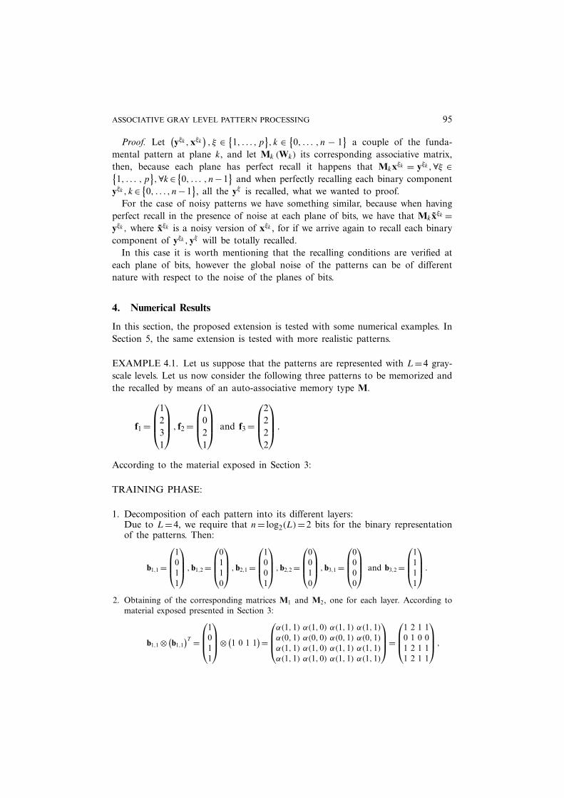
ASSOCIATIVE GRAY LEVEL PATTERN PROCESSING 95
Proof. Let(yξk ,xξk
), ξ ∈ {
1, . . . , p}, k ∈ {
0, . . . , n − 1}
a couple of the funda-mental pattern at plane k, and let Mk (Wk) its corresponding associative matrix,then, because each plane has perfect recall it happens that Mkxξk = yξk ,∀ξ ∈{1, . . . , p
},∀k ∈{
0, . . . , n−1}
and when perfectly recalling each binary componentyξk , k ∈{
0, . . . , n−1}, all the yξ is recalled, what we wanted to proof.
For the case of noisy patterns we have something similar, because when havingperfect recall in the presence of noise at each plane of bits, we have that Mkxξk =yξk , where xξk is a noisy version of xξk , for if we arrive again to recall each binarycomponent of yξk ,yξ will be totally recalled.
In this case it is worth mentioning that the recalling conditions are verified ateach plane of bits, however the global noise of the patterns can be of differentnature with respect to the noise of the planes of bits.
4. Numerical Results
In this section, the proposed extension is tested with some numerical examples. InSection 5, the same extension is tested with more realistic patterns.
EXAMPLE 4.1. Let us suppose that the patterns are represented with L=4 gray-scale levels. Let us now consider the following three patterns to be memorized andthe recalled by means of an auto-associative memory type M.
f1 =
1231
, f2 =
1021
and f3 =
2222
.
According to the material exposed in Section 3:
TRAINING PHASE:
1. Decomposition of each pattern into its different layers:Due to L=4, we require that n= log2(L)=2 bits for the binary representationof the patterns. Then:
b1,1 =
1011
,b1,2 =
0110
,b2,1 =
1001
,b2,2 =
0010
,b3,1 =
0000
and b3,2 =
1111
.
2. Obtaining of the corresponding matrices M1 and M2, one for each layer. According tomaterial exposed presented in Section 3:
b1,1 ⊗ (b1,1
)T =
1011
⊗ (
1 0 1 1)=
α(1,1) α(1,0) α(1,1) α(1,1)
α(0,1) α(0,0) α(0,1) α(0,1)
α(1,1) α(1,0) α(1,1) α(1,1)
α(1,1) α(1,0) α(1,1) α(1,1)
=
1 2 1 10 1 0 01 2 1 11 2 1 1
,

96 HUMBERTO SOSSA ET AL.
b2,1 ⊗ (b2,1
)T =
1001
⊗ (
1 0 0 1)=
α(1,1) α(1,0) α(1,0) α(1,1)
α(0,1) α(0,0) α(0,0) α(0,1)
α(0,1) α(0,0) α(0,0) α(0,1)
α(1,1) α(1,0) α(1,0) α(1,1)
=
1 2 2 10 1 1 00 1 1 01 2 2 1
,
b3,1 ⊗ (b3,1
)T =
0000
⊗ (
0 0 0 0)=
α(0,0) α(0,0) α(0,0) α(0,0)
α(0,0) α(0,0) α(0,0) α(0,0)
α(0,0) α(0,0) α(0,0) α(0,0)
α(0,0) α(0,0) α(0,0) α(0,0)
=
1 1 1 11 1 1 11 1 1 11 1 1 1
,
b1,2 ⊗ (b1,2
)T =
0110
⊗ (
0 1 1 0)=
α(0,0) α(0,1) α(0,1) α(0,0)
α(1,0) α(1,1) α(1,1) α(1,0)
α(1,0) α(1,1) α(1,1) α(1,0)
α(0,0) α(0,1) α(0,1) α(0,0)
=
1 0 0 12 1 1 22 1 1 21 0 0 1
,
b2,2 ⊗ (b2,2
)T =
0010
⊗ (
0 0 1 0)=
α(0,1) α(0,0) α(0,1) α(0,0)
α(0,1) α(0,0) α(0,1) α(0,0)
α(1,0) α(1,0) α(1,1) α(1,0)
α(0,0) α(0,0) α(0,1) α(0,0)
=
1 1 0 11 1 0 12 2 1 21 1 0 1
,
b3,2 ⊗ (b3,2
)T =
1111
⊗ (
1 1 1 1)=
α(1,1) α(1,1) α(1,1) α(1,1)
α(1,1) α(1,1) α(1,1) α(1,1)
α(1,1) α(1,1) α(1,1) α(1,1)
α(1,1) α(1,1) α(1,1) α(1,1)
=
1 1 1 11 1 1 11 1 1 11 1 1 1
,
Now, according to Equation (29):
M1 =
1 2 1 10 1 0 01 2 1 11 2 1 1
∨
1 2 1 10 1 1 00 1 1 01 2 2 1
∨
1 1 1 11 1 1 11 1 1 11 1 1 1
=
1∨1∨1 2∨2∨1 1∨2∨1 1∨1∨10∨0∨1 1∨1∨1 0∨1∨1 0∨0∨11∨0∨1 2∨1∨1 1∨1∨1 1∨0∨11∨1∨1 2∨2∨1 1∨2∨1 1∨1∨1
=
1 2 2 11 1 1 11 2 1 11 2 2 1
,
M2 =
1 0 0 12 1 1 22 1 1 21 0 0 1
∨
1 1 0 11 1 0 12 2 1 21 1 0 1
∨
1 1 1 11 1 1 11 1 1 11 1 1 1
=
1∨1∨1 0∨1∨1 0∨0∨1 1∨1∨12∨1∨1 1∨1∨1 1∨0∨1 2∨1∨12∨2∨1 1∨2∨1 1∨1∨1 2∨2∨11∨1∨1 0∨1∨1 0∨0∨1 1∨1∨1
=
1 1 1 12 1 1 22 2 1 21 1 1 1
.

ASSOCIATIVE GRAY LEVEL PATTERN PROCESSING 97
RECALLING PHASE:
Recall, for example, of pattern: f2 =
1021
. Knowing that L=4:
1. Decomposition of the pattern into its different layers:
b2,1 =
1001
and b2,2 =
0010
.
2. Recalling of the pattern at each level. According to Equation (31):
M1 ∧β b2,1 =
1 2 2 11 1 1 11 2 1 11 2 2 1
∧β
1001
=
β(1,1)∧β(2,0)∧β(2,0)∧β(1,1)
β(1,1)∧β(1,0)∧β(1,0)∧β(1,1)
β(1,1)∧β(2,0)∧β(1,0)∧β(1,1)
β(1,1)∧β(2,0)∧β(2,0)∧β(1,1)
=
1∧1∧1∧11∧0∧0∧11∧1∧0∧11∧1∧1∧1
=
1001
,
M2 ∧β b2,2 =
1 1 1 12 1 1 22 2 1 21 1 1 1
∧β
0010
=
β(1,0)∧β(1,0)∧β(1,1)∧β(1,0)
β(2,0)∧β(1,0)∧β(1,1)∧β(2,0)
β(2,0)∧β(2,0)∧β(1,1)∧β(2,0)
β(1,0)∧β(1,0)∧β(1,1)∧β(1,0)
=
0∧0∧1∧01∧0∧1∧11∧1∧1∧10∧0∧1∧0
=
0010
.
3. Reconstruction of the total pattern by using Equation (33):
f1 =
20 ×1+21 ×020 ×0+21 ×020 ×0+21 ×120 ×1+21 ×0
=
1021
.
As you can see the fundamental pattern is perfectly recalled. This as we saw is oneof the properties of the αβ associative memories. The reader can easily verify thatthe other two patterns are also perfectly recalled.

98 HUMBERTO SOSSA ET AL.
EXAMPLE 4.2. Recalling of a fundamental pattern from a noisy version of itusing an auto-associative memory of type M.
According to material discussed in Section 2, M memories work well with addi-tive noise (not with any additive noise) but with additive noise such as all com-ponents at the different layers of the decomposed pattern change from 0 to 1, butnot inversely. If this does not happened then perfect recall could not occur. Let usfirst consider the following distorted version of pattern f1:
f1 =
3231
.
In this case additive noise has been only added to the first component of f1 (com-ponent has changed from 1 to 3).
1. Decomposition of the pattern by planes:
b1,1 =
1011
and b1,2 =
1110
.
Notice how in this case at both layers, and for the same pixel, additive noise hasbeen also added to the corresponding bits. In particular bit number 1 of patternb1,2 has changed from 0 to 1. Bit number 1 of pattern b1,1 has no modifica-tions. Because additive noise has been also added to each binary layer of thedecomposition, we should expect perfect recall according to Theorem 3.1. Letus verify this.
2. Recall of the pattern at each level. According to Equation(31):
V1 ∧β b1,1 =
1 2 2 11 1 1 11 2 1 11 2 2 1
∧β
1011
=
β (1,1)∧β (2,0)∧β (2,1)∧β (1,1)
β (1,1)∧β (1,0)∧β (1,1)∧β (1,1)
β (1,1)∧β (2,0)∧β (1,1)∧β (1,1)
β (1,1)∧β (2,0)∧β (2,1)∧β (1,1)
=
1∧1∧1∧11∧0∧1∧11∧1∧1∧11∧1∧1∧1
=
1011
,

ASSOCIATIVE GRAY LEVEL PATTERN PROCESSING 99
V2 ∧β b1,2 =
1 1 1 12 1 1 22 2 1 21 1 1 1
∧β
1110
=
β (1,1)∧β (1,1)∧β (1,1)∧β (1,0)
β (2,1)∧β (1,1)∧β (1,1)∧β (2,0)
β (2,1)∧β (2,1)∧β (1,1)∧β (2,0)
β (1,1)∧β (1,1)∧β (1,1)∧β (1,0)
=
1∧1∧1∧01∧1∧1∧11∧1∧1∧10∧1∧1∧0
=
0110
.
Notice how the fundamental binary patterns were perfectly recalled. From thiswe can wait that the recalling of the total pattern will be also possible, let ussee.
3. Final reconstruction of the pattern (Equation (33)):
f1 =
20 ×1+21 ×020 ×0+21 ×120 ×1+21 ×120 ×1+21 ×0
=
1231
= f1
From this example we can see that the recall of a pattern with L>2 (according toTheorem 3.1) depends on recalling of its binary patterns.
In the last example, the original pattern could not be recalled if instead of a 3 a2 would be selected as the value of the first component. Even if this noise is addi-tive, the corresponding noise at the binary patterns is not. In this case the corre-sponding binary patterns are:
b1,1 =
0011
and b1,2 =
1110
.
Although for the second pattern, the value of the first component changes from0 to 1 (additive noise), the corresponding value for the first component of b1,1
changes from 1 a 0 (subtractive noise). This contradicts Theorem 3.1 and of courseno perfect recall of pattern f1 should be expected.
EXAMPLE 4.3. Let us consider the same three patterns used in Example 4.1 andsuppose that now we want to recall them by means of an auto-associative memoryof type W. According to the exposed material in Section 3:

100 HUMBERTO SOSSA ET AL.
TRAINING PHASE:
1. Decomposition of each pattern into its different layers:
b1,1 =
1011
,b1,2 =
0110
,b2,1 =
1001
,b2,2 =
0010
,b3,1 =
0000
and b3,2 =
1111
.
2. Obtaining of the corresponding matrices W1 and W2. According to material exposed pre-sented in Section 3:
b1,1 ⊗ (b1,1
)T =
1011
⊗ (
1 0 1 1)=
α(1,1) α(1,0) α(1,1) α(1,1)
α(0,1) α(0,0) α(0,1) α(0,1)
α(1,1) α(1,0) α(1,1) α(1,1)
α(1,1) α(1,0) α(1,1) α(1,1)
=
1 2 1 10 1 0 01 2 1 11 2 1 1
,
b2,1 ⊗ (b2,1
)T =
1001
⊗ (
1 0 0 1)=
α(1,1) α(1,0) α(1,0) α(1,1)
α(0,1) α(0,0) α(0,0) α(0,0)
α(0,1) α(0,0) α(0,0) α(0,0)
α(1,1) α(1,0) α(1,0) α(1,1)
=
1 2 2 10 0 0 00 0 0 01 2 2 1
,
b3,1 ⊗ (b3,1
)T =
0000
⊗ (
0 0 0 0)=
α(0,0) α(0,0) α(0,0) α(0,0)
α(0,0) α(0,0) α(0,0) α(0,0)
α(0,0) α(0,0) α(0,0) α(0,0)
α(0,0) α(0,0) α(0,0) α(0,0)
=
1 1 1 11 1 1 11 1 1 11 1 1 1
,
b1,2 ⊗ (b1,2
)T =
0110
⊗ (
0 1 1 0)=
α(0,0) α(0,1) α(0,1) α(0,0)
α(1,0) α(1,1) α(1,1) α(1,0)
α(1,0) α(1,1) α(1,1) α(1,0)
α(0,0) α(0,1) α(0,1) α(0,0)
=
1 0 0 12 1 1 22 1 1 21 0 0 1
,
b2,2 ⊗ (b2,2
)T =
0010
⊗ (
0 0 1 0)=
α(0,0) α(0,0) α(0,1) α(0,0)
α(0,0) α(0,0) α(0,1) α(0,0)
α(1,0) α(1,0) α(1,1) α(1,0)
α(0,0) α(0,0) α(0,1) α(0,0)
=
1 1 0 11 1 0 12 2 1 21 1 0 1
,
b3,2 ⊗ (b3,2
)T =
1111
⊗ (
1 1 1 1)=
α(1,1) α(1,1) α(1,1) α(1,1)
α(1,1) α(1,1) α(1,1) α(1,1)
α(1,1) α(1,1) α(1,1) α(1,1)
α(1,1) α(1,1) α(1,1) α(1,1)
=
1 1 1 11 1 1 11 1 1 11 1 1 1
.

ASSOCIATIVE GRAY LEVEL PATTERN PROCESSING 101
According to Equation (30):
W1 =
1 2 1 1
0 1 0 0
1 2 1 1
1 2 1 1
∧
1 2 2 1
0 1 1 0
0 1 1 0
1 2 2 1
∧
1 1 1 1
1 1 1 1
1 1 1 1
1 1 1 1
=
1∧1∧1 2∧2∧1 1∧2∧1 1∧1∧1
0∧0∧1 1∧1∧1 0∧1∧1 0∧0∧1
1∧0∧1 2∧1∧1 1∧1∧1 1∧0∧1
1∧1∧1 2∧2∧1 1∧2∧1 1∧1∧1
=
1 1 1 1
0 1 0 0
0 1 1 0
1 1 1 1
,
W2 =
1 0 0 1
2 1 1 2
2 1 1 2
1 0 0 1
∧
1 1 0 1
1 1 0 1
2 2 1 2
1 1 0 1
∧
1 1 1 1
1 1 1 1
1 1 1 1
1 1 1 1
=
1∧1∧1 0∧1∧1 0∧0∧1 1∧1∧1
2∧1∧1 1∧1∧1 1∧0∧1 2∧1∧1
2∧2∧1 1∧2∧1 1∧1∧1 2∧2∧1
1∧1∧1 0∧1∧1 0∧0∧1 1∧1∧1
=
1 0 0 1
1 1 0 1
1 1 1 1
1 0 0 1
.
RECALLING PHASE:
Recall, for example, of pattern: f1 =
1231
. Knowing that L=4:
1. Decomposition of the pattern into its different layers:
b1,1 =
1011
and b1,2 =
0110
.

102 HUMBERTO SOSSA ET AL.
2. Recalling of the pattern at each level. According to Equation (32):
W1 ∨β b1,1 =
1 1 1 10 1 0 00 1 1 01 1 1 1
∨β
1011
=
β(1,1)∨β(1,0)∨β(1,1)∨β(1,1)
β(0,1)∨β(1,0)∨β(0,1)∨β(0,1)
β(0,1)∨β(1,0)∨β(1,1)∨β(0,1)
β(1,1)∨β(1,0)∨β(1,1)∨β(1,1)
=
1∨0∨1∨10∨0∨0∨00∨0∨1∨01∨0∨1∨1
=
1011
.
W2 ∨β b1,2 =
1 0 0 11 1 0 11 1 1 11 0 0 1
∨β
0110
=
β(1,0)∨β(0,1)∨β(0,1)∨β(1,0)
β(1,0)∨β(1,1)∨β(0,1)∨β(1,0)
β(1,0)∨β(1,1)∨β(1,1)∨β(1,0)
β(1,0)∨β(0,1)∨β(0,1)∨β(1,0)
=
0∨0∨0∨00∨1∨0∨00∨1∨1∨00∨0∨0∨0
=
0110
.
3. Reconstruction of the total pattern by using Equation (33):
f1 =
20 ×1+21 ×020 ×0+21 ×120 ×1+21 ×120 ×1+21 ×0
=
1231
.
As hoped, the fundamental pattern is perfectly recalled. The reader can easily ver-ify that the other two patterns are also perfectly recalled.
EXAMPLE 4.4. Recalling of a fundamental pattern from a noisy version of itusing an auto-associative memory of type W.
According to material discussed in Section 2, the memories type W work wellwith subtractive noise; this is with noise such as all components at the differentlayers change from 1 to 0, but not inversely. In this case it will be additive noisefor that component. Let us suppose that we want to recuperate pattern f1 from adistorted version of it, for example:
f1 =
1230
.

ASSOCIATIVE GRAY LEVEL PATTERN PROCESSING 103
In this case subtractive noise has been only added to the first component of f1
(component has changed from 1 to 0).
1. Decomposition of the input pattern by planes:
b1,1 =
1010
and b1,2 =
0110
.
Notice how the subtracted noise to both components of the pattern in bothplanes is also subtractive (some values change from 1 to 0, but from 0 to 1).This as mentioned before is a necessary condition for the memories of kind Wto recall a pattern from a noisy version of it.
2. Recalling of the pattern at each level. According to Equation(32):
W1 ∨β b1,1 =
1 1 1 10 1 0 00 1 1 01 1 1 1
∨β
1010
=
β (1,1)∨β (1,0)∨β (1,1)∨β (1,0)
β (0,1)∨β (1,0)∨β (0,1)∨β (0,0)
β (0,1)∨β (1,0)∨β (1,1)∨β (0,0)
β (1,1)∨β (1,0)∨β (1,1)∨β (1,0)
=
1∨0∨1∨00∨0∨0∨00∨0∨1∨01∨0∨1∨0
=
1011
.
W2 ∨β b1,2 =
1 0 0 11 1 0 11 1 1 11 0 0 1
∨β
0110
=
β (1,0)∨β (0,1)∨β (0,1)∨β (1,0)
β (1,0)∨β (1,1)∨β (0,1)∨β (1,0)
β (1,0)∨β (1,1)∨β (1,1)∨β (1,0)
β (1,0)∨β (0,1)∨β (0,1)∨β (1,0)
=
0∨0∨0∨00∨1∨0∨00∨1∨1∨00∨0∨0∨0
=
0110
.
Notice how the fundamental binary patterns were perfectly recalled. From thiswe can wait that the recalling of the total pattern will be also possible, let ussee.
3. Final reconstruction of the pattern (Equation (33)):
f1 =
20 ×1+21 ×020 ×0+21 ×120 ×1+21 ×120 ×1+21 ×0
=
1231
= f1

104 HUMBERTO SOSSA ET AL.
Figure 1. Images of the five objects used in to test the proposed extension.
As in the case of αβ auto-associative memories of type M, the desired pattern canbe recalled from an altered version of it (by using a W memory), if its set of fun-damental binary patterns is first recalled.
5. Experiments with Real Patterns
In this section the proposed extension is tested with more realistic patterns. Imagesof five real objects (a bolt, a washer, an eyebolt, a hook and a dovetail) were usedare shown in Figure 1. The images are 32×29 pixels and 256 gray levels. Only αβ
auto-associative memories of type M were tested.
5.1. construction of the association matrices
The five images were first converted to vectors of 968 elements (32 times 29) eachone. These vectors were next decomposed into their eight binary layers. They werefinally used to construct the eight matrices M1,M2, . . . ,M8, by using the corre-sponding equations given in Section 3.
5.2. recalling of the fundamental set
In this first experiment, the five images were fed to the eight memories. To all ofthem, the procedures described in Section 3 were applied. In all cases, of coursethe five patterns were perfectly recalled.
5.3. recalling of a pattern by a corrupted version of it
5.3.1. Case of M memory
Three groups of images were generated. The first one with additive noise, thesecond one with saturated noise of type salt, and the third one with manuallysaturated noise. In the first case, to the gray-value f (x, y) of pixel with coordinates(x, y), an integer ν was added, such that f (x, y)+ν ≤ (L−1). In the second case,the gray-value of the pixel was simply saturated to the value (L−1).
In the first case, the value ν was first randomly selected. It was then added tothe gray-value f (x, y) of the pixel if s < t.s ∈ [0,1] is an uniformly randomly dis-tributed random variable, t is the parameter controlling how much of the image iscorrupted. This way, the bigger the value of t , the more of the image pixels shouldbe corrupted. If t =0, no pixel value is modified. In the contrary, if t =1, all pixels

ASSOCIATIVE GRAY LEVEL PATTERN PROCESSING 105
Figure 2. (a) Versions with additive noise, t varied from 0.1 to 0.5 with steps of 0.1. (b) Recalled ver-sions. The number of pixels here is the number of non-recalled pixel values. In this case, most of thecontent of the original image was not recalled.
values should be changed. In the second case, the gray-value f (x, y) was simplysaturated to (L − 1) if s < t . In the third case Microsoft PAINT utility was usedmanually modify the gray-values of the pixels.
A quantitative measure as to how good the recall is all cases was chosen as fol-lows. Let frecalled (x, y) , forignal (x, y) the gray levels of a pixel in the originalimage and the corresponding pixel in the recalled image. Let NMP the numberof modified pixels in the recalled image with respect to the original image whensubtracting pair by pair their gray levels. If NPI is total number of pixels of theimage, then percentage of modified pixels PP of the recalled image with respect tothe original image is given as:
PP =100(
NMPNPI
). (21)
5.3.1.1. Performance in the presence of additive noise. Twenty-five images wereobtained as explained. Parameter t was varied from 0.1 to 0.5 in steps of 0.1. Fig-ure 2(a) shows the obtained images. The number (percentage) of modified pixels ateach image is shown above each image. Recalled versions are shown in Figure 2(b).As anticipated by Theorem 1, none of the original images was perfectly recalled.Again, the number (percentage) of non-recalled pixels in the recalled image withrespect to the original image is shown above each image. Notice also how as thelevel of noise increases, the recalled versions appear more or less the same.5.3.1.2. Performance in the presence of salt noise. Again, 25 images were obtainedas explained. Parameter t was again varied from 0.1 to 0.5 in steps of 0.1. Thevalue of the pixel was saturated to L− 1. Figure 3(a) shows the obtained images.The number (percentage) of modified pixels at each image is shown above each

106 HUMBERTO SOSSA ET AL.
Figure 3. (a) Versions with salt noise, t varied from 0.1 to 0.5 with steps of 0.1. (b) Recalled versions.The number of pixels here is the number of non-recalled pixel values. In this case, most of the contentof original image was recalled.
image. Recalled versions are shown in Figure 3(b). Above each recalled image it isindicated the number (percentage) of non-recalled pixels with respect to the origi-nal image is shown above each image. Notice how despite the level of noise intro-duced to the images is bigger than in the first case, recalled versions match muchbetter with the originals. This is normal due to saturating noise does not add sub-tractive noise to the binary layers of the patterns.5.3.1.3. Performance in the presence of manually added noise. Twenty-five imageswere obtained by occluding part of the original image with one or more whiteregions of different shapes and sizes. Figure 4(a) shows these extra images. Thenumber (percentage) of modified pixels at each image is shown above each image.Recalled versions from these noisy versions are shown in Figure 4(b). As shown, inthis third case, although the desired image was not also perfectly recalled, it prettywell matches the original one. Above each recalled image it is indicated the num-ber (percentage) of non-recalled pixels with respect to the original image.5.3.1.4. Performance in the presence of big quantities of positive saturating noise. Wewanted to test the performance of the proposal with big quantities of positive sat-urating noise. Five noisy, versions, one for each original image with t = 0.95 weregenerated. These are shown in Figure 5(a). Notice the level of noise introducedto each image. Even for as humans is impossible to re-built the original imagefrom such distorted pattern. Recalled versions from these extremely noisy versionsare shown in Figure 5(b). Notice how despite the level of noise introduced to theimages, the recalled versions well match their originals.
It is worth to mention that the average time to recall an image in the three casesis of 6 s in a Pentium 4 running at 1.3 GHz.

ASSOCIATIVE GRAY LEVEL PATTERN PROCESSING 107
Figure 4. (a) Versions with manually generated saturated noise. (b) Recalled versions. In this case, mostof the content of original image was recalled.
Figure 5. (a) Versions with saturated salt noise with t =0.95. (b) Recalled versions.
5.3.2. Case of W memory
Again, three groups of images were generated. The first one with subtractive noise,the second one with saturated noise of type pepper, and the third one with man-ually added saturated pepper noise. In the first case, to the gray-value f (x, y) ofpixel with coordinates (x, y), an integer ν was subtracted, such that f (x, y)− ν ≤(L−1). In the second case, again to the gray-value of a pixel an integer was sub-tracted, such that f (x, y)− ν = (L− 1). The value of v was chosen as in the caseadditive noise.5.3.2.1 Performance in the presence of subtractive noise. Twenty-five images wereobtained as explained. Parameter t was varied from 0.1 to 0.5 in steps of 0.1. Fig-ure 6(a) shows the obtained images. The number (percentage) of modified pixelsat each image is shown above each image. The recalled versions are shown in Fig-ure 6(b). As hoped, also in this case, none of the images was perfectly recalled.This is indicated by the number (percentage) of non-recalled pixels with respectto the original image as shown above each image. Notice also how as the level ofnoise increases, the recalled versions appear more or less the same.5.3.2.2 Performance in the presence of pepper noise. Twenty-five images wereobtained as explained. Parameter t was varied from 0.1 to 0.5 in steps of 0.1. Thevalue of the pixel was saturated to 0. Figure 7(a) shows the obtained images. The

108 HUMBERTO SOSSA ET AL.
Figure 6. (a) Versions with subtractive, t varied from 0.1 to 0.5 with steps of 0.1. (b) Recalled versions.In this case, most of the content of the original image was not recalled.
Figure 7. (a) Versions with pepper noise, t varied from 0.1 to 0.5 with steps of 0.1. (b) Recalled versions.In this case, the content of original image was recalled.
number (percentage) of modified pixels at each image is shown above each image.In this case, in all cases the desired image was correctly recalled as shown in Fig-ure 6(b).5.3.2.3 Performance in the presence of manually subtractive noise. Twenty-fiveimages were obtained by occluding part of the image with one or more blackregions of different shapes and sizes. Figure 8(a) shows these extra images. In thisthird case, in all cases the desired image was perfectly recalled.

ASSOCIATIVE GRAY LEVEL PATTERN PROCESSING 109
Figure 8. (a) Versions with manually generated saturated noise. (b) Recalled versions. In this case, thecontent of original image was recalled.
Figure 9. (a)Versions with saturated pepper noise with t =0.95 (b) Recalled versions.
5.3.2.4 Performance in the presence of big quantities of negative saturating noise.We wanted to test the performance of the proposal with big quantities of negativesaturating noise. Five noisy, versions, one for each original image with t = 0.95were generated. These are shown in Figure 9(a). Notice the level of noise intro-duced to each image. As in the case of highly distorted images with positive satu-rating noise, even for as humans is impossible to re-built the original image fromsuch distorted pattern. Recalled versions from these extremely noisy versions areshown in Figure 9(b). Notice how despite the level of noise introduced to theimages, the recalled versions well match their originals.
The average time to recall an image in these last three cases was of 6 seconds ina Pentium 4 running at 1.3 GHz.
5.3.3. Discussion
From the experiments we can conclude that the proposal is more adequate forthe case of patterns distorted by saturating (salt or pepper noise). The proposalcan thus be adopted with success in any application where the patterns con-cerned appear distorted by saturating noise, either salt or pepper. The proposal will

110 HUMBERTO SOSSA ET AL.
not provide good results if non-saturating is added to the patterns due to eitheradditive or subtractive noise will be added to the binary layers representing thepatterns, provoking a non-desired recalling as shown in the experiments.
6. Conclusions and Present Research
In this paper, we have shown how is possible to use binary memories (αβ memo-ries in this), to efficiently recall patterns in more than two gray levels (L>2). Thisis possible due to a pattern can be decomposed into binary layers. In this case αβ
memories are applied by layers, combining the partial results for the recalling ofa pattern on posterior steps. One feature of the proposed extension is that layerscan be processed in parallel allowing huge computation time reductions.
It is worth to mention that the proposed technique can be adapted to any kindof binary associative memories while their input patterns can be decomposed intobinary layers.
Actually, we are investigating how to use the proposed approach in the presenceof mixed noise and other variations. We are also working through an applicationthat allows us to operate with bigger images and other patterns such a voice wherethe proposal would have a more realistic application. We are also working towardthe proposal of new associative memories able to operate with gray level patternswhere no binary layer decomposition is needed.
Acknowledgements
The authors would like to thank the reviewers for their appropriate comment thatallowed improving the content and presentation of this work. We would like alsoto thank Hector Cortes for his help with some of the experiments. This work waseconomically supported by CGPI-IPN under grants 20020214, 20030658, 20040646and 20050156 and CONACYT by means of grants 41529 and 46805.
References
1. Yanez, C.: Associative Memories based on Order Relations and Binary Operators (InSpanish), PhD Thesis, Center for Computing Research, February of 2002.
2. Steinbuch, K.: Die Lermatrix, Kybernetik, 1(1) 1961, 26–45.3. Wilshaw, D., Buneman, O. and Longuet-Higgings, H.: Non-holographic associative mem-
ory, Nature 222 (1969), 960–962.4. Anderson, J. A.: A simple neural network generating an interactive memory, Mathematical
Biosciences, 14 (1972), 197–220.5. Kohonen, T.: Correlation matrix memories, IEEE Transactions on Computers, 21(4)
(1972), 353–359.6. Hopfield, J. J.: Neural networks and physical systems with emergent collective computa-
tional abilities, Proceedings of the National Academy of Sciences, 79 (1982), 2554–2558.7. Ritter, G. X., Sussner P. and Dıaz de Leon, J. L.: Morphological associative memories,
IEEE Transactions on Neural Networks, 9 (1998), 281–293.

ASSOCIATIVE GRAY LEVEL PATTERN PROCESSING 111
8. Ritter, G. X., Dıaz de Leon, J. L. and Sussner P.: Morphological bi-directional associativememories, Neural Networks, 12 (1999), 851–867.
9. Hassoun, M.: Associative neural memories: Theory and implementation. Oxford Univer-sity Press, Oxford, 1993.