assessment of climate change impact on
315
ASSESSMENT OF CLIMATE CHANGE IMPACT ON RUNOFF AND PEAK FLOW – A CASE STUDY ON KLANG WATERSHED IN WEST MALAYSIA Reza Kabiri Thesis submitted to the University of Nottingham for the degree of Doctor of Philosophy April 2014
-
Upload
khangminh22 -
Category
Documents
-
view
1 -
download
0
Transcript of assessment of climate change impact on
1
ASSESSMENT OF CLIMATE CHANGE IMPACT ON
RUNOFF AND PEAK FLOW – A CASE STUDY
ON KLANG WATERSHED
IN WEST MALAYSIA
Reza Kabiri
Thesis submitted to the University of Nottingham for the
degree of Doctor of Philosophy
April 2014
i
ABSTRACT
Climate change is a consequence of changing in climate on environment over the
worldwide. The increase in developmental activities and Greenhouse Gases (GHGS)
put a strain on environment, resulting in increased use of fuel resources. The
consequence of such an emission to the atmosphere exacerbates climate pattern.
There are numerous Climate Change Downscaling studies in coarse resolution, which
have largely centred on employing the dynamic approaches, and in most of these
investigations, the Regional Climate Model (RCM) has been reported to numerically
predict the local climatic variables. The majority of previous investigations have
failed to account for the spatial watershed scale, which could generate an average
value of downscaled variables over the watershed scale.
To address shortcomings of previous investigations, the work undertaken in this
project has two main objectives. The study first aims to implement a spatially
distributed Statistical Downscaling Model (SDSM) to downscale the predictands, and
second to evaluate the impact of climate changes on the future discharge and peak
flow. It is conducted based on the IPCC Scenarios A2 (Medium–High Emission
scenario) and B2 (Medium–Low Emission scenario). The main objectives of the
study are as follows:
To generate fine resolution climate change scenarios using Statistical
Downscaling Model in the watershed scale,
To project the variability in temperature, precipitation and evaporation for the
three time slices, 2020s (2010 to 2039), 2050s (2040 to 2069) and 2080s
(2070 to 2099), based on A2 and B2 scenarios,
To calibrate and validate hydrological model using historical observed flow
data to verify the performance of the hydrological model,
ii
To evaluate the impact of climate changes on the future discharge and future
peak flow for three timeslices: 2020s (2010 to 2039), 2050s (2040 to 2069)
and 2080s (2070 to 2099).
Thus, to meet the objectives of the study, projection of the future climate based on
climate change scenarios from IPCC is carried out as the most important component
in the research. The results of this research are presented as follows:
The study indicates that there will be an increase of mean monthly
precipitation but with an intensified decrease in the number of consecutive
wet-days and can be concluded as a possibility of more precipitation amount
in fewer days.
The watershed is found to experience increased rainfall towards the end of the
century. However, the analysis indicates that there will likely be a negative
trend of mean precipitation in 2020s and with no difference in 2050s. The
precipitation experiences a mean annual decrease by 7.9%, 0.6% in 2020s and
2050s and an increase by 12.4% in 2080s corresponding A2 scenario.
The maximum and minimum temperatures are likely to be increased toward
the end of the century by 2.7oC and 0.8
oC respectively when compared to the
current observed temperature (1975-2001) at the Subang temperature station.
The average annual mean discharge is predicted to be decreasing by 9.4%,
4.9% and an increase of 3.4% for the A2 and a decrease of 17.3%, 13.6% and
5.1% for the B2 scenario, respectively in the 2020s, 2050s and 2080s.
The average annual maximum discharge is projected to decrease by 7.7% in
2020s and an increase by 4.2% and 29% in A2 scenario for 2050s and 2080s,
respectively. But there will most likely be a decrease in the maximum
discharge for all the future under B2 scenario. It is projected a decrease of
32.3%, 19.5% and 2.3% for 2020s, 2050s and 2080s, respectively.

iii
The projected mean discharge indicates a decline in the months from January
to April and also from July to August in all the three future periods for A2 and
B2 scenarios. There is an increasing trend in the discharge of September and
October in the 2020s according to the A2 and B2 scenarios.
The highest increase in precipitation frequency occurs in 2080s under A2
scenario in which the increase in the magnitude of 100 Return Year is found
to be 88% greater than the one of the maximum observed.
The highest increase in flood frequency at Sulaiman streamflow station occurs
in 2080s under A2 scenario. The increase in the magnitude of 100 Return
Year is found to be 26.5% greater than the one of the maximum observed.
iv
PUBLICATIONS
Journal
Kabiri, R., Ramani Bai V., and Chan, A. 2013. Comparison of SCS and Green-Ampt
methods in surface runoff-Flooding simulation for Klang watershed in
Malaysia. Open Journal of Modern Hydrology. 3 (3), PP. 102-114.
doi: 10.4236/ojmh.2013.33014
Kabiri, R., Ramani Bai V., and Chan, A. 2013. Regional precipitation scenarios using
a spatial statistical downscaling approach for Klang watershed in Malaysia,
Journal of Environmental Research and Development. 8 (1), pp.126-134
Kabiri, R., Ramani Bai V., and Chan, A. 2013. Simulation of runoff using modified
SCS-CN method using GIS system, case study: Klang watershed in Malaysia.
Journal of Applied Sciences. (54651-RJES-AJ -In Press)
Conference Proceeding
Kabiri, R., Ramani Bai V., and Chan, A. 2012. Estimation of Climate change impacts
on frequency of precipitation extremes Case study: Klang watershed,
Malaysia. International Conference on Environment, Chemistry and Biology-
ICECB Hong Kong, 49, pp.144-149.
Kabiri, R., Ramani Bai V., and Chan, A. 2012.Using Green-Ampt loss method in
surface runoff simulation, Case study: Klang watershed, Malaysia. 10th
WSEAS International Conference on Environment, Ecosystems and
Development (EED '12). Montreux, Switzerland, pp. 217-222.
Kabiri, R., Ramani Bai V., and Chan, A. 2012. Climate change impacts on river
runoff in Klang watershed in Malaysia. 10th WSEAS International Conference
on Environment, Ecosystems and Development (EED '12). Montreux,
Switzerland, pp. 223-228.

v
Book Chapter
Ramani Bai V., S. Mohan and Kabiri, R. 2011. Towards a Database for an
Information Management System on Climate Change: An Online Resource.
Climate Change and the Sustainable Use of Water Resources, Climate
Change Management, Springer, pp. 61-67. ISSN: 1610-2010, ISBN: 978-3-
642-22265-8. www.springerlink.com/content/p38r44v1858t3538/

vi
ACKNOWLEDGEMENT
The author would like to take this opportunity to convey his deepest gratitude to the
supervisor, Associate Professor Dr. Ramani Bai V., who has guided, encouraged and
supported him throughout the completion of this research with her expertise in Water
resources and Environmental Engineering. Moreover, the author would like to
express his deepest gratitude to Professor Andrew Chan for his guidance and valuable
advices.
The Author also takes this opportunity to express a deep sense of gratitude to Dr.
Raju, National University of Singapore (NUS), for supporting the Climate Change
Research and GIS system.
The author is obliged to the staff members of the government agencies, Engineers
from the Hydrology Unit of the Department of Irrigation and Drainage (DID)
Malaysia, as well as the Department of Survey and Mapping (JUPEM), Malaysia for
the valuable information provided by them in their respective fields during the
acquisition of data and supporting material for this research.
This thesis is done as a part of the big project which is currently conducting by the
collaborator, Asia Pacific Network (APN), under a broad project title of “climate
change and DIMS technology”. It is appreciated to thank Science Fund, Ministry of
Science, Technology and Innovation (MOSTI), Malaysia and APN, Japan for
providing the research grant and their support in providing the required data for this
research.
Lastly, the author would like to thank his family particularly his wife, Sara, for her
constant encouragement to conduct his PhD at University of Nottingham.
vii
TABLE OF CONTENTS
ABSTRACT ............................................................................................................................................................. i
PUBLICATIONS ................................................................................................................................................... iv
Journal .................................................................................................................................................................... iv
Conference Proceeding ........................................................................................................................................... iv
Book Chapter ........................................................................................................................................................... v
ACKNOWLEDGEMENT ...................................................................................................................................... vi
1- INTRODUCTION ....................................................................................................................................... 1
1-1- Problem Definition ........................................................................................................................................ 1
1-2- Literature Review .......................................................................................................................................... 3
1-2-1-Climate Change Model .................................................................................................................................. 3
1-2-2-Methods of Downscaling ............................................................................................................................... 5
1-2-3-Hydrology Model .......................................................................................................................................... 8
1-2-4-Hydrology Modelling in Climate Change Study ......................................................................................... 11
1-3- Significance of the Study ............................................................................................................................. 18
1-4- Objectives of the Study ............................................................................................................................... 19
1-5- Scope of the Research ................................................................................................................................. 20
1-6- Limitations of the Study .............................................................................................................................. 21
1-7- Thesis Outline .............................................................................................................................................. 21
2- METHODOLOGY .................................................................................................................................... 24
2-1- Overall Framework of the Research ............................................................................................................ 24
2-2- Climate Change Downscale Modelling ....................................................................................................... 26
2-2-1-Climate Change Scenarios ........................................................................................................................... 26
2-2-2-Large Scale Predictor NCEP/NCAR Re-Analysis Data .............................................................................. 29
2-2-3-Global Climate Change - HadCM3 Model .................................................................................................. 31
2-2-3-1-NCEP-1961-2001 ..................................................................................................................................... 33
2-2-3-2-H3A2a-1961-2099 .................................................................................................................................... 33
2-2-3-3-H3B2a-1961-2099 .................................................................................................................................... 33
2-2-4-Statistical Downscaling Model (SDSM) ...................................................................................................... 33
2-2-4-1-Conditional Probability ............................................................................................................................ 36
2-2-4-2-Selection of Predictor Variables for Downscaling ................................................................................... 37
2-2-4-3-Model Evaluation and Validation ............................................................................................................. 39
2-2-4-4-Optimisation ............................................................................................................................................. 40
2-3- Model Error ................................................................................................................................................. 40
2-4- Hydrological Modelling .............................................................................................................................. 42
2-4-1-Watershed Delineation ................................................................................................................................. 42
2-4-2-Loss Model .................................................................................................................................................. 43
2-4-3-Time of Concentration ................................................................................................................................. 44
2-4-4-Channel Routing .......................................................................................................................................... 44
viii
2-4-5-Stage-Storage-Discharge Relationship ........................................................................................................ 45
2-5- Flood Frequency Analysis ........................................................................................................................... 45
3- CLIMATE BASE AND HYDRO-METEOROLOGICAL ANALYSIS ............................................... 47
3-1- Study Area ................................................................................................................................................... 47
3-1-1-Watershed Description ................................................................................................................................. 47
3-1-2-Geology ....................................................................................................................................................... 48
3-1-3-Soil ............................................................................................................................................................... 48
3-1-4-Landuse ........................................................................................................................................................ 49
3-1-5-Topography .................................................................................................................................................. 52
3-1-6-Slope ............................................................................................................................................................ 53
3-2- Data Preparation .......................................................................................................................................... 61
3-2-1-Data Sources ................................................................................................................................................ 61
3-2-2-Rainfall Data ................................................................................................................................................ 61
3-2-3-Hydro-Meteorological Data ......................................................................................................................... 62
3-2-4-Data Quality Control.................................................................................................................................... 62
3-2-4-1-Meteorological Data Screening ................................................................................................................ 62
3-2-4-1-1-Homogeneity Analysis .......................................................................................................................... 62
3-2-4-1-2-Visual Examination ............................................................................................................................... 63
3-2-4-1-3-Double-Mass Curve .............................................................................................................................. 64
3-2-4-2-Raingauge Network Analysis ................................................................................................................... 65
3-2-4-2-1-Spatial Homogeneity ............................................................................................................................. 65
3-2-4-2-2-Spatial Raingauge Network Analysis .................................................................................................... 66
3-2-4-3-Flow/Discharge Data Screening ............................................................................................................... 68
3-2-4-4-Filling Missing Data ................................................................................................................................. 72
3-2-4-4-1-Filling Rainfall Data .............................................................................................................................. 72
3-2-4-4-2-Filling Discharge Data .......................................................................................................................... 73
3-3- Climate Base Analysis ................................................................................................................................. 74
3-3-1-Temperature Trend ...................................................................................................................................... 74
3-3-2-Rainfall Trend .............................................................................................................................................. 76
3-3-3-Spatial Annual Mean Rainfall...................................................................................................................... 78
3-3-4-Probable Maximum Precipitation (PMP)..................................................................................................... 79
3-3-5-Frequency Analysis ..................................................................................................................................... 86
3-4- River Discharge Analysis ............................................................................................................................ 92
3-4-1-Mean Monthly River Discharge .................................................................................................................. 92
3-4-2-Annual River Discharge Analysis ................................................................................................................ 93
3-4-3-Flood Frequency Analysis ........................................................................................................................... 94
3-4-4-Flow Duration Curve ................................................................................................................................... 95
4- CLIMATE CHANGE DOWNSCALING ................................................................................................ 97
4-1- Data used in SDSM ..................................................................................................................................... 97
4-1-1-Predictand Data ............................................................................................................................................ 97
ix
4-1-2-Predictor Data .............................................................................................................................................. 98
4-2- Statistical Downscaling Model (SDSM) for Daily Precipitation, Temperature and
Evaporation .......................................................................................................................................................... 100
4-2-1- SDSM for Klang Watershed ..................................................................................................................... 101
4-2-2-Exploratory Data Analysis ......................................................................................................................... 102
4-2-3-Selection of Predictors ............................................................................................................................... 107
4-2-4-Model Calibration ...................................................................................................................................... 109
4-2-5-Model Validation ....................................................................................................................................... 113
4-2-6-Scenario Generator .................................................................................................................................... 117
5- HYDROLOGICAL MODELLING ....................................................................................................... 120
5-1- Hydrologic Modelling for Klang Watershed ............................................................................................. 120
5-2- Watershed Modelling ................................................................................................................................ 123
5-2-1.Building a Digital Elevation Model of Klang Watershed Using TIN (Triangular Irregular
Network) .............................................................................................................................................................. 123
5-2-2.DEM Optimisation ..................................................................................................................................... 124
5-2-3.Delineation of watershed Boundary, Outlet and Stream Network Layers ................................................. 124
5-2-3-1-DEM Smoothing .................................................................................................................................... 124
5-2-3-2-Filling Depressions / Sinks ..................................................................................................................... 125
5-2-3-3-DEM Reconditioning ............................................................................................................................. 125
5-2-3-4-Flow Direction ........................................................................................................................................ 126
5-2-3-5-Flow Accumulation ................................................................................................................................ 126
5-2-3-6-Stream Definition and Stream Segmentation ......................................................................................... 126
5-2-3-7-Watershed Delineation ........................................................................................................................... 127
5-2-3-8-Optimisation of the Delineated Watershed ............................................................................................. 127
5-3- The Runoff Simulation .............................................................................................................................. 137
5-3-1-Loss Model ................................................................................................................................................ 140
5-3-1-1-Determining Curve Number ................................................................................................................... 142
5-3-1-1-1-Soil Categorisation .............................................................................................................................. 142
5-3-1-1-2-Landuse Categorisation ....................................................................................................................... 143
5-3-1-1-3-Overlaying the Landuse and Soil maps ............................................................................................... 143
5-3-2-SCS Unit Hydrograph Transform .............................................................................................................. 147
5-3-3-Impervious Surface .................................................................................................................................... 148
5-3-4-Streamflow (Channel) Routing .................................................................................................................. 149
5-3-5-Reservoir Flood Routing ............................................................................................................................ 149
5-3-6-Meteorological Model ............................................................................................................................... 151
5-3-7-Model Calibration and Validation ............................................................................................................. 152
6- RESULTS AND DISCUSSION .............................................................................................................. 158
6-1- Changes in Temperature ............................................................................................................................ 158
6-2- Change in Evaporation .............................................................................................................................. 161
6-3- Change in Evapotranspiration ................................................................................................................... 162
x
6-4- Change in Rainfall Variables ..................................................................................................................... 163
6-5- Assessment of Climate Change Impact on the Mean and Maximum River Discharge ............................. 168
6-6- Assessment of Climate Change Impact on the Flood Frequency .............................................................. 178
6-6-1-Assessment of Climate Change Impact on the Occurrence of Extreme Precipitation
Events .................................................................................................................................................................. 178
6-6-2- Assessment of Climate Change Impacts on the Frequency of Mean and Extreme Flood
Events at the Discharge Station ........................................................................................................................... 178
6-7- Error Analysis of Downscaling output ...................................................................................................... 190
6-7-1-Model Error in the Estimates of Mean and Variance ................................................................................. 190
6-7-2-Error Evaluation in Estimates of Means and Variances............................................................................. 195
7- CONCLUSION ........................................................................................................................................ 199
7-1- Assessment of Climate Change Impact on Climate Variables .................................................................. 199
7-2- Assessment of Climate Change Impact on the River Discharge ............................................................... 201
7-3- Assessment of Climate Change Impact on the Flood Frequency .............................................................. 202
7-4- Recommendation for Future Research ...................................................................................................... 203
REFERENCES .................................................................................................................................................. 205
Appendix A- Climate Change Models ................................................................................................................. 227
Appendix B – Double-Mass Curve ...................................................................................................................... 229
Appendix C– Correlation between Raingauge Stations of Daily Rainfall Data .................................................. 232
Appendix D- The Correlation of Daily Discharge Data between the Discharge Stations in Klang
Watershed ............................................................................................................................................................ 234
Appendix E- Mean Monthly Rainfall for All the Raingauge Stations ................................................................. 235
Appendix F- Mean Monthly River Discharge ..................................................................................................... 238
Appendix G- Annual River Discharge Analysis: Mean Annual Flow and Anomaly of Mean at
Discharge Stations ............................................................................................................................................... 239
Appendix H- Flood Frequency Curve at Discharge Stations ............................................................................... 240
Appendix I- Flow Duration Curves at Discharge Stations .................................................................................. 241
Appendix J- Exploratory Data Analysis at All the Raingauge Stations Used for Downscaling .......................... 242
Appendix K- Comparison between observed and calibrated of mean and variance precipitation
(mm) ................................................................................................................................................................... 251
Appendix L- SDSM Output: Summary of Statistics for Observed and Validated Data ..................................... 254
Appendix M- Statistical Summary of Statistics for Simulated Precipitation for Future Period .......................... 261
Appendix N- The Maps of Infiltration Parameters for Klang Watershed ............................................................ 282
Appendix O- Storage-Discharge Relationships of Klang Gate Dam and Batu Dam ........................................... 284
Appendix P- Performance of Daily and Monthly Discharges in the Calibration and Validation
Periods in HEC-HMS .......................................................................................................................................... 285
Appendix Q- Maps of Rainfall Intensity for the Future Corresponding to A2 and B2 Scenarios ....................... 287
Appendix R- Model Error in the Estimates of Mean and Variance ..................................................................... 293
Appendix S- Confidence Interval in the Estimates of Mean and Variance Daily Precipitation
Downscaled with NCEP ...................................................................................................................................... 296
xi
LIST of FIGURES
Figure 1 The schematic of downscaling spatial resolution ............................................................................................. 6 Figure 2 A GCM map of precipitation projection for the future in three time slices: Ensemble
precipitation projection for the period: (A) 2020-2029, (B) 2050-2059 and (C)
2090-2099 ............................................................................................................................................. 15 Figure 3 The RCM map of temperature anomaly (
oC) for the future in three time slices. ........................................... 16
Figure 4 The RCM map of precipitation anomaly (%) for the future in three time slices. ........................................... 16 Figure 5 Conceptual framework for the study .............................................................................................................. 25 Figure 6 Annual Global Average Surface Air Temperature (
oC) by end of the century for various
SRES (IPCC 2007) ............................................................................................................................... 29 Figure 7 Large Scale Predictor NCEP/NCAR Re-Analysis Data for Asia ................................................................... 31 Figure 8 The fine resolution of the HadCM3 Model- GCM......................................................................................... 32 Figure 9 The structure of Statistical Downscaling Model ............................................................................................ 35 Figure 10 Generating watershed delineation from a raw elevation map in GIS ........................................................... 42 Figure 11 Location of the raingauges and stream gauging stations in Klang watershed .............................................. 54 Figure 12 Geology map of Klang watershed ................................................................................................................ 55 Figure 13 Soil map of Klang watershed ....................................................................................................................... 56 Figure 14 Landuse map of Klang watershed ................................................................................................................ 57 Figure 15 The topographic map of Klang watershed (A: Gap data seen at scale of 1:25000, B:
filled the gap by topo at 1:10000) ......................................................................................................... 58 Figure 16 Elevation classification for Klang watershed ............................................................................................... 59 Figure 17 Slope classification for Klang watershed ..................................................................................................... 60 Figure 18 Non-dimensionalised analysis for 23 raingauge stations for Klang watershed ............................................ 63 Figure 19 Monthly rainfall over 23 raingauge stations for Klang watershed [mm/month] .......................................... 64 Figure 20 Double Mass Curve at station 3217003 ....................................................................................................... 64 Figure 21 Spatial Correlation of the rainfall data for 23 Meteorological stations with respect to
inter-station distance. ............................................................................................................................ 66 Figure 22 Proximity map of raingauge stations in Klang watershed ........................................................................... 69 Figure 23 Distance map of raingauge stations in Klang watershed .............................................................................. 70 Figure 24 Observed streamflow from three streamflow stations, Jambatan Sulaiman (A), Jln.
Tun Razak (B) and Batu Sentul (C) in Klang watershed. ..................................................................... 71 Figure 25 Absolute Maximum, Mean and Minimum temperature values of Subang temperature
Station ................................................................................................................................................... 74 Figure 26 Annual variability of temperature over Klang watershed (A: Average temperature, B:
Maximum Temperature and C: Minimum temperature) ...................................................................... 75 Figure 27 Mean monthly rainfall from four raingauge stations in Klang watershed. ................................................... 77 Figure 28 Mean annual rainfall distribution in Klang watershed ................................................................................. 82 Figure 29 Probable Maximum Precipitation of one day rainfall .................................................................................. 83 Figure 30 Probable Maximum Precipitation of three day rainfall ................................................................................ 84 Figure 31 Probable Maximum Precipitation of seven day rainfall ............................................................................... 85 Figure 32 Extreme Precipitation Intensity of 23 raingauge stations for one day duration rainfall
in Klang watershed, for 10 years of recurrence interval. ...................................................................... 88 Figure 33 Extreme Precipitation Intensity of 23 raingauge stations for one day duration rainfall
in Klang watershed, for 25 years of recurrence interval. ...................................................................... 89 Figure 34 Extreme Precipitation Intensity of 23 raingauge stations for one day duration rainfall
in Klang watershed, for 50 years of recurrence interval. ...................................................................... 90 Figure 35 Extreme Precipitation Intensity of 23 raingauge stations for one day duration rainfall
in Klang watershed, for 100 years of recurrence interval. .................................................................... 91 Figure 36 Mean monthly flow of River at Jln. Sulaiman streamflow station. .............................................................. 93 Figure 37 Mean annual flow of River Klang at Sulaiman streamflow station ............................................................. 94 Figure 38 Annual variability of mean annual discharge of River Klang at Sulaiman streamflow
station ................................................................................................................................................... 94 Figure 39 The Flood frequency curve of Sulaiman streamflow station using log-Pearson type III
using average daily maximum streamflow data (1975-2007) ............................................................... 95 Figure 40 Flow duration curve at Sulaiman streamflow station .................................................................................. 96 Figure 41 Grid box (28X, 34Y) of large scale predictor (NCEP, H3A2a and H3B2a) of the study
area ....................................................................................................................................................... 99
xii
Figure 42 Graphical user interface of SDSM version 4.2........................................................................................... 100 Figure 43 The exploratory analysis plots (A: frequency, B: density, C: Q-Q and D: ACF plot)
of observed daily precipitation, at station no.3217003 ....................................................................... 103 Figure 44 The exploratory analysis plots (A: frequency, B: density, C: Q-Q and D: ACF plot)
of observed daily Tmax at Subang Station ........................................................................................... 104 Figure 45 The exploratory analysis plots (A: frequency, B: density, C: Q-Q and D: ACF plot)
of observed daily Tmin at Subang station............................................................................................. 105 Figure 46 The exploratory analysis plots (A: frequency, B: density, C: Q-Q and D: ACF plot) of
observed daily evaporation at Batu dam station ................................................................................. 106 Figure 47 Daily mean precipitation between observed and calibrated at 3217003 ................................................... 110 Figure 48 Daily mean precipitation distribution between observed and calibrated at 3217003 ................................. 111 Figure 49 Mean daily maximum temperature between observed and calibrated at Subang station ........................... 111 Figure 50 Daily mean maximum distribution between observed and calibrated at Subang station ........................... 111 Figure 51 Mean daily minimum temperature between observed and calibrated at Subang station ............................ 112 Figure 52 Daily mean minimum temperature distribution between observed and calibrated at
Subang station .................................................................................................................................... 112 Figure 53 Daily mean evaporation between observed and calibrated at Batu dam station ........................................ 112 Figure 54 Daily mean evaporation distribution between observed and calibrated at Batu dam
station ................................................................................................................................................. 113 Figure 55 Daily mean precipitation between observed and validated at 3217003 .................................................... 114 Figure 56 Daily mean precipitation between observed and validated at 3217003 .................................................... 114 Figure 57 Mean daily maximum temperature between observed and validated at Subang station ............................ 115 Figure 58 Daily mean maximum distribution between observed and validated at Subang station ............................ 115 Figure 59 Mean daily minimum temperature between observed and validated at Subang station ............................. 115 Figure 60 Daily mean minimum distribution between observed and validated at Subang station ............................. 116 Figure 61 Daily mean evaporation between observed and validated Batu dam station.............................................. 116 Figure 62 Daily mean evaporation distribution between observed and validated at Batu dam
station ................................................................................................................................................. 116 Figure 63 Flow diagram of runoff and peak flow modelling using HEC-HMS ......................................................... 122 Figure 64 Digital Elevation Model of Klang watershed (DEM format) ..................................................................... 128 Figure 65 Spot heights for DEM optimisation ........................................................................................................... 129 Figure 66 Smoothed DEM of Klang watershed ......................................................................................................... 130 Figure 67 DEM Reconditioning for Klang watershed ................................................................................................ 131 Figure 68 Flow direction map for Klang watershed ................................................................................................... 132 Figure 69 Flow accumulation map for Klang watershed ............................................................................................ 133 Figure 70 Stream segmentation map for Klang watershed ......................................................................................... 134 Figure 71 Automatic watershed delineation of raw elevation map in GIS system for Klang
watershed ............................................................................................................................................ 135 Figure 72 Benchmark points used for optimisation of delineated sub-watershed ...................................................... 136 Figure 73 Klang watershed model using Hec-Geo-HMS ........................................................................................... 138 Figure 74 Curve Number (CN0.2) map of Klang watershed ....................................................................................... 146 Figure 75 Storage-discharge relationship of Klang Gate dam (output of HEC-HMS) ............................................... 150 Figure 76 Storage-discharge relationship of Batu dam (output of HEC-HMS) ......................................................... 150 Figure 77 Calibration result of observed and simulated daily discharge at Sulaiman streamflow
station during the calibration period (1975–1990) ............................................................................. 155 Figure 78 Calibration result of observed and simulated monthly discharge at Sulaiman
streamflow station during the calibration period (1975–1990) ........................................................... 155 Figure 79 Calibration result of observed and simulated average monthly discharge at the
gauging streamflow during the calibration period (1975–1990) ........................................................ 155 Figure 80 Validation result of observed and simulated daily discharge at Sulaiman streamflow
station during the calibration period (1990–2001) ............................................................................. 156 Figure 81 Validation result of observed and simulated monthly discharge at Sulaiman
streamflow station during the calibration period (1990–2001) ........................................................... 156 Figure 82 Validation result of observed and simulated average monthly discharge at the
gauging streamflow during the calibration period (1990–2001) ........................................................ 156 Figure 83 Projected changes in maximum daily temperature at Subang station to A2 scenario ................................ 160 Figure 84 Projected changes in maximum daily temperature at Subang station to B2 scenario ................................ 160 Figure 85 Projected changes in minimum daily temperature at Subang station to A2 scenario ................................. 160 Figure 86 Projected changes in minimum daily temperature at Subang station toB2scenario ................................... 161 Figure 87 Projected changes in mean monthly evapotranspiration to A2 scenario .................................................... 163
xiii
Figure 88 Projected changes in mean monthly evapotranspiration to B2 scenario .................................................... 163 Figure 89 Comparison between the observed and 2020s average monthly streamflows simulated
at Sulaiman streamflow station under A2 scenario ............................................................................ 174 Figure 90 Comparison between the observed and 2050s average monthly streamflows simulated
at Sulaiman streamflow station under A2 scenario ............................................................................ 174 Figure 91 Comparison between the observed and 2080s average monthly streamflows simulated
at Sulaiman streamflow station under A2 scenario ............................................................................ 174 Figure 92 Comparison between the observed and 2020s average monthly streamflows simulated
at Sulaiman streamflow station under B2 scenario ............................................................................. 175 Figure 93 Comparison between the observed and 2050s average monthly streamflows simulated
at Sulaiman streamflow station under B2 scenario ............................................................................. 175 Figure 94 Comparison between the observed and 2080s average monthly streamflows simulated
at Sulaiman streamflow station under B2 scenario ............................................................................. 175 Figure 95 Comparison between the observed and 2020s maximum monthly streamflows
simulated at Sulaiman streamflow station under A2 scenario ............................................................ 176 Figure 96 Comparison between the observed and 2050s maximum monthly streamflows
simulated at Sulaiman streamflow station under A2 scenario ............................................................ 176 Figure 97 Comparison between the observed and 2080s maximum monthly streamflows
simulated at Sulaiman streamflow station under A2 scenario ............................................................ 176 Figure 98 Comparison between the observed and 2020s maximum monthly streamflows
simulated at Sulaiman streamflow station under B2 scenario ............................................................ 177 Figure 99 Comparison between the observed and 2050s maximum monthly streamflows
simulated at Sulaiman streamflow station under B2 scenario ............................................................ 177 Figure 100 Comparison between the observed and 2080s maximum monthly streamflows
simulated at Sulaiman streamflow station under B2 scenario ............................................................ 177 Figure 101 Comparison between the baseline and future extreme precipitation events based on
average maximum precipitation events for whole Klang watershed under A2
scenario ............................................................................................................................................... 184 Figure 102 Comparison between the baseline and future extreme precipitation events based on
average maximum precipitation events for whole Klang watershed under B2
scenario ............................................................................................................................................... 184 Figure 103 Comparison between the baseline and future flood frequency curve based on mean
flood events calculated at Sulaiman streamflow station under A2 scenario (in
m3/s) ................................................................................................................................................... 188
Figure 104 Comparison between the baseline and future flood frequency curve based on mean
flood events calculated at Sulaiman streamflow station under B2 scenario (in
m3/s) ................................................................................................................................................... 189
Figure 105 Comparison between the baseline and future flood frequency curve based on
extreme flood events calculated at Sulaiman streamflow station under A2
scenario (in m3/s) ................................................................................................................................ 189
Figure 106 Comparison between the baseline and future flood frequency curve based on
extreme flood events calculated at Sulaiman streamflow station under B2
scenario (in m3/s) ................................................................................................................................ 189
Figure 107 Model errors in downscaled mean daily precipitation with NCEP at the raingauge
station: 3217003, (1975-2001) ........................................................................................................... 192 Figure 108 Model error in downscaled maximum temperature with NCEP at Subang station
(1975-2001) ........................................................................................................................................ 192 Figure 109 Model error in downscaled minimum temperature with NCEP at Subang station
(1975-2001) ........................................................................................................................................ 192 Figure 110 Model error in downscaled evaporation with NCEP at Batu dam station (1985-2001) ........................... 193 Figure 111 Comparison Variances plots of the downscaled daily mean precipitation with NCEP
at the raingauge station: 3217003, (1975-2001) ................................................................................. 193 Figure 112 Comparison Variances plots of the downscaled maximum temperature with NCEP
at Subang station (1975-2001) ............................................................................................................ 193 Figure 113 Comparison Variances plots of the downscaled minimum temperature with NCEP at
Subang station (1975-2001) ............................................................................................................... 194 Figure 114 Comparison Variances plots of the downscaled evaporation with NCEP at Batu dam
station (1985-2001) ............................................................................................................................ 194 Figure 115 Non-parametric 95% confidence intervals for the estimation of mean daily
precipitation downscaled with NCEP at raingauge station: 3217003 (1975-2001) ............................ 196
xiv
Figure 116 Non-parametric 95% confidence intervals for the estimation of variance daily
precipitation downscaled with NCEP at raingauge station: 3217003 (1975-2001) ............................ 196 Figure 117 Non-parametric 95% confidence intervals for the estimation of mean daily Tmax
downscaled with NCEP at Subang station (1975-2001) ..................................................................... 196 Figure 118 Non-parametric 95% confidence intervals for the estimation of variance daily Tmax
downscaled with NCEP at Subang station (1975-2001) ..................................................................... 197 Figure 119 Non-parametric 95% confidence intervals for the estimation of mean daily Tmin
downscaled with NCEP at Subang station (1975-2001) ..................................................................... 197 Figure 120 Non-parametric 95% confidence intervals for the estimation of variance daily Tmin
downscaled with NCEP at Subang station (1975-2001) ..................................................................... 197 Figure 121 Non-parametric 95% confidence intervals for the estimation of mean daily
evaporation downscaled with NCEP at Batu dam station (1975-2001) .............................................. 198 Figure 122 Non-parametric 95% confidence intervals for the estimation of variance daily
evaporation downscaled with NCEP at Batu dam station (1975-2001) .............................................. 198
xv
LIST of TABLES
Table 1 Flood events in Kuala Lumpur ........................................................................................................................ 19 Table 2 Large scale predictor variable NCEP Re-Analysis available in SDSM .......................................................... 30 Table 3 Geological units of Klang watershed .............................................................................................................. 48 Table 4 Soil units of Klang watershed ......................................................................................................................... 49 Table 5 Malaysian and USGS Landuse/cover matching in Klang watershed .............................................................. 51 Table 6 The characterisations of the meteorological stations ....................................................................................... 61 Table 7 Geographical coordinates and length of years for hydro-meteorological data ................................................ 62 Table 8 The Correlation coefficient of ten raingauge stations with daily rainfall series for the
period years according to Table (13) .................................................................................................... 73 Table 9 The Maximum precipitation and Probable Maximum Precipitation (PMP) for 23
raingauge stations in Klang watershed ................................................................................................. 81 Table 10 Extreme precipitation intensities of 23 raingauge stations for 5, 10, 25, 50 and 100
years of recurrence interval using Gumbel Extremal Type I ................................................................ 87 Table 11 Mean and percent monthly flow of River at Jln. Sulaiman streamflow station ............................................. 93 Table 12 The results of Log-Pearson type III distribution design flood in SMADA ................................................... 95 Table 13 The climatological stations used for downscaling in Klang watershed ......................................................... 98 Table 14 The statistical characteristics of 10 daily raingauge stations, Subang temperature and
Batu dam evaporation station ............................................................................................................. 102 Table 15 Large scale predictor variables selected for predicting daily precipitation, maximum
and minimum temperature and evaporation ....................................................................................... 108 Table 16 P-Value of correlation of large scale predictor variables and predictands .................................................. 109 Table 17 Time series for calibration and validation in SDSM downscaling .............................................................. 110 Table 18 Coefficient of Determination of the calibration test .................................................................................... 113 Table 19 Pearson Correlation results of the validation ............................................................................................... 117 Table 20 The smoothing statistics of DEM ................................................................................................................ 125 Table 21 Changing the parameters of DEM reconditioning for stream segments of the drainage
network of Klang watershed ............................................................................................................... 125 Table 22 Physical characteristics of Klang watershed ............................................................................................... 139 Table 23 The relation between the soil units and Hydrological Soil Groups for Klang watershed ............................ 142 Table 24 Landuse classes present in Klang watershed ............................................................................................... 143 Table 25 Linking landuse, soil unit and CN of Klang watershed ............................................................................... 144 Table 26 The relation between . and . values for each sub-watershed in Klang
watershed ............................................................................................................................................ 145 Table 27 Hydrologic parameters of Klang watershed ................................................................................................ 147 Table 28 Impervious area for each sub-watershed in Klang watershed ..................................................................... 148 Table 29 Calculation of the daily and monthly evapotranspiration values for the year 1985-2001 ........................... 152 Table 30 Statistics of the observed and simulated daily flows at Sulaiman streamflow station
during calibration and validation ........................................................................................................ 157 Table 31 Performance assessment of hydrological model at Sulaiman streamflow station during
calibration and validation ................................................................................................................... 157 Table 32 SDSM results on mean monthly maximum temperature at Subang temperature station
(in oC) ................................................................................................................................................. 159
Table 33 SDSM results on mean monthly minimum temperature at Subang temperature station
(in oC) ................................................................................................................................................. 159
Table 34 SDSM results on mean daily evaporation relative at Batu dam evaporation station (in
mm) .................................................................................................................................................... 161 Table 35 Projected changes in the monthly evapotranspiration values (in mm) ....................................................... 162 Table 36 Average monthly precipitation observed and projected for Klang watershed ............................................. 166 Table 37 Changes in precipitation variables in Klang watershed under A2 scenario ................................................ 167 Table 38 Changes in precipitation variables in Klang watershed under B2 scenario ................................................. 167 Table 39 Projected changes for monthly mean streamflows at Sulaiman streamflow station
under A2 and B2 scenarios (in m3/s) .................................................................................................. 173
Table 40 Projected changes for monthly maximum streamflows at Sulaiman streamflow station
under A2 and B2 scenarios (in m3/s) .................................................................................................. 173
Table 41 Projected maximum precipitation for 2020s under A2 scenario ................................................................. 180 Table 42 Projected maximum precipitation for 2050s under A2 scenario ................................................................. 180
xvi
Table 43 Projected maximum precipitation for 2080s under A2 scenario ................................................................. 180 Table 44 Projected maximum precipitation for 2020s under B2 scenario .................................................................. 181 Table 45 Projected maximum precipitation for 2050s under B2 scenario .................................................................. 181 Table 46 Projected maximum precipitation for 2080s under B2 scenario .................................................................. 181 Table 47 Return periods at 10 raingauge stations for 2020s under A2 scenario ........................................................ 182 Table 48 Return periods at 10 raingauge stations for 2050s under A2 scenario ........................................................ 182 Table 49 Return periods at 10 raingauge stations for 2080s under A2 scenario ........................................................ 182 Table 50 Return periods at 10 raingauge stations for 2020s under B2 scenario ......................................................... 183 Table 51 Return periods at 10 raingauge stations for 2050s under B2 scenario ......................................................... 183 Table 52 Return periods at 10 raingauge stations for 2080s under B2 scenario ......................................................... 183 Table 53 Comparison between the baseline and future Extreme Precipitation Intensities based
on average maximum precipitation events for whole Klang watershed under A2
and B2 scenarios ................................................................................................................................. 184 Table 54 Changes in percentage for mean flood magnitudes between current and future at
Sulaiman discharge station under A2 and B2 scenarios ( in %) ......................................................... 188 Table 55 Changes in percentage for maximum flood magnitudes between current and future at
Sulaiman streamflow station under A2 and B2 scenarios (in %) ....................................................... 188 Table 56- P-value of the Wilcoxon and leven’s tests for the difference of means and variances of
the observed and downscaled daily rainfall, tmax and tmin and evaporation at 95%
confidence level .................................................................................................................................. 195
1
1- INTRODUCTION
Climate change can be defined as any changes in the mean or the variability of its
properties throughout the long time. The Intergovernmental Panel on Climate Change,
IPCC (2007) defines climate change as a significant change of climate which is
attributed directly or indirectly to human activity that alters the composition of the
global atmosphere and which is in addition to natural climate variability observed
over comparable time periods. The climate system is connected with the water cycle.
Hence any perturbation change in climate would result in the hydrological cycle.
Climate is one of the most important components in the physical environment and can
reflect the statistical characterisations of the average weather over a period of time
(Arnell and Liu, 2001). Water resources studies assess streamflow responds in
hydrological modelling to the climatic conditions and environmental changes
(Compagnucci et al., 2007).
1-1- Problem Definition
Climate is a dynamic system in which changes are expected through the natural cycle.
Some crucial natural causes that affect the climate are continental drift, volcanoes,
earth’s tilt and ocean currents. It has been confirmed through climate change
researches as global warming is induced by anthropogenic forcing (IPCC, 2007).
However, some believe the surface energy budget effects are the most important
factor affecting the climate rather than carbon cycle effects (Pielke et al., 2002).
Climate change is a consequence of changing in climate on environmental
components on the earth. Obviously it is not homogeneous over the whole globe but
depends on the geographical regions which face the impacts of climate changes.
IPCC responded the question on impacts of climate change on human activities and
environment as follows: “Anthropogenic warming over the last three decades has
likely had a discernible influence at the global and regional scales on observed
changes in many physical and biological systems” (IPCC, 2007). Piechota et al.,
(2006) stated the activities which are capable to change climate are as follows:
industrial activities, development of cities, dams and lakes, conversion of grassland
2
and forest to cropland activities, burning of fossil fuels and deforestation. The rise in
greenhouse gas emissions for the late twentieth century is most likely attributed to
anthropogenic causes (Hegerl et al., 2007). Since 1750, atmospheric concentrations
of Green House Gases (GHGs) have been increased significantly (IPCC, 2007).
Carbon dioxide has increased by 31 percent, methane by 151 percent and nitrous
oxide by 17 percent (Prentice et al., 2001). The continuing of this greenhouse gas
emissions phenomena at this rate, will lead to further warming and unexpected
changes in the global climate system in the future (Solomon et al., 2007).
Obviously, climate change variables developed by IPCC are the most useful data to
comprehend the climatic condition whether it is at global level or national level
(Mearns et al., 2001). Projection of future climate trend will be highly essential for the
environmental planning and management. Changes in climate conditions may
promote the events of draught or flood extremes (IPCC, 2007). Therefore, the
investigation on the climate change impacts on the present and future hydrological
variability is highly demanded.
Hydrological variability is one of the most significant climate change impacts on
watershed management (kabat et al., 2002). Therefore, it is essential to understand the
hydrological processes existing within the watershed through hydrologic modelling
which estimates surface runoff and its peak flow in the future, based on climate
change scenarios at a watershed scale. Determination of the amount of flow through
river would help the authorities and decision makers in planning the environmental
hazardous and costs such as estimating the cost involved in flood protection (IPCC,
2007).
3
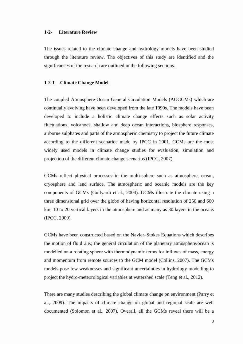
1-2- Literature Review
The issues related to the climate change and hydrology models have been studied
through the literature review. The objectives of this study are identified and the
significances of the research are outlined in the following sections.
1-2-1- Climate Change Model
The coupled Atmosphere-Ocean General Circulation Models (AOGCMs) which are
continually evolving have been developed from the late 1990s. The models have been
developed to include a holistic climate change effects such as solar activity
fluctuations, volcanoes, shallow and deep ocean interactions, biosphere responses,
airborne sulphates and parts of the atmospheric chemistry to project the future climate
according to the different scenarios made by IPCC in 2001. GCMs are the most
widely used models in climate change studies for evaluation, simulation and
projection of the different climate change scenarios (IPCC, 2007).
GCMs reflect physical processes in the multi-sphere such as atmosphere, ocean,
cryosphere and land surface. The atmospheric and oceanic models are the key
components of GCMs (Guilyardi et al., 2004). GCMs illustrate the climate using a
three dimensional grid over the globe of having horizontal resolution of 250 and 600
km, 10 to 20 vertical layers in the atmosphere and as many as 30 layers in the oceans
(IPCC, 2009).
GCMs have been constructed based on the Navier–Stokes Equations which describes
the motion of fluid .i.e.; the general circulation of the planetary atmosphere/ocean is
modelled on a rotating sphere with thermodynamic terms for influxes of mass, energy
and momentum from remote sources to the GCM model (Collins, 2007). The GCMs
models pose few weaknesses and significant uncertainties in hydrology modelling to
project the hydro-meteorological variables at watershed scale (Teng et al., 2012).
There are many studies describing the global climate change on environment (Parry et
al., 2009). The impacts of climate change on global and regional scale are well
documented (Solomon et al., 2007). Overall, all the GCMs reveal there will be a

4
warm rise, increasing hot days, sea level rise, changes in season patterns, occurrences
in extreme rainfall and flooding, environmental damages and spreading of tropical
diseases at the global scale in the century (IPCC, 2007).
On the other hand, GCMs are the currently most reliable tools to assess climate
change at coarse scale but GCMs output do not meet the needed resolution to assess
the climate change at regional or local scales which is required for hydrological
modelling. The grid-boxes used by GCMs are too coarse especially for regions of
complex topography, coastal or island locations, and in regions of highly
heterogeneous land-cover (Wilby et al., 2004). Then, GCMs cannot present the local
weather and micro-climate processes used in hydrology studies.
There are several GCMs with different resolutions such as HadCM3, CNCM3,
MRCGCM, FGOALS, GFCM20, MIHR, MPEH5, NCPCM, CSMK3, CGMR,
MIMR, GFDL-R30, CCSR/NIES, CGCM, CSIRO-MK2, ECHAM4, and NCAR-
PCM with different grid resolution and process. The characterisation of the climate
change models are listed in Appendix A. They are different based on the horizontal
and vertical layers included in the models such as columns of momentum, heat and
moisture in both atmosphere and oceanic parts.
Subsequent to these initial studies, the investigations were extended to a fairly coarse
resolution, Regional Climate Model (RCM), to capture the variability of precipitation
which is dependent on the physical nature of watershed. RCMs have been developed
to assess the climate change impact in regional scale (IPCC, 2007). The use of RCMs
for climate downscaling has been initiated by (Dickinson et al., 1989; Giorgi et al.,
1990).
RCMs use the same parameters of GCMs in order to simulate the hydraulic processes.
However, RCMs are highly dependent on the domain resolution and they are
computationally more expensive. The advantage of RCMs to GCMs is to perform the
regional redistribution of mass, energy and momentum in the fine domain which
affects on quantitative relationships of the physical parameters through the land-
atmosphere-ocean and convection-cloud-radiation interactions (e.g., Liang et al.,
2004).

5
RCMs are able to produce downscaling results more accurately than GCMs due to the
spatial resolution enhancement (Maurer and Hidalgo, 2008). Regional Climate
Models project more accurately temperature data compared to GCMs, but reveal
problems when downscaling maximum precipitation (Dankers et al., 2007).
1-2-2- Methods of Downscaling
It has been a crucial challenge to make a bridge for the gap between a coarse and a
fine scale. Downscaling technique was emerged by a lot of efforts on the climate
community to represent climate change at a regional and local scale. Downscaling is a
technique of changing in climate data resolution from a coarse resolution into a fine
resolution. It can be developed for an area and even a point. It is necessary to
downscale the variables from large scale GCMs output into fine scale which are
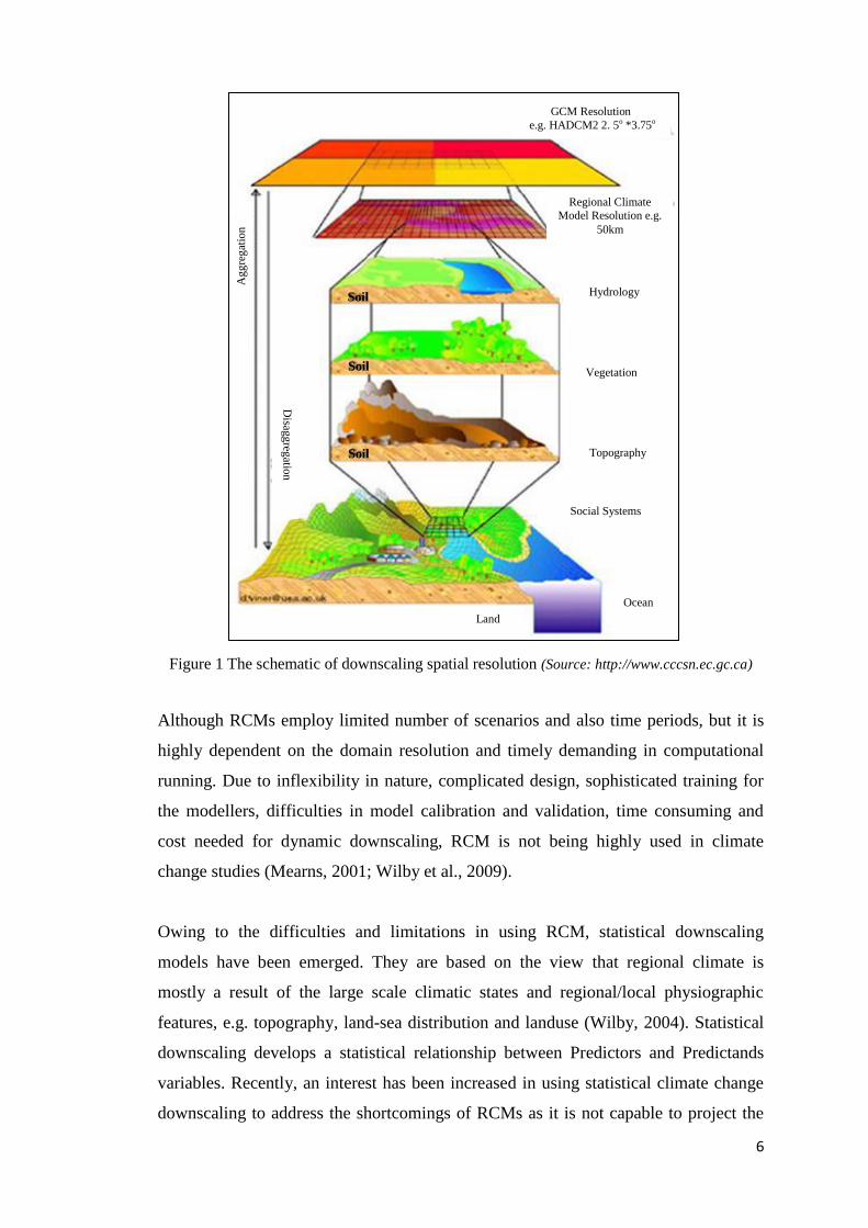
useful in hydrological modelling. Figure 1 illustrates various resolutions from coarse
scale GCM to a watershed scale in climate change downscaling model.
There are several techniques available for downscaling coarse resolution GCM data to
a fine resolution to use in hydrological studies. However, there is no specific approach
to suggest for the most reliable method as different climate models give different
results (Dibike and Coulibaly, 2005).
Downscaling techniques are generally categorised into two groups which are:
dynamic downscaling and statistical downscaling (Fowler, 2007). Dynamic
downscaling technique refers to the RCMs (Fowler et al., 2007). They were
developed to overcome the very large resolution in GCMs (Gutmann et al., 2012).
RCMs are a nested regional modelling technique that includes forcing of the large
scale component of GCMs throughout the entire RCM domain (Diallo et al., 2012).
Therefore, the resolution of RCMs is a sub-grid of GCM grid and is dependent on
domain size which is usually of tens kilometres or less (IPCC, 2007). However,
RCMs models are not able to predict the regular periodic monsoon currents and
ocean-atmospheric oscillations (IPCC, 2007).
6
Figure 1 The schematic of downscaling spatial resolution (Source: http://www.cccsn.ec.gc.ca)
Although RCMs employ limited number of scenarios and also time periods, but it is
highly dependent on the domain resolution and timely demanding in computational
running. Due to inflexibility in nature, complicated design, sophisticated training for
the modellers, difficulties in model calibration and validation, time consuming and
cost needed for dynamic downscaling, RCM is not being highly used in climate
change studies (Mearns, 2001; Wilby et al., 2009).
Owing to the difficulties and limitations in using RCM, statistical downscaling
models have been emerged. They are based on the view that regional climate is
mostly a result of the large scale climatic states and regional/local physiographic
features, e.g. topography, land-sea distribution and landuse (Wilby, 2004). Statistical
downscaling develops a statistical relationship between Predictors and Predictands
variables. Recently, an interest has been increased in using statistical climate change
downscaling to address the shortcomings of RCMs as it is not capable to project the
Ocean
Land
Social Systems
Topography
Vegetation
Hydrology
Soil
Soil
Soil
Regional Climate
Model Resolution e.g.
50km
GCM Resolution
e.g. HADCM2 2. 5o *3.75o
Ag
gre
gat
ion
Disag
greg
ation
7
climate change scenarios at a local or point scale (Chen et al., 2012; Mearns et al.,
2012; Meenu et al., 2012; Fiseha et al., 2012; Yang et al., 2012; Hassan and Haroun,
2012; Liu et al., 2011; Samadi et al., 2012).
There are many statistical downscaling methods in climate change studies. In
Weather-Pattern Method, a link between observational point data and a weather
classification schemes is developed (Yarnal et al., 2001; Anandhi et al., 2011).
Weather-typing approaches categorise the various local predictand data to construct
the Circulation Patterns (CPs) at the local scale. The weather state definition is
archived directly by applying methods such as cluster analysis (PCA) to atmospheric
fields (Huth, 2000).
The method developed by Bardossy et al. (2005) provides a basis daily classified
circulation pattern for downscaling the most common climate data (temperature and
precipitation). The presented classification is objective providing CPs that explain the
dependency between the predictors and surface climate. Local climate change
scenarios are then generated by resampling observed predictands from probability
distributions conditioned on synthetic series of CPs. In spite of its applicability to a
wide variety of atmosphere variables such as temperature and precipitation, have
difficulty simulating extreme events, and must assume stationary circulation-to-
surface climate conditioning (Wilby et al., 1999).
Stochastic Weather Generators (WG) as a statistical downscaling method has been
used in water resource management (Wilks, 2012; Tan et al., 2008; Ivanov et al.,
2007). The generators were developed by (Richardson, 1981; Richardson and Wright,
1984; Racsko et al., 1991 and Semenov et al., 1998). Daily precipitation occurrence is
governed by a two-state (either precipitation occurs or it does not) and first-order
Markov chain (the probability of precipitation depends only on whether or not
precipitation occurred on the previous day). The key disadvantages of stochastic
weather generators method in climate change downscaling relate to the
underestimation of low frequency variance (Hansen and Mavromatis, 2001), the
projection of unrealistic properties for extremes precipitation and limitation of the
length of the synthetic climate data by length of the observed (Wilks and Wilby,
1999).
8
Regression Methods were developed by Wilby and Wigley (1997) which establishes a
linear or non-linear regression between predictands and predictors. Therefore, this
method is highly dependent on the empirical statistical relationships. The most
famous statistical downscaling tools are LARS-WG and SDSM. LARS-WG is a
sophisticated stochastic weather generator whereas SDSM is a hybrid between a
stochastic weather generator and regression methods.
SDSM combined the regression models, weather typing schemes and weather
generators (Vrac and Naveau, 2007). SDSM generates the unique meteorological
characteristics at a single station scale which is a valuable ability in hydrology studies.
SDSM downscaling method is recommended by Canadian Climate Impact Scenarios
Project (CCIS) for climate change impact studies. It is one of the most efficient tools
in downscaling of large scale daily GCMs climate variables into local scale,
particularly in heterogeneous regions (Wilby, 2004).
The main advantage of Statistical Downscaling Model (SDSM) is simplicity, less
computationally demanding and running the regression statistical method. However, it
is limited to the locations where good regression results could be found. The major
theoretical weakness of statistical downscaling is that their basic assumption is not
verifiable, i.e., the statistical relationships developed for the present day climate will
also hold for the different forcing conditions in the future climates (Fowler, 2007).
The statistical downscaling technique is used in the present research and the details of
this research are given in Chapter 2 (Section 2-2-4).
1-2-3- Hydrology Model
Hydrological models are generally categorised into deterministic and stochastic
models (Beven, 2001). Deterministic models simulate runoff with a set of
hydrological parameters require a large amount of data (Gosain et al., 2009), whereas
stochastic models use mathematical techniques to link climate variables to runoff
(Ahmad et al., 2001). Gosain et al. (2009) explained the development of various
hydrological models. They simply defined hydrological models as a black-box or
empirical model, statistically develops a relationship of input and output data (Nor et
9
al., 2007). Thus, Empirical models are invaluable in predicting streamflow in a
watershed with no gauging data.
Cunderlik (2003) classified deterministic hydrologic models into three major
categories: lumped model, semi-distributed model and distributed model. Lumped
model is a simple approach to simulate runoff which is developed based on the water
balance equation. It assumes the whole watershed system such as soli and landuse
data as a single unit (Bormann et al., 2009). Thus, such this model does not provide
the heterogeneity of physiographic properties in a large watershed. On the contrary,
distributed hydrological models incorporate spatial variables of the hydrological
parameters by dividing the watershed into the homogenous variables (Ghavidelfar et
al., 2011).
Carpenter and Georgakakos (2006) have demonstrated the skill of distributed models
compared to lumped models in simulation of runoff. As such, distributed models are
able to provide a more representative description of watershed scale processes than
lumped models (Collischonn et al., 2007). However, there are limitations related to
resolution and nonlinearity of distributed models (Beven, 2001).
Conceptual models are divided into single event, for a short time period and
continuous events, for long time series to simulate runoff (Salarpour, 2011).
Conceptual models are highly dependent on spatial variability. Representative
Element Area (REA), Hydrological Response Units (HRU) and Grouped Response
Unit (GRU) are a few types of discretisation in the distributed conceptual model
(Neitsch, 2005).
Semi distributed hydrological model have been developed to overcome the difficulties
in using conceptual model (Beven, 2012). It performs less complex spatial resolution
compared to fully distributed model by generating hydrological response units to
simulate runoff in the watershed (Grayson and Blöschl, 2001).
There are literatures of hydrological models’ application rang from small to large
watershed scale (Singh and Frevert, 2002 a, b). Water resource management plans are
generally performed at watershed scale. Then, a physically-based hydrologic model
10
can be employed to take into account the variety of climatic and physiographic
parameters to simulate streamflow at the watershed scale (Praskievicz and Chang,
2009). For instance, the semi distributed DHSVM model is used for urbanised
watersheds with representations of impervious surfaces and retention ponds in the
model (Cuo et al., 2008) while rainfall-runoff HEC-HMS and SWAT models are
usually used for regional watershed scale.
IHACRES (Jakeman et al. 1990; Jakeman and Hornberger, 1993), SRM (Rango,
1995), WATBAL (Knudsen et al., 1986) and Sacramento (Burnash, 1995) are the
typical lumped models. Typical models of semi distributed physically based are HBV
(Bergström, 1995), HEC-HMS (Ford et al., 2008), HSPF (Crawford and Linsley,
1966), SSARR (USGS-NPD, 1991), SWAT (Arnold et al., 1998; Arnold and Fohrer,
2005), SWMM (Huber and Dickinson, 1988), TOPMODEL (Beven and Kirkby,
1979), IHDM (Beven et al., 1987) and Thales (Grayson et al., 1992). The most
famous distributed models are CASC2D (Ogden, 1998), CEQUEAU (Morin, 2002),
GAWSER/GRIFFS (Schroeter et al., 1996), MIKE (DHI, 2000) and WATFLOOD
(Kouwen, 2001).
The choice of a hydrological model is dependent on the many factors such as
resolution, time series (daily or monthly) of climate variables to simulate the surface
runoff (Xu and Singh, 1998). However, the physiographic features of watershed play
a significant role in predicting the streamflow behaviour (Viessman and Lewis,
2003.).
Loss model is one of the most important components in hydrology models to estimate
rainfall infiltrated by the ground. Green-Ampt (Mein and Larson 1973) and SCS
Curve Number USDA-NRCS, 2000) are extensively used in hydrology modelling to
calculate the rainfall loss rate (e.g., Kabiri et al., 2013; Petrosellia et al., 2013).
The SCS-CN method is the most popular methods for computing the volume of direct
surface runoff for a given rainfall event (Mishra et al., 2006). Abood et al. (2012)
have evaluated the performance of the two infiltration methods (SCS-CN and Green-
Ampt) in rainfall-runoff simulation using HEC-HMS for the Kenyir and Berang
watershed, Terengganu, in Malaysia which the storm events of September and
11
October through the year 1990 has been used for calibration simulation, whereas the
storm events of November and December in the year 1990 data have been used for
validation simulation. They found that the both loss methods have a good agreement
with the observed data. However, the SCS-CN method was recommended for the
watersheds due to its high accuracy in the modelling results.
Kabiri et al. (2013) have evaluated the performance of two loss models (Green-Ampt
and SCS-CN) for some storm events in Klang watershed. They found out that there
was no significant deference between two loss models in the rainfall-runoff model for
Klang watershed. Many studies have conducted to improve the SCS-CN loss model
and finding a better performance of rainfall loss estimation in runoff modelling
(Huang et al., 2007; Sahu et al., 2010; Descheemaeker et al., 2008 and Shi et al.,
2009). Fu et al. (2011) found out that the prediction accuracy for initial abstraction
ratio equals to 0.05 was greater than the one for 0.2 to simulate surface runoff of 757
rainfall events in China.
Akbari et al. (2012) have investigated the assessment of the SCS-CN loss method on
Klang watershed to evaluate the performance of SCS-CN loss method. They have
concluded that the SCS-CN loss method can be used for Klang watershed due to its
good agreement between observed and modelled in HEC-HMS. However, they have
suggested a modified CN using initial abstraction ratio in value of 0.05 which gives a
better fit than 0.2 (as default in HEC-HMS). It may produce the best performance of
historical daily rainfall data compared to the other available loss models in HEC
system.
1-2-4- Hydrology Modelling in Climate Change Study
Earlier studies on the projection of runoff corresponding to the climate change
downscaling were conducted using a total coarse resolution GCM model. Only a
handful of publications on assessing the climate change impacts on water resources by
2005 are available (Fowler et al., 2007). But lately, many studies have conducted
statistical downscaling using GCMs models to estimate the hydrological behaviour
based on climate change scenarios at a fine scale (e.g., Khazaei, et al., 2012; Randin
et al., 2009; Day, 2013).
12
Numerous studies on climate change downscaling, ranging from small to large scale,
have been conducted on the downscaling methods to make a link between GCMs
output and hydrologic models at watershed scale (Fowler et al., 2007; Dibike and
Coulibaly, 2007). A review on downscaling global climate models for hydrological
analysis has been given by Prudhomme et al., (2002). All these studies deal with a
coupled atmosphere-ocean general circulation model, since the resolution and
certainties are considered to be most critical for climate change downscaling in the
watershed scale.
A number of studies have been conducted for the runoff and flooding corresponding
to the future climate for a region (e.g., Music and Caya, 2007; Bolle et al., 2008; Teng
et al., 2012; Vaze and Teng, 2011; Zhang and Chiew, 2009) but the resolution
remains the most widely examined configuration in climate change downscaling
problems. For instance, rainfall-runoff modelling system has been used to simulate
streamflow regime affected by climate change in many hydrologically heterogeneous
regions (Qi et al., 2009).
The impact of climate variability on streamflow and peak flow is found in (e.g.
.Chang et al., 2001; Rose and Peters, 2001; Brian et al., 2004; Brown et al., 2005; Qi
et al., 2009; Miller and Russel, 2012; Petheram et al., 2012 ). The changes in climate
potentially affect the regional hydrological processes and long-term water availability
(Fu et al., 2007) changing in overall flow magnitude, variability and timing of the
main flow event (Wurbs et al., 2005) and the occurrences of floods (Bronstert et al.,
2007). Hydrological impacts on the intraannual variability over the annual cycle
(Jasper et al., 2004; Graham et al., 2007; Bosshard et al., 2011; Teng et al., 2012)
seasons (Tague et al., 2008; Schmidli et al., 2007), months (Kleinn et al., 2005) have
been investigated.
Meenu et al (2012) have used HEC-HMS hydrological model to assess hydrologic
impacts of climate change on daily maximum, minimum temperature and
precipitation in the four sub-basins of the study area in Tunga–Bhadra river basin,
India. They found out that HEC-HMS can be used for hydrological modelling in the
river basin. The monthly flows are better simulated than daily flows. However, under

13
prediction of high flows was estimated during calibration and validation of
hydrological modelling.
The use of hydrological models in climate change studies ranges from simple lumped
models (Massari et al., 2013; Driessen et al., 2010) to complex distributed models
(Mascaro et al., 2013; Guo et al., 2009) to assess the streamflow and peak flow
variation.
Maurer et al (2010) have used two hydrology models: the Sacramento Soil Moisture
Accounting model and the variable infiltration capacity model to project changes of
streamflows for three Sierra Nevada rivers using Statistical Downscaling Model. They
found out that the two hydrological models produced significantly different
simulations of current and future daily and seasonal extreme flow. However, the
changes in monthly streamflows generally did not differ.
Petheram et al (2012) have studies the estimation of the impact climate change on
runoff across the tropical region in Australia using conceptual rainfall-runoff models
(RRMs). 115 streamflow gauging stations were calibrated in PRMs model. They
revealed that there will be an increase in mean annual runoff to 29% and a decrease to
26%. However, they commented that for extreme runoff events and low flows,
improvements are required in both GCMs and rainfall-runoff modelling.
Many investigations have been conducted to estimate rainfall intensity considering the
climate change impacts to reveal the probability of extreme precipitation in the future
(e.g., Nguyen et al., 2007; Prodanovic and Simonovic, 2007; Simonovic and Peck,
2009; Onof and Arnbjeg-Nielsen, 2009; Mirhosseini et al., 2012; Zhu et al., 2012).
Mirhosseini et al (2012) have studied the impact of climate change on rainfall IDF
curves in Alabama, using 3-hourly precipitation data simulated by six combinations of
global and regional climate models. They found out that there will be expected to
change toward less intense rainfalls for short duration events. However, due to
employing six climate change models, a large uncertainty existed on projected rainfall
intensity.
14
Simonovic and Peck (2009) have investigated the impact of climate change on rainfall
intensity for the city of London for 2050s under CCSR/NIES-GCM model to estimate
rainfall intensity using daily rainfall data. The results revealed that there will be
approximately from 11% to 35% changes in rainfall intensity information for 2050s.
Many studies have shown the role of the evapotranspiration into hydrological
modelling (Zhao et al., 2013; Meenue et al., 2012; Milly et al., 2011). The methods to
calculate the ET include Gridded Priestly Taylor, Priestly Taylor and Monthly
Average methods. The Gridded Priestly Taylor and Priestly Taylor equations require
some data such as solar radiation, crop factors and dryness factor and that make them
difficult to use in hydrological models. Several studies have evaluated Hargreaves'
method and found out that the method has a good result in various climates (Das et
al., 2012; Temesgen, et al., 2005). Since Hargreaves' method just depends on the air
temperature, so it is well-known in evapotranspiration calculation enormously.
Temesgen et al. (2005) have evaluated the performance of FAO-P&M with
Hargreaves. They found that Hargreaves’ equation can compensate the lack of data
required in Penman and Penman- Monteith Methods.
Hargreaves and Allen (2003) have shown that the Hargreaves’ results were close to
FAO-P&M’s results due to the study conducted on more than 3, stations
worldwide. They have shown that there is no substantial problem using Hargreaves’
equation at low latitudes in equatorial zones. Saghravani et al. (2009) have evaluated
the performance of the three ET equations (Hargreaves, FAO-P&M and P&M) in one
station at Klang watershed. They found that there is a different between the results
obtained from three different methods. However, the differences did not reject the
results given by Hargreaves and Allen (2003) as the difference between Hargreaves
and FAO-P&M may reach a maximum of one mm/d in the tropical regions. This
method was used due to its simplicity and modest data requirement, which made it
attractive for the hydrology modelling.
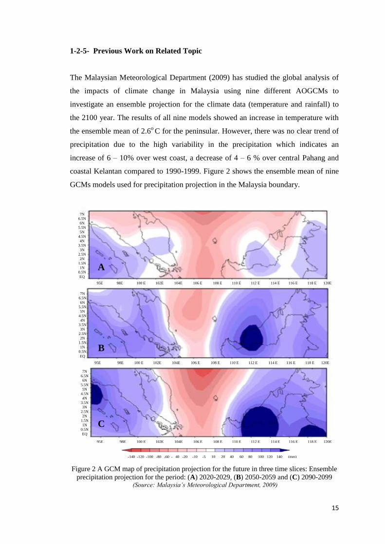
15
1-2-5- Previous Work on Related Topic
The Malaysian Meteorological Department (2009) has studied the global analysis of
the impacts of climate change in Malaysia using nine different AOGCMs to
investigate an ensemble projection for the climate data (temperature and rainfall) to
the 2100 year. The results of all nine models showed an increase in temperature with
the ensemble mean of 2.6o C for the peninsular. However, there was no clear trend of
precipitation due to the high variability in the precipitation which indicates an
increase of 6 – 10% over west coast, a decrease of 4 – 6 % over central Pahang and
coastal Kelantan compared to 1990-1999. Figure 2 shows the ensemble mean of nine
GCMs models used for precipitation projection in the Malaysia boundary.
Figure 2 A GCM map of precipitation projection for the future in three time slices: Ensemble
precipitation projection for the period: (A) 2020-2029, (B) 2050-2059 and (C) 2090-2099 (Source: Malaysia’s Meteorological Department, 2009)
A
B
C
-140 -120 -100 -80 -60 - 40 -20 -10 -5 10 20 40 60 80 100 120 140 (mm)
7N
6.5N
6N
5.5N
5N
4.5N
4N
3.5N
3N
2.5N
2N
1.5N
1N
0.5N
EQ
7N
6.5N
6N
5.5N
5N
4.5N
4N
3.5N
3N
2.5N
2N
1.5N
1N
0.5N
EQ
7N
6.5N
6N
5.5N
5N
4.5N
4N
3.5N
3N
2.5N
2N
1.5N
1N
0.5N
EQ
95E 98E 100 E 102E 104E 106 E 108 E 110 E 112 E 114 E 116 E 118 E 120E
95E 98E 100 E 102E 104E 106 E 108 E 110 E 112 E 114 E 116 E 118 E 120E
95E 98E 100 E 102E 104E 106 E 108 E 110 E 112 E 114 E 116 E 118 E 120E
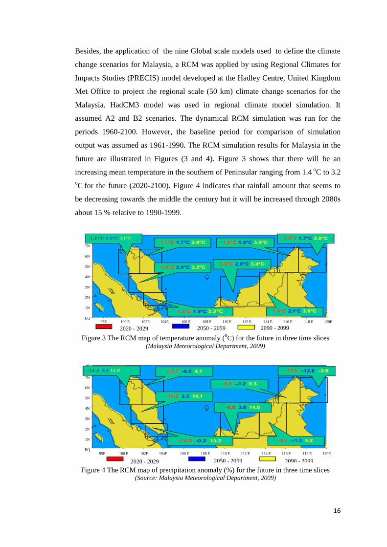
16
Besides, the application of the nine Global scale models used to define the climate
change scenarios for Malaysia, a RCM was applied by using Regional Climates for
Impacts Studies (PRECIS) model developed at the Hadley Centre, United Kingdom
Met Office to project the regional scale (50 km) climate change scenarios for the
Malaysia. HadCM3 model was used in regional climate model simulation. It
assumed A2 and B2 scenarios. The dynamical RCM simulation was run for the
periods 1960-2100. However, the baseline period for comparison of simulation
output was assumed as 1961-1990. The RCM simulation results for Malaysia in the
future are illustrated in Figures (3 and 4). Figure 3 shows that there will be an
increasing mean temperature in the southern of Peninsular ranging from 1.4 oC to 3.2
oC
for the future (2020-2100). Figure 4 indicates that rainfall amount that seems to
be decreasing towards the middle the century but it will be increased through 2080s
about 15 % relative to 1990-1999.
Figure 3 The RCM map of temperature anomaly (
oC) for the future in three time slices
(Malaysia Meteorological Department, 2009)
Figure 4 The RCM map of precipitation anomaly (%) for the future in three time slices
(Source: Malaysia Meteorological Department, 2009)
95E 100 E 102E 104E 106 E 108 E 110 E 112 E 114 E 116 E 118 E 120E
2090 - 2099 2050 - 2059 2020 - 2029
2020 - 2029 2050 - 2059 2090 - 2099
7N
6N
5N
4N
3N
2N
1N
EQ
7N
6N
5N
4N
3N
2N
1N
EQ
95E 100 E 102E 104E 106 E 108 E 110 E 112 E 114 E 116 E 118 E 120E
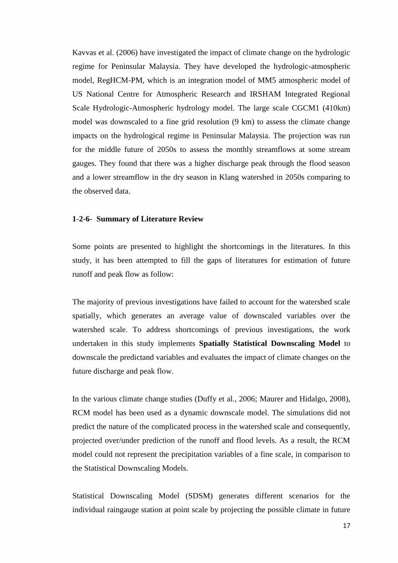
17
Kavvas et al. (2006) have investigated the impact of climate change on the hydrologic
regime for Peninsular Malaysia. They have developed the hydrologic-atmospheric
model, RegHCM-PM, which is an integration model of MM5 atmospheric model of
US National Centre for Atmospheric Research and IRSHAM Integrated Regional
Scale Hydrologic-Atmospheric hydrology model. The large scale CGCM1 (410km)
model was downscaled to a fine grid resolution (9 km) to assess the climate change
impacts on the hydrological regime in Peninsular Malaysia. The projection was run
for the middle future of 2050s to assess the monthly streamflows at some stream
gauges. They found that there was a higher discharge peak through the flood season
and a lower streamflow in the dry season in Klang watershed in 2050s comparing to
the observed data.
1-2-6- Summary of Literature Review
Some points are presented to highlight the shortcomings in the literatures. In this
study, it has been attempted to fill the gaps of literatures for estimation of future
runoff and peak flow as follow:
The majority of previous investigations have failed to account for the watershed scale
spatially, which generates an average value of downscaled variables over the
watershed scale. To address shortcomings of previous investigations, the work
undertaken in this study implements Spatially Statistical Downscaling Model to
downscale the predictand variables and evaluates the impact of climate changes on the
future discharge and peak flow.
In the various climate change studies (Duffy et al., 2006; Maurer and Hidalgo, 2008),
RCM model has been used as a dynamic downscale model. The simulations did not
predict the nature of the complicated process in the watershed scale and consequently,
projected over/under prediction of the runoff and flood levels. As a result, the RCM
model could not represent the precipitation variables of a fine scale, in comparison to
the Statistical Downscaling Models.
Statistical Downscaling Model (SDSM) generates different scenarios for the
individual raingauge station at point scale by projecting the possible climate in future
18
(Meenu et al., 2012; Fiseha et al., 2012). SDSM projects the future patterns for each
raingauge station individually and does not represent the overall pattern of the rainfall
variables over the watershed. To fill the gap, the Multi Rainfall is used to robust the
precipitation downscaling over Klang watershed. The Geospatial interpolation
technique in GIS is used to generate the areal maps by making spatial average to
estimate the mean value of precipitation over the watershed.
In the studies that have been conducted by (Yang et al., 2012; Nguyen et al., 2007;
Prodanovic and Simonovic, 2007; Simonovic and Peck, 2009; Onof and Arnbjeg-
Nielsen, 2009; Mirhosseini et al., 2012; Zhu et al., 2012), the impact of climate
change on the occurrence of extreme precipitation events has been estimated for
single raingauge station. It makes it difficult to estimate the mean extreme
precipitation events for entire the watershed. To fill the gap, rainfall intensity is
evaluated by spatial mapping in GIS using the appropriate distribution equation for
estimation of rainfall quantiles for all the raingauge stations in Klang watershed.
1-3- Significance of the Study
One of the most important consequences of climate change impacts in South Asian
regions is the lack of water resources due to the adverse impact on water demand and
quality. Drying of wetlands and severe degradation of ecosystems has resulted in delta
regions of South Asian countries due to precipitation decline and droughts (IPCC,
2007). According to IPCC (2007), Malaysia is a developing country which will be
vulnerable to climate change. Because of the less flexibility to adjust the economical
structure and being largely dependent on agriculture, the impact of climate change has
far reach implication in Malaysia.
Klang watershed which is located in Kuala Lumpur city terrestrial has been chosen as
a study area for this project. This site has been contributed to the environmental
damages especially in land degradation and also soil erosion which will potentially
produce more extent area affected by intensified flood events in the watershed. In this
area, most flooding events are originated from convectional storms which caused
intensive and localised rainfall. The watershed has been facing often flash floods,
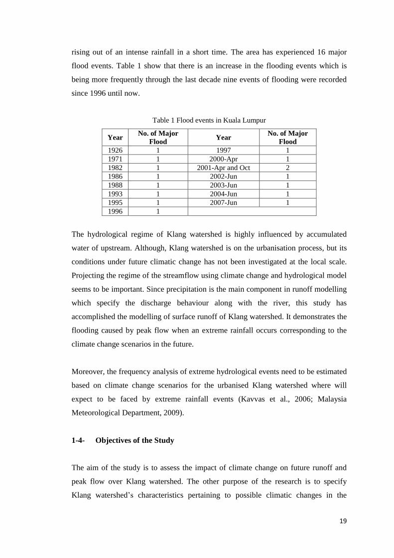
19
rising out of an intense rainfall in a short time. The area has experienced 16 major
flood events. Table 1 show that there is an increase in the flooding events which is
being more frequently through the last decade nine events of flooding were recorded
since 1996 until now.
Table 1 Flood events in Kuala Lumpur
Year No. of Major
Flood Year
No. of Major
Flood
1926 1 1997 1
1971 1 2000-Apr 1
1982 1 2001-Apr and Oct 2
1986 1 2002-Jun 1
1988 1 2003-Jun 1
1993 1 2004-Jun 1
1995 1 2007-Jun 1
1996 1
The hydrological regime of Klang watershed is highly influenced by accumulated
water of upstream. Although, Klang watershed is on the urbanisation process, but its
conditions under future climatic change has not been investigated at the local scale.
Projecting the regime of the streamflow using climate change and hydrological model
seems to be important. Since precipitation is the main component in runoff modelling
which specify the discharge behaviour along with the river, this study has
accomplished the modelling of surface runoff of Klang watershed. It demonstrates the
flooding caused by peak flow when an extreme rainfall occurs corresponding to the
climate change scenarios in the future.
Moreover, the frequency analysis of extreme hydrological events need to be estimated
based on climate change scenarios for the urbanised Klang watershed where will
expect to be faced by extreme rainfall events (Kavvas et al., 2006; Malaysia
Meteorological Department, 2009).
1-4- Objectives of the Study
The aim of the study is to assess the impact of climate change on future runoff and
peak flow over Klang watershed. The other purpose of the research is to specify
Klang watershed’s characteristics pertaining to possible climatic changes in the

20
future. The result of the hydrological model is generation of the runoff hydrograph by
a spatially distributed rainfall over the watershed in the future (2100 year). The
detailed objectives of this research are as follow:
To generate fine resolution climate change scenarios using Statistical
Downscaling Model in the watershed scale,
To project the variability in temperature, precipitation and evaporation for the
three time slices, 2020s, 2050s and 2080s, based on A2 and B2 scenarios,
To calibrate and validate hydrological model using historical observed flow
data to verify the performance of hydrological model,
To evaluate the impact of climate changes on the future discharge and future
peak flow for three timeslices 2020s, 2050s and 2080s.
Thus, to meet the objectives in this study, projection of the future climate based on
climate change scenarios from IPCC in the study area can be considered as the most
important component throughout the research. Therefore, the assessment on the
quality and adequacy of the hydro-climatological data must be estimated to ensure the
reliability of model output.
1-5- Scope of the Research
The study focuses on the impact of climate change on runoff and peak flow by
downscaling the Climate Change Scenarios at a watershed scale. The criteria for
selecting appropriate IPCC scenarios are based on the physically consistency at a fine
scale. The A2 (Medium-High emissions scenario) and B2 (Medium-Low emissions
scenario) scenarios reveal the reliable projection of a plausible future climate
condition at the regional scale while other scenarios represent at the global scale.
Thus, applicability of A2 and B2 scenarios in estimating impacts of climate change at
the watershed scale is more realistic compared to other scenarios which were
constructed at global scale. Hence, A2 and B2 scenarios have been used to generate
21
the local climate change scenarios using statistical downscaling model in the
watershed scale.
1-6- Limitations of the Study
The lack of data on streamflow does not allow the calibration and validation of
hydrological modelling for each sub-basin. The only streamflow station (Jambatan
Sulaiman) is situated at the outlet of Upper Klang watershed and the hydrological
modelling uses it for calibration and validation to simulate runoff. Furthermore, the
lack of updated land use, soil and topography data have forced the study to consider it
as an assumption with no change during the time.
1-7- Thesis Outline
This thesis comprises seven chapters, which are briefly outlined below. The study has
three main steps:
Study of physical characteristics and history of the watershed which includes a
review on hydro-climate trends to prepare all the required data for the
hydrological modelling.
Making Climate Change Downscaling Model and linking between climate
change downscaled output and hydrological model in providing the potential
impacts of climate change on flow through Klang watershed.
Runoff and peak flow modelling have been developed using HEC-HMS model
for all sub-watersheds in Klang watershed.
Chapter 1 explores the climate changes and its future scenarios. It describes impacts
of climate change on precipitation, run off and flooding events. It is also presents the
objectives, scope and importance of the study on Klang watershed. The chapter also
describes some literatures on Climate Change Downscaling Model, hydrology models
and climate change impacts on runoff and peak flow studies.
22
Chapter 2 describes the methods used to make various modelling in this study. The
models used in this study are as follow: Climate Change Downscaling Model,
Hydrological (Watershed Management, Surface Runoff) and Peak flow modelling.
Chapter 3 consists of two parts. The first part of the chapter introduces the case
study, Klang watershed, and describes the environmental-physical features such as
terrain, river network, geology, landuse and soil obtained from various sources in this
study. The second part of the chapter is to describe the climate pattern and
hydrological characteristics of study area. It also describes the baseline hydro-
climatology for Klang watershed using a long term series of climate data to reflect the
observed trend n the hydro-climate data such as precipitation, temperature and
streamflow. Furthermore, data preparation and quality control on the historic data are
conducted using graphical, statistical and spatial methods.
Chapter 4 presents the implementation of the Climate Change Downscaling Model
using SDSM tool. SDSM uses NCEP-Predictor variables to make a linear regression
to the local predictand data from Klang watershed. The output of downscaled climate
parameters is used as an input to the hydrology modelling in Chapter 5.
Chapter 5 presents the implementation of hydrological modelling using Hec-Geo-
HMS, a GIS module. The algorithm is used to delineate the sub-watersheds which
distribute over whole Klang watershed. It can extract the necessary parameters
required in hydrological modelling. Then, it attempts to implement HEC-HMS to
generate the runoff hydrographs for each sub-watershed.
Chapter 6 describes the findings and results of the research. It demonstrates the
climate change scenarios over the watershed’s meteorological parameters such as
precipitation, temperature and evaporation and its trends in the future. The discussion
is based on the plausible changes of the future climate and runoff corresponding to the
A2 and B2 scenarios at the watershed scale.
Chapter 7 conclusion arrived through the study for future research is presented. It
includes conclusion on the climate change impacts on the mean and maximum

23
streamflow regime and the frequency of extreme flood events with regard to the
climate change scenarios.

24
2- METHODOLOGY
This chapter is divided into four sub-sections consists of Climate Change
Downscaling Model (SDSM), Watershed Modelling, Runoff simulation and Flood
Frequency Analysis (FFA). Statistical downscaling model is used to produce the local
climate change scenarios at the local scale. The climate change downscaling results
are used as input into rainfall-runoff HEC-HMS modelling to forecast the future
surface runoff at the discharge station. Watershed Modelling is carried out using Hec-
Geo-HMS in GIS system to derive physiographic parameters of the watershed which
need to be used in hydrological modelling. Thus, runoff processes are simulated on
each sub-watershed system from the upstream to the watershed outlet throughout the
streamflow network.
2-1- Overall Framework of the Research
This research involves connecting hydrology modelling to climate change downscaled
output by GIS system. The study initiates to enhance the understanding of the impact
of climate change scenarios by quantifying the potential changes including hydro-
climatological data. It provides the variety in future rainfall based on areal rainfall for
Klang watershed instead of relying just on some raingauge stations independently.
GIS system plays a pivotal role in these analyses because of various data
representation and running different modelling such as climate change and hydrology
modelling to estimate the hydrological parameters in Klang watershed. The study also
provides forecast on hydrology data for the future development in Klang watershed.
The scenarios would be downscaled in the watershed scale to employ in the
hydrologic models.
Flood management plans for the watershed should consider climate change scenarios
in addition to landuse change and urbanisation. Regarding the linking climate change
to flooding, a major focus has been given to extremes such as peak runoff, frequency
and intensity of heavy rainfall. However, there are an uncertainty according to landuse
changes and its impact on streamflows. Figure 5 illustrates the conceptualised
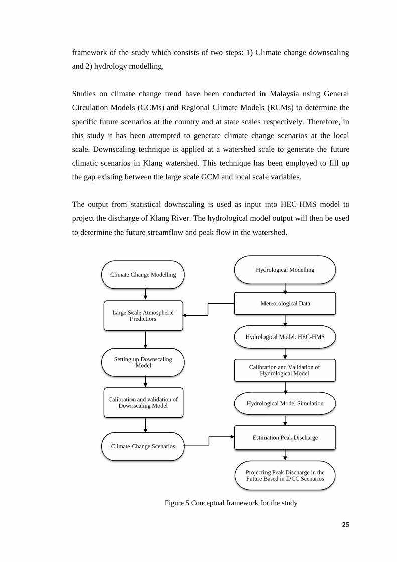
25
framework of the study which consists of two steps: 1) Climate change downscaling
and 2) hydrology modelling.
Studies on climate change trend have been conducted in Malaysia using General
Circulation Models (GCMs) and Regional Climate Models (RCMs) to determine the
specific future scenarios at the country and at state scales respectively. Therefore, in
this study it has been attempted to generate climate change scenarios at the local
scale. Downscaling technique is applied at a watershed scale to generate the future
climatic scenarios in Klang watershed. This technique has been employed to fill up
the gap existing between the large scale GCM and local scale variables.
The output from statistical downscaling is used as input into HEC-HMS model to
project the discharge of Klang River. The hydrological model output will then be used
to determine the future streamflow and peak flow in the watershed.
Figure 5 Conceptual framework for the study
Climate Change Modelling
Large Scale Atmospheric Predictiors
Setting up Downscaling Model
Calibration and validation of Downscaling Model
Climate Change Scenarios
Hydrological Modelling
Meteorological Data
Hydrological Model: HEC-HMS
Calibration and Validation of Hydrological Model
Hydrological Model Simulation
Estimation Peak Discharge
Projecting Peak Discharge in the Future Based in IPCC Scenarios

26
2-2- Climate Change Downscale Modelling
The methods of climate change downscaling, the IPCC scenarios and climate change
models are summarised. In the following section, the IPCC scenarios are described to
highlight their applications into climate change downscaling at the watershed scale.
Furthermore, the advantages of using statistical downscaling technique compared to
the dynamical downscaling for hydrology modelling are described.
2-2-1- Climate Change Scenarios
According to the IPCC (2007), a scenario is a coherent, internally consistent and
plausible description of a possible future state of the world. A set of four main groups
of emission scenarios namely A1, A2, B1 and B2 were released by IPCC in 2000 and
are published in Special Report on Emissions Scenarios (SRES). The SRES were
constructed by considering the economical, technological, demographic and
environmental developments, which reflect the possible future developments in the
world pertaining to the production of greenhouse gas emissions. The scenarios are
neither predictions nor forecasts. However, it was developed based on realistic future
emission scenarios over the world representing the complex and interrelated dynamics
of demographic development, socio-economic development and technological
change.
The scenarios are the only sources to implement a projection of future, which reflect
the condition of demography, society, economy, technology, emissions and climate.
A1 and B1 scenarios form the world homogeneously with an increasing in population
by mid century and a decreasing afterwards, but an economy focus in A1 and an
environmentally focus in B1. A2 scenario is a scenario with higher rates of
greenhouse gas emissions in combination with higher sulphate and other aerosol
emissions while B2 scenario is a lower rate of emissions that assumes the world is
more committed to solving global and local environmental (IPCC, 2007). The four
main groups of emission scenarios are explained as below.

27
A1 scenario is constructed based on the homogeneous world. It describes the world
of very rapid economic growth, global population and the rapid introduction of
efficient technologies. Major focuses are convergence among regions, capacity
building, and increased cultural and social interactions, with a substantial reduction in
regional differences in per capita income (IPCC, 2007). A1 scenario is developed into
three groups that describe alternative directions of technological change in the energy
system. A1 scenario family develops into three groups: fossil intensive (A1FI), non-
fossil energy sources (A1T), or a balance across all sources (A1B). In A1 scenario,
population will be increasing to 8.7 billion in 2050 and declining toward 7 billion
people by end of the century (IPCC, 2007).
A2 scenario (Medium-High Emissions scenario) is a scenario with higher rates of
greenhouse gas emissions in combination with higher sulphate and other aerosol
emissions. It represents a differentiated world and describes the world in a various
economic regions in which the income gap between developed and developing
countries is not narrow. The rate of technology growth is more rapid than average in
some regions and slower in others and dependent on industry adjusts to local resource.
Regions with abundant energy and mineral resources evolve more resource-intensive
economies. In this scenario, global environmental concerns are relatively weak but
regional and local pollutions are planned to mitigate. A2 scenario is constructed based
on the different economy growth rate and efficiency of technology dependent on the
regional scale in which population reaches to 15 billion people in year 2100 and will
be increased after 2100 (IPCC, 2007).
B1 scenario describes a future based on the high level of environmental approach and
a balanced economic development. It is similar to A1 scenario into fast-changing and
convergent world but the priorities differ. In fact, A1 focuses on global investments
by further economic growth and benefits from increased productivity while, B1
scenario focuses on global environmental protection and gains in improved efficiency
of resource use. The best measures are taken to reduce material wastage by
maximising recycling and enhancing energy saving lead to reductions in pollution. B1
scenario has a major push toward post-fossil technologies. Population is the same as
A1 scenario but a slower rate (IPCC, 2007).

28
B2 scenario (Medium-Low Emissions scenario) is a lower rate of emissions that
assumes the world is more committed to solving global and local environmental
(IPCC, 2007). It is designed based on the world emphasises on local solutions to
economic, social, and environmental sustainability. Increasing in population is
assumed at a lower rate than A2 scenario. B2 Scenario focuses on intermediate levels
of economic development, less rapid technological development compared to B1 and
A1 scenarios. However, it focuses toward environmental protection and social equity
at the local and regional scale. In B2 scenario, population reaches to 10 billion in
2100 and increasing with slower development rate of technology compared to A1 or
B1 scenarios.
GHG and aerosols are the two main groups of atmospheric concentrations to construct
the climate change scenarios. Sulphate is the major aerosol component plays a cooling
effect role in the lower atmosphere by scattering back sunlight. Figure 6 shows the
Annual Global mean temperature to 2100 according to the IPCC Scenarios. It is found
out that global warming rates will strongly be seen after 2050 to 2100 ranges from
1.9°C for the B1 to 4.0°C for the A1FI emission scenario, as minimal using fossil fuel
in B1 to a total reliance on fossil fuel in A1FI scenarios. The diverging of the
temperature in the middle of century can be described as being highly influenced by
the past emissions, particularly sulphate aerosols and GHG in the world. IPCC (2007)
has stated that according to the scenarios, the respond of the climate system will likely
be in the land areas of the equatorial belt to the least warming.
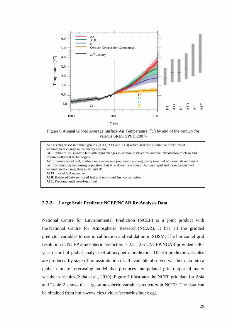
29
Figure 6 Annual Global Average Surface Air Temperature (oC) by end of the century for
various SRES (IPCC 2007)
2-2-2- Large Scale Predictor NCEP/NCAR Re-Analysis Data
National Centre for Environmental Prediction (NCEP) is a joint product with
the National Centre for Atmospheric Research (NCAR). It has all the gridded
predictor variables to use in calibration and validation in SDSM. The horizontal grid
resolution in NCEP atmospheric predictors is 2.5°, 2.5°. NCEP/NCAR provided a 40-
year record of global analysis of atmospheric predictors. The 26 predictor variables
are produced by state-of-art assimilation of all available observed weather data into a
global climate forecasting model that produces interpolated grid output of many
weather variables (Saha et al., 2010). Figure 7 illustrates the NCEP grid data for Asia
and Table 2 shows the large atmospheric variable predictors in NCEP. The data can
be obtained from httt://www.cics.uvic.ca/scenarios/index.cgi.
Tem
pera
ture
(o C
)
Year
A1: Is categorised into three groups (A1FI, A1T and A1B) which describe alternative directions of
technological change in the energy system.
B1: Similar to A1 scenario but with rapid changes in economic structures and the introduction of clean and
resource-efficient technologies.
A2: Intensive fossil fuel, continuously increasing population and regionally oriented economic development
B2: Continuously increasing population, but at a slower rate than in A2, less rapid and more fragmented
technological change than in A1 and B1.
A1F1: Fossil fuel intensive
A1B: Balanced between fossil fuel and non-fossil fuel consumption
A1T: Predominantly non-fossil fuel
B1
A1
T
B2
A1
B
A2
A1
F
6.0
5.0
4.0
3.0
2.0
1.0
0.0
-1.0
1900 2000 2100
A2 A1B
B1
Constant Composition Commitment
20th Century
17
21
21
16
23
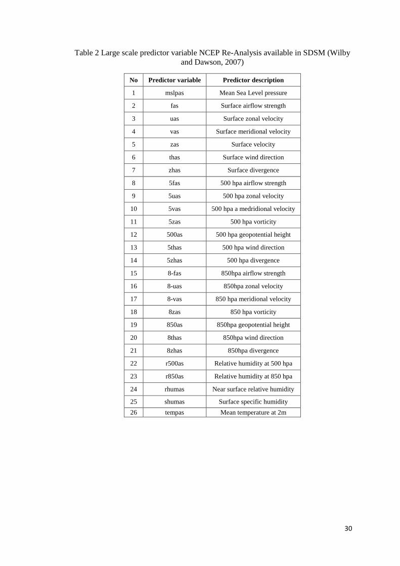
30
Table 2 Large scale predictor variable NCEP Re-Analysis available in SDSM (Wilby
and Dawson, 2007)
No Predictor variable Predictor description
1 mslpas Mean Sea Level pressure
2 fas Surface airflow strength
3 uas Surface zonal velocity
4 vas Surface meridional velocity
5 zas Surface velocity
6 thas Surface wind direction
7 zhas Surface divergence
8 5fas 500 hpa airflow strength
9 5uas 500 hpa zonal velocity
10 5vas 500 hpa a medridional velocity
11 5zas 500 hpa vorticity
12 500as 500 hpa geopotential height
13 5thas 500 hpa wind direction
14 5zhas 500 hpa divergence
15 8-fas 850hpa airflow strength
16 8-uas 850hpa zonal velocity
17 8-vas 850 hpa meridional velocity
18 8zas 850 hpa vorticity
19 850as 850hpa geopotential height
20 8thas 850hpa wind direction
21 8zhas 850hpa divergence
22 r500as Relative humidity at 500 hpa
23 r850as Relative humidity at 850 hpa
24 rhumas Near surface relative humidity
25 shumas Surface specific humidity
26 tempas Mean temperature at 2m
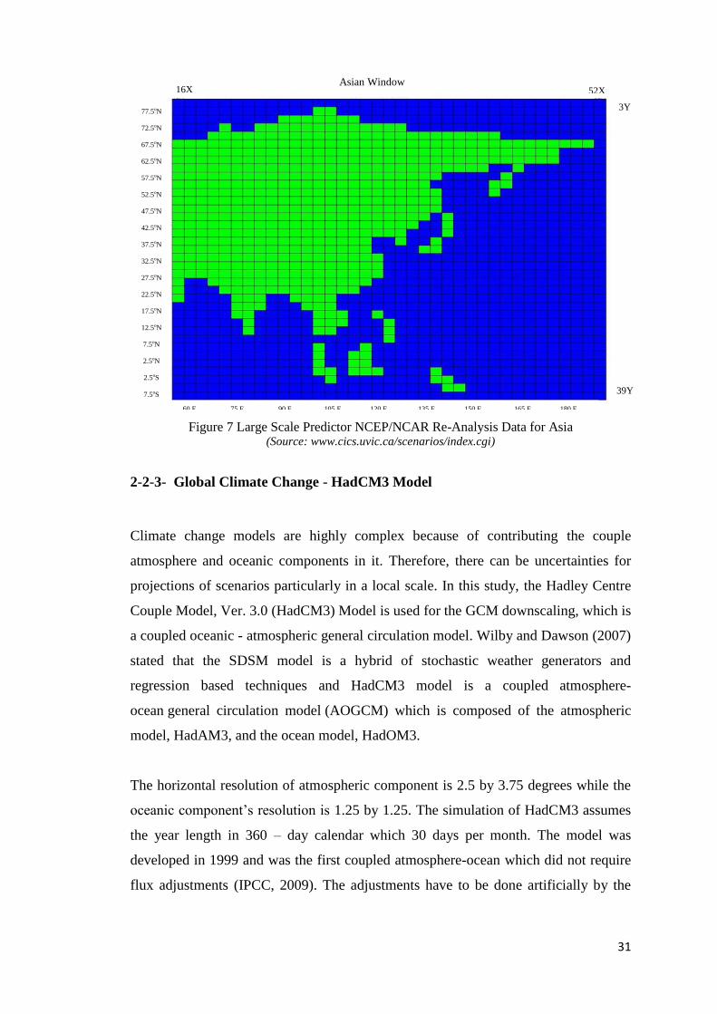
31
Figure 7 Large Scale Predictor NCEP/NCAR Re-Analysis Data for Asia (Source: www.cics.uvic.ca/scenarios/index.cgi)
2-2-3- Global Climate Change - HadCM3 Model
Climate change models are highly complex because of contributing the couple
atmosphere and oceanic components in it. Therefore, there can be uncertainties for
projections of scenarios particularly in a local scale. In this study, the Hadley Centre
Couple Model, Ver. 3.0 (HadCM3) Model is used for the GCM downscaling, which is
a coupled oceanic - atmospheric general circulation model. Wilby and Dawson (2007)
stated that the SDSM model is a hybrid of stochastic weather generators and
regression based techniques and HadCM3 model is a coupled atmosphere-
ocean general circulation model (AOGCM) which is composed of the atmospheric
model, HadAM3, and the ocean model, HadOM3.
The horizontal resolution of atmospheric component is 2.5 by 3.75 degrees while the
oceanic component’s resolution is 1.25 by 1.25. The simulation of HadCM3 assumes
the year length in 360 – day calendar which 30 days per month. The model was
developed in 1999 and was the first coupled atmosphere-ocean which did not require
flux adjustments (IPCC, 2009). The adjustments have to be done artificially by the
77.5oN
72.5oN
67.5oN
62.5oN
57.5oN
52.5oN
47.5oN
42.5oN
37.5oN
32.5oN
27.5oN
22.5oN
17.5oN
12.5oN
7.5oN
2.5oN
2.5oS
7.5oS
Asian Window 16X
39Y
52X
3Y
60 E 75 E 90 E 105 E 120 E 135 E 150 E 165 E 180 E
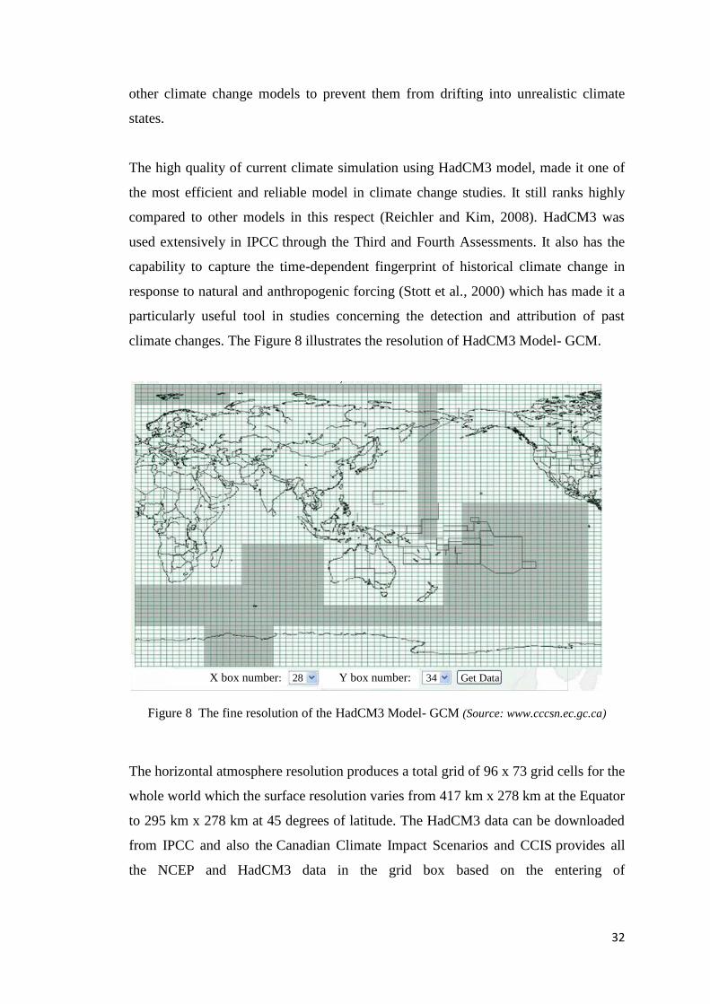
32
other climate change models to prevent them from drifting into unrealistic climate
states.
The high quality of current climate simulation using HadCM3 model, made it one of
the most efficient and reliable model in climate change studies. It still ranks highly
compared to other models in this respect (Reichler and Kim, 2008). HadCM3 was
used extensively in IPCC through the Third and Fourth Assessments. It also has the
capability to capture the time-dependent fingerprint of historical climate change in
response to natural and anthropogenic forcing (Stott et al., 2000) which has made it a
particularly useful tool in studies concerning the detection and attribution of past
climate changes. The Figure 8 illustrates the resolution of HadCM3 Model- GCM.
Figure 8 The fine resolution of the HadCM3 Model- GCM (Source: www.cccsn.ec.gc.ca)
The horizontal atmosphere resolution produces a total grid of 96 x 73 grid cells for the
whole world which the surface resolution varies from 417 km x 278 km at the Equator
to 295 km x 278 km at 45 degrees of latitude. The HadCM3 data can be downloaded
from IPCC and also the Canadian Climate Impact Scenarios and CCIS provides all
the NCEP and HadCM3 data in the grid box based on the entering of
X box number: 28 Y box number: 34 Get Data
33
latitude/longitude of the study area and the grid box provides a zip file contains three
directories: NCEP-1961-2001, H3A2a-1961-2099 and H3B2a-1961-2099.
2-2-3-1- NCEP-1961-2001
It contains all the observed predictors data produced from NCEP/NCAR. Since there
is a difference in the resolution in grid cells of NCEP and HadCM3, all the 41 years of
daily observed predictor data were interpolated to the same grid as HadCM3 and then
the data were normalised.
2-2-3-2- H3A2a-1961-2099
It contains 139 years of daily GCM predictor data assuming a characteristic of
scenarios with higher rates of GHG emissions in combination with higher sulphate
and other aerosol emissions. H3A2a was normalised over the 1961-1990 period.
2-2-3-3- H3B2a-1961-2099
It contains 139 years of daily GCM predictor data assuming a characteristic of
scenarios with higher rates of GHG emissions in combination with lower rate of
sulphate and other aerosol emissions. H3B2a data was normalised over the 1961-1990
period.
The normalisation was done by dividing each time slice of future (2011-2040, 2041-
2070 and 2071-2099) to the current period (1961-1990). This method is described by
NCEP and makes an appropriate method to construct the comparable future scenarios
to the base period which are in the same number years.
2-2-4- Statistical Downscaling Model (SDSM)
The SDSM is a tool to downscale the climate variables to fine scale in climate change
studies. SDSM is the best described as a hybrid of the stochastic weather generator
and regression-based downscaling methods. This is because large-scale circulation
34
patterns and atmospheric moisture variables are used to linearly condition local-scale
weather generate parameters (Wilby et al., 2004). There are many studies which used
SDMS in climate change impact assessments (Wilby and Dawson, 2012; Meenu et
al., 2012; Fiseha et al., 2012; Yang et al., 2012).
The version 4.2 of SDSM was used in this research obtained from Canadian Institute
for Climate Studies (CICS), (https://co-public.lboro.ac.uk/cocwd/SDSM/). The
software involves of several tasks as follows: quality control, data transformation;
predictor variable screening; model calibration; weather generation; statistical
analyses; graphing model output; and scenario generation. Figure 9 illustrates the
structure of SDSM which has been developed by Wilby and Dawson, 2007.
Advantages of using SDSM in downscaling climate parameters
It has been widely used in many watershed scales over a range of different
climatic condition in the world by producing reliable results.
It is user friendly and freely available software which can be downloaded from
https://co-public.lboor.ac.uk/cocwd/SDSM/
It generates ensembles which enable the user to implement uncertainty
analyses.
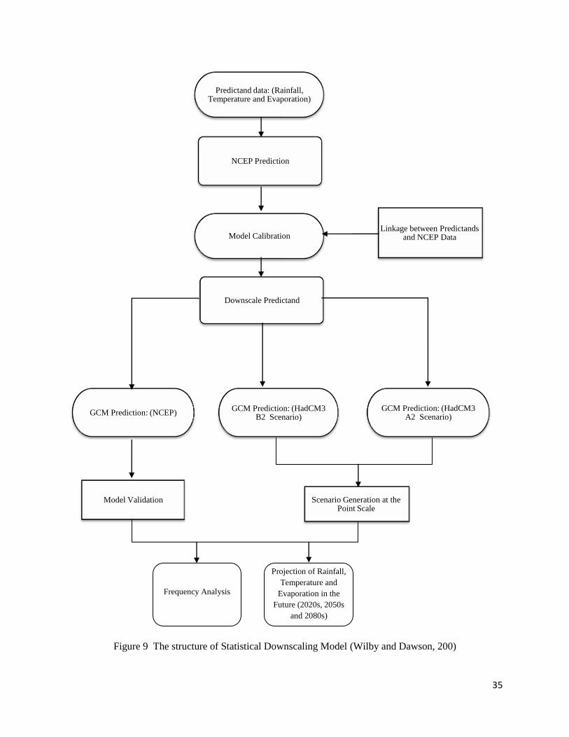
35
Figure 9 The structure of Statistical Downscaling Model (Wilby and Dawson, 200)
Predictand data: (Rainfall, Temperature and Evaporation)
NCEP Prediction
Model Calibration
Downscale Predictand
GCM Prediction: (NCEP) GCM Prediction: (HadCM3
B2 Scenario) GCM Prediction: (HadCM3
A2 Scenario)
Linkage between Predictands and NCEP Data
Projection of Rainfall,
Temperature and
Evaporation in the
Future (2020s, 2050s
and 2080s)
Model Validation Scenario Generation at the Point Scale
Frequency Analysis
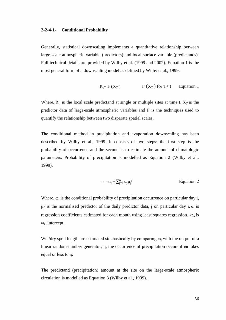
36
2-2-4-1- Conditional Probability
Generally, statistical downscaling implements a quantitative relationship between
large scale atmospheric variable (predictors) and local surface variable (predictands).
Full technical details are provided by Wilby et al. (1999 and 2002). Equation 1 is the
most general form of a downscaling model as defined by Wilby et al., 1999.
t ( T T for T≤ t Equation 1
Where, t is the local scale predictand at single or multiple sites at time t, T is the
predictor data of large-scale atmospheric variables and F is the techniques used to
quantify the relationship between two disparate spatial scales.
The conditional method in precipitation and evaporation downscaling has been
described by Wilby et al., 1999. It consists of two steps: the first step is the
probability of occurrence and the second is to estimate the amount of climatologic
parameters. Probability of precipitation is modelled as Equation 2 (Wilby et al.,
1999).
i o i n
Equation 2
Where, i is the conditional probability of precipitation occurrence on particular day i,
i is the normalised predictor of the daily predictor data, j on particular day i. is
regression coefficients estimated for each month using least squares regression. is
i - intercept.
Wet/dry spell length are estimated stochastically by comparing i with the output of a
linear random-number generator, ri, the occurrence of precipitation occurs if i takes
equal or less to ri.
The predictand (precipitation) amount at the site on the large-scale atmospheric
circulation is modelled as Equation 3 (Wilby et al., 1999).
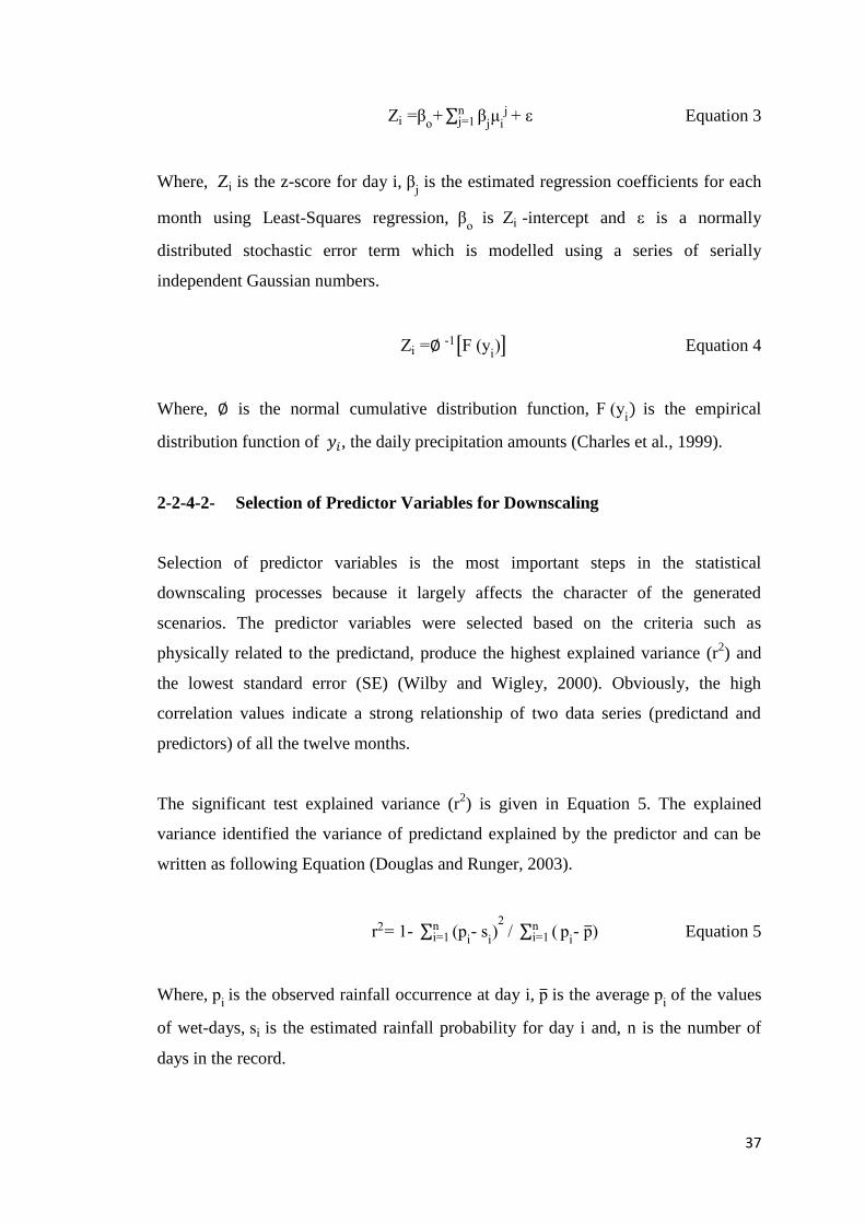
37
i o i n
Equation 3
Where, i is the z-score for day i, is the estimated regression coefficients for each
month using Least-Squares regression, o
is i -intercept and is a normally
distributed stochastic error term which is modelled using a series of serially
independent Gaussian numbers.
i - (yi Equation 4
Where, is the normal cumulative distribution function, (yi is the empirical
distribution function of , the daily precipitation amounts (Charles et al., 1999).
2-2-4-2- Selection of Predictor Variables for Downscaling
Selection of predictor variables is the most important steps in the statistical
downscaling processes because it largely affects the character of the generated
scenarios. The predictor variables were selected based on the criteria such as
physically related to the predictand, produce the highest explained variance (r2) and
the lowest standard error (SE) (Wilby and Wigley, 2000). Obviously, the high
correlation values indicate a strong relationship of two data series (predictand and
predictors) of all the twelve months.
The significant test explained variance (r2) is given in Equation 5. The explained
variance identified the variance of predictand explained by the predictor and can be
written as following Equation (Douglas and Runger, 2003).
r - (pi- s
i n
i (ni p
i- p Equation 5
Where, pi is the observed rainfall occurrence at day i, p is the average p
i of the values
of wet-days, si is the estimated rainfall probability for day i and, n is the number of
days in the record.
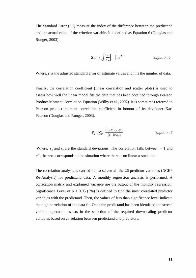
38
The Standard Error (SE) measure the index of the difference between the predictand
and the actual value of the criterion variable. It is defined as Equation 6 (Douglas and
Runger, 2003).
S s n-
n- -r Equation 6
Where, is the adjusted standard error of estimate values and n is the number of data.
Finally, the correlation coefficient (linear correlation and scatter plots) is used to
assess how well the linear model fits the data that has been obtained through Pearson
Product-Moment Correlation Equation (Wilby et al., 2002). It is sometimes referred to
Pearson product moment correlation coefficient in honour of its developer Karl
Pearson (Douglas and Runger, 2003).
Pc xi- x (yi- y
n- (sxsy
ni Equation 7
Where, sx and sy are the standard deviations. The correlation falls between – 1 and
+1, the zero corresponds to the situation where there is no linear association.
The correlation analysis is carried out to screen all the 26 predictor variables (NCEP
Re-Analysis) for predictand data. A monthly regression analysis is performed. A
correlation matrix and explained variance are the output of the monthly regression.
Significance Level of p < 0.05 (5%) is defined to find the most correlated predictor
variables with the predictand. Then, the values of less than significance level indicate
the high correlation of the data fit. Once the predictand has been identified the screen
variable operation assists in the selection of the required downscaling predictor
variables based on correlation between predictand and predictors.
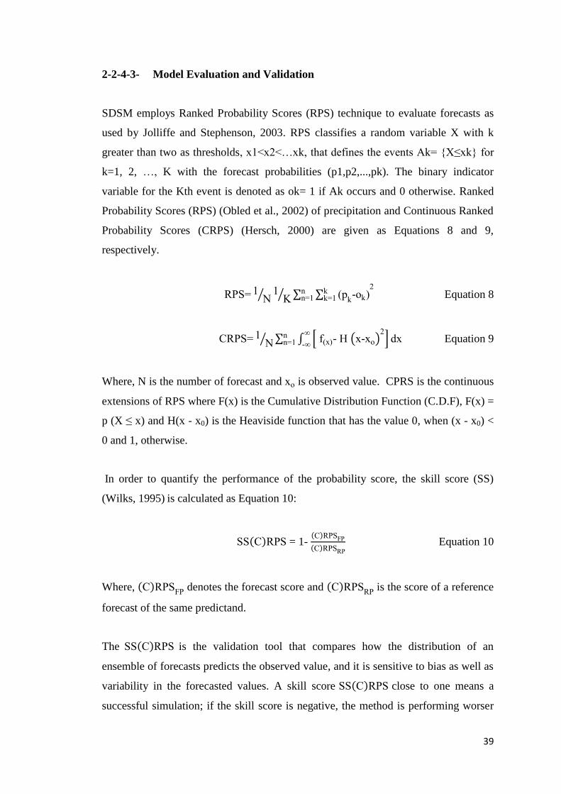
39
2-2-4-3- Model Evaluation and Validation
SDSM employs Ranked Probability Scores (RPS) technique to evaluate forecasts as
used by Jolliffe and Stephenson, 2003. RPS classifies a random variable X with k
greater than two as thresholds, x <x <…xk, that defines the events Ak { ≤xk} for
k=1, 2, …, K with the forecast probabilities (p1,p2,...,pk). The binary indicator
variable for the Kth event is denoted as ok= 1 if Ak occurs and 0 otherwise. Ranked
Probability Scores (RPS) (Obled et al., 2002) of precipitation and Continuous Ranked
Probability Scores (CRPS) (Hersch, 2000) are given as Equations 8 and 9,
respectively.
PS (p
k-ok
kk
nn
Equation 8
PS f(x - H x-xo dx
-
nn Equation 9
Where, N is the number of forecast and xo is observed value. CPRS is the continuous
extensions of RPS where F(x) is the Cumulative Distribution Function (C.D.F), F(x) =
p (X ≤ x) and H(x - x0) is the Heaviside function that has the value 0, when (x - x0) <
0 and 1, otherwise.
In order to quantify the performance of the probability score, the skill score (SS)
(Wilks, 1995) is calculated as Equation 10:
SS PS = 1- PS P PS P
Equation 10
Where, PS P
denotes the forecast score and PS P
is the score of a reference
forecast of the same predictand.
The SS PS is the validation tool that compares how the distribution of an
ensemble of forecasts predicts the observed value, and it is sensitive to bias as well as
variability in the forecasted values. A skill score SS PS close to one means a
successful simulation; if the skill score is negative, the method is performing worser
40
than the reference forecast.
2-2-4-4- Optimisation
The classifications are evaluated using measures of their ability to classify Patterns
with large differences in precipitation structure. These measures are designed for
precipitation occurrence I1 and amount I2 for a specific pattern. The optimisation
derives circulation patterns that explain precipitation patterns (dry and wet conditions)
and this is achieved by maximising two objective functions developed by Bardossy et
al., 2001:
I
T p( Pt- p
T
t Equation 11
I
T ln
PT
T
t Equation 12
Where, T is the number of classified days, p( Pt is the probability of the
precipitation on day t, z is the mean precipitation amount in day t with classification
CP and p is the probability of precipitation for all days.
2-3- Model Error
The Large Scale Predictor NCEP is the most reliable source to check the performance
of downscaling model for the predictand variables. Error analysis in climate change
downscaling is conducted by comparison with mean and variance between historical
and downscaled output. There are some studies to implement the model error analysis
in statistical climate change downscaling (Ebrahim et al., 2012; Buytaert et al., 2010;
Raje and Mujumdar, 2010).
The techniques such as Wilcoxon Test ( onover, 98 and Leven’s Test (Levene,
1960) are used to indicate the model errors. These techniques have been employed to
investigate the model error in statistical climate change downscaling by (Khan et al.,
2005; Ebrahim et al., 2012; khan and Coulibaly, 2010).
41
These two tests are used to construct a hypothesis test p-value to estimate variability
of two population means. The p-value is the level of significance for which observed
test statistic lies on the boundary between acceptance and rejection of the null
hypothesis. The p-value great than 0.05 (95% significant level) indicates the similarity
of two observed and modelled data.
Rainfall dataset does not follow normal distribution, a non-parametric analysis is
applied on it. On the other hand, temperature and evaporation dataset can be
considered as normal variables. The parametric analysis is used to estimate the model
error.
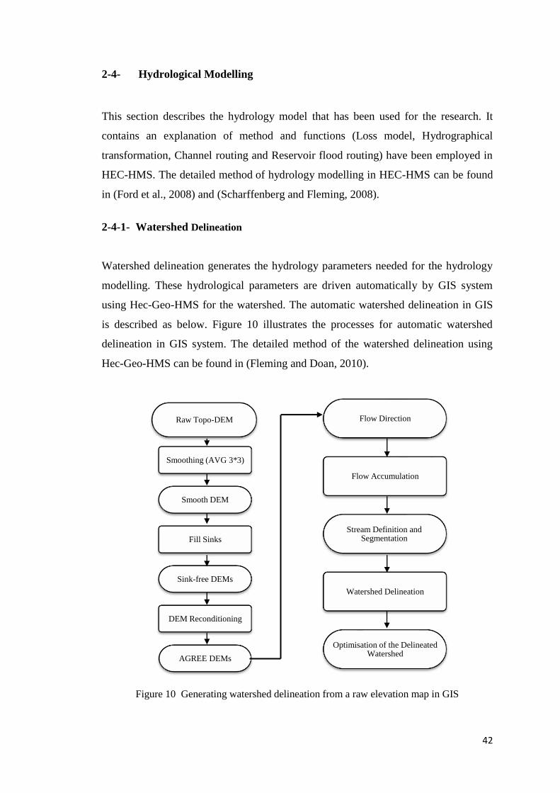
42
2-4- Hydrological Modelling
This section describes the hydrology model that has been used for the research. It
contains an explanation of method and functions (Loss model, Hydrographical
transformation, Channel routing and Reservoir flood routing) have been employed in
HEC-HMS. The detailed method of hydrology modelling in HEC-HMS can be found
in (Ford et al., 2008) and (Scharffenberg and Fleming, 2008).
2-4-1- Watershed Delineation
Watershed delineation generates the hydrology parameters needed for the hydrology
modelling. These hydrological parameters are driven automatically by GIS system
using Hec-Geo-HMS for the watershed. The automatic watershed delineation in GIS
is described as below. Figure 10 illustrates the processes for automatic watershed
delineation in GIS system. The detailed method of the watershed delineation using
Hec-Geo-HMS can be found in (Fleming and Doan, 2010).
Figure 10 Generating watershed delineation from a raw elevation map in GIS
Raw Topo-DEM
Smoothing (AVG 3*3)
Smooth DEM
Fill Sinks
Sink-free DEMs
DEM Reconditioning
AGREE DEMs
Flow Direction
Flow Accumulation
Stream Definition and Segmentation
Watershed Delineation
Optimisation of the Delineated Watershed
43
2-4-2- Loss Model
Loss model estimates the rainfall losses infiltrated by the ground. HEC-HMS provides
various methods to calculate the loss rate in the watershed/sub-watershed such as
deficit and constant, exponential loss, Green-Ampt, SCS Curve Number, initial and
constant.
The HSGs consists of four categories A, B, C, and D, which A and D are the highest
and the lowest infiltration rate respectively. In this study, based on the range
infiltration rate of various soil units in Klang watershed, Hydrological Soil Groups
(HSGs) has been identified as Table 23 in Chapter 5.
The SCS-CN loss method is used in runoff estimation to specify the amount of
infiltration rates of soils. The method uses an integration of landuse and soil data to
determine CN values of the watershed. In this study the CN values were adopted from
Technical Release 55, United States Department of Agriculture- Natural Resources
Conservation Service (USDA-NRCS, 2000). To develop the CN map, the soil data of
Klang watershed has been categorised into hydrologic soil groups (HSGs) and then
have been combined with landuse data. CN map indicates the integrated landuse-soil
of Klang watershed. The relevant equations developed by Natural Resources
Conservation Service (USDA-NRCS, 2000) are as follows:
S =
- Equation 13
= (P- . S
P .8S Equation 14
Where, Q is direct runoff (mm), P is accumulated rainfall (mm), S is potential
maximum soil retention (mm) and CN is Curve Number.
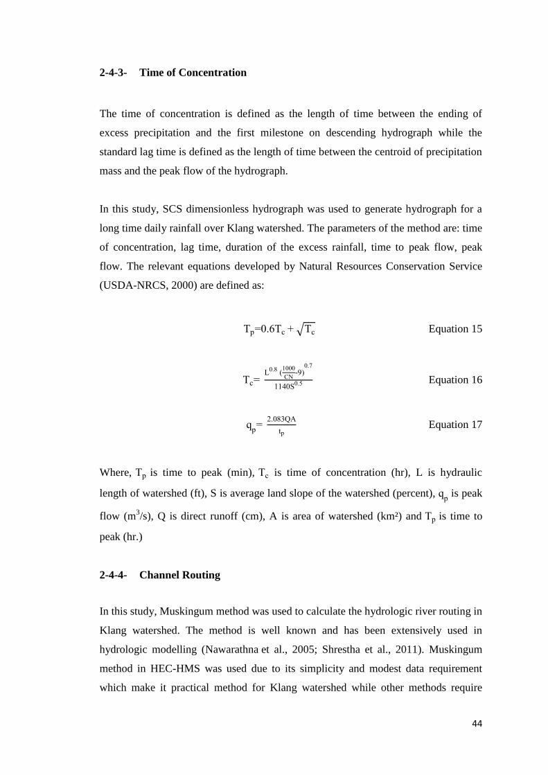
44
2-4-3- Time of Concentration
The time of concentration is defined as the length of time between the ending of
excess precipitation and the first milestone on descending hydrograph while the
standard lag time is defined as the length of time between the centroid of precipitation
mass and the peak flow of the hydrograph.
In this study, SCS dimensionless hydrograph was used to generate hydrograph for a
long time daily rainfall over Klang watershed. The parameters of the method are: time
of concentration, lag time, duration of the excess rainfall, time to peak flow, peak
flow. The relevant equations developed by Natural Resources Conservation Service
(USDA-NRCS, 2000) are defined as:
Tp . Tc Tc Equation 15
Tc L .8 (
-9
.
S . Equation 16
qp
. 83 A
tp Equation 17
Where, Tp is time to peak (min), Tc is time of concentration (hr), L is hydraulic
length of watershed (ft), S is average land slope of the watershed (percent), qp is peak
flow (m3/s), Q is direct runoff (cm), A is area of watershed (km²) and Tp is time to
peak (hr.)
2-4-4- Channel Routing
In this study, Muskingum method was used to calculate the hydrologic river routing in
Klang watershed. The method is well known and has been extensively used in
hydrologic modelling (Nawarathna et al., 2005; Shrestha et al., 2011). Muskingum
method in HEC-HMS was used due to its simplicity and modest data requirement
which make it practical method for Klang watershed while other methods require
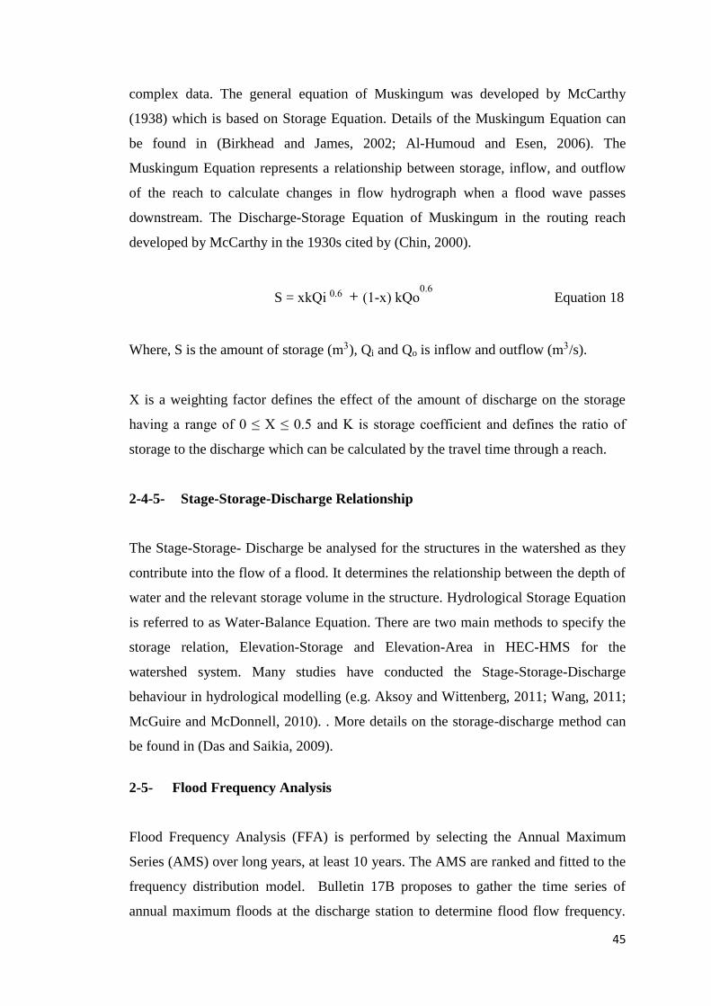
45
complex data. The general equation of Muskingum was developed by McCarthy
(1938) which is based on Storage Equation. Details of the Muskingum Equation can
be found in (Birkhead and James, 2002; Al-Humoud and Esen, 2006). The
Muskingum Equation represents a relationship between storage, inflow, and outflow
of the reach to calculate changes in flow hydrograph when a flood wave passes
downstream. The Discharge-Storage Equation of Muskingum in the routing reach
developed by McCarthy in the 1930s cited by (Chin, 2000).
S = xk i . + ( -x k .
Equation 18
Where, S is the amount of storage (m3), Qi and Qo is inflow and outflow (m3/s).
X is a weighting factor defines the effect of the amount of discharge on the storage
having a range of ≤ ≤ . and is storage coefficient and defines the ratio of
storage to the discharge which can be calculated by the travel time through a reach.
2-4-5- Stage-Storage-Discharge Relationship
The Stage-Storage- Discharge be analysed for the structures in the watershed as they
contribute into the flow of a flood. It determines the relationship between the depth of
water and the relevant storage volume in the structure. Hydrological Storage Equation
is referred to as Water-Balance Equation. There are two main methods to specify the
storage relation, Elevation-Storage and Elevation-Area in HEC-HMS for the
watershed system. Many studies have conducted the Stage-Storage-Discharge
behaviour in hydrological modelling (e.g. Aksoy and Wittenberg, 2011; Wang, 2011;
McGuire and McDonnell, 2010). . More details on the storage-discharge method can
be found in (Das and Saikia, 2009).
2-5- Flood Frequency Analysis
Flood Frequency Analysis (FFA) is performed by selecting the Annual Maximum
Series (AMS) over long years, at least 10 years. The AMS are ranked and fitted to the
frequency distribution model. Bulletin 17B proposes to gather the time series of
annual maximum floods at the discharge station to determine flood flow frequency.
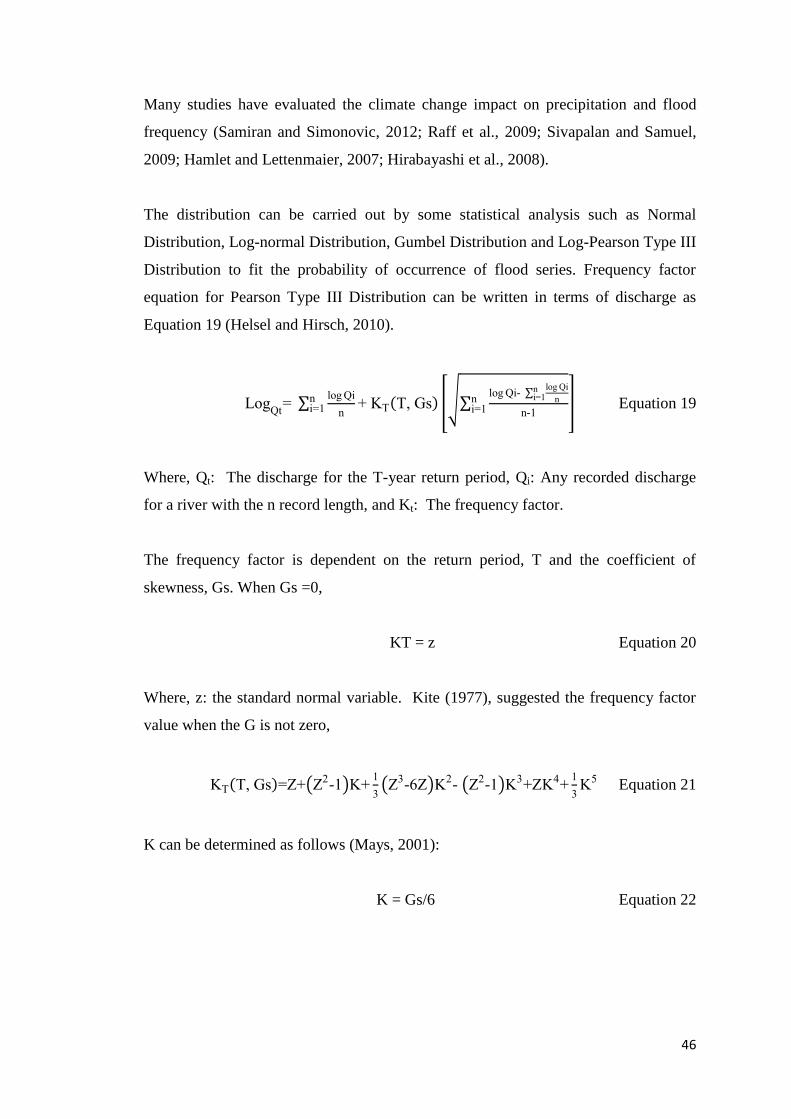
46
Many studies have evaluated the climate change impact on precipitation and flood
frequency (Samiran and Simonovic, 2012; Raff et al., 2009; Sivapalan and Samuel,
2009; Hamlet and Lettenmaier, 2007; Hirabayashi et al., 2008).
The distribution can be carried out by some statistical analysis such as Normal
Distribution, Log-normal Distribution, Gumbel Distribution and Log-Pearson Type III
Distribution to fit the probability of occurrence of flood series. Frequency factor
equation for Pearson Type III Distribution can be written in terms of discharge as
Equation 19 (Helsel and Hirsch, 2010).
Log t
log i
n
ni T T, s
log i- log i
nni
n-
ni Equation 19
Where, Qt: The discharge for the T-year return period, Qi: Any recorded discharge
for a river with the n record length, and Kt: The frequency factor.
The frequency factor is dependent on the return period, T and the coefficient of
skewness, Gs. When Gs =0,
KT = z Equation 20
Where, z: the standard normal variable. Kite (1977), suggested the frequency factor
value when the G is not zero,
T T, s -
3 3- - - 3
3 Equation 21
K can be determined as follows (Mays, 2001):
K = Gs/6 Equation 22
47
3- CLIMATE BASE AND HYDRO-METEOROLOGICAL
ANALYSIS
This chapter consists of two parts. The first part of the chapter focuses on the
characteristics of the study area, Klang watershed in Kuala Lumpur. It presents a
description of the watershed by determining the environmental-physical aspects such
as topography, geology, soil and landuse. The second part of the chapter describes
the climate pattern and hydrological characteristics of study area. A study on
interpretation on flow and flood through the watershed conducted by Flood Frequency
Analysis (FFA) and Flow Duration Curve (FDC) techniques to reflect the behaviour
of flow regime. Furthermore, data preparation and quality control on the historic data
are conducted using graphical, statistical and spatial methods.
3-1- Study Area
3-1-1- Watershed Description
Klang watershed is located at the West Coast of Peninsular Malaysia. The watershed
consists of Kuala Lumpur in the state of Selangor in Malaysia, a country in the South
East of Asia; between 101°.30´ to 101°.55´ E longitudes and 3° to 3°.30´ N latitude.
Klang River originates from the main range at an elevation of 1400 metres above
mean sea level around the East and North-East of Selangor. It is 120 km in length and
the area of watershed is 674 km² approximately. Klang River traverses through the
two states, Selangor and Wilayah Persekutuan and finally discharges into the straits of
Malacca to the west. The upstream of the river comprises of mountainous terrains
which are steeper. Most parts of the watershed are intact, underdeveloped and covered
by a thick canopy of tropical jungle. Klang River has 11 major tributaries, these
include Gombak River, Batu River, Kerayong River, Damansara River, Keruh River,
Kuyoh River, Penchala River and Ampang River. Figure 11 shows the geographical
location of the study area chosen.
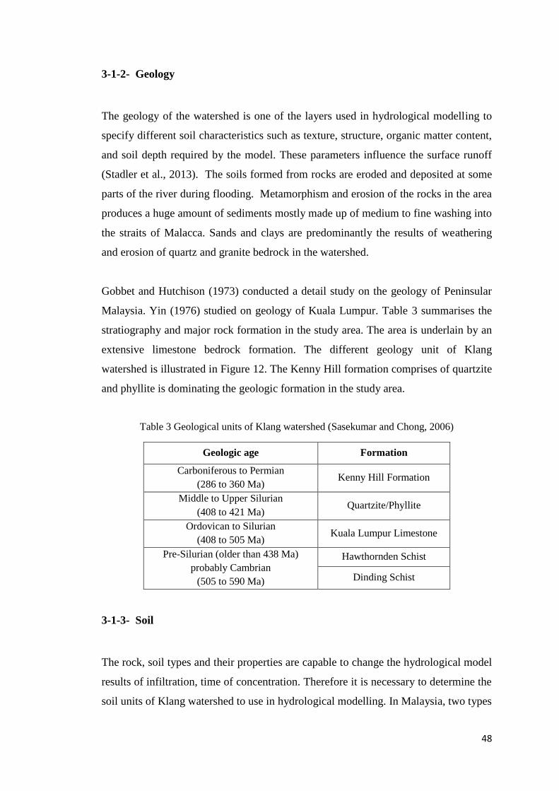
48
3-1-2- Geology
The geology of the watershed is one of the layers used in hydrological modelling to
specify different soil characteristics such as texture, structure, organic matter content,
and soil depth required by the model. These parameters influence the surface runoff
(Stadler et al., 2013). The soils formed from rocks are eroded and deposited at some
parts of the river during flooding. Metamorphism and erosion of the rocks in the area
produces a huge amount of sediments mostly made up of medium to fine washing into
the straits of Malacca. Sands and clays are predominantly the results of weathering
and erosion of quartz and granite bedrock in the watershed.
Gobbet and Hutchison (1973) conducted a detail study on the geology of Peninsular
Malaysia. Yin (1976) studied on geology of Kuala Lumpur. Table 3 summarises the
stratiography and major rock formation in the study area. The area is underlain by an
extensive limestone bedrock formation. The different geology unit of Klang
watershed is illustrated in Figure 12. The Kenny Hill formation comprises of quartzite
and phyllite is dominating the geologic formation in the study area.
Table 3 Geological units of Klang watershed (Sasekumar and Chong, 2006)
Geologic age Formation
Carboniferous to Permian
(286 to 360 Ma) Kenny Hill Formation
Middle to Upper Silurian
(408 to 421 Ma) Quartzite/Phyllite
Ordovican to Silurian
(408 to 505 Ma) Kuala Lumpur Limestone
Pre-Silurian (older than 438 Ma)
probably Cambrian
(505 to 590 Ma)
Hawthornden Schist
Dinding Schist
3-1-3- Soil
The rock, soil types and their properties are capable to change the hydrological model
results of infiltration, time of concentration. Therefore it is necessary to determine the
soil units of Klang watershed to use in hydrological modelling. In Malaysia, two types
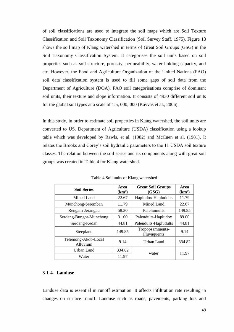
49
of soil classifications are used to integrate the soil maps which are Soil Texture
Classification and Soil Taxonomy Classification (Soil Survey Staff, 1975). Figure 13
shows the soil map of Klang watershed in terms of Great Soil Groups (GSG) in the
Soil Taxonomy Classification System. It categorises the soil units based on soil
properties such as soil structure, porosity, permeability, water holding capacity, and
etc. However, the Food and Agriculture Organization of the United Nations (FAO)
soil data classification system is used to fill some gaps of soil data from the
Department of Agriculture (DOA). FAO soil categorisations comprise of dominant
soil units, their texture and slope information. It consists of 4930 different soil units
for the global soil types at a scale of 1:5, 000, 000 (Kavvas et al., 2006).
In this study, in order to estimate soil properties in Klang watershed, the soil units are
converted to US. Department of Agriculture (USDA) classification using a lookup
table which was developed by Rawls, et al. (1982) and McCuen et al. (1981). It
relates the Brooks and orey’s soil hydraulic parameters to the USDA soil texture
classes. The relation between the soil series and its components along with great soil
groups was created in Table 4 for Klang watershed.
Table 4 Soil units of Klang watershed
Soil Series Area
(km²)
Great Soil Groups
(GSG)
Area
(km²)
Mined Land 22.67 Hapludox-Hapludults 11.79
Munchong-Seremban 11.79 Mined Land 22.67
Rengam-Jerangau 58.30 Palehumults 149.85
Serdang-Bungor-Munchong 31.00 Paleudults-Hapludox 89.00
Serdang-Kedah 44.81 Paleudults-Hapludults 44.81
Steepland 149.85 Tropopsamments-
Fluvaquents 9.14
Telemong-Akob-Local
Alluvium 9.14 Urban Land 334.82
Urban Land 334.82 water 11.97
Water 11.97
3-1-4- Landuse
Landuse data is essential in runoff estimation. It affects infiltration rate resulting in
changes on surface runoff. Landuse such as roads, pavements, parking lots and
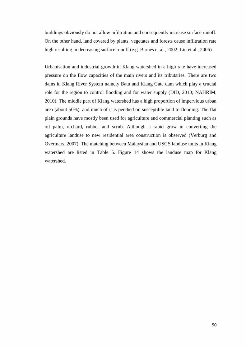
50
buildings obviously do not allow infiltration and consequently increase surface runoff.
On the other hand, land covered by plants, vegetates and forests cause infiltration rate
high resulting in decreasing surface runoff (e.g. Barnes et al., 2002; Liu et al., 2006).
Urbanisation and industrial growth in Klang watershed in a high rate have increased
pressure on the flow capacities of the main rivers and its tributaries. There are two
dams in Klang River System namely Batu and Klang Gate dam which play a crucial
role for the region to control flooding and for water supply (DID, 2010; NAHRIM,
2010). The middle part of Klang watershed has a high proportion of impervious urban
area (about 50%), and much of it is perched on susceptible land to flooding. The flat
plain grounds have mostly been used for agriculture and commercial planting such as
oil palm, orchard, rubber and scrub. Although a rapid grow in converting the
agriculture landuse to new residential area construction is observed (Verburg and
Overmars, 2007). The matching between Malaysian and USGS landuse units in Klang
watershed are listed in Table 5. Figure 14 shows the landuse map for Klang
watershed.
51
Table 5 Malaysian and USGS Landuse/cover matching in Klang watershed
Malaysia Classification USGS Classification
Agricultural station Agriculture
Agricultural station (cattle farm) Agriculture
Agricultural station (diversified crops) Agriculture
Agricultural station (oil palm) Agriculture
Agricultural station (orchards) Agriculture
Aquaculture Agriculture
Cemetery Urban
Estate building and associated areas Urban
Ex-tin mining areas Mining
Forest Forest
Main road and highway Urban
Market gardening Agriculture
mixed horticulture Agriculture
mixed horticulture, neglected grassland Agriculture
mixed horticulture, rubber Agriculture
Neglected grassland Pasture
Neglected grassland (main road and highway) Pasture
Neglected grassland/orchards Pasture
Neglected grassland, scrubs Pasture
Neglected grassland, scrubs (recreational areas) Pasture
Newly cleared land Newly cleared land
Newly cleared land (urban and associated areas) Newly cleared land
Oil palm Agriculture
Orchards Agriculture
Orchards/rubber Agriculture
Orchards/scrubs Agriculture
Orchards, neglected grassland Agriculture
Orchards, scrubs Agriculture
Other mining areas Mining
Other mining areas, neglected grassland Mining
Pond/lake Water body
Poultry/ducks Agriculture
Power lines Urban
Railway Urban
Recreational areas Urban
Reforested Forest
Rubber Agriculture
Scrubs/orchards Agriculture
Scrubs, orchards Agriculture
Swamps Swamps
Swamps/orchards Swamps
Swamps, scrubs Swamps
Tin mining areas Mining
Urban and associated areas Urban
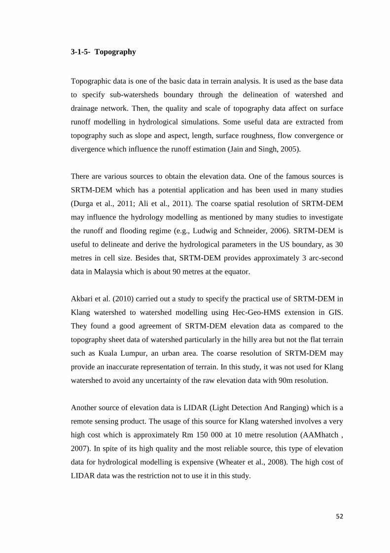
52
3-1-5- Topography
Topographic data is one of the basic data in terrain analysis. It is used as the base data
to specify sub-watersheds boundary through the delineation of watershed and
drainage network. Then, the quality and scale of topography data affect on surface
runoff modelling in hydrological simulations. Some useful data are extracted from
topography such as slope and aspect, length, surface roughness, flow convergence or
divergence which influence the runoff estimation (Jain and Singh, 2005).
There are various sources to obtain the elevation data. One of the famous sources is
SRTM-DEM which has a potential application and has been used in many studies
(Durga et al., 2011; Ali et al., 2011). The coarse spatial resolution of SRTM-DEM
may influence the hydrology modelling as mentioned by many studies to investigate
the runoff and flooding regime (e.g., Ludwig and Schneider, 2006). SRTM-DEM is
useful to delineate and derive the hydrological parameters in the US boundary, as 30
metres in cell size. Besides that, SRTM-DEM provides approximately 3 arc-second
data in Malaysia which is about 90 metres at the equator.
Akbari et al. (2010) carried out a study to specify the practical use of SRTM-DEM in
Klang watershed to watershed modelling using Hec-Geo-HMS extension in GIS.
They found a good agreement of SRTM-DEM elevation data as compared to the
topography sheet data of watershed particularly in the hilly area but not the flat terrain
such as Kuala Lumpur, an urban area. The coarse resolution of SRTM-DEM may
provide an inaccurate representation of terrain. In this study, it was not used for Klang
watershed to avoid any uncertainty of the raw elevation data with 90m resolution.
Another source of elevation data is LIDAR (Light Detection And Ranging) which is a
remote sensing product. The usage of this source for Klang watershed involves a very
high cost which is approximately Rm 150 000 at 10 metre resolution (AAMhatch ,
2007). In spite of its high quality and the most reliable source, this type of elevation
data for hydrological modelling is expensive (Wheater et al., 2008). The high cost of
LIDAR data was the restriction not to use it in this study.
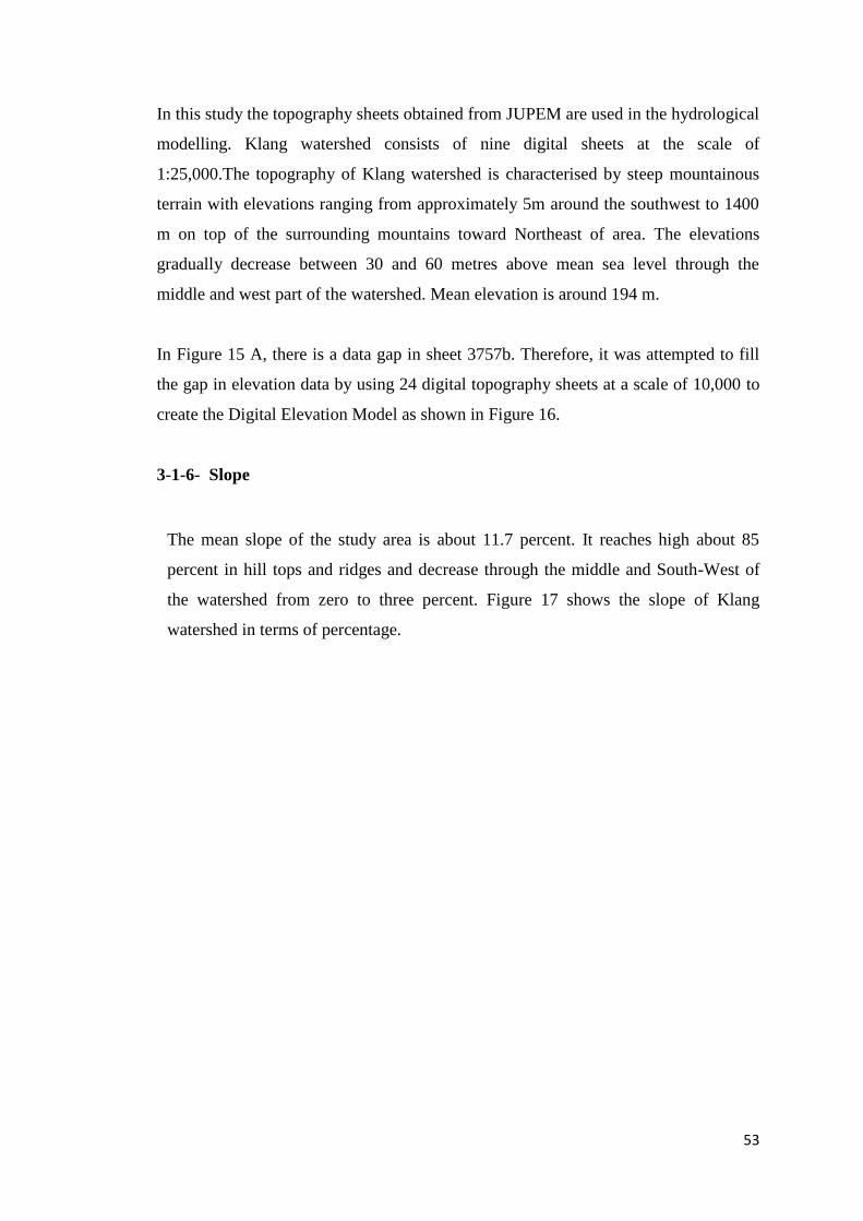
53
In this study the topography sheets obtained from JUPEM are used in the hydrological
modelling. Klang watershed consists of nine digital sheets at the scale of
1:25,000.The topography of Klang watershed is characterised by steep mountainous
terrain with elevations ranging from approximately 5m around the southwest to 1400
m on top of the surrounding mountains toward Northeast of area. The elevations
gradually decrease between 30 and 60 metres above mean sea level through the
middle and west part of the watershed. Mean elevation is around 194 m.
In Figure 15 A, there is a data gap in sheet 3757b. Therefore, it was attempted to fill
the gap in elevation data by using 24 digital topography sheets at a scale of 10,000 to
create the Digital Elevation Model as shown in Figure 16.
3-1-6- Slope
The mean slope of the study area is about 11.7 percent. It reaches high about 85
percent in hill tops and ridges and decrease through the middle and South-West of
the watershed from zero to three percent. Figure 17 shows the slope of Klang
watershed in terms of percentage.
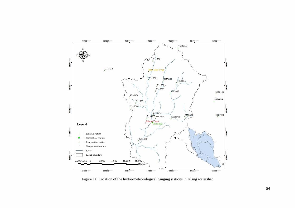
54
Figure 11 Location of the hydro-meteorological gauging stations in Klang watershed
Legend
Rainfall station
Streamflow station
Evaporation station
Temperature station
River
Klang boundary
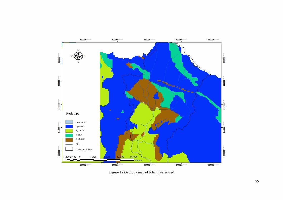
55
Figure 12 Geology map of Klang watershed
Rock type
Alluvium
Igneous
Quartzite
Schist
Sediment
River
Klang boundary
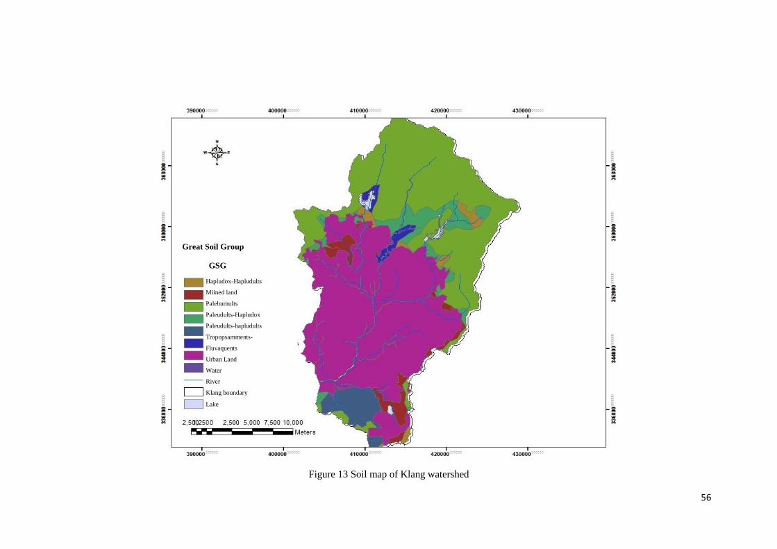
56
Figure 13 Soil map of Klang watershed
Great Soil Group
GSG
Hapludox-Hapludults
Miined land
Palehumults
Paleudults-Hapludox
Paleudults-hapludults
Tropopsamments-
Fluvaquents
Urban Land
Water
River
Klang boundary
Lake
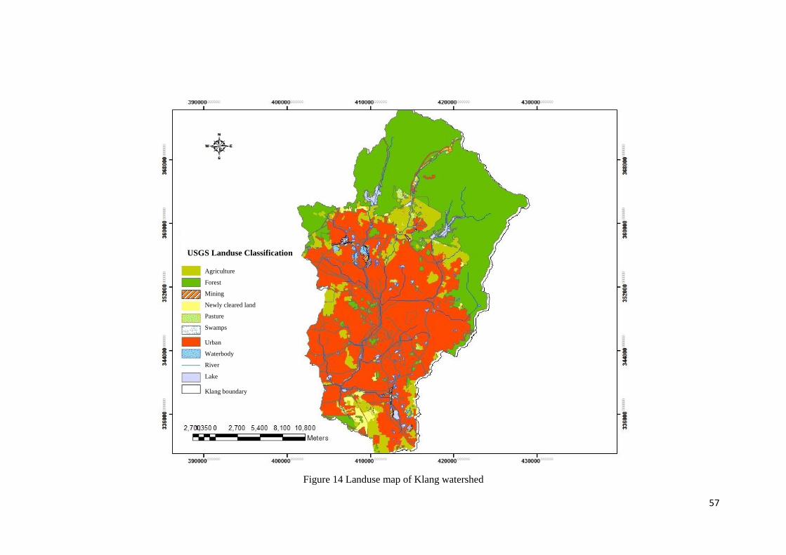
57
Figure 14 Landuse map of Klang watershed
USGS Landuse Classification
Agriculture
Forest
Mining
Newly cleared land
Pasture
Swamps
Urban
Waterbody
River
Lake
Klang boundary
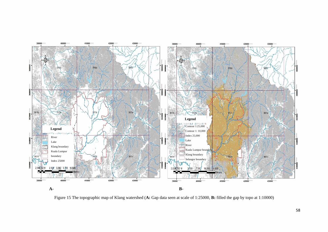
58
A- B-
Figure 15 The topographic map of Klang watershed (A: Gap data seen at scale of 1:25000, B: filled the gap by topo at 1:10000)
River
Lake
Klang boundary
Kuala Lumpur
boundary
Index 25000
Contour 1:25,000
Contour 1: 10,000
Index 25,000
Lake
River
Kuala Lumpur boundary
Klang boundary
Selangor boundary
Legend
Legend

59
Figure 16 Elevation classification for Klang watershed
Elevation Model
5-133
133-295
295-494
494-766
766-1,404
River
Lake
Klang boundary
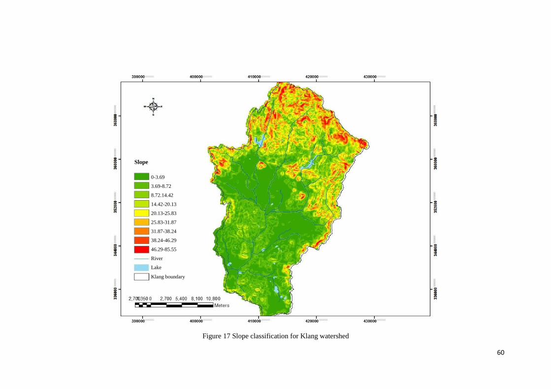
60
Figure 17 Slope classification for Klang watershed
Slope
0-3.69
3.69-8.72
8.72.14.42
14.42-20.13
20.13-25.83
25.83-31.87
31.87-38.24
38.24-46.29
46.29-85.55
River
Lake
Klang boundary
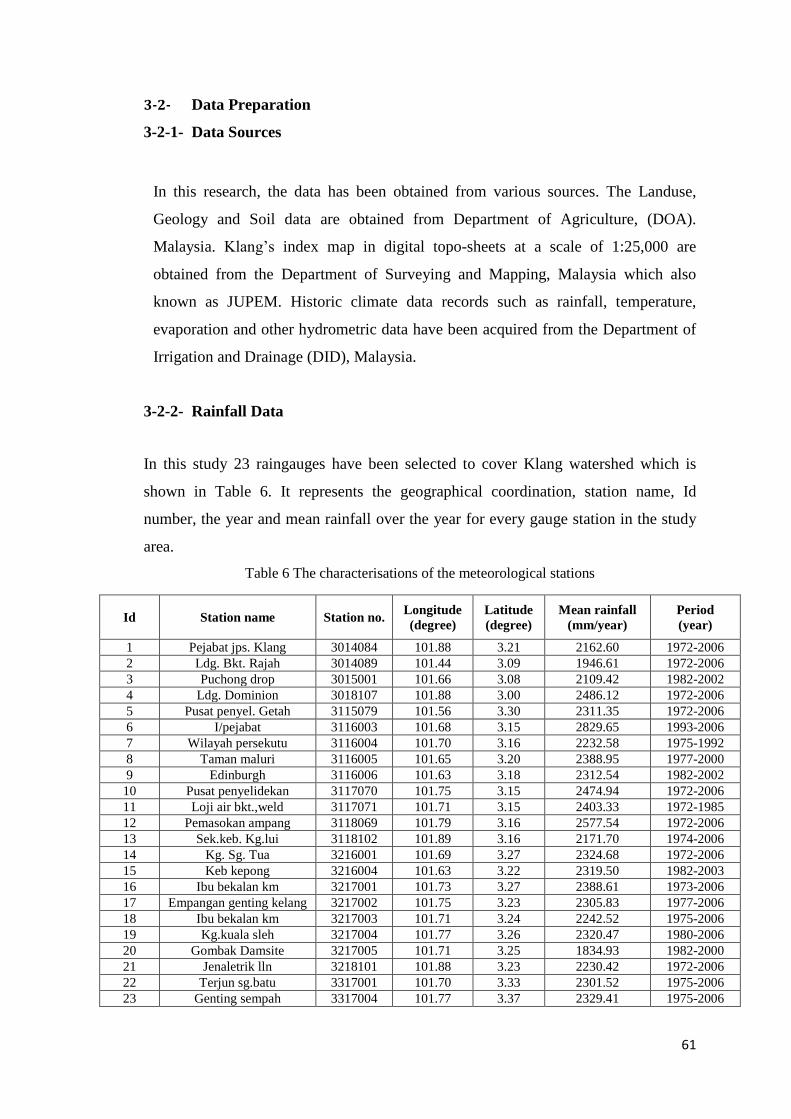
61
3-2- Data Preparation
3-2-1- Data Sources
In this research, the data has been obtained from various sources. The Landuse,
Geology and Soil data are obtained from Department of Agriculture, (DOA).
Malaysia. lang’s index map in digital topo-sheets at a scale of 1:25,000 are
obtained from the Department of Surveying and Mapping, Malaysia which also
known as JUPEM. Historic climate data records such as rainfall, temperature,
evaporation and other hydrometric data have been acquired from the Department of
Irrigation and Drainage (DID), Malaysia.
3-2-2- Rainfall Data
In this study 23 raingauges have been selected to cover Klang watershed which is
shown in Table 6. It represents the geographical coordination, station name, Id
number, the year and mean rainfall over the year for every gauge station in the study
area.
Table 6 The characterisations of the meteorological stations
Id Station name Station no. Longitude
(degree)
Latitude
(degree)
Mean rainfall
(mm/year)
Period
(year)
1 Pejabat jps. Klang 3014084 101.88 3.21 2162.60 1972-2006
2 Ldg. Bkt. Rajah 3014089 101.44 3.09 1946.61 1972-2006
3 Puchong drop 3015001 101.66 3.08 2109.42 1982-2002
4 Ldg. Dominion 3018107 101.88 3.00 2486.12 1972-2006
5 Pusat penyel. Getah 3115079 101.56 3.30 2311.35 1972-2006
6 I/pejabat 3116003 101.68 3.15 2829.65 1993-2006
7 Wilayah persekutu 3116004 101.70 3.16 2232.58 1975-1992
8 Taman maluri 3116005 101.65 3.20 2388.95 1977-2000
9 Edinburgh 3116006 101.63 3.18 2312.54 1982-2002
10 Pusat penyelidekan 3117070 101.75 3.15 2474.94 1972-2006
11 Loji air bkt.,weld 3117071 101.71 3.15 2403.33 1972-1985
12 Pemasokan ampang 3118069 101.79 3.16 2577.54 1972-2006
13 Sek.keb. Kg.lui 3118102 101.89 3.16 2171.70 1974-2006
14 Kg. Sg. Tua 3216001 101.69 3.27 2324.68 1972-2006
15 Keb kepong 3216004 101.63 3.22 2319.50 1982-2003
16 Ibu bekalan km 3217001 101.73 3.27 2388.61 1973-2006
17 Empangan genting kelang 3217002 101.75 3.23 2305.83 1977-2006
18 Ibu bekalan km 3217003 101.71 3.24 2242.52 1975-2006
19 Kg.kuala sleh 3217004 101.77 3.26 2320.47 1980-2006
20 Gombak Damsite 3217005 101.71 3.25 1834.93 1982-2000
21 Jenaletrik lln 3218101 101.88 3.23 2230.42 1972-2006
22 Terjun sg.batu 3317001 101.70 3.33 2301.52 1975-2006
23 Genting sempah 3317004 101.77 3.37 2329.41 1975-2006
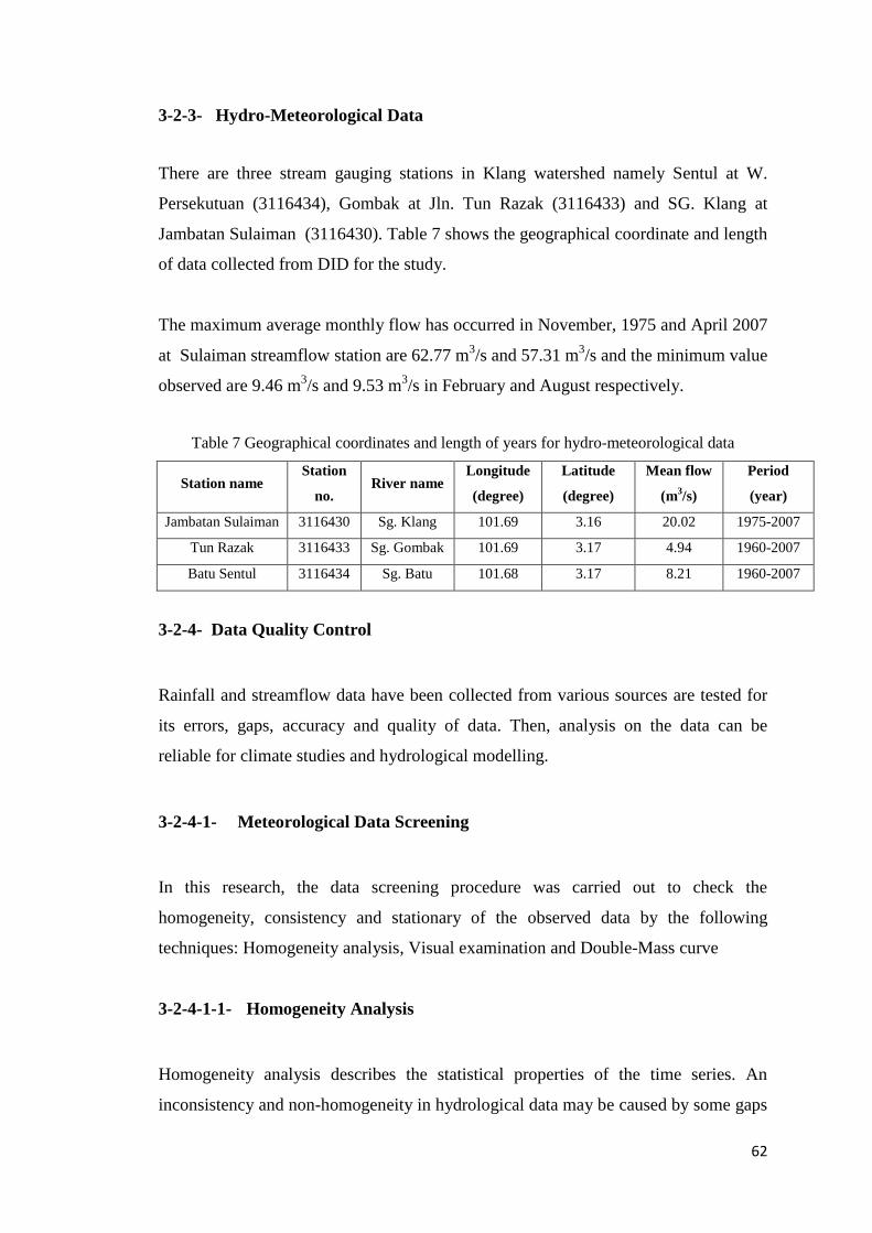
62
3-2-3- Hydro-Meteorological Data
There are three stream gauging stations in Klang watershed namely Sentul at W.
Persekutuan (3116434), Gombak at Jln. Tun Razak (3116433) and SG. Klang at
Jambatan Sulaiman (3116430). Table 7 shows the geographical coordinate and length
of data collected from DID for the study.
The maximum average monthly flow has occurred in November, 1975 and April 2007
at Sulaiman streamflow station are 62.77 m3/s and 57.31 m
3/s and the minimum value
observed are 9.46 m3/s and 9.53 m
3/s in February and August respectively.
Table 7 Geographical coordinates and length of years for hydro-meteorological data
Station name Station
no. River name
Longitude
(degree)
Latitude
(degree)
Mean flow
(m3/s)
Period
(year)
Jambatan Sulaiman 3116430 Sg. Klang 101.69 3.16 20.02 1975-2007
Tun Razak 3116433 Sg. Gombak 101.69 3.17 4.94 1960-2007
Batu Sentul 3116434 Sg. Batu 101.68 3.17 8.21 1960-2007
3-2-4- Data Quality Control
Rainfall and streamflow data have been collected from various sources are tested for
its errors, gaps, accuracy and quality of data. Then, analysis on the data can be
reliable for climate studies and hydrological modelling.
3-2-4-1- Meteorological Data Screening
In this research, the data screening procedure was carried out to check the
homogeneity, consistency and stationary of the observed data by the following
techniques: Homogeneity analysis, Visual examination and Double-Mass curve
3-2-4-1-1- Homogeneity Analysis
Homogeneity analysis describes the statistical properties of the time series. An
inconsistency and non-homogeneity in hydrological data may be caused by some gaps
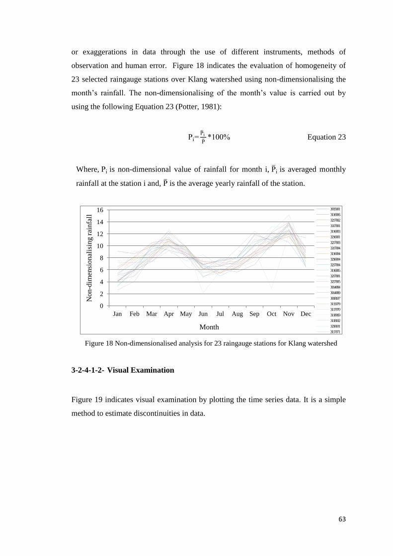
63
or exaggerations in data through the use of different instruments, methods of
observation and human error. Figure 18 indicates the evaluation of homogeneity of
23 selected raingauge stations over Klang watershed using non-dimensionalising the
month’s rainfall. The non-dimensionalising of the month’s value is carried out by
using the following Equation 23 (Potter, 1981):
Pi P i
P Equation 23
Where, Pi is non-dimensional value of rainfall for month i, P i is averaged monthly
rainfall at the station i and, P is the average yearly rainfall of the station.
Figure 18 Non-dimensionalised analysis for 23 raingauge stations for Klang watershed
3-2-4-1-2- Visual Examination
Figure 19 indicates visual examination by plotting the time series data. It is a simple
method to estimate discontinuities in data.
0
2
4
6
8
10
12
14
16
Jan Feb Mar Apr May Jun Jul Aug Sep Oct Nov Dec
3015001
3116006
3217002
3317001
3116003
3216001
3217003
3317004
3116004
3216004
3217004
3116005
3217001
3217005
3014084
3014089
3018107
3115079
3117070
3118069
3118102
3218101
3117071 Month
Non
-dim
ensi
onal
isin
g r
ainfa
ll
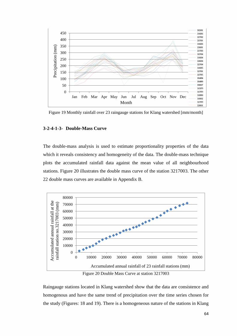
64
Figure 19 Monthly rainfall over 23 raingauge stations for Klang watershed [mm/month]
3-2-4-1-3- Double-Mass Curve
The double-mass analysis is used to estimate proportionality properties of the data
which it reveals consistency and homogeneity of the data. The double-mass technique
plots the accumulated rainfall data against the mean value of all neighbourhood
stations. Figure 20 illustrates the double mass curve of the station 3217003. The other
22 double mass curves are available in Appendix B.
Figure 20 Double Mass Curve at station 3217003
Raingauge stations located in Klang watershed show that the data are consistence and
homogenous and have the same trend of precipitation over the time series chosen for
the study (Figures: 18 and 19). There is a homogeneous nature of the stations in Klang
0
50
100
150
200
250
300
350
400
450
Jan Feb Mar Apr May Jun Jul Aug Sep Oct Nov Dec
3015001
3116006
3217002
3317001
3116003
3216001
3217003
3317004
3116004
3216004
3217004
3116005
3217001
3217005
3014084
3014089
3018107
3115079
3117070
3118069
3118102
3117070
3218101 Month
Pre
cip
itat
ion
(m
m)
0
10000
20000
30000
40000
50000
60000
70000
80000
0 10000 20000 30000 40000 50000 60000 70000 80000
Accumulated annual rainfall of 23 rainfall stations (mm)
Acc
um
ula
ted
an
nual
rai
nfa
ll a
t th
e
rain
fall
sta
tio
n n
o.3
217003 (
mm
)
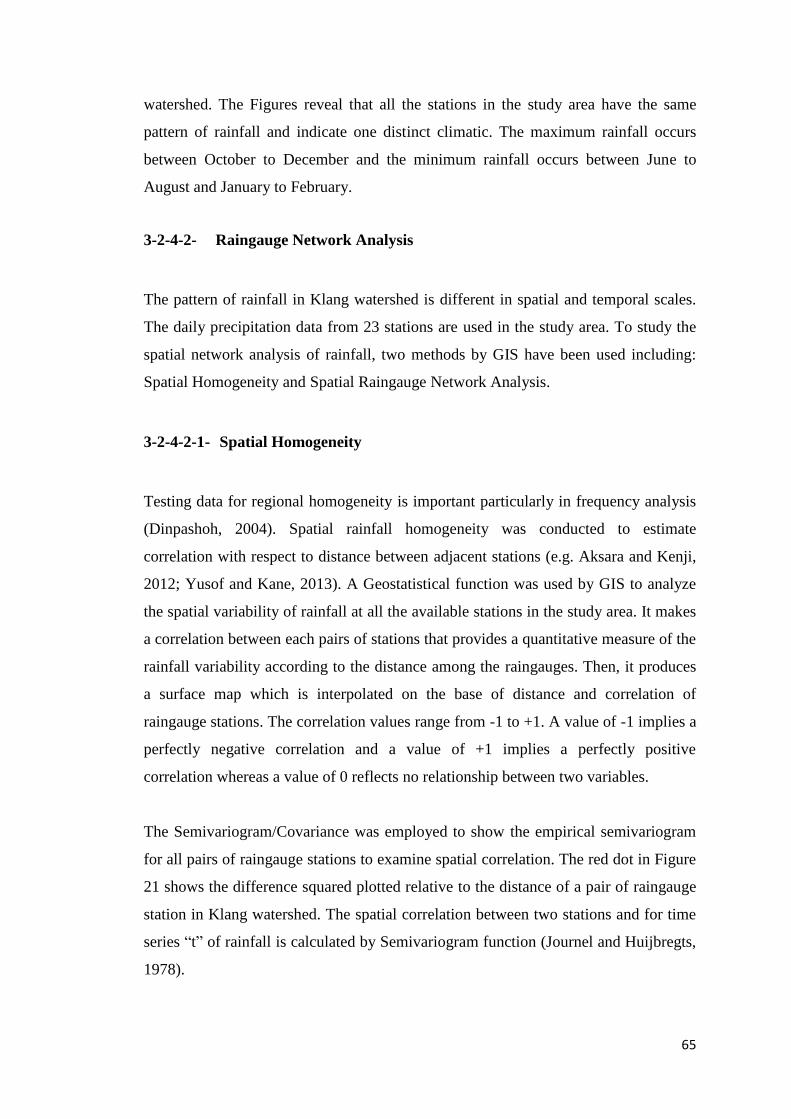
65
watershed. The Figures reveal that all the stations in the study area have the same
pattern of rainfall and indicate one distinct climatic. The maximum rainfall occurs
between October to December and the minimum rainfall occurs between June to
August and January to February.
3-2-4-2- Raingauge Network Analysis
The pattern of rainfall in Klang watershed is different in spatial and temporal scales.
The daily precipitation data from 23 stations are used in the study area. To study the
spatial network analysis of rainfall, two methods by GIS have been used including:
Spatial Homogeneity and Spatial Raingauge Network Analysis.
3-2-4-2-1- Spatial Homogeneity
Testing data for regional homogeneity is important particularly in frequency analysis
(Dinpashoh, 2004). Spatial rainfall homogeneity was conducted to estimate
correlation with respect to distance between adjacent stations (e.g. Aksara and Kenji,
2012; Yusof and Kane, 2013). A Geostatistical function was used by GIS to analyze
the spatial variability of rainfall at all the available stations in the study area. It makes
a correlation between each pairs of stations that provides a quantitative measure of the
rainfall variability according to the distance among the raingauges. Then, it produces
a surface map which is interpolated on the base of distance and correlation of
raingauge stations. The correlation values range from -1 to +1. A value of -1 implies a
perfectly negative correlation and a value of +1 implies a perfectly positive
correlation whereas a value of 0 reflects no relationship between two variables.
The Semivariogram/Covariance was employed to show the empirical semivariogram
for all pairs of raingauge stations to examine spatial correlation. The red dot in Figure
21 shows the difference squared plotted relative to the distance of a pair of raingauge
station in Klang watershed. The spatial correlation between two stations and for time
series “t” of rainfall is calculated by Semivariogram function (Journel and Huijbregts,
1978).
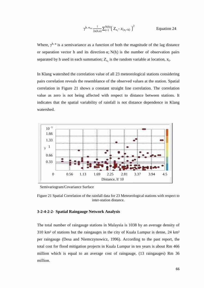
66
h,
n(h, xi- xi h
(h
i Equation 24
Where, h, is a semivariance as a function of both the magnitude of the lag distance
or separation vector h and its direction ; (h is the number of observation pairs
separated by h used in each summation; xi is the random variable at location,
In Klang watershed the correlation value of all 23 meteorological stations considering
pairs correlation reveals the resemblance of the observed values at the station. Spatial
correlation in Figure 21 shows a constant straight line correlation. The correlation
value as zero is not being affected with respect to distance between stations. It
indicates that the spatial variability of rainfall is not distance dependence in Klang
watershed.
Figure 21 Spatial Correlation of the rainfall data for 23 Meteorological stations with respect to
inter-station distance.
3-2-4-2-2- Spatial Raingauge Network Analysis
The total number of raingauge stations in Malaysia is 1038 by an average density of
310 km² of stations but the raingauges in the city of Kuala Lumpur is dense, 24 km²
per raingauge (Desa and Niemczynowicz, 1996). According to the past report, the
total cost for flood mitigation projects in Kuala Lumpur in ten years is about Rm 466
million which is equal to an average cost of raingauge, (13 raingauges) Rm 36
million.
Distance, h'
10
γ
Distance, h' 10
Semivariogram/Covariance Surface
0 0.56 1.13 1.69 2.25 2.81 3.37 3.94 4.5
10 -5
1.66
1.33
1
0.66
0.33
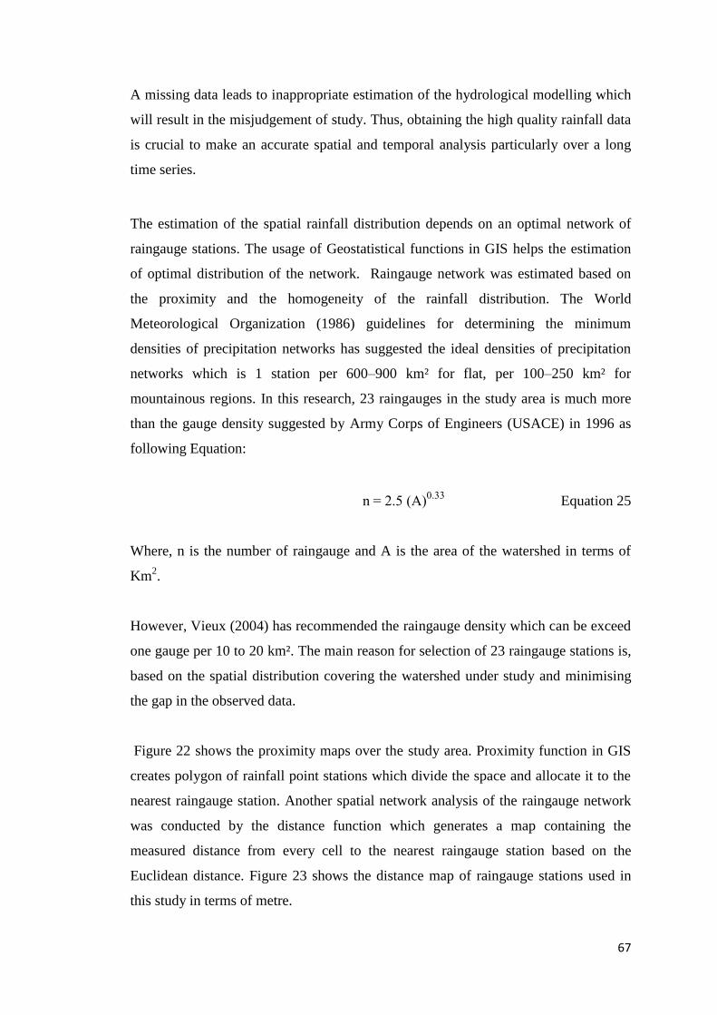
67
A missing data leads to inappropriate estimation of the hydrological modelling which
will result in the misjudgement of study. Thus, obtaining the high quality rainfall data
is crucial to make an accurate spatial and temporal analysis particularly over a long
time series.
The estimation of the spatial rainfall distribution depends on an optimal network of
raingauge stations. The usage of Geostatistical functions in GIS helps the estimation
of optimal distribution of the network. Raingauge network was estimated based on
the proximity and the homogeneity of the rainfall distribution. The World
Meteorological Organization (1986) guidelines for determining the minimum
densities of precipitation networks has suggested the ideal densities of precipitation
networks which is 1 station per 600–900 km² for flat, per 100–250 km² for
mountainous regions. In this research, 23 raingauges in the study area is much more
than the gauge density suggested by Army Corps of Engineers (USACE) in 1996 as
following Equation:
n . (A .33 Equation 25
Where, n is the number of raingauge and A is the area of the watershed in terms of
Km2.
However, Vieux (2004) has recommended the raingauge density which can be exceed
one gauge per 10 to 20 km². The main reason for selection of 23 raingauge stations is,
based on the spatial distribution covering the watershed under study and minimising
the gap in the observed data.
Figure 22 shows the proximity maps over the study area. Proximity function in GIS
creates polygon of rainfall point stations which divide the space and allocate it to the
nearest raingauge station. Another spatial network analysis of the raingauge network
was conducted by the distance function which generates a map containing the
measured distance from every cell to the nearest raingauge station based on the
Euclidean distance. Figure 23 shows the distance map of raingauge stations used in
this study in terms of metre.

68
3-2-4-3- Flow/Discharge Data Screening
Hydro meteorological data is one of the most important data in water resources
studies. Thus it is required to estimate the quality of the data before using it for the
hydrological system simulation. Figure 24 (A, B and C) illustrates visual scan of the
monthly time series for three streamflow stations in Klang watershed to show the gap,
detect the gross errors and missed recordings.
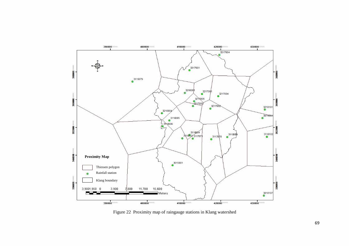
69
Figure 22 Proximity map of raingauge stations in Klang watershed
Proximity Map
Thiessen polygon
Rainfall station
Klang boundary
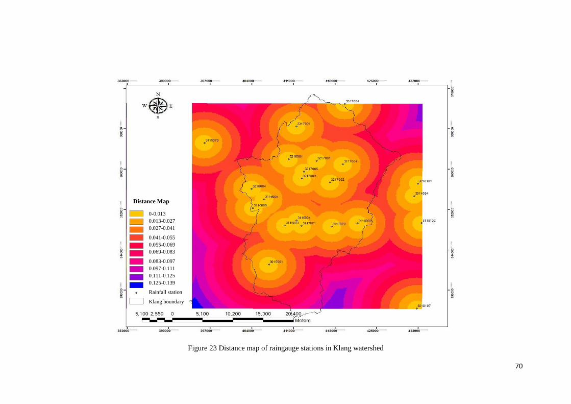
70
Figure 23 Distance map of raingauge stations in Klang watershed
Distance Map
0-0.013
0.013-0.027
0.027-0.041
0.041-0.055
0.055-0.069
0.069-0.083
0.083-0.097
0.097-0.111
0.111-0.125
0.125-0.139
Rainfall station
Klang boundary
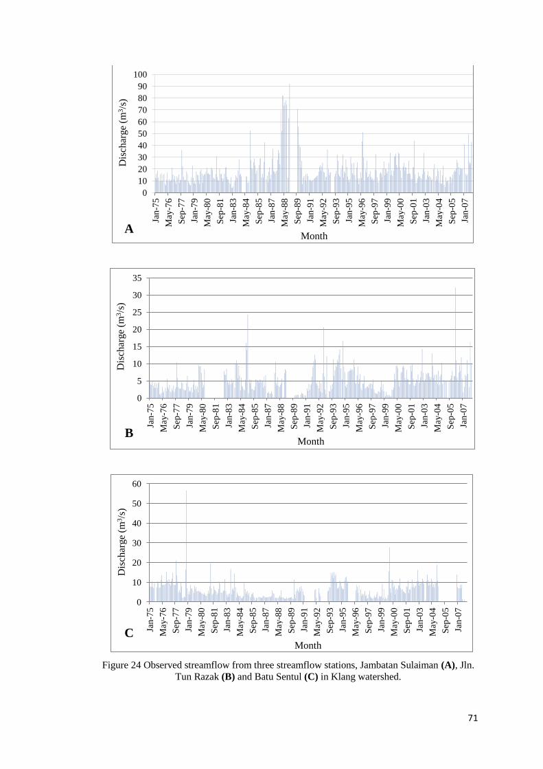
71
Figure 24 Observed streamflow from three streamflow stations, Jambatan Sulaiman (A), Jln.
Tun Razak (B) and Batu Sentul (C) in Klang watershed.
0
10
20
30
40
50
60
70
80
90
100
Jan-7
5
May
-76
Sep
-77
Jan-7
9
May
-80
Sep
-81
Jan-8
3
May
-84
Sep
-85
Jan-8
7
May
-88
Sep
-89
Jan-9
1
May
-92
Sep
-93
Jan-9
5
May
-96
Sep
-97
Jan-9
9
May
-00
Sep
-01
Jan-0
3
May
-04
Sep
-05
Jan-0
7
Dis
char
ge
(m3/s
)
Month
0
5
10
15
20
25
30
35
Jan-7
5
May
-76
Sep
-77
Jan-7
9
May
-80
Sep
-81
Jan-8
3
May
-84
Sep
-85
Jan-8
7
May
-88
Sep
-89
Jan-9
1
May
-92
Sep
-93
Jan-9
5
May
-96
Sep
-97
Jan-9
9
May
-00
Sep
-01
Jan-0
3
May
-04
Sep
-05
Jan-0
7
Dis
char
ge
(m3/s
)
Month
0
10
20
30
40
50
60
Jan-7
5
May
-76
Sep
-77
Jan-7
9
May
-80
Sep
-81
Jan-8
3
May
-84
Sep
-85
Jan-8
7
May
-88
Sep
-89
Jan-9
1
May
-92
Sep
-93
Jan-9
5
May
-96
Sep
-97
Jan-9
9
May
-00
Sep
-01
Jan-0
3
May
-04
Sep
-05
Jan-0
7
Dis
char
ge
(m3/s
)
Month
A
B
C
72
3-2-4-4- Filling Missing Data
There are various methods such as Arithmetic Mean method and Normal Ratio
method (Chow et al., 1988) to fill in the missing data. Homogeneity analysis and
double mass curve techniques are used to fill the gap of monthly and yearly rainfall
data.
3-2-4-4-1- Filling Rainfall Data
Linear interpolation regression was used to fill up the gaps of long series daily
rainfall data. The method is applied due to a large number of daily data of the
multiple raingauge stations. To run the regression, the correlations among the daily
rainfall data are ranked and then the missing data is estimated using a linear
regression with the station that has the highest correlation through the common
period. The linear regression is expressed by the following formula (Helsel and
Hirsch, 2010):
P b b p b p … bn pn Equation 26
Where, the missing precipitation value for station x, P1, P2, … Pn are
precipitation values at the neighbouring stations for the current period, b0,… bn are
coefficients calculated by least-squares methods and n is the number of nearby
gauges.
The correlation coefficient of ten raingauge stations used for the climate change
downscaling in SDSM was determined to fill the gaps of daily rainfall data in the
study area which have the high correlation with the other neighbouring stations. Ten
raingauge stations were selected based on the high quality, with no gap in daily time
series and spatially distributed in the study area covering the whole watershed. Table
8 illustrates the correlation coefficient among the raingauge stations used for
downscaling purpose. The higher correlation between a raingauge station and
corresponding stations are used to fill up gaps between them. Appendix C illustrates
the correlation coefficient between the raingauge stations.
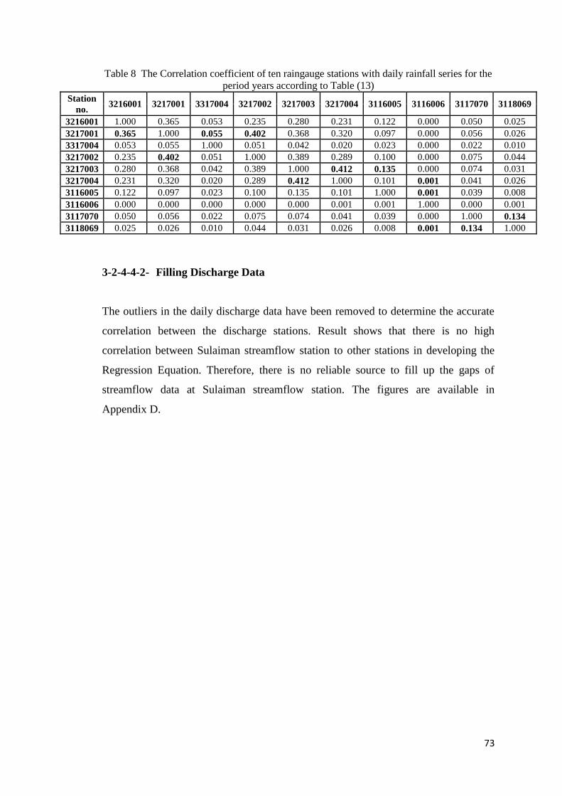
73
Table 8 The Correlation coefficient of ten raingauge stations with daily rainfall series for the
period years according to Table (13)
Station
no. 3216001 3217001 3317004 3217002 3217003 3217004 3116005 3116006 3117070 3118069
3216001 1.000 0.365 0.053 0.235 0.280 0.231 0.122 0.000 0.050 0.025
3217001 0.365 1.000 0.055 0.402 0.368 0.320 0.097 0.000 0.056 0.026
3317004 0.053 0.055 1.000 0.051 0.042 0.020 0.023 0.000 0.022 0.010
3217002 0.235 0.402 0.051 1.000 0.389 0.289 0.100 0.000 0.075 0.044
3217003 0.280 0.368 0.042 0.389 1.000 0.412 0.135 0.000 0.074 0.031
3217004 0.231 0.320 0.020 0.289 0.412 1.000 0.101 0.001 0.041 0.026
3116005 0.122 0.097 0.023 0.100 0.135 0.101 1.000 0.001 0.039 0.008
3116006 0.000 0.000 0.000 0.000 0.000 0.001 0.001 1.000 0.000 0.001
3117070 0.050 0.056 0.022 0.075 0.074 0.041 0.039 0.000 1.000 0.134
3118069 0.025 0.026 0.010 0.044 0.031 0.026 0.008 0.001 0.134 1.000
3-2-4-4-2- Filling Discharge Data
The outliers in the daily discharge data have been removed to determine the accurate
correlation between the discharge stations. Result shows that there is no high
correlation between Sulaiman streamflow station to other stations in developing the
Regression Equation. Therefore, there is no reliable source to fill up the gaps of
streamflow data at Sulaiman streamflow station. The figures are available in
Appendix D.
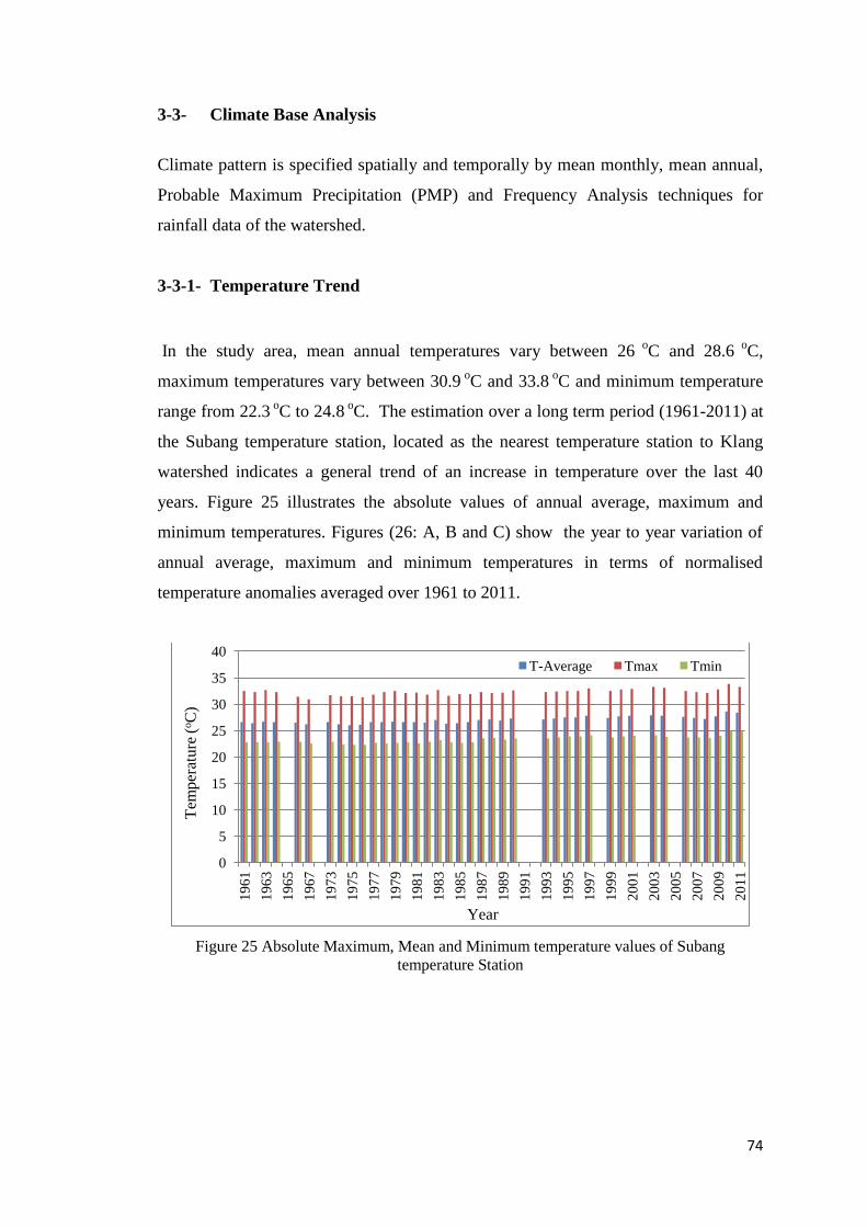
74
3-3- Climate Base Analysis
Climate pattern is specified spatially and temporally by mean monthly, mean annual,
Probable Maximum Precipitation (PMP) and Frequency Analysis techniques for
rainfall data of the watershed.
3-3-1- Temperature Trend
In the study area, mean annual temperatures vary between 26 o
C and 28.6 o
C,
maximum temperatures vary between 30.9 o
C and 33.8 o
C and minimum temperature
range from 22.3 oC to 24.8
oC. The estimation over a long term period (1961-2011) at
the Subang temperature station, located as the nearest temperature station to Klang
watershed indicates a general trend of an increase in temperature over the last 40
years. Figure 25 illustrates the absolute values of annual average, maximum and
minimum temperatures. Figures (26: A, B and C) show the year to year variation of
annual average, maximum and minimum temperatures in terms of normalised
temperature anomalies averaged over 1961 to 2011.
Figure 25 Absolute Maximum, Mean and Minimum temperature values of Subang
temperature Station
0
5
10
15
20
25
30
35
40
19
61
19
63
19
65
19
67
19
73
19
75
19
77
19
79
19
81
19
83
19
85
19
87
19
89
19
91
19
93
19
95
19
97
19
99
20
01
20
03
20
05
20
07
20
09
20
11
T-Average Tmax Tmin
Year
Tem
per
ature
(oC
)
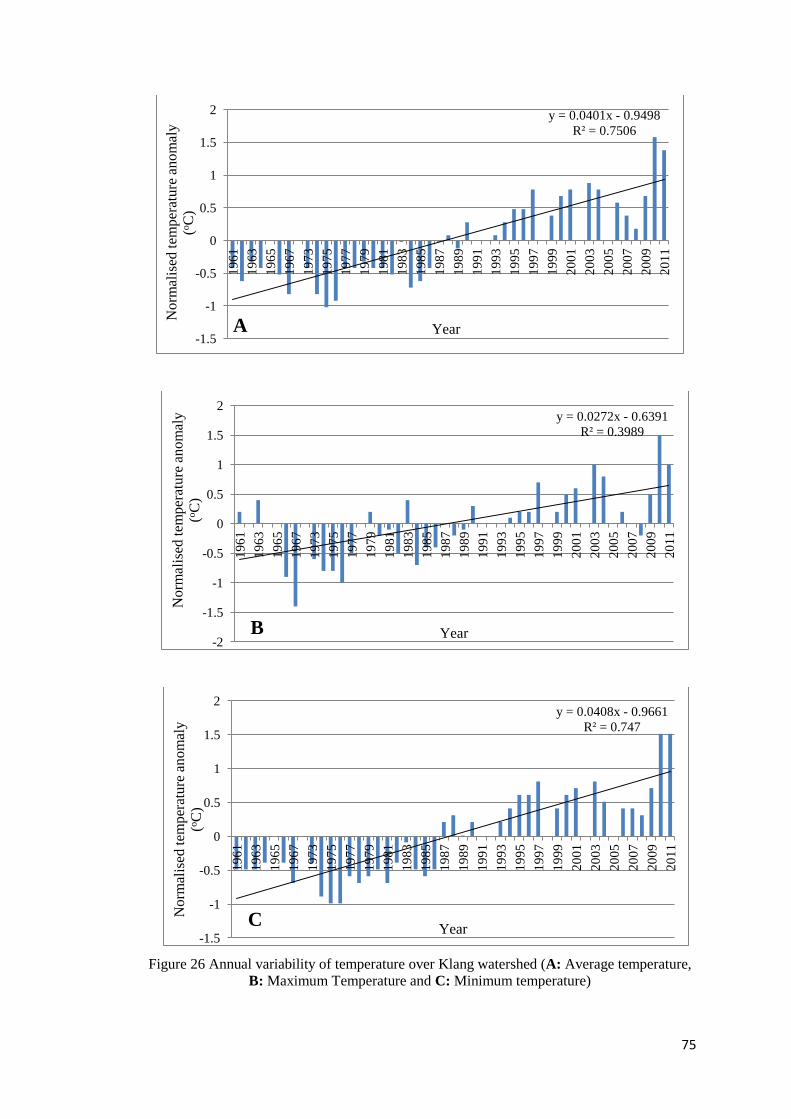
75
Figure 26 Annual variability of temperature over Klang watershed (A: Average temperature,
B: Maximum Temperature and C: Minimum temperature)
y = 0.0401x - 0.9498
R² = 0.7506
-1.5
-1
-0.5
0
0.5
1
1.5
2
19
61
19
63
19
65
19
67
19
73
19
75
19
77
19
79
19
81
19
83
19
85
19
87
19
89
19
91
19
93
19
95
19
97
19
99
20
01
20
03
20
05
20
07
20
09
20
11
No
rmal
ised
tem
per
atu
re a
no
mal
y
(oC
)
Year
y = 0.0272x - 0.6391
R² = 0.3989
-2
-1.5
-1
-0.5
0
0.5
1
1.5
2
19
61
19
63
19
65
19
67
19
73
19
75
19
77
19
79
19
81
19
83
19
85
19
87
19
89
19
91
19
93
19
95
19
97
19
99
20
01
20
03
20
05
20
07
20
09
20
11
No
rmal
ised
tem
per
atu
re a
no
mal
y
(oC
)
Year
y = 0.0408x - 0.9661
R² = 0.747
-1.5
-1
-0.5
0
0.5
1
1.5
2
19
61
19
63
19
65
19
67
19
73
19
75
19
77
19
79
19
81
19
83
19
85
19
87
19
89
19
91
19
93
19
95
19
97
19
99
20
01
20
03
20
05
20
07
20
09
20
11
No
rmal
ised
tem
per
atu
re a
nom
aly
(oC
)
Year
A
B
C
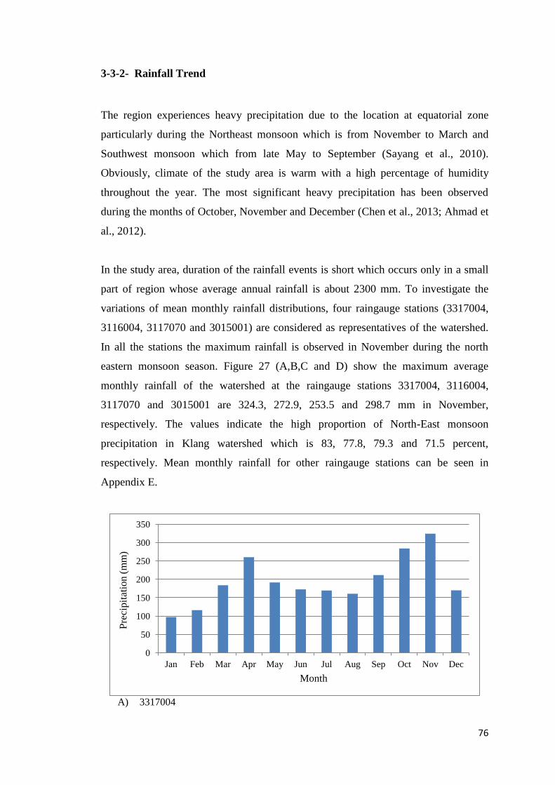
76
3-3-2- Rainfall Trend
The region experiences heavy precipitation due to the location at equatorial zone
particularly during the Northeast monsoon which is from November to March and
Southwest monsoon which from late May to September (Sayang et al., 2010).
Obviously, climate of the study area is warm with a high percentage of humidity
throughout the year. The most significant heavy precipitation has been observed
during the months of October, November and December (Chen et al., 2013; Ahmad et
al., 2012).
In the study area, duration of the rainfall events is short which occurs only in a small
part of region whose average annual rainfall is about 2300 mm. To investigate the
variations of mean monthly rainfall distributions, four raingauge stations (3317004,
3116004, 3117070 and 3015001) are considered as representatives of the watershed.
In all the stations the maximum rainfall is observed in November during the north
eastern monsoon season. Figure 27 (A,B,C and D) show the maximum average
monthly rainfall of the watershed at the raingauge stations 3317004, 3116004,
3117070 and 3015001 are 324.3, 272.9, 253.5 and 298.7 mm in November,
respectively. The values indicate the high proportion of North-East monsoon
precipitation in Klang watershed which is 83, 77.8, 79.3 and 71.5 percent,
respectively. Mean monthly rainfall for other raingauge stations can be seen in
Appendix E.
A) 3317004
0
50
100
150
200
250
300
350
Jan Feb Mar Apr May Jun Jul Aug Sep Oct Nov Dec
Pre
cip
itat
ion
(m
m)
Month
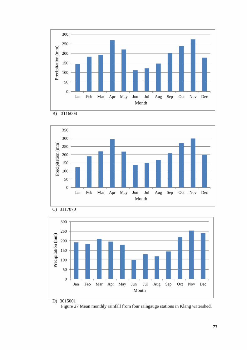
77
B) 3116004
C) 3117070
D) 3015001
Figure 27 Mean monthly rainfall from four raingauge stations in Klang watershed.
0
50
100
150
200
250
300
Jan Feb Mar Apr May Jun Jul Aug Sep Oct Nov Dec
Pre
cipit
atio
n (
mm
)
Month
0
50
100
150
200
250
300
350
Jan Feb Mar Apr May Jun Jul Aug Sep Oct Nov Dec
Pre
cipit
atio
n (
mm
)
Month
0
50
100
150
200
250
300
Jan Feb Mar Apr May Jun Jul Aug Sep Oct Nov Dec
Pre
cipit
atio
n (
mm
)
Month
78
3-3-3- Spatial Annual Mean Rainfall
The simplest method to make the spatial mean of data was provided by Thiessen
(1911). But it does not reflect all the physical aspects particularly topography data as
it amounts at drawing around each gauge, a polygon of influence with the boundaries
at a distance of halfway between gauge pairs.
The Isohyetal method (McCuen, 1998) is used to estimate the non-sample location by
interpolation within the isohyets. However, the main limitation of isohyetal is an
extensive gauge network is required to draw isohyets accurately. Kriging is the most
famous Geostatistical method used in ArcGIS to produce the spatial map from the
certain points. However, there are known limitations with Kriging, especially its
numerical instability for large samples and/or dimensions (Cressie and Johannesson,
2008).
To estimate rainfall trend over Klang watershed it was attempted to establish a spatial
rainfall analysis over 23 selected raingauge stations using GIS system. Mean annual
rainfall is about 2400 mm and mean monthly rainfall ranges from 200 to 400 mm
(Tick and Samah, 2004).
Inverse Distance weighting (IDW), developed by U.S. National Weather Service in
1972, is based on the distance weighting. Many studies have used this method for a
long range of precipitation data (Segond et al., 2007; Lu and Wong, 2008; Wu et al.,
2010). Hsieh et al., (2006) studied spatial interpolation of daily rainfall record from 20
raingauges in 11 year period. They found out that IDW has a good performance for
interpolation of rainfall in Shih-Men watershed in Taiwan.
In this study, the interpolation processes employed the IDW method to estimate
spatial mean precipitation as the available data of distributed raingauges in Klang
watershed and also with long time series. The amount of rainfall at the non-sampling
location is then estimated by interpolation with IDW. The IDW formula defined by
Morrison (1971) is given below:
79
p (di
-
di- n
i
ni i Equation 27
Where, p is the unknown rainfall data (mm), i is the rainfall value at the known
location (mm), di is the distance from each raingauge station to unknown site, n is the
number of raingauge station and is the coefficient, which is assumed equal to 2 (Lin
and Yu, 2008).
The watershed has an average annual rainfall of 2282 mm, the largest portion of the
rainfall occurs in October, November and December. As it is observed from Figure
28, the spatial variability of rainfall in the watershed indicates that the mean annual
rainfall is high on the central area of the scope at the centre and West where two of
the main rivers, Klang and Batu river are connected near to the coastal line.
3-3-4- Probable Maximum Precipitation (PMP)
PMP is defined as the greatest depth of precipitation for a given duration that is
physically or meteorologically possible over a given station or area at a particular
geographical location at a certain time of the year (WMO, 1986). PMP is calculated
at a point site and for preparing a spatial map of PMP which needs to be interpolated
by GIS to a surface map for the whole watershed. Obviously, using long time period
of data gives an accurate value of PMP for each raingauge.
In this study, the Harshfield method (WMO, 1986) is used to calculate the probable
maximum precipitation because of statistical approach which uses annual maximum
rainfall series in the study area. The Harshfield Equation is given as:
PMP n Equation 28
PMP is Probable maximum precipitation, n is mean of the series of annual
maximum daily rainfall, K is frequency factor, is Standard deviation of the series of
annual maximum daily rainfall.
80
Hydrologic frequency factor, K, is a location dependant and it is a primarily function
of the recurrence interval for a particular probability distribution. Desa et al. (2001)
have suggested frequency factor, k, equals to 8.7 employing the Harshfield method to
analyse the frequency factor for the Peninsula Malaysia using annual daily maximum
series rainfall.
Table 9 gives PMP values of 1, 3 and 7 day and Figures (from 29 to 31) show spatial
PMP maps using annual daily maximum rainfall series in Klang watershed. The
Figures reveal that the mountain parts particularly in east and north-east have the
highest value of PMP and on the other hand the inland area of Klang watershed has
the lowest values. It can be concluded that the trend of PMP in the watershed is
dependent on the influence of northeast monsoon winds although the mountains can
play an obstruction in the area.
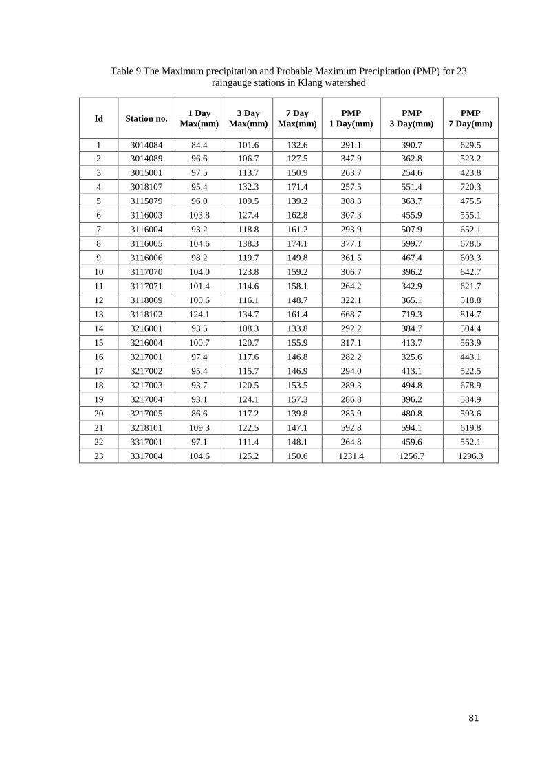
81
Table 9 The Maximum precipitation and Probable Maximum Precipitation (PMP) for 23
raingauge stations in Klang watershed
Id Station no. 1 Day
Max(mm)
3 Day
Max(mm)
7 Day
Max(mm)
PMP
1 Day(mm)
PMP
3 Day(mm)
PMP
7 Day(mm)
1 3014084 84.4 101.6 132.6 291.1 390.7 629.5
2 3014089 96.6 106.7 127.5 347.9 362.8 523.2
3 3015001 97.5 113.7 150.9 263.7 254.6 423.8
4 3018107 95.4 132.3 171.4 257.5 551.4 720.3
5 3115079 96.0 109.5 139.2 308.3 363.7 475.5
6 3116003 103.8 127.4 162.8 307.3 455.9 555.1
7 3116004 93.2 118.8 161.2 293.9 507.9 652.1
8 3116005 104.6 138.3 174.1 377.1 599.7 678.5
9 3116006 98.2 119.7 149.8 361.5 467.4 603.3
10 3117070 104.0 123.8 159.2 306.7 396.2 642.7
11 3117071 101.4 114.6 158.1 264.2 342.9 621.7
12 3118069 100.6 116.1 148.7 322.1 365.1 518.8
13 3118102 124.1 134.7 161.4 668.7 719.3 814.7
14 3216001 93.5 108.3 133.8 292.2 384.7 504.4
15 3216004 100.7 120.7 155.9 317.1 413.7 563.9
16 3217001 97.4 117.6 146.8 282.2 325.6 443.1
17 3217002 95.4 115.7 146.9 294.0 413.1 522.5
18 3217003 93.7 120.5 153.5 289.3 494.8 678.9
19 3217004 93.1 124.1 157.3 286.8 396.2 584.9
20 3217005 86.6 117.2 139.8 285.9 480.8 593.6
21 3218101 109.3 122.5 147.1 592.8 594.1 619.8
22 3317001 97.1 111.4 148.1 264.8 459.6 552.1
23 3317004 104.6 125.2 150.6 1231.4 1256.7 1296.3
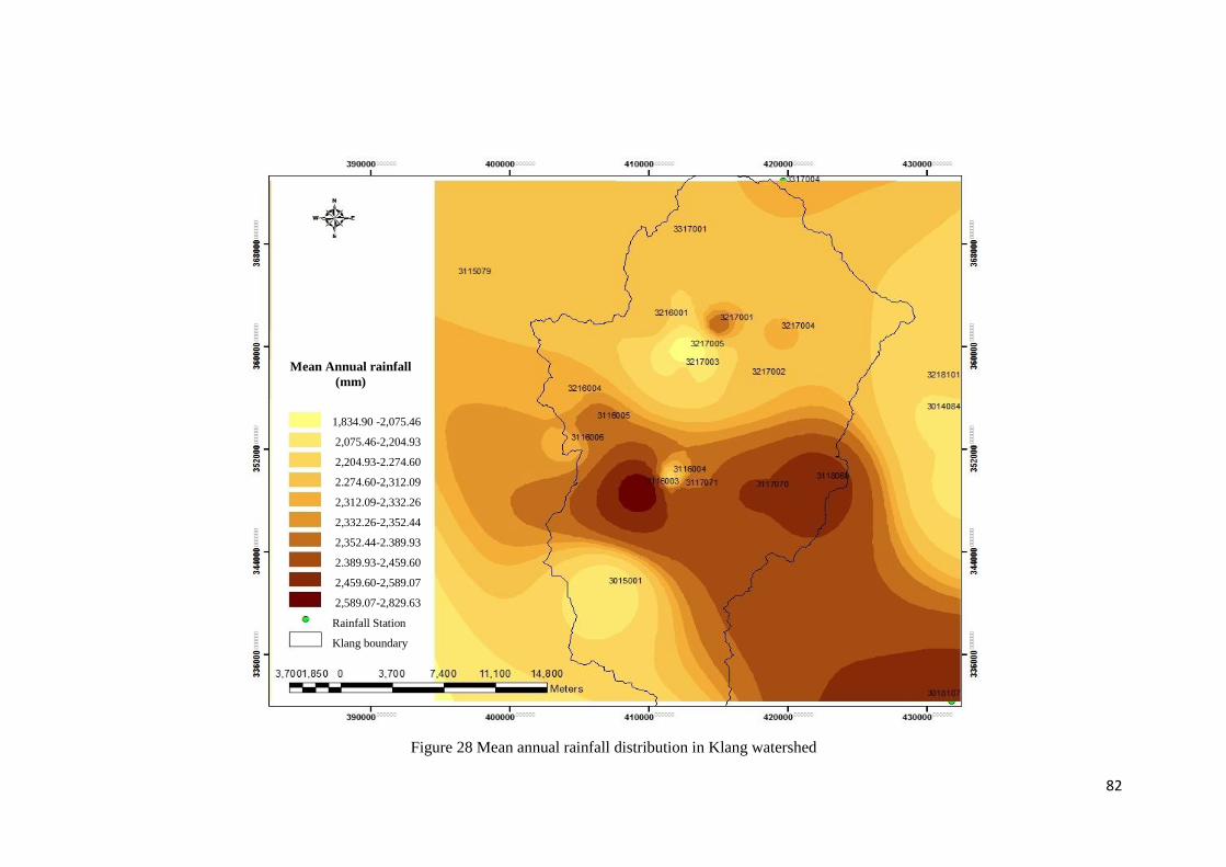
82
Figure 28 Mean annual rainfall distribution in Klang watershed
Mean Annual rainfall
(mm)
1,834.90 -2,075.46
2,075.46-2,204.93
2,204.93-2.274.60
2.274.60-2,312.09
2,312.09-2,332.26
2,332.26-2,352.44
2,352.44-2.389.93
2.389.93-2,459.60
2,459.60-2,589.07
2,589.07-2,829.63
Rainfall Station
Klang boundary
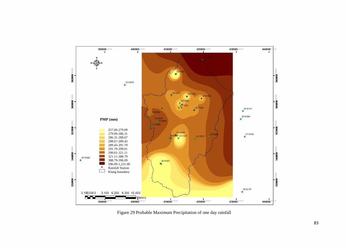
83
Figure 29 Probable Maximum Precipitation of one day rainfall
PMP (mm)
257.00-279.09
279.09-286.31 286.31-288.67
288.67-289.43
289.43-291.79 291.79-299.01
299.01-321.11
321.11-388.79 388.79-596.09
596.09-1,231.00
Rainfall Station
Klang boundary
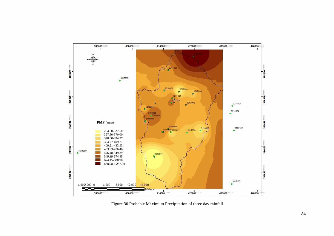
84
Figure 30 Probable Maximum Precipitation of three day rainfall
PMP (mm)
254.60-327.50 327.50-370.00
370.00-394.77
394.77-409.21 409.21-433.93
433.93-476.48
476.48-549.39 549.39-674.45
674.45-888.98
888.98-1,257.00
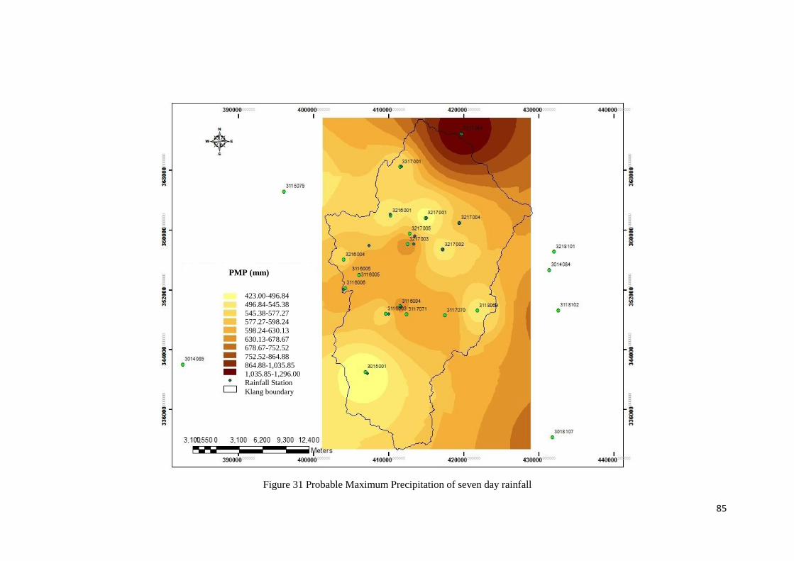
85
Figure 31 Probable Maximum Precipitation of seven day rainfall
PMP (mm)
423.00-496.84
496.84-545.38
545.38-577.27 577.27-598.24
598.24-630.13
630.13-678.67 678.67-752.52
752.52-864.88
864.88-1,035.85 1,035.85-1,296.00
Rainfall Station
Klang boundary
86
3-3-5- Frequency Analysis
Frequency analysis is a technique of fitting a probability distribution to a series of
observations to define the probabilities of future occurrences of some events of
interest. In this study, the daily rainfall is used. The duration of rainfall is one, three,
seven, ten and fifteen day for 5, 10, 25, 50 and 100 years of recurrence interval.
Gumbel Extremal Type I as a distribution analysis was employed to estimate extreme
precipitation intensity. The data are used to calculate intensities using SMADA
software as shown in Table 10. Figures (from 32 to 35) show the maps of extreme
precipitation intensity of 23 raingauge stations for one day duration rainfall for the
years of recurrence interval. SMADA fits a Gumbel Type 1 distribution to the data
using the annual maximum series (Helsel and Hirsch, 2010).
x -e-ee-(x-
Equation 29
Where, x is the maximum daily rainfall, and are the mean and variance of
maximum daily rainfall, respectively.
The annual maximum for a return period of T-years can be calculated from:
T S Equation 30
T - / ( Ln Ln T x
T - Equation 31
Which, Q is the mean annual maximums, S is the standard deviation of the
maximums, T is a frequency factor, T(X) is the return period in years, and is a
constant equal to 0.5772.
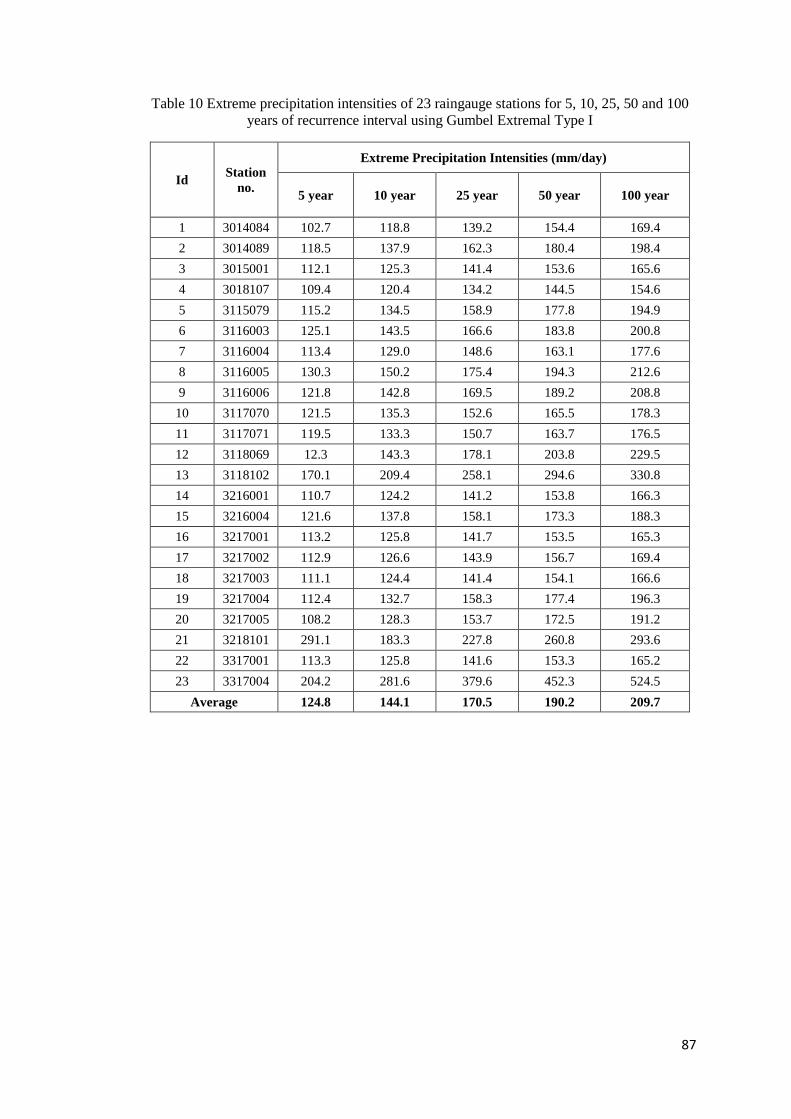
87
Table 10 Extreme precipitation intensities of 23 raingauge stations for 5, 10, 25, 50 and 100
years of recurrence interval using Gumbel Extremal Type I
Id Station
no.
Extreme Precipitation Intensities (mm/day)
5 year 10 year 25 year 50 year 100 year
1 3014084 102.7 118.8 139.2 154.4 169.4
2 3014089 118.5 137.9 162.3 180.4 198.4
3 3015001 112.1 125.3 141.4 153.6 165.6
4 3018107 109.4 120.4 134.2 144.5 154.6
5 3115079 115.2 134.5 158.9 177.8 194.9
6 3116003 125.1 143.5 166.6 183.8 200.8
7 3116004 113.4 129.0 148.6 163.1 177.6
8 3116005 130.3 150.2 175.4 194.3 212.6
9 3116006 121.8 142.8 169.5 189.2 208.8
10 3117070 121.5 135.3 152.6 165.5 178.3
11 3117071 119.5 133.3 150.7 163.7 176.5
12 3118069 12.3 143.3 178.1 203.8 229.5
13 3118102 170.1 209.4 258.1 294.6 330.8
14 3216001 110.7 124.2 141.2 153.8 166.3
15 3216004 121.6 137.8 158.1 173.3 188.3
16 3217001 113.2 125.8 141.7 153.5 165.3
17 3217002 112.9 126.6 143.9 156.7 169.4
18 3217003 111.1 124.4 141.4 154.1 166.6
19 3217004 112.4 132.7 158.3 177.4 196.3
20 3217005 108.2 128.3 153.7 172.5 191.2
21 3218101 291.1 183.3 227.8 260.8 293.6
22 3317001 113.3 125.8 141.6 153.3 165.2
23 3317004 204.2 281.6 379.6 452.3 524.5
Average 124.8 144.1 170.5 190.2 209.7
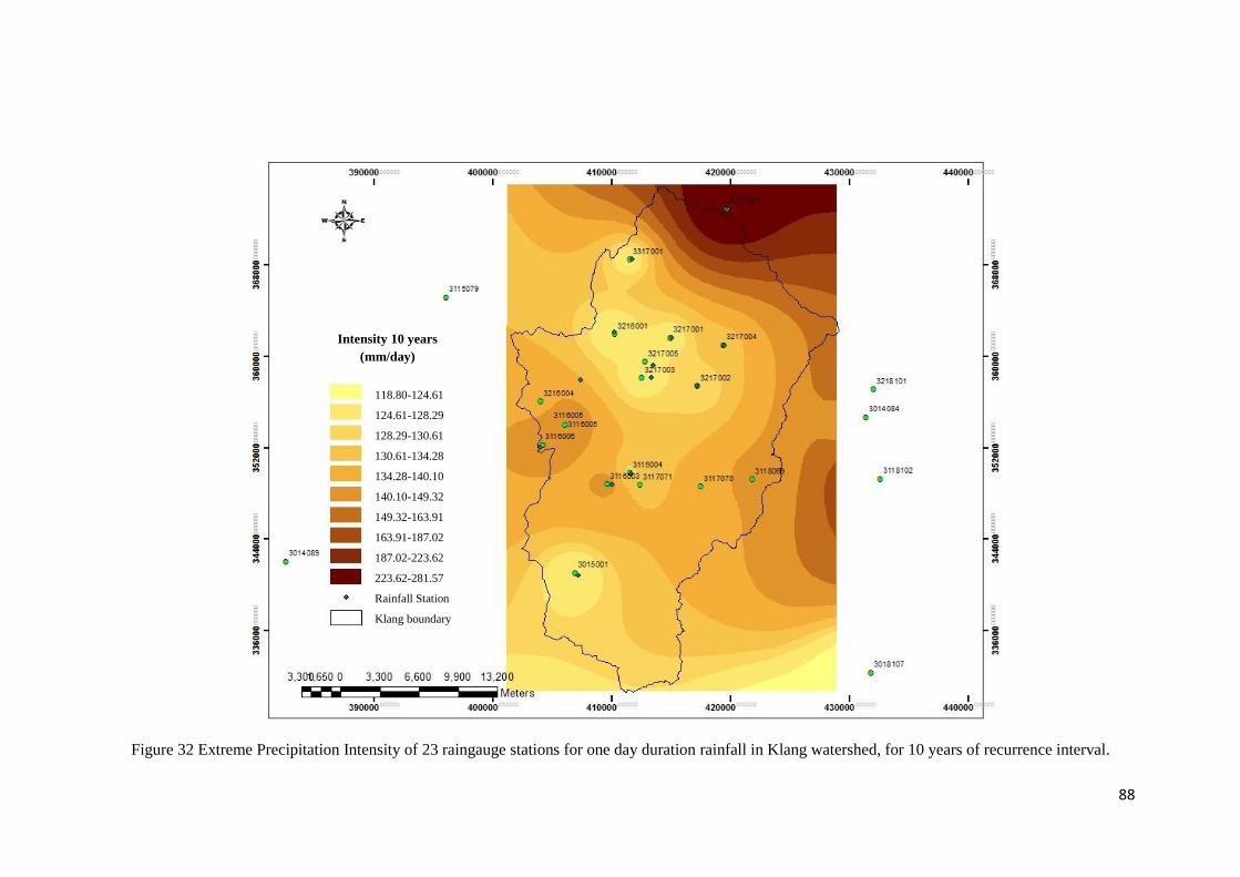
88
Figure 32 Extreme Precipitation Intensity of 23 raingauge stations for one day duration rainfall in Klang watershed, for 10 years of recurrence interval.
Intensity 10 yearsIntensity 10 years
(mm/day)
118.80-124.61
124.61-128.29
128.29-130.61
130.61-134.28
134.28-140.10
140.10-149.32
149.32-163.91
163.91-187.02
187.02-223.62
223.62-281.57
Rainfall Station
Klang boundary
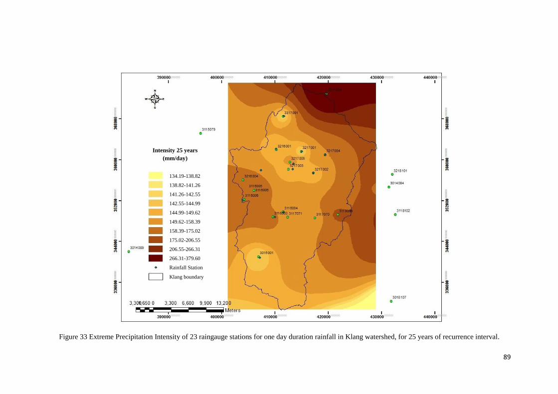
89
Figure 33 Extreme Precipitation Intensity of 23 raingauge stations for one day duration rainfall in Klang watershed, for 25 years of recurrence interval.
Intensity 25 yearsIntensity 25 years
(mm/day)
134.19-138.82
138.82-141.26
141.26-142.55
142.55-144.99
144.99-149.62
149.62-158.39
158.39-175.02
175.02-206.55
206.55-266.31
266.31-379.60
Rainfall Station
Klang boundary
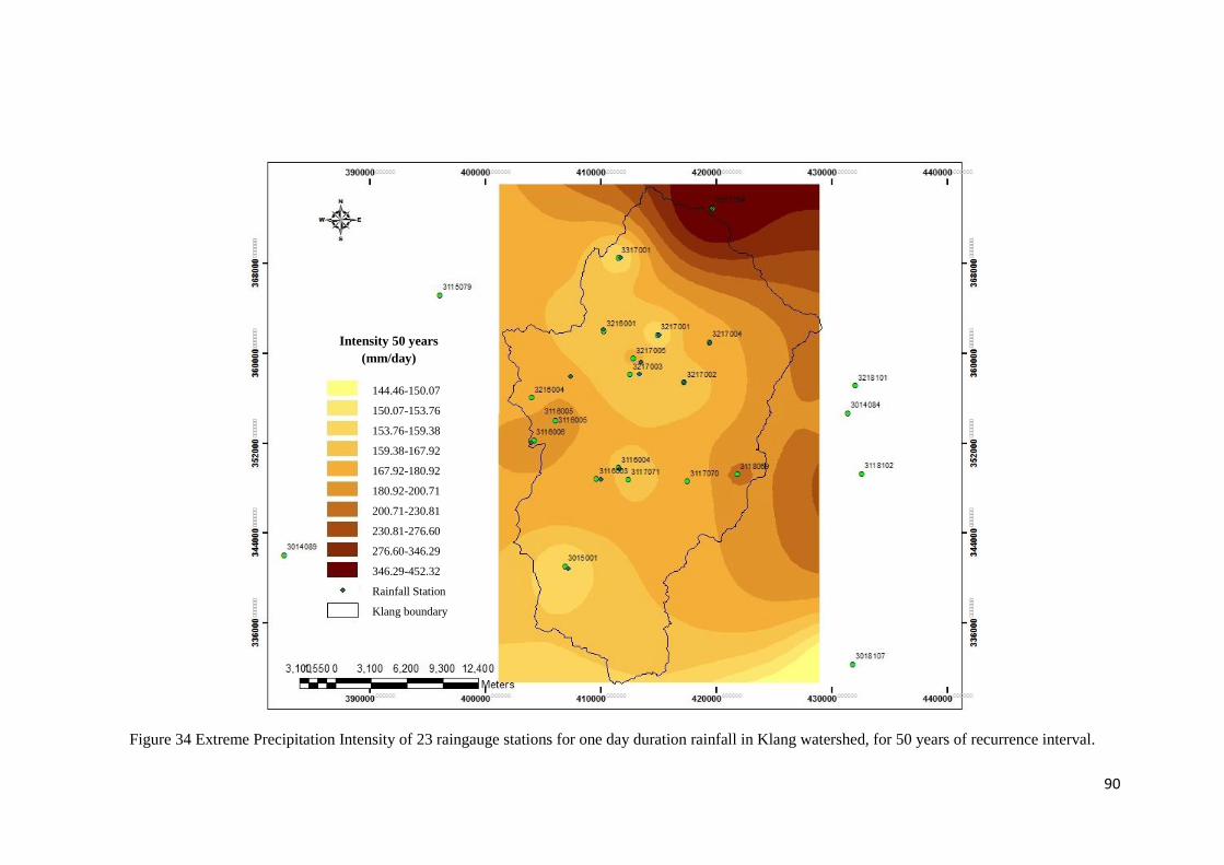
90
Figure 34 Extreme Precipitation Intensity of 23 raingauge stations for one day duration rainfall in Klang watershed, for 50 years of recurrence interval.
Intensity 50 yearsIntensity 50 years
(mm/day)
144.46-150.07
150.07-153.76
153.76-159.38
159.38-167.92
167.92-180.92
180.92-200.71
200.71-230.81
230.81-276.60
276.60-346.29
346.29-452.32
Rainfall Station
Klang boundary
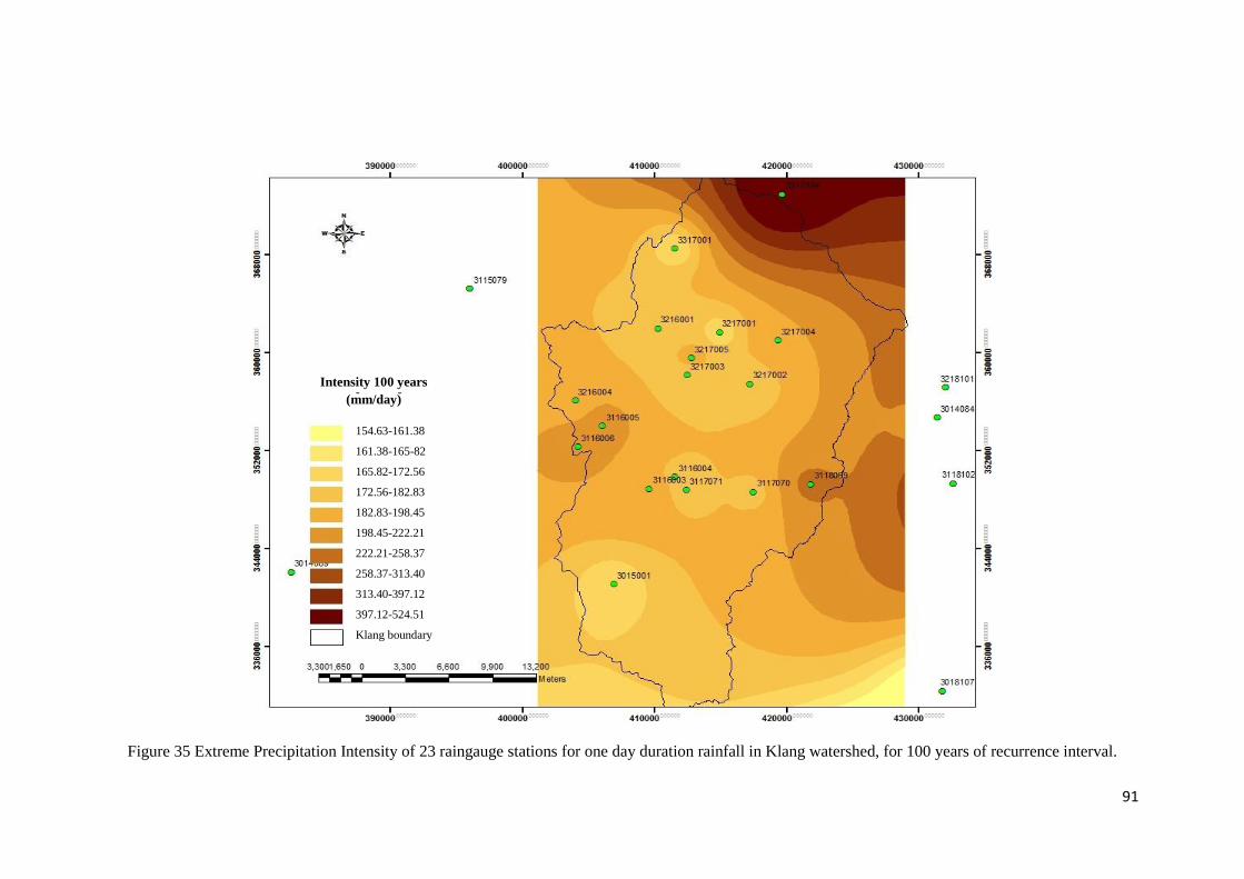
91
Figure 35 Extreme Precipitation Intensity of 23 raingauge stations for one day duration rainfall in Klang watershed, for 100 years of recurrence interval.
Intensity 100 yearsIntensity 100 years
(mm/day)
154.63-161.38
161.38-165-82
165.82-172.56
172.56-182.83
182.83-198.45
198.45-222.21
222.21-258.37
258.37-313.40
313.40-397.12
397.12-524.51
Klang boundary
92
3-4- River Discharge Analysis
River discharge is the volume of water moving across a vertical section of water flow
in a time unit. It is usually measured in cubic metre per second for rivers. There are
parameters such as topography, landuse and soil affect the behaviour of the
streamflow by altering the rainfall-runoff relationship. For example, changing landuse
toward increasing area of impervious surfaces would increase peak discharges by not
allowing the water to infiltrate into the ground.
In this study, daily river discharge data over 33 years (1975-2007) are used to analysis
the monthly and annual variation of the streamflow. It reveals the historic pattern of
streamflow and the frequency of extreme flow events occurrence to show the
expected trend of future streamflow and also yearly flow duration relations.
The trend analysis of the discharge at Sulaiman streamflow station in Klang River can
help reveal the streamflow behaviour. Since Sulaiman streamflow station is situated
along the main Klang river at the outlet of Upper Klang watershed, the hydrological
modelling uses this discharge station for calibration and validation of modelled
runoff.
3-4-1- Mean Monthly River Discharge
Figure 36 is the plot of the mean monthly discharge of the river for the period of 1975
to 2007 at the Jambatan Sulaiman streamflow station. The Figure reveals the highest
river discharge records between October to December and also through April and
May. The streamflow is the lowest between June to September and January to March.
The flow data of Klang River at Sulaiman streamflow station reveals that the flow
regime mainly depends on the North-East monsoon which is from November to
March contributes around 41 percent compared to the South-West monsoon equals to
31 percent of the annual streamflow as Table 11. The mean monthly river discharge
for the period of 1960 -2007 for the Tun Razak and Batu Sentul streamflow stations
are available in Appendix F.
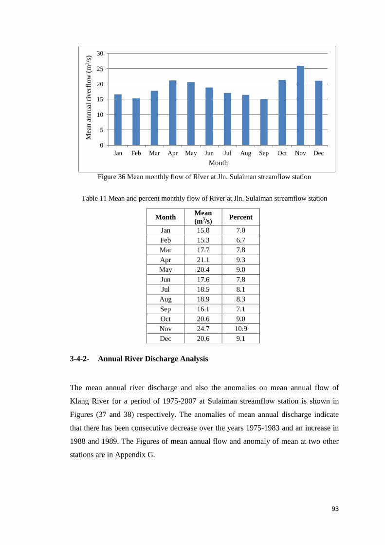
93
Figure 36 Mean monthly flow of River at Jln. Sulaiman streamflow station
Table 11 Mean and percent monthly flow of River at Jln. Sulaiman streamflow station
3-4-2- Annual River Discharge Analysis
The mean annual river discharge and also the anomalies on mean annual flow of
Klang River for a period of 1975-2007 at Sulaiman streamflow station is shown in
Figures (37 and 38) respectively. The anomalies of mean annual discharge indicate
that there has been consecutive decrease over the years 1975-1983 and an increase in
1988 and 1989. The Figures of mean annual flow and anomaly of mean at two other
stations are in Appendix G.
0
5
10
15
20
25
30
Jan Feb Mar Apr May Jun Jul Aug Sep Oct Nov Dec
Mea
n a
nnual
riv
erfl
ow
(m
3/s
)
Month
Month Mean
(m3/s)
Percent
Jan 15.8 7.0
Feb 15.3 6.7
Mar 17.7 7.8
Apr 21.1 9.3
May 20.4 9.0
Jun 17.6 7.8
Jul 18.5 8.1
Aug 18.9 8.3
Sep 16.1 7.1
Oct 20.6 9.0
Nov 24.7 10.9
Dec 20.6 9.1
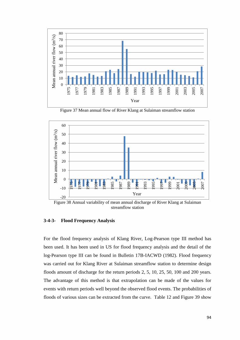
94
Figure 37 Mean annual flow of River Klang at Sulaiman streamflow station
Figure 38 Annual variability of mean annual discharge of River Klang at Sulaiman
streamflow station
3-4-3- Flood Frequency Analysis
For the flood frequency analysis of Klang River, Log-Pearson type III method has
been used. It has been used in US for flood frequency analysis and the detail of the
log-Pearson type III can be found in Bulletin 17B-IACWD (1982). Flood frequency
was carried out for Klang River at Sulaiman streamflow station to determine design
floods amount of discharge for the return periods 2, 5, 10, 25, 50, 100 and 200 years.
The advantage of this method is that extrapolation can be made of the values for
events with return periods well beyond the observed flood events. The probabilities of
floods of various sizes can be extracted from the curve. Table 12 and Figure 39 show
0
10
20
30
40
50
60
70
80
19
75
19
77
19
79
19
81
19
83
19
85
19
87
19
89
19
91
19
93
19
95
19
97
19
99
20
01
20
03
20
05
20
07
Mea
n a
nnual
riv
er f
low
(m
3/s
)
Year
-20
-10
0
10
20
30
40
50
60
19
75
19
77
19
79
19
81
19
83
19
85
19
87
19
89
19
91
19
93
19
95
19
97
19
99
20
01
20
03
20
05
20
07
Mea
n a
nnual
riv
er f
low
(m
3/s
)
Year
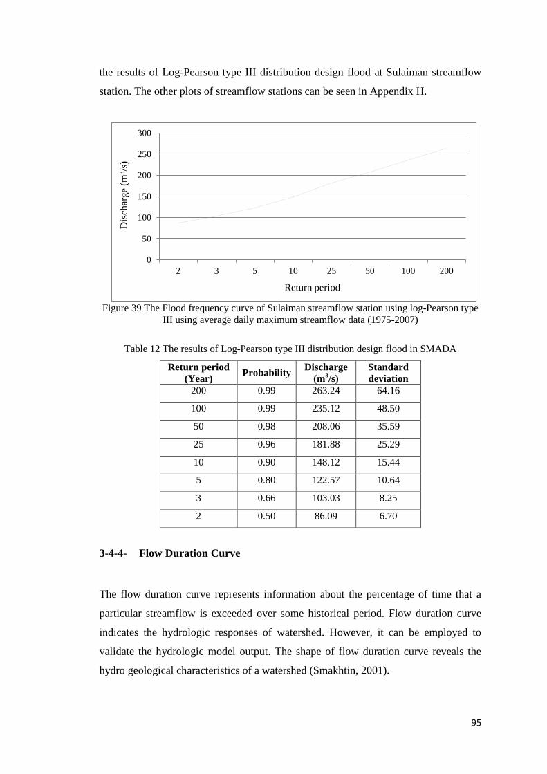
95
the results of Log-Pearson type III distribution design flood at Sulaiman streamflow
station. The other plots of streamflow stations can be seen in Appendix H.
Figure 39 The Flood frequency curve of Sulaiman streamflow station using log-Pearson type
III using average daily maximum streamflow data (1975-2007)
Table 12 The results of Log-Pearson type III distribution design flood in SMADA
Return period
(Year) Probability
Discharge
(m3/s)
Standard
deviation
200 0.99 263.24 64.16
100 0.99 235.12 48.50
50 0.98 208.06 35.59
25 0.96 181.88 25.29
10 0.90 148.12 15.44
5 0.80 122.57 10.64
3 0.66 103.03 8.25
2 0.50 86.09 6.70
3-4-4- Flow Duration Curve
The flow duration curve represents information about the percentage of time that a
particular streamflow is exceeded over some historical period. Flow duration curve
indicates the hydrologic responses of watershed. However, it can be employed to
validate the hydrologic model output. The shape of flow duration curve reveals the
hydro geological characteristics of a watershed (Smakhtin, 2001).
0
50
100
150
200
250
300
2 3 5 10 25 50 100 200
Dis
char
ge
(m3/s
)
Return period
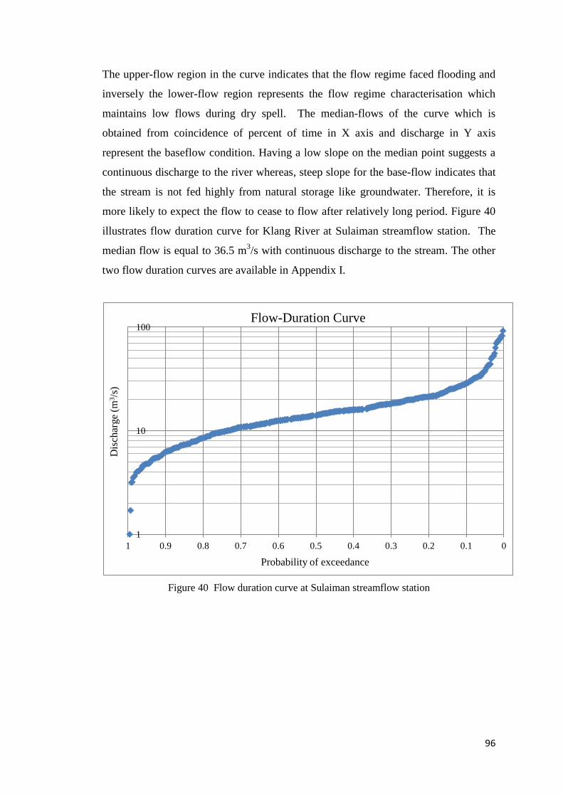
96
The upper-flow region in the curve indicates that the flow regime faced flooding and
inversely the lower-flow region represents the flow regime characterisation which
maintains low flows during dry spell. The median-flows of the curve which is
obtained from coincidence of percent of time in X axis and discharge in Y axis
represent the baseflow condition. Having a low slope on the median point suggests a
continuous discharge to the river whereas, steep slope for the base-flow indicates that
the stream is not fed highly from natural storage like groundwater. Therefore, it is
more likely to expect the flow to cease to flow after relatively long period. Figure 40
illustrates flow duration curve for Klang River at Sulaiman streamflow station. The
median flow is equal to 36.5 m3/s with continuous discharge to the stream. The other
two flow duration curves are available in Appendix I.
Figure 40 Flow duration curve at Sulaiman streamflow station
1
10
100
0 0.1 0.2 0.3 0.4 0.5 0.6 0.7 0.8 0.9 1
Dis
char
ge
(m3/s
)
Probability of exceedance
Flow-Duration Curve
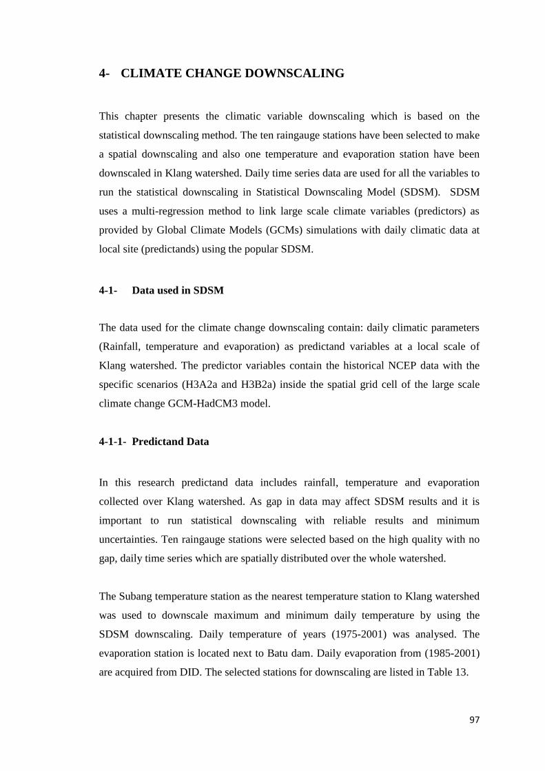
97
4- CLIMATE CHANGE DOWNSCALING
This chapter presents the climatic variable downscaling which is based on the
statistical downscaling method. The ten raingauge stations have been selected to make
a spatial downscaling and also one temperature and evaporation station have been
downscaled in Klang watershed. Daily time series data are used for all the variables to
run the statistical downscaling in Statistical Downscaling Model (SDSM). SDSM
uses a multi-regression method to link large scale climate variables (predictors) as
provided by Global Climate Models (GCMs) simulations with daily climatic data at
local site (predictands) using the popular SDSM.
4-1- Data used in SDSM
The data used for the climate change downscaling contain: daily climatic parameters
(Rainfall, temperature and evaporation) as predictand variables at a local scale of
Klang watershed. The predictor variables contain the historical NCEP data with the
specific scenarios (H3A2a and H3B2a) inside the spatial grid cell of the large scale
climate change GCM-HadCM3 model.
4-1-1- Predictand Data
In this research predictand data includes rainfall, temperature and evaporation
collected over Klang watershed. As gap in data may affect SDSM results and it is
important to run statistical downscaling with reliable results and minimum
uncertainties. Ten raingauge stations were selected based on the high quality with no
gap, daily time series which are spatially distributed over the whole watershed.
The Subang temperature station as the nearest temperature station to Klang watershed
was used to downscale maximum and minimum daily temperature by using the
SDSM downscaling. Daily temperature of years (1975-2001) was analysed. The
evaporation station is located next to Batu dam. Daily evaporation from (1985-2001)
are acquired from DID. The selected stations for downscaling are listed in Table 13.
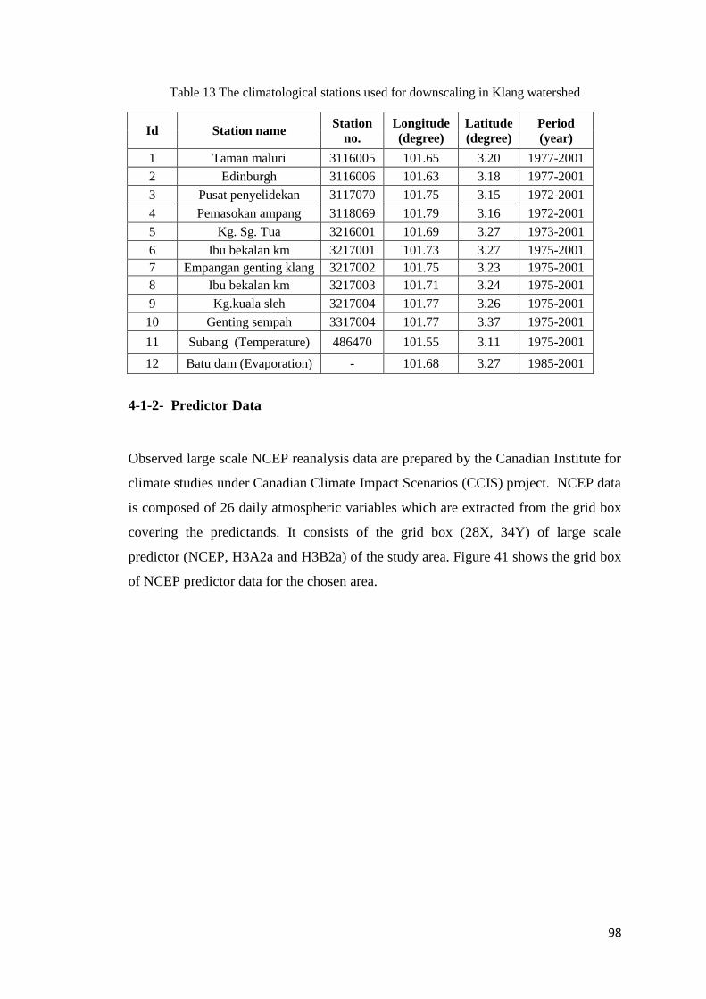
98
Table 13 The climatological stations used for downscaling in Klang watershed
Id Station name Station
no.
Longitude
(degree)
Latitude
(degree)
Period
(year)
1 Taman maluri 3116005 101.65 3.20 1977-2001
2 Edinburgh 3116006 101.63 3.18 1977-2001
3 Pusat penyelidekan 3117070 101.75 3.15 1972-2001
4 Pemasokan ampang 3118069 101.79 3.16 1972-2001
5 Kg. Sg. Tua 3216001 101.69 3.27 1973-2001
6 Ibu bekalan km 3217001 101.73 3.27 1975-2001
7 Empangan genting klang 3217002 101.75 3.23 1975-2001
8 Ibu bekalan km 3217003 101.71 3.24 1975-2001
9 Kg.kuala sleh 3217004 101.77 3.26 1975-2001
10 Genting sempah 3317004 101.77 3.37 1975-2001
11 Subang (Temperature) 486470 101.55 3.11 1975-2001
12 Batu dam (Evaporation) - 101.68 3.27 1985-2001
4-1-2- Predictor Data
Observed large scale NCEP reanalysis data are prepared by the Canadian Institute for
climate studies under Canadian Climate Impact Scenarios (CCIS) project. NCEP data
is composed of 26 daily atmospheric variables which are extracted from the grid box
covering the predictands. It consists of the grid box (28X, 34Y) of large scale
predictor (NCEP, H3A2a and H3B2a) of the study area. Figure 41 shows the grid box
of NCEP predictor data for the chosen area.
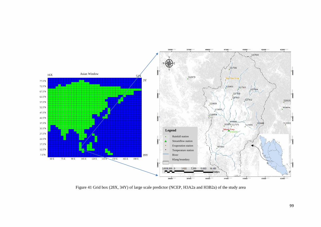
99
Figure 41 Grid box (28X, 34Y) of large scale predictor (NCEP, H3A2a and H3B2a) of the study area
39Y
3Y
Asian Window
Rainfall station
Streamflow station
Evaporation station
Temperature station
River
Klang boundary
Legend
60 E 75 E 90 E 105 E 120 E 135 E 150 E 165 E 180 E
77.5oN
72.5oN
67.5oN
62.5oN
57.5oN
52.5oN
47.5oN
42.5oN
37.5oN
32.5oN
27.5oN
22.5oN
17.5oN
12.5oN
7.5oN
2.5oN
2.5oS
7.5oS
EQ
16X 52X
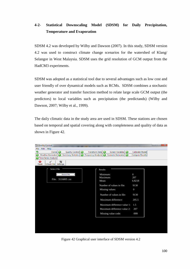
100
4-2- Statistical Downscaling Model (SDSM) for Daily Precipitation,
Temperature and Evaporation
SDSM 4.2 was developed by Wilby and Dawson (2007). In this study, SDSM version
4.2 was used to construct climate change scenarios for the watershed of Klang/
Selangor in West Malaysia. SDSM uses the grid resolution of GCM output from the
HadCM3 experiments.
SDSM was adopted as a statistical tool due to several advantages such as low cost and
user friendly of over dynamical models such as RCMs. SDSM combines a stochastic
weather generator and transfer function method to relate large scale GCM output (the
predictors) to local variables such as precipitation (the predictands) (Wilby and
Dawson, 2007; Wilby et al., 1999).
The daily climatic data in the study area are used in SDSM. These stations are chosen
based on temporal and spatial covering along with completeness and quality of data as
shown in Figure 42.
Figure 42 Graphical user interface of SDSM version 4.2
Mean: 6.8218
Number of values in file: 9130
207 Missing values: 0
207 Number of values in file: 9130
207 Maximum difference: 205.5
Maximum difference value 1: 1.5
File: 3116005 .txt
Minimum: 0
Select File Results
Maximum difference value 2: 207
Missing value code: -999
207
Maximum: 207
101
4-2-1- SDSM for Klang Watershed
In this study, precipitation, maximum and minimum temperatures and evaporation as
predictand data are downscaled for the study area. According to Wilby et al. (2001)
SDSM needs to set up for the various predictands to get a reliable result. This task
runs quality control checks of the observed daily climate data to identify the gross
data error and missing data. It also transforms a fourth root model function to
normalise the distribution and make it less skewed to low precipitation values. The
fourth root transformation is used as distribution of data is skewed in a conditional
process (Khan et al., 2005). Setting up of SDSM involves following steps:
Adjusting a 366 days as the year length for the predictand and NCEP data,
Adjusting a 360 days as the year length for HadCM3-GCM model where, each
month is 30 days,
To set the value of 0.3 mm per day as threshold value in precipitation data
(Khan et al., 2005) and a zero value for temperature: Specifying the threshold
value which is useful to trace the rainy days in calibration and validation in
SDSM,
Defining the conditional model for precipitation and evaporation in
downscaling,
Defining the non-conditional model for temperature in downscaling,
Defining the fourth root transformation for transformation of precipitation and
evaporation data. However, no transformation function was used for
temperature data.
Setting variance inflation value of 12 as default for all the predictands data.
(The variance inflation controls the range of variation of downscaled daily
predictands) and
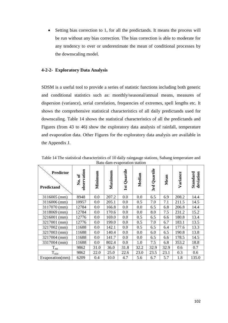
102
Setting bias correction to 1, for all the predictands. It means the process will
be run without any bias correction. The bias correction is able to moderate for
any tendency to over or underestimate the mean of conditional processes by
the downscaling model.
4-2-2- Exploratory Data Analysis
SDSM is a useful tool to provide a series of statistic functions including both generic
and conditional statistics such as: monthly/seasonal/annual means, measures of
dispersion (variance), serial correlation, frequencies of extremes, spell lengths etc. It
shows the comprehensive statistical characteristics of all daily predictands used for
downscaling. Table 14 shows the statistical characteristics of all the predictands and
Figures (from 43 to 46) show the exploratory data analysis of rainfall, temperature
and evaporation data. Other Figures for the exploratory data analysis are available in
the Appendix J.
Table 14 The statistical characteristics of 10 daily raingauge stations, Subang temperature and
Batu dam evaporation station
Predictor
Predictand
No.
of
ob
servati
on
Min
imu
m
Maxim
um
1st
Qu
art
ile
Med
ian
3rd
Qu
art
ile
Mea
n
Vari
an
ce
Sta
nd
ard
dev
iati
on
3116005 (mm) 8948 0.0 207.2 0.0 0.0 6.5 6.9 208.2 14.4
3116006 (mm) 10957 0.0 205.1 0.0 0.5 7.0 7.1 211.5 14.5
3117070 (mm) 12784 0.0 166.8 0.0 0.0 6.5 6.8 206.8 14.4
3118069 (mm) 12784 0.0 170.6 0.0 0.0 8.0 7.5 231.2 15.2
3216001 (mm) 12776 0.0 169.0 0.0 0.5 6.5 6.6 180.8 13.4
3217001 (mm) 12776 0.0 199.0 0.0 0.5 7.0 6.7 183.1 13.5
3217002 (mm) 11688 0.0 142.1 0.0 0.5 6.5 6.4 177.6 13.3
3217003 (mm) 11688 0.0 140.4 0.0 0.0 6.0 6.5 190.8 13.8
3217004 (mm) 11688 0.0 141.7 0.0 0.0 6.5 6.6 178.5 14.5
3317004 (mm) 11688 0.0 802.4 0.0 1.0 7.5 6.8 353.2 18.8
Tma 9862 31.0 36.0 31.8 32.2 32.9 32.9 0.6 0.7
Tmin 9862 22.0 25.0 22.6 23.0 23.5 23.1 0.3 0.6
Evaporation(mm) 6209 0.4 10.0 4.7 5.6 6.7 5.7 1.8 135.0
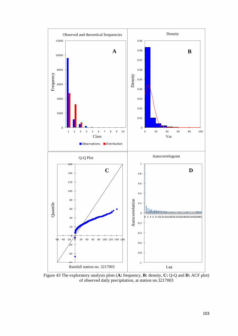
103
Figure 43 The exploratory analysis plots (A: frequency, B: density, C: Q-Q and D: ACF plot)
of observed daily precipitation, at station no.3217003
0
2000
4000
6000
8000
10000
12000
1 2 3 4 5 6 7 8 9 10
Fre
qu
en
cy
Class
Observed and theoretical frequencies
Observations Distribution
0
0.01
0.02
0.03
0.04
0.05
0.06
0.07
0.08
0.09
0 20 40 60 80 100D
en
sity
Var1
Histograms
Var1 Normal(6.310,9.113)
-1
-0.8
-0.6
-0.4
-0.2
0
0.2
0.4
0.6
0.8
1
0 2 4 6 8 10121416182022242628303234363840
Au
toco
rre
lati
on
Lag
Autocorrelogram (Series1)
-60
-40
-20
0
20
40
60
80
100
120
140
160
-60 -40 -20 0 20 40 60 80 100 120 140 160
Qu
anti
le -
No
rmal
(6.5
1, 1
3.8
1)
Var1
Q-Q plot (Var1)
Fre
qu
ency
Den
sity
Qu
anti
le
Au
toco
rrel
atio
n
A
C
B
D
Observed and theoretical frequencies
Q-Q Plot
Lag
Density
Autocorrelogram
Rainfall station no. 3217003
Var Class
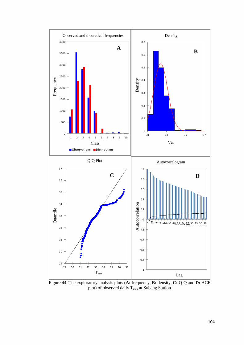
104
Figure 44 The exploratory analysis plots (A: frequency, B: density, C: Q-Q and D: ACF
plot) of observed daily Tmax at Subang Station
0
500
1000
1500
2000
2500
3000
3500
4000
1 2 3 4 5 6 7 8 9 10
Fre
qu
en
cy
Class
Observed and theoretical frequencies
Observations Distribution
0
0.1
0.2
0.3
0.4
0.5
0.6
0.7
31 33 35 37D
en
sity
Var1
Histograms
Var1 Normal(32.383,0.753)
-1
-0.8
-0.6
-0.4
-0.2
0
0.2
0.4
0.6
0.8
1
0 3 6 9 12 15 18 21 24 27 30 33 36 39
Au
toco
rre
lati
on
Lag
Autocorrelogram (Series1)
29
30
31
32
33
34
35
36
37
29 30 31 32 33 34 35 36 37
Qu
anti
le -
No
rmal
(32
.38
, 0.7
5)
Var1
Q-Q plot (Var1)
Fre
qu
ency
Den
sity
Qu
anti
le
Au
toco
rrel
atio
n
C
A
D
Q-Q Plot
Lag
Density
Autocorrelogram
Tmax
Var Class
Observed and theoretical frequencies
B
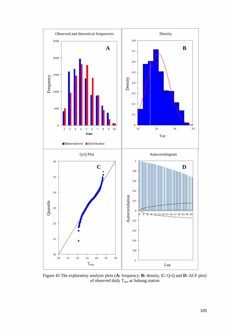
105
Figure 45 The exploratory analysis plots (A: frequency, B: density, C: Q-Q and D: ACF plot)
of observed daily Tmin at Subang station
20
21
22
23
24
25
26
20 21 22 23 24 25 26
Qu
anti
le -
No
rmal
(23
.10
, 0.5
9)
Var1
Q-Q plot (Var1)
-1
-0.8
-0.6
-0.4
-0.2
0
0.2
0.4
0.6
0.8
1
0 3 6 9 12 15 18 21 24 27 30 33 36 39
Au
toco
rre
lati
on
Lag
Autocorrelogram (Series1)
0
500
1000
1500
2000
2500
1 2 3 4 5 6 7 8 9 10
Fre
qu
en
cy
Class
Observed and theoretical frequencies
Observations Distribution
0
0.1
0.2
0.3
0.4
0.5
0.6
0.7
0.8
22 23 24 25D
en
sity
Var1
Histograms
Var1 Normal(23.100,0.590)
Au
toco
rrel
atio
n
Fre
qu
ency
Den
sity
Qu
anti
leA B
Observed and theoretical frequencies Density
Tmin
Var
Lag
Autocorrelogram Q-Q Plot
C D
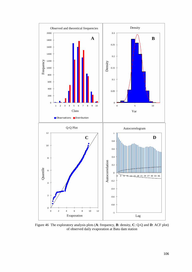
106
Figure 46 The exploratory analysis plots (A: frequency, B: density, C: Q-Q and D: ACF plot)
of observed daily evaporation at Batu dam station
0
200
400
600
800
1000
1200
1400
1600
1800
2000
1 2 3 4 5 6 7 8 9 10
Fre
qu
en
cy
Class
Observed and theoretical frequencies
Observations Distribution
0
0.05
0.1
0.15
0.2
0.25
0.3
0 5 10D
en
sity
Var1
Histograms
Var1 Normal(5.694,1.355)
0
2
4
6
8
10
12
0 2 4 6 8 10 12
Qu
anti
le -
No
rmal
(5.6
9, 1
.36
)
Var1
Q-Q plot (Var1)
-1
-0.8
-0.6
-0.4
-0.2
0
0.2
0.4
0.6
0.8
1
0 3 6 9 12 15 18 21 24 27 30 33 36
Au
toco
rre
lati
on
Lag
Autocorrelogram (Series1)
Fre
qu
ency
Den
sity
Au
toco
rrel
atio
n
Qu
anti
le
C
A B
D
Q-Q Plot
Var Class
Evaporation Lag
Density
Autocorrelogram
Observed and theoretical frequencies
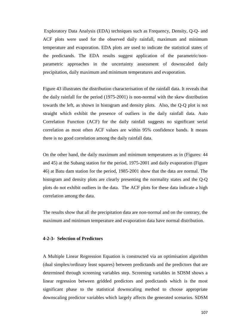
107
Exploratory Data Analysis (EDA) techniques such as Frequency, Density, Q-Q- and
ACF plots were used for the observed daily rainfall, maximum and minimum
temperature and evaporation. EDA plots are used to indicate the statistical states of
the predictands. The EDA results suggest application of the parametric/non-
parametric approaches in the uncertainty assessment of downscaled daily
precipitation, daily maximum and minimum temperatures and evaporation.
Figure 43 illustrates the distribution characterisation of the rainfall data. It reveals that
the daily rainfall for the period (1975-2001) is non-normal with the skew distribution
towards the left, as shown in histogram and density plots. Also, the Q-Q plot is not
straight which exhibit the presence of outliers in the daily rainfall data. Auto
Correlation Function (ACF) for the daily rainfall suggests no significant serial
correlation as most often ACF values are within 95% confidence bands. It means
there is no good correlation among the daily rainfall data.
On the other hand, the daily maximum and minimum temperatures as in (Figures: 44
and 45) at the Subang station for the period, 1975-2001 and daily evaporation (Figure
46) at Batu dam station for the period, 1985-2001 show that the data are normal. The
histogram and density plots are clearly presenting the normality states and the Q-Q
plots do not exhibit outliers in the data. The ACF plots for these data indicate a high
correlation among the data.
The results show that all the precipitation data are non-normal and on the contrary, the
maximum and minimum temperature and evaporation data have normal distribution.
4-2-3- Selection of Predictors
A Multiple Linear Regression Equation is constructed via an optimisation algorithm
(dual simplex/ordinary least squares) between predictands and the predictors that are
determined through screening variables step. Screening variables in SDSM shows a
linear regression between gridded predictors and predictands which is the most
significant phase to the statistical downscaling method to choose appropriate
downscaling predictor variables which largely affects the generated scenarios. SDSM
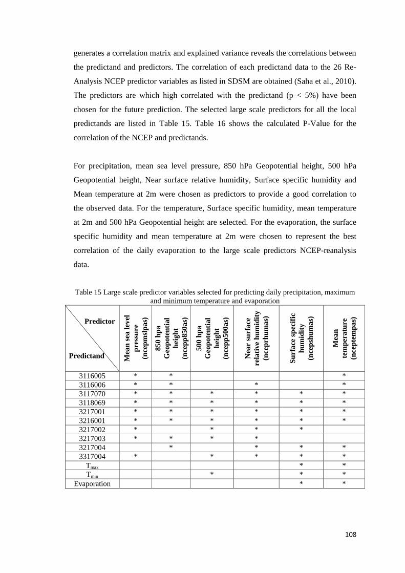
108
generates a correlation matrix and explained variance reveals the correlations between
the predictand and predictors. The correlation of each predictand data to the 26 Re-
Analysis NCEP predictor variables as listed in SDSM are obtained (Saha et al., 2010).
The predictors are which high correlated with the predictand (p < 5%) have been
chosen for the future prediction. The selected large scale predictors for all the local
predictands are listed in Table 15. Table 16 shows the calculated P-Value for the
correlation of the NCEP and predictands.
For precipitation, mean sea level pressure, 850 hPa Geopotential height, 500 hPa
Geopotential height, Near surface relative humidity, Surface specific humidity and
Mean temperature at 2m were chosen as predictors to provide a good correlation to
the observed data. For the temperature, Surface specific humidity, mean temperature
at 2m and 500 hPa Geopotential height are selected. For the evaporation, the surface
specific humidity and mean temperature at 2m were chosen to represent the best
correlation of the daily evaporation to the large scale predictors NCEP-reanalysis
data.
Table 15 Large scale predictor variables selected for predicting daily precipitation, maximum
and minimum temperature and evaporation
Predictor
Predictand
Mea
n s
ea l
evel
pre
ssu
re
(nce
pm
slp
as)
850 h
pa
Geo
pote
nti
al
hei
gh
t
(nce
pp
850as)
500 h
pa
Geo
pote
nti
al
hei
gh
t
(nce
pp
500as)
Nea
r su
rface
rela
tive
hu
mid
ity
(nce
prh
um
as)
Su
rface
sp
ecif
ic
hu
mid
ity
(nce
psh
um
as)
Mea
n
tem
per
atu
re
(nce
pte
mp
as)
3116005 * *
*
3116006 * *
*
*
3117070 * * * * * *
3118069 * * * * * *
3217001 * * * * * *
3216001 * * * * * *
3217002 *
* * *
3217003 * * * *
3217004
*
* * *
3317004 *
* * * *
Tmax * *
Tmin *
* *
Evaporation
* *
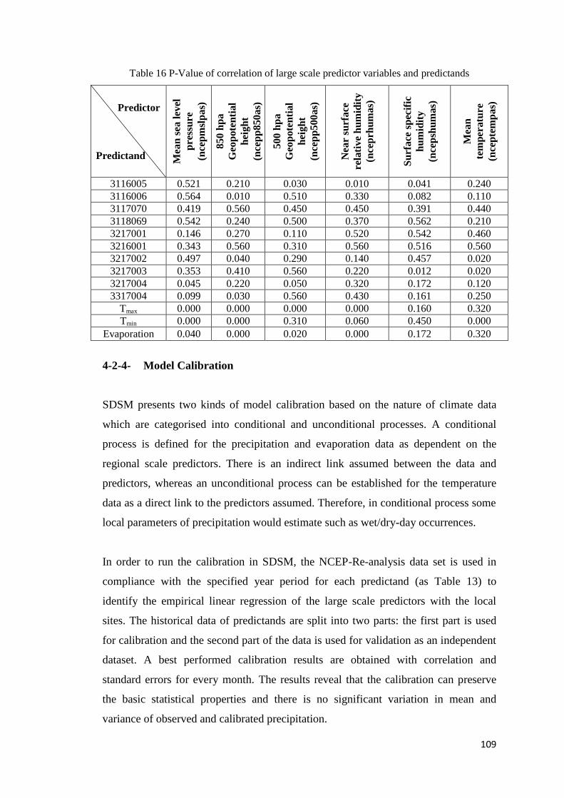
109
Table 16 P-Value of correlation of large scale predictor variables and predictands
Predictor
Predictand
M
ean
sea
lev
el
pre
ssu
re
(nce
pm
slp
as)
85
0 h
pa
Geo
pote
nti
al
hei
gh
t
(nce
pp
850
as)
50
0 h
pa
Geo
pote
nti
al
hei
gh
t
(nce
pp
500
as)
Nea
r su
rfa
ce
rela
tive
hu
mid
ity
(nce
prh
um
as)
Su
rfa
ce s
pec
ific
hu
mid
ity
(nce
psh
um
as)
Mea
n
tem
pera
ture
(nce
pte
mp
as)
3116005 0.521 0.210 0.030 0.010 0.041 0.240
3116006 0.564 0.010 0.510 0.330 0.082 0.110
3117070 0.419 0.560 0.450 0.450 0.391 0.440
3118069 0.542 0.240 0.500 0.370 0.562 0.210
3217001 0.146 0.270 0.110 0.520 0.542 0.460
3216001 0.343 0.560 0.310 0.560 0.516 0.560
3217002 0.497 0.040 0.290 0.140 0.457 0.020
3217003 0.353 0.410 0.560 0.220 0.012 0.020
3217004 0.045 0.220 0.050 0.320 0.172 0.120
3317004 0.099 0.030 0.560 0.430 0.161 0.250
Tmax 0.000 0.000 0.000 0.000 0.160 0.320
Tmin 0.000 0.000 0.310 0.060 0.450 0.000
Evaporation 0.040 0.000 0.020 0.000 0.172 0.320
4-2-4- Model Calibration
SDSM presents two kinds of model calibration based on the nature of climate data
which are categorised into conditional and unconditional processes. A conditional
process is defined for the precipitation and evaporation data as dependent on the
regional scale predictors. There is an indirect link assumed between the data and
predictors, whereas an unconditional process can be established for the temperature
data as a direct link to the predictors assumed. Therefore, in conditional process some
local parameters of precipitation would estimate such as wet/dry-day occurrences.
In order to run the calibration in SDSM, the NCEP-Re-analysis data set is used in
compliance with the specified year period for each predictand (as Table 13) to
identify the empirical linear regression of the large scale predictors with the local
sites. The historical data of predictands are split into two parts: the first part is used
for calibration and the second part of the data is used for validation as an independent
dataset. A best performed calibration results are obtained with correlation and
standard errors for every month. The results reveal that the calibration can preserve
the basic statistical properties and there is no significant variation in mean and
variance of observed and calibrated precipitation.
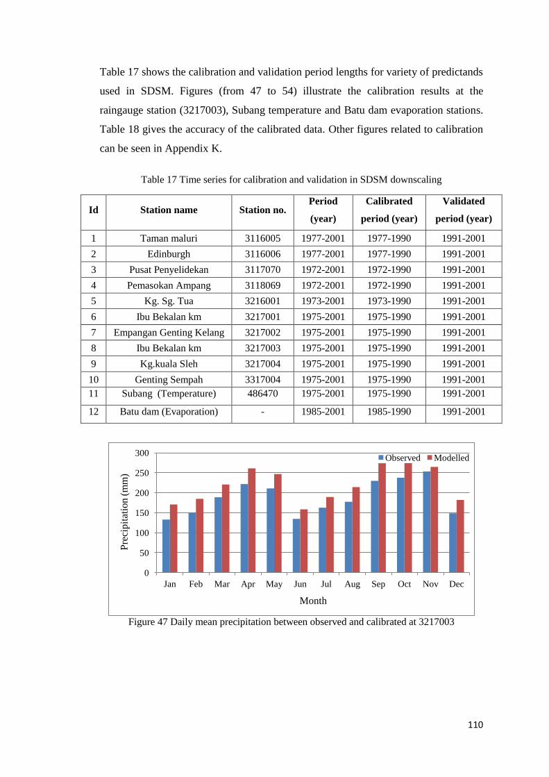
110
Table 17 shows the calibration and validation period lengths for variety of predictands
used in SDSM. Figures (from 47 to 54) illustrate the calibration results at the
raingauge station (3217003), Subang temperature and Batu dam evaporation stations.
Table 18 gives the accuracy of the calibrated data. Other figures related to calibration
can be seen in Appendix K.
Table 17 Time series for calibration and validation in SDSM downscaling
Id Station name Station no. Period
(year)
Calibrated
period (year)
Validated
period (year)
1 Taman maluri 3116005 1977-2001 1977-1990 1991-2001
2 Edinburgh 3116006 1977-2001 1977-1990 1991-2001
3 Pusat Penyelidekan 3117070 1972-2001 1972-1990 1991-2001
4 Pemasokan Ampang 3118069 1972-2001 1972-1990 1991-2001
5 Kg. Sg. Tua 3216001 1973-2001 1973-1990 1991-2001
6 Ibu Bekalan km 3217001 1975-2001 1975-1990 1991-2001
7 Empangan Genting Kelang 3217002 1975-2001 1975-1990 1991-2001
8 Ibu Bekalan km 3217003 1975-2001 1975-1990 1991-2001
9 Kg.kuala Sleh 3217004 1975-2001 1975-1990 1991-2001
10 Genting Sempah 3317004 1975-2001 1975-1990 1991-2001
11 Subang (Temperature) 486470 1975-2001 1975-1990 1991-2001
12 Batu dam (Evaporation) - 1985-2001 1985-1990 1991-2001
Figure 47 Daily mean precipitation between observed and calibrated at 3217003
0
50
100
150
200
250
300
Jan Feb Mar Apr May Jun Jul Aug Sep Oct Nov Dec
Pre
cipit
atio
n (
mm
)
Month
Observed Modelled
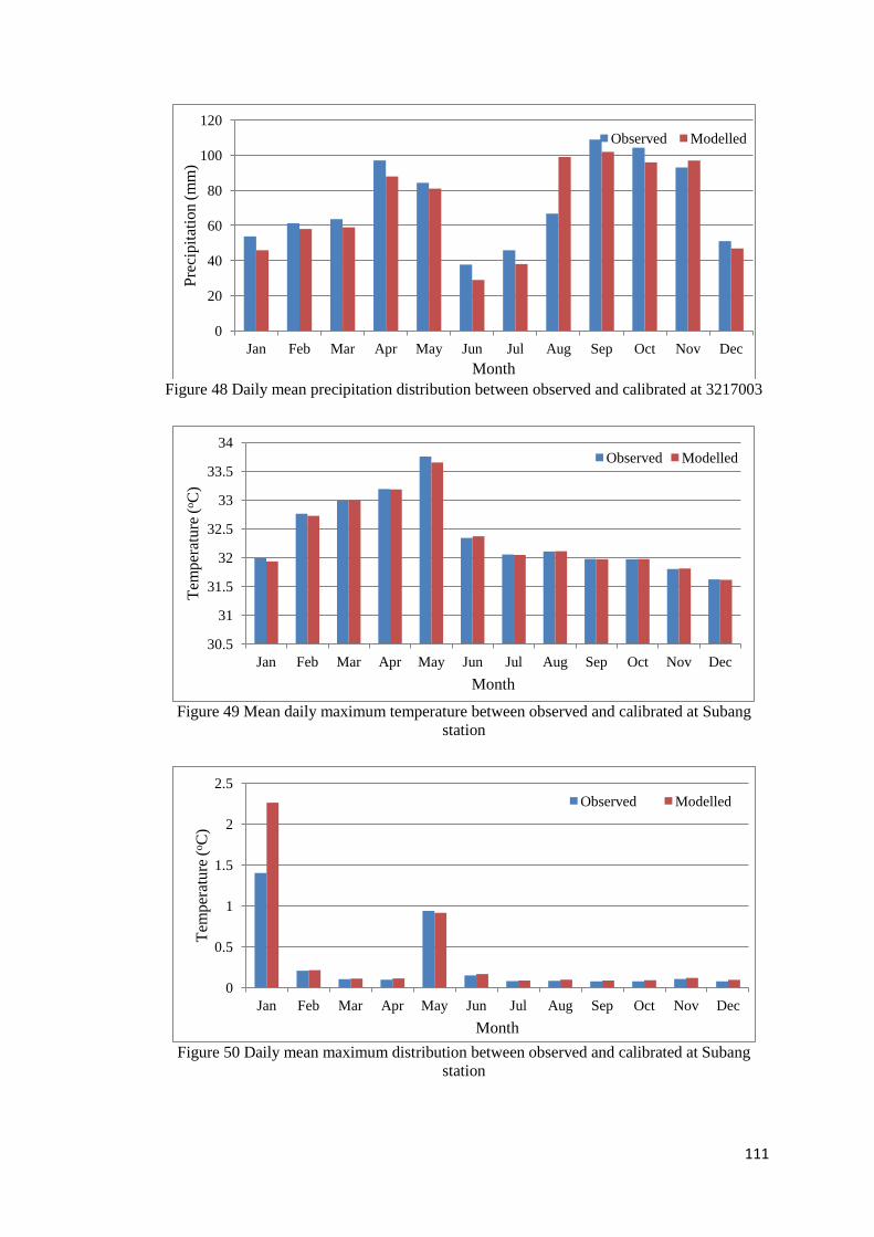
111
Figure 48 Daily mean precipitation distribution between observed and calibrated at 3217003
Figure 49 Mean daily maximum temperature between observed and calibrated at Subang
station
Figure 50 Daily mean maximum distribution between observed and calibrated at Subang
station
0
20
40
60
80
100
120
Jan Feb Mar Apr May Jun Jul Aug Sep Oct Nov Dec
Pre
cip
itat
ion
(m
m)
Month
Observed Modelled
30.5
31
31.5
32
32.5
33
33.5
34
Jan Feb Mar Apr May Jun Jul Aug Sep Oct Nov Dec
Tem
per
ature
(oC
)
Month
Observed Modelled
0
0.5
1
1.5
2
2.5
Jan Feb Mar Apr May Jun Jul Aug Sep Oct Nov Dec
Tem
per
atu
re (
oC
)
Month
Observed Modelled
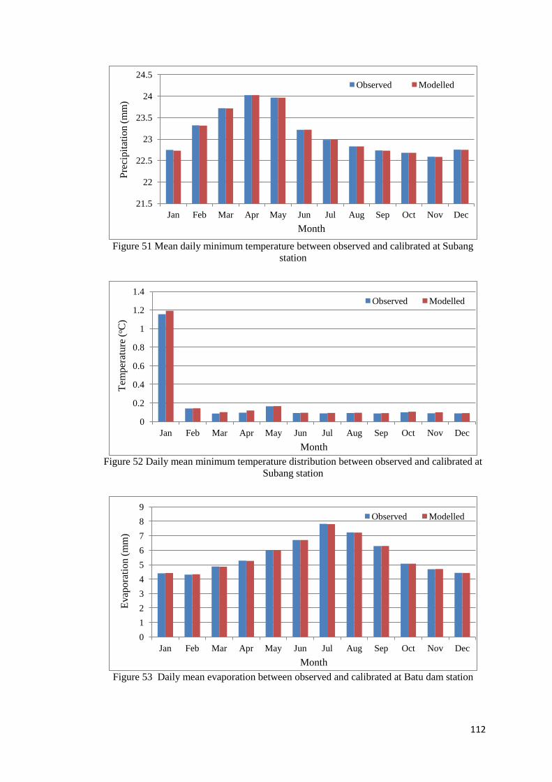
112
Figure 51 Mean daily minimum temperature between observed and calibrated at Subang
station
Figure 52 Daily mean minimum temperature distribution between observed and calibrated at
Subang station
Figure 53 Daily mean evaporation between observed and calibrated at Batu dam station
21.5
22
22.5
23
23.5
24
24.5
Jan Feb Mar Apr May Jun Jul Aug Sep Oct Nov Dec
Observed Modelled
Month
Pre
cip
itat
ion
(m
m)
0
0.2
0.4
0.6
0.8
1
1.2
1.4
Jan Feb Mar Apr May Jun Jul Aug Sep Oct Nov Dec
Tem
per
ature
(oC
)
Month
Observed Modelled
0
1
2
3
4
5
6
7
8
9
Jan Feb Mar Apr May Jun Jul Aug Sep Oct Nov Dec
Evap
ora
tio
n (
mm
)
Month
Observed Modelled
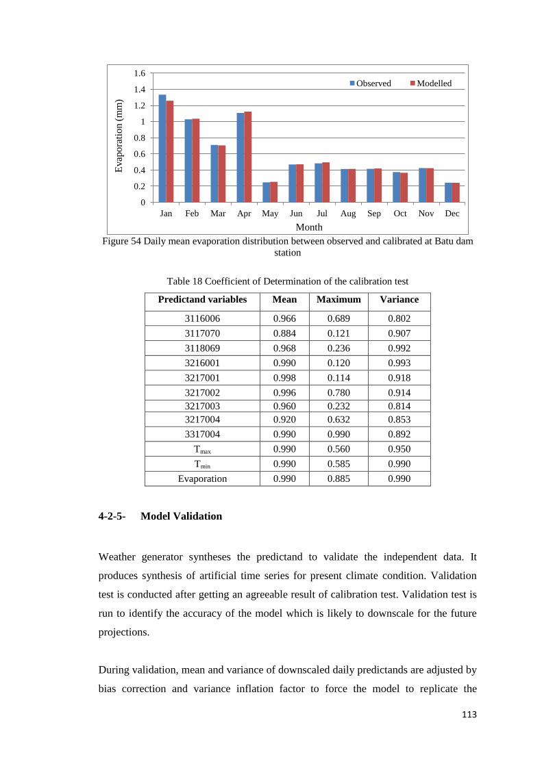
113
Figure 54 Daily mean evaporation distribution between observed and calibrated at Batu dam
station
Table 18 Coefficient of Determination of the calibration test
Predictand variables Mean Maximum Variance
3116006 0.966 0.689 0.802
3117070 0.884 0.121 0.907
3118069 0.968 0.236 0.992
3216001 0.990 0.120 0.993
3217001 0.998 0.114 0.918
3217002 0.996 0.780 0.914
3217003 0.960 0.232 0.814
3217004 0.920 0.632 0.853
3317004 0.990 0.990 0.892
Tmax 0.990 0.560 0.950
Tmin 0.990 0.585 0.990
Evaporation 0.990 0.885 0.990
4-2-5- Model Validation
Weather generator syntheses the predictand to validate the independent data. It
produces synthesis of artificial time series for present climate condition. Validation
test is conducted after getting an agreeable result of calibration test. Validation test is
run to identify the accuracy of the model which is likely to downscale for the future
projections.
During validation, mean and variance of downscaled daily predictands are adjusted by
bias correction and variance inflation factor to force the model to replicate the
0
0.2
0.4
0.6
0.8
1
1.2
1.4
1.6
Jan Feb Mar Apr May Jun Jul Aug Sep Oct Nov Dec
Evap
ora
tio
n (
mm
)
Month
Observed Modelled
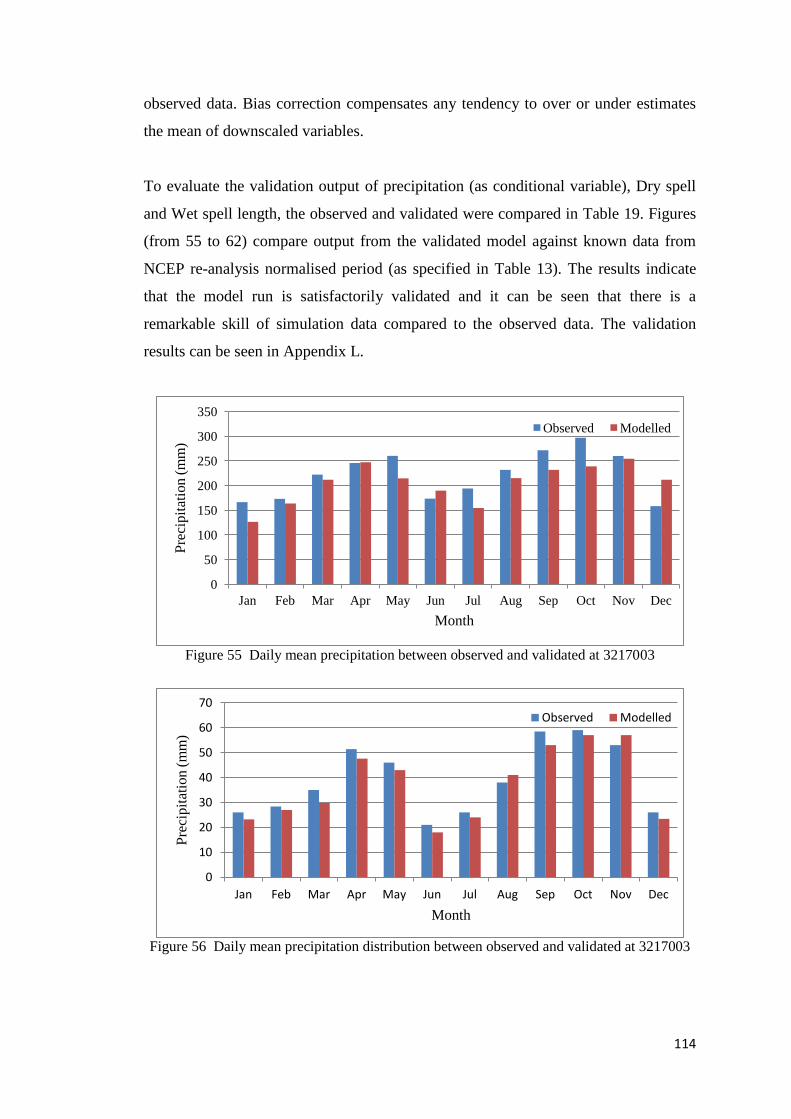
114
observed data. Bias correction compensates any tendency to over or under estimates
the mean of downscaled variables.
To evaluate the validation output of precipitation (as conditional variable), Dry spell
and Wet spell length, the observed and validated were compared in Table 19. Figures
(from 55 to 62) compare output from the validated model against known data from
NCEP re-analysis normalised period (as specified in Table 13). The results indicate
that the model run is satisfactorily validated and it can be seen that there is a
remarkable skill of simulation data compared to the observed data. The validation
results can be seen in Appendix L.
Figure 55 Daily mean precipitation between observed and validated at 3217003
Figure 56 Daily mean precipitation distribution between observed and validated at 3217003
0
50
100
150
200
250
300
350
Jan Feb Mar Apr May Jun Jul Aug Sep Oct Nov Dec
Pre
cipit
atio
n (
mm
)
Month
Observed Modelled
0
10
20
30
40
50
60
70
Jan Feb Mar Apr May Jun Jul Aug Sep Oct Nov Dec
Pre
cip
itat
ion
(m
m)
Month
Observed Modelled
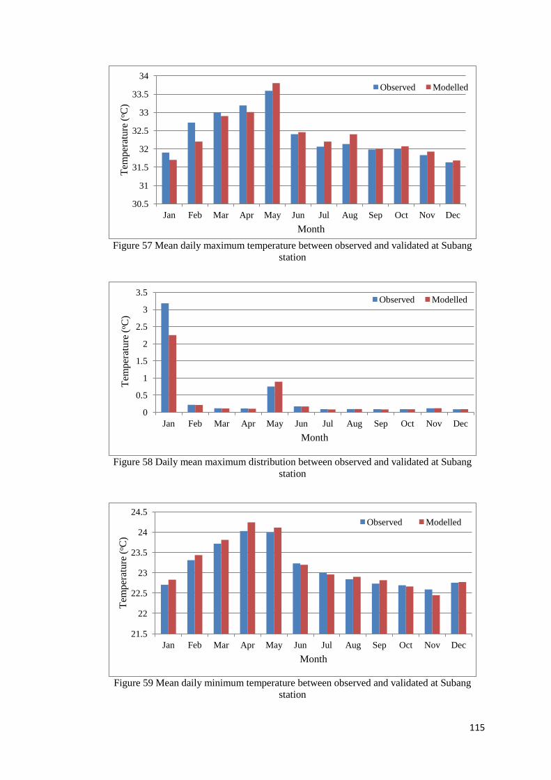
115
Figure 57 Mean daily maximum temperature between observed and validated at Subang
station
Figure 58 Daily mean maximum distribution between observed and validated at Subang
station
Figure 59 Mean daily minimum temperature between observed and validated at Subang
station
30.5
31
31.5
32
32.5
33
33.5
34
Jan Feb Mar Apr May Jun Jul Aug Sep Oct Nov Dec
Tem
per
atu
re (
oC
)
Month
Observed Modelled
0
0.5
1
1.5
2
2.5
3
3.5
Jan Feb Mar Apr May Jun Jul Aug Sep Oct Nov Dec
Tem
per
ature
(oC
)
Month
Observed Modelled
21.5
22
22.5
23
23.5
24
24.5
Jan Feb Mar Apr May Jun Jul Aug Sep Oct Nov Dec
Tem
per
atu
re (
oC
)
Month
Observed Modelled
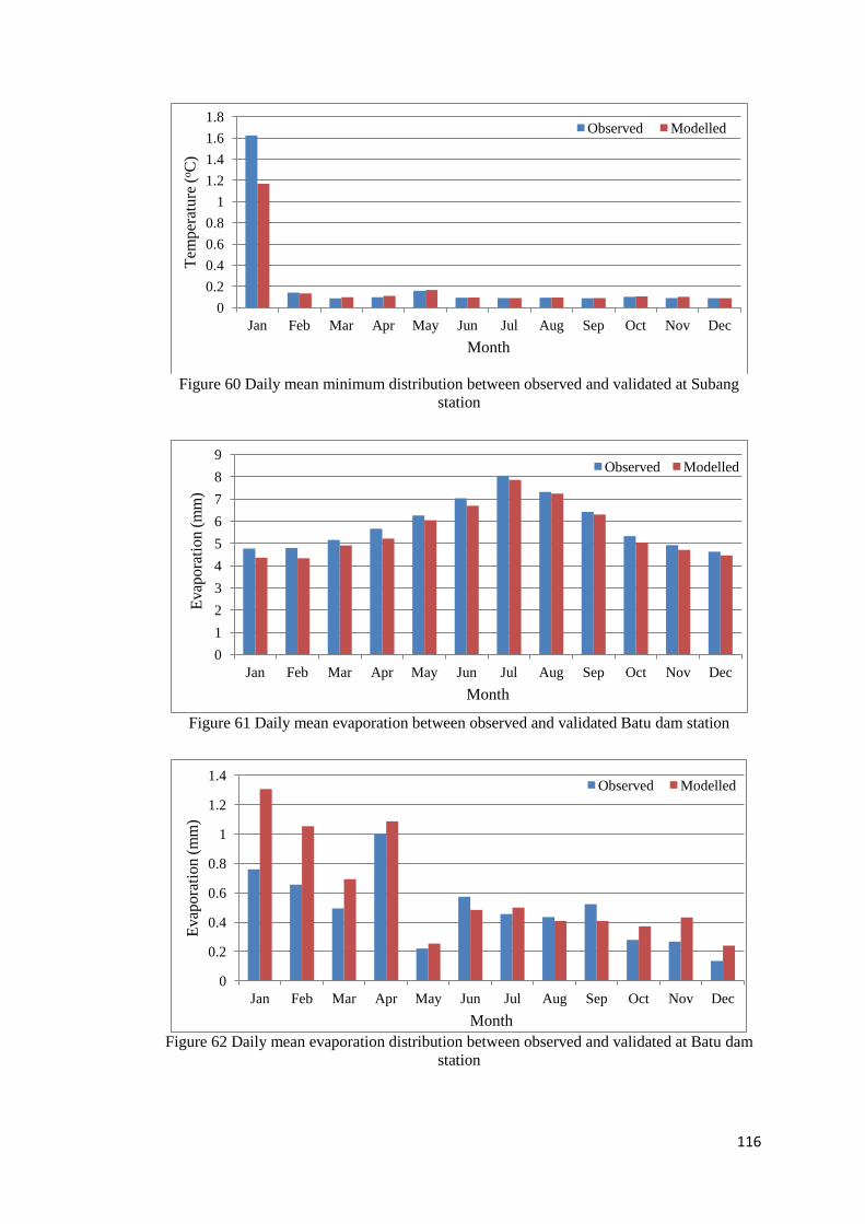
116
Figure 60 Daily mean minimum distribution between observed and validated at Subang
station
Figure 61 Daily mean evaporation between observed and validated Batu dam station
Figure 62 Daily mean evaporation distribution between observed and validated at Batu dam
station
0
0.2
0.4
0.6
0.8
1
1.2
1.4
1.6
1.8
Jan Feb Mar Apr May Jun Jul Aug Sep Oct Nov Dec
Tem
per
atu
re (
oC
)
Month
Observed Modelled
0
1
2
3
4
5
6
7
8
9
Jan Feb Mar Apr May Jun Jul Aug Sep Oct Nov Dec
Evap
ora
tio
n (
mm
)
Month
Observed Modelled
0
0.2
0.4
0.6
0.8
1
1.2
1.4
Jan Feb Mar Apr May Jun Jul Aug Sep Oct Nov Dec
Evap
ora
tion (
mm
)
Month
Observed Modelled
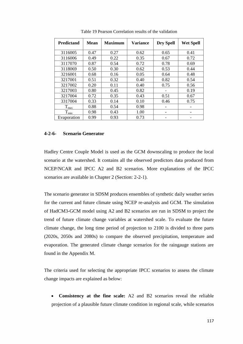
117
Table 19 Pearson Correlation results of the validation
Predictand Mean Maximum Variance Dry Spell Wet Spell
3116005 0.47 0.27 0.62 0.65 0.41
3116006 0.49 0.22 0.35 0.67 0.72
3117070 0.87 0.54 0.72 0.78 0.69
3118069 0.50 0.30 0.62 0.53 0.44
3216001 0.68 0.16 0.05 0.64 0.48
3217001 0.51 0.32 0.40 0.82 0.54
3217002 0.20 0.11 0.40 0.75 0.56
3217003 0.80 0.45 0.82 - 0.19
3217004 0.72 0.35 0.43 0.51 0.67
3317004 0.33 0.14 0.10 0.46 0.75
Tmax 0.88 0.54 0.98 - -
Tmin 0.98 0.43 1.00 - -
Evaporation 0.99 0.93 0.73 - -
4-2-6- Scenario Generator
Hadley Centre Couple Model is used as the GCM downscaling to produce the local
scenario at the watershed. It contains all the observed predictors data produced from
NCEP/NCAR and IPCC A2 and B2 scenarios. More explanations of the IPCC
scenarios are available in Chapter 2 (Section: 2-2-1).
The scenario generator in SDSM produces ensembles of synthetic daily weather series
for the current and future climate using NCEP re-analysis and GCM. The simulation
of HadCM3-GCM model using A2 and B2 scenarios are run in SDSM to project the
trend of future climate change variables at watershed scale. To evaluate the future
climate change, the long time period of projection to 2100 is divided to three parts
(2020s, 2050s and 2080s) to compare the observed precipitation, temperature and
evaporation. The generated climate change scenarios for the raingauge stations are
found in the Appendix M.
The criteria used for selecting the appropriate IPCC scenarios to assess the climate
change impacts are explained as below:
Consistency at the fine scale: A2 and B2 scenarios reveal the reliable
projection of a plausible future climate condition in regional scale, while scenarios

118
A1 and B1 form the world homogeneously A1 and B1 represent at global scale.
According to IPCC (2007), Malaysia is a developing country which will be
vulnerable to climate change and has less flexibility to adjust the economical structure
and being largely dependent on agriculture. Likewise, Malaysia is expected to a high
rate of population growth which affects on the future social, economic and
technological state of the region. These characteristics of the region possibly cause a
high rate of GHG emissions in the future.
Applicability in impact assessments in hydrological modelling: Scenarios
should describe changes in a sufficient number of climate variables on a spatial
and temporal scale that allows for impact assessment (Nigel, 2004). Hydrology
modelling at watershed scale is restricted to the climate change impact to the
streamflow. Then, the resolution of climate change downscaling may affect on the
local scenarios over the watershed scale. In this regard, A2 and B2 scenarios as
the finest IPCC scenarios meet the requirements of the climate change data in
hydrology modelling. Thus, the applicability of A2 and B2 scenarios in estimating
impacts of climate change at a watershed scale is more realistic compared to other
scenarios, which were constructed at a global scale.
Representativeness: The scenarios should be representative of the potential
range of future Using a single climate change scenario is not recommended for an
environmental investigation. Then, two scenarios were selected, HadCM3-A2, and
HadCM3-B2. A2 scenario (Medium-High Emissions scenario) is a scenario with
higher rates of greenhouse gas emissions in combination with higher sulphate and
other aerosol emissions while B2 scenario (Medium-Low Emissions scenario) is a
lower rate of emissions that assumes the world is more committed to solving
global and local environmental (IPCC, 2007).
Compatibility with HadCM3-GCM model: HadCM3 model in SDSM
involves A2 and B2 scenarios. The predictor variables are supplied on a grid box.
It provides a zip file contains three directories: NCEP-1961-2001, H3A2a-1961-
2099 and H3B2a-1961-2099.

119
Uncertainty: It brings to the question that to what would be the effect of
IPCC different scenarios in downscaling and to what extent they would affect the
local hydrology processes. The main reason in selection of multiple climate
change scenarios is to build a realistic picture of the range of climate and reveal
impact response to changes in atmospheric composition. However, the main
source of uncertainty of climate change impact studies in humid climates stems
from the choice of Climate Change Models rather than IPCC scenarios
(Prudhomme and Davies, 2009). HadCM3 model assumes IPCC different A2 and
B2 scenarios as a higher and lower rate of emissions respectively to project the
future climate. Hence, A2 and B2 scenarios have been used to generate a range of
local climate change scenarios using statistical downscaling model in the
watershed scale.
As a result, A2 and B2 IPCC scenarios are the currently most reliable scenarios to
assess climate change at fine scale but A1 and B1 scenarios do not meet the needed
resolution to assess the climate change at local scale which is required for
hydrological modelling. Thus, applicability of A2 and B2 scenarios in estimating
impacts of climate change at a watershed scale is more realistic compared to other
scenarios, which were constructed at a global scale.
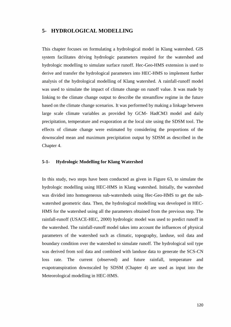
120
5- HYDROLOGICAL MODELLING
This chapter focuses on formulating a hydrological model in Klang watershed. GIS
system facilitates driving hydrologic parameters required for the watershed and
hydrologic modelling to simulate surface runoff. Hec-Geo-HMS extension is used to
derive and transfer the hydrological parameters into HEC-HMS to implement further
analysis of the hydrological modelling of Klang watershed. A rainfall-runoff model
was used to simulate the impact of climate change on runoff value. It was made by
linking to the climate change output to describe the streamflow regime in the future
based on the climate change scenarios. It was performed by making a linkage between
large scale climate variables as provided by GCM- HadCM3 model and daily
precipitation, temperature and evaporation at the local site using the SDSM tool. The
effects of climate change were estimated by considering the proportions of the
downscaled mean and maximum precipitation output by SDSM as described in the
Chapter 4.
5-1- Hydrologic Modelling for Klang Watershed
In this study, two steps have been conducted as given in Figure 63, to simulate the
hydrologic modelling using HEC-HMS in Klang watershed. Initially, the watershed
was divided into homogeneous sub-watersheds using Hec-Geo-HMS to get the sub-
watershed geometric data. Then, the hydrological modelling was developed in HEC-
HMS for the watershed using all the parameters obtained from the previous step. The
rainfall-runoff (USACE-HEC, 2000) hydrologic model was used to predict runoff in
the watershed. The rainfall-runoff model takes into account the influences of physical
parameters of the watershed such as climatic, topography, landuse, soil data and
boundary condition over the watershed to simulate runoff. The hydrological soil type
was derived from soil data and combined with landuse data to generate the SCS-CN
loss rate. The current (observed) and future rainfall, temperature and
evapotranspiration downscaled by SDSM (Chapter 4) are used as input into the
Meteorological modelling in HEC-HMS.

121
Finally, the flow hydrographs was produced to determine the streamflow regime for
the future corresponding to the IPCC scenarios. Figure 63 illustrates a diagram
representing the flow diagram of runoff and peak flow estimation and prediction for
the future in Klang watershed.
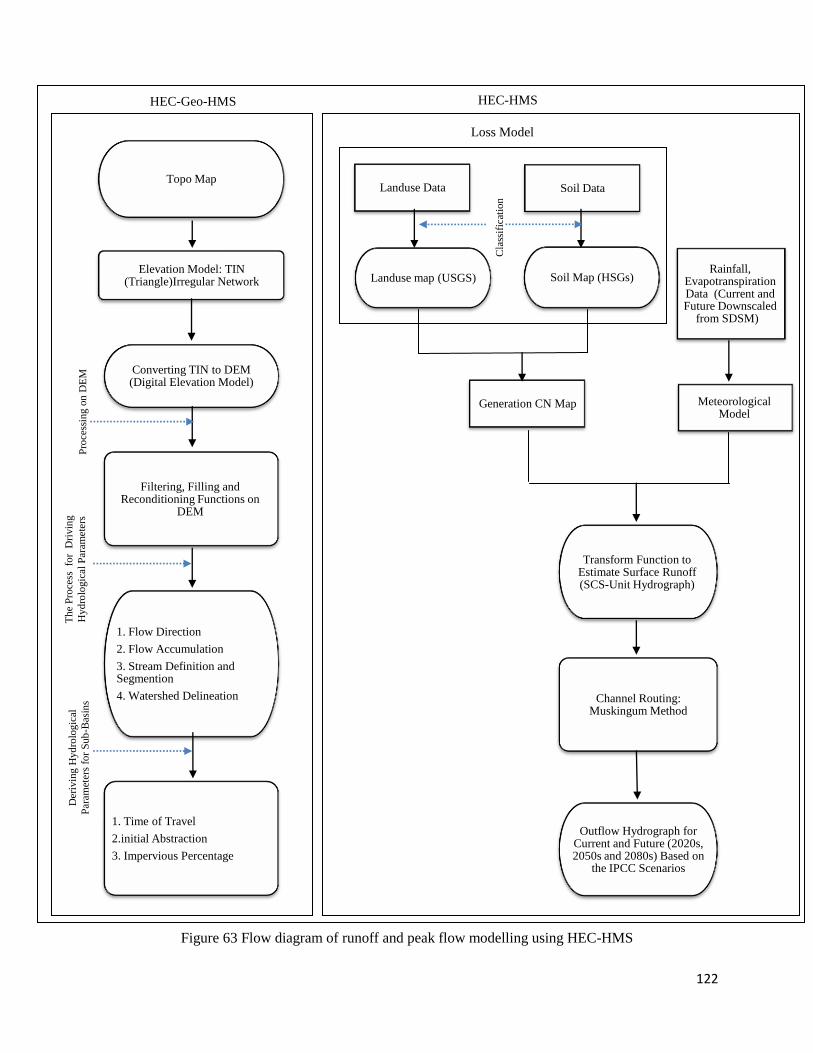
122
Figure 63 Flow diagram of runoff and peak flow modelling using HEC-HMS
Pro
cess
ing
on
DE
M
Cla
ssif
icat
ion
Th
e P
roce
ss fo
r D
rivin
g
Hy
dro
logic
al P
aram
eter
s
Transform Function to Estimate Surface Runoff (SCS-Unit Hydrograph)
Channel Routing: Muskingum Method
Outflow Hydrograph for Current and Future (2020s, 2050s and 2080s) Based on
the IPCC Scenarios
Landuse map (USGS)
Meteorological Model
Generation CN Map
Rainfall, Evapotranspiration Data (Current and Future Downscaled
from SDSM)
Landuse Data Soil Data
Soil Map (HSGs)
Topo Map
Elevation Model: TIN (Triangle)Irregular Network
Converting TIN to DEM (Digital Elevation Model)
Filtering, Filling and Reconditioning Functions on
DEM
1. Flow Direction
2. Flow Accumulation
3. Stream Definition and Segmention
4. Watershed Delineation
1. Time of Travel
2.initial Abstraction
3. Impervious Percentage
HEC-HMS HEC-Geo-HMS
Loss Model
Der
ivin
g H
yd
rolo
gic
al
Par
amet
ers
for
Sub
-Bas
ins
123
5-2- Watershed Modelling
The hydrological parameters needed in the rainfall-runoff modelling were generated
using Hec-Geo-HMS. The data layers have been driven from the watershed physical
characteristics including watershed area, perimeter, length of the river, mean
elevation, slope, runoff coefficient, lag time, landuse and soil unites. These
hydrological parameters could be generated automatically by GIS system using Hec-
Geo-HMS for each sub-watershed of Klang. Thus, runoff values are estimated on
each sub-watershed system from the upstream to the watershed outlet throughout the
streamflow network.
5-2-1- Building a Digital Elevation Model of Klang Watershed Using TIN
(Triangular Irregular Network)
To build the TIN of Klang watershed, the topo maps (at scale of 1:25000 and
1:10000) and also spot heights were used. The topo maps have Malaysia’s coordinate
system (Rectified Skewed Orthomorphic-RSO projection). The highest and lowest
elevations of the elevation points are 5 and 1404, respectively. Figure 64 illustrates
the elevation model of the watershed developed in ArcGIS. Hec-Geo-HMS requires
the DEM format as the basic input for the watershed delineation. Therefore, the TIN
of Klang watershed was converted to the DEM format. One of the most important
concerns in building DEM is to determine its cell size. Maidment (2002) has proposed
a holistic DEM cell size in terms of their application. It has been represented by a 30
m cell size of DEM in urban watershed.
In this study, the DEM was developed at 30 metre cell size which seems to be
efficient for a scale of 1:25000 (Hengl, 2006). Nine series of topo maps at 1:25000
scale were used to make the elevation map of Klang watershed. The data were
acquired from the Malaysian department of surveying and mapping (JUPEM).
However, the digital topography at the scale of 1:25000 does not cover the urban area
of Klang watershed. Then the topo maps in the scale of 1:10000 used to fill the gap of
elevation data.
124
5-2-2- DEM Optimisation
Topography is the base data to determine the flow direction of streamflow across a
watershed. This data is considered as the most significant data which affects the
hydrological models. Consequently, any uncertainty in the topographic models is
propagated into the output of hydrologic model prediction, causing inaccuracies (Wua
et al., 2008). The spot heights (Figure 65) was used to combine to the topo maps to
promote the accuracy of the developed DEM, as the spot heights are often point
elevations of the ridges and peaks of Klang watershed.
5-2-3- Delineation of watershed Boundary, Outlet and Stream Network Layers
As mentioned before, the initial DEM of Klang watershed was built from topo maps.
At first, raw DEM was smoothed by filtering in GIS to smooth the sharp ridges and
pits. Then, the fill function in GIS was run on it to remove the pits to delineate the
stream network. Burn-DEM method was run using AGREE-DEM algorithm in Hec-
Geo-HMS extension to extract the more accurate stream network from the DEM.
Smoothing, filling depressions/sinks and reconditioning functions were run on the
DEM of Klang watershed for automatic delineation which will be preceded through
the flow direction, flow accumulation, stream definition, stream segmentation and
watershed delineation.
5-2-3-1- DEM Smoothing
Filtering is a spatial analysis tool in GIS for smoothing the sharp ridges and pits exists
in the created DEM. GIS involves two kinds of filtering which are Low Pass
(smoothes the DEM) and high pass (enhances the edges and boundaries of DEM),
processing on focal functions with a weighted kernel neighbours. Low filter option in
GIS as an averaging filter was run to assign the value of cells in the 3*3 window. The
centre is assigned by the sum of the products of the cell value and its direct
neighbours which are 8 adjacent pixels in a 3 x 3 filter. In low filter all 9 cells have an
equal weight to determine the value of the centre cell. The sum of all 9 specified
weights in the low filtering is equal to 1 as not changing the general elevation after
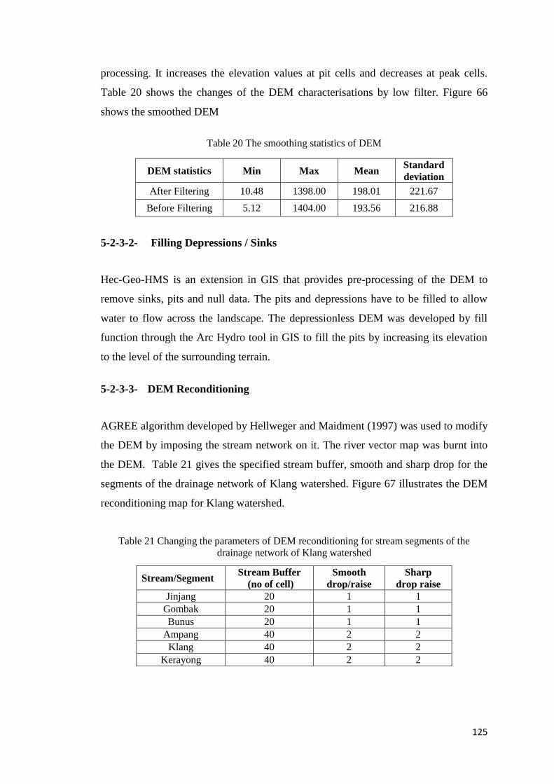
125
processing. It increases the elevation values at pit cells and decreases at peak cells.
Table 20 shows the changes of the DEM characterisations by low filter. Figure 66
shows the smoothed DEM
Table 20 The smoothing statistics of DEM
DEM statistics Min Max Mean Standard
deviation
After Filtering 10.48 1398.00 198.01 221.67
Before Filtering 5.12 1404.00 193.56 216.88
5-2-3-2- Filling Depressions / Sinks
Hec-Geo-HMS is an extension in GIS that provides pre-processing of the DEM to
remove sinks, pits and null data. The pits and depressions have to be filled to allow
water to flow across the landscape. The depressionless DEM was developed by fill
function through the Arc Hydro tool in GIS to fill the pits by increasing its elevation
to the level of the surrounding terrain.
5-2-3-3- DEM Reconditioning
AGREE algorithm developed by Hellweger and Maidment (1997) was used to modify
the DEM by imposing the stream network on it. The river vector map was burnt into
the DEM. Table 21 gives the specified stream buffer, smooth and sharp drop for the
segments of the drainage network of Klang watershed. Figure 67 illustrates the DEM
reconditioning map for Klang watershed.
Table 21 Changing the parameters of DEM reconditioning for stream segments of the
drainage network of Klang watershed
Stream/Segment
Stream Buffer
(no of cell)
Smooth
drop/raise
Sharp
drop raise
Jinjang 20 1 1
Gombak 20 1 1
Bunus 20 1 1
Ampang 40 2 2
Klang 40 2 2
Kerayong 40 2 2
126
5-2-3-4- Flow Direction
The flow direction of Klang DEM was created based on D8 algorithm (Jenson and
Domingue, 988 . The direction of flow is determined based on the lowest cell’s
slope than its neighbour. As Archydro extension was used, the maximum drop was
assumed for each cell to specify the flow direction. The maximum drop is calculated
by the most changing in elevation corresponding to the distance between two cells
centre. Figure 68 shows the Flow Direction of Klang watershed.
5-2-3-5- Flow Accumulation
Flow direction grid is used as input to create flow accumulation of Klang DEM. Flow
accumulation is produced by taking the total number of cells of flow direction grid
which flows into each cell. The cells with high accumulation are designated as stream
network. Figure 69 shows the flow accumulation for Klang DEM.
5-2-3-6- Stream Definition and Stream Segmentation
This function provides a threshold value to compute the stream grid. It assigns a value
of 1 to all the cells in the flow direction grid which have the value greater than the
given threshold. A threshold value in this function can be defined based on number of
cells or area. Then, it affects on dense of the stream network which will result the
number of sub-watersheds delineated. Tarboton and Mohammed (2010) have
developed TauDEM software for watershed delineation. They provided threshold
value to delineate the watershed according to geomorphological river network
properties. The threshold value of 8 km2 for Klang watershed was assumed for stream
definition function. In stream segmentation function, a unique value was given to each
segment of the stream network. In Klang watershed 39 separated segments were
identified in which each segment composed of cells with a same grid code. Figure 70
illustrates the stream segmentation of Klang watershed.
127
5-2-3-7- Watershed Delineation
Once the stream segmentation grid has been prepared, the watershed delineation can
be run to delineate the sub-watersheds that belong to the stream segment. Delineation
is performed for a grid in which each cell allocates a specific value based on the
stream segments in the whole of DEM. Since 39 streams were produced by stream
segmentation function with the same number, 39 sub-watersheds were generated
indicating to which sub-watershed the segment stream belongs. Figure 71 illustrates
the automatic watershed delineation of Klang watershed.
5-2-3-8- Optimisation of the Delineated Watershed
To optimise the final watershed map, some useful points and objects located in Klang
watershed were identified in compliance with reality of the sub-watershed boundaries.
The benchmark points have been found in the area distributed on the watershed map.
Hec-Geo-HMS has useful tools such as watershed merge, delineate batch point and
split watershed at confluences to amend the boundaries and outlets. Finally, 33 sub-
watersheds were generated. Figure 72 shows the benchmarks used to conduct
optimisation of Klang watershed.
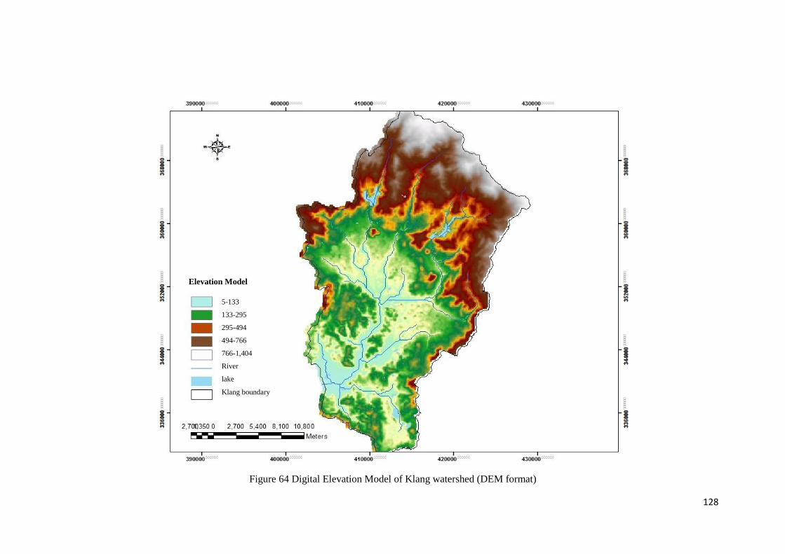
128
Figure 64 Digital Elevation Model of Klang watershed (DEM format)
Elevation Model
5-133
133-295
295-494
494-766
766-1,404
River
lake
Klang boundary
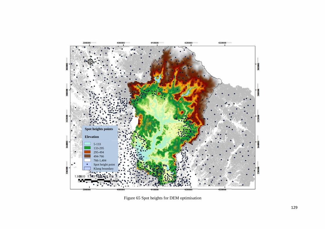
129
Figure 65 Spot heights for DEM optimisation
Spot heights points
Elevation
5-133
133-295
295-494
494-766
766-1,404
Spot height point
Klang boundary
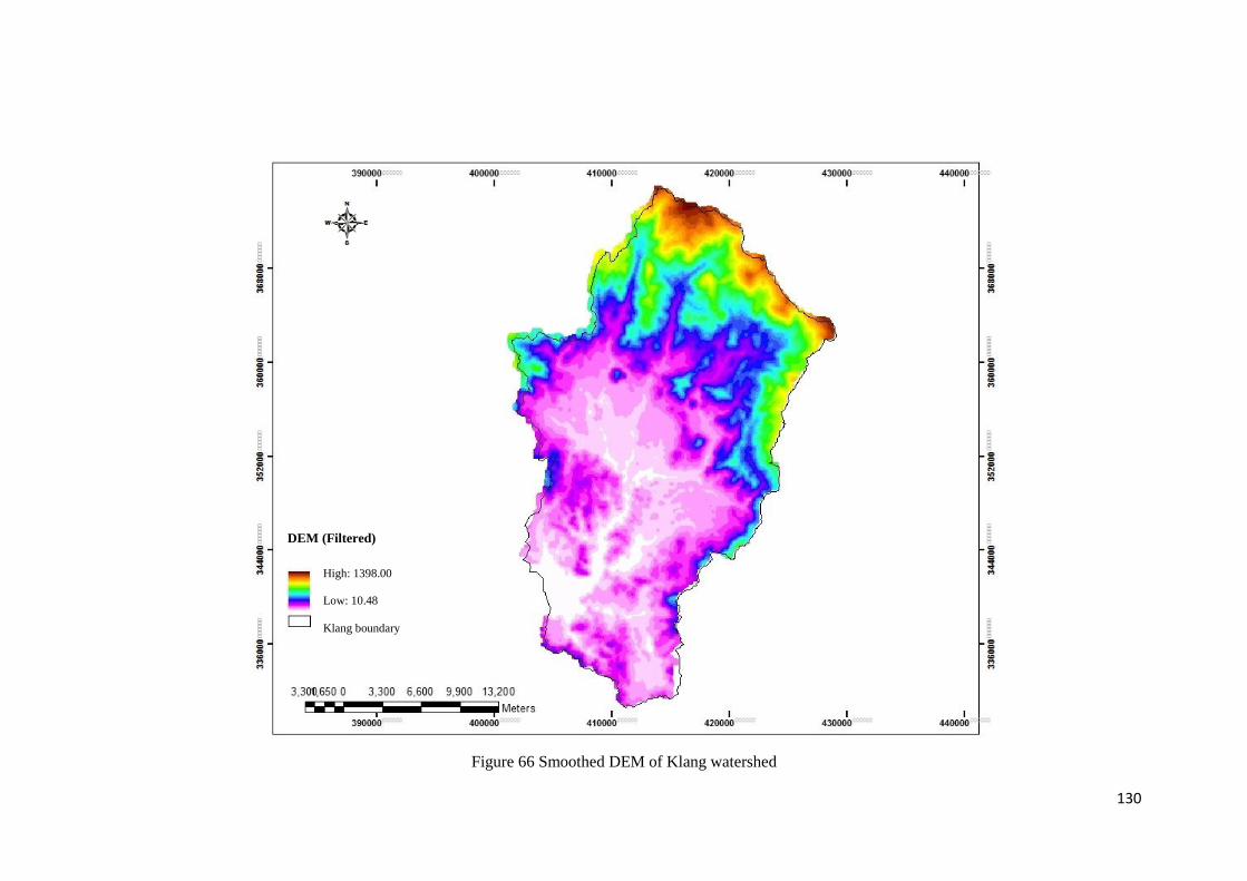
130
Figure 66 Smoothed DEM of Klang watershed
DEM (Filtered)
High: 1398.00
Low: 10.48
Klang boundary
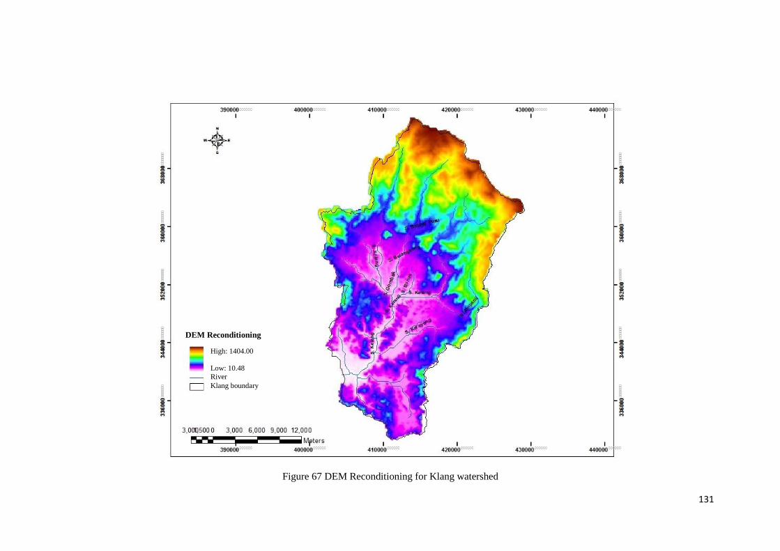
131
Figure 67 DEM Reconditioning for Klang watershed
DEM Reconditioning
High: 1404.00
Low: 10.48
River
Klang boundary
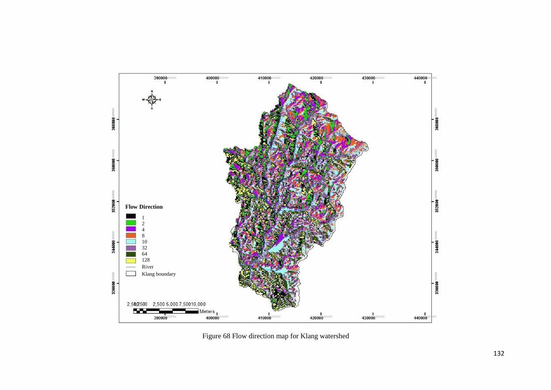
132
Figure 68 Flow direction map for Klang watershed
Flow Direction
1 2
4
8 10
32
64
128
River
Klang boundary
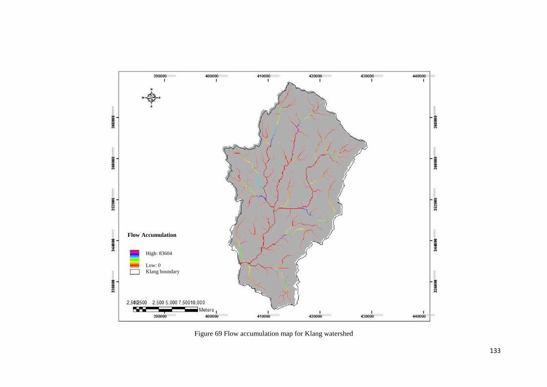
133
Figure 69 Flow accumulation map for Klang watershed
Flow Accumulation
High: 83604
Low: 0
Klang boundary
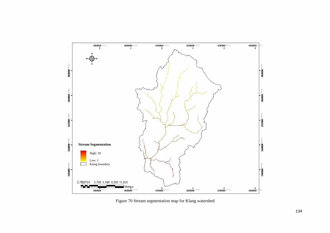
134
Figure 70 Stream segmentation map for Klang watershed
Stream Segmentation
High: 39
Low: 1
Klang boundary
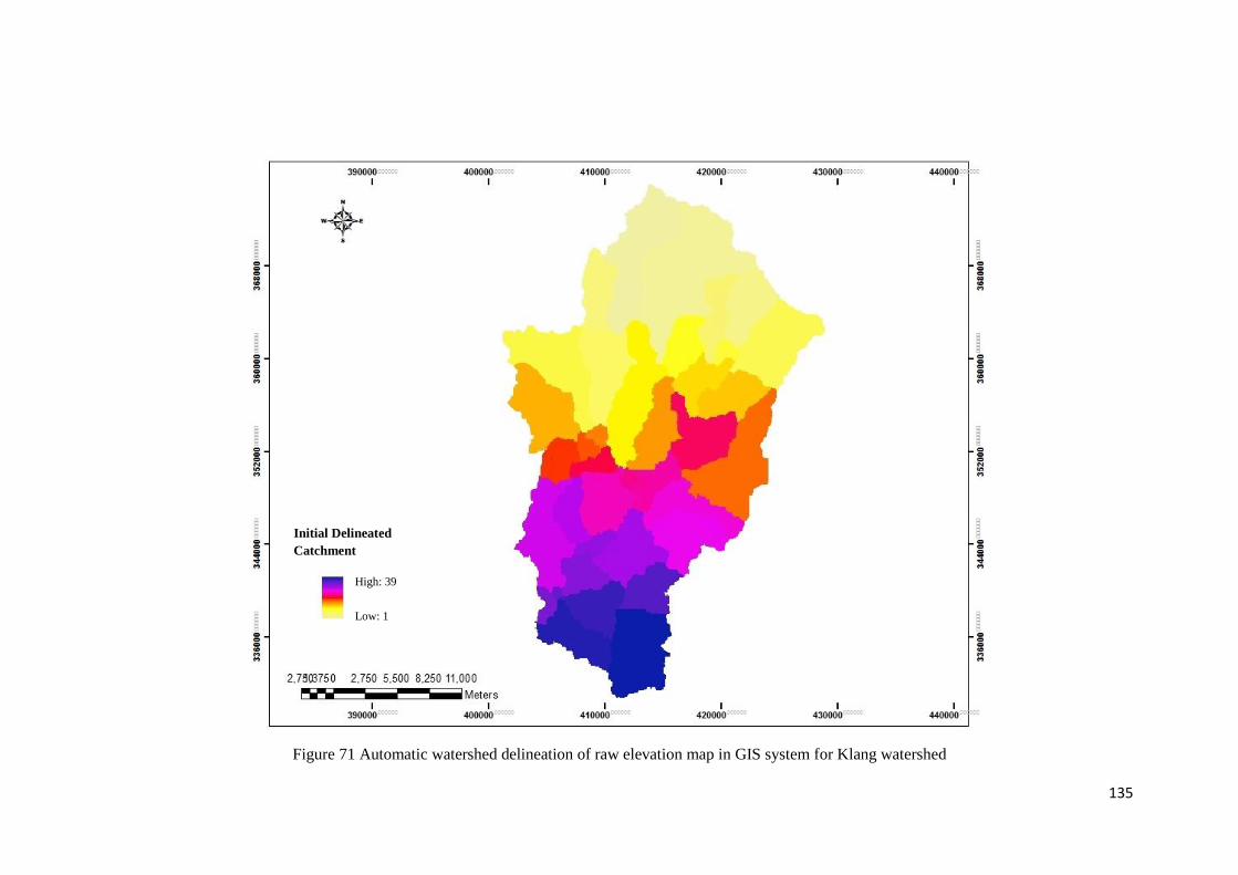
135
Figure 71 Automatic watershed delineation of raw elevation map in GIS system for Klang watershed
Initial Delineated
Catchment
High: 39
Low: 1
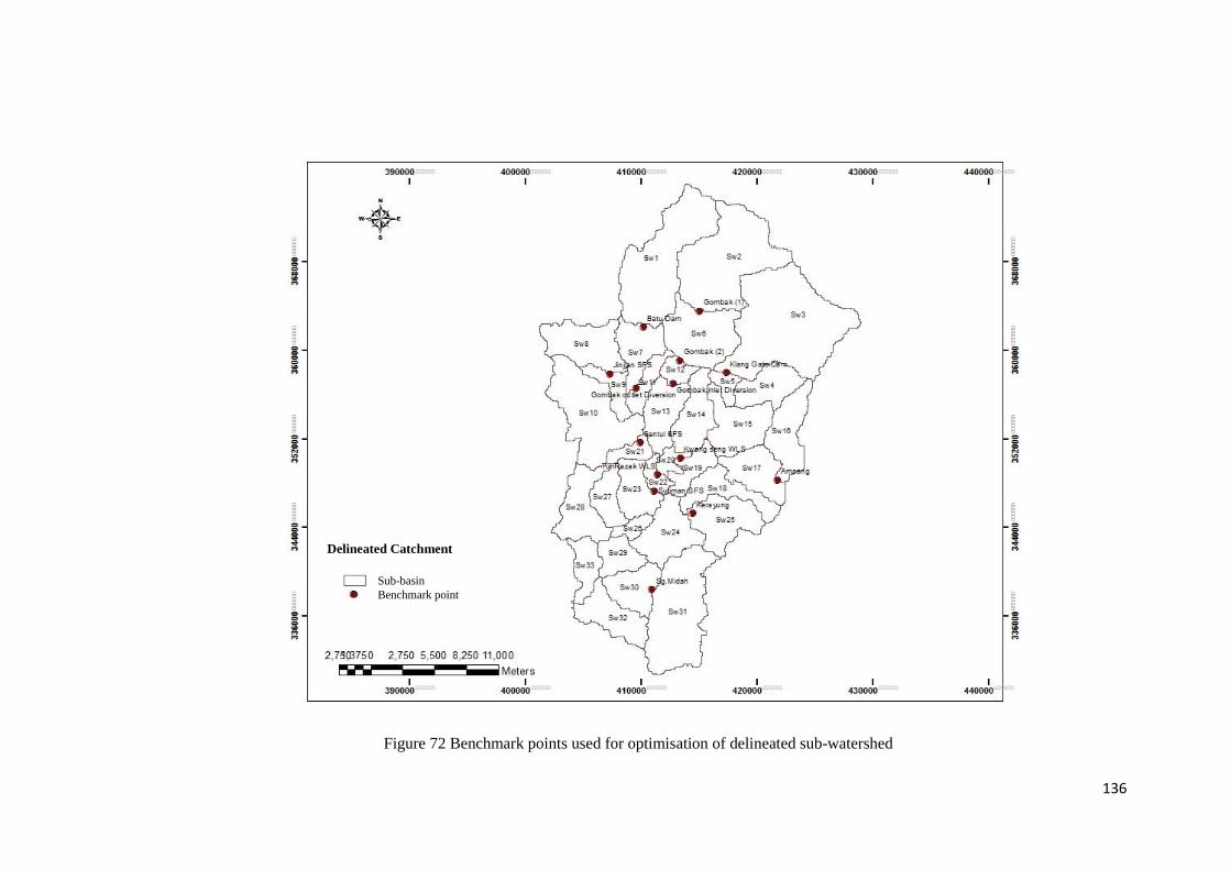
136
Figure 72 Benchmark points used for optimisation of delineated sub-watershed
Delineated Catchment
Sub-basin
Benchmark point

137
5-3- The Runoff Simulation
HEC-HMS is software to simulate the rainfall-runoff relations of a watershed system
which can be obtained from the Hydrologic Engineering entre’s home page at:
http://www.wrc-hec.usace.army.mil/.
The main reason for using rainfall-runoff is to account for the influences of physical
parameters of the watershed representing the boundary condition over the watershed
to simulate runoff. HEC-HMS provides various methods suitable for a long period
continuous simulation which are necessary in this research. The steps involved in
hydrology modelling for Klang watershed can be divided into five categories:
Estimation of Rainfall loss rate, Hydrographical Transformation, Channel routing,
Reservoir flood routing and Meteorological modelling.
The overall framework of HEC-HMS is described as follows, Watershed delineations
have been driven for Klang watershed to extract hydrological parameters which was
used as an input into HEC-HMS hydrology model. The SCS-CN loss method in HEC-
HMS needs the data such as CN, initial abstraction, potential soil storage and
imperviousness. These data have been developed using GIS spatially. Figure 73
shows the Hec-Geo-HMS model for Klang watershed. The physical watershed
characteristics such as watershed area, perimeter, watershed length and slope were
automatically calculated in Hec-Geo-HMS (Table 22).
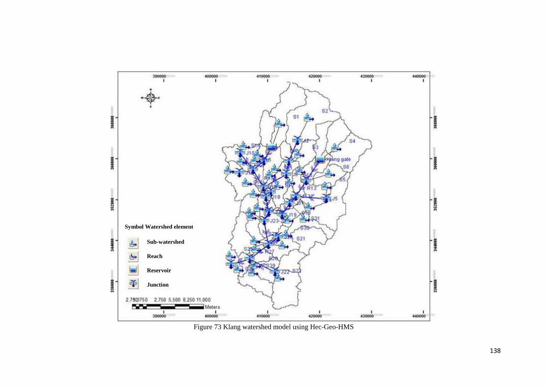
138
Figure 73 Klang watershed model using Hec-Geo-HMS
Symbol Watershed element
Sub-watershed
Reach
Reservoir
Junction
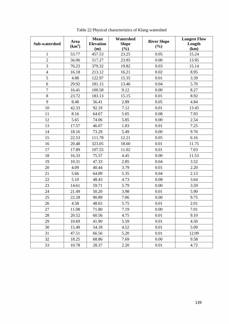
139
Table 22 Physical characteristics of Klang watershed
Sub-watershed Area
(km2)
Mean
Elevation
(m)
Watershed
Slope
(%)
River Slope
(%)
Longest Flow
Length
(km)
1 53.77 457.53 23.25 0.05 15.24
2 56.06 517.27 23.95 0.00 13.95
3 76.23 379.32 19.82 0.03 15.14
4 16.18 213.12 16.21 0.02 8.95
5 4.88 122.97 15.35 0.01 3.39
6 29.92 181.15 13.46 0.04 5.70
7 16.41 100.58 9.12 0.00 8.27
8 23.72 183.13 15.15 0.01 8.92
9 8.48 56.41 2.89 0.05 4.84
10 42.33 92.19 7.12 0.01 13.45
11 8.16 64.67 5.05 0.08 7.93
12 5.65 74.06 5.85 0.00 2.54
13 17.57 46.07 1.83 0.01 7.25
14 18.16 73.29 5.49 0.00 9.76
15 22.53 111.78 12.21 0.05 6.16
16 20.48 323.05 18.60 0.01 11.75
17 17.89 107.55 11.02 0.01 7.03
18 16.33 75.57 4.45 0.00 11.53
19 10.31 47.33 2.85 0.04 3.52
20 4.09 40.44 3.79 0.01 2.20
21 5.66 64.89 5.35 0.04 2.13
22 5.10 48.43 4.73 0.08 3.64
23 14.61 59.71 5.79 0.00 3.59
24 21.49 50.20 3.98 0.01 5.90
25 22.28 90.89 7.06 0.00 9.75
26 4.58 48.65 5.75 0.01 2.01
27 11.08 71.80 7.19 0.00 7.01
28 20.52 60.56 4.75 0.01 9.10
29 10.69 41.90 5.59 0.01 4.50
30 15.49 54.18 4.52 0.01 5.09
31 47.51 66.56 5.20 0.01 12.09
32 18.25 68.86 7.69 0.00 9.58
33 10.78 28.37 2.20 0.01 4.72
140
5-3-1- Loss Model
Five loss models in the Urban Stormwater Management Manual for Malaysia
(MSMA) were proposed by the Department of Irrigation and Drainage (DID) in 2004.
In this study, SCS Curve Number (CN) was used as loss model to estimate rainfall
loss in the watershed. The applicability of CN loss model for Klang watershed has
been investigated by Kabiri et al., 2013 and Akbari et al., 2012. The loss model is
highly dependent on the Curve Number which is a function of the physical parameters
of the watershed such as types of soil and landuse units, antecedent moisture
condition to estimate amount of infiltration rates of soils. The advantages of using CN
loss model for Klang watershed are explained as below:
It is a simple conceptual method in distributed rainfall-runoff model to
estimate the surface runoff amount from a storm rainfall amount which is well
supported by empirical data (Shrestha et al., 2011). Then, Curve Number can be
used as loss model in Klang watershed to estimate rainfall loss infiltrated by
ground using empirical daily rainfall (26 years). The long period daily rainfall
data were used for calibration and validation of HEC-HMS simulation for Klang
watershed. The numbers of 16 years (from 1975- 1990) and the 11 year lengths
from 1991- 2001 were selected for calibration and validation, respectively.
It was not developed to consider the complexity of a small urban watershed
with many different land-covers (USDA-NRCS, 2000). The area of klang
watershed is 674 km² which is a fairly large watershed. Thus, applicability of CN
loss model in estimating rainfall loss at Klang watershed scale is more realistic
compared to other methods in HEC system.
It is believed to be relatively accurate for larger scale watersheds include the
storage ponds and flood control facility (Ramakrishnan et al., 2009). There are
two major reservoirs in Klang watershed which are Batu dam and Klang Gate dam
which play a crucial role for the region to control flooding and for water supply
(DID, 2010; NAHRIM, 2010). HEC system provides various methods to conduct
flow routing which is compatible with SCS-CN loss model.
141
It has difficulty accurately to determine runoff for small precipitation events
(less than 3” (Peters, while, lang watershed often experiences the
extreme precipitation events. Then, the method is believed to be more accurate for
the watershed where extreme precipitation events occur.
Curve Number loss model can be employed in the urbanised watershed with a
long-term hydrologic simulation (Mishra and Singh, 2004). Urbanisation in Klang
watershed has highly been increasing which reduces the infiltration rate,
consequently. Therefore, the impervious area contributes as a significant data,
demonstrating various infiltration rates in the watershed.
It contributes directly vegetation cover type and density to runoff while, other
methods such as Green-Ampt loss model was developed based on bare soil and
does not directly consider the effects of landuse and vegetation cover which cause
a high infiltration rate resulting in decreasing surface runoff (e.g. Barnes et al.,
2002; Liu et al., 2006).
Modified CN value is constructed by changing the value of two parameters
(CN and Initial abstraction) to determine their effects on peak discharge.
Optimisation is performed in amount of initial abstraction ratio (λ . into (λ
0.05) for Klang watershed and consequently changing the curve number values for
all the sub-watersheds (Akbari wt al., 2012). Woodward et al. (2003) developed
the equation to convert . to . . The values of two parameters (CN and
Initial abstraction) are changed to determine their effects on peak discharge of
flood. esults revealed that initial abstraction (λ . and . of daily rainfall
by percent error in peak have given no significant difference rather than initial
abstraction with 0.2 value and . . The relation between . and .
values are given in Table 26. The equation assumes the potential soil storage
equivalent to initial abstraction (λ . as in Equation 32 (Woodward et al.,
2003).
S . .33(S . .
Equation 32
Where, is the potential soil storage (mm).
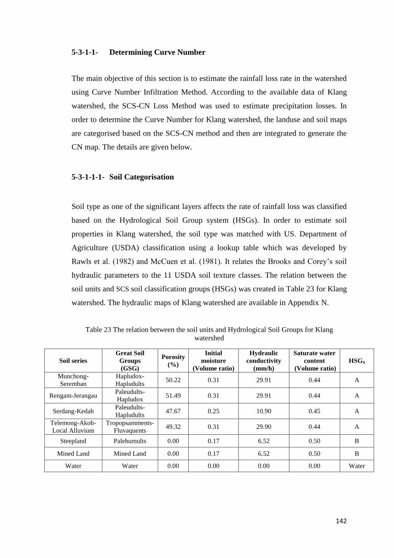
142
5-3-1-1- Determining Curve Number
The main objective of this section is to estimate the rainfall loss rate in the watershed
using Curve Number Infiltration Method. According to the available data of Klang
watershed, the SCS-CN Loss Method was used to estimate precipitation losses. In
order to determine the Curve Number for Klang watershed, the landuse and soil maps
are categorised based on the SCS-CN method and then are integrated to generate the
CN map. The details are given below.
5-3-1-1-1- Soil Categorisation
Soil type as one of the significant layers affects the rate of rainfall loss was classified
based on the Hydrological Soil Group system (HSGs). In order to estimate soil
properties in Klang watershed, the soil type was matched with US. Department of
Agriculture (USDA) classification using a lookup table which was developed by
Rawls et al. ( 98 and Mc uen et al. ( 98 . It relates the Brooks and orey’s soil
hydraulic parameters to the 11 USDA soil texture classes. The relation between the
soil units and SCS soil classification groups (HSGs) was created in Table 23 for Klang
watershed. The hydraulic maps of Klang watershed are available in Appendix N.
Table 23 The relation between the soil units and Hydrological Soil Groups for Klang
watershed
Soil series
Great Soil
Groups
(GSG)
Porosity
(%)
Initial
moisture
(Volume ratio)
Hydraulic
conductivity
(mm/h)
Saturate water
content
(Volume ratio)
HSGS
Munchong-
Seremban
Hapludox-
Hapludults 50.22 0.31 29.91 0.44 A
Rengam-Jerangau Paleudults-
Hapludox 51.49 0.31 29.91 0.44 A
Serdang-Kedah Paleudults-
Hapludults 47.67 0.25 10.90 0.45 A
Telemong-Akob-
Local Alluvium
Tropopsamments-
Fluvaquents 49.32 0.31 29.90 0.44 A
Steepland Palehumults 0.00 0.17 6.52 0.50 B
Mined Land Mined Land 0.00 0.17 6.52 0.50 B
Water Water 0.00 0.00 0.00 0.00 Water
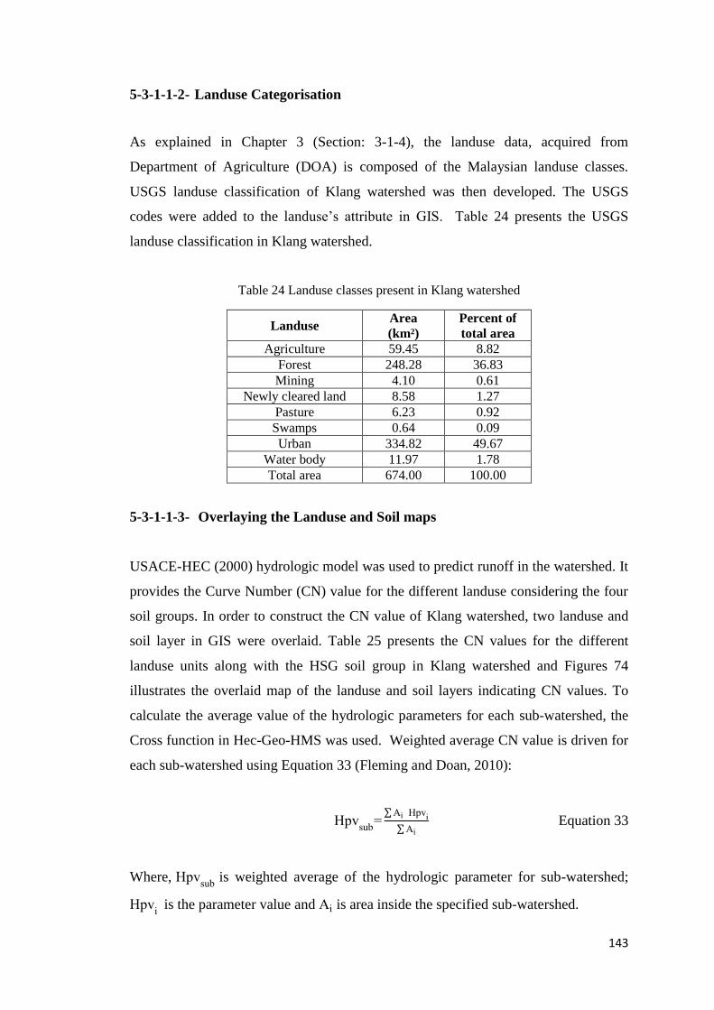
143
5-3-1-1-2- Landuse Categorisation
As explained in Chapter 3 (Section: 3-1-4), the landuse data, acquired from
Department of Agriculture (DOA) is composed of the Malaysian landuse classes.
USGS landuse classification of Klang watershed was then developed. The USGS
codes were added to the landuse’s attribute in IS. Table 24 presents the USGS
landuse classification in Klang watershed.
Table 24 Landuse classes present in Klang watershed
Landuse Area
(km²)
Percent of
total area
Agriculture 59.45 8.82
Forest 248.28 36.83
Mining 4.10 0.61
Newly cleared land 8.58 1.27
Pasture 6.23 0.92
Swamps 0.64 0.09
Urban 334.82 49.67
Water body 11.97 1.78
Total area 674.00 100.00
5-3-1-1-3- Overlaying the Landuse and Soil maps
USACE-HEC (2000) hydrologic model was used to predict runoff in the watershed. It
provides the Curve Number (CN) value for the different landuse considering the four
soil groups. In order to construct the CN value of Klang watershed, two landuse and
soil layer in GIS were overlaid. Table 25 presents the CN values for the different
landuse units along with the HSG soil group in Klang watershed and Figures 74
illustrates the overlaid map of the landuse and soil layers indicating CN values. To
calculate the average value of the hydrologic parameters for each sub-watershed, the
Cross function in Hec-Geo-HMS was used. Weighted average CN value is driven for
each sub-watershed using Equation 33 (Fleming and Doan, 2010):
Hpvsub
Ai Hpvi Ai
Equation 33
Where, Hpvsub
is weighted average of the hydrologic parameter for sub-watershed;
Hpvi is the parameter value and Ai is area inside the specified sub-watershed.
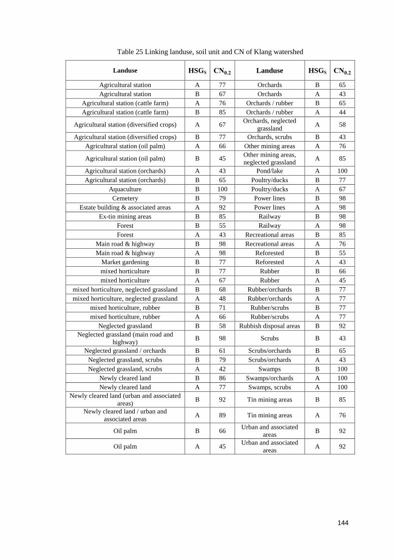
144
Table 25 Linking landuse, soil unit and CN of Klang watershed
Landuse HSGS Landuse HSGS
Agricultural station A 77 Orchards B 65
Agricultural station B 67 Orchards A 43
Agricultural station (cattle farm) A 76 Orchards / rubber B 65
Agricultural station (cattle farm) B 85 Orchards / rubber A 44
Agricultural station (diversified crops) A 67 Orchards, neglected
grassland A 58
Agricultural station (diversified crops) B 77 Orchards, scrubs B 43
Agricultural station (oil palm) A 66 Other mining areas A 76
Agricultural station (oil palm) B 45 Other mining areas,
neglected grassland A 85
Agricultural station (orchards) A 43 Pond/lake A 100
Agricultural station (orchards) B 65 Poultry/ducks B 77
Aquaculture B 100 Poultry/ducks A 67
Cemetery B 79 Power lines B 98
Estate building & associated areas A 92 Power lines A 98
Ex-tin mining areas B 85 Railway B 98
Forest B 55 Railway A 98
Forest A 43 Recreational areas B 85
Main road & highway B 98 Recreational areas A 76
Main road & highway A 98 Reforested B 55
Market gardening B 77 Reforested A 43
mixed horticulture B 77 Rubber B 66
mixed horticulture A 67 Rubber A 45
mixed horticulture, neglected grassland B 68 Rubber/orchards B 77
mixed horticulture, neglected grassland A 48 Rubber/orchards A 77
mixed horticulture, rubber B 71 Rubber/scrubs B 77
mixed horticulture, rubber A 66 Rubber/scrubs A 77
Neglected grassland B 58 Rubbish disposal areas B 92
Neglected grassland (main road and
highway) B 98 Scrubs B 43
Neglected grassland / orchards B 61 Scrubs/orchards B 65
Neglected grassland, scrubs B 79 Scrubs/orchards A 43
Neglected grassland, scrubs A 42 Swamps B 100
Newly cleared land B 86 Swamps/orchards A 100
Newly cleared land A 77 Swamps, scrubs A 100
Newly cleared land (urban and associated
areas) B 92 Tin mining areas B 85
Newly cleared land / urban and
associated areas A 89 Tin mining areas A 76
Oil palm B 66 Urban and associated
areas B 92
Oil palm A 45 Urban and associated
areas A 92
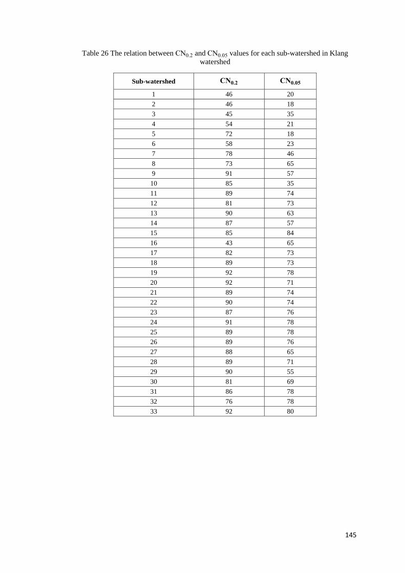
145
Table 26 The relation between . and . values for each sub-watershed in Klang
watershed
Sub-watershed
1 46 20
2 46 18
3 45 35
4 54 21
5 72 18
6 58 23
7 78 46
8 73 65
9 91 57
10 85 35
11 89 74
12 81 73
13 90 63
14 87 57
15 85 84
16 43 65
17 82 73
18 89 73
19 92 78
20 92 71
21 89 74
22 90 74
23 87 76
24 91 78
25 89 78
26 89 76
27 88 65
28 89 71
29 90 55
30 81 69
31 86 78
32 76 78
33 92 80
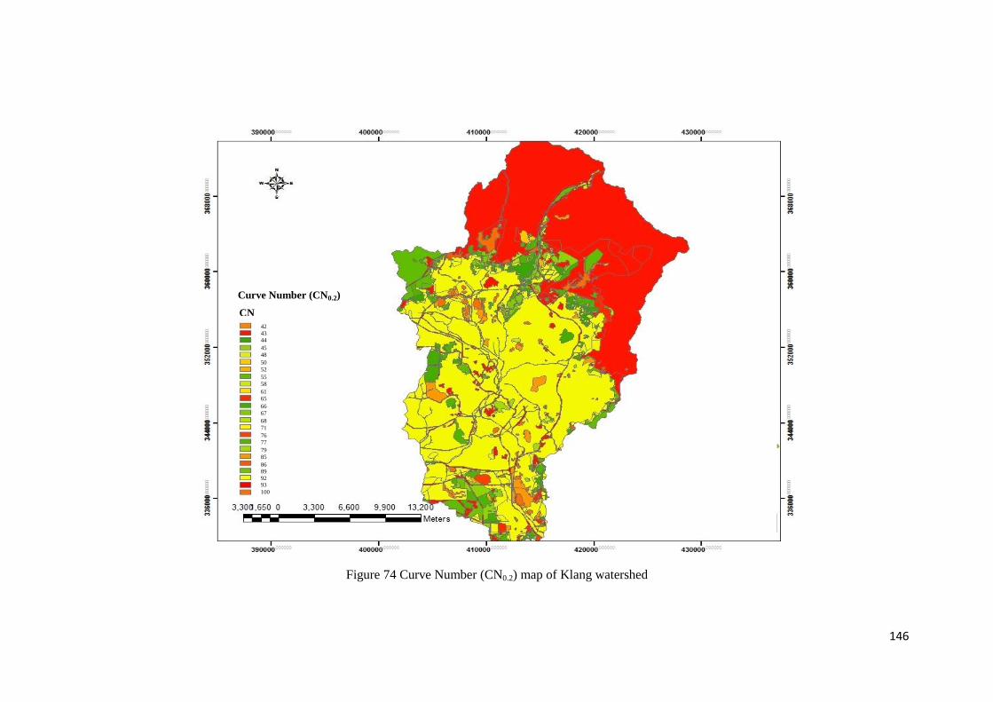
146
Figure 74 Curve Number (CN0.2) map of Klang watershed
Curve Number (CN0.2)
42
43
44
45
48
50
52
55
58
61
65
66
67
68
71
76
77
79
85
86
89
92 93
100
CN
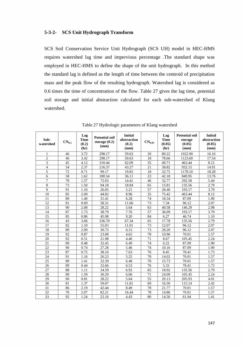
147
5-3-2- SCS Unit Hydrograph Transform
SCS Soil Conservation Service Unit Hydrograph (SCS UH) model in HEC-HMS
requires watershed lag time and impervious percentage .The standard shape was
employed in HEC-HMS to define the shape of the unit hydrograph. In this method
the standard lag is defined as the length of time between the centroid of precipitation
mass and the peak flow of the resulting hydrograph. Watershed lag is considered as
0.6 times the time of concentration of the flow. Table 27 gives the lag time, potential
soil storage and initial abstraction calculated for each sub-watershed of Klang
watershed.
Table 27 Hydrologic parameters of Klang watershed
Sub-
watershed CN0.2
Lag
Time
(0.2)
(hr)
Potential soil
storage (0.2)
(mm)
Initial
abstraction
(0.2)
(mm)
CN0.05
Lag
Time
(0.05)
(hr)
Potential soil
storage
(0.05)
(mm)
Initial
abstraction
(0.05)
(mm)
1 46 3.72 298.17 59.63 20 80.22 1022.90 16.16
2 46 3.42 298.17 59.63 18 78.66 1123.60 17.54
3 45 4.12 310.44 62.09 35 49.71 463.44 8.12
4 54 2.37 216.37 43.27 21 58.82 932.15 14.91
5 72 0.71 99.17 19.83 18 32.75 1178.10 18.28
6 58 1.62 180.54 36.11 23 42.18 849.95 13.76
7 78 1.57 72.03 14.41 46 32.77 292.58 5.44
8 73 1.50 94.18 18.84 65 15.81 135.56 2.79
9 91 1.16 26.05 5.21 57 28.40 193.17 3.79
10 85 2.09 44.82 8.96 35 75.42 463.44 8.12
11 89 1.40 31.41 6.28 74 18.34 87.09 1.90
12 81 0.69 58.31 11.66 73 7.34 96.12 2.07
13 90 2.08 28.22 5.64 63 40.58 146.29 2.98
14 87 1.73 38.79 7.76 57 36.09 193.17 3.79
15 85 0.86 45.98 9.20 84 6.27 46.74 1.10
16 43 3.66 336.70 67.34 65 17.78 135.56 2.79
17 82 1.10 55.03 11.01 73 12.07 96.12 2.07
18 89 2.00 30.73 6.15 73 28.20 96.12 2.07
19 92 0.87 23.08 4.62 78 10.96 70.01 1.57
20 92 0.51 21.98 4.40 71 8.67 105.45 2.24
21 89 0.48 32.45 6.49 74 6.22 87.09 1.90
22 90 0.74 27.28 5.46 74 10.16 87.09 1.90
23 87 0.75 38.16 7.63 76 8.45 78.41 1.73
24 91 1.16 26.23 5.25 78 14.02 70.01 1.57
25 89 1.41 32.39 6.48 78 15.73 70.01 1.57
26 89 0.44 32.66 6.53 76 5.33 78.41 1.73
27 88 1.11 34.59 6.92 65 18.92 135.56 2.79
28 89 1.59 30.29 6.06 71 24.09 105.45 2.24
29 90 0.81 28.22 5.64 55 20.13 205.93 4.01
30 81 1.37 59.07 11.81 69 16.50 115.14 2.42
31 86 2.19 42.44 8.49 78 21.77 70.01 1.57
32 76 2.07 82.21 16.44 78 14.86 70.01 1.57
33 92 1.24 22.16 4.43 80 14.50 61.94 1.41
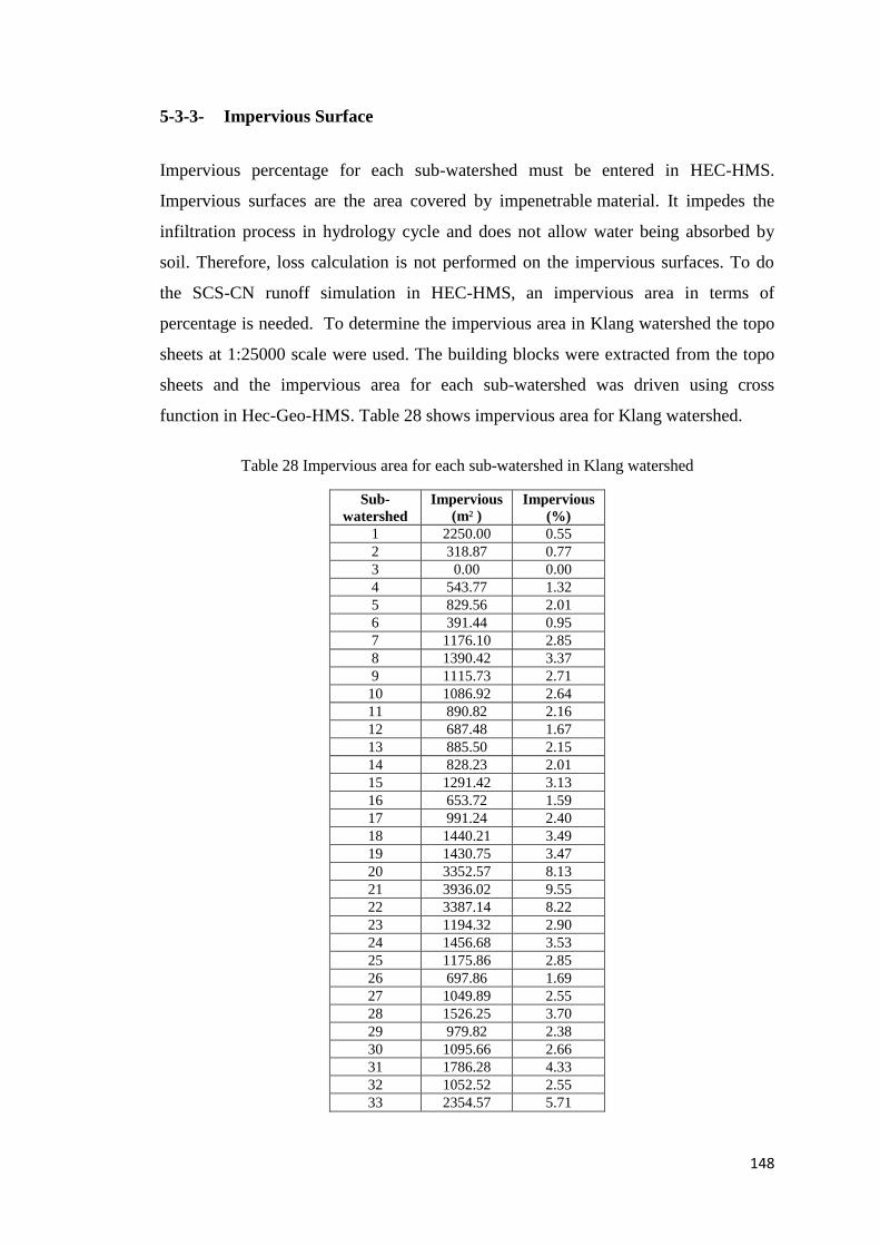
148
5-3-3- Impervious Surface
Impervious percentage for each sub-watershed must be entered in HEC-HMS.
Impervious surfaces are the area covered by impenetrable material. It impedes the
infiltration process in hydrology cycle and does not allow water being absorbed by
soil. Therefore, loss calculation is not performed on the impervious surfaces. To do
the SCS-CN runoff simulation in HEC-HMS, an impervious area in terms of
percentage is needed. To determine the impervious area in Klang watershed the topo
sheets at 1:25000 scale were used. The building blocks were extracted from the topo
sheets and the impervious area for each sub-watershed was driven using cross
function in Hec-Geo-HMS. Table 28 shows impervious area for Klang watershed.
Table 28 Impervious area for each sub-watershed in Klang watershed
Sub-
watershed
Impervious
(m² ) Impervious
(%)
1 2250.00 0.55
2 318.87 0.77
3 0.00 0.00
4 543.77 1.32
5 829.56 2.01
6 391.44 0.95
7 1176.10 2.85
8 1390.42 3.37
9 1115.73 2.71
10 1086.92 2.64
11 890.82 2.16
12 687.48 1.67
13 885.50 2.15
14 828.23 2.01
15 1291.42 3.13
16 653.72 1.59
17 991.24 2.40
18 1440.21 3.49
19 1430.75 3.47
20 3352.57 8.13
21 3936.02 9.55
22 3387.14 8.22
23 1194.32 2.90
24 1456.68 3.53
25 1175.86 2.85
26 697.86 1.69
27 1049.89 2.55
28 1526.25 3.70
29 979.82 2.38
30 1095.66 2.66
31 1786.28 4.33
32 1052.52 2.55
33 2354.57 5.71
149
5-3-4- Streamflow (Channel) Routing
HEC-HMS provides various methods to conduct flow routing in reach element which
needs a different level of details. In this study, Muskingum method was used to
calculate the hydrologic river routing in Klang watershed. Muskingum method in
HEC-HMS was used due to its simplicity and modest data requirement which make it
practical to be used for Klang watershed while other methods require complex data to
use in HEC-HMS. The value of K can be calculated by length of reach divided by the
average flow velocity and the value of X is between 0.0 and 0.5. A value of 0.0
represents maximum attenuation from the procedure and 0.5 provides the minimum
attenuation. However, in natural channels X ranges from 0.1 to 0.3 (Raghunath,
2006). To assign the value of X in the Muskingum method in Klang watershed, a
value of 0.4 was used in a landuse map of the watershed. This reveals the drainage
system has been strongly urbanised and the natural channel in the area has been
transformed into concreted channels. According to the channel properties, a high
value of 0.4 was assumed.
5-3-5- Reservoir Flood Routing
There are two major reservoirs in Klang watershed which are Batu dam and Klang
Gate dam. Routing methods are used to simulate the storage of reservoir. In this
regard, HEC-HMS provides three methods namely storage-outflow relationships,
specified release and the method based on individual components of the outlet works.
With the available data from reservoirs (Appendix O), the Storage-Discharge Method
was used for both dams. Figures 75 and 76 illustrate Storage-Discharge relationships
of Klang Gate dam and Batu dam as derived in HEC-HMS, respectively.
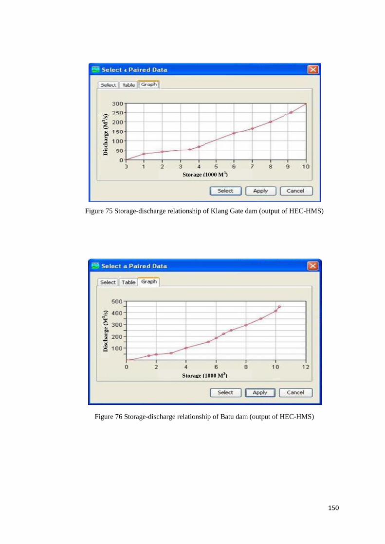
150
Figure 75 Storage-discharge relationship of Klang Gate dam (output of HEC-HMS)
Figure 76 Storage-discharge relationship of Batu dam (output of HEC-HMS)
Storage (1000 M3)
Storage (1000 M3)
Dis
cha
rge
(M3/s
) D
isch
arg
e (M
3/s
)
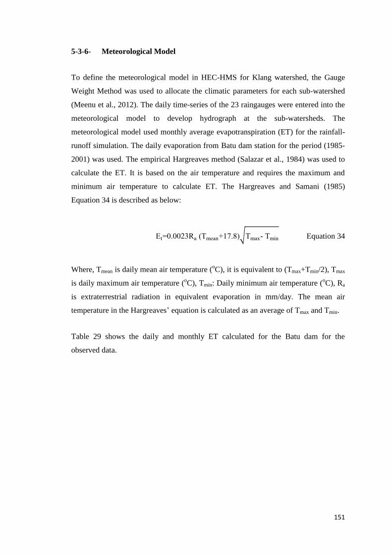
151
5-3-6- Meteorological Model
To define the meteorological model in HEC-HMS for Klang watershed, the Gauge
Weight Method was used to allocate the climatic parameters for each sub-watershed
(Meenu et al., 2012). The daily time-series of the 23 raingauges were entered into the
meteorological model to develop hydrograph at the sub-watersheds. The
meteorological model used monthly average evapotranspiration (ET) for the rainfall-
runoff simulation. The daily evaporation from Batu dam station for the period (1985-
2001) was used. The empirical Hargreaves method (Salazar et al., 1984) was used to
calculate the ET. It is based on the air temperature and requires the maximum and
minimum air temperature to calculate ET. The Hargreaves and Samani (1985)
Equation 34 is described as below:
t . 3 a (Tmean .8 Tmax- Tmin Equation 34
Where, Tmean is daily mean air temperature (oC), it is equivalent to (Tmax+Tmin/2), Tmax
is daily maximum air temperature (oC), Tmin: Daily minimum air temperature (
oC), Ra
is extraterrestrial radiation in equivalent evaporation in mm/day. The mean air
temperature in the Hargreaves’ equation is calculated as an average of Tmax and Tmin.
Table 29 shows the daily and monthly ET calculated for the Batu dam for the
observed data.
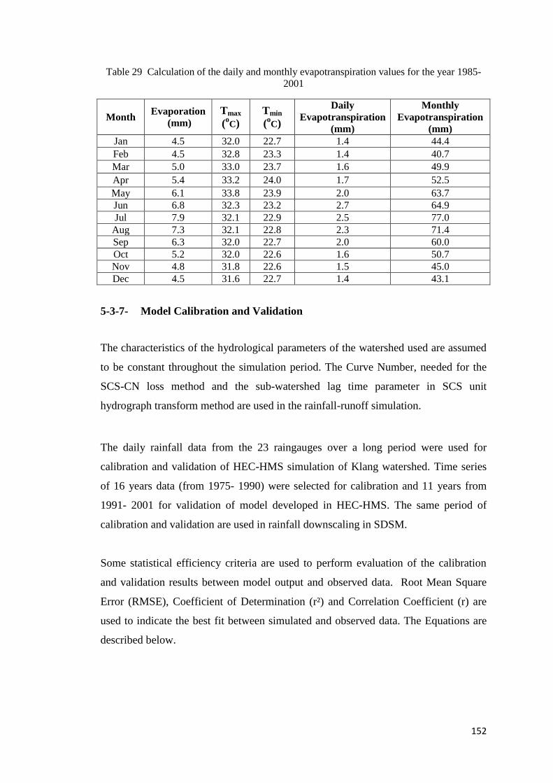
152
Table 29 Calculation of the daily and monthly evapotranspiration values for the year 1985-
2001
Month Evaporation
(mm)
Tmax
(oC)
Tmin
(oC)
Daily
Evapotranspiration
(mm)
Monthly
Evapotranspiration
(mm)
Jan 4.5 32.0 22.7 1.4 44.4
Feb 4.5 32.8 23.3 1.4 40.7
Mar 5.0 33.0 23.7 1.6 49.9
Apr 5.4 33.2 24.0 1.7 52.5
May 6.1 33.8 23.9 2.0 63.7
Jun 6.8 32.3 23.2 2.7 64.9
Jul 7.9 32.1 22.9 2.5 77.0
Aug 7.3 32.1 22.8 2.3 71.4
Sep 6.3 32.0 22.7 2.0 60.0
Oct 5.2 32.0 22.6 1.6 50.7
Nov 4.8 31.8 22.6 1.5 45.0
Dec 4.5 31.6 22.7 1.4 43.1
5-3-7- Model Calibration and Validation
The characteristics of the hydrological parameters of the watershed used are assumed
to be constant throughout the simulation period. The Curve Number, needed for the
SCS-CN loss method and the sub-watershed lag time parameter in SCS unit
hydrograph transform method are used in the rainfall-runoff simulation.
The daily rainfall data from the 23 raingauges over a long period were used for
calibration and validation of HEC-HMS simulation of Klang watershed. Time series
of 16 years data (from 1975- 1990) were selected for calibration and 11 years from
1991- 2001 for validation of model developed in HEC-HMS. The same period of
calibration and validation are used in rainfall downscaling in SDSM.
Some statistical efficiency criteria are used to perform evaluation of the calibration
and validation results between model output and observed data. Root Mean Square
Error (RMSE), Coefficient of Determination (r²) and Correlation Coefficient (r) are
used to indicate the best fit between simulated and observed data. The Equations are
described below.
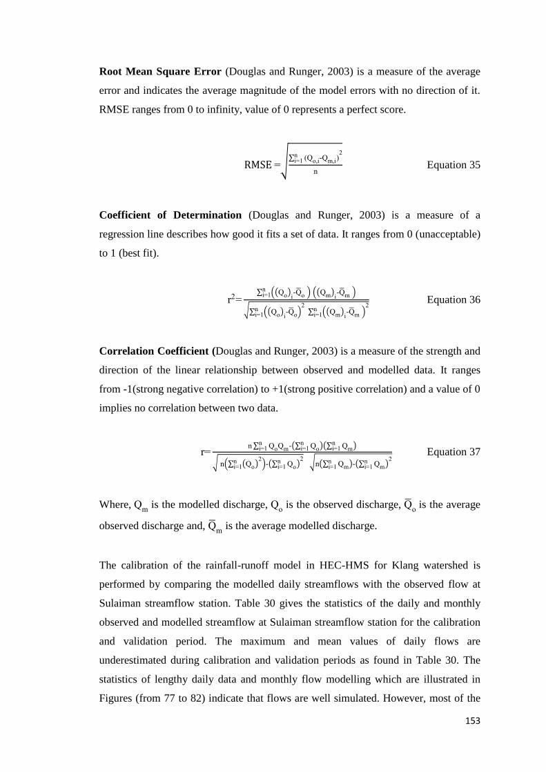
153
Root Mean Square Error (Douglas and Runger, 2003) is a measure of the average
error and indicates the average magnitude of the model errors with no direction of it.
RMSE ranges from 0 to infinity, value of 0 represents a perfect score.
( o,i- m,i
ni
n
Equation 35
Coefficient of Determination (Douglas and Runger, 2003) is a measure of a
regression line describes how good it fits a set of data. It ranges from 0 (unacceptable)
to 1 (best fit).
r o i
- o m i- m
ni
o i- o
m
i- m
ni
ni
Equation 36
Correlation Coefficient (Douglas and Runger, 2003) is a measure of the strength and
direction of the linear relationship between observed and modelled data. It ranges
from -1(strong negative correlation) to +1(strong positive correlation) and a value of 0
implies no correlation between two data.
r n o
ni m- o
ni m
ni
n o n
i - oni
n m
ni - m
ni
Equation 37
Where, m
is the modelled discharge, o is the observed discharge,
o is the average
observed discharge and, m
is the average modelled discharge.
The calibration of the rainfall-runoff model in HEC-HMS for Klang watershed is
performed by comparing the modelled daily streamflows with the observed flow at
Sulaiman streamflow station. Table 30 gives the statistics of the daily and monthly
observed and modelled streamflow at Sulaiman streamflow station for the calibration
and validation period. The maximum and mean values of daily flows are
underestimated during calibration and validation periods as found in Table 30. The
statistics of lengthy daily data and monthly flow modelling which are illustrated in
Figures (from 77 to 82) indicate that flows are well simulated. However, most of the
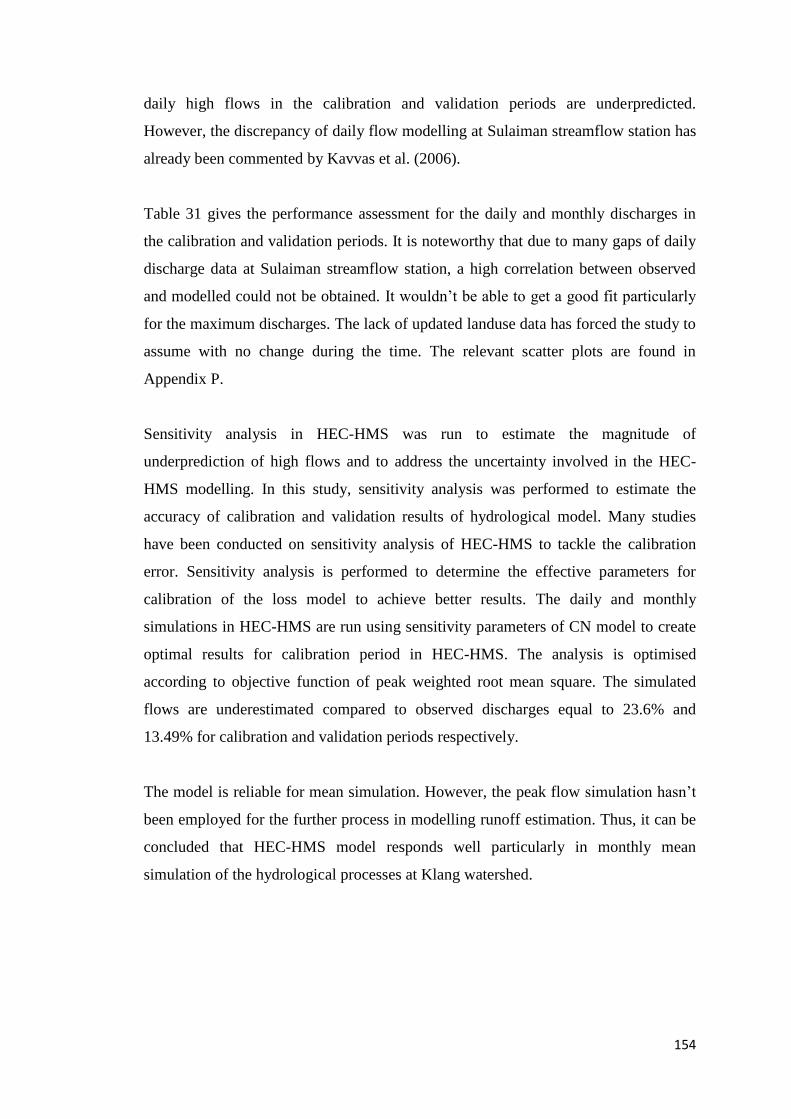
154
daily high flows in the calibration and validation periods are underpredicted.
However, the discrepancy of daily flow modelling at Sulaiman streamflow station has
already been commented by Kavvas et al. (2006).
Table 31 gives the performance assessment for the daily and monthly discharges in
the calibration and validation periods. It is noteworthy that due to many gaps of daily
discharge data at Sulaiman streamflow station, a high correlation between observed
and modelled could not be obtained. It wouldn’t be able to get a good fit particularly
for the maximum discharges. The lack of updated landuse data has forced the study to
assume with no change during the time. The relevant scatter plots are found in
Appendix P.
Sensitivity analysis in HEC-HMS was run to estimate the magnitude of
underprediction of high flows and to address the uncertainty involved in the HEC-
HMS modelling. In this study, sensitivity analysis was performed to estimate the
accuracy of calibration and validation results of hydrological model. Many studies
have been conducted on sensitivity analysis of HEC-HMS to tackle the calibration
error. Sensitivity analysis is performed to determine the effective parameters for
calibration of the loss model to achieve better results. The daily and monthly
simulations in HEC-HMS are run using sensitivity parameters of CN model to create
optimal results for calibration period in HEC-HMS. The analysis is optimised
according to objective function of peak weighted root mean square. The simulated
flows are underestimated compared to observed discharges equal to 23.6% and
13.49% for calibration and validation periods respectively.
The model is reliable for mean simulation. However, the peak flow simulation hasn’t
been employed for the further process in modelling runoff estimation. Thus, it can be
concluded that HEC-HMS model responds well particularly in monthly mean
simulation of the hydrological processes at Klang watershed.
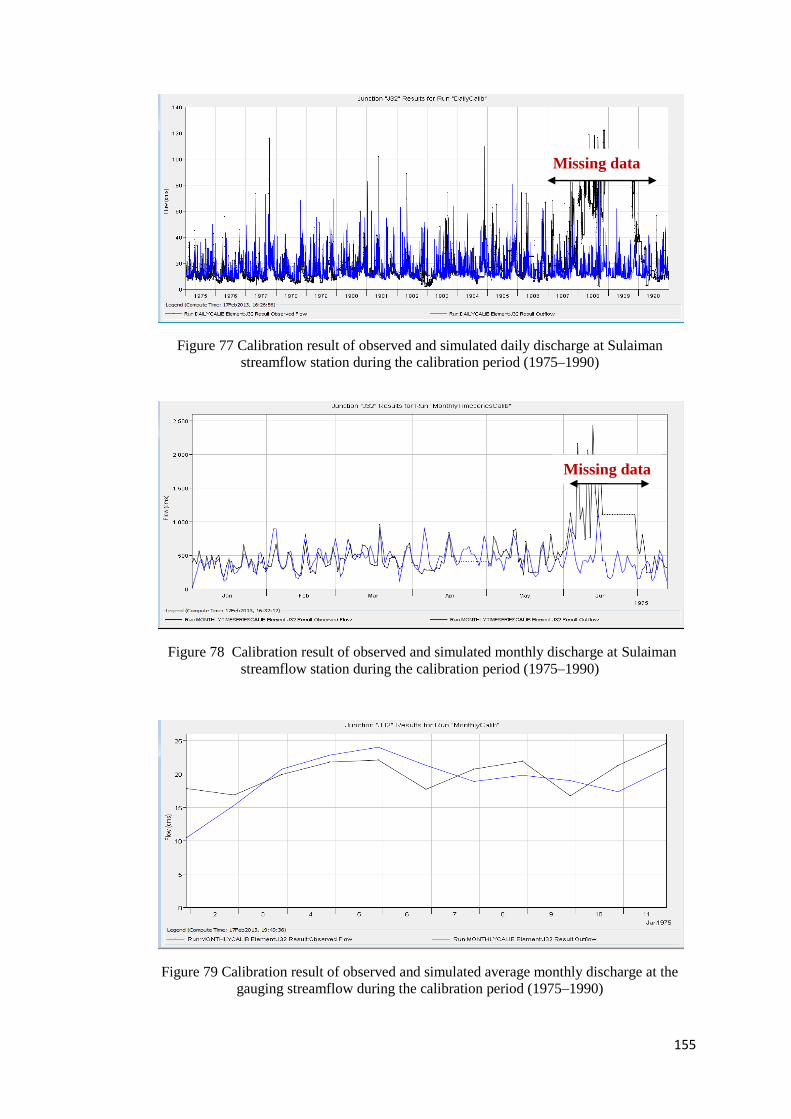
155
Figure 77 Calibration result of observed and simulated daily discharge at Sulaiman
streamflow station during the calibration period (1975–1990)
Figure 78 Calibration result of observed and simulated monthly discharge at Sulaiman
streamflow station during the calibration period (1975–1990)
Figure 79 Calibration result of observed and simulated average monthly discharge at the
gauging streamflow during the calibration period (1975–1990)
Missing data
Missing data
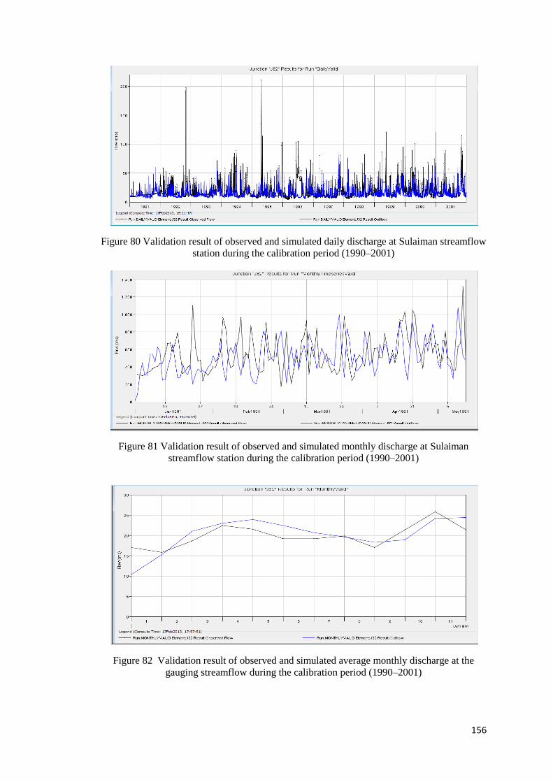
156
Figure 80 Validation result of observed and simulated daily discharge at Sulaiman streamflow
station during the calibration period (1990–2001)
Figure 81 Validation result of observed and simulated monthly discharge at Sulaiman
streamflow station during the calibration period (1990–2001)
Figure 82 Validation result of observed and simulated average monthly discharge at the
gauging streamflow during the calibration period (1990–2001)
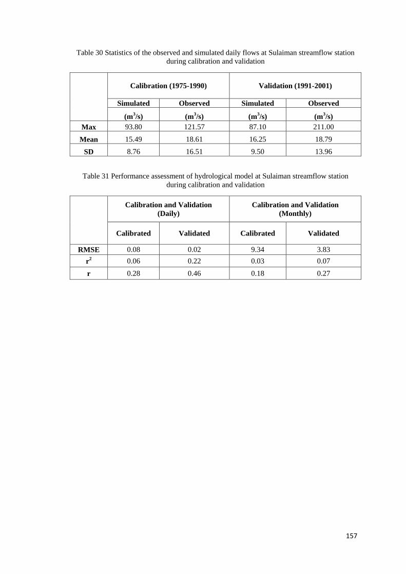
157
Table 30 Statistics of the observed and simulated daily flows at Sulaiman streamflow station
during calibration and validation
Calibration (1975-1990) Validation (1991-2001)
Simulated Observed Simulated Observed
(m3/s) (m
3/s) (m
3/s) (m
3/s)
Max 93.80 121.57 87.10 211.00
Mean 15.49 18.61 16.25 18.79
SD 8.76 16.51 9.50 13.96
Table 31 Performance assessment of hydrological model at Sulaiman streamflow station
during calibration and validation
Calibration and Validation
(Daily)
Calibration and Validation
(Monthly)
Calibrated Validated Calibrated Validated
RMSE 0.08 0.02 9.34 3.83
r2 0.06 0.22 0.03 0.07
r 0.28 0.46 0.18 0.27
158
6- RESULTS AND DISCUSSION
This section represents the climate change downscale scenarios which are generated
by SDSM and also describes the impacts of climate change using the hydrological
model. It simulates the streamflow behaviour corresponding to the current and future
climate condition. The future climate was projected using SDSM as presented in
Chapter 4.
6-1- Changes in Temperature
The output generated by the HadCM3 GCM model has projected an increase in both
maximum and minimum temperature for Klang watershed. The maximum and
minimum temperatures increased towards the end of the century by 2.7 oC and 0.8
oC,
respectively compared to the current observed temperature at Subang temperature
station. The maximum daily temperature under A2 scenario increased the most in
May by 1.6 oC, 2.2
oC and 2.7
oC for 2020s, 2050s and 2080s, respectively which is a
considerable increase in daily temperature through the year. The trend under B2
scenario is similar in May which is 1.4 oC, 1.5
oC and 2.4
oC. The minimum daily
temperature decreased in months (October, November and December) and increased
in months from January to May, August and September, with no significant vary
through June and July under A2 and B2 scenarios. Tables (32 and 33) show the
monthly analysis in three time slices to show the temperature pattern based on IPCC
scenarios. Figures (from 83 to 86) illustrate projected changes in maximum and
minimum daily temperature at Subang station.
The graphs reveal a continually increasing temperature of Subang station at Klang
watershed as per A2 simulation which is generally higher than B2 scenario
simulation. Because A2 includes the highest concentration of CO2 equal to 850 ppm
(IPCC, 2000). Scenario A2 is a Medium-High emission scenario assumes the higher
usage of fossil fuel while Medium-Low emissions scenario B2 is a lower rate of
emissions which is based on least using fossil fuel and taking environmental
approaches at local scale.
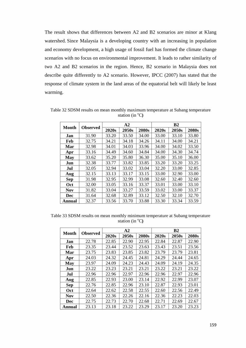
159
The result shows that differences between A2 and B2 scenarios are minor at Klang
watershed. Since Malaysia is a developing country with an increasing in population
and economy development, a high usage of fossil fuel has formed the climate change
scenarios with no focus on environmental improvement. It leads to rather similarity of
two A2 and B2 scenarios in the region. Hence, B2 scenario in Malaysia does not
describe quite differently to A2 scenario. However, IPCC (2007) has stated that the
response of climate system in the land areas of the equatorial belt will likely be least
warming.
Table 32 SDSM results on mean monthly maximum temperature at Subang temperature
station (in oC)
Month Observed A2 B2
2020s 2050s 2080s 2020s 2050s 2080s
Jan 31.90 33.20 33.50 34.00 33.00 33.10 33.80
Feb 32.75 34.21 34.18 34.26 34.11 34.00 34.21
Mar 32.98 34.01 34.03 33.96 34.00 34.02 33.50
Apr 33.16 34.49 34.60 34.84 34.00 34.30 34.74
May 33.62 35.20 35.80 36.30 35.00 35.10 36.00
Jun 32.38 33.77 33.82 33.85 33.20 33.20 33.25
Jul 32.05 32.94 33.02 33.04 32.20 33.00 32.85
Aug 32.15 33.13 33.17 33.15 33.00 32.90 33.00
Sep 31.98 32.95 32.99 33.08 32.60 32.40 32.60
Oct 32.00 33.05 33.16 33.37 33.01 33.00 33.10
Nov 31.82 33.04 33.27 33.59 33.02 33.00 33.37
Dec 31.64 32.68 32.89 33.12 32.50 32.10 32.70
Annual 32.37 33.56 33.70 33.88 33.30 33.34 33.59
Table 33 SDSM results on mean monthly minimum temperature at Subang temperature
station (in oC)
Month Observed A2 B2
2020s 2050s 2080s 2020s 2050s 2080s
Jan 22.78 22.85 22.90 22.95 22.84 22.87 22.90
Feb 23.35 23.44 23.52 23.63 23.43 23.51 23.56
Mar 23.75 23.83 23.85 23.82 23.79 23.79 23.81
Apr 24.03 24.32 24.45 24.81 24.29 24.44 24.65
May 23.97 24.09 24.23 24.43 24.09 24.19 24.35
Jun 23.22 23.23 23.21 23.21 23.22 23.21 23.22
Jul 22.96 22.96 22.97 22.96 22.96 22.97 22.96
Aug 22.85 22.93 23.00 23.14 22.92 22.99 23.07
Sep 22.76 22.85 22.96 23.10 22.87 22.93 23.01
Oct 22.64 22.62 22.58 22.55 22.60 22.56 22.49
Nov 22.50 22.36 22.26 22.16 22.36 22.23 22.03
Dec 22.75 22.73 22.70 22.68 22.71 22.69 22.67
Annual 23.13 23.18 23.22 23.29 23.17 23.20 23.23
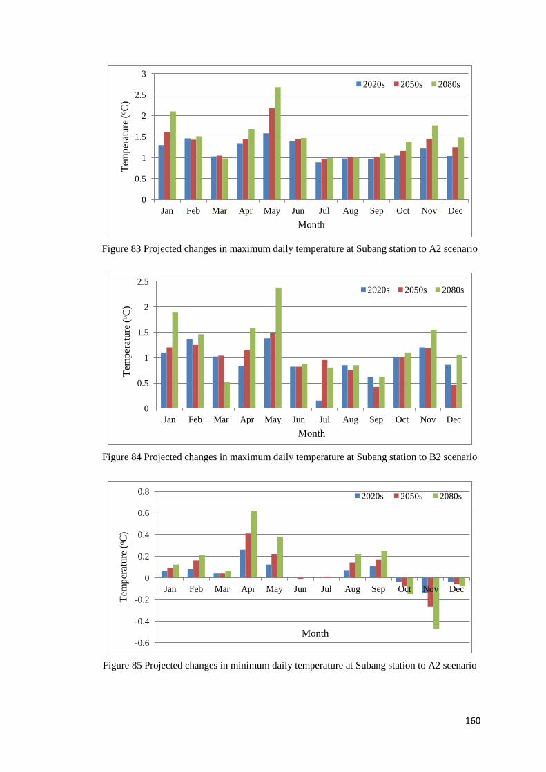
160
Figure 83 Projected changes in maximum daily temperature at Subang station to A2 scenario
Figure 84 Projected changes in maximum daily temperature at Subang station to B2 scenario
Figure 85 Projected changes in minimum daily temperature at Subang station to A2 scenario
0
0.5
1
1.5
2
2.5
3
Jan Feb Mar Apr May Jun Jul Aug Sep Oct Nov Dec
Tem
per
atu
re (
oC
)
Month
2020s 2050s 2080s
0
0.5
1
1.5
2
2.5
Jan Feb Mar Apr May Jun Jul Aug Sep Oct Nov Dec
Tem
per
ature
(oC
)
Month
2020s 2050s 2080s
-0.6
-0.4
-0.2
0
0.2
0.4
0.6
0.8
Jan Feb Mar Apr May Jun Jul Aug Sep Oct Nov Dec
Tem
per
atu
re (
oC
)
Month
2020s 2050s 2080s
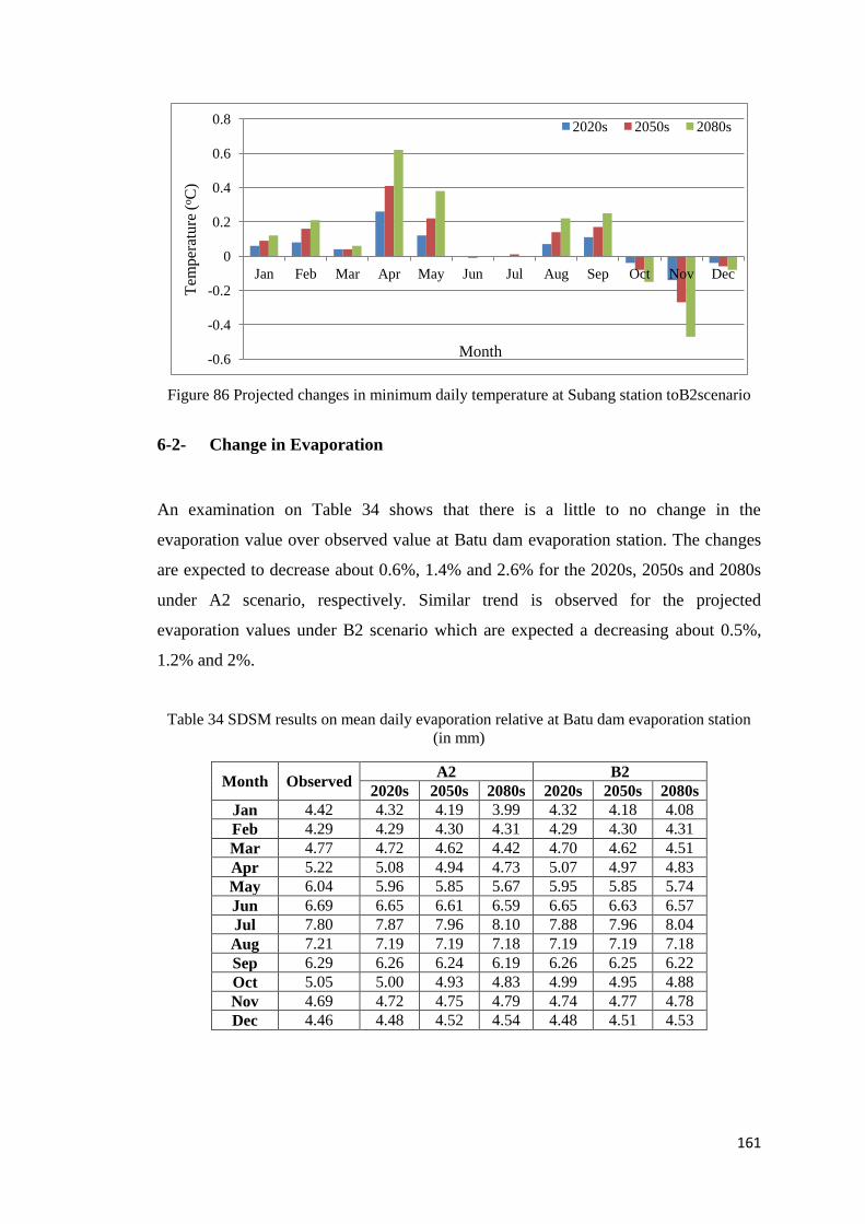
161
Figure 86 Projected changes in minimum daily temperature at Subang station toB2scenario
6-2- Change in Evaporation
An examination on Table 34 shows that there is a little to no change in the
evaporation value over observed value at Batu dam evaporation station. The changes
are expected to decrease about 0.6%, 1.4% and 2.6% for the 2020s, 2050s and 2080s
under A2 scenario, respectively. Similar trend is observed for the projected
evaporation values under B2 scenario which are expected a decreasing about 0.5%,
1.2% and 2%.
Table 34 SDSM results on mean daily evaporation relative at Batu dam evaporation station
(in mm)
Month Observed A2 B2
2020s 2050s 2080s 2020s 2050s 2080s
Jan 4.42 4.32 4.19 3.99 4.32 4.18 4.08
Feb 4.29 4.29 4.30 4.31 4.29 4.30 4.31
Mar 4.77 4.72 4.62 4.42 4.70 4.62 4.51
Apr 5.22 5.08 4.94 4.73 5.07 4.97 4.83
May 6.04 5.96 5.85 5.67 5.95 5.85 5.74
Jun 6.69 6.65 6.61 6.59 6.65 6.63 6.57
Jul 7.80 7.87 7.96 8.10 7.88 7.96 8.04
Aug 7.21 7.19 7.19 7.18 7.19 7.19 7.18
Sep 6.29 6.26 6.24 6.19 6.26 6.25 6.22
Oct 5.05 5.00 4.93 4.83 4.99 4.95 4.88
Nov 4.69 4.72 4.75 4.79 4.74 4.77 4.78
Dec 4.46 4.48 4.52 4.54 4.48 4.51 4.53
-0.6
-0.4
-0.2
0
0.2
0.4
0.6
0.8
Jan Feb Mar Apr May Jun Jul Aug Sep Oct Nov Dec
Tem
per
atu
re (
oC
)
Month
2020s 2050s 2080s
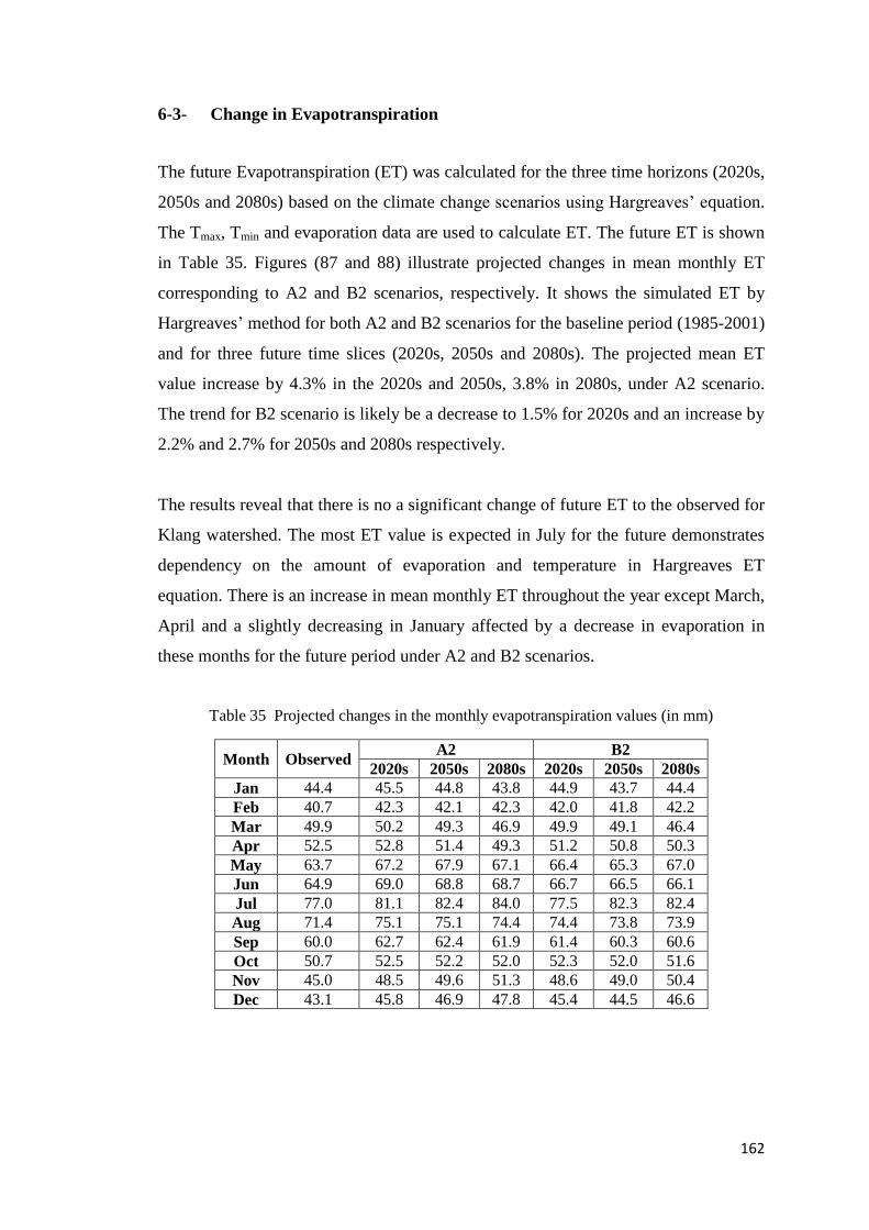
162
6-3- Change in Evapotranspiration
The future Evapotranspiration (ET) was calculated for the three time horizons (2020s,
2050s and 2080s) based on the climate change scenarios using Hargreaves’ equation.
The Tmax, Tmin and evaporation data are used to calculate ET. The future ET is shown
in Table 35. Figures (87 and 88) illustrate projected changes in mean monthly ET
corresponding to A2 and B2 scenarios, respectively. It shows the simulated ET by
Hargreaves’ method for both A2 and B2 scenarios for the baseline period (1985-2001)
and for three future time slices (2020s, 2050s and 2080s). The projected mean ET
value increase by 4.3% in the 2020s and 2050s, 3.8% in 2080s, under A2 scenario.
The trend for B2 scenario is likely be a decrease to 1.5% for 2020s and an increase by
2.2% and 2.7% for 2050s and 2080s respectively.
The results reveal that there is no a significant change of future ET to the observed for
Klang watershed. The most ET value is expected in July for the future demonstrates
dependency on the amount of evaporation and temperature in Hargreaves ET
equation. There is an increase in mean monthly ET throughout the year except March,
April and a slightly decreasing in January affected by a decrease in evaporation in
these months for the future period under A2 and B2 scenarios.
Table 35 Projected changes in the monthly evapotranspiration values (in mm)
Month Observed A2 B2
2020s 2050s 2080s 2020s 2050s 2080s
Jan 44.4 45.5 44.8 43.8 44.9 43.7 44.4
Feb 40.7 42.3 42.1 42.3 42.0 41.8 42.2
Mar 49.9 50.2 49.3 46.9 49.9 49.1 46.4
Apr 52.5 52.8 51.4 49.3 51.2 50.8 50.3
May 63.7 67.2 67.9 67.1 66.4 65.3 67.0
Jun 64.9 69.0 68.8 68.7 66.7 66.5 66.1
Jul 77.0 81.1 82.4 84.0 77.5 82.3 82.4
Aug 71.4 75.1 75.1 74.4 74.4 73.8 73.9
Sep 60.0 62.7 62.4 61.9 61.4 60.3 60.6
Oct 50.7 52.5 52.2 52.0 52.3 52.0 51.6
Nov 45.0 48.5 49.6 51.3 48.6 49.0 50.4
Dec 43.1 45.8 46.9 47.8 45.4 44.5 46.6
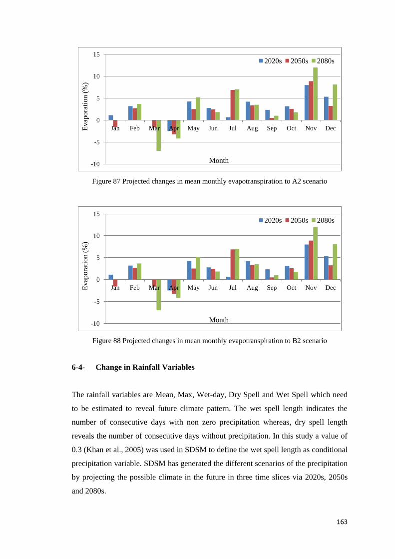
163
Figure 87 Projected changes in mean monthly evapotranspiration to A2 scenario
Figure 88 Projected changes in mean monthly evapotranspiration to B2 scenario
6-4- Change in Rainfall Variables
The rainfall variables are Mean, Max, Wet-day, Dry Spell and Wet Spell which need
to be estimated to reveal future climate pattern. The wet spell length indicates the
number of consecutive days with non zero precipitation whereas, dry spell length
reveals the number of consecutive days without precipitation. In this study a value of
0.3 (Khan et al., 2005) was used in SDSM to define the wet spell length as conditional
precipitation variable. SDSM has generated the different scenarios of the precipitation
by projecting the possible climate in the future in three time slices via 2020s, 2050s
and 2080s.
-10
-5
0
5
10
15
Jan Feb Mar Apr May Jun Jul Aug Sep Oct Nov Dec Evap
ora
tio
n (
%)
Month
2020s 2050s 2080s
-10
-5
0
5
10
15
Jan Feb Mar Apr May Jun Jul Aug Sep Oct Nov Dec Evap
ora
tion (
%)
Month
2020s 2050s 2080s
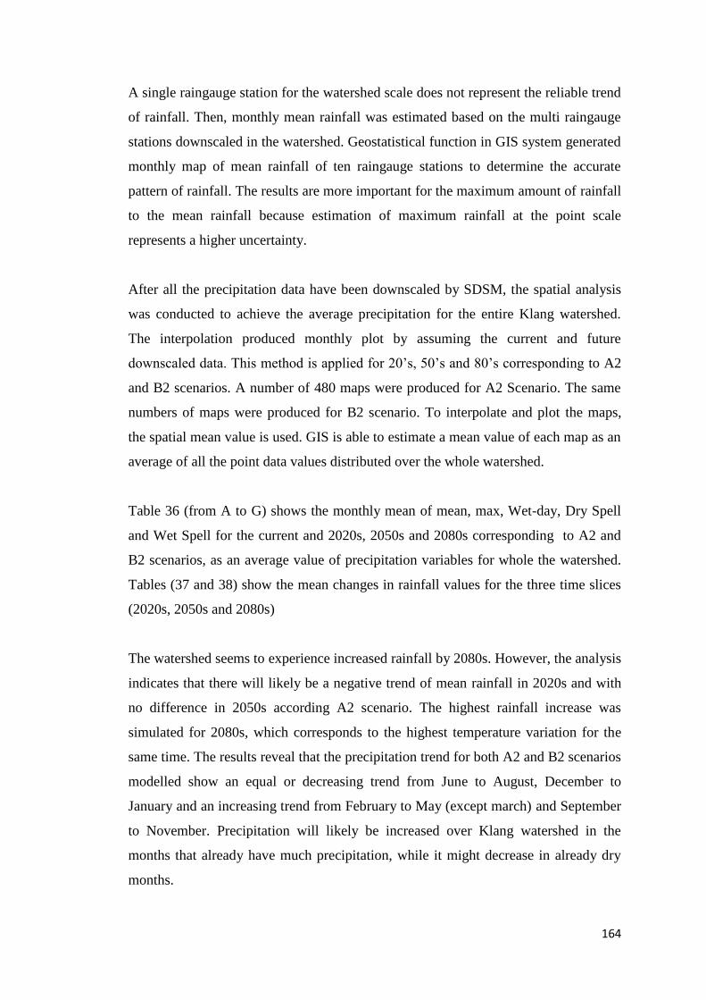
164
A single raingauge station for the watershed scale does not represent the reliable trend
of rainfall. Then, monthly mean rainfall was estimated based on the multi raingauge
stations downscaled in the watershed. Geostatistical function in GIS system generated
monthly map of mean rainfall of ten raingauge stations to determine the accurate
pattern of rainfall. The results are more important for the maximum amount of rainfall
to the mean rainfall because estimation of maximum rainfall at the point scale
represents a higher uncertainty.
After all the precipitation data have been downscaled by SDSM, the spatial analysis
was conducted to achieve the average precipitation for the entire Klang watershed.
The interpolation produced monthly plot by assuming the current and future
downscaled data. This method is applied for ’s, ’s and 8 ’s corresponding to A2
and B2 scenarios. A number of 480 maps were produced for A2 Scenario. The same
numbers of maps were produced for B2 scenario. To interpolate and plot the maps,
the spatial mean value is used. GIS is able to estimate a mean value of each map as an
average of all the point data values distributed over the whole watershed.
Table 36 (from A to G) shows the monthly mean of mean, max, Wet-day, Dry Spell
and Wet Spell for the current and 2020s, 2050s and 2080s corresponding to A2 and
B2 scenarios, as an average value of precipitation variables for whole the watershed.
Tables (37 and 38) show the mean changes in rainfall values for the three time slices
(2020s, 2050s and 2080s)
The watershed seems to experience increased rainfall by 2080s. However, the analysis
indicates that there will likely be a negative trend of mean rainfall in 2020s and with
no difference in 2050s according A2 scenario. The highest rainfall increase was
simulated for 2080s, which corresponds to the highest temperature variation for the
same time. The results reveal that the precipitation trend for both A2 and B2 scenarios
modelled show an equal or decreasing trend from June to August, December to
January and an increasing trend from February to May (except march) and September
to November. Precipitation will likely be increased over Klang watershed in the
months that already have much precipitation, while it might decrease in already dry
months.
165
Mean annual precipitations are projected to increase in the future for A2 compared to
B2 scenario. The precipitation experiences a mean annual decrease by 7.9%, 0.6% for
A2 scenario in 2020s, 2050s respectively and an increase by 12.4% in 2080s under A2
scenario. The change for B2 scenario is projected to decrease 11.5% in the 2020s,
6.6% in 2050s and increase 2.6% in 2080s.
The precipitation in month February, April and September in all the three time slices
of future increased under A2 and B2 scenarios. In 2080s, 26.4%, 30% and 88%
increase in February, April and September are projected under A2 scenario, while the
increase for B2 scenario are projected 21.5%, 19.7% and 65.2% in these months.
A decrease of 50% of mean wet spell length was projected for the future, an
increasing of mean dry spell length probably will reach to 10% compared to the
current condition by 2080s while there will expect to decrease in consecutive days
without rainfall approximately 10% and 15.5% for A2 scenario in 2020s and 2050s,
respectively.
It can be concluded that the probability of flood happening are higher due to
increasing rainfall intensity. Hence, the days with heavy precipitation will be expected
to occur very frequently during the year.
The analysis indicates that there will be an increase in mean monthly precipitation but
with a decrease in the number of consecutive wet-days which can be concluded as a
possibility of more precipitation amount in fewer days.
The results is agreement with the dynamical climate change downscaling model
(RCM) conducted by Meteorological Dep. Malaysia (2009). However, RCM model
used nine GCM models to project the rainfall trend in Malaysia. The results of RCM
model demonstrated no clear trend of rainfall due to high variability in the rainfall-
modulating factor for Klang area. However, the weakness of a number of 32 GCM
models to predict monsoon rainfall over Southeast Asia has been examined by Vitart
in 2004.
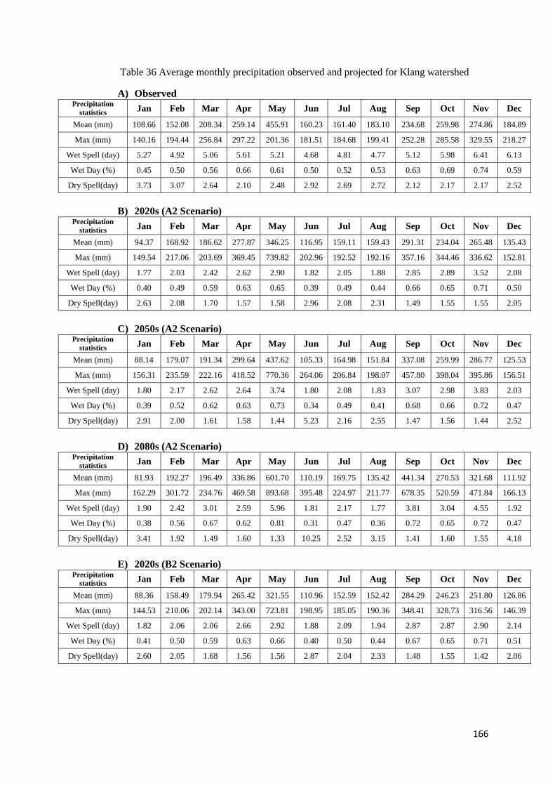
166
Table 36 Average monthly precipitation observed and projected for Klang watershed
A) Observed Precipitation
statistics Jan Feb Mar Apr May Jun Jul Aug Sep Oct Nov Dec
Mean (mm) 108.66 152.08 208.34 259.14 455.91 160.23 161.40 183.10 234.68 259.98 274.86 184.89
Max (mm) 140.16 194.44 256.84 297.22 201.36 181.51 184.68 199.41 252.28 285.58 329.55 218.27
Wet Spell (day) 5.27 4.92 5.06 5.61 5.21 4.68 4.81 4.77 5.12 5.98 6.41 6.13
Wet Day (%) 0.45 0.50 0.56 0.66 0.61 0.50 0.52 0.53 0.63 0.69 0.74 0.59
Dry Spell(day) 3.73 3.07 2.64 2.10 2.48 2.92 2.69 2.72 2.12 2.17 2.17 2.52
B) 2020s (A2 Scenario) Precipitation
statistics Jan Feb Mar Apr May Jun Jul Aug Sep Oct Nov Dec
Mean (mm) 94.37 168.92 186.62 277.87 346.25 116.95 159.11 159.43 291.31 234.04 265.48 135.43
Max (mm) 149.54 217.06 203.69 369.45 739.82 202.96 192.52 192.16 357.16 344.46 336.62 152.81
Wet Spell (day) 1.77 2.03 2.42 2.62 2.90 1.82 2.05 1.88 2.85 2.89 3.52 2.08
Wet Day (%) 0.40 0.49 0.59 0.63 0.65 0.39 0.49 0.44 0.66 0.65 0.71 0.50
Dry Spell(day) 2.63 2.08 1.70 1.57 1.58 2.96 2.08 2.31 1.49 1.55 1.55 2.05
C) 2050s (A2 Scenario) Precipitation
statistics Jan Feb Mar Apr May Jun Jul Aug Sep Oct Nov Dec
Mean (mm) 88.14 179.07 191.34 299.64 437.62 105.33 164.98 151.84 337.08 259.99 286.77 125.53
Max (mm) 156.31 235.59 222.16 418.52 770.36 264.06 206.84 198.07 457.80 398.04 395.86 156.51
Wet Spell (day) 1.80 2.17 2.62 2.64 3.74 1.80 2.08 1.83 3.07 2.98 3.83 2.03
Wet Day (%) 0.39 0.52 0.62 0.63 0.73 0.34 0.49 0.41 0.68 0.66 0.72 0.47
Dry Spell(day) 2.91 2.00 1.61 1.58 1.44 5.23 2.16 2.55 1.47 1.56 1.44 2.52
D) 2080s (A2 Scenario) Precipitation
statistics Jan Feb Mar Apr May Jun Jul Aug Sep Oct Nov Dec
Mean (mm) 81.93 192.27 196.49 336.86 601.70 110.19 169.75 135.42 441.34 270.53 321.68 111.92
Max (mm) 162.29 301.72 234.76 469.58 893.68 395.48 224.97 211.77 678.35 520.59 471.84 166.13
Wet Spell (day) 1.90 2.42 3.01 2.59 5.96 1.81 2.17 1.77 3.81 3.04 4.55 1.92
Wet Day (%) 0.38 0.56 0.67 0.62 0.81 0.31 0.47 0.36 0.72 0.65 0.72 0.47
Dry Spell(day) 3.41 1.92 1.49 1.60 1.33 10.25 2.52 3.15 1.41 1.60 1.55 4.18
E) 2020s (B2 Scenario) Precipitation
statistics Jan Feb Mar Apr May Jun Jul Aug Sep Oct Nov Dec
Mean (mm) 88.36 158.49 179.94 265.42 321.55 110.96 152.59 152.42 284.29 246.23 251.80 126.86
Max (mm) 144.53 210.06 202.14 343.00 723.81 198.95 185.05 190.36 348.41 328.73 316.56 146.39
Wet Spell (day) 1.82 2.06 2.06 2.66 2.92 1.88 2.09 1.94 2.87 2.87 2.90 2.14
Wet Day (%) 0.41 0.50 0.59 0.63 0.66 0.40 0.50 0.44 0.67 0.65 0.71 0.51
Dry Spell(day) 2.60 2.05 1.68 1.56 1.56 2.87 2.04 2.33 1.48 1.55 1.42 2.06
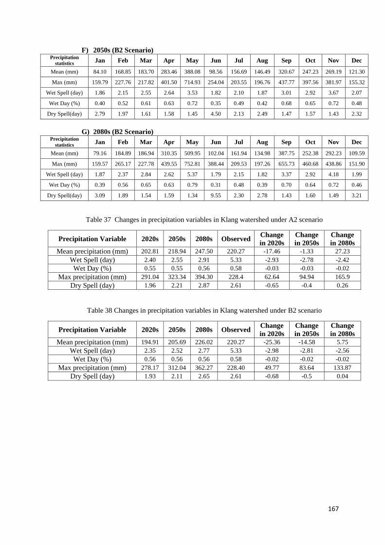
167
F) 2050s (B2 Scenario) Precipitation
statistics Jan Feb Mar Apr May Jun Jul Aug Sep Oct Nov Dec
Mean (mm) 84.10 168.85 183.70 283.46 388.08 98.56 156.69 146.49 320.67 247.23 269.19 121.30
Max (mm) 159.79 227.76 217.82 401.50 714.93 254.04 203.55 196.76 437.77 397.56 381.97 155.32
Wet Spell (day) 1.86 2.15 2.55 2.64 3.53 1.82 2.10 1.87 3.01 2.92 3.67 2.07
Wet Day (%) 0.40 0.52 0.61 0.63 0.72 0.35 0.49 0.42 0.68 0.65 0.72 0.48
Dry Spell(day) 2.79 1.97 1.61 1.58 1.45 4.50 2.13 2.49 1.47 1.57 1.43 2.32
G) 2080s (B2 Scenario) Precipitation
statistics Jan Feb Mar Apr May Jun Jul Aug Sep Oct Nov Dec
Mean (mm) 79.16 184.89 186.94 310.35 509.95 102.04 161.94 134.98 387.75 252.38 292.23 109.59
Max (mm) 159.57 265.17 227.78 439.55 752.81 388.44 209.53 197.26 655.73 460.68 438.86 151.90
Wet Spell (day) 1.87 2.37 2.84 2.62 5.37 1.79 2.15 1.82 3.37 2.92 4.18 1.99
Wet Day (%) 0.39 0.56 0.65 0.63 0.79 0.31 0.48 0.39 0.70 0.64 0.72 0.46
Dry Spell(day) 3.09 1.89 1.54 1.59 1.34 9.55 2.30 2.78 1.43 1.60 1.49 3.21
Table 37 Changes in precipitation variables in Klang watershed under A2 scenario
Precipitation Variable 2020s 2050s 2080s Observed Change
in 2020s
Change
in 2050s
Change
in 2080s
Mean precipitation (mm) 202.81 218.94 247.50 220.27 -17.46 -1.33 27.23
Wet Spell (day) 2.40 2.55 2.91 5.33 -2.93 -2.78 -2.42
Wet Day (%) 0.55 0.55 0.56 0.58 -0.03 -0.03 -0.02
Max precipitation (mm) 291.04 323.34 394.30 228.4 62.64 94.94 165.9
Dry Spell (day) 1.96 2.21 2.87 2.61 -0.65 -0.4 0.26
Table 38 Changes in precipitation variables in Klang watershed under B2 scenario
Precipitation Variable 2020s 2050s 2080s Observed Change
in 2020s
Change
in 2050s
Change
in 2080s
Mean precipitation (mm) 194.91 205.69 226.02 220.27 -25.36 -14.58 5.75
Wet Spell (day) 2.35 2.52 2.77 5.33 -2.98 -2.81 -2.56
Wet Day (%) 0.56 0.56 0.56 0.58 -0.02 -0.02 -0.02
Max precipitation (mm) 278.17 312.04 362.27 228.40 49.77 83.64 133.87
Dry Spell (day) 1.93 2.11 2.65 2.61 -0.68 -0.5 0.04

168
6-5- Assessment of Climate Change Impact on the Mean and Maximum River
Discharge
The present and future streamflow were compared to reveal the possible changes of
runoff behaviour for the future based on the climate change scenarios. HEC-HMS
hydrological model in Klang watershed was found skilful through the long time series
streamflow record. It handles geospatial data and distributed grid-based precipitation
data for the multi raingauge stations. Using appropriate hydrological model to predict
the future streamflow depends on its ability to model the current scenarios (Dibike
and Coulibaly, 2007).
Tables (39 and 40) show the projected changes for the mean and maximum monthly
discharge for three time slices of future corresponding to A2 and B2 scenarios with
respect to the baseline discharge at Sulaiman streamflow station. Figures (from 89 to
100) illustrate the projected changes in the mean and maximum monthly river
hydrograph for three time slices period (2020s, 2050s and 2080s).
The assessment of climate change impacts on the river discharge at Sulaiman
streamflow station has been performed to estimate mean and maximum monthly river
hydrograph for the future. The downscaled baseline and future precipitation,
temperature and evaporation obtained from SDSM are entered into HEC-HMS model
to simulate the baseline and future streamflows. Downscaled temperature data to
calculate ET using Hargreaves’ method, are also entered into HEC-HMS for
discharge simulation. The validated HEC-HMS model is used to simulate the runoff
at Sulaiman streamflow station located at the outlet of the watershed.
The lack of updated landuse, soil and topography data have forced the study to
consider it as an assumption with no change during the time. Neither change in soil
nor landuse cover is considered to project future streamflow which makes it assure
that the streamflow projections for future are solely dependent on the climate change
scenarios.
Results of HEC-HMS model indicate that the discharge patterns will change for the
future. It is seen that the downscaled mean and maximum precipitation may produce a
169
wide range of changes in the hydrology of Klang watershed. Sulaiman streamflow
station in Klang River is identified by a typical hydrograph includes two main
discharge peaks which are in April and November for the period 1975-2001,whereas
February and September is attributed as the least amount of discharge of Sulaiman
streamflow station. It reveals that the wet season is from April to June and October to
December, while the dry season is from January to March and July to September.
It is obvious from the results that predicted annual mean discharge for future periods
are decreasing except the period 2080s is increasing according to A2 scenario. The
projected mean discharge indicated a decline in months from January to April and
also from July to August in all the three time slices periods for A2 and B2 scenarios.
There is an increasing trend in the discharge of June, September and October in all the
three future periods under A2 scenario. However, peak flow of mean runoff in May
and June did not change much for 2020s and 2050s. Obviously, the magnitude of
increasing is higher in A2 than in B2 scenario.
In the three future time slices predicted, the annual mean discharge is predicted a
decrease by 9.4%, 4.9% and an increase of 3.4% for A2 while a decrease about
17.3%, 14.3% and 6.2% for B2 scenario. The average annual maximum discharge is
projected a decrease of 7.7% in 2020s and an increase of 4.2% and 29% in A2
scenario for 2050s and 2080s respectively, while there will most likely be a decrease
as the maximum discharge for all the future under B2 scenario. It is projected a
decrease of 32.4%, 19.5% and 2.1% for 2020s, 2050s and 2080s, respectively.
The maximum absolute increase in the mean peak runoff was projected in May and
October for 2080s under A2 scenario, with a difference of 7.6 m3/s (29.7 m
3/s as
compare to 21.9 m3/s in May) and 7.6 m
3/s (28.9 m
3/s as compare to 21.3 m
3/s in
October). On the other hand, the maximum absolute increase in the maximum peak
runoff was projected in May and October for 2080s under A2 scenario, with a
difference of 36.8 m3/s (90.3 m
3/s as compare to 53.5 m
3/s in May) and 53.4 m
3/s
(105.3 m3/s as compare to 51.9 m
3/s in October).
Absolute increase of mean precipitation in months of May, September and November
are 145.8 mm, 206.7 mm and 46.8 mm in 2080s under A2 scenario. The changes in
170
mean precipitation in these months (32% in May, 88% in September, 17% in
November) result in the increase of mean runoff by 34%, 52% and 4%., respectively.
The highest increase in evapotranspiration and rather increase in maximum
temperature in November, cause the changes of mean runoff by 4% in this month.
Mean precipitation is expected to a rather increase in July by 5% but an increase in
evapotranspiration in this month causes a reduction in mean runoff.
A reduction of precipitation by 24.6% and 5.7% in January and March in 2080s under
A2 scenario, result a reduction of runoff by 52% and 17%, respectively. However,
there is a reduction of precipitation in June by 31%, the runoff is affected by the high
volume of precipitation in May (455.9 mm). It can produce a large amount of
baseflow or delayed runoff in the watershed. The baseflow or delayed runoff affects
the part of runoff occurs after the end of the flood which produces the continuous high
flow rates in the hydrograph.
Absolute increase of maximum precipitation in months of September, October and
November are 426 mm, 235 mm and 142.3 mm in 2080s under A2 scenario. The
changes in mean precipitation in these months (168.9% in September, 82% in
October, and 43.2% in November) result in the increase of maximum runoff by
122.5%, 102.9% and 28.8%., respectively. There is an increase in maximum
precipitation by 118% in June, which causes an increase in maximum discharge by
93%. It was affected by the delayed runoff of month May. Maximum precipitation is
quite high in May which is 893.7 mm in 2080s. However, a reduction of runoff by
30.6% is observed, which is highly affected by baseflow runoff in March. A reduction
of maximum precipitation by 8.6% in March causes a decrease in runoff by 22%.
Results of comparison between the projected changes for monthly mean streamflows
at Sulaiman streamflow station indicate small difference between the two IPCC
scenarios. This difference ranges between 8.7%, 10.3% and 9.5% for 2020s, 2050s
and 2080s, respectively. The most significant heavy precipitation has been observed
during the months of October, November and December as the watershed experiences
the north-eastern monsoon season in those months (Chen et al., 2013; Ahmad et al.,
2012). The flow data of Klang River at Sulaiman streamflow station reveals that the
flow regime mainly depends on the northeast monsoon which is from November to
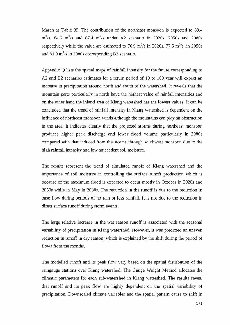
171
March as Table 39. The contribution of the northeast monsoon is expected to 83.4
m3/s, 84.6 m
3/s and 87.4 m
3/s under A2 scenario in 2020s, 2050s and 2080s
respectively while the value are estimated to 76.9 m3/s in 2020s, 77.5 m
3/s .in 2050s
and 81.9 m3/s in 2080s corresponding B2 scenario.
Appendix Q lists the spatial maps of rainfall intensity for the future corresponding to
A2 and B2 scenarios estimates for a return period of 10 to 100 year will expect an
increase in precipitation around north and south of the watershed. It reveals that the
mountain parts particularly in north have the highest value of rainfall intensities and
on the other hand the inland area of Klang watershed has the lowest values. It can be
concluded that the trend of rainfall intensity in Klang watershed is dependent on the
influence of northeast monsoon winds although the mountains can play an obstruction
in the area. It indicates clearly that the projected storms during northeast monsoon
produces higher peak discharge and lower flood volume particularly in 2080s
compared with that induced from the storms through southwest monsoon due to the
high rainfall intensity and low antecedent soil moisture.
The results represent the trend of simulated runoff of Klang watershed and the
importance of soil moisture in controlling the surface runoff production which is
because of the maximum flood is expected to occur mostly in October in 2020s and
2050s while in May in 2080s. The reduction in the runoff is due to the reduction in
base flow during periods of no rain or less rainfall. It is not due to the reduction in
direct surface runoff during storm events.
The large relative increase in the wet season runoff is associated with the seasonal
variability of precipitation in Klang watershed. However, it was predicted an uneven
reduction in runoff in dry season, which is explained by the shift during the period of
flows from the months.
The modelled runoff and its peak flow vary based on the spatial distribution of the
raingauge stations over Klang watershed. The Gauge Weight Method allocates the
climatic parameters for each sub-watershed in Klang watershed. The results reveal
that runoff and its peak flow are highly dependent on the spatial variability of
precipitation. Downscaled climate variables and the spatial pattern cause to shift in
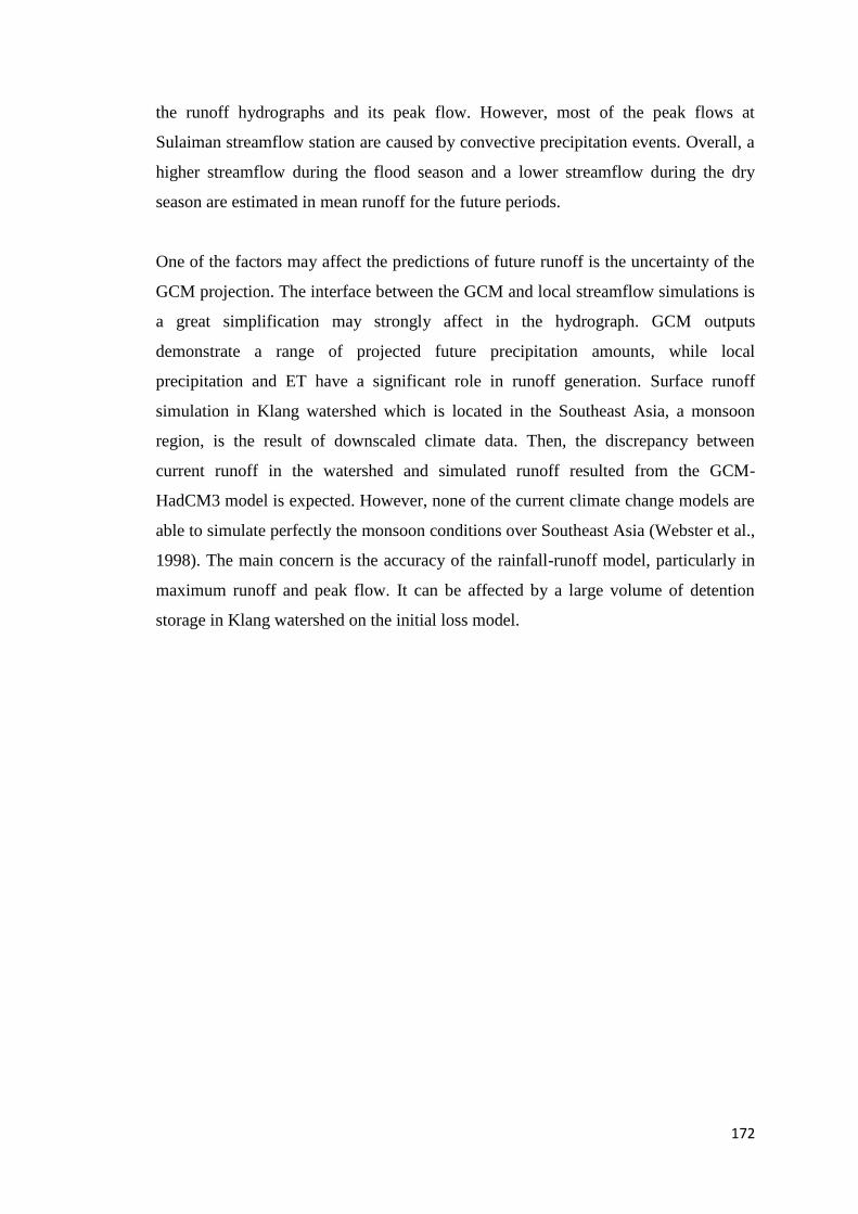
172
the runoff hydrographs and its peak flow. However, most of the peak flows at
Sulaiman streamflow station are caused by convective precipitation events. Overall, a
higher streamflow during the flood season and a lower streamflow during the dry
season are estimated in mean runoff for the future periods.
One of the factors may affect the predictions of future runoff is the uncertainty of the
GCM projection. The interface between the GCM and local streamflow simulations is
a great simplification may strongly affect in the hydrograph. GCM outputs
demonstrate a range of projected future precipitation amounts, while local
precipitation and ET have a significant role in runoff generation. Surface runoff
simulation in Klang watershed which is located in the Southeast Asia, a monsoon
region, is the result of downscaled climate data. Then, the discrepancy between
current runoff in the watershed and simulated runoff resulted from the GCM-
HadCM3 model is expected. However, none of the current climate change models are
able to simulate perfectly the monsoon conditions over Southeast Asia (Webster et al.,
1998). The main concern is the accuracy of the rainfall-runoff model, particularly in
maximum runoff and peak flow. It can be affected by a large volume of detention
storage in Klang watershed on the initial loss model.
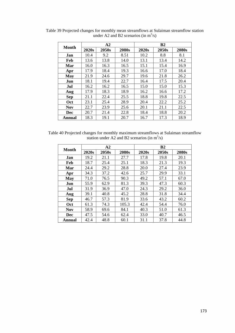
173
Table 39 Projected changes for monthly mean streamflows at Sulaiman streamflow station
under A2 and B2 scenarios (in m3/s)
Month A2 B2
2020s 2050s 2080s 2020s 2050s 2080s
Jan 10.4 9.2 8.51 10.2 8.8 8.1
Feb 13.6 13.8 14.0 13.1 13.4 14.2
Mar 16.0 16.3 16.5 15.1 15.4 16.9
Apr 17.9 18.4 19.3 16.6 17.0 18.4
May 21.9 24.6 29.7 19.6 21.8 26.2
Jun 18.1 19.4 22.7 16.4 17.5 20.4
Jul 16.2 16.2 16.5 15.0 15.0 15.3
Aug 17.9 18.3 18.9 16.2 16.6 17.2
Sep 21.1 22.4 25.5 18.8 19.8 22.5
Oct 23.1 25.4 28.9 20.4 22.2 25.2
Nov 22.7 23.9 25.6 20.1 21.1 22.5
Dec 20.7 21.4 22.8 18.4 18.8 20.2
Annual 18.3 19.1 20.7 16.7 17.3 18.9
Table 40 Projected changes for monthly maximum streamflows at Sulaiman streamflow
station under A2 and B2 scenarios (in m3/s)
Month A2 B2
2020s 2050s 2080s 2020s 2050s 2080s
Jan 19.2 21.1 27.7 17.8 19.8 20.1
Feb 18.7 25.4 25.1 18.3 21.3 19.3
Mar 24.4 29.2 28.8 20.0 27.4 23.9
Apr 34.3 37.2 42.6 25.7 29.9 33.1
May 71.0 76.5 90.3 49.2 57.1 67.0
Jun 55.9 62.9 81.3 39.3 47.3 60.3
Jul 31.9 36.9 47.0 24.3 29.2 36.0
Aug 39.1 40.8 45.2 28.8 31.8 34.4
Sep 46.7 57.3 81.9 33.6 43.2 60.2
Oct 61.3 74.3 105.3 42.4 54.4 76.0
Nov 58.9 69.6 84.1 40.3 51.0 61.3
Dec 47.5 54.6 62.4 33.0 40.7 46.5
Annual 42.4 48.8 60.1 31.1 37.8 44.8
174
Figure 89 Comparison between the observed and 2020s average monthly streamflows
simulated at Sulaiman streamflow station under A2 scenario
Figure 90 Comparison between the observed and 2050s average monthly streamflows
simulated at Sulaiman streamflow station under A2 scenario
Figure 91 Comparison between the observed and 2080s average monthly streamflows
simulated at Sulaiman streamflow station under A2 scenario
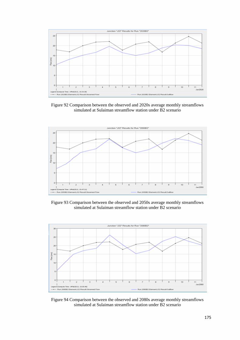
175
Figure 92 Comparison between the observed and 2020s average monthly streamflows
simulated at Sulaiman streamflow station under B2 scenario
Figure 93 Comparison between the observed and 2050s average monthly streamflows
simulated at Sulaiman streamflow station under B2 scenario
Figure 94 Comparison between the observed and 2080s average monthly streamflows
simulated at Sulaiman streamflow station under B2 scenario
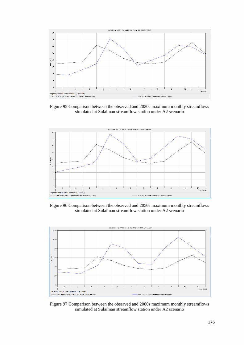
176
Figure 95 Comparison between the observed and 2020s maximum monthly streamflows
simulated at Sulaiman streamflow station under A2 scenario
Figure 96 Comparison between the observed and 2050s maximum monthly streamflows
simulated at Sulaiman streamflow station under A2 scenario
Figure 97 Comparison between the observed and 2080s maximum monthly streamflows
simulated at Sulaiman streamflow station under A2 scenario
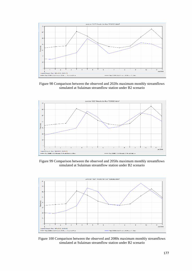
177
Figure 98 Comparison between the observed and 2020s maximum monthly streamflows
simulated at Sulaiman streamflow station under B2 scenario
Figure 99 Comparison between the observed and 2050s maximum monthly streamflows
simulated at Sulaiman streamflow station under B2 scenario
Figure 100 Comparison between the observed and 2080s maximum monthly streamflows
simulated at Sulaiman streamflow station under B2 scenario
178
6-6- Assessment of Climate Change Impact on the Flood Frequency
The analysis was done for assessment of climate change impacts on the occurrence of
extreme precipitation events at 10 raingauge stations and also on the discharge station
to determine the amount of discharge for the return periods 5, 10, 25, 50 and100 years
for three time slices (2020s, 2050s and 2080s) corresponding to A2 and B2 scenarios.
6-6-1- Assessment of Climate Change Impact on the Occurrence of Extreme
Precipitation Events
The impact of climate change on the occurrence of precipitation events was evaluated
by spatial mapping in GIS (Appendix Q). The Gumbel Distribution was run for
estimation of extreme precipitation events at 10 raingauge stations over Klang
watershed. Tables (from 41 to 46) show the maximum precipitation downscaled for
the future which is used as input into Gumbel Distribution function. Tables (from 47
to 53) and Figures (101 and 102) show results for 5, 10.20,50 and 100 year return
periods according to current and future depths.
Maximum precipitation intensity for return period of 5 year is estimated to 146.97
mm in 2020s, 150.11 mm in 2050s and 164.45 mm in 2080s corresponding A2
scenario. It is found an increase about 22.18 mm, 25.32 mm and 39.66 mm for 2020s,
2050s and 2080s respectively compared to the observed extreme precipitation. B2
scenario for return period of 5 year is projected lower values than A2 scenario. A
decrease of 7.78 mm in 2020s, 7.35 mm in 2050s and increase of 10.22 mm in 2080s
are estimated for B2 scenario.
There is an increase of extreme precipitation intensity for return period of 5 to 100
years range between 146.97 mm to 281.05 mm in 2020s, 150.11 mm to 288.93 mm in
2050s and 164.45 mm to 340.45 mm in 2080s. This trend for B2 scenario was
estimated to a range from 139.10 mm to 263.79 mm in 2020s, 142.76 mm to 271.56
mm in 2050s and 154.23 mm to 311.85 mm in 2080s.
The minimum increase of extreme precipitation intensity is observed in 2020s under
A2 scenario for the return period of 5 year by 22.18 mm and the maximum increase of
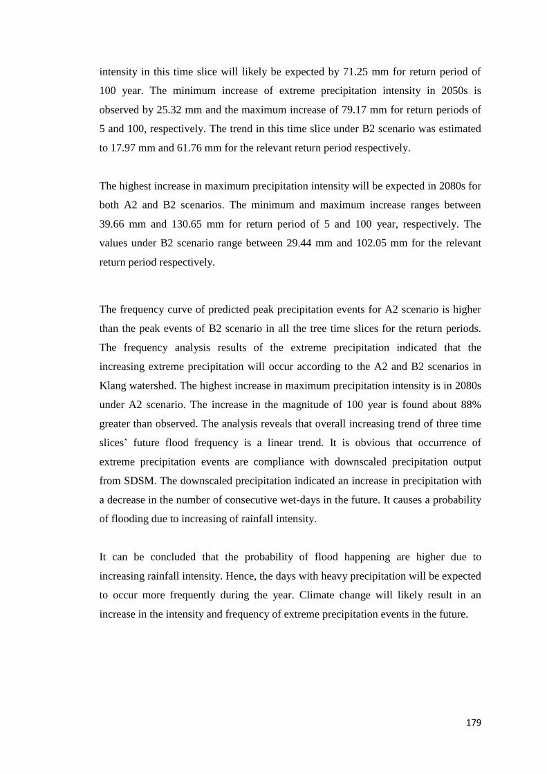
179
intensity in this time slice will likely be expected by 71.25 mm for return period of
100 year. The minimum increase of extreme precipitation intensity in 2050s is
observed by 25.32 mm and the maximum increase of 79.17 mm for return periods of
5 and 100, respectively. The trend in this time slice under B2 scenario was estimated
to 17.97 mm and 61.76 mm for the relevant return period respectively.
The highest increase in maximum precipitation intensity will be expected in 2080s for
both A2 and B2 scenarios. The minimum and maximum increase ranges between
39.66 mm and 130.65 mm for return period of 5 and 100 year, respectively. The
values under B2 scenario range between 29.44 mm and 102.05 mm for the relevant
return period respectively.
The frequency curve of predicted peak precipitation events for A2 scenario is higher
than the peak events of B2 scenario in all the tree time slices for the return periods.
The frequency analysis results of the extreme precipitation indicated that the
increasing extreme precipitation will occur according to the A2 and B2 scenarios in
Klang watershed. The highest increase in maximum precipitation intensity is in 2080s
under A2 scenario. The increase in the magnitude of 100 year is found about 88%
greater than observed. The analysis reveals that overall increasing trend of three time
slices’ future flood frequency is a linear trend. It is obvious that occurrence of
extreme precipitation events are compliance with downscaled precipitation output
from SDSM. The downscaled precipitation indicated an increase in precipitation with
a decrease in the number of consecutive wet-days in the future. It causes a probability
of flooding due to increasing of rainfall intensity.
It can be concluded that the probability of flood happening are higher due to
increasing rainfall intensity. Hence, the days with heavy precipitation will be expected
to occur more frequently during the year. Climate change will likely result in an
increase in the intensity and frequency of extreme precipitation events in the future.
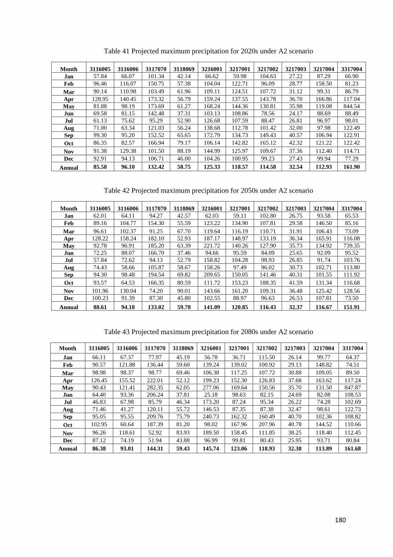
180
Table 41 Projected maximum precipitation for 2020s under A2 scenario
Month 3116005 3116006 3117070 3118069 3216001 3217001 3217002 3217003 3217004 3317004
Jan 57.84 66.07 101.34 42.14 66.62 59.98 104.63 27.22 87.29 66.90
Feb 96.46 116.07 150.75 57.38 104.04 122.71 96.09 28.77 158.50 81.23
Mar 90.14 110.98 103.49 61.96 109.11 124.51 107.72 31.12 99.31 86.79
Apr 128.95 140.45 173.32 56.79 159.24 137.55 143.78 36.70 166.86 117.04
May 81.88 98.19 173.69 61.27 168.24 144.36 130.81 35.98 119.08 844.54
Jun 69.58 81.15 142.48 37.31 103.13 108.86 78.56 24.17 88.69 88.49
Jul 61.13 75.62 95.29 52.90 126.68 107.59 88.47 26.81 96.97 98.01
Aug 71.00 63.34 121.03 56.24 138.68 112.78 101.42 32.00 97.98 122.49
Sep 99.30 95.20 152.52 65.65 172.79 134.73 149.43 40.57 106.94 122.91
Oct 86.35 82.57 166.94 79.17 106.14 142.82 165.12 42.32 121.22 122.42
Nov 91.38 129.38 101.50 88.19 144.99 125.97 109.67 37.36 112.40 114.71
Dec 92.91 94.13 106.71 46.00 104.26 100.95 99.23 27.43 99.94 77.29
Annual 85.58 96.10 132.42 58.75 125.33 118.57 114.58 32.54 112.93 161.90
Table 42 Projected maximum precipitation for 2050s under A2 scenario
Month 3116005 3116006 3117070 3118069 3216001 3217001 3217002 3217003 3217004 3317004
Jan 62.01 64.11 94.27 42.57 62.03 59.11 102.80 26.75 93.58 65.53
Feb 89.16 104.77 154.30 55.59 123.22 134.90 107.81 29.58 146.50 85.16
Mar 96.61 102.37 91.25 67.70 119.64 116.19 110.71 31.91 106.43 73.09
Apr 128.22 158.24 182.10 52.93 187.17 148.97 133.19 36.34 165.91 116.08
May 92.78 96.91 185.20 63.39 221.72 140.26 127.90 35.73 134.92 739.35
Jun 72.25 88.07 166.70 37.46 94.66 95.59 84.09 25.65 92.09 95.52
Jul 57.84 72.62 94.13 52.79 158.82 104.28 98.93 26.85 91.74 103.76
Aug 74.43 58.66 105.87 58.67 158.26 97.49 96.02 30.73 102.71 113.80
Sep 94.30 98.48 194.54 69.82 209.65 150.05 141.46 40.31 101.55 111.92
Oct 93.57 64.53 166.35 80.59 111.72 153.23 188.35 41.59 131.34 116.68
Nov 101.96 130.04 74.20 90.01 143.66 161.20 109.31 36.48 125.42 128.56
Dec 100.23 91.39 87.30 45.80 102.55 88.97 96.63 26.53 107.81 73.50
Annual 88.61 94.18 133.02 59.78 141.09 120.85 116.43 32.37 116.67 151.91
Table 43 Projected maximum precipitation for 2080s under A2 scenario
Month 3116005 3116006 3117070 3118069 3216001 3217001 3217002 3217003 3217004 3317004
Jan 66.11 67.37 77.97 45.19 56.78 36.71 115.50 26.14 99.77 64.37
Feb 90.57 121.88 136.44 59.60 139.24 139.02 100.92 29.13 148.82 74.51
Mar 98.98 98.37 98.77 69.46 106.38 117.25 107.72 30.88 109.05 89.50
Apr 126.45 155.52 222.01 52.12 199.23 152.30 126.83 37.68 163.62 117.24
May 90.43 121.41 282.35 62.05 277.06 169.64 150.56 35.70 131.50 847.87
Jun 64.40 93.36 206.24 37.81 25.18 98.63 82.15 24.69 82.08 108.53
Jul 46.83 67.98 85.79 46.34 173.20 87.24 95.34 26.22 74.28 102.69
Aug 71.46 41.27 120.11 55.72 146.53 87.35 87.38 32.47 98.61 122.73
Sep 95.05 95.55 209.76 75.79 240.73 162.32 160.49 40.70 102.36 108.82
Oct 102.95 60.64 187.39 81.20 98.02 167.96 207.96 40.78 144.52 110.66
Nov 96.26 118.61 52.92 83.93 189.50 158.45 111.85 38.25 118.40 112.45
Dec 87.12 74.19 51.94 43.88 96.99 99.81 80.43 25.95 93.71 80.84
Annual 86.38 93.01 144.31 59.43 145.74 123.06 118.93 32.38 113.89 161.68
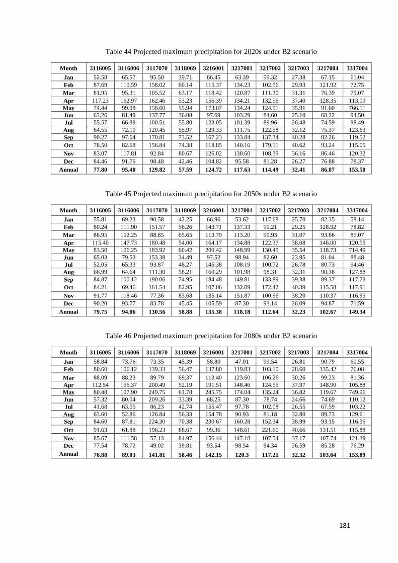
181
Table 44 Projected maximum precipitation for 2020s under B2 scenario
Month 3116005 3116006 3117070 3118069 3216001 3217001 3217002 3217003 3217004 3317004
Jan 52.58 65.57 95.50 39.71 66.45 63.39 99.32 27.38 67.15 61.04
Feb 87.69 110.59 158.02 60.14 115.37 134.23 102.56 29.93 121.92 72.75
Mar 81.95 95.31 105.52 63.17 118.42 120.87 111.30 31.31 76.39 79.07
Apr 117.23 162.97 162.46 53.23 156.39 134.21 132.56 37.40 128.35 113.09
May 74.44 99.98 158.60 55.94 173.07 134.24 124.91 35.91 91.60 766.11
Jun 63.26 81.49 137.77 36.08 97.69 103.29 84.60 25.10 68.22 94.50
Jul 55.57 66.89 100.51 55.80 123.05 101.39 89.96 26.48 74.59 98.49
Aug 64.55 72.10 120.45 55.97 129.33 111.75 122.58 32.12 75.37 123.63
Sep 90.27 97.64 170.81 73.52 167.23 133.84 137.34 40.28 82.26 119.52
Oct 78.50 82.68 156.84 74.38 118.85 140.16 179.11 40.62 93.24 115.05
Nov 83.07 117.81 92.84 80.67 126.02 138.60 108.39 36.16 86.46 120.32
Dec 84.46 91.76 98.48 42.46 104.82 95.58 81.28 26.27 76.88 78.37
Annual 77.80 95.40 129.82 57.59 124.72 117.63 114.49 32.41 86.87 153.50
Table 45 Projected maximum precipitation for 2050s under B2 scenario
Month 3116005 3116006 3117070 3118069 3216001 3217001 3217002 3217003 3217004 3317004
Jan 55.81 69.23 90.58 42.25 66.96 53.62 117.68 25.70 82.35 58.14
Feb 80.24 111.90 151.57 56.26 143.71 137.33 99.21 29.25 128.92 78.82
Mar 86.95 102.25 88.85 65.65 113.79 113.20 99.93 31.07 93.66 85.07
Apr 115.40 147.73 180.48 54.00 164.17 134.88 122.37 38.08 146.00 120.59
May 83.50 106.25 183.92 60.42 200.42 148.99 130.45 35.54 118.73 714.49
Jun 65.03 79.53 153.38 34.49 97.52 98.94 82.60 23.95 81.04 88.48
Jul 52.05 65.33 93.87 48.27 145.38 108.19 100.72 26.78 80.73 94.46
Aug 66.99 64.64 111.30 58.21 160.29 101.98 98.31 32.31 90.38 127.88
Sep 84.87 100.12 190.06 74.95 184.48 149.81 133.89 39.38 89.37 117.73
Oct 84.21 69.46 161.54 82.95 107.06 132.09 172.42 40.39 115.58 117.91
Nov 91.77 118.46 77.36 83.68 135.14 151.87 100.96 38.20 110.37 116.95
Dec 90.20 93.77 83.78 45.45 105.59 87.30 93.14 26.09 94.87 71.59
Annual 79.75 94.06 130.56 58.88 135.38 118.18 112.64 32.23 102.67 149.34
Table 46 Projected maximum precipitation for 2080s under B2 scenario
Month 3116005 3116006 3117070 3118069 3216001 3217001 3217002 3217003 3217004 3317004
Jan 58.84 73.76 73.35 45.39 58.80 47.01 99.54 26.81 90.79 60.55
Feb 80.60 106.12 139.33 56.47 137.80 119.83 103.10 28.60 135.42 76.08
Mar 88.09 88.23 89.79 69.37 113.40 123.60 106.26 30.26 99.23 81.36
Apr 112.54 156.37 200.49 52.19 191.51 148.46 124.55 37.97 148.90 105.88
May 80.48 107.90 249.75 61.78 245.75 174.04 135.24 36.82 119.67 749.96
Jun 57.32 80.04 209.26 33.39 68.25 87.30 78.74 24.66 74.69 110.12
Jul 41.68 63.05 86.23 42.74 155.47 97.78 102.08 26.55 67.59 103.22
Aug 63.60 52.86 126.84 56.33 154.78 90.93 81.18 32.80 89.73 129.61
Sep 84.60 87.81 224.30 70.38 230.67 160.28 152.34 38.99 93.15 116.36
Oct 91.63 61.88 196.23 88.67 99.36 148.61 221.60 40.66 131.51 115.88
Nov 85.67 111.58 57.13 84.97 156.44 147.18 107.54 37.17 107.74 121.39
Dec 77.54 78.72 49.02 39.81 93.54 98.54 94.34 26.59 85.28 76.29
Annual 76.88 89.03 141.81 58.46 142.15 120.3 117.21 32.32 103.64 153.89
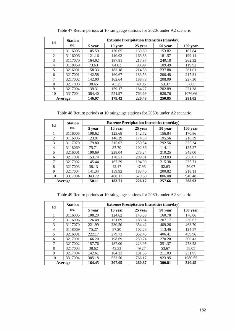
182
Table 47 Return periods at 10 raingauge stations for 2020s under A2 scenario
Id Station
no.
Extreme Precipitation Intensities (mm/day)
5 year 10 year 25 year 50 year 100 year
1 3116005 105.59 120.65 139.69 153.82 167.84
2 3116006 121.16 140.03 163.88 181.57 199.14
3 3117070 164.02 187.81 217.87 240.18 262.32
4 3118069 73.63 84.83 98.99 109.49 119.92
5 3216001 158.33 183.18 214.58 237.88 261.01
6 3217001 142.58 160.67 183.53 200.48 217.31
7 3217002 142.00 162.64 188.73 208.09 227.30
8 3217003 38.65 43.25 49.06 53.37 57.65
9 3217004 139.31 159.17 184.27 202.89 221.38
10 3317004 384.40 551.97 763.69 920.76 1076.66
Average 146.97 179.42 220.43 250.85 281.05
Table 48 Return periods at 10 raingauge stations for 2050s under A2 scenario
Id Station
no.
Extreme Precipitation Intensities (mm/day)
5 year 10 year 25 year 50 year 100 year
1 3116005 108.62 123.68 142.72 156.84 170.86
2 3116006 123.91 146.29 174.58 195.56 216.39
3 3117070 179.80 215.02 259.54 292.56 325.34
4 3118069 75.71 87.70 102.86 114.11 125.27
5 3216001 190.69 228.04 275.24 310.25 345.00
6 3217001 153.74 178.51 209.81 233.03 256.07
7 3217002 145.44 167.29 194.90 215.38 235.71
8 3217003 38.13 42.47 47.96 52.03 56.07
9 3217004 141.34 159.92 183.40 200.82 218.11
10 3317004 343.72 488.17 670.68 806.08 940.48
Average 150.11 183.71 226.17 257.66 288.93
Table 49 Return periods at 10 raingauge stations for 2080s under A2 scenario
Id Station
no.
Extreme Precipitation Intensities (mm/day)
5 year 10 year 25 year 50 year 100 year
1 3116005 108.20 124.62 145.38 160.78 176.06
2 3116006 126.48 151.69 183.54 207.17 230.62
3 3117070 221.99 280.50 354.42 409.26 463.70
4 3118069 75.27 87.20 102.28 113.46 124.57
5 3216001 222.17 279.73 352.45 406.41 459.96
6 3217001 166.20 198.69 239.74 270.20 300.43
7 3217002 157.76 187.00 223.95 251.37 278.58
8 3217003 38.62 43.33 49.27 53.67 58.05
9 3217004 142.61 164.23 191.56 211.83 231.95
10 3317004 385.18 553.50 766.17 923.95 1080.55
Average 164.45 207.05 260.87 300.81 340.45
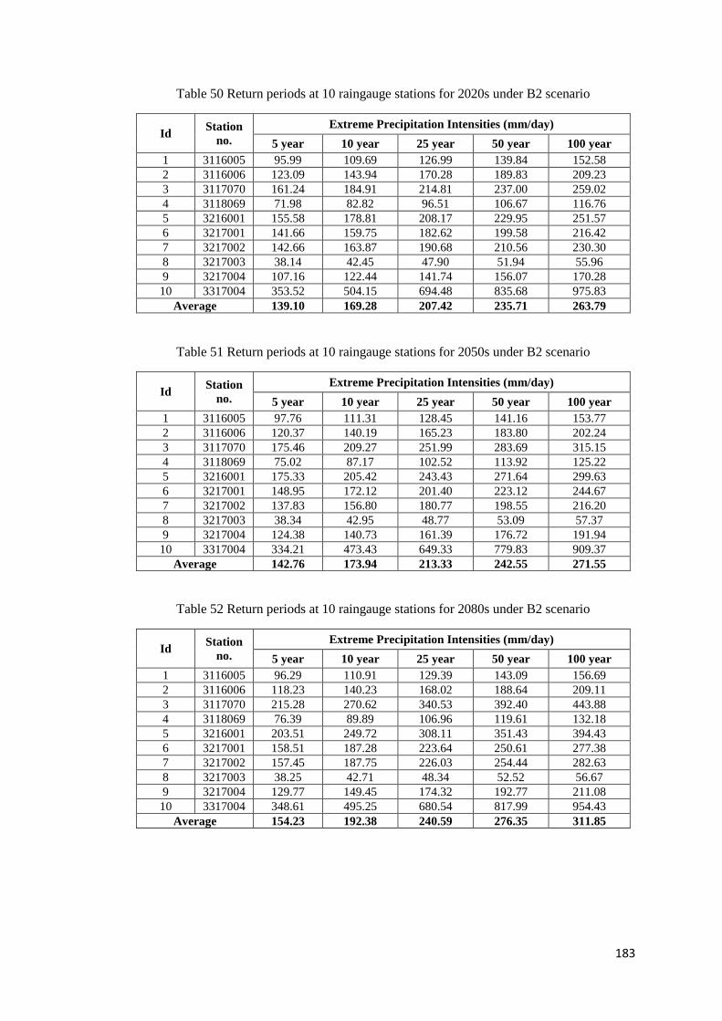
183
Table 50 Return periods at 10 raingauge stations for 2020s under B2 scenario
Id Station
no.
Extreme Precipitation Intensities (mm/day)
5 year 10 year 25 year 50 year 100 year
1 3116005 95.99 109.69 126.99 139.84 152.58
2 3116006 123.09 143.94 170.28 189.83 209.23
3 3117070 161.24 184.91 214.81 237.00 259.02
4 3118069 71.98 82.82 96.51 106.67 116.76
5 3216001 155.58 178.81 208.17 229.95 251.57
6 3217001 141.66 159.75 182.62 199.58 216.42
7 3217002 142.66 163.87 190.68 210.56 230.30
8 3217003 38.14 42.45 47.90 51.94 55.96
9 3217004 107.16 122.44 141.74 156.07 170.28
10 3317004 353.52 504.15 694.48 835.68 975.83
Average 139.10 169.28 207.42 235.71 263.79
Table 51 Return periods at 10 raingauge stations for 2050s under B2 scenario
Id Station
no.
Extreme Precipitation Intensities (mm/day)
5 year 10 year 25 year 50 year 100 year
1 3116005 97.76 111.31 128.45 141.16 153.77
2 3116006 120.37 140.19 165.23 183.80 202.24
3 3117070 175.46 209.27 251.99 283.69 315.15
4 3118069 75.02 87.17 102.52 113.92 125.22
5 3216001 175.33 205.42 243.43 271.64 299.63
6 3217001 148.95 172.12 201.40 223.12 244.67
7 3217002 137.83 156.80 180.77 198.55 216.20
8 3217003 38.34 42.95 48.77 53.09 57.37
9 3217004 124.38 140.73 161.39 176.72 191.94
10 3317004 334.21 473.43 649.33 779.83 909.37
Average 142.76 173.94 213.33 242.55 271.55
Table 52 Return periods at 10 raingauge stations for 2080s under B2 scenario
Id Station
no.
Extreme Precipitation Intensities (mm/day)
5 year 10 year 25 year 50 year 100 year
1 3116005 96.29 110.91 129.39 143.09 156.69
2 3116006 118.23 140.23 168.02 188.64 209.11
3 3117070 215.28 270.62 340.53 392.40 443.88
4 3118069 76.39 89.89 106.96 119.61 132.18
5 3216001 203.51 249.72 308.11 351.43 394.43
6 3217001 158.51 187.28 223.64 250.61 277.38
7 3217002 157.45 187.75 226.03 254.44 282.63
8 3217003 38.25 42.71 48.34 52.52 56.67
9 3217004 129.77 149.45 174.32 192.77 211.08
10 3317004 348.61 495.25 680.54 817.99 954.43
Average 154.23 192.38 240.59 276.35 311.85
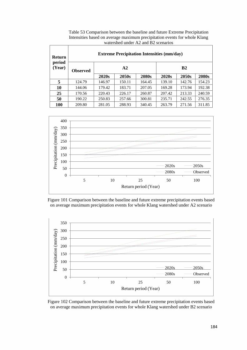
184
Table 53 Comparison between the baseline and future Extreme Precipitation
Intensities based on average maximum precipitation events for whole Klang
watershed under A2 and B2 scenarios
Return
period
(Year)
Extreme Precipitation Intensities (mm/day)
Observed A2 B2
2020s 2050s 2080s 2020s 2050s 2080s
5 124.79 146.97 150.11 164.45 139.10 142.76 154.23
10 144.06 179.42 183.71 207.05 169.28 173.94 192.38
25 170.56 220.43 226.17 260.87 207.42 213.33 240.59
50 190.22 250.83 257.66 300.81 235.71 242.55 276.35
100 209.80 281.05 288.93 340.45 263.79 271.56 311.85
Figure 101 Comparison between the baseline and future extreme precipitation events based
on average maximum precipitation events for whole Klang watershed under A2 scenario
Figure 102 Comparison between the baseline and future extreme precipitation events based
on average maximum precipitation events for whole Klang watershed under B2 scenario
0
50
100
150
200
250
300
350
400
5 10 25 50 100
Pre
cipit
atio
n (
mm
/day
)
Return period (Year)
2020s 2050s
2080s Observed
0
50
100
150
200
250
300
350
5 10 25 50 100
Pre
cip
itat
ion
(m
m/d
ay)
Return period (Year)
2020s 2050s
2080s Observed
185
6-6-2- Assessment of Climate Change Impacts on the Frequency of Mean and
Extreme Flood Events at the Discharge Station
This section represents the potential impacts of possible consequences of climate
change on average and maximum future flood flows according to the predicted runoff
under A2 and B2 scenarios. Log-Pearson type III method, Bulletin 17B-IACWD
(1982), was used to fit the frequency distributions for the downscaled discharge. The
historic annual maximum floods (1975-1990) at Sulaiman streamflow station as the
current potential and the downscaled discharges for the future are used to estimate
flood frequency. The mean and maximum discharge simulation output made by HEC-
HMS hydrology model is the basis input data to assess the flood frequency. The
analysis was done for Klang River at Sulaiman streamflow station to provide amount
of discharge for the return periods of 5, 10, 25, 50 and100 years for three time slices
(2020s, 2050s and 2080s) corresponding A2 and B2 scenarios.
The percentage change in mean flood flows for Sulaiman streamflow station under the
A2 and B2 scenarios is shown in Table 54. Figures (103 and 104) show the results of
flood frequency curves for mean flood events. Table (55) and. Figures (105 and 106)
show the results of flood frequency analysis of extreme flood events at Sulaiman
streamflow station.
The greatest mean floods predicted for return period of 5 year are estimated to 21.9
m3/s, 23.9 m
3/s and 27.2 m
3/s for 2020s, 2050s and 2080s corresponding A2 scenario.
It is found a decrease of 2.62 % in 2020s and an increase of 5.15% and 20.95 % in
2050s and 2080s, respectively compared to the observed mean flood at Sulaiman
streamflow station. The trend of mean flood prediction for B2 scenario is expected to
a decrease of 13.49% in 2020s and 7.5 % in 2050s and an increase of 4.79% in 2080s.
The greatest osf mean floods predicted at Sulaiman streamflow station are expected to
21.90 m3/s in May, 23.1 m
3/s in October and 22.7 m
3/s in November for 2020s, 24.6
m3/s in May, 22.4 m
3/s in September, 25.4 m
3/s in October and 23.9 m
3/s in
November for 2050s, 29.7 m3/s in May, 25.5 m
3/s in September, 28.9 m
3/s in October
and 25.6 m3/s in November for 2080s under A2 scenario. On the other hand, the
greatest of mean floods are expected with a maximum discharge of 19.6 m3/s, 20.4
186
m3/s and 20.1 m3/s for 2020s, 21.8 m
3/s, 19.8 m
3/s, 22.2 m
3/s and 22.1 m
3/s for 2050s,
26.2 m3/s, 22.5 m
3/s, 24.4 m
3/s and 22.5 m
3/s for 2080 in those months under B2
scenario.
There is a decreasing trend of greatest mean floods of return period years from 5 to
100 years range between 21.9 m3/s to 23.85 m
3/s in 2020s while, this increasing trend
of the mean flood prediction at the streamflow station range from 23.6 m3/s to 27.2
m3/s in 2050s and 27.2 m
3/s to 32.6 m
3/s in 2080s corresponding A2 scenario. The
minimum increase of mean flood predicted as compared to the observed data, is
observed in 2050s under A2 scenario for the return period of 100 year by 27.2 m3/s
and the maximum increase of intensity in this time slice will likely be expected for
return period of 10 year by 25.1 m3/s. The trend in this time slice under B2 scenario is
estimated about 21.9 m3/s and 23.6 m
3/s for return period of 10 and 100 year,
respectively.
The greatest maximum floods predicted for return period of 5 year are projected to
60.5 m3/s, 69.9 m
3/s and 89.8 m
3/s for 2020s, 2050s and 2080s respectively
corresponding A2 scenario. It is found an increase of 13.71% in 2020s, 31.55% in
2050s and 68.96% in 2080s compared to the observed maximum flood at Sulaiman
streamflow station. The trend of maximum flood prediction for B2 scenario is
expected to a decrease of 21.41% in 2020s and 3.4% in 2050s and an increase of
23.06% in 2080s which is based on the maximum discharge estimated for those years
in the future runoff simulation. The increasing trend of the greatest maximum floods
is expected for all the return period years range between 60.7 m3/s to 75.5 m
3/s in
2020s, 69.9 m3/s to 87.2 m
3/s in 2050s and 89.8 m
3/s to 117.7 m
3/s in 2080s. The
trend under B2 scenario is expected the range between 41.7 m3/s to 52.7 m
3/s, 51.5
m3/s to 65.5 m
3/s and 65.4 m
3/s to 88.5 m
3/s.
The discharge reduction drops below from 1.3% in return period of 25 year to 18.8%
in return period of 100 year for 2020s, 6.3% in return period of 100 year for 2050s
under A2 scenario. On the other hand, all the predicted maximum discharges in 2020s
and 2050s, is lower than the observed under B2 scenario. The frequency curve of
maximum observed peak discharge events is higher than the peak discharge in 2020s
for the return periods greater than 25 year and in 2050s for the return periods greater
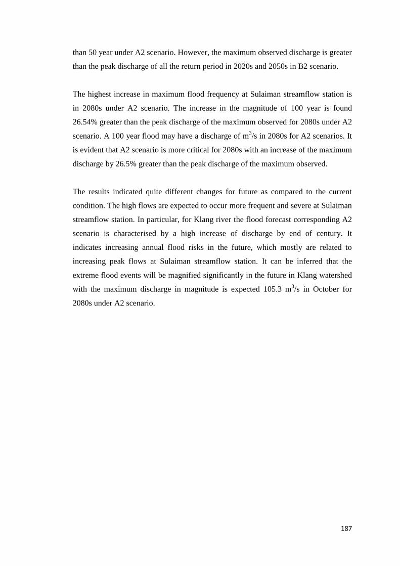
187
than 50 year under A2 scenario. However, the maximum observed discharge is greater
than the peak discharge of all the return period in 2020s and 2050s in B2 scenario.
The highest increase in maximum flood frequency at Sulaiman streamflow station is
in 2080s under A2 scenario. The increase in the magnitude of 100 year is found
26.54% greater than the peak discharge of the maximum observed for 2080s under A2
scenario. A 100 year flood may have a discharge of m3/s in 2080s for A2 scenarios. It
is evident that A2 scenario is more critical for 2080s with an increase of the maximum
discharge by 26.5% greater than the peak discharge of the maximum observed.
The results indicated quite different changes for future as compared to the current
condition. The high flows are expected to occur more frequent and severe at Sulaiman
streamflow station. In particular, for Klang river the flood forecast corresponding A2
scenario is characterised by a high increase of discharge by end of century. It
indicates increasing annual flood risks in the future, which mostly are related to
increasing peak flows at Sulaiman streamflow station. It can be inferred that the
extreme flood events will be magnified significantly in the future in Klang watershed
with the maximum discharge in magnitude is expected 105.3 m3/s in October for
2080s under A2 scenario.
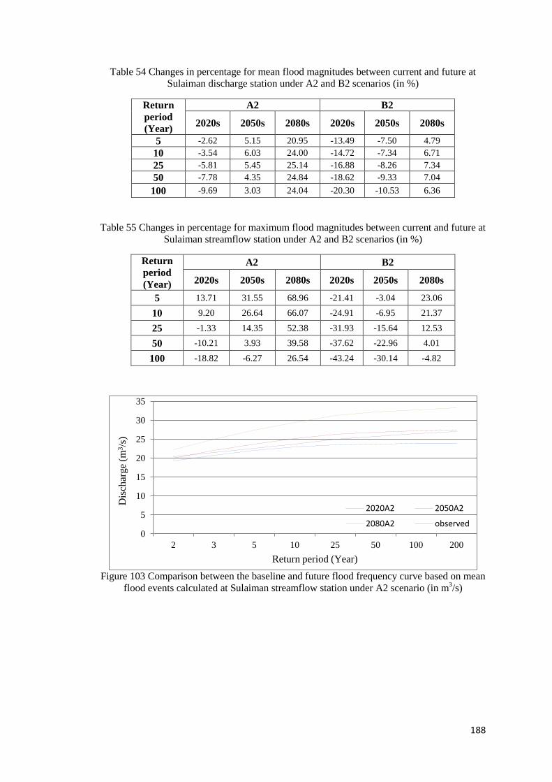
188
Table 54 Changes in percentage for mean flood magnitudes between current and future at
Sulaiman discharge station under A2 and B2 scenarios (in %)
Return
period
(Year)
A2 B2
2020s 2050s 2080s 2020s 2050s 2080s
5 -2.62 5.15 20.95 -13.49 -7.50 4.79
10 -3.54 6.03 24.00 -14.72 -7.34 6.71
25 -5.81 5.45 25.14 -16.88 -8.26 7.34
50 -7.78 4.35 24.84 -18.62 -9.33 7.04
100 -9.69 3.03 24.04 -20.30 -10.53 6.36
Table 55 Changes in percentage for maximum flood magnitudes between current and future at
Sulaiman streamflow station under A2 and B2 scenarios (in %)
Return
period
(Year)
A2 B2
2020s 2050s 2080s 2020s 2050s 2080s
5 13.71 31.55 68.96 -21.41 -3.04 23.06
10 9.20 26.64 66.07 -24.91 -6.95 21.37
25 -1.33 14.35 52.38 -31.93 -15.64 12.53
50 -10.21 3.93 39.58 -37.62 -22.96 4.01
100 -18.82 -6.27 26.54 -43.24 -30.14 -4.82
Figure 103 Comparison between the baseline and future flood frequency curve based on mean
flood events calculated at Sulaiman streamflow station under A2 scenario (in m3/s)
0
5
10
15
20
25
30
35
2 3 5 10 25 50 100 200
Dis
char
ge
(m3/s
)
Return period (Year)
2020A2 2050A2
2080A2 observed
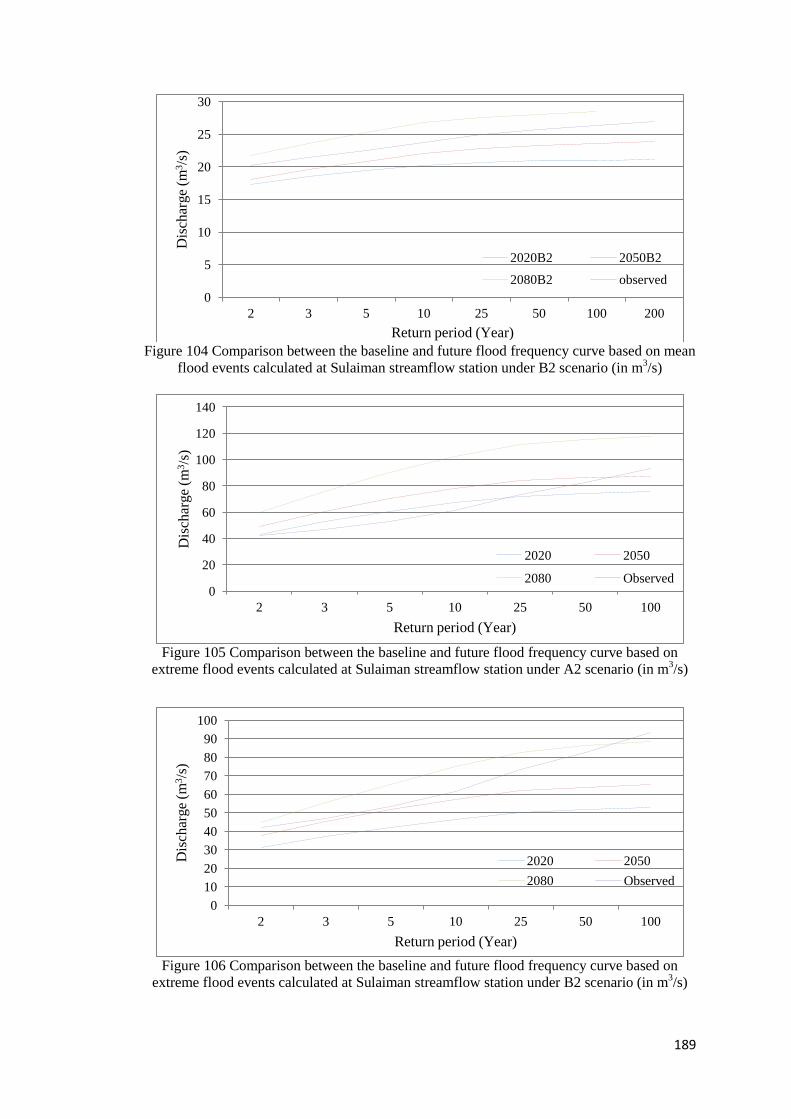
189
Figure 104 Comparison between the baseline and future flood frequency curve based on mean
flood events calculated at Sulaiman streamflow station under B2 scenario (in m3/s)
Figure 105 Comparison between the baseline and future flood frequency curve based on
extreme flood events calculated at Sulaiman streamflow station under A2 scenario (in m3/s)
Figure 106 Comparison between the baseline and future flood frequency curve based on
extreme flood events calculated at Sulaiman streamflow station under B2 scenario (in m3/s)
0
5
10
15
20
25
30
2 3 5 10 25 50 100 200
Dis
char
ge
(m3/s
)
Return period (Year)
2020B2 2050B2
2080B2 observed
0
20
40
60
80
100
120
140
2 3 5 10 25 50 100
Dis
char
ge
(m3/s
)
Return period (Year)
2020 2050
2080 Observed
0
10
20
30
40
50
60
70
80
90
100
2 3 5 10 25 50 100
Dis
char
ge
(m3/s
)
Return period (Year)
2020 2050
2080 Observed
190
6-7- Error Analysis of Downscaling output
6-7-1- Model Error in the Estimates of Mean and Variance
Although calibration and validation test have been run for the historical dataset a
comparison for the observed to the simulated output to indicate the model error, but in
this section it was attempted to perform a further error assessment using
parametric/non-parametric confidence intervals to estimate mean and variance
differences of observed and downscaled output.
The error analysis was conducted on daily rainfall downscaled at 10 raingauge
stations, maximum and minimum temperature downscaled at Subang temperature
station and evaporation downscaled at Batu dam station with SDSM. The assessment
was done on the downscaling output using Large Scale Predictor Re-analysis NCEP
and Had-CM3 GCM model. Error assessment in climate change downscaling is
conducted by comparison with mean and variance between observed/historical and
downscaled output. The Sigma XL extension in Microsoft Excel which is a statistical
package was used for the model error. The evaluation was conducted to estimate the
model error in terms of differences between the mean values of observed and
downscaled output. The historical NCEP Large Scale Re-analysis data over 1975-
2001 was used as observed data in error model.
Figures (from 107 to 114) show the differences between observed and modelled for
the data. It seems that SDSM can preserve downscaling model in the study area. As
Figures (from 115 to 122) indicate the model error in the SDSM with the p-value
higher than 0.05 which presents the similarity of two observed and simulated output.
In fact, SDSM does not produce significant error of the rainfall, maximum and
minimum temperature and evaporation for all the months over the year. However,
there can be seen a slight error in the December at raingauge station (3217003). P-
values are found greater than the significance level alpha = 0.05, which cannot reject
the null hypothesis H0.
The confidence interval at 5% significant level was run to estimate the variance
variability of observed and modelled. The p-values are found greater than 0.05

191
indicate that the observed and modelled variances are close together and can be
considered as one group. All the model error calculated for other raingauge stations
are in the Appendix R.
In daily precipitation, temperature and evaporation downscaling at all the stations in
Klang watershed, the statistical downscaling model errors are insignificant in all the
months as p-values at 5% significance level are found above 0.05 which means the
model errors are insignificant at 95% confidence level.
Regarding to the maximum temperature, the performance of the SDSM model was
less satisfactory than extreme precipitation. It has found that the skill of SDSM to
reproduce the maximum temperature is limited. However, the error of maximum
temperature is less significant in this study because the maximum temperature
downscaling output are used for calculating evapotranspiration while the precipitation
downscaling output are mainly employed for the rainfall-runoff hydrological
modelling in HEC-HMS.
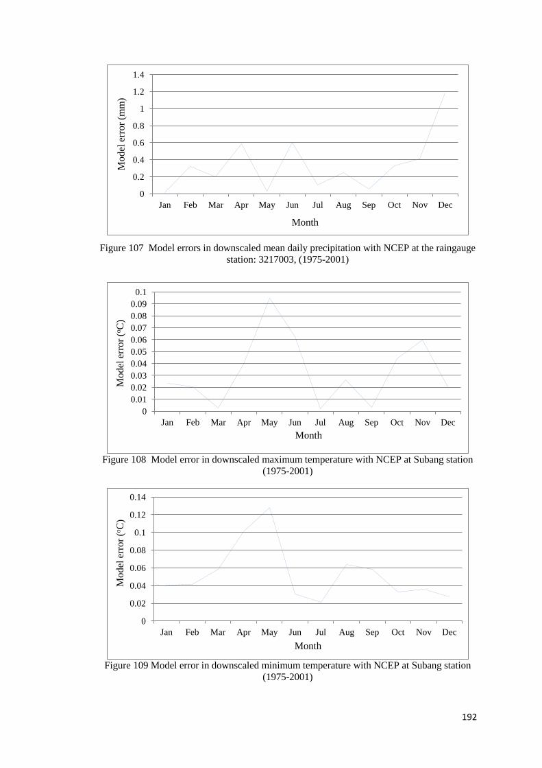
192
Figure 107 Model errors in downscaled mean daily precipitation with NCEP at the raingauge
station: 3217003, (1975-2001)
Figure 108 Model error in downscaled maximum temperature with NCEP at Subang station
(1975-2001)
Figure 109 Model error in downscaled minimum temperature with NCEP at Subang station
(1975-2001)
0
0.2
0.4
0.6
0.8
1
1.2
1.4
Jan Feb Mar Apr May Jun Jul Aug Sep Oct Nov Dec
Mo
del
err
or
(mm
)
Month
0
0.01
0.02
0.03
0.04
0.05
0.06
0.07
0.08
0.09
0.1
Jan Feb Mar Apr May Jun Jul Aug Sep Oct Nov Dec
Model
err
or
(oC
)
Month
0
0.02
0.04
0.06
0.08
0.1
0.12
0.14
Jan Feb Mar Apr May Jun Jul Aug Sep Oct Nov Dec
Mo
del
err
or
(oC
)
Month
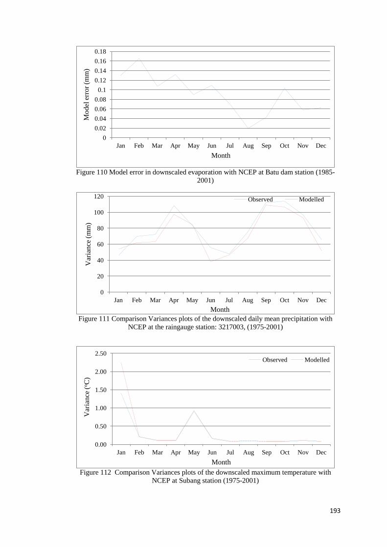
193
Figure 110 Model error in downscaled evaporation with NCEP at Batu dam station (1985-
2001)
Figure 111 Comparison Variances plots of the downscaled daily mean precipitation with
NCEP at the raingauge station: 3217003, (1975-2001)
Figure 112 Comparison Variances plots of the downscaled maximum temperature with
NCEP at Subang station (1975-2001)
0
0.02
0.04
0.06
0.08
0.1
0.12
0.14
0.16
0.18
Jan Feb Mar Apr May Jun Jul Aug Sep Oct Nov Dec
Mo
del
err
or
(mm
)
Month
0
20
40
60
80
100
120
Jan Feb Mar Apr May Jun Jul Aug Sep Oct Nov Dec
Var
iance
(m
m)
Month
Observed Modelled
0.00
0.50
1.00
1.50
2.00
2.50
Jan Feb Mar Apr May Jun Jul Aug Sep Oct Nov Dec
Var
ian
ce (
oC
)
Month
Observed Modelled
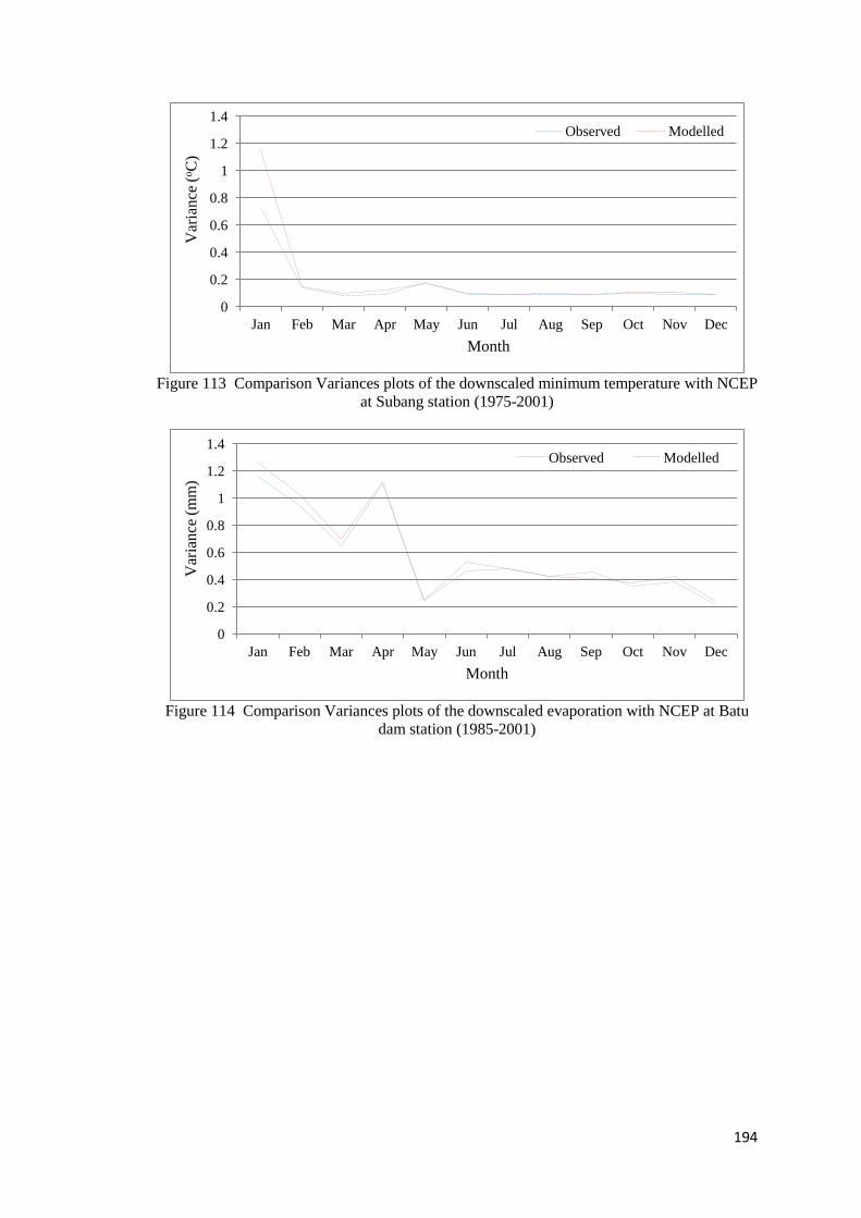
194
Figure 113 Comparison Variances plots of the downscaled minimum temperature with NCEP
at Subang station (1975-2001)
Figure 114 Comparison Variances plots of the downscaled evaporation with NCEP at Batu
dam station (1985-2001)
0
0.2
0.4
0.6
0.8
1
1.2
1.4
Jan Feb Mar Apr May Jun Jul Aug Sep Oct Nov Dec
Var
ian
ce (
oC
)
Month
Observed Modelled
0
0.2
0.4
0.6
0.8
1
1.2
1.4
Jan Feb Mar Apr May Jun Jul Aug Sep Oct Nov Dec
Var
iance
(m
m)
Month
Observed Modelled
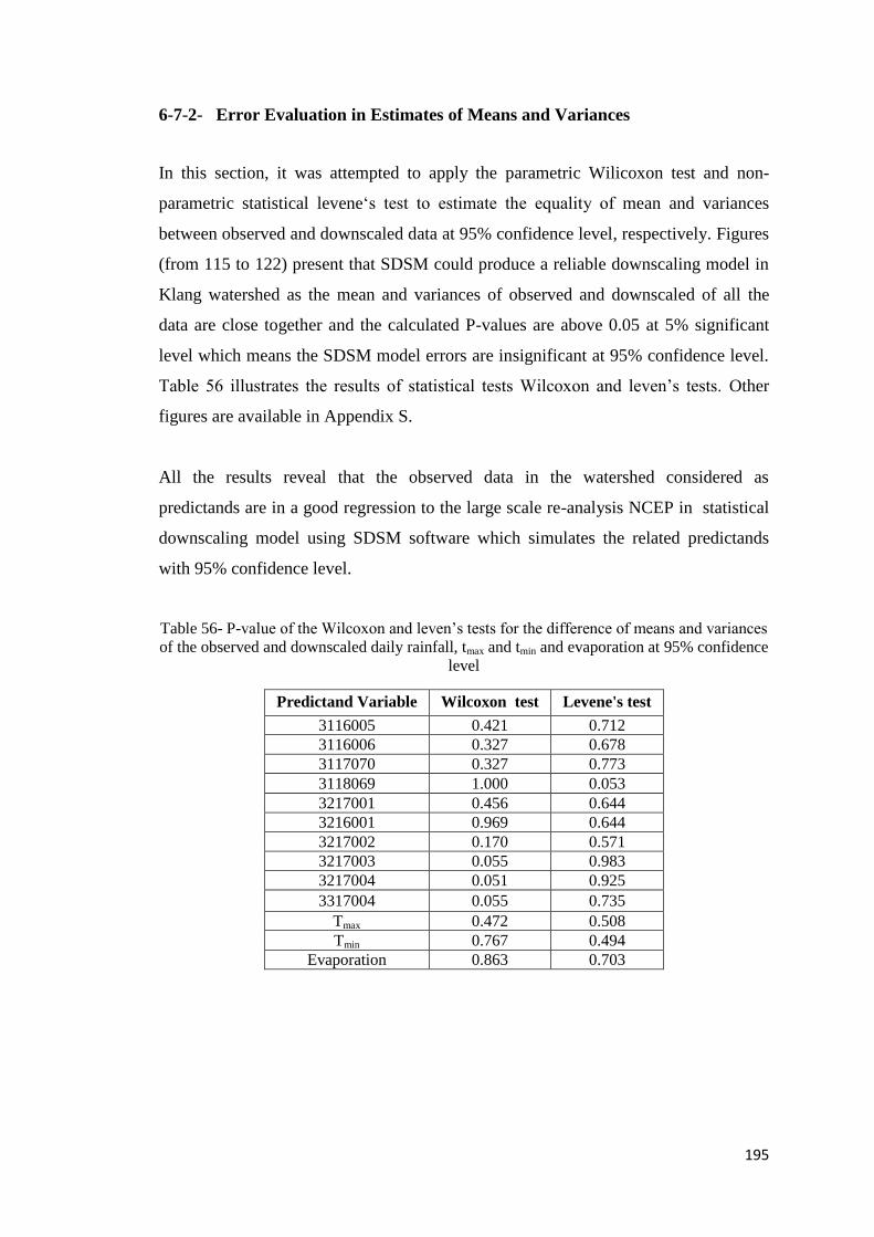
195
6-7-2- Error Evaluation in Estimates of Means and Variances
In this section, it was attempted to apply the parametric Wilicoxon test and non-
parametric statistical levene‘s test to estimate the equality of mean and variances
between observed and downscaled data at 95% confidence level, respectively. Figures
(from 115 to 122) present that SDSM could produce a reliable downscaling model in
Klang watershed as the mean and variances of observed and downscaled of all the
data are close together and the calculated P-values are above 0.05 at 5% significant
level which means the SDSM model errors are insignificant at 95% confidence level.
Table illustrates the results of statistical tests Wilcoxon and leven’s tests. Other
figures are available in Appendix S.
All the results reveal that the observed data in the watershed considered as
predictands are in a good regression to the large scale re-analysis NCEP in statistical
downscaling model using SDSM software which simulates the related predictands
with 95% confidence level.
Table 56- P-value of the Wilcoxon and leven’s tests for the difference of means and variances
of the observed and downscaled daily rainfall, tmax and tmin and evaporation at 95% confidence
level
Predictand Variable Wilcoxon test Levene's test
3116005 0.421 0.712
3116006 0.327 0.678
3117070 0.327 0.773
3118069 1.000 0.053
3217001 0.456 0.644
3216001 0.969 0.644
3217002 0.170 0.571
3217003 0.055 0.983
3217004 0.051 0.925
3317004 0.055 0.735
Tmax 0.472 0.508
Tmin 0.767 0.494
Evaporation 0.863 0.703
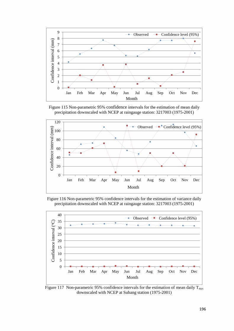
196
Figure 115 Non-parametric 95% confidence intervals for the estimation of mean daily
precipitation downscaled with NCEP at raingauge station: 3217003 (1975-2001)
Figure 116 Non-parametric 95% confidence intervals for the estimation of variance daily
precipitation downscaled with NCEP at raingauge station: 3217003 (1975-2001)
Figure 117 Non-parametric 95% confidence intervals for the estimation of mean daily Tmax
downscaled with NCEP at Subang station (1975-2001)
0
1
2
3
4
5
6
7
8
9
Jan Feb Mar Apr May Jun Jul Aug Sep Oct Nov Dec
Co
nfi
den
ce in
terv
al (
mm
)
Month
Observed Confidence level (95%)
0
20
40
60
80
100
120
Jan Feb Mar Apr May Jun Jul Aug Sep Oct Nov Dec
Confi
den
ce inte
rval
(m
m)
Month
Observed Confidence level (95%)
0
5
10
15
20
25
30
35
40
Jan Feb Mar Apr May Jun Jul Aug Sep Oct Nov Dec
Co
nfi
den
ce in
terv
al (
oC
)
Month
Observed Confidence level (95%)
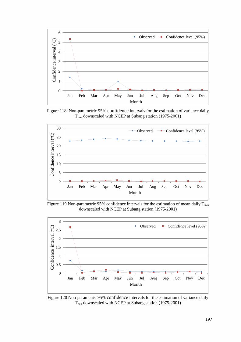
197
Figure 118 Non-parametric 95% confidence intervals for the estimation of variance daily
Tmax downscaled with NCEP at Subang station (1975-2001)
Figure 119 Non-parametric 95% confidence intervals for the estimation of mean daily Tmin
downscaled with NCEP at Subang station (1975-2001)
Figure 120 Non-parametric 95% confidence intervals for the estimation of variance daily
Tmin downscaled with NCEP at Subang station (1975-2001)
0
1
2
3
4
5
6
Jan Feb Mar Apr May Jun Jul Aug Sep Oct Nov Dec
Co
nfi
den
ce in
terv
al (
oC
)
Month
Observed Confidence level (95%)
0
5
10
15
20
25
30
Jan Feb Mar Apr May Jun Jul Aug Sep Oct Nov Dec
Confi
den
ce inte
rval
(oC
)
Month
Observed Confidence level (95%)
0
0.5
1
1.5
2
2.5
3
Jan Feb Mar Apr May Jun Jul Aug Sep Oct Nov Dec
Co
nfi
den
ce in
terv
al (
oC
)
Month
Observed Confidence level (95%)
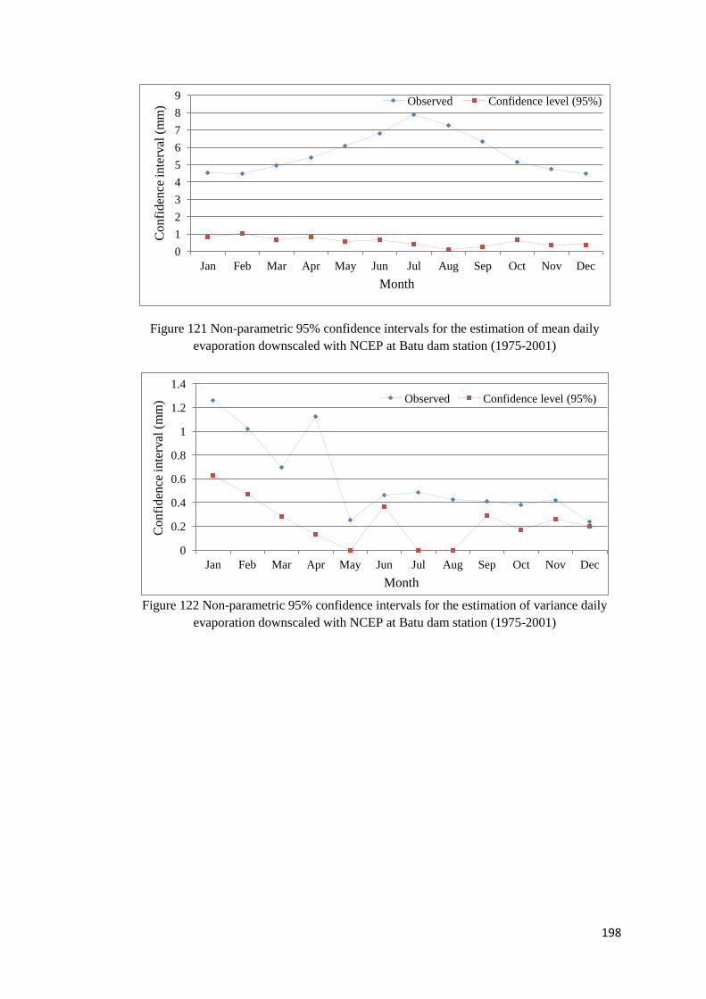
198
Figure 121 Non-parametric 95% confidence intervals for the estimation of mean daily
evaporation downscaled with NCEP at Batu dam station (1975-2001)
Figure 122 Non-parametric 95% confidence intervals for the estimation of variance daily
evaporation downscaled with NCEP at Batu dam station (1975-2001)
0
1
2
3
4
5
6
7
8
9
Jan Feb Mar Apr May Jun Jul Aug Sep Oct Nov Dec
Co
nfi
den
ce in
terv
al (
mm
)
Month
Observed Confidence level (95%)
0
0.2
0.4
0.6
0.8
1
1.2
1.4
Jan Feb Mar Apr May Jun Jul Aug Sep Oct Nov Dec
Co
nfi
den
ce in
terv
al (
mm
)
Month
Observed Confidence level (95%)
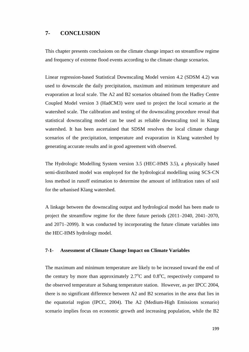
199
7- CONCLUSION
This chapter presents conclusions on the climate change impact on streamflow regime
and frequency of extreme flood events according to the climate change scenarios.
Linear regression-based Statistical Downscaling Model version 4.2 (SDSM 4.2) was
used to downscale the daily precipitation, maximum and minimum temperature and
evaporation at local scale. The A2 and B2 scenarios obtained from the Hadley Centre
Coupled Model version 3 (HadCM3) were used to project the local scenario at the
watershed scale. The calibration and testing of the downscaling procedure reveal that
statistical downscaling model can be used as reliable downscaling tool in Klang
watershed. It has been ascertained that SDSM resolves the local climate change
scenarios of the precipitation, temperature and evaporation in Klang watershed by
generating accurate results and in good agreement with observed.
The Hydrologic Modelling System version 3.5 (HEC-HMS 3.5), a physically based
semi-distributed model was employed for the hydrological modelling using SCS-CN
loss method in runoff estimation to determine the amount of infiltration rates of soil
for the urbanised Klang watershed.
A linkage between the downscaling output and hydrological model has been made to
project the streamflow regime for the three future periods (2011–2040, 2041–2070,
and 2071–2099). It was conducted by incorporating the future climate variables into
the HEC-HMS hydrology model.
7-1- Assessment of Climate Change Impact on Climate Variables
The maximum and minimum temperature are likely to be increased toward the end of
the century by more than approximately 2.7oC and 0.8
oC, respectively compared to
the observed temperature at Subang temperature station. However, as per IPCC 2004,
there is no significant difference between A2 and B2 scenarios in the area that lies in
the equatorial region (IPCC, 2004). The A2 (Medium-High Emissions scenario)
scenario implies focus on economic growth and increasing population, while the B2
200
(Medium-Low Emissions scenario) scenario focuses on environmental sustainability.
Since Malaysia is a developing country with an increasing in population and economy
development, a high usage of fossil fuel has formed the climate change scenarios with
no focus on environmental improvement. It leads to rather similarity of two A2 and
B2 scenarios in the region. Hence, B2 scenario in Malaysia does not describe quite
differently to A2 scenario.
Mean yearly downscaled precipitation variables were determined to indicate mean,
maximum, wet spell and dry spell. Precipitation will likely be increased over Klang
watershed in the months that already have much precipitation, while it might decrease
in already dry months.
The watershed seems to experience increased rainfall towards the end of the century.
However, the analysis indicates that there will likely be a negative trend of mean
precipitation in 2020s and with no difference in 2050s according A2 scenario.
According to the RCM result investigated by Meteorological Dep. Malaysia (2009),
the change in rainfall shows no clear trend by all of the nine models due to the high
variability in the precipitation-modulating factor.
The results show that mean annual precipitation amount are projected to increase in
the future for A2 as compare to B2 scenario. The precipitation experiences a mean
annual decrease by 7.9%, 0.6% for A2 scenario in 2020s and 2050s respectively and
an increase by 12.4% in 2080s.
Among three time slice years, highest rainfall reduction is obtained for 2020s, which
corresponds to the lowest temperature variation being simulated for annual
temperature anomaly. In contrast, the highest rainfall increase is obtained for 2080s,
which corresponds to the highest temperature variation for the same time.
It is projected a decreasing of average wet spell length for the future, approximately
50%, an increasing of average dry spell length to 10% as compared to the current
condition by 2080s. There will decrease in consecutive days without rainfall
approximately 10% and 15.5% for A2 scenario in 2020s and 2050s, respectively.
201
It can be concluded that the probability of flood happening are higher due to
increasing rainfall intensity. Hence, the days with heavy precipitation will be expected
to be occurred very frequently during the year.
The analysis indicates that there will be an increase in mean monthly precipitation but
with a decrease in the number of consecutive wet-days which can be concluded as a
possibility of more precipitation amount in fewer days.
The study shows that differences between the IPCC scenarios (A2 and B2) results are
minor in Klang watershed and are mainly major for maximum precipitation. As the
climate forcing is smaller in B2 case and the climate response correspondingly is
weaker and so some differences of this nature are expected.
7-2- Assessment of Climate Change Impact on the River Discharge
In the future time slices predicted, the average annual mean discharge is predicted to
be decreasing by 9.4%, 4.9%, and an increase of 3.4 % for the A2 and a decrease
about 17.3% and 14.3% and 6.2% for the B2 scenario, respectively. The average
annual maximum discharge is projected to decrease by 7.7% in 2020s, and an increase
by 4.2% and 29% in A2 scenario for 2050s and 2080s, respectively. But there will
most likely be a decrease in the maximum discharge for all the future under B2
scenario. It is projected a decrease of 32.4%, 19.5% and 2.1% for 2020s, 2050s and
2080s, respectively.
The projected discharge indicates a decline in the months from January to April and
also from July to August in all the three future periods for A2 and B2 scenarios. There
is an increasing trend in the discharge of September and October in the 2020s
according to the A2 and B2 scenarios.
There are two peak flows in the hydrograph in 2050s, May-June for the first peak and
September-October for the second peak. Finally, it is found out that there is an
increase in the discharge regime in 2080s from September to December and also from
202
May to June. Obviously, the magnitude of increasing is higher in the A2 than in the
B2 scenario.
The changes in runoff values considering the control period will be expected
according to both scenarios. It can be concluded that days with heavy precipitation
will occur more frequently causing a higher frequency of peak river flow events.
7-3- Assessment of Climate Change Impact on the Flood Frequency
The impact of climate change on the occurrence of precipitation events was evaluated
by spatial mapping in GIS. The frequency analysis of the extreme precipitation
indicated that the increasing extreme precipitation will occur according to the A2 and
B2 scenarios in Klang watershed. The highest increase in maximum rainfall intensity
is in 2080s under A2 scenario. The increase in the magnitude of 100 year is found
about 88% greater than observed. The analysis reveals that overall increasing trend of
three time slices’ future flood frequency is a linear trend. It is obvious those extreme
precipitation events are compliance with downscaled precipitation output from
SDSM. The downscaled precipitation indicated an increase in precipitation with a
decrease in the number of consecutive wet-days in the future which causes a
probability of flooding due to increasing of rainfall intensity.
It can be concluded that the probability of flood happening are higher due to
increasing rainfall intensity. Hence, the days with heavy precipitation will be expected
to occur more frequently during the year. Climate change will likely result in an
increase in the intensity and frequency of extreme precipitation events in the future.
The analysis was done for Klang river at Sulaiman streamflow station to provide
amount of discharge for the return periods of 5, 10, 25, 50 and100 years for three time
slices (2020s, 2050s and 2080s) corresponding A2 and B2 scenarios. The results
indicated quite different changes for future as compared to the current condition. The
high flows are expected to occur more frequent and severe at Sulaiman streamflow
discharge. The frequency curve of observed peak discharge events is higher than the
peak discharge in 2020s and 2050s under A2 scenario, for the return periods greater

203
than 25 year. However, the maximum observed discharge is greater than the peak
discharge of the return period in 2020s and 2050s. The highest increase in flood
frequency at Sulaiman streamflow station is in 2080s under A2 scenario. The increase
in the magnitude of 100 year is found about 26.5% greater than the peak discharge of
the maximum observed.
It indicates increasing annual flood risks in the future, which mostly are related to
increasing peak flows at Sulaiman streamflow station. It can be inferred that the
extreme flood events will be magnified significantly in the future in Klang watershed.
7-4- Recommendation for Future Research
This study has significantly contributed to the research on the hydrology of Klang
watershed and its environmental management in the future. However, some critical
questions still remain unanswered. For example, the landuse and soil were assumed
constant and the impacts of the changes in these parameters were not taken into
account in the investigation. These data and also uncertainty due to climate change
scenarios developed by IPCC can interact with hydrological cycle in many ways by
changing the climatic and discharge behaviour.
In light of these findings, the study can be extended to cover other factors in order to
establish better understanding of climate change impact on environment. It can also
find the mitigation measures and to manage the environmental costs for the watershed
system.
An Environmental Impact Assessment (EIA) using climate change approach for the
existing dams in Klang watershed can be considered to demonstrate the future supply
and demand of water body of the watershed. This would investigate the changes in all
hydrogeology variables. Detailed investigations on the watershed system should be
implemented using both physical and biological parameters to establish a series of
indicators encompassing the effects of climate change on the watershed scale.

204
In addition, flood zone mapping of the river can also be investigated including the 3D
maps of floods along with streamflow demonstrating the potential impacts of climate
change on the flood zones. The generated scenarios and flood maps can be developed
as a Decision Support System (DSS) to be used for operational purposes by policy
makers and environmental managers.
205
REFERENCES
Abood M., A.M., Thamer, A.H. Ghazali, A. R. Mahmud & L.M. Sidek, 2012. Impact
of Infiltration Methods on the Accuracy of Rainfall-Runoff Simulation.
Research Journal of Applied Sciences Engineering and Technology,4 (12),
pp.1708-1713.
Ahmad, K., W. Tahir, A.B.S. Hamid & W.W. Maisarah, 2012. Statistical verification
of two numerical weather prediction models for quantitative precipitation
forecast, International Sustainability and Civil Engineering Journal, 1(1).pp.
16-24.
Ahmad, S., I.H. Khan & B.P., Parida, 2001. Performance of stochastic approaches for
forecasting river water quality. Water Research, 35, 18, pp. 4261-4266.
Akbari, A., A. Samah & F. Othman, 2012. Practical use of SRTM digital elevation
dataset in the urban-watershed modelling, Journal of Spatial Hydrology, V.10
(2). doi:10.5194/hessd-9-4747.
Aksara P. & T. Kenji, 2012. Optimal Raingauge Network Design and Spatial
Precipitation Mapping Based on Geostatistical Analysis from Colocated
Elevation and Humidity Data, International Journal of Environmental Science
and Development, 3(2), pp. 124-129
Aksoy, H. & H. Wittenberg, 2011. Nonlinear baseflow recession analysis in
watersheds with intermittent streamflow. Hydrological Sciences Journal,
56(2), pp.226 -237.
Al-Humoud, J. M. & I. Esen, 2006. Approximate method for the estimation of
Muskingum flood routing parameters. Water Resources Management, 20,
pp.979-990.
Ali, M., S. Khan, I. slam & Z. Khan, 2011. Simulation of the impacts of land-use
change on surface runoff of Lai Nullah Watershed in Islamabad, Pakistan.
Landscape and Urban Planning, 102, pp. 271-279.
Anandhi A, A., Frei, D.C., Pierson, E.M., Schneiderman, M.S., Zion, D., Lounsbury,
& A.H., Matonse, 2011. Examination of change factor methodologies for
climate change impact assessment. Water Resources Research, 47, W03501,
doi: 10.1029/2010WR009104.
Arnell, N. & C., Liu, 2001. Hydrology and water resources. In Climate Change:
Impacts, Adaptation, and Vulnerability. Contribution of Working Group II to
the Third Assessment Report of the Intergovernmental Panel on Climate
Change, by McCarthy J.J., O.F. Canziani, N.A. Leary, D.J., Dokken and K.S.
White (eds.). Cambridge University Press, Cambridge.
206
Arnold, J. G., & N. Fohrer. 2005. SWAT2000: Current capabilities and research
opportunities in applied watershed modeling. Hydrological Processes. 19 (3),
pp. 563-572.
Arnold, J. G., R. Srinivasan, R. S. Muttiah, & J. R. Williams, 1998. Large-area
hydrologic modeling and assessment: Part I. Model development. Journal of
the American Water Resources Association, 34 (1), pp. 73-89.
Bardossy, A., I., Bogardi & I., Matyasovszky, 2005. Fuzzy Rule-Based Downscaling
of precipitation. The oreticaland Applied Climatology, 82, pp. 119-129.
Bardossy, A., J. Stehlik, & H.J. Caspary, 2001. Generating of areal precipitation
series in the Upper Neckar Catchment, Journal of Physics and Chemistry of
the Earth, 26, pp. 683-687.
Barnes, K. B., J. M. Morgan & M . C. Roberge, 2002. Impervious surfaces and the
quality of natural and built environments. Publication. Department of
Geography and Environmental Planning, Towson University.
Bergström, S., 1995. The HBV model. In: Singh, V.P. (Ed.) Computer Models of
Watershed Hydrology. Water Resources Publications, Highlands Ranch, CO.,
pp. 443-476.
Beven, K. J. & M.J. Kirkby,1979. A physically based variable contributing area
model of catchment hydrology. Hydrological Sciences Bulletin, 24, pp. 43-69.
Beven, K., 2012. Hydrological Similarity, Distribution Functions and Semi-
Distributed Rainfall-Runoff Models, in Rainfall-Runoff Modelling: The
Primer, Second Edition, John Wiley & Sons, Ltd, Chichester, UK. doi:
10.1002/9781119951001.ch6
Beven, k.J., 2001. How far can we go in distributed hydrological modelling?,
Hydrology and Earth System Sciences, 5, pp. 1-12.
Beven, K.J., A. Calver & A.M. Morris, 1987. The institute of hydrology distributed
mode, Institute of hydrology: Report 98, Wallingford, UK.
Birkhead, A.L., C.S. James, 2002. Muskingum river routing with dynamic bank
storage. Journal of Hydrology, 264, pp.113-132.
Bolle, H.J., M. Menenti & I. Rasool, 2008. Assessment of climate change for the
Baltic Sea watershed. Regional Climate Studies. Springer-Verlag,
Berlin/Heidelberg.
Bormann H., L. Breuer, S. Giertz, J.A. Huisman & N. R. Viney, 2009. Spatially
explicit versus lumped models in catchment hydrology – experiences from two
case studies. Uncertainties in Environmental Modelling and Consequences for
Policy Making, pp.3-26
207
Bosshard, T., S. Kotlarski, T. Ewen & C. Schar, 2011. Spectral representation of the
annual cycle in the climate change signal, Hydrological Sciences Journal, 15,
pp. 777-2788. doi:10.5194/hess-15-2777-2011
Brian, H. H., M. Callaway, J. Smith & P. Karshen, 2004. Climatic change and U.S.
water resources: From modelled watershed, Journal of the American Water
Resources Association, 40, pp. 129-148.
Bronstert, A., V. Kolokotronis, D. Schwandt & H. Straub, 2007. Comparison and
evaluation of regional climate scenarios for hydrological impact analysis:
General scheme and application example. International Journal of
Climatology, 27(12), pp.1579-1594.
Brown, A. E., L. Zhang, T. A. McMahon, A. W. Westen & R. A. Vertessy. 2005. A
review of paired catchment studies for determining changes in water yield
resulting from alterations in vegetation. Journal of Hydrology. 310, pp. 28-61.
Burnash, R.J.C., 1995. The NWS River Forecast System - Catchment Modeling,
Computer Models of Watershed Hydrology, Singh, V.P., ed., pp. 311-366.
Buytaert, W., M. Vuille, A. Dewulf, R. Urrutia, A. Karmalkar & R.
Célleri, 2010. Uncertainties in climate change projections and regional
downscaling in the tropical Andes: Implications for water resources
management. Hydrology and Earth System Sciences, 14, pp.1247-1258.
Carpenter, T.M. & K.P. Georgakakos, 2006. Discretisation scale dependencies of the
ensemble flow range versus catchment area relationship in distributed
hydrologic modelling. Journal of hydrology, 328, pp. 242-257.
Chang, H., B. M. Evans & D. R. Easterling, 2001. The effects of climate change on
stream flow and nutrient loading, Journal of the American Water Resources
Association. 37, pp. 973-985
Charles, S.P., B.C. Bates & J.P. Hughes, 1999. A spatio-temporal model for
downscaling precipitation occurrence and amounts. Geophysical Research,
104, pp. 31657-31669.
Chen H., C. Xu & S. Guo, 2012. Comparison and evaluation of multiple GCMs,
statistical downscaling and hydrological models in the study of climate change
impacts on runoff. Journal of Hydrology, 434-435, PP. 36-45,
doi:10.1016/j.jhydrol.2012.02.040.
Chen, T.S., J.D. Tsay, M.C., Yen & J. Matsumoto, 2013. Interannual Variation of the
Winter Rainfall in Malaysia Caused by the Activity of Rain-Producing
Disturbances. Journal of Climate, 26, pp. 4630-4648. doi:
http://dx.doi.org/10.1175/JCLI-D-12-00367.1
Chin, D., 2000. Water Resources Engineering, New Jersey: Prentice Hall.
208
Chow V.T., D.R. Maidment & L.W. Mays, 1988. Applied Hydrology. Mc Graw Hill
Book Company, ISBN 0-07-010810-2.
Collins, M. 2007. Ensembles and probabilities: a new era in the prediction of climate
change, Philosophical Transaction of the Royal Society, 365, pp. 1957-1970,
doi:10.1098/rsta.2007.2068
Collischonn, W., D. Allasia, B. C. DA Silva & C. E. M. Tucci, 2007. The MGB-IPH
model for large-scale rainfall-runoff modelling. Hydrological Sciences, 5 (5),
pp. 878-895
Conover, W.J., 1980. Practical Nonparametric Statistics. Second ed. Wiley, New
York.
Crawford, N.H. & R.K. Linsley, 1966. Digital Simulation in Hydrology: Stanford
Watershed Model IV. Stanford University, Dept. Civ. Eng. Tech. Rep. 39
Cressie, N. & G. Johannesson, 2008. Fixed rank Kriging for very large data sets.
Journal of the Royal Statistical Society, B, 70, pp. 209-226.
Cunderlik, M.J., 2003. Hydrologic model selection for the CFCAS project:
Assessment of water resources risk and vulnerability to changing climatic
conditions, project Report I. university of Western Ontario, Canada.
Cuo L., D.P. Lettenmaier, B.V. Mattheussen, P. Storck, M. Wiley, 2008. Hydrologic
prediction for urban watersheds with the Distributed Hydrology-Soil-
Vegetation Model. Hydrological Processes. 22, pp. 4205-4213.
Dankers, R., O.B., Christensen, L., Feyen, M., Kalas & A., de Roo, 2007. Evaluation
of very highresolution climate model data for simulating flood hazards in the
Upper Danube Watershed. Journal of Hydrology, 347, pp.319-331
Das, L., J. D. Annan, J. C. Hargreaves1, S. Emori, 2012. Improvements over three
generations of climate model simulations for eastern India, Journal of climate
research, 51, pp. 201-216. doi: 10.3354/cr01064.
Das, M.M & M.S. Saikia, 2009. Hydrology. Delhi, India. ISBN 978-81-203-3707-7
Day C.A, 2013. Statistically Downscaled Climate Change Projections for the Animas
River Watershed, Colorado, USA. Mountain Research and Development, 33
(1), pp.75-84. doi: http://dx.doi.org/10.1659/MRD-JOURNAL-D-12-00067.1.
Desa M.M.N., A.B. Noriah & P.R. Rakhecha, 2001. Probable Maximum Precipitation
for 24 hrs Duration Over Southeast Asian Monsoon Region-Selangor,
Malaysia. Atmospheric Research Journal, 58, pp. 41-54.
Desa, M.N., J. Niemczynowicz, 1996. Spatial variability of rainfall in Kuala Lumpur
Malaysia: long and short term characteristics. Hydrological. Sciences Journal,
41, pp. 345-362.
209
Descheemaeker, K., J. Posen, L. Borselli, J. Nyssen, D. Raes, M. Haile, B. Muys &
J. Deckers, 2008. Runoff curve numbers for steep hillslopes with natural
vegetation in semi-arid tropical highland, Northern Ethiopia, Journal of
Hydrological Processes, 22. pp. 4097-4105.
DHI, 2000. MIKE: A modelling system for rivers and channels. DHI Water and
Environment, 82 p.
Diallo, I., M. B. Sylla, F. Giorgi, A. T. Gaye & M. Camara, 2012. Multimodel GCM-
RCM Ensemble-Based Projections of Temperature and Precipitation over
West Africa for the Early 21st Century. International Journal of Geophysics.
doi:10.1155/2012/972896
Dibike & P. Coulibaly, 2007. Validation of hydrologic models for climate scenario
simulation: The case of Saguenay watershed in Quebec. Hydrological
Processes, 21(23), pp. 3123-31235.
Dibike, Y. B., & P. Coulibaly, 2005. Hydrologic impact of climate change in the
Saguenay watershed, comparison of downscaling methods and hydrologic
models. Hydrology, 307(1-4), pp. 145-163.
Dibike, Y.B. & P. Coulibaly, 2007.Validation of hydrologic models for climate
scenario simulation: The case of Saguenay watershed in Quebec. Hydrological
Processes, 21(23), pp.3123-3135.
Dickinson, R., R. Errico, F. Giorgi & G. Bates, 1989. A regional climate model for
the Western Unites States. Journal of Climate Change, 15 (3), pp. 383-422.
DID: Department of Irrigation and Drainage, 2010. Processed Data of Batu dam from
1989 up to 2010. Manual report , Dam Measurement Office.
Dinpashoh, Y., et al., 2004. Selection of variables for the purpose of regionalization
climate using multivariate methods. Journal of Hydrology, 297, pp.109-123.
doi: http://dx.doi.org/10.1175/2009JHM1160.1.
Douglas C. M & G. C. Runger, 2003. Applied Statistics and Probability for
Engineers, 3rd edition, Wiley and sons.
Driessen, T. L. A., R. T. W. L. Hurkmans, W. Terink, P. Hazenberg, P. J. J. F. Torfs,
& R. Uijlenhoet, 2010. The hydrological response of the Ourthe catchment to
climate change as modelled by the HBV model. Hydrology and Earth System
Sciences, 14, pp. 651-665.
Duffy P.B., R.W. Arritt, J. Coquar, W. Gutowski, J. Han, J. Iorio, J. Kim, L.R. Leung,
J. Roads & E. Zeledon, 2006. Simulations of present and future climates in the
Western United States with four nested Regional Climate Models. Journal of
Climate,19, pp.873-895. doi:10.1175/ JCLI3669.1.
Ebrahim, G.Y., A. Jonoski, A.Griensven & G.D. Baldassarre, 2012. Downscaling
technique uncertainty in assessing hydrological impact of climate change in
210
the Upper Beles River Watershed, Ethiopia. Hydrology Research, 44, 2,
pp.377-398.
Fiseha, B.M., A.M. Melesse., E . Romano., Volpi. and E. A. Fiori, 2012. Statistical
Downscaling of Precipitation and Temperature for the Upper Tiber Watershed
in Central Italy. International Journal of Water Sciences. 1, pp.14, doi:
10.5772/52890
Fleming, M.J. & J.H. Doan, 2010. HEC-GEOHMS: Geospatial Hydrologic Modelling
Extension, User's Manual. Davis, CA: U.S. Army Corps of Engineers.
Hydrologic Engineering Centre, HEC.
Ford, D., N. Pingel, & J. J. Devries, 2008. Hydrologic Modelling System HEC-HMS
,Applications Guid. Davis, CA: U.S. Army Corps of Engineers. Hydrologic
Engineering Centre, HEC.
Fowler, H.J., S. Blenkinsop & C. Tebaldi, 2007. Linking climate change modelling to
impacts studies: recent advances in downscaling techniques for hydrological
modelling. Climatology, 27, pp.1547-1578.
Fu, G.B., S. P. Charles & F. H. S. Chiew, 2007. A two-parameter climate elasticity of
streamflow index to assess climate change effects on annual streamflow.
Water Resoures Research., 43, W11419, doi:10.1029/2007WR005890.
Fu, S., G. Zhang; N. Wang & L. Luo, 2011. Initial abstraction ratio in the SCS-CN
method in the Loess Plateau of China, Trans. ASABE, 54, pp.163-169.
Ghavidelfar, S., S.R. Alvankar & A. Razmkhah, 2011. Comparison of the Lumped
and Quasi-distributed Clark Runoff Models in Simulating Flood Hydrographs
on a Semi-arid Watershed. Water Resources Management, 25 (6), pp.1775-
1790
Giorgio, F., M. Marinucci & G. Visconti, 1990. Use of a limited- area model nested in
a General-Circulation model for regional climate simulation over Euroupe.
Journal of Geophysical Research Atmospheres, 95, D11, pp. 18411-18431.
Gobbett, D.J. & C.S. Hutchison, 1973. Geology of the Malay Peninsula: West
Malaysia and Singapore. John Wiley-Interscience, New York, 438 p.
Graham, L.P., S. Hagemann, S. Jaun & M. Beniston, 2007. On interpreting
hydrological change from regional climate models, Climatic Change, 81, pp.
97-122, doi:10.1007/s10584-006-9217-0
Grayson, R. & G. Blöschl, 2001. Spatial Patterns in Catchment Hydrology:
observation and modelling. Cambridge University Press, 416, ISBN 0-521-
63316-8
211
Grayson, R.B., I.D. Moore & T.A. Mcmahon, 1992. Physically-based hydrologic
modelling. A terrain-based model for investigative purposes. Water resources
research, 28 (10), pp. 2639-2658.
Guilyardi, E., & Coauthors, 2004: Representing El Niño in Coupled Ocean–
Atmosphere GCMs: The Dominant Role of the Atmospheric
Component. Journal of Climate, 17, pp. 4623-4629.
doi: http://dx.doi.org/10.1175/JCLI-3260.1
Guo, S.L., J. Guo, J. Zhang & H. Chen, 2009. VIC distributed hydrological model to
predict climate change impact in the Hanjiang basin. Science in China Series
E: Technological Sciences, 52 (11), pp. 3234-3239
Gutmann, E.D., R.M. Rasmussen, C. Liu, K. Ikeda, D. J. Gochis, M P. Clark, J.
Dudhia & G. Thompson, 2012.A Comparison of Statistical and Dynamical
Downscaling of Winter Precipitation over Complex Terrain. Journal of
Climate, 25, pp.262-281. doi: http://dx.doi.org/10.1175/2011JCLI4109.1
Hamlet, A.F. & D.P. Lettenmaier, 2007. Effects of 20th century warming and climate
variability on flood risk in the western US. Water Resources Research, 43,
W06427.
Hansen, J. W. & T. Mavromatis, 2001. Correcting low-frequency variability bias in
stochastic weather generators. Agricultural and Forest Meteorology, 109 (4),
pp. 297-310
Hargreaves, G.H. & R.G. Allen, 2003. History and evaluation of Hargreaves evapo-
transpiration equation. Journal of Irrigation and Drainage. Eng., ASCE,
129(1), pp.53-63.
Hargreaves, G.H. & Z.A. Samani, 1985. Reference crop evapo-transpiration from
temperature. Applied Engineering in Agriculture, 1(2), pp.96-99.
Hassan, Z. & S., Haroun, 2012. Application of statistical downscaling model for long
lead rainfall prediction in Kurau river catchment of Malaysia. Malaysian
Journal of Civil Engineering, 24 (1), pp. 1-12.
Hegerl, G. C. & Coauthors, 2007. Understanding and attributing climate change.
Climate Change 2007: The Physical Science Basis. Contribution of Working
Group I to the Fourth Assessment Report of the Inter-governmental Panel on
Climate Change, S. Solomon et al., Eds., Cambridge University Press, pp.663–
745.
Hellweger, F. & D. Maidment, 1997. AGREE - DEM Surface Reconditioning System.
http://www.crwr.utexas.edu/gis/gishyd98/quality/agree/agree.htm
Helsel, D.R. & R. M. Hirsch, 2010. Statistical Methods in Water Resources
Techniques of Water Resources Investigations. Book 4, Chapter A3. U.S.
Geological Survey. 522 pp
212
Hengl, T. 2006. Finding the right pixel size. Journal of Computer & Geosciences, 32,
pp.1283-1298.
Hersch, H., 2000. Decomposition of the continuous ranked probability score for
ensemble prediction systems, Weather Forecasting, 15, pp. 559-570.
Hirabayashi,Y., S. Kanae , S. Emori, T. Oki & M. Kimoto, 2008. Global projections
of changing risks of floods and droughts in a changing climate. Hydrological
Science Journal, 53(4), pp.754-773.
Hsieh H.H., S.J., Cheng, J.Y., Liou, S.C., Chou & B.R., Siao, 2006. Characterisation
of spatially distributed summer daily rainfall. Agricultural and Biological
Engineering, 52(1). pp.47-55
Huang, M. B., J. Gallichand, C. Y. Dong, Wang, Z. L., & M. A. Shao, 2007. Use of
moisture data and curve number method for estimating runoff in the Loess
Plateau of China, Journal of Hydrological Processes, 21, pp.1471-1481.
Huber, W.C. & R.E. Dickinson, 1988. Storm Water Mangement Model, version 4,
user's manual , EPA, 600/3-88-001a, U.S. Environmental Protection Agency,
Athens, GA.
Huth, R., 2000, A circulation classification scheme applicable in GCM studies.
Theoretical and Applied Climatology, 67, pp.1-18
Interagency Advisory Committee on Water Data (IACWD), 1982. Guidelines for
determining flood flow frequency, Bulletin 17B, U.S. Department of the
Interior, Geological Survey, Office of Water Data Collection, Reston, VA.
IPCC, 2001. Climate Change: The Scientific Basis. Contribution of Working Group I
to the Third Assessment Report of the Intergovernmental Panel on Climate
Change. J.T. Houghton, Y. Ding, D.J. Griggs, M. Noguer, P.J. van der Linden,
X. Dai, K. Maskell and C.A. Johnson (eds.). Intergovernmental Panel on
Climate Change. Cambridge University Press, 881pp.
IPCC, 2007. Regional Climate Projections. In: Climate Change 2007: The Physical
Science Basis. Contribution of Working Group I to the Fourth Assessment
Report of the Intergovernmental Panel on Climate Change. Cambridge
University Press. Cambridge, United Kingdom and New York, NY, USA.
Ivanov, V.Y., R. L. Bras & D. C. Curtis, 2007. A weather generator for hydrological,
ecological, and agricultural applications. Journal of Water Resources
Research, 43 (10), doi. 10.1029/2006WR005364
Jain, M.K. & V.P. Singh, 2005. DEM Based Modelling of Surface Runoff using
Diffusion Wave equation. Journal of Hydrology, Elsevier Science, 302, 1-4,
pp.107-126.
Jakeman, A.J. & G.M. Hornberger, 1993. How Much Complexity Is Warranted in a
Rainfall-Runoff Model?. Water Resources Research 29, 8, pp. 2637-49.
213
Jakeman, A.J., I.G. Littlewood, P.G. Whitehead, 1990. Computation of the
instantaneous unit hydrograph and identifiable component flows with
application to two small upland catchments. Journal of Hydrology, 117, (1-4),
pp.275-300.
Jasper, K., P. Calanca, D. Gaylistras & J. Fuhrer, 2004. Differential impacts of
climate change on the hydrology of two alpine river basins, Climate Research,
26, pp.113-129,
Jenson, S. K. & J. O. Domingue, 1988. Extracting Topographic Structure from Digital
Elevation Data for Geographic Information System Analysis.
Photogrammetric Engineering and Remote Sensing, 54, pp. 1593-1600.
Journel, A.G. & C.J., Huijbregts, 1978. Mining Geostatistics. Academic Press Inc,
London, UK, 600pp.
Kabat, P., R.E.Schulze, M.E.Hellmuth & J.A. Veraart, 2002. Coping with Impacts of
Climate Variability and Climate Change in Water Management: A Scoping
Paper. DWC-Report no. DWCSSO-01(2002), International Secretariat of the
Dialogue on Water and Climate, Wageningen.
Kabiri, R., A. Chan & Ramani Bai.V., 2013. Comparison of SCS and Green-Ampt
Methods in Surface Runoff-Flooding Simulation for Klang Watershed in
Malaysia. Open Journal of Modern Hydrology, 3(3), pp. 102-114. doi:
10.4236/ojmh.2013.33014
Kavvas, M. L., Z.Q. Chen, & N. Ohara, 2006. Study of the Impact of Climate Change
on the Hydrologic Regime And Water Resources of Peninsular Malaysia.
California Hydrologic Research Laboratory 526 Isla Place, Davis, California
95616 U.S.A.
Khan, M.S. & P. Coulibaly, 2010. Assessing Hydrologic Impact of Climate Change
with Uncertainty Estimates: Bayesian Neural Network Approach. American
Meteorological Society., 11, pp.482-495.
Khan, M.S., P. Coulibaly & Y. Dibike, 2005. Uncertainty analysis of statistical
downscaling methods, Journal of Hydrology, 319, pp. 357-382.
Khazaei M.R, B. Zahabiyoun, B.
Saghafian,
2012. Assessment of climate change
impact on floods using weather generator and continuous rainfall-runoff
model. International Journal of Climatology, 32 (13), pp. 1997-2006.
doi: 10.1002/joc.2416.
Kite, G. M., 1977. Frequency and Risk Analysis in Hydrology. Water Resources
Publications, Fort Collins, N.Y.
Kleinn, I., C. Frei, J. Gurtz, D. Luthi, P.L. Vidale & C. Schar, 2005. Hydrologic
simulations in the Rhine basin driven by a regional climate model, Journal of
Geophysical Research, 110, D04102, doi:10.1029/2004JD005143, 2005
214
Knudsen, J., A. Thomsen, & J.C. Refsgaard, 1986. WATBAL - A semi-distributed
physically based hydrological modeling system. NORDIC HYDROLOGY. 17,
pp. 415
Korada, H et al., 2011. A distributed model for real-time flood forecasting in the
Godavari Watershed using space inputs. International Journal of Disaster Risk
Science, 2(3), pp. 31-40.
Kouwen, N. 2001. WATFLOOD/SPL9 Hydrological Model & Flood Forecasting
System. University of Waterloo, 192 p
Levene, H., 1960. Contributions to Probability and Statistics. Stanford University
Press.
Liang, X.Z., L. Li, A. Dai & K. E. Kunkel, 2004. Regional climate model simulation
of summer precipitation diurnal cycle over the United States. Geophysical
Research Letters., 31(24). doi: 10.1029/2004GL021054
Lin, X.S & Q. Yu, 2008. Study on the spatial interpolation of agroclimatic resources
in Chongqing. Journal of Anhui Agriculture science, 36(30), pp.13431–13463
Linsley R.k., M.A. Kohler & J. Paulus, 1982. Hydrology for Engineers. McGraw-Hill
New York, USA.
Liu, Y. B., S. Gebremeskel, F. De. Smedt, L. Hoffmann & L. Pfister, 2006. Predicting
storm runoff from different land-use classes using a geographical information
system-based distributed model. Journal of Hydrological Processes, 20, pp.
533-548. doi: 10.1002/hyp.5920
Liu, Z., Z.., Xu, S.P., Charles, Fu, G., & L., Liu, 2011, Evaluation of two statistical
downscaling models for daily precipitation over an arid watershed in China.
International Journal of Climatology, 31, pp. 2006-2020.
Lorraine E.F., & L.F. Alan, 2012. Downscaling future climate scenarios to fine scales
for hydrologic and ecological modelling and analysis. Ecological
Processes, 1(2), doi: 10.1186/2192-1709-1-2.
Lu, G.Y., and D.W. Wong, 2008. An adaptive inverse-distance weighting spatial
interpolation technique. Computers & Geosciences, 34 (9), pp.1044–1055
Ludwig, R. & P. Schneider, 2006. Validation of digital elevation models from SRTM
X-SAR for applications in hydrologic modelling. ISPRS Journal of
Photogrammetry & Remote Sensing, 60, pp.339-358.
Maidment, D. R., 2002. Arc Hydro: GIS for Water Resources, ESRI Press, Redlands,
Ca.
215
Malaysian Meteorological Department, 2009. Climate change scenarios for Malaysia
2001- 2099.
Mascaro, G., M. Piras, R. Deidda & E.R. Vivoni, 2013. Distributed hydrologic
modeling of a sparsely monitored basin in Sardinia, Italy, through
hydrometeorological downscaling, Hydrology and Earth System Science, 17,
pp. 4143-4158, doi:10.5194/hess-17-4143-2013
Massari, C., L. Brocca, S. Barbetta, C. Papathanasiou, M. Mimikou & T. Moramarco,
2013. Using globally available soil moisture indicators for flood modelling in
Mediterranean catchments. Hydrology and Earth System Sciences, 10,
pp.10997-11033. doi:10.5194/hessd-10-10997-2013
Maurer E. P., L. D. Brekke, & T. Pruitt, 2010. Contrasting Lumped and Distributed
Hydrology Models for Estimating Climate Change Impacts on California
Watersheds. Journal of the American Water Resources Association, 46 (5),
pp.1024-1035. doi: 10.1111/j.1752-1688.2010.00473.x
Maurer, E. P. & H. G. Hidalgo, 2008. Utility of daily vs. monthly large-scale climate
data: An intercomparison of two statistical downscaling methods. Hydrology
and Earth System Sciences, 12, pp. 551-563, doi: 10.5194hess-12-551-2008.
Mccarthy, G.T., 1938. The unit hydrograph and flood routing, Conference of North
Atlantic Division. US Army Corps of Engineers, New London, CT. US
Engineering.
McCuen, R. H., W.J. Rawls & D.L. Brakensiek, 1981. Statistical analysis of the
Brooks-Corey and the Green-Ampt parameters across soil textures. Water
Resources Research, 2(4), pp.1005-1013.
McCuen, R.H., 1998. Hydrologic Analysis and Design. 2nd ed, Prentice Hall,
Englewood Cliffs, NJ.
McGuire, K. & J. McDonnell, 2010. Hydrological connectivity of hillslope and
stream: Characteristic timescales and non-linearities. Journal of Water
Resources Research, 46, W10543. doi:10.1029/2010WR009341.
Mearns L. O., I. Bogardi, F. Giorgi, I. Matyasovszky , M. Palecki, 2012. Comparison
of climate change scenarios generated from regional climate model
experiments and statistical downscaling. Journal of Geophysical Research:
Atmospheres , 104, pp. 6603-6621, doi: 10.1029/1998JD200042.
Mearns, L.O., M. Hulme, T.R. Carter, R. Leemans, M. Lal & P. Whetton, 2001.
Climate scenario development. In: Climate Change 2001: The Scientific
Basis. Contribution of Working Group I to the Third Assessment Report of the
Intergovernmental Panel on Climate Change, J.T. Houghton, Y. Ding, D.J.
Griggs, M. Noguer, P.J. van der Linden, X. Dai, K. Maskell & C.A. Johnson
(Eds.), Cambridge University Press, Cambridge, UK and New York, NY, pp.
216
739-768. Available for download from: http://www.ipcc.ch (Chapter 13 of the
IPCC WG1 Assessment).
Meenu, R., S. Rehan, & P. P. Mujumdar, 2012. Assessment of hydrologic impacts of
climate change in Tunga–Bhadra river watershed, India with HEC-HMS and
SDSM. Hydrological Processes, pp. 1085-1099, doi: 10.1002/hyp.9220.
Miller, J.R. & G. L. Russell, 2012. The impact of global warming on river runoff.
Journal of Geophysical Research, 97, D3, pp.2757-2764. doi:
10.1029/91JD01700
Milly, P. C. D., Krista A. Dunne, 2011: On the Hydrologic Adjustment of Climate-
Model Projections: The Potential Pitfall of Potential Evapo-Transpiration.
Earth Interactions. 15, pp. 1-14.
Mirhosseini, G., P. Srivastava & L. Stefanova, 2012. The impact of climate change
on rainfall Intensity–Duration–Frequency (IDF) curves in Alabama. Regional
Environmental Change, doi: 10.1007/s10113-012-0375-5
Mishra, S. K. & V. P. Singh, 2004. Long-term hydrological simulation based on the
Soil Conservation Service curve number, Journal of Hydrological Process, 18,
pp. 1291-1313.
Mishra, S., R. Sahu, T. Eldho & M. Jain, 2006. An improved Ia–S relation
incorporating antecedent moisture in SCS-CN methodology. Water Resources
Management, 20 (5), pp. 643–660.
Morin, G., 2002. CEQUEAU hydrological model. In: V.P. Singh et D.K. Frevert
(Editors), MAthematical models of large watershed hydrology. Journal of
Water Resource, Publ. Highlands Ranch, Colorado, pp. 507-576.
Morrison, J.L., 1971. Method- Produced Error in Isarithmic Mapping, American
Congress on Surveying and Mapping, Cartography Division. Technical
Monograph No. CA -5.
Music, B. & D. Caya, 2000. Evaluation of the hydrological cycle over the Mississippi
River Watershed as simulated by the Canadian Regional Climate Model
(CRCM), Journal of Hydrometeorology. 8, pp. 969-988.
NAHRIM: National Hydraulic Research Institute of Malaysia, 2010. Urbanisation
and water quality control for the source of water in Kuala Lumpur city,
Ministry of Natural Resources and Environment, Malaysia.
Nawarathna, N., Y. Tachikawa & K. Takara, 2005. Water resources distribution of the
lower Mekong region: distributed hydrological modelling approach, Role of
Water Sciences in Transboundary River Watershed Management.
Thailand, pp.43-48, http://www.mekongnet.org/images/b/bf/Bandara.pdf.
217
Neitsch, S.L., J.G. Arnold, J.R. Kiniry & J.R. Williams, 2005. Soil and water
assessment tool, input/output file documentation. Version 2005, Grassland,
Soil and water Research Laboratory, USDA ARS/blackland Research Centre,
Temple, Texas Agricultural Experiment Station, Texas. Available at:
http://swat.tamu.edu/media/1291/swat2005io.pdf (Accessed 14 Jan 20140).
Nguyen, T.D., V.T., Nguyen & P. Gachon, 2007. A spatial-temporal downscaling
approach for construction of intensity-duration-frequency curves in
consideration of GCMbased climate change scenarios. Advances in
Geosciences, 6, pp. 11-21.
Nigel W. A, 2004. Climate change and global water resources: SRES emissions and
socio-economic scenarios. journal of Global Environmental Change., 14, pp.
31-52
Nor, N.I.A., S. Harun & A.H.M. Kassim, 2007. Radial basis function modeling of
hourly streamflow hydrograph. Journal of Hydrologic Engineering, 12, pp.
113-123.
Obled, C., G. Bontron, & R. Garcon, 2002. Quantitative precipitation forecasts: A
statistical adaptation of model outputs through an analogues sorting approach,
Journal of Atmospheric Research, 63, pp. 303-324.
Ogden, F.L., 1998. CASC2D Reference Manual. Department of Civil and
Environmental Engineering, U-37, University of Connecticut, 83 p
Onof, C. & K., Arnbjerg-Nielsen, 2009. Quantification of anticipated future changes
in high resolution design rainfall for urban areas. Atmospheric Research,
92,pp.350-363. doi:10.1016/j.atmosres.2009.01.014.
Parry, M.L., J.A. Lowe, C. Hanson, 2009.Overshoot, adapt and recover. Nature. 258
(7242), pp.1102-1103.
Peters, E G., 2010. Improving the Practice of Modelling Urban Hydrology,
Stormwater. Journal of Surface Water Quality professionals. Accessed on 30-
Aug-2012, (online) Available: http://www.stormh2o.com/marchapril-
2012/improving-practice-modeling.aspx
Petheram, C. et al., 2012: Estimating the Impact of Projected Climate Change on
Runoff across the Tropical Savannas and Semiarid Rangelands of Northern
Australia. Journal of Hydrometeorology, 13, pp. 483-503.doi:
http://dx.doi.org/10.1175/JHM-D-11-062.1
Petrosellia, A., S. Grimaldib & N. Romanoe, 2013. Curve-Number/Green-Ampt
Mixed Procedure for Net Rainfall Estimation: A Case Study of the Mignone
Watershed, IT, Procedia Environmental Sciences, 19, pp. 113-121
Piechota, T.C., J.D. Garbrecht & J.M. Schneider, 2006. Climate variability and
climate change. In: Garbrecht, J.D., T.C. Piechota, (Eds.), Climate Variations,
Climate Change, and Water Resources Engineering. ASCE.
218
Pielke S.r., R.A. Marland, G. Betts, R.A. Chase, T.N. Eastman, J.L. Niles & J.O.
iyogi, . The influence of land-use change and landscape dynamics on
the climate system-relevance to climate change policy beyond the radiative
effect of greenhouse gases. Philos. Trans, A 1797, pp.1705-1719.
Potter, K.W., 1981. Illustration of a new test for detecting a shift in mean in
precipitation series, Monthly Weather Review., 109, pp. 2040-2045.
Praskievicz, S. & H., C. hang, 2009. A review of hydrological modelling of basin
scale climate change & urban development impacts. Progress in Physical
Geography, 33 (5), pp. 650-671. doi: 10.1177/0309133309348098
Prentice, C., G. Farquhar, M. Fasham, M. Goulden, M. Heimann, V. Jaramillo, H.
Kheshgi, C. L. Quere, R. Scholes, & D. Wallace, 2001. The carbon cycle and
atmospheric CO2, in Climate Change 2001: The Scientific Basis: Contribution
of WGI to the Third Assessment Report of the IPCC, edited by J. T. Houghton
et al., pp. 183-237, Cambridge Univ. Press, New York.
Prodanovic,P. & S.P. Simonovic, 2007. Development of Rainfall Intensity Duration
Frequency Curves for the City of London Under the Changing Climate. Water
Resources Research Report no. 058, Facility for Intelligent Decision Support,
Department of Civil and Environmental Engineering, London, Ontario,
Canada, 51 pages.
Prudhomme, C., H. Davies, 2009. Assessing uncertainties in climate change impact
analyses on the river flow regimes in the UK. Part 2: future climate. Journal of
Climatic Change, 93, pp. 197-222.
Prudhomme, C., N., Renard, & S., Crooks, 2002. Downscaling of global climate
models for flood frequency analysis: where we are now? Journal of
Hydrological Processes, 16, pp. 1137-1150
Qi, S., G. Sun, Y. Wang, S. G. McNulty & J. A. Moore Myers, 2009. Streamflow
response to climate and landuse changes in a coastal watershed in North
Carolina. American Society of Agricultural and Biological Engineers, 52 (3)
pp. 739-749. doi: 10.13031/2013.27395
Racsko, P., L. Szeidl & M.A. Semenov,1991. A serial approach to local stochastic
weather models. Ecological Modelling, 57, pp. 27-41.
Raff, D. A., T. Pruitt & L. D. Brekke, 2009. A framework for assessing flood
frequency based on climate projection information. Hydrology and Earth
System Sciences, 13, pp. 2119-2136.
Raghunath, H. M., 2006. Hydrology: Principles, Analysis and Design. New Delhi,
New Age International.
219
Raje, D., & P.P. Mujumdar, 2010. Constraining uncertainty in regional hydrologic
impacts of climate change: Nonstationarity in downscaling. Water Resources
Research, 46, W07543.
Ramakrishnan, D., A. Bandyopadhyay & K.N. Kusuma, 2009. SCS-CN and GIS-
based approach for identifying potential water harvesting sites in the Kali
Watershed, Mahi River Basin, India. Journal of Hydrology and earth system
science, 118 (4), pp. 355-368.
Randin C.F., R.Engler, S. Normand, M. Zappa, N.E. Zimmermann, P.B. Pearman, P.
Vittoz, W. Thuiller & A. Guisan, 2009. Climate change and plant distribution:
local models predict high elevation persistence. Global Change Biology, 15,
pp. 1557-1569.
Rango, A. 1995. The snowmelt runoff model SRM in: Singh, V., (ed): Computer
Models of Watershed Hydrology, Water Resources Publications. pp. 477-520
Rawls, W.J., D.L. Brakensiek, & K.E. Saxton, 1982. Estimation of Soil Water
Properties. Transactions of the ASCE, pp.1316-1320.
Reichler, T., & J. Kim, 2008. How Well Do Coupled Models Simulate Today's
Climate? American Meteorological Society, 89, pp. 303-311.
Richardson, C.W. & D.A. Wright, 1984. WGEN: a model for generating daily
weather variables. US Department of Agriculture. Agricultural Research
Service, ARS-8, pp. 83.
Richardson, C.W., 1981. Stochastic simulation of daily precipitation, temperature and
solar radiation. Water Resources Research, 17: 182-190.
Rose, S., & N. E. Peters, 2001. Effects of urbanization on streamflow in the Atlanta
area (Georgia, USA): A comparative hydrological approach. Hydrology
Process, 15 (8), pp.1441-1457
Saghravani S. R., S. Mustapha, S. Ibrahim & E. Randjbaran, 2009. Comparison of
Daily and Monthly Results of Three Evapo-transpiration Models in Tropical
Zone: A Case Study. American Journal of Environmental Sciences, 5(6), pp.
698-705.
Saha, S., & Coauthors, 2010. The NCEP climate forecast system reanalysis. Bulletin
of the American Meteorological Society, 91(8), pp. 1015-1057. doi:
http://dx.doi.org/10.1175/2010BAMS3001.1
Sahu, R. K., S. K. Mishra & T. I., Eldho, 2010. An improved AMC-Coupled runoff
curve number model, Journal of Hydrological Processes, 24, pp. 2834-2839.
Salarpour, M., N.A. Rahman & Z. Yusop, 2011. Simulation of flood extent mapping
by InfoWorks RS-case study for tropical catchment. Journal of Software
Engineering, 5, pp. 127-135.
220
Salazar, L., G.H. Hargreaves, R.K. Stutler & J. Garcia, 1984. Irrigation scheduling
manual. Irrigation Centre. Utah State University, Logan UT.
Samadi, S., G. J. Carbone, M. Mahdavi, . Sharifi, & M. . Bihamta, . Statistical
downscaling of climate data to estimate streamflow in a semi-arid catchment.
Hydrology and Earth System Sciences Discussion, 9, pp. 4869-4918.
Samiran Das & S.P. Simonovic, 2012. Guidelines for Flood Frequency Estimation
under Climate Change. Water Resources Research Report no. 082, Facility for
Intelligent Decision Support, Department of Civil and Environmental
Engineering, London, Ontario, Canada, pp.44.
Sasekumar A., & V.C. Chong, 2006. Ecology of Klang Strait. University of Malaya
Press, University of Malaya, Kuala Lumpur, p.269. ISBN: 983-100-304-7
Sayang M. D., A.A. Jemain & I. Kamarulzaman, 2010. The best probability models
for dry and wet spells in Peninsular Malaysia during monsoon seasons,
International Journal of Climatology, 30 (8), pp.1194-1205.
Scharffenberg, W. A. & M. J. Fleming, 2008. Hydrologic Modelling System HEC-
HMS; User's Manual. Davis, California: US Army Corps of Engineers.
Institute for Water Resources, Hydrologic Engineering Centre.
Schmidli, J., C.M. Goodess, C. Frei, M.R. Haylock, M. R. Hundecha, Y. Ribalaygua,
& T. Schmith, 2007. Statistical and dynamical downscaling of precipitation:
An evaluation and comparison of scenarios for the European Alps, Journal of
Geophysical Research Atmosphere, 112, D04105,
doi:10.1029/2005JD007026.
Schneider, S.H., 2009. The worst-case scenario. Nature, 458 (7242) pp. 1104-1105.
Schroeter et al.., 1996. GAWSER: Guelph All-Weather Sequential-Events Runoff
Model, Version 6.5, Training Guide and Reference Manual. Ontario Ministry
of Natural Resources and the Grand River Conservation Authority
Segond M.L., N. Neokleous, C. Makropoulos & C. Maksimovic, 2007. Simulation
and spatio-temporal disaggregation of multisite rainfall data for urban
drainage applications. Journal of Hydrology Science, 52 (5), pp.917-935
Semenov, M.A., R.J. Brooks, E.M. Barrow & C.W. Richardson, 1998. Comparison of
WGEN and LARS-WG stochastic weather generators for diverse
climates. Climate Research, 10, pp. 95-107.
Sharma, A., A. Das Gupta, & M. S. Babel, 2007. Spatial disaggregation of bias-
corrected GCM precipitation for improved hydrologic simulation: Ping River
Watershed, Thailand. Hydrology and Earth System Sciences, 11, pp. 1373-
1390.
221
Shi, Z. H., L. D. Chen, N. F. Fang, D. F. Qin & C. F. Cai, 2009. Research on the
SCS-CN initial abstraction ratio using rainfall-runoff event analysis in the
Three Gorges Area, China, CATENA, 77(1), pp.1-7.
Shrestha, R.R., Y.B. Dibike & T.D. Prowse, 2011. Modelling of climate-induced
hydrologic changes in the Lake Winnipeg watershed. Journal Great Lakes
Research, doi:10.1016/j.jglr.2011.02.004.
Simonovic S.P & A. Peck, 2009. Updated Rainfall Intensity Duration Frequency
Curves for the City of London under Changing Climate. Water Resources
Research Report no. 065, Facility for Intelligent Decision Support,
Department of Civil and Environmental Engineering, London, Ontario,
Canada, 64pages. ISBN: (print) 978-0-7714-2819-7; (online) 987-0-7714-
2820-3.
Singh, V.P. & D.K. Frevert, 2002. Mathematical Models of Large Watershed
Hydrology. Water Resource Publications, Highlands Ranch, Colorado, USA.,
ISBN: 9781887201346, pp. 891.
Singh, V.P. & D.K. Frevert, 2002. Mathematical Models of Small Watershed
Hydrology and Applications. Water Research Publication, USA, ISBN-13:
9781887201353, pp. 950.
Sivapalan, M. & J.M. Samuel, 2009. Transcending lmitations of stationarity and the
return period: process-based approach to flood estimation and risk assessment.
Hydrological Process. 23, pp. 1671-1675, doi:10.1002/hyp.7292, 2009.
Soil Survey Staff, 1975. Soil taxonomy: A basic system of soil classification for
making and interpreting soil surveys. U.S. Soil Conservation Service
Agricultural Handbook No. 436 (U.S. Department of Agriculture),
Washington, D.C. 754 pp.
Solomon, S. et al., 2007, Technical Summary, Climate Change 2007: The Physical
Science Basis, Contribution of Working Group 1 to the Fourth Assessment
Report of the Intergovernmental Panel on Climate Change, S. Solomon et al.
(eds.), Cambridge University Press, Cambridge, United Kingdom and New
York, http://www.ipcc.ch/
Stadler, H., C. Reszler, J. Komma, W. Poltnig, E. Strobl, & G. Blöschl, 2013.
Hydrogeological Mapping and Hydrological Process Modelling for
understanding the interaction of surface runoff and infiltration in a karstic
catchment, Geophysical Research Abstracts,15, EGU2013-7857-1
USDA/NRC (1986) Urban Hydrology for Small Watersheds TR-55, Technical
Release 55. Washington DC. pp. 132-139.
Stott, P.A., M.R. Allen & G.S. Jones, 2000. Estimating signal amplitudes in optimal
fingerprinting II: Application to general circulation models. Hadley Centre
Tech Note 20, Hadley Centre for Climate Prediction and Response.
Meteorological Office, RG12, 2SY, UK.
222
Sun, S., & J.E. Hansen, 2003. Climate simulations for 1951-2050 with a coupled
atmosphere-ocean model. Journal of Climate, 16, pp. 2807-2826.
Tague, C., G. Grant, M. Farrell, J. Choate & A. Jefferson, 2008. Deep groundwater
mediates streamflow response to climate warming in the Oregon ascades,
Climatic Change, 86, pp. 189-210.
Tan, K.S., H. S. Chiew & R. B. Grayson, 2008. Stochastic Event-Based Approach to
Generate Concurrent Hourly Mean Sea Level Pressure and Wind Sequences
for Estuarine Flood Risk Assessment. Journal of Hydrologic Engineering, 13
(6), pp. 449-460.
Tarboton, D.G., & I.N. Mohammed, 2010. Terrain analysis using digital elevation
models. TauDEM, version 5.0. Available
from: http://hydrology.usu.edu/taudem/taudem5.0/
Temesgen, B., S. Eching, B. Davidoff & K. Frame, 2005. Comparison of some
reference evapo-transpiration equations for California.Journal of Irrigation
and Drainage, Eng., ASCE, 131(1), pp.73-84.
Teng, J., F. H. S. Chiew, J. Vaze, S. Marvanek & D. G. C. Kirono, 2012: Estimation
of Climate Change Impact on Mean Annual Runoff across Continental
Australia Using Budyko and Fu Equations and Hydrological Models. Journal
of Hydrometeorology, 13, pp.1094-1106. doi: http://dx.doi.org/10.1175/JHM-
D-11-097.1
Teng, J., F. H. S. Chiew, J. Vaze, S. Marvanek & D. G. C. Kirono, 2012. Estimation
of Climate Change Impact on Mean Annual Runoff across Continental
Australia Using Budyko and Fu equations and Hydrological Models.
Hydrometeor, 13, pp.1094-1106. doi: http://dx.doi.org/10.1175/JHM-D-11-
097.1
Thiessen, A.H., 1911. Precipitation averages for large areas. Monthly Weather
Reveiw, 39 (7), pp.1082-1084.
Tick, L.J. & A.A. Samah, 2004. Weather and Climate of Malaysia. 1st Edn.,
University Malaya Perss, Kuala Lumpur, ISBN: 9831001761.
U.S. Dept. Agric., Soil Conservation Service, 2000. Urban Hydrology for small
watersheds SCS Technical release 55. U.S. Government Printing Office,
Washington, D.C.
Urban Stormwater Management Manual for Malaysia, MSMA, 2004. Flow estimation
and Routing, Chapter 14.
USACE, 2000. Hydrologic Aspects of Flood Warning-Preparedness Programs, in:
Engineers, Technical Letter, edited by: U. S. A. C. O., U.S. Army Corps of
Engineers, Washington, DC.
223
USGS-NPD, 1991. SSARR Model Streamflow Synthesis and Reservoir Regulation,
426 p
Vaze, J. & J. Teng, 2011. Future climate and runoff projections across New South
Wales, Australia: results and practical applications. Hydrological Process,
25(1), pp. 18-35.
Verburg, P.H., & K.P. Overmars, 2007. Dynamic simulation of landuse change
trajectories with the CLUES model. In: Koomen E, Stillwell J, Bakema A, and
Scholten HJ (eds.). Modelling Landuse Change. Progress and applications.
The GeoJournal Library, 90. Springer. pp.321-338
Viessman, J.R.W. & G.L. Lewis, 2003. Introduction to Hydrology. Prentice Hall,
Englewood Cliffs, New Jersey
Vieux, B. E, 2004. Distributed Hdyrologic Modelling Using GIS. Kluwer Academic
Publishers.
Vitart.F., 2004. Dynamical seasonal forecasts of tropical storm statistics. In
Hurricanes and Typhoons: Past, Present and Future, ed. by Murnane, R.J. and
K.-B. Liu, Columbia Univ. Press.
Vrac, M. & P., Naveau, 2007. Stochastic downscaling of precipitation: From dry
events to heavy rainfalls, Journal of Water Resource Research, 43, W07402,
doi:10.1029/2006WR005308.
Wang, D. 2011. On the base flow recession at the Panola Mountain Research
Watershed, Georgia, United States. Journal of Water Resources Research, 47,
W03527. doi:10.1029/2010WR009910.
Webster,P.J., V.O.Magana, T.N.Palmer, J.Shukla, R.A.Tomas, M.Yanai, &
T.Yasunari, 1998. Monsoons: Processes, predictability, and the prospects for
prediction. Journal of Geophysics Research. 103(C7), pp. 14451-14510
Wheater, H., S. Sorooshian, K. Sharma & E. Corporation, 2008. Hydrological
modelling in arid and semi-arid areas. Cambridge University Press.
Wigmosta, M.S., L. Vail, & D.P. Lettenmaier, 1994. A distributed hydrology-
vegetation model for complex terrain, Water Resource and Research, 30, pp.
1665-1679, doi: 10.1029/94WR00436
Wilby R.L & C.W. Dawson, 2007. SDSM (4.2) - A decision support tool for the
assessment of regional climate impacts, User Manual. ing’s ollege London.
Wilby, R. L. & C. W. Dawson,
2012, The Statistical DownScaling Model: insights
from one decade of application. International Journal of Climatology, pp.
1097-0088.
224
Wilby, R.L., & T.M.L. Wigley, 1997. Downscaling general circulation model output:
a review of methods and limitations. Progress in Physical Geography, 21, pp.
530–548.
Wilby, R.L., & T.M.L. Wigley, 2000. Precipitation predictors for downscaling
observed and general circulation model relationships. Journal of Climatology,
20(6): pp. 641-661.
Wilby, R.L., C.W. Dawson & E.M. Barrow, 2002. SDSM - a decision support tool for
the assessment of climate change impacts. Environmental Modelling and
Software, 17, pp. 147–159.
Wilby, R.L., L.E. Hay & G.H. Leavesley, 1999. A comparison of downscaled and raw
GCM output: implications for climate change scenarios in the San Juan River
Watershed, Colorado. Journal of Hydrology, 225, pp.67–91.
Wilby, R.L., S.P. Charles, E. Zorita, B. Timbal, P. Whetton & L.O. Mearns, 2004.
The guidelines for use of climate scenarios developed from statistical
downscaling methods. Supporting material of the Intergovernmental Panel on
Climate Change (IPCC), prepared on behalf of Task Group on Data and
Scenario Support for Impacts and Climate Analysis.
Wilby,R.L., J. Troni, Y. Biot, L. Tedd, B. C. Hewitson, D. M. Smithe & R. T. Suttonf,
2009. Review a review of climate risk information for adaptation and
development planning, International Journal Of Climatology, 29, pp.1193–
1215, doi: 10.1002/joc.1839.
Wilks D.S & R.L. Wilby, 1999. The weather generator game: a review of stochastic
weather models. Progress in Physical Geography. 23, pp.29-357
Wilks D.S., 2012. Stochastic weather generators for climate change downscaling, part
II: multivariable and spatially coherent multisite downscaling. Journal of
Wiley Interdisciplinary Reviews: Climate Change, 3 (3). doi: 10.1002/wcc.167
Wilks, D. S., 1995. Statistical Methods in the Atmospheric Sciences. International
Geophysics Series, 59, Academic Press, 467 pp.
Woodward, D. E., R.H. Hawkins, R. Jiang, A.T. Hjelmfelt, J.A. Van Mullem & D.Q.
Quan, 2003. Runoff Curve Number Method: Examination of the Initial
Abstraction Ratio. World Water and Environmental Resources. Congress
2003 and Related Symposia EWRI, ASCE, 23-26 June, 2003, Philadelphia,
Pennsylvania, USA, doi:10.1061/40685(2003)308.
World Meteorological Organization (WMO), 1986. Manual for Estimation of
Probable Maximum Precipitation. Operational Hydrological Report No 1;
second edition; Geneva; p. 96.
225
Wu L., Wu X.J., Xiao & C. Tian, 2010. On temporal and spatial error distribution of
five precipitation interpolation models. Journal
of Geographical Information Science, 26(3), pp.19-24.
Wua, S., J. Lib & G.H. Huang, 2008. A study on DEM-derived primary topographic
attributes for hydrologic applications: Sensitivity to elevation data resolution.
Applied Geography,28, pp. 210–223.
Wurbs, R.A., R.S. Muttiah, F. Felden, 2005. Incorporation of climate change in water
avaibility modelling. Journal of hydrologic Engineering, 10 (5), pp. 375-385.
Xu, C.Y. & V.P. Singh, 1998. A review on monthly water balance models for water
resources investigations. Journal of Water Resources Management, 12, pp. 31-
50.
Yang,
L. Huihui, W. Weiguang , X. Chong-Yu, Y. Zhongbo,
2012.Statistical
downscaling of extreme daily precipitation, evaporation, and temperature and
construction of future scenarios. Hydrological Processes, 26(23), pp. 3510–
3523. doi: 10.1002/hyp.8427.
Yarnal, B., A.C., Comrie, B., Frakes & D.P., Brown, 2001. Developments and
prospects in synoptic climatology. International Journal of Climatology, 21,
pp. 1923-1950.
Yin, E.H. 1976. Geologic Map of Selangor. Jabatan Penyiasatan Kajibumi Malaysia.
Yoon, J.H., M.O. Kingtse & E.F. Wood, 2012. Dynamic-Model-Based Seasonal
Prediction of Meteorological Drought over the Contiguous United States.
Journal of Hydrometeor, 13, pp. 463-482 doi: http://dx.doi.org/10.1175/JHM-
D-11-038.1
Yusof, F. & I. L. Kane, 2013. Volatility modeling of rainfall time series. Journal of
Theoretical and Applied Climatology, doi: 10.1007/s00704-012-0778-8.
Zhang, Y., & F. Chiew, 2009. Evaluation of regionalisation methods for predicting
runoff in ungauged catchments in southeast Australia. In: Anderssen, R.,
Braddock, R., and Newham, L. (eds), 18th World IMACS Congress and
MODSIM09 International Congress on Modelling and Simulation, July 2009,
Cairns: Modelling and Simulation Society of Australian and New Zealand and
International Association for Mathematics and Computers in Simulation. pp.
3442-3448. http://www.mssanz.org.au/modsim09/I7/zhang_yq.pdf
Zhao, L., J. Xia, C. Xu, Z. Wang & L. Sobkowiak, 2013. Cangrui Long Evapo-
transpiration estimation methods in hydrological models, Journal of
Geographical Sciences, 23 (2), pp. 359-369.

226
Zhu, J., C. M. Stone & W. Forsee, 2012. Analysis of potential impacts of climate
change on intensity-duration-frequency (IDF) relationships for six regions in
the United States. Journal of Water and Climate Change, 3 (3), pp. 185-196.
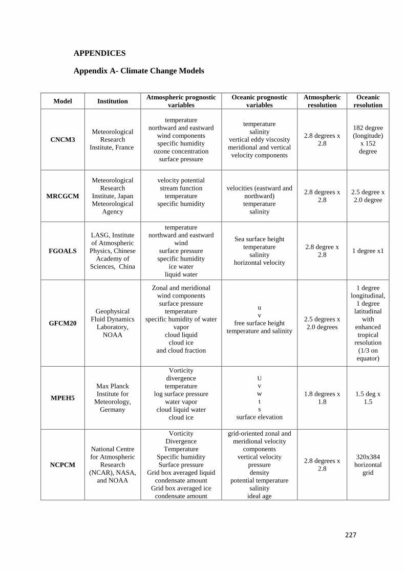
227
APPENDICES
Appendix A- Climate Change Models
Model Institution Atmospheric prognostic
variables
Oceanic prognostic
variables
Atmospheric
resolution
Oceanic
resolution
CNCM3
Meteorological
Research
Institute, France
temperature
northward and eastward
wind components
specific humidity
ozone concentration
surface pressure
temperature
salinity
vertical eddy viscosity
meridional and vertical
velocity components
2.8 degrees x
2.8
182 degree
(longitude)
x 152
degree
MRCGCM
Meteorological
Research
Institute, Japan
Meteorological
Agency
velocity potential
stream function
temperature
specific humidity
velocities (eastward and
northward)
temperature
salinity
2.8 degrees x
2.8
2.5 degree x
2.0 degree
FGOALS
LASG, Institute
of Atmospheric
Physics, Chinese
Academy of
Sciences, China
temperature
northward and eastward
wind
surface pressure
specific humidity
ice water
liquid water
Sea surface height
temperature
salinity
horizontal velocity
2.8 degree x
2.8 1 degree x1
GFCM20
Geophysical
Fluid Dynamics
Laboratory,
NOAA
Zonal and meridional
wind components
surface pressure
temperature
specific humidity of water
vapor
cloud liquid
cloud ice
and cloud fraction
u
v
free surface height
temperature and salinity
2.5 degrees x
2.0 degrees
1 degree
longitudinal,
1 degree
latitudinal
with
enhanced
tropical
resolution
(1/3 on
equator)
MPEH5
Max Planck
Institute for
Meteorology,
Germany
Vorticity
divergence
temperature
log surface pressure
water vapor
cloud liquid water
cloud ice
U
v
w
t
s
surface elevation
1.8 degrees x
1.8
1.5 deg x
1.5
NCPCM
National Centre
for Atmospheric
Research
(NCAR), NASA,
and NOAA
Vorticity
Divergence
Temperature
Specific humidity
Surface pressure
Grid box averaged liquid
condensate amount
Grid box averaged ice
condensate amount
grid-oriented zonal and
meridional velocity
components
vertical velocity
pressure
density
potential temperature
salinity
ideal age
2.8 degrees x
2.8
320x384
horizontal
grid
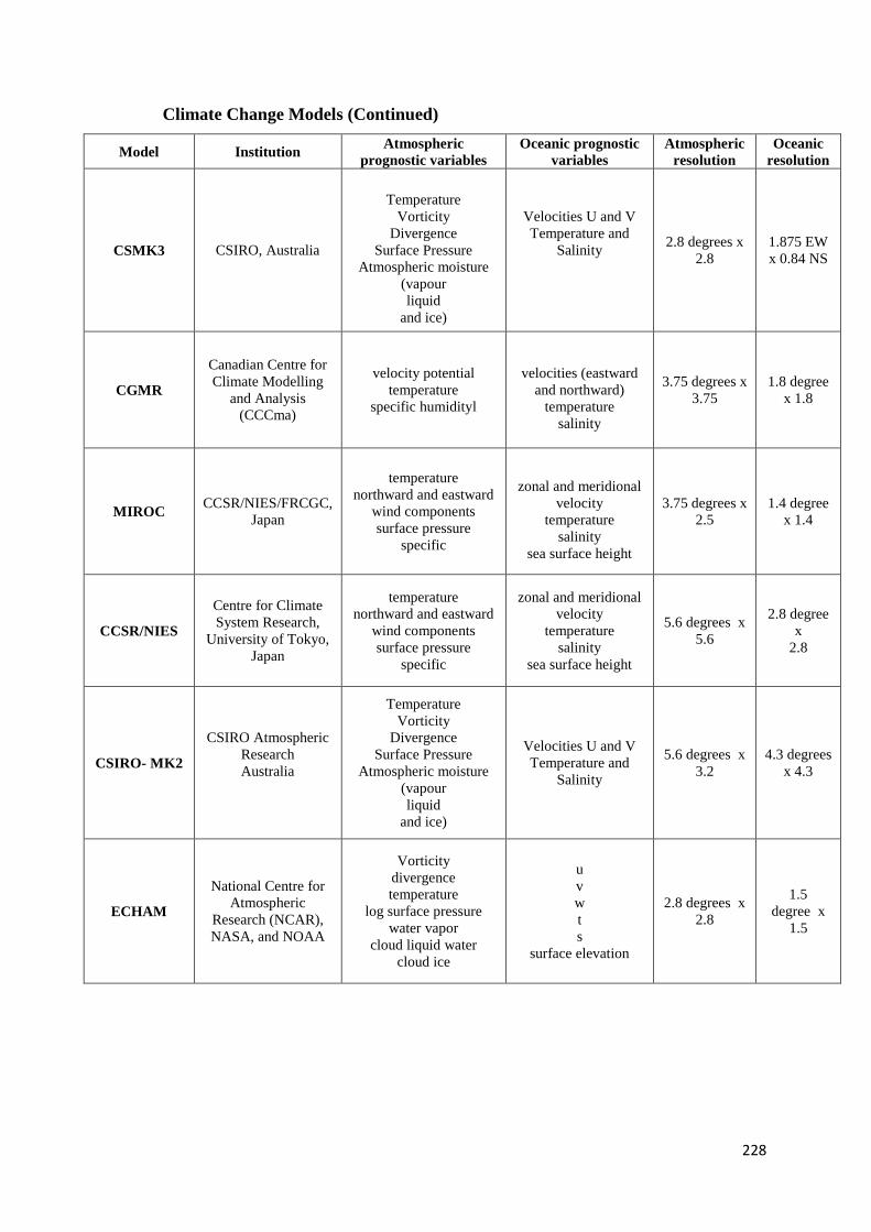
228
Climate Change Models (Continued)
Model Institution Atmospheric
prognostic variables
Oceanic prognostic
variables
Atmospheric
resolution
Oceanic
resolution
CSMK3 CSIRO, Australia
Temperature
Vorticity
Divergence
Surface Pressure
Atmospheric moisture
(vapour
liquid
and ice)
Velocities U and V
Temperature and
Salinity
2.8 degrees x
2.8
1.875 EW
x 0.84 NS
CGMR
Canadian Centre for
Climate Modelling
and Analysis
(CCCma)
velocity potential
temperature
specific humidityl
velocities (eastward
and northward)
temperature
salinity
3.75 degrees x
3.75
1.8 degree
x 1.8
MIROC CCSR/NIES/FRCGC,
Japan
temperature
northward and eastward
wind components
surface pressure
specific
zonal and meridional
velocity
temperature
salinity
sea surface height
3.75 degrees x
2.5
1.4 degree
x 1.4
CCSR/NIES
Centre for Climate
System Research,
University of Tokyo,
Japan
temperature
northward and eastward
wind components
surface pressure
specific
zonal and meridional
velocity
temperature
salinity
sea surface height
5.6 degrees x
5.6
2.8 degree
x
2.8
CSIRO- MK2
CSIRO Atmospheric
Research
Australia
Temperature
Vorticity
Divergence
Surface Pressure
Atmospheric moisture
(vapour
liquid
and ice)
Velocities U and V
Temperature and
Salinity
5.6 degrees x
3.2
4.3 degrees
x 4.3
ECHAM
National Centre for
Atmospheric
Research (NCAR),
NASA, and NOAA
Vorticity
divergence
temperature
log surface pressure
water vapor
cloud liquid water
cloud ice
u
v
w
t
s
surface elevation
2.8 degrees x
2.8
1.5
degree x
1.5
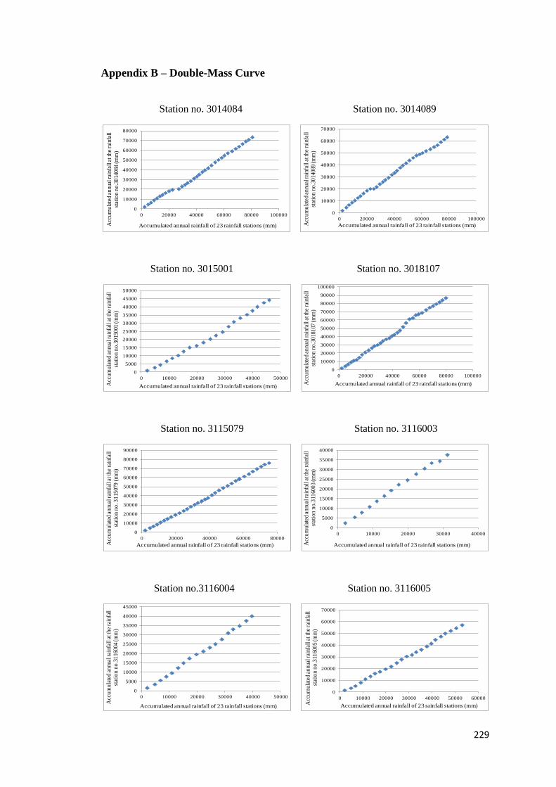
229
Appendix B – Double-Mass Curve
Station no. 3014084 Station no. 3014089
Station no. 3015001 Station no. 3018107
Station no. 3115079 Station no. 3116003
Station no.3116004 Station no. 3116005
0
10000
20000
30000
40000
50000
60000
70000
80000
0 20000 40000 60000 80000 100000
Accumulated annual rainfall of 23 rainfall stations (mm)Acc
um
ula
ted
annu
al r
ainf
all a
tth
e ra
infa
ll
stat
ion
no
.30
140
84 (
mm
)
0
10000
20000
30000
40000
50000
60000
70000
0 20000 40000 60000 80000 100000
Accumulated annual rainfall of 23 rainfall stations (mm)Acc
um
ula
ted
annu
al r
ainf
all a
tth
e ra
infa
ll
stat
ion
no
.30
140
89 (
mm
)
0
5000
10000
15000
20000
25000
30000
35000
40000
45000
50000
0 10000 20000 30000 40000 50000
Accumulated annual rainfall of 23 rainfall stations (mm)Acc
um
ula
ted
annu
al r
ainf
all a
tth
e ra
infa
ll
stat
ion
no
.30
150
01 (
mm
)
0
10000
20000
30000
40000
50000
60000
70000
80000
90000
100000
0 20000 40000 60000 80000 100000
Accumulated annual rainfall of 23 rainfall stations (mm)Acc
um
ula
ted
annu
al r
ainf
all a
tth
e ra
infa
ll
stat
ion
no
.30
181
07 (
mm
)
0
10000
20000
30000
40000
50000
60000
70000
80000
90000
0 20000 40000 60000 80000
Accumulated annual rainfall of 23 rainfall stations (mm)Acc
um
ula
ted
annu
al r
ainf
all a
tth
e ra
infa
llst
atio
n n
o. 3
115
079
(mm
)
0
5000
10000
15000
20000
25000
30000
35000
40000
0 10000 20000 30000 40000
Accumulated annual rainfall of 23 rainfall stations (mm)Acc
um
ula
ted
annu
al r
ainf
all a
tth
e ra
infa
llst
atio
n n
o.3
1160
03
(mm
)
0
5000
10000
15000
20000
25000
30000
35000
40000
45000
0 10000 20000 30000 40000 50000
Accumulated annual rainfall of 23 rainfall stations (mm)
Acc
um
ula
ted
annu
al r
ainf
all a
tth
e ra
infa
ll st
atio
n n
o.3
116
004
(m
m)
0
10000
20000
30000
40000
50000
60000
70000
0 10000 20000 30000 40000 50000 60000
Accumulated annual rainfall of 23 rainfall stations (mm)Acc
um
ula
ted
annu
al r
ainf
all a
tth
e ra
infa
llst
atio
n n
o.3
1160
05
(mm
)
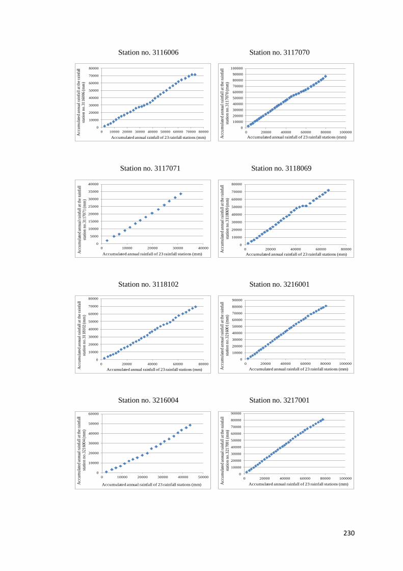
230
Station no. 3116006 Station no. 3117070
Station no. 3117071 Station no. 3118069
Station no. 3118102 Station no. 3216001
Station no. 3216004 Station no. 3217001
0
10000
20000
30000
40000
50000
60000
70000
80000
0 10000 20000 30000 40000 50000 60000 70000 80000
Accumulated annual rainfall of 23 rainfall stations (mm)
Acc
um
ula
ted
annu
al r
ainf
all a
tth
e ra
infa
ll st
atio
n n
o.3
116
006
(m
m)
0
10000
20000
30000
40000
50000
60000
70000
80000
90000
100000
0 20000 40000 60000 80000 100000
Accumulated annual rainfall of 23 rainfall stations (mm)Acc
um
ula
ted
annu
al r
ainf
all a
tth
e ra
infa
llst
atio
n n
o.3
1170
70
(mm
)
0
5000
10000
15000
20000
25000
30000
35000
40000
0 10000 20000 30000 40000
Accumulated annual rainfall of 23 rainfall stations (mm)Acc
um
ula
ted
annu
al r
ainf
all a
tth
e ra
infa
ll
stat
ion
no
.31
170
71 (
mm
)
0
10000
20000
30000
40000
50000
60000
70000
80000
0 20000 40000 60000 80000
Accumulated annual rainfall of 23 rainfall stations (mm)
Acc
um
ula
ted
annu
al r
ainf
all a
tth
e ra
infa
llst
atio
n n
o.3
1180
69
(mm
)
0
10000
20000
30000
40000
50000
60000
70000
80000
0 20000 40000 60000 80000
Accumulated annual rainfall of 23 rainfall stations (mm)Acc
um
ula
ted
annu
al r
ainf
all a
tth
e ra
infa
ll
stat
ion
no
.31
181
02 (
mm
)
0
10000
20000
30000
40000
50000
60000
70000
80000
90000
0 20000 40000 60000 80000 100000
Accumulated annual rainfall of 23 rainfall stations (mm)Acc
um
ula
ted
annu
al r
ainf
all a
tth
e ra
infa
llst
atio
n n
o.3
2160
01
(mm
)
0
10000
20000
30000
40000
50000
60000
0 10000 20000 30000 40000 50000
Accumulated annual rainfall of 23 rainfall stations (mm)Acc
um
ula
ted
annu
al r
ainf
all a
tth
e ra
infa
llst
atio
n n
o.3
2160
04
(mm
)
0
10000
20000
30000
40000
50000
60000
70000
80000
90000
0 20000 40000 60000 80000 100000
Accumulated annual rainfall of 23 rainfall stations (mm)Acc
um
ula
ted
annu
al r
ainf
all a
tth
e ra
infa
llst
atio
n n
o.3
2170
01
(mm
)
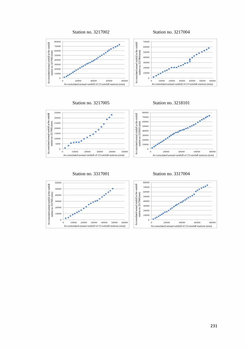
231
Station no. 3217002 Station no. 3217004
Station no. 3217005 Station no. 3218101
Station no. 3317001 Station no. 3317004
0
10000
20000
30000
40000
50000
60000
70000
80000
0 20000 40000 60000 80000
Accumulated annual rainfall of 23 rainfall stations (mm)
Acc
um
ula
ted
annu
al r
ainf
all a
tth
e ra
infa
ll
stat
ion
no
.32
170
02 (
mm
)
0
10000
20000
30000
40000
50000
60000
70000
0 10000 20000 30000 40000 50000 60000
Accumulated annual rainfall of 23 rainfall stations (mm)
Acc
um
ula
ted
annu
al r
ainf
all a
tth
e ra
infa
llst
atio
n n
o.3
2170
04
(mm
)
0
5000
10000
15000
20000
25000
30000
35000
0 10000 20000 30000 40000 50000
Accumulated annual rainfall of 23 rainfall stations (mm)
Acc
um
ula
ted
annu
al r
ainf
all a
tth
e ra
infa
ll st
atio
n n
o.3
217
005
(m
m)
0
10000
20000
30000
40000
50000
60000
70000
80000
0 20000 40000 60000 80000
Accumulated annual rainfall of 23 rainfall stations (mm)
Acc
um
ula
ted
annu
al r
ainf
all a
tth
e ra
infa
llst
atio
n n
o.3
2181
01
(mm
)
0
10000
20000
30000
40000
50000
60000
0 10000 20000 30000 40000 50000 60000
Accumulated annual rainfall of 23 rainfall stations (mm)
Acc
um
ula
ted
annu
al r
ainf
all a
tth
e ra
infa
ll st
atio
n n
o.3
317
001
(m
m)
0
10000
20000
30000
40000
50000
60000
70000
80000
0 20000 40000 60000 80000
Accumulated annual rainfall of 23 rainfall stations (mm)
Acc
um
ula
ted
annu
al r
ainf
all a
tth
e ra
infa
ll
stat
ion
no
.33
170
04 (
mm
)
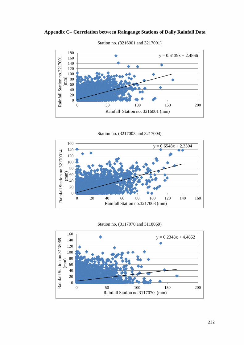
232
Appendix C– Correlation between Raingauge Stations of Daily Rainfall Data
Station no. (3216001 and 3217001)
Station no. (3217003 and 3217004)
Station no. (3117070 and 3118069)
y = 0.6139x + 2.4866
0
20
40
60
80
100
120
140
160
180
0 50 100 150 200
Rainfall Station no. 3216001 (mm)
Rai
nfa
ll S
tati
on
no
.32
17
00
1
(mm
)
y = 0.6548x + 2.3304
0
20
40
60
80
100
120
140
160
0 20 40 60 80 100 120 140 160
Rai
nfa
ll S
tati
on n
o.3
2170014
(mm
)
Rainfall Station no.3217003 (mm)
y = 0.2348x + 4.4852
0
20
40
60
80
100
120
140
160
0 50 100 150 200 Rai
nfa
ll S
tati
on
no
.31
18
06
9
(mm
)
Rainfall Station no.3117070 (mm)
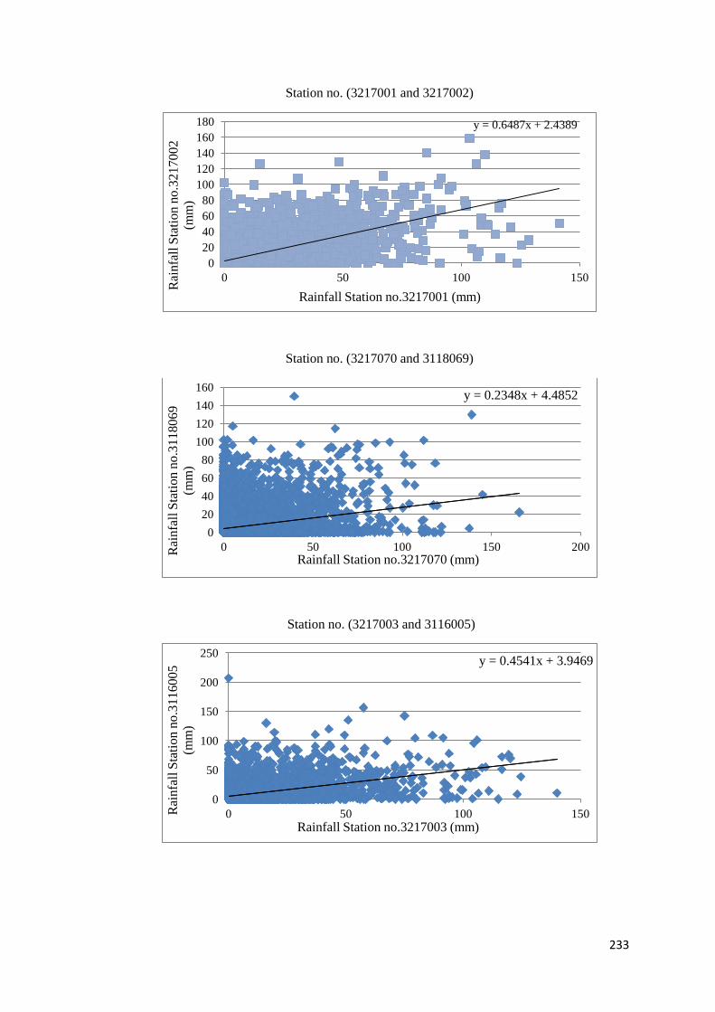
233
Station no. (3217001 and 3217002)
Station no. (3217070 and 3118069)
Station no. (3217003 and 3116005)
y = 0.6487x + 2.4389
0
20
40
60
80
100
120
140
160
180
0 50 100 150
Rai
nfa
ll S
tati
on
no
.32
17
00
2
(mm
)
Rainfall Station no.3217001 (mm)
y = 0.2348x + 4.4852
0
20
40
60
80
100
120
140
160
0 50 100 150 200 Rai
nfa
ll S
tati
on n
o.3
118069
(mm
)
Rainfall Station no.3217070 (mm)
y = 0.4541x + 3.9469
0
50
100
150
200
250
0 50 100 150 Rai
nfa
ll S
tati
on
no
.3116005
(mm
)
Rainfall Station no.3217003 (mm)
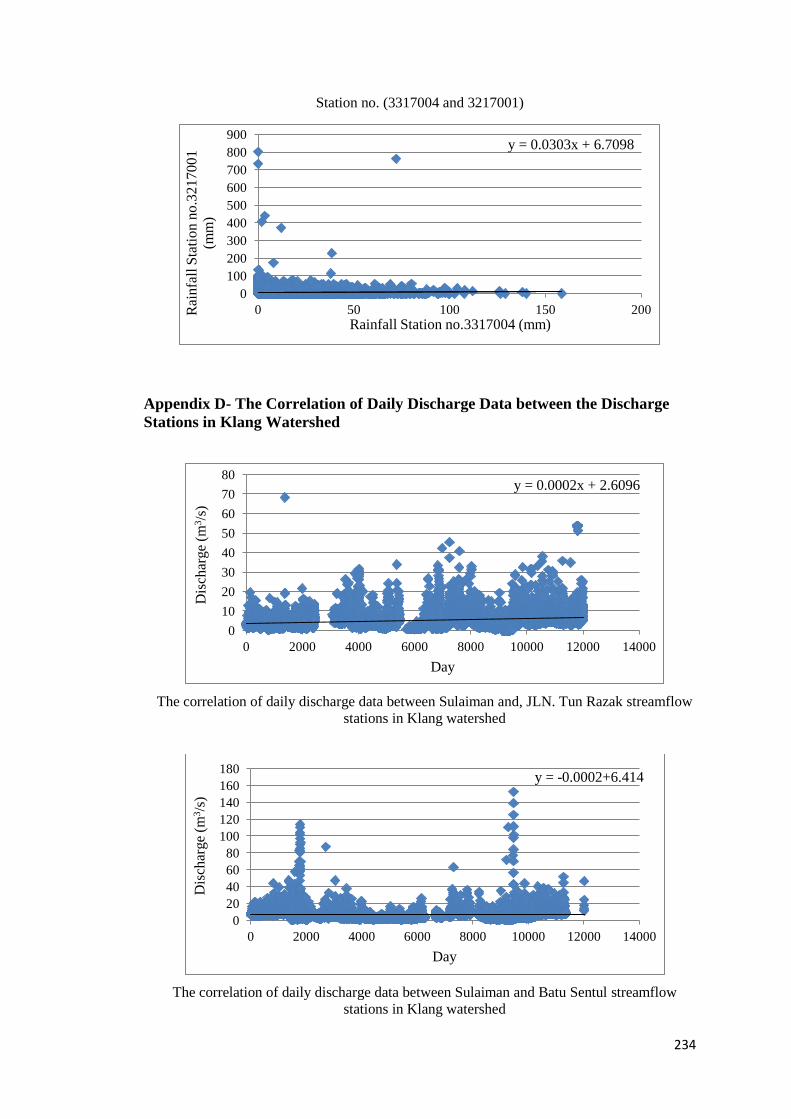
234
Station no. (3317004 and 3217001)
Appendix D- The Correlation of Daily Discharge Data between the Discharge
Stations in Klang Watershed
The correlation of daily discharge data between Sulaiman and, JLN. Tun Razak streamflow
stations in Klang watershed
The correlation of daily discharge data between Sulaiman and Batu Sentul streamflow
stations in Klang watershed
y = 0.0303x + 6.7098
0
100
200
300
400
500
600
700
800
900
0 50 100 150 200 Rai
nfa
ll S
tati
on
no
.32
17
00
1
(mm
)
Rainfall Station no.3317004 (mm)
y = 0.0002x + 2.6096
0
10
20
30
40
50
60
70
80
0 2000 4000 6000 8000 10000 12000 14000
Dis
char
ge
(m3/s
)
Day
y = -0.0002+6.414
0
20
40
60
80
100
120
140
160
180
0 2000 4000 6000 8000 10000 12000 14000
Dis
char
ge
(m3/s
)
Day
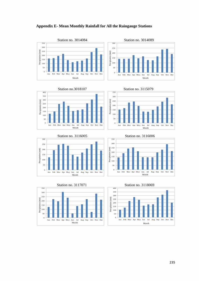
235
Appendix E- Mean Monthly Rainfall for All the Raingauge Stations
Station no. 3014084 Station no. 3014089
Station no.3018107 Station no. 3115079
Station no. 3116005 Station no. 3116006
Station no. 3117071 Station no. 3118069
0
50
100
150
200
250
300
350
Jan Feb Mar Apr May Jun Jul Aug Sep Oct Nov Dec
Pre
cip
itat
ion
(m
m)
Month
0
50
100
150
200
250
300
Jan Feb Mar Apr May Jun Jul Aug Sep Oct Nov Dec
Pre
cip
itat
ion
(m
m)
Month
0
50
100
150
200
250
300
350
400
Jan Feb Mar Apr May Jun Jul Aug Sep Oct Nov Dec
Pre
cip
itat
ion
(m
m)
Month
0
50
100
150
200
250
300
350
Jan Feb Mar Apr May Jun Jul Aug Sep Oct Nov Dec
Pre
cip
itat
ion
(m
m)
Month
0
50
100
150
200
250
300
Jan Feb Mar Apr May Jun Jul Aug Sep Oct Nov Dec
Pre
cip
itat
ion
(m
m)
Month
0
50
100
150
200
250
300
350
Jan Feb Mar Apr May Jun Jul Aug Sep Oct Nov Dec
Pre
cip
itat
ion
(m
m)
Month
0
50
100
150
200
250
300
350
Jan Feb Mar Apr May Jun Jul Aug Sep Oct Nov Dec
Pre
cip
itat
ion
(m
m)
Month
0
50
100
150
200
250
300
350
400
Jan Feb Mar Apr May Jun Jul Aug Sep Oct Nov Dec
Pre
cip
itat
ion
(m
m)
Month
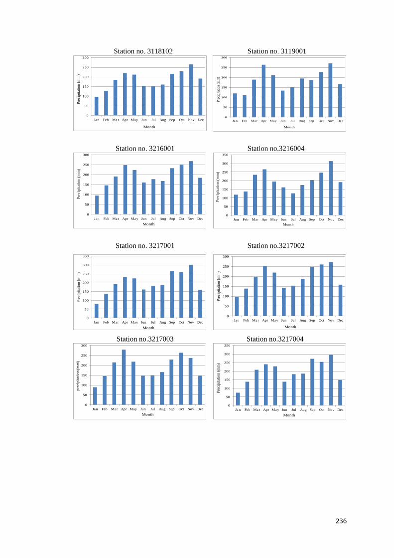
236
Station no. 3118102 Station no. 3119001
Station no. 3216001 Station no.3216004
Station no. 3217001 Station no.3217002
Station no.3217003 Station no.3217004
0
50
100
150
200
250
300
Jan Feb Mar Apr May Jun Jul Aug Sep Oct Nov Dec
Pre
cip
itat
ion
(m
m)
Month
0
50
100
150
200
250
300
Jan Feb Mar Apr May Jun Jul Aug Sep Oct Nov Dec
Prec
ipita
tion
(mm
)
Month
0
50
100
150
200
250
300
Jan Feb Mar Apr May Jun Jul Aug Sep Oct Nov Dec
Pre
cip
itat
ion
(m
m)
Month
0
50
100
150
200
250
300
350
Jan Feb Mar Apr May Jun Jul Aug Sep Oct Nov DecP
reci
pit
atio
n (
mm
)
Month
0
50
100
150
200
250
300
350
Jan Feb Mar Apr May Jun Jul Aug Sep Oct Nov Dec
Pre
cip
itat
ion
(m
m)
Month
0
50
100
150
200
250
300
Jan Feb Mar Apr May Jun Jul Aug Sep Oct Nov Dec
Pre
cip
itat
ion
(m
m)
Month
0
50
100
150
200
250
300
Jan Feb Mar Apr May Jun Jul Aug Sep Oct Nov Dec
pre
cip
itat
ion
(mm
)
Month
0
50
100
150
200
250
300
350
Jan Feb Mar Apr May Jun Jul Aug Sep Oct Nov Dec
Pre
cip
itat
ion
(m
m)
Month
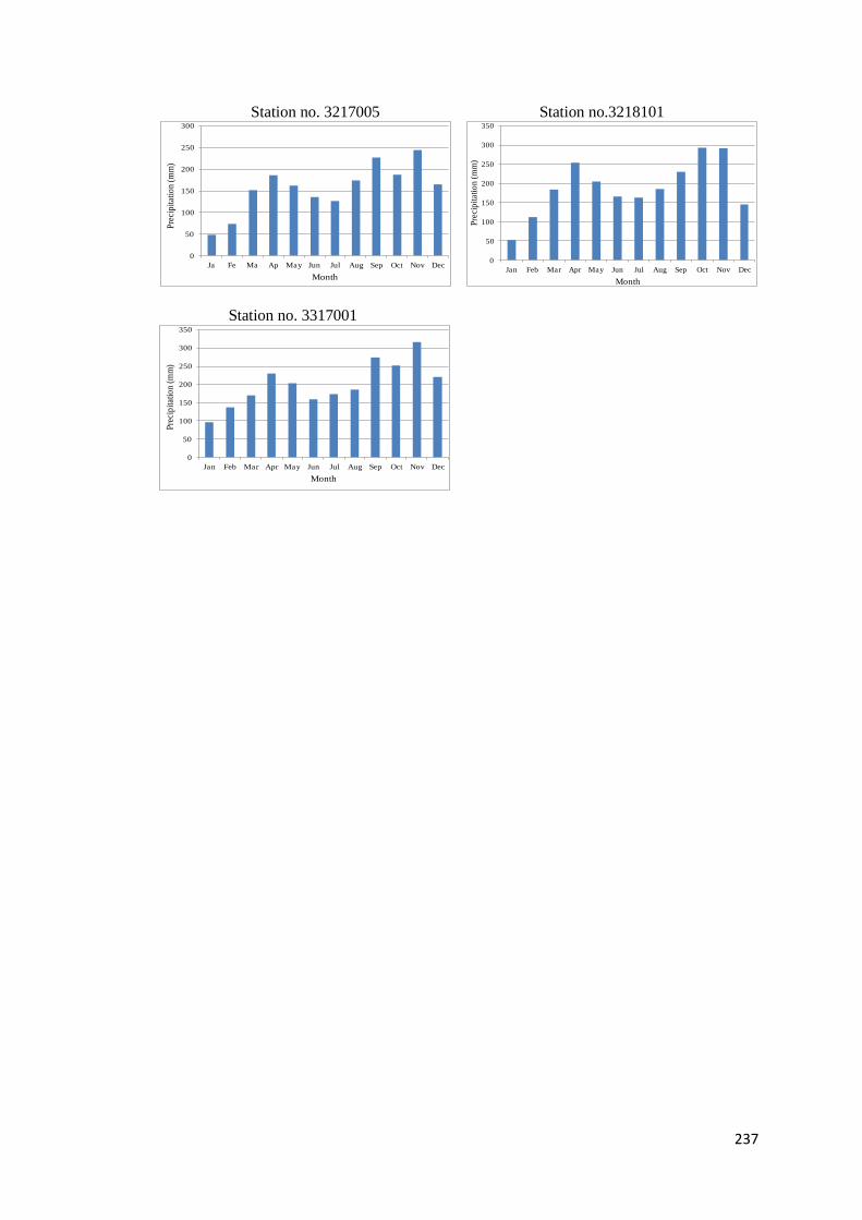
237
Station no. 3217005 Station no.3218101
Station no. 3317001
0
50
100
150
200
250
300
Ja Fe Ma Ap May Jun Jul Aug Sep Oct Nov Dec
Pre
cip
itat
ion
(m
m)
Month
0
50
100
150
200
250
300
350
Jan Feb Mar Apr May Jun Jul Aug Sep Oct Nov Dec
Pre
cip
itat
ion
(m
m)
Month
0
50
100
150
200
250
300
350
Jan Feb Mar Apr May Jun Jul Aug Sep Oct Nov Dec
Pre
cip
itat
ion
(m
m)
Month
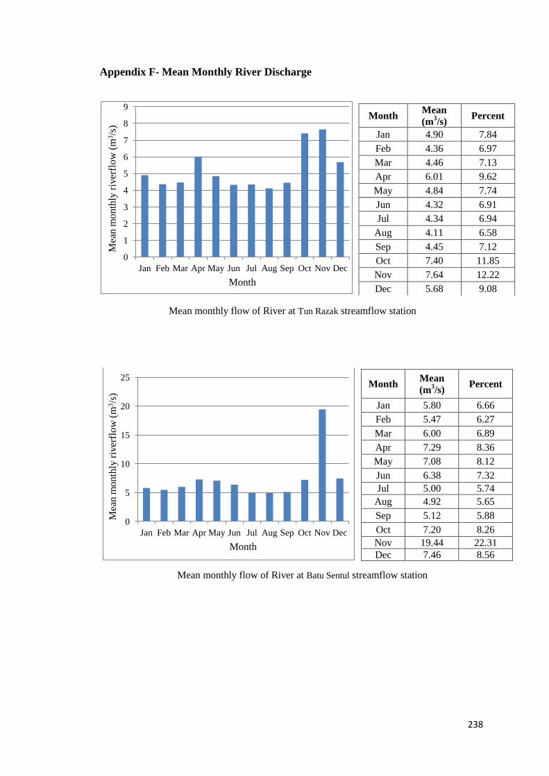
238
Appendix F- Mean Monthly River Discharge
Mean monthly flow of River at Tun Razak streamflow station
Mean monthly flow of River at Batu Sentul streamflow station
0
1
2
3
4
5
6
7
8
9
Jan Feb Mar Apr May Jun Jul Aug Sep Oct Nov Dec
Mea
n m
on
thly
riv
erfl
ow
(m
3/s
)
Month
0
5
10
15
20
25
Jan Feb Mar Apr May Jun Jul Aug Sep Oct Nov Dec
Mea
n m
onth
ly r
iver
flow
(m
3/s
)
Month
Month Mean
(m3/s)
Percent
Jan 4.90 7.84
Feb 4.36 6.97
Mar 4.46 7.13
Apr 6.01 9.62
May 4.84 7.74
Jun 4.32 6.91
Jul 4.34 6.94
Aug 4.11 6.58
Sep 4.45 7.12
Oct 7.40 11.85
Nov 7.64 12.22
Dec 5.68 9.08
Month Mean
(m3/s)
Percent
Jan 5.80 6.66
Feb 5.47 6.27
Mar 6.00 6.89
Apr 7.29 8.36
May 7.08 8.12
Jun 6.38 7.32
Jul 5.00 5.74
Aug 4.92 5.65
Sep 5.12 5.88
Oct 7.20 8.26
Nov 19.44 22.31
Dec 7.46 8.56
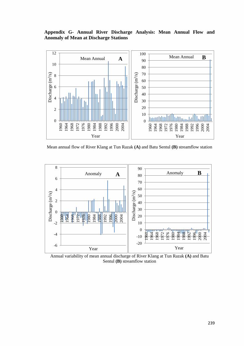
239
Appendix G- Annual River Discharge Analysis: Mean Annual Flow and
Anomaly of Mean at Discharge Stations
Mean annual flow of River Klang at Tun Razak (A) and Batu Sentul (B) streamflow station
Annual variability of mean annual discharge of River Klang at Tun Razak (A) and Batu
Sentul (B) streamflow station
0
2
4
6
8
10
12
19
60
19
64
19
68
19
72
19
76
19
80
19
84
19
88
19
92
19
96
20
00
20
04
Dis
char
ge
(m3/s
)
Year
Mean Annual
0
10
20
30
40
50
60
70
80
90
100
19
60
19
64
19
68
19
72
19
76
19
80
19
84
19
88
19
92
19
96
20
00
20
04
Dis
char
ge
(m3/s
) Year
Mean Annual
-6
-4
-2
0
2
4
6
8
19
60
19
64
19
68
19
72
19
76
19
80
19
84
19
88
19
92
19
96
20
00
20
04
Dis
char
ge
(m3/s
)
Year
Anomaly
-20
-10
0
10
20
30
40
50
60
70
80
90
19
60
19
64
19
68
19
72
19
76
19
80
19
84
19
88
19
92
19
96
20
00
20
04
Dis
char
ge
(m3/s
)
Year
Anomaly
A
A
B
B
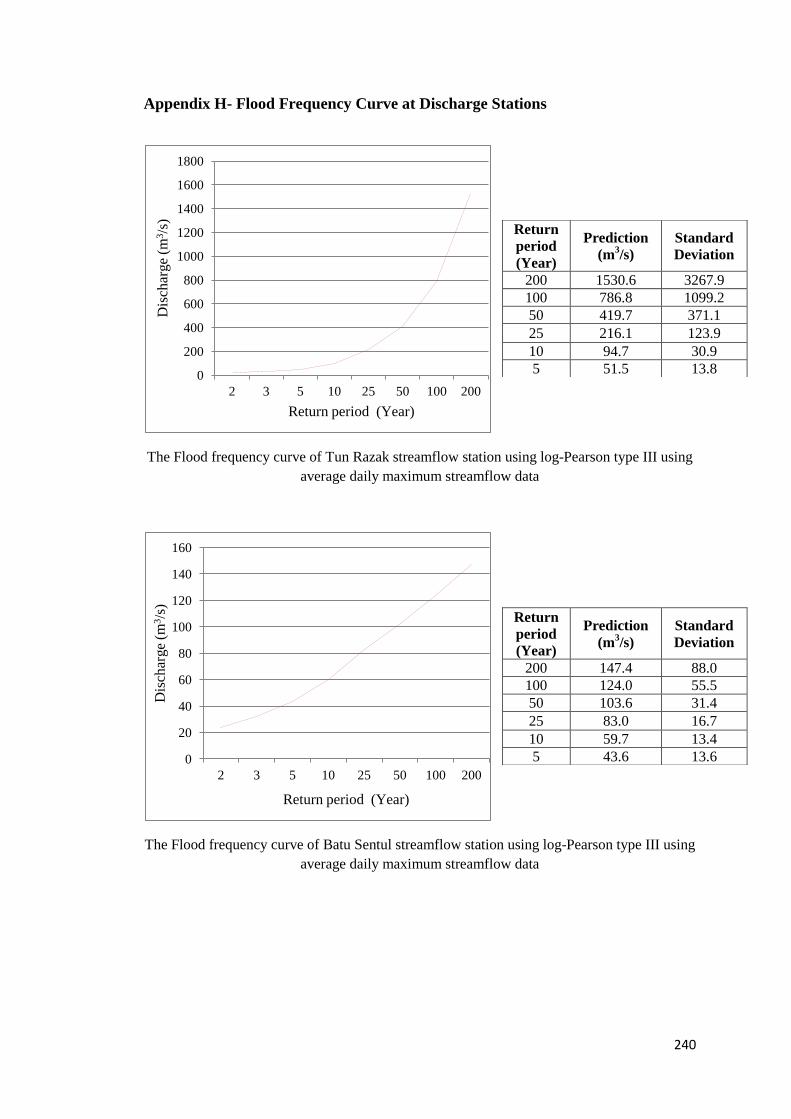
240
Appendix H- Flood Frequency Curve at Discharge Stations
The Flood frequency curve of Tun Razak streamflow station using log-Pearson type III using
average daily maximum streamflow data
The Flood frequency curve of Batu Sentul streamflow station using log-Pearson type III using
average daily maximum streamflow data
0
200
400
600
800
1000
1200
1400
1600
1800
2 3 5 10 25 50 100 200
Dis
char
ge
(m3/s
)
Return period (Year)
0
20
40
60
80
100
120
140
160
2 3 5 10 25 50 100 200
Dis
char
ge
(m3/s
)
Return period (Year)
Return
period
(Year)
Prediction
(m3/s)
Standard
Deviation
200 1530.6 3267.9
100 786.8 1099.2
50 419.7 371.1
25 216.1 123.9
10 94.7 30.9
5 51.5 13.8
Return
period
(Year)
Prediction
(m3/s)
Standard
Deviation
200 147.4 88.0
100 124.0 55.5
50 103.6 31.4
25 83.0 16.7
10 59.7 13.4
5 43.6 13.6
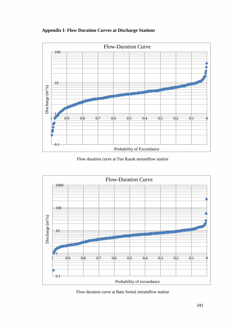
241
Appendix I- Flow Duration Curves at Discharge Stations
Flow duration curve at Tun Razak streamflow station
Flow duration curve at Batu Sentul streamflow station
0.1
1
10
100
0 0.1 0.2 0.3 0.4 0.5 0.6 0.7 0.8 0.9 1
Dis
char
ge
(m3/s
)
Probability of Exceedance
Flow-Duration Curve
0.1
1
10
100
1000
0 0.1 0.2 0.3 0.4 0.5 0.6 0.7 0.8 0.9 1
Dis
char
ge
(m3/s
)
Probability of exceedance
Flow-Duration Curve
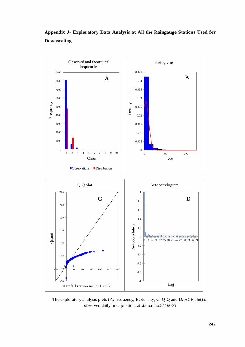
242
Appendix J- Exploratory Data Analysis at All the Raingauge Stations Used for
Downscaling
The exploratory analysis plots (A: frequency, B: density, C: Q-Q and D: ACF plot) of
observed daily precipitation, at station no.3116005
0
1000
2000
3000
4000
5000
6000
7000
8000
9000
1 2 3 4 5 6 7 8 9 10
Fre
quen
cy
Class
Observed and theoretical
frequencies
Observations Distribution
0
0.005
0.01
0.015
0.02
0.025
0.03
0.035
0.04
0.045
0 100 200
Den
sity
Var
Histograms
-60
-10
40
90
140
190
240
290
-60 -10 40 90 140 190 240 290
Quan
tile
Rainfall station no. 3116005
Q-Q plot
-1
-0.8
-0.6
-0.4
-0.2
0
0.2
0.4
0.6
0.8
1
0 3 6 9 12 15 18 21 24 27 30 33 36 39
Auto
corr
elat
ion
Lag
Autocorrelogram
A B
C D
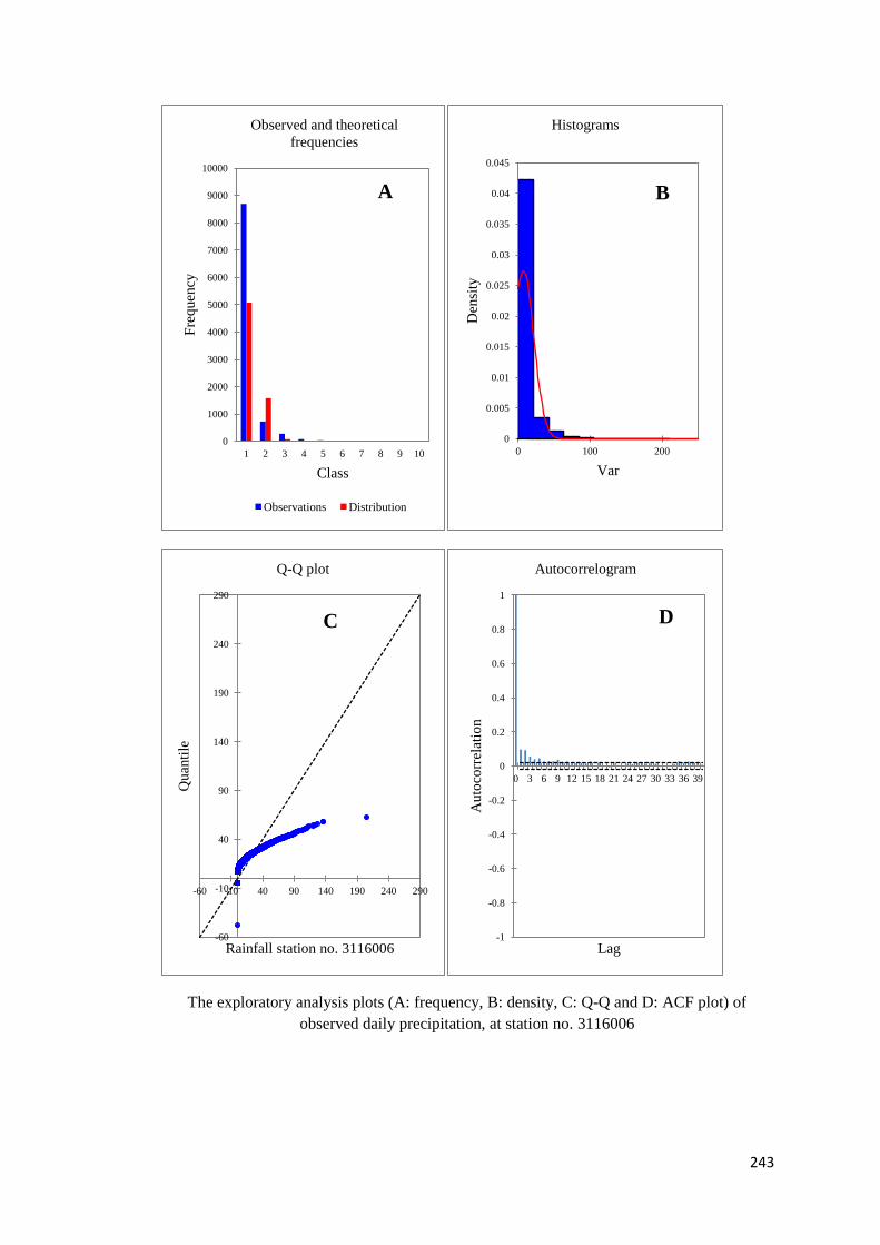
243
The exploratory analysis plots (A: frequency, B: density, C: Q-Q and D: ACF plot) of
observed daily precipitation, at station no. 3116006
0
1000
2000
3000
4000
5000
6000
7000
8000
9000
10000
1 2 3 4 5 6 7 8 9 10
Fre
quen
cy
Class
Observed and theoretical
frequencies
Observations Distribution
0
0.005
0.01
0.015
0.02
0.025
0.03
0.035
0.04
0.045
0 100 200
Den
sity
Var
Histograms
-60
-10
40
90
140
190
240
290
-60 -10 40 90 140 190 240 290
Quan
tile
Rainfall station no. 3116006
Q-Q plot
-1
-0.8
-0.6
-0.4
-0.2
0
0.2
0.4
0.6
0.8
1
0 3 6 9 12 15 18 21 24 27 30 33 36 39
Auto
corr
elat
ion
Lag
Autocorrelogram
A B
C D
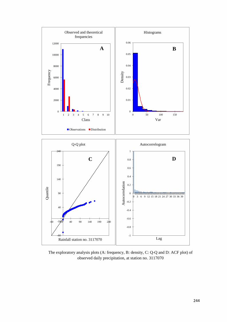
244
The exploratory analysis plots (A: frequency, B: density, C: Q-Q and D: ACF plot) of
observed daily precipitation, at station no. 3117070
0
2000
4000
6000
8000
10000
12000
1 2 3 4 5 6 7 8 9 10
Fre
quen
cy
Class
Observed and theoretical
frequencies
Observations Distribution
0
0.01
0.02
0.03
0.04
0.05
0.06
0 50 100 150
Den
sity
Var
Histograms
-60
-10
40
90
140
190
240
-60 -10 40 90 140 190 240
Quan
tile
Rainfall station no. 3117070
Q-Q plot
-1
-0.8
-0.6
-0.4
-0.2
0
0.2
0.4
0.6
0.8
1
0 3 6 9 12 15 18 21 24 27 30 33 36 39
Auto
corr
elat
ion
Lag
Autocorrelogram
A B
C D
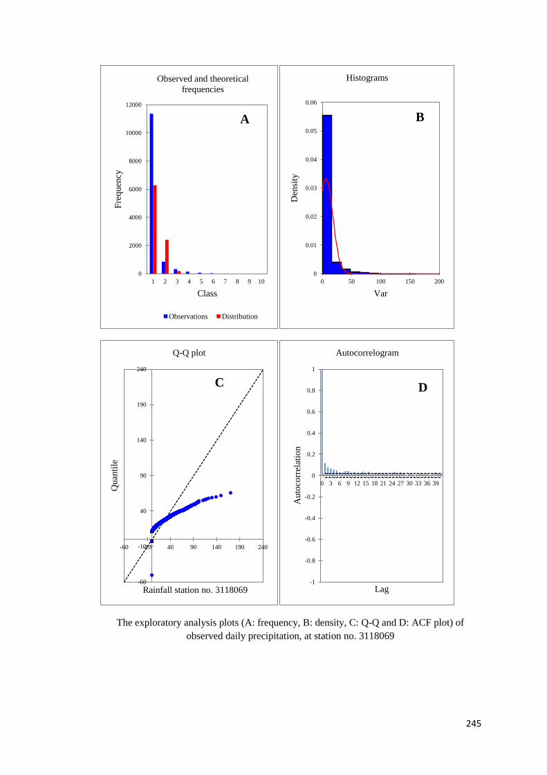
245
The exploratory analysis plots (A: frequency, B: density, C: Q-Q and D: ACF plot) of
observed daily precipitation, at station no. 3118069
0
2000
4000
6000
8000
10000
12000
1 2 3 4 5 6 7 8 9 10
Fre
quen
cy
Class
Observed and theoretical
frequencies
Observations Distribution
0
0.01
0.02
0.03
0.04
0.05
0.06
0 50 100 150 200
Den
sity
Var
Histograms
-60
-10
40
90
140
190
240
-60 -10 40 90 140 190 240
Quan
tile
Rainfall station no. 3118069
Q-Q plot
-1
-0.8
-0.6
-0.4
-0.2
0
0.2
0.4
0.6
0.8
1
0 3 6 9 12 15 18 21 24 27 30 33 36 39
Auto
corr
elat
ion
Lag
Autocorrelogram
A B
C D
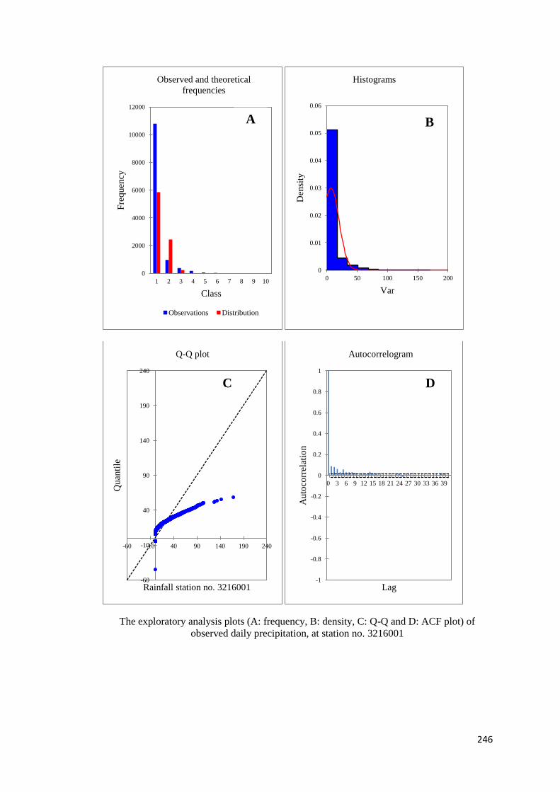
246
The exploratory analysis plots (A: frequency, B: density, C: Q-Q and D: ACF plot) of
observed daily precipitation, at station no. 3216001
0
2000
4000
6000
8000
10000
12000
1 2 3 4 5 6 7 8 9 10
Fre
quen
cy
Class
Observed and theoretical
frequencies
Observations Distribution
0
0.01
0.02
0.03
0.04
0.05
0.06
0 50 100 150 200
Den
sity
Var
Histograms
-60
-10
40
90
140
190
240
-60 -10 40 90 140 190 240
Quan
tile
Rainfall station no. 3216001
Q-Q plot
-1
-0.8
-0.6
-0.4
-0.2
0
0.2
0.4
0.6
0.8
1
0 3 6 9 12 15 18 21 24 27 30 33 36 39
Auto
corr
elat
ion
Lag
Autocorrelogram
A B
C D
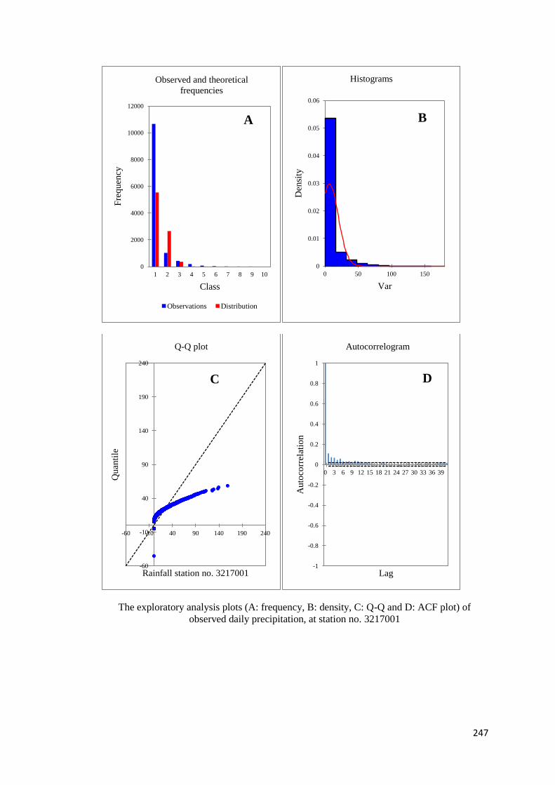
247
The exploratory analysis plots (A: frequency, B: density, C: Q-Q and D: ACF plot) of
observed daily precipitation, at station no. 3217001
0
2000
4000
6000
8000
10000
12000
1 2 3 4 5 6 7 8 9 10
Fre
quen
cy
Class
Observed and theoretical
frequencies
Observations Distribution
0
0.01
0.02
0.03
0.04
0.05
0.06
0 50 100 150
Den
sity
Var
Histograms
-60
-10
40
90
140
190
240
-60 -10 40 90 140 190 240
Quan
tile
Rainfall station no. 3217001
Q-Q plot
-1
-0.8
-0.6
-0.4
-0.2
0
0.2
0.4
0.6
0.8
1
0 3 6 9 12 15 18 21 24 27 30 33 36 39
Auto
corr
elat
ion
Lag
Autocorrelogram
A B
C D
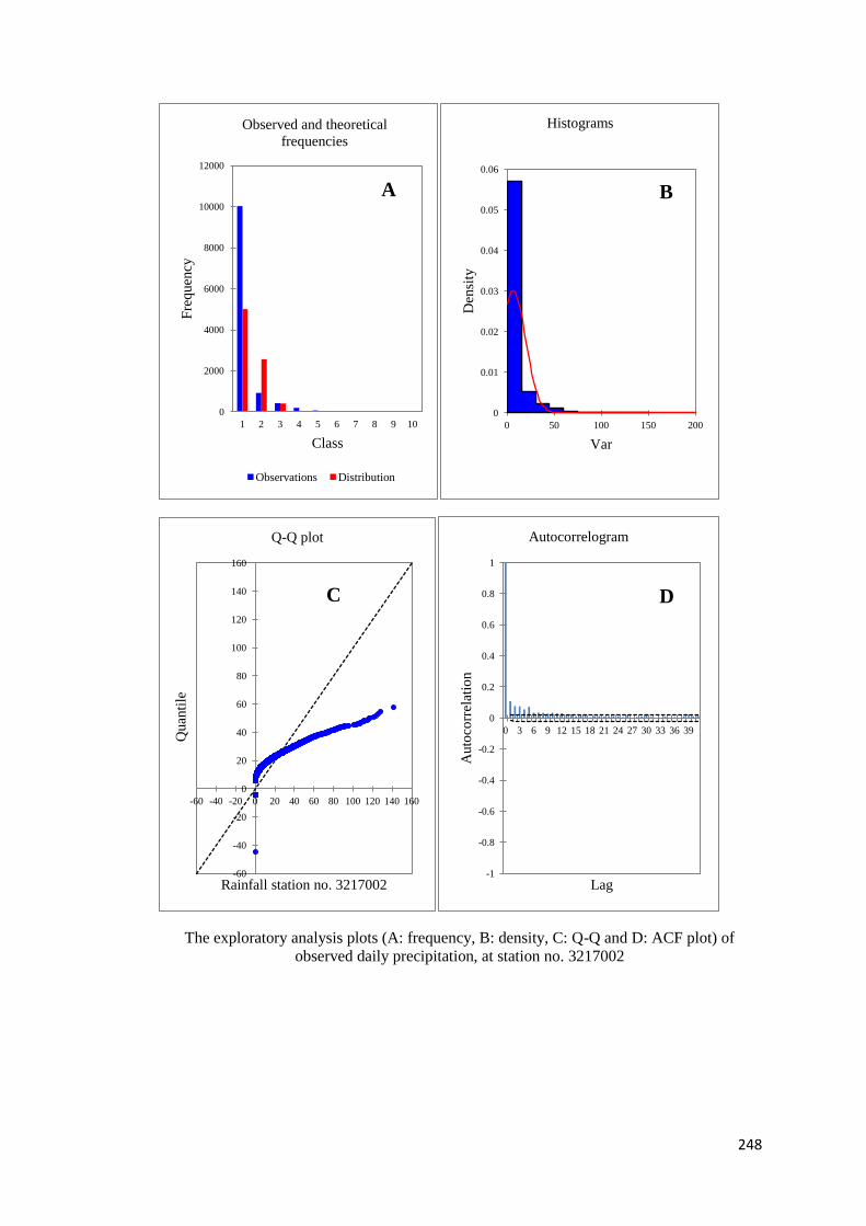
248
The exploratory analysis plots (A: frequency, B: density, C: Q-Q and D: ACF plot) of
observed daily precipitation, at station no. 3217002
0
2000
4000
6000
8000
10000
12000
1 2 3 4 5 6 7 8 9 10
Fre
quen
cy
Class
Observed and theoretical
frequencies
Observations Distribution
0
0.01
0.02
0.03
0.04
0.05
0.06
0 50 100 150 200
Den
sity
Var
Histograms
-60
-40
-20
0
20
40
60
80
100
120
140
160
-60 -40 -20 0 20 40 60 80 100 120 140 160
Quan
tile
Rainfall station no. 3217002
Q-Q plot
-1
-0.8
-0.6
-0.4
-0.2
0
0.2
0.4
0.6
0.8
1
0 3 6 9 12 15 18 21 24 27 30 33 36 39
Auto
corr
elat
ion
Lag
Autocorrelogram
A B
C D
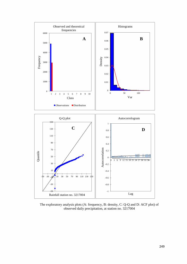
249
The exploratory analysis plots (A: frequency, B: density, C: Q-Q and D: ACF plot) of
observed daily precipitation, at station no. 3217004
0
1000
2000
3000
4000
5000
6000
1 2 3 4 5 6 7 8 9 10
Fre
quen
cy
Class
Observed and theoretical
frequencies
Observations Distribution
0
0.01
0.02
0.03
0.04
0.05
0.06
0.07
0 50 100
Den
sity
Var
Histograms
-50
-30
-10
10
30
50
70
90
110
130
150
-50 -30 -10 10 30 50 70 90 110 130 150
Quan
tile
Rainfall station no. 3217004
Q-Q plot
-1
-0.8
-0.6
-0.4
-0.2
0
0.2
0.4
0.6
0.8
1
0 3 6 9 12 15 18 21 24 27 30 33 36
Auto
corr
elat
ion
Lag
Autocorrelogram
A B
C D
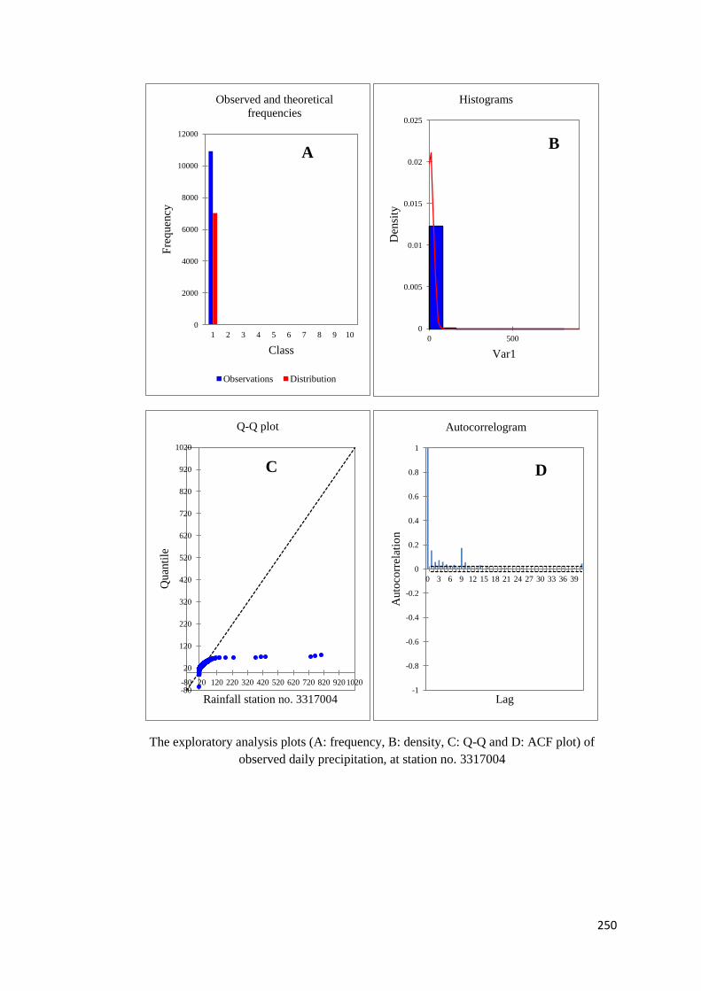
250
The exploratory analysis plots (A: frequency, B: density, C: Q-Q and D: ACF plot) of
observed daily precipitation, at station no. 3317004
0
2000
4000
6000
8000
10000
12000
1 2 3 4 5 6 7 8 9 10
Fre
quen
cy
Class
Observed and theoretical
frequencies
Observations Distribution
0
0.005
0.01
0.015
0.02
0.025
0 500
Den
sity
Var1
Histograms
-80
20
120
220
320
420
520
620
720
820
920
1020
-80 20 120 220 320 420 520 620 720 820 920 1020
Quan
tile
Rainfall station no. 3317004
Q-Q plot
-1
-0.8
-0.6
-0.4
-0.2
0
0.2
0.4
0.6
0.8
1
0 3 6 9 12 15 18 21 24 27 30 33 36 39
Auto
corr
elat
ion
Lag
Autocorrelogram
A B
C D
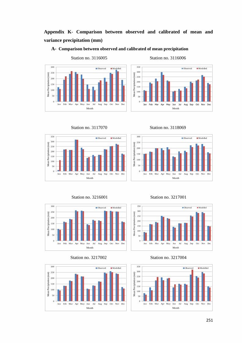
251
Appendix K- Comparison between observed and calibrated of mean and
variance precipitation (mm)
A- Comparison between observed and calibrated of mean precipitation
Station no. 3116005 Station no. 3116006
Station no. 3117070 Station no. 3118069
Station no. 3216001 Station no. 3217001
Station no. 3217002 Station no. 3217004
0
50
100
150
200
250
300
Jan Feb Mar Apr May Jun Jul Aug Sep Oct Nov Dec
Observed Modelled
Month
Mea
n P
reci
pit
atio
n (m
m)
0
50
100
150
200
250
300
350
Jan Feb Mar Apr May Jun Jul Aug Sep Oct Nov Dec
Observed Modelled
Month
Mea
n P
reci
pit
atio
n (m
m)
0
50
100
150
200
250
300
350
Jan Feb Mar Apr May Jun Jul Aug Sep Oct Nov Dec
Observed Modelled
Month
Mea
n P
reci
pit
atio
n (m
m)
0
50
100
150
200
250
300
Jan Feb Mar Apr May Jun Jul Aug Sep Oct Nov Dec
Observed Modelled
Month
Mea
n P
reci
pit
atio
n (m
m)
0
50
100
150
200
250
300
Jan Feb Mar Apr May Jun Jul Aug Sep Oct Nov Dec
Observed Modelled
Month
Mea
n P
reci
pit
atio
n (m
m)
0
50
100
150
200
250
300
350
Jan Feb Mar Apr May Jun Jul Aug Sep Oct Nov Dec
Observed Modelled
Month
Mean
Pre
cip
itati
on (
mm
)
0
50
100
150
200
250
300
Jan Feb Mar Apr May Jun Jul Aug Sep Oct Nov Dec
Observed Modelled
Month
Mea
n P
reci
pit
atio
n (m
m)
0
50
100
150
200
250
300
350
Jan Feb Mar Apr May Jun Jul Aug Sep Oct Nov Dec
Observed Modelled
Month
Mea
n P
reci
pit
atio
n (m
m)
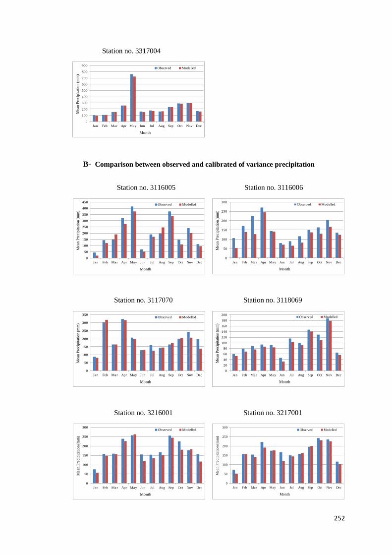
252
Station no. 3317004
B- Comparison between observed and calibrated of variance precipitation
Station no. 3116005 Station no. 3116006
Station no. 3117070 Station no. 3118069
Station no. 3216001 Station no. 3217001
0
100
200
300
400
500
600
700
800
900
Jan Feb Mar Apr May Jun Jul Aug Sep Oct Nov Dec
Observed Modelled
Month
Mea
n P
reci
pit
atio
n (m
m)
0
50
100
150
200
250
300
350
400
450
Jan Feb Mar Apr May Jun Jul Aug Sep Oct Nov Dec
Observed Modelled
Month
Mea
n P
reci
pit
atio
n (m
m)
0
50
100
150
200
250
300
Jan Feb Mar Apr May Jun Jul Aug Sep Oct Nov Dec
Observed Modelled
Month
Mea
n P
reci
pit
atio
n (m
m)
0
50
100
150
200
250
300
350
Jan Feb Mar Apr May Jun Jul Aug Sep Oct Nov Dec
Observed Modelled
Month
Mea
n P
reci
pit
atio
n (m
m)
0
20
40
60
80
100
120
140
160
180
200
Jan Feb Mar Apr May Jun Jul Aug Sep Oct Nov Dec
Observed Modelled
Month
Mea
n P
reci
pit
atio
n (m
m)
0
50
100
150
200
250
300
Jan Feb Mar Apr May Jun Jul Aug Sep Oct Nov Dec
Observed Modelled
Month
Mea
n P
reci
pit
atio
n (m
m)
0
50
100
150
200
250
300
Jan Feb Mar Apr May Jun Jul Aug Sep Oct Nov Dec
Observed Modelled
Month
Mean
Pre
cip
itati
on (
mm
)
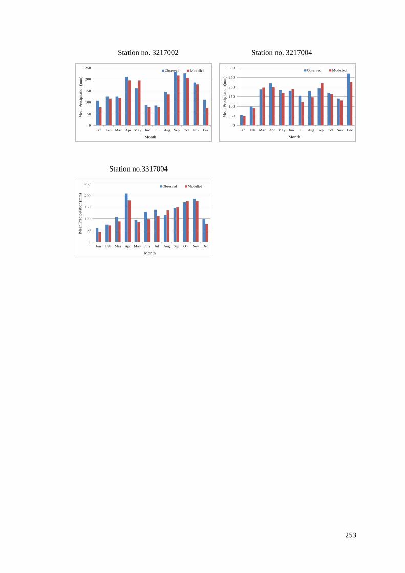
253
Station no. 3217002 Station no. 3217004
Station no.3317004
0
50
100
150
200
250
Jan Feb Mar Apr May Jun Jul Aug Sep Oct Nov Dec
Observed Modelled
Month
Mea
n P
reci
pit
atio
n (m
m)
0
50
100
150
200
250
300
Jan Feb Mar Apr May Jun Jul Aug Sep Oct Nov Dec
Observed Modelled
Month
Mea
n P
reci
pit
atio
n (m
m)
0
50
100
150
200
250
Jan Feb Mar Apr May Jun Jul Aug Sep Oct Nov Dec
Observed Modelled
Month
Mea
n P
reci
pit
atio
n (m
m)
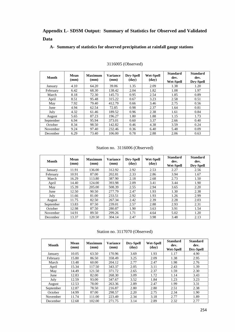
254
Appendix L- SDSM Output: Summary of Statistics for Observed and Validated
Data
A- Summary of statistics for observed precipitation at rainfall gauge stations
3116005 (Observed)
Month Mean
(mm)
Maximum
(mm)
Variance
(mm)
Dry-Spell
(day)
Wet-Spell
(day)
Standard
dev.
Wet-Spell
Standard
dev.
Dry-Spell
January 4.10 64.20 39.06 1.35 2.09 1.38 1.20
February 6.42 68.30 138.42 2.04 1.82 1.08 1.97
March 8.18 72.30 145.73 0.95 2.54 1.85 0.89
April 8.51 95.48 315.22 0.67 3.23 2.58 0.51
May 7.92 79.40 412.79 0.66 3.46 2.75 0.56
June 4.94 62.54 72.85 0.98 2.37 1.64 0.81
July 4.32 61.46 189.52 0.96 2.38 1.61 0.84
August 5.65 87.23 196.27 1.80 1.88 1.15 1.73
September 6.94 95.94 373.01 0.60 3.37 2.66 0.40
October 8.34 98.50 142.82 0.46 4.38 3.59 0.24
November 9.24 97.40 232.46 0.36 6.40 5.48 0.09
December 6.29 73.40 106.00 0.78 2.88 2.06 0.63
Station no. 3116006 (Observed)
Month Mean
(mm)
Maximum
(mm)
Variance
(mm)
Dry-Spell
(day)
Wet-Spell
(day)
Standard
dev.
Wet-Spell
Standard
dev.
Dry-Spell
January 11.91 136.00 312.92 2.92 2.53 2.27 2.56
February 10.91 87.00 202.81 2.33 2.86 3.94 1.67
March 16.29 113.80 387.90 2.18 2.68 2.73 1.50
April 14.40 124.00 393.98 2.09 3.41 3.44 1.90
May 15.39 205.00 508.39 2.55 2.94 3.65 2.20
June 12.50 90.50 277.79 2.47 1.93 1.30 2.38
July 11.66 81.00 233.51 2.92 1.93 1.26 2.99
August 11.75 82.50 267.34 2.42 2.39 2.28 2.03
September 13.83 87.50 239.01 2.57 2.88 2.93 2.31
October 12.98 87.50 280.87 1.90 3.63 3.91 1.54
November 14.91 89.50 299.26 1.71 4.64 5.02 1.20
December 13.37 120.50 304.14 2.47 3.98 3.48 2.13
Station no. 3117070 (Observed)
Month Mean
(mm)
Maximum
(mm)
Variance
(mm)
Dry-Spell
(day)
Wet-Spell
(day)
Standard
dev.
Wet-Spell
Standard
dev.
Dry-Spell
January 10.05 63.50 170.96 3.69 1.93 1.17 4.90
February 15.80 86.50 358.49 3.25 2.09 1.38 2.95
March 13.48 60.00 204.12 2.77 2.47 1.98 2.76
April 15.34 117.50 343.37 2.05 3.11 2.43 1.39
May 14.49 121.50 371.72 2.65 2.37 1.59 2.30
June 12.83 82.00 268.30 3.09 1.72 1.14 3.43
July 12.59 93.00 347.67 3.52 1.84 1.23 3.23
August 12.53 78.00 263.36 2.89 2.47 1.99 3.31
September 12.87 78.50 216.87 2.80 2.80 2.51 2.38
October 14.99 87.00 298.57 2.20 2.75 2.34 1.90
November 11.74 111.00 223.49 2.34 3.18 2.77 1.89
December 12.68 102.00 271.75 3.14 2.89 2.32 2.77
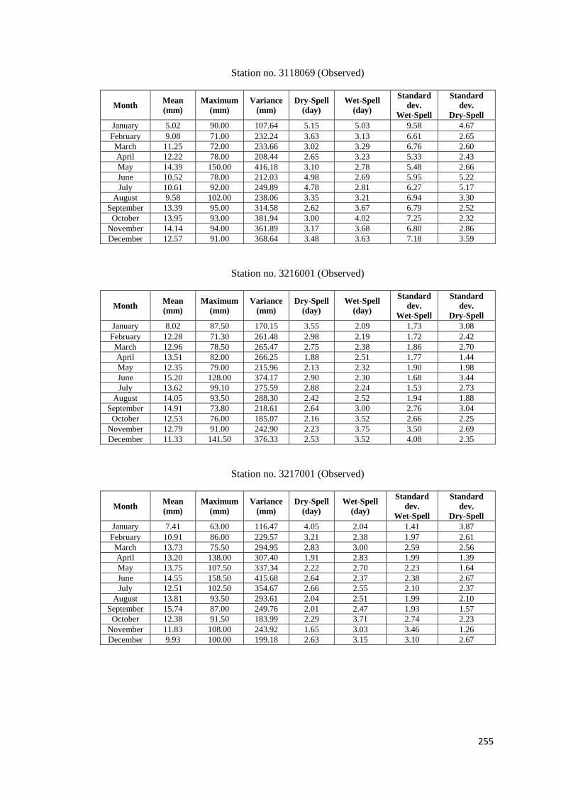
255
Station no. 3118069 (Observed)
Month Mean
(mm)
Maximum
(mm)
Variance
(mm)
Dry-Spell
(day)
Wet-Spell
(day)
Standard
dev.
Wet-Spell
Standard
dev.
Dry-Spell
January 5.02 90.00 107.64 5.15 5.03 9.58 4.67
February 9.08 71.00 232.24 3.63 3.13 6.61 2.65
March 11.25 72.00 233.66 3.02 3.29 6.76 2.60
April 12.22 78.00 208.44 2.65 3.23 5.33 2.43
May 14.39 150.00 416.18 3.10 2.78 5.48 2.66
June 10.52 78.00 212.03 4.98 2.69 5.95 5.22
July 10.61 92.00 249.89 4.78 2.81 6.27 5.17
August 9.58 102.00 238.06 3.35 3.21 6.94 3.30
September 13.39 95.00 314.58 2.62 3.67 6.79 2.52
October 13.95 93.00 381.94 3.00 4.02 7.25 2.32
November 14.14 94.00 361.89 3.17 3.68 6.80 2.86
December 12.57 91.00 368.64 3.48 3.63 7.18 3.59
Station no. 3216001 (Observed)
Month Mean
(mm)
Maximum
(mm)
Variance
(mm)
Dry-Spell
(day)
Wet-Spell
(day)
Standard
dev.
Wet-Spell
Standard
dev.
Dry-Spell
January 8.02 87.50 170.15 3.55 2.09 1.73 3.08
February 12.28 71.30 261.48 2.98 2.19 1.72 2.42
March 12.96 78.50 265.47 2.75 2.38 1.86 2.70
April 13.51 82.00 266.25 1.88 2.51 1.77 1.44
May 12.35 79.00 215.96 2.13 2.32 1.90 1.98
June 15.20 128.00 374.17 2.90 2.30 1.68 3.44
July 13.62 99.10 275.59 2.88 2.24 1.53 2.73
August 14.05 93.50 288.30 2.42 2.52 1.94 1.88
September 14.91 73.80 218.61 2.64 3.00 2.76 3.04
October 12.53 76.00 185.07 2.16 3.52 2.66 2.25
November 12.79 91.00 242.90 2.23 3.75 3.50 2.69
December 11.33 141.50 376.33 2.53 3.52 4.08 2.35
Station no. 3217001 (Observed)
Month Mean
(mm)
Maximum
(mm)
Variance
(mm)
Dry-Spell
(day)
Wet-Spell
(day)
Standard
dev.
Wet-Spell
Standard
dev.
Dry-Spell
January 7.41 63.00 116.47 4.05 2.04 1.41 3.87
February 10.91 86.00 229.57 3.21 2.38 1.97 2.61
March 13.73 75.50 294.95 2.83 3.00 2.59 2.56
April 13.20 138.00 307.40 1.91 2.83 1.99 1.39
May 13.75 107.50 337.34 2.22 2.70 2.23 1.64
June 14.55 158.50 415.68 2.64 2.37 2.38 2.67
July 12.51 102.50 354.67 2.66 2.55 2.10 2.37
August 13.81 93.50 293.61 2.04 2.51 1.99 2.10
September 15.74 87.00 249.76 2.01 2.47 1.93 1.57
October 12.38 91.50 183.99 2.29 3.71 2.74 2.23
November 11.83 108.00 243.92 1.65 3.03 3.46 1.26
December 9.93 100.00 199.18 2.63 3.15 3.10 2.67
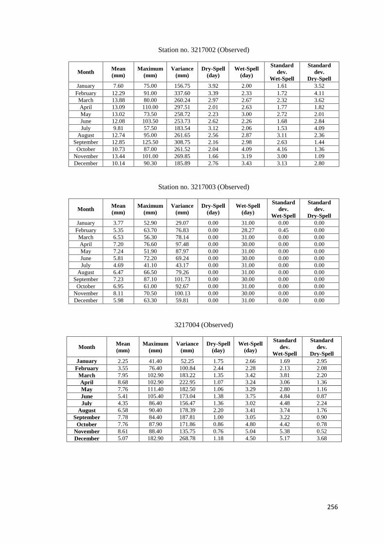
256
Station no. 3217002 (Observed)
Month Mean
(mm)
Maximum
(mm)
Variance
(mm)
Dry-Spell
(day)
Wet-Spell
(day)
Standard
dev.
Wet-Spell
Standard
dev.
Dry-Spell
January 7.60 75.00 156.75 3.92 2.00 1.61 3.52
February 12.29 91.00 337.60 3.39 2.33 1.72 4.11
March 13.88 80.00 260.24 2.97 2.67 2.32 3.62
April 13.09 110.00 297.51 2.01 2.63 1.77 1.82
May 13.02 73.50 258.72 2.23 3.00 2.72 2.01
June 12.08 103.50 253.73 2.62 2.26 1.68 2.84
July 9.81 57.50 183.54 3.12 2.06 1.53 4.09
August 12.74 95.00 261.65 2.56 2.87 3.11 2.36
September 12.85 125.50 308.75 2.16 2.98 2.63 1.44
October 10.73 87.00 261.52 2.04 4.09 4.16 1.36
November 13.44 101.00 269.85 1.66 3.19 3.00 1.09
December 10.14 90.30 185.89 2.76 3.43 3.13 2.80
Station no. 3217003 (Observed)
Month Mean
(mm)
Maximum
(mm)
Variance
(mm)
Dry-Spell
(day)
Wet-Spell
(day)
Standard
dev.
Wet-Spell
Standard
dev.
Dry-Spell
January 3.77 52.90 29.07 0.00 31.00 0.00 0.00
February 5.35 63.70 76.83 0.00 28.27 0.45 0.00
March 6.53 56.30 78.14 0.00 31.00 0.00 0.00
April 7.20 76.60 97.48 0.00 30.00 0.00 0.00
May 7.24 51.90 87.97 0.00 31.00 0.00 0.00
June 5.81 72.20 69.24 0.00 30.00 0.00 0.00
July 4.69 41.10 43.17 0.00 31.00 0.00 0.00
August 6.47 66.50 79.26 0.00 31.00 0.00 0.00
September 7.23 87.10 101.73 0.00 30.00 0.00 0.00
October 6.95 61.00 92.67 0.00 31.00 0.00 0.00
November 8.11 70.50 100.13 0.00 30.00 0.00 0.00
December 5.98 63.30 59.81 0.00 31.00 0.00 0.00
3217004 (Observed)
Month Mean
(mm)
Maximum
(mm)
Variance
(mm)
Dry-Spell
(day)
Wet-Spell
(day)
Standard
dev.
Wet-Spell
Standard
dev.
Dry-Spell
January 2.25 41.40 52.25 1.75 2.66 1.69 2.95
February 3.55 76.40 100.84 2.44 2.28 2.13 2.08
March 7.95 102.90 183.22 1.35 3.42 3.81 2.20
April 8.68 102.90 222.95 1.07 3.24 3.06 1.36
May 7.76 111.40 182.50 1.06 3.29 2.80 1.16
June 5.41 105.40 173.04 1.38 3.75 4.84 0.87
July 4.35 86.40 156.47 1.36 3.02 4.48 2.24
August 6.58 90.40 178.39 2.20 3.41 3.74 1.76
September 7.78 84.40 187.81 1.00 3.05 3.22 0.90
October 7.76 87.90 171.86 0.86 4.80 4.42 0.78
November 8.61 88.40 135.75 0.76 5.04 5.38 0.52
December 5.07 182.90 268.78 1.18 4.50 5.17 3.68
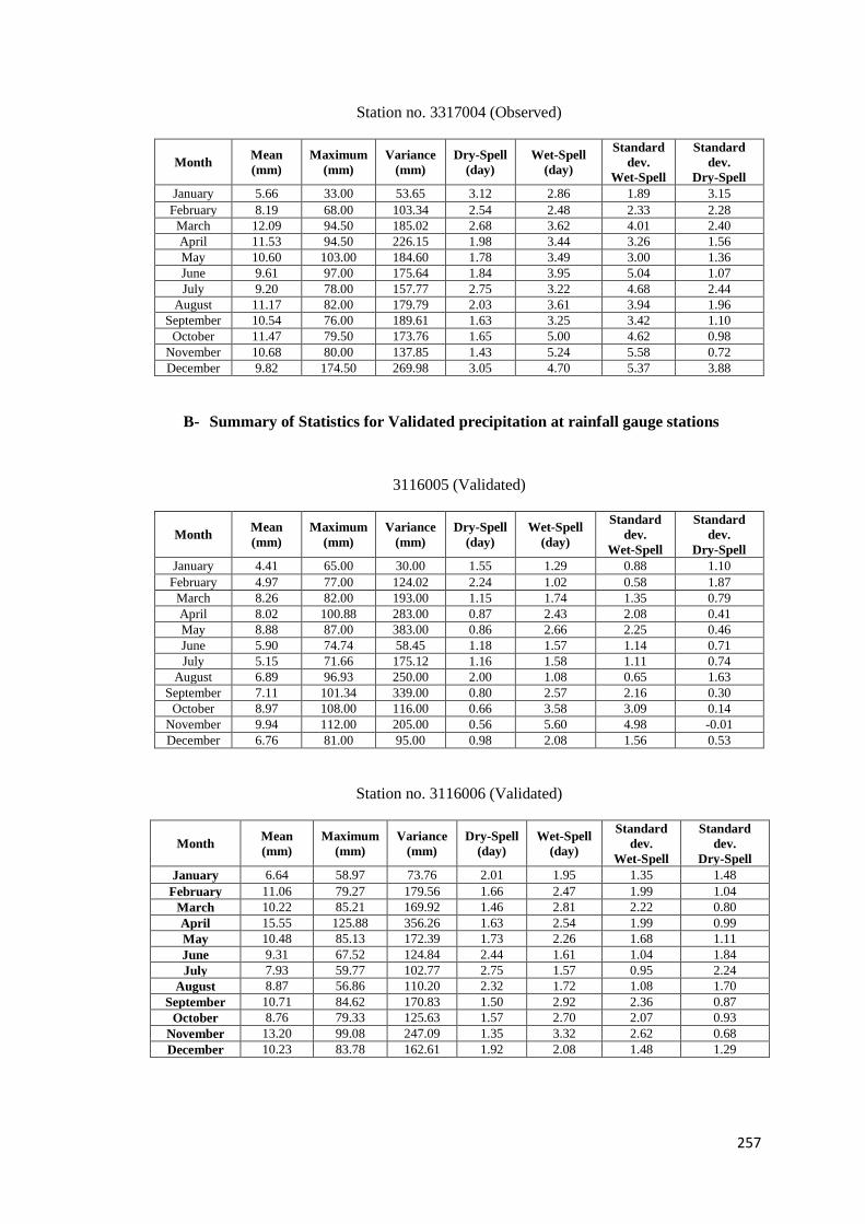
257
Station no. 3317004 (Observed)
Month Mean
(mm)
Maximum
(mm)
Variance
(mm)
Dry-Spell
(day)
Wet-Spell
(day)
Standard
dev.
Wet-Spell
Standard
dev.
Dry-Spell
January 5.66 33.00 53.65 3.12 2.86 1.89 3.15
February 8.19 68.00 103.34 2.54 2.48 2.33 2.28
March 12.09 94.50 185.02 2.68 3.62 4.01 2.40
April 11.53 94.50 226.15 1.98 3.44 3.26 1.56
May 10.60 103.00 184.60 1.78 3.49 3.00 1.36
June 9.61 97.00 175.64 1.84 3.95 5.04 1.07
July 9.20 78.00 157.77 2.75 3.22 4.68 2.44
August 11.17 82.00 179.79 2.03 3.61 3.94 1.96
September 10.54 76.00 189.61 1.63 3.25 3.42 1.10
October 11.47 79.50 173.76 1.65 5.00 4.62 0.98
November 10.68 80.00 137.85 1.43 5.24 5.58 0.72
December 9.82 174.50 269.98 3.05 4.70 5.37 3.88
B- Summary of Statistics for Validated precipitation at rainfall gauge stations
3116005 (Validated)
Month Mean
(mm)
Maximum
(mm)
Variance
(mm)
Dry-Spell
(day)
Wet-Spell
(day)
Standard
dev.
Wet-Spell
Standard
dev.
Dry-Spell
January 4.41 65.00 30.00 1.55 1.29 0.88 1.10
February 4.97 77.00 124.02 2.24 1.02 0.58 1.87
March 8.26 82.00 193.00 1.15 1.74 1.35 0.79
April 8.02 100.88 283.00 0.87 2.43 2.08 0.41
May 8.88 87.00 383.00 0.86 2.66 2.25 0.46
June 5.90 74.74 58.45 1.18 1.57 1.14 0.71
July 5.15 71.66 175.12 1.16 1.58 1.11 0.74
August 6.89 96.93 250.00 2.00 1.08 0.65 1.63
September 7.11 101.34 339.00 0.80 2.57 2.16 0.30
October 8.97 108.00 116.00 0.66 3.58 3.09 0.14
November 9.94 112.00 205.00 0.56 5.60 4.98 -0.01
December 6.76 81.00 95.00 0.98 2.08 1.56 0.53
Station no. 3116006 (Validated)
Month Mean
(mm)
Maximum
(mm)
Variance
(mm)
Dry-Spell
(day)
Wet-Spell
(day)
Standard
dev.
Wet-Spell
Standard
dev.
Dry-Spell
January 6.64 58.97 73.76 2.01 1.95 1.35 1.48
February 11.06 79.27 179.56 1.66 2.47 1.99 1.04
March 10.22 85.21 169.92 1.46 2.81 2.22 0.80
April 15.55 125.88 356.26 1.63 2.54 1.99 0.99
May 10.48 85.13 172.39 1.73 2.26 1.68 1.11
June 9.31 67.52 124.84 2.44 1.61 1.04 1.84
July 7.93 59.77 102.77 2.75 1.57 0.95 2.24
August 8.87 56.86 110.20 2.32 1.72 1.08 1.70
September 10.71 84.62 170.83 1.50 2.92 2.36 0.87
October 8.76 79.33 125.63 1.57 2.70 2.07 0.93
November 13.20 99.08 247.09 1.35 3.32 2.62 0.68
December 10.23 83.78 162.61 1.92 2.08 1.48 1.29
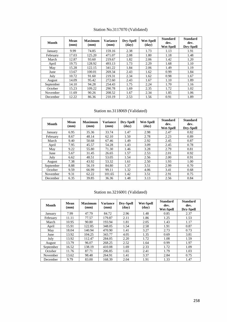
258
Station No.3117070 (Validated)
Month Mean
(mm)
Maximum
(mm)
Variance
(mm)
Dry-Spell
(day)
Wet-Spell
(day)
Standard
dev.
Wet-Spell
Standard
dev.
Dry-Spell
January 9.99 74.85 159.16 2.38 1.73 1.13 1.91
February 17.03 125.20 471.07 2.08 1.80 1.18 1.48
March 12.87 93.60 219.67 1.82 2.06 1.42 1.20
April 19.75 128.92 493.13 1.73 2.29 1.68 1.10
May 15.28 122.15 341.22 1.84 2.06 1.49 1.19
June 13.67 100.01 269.34 2.43 1.62 0.99 1.84
July 10.72 91.60 219.31 2.34 1.62 0.98 1.67
August 14.09 95.42 272.60 2.43 1.67 1.10 1.89
September 14.10 94.28 254.43 1.75 2.24 1.70 1.16
October 15.23 109.22 290.78 1.69 2.35 1.72 1.02
November 11.69 90.26 208.52 1.67 2.34 1.85 1.06
December 12.22 86.36 210.19 2.53 1.56 0.91 1.89
Station no.3118069 (Validated)
Month Mean
(mm)
Maximum
(mm)
Variance
(mm)
Dry-Spell
(day)
Wet-Spell
(day)
Standard
dev.
Wet-Spell
Standard
dev.
Dry-Spell
January 6.95 35.36 33.74 1.47 2.98 2.47 0.82
February 8.67 48.14 62.10 1.50 2.78 2.23 0.89
March 9.40 50.68 67.46 1.49 2.92 2.45 0.87
April 7.95 45.57 54.28 1.43 3.09 2.45 0.78
May 9.22 55.80 71.30 1.46 3.28 2.79 0.81
June 5.67 31.45 26.65 1.57 2.53 2.01 0.92
July 6.62 48.51 53.05 1.54 2.56 2.00 0.91
August 7.38 43.92 53.32 1.61 2.50 1.93 1.00
September 8.88 56.19 84.80 1.37 3.51 2.99 0.70
October 9.59 66.99 99.11 1.32 4.06 3.41 0.68
November 9.31 62.22 101.65 1.42 3.51 2.91 0.75
December 6.35 39.85 36.36 1.48 3.13 2.56 0.84
Station no.3216001 (Validated)
Month Mean
(mm)
Maximum
(mm)
Variance
(mm)
Dry-Spell
(day)
Wet-Spell
(day)
Standard
dev.
Wet-Spell
Standard
dev.
Dry-Spell
January 7.99 47.79 84.72 2.96 1.48 0.85 2.37
February 11.11 77.57 179.87 2.11 1.86 1.25 1.53
March 10.95 90.80 193.94 1.81 2.05 1.43 1.17
April 15.91 122.85 348.05 1.54 2.58 1.91 0.87
May 18.04 140.94 470.90 1.41 3.27 2.73 0.73
June 13.92 104.25 343.77 4.05 1.35 0.69 3.81
July 13.92 112.47 284.05 2.20 1.72 1.08 1.59
August 13.79 96.07 268.25 2.52 1.64 0.99 1.97
September 16.52 138.19 410.08 1.69 2.33 1.72 1.09
October 11.76 87.71 206.85 1.65 2.41 1.79 1.03
November 13.62 98.48 264.91 1.41 3.37 2.84 0.75
December 9.79 83.00 168.39 2.04 1.91 1.33 1.47
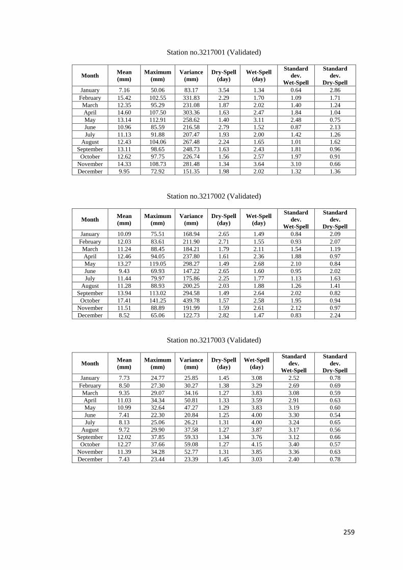
259
Station no.3217001 (Validated)
Month Mean
(mm)
Maximum
(mm)
Variance
(mm)
Dry-Spell
(day)
Wet-Spell
(day)
Standard
dev.
Wet-Spell
Standard
dev.
Dry-Spell
January 7.16 50.06 83.17 3.54 1.34 0.64 2.86
February 15.42 102.55 331.83 2.29 1.70 1.09 1.71
March 12.35 95.29 231.08 1.87 2.02 1.40 1.24
April 14.60 107.50 303.36 1.63 2.47 1.84 1.04
May 13.14 112.91 258.62 1.40 3.11 2.48 0.75
June 10.96 85.59 216.58 2.79 1.52 0.87 2.13
July 11.13 91.88 207.47 1.93 2.00 1.42 1.26
August 12.43 104.06 267.48 2.24 1.65 1.01 1.62
September 13.11 98.65 248.73 1.63 2.43 1.81 0.96
October 12.62 97.75 226.74 1.56 2.57 1.97 0.91
November 14.33 108.73 281.48 1.34 3.64 3.10 0.66
December 9.95 72.92 151.35 1.98 2.02 1.32 1.36
Station no.3217002 (Validated)
Month Mean
(mm)
Maximum
(mm)
Variance
(mm)
Dry-Spell
(day)
Wet-Spell
(day)
Standard
dev.
Wet-Spell
Standard
dev.
Dry-Spell
January 10.09 75.51 168.94 2.65 1.49 0.84 2.09
February 12.03 83.61 211.90 2.71 1.55 0.93 2.07
March 11.24 88.45 184.21 1.79 2.11 1.54 1.19
April 12.46 94.05 237.80 1.61 2.36 1.88 0.97
May 13.27 119.05 298.27 1.49 2.68 2.10 0.84
June 9.43 69.93 147.22 2.65 1.60 0.95 2.02
July 11.44 79.97 175.86 2.25 1.77 1.13 1.63
August 11.28 88.93 200.25 2.03 1.88 1.26 1.41
September 13.94 113.02 294.58 1.49 2.64 2.02 0.82
October 17.41 141.25 439.78 1.57 2.58 1.95 0.94
November 11.51 88.89 191.99 1.59 2.61 2.12 0.97
December 8.52 65.06 122.73 2.82 1.47 0.83 2.24
Station no.3217003 (Validated)
Month Mean
(mm)
Maximum
(mm)
Variance
(mm)
Dry-Spell
(day)
Wet-Spell
(day)
Standard
dev.
Wet-Spell
Standard
dev.
Dry-Spell
January 7.73 24.77 25.85 1.45 3.08 2.52 0.78
February 8.50 27.30 30.27 1.38 3.29 2.69 0.69
March 9.35 29.07 34.16 1.27 3.83 3.08 0.59
April 11.03 34.34 50.81 1.33 3.59 2.91 0.63
May 10.99 32.64 47.27 1.29 3.83 3.19 0.60
June 7.41 22.30 20.84 1.25 4.00 3.30 0.54
July 8.13 25.06 26.21 1.31 4.00 3.24 0.65
August 9.72 29.90 37.58 1.27 3.87 3.17 0.56
September 12.02 37.85 59.33 1.34 3.76 3.12 0.66
October 12.27 37.66 59.08 1.27 4.15 3.40 0.57
November 11.39 34.28 52.77 1.31 3.85 3.36 0.63
December 7.43 23.44 23.39 1.45 3.03 2.40 0.78
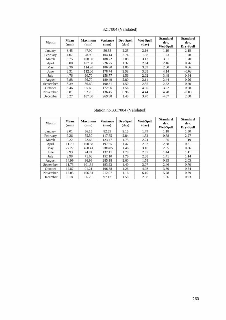
260
3217004 (Validated)
Month Mean
(mm)
Maximum
(mm)
Variance
(mm)
Dry-Spell
(day)
Wet-Spell
(day)
Standard
dev.
Wet-Spell
Standard
dev.
Dry-Spell
January 3.45 47.90 56.55 2.25 2.16 1.19 2.15
February 4.07 78.90 104.14 2.74 1.38 1.23 1.78
March 8.75 108.30 188.72 2.05 3.12 3.51 1.70
April 8.88 107.30 226.75 1.37 2.64 2.46 0.76
May 8.36 114.20 186.90 1.86 3.09 2.60 0.66
June 6.31 112.00 178.74 2.58 3.05 4.14 -0.03
July 4.76 90.70 158.77 1.56 2.02 3.48 0.84
August 6.88 96.70 180.49 2.80 2.11 2.44 0.26
September 8.39 86.60 190.31 1.50 2.35 2.52 0.50
October 8.46 95.60 172.96 1.56 4.30 3.92 0.08
November 8.81 92.70 136.45 0.96 4.44 4.78 -0.08
December 6.27 187.80 269.98 1.48 3.70 4.37 2.88
Station no.3317004 (Validated)
Month Mean
(mm)
Maximum
(mm)
Variance
(mm)
Dry-Spell
(day)
Wet-Spell
(day)
Standard
dev.
Wet-Spell
Standard
dev.
Dry-Spell
January 8.01 56.15 82.53 2.15 1.79 1.18 1.50
February 9.26 55.50 117.85 2.84 1.52 0.88 2.27
March 9.22 72.66 123.47 1.75 2.24 1.65 1.19
April 11.79 100.88 197.65 1.47 2.93 2.38 0.81
May 27.27 460.41 3388.85 1.46 3.16 2.55 0.86
June 9.93 74.74 132.11 1.78 2.07 1.44 1.11
July 9.98 71.66 152.10 1.76 2.08 1.41 1.14
August 14.99 96.93 285.18 2.60 1.58 0.95 2.03
September 11.73 101.34 193.93 1.40 3.07 2.46 0.70
October 12.87 91.21 196.58 1.26 4.08 3.39 0.54
November 12.05 106.81 212.07 1.16 6.10 5.28 0.39
December 8.18 66.23 97.12 1.58 2.58 1.86 0.93
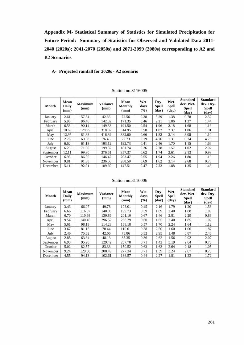
261
Appendix M- Statistical Summary of Statistics for Simulated Precipitation for
Future Period: Summary of Statistics for Observed and Validated Data 2011-
2040 (2020s); 2041-2070 (2050s) and 2071-2099 (2080s) corresponding to A2 and
B2 Scenarios
A- Projected rainfall for 2020s - A2 scenario
Station no.3116005
Month
Mean
Daily
(mm)
Maximum
(mm)
Variance
(mm)
Mean
Monthly
(mm)
Wet-
days
(%)
Dry-
Spell
(day)
Wet-
Spell
(day)
Standard
dev. Wet-
Spell
(day)
Standard
dev. Dry-
Spell
(day)
January 2.61 57.84 42.66 72.56 0.28 3.29 1.38 0.78 2.52
February 5.90 96.46 142.02 171.35 0.46 2.21 1.86 1.37 1.44
March 6.58 90.14 149.33 191.50 0.54 1.96 2.18 1.68 1.16
April 10.69 128.95 318.82 314.95 0.58 1.82 2.37 1.86 1.01
May 12.95 81.88 416.39 382.60 0.66 1.82 3.14 3.08 1.10
June 2.78 69.58 76.45 77.73 0.19 4.76 1.31 0.74 4.73
July 6.62 61.13 193.12 192.73 0.41 2.46 1.70 1.15 1.66
August 6.25 71.00 199.87 181.74 0.36 2.78 1.57 1.02 2.07
September 12.11 99.30 376.61 357.37 0.62 1.74 2.61 2.13 0.93
October 6.98 86.35 146.42 203.47 0.55 1.94 2.26 1.80 1.15
November 9.81 91.38 236.06 288.59 0.69 1.62 3.14 2.68 0.78
December 5.11 92.91 109.60 147.51 0.47 2.22 1.88 1.35 1.43
Station no.3116006
Month Mean
Daily
(mm)
Maximum
(mm) Variance
(mm)
Mean
Monthly
(mm)
Wet-
days
(%)
Dry-
Spell
(day)
Wet-
Spell
(day)
Standard
dev. Wet-
Spell
(day)
Standard
dev. Dry-
Spell
(day) January 3.43 66.07 49.78 103.01 0.45 2.16 1.79 1.20 1.58
February 6.66 116.07 140.06 199.73 0.59 1.69 2.40 1.88 1.09
March 6.70 110.98 130.89 201.10 0.67 1.46 2.81 2.29 0.83
April 9.54 140.45 296.52 286.29 0.60 1.65 2.40 1.85 1.02
May 5.61 98.19 114.28 168.18 0.57 1.70 2.24 1.64 1.12
June 3.67 81.15 70.44 110.01 0.38 2.50 1.60 1.00 1.87
July 2.46 75.62 42.66 73.86 0.32 2.95 1.48 0.87 2.46
August 2.85 63.34 48.13 85.35 0.36 2.62 1.56 0.92 2.07
September 6.93 95.20 129.42 207.78 0.71 1.42 3.19 2.64 0.78
October 5.02 82.57 83.33 150.52 0.63 1.63 2.64 2.18 1.05
November 9.24 129.38 208.49 277.34 0.71 1.39 3.24 2.67 0.73
December 4.55 94.13 102.61 136.57 0.44 2.27 1.81 1.23 1.72

262
Station no.3117070
Month Mean
Daily
(mm)
Maximum
(mm) Variance
(mm)
Mean
Monthly
(mm)
Wet-
days
(%)
Dry-
Spell
(day)
Wet-
Spell
(day)
Standard
dev. Wet-
Spell
(day)
Standard
dev. Dry-
Spell
(day) January 4.65 101.34 99.03 139.40 0.47 2.08 1.84 1.23 1.56
February 7.24 150.75 268.72 217.07 0.45 2.17 1.82 1.23 1.61
March 6.43 103.49 138.47 192.89 0.55 1.79 2.18 1.62 1.18
April 12.32 173.32 392.70 369.45 0.61 1.62 2.49 1.94 0.98
May 11.38 173.69 353.36 341.53 0.60 1.67 2.43 1.93 1.05
June 6.77 142.48 220.18 202.97 0.40 2.37 1.63 1.00 1.79
July 4.19 95.29 95.80 125.68 0.41 2.30 1.67 1.05 1.76
August 5.31 121.03 151.43 159.42 0.38 2.50 1.57 0.95 1.94
September 11.38 152.52 368.45 341.30 0.56 1.78 2.20 1.66 1.17
October 10.87 166.94 334.63 326.07 0.58 1.68 2.27 1.66 1.05
November 4.26 101.50 80.16 127.81 0.54 1.87 2.14 1.60 1.32
December 3.00 106.71 78.70 89.88 0.30 3.22 1.44 0.82 2.80
Station no.3118069
Month
Mean
Daily
(mm)
Maximum
(mm)
Variance
(mm)
Mean
Monthly
(mm)
Wet-
days
(%)
Dry-
Spell
(day)
Wet-
Spell
(day)
Standard
dev. Wet-
Spell
(day)
Standard
dev. Dry-
Spell
(day)
January 4.98 42.14 33.18 149.54 0.72 1.43 3.39 2.93 0.80
February 5.75 57.38 59.36 172.49 0.67 1.52 2.96 2.55 0.90
March 6.79 61.96 71.35 203.69 0.72 1.38 3.27 2.71 0.73
April 6.05 56.79 56.26 181.59 0.72 1.39 3.36 2.95 0.74
May 5.96 61.27 58.68 178.77 0.70 1.46 3.22 2.72 0.86
June 3.56 37.31 23.35 106.94 0.62 1.59 2.53 1.97 0.96
July 4.02 52.90 40.78 120.48 0.63 1.58 2.55 1.98 0.96
August 4.56 56.24 50.95 136.93 0.57 1.77 2.33 1.85 1.20
September 6.38 65.65 79.45 191.30 0.72 1.41 3.40 2.92 0.76
October 7.44 79.17 94.69 223.30 0.76 1.32 3.82 3.34 0.64
November 6.98 88.19 101.32 209.38 0.70 1.45 3.22 2.73 0.81
December 4.68 46.00 33.66 140.44 0.72 1.41 3.48 3.03 0.80
Station no.3216001
Month Mean
Daily
(mm)
Maximum
(mm) Variance
(mm)
Mean
Monthly
(mm)
Wet-
days
(%)
Dry-
Spell
(day)
Wet-
Spell
(day)
Standard
dev. Wet-
Spell
(day)
Standard
dev. Dry-
Spell
(day) January 2.41 66.62 42.46 72.35 0.30 3.08 1.41 0.74 2.50
February 5.70 104.04 141.82 171.14 0.48 2.00 1.89 1.33 1.42
March 6.38 109.11 149.13 191.29 0.56 1.75 2.21 1.64 1.14
April 10.49 159.24 318.62 314.74 0.60 1.61 2.40 1.82 0.99
May 12.75 168.24 416.19 382.39 0.68 1.61 3.17 3.04 1.08
June 2.58 103.13 76.25 77.52 0.21 4.55 1.34 0.70 4.71
July 6.42 126.68 192.92 192.52 0.43 2.25 1.73 1.11 1.64
August 6.05 138.68 199.67 181.53 0.38 2.57 1.60 0.98 2.05
September 11.91 172.79 376.41 357.16 0.64 1.53 2.64 2.09 0.91
October 6.78 106.14 146.22 203.26 0.57 1.73 2.29 1.76 1.13
November 9.61 144.99 235.86 288.38 0.71 1.41 3.17 2.64 0.76
December 4.91 104.26 109.40 147.30 0.49 2.01 1.91 1.31 1.41
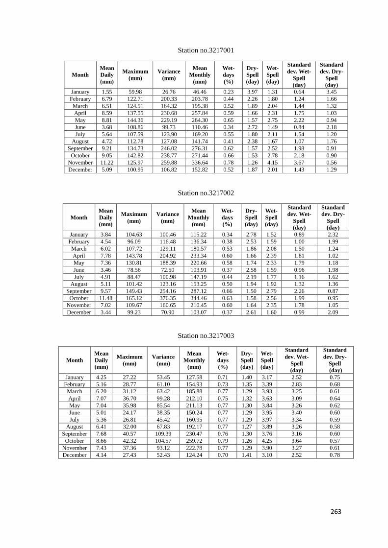
263
Station no.3217001
Month Mean
Daily
(mm)
Maximum
(mm) Variance
(mm)
Mean
Monthly
(mm)
Wet-
days
(%)
Dry-
Spell
(day)
Wet-
Spell
(day)
Standard
dev. Wet-
Spell
(day)
Standard
dev. Dry-
Spell
(day) January 1.55 59.98 26.76 46.46 0.23 3.97 1.31 0.64 3.45
February 6.79 122.71 200.33 203.78 0.44 2.26 1.80 1.24 1.66
March 6.51 124.51 164.32 195.38 0.52 1.89 2.04 1.44 1.32
April 8.59 137.55 230.68 257.84 0.59 1.66 2.31 1.75 1.03
May 8.81 144.36 229.19 264.30 0.65 1.57 2.75 2.22 0.94
June 3.68 108.86 99.73 110.46 0.34 2.72 1.49 0.84 2.18
July 5.64 107.59 123.90 169.20 0.55 1.80 2.11 1.54 1.20
August 4.72 112.78 127.08 141.74 0.41 2.38 1.67 1.07 1.76
September 9.21 134.73 246.02 276.31 0.62 1.57 2.52 1.98 0.91
October 9.05 142.82 238.77 271.44 0.66 1.53 2.78 2.18 0.90
November 11.22 125.97 259.88 336.64 0.78 1.26 4.15 3.67 0.56
December 5.09 100.95 106.82 152.82 0.52 1.87 2.01 1.43 1.29
Station no.3217002
Month Mean
Daily
(mm)
Maximum
(mm) Variance
(mm)
Mean
Monthly
(mm)
Wet-
days
(%)
Dry-
Spell
(day)
Wet-
Spell
(day)
Standard
dev. Wet-
Spell
(day)
Standard
dev. Dry-
Spell
(day) January 3.84 104.63 100.46 115.22 0.34 2.78 1.52 0.89 2.32
February 4.54 96.09 116.48 136.34 0.38 2.53 1.59 1.00 1.99
March 6.02 107.72 129.11 180.57 0.53 1.86 2.08 1.50 1.24
April 7.78 143.78 204.92 233.34 0.60 1.66 2.39 1.81 1.02
May 7.36 130.81 188.39 220.66 0.58 1.74 2.33 1.79 1.18
June 3.46 78.56 72.50 103.91 0.37 2.58 1.59 0.96 1.98
July 4.91 88.47 100.98 147.19 0.44 2.19 1.77 1.16 1.62
August 5.11 101.42 123.16 153.25 0.50 1.94 1.92 1.32 1.36
September 9.57 149.43 254.16 287.12 0.66 1.50 2.79 2.26 0.87
October 11.48 165.12 376.35 344.46 0.63 1.58 2.56 1.99 0.95
November 7.02 109.67 160.65 210.45 0.60 1.64 2.35 1.78 1.05
December 3.44 99.23 70.90 103.07 0.37 2.61 1.60 0.99 2.09
Station no.3217003
Month Mean
Daily
(mm)
Maximum
(mm) Variance
(mm)
Mean
Monthly
(mm)
Wet-
days
(%)
Dry-
Spell
(day)
Wet-
Spell
(day)
Standard
dev. Wet-
Spell
(day)
Standard
dev. Dry-
Spell
(day) January 4.25 27.22 53.45 127.58 0.71 1.40 3.17 2.52 0.75
February 5.16 28.77 61.10 154.93 0.73 1.35 3.39 2.83 0.68
March 6.20 31.12 63.42 185.88 0.77 1.29 3.93 3.25 0.61
April 7.07 36.70 99.28 212.10 0.75 1.32 3.63 3.09 0.64
May 7.04 35.98 85.54 211.13 0.77 1.30 3.84 3.26 0.62
June 5.01 24.17 38.35 150.24 0.77 1.29 3.95 3.40 0.60
July 5.36 26.81 45.42 160.95 0.77 1.29 3.97 3.34 0.59
August 6.41 32.00 67.83 192.17 0.77 1.27 3.89 3.26 0.58
September 7.68 40.57 109.39 230.47 0.76 1.30 3.76 3.16 0.60
October 8.66 42.32 104.57 259.72 0.79 1.26 4.25 3.64 0.57
November 7.43 37.36 93.12 222.78 0.77 1.29 3.90 3.27 0.61
December 4.14 27.43 52.43 124.24 0.70 1.41 3.10 2.52 0.78
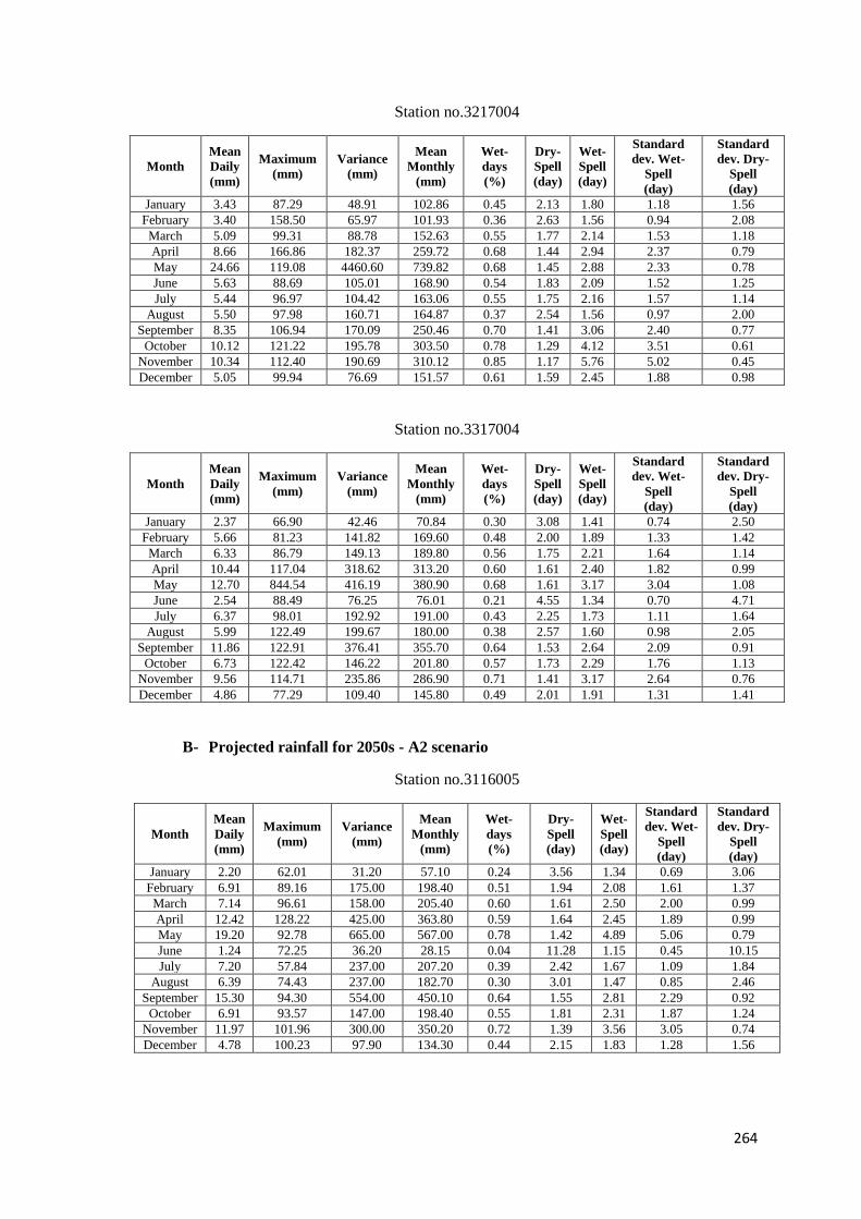
264
Station no.3217004
Month Mean
Daily
(mm)
Maximum
(mm) Variance
(mm)
Mean
Monthly
(mm)
Wet-
days
(%)
Dry-
Spell
(day)
Wet-
Spell
(day)
Standard
dev. Wet-
Spell
(day)
Standard
dev. Dry-
Spell
(day) January 3.43 87.29 48.91 102.86 0.45 2.13 1.80 1.18 1.56
February 3.40 158.50 65.97 101.93 0.36 2.63 1.56 0.94 2.08
March 5.09 99.31 88.78 152.63 0.55 1.77 2.14 1.53 1.18
April 8.66 166.86 182.37 259.72 0.68 1.44 2.94 2.37 0.79
May 24.66 119.08 4460.60 739.82 0.68 1.45 2.88 2.33 0.78
June 5.63 88.69 105.01 168.90 0.54 1.83 2.09 1.52 1.25
July 5.44 96.97 104.42 163.06 0.55 1.75 2.16 1.57 1.14
August 5.50 97.98 160.71 164.87 0.37 2.54 1.56 0.97 2.00
September 8.35 106.94 170.09 250.46 0.70 1.41 3.06 2.40 0.77
October 10.12 121.22 195.78 303.50 0.78 1.29 4.12 3.51 0.61
November 10.34 112.40 190.69 310.12 0.85 1.17 5.76 5.02 0.45
December 5.05 99.94 76.69 151.57 0.61 1.59 2.45 1.88 0.98
Station no.3317004
Month
Mean
Daily
(mm)
Maximum
(mm)
Variance
(mm)
Mean
Monthly
(mm)
Wet-
days
(%)
Dry-
Spell
(day)
Wet-
Spell
(day)
Standard
dev. Wet-
Spell
(day)
Standard
dev. Dry-
Spell
(day)
January 2.37 66.90 42.46 70.84 0.30 3.08 1.41 0.74 2.50
February 5.66 81.23 141.82 169.60 0.48 2.00 1.89 1.33 1.42
March 6.33 86.79 149.13 189.80 0.56 1.75 2.21 1.64 1.14
April 10.44 117.04 318.62 313.20 0.60 1.61 2.40 1.82 0.99
May 12.70 844.54 416.19 380.90 0.68 1.61 3.17 3.04 1.08
June 2.54 88.49 76.25 76.01 0.21 4.55 1.34 0.70 4.71
July 6.37 98.01 192.92 191.00 0.43 2.25 1.73 1.11 1.64
August 5.99 122.49 199.67 180.00 0.38 2.57 1.60 0.98 2.05
September 11.86 122.91 376.41 355.70 0.64 1.53 2.64 2.09 0.91
October 6.73 122.42 146.22 201.80 0.57 1.73 2.29 1.76 1.13
November 9.56 114.71 235.86 286.90 0.71 1.41 3.17 2.64 0.76
December 4.86 77.29 109.40 145.80 0.49 2.01 1.91 1.31 1.41
B- Projected rainfall for 2050s - A2 scenario
Station no.3116005
Month Mean
Daily
(mm)
Maximum
(mm) Variance
(mm)
Mean
Monthly
(mm)
Wet-
days
(%)
Dry-
Spell
(day)
Wet-
Spell
(day)
Standard
dev. Wet-
Spell
(day)
Standard
dev. Dry-
Spell
(day) January 2.20 62.01 31.20 57.10 0.24 3.56 1.34 0.69 3.06
February 6.91 89.16 175.00 198.40 0.51 1.94 2.08 1.61 1.37
March 7.14 96.61 158.00 205.40 0.60 1.61 2.50 2.00 0.99
April 12.42 128.22 425.00 363.80 0.59 1.64 2.45 1.89 0.99
May 19.20 92.78 665.00 567.00 0.78 1.42 4.89 5.06 0.79
June 1.24 72.25 36.20 28.15 0.04 11.28 1.15 0.45 10.15
July 7.20 57.84 237.00 207.20 0.39 2.42 1.67 1.09 1.84
August 6.39 74.43 237.00 182.70 0.30 3.01 1.47 0.85 2.46
September 15.30 94.30 554.00 450.10 0.64 1.55 2.81 2.29 0.92
October 6.91 93.57 147.00 198.40 0.55 1.81 2.31 1.87 1.24
November 11.97 101.96 300.00 350.20 0.72 1.39 3.56 3.05 0.74
December 4.78 100.23 97.90 134.30 0.44 2.15 1.83 1.28 1.56
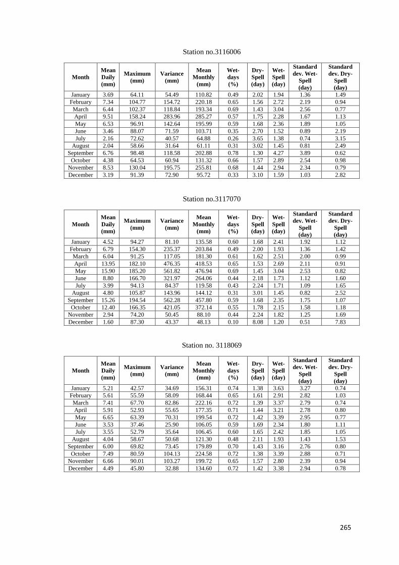
265
Station no.3116006
Month Mean
Daily
(mm)
Maximum
(mm) Variance
(mm)
Mean
Monthly
(mm)
Wet-
days
(%)
Dry-
Spell
(day)
Wet-
Spell
(day)
Standard
dev. Wet-
Spell
(day)
Standard
dev. Dry-
Spell
(day) January 3.69 64.11 54.49 110.82 0.49 2.02 1.94 1.36 1.49
February 7.34 104.77 154.72 220.18 0.65 1.56 2.72 2.19 0.94
March 6.44 102.37 118.84 193.34 0.69 1.43 3.04 2.56 0.77
April 9.51 158.24 283.96 285.27 0.57 1.75 2.28 1.67 1.13
May 6.53 96.91 142.64 195.99 0.59 1.68 2.36 1.89 1.05
June 3.46 88.07 71.59 103.71 0.35 2.70 1.52 0.89 2.19
July 2.16 72.62 40.57 64.88 0.26 3.65 1.38 0.74 3.15
August 2.04 58.66 31.64 61.11 0.31 3.02 1.45 0.81 2.49
September 6.76 98.48 118.58 202.88 0.78 1.30 4.27 3.89 0.62
October 4.38 64.53 60.94 131.32 0.66 1.57 2.89 2.54 0.98
November 8.53 130.04 195.75 255.81 0.68 1.44 2.94 2.34 0.79
December 3.19 91.39 72.90 95.72 0.33 3.10 1.59 1.03 2.82
Station no.3117070
Month Mean
Daily
(mm)
Maximum
(mm) Variance
(mm)
Mean
Monthly
(mm)
Wet-
days
(%)
Dry-
Spell
(day)
Wet-
Spell
(day)
Standard
dev. Wet-
Spell
(day)
Standard
dev. Dry-
Spell
(day) January 4.52 94.27 81.10 135.58 0.60 1.68 2.41 1.92 1.12
February 6.79 154.30 235.37 203.84 0.49 2.00 1.93 1.36 1.42
March 6.04 91.25 117.05 181.30 0.61 1.62 2.51 2.00 0.99
April 13.95 182.10 476.35 418.53 0.65 1.53 2.69 2.11 0.91
May 15.90 185.20 561.82 476.94 0.69 1.45 3.04 2.53 0.82
June 8.80 166.70 321.97 264.06 0.44 2.18 1.73 1.12 1.60
July 3.99 94.13 84.37 119.58 0.43 2.24 1.71 1.09 1.65
August 4.80 105.87 143.96 144.12 0.31 3.01 1.45 0.82 2.52
September 15.26 194.54 562.28 457.80 0.59 1.68 2.35 1.75 1.07
October 12.40 166.35 421.05 372.14 0.55 1.78 2.15 1.58 1.18
November 2.94 74.20 50.45 88.10 0.44 2.24 1.82 1.25 1.69
December 1.60 87.30 43.37 48.13 0.10 8.08 1.20 0.51 7.83
Station no. 3118069
Month Mean
Daily
(mm)
Maximum
(mm) Variance
(mm)
Mean
Monthly
(mm)
Wet-
days
(%)
Dry-
Spell
(day)
Wet-
Spell
(day)
Standard
dev. Wet-
Spell
(day)
Standard
dev. Dry-
Spell
(day) January 5.21 42.57 34.69 156.31 0.74 1.38 3.63 3.27 0.74
February 5.61 55.59 58.09 168.44 0.65 1.61 2.91 2.82 1.03
March 7.41 67.70 82.86 222.16 0.72 1.39 3.37 2.79 0.74
April 5.91 52.93 55.65 177.35 0.71 1.44 3.21 2.78 0.80
May 6.65 63.39 70.31 199.54 0.72 1.42 3.39 2.95 0.77
June 3.53 37.46 25.90 106.05 0.59 1.69 2.34 1.80 1.11
July 3.55 52.79 35.64 106.45 0.60 1.65 2.42 1.85 1.05
August 4.04 58.67 50.68 121.30 0.48 2.11 1.93 1.43 1.53
September 6.00 69.82 73.45 179.89 0.70 1.43 3.16 2.76 0.80
October 7.49 80.59 104.13 224.58 0.72 1.38 3.39 2.88 0.71
November 6.66 90.01 103.27 199.72 0.65 1.57 2.80 2.39 0.94
December 4.49 45.80 32.88 134.60 0.72 1.42 3.38 2.94 0.78
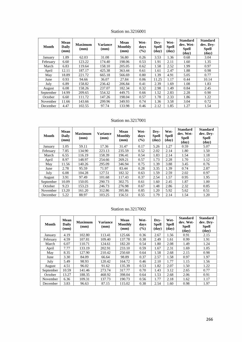
266
Station no.3216001
Month Mean
Daily
(mm)
Maximum
(mm) Variance
(mm)
Mean
Monthly
(mm)
Wet-
days
(%)
Dry-
Spell
(day)
Wet-
Spell
(day)
Standard
dev. Wet-
Spell
(day)
Standard
dev. Dry-
Spell
(day) January 1.89 62.03 31.08 56.80 0.26 3.53 1.36 0.68 3.04
February 6.60 123.22 174.40 198.06 0.53 1.91 2.11 1.60 1.35
March 6.83 119.64 158.10 205.05 0.62 1.58 2.52 1.99 0.97
April 12.11 187.17 425.38 363.44 0.61 1.61 2.47 1.88 0.98
May 18.89 221.72 665.18 566.69 0.80 1.39 4.91 5.05 0.77
June 0.93 94.66 36.07 27.84 0.06 11.25 1.17 0.44 10.14
July 6.89 158.82 236.42 206.84 0.41 2.39 1.69 1.08 1.83
August 6.08 158.26 237.07 182.34 0.32 2.98 1.49 0.84 2.45
September 14.99 209.65 554.32 449.75 0.66 1.52 2.83 2.28 0.90
October 6.60 111.72 147.26 198.04 0.57 1.78 2.33 1.86 1.22
November 11.66 143.66 299.96 349.93 0.74 1.36 3.58 3.04 0.72
December 4.47 102.55 97.74 133.98 0.46 2.12 1.85 1.27 1.54
Station no.3217001
Month Mean
Daily
(mm)
Maximum
(mm) Variance
(mm)
Mean
Monthly
(mm)
Wet-
days
(%)
Dry-
Spell
(day)
Wet-
Spell
(day)
Standard
dev. Wet-
Spell
(day)
Standard
dev. Dry-
Spell
(day) January 1.05 59.11 17.36 31.47 0.17 5.26 1.27 0.59 5.07
February 7.85 134.90 223.13 235.59 0.52 2.02 2.14 1.80 1.50
March 6.55 116.19 158.39 196.41 0.54 1.83 2.14 1.54 1.18
April 8.97 148.97 254.66 269.21 0.57 1.73 2.28 1.70 1.12
May 11.56 140.26 295.09 346.94 0.75 1.39 3.88 3.45 0.76
June 2.78 95.59 71.97 83.44 0.28 3.35 1.39 0.74 2.87
July 6.08 104.28 127.51 182.32 0.63 1.59 2.59 2.02 0.97
August 3.91 97.49 101.68 117.43 0.37 2.54 1.57 0.95 1.95
September 10.09 150.05 290.73 302.75 0.61 1.60 2.45 1.87 1.00
October 9.23 153.23 246.73 276.98 0.67 1.48 2.86 2.32 0.85
November 13.20 161.20 312.86 395.86 0.85 1.20 5.92 5.62 0.51
December 5.22 88.97 103.25 156.51 0.55 1.79 2.14 1.54 1.20
Station no.3217002
Month Mean
Daily
(mm)
Maximum
(mm) Variance
(mm)
Mean
Monthly
(mm)
Wet-
days
(%)
Dry-
Spell
(day)
Wet-
Spell
(day)
Standard
dev. Wet-
Spell
(day)
Standard
dev. Dry-
Spell
(day) January 4.19 102.80 113.41 125.66 0.36 2.67 1.56 0.91 2.15
February 4.59 107.81 109.40 137.78 0.38 2.49 1.61 0.99 1.91
March 6.07 110.71 124.61 182.20 0.54 1.80 2.08 1.49 1.24
April 7.77 133.19 202.91 233.10 0.59 1.67 2.31 1.69 1.05
May 8.35 127.90 210.42 250.60 0.64 1.58 2.68 2.15 0.98
June 3.30 84.09 66.64 98.89 0.37 2.57 1.58 0.97 1.97
July 5.49 98.93 120.42 164.72 0.46 2.10 1.77 1.15 1.56
August 4.51 96.02 91.62 135.39 0.53 1.82 2.07 1.50 1.22
September 10.59 141.46 273.74 317.77 0.70 1.43 3.12 2.65 0.77
October 13.27 188.35 468.92 398.04 0.64 1.53 2.68 2.06 0.91
November 6.36 109.31 137.73 190.73 0.56 1.77 2.18 1.62 1.17
December 3.83 96.63 87.15 115.02 0.38 2.54 1.60 0.98 1.97
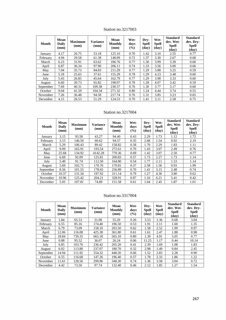
267
Station no.3217003
Month Mean
Daily
(mm)
Maximum
(mm) Variance
(mm)
Mean
Monthly
(mm)
Wet-
days
(%)
Dry-
Spell
(day)
Wet-
Spell
(day)
Standard
dev. Wet-
Spell
(day)
Standard
dev. Dry-
Spell
(day) January 4.17 26.75 53.18 125.10 0.70 1.42 3.10 2.55 0.77
February 4.94 29.58 61.38 148.09 0.72 1.37 3.30 2.67 0.68
March 6.23 31.91 63.62 186.76 0.77 1.30 3.99 3.39 0.60
April 6.87 36.34 97.90 206.11 0.74 1.33 3.56 3.00 0.66
May 7.04 35.73 84.83 211.29 0.77 1.29 3.88 3.25 0.59
June 5.18 25.65 37.61 155.29 0.78 1.29 4.23 3.48 0.60
July 5.43 26.85 45.64 162.79 0.77 1.29 3.98 3.33 0.60
August 6.60 30.73 65.82 198.07 0.78 1.28 4.07 3.42 0.59
September 7.69 40.31 109.38 230.57 0.76 1.30 3.77 3.17 0.60
October 9.04 41.59 104.34 271.32 0.80 1.24 4.44 3.74 0.55
November 7.26 36.48 94.58 217.74 0.76 1.31 3.85 3.23 0.65
December 4.15 26.53 51.29 124.53 0.70 1.41 3.11 2.58 0.75
Station no.3217004
Month Mean
Daily
(mm)
Maximum
(mm) Variance
(mm)
Mean
Monthly
(mm)
Wet-
days
(%)
Dry-
Spell
(day)
Wet-
Spell
(day)
Standard
dev. Wet-
Spell
(day)
Standard
dev. Dry-
Spell
(day) January 3.15 93.58 43.27 94.40 0.43 2.29 1.73 1.12 1.72
February 3.15 146.50 60.62 94.57 0.35 2.68 1.54 0.92 2.19
March 5.29 106.43 89.42 158.82 0.58 1.70 2.29 1.83 1.11
April 9.09 165.91 193.54 272.61 0.70 1.43 3.07 2.49 0.76
May 25.68 134.92 4142.28 770.36 0.69 1.42 3.07 2.50 0.77
June 6.69 92.09 125.81 200.83 0.57 1.73 2.27 1.73 1.14
July 5.49 91.74 112.50 164.80 0.54 1.77 2.11 1.53 1.14
August 5.69 102.71 170.76 170.81 0.37 2.58 1.56 0.93 1.99
September 8.56 101.55 178.65 256.89 0.70 1.41 3.15 2.48 0.74
October 10.37 131.34 197.92 311.14 0.79 1.27 4.36 3.80 0.62
November 10.96 125.42 204.21 328.91 0.87 1.16 6.21 5.41 0.42
December 5.05 107.81 74.89 151.58 0.61 1.64 2.45 1.87 1.01
Station no.3317004
Month Mean
Daily
(mm)
Maximum
(mm) Variance
(mm)
Mean
Monthly
(mm)
Wet-
days
(%)
Dry-
Spell
(day)
Wet-
Spell
(day)
Standard
dev. Wet-
Spell
(day)
Standard
dev. Dry-
Spell
(day) January 1.84 65.53 31.08 55.20 0.26 3.53 1.36 0.68 3.04
February 6.55 85.16 174.40 196.50 0.53 1.91 2.11 1.60 1.35
March 6.79 73.09 158.10 203.50 0.62 1.58 2.52 1.99 0.97
April 12.06 116.08 425.38 361.80 0.61 1.61 2.47 1.88 0.98
May 18.84 739.35 665.18 565.10 0.80 1.39 4.91 5.05 0.77
June 0.88 95.52 36.07 26.24 0.06 11.25 1.17 0.44 10.14
July 6.85 103.76 236.42 205.20 0.41 2.39 1.69 1.08 1.83
August 6.02 113.80 237.07 180.70 0.32 2.98 1.49 0.84 2.45
September 14.94 111.92 554.32 448.20 0.66 1.52 2.83 2.28 0.90
October 6.55 116.68 147.26 196.40 0.57 1.78 2.33 1.86 1.22
November 11.61 128.56 299.96 348.30 0.74 1.36 3.58 3.04 0.72
December 4.42 73.50 97.74 132.40 0.46 2.12 1.85 1.27 1.54
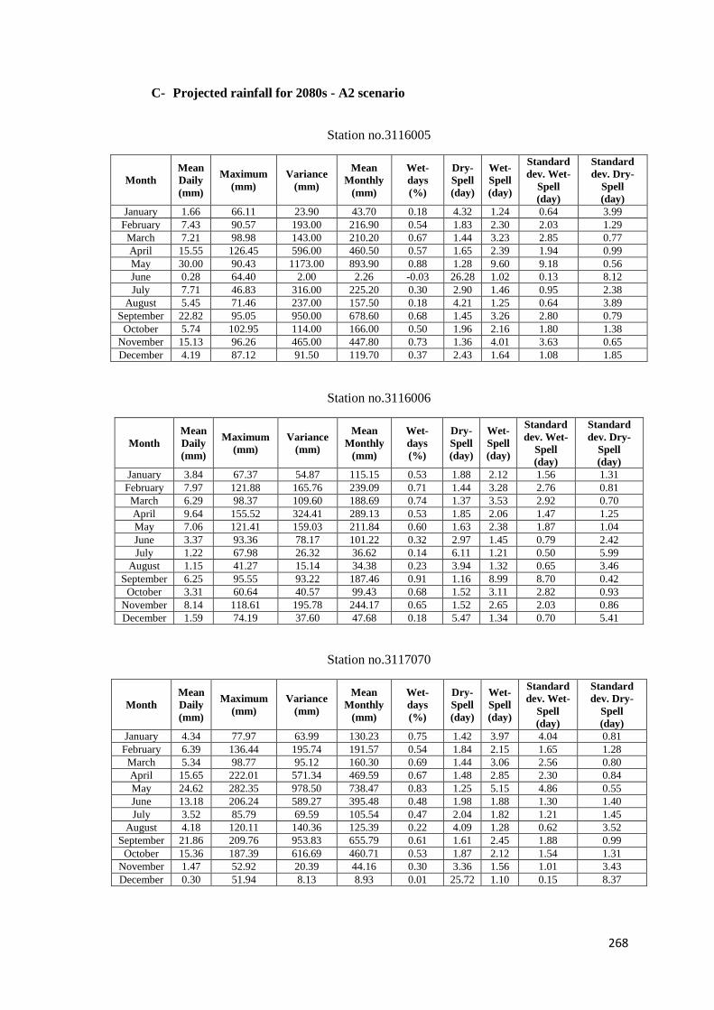
268
C- Projected rainfall for 2080s - A2 scenario
Station no.3116005
Month Mean
Daily
(mm)
Maximum
(mm) Variance
(mm)
Mean
Monthly
(mm)
Wet-
days
(%)
Dry-
Spell
(day)
Wet-
Spell
(day)
Standard
dev. Wet-
Spell
(day)
Standard
dev. Dry-
Spell
(day) January 1.66 66.11 23.90 43.70 0.18 4.32 1.24 0.64 3.99
February 7.43 90.57 193.00 216.90 0.54 1.83 2.30 2.03 1.29
March 7.21 98.98 143.00 210.20 0.67 1.44 3.23 2.85 0.77
April 15.55 126.45 596.00 460.50 0.57 1.65 2.39 1.94 0.99
May 30.00 90.43 1173.00 893.90 0.88 1.28 9.60 9.18 0.56
June 0.28 64.40 2.00 2.26 -0.03 26.28 1.02 0.13 8.12
July 7.71 46.83 316.00 225.20 0.30 2.90 1.46 0.95 2.38
August 5.45 71.46 237.00 157.50 0.18 4.21 1.25 0.64 3.89
September 22.82 95.05 950.00 678.60 0.68 1.45 3.26 2.80 0.79
October 5.74 102.95 114.00 166.00 0.50 1.96 2.16 1.80 1.38
November 15.13 96.26 465.00 447.80 0.73 1.36 4.01 3.63 0.65
December 4.19 87.12 91.50 119.70 0.37 2.43 1.64 1.08 1.85
Station no.3116006
Month Mean
Daily
(mm)
Maximum
(mm) Variance
(mm)
Mean
Monthly
(mm)
Wet-
days
(%)
Dry-
Spell
(day)
Wet-
Spell
(day)
Standard
dev. Wet-
Spell
(day)
Standard
dev. Dry-
Spell
(day) January 3.84 67.37 54.87 115.15 0.53 1.88 2.12 1.56 1.31
February 7.97 121.88 165.76 239.09 0.71 1.44 3.28 2.76 0.81
March 6.29 98.37 109.60 188.69 0.74 1.37 3.53 2.92 0.70
April 9.64 155.52 324.41 289.13 0.53 1.85 2.06 1.47 1.25
May 7.06 121.41 159.03 211.84 0.60 1.63 2.38 1.87 1.04
June 3.37 93.36 78.17 101.22 0.32 2.97 1.45 0.79 2.42
July 1.22 67.98 26.32 36.62 0.14 6.11 1.21 0.50 5.99
August 1.15 41.27 15.14 34.38 0.23 3.94 1.32 0.65 3.46
September 6.25 95.55 93.22 187.46 0.91 1.16 8.99 8.70 0.42
October 3.31 60.64 40.57 99.43 0.68 1.52 3.11 2.82 0.93
November 8.14 118.61 195.78 244.17 0.65 1.52 2.65 2.03 0.86
December 1.59 74.19 37.60 47.68 0.18 5.47 1.34 0.70 5.41
Station no.3117070
Month Mean
Daily
(mm)
Maximum
(mm) Variance
(mm)
Mean
Monthly
(mm)
Wet-
days
(%)
Dry-
Spell
(day)
Wet-
Spell
(day)
Standard
dev. Wet-
Spell
(day)
Standard
dev. Dry-
Spell
(day) January 4.34 77.97 63.99 130.23 0.75 1.42 3.97 4.04 0.81
February 6.39 136.44 195.74 191.57 0.54 1.84 2.15 1.65 1.28
March 5.34 98.77 95.12 160.30 0.69 1.44 3.06 2.56 0.80
April 15.65 222.01 571.34 469.59 0.67 1.48 2.85 2.30 0.84
May 24.62 282.35 978.50 738.47 0.83 1.25 5.15 4.86 0.55
June 13.18 206.24 589.27 395.48 0.48 1.98 1.88 1.30 1.40
July 3.52 85.79 69.59 105.54 0.47 2.04 1.82 1.21 1.45
August 4.18 120.11 140.36 125.39 0.22 4.09 1.28 0.62 3.52
September 21.86 209.76 953.83 655.79 0.61 1.61 2.45 1.88 0.99
October 15.36 187.39 616.69 460.71 0.53 1.87 2.12 1.54 1.31
November 1.47 52.92 20.39 44.16 0.30 3.36 1.56 1.01 3.43
December 0.30 51.94 8.13 8.93 0.01 25.72 1.10 0.15 8.37

269
Station no.3118069
Month Mean
Daily
(mm)
Maximum
(mm) Variance
(mm)
Mean
Monthly
(mm)
Wet-
days
(%)
Dry-
Spell
(day)
Wet-
Spell
(day)
Standard
dev. Wet-
Spell
(day)
Standard
dev. Dry-
Spell
(day) January 5.41 45.19 38.53 162.29 0.73 1.40 3.51 2.93 0.75
February 5.53 59.60 59.78 165.89 0.63 1.75 2.89 3.18 1.22
March 7.83 69.46 96.27 234.76 0.69 1.46 3.12 2.58 0.82
April 5.38 52.12 53.84 161.38 0.64 1.58 2.72 2.19 0.99
May 7.25 62.05 79.29 217.60 0.73 1.39 3.44 3.01 0.74
June 3.14 37.81 22.38 94.18 0.54 1.86 2.14 1.60 1.26
July 2.66 46.34 24.27 79.77 0.56 1.79 2.19 1.62 1.17
August 3.26 55.72 46.16 97.72 0.35 2.88 1.65 1.21 2.59
September 5.31 75.79 74.31 159.33 0.61 1.68 2.56 2.16 1.10
October 7.43 81.20 114.66 222.87 0.66 1.51 2.86 2.31 0.88
November 6.42 83.93 111.54 192.68 0.57 1.81 2.34 1.88 1.28
December 3.99 43.88 29.56 119.76 0.66 1.53 2.90 2.42 0.91
Station no.3216001
Month Mean
Daily
(mm)
Maximum
(mm) Variance
(mm)
Mean
Monthly
(mm)
Wet-
days
(%)
Dry-
Spell
(day)
Wet-
Spell
(day)
Standard
dev. Wet-
Spell
(day)
Standard
dev. Dry-
Spell
(day) January 1.45 56.78 23.65 43.52 0.22 4.27 1.30 0.62 3.98
February 7.22 139.24 193.06 216.65 0.58 1.78 2.36 2.01 1.27
March 7.00 106.38 142.81 210.02 0.71 1.39 3.29 2.83 0.75
April 15.34 199.23 595.69 460.26 0.61 1.60 2.45 1.92 0.97
May 29.79 277.06 1172.79 893.68 0.92 1.23 9.66 9.16 0.54
June 0.07 25.18 1.77 2.05 0.01 26.23 1.08 0.11 8.10
July 7.50 173.20 315.29 224.97 0.34 2.85 1.52 0.93 2.36
August 5.24 146.53 237.00 157.28 0.22 4.16 1.31 0.62 3.87
September 22.61 240.73 950.18 678.35 0.72 1.40 3.32 2.78 0.77
October 5.53 98.02 113.67 165.75 0.54 1.91 2.22 1.78 1.36
November 14.92 189.50 464.94 447.63 0.77 1.31 4.07 3.61 0.63
December 3.98 96.99 91.26 119.50 0.41 2.38 1.70 1.06 1.83
Station no.3217001
Month Mean
Daily
(mm)
Maximum
(mm) Variance
(mm)
Mean
Monthly
(mm)
Wet-
days
(%)
Dry-
Spell
(day)
Wet-
Spell
(day)
Standard
dev. Wet-
Spell
(day)
Standard
dev. Dry-
Spell
(day) January 0.56 36.71 7.55 16.75 0.11 7.55 1.21 0.49 7.13
February 10.06 139.02 260.42 301.72 0.65 1.68 2.99 3.05 1.14
March 6.99 117.25 167.94 209.74 0.58 1.68 2.33 1.74 1.06
April 9.51 152.30 289.49 285.31 0.55 1.79 2.15 1.56 1.22
May 16.35 169.64 454.05 490.48 0.87 1.23 6.78 6.75 0.52
June 1.96 98.63 53.71 58.81 0.20 4.51 1.27 0.60 4.15
July 6.27 87.24 103.29 187.96 0.76 1.34 3.81 3.36 0.69
August 3.18 87.35 73.38 95.33 0.35 2.69 1.52 0.89 2.09
September 11.49 162.32 360.47 344.81 0.61 1.61 2.42 1.88 0.97
October 9.60 167.96 303.27 287.93 0.68 1.45 2.94 2.35 0.78
November 15.73 158.45 368.80 471.84 0.93 1.15 10.89 9.24 0.40
December 5.54 99.81 112.51 166.14 0.59 1.66 2.35 1.76 1.07

270
Station no.3217002
Month Mean
Daily
(mm)
Maximum
(mm) Variance
(mm)
Mean
Monthly
(mm)
Wet-
days
(%)
Dry-
Spell
(day)
Wet-
Spell
(day)
Standard
dev. Wet-
Spell
(day)
Standard
dev. Dry-
Spell
(day) January 4.53 115.50 115.88 136.05 0.38 2.55 1.61 1.01 2.05
February 4.68 100.92 117.17 140.26 0.38 2.50 1.60 0.98 1.95
March 6.32 107.72 135.03 189.61 0.55 1.78 2.13 1.51 1.18
April 7.81 126.83 207.71 234.24 0.57 1.71 2.21 1.62 1.12
May 9.72 150.56 237.37 291.56 0.72 1.45 3.40 3.04 0.82
June 3.29 82.15 64.11 98.60 0.39 2.45 1.61 1.02 1.88
July 6.21 95.34 138.22 186.32 0.47 2.03 1.83 1.21 1.47
August 3.76 87.38 67.84 112.79 0.56 1.73 2.21 1.66 1.11
September 12.95 160.49 356.88 388.61 0.76 1.33 3.96 3.53 0.69
October 17.35 207.96 730.87 520.59 0.66 1.50 2.75 2.17 0.85
November 5.62 111.85 134.43 168.53 0.48 2.04 1.93 1.39 1.47
December 3.93 80.43 90.74 117.99 0.37 2.59 1.57 0.94 2.04
Station no.3217003
Month Mean
Daily
(mm)
Maximum
(mm) Variance
(mm)
Mean
Monthly
(mm)
Wet-
days
(%)
Dry-
Spell
(day)
Wet-
Spell
(day)
Standard
dev. Wet-
Spell
(day)
Standard
dev. Dry-
Spell
(day) January 4.08 26.14 53.91 122.44 0.69 1.44 3.06 2.46 0.79
February 4.74 29.13 60.30 142.17 0.71 1.40 3.21 2.63 0.73
March 6.37 30.88 63.45 191.03 0.77 1.28 3.95 3.36 0.61
April 6.64 37.68 96.28 199.32 0.74 1.34 3.49 2.90 0.66
May 7.30 35.70 84.12 218.95 0.78 1.29 4.02 3.32 0.60
June 5.71 24.69 37.79 171.28 0.81 1.22 4.57 3.94 0.52
July 5.38 26.22 45.73 161.35 0.77 1.29 4.04 3.34 0.58
August 7.06 32.47 66.73 211.77 0.79 1.26 4.32 3.83 0.59
September 7.82 40.70 109.44 234.54 0.76 1.32 3.81 3.15 0.65
October 9.54 40.78 105.54 286.13 0.82 1.24 4.86 4.33 0.53
November 7.24 38.25 92.43 217.27 0.76 1.30 3.84 3.21 0.61
December 3.72 25.95 51.20 111.50 0.68 1.45 2.96 2.41 0.79
Station no.3217004
Month Mean
Daily
(mm)
Maximum
(mm) Variance
(mm)
Mean
Monthly
(mm)
Wet-
days
(%)
Dry-
Spell
(day)
Wet-
Spell
(day)
Standard
dev. Wet-
Spell
(day)
Standard
dev. Dry-
Spell
(day) January 2.80 99.77 41.66 84.11 0.38 2.52 1.62 0.99 1.97
February 2.78 148.82 49.72 83.29 0.33 2.89 1.51 0.89 2.41
March 5.88 109.05 99.62 176.26 0.63 1.59 2.59 2.10 0.95
April 9.21 163.62 186.66 276.43 0.72 1.38 3.23 2.62 0.74
May 28.92 131.50 5086.85 867.73 0.73 1.39 3.48 2.87 0.75
June 8.15 82.08 169.71 244.52 0.60 1.65 2.46 1.91 1.02
July 5.65 74.28 120.24 169.46 0.54 1.81 2.12 1.52 1.20
August 5.88 98.61 184.77 176.44 0.36 2.62 1.54 0.90 2.08
September 9.37 102.36 197.34 281.13 0.72 1.36 3.32 2.79 0.70
October 10.49 144.52 199.21 314.79 0.81 1.22 4.71 4.31 0.50
November 11.28 118.40 199.82 338.30 0.88 1.13 6.67 5.88 0.38
December 4.83 93.71 74.52 144.84 0.57 1.75 2.27 1.71 1.15
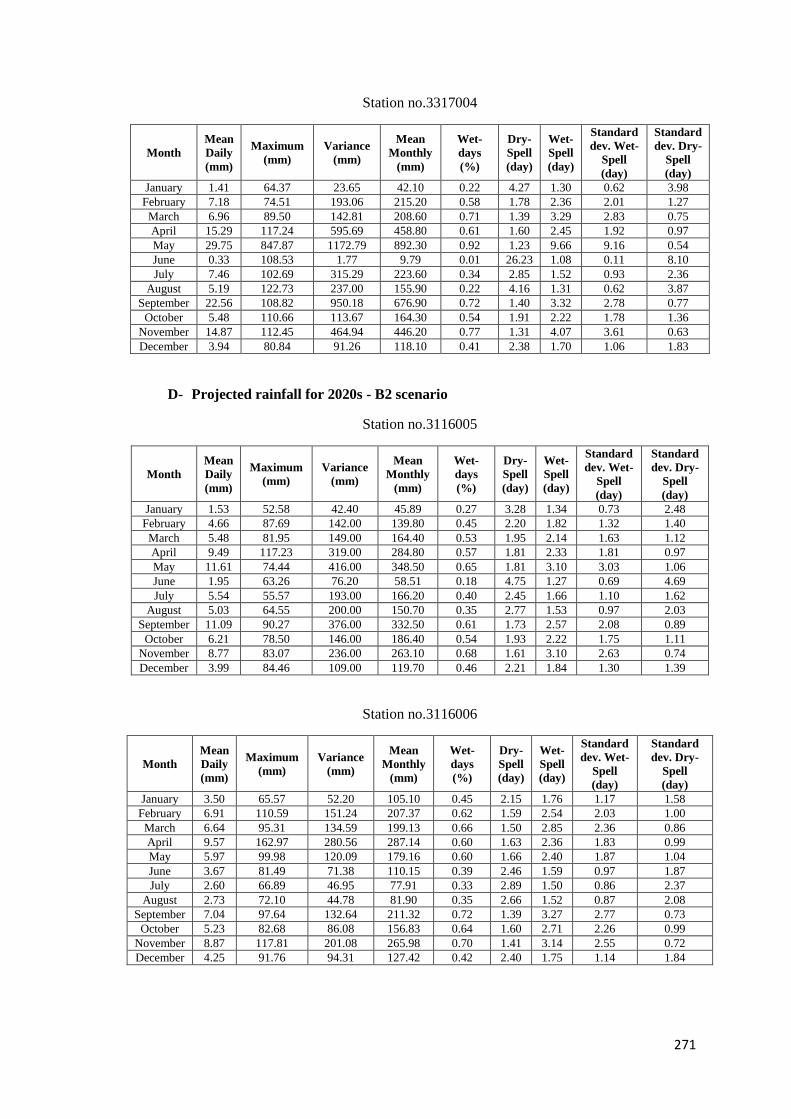
271
Station no.3317004
Month Mean
Daily
(mm)
Maximum
(mm) Variance
(mm)
Mean
Monthly
(mm)
Wet-
days
(%)
Dry-
Spell
(day)
Wet-
Spell
(day)
Standard
dev. Wet-
Spell
(day)
Standard
dev. Dry-
Spell
(day) January 1.41 64.37 23.65 42.10 0.22 4.27 1.30 0.62 3.98
February 7.18 74.51 193.06 215.20 0.58 1.78 2.36 2.01 1.27
March 6.96 89.50 142.81 208.60 0.71 1.39 3.29 2.83 0.75
April 15.29 117.24 595.69 458.80 0.61 1.60 2.45 1.92 0.97
May 29.75 847.87 1172.79 892.30 0.92 1.23 9.66 9.16 0.54
June 0.33 108.53 1.77 9.79 0.01 26.23 1.08 0.11 8.10
July 7.46 102.69 315.29 223.60 0.34 2.85 1.52 0.93 2.36
August 5.19 122.73 237.00 155.90 0.22 4.16 1.31 0.62 3.87
September 22.56 108.82 950.18 676.90 0.72 1.40 3.32 2.78 0.77
October 5.48 110.66 113.67 164.30 0.54 1.91 2.22 1.78 1.36
November 14.87 112.45 464.94 446.20 0.77 1.31 4.07 3.61 0.63
December 3.94 80.84 91.26 118.10 0.41 2.38 1.70 1.06 1.83
D- Projected rainfall for 2020s - B2 scenario
Station no.3116005
Month
Mean
Daily
(mm)
Maximum
(mm)
Variance
(mm)
Mean
Monthly
(mm)
Wet-
days
(%)
Dry-
Spell
(day)
Wet-
Spell
(day)
Standard
dev. Wet-
Spell
(day)
Standard
dev. Dry-
Spell
(day)
January 1.53 52.58 42.40 45.89 0.27 3.28 1.34 0.73 2.48
February 4.66 87.69 142.00 139.80 0.45 2.20 1.82 1.32 1.40
March 5.48 81.95 149.00 164.40 0.53 1.95 2.14 1.63 1.12
April 9.49 117.23 319.00 284.80 0.57 1.81 2.33 1.81 0.97
May 11.61 74.44 416.00 348.50 0.65 1.81 3.10 3.03 1.06
June 1.95 63.26 76.20 58.51 0.18 4.75 1.27 0.69 4.69
July 5.54 55.57 193.00 166.20 0.40 2.45 1.66 1.10 1.62
August 5.03 64.55 200.00 150.70 0.35 2.77 1.53 0.97 2.03
September 11.09 90.27 376.00 332.50 0.61 1.73 2.57 2.08 0.89
October 6.21 78.50 146.00 186.40 0.54 1.93 2.22 1.75 1.11
November 8.77 83.07 236.00 263.10 0.68 1.61 3.10 2.63 0.74
December 3.99 84.46 109.00 119.70 0.46 2.21 1.84 1.30 1.39
Station no.3116006
Month Mean
Daily
(mm)
Maximum
(mm) Variance
(mm)
Mean
Monthly
(mm)
Wet-
days
(%)
Dry-
Spell
(day)
Wet-
Spell
(day)
Standard
dev. Wet-
Spell
(day)
Standard
dev. Dry-
Spell
(day) January 3.50 65.57 52.20 105.10 0.45 2.15 1.76 1.17 1.58
February 6.91 110.59 151.24 207.37 0.62 1.59 2.54 2.03 1.00
March 6.64 95.31 134.59 199.13 0.66 1.50 2.85 2.36 0.86
April 9.57 162.97 280.56 287.14 0.60 1.63 2.36 1.83 0.99
May 5.97 99.98 120.09 179.16 0.60 1.66 2.40 1.87 1.04
June 3.67 81.49 71.38 110.15 0.39 2.46 1.59 0.97 1.87
July 2.60 66.89 46.95 77.91 0.33 2.89 1.50 0.86 2.37
August 2.73 72.10 44.78 81.90 0.35 2.66 1.52 0.87 2.08
September 7.04 97.64 132.64 211.32 0.72 1.39 3.27 2.77 0.73
October 5.23 82.68 86.08 156.83 0.64 1.60 2.71 2.26 0.99
November 8.87 117.81 201.08 265.98 0.70 1.41 3.14 2.55 0.72
December 4.25 91.76 94.31 127.42 0.42 2.40 1.75 1.14 1.84
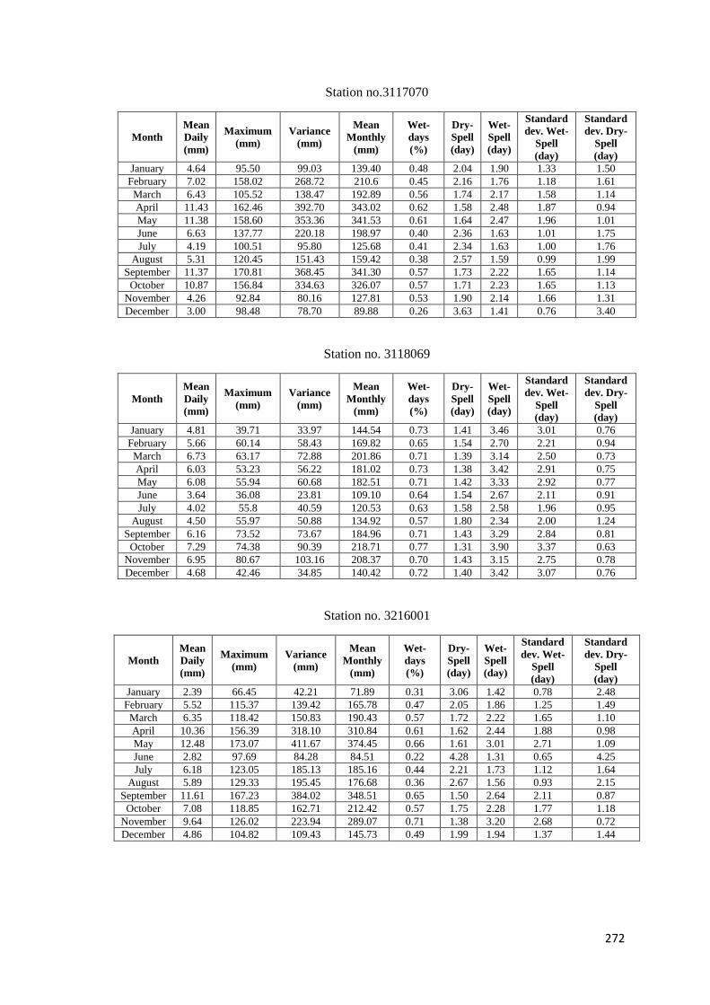
272
Station no.3117070
Month
Mean
Daily
(mm)
Maximum
(mm)
Variance
(mm)
Mean
Monthly
(mm)
Wet-
days
(%)
Dry-
Spell
(day)
Wet-
Spell
(day)
Standard
dev. Wet-
Spell
(day)
Standard
dev. Dry-
Spell
(day)
January 4.64 95.50 99.03 139.40 0.48 2.04 1.90 1.33 1.50
February 7.02 158.02 268.72 210.6 0.45 2.16 1.76 1.18 1.61
March 6.43 105.52 138.47 192.89 0.56 1.74 2.17 1.58 1.14
April 11.43 162.46 392.70 343.02 0.62 1.58 2.48 1.87 0.94
May 11.38 158.60 353.36 341.53 0.61 1.64 2.47 1.96 1.01
June 6.63 137.77 220.18 198.97 0.40 2.36 1.63 1.01 1.75
July 4.19 100.51 95.80 125.68 0.41 2.34 1.63 1.00 1.76
August 5.31 120.45 151.43 159.42 0.38 2.57 1.59 0.99 1.99
September 11.37 170.81 368.45 341.30 0.57 1.73 2.22 1.65 1.14
October 10.87 156.84 334.63 326.07 0.57 1.71 2.23 1.65 1.13
November 4.26 92.84 80.16 127.81 0.53 1.90 2.14 1.66 1.31
December 3.00 98.48 78.70 89.88 0.26 3.63 1.41 0.76 3.40
Station no. 3118069
Month
Mean
Daily
(mm)
Maximum
(mm)
Variance
(mm)
Mean
Monthly
(mm)
Wet-
days
(%)
Dry-
Spell
(day)
Wet-
Spell
(day)
Standard
dev. Wet-
Spell
(day)
Standard
dev. Dry-
Spell
(day)
January 4.81 39.71 33.97 144.54 0.73 1.41 3.46 3.01 0.76
February 5.66 60.14 58.43 169.82 0.65 1.54 2.70 2.21 0.94
March 6.73 63.17 72.88 201.86 0.71 1.39 3.14 2.50 0.73
April 6.03 53.23 56.22 181.02 0.73 1.38 3.42 2.91 0.75
May 6.08 55.94 60.68 182.51 0.71 1.42 3.33 2.92 0.77
June 3.64 36.08 23.81 109.10 0.64 1.54 2.67 2.11 0.91
July 4.02 55.8 40.59 120.53 0.63 1.58 2.58 1.96 0.95
August 4.50 55.97 50.88 134.92 0.57 1.80 2.34 2.00 1.24
September 6.16 73.52 73.67 184.96 0.71 1.43 3.29 2.84 0.81
October 7.29 74.38 90.39 218.71 0.77 1.31 3.90 3.37 0.63
November 6.95 80.67 103.16 208.37 0.70 1.43 3.15 2.75 0.78
December 4.68 42.46 34.85 140.42 0.72 1.40 3.42 3.07 0.76
Station no. 3216001
Month
Mean
Daily
(mm)
Maximum
(mm)
Variance
(mm)
Mean
Monthly
(mm)
Wet-
days
(%)
Dry-
Spell
(day)
Wet-
Spell
(day)
Standard
dev. Wet-
Spell
(day)
Standard
dev. Dry-
Spell
(day)
January 2.39 66.45 42.21 71.89 0.31 3.06 1.42 0.78 2.48
February 5.52 115.37 139.42 165.78 0.47 2.05 1.86 1.25 1.49
March 6.35 118.42 150.83 190.43 0.57 1.72 2.22 1.65 1.10
April 10.36 156.39 318.10 310.84 0.61 1.62 2.44 1.88 0.98
May 12.48 173.07 411.67 374.45 0.66 1.61 3.01 2.71 1.09
June 2.82 97.69 84.28 84.51 0.22 4.28 1.31 0.65 4.25
July 6.18 123.05 185.13 185.16 0.44 2.21 1.73 1.12 1.64
August 5.89 129.33 195.45 176.68 0.36 2.67 1.56 0.93 2.15
September 11.61 167.23 384.02 348.51 0.65 1.50 2.64 2.11 0.87
October 7.08 118.85 162.71 212.42 0.57 1.75 2.28 1.77 1.18
November 9.64 126.02 223.94 289.07 0.71 1.38 3.20 2.68 0.72
December 4.86 104.82 109.43 145.73 0.49 1.99 1.94 1.37 1.44
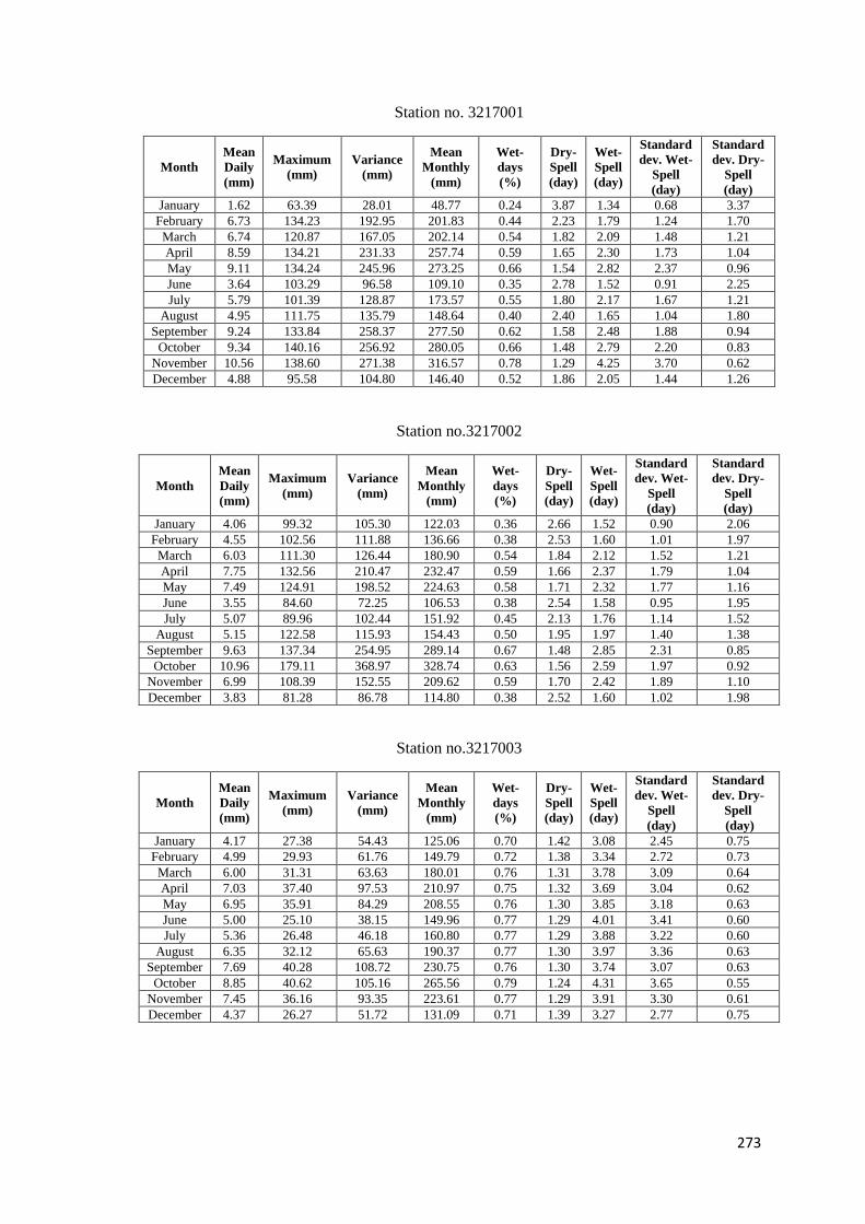
273
Station no. 3217001
Month Mean
Daily
(mm)
Maximum
(mm) Variance
(mm)
Mean
Monthly
(mm)
Wet-
days
(%)
Dry-
Spell
(day)
Wet-
Spell
(day)
Standard
dev. Wet-
Spell
(day)
Standard
dev. Dry-
Spell
(day) January 1.62 63.39 28.01 48.77 0.24 3.87 1.34 0.68 3.37
February 6.73 134.23 192.95 201.83 0.44 2.23 1.79 1.24 1.70
March 6.74 120.87 167.05 202.14 0.54 1.82 2.09 1.48 1.21
April 8.59 134.21 231.33 257.74 0.59 1.65 2.30 1.73 1.04
May 9.11 134.24 245.96 273.25 0.66 1.54 2.82 2.37 0.96
June 3.64 103.29 96.58 109.10 0.35 2.78 1.52 0.91 2.25
July 5.79 101.39 128.87 173.57 0.55 1.80 2.17 1.67 1.21
August 4.95 111.75 135.79 148.64 0.40 2.40 1.65 1.04 1.80
September 9.24 133.84 258.37 277.50 0.62 1.58 2.48 1.88 0.94
October 9.34 140.16 256.92 280.05 0.66 1.48 2.79 2.20 0.83
November 10.56 138.60 271.38 316.57 0.78 1.29 4.25 3.70 0.62
December 4.88 95.58 104.80 146.40 0.52 1.86 2.05 1.44 1.26
Station no.3217002
Month
Mean
Daily
(mm)
Maximum
(mm)
Variance
(mm)
Mean
Monthly
(mm)
Wet-
days
(%)
Dry-
Spell
(day)
Wet-
Spell
(day)
Standard
dev. Wet-
Spell
(day)
Standard
dev. Dry-
Spell
(day)
January 4.06 99.32 105.30 122.03 0.36 2.66 1.52 0.90 2.06
February 4.55 102.56 111.88 136.66 0.38 2.53 1.60 1.01 1.97
March 6.03 111.30 126.44 180.90 0.54 1.84 2.12 1.52 1.21
April 7.75 132.56 210.47 232.47 0.59 1.66 2.37 1.79 1.04
May 7.49 124.91 198.52 224.63 0.58 1.71 2.32 1.77 1.16
June 3.55 84.60 72.25 106.53 0.38 2.54 1.58 0.95 1.95
July 5.07 89.96 102.44 151.92 0.45 2.13 1.76 1.14 1.52
August 5.15 122.58 115.93 154.43 0.50 1.95 1.97 1.40 1.38
September 9.63 137.34 254.95 289.14 0.67 1.48 2.85 2.31 0.85
October 10.96 179.11 368.97 328.74 0.63 1.56 2.59 1.97 0.92
November 6.99 108.39 152.55 209.62 0.59 1.70 2.42 1.89 1.10
December 3.83 81.28 86.78 114.80 0.38 2.52 1.60 1.02 1.98
Station no.3217003
Month Mean
Daily
(mm)
Maximum
(mm) Variance
(mm)
Mean
Monthly
(mm)
Wet-
days
(%)
Dry-
Spell
(day)
Wet-
Spell
(day)
Standard
dev. Wet-
Spell
(day)
Standard
dev. Dry-
Spell
(day) January 4.17 27.38 54.43 125.06 0.70 1.42 3.08 2.45 0.75
February 4.99 29.93 61.76 149.79 0.72 1.38 3.34 2.72 0.73
March 6.00 31.31 63.63 180.01 0.76 1.31 3.78 3.09 0.64
April 7.03 37.40 97.53 210.97 0.75 1.32 3.69 3.04 0.62
May 6.95 35.91 84.29 208.55 0.76 1.30 3.85 3.18 0.63
June 5.00 25.10 38.15 149.96 0.77 1.29 4.01 3.41 0.60
July 5.36 26.48 46.18 160.80 0.77 1.29 3.88 3.22 0.60
August 6.35 32.12 65.63 190.37 0.77 1.30 3.97 3.36 0.63
September 7.69 40.28 108.72 230.75 0.76 1.30 3.74 3.07 0.63
October 8.85 40.62 105.16 265.56 0.79 1.24 4.31 3.65 0.55
November 7.45 36.16 93.35 223.61 0.77 1.29 3.91 3.30 0.61
December 4.37 26.27 51.72 131.09 0.71 1.39 3.27 2.77 0.75
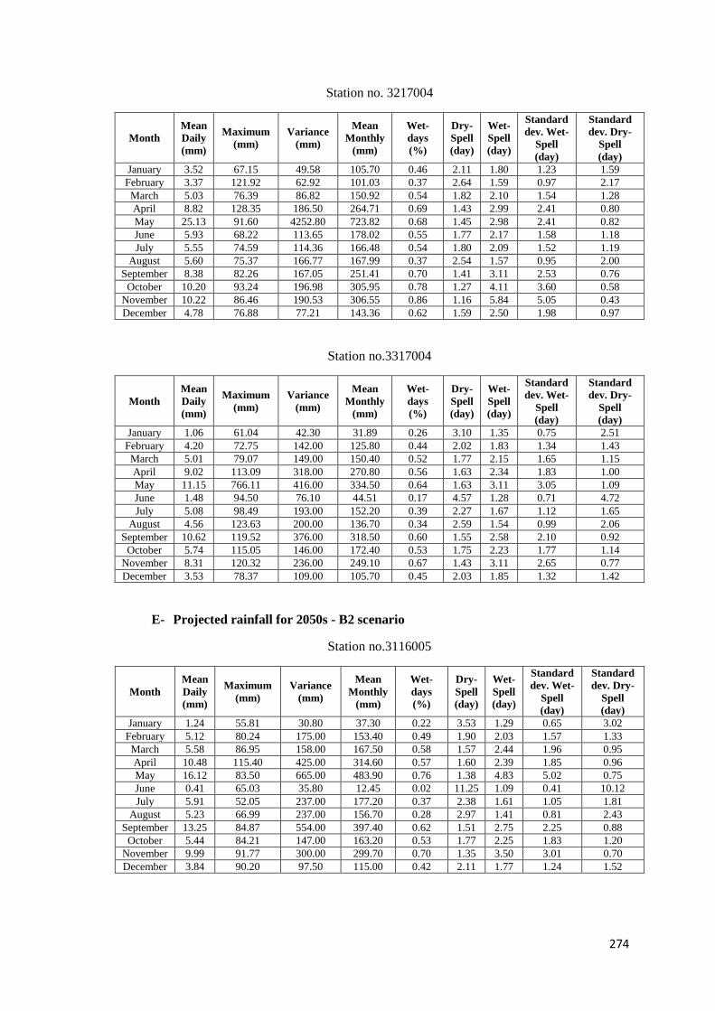
274
Station no. 3217004
Month Mean
Daily
(mm)
Maximum
(mm) Variance
(mm)
Mean
Monthly
(mm)
Wet-
days
(%)
Dry-
Spell
(day)
Wet-
Spell
(day)
Standard
dev. Wet-
Spell
(day)
Standard
dev. Dry-
Spell
(day) January 3.52 67.15 49.58 105.70 0.46 2.11 1.80 1.23 1.59
February 3.37 121.92 62.92 101.03 0.37 2.64 1.59 0.97 2.17
March 5.03 76.39 86.82 150.92 0.54 1.82 2.10 1.54 1.28
April 8.82 128.35 186.50 264.71 0.69 1.43 2.99 2.41 0.80
May 25.13 91.60 4252.80 723.82 0.68 1.45 2.98 2.41 0.82
June 5.93 68.22 113.65 178.02 0.55 1.77 2.17 1.58 1.18
July 5.55 74.59 114.36 166.48 0.54 1.80 2.09 1.52 1.19
August 5.60 75.37 166.77 167.99 0.37 2.54 1.57 0.95 2.00
September 8.38 82.26 167.05 251.41 0.70 1.41 3.11 2.53 0.76
October 10.20 93.24 196.98 305.95 0.78 1.27 4.11 3.60 0.58
November 10.22 86.46 190.53 306.55 0.86 1.16 5.84 5.05 0.43
December 4.78 76.88 77.21 143.36 0.62 1.59 2.50 1.98 0.97
Station no.3317004
Month
Mean
Daily
(mm)
Maximum
(mm)
Variance
(mm)
Mean
Monthly
(mm)
Wet-
days
(%)
Dry-
Spell
(day)
Wet-
Spell
(day)
Standard
dev. Wet-
Spell
(day)
Standard
dev. Dry-
Spell
(day)
January 1.06 61.04 42.30 31.89 0.26 3.10 1.35 0.75 2.51
February 4.20 72.75 142.00 125.80 0.44 2.02 1.83 1.34 1.43
March 5.01 79.07 149.00 150.40 0.52 1.77 2.15 1.65 1.15
April 9.02 113.09 318.00 270.80 0.56 1.63 2.34 1.83 1.00
May 11.15 766.11 416.00 334.50 0.64 1.63 3.11 3.05 1.09
June 1.48 94.50 76.10 44.51 0.17 4.57 1.28 0.71 4.72
July 5.08 98.49 193.00 152.20 0.39 2.27 1.67 1.12 1.65
August 4.56 123.63 200.00 136.70 0.34 2.59 1.54 0.99 2.06
September 10.62 119.52 376.00 318.50 0.60 1.55 2.58 2.10 0.92
October 5.74 115.05 146.00 172.40 0.53 1.75 2.23 1.77 1.14
November 8.31 120.32 236.00 249.10 0.67 1.43 3.11 2.65 0.77
December 3.53 78.37 109.00 105.70 0.45 2.03 1.85 1.32 1.42
E- Projected rainfall for 2050s - B2 scenario
Station no.3116005
Month Mean
Daily
(mm)
Maximum
(mm) Variance
(mm)
Mean
Monthly
(mm)
Wet-
days
(%)
Dry-
Spell
(day)
Wet-
Spell
(day)
Standard
dev. Wet-
Spell
(day)
Standard
dev. Dry-
Spell
(day) January 1.24 55.81 30.80 37.30 0.22 3.53 1.29 0.65 3.02
February 5.12 80.24 175.00 153.40 0.49 1.90 2.03 1.57 1.33
March 5.58 86.95 158.00 167.50 0.58 1.57 2.44 1.96 0.95
April 10.48 115.40 425.00 314.60 0.57 1.60 2.39 1.85 0.96
May 16.12 83.50 665.00 483.90 0.76 1.38 4.83 5.02 0.75
June 0.41 65.03 35.80 12.45 0.02 11.25 1.09 0.41 10.12
July 5.91 52.05 237.00 177.20 0.37 2.38 1.61 1.05 1.81
August 5.23 66.99 237.00 156.70 0.28 2.97 1.41 0.81 2.43
September 13.25 84.87 554.00 397.40 0.62 1.51 2.75 2.25 0.88
October 5.44 84.21 147.00 163.20 0.53 1.77 2.25 1.83 1.20
November 9.99 91.77 300.00 299.70 0.70 1.35 3.50 3.01 0.70
December 3.84 90.20 97.50 115.00 0.42 2.11 1.77 1.24 1.52

275
Station no.3116006
Month Mean
Daily
(mm)
Maximum
(mm) Variance
(mm)
Mean
Monthly
(mm)
Wet-
days
(%)
Dry-
Spell
(day)
Wet-
Spell
(day)
Standard
dev. Wet-
Spell
(day)
Standard
dev. Dry-
Spell
(day) January 3.68 69.23 53.99 110.31 0.48 2.02 1.89 1.30 1.46
February 7.20 111.90 140.55 216.07 0.68 1.49 2.95 2.45 0.86
March 6.68 102.25 132.12 200.46 0.68 1.44 2.91 2.39 0.78
April 9.83 147.73 312.64 294.91 0.59 1.67 2.30 1.73 1.05
May 6.22 106.25 128.68 186.48 0.58 1.69 2.31 1.74 1.08
June 3.52 79.53 72.51 105.65 0.36 2.60 1.53 0.88 2.07
July 2.07 65.33 40.39 62.03 0.26 3.66 1.37 0.70 3.21
August 2.06 64.64 31.64 61.89 0.32 3.00 1.45 0.80 2.40
September 6.62 100.12 116.66 198.47 0.76 1.33 3.85 3.32 0.66
October 4.30 69.46 60.89 128.92 0.63 1.66 2.72 2.36 1.10
November 8.74 118.46 201.62 262.30 0.70 1.42 3.06 2.48 0.76
December 3.28 93.77 74.25 98.38 0.34 2.94 1.55 0.99 2.48
Station no. 3117070
Month Mean
Daily
(mm)
Maximum
(mm) Variance
(mm)
Mean
Monthly
(mm)
Wet-
days
(%)
Dry-
Spell
(day)
Wet-
Spell
(day)
Standard
dev. Wet-
Spell
(day)
Standard
dev. Dry-
Spell
(day) January 4.52 90.58 81.10 135.58 0.58 1.72 2.33 1.78 1.16
February 6.79 151.57 235.37 203.84 0.47 2.09 1.84 1.27 1.52
March 6.05 88.85 117.05 181.30 0.59 1.66 2.32 1.70 1.03
April 13.38 180.48 476.35 401.53 0.65 1.54 2.69 2.12 0.92
May 15.89 183.92 561.82 476.94 0.67 1.49 2.86 2.29 0.85
June 8.46 153.38 321.97 254.06 0.43 2.24 1.71 1.09 1.67
July 3.99 93.87 84.37 119.58 0.43 2.20 1.70 1.10 1.58
August 4.80 111.30 143.96 144.12 0.32 2.95 1.46 0.82 2.40
September 14.59 190.06 562.28 437.80 0.58 1.69 2.32 1.73 1.06
October 12.41 161.54 421.05 372.14 0.56 1.76 2.19 1.62 1.15
November 2.94 77.36 50.45 88.10 0.47 2.12 1.90 1.35 1.55
December 1.61 83.78 43.37 48.13 0.15 5.94 1.20 0.48 5.47
Station no. 3118069
Month Mean
Daily
(mm)
Maximum
(mm) Variance
(mm)
Mean
Monthly
(mm)
Wet-
days
(%)
Dry-
Spell
(day)
Wet-
Spell
(day)
Standard
dev. Wet-
Spell
(day)
Standard
dev. Dry-
Spell
(day) January 4.95 42.25 34.69 148.71 0.76 1.34 3.86 3.39 0.68
February 5.39 56.26 56.59 161.81 0.63 1.62 2.61 2.09 1.00
March 7.26 65.65 84.05 217.82 0.71 1.42 3.29 2.80 0.78
April 6.01 54.00 55.61 180.40 0.71 1.40 3.28 2.81 0.73
May 6.46 60.42 65.04 193.76 0.72 1.42 3.46 2.97 0.79
June 3.47 34.49 23.30 104.02 0.60 1.68 2.43 1.94 1.08
July 3.51 48.27 32.66 105.10 0.61 1.61 2.50 1.96 1.00
August 4.22 58.21 52.12 126.52 0.50 2.03 2.02 1.61 1.48
September 6.14 74.95 78.12 184.35 0.70 1.44 3.23 2.82 0.79
October 7.28 82.95 96.64 218.45 0.73 1.36 3.45 2.98 0.70
November 6.68 83.68 103.04 200.21 0.66 1.51 2.84 2.35 0.88
December 4.62 45.45 34.11 138.42 0.72 1.43 3.35 2.93 0.77
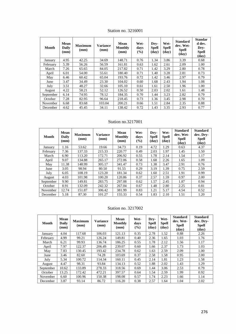
276
Station no. 3216001
Month Mean
Daily
(mm)
Maximum
(mm) Variance
(mm)
Mean
Monthly
(mm)
Wet-
days
(%)
Dry-
Spell
(day)
Wet-
Spell
(day)
Standard
dev. Wet-
Spell
(day)
Standar
d dev.
Dry-
Spell
(day) January 4.95 42.25 34.69 148.71 0.76 1.34 3.86 3.39 0.68
February 5.39 56.26 56.59 161.81 0.63 1.62 2.61 2.09 1.00
March 7.26 65.65 84.05 217.82 0.71 1.42 3.29 2.80 0.78
April 6.01 54.00 55.61 180.40 0.71 1.40 3.28 2.81 0.73
May 6.46 60.42 65.04 193.76 0.72 1.42 3.46 2.97 0.79
June 3.47 34.49 23.30 104.02 0.60 1.68 2.43 1.94 1.08
July 3.51 48.27 32.66 105.10 0.61 1.61 2.50 1.96 1.00
August 4.22 58.21 52.12 126.52 0.50 2.03 2.02 1.61 1.48
September 6.14 74.95 78.12 184.35 0.70 1.44 3.23 2.82 0.79
October 7.28 82.95 96.64 218.45 0.73 1.36 3.45 2.98 0.70
November 6.68 83.68 103.04 200.21 0.66 1.51 2.84 2.35 0.88
December 4.62 45.45 34.11 138.42 0.72 1.43 3.35 2.93 0.77
Station no.3217001
Month Mean
Daily
(mm)
Maximum
(mm) Variance
(mm)
Mean
Monthly
(mm)
Wet-
days
(%)
Dry-
Spell
(day)
Wet-
Spell
(day)
Standard
dev. Wet-
Spell
(day)
Standard
dev. Dry-
Spell
(day) January 1.16 53.62 19.66 34.73 0.19 4.72 1.29 0.63 4.37
February 7.36 137.33 215.33 220.77 0.49 2.03 1.97 1.45 1.50
March 6.90 113.20 172.71 206.92 0.55 1.78 2.14 1.54 1.17
April 9.07 134.88 265.17 272.06 0.58 1.68 2.26 1.65 1.09
May 11.38 148.99 305.17 341.47 0.73 1.38 3.47 2.91 0.76
June 3.05 98.94 80.50 91.55 0.29 3.19 1.39 0.75 2.59
July 6.05 108.19 123.20 181.34 0.62 1.60 2.51 1.91 0.99
August 4.03 101.98 100.20 120.86 0.37 2.57 1.59 0.97 2.00
September 9.90 149.81 283.75 297.08 0.62 1.57 2.45 1.87 0.94
October 8.91 132.09 242.32 267.04 0.67 1.48 2.80 2.25 0.81
November 12.74 151.87 306.42 381.99 0.83 1.21 5.17 4.54 0.52
December 5.18 87.30 101.27 155.33 0.54 1.83 2.10 1.51 1.20
Station no. 3217002
Month Mean
Daily
(mm)
Maximum
(mm) Variance
(mm)
Mean
Monthly
(mm)
Wet-
days
(%)
Dry-
Spell
(day)
Wet-
Spell
(day)
Standard
dev. Wet-
Spell
(day)
Standard
dev. Dry-
Spell
(day) January 4.04 117.68 106.03 121.13 0.35 2.78 1.52 0.88 2.26
February 4.99 99.21 126.24 149.81 0.40 2.36 1.65 1.03 1.76
March 6.21 99.93 136.74 186.25 0.55 1.78 2.12 1.56 1.17
April 7.97 122.37 206.49 239.07 0.60 1.66 2.37 1.73 1.03
May 7.83 130.45 193.42 234.78 0.62 1.63 2.59 2.09 1.00
June 3.46 82.60 74.28 103.69 0.37 2.58 1.58 0.95 2.00
July 5.34 100.72 114.34 160.11 0.45 2.14 1.81 1.23 1.58
August 4.47 98.31 93.84 134.13 0.52 1.88 2.02 1.43 1.29
September 10.62 133.89 278.33 318.56 0.69 1.44 3.06 2.53 0.79
October 13.25 172.42 472.21 397.57 0.64 1.54 2.59 1.99 0.92
November 6.60 100.96 150.38 198.08 0.57 1.74 2.23 1.66 1.14
December 3.87 93.14 86.72 116.20 0.38 2.57 1.64 1.04 2.02
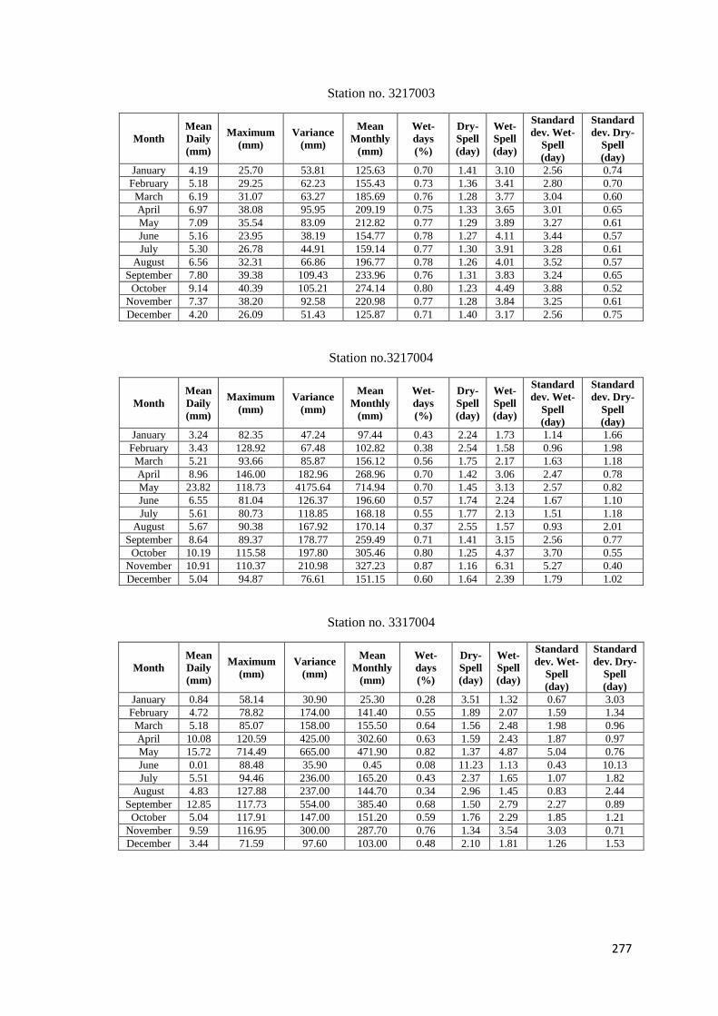
277
Station no. 3217003
Month Mean
Daily
(mm)
Maximum
(mm) Variance
(mm)
Mean
Monthly
(mm)
Wet-
days
(%)
Dry-
Spell
(day)
Wet-
Spell
(day)
Standard
dev. Wet-
Spell
(day)
Standard
dev. Dry-
Spell
(day) January 4.19 25.70 53.81 125.63 0.70 1.41 3.10 2.56 0.74
February 5.18 29.25 62.23 155.43 0.73 1.36 3.41 2.80 0.70
March 6.19 31.07 63.27 185.69 0.76 1.28 3.77 3.04 0.60
April 6.97 38.08 95.95 209.19 0.75 1.33 3.65 3.01 0.65
May 7.09 35.54 83.09 212.82 0.77 1.29 3.89 3.27 0.61
June 5.16 23.95 38.19 154.77 0.78 1.27 4.11 3.44 0.57
July 5.30 26.78 44.91 159.14 0.77 1.30 3.91 3.28 0.61
August 6.56 32.31 66.86 196.77 0.78 1.26 4.01 3.52 0.57
September 7.80 39.38 109.43 233.96 0.76 1.31 3.83 3.24 0.65
October 9.14 40.39 105.21 274.14 0.80 1.23 4.49 3.88 0.52
November 7.37 38.20 92.58 220.98 0.77 1.28 3.84 3.25 0.61
December 4.20 26.09 51.43 125.87 0.71 1.40 3.17 2.56 0.75
Station no.3217004
Month Mean
Daily
(mm)
Maximum
(mm) Variance
(mm)
Mean
Monthly
(mm)
Wet-
days
(%)
Dry-
Spell
(day)
Wet-
Spell
(day)
Standard
dev. Wet-
Spell
(day)
Standard
dev. Dry-
Spell
(day) January 3.24 82.35 47.24 97.44 0.43 2.24 1.73 1.14 1.66
February 3.43 128.92 67.48 102.82 0.38 2.54 1.58 0.96 1.98
March 5.21 93.66 85.87 156.12 0.56 1.75 2.17 1.63 1.18
April 8.96 146.00 182.96 268.96 0.70 1.42 3.06 2.47 0.78
May 23.82 118.73 4175.64 714.94 0.70 1.45 3.13 2.57 0.82
June 6.55 81.04 126.37 196.60 0.57 1.74 2.24 1.67 1.10
July 5.61 80.73 118.85 168.18 0.55 1.77 2.13 1.51 1.18
August 5.67 90.38 167.92 170.14 0.37 2.55 1.57 0.93 2.01
September 8.64 89.37 178.77 259.49 0.71 1.41 3.15 2.56 0.77
October 10.19 115.58 197.80 305.46 0.80 1.25 4.37 3.70 0.55
November 10.91 110.37 210.98 327.23 0.87 1.16 6.31 5.27 0.40
December 5.04 94.87 76.61 151.15 0.60 1.64 2.39 1.79 1.02
Station no. 3317004
Month Mean
Daily
(mm)
Maximum
(mm) Variance
(mm)
Mean
Monthly
(mm)
Wet-
days
(%)
Dry-
Spell
(day)
Wet-
Spell
(day)
Standard
dev. Wet-
Spell
(day)
Standard
dev. Dry-
Spell
(day) January 0.84 58.14 30.90 25.30 0.28 3.51 1.32 0.67 3.03
February 4.72 78.82 174.00 141.40 0.55 1.89 2.07 1.59 1.34
March 5.18 85.07 158.00 155.50 0.64 1.56 2.48 1.98 0.96
April 10.08 120.59 425.00 302.60 0.63 1.59 2.43 1.87 0.97
May 15.72 714.49 665.00 471.90 0.82 1.37 4.87 5.04 0.76
June 0.01 88.48 35.90 0.45 0.08 11.23 1.13 0.43 10.13
July 5.51 94.46 236.00 165.20 0.43 2.37 1.65 1.07 1.82
August 4.83 127.88 237.00 144.70 0.34 2.96 1.45 0.83 2.44
September 12.85 117.73 554.00 385.40 0.68 1.50 2.79 2.27 0.89
October 5.04 117.91 147.00 151.20 0.59 1.76 2.29 1.85 1.21
November 9.59 116.95 300.00 287.70 0.76 1.34 3.54 3.03 0.71
December 3.44 71.59 97.60 103.00 0.48 2.10 1.81 1.26 1.53
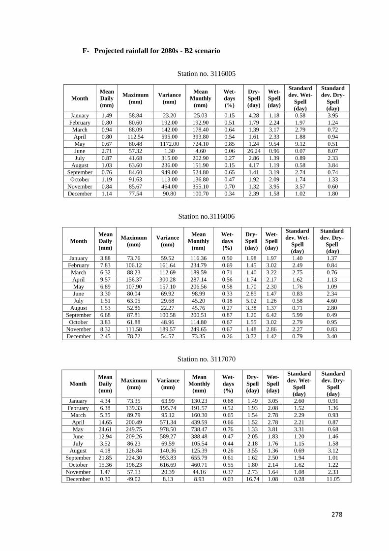
278
F- Projected rainfall for 2080s - B2 scenario
Station no. 3116005
Month Mean
Daily
(mm)
Maximum
(mm) Variance
(mm)
Mean
Monthly
(mm)
Wet-
days
(%)
Dry-
Spell
(day)
Wet-
Spell
(day)
Standard
dev. Wet-
Spell
(day)
Standard
dev. Dry-
Spell
(day) January 1.49 58.84 23.20 25.03 0.15 4.28 1.18 0.58 3.95
February 0.80 80.60 192.00 192.90 0.51 1.79 2.24 1.97 1.24
March 0.94 88.09 142.00 178.40 0.64 1.39 3.17 2.79 0.72
April 0.80 112.54 595.00 393.80 0.54 1.61 2.33 1.88 0.94
May 0.67 80.48 1172.00 724.10 0.85 1.24 9.54 9.12 0.51
June 2.71 57.32 1.30 4.60 0.06 26.24 0.96 0.07 8.07
July 0.87 41.68 315.00 202.90 0.27 2.86 1.39 0.89 2.33
August 1.03 63.60 236.00 151.90 0.15 4.17 1.19 0.58 3.84
September 0.76 84.60 949.00 524.80 0.65 1.41 3.19 2.74 0.74
October 1.19 91.63 113.00 136.80 0.47 1.92 2.09 1.74 1.33
November 0.84 85.67 464.00 355.10 0.70 1.32 3.95 3.57 0.60
December 1.14 77.54 90.80 100.70 0.34 2.39 1.58 1.02 1.80
Station no.3116006
Month Mean
Daily
(mm)
Maximum
(mm) Variance
(mm)
Mean
Monthly
(mm)
Wet-
days
(%)
Dry-
Spell
(day)
Wet-
Spell
(day)
Standard
dev. Wet-
Spell
(day)
Standard
dev. Dry-
Spell
(day) January 3.88 73.76 59.52 116.36 0.50 1.98 1.97 1.40 1.37
February 7.83 106.12 161.64 234.79 0.69 1.45 3.02 2.49 0.84
March 6.32 88.23 112.69 189.59 0.71 1.40 3.22 2.75 0.76
April 9.57 156.37 300.28 287.14 0.56 1.74 2.17 1.62 1.13
May 6.89 107.90 157.10 206.56 0.58 1.70 2.30 1.76 1.09
June 3.30 80.04 69.92 98.99 0.33 2.85 1.47 0.83 2.34
July 1.51 63.05 29.68 45.20 0.18 5.02 1.26 0.58 4.60
August 1.53 52.86 22.27 45.76 0.27 3.38 1.37 0.71 2.80
September 6.68 87.81 100.58 200.51 0.87 1.20 6.42 5.99 0.49
October 3.83 61.88 48.96 114.80 0.67 1.55 3.02 2.79 0.95
November 8.32 111.58 189.57 249.65 0.67 1.48 2.86 2.27 0.83
December 2.45 78.72 54.57 73.35 0.26 3.72 1.42 0.79 3.40
Station no. 3117070
Month Mean
Daily
(mm)
Maximum
(mm) Variance
(mm)
Mean
Monthly
(mm)
Wet-
days
(%)
Dry-
Spell
(day)
Wet-
Spell
(day)
Standard
dev. Wet-
Spell
(day)
Standard
dev. Dry-
Spell
(day) January 4.34 73.35 63.99 130.23 0.68 1.49 3.05 2.60 0.91
February 6.38 139.33 195.74 191.57 0.52 1.93 2.08 1.52 1.36
March 5.35 89.79 95.12 160.30 0.65 1.54 2.78 2.29 0.93
April 14.65 200.49 571.34 439.59 0.66 1.52 2.78 2.21 0.87
May 24.61 249.75 978.50 738.47 0.76 1.33 3.81 3.31 0.68
June 12.94 209.26 589.27 388.48 0.47 2.05 1.83 1.20 1.46
July 3.52 86.23 69.59 105.54 0.44 2.18 1.76 1.15 1.58
August 4.18 126.84 140.36 125.39 0.26 3.55 1.36 0.69 3.12
September 21.85 224.30 953.83 655.79 0.61 1.62 2.50 1.94 1.01
October 15.36 196.23 616.69 460.71 0.55 1.80 2.14 1.62 1.22
November 1.47 57.13 20.39 44.16 0.37 2.73 1.64 1.08 2.33
December 0.30 49.02 8.13 8.93 0.03 16.74 1.08 0.28 11.05
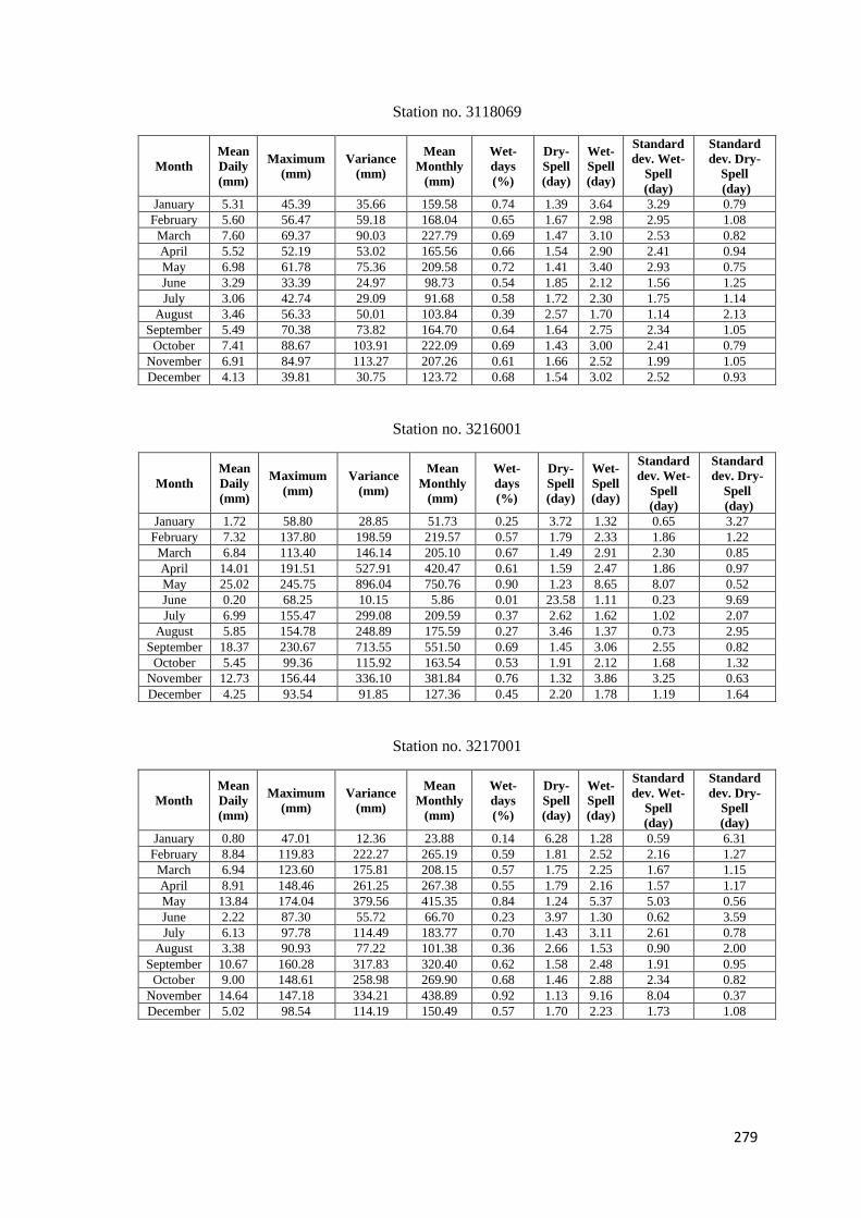
279
Station no. 3118069
Month Mean
Daily
(mm)
Maximum
(mm) Variance
(mm)
Mean
Monthly
(mm)
Wet-
days
(%)
Dry-
Spell
(day)
Wet-
Spell
(day)
Standard
dev. Wet-
Spell
(day)
Standard
dev. Dry-
Spell
(day) January 5.31 45.39 35.66 159.58 0.74 1.39 3.64 3.29 0.79
February 5.60 56.47 59.18 168.04 0.65 1.67 2.98 2.95 1.08
March 7.60 69.37 90.03 227.79 0.69 1.47 3.10 2.53 0.82
April 5.52 52.19 53.02 165.56 0.66 1.54 2.90 2.41 0.94
May 6.98 61.78 75.36 209.58 0.72 1.41 3.40 2.93 0.75
June 3.29 33.39 24.97 98.73 0.54 1.85 2.12 1.56 1.25
July 3.06 42.74 29.09 91.68 0.58 1.72 2.30 1.75 1.14
August 3.46 56.33 50.01 103.84 0.39 2.57 1.70 1.14 2.13
September 5.49 70.38 73.82 164.70 0.64 1.64 2.75 2.34 1.05
October 7.41 88.67 103.91 222.09 0.69 1.43 3.00 2.41 0.79
November 6.91 84.97 113.27 207.26 0.61 1.66 2.52 1.99 1.05
December 4.13 39.81 30.75 123.72 0.68 1.54 3.02 2.52 0.93
Station no. 3216001
Month Mean
Daily
(mm)
Maximum
(mm) Variance
(mm)
Mean
Monthly
(mm)
Wet-
days
(%)
Dry-
Spell
(day)
Wet-
Spell
(day)
Standard
dev. Wet-
Spell
(day)
Standard
dev. Dry-
Spell
(day) January 1.72 58.80 28.85 51.73 0.25 3.72 1.32 0.65 3.27
February 7.32 137.80 198.59 219.57 0.57 1.79 2.33 1.86 1.22
March 6.84 113.40 146.14 205.10 0.67 1.49 2.91 2.30 0.85
April 14.01 191.51 527.91 420.47 0.61 1.59 2.47 1.86 0.97
May 25.02 245.75 896.04 750.76 0.90 1.23 8.65 8.07 0.52
June 0.20 68.25 10.15 5.86 0.01 23.58 1.11 0.23 9.69
July 6.99 155.47 299.08 209.59 0.37 2.62 1.62 1.02 2.07
August 5.85 154.78 248.89 175.59 0.27 3.46 1.37 0.73 2.95
September 18.37 230.67 713.55 551.50 0.69 1.45 3.06 2.55 0.82
October 5.45 99.36 115.92 163.54 0.53 1.91 2.12 1.68 1.32
November 12.73 156.44 336.10 381.84 0.76 1.32 3.86 3.25 0.63
December 4.25 93.54 91.85 127.36 0.45 2.20 1.78 1.19 1.64
Station no. 3217001
Month Mean
Daily
(mm)
Maximum
(mm) Variance
(mm)
Mean
Monthly
(mm)
Wet-
days
(%)
Dry-
Spell
(day)
Wet-
Spell
(day)
Standard
dev. Wet-
Spell
(day)
Standard
dev. Dry-
Spell
(day) January 0.80 47.01 12.36 23.88 0.14 6.28 1.28 0.59 6.31
February 8.84 119.83 222.27 265.19 0.59 1.81 2.52 2.16 1.27
March 6.94 123.60 175.81 208.15 0.57 1.75 2.25 1.67 1.15
April 8.91 148.46 261.25 267.38 0.55 1.79 2.16 1.57 1.17
May 13.84 174.04 379.56 415.35 0.84 1.24 5.37 5.03 0.56
June 2.22 87.30 55.72 66.70 0.23 3.97 1.30 0.62 3.59
July 6.13 97.78 114.49 183.77 0.70 1.43 3.11 2.61 0.78
August 3.38 90.93 77.22 101.38 0.36 2.66 1.53 0.90 2.00
September 10.67 160.28 317.83 320.40 0.62 1.58 2.48 1.91 0.95
October 9.00 148.61 258.98 269.90 0.68 1.46 2.88 2.34 0.82
November 14.64 147.18 334.21 438.89 0.92 1.13 9.16 8.04 0.37
December 5.02 98.54 114.19 150.49 0.57 1.70 2.23 1.73 1.08
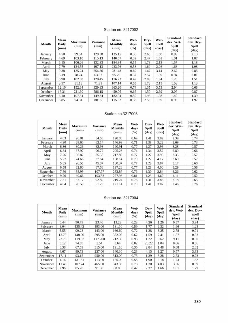
280
Station no. 3217002
Month Mean
Daily
(mm)
Maximum
(mm) Variance
(mm)
Mean
Monthly
(mm)
Wet-
days
(%)
Dry-
Spell
(day)
Wet-
Spell
(day)
Standard
dev. Wet-
Spell
(day)
Standard
dev. Dry-
Spell
(day) January 4.50 99.54 129.38 135.15 0.36 2.65 1.58 0.99 2.13
February 4.69 103.10 115.13 140.67 0.39 2.47 1.61 1.01 1.87
March 6.15 106.26 132.33 184.34 0.55 1.78 2.13 1.57 1.18
April 7.79 124.55 197.13 233.76 0.58 1.69 2.26 1.68 1.08
May 9.38 135.24 254.86 281.48 0.69 1.47 3.14 2.67 0.85
June 3.19 78.74 63.67 95.79 0.37 2.57 1.59 0.94 2.01
July 5.90 102.08 128.45 176.73 0.47 2.09 1.84 1.28 1.51
August 3.57 81.18 71.91 107.14 0.55 1.78 2.13 1.53 1.13
September 12.10 152.34 329.93 363.20 0.74 1.35 3.53 2.94 0.68
October 15.31 221.60 586.15 459.06 0.65 1.50 2.69 2.07 0.87
November 6.10 107.54 149.34 182.94 0.50 1.96 1.98 1.40 1.39
December 3.85 94.34 80.95 115.32 0.38 2.55 1.59 0.95 1.97
Station no.3217003
Month Mean
Daily
(mm)
Maximum
(mm) Variance
(mm)
Mean
Monthly
(mm)
Wet-
days
(%)
Dry-
Spell
(day)
Wet-
Spell
(day)
Standard
dev. Wet-
Spell
(day)
Standard
dev. Dry-
Spell
(day) January 4.03 26.81 54.65 120.83 0.69 1.41 3.02 2.39 0.74
February 4.90 28.60 62.14 146.93 0.71 1.38 3.22 2.69 0.73
March 6.36 30.26 62.93 190.91 0.77 1.27 3.96 3.28 0.57
April 6.84 37.97 96.72 205.26 0.74 1.34 3.52 2.89 0.66
May 7.26 36.82 85.53 217.89 0.77 1.27 3.95 3.35 0.57
June 5.27 24.66 37.64 158.14 0.79 1.27 4.17 3.69 0.57
July 5.35 26.55 45.87 160.37 0.77 1.29 3.87 3.17 0.60
August 6.58 32.80 67.68 197.28 0.77 1.28 4.00 3.29 0.58
September 7.80 38.99 107.77 233.86 0.76 1.30 3.84 3.26 0.62
October 9.26 40.66 103.38 277.93 0.81 1.23 4.69 4.11 0.52
November 7.31 37.17 92.80 219.24 0.76 1.31 3.85 3.18 0.65
December 4.04 26.59 51.23 121.14 0.70 1.41 3.07 2.46 0.76
Station no. 3217004
Month Mean
Daily
(mm)
Maximum
(mm) Variance
(mm)
Mean
Monthly
(mm)
Wet-
days
(%)
Dry-
Spell
(day)
Wet-
Spell
(day)
Standard
dev. Wet-
Spell
(day)
Standard
dev. Dry-
Spell
(day) January 0.44 90.79 23.40 13.23 0.23 4.26 1.26 0.57 3.94
February 6.04 135.42 193.00 181.10 0.59 1.77 2.32 1.96 1.23
March 5.55 99.23 143.00 166.60 0.72 1.38 3.25 2.78 0.71
April 12.73 148.90 595.00 382.00 0.62 1.59 2.41 1.87 0.93
May 23.73 119.67 1173.00 712.30 0.93 1.22 9.62 9.11 0.50
June 0.12 74.69 1.54 3.64 0.02 26.22 1.04 0.06 8.06
July 6.38 67.59 315.00 191.10 0.35 2.84 1.48 0.88 2.32
August 4.67 89.73 237.00 140.10 0.23 4.15 1.27 0.57 3.83
September 17.11 93.15 950.00 513.00 0.73 1.39 3.28 2.73 0.73
October 4.16 131.51 113.00 125.00 0.55 1.90 2.18 1.73 1.32
November 11.45 107.74 465.00 343.30 0.78 1.30 4.03 3.56 0.59
December 2.96 85.28 91.00 88.90 0.42 2.37 1.66 1.01 1.79
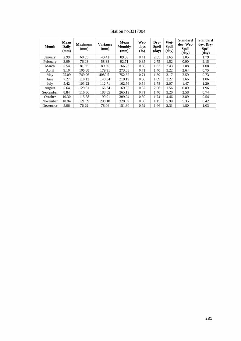
281
Station no.3317004
Month Mean
Daily
(mm)
Maximum
(mm) Variance
(mm)
Mean
Monthly
(mm)
Wet-
days
(%)
Dry-
Spell
(day)
Wet-
Spell
(day)
Standard
dev. Wet-
Spell
(day)
Standard
dev. Dry-
Spell
(day) January 2.99 60.55 43.41 89.59 0.41 2.35 1.65 1.05 1.79
February 3.09 76.08 58.38 92.71 0.35 2.75 1.52 0.90 2.15
March 5.54 81.36 89.50 166.26 0.60 1.67 2.43 1.88 1.08
April 9.10 105.88 179.91 273.08 0.71 1.40 3.22 2.64 0.75
May 25.09 749.96 4089.51 752.82 0.71 1.39 3.17 2.59 0.73
June 7.27 110.12 148.04 218.19 0.58 1.69 2.27 1.66 1.06
July 5.42 103.22 112.71 162.56 0.54 1.78 2.07 1.47 1.20
August 5.64 129.61 166.34 169.05 0.37 2.56 1.56 0.89 1.96
September 8.84 116.36 188.65 265.19 0.71 1.40 3.20 2.58 0.74
October 10.30 115.88 199.01 309.04 0.80 1.24 4.46 3.89 0.54
November 10.94 121.39 208.10 328.09 0.86 1.15 5.99 5.35 0.42
December 5.06 76.29 78.06 151.90 0.59 1.66 2.31 1.80 1.03
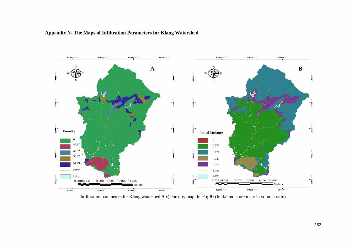
282
Appendix N- The Maps of Infiltration Parameters for Klang Watershed
Infiltration parameters for Klang watershed A :( Porosity map: in %); B: (Initial moisture map: in volume ratio)
Porosity Initial Moisture
A B
0
0.079
0.171
0.246
0.312
River
Lake
0
47.67
49.32
50.22
51.49
River
Lake
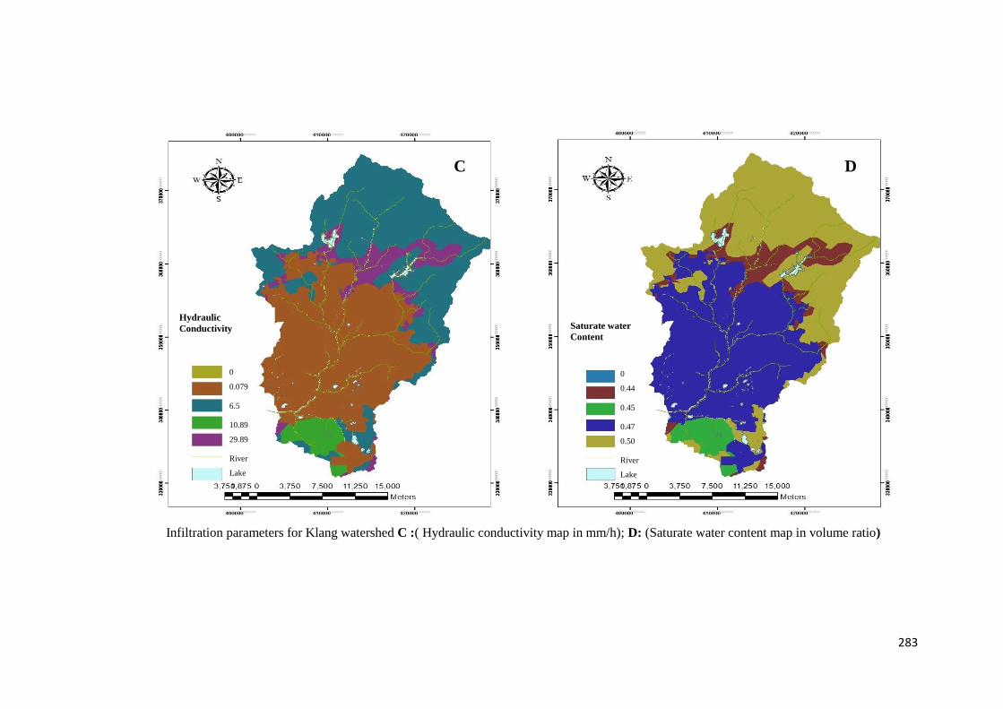
283
Infiltration parameters for Klang watershed C :( Hydraulic conductivity map in mm/h); D: (Saturate water content map in volume ratio)
Hydraulic
Conductivity Saturate water
Content
C D
0
0.079
6.5
10.89
29.89
River
Lake
0
0.44
0.45
0.47
0.50
River
Lake
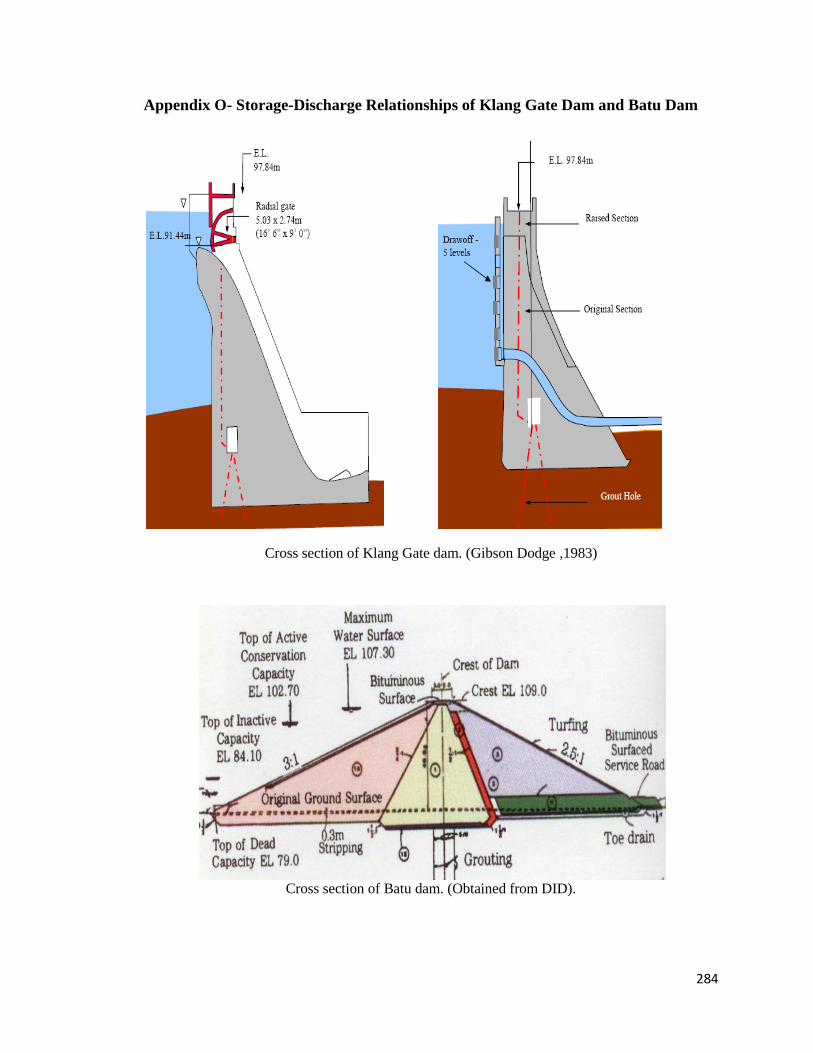
284
Appendix O- Storage-Discharge Relationships of Klang Gate Dam and Batu Dam
Cross section of Klang Gate dam. (Gibson Dodge ,1983)
Cross section of Batu dam. (Obtained from DID).
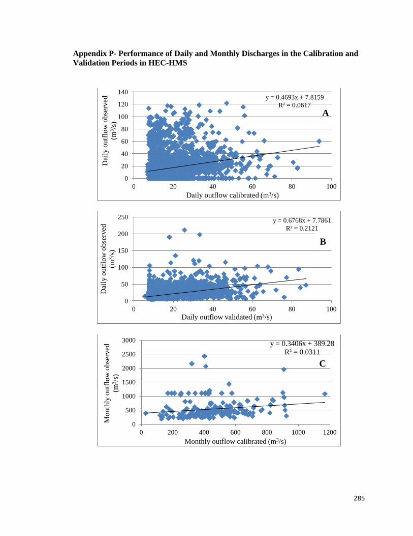
285
Appendix P- Performance of Daily and Monthly Discharges in the Calibration and
Validation Periods in HEC-HMS
y = 0.4693x + 7.8159
R² = 0.0617
0
20
40
60
80
100
120
140
0 20 40 60 80 100
Dai
ly o
utf
low
ob
serv
ed
(m3/s
)
Daily outflow calibrated (m3/s)
y = 0.6768x + 7.7861
R² = 0.2121
0
50
100
150
200
250
0 20 40 60 80 100
Dai
ly o
utf
low
obse
rved
(m3/s
)
Daily outflow validated (m3/s)
y = 0.3406x + 389.28
R² = 0.0311
0
500
1000
1500
2000
2500
3000
0 200 400 600 800 1000 1200
Mo
nth
ly o
utf
low
ob
serv
ed
(m3/s
)
Monthly outflow calibrated (m3/s)
A
B
C
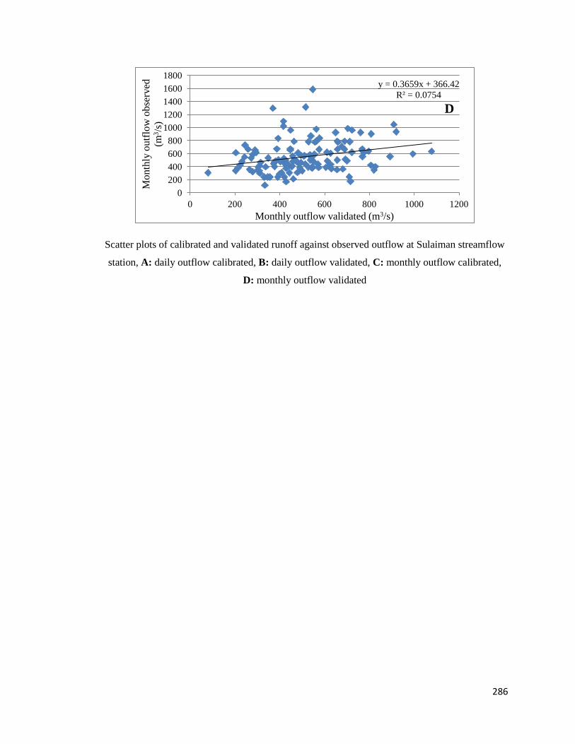
286
Scatter plots of calibrated and validated runoff against observed outflow at Sulaiman streamflow
station, A: daily outflow calibrated, B: daily outflow validated, C: monthly outflow calibrated,
D: monthly outflow validated
y = 0.3659x + 366.42
R² = 0.0754
0
200
400
600
800
1000
1200
1400
1600
1800
0 200 400 600 800 1000 1200
Mo
nth
ly o
utf
low
ob
serv
ed
(m3/s
)
Monthly outflow validated (m3/s)
D
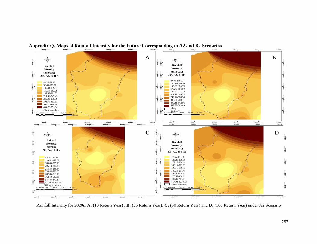
287
Appendix Q- Maps of Rainfall Intensity for the Future Corresponding to A2 and B2 Scenarios
Rainfall Intensity for 2020s: A: (10 Return Year) ; B: (25 Return Year); C: (50 Return Year) and D: (100 Return Year) under A2 Scenario
B
D
A
C
Rainfall
Intensity:
(mm/day)
20s, A2, 10 RY
Rainfall
Intensity:
(mm/day)
20s, A2, 25 RY
Rainfall
Intensity:
(mm/day)
20s, A2, 50 RY
Rainfall
Intensity:
(mm/day)
20s, A2, 100 RY
57.65-133.86
133.86-179.19
179.19-206.14
206.14-222.17
222.17-249.13
249.13-294.45
294.45-370.67
370.67-498.82
498.82-714.31
714.31-1,076.66
Klang boundary
53.36-139.41
139.41-183.03
183.03-205.13
205.13-216.33
216.33-238.44
238.44-282.05
282.05-368.10
368.10-537.88
537.88-872.87
872.87-1,533.81
Klang boundary
43.25-92.40
92.40-130.31
130.31-159.54
159.54-182.09
182.09-211.32
211.32-249.23
249.23-298.39
298.39-362.13
362.13-444.78
444.78-551.96
Klang boundary
49.06-108.17
108.17-146.26
146.26-170-79
170.79-186.60
186.60-211.13
211.13-249.22
249.22-308.34
308.34-400.11
400.11-542.56
542.56-763.69
Klang
boundary
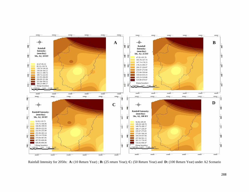
288
Rainfall Intensity for 2050s: A: (10 Return Year) ; B: (25 return Year); C: (50 Return Year) and D: (100 Return Year) under A2 Scenario
A B
C D
Rainfall
Intensity:
(mm/day)
50s, A2, 10 RY
Rainfall
Intensity:
(mm/day)
50s, A2, 25 RY
Rainfall Intensity:
(mm/day)
50s, A2, 50 RY
Rainfall Intensity:
(mm/day)
50s, A2, 100 RY
56.06-109.39
109.39-149.70
149.70-180.17
180.17-220.47
220.47-273.81
273.81-344.34
344.34-437.66
437.66-561.11
561.11-724.42
724.42-940.47
Klang boundary
47.95-105.78
105.78-147.74
147.74-178.23
178.23-200.37
200.37-230.87
230.87-272.84
272.84-330.64
330.64-410.23
410.23-519.80
519.80-670.67
Klang boundary
42.47-85.53
85.53-118.74
118.74-144.36
144.36-164.11
164.11-189.72
189.72-222.93
222.93-266.00
266.00-321.84
321.84-394.25
394.25-488.17
Klang boundary
52.02-119.72
119.72-166.96
166.96-199.93
199.93-222.93
222.93-255.90
255.90-303.14
303.14-370.84
370.84-467.85
467.85-606.86
606.86-806.08
Klang boundary
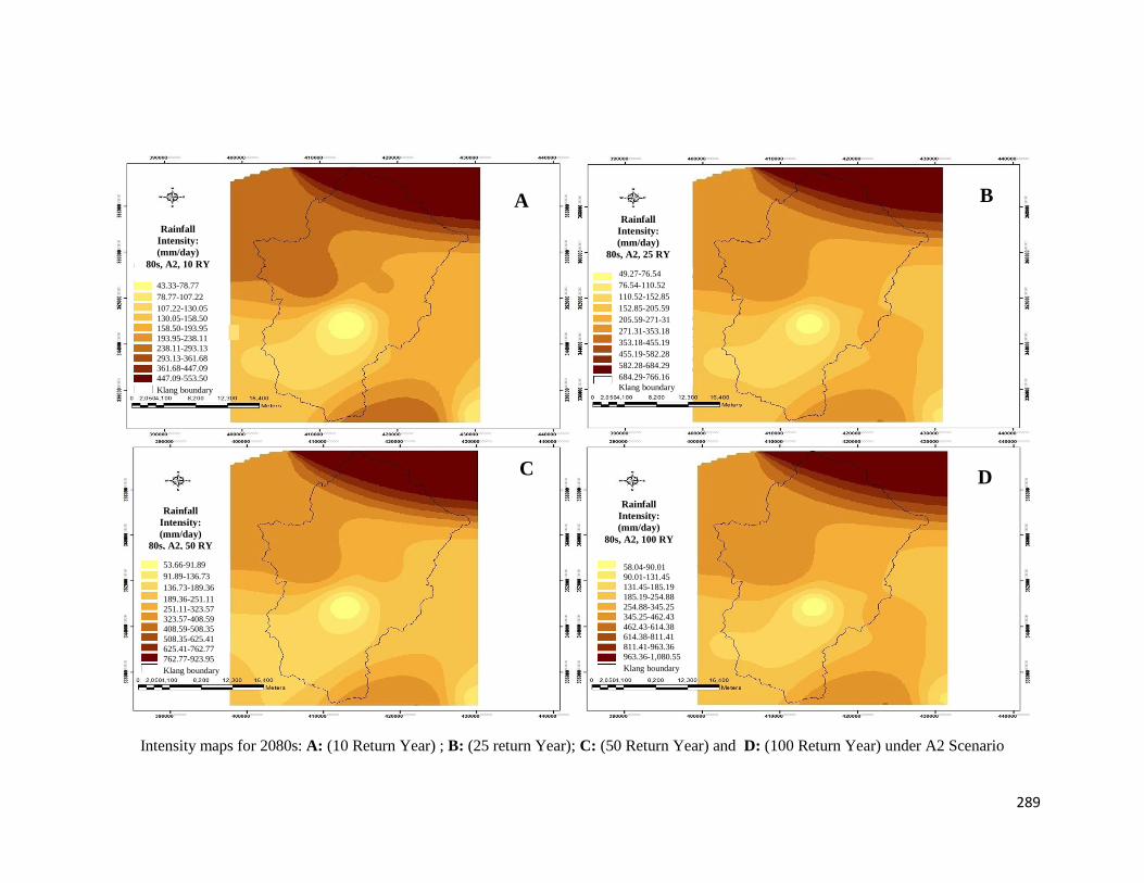
289
Intensity maps for 2080s: A: (10 Return Year) ; B: (25 return Year); C: (50 Return Year) and D: (100 Return Year) under A2 Scenario
A B
C D
Rainfall
Intensity:
(mm/day)
80s, A2, 10 RY
Rainfall
Intensity:
(mm/day)
80s, A2, 25 RY
Rainfall
Intensity:
(mm/day)
80s, A2, 50 RY
Rainfall
Intensity:
(mm/day)
80s, A2, 100 RY
58.04-90.01
90.01-131.45
131.45-185.19
185.19-254.88
254.88-345.25
345.25-462.43
462.43-614.38
614.38-811.41
811.41-963.36
963.36-1,080.55
Klang boundary
53.66-91.89
91.89-136.73
136.73-189.36
189.36-251.11
251.11-323.57
323.57-408.59
408.59-508.35
508.35-625.41
625.41-762.77
762.77-923.95
Klang boundary
43.33-78.77
78.77-107.22
107.22-130.05
130.05-158.50
158.50-193.95
193.95-238.11
238.11-293.13
293.13-361.68
361.68-447.09
447.09-553.50
Klang boundary
49.27-76.54
76.54-110.52
110.52-152.85
152.85-205.59
205.59-271-31
271.31-353.18
353.18-455.19
455.19-582.28
582.28-684.29
684.29-766.16
Klang boundary
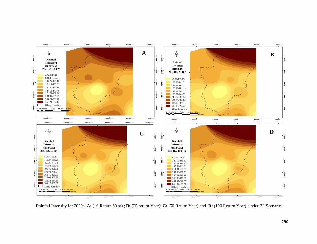
290
Rainfall Intensity for 2020s: A: (10 Return Year) ; B: (25 return Year); C: (50 Return Year) and D: (100 Return Year) under B2 Scenario
A B
C D
Rainfall
Intensity:
(mm/day)
20s, B2, 10 RY
Rainfall
Intensity:
(mm/day)
20s, B2, 25 RY
Rainfall
Intensity:
(mm/day)
20s, B2, 50 RY
Rainfall
Intensity:
(mm/day)
20s, B2, 100 RY
42.45-80.64
80.64-105.25
105.25-121.10
121.10-131.31
131.31-147.16
147.16-171.76
171.76-209.96
209.96-269.25
269.25-361.28
361.28-504.14
Klang boundary
47.90-103.75
103.75-141.21
141.21-166.32
166.32-183.16
183.16-208.27
208.27-245.72
245.72-301.58
301.58-384.88
384.88-509.15
509.15-694.47
Klang boundary
55.95-126.63
126.63-169.51
169.51-195.53
195.53-211.31
211.31-237.33
237.33-290.21
290.21-360.88
360.88-487.37
487.37-669.37
669.37-975.58
Klang boundary
51.93-115.27
115.27-155.26
155.26-180.51
180.51-196.46
196.46-221.71
221.71-261.70
261.70-325.03
325.03-425.33
425.33-584.15
584.15-835.67
Klang boundary
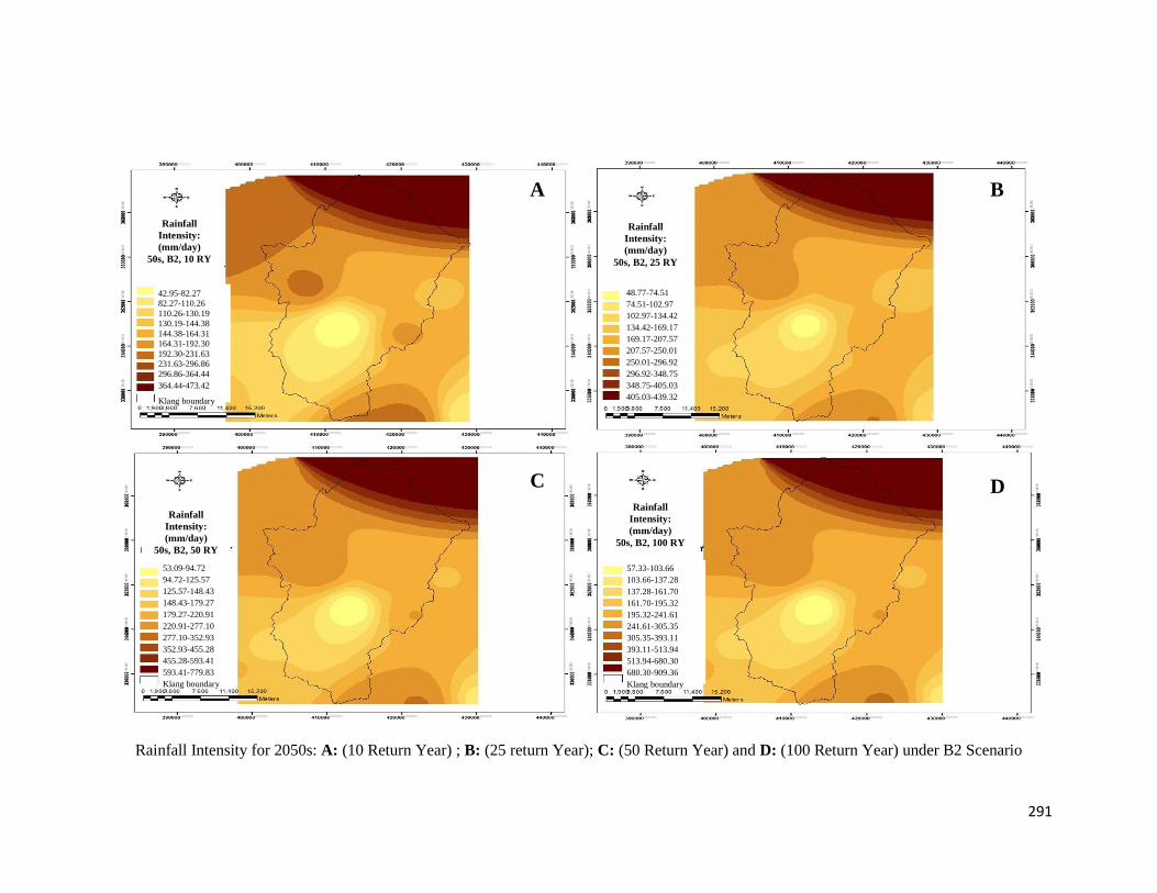
291
Rainfall Intensity for 2050s: A: (10 Return Year) ; B: (25 return Year); C: (50 Return Year) and D: (100 Return Year) under B2 Scenario
A B
C D
Rainfall
Intensity:
(mm/day)
50s, B2, 10 RY
Rainfall
Intensity:
(mm/day)
50s, B2, 25 RY
Rainfall
Intensity:
(mm/day)
50s, B2, 50 RY
Rainfall
Intensity:
(mm/day)
50s, B2, 100 RY
57.33-103.66
103.66-137.28
137.28-161.70
161.70-195.32
195.32-241.61
241.61-305.35
305.35-393.11
393.11-513.94
513.94-680.30
680.30-909.36
Klang boundary
53.09-94.72
94.72-125.57
125.57-148.43
148.43-179.27
179.27-220.91
220.91-277.10
277.10-352.93
352.93-455.28
455.28-593.41
593.41-779.83
Klang boundary
48.77-74.51
74.51-102.97
102.97-134.42
134.42-169.17
169.17-207.57
207.57-250.01
250.01-296.92
296.92-348.75
348.75-405.03
405.03-439.32
42.95-82.27
82.27-110.26
110.26-130.19
130.19-144.38
144.38-164.31
164.31-192.30
192.30-231.63
231.63-296.86
296.86-364.44
364.44-473.42
Klang boundary
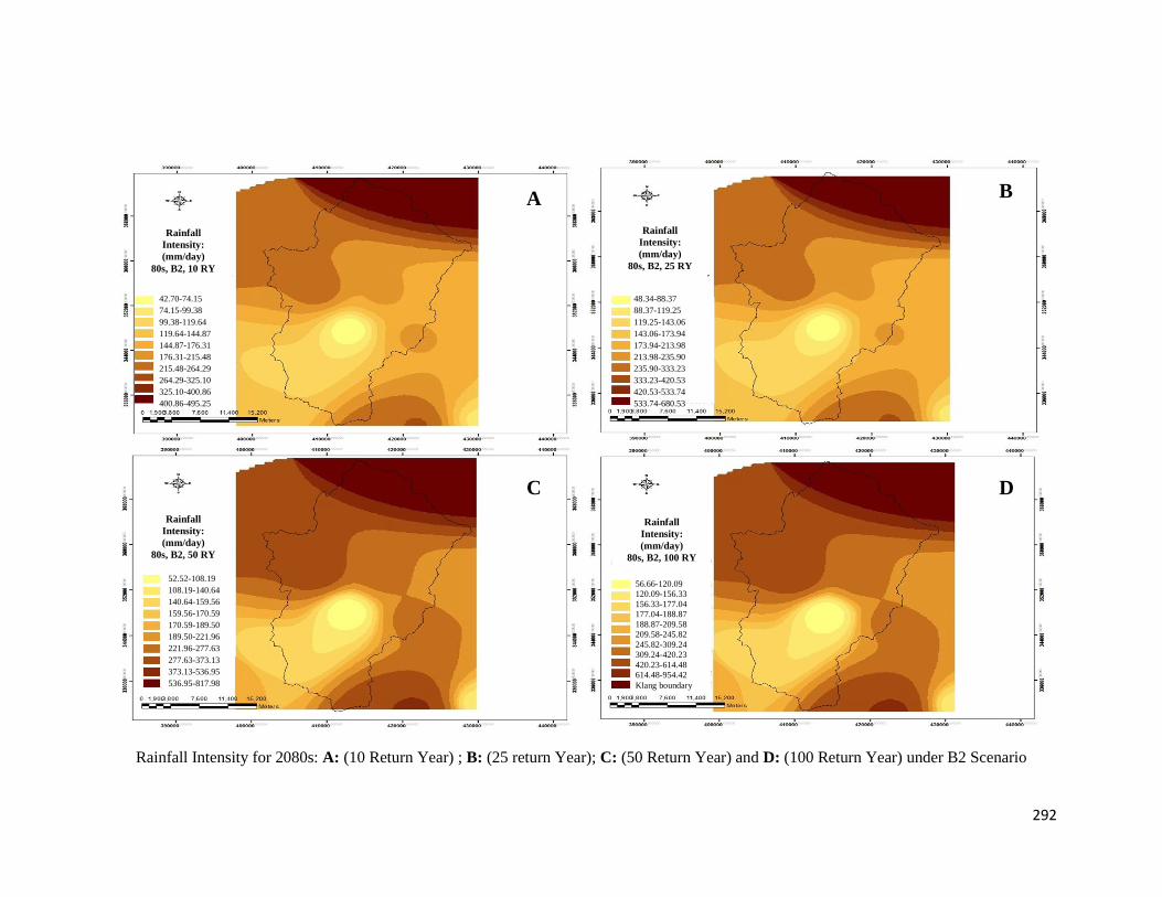
292
Rainfall Intensity for 2080s: A: (10 Return Year) ; B: (25 return Year); C: (50 Return Year) and D: (100 Return Year) under B2 Scenario
A B
C D
Rainfall
Intensity:
(mm/day)
80s, B2, 10 RY
Rainfall
Intensity:
(mm/day)
80s, B2, 25 RY
Rainfall
Intensity:
(mm/day)
80s, B2, 50 RY
Rainfall
Intensity:
(mm/day)
80s, B2, 100 RY
56.66-120.09
120.09-156.33
156.33-177.04
177.04-188.87
188.87-209.58
209.58-245.82
245.82-309.24
309.24-420.23
420.23-614.48
614.48-954.42
Klang boundary
52.52-108.19
108.19-140.64
140.64-159.56
159.56-170.59
170.59-189.50
189.50-221.96
221.96-277.63
277.63-373.13
373.13-536.95
536.95-817.98
42.70-74.15
74.15-99.38
99.38-119.64
119.64-144.87
144.87-176.31
176.31-215.48
215.48-264.29
264.29-325.10
325.10-400.86
400.86-495.25
48.34-88.37
88.37-119.25
119.25-143.06
143.06-173.94
173.94-213.98
213.98-235.90
235.90-333.23
333.23-420.53
420.53-533.74
533.74-680.53
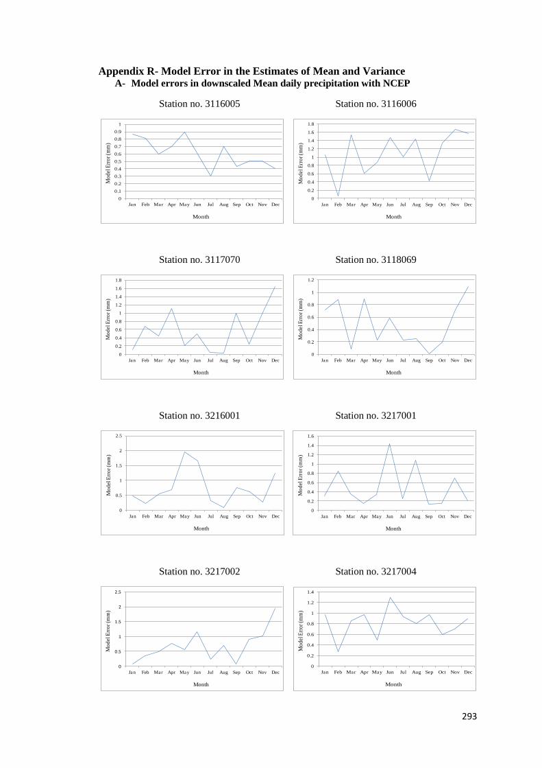
293
Appendix R- Model Error in the Estimates of Mean and Variance A- Model errors in downscaled Mean daily precipitation with NCEP
Station no. 3116005 Station no. 3116006
Station no. 3117070 Station no. 3118069
Station no. 3216001 Station no. 3217001
Station no. 3217002 Station no. 3217004
0
0.1
0.2
0.3
0.4
0.5
0.6
0.7
0.8
0.9
1
Jan Feb Mar Apr May Jun Jul Aug Sep Oct Nov Dec
Month
Mo
del
Err
or
(mm
)
0
0.2
0.4
0.6
0.8
1
1.2
1.4
1.6
1.8
Jan Feb Mar Apr May Jun Jul Aug Sep Oct Nov Dec
Month
Mo
del
Err
or
(mm
)
0
0.2
0.4
0.6
0.8
1
1.2
1.4
1.6
1.8
Jan Feb Mar Apr May Jun Jul Aug Sep Oct Nov Dec
Month
Mo
del
Err
or
(mm
)
0
0.2
0.4
0.6
0.8
1
1.2
Jan Feb Mar Apr May Jun Jul Aug Sep Oct Nov Dec
Month
Mo
del
Err
or
(mm
)
0
0.5
1
1.5
2
2.5
Jan Feb Mar Apr May Jun Jul Aug Sep Oct Nov Dec
Month
Mo
del
Err
or
(mm
)
0
0.2
0.4
0.6
0.8
1
1.2
1.4
1.6
Jan Feb Mar Apr May Jun Jul Aug Sep Oct Nov Dec
Month
Mo
del
Err
or
(mm
)
0
0.5
1
1.5
2
2.5
Jan Feb Mar Apr May Jun Jul Aug Sep Oct Nov Dec
Month
Mo
del
Err
or
(mm
)
0
0.2
0.4
0.6
0.8
1
1.2
1.4
Jan Feb Mar Apr May Jun Jul Aug Sep Oct Nov Dec
Month
Mo
del
Err
or
(mm
)
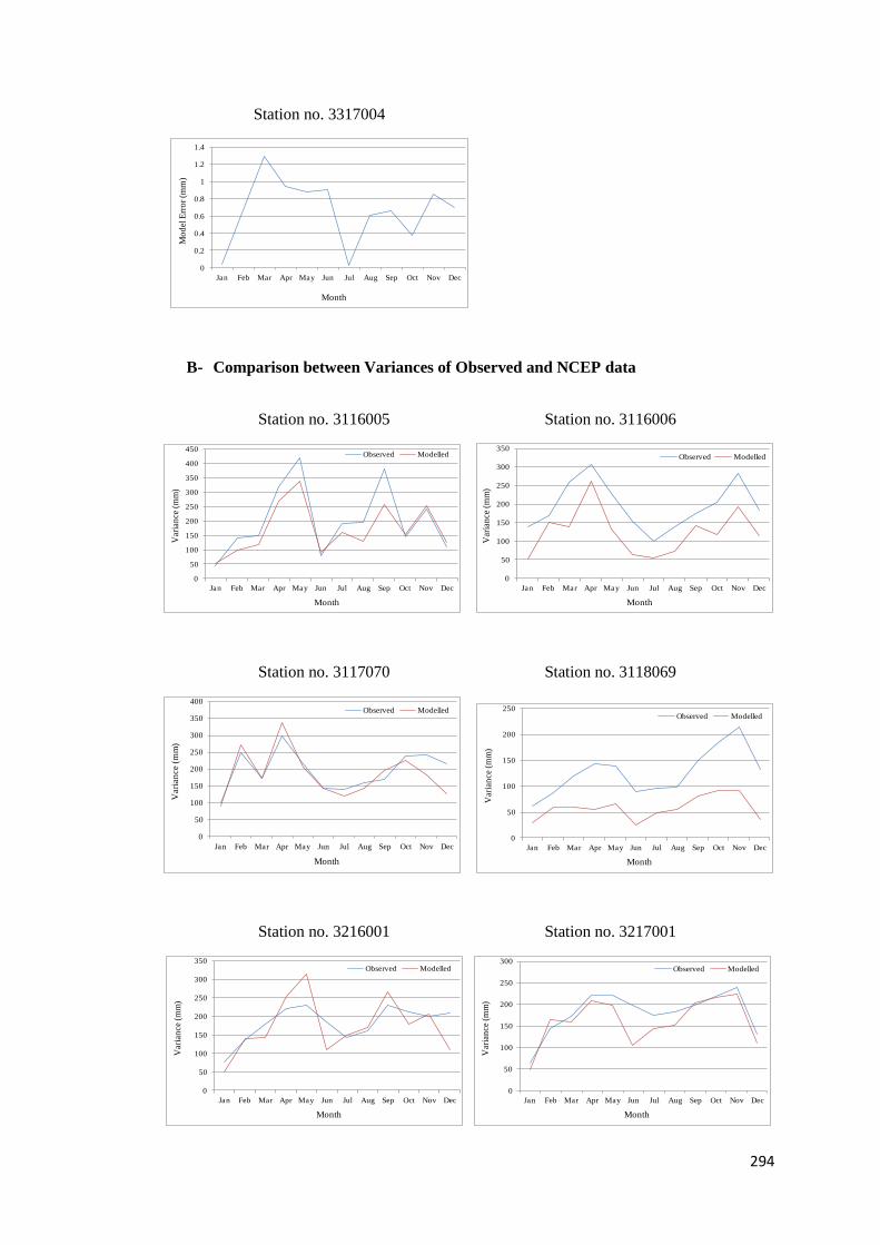
294
Station no. 3317004
B- Comparison between Variances of Observed and NCEP data
Station no. 3116005 Station no. 3116006
Station no. 3117070 Station no. 3118069
Station no. 3216001 Station no. 3217001
0
0.2
0.4
0.6
0.8
1
1.2
1.4
Jan Feb Mar Apr May Jun Jul Aug Sep Oct Nov Dec
Month
Mo
del
Err
or
(mm
)
0
50
100
150
200
250
300
350
400
450
Jan Feb Mar Apr May Jun Jul Aug Sep Oct Nov Dec
Observed Modelled
Month
Var
ian
ce (
mm
)
0
50
100
150
200
250
300
350
Jan Feb Mar Apr May Jun Jul Aug Sep Oct Nov Dec
Observed Modelled
Month
Var
ian
ce (
mm
)
0
50
100
150
200
250
300
350
400
Jan Feb Mar Apr May Jun Jul Aug Sep Oct Nov Dec
Observed Modelled
Month
Vari
an
ce (
mm
)
0
50
100
150
200
250
Jan Feb Mar Apr May Jun Jul Aug Sep Oct Nov Dec
Observed Modelled
Month
Var
ian
ce (
mm
)
0
50
100
150
200
250
300
350
Jan Feb Mar Apr May Jun Jul Aug Sep Oct Nov Dec
Observed Modelled
Month
Var
ian
ce (
mm
)
0
50
100
150
200
250
300
Jan Feb Mar Apr May Jun Jul Aug Sep Oct Nov Dec
Observed Modelled
Month
Var
ian
ce (
mm
)
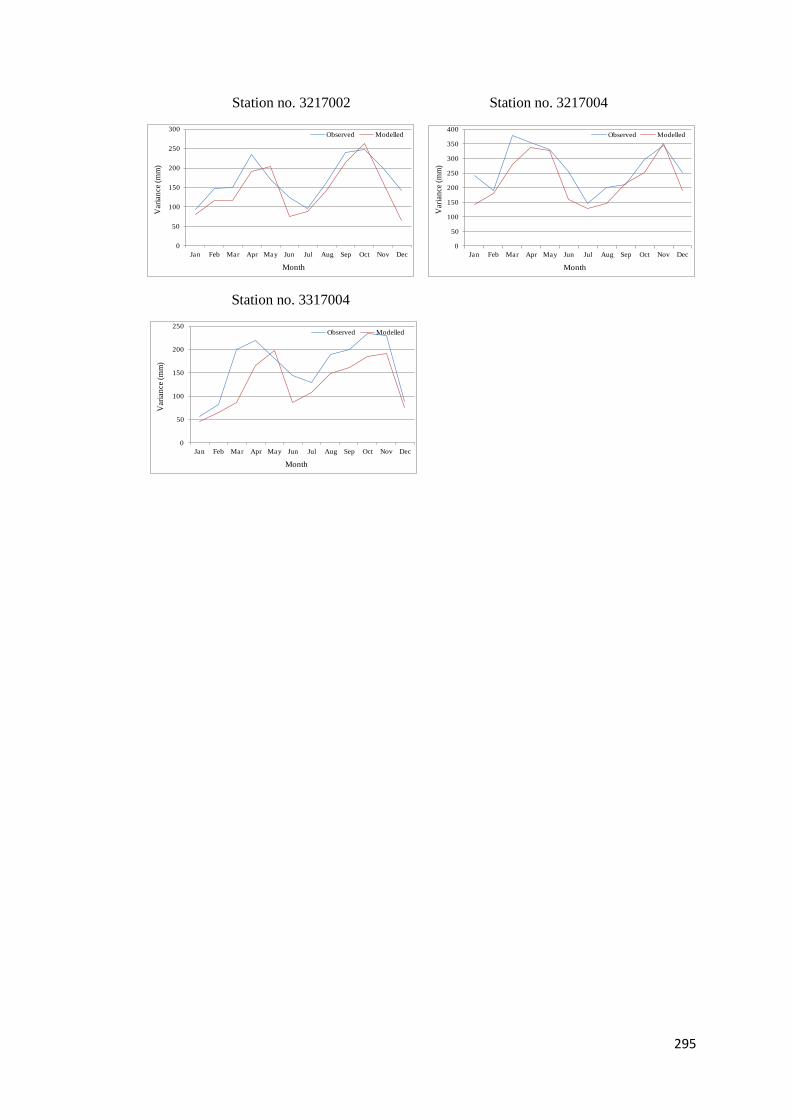
295
Station no. 3217002 Station no. 3217004
Station no. 3317004
0
50
100
150
200
250
300
Jan Feb Mar Apr May Jun Jul Aug Sep Oct Nov Dec
Observed Modelled
Month
Var
ian
ce (
mm
)
0
50
100
150
200
250
300
350
400
Jan Feb Mar Apr May Jun Jul Aug Sep Oct Nov Dec
Observed Modelled
Month
Var
ian
ce (
mm
)0
50
100
150
200
250
Jan Feb Mar Apr May Jun Jul Aug Sep Oct Nov Dec
Observed Modelled
Month
Var
ian
ce (
mm
)
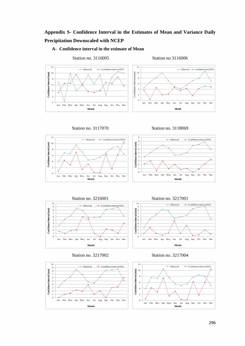
296
Appendix S- Confidence Interval in the Estimates of Mean and Variance Daily
Precipitation Downscaled with NCEP
A- Confidence interval in the estimate of Mean
Station no. 3116005 Station no 3116006
Station no. 3117070 Station no. 3118069
Station no. 3216001 Station no. 3217001
Station no. 3217002 Station no. 3217004
0
2
4
6
8
10
12
Jan Feb Mar Apr May Jun Jul Aug Sep Oct Nov Dec
Observed Confidence interval 95%
Month
Co
nfi
den
ce I
nter
val(m
m)
Month
Co
nfi
den
ce I
nter
val(m
m)
0
2
4
6
8
10
12
Jan Feb Mar Apr May Jun Jul Aug Sep Oct Nov Dec
Observed Confidence level 95%
Month
Co
nfi
den
ce I
nte
rval(m
m)
Month
0
2
4
6
8
10
12
Jan Feb Mar Apr May Jun Jul Aug Sep Oct Nov Dec
Observed Confidence interval 95%
Month
Co
nfi
den
ce I
nter
val(
mm
)
Month
Co
nfi
den
ce I
nter
val(
mm
)
0
1
2
3
4
5
6
7
8
9
Jan Feb Mar Apr May Jun Jul Aug Sep Oct Nov Dec
Observed Confidence interval 95%
Month
Co
nfi
den
ce I
nter
val(m
m)
Month
Co
nfi
den
ce I
nter
val(m
m)
0
1
2
3
4
5
6
7
8
9
10
Jan Feb Mar Apr May Jun Jul Aug Sep Oct Nov Dec
Observed Confidence interval 95%
Month
Co
nfi
den
ce I
nter
val(
mm
)
Month
Co
nfi
den
ce I
nter
val(
mm
)
0
1
2
3
4
5
6
7
8
9
10
Jan Feb Mar Apr May Jun Jul Aug Sep Oct Nov Dec
Observed Confidence interval 95%
Month
Co
nfi
den
ce I
nter
val(
mm
)
Month
Co
nfi
den
ce I
nter
val(
mm
)
0
1
2
3
4
5
6
7
8
9
10
Jan Feb Mar Apr May Jun Jul Aug Sep Oct Nov Dec
Observed Confidence interval 95%
Month
Co
nfi
den
ce I
nter
val(m
m)
Month
Co
nfi
den
ce I
nter
val(m
m)
0
2
4
6
8
10
12
Jan Feb Mar Apr May Jun Jul Aug Sep Oct Nov Dec
Observed Confidence interval 95%
Month
Co
nfi
den
ce I
nter
val(
mm
)
Month
Co
nfi
den
ce I
nter
val(
mm
)
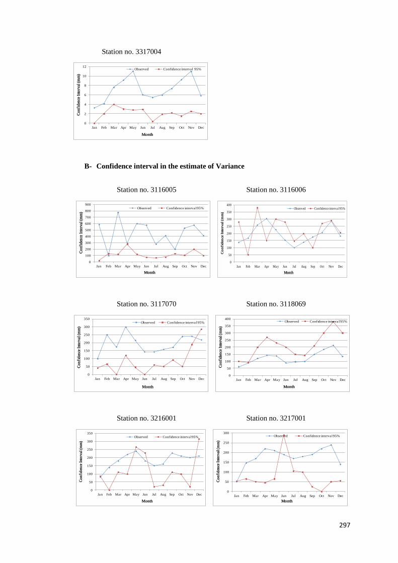
297
Station no. 3317004
B- Confidence interval in the estimate of Variance
Station no. 3116005 Station no. 3116006
Station no. 3117070 Station no. 3118069
Station no. 3216001 Station no. 3217001
0
2
4
6
8
10
12
Jan Feb Mar Apr May Jun Jul Aug Sep Oct Nov Dec
Observed Confidence interval 95%
Month
Co
nfi
den
ce I
nter
val(
mm
)
Month
Co
nfi
den
ce I
nter
val(
mm
)
0
100
200
300
400
500
600
700
800
900
Jan Feb Mar Apr May Jun Jul Aug Sep Oct Nov Dec
Observed Confidence interval 95%
Month
Co
nfi
den
ce I
nter
val(m
m)
Month
Co
nfi
den
ce I
nter
val(m
m)
0
50
100
150
200
250
300
350
400
Jan Feb Mar Apr May Jun Jul Aug Sep Oct Nov Dec
Observed Confidence interval 95%
Month
Co
nfid
en
ce I
nte
rval(m
m)
Month
Co
nfid
en
ce I
nte
rval(m
m)
0
50
100
150
200
250
300
350
Jan Feb Mar Apr May Jun Jul Aug Sep Oct Nov Dec
Observed Confidence interval 95%
Month
Co
nfi
den
ce I
nter
val(
mm
)
Month
Co
nfi
den
ce I
nter
val(
mm
)
0
50
100
150
200
250
300
350
400
Jan Feb Mar Apr May Jun Jul Aug Sep Oct Nov Dec
Observed Confidence interval 95%
Month
Co
nfi
den
ce I
nter
val(
mm
)
Month
Co
nfi
den
ce I
nter
val(
mm
)
0
50
100
150
200
250
300
350
Jan Feb Mar Apr May Jun Jul Aug Sep Oct Nov Dec
Observed Confidence interval 95%
Month
Co
nfi
den
ce I
nte
rval(
mm
)
Month
Co
nfi
den
ce I
nte
rval(
mm
)
0
50
100
150
200
250
300
Jan Feb Mar Apr May Jun Jul Aug Sep Oct Nov Dec
Observed Confidence interval 95%
Month
Co
nfi
den
ce I
nte
rval
(mm
)
Month
Co
nfi
den
ce I
nte
rval
(mm
)
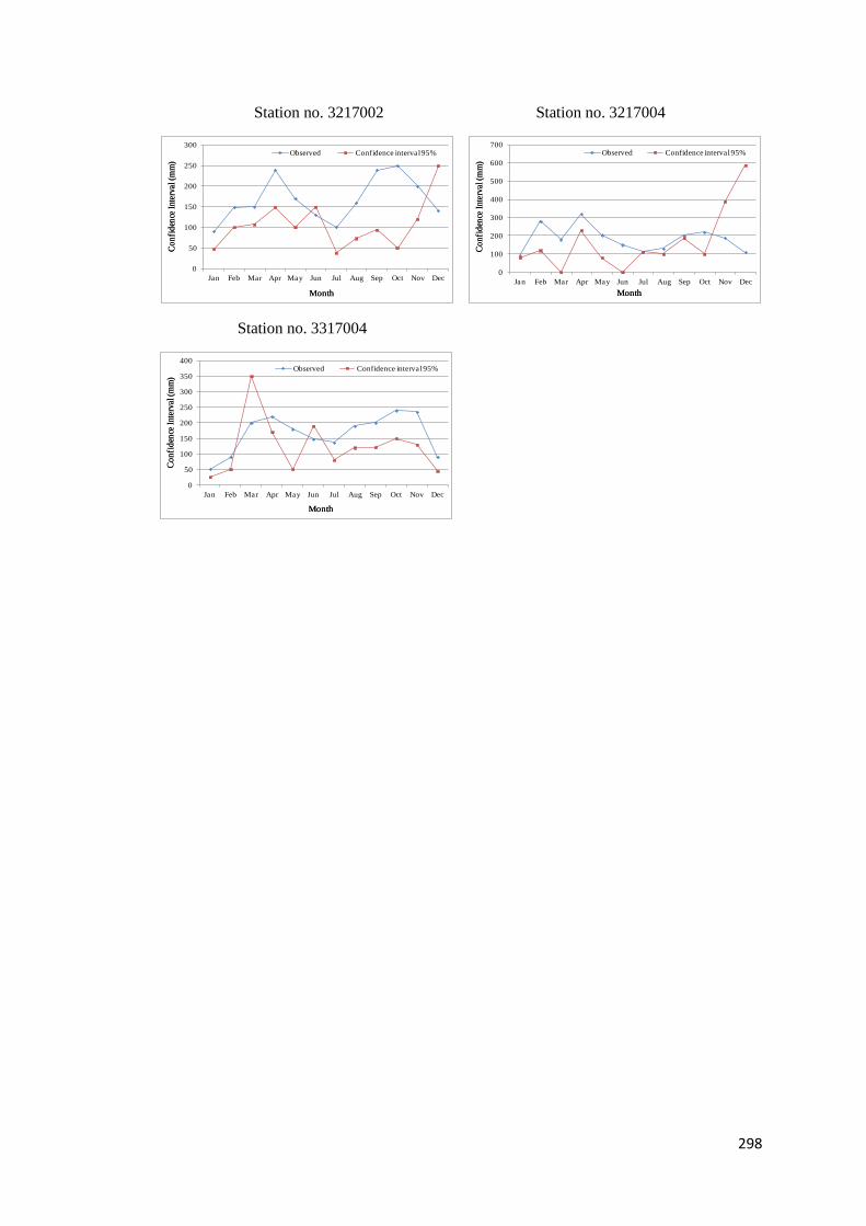
298
Station no. 3217002 Station no. 3217004
Station no. 3317004
0
50
100
150
200
250
300
Jan Feb Mar Apr May Jun Jul Aug Sep Oct Nov Dec
Observed Confidence interval 95%
Month
Co
nfi
den
ce I
nter
val(m
m)
Month
Co
nfi
den
ce I
nter
val(m
m)
0
100
200
300
400
500
600
700
Jan Feb Mar Apr May Jun Jul Aug Sep Oct Nov Dec
Observed Confidence interval 95%
Month
Co
nfi
den
ce I
nter
val(
mm
)
Month
Co
nfi
den
ce I
nter
val(
mm
)0
50
100
150
200
250
300
350
400
Jan Feb Mar Apr May Jun Jul Aug Sep Oct Nov Dec
Observed Confidence interval 95%
Month
Co
nfi
den
ce I
nter
val(
mm
)
Month
Co
nfi
den
ce I
nter
val(
mm
)