1

Assessing climate change adaptation strategies for small scale, semi-subsistence farming

L. Claessens1,2,*, J.M. Antle3, J.J. Stoorvogel2, P.K. Thornton4, M. Herrero4

1International Potato Center (CIP), P.O. Box 25171, Nairobi, Kenya, l.claessens@cgiar.org 2Wageningen University, P.O. Box 47, 6700AA Wageningen, the Netherlands, jetse.stoorvogel@wur.nl 3Oregon State University, Corvallis, Oregon, USA, jantle@montana.edu 4International Livestock Research Institute (ILRI), P.O. Box 30709, Nairobi, Kenya, p.thornton@cgiar.org, m.herrero@cgiar.org *Corresponding author, Tel.: +254204223612, Fax: +254204223001

ABSTRACT Sub-Saharan Africa (SSA) is predicted to experience considerable negative impacts of climate change. The IPCC Fourth Assessment emphasizes that adaptation strategies are essential. Addressing adaptation in the context of small-scale, semi-subsistence agriculture raises special challenges. High data demands including site-specific bio-physical and economic data are an important constraint. This calls for the development of relatively simple methods for ex ante evaluation of adaptation at the household and agricultural system levels. This paper proposes and applies a new approach to ex ante impact assessment, the Tradeoff Analysis Minimum Data (TOA-MD) methodology, which simulates economic, environmental and social outcomes in a heterogeneous farm population that can be aggregated for a regional impact assessment. The methodology uses data that are typically available in resource-poor countries. The TOA-MD approach integrates socio-economic and bio-physical data on farmers’ land allocation, production and input use. Spatially heterogeneous characteristics of the agricultural system regarding resources and productivity are analyzed and compared for both current and projected future climate (2050). Possible adaptation strategies are then assessed for their capability to overcome or reduce the adverse effects of climate change. The methodology is applied to two study areas in Kenya. After characterizing the current systems with actual climate, the effects of a perturbed climate with changed crop and livestock productivity on farmers’ livelihoods are analyzed and a number of adaptation strategies are tested. This approach offers a flexible framework for evaluating adaptation strategies using scarce data of resource-poor countries in SSA and other parts of the world. It allows a rapid integrative analysis for timely advice to farmers and policymakers and for exploration of adaptation strategies with their impacts on poverty. Keywords: adaptation; climate change; East Africa; impact assessment; sweet potato

2

1. INTRODUCTION The changing climate is exacerbating existing vulnerabilities of the poorest people who

depend on semi-subsistence agriculture for their survival (Slingo et al., 2005, IPCC, 2007, Nelson et al., 2009). Sub-Saharan Africa (SSA) in particular is predicted to experience considerable negative impacts of climate change (e.g., Thornton et al., 2006). The IPCC Fourth Assessment emphasizes that adaptation strategies are essential and these must be developed within the broader economic development policy context (IPCC, 2007). Addressing adaptation in the context of small-scale, semi-subsistence agriculture in SSA raises special challenges that cannot be addressed adequately by the approaches taken thus far in most studies (Adger et al., 2003). Most of the existing research has focused on impacts of climate change and adaptation to climate change in the agricultures of industrialized countries. In the relatively few studies conducted in Africa, agricultural research has either focused on individual crops (e.g., Hijmans, 2003, Jones and Thornton, 2003), has used aggregated data and models (e.g., Winters et al., 1998, Mendelsohn et al., 2000), or used statistical analysis that does not allow for site-specific adaptation strategies (e.g., Kurukulasuriya and Mendelsohn, 2006). IPCC and some recent studies at the sub-continental scale for Africa indicate the importance of assessing the effects of climate change and possible adaptation strategies at the agricultural system and/or household level, rather than focusing on aggregated results that hide a large amount of variability (Burke et al., 2009, Nelson et al., 2009, Thornton et al., 2009a, 2010, Baethgen, 2010). High data demands are one of the important constraints for this type of analysis because site-specific bio-physical and economic data are required, typically obtained from costly multi-year farm-level surveys. At the spatial resolution required, another drawback is that projections of climate change and simulations of the effects on crop and livestock productivity come with a high degree of variability and associated uncertainties depending on the climate models and methodologies used. The development and application of relatively simple and reliable enough methods for ex ante evaluation of adaptation strategies at the household and agricultural system levels are needed to provide timely assessments of the potential impacts in the context of climate change.

This paper describes and applies a new approach to ex ante impact assessment that produces locally useful, site-specific results that can also be aggregated for regional policy analysis. The methodology is applied to two study areas in Kenya. It makes use of the kinds of data that are more often available, especially in resource-poor countries. The approach uses and integrates available socio-economic and bio-physical data on farmers’ land use allocation, production and input and output use. Spatially heterogeneous characteristics of the agricultural system regarding resources and productivity are analyzed and compared for both current climate conditions and projected climate changes. A variety of possible adaptation strategies is then assessed for their capability to overcome or reduce the adverse effects of climate change.

2. STUDY AREAS

2.1. Vihiga Vihiga district in western Kenya lies between 1,300 and 1,500 m above sea level and covers

an area of 563 km2 of which 419 km2 is arable land (CBS, 2003) (Fig. 1). Vihiga district is broadly representative of other areas of the East African highlands found in Uganda, Ethiopia, and Madagascar in terms of soils, climate, technology, and production potential (Soule and Shepherd, 2000). The district’s high potential agricultural area is characterized by well drained nitisols that support the growing of various cash and food crops (Waithaka et al., 2006). Soil fertility is low due to leaching and continuous cropping without sufficient replenishment

3

(AFRENA, 1998, Salasya et al., 1998). Nitrogen and phosphorus are the main limiting nutrients for food crops (Soule and Shepherd, 2000). Currently the area receives adequate bimodal rainfall that ranges between 1,800 – 2,000 mm per year with heavier long rains from March to June and short rains between September and December. Temperatures are moderate and range from 14 to 32o C with limited diurnal variations.

In 1999 Vihiga district had a total population of 500,000 with a population growth rate of 2.2% (CBS, 2001). Poverty mapping in Kenya places Vihiga among the poorest districts in the country (CBS, 2003). Most households in Vihiga show a maize deficit of 200-400 kg per year, which is equivalent to shortage in six to ten months each year (Waithaka et al., 2005). The shortage is aggravated by the increasing conflicts among food, cash and fodder crops as farm sizes continue to decline. This has greatly reduced available fodder with hardly enough to feed livestock all year round. With high poverty levels, farmers do not use high-return inputs such as certified seeds, fertilizers, disease and pest control measures, and rotations, but are limited to low-input, low-return enterprises (Waithaka et al., 2006). The average household has 4.7 persons living on a 0.5 ha farm creating a high pressure on agriculture.

About 60% of the Vihiga population falls below the poverty line of 1 US$/person/day (CBS, 2003) with an average total income of 56 Kenyan Shillings (KSh) per household per day (1 US$ was equivalent to KSh 77 in mid-2005). Households obtain 65% of their income from off-farm sources in the form of wages and remittances (Waithaka et al., 2006). A high proportion of farm income is obtained from milk sales. In an effort to enhance household income and food security, farmers in the district appear to pursue risk management strategies, such as matching (i.e. the tendency of a household to produce much of the food it consumes to avoid market risk) and diversification, and hence grow many crops on their small land holdings.

The main food crops are maize, beans, sorghum, groundnuts, bananas and a variety of vegetables and the main cash crop is tea. The predominant livestock is local Zebu, which is mainly used for dairy production. Most farmers practice zero grazing and grow Napier grass for fodder, which competes with high value crops in the small holdings. With investments in transportation infrastructure, the area could have improved market opportunities as most farms are within 50 km of the large urban centers of Kakamega and Kisumu with more than 500,000 people each (CBS, 2001).

2.2. Machakos The 13,500 km2 study area is located in the Eastern Province of Kenya and contains both

Machakos and Makueni districts. Elevation ranges from 400 to 2,100 meters above sea level (Fig.1). Almost half of the total surface of the study area is under agricultural use (6,615 km2). Most of the soils in the area are deep, friable, with textures ranging from sandy clay loam to sandy clay. Inherent fertility is very poor and soils are generally deficient in nitrogen, phosphorus and soil organic carbon (<1%) (Onduru et al., 2001). The semi-arid climate in the area has low, highly variable rainfall, distributed in two rainy seasons. Short rains occur from November to January and long rains from March to June. Average annual rainfall average ranges from 500 to 1,300 mm and mean annual temperature varies from 15ºC to 25ºC, resulting in a wide range of agro-ecological conditions (MoA, 1987). Drought events do happen in cycles of four or five years, normally in runs of two or more seasons, and they have great impact on food security (Tiffen et al., 1994).

4

Agriculture is represented mainly by subsistence-oriented mixed farming systems that include both crop and livestock production, although some coffee and cotton are cultivated in the area as cash crops. Maize is the most important staple crop, but a wide variety of other food crops are grown (beans, millet and sorghum), vegetables (tomatoes and kales), fruit trees (orange, banana, mango and pawpaw) and tubers (cassava). For all crops, yields are generally low and crop failure is a common problem. Soil nutrient management through application of manure and chemical fertilizer is practiced by farmers. However, due to the relatively high prices of chemical fertilizer, this is only applied on plots that are of good quality and have less risk of crop failure, manure is more often applied on plots that do have some kind of land problem (de Jager et al., 2004). On fields with continuous cultivation without external inputs, a sharp yield decline has been observed (Lal, 2010). Soil conservation practices have been implemented in the area since colonial times. While in the 1930s the building of erosion control structures was enforced after severe land degradation took place, nowadays the majority of the farmers (almost 75%) voluntarily maintain these structures and the area is well known for the widespread use of terrace cultivation (de Jager et al., 2004, Tiffen et al., 1994). Irrigation is hardly available for the majority of the farmers but some cases exist in locations neighboring Athi river. Access to simple small-scale irrigation allows the cultivation of vegetables such as chilli peppers, tomatoes, onions and eggplant for commercial production. In such cases, where water and marketing constraints are alleviated, farmers directly respond by applying higher doses of mineral and organic fertilizer. This change in farm management results in higher and more stable yields and higher financial returns (de Jager et al., 2004). # Figure 1 approx. here#

3. MATERIALS AND METHODS

3.1. Survey data The data for Vihiga originate from the PROSAM project, ‘systems prototyping and impact

assessment for sustainable alternatives in mixed farming systems in high-potential areas of east Africa’ (Waithaka et al., 2005), that aimed to assess natural resource management interventions that promote sustainability of prototype farming systems. Farm data were collected in 2000 and 2002 (Waithaka et al., 2005, Salasya, 2005, Herrero et al., 2007). For this analysis, a selection of 119 farms was extracted from the database for which complete data (quantities and prices) on inputs (such as seeds, labor, fertilizer, and manure), outputs (crop yields, milk production and land areas), and farm management were available (Table 1). For Machakos we used similar farm survey data for 120 households in six villages obtained from studies conducted in the NUTMON project (de Jager et al. 2001, Gachimbi et al. 2005). The survey data are used to calculate net returns (mean and standard deviation) for the different activities (crops and milk production) in each study area (Table 1). Annual crops (such as fruits and non-irrigated vegetables), that are grown heterogeneously across farms and occupy very small land units in both study areas are grouped for this analysis under one activity called ‘mixed crops’. Crops such as tea, coffee, sugar cane, and woodlots are treated as fixed activities and thus are not included in this analysis.

3.2. TOA-MD as a Climate Impact and Adaptation Assessment Tool

5

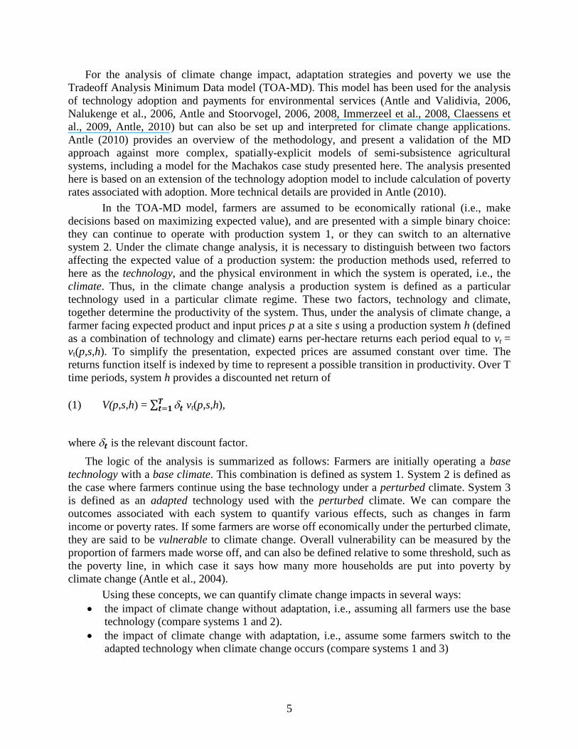
For the analysis of climate change impact, adaptation strategies and poverty we use the Tradeoff Analysis Minimum Data model (TOA-MD). This model has been used for the analysis of technology adoption and payments for environmental services (Antle and Validivia, 2006, Nalukenge et al., 2006, Antle and Stoorvogel, 2006, 2008, Immerzeel et al., 2008, Claessens et al., 2009, Antle, 2010) but can also be set up and interpreted for climate change applications. Antle (2010) provides an overview of the methodology, and present a validation of the MD approach against more complex, spatially-explicit models of semi-subsistence agricultural systems, including a model for the Machakos case study presented here. The analysis presented here is based on an extension of the technology adoption model to include calculation of poverty rates associated with adoption. More technical details are provided in Antle (2010).

In the TOA-MD model, farmers are assumed to be economically rational (i.e., make decisions based on maximizing expected value), and are presented with a simple binary choice: they can continue to operate with production system 1, or they can switch to an alternative system 2. Under the climate change analysis, it is necessary to distinguish between two factors affecting the expected value of a production system: the production methods used, referred to here as the technology, and the physical environment in which the system is operated, i.e., the climate. Thus, in the climate change analysis a production system is defined as a particular technology used in a particular climate regime. These two factors, technology and climate, together determine the productivity of the system. Thus, under the analysis of climate change, a farmer facing expected product and input prices p at a site s using a production system h (defined as a combination of technology and climate) earns per-hectare returns each period equal to vt = vt(p,s,h). To simplify the presentation, expected prices are assumed constant over time. The returns function itself is indexed by time to represent a possible transition in productivity. Over T time periods, system h provides a discounted net return of

(1) V(p,s,h) = ∑ δ𝒕𝒕𝑻𝑻

𝒕𝒕=𝟏𝟏 vt(p,s,h),

where δ𝒕𝒕 is the relevant discount factor. The logic of the analysis is summarized as follows: Farmers are initially operating a base

technology with a base climate. This combination is defined as system 1. System 2 is defined as the case where farmers continue using the base technology under a perturbed climate. System 3 is defined as an adapted technology used with the perturbed climate. We can compare the outcomes associated with each system to quantify various effects, such as changes in farm income or poverty rates. If some farmers are worse off economically under the perturbed climate, they are said to be vulnerable to climate change. Overall vulnerability can be measured by the proportion of farmers made worse off, and can also be defined relative to some threshold, such as the poverty line, in which case it says how many more households are put into poverty by climate change (Antle et al., 2004). Using these concepts, we can quantify climate change impacts in several ways:

• the impact of climate change without adaptation, i.e., assuming all farmers use the base technology (compare systems 1 and 2).

• the impact of climate change with adaptation, i.e., assume some farmers switch to the adapted technology when climate change occurs (compare systems 1 and 3)

6

• the effects of adaptation (switching from the base technology to the adapted technology) under the perturbed climate (compare systems 2 and 3).

Of course, we can also compare the two technologies under the base climate to assess how an alternative technology could impact the farm population now (e.g. Claessens et al., 2009). It is worth noting that in most analyses of climate change adaptation, it is assumed all farms use the adapted technology. However, that assumption is not appropriate, because the population of farms is heterogeneous (see for example Salasya and Stoorvogel, 2010) and farms will be impacted differently by climate change, and all farms are not necessarily adversely impacted. Using the TOA-MD model, which simulates technology adoption together with impact, we can simulate what happens when farmers can choose between the base and adapted technologies under the perturbed climate. This provides a more accurate assessment of climate change impact and the effects of adaptation.

When the production system changes, because of a change in technology or climate or both, expected returns at each site also change. The effect on a farm’s returns of changing from system j to system k is ω(p,s,j,k) = V(p,s,j) – V(p,s,k). Thus, if ω(p,s,j,k) is positive it represents the loss associated with switching from system j to system k, and if negative it represents the gain from switching from system j to k. Define the density ϕ(ω|p,j,k) as the spatial distribution of gains or losses in the population of farms indexed by s. The percentage of farms with ω(p,s,j,k) < a (with a an amount in e.g. dollars per hectare) is

(2) r(a,p,j,k) = 100 ∫ ϕ(ω| 𝒂𝒂−∞ p,j,k) dω.

Two interpretations of (2) are possible. Technology Adoption

In the standard technology adoption analysis, farms may be able to choose to continue using system j which embodies one type of technology (say, the base technology defined above), or to switch to system k which embodies a different technology (say, the adapted technology). In this case of voluntary technology adoption, note that a farm will switch if ω(p,s,j,k) = V(p,s,j) – V(p,s,k) < a, which implies V(p,s,j) < V(p,s,k) + a. Thus r(a,p,j,k) can be interpreted as the percentage of adopters of system k when they experience the gain or loss ω(p,s,j,k) from switching, and are also given a payment (if positive) or made to pay a penalty or tax (if negative) of a dollars per hectare to switch. If ω(p,s,j,k) < 0, the farmer will switch from j to k without any positive incentive payment, and r(0,p,j,k) is interpreted as the adoption rate that would occur without any incentive payment or penalty. If a government or other entity wants to encourage additional adoption, a positive incentive can be offered to adopters, in which case the adoption rate is r(a,p,j,k) > r(0,p,j,k) for a > 0. Conversely, to discourage adoption, a negative incentive (i.e., a penalty or tax) can be imposed on adopters (say, a tax on the decrease in environmental services associated with the use of system k). In order to simulate the full range of possible adoption rates in between zero and 100 percent, the simulation can be executed over a sufficiently large range of negative and positive values of a. Impact Assessment and Adaptation

7

In an impact assessment, farmers are initially using system j, and then are forced to use system k, as when the change in system represents climate change. In this type of analysis, equation (2) can be interpreted as showing the proportion of farms with losses less than a, i.e., with ω(p,s,j,k) < a. Thus, r(0,p,j,k) is interpreted as the percentage of farms that are positively impacted, and 1 – r(0,p,j,k) is interpreted as the percentage of farms that is negatively impacted. For a > 0, r(a,p,j,k) – r(0,p,j,k) can be interpreted as the percentage of farms that have losses between zero and a, for a < 0, r(0,p,j,k) – r(a,p,j,k) can be interpreted as the percentage of farms with gains between zero and –a.

When farmers are confronted with an environmental change such as climate change, they may choose a different production system that performs better in the new environment. This adaptation to climate change can be evaluated by considering an adapted technology (e.g., the system 3 described above) under the perturbed climate. By comparing the base system to the adapted system, the TOA-MD analysis shows the benefits of adaptation. For example, following the system definitions presented above, r(0,p,1,2) is the percentage of farms that are impacted positively by climate change, and we expect that with adaptation this percentage increases so that r(0,p,1,2) < r(0,p,1,3). This means that the percentage of farms negatively impacted by climate change is reduced by adaptation. In terms of standard economic analysis, the function r(a,p,j,k) defined in equation (2) has an interesting interpretation. In economic analysis of producer welfare, net returns is sometimes referred to as the firm’s producer surplus, and the change in producer surplus is used as a measure of the change in economic welfare of the firm. Thus, when systems j and k represent a change in climate, ω(p,s,j,k) measures the change in producer surplus associated with the climate change. Since r(a,p,j,k) gives the percentage of farms earning losses less than or equal to a, we can invert r(a,p,j,k) to obtain the function a(r,p,j,k). This function tells us that r percent of the population has a loss less than or equal to a, so the area under this function over an interval between 0 and 100 percent measures the change in producer surplus associated with that segment of the population:

(3) PS(r1,r2,p,j,k) = ∫ 𝒂𝒂(𝒓𝒓𝟐𝟐𝒓𝒓𝟏𝟏

r,p,j,k) dr.

Letting r0 ≡ r(0,p,j,k), those who gain from climate change are made better off by PS(0,r0,p,j,k), and those who lose are made worse off by PS(r0,1,p,j,k), with the total net gain or loss given by PS(0,1,p,j,k) = PS(0,r0,p,j,k) + PS(r0,1,p,j,k). Note that if a is measured as gain or loss per hectare, and the total land area under production is A, then the total net gain or loss over that region is A times the per-hectare value PS(0,1,p,j,k).

3.3. Climate change projections For climate change projections to 2050, we used data from the IPCC Fourth Assessment

report (2007) and downscaling techniques as described in Thornton et al. (2009a, 2010) and Jones et al. (2009). Data from two Global Circulation Models (GCMs) and two scenarios from the Special Report on Emissions Scenarios (SRES) were used. There are considerable differences between different GCMs and SRES scenarios in terms of projected changes in temperatures and rainfall. In this study we used a combination of the HadCM3 and ECHam4

8

GCMs, and SRES A1FI and B1 (very high and low emissions) on the basis of the arguments provided in Thornton et al. (2009a).

3.4. Effects of climate change on productivity and simulated adaptation strategies A summary of model settings for the base, climate change and adaptation scenarios is given

in Table 1. To simulate the potential effects of climate change on crop yields, crop growth simulation models as currently implemented in version 4.0 of the Decision Support System for Agrotechnology Transfer (DSSAT, Jones et al., 2003; ICASA, 2007) were used for maize and beans (Thornton et al., 2009a). The yields used are the mean simulated yields for four combinations of the two GCMs and SRES scenarios. Effects of CO2 fertilization were not taken into account. For both crops and both study areas, a declining yield trend is projected, caused by an increased temperature without adequate rainfall (Thornton et al., 2010). The introduction and adoption of an improved (heat/drought tolerant) maize variety, bringing yields back to 95% of the base level, is tested as an adaptation strategy in both study areas (‘imz’ in Table 1). For sweet potato, Napier and the ‘mixed crops’, no crop growth simulation models are currently available. For Napier and ‘mixed’, a 20% yield decline was estimated. The vegetables in Machakos are irrigated and no yield reduction was assumed under climate change. Drought and heat tolerant varieties of sweet potato are currently being promoted in Kenya and in general sweet potatoes are known as a reliable food security crop giving good yields in marginal climatic and soil conditions (Diop, 1998, Bovell-Benjamin, 2007, Andrade et al., 2009). For Vihiga, no yield decline was assumed under climate change for (non dual-purpose) sweet potato. Adoption of dual-purpose sweet potato (DPSP, roots for food and vines for livestock feed) is tested as an adaptation strategy and treated essentially as a new crop in both study areas (as in Claessens et al., 2009). For Vihiga, yield data for DPSP were taken from on farm field trials in nearby locations in western Kenya and eastern Uganda (Ndolo et al., 2007, Mwanga et al., 2006). For Machakos, yield data for DPSP were obtained from on farm field trials in Kibwezi, which is centrally located in the study area. We tested both the lowest quartile and average yields from these datasets (‘dpsplw’ and ‘dpsp’ respectively in Table 1). As an example, the option of substituting half of the area under the ‘mixed’ crops with DPSP was tested for both study areas.

The physiological effects of increased temperatures on animals and their productivity are well known (Blaxter, 1962; SCA, 1990). However little information is available at the local level to be able to assess impacts on animal productivity in different systems, especially in the tropics. The main effect of increased temperature is a decreased feed intake due to the inability of animals to dissipate the heat associated with digestion and metabolism of feeds (Blaxter, 1962). Above the thermo-neutral zone, intake may decrease to a point where significant reductions in milk yield can be observed (for systems with little control over the exposure of animals to climate like in Kenya). For the climate change scenario, as a proxy for heat stress, we tested a 20% milk yield reduction for both study areas, caused by a declined intake of fodder and their respective yield declines (less on farm produced fodder available for feed). Introducing DPSP as an adaptation strategy increases both quantity and quality (mainly crude protein content) of on farm produced animal feed and can substantially improve milk yields and farm incomes, even under the current climate (Claessens et al., 2009). In combination with an anticipated genetic improvement of the animals through both natural and artificial selection as adaptation strategy (Seré et al., 2008; Thornton et al., 2009b), we tested bringing up the milk yield back to 100% and 120% of the base production for both study areas (‘dpsp100’ and ‘dpsp120’ respectively in Table 1).

9

In order to obtain a more in-depth analysis of different sub-groups of farmers in the two study areas, the data from Table 1 were disaggregated in the TOA-MD model for farmers with and without dairy production. A third category of farmers, those with irrigated vegetables, was differentiated for Machakos. #Table 1 approx. here#

3.5. Effects of climate change and adaptation strategies Aggregated results of the TOA-MD analysis for both study areas are shown in Figure 2. The

interpretation of the curves is as follows: The point where a curve crosses the x axis tells the percentage of farms that gain from the scenario (i.e., the value r(0,p,j,k) discussed in section 3.2). Accordingly, the points on a curve to the left of where it crosses the x axis show the percentage of farms with gains (i.e., negative losses) greater than the amount shown on the vertical axis. Conversely, points to the right of where a curve crosses the x axis show the percentage of farms with losses less than or equal to the amount on the vertical axis. Figure 2 shows that climate change is projected to have a negative economic impact on 82% of the farmers in Vihiga and on 60% in Machakos.

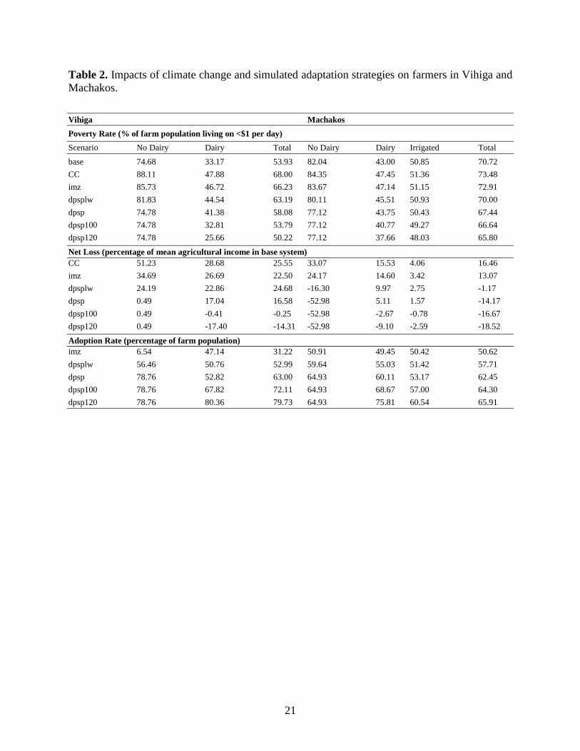
By testing different adaptation strategies with the TOA-MD model, we can simulate the aggregate economic impact on each of the study areas. As explained in the methodology, the TOA-MD model can also be used to analyze the effects of different adaptation strategies on poverty rates, and on net losses (calculated as the difference in areas under the curve above and below the x axis), and can calculate adoption rates (economic feasibility) of these strategies. Both disaggregated and aggregated impacts of the simulated adaptation strategies are shown in Table 2. The base poverty rate (expressed as % of farm population living on <$1 a day) in Machakos is higher than in Vihiga (71 vs. 54%), but in terms of net losses, Vihiga is much more negatively impacted by climate change than Machakos (26 vs. 16% loss of mean agricultural income). The introduction of an improved maize variety as adaptation strategy (bringing back yields to 95% of the base level), has very limited effect in both study areas. Substituting half of the mixed system with low yielding DPSP has almost no effect in Vihiga, but does have already a profound effect in Machakos, reducing the percentage of farmers that are negatively affected from 60 to 50% and offsetting the negative effects of climate change on the aggregate level (aggregated net gain of 1.17%, although only non-dairy producers gain in this scenario; aggregated poverty levels are back to the base level). Increasing the average yield of DPSP to the observed levels but keeping the loss in milk yield at 20%, has a positive effect in both study areas (negatively affected farmers from 82 to 50% in Vihiga and from 60 to 42% in Machakos). In general the Vihiga study area still has negative impacts of climate change (aggregated net loss of 16.58% compared with the base system) while Machakos gains with this adaptation strategy (e.g. poverty levels down with 3% compared to the base level). By increasing milk yields to 100 and 120% of the base level, Machakos has almost no additional gain, whereas in Vihiga this offsets the negative effects of climate change (poverty level slightly below base level and aggregate net gain of 0.25% for 100% milk yield) or even brings down the percentage of negatively affected farmers from 82 to 50 and 42%. Bringing in a low yielding DPSP in the cropping system of Machakos is simulated to be sufficient to offset the negative effects of climate change whereas improved fodder quantity and quality in combination with improved

10

livestock breeds that can perform under increased heat stress are and additional requirement for adaptation to climate change in Vihiga.

When we look at the disaggregated results in Table 2, it is apparent that farmers with dairy in Vihiga benefit relatively more from increases in milk yield than dairy farmers in Machakos. Vihiga has a larger percentage of dairy farmers in the whole population (62 vs. 15% in Machakos) and higher base milk yields and net returns (Table 1). Looking at adoption rates (defined here as the percentage of farmers economically benefiting from adopting an adaptation strategy), the same trends appear: increased milk yield does not affect the adoption rates in Machakos as much as it does in Vihiga. #Figure 2 approx. here# #Table 2 approx. here#

4. DISCUSSION In this paper we proposed the TOA-MD model as a methodology to test climate change

adaptation strategies with ‘minimum-data’, that is with data that are typically available for smallholder agricultural systems in resource-poor countries. There is however an inherent tradeoff between using minimum-data and the amount of uncertainty in model outcomes. The real issue of course is how much certainty one can gain with expensive and time consuming gathering of additional data or parameterizing more complex models. For both examples, existing datasets (farm surveys) were used to characterize the base systems. Various assumptions had to be made, hence substantial uncertainty is associated with the parameterization of the climate change and adaptation scenarios. As mentioned in the methodology, there is already a high level of variability in climate projections between different GCMs and SRES scenarios. The choice of a specific combination of GCMs and SRES scenarios is discussed in Thornton et al. (2009a). More uncertainty is added when downscaling GCM data to the appropriate spatial and temporal resolution to be used in the DSSAT crop growth simulation models. And there is the parameterization of the crop growth models itself which is generalizing genetic coefficients for maize and beans. Hence it is worth to stress that the projected yield changes to 2050 should merely be seen as a mean response in relation to all possible combinations of GCMs and SRES scenarios, making use of the best information we can currently obtain for crop growth simulation. It is also likely that the impacts of climate change on productivity are underestimated because the effects of increasing climate and weather variability have not been included (and this is one of the biggest constraints in rain-fed agriculture). Methods are becoming available to evaluate the effects of climate variability at the agricultural system level (Cooper et al., 2008), but there are still challenges to use the relatively coarse data of GCMs at an appropriate spatial and temporal resolution (Baethgen, 2010; Thornton et al., 2010). In addition, the effects of an increased prevalence of crop and livestock pests and diseases under climate change are also not included in the analysis. There is considerable on-going debate as to the size of the effects of CO2 fertilization on the physiology of crops (Ainsworth et al., 2008, Challinor et al., 2009), and there are more uncertainties concerning yield benefits in low-input, rain-fed subsistence production systems such as those that prevail in both study areas (Thornton et al., 2010), so we decided not to include these effects in the analysis. Productivity changes for other crops than maize and beans and for milk were estimated based on the trends for maize and beans and information we obtained from the literature. If required, changes in productivity can be subjected

11

to a sensitivity analysis (and that is in principle what bringing up the milk yields to 100 and 120% of the base level and working with lower and average observed yields for DPSP is). If productivity changes can get better substantiated with minimal effort by e.g. using additional available data or methodologies outside the TOA-MD model, then this is of course possible and desirable. In this context it is foreseen to use more elaborate livestock models to better simulate the effects of climate and feed quantity and quality on livestock productivity (e.g. Herrero et al., 2008).

The TOA-MD methodology utilized here is based on economic feasibility (expected profitability). Adoption rates should be interpreted as providing an upper bound on likely adoption rates because other factors that have been found to be important in technology adoption, such as financial constraints, risk aversion and cultural considerations are not taken into account (see Claessens et al., 2009).

The main reasons why introduction of DPSP as adaptation strategy is economically viable for a relatively large percentage of farms appear to be the relatively high yields, net returns and the positive effect of increased feed quality on milk production and income. The researchers who collected the DPSP yield data from on farm field trials (Mwanga et al., 2006, Ndolo et al., 2007) suggest that the yields they observed are higher than most farmers would achieve because crop management and soil conditions would be less favorable than in the farm trial sites. A sensitivity analysis was therefore conducted using low yielding DPSP as one of the adaptation strategies.

Both Vihiga and Machakos are broadly representative of agricultural systems in other parts of East Africa. By using an agricultural systems classification like e.g. the one by Seré and Steinfeld (1996), results could be scaled up to the agricultural system and regional scale levels.

5. CONCLUSION The development and application of relatively simple and reliable methods for assessing the

impacts of climate change and adaptation strategies at the agricultural system and/or household level are needed to provide timely recommendations on the potential impacts of alternative technologies and policies. In this paper the TOA-MD methodology was proposed to evaluate the impacts of climate change and the economic viability of adaptation strategies using limited data that are often available in resource-poor countries. The method was applied to the mixed crop-livestock systems of the Vihiga and Machakos study areas in Kenya. With a combination of simulated and estimated changes in crop and livestock productivity, the economic impacts of climate change to 2050 were analyzed. Climate change is projected to have a negative economic impact on 82% of the farmers in Vihiga and on 60% in Machakos. Different adaptation strategies were tested by changing crop and livestock productivity under climate change. For Machakos, the introduction of a low yielding variety of DPSP can already offset the negative economic impacts of climate change. For Vihiga, high yielding DPSP and improved quantity and quality of feed and livestock breeds adapted to increased temperatures are needed to counter the effects of climate change and improve farmers’ livelihoods. As in all scenario studies using models, and especially in the context of climate change, various assumptions and uncertainties are associated with using the proposed approach and results should be interpreted with caution. But despite the limitations of the methodology, this study yielded insights into the way different adaptation strategies could assist in improving the livelihoods of smallholder farmers operating in the mixed crop-livestock systems in East Africa. The TOA-MD approach offers a rapid integrative analysis for exploring options and timely advice to farmers and policymakers.

12

Acknowledgements This research was conducted within the framework of a project funded by BMZ/GTZ on behalf of the Government of the Federal Republic of Germany. This study used data from the PROSAM and NUTMON Projects, co-funded by the Ecoregional Fund to Support Methodological Initiatives of the Dutch government.

6. REFERENCES

Adger, W. N., Huq, S., Brown, K., Conway, D., Hulme, M., 2003. Adaptation to climate change in the developing world. Progress in Development Studies 3(3), 179-195.

Ainsworth, E.A., Leakey, A.D.B., Ort, D.R., Long, S.P., 2008. FACE-ing the facts: inconsistencies and interdependence among field, chamber and modeling studies of elevated CO2 impacts on crop yield and food supply. The New Phytologist 179, 5–9.

AFRENA, 1998. Agroforestry Potential for Land Use Systems in the Bimodal Highlands of Eastern Africa. AFRENA Report No. 3, ICRAF, Nairobi, Kenya.

Andrade, M., Barker, I., Cole, D., Dapaah, H., Elliott, H., Fuentes, S., Grüneberg, W., Kapinga, R., Kroschel, J., Labarta, R., Lemaga, B., Loechl, C., Low, J., Lynam , J., Mwanga, R., Ortiz, O., Oswald, A., Thiele, G., 2009. Unleashing the potential of sweetpotato in Sub-Saharan Africa: Current challenges and way forward. International Potato Center (CIP), Lima, Peru. Working Paper 2009-1. 197 p.

Antle, J.M., 2010. Parsimonious Technology Impact Assessment. American Journal of Agricultural Economics, in press.

Antle, J.M., Stoorvogel, J.J., 2006. Predicting the supply of ecosystem services from agriculture American Journal of Agricultural Economics, 88(5), 1174-1180.

Antle, J.M., Stoorvogel, J.J., 2008. Agricultural carbon sequestration, poverty and sustainability. Environment and Development Economics 13, 327-352.

Antle, J.M., Valdivia, R.O., 2006. Modelling the supply of ecosystem services from agriculture: a minimum-data approach. The Australian Journal of Agricultural and Resource Economics 50: 1–15.

Antle, J.M., B. Diagana, J. Stoorvogel, Valdivia, R.O., 2010. Minimum-Data Analysis of Ecosystem Service Supply in Semi-Subsistence Agricultural Systems: Evidence from Kenya and Senegal. Australian Journal of Agricultural and Resource Economics, in press.

Baethgen, W.E., 2010. Climate Risk Management for Adaptation to Climate Variability and Change. Crop Science 50, 70-76.

Blaxter, K.L., 1962. The Energy Metabolism of Ruminants. Hutchingson Press, London, UK.

Bovell-Benjamin, A., 2007. Sweet potato: a review of its past, present, and future role in human nutrition. Advances in Food and Nutrition Research 52, 1-59.

Burke, M.B., Lobell, D.B., Guarino, L., 2009. Shifts in African crop climates by 2050, and the implications for crop improvement and genetic resources conservation. Global Environmental Change 19(3), 317-325.

13

Central Bureau of Statistics (CBS), 2001. Population and housing census. Counting our people for development. Vol.1. Population distribution by administrative areas and urban centres. Ministry of Finance and Planning, Nairobi, Kenya.

Central Bureau of Statistics (CBS), 2003. Geographic dimensions of well-being in Kenya. Where are the poor? From districts to locations. Vol.1. CBS, Ministry of Planning and National Development, Nairobi, Kenya.

Challinor, A.J., Ewert, F., Arnold, S., Simelton, E., Fraser, E., 2009. Crops and climate change: progress, trends, and challenges in simulating impacts and informing adaptation. Journal of Experimental Botany 60(10), 2775-2789.

Claessens, L., Stoorvogel, J.J., Antle, J.M., 2009. Ex ante assessment of dual-purpose sweet potato in the crop-livestock system of western Kenya: A minimum-data approach. Agricultural Systems 99(1), 13-22.

Cooper, P.J.M., Dimes, J., Rao, K.P.C., Shapiro, B., Shiferawa, B., Twomlow, S., 2008. Coping better with current climatic variability in the rain-fed farming systems of sub-Saharan Africa: an essential first step in adapting to future climate change? Agriculture, Ecosystems and Environment 126, 24–35.

de Jager, A., D. Onduru, M. S. van Wijk, J. Vlaming, Gachini, G. N., 2001. Assessing sustainability of low-external-input farm management systems with the nutrient monitoring approach, a case study in Kenya, Agricultural Systems 69(1-2), 99-118.

de Jager, A., van Keulen, H., Mainah, F., Gachimbi, L.N., Itabari, J.K., Thuranira, E.G., Karuku, A.M., 2004. Attaining sustainable farm management systems in semi-arid areas in Kenya: few technical options, many policy challenges. Final Project Report (draft). Wageningen University and Research Center, The Netherlands.

Diop, A., 1998. Storage and processing of roots and tubers in the tropics. In ‘‘Food and Agriculture Organization of the United Nations, Agro-Industries and Post-Harvest Management Service’’ (D.J.B. Calverley, ed.), pp. 38–50. Agricultural Support Systems Division. Food and Agriculture Organization, Rome, Italy.

Easterling, W., Apps, M., 2005. Assessing the consequences of climate change for food and forest resources: a view from the IPCC. Climatic Change 70,165-189.

Gachimbi, L. N., H. van Keulen, E. G. Thuranira, A. M. Karuku, A. Jager, S. Nguluu, B. M. Ikombo, J. M. Kinama, J. K. Itabari, Nandwa, S. M., 2005. Nutrient balances at farm level in Machakos (Kenya), using a participatory nutrient monitoring (NUTMON) approach, Land Use Policy 22(1), 13-22.

ICASA, 2007. The International Consortium for Agricultural Systems Applications website. Online at www.icasa.net.

Immerzeel, W., J. Stoorvogel, Antle, J., 2008. Can payments for ecosystem services secure the water tower of Tibet? Agricultural Systems 96(1-3), 52-63.

IPCC (Intergovernmental Panel on Climate Change), 2007. Climate Change 2007: Impacts, Adaptation and Vulnerability. Contribution of Working Group II to the Fourth Assessment Report of the Intergovernmental Panel on Climate Change. Cambridge University Press, Cambridge, UK.

14

Herrero, M., Thornton, P.K., Kruska, R., Reid, R.S., 2008. Systems dynamics and the spatial distribution of methane emissions from African domestic ruminants to 2030. Agriculture Ecosystems and Environment 126, 122-137.

Hijmans, R.J., 2003. The effect of climate change on global potato production. American Journal of Potato Research 80(4), 271-280.

Jaetzold, R., Schmidt, H., 1983. Farm Management Handbook of Kenya. Natural Conditions and Farm Management Information, vol. 2. Ministry of Agriculture, Nairobi, Kenya.

Jones, J.W., Hoogenboom, G., Porter, C.H., Boote, K.J., Batchelor, W.D., Hunt, L.A., Wilkens, P.W., Singh, U., Gijsman, A.J., Ritchie, J.T., 2003. The DSSAT cropping system model. European Journal of Agronomy 18, 235-265.

Jones, P.G., Thornton, P.K., 2003. The potential impacts of climate change on maize production in Africa and Latin America in 2055. Global Environmental Change 13(1), 51-59.

Jones, P. G., Thornton, P. K., Heinke, J., 2009. Software to generate characteristic daily weather data at any resolution using downscaled climate model data from the IPCC's Fourth Assessment. BMZ Project Discussion Paper, ILRI, Nairobi.

Kurukulasuriya, P., Mendelsohn, R., 2006. Crop Selection: Adapting Climate Change in Africa. CEEPA Publication 26. http://www.ceepa.co.za/docs/CDPNo26.pdf

Lal, R., 2010. Enhancing Eco-efficiency in Agro-ecosystems through Soil Carbon Sequestration. Crop Science 50, 120-131.

Mendelsohn, R., Morrison, W., Schlesinger, M.E., Andronova, N.G., 2000. Country-Specific Market Impacts of Climate Change. Climatic Change 45(3-4), 553-569.

MoA, 1987. Fertilizer Use Recommendation Project (Phase I). Ministry of Agriculture, National Agricultural Research Laboratories, Nairobi, Kenya.

Mwanga, R.O.M., Stevenson, R.C., Yencho, C.G., 2006. Development of High Yielding Multiple Resistant Sweet Potato Germplasm. Harvest Plus Research Progress Report April 1, 2005 through March 31, 2006.

Nalukenge, I., Antle, J.M., Stoorvogel J.J., Claessens, L., 2006. Payments for Environmental Services (PES) as a new approach to tackle land degradation in Pallisa District. Workshop Report USAID (Soil Management CRSP) and FAO, Pallisa, Uganda.

Ndolo J., P., Gethi, J., Agili, S., 2007. Potential of improved orange fleshed sweet potato clones in different agro-ecologies in Kenya. In: Eighth African Crop Science Society Conference, El-Minia, Egypt, 2007 October 27–31.

Nelson, G.C., Rosegrant, M.W., Koo, J., Robertson, R., Sulser, T., Zhu, T., Ringler, C., Msangi, S., Palazzo, A., Batka, M., Magalhaes, M., Valmonte-Santos, R., Ewing, M., Lee, D., 2009. Climate change: impact on agriculture and costs of adaptation. Food Policy Report 21, International Food Policy Research Institute (IFPRI), Washington DC, USA.

Onduru, D.D., A. de Jager, G. Gachini, and D. J.M., 2001. Exploring new pathways for innovative soil fertility management in Kenya Managing Africa's Soils. IIED-Drylands Programme.

15

Salasya, B.D.S., 2005. Crop production and soil nutrient management: an economic analysis of households in western and central Kenya. PhD Thesis, Wageningen University, Wageningen, The Netherlands.

Salasya, B.D.S., Mwangi, W., Hugo, V., 1998. Assessment of the Adoption of Seed and fertilizer Packages and the role of Credit in Smallholder Maize Production in Western Kenya. In: EARO, C.a. (Editor), 6th East and Southern Africa Regional Maize conference, Addis Ababa, Ethiopia, pp. 357-360.

Salasya, B.D.S., Stoorvogel, J.J., 2010. Fuzzy classification for farm household characterization. Outlook on Agriculture 39: 57–63.

SCA, 1990. Feeding systems for Australian livestock: Ruminants. Standing Subcommittee on Agriculture, Commonwealth Scientific and Industrial Research Organisation (CSIRO). CSIRO Publications, Melbourne, Australia.

Seré, C., Steinfeld, H., 1996. World livestock production systems: Current status, issues and trends. FAO Animal Production and Health Paper 127. FAO (Food and Agriculture Organization of the United Nations), Rome, Italy.

Seré, C., van der Zijpp, A., Persley, G., Rege, E., 2008. Dynamics of livestock production systems, drivers of change and prospects for animal genetic resources. Animal Genetic Resources Information 42, 3-27.

Slingo,J. M., Challinor, A. J., Hoskins, B. J., Wheeler, T. R., 2005. Food crops in a changing climate. Philosophical Transactions of the Royal Society B 360(1463), 1983-1989.

Soule, M.J., Shepherd, K.D., 2000. An ecological and economic analysis of phosphorus replenishment for Vihiga Division, western Kenya. Agricultural Systems 64(2), 83-98.

Thornton, P.K., Jones, P.G., Owiyo, T., Kruska, R.L., Herrero, M., Kristjanson, P., Notenbaert, A., Bekele, N., Omolo, A., with contributions from Orindi, V., Ochieng, A., Otiende, B., Bhadwal, S., Anantram, K., Nair, S., Kumar, V., Kelkar, U., 2006. Mapping climate vulnerability and poverty in Africa. Report to the Department for International Development, ILRI, Nairobi, Kenya, May 2006, 200 pp. http://www.dfid.gov.uk/research/mapping-climate.pdf.

Thornton, P.K., Jones, P.G., Alagarswamy, G., Andresen, J., 2009a. Spatial variation of crop yield response to climate change in East Africa. Global Environmental Change 19(1), 54-65.

Thornton, P.K., van de Steeg, J., Notenbaert, A., Herrero, M., 2009b. The impacts of climate change on livestock and livestock systems in developing countries: A review of what we know and what we need to know. Agricultural Systems 101, 113-127.

Thornton, P.K., Jones, P.G., Alagarswamy, G., Andresen, J., Herrero, M., 2010. Adapting to climate change: Agricultural system and household impacts in East Africa. Agricultural Systems 103, 73-82.

Tiffen, M., M. Mortimore, Gichuki., F., 1994 More people, less erosion: environmental recovery in Kenya. Wiley & Sons, Sussex.

Waithaka, M.M., Thornton, P.K., Herrero, M., Shepherd, K.D., Stoorvogel, J.J., Salasya, B., Ndiwa, N., Bekele, N., Croucher, M., Karanja, S., Booltink, H., 2005. System prototyping

16

and impact assessment for sustainable alternatives in mixed farming systems in high-potential areas of Eastern Africa. Final Program Report to the Ecoregional Fund to Support Methodological Initiatives.

Waithaka, M.M., Thornton, P.K., Herrero, M., Shepherd, K.D., 2006. Bio-economic evaluation of farmers' perceptions of viable farms in western Kenya. Agricultural Systems 90(1-3), 243-271.

Winters, P., Murgai, R., Sadoulet, E., de Janvry, A., Frisvold, G., 1998. Economic and Welfare Impacts of Climate Change on Developing Countries. Environmental & Resource Economics 12(1), 1-24.

17

Figure 1. Location of the study areas in Kenya. The Machakos study area comprises both Machakos and Makueni districts.

18

Figure 2. Economic impact of climate change and simulated adaptation strategies on farmers in Vihiga and Machakos-Makueni, Kenya. Notation of legend as in Table 1.

19

Table 1. Summary of data used in the TOA-MD analysis. Characterization of base system from survey data (means with standard deviation between brackets). Alternative systems are expressed as % of base system productivity (100%). Vihiga Base System Alternative Systems*

System 1 System 2 System 3 Activities Area Crop Yield Net Returns CC imz dpsplw dpsp dpsp100 dpsp120 Ha/season/farm Kg/ha/season KSh/ha ----------------------------% of base yield---------------------------------------- Maize-Beans 0.24 (0.21) 1512 (1319) 15360 (16726) 68 95 68 68 68 68 Napier Grass 0.16 (0.19) 34450 (23643) 22366 (23545) 80 80 80 80 80 80 Mixed 0.23 (0.21) 4031 (1701) 27551 (15971) 80 80 80 80 80 80 Sweet potato 0.05 (0.04) 4006 (2092) 11587 (8352) 100 100 100 100 100 100 DPSP roots - 8000 (3676) 27618 (13233) - - 37.5 100 100 100 DPSP vines - 14800 (8036) 21018 (12054) - - 70 100 100 100 Liters/season/farm Milk - 3211 (2473) 52317 (51723) 80 80 80 80 100 120 Machakos Base System Alternative Systems*

System 1 System 2 System 3 Activities Area Crop Yield Net Returns CC imz dpsplw dpsp dpsp100 dpsp120

Ha/season/farm Kg/ha/season KSh/ha ---------------------------% of base yield-----------------------------------------

Mixed 0.95 (1.39) 1187 (1631) 7085 (13313) 80 80 80 80 80 80 Maize 0.78 (0.79) 1597 (1624) 12704 (16996) 75 95 75 75 75 75 Beans 0.44 (0.59) 1390 (1374) 24658 (17942) 75 75 75 75 75 75 Vegetables 0.75 (1.00) 4121 (3369) 40718 (139490) 100 100 100 100 100 100 Napier Grass 1.49 (3.10) 12318 (14435) 11310 (18146) 80 80 80 80 80 80 DPSP roots - 7100 (4501) 24475 (16204) - - 42 100 100 100 DPSP vines - 12600 (9013) 18900 (13520) - - 83 100 100 100

Liters/season/farm Milk - 1784 (1992) 39238 (48208) 80 80 80 80 100 120

20

*CC = climate change, imz = improved maize, dpsp = dual purpose sweet potato, dpsplw = low yielding dpsp, dpsp100 = dpsp with 100% of base milk yield under CC, dpsp120 = dpsp with 120% of base milk yield under CC.

21

Table 2. Impacts of climate change and simulated adaptation strategies on farmers in Vihiga and Machakos. Vihiga Machakos Poverty Rate (% of farm population living on <$1 per day) Scenario No Dairy Dairy Total No Dairy Dairy Irrigated Total

base 74.68 33.17 53.93 82.04 43.00 50.85 70.72 CC 88.11 47.88 68.00 84.35 47.45 51.36 73.48 imz 85.73 46.72 66.23 83.67 47.14 51.15 72.91 dpsplw 81.83 44.54 63.19 80.11 45.51 50.93 70.00 dpsp 74.78 41.38 58.08 77.12 43.75 50.43 67.44 dpsp100 74.78 32.81 53.79 77.12 40.77 49.27 66.64 dpsp120 74.78 25.66 50.22 77.12 37.66 48.03 65.80

Net Loss (percentage of mean agricultural income in base system) CC 51.23 28.68 25.55 33.07 15.53 4.06 16.46 imz 34.69 26.69 22.50 24.17 14.60 3.42 13.07 dpsplw 24.19 22.86 24.68 -16.30 9.97 2.75 -1.17 dpsp 0.49 17.04 16.58 -52.98 5.11 1.57 -14.17 dpsp100 0.49 -0.41 -0.25 -52.98 -2.67 -0.78 -16.67 dpsp120 0.49 -17.40 -14.31 -52.98 -9.10 -2.59 -18.52

Adoption Rate (percentage of farm population) imz 6.54 47.14 31.22 50.91 49.45 50.42 50.62 dpsplw 56.46 50.76 52.99 59.64 55.03 51.42 57.71 dpsp 78.76 52.82 63.00 64.93 60.11 53.17 62.45 dpsp100 78.76 67.82 72.11 64.93 68.67 57.00 64.30 dpsp120 78.76 80.36 79.73 64.93 75.81 60.54 65.91