Asian Development Review: Volume 39, Number 1
358
World Scientific Asian Development Review Volume 39 · Number 1 · March 2022 Mini Symposium on Demographic Change and Human Capital in Asia Guest Editor: Isaac Ehrlich A Cross-Country Comparison of Old-Age Financial Readiness in Asian Countries versus the United States: The Case of Japan and the Republic of Korea Isaac Ehrlich and Yong Yin Educational Gradients in Disability among Asia’s Future Elderly: Projections for the Republic of Korea and Singapore Cynthia Chen, Jue Tao Lim, Ngee Choon Chia, Daejung Kim, Haemi Park, Lijia Wang, Bryan Tysinger, Michelle Zhao, Alex R. Cook, Ming Zhe Chong, Jian-Min Yuan, Stefan Ma, Kelvin Bryan Tan, Tze Pin Ng, Koh Woon-Puay, Joanne Yoong, Jay Bhattacharya, and Karen Eggleston Cognitive Functioning among Older Adults in Japan and Other Selected Asian Countries: In Search of a Better Way to Remeasure Population Aging Naohiro Ogawa, Taiyo Fukai, Norma Mansor, and Nurul Diyana Kamarulzaman Demographic Change, Economic Growth, and Old-Age Economic Security: Asia and the World Andrew Mason, Sang-Hyop Lee, and Donghyun Park Trends in Employment and Wages of Female and Male Workers in India: A Task-Content-Of-Occupations Approach Shruti Sharma (Continued )
-
Upload
khangminh22 -
Category
Documents
-
view
0 -
download
0
Transcript of Asian Development Review: Volume 39, Number 1

World Scientific
Vol. 39 • N
o. 1 • M
arch 2022ISSN: 0116-1105
Asian Development ReviewThe Asian Development Review (ADR) is a professional journal that publishes research on development issues relevant to the Asia and Pacific region, specifically members of the Asian Development Bank. The ADR publishes high-quality empirical papers, survey articles, historical analyses, and policy-oriented work. The ADR bridges theoretical work and rigorous empirical studies that advance the understanding of Asia’s development; and it is open to discussions of alternative perspectives on all aspects of development, including globalization, inequality, structural transformation, and poverty. The ADR aims to disseminate the best research, with contributions from scholars in all fields, with the objective of providing the knowledge necessary for designing, implementing, and sustaining effective development policies. Its intended audience comprises a worldwide readership of economists and other social scientists.
Asian Development ReviewVolume 39 · Number 1 · March 2022Asian Development Review
MCI (P) 076/09/2021
Volume 39 2022 Number 1
Mini Symposium on Demographic Change andHuman Capital in Asia 1
Guest Editor: Isaac Ehrlich
A Cross-Country Comparison of Old-Age FinancialReadiness in Asian Countries versus the United States:The Case of Japan and the Republic of Korea 5
Isaac Ehrlich and Yong Yin
Educational Gradients in Disability among Asia’s FutureElderly: Projections for the Republic of Korea andSingapore 51
Cynthia Chen, Jue Tao Lim, Ngee Choon Chia, Daejung Kim,Haemi Park, Lijia Wang, Bryan Tysinger, Michelle Zhao,Alex R. Cook, Ming Zhe Chong, Jian-Min Yuan, Stefan Ma,Kelvin Bryan Tan, Tze Pin Ng, Koh Woon-Puay, Joanne Yoong,Jay Bhattacharya, and Karen Eggleston
Cognitive Functioning among Older Adults in Japan andOther Selected Asian Countries: In Search of a Better Wayto Remeasure Population Aging 91
Naohiro Ogawa, Taiyo Fukai, Norma Mansor, andNurul Diyana Kamarulzaman
Demographic Change, Economic Growth, and Old-AgeEconomic Security: Asia and the World 131
Andrew Mason, Sang-Hyop Lee, and Donghyun Park
Trends in Employment and Wages of Female and MaleWorkers in India: A Task-Content-Of-OccupationsApproach 169
Shruti Sharma
(Continued )
March 23, 2022 1:06:35pm WSPC/331-ADR content ISSN: 0116-1105FA1

EDITORS
ALBERT PARK, Asian Development BankTETSUSHI SONOBE, Asian Development Bank Institute
MANAGING EDITOR
JESUS FELIPE, Asian Development Bank
EDITORIAL TEAM MEMBERS
GEMMA ESTHER B. ESTRADA, Asian Development BankORLEE P. VELARDE, Asian Development Bank
EDITORIAL BOARD
KYM ANDERSON, University of AdelaidePREMA-CHANDRA ATHUKORALA,
Australian National UniversityKLAUS DESMET, Southern Methodist UniversityJESUS FELIPE, Asian Development BankNEIL FOSTER-MCGREGOR, UNU-MERITSHIN-ICHI FUKUDA, The University of TokyoRANA HASAN, Asian Development BankSUNG JIN KANG, Korea UniversityHONGBIN LI, Stanford University
XIN MENG, Australian National UniversityAHMED MUSHFIQ MOBARAK, Yale UniversityNANCY QIAN, Northwestern UniversityKRISLERT SAMPHANTHARAK, University of
California, San DiegoKUNAL SEN, UNU-WIDER and The University of
ManchesterAYA SUZUKI, The University of TokyoMAISY WONG, University of PennsylvaniaJOSEPH E. ZVEGLICH, JR., Asian Development Bank
The Asian Development Review is a professional journal for disseminating the results of economic anddevelopment research relevant to Asia. The journal seeks high-quality papers done in an empirically rigorous way.Articles are intended for readership among economists and social scientists in government, private sector,academia, and international organizations.
The views expressed in this publication are those of the authors and do not necessarily reflect the views andpolicies of the Asian Development Bank (ADB), the Asian Development Bank Institute (ADBI), the ADB Boardof Governors, or the governments they represent.
ADB and ADBI do not guarantee the accuracy of the data included in this publication and accept noresponsibility for any consequence of their use.
By making any designation of or reference to a particular territory or geographic area, or by using the term“country” in this document, ADB and ADBI do not intend to make any judgments as to the legal or other status ofany territory or area.
Please direct all editorial correspondence to the Managing Editor, Asian Development Review, EconomicResearch and Regional Cooperation Department, Asian Development Bank, 6 ADB Avenue, Mandaluyong City,1550 Metro Manila, Philippines. E-mail: [email protected].
Notes: In this publication, \$" refers to United States dollars, unless otherwise stated.ADB recognizes \China" as the People’s Republic of China, \Korea" and \South Korea" as the Republic of
Korea, \United States of America" as the United States, and \Vietnam" as Viet Nam.For more information, please visit the website of the publicationat www.adb.org/publications/series/asian-development-review.
March 23, 2022 3:29:46pm WSPC/ADB ISSN: XXXX-XXXX

CONTENTS — (Continued )
Open Submissions
Disability and Intrahousehold Investment Decisions inEducation: Empirical Evidence from Bangladesh 201
Kamal Lamichhane and Takaki Takeda
The Social Costs of Success: The Impact of World TradeOrganization Rules on Insulin Prices in Bangladesh uponGraduation from Least Developed Country Status 239
Md. Deen Islam, Warren A. Kaplan, Veronika J. Wirtz, andKevin P. Gallagher
Institutions and the Rate of Return on Cattle: Evidencefrom Bangladesh 281
Kazi Iqbal, Kazi Ali Toufique, and Md. Wahid Ferdous Ibon
Impacts of Fuel Subsidy Rationalization on SectoralOutput and Employment in Malaysia 315
Noorasiah Sulaiman, Mukaramah Harun, andArief Anshory Yusuf
March 23, 2022 1:06:35pm WSPC/331-ADR content ISSN: 0116-1105FA1


Asian Development ReviewVolume 39 · Number 1 · March 2022
World Scientific


Volume 39 2022 Number 1
Mini Symposium on Demographic Change andHuman Capital in Asia 1
Guest Editor: Isaac Ehrlich
A Cross-Country Comparison of Old-Age FinancialReadiness in Asian Countries versus the United States:The Case of Japan and the Republic of Korea 5
Isaac Ehrlich and Yong Yin
Educational Gradients in Disability among Asia’s FutureElderly: Projections for the Republic of Korea andSingapore 51
Cynthia Chen, Jue Tao Lim, Ngee Choon Chia, Daejung Kim,Haemi Park, Lijia Wang, Bryan Tysinger, Michelle Zhao,Alex R. Cook, Ming Zhe Chong, Jian-Min Yuan, Stefan Ma,Kelvin Bryan Tan, Tze Pin Ng, Koh Woon-Puay, Joanne Yoong,Jay Bhattacharya, and Karen Eggleston
Cognitive Functioning among Older Adults in Japan andOther Selected Asian Countries: In Search of a Better Wayto Remeasure Population Aging 91
Naohiro Ogawa, Taiyo Fukai, Norma Mansor, andNurul Diyana Kamarulzaman
Demographic Change, Economic Growth, and Old-AgeEconomic Security: Asia and the World 131
Andrew Mason, Sang-Hyop Lee, and Donghyun Park
Trends in Employment and Wages of Female and MaleWorkers in India: A Task-Content-Of-OccupationsApproach 169
Shruti Sharma
(Continued )
March 23, 2022 1:06:35pm WSPC/331-ADR content ISSN: 0116-1105FA1

CONTENTS — (Continued )
Open Submissions
Disability and Intrahousehold Investment Decisions inEducation: Empirical Evidence from Bangladesh 201
Kamal Lamichhane and Takaki Takeda
The Social Costs of Success: The Impact of World TradeOrganization Rules on Insulin Prices in Bangladesh uponGraduation from Least Developed Country Status 239
Md. Deen Islam, Warren A. Kaplan, Veronika J. Wirtz, andKevin P. Gallagher
Institutions and the Rate of Return on Cattle: Evidencefrom Bangladesh 281
Kazi Iqbal, Kazi Ali Toufique, and Md. Wahid Ferdous Ibon
Impacts of Fuel Subsidy Rationalization on SectoralOutput and Employment in Malaysia 315
Noorasiah Sulaiman, Mukaramah Harun, andArief Anshory Yusuf
March 23, 2022 1:06:35pm WSPC/331-ADR content ISSN: 0116-1105FA1

Mini Symposium on Demographic Changeand Human Capital in Asia
Older households in aging populations around the world, especially in the Asian
countries, are facing rising challenges in maintaining their overall financial
independence and well-being. The challenges are rising because of interrelated
demographic developments. The basic one is the “demographic transition” consisting
of rising life expectancy and declining fertility, which together contribute to a faster
rise in population aging. Moreover, this challenge is particularly acute in connection to
the rising percentage of older-age groups in the population. Japan stands out relative to
the world with 28% of the population aged 65 and over. The pace of median age
growth is particularly high in East Asia, where it has been rising faster than in any
other region of the world, except Africa. Even more significant is that this pace is
forecasted to remain the highest in the world through 2040.
Is the aging of the population a blessing or a challenge? The blessing is obvious:
living longer may be the most natural and oldest human aspiration and is one of the
most popular blessings in any language. Higher longevity also tends to be the result of
technological breakthroughs that bolster health conditions at all chronological ages.
At the same time, this process creates challenges concerning the impact of the fast pace
of population aging on labor market outcomes, income distribution, financial
preparedness of older-age workers and retirees, the solvency of defined-benefits
public pension systems and public health insurance programs, and their unintended
consequences.
Most of the papers in this issue attempt to explore the broad question in the
preceding paragraph by focusing on one or more of the channels of old-age support
that affect individuals’ ability to maintain their wealth and wellness as they age, in the
aging populations of Asia and the Pacific economies. These channels are equivalent to
four general types of “old-age insurance.” The first is self- or family-insurance.
This channel refers to the ability of old parents to rely on financial support and care
from their extended family—mainly from their adult children. A second “insurance”
February 18, 2022 3:18:50pm WSPC/331-adr 2202001 ISSN: 0116-11052ndReading
Asian Development Review, Vol. 39, No. 1, pp. 1–3DOI: 10.1142/S0116110522020012
© 2022 Asian Development Bank andAsian Development Bank Institute.

channel is the self-protection and management of privately owned assets that include
guaranteed savings plans and investments in a range of risky assets, such as
commercial property and real estate as well as corporate bonds and stocks that offer
variable returns. A third channel of support involves reliance on employer-based
private pension plans and annuities, as well as private health insurance, which are
forms of “market insurance.” A fourth and major channel of old-age support is “public
insurance” programs in the form of defined-benefits pension systems or
defined-contribution provident funds, and public health insurance programs that
have emerged in more recent decades in the Asian welfare states.
Ehrlich and Yin pursue a cross-country comparison of the financial readiness
of elderly people who are near or at their retirement phase in three developed
economies—Japan, the Republic of Korea (ROK), and the United States. Using the
generally harmonized respective samples from the longitudinal micro-datasets in each
of them, they find that the two Asian economies, especially the ROK, face acute
challenges due to their sharply rising life expectancies along with sharply falling total
fertility rates. By comparing the retirement income systems in the three economies, the
authors find that older Americans benefit from a more developed and better-funded
private pension system than their Japanese and Korean counterparts. They also
compare the degree to which households contribute to their own old-age financial
preparedness through their holding of risky financial assets, which is higher in the
United States.
Chen et al. address the roles of educational attainments and population aging in
determining the health status of future cohorts of older individuals in two Asian
countries experiencing high rates of population aging—the ROK and Singapore.
The idea is to identify the independent role that each of these factors plays in
explaining future disability measures of the elderly population in these countries.
To conduct the study, the authors first forecast the functional status and disability level
among future cohorts of older adults and the disparities in disability prevalence by
educational attainments in 2050. They find a larger increase in the rate of disability
levels and disparities among individuals in the ROK relative to Singapore.
However, when the authors account for the independent role of the higher aging
rate in the ROK relative to Singapore’s, the differences in the trends of disability levels
and disparities disappear. These results indicate that aging has a distinct and
independent positive influence on future disability. The results imply that continuous
aging will necessitate greater medical and caregiving expenditure on older-age groups
in the population.
2 ASIAN DEVELOPMENT REVIEW
February 18, 2022 3:18:51pm WSPC/331-adr 2202001 ISSN: 0116-11052ndReading

Ogawa et al. address an important question in aging research, namely the
measure of population aging itself. The conventional measure is the percentage of the
population aged 65 and over. The authors propose a new index to compute old age,
which they call Cognition-Adjustment Dependency Ratio (CADR). The idea is
interesting since it calls for a shift from a static measure of “aging,” based on a
chronological age, to a more dynamic and variable measure, based on a cognitive
assessment of when it begins. The authors’ main result is that Japan, which has the
largest level of aging by the conventional definition, exhibits a contemporary pattern
of age-related decline in cognitive functioning that is highly comparable to those of
many other developed nations, particularly in the Continental Europe. The authors
interpret the finding to imply that Japan’s “elderly population” is cognitively younger
in age by the CADR index relative to what the conventional definition of
chronological aging would imply.
Mason, Lee, and Park focus on the demographic transition in the Asia and
Pacific economies and the age-related labor income and consumption profiles of
individual households in these economies by studying the National Transfer Accounts,
related administrative data, and system of national accounts. The analysis provides
estimates of the effective labor available to the economy from earnings of the
working-age groups to support income and spending necessary to provide public
funding for the consumption needs of the elderly retirees. The authors’ analysis
indicates that the intensifying increases in life expectancy and imploding fertility rates
generate a potential demographic time bomb in countries like the ROK, where labor
supply and economic growth are raising significantly the cost of the public pension
plans. This implies that old-age support would need to come from some of the other
old-age support channels.
Sharma likewise deals with the role of technological changes that affect the
cognitive content of occupations within and across industries in measuring
employment and wage levels of male and female workers in India over the period
of 1994–2014. The paper uses a task-based approach to analyze labor trends in India
and its possible implications for the measurement of labor productivity, the gender
wage gap, and economic growth.
Isaac Ehrlich
Guest Editor
State University of New York at Buffalo
3
February 18, 2022 3:18:51pm WSPC/331-adr 2202001 ISSN: 0116-11052ndReading


A Cross-Country Comparison of Old-AgeFinancial Readiness in Asian Countriesversus the United States: The Caseof Japan and the Republic of Korea
ISAAC EHRLICH AND YONG YIN¤
We pursue a cross-country comparison of relative financial readiness of olderhouseholds in Japan and the Republic of Korea relative to the United States.Our comparative analysis, using macro-level and harmonized longitudinalhousehold financial data, covers the principal financial channels of old-agesupport: public and private pension plans, family support, andself-management of private financial portfolios. We find that while all threecountries have similar public pension systems, older Americans benefit frommore developed and better-funded public and private pension systems, as wellas individual management of risky financial portfolios. We find thateducational and health attainments of household heads and household wealthlead to a greater tendency to hold and manage risky assets. Our decompositionanalysis also shows that the gap in stock ownership in Asian countries relativeto the United States can be attributed to lower levels of development infinancial and pension markets. However, these gaps have been shrinking morerecently.
⁄Isaac Ehrlich (corresponding author): School of Management, State University of New York at Buffalo.Email: [email protected]; Yong Yin: Department of Economics, State University of New York atBuffalo. Email: [email protected]. This analysis uses data or information from the Harmonized JapaneseStudy of Aging and Retirement (JSTAR) dataset and Codebook, Version B as of August 2014, and fromthe Harmonized Korean Longitudinal Study of Aging (KLoSA) dataset and Codebook, Version C as ofJune 2019, both developed by the Gateway to Global Aging Data. The development of the HarmonizedJSTAR and KLoSA was funded by the National Institute on Ageing (R01 AG030153, RC2 AG036619,R03 AG043052). For more information, please refer to www.g2aging.org. The Asian Development Bankrecognizes “Korea” as the “Republic of Korea.”
This is an Open Access article published by World Scientific Publishing Company. It is distributed underthe terms of the Creative Commons Attribution 3.0 International (CC BY 3.0) License which permits use,distribution and reproduction in any medium, provided the original work is properly cited.
March 23, 2022 10:30:39am WSPC/331-adr 2250004 ISSN: 0116-11052ndReading
Asian Development Review, Vol. 39, No. 1, pp. 5–49DOI: 10.1142/S0116110522500044
© 2022 Asian Development Bank andAsian Development Bank Institute.

Keywords: education, financial markets development, health and wealth,household portfolio management, old-age financial preparedness and inclusion,public and private pensions
JEL codes: G11, G12, G51
I. Introduction
The financial well-being and inclusion of older age groups and retirees have long
been issues of academic interest as well as public concern in the modern welfare states.
The concern is based on the idea that large segments of the population may not be able
to adequately secure their financial well-being after retirement through their
accumulated savings, and thus need to be supplemented by private (typically
employer- or employee-based plans) and public pension systems. The traditional
private old-age support system has consisted largely of informal “family insurance”
arrangements whereby adult children or extended family members would provide care
and material support for their parents and close relatives. With the development of
modern enterprises and financial markets, old-age support started coming from
employer severance payments to retirees, and employer-based or private pension
funds. To better deal with old-age financial needs, however, welfare states, starting
with Germany in 1889 and the United States (US) in 1935, have established old-age
social insurance programs to supplement the private old-age support mechanisms.
According to the Organisation for Economic Co-operation and Development (OECD
2019), the combined old-age financial support systems in the OECD countries—
private and public—provide a gross pension replacement rate of 49% for men and
48.2% for women earning average incomes. Asian countries have also developed such
systems, but largely only after World War II.
The retirement-income support systems in both Western and Asian countries
have been facing increasing financial vulnerability, however, due to the ongoing
demographic transition process and some slowdown in global economic growth,
especially in developed countries. Total fertility rates, measured as the average number
of children a representative woman would have over her childbearing years, have
fallen significantly from 2.82 during the 5-year period ending in 1955 to 1.57 in the
5-year period ending in 2000 in the more developed region (MDR).1 They have risen
1The more developed region is a term used by the United Nations. The region includes all Europeanand North American countries, plus Australia, New Zealand, and Japan.
6 ASIAN DEVELOPMENT REVIEW
March 23, 2022 10:30:39am WSPC/331-adr 2250004 ISSN: 0116-11052ndReading

only modestly since then and are predicted to reach 1.71 in 2040 (Figure 1). Over the
same period, life expectancy at age 65 in the MDR increased from an average of 13.46
years in 1950–1955 to 16.12 years in 1985–1990 before accelerating to 19.57 years in
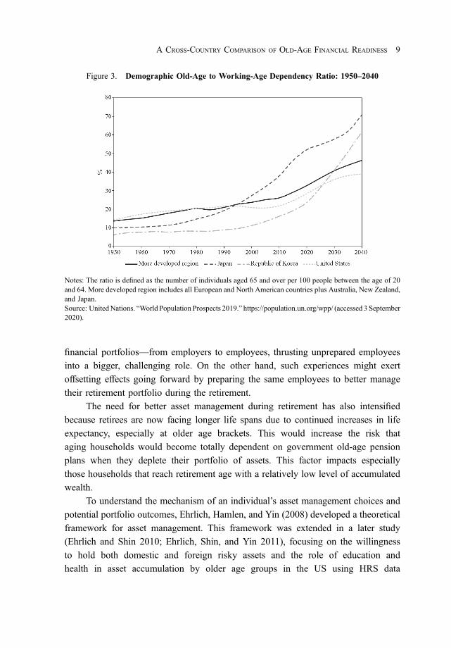
2015–2020 (Figure 2). These aging trends have contributed, in turn, to a steady
increase in the old-age to working-age dependency ratio, which is measured as the
ratio of the number of people aged 65 and over for every 100 people aged 20 to 64 in
1950. This number has risen from 13.6 in 1950 to 21 in 1990, and it was predicted to
have risen to 32.7 in 2020 and to increase to an alarming 46.3 by 2040 (Figure 3).
In the US, the inversely related potential old-age support ratio fell from 6 in 1960
to an expected 3.6 in 2020, while in Japan it shrunk from 8.7 to 2.2 in 2015 (Mather
and Kilduff 2020, Knoema 2020). This has put tremendous financial stress on both
public and private defined-benefits pension systems around the world. The challenges
have led to reforms in retirement-income systems in recent years, including increases
in the eligible age for full social security, more use of means tests, and a shift from
defined-benefit to defined-contribution pension schemes in both the public and private
sectors.
One of the potential remedies that could mitigate the increasing prospect of
financial insolvency of private and public pension programs is for households to
Figure 1. Total Fertility Rates: 1955–2040
Note: More developed region includes all European and North American countries plus Australia, New Zealand,and Japan.Source: United Nations. World Population Prospects 2019. https://population.un.org/wpp/ (accessed 3 September2020).
A CROSS-COUNTRY COMPARISON OF OLD-AGE FINANCIAL READINESS 7
March 23, 2022 10:30:39am WSPC/331-adr 2250004 ISSN: 0116-11052ndReading

improve the management of their individually held retirement assets. Households can
meet this challenge by raising their participation in risky financial markets and
increasing their demand for shares of stocks and corporate bonds they hold in their
individual portfolios. However, the current participation rate of households in risky
financial markets remains low even in the most developed economies. Using the US
Health and Retirement Study (HRS), Ehrlich and Yin (2021) report that just 24% to
34% of American households hold stocks.2 Venti and Wise (2001) used the first wave
of HRS data to illustrate that a considerable amount of the dispersion in wealth among
US households is due to investments in less risky assets such as bonds or bank saving
accounts as opposed to more risky assets such as stocks and corporate bonds.
The recent changing structure of employer-based pension plans in many
countries from defined-benefits to defined-contribution schemes has two opposite
impacts on employees. On the one hand, this change shifts the onus of financial
management of assets—the selection, allocation, and management of the household
Figure 2. Life Expectancy at Age 65: 1955–2040
Note: More developed region includes all European and North American countries plus Australia, New Zealand,and Japan.Source: UnitedNations. “World Population Prospects 2019.” https://population.un.org/wpp/ (accessed 3 September2020).
2Ehrlich, Hamlen, and Yin (2008) report similar percentages using the Survey of ConsumerFinance. It is interesting to note that Ehrlich and Shin (2021) report similar percentages for Europeanhouseholds (24%) using the Survey of Health, Aging and Retirement in Europe (SHARE).
8 ASIAN DEVELOPMENT REVIEW
March 23, 2022 10:30:44am WSPC/331-adr 2250004 ISSN: 0116-11052ndReading
financial portfolios—from employers to employees, thrusting unprepared employees
into a bigger, challenging role. On the other hand, such experiences might exert
offsetting effects going forward by preparing the same employees to better manage
their retirement portfolio during the retirement.
The need for better asset management during retirement has also intensified
because retirees are now facing longer life spans due to continued increases in life
expectancy, especially at older age brackets. This would increase the risk that
aging households would become totally dependent on government old-age pension
plans when they deplete their portfolio of assets. This factor impacts especially
those households that reach retirement age with a relatively low level of accumulated
wealth.
To understand the mechanism of an individual’s asset management choices and
potential portfolio outcomes, Ehrlich, Hamlen, and Yin (2008) developed a theoretical
framework for asset management. This framework was extended in a later study
(Ehrlich and Shin 2010; Ehrlich, Shin, and Yin 2011), focusing on the willingness
to hold both domestic and foreign risky assets and the role of education and
health in asset accumulation by older age groups in the US using HRS data
Figure 3. Demographic Old-Age to Working-Age Dependency Ratio: 1950–2040
Notes: The ratio is defined as the number of individuals aged 65 and over per 100 people between the age of 20and 64. More developed region includes all European and North American countries plus Australia, New Zealand,and Japan.Source: UnitedNations. “World Population Prospects 2019.” https://population.un.org/wpp/ (accessed 3 September2020).
A CROSS-COUNTRY COMPARISON OF OLD-AGE FINANCIAL READINESS 9
March 23, 2022 10:30:48am WSPC/331-adr 2250004 ISSN: 0116-11052ndReading

(Ehrlich and Yin 2021). In this paper, we greatly extend the same framework to study
simultaneously the factors affecting the demand for holding risky assets in two Asian
countries—Japan and the Republic of Korea (ROK)—and the US. One reason for
selecting these countries is that they represent three OECD countries in different stages
of development, with the US having the most developed and experienced financial
industry, Japan ranking second behind the US, and the ROK having the least
developed financial industry. Another important reason is that these three countries
have a relatively comparable micro-level longitudinal survey-type data (Health and
Retirement Study [HRS], the Japanese Study of Aging and Retirement [JSTAR], and
the Korean Longitudinal Study of Aging [KLoSA]), although the Japanese survey
differs somewhat by specific characteristics, which we explore in later sections.
The macro-level analysis leads to a better understanding of the role of the individual
determinants of demand for risky asset holding relative to that of the market-level
determinants. More specifically, our analysis has five major objectives:
(i) analyzing and comparing the macro-level accumulated components of wealth by
type of asset across the three countries along with comparing the overall
characteristics of investors in the three countries;
(ii) reviewing the role of old-age pension systems—both private and public—in
supporting the financial well-being of retirees;
(iii) estimating the role of individual investors’ characteristics in explaining household
willingness to hold risky financial assets to achieve better outcomes in
accumulating total and financial assets near and during retirement;
(iv) decomposing the role of individual characteristics, as predicted by our theoretical
model, relative to the role of financial market development in explaining gaps in
households’ willingness to hold risky assets across different countries, by using
an econometric decomposition analysis; and
(v) deriving some general policy implications based on our findings from the
preceding objectives.
The remaining sections of this paper are organized as follows. In Section II, we
briefly describe the retirement-income systems and demographic characteristics of the
three countries we analyze. In Section III, we describe the data surveys used in our
analysis. Section IV contains the basic descriptions of household characteristics,
retirement decisions, income sources, and wealth distributions in these three countries.
In Section V, we develop our theoretical model of asset management and apply it
empirically via a regression analysis using micro data and through a decomposition
analysis. We conclude with the main policy implications of our findings.
10 ASIAN DEVELOPMENT REVIEW
March 23, 2022 10:30:52am WSPC/331-adr 2250004 ISSN: 0116-11052ndReading

II. Comparing the Retirement-Income Systems in Japan,
the Republic of Korea, and the United States
We compare the retirement-income systems in Japan, the ROK, and the US
in terms of their completeness—the combination of both public and private
components—supporting demographic factors, and funding strength.
A. Japan
Japan has a two-tier public pension plan (Rajnes 2007, Social Security
Administration [SSA] 2008): the employees’ pension insurance (EPI), which was
established by law in 1941 and later updated in 1954; and the national pension (NP)
law, which was introduced in 1959 and amended in 1985. The current system can be
described as a social insurance system, which involves a flat-rate benefit for all
residents under the national pension program (first tier) and earnings-related benefits
under the employees’ pension insurance program or other employment-related program.
The full pensionable age for NPwas 60 years old in 2001 but started to increase by 1 year
every 3 years to 65 by 2013. The early pensionable age is currently 60. For EPI, the
eligible age was also 60 in 2001. But starting in 2013 it increased by 1 year every 3 years
for men until it reaches 65 in 2025. For women, the eligible age also started rising in 2018
by 1 year every 3 years until it reaches 65 in 2030. The full benefit requires a minimum of
40 years of contributions, and reduced benefit requires at least 25 years of contributions.
Both NP and EPI also provide disability insurance depending on meeting disability
criteria as well as a contribution requirement (SSA 2008).
The private sector in Japan also offers voluntary employer-sponsored retirement
plans, with retirement typically mandated at age 60. There had been two
defined-benefit (DB) plans offered, both receiving preferential tax treatment (Rajnes
2007). Two laws were passed in 2001 with the aim of reforming these plans. The DB
plans went through a major overhaul to address underfunding problems and allow for
convertibility to a DC plan. In addition, influenced by the expanding US economy and
stock market boom of the 1990s that was enhanced by the growth of DC plans,
primarily 401(k)’s in the US, a separate legislation established both corporate and
individual defined-contribution (DC) plans with the aim of stimulating the flow of
individual retirement-account assets into Japanese financial markets.
In 2019, the gross pension replacement rates for Japanese retirees with mean
earnings were projected by OECD pension models to be 32.5% for public plans and
23.8% for private plans (OECD 2019). The total gross replacement rate, which
includes total mandatory and voluntary plans, is thus 55.8%. By comparison, the
A CROSS-COUNTRY COMPARISON OF OLD-AGE FINANCIAL READINESS 11
March 23, 2022 10:30:52am WSPC/331-adr 2250004 ISSN: 0116-11052ndReading

OECD average replacement rate for public plans and private, voluntary plans are
39.6%, and 55.2%, respectively. Compared with other OECD countries, the Japanese
public system is less generous, but it offers better overall income security by
combining private and public sources.
B. Republic of Korea
The ROK has a national pension (NP) system for all citizens except government
employees, private teachers, military personnel, and employees of the special post
office, who are covered in a separate, special occupational pension program. Both
plans are mandatory. These were established by law in 1986 and later updated in 2007.
In 2008, the eligibility age for full pension benefits was set at 60 years old, requiring at
least 20 years of employment coverage. This age is set to gradually increase, however,
to 65 by 2033. The early eligibility age was 55 in 2008, but this is also set to gradually
rise to 60 by 2033 (SSA 2008). NP provides a basic old-age pension for people over
65 with an income below a maximum set by presidential order, and this benefit is not
subject to a minimum of 20 years of coverage. NP provides disability pension as well,
depending on the degree of disability assessed by the National Pension Corporation.
The private sector in the ROK used to have a mandatory severance payment
system (it started out as voluntary in 1953 and became mandatory in 1961) for
businesses with more than five employees, which provided a defined benefit in the
form of a lump-sum payment to employees. It was funded entirely by employers. This
plan was replaced by the Korean retirement benefit system (RBS) in 2005. The RBS
provides a choice between retirement pension plans (RPP) and retirement pay schemes
(RPS), which corporations can form. There are two types of RPP—DC and DB
plans—while RPS is a DB plan by design. There are also voluntary personal pension
plans in the form of individual retirements accounts (IRAs) that have been available in
the ROK since 1994 (OECD 2009).
According to OECD pension models, the gross pension replacement rate in 2019
for retirees with mean earnings in the ROK is 37.7% for mandatory public plans.
There is no estimated figure available, however, for mandatory and voluntary private
plans. Thus, the ROK offers a slightly less generous public pension system compared
to its OECD peers, but the overall gross pension replacement rate is well below the
OECD average of 55.2%.3
3As pointed out by one of our referees, the real-world situation in the ROK is even worse. TheOECD pension models make an unrealistic assumption concerning the number of years in which pensioncontributions have been made in that country. The actual number of contribution years is much lower. Thisis one of the factors contributing to the highest poverty rate among the elderly in the OECD.
12 ASIAN DEVELOPMENT REVIEW
March 23, 2022 10:30:53am WSPC/331-adr 2250004 ISSN: 0116-11052ndReading

C. The United States
In the US, the basic public system is a pay-as-you-go social security system. The
eligibility age for full benefits is 66 years old with at least 40 quarters of coverage, and
the eligible age will be lifted to 67 by 2027 (SSA 2018). Early pensionable age is 62
with the same limitation on coverage. The US system offers a generous disability and
supplemental income security for persons with disabilities and acute needs.
The private sector in the US offers various types of voluntary retirement plans.
Individuals can voluntarily contribute to additional retirement plans typically known
as IRAs. In the US employment-based system, pension plans were originally
dominated by DB plans. Starting around 1980, a quiet revolution took place: DC plans
quickly rose to dominance over DB plans. By 2011, 93% of covered private-sector
workers participated in a DC plan, while only 31% participated in a DB plan (Ehrlich
and Kim 2005). The sum exceeds 100% because the same individual can
simultaneously participate in multiple retirement plans.
The OECD pension models estimate that in 2019 the gross pension replacement
rate for US retirees with mean earnings is 39.4% for mandatory public plans, which is
virtually the same as the OECD average of 39.6%. However, the gross replacement
rate in the US, counting both mandatory and voluntary plans is 70.3%, well above the
OECD average of 55.2%.
D. Comparing the Demographic Changes Affecting the Retirement Systemsin the Three Countries
Figure 1 plots historical and projected total fertility rates for the three countries
under consideration along with the average for the MDR as a benchmark. As the chart
indicates, total fertility rate started to decline significantly in late 1970s for the US, but
it recovered after the 1990s until the early 2000s. It is currently projected to fall below
the replacement rate going forward, but to remain above the average of the MDR. In
Japan, the decline in total fertility rate accelerated in the 1970s, continuing into the
1990s. It is projected to be stable and to even recover somewhat in the near future,
though it will remain significantly below the average in the MDR. The ROK is
undergoing a more dramatic demographic transition. Its total fertility rate fell from
6.33 in 1960 to 2.92 in 1980 (around the time its economy started to take off ) and fell
even further to 1.5 in 2000, a level below the MDR average.4 The decline is projected
4Note that in the recent decade there were years in which the fertility rate fell below one. However,the data exhibited in Figure 1 represent five-year averages, which do not fall below 1.
A CROSS-COUNTRY COMPARISON OF OLD-AGE FINANCIAL READINESS 13
March 23, 2022 10:30:53am WSPC/331-adr 2250004 ISSN: 0116-11052ndReading

to continue and then stabilize over the next two decades but will remain well below
that of MDR countries. It is noteworthy that the decline in total fertility rates in the
ROK has been more rapid than that in Japan, and that the ROK’s total fertility rate
would remain significantly lower than that of Japan in the near future.
Figure 4 plots life expectancies at birth for these three countries, along with the
average for MDR. While all countries have experienced steady increase in life
expectancy over the last 5 decades, the rise in the ROK has been more dramatic. It rose
quickly from 52.76 years in 1960 to 70.34 in 1990, and caught up with the US in 2005,
reaching 77.17. It then surpassed both the US and the average of the MDR in 2010 and
has narrowed the gap with Japan in recent years.
Life expectancy trends at age 65 for these countries are plotted in Figure 2. If age
65 is taken to be the unofficial retirement age, the data suggest that in the 1960s people
expected to live another 14 years during retirement. But by 2010 this number
increased to 19 years. For Japan, which exhibits the highest life expectancy at 65,
longevity in retirement is currently expected to be 22.44 years (in 2020) and it is
projected to reach 24.16 years in 2040. Japanese life expectancy at 65 caught up with
that of the US around 1985, much sooner than the ROK, which achieved this feat
around 2010.
Figure 4. Life Expectancy at Birth: 1955–2040
Note: More developed region includes all European and North American countries plus Australia, New Zealand,and Japan.Source: UnitedNations. “World Population Prospects 2019.” https://population.un.org/wpp/ (accessed 3 September2020).
14 ASIAN DEVELOPMENT REVIEW
March 23, 2022 10:30:53am WSPC/331-adr 2250004 ISSN: 0116-11052ndReading

The demographic transition in the three countries we survey—declining fertility
along with rising life expectancy—has generated sharp increases in the shares of
old-age population to total population in these countries. Figure 3 plots the old-age to
working-age dependency ratio, defined as number of individuals aged 65 and over for
every 100 people aged 20 to 64, for these countries. While the US and the ROK
dependency ratios in 2020 of 28.4 and 23.6, respectively, are slightly below the
average of 32.7 for the MDR, Japan’s ratio of 52 is well above the average. The ratio is
projected to go up to 46.3 for the average MDR in 2040. While the US would still see
a figure below this average in 2040 (39.0), both Japan and the ROK (70.7 and 61.6,
respectively) would be well above this average. Thus, based on these ratios, both the
Japanese and Korean retirement-income systems will face a lot more headwinds than
other more developed countries, including the US. This is especially true for the ROK
as it started its mandatory retirement system much later than other countries, and the
rate of increase in this ratio is almost exponential.
As for the extent to which the public pension system is funded, the US is in a
much better place compared to its peers. According to OECD (2020a), in 2019, total
assets in pension funds in the US equaled 87.5% of gross domestic product, while this
figure was only 28.4% for Japan and 11.6% for the ROK. By comparison, the OECD
average was 60.1%.
E. Implications for the Relative Financial Strengths of the Retirement Systemsin the Three Countries
Based on the preceding comparisons of the structure and demographic trends
affecting the private and public retirement systems across the three countries, it seems
apparent that among the three countries, the US has the relatively most complete and
funded public and private retirement system, including the traditional “family-support”
system, due to its relatively higher fertility rate and retirement-income support ratio. Its
demographic pattern going forward is also more favorable compared to the other two
countries. In contrast, the ROK due to its late start and rapid decline in total fertility
rate may face more serious challenges in the near term.
Table 1 reports the net pension average replacement rates of earnings for workers
earning multiples of the mean earnings in the three countries, as estimated by the
OECD pension models (OECD 2019), along with the OECD average replacement
rates serving as reference points. As the table shows, the US provides better
replacement rates of individual earnings relative to both the ROK and Japan, although
all three countries fall below the OECD average rates. Japan, due to its relatively low
A CROSS-COUNTRY COMPARISON OF OLD-AGE FINANCIAL READINESS 15
March 23, 2022 10:30:57am WSPC/331-adr 2250004 ISSN: 0116-11052ndReading

reliance on the private sector, provides far less overall coverage relative to both the US
and the ROK. By contrast, the ROK offers comparable replacement rates to those in
the US only for workers earning 50% of mean earnings, while falling slightly short of
Japan in terms of the replacement rate it offers for high earners—retirees who earn
150% of average earnings. This might be a reflection of the ROK’s late start in pension
reforms in the private sector.
It is interesting to note that, even though both Japan and the ROK have higher
life expectancies at birth than the US (84.1 years for Japan and 82.63 years for the
ROK compared to 78.54 years for the US in 2017), both have set a pensionable age
2 years younger than that of the US. The pension eligible age is currently 65 years old
in Japan—the same as the planned pension eligible age in the ROK, compared to 67 in
the US. The lower eligibility ages in Japan and the ROK may accentuate the need for
future potential reforms in the Japanese and Korean systems. In contrast, the OECD
(2019) reported that in 2018, the ROK had the highest average effective age of labor
market exit (72.3 for both men and women), Japan had the second-highest averages
(70.8 for men and 69.1 for women), and the US had the third highest (67.9 for men
and 66.5 for women), while the OECD average was lower (65.4 for men and 63.7 for
women) than in these three countries. These differences translate into a remaining life
expectancy in retirement of 12.9 years for men and 16.3 years for women in the ROK,
15.5 for men and 21.0 for women in Japan, and 16.4 for men and 19.8 for women in
the US. In this regard, all three countries rank below the OECD average, where the
average remaining life expectancy in retirement is 17.8 years for men and 22.5 years
for women. These contrasting statistics suggest that both Japan and the ROK can
mitigate their disadvantages in demographics and workers’ dependencies on pension
Table 1. Net Pension Replacement Rates of Earnings for WorkersEarning Multiples of Mean Earnings
Replacement Rates of Individual Earnings,by Multiples of Mean Earnings
EconomyPensionAge 0.5 1.0 1.5
Japan 65 45.9 36.8 33.3Republic of Korea 65 60.8 43.4 32.6United States 67 61.2 49.4 42.7OECD 66.1 68.3 58.6 54.7
OECD = Organisation for Economic Co-operation and Development.Source: OECD pension models, as reported in OECD. 2019. Pensions at a Glance:OECD and G20 Indicators. Paris: OECD Publishing.
16 ASIAN DEVELOPMENT REVIEW
March 23, 2022 10:30:57am WSPC/331-adr 2250004 ISSN: 0116-11052ndReading

replacement rates because workers in these Asian countries tend to work longer than
those in the US, and much longer than workers in most OECD countries.
III. Data Description and Variable Construction
A. Comparative Samples and Waves
Our study relies on three longitudinal studies sharing a common questionnaire
design: the Health and Retirement Study (HRS) in the US, the Japanese Study of
Aging and Retirement (JSTAR) in Japan, and the Korean Longitudinal Study of Aging
(KLoSA) in the ROK.
The HRS is the seminal longitudinal household survey dataset that has been used
to study retirement and health issues for the elderly in the US (Juster and Suzman
1995). The original survey was conducted in 1992, covering household heads who
were aged 50 to 60 at the time. The survey followed up with the original households
every 2 years since then. A separate survey of the American oldest old population
(AHEAD) was later merged with the original HRS. To maintain a continuing dynamic
survey of the elderly population, a new cohort of households aged 50 and 55 has been
added to the longitudinal survey every 6 years. Such refresher samples were added in
1998, 2004, 2010, and 2016.
The 2015 RAND HRS file version O, which we use in this study, is the result of
several data developments aiming to provide a user-friendly version of HRS (Chien
et al. 2015). It includes final data files from 12 waves (1992 to 2010). This longitudinal
data contains only a subset of variables from the original HRS, but the survey reports
cleaned and processed variables with consistent and intuitive naming conventions and
model-based imputations. Most importantly, it includes a large number of individual
variables, including demographics, job status and history, health, as well as imputed
income and assets. The success of HRS has inspired the development of similar
surveys we use in our three-country study, as detailed in what follows. Notable surveys
also include the English Longitudinal Study of Ageing (ELSA) and the Survey of
Health, Ageing, and Retirement in Europe (SHARE). All these studies share virtually
identical questionnaires. This makes our cross-country comparison possible.
JSTAR is a panel survey of elderly people aged 50 or older conducted by the
Research Institute of Economy, Trade, and Industry (RIETI), Hitotsubashi University,
and the University of Tokyo (Ichimura, Shimizutani, and Hashimoto 2009). The
survey is designed to ensure, to the maximum extent possible, comparability with
A CROSS-COUNTRY COMPARISON OF OLD-AGE FINANCIAL READINESS 17
March 23, 2022 10:30:58am WSPC/331-adr 2250004 ISSN: 0116-11052ndReading

HRS, ELSA, and SHARE. To facilitate cross-country comparisons, RIETI also created
the Harmonized JSTAR data to be compatible with the procedures and imputation
methods employed in generating the RAND HRS. The JSTAR version we use is
Version B.
JSTAR surveyed people between the age of 50 and 75 along with their partners.
The first wave was conducted in 2007 with five municipalities. The survey followed
up with these households in wave 2 in 2009. Two more municipalities were added to
the study in wave 2. All households were included in the follow-up wave 3 survey in
2011, along with three new municipalities added to the survey. The unit of analysis in
JSTAR is the household, with survey weights at the household level provided for
analysis. This differs from HRS where both personal-level and household-level survey
weights are provided.
KLoSA is a panel survey in the ROK conducted initially by the Korean Institute
of Labor. KLoSA started the first wave in 2006 for households with at least one person
45 years and older, and the respondents were then surveyed every 2 years. Starting in
wave 3, the data were collected by the Korea Employment Information Service
(KEIS). There were no refresher samples in waves 2 through 4.5 This difference may
cause a downward bias when we aggregate individual data to form the household-level
data. The data we use are the Harmonized KLoSA version C. We have obtained the
original wave data from KEIS and then used a Stata program provided by a team at the
Global Aging Project to generate the Harmonized version C data.
For comparison purposes, we used only waves 8, 9, and 10 from the RAND
HRS, and waves 1, 2, and 3 from the Harmonized JSTAR and KLoSA. We note that
KLoSA data were collected in the same year as the corresponding HRS, while JSTAR
data were collected a year later (see Table 2 for details, which also includes the total
number of units with nonzero survey weights in each wave). In this context, we note
that HRS added a fresh cohort in 2010, leading to a larger number of units compared
with the previous two waves. For KLoSA, the number of units kept falling due to
attrition, and this is also true for wave 9 of HRS compared with wave 8. In contrast,
JSTAR added more municipalities in both the second and third waves, so the number
of units in JSTAR have risen throughout the three waves. To achieve greater
consistency among all three datasets, we also conduct the analysis at the household
level. To capture individual characteristics such as age and education, however, we
also use information on household heads.
5One notable difference about KLoSA is that it does not interview spouses or partners younger than45 years old, a deviation from the treatment in HRS and JSTAR.
18 ASIAN DEVELOPMENT REVIEW
March 23, 2022 10:30:58am WSPC/331-adr 2250004 ISSN: 0116-11052ndReading

We need to point out briefly some differences we observe in these three micro
datasets when using the 2006–2007 wave. First, the household heads in HRS and
JSTAR have similar average ages, with HRS exhibiting a slightly higher average. This
is due to the introduction of a new cohort of individuals aged 50 and 59 into the survey
in 2004, which was the first wave of JSTAR. KLoSA reports a much lower average
age because in the first wave of that survey, the age eligibility for KLoSA was 45,
which was 10 years younger than the early pensionable age of 55 at the time.
Throughout all waves, KLoSA contains much younger households, but the gap with
HRS fell modestly in 2010 when a new cohort was added to HRS. Average age stayed
almost the same between waves 1 and 2 for JSTAR even though there were more
municipalities introduced in the second wave. However, the average age in the JSTAR
sample became older in wave 3, where more municipalities were included.
We should also note that, even though we use the harmonized version of three
micro datasets, these data have their own limitations. For example, JSTAR does not
use a national probabilistic sample. Furthermore, the micro datasets are often
inconsistent with the reported administrative data. Consequently, the data comparisons
we report below should be viewed with caution, subject to this caveat.
B. Comparative Key Variables
To construct comparable variables in nominal local currencies, such as income
and wealth, we first convert them into nominal US dollars using purchasing-power-
parity (PPP) exchange rates (OECD 2020b), and then convert them into 2010 US
Table 2. Wave, Year, and Number of Units
HRS JSTAR KLoSA
Wave 8 1 1Year conducted 2006 2007 2006Number of units with positive weights 12,086 3,521 6,763
Wave 9 2 2Year conducted 2008 2009 2008Number of units with positive weights 11,346 3,987 5,689
Wave 10 3 3Year conducted 2010 2011 2010Number of units with positive weights 14,682 4,352 5,206
HRS ¼ Health and Retirement Study (United States), JSTAR ¼ JapaneseStudy of Aging and Retirement, KLoSA ¼ Korean Longitudinal Study ofAging.Source: Authors’ compilation.
A CROSS-COUNTRY COMPARISON OF OLD-AGE FINANCIAL READINESS 19
March 23, 2022 10:30:58am WSPC/331-adr 2250004 ISSN: 0116-11052ndReading
constant dollars by using annual US consumer price indexes (CPI) available from the
Bureau of Labor Statistics (BLS).
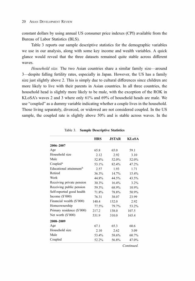
Table 3 reports our sample descriptive statistics for the demographic variables
we use in our analysis, along with some key income and wealth variables. A quick
glance would reveal that the three datasets remained quite stable across different
waves.
Household size. The two Asian countries share a similar family size—around
3—despite falling fertility rates, especially in Japan. However, the US has a family
size just slightly above 2. This is simply due to cultural differences since children are
more likely to live with their parents in Asian countries. In all three countries, the
household head is slightly more likely to be male, with the exception of the ROK in
KLoSA’s waves 2 and 3 where only 61% and 69% of household heads are male. We
use “coupled” as a dummy variable indicating whether a couple lives in the household.
Those living separately, divorced, or widowed are not considered coupled. In the US
sample, the coupled rate is slightly above 50% and is stable across waves. In the
Table 3. Sample Descriptive Statistics
HRS JSTAR KLoSA
2006–2007Age 65.8 65.0 59.1Household size 2.12 2.92 3.10Male 52.8% 52.0% 52.0%Coupleda 53.1% 82.4% 47.2%Educational attainmentb 2.57 1.93 1.71Retired 36.3% 14.7% 15.4%Work 44.8% 44.5% 43.5%Receiving private pension 30.3% 16.4% 3.2%Receiving public pension 59.3% 68.9% 10.9%Self-reported good health 71.8% 78.8% 50.9%Income ($’000) 76.31 38.07 23.99Financial wealth ($’000) 140.4 132.0 2.92Homeownership 77.5% 79.7% 53.2%Primary residence ($’000) 217.2 138.0 107.5Net worth ($’000) 531.9 310.0 165.4
2008–2009Age 67.1 65.3 60.6Household size 2.10 2.62 3.09Male 53.4% 58.6% 60.7%Coupled 52.2% 56.8% 47.0%
Continued.
20 ASIAN DEVELOPMENT REVIEW
March 23, 2022 10:30:59am WSPC/331-adr 2250004 ISSN: 0116-11052ndReading

Table 3. Continued.
HRS JSTAR KLoSA
Educational attainment 2.58 2.00 1.68Retired 39.3% 13.3% 19.8%Work 42.9% 46.6% 45.5%Receiving private pension 30.8% 18.3% 3.8%Receiving public pension 62.7% 66.9% 16.2%Self-reported good health 71.7% 78.4% 51.3%Income ($’000) 74.0 31.99 22.27Financial wealth ($’000) 134.5 97.36 7.96Homeownership 77.8% 63.6% 57.3%Primary residence ($’000) 208.4 139.7 127.8Net worth ($’000) 518.0 289.1 204.3
2010–2011Age 64.5 67.3 62.1Household size 2.20 2.70 3.07Male 52.4% 54.5% 68.9%Coupled 54.8% 74.4% 45.9%Educational attainment 2.69 2.15 1.64Retired 33.2% 15.5% 20.0%Work 47.1% 49.3% 44.7%Receiving private pension 22.7% 12.3% 4.5%Receiving public pension 55.3% 78.4% 22.1%Self-reported good health 74.2% 84.8% 48.4%Income ($’000) 71.72 34.54 21.13Financial wealth ($’000) 122.9 98.81 11.12Homeownership 76.4% 45.4% 57.3%Primary residence ($’000) 184.5 97.2 115.8Net worth ($’000) 449.9 238.7 201.5
HRS ¼ Health and Retirement Study (United States),JSTAR ¼ Japanese Study of Aging and Retirement, KLoSA ¼Korean Longitudinal Study of Aging.aCoupled is a dummy variable indicating whether a couple livesin the household. Survey respondents who are separated,divorced, or widowed are not considered coupled.bEducational attainment is classified as 1 for respondents with aneducational attainment less than a high school degree; 2 for highschool graduates; 3 for those with some college; and 4 for thosewith a college degree or higher.Source: Authors’ calculations using data from the Healthand Retirement Study (United States), the Japanese Study ofAging and Retirement, and the Korean Longitudinal Study ofAging.
A CROSS-COUNTRY COMPARISON OF OLD-AGE FINANCIAL READINESS 21
March 23, 2022 10:31:00am WSPC/331-adr 2250004 ISSN: 0116-11052ndReading

Korean sample, the coupled rate is surprisingly below 50%. JSTAR reports a
somewhat unstable pattern: this rate is 82.4% in wave 1 and 74.4% in wave 3, but only
56.8% in wave 2.
Educational attainments. Only HRS reports continuous years of education. Both
JSTAR and KLoSA report only educational attainments. For compatibility reasons, we
use the following unified version of educational attainments:6 educational attainment
is classified as 1 for respondents with an educational attainment less than a high school
degree; 2 for high school graduates; 3 for those with some college; and 4 for those with
a college degree or higher. Among the three countries, the US has the highest average
educational attainment in all waves, with the average being above a high school
degree. Japan’s average educational attainment is around a high school degree, while
the ROK’s average is just below a high school degree.
Retirement status. The data concerning individual retirement status are
considerably different in the three countries. In Japan only 13.3% to 15.5% of the
population report being fully retired. In the ROK, the reported percentages are slightly
higher at 15.4% to 20%. But in the US, the reported percentages are much higher—
they range from 33.2% to 39.3%.
Wage earners. The percentage of household heads who report working to earn a
wage is very similar among the three countries, ranging from 42.9% to 49.3% across
different waves.
Public pension receivers. The percentage of households receiving public pension
is highest for Japan, ranging from 66.9% in 2008–2009 to 78.4% in 2010–2011. In the
US, the reported percentages are lower, ranging from 55.3% in 2010–2011 (wave 3) to
62.7% in 2008–2009 (wave 1). The lower number in 2010–2011 (wave 3) is due to the
inclusion of a new younger cohort. The percentages for the ROK rose steadily from
10.9% to 22.1% across the three waves as respondents became older, but they are
significantly lower than those reported in Japan and the US.
Private pension receivers. As for the data on individuals receiving private
pensions, the ROK reported dismal percentages ranging from 3.2% to 4.5%. On
the other hand, JSTAR reported percentages ranging from 12.3% to 18.3%.
The percentages are much higher in the US: around 30% received private pension
in 2006–2007 (wave 1) and 2008–2009 (wave 2) (the 22.7% figure in the third wave in
2010–2011 is due to the influx of a new, younger cohort).
Health status. HRS used a five-point scale for self-reported health status (from
poor to excellent). Both JSTAR and KLoSA included this variable in their
6KLoSA uses a slightly different version, which we convert to our unified version.
22 ASIAN DEVELOPMENT REVIEW
March 23, 2022 10:31:00am WSPC/331-adr 2250004 ISSN: 0116-11052ndReading

questionnaire. Following the literature and our own earlier work, we convert this
health status measure into a dummy variable for people whose self-reported status is
“good” or “better.” Around 80% of Japanese household heads reported their health
being good or better. In the US, this percentage is lower at 72%–74%. However, only
about half of Korean household heads report their health status as good or better.
Whether this difference is due to technical issues such as reporting methods or how
people assess their health status remains a question, but it may affect our regression
results concerning the expected effect of this variable.
Average household income. As expected, the US has a much higher average
income than the two Asian countries. We do see a slightly lower average in the US in
2008–2009 (wave 2) compared with 2006–2007 (wave 1) due to the 2008 financial
crisis. Average Japanese household incomes are about half of those of the US while
the Korean averages are about one-third of those of the US. Note that we use
PPP exchange rates to convert nominal figures. For Japan, this exchange rate is
typically higher than the nominal market exchange rate. This means that if we use the
nominal exchange rate to convert yen to US dollars, the estimated Japanese income
variables would be higher than what is reported in Table 3. For the ROK, the opposite
is true.
Household wealth (net worth). We construct this variable as the sum of
households’ net financial and nonfinancial assets. The former includes stocks, bonds,
and other banking accounts (and IRA accounts in the US), while the latter includes
households’ main residence, other real estate, business assets, vehicles, and other
assets. As expected, household wealth is much higher in the US than in the Asian
countries, with Japanese and Korean household wealth on average about 60% and
40%, respectively, of that of the US. Interestingly, even though the Japanese on
average hold fewer financial assets than their US counterparts, the percentage of these
assets in total wealth is higher. On the other hand, Korean households typically hold
less than 6% of total wealth in financial assets.
Homeownership percentage and value. The first variable is defined by whether
the households’ current residence value is positive or not. Americans have the highest
ownership rate, which is around 80%. It dipped slightly after the financial crisis and
the influx of a new, younger cohort to 76.4%, which is still significantly higher than
the homeownership percentage in the two other Asian countries. The ROK’s
homeownership rates across the three waves remains quite consistent at just under
60%. However, homeownership rates have changed drastically across waves in Japan.
They reached close to 80% in wave 1, fell to 63.6% in wave 2, and dropped to just
45.4% in wave 3. We note, however, that new municipalities were introduced in both
A CROSS-COUNTRY COMPARISON OF OLD-AGE FINANCIAL READINESS 23
March 23, 2022 10:31:00am WSPC/331-adr 2250004 ISSN: 0116-11052ndReading

waves 2 and 3, so this drop could be the result of survey design as JSTAR is not a
random probabilistic survey at the national level.
The second variable—the value of homeownership (i.e., primary residence)—
exhibits a more consistent level across waves: the US variable features the highest
average values while the values across the two Asian countries are steady over the
three waves.
IV. Retirement, Pension Dependency, and Wealth Distribution
In this section, we offer additional detailed analysis regarding the variations of
retirement status, working status, income, and wealth among the elderly in the three
countries under study. This analysis reveals some additional insights about the sources
of the differences across the three countries beyond what we learn from the descriptive
statistics.
A. Retirement
We start with the individual retirement status. The survey question asks
respondents to declare whether they consider themselves fully retired. This means
that individuals can stay out of the labor force or run their own business or do some
voluntary work but still claim that they are retired. Table 4 reports the percentage of
household heads who consider themselves retired in the following age brackets: less
than 60; 60–64; 65–69; and 70 and above. The first bracket applies to workers who are
below early pensionable ages, except for Koreans during a transition period discussed
earlier. The second bracket includes workers in early pensionable ages, while the third
bracket applies to people who have reached full retirement age (66 in the US at the
time of the survey), and the fourth bracket can be thought of as late retirement age.
Table 4 indicates that more Americans (36.3%) consider themselves retired
compared to workers in other countries. The two Asian countries’ data reveal that a
significantly lower percentage of workers—around 15%—consider themselves retired
at all three age brackets (the Korean average rose to 20% in wave 3 due to aging of the
only cohort covered in the country’s survey). Due to the unique opportunity to retire
early in the ROK before reaching the age of 60, 8.0% to 9.3% of Koreans chose to do
so, while for Americans this figure is only 3.6% to 5.8% due to social security’s
generous disability programs. Among people who might be eligible for early
retirement, 18.2% to 24.5% of Koreans chose to retire compared to 22.2% to 26.1% of
Americans. Among respondents who are in the full retirement age group, 17.1% to
24 ASIAN DEVELOPMENT REVIEW
March 23, 2022 10:31:00am WSPC/331-adr 2250004 ISSN: 0116-11052ndReading

29.0% Asians consider themselves retired compared to about half of Americans in this
age group (but this figure went down to 47.5% in 2008–2009 because of the financial
crisis). For those aged 70 and older, the retirement percentages are below 30% in Japan
and 37% in the ROK, compared to about 70% in the US.
Because one does not have to claim full retirement to receive pension benefits, it
is interesting to compare the percentage of people who stay in the labor force in the
three countries. The survey asked whether respondents were working for pay, and the
results for the same age brackets in Table 4 are reported in Table 5. Here we see that
the percentage of working household heads are quite similar across the three countries
in all age brackets. However, among Japanese workers younger than 60 this
percentage is above 90%, although it declines in later waves closer to the percentages
seen among workers in the ROK and the US. Surprisingly, the Korean average over all
age brackets is lower than that of the US. In the group eligible for early retirement,
61% of Japanese workers continue to work compared to 55% of Americans in this
Table 4. Percentage Retired by Age
Age Brackets HRS JSTAR KLoSA
2006–2007All ages 36.3% 14.8% 15.4%Age < 60 5.0% 0.3% 8.0%60 � Age < 65 26.1% 5.5% 18.2%65 � Age < 70 50.5% 21.4% 26.8%Age � 70 68.8% 25.8% 28.8%
2008–2009All ages 39.3% 13.3% 19.8%Age < 60 5.8% 0.6% 9.3%60 � Age < 65 24.3% 8.13% 24.5%65 � Age < 70 47.5% 19.8% 28.7%Age � 70 70.2% 21.0% 37.1%
2010–2011All ages 33.2% 14.5% 20.0%Age < 60 3.6% 0.7% 9.2%60 � Age < 65 22.2% 4.8% 21.5%65 � Age < 70 49.8% 17.1% 29.0%Age � 70 70.4% 25.4% 35.8%
HRS ¼ Health and Retirement Study (United States),JSTAR ¼ Japanese Study of Aging and Retirement,KLoSA ¼ Korean Longitudinal Study of Aging.Source: Authors’ calculations using data from the Healthand Retirement Study (United States), the JapaneseStudy of Aging and Retirement, and the KoreanLongitudinal Study of Aging.
A CROSS-COUNTRY COMPARISON OF OLD-AGE FINANCIAL READINESS 25
March 23, 2022 10:31:00am WSPC/331-adr 2250004 ISSN: 0116-11052ndReading

group. Koreans belonging to this group work the least, as only 36% continue working.
For the full retirement age group, all three countries have numbers around 30%.
However, 13% of Americans work well into late retirement age, while only 9% of
Japanese work into their 70s. In later waves (waves 2 and 3), however, the share of
Japanese older than 70 who reported working (23.8% and 29.1% for waves 2 and 3,
respectively) is higher than in the other two countries. In the ROK, however, only
14.4% to 16.8% of Koreans over 70 years old continue to work. Thus, except for wave
1, the two Asian countries’ workers retire later in life and continue working well into
full retirement age.
B. Public and Private Pensions
Next, we compare pension coverages for these three countries. We first consider
public pensions. Table 6 reports percentages of people receiving public pension by age
groups. It is quite clear that Japan has the widest public pension coverage among the
Table 5. Percentage Working by Age
Age Brackets HRS JSTAR KLoSA
2006–2007All ages 44.8% 44.5% 43.5%Age < 60 74.2% 92.2% 59.1%60 � Age < 65 54.6% 60.7% 36.4%65 � Age < 70 34.6% 33.1% 29.2%Age � 70 13.0% 8.9% 10.5%
2008–2009All ages 42.9% 46.6% 45.5%Age < 60 72.9% 70.9% 63.2%60 � Age < 65 57.4% 64.3% 39.8%65 � Age < 70 39.2% 45.3% 31.8%Age � 70 13.1% 23.8% 14.4%
2010–2011All ages 47.1% 49.3% 44.7%Age < 60 73.2% 77.1% 63.4%60 � Age < 65 53.9% 70.7% 42.7%65 � Age < 70 38.0% 48.9% 28.7%Age � 70 13.7% 29.1% 16.8%
HRS ¼ Health and Retirement Study (United States),JSTAR ¼ Japanese Study of Aging and Retirement,KLoSA ¼ Korean Longitudinal Study of Aging.Source: Authors’ calculations using data from theHealth and Retirement Study (United States), theJapanese Study of Aging and Retirement, andthe Korean Longitudinal Study of Aging.
26 ASIAN DEVELOPMENT REVIEW
March 23, 2022 10:31:01am WSPC/331-adr 2250004 ISSN: 0116-11052ndReading

three countries, while the public pension coverage for the ROK clearly lags behind the
other two countries due to the fact that its pension system was developed quite late.
For people who are eligible for full public pension, 92.3% of Americans and 95.8% of
Japanese are covered, while only 30.1% of Koreans are covered (wave 1). For people
aged 70 and older, coverage is almost universal in Japan and the US, while only 10.8%
of Koreans in wave 1 and 27% of Koreans in wave 3 received coverage. Even people
in the 60–69 age group in the ROK who have a better chance of meeting the eligibility
criteria, only around 30% of them in wave 1 and 50% in wave 3 reported receiving
coverage.
Table 7 reports coverage rates by age bracket for people receiving private
pensions. In this pension category, Americans clearly have a significant advantage
over their Asian counterparts. Among Americans in their early retirement age, 29%
Table 6. Percentage Receiving PublicPension by Age
Age Brackets HRS JSTAR KLoSA
2006–2007All ages 59.3% 68.9% 10.9%Age < 60 16.0% 8.1% 3.2%60 � Age < 65 46.9% 78.8% 32.5%65 � Age < 70 92.3% 95.8% 30.1%Age � 70 98.3% 97.8% 10.8%
2008–2009All ages 62.7% 66.9% 16.2%Age < 60 18.0% 11.1% 5.3%60 � Age < 65 42.5% 67.6% 38.1%65 � Age < 70 88.9% 94.1% 41.0%Age � 70 98.1% 93.3% 17.4%
2010–2011All ages 55.3% 78.4% 22.1%Age < 60 16.1% 16.1% 7.5%60 � Age < 65 44.3% 75.3% 42.9%65 � Age < 70 90.0% 96.8% 50.0%Age � 70 97.9% 96.0% 27.0%
HRS ¼ Health and Retirement Study (UnitedStates), JSTAR ¼ Japanese Study of Aging andRetirement, KLoSA ¼ Korean LongitudinalStudy of Aging.Source: Authors’ calculations using data from theHealth and Retirement Study (United States), theJapanese Study of Aging and Retirement, andthe Korean Longitudinal Study of Aging.
A CROSS-COUNTRY COMPARISON OF OLD-AGE FINANCIAL READINESS 27
March 23, 2022 10:31:02am WSPC/331-adr 2250004 ISSN: 0116-11052ndReading

receive private pensions. The coverage rates reach 41% when they reach full
retirement age and it goes to almost 50% when they are in their 70s. The coverage
rates dipped after the financial crisis, as reported in the 2010–2011 wave, but they are
still much higher than the coverage rates of their Asian counterparts. For the Japanese,
the coverage rates hover around 20%, and only 12.6% of Japanese in their 70s claimed
pension from private sources. For Koreans, the coverage rates are never higher than
9% across all waves in all the age brackets reported in Table 7. One caveat is that the
old income-retirement systems in Japan (before 2001) and the ROK (before 2005)
offered lump sum severance payments. It is not clear how these payments have
impacted the coverage rates reported in these two countries.
To assess the degree of dependency on pensions of old-age groups in the three
countries in our sample, we first consider the income distribution of the whole sample
of old-age groups in each country and those who are fully retired. Table 8 reports this
Table 7. Percentage Receiving Private Pensionby Age
Age Brackets HRS JSTAR KLoSA
2006–2007All ages 30.3% 16.4% 3.2%Age < 60 9.4% 17.6% 1.4%60 � Age < 65 29.1% 20.3% 7.4%65 � Age < 70 40.7% 19.7% 6.0%Age � 70 49.0% 12.6% 4.7%
2008–2009All ages 30.1% 18.3% 3.8%Age < 60 10.6% 10.3% 1.3%60 � Age < 65 24.8% 24.2% 8.5%65 � Age < 70 39.9% 25.7% 6.6%Age � 70 46.2% 18.4% 5.7%
2010–2011All ages 22.7% 12.3% 4.5%Age < 60 4.7% 2.0% 1.8%60 � Age < 65 20.3% 14.8% 8.8%65 � Age < 70 34.5% 17.9% 8.3%Age � 70 42.5% 12.6% 5.5%
HRS ¼ Health and Retirement Study (United States),JSTAR ¼ Japanese Study of Aging and Retirement,KLoSA ¼ Korean Longitudinal Study of Aging.Source: Authors’ calculations using data fromthe Health and Retirement Study (United States), theJapanese Study of Aging and Retirement, and theKorean Longitudinal Study of Aging.
28 ASIAN DEVELOPMENT REVIEW
March 23, 2022 10:31:03am WSPC/331-adr 2250004 ISSN: 0116-11052ndReading

distribution of income at the 10th, 25th, 50th (median), 75th, and 90th percentiles of
income. The two tail percentiles (10th and 90th) are included in order to see the impact
of pensions on people at the tails of the distribution, which typically have skewed tails.
This analysis has potentially important policy implications as well, because those who
are most affected by any policy reforms are those in the extreme ends of the spectrum.
The median incomes reported in Table 8 for the three countries are somewhat
different from the average incomes we report in the summary statistics presented in
Table 3. More specifically, the median income for Japan is closer to that of the US. For
the whole sample, the median income in Japan is 80% of that of the US. For people
who are fully retired, the gap is even smaller: the median income for that group in
Japan is almost 90% of that of the US. The lower tails are similar for these two
countries although the US maintains its advantages over Japan in the upper tails,
especially at the 90th percentile, with the Japanese 90th percentile income equal to just
50% of US income in the whole sample, and two-thirds in the fully retired subsample.
This clearly is the driving force behind the average income gap between these two
countries.
For the ROK, both the median income and the average income are about one-
third of US median and average income, respectively. However, the lower tail looks
very different from that of the US. The whole lower tail of the Korean income
Table 8. Income Distribution for Whole Sample and Retired ($’000)
Whole Sample Retired
10% 25% Median 75% 90% 10% 25% Median 75% 90%
2006–2007HRS 10.6 19.5 41.3 81.1 146.1 10.9 17.1 30.9 54.3 91.8JSTAR 8.7 18.9 32.9 52.4 73.4 8.7 15.7 27.1 41.9 61.2KLoSA 0.0 0.2 11.8 33.6 65.0 0.0 0.0 1.7 13.7 38.6
2008–2009HRS 10.1 18.8 40.5 79.6 142.4 10.3 16.4 30.3 56.0 98.1JSTAR 6.2 13.2 24.3 39.7 61.8 7.1 15.9 26.5 39.7 59.5KLoSA 0.0 1.6 13.9 32.5 57.4 0.0 0.2 2.9 14.9 33.9
2010–2011HRS 10.5 19.8 42.5 85.1 156.2 10.8 17.1 31.6 56.2 94.0JSTAR 9.0 17.1 28.9 45.1 69.0 9.2 18.1 27.1 39.3 58.7KLoSA 0.0 2.0 14.1 29.5 57.1 0.0 0.4 4.0 15.7 33.3
HRS ¼ Health and Retirement Study (United States), JSTAR ¼ Japanese Study of Aging andRetirement, KLoSA ¼ Korean Longitudinal Study of Aging.Source: Authors’ calculations using data from the Health and Retirement Study (United States), theJapanese Study of Aging and Retirement, and the Korean Longitudinal Study of Aging.
A CROSS-COUNTRY COMPARISON OF OLD-AGE FINANCIAL READINESS 29
March 23, 2022 10:31:04am WSPC/331-adr 2250004 ISSN: 0116-11052ndReading

distribution is close to 0, which is also the case for the fully retired subset. At the same
time, Table 8 indicates that the ROK has managed to narrow the gap in the upper tail
of the income distribution compared to the US relative to the larger gap in the lower
tail. The 90th percentile income is 44% of that of the US for the whole sample and
42% in the fully retired subsample. The fat right tail of the income distribution in the
ROK is quite striking: the median income is only one-third of the upper quartile for
the whole sample while the median income for the fully retired is only one-tenth of the
upper quartile. It seems that many Korean retirees have to resort to their savings to
support their consumption.
The median percentage of total income received from total pension income can
be used as a rough measure of dependency on pension income during retirement.
Because relatively few Asians would claim they are fully retired, we calculate the
median percentage for people over the age of 65. However, while public pension
coverage in both Japan and the US is almost universal for this age group, there is still
limited pension coverage (well below 50%) for Koreans in the same group. For this
reason, Table 9 compares the median percentage of income received from pensions
just for Japan and the US. We compute it for all the age groups above 65 in our sample
and break it down by income quartiles.
Table 9. Median Percentage of Total Income Received fromTotal Pension Income for 65 and Older by Income Quartile
Income Quartiles
Overall 1st 2nd 3rd 4th
2006–2007HRS 85.7 100 95.4 76.3 36.9JSTAR 77.3 120 97.1 76.0 36.3
2008–2009HRS 84.1 100 93.3 72.2 31.7JSTAR 80.0 103 96.4 80.0 40.0
2010–2011HRS 85.1 100 95.6 76.2 32.4JSTAR 76.7 103 94.3 70.0 41.0
HRS ¼ Health and Retirement Study (United States), JSTAR ¼Japanese Study of Aging and Retirement.Note: We chose not to report the results for the Korean LongitudinalStudy of Aging (KLoSA) because median percentages are mostly zero,the highest being 10% for the fourth quartile in 2010.Source: Authors’ calculations using data from the Health and RetirementStudy (United States) and the Japanese Study of Aging and Retirement.
30 ASIAN DEVELOPMENT REVIEW
March 23, 2022 10:31:04am WSPC/331-adr 2250004 ISSN: 0116-11052ndReading

Table 9 shows that for Americans over age 65, 85.7% of their retirement income
comes from public and private pensions. For the Japanese in the same age group,
however, only 77.3% of retirement income comes from public and private pensions.
This evidence implies that the US has a more rewarding retirement system than Japan.
At the same time, to the extent that most of the pension coverage comes from public
pensions, our finding implies that Americans rely on the public pension system more
than their Japanese counterparts. Indeed, Table 9 shows that people at the lowest
income quartiles, on average, rely entirely on pension income, and those in the second
lowest quartiles rely heavily on pension income as well. For those whose incomes are
in the third quartile, however, more than one-quarter of their incomes come from
sources other than pensions. For people in the highest income bracket, the median
percentage coming from non-pension sources is only 63%. In sum, we can say that
three-quarters of people in both the US and Japan rely heavily on the retirement
pension system for their old-age income. Even wealthier people (in the highest
quartile) derive a substantial portion of their incomes from the pension system.
C. Wealth, Financial Wealth, and Stock Ownership
The previous section, which focused on the extent to which old-age income in
the three countries is dependent on the existence of private and public pensions, raises
a question about the role of accumulation and management of private savings as an
additional channel which affects the financial well-being of individuals and
households. The question is important because if the majority of people derive their
income just from the pension system, especially if the latter is in the form of defined
benefits rather than defined contributions, such dependency limits the opportunities for
older and retired people to cope with unforeseen financial and health predicaments
affecting themselves or their family members. Since high degrees of dependency on
pension income are the result of insufficient private wealth accumulation, we explore
in this section the distribution of personal wealth in the three countries under study.
Table 10 reports the distribution of household net worth at the 10th, 25th, 50th
(median), 75th, and 90th percentiles in 2010 US constant dollars (see Section III.B for
a definition of household net worth) for the whole sample of older age groups as well
as the fully retired in the three countries. A quick overview indicates that Japan and the
US share similar wealth distributions, especially for the whole sample. The Korean
wealth distribution is quite different, however, and resembles to a large extent the
country’s income distribution, which immediately indicates the large influence of
private and public pensions in the country.
A CROSS-COUNTRY COMPARISON OF OLD-AGE FINANCIAL READINESS 31
March 23, 2022 10:31:04am WSPC/331-adr 2250004 ISSN: 0116-11052ndReading

While the Japanese wealth distribution is thicker in the lower half of the
distribution and even at its median in wave 1, the American wealth distribution is
thicker in the upper half, which clearly dominates the distribution. Looking only at
those who are fully retired, the American distribution dominates the Japanese over the
whole distribution and across all waves. The same applies to the comparison between
the American and the Korean distributions. Just like the income distribution, the
wealth distribution of the ROK is heavily skewed and wealth accumulation seriously
lagging that of other developed countries. This is largely the result of higher human
and physical capital accumulation in the US relative to the two Asian countries in
recent centuries. The obvious implication is that Americans enjoy a higher level of
retirement income relative to their Asian counterparts. An interesting question to ask is
to what extent is this the result of private accumulation of assets as opposed to the
private and public pension systems in the three countries.
We are tempted to think that the larger accumulation of wealth in the US might
be due to their relatively large holdings of stocks and financial assets. However, as
reported in Table 11, this conjecture is not entirely correct. Looking at the whole
sample, the Japanese almost dominate the Americans over the entire financial wealth
distribution. Moreover, it is surprising to see that the median value of financial assets
in Japan is almost five times higher than that of the US. Even for people who are fully
Table 10. Wealth Distribution for Whole Sample and Retired ($’000)
Whole Sample Retired
10% 25% Median 75% 90% 10% 25% Median 75% 90%
2006–2007HRS 0.7 44.0 202.3 557.2 1,219.0 4.1 71.8 269.4 643.7 1,308.0JSTAR 0.0 61.2 227.1 436.8 742.5 0.0 52.4 209.7 436.8 698.9KLoSA 0.0 5.6 70.0 191.5 401.6 0.0 2.8 65.8 202.2 432.8
2008–2009HRS 0.6 40.7 189.2 532.9 1,174.0 3.0 64.8 249.5 625.7 1,290.0JSTAR 0.0 26.5 164.2 361.4 713.6 8.7 84.4 216.3 379.5 697.3KLoSA 0.0 12.9 91.9 253.0 515.7 1.0 2.58 77.4 257.9 555.2
2010–2011HRS 0.0 25.7 154.0 464.0 1,063.0 4.1 69.5 241.8 593.8 1,204.0JSTAR 0.0 9.9 135.3 328.7 615.5 0.0 45.1 180.5 357.3 604.5KLoSA 0.0 11.9 95.5 249.7 500.0 0.0 3.57 71.4 237.8 444.9
HRS ¼ Health and Retirement Study (United States), JSTAR ¼ Japanese Study of Aging andRetirement, KLoSA ¼ Korean Longitudinal Study of Aging.Source: Authors’ calculations using data from the Health and Retirement Study (United States), theJapanese Study of Aging and Retirement, and the Korean Longitudinal Study of Aging.
32 ASIAN DEVELOPMENT REVIEW
March 23, 2022 10:31:05am WSPC/331-adr 2250004 ISSN: 0116-11052ndReading
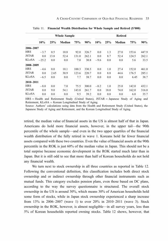
retired, the median value of financial assets in the US is almost half of that in Japan.
Americans do hold more financial assets, however, in the upper tail—the 90th
percentile of the whole sample—and even in the two upper quartiles of the financial
wealth distribution of the fully retired in wave 1. Koreans hold far fewer financial
assets compared with these two countries. Even the value of financial assets at the 90th
percentile in the ROK is just 60% of the median value in Japan. This should not be a
total surprise because economic development in the ROK started much later than in
Japan. But it is still odd to see that more than half of Korean households do not hold
any financial wealth.
We turn next to stock ownership in all three countries as reported in Table 12.
Following the conventional definition, this classification includes both direct stock
ownership and or indirect ownership through other financial instruments such as
mutual funds. This category excludes pension plans, even those based on DC plans,
according to the way the survey questionnaire is structured. The overall stock
ownership in the US is around 30%, which means 30% of American households hold
some form of stocks, while in Japan stock ownership experienced a sharp increase
from 13% in 2006–2007 (wave 1) to over 20% in 2010–2011 (wave 3). Stock
ownership in the ROK, however, is almost negligible—in all survey years, less than
5% of Korean households reported owning stocks. Table 12 shows, however, that
Table 11. Financial Wealth Distribution for Whole Sample and Retired ($’000)
Whole Sample Retired
10% 25% Median 75% 90% 10% 25% Median 75% 90%
2006–2007HRS �3.7 0.5 10.8 92.0 326.7 0.0 1.3 27.0 153.6 447.9JSTAR 0.0 13.8 52.4 131.0 262.1 0.0 8.7 52.4 124.5 262.1KLoSA �25.2 0.0 0.0 7.0 30.8 �9.6 0.0 0.0 5.6 33.5
2008–2009HRS �4.6 0.0 10.1 100.3 330.3 0.0 1.0 27.4 152.0 461.0JSTAR 0.0 2.65 30.9 123.6 220.7 0.0 8.8 44.6 176.5 285.1KLoSA �6.5 0.0 0.0 7.7 38.7 0.0 0.0 0.0 6.45 38.7
2010–2011HRS �8.0 0.0 7.0 75.5 300.0 �0.2 1.0 25.0 142.0 432.1JSTAR 0.0 9.0 54.1 143.8 261.7 0.0 18.0 74.0 162.0 316.0KLoSA 0.0 0.0 0.0 9.5 39.2 0.0 0.0 0.0 6.0 35.7
HRS ¼ Health and Retirement Study (United States), JSTAR ¼ Japanese Study of Aging andRetirement, KLoSA ¼ Korean Longitudinal Study of Aging.Source: Authors’ calculations using data from the Health and Retirement Study (United States), theJapanese Study of Aging and Retirement, and the Korean Longitudinal Study of Aging.
A CROSS-COUNTRY COMPARISON OF OLD-AGE FINANCIAL READINESS 33
March 23, 2022 10:31:06am WSPC/331-adr 2250004 ISSN: 0116-11052ndReading

stock ownership rises when we restrict the sample to include only households that
report positive overall wealth and positive financial wealth. In the latter group, stock
ownership reaches almost 40% of all US households. It also increases to around 15%
in waves 1 and 2 for Japanese households with positive financial wealth, and it shoots
up to 24% in wave 3.
The data on stock holding can provide an explanation as to why Americans hold
more financial assets in the upper tails of the distribution of financial assets. The
driving force behind the thick upper tails of the distribution is stock ownership, due to
the higher expected values of stocks relative to fixed-income assets. The median value
of personal stocks in the US is $70,300 in 2006–2007 (wave 1), 2.7 folds higher than
the median of $26,200 in Japan. This gap between the US and Japan stays the same
even in 2010–2011 (wave 3) when stock ownership rate in Japan increases
dramatically to 24%. The median value of personal stocks in the ROK is only
$14,000 in 2006–2007 (wave 1). Comparing the fully retired households with
households in the whole sample, we see an increase in stock ownership by retirees in
the US and Japan (except in wave 1), while stock ownership becomes smaller for
Table 12. Stock Ownership
HRS JSTAR KLoSA
WholeSample Retired
WholeSample Retired
WholeSample Retired
2006–2007Overall 27.9% 32.6% 13.1% 11.6% 2.4% 2.1%Given positive wealth 30.2% 34.3% 14.4% 13.4% 2.8% 2.7%Given positive financial 36.1% 38.7% 15.1% 12.7% 4.5% 4.2%Median value ($’000) 70.3 108.2 26.2 34.9 14.0 19.5
2008–2009Overall 26.5% 30.6% 12.2% 13.6% 3.4% 2.6%Given positive wealth 28.7% 32.2% 13.7% 14.5% 4.0% 3.3%Given positive financial 34.7% 36.6% 15.0% 15.3% 6.7% 5.9%Median value ($’000) 81.1 101.3 17.7 17.7 23.9 25.8
2010–2011Overall 25.6% 30.2% 21.0% 26.1% 2.1% 1.0%Given positive wealth 28.5% 32.0% 24.2% 26.8% 2.4% 1.3%Given positive financial 35.5% 37.0% 23.6% 28.9% 4.1% 2.0%Median value ($’000) 62.0 100.0 18.1 18.1 35.7 47.6
HRS ¼ Health and Retirement Study (United States), JSTAR ¼ Japanese Study of Aging andRetirement, KLoSA ¼ Korean Longitudinal Study of Aging.Source: Authors’ calculations using data from the Health and Retirement Study (United States),the Japanese Study of Aging and Retirement, and the Korean Longitudinal Study of Aging.
34 ASIAN DEVELOPMENT REVIEW
March 23, 2022 10:31:07am WSPC/331-adr 2250004 ISSN: 0116-11052ndReading

retirees in the ROK. However, in all three countries, the median retiree holds a higher
value of stocks than the median household in the whole sample.
The policy ramifications from our analysis of stock ownership are quite clear. If
more American households were willing to hold stocks, then they would be likely to
hold more financial wealth and total wealth over the entire wealth distribution relative
to Japanese households. The lesson from this analysis especially for Korean
households and policy makers appears to be that households may gain significantly
from policies promoting stock ownership in the ROK. The lesson may have already
started to sink in: in recent years, some financial reports have indicated that the overall
stock ownership by Koreans has started to crack the 10% barrier. But this pace of
increase may not be fast enough to improve the country’s wealth distribution,
especially among current or soon-to-be retirees, to a level comparable to that of Japan
and the US.
V. The Asset Management Model and Participation in Risky Asset Holding
Given the apparent importance of the contribution of stock ownership to the
accumulation of financial wealth and overall wealth, and thus the promotion of
financial well-being for retirees, this section focuses on the determinants of
participation in stock ownership. This is a well-researched topic in the literature.
Traditionally, however, the approach used in the household finance literature to explain
this issue (see, for example, Campbell 2006) has tended to focus on preferences and
bequest motives as well as underlying income and savings constraints, or the role of
financial literacy. Ehrlich, Hamlen, and Yin (EHY) (2008) and Ehrlich, Shin, and Yin
(ESY) (2011) develop a labor-theoretic model of asset management based on noisy
rational expectations (Grossman and Stiglitz 1976, Verrecchia 1982) and the
determinants of productive savings through asset management (Ehrlich and
Ben-Zion 1976). Our point of reference is what we call “the asset management
hypothesis” (AMH). We present the outline of this approach and implement it
empirically by following the econometric model that Ehrlich and Yin (2021)
developed to analyze the HRS data from the US. We then modify this model to apply
to all three datasets used in our current study. The value added of this application of the
AMH lies not only in a comparative analysis across countries but also in a
decomposition analysis we pursue empirically to determine the separate contribution
of individual asset management relative to the distinct contribution of financial
markets within which individuals manage their assets. This decomposition analysis is
similar to the method used in labor economics to address racial or gender gap.
A CROSS-COUNTRY COMPARISON OF OLD-AGE FINANCIAL READINESS 35
March 23, 2022 10:31:07am WSPC/331-adr 2250004 ISSN: 0116-11052ndReading

A. The Asset Management Hypothesis
The standard assumption in the finance literature that equilibrium prices of
financial assets are “fully revealing” of all relevant information on the performance of
these assets raises a puzzle at the micro level: it leaves no incentive for individuals to
collect any private information (see, for example, Grossman and Stiglitz 1976). But
how, then, do prices become fully revealing? To resolve this puzzle, it seems necessary
to augment the equilibrium theory of efficient markets with complementary micro
foundations. In the context of centrally traded homogeneous assets, the idea is that the
public information revealed by market prices is incomplete or imperfect even in
equilibrium, leaving room for at least some asset management activity by
heterogeneous investors endowed with different abilities, opportunities, and prior
knowledge.
The asset management hypothesis, as formulated by EHY (2008), for example, is
a natural extension of the “costly information” or “noisy prices” literature. In
extending the basic framework of the “noisy” rational expectations model (see,
for example, Verrecchia 1982), EHY specify a precision production function of a
Cobb–Douglas type, which is a function of one’s human capital and time spent on
information acquisition. By developing market equilibrium properties associated with
imperfectly informed markets, the EHY and extended models yield solutions for the
optimal demand for investment in information precision, based on both market and
private signals, and the associated expected individual demand for alternative risky
assets, as well as the resulting overall portfolio returns.
In particular, the theoretical models lead to an explicit reduced form specification
of the determinants of the expected demand for a risky asset (RA), which stems from
greater demand for asset management activity, that is, gaining private information about
the productivity of traded assets. Such activity can be shown to enhance the expected
demand for risky asset holding due to a more precise assessment of the riskiness of these
assets. Modified to account for asset management by those approaching retirement age
or retirees, the reduced-form regression can be outlined as follows:
E(RA) ¼ �(HC,H,w,FA): ð1ÞIn equation (1), E(RA) is the expected demand for risky assets. HC is human capital
(or knowledge), either general or specific, which in turn can be modeled as a function
of schooling (S) and experience (Exp), or HC ¼ f (S,Exp); H stands for individual
health, both physical and mental, which can be taken as a constraint on productive
time that can be devoted to asset management; w denotes the opportunity cost of asset
management time, usually proxied by the wage rate; and FA denotes investor’s
36 ASIAN DEVELOPMENT REVIEW
March 23, 2022 10:31:07am WSPC/331-adr 2250004 ISSN: 0116-11052ndReading

accumulated portfolio size—a proxy for experience in managing assets and lower
fixed costs of entry to risky markets due to scale economies.
We do not explore the role of the wage rate in our current regression analysis
because this information is not reported in the sample of older workers who are still
active and is naturally absent in the sample of fully retired workers who earn no wages
during their retirement phase. Partly because of this fact, we expect that general
education, which raises efficiency in managing assets as well as one’s wage earnings
power, will tend to have an unambiguous positive effect on asset management and the
expected demand for risky assets, E(RA), especially in the case of retired persons.
More generally, the regression results reported in EHY (2008) and ESY (2011)
indicate that the impact of education on asset management efficiency exceeds that of
the opportunity cost of asset management time, which should be the case especially for
retirees who earn no wages.
From this expected demand for RA, we also derive an expected portfolio return
equation:
E(Portfolio Return) ¼ Ψ (S,Exp,H,w,FA): ð2ÞThe asset management hypothesis thus implies that investors in general, including
older workers and retirees who have higher educational attainments and are in better
health, will be more efficient in managing risky portfolios and thus more willing to
participate in (enter into) the market for risky assets. By participation we mean
willingness to hold at least some risky assets in their financial portfolios, which can be
best proxied by stocks (RA > 0). The hypothesis also implies that people with higher
education or better health would tend to have a larger expected demand (i.e., average
demand over the long term) for risky assets, and thus allocate a larger percentage of
their portfolios to risky assets. Such tendency to manage, rebalance, and hold more
risky securities ultimately yields a higher corresponding market return for individuals
with more education and better health, independent of their attitudes toward
financial risks.
Note, however, that the hypothesis does not imply that asset management directly
affects the returns on the observed risky market portfolio, comprised of just risky
securities. The return on any risky asset held is determined strictly by the market in
which it is traded. However, higher general and specific knowledge and better health
enable investors to assess risk more accurately and select and rebalance efficient
portfolio compositions, for example, when portfolios include securities that are traded
in different international markets. Therefore, these investors have, on average, a
greater demand for or a larger portion of risky assets in their financial portfolios (ESY
2011). A more informed selection of risky assets can thus yield higher returns on
A CROSS-COUNTRY COMPARISON OF OLD-AGE FINANCIAL READINESS 37
March 23, 2022 10:31:07am WSPC/331-adr 2250004 ISSN: 0116-11052ndReading
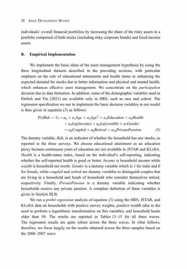
individuals’ overall financial portfolios by increasing the share of the risky assets in a
portfolio comprised of both stocks (including risky corporate bonds) and fixed-income
assets.
B. Empirical Implementation
We implement the basic ideas of the asset management hypothesis by using the
three longitudinal datasets described in the preceding sections, with particular
emphasis on the role of educational attainments and health status in enhancing the
expected demand for stocks due to better information and physical and mental health,
which enhances effective asset management. We concentrate on the participation
decision due to data limitation. In addition, some of the demographic variables used in
Ehrlich and Yin (2021) are available only in HRS, such as race and cohort. The
regression specification we use to implement the basic decision variables in our model
is thus given in equation (3) as follows:
Pr(Rah ¼ 1) ¼ a0 þ a1Ageþ a2Age2 þ a3Educationþ a4Health
þ a5log(income)þ a6log(wealth)þ a7Gender
þ a8Coupled þ a9Retired þ a10PrivatePension: (3)
The dummy variable, Rah, is an indicator of whether the household has any stocks, as
reported in the three surveys. We choose educational attainment as an education
proxy because continuous years of education are not available in JSTAR and KLoSA.
Health is a health-status index, based on the individual’s self-reporting, indicating
whether the self-reported health is good or better. Income is household income while
wealth is household net worth. Gender is a dummy variable which is 1 for male and 0
for female, while coupled and retired are dummy variables to distinguish couples that
are living in a household and heads of household who consider themselves retired,
respectively. Finally, PrivatePension is a dummy variable indicating whether
households receive any private pension. A complete definition of these variables is
given in Section III.B.
We run a probit regression analysis of equation (3) using the HRS, JSTAR, and
KLoSA data on households with positive survey weights, positive wealth (due to the
need to perform a logarithmic transformation on this variable), and household heads
older than 50. The results are reported in Tables 13–15 for all three waves.
The regression results are quite robust across the three waves. In what follows,
therefore, we focus largely on the results obtained across the three samples based on
the 2006–2007 wave.
38 ASIAN DEVELOPMENT REVIEW
March 23, 2022 10:31:07am WSPC/331-adr 2250004 ISSN: 0116-11052ndReading

C. Regression Results
A quick inspection of the results across the three samples in Tables 13–15
indicates that the probit regression specification yields the most robust results using the
HRS sample, where all coefficients are statistically significant at 5%, the only
exception being the coefficient of age, which is significant at the 10% level. In the
probit analysis using JSTAR and KLoSA, some of the demographic variables become
insignificant, in particular gender, coupled, and retired.
Table 13. Participation Decision for Stocks,2006–2007 Wave
Characteristics HRS JSTAR KLoSA
Intercept �6.438 �2.281 0.265(�9.42) (�2.70) (2.47)
Age �0.0348 0.0579 �0.00112(�1.83) (2.16) (�3.45)
Age2 0.00032 �0.00045 0.0000787(2.40) (�2.17) (3.19)
Education 0.205 0.067 0.0216(12.4) (7.79) (7.95)
Health 0.128 0.0097 �0.00293(3.38) (0.49) (�0.63)
log(income) 0.105 0.0154 0.0005(5.94) (3.28) (0.82)
log(net worth) 0.401 0.0238 0.0102(29.9) (3.66) (6.63)
Gender �0.0639 �0.0138 �0.0064(�1.98) (�0.73) (�1.34)
Coupled �0.0974 �0.00102 �0.0017(�2.77) (�0.04) (�0.34)
Retired 0.103 0.0138 0.0036(2.70) (0.57) (0.63)
PrivatePension 0.0823 0.0772 �0.0146(2.38) (3.91) (�1.45)
HRS ¼ United States Health and Retirement Study, JSTAR ¼Japanese Study of Aging and Retirement, KLoSA ¼ KoreanLongitudinal Study of Aging.Notes: The table shows the results of a probit analysis on stockownership for households with positive net worth and householdheads older than 50. t-statistics are in parentheses.Source: Authors’ calculations using data from the Health andRetirement Study (United States), the Japanese Study of Agingand Retirement, and the Korean Longitudinal Study of Aging.
A CROSS-COUNTRY COMPARISON OF OLD-AGE FINANCIAL READINESS 39
March 23, 2022 10:31:08am WSPC/331-adr 2250004 ISSN: 0116-11052ndReading

The most important result of our probit analysis is that it verifies the key
proposition of the asset management hypothesis: the educational attainment of the
household head has a statistically positive and significant impact on the probability
that households will be holding risky assets, which in this application are represented
by stocks. We observe this significant effect of education across all countries as well as
across all waves within the three countries, with no exception.
Due to the nonlinearity in the probit model, it is difficult to assess the quantitative
impacts of educational attainments on participation solely based on regression results.
Table 14. Participation Decision for Stocks,2008–2009 Wave
Characteristics HRS JSTAR KLoSA
Intercept �6.123 �1.329 0.529(�8.25) (�2.17) (4.25)
Age �0.0444 0.0235 �0.0194(�2.16) (1.21) (�5.13)
Age2 0.000374 �0.000182 0.000135(2.62) (�1.21) (4.74)
Education 0.192 0.0727 0.0181(11.20) (9.48) (5.59)
Health 0.0733 0.00737 0.0049(1.79) (0.44) (0.87)
log(income) 0.103 0.0372 0.00197(5.97) (1.05) (2.27)
log(net worth) 0.414 0.0426 0.0118(29.40) (9.51) (6.70)
Gender �0.0946 0.00244 �0.00827(�2.83) (0.15) (�1.49)
Coupled �0.0775 0.00654 �0.0188(�2.13) (0.42) (�3.31)
Retired 0.0959 �0.00638 0.0118(2.47) (�0.29) (6.70)
PrivatePension 0.0576 0.0972 0.00836(2.62) (5.20) (0.48)
HRS ¼ United States Health and Retirement Study, JSTAR ¼Japanese Study of Aging and Retirement, KLoSA ¼ KoreanLongitudinal Study of Aging.Notes: The table shows the results of a probit analysis on stockownership for households with positive net worth and householdheads older than 50. t-statistics are in parentheses.Source: Authors’ calculations using data from the Health andRetirement Study (United States), the Japanese Study of Agingand Retirement, and the Korean Longitudinal Study of Aging.
40 ASIAN DEVELOPMENT REVIEW
March 23, 2022 10:31:09am WSPC/331-adr 2250004 ISSN: 0116-11052ndReading

To generate a quantitative measure of the difference in participation, we compare the
participation probabilities across households attaining high school education versus
some college education. We make sure that the two groups are identical, except for
their different educational attainments, by assuming that all their other characteristics
follow the sample-weighted averages. For the 2006–2007 wave, the differences in the
probability of holding risky assets between these two groups are 7.96%, 7%, and
5.42% in the HRS, JSTAR, and KLoSA, respectively. Turning into percentage
Table 15. Participation Decision for Stocks,2010–2011 Wave
Characteristics HRS JSTAR KLoSA
Intercept �4.899 �0.571 �0.0637(�8.05) (�0.58) (�0.65)
Age �0.0716 �0.0058 �0.00056(�4.19) (�0.19) (�0.19)
Age2 0.000552 0.00004 0.00000057(2.62) (0.17) (0.03)
Education 0.163 0.0509 0.0144(9.92) (3.82) (5.39)
Health 0.161 0.00054 0.000825(4.10) (0.02) (0.18)
log(income) 0.0932 0.00103 0.000725(6.00) (1.20) (1.02)
log(net worth) 0.402 0.0627 0.0085(31.00) (7.76) (5.82)
Gender 0.00462 �0.0457 �0.0191(0.15) (�1.69) (�3.94)
Coupled �0.0588 0.0101 �0.00976(�1.73) (2.89) (�2.07)
Retired 0.0327 0.030 �0.00666(0.086) (0.81) (�1.23)
PrivatePension 0.141 0.114 0.0126(3.93) (1.63) (1.32)
HRS ¼ United States Health and Retirement Study, JSTAR ¼Japanese Study of Aging and Retirement, KLoSA ¼ KoreanLongitudinal Study of Aging.Notes: The table shows the results of a probit analysis on stockownership for households with positive net worth and householdheads older than 50. t-statistics are in parentheses.Source: Authors’ calculations using data from the Health andRetirement Study (United States), the Japanese Study of Agingand Retirement, and the Korean Longitudinal Study of Aging.
A CROSS-COUNTRY COMPARISON OF OLD-AGE FINANCIAL READINESS 41
March 23, 2022 10:31:10am WSPC/331-adr 2250004 ISSN: 0116-11052ndReading

differences, a higher educational attainment would boost stock ownership by 21.53%,
27.3%, and 34.56%, respectively.7
Our secondary conjecture, that better health would more likely lead people to
own stock, is verified only by our regression analysis using HRS data. This variable
becomes insignificant in both JSTAR and KLoSA. A possible reason is that the health
variable is a subjective measure of how well people perceive their health to be, and
these perceptions may differ across countries. In Japan, as we see in the descriptive
statistics, most people rate their health status to be quite high. The opposite seems to
be the case in the ROK (see descriptive statistics in Section III.B). The sharply
divergent concentrations of the individual data may bias the regression coefficient
associated with the health dummy downwards. The lower participation rate in stock
holding might bias the impact of health as well since, as a proxy for productive asset
management, it becomes less relevant.
The total effect of the age variable is found to be U-shaped in the HRS
regressions. But the age effect is not symmetrical across waves in the Asian countries:
it is hump-shaped in Japan (in wave 1), U-shaped in the ROK (in waves 1 and 2), and flat
in other waves (in Japan in waves 1 and 2 and in the ROK in wave 3). The U-shaped age
effect in the HRS regressions means that older people tend to hold stocks. We compute
the age at which older US investors start raising their stock holdings to be around age 60,
59.4, and 64.9 in the 2006–2007, 2008–2009, and 2010–2011waves, respectively, which
is reasonable since at this age wealth accumulation becomes more substantial for most
households, although this may be the case mainly in the US.
Income is included merely as a control variable. Without its presence, the
education effect might mistakenly pick up its explanatory power. Its positive
coefficient is statistically significant in regressions using HRS and JSTAR data. In
contrast, wealth is included as an efficiency measure, since it may represent experience
at managing assets. Its positive impact is statistically significant in all regressions.
In regressions based on the HRS sample, both retirement status and having
private pension as income have a statistically positive impact as well. This might be an
indication of the presence of spillover effects from having pension funds, especially
those based on defined contributions or IRAs, since individual account holders have a
direct responsibility for making decisions about portfolio composition in such funds.
However, the market for such funds appears to be weaker in Japan and especially in
the ROK.
7We did this comparison for other waves as well, using the corresponding data sets, and foundcomparable results.
42 ASIAN DEVELOPMENT REVIEW
March 23, 2022 10:31:10am WSPC/331-adr 2250004 ISSN: 0116-11052ndReading
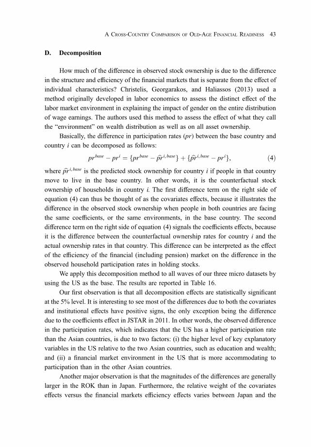
D. Decomposition
How much of the difference in observed stock ownership is due to the difference
in the structure and efficiency of the financial markets that is separate from the effect of
individual characteristics? Christelis, Georgarakos, and Haliassos (2013) used a
method originally developed in labor economics to assess the distinct effect of the
labor market environment in explaining the impact of gender on the entire distribution
of wage earnings. The authors used this method to assess the effect of what they call
the “environment” on wealth distribution as well as on all asset ownership.
Basically, the difference in participation rates (pr) between the base country and
country i can be decomposed as follows:
prbase � pr i ¼ fprbase � bpr i, baseg þ f bpr i, base � pr ig, ð4Þwhere bpr i, base is the predicted stock ownership for country i if people in that country
move to live in the base country. In other words, it is the counterfactual stock
ownership of households in country i. The first difference term on the right side of
equation (4) can thus be thought of as the covariates effects, because it illustrates the
difference in the observed stock ownership when people in both countries are facing
the same coefficients, or the same environments, in the base country. The second
difference term on the right side of equation (4) signals the coefficients effects, because
it is the difference between the counterfactual ownership rates for country i and the
actual ownership rates in that country. This difference can be interpreted as the effect
of the efficiency of the financial (including pension) market on the difference in the
observed household participation rates in holding stocks.
We apply this decomposition method to all waves of our three micro datasets by
using the US as the base. The results are reported in Table 16.
Our first observation is that all decomposition effects are statistically significant
at the 5% level. It is interesting to see most of the differences due to both the covariates
and institutional effects have positive signs, the only exception being the difference
due to the coefficients effect in JSTAR in 2011. In other words, the observed difference
in the participation rates, which indicates that the US has a higher participation rate
than the Asian countries, is due to two factors: (i) the higher level of key explanatory
variables in the US relative to the two Asian countries, such as education and wealth;
and (ii) a financial market environment in the US that is more accommodating to
participation than in the other Asian countries.
Another major observation is that the magnitudes of the differences are generally
larger in the ROK than in Japan. Furthermore, the relative weight of the covariates
effects versus the financial markets efficiency effects varies between Japan and the
A CROSS-COUNTRY COMPARISON OF OLD-AGE FINANCIAL READINESS 43
March 23, 2022 10:31:10am WSPC/331-adr 2250004 ISSN: 0116-11052ndReading

ROK. In Japan, the weight of the independent effects is more equal than in the ROK.
This implies that the financial market effect has more weight in the ROK relative to
Japan in explaining the participation gap in the ROK relative to the US.
The differences due to covariates are very robust for both countries across waves.
They vary from 7.72% for Japan in wave 1 to almost 10% in wave 2 and 9.16% in
wave 3. For the ROK, this difference steadily decreases from 20.78% in wave 1, down
to 17.15% in wave 2, and further down to 15.85% in wave 3. The explanation for the
decline in the ROK is quite straightforward. The most powerful driving force in stock
ownership is the household’s net worth, and we see a gradual, albeit slow rise in net
worth in ROK over this time period relative to the US.
As for the difference in the effects of the financial market environment on
participation, we observe a widening gap in the ROK: the difference due to coefficients
grows from 7.43% in wave 1 to 8.90% in wave 2 and further expands to 11% in wave
3. This might be a result of a combination of improvement in institutional arrangement
in the US (more DC plans encourage more stock ownership) and a lagging
development in institutional arrangement in the ROK (slow development of the stock
market and modernization of private pension plans). This pattern needs to be further
analyzed in future research.
In Japan, we see a quick reversal of the difference in the impact of the financial
market efficiency on participation—while this difference accounts for almost half of
the total difference in wave 1 at 8.24%, it narrows to 5.24% in wave 2, and then turns
negative at �4.65% in wave 3. The negative difference in 2010–2011 means that
Table 16. Decomposition of Differences in Participation Decision for Stocks UsingUnited States as the Base
Japan Republic of Korea
WaveTotal
Difference
DifferenceDue to
Covariates
DifferenceDue to
CoefficientsTotal
Difference
DifferenceDue to
Covariates
DifferenceDue to
Coefficients
(1) 2006–2007 15.96% 7.72% 8.24% 28.21% 20.78% 7.43%(11.2) (11.9) (42.2) (16.9)
(2) 2008–2009 15.06% 9.82% 5.24% 26.05% 17.15% 8.90%(17.5) (9.4) (32.4) (16.8)
(3) 2010–2011 4.51% 9.16% �4.65% 26.85% 15.85% 11.00%(15.8) (�8.0) (29.9) (20.8)
Notes: See Section V.D for a description of the decomposition analysis. t-statistics are in parentheses.Source: Authors’ calculations using data from the Health and Retirement Study (United States), theJapanese Study of Aging and Retirement, and the Korean Longitudinal Study of Aging.
44 ASIAN DEVELOPMENT REVIEW
March 23, 2022 10:31:11am WSPC/331-adr 2250004 ISSN: 0116-11052ndReading

Japan now holds an advantage in pension market efficiency relative to the US, which
encourages stock ownership. Whether this interpretation is valid, however, requires
further research. This is because there are several factors that may lead to this
interpretation. One factor is that JSTAR is not a national probabilistic survey, and it
added new municipalities in both waves 2 and 3. So the reversal in apparent market
productivity may merely reflect the difference between the newly added municipalities
and the old ones. Another possible explanation is that by 2011 private pension plan
reforms that were introduced by 2001 in Japan may have begun bearing fruit. We leave
this issue to further research.
VI. Conclusion
In this paper, we attempt to estimate the degree of financial readiness of older
cohorts in two relatively developed Asian countries by identifying the main channels
affecting their financial readiness or government dependency and assessing their
relative importance through a comparative analysis within and across the two
countries and in comparison to a reference country. We selected Japan and the ROK
as representatives of the Asian countries and added the US to serve as a reference
point for both for two reasons: all three countries have conducted similar micro-level
longitudinal surveys of the financial wellness and health of elderly individuals and
households using the same survey methodologies. These surveys report information
on the three main channels of old-age support for older households and retirees: the
income benefits they derive from the public and private pension systems in their
corresponding countries and the accumulated values of their households’ total and
financial assets. The latter channel allows us to study the extent to which households’
wealth and asset management contribute to their own financial readiness at old age.
All countries have experienced a demographic transition that has tended to accentuate
the degree of dependency of older and retired cohorts on old-age financial support
systems in their respective countries. The rapid aging of the populations, especially in
Japan and the ROK, makes the analysis of the determinants of the households’
financial readiness during their retirement a topic of academic importance and policy
relevance.
To compare the strength of old-age support systems in the three countries, we
first looked at the macro environments in these countries to determine the extent to
which demographic transitions have affected these countries’ old-age dependency
ratios. We find that the two Asian countries, especially the ROK, are facing an
A CROSS-COUNTRY COMPARISON OF OLD-AGE FINANCIAL READINESS 45
March 23, 2022 10:31:11am WSPC/331-adr 2250004 ISSN: 0116-11052ndReading

increasing overall level of dependency on both their public and private pension
systems due to rising life expectancies along with sharply declining total fertility
rates relative to the US. These demographic trends raise serious potential challenges
to the financial viability of old-age retirement systems in the Asian countries relative
to the US.
We then briefly assessed the retirement-income systems in these countries,
including both the public and private pension systems. Japan and the US have a clear
advantage over the ROK in terms of the financial strengths of their pension systems,
not only because they are more developed but also because they were established
much earlier than the Korean systems. Although the public pension systems in Japan
and the US are comparable in terms of their current financial viability, we find that US
households obtain higher benefits from their private pension system compared to their
Japanese and Korean counterparts, and their private pension system is better funded as
well. In contrast, the Korean private pension system is much weaker.
We examined the three countries further by studying the extensive personal and
financial household data provided in their micro-level longitudinal surveys—the HRS,
JSTAR, and KLoSA surveys—to further analyze the differences among the three
countries in terms of their old-age financial readiness. We find that Americans
typically retire earlier than their Asian counterparts—both Japanese and Koreans
workers tend to work into their 70s, whereas more Americans retire at early and full
pension-eligible ages. We also find that the replacement rate of income in retirement is
comparable in Japan and the US for retirees earning average incomes, while Koreans
have much lower replacement rates.
Using our micro-level data, we were also able to construct aggregate
distributions of income, net worth, and financial assets for the three countries.
While the US dominates both countries in all distributions, it only dominates Japan at
the upper part of their respective distributions of net worth and financial assets. The
corresponding net worth and financial wealth in the ROK lag significantly behind
those of the other two countries.
Turning finally to the extent to which individuals and households contribute to
their own financial readiness through their accumulated savings and asset allocation
decisions, we examine the role of a key determinant of wealth accumulation and old-
age financial readiness in developed countries: stock ownership. To determine the
extent to which this private source of old-age financial well-being is functioning in the
three countries, we implement the asset management model of the demand for risky
assets developed in EHY (2008). Specifically, we conduct a probit analysis of stock
46 ASIAN DEVELOPMENT REVIEW
March 23, 2022 10:31:11am WSPC/331-adr 2250004 ISSN: 0116-11052ndReading

ownership using the data on individual-level characteristics of household heads that
are expected to contribute to the willingness to hold stocks.
Our empirical analysis strongly confirms the key proposition of our model. The
regression results we obtain, using samples of older-age cohorts and retired cohorts in
each of the three countries and all wave samples within each country, show that
educational attainments of household heads and household wealth accumulation exert
a significant positive effect on the willingness of the households to hold stocks in their
financial portfolios. In addition, we utilize an econometric model to decompose the
total gap in stock ownership across countries into the portion that is attributable to
differences in the individual characteristics of investors and the portion that is due to
the differences in the level of development of the financial markets and pension
systems that exist in the respective countries. We find that much of the total difference
in stock holding between Korean, and to some extent Japanese, households and their
US counterparts is attributable to differences in the household’s individual
characteristics. However, our decomposition analysis also shows that a large part of
the gap in stock ownership is attributable to the institutional characteristics of the
different financial systems, largely because of the level of development of the private
pension sector in the Asian countries, especially in the ROK relative to the US. A more
encouraging finding from this analysis is that the difference in the institutional
characteristics of the pension systems between the US and Japan, and to some extent
even the ROK, have started shrinking in later waves of the households’ individual
longitudinal surveys we explore. Whether this trend will continue going forward may
be a subject of future research.
Our model suggests that the significant contributions of household asset
management and the level of development of the pension systems in the three
countries to the willingness of investors to hold stocks and other risky assets are
expected to enhance portfolio returns as well (for concrete evidence see Ehrlich and
Yin (2021) and Ehrlich and Shin (2021)). Our findings thus offer important policy
implications on the way the financial readiness of older and retired cohorts can be
improved in all surveyed countries, especially in the ROK. This is achievable through
a faster development of the markets for private pensions as well as via a concerted
effort to use special education programs to raise the financial knowledge of older age
groups. In future research, we plan to further explore more specific policy reforms
based on our findings, which might help improve the financial readiness of older age
groups and lower their dependency on the public support systems in their respective
countries.
A CROSS-COUNTRY COMPARISON OF OLD-AGE FINANCIAL READINESS 47
March 23, 2022 10:31:11am WSPC/331-adr 2250004 ISSN: 0116-11052ndReading

References
Campbell, John. 2006. “Household Finance.” Journal of Finance 61 (4): 1553–1604.Chien, Sandy, Nancy Campbell, Chris Chan, Orla Hayden, Michael Hurd, Regan Main, Joshua
Mallett, Craig Martin, Colleen McCullough, Erik Meijer, Michael Moldoff, PhilipPantoja, Susann Rohwedder, and Patricia St. Clair. 2015. “RAND HRS DataDocumentation, Version O. Labor & Population Program, RAND Center for the Studyof Aging.” http://hrsonline.isr.umich.edu/modules/meta/rand/randhrso/randhrs_O.pdf.
Christelis, Dimitris, Dimitris Georgarakos, and Michael Haliassos. 2013. “Differences inPortfolios across Countries: Economic Environment versus Household Characteristics.”The Review of Economics and Statistics 95 (1): 220–36.
Ehrlich, Isaac, and U. Ben-Zion. 1976. “Asset Management, Allocation of Time and Returns toSavings.” Economic Inquiry 14 (4): 558–86.
Ehrlich, Isaac, and Jinyoung Kim. 2005. “Endogenous Fertility, Longevity, and EconomicDynamics: Using a Malthusian Framework to Account for the Historical Evidence onPopulation and Economic Growth.” Journal of Asian Economics 15 (6): 789–806.
Ehrlich, Isaac, and Jong Kook Shin. 2010. “Human Capital and Imperfectly InformedInternational Financial Markets.” American Economic Review 100 (2): 244–49.
_____. 2021. “Can Human Capital and Asset Management Improve the Financial Performanceof Older Age Groups? Evidence from Europe.” Unpublished.
Ehrlich, Isaac, and Yong Yin. 2021. “The Role of Asset Management, Education, and Health inFinancial Decisions of Older Adults.” Unpublished.
Ehrlich, Isaac, William A. Hamlen, and Yong Yin. 2008. “Asset Management, Human Capital,and the Market for Risky Assets.” Journal of Human Capital 2 (3): 217–62.
Ehrlich, Isaac, Jong Kook Shin, and Yong Yin. 2011. “Private Information, Human Capital, andOptimal ‘Home Bias’ in Financial Markets.” Journal of Human Capital 5 (3): 255–301.
Grossman, Sanford, and Joseph Stiglitz. 1976. “Information and Competitive Price Systems.”The American Economic Review 66 (2): 246–53.
Ichimura, Hidehiko, Satoshi Shimizutani, and Hideki Hashimoto. 2009. JSTAR First Results2009 Report. Research Institute of Economy, Trade and Industry (RIETI).
Juster, F. Thomas, and Richard Suzman. 1995. “An Overview of the Health and RetirementStudy.” Journal of Human Resources 30: S7–S56.
Knoema. 2020. “Japan — Ratio of Population Aged 20–64 per Population 65+ Years.” https://knoema.com/atlas/Japan/topics/Demographics/Dependency-Ratios/Potential-support-ratio-20-64-per-65.
Mather, Mark, and Lillian Kilduff. 2020. “The U.S. Population Is Growing Older, and theGender Gap in Life Expectancy Is Narrowing.” Population Reference Bureau. https://www.prb.org/resources/u-s-population-is-growing-older/.
Organisation for Economic Co-operation and Development (OECD). 2009. OECD PrivatePensions Outlook 2008. Paris: OECD Publishing.
_____. 2019. Pensions at a Glance: OECD and G20 Indicators. Paris: OECD Publishing._____. 2020a. Pension Funds in Figures. Paris: OECD Publishing._____. 2020b. “Purchasing Power Parities (PPP).” https://doi.org/10.1787/1290ee5a-en
(accessed 29 October 2020).
48 ASIAN DEVELOPMENT REVIEW
March 23, 2022 5:33:57pm WSPC/331-adr 2250004 ISSN: 0116-11052ndReading
Rajnes, David. 2007. “The Evolution of Japanese Employer-Sponsored Retirement Plans.”Social Security Bulletin 67 (3): 89–104.
Social Security Administration (SSA). 2008, 2018. Social Security Programs Throughout theWorld: Asia and the Pacific. Woodlawn, Maryland.
United Nations. 2019. “World Population Prospects 2019.” Population Division, Department ofEconomic and Social Affairs. https://population.un.org/wpp/ (accessed 3 September2020).
Venti, Steven F., and David A. Wise. 2001. “Choice, Chance, and Wealth Dispersion atRetirement.” In Aging Issues in the United States and Japan, edited by Seiritsu Ogura,Toshiaki Tachibanaki, and David Wise, 25–64. Chicago: University of Chicago Press.
Verrecchia, Robert. 1982. “Information Acquisition in a Noisy Rational Expectation Economy.”Econometrica 50 (6): 1415–30.
A CROSS-COUNTRY COMPARISON OF OLD-AGE FINANCIAL READINESS 49
March 23, 2022 5:33:57pm WSPC/331-adr 2250004 ISSN: 0116-11052ndReading


Educational Gradients in Disabilityamong Asia’s Future Elderly: Projectionsfor the Republic of Korea and Singapore
CYNTHIA CHEN, JUE TAO LIM, NGEE CHOON CHIA,DAEJUNG KIM, HAEMI PARK, LIJIA WANG, BRYAN TYSINGER,
MICHELLE ZHAO, ALEX R. COOK, MING ZHE CHONG,JIAN-MIN YUAN, STEFAN MA, KELVIN BRYAN TAN, TZE PIN NG,
KOH WOON-PUAY, JOANNE YOONG, JAY BHATTACHARYA,AND KAREN EGGLESTON¤
Asia is home to the most rapidly aging populations in the world. This studyfocuses on two countries in Asia that are advanced in terms of theirdemographic transition: the Republic of Korea and Singapore. We developed ademographic and economic state-transition microsimulation model based onthe Korean Longitudinal Study of Aging and the Singapore Chinese HealthStudy. The model was employed to compare projections of functional statusand disability among future cohorts of older adults, including disparities in
⁄Cynthia Chen: Saw Swee Hock School of Public Health, National University of Singapore and NationalUniversity Health System, Singapore; and Schaeffer Center for Health Policy and Economics, Universityof Southern California, United States (US). E-mail: [email protected]; Jue Tao Lim: Saw Swee HockSchool of Public Health, National University of Singapore and National University Health System,Singapore. E-mail: [email protected]; Ngee Choon Chia: Department of Economics, National Universityof Singapore, Singapore. E-mail: [email protected]; Daejung Kim (corresponding author): Departmentof Health Care Policy Research, Korea Institute for Health and Social Affairs, Republic of Korea. E-mail:[email protected]; Haemi Park: Department of Social Welfare, Daejeon University, Republic ofKorea; Lijia Wang: Department of Statistics and Actuarial Science, University of Waterloo, Canada; BryanTysinger: Schaeffer Center for Health Policy and Economics, University of Southern California, US;Michelle Zhao: Stanford University, US; Alex R. Cook: Saw Swee Hock School of Public Health, NationalUniversity of Singapore and National University Health System, Singapore; Ming Zhe Chong: Saw SweeHock School of Public Health, National University of Singapore and National University HealthSystem, Singapore; Jian-Min Yuan: Department of Epidemiology, Graduate School of Public Health,University of Pittsburgh, US; and Division of Cancer Control and Population Sciences, UPMC HillmanCancer Center, US; Stefan Ma: Epidemiology and Disease Control Division, Ministry of Health, Singapore;
This is an Open Access article published by World Scientific Publishing Company. It is distributed underthe terms of the Creative Commons Attribution 3.0 International (CC BY 3.0) License which permits use,distribution and reproduction in any medium, provided the original work is properly cited.
March 23, 2022 10:23:19am WSPC/331-adr 2250005 ISSN: 0116-11052ndReading
Asian Development Review, Vol. 39, No. 1, pp. 51–89DOI: 10.1142/S0116110522500056
© 2022 Asian Development Bank andAsian Development Bank Institute.
disability prevalence by educational attainment. The model also projectsincreasing disparities in the prevalence of activities-of-daily-living disabilityand other chronic diseases between those with low and high educationalattainment. Despite overall increases in educational attainment, all elderly,including those with a college degree, experience an increased burden offunctional disability and chronic diseases because of survival to older ages.These increases have significant economic and social implications, includingincreased medical and long-term care expenditures, and an increased caregiverburden.
Keywords: ADL disability, microsimulation model, Republic of Korea,Singapore
JEL code: I14
I. Introduction
The Republic of Korea and Singapore are home to the most rapidly aging
populations in the world and are projected to have continually increasing proportions
of older adults in the coming decades. These countries are projected to be “top-heavy”
societies because of continued increase in life expectancy coupled with low,
below-replacement fertility rates. Although the changes in population size and
demographics in these countries have been studied, the complex evolution of the
health and functional disparities of the future elderly has not been fully explored.
These changes will have important implications for social protection systems,
including the financing and delivery of long-term care and health care.
Both Singapore and the Republic of Korea experienced rapid industrialization,
with exceptionally high average annual real gross domestic product growth rates of
Kelvin Bryan Tan: Policy Research and Economics Office, Ministry of Health, Singapore; Tze Pin Ng:Yong Loo Lin School of Medicine, National University of Singapore, Singapore; Koh Woon-Puay:Healthy Longevity Translational Research Programme, Yong Loo Lin School of Medicine, NationalUniversity of Singapore, Singapore; and Singapore Institute for Clinical Sciences, Agency for ScienceTechnology and Research, Singapore; Joanne Yoong: Center for Economic and Social Research,University of Southern California, US; Jay Bhattacharya: School of Medicine, Stanford University, US;Karen Eggleston: Shorenstein Asia Pacific Research Center, Stanford University, US. We thank KenwinMaung for the helpful discussions and statistical support that have contributed to this work. The researchwas supported by the National Medical Research Council (MOH-HSRGMH18may-0001) and the NationalInstitute on Aging of the National Institutes of Health (P30AG024968). The Singapore Chinese HealthStudy was supported by US National Institutes of Health (R01CA144034 and UM1CA182876). KohWoon-Puay was supported by the National Medical Research Council, Singapore (NMRC/CSA/0055/2013). The funding sources had no role in the design and conduct of the study; collection, management,analysis, or interpretation of the data; preparation, review, or approval of the paper; and decision to submitthe paper for publication. The Asian Development Bank recognizes “China” as the People’s Republic ofChina and “Korea” and “South Korea” as the Republic of Korea.
52 ASIAN DEVELOPMENT REVIEW
March 25, 2022 12:09:37pm WSPC/331-adr 2250005 ISSN: 0116-11052ndReading
7.38% and 7.42%, respectively, from 1960 to 2017 (World Bank 2017). They transited
from low-income to high-income economies within 50 years. Out of 188 economies
ranked in the Human Development Index, Singapore and the Republic of Korea are
considered to be highly developed economies with Human Development Index values
of 0.925 (ranked 4th) and 0.901 (ranked 18th), respectively (United Nations
Development Programme 2018). Their high scores are in part due to good universal
health care accessibility and high levels of educational attainment.
Our conceptual framework for studying the Republic of Korea and Singapore is
based on hypotheses and evidence from a large literature showing that human capital
accumulation is associated with broad socioeconomic development (Lee and Mason
2010) and can have a large effect on individuals and the economy. Good health allows
for more schooling and better absorption of knowledge, and education provides people
with the skills that translate into higher labor productivity and wages (Barro 2013).
Thus, higher educational attainment can affect health directly (e.g., through better
knowledge of how lifestyle choices impact health) as well as through its association
with higher socioeconomic status, including (depending on the health system)
improved financial access to quality health care and health insurance (Cutler and
Lleras-Muney 2010; Leopold and Engelhartdt 2012; Basu, Jones, and Dias 2018).
While many studies have examined the return-on-investment from education, few
have investigated how health disparities across education groups vary across time in
Asia. This endeavor may be challenging given the complex economic and social
interdependence between demographic change and population health. The Republic of
Korea and Singapore are both fast-growing industrialized countries, with sparse
mineral resources and human capital as their primary resource. While both the
Republic of Korea and Singapore are aging rapidly, they have differing trends in
educational attainment across genders. As the formation of human capital developed
differently over time in each country, this might have had different impacts on health.
Therefore, a study involving both countries allows us to examine human capital’s
comparative impacts on population health and the consequent disparities over time.
This may provide supporting evidence to aid policy makers in formulating effective
responses, especially for disadvantaged groups.
Education is linked to prevention of chronic disease (Harris 2007), disability
(Lutz et al. 2007, K. C. and Lentzner 2010) and mortality (Baker et al. 2011).
Higher-educated and wealthier individuals are less prone to physical disability later in
life (Gjonça, Tabassum, and Breeze 2009), and they possess longer disability-free life
expectancy (Minicuci and Noale 2005, Nogueira and Reis 2014). Thus, health
EDUCATIONAL GRADIENTS IN DISABILITY AMONG ASIA’S FUTURE ELDERLY 53
March 23, 2022 10:23:19am WSPC/331-adr 2250005 ISSN: 0116-11052ndReading

differences by educational attainment are expected, although it is not clear if these
educational gradients in health are steepening as the average education or human
capital of a society increases. Moreover, other factors might crowd out education’s
beneficial impact on health outcomes (Behrman and Wolfe 1987; Fuchs 2004; Conti,
Heckman, and Urzua 2010). A recent study in the People’s Republic of China found
steepening educational gradients in health, although the gradient flattens with age and
is mediated by economic and social resource variables (Chen et al. 2017). Lastly, age
and income also have a complex interplay with morbidity and mortality (McDonough
et al. 1997, Schnittker 2004, Kennedy et al. 2014). As such, a projection of the health
and functional disability of the middle-aged and elderly population needs to account
for socioeconomic and demographic trends, as well as competing risk factors to
provide an accurate picture for policy making.
Improvements in the educational composition of the population can also have a
considerable impact on decreasing the future prevalence of disability at any given age
(Lutz et al. 2007). There are many mechanisms. For example, Caldwell (1996) showed
that women’s education has a direct effect on the health status of the population
through improved maternal–child health. Gender disparities in education also
narrowed as educational attainment increased in the Republic of Korea and Singapore.
In the past, women were unlikely to be formally employed and had fewer educational
opportunities. However, much has changed and both countries have made great strides
in education; for example, in Singapore, female literacy rates rose from 34% in 1957 to
94% in 2010 (Moi 2010). This resulted in increased female wages (median income
rose from $2,863 in 2010 to $3,518 in 2014) and labor force participation (21.6% in
1957 to 58.6% in 2014), and induced better health outcomes, as an increase in literacy
rates is associated with increases in health-care access and utilization (Sudore et al.
2006, Bustamante et al. 2012). In addition, higher education is associated with lower
mortality, an improvement in psychosocial health, a reduction in bad lifestyle habits,
and lower occupational and health risks from jobs that demand manual labor such as
agriculture or construction (Currie and Hyson 1999, Deaton and Paxson 1999,
National Research Council 2012). Lower mortality among the better-educated, in turn,
implies survival to older ages. As a result, our conceptual framework suggests that the
increasing educational attainment of the Korean and Singaporean populations will lead
to lower age-standardized disability rates but higher overall disability rates because of
a higher proportion of the oldest-old and their associated disabilities. The educational
gradient in disability may decline or increase, depending on the relative health benefit
of better education among the low- versus high-educated groups.
54 ASIAN DEVELOPMENT REVIEW
March 23, 2022 10:23:19am WSPC/331-adr 2250005 ISSN: 0116-11052ndReading

To take into consideration the dynamic interplay between a rapidly aging
population, increases in educational attainment, age-dependent susceptibility to health
conditions, and functional disability in Asia, we develop a Future Elderly Model
(FEM) for the Republic of Korea and Singapore. The FEM is a sociodemographic and
economic state-transition microsimulation model with flexibility as a key strength: it
can take into account the evolving educational attainment of future elderly cohorts and
competing risks when projecting functional disability outcomes for the future elderly
population. We employ these models to project and compare functional disability
across the two countries, including disparities in functional disability prevalence by
educational attainment and gender, up to 2050. The models in this paper are similar in
spirit to the American FEM (Goldman et al. 2005), but with country-specific
prevalence rates of diseases, demographic trends, and transition probabilities for
different health states. The Republic of Korea’s estimates are based on the harmonized
version of the Korean Longitudinal Study of Aging (KLoSA), while the Singapore
model is based on the Singapore Chinese Health Study (SCHS).
We find that from 2015 to 2050, the educational gradient in health and functional
status will steepen, with a wider gap in the prevalence of functional disability between
those with low and high educational attainment. For example, in Singapore, the
disparity in functional disability prevalence, as measured by limitation in at least one
activity of daily living (ADL), starts at a difference of 9.5 percentage points in 2015
and climbs by 2050 to a difference of over 23 percentage points (31.9% among those
with low education, compared to 8.7% among the college-educated). Functional
disability as measured by instrumental activities of daily living (IADL) shows a
similar pattern. The Republic of Korea’s model projects even larger disparities by
2050, as exemplified by a difference of 41.7 percentage points in the prevalence of any
functional disability between low- and high-educational attainment groups (i.e., 51.7%
among those with less than a high school education, compared to 10.0% among the
college-educated). These disparities are driven almost entirely by population aging and
increasing education so that the population in the lower educational attainment group
is a small, selected disadvantaged group. Improved survival of those with low
education and their declining share of the population leads to their concentration
among the oldest-old (therefore with the highest disability burden), especially in the
Republic of Korea.
The remainder of this paper is organized as follows. Section II describes the data
and method for operationalizing the FEM for the Republic of Korea and Singapore.
Section III presents the results on functional disability and the associated educational
gradient in the future elderly by country. The last section identifies economic and
EDUCATIONAL GRADIENTS IN DISABILITY AMONG ASIA’S FUTURE ELDERLY 55
March 23, 2022 10:23:19am WSPC/331-adr 2250005 ISSN: 0116-11052ndReading

policy implications, as well as areas for mutual learning and improvement. Further
details on the models for individual countries are reported in the appendixes.1
II. Method
A. Data
Data were drawn from comprehensive longitudinal surveys of older adults from
two rapidly aging economies, the Republic of Korea and Singapore. The KLoSA is a
longitudinal study of individuals over age 45 years old in the Republic of Korea. It was
designed to help researchers and policy makers better understand the socioeconomic
determinants and consequences of aging. The survey includes a rich set of questions
regarding the economic standing, physical and psychological health, demographics,
and social networks of aged persons. We used the harmonized KLoSA dataset, which
contains Waves 1, 2, 3, and 4 as of October 2015. The first wave of the KLoSA survey
was conducted in 2006 and included 10,254 respondents aged 45 years and over. The
second wave was done in 2008 with 8,688 respondents. The third wave was done in
2010 with 7,920 respondents. The fourth wave was done in 2012 with 7,486
respondents.
The SCHS is a prospective cohort study of ethnic Chinese men and women aged
45–74 years old in the baseline who were followed up for a mean duration of 12 years.
Inclusion criteria were similar to an earlier study (Chen et al. 2019b), with respondents
being either citizens or permanent residents, residing in government-built housing, and
belonging to either of the two major dialect groups of Chinese in Singapore (Hokkien
and Cantonese). The baseline study (n ¼ 63,257) was collected between 1993 and
1999, follow-up 1 (n ¼ 52,325) was collected between 1999 and 2004, and follow-up
2 (n ¼ 39,528) was collected between 2006 and 2010. At baseline, each participant
completed an in-person interview at their home using a structured questionnaire that
requested information about demographic characteristics, self-reported height and
weight, smoking status, current physical activity, occupational exposure, medical
history, and family history of cancer. A follow-up telephone interview asked
participants for an update on their tobacco and alcohol use as well as medical history.
We used the Singapore Longitudinal Aging Study (SLAS)—a smaller cohort
that consists of 2,804 subjects aged 55 years or above interviewed in 2004–2005,
1The online Appendixes can be accessed at: https://sph.nus.edu.sg/wp-content/uploads/2022/03/Appendix_FEM_SGSK_v2.pdf.
56 ASIAN DEVELOPMENT REVIEW
March 23, 2022 10:23:19am WSPC/331-adr 2250005 ISSN: 0116-11052ndReading

2007–2008, and 2010–2011—to model functional disability. Older adults who were
citizens or permanent residents aged 55 years or above were identified by door-to-door
census and invited to participate voluntarily in the study.
B. Microsimulation Model
The FEM microsimulation model includes disease transitions and accounts for
population aging within the middle-aged and elderly population. Using the FEM, we
are able to model individual-level longitudinal dynamics, allowing for greater
heterogeneity than cell-based approaches. Moreover, populations entering the
microsimulation reflect current trends in sociodemographic characteristics and health
status based on data from population surveys. The FEM was successfully implemented
first to support decision-making related to Medicare and Medicaid, the public health
insurance and welfare programs for the elderly and needy, respectively, in the United
States (Goldman et al. 2005). Since then, the FEM has been used for dozens of
important papers for informing health and social issues in aging societies such as the
United States, European Union, and Japan (Michaud et al. 2011, Chen et al. 2016,
Chen et al. 2019b). Its ongoing development is supported by the National Institute on
Aging through the University of Southern California’s Roybal Center for Health
Policy Simulation (University of Southern California 2019). In using the same FEM
model to project functional disability for Singapore and the Republic of Korea, we aim
to: (i) highlight potential differences in the aging experience by gender and education
in each country to inform social and health-care policy, and (ii) provide a common
platform for international comparison to identify and compare challenges across
countries.
Individuals in the FEM are characterized by their socioeconomic status and
health states. From period to period, they transit from one health state to another with
probabilities that are estimated from the data (see Section II.C). The Singapore FEM is
modeled with a 6-year time step, as the SCHS was surveyed with a mean of 6 years
between each study wave. The Republic of Korea’s FEM model follows a 2-year time
step mirroring the mean time between waves of the KLoSA study. We then interpolate
linearly the outcomes to yearly rates. As there was no difference in results when
presenting with 6-year compared to 5-year intervals, we reported the 5-year charts for
ease of interpretation. Also, a replenishing cohort is introduced every period at the
default starting age, set at 55–60 years old for Singapore and 51–52 years old for the
Republic of Korea. Individuals within the simulation exit from the model at the time of
death. Hence, although some individuals are lost to mortality, the population expands
EDUCATIONAL GRADIENTS IN DISABILITY AMONG ASIA’S FUTURE ELDERLY 57
March 23, 2022 10:23:19am WSPC/331-adr 2250005 ISSN: 0116-11052ndReading

with renewal. KLoSA and SCHS are post-stratified by age group, gender, and
education. They are then rebalanced with the corresponding population weights using
population projections obtained from the International Institute for Applied Systems
Analysis and the Vienna Institute of Demography projections for Singapore. In the
Republic of Korea, the education profile was rebalanced using the Barro–Lee
projections. This adjustment is made for both the initial cohort as well as the
replenishing cohorts over the simulation cycles. The distribution of socioeconomic
status, particularly education, and health status vary across the new cohorts depending
on the trends derived from the data and on the time of their introduction. In each
simulation cycle, the population moves forward in time and individuals transit to new
states probabilistically; this results in an observable distribution of health in the
population at the end of each cycle. The replenishing cohort model, which determines
the distribution of states among individuals in the new cohorts, is estimated in Stata,
while the overarching simulation is implemented in C++ for computational efficiency.
To calculate the Monte Carlo confidence intervals, we repeated the sample process
described above 1,000 times and used the 2.5th and 97.5th percentiles as the prediction
interval, similar to other studies (Pericchi and Walley 1991, O’Brien et al. 2009, Chen
et al. 2019a).
C. Health Transition Model
The FEM uses a discrete piecewise linear hazard model on longitudinal data to
estimate transitional probabilities for selected measures of health status. The hazard of
getting a disease, dying, or becoming disabled depends on risk factors such as gender,
education, lifestyle, comorbidities, functional status, and age (Appendix 4).
The resulting hazards will then be used as parameters in the microsimulation model
to determine how individuals transit between health states from one period to the next.
The health transition model is estimated in Stata. We used probit regressions to
estimate the probability of transition to each health condition, controlling for
education, demographic variables, and comorbidities at the previous period.
We treated all diseases as an absorbing state—as there is currently no cure for
chronic diseases such as diabetes, hypertension, heart disease, or stroke—in reflection
of the question asked: “Have you ever been told . . . by a doctor?” In the Republic of
Korea, variables were measured with a 2-year lag in the KLoSA (Jang 2016).
In Singapore, all independent variables were measured with a 6-year lag in the SCHS
and represent the respondent’s characteristics from 1993 to 2010 (National University
of Singapore 2018). In both countries, as diseases were treated as an absorbing state,
we assumed that those with a chronic condition in the previous wave would continue
58 ASIAN DEVELOPMENT REVIEW
March 23, 2022 10:23:19am WSPC/331-adr 2250005 ISSN: 0116-11052ndReading

to have that disease in the current wave. As such, transition probabilities were only
estimated on those who did not suffer from a specific condition at the time of the
previous survey wave.
The transition model is the core of the FEM. The transition model describes the
health status of individuals and how it evolves between periods over the course of the
simulation. The model’s main variables consist of sociodemographic and behavioral
variables denoted as AGEit, GENDERi, EDUCATIONi, MARITAL_STATUSi,
SMOKE_CURRENTit, SMOKE_EVERit, and BMIit, as well as a set of indicator
variables for diseases: DISEASEit ¼ fDISEASE1it, . . . , DISEASENitg with reference
to the N chronic conditions, where i refers to the individual and t refers to the time.
In addition, a mortality indicator variable denoted DIEDit was created and is equal to 1
if the simulated individual i dies at time t during the simulation or 0 otherwise.
The baseline cohort is defined at the initial time period (t ¼ 1). The variables of AGEit,
GENDER i, EDUCATION i, MARITAL_STATUS i, SMOKE_CURRENT it,
SMOKE_EVERit, BMIit, and DISEASEit in the baseline cohort are retrievable from
the KloSA and SCHS datasets. All of these samples are allocated with a specific
weight such that the number of individuals in each age, sex, and education level
category is consistent with that of the population distribution in each country.
Figure 1 provides a schematic overview of the model. The FEM simulation starts
from 2008 with initial populations aged 51 years and above in the Republic of Korea
and Singapore. We then predict outcomes using our estimation for the initial cohort
(Appendix 4) to begin the simulation. Individuals who survive are defined as those for
whom the transition model predicts DIEDit not equal to 1 (nondecedents) at the end of
the corresponding year. Projections on policy outcomes are then made for that year.
Thereafter, the FEM moves to the following time period within the simulation cycle
when a new cohort enters. The current cohort and the replenishing cohort form the
new population of those aged 51 years and above (Republic of Korea) or 55 years and
above (Singapore), which then proceeds through the transition module as before. The
replenishing cohort enters the simulation every 2 years for the Republic of Korea and
every 6 years for Singapore. This process of replenishing new cohorts and transiting
across various health states is repeated until we reach the final year of the simulation.
Each individual module is explained in more detail in Appendix 4.
D. Functional Disability Model
We defined functional disability as having any ADL disability such as
limitation in washing, dressing, feeding, toileting, mobility, and transferring
EDUCATIONAL GRADIENTS IN DISABILITY AMONG ASIA’S FUTURE ELDERLY 59
March 23, 2022 10:23:19am WSPC/331-adr 2250005 ISSN: 0116-11052ndReading

(Ministry of Health 2018), or having any IADL disability such as limitation in taking
transportation, shopping, managing money, making phone calls, doing household
chores, and meal preparation. The former measures an individual’s physical ability to
perform basic tasks, whereas the latter includes higher-order tasks that measure an
individual’s engagement and management of resources. We projected future functional
disability using probit regressions for any ADL and IADL disability, and ordered
probit regressions for disability measured on an ordinal scale. In the ordered probit
regression for each country, we summed the number of ADL functional disabilities in
washing, dressing, feeding, toileting, mobility, and transferring. We then modeled
adlstat as three categories: (i) having no disability, (ii) having one or two disabilities,
or (iii) having three or more disabilities. We modeled adlstat as an ordinal outcome
using ordered probit regression. Similar analysis was performed for IADL.
The covariates included were age, gender, educational attainment, body mass index,
marital status, and chronic diseases.
Figure 1. Schematic Overview of Future Elderly Model Simulation in theRepublic of Korea and Singapore
Population
T0
Replenishingcohort
T1
Health andspendingoutcomes
T2
Replenishingcohort
T1
Health andspendingoutcomes
T1
Health andspendingoutcomes
T0
Health Transitions Module Module
Policy OutcomesReplenishing Cohort Module
Population
T1
Population
T2
Source: Authors’ illustration.
60 ASIAN DEVELOPMENT REVIEW
March 23, 2022 10:23:19am WSPC/331-adr 2250005 ISSN: 0116-11052ndReading

E. Educational Attainment
Only educational attainment was modeled according to countries’ specific
categorization. In the Republic of Korea, low attainment is defined as less than high
school, middle attainment is defined as high school, and high attainment is defined as
having a college education. In Singapore, low attainment is defined as having a
primary education or less (6 years of education or less); middle attainment as having a
secondary school education, technical education, or diploma (7–15 years of
education); and high attainment as having a college education or above (at least 15
years of education). We wanted to capture each country’s specific distribution of
relative educational attainment, as this distribution better captures each country’s
dispersion in human capital and helps us therefore to understand the relationship
between educational differences and health disparities. Given this categorization, those
with low educational attainment in the Republic of Korea are on average more
educated than those categorized as low educational attainment in Singapore, whereas
high educational attainment is comparable across the two countries. Our appendixes
also include figures depicting the model projections when using a consistent definition
of low educational attainment for both countries, defined as having less than a college
education. Education was used as a measure of socioeconomic status, and we used
these two terms interchangeably.
III. Results
A. Country Characteristics
The United Nations (UN) has projected both the Republic of Korea and
Singapore to age rapidly in the future (Figure 2). This aging within the middle-aged
and older population reflects the large post-war baby boomer cohorts, subsequent
low fertility, and improved survival (lower age-specific mortality) across the
population. Using UN data, the proportion aged 65 years and above in 2015 was
13.0% in the Republic of Korea and 11.7% in Singapore; in 2050, these shares will
have increased to 35.3% and 33.6%, respectively. The old-age support ratio, defined
as the population aged 20–64 years (working age) divided by the population aged 65
years and above, declines at similar rates in both countries from about 6 working
adults per elderly person in 2015 to about 1.5 working adults per elderly person in
2050. Using the UN projections, Figure 3 shows that both countries will have an
increasing percentage of the elderly with a college education among both men and
EDUCATIONAL GRADIENTS IN DISABILITY AMONG ASIA’S FUTURE ELDERLY 61
March 23, 2022 10:23:20am WSPC/331-adr 2250005 ISSN: 0116-11052ndReading

women. The projection also shows that the number of the elderly with low or no
education will decrease continuously. Using UN data, in 2015 the percentage of
older adults with low or no formal education was higher in females compared to
males: for the Republic of Korea, 64% (females) and 30% (males); for Singapore,
Figure 2. Share of Population Aged 65 Years and Above
0
5
10
15
20
25
30
35
40
2015 2020 2025 2030 2035 2040 2045 2050
Perc
enta
ge a
ged
65+
Republic of Korea Singapore
Source: United Nations Department of Economic and Social Affairs. 2017. World Population Prospects: The2017 Revision. https://www.un.org/development/desa/publications/world-population-prospects-the-2017-revi-sion.html.
Figure 3. Percentage of Low and High Educational Attainment among Those Aged65 Years and Above
Low edu female Low edu male
High edu female High edu male
–64%
1970 1980 1990 2000 2010 2020 2030 2040 2050
Republic of Korea
–30%
1%%–4%
39% F
1970 1980 1990 2000 2010 2020 2030 2040 2050
Singapore
–18%
50% M
0%
20%
40%
60%
80%
100%
–67%
–6%
36% F
–13%
42% M
0%
20%
40%
60%
80%
100%
3%%% FF M
18% F 13% M
–46%
edu ¼ education, M ¼ male, F ¼ female.Source: International Institute for Applied Systems Analysis and the Vienna Institute of Demography projectionextracted from United Nations Department of Economic and Social Affairs. 2017. World Population Prospects:The 2017 Revision. https://www.un.org/development/desa/publications/world-population-prospects-the-2017-revision.html.
62 ASIAN DEVELOPMENT REVIEW
March 23, 2022 10:23:20am WSPC/331-adr 2250005 ISSN: 0116-11052ndReading

67% (females) and 46% (males). By 2050, the percentage is projected to have
decreased substantially for both countries: for the Republic of Korea, 3% (females)
and 1% (males); for Singapore, 18% (females) and 13% (males). Over the same
period, there will be a sharper increase in college education among women than
men: for females, from 4.3% in 2015 to 38.9% in 2050 in the Republic of Korea
and from 6.0% in 2015 to 36.1% in 2050 in Singapore; compared with males, from
18.1% in 2015 to 50.2% in 2050 in the Republic of Korea and from 13.1% in 2015
to 41.8% in 2050 in Singapore.
Thus, educational attainment among our replenishing cohorts was projected to
increase (Figure 4). In the Republic of Korea, the proportion of primary school
graduates entering middle school was 99.9% in 2000, and the proportion of middle
school graduates entering high school was 99.7% (Ministry of Education 2000).
Our model captures how this change in educational attainment of future older adults
will shape trends in health, incorporating both differences in mortality and morbidity.
Based on our FEM simulations, Figure 5 shows the aging pyramid in both countries
with growing numbers of elderly with college education.
In both countries, chronic conditions and functional disability were projected to
rise during the review period. IADL disability is projected to be much higher in
Singapore than the Republic of Korea in 2050 (Figure 6). The prevalence of chronic
disease burden for diabetes, stroke, and heart disease will be higher in the Republic of
Korea.
By 2050, the total number of people with any ADL disability was projected to
increase to 275,000 (18.9%) in Singapore and 2.48 million (15.9%) in the Republic of
Figure 4. Educational Attainment among Future Middle-Aged and Elderly in Singapore andthe Republic of Korea: Trends in the Replenishing Cohorts in the Future Elderly Model
Highsch ¼ high school, PSLE ¼ primary school leaving examination.Source: Authors’ calculations using the Future Elderly Model based on data from the Korean Longitudinal Studyof Aging and the Singapore Chinese Health Study.
EDUCATIONAL GRADIENTS IN DISABILITY AMONG ASIA’S FUTURE ELDERLY 63
March 23, 2022 10:23:23am WSPC/331-adr 2250005 ISSN: 0116-11052ndReading
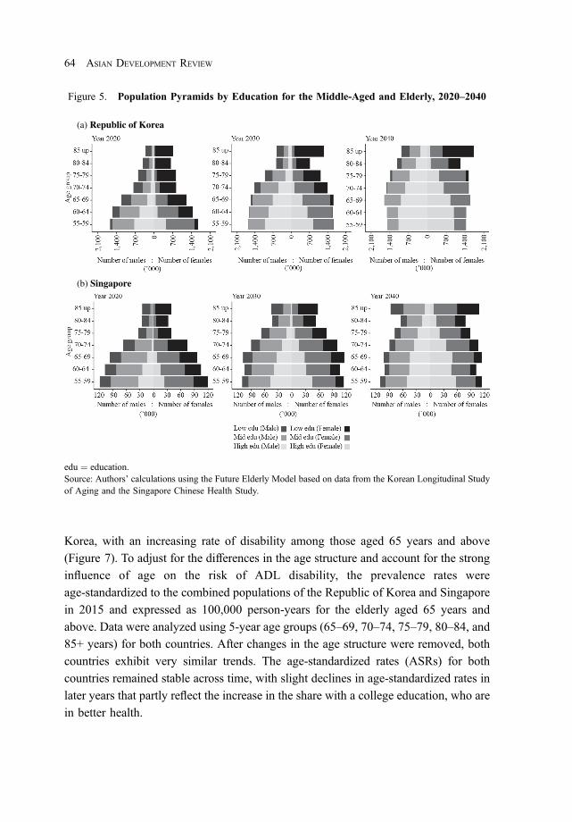
Korea, with an increasing rate of disability among those aged 65 years and above
(Figure 7). To adjust for the differences in the age structure and account for the strong
influence of age on the risk of ADL disability, the prevalence rates were
age-standardized to the combined populations of the Republic of Korea and Singapore
in 2015 and expressed as 100,000 person-years for the elderly aged 65 years and
above. Data were analyzed using 5-year age groups (65–69, 70–74, 75–79, 80–84, and
85+ years) for both countries. After changes in the age structure were removed, both
countries exhibit very similar trends. The age-standardized rates (ASRs) for both
countries remained stable across time, with slight declines in age-standardized rates in
later years that partly reflect the increase in the share with a college education, who are
in better health.
Figure 5. Population Pyramids by Education for the Middle-Aged and Elderly, 2020–2040
(b) Singapore
(a) Republic of Korea
edu ¼ education.Source: Authors’ calculations using the Future Elderly Model based on data from the Korean Longitudinal Studyof Aging and the Singapore Chinese Health Study.
64 ASIAN DEVELOPMENT REVIEW
March 23, 2022 10:23:25am WSPC/331-adr 2250005 ISSN: 0116-11052ndReading
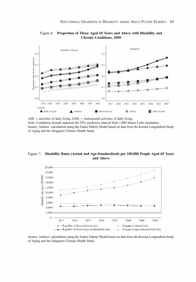
Figure 6. Proportion of Those Aged 65 Years and Above with Disability andChronic Conditions, 2050
0.0
0.1
0.2
0.3
0.4
Prop
ortio
n w
ith c
hron
ic c
ondi
tions
0.0
0.1
0.2
0.3
0.4
Legend
IADL Overall Diabetes Heart Disease Stroke ADL Overall
Republic of KoreaSingapore
2015 2020 2025 2030 2035 2040 2045 20502015 2020 2025 2030 2035 2040 2045 2050
ADL ¼ activities of daily living, IADL ¼ instrumental activities of daily living.Note: Confidence bounds represent the 95% prediction interval from 1,000 Monte Carlo simulation.Source: Authors’ calculations using the Future Elderly Model based on data from the Korean Longitudinal Studyof Aging and the Singapore Chinese Health Study.
Figure 7. Disability Rates (Actual and Age-Standardized) per 100,000 People Aged 65 Yearsand Above
Source: Authors’ calculations using the Future Elderly Model based on data from the Korean Longitudinal Studyof Aging and the Singapore Chinese Health Study.
EDUCATIONAL GRADIENTS IN DISABILITY AMONG ASIA’S FUTURE ELDERLY 65
March 23, 2022 10:23:31am WSPC/331-adr 2250005 ISSN: 0116-11052ndReading

B. Educational Gradients in Disability
The model projects a continuing—and in some cases steepening—educational
gradient in disability and chronic conditions, with those of lower education
experiencing a higher prevalence of disability and chronic diseases. This result was
consistent across genders, although varying in magnitude across countries over time.
For men in Singapore, in 2015, the difference in the prevalence of poor health
between elderly with low and high educational attainment was largest for IADL
disability (21.3 percentage points), followed by diabetes (6.4 percentage points) and
ADL (5.8 percentage points). For women in Singapore, the difference was largest for
IADL disability (16.7 percentage points), followed by diabetes (15.5 percentage
points) and hypertension (15.2 percentage points). For men in the Republic of Korea,
in 2015 the absolute difference in the prevalence between elderly with low and high
educational attainment was largest for IADL disability (7.0 percentage points),
followed by heart disease (5.2 percentage points), and ADL disability (4.1 percentage
points). For women, the difference was largest for hypertension (20.0 percentage
points), followed by IADL disability (12.2 percentage points) and diabetes (10.7
percentage points).
Over time, ADL disability is projected to rise sharply for the elderly with low
educational attainment in the Republic of Korea from 10.3% in 2015 to 51.7% in
2050, while increasing at a slower pace in Singapore from 13.1% to 31.9% over the
same period (Figure 8a). In part, this reflects the fact that low-educated Koreans will
be concentrated exclusively among the oldest-old by 2050 (see Figures 2 and 3),
rather than also including those in their 60s and 70s as in Singapore. For female
elderly with high educational attainment, the prevalence of ADL disability was
projected to be higher in Singapore compared to the Republic of Korea. The disparities
in the burden of ADL disability appeared larger for the Republic of Korea and are
projected to increase in the future as the low-education group becomes a tiny fraction
of the population, whereas the difference is projected to stabilize for Singapore in the
future. Similar trends were observed in both males (Figure 8b) and females
(Figure 8c). Also, the difference in ADL disability among low- and high-education
groups is projected to be larger for females than males in both countries.
IADL disability is projected to rise sharply for elderly with low education in the
Republic of Korea from 19.9% in 2015 to 71.8% in 2050, while it increases less
quickly for Singapore from 27.2% to 57.0% during the same period (Figure 9a).
Although the overall projected prevalence of IADL disability is lower in Singaporean
elderly with high education, this is driven mainly by males (Figures 9b and 9c).
66 ASIAN DEVELOPMENT REVIEW
March 23, 2022 10:23:34am WSPC/331-adr 2250005 ISSN: 0116-11052ndReading
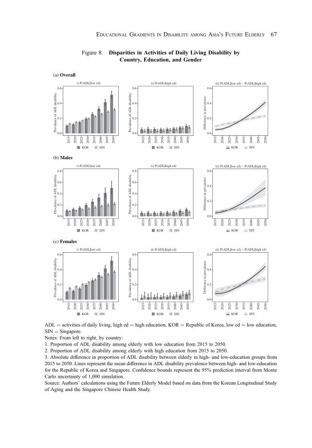
Figure 8. Disparities in Activities of Daily Living Disability byCountry, Education, and Gender
0.0
0.2
0.4
0.6
Prev
alen
ce o
f A
DL
dis
abili
ty
(a) Overall
i) P(ADL|low ed)
0.0
0.2
0.4
0.6
Prev
alen
ce o
f A
DL
dis
abili
ty
ii) P(ADL|high ed)
0.0
0.2
0.4
0.6
Dif
fere
nce
in p
reva
lenc
e
2015
iii) P(ADL|low ed) − P(ADL|high ed)
2020
2025
2030
2035
2040
2045
2050
2015
2020
2025
2030
2035
2040
2045
2050
2015
2020
2025
2030
2035
2040
2045
2050
SINKOR SINKOR KOR SIN
Dif
fere
nce
in p
reva
lenc
e
ii) P(ADL|high ed)
(b) Males
i) P(ADL|low ed) iii) P(ADL|low ed) − P(ADL|high ed)
0.0
0.2
0.4
0.6
0.8
Prev
alen
ce o
f A
DL
dis
abili
ty
0.0
0.2
0.4
0.6
0.8
Prev
alen
ce o
f A
DL
dis
abili
ty
0.0
0.2
0.4
0.6
2015
2020
2025
2030
2035
2040
2045
2050
2015
2020
2025
2030
2035
2040
2045
2050
2015
2020
2025
2030
2035
2040
2045
2050
SINKOR SINKOR KOR SIN
Dif
fere
nce
in p
reva
lenc
e
iii) P(ADL|low ed) − P(ADL|high ed)
0.0
0.2
0.4
0.6
Prev
alen
ce o
f A
DL
dis
abili
ty
(c) Females
i) P(ADL|low ed)
0.0
0.2
0.4
0.6
Prev
alen
ce o
f A
DL
dis
abili
ty
ii) P(ADL|high ed)
0.0
0.2
0.4
0.6
2015
2020
2025
2030
2035
2040
2045
2050
2015
2020
2025
2030
2035
2040
2045
2050
2015
2020
2025
2030
2035
2040
2045
2050
SINKOR SINKOR KOR SIN
ADL ¼ activities of daily living, high ed ¼ high education, KOR ¼ Republic of Korea, low ed ¼ low education,SIN ¼ Singapore.Notes: From left to right, by country:1. Proportion of ADL disability among elderly with low education from 2015 to 2050.2. Proportion of ADL disability among elderly with high education from 2015 to 2050.3. Absolute difference in proportion of ADL disability between elderly in high- and low-education groups from2015 to 2050. Lines represent the mean difference in ADL disability prevalence between high- and low-educationfor the Republic of Korea and Singapore. Confidence bounds represent the 95% prediction interval from MonteCarlo uncertainty of 1,000 simulation.Source: Authors’ calculations using the Future Elderly Model based on data from the Korean Longitudinal Studyof Aging and the Singapore Chinese Health Study.
EDUCATIONAL GRADIENTS IN DISABILITY AMONG ASIA’S FUTURE ELDERLY 67
March 23, 2022 10:23:34am WSPC/331-adr 2250005 ISSN: 0116-11052ndReading

Figure 9. Disparities in Instrumental Activities of Daily Living Disability byCountry, Education, and Gender
0.0
0.2
0.4
0.6
0.8
Prev
alen
ce o
f IA
DL
dis
abili
ty
(a) Overalli) P(IADL|low ed)
0.0
0.2
0.4
0.6
0.8
Prev
alen
ce o
f IA
DL
dis
abili
ty
ii) P(IADL|high ed)
0.0
0.2
0.4
iii) P(IADL|low ed) − P(IADL|high ed)
0.6
2015
2020
2025
2030
2035
2040
2045
2050
2015
2020
2025
2030
2035
2040
2045
2050
2015
2020
2025
2030
2035
2040
2045
2050
Dif
fere
nce
in p
reva
lenc
e
SINKOR SINKOR KOR SIN
0.00
0.25
0.50
0.75
1.00
Prev
alen
ce o
f IA
DL
dis
abili
ty
(b) Males)de wol|LDAI(P )i
0.00
0.25
0.50
0.75
1.00
Prev
alen
ce o
f IA
DL
dis
abili
ty
ii) P(IADL|high ed)
0.0
0.2
0.4
0.6
2015
2020
iii) P(IADL|low ed) − P(IADL|high ed)
2025
2030
2035
2040
2045
2050
2015
2020
2025
2030
2035
2040
2045
2050
2015
2020
2025
2030
2035
2040
2045
2050
Dif
fere
nce
in p
reva
lenc
e
SINKOR SINKOR KOR SIN
0.0
0.2
0.4
0.6
0.8
Prev
alen
ce o
f IA
DL
dis
abili
ty
(c) Femalesi) P(IADL|low ed)
0.0
0.2
0.4
0.6
0.8
Prev
alen
ce o
f IA
DL
dis
abili
ty
ii) P(IADL|high ed)
0.0
0.2
0.4
0.6
2015
2020
iii) P(IADL|low ed) − P(IADL|high ed)
2025
2030
2035
2040
2045
2050
2015
2020
2025
2030
2035
2040
2045
2050
2015
2020
2025
2030
2035
2040
2045
2050
Dif
fere
nce
in p
reva
lenc
e
SINKOR SINKOR KOR SIN
IADL ¼ Instrumental activities of daily living, high ed ¼ high education, KOR ¼ Republic of Korea, low ed ¼low education, SIN ¼ Singapore.Notes: From left to right, by country:1. Proportion of IADL disability among elderly with low education from 2015 to 2050.2. Proportion of IADL disability among elderly with high education from 2015 to 2050.3. Absolute difference in proportion of IADL disability between elderly in high- and low-education groups from2015 to 2050. Lines represent the mean difference in IADL disability prevalence between high- and low-education for the Republic of Korea and Singapore. Confidence bounds represent the 95% prediction intervalfrom Monte Carlo uncertainty of 1,000 simulation.Source: Authors’ calculations using the Future Elderly Model based on data from the Korean Longitudinal Studyof Aging and the Singapore Chinese Health Study.
68 ASIAN DEVELOPMENT REVIEW
March 23, 2022 10:23:36am WSPC/331-adr 2250005 ISSN: 0116-11052ndReading

The educational disparities in the burden of IADL disability is projected to increase in
the Republic of Korea in the future, whereas the difference is projected to stabilize for
Singapore. Also, the educational disparities appeared larger for females in both
countries.
For the most part, diabetes prevalence is projected to increase among elderly in
both the low-education group (Republic of Korea: 23.3% in 2015 to 31.0% in 2050;
Singapore: 25.1% in 2015 to 37.1% in 2050) and the high-education group (Republic
of Korea: 20.7% in 2015 to 29.9% in 2050; Singapore: 16.6% in 2015 to 20.4% in
2050) (Figure 10a). However, in the Republic of Korea, there is a decline in the
growth rate of diabetes prevalence among elderly with low education in both males
(Figure 10b) and females (Figure 10c). As such, there is a decreasing trend in the
difference in diabetes prevalence among the low- and high-education groups for the
Republic of Korea, but a greater difference in diabetes prevalence in Singapore.
Low-educated males in Singapore have a higher prevalence of diabetes compared to
the Republic of Korea.
While stroke prevalence is projected to increase rapidly in the Republic of Korea
among the low-educated (9.3% in 2015 to 21.8% in 2050) and high-educated (9.6% in
2015 to 15.2% in 2050) elderly, Singapore’s prevalence is projected to increase at a
much slower rate for both the low educated (7.1% in 2015 to 13.1% in 2050) and high
educated (4.7% in 2015 to 6.6% in 2050) (Figure 11a). A similar pattern is seen for
both males (Figure 11b) and females (Figure 11c). The educational difference in
stroke prevalence increased in the Republic of Korea and remained stable in Singapore
during the review period.
Heart disease prevalence is projected to increase in both the Republic of Korea
and Singapore among the low-education group (Republic of Korea: from 12.9% in
2015 to 22.3% in 2050; Singapore: from 13.7% in 2015 to 24.7% in 2050) and in the
high-education group in the Republic of Korea from 14.8% in 2015 to 19.9% in 2050.
In Singapore, there is a slight decline from 12.3% in 2015 to 12.1% in 2050
(Figure 12a). In the Republic of Korea, males were less likely to experience heart
disease than their female compatriots, but the converse was found in Singapore.
As such, while the overall growth in heart disease prevalence in the Republic of Korea
tapers off during the review period, the decline was driven by the drop in prevalence
among males (Figure 12b), as heart disease in females continued to increase
(Figure 12c). By contrast, in Singapore the overall disparities in the prevalence of
heart disease were projected to increase. The difference in heart disease prevalence
among the low and high educated is projected to decrease in the later years in the
Republic of Korea and remain stable in Singapore.
EDUCATIONAL GRADIENTS IN DISABILITY AMONG ASIA’S FUTURE ELDERLY 69
March 23, 2022 10:23:38am WSPC/331-adr 2250005 ISSN: 0116-11052ndReading

Figure 10. Disparities in Diabetes Prevalence by Country, Education, and Gender
(c) Females
0.0
0.1
0.2
0.3
0.4
Prev
alen
ce o
f di
abet
es
(a) Overall
i) P(Diabetes|low ed)
0.0
0.1
0.2
0.3
0.4
Prev
alen
ce o
f di
abet
es
ii) P(Diabetes|high ed)
0.00
0.05
0.10
0.15
iii) P(Diabetes|low ed)−P(Diabetes|high ed)
0.20
Dif
fere
nce
in p
reva
lenc
e
2015
2020
2025
2030
2035
2040
2045
2050
2015
2020
2025
2030
2035
2040
2045
2050
2015
2020
2025
2030
2035
2040
2045
2050
SINKOR SINKOR KOR SIN
Dif
fere
nce
in p
reva
lenc
e
ii) P(Diabetes|high ed)
0.0
0.1
0.2
0.3
0.4
0.5
Prev
alen
ce o
f di
abet
es
(b) Males
i) P(Diabetes|low ed)
0.0
0.1
0.2
0.3
0.4
0.5
Prev
alen
ce o
f di
abet
es
0.0
0.1
0.2
2015
2020
iii) P(Diabetes|low ed)−P(Diabetes|high ed)
0.3
2025
2030
2035
2040
2045
2050
2015
2020
2025
2030
2035
2040
2045
2050
2015
2020
2025
2030
2035
2040
2045
2050
SINKOR SINKOR KOR SIN
Dif
fere
nce
in p
reva
lenc
e
ii) P(Diabetes|high ed)P(Diabetes|low ed)
0.0
0.1
0.2
0.3
0.4
Pre
vale
nce
of d
iabe
tes
0.0
0.1
0.2
0.3
0.4
Pre
vale
nce
of d
iabe
tes
0.0
0.1
0.2
iii) P(Diabetes|low ed)−P(Diabetes|high ed)
0.3
2015
2020
2025
2030
2035
2040
2045
2050
2015
2020
2025
2030
2035
2040
2045
2050
2015
2020
2025
2030
2035
2040
2045
2050
SINKOR SINKOR KOR SIN
high ed ¼ high education, KOR ¼ Republic of Korea, low ed ¼ low education, SIN ¼ Singapore.Notes: From left to right, by country:1. Proportion of diabetes among elderly with low education from 2015 to 2050.2. Proportion of diabetes among elderly with high education from 2015 to 2050.3. Absolute difference in proportion of diabetes between elderly in high- and low-education groups from 2015 to2050. Lines represent the mean difference in diabetes prevalence between high- and low-education for theRepublic of Korea and Singapore. Confidence bounds represent the 95% prediction interval from Monte Carlouncertainty of 1,000 simulation.Source: Authors’ calculations using the Future Elderly Model based on data from the Korean Longitudinal Studyof Aging and the Singapore Chinese Health Study.
70 ASIAN DEVELOPMENT REVIEW
March 23, 2022 10:23:38am WSPC/331-adr 2250005 ISSN: 0116-11052ndReading

Figure 11. Disparities in Stroke Prevalence by Country, Education, and Gender
(b) Males
(c) Females
(a) Overall
high ed ¼ high education, KOR ¼ Republic of Korea, low ed ¼ low education, SIN ¼ Singapore.Notes: From left to right, by country:1. Proportion of stroke among elderly with low education from 2015 to 2050.2. Proportion of stroke among elderly with high education from 2015 to 2050.3. Absolute difference in proportion of stroke between elderly in high- and low-education groups from 2015 to2050. Lines represent the mean difference in stroke prevalence between high- and low-education for the Republicof Korea and Singapore. Confidence bounds represent the 95% prediction interval from Monte Carlo uncertaintyof 1,000 simulation.Source: Authors’ calculations using the Future Elderly Model based on data from the Korean Longitudinal Studyof Aging and the Singapore Chinese Health Study.
EDUCATIONAL GRADIENTS IN DISABILITY AMONG ASIA’S FUTURE ELDERLY 71
March 23, 2022 10:23:39am WSPC/331-adr 2250005 ISSN: 0116-11052ndReading

Figure 12. Disparities in Heart Disease Prevalence by Country, Education, and Gender
0.0
0.1
0.2
0.3
Prev
alen
ce o
f he
art d
isea
se
0.0
0.1
0.2
0.3
Prev
alen
ce o
f he
art d
isea
se
ii) P(Heart Disease|high ed)
0.00
0.05
0.10
0.15
0.20
Dif
fere
nce
in
pre
vale
nce
2015
2020
iii)P(Heart Disease|low ed)−P(Heart Disease|high ed)
2025
2030
(a) Overalli) P(Heart Disease|low ed)
2035
2040
2045
2050
2015
2020
2025
2030
2035
2040
2045
2050
2015
2020
2025
2030
2035
2040
2045
2050
SINKOR SINKOR KOR SIN
iii)P(Heart Disease|low ed)−P(Heart Disease|high ed)
0.0
0.1
0.2
0.3
0.4
Prev
alen
ce o
f he
art d
isea
se
(b) Malesi) P(Heart Disease|low ed)
0.0
0.1
0.2
0.3
0.4
Prev
alen
ce o
f he
art d
isea
se
ii) P(Heart Disease|high ed)
0.00
0.05
0.10
0.15
0.20
Dif
fere
nce
in p
reva
lenc
e
2015
2020
2025
2030
2035
2040
2045
2050
2015
2020
2025
2030
2035
2040
2045
2050
2015
2020
2025
2030
2035
2040
2045
2050
SINKOR SINKOR KOR SIN
iii)P(Heart Disease|low ed)−P(Heart Disease|high ed)
Dif
fere
nce
in p
reva
lenc
e
ii) P(Heart Disease|high ed)
(c) Femalesi) P(Heart Disease|low ed)
0.0
0.1
0.2
0.3
0.4
Pre
vale
nce
of h
eart
dis
ease
0.0
0.1
0.2
0.3
0.4
Pre
vale
nce
of h
eart
dis
ease
0.00
0.05
0.10
0.15
0.20
2015
2020
2025
2030
2035
2040
2045
2050
2015
2020
2025
2030
2035
2040
2045
2050
2015
2020
2025
2030
2035
2040
2045
2050
SINKOR SINKOR KOR SIN
high ed ¼ high education, KOR ¼ Republic of Korea, low ed ¼ low education, SIN ¼ Singapore.Notes: From left to right, by country:1. Proportion of heart disease among elderly with low education from 2015 to 2050.2. Proportion of heart disease among elderly with high education from 2015 to 2050.3. Absolute difference in proportion of heart disease between elderly in high- and low-education groups from2015 to 2050. Lines represent the mean difference in heart disease prevalence between high- and low-educationfor the Republic of Korea and Singapore. Confidence bounds represent the 95% prediction interval from MonteCarlo uncertainty of 1,000 simulation.Source: Authors’ calculations using the Future Elderly Model based on data from the Korean Longitudinal Studyof Aging and the Singapore Chinese Health Study.
72 ASIAN DEVELOPMENT REVIEW
March 23, 2022 10:23:44am WSPC/331-adr 2250005 ISSN: 0116-11052ndReading

Figure 13. Disparities in Hypertension Prevalence by Country, Education, and Gender
(b) Males
(c) Females
(a) Overall
0.00
0.25
0.50
0.75
1.00
2015
2020
2025
2030
2035
2040
2045
2050
2015
2020
2025
2030
2035
2040
2045
2050
2015
2020
2025
2030
2035
2040
2045
2050
SINKOR SINKOR
i ) P(Hypertension|low ed)
0.00
0.25
0.50
0.75
1.00
ii) P(Hypertension |high ed)
0.0
0.1
0.2
0.3
Dif
fere
nce
in p
reva
lenc
e
KOR SIN
Prev
alen
ce o
f h
yper
tens
ion
Prev
alen
ce o
f h
yper
tens
ion
iii) P(Hypertension|low ed)−P(Hypertension|high ed)
2015
2020
2025
2030
2035
2040
2045
2050
2015
2020
2025
2030
2035
2040
2045
2050
2015
2020
2025
2030
2035
2040
2045
2050
SINKOR SINKOR
Dif
fere
nce
in p
reva
lenc
e
KOR SIN
i ) P(Hypertension|low ed) ii) P(Hypertension |high ed) iii) P(Hypertension|low ed)−P(Hypertension|high ed)
0.00
0.25
0.50
0.75
1.00
0.00
0.25
0.50
0.75
1.00
Prev
alen
ce o
f h
yper
tens
ion
Prev
alen
ce o
f h
yper
tens
ion
0.0
0.1
0.2
0.3
2015
2020
2025
2030
2035
2040
2045
2050
2015
2020
2025
2030
2035
2040
2045
2050
2015
2020
2025
2030
2035
2040
2045
2050
SINKOR SINKOR
Dif
fere
nce
in p
reva
lenc
e
KOR SIN
i ) P(Hypertension|low ed) iii) P(Hypertension|low ed)−P(Hypertension|high ed)
Pre
vale
nce
of h
yper
tens
ion
ii) P(Hypertension |high ed)
Pre
vale
nce
of h
yper
tens
ion
0.00
0.25
0.50
0.75
1.00
0.00
0.25
0.50
0.75
1.00
0.0
0.1
0.2
0.3
high ed ¼ high education, KOR ¼ Republic of Korea, low ed ¼ low education, SIN ¼ Singapore.Notes: From left to right, by country:1. Proportion of hypertension among elderly with low education from 2015 to 2050.2. Proportion of hypertension among elderly with high education from 2015 to 2050.3. Absolute difference in proportion of hypertension between elderly in high- and low-education groups from2015 to 2050. Lines represent the mean difference in hypertension prevalence between high- and low-educationfor the Republic of Korea and Singapore. Confidence bounds represent the 95% prediction interval from MonteCarlo uncertainty of 1,000 simulation.Source: Authors’ calculations using the Future Elderly Model based on data from the Korean Longitudinal Studyof Aging and the Singapore Chinese Health Study.
EDUCATIONAL GRADIENTS IN DISABILITY AMONG ASIA’S FUTURE ELDERLY 73
March 23, 2022 10:23:46am WSPC/331-adr 2250005 ISSN: 0116-11052ndReading

Table
1.Preva
lence
ofCon
ditionsin
2050
forthoseAge
65yearsan
dAbov
ebyCou
ntry,
Education
,an
dGender
Singa
pore
Republic
ofKorea
Difference
inPreva
lence
(Low
versus
HighEducation
)
Con
dition
Low
Education
HighEducation
Low
Education
HighEducation
Singa
pore
Republic
ofKorea
Overall
ADLdisability
0.31
90.08
70.51
70.10
00.23
30.41
7IA
DLdisability
0.57
00.20
10.71
80.211
0.36
90.50
7Diabetes
0.37
10.20
40.31
00.29
90.16
70.02
2Strok
e0.13
10.06
60.21
80.15
20.06
50.06
6Heartdisease
0.24
70.12
10.22
30.19
90.12
60.02
7Hyp
ertension
0.84
00.77
00.80
90.59
50.07
00.21
4
Fem
ale
ADLdisability
0.37
30.09
40.52
10.07
50.27
80.44
6IA
DLdisability
0.55
80.15
80.71
20.14
20.40
00.56
9Diabetes
0.34
00.17
90.31
70.29
70.16
20.02
9Strok
e0.10
80.05
80.21
00.12
20.05
00.08
8Heartdisease
0.19
90.06
50.22
90.20
90.13
40.02
7Hyp
ertension
0.83
20.70
90.82
80.60
30.12
30.22
5
Male
ADLdisability
0.22
30.07
90.50
30.12
20.14
40.38
0IA
DLdisability
0.59
30.24
30.74
00.27
00.35
00.47
0Diabetes
0.42
70.22
90.28
50.30
20.19
8�0
.044
Strok
e0.17
20.07
40.25
00.17
90.09
80.07
3Heartdisease
0.33
40.17
60.20
00.19
10.15
90.03
8Hyp
ertension
0.85
50.82
90.73
60.58
80.02
60.14
8
ADL¼
activ
ities
ofdaily
living,
IADL¼
instrumentalactiv
ities
ofdaily
living.
Sou
rce:
Autho
rs’calculations
usingtheFutureElderly
Mod
elbasedon
data
from
theKoreanLon
gitudinalStudy
ofAging
andtheSingapo
reChinese
Health
Study.
74 ASIAN DEVELOPMENT REVIEW
March 23, 2022 10:23:49am WSPC/331-adr 2250005 ISSN: 0116-11052ndReading

Interestingly, while hypertension prevalence is similar in the Republic of Korea
and Singapore among elderly with low education, elderly with high education in
Singapore have a higher prevalence of hypertension compared to the Republic of
Korea (Figure 13a). The increase in the educational gradient for hypertension tapers
off in both countries between 2015 and 2050, driven in the Republic of Korea more by
decreasing growth in male hypertension prevalence, while in Singapore it is driven by
both genders (Figures 13b and 13c).
Table 1 summarizes the projected prevalence rate of all conditions in 2050
(Figures 7–12). The respective results were described in the above paragraphs.
Diabetes is the only chronic condition for which there is a projected decline in the
educational gradient such that among men in the Republic of Korea in 2050 the
prevalence of diabetes is higher among those with a college education than among
men with less than a high school education.
Sensitivity analysis was performed comparing the elderly aged 55–64, 65–74,
and 75–84 years, where low education was recorded as having no college education
(high school or less) and high education was having at least a college education.
Overall, we found decreasing trends in disparities for both the Republic of Korea and
Singapore (Appendix 7). In general, the elderly with a college education had a lower
prevalence of diseases compared to the elderly without a college education, except for
diabetes (aged 65–74 and 75–84 years) and stroke in the Republic of Korea. While
disparities in diabetes increase in Singapore, this was driven by the sharper rise in
prevalence among elderly without a college education.
IV. Discussion
These findings show associations between education and health for two rapidly
aging countries in East Asia. Overall, despite increases in educational attainment, we
project an increasing prevalence of functional disability as well as chronic conditions
from 2015 to 2050, due entirely to survival to older ages and thus population aging
within the over-50 population in each country. The elderly with high educational
attainment are projected to have a lower prevalence of functional disability and chronic
diseases compared to the elderly with low educational attainment across time.
This was found to be consistent across gender in both the Republic of Korea and
Singapore. After stratification by age group (55–64, 65–74, and 75–84 years old), we
found disparities in functional disability between low- and high-education groups in
each age group. However, these disparities decrease across time in both countries.
EDUCATIONAL GRADIENTS IN DISABILITY AMONG ASIA’S FUTURE ELDERLY 75
March 23, 2022 10:23:49am WSPC/331-adr 2250005 ISSN: 0116-11052ndReading

Individuals with high educational attainment also experience an increasing burden of
functional disability and chronic diseases. This is consistent with studies that found
diminishing marginal health returns to education (Harris 2007). While those with high
educational attainment are more efficient producers of health and may have greater
ability to pay for life-protection activities, their lower age-specific mortality and hence
survival to older ages leads to greater functional disability and chronic disease burden.
Those with relatively lower education also benefited from individual and social
investments that lowered age-specific morbidity less than age-specific mortality,
relative to their better-educated counterparts. If we remove these survival
improvements by holding age structure constant through age standardization, we
find that functional disability remains stable across time.
By comparing disease projections by education and across population groups, we
can better understand how health disparities change dynamically. In what follows, we
discuss in more detail the underlying factors that may be responsible for the dynamic
pattern of changes in survival and disability projected by our simulation, including
differential self-protective behaviors and early-life exposures shaping life expectancy
and age-specific health across different groups, as well as the economic and social
implications of our results.
Our simulation model builds on a rich literature that shows that mortality and
morbidity are partially endogenous choices of human capital rather than biological
endowments. Public health measures, prevention, and primary care have supported a
rapid demographic transition in both Singapore and the Republic of Korea,
representing what a complementary literature characterize as investments in life
protection at the individual, community, and national levels (Ehrlich 2000, Ehrlich and
Yin 2005). These activities include control of infectious diseases, better nutrition, and
enhanced access to the technological frontier in treating acute conditions, as well as
screening for and treating chronic disease, through organized financing and universal
health coverage in both countries. Thus, the primary finding from our projections is
that in both countries, across men and women of different educational attainment,
improved survival will lead to population aging within the over-65 population, a
pattern intensified within successive cohorts and compressed over a shorter period than
in many other parts of the world.
The significant increase in the proportion of younger cohorts with a college
education itself represents substantial individual, household, and social investments in
self-protective behaviors in both countries (through public schools, private tutoring,
and subsidized access to other educational programs). These populations clearly
invested in human capital at earlier stages of the life course, which contributed to the
76 ASIAN DEVELOPMENT REVIEW
March 23, 2022 10:23:49am WSPC/331-adr 2250005 ISSN: 0116-11052ndReading

observed lower age-specific mortality rates, as demonstrated by successive cohorts
rapidly increasing the proportion with higher educational attainment (see Figures 3–5).
This significant increase in educational attainment in both countries, especially among
women, is important to take into account when considering the health needs of the
future elderly. As shown in Figure 3, the percentage of women with a college
education increased steadily across birth cohorts; in the Republic of Korea, women
with less than a high school education will represent only 3% of women aged 65 years
and above by 2050. In Singapore, gender parity in education predates the compulsory
education policy in 2000 (Attorney-General’s Chambers Compulsory Education Act
2000). There has been a huge transition into higher education among females.
By 2007, parity was achieved at all levels of education, and women in college now
outnumber men by a 10% margin (Pan 2013, Thong 2017). This trend is not isolated to
Asia but also observed in other high-income economies (Fiske 2012). While women
have seen a faster increase in college education, they have yet to catch up with men on
some other aspects of socioeconomic status (SES) such as earnings, which might
contribute to a delay in seeking medical or long-term care. Women tend to live longer,
incur higher health-care expenditures, and utilize more health-care resources.
Empowering females through education leads to better outcomes in health and
income. As a larger proportion of women reach old age with greater education, they
benefit from longer survival. Moreover, we find that health disparities between the
shrinking group of low-educated women and the growing group of high-educated
women for certain chronic diseases (e.g., hypertension) are projected to decline.
The projected male–female differences in functional disability shown in our
simulations also reflect changing social norms and opportunities for wage-income
streams over the life course—both because of greater formal sector female labor force
participation conditional on educational attainment and because of greater increases in
human capital for females (starting from a lower base of schooling among the oldest
female cohorts). Increased educational attainment and the associated growth in the
age-earning profiles of women relative to those of men may allow future elderly
women to afford the increased amount of health care necessary for them in old age,
perhaps contributing to a further narrowing of disparities (Owens 2008; Vaidya,
Partha, and Karmakar 2012; Doumas et al. 2013).
Our results do not permit an interpretation of causality as our FEM model uses a
reduced form equation to estimate the association between educational attainment and
mortality. However, studies have shown that education may enhance knowledge on
living a healthy life, leading to improved choices that affect health and shape mortality
risks over the life span through self-protective behavior and life-protection investments
EDUCATIONAL GRADIENTS IN DISABILITY AMONG ASIA’S FUTURE ELDERLY 77
March 23, 2022 10:23:49am WSPC/331-adr 2250005 ISSN: 0116-11052ndReading

over the life cycle (Kenkel 1991, Ehrlich 2000, Ehrlich and Yin 2005). Age-specific
mortality risk is lowered through self-protective inputs such as medical care services,
diet, and exercise, collectively termed as life-protection (Ehrlich and Yin 2005).
Higher-educated adults also possess higher wealth and have a higher incentive to
protect this wealth by insuring more against mortality risk through life insurance and
annuities (Ehrlich and Yin 2005). Thus, they may benefit more from these cumulative
or persistent effects of life-protection outlay earlier in their lives, where the existence
of insurance increases the likelihood of larger health endowments (Ehrlich 2000,
Ehrlich and Yin 2005). In addition, when focusing on the middle-aged and elderly as
we do, one could argue that it is more likely that education influences choices of use of
time and goods that affect health (Kenkel 1991). Our simulations suggest a generally
increasing educational disparity, with ADL and IADL disability showing stark
differences in prevalence between the high- and low-education groups in both
Singapore and the Republic of Korea—larger than disparities in chronic diseases such
as hypertension and diabetes.
These results are consistent with the current body of the literature on educational
disparities on health outcomes in both Eastern and Western countries. Higher
educational attainment of both males and females in the Republic of Korea led to
comparatively lower odds of having ADLs or IADLs (Kye et al. 2014), and a
Singapore-based projection showed that individuals with higher education have lower
risk of functional disability status over their life course (Ansah et al. 2015). There are
numerous reasons why those with higher education may enjoy better health status
(Cubbin and Winkleby 2005, Chandola et al. 2008, Berkman 2009). The elderly with
higher socioeconomic status is more efficient producers of health due to more
informed health choices and better network effects, which lead to better health
outcomes (Cutler and Lleras-Muney 2010). Higher educational attainment early in life
is usually correlated with healthier lifestyle choices in adulthood such as less smoking,
more physical activity, better weight management, and greater accumulation of healthy
years of life over the life span (Clarke et al. 2009; Basu, Jones, and Dias 2018).
The elderly with low educational attainment may not benefit as much from advances in
medicine due to poorer adherence to treatment (Goldman and Lakdawalla 2001), in
addition to barriers from the financial and time investments required (Goldman and
Lakdawalla 2001). The positive association between SES inequality and poorer health
outcomes supports the general notion that inequality affects health negatively
(Kawachi, Kennedy, and Wilkinson 1999). Disparities in life expectancy between the
well-educated and those with less education are also well documented (Olshansky
et al. 2012; Goldring, Lange, and Richards-Shubik 2016; Sasson 2016).
78 ASIAN DEVELOPMENT REVIEW
March 23, 2022 10:23:49am WSPC/331-adr 2250005 ISSN: 0116-11052ndReading

Subgroup analysis done on the 65–74 and 74–85 year-old age groups showed that
disparities in chronic conditions, ADL disability, and IADL disability by education
exist but decrease over time (Appendix 7). Our result is consistent with the existing
literature showing that compositional changes in education can have considerable
impact on decreasing future disability prevalence (Lutz et al. 2007). We find that
increasing educational attainment among the populations of the Republic of Korea and
Singapore will lead to decreasing age-standardized disability rates. However, due to
the rapidly aging population in both countries, the overall crude disability rates will
increase because of a higher proportion of the oldest-old and their associated disability.
While elderly with a college education had fewer diseases compared to those without a
college education, the disparities are projected to decline over time as survival
continues to improve among the least advantaged and disparities converge among the
oldest-old. Nevertheless, disparities persist, in part because several beneficial assets
accumulate with education: more effective coping skills, better access to preventative
services, better use of resources, and the network of family and friends where
adaptation of positive health behavior is being reinforced (Winkleby, Fortmann, and
Barrett 1990). Thus, improving human capital through the improvement of the
educational composition may offer a way to avoid some of the possible negative
consequences associated with rapid aging (Lutz et al. 2007).
In addition to the evolving educational gradient in disability, our simulations
capture the likely future differential health impacts of social developments over the
past half century in both countries. Younger cohorts have also been exposed over
a larger share of their life span to social safety nets and expanding social welfare
systems—such as the Republic of Korea’s National Health Insurance since 1989 and
long-term care insurance since 2008—that provide greater insurance value to those of
low SES, helping to smooth consumption and lower the cost of self-protective
behaviors such as preventive care. This growth of the social protection system may
help to explain the dynamic pattern of improved survival to older ages for both low
and high SES individuals, as well as the decreasing educational gradient in some
chronic diseases.
Since a substantial share of life-protection investments occur at earlier ages than
we model, our estimates must take as given the young-adult choices and investments
that determined heterogeneity of age-specific mortality and morbidity by sex and
educational attainment of our modeled populations. These earlier investments could
explain a large share of the disparities we document and project. For example,
modeling the United States, Ehrlich and Yin (2005) find that the impact of life
protection on life expectancy at age 30 accounted for a higher percentage of remaining
EDUCATIONAL GRADIENTS IN DISABILITY AMONG ASIA’S FUTURE ELDERLY 79
March 23, 2022 10:23:49am WSPC/331-adr 2250005 ISSN: 0116-11052ndReading

life expectancy, and a greater share of the educational disparities in life expectancy,
than at age 65.
Our results also indicate an increase in functional disability among the future
elderly in both countries, across genders and education groups, primarily because of an
increase in the number of oldest-old. Depending on whether current cohorts’
self-protection activities decrease morbidity risks at the same rate as mortality risk, the
future elderly may experience compression of morbidity at older ages (i.e., reductions
in age-specific morbidity) that may reduce projected disability at older ages.
Such activities should be encouraged since increased prevalence of functional
disability has significant economic implications. First, functional disability has direct
medical costs, impedes extension of labor force participation and work productivity,
and may negatively impact standards of living (Fried et al. 2001, Loyalka et al. 2014).
Indirect costs from caregiver burden can be significant. Managing disability could
mean substantial increases in primary and secondary medical care and long-term care
expenditure for both individuals and health-care systems. In the low-education group
for both Singapore and the Republic of Korea, we projected a drastic increase in
functional disability compared to the high-education group. Compared to their better
educated peers, individuals in the low-education group are less likely to benefit from
human capital accumulation through employment (Redding 1996). They are also more
likely to experience functional disability that induces early retirement or suspension of
work with limited likelihood of reentering the workforce permanently (Dahl, Nilsen
IV, and Vaage 2000).
With rapidly aging populations, both the Republic of Korea and Singapore face a
higher proportion of their respective populations at a period in life when life-protection
efforts are reaching diminishing returns (given higher biological risk of mortality at
older ages), so spending in self-protection may decrease. Yet, as noted, the future
elderly of both countries will also be much wealthier with more human capital than
earlier cohorts, especially among women; this latter pattern pushes in the opposite
direction toward higher investments in health and life protection. Similarly, although
higher health endowments of the current young cohorts might seem to suggest that we
would expect lower life-protection efforts in the future, models such as Ehrlich and
Yin (2005) point out that longer life expectancies also generate a wealth effect that
increases the value of life-protection investments. Thus, our estimates might be
conservative to the extent that such investments generate a further compression of
morbidity not included in our projections. Policies that encourage prevention and
healthy lifestyles, especially supporting the vulnerable, could help both countries
narrow the gap by education and sex in healthy life expectancy.
80 ASIAN DEVELOPMENT REVIEW
March 23, 2022 10:23:49am WSPC/331-adr 2250005 ISSN: 0116-11052ndReading

A. Limitations
Modeling in this complex environment necessarily reflects only the best
available information and is subject to certain limitations. Our study uses data from
surveys that only included community-dwelling individuals and did not include those
in nursing homes or other institutionalized patients, thus underestimating the disability
and chronic disease burden in both the Republic of Korea and Singapore.
Nevertheless, our results are still relevant for policy planning to cater to the growing
needs of the elderly with disabilities living in the community. The number of nursing
home beds per 1,000 population aged 65 years and over is 24 for the Republic of
Korea and 26 for Singapore, or 2.4% and 2.6% of the over-65 population, respectively.
Although our forecast of dependency is an underestimate, the risk of institutionalization
is low in the Republic of Korea and Singapore. Due to small numbers, we were also
unable to model the severity of disability after adjusting for individual heterogeneity in
Singapore. While similar ADL tasks were assessed in both the Republic of Korea and
Singapore, Singapore had an additional question on IADL tasks. Specifically, the
question was whether the respondent needs help using transportation. As such,
Singapore has one more IADL task compared to the Republic of Korea and would have a
slightly overestimated prevalence for IADL disability. Nevertheless, among older adults
who needed help with any IADL tasks, only 2% of older adults needed help with
transportation only. The rest of the older adults required help in IADL tasks as captured in
surveys in both the Republic of Korea and Singapore.
From 2010 to 2015, Singapore had a racial composition of around 74% Chinese,
14% Malay, 9% Indian, and 3% other races (Department of Statistics 2012). As a
result, our chronic disease projections may be an underestimate as minority groups
have a greater chronic disease burden (Venketasubramaniam et al. 2005, Williams and
Mohammed 2009, Lee et al. 2009, Sharma et al. 2012). Transition models were
estimated using panel data, which suffer from issues of nonresponse and attrition.
Recall bias may be possible as health status is reported in 2-year and 6-year surveys
for the Republic of Korea and Singapore, respectively. We were also unable to model
shorter disease dynamics in Singapore as our transitional probabilities were estimated
based on the survey with a 6-year median follow-up. However, as we are comparing
the disparity in socioeconomic standing between the low- and high-educational
attainment groups, the difference in years between survey waves may not bias our
results. Singapore has a quota for college education (Toh 2017), which makes the
proportion of individuals in that group perhaps more selective compared to the
Republic of Korea, although a nontrivial fraction of individuals in both countries can
EDUCATIONAL GRADIENTS IN DISABILITY AMONG ASIA’S FUTURE ELDERLY 81
March 23, 2022 10:23:49am WSPC/331-adr 2250005 ISSN: 0116-11052ndReading

also obtain education abroad. In addition, the Republic of Korea’s improvement in
education has been so dramatic that the country will no longer have elderly with less
than a high school education in the replenishing cohort by 2030 (see Figure 4);
therefore, the higher disparities we found in the Republic of Korea are largely driven
by the fact that those with low education in the Republic of Korea are older on average
than those with low education in Singapore. We also assumed that the protective effect
of college education on functional disability is maintained over time. However, as it
was harder for post-war generation elderly to attain a college degree compared to the
more recent replenishing cohorts, we might have overestimated the disparities since
we assumed the same protective effect of college education across time.
In addition, older adults born after industrialization spend their childhood in a
more affluent society than previous generations. As such, an increase in health
problems in the future could be overestimated. Nevertheless, these birth cohorts are
also less involved in physically laborious work and tend to have diets with a higher
composition of fat and sodium. The changes in work, lifestyle, and diet may lead to
higher incidence of health problems in the future, as shown for example by the
increased prevalence and declining educational gradient in diabetes, especially evident
for the Republic of Korea. Lastly, Singapore’s incoming cohort is slightly older,
starting at aged 55 years and above, whereas the Republic of Korea’s cohort is aged 51
years and above. Nevertheless, as most diseases tend to occur later in life, we do not
expect our disparity projections to be significantly biased by that difference. We are
also unable to tease apart the difference between educational attainment versus the
selection of high-ability people due to entrance exams to enter high school, thus the
effect of improved educational attainment on old-age health could be overestimated.
It would be valuable to extend these microsimulation results with more detailed data to
estimate the dynamic evolution of age-specific hazards of mortality, morbidity, and
functional disability by sex and educational attainment.
B. Conclusion
Our work allows comparisons of the challenges rapidly aging countries in Asia
face by providing a common platform (FEM) to derive projections. Although similar
microsimulations have been conducted in projecting elderly health and functional
disability for Japan (Fukawa 2007), the Republic of Korea (Kye et al. 2014), and
Singapore (Ansah et al. 2015), it is unclear whether valid cross-country comparisons
can be made given the underlying differences in model estimation, assumptions, and
projection timelines. Previous research comparing elderly health in Asia tended to
82 ASIAN DEVELOPMENT REVIEW
March 23, 2022 10:23:49am WSPC/331-adr 2250005 ISSN: 0116-11052ndReading
report trends without modeling the micro-dynamics (Lee and Shinkai 2003, Ofstedal
et al. 2007). Thus, our comparison of future developments in elderly functional
disability and diseases, along with the associated educational gradient, contributes to
the literature on each country and to the literature comparing aging internationally,
especially because of the marked differences in health-care and social support systems
across countries.2
Our microsimulation analyses indicate that from 2015 to 2050, the educational
gradient in health and functional status will steepen, with a wider gap in the prevalence
of disability between older adults with low and high educational attainment.
For example, in Singapore, the disparity in functional disability prevalence—as
measured by limitation in at least one ADL—starts at 9.0 percentage points in 2015
and is projected to increase to 23.3 percentage points by 2050. The Republic of
Korea’s model projects even larger disparities by 2050, despite having more years of
schooling among the low-education group (i.e., high school versus primary school),
with a 41.7-percentage-point difference in the prevalence of ADL disability between
low- and high-educational attainment groups (51.7% compared to 10%).
These disparities also hold across most other chronic diseases such as heart disease.
For the Republic of Korea, the low-educational attainment group by 2050 represents
only 1% of men and 3% of women, and these most-disadvantaged elderly are entirely
concentrated in the oldest-old group (Figure 3). Their rates of disability are higher than
in a population aged 65 years and above that includes “young-old” in their 60s and 70s
as well as those in their 80s and 90s such as Singapore. Age-standardized disability
rates are constant or declining in both countries (Figure 7).
Overall, the model projects an increasing prevalence of functional disability as
well as chronic conditions from 2015 to 2050. Elders with high educational attainment
are projected to have a lower prevalence of functional disability and chronic conditions
compared to elderly with low educational attainment. Even with increases in
educational attainment, reduced mortality and improved survival lead to greater
disease prevalence among the elderly across all educational groups due to a higher
proportion of over-80 within the over-65 population. While both the Republic of
Korea and Singapore have universal health coverage, and the Republic of Korea has
long-term care insurance, there might be differences in the out-of-pocket burden for
medical care and gaps in the provision of and access to long-term care services that
exacerbate disparities. Health insurance enhances access to care and reduces the risk of
2For example, Singapore employs a compulsory savings plan linked to an individual retirementaccount without social risk pooling, while schemes in East Asia are characterized by employer-based pay-as-you-go plans.
EDUCATIONAL GRADIENTS IN DISABILITY AMONG ASIA’S FUTURE ELDERLY 83
March 23, 2022 10:23:49am WSPC/331-adr 2250005 ISSN: 0116-11052ndReading

catastrophic medical expenditures, lowering the cost of health investments through
self-protection. Nevertheless, medical care in adulthood may be imperfectly able to
compensate for the exposures to less healthy environments in childhood that cumulate
through differential education and other human capital. Moreover, the benefits of
consumption smoothing from universal health-care coverage may be offset somewhat
by the moral hazard of low out-of-pocket costs for care, leading to fewer preventive
activities (ex ante moral hazard) and overuse of curative services (ex post moral
hazard), as evident in our projections by the increase in some chronic diseases among
the high-SES group.
To the best of our knowledge, our study is the first to compare the progression of
educational disparities in disability across two rapidly aging Asian societies,
accounting for their complex interrelationship with sociodemographic and health
behaviors as covariates that evolve across time. By studying these evolving patterns of
morbidity and disability, our study complements the literature on life-protection
activities that endogenizes mortality while abstracting from effects on morbidity
(Ehrlich and Yin 2005), further underscoring the importance of investment in healthy
aging and control of chronic disease so that added years of life can be relatively
healthy ones. We projected a widening disparity in health outcomes across education
and between genders for both Singapore and the Republic of Korea. Lastly, we
delineated possible mechanisms explaining the education–gender disparity in health
outcomes and suggested possible policy actions to narrow those disparities in
super-aging societies.
References
Ansah, John P., Rahul Malhotra, Nicola Lew, Chi-Tsun Chiu, Angelique Chan, Steffen Bayer,and David B. Matchar. 2015. “Projection of Young-Old and Old-Old with FunctionalDisability: Does Accounting for the Changing Educational Composition of the ElderlyPopulation Make a Difference?” PloS One 10 (5): e0126471.
Attorney-General’s Chambers, Government of Singapore. 2003. Compulsory Education Act2000. Singapore Statutes Online. https://sso.agc.gov.sg/Act/CEA2000.
Baker, David P., Juan Leon, Emily G. Smith Greenaway, John Collins, and Marcela Movit.2011. “The Education Effect on Population Health: A Reassessment.” Population andDevelopment Review 37 (2): 307–32.
Barro, Robert. 2013. “Education and Economic Growth.” Annals of Economics and Finance14 (2A): 277–304.
84 ASIAN DEVELOPMENT REVIEW
March 23, 2022 10:23:49am WSPC/331-adr 2250005 ISSN: 0116-11052ndReading

Basu, Anirban, Andrew M. Jones, and Pedro Rosa Dias. 2018. “Heterogeneity in the Impact ofType of Schooling on Adult Health and Lifestyle.” Journal of Health Economics57 (2018): 1–14.
Behrman, Jere R., and Barbara L. Wolfe. 1987. “How Does Mother’s Schooling Affect FamilyHealth, Nutrition, Medical Care Usage, and Household Sanitation?” Journal ofEconometrics 36 (1–2): 185–204.
Berkman, Lisa F. 2009. “Social Epidemiology: Social Determinants of Health in the UnitedStates: Are We Losing Ground?” Annual Review of Public Health 30: 27.
Bustamante, Arturo Vargas, Hai Fang, Jeremiah Garza, Olivia Carter-Pokras, Steven P. Wallace,John A. Rizzo, and Alexander N. Ortega. 2012. “Variations in Healthcare Access andUtilization among Mexican Immigrants: The Role of Documentation Status.” Journal ofImmigrant and Minority Health 14 (1): 146–55.
Caldwell, Brian J. 1996. “School Reform for the Knowledge Society: An EconomicPerspective.” Australian Economic Review 29 (4): 416–22.
Chandola, Tarani, Annie Britton, Eric Brunner, Harry Hemingway, Marek Malik, MeenaKumari, Ellena Badrick, Mika Kivimaki, and Michael Marmot. 2008. “Work Stress andCoronary Heart Disease: What Are the Mechanisms?” European Heart Journal 29 (5):640–648.
Chen, Brian K., Sze-Chuan Suen, Lena Schoemaker, Hawre Jalal, Michael Hurley, HidekiHashimoto, Karen Eggleston, and Jay Bhattacharya. 2016. “Forecasting Trends inDisability in a Super-Aging Society: Adapting the Future Elderly Model to Japan.”National Bureau of Economic Research Working Paper Series No. 21870.
Chen, Cynthia, Francisco Cervero Liceras, Stefan Flasche, Sucitro Sidharta, Joanne Yoong,Neisha Sundaram, and Mark Jit. 2019a. “Effect and Cost-Effectiveness of PneumococcalConjugate Vaccination: A Global Modelling Analysis.” The Lancet Global Health 7 (1):e58–e67.
Chen, Cynthia, Jue Tao Lim, Ngee Choon Chia, Lijia Wang, Bryan Tysinger, JulieZissimopoulos, and Ming Zhe Chong. 2019b. “The Long-Term Impact of FunctionalDisability on Hospitalization Spending in Singapore.” The Journal of the Economics ofAgeing 14: 100193.
Chen, Qiulin, Karen Eggleston, Wei Zhang, Jiaying Zhao, and Sen Zhou. 2017. “TheEducational Gradient in Health in China.” The China Quarterly (London) 230: 289–322.
Clarke, Philippa, Patrick M. O’Malley, Lloyd D. Johnston, and John E. Schulenberg. 2009.“Social Disparities in BMI Trajectories Across Adulthood by Gender, Race/Ethnicity andLifetime Socio-Economic Position: 1986–2004.” International Journal of Epidemiology38 (2): 499–509.
Conti, Gabriella, James J. Heckman, and Sergio Urzua. 2010. “The Education-HealthGradient.” The American Economic Review 100 (2): 234–38.
Cubbin, Catherine, and Marilyn A. Winkleby. 2005. “Protective and Harmful Effects ofNeighborhood-Level Deprivation on Individual-Level Health Knowledge, BehaviorChanges, and Risk of Coronary Heart Disease.” American Journal of Epidemiology162 (6): 559–68.
Currie, Janet, and Rosemary Hyson. 1999. “Is the Impact of Health Shocks Cushioned bySocioeconomic Status? The Case of Low Birthweight.” The American Economic Review89 (2): 245–50.
EDUCATIONAL GRADIENTS IN DISABILITY AMONG ASIA’S FUTURE ELDERLY 85
March 23, 2022 10:23:49am WSPC/331-adr 2250005 ISSN: 0116-11052ndReading

Cutler, David M., and Adriana Lleras-Muney. 2010. “Understanding Differences in HealthBehaviors by Education.” Journal of Health Economics 29 (1): 1–28.
Dahl, Svenn-Age, Oivind Anti Nilsen, and Kjell Vaage. 2000. “Work Or Retirement? ExitRoutes for Norwegian Elderly.” Applied Economics 32 (14): 1865–76.
Deaton, Angus, and Christina Paxson. 1999. “Mortality, Education, Income, and Inequalityamong American Cohorts.” National Bureau of Economic Research Working PaperSeries No. 7140.
Department of Statistics, Government of Singapore. 2012. Population Trends 2012. http://costofhealthyliving.com/wp-content/uploads/2013/11/population2012.pdf.
Doumas, Michael, Vasilios Papademetriou, Charles Faselis, and Peter Kokkinos. 2013. “GenderDifferences in Hypertension: Myths and Reality.” Current Hypertension Reports 15 (4):321.
Ehrlich, Isaac. 2000. “Uncertain Lifetime, Life Protection, and the Value of Life Saving.”Journal of Health Economics 19 (3): 341–67.
Ehrlich, Isaac, and Yong Yin. 2005. “Explaining Diversities in Age-Specific Life Expectanciesand Values of Life Saving: A Numerical Analysis.” Journal of Risk and Uncertainty31 (2): 129–162.
Fiske, E. B. 2012. World Atlas of Gender Equality in Education. Paris: UNESCO.Fried, T. R., E. H. Bradley, C. S. Williams, and M. E. Tinetti. 2001. “Functional Disability and
Health Care Expenditures for Older Persons.” Archives of Internal Medicine (1960)161 (21): 2602.
Fuchs, Victor R. 2004. “Reflections on the Socio-Economic Correlates of Health.” Journal ofHealth Economics 23 (4): 653–61.
Fukawa, Tetsuo. 2007. “Health and Long-term Care Expenditures of the Elderly in JapanUsing a Micro-simulation Model.” The Japanese Journal of Social Security Policy 6 (2):199–206.
Gjonça, E., F. Tabassum, and E. Breeze. 2009. “Socioeconomic Differences in PhysicalDisability at Older Age.” Journal of Epidemiology and Community Health (1979)63 (11): 928–74.
Goldman, Dana P., Baoping Shang, Jayanta Bhattacharya, Alan M. Garber, Michael Hurd,Geoffrey F. Joyce, Darius N. Lakdawalla, Constantijn Panis, and Paul G. Shekelle. 2005.“Consequences of Health Trends and Medical Innovation for the Future Elderly.” HealthAffairs (Project Hope) 24 (Suppl. 2): W515–17.
Goldman, Dana, and Darius N. Lakdawalla. 2001. “Understanding Health Disparities AcrossEducation Groups.” National Bureau of Economic Research Working Paper SeriesNo. 8328.
Goldring, Thomas, Fabian Lange, and Seth Richards-Shubik. 2016. “Testing for Changes in theSES-Mortality Gradient when the Distribution of Education Changes Too.” Journal ofHealth Economics 46 (2016): 120–30.
Harris, Douglas N. 2007. “Diminishing Marginal Returns and the Production of Education: AnInternational Analysis.” Education Economics 15 (1): 31–53.
Jang, Soong-Nang. 2016. “Korean Longitudinal Study of Ageing: Overview of ResearchDesign and Contents.” In Encyclopedia of Geropsychology, edited by Nancy Pachana.Singapore: Springer.
86 ASIAN DEVELOPMENT REVIEW
March 23, 2022 10:23:49am WSPC/331-adr 2250005 ISSN: 0116-11052ndReading

Kawachi, Ichiro, Kennedy, Bruce P., and Wilkinson, Richard G. 1999. Income Inequality andHealth (Vol. 1). New York: New Press.
Kenkel, Don. 1991. “Health Behavior, Health Knowledge, and Education.” Journal of PoliticalEconomy 99 (2): 287–305.
Kennedy, Brian K., Shelley L. Berger, Anne Brunet, Judith Campisi, Ana Maria Cuervo, ElissaS. Epel, and Claudio Franceschi. 2014. “Geroscience: Linking Aging to ChronicDisease.” Cell 159 (4): 709–13.
Kye, Bongoh, Erika Arenas, Graciela Teruel, and Luis Rubalcava. 2014. “Education, ElderlyHealth, and Differential Population Aging in South Korea: A Demographic Approach.”Demographic Research 30: 753–94.
Lee, Raymond, Siew-Pang Chan, Yiong-Huak Chan, Jennifer Wong, Diana Lau, and KennethNg. 2009. “Impact of Race on Morbidity and Mortality in Patients with Congestive HeartFailure: A Study of the Multiracial Population in Singapore.” International Journal ofCardiology 134 (3): 422–25.
Lee, Ronald, and Andrew Mason. 2010. “Fertility, Human Capital, and Economic Growth Overthe Demographic Transition.” European Journal of Population 26 (2): 159–82.
Lee, Yunhwan, and Shoji Shinkai. 2003. “A Comparison of Correlates of Self-Rated Health andFunctional Disability of Older Persons in the Far East: Japan and Korea.” Archives ofGerontology and Geriatrics 37 (1): 63–76.
Leopold, Liliya, and Henriette Engelhartdt. 2012. “Education and Physical Health Trajectoriesin Old Age. Evidence from the Survey of Health, Ageing and Retirement in Europe(SHARE).” International Journal of Public Health 58 (1): 23–31.
Loyalka, Prashant, Lan Liu, Gong Chen, and Xiaoying Zheng. 2014. “The Cost of Disability inChina.” Demography 51 (1): 97–118.
Lutz, W., K. C. Samir, H. T. A. Khan, S. Scherbov, and G. W. Leeson. 2007. Future Ageing inSoutheast Asia: Demographic Trends, Human Capital and Health Status IR-07-026.https://go.exlibris.link/W6l6gJKw.
McDonough, P., G. J. Duncan, D. Williams, and J. House. 1997. “Income Dynamics and AdultMortality in the United States, 1972 through 1989.” American Journal of Public Health(1971) 87 (9): 1476–83.
Michaud, Pierre-Carl, Dana Goldman, Darius Lakdawalla, Adam Gailey, and Yuhui Zheng.2011. “Differences in Health between Americans and Western Europeans: Effects onLongevity and Public Finance.” Social Science & Medicine (1982) 73 (2): 254–63.
Minicuci, N., and M. Noale. 2005. “Influence of Level of Education on Disability Free LifeExpectancy by Sex: The ILSA Study.” Experimental Gerontology 40 (12): 997–1003.
Ministry of Education, Government of the Republic of Korea. 2000. Korea Statistical YearbookEducation. http://kess.kedi.re.kr/eng.
Ministry of Health, Government of Singapore. 2018. About Eldershield. Singapore.Moi, Kho Ee. 2010. Economic Pragmatism and the “Schooling” of Girls in Singapore.
Singapore.National Research Council. 2012. Aging and the Macroeconomy: Long-Term Implications of an
Older Population. Washington, DC: The National Academies Press. https://doi.org/10.17226/13465.
National University of Singapore. 2018. Introduction to the Singapore Chinese Health Study.Singapore.
EDUCATIONAL GRADIENTS IN DISABILITY AMONG ASIA’S FUTURE ELDERLY 87
March 23, 2022 10:23:49am WSPC/331-adr 2250005 ISSN: 0116-11052ndReading

Nogueira, Dália, and Elizabeth Reis. 2014. “Longevity and Health: Trends in FunctionalLimitations and Disability among Older Adults in Portugal, 1985–2005.” AgeingInternational 39 (3): 195–209.
O’Brien, Katherine L., Lara J. Wolfson, James P. Watt, Emily Henkle, Maria Deloria-Knoll,Natalie McCall, and Ellen Lee. 2009. “Burden of Disease Caused by StreptococcusPneumoniae in Children Younger than 5 Years: Global Estimates.” The Lancet (BritishEdition) 374 (9693): 893–902.
Ofstedal, Mary Beth, Zachary Zimmer, Albert I. Hermalin, Angelique Chan, Yi-Li Chuang,Josefina Natividad, and Zhe Tang. 2007. “Short-Term Trends in Functional Limitationand Disability among Older Asians: A Comparison of Five Asian Settings.” Journal ofCross-Cultural Gerontology 22 (3): 243–61.
Olshansky, S. Jay, Toni Antonucci, Lisa Berkman, Robert H. Binstock, Axel Boersch-Supan,John T. Cacioppo, and Bruce A. Carnes. 2012. “Differences in Life Expectancy Due toRace and Educational Differences are Widening, and Many may Not Catch Up.” HealthAffairs Web Exclusive 31 (8): 1803–13.
Owens, Gary M. 2008. “Gender Differences in Health Care Expenditures, Resource Utilization,and Quality of Care.” Journal of Managed Care Pharmacy 14 (3 Suppl.): 2.
Pan, Jessica. 2013. “The Rise and Rise of Women in Higher Education.” The Straits Times,March 7. https://fass.nus.edu.sg/srn/2013/03/07/the-rise-and-rise-of-women-in-higher-education/.
Pericchi, Luis Raúl, and Peter Walley. 1991. “Robust Bayesian Credible Intervals and PriorIgnorance.” International Statistical Review 59 (1): 1–23.
Redding, Stephen. 1996. “The Low-Skill, Low-Quality Trap: Strategic Complementaritiesbetween Human Capital and R & D.” The Economic Journal (London) 106 (435):458–70.
Samir, KC, and Harold Lentzner. 2010. “The Effect of Education on Adult Mortality andDisability: A Global Perspective.” Vienna Yearbook of Population Research 8: 201–35.
Sasson, Isaac. 2016. “Trends in Life Expectancy and Lifespan Variation by EducationalAttainment: United States, 1990–2010.” Demography 53 (2): 269–93.
Schnittker, Jason. 2004. “Education and the Changing Shape of the Income Gradient inHealth.” Journal of Health and Social Behavior 45 (3): 286–305.
Sharma, Vijay K., Georgios Tsivgoulis, Hock Luen Teoh, Benjamin K. C. Ong, and Bernard P.L. Chan. 2012. “Stroke Risk Factors and Outcomes among various Asian Ethnic Groupsin Singapore.” Journal of Stroke and Cerebrovascular Diseases 21 (4): 299–304.
Sudore, Rebecca L., Kala M. Mehta, Eleanor M. Simonsick, Tamara B. Harris, Anne B.Newman, Suzanne Satterfield, Caterina Rosano, Ronica N. Rooks, Susan M. Rubin, HilsaN. Ayonayon, and Kristine Yaffe. 2006. “Limited Literacy in Older People andDisparities in Health and Healthcare Access.” Journal of the American Geriatrics Society54 (5): 770.
Thong, Yong Jun. 2017. “Women’s Quiet Achievement on the Education Front.” Hidden DataStories. https://blog.data.gov.sg/hidden-data-stories-womens-quiet-achievement-on-the-education-front-2a541c442430?gi=2a60d364b2d8.
Toh, Ee Ming. 2017. “Skills, Not Degrees, at a Premium Now.” Today. 8 May. https://www.todayonline.com/singapore/what-matters-ability-not-university-degree-ong-ke-yung.
88 ASIAN DEVELOPMENT REVIEW
March 23, 2022 10:23:49am WSPC/331-adr 2250005 ISSN: 0116-11052ndReading

United Nations Department of Economic and Social Affairs. 2017. World PopulationProspects: The 2017 Revision. https://www.un.org/development/desa/publications/world-population-prospects-the-2017-revision.html.
United Nations Development Programme. 2018. Human Development Indices and Indicators2018 Statistical Update. New York.
University of Southern California. 2019. The Future Elderly Model. https://healthpolicy.usc.edu/future-elderly-model.
Vaidya, Varun, Gautam Partha, and Monita Karmakar. 2012. “Gender Differences in Utilizationof Preventive Care Services in the United States.” Journal of Women’s Health(Larchmont, N.Y. 2002) 21 (2): 140.
Venketasubramaniam, Narayanaswamy, Louis C. S. Tan, Suresh Sahadevan, Jing J. Chin,Ennapadam S. Krishnamoorthy, Ching Y. Hong, and Seang M. Saw. 2005. “Prevalence ofStroke among Chinese, Malay, and Indian Singaporeans: A Community-Based Tri-RacialCross-Sectional Survey.” Stroke (1970) 36 (3): 551–56.
Williams, David R., and Selina A. Mohammed. 2009. “Discrimination and Racial Disparities inHealth: Evidence and Needed Research.” Journal of Behavioral Medicine 32 (1): 20.
Winkleby, Marilyn A., Stephen P. Fortmann, and Donald C. Barrett. 1990. “Social ClassDisparities in Risk Factors for Disease: Eight-Year Prevalence Patterns by Level ofEducation.” Preventive Medicine 19 (1): 1.
World Bank. 2017. Open Data. https://data.worldbank.org/ (accessed 2 August 2019).
EDUCATIONAL GRADIENTS IN DISABILITY AMONG ASIA’S FUTURE ELDERLY 89
March 25, 2022 12:11:56pm WSPC/331-adr 2250005 ISSN: 0116-11052ndReading


Cognitive Functioning among OlderAdults in Japan and Other Selected AsianCountries: In Search of a Better Way
to Remeasure Population Aging
NAOHIRO OGAWA, TAIYO FUKAI, NORMA MANSOR,AND NURUL DIYANA KAMARULZAMAN
¤
⁄Naohiro Ogawa (corresponding author): Asian Development Bank Institute (ADBI), Japan; TheUniversity of Tokyo, Japan; and University of Malaya, Malaysia. E-mail: [email protected],[email protected]; Taiyo Fukai: Graduate School of Economics, The University of Tokyo, Japan. E-mail:[email protected], [email protected]; Norma Mansor: Social Wellbeing Research Centre,Faculty of Economics & Administration, University of Malaya, Malaysia. E-mail: [email protected];Nurul Diyana Kamarulzaman: Social Wellbeing Research Centre, Faculty of Economics & Administration,University of Malaya, Malaysia. E-mail: [email protected]. We thank the Managing Editor and theanonymous referees for helpful comments and suggestions. We are also grateful to the Research Institute ofEconomy, Trade and Industry (RIETI), Hitotsubashi University, Japan, and The University of Tokyo,Japan, for allowing us to use the Japanese Study of Aging and Retirement (JSTAR) dataset. Our thanks arealso to the Center for Aging Society Research/Research Center of the National Institute of DevelopmentAdministration, Thailand, for permitting us to access the Health, Aging, and Retirement in Thailand(HART) dataset. Moreover, our analysis for the People’s Republic of China has used data and informationfrom the Harmonized CHARLS dataset and Codebook, Version C as of April 2018, developed by theGateway to Global Aging Data, USA, and funded by the National Institute on Aging, USA (R01AG030153, RC2 AG036619, and R03 AG043052). For more information, readers can refer to https://g2aging.org. Furthermore, our analysis for India has used data and information from the LongitudinalAgeing Study in India (LASI) Pilot microdata and documentation, which was funded by the NationalInstitute on Aging/National Institutes of Health, USA (R21AG032572, R03AG043052, and R01AG030153). The LASI Project is funded by the Ministry of Health and Family Welfare, Government ofIndia, the National Institute on Aging (R01 AG042778 and R01 AG030153), and the United NationsPopulation Fund, India. We have also used the LASI data that were produced by the International Institutefor Population Sciences, Mumbai, Harvard T.H. Chan School of Public Health, Boston, and University ofSouthern California, Los Angeles, and distributed by the University of Southern California with fundingfrom the Ministry of Health and Family Welfare, Government of India, the National Institute on Aging(R01 AG042778 and R01 AG030153), and the United Nations Population Fund, India. The AsianDevelopment Bank recognizes “China” as the People’s Republic of China, “South Korea” as the Republicof Korea, and “United States of America” as the United States.
This is an Open Access article published by World Scientific Publishing Company. It is distributed underthe terms of the Creative Commons Attribution 3.0 International (CC BY 3.0) License which permits use,distribution and reproduction in any medium, provided the original work is properly cited.
March 25, 2022 12:23:04pm WSPC/331-adr 2250006 ISSN: 0116-11052ndReading
Asian Development Review, Vol. 39, No. 1, pp. 91–130DOI: 10.1142/S0116110522500068
© 2022 Asian Development Bank andAsian Development Bank Institute.

Japan is the oldest society in the world. It has the highest proportion of thepopulation aged 65 and over, a demographic indicator that has been used bydemographers for more than a century. One of the main objectives of this study is toapply a new indicator—the cognition-adjusted dependency ratio (CADR)—toremeasure the level of population aging from an innovative point of view. To computethis new index, we apply the mean age-group-specific immediate recall scores forJapan and four other Asian countries, and we compare the results with those derivedfrom the United States and various developed nations in Europe. Our analysis showsthat Japan’s pattern and level of age-related decline in cognitive functioning are highlycomparable to those of many other developed nations, particularly in ContinentalEurope.Among the otherAsian countries,Malaysia shows a pattern of change similarto countries in Southern Europe, although Malaysia has slightly lower scores thanSouthern Europe in all age groups. More importantly, these comparative resultsbased on CADR are astonishingly different from the corresponding resultsobtained from conventional old-age dependency ratios. The Japanese case is themost salient example.
Keywords: cognition-adjusted dependency ratio, cognitive functioning,immediate word recall, population aging
JEL codes: J11, J14
I. Introduction
Since the second half of the 1960s, the tempo of world population growth has
been gradually slowing down due to substantial fertility declines in various countries,
both developed and developing. Population aging has become a worldwide
phenomenon, attracting growing attention from researchers and policy makers
particularly for its escalating economic and social costs (Sanderson and Scherbov
2010). The field of demography has increasingly recognized that while the 20th
century was the century of “population explosion,” the 21st century is becoming the
century of “population aging” (Hermalin 2003; Lutz, Sanderson, and Scherbov 2004;
United Nations 2007; Clark, Ogawa, and Mason 2007; Fu and Hughes 2009;
Uhlenberg 2009; Arifin and Ananta 2009; Tuljapurkar, Ogawa, and Gauthier 2010;
Eggleston and Tuljapurkar 2010; Lee and Mason 2011; Park, Lee, and Mason 2012;
Kendig, McDonald, and Piggott 2016).
At present, almost 60% of the world population inhabits Asia, making it the most
populous region in the world. Also, the proportion of Asia’s population aged 65 and
over in the world’s elderly population has been continuously rising since the end of
World War II. In 1950 it was 44%, but it reached 57% by 2020 and is now projected to
grow to 62% in 2050 (United Nations 2019).
92 ASIAN DEVELOPMENT REVIEW
March 25, 2022 12:23:04pm WSPC/331-adr 2250006 ISSN: 0116-11052ndReading

In parallel with such rapid growth of its older population, Asia has also witnessed
dramatic changes in its demographic landscape, particularly its population’s age
composition. Asia’s total dependency ratio, which is expressed as the ratio of the
number of dependents to the working-age population {[(0–14 years old) þ (65 years
old and over)]/(15–64 years old)}, reached its peak value (0.81) in 1966, after which
its projected long-term trend showed a U-shaped pattern reaching its trough value
(0.47) in 2015. In addition, there have been substantial inter-country differences in the
trends and levels of population aging within Asia in the past several decades (Mason
2001, Lee and Mason 2011, Ogawa et al. 2021).1
To compare the burden of population aging across countries, we frequently use
conventional demographic indicators such as the age dependency ratio, which is
defined as the ratio of the number of elderly people to the working-age population [(65
years old and over)/(15–64 years old)], and the index of aging, expressed as the ratio
of the number of elderly persons to the young population [(65 years old and over)/(0–14
years old)]. Based on these commonly used demographic indicators, we characterize and
rank how old countries are. Although these demographic indicators are readily available
to researchers, one of their most serious limitations is that they are exclusively based on
chronological age distributions. Because of this, they fail to provide a powerful base for
deriving persuasive conclusions on the consequences of and possible responses to
population aging. To cope with this major drawback, Skirbekk, Loichinger, and Weber
(2012) recommend a new approach in which age variation in cognitive abilities among
older persons is incorporated into a revised version of the conventional total dependency
ratio, with a view to comparing the extent of aging across countries from an innovative
standpoint. It is important to note that this new approach has become feasible primarily
thanks to an increasing number of surveys collecting individual data on cognitive
abilities among older persons in numerous countries, both developed and developing,
particularly since the 1990s.
Among them, the Health and Retirement Study (HRS), a longitudinal survey of a
representative sample of United States (US) citizens over the age of 50, is the most
well-known and has served as a public resource for data on aging since 1990. The
HRS has a number of sister studies in many countries all over the world. In recent
1Apparently, such inter-country differences in the age-composition transformation have contributedto generating marked differences in the magnitude and timing of the “first demographic dividends,” whichhave, in turn, facilitated a remarkable economic growth in various Asian countries. The economic“miracle” of East Asian economies between 1960 and 1997 is a salient example (Bloom and Williamson1998).
COGNITIVE FUNCTIONING AMONG OLDER ADULTS 93
March 25, 2022 12:23:04pm WSPC/331-adr 2250006 ISSN: 0116-11052ndReading
years, such studies have been implemented in five Asian countries: Japan (the
Japanese Study of Aging and Retirement or JSTAR), the People’s Republic of China
(PRC; the China Health and Retirement Longitudinal Study or CHARLS), India (the
Longitudinal Ageing Study in India or LASI), Thailand (the Health, Aging, and
Retirement in Thailand or HART), and Malaysia (the Malaysia Ageing and Retirement
Survey or MARS).2
By drawing heavily on microlevel datasets gathered from these surveys, we
compute age-specific cognitive abilities among adults aged 50 and over in each of
these Asian countries, and then compare the differences in their cognitive
performance. We also compare them with their counterparts in selected Western
countries. In the second half of the paper, we examine, by applying microlevel data
from the Asian surveys to the regression model, how and to what extent the cognitive
abilities of older adults in each country are related to a host of demographic,
socioeconomic, and biopsychological factors. Based on the computed results, we
discuss both similarities and dissimilarities of the relationships between cognitive
functioning and its covariates such as demographic, socioeconomic, and medical
factors in the five Asian countries. Subsequently, we briefly discuss the likely future
trends in older adults’ cognitive abilities in these countries.
The paper is organized as follows. Section II discusses cognition measures and
matters related to them to facilitate later on in the paper a variety of analyses on
inter-country variations in cognitive functioning of older workers in the five selected
Asian countries, the US, and a number of industrialized nations in Europe. To provide
a solid base for conducting such analyses, Section III reviews several important earlier
studies, which have examined numerous key factors linking the relationships between
cognitive functioning and a host of demographic and socioeconomic factors.
Section IV describes the data from the five Asian surveys mentioned earlier, which
will be used in Section V to compute the mean age-group-specific immediate recall
scores in the Asian countries. These scores will be compared to those for Europe and
the US, as derived from an earlier study by Skirbekk, Loichinger, and Weber (2012).
In Section VI, we relate the computed mean age-group-specific immediate recall score
to population aging using the cognition-adjusted dependency ratio (CADR).
In Section VII, we attempt to identify the factors associated with immediate recall
2Besides these five countries, the HRS was extended to the Republic of Korea (the KoreanLongitudinal Study of Aging or KLoSA). Unfortunately, the immediate recall data gathered in KLoSAwere not measured in a way comparable to those employed in this study. For this reason, we have excludedKLoSA from our study.
94 ASIAN DEVELOPMENT REVIEW
March 25, 2022 12:23:05pm WSPC/331-adr 2250006 ISSN: 0116-11052ndReading

scores among the adults aged 50–79. Section VIII summarizes the main findings with
a few policy implications.
II. Measuring Cognitive Functioning
Over the past few decades, rapid population aging worldwide has compelled
several countries in Europe, Asia, and elsewhere to gradually postpone the mandatory
retirement age to maintain financial solvency and sustainability of their public pension
schemes (Clark and Ogawa 1992, Clark et al. 2008). At the same time, because
cognition affects the capacity to acquire and use information, improving cognitive
functioning at older ages has been adopted as a top public health priority in many
countries to enable individuals to make good decisions and, ultimately, to remain
independent and care for themselves longer (Maurer 2010). However, cognitive
functioning of older workers can vary widely across countries, which can create large
differences between them in the severity of various problems arising from aging
(Skirbekk, Loichinger, and Weber 2012).
Due to the importance of cognition and cognitive variation among older adults,
the HRS and its sister studies have made cognitive measurement a priority (Ofstedal,
Fisher, and Herzog 2005; Weir, Lay, and Langa 2014). In general, the following
activities are regarded as cognitive processes: thinking, knowing, remembering,
judging, and problem-solving. Both fluid intelligence and crystallized intelligence are
used in these cognitive activities (van Aken et al. 2016).
Fluid intelligence is the ability to use logic and solve problems in new or novel
situations without resorting to pre-existing knowledge. Fluid intelligence plays a role
in the creative process, and we often use it to handle nonverbal tasks such as
mathematical problems and puzzles. On the other hand, crystallized intelligence is the
ability to make use of information or knowledge previously acquired through
education and experience. We usually employ crystallized intelligence when we
encounter verbal tasks, such as reading comprehension or grammar. Crystallized
intelligence is generally retained or even improved over time. By contrast, because
fluid intelligence is rooted in physiological functioning, it typically peaks in young
adulthood (approximately at an age of 25) and then steadily declines. Although fluid
and crystallized intelligence represent two distinctly different sets of abilities, they
often work jointly. For instance, when taking a test in mathematics, we use
mathematical formulas and notations such as (þ) and (�), which come from
COGNITIVE FUNCTIONING AMONG OLDER ADULTS 95
March 25, 2022 12:23:05pm WSPC/331-adr 2250006 ISSN: 0116-11052ndReading

crystallized intelligence as pieces of pre-existing knowledge, but also utilize fluid
intelligence to develop strategies and derive solutions to accomplish the task.
In the HRS family of studies, different cognitive tests have been used to measure
specific mental capacities. For instance, the capacities frequently tapped in previous
research investigations are episodic memory, numeracy, orientation, attention, working
memory, and verbal fluency.
One of the key domains of measuring cognition in an aging population is
short-term memory, which is frequently evaluated using word recall tasks (Weir, Lay,
and Langa 2014).3 The ability to recall words read from a randomly selected list of a
certain number of given words generally declines with age.4 This ability is usually
measured in two ways: (i) immediate word recall and (ii) delayed word recall.
In immediate word recall, the respondent reads a list of 10 words and, after a very brief
interval, recalls as many words as possible, not necessarily in order, within one minute.
In delayed word recall, the respondent is asked to recall as many words as possible
approximately five minutes after the immediate word recall task out of the same list the
respondent had read for the immediate recall task.
The number of words and the length of time allowed for recalling the words can
vary from survey to survey. For example, in the HRS, for both immediate and delayed
recall tasks, a respondent reads one out of four possible lists of 10 words and then has
two minutes to recall the words. Despite being given two minutes, a majority of HRS
respondents do not make use of the second minute: 90% of the respondents used less
than 49.2 seconds in the immediate recall task, and less than 50.4 seconds in the
delayed recall task. Based on these results, Skirbekk, Loichinger, and Weber (2012)
assert that recalling the words within one or two minutes does not affect the validity of
inter-country comparative results in cognitive abilities.
In addition to short-term memory (e.g., immediate word recall and delayed word
recall), a person’s working memory is also used in the literature to measure variation in
cognitive functioning. A common procedure for assessing working memory is a
task called serial-7s, which is the repeated subtraction of sevens starting from 100.
This activity involves numeric ability as well as the ability to attend to a task, thus
falling into the category of fluid intelligence.
3Word recall measures are designed to capture the ability to remember and use relevant informationwhile in the middle of an activity such as information processing. For this reason, word recall measures fallinto the category of fluid intelligence.
4The ability to recall words is sensitive to brain changes that often occur at an early stage ofAlzheimer’s disease.
96 ASIAN DEVELOPMENT REVIEW
March 25, 2022 12:23:05pm WSPC/331-adr 2250006 ISSN: 0116-11052ndReading

Apart from these measures of fluid intelligence, indicators of crystallized
intelligence such as verbal fluency are also used to measure cognitive functioning.
A well-known task in verbal fluency is naming animals—respondents list as many
names of animals as they can in one minute.5
In view of the availability and comparability of HRS-type survey data among the
five Asian countries, we confine our analysis of the cognitive functioning of older
adults to immediate word recall scores.6 Another reason for this restriction is that an
overwhelming majority of empirical studies conducted outside Asia thus far have been
based on such scores, which means that we can compare our results with these studies
(e.g., Weber et al. 2014; Bonsang, Skirbekk, and Staudinger 2017).
III. Earlier Studies Pertaining to Cognitive Functioning among Older Adults
The 20th century saw considerable growth in cognitive functioning in many
countries. The factors that induced such cognitive improvements include greater
exposure to cognitive stimulation through better education, improved living
conditions, steady improvements in health, and declining average family size
triggered by lower fertility and changing marriage values (Sundet, Borren, and
Tambs 2008; Lynn 2009).
The study conducted by Skirbekk, Loichinger, and Weber (2012) examined
inter-country age variation in cognitive functioning by measuring the immediate recall
scores. The authors computed the mean age-group-specific immediate recall score
using data from the HRS, the World Health Organization Study on global AGEing and
adult health (SAGE), and the Survey of Health, Ageing and Retirement in Europe
(SHARE). Caution should be exercised, however, in interpreting their results. For each
5-year age group, the mean value of the immediate recall score for older persons in a
certain age group was computed from each relevant survey, but there are some
5Orientation is another measure of crystallized intelligence. Orientation is measured using a set oftests involving simple questions about the date and day of the week. The HRS contains additional itemsconcerning the names of US presidents and vice-presidents.
6Immediate word recall has been shown to be important for a variety of outcomes, ranging fromfinancial decision-making to the risk of developing dementia (Fein, McGillivray, and Finn 2007; Skirbekk,Loichinger, and Weber 2012). Moreover, technological advances and changes in working proceduresimply that the importance of the ability to learn and remember is increasing (Machin and Van Reenen1998). Employers are particularly interested in whether their employees are able to learn new workprocedures and process new information (Munnell, Sass, and Soto 2006), which also suggests thatemployers view the ability to immediately recall information as advantageous to labor market performance.
COGNITIVE FUNCTIONING AMONG OLDER ADULTS 97
March 25, 2022 12:23:05pm WSPC/331-adr 2250006 ISSN: 0116-11052ndReading

differences in the way the respondents were tested by the interviewers. That is,
respondents in as many as 18 countries were given one minute for recalling, but
respondents in the US were allowed two minutes.7 Furthermore, the interviewers read
out the 10 words to be recalled only once in all surveys except for SAGE, where
interviewers read out the words three times before the respondents recalled the words.
Despite these differences in the way the data on immediate word recall were collected,
the computed results showed a statistically significant age-related decline in all the
countries within the 50–84 age group.
In the face of rapid societal improvements over time, particularly during the 20th
century, cognitive gender differences continue to be a source of scientific and political
debate, and the magnitude, pattern, and explanation of these differences remain
important research topics. By using data from SHARE, Weber et al. (2014)
investigated gender differences in cognitive performance in the middle-aged and
older populations across 13 European countries. They found that the magnitude of the
differences varied systematically across cognitive tasks, birth cohorts, and
geographical regions. In addition, both the living conditions and educational
opportunities the individuals were exposed to during their formative years were
related to increased gender differences favoring women in episodic memory
(immediate word recall scores), decreased gender differences in the case of numeracy
(arithmetic computation), and the elimination of differences in verbal fluency (animal
naming). It is also interesting to note that their analysis of immediate word recall
scores shows that although women in Northern Europe perform at a higher level than
men across all birth cohorts, the pattern is different in Central and Southern Europe. In
Central Europe, the female advantage is found only for birth cohorts born in 1932 or
later, but not in earlier cohorts. In Southern Europe, there is even less of a female
advantage, which gradually switches to a male advantage in earlier cohorts.
Weir, Lay, and Langa (2014) also examined gender inequality in cognition, by
analyzing data from the PRC’s CHARLS and India’s LASI pilot survey, as well as
from SAGE, using individual data derived from cognitive tests such as immediate
word recall, orientation, serial-7s, and listing the names of animals. In both countries
and in virtually all the cognitive tasks, men performed considerably better than
women. In addition, the study found that despite some notable differences in survey
samples and measures, a strong general association of cognition in older ages with
education emerges as a potential explanation for the gender gaps and cohort
7In the HRS 92–94 version, 20 words were given to the respondents.
98 ASIAN DEVELOPMENT REVIEW
March 25, 2022 12:23:05pm WSPC/331-adr 2250006 ISSN: 0116-11052ndReading

differences. They also found that the female disadvantage in cognition is greater in
India than in the PRC, both before and after controlling for education.
It is generally considered that being married is associated with a healthier
lifestyle and greater daily social interaction (Fuller 2010). These behaviors may
improve cognitive reserve and reduce dementia (Kuiper et al. 2015). In this context, as
briefly mentioned in footnote 4, the incidence of Alzheimer’s disease (one of the
subtypes of dementia) is closely connected with the ability to recall words.8 For this
reason, it is highly conceivable that being married is positively related to the ability to
perform short-term memory tasks such as immediate word recall. More importantly, a
recent study carried out by Sommerlad et al. (2018), which is based on a systematic
review and meta-analysis of 15 studies on the association between marital status and
the risk of developing dementia, shows that being married is associated with a
significantly smaller risk of dementia compared to lifelong single people.9 Hence,
changing one’s marital status may affect cognitive abilities throughout one’s life.10
It is well known that old age tends to be related to a host of health risks such as
cardiac infarction and cerebral hemorrhage (Slomski 2014). Furthermore, it is
increasingly recognized that cognitive functioning tends to be a good predictor of
future morbidity and mortality (Negash et al. 2011). Therefore, individuals with higher
cognitive abilities are more likely to be healthier and live longer than those with low
cognitive abilities. Cognitive abilities predict individual productivity better than any
other observable individual characteristic, and they are increasingly relevant for labor
market performance (Skirbekk, Loichinger, and Weber 2012). Moreover, this finding
is applicable to many countries, both developed and developing, and in different
settings, both urban and rural (Behrman, Ross, and Sabot 2008).
Over the past few decades, the number of seniors have been increasing in labor
markets at an accelerating pace. Because certain cognitive abilities decline
substantially at late adult ages, most studies previously conducted on older workers
have focused on those aged 50 and over (Anderson and Craik 2000). A substantial
fraction of these seniors can remain in the labor market for a long time, but how long
they stay depends on how long they can retain high cognitive performance.
8Among dementia subtypes, Alzheimer’s disease occupies the largest share in most countries in theworld. In Japan, for example, approximately 70% of persons with dementia fall under the category ofAlzheimer’s disease.
9The following three Asian economies are included in this meta-analysis: Japan; Taipei,China; andthe Republic of Korea.
10There is no significant difference in the risk of dementia among those currently married, divorced,or widowed.
COGNITIVE FUNCTIONING AMONG OLDER ADULTS 99
March 25, 2022 12:23:05pm WSPC/331-adr 2250006 ISSN: 0116-11052ndReading

Staying in the labor market could even improve cognitive performance.
Using six waves of the HRS (1998–2008), Bonsang, Adam, and Perelman (2012)
demonstrated that retirement negatively influences cognitive functioning for older
Americans. This finding suggests that reforms aimed at promoting labor force
participation at an older age may not only ensure the sustainability of social security
systems but also create positive health externalities for older individuals. However, a
study by de Grip et al. (2015) based on a Dutch survey dataset have found the opposite
result. Using data from the Maastricht Aging Study (MAAS), they examined the
relation between retirement and cognitive development in the Netherlands and showed
that retirees experienced lower decline in cognitive flexibility than those who remained
employed.11
Primarily due to the growing availability of representative surveys on the
cognitive functioning of elderly persons in different countries and regions, an
increasing number of empirical studies on the determinants of cognitive performance
among the elderly have been carried out in recent years. In addition, almost all of these
surveys have used highly comparable questionnaires, thus making inter-country
comparisons feasible. One salient example is the study carried out by Maharani and
Tampubolon (2016). Using data from the 2006 round of the English Longitudinal
Study of Ageing (ELSA) and the 2007 round of the Indonesian Family Life Survey
Wave 4, the authors examined the associations between central obesity, as measured
by waist circumference, and the cognition level in adults aged 50 and over in England
and Indonesia. Conducting regression analysis, after controlling for some selected
demographic, socioeconomic, and biomedical variables, they found that centrally
obese respondents had lower cognition levels than non-centrally obese respondents in
England, while the opposite was true for Indonesia.
Similarly, using data gathered in rural Central Java, LaFave and Thomas (2017)
examined the relationship between the respondents’ height and cognitive ability.
By and large, taller workers earned more. In lower income settings, an adult’s height is
normally a marker of strength, which is rewarded in the labor market. Adult height is
also a proxy for cognitive performance or other dimensions of human capital such as
school quality, a proxy for health status, and a proxy for family background and
genetic characteristics. Taking these observations into account, the authors conducted
a regression analysis and showed that the respondents’ cognitive abilities were
significantly related to their height.
11The authors also found that the decline in information processing speed after retirementparticularly holds for those who are less educated.
100 ASIAN DEVELOPMENT REVIEW
March 25, 2022 12:23:05pm WSPC/331-adr 2250006 ISSN: 0116-11052ndReading

By drawing on data derived from SHARE, Doblhammer, van den Berg, and
Fritze (2013) examined cognitive functioning at the age of 60 and over. In their study,
a total of 17,070 persons in 10 SHARE member countries were included in the
analysis of several domains of cognitive functioning, which were linked to
macroeconomic conditions during their birth year.12 One of the main findings of
this study was that economic conditions at birth significantly influenced cognitive
functioning in late life in various domains. Another finding was that economic
recessions adversely affected numeracy, verbal fluency, and recall abilities, as well as
scores on omnibus cognitive indicators.
Furthermore, Bordone, Scherbov, and Steiber (2015) investigated if and why
individuals aged 50 and over who were born into more recent cohorts performed better
in terms of cognition than their counterparts of the same age born into earlier cohorts, a
phenomenon called the “Flynn effect.” They used data from two waves of ELSA and
the German Socio-Economic Panel (SOEP) surveys and showed that cognitive test
scores of participants aged 50 and over in the later wave were higher than those of
participants aged 50 and over in the earlier wave. In addition to identifying the Flynn
effect based on the two cross-sectional waves, they pointed out that the reason why
they used two waves was because a repeat cross-sectional design overcomes potential
bias of retest effects. They also showed that although compositional changes of the
older population in terms of education partly explain the Flynn effect, the increasing
use of modern technology (i.e., computers and mobile phones) in the first decade of
the 2000s also accounts for it.
IV. Description of Data Sources Used
In the rest of the paper, we aim to shed light on the age-specific pattern of
cognitive abilities among older adults in Japan and four selected Asian countries, and
then offer a statistical analysis of the demographic, biomedical, and socioeconomic
factors associated with cognitive functioning in each country. To facilitate these
quantitative analyses, we employ the following survey datasets: JSTAR for Japan,
CHARLS for the PRC, LASI pilot survey for India, HART for Thailand, and MARS
for Malaysia.
12The 10 countries included in the study are Austria, Belgium, Denmark, France, Germany, Italy,the Netherlands, Spain, Sweden, and Switzerland.
COGNITIVE FUNCTIONING AMONG OLDER ADULTS 101
March 25, 2022 12:23:05pm WSPC/331-adr 2250006 ISSN: 0116-11052ndReading

A. Japanese Study of Aging and Retirement
JSTAR is a longitudinal, interdisciplinary survey that collects internationally
comparable data on middle-aged and older adults. The JSTAR project commenced in
2007 and the survey has been implemented in 2-year intervals. Because JSTAR is a
sister survey compatible with the HRS, a considerable proportion of the content
included in the JSTAR questionnaire is comparable to the content in the other four
Asian surveys, which were also modeled after the HRS. JSTAR’s design and sample
methodology are described elsewhere (Ichimura, Hashimoto, and Shimizutani 2009).
The baseline sample consists of male and female respondents aged 50–75 from
10 Japanese municipalities.13 The respondents were randomly chosen from household
registries in each of the 10 cities, towns, or villages. The sample size and the average
response rate at the baseline were approximately 8,000 and 60%, respectively. JSTAR
collects a wide range of variables, including economic, social, family, and health
conditions of the sampled respondents. As for cognition-related variables, JSTAR
gathers data on cognitive tasks such as short-term memory (both immediate and
delayed word recall) and serial-7s.
Caution should be exercised in interpreting our results because we use data only
from the first round of JSTAR from the following three groups: the five municipalities
surveyed in 2007 (Takikawa, Sendai, Adachi, Kanazawa, and Shirakawa), the two
municipalities added in 2009 (Naha and Tosu), and the three that joined the survey in
2011 (Chofu, Tondabayashi, and Hiroshima). This data treatment is chosen for the
purpose of avoiding problems that arise from nonrandom dropout and retest-practice
effects associated with cognitive tests in longitudinal surveys, including JSTAR
(Thorvaldsson et al. 2006; Skirbekk, Bordone, and Weber 2014). As is the case with
most internationally comparable surveys such as SHARE, the JSTAR respondents
listened to 10 words read out by the interviewers and were given one minute each to
recall them, both in the immediate and delayed word recall tasks.
B. China Health and Retirement Longitudinal Study
CHARLS is a nationally representative longitudinal survey of persons 45 years
of age or older and their spouses, and includes assessments of the social, economic,
and health circumstances of community residents in the PRC. CHARLS examines
13These 10 municipalities joined the JSTAR project at different points in time: Takikawa, Sendai,Adachi, Kanazawa, and Shirakawa joined in 2007; Naha and Tosu in 2009; and Tondabayashi, Hiroshima,and Chofu in 2011.
102 ASIAN DEVELOPMENT REVIEW
March 25, 2022 12:23:05pm WSPC/331-adr 2250006 ISSN: 0116-11052ndReading

health and economic adjustments to the rapidly aging population of the PRC.
The national baseline sample size is 10,287 households and 17,708 individuals,
covering 150 counties in 28 provinces. The first national baseline wave was fielded
from June 2011 to March 2012, followed by wave 2 in 2013 and wave 3 in 2015.
Core CHARLS questionnaires include numerous sections dedicated to demographics,
family structure and changes, health status and functioning, general health now and
before the age of 16, physician-diagnosed chronic illnesses, lifestyle and health-related
behaviors (smoking, drinking, and physical activities), subjective expectation of
mortality, activities of daily living (ADLs), instrumental activities of daily living
(IADLs), helpers, cognition testing (short-term memory task: two minutes to recall 10
words), depression (Center for Epidemiological Studies Depression Scale or CES-D),
health care and insurance, work, retirement and pension, income and consumption,
and assets (individual and household).
The interviewers conduct and carry equipment for measurements of health
functioning and performance in respondents’ households. These include the
anthropometric measurements of height, weight, waist circumference, lower right
leg length and arm length, lung capacity, grip strength, speed in repeated chair stand
test, blood pressure, walking speed, and balance tests.
C. Longitudinal Ageing Study in India
In 2010, a LASI pilot survey was undertaken in four Indian states (Karnataka,
Kerala, Punjab, and Rajasthan) on a targeted sample of 1,600 individuals aged 45 and
older and their spouses. To capture regional variation, two northern states (Punjab and
Rajasthan) and two southern states (Karnataka and Kerala) were included in the
survey. Punjab is an example of an economically developed state, while Rajasthan is
relatively poor, with very low female literacy, high fertility, and persisting gender
disparities. Kerala, which is known for its relatively efficient health-care system, has
undergone rapid social development and is included as a potential harbinger of how
other Indian states might evolve.
The survey questionnaire consisted of sections such as the household roster,
housing environment, household consumption, individual income of all household
members, household real estate, household financial and non-financial assets, and
household debts. In addition, the survey gathered various information concerning
family and social network, social activities, psychosocial measures, life satisfaction,
health conditions, and health-care utilization. In the section on mental health, the
following cognitive task scores were collected: time orientation, short-term memory
COGNITIVE FUNCTIONING AMONG OLDER ADULTS 103
March 25, 2022 12:23:05pm WSPC/331-adr 2250006 ISSN: 0116-11052ndReading

(two minutes to recall 10 words), verbal fluency (animal naming), numeric ability
(counting backwards from 20), and computation (serial-7s).
D. Health, Aging, and Retirement in Thailand
The primary objective of the HART project is to create a national longitudinal
and household panel dataset on aging in Thailand.14 HART is a biannual household
panel survey designed to provide panel data on the multidisciplinary dimensions of
aging in older Thai adults, including (i) demographic characteristics, (ii) family and
transfers, (iii) health and cognition, (iv) employment and retirement, (v) income, (vi)
assets and debts, and (vii) life expectations and life satisfaction. Five thousand and six
hundred households from five regions and Bangkok and its vicinity were sampled to
represent national households. More concretely, 13 provinces were selected for
forming a household panel in the baseline survey. In each household, one member
aged 45 and over was selected as the respondent.15
The data collected from the national longitudinal survey in 2015 (wave 1) and
2016 (wave 2) are maintained in the data archive at the Intelligence and Information
Center of the National Institute of Development Administration, Bangkok. The
cognitive test consisted of three tasks: (i) word recall (immediate and delayed word
recall tasks: two minutes to recall 10 words), (ii) numeracy (serial-7s), and (iii) data
memory. Because cognitive test scores are available only in wave 2, we draw upon the
individual data gleaned in wave 2 for our statistical analysis on the cognitive
performance of older adults in Thailand.
E. Malaysia Ageing and Retirement Survey
MARS is a longitudinal study launched in 2018 which aims to produce
nationally representative data on topics related to aging. MARS was motivated by the
country’s aging population and the importance of having such data to formulate and
implement relevant policies. The baseline sample consists of households from all
states in Malaysia, which were randomly selected based on Malaysia’s 2010
Population and Housing Census. The Department of Statistics Malaysia (DOSM)
selected the sample using a multistage sampling procedure. For each selected
household, any member aged 40 and above who lived in the household most of the
14HART is harmonized with the HRS and its sister studies, including JSTAR, CHARLS, LASI, andMARS.
15For a more detailed description of HART, see: https://g2aging.org/?section=study&studyid=44.
104 ASIAN DEVELOPMENT REVIEW
March 25, 2022 12:23:05pm WSPC/331-adr 2250006 ISSN: 0116-11052ndReading

time would be eligible to be selected as a respondent. Should there be more than one
eligible member, a maximum of three oldest eligible members would be selected.
The sample size of the first wave was 5,613 respondents with a response rate of 84%.
These respondents will be interviewed every 2 years to measure changes in their health
and economic and social circumstances.
MARS collects comprehensive information on various aspects of life and
personal experiences covering six sections: (i) respondent background; (ii) family
information and support; (iii) health and health-care utilization; (iv) work and
employment; (v) income and consumption; and (vi) savings and assets. The cognitive
abilities of respondents are measured in the health section where they are required to
perform several tasks such as word recall (both immediate and delayed: two minutes to
recall 10 words), serial-7s, time orientation, and semantic fluency (animal naming).
The word recall task was included in the questionnaires of all five Asian
countries. We have carefully examined the inter-country comparability of the words
asked in the immediate word recall tasks. Because all the countries developed their
survey questionnaires through a close contact with the US HRS team and its
international network, the words chosen for the immediate word recall test are not only
very basic but also similar. Respondents were assigned a list of words from multiple
word lists. In India’s LASI pilot survey, for example, the interviewer randomly
assigned one of the three lists each consisting of 10 words to a respondent.
Interviewers for the PRC’s CHARLS, Thailand’s HART, and Malaysia’s MARS
randomly assigned one out of four lists each consisting of 10 words to a respondent.16
To overcome language barriers in India, the questionnaire was translated into four
regional languages: Hindi, Kannada, Malayalam, and Punjabi. In Malaysia, the
questionnaire was prepared in the following four languages: English, Malay,
Chinese/Mandarin, and Tamil. It is conceivable that these additional adjustments
incorporated in the questionnaires to overcome language barriers reduce some of the
potential biases likely to emerge in inter-country comparative analyses of the immediate
word recall task.
V. Inter-Country Comparison of Immediate Word Recall Scores
By closely following the computational steps taken by Skirbekk, Loichinger, and
Weber (2012), we compute the mean age-group-specific immediate recall scores for
16Unlike the other Asian countries, Japan’s JSTAR had only one list of 10 words for measuringimmediate word recall. However, the 10 Japanese words selected for this task are very basic andcommonly used not only in Japan but also elsewhere in Asia.
COGNITIVE FUNCTIONING AMONG OLDER ADULTS 105
March 25, 2022 12:23:05pm WSPC/331-adr 2250006 ISSN: 0116-11052ndReading

the five Asian countries by drawing on the microlevel data derived from JSTAR,
CHARLS, LASI pilot survey, HART, and MARS. In addition, we quantitatively show
where the cognitive abilities of the five Asian countries stand relative to developed
Western countries, which have been computed by Skirbekk, Loichinger, and Weber
(2012) using survey data from the HRS and SHARE.17 Caution should be exercised in
interpreting the computed results because the time periods covered for the analyzed
countries vary to a certain extent. For the Asian countries, the first wave of JSTAR was
undertaken from 2007 to 2011, while CHARLS data were obtained in 2011–2012.
Furthermore, HART was conducted in 2017, MARS in 2018, and the LASI pilot
survey in 2010.18 In contrast, the HRS data were gathered in 2006–2007, while the
SHARE datasets for various European countries were generated from the 2006–2007
round. Except for HART in 2017 and MARS in 2018, the datasets for JSTAR,
CHARLS, LASI pilot survey, HRS, and SHARE employed in this study are relatively
comparable in terms of the time period covered, circa 2010.
The study by Skirbekk, Loichinger, and Weber (2012) computed the immediate
word recall scores for all the countries reported in this study, drawing on the
microlevel survey data together with their sampling weights. To keep the Asian results
compatible with those derived from the study by Skirbekk, Loichinger, and Weber
(2012), we have attempted to use the RAND harmonized version of each country
survey in Asia. One of the great advantages of using the RAND harmonized versions
is that the sampling weights are computed for each data file.19 At the time of writing
this paper, however, the RAND harmonized versions with sampling weights were
available only for JSTAR, CHARLS, and the LASI pilot survey.
We have encountered another limitation with the harmonized JSTAR. As pointed
out in footnote 13, the 10 survey sites did not join the harmonized JSTAR in the same
year but in three different years. Moreover, to avoid problems arising from the
nonrandom dropout and retest-practice effects associated with cognitive tests in
longitudinal surveys, we have used only the immediate recall scores from the first
round for each JSTAR survey site (cohort 1 residing in the five survey sites in 2007,
cohort 2 living in the two sites in 2009, and cohort 3 in the three sites in 2011). For this
17We are grateful to Skirbekk and his associates for providing us with the data on immediate wordrecall scores used in their study published in the Proceedings of the National Academy of Sciences of theUnited States of America (PNAS) in 2012.
18At the time of writing this paper, we did not have access to the individual data gathered in mainwave 1 and wave 2 of LASI conducted during 2016–2020. We plan to update our findings for India when anew dataset becomes available.
19Since 1989, the RAND Center for the Study of Aging has been producing harmonized versions ofvarious national aging survey data files to facilitate international comparative research on aging.
106 ASIAN DEVELOPMENT REVIEW
March 25, 2022 12:23:05pm WSPC/331-adr 2250006 ISSN: 0116-11052ndReading

reason, three different sets of computed sampling weights covering different numbers
of survey sites exist. Technically, no single set of sampling weights can be computed
for the entire sample combining the three different cohorts. Hence, in this study, we do
not use the sampling weights available in the harmonized JSTAR.20 Despite this
limitation, we still use the harmonized JSTAR data file (without sampling weights) for
computation since the JSTAR dataset was carefully cleaned by the country team who,
in collaboration with RAND, conducted a consistency check. For this reason, we
assume that various types of data entry errors and unreasonable outliers have been
expunged before the datasets became available for public use.
With MARS and HART, we have not been able to obtain information on
sampling weights to retain the comparability of the computed results. In the case of
MARS, the Social Wellbeing Research Centre of the University of Malaya is currently
collaborating with the RAND Center to rearrange the survey data file to be in line with
RAND’s harmonized version, and their work is expected to be completed by the end of
2021. Furthermore, in their preliminary computations, they have found that there is
only a very small difference between weighted and unweighted results, which seems to
indicate that the use of sampling weights may not be critically important. Thailand’s
HART has not started to compute its sampling weights.
Thus, in the rest of the paper, we will employ as the base for our computation the
harmonized versions of the LASI pilot survey, CHARLS, and JSTAR. In addition, we
will use the original MARS and HART to analyze Malaysia and Thailand, respectively.
Figure 1 compares the mean age-group-specific immediate recall scores21 for the
five Asian countries, the US, and three European regions.22 Clearly, the mean
age-group-specific immediate recall scores continuously decline with age in virtually
all the countries and regions.23 For the sake of clear exposition, we have plotted the
results in Figure 1 using a solid line for the countries computed from the harmonized
data files, and a dotted line for the remaining countries computed without sampling
weights.
20We have compared the results for the immediate recall scores, calculated with and withoutsampling weights for each of the three cohorts. The computed results show virtually the same for eachcohort, which seems to indicate that our analytical results are fairly comparable whether or not we usesampling weights. The plotted results for the three cohorts are available from the authors upon request.
21The scores are expressed in terms of the number of words recalled, ranging from 0 to 10.22The SHARE data were used for the following three European regions: Northern Europe
(Denmark, Ireland, and Sweden), Continental Europe (Austria, Belgium, Czech Republic, France,Germany, the Netherlands, Poland, and Switzerland), and Southern Europe (Greece, Italy, and Spain). Thethree European groups of economies were set up by Skirbekk, Loichinger, and Weber (2012), who alsoadded England to the Northern Europe group, using data collected by ELSA.
23In the case of the Northern European countries, the immediate recall score increased slightly fromthe 50–54 age group to the 55–59 age group.
COGNITIVE FUNCTIONING AMONG OLDER ADULTS 107
March 25, 2022 12:23:05pm WSPC/331-adr 2250006 ISSN: 0116-11052ndReading

Figure 1 reveals a few interesting results. First, the US has the highest score for
the 50–54 age group (6.1 words recalled out of 10), followed by the Northern
European group (six words). Both the US and the Northern European group show
a similar declining pattern with age in almost all age groups except for 50–54 and
80–84. Second, immediate recall age trajectories for Continental European countries
and Japan are fairly comparable.24 Furthermore, though not displayed in Figure 1,
Japan’s trajectory of change in the age-group-specific immediate recall scores is
Figure 1. Mean Age-Group-Specific Immediate Recall Scores in Selected Economies,circa 2010
PRC ¼ People’s Republic of China, USA ¼ United States.Note: “Northern Europe” includes Denmark, England, Ireland, and Sweden; “Continental Europe” comprisesAustria, Belgium, Czech Republic, France, Germany, the Netherlands, Poland, and Switzerland; and “SouthernEurope” covers Greece, Italy, and Spain.Sources: Skirbekk, Vegard, Elke Loichinger, and Daniela Weber. 2012. “Variation in Cognitive Functioning as aRefined Approach to Comparing Aging across Countries.” Proceedings of the National Academy of Sciences ofthe United States of America 109 (3): 770–74; and authors’ calculations based on data from the following:(i) Japanese Study of Aging and Retirement of the Research Institute of Economy, Trade and Industry (RIETI),Hitotsubashi University, Japan, and The University of Tokyo, Japan; (ii) China Health and RetirementLongitudinal Study of the National School of Development of Peking University, Beijing; (iii) the pilot portion ofthe Longitudinal Ageing Study in India of the Harvard T.H. Chan School of Public Health, Boston, theInternational Institute for Population Sciences, Mumbai, and the University of Southern California, Los Angeles;(iv) Malaysia Ageing and Retirement Survey of the Social Wellbeing Research Centre of the University ofMalaya, Kuala Lumpur; and (v) Health, Aging, and Retirement in Thailand of the Center for Aging SocietyResearch/Research Center of the National Institute of Development Administration, Bangkok.
24JSTAR covers subjects aged 50–75. Because the age group 75–79 includes only those JSTARrespondents who are 75 years old, we have excluded this group from the analysis due to its skeweddistribution.
108 ASIAN DEVELOPMENT REVIEW
March 25, 2022 12:23:05pm WSPC/331-adr 2250006 ISSN: 0116-11052ndReading

between the Netherlands and France—Japan’s scores are slightly lower than those for
the Netherlands but are consistently higher than those for France by a considerable
margin.
Among the five Asian countries, Japan’s age-group-specific immediate recall
scores are the highest in all groups until the 70–74 age group. Note that India’s score
(4.5 words) for the 75–79 age group is higher than the corresponding value for the
Continental European countries. This result needs to be interpreted with great caution.
The total number of observations in India’s LASI pilot survey used for calculating the
age-group-specific immediate recall scores is 1,007, but the number of observations
for the 75–79 age group is only 65.25 For this reason, the reliability of India’s score for
those aged 75–79 is open to question.26
The age-group-specific immediate recall scores for the Southern European group
show a pattern of change similar to that for Malaysia, although Malaysia has slightly
lower scores than Southern Europe in all age groups. Furthermore, Thailand exhibits a
declining pattern in age-group-specific immediate recall scores and has the lowest
scores among the five Asian countries in the 60–64 age group and older.
Attention should be drawn to the pattern of change in the PRC’s
age-group-specific immediate recall scores. In the age groups 50–54 and 55–59, the
PRC’s scores are marginally lower than those for Thailand, but in the remaining age
groups, the PRC has substantially higher scores than Thailand. Moreover, the PRC
overtakes Malaysia at ages 75–79.
In Figure 1, we have also drawn a horizontal dotted line at score 4 to facilitate an
interesting discussion. Let us briefly turn our attention to Thailand and Continental
Europe. In the case of Thailand, the average score for the 60–64 age group plunges
below four words, which is a result obtained by those aged 80–84 in Continental
Europe. Although the age difference amounts to approximately 20 years, the cognitive
performances of these two groups are at the same level (four words). This suggests a
huge difference in cognitive functioning between Thailand and the countries in
Continental Europe. Such inter-country differences in cognitive abilities are likely to
constitute a crucial and decisive drawback in the future to the transfer of new
digitalized technologies and innovative production methods from advanced countries
with higher cognition levels to the countries with lower cognition. More importantly,
25The number of observations for India’s age group 80–84 is only 32.26The cohorts that are presently 50 years and older in India have grown up during a period of
widespread poverty and high mortality and, as a result, the population has been positively selected in termsof cognitive performance at a more advanced age (Skirbekk, Loichinger, and Weber 2012). We plan tosubstantiate the validity of this view once we gain access to data from waves 1 and 2 of LASI(2016–2020).
COGNITIVE FUNCTIONING AMONG OLDER ADULTS 109
March 25, 2022 12:23:07pm WSPC/331-adr 2250006 ISSN: 0116-11052ndReading

in view of the slow process of cohort replacement, those countries whose seniors
already have higher cognitive levels today are very likely to continue to be at an
advantage for many decades to come. Thus, the legacy of low cognition among the
older populations of today’s developing countries will put them at a disadvantage for a
very long time (Skirbekk, Loichinger, and Weber 2012; Weir, Lay, and Langa 2014).
VI. Introducing Cognitive Performance into the Measurement of
Population Aging
In this section, we relate the computed mean age-group-specific immediate recall
score to the context of population aging. For this purpose, we draw upon a new
indicator that focuses on cognition and demographic change: the cognition-adjusted
dependency ratio, which was proposed by Skirbekk, Loichinger, and Weber (2012).
The formula for CADR is expressed as follows:
CADR ¼ jfx 2 P j (mx < 5) ^ (agex � 50)gjjfx 2 P j (15 � agex < 50)g [ f(mx � 5) ^ (agex � 50)gj ,
where mx represents the memory score of person x, agex represents the age of person x,
while P stands for the population. To compute CADR, we have applied the mean
age-group-specific immediate recall scores for Japan and other countries in Asia, as
well as in the US and Europe, to the relevant age-composition data derived from the
United Nations (UN) population projection prepared in 2019.27 This formula implies
that if a country has a low value of CADR, then it is effectively “younger,” since it has
a lower share of seniors with poor cognitive performance.
The calculated results are displayed in Table 1.28 Although Japan’s CADR value
(0.22) is higher than the corresponding values for the US and Northern Europe
(Denmark, England, Ireland, and Sweden), Japan’s dependency ratio adjusted by
age-specific cognitive scores is fairly comparable to that (0.18) of Continental Europe
(Austria, Belgium, Czech Republic, France, Germany, the Netherlands, Poland, and
27Because CADRs have already been computed based on the data derived from the 2009 UNpopulation projection for the year 2005 for many European countries by Skirbekk, Loichinger, and Weber(2012), we have applied the 2005 age-composition data gleaned from the 2019 UN population projectionto all the Asian countries except Japan to facilitate inter-country comparisons. In the case of Japan, becauseof the unique survey setup of JSTAR (2007–2011) described in Section V, we have applied the 2010 agecomposition.
28As mentioned earlier, data for age groups 75–79 and 80–84 are not available in JSTAR. Tocalculate CADR, however, cognitive scores for these two old-age groups are required. For this purpose, wehave conducted a linear extrapolation based on the data for those aged 50–74, and the linearity has beenconfirmed by comparing the extrapolated values with the observed values for other countries.
110 ASIAN DEVELOPMENT REVIEW
March 25, 2022 12:23:07pm WSPC/331-adr 2250006 ISSN: 0116-11052ndReading

Switzerland), and is considerably lower than that (0.32) of Southern Europe (Greece,
Italy, and Spain).
More importantly, these comparative results based on the CADRs are
astonishingly different from those shown in Table 2, which reports the conventional
age-composition indicators such as old-age dependency ratios and age dependency
ratios for various countries, both developed and developing. Among the countries
listed in Table 2, Japan’s population is by far the oldest, but based on the CADRs
listed in Table 1, Japan’s is fairly close to the medium level observed among the
European countries. This finding seems to justify the UN’s recent efforts to raise
awareness regarding the urgent need for remeasuring population aging in both
developed and developing nations with a view to formulating effective policies for
coping with aging.29
Table 1. International Comparison of Cognition-Adjusted Dependency Ratio Scores,circa 2010
Economy CADR Score
United States 0.10Northern Europe (Denmark, England, Ireland, and Sweden) 0.12Continental Europe (Austria, Belgium, Czech Republic, France, Germany,
the Netherlands, Poland, and Switzerland)0.18
Southern Europe (Greece, Italy, and Spain) 0.32
AsiaJapan 0.22India 0.10People’s Republic of China 0.20Thailand 0.21Malaysia 0.12
CADR ¼ Cognition-adjusted dependency ratio.Sources: Skirbekk, Vegard, Elke Loichinger, and Daniela Weber. 2012. “Variation in CognitiveFunctioning as a Refined Approach to Comparing Aging across Countries.” Proceedings of theNational Academy of Sciences of the United States of America 109 (3): 770–74; and authors’calculations based on data from the following: (i) Japanese Study of Aging and Retirement of theResearch Institute of Economy, Trade and Industry, Hitotsubashi University, Japan, and The Universityof Tokyo, Japan; (ii) China Health and Retirement Longitudinal Study of the National School ofDevelopment of Peking University, Beijing; (iii) the pilot portion of the Longitudinal Ageing Study inIndia of the Harvard T.H. Chan School of Public Health, Boston, the International Institute forPopulation Sciences, Mumbai, and the University of Southern California, Los Angeles; (iv) MalaysiaAgeing and Retirement Survey of the Social Wellbeing Research Centre of the University of Malaya,Kuala Lumpur; and (v) Health, Aging, and Retirement in Thailand of the Center for Aging SocietyResearch/Research Center of the National Institute of Development Administration, Bangkok.
29For instance, the United Nations Population Division organized, in collaboration with the Institutefor Applied System Analysis, Laxenburg, an expert group meeting called “Measuring Population Aging:Bridging Research and Policy” in Bangkok on February 25–26, 2019.
COGNITIVE FUNCTIONING AMONG OLDER ADULTS 111
March 25, 2022 12:23:07pm WSPC/331-adr 2250006 ISSN: 0116-11052ndReading

Furthermore, in Table 1, Japan’s CADR (0.22) is the highest among the five
Asian countries, followed by Thailand (0.21) and the PRC (0.20). Because the PRC
and Thailand have recently passed the first demographic dividend stage,30 as
illustrated in Figure 2, their aging process will be accelerating in the future, so their
CADR values will also be swiftly rising in the years ahead.
In contrast, both Malaysia and India have a considerably younger age
composition than the other three Asian countries, as reported in Table 2. Moreover,
Table 2. Inter-Country Comparison of Selected Age-Composition Indices
Region or Country Year Total Dependency Ratio Age Dependency Ratio
Northern AmericaUnited States 2010 49.7 19.4
Northern EuropeDenmark 2010 52.9 25.5United Kingdom 2010 51.7 25.1Ireland 2010 46.6 16.1Sweden 2010 53.2 27.9
Continental EuropeAustria 2010 48.2 26.4Belgium 2010 52.0 26.4Czech Republic 2010 42.2 22.0France 2010 54.6 26.1Germany 2010 51.8 31.2The Netherlands 2010 49.2 23.0Poland 2010 40.2 18.9Switzerland 2010 47.0 24.8
Southern EuropeGreece 2010 49.9 27.5Italy 2010 52.7 31.3Spain 2010 46.7 25.2
AsiaIndia 2010 56.3 8.0People’s Republic of China 2010 35.6 11.4Japan 2010 55.9 35.1Malaysia 2010 49.0 7.4Thailand 2010 39.0 12.4
Source: Authors’ calculations based on the data from the United Nations. 2019. World PopulationProspects: The 2019 Revision. New York: United Nations.
30For a more detailed description of the first demographic dividend, see Ogawa et al. (2021, 44–52).
112 ASIAN DEVELOPMENT REVIEW
March 25, 2022 12:23:08pm WSPC/331-adr 2250006 ISSN: 0116-11052ndReading

as depicted in Figure 2, Malaysia and India are still enjoying the benefits of the first
demographic dividend. Depending on their future fertility trends, their CADR values
may vary greatly in the future. For instance, assuming the UN’s low-fertility-variant
population projection, Malaysia’s CADR will be higher than Japan’s current level by
the mid-2060s.
Figure 2. Comparison of the Temporal Change in the Magnitude of theFirst Demographic Dividend
PRC = People’s Republic of China.Note: Each year enclosed in parentheses represents the survey year in which the data of per capita labor incomeand consumption for each country were gathered.Source: Adapted from Figure 9 in Ogawa, Naohiro, Norma Mansor, Sang-Hyop Lee, Michael Abrigo, and TahirAris. 2021. “Population Aging and the Three Demographic Dividends in Asia.” Asian Development Review38 (1): 32–67.
COGNITIVE FUNCTIONING AMONG OLDER ADULTS 113
March 25, 2022 12:23:08pm WSPC/331-adr 2250006 ISSN: 0116-11052ndReading

VII. Factors Associated with Cognitive Functioning among Older Adults
in the Five Asian Countries
In this section, we attempt to identify the factors associated with immediate recall
scores among the adults aged 50–79 who are included in recent aging surveys in the
five Asian countries by running a linear regression.
Before going any further, caution should be exercised with regard to our
empirical analysis. In our regressions, the dependent variable representing immediate
recall scores and a few explanatory variables such as education and work status have a
problem of causal ordering. However, we are not able to resolve this endogeneity issue
due to the absence of powerful instrumental variables in the datasets available to us.31
Thus, the regression results presented in this section primarily indicate associations
between the dependent variable and the explanatory variables that cannot be
interpreted in terms of causal effects. Nevertheless, our statistical analysis can be used
to see whether the relationships between the immediate recall scores among the
respondents and their individual attributes that have been discovered in various
Western countries can also be confirmed in the context of the five selected Asian
countries.
Let us first look at the computational results derived from the harmonized JSTAR
(without sampling weights) in relative detail. As shown at the bottom of Table 3,
the total number of observations is 4,873. The dependent variable is the number of
words recalled by the respondent immediately after 10 words were read out by the
interviewer. Except for the respondents’ height, all other explanatory variables are
dummy variables, with the dagger notation (†) representing the reference group. In this
31In our regression model, the issue of causal ordering between the dependent variable, cognitiveperformance, and some explanatory variables, such as education and work status, needs to be properlyaddressed. In the past, numerous studies have been undertaken which shed light on the relationshipsbetween cognitive functioning (measured in terms of immediately recalled words) and a host of othervariables (demographic, socioeconomic, cultural, psychosocial, biomedical, etc.). However, most of thesestudies have not addressed the issue of potential endogeneity bias in their estimations, primarily because ofthe unavailability of appropriate instrumental variables. The issue of causal ordering has been solvedsuccessfully only in a very limited number of studies, including a study by Atalay, Barret, and Staneva(2019) and another by Schneeweis, Skirbekk, and Winter-Ebmer (2014). These studies successfullyaddressed the issue of causal ordering by drawing heavily on powerful instrumental variables created basedon the variation caused by major policy reforms. Although we have, in the hope of addressing the issue ofendogeneity, attempted to identify appropriate instrumental variables by going through various datasetsavailable in the five Asian countries, our attempts have met no success at the time of revising our paper.Thus, following many earlier studies on this research topic, we confine ourselves in this study to examiningthe association between individuals’ cognitive performance and their demographic and socioeconomicbackgrounds. The issue of endogeneity remains to be addressed in our future work.
114 ASIAN DEVELOPMENT REVIEW
March 25, 2022 12:23:10pm WSPC/331-adr 2250006 ISSN: 0116-11052ndReading
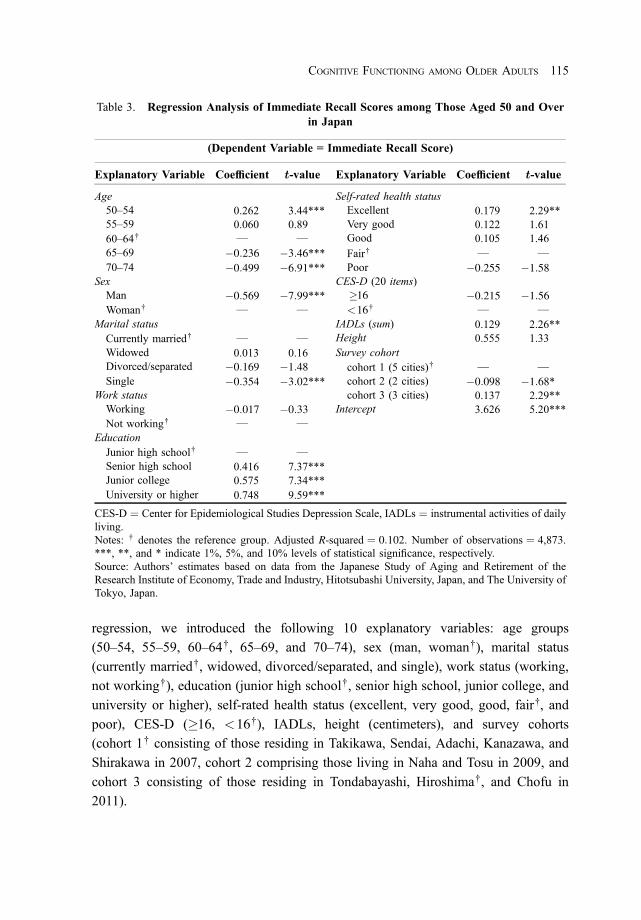
regression, we introduced the following 10 explanatory variables: age groups
(50–54, 55–59, 60–64†, 65–69, and 70–74), sex (man, woman†), marital status
(currently married†, widowed, divorced/separated, and single), work status (working,
not working†), education (junior high school†, senior high school, junior college, and
university or higher), self-rated health status (excellent, very good, good, fair†, and
poor), CES-D (�16, <16†), IADLs, height (centimeters), and survey cohorts
(cohort 1† consisting of those residing in Takikawa, Sendai, Adachi, Kanazawa, and
Shirakawa in 2007, cohort 2 comprising those living in Naha and Tosu in 2009, and
cohort 3 consisting of those residing in Tondabayashi, Hiroshima†, and Chofu in
2011).
Table 3. Regression Analysis of Immediate Recall Scores among Those Aged 50 and Overin Japan
(Dependent Variable = Immediate Recall Score)
Explanatory Variable Coefficient t-value Explanatory Variable Coefficient t-value
Age Self-rated health status50–54 0.262 3.44*** Excellent 0.179 2.29**55–59 0.060 0.89 Very good 0.122 1.6160–64† — — Good 0.105 1.4665–69 �0:236 �3:46*** Fair† — —
70–74 �0:499 �6:91*** Poor �0:255 �1:58Sex CES-D (20 items)Man �0:569 �7:99*** �16 �0:215 �1:56Woman† — — <16† — —
Marital status IADLs (sum) 0.129 2.26**Currently married† — — Height 0.555 1.33Widowed 0.013 0.16 Survey cohortDivorced/separated �0:169 �1:48 cohort 1 (5 cities)† — —
Single �0:354 �3:02*** cohort 2 (2 cities) �0:098 �1:68*Work status cohort 3 (3 cities) 0.137 2.29**Working �0:017 �0:33 Intercept 3.626 5.20***Not working† — —
EducationJunior high school† — —
Senior high school 0.416 7.37***Junior college 0.575 7.34***University or higher 0.748 9.59***
CES-D ¼ Center for Epidemiological Studies Depression Scale, IADLs ¼ instrumental activities of dailyliving.Notes: † denotes the reference group. Adjusted R-squared ¼ 0:102. Number of observations ¼ 4,873.***, **, and * indicate 1%, 5%, and 10% levels of statistical significance, respectively.Source: Authors’ estimates based on data from the Japanese Study of Aging and Retirement of theResearch Institute of Economy, Trade and Industry, Hitotsubashi University, Japan, and The University ofTokyo, Japan.
COGNITIVE FUNCTIONING AMONG OLDER ADULTS 115
March 25, 2022 12:23:12pm WSPC/331-adr 2250006 ISSN: 0116-11052ndReading

The respondents’ age and education have been incorporated in this regression to
capture the effect of two types of intelligence on cognitive functioning. Fluid
intelligence refers to the ability to reason and think flexibly, while crystallized
intelligence refers to the accumulation of knowledge, facts, and skills throughout life
(Cattell 1978). The explanatory variable, age, is expected to capture the change in fluid
intelligence, which peaks approximately at an age of 25. Because the respondents
included in the regression are 50 years or older, the estimated coefficients are expected
to have negative signs. The other explanatory variable (educational attainment) is
intended to capture the effect of education on crystallized intelligence, which is based
on facts and rooted in experiences. As we age and accumulate new knowledge and
understanding, crystallized intelligence becomes stronger. More importantly, because
education can also improve learning techniques such as memorization skills, education
helps improve performance in fluid intelligence even in the case of immediate word
recall. Therefore, since fluid abilities are improved by crystallized intelligence to a
substantial degree, we expect the estimated coefficient for education to have a positive
sign. In addition, we can anticipate that the higher the level of education the larger the
estimated coefficient will be.
As discussed in Section III, the magnitude, pattern, and explanation of cognitive
gender differences remain important research topics. As demonstrated in a SHARE-
based study undertaken by Weber et al. (2014), the magnitude of the gender
differences in cognitive performance in middle-aged and older populations across 13
European countries varies systematically across cognitive tasks, birth cohorts, and
geographical regions. Bonsang, Skirbekk, and Staudinger (2017) have also found that
both living conditions and educational opportunities to which individuals are exposed
during their formative years are related to increased gender differences, favoring
women in immediate word recall scores. Whether these findings based on the
European data are applicable to Japan and other Asian countries will be examined later
in this study.
As for the other explanatory variables, the health-related variables such as
self-rated health status, CES-D,32 and IADLs33 are expected to be associated with
cognitive performance. Moreover, a respondent without a spouse is likely to be left
alone without anybody to communicate with, which may weaken his or her cognitive
32Scores on the CES-D range from 0 to 60, where higher scores suggest a greater presence ofdepression symptoms. A score of 16 or higher is interpreted as indicating a risk for depression.
33In JSTAR, the respondents were asked 15 questions pertaining to IADLs, and the variable’s score,which ranges from 0 to 15 (IADLs sum), represents the number of activities that the respondent has nodifficulty performing, such as shopping, preparing meals, housekeeping, managing finances, takingresponsibility for having medication in correct dosages at the right time, etc.
116 ASIAN DEVELOPMENT REVIEW
March 25, 2022 12:23:12pm WSPC/331-adr 2250006 ISSN: 0116-11052ndReading

functioning. Similarly, whether the respondent holds a job is likely to affect his or her
level of life satisfaction and career development, both of which may affect cognitive
performance.
The respondent’s height has been incorporated in the regression because adult
height is closely related to childhood nutritional condition which, in turn, affects
cognitive functioning and other dimensions of human capital, such as school ability
(Weir, Lay, and Langa 2014; LaFave and Thomas 2017).
We have also included in the regression a set of explanatory variables representing
survey cohorts, which differ significantly in terms of the level of urbanization of the areas
where the respondents live and their lifestyles. It is quite conceivable that, because a
considerable proportion of the respondents included in cohort 3 live in wealthy urban
areas such as Chofu in Tokyo, this cohort is more likely to be exposed to modern
technologies, such as the Internet and computers, than their counterparts in cohort 1.34
It is plausible that those who often use such modern technologies, by doing so, stimulate
their crystallized intelligence (Bordone, Scherbov, and Steiber 2015). For these reasons,
we expect that modern technologies will be more significantly associated with the
cognitive score in cohort 3 than in cohort 1.
Table 3 shows the estimated results derived from the JSTAR dataset. Except for
work status and height, all explanatory variables introduced in the regression are
statistically significant, with the coefficients having expected signs.
As expected, the cognitive abilities of Japanese older adults are negatively
associated with age. It is important to observe that education is positively related to
immediate recall scores—the higher the educational level, the better the cognitive
performance. Another important finding is that the respondent’s own health evaluation
(self-related health status) and physical limitations (IADLs) are also positively
associated with the immediate recall score. Moreover, women show a considerably
higher cognitive score than men, which is comparable to the pattern widely seen in the
Northern and Central European regions. Those who are currently married have higher
cognitive abilities than those who have never been married. In view of the rising
prevalence of lifetime singlehood in Japan over the past few decades, this variable may
play an increasingly important role in the future. Where respondents live also plays a
role in cognitive performance—the coefficient for cohort 3, which includes a
considerable number of respondents who live in relatively wealthy residential areas, is
not only statistically significant but also positive, which agrees with our a-priori
expectation.
34For example, Shirakawa Town, which is included in cohort 1, is predominantly rural.
COGNITIVE FUNCTIONING AMONG OLDER ADULTS 117
March 25, 2022 12:23:12pm WSPC/331-adr 2250006 ISSN: 0116-11052ndReading

Let us now compare these JSTAR-based regression results with those estimated
based on CHARLS, the LASI pilot survey, HART, and MARS. The results based on
the PRC’s CHARLS in Table 4 show that the coefficients of all the explanatory
variables, except for marital status and work status, are statistically significant with
theoretically expected signs. Compared to JSTAR, the coefficients for age, sex,
education, and self-rated health status are statistically significant for both datasets with
the theoretically expected signs, while marital status is statistically significant only for
Japan. However, unlike in Japan, both height (childhood nutritional conditions) and
CES-D (representing the level of depression) yielded statistically significant results in
the case of the People’s Republic of China.
Table 5 displays the regression results based on India’s LASI pilot survey data.
As mentioned, the number of observations in this dataset is relatively small—only 832
observations, which casts some doubt on the reliability of some of the estimated
results. For instance, age, sex, work status, and CES-D are not statistically significant.
However, education is a statistically significant predictor at the 1% significance level.
It is also worth noting that Punjab, which is the most developed state among the four
Indian states included in the pilot, exhibits a considerably higher cognitive
performance.
Table 6 presents the regression results estimated from Thailand’s HART dataset.
Age, sex, marital status, education, and CES-D are significant predictors with
theoretically expected signs. Due to the paucity of data, however, we could not
incorporate the explanatory variables representing self-rated health status and IADLs.
All provinces except for Surin have higher cognitive abilities than Bangkok (reference
group). This result is rather unexpected, and we do not have a reasonably good
explanation at hand.
Table 7 shows the regression results based on Malaysia’s MARS data.
All categories of the explanatory variables are statistically significant. As expected,
cognitive functioning decreases as age increases. In addition, the estimated coefficients
for sex, marital status, education, depression signs,35 IADLs, and work status are
statistically significant. Work status, unlike in other Asian countries, has a positive
coefficient.36
35The depression symptom score is constructed using 17 negative and positive statements related toa respondent’s experienced psychological well-being. The response scale for positive statements isinversely converted. The total score was calculated as the aggregate for all 17 statements. The total scoresthus range from 17 to 85, with the scores in the top 15th percentile (44 or higher) interpreted as indicating ahigher risk of depression (�44, <44†).
36Although the Malaysian survey data indicate that many of those still working are in theagriculture sector, it is not clear why this contributes to increasing their cognitive functioning.
118 ASIAN DEVELOPMENT REVIEW
March 25, 2022 12:23:12pm WSPC/331-adr 2250006 ISSN: 0116-11052ndReading

Another significant finding is the link between the respondent’s health and
cognitive ability, whereby poor self-rated health and higher signs of depression relate
negatively to immediate recall scores. Nutrition, as represented by the respondent’s
height, is also seen to play an important role in cognitive functioning. We also observe
that the coefficient for the more urbanized states, such as Kuala Lumpur, Pulau Pinang,
and Perak, are positive and statistically significant. Better cognitive ability in these
states may be attributed to greater exposure and utilization of technology in the
subjects’ daily lives.
Table 4. Regression Analysis of Immediate Recall Scores among Those Aged 50 and Overin the People’s Republic of China
(Dependent Variable = Immediate Recall Score)
Explanatory Variable Coefficient t-value Explanatory Variable Coefficient t-value
Age Self-rated health status50–54 0.059 0.79 Very good 0.250 2.47***55–59 0.070 1.18 Good 0.136 1.79*60–64† — — Fair 0.116 2.15***65–69 �0:049 �0:43 Poor† — —
70–74 �0:598 �7:73*** Very poor �0:209 �2:08**75–79 �0:923 �9:78*** CES-D (10 items)
Sex �10 �0:402 �7:98***Man �0:137 �2:07** <10† — —
Woman† — — Height 2.568 7.24***Marital status RegionCurrently married† — — Urban community† — —
Partnered 0.328 1.02 Rural �0:244 �3:70***Widowed 0.024 0.33 Intercept 0.182 0.33Divorced/separated 0.194 1.39Single �0:320 �1:25
Work statusWorking �0:105 �1:52Not working† — —
EducationLess than lowersecondary†
— —
Upper secondaryand vocational
0.819 10.79***
Tertiary 1.545 7.21***
CES-D ¼ Center for Epidemiological Studies Depression Scale.Notes: † denotes the reference group. Adjusted R-squared ¼ 0:136. Number of observations ¼ 8,738.***, **, and * indicate 1%, 5%, and 10% levels of statistical significance, respectively.Source: Authors’ estimates based on data from the China Health and Retirement Longitudinal Study ofthe National School of Development of Peking University, Beijing; see http://charls.pku.edu.cn/index/en.html (accessed 5 August 2020).
COGNITIVE FUNCTIONING AMONG OLDER ADULTS 119
March 25, 2022 12:23:13pm WSPC/331-adr 2250006 ISSN: 0116-11052ndReading

Several points of interest emerge from the foregoing discussions on the
regression results for the five Asian countries. First, in all five Asian countries, the
cognitive abilities of older adults decline with age. Second, education is highly and
positively associated with immediate recall scores. Third, health condition is positively
related with cognitive performance, and height is positively linked to better cognitive
abilities, which implies that nutritional condition in childhood plays an important role
in developing cognitive functioning at a later stage.
Fourth, those who are currently married have higher cognitive abilities than those
who have never been married. In view of the recent gradual shift from universal
Table 5. Regression Analysis of Immediate Recall Scores among Those Aged 50 and Overin India
(Dependent Variable = Immediate Recall Score)
Explanatory Variable Coefficient t-value Explanatory Variable Coefficient t-value
Age Self-rated health status50–54 0.114 0.63 Excellent 0.285 0.6155–59 0.161 0.84 Very good 0.424 1.70*60–64† — — Good 0.171 0.7965–69 �0:230 �1:01 Fair† — —
70–74 �0:183 �0:66 Poor �0:604 �1:5875–79 �0:328 �1 CES-D (8 items)
Sex �8 �0:257 �1:84*Man �0:012 �0:06 <8† — —
Woman† — — Height 1.712 1.78*Marital status State
Currently married† — — Punjab† — —
Widowed �0:326 �1:69* Rajasthan �0:563 �2:98***Divorced/separated 0.082 0.20 Kerala �0:718 �3:93***Single �0:036 �0:07 Karnataka �0:879 �4:26***
Work status Intercept 2.593 1.72*Working �0:015 �0:10Not working† — —
Education
Junior high school† — —
Senior high school 0.682 4.12***Junior college 1.247 4.22***University or higher 1.333 4.12***
CES-D ¼ Center for Epidemiological Studies Depression Scale.Notes: † denotes the reference group. Adjusted R-squared ¼ 0:126. Number of observations ¼ 832.***, **, and * indicate 1%, 5%, and 10% levels of statistical significance, respectively.Source: Authors’ estimates based on data from the Longitudinal Ageing Study in India of the HarvardT.H. Chan School of Public Health, Boston, the International Institute for Population Sciences,Mumbai, and the University of Southern California, Los Angeles; see https://g2aging.org/downloads(accessed 5 August 2020).
120 ASIAN DEVELOPMENT REVIEW
March 25, 2022 12:23:15pm WSPC/331-adr 2250006 ISSN: 0116-11052ndReading

marriage to lifetime singlehood in Japan and other Asian countries, policy makers and
researchers should pay more attention to Asia’s changing marriage patterns in the
years to come, particularly from a standpoint of cognitive performance among older
adults.
Fifth, women show considerably higher cognitive scores than men. Nevertheless,
to gain further insights into Asia’s gender differences in cognition, we plotted male and
female age-specific immediate recall scores for the five Asian countries in Figure 3.
Although our regression results have uniformly indicated that women have higher
Table 6. Regression Analysis of Immediate Recall Scores among Those Aged 50 and Overin Thailand
(Dependent Variable ¼ Immediate Recall Score)
Explanatory Variable Coefficient t-value Explanatory Variable Coefficient t-value
Age CES-D (20 items)50–54 0.485 3.58*** �16 �0:760 �2:94***55–59 0.393 3.13*** <16† — —
60–64† — — Height 0.001 0.2365–69 �0:281 �2:25** State70–74 �0:652 �4:88*** Bangkok† — —
75–79 �0:931 �6:90*** Samut Prakan 0.901 3.12***Sex Nonthaburi 0.062 0.10
Man �0:231 �2:31** Pathum Thani 0.558 1.61Woman† — — Sing Buri 0.845 3.49***
Marital status Chanthaburi 0.973 4.05***Currently married† — — Surin �0:161 �0:62Widowed �0:025 �0:25 Khon Kaen 0.948 4.05***Divorced/separated 0.235 1.28 Chiang Mai 1.250 5.29***Single �0:397 �2:35** Uttaradit 0.737 2.64***
Work status Phetchabun 0.576 2.45**Working 0.054 0.060 Krabi 0.477 1.72*Not working† — — Songkhla 1.119 4.83***
Education Intercept 1.663 1.91*No formal education† — —
P1–P6 1.041 5.76***M1–M6 1.661 8.14***First year collegeor higher
2.295 7.21***
CES-D ¼ Center for Epidemiological Studies Depression Scale, M ¼ secondary education, and P ¼primary education.Notes: † denotes the reference group. Adjusted R-squared ¼ 0:170. Number of observations ¼ 2,264.***, **, and * indicate 1%, 5%, and 10% levels of statistical significance, respectively.Source: Authors’ estimates based on data from the Health, Aging, and Retirement in Thailand of theCenter for Aging Society Research/Research Center of the National Institute of DevelopmentAdministration, Bangkok.
COGNITIVE FUNCTIONING AMONG OLDER ADULTS 121
March 25, 2022 12:23:17pm WSPC/331-adr 2250006 ISSN: 0116-11052ndReading

scores than men in these Asian countries,37 Figure 3 reveals considerable differences
across the five Asian countries—in the PRC and India, for example, women have
distinctively lower cognitive scores than men. To account for the gap between our
Table 7. Regression Analysis of Immediate Recall Scores among Those Aged 50 and Over inMalaysia
(Dependent Variable = Immediate Recall Score)
Explanatory Variable Coefficient t-value Explanatory Variable Coefficient t-value
Age Depression symptom score50–54 0.307 3.51*** �44 �0:229 �2:83***55–59 0.272 3.21*** <44† — —
60–64† — — IADLs (sum) 0.113 7.46***65–69 �0:178 �1:91* Height 0.017 3.87***70–74 �0:478 �4:39*** State75–79 �0:788 �5:66*** Johor† — —
Sex Kedah �0:195 �1:52Man �0:602 �7:41*** Kelantan �0:053 �0:39Woman† — — Kuala Lumpur 1.028 5.42***
Marital status Melaka �0:436 �1:88*Currently married† — — Negeri Sembilan �0:334 �1:93*Widowed �0:050 �0:60 Pahang �0:309 �2:36**Divorced/separated �0:176 �1:06 Perak 0.513 4.17***Single �0:270 �1:71* Perlis �0:154 �0:44
Work status Pulau Pinang 0.358 2.22**Working 0.140 2.01* Sabah �0:008 �0:07Not working† — — Sarawak �0:55 �4:53***
Education Selangor 0.165 1.45No schooling† — — Terengganu �0:299 �1:99**Primary 0.426 4.64*** Intercept 0.532 0.78Secondary 1.010 10.54***Tertiary 1.537 11.49***
Self-rated health statusVery good �0:123 �0:88Good �0:039 �0:63Moderate† — —
Poor �0:125 �1:34Very poor �0:444 �1:65*
IADLs ¼ Instrumental activities of daily living.Notes: † denotes the reference group. Adjusted R-squared ¼ 0:219. Number of observations ¼ 3,680.***, **, and * indicate 1%, 5%, and 10% levels of statistical significance, respectively.Source: Authors’ estimates based on data from the Malaysia Ageing and Retirement Survey of the SocialWellbeing Research Centre of the University of Malaya, Kuala Lumpur.
37In the case of India, the estimated coefficient for sex is statistically insignificant, presumably dueto the small sample size.
122 ASIAN DEVELOPMENT REVIEW
March 25, 2022 12:23:19pm WSPC/331-adr 2250006 ISSN: 0116-11052ndReading

Figure 3. Immediate Recall Scores in Five Asian Countries by Sex and Age Group
PRC = People’s Republic of China.Sources: Authors’ calculations based on data from the following: (i) Japanese Study of Aging and Retirement ofthe Research Institute of Economy, Trade and Industry, Hitotsubashi University, Japan, and The Universityof Tokyo, Japan; (ii) China Health and Retirement Longitudinal Study of the National School of Development ofPeking University, Beijing; (iii) the pilot portion of the Longitudinal Ageing Study in India of the Harvard T.H.Chan School of Public Health, Boston, the International Institute for Population Sciences, Mumbai, and theUniversity of Southern California, Los Angeles; (iv) Malaysia Ageing and Retirement Survey of the SocialWellbeing Research Centre of the University of Malaya, Kuala Lumpur; and (v) Health, Aging, and Retirement inThailand of the Center for Aging Society Research/Research Center of the National Institute of DevelopmentAdministration, Bangkok.
COGNITIVE FUNCTIONING AMONG OLDER ADULTS 123
March 25, 2022 12:23:19pm WSPC/331-adr 2250006 ISSN: 0116-11052ndReading

regression results and the patterns in Figure 3, we need to pay attention to gender
differences in educational attainment in these Asian countries. Once we control for
education as we did in our regressions, women have an advantage over men in
cognition, suggesting that Asia’s gender difference in cognition performance is
primarily caused by gender gaps in education.
Although it falls outside the scope of this study, we are planning to carry out a
series of simulation exercises in a future study by using the regression results for the
five Asian countries generated here. In the case of Japan, for instance, the statistical
results indicate that the cognitive ability of Japanese elderly persons is likely to
improve due to the following potential factors: (i) the level of education among those
50 years and over is expected to rise at a phenomenal rate, as shown in Figure 4;
(ii) future generations of the elderly are likely to have an advantage over past
generations because children’s nutrition started to improve considerably in Japan in the
late 1950s when the school lunch program was introduced nationwide; and (iii) the use
of modern communication technologies among the elderly is likely to increase at a
remarkable rate because the overwhelming majority of young cohorts have already
been exposed to extensive use of computers and mobile phones, as illustrated in
Figure 5. By conducting various simulation exercises of this nature, we will be able to
project to what extent cognitive functioning among older adults in Japan will improve,
and how high Japan’s CADR will be in the years ahead.
Figure 4. Changes in Educational Composition in Japan by Sex, 1920–1980
CG ¼ University or higher, HSG ¼ senior high school, JCG ¼ junior college, and JSG ¼ junior high school.Source: Statistics Bureau of Japan. 2013. Population Census 2010. Tokyo: Japan Statistical Association.
124 ASIAN DEVELOPMENT REVIEW
March 25, 2022 12:23:21pm WSPC/331-adr 2250006 ISSN: 0116-11052ndReading

VIII. Concluding Remarks
In recent years, the five Asian countries intensively analyzed in this paper have
been facing increasingly difficult policy challenges induced by rapid population aging.
Among these five countries, Japan’s level of population aging has been the most
pronounced over the past few decades. Japan has the highest proportion of those aged
65 and over, an indicator which has been used by demographers for more than a
century. One of the main objectives of this study was to introduce from an innovative
angle a new index to measure the level of population aging to shed a different light on
policy-oriented research on this phenomenon. To compute this new index—the
cognition-adjusted dependency ratio—we applied the mean age-group-specific
immediate recall scores for Japan and four other Asian countries and compared the
computed results with those derived from the US and various developed nations in
Europe.
Our computed results have shown that Japan’s pattern and level of age-related
decline in cognitive functioning are highly comparable to those of many other
developed nations, particularly those in the group designated as Continental Europe in
previous research. This finding seems to have a few important policy implications for
the aging Japanese economy, particularly its labor market. The population census data
show that the size of Japan’s total labor force, after reaching a peak in 1995, has been
shrinking continuously, while the overall labor force participation rate has been on a
Figure 5. Age-Specific Pattern of Using the Internet in Japan, 2016
Source: Ministry of Internal Affairs and Communications. 2017. Communications Usage Trend Survey. https://www.soumu.go.jp/johotsusintokei/tsusin_riyou/data/eng_tsusin_riyou02_2017.pdf.
COGNITIVE FUNCTIONING AMONG OLDER ADULTS 125
March 25, 2022 12:23:23pm WSPC/331-adr 2250006 ISSN: 0116-11052ndReading
downward trend since 1970. Despite these substantial changes, Japan’s age-based
employment practices, which comprise lifetime employment, seniority wage system,
and mandatory retirement age, remained virtually intact (Kato 2016). Particularly,
Japan’s policies related to the mandatory retirement age—requiring workers to leave
the company at a relatively young age, typically at an age of 60—are considered
extreme compared to the practices in other industrialized nations.38 Due to the
existence of such age-based employment practices, many Japanese businesses that
face fierce competition from overseas rivals have been confronted in recent years with
a shortage of highly qualified workers with specialized skills acquired from career
experiences. Our research finding is not yet widely known in Japan’s labor market, but
once the market recognizes that older Japanese have reasonably good cognitive
performance, the finding could provide a strong incentive for many employers to
modify or even abandon the long-running age-based employment practices. This
would allow a sizable number of older Japanese with a reasonably good level of
cognitive functioning to be recruited, which would likely generate a considerable
amount of economic dynamism.
It is also worth noting that among the selected Asian countries, Malaysia shows a
pattern of change in age-specific cognitive functioning that is similar to the Southern
European group, although Malaysia has somewhat lower scores than Southern Europe
in all age groups.
More importantly, these inter-country comparative results based on cognition-
adjusted dependency ratios are astonishingly different from the results emerging from
the conventional old-age dependency ratios. This conclusion seems to justify the UN’s
recent efforts to raise awareness regarding the urgent need for remeasuring population
aging with a view to formulating more efficient and effective policies to cope with
rapid population aging in both developed and developing nations.
References
Anderson, Nicole, and Fergus Craik. 2000. “Memory in the Aging Brain.” In The OxfordHandbook of Memory, edited by Endel Tulving and Fergus Craik, 411–25. Oxford:Oxford University Press.
Arifin, Evi Nurvidya, and Aris Ananta, eds. 2009. Older Persons in Southeast Asia: AnEmerging Asset. Singapore: Institute of Southeast Asian Studies.
38In Western industrialized nations, cognitive performance is becoming increasingly important forlabor market outcomes (Gordo and Skirbekk 2013).
126 ASIAN DEVELOPMENT REVIEW
March 25, 2022 12:23:24pm WSPC/331-adr 2250006 ISSN: 0116-11052ndReading

Atalay, Kadir, Garry Barret, and Anita Staneva. 2019. “The Effect of Retirement on ElderlyCognitive Functioning.” Journal of Health Economics 66 (C): 37–53.
Behrman, Jere, David Ross, and Richard Sabot. 2008. “Improving Quality versus Increasing theQuantity of Schooling: Estimates of Rates of Return from Rural Pakistan.” Journal ofDevelopment Economics 85 (1–2): 94–104.
Bloom, David, and Jeffrey Williamson. 1998. “Demographic Transitions and EconomicMiracles in Emerging Asia.” The World Bank Economic Review 12 (3): 419–55.
Bonsang, Eric, Stephane Adam, and Sergio Perelman. 2012. “Does Retirement AffectCognitive Functioning?” Journal of Health Economics 31: 490–501.
Bonsang, Eric, Vegard Skirbekk, and Ursula Staudinger. 2017. “As You Sow, So shall YouReap: Gender-Role Attitudes and Late-Life Cognition.” Psychological Science 28 (9):1201–13.
Bordone, Valeria, Sergei Scherbov, and Nadia Steiber. 2015. “Smarter Every Day: TheDeceleration of Population Ageing in Terms of Cognition.” Intelligence 52: 90–96.
Cattell, Raymond. 1978. The Scientific Use of Factor Analysis. New York: Plenum Press.Clark, Robert, and Naohiro Ogawa. 1992. “Employment Tenure and Earnings Profiles in Japan
and the United States: Comments.” The American Economic Review 82 (1): 336–45.Clark, Robert, Naohiro Ogawa, and Andrew Mason, eds. 2007. Population Aging,
Intergenerational Transfers and the Macroeconomy. Cheltenham, UK and Northampton,MA: Edward Elgar.
Clark, Robert, Naohiro Ogawa, Sang-Hyop Lee, and Rikiya Matsukura. 2008. “Older Workersand National Productivity in Japan.” In Population Aging, Human Capital Accumulation,and Productivity Growth: A Supplement to Vol. 34, 2008: Population and DevelopmentReview, edited by Alexia Prskawetz, David Bloom, and Wolfgang Lutz, 257–74.Hoboken, NJ: Blackwell Publishing (On Behalf of the Population Council).
de Grip, Andries, Arnaud Dupuy, Jelle Jolles, and Martin van Boxtel. 2015. “Retirement andCognitive Development in the Netherlands: Are the Retired Really Inactive?” Economics& Human Biology 19: 157–69.
Doblhammer, Gabriele, Gerald van den Berg, and Thomas Fritze. 2013. “Economic Conditionsat the Time of Birth and Cognitive Abilities Late in Life: Evidence from Ten EuropeanCountries.” PLoS ONE 8 (9): e74915.
Eggleston, Karen, and Shripad Tuljapurkar, eds. 2010. Aging Asia: The Economic and SocialImplications of Rapid Demographic Change in China, Japan, and South Korea. Stanford,CA: Walter H. Shorenstein Asia-Pacific Research Center and Baltimore, MD: TheBrookings Institution.
Fein, George, Shannon McGillivray, and Peter Finn. 2007. “Older Adults make LessAdvantageous Decisions than Younger Adults: Cognitive and Psychological Correlates.”Journal of the International Neuropsychological Society 13 (3): 480–89.
Fu, Tsung-hsi, and Rhidian Hughes. 2009. Ageing in East Asia: Challenges and Policies for theTwenty-First Century. Volume 4. Comparative Development and Policy in Asia Series.London and New York: Routledge.
Fuller, Theodore. 2010. “Relationship Status, Health, and Health Behavior: An Examination ofCohabiters and Commuters.” Sociological Perspectives 53 (2): 221–45.
COGNITIVE FUNCTIONING AMONG OLDER ADULTS 127
March 25, 2022 12:23:24pm WSPC/331-adr 2250006 ISSN: 0116-11052ndReading

Gordo, Laura, and Vegard Skirbekk. 2013. “Skill Demand and the Comparative Advantage ofAge: Job Tasks and Earnings from the 1980s to the 2000s in Germany.” LabourEconomics 22 (C): 61–69.
Hermalin, Albert, ed. 2003. The Well-Being of the Elderly in Asia: A Four-CountryComparative Study. Ann Arbor, MI: The University of Michigan Press.
Ichimura, Hidehiko, Hideki Hashimoto, and Satoshi Shimizutani. 2009. “Japanese Study ofAging and Retirement: First Results.” RIETI Discussion Paper Series 09-E-047, TheResearch Institute of Economy, Trade and Industry, Tokyo.
Kato, Takao. 2016. “Productivity, Wages and Unions in Japan.” Conditions of Work andEmployment Series No. 73, International Labour Office, Geneva.
Kendig, Hal, Peter McDonald, and John Piggott, eds. 2016. Population Ageing and Australia’sFuture. Acton, ACT: Australian National University Press.
Kuiper, Jisca, Marij Zuidersma, Richard Voshaar, Sytse Zuidema, Edwin van den Heuvel,Ronald Stolk, and Nynke Smidt. 2015. “Social Relationships and Risk of Dementia: ASystematic Review and Meta-analysis of Longitudinal Cohort Studies.” Ageing ResearchReviews 22: 39–57.
LaFave, Daniel, and Duncan Thomas. 2017. “Height and Cognition at Work: Labor MarketProductivity in a Low-Income Setting.” Economics & Human Biology 25: 52–64.
Lee, Ronald, and Andrew Mason, eds. 2011. Population Aging and the Generational Economy:A Global Perspective. Cheltenham, UK: Edward Elgar Publishing.
Lutz, Wolfgang, Warren Sanderson, and Sergei Scherbov. 2004. The End of World PopulationGrowth in the 21st Century: New Challenges for Human Capital Formation andSustainable Development. London: Earthscan.
Lynn, Richard. 2009. “Fluid Intelligence But not Vocabulary has Increased in Britain, 1979–2008.” Intelligence 37 (3): 249–55.
Machin, Stephen, and John Van Reenen. 1998. “Technology and Changes in Skill Structure:Evidence from Seven OECD Countries.” The Quarterly Journal of Economics 113 (4):1215–44.
Maharani, Asri, and Gindo Tampubolon. 2016. “National Economic Development Status mayAffect the Association between Central Adiposity and Cognition in Older Adults.” PLoSONE 11 (2): e0148406.
Mason, Andrew, ed. 2001. Population Change and Economic Development in East Asia:Challenges Met, and Opportunities Seized. Stanford, CA: Stanford University Press.
Maurer, Jurgen. 2010. “Height, Education and Later-Life Cognition in Latin America and theCaribbean.” Economics & Human Biology 8 (2): 168–76.
Ministry of Internal Affairs and Communications. 2017. Communications Usage Trend Survey.https://www.soumu.go.jp/johotsusintokei/tsusin_riyou/data/eng_tsusin_riyou02_2017.pdf.
Munnell, Alicia, Steven Sass, and Mauricio Soto. 2006. “Employer Attitudes towards OlderWorkers: Survey Results.” Work Opportunities for Older Americans, Series 3, June,Center for Retirement Research at Boston College.
Negash, Selam, Glenn Smith, Shane Pankratz, Jeremiah Aakre, Yonas Geda, Rosebud Roberts,David Knopman, Bradley Boeve, Robert Ivnik, and Ronald Petersen. 2011. “SuccessfulAging: Definitions, and Prediction of Longevity and Conversion to Mild CognitiveImpairment.” The American Journal of Geriatric Psychiatry 19 (6): 581–88.
128 ASIAN DEVELOPMENT REVIEW
March 25, 2022 12:23:24pm WSPC/331-adr 2250006 ISSN: 0116-11052ndReading

Ofstedal, Mary Beth, Gwenith Fisher, and Regula Herzog. 2005. Documentation of CognitiveFunctioning Measures in the Health and Retirement Study. Ann Arbor, MI: Institute ofSocial Research, University of Michigan.
Ogawa, Naohiro, Norma Mansor, Sang-Hyop Lee, Michael Abrigo, and Tahir Aris. 2021.“Population Aging and the Three Demographic Dividends in Asia.” Asian DevelopmentReview 38 (1): 32–67.
Park, Donghyun, Sang-Hyop Lee, and Andrew Mason, eds. 2012. Aging, Economic Growth,and Old-Age Security in Asia. Cheltenham, UK and Northampton, MA: Edward Elgar.
Sanderson, Warren, and Sergei Scherbov. 2010. “Remeasuring Aging.” Science 329 (5997):1287–88.
Schneeweis, Nicole, Vegard Skirbekk, and Rudolf Winter-Ebmer. 2014. “Does EducationImprove Cognitive Performance Four Decades after School Completion?” Demography51 (2): 619–43.
Skirbekk, Vegard, Valeria Bordone, and Daniela Weber. 2014. “A Cross-Country Comparisonof Math Achievement at Teen Age and Cognitive Performance 40 Years Later.”Demographic Research 31: 105–18.
Skirbekk, Vegard, Elke Loichinger, and Daniela Weber. 2012. “Variation in CognitiveFunctioning as a Refined Approach to Comparing Aging across Countries.” Proceedingsof the National Academy of Sciences of the United States of America 109 (3): 770–74.
Slomski, Anita. 2014. “Midlife Diabetes, Hypertension, May Affect Cognition Later in Life.”JAMA 311 (20): 2056.
Sommerlad, Andrew, Joshua Ruegger, Archana Singh-Manoux, Glyn Lewis, and GillLivingston. 2018. “Marriage and Risk of Dementia: Systematic Review andMeta-analysis of Observational Studies.” Journal of Neurology, Neurosurgery andPsychiatry 89 (3): 231–38.
Statistics Bureau of Japan. 2013. Population Census 2010. Tokyo: Japan StatisticalAssociation.
Sundet, Jon, Ingrid Borren, and Kristian Tambs. 2008. “The Flynn Effect Is Partly Caused byChanged Fertility Patterns.” Intelligence 36 (3): 183–91.
Thorvaldsson, Valgeir, Scott Hofer, Stig Berg, and Boo Johansson. 2006. “Effects ofRepeated Testing in a Longitudinal Age-Homogeneous Study of Cognitive Aging.”The Journals of Gerontology, Series B: Psychological Sciences and Social Sciences61 (6): 348–54.
Tuljapurkar, Shripad, Naohiro Ogawa, and Anne Gauthier, eds. 2010. Ageing in AdvancedIndustrial States: Riding the Age Waves—Volume 3. International Studies in Population.London and New York: Springer.
Uhlenberg, Peter, ed. 2009. International Handbook of Population Aging. London and NewYork: Springer.
United Nations. 2007. World Economic and Social Survey 2007: Development in an AgeingWorld. New York: United Nations.
_____. 2019. World Population Prospects: The 2019 Revision. New York: United Nations.van Aken, Loes, Roy Kessels, Ellen Wingbermuhle, William van der Veld, and Jos Egger.
2016. “Fluid Intelligence and Executive Functioning More Alike than Different?” ActaNeuropsychiatrica 28 (1): 31–37.
COGNITIVE FUNCTIONING AMONG OLDER ADULTS 129
March 25, 2022 12:23:24pm WSPC/331-adr 2250006 ISSN: 0116-11052ndReading

Weber, Daniela, Vegard Skirbekk, Inga Freund, and Agneta Herlitz. 2014. “The Changing Faceof Cognitive Gender Differences in Europe.” Proceedings of the National Academy ofSciences of the United States of America 111 (32): 11673–78.
Weir, David, Margaret Lay, and Kenneth Langa. 2014. “Economic Development and GenderInequality in Cognition: A Comparison of China and India, and of SAGE and the HRSSister Studies.” The Journal of the Economics of Ageing 4: 114–25.
130 ASIAN DEVELOPMENT REVIEW
March 25, 2022 12:23:24pm WSPC/331-adr 2250006 ISSN: 0116-11052ndReading

Demographic Change, Economic Growth,and Old-Age Economic Security:
Asia and the World
ANDREW MASON, SANG-HYOP LEE,AND DONGHYUN PARK¤
Asia is aging, although there is significant heterogeneity across subregions andeconomies. Population aging poses two strategic challenges for the region:sustaining economic growth and delivering old-age economic security. In thispaper, we leverage the lifecycle perspective—that individuals’ consumptionand labor income differ at each age—and the National Transfer Accountsdatabase to construct and analyze key economic indicators. Our analysisconfirms that demographic change will challenge the region’s future growthand increase the cost of funding the consumption of the elderly. We also findthat it will have a substantial impact on the public finances of some Asianeconomies.
Keywords: population aging, demographic change, Asia, economic growth,old-age economic security
JEL codes: J11, J14
⁄Andrew Mason: East-West Center, Honolulu, HI, United States. E-mail: [email protected];Sang-Hyop Lee: East-West Center, Honolulu, HI, United States and University of Hawai‘i at Mānoa,Honolulu, HI, United States. E-mail: [email protected]; Donghyun Park (corresponding author):Asian Development Bank, Metro Manila, Philippines. E-mail: [email protected]. We thank the ManagingEditor and the anonymous referees for helpful comments and suggestions.
This is an Open Access article published by World Scientific Publishing Company. It is distributed underthe terms of the Creative Commons Attribution 3.0 International (CC BY 3.0) License which permits use,distribution and reproduction in any medium, provided the original work is properly cited.
March 23, 2022 11:19:08am WSPC/331-adr 2250001 ISSN: 0116-11052ndReading
Asian Development Review, Vol. 39, No. 1, pp. 131–167DOI: 10.1142/S0116110522500019
© 2022 Asian Development Bank andAsian Development Bank Institute.

I. Introduction
Asia and the Pacific, and indeed the entire world, is in the midst of a
demographic transition that has fundamental implications for economic growth,
generational equity, public finances, and other important features of national and
regional economies. It is widely recognized that population aging may adversely affect
economic dynamism, exacerbate inequality between generations, and harm public
finances. More broadly, older populations pose two strategic challenges for Asia:
(i) sustaining economic growth in the face of less favorable demographics; and
(ii) delivering old-age economic security for a large and growing elderly population.
In this paper, we undertake a granular analysis of demographic and economic data to
improve our understanding of the economic impact of the demographic transition in
Asia and the world.
Demographic data point to two interrelated and stylized global trends: population
aging and slowing population growth. Significantly, Asian economies, which enjoyed
a substantial dividend from large workforces in the past, will see effective labor growth
drop sharply between 2020 and 2060. While the populations of Asia and the world are
aging and growing more slowly, there is substantial heterogeneity within the world
and Asia. A key objective of this paper is to explore this heterogeneity within Asia
and the Pacific.
A lifecycle perspective allows us to better understand exactly how demographic
change affects the economy at any point in time. The key principle here is that the
profiles of average labor income and consumption depend heavily on age. Individuals
consume more than they earn when they are young or old, and they earn more than
they consume during productive middle-ages. While these broad stylized facts hold for
all economies, there are significant differences across economies. The lifecycle
perspective dates back to some of the earliest literature on population and economic
growth. What is new here are the comprehensive efforts to quantify how economic
data vary over the lifecycle and how patterns vary across economies due to
development level and other factors.
Combining the lifecycle profiles of consumption and labor income with
population estimates and projections from the United Nations (United Nations
Population Division 2019), we are able to project three key indicators that capture the
impact of demographic transition on the economy. These are (i) effective number of
workers; (ii) effective number of consumers; and (iii) support ratio, which is the ratio
of (i) to (ii). Asia will see a sharp decline in the effective number of workers in the
coming decades. As a result, the first demographic dividend, or the boost to economic
132 ASIAN DEVELOPMENT REVIEW
March 23, 2022 11:19:08am WSPC/331-adr 2250001 ISSN: 0116-11052ndReading

growth due to rising support ratios, will dwindle across the region. The decrease will
be most pronounced in East Asia, which has experienced a rapid decline in fertility.
Population aging gives rise to two strategic challenges: sustaining economic
growth and securing adequate resources for old-age consumption. The resources for
old-age consumption can come from two sources, either lifecycle savings or
contemporaneous private or public transfers. We estimate the old-age GAP ratio
(OAGAP), or the amount of resources required to meet the old-age deficit. Funding the
old-age gap through 2060 would require funding in excess of 40% of contemporaneous
labor income in East Asia and more than 20% of labor income in the rest of developing
Asia.1 We estimate the retirement wealth that would be required to fund old-age needs.
The estimates vary widely across developing Asia’s subregions and economies. We also
show that, compared with relying on funded approaches to meeting old-age needs,
relying on transfers is relatively cheap in the beginning but very expensive when aging
sets in.
Finally, population aging will have sizable implications for the public finances of
developing Asian economies. Public transfers are one of the main avenues for funding
the gap between labor income and consumption at old age. The size of public
transfer inflows and outflows will differ at each age. For example, during productive
middle-ages we can expect outflows to the government (i.e., tax payments) to exceed
inflows from the government (i.e., benefits). We use such age profiles to project the
impact of population on public finances. The old-age gap, or the difference between
labor income and consumption for those aged 65 years and above, varies significantly
among economies and is rising significantly in the Republic of Korea, Thailand, and
Taipei,China. As a result, net public transfers to those aged 65 and older are projected
to rise sharply by 2060 to 15% and 25% of total labor income in the Republic of Korea
and Taipei,China, respectively, although they will remain a much more modest 4% in
Thailand.
The contribution of this paper to the literature is to provide new National
Transfer Accounts (NTA) data for Asia and the Pacific and to assess the potential
impact of population change on key dimensions of the economy. These data are
sufficient to highlight very important differences within and between the subregions of
Asia and the Pacific. We emphasize some of the simple, first-order effects of
population rather than the complexities that have been explored elsewhere in our own
work and the works of others. For example, we do not consider the impact of
fertility on human capital (Becker, Murphy, and Tamura 1990; Lee and Mason 2010;
1Developing Asia refers to the 46 developing member economies of the Asian Development Bank.
DEMOGRAPHIC CHANGE, ECONOMIC GROWTH, AND OLD-AGE ECONOMIC SECURITY 133
March 23, 2022 11:19:08am WSPC/331-adr 2250001 ISSN: 0116-11052ndReading

Lee et al. 2014); relationship between population and capital deepening (Tobin 1967);
endogeneity of health-care spending, fertility, and economic growth (Ehrlich and Yin
2013, de la Croix 2017); or the possibility that population change will lead to secular
stagnation and low interest rates in advanced economies (Eggertsson, Lancaster, and
Summers 2019). These issues are more appropriately addressed in simulation or
econometric models that are usually constructed for a single economy.
Another aspect of this study is that the availability of NTA data is limited. The
growth of NTA has been rapid and there is widespread interest. The methods have
been codified through close cooperation with the United Nations (UN) Department of
Economic and Social Affairs. Resources for training and implementation have been
provided by many agencies and foundations. Estimates are now available for 19
economies in Asia and the Pacific, 14 of which have a World Bank income status of
upper–middle income or below. However, NTAs for some very important economies
have not been constructed in recent years. Institutional support is essential to maintain
up-to-date estimates, construct time series, and extend coverage to economies that
have not yet participated.
II. Setting the Stage: Demographic Transition
The global demographic transition began with a decline in death rates,
particularly among infants and children. This led to rapid population growth and a
high concentration of the global population at young ages. During the 1970s, many
economies entered a new phase of their demographic transition when declining birth
rates led to slower population growth and a major shift in age distributions, a reduced
concentration at child ages, and an increased concentration at working ages. As the
demographic transition proceeds, low fertility rates lead to even slower population
growth, population decline in some economies, and further changes in age structure
(i.e., a lower concentration at working ages and a higher concentration at older ages).
Important differences in age structure across regions of the world are shown in
Figure 1. Age structure as measured here incorporates differences across economies in
the extent to which members of each age group rely on their own labor income to fund
their own consumption. The “GAP ratio” is an estimate of the gap between total
consumption and total labor income at each age as a percentage of total labor income.
The significance of this distinction and the differences across economies are discussed
in more detail below.
The GAP ratio varies considerably across the world and within Asia and the
Pacific because some economies are very far along in their demographic transition and
134 ASIAN DEVELOPMENT REVIEW
March 23, 2022 11:19:08am WSPC/331-adr 2250001 ISSN: 0116-11052ndReading
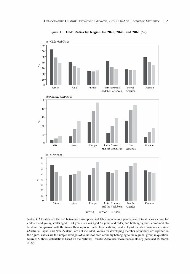
Figure 1. GAP Ratios by Region for 2020, 2040, and 2060 (%)
Notes: GAP ratios are the gap between consumption and labor income as a percentage of total labor income forchildren and young adults aged 0−24 years, seniors aged 65 years and older, and both age groups combined. Tofacilitate comparison with the Asian Development Bank classifications, the developed member economies in Asia(Australia, Japan, and New Zealand) are not included. Values for developing member economies are reported inthe figure. Values are the simple averages of values for each economy belonging to the regional group in question.Source: Authors’ calculations based on the National Transfer Accounts, www.ntaccounts.org (accessed 15 March2020).
DEMOGRAPHIC CHANGE, ECONOMIC GROWTH, AND OLD-AGE ECONOMIC SECURITY 135
March 23, 2022 11:19:08am WSPC/331-adr 2250001 ISSN: 0116-11052ndReading

others are at a relatively early stage. Currently, countries in Africa are relatively early
in their demographic transitions. They have a very high GAP ratio because the material
needs of children greatly exceed what they produce through their labor. In 2020, almost
63% of the total labor income of African economies was needed to fund the gap between
consumption and labor income for those under the age of 25. The burden of supporting
children and youth in Africa is expected to decline very sharply over the next 40 years.
The projected changes in the child GAP ratio are also projected to be substantial in Asia
and in Latin America and the Caribbean. Based on the situations in Europe and North
America, the child GAP ratio might stabilize at about one-quarter of total labor income
for each region in the future, but that will depend on trends in consumption among
children and young adults and features of labor markets that are uncertain.
Aging, as measured by the old-age GAP ratio, is a universal phenomenon
occurring in all regions of the world. The countries of Europe and North America have
higher old-age GAP ratios, and that will continue to be the case in the future. The
situations are similar in Asia and in Latin America and the Caribbean, although Asia is
not quite as “old.” Both regions will experience sharp increases in the old-age share of
their respective populations. African and Pacific Island economies are, on average,
aging more slowly than economies in other parts of the world.
The second global trend is slower growth. Throughout the world, the number of
children is growing more slowly than in the past. In many economies, the number of
children has declined substantially. This has been matched, with a delayed effect, by
slower growth or a decline in the number of workers. This slowdown in population
growth has fundamental implications for economic growth. Given the productivity of
effective labor, slower growth in the number of workers means slower growth in gross
domestic product (GDP). This trend for each major region is captured in Figure 2
using estimates and projections of the annual growth rate of effective labor. Effective
labor is the population weighted to capture age variation in labor force participation,
unemployment, hours worked, and wages.
Starting in the 1970s, rapid growth in the number of effective workers has led to
more rapid growth in GDP throughout the world. But the era of population-driven
economic growth is coming to an end everywhere except in Africa. There, growth in the
effective number of workers was estimated to add 2.9 percentage points per year to
economic growth in 2020. In Asia and the Pacific economies, growth in the number of
effective workers was estimated to add only 1.5 percentage points to GDP growth per
year. The effect is somewhat smaller in Latin America and the Caribbean. Among
countries in North America, growth in the number of effective workers was estimated to
add only 0.4 percentage points per year to GDP growth in 2020. In Europe, growth in
the effective labor force is already estimated to have a negative impact on GDP growth.
136 ASIAN DEVELOPMENT REVIEW
March 23, 2022 11:19:28am WSPC/331-adr 2250001 ISSN: 0116-11052ndReading
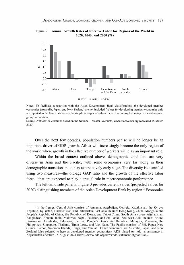
Over the next few decades, population numbers per se will no longer be an
important driver of GDP growth. Africa will increasingly become the only region of
the world where growth in the effective number of workers will play an important role.
Within the broad context outlined above, demographic conditions are very
diverse in Asia and the Pacific, with some economies very far along in their
demographic transition and others at a relatively early stage. The diversity is quantified
using two measures—the old-age GAP ratio and the growth of the effective labor
force—that are expected to play a crucial role in macroeconomic performance.
The left-hand side panel in Figure 3 provides current values (projected values for
2020) distinguishing members of the Asian Development Bank by region.2 Economies
2In the figures, Central Asia consists of Armenia, Azerbaijan, Georgia, Kazakhstan, the KyrgyzRepublic, Tajikistan, Turkmenistan, and Uzbekistan. East Asia includes Hong Kong, China; Mongolia; thePeople’s Republic of China; the Republic of Korea; and Taipei,China. South Asia covers Afghanistan,Bangladesh, Bhutan, India, Maldives, Nepal, Pakistan, and Sri Lanka. Southeast Asia includes BruneiDarussalam, Cambodia, Indonesia, the Lao People’s Democratic Republic, Malaysia, Myanmar, thePhilippines, Singapore, Thailand, Timor-Leste, and Viet Nam. The Pacific consists of Fiji, Papua NewGuinea, Samoa, Solomon Islands, Tonga, and Vanuatu. Other economies are Australia, Japan, and NewZealand (also referred to here as developed member economies). ADB placed on hold its assistance inAfghanistan effective 15 August 2021 (https://www.adb.org/news/adb-statement-afghanistan).
Figure 2. Annual Growth Rates of Effective Labor for Regions of the World in2020, 2040, and 2060 (%)
Notes: To facilitate comparison with the Asian Development Bank classifications, the developed membereconomies (Australia, Japan, and New Zealand) are not included. Values for developing member economies onlyare reported in the figure. Values are the simple averages of values for each economy belonging to the subregionalgroup in question.Source: Authors’ calculations based on the National Transfer Accounts, www.ntaccounts.org (accessed 15 March2020).
DEMOGRAPHIC CHANGE, ECONOMIC GROWTH, AND OLD-AGE ECONOMIC SECURITY 137
March 23, 2022 11:19:28am WSPC/331-adr 2250001 ISSN: 0116-11052ndReading

that are earliest in their demographic transition are frequently found in South Asia. In
Nepal, for example, effective labor force growth is very rapid at about 4% per annum
and the old-age GAP ratio is 8.4%. In many economies, the old-age GAP ratio is less
than in Nepal. Thirteen economies have a GAP ratio of less than 5%. Among the
developing Asian economies, those that are furthest along in their demographic
transition are a varied group. Growth in the effective labor force is negative in four
East Asian economies—the People’s Republic of China (PRC); Hong Kong, China;
the Republic of Korea; and Taipei,China—but also in Armenia, Georgia, and
Thailand. The extent of aging in these economies varies greatly, however. The PRC is
not yet very old, for example, with an old-age GAP ratio of only about 6%.
As the demographic transition proceeds in Asia and the Pacific, further aging and
slower growth will become pervasive. By 2060, the old-age GAP ratio will exceed
20% in 14 developing member economies, compared with only two—Georgia and
Hong Kong, China—in 2020. Growth of the effective labor force will be negative or
essentially zero in 21 developing member economies in 2060, compared with six
today. Aging and slower growth are pervasive in the region, however. Every
Figure 3. Old-Age GAP Ratios and Growth Rates of the Effective Labor Force in Asia andthe Pacific, 2020 and 2060
Source: Authors’ calculations based on the National Transfer Accounts, www.ntaccounts.org (accessed 15 March2020).
138 ASIAN DEVELOPMENT REVIEW
March 23, 2022 11:19:35am WSPC/331-adr 2250001 ISSN: 0116-11052ndReading
developing member economy in Asia and the Pacific will have a population that is
older and growing more slowly in 2060 than in 2020.
Both demographic and economic factors explain the distinctive features of regions
and economies, which are highlighted further below. Although the broad outlines of the
age transition appear to be common to all economies in Asia, there is enormous
diversity across subregions and economies. Most East Asian economies have
experienced a rapid fertility decline, leading to rapid population aging and slowing
population growth. The same is true of some Southeast Asian economies like Thailand
and Singapore. However, in Singapore, the effects of low fertility have had less effect
because of its liberal immigration policies. Elsewhere in Asia, especially in South Asia,
the demographic transition is an evolving event where birth and death rates continue to
decline more slowly and steadily in many cases than in other rapidly aging economies.
Economic behavior matters as well. In Japan, the effects of aging are reinforced
by high levels of health-care spending. In the Republic of Korea, the economic effects
of aging are more moderate because consumption by seniors is low relative to
consumption by children and younger adults. In India, the impact of aging is affected
by the sharp drop in labor income at age 60 due to labor policies.
III. The Generational Economy and the Lifecycle: An Overview
Understanding how a change in population will influence the economy builds on
an understanding of the lifecycle. What does it mean to be young or to be old from an
economic perspective? Chronological age is widely used with those under 15 years old
often classified as children, those 15–64 years old as working-age adults, and those
65 years and older as seniors. However, the meaning of childhood or youth varies from
economy to economy and is changing over time depending on many factors. How long
do children remain in school and how quickly can they secure quality jobs when they
leave school? Likewise, the meaning of old age depends on the health of older
individuals, attitudes and policies toward working at older ages, public policies toward
pensions and health-care spending, and other features of later years of life. Several
other scholars have also recently explored different concepts of age that are not based
on years since birth but other markers of the aging process (Balachandran et al. 2019,
Sanderson and Scherbov 2010).
The results presented make use of detailed data from the NTA project and
population projections by age prepared by the UN to explore how changing age
structure is likely to interact with age-specific economic behavior to influence
the macroeconomy (United Nations Population Division 2013, Lee and Mason 2011).
DEMOGRAPHIC CHANGE, ECONOMIC GROWTH, AND OLD-AGE ECONOMIC SECURITY 139
March 23, 2022 11:19:38am WSPC/331-adr 2250001 ISSN: 0116-11052ndReading

The NTA framework provides a comprehensive accounting of any economy that
incorporates age details while maintaining broad consistency with the UN System of
National Accounts. The NTA flow accounts can be expressed in simplest terms by the
following identity:
C(x, t)� Yl(x, t) ¼ T(x, t)þ Ya(x, t)� S(x, t), ð1Þwhere C, Yl, T , Ya, and S are the aggregate consumption, labor income, net transfers,
asset income, and saving, respectively, of persons aged x in year t. The left-hand side
of equation (1) captures the basic lifecycle problem: the considerable differences
between consumption and labor income depending on the age of individuals. The
right-hand side, referred to as age reallocations, quantifies the economic mechanisms
available to deal with the lifecycle. Economies can rely on net transfers from parents to
children, for example, or from taxpayers to retirees, as another example, to fund
lifecycle needs. The alternative economic mechanism is asset-based reallocations.
People can rely on asset income or dis-saving to fund lifecycle needs.
The terms in equation (1) are broad macroeconomic measures, and NTA
accounts are constructed to conform to each economy’s total income accounts data.
The classification of these data by age provides a simple mechanism for assessing how
demographic change will influence the economy. The lifecycle patterns of behavior are
quantified using per capita age profiles. To illustrate, aggregate consumption and labor
income are equal to
C(x, t) ¼ �c(x, t)P(x, t),
Yl(x, t) ¼ �yl(x, t)P(x, t),ð2Þ
where �c(x, t) is the per capita consumption of persons aged x in year t, �yl(x, t) is the per
capita labor income of persons aged x in year t, and P(x, t) is the population aged x in
year t.
Considering economies at different income levels illustrates some of the key
features of the lifecycle of consumption and labor income. In Figure 4, labor income
and consumption are compared across economies by calculating the per capita values
relative to the average value for the 30–49-year-old age group. This normalization
allows us to compare age shapes for economies at very different levels of
development. The estimates are available for 70 economies, which have been grouped
by income class. The median value for each income group is charted.
At young ages, children consume less than adults in all economies irrespective of
their income level, but consumption increases as children mature and, in particular, as
they enter school. The increase is particularly sharp in high-income, low-fertility
economies due to high levels of spending on education. The age pattern of consumption
at adult ages also varies with the level of income. In low-income economies,
140 ASIAN DEVELOPMENT REVIEW
March 23, 2022 11:19:38am WSPC/331-adr 2250001 ISSN: 0116-11052ndReading

consumption per adult is lower at older ages. Adults in their mid-20s are consuming
about 10% more while adults at age 70 are consuming about 10–15% less than adults in
the 30–49-year-old age range. Consumption is flatter for adults living in middle-income
economies. And for high-income economies, on average, consumption is much higher at
older ages. By age 60, adults in high-income economies are consuming about 10% more
than those in the 30–49-year-old age range. Under the influence of spending on health
care, adults in their late 80s are consuming about 20%more than adults aged 30–49 years.
Labor income is low for the young, rises with age during the 20s and 30s,
reaches a plateau during the 40s, and declines beginning in the 50s and early 60s.
Labor income is concentrated in a narrower age range in high-income economies, with
labor income rising at later youth ages and declining to low levels at an earlier point in
old age. Even though older adults are healthier in high-income economies, they have
lower labor income relative to earnings at prime ages than do older adults in middle- or
low-income economies.
Figure 4. Consumption and Labor Income by Age and Income Group
Notes: Values for each economy are expressed relative to the mean value of those in the 30–49-year-old agegroup. Average values for each income group are calculated as the median value for the economies belonging tothat group. See Appendix for additional information.Source: Authors’ calculations based on the National Transfer Accounts, www.ntaccounts.org (accessed 15 March2020).
DEMOGRAPHIC CHANGE, ECONOMIC GROWTH, AND OLD-AGE ECONOMIC SECURITY 141
March 23, 2022 11:19:38am WSPC/331-adr 2250001 ISSN: 0116-11052ndReading

The remaining results presented in this paper emphasize Asia and the Pacific. NTA
estimates are now available for the 19 Asia and the Pacific economies shown in
Figure 5. (These estimates have been constructed by research teams in each of the
19 economies with support provided by the NTA project and the UN Population Fund.)
The broadest patterns reported above generally hold for individual economies, but there
are important differences in the details. In high-income economies, for example,
consumption rises with age in Japan and Australia, but not in the Republic of Korea,
Singapore, or Taipei,China. Labor income reaches a peak at very young ages in the PRC
and Viet Nam. In India, labor income declines very sharply at age 60 due to the effects of
mandatory retirement on high-paid workers in the formal sector. Of all NTA economies,
including those outside Asia and the Pacific, the PRC has very low consumption at
every age. Some like the Philippines and Timor-Leste have high consumption relative to
their labor income. This can occur due to high net transfers from the rest of the world or
due to high total income from natural resources, although this is not a factor for the
economies shown in Figure 5. These differences are important for assessing how
changes in population age structure will influence economic growth.
An important general feature of the labor income profiles is that they do not rely on
an arbitrary definition of the working-age population. The labor income profile for each
economy reflects actual labor force participation plus three other important dimensions
of labor: unemployment, hours worked, and earnings per hour. These elements are
critical to assessing the contribution of adults in the working ages and older.
Reallocation systems receive less attention in this paper, but in every economy the
lifecycle deficit of children is funded almost entirely by transfers. For young children,
private (familial) transfers are particularly important. For older children, public transfers
approach or even exceed private transfers due to the high level of public spending on
education in many economies. The reallocation system for funding old-age needs is
much more varied. In continental Europe and Latin America, public transfer systems
play a very prominent role. In Australia, Canada, Japan, the United Kingdom, and the
United States, seniors depend on a more balanced combination of public transfers and
asset-based reallocations. In several East Asian economies, net private transfers from
children still remain important to seniors. In many Asian developing economies for
which data are available, seniors rely heavily on asset-based reallocations.
A. Transforming Population and Lifecycle Profiles into NTA Indicators
Population data and age profiles of consumption and labor income are combined
to produce indicators that capture the effects of population trends on the aggregate
142 ASIAN DEVELOPMENT REVIEW
March 25, 2022 12:19:48pm WSPC/331-adr 2250001 ISSN: 0116-11052ndReading

Figure 5. Per Capita Consumption and Labor Income in International Dollars by IncomeGroup in Asia and the Pacific (Purchasing Power Parity-Adjusted)
C ppp = per capita consumption, Yl ppp = labor income.Source: National Transfer Accounts, www.ntaccounts.org (accessed 15 March 2020).
DEMOGRAPHIC CHANGE, ECONOMIC GROWTH, AND OLD-AGE ECONOMIC SECURITY 143
March 23, 2022 5:29:30pm WSPC/331-adr 2250001 ISSN: 0116-11052ndReading

economy (Mason et al. 2017). The approach taken here is to answer a simple question.
Suppose the age patterns of consumption and labor income do not change in the future,
how would changes in population age structure lead to strains or imbalances in the
macroeconomy? The results are not a forecast of changes in the macroeconomy.
Without question, patterns of consumption and labor income must change to restore
balance in the macroeconomy. The goal is to assess the nature, timing, and magnitude
of those imbalances.
Three measures are emphasized in this subsection—effective labor, effective
consumers, and the support ratio—that capture the impact of age structure on
economic growth. Additional indicators are considered below. In all cases, we project
values by combining population projections by age with per-age profiles held at the
baseline value estimated from NTA.
For any economy, the effective number of workers measures the impact of
population change on effective labor by incorporating age variation in labor force
participation, unemployment, hours worked, and wages (or estimated productivity for
those who are self-employed or unpaid family workers). Effective labor in year t is as
follows:
L(t) ¼X!x¼0
yl(x, b)P49x¼30 yl(x, b)
P(x, t), ð3Þ
where L(t) is the total number of effective workers in year t, yl(x, b) is per capita labor
income of persons aged x in the base year, and P(x, t) is the population of age x in the
year t. This formulation counts adults in the 30–49-year-old age range as one effective
worker, on average, while those at each single year of age are counted as more or less
than one effective worker depending on how their per capita labor income compares
with that of the 30–49-year-old age group. The age profiles of per capita labor income
shown in Figure 5 are used for this purpose.
The effective number of consumers captures the reality that needs, as well as
productivity, vary over the lifecycle. The effective number of consumers is given as
follows:
N(t) ¼X!x¼0
c(x, b)P49x¼30 c(x, b)
P(x, t), ð4Þ
where N(t) is the total number of effective consumers in year t, c(x, b) is per capita
consumption of persons aged x in the base year, and P(x, t) is the population of age x in
the year t. This formulation counts adults in the 30–49-year-old age range as one
effective consumer, on average, while those at each single year of age are counted as
144 ASIAN DEVELOPMENT REVIEW
March 23, 2022 11:20:14am WSPC/331-adr 2250001 ISSN: 0116-11052ndReading

more or less than one effective consumer depending on how their per capita
consumption compares with that of the 30–49-year-old age group. The age profiles of
per capita consumption shown in Figure 5 are used for this purpose.
The support ratio is the ratio of the number of effective workers to the number of
effective consumers in year t:
SR(t) ¼ L(t)N(t)
: ð5Þ
IV. The Great Slowdown of Labor Force Growth
At the global level, the effective labor force was growing rapidly during the last
half of the 20th century, providing a tailwind to economic growth. The winds are
shifting, however, and for many economies labor force growth is slowing or even
turning negative. The first-order effects of population on GDP are captured by a simple
identity
Y(t) ¼ Y(t)L(t)
L(t): ð6Þ
Output or GDP in year t, Y(t), is equal to output per effective worker times the
number of effective workers. The relationship in growth terms is as follows:
gr(Y(t)) ¼ grY(t)L(t)
� �þ gr(L(t)), ð7Þ
where gr() represents the growth rate of the argument. Given the growth in output per
effective worker, a 1 percentage point increase (decrease) in the effective number of
workers leads to a 1 percentage point increase (decrease) in the growth of GDP.
The impact of demography on GDP growth is remarkably diverse in Asia and the
Pacific. In 2020, the effective labor force was expected to have grown most rapidly
(between 3.5% and 3.6%) in Afghanistan, Cambodia, and Solomon Islands.
In contrast, the most rapid declines (between �0.5% and �0.6%) were expected in
Georgia, the PRC, and Japan. In most economies, demographic change is currently
providing a tailwind for GDP growth. The effective labor force was expected to grow
in 2020 in all Central Asian economies except Armenia and Georgia, all South Asian
economies, all Southeast Asian economies except Thailand, and all Pacific economies.
East Asia is an exception to this regional pattern. Total effective labor was projected to
decline in 2020 in all East Asian economies except Mongolia. Among the developed
member economies, Australia and New Zealand were also projected to experience
moderate growth in their respective effective labor force (Figure 6).
DEMOGRAPHIC CHANGE, ECONOMIC GROWTH, AND OLD-AGE ECONOMIC SECURITY 145
March 23, 2022 3:45:10pm WSPC/331-adr 2250001 ISSN: 0116-11052ndReading

With rare exception, however, growth in the effective number of workers is
expected to decline over the coming decades, serving as a significant drag on GDP
growth. Some economies that are experiencing a moderate decline now are projected
to experience a much more rapid decline in the future. The rate of growth of the
effective number of workers is projected to decline by more than 1 percentage point
per annum by 2060 in Japan, the Republic of Korea, and Taipei,China. In many
economies, the effective number of workers will continue to grow over the next two
decades but much more slowly than today or in the recent past. The growth rate of the
effective number of workers in Bangladesh, for example, is projected to decline from
1.7% per year in 2020 to 0.3% per year in 2040. The growth rate for the effective
number of workers in India is projected to decline by a full percentage point between
2020 and 2040.
Projections of effective labor for 2040 are somewhat more reliable than other
indicators because everyone 20 years and older has already been born. Projections
Figure 6. Effective Labor Force Annual Rates of Growth in 2000, 2020, 2040, and 2060 (%)
AFG = Afghanistan; ARM = Armenia; AUS = Australia; AZE = Azerbaijan; BAN = Bangladesh; BHU = Bhutan;BRU = Brunei Darussalam; CAM = Cambodia; FIJ = Fiji; GEO = Georgia; HKG = Hong Kong, China; IND =India; INO = Indonesia; JPN = Japan; KAZ = Kazakhstan; KOR = Republic of Korea; KGZ = Kyrgyz Republic;LAO = Lao People’s Democratic Republic; MAL = Malaysia; MLD = Maldives; MON = Mongolia; MYA =Myanmar; NEP = Nepal; NZL = New Zealand; PAK = Pakistan; PNG = Papua New Guinea; PHI = Philippines;PRC = People's Republic of China; SAM = Samoa; SIN = Singapore; SOL = Solomon Islands; SRI = Sri Lanka;TAP = Taipei,China; TAJ = Tajikistan; THA = Thailand; TIM = Timor-Leste; TON = Tonga; TKM =Turkmenistan; UZB = Uzbekistan; VAN = Vanuatu; VIE = Viet Nam.Source: Authors’ calculations based on the National Transfer Accounts, www.ntaccounts.org (accessed 15 March2020).
146 ASIAN DEVELOPMENT REVIEW
March 23, 2022 3:45:10pm WSPC/331-adr 2250001 ISSN: 0116-11052ndReading

beyond 2040 are less reliable due to uncertainty about fertility trends. Accepting UN
projections at face value indicates that the slowdown in the effective number of workers
will continue. The decline is projected to moderate in a few economies—such as
Georgia, Japan, and Taipei,China—that have already experienced a very rapid decline.
Projections of effective number of workers for smaller economies are also subject
to uncertainty to the extent that their future will depend to a large degree on
immigration. Singapore and Hong Kong, China are two obvious cases in point.
V. The First Demographic Dividend: The Adverse Impact of
Population Aging on Growth in Asia
The first demographic dividend refers to the positive effect of demographic
change on standards of living due to a rise in the support ratio; that is, when the
effective number of workers is growing more rapidly than the effective number of
consumers (Bloom and Canning 2001, Bloom and Williamson 1998, Mason 2001,
Mason and Lee 2007). Extending the identities presented in equations (2) and (3),
output per effective consumer is equal to the following:
Y(t)N(t)
¼ Y(t)L(t)
SR(t): ð8Þ
Given the productivity Y(t)=L(t), income per effective consumer varies directly with
the support ratio. In growth terms,
grY(t)N(t)
� �¼ gr
Y(t)L(t)
� �þ gr(SR(t)), ð9Þ
where gr() represents the growth rate of the argument. The growth rate of income per
effective consumer is equal to the growth rate of productivity plus the growth rate of
the support ratio.
The effect of population on the support ratio is referred to as the first
demographic dividend while the effect of population on productivity is referred to as
the second demographic dividend. The rise in the support ratio over the demographic
transition is referred to as the dividend phase.
The first dividend was especially pronounced in East Asia. Using the values for the
median economy as a marker, the support ratio began to increase in the early 1970s and
continued to be favorable for about four decades (Figure 7). The first dividend has now
turned negative as population aging is leading to a decline in the support ratio.
This condition is expected to persist to 2060 and beyond. During its peak years, mostly
in the 1980s and 1990s, the dividend added more than 1% per year to GDP per effective
DEMOGRAPHIC CHANGE, ECONOMIC GROWTH, AND OLD-AGE ECONOMIC SECURITY 147
March 23, 2022 11:20:25am WSPC/331-adr 2250001 ISSN: 0116-11052ndReading

consumer. At the trough, the decline in the support ratio will be about 1% or less per
year and will persist for two decades before tapering off. Comparing the least and the
most favorable periods, the downturn in economic growth as measured in GDP per
effective consumer due to population change amounts to a swing of 2 percentage points.
The actual and projected first dividends in other regions of Asia and the Pacific
are similar to the East Asia pattern, although the swings are somewhat more moderate.
The median support ratio began to increase in the 1970s everywhere in the region
except in South Asia, where the dividend phase was delayed until the early 1990s.
The rise and fall of the dividend is less pronounced outside of East Asia because
fertility declines were not as rapid in other subregions. The historical and projected
first dividends have been or will be most moderate in the Pacific and developed
member economies. Swings in the support ratio of developed member economies were
generally moderate, although in Japan the impact of aging has already begun and is
substantial.
Figure 7. The First Demographic Dividend in Subregions of Asia and the Pacific, 1970–2060(% Per Year)
Notes: The median economy value is shown as the black dotted line for each subregional grouping. The firstdividend is equal to the rate of growth of the support ratio. See Appendix for more information.Source: Authors’ calculations based on the National Transfer Accounts, www.ntaccounts.org (accessed 15 March2020).
148 ASIAN DEVELOPMENT REVIEW
March 23, 2022 11:20:25am WSPC/331-adr 2250001 ISSN: 0116-11052ndReading

Some highlights of our findings on the first demographic dividend in Asia and
the Pacific include the following:
. 1950–1999: the effective labor force was growing in every member economy of the
Asian Development Bank except Georgia and Armenia;
. 2000: the growth of the effective labor force ended in Japan; and
. 2016–2017: the growth of the effective labor force ended in the PRC; Hong Kong,
China; the Republic of Korea; Taipei,China; and Thailand.
Based on median values, the dividend phase began and ended in subregions of Asia
and the Pacific at the following times:
. 1968–1999: dividend phase in developed member economies;
. 1970–1975: dividend phase began in Central Asia, East Asia, Southeast Asia, and
the Pacific;
. 1992: dividend phase began in South Asia;
. 2014 and 2018: dividend phase ended in East Asia and Central Asia, respectively;
. 2028 and 2038: dividend phase will end in Southeast Asia and South Asia,
respectively; and
. 2076: dividend phase will end in the Pacific.
VI. Funding the Consumption of the Elderly
Aging is beginning to have important economic implications for many
economies in Asia and the Pacific. The pace of aging is accelerating so the
interactions between aging and the economy will become increasingly important in the
coming decades (Mason and Lee 2018).
The economic impact of aging depends on the institutions and economic
mechanisms on which the elderly rely to fund old-age needs. One possibility is
lifecycle saving. Assets can be accumulated during the surplus ages to fund deficits, by
relying on asset income and dis-saving, during old age. This mechanism is explored in
more detail below. The second possibility is that societies may rely on inter-age
transfers with resources flowing from surplus ages to old-age deficit ages. These
transfers may be private, funded by family members, often between co-resident family
members. Or they may be public, funded through public transfer programs such as
publicly funded health-care programs that support the elderly or through public
pension programs based on pay-as-you-go principles.
DEMOGRAPHIC CHANGE, ECONOMIC GROWTH, AND OLD-AGE ECONOMIC SECURITY 149
March 23, 2022 11:20:43am WSPC/331-adr 2250001 ISSN: 0116-11052ndReading
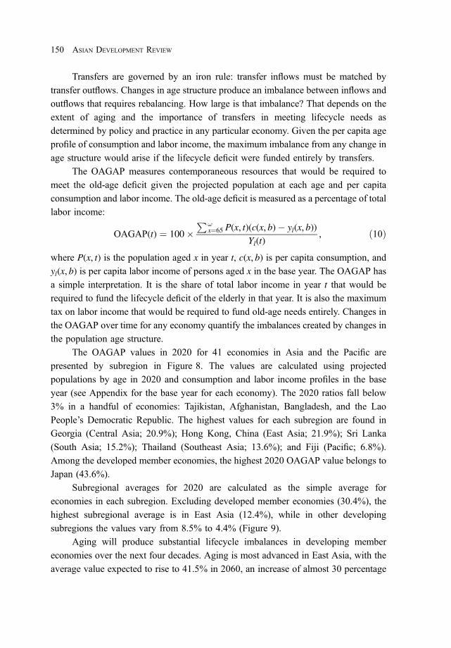
Transfers are governed by an iron rule: transfer inflows must be matched by
transfer outflows. Changes in age structure produce an imbalance between inflows and
outflows that requires rebalancing. How large is that imbalance? That depends on the
extent of aging and the importance of transfers in meeting lifecycle needs as
determined by policy and practice in any particular economy. Given the per capita age
profile of consumption and labor income, the maximum imbalance from any change in
age structure would arise if the lifecycle deficit were funded entirely by transfers.
The OAGAP measures contemporaneous resources that would be required to
meet the old-age deficit given the projected population at each age and per capita
consumption and labor income. The old-age deficit is measured as a percentage of total
labor income:
OAGAP(t) ¼ 100�P!
x¼65 P(x, t)(c(x, b)� yl(x, b))Yl(t)
, ð10Þ
where P(x, t) is the population aged x in year t, c(x, b) is per capita consumption, and
yl(x, b) is per capita labor income of persons aged x in the base year. The OAGAP has
a simple interpretation. It is the share of total labor income in year t that would be
required to fund the lifecycle deficit of the elderly in that year. It is also the maximum
tax on labor income that would be required to fund old-age needs entirely. Changes in
the OAGAP over time for any economy quantify the imbalances created by changes in
the population age structure.
The OAGAP values in 2020 for 41 economies in Asia and the Pacific are
presented by subregion in Figure 8. The values are calculated using projected
populations by age in 2020 and consumption and labor income profiles in the base
year (see Appendix for the base year for each economy). The 2020 ratios fall below
3% in a handful of economies: Tajikistan, Afghanistan, Bangladesh, and the Lao
People’s Democratic Republic. The highest values for each subregion are found in
Georgia (Central Asia; 20.9%); Hong Kong, China (East Asia; 21.9%); Sri Lanka
(South Asia; 15.2%); Thailand (Southeast Asia; 13.6%); and Fiji (Pacific; 6.8%).
Among the developed member economies, the highest 2020 OAGAP value belongs to
Japan (43.6%).
Subregional averages for 2020 are calculated as the simple average for
economies in each subregion. Excluding developed member economies (30.4%), the
highest subregional average is in East Asia (12.4%), while in other developing
subregions the values vary from 8.5% to 4.4% (Figure 9).
Aging will produce substantial lifecycle imbalances in developing member
economies over the next four decades. Aging is most advanced in East Asia, with the
average value expected to rise to 41.5% in 2060, an increase of almost 30 percentage
150 ASIAN DEVELOPMENT REVIEW
March 23, 2022 11:20:43am WSPC/331-adr 2250001 ISSN: 0116-11052ndReading

points from 2020. The projected OAGAP values in 2060 are very similar for Central
Asia, South Asia, and Southeast Asia at 21% to 22%, with an increase in the OAGAP
of 13–16 percentage points for each subregion during the review period. The Pacific
economies are aging more slowly, with a projected OAGAP value of only 8.4% in
2060, which is a 4-percentage-point increase compared with 2020. For developed
member economies, the average OAGAP is projected to reach 53.7% by 2060,
reflecting a 24-percentage-point increase compared with 2020.
The bottom line is that maintaining the existing lifecycle profiles in the presence
of population aging would require funding in excess of 40% of labor income in East
Asia and more than 20% in the rest of developing Asia by 2060. This funding could
rely to some extent on transfers but also on asset-based reallocations: asset income,
and dis-saving. To explore this possibility, we consider the implications of aging from
a longitudinal perspective.
Figure 8. OAGAP Values for Economies in Asia and the Pacific in 2020 (%)
Notes: The OAGAP measures contemporaneous resources that would be required to meet the old-age deficitgiven the projected population at each age and per capita consumption and labor income. The old-age deficit ismeasured as a percentage of total labor income.Source: Authors’ calculations based on the National Transfer Accounts, www.ntaccounts.org (accessed 15 March2020).
DEMOGRAPHIC CHANGE, ECONOMIC GROWTH, AND OLD-AGE ECONOMIC SECURITY 151
March 23, 2022 11:20:43am WSPC/331-adr 2250001 ISSN: 0116-11052ndReading

VII. Lifecycle Asset Accumulation for Old Age in Asia
Old-age needs can be met relying exclusively on current income through a
combination of public and private transfers. The old-age gap measures presented
above are particularly relevant for assessing transfer programs, but many economies,
particularly in Asia, do not rely heavily on transfer systems to meet old-age needs.
Instead, they rely on assets to fund old-age needs. In this section, we consider the
implications of population aging for asset-based systems relying again on a polar case
where economies rely exclusively on assets and not at all on transfers to fund old-age
needs (i.e., the gap between consumption and labor income at old ages).
Asset-based systems are more complex than transfer systems. During their working
years, each cohort must accumulate the lifecycle wealth on which it will rely during their
retirement phase.We call this the preretirement or accumulation phase. To some extent, the
accumulation of retirement wealth occurs at all working ages. For example, workers may
participate in employment-based funded pension plans. We abstract from this, however,
and assume that the lifecycle surplus for young adults is devoted to supporting children,
while the lifecycle surplus for older adults is devoted exclusively to accumulating
retirementwealth. The accumulation phase is definedby the age range overwhich lifecycle
wealth is positive and rising. See Mason et al. (2017) for more details.
Figure 9. OAGAP Values for the Subregions of Asia and the Pacific in 2020, 2040, and2060 (%)
Notes: The OAGAP measures contemporaneous resources that would be required to meet the old-age deficitgiven the projected population at each age and per capita consumption and labor income. The old-age deficit ismeasured as a percentage of total labor income. Regional values are simple averages of the values for economiesin each region.Source: Authors’ calculations based on the National Transfer Accounts, www.ntaccounts.org (accessed 15 March2020).
152 ASIAN DEVELOPMENT REVIEW
March 23, 2022 11:20:53am WSPC/331-adr 2250001 ISSN: 0116-11052ndReading

The accumulation phase is followed by the retirement phase. During this phase,
lifecycle wealth is declining but sufficient to meet anticipated retirement needs in the
future. The cohort relies on asset income and dis-saving to fund the old-age lifecycle
deficit. (Note that the peak of lifecycle wealth may occur later than the age at which
the lifecycle deficit first occurs because seniors may rely on only some part of their
asset income to fund the lifecycle deficit. For simplicity, we refer to the retirement
phase with reference to the peak of lifecycle wealth, but this has no bearing on the
analysis.)
Estimates of the retirement wealth that would be required to fund old-age needs
are presented for economies in Asia and the Pacific in 2020 in Figure 10 (see
Appendix for details). There is a wide range in the values. In Japan, lifecycle wealth is
12 times the total labor income, with similarly high values found in Hong Kong,
China; Australia; and New Zealand. In nine additional economies, retirement wealth
ranges from about 5 to 7.5 times the total labor income. Much lower values of
Figure 10. Lifecycle Retirement Wealth as a Percentage of Total Labor Income forAsia and the Pacific in 2020
Lao PDR = Lao People’s Democratic Republic, WR = aggregate lifecycle retirement wealth, YI = labor income.Source: Authors’ calculations based on the National Transfer Accounts, www.ntaccounts.org (accessed 15 March2020).
DEMOGRAPHIC CHANGE, ECONOMIC GROWTH, AND OLD-AGE ECONOMIC SECURITY 153
March 23, 2022 11:20:54am WSPC/331-adr 2250001 ISSN: 0116-11052ndReading

retirement wealth are found in seven economies, with the lowest in Tonga (49%) and
the Lao People’s Democratic Republic (44%).
These values might strike people as extraordinarily high when compared, for
example, with capital–output ratios that are often in the 4–5 range in rich countries.
It is important to keep two considerations in mind, however. The values presented here
take labor income as the denominator, which would be about two-thirds of net national
income and even smaller when compared with GDP. In Japan, for example, the ratio of
lifecycle wealth to GDP would be less than 8. Second, economies do not rely
exclusively on assets for their retirement. In the analysis presented elsewhere, we find
that Japan relies on transfer for about half of old-age needs. Applying this value would
bring the demand for retirement assets to fund old-age needs to around four times the
GDP in Japan.
The result for the PRC is also somewhat surprising. Retirement wealth is only
243% of labor income even though the PRC will be aging very rapidly over the
coming decades. Moreover, labor income among the elderly in the PRC is relatively
low. These two factors are outweighed, however, by the PRC’s very low level of
consumption among those in the retirement and preretirement phases.
There are pronounced regional differences in lifecycle wealth across Asia and the
Pacific (Figure 11). Currently, East Asia has the highest subregional average value at
Figure 11. Lifecycle Retirement Wealth as a Percentage of Total Labor Income in2020, 2040, and 2060
WR = Aggregate lifecycle retirement wealth, YI = labor income.Notes: Subregional values are simple averages of values for the member economies.Source: Authors’ calculations based on the National Transfer Accounts, www.ntaccounts.org (accessed 15 March2020).
154 ASIAN DEVELOPMENT REVIEW
March 23, 2022 11:21:06am WSPC/331-adr 2250001 ISSN: 0116-11052ndReading

561% of total labor income. In Central Asia and Southeast Asia, lifecycle wealth falls
between 300% and 400%, while lower values are found in South Asia (259%) and the
Pacific (149%). Between 2020 and 2060, the retirement wealth relative to labor
income is projected to almost double in Central Asia, East Asia, and the Pacific, and to
more than double in South Asia and Southeast Asia.
In every economy in Asia and the Pacific, retirement assets are projected to rise
much more rapidly than labor income. This would be possible only if an economy’s
total saving rates were sufficient, but how high would saving rates have to be to
achieve the projected wealth paths that underlie the results presented in Figure 11?
And how would those saving rates compare with transfers if an economy were to rely
on transfers rather than assets to fund old-age needs?
The connection between saving and wealth operates under the influence of two
opposing effects. In many economies in Asia and the Pacific, slower growth in the
effective labor force is leading to downward pressure on the rate of growth of labor
income. This will reduce the need for capital widening. A lower saving rate will
maintain the existing ratio of assets to labor income if labor income is growing
more slowly. This effect of slower economic growth is countered by the demand for
capital deepening, an increase in the ratio of asset to labor income, due to population
aging.
The existence of these two effects is easily formalized. We use the following
terminology. Aggregate lifecycle retirement wealth is represented by WR(t), labor
income by Yl(t), saving by S(t), and the rate of growth of total labor income by
gr(Yl(t)):
WR(t þ 1) ¼ WR(t)þ S(t) ð11Þ
and
Yl(t þ 1) ¼ (1þ gr(Yl(t)))Yl(t): ð12Þ
Dividing equation (11) by equation (12) gives us the following:
WR(t þ 1)Yl(t þ 1)
¼ WR(t)þ S(t)(1þ gr(Yl(t)))Yl(t)
: ð13Þ
Letting w ¼ WR=Yl, the ratio of wealth to labor income, and s ¼ S=Yl, the ratio of
saving to labor income, and rearranging terms gives us the following:
(1þ gr(Yl(t)))w(t þ 1) ¼ w(t)þ s(t): ð14Þ
DEMOGRAPHIC CHANGE, ECONOMIC GROWTH, AND OLD-AGE ECONOMIC SECURITY 155
March 23, 2022 11:21:13am WSPC/331-adr 2250001 ISSN: 0116-11052ndReading

The saving rate required to produce the wealth path from the beginning of period t to
the beginning of period t þ 1 is as follows:
s(t) ¼ gr(Yl(t))w(t)þ Δw(t), where Δw(t) ¼ w(t þ 1)� w(t): ð15Þ
Rearranging the terms, we have
s(t) ¼ gr(Yl(t))þΔw(t)w(t)
� �w(t): ð16Þ
Or letting gr(w(t)) represent the growth rate of the ratio of wealth to labor income, we
have
s(t) ¼ (gr(Yl(t))þ gr(w(t)))w(t): ð17Þ
In general, the demographic transition will lead to a temporarily elevated saving
rate. Both growth terms in equation (17) will be high. Growth in total labor income
will be high because of growth in the effective labor force. Growth in wealth relative to
labor income will be high due to the effects of aging. The growth effects will be
reinforced by the upward trends in wealth. These effects are likely to dissipate over
time, however. Growth in total labor income will decline with growth in the effective
labor force. Growth in the wealth-to-labor-income ratio will decline as the age
distributions of economies stabilize. The outcome in the distant future will depend on
many details that are unknowable. Simulations can be used, however, to consider
possible effects. The results presented in Figure 6 rely on the assumptions and results
presented above. The growth in total labor income is equal to growth in productivity
(1.5% per annum) and growth in the effective labor force (see Figure 6 for growth in
the effective labor force at 20-year intervals). The simulated ratios of wealth to labor
income are based on the same assumptions and methods used in Figures 10 and 11.
The economies of Asia and the Pacific follow a broadly similar pattern of rising
over the demographic transition and then falling as the effects of the demographic
dividend dissipate and the forces of aging set in (Figure 12). Simulated saving for East
Asian economies reached a peak of about 25% of labor income in 2013 and is
projected to decline through the mid-2050s, reaching a low of only about 9% of total
labor income. The simulated saving rate in Southeast Asian economies is similar in
that the peak value also occurs in 2013, but the peak is lower and saving rates remain
at a high plateau for longer. The patterns for Central Asian and South Asian economies
are similar but the simulated saving rate peaks are not reached until the mid-2030s.
The simulated saving rates for the Pacific economies are generally lower, rising slowly,
and do not reach a peak until around 2070.
156 ASIAN DEVELOPMENT REVIEW
March 23, 2022 11:21:13am WSPC/331-adr 2250001 ISSN: 0116-11052ndReading

Simulated savings and the old-age deficits as a share of total labor income are
compared in Figure 12. An important and general lesson is illustrated. Funding
old-age needs by accumulating assets requires a commitment of resources long before
aging sets in. Taking East Asia in 2020 as an example, the gap between consumption
and labor income could be funded with only 12% of total labor income; but in the
same year, accumulating the assets needed to fund old-age needs in the future would
require 23% of total labor income.
There is a natural temptation then to rely on transfer programs rather than asset
accumulation to deal with old-age needs. One impact of this approach, however, is
very evident in Figure 12. By 2033, the resources needed to fund a transfer system in
East Asia would exceed the resources needed to accumulate pension assets. Thereafter,
the resource requirements diverge sharply. By 2050, funding pensions through
transfers would require 38% of total labor income, while the required funding for
pension assets would drop to 10% of total labor income.
Figure 12. Simulated Saving and Old-Age Deficit as a Share of Total Labor Income in theSubregions of Asia and the Pacific, 1975–2060
Source: Authors’ calculations based on the National Transfer Accounts, www.ntaccounts.org (accessed 15 March2020).
DEMOGRAPHIC CHANGE, ECONOMIC GROWTH, AND OLD-AGE ECONOMIC SECURITY 157
March 23, 2022 11:21:13am WSPC/331-adr 2250001 ISSN: 0116-11052ndReading

A second implication of the asset-based approach has been discussed more
extensively. Higher saving rates and greater capital accumulation will lead to higher
productivity and higher standards of living, which is often referred to as the second
demographic dividend. As a practical matter, however, governments are relying on a
combination of public transfers and capital accumulation to fund old-age needs. In the
following section, we consider the impact of aging on the public sector in economies
for which detailed data are available.
VIII. Aging and Its Implications for Asia’s Public Finances
The connection between aging and the public sector is very important in Asia
and the Pacific as it is everywhere. In some economies, the impact of aging on public
finances is of immediate concern. As discussed above, aging is expected to lead to an
increase in the old-age resource gap, and in some economies, governments are heavily
involved in filling that resource gap for their older populations. In economies with
rapid aging and expansive public support for the elderly, the pressure to increase
public spending may outstrip the availability of public resources. In many economies,
the public sector is playing a more limited role. This is due in part to the fact that aging
is delayed and in part to the fact that the public sector is less involved in filling the
resource gap for their senior citizens.
Figure 13. Public Transfer Inflows and Outflows by Age in Indonesia (2005) and theRepublic of Korea (2012)
Notes: Values are expressed relative to the per capita labor income of persons aged 30–49 years.Source: Authors’ calculations based on the National Transfer Accounts, www.ntaccounts.org (accessed 15 March2020).
158 ASIAN DEVELOPMENT REVIEW
March 23, 2022 11:21:35am WSPC/331-adr 2250001 ISSN: 0116-11052ndReading

The differences in old-age support systems are illustrated using estimates of
public transfer inflows and outflows by age in Indonesia and the Republic of Korea
(Figure 13). The Republic of Korea’s public sector is much larger than Indonesia’s.
At peak ages in the Republic of Korea (early 40s), public transfer outflows are about
40% of the per capita labor income of an adult aged 30–49 years, compared with about
15% for those at their peak age in Indonesia (mid-40s). If we consider the importance
of the public sector based on public transfer inflows, the Republic of Korea’s public
sector is also much larger than Indonesia’s.
The age patterns of inflows also differ markedly between the Republic of Korea
and Indonesia. Inflows to children are higher than inflows to prime age adults in both
countries, although the inflows are especially high in the Republic of Korea compared
with Indonesia and almost every other economy in the world. Of particular importance
to the impact of aging is the very large difference in public transfer inflows to seniors.
In Indonesia, we see virtually no tendency for inflows to be higher at older ages;
neither major spending on pensions nor that on health lead to higher support for the
elderly. The Republic of Korea, on the other hand, has a pattern that is similar to many
high-income economies: substantial public transfer inflows to the elderly.
Age profiles like those presented in Figure 13 are used below to project the
impact of population aging on public finances in the absence of public sector reform
for eight developing member economies—Cambodia, the PRC; India; Indonesia; the
Philippines; the Republic of Korea; Taipei,China; and Thailand—and two developed
Figure 14. Old-Age GAP Ratio as a Percentage of Total Labor Income for 10 Economiesin Asia and the Pacific in 2020, 2040, and 2060
Notes: The old-age GAP ratio is the difference between consumption and labor income for those 65 years andolder. Values are projected using per capita consumption and labor by age and population projections.Source: Authors’ calculations based on the National Transfer Accounts, www.ntaccounts.org (accessed 15 March2020).
DEMOGRAPHIC CHANGE, ECONOMIC GROWTH, AND OLD-AGE ECONOMIC SECURITY 159
March 23, 2022 11:21:37am WSPC/331-adr 2250001 ISSN: 0116-11052ndReading

member economies—Australia and Japan. Before those results are presented,
however, we present our earlier estimates of the impact of aging on the old-age gap
as a ratio of total labor income in those economies for 2020, 2040, and 2060. These
results show the maximum impact of aging on public sector spending irrespective of
the public policy pursued (Figure 14).
The OAGAP is rising sharply in three developing member economies: the
Republic of Korea, Thailand, and Taipei,China. By 2060, resources needed by the
elderly in those economies will range from 40% of total labor income in Thailand to
almost 70% in Taipei,China. The percentage of resources needed in Australia by 2060
will be less at about 38%, while in Japan the OAGAP is projected to reach 76% of
total labor income.
In the other five developing economies in Asia and the Pacific—Cambodia, the
PRC, India, Indonesia, and the Philippines—the maximum impact of aging on public
transfer systems is much smaller. But the increases are by no means inconsequential.
The old-age GAP ratios will be three–four times as large in 2040 as they were in 2020.
Still, the results suggest that very generous old-age support systems in these
economies are an attractive option. Expansive programs may be feasible in the shorter
term, but they could well prove to be unsustainable in the more distant future
depending on how they are designed.
In Figure 15, we consider projections of net public transfers if the normalized
age profiles of inflows and outflows are held constant relative to labor income of
those aged 30–49 years. Of the five economies experiencing medium-level gains in the
Figure 15. Projected Net Public Transfers to Those Aged 65 Years and Older as aPercentage of Total Labor Income in 2020, 2040, and 2060
Source: Authors’ calculations based on the National Transfer Accounts, www.ntaccounts.org (accessed 15 March2020).
160 ASIAN DEVELOPMENT REVIEW
March 23, 2022 11:21:39am WSPC/331-adr 2250001 ISSN: 0116-11052ndReading

old-age GAP ratio, none but the PRC will experience significant upward pressure on
net public transfers. By 2060, the projected value of net public transfers to the elderly
will increase to 1% of total labor income in Cambodia and by less in the other four
economies. In the Philippines, net transfers to seniors are projected to be negative,
with seniors receiving less in benefits than they pay in taxes. The PRC is an exception
among these economies with net public transfers projected to reach between 10% and
15% of total labor income by 2060.
The importance of policy in conjunction with aging is also apparent in the
projections for the Republic of Korea; Taipei,China; and Thailand. Net public transfers
to the elderly are relatively modest in Thailand and, hence, the projected values in
2060 reach only 4% of the total labor income. The increases are much more substantial
in the Republic of Korea and Taipei,China, where the net public transfers are projected
to reach 15% and 25%, respectively, in 2060. In Japan, the projected increases in net
public transfers to the elderly are very substantial, reaching 45% of total labor income
by 2060.
IX. Conclusions
For many decades to come, the landscape in Asia and the Pacific will be
dominated by two demographic trends: slower population growth and population
aging. The region is diverse and, hence, the timing and severity of these trends will
vary considerably from economy to economy. However, these trends will intensify, not
dissipate, with significant implications for economies over the foreseeable future.
Demographic transition will pose two strategic challenges for the region: maintaining
economic growth in the face of less favorable demographics and securing adequate
resources to meet the consumption needs of the elderly.
By and large, our analysis confirms the conventional wisdom that population
aging will adversely affect Asia’s economic growth. GDP and other aggregate
economic indicators can be expected to grow more slowly in the future. In the past,
recent growth in the effective labor force led to more rapid GDP growth, but this will
not be the case in the future. In some instances, where fertility rates are very low, the
effective labor force may shrink substantially and GDP may actually decline.
Per capita income could also grow more slowly because of a decline in the support
ratio. The effective number of workers is expected to grow more slowly than the
effective number of consumers.
DEMOGRAPHIC CHANGE, ECONOMIC GROWTH, AND OLD-AGE ECONOMIC SECURITY 161
March 23, 2022 11:21:41am WSPC/331-adr 2250001 ISSN: 0116-11052ndReading
Our analysis also underlines the challenges of securing adequate resources for
the region’s large and growing elderly population. Generational features of economies
in Asia and the Pacific are in the midst of change. Other things being equal, aging will
lead to a very substantial increase in the resources required to support seniors. The
implications of this change are very complex and difficult to anticipate. Some of the
most important effects may be felt at the family level rather than the aggregate level.
Providing support to the elderly could prove to be a significant financial burden to
prime-age adults, particularly in societies where spending on children is reaching high
levels. In many families, the financial costs may prove to be less important than the
burdens from caregiving that often fall on women.
In some societies, providing for seniors is less a family responsibility and more a
social responsibility. In most of the region’s economies, public transfers to the elderly
are less important than in many European and Latin American countries. In those
places where public transfer systems are important, tax revenues are expected to rise
much more slowly than promised benefits. Either tax rates will have to rise or benefits
will have to be curtailed, or both. Other economies may hope to implement more
extensive old-age support systems in response to the greater needs of seniors in aging
societies. A cautious approach is surely warranted.
Many working-age adults may accumulate assets in anticipation of their
retirement. They may participate in funded pension programs, buy a home, pay down
debt, or accumulate assets in many other ways. For now, elevated saving rates will be
essential to fund future retirement needs. Eventually, however, accumulating assets
will ease the financial burden imposed by an aging society.
“Demographics is destiny” refers to the widely held pessimistic view that
economies are powerless in the face of population aging; that is, the demographic
transition to older populations is often blamed for the loss of economic dynamism.
However, there are many things that Asian policy makers can do to mitigate the impact
of population aging on economic growth and old-age economic security. For example,
governments can invest more in education and human capital so that higher labor
productivity can mitigate the reduction of the first demographic dividend. Another
example is creating a working environment that enables seniors to remain productive
for a longer time. This will contribute to both old-age economic security and economic
growth. In short, public policy is hardly impotent in the quest to achieve a more benign
demographic destiny in Asia and elsewhere.
162 ASIAN DEVELOPMENT REVIEW
March 23, 2022 11:21:41am WSPC/331-adr 2250001 ISSN: 0116-11052ndReading

Appendix. Methodology
A1. Consumption and Labor Income Profiles
Consumption and labor income profiles have been estimated by members of the
NTA network using methods described in the United Nations’ National Transfer
Accounts Manual: Measuring and Analyzing the Generational Economy (United
Nations Population Division 2013). These members belong to the Asia Regional
Group led by Sang-Hyop Lee, and their work has relied heavily on financial support
from the United Nations Population Fund and their home institutions.
Labor income consists of wages and earnings of employees and estimates of the
value of labor of the self-employed and unpaid family workers. The age profile is
affected by age variation in labor force participation, unemployment, hours worked,
and productivity. Consumption consists of both public and private consumption, with
separate estimates for health, education, and all other consumption expenditure
combined.
All estimates are based on surveys and administrative data. They are adjusted to
match aggregate data from the System of National Accounts.
Data are available for the following economies included in Table A1, as well as
the year for which data have been estimated.
Age profiles have been rescaled to match the most recently available System of
National Accounts data, but important changes may have occurred in the age patterns
of estimates in some economies. More recent estimates for Japan (not yet released by
the Statistics Bureau) show considerable stability in the age profiles. Efforts are
underway to update estimates for India, but they are not yet completed.
Table A1. Data Availability by Income Group
High Income Upper-Middle Income Lower-Middle Income Low Income
Australia (2010) People’s Republicof China (2014)
Bangladesh (2010) Nepal (2011)
Japan (2004) Malaysia (2009) Cambodia (2009)
Republic of Korea (2015) Maldives (2016) India (2004)
Singapore (2013) Thailand (2013) Indonesia (2012)
Taipei,China (2015) Lao People’s DemocraticRepublic (2012)
Mongolia (2014)
Philippines (2015)
Timor-Leste (2011)
Viet Nam (2012)
Source: Authors’ compilation.
DEMOGRAPHIC CHANGE, ECONOMIC GROWTH, AND OLD-AGE ECONOMIC SECURITY 163
March 23, 2022 11:21:41am WSPC/331-adr 2250001 ISSN: 0116-11052ndReading
A2. Lifecycle Retirement Wealth
An economy relies on lifecycle wealth, broadly defined, to fund old-age needs.
For a cohort of age x in year t, lifecycle wealth is equal to the present value of
prospective consumption less the present value of prospective labor income of
members of that cohort over the remainder of their lifetimes. The accumulation
of lifecycle wealth can be divided into two phases: the retirement phase and the
preretirement (or accumulation) phase. During the retirement phase, lifecycle wealth
will be declining as members of the cohort rely on their wealth to fund consumption in
excess of labor income. During the preretirement phase, lifecycle wealth is rising,
being accumulated as members of the cohort approach retirement. The cohort’s
lifecycle wealth will depend on the per capita consumption and labor income at each
age and the number of cohort members who are still alive.
For members of the cohort, wealth consists in part of assets accumulated through
saving or from bequests received in previous years. But wealth also consists of the
value of prospective net transfers. Prospective public transfers have a value determined
by the prospective benefits received from public programs less the prospective taxes
paid to support public programs. Likewise, the prospective private transfers have a
value that depends on the prospective private transfers received less the prospective
private transfers given. We refer to these two forms of lifecycle wealth as assets and
transfer wealth.
Assets and transfer wealth are equivalent as a means of meeting lifecycle needs.
In other respects, they are quite different, however. Assets are invested and lead to an
increase in capital, a rise in labor productivity, and possibly a decline in interest rates.
Transfer wealth is not invested and consists of nothing more than an obligation of
future generations to transfer resources to the cohort in question. Indeed, transfer
wealth must be balanced by transfer debt, including the net obligations of future
generations.
Formally, per capita lifecycle wealth for the cohort aged x in year t, wr(x, t), for x
equal to or greater than the beginning of preretirement (xp), is equal to the present
value of consumption less the present value of labor income,
wr(x, t) ¼ PVc(x, t)� PVyl(x, t) for x � xp,
PVcr(x, t) ¼X!�xp
z¼0
(1þ r)�zc(xþ z, t þ z) for x � xp,
PVylr (x, t) ¼X!�xp
z¼0
(1þ r)�zyl(xþ z, t þ z) for x � xp,
ðA1Þ
164 ASIAN DEVELOPMENT REVIEW
March 23, 2022 11:21:41am WSPC/331-adr 2250001 ISSN: 0116-11052ndReading

where c and yl are prospective per capita consumption and labor income, respectively,
over the remaining lifetime of the cohort aged x in year t. Total lifecycle wealth is
equal to the following:
WR(t) ¼ PVCR(t)� PVYlR (t),
PVCR(t) ¼X!x¼xp
P(x, t)PVcr (x, t),
PVYlR (t) ¼X!x¼xp
P(x, t)PVylr (x, t),
ðA2Þ
where WR(t) is the total lifecycle wealth in year t; PVCR(t) is the total prospective
consumption and PVYlR (t) is the total prospective labor income, both in present value
terms in the year t; and P(x, t) is the population of age x in year t. All values are
calculated for preretirement and retirement age cohorts.
The calculations presented here are based on the consumption and labor income
profiles for each economy, an exogenous rate of growth of the profiles by 1.5% per
annum, and a discount rate of 3% per annum. More detailed information about the
calculation of the lifecycle phases and the values of xp calculated for each economy is
available in Mason et al. (2017).
A3. Accumulating Wealth and Saving
In this subsection, we consider the connection between savings in wealth under
the influence of two opposing effects. Aging is leading to an increase in wealth relative
to total labor income, but at the same time, slower growth in labor income has the
opposite effect. Here is the derivation using the following terminology: lifecycle
wealth isW(t) and labor income is Yl(t), the rate of growth of total labor income is g(t),
and S(t) is the net saving of lifecycle wealth during the year t,
W(t þ 1) ¼ W(t)þ S(t): ðA3ÞLet g(t) be the growth rate of total labor income:
Yl(t þ 1) ¼ (1þ g(t))Yl(t): ðA4Þ
Dividing equation (A3) by equation (A4) gives the following:
W(t þ 1)Yl(t þ 1)
¼ W(t)þ S(t)(1þ g(t))Yl(t)
: ðA5Þ
DEMOGRAPHIC CHANGE, ECONOMIC GROWTH, AND OLD-AGE ECONOMIC SECURITY 165
March 23, 2022 11:21:42am WSPC/331-adr 2250001 ISSN: 0116-11052ndReading

Letting w ¼ W=Yl, the ratio of wealth to labor income, and s ¼ S=Yl, the ratio of
saving to labor income, and rearranging the terms, we have
(1þ g(t))w(t þ 1) ¼ w(t)þ s(t): ðA6ÞThe saving rate required to produce the wealth path from the beginning of period t to
the beginning of period t þ 1 is as follows:
s(t) ¼ g(t)w(t)þ Δw(t), where Δw(t) ¼ w(t þ 1)� w(t): ðA7ÞRearranging the terms, we have
s(t) ¼ g(t)þ Δw(t)w(t)
� �w(t): ðA8Þ
Or letting gr(w(t)) represent the growth rate of the ratio of wealth to labor income, we
have the following:
s(t) ¼ (g(t)þ gr(w(t)))w(t): ðA9Þ
References
Balachandran, Arun, Joop de Beer, K. S. James, Leo van Wissen, and Fanny Janssen. 2019.“Comparison of Population Aging in Europe and Asia Using a Time-consistent andComparative Aging Measure.” Journal of Aging and Health 32 (5–6): 340–51.
Becker, Gary S., Kevin M. Murphy, and Robert S. Tamura. 1990. “Human Capital, Fertility,and Economic Growth.” Journal of Political Economy 98 (5): S12–37.
Bloom, David E., and David Canning. 2001. “Cumulative Causality, Economic Growth, andthe Demographic Transition.” In Population Matters: Demographic Change, EconomicGrowth, and Poverty in the Developing World, edited by Nancy Birdsall, Allen C. Kelley,and Steven W. Sinding, 165–200. Oxford: Oxford University Press.
Bloom, David E., and Jeffrey G. Williamson. 1998. “Demographic Transitions and EconomicMiracles in Emerging Asia.” The World Bank Economic Review 12 (3): 419–56.
de la Croix, David. 2017. “Did Longer Lives Buy Economic Growth? From Malthus to Lucasand Ben-Porath.” In Demographic Change and Long-Run Development, edited byM. Cervellati and U. Sunde, 69–89. Cambridge, MA: The MIT Press.
Eggertsson, Gauti B., Manuel Lancaster, and Lawrence H. Summers. 2019. “Aging,Output Per Capita, and Secular Stagnation.” American Economic Review: Insights1 (3): 325–42.
Ehrlich, Isaac, and Yong Yin. 2013. “Equilibrium Health Spending and Population Aging in aModel of Endogenous Growth: Will the GDP Share of Health Spending Keep Rising?”Journal of Human Capital 7 (4): 441–47.
166 ASIAN DEVELOPMENT REVIEW
March 23, 2022 11:21:42am WSPC/331-adr 2250001 ISSN: 0116-11052ndReading

Lee, Ronald, and Andrew Mason. 2010. “Fertility, Human Capital, and Economic Growth overthe Demographic Transition.” European Journal of Population 26 (2): 159–82.
Lee, Ronald, and Andrew Mason, eds. 2011. Population Aging and the Generational Economy:A Global Perspective. Cheltenham: Edward Elgar.
Lee, Ronald, Andrew Mason, and Members of the NTA Network. 2014. “Is Low FertilityReally a Problem? Population Aging, Dependency, and Consumption.” Science 346(6206): 229–34.
Mason, Andrew, ed. 2001. Population Change and Economic Development in East Asia:Challenges Met, Opportunities Seized. Stanford: Stanford University Press.
Mason, Andrew, and Ronald Lee. 2007. “Transfers, Capital, and Consumption over theDemographic Transition.” In Population Aging, Intergenerational Transfers and theMacroeconomy, edited by Robert Clark, Andrew Mason, and Naohiro Ogawa, 128–62.Cheltenham, United Kingdom and Northampton, United States: Elgar Press.
_____. 2018. “Intergenerational Transfers and the Older Population.” In IntergenerationalTransfers and the Older Population, edited by The National Academies Press, 187–214.Washington, DC: National Academies of Sciences, Engineering, and Medicine.
Mason, Andrew, Ronald Lee, Michael Abrigo, and Sang-Hyop Lee. 2017. “Support Ratios andDemographic Dividends: Estimates for the World.” United Nations Population DivisionTechnical Paper No. 2017/1.
Sanderson, Warren, and Sergei Scherbov. 2010. “Remeasuring Aging.” Science 329 (10):1287–88.
Tobin, James. 1967. “Life Cycle Saving and Balanced Economic Growth.” In Ten EconomicStudies in the Tradition of Irving Fisher, edited by William Fellner, 231–56. New York:Wiley.
United Nations Population Division. 2013. National Transfer Accounts Manual: Measuringand Analyzing the Generational Economy. New York: United Nations.
_____. 2019. World Population Prospects: The 2019 Revision. New York: United Nations.
DEMOGRAPHIC CHANGE, ECONOMIC GROWTH, AND OLD-AGE ECONOMIC SECURITY 167
March 23, 2022 11:21:42am WSPC/331-adr 2250001 ISSN: 0116-11052ndReading


Trends in Employment and Wagesof Female and Male Workers in India:
A Task-Content-of-Occupations Approach
SHRUTI SHARMA
This paper uses the task-content-of-occupations framework to analyze trends inemployment and wages of female and male workers in the Indian labor marketfrom 1994 to 2017. Workers are classified into four main occupationalcategories: nonroutine cognitive, routine cognitive, nonroutine manual, androutine manual. Decomposing the changes in employment shares intobetween-industry changes and within-industry changes across occupationalcategories reveals that within-industry employment changes have increasinglyplayed an important role, suggesting the growing importance of using thetask-content framework to analyze labor market trends. The biggest increase inemployment shares is for nonroutine cognitive occupations for both female andmale workers. The wage analysis reveals that, on average, the gender wage gaphas been lowest in routine cognitive occupations for most of the period ofanalysis. However, the analysis finds no consistent, significant changes inwages based on occupational specialization during the period of analysis.
Keywords: employment, gender, occupations, wages, tasks
JEL codes: J20, J24, J30, J31
Shruti Sharma: Department of Social Sciences, Human Services and Criminal Justice, Borough ofManhattan Community College, City University of New York. Email: [email protected]. Supportfor this project was provided by a PSC-CUNYAward, jointly funded by The Professional Staff Congressand The City University of New York. I am grateful to the participants of the Faculty FellowshipPublication Program 2020 (City University of New York), the managing editor, and two anonymousreferees for very helpful suggestions on this paper.
This is an Open Access article published by World Scientific Publishing Company. It is distributed underthe terms of the Creative Commons Attribution 3.0 International (CC BY 3.0) License which permits use,distribution and reproduction in any medium, provided the original work is properly cited.
March 23, 2022 11:30:40am WSPC/331-adr 2250002 ISSN: 0116-11052ndReading
Asian Development Review, Vol. 39, No. 1, pp. 169–199DOI: 10.1142/S0116110522500020
© 2022 Asian Development Bank andAsian Development Bank Institute.

I. Introduction
Labor markets in both developed and developing countries have been
significantly impacted by technological innovations and advancements (James 1999;
Autor, Levy, and Murnane 2003; Bruckner, LaFleur, and Pitterle 2017). India, since its
economic reforms in the 1990s, has also experienced an increase in technological
adoption brought about by substantial growth of its technology sector (Kapur 2002,
Heeks 2015) as well as trade-induced technological transfers (Goldberg et al. 2010,
Topalova and Khandelwal 2011, Bas and Berthou 2012, Sharma 2018). It is therefore
important to incorporate the likely impacts of such technological developments in
analyzing India’s labor market.
Traditional literature that examines the impact of technology on workers focuses
on the skills of workers, hypothesizing that the impact of technological advancement
on the labor force should be skill biased (Tinbergen 1974, 1975, Bound and Johnson
1992, Katz and Murphy 1992). However, Acemoglu and Autor (2011) develop a
framework that focuses on tasks involved in various occupations. These are
distinguished along two dimensions—whether they are routine or not (which captures
the differential effects of technology adoption), and whether they are cognitive or not
(which captures the effects of skills or education). Accordingly, they divide
occupations into four categories—routine manual, routine cognitive, nonroutine
manual, and nonroutine cognitive. The hypothesis is that technology is likely to
displace routine tasks, whether these are cognitive or not. In their paper, they find
evidence of job polarization for the United States (US)—a decline in the share of
“middle-skilled” occupations, which are mainly routine occupations, both cognitive
and manual, while the share of workers in nonroutine cognitive and nonroutine manual
occupations increased. This framework performs better than previous models in
explaining the trends in employment and wages of US workers in recent decades
(Acemoglu and Autor 2011, Autor and Dorn 2013).
While the Indian context is very different compared to a developed country such
as the US when it comes to technological adoption, it is nonetheless useful to
understand labor market trends from the perspective of the task content of various
occupations given the increase in technological adoption and advancement in India in
the period after liberalization (Kapur 2002, Heeks 2015). This paper applies the
task-content-of-occupations framework to analyze the Indian labor market separately
for female and male workers and to examine the differences between them. One can
expect technology adoption (captured by whether occupations are routine or
nonroutine) and education (captured by whether occupations are cognitive or
170 ASIAN DEVELOPMENT REVIEW
March 23, 2022 11:30:40am WSPC/331-adr 2250002 ISSN: 0116-11052ndReading

noncognitive) to impact gender inequality in labor markets. There is empirical
evidence that adoption of technology can reduce gender wage gaps. Juhn, Ujhelyi, and
Villegas-Sanchez (2014) show that technological adoption through trade liberalization
in Mexico reduced the demand for “brawn-intensive skills” and favored employment
of blue-collar female workers. There is also evidence that female workers with
cognitive skills earn higher wages and suffer from lower gender wage gaps than those
with noncognitive skills, although education does not entirely reduce the gender wage
gap (Gunewardena, King, and Valerio 2018). This paper studies the trends in
employment and wages of female and male workers separately to capture the
differences in average trends that emerge from using a task-content-of-occupations
framework.
To examine these trends, the paper uses data on India’s labor force for the years
1994, 2000, 2005, 2008, and 2012 from the National Sample Survey of India, and for
the year 2017 from the Periodic Labor Force Survey. The data provide detailed
information on the principal activity, occupational code, wages, gender, age,
education, region, and industry of workers. To create occupational categories, as in
Acemoglu and Autor (2011), information on the task content of each occupation was
obtained from the Occupational Network (O�NET) database and merged onto the
main worker-level dataset.
Employment analysis reveals that, on average, for both female and male
workers, the share of nonroutine cognitive occupations increased the most during
the period of analysis, mainly at the cost of the share of occupations in nonroutine
manual occupations. This was followed by an employment decomposition exercise,
which further revealed interesting findings. Examining whether changes in
employment shares are mainly driven by changes in industrial structure (referred
to as “between-industry” changes hereinafter) or by changes in the occupational
shares within industries (referred to as “within-industry” changes hereinafter), I find
that in the more recent decade (2005–2017), within-industry changes in occupational
shares primarily influenced total changes across all occupational categories. In the
previous decade (1994–2005), however, changes in industrial structure played a more
important role in determining total change in employment shares. This shows that
within-industry changes in occupational categories are becoming increasingly
important in determining changes in employment shares of occupations, which
suggests that the demand and supply of workers performing certain tasks within
industries have been increasingly responsible for shifts in employment trends. In
particular, within-industry changes in nonroutine cognitive shares increased
significantly between the two periods and contributed to an overall increase in the
TRENDS IN EMPLOYMENT AND WAGES OF FEMALE AND MALE WORKERS IN INDIA 171
March 23, 2022 11:30:40am WSPC/331-adr 2250002 ISSN: 0116-11052ndReading

employment share for both female and male workers. However, there are some
differences across female and male workers across occupational categories. During
2005–2017, while within-industry declines in employment shares for male routine
manual workers was the primary factor behind the changes in total employment shares,
the same was not true for female workers in routine manual occupations. In fact, the
employment share of routine manual female workers increased whereas male workers
experienced a decline in this category. This could be indicative of the fact that
routinization, especially inmanual occupations, affectsmaleworkersmore severely and
could serve to reduce the perceived differences between the abilities of female and male
workers. Overall, these findings emphasize the importance of within-industry changes
in occupational structures in determining trends in employment and occupational
structures in India.
Examining trends in wages across occupational categories also yield interesting
findings. Average real wages and relative wages (measured as the ratio of average
wages earned by female workers to male workers) increased during the period of
analysis. Workers in nonroutine cognitive occupations earned the highest wages
throughout the period, followed by those employed in routine cognitive occupations,
for both male and female workers. The analysis also reveals that average wages earned
by routine manual workers are higher than those of nonroutine manual workers. When
considering relative wages, the gender wage gap on average is lowest for almost the
entire period for routine cognitive occupations, followed by nonroutine cognitive
occupations. However, examining how wages have changed over time based on the
occupational specialization of the workers after controlling education, age, and region
fixed effects reveals that there have been no significant changes in trends across all
occupational categories. This could be possible because within-industry occupational
shares in employment have only recently started playing an important role. Thus, these
changes might become more prominent in the future.
The paper is divided into six sections. A description of the datasets used in the
analysis and the task-content model is described in Section II. Section III presents
summary statistics and trends in employment and wages of workers after classifying
them into four categories based on the task-content model. A decomposition of the
percentage change in employment across these categories into between-industry and
within-industry changes can be found in Section IV. An analysis of changes in wages
of male and female workers based on their occupational category is presented in
Section V. Section VI concludes.
172 ASIAN DEVELOPMENT REVIEW
March 23, 2022 11:30:40am WSPC/331-adr 2250002 ISSN: 0116-11052ndReading

II. Data
This paper uses data from the employment-unemployment rounds of the National
Sample Survey (NSS) of India and the Periodic Labor Force Survey (PLFS). These are
household-level datasets that provide information on the activities of all household
members. This includes whether they are employed, their occupation, industry of
employment, wages, age, educational qualification, gender, and the region they are
employed in. Both datasets use a sampling methodology that is representative of the
Indian labor force, and they are available as repeated cross sections. Data for years
1994, 2000, 2005, 2008, and 2012 are from the NSS, and data for the year 2017 are
from the PLFS. The last NSS employment-unemployment round available is from the
year 2012, and labor force data are only available in the form of the PLFS since then.
All the rounds used in this study are thick rounds.1 Occupation data are reported using
a three-digit National Classification of Occupations (NCO) code, and industry data are
reported using a four-digit National Industrial Classification (NIC) code. For the
purpose of the study, any member who reported an occupation code as a current
employment activity is considered employed. Workers who did not report an industry
of employment have been dropped from the analysis.2 The data include both full-time
and part-time workers as well as workers from both the formal and informal sectors.
Salaried as well as self-employed workers and wage laborers are included.
The industry classifications change over time—NIC-1987 for the year 1994,
NIC-1998 for the years 2000 and 2005, NIC-2004 for the year 2008, and NIC-2008
for the years 2012 and 2017, and concordances used from the Ministry of Statistics
and Programme Implementation were used to map all classifications to the NIC-2004
classification. The occupation classifications also change over time—NCO-1968 for
the years 1994, 2000, and 2005, and NCO-2004 for the years 2008, 2012, and 2017,
and a concordance from the Ministry of Labor and Employment was used to map
NCO-1968 to NCO-2004 classification.
Data on wages are reported as weekly wages in Indian rupees. Real wages are
obtained by using a deflator from the consumer price index data of the Organisation
1Thick rounds consider a large sample of households (which ranges from roughly 100,000 to125,000 in this dataset) and are conducted approximately every five years. Thin rounds, on the other hand,consider 35% to 40% of thick round samples and are conducted in the intervening years.
2As a result, a total of 1.2% workers were dropped over six years. Of the workers excluded from theanalysis, 43% were in routine manual occupations whereas 50% were in nonroutine manual occupations.Of the workers dropped in routine manual occupations, 73% were male workers while 27% were female.For nonroutine manual workers, this breakdown was 87% male workers and 13% female workers.
TRENDS IN EMPLOYMENT AND WAGES OF FEMALE AND MALE WORKERS IN INDIA 173
March 23, 2022 11:30:40am WSPC/331-adr 2250002 ISSN: 0116-11052ndReading
for Economic Co-operation and Development (OECD 2021). I consider the wages
reported for the current activity of the workers for each year of the survey.3
To obtain the task content of occupations, this paper follows Acemoglu and
Autor (2011). The O�NET database version 20.3 from April 2016 is used to obtain
this information. This dataset provides the task content of occupations using various
descriptors—variables that describe various tasks involved in each occupation—with
values assigned along different scales for each occupation. I consider a subset of
descriptors to classify O�NET occupations into nonroutine cognitive, routine
cognitive, nonroutine manual, and routine manual occupations. The descriptors are
based on the abilities, skills, work context, and work activities used for each
occupational category.
The descriptors used in this study are provided in Table A1 of Appendix.4 The
value for the “importance” of each descriptor for all occupations is normalized, and the
values across all descriptors for each occupational category are added up to obtain a
score. This score is then normalized, and each occupation is classified as belonging to
an occupational category based on which occupational category has the highest
normalized score for that occupation code. For instance, a high normalized value for
the descriptor “the amount of time spent making repetitive motions” would suggest
that an occupation is intensive in routine manual tasks, whereas a high normalized
value for the descriptor “thinking creatively” would mean that an occupation is
intensive in nonroutine cognitive tasks. Once we obtain this classification, data from
O�NET are then merged onto the NSS data. This is accomplished by first using a
concordance from the O�NET occupation classification to the ISCO-1988 occupation
codes (which is the same classification used by NCO-2004). For years in which NSS
data report occupations using NCO-1968 codes, a concordance between NCO-1968
and NCO-2004 is used. Table A2 of Appendix shows a mapping between the
one-digit NCO division and the percentage of three-digit NCO occupations in that
division classified as either routine manual, nonroutine manual, routine cognitive, or
3The wages are reported as weekly earnings. I use the “principal activity” occupation code specifiedfor individual persons in the dataset to classify the workers in their occupational categories. The wages arereported for the “current activity” of a person, which could have multiple entries. In 97% of the cases, thereis only one current activity for a person, and in all these cases, it matches the principal activity. For theremaining 3% of the cases where there are multiple entries for the current activity, I sum up the wages forall the current activities. These are mainly workers classified as “Agriculture and Fishery workers” or as“Elementary occupations.” However, all current activities for these workers fall within nonroutine manualoccupations.
4Unlike Sharma (2016), which uses an interaction of level and importance values reported to obtainthe score for each task category, I consider only the “importance” of each occupational category based onAcemoglu and Autor (2011) to match their analysis. This explains why Sharma (2016) finds only threemain occupational categories, whereas this study finds four main occupational categories.
174 ASIAN DEVELOPMENT REVIEW
March 23, 2022 11:30:40am WSPC/331-adr 2250002 ISSN: 0116-11052ndReading

nonroutine cognitive. This can provide an understanding of how one-digit NCO codes
roughly match occupational categories.
The following section describes the trends in employment and wages for female
and male workers based on this classification of occupations.
III. Summary Statistics
In analyzing the trends in female and male workers in India, it is important to
first understand the labor force participation rates. Figure 1 shows the labor force
participation rates from 1994 to 2017. Labor force participation rate for male workers
was 84.7% in 1994 and declined to 83% in 2017. For female workers, the labor force
participation rate was 30.5% in 1994 and declined to 22.2% in 2017.
In terms of gender composition of the workforce, Figure 2 shows that female
workers comprised 19% of the workforce in 2017, down from 23% in 1994, whereas
the share of male workers increased to 81% in 2017 from 77% in 1994.
The next set of statistics is based on examining the task content of occupations,
which would help identify occupations that are experiencing the biggest changes in
employment shares.
Table 1 reports summary statistics for employment of all workers and male and
female across all occupational categories. I compute the shares of workers in
nonroutine manual, nonroutine cognitive, routine manual, and routine cognitive
occupations for both male and female workers (Table A3). Figure 3 presents the
trends in employment obtained from this classification. I find that for both male and
female workers, the share of workers employed in nonroutine manual occupations5 is
the highest, although it has been decreasing over time. For male workers, this share
declined from 81% in 1994 to 72% in 2017, whereas for female workers, the share
declined from 80% in 1994 to 65% in 2017. For both female and male workers, the
biggest increase in employment shares is for nonroutine cognitive workers. For routine
cognitive occupations, on the other hand, the share of male workers employed in this
category decreased from 5% in 1994 to 4% in 2017, while for female workers, this
share increased from 2% in 1994 to 3% in 2017. Finally, for routine manual
occupations, employment shares in this category increased from 18% in 1994 to 21%
5Unlike Acemoglu and Autor (2011), I do not drop occupations in the agriculture sector, all ofwhich classified as nonroutine occupations, to be able to provide an analysis of all possible sectors.Mechanization in the agriculture sector is not properly captured in the classification of occupations asroutine and nonroutine, which might explain why this analysis presents a decline in the share of nonroutinemanual occupations.
TRENDS IN EMPLOYMENT AND WAGES OF FEMALE AND MALE WORKERS IN INDIA 175
March 23, 2022 11:30:40am WSPC/331-adr 2250002 ISSN: 0116-11052ndReading

in 2017 for female workers; however, for male workers, this share declined from 12%
in 1994 to 10% in 2017. This reflects the share in the economy and growth of India’s
manufacturing sector (Sharma and Singh 2013) where most routine manual
occupations are concentrated.
Figure 1. Labor Force Participation Rate
Source: Author’s calculations using data from the National Sample Survey of India (1994, 2000, 2005, 2008,2012) and the Periodic Labor Force Survey (2017).
Figure 2. Share of Employment by Gender
Source: Author’s calculations using data from the National Sample Survey of India (1994, 2000, 2005, 2008,2012) and the Periodic Labor Force Survey (2017).
176 ASIAN DEVELOPMENT REVIEW
March 23, 2022 11:30:40am WSPC/331-adr 2250002 ISSN: 0116-11052ndReading

The next set of summary statistics considers trends in average and relative wages.
Wages are weekly and in Indian rupees, and have been deflated using the consumer
price index (OECD 2021). Figure 4 shows that average real wages for both male and
female workers increased from 1994 to 2017, and Figure 5 shows that relative wages
Table 1. Summary Statistics: Employment (million)
1994 2000 2005 2008 2012 2017
AllMale 151.0 186.0 215.0 214.0 227.0 250.0Female 45.1 54.2 70.0 57.1 56.6 59.5
Routine manualMale 14.0 21.3 24.6 25.6 23.5 25.7Female 6.9 10.5 13.1 11.9 11.5 12.5
Routine cognitiveMale 7.4 8.8 8.4 9.3 9.0 10.2Female 0.84 1.1 1.3 1.1 1.2 1.6
Nonroutine manualMale 122.0 144.0 168.0 154.0 166.0 179.0Female 36.0 40.5 52.9 40.0 39.0 38.8
Nonroutine cognitiveMale 7.4 11.8 14.0 25.4 28.8 35.7Female 1.4 2.1 2.7 4.1 4.9 6.7
Source: Author’s calculations using data from the National Sample Survey of India (1994,2000, 2005, 2008, 2012) and the Periodic Labor Force Survey (2017).
Figure 3. Share of Employment across Occupational Categories
Source: Author’s calculations using data from the National Sample Survey of India (1994, 2000, 2005, 2008,2012) and the Periodic Labor Force Survey (2017).
TRENDS IN EMPLOYMENT AND WAGES OF FEMALE AND MALE WORKERS IN INDIA 177
March 23, 2022 11:30:43am WSPC/331-adr 2250002 ISSN: 0116-11052ndReading

Figure 4. Average Wage by Gender
Source: Author’s calculations using data from the National Sample Survey of India (1994, 2000, 2005, 2008,2012) and the Periodic Labor Force Survey (2017).
Figure 5. Relative Wage
Note: Relative wage is measured as the ratio of the average wage of female workers to the average wage of maleworkers.Source: Author’s calculations using data from the National Sample Survey of India (1994, 2000, 2005, 2008,2012) and the Periodic Labor Force Survey (2017).
178 ASIAN DEVELOPMENT REVIEW
March 23, 2022 11:30:45am WSPC/331-adr 2250002 ISSN: 0116-11052ndReading

(measured as the ratio of average wages of female workers to average wages of male
workers) have also increased for the period of analysis.
Table 2 presents the summary statistics for the average weekly real wages earned
by all workers, male workers, and female workers. This is provided for the entire labor
Table 2. Average Weekly Real Wages across Occupational Categories (�)
All Male (M) Female (F) Relative Wage (F/M)
1994
All 858.96 948.92*** 565.13*** 0.60(2.93) (3.41) (5.16)
Routine manual 956.09 1,031.77*** 362.99*** 0.35(5.79) (6.14) (8.55)
Routine cognitive 1,314.12 1,321.55** 1,264.80** 0.96(7.65) (8.13) (22.44)
Nonroutine manual 427.42 488.19*** 285.08*** 0.58(1.56) (1.99) (1.82)
Nonroutine cognitive 2,011.37 2,113.09*** 1,698.37*** 0.80(10.07) (11.62) (18.93)
2000
All 1,096.38 1,203.20*** 748.24*** 0.62(4.03) (4.68) (7.36)
Routine manual 1,180.30 1,241.38*** 530.80*** 0.43(7.59) (8.00) (14.51)
Routine cognitive 1,730.15 1,748.76*** 1,606.92*** 0.92(10.85) (11.49) (32.28)
Nonroutine manual 512.30 588.28*** 335.62*** 0.57(2.09) (2.70) (2.33)
Nonroutine cognitive 2,759.63 2,939.71*** 2,290.82*** 0.78(14.77) (17.25) (26.80)
2005
All 1,135.25 1,246.88*** 771.20*** 0.62(4.27) (4.96) (7.77)
Routine manual 1,075.50 1,138.43*** 459.45*** 0.40(7.04) (7.50) (11.27)
Routine cognitive 1,632.09 1,682.04*** 1,353.21*** 0.80(10.73) (11.59) (27.56)
Nonroutine manual 518.76 598.94*** 339.27*** 0.57(2.27) (2.96) (2.57)
Nonroutine cognitive 2,671.22 2,883.88*** 2,117.64*** 0.73(14.71) (16.97) (27.13)
Continued.
TRENDS IN EMPLOYMENT AND WAGES OF FEMALE AND MALE WORKERS IN INDIA 179
March 23, 2022 11:30:49am WSPC/331-adr 2250002 ISSN: 0116-11052ndReading

Table 2. Continued.
All Male (M) Female (F) Relative Wage (F/M)
2008
All 1,135.48 1,228.93*** 819.10*** 0.67(4.24) (4.91) (7.95)
Routine manual 1,163.70 1,210.86*** 574.10*** 0.47(7.60) (8.00) (15.01)
Routine cognitive 1,740.20 1,799.45*** 1,402.27*** 0.78(11.64) (12.55) (29.96)
Nonroutine manual 556.38 625.92*** 378.06*** 0.60(2.00) (2.52) (2.45)
Nonroutine cognitive 2,845.78 3,102.36*** 2,264.87*** 0.73(16.83) (20.23) (27.93)
2012
All 1,599.33 1,701.22*** 1,195.20*** 0.70(6.48) (7.30) (13.38)
Routine manual 1,286.59 1,335.65*** 688.38*** 0.52(8.43) (8.90) (16.57)
Routine cognitive 2,048.36 2,166.66*** 1,453.69*** 0.67(16.40) (17.95) (36.90)
Nonroutine manual 828.41 920.14*** 563.47*** 0.61(3.88) (4.77) (4.89)
Nonroutine cognitive 3,309.58 3,609.05*** 2,523.94*** 0.70(20.40) (23.56) (37.14)
2017
All 1,859.17 1,940.36*** 1,431.70*** 0.74(4.70) (5.05) (12.10)
Routine manual 1,606.90 1,708.99*** 730.83*** 0.43(7.52) (7.86) (15.12)
Routine cognitive 2,005.17 2,095.45*** 1,542.80*** 0.74(10.15) (11.05) (24.09)
Nonroutine manual 1,283.83 1,364.15*** 781.53*** 0.57(5.04) (5.48) (9.71)
Nonroutine cognitive 2,684.02 2,848.47*** 2,127.55*** 0.75(11.90) (13.31) (24.97)
�¼ Indian rupee.Notes: Standard errors in parentheses. ** and *** indicate that the means of weekly real wagesfor male and female workers are significantly different at p < 0:05 and p < 0:01, respectively.Source: Author’s calculations using data from the National Sample Survey of India (1994,2000, 2005, 2008, 2012) and the Periodic Labor Force Survey (2017).
180 ASIAN DEVELOPMENT REVIEW
March 23, 2022 11:30:49am WSPC/331-adr 2250002 ISSN: 0116-11052ndReading

force as well as by occupation type. The data show that there exists a gender wage gap
on average and across all occupation types, with wages earned by male workers
significantly higher than that of female workers across all years.
Figure 6 presents the average log real wages for female and male workers across
occupational categories. For both female and male workers, average trends reveal that
wages are highest for workers in nonroutine cognitive occupations, followed by
routine cognitive occupations. The lowest average wages are earned by workers in
nonroutine manual occupations.
The relative wages shown in Figure 7 are a ratio of average weekly real wages of
female workers to the average weekly real wages of male workers. The figure shows
that relative wages are highest for female workers in nonroutine cognitive and routine
cognitive occupations. However, these wages have been declining over time. On the
other hand, gender wage inequality is higher in manual occupations but has been
exhibiting a decreasing trend over time. It is also interesting to note that gender wage
inequality for the most part has been lowest in routine cognitive occupations. The fact
that the gender wage gap is lower for cognitive occupations is not surprising. Evidence
from Gunewardena, King, and Valerio (2018) shows that obtaining cognitive skills
reduces the gender wage gap for female workers. Sections IV and V delve into these
trends in employment and wages in more detail.
Figure 6. Average Wage by Gender and across Occupation Types
Source: Author’s calculations using data from the National Sample Survey of India (1994, 2000, 2005, 2008,2012) and the Periodic Labor Force Survey (2017).
TRENDS IN EMPLOYMENT AND WAGES OF FEMALE AND MALE WORKERS IN INDIA 181
March 23, 2022 11:30:49am WSPC/331-adr 2250002 ISSN: 0116-11052ndReading
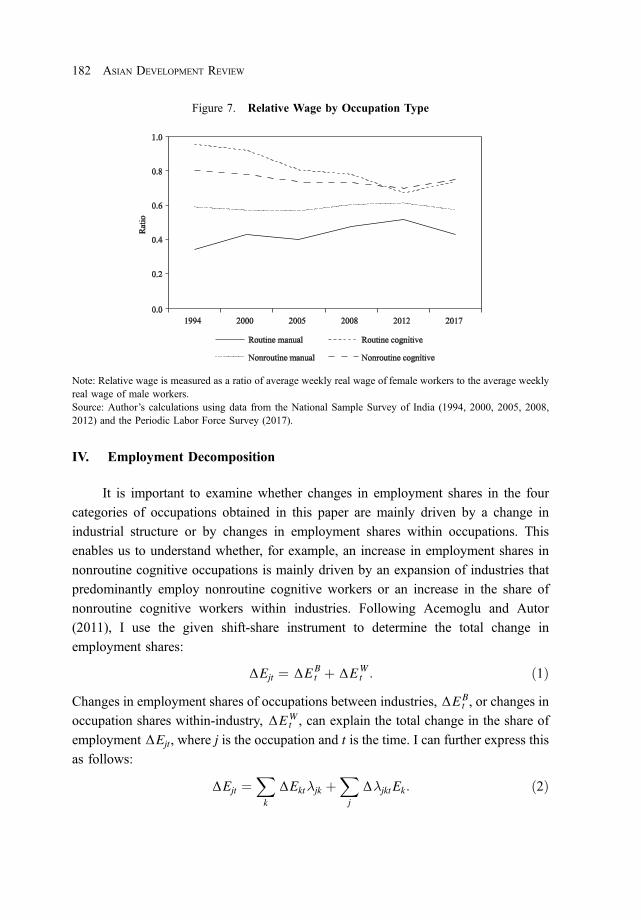
IV. Employment Decomposition
It is important to examine whether changes in employment shares in the four
categories of occupations obtained in this paper are mainly driven by a change in
industrial structure or by changes in employment shares within occupations. This
enables us to understand whether, for example, an increase in employment shares in
nonroutine cognitive occupations is mainly driven by an expansion of industries that
predominantly employ nonroutine cognitive workers or an increase in the share of
nonroutine cognitive workers within industries. Following Acemoglu and Autor
(2011), I use the given shift-share instrument to determine the total change in
employment shares:
ΔEjt ¼ ΔEBt þ ΔEW
t : ð1ÞChanges in employment shares of occupations between industries, ΔEB
t , or changes in
occupation shares within-industry, ΔEWt , can explain the total change in the share of
employment ΔEjt, where j is the occupation and t is the time. I can further express this
as follows:
ΔEjt ¼X
k
ΔEkt�jk þX
j
Δ�jkt Ek: ð2Þ
Figure 7. Relative Wage by Occupation Type
Note: Relative wage is measured as a ratio of average weekly real wage of female workers to the average weeklyreal wage of male workers.Source: Author’s calculations using data from the National Sample Survey of India (1994, 2000, 2005, 2008,2012) and the Periodic Labor Force Survey (2017).
182 ASIAN DEVELOPMENT REVIEW
March 23, 2022 11:30:51am WSPC/331-adr 2250002 ISSN: 0116-11052ndReading

ΔEkt represents the change in industry k’s share over the period under consideration,
whereas Ek represents the average employment share. Similarly, Δ�jkt gives the
change in occupation j’s share of industry k’s employment over the period under
consideration, whereas �jk gives the average share. The industries in this analysis are
at the NIC four-digit level.
Table 3 reports the decomposition of changes in employment shares, in
percentage points, of the four main occupation categories for all workers, male
workers, and female workers. I divided the data into roughly 2 decades to examine
Table 3. Employment Decomposition (Percentage Points)
1994–2005 2005–2017 1994–2017
All
Routine manualTotal Δ 2.55 �0.94 1.61Between industry Δ 2.22 �0.06 1.88Within industry Δ 0.33 �0.88 �0.27
Routine cognitiveTotal Δ �0.80 0.44 �0.36Between industry Δ �1.00 0.72 �0.50Within industry Δ 0.20 �0.28 0.14
Nonroutine manualTotal Δ �3.10 �7.32 �10.42Between industry Δ �4.58 �1.66 �7.68Within industry Δ 1.48 �5.66 �2.74
Nonroutine cognitiveTotal Δ 1.35 7.82 9.17Between industry Δ 0.36 2.86 3.39Within industry Δ 0.99 4.96 5.78
Male
Routine manualTotal Δ 2.13 �1.20 0.93Between industry Δ 1.93 �0.23 1.49Within industry Δ 0.20 �0.97 �0.56
Routine cognitiveTotal Δ �0.98 0.20 �0.78Between industry Δ �1.18 0.49 �0.97Within industry Δ 0.20 �0.29 0.19
Nonroutine manualTotal Δ �2.75 �6.73 �9.48Between industry Δ �4.33 �0.87 �6.23Within industry Δ 1.58 �5.86 �3.25
Continued.
TRENDS IN EMPLOYMENT AND WAGES OF FEMALE AND MALE WORKERS IN INDIA 183
March 23, 2022 11:30:54am WSPC/331-adr 2250002 ISSN: 0116-11052ndReading
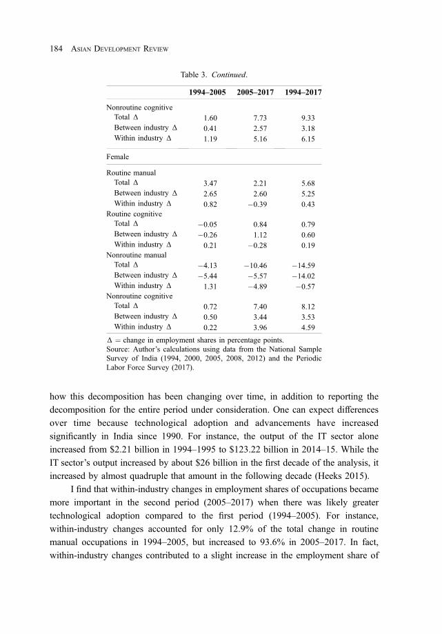
how this decomposition has been changing over time, in addition to reporting the
decomposition for the entire period under consideration. One can expect differences
over time because technological adoption and advancements have increased
significantly in India since 1990. For instance, the output of the IT sector alone
increased from $2.21 billion in 1994–1995 to $123.22 billion in 2014–15. While the
IT sector’s output increased by about $26 billion in the first decade of the analysis, it
increased by almost quadruple that amount in the following decade (Heeks 2015).
I find that within-industry changes in employment shares of occupations became
more important in the second period (2005–2017) when there was likely greater
technological adoption compared to the first period (1994–2005). For instance,
within-industry changes accounted for only 12.9% of the total change in routine
manual occupations in 1994–2005, but increased to 93.6% in 2005–2017. In fact,
within-industry changes contributed to a slight increase in the employment share of
Table 3. Continued.
1994–2005 2005–2017 1994–2017
Nonroutine cognitiveTotal Δ 1.60 7.73 9.33Between industry Δ 0.41 2.57 3.18Within industry Δ 1.19 5.16 6.15
Female
Routine manualTotal Δ 3.47 2.21 5.68Between industry Δ 2.65 2.60 5.25Within industry Δ 0.82 �0.39 0.43
Routine cognitiveTotal Δ �0.05 0.84 0.79Between industry Δ �0.26 1.12 0.60Within industry Δ 0.21 �0.28 0.19
Nonroutine manualTotal Δ �4.13 �10.46 �14.59Between industry Δ �5.44 �5.57 �14.02Within industry Δ 1.31 �4.89 �0.57
Nonroutine cognitiveTotal Δ 0.72 7.40 8.12Between industry Δ 0.50 3.44 3.53Within industry Δ 0.22 3.96 4.59
Δ ¼ change in employment shares in percentage points.Source: Author’s calculations using data from the National SampleSurvey of India (1994, 2000, 2005, 2008, 2012) and the PeriodicLabor Force Survey (2017).
184 ASIAN DEVELOPMENT REVIEW
March 23, 2022 11:30:54am WSPC/331-adr 2250002 ISSN: 0116-11052ndReading

these occupations in the first period but caused the employment share to shrink in the
second period. The growing importance of within-industry shifts over time is
consistent across almost all occupational categories and for both female and male
workers. This highlights the need for following a task-content-of-occupations
approach to understand changes in employment structures, especially with greater
technological advances and adoption over time.
The results from the analysis suggest that routinization could be causing a
decline in within-industry employment shares in routine occupational categories. For
instance, for both male and female workers, the contribution of within-industry
employment share to the total change in employment shares for routine manual
occupations went from positive in 1994–2005 to negative in 2005–2017. It is
interesting to note, however, that in the period 2005–2017 for male workers in routine
manual occupations, within-industry declines accounted for 80% of the total decline in
employment shares, whereas for female workers this decline was much smaller than
the positive increase in employment share between industries. Similarly, for routine
cognitive occupations for male workers, within-industry changes during 2005–2017
accounted for the larger percentage of the total change in employment shares, whereas
this change was smaller for female workers. This might suggest that routinization has
differential impacts on female and male workers, affecting the employment of male
workers more adversely than that of female workers. Mechanization and technological
adoption, while automating jobs, also reduces the perceived differences in female and
male workers (Juhn, Ujhelyi, and Villegas-Sanchez 2014).
It is also interesting to note that while within-industry employment shares of
nonroutine cognitive occupations have been increasing as expected, the
within-industry employment shares for nonroutine manual occupations have been
declining. The latter runs counter to the hypothesis that automation should be
increasing the relative demand for workers in nonroutine occupations. This could be
explained by the fact the task-content framework does not capture mechanization that
can occur within the agriculture sector, which is primarily categorized as nonroutine
manual in the occupational categorization. Also, there may be supply-side effects
with workers moving to cognitive occupations as they gain greater access to
education. In fact, Acemoglu and Autor (2011) drop the agriculture sector from their
analysis. Table A4 of Appendix shows the employment decomposition after leaving
out the agriculture sector from the analysis. Compared to Table 3, Table A4 shows a
smaller decline in the employment shares of nonroutine manual occupations, and a
bigger decline in the employment of routine occupations, which is more in line with
expectations. Table A5 provides an employment decomposition at the one-digit
TRENDS IN EMPLOYMENT AND WAGES OF FEMALE AND MALE WORKERS IN INDIA 185
March 23, 2022 11:30:54am WSPC/331-adr 2250002 ISSN: 0116-11052ndReading

NCO for female workers to provide a description of each occupational type.
For instance, technicians and associate professionals experienced the biggest increase
in the share of employment overall, and also the largest within-industry increase in
employment shares.
An important concern is whether the between-industry changes in employment
shares could be a result of the changing classification of NIC codes over the years.
Table A6 of Appendix reports the share of employment in the data that is affected by
these changes in classification. Table A7 then reports the results of the employment
decomposition exercise without the employment data that have changed because of
changes in industrial classification. This change does not affect the analysis
significantly, and the main inferences stay the same.
V. Wage Analysis
In this section, I analyze whether routinization of tasks has impacted the returns
to workers based on their occupational specialization. To do so, I follow Acemoglu
and Autor (2011) in examining how wages of workers have changed over time
depending on their occupational specialization. They divide workers into three main
categories: workers performing routine tasks, those in nonroutine cognitive tasks, and
those in occupations intensive in nonroutine manual tasks. The main hypothesis is that
increased routinization leads to a decline in wages of workers in occupations intensive
in routine tasks. This should be reflected in a relative increase in wages of workers in
both nonroutine cognitive and nonroutine manual occupations.
To estimate this, Acemoglu and Autor first create demographic groups based on
gender, education, age, and region and then construct employment shares of workers in
routine occupations, nonroutine cognitive occupations, and nonroutine manual
occupations at the beginning of the period of their analysis, with the assumption that
workers self-select into each of these categories based on their comparative advantage
or task specialization. I similarly create these demographic groups and then construct
γRsejk, γNRMsejk , and γNRCsejk , which are the shares of workers employed in routine occupations
(including both routine manual and routine cognitive), nonroutine manual occupations,
and nonroutine cognitive occupations in each demographic group, respectively, for the
year 1994, which is the first year of the analysis. The age and education buckets used for
creating these cohorts are presented in Appendix in Tables A8 and A9, respectively.
NSS state-region codes (125 codes) were used for the region category. The variables
gender, education, age, and region are denoted by s, e, j, and k, respectively. Then based
186 ASIAN DEVELOPMENT REVIEW
March 23, 2022 11:30:54am WSPC/331-adr 2250002 ISSN: 0116-11052ndReading

on Acemoglu and Autor’s analysis, I estimate the following:
Δwsejkt ¼ β0 þ β1 � γNRMsejk � ti þ β2 � γNRCsejk � ti þ ti þ θe þ θj þ θk þ �sejkt: ð3ÞγRsejk was dropped from the regression because by construction γRsejk þ γNRMsejk þ γNRCsejk ¼ 1.
The education, region, and age fixed effects are denoted by θe, θj, and θk, respectively,
and ti is the time (year) dummy where t stands for time. Δwsejkt stands for the change
in mean log wages for each demographic group in the analysis. The difference in this
analysis compared to Acemoglu and Autor (2011) is that the change in wages is not
within a decade but across the various time periods available for this analysis.
The estimation results are presented in Table 4. Model 1 reports the estimates for
male workers without fixed effects, which are included in Model 2. Similarly, Model 3
reports the results for female workers without fixed effects, which are then included in
Model 4. There are more male workers than female workers in the survey, which is
reflected in the total number of observations for each.
Table 4. Wage Analysis
Male withoutFixed Effects
Male withFixed Effects
Female withoutFixed Effects
Female withFixed Effects
(1) (2) (3) (4)
Nonroutine manual2000 share� 2000 time dummy �0.210** �0.288*** �0.156 �0.0863
(0.0902) (0.0985) (0.131) (0.135)2005 share� 2005 time dummy 0.212** 0.134 �0.108 �0.0380
(0.103) (0.108) (0.137) (0.137)2008 share� 2008 time dummy 0.0343 �0.0434 0.118 0.188*
(0.0797) (0.0864) (0.0989) (0.107)2012 share� 2012 time dummy �0.0191 �0.0968 �0.191* �0.121
(0.0830) (0.0898) (0.110) (0.113)2017 share� 2017 time dummy 0.314*** 0.237*** �0.106 �0.0364
(0.0795) (0.0849) (0.119) (0.123)
Nonroutine cognitive2000 share� 2000 time dummy �0.181 �0.158 0.106 0.198
(0.114) (0.119) (0.177) (0.186)2005 share� 2005 time dummy 0.159 0.182 �0.244 �0.152
(0.112) (0.116) (0.166) (0.173)2008 share� 2008 time dummy 0.0388 0.0620 �0.00166 0.0903
(0.0993) (0.109) (0.128) (0.146)2012 share� 2012 time dummy �0.0639 �0.0408 �0.235* �0.143
(0.0865) (0.0931) (0.140) (0.155)2017 share� 2017 time dummy �0.240** �0.217** �0.172 �0.0797
(0.0970) (0.101) (0.152) (0.163)
Continued.
TRENDS IN EMPLOYMENT AND WAGES OF FEMALE AND MALE WORKERS IN INDIA 187
March 23, 2022 11:30:56am WSPC/331-adr 2250002 ISSN: 0116-11052ndReading

The results obtained are mixed. Relative to routine occupations, male workers in
nonroutine manual occupations experienced a significant decline in their wages in
2000, which is robust to the inclusion of fixed effects. These relative returns however
increased significantly in 2017 for both Models 1 and 2. This provides some support
for the fact that returns to workers specialized in nonroutine manual tasks have been
increasing recently relative to routine occupations. On the other hand, while wages of
male workers in nonroutine cognitive occupations did not change significantly relative
to workers in routine occupations in most years, a significant decline is observed for
2017, which runs counter to expectations. Female workers in nonroutine manual and
nonroutine cognitive occupations, on the other hand, for most years, did not
experience any significant changes in wages relative to those in routine occupations
Table 4. Continued.
Male withoutFixed Effects
Male withFixed Effects
Female withoutFixed Effects
Female withFixed Effects
(1) (2) (3) (4)
2000 year dummy 0.424*** 0.550*** 0.347*** 0.286**(0.0659) (0.0873) (0.0888) (0.140)
2005 year dummy �0.387*** �0.261*** �0.235** �0.296**(0.0700) (0.0884) (0.0988) (0.145)
2008 year dummy 0.191*** 0.317*** 0.181*** 0.119(0.0567) (0.0796) (0.0671) (0.129)
2012 year dummy 0.124** 0.250*** 0.227*** 0.165
(0.0594) (0.0840) (0.0748) (0.130)2017 year dummy �0.0552 0.0711 0.0608 �0.000817
(0.0580) (0.0812) (0.0866) (0.144)
Region fixed effect No Yes No YesEducation fixed effect No Yes No YesAge fixed effect No Yes No Yes
Observations 3,165 3,165 2,005 2,005R2 0.239 0.259 0.124 0.152
Notes: Standard errors in parentheses. *p < 0:10, **p < 0:05, ***p < 0:01. Models 1�4 in eachcolumn present a separate ordinary least squares regression of stacked changes in mean log weekly realwages by cohort and year, where cohorts are created using sex, age group (Table A8), education group(Table A9), and state (125 State-region codes are reported in NSS) of the workers in the NationalSample Survey (1994, 2000, 2005, 2008, 2012) and Periodic Labor Force Survey (2017) data.Occupation shares are calculated for each demographic group in 1994 and interacted with decadedummies. Occupations are grouped into three categories: (1) nonroutine cognitive; (2) nonroutinemanual; and (3) routine—both cognitive and manual. The routine group is the omitted category in theregression models. For the year dummy variables, the reference year is 1994.Source: Author’s calculations using data from the National Sample Survey of India (1994, 2000, 2005,2008, 2012) and the Periodic Labor Force Survey (2017).
188 ASIAN DEVELOPMENT REVIEW
March 23, 2022 11:30:56am WSPC/331-adr 2250002 ISSN: 0116-11052ndReading

during the period of analysis. One exception is an increase in the wages of female
workers in nonroutine manual occupations to those in routine occupations for 2008.
The coefficients of the time dummies in this analysis provide an estimate of the
wage trends of workers specializing in routine occupations at the beginning of the
analysis. For female workers in routine occupations, wages increased significantly in
2000 and then declined significantly in 2005, which is consistent with the hypothesis
that the returns to these occupations should decline over time. For male workers in
routine occupations, on the other hand, the results are not consistent—wages initially
increase significantly in 2000, then decline significantly in 2005, and then increase
thereafter.
This analysis is a preliminary exercise in determining how returns to workers in
various occupational specializations are evolving over time. While there is some
evidence of a decline in returns to workers in routine occupations over time, especially
for female workers, this is not strongly corroborated. Given that a developing country
such as India is still lagging in terms of technological adoption compared to the US,
one might observe these effects on wages becoming more prominent as technological
adoption increases in the future. The fact that changes in within-industry employment
shares have only recently become prominent in impacting overall changes in
employment across occupational categories also suggests that we can probably expect
these results to be stronger in the future.
VI. Conclusion
This paper uses a task-content-of-occupations approach to analyze trends in
employment and wages of male and female workers in India from 1994 to 2017. This
approach provides a better framework to take into account the impact of technological
advancements and automation while analyzing these labor market trends. Accordingly,
it classifies male and female workers into four occupational categories: routine
cognitive, nonroutine cognitive, routine manual, and nonroutine manual. The paper
considers the trends in male and female workers separately to understand how
technological advancements on average might be impacting these two groups of
workers differently.
Analyzing the employment trends I find that, on average, the share of workers in
nonroutine manual work is highest for both male and female workers but declining
over time, whereas the share of nonroutine cognitive workers is increasing.
An employment decomposition exercise, which uses a shift-share instrument to
determine the extent to which changes in employment shares across occupations are
TRENDS IN EMPLOYMENT AND WAGES OF FEMALE AND MALE WORKERS IN INDIA 189
March 23, 2022 11:30:56am WSPC/331-adr 2250002 ISSN: 0116-11052ndReading

due to changes in industrial structure compared to changes in within-industry
occupational shares, reveals interesting results. I find that in the more recent decade,
changes in within-industry employment shares are more important in determining the
overall change in occupational shares. This suggests that using the task-content
framework to understand changes in employment trends is becoming more important
in the Indian context. I find that, as expected, there is a decline in within-industry
shares of employment for routine cognitive and routine manual occupations. This
decline in occupational shares in routine occupations is the main factor driving the
overall changes in employment shares of male workers, while the same is not true for
female workers. This suggests that routinization might not be impacting female
workers as adversely as male workers. Within-industry employment shares of
nonroutine cognitive occupations for both female and male workers have been
increasing, in line with expectations.
I also examine average trends in wages across all occupational categories.
For both male and female workers, average wages are highest for nonroutine cognitive
occupations, followed by routine cognitive occupations and then routine manual
occupations, with the lowest wages for nonroutine manual occupations. The gender
wage gap is lowest in cognitive occupations—with routine cognitive occupations
recording the lowest gap for most of the period of analysis. A wage analysis that
considers changes in wages for workers specializing in a certain occupational category
at the beginning of the period, however, finds that there are no consistent, significant
changes in the earnings of workers of nonroutine occupations compared to those in
routine occupations.
The paper highlights the importance of using a task-content framework in
analyzing trends in employment and wages of workers by showing that changes in
employment shares across occupational categories are increasingly driven by
within-industry changes in occupational shares. Nonroutine cognitive occupations
experienced the biggest increases in employment shares—both between and within
industries—and we can expect the employment shares of workers in routine
occupations to decline over time. Labor market policies need to take these findings
into account as policy makers prepare for the future of the Indian workforce.
References
Acemoglu, Daron, and David Autor. 2011. “Skills, Tasks and Technologies: Implications forEmployment and Earnings.” In Handbook of Labor Economics, Volume 4, edited byOrley Ashenfelter and David Card, 1043–171. Amsterdam: Elsevier-North Holland.
190 ASIAN DEVELOPMENT REVIEW
March 23, 2022 11:30:56am WSPC/331-adr 2250002 ISSN: 0116-11052ndReading

Autor, David, Frank Levy, and Richard J. Murnane. 2003. “The Skill Content of RecentTechnological Change: An Empirical Exploration.” The Quarterly Journal of Economics118 (4): 1279–333.
Autor, David H., and David Dorn. 2013. “The Growth of Low-Skill Service Jobs andthe Polarization of the US Labor Market.” American Economic Review 103 (5): 1553–97.
Bas, Maria, and Antoine Berthou. 2012. “The Decision to Import Capital Goods inIndia: Firms’ Financial Factors Matter.” The World Bank Economic Review 26 (3):486–513.
Bound, John, and George Johnson. 1992. “Changes in the Structure of Wages in the1980’s: An Evaluation of Alternative Explanations.” American Economic Review 82 (3):371–92.
Bruckner, Matthias, Marcelo LaFleur, and Ingo Pitterle. 2017. “Frontier Issues: The Impact ofthe Technological Revolution on Labor Markets and Income Distribution.” UnitedNations Department of Economic and Social Affairs.
Goldberg, Pinelopi Koujianou, Amit Kumar Khandelwal, Nina Pavcnik, and Petia Topalova.2010. “Imported Intermediate Inputs and Domestic Product Growth: Evidence fromIndia.” The Quarterly Journal of Economics 125 (4): 1727–67.
Gunewardena, Dileni N., Elizabeth M. King, and Alexandria Valerio. 2018. “More ThanSchooling: Understanding Gender Differences in the Labor Market When Measures ofSkill Are Available.” The World Bank Policy Research Working Paper Series 8588.
Heeks, Richard. 2015. “Indian IT/Software Sector Statistics: 1980–2015 Time Series Data.”Retrieved from Reserve Bank of India. https://ict4dblog.wordpress.com/2015/04/28/indian-itsoftware-sector-statistics-1980-2015-time-series-data/ (accessed 31 May 2021).
James, Jeffrey. 1999. “New Technologies, Employment and Labor Markets in DevelopingCountries.” In Globalization, Information Technology and Development, 116–54.London: Palgrave Macmillan UK.
Juhn, Chinhui, Gergely Ujhelyi, and Carolina Villegas-Sanchez. 2014. “Men, Women, andMachines: How Trade Impacts Gender Inequality.” Journal of Development Economics106 (C): 179–93.
Kapur, Devesh. 2002. “The Causes and Consequences of India’s IT Boom.” India Review 1:91–110.
Katz, Lawrence F., and Kevin M. Murphy. 1992. “Changes in Relative Wages, 1963–1987:Supply and Demand Factors.” The Quarterly Journal of Economics 107 (1): 35–78.
Organisation for Economic Co-operation and Development (OECD). 2021. Consumer PriceIndex: All Items for India [INDCPIALLMINMEI]. Retrieved from FRED, FederalReserve Bank of St. Louis. https://fred.stlouisfed.org/series/INDCPIALLMINMEI(accessed 14 May 2021).
Sharma, Shruti. 2016. “Employment, Wages and Inequality in India: An Occupations and TasksBased Approach.” The Indian Journal of Labor Economics 59 (4): 471–87.
_____. 2018. “Heterogeneity of Imported Intermediate Inputs and Labor: Evidence from India’sInput Tariff Liberalization.” Applied Economics 50 (11): 1171–87.
Sharma, Shruti, and Nirvikar Singh. 2013. “Information Technology and Productivity in IndianManufacturing India Policy.” India Policy Forum 9 (1): 189–238.
Tinbergen, Jan. 1974. “Substitution of Graduate by Other Labor.” Kyklos 27 (2): 217–26.
TRENDS IN EMPLOYMENT AND WAGES OF FEMALE AND MALE WORKERS IN INDIA 191
March 23, 2022 11:30:56am WSPC/331-adr 2250002 ISSN: 0116-11052ndReading

_____. 1975. Income Differences: Recent Research. Amsterdam: North-Holland PublishingCompany.
Topalova, Petia, and Amit Khandelwal. 2011. “Trade Liberalization and Firm Productivity: TheCase of India.” The Review of Economics and Statistics 93 (3): 995–1009.
Appendix
Table A1. Classification of Occupations Based on Tasks
Occupation Type Tasks
Routine manual 4.C.3.d.3 Pace determined by speed of equipment4.A.3.a.3 Controlling machines and processes
4.C.2.d.1.i Spend time making repetitive motions
Routine cognitive 4.C.3.b.7 Importance of repeating the same tasks4.C.3.b.4 Importance of being exact or accurate
4.C.3.b.8 Structured vs. unstructured work (reverse)
Nonroutine manual 4.A.3.a.4 Operating vehicles, mechanized devices, or equipment4.C.2.d.1.g Spend time using hands to handle, control, or feel objects, tools, or
controls1.A.2.a.2 Manual dexterity
1.A.1.f.1 Spatial orientation
2.B.1.a Social perceptiveness
Nonroutine cognitive 4.A.2.a.4 Analyzing data/information4.A.2.b.2 Thinking creatively
4.A.4.a.1 Interpreting information for others
4.A.4.a.4 Establishing and maintaining personal relationships
4.A.4.b.4 Guiding, directing, and motivating subordinates
4.A.4.b.5 Coaching/developing others
Source: Acemoglu and Autor (2011)
192 ASIAN DEVELOPMENT REVIEW
March 23, 2022 11:30:57am WSPC/331-adr 2250002 ISSN: 0116-11052ndReading

Table
A2.
Classification
ofOccupations
Division
Dom
inan
tCategory
Total
3-Digit
Occupations
%Rou
tine
Man
ual
%Rou
tine
Cog
nitive
%Non
routine
Man
ual
%Non
routine
Cog
nitive
Legislators,senior
officials,andmanagers
Non
routinecogn
itive
70
00
100
Professionals
Non
routinecogn
itive
180
00
100
Techn
icians
andassociateprofession
als
Non
routinecogn
itive
200
405
55Clerks
Rou
tinecogn
itive
70
100
00
Service
workers
Rou
tinecogn
itive
837
5013
0Skilledagricultu
reandfisheryworkers
Non
routinemanual
60
010
00
Craftsandtrades-related
workers
Rou
tinemanual
1656
044
0Plant
andmachine
operatorsandassemblers
Rou
tinemanual
2080
020
0Elementary
occupatio
nsNon
routinemanual
933
1145
11
Sou
rce:
Autho
r’scalculations
usingdata
from
theNationalSam
pleSurveyof
India(199
4,20
00,20
05,20
08,20
12)andthePeriodicLabor
Force
Survey
(201
7).
TRENDS IN EMPLOYMENT AND WAGES OF FEMALE AND MALE WORKERS IN INDIA 193
March 23, 2022 11:30:57am WSPC/331-adr 2250002 ISSN: 0116-11052ndReading

Table A3. Share of Workers across Occupation Types (%)
1994 2000 2005 2008 2012 2017
All
Routine manual 11 13 13 14 12 12Routine cognitive 4 4 3 3 4 4Nonroutine manual 81 77 78 72 72 70Nonroutine cognitive 4 6 6 11 12 14
Male
Routine manual 9 11 11 12 10 10Routine cognitive 5 5 4 4 4 4Nonroutine manual 81 78 78 72 73 72Nonroutine cognitive 5 6 7 12 13 14
Female
Routine manual 15 19 19 21 20 21Routine cognitive 2 2 2 2 2 3Nonroutine manual 80 75 75 70 69 65Nonroutine cognitive 3 4 4 7 9 11
Source: Author’s calculations using data from the National Sample Survey of India(1994, 2000, 2005, 2008, 2012) and the Periodic Labor Force Survey (2017).
Table A4. Employment Decomposition without Agriculture
1994–2005 2005–2017 1994–2017
All
Routine manualTotal Δ 1.39 �5.08 �3.69Between industry Δ 0.87 �3.39 �2.76Within industry Δ 0.52 �1.69 �0.93
Routine cognitiveTotal Δ �2.66 �0.25 �2.91Between industry Δ �2.96 0.30 �2.94Within industry Δ 0.30 �0.55 0.03
Nonroutine manualTotal Δ 0.08 �3.95 �3.87Between industry Δ �2.28 3.47 0.88Within industry Δ 2.36 �7.42 �4.88
Nonroutine cognitiveTotal Δ 1.18 9.30 10.48Between industry Δ �0.68 2.65 1.73Within industry Δ 1.86 6.65 8.75
Continued.
194 ASIAN DEVELOPMENT REVIEW
March 23, 2022 11:30:59am WSPC/331-adr 2250002 ISSN: 0116-11052ndReading

Table A4. Continued.
1994–2005 2005–2017 1994–2017
Male
Routine manualTotal Δ 0.85 �3.85 �3.00Between industry Δ 0.59 �2.15 �1.73Within industry Δ 0.26 �1.70 �1.27
Routine cognitiveTotal Δ �3.04 �0.40 �3.44Between industry Δ �3.31 0.15 �3.53Within industry Δ 0.27 �0.55 0.09
Nonroutine manualTotal Δ 0.88 �4.97 �4.09Between industry Δ �1.42 2.52 1.24Within industry Δ 2.30 �7.49 �5.33
Nonroutine cognitiveTotal Δ 1.31 9.23 10.54Between industry Δ �0.75 2.59 1.51Within industry Δ 2.06 6.64 9.03
Female
Routine manualTotal Δ 2.46 �8.66 �6.20Between industry Δ 0.61 �7.17 �5.30Within industry Δ 1.85 �1.49 �0.90
Routine cognitiveTotal Δ �0.75 0.28 �0.47Between industry Δ �1.26 1.02 �0.48Within industry Δ 0.52 �0.74 0.01
Nonroutine manualTotal Δ �2.39 �1.07 �3.46Between industry Δ �5.11 6.22 �0.88Within industry Δ 2.72 �7.29 �2.58
Nonroutine cognitiveTotal Δ 0.67 9.47 10.14Between industry Δ 0.32 2.77 2.48Within industry Δ 0.35 6.70 7.66
Δ ¼ change in employment shares in percentage points.Source: Author’s calculations using data from the National SampleSurvey of India (1994, 2000, 2005, 2008, 2012) and the Periodic LaborForce Survey (2017).
TRENDS IN EMPLOYMENT AND WAGES OF FEMALE AND MALE WORKERS IN INDIA 195
March 23, 2022 11:31:00am WSPC/331-adr 2250002 ISSN: 0116-11052ndReading

Table A5. Employment Decomposition for Female Workers atOne-digit NCO Divisions
1994–2005 2005–2017 1994–2017
Legislators, senior officials, and managers
Total Δ 0.64 3.33 3.97Between industry Δ 0.22 0.70 1.00Within industry Δ 0.42 2.63 2.97
Professionals
Total Δ 0.51 4.11 4.62Between industry Δ 0.32 3.43 2.91Within industry Δ 0.19 0.68 1.71
Technicians and associate professionals
Total Δ 0.48 4.54 5.02Between industry Δ �0.08 4.16 1.23Within industry Δ 0.56 0.38 3.79
Clerks
Total Δ �0.11 0.77 0.66Between industry Δ �0.15 1.00 0.55Within industry Δ 0.04 �0.23 0.11
Service workers
Total Δ 0.92 3.02 3.94Between industry Δ 0.61 3.44 3.41Within industry Δ 0.31 �0.42 0.53
Skilled agriculture and fishery workers
Total Δ �5.79 �16.33 �22.12Between industry Δ �5.85 �14.53 �21.50Within industry Δ 0.06 �1.80 �0.62
Crafts and trades related workers
Total Δ 2.46 �0.45 2.01Between industry Δ 2.03 1.09 2.85Within industry Δ 0.43 �1.54 �0.84
Plant and machine operators and assemblers
Total Δ 0.64 �0.84 �0.20Between industry Δ 0.10 �0.20 0.20Within industry Δ 0.54 �0.64 �0.40
Continued.
196 ASIAN DEVELOPMENT REVIEW
March 23, 2022 11:31:01am WSPC/331-adr 2250002 ISSN: 0116-11052ndReading

Table A5. Continued.
1994–2005 2005–2017 1994–2017
Elementary occupations
Total Δ 0.25 1.83 2.08Between industry Δ 0.27 2.47 2.68Within industry Δ �0.02 �0.64 �0.60
Δ ¼ change in employment shares in percentage points, NCO ¼National Classification of Occupations.Source: Author’s calculations using data from the National SampleSurvey of India (1994, 2000, 2005, 2008, 2012) and the Periodic LaborForce Survey (2017).
Table A6. Industries and their Share of Employment
YearTotal Numberof Industries
Number ofNew
Industries
EmploymentShare of
New Industries (%)
Number ofIndustriesLeaving
EmploymentShare of Industries
Leaving (%)
1994 238 — — — —
2000 302 65 4.35 1 0.012005 305 5 0.09 2 0.012008 300 2 0.002 7 0.012012 303 7 0.01 4 0.112017 307 4 0.02 0 0.00
— means data not available.Source: Author’s calculations using data from the National Sample Survey of India (1994, 2000, 2005,2008, 2012) and the Periodic Labor Force Survey (2017).
Table A7. Employment Decomposition without the Effects ofChanges in Industrial Classification
1994–2005 2005–2017 1994–2017
All
Routine manualTotal Δ 2.65 �0.55 2.10Between industry Δ 2.67 0.36 2.71Within industry Δ �0.02 �0.91 �0.61
Routine cognitiveTotal Δ �1.35 0.24 �1.11Between industry Δ �1.15 0.42 �0.72Within industry Δ �0.20 �0.18 �0.39
Continued.
TRENDS IN EMPLOYMENT AND WAGES OF FEMALE AND MALE WORKERS IN INDIA 197
March 23, 2022 11:31:03am WSPC/331-adr 2250002 ISSN: 0116-11052ndReading
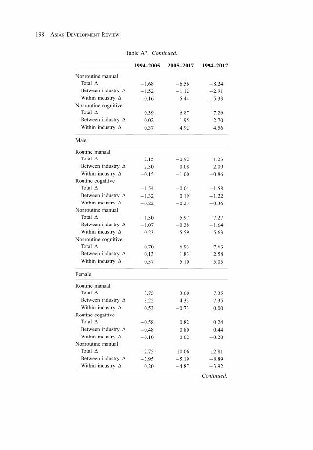
Table A7. Continued.
1994–2005 2005–2017 1994–2017
Nonroutine manualTotal Δ �1.68 �6.56 �8.24Between industry Δ �1.52 �1.12 �2.91Within industry Δ �0.16 �5.44 �5.33
Nonroutine cognitiveTotal Δ 0.39 6.87 7.26Between industry Δ 0.02 1.95 2.70Within industry Δ 0.37 4.92 4.56
Male
Routine manualTotal Δ 2.15 �0.92 1.23Between industry Δ 2.30 0.08 2.09Within industry Δ �0.15 �1.00 �0.86
Routine cognitiveTotal Δ �1.54 �0.04 �1.58Between industry Δ �1.32 0.19 �1.22Within industry Δ �0.22 �0.23 �0.36
Nonroutine manualTotal Δ �1.30 �5.97 �7.27Between industry Δ �1.07 �0.38 �1.64Within industry Δ �0.23 �5.59 �5.63
Nonroutine cognitiveTotal Δ 0.70 6.93 7.63Between industry Δ 0.13 1.83 2.58Within industry Δ 0.57 5.10 5.05
Female
Routine manualTotal Δ 3.75 3.60 7.35Between industry Δ 3.22 4.33 7.35Within industry Δ 0.53 �0.73 0.00
Routine cognitiveTotal Δ �0.58 0.82 0.24Between industry Δ �0.48 0.80 0.44Within industry Δ �0.10 0.02 �0.20
Nonroutine manualTotal Δ �2.75 �10.06 �12.81Between industry Δ �2.95 �5.19 �8.89Within industry Δ 0.20 �4.87 �3.92
Continued.
198 ASIAN DEVELOPMENT REVIEW
March 23, 2022 11:31:04am WSPC/331-adr 2250002 ISSN: 0116-11052ndReading

Table A8. Age Buckets
Age Bucket Age Range (years)
1 < 182 18–243 25–344 35–445 45–546 55–647 65þSource: Author’s categories.
Table A7. Continued.
1994–2005 2005–2017 1994–2017
Nonroutine cognitiveTotal Δ �0.42 5.64 5.22Between industry Δ 0.00 1.63 2.32Within industry Δ �0.42 4.01 2.90
Δ ¼ change in employment shares in percentage points.Source: Author’s calculations using data from the National SampleSurvey of India (1994, 2000, 2005, 2008, 2012) and the PeriodicLabor Force Survey (2017).
Table A9. Education Buckets
Education Bucket Label Years of Education
1 Below middle school Up to grade 82 Secondary/higher secondary Grade 9 to grade 123 Higher education College or more
Source: Author’s categories.
TRENDS IN EMPLOYMENT AND WAGES OF FEMALE AND MALE WORKERS IN INDIA 199
March 23, 2022 11:31:04am WSPC/331-adr 2250002 ISSN: 0116-11052ndReading


Disability and Intrahousehold InvestmentDecisions in Education: Empirical
Evidence from Bangladesh
KAMAL LAMICHHANE AND TAKAKI TAKEDA¤
Investment disparity in the education of personswith disabilitiesmay be larger on thepart of parents, in part resulting from predicted lower returns to the investment due tomistaken beliefs about their capabilities, or actual lower returns due to barriers in thelabor market. Using a nationally representative dataset fromBangladesh and utilizingthe framework of the Engel curve, we investigate intrahousehold investmentdecisions in education between children with and without disabilities. The resultsof the hurdle model show the existence of disability bias in enrollment decisions,whereas individual-level analysis suggests that bias exists on educationalexpenditure after children with disabilities enroll in school. Additionally, thoughwe observe a lower level of bargaining power among household heads oneducational investments for their children with disabilities, interaction effectssuggest the importance of greater income stability and maternal education statusbeing instrumental to improving the education of persons with disabilities.
Keywords: Bangladesh, disability bias, Engel curve, hurdle model, investmentin education
JEL codes: I2, E2, O1
⁄Kamal Lamichhane (corresponding author): Faculty of Human Sciences, University of Tsukuba,Tsukuba, Japan. E-mail: [email protected]; Takaki Takeda: Independent Researcher.E-mail: [email protected]. We thank the Bangladesh Bureau of Statistics for the inclusion of globallyaccepted questions on disability in their survey, which has enabled us to research the topic. In addition, wealso wish to thank Aya Suzuki at the University of Tokyo, Toby Long at Georgetown University, DanielMont at the Center for Inclusive Policy Research, Guenwoo Lee at Hitotsubashi University, and Juan N.Martínez and Takahiro Tsujimoto for their helpful comments while drafting the paper. Last but not theleast, we wish to thank two anonymous reviewers for their comments that have helped improve the paper.The Asian Development Bank recognizes “Vietnam” as Viet Nam.
This is an Open Access article published by World Scientific Publishing Company. It is distributed underthe terms of the Creative Commons Attribution 3.0 International (CC BY 3.0) License which permits use,distribution and reproduction in any medium, provided the original work is properly cited.
March 23, 2022 1:05:37pm WSPC/331-adr 2250003 ISSN: 0116-11052ndReading
Asian Development Review, Vol. 39, No. 1, pp. 201–238DOI: 10.1142/S0116110522500032
© 2022 Asian Development Bank andAsian Development Bank Institute.

I. Introduction
Studies have shown the effect of household and individual factors such as
parental education, family size, and the gender of the child on educational investment
for children (Kingdon 2002, Sawada and Lokshin 2009). Similarly, there is ample
evidence regarding gender disparities in intrahousehold resource allocation
(Subramanian and Deaton 1991; Subramanian 1995; Deaton 1997; Burgess and
Zhuang 2000; Lancaster, Maitra, and Ray 2003; Kingdon 2005; Aslam and Kingdon
2008; Lancaster, Maitra, and Ray 2008; Himaz 2010; Masterson 2012; Azam and
Kingdon 2013).
On the other hand, why school enrollment and educational attainment of persons
with disabilities (PWDs) are lower than those of non-PWDs is still a matter of intense
debate. Several studies have discussed discriminatory attitudes, parents’ financial
constraints, and institutional barriers as some of the plausible reasons for the lower
level of schooling of PWDs (Lamichhane 2013, 2015; Lamichhane and Kawakatsu
2015; Takeda and Lamichhane 2018). Despite growing attention regarding the social
inclusion and economic empowerment of PWDs in recent years, to the best of our
knowledge, except for a study by Rosales-Rueda (2014) on children with mental
health conditions in the United States, there are no studies that examine the
relationship between children’s disability and household investment decisions for
education. The lack of rigorous studies on this topic and the importance of providing
evidence-based policy implications on the education of PWDs is the main motivation
for this study. Given the fact that there is dearth of specific data on disability and
intrahousehold resource allocation in education in Bangladesh, our study has the
potential to be a powerful planning tool for policy makers.
Investment disparity in the education of PWDs may be largely due to parents, as
in many countries discrimination toward PWDs is widespread. Consequently,
household financial constraints, combined with discriminatory attitudes on the part
of parents, may negatively affect their decision to invest in education of PWDs, in part
resulting from the predicted lower returns to education of PWDs due to mistaken
beliefs about their capabilities, or actual lower returns due to barriers in the labor
market. Thus, the education of PWDs may be partly driven by shifts in parental
investment strategies that may give priority to their nondisabled children. Therefore,
utilizing a large and nationally representative Household Income Expenditure Survey
(HIES) dataset from 2010 of a developing economy, Bangladesh, we aim to detect the
biases against children’s education caused by disability status in the process of
intrahousehold investment decisions.
202 ASIAN DEVELOPMENT REVIEW
March 23, 2022 1:05:37pm WSPC/331-adr 2250003 ISSN: 0116-11052ndReading

According to Lamichhane and Kawakatsu (2015), the education system in
Bangladesh comprises 3 years of preprimary, 5 years of compulsory primary, 3 years
of junior secondary, 2 years of secondary, and 2 years of higher secondary education.
Education is only compulsory at the primary level and is free up to that level, with girls
continuing to receive free education up to the secondary level (Lamichhane 2015).
Bangladesh has initiated policies such as the National Education Policy, 2010 and a
series of Primary Education Development Programs (e.g., PEDP II and III) to meet its
constitutional obligations to provide a uniform, mass-oriented, and universal system of
education as well as its international commitments to educating all school-aged
children within the mainstream education system. A study by Ahmmed, Sharma, and
Deppeler (2012) discussed teachers’ perceptions of school support for implementing
inclusive education. While inclusive education is still gaining momentum in
Bangladesh, disability issues have been recognized in the country’s midterm
development plans, gradually placing policy attention on critical issues of education.
As one of the world’s least developed countries per United Nations classification
(World Bank 2021), Bangladesh is characterized by little or no access to social benefits
and little implementation on the ground to ensure that vulnerable people, including
individuals with disabilities, get what they are promised. The study of Chowdhury and
Foley (2006) shows how persons with disabilities in rural Bangladesh can slide into
economic impoverishment once they are labeled as such due to the various
deprivations that their impairments expose them to. Bangladesh developed a national
policy in 1995 emphasizing the provision of services for PWDs. It also enacted the
comprehensive disability law known as the Disability Welfare Act in April 2001,
which aimed to protect the rights of PWDs. Additionally, Bangladesh ratified the
Convention on the Rights of Persons with Disabilities in November 2007 and ratified
the optional protocol in May 2008. In 2013, a new Disability Act in line with the
convention was enacted. Despite such legal accomplishments, the increased
participation of PWDs in educational, social, and economic sectors is still critical
(Lamichhane 2015).
Additionally, Lamichhane and Kawakatsu (2015) examined the determinants of
school participation between children with and without disabilities in Bangladesh and
found that those with disabilities are less likely to participate in school. However, once
the sample is restricted to those with disabilities only, their study shows that household
monthly expenditure and working-age members are positively correlated with the
probability of school participation. If PWDs are deprived of education, this will hurt
their quality of life. For example, Lamichhane and Sawada (2013) found that in Nepal
wage returns to the investment in education of PWDs were between 19.2% and 25.6%,
DISABILITY AND INTRAHOUSEHOLD INVESTMENT DECISIONS IN EDUCATION 203
March 23, 2022 1:05:37pm WSPC/331-adr 2250003 ISSN: 0116-11052ndReading

which is two or three times higher than estimates for the general population
(Psacharopoulos and Patrinos 2004). While studies on disability and education in
Bangladesh are rare, with this paper we aim to at least partially fill the gap in existing
knowledge by examining the existence of disability bias and related factors associated
with parental decisions on educational investments. By doing so, we intend to help
identify constraints preventing PWDs from enjoying the multifaceted benefits of
education. The research questions posed herein are as follows: Does disability bias
exist in intrahousehold investment in education? If so, where does such bias exist, in
the stage of enrollment or thereafter? What are the key factors affecting parental
investment decisions with regard to the education of children with disabilities
(CWDs)? Although there is a serious lack of scientific and evidence-based information
on disabilities, Bangladesh provides a good setting for studying parental decisions on
intrahousehold resource allocation in education due to the availability of nationally
representative data.
II. Dataset from Bangladesh
We use the large-scale and nationally representative 2010 HIES dataset published
by the Bangladesh Bureau of Statistics. This dataset includes a wide variety of
information on the country’s socioeconomic situation—including demographic
characteristics, educational attainment, employment status, and access to facilities,
among others—and consists of more than 12,000 households: 20 each from 612
primary sampling units. Out of the total sample of 55,580 household members, there
are 16,696 school-aged children (6–18 years old) who are supposed to attend school in
Bangladesh.
Additionally, the survey identifies people’s disability status based on a short set
of questions recommended by the Washington Group on Disability Statistics (2020).
The questions focus on the difficulties people face in seeing, hearing, walking,
cognition, self-care, and communication according to a four-point scale: (1) no
difficulty, (2) some difficulty, (3) a lot of difficulty, and (4) cannot do. From these
questions, we obtain information on the type and severity of activity limitations.
Having some difficulty is considered to be a moderate limitation, whereas a lot of
difficulty and cannot see, hear, speak, walk, and so on are considered to be severe
limitations. The inclusion of the Washington Group on Disability Statistics’ questions
is also helpful for the international comparability of the situation regarding disability.
In the 2010 HIES, disability modules were asked under section three (health),
204 ASIAN DEVELOPMENT REVIEW
March 23, 2022 1:05:37pm WSPC/331-adr 2250003 ISSN: 0116-11052ndReading

subsection (d). Together with 18 questions, including the question on onset of
impairment, two additional questions on any difficulty caused by disability at home, in
the workplace, or at school were included in the 2010 HIES. Sadly, the 2016 HIES
included only six questions about participants’ impairment as part of a household
information roster, excluding all other questions such as onset of impairment and any
difficulty caused by disability at home, work, and school. The exclusion of disability
modules in the 2016 HIES dataset led us to believe that the 2010 HIES was more
comprehensive in relation to the information on disability. For this reason, 2010 HIES
data have been used in this study.
III. Empirical Strategy and Related Literature
We investigate the existence of disability bias by examining the discriminatory
allocation of educational expenditure within households. We use the Engel curve
framework, which has been used in numerous previous studies to detect gender bias in
intrahousehold resource allocation. It is equally important to detect disability bias
through the Engel curve framework, which seeks differential treatment within
households indirectly. Such bias can be identified by examining how the household
composition of people with and without disabilities affects household expenditure on
education. To detect these biases, we use both an indirect and direct method. The
indirect method, known as household-level analysis, is based on conventional Engel
curve methodology, while the direct method refers to individual-level analysis that
uses individual-child-level data.
A. Household-Level Analysis
We follow Subramanian and Deaton (1991) and Deaton (1997) and employ the
Working and Leser specification, extended by adding household demographic
composition to Working’s Engel curve (Working 1943). To estimate the Engel
curve, the equation is also relaxed for nonlinearity of the log of per capita expenditure
along with the shape of the Engel curve
si ¼ αþ β lnxini
� �þ γ ln (ni)þ
XK�1
k¼1
θknkini
þ �zi þ "i, ð1Þ
where si is the budget share of total educational expenditure of ith household; xi is the
total expenditure of that household; ni is the number of members (i.e., household size)
DISABILITY AND INTRAHOUSEHOLD INVESTMENT DECISIONS IN EDUCATION 205
March 23, 2022 1:05:37pm WSPC/331-adr 2250003 ISSN: 0116-11052ndReading

of the ith household; nki is the number of household members in the kth disability-age
cohort where k ¼ 1, 2, . . . ,K; zi is a vector of other household characteristics (i.e.,
information on household head, religion, and dependency ratio) that are incorporated
as controls; and "i is the error term. Accordingly, ln (xi=ni) is the natural log of total
per capita expenditure of the ith household. When detecting bias, we elaborate
disability-age category variables, which are divided into 14 categorical groups for
PWDs and non-PWDs following Kingdon (2005): 0–4 years, 5–9 years, 10–14 years,
15–19 years, 20–24 years, 25–60 years, and over 60 years. The variable for over 60
years old is omitted as this is the base observation against the results of variables for
other groups. Using these disability-age categories, nki=ni is the share of the kth
disability-age fraction and the value of coefficient θk is the effect of household
composition by disability-age category on the budget allocation with the difference in
the household size of each household being considered. As our main objective is to
identify disability bias, we test the difference of the marginal effect (DME) of the
disability-age category variable (difference among the same age category) only for
variables along with school age, and the following null hypothesis is tested for each
school age (i.e., children aged 5–9, 10–14, and 15–19 years old):
θkCWD ¼ θknCWD, ð2Þwhere CWD is a child with disabilities and nCWD is a child without disabilities. k
refers to a given age category within school age roughly in line with the Bangladeshi
education system from ages 5 to 19 years old (5–9 ¼ primary education,
10–14 ¼ junior secondary and secondary education, 15–19 ¼ higher secondary and
higher education).
Additionally, as a strategy to identify disability bias, we employ the hurdle model
(Cragg 1971, Cameron and Trivedi 2005, Wooldridge 2010), which has also been used
to examine gender bias (Kingdon 2005, Aslam and Kingdon 2008, Himaz 2010, Azam
and Kingdon 2013).1 While the Engel curve model (equation [1]) has been estimated
using ordinary least squares (OLS) and including all households regardless of
children’s enrollment status, Kingdon (2005) highlighted the failure of such
conventional research and proposed that there should be two possible channels
through which pro-male bias is observed in expenditure: (i) via zero purchases for
daughters and positive purchases for sons, and (ii) conditional on positive purchases
for both daughters and sons via lower expenditure on daughters than on sons. More
succinctly, bias against girls must exist in two types of decision-making patterns by
1The hurdle model is also referred to as a two-part model and is primarily applied by Duan et al.(1983) for forecasting medical expenses (Cameron and Trivedi 2005, Wooldridge 2010).
206 ASIAN DEVELOPMENT REVIEW
March 23, 2022 1:05:37pm WSPC/331-adr 2250003 ISSN: 0116-11052ndReading

parents—that is, whether to enroll their children (zero-versus-positive spending
decision) and how much to pay for their education on the condition that a child is
already in school (spending conditioned on enrollment decision). The Engel curve
method with conventional OLS neglects the first part of decision-making (neglect zero
expenditure) and this leads to the downward bias of estimation results.2
The hurdle model detects bias efficiently under censoring and two types of
decision-making. The simple hurdle model is as follows:
P(s ¼ 0jx) ¼ 1� �(xγ), ð3Þ
ln (s)j(x, s > 0) � Normal(xβ,�2), ð4Þ
where s is the budget share of educational expenditure in total household expenditure,
x is a vector of other explanatory variables, and γ and β are parameters to be estimated.
Once we obtain the results of the maximum likelihood estimation of the probit model
(binary choice of whether s > 0) and OLS conditional on nonzero expenditure (s > 0)
using the hurdle model results, we calculate the combined marginal effect (CME),
which shows the effect of x on outcomes of both models (i.e., probability of s > 0 and
the amount of sjs > 0). This CME is calculated as follows (Kingdon 2005)3:
@E(sjx)@x
¼ fγ’(xy)þ �(xγ)βg exp xβ þ �2
2
� �: ð5Þ
Estimators are derived separately in each stage of the hurdle model in equations (3)
and (4). �( � ) is the cumulative normal density function and ’(xy) is the standard
normal density function. We apply the model to investigate the existence of disability
bias between CWDs and non-CWDs within households.
Moreover, this model can solve the averaging problems of the conventional
Engel model (Kingdon 2005). Additionally, educational expenditure is used in
household analysis as if this were expenditure for all household members, but this is
actually a more personalized cost. Specifically, while enrollment itself is lower, the
educational cost for CWDs is considered to be higher than that for non-CWDs as
educational materials such as textbooks in braille or providing sign language,
equipment, and inaccessible infrastructure may require additional costs. Addressing
these issues is crucial for CWDs.
2Deaton (1997) states that a large proportion of households pay nothing for education.3For more specific calculation for derivation of an equation, see Kingdon (2005).
DISABILITY AND INTRAHOUSEHOLD INVESTMENT DECISIONS IN EDUCATION 207
March 23, 2022 1:05:38pm WSPC/331-adr 2250003 ISSN: 0116-11052ndReading

B. Individual-Level Analysis
We also employ the direct method with individual-child-level data to check the
robustness of our analysis to confirm disability-based bias, as well as to consider
disability-based bias and parents’ investment behaviors in detail. Here, equation (1) is
slightly changed as follows:
pij ¼ αþ β lnxini
� �þ γ ln (ni)þ θ impairmentij þ �zij þ "ij, ð6Þ
where pij is personal educational expenditure on the jth child in the ith household, xi is
total household expenditure, ni is household size, impairment is a dummy variable
(1 ¼ disabled, 0 ¼ otherwise), and zij is a vector of other child-specific (includes
timing of getting disability) and household characteristics. In this individual
regression, the impairment dummy captures the effect of disability bias. We use
interaction terms between children’s disability status and other characteristics to test
whether there are heterogeneous effects of disability depending on certain
characteristics. Here, disability status is interacted with a female dummy, mother’s
years of schooling, father’s years of schooling, and employment status of the
household head. These terms can reveal whether female CWDs suffer more bias
relative to male CWDs, and whether parents’ education and income stability alter the
levels of disability bias.
Table 1 reports the results for three equations: the unconditional OLS model (D),
the probit model for binary choice of school enrollment (A), and the conditional OLS
model conditioned on enrollment (B). Additionally, we add a column for CME in (C).
We restricted the household-level analysis to households that have children aged 5–19
years old, while individual-level analysis is conducted for each schooling level group
of children (i.e., 5–9, 10–14, and 15–19 years old). Estimations for the hurdle model
are calculated using the “twopm” command in Stata (Belotti et al. 2015).
While the estimation framework does not enable us to determine a clear direction
of causality, we think that this allows us to pursue our objectives to determine the
existence of bias itself. Additionally, the estimation can be complicated by a problem
of endogeneity. Among independent variables, monthly expenditure and dependency
ratio can be the index of poverty level and this may cause child impairment
(impairment dummy) through malnutrition and serious illness. This may underestimate
the impact of the impairment dummy variable, making it hard to identify a causal
relationship between disability status and individual educational expenditure, which
leads to failure to disclose disability bias. To handle this, we include household-level
(family) fixed effects to consider all time-invariant heterogeneity of household
208 ASIAN DEVELOPMENT REVIEW
March 23, 2022 1:05:38pm WSPC/331-adr 2250003 ISSN: 0116-11052ndReading

characteristics and minimize the effect of the impairment dummy. Filmer (2008)
argues the effectiveness of incorporating household fixed effects to deal with
endogeneity of disability status that may arise from poverty in the developing world,
which is presented in the final section.4 Additionally, a Durbin–Wu–Hausman test is
unable to reject the null hypothesis that household size is exogenous. Therefore, we do
not present the result of the instrumental variable regression model. To control district-
level characteristics, we also incorporate district-level fixed effects for all analysis.
IV. Results and Findings
A. Descriptive Results
We observe significant differences in enrollment between CWDs and non-CWDs
for both rural and urban areas (Table 1). In particular, the primary enrollment rates of
non-CWDs are 23 percentage points and 17 percentage points higher than that of their
counterparts in urban and rural areas, respectively. We observe a similar trend for the
secondary level enrollment rate. Enrollment rates for non-CWDs are higher by more
than 10 percentage points in both areas. Similarly, at the tertiary level, we also find that
CWDs are in a disadvantageous position. Additionally, Table 1 shows mean
differences of literacy status (reading and writing skills) where differences are
observed in reading skills for both groups.
Table 2 shows the investment breakdown of educational expenditure, which is
divided into six categories. Admission includes admission, seasonal, and registration
fees. Tuition includes annual tuition and examination fees. Books includes textbooks
and exercise books. Other costs include hostel costs, conveyance, internet and e-mail
fees, meals, and other costs. Generally, tuition fees are the single-largest category of all
expenditures. Other costs are higher in rural areas than in urban areas, which may
indicate why transportation fees account for a relatively large proportion.
Table 3 shows the educational expenditure differential by schooling level and
disability status for both urban and rural areas, and for both the entire child sample and
the sample restricted to enrolled children only. The sample that includes out-of-school
children suggests that there is a significant difference in educational expenditure at the
primary level in rural areas. Surprisingly, there is little difference in educational
investment by disability status for enrolled children. This may be because school
4The possibility of the problem of endogeneity of the impairment dummy is also rejected by theDurbin–Wu–Hausman test.
DISABILITY AND INTRAHOUSEHOLD INVESTMENT DECISIONS IN EDUCATION 209
March 23, 2022 1:05:38pm WSPC/331-adr 2250003 ISSN: 0116-11052ndReading

Table 1. Differences in Educational Indices by Area and Disability Status
Urban Rural
Non-CWDs CWDs
MeanDifference(Non-CWDs
VersusCWDs) t-Value
Non-CWDs CWDs
MeanDifference(Non-CWDs
VersusCWDs) t-Value
Enrollment (school-aged children)Primary level 0.69 0.47 0.23*** 2.69 0.67 0.51 0.17*** 3.36Secondary level 0.45 0.34 0.11* 1.89 0.39 0.27 0.13*** 2.75Higher level 0.39 0.25 0.14* 1.86 0.28 0.18 0.10** 2.31
Literacy (school-aged children)Reading 0.76 0.59 0.17*** 4.76 0.67 0.58 0.10*** 3.58Writing 0.97 0.97 0.00 0.09 0.96 0.98 �0:02 �1:41
CWDs ¼ children with disabilities.Notes: *, **, and *** represent significance in gap by disability at the 10%, 5%, and 1% levels,respectively. Enrollment rate is calculated using the proportion of enrolled children within school-agedchildren divided by the population of school-aged children. School age is defined following Kingdon(2005): primary level (aged 5–9 years), secondary (aged 10–14 years), and higher (aged 15–19 years). Thedefinition of CWDs is children with disabilities below the age of 20 years old who acquire impairmentssuch as visual, hearing, physical, cognitive, and communication.Source: Authors’ calculations using data from the 2010 Bangladesh Household Income ExpenditureSurvey.
Table 2. Breakdowns of Educational Expenditure by Area (%)
Urban Rural
Public Private Madrasa Public Private Madrasa
Admission fee 13.17 14.87 5.90 6.27 8.22 5.82Tuition fee 48.36 52.96 43.54 35.81 40.71 33.61Books 14.49 13.81 17.96 19.13 20.71 25.26Uniform 5.65 5.14 8.93 10.45 8.04 11.45Contribution (donation) 0.07 0.02 0.00 0.48 0.15 0.00Other costs 18.26 13.20 23.67 27.86 22.17 23.86
Notes: Educational expenditure is divided into six categories. Admission includes admission fees,seasonal fees, and registration fees. Tuition includes annual tuition and examination fees. Booksincludes textbooks and excise books. Other costs are the sum of hostel costs, conveyance, internetand e-mail fees, tiffin (lunch), and other costs.Source: Authors’ calculations using data from the 2010 Bangladesh Household IncomeExpenditure Survey.
210 ASIAN DEVELOPMENT REVIEW
March 23, 2022 1:05:40pm WSPC/331-adr 2250003 ISSN: 0116-11052ndReading

Table3.
Difference
ofEducation
alExp
enditure
byAreaan
dDisab
ility
Status(Tk)
Urban
Rural
Non
-CW
Ds
CW
Ds
MeanDifference
(Non
-CW
Ds
VersusCW
Ds)
t-Value
Non
-CW
Ds
CW
Ds
MeanDifference
(Non
-CW
Ds
VersusCW
Ds)
t-Value
Education
alexpenditure
forbothenrolledan
dnon
enrolledchild
ren
Primarylevel
3,08
2.09
1,94
3.33
1,83
8.75
1.59
1,14
6.76
709.07
437.69
*1.90
Secon
dary
level
6,76
2.93
4,34
5.00
2,41
7.93
*1.92
2,85
8.27
1,98
2.99
875.28
**2.51
Higherlevel
7,86
2.18
7,44
2.39
419.79
0.11
3,87
5.85
4,15
7.38
�281:53
�0:33
Education
alexpenditure
forenrolledchild
ren
Primarylevel
4,59
8.08
3,64
3.75
954.33
0.57
1,53
1.15
1,13
2.02
399.13
1.25
Secon
dary
level
8,01
2.52
7,011.25
1,00
1.27
0.60
3,38
1.98
2,98
7.71
394.27
0.90
Higherlevel
15,916
.88
16,373
.25
�456:37
�0:06
9,38
5.83
11,997
�2,611:17
�1:41
CWDs¼
child
renwith
disabilities,Tk¼
Bangladeshtaka.
Notes:*and**
representsign
ificanceat
the10
%and5%
levels,respectiv
ely.Schoo
lingageisdefinedfollo
wingKingd
on(200
5):prim
arylevel
(aged5–
9years),secon
dary
(aged10
–14
years),and
high
er(aged15
–19
years).T
hedefinitio
nof
CWDsischild
renwith
disabilitiesbelowtheage
of20
who
acqu
ireim
pairmentssuch
asvisual,hearing,
physical,cogn
itive,andcommun
ication.
Sou
rce:
Autho
rs’calculations
usingdata
from
the20
10BangladeshHou
seho
ldIncomeExp
enditure
Survey.
DISABILITY AND INTRAHOUSEHOLD INVESTMENT DECISIONS IN EDUCATION 211
March 23, 2022 1:05:41pm WSPC/331-adr 2250003 ISSN: 0116-11052ndReading

enrollment of CWDs can require more costs than that of non-CWDs when the
infrastructure is not disability friendly, as well as when the proper support systems are
not in place. However, once enrolled, the results reveal only small differences in
educational expenditure.
Table 4 reports the descriptive statistics of the variables used for the regression
analysis. This table also shows differences in child enrollment and educational
spending between urban and rural areas. In the results of the t-test among variables
between these areas, we can observe significant differences at the 1% level for the
budget share of educational expenditure, total household expenditure, household size,
and dependency ratio, clearly showing the advantages regarding education for
households in urban areas in terms of income level, number of household members,
and family structure. These results indicate that disparities in income level and
educational achievement exist between urban and rural areas in Bangladesh.
B. Regression Results of Household-Level Analysis
Table 5 presents the results of household-level analysis for factors affecting the
budget share of educational expenditure with disability-age category variables. We
perform regression analysis separately for the entire sample, urban areas, and rural
areas. Column (1) is the marginal effect in the probit model of whether parents enroll
their child in school. Column (2) is the result of conditional OLS analysis when a child
is enrolled. Column (3) shows the CME derived from the results of the probit and
conditional OLS models. Finally, column (4) is the result of unconditional OLS
analysis.
In the results of the entire sample and those broken down by rural or urban area,
the log of monthly expenditure per capita has a positive and significant effect on the
budget share for educational expenditure. These results reveal that income level is a
strong predictor of educational investment, as found in Glewwe and Patrinos (1999)
and Glewwe and Jacoby (2003). Household size has a positive correlation with
educational expenditure, and this variable works appropriately as a control variable
since larger households generally have more educational expenditure. The positive and
significant effect of a household head’s years of schooling on educational expenditure
for their children is consistent as the educational level of household head or parents is
considered a strong predictor of investment in their children’s education (Behrman and
Deolalikar 1995, Haveman and Wolfe 1995, Cameron and Heckman 1998). Similarly,
the dummy variable of female household head shows that female bargaining power has
a positive effect on both school enrollment and educational investment for their
212 ASIAN DEVELOPMENT REVIEW
March 23, 2022 1:05:41pm WSPC/331-adr 2250003 ISSN: 0116-11052ndReading

Table4.
Descriptive
Statisticsof
Cov
ariatesat
theHou
seholdan
dIndividual
Levels
Urban
Rural
Number
ofObs.
Mean
Std.Dev.
Number
ofObs.
Mean
Std.Dev.
MeanDifference
(Urban
–Rural)
t-Value
Variablesforhou
sehold-level
analysis
Share
ofeducationalexpend
iture
4,39
40.05
0.07
7,81
30.03
0.05
0.01
7***
15.62
Total
mon
thly
householdexpend
iture
(Tk)
4,39
413
,852
.34
11,803
.18
7,81
39,65
5.47
7,42
2.88
4,19
6.87
2***
24.08
Hou
seho
ldsize
(num
berof
person
s)4,39
44.48
1.81
7,81
34.58
1.93
�0:107**
*�3
:01
Share
ofno
n-CWDsaged
5–9years
4,39
90.10
0.14
7,84
00.12
0.15
�0:014**
*�5
:11
Share
ofCWDsaged
5–9years
4,39
90.00
0.02
7,84
00.00
0.02
�0:001*
�1:94
Share
ofno
n-CWDsaged
10–14
years
4,39
90.10
0.14
7,84
00.11
0.14
�0:004
�1:36
Share
ofCWDsaged
10–14
years
4,39
90.00
0.03
7,84
00.00
0.02
0.00
040.73
Share
ofno
n-CWDsaged
15–19
years
4,39
90.09
0.14
7,84
00.08
0.13
0.00
8***
3.06
Share
ofCWDsaged
15–19
years
4,39
90.00
0.02
7,84
00.00
0.02
�0:001
�1:46
Years
ofeducationof
householdhead
4,38
75.95
5.72
7,82
33.08
4.29
2.87
5***
31.43
Hou
seho
ldhead
isfemale(¼
1)4,38
70.13
0.33
7,82
30.15
0.36
�0:026**
*�3
:99
Hou
seho
ldhead
with
impairment(¼
1)4,38
70.14
0.35
7,82
30.18
0.38
�0:037**
*�5
:29
Hou
seho
ldhead
isfulltim
ewageworker(¼
1)4,38
70.41
0.49
7,82
30.28
0.45
0.12
9***
14.75
Muslim
(¼1)
4,39
90.89
0.32
7,84
00.87
0.33
0.01
2**
1.99
Hindu
(¼1)
4,39
90.11
0.31
7,84
00.11
0.31
0.00
10.15
Dependencyratio
4,39
90.35
0.21
7,84
00.39
0.23
�0:047**
*�1
1:20
Con
tinued.
DISABILITY AND INTRAHOUSEHOLD INVESTMENT DECISIONS IN EDUCATION 213
March 23, 2022 1:05:43pm WSPC/331-adr 2250003 ISSN: 0116-11052ndReading
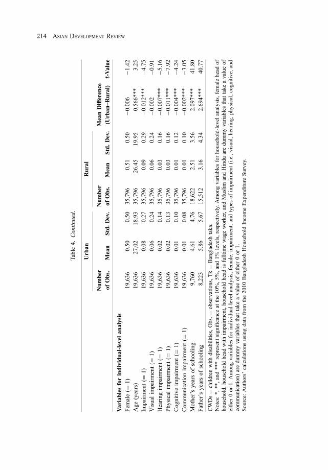
Table
4.Con
tinued.
Urban
Rural
Number
ofObs.
Mean
Std.Dev.
Number
ofObs.
Mean
Std.Dev.
MeanDifference
(Urban
–Rural)
t-Value
Variablesforindividual-level
analysis
Fem
ale(¼
1)19
,636
0.50
0.50
35,796
0.51
0.50
�0:006
�1:42
Age
(years)
19,636
27.02
18.93
35,796
26.45
19.95
0.56
6***
3.25
Impairment(¼
1)19
,636
0.08
0.27
35,796
0.09
0.29
�0:012**
*�4
:75
Visualim
pairment(¼
1)19
,636
0.06
0.24
35,796
0.06
0.24
�0:002
�0:91
Hearing
impairment(¼
1)19
,636
0.02
0.14
35,796
0.03
0.16
�0:007**
*�5
:16
Phy
sicalim
pairment(¼
1)19
,636
0.02
0.13
35,796
0.03
0.16
�0:011**
*�7
:92
Cog
nitiv
eim
pairment(¼
1)19
,636
0.01
0.10
35,796
0.01
0.12
�0:004**
*�4
:24
Com
mun
icationim
pairment(¼
1)19
,636
0.01
0.08
35,796
0.01
0.10
�0:002**
*�3
:05
Mother’syearsof
scho
oling
9,76
04.61
4.76
18,622
2.51
3.56
2.09
7***
41.80
Father’syearsof
scho
oling
8,22
35.86
5.67
15,512
3.16
4.34
2.69
4***
40.77
CWDs¼
child
renwith
disabilities,Obs:¼
observations,Tk¼
Bangladeshtaka.
Notes:*,
**,and**
*representsign
ificanceat
the10
%,5%
,and1%
levels,respectiv
ely.Amon
gvariablesforho
usehold-levelanalysis,femalehead
ofho
usehold,
householdhead
with
impairment,ho
useholdhead
isfulltim
ewageworker,andMuslim
andHindu
aredu
mmyvariablesthat
take
avalueof
either
0or
1.Amon
gvariablesforindividu
al-level
analysis,female,im
pairment,andtypesof
impairment(i.e.,visual,hearing,
physical,cogn
itive,and
commun
ication)
aredu
mmyvariablesthat
take
avalueof
either
0or
1.Sou
rce:
Autho
rs’calculations
usingdata
from
the20
10BangladeshHou
seho
ldIncomeExp
enditure
Survey.
214 ASIAN DEVELOPMENT REVIEW
March 23, 2022 1:05:44pm WSPC/331-adr 2250003 ISSN: 0116-11052ndReading
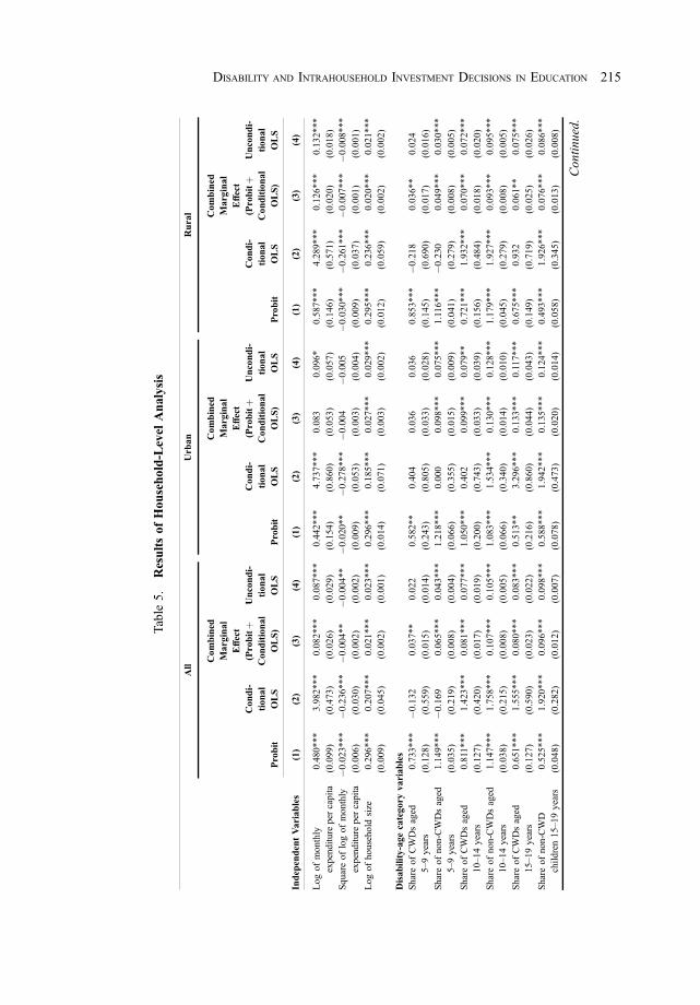
Table5.
Resultsof
Hou
sehold-Level
Analysis
All
Urban
Rural
Probit
Con
di-
tion
alOLS
Com
bined
Marginal
Effect
(Probitþ
Con
ditional
OLS)
Uncondi-
tion
alOLS
Probit
Con
di-
tion
alOLS
Com
bined
Marginal
Effect
(Probitþ
Con
ditional
OLS)
Uncondi-
tion
alOLS
Probit
Con
di-
tion
alOLS
Com
bined
Marginal
Effect
(Probitþ
Con
ditional
OLS)
Uncondi-
tion
alOLS
IndependentVariables
(1)
(2)
(3)
(4)
(1)
(2)
(3)
(4)
(1)
(2)
(3)
(4)
Log
ofmonthly
expenditu
repercapita
0.480***
3.982***
0.082***
0.087***
0.442***
4.737***
0.083
0.096*
0.587***
4.289***
0.126***
0.132***
(0.099)
(0.473)
(0.026)
(0.029)
(0.154)
(0.860)
(0.053)
(0.057)
(0.146)
(0.571)
(0.020)
(0.018)
Squareof
logof
monthly
expenditu
repercapita
�0:023***
�0:236***
�0:004**
�0:004**
�0:020**
�0:278***
�0:004
�0:005
�0:030***
�0:261***
�0:007***
�0:008***
(0.006)
(0.030)
(0.002)
(0.002)
(0.009)
(0.053)
(0.003)
(0.004)
(0.009)
(0.037)
(0.001)
(0.001)
Log
ofhouseholdsize
0.296***
0.207***
0.021***
0.023***
0.296***
0.185***
0.027***
0.029***
0.295***
0.236***
0.020***
0.021***
(0.009)
(0.045)
(0.002)
(0.001)
(0.014)
(0.071)
(0.003)
(0.002)
(0.012)
(0.059)
(0.002)
(0.002)
Disab
ility-age
category
variab
les
Share
ofCWDsaged
5–9years
0.733***
�0:132
0.037**
0.022
0.582**
0.404
0.036
0.036
0.853***
�0:218
0.036**
0.024
(0.128)
(0.559)
(0.015)
(0.014)
(0.243)
(0.805)
(0.033)
(0.028)
(0.145)
(0.690)
(0.017)
(0.016)
Share
ofnon-CWDsaged
5–9years
1.149***
�0:169
0.065***
0.043***
1.218***
0.000
0.098***
0.075***
1.116***
�0:230
0.049***
0.030***
(0.035)
(0.219)
(0.008)
(0.004)
(0.066)
(0.355)
(0.015)
(0.009)
(0.041)
(0.279)
(0.008)
(0.005)
Share
ofCWDsaged
10–14
years
0.811***
1.423***
0.081***
0.077***
1.050***
0.402
0.099***
0.079**
0.721***
1.932***
0.070***
0.072***
(0.127)
(0.420)
(0.017)
(0.019)
(0.200)
(0.743)
(0.033)
(0.039)
(0.156)
(0.484)
(0.018)
(0.020)
Share
ofnon-CWDsaged
10–14
years
1.147***
1.758***
0.107***
0.105***
1.083***
1.534***
0.130***
0.128***
1.179***
1.927***
0.093***
0.095***
(0.038)
(0.215)
(0.008)
(0.005)
(0.066)
(0.340)
(0.014)
(0.010)
(0.045)
(0.279)
(0.008)
(0.005)
Share
ofCWDsaged
15–19
years
0.651***
1.555***
0.080***
0.083***
0.513**
3.296***
0.133***
0.117***
0.675***
0.932
0.061**
0.075***
(0.127)
(0.590)
(0.023)
(0.022)
(0.216)
(0.860)
(0.044)
(0.043)
(0.149)
(0.719)
(0.025)
(0.026)
Share
ofnon-CWD
child
ren15–19
years
0.525***
1.920***
0.096***
0.098***
0.588***
1.942***
0.135***
0.124***
0.493***
1.926***
0.076***
0.086***
(0.048)
(0.282)
(0.012)
(0.007)
(0.078)
(0.473)
(0.020)
(0.014)
(0.058)
(0.345)
(0.013)
(0.008)
Con
tinued.
DISABILITY AND INTRAHOUSEHOLD INVESTMENT DECISIONS IN EDUCATION 215
March 23, 2022 1:05:48pm WSPC/331-adr 2250003 ISSN: 0116-11052ndReading

Table
5.Con
tinued.
All
Urban
Rural
Probit
Con
di-
tion
alOLS
Com
bined
Marginal
Effect
(Probitþ
Con
ditional
OLS)
Uncondi-
tion
alOLS
Probit
Con
di-
tion
alOLS
Com
bined
Marginal
Effect
(Probitþ
Con
ditional
OLS)
Uncondi-
tion
alOLS
Probit
Con
di-
tion
alOLS
Com
bined
Marginal
Effect
(Probitþ
Con
ditional
OLS)
Uncondi-
tion
alOLS
IndependentVariables
(1)
(2)
(3)
(4)
(1)
(2)
(3)
(4)
(1)
(2)
(3)
(4)
Hou
seho
ld-level
characteristics
Years
ofschoolingfor
householdhead
0.006***
0.060***
0.002***
0.002***
0.007***
0.057***
0.002***
0.003***
0.005***
0.054***
0.002***
0.002***
(0.001)
(0.003)
(0.000)
(0.000)
(0.001)
(0.004)
(0.000)
(0.000)
(0.001)
(0.004)
(0.000)
(0.000)
Household
head
isfemale
0.029***
0.172***
0.007***
0.009***
0.013
0.199***
0.008**
0.012***
0.035***
0.156***
0.008***
0.008***
(0.011)
(0.043)
(0.002)
(0.002)
(0.018)
(0.072)
(0.003)
(0.003)
(0.013)
(0.054)
(0.002)
(0.002)
Household
head
with
disabilities
0.010
�0:090*
�0:002
�0:001
0.037*
�0:180**
�0:002
0.000
�0:003
�0:053
�0:002
�0:002
(0.011)
(0.049)
(0.002)
(0.002)
(0.020)
(0.088)
(0.004)
(0.004)
(0.013)
(0.058)
(0.002)
(0.002)
Household
head
isfulltim
ewageworker
0.018***
0.121***
0.007***
0.006***
0.018
0.048
0.007***
0.007***
0.021**
0.164***
0.006***
0.006***
(0.007)
(0.028)
(0.001)
(0.001)
(0.011)
(0.044)
(0.002)
(0.002)
(0.009)
(0.038)
(0.001)
(0.001)
Muslim
�0:017*
�0:136***
�0:006***
�0:006***
�0:01
�0:148***
�0:007**
�0:006*
�0:016
�0:110**
�0:004**
�0:005***
(0.009)
(0.038)
(0.002)
(0.002)
(0.015)
(0.057)
(0.003)
(0.003)
(0.012)
(0.051)
(0.002)
(0.002)
Dependencyratio
0.069
�0:114
�0:008
0.001
0.104
0.354
0.017
0.009
0.047
�0:398
�0:019
�0:004
(0.049)
(0.288)
(0.012)
(0.005)
(0.085)
(0.496)
(0.021)
(0.011)
(0.058)
(0.348)
(0.013)
(0.005)
Fixed
effects
District-levelfixedeffect
Yes
Yes
Yes
Yes
Yes
Yes
Yes
Yes
Yes
Yes
Yes
Yes
Constant
�20:686***
�0:417***
�24:316***
�0:503**
�21:305***
�0:560***
(1.896)
(0.112)
(3.508)
(0.222)
(2.252)
(0.070)
Num
berof
Observatio
ns12,178
7,957
12,178
12,178
4,382
2,947
4,382
4,382
7,796
5,010
7,796
7,796
CWDs¼
child
renwith
disabilities,OLS¼
ordinary
leastsquares.
Notes:Stand
arderrors
arein
parentheses.*,
**,and**
*representsign
ificanceat
the10
%,5%
,and1%
levels,respectiv
ely.Stand
arderrors
ofcolumns
(1)
(binaryprob
it),(2)
(con
ditio
nalOLS),and(4)(uncon
ditio
nalO
LS)arerobu
standclusteredby
householdto
consider
thepo
ssibility
thatresidu
alswith
inthe
sameho
useholdarelik
elyto
becorrelated.For
column(3)(resultof
combinedmarginaleffect:prob
itþcond
ition
alOLS),thestandard
errorisob
tained
bybo
otstrapp
ingwith
400replications.Dependent
variable
inprob
itmod
el(colum
n(1))analysisisabinary
variable
ofwhether
aho
useholdhadeducational
expend
iture
inthepast12
mon
ths.The
naturallogof
shareof
educationalexpend
iture
andabsolutevalueof
shareof
educationalexpend
iture
aredepend
ent
variablesof
columns
(2)and(4),respectiv
ely.
Allequatio
nsinclud
edistrict-level
fixedeffects.
Sou
rce:
Autho
rs’calculations
usingdata
from
the20
10BangladeshHou
seho
ldIncomeExp
enditure
Survey.
216 ASIAN DEVELOPMENT REVIEW
March 23, 2022 1:05:49pm WSPC/331-adr 2250003 ISSN: 0116-11052ndReading

children. This finding partly suggests that if a mother receives more education, she is
likely to allow her children to receive more and better education. Takeda and
Lamichhane (2018) found that mother’s education can be an important predictor for
CWDs to receive better education, claiming that strong female bargaining power can
increase their understanding of CWDs in the household. Regardless of disability, some
studies have also discussed the positive effect of the strong bargaining power of
women (Thomas 1994, Duflo and Udry 2004).
The dummy variable of household head with disabilities also provides interesting
results. While it shows an insignificant effect on the probability of children’s
enrollment in the analysis using the entire sample (i.e., all areas in Bangladesh)
(column [1]), this variable is found to have a negative effect on educational
expenditure at the 10% significance level (column [2]). Similarly, the dummy variable
of disabled household head is positively correlated (column [1]) with child enrollment
at the 10% significance level in the probit model, while it negatively affects the
conditional share of expenditure at the 5% level (column [2]) in urban areas. These
interesting findings suggest that if the household head has some form of disability,
they are more likely to understand the value of access to education and thus enroll their
children in schools. At the same time, as PWDs are more likely to experience poverty,
they may not be able to afford educational fees once their child is enrolled. Finally, the
dummy variable for household head as full-time wage earner is a strong predictor of
educational expenditure, again suggesting that the income stability of parents and
household heads is important in terms of investing in their children’s education.
We test the DME for disability-age variables for each school-aged group to
confirm whether a biased allocation of parental investment toward CWDs exists
(Table 6). The DME shows a difference in the value of non-CWDs minus the
marginal effect of CWDs. We test whether this difference is statistically significant
(equation [2]) and observe a clear bias against CWDs in the results for the entire
sample. In column (1), which examines disability bias in enrollment using the probit
model analysis, the DME of children aged 5–9 years and 10–14 years are positive and
statistically significant at the 1% level. This finding suggests the likelihood of bias in
age for primary and secondary education. In column (2), which is the conditional OLS
regression model, no significant results for the DME are observed.
We attempt to identify biases in educational expenditure by restricting to
households with only enrolled children but found insignificant results. This finding
suggests that the bias or discrimination for CWDs exists at the stage of deciding
whether to enroll them in school, but once they are enrolled, they may not experience
significant bias. In column (3), which shows the CME of the probit and conditional
DISABILITY AND INTRAHOUSEHOLD INVESTMENT DECISIONS IN EDUCATION 217
March 23, 2022 1:05:49pm WSPC/331-adr 2250003 ISSN: 0116-11052ndReading

Table
6.Summaryof
Difference
inMarginal
Effect�10
0of
Hou
sehold-Level
Analysis
AllAreas
Urban
Rural
Probit
Con
di-
tion
alOLS
Com
bined
Marginal
Effect
(Probitþ
Con
ditional
OLS)
Uncondi-
tion
alOLS
Probit
Con
di-
tion
alOLS
Com
bined
Marginal
Effect
(Probitþ
Con
ditional
OLS)
Uncondi-
tion
alOLS
Probit
Con
di-
tion
alOLS
Com
bined
Marginal
Effect
(Probitþ
Con
ditional
OLS)
Uncondi-
tion
alOLS
IndependentVariables
(1)
(2)
(3)
(4)
(1)
(2)
(3)
(4)
(1)
(2)
(3)
(4)
Childrenaged
5–9years
41.59***
�3:75
2.84**
2.12
63.62***
�40:40
6.17**
3.93
26.27*
�1:19
1.23
0.61
(0.001)
(0.943)
(0.034)
(0.126)
(0.008)
(0.584)
(0.041)
(0.151)
(0.064)
(0.985)
(0.440)
(0.706)
Childrenaged
10–14
years
33.58***
33.51
2.68*
2.83
3.26
113.27*
3.11
4.89
45.79***
�0:43
2.29
2.29
(0.008)
(0.371)
(0.086)
(0.140)
(0.869)
(0.098)
(0.317)
(0.211)
(0.003)
(0.992)
(0.183)
(0.257)
Childrenaged
15–19
years
�12:61
36.51
1.55
1.51
7.52
�135
:47
0.12
0.62
�18:18
99.4
1.48
1.10
(0.295)
(0.494)
(0.432)
(0.501)
(0.714)
(0.066)
(0.978)
(0.883)
(0.199)
(0.129)
(0.507)
(0.681)
OLS¼
ordinary
leastsquares.
Notes:Eachvalueshow
sthedifference
inthemarginaleffect
(DME)of
disability-agecatego
ryvariables,which
ismultip
liedby
100.
The
DMEisthe
difference
inthecoefficientor
marginaleffect
ofachild
with
disabilitiesandachild
with
outdisabilities(¼
non-CWDs–CWDs)
foreach
agecatego
ry;
positiv
evalueshow
stheexistenceof
disabilitybias.The
figu
resin
parenthesesareP-valuesof
theF-testthat
DMEis
equalto
zero.*,
**,and**
*representsign
ificancein
gapby
disabilityat
the10
%,5%
,and1%
levels,respectiv
ely.
Sou
rce:
Autho
rs’calculations
usingdata
from
the20
10BangladeshHou
seho
ldIncomeExp
enditure
Survey.
218 ASIAN DEVELOPMENT REVIEW
March 23, 2022 1:05:51pm WSPC/331-adr 2250003 ISSN: 0116-11052ndReading

OLS models, the DMEs in cohorts of children aged 5–9 years and 10–14 years are
positive and significant at the 5% and 10% levels, respectively, while in column (4) for
the unconditional model, no cohorts show significant effects. Again, these results
suggest that there is a bias mainly in the enrollment decision; the significant difference
is reflected in the probit model and CME. Moreover, disability bias is found at the
primary and secondary levels for all areas, indicating that such bias exists at the stage
of providing basic education.
Parents’ investment motives regarding children’s education could reflect unequal
allocations to the differential returns of CWDs and non-CWDs. We assume that
parents’ expectation of returns to education of CWDs is much lower than that of non-
CWDs (i.e., the expected contribution to household income is lower). This gap in
parents’ expectation of returns is larger than the gap between boys and girls, even in
developing countries, as parents expect to face more physical and institutional barriers
when they raise CWDs compared to non-CWDs (including girls). Findings for both
rural and urban areas consistently suggest the likelihood of biases, mainly in the
decision whether to enroll their child. Unlike the results in rural areas, we did not find
significant differences for secondary level enrollment for CWDs in urban areas.
Additionally, although it is important to identify which impairment groups are
more vulnerable to household investment disparities for their schooling and which
impairments drive the disability bias, due to the smaller sample size, we are not able to
perform statistical analysis. Nonetheless, we want to see descriptively if there exist any
gaps among different impairment groups. We have presented this descriptive table in
the appendix. Except for the primary level, individuals with visual impairments have
higher enrollment rates among different disability types: 51% and 31% for secondary
and higher-level enrollment, respectively. For enrollment at the primary level,
participants who are deaf and hard of hearing have higher enrollment rates (57%).
Likewise, the enrollment rate for participants with physical impairments (29%, 14%,
and 0%), cognitive difficulties (17%, 7%, and 7%), and communication difficulties
(12%, 6%, and 0%) is observed for primary, secondary, and higher education,
respectively. Furthermore, for literacy in reading and writing, which are considered
important components for academic achievement, participants with visual
impairments, hearing difficulties, and physical impairments have higher literacy
rates than those with cognitive and communication difficulties. Literacy rates of 71%,
49%, 39%, 22%, and 22% are observed, respectively, for participants with visual
impairments, hearing impairments, physical impairments, cognitive difficulties, and
communication difficulties. As Lamichhane (2013) and Takeda and Lamichhane
(2018) acknowledge, our findings indicate that if the different needs of each disability
DISABILITY AND INTRAHOUSEHOLD INVESTMENT DECISIONS IN EDUCATION 219
March 23, 2022 1:05:51pm WSPC/331-adr 2250003 ISSN: 0116-11052ndReading

group are not addressed, then children with severe difficulties may face significant
barriers in education.
For writing literacy, we find a similar trend: groups of children with visual or
hearing impairments (98%), physical impairments (95%), cognitive difficulties (95%),
and communication difficulties (96%). Though we find gaps for enrollment depending
on the disability type, we cannot conclude if they are consistent as the already small
sample size further decreases at the secondary and higher education levels, thus not
allowing us to explore it further. Similarly, the question on reading and writing literacy
asked only whether the participant can read or write a letter or not. These are plausible
reasons for the higher performance of individuals with different impairment groups in
reading and writing. Furthermore, though we find an enrollment disparity for girls
versus boys with disabilities at the primary level, based on our econometric analysis,
we see an improvement in gender parity in the enrollment of girls at the primary
education level, which can be attributed to various demand-side interventions taking
place in Bangladesh.
C. Regression Results of Individual-Level Analysis
1. Reaffirming Disability Bias
We run individual-level regressions and compare the results of household-level
analysis with individual child data. Table 7 reports the results of individual-level
analysis for children aged 5–9 years (entire sample). In addition to the impairment
dummy, we prepared two variables that explain the timing of acquiring disability:
impairment at birth and impairment acquired during enrollment. These are
incorporated into our estimation with the aim of identifying differences in disability-
based bias toward CWDs depending on when the impairment first occurred. As these
dummy variables can be used as interaction terms between impairment dummy and
impairment timing, the results (coefficients and marginal effects) need to be interpreted
with a combination of these variables. We also present the results of estimation with
and without interaction term variables between other individual and household
characteristics (i.e., interactions with female, parents’ education, and household head
is full-time wage worker).
In Table 7 (primary level children), the impairment dummy has a negative effect
on the probability of enrolling in elementary school at the 1% significance level
(column [1]). This finding suggests that CWDs are less likely to enroll in primary
school due to bias on the part of their parents, who may not consider their CWDs as a
subject for investment in education. In addition, the dummy variable of impairment
220 ASIAN DEVELOPMENT REVIEW
March 23, 2022 1:05:51pm WSPC/331-adr 2250003 ISSN: 0116-11052ndReading

Table
7.Resultsof
Individual-Level
Analysis(A
llAreas:Aged5–9Years)
Aged5–
9years
Probit
Probitwith
Interaction
Con
ditional
OLS
Con
ditional
OLSwith
Interaction
Com
bined
Marginal
Effect
(Probitþ
Con
ditional
OLS)
Com
bined
Margina
l
Effect
(Probitþ
Con
ditional
OLS)with
Interaction
Uncond
itional
OLS
Uncond
itional
OLSwith
Interaction
IndependentVariables
(1)
(1)
(2)
(2)
(3)
(3)
(4)
(4)
Log
ofmon
thly
expenditu
repercapita
0.09
7***
0.097*
**1.022*
**1.02
3***
1.391*
**1.39
3***
2,94
0.078*
**2,94
3.689*
**
(0.015
)(0.015
)(0.049
)(0.049
)(0.094
)(0.095
)(245
.002)
(244
.848)
Log
ofho
useholdsize
0.00
70.007
0.002
0.00
00.047
0.04
513
8.16
413
1.26
2
(0.019
)(0.019
)(0.070
)(0.070
)(0.120
)(0.121
)(242
.910)
(242
.565)
Individual
characteristics
Fem
ale
0.02
1**
0.021*
*�0
:083**
�0:078
**0.074
0.07
5�1
34:956
�131:214
(0.010
)(0.010
)(0.033
)(0.033
)(0.073
)(0.073
)(96.69
6)(98.36
2)
Age
0.13
7***
0.137*
**0.213*
**0.211*
**1.047*
**1.04
5***
460.52
4***
456.61
4***
(0.003
)(0.003
)(0.014
)(0.014
)(0.024
)(0.024
)(33.41
5)(33.41
2)
Impairment
�0:155
***
�0:177**
0.025
0.78
5**
�0:982**
�0:557
�497:632
830.84
3**
(0.056
)(0.077
)(0.288
)(0.323
)(0.455
)(0.666
)(347
.111)
(373
.028)
Impairmentby
birth
�0:155
*�0
:160*
�0:326
� 0:591
*�1
:246*
�1:479**
�346:848
�776:135**
(0.085
)(0.087
)(0.417
)(0.338
)(0.662
)(0.664
)(449
.503)
(377
.773)
Impairmentacquired
during
enrollm
ent
0.181*
0.199*
�0:25
�0:552
*0.984
0.87
4�3
35:077
�742:783**
(0.104
)(0.109
)(0.351
)(0.310
)(0.699
)(0.793
)(500
.550)
(376
.489)
Con
tinued.
DISABILITY AND INTRAHOUSEHOLD INVESTMENT DECISIONS IN EDUCATION 221
March 23, 2022 1:05:54pm WSPC/331-adr 2250003 ISSN: 0116-11052ndReading

Table
7.Con
tinued.
Aged5–
9years
Probit
Probitwith
Interaction
Con
ditional
OLS
Con
ditional
OLSwith
Interaction
Com
bined
Marginal
Effect
(Probitþ
Con
ditional
OLS)
Com
bined
Margina
l
Effect
(Probitþ
Con
ditional
OLS)with
Interaction
Uncond
itional
OLS
Uncond
itional
OLSwith
Interaction
IndependentVariables
(1)
(1)
(2)
(2)
(3)
(3)
(4)
(4)
Hou
seholdcharacteristics
Dependencyratio
0.023
0.024
�0:436**
*�0
:432
***
�0:174
�0:166
607.67
962
9.91
3
(0.044
)(0.044
)(0.153
)(0.153
)(0.292
)(0.294
)(452
.140)
(452
.520)
Mother’syearsof
schooling
0.010***
0.009***
0.041***
0.041***
0.095***
0.091***
134.451***
133.586***
(0.002
)(0.002
)(0.006
)(0.006
)(0.013
)(0.012
)(20.36
2)(20.66
3)
Father’syearsof
schooling
0.006***
0.006***
0.036***
0.037***
0.063***
0.066***
102.469***
106.438***
(0.002
)(0.002
)(0.006
)(0.006
)(0.012
)(0.012
)(14.71
8)(14.91
3)
Hou
seho
ldhead
isfemale
�0:013
�0:013
0.093
0.09
3�0
:015
�0:012
�195:44
�197:052
(0.038
)(0.038
)(0.119
)(0.119
)(0.264
)(0.264
)(310
.046)
(310
.650)
Hou
seho
ldhead
with
disabilities
0.00
10.002
�0:086*
�0:083
�0:055
�0:051
172.89
917
9.37
7
(0.017
)(0.017
)(0.052
)(0.052
)(0.111)
(0.113
)(260
.389)
(260
.511)
Household
head
isfulltim
ewageworker
0.013
0.011
0.115**
0.115**
0.168*
0.160*
202.648
199.823
(0.013
)(0.013
)(0.046
)(0.046
)(0.091
)(0.092
)(156
.478)
(158
.880)
Muslim
0.02
60.026
�0:216**
*�0
:214
***
0.008
0.00
6�4
22:647**
�421:178**
(0.017
)(0.017
)(0.064
)(0.063
)(0.111)
(0.111)
(192
.789)
(192
.856)
Interactionterm
s
Impairment�
Fem
ale
0.004
�0:213
�0:133
108.49
(0.080
)(0.288
)(0.677
)(331
.699)
Con
tinued.
222 ASIAN DEVELOPMENT REVIEW
March 23, 2022 1:05:55pm WSPC/331-adr 2250003 ISSN: 0116-11052ndReading

Table
7.Con
tinued.
Aged5–
9years
Probit
Probitwith
Interaction
Con
ditional
OLS
Con
ditional
OLSwith
Interaction
Com
bined
Marginal
Effect
(Probitþ
Con
ditional
OLS)
Com
bined
Margina
l
Effect
(Probitþ
Con
ditional
OLS)with
Interaction
Uncond
itional
OLS
Uncond
itional
OLSwith
Interaction
IndependentVariables
(1)
(1)
(2)
(2)
(3)
(3)
(4)
(4)
Impairment�
Mother’syearsof
schooling
0.016
�0:005
0.10
1�7
5:80
6
(0.013
)(0.039
)(0.118
)(60.56
6)
Impairment�
Father’syearsof
schooling
�0:013
�0:139
***
�0:188
�276:359**
*
(0.013
)(0.048
)(0.120
)(53.77
2)
Impairment�
Hou
seho
ldhead
is
fulltim
ewageworker
0.062
�0:21
0.24
4�1
82:221
(0.108
)(0.361
)(0.950
)(444
.352)
Fixed
effect
District-levelfixedeffect
Yes
Yes
Yes
Yes
Yes
Yes
Yes
Yes
Constant
�2:178**
*�2
:166
***
�23,92
4:92
3***
�23,91
6:15
1***
(0.433
)(0.433
)(2,259
.818
)(2,256
.811)
Num
berof
Observatio
ns5,694
5,694
4,259
4,259
5,694
5,694
5,694
5,694
OLS¼
ordinary
leastsquares.
Notes:Stand
arderrors
arein
parentheses.*,
**,and**
*representsign
ificancein
themarginaleffectsof
independ
entvariablesat
the10
%,5%
,and1%
levels,respectiv
ely.
Stand
arderrors
ofcolumn(1)(binaryprob
it),column(2)(con
ditio
nalOLS),andcolumn(4)(uncon
ditio
nalOLS)arerobu
stand
clusteredby
householdto
consider
thepo
ssibility
that
residu
alswith
inthesameho
useholdarelik
elyto
becorrelated.For
column(3)(resultof
combined
marginaleffect:prob
itþcond
ition
alOLS),thestandard
errorisob
tained
bybo
otstrapp
ingwith
400replications.T
hedepend
entv
ariablein
theprob
itmod
el(colum
n(1))analysisisabinary
variableof
whether
aho
useholdhashadanyeducationalexp
enditure
inthepast12
mon
thsforeach
child
.The
naturallog
ofeducationalexp
enditure
andtheabsolutevalueof
educationalexp
enditure
foreach
child
arethedepend
entv
ariables
ofcolumns
(2)and(4),respectiv
ely.All
equatio
nsinclud
edistrict-level
fixedeffects.
Sou
rce:
Autho
rs’calculations
usingdata
from
the20
10BangladeshHou
seho
ldIncomeExp
enditure
Survey.
DISABILITY AND INTRAHOUSEHOLD INVESTMENT DECISIONS IN EDUCATION 223
March 23, 2022 1:05:56pm WSPC/331-adr 2250003 ISSN: 0116-11052ndReading

from birth has a negative effect and the dummy variable of impairment while in
education has a positive effect at the 10% significance level. This finding suggests that
fewer children with congenital impairments who are enrolled in education are more
likely to experience disability-based bias compared to children acquiring impairment
during primary school age. For conditional OLS, significant results are shown only for
estimations with interaction terms. The impairment dummy has a positive effect on
educational expenditure for enrolled CWDs at the 5% significance level. Both the
dummy variables of impairment at birth and acquired during enrollment have negative
effects at the 10% significance level. These results suggest that even if children have
impairments, enrolled CWDs can receive more educational investment. We can
assume that such investment includes extra expenditure particular to their needs.
However, the degree of these extra investments decreases for children who are
impaired from birth or acquire it during primary school age. Importantly, CME shows
different results from unconditional OLS and can appropriately extract the negative
disability-based bias. The disability dummy in the result of CME without interaction
terms is negatively significant at the 5% level, while that of unconditional OLS
without interaction terms is not significant. Combined with the results of the dummy
variable of impairment at birth, results are consistent with the fact that children with
congenital impairments face disability bias more than those who acquire it later in life.
On the other hand, considering both the enrollment decision and how much to spend
for enrolled children, we find that the major difficulty for CWDs is having the
opportunity to enroll in schools. Once enrolled, parents are likely to invest in them as
results show that the impairment dummy is negative regarding enrollment but positive
or not significant for conditional educational expenditure.
Tables 8 and 9 report the results for children aged 10–14 years and 15–19 years,
respectively. The disability dummy in Table 8 is negatively correlated with individual
educational expenditure for all estimations except for unconditional OLS without
interaction terms. Compared with the results in Table 7 (primary school age), the
results in Table 8 suggest that CWDs are disadvantaged, having a significantly lower
probability of enrollment given the lower level of investment in education by their
parents. Based on this finding, we cannot reject the possibility of disability bias even if
CWDs are enrolled in secondary school. Due to disability-related biases, parents are
likely to consider that education is less important for CWDs. Therefore, in terms of
investment, since secondary education is not compulsory in Bangladesh, it is likely
that parents do not feel an obligation to educate CWDs beyond primary level. Finally,
in Table 9, we obtain no significant results regarding these disability-related variables,
indicating that hardly any disability bias exists in higher education.
224 ASIAN DEVELOPMENT REVIEW
March 23, 2022 1:05:56pm WSPC/331-adr 2250003 ISSN: 0116-11052ndReading

Table8.
Resultsof
Individual-Level
Analysis(A
llAreas:Aged10–1
4Years)
Aged10–14years
Probit
Probit
Con
ditional
OLS
Con
ditional
OLS
Com
bined
Marginal
Effect
(Probitþ
Con
ditional
OLS)
Com
bined
Margina
lEffect
(Probitþ
Con
ditional
OLS)
Unconditional
OLS
Uncond
itional
OLS
IndependentVariables
(1)
(1)
(2)
(2)
(3)
(3)
(4)
(4)
Log
ofmon
thly
expenditu
repercapita
0.143*
**0.14
6***
0.971*
**0.97
1***
1.904*
**1.920*
**2,940.07
8***
5,26
8.570*
**(0.014
)(0.014
)(0.038
)(0.038
)(0.108
)(0.107
)(245.002
)(378
.583)
Log
ofho
useholdsize
0.017
0.01
80.117*
*0.118*
*0.231*
0.239*
138.16
478
1.60
6**
(0.017
)(0.017
)(0.051
)(0.051
)(0.124
)(0.124
)(242.910
)(351
.163)
Individual
characteristics
Fem
ale
0.097*
**0.09
9***
�0:035
�0:039
0.702*
**0.716*
**�1
34:956
230.39
9(0.009
)(0.009
)(0.026
)(0.026
)(0.072
)(0.073
)(96.69
6)(147
.094)
Age
�0:047**
*�0
:048
***
0.223*
**0.22
3***
�0:171**
*�0
:173**
*46
0.52
4***
552.72
5***
(0.003
)(0.003
)(0.009
)(0.009
)(0.026
)(0.027
)(33.41
5)(47.34
0)Im
pairment
�0:227**
*�0
:156
***
�0:393**
�0:498
***
�2:049**
*�1
:597**
*�4
97:632
�1,636:995**
(0.052
)(0.050
)(0.158
)(0.173
)(0.407
)(0.408
)(347.111)
(735
.784)
Impairmentat
birth
�0:019
�0:017
�0:205
�0:111
�0:318
�0:219
�346:848
�996:727
(0.068
)(0.062
)(0.250
)(0.236
)(0.545
)(0.509
)(449.503
)(837
.842)
Impairmentacquired
during
enrollm
ent
0.217***
0.210***
0.339*
0.351**
1.928***
1.889***
�335:077
1,99
9.258*
**(0.063
)(0.056
)(0.189
)(0.169
)(0.517
)(0.482
)(500.550
)(753
.266)
Con
tinued.
DISABILITY AND INTRAHOUSEHOLD INVESTMENT DECISIONS IN EDUCATION 225
March 23, 2022 1:05:59pm WSPC/331-adr 2250003 ISSN: 0116-11052ndReading

Table
8.Con
tinued.
Aged10–14years
Probit
Probit
Con
ditional
OLS
Con
ditional
OLS
Com
bined
Marginal
Effect
(Probitþ
Con
ditional
OLS)
Com
bined
Margina
lEffect
(Probitþ
Con
ditional
OLS)
Unconditional
OLS
Uncond
itional
OLS
IndependentVariables
(1)
(1)
(2)
(2)
(3)
(3)
(4)
(4)
Hou
seholdcharacteristics
Dependencyratio
�0:087**
�0:085
**0.226*
*0.22
2**
�0:466*
�0:460
607.67
91,41
0.162*
*(0.036
)(0.036
)(0.105
)(0.105
)(0.281
)(0.283
)(452.140
)(672
.861)
Mother’syearsof
schooling
0.015***
0.016***
0.031***
0.030***
0.141***
0.146***
134.451***
270.593***
(0.002
)(0.002
)(0.005
)(0.005
)(0.015
)(0.016
)(20.36
2)(34.30
7)Father’syearsof
schooling
0.010*
**0.011*
**0.030*
**0.03
1***
0.103*
**0.107*
**10
2.46
9***
182.87
1***
(0.002
)(0.002
)(0.004
)(0.004
)(0.012
)(0.013
)(14.71
8)(24.97
3)Hou
seho
ldhead
isfemale
0.006
0.00
2�0
:125
�0:123
�0:06
�0:087
�195:440
698.66
4(0.040
)(0.040
)(0.133
)(0.133
)(0.349
)(0.350
)(310.046
)(1,315
.242
)Hou
seho
ldhead
with
disabilities
�0:026**
�0:025
*�0
:036
�0:036
�0:225**
�0:217**
172.89
958
.622
(0.013
)(0.013
)(0.038
)(0.038
)(0.107
)(0.107
)(260.389
)(238
.451)
Household
head
isfulltim
ewageworker
�0:005
0.00
00.087*
*0.07
8**
0.038
0.062
202.64
872
1.66
3***
(0.013
)(0.013
)(0.035
)(0.036
)(0.106
)(0.108
)(156.478
)(226
.229)
Muslim
�0:003
�0:003
�0:135**
*�0
:136
***
�0:137
�0:136
�422:647
**�3
59:698
(0.015
)(0.015
)(0.043
)(0.043
)(0.123
)(0.123
)(192.789
)(222
.773)
Interactionterm
sIm
pairment�
Fem
ale
�0:048
0.18
4�0
:209
194.38
8(0.048
)(0.162
)(0.405
)(760
.037)
Con
tinued.
226 ASIAN DEVELOPMENT REVIEW
March 23, 2022 1:06:00pm WSPC/331-adr 2250003 ISSN: 0116-11052ndReading

Table
8.Con
tinued.
Aged10–14years
Probit
Probit
Con
ditional
OLS
Con
ditional
OLS
Com
bined
Marginal
Effect
(Probitþ
Con
ditional
OLS)
Com
bined
Margina
lEffect
(Probitþ
Con
ditional
OLS)
Unconditional
OLS
Uncond
itional
OLS
IndependentVariables
(1)
(1)
(2)
(2)
(3)
(3)
(4)
(4)
Impairment�
Mother’syearsof
schooling
�0:009
0.01
2�0
:059
51.821
(0.009
)(0.024
)(0.076
)(167
.526)
Impairment�
Father’syearsof
schooling
�0:006
�0:029
*�0
:069
�209:280**
(0.007
)(0.015
)(0.068
)(99.17
1)Im
pairment�
Household
head
isfulltim
ewageworker
�0:094
0.43
3**
�0:344
852.63
2(0.071
)(0.221
)(0.594
)(1,247
.332
)
Fixed
effect
District-levelfixedeffect
Yes
Yes
Yes
Yes
Yes
Yes
Yes
Yes
Constant
�2:287**
*�2
:271
***
�45,15
4:36
7***
�45,13
3:66
9***
(0.374
)(0.374
)(3,356
.073
)(3,371
.935
)Num
berof
Observatio
ns5,44
15,441
4,58
64,586
5,441
5,441
5,44
15,441
OLS¼
ordinary
leastsquares.
Notes:S
tand
arderrorsarein
parentheses.*,
**,and
***representsignificancein
themarginaleffectsof
independ
entv
ariables
atthe10
%,5
%,and
1%levels,
respectiv
ely.
Stand
arderrors
ofcolumn(1)(binaryprob
it),column(2)(con
ditio
nalOLS),andcolumn(4)(uncon
ditio
nalOLS)arerobu
standclusteredby
householdto
consider
thepo
ssibility
thatresidu
alswith
inthesameho
useholdarelik
elyto
becorrelated.F
orcolumn(3)(resultof
combinedmarginaleffect:
prob
itþcond
ition
alOLS),thestandard
erroris
obtained
bybo
otstrapp
ingwith
400replications.The
depend
entvariable
intheprob
itmod
el(colum
n(1))
analysis
isabinary
variable
ofwhether
aho
useholdhadanyeducationalexpend
iture
inthepast
12mon
thsforeach
child
.The
naturallogof
educational
expend
iture
andtheabsolute
valueof
educationalexpend
iture
foreach
child
arethedepend
entvariablesof
columns
(2)and(4),respectiv
ely.
Allequatio
nsinclud
edistrict-level
fixedeffects.
Sou
rce:
Autho
rs’calculations
usingdata
from
the20
10BangladeshHou
seho
ldIncomeExp
enditure
Survey.
DISABILITY AND INTRAHOUSEHOLD INVESTMENT DECISIONS IN EDUCATION 227
March 23, 2022 1:06:01pm WSPC/331-adr 2250003 ISSN: 0116-11052ndReading

Table9.
Resultsof
Individual-Level
Analysis(A
llAreas:Aged15–1
9Years)
Aged15–19years
Probit
Probit
Con
ditional
OLS
Con
ditional
OLS
Com
bined
Marginal
Effect
(Probitþ
Con
ditional
OLS)
Com
bined
Margina
lEffect
(Probitþ
Con
ditional
OLS)
Unconditional
OLS
Uncond
itional
OLS
IndependentVariables
(1)
(1)
(2)
(2)
(3)
(3)
(4)
(4)
Log
ofmon
thly
expenditu
repercapita
0.235*
**0.23
5***
0.854*
**0.85
3***
2.493*
**2.494*
**10
,358
.898
***
10,387
.140
***
(0.021
)(0.021
)(0.049
)(0.049
)(0.172
)(0.172
)(2,058
.823
)(2,064
.466
)Log
ofho
useholdsize
0.053*
0.05
6**
0.269*
**0.26
5***
0.603*
**0.624*
**1,782.711*
*1,75
9.864*
*(0.028
)(0.028
)(0.067
)(0.068
)(0.223
)(0.225
)(741.187
)(738
.537)
Individual
characteristics
Fem
ale
0.131*
**0.13
5***
�0:119**
*�0
:124
***
1.082*
**1.112*
**�1
76:560
�289:628
(0.014
)(0.014
)(0.033
)(0.033
)(0.126
)(0.128
)(672.459
)(699
.117
)Age
�0:076**
*�0
:076
***
0.074*
**0.07
4***
�0:621**
*�0
:621**
*�8
7:22
6�8
5:71
8(0.005
)(0.005
)(0.013
)(0.013
)(0.044
)(0.044
)(186.921
)(188
.112
)Im
pairment
�0:081
�0:034
0.121
0.01
7�0
:646
�0:291
1688.746
1391.512
(0.084
)(0.088
)(0.280
)(0.320
)(0.810
)(0.934
)(1,287
.444
)(1,615
.110
)Im
pairmentat
birth
�0:109
�0:026
�0:346
�0:270
�1:129
�0:363
�676:478
�989:758
(0.113
)(0.115
)(0.401
)(0.405
)(1.060
)(1.182
)(3,049
.862
)(2,725
.554
)Im
pairmentacquired
during
enrollm
ent
0.104
0.183*
0.051
0.044
0.930
1.615
�830:625
�151:496
(0.106
)(0.107
)(0.307
)(0.303
)(1.045
)(1.140
)(2,032
.072
)(1,914
.476
)
Con
tinued.
228 ASIAN DEVELOPMENT REVIEW
March 23, 2022 1:06:04pm WSPC/331-adr 2250003 ISSN: 0116-11052ndReading

Table
9.Con
tinued.
Aged15–19years
Probit
Probit
Con
ditional
OLS
Con
ditional
OLS
Com
bined
Marginal
Effect
(Probitþ
Con
ditional
OLS)
Com
bined
Margina
lEffect
(Probitþ
Con
ditional
OLS)
Unconditional
OLS
Uncond
itional
OLS
IndependentVariables
(1)
(1)
(2)
(2)
(3)
(3)
(4)
(4)
Hou
seholdcharacteristics
Dependencyratio
�0:046
�0:050
�0:008
�0:009
�0:406
�0:440
1,103.66
31,19
0.330
(0.051
)(0.051
)(0.126
)(0.126
)(0.423
)(0.424
)(1,319
.547
)(1,316
.366
)Mother’syearsof
schooling
0.022***
0.022***
0.021***
0.020***
0.205***
0.205***
748.261***
741.794***
(0.003
)(0.003
)(0.006
)(0.006
)(0.027
)(0.027
)(205.037
)(209
.653)
Father’syearsof
schooling
0.014*
**0.01
4***
0.015*
**0.01
5***
0.126*
**0.127*
**22
1.17
2***
231.85
1***
(0.002
)(0.002
)(0.005
)(0.005
)(0.020
)(0.020
)(70.52
8)(69.16
7)Hou
seho
ldhead
isfemale
�0:045
�0:046
�0:093
�0:090
�0:443
�0:448
�2,279:240
�244
5:86
(0.097
)(0.097
)(0.189
)(0.190
)(0.954
)(0.958
)(2,079
.269
)(2,008
.789
)Hou
seho
ldhead
with
disabilities
�0:024
�0:022
0.051
0.04
9�0
:183
�0:168
146.67
814
4.70
3(0.020
)(0.020
)(0.044
)(0.044
)(0.163
)(0.163
)(522.590
)(513
.782)
Household
head
isfulltim
ewageworker
0.007
0.011
0.086**
0.090**
0.102
0.144
�176:290
�76:71
1(0.019
)(0.019
)(0.040
)(0.040
)(0.163
)(0.167
)(1,404
.275
)(1,441
.509
)Muslim
�0:002
�0:002
�0:129**
*�0
:130
***
�0:082
�0:087
�814:591
�786:218
(0.022
)(0.023
)(0.050
)(0.050
)(0.198
)(0.200
)(630.650
)(633
.883)
Interactionterm
sIm
pairment�
Fem
ale
�0:133
0.31
9�0
:997
4,20
5.383*
(0.087
)(0.240
)(0.930
)(2,315
.953
)
Con
tinued.
DISABILITY AND INTRAHOUSEHOLD INVESTMENT DECISIONS IN EDUCATION 229
March 23, 2022 1:06:05pm WSPC/331-adr 2250003 ISSN: 0116-11052ndReading

Table
9.Con
tinued.
Aged15–19years
Probit
Probit
Con
ditional
OLS
Con
ditional
OLS
Com
bined
Marginal
Effect
(Probitþ
Con
ditional
OLS)
Com
bined
Margina
lEffect
(Probitþ
Con
ditional
OLS)
Unconditional
OLS
Uncond
itional
OLS
IndependentVariables
(1)
(1)
(2)
(2)
(3)
(3)
(4)
(4)
Impairment�
Mother’syearsof
schooling
0.00
70.04
70.082
251.39
1(0.020
)(0.032
)(0.219
)(598
.876)
Impairment�
Father’syearsof
schooling
�0:01
�0:024
�0:099
�361:507
(0.012
)(0.026
)(0.131
)(243
.893)
Impairment�
Household
head
isfulltim
ewageworker
�0:137
�0:313
�1:354
�5,084:805
(0.110
)(0.264
)(1.266
)(3,437
.347
)
Fixed
effect
District-levelfixedeffect
Yes
Yes
Yes
Yes
Yes
Yes
Yes
Yes
Constant
0.365
0.39
2�7
7,36
6:44
1***
�77,53
7:62
6***
(0.478
)(0.477
)(18,01
6.46
6)(18,08
4.26
3)Num
berof
Observatio
ns3,59
83,598
1,88
31,883
3,598
3,598
3,59
83,598
OLS¼
ordinary
leastsquares.
Notes:S
tand
arderrorsarein
parentheses.*,
**,and
***representsignificancein
themarginaleffectsof
independ
entv
ariables
atthe10
%,5
%,and
1%levels,
respectiv
ely.
Stand
arderrors
ofcolumn(1)(binaryprob
it),column(2)(con
ditio
nalOLS),andcolumn(4)(uncon
ditio
nalOLS)arerobu
standclusteredby
householdto
consider
thepo
ssibility
thatresidu
alswith
inthesameho
useholdarelik
elyto
becorrelated.F
orcolumn(3)(resultof
combinedmarginaleffect:
prob
itþcond
ition
alOLS),thestandard
erroris
obtained
bybo
otstrapp
ingwith
400replications.The
depend
entvariable
intheprob
itmod
el(colum
n(1))
analysis
isabinary
variable
ofwhether
aho
useholdhadanyeducationalexpend
iture
inthepast
12mon
thsforeach
child
.The
naturallogof
educational
expend
iture
andtheabsolute
valueof
educationalexpend
iture
foreach
child
arethedepend
entvariablesof
columns
(2)and(4),respectiv
ely.
Allequatio
nsinclud
edistrict-level
fixedeffects.
Sou
rce:
Autho
rs’calculations
usingdata
from
the20
10BangladeshHou
seho
ldIncomeExp
enditure
Survey.
230 ASIAN DEVELOPMENT REVIEW
March 23, 2022 1:06:06pm WSPC/331-adr 2250003 ISSN: 0116-11052ndReading

2. Disability Bias for Girls
While analyzing girls and disability, we generally find pro-female bias in
enrollment at all levels of education and pro-male bias in investment on education for
enrolled children in primary and higher education. This might reflect the evidence that
the returns to education for girls are the same as or even higher than for boys
(Behrman and Deolalikar 1995), and therefore, parents might allow girls to enroll in
school. Additionally, recent and ongoing global initiatives for girls’ education in line
with the United Nations Sustainable Development Goals and other related plans could
have contributed to increasing access to education for girls. These findings are
consistent with previous studies on intrahousehold gender bias such as Azam and
Kingdon (2013) and Kingdon (2005). Though Bangladesh is expanding access to
basic education for girls, when compared to their male counterparts, girls may still face
challenges to continuing their education as results show a negative effect on
educational expenditure for enrolled children. The difference between girls and CWDs
is that girls are found to not face gender bias for enrollment, while disability bias exists
for enrollment and even beyond the primary level of education. Moreover, girls with
disabilities are expected to face severe discrimination and are regarded as being in a
disadvantageous position compared to boys with disabilities, as the former may
experience both gender and disability bias. Although we tried to examine it by
incorporating an interaction term between the female dummy and impairment dummy,
we generally could not obtain significant findings to support this argument.
3. The Effects of Parental Education on Disability
Unlike other studies that have shown that parents’ years of schooling generally
have a positive effect on a child’s education (Behrman and Deolalikar 1995, Cameron
and Heckman 1998), we find a negative correlation between a CWD’s father’s
education and educational expenditure on enrolled children, whereas no correlation is
observed between a CWD’s mother’s education and child enrollment. Takeda and
Lamichhane (2018) found that in India the mother’s, but not necessarily the father’s,
education level can be an important predictor of the school enrollment of CWDs. In
this sense, investment in girls’ education is crucial and should be increased as these
girls will become mothers who affect enrollment decisions in the future.
Finally, we also incorporate a dummy variable of whether the household head is
a fulltime wage earner, as we do in the household-level analysis. The interaction terms
between the impairment dummy and this variable show a positive effect on educational
expenditure for CWDs aged 10–14 years in the entire sample. This finding indicates
DISABILITY AND INTRAHOUSEHOLD INVESTMENT DECISIONS IN EDUCATION 231
March 23, 2022 1:06:06pm WSPC/331-adr 2250003 ISSN: 0116-11052ndReading

that the income stability of the household head is connected to a greater probability of
their CWDs receiving more investment in secondary education.
4. Bargaining Power of Persons with Disabilities
Finally, we test whether PWDs having decision-making power in the household
helps improve the educational situation of their children. This is with the casual
observation that individuals with disabilities who are in a decision-making position
may have a deep and fair understanding of the importance of education for all children
regardless of disability status. Following Masterson (2012), we incorporate a variable
to test female bargaining power or objective bias. We incorporate a dummy variable of
female household head as a proxy for female bargaining power.
Although previous studies demonstrate that strong female bargaining power is
crucial to improving their children’s education (Thomas 1994, Duflo and Udry 2004),
we mostly find no significant results in our individual-level analysis, whereas the
results are positive and significant in the household-level analysis. We obtain
significant results for the variable for household head with disabilities. In Table 7, the
dummy variable for household head with disabilities is negative in conditional OLS
(without interaction), suggesting the difficulty for such household heads regarding
educational spending even if their children are already enrolled.
In Table 8, this variable is negatively correlated with the enrollment decision, as
shown in the probit model. Again, this finding suggests that household heads with
disabilities face difficulty sending their children to secondary school itself. This finding
is consistent with the educational situation in Bangladesh in which primary education
up to grade 5 is free and compulsory, enabling parents to send their children to school
at low cost. Once their children are in secondary level education, they have to pay
costs such as tuition. Financing for education may, therefore, be a challenge for rural
household heads with a disability who may be struggling with poverty. These results
lead to our interpretation that the bargaining power of household heads with a
disability is conditional on income stability. Regardless of how deep their
understanding of the importance of education for their children is, they cannot have
bargaining power without being financially stable themselves. Some of the findings in
our individual-level analysis that show a negative effect of household heads with
disabilities on enrollment support this argument.
5. Household Fixed Effect
By controlling all household-level characteristics with a household fixed-effects
model, we rigorously check whether disability bias exists. As shown in Table 10, we
232 ASIAN DEVELOPMENT REVIEW
March 23, 2022 1:06:06pm WSPC/331-adr 2250003 ISSN: 0116-11052ndReading

Table
10.
Summaryof
Marginal
Effectof
Impairm
entDummywithHou
seholdFixed
Effects
All
Urban
Rural
Probit
Con
ditional
OLS
Unconditional
OLS
Probit
Con
ditional
OLS
Unconditional
OLS
Probit
Con
ditional
OLS
Unconditional
OLS
Age
Category
(1)
(2)
(3)
(1)
(2)
(3)
(1)
(2)
(3)
Childrenaged
5–9years
�0:478**
*�0
:012
�325
:664
�0:427**
*�0
:274
�869:829
�0:433
***
�0:437
�419:577**
(0.110
)(0.437
)(231
.414
)(0.084
)(0.255
)(865
.247
)(0.123
)(0.293
)(204
.000
)Childrenaged
10–14
years
�0:332**
*�0
:350
�1,522
:422
**�0
:428**
*�0
:467
�2,158:441*
�0:185
***
�0:437
�1,113:266*
(0.074
)(0.232
)(628
.317
)(0.080
)(0.353
)(119
0.12
2)(0.050
)(0.293
)(629
.094
)Childrenaged
15–19
years
0.06
2�0
:247
1,86
8.02
10.58
9***
�0:341
3,91
7.54
8�0
:099
�0:194
774.44
7
(0.112
)(0.850
)(2,384
.077
)(0.106
)(1.180
)(3,210
.105
)(0.132
)(0.674
)(3,186
.215
)
OLS¼
ordinary
leastsquares.
Notes:Rob
uststandard
errors
arein
parentheses.*,
**,and**
*representsign
ificanceat
the10
%,5%
,and1%
levels,respectiv
ely.
For
each
column,
the
marginaleffectsof
theim
pairmentd
ummyarepresented.The
equatio
nsarefittedon
lyto
thesubsam
pleof
households
who
have
atleasttwochild
ren,on
ebeing
disabled.Individu
alcharacteristics(i.e.,femaledu
mmy,
age)
areinclud
edas
controls.
Sou
rce:
Autho
rs’calculations
usingdata
from
the20
10BangladeshHou
seho
ldIncomeExp
enditure
Survey.
DISABILITY AND INTRAHOUSEHOLD INVESTMENT DECISIONS IN EDUCATION 233
March 23, 2022 1:06:08pm WSPC/331-adr 2250003 ISSN: 0116-11052ndReading

obtain mostly similar results with previous tables showing individual-level analysis,
confirming that our findings are robust.
V. Conclusion
Utilizing a nationally representative dataset from Bangladesh, we examine
disability bias in household investment decisions regarding education. We apply the
hurdle model, which enables us to consider investment decisions more systematically,
to household analysis based on the Engel curve. Consequently, we find the existence
of disability bias on the part of parents, especially with regard to the enrollment
decision for their children. Results from the direct method using the individual child
dataset suggest that there is also a possibility of disability bias in investment decisions
even for children who are already enrolled.
Additionally, individual-level analysis provides ample evidence of disability
bias. Variables on the bargaining power of PWDs suggest that they have low
bargaining power in terms of educational investment for their children. Similarly,
interaction effects suggest the importance of income stability and mother’s education
as instrumental in improving the education of disabled children.
By investing heavily in non-CWDs, parents attempt to provide them with a
competitive advantage in the acquisition of both resources and mates. However,
wealthier and economically stable parents opt for a more opportunistic strategy of
educational investment that does not discriminate between offspring regardless of
disability status. Therefore, at the household level, strategies aiming to increase the
financial stability of parents who have CWDs are important. It is also equally
necessary to design programs to increase parents’ awareness of the fact that investment
in education for CWDs produces two- or three-times higher wage returns (Lamichhane
and Sawada 2013). Investment discrimination regarding disability has a detrimental
effect on the accumulation of human capital, thereby depriving both individuals and
societies of the benefits of private and social returns. This is, therefore, a sufficient
reason for adopting affirmative action plans and anti-discrimination educational
policies. Besides programs that raise awareness, government support programs such as
conditional cash transfers or other encouraging alternatives may be effective in
reducing parental investment disparity and increasing access to quality education.
The main purpose of this study is to identify whether disability-based bias exists
and to clarify the direct causality between a child’s disability and parents’ investment
decisions. However, our research is a preliminary attempt at examining this issue, and
234 ASIAN DEVELOPMENT REVIEW
March 23, 2022 1:06:08pm WSPC/331-adr 2250003 ISSN: 0116-11052ndReading

further study with a more organized dataset is required to examine the causality.
Similarly, the presence of a disabled child may affect the family to a large extent. In
particular, the disability of a child may affect the mother’s fertility behavior; that is,
caring for a disabled child may require more time and financial resources, preventing
the family from having another child. As this important information is not captured by
the 2010 Bangladesh HIES, we could not examine the effect of birth order and whether
there is a difference in the number of children if one of the older children is disabled
compared to one of the younger children. While we cannot reject the possible bias
related to these issues, future research can examine the effect of disability on fertility
decisions, which in turn may affect educational investment decisions.
Additionally, although we were able to examine the disability biases for
intrahousehold investment decisions in education generally, we could not identify
which types of impairment actually drive the disability bias. Depending on the type of
impairment and its severity, a CWD’s needs can differ as can the required extra
educational cost. If individual needs arising from the type and severity of impairment
are not addressed, then children with severe difficulties may face significant barriers in
education. Though we find gaps for enrollment depending on disability type in our
descriptive analysis, we cannot conclude if this is actually the case. Due to the smaller
sample size for each disability type, we were not able to perform statistical analysis.
The availability of a robust dataset with the inclusion of a short set of disability-related
questions recommended by the Washington Group on Disability Statistics (2020)
would help conduct future research on the topic by focusing on which impairments
group are more vulnerable to household investment disparities as they relate to
schooling.
References
Ahmmed, Masud, Umesh Sharma, and Joanne Deppeler. 2012. “Variables Affecting Teachers’Attitudes Towards Inclusive Education in Bangladesh.” Journal of Research in SpecialEducational Needs 12 (3): 132–40.
Aslam, Monazza, and Geeta G. Kingdon. 2008. “Gender and Household EducationExpenditure in Pakistan.” Applied Economics 40 (20): 2573–91.
Azam, Mehtabul, and Geeta G. Kingdon. 2013. “Are Girls the Fairer Sex in India? RevisitingIntra-Household Allocation of Education Expenditure.” World Development 42 (C):143–64.
Behrman, Jere R., and Anil B. Deolalikar. 1995. “Are There Differential Returns to Schoolingby Gender? The Case of Indonesian Labor Markets.” Oxford Bulletin of Economics andStatistics 57 (1): 97–117.
DISABILITY AND INTRAHOUSEHOLD INVESTMENT DECISIONS IN EDUCATION 235
March 23, 2022 1:06:08pm WSPC/331-adr 2250003 ISSN: 0116-11052ndReading

Belotti, Federico, Partha Deb, Willard G. Manning, and Edward C. Norton. 2015. “twopm:Two-Part Models.” The Stata Journal 15 (1): 3–20.
Burgess, Robin, and Juzhong Zhuang. 2000. “Modernisation and Son Preference.” Suntory andToyota International Centres for Economics and Related Disciplines, London School ofEconomics Development Economics Discussion Paper No. 29.
Cameron, Colin A., and Pravin Trivedi. 2005. Microeconometrics: Methods and Applications.New York: Cambridge University Press.
Cameron, Stephen V., and James Heckman. 1998. “Life Cycle Schooling and DynamicSelection Bias: Models and Evidence for Five Cohorts of American Males.” Journal ofPolitical Economy 106 (1998): 262–333.
Chowdhury, Jahan, and Dermot Foley. 2006. “Economics of Disability: An Empirical Study ofDisability and Employment in the Bangladesh District of Chuadanga.” Disability StudiesQuarterly 26 (4).
Cragg, John G. 1971. “Some Statistical Models for Limited Dependent Variables withApplication to the Demand for Durable Goods.” Econometrica 39 (5): 829–44.
Deaton, Angus. 1997. The Analysis of Household Surveys: A Microeconometric Approach toDevelopment Policy. Baltimore: Johns Hopkins University Press for the World Bank.
Duan, Naihua, Willard G. Manning, Carl N. Morris, and Joseph P. Newhouse. 1983. “AComparison of Alternative Models for the Demand for Medical Care.” Journal ofBusiness & Economic Statistics 1 (2): 115–26.
Duflo, Esther, and Christopher Udry. 2004. “Intrahousehold Resource Allocation in Coted’Ivoire: Social Norms, Separate Accounts and Consumption Choices.” National Bureauof Economic Research Working Paper 10498.
Filmer, Deon. 2008. “Disability, Poverty, and Schooling in Developing Countries: Results from14 Household Surveys.” The World Bank Economic Review 22 (1): 141–63.
Glewwe, Paul, and Hanan G. Jacoby. 2003. “Economic Growth and the Demand for Education:Is There a Wealth Effect?” Journal of Development Economics 74 (1): 33–51.
Glewwe, Paul, and Harry A. Patrinos. 1999. “The Role of the Private Sector in Education inVietnam: Evidence from the Vietnam Living Standards Survey.” World Development27 (5): 887–902.
Haveman, Robert, and Barbara Wolfe. 1995. “The Determinants of Children Attainments: AReview of Methods and Findings.” Journal of Economic Literature 33 (4): 1829–78.
Himaz, Rozana. 2010. “Intrahousehold Allocation of Education Expenditure: The Case ofSri Lanka.” Economic Development and Cultural Change 58 (2): 231–58.
Kingdon, Geeta G. 2002. “The Gender Gap in Educational Attainment in India: How MuchCan Be Explained?” The Journal of Development Studies 39 (2): 25–53.
_____. 2005. “Where Has All the Bias Gone? Detecting Gender Bias in the IntrahouseholdAllocation of Educational Expenditure.” Economic Development and Cultural Change53 (2): 409–51.
Lamichhane, Kamal. 2013. “Disability and Barriers to Education: Evidence from Nepal.”Scandinavian Journal of Disability Research 15 (4): 311–24.
_____. 2015. Disability, Education and Employment in Developing Countries: From Charity toInvestment. New Delhi: Cambridge University Press.
236 ASIAN DEVELOPMENT REVIEW
March 23, 2022 1:06:08pm WSPC/331-adr 2250003 ISSN: 0116-11052ndReading

Lamichhane, Kamal, and Yoshito Kawakatsu. 2015. “Disability and Determinants ofSchooling: A Case from Bangladesh.” International Journal of Educational Development40 (C): 98–105.
Lamichhane, Kamal, and Yasuyuki Sawada. 2013. “Disability and Returns to Education in aDeveloping Country.” Economics of Education Review 37 (C): 85–94.
Lancaster, Geoffrey, Pushkar Maitra, and Ranjan Ray. 2003. “Endogenous Power, HouseholdExpenditure Patterns, and New Tests of Gender Bias: Evidence from India.” Departmentof Economics, Monash University Technical Report Discussion Paper No. 20/03.
_____. 2008. “Household Expenditure Patterns and Gender Bias: Evidence from SelectedIndian States.” Oxford Development Studies 36 (2): 133–57.
Masterson, Thomas. 2012. “An Empirical Analysis of Gender Bias in Education Spending inParaguay.” World Development 40 (3): 583–93.
Psacharopoulos, George, and Harry A. Patrinos. 2004. “Returns to Investment in Education:A Further Update.” Education Economics 12 (2): 111–34.
Rosales-Rueda, Maria F. 2014. “Family Investment Responses to Childhood HealthConditions: Intrafamily Allocation of Resources.” Journal of Health Economics 37(2014): 41–57.
Sawada, Yasuyuki, and Michael Lokshin. 2009. “Obstacles to School Progression in RuralPakistan: An Analysis of Gender and Sibling Rivalry Using Field Survey Data.” Journalof Development Economics 88 (2): 335–47.
Subramanian, Shankar. 1995. “Gender Discrimination in Intra-Household Allocation in India.”Unpublished.
Subramanian, Shankar, and Angus Deaton. 1991. “Gender Effects in Indian ConsumptionPatterns.” Sarvekhshana 14 (4): 1–12.
Takeda, Takaki, and Kamal Lamichhane. 2018. “Determinants of Schooling and AcademicAchievements: Comparison between Children with and without Disabilities in India.”International Journal of Educational Development 61 (C): 184–95.
Thomas, Duncan. 1994. “Like Father, like Son; Like Mother, like Daughter: Parental Resourcesand Child Height.” Journal of Human Resources 29 (4): 950–88.
Washington Group on Disability Statistics. 2020. The Washington Group Short Set onFunctioning. https://www.washingtongroup-disability.com/fileadmin/uploads/wg/Docu-ments/Questions/Washington_Group_Questionnaire__1_-_WG_Short_Set_on_Function-ing.pdf.
Wooldridge, Jeffrey M. 2010. Econometric Analysis of Cross Section and Panel Data, SecondEdition. Cambridge: MIT Press.
Working, Holbrook. 1943. “Statistical Laws of Family Expenditures.” Journal of the AmericanStatistical Association 38 (221): 43–56.
World Bank. 2021. “Least Developed Countries: UN Classification.” https://data.worldbank.org/region/least-developed-countries:-un-classification (accessed 16 October 2021).
DISABILITY AND INTRAHOUSEHOLD INVESTMENT DECISIONS IN EDUCATION 237
March 23, 2022 1:06:08pm WSPC/331-adr 2250003 ISSN: 0116-11052ndReading

Appendix
Table A1. Impairment-Wise Comparison of Children with and without Disabilities(Aged 5–19 Years)
Type of Impairment
Visual Hearing Physical Cognitive Communication Non-CWDs
Enrollment (among school-aged children)Primary level 0.42 0.57 0.29 0.17 0.12 0.68Secondary level 0.51 0.19 0.14 0.07 0.06 0.41Higher level 0.31 0.20 0.00 0.07 0.00 0.32
Literacy (among school-aged children)Reading 0.71 0.49 0.39 0.22 0.22 0.66Writing 0.98 0.98 0.95 0.95 0.96 0.96
CWDs ¼ children with disabilities.Notes: Enrollment rate is calculated using the proportion of enrolled children within school-aged childrendivided by the population of school-aged children. School age is defined following Kingdon (2005):primary level (aged 5–9 years), secondary level (aged 10–14 years), and higher level (aged 15–19 years).Source: Authors’ calculations using data from the 2010 Bangladesh Household Income ExpenditureSurvey.
238 ASIAN DEVELOPMENT REVIEW
March 23, 2022 1:06:08pm WSPC/331-adr 2250003 ISSN: 0116-11052ndReading

The Social Costs of Success: The Impact ofWorldTradeOrganizationRules on InsulinPrices in Bangladesh upon Graduationfrom Least Developed Country Status
MD. DEEN ISLAM, WARREN A. KAPLAN, VERONIKA J. WIRTZ,AND KEVIN P. GALLAGHER
¤
In 2021, the United Nations Committee on Development Policy adopted aresolution that Bangladesh would graduate from least developed country(LDC) status after a period of 5 years. This means that in 2026 Bangladeshwould have to forego its exemption to intellectual property (IP) provisions ofthe World Trade Organization (WTO). Bangladesh has taken advantage of thepolicy space it was granted under the LDC exemption to build a genericmedicines industry that not only serves Bangladesh but also other LDCs. Weexamine how IP provisions in the WTO will impact the price of insulin inBangladesh and the subsequent impacts on welfare and poverty. We find thatLDC graduation will trigger a significant jump in insulin prices that couldcause about a 15% decline in the welfare of households in Bangladesh with oneor more members living with diabetes, increasing the poverty rate of suchhouseholds unless policy adjustments are carried out.
Keywords: affordability, cost of illness, insulin, intellectual property,low-income country
JEL codes: I10, I18, I32, I38
⁄Md. Deen Islam (corresponding author): Department of Economics and Global Policy DevelopmentCenter (GDPC), Boston University, USA. E-mail: [email protected]; Warren A. Kaplan, Department ofGlobal Health and GDPC, Boston University, USA. E-mail: [email protected]; Veronika J. Wirtz, Departmentof Global Health and GDPC, Boston University, USA. E-mail: [email protected]; Kevin P. Gallagher,Frederick S. Pardee School of Global Studies and GDPC, USA. E-mail: [email protected].
This is an Open Access article published by World Scientific Publishing Company. It is distributed underthe terms of the Creative Commons Attribution 3.0 International (CC BY 3.0) License which permits use,distribution and reproduction in any medium, provided the original work is properly cited.
March 23, 2022 1:15:07pm WSPC/331-adr 2250009 ISSN: 0116-11052ndReading
Asian Development Review, Vol. 39, No. 1, pp. 239–279DOI: 10.1142/S0116110522500093
© 2022 Asian Development Bank andAsian Development Bank Institute.

I. Introduction
Least developed countries (LDCs) are exempt from granting pharmaceutical
patents until 1 January 2033 (World Trade Organization [WTO] 2015). In addition,
LDC members of the WTO have the option of not filing patent mailbox applications
and obtaining exclusive marketing rights until January 2033 (WTO 2015). This
implies that LDC members have the freedom to reject a pharmaceutical patent
application if the exemption is active. This temporary exemption is important to ensure
access to essential medicines in LDCs. The temporary exemption may facilitate local
production of generic versions of many essential medicines among those LDC
members who are capable, while allowing others to import generic medicines.
However, once this temporary exemption is over, LDC members must ensure
patent protection and provide exclusive marketing rights for any patented medicines.
This change may greatly restrict access to essential medicines in low-income
countries. We use the case of Bangladesh’s LDC graduation to carry out an ex ante
analysis of the impact of such graduation on access to insulin, a lifesaving medicine
for individuals with diabetes.
As an LDC, Bangladesh does not presently need to comply with global
commitments under the WTO’s Trade Related Intellectual Property Rights (TRIPS)
provisions, commonly referred to as the TRIPS Agreement. Currently, Bangladesh can
produce the generic version of any medicine, and patent protection for
pharmaceuticals is not allowed. In 2021, the United Nations recommended
Bangladesh for graduation from the LDC category in 2026. Consequently, firms
will no longer be able to produce copies of medicines that are on patent in Bangladesh
after the country’s graduation from LDC status. Household out-of-pocket expenditure
as a percentage of total health expenditure in Bangladesh was more than 67% in 2015,
of which more than 75% was on pharmaceuticals (Government of Bangladesh,
Ministry of Health and Family Welfare 2016). This implies that prices of some
medicines may increase significantly after 2026, which will place an even larger
burden of health expenditure on households.
Higher prices can affect access to medicines in several ways. First, higher prices
of medicines may force some households to stop taking medicines or take less than the
recommended dose. Second, households may also reduce other forms of consumption,
such as food or spending on children’s education, to cope with the additional
expenditure on medicines. Thus, higher prices of medicines not only affect their usage
but may also reduce consumption of foods, education, and other essential amenities
that are necessary to lead a healthy life. This paper estimates the impact of these
240 ASIAN DEVELOPMENT REVIEW
March 23, 2022 1:15:07pm WSPC/331-adr 2250009 ISSN: 0116-11052ndReading

different types of expenditure substitution. We estimate the changes in household
welfare following the implementation of pharmaceutical patenting and stricter
intellectual property rights (IPRs) that would potentially increase the prices of some
medicines. For this purpose, we choose the market for insulin to estimate these effects.
Insulin is a good tracer medicine to measure the effects of stronger IPR on access
to medicines for several reasons. First, some types of insulin would still be under
patent (in other countries) after Bangladesh’s LDC graduation, which implies that IPR
provisions will be a binding constraint on the insulin market. Second, the burden of
diabetes is increasing in Bangladesh. More than 10% of adults have diabetes (mostly
type 2), and more than 70,000 deaths per year are attributable to diabetes or high blood
glucose (World Health Organization [WHO] 2016). This means that insulin is widely
required to satisfy the health needs of the population. Finally, expenditure on insulin is
mostly out of pocket (WHO 2016). Thus, after Bangladesh’s LDC graduation, the
price of insulin may significantly increase as patented versions are imported.
In this paper, we use 2016 Household Income and Expenditure Survey (HIES)
data (Bangladesh Bureau of Statistics [BBS] 2019) and the quadratic almost ideal
demand system (QUAIDS) to estimate household substitution patterns between food,
medicines, and education for households with potential expenditure on insulin. In
addition, we estimate the loss in household welfare and increase in household poverty
resulting from the higher prices of insulins. Unlike other ex ante studies that
investigate a similar question for different medicines in other LDCs or developing
countries, we use household-level data to estimate elasticities of medicine demand and
perform welfare analysis.
There are several advantages of using household data rather than the market
share data of different brands and generic medicines, or aggregate sales and average
prices data. First, household data allow us to control many characteristics of a
household and individuals living in the household, which are important determinants
of demand for medicines along with the price of medicine. Thus, controlling for those
characteristics will enable us to estimate the demand parameters consistently and
efficiently. Second, household data enable us to estimate the different types of
substitution between medicines and other important expenditure items, such as food
and education. Third, sales data for different brands or generic medicines are often
proprietary, and it can be very hard and expensive to get access to that data. Moreover,
sales data may not be very representative, especially for LDCs. On the other hand,
HIES data are available for most LDCs, which is the best representative sample of the
population. In addition, HIES data are often publicly available. Thus, our paper
provides an effective way to estimate the demand parameters of insulin and perform
THE SOCIAL COSTS OF SUCCESS 241
March 23, 2022 1:15:07pm WSPC/331-adr 2250009 ISSN: 0116-11052ndReading

household welfare analysis with household data for Bangladesh, which could also be
applied for any other medicine and HIES data of any other LDC to carry out a similar
analysis.
The paper finds that household demand for insulin is highly price inelastic, even
more inelastic than household demand for food. The price elasticity of insulin is less
than 1 in absolute value, and the price of insulin could increase more than 11 times its
current price if a stronger IPR regime facilitates an unregulated monopoly for insulin;
this would have a significant welfare effect for households with members who need
insulin. We find that the aggregate annual expenditure of those households goes up by
$336 million, which can be as low as $148 million and as high as $656 million. The
welfare cost of the unregulated monopoly of insulin would vary from $71 million to
$408 million under various estimation methods and measures of welfare. Moreover,
the increase in the price of insulin would have a serious impact on household poverty:
poverty rates for households needing insulin could increase between 3 and 40
percentage points.
The rest of the paper is organized as follows. Section II provides some
background on Bangladesh’s LDC graduation and the current status of IP regulation
and the pharmaceutical industry in Bangladesh. Section III is a discussion of relevant
studies. Section IV details the methodology and estimation techniques with a
description of the data and sources. Section V shows the estimation results along with
the household welfare and poverty analysis. Section VI discusses some policy
implications, the limitations of our analysis, and our conclusions.
II. Background
Bangladesh is in the process of making its transition out from the group of LDCs
(United Nations [UN] 2020). This involves a country meeting a graduation threshold
under at least two of the following three predefined criteria: per capita income, human
assets, and economic vulnerability.1 Decisions on inclusion into, and graduation from,
1Income criterion is based on a 3-year average estimate of gross national income per capita for2011–2013, based on the World Bank Atlas method (under $1,025 for inclusion and above $1,230 forgraduation, as applied in the 2018 triennial review).
The Human Assets Index is based on indicators of (i) nutrition: percentage of populationundernourished; (ii) health: mortality rate for children aged 5 years or under; (iii) education: the grosssecondary school enrolment ratio; and (iv) adult literacy rate.
The Economic Vulnerability Index is based on indicators of (i) population size; (ii) remoteness; (iii)merchandise export concentration; (iv) share of agriculture, forestry, and fisheries; (v) share of populationin low elevated coastal zones; (vi) instability of exports of goods and services; (vii) victims of disastertriggered by natural hazard; and (viii) instability of agricultural production.
242 ASIAN DEVELOPMENT REVIEW
March 23, 2022 1:15:07pm WSPC/331-adr 2250009 ISSN: 0116-11052ndReading

the list of LDCs is made by the UN General Assembly based on recommendations
from the Committee for Development Policy (CDP), a subsidiary body of the UN
Economic and Social Council. The CDP is, among other things, mandated to review
the category of LDCs every 3 years and to monitor their progress after graduation
from the category (Bhattacharya 2009). In March 2018, the CDP found that
Bangladesh met the criteria for graduation for the first time by satisfying all three
criteria. Bangladesh met the graduation criteria in the triennial review in 2021, and
therefore the CDP recommended the country for graduation from the LDC category in
2026 (United Nations 2021).
LDC classification accords a country duty-free access to the richer economies of
the world, exemption from IPR enforcement, and other economic benefits (UN 2020).
The loss of LDC privileges for Bangladesh would carry with it a 3-year grace period,
during which time Bangladesh must prepare itself for graduation. The most visible
trade-related implication of LDC graduation is the loss of preferential market access,
such as the loss of concessions granted to LDCs under the global system of trade
preferences among developing countries (UN 2019). Since LDCs are also exempt
from the trade-related aspects of the TRIPS Agreement, graduation from LDC status
may have significant implications for IPR enforcement in Bangladesh, which will
have to be addressed by the pharmaceutical and software industries, among others
(UN 2019).
Bangladesh has a burgeoning manufacturing capability and a relatively
self-sufficient pharmaceutical sector. Companies generally manufacture finished
medicine formulations by assembling known generic and, in some cases, patented
components. Since pharmaceutical patents in Bangladesh were suspended in 2008, this
created opportunities for local generic production of medicines patented outside
Bangladesh, with several generic companies supplying the same medicine. For
example, local firms manufacturing medicines patented abroad include Incepta,
Beximco, Beacon, Renata, Square, and Eskayef. Domestically produced medicines
patented abroad include sofosbuvir, sitagliptin, linagliptin, vildagliptin, rivaroxaban,
and empagliflozin (Islam et al. 2017). Some firms have been engaged in producing
active pharmaceuticals ingredients, excipients, and solvents that are used as raw
material in producing the final medicine formulations. Innovative R&D activity is,
however, virtually nonexistent in the Bangladesh pharmaceutical industry as it is a
generics market and generic formulations represent the main business of the
Bangladesh pharmaceutical industry. Presently, the market consists of approximately
8,000 generic products and 258 firms with manufacturing capability, in addition to
imported already-patented products (Islam, Rahman, and Al-Mahmood 2018). This
THE SOCIAL COSTS OF SUCCESS 243
March 23, 2022 1:15:07pm WSPC/331-adr 2250009 ISSN: 0116-11052ndReading

local production supplies over 95% of Bangladesh’s pharmaceutical needs, and about
80% of these medicines are generics. The top 30–40 companies by value dominate
almost the entire market in which the top 10 hold a 70% domestic market share, and
the top two—Beximco and Square Pharma—capture over 25% of the market (Islam,
Rahman, and Al-Mahmood 2018). In brief, the Bangladesh pharmaceutical market can
be divided as follows:
1. High-end products (anti-cancer, insulin, and vaccines) produced by
multinationals—if on patent, they are not patented yet in Bangladesh;
2. Branded generics (antibiotics, GI medicines);
3. Low-end generics; and
4. Contract manufacturing (domestic and export).
The dynamic nature of the Bangladesh pharmaceutical industry contrasts with its
long-standing IP system. Patent rules and procedures are governed by the original
Patents and Designs Acts of 1911. Bangladesh has not replaced or amended the 1911
Act. It only issued a Notification in 2008 that applications for pharmaceutical and
agrochemical product patents were to be suspended since LDC members of the WTO
could exempt pharmaceutical products from patent protection. This waiver has been
extended until 2033 by the TRIPS Council. Bangladesh can benefit from these
transition periods but only if it retains LDC status (Chowdhury 2018). Some
companies in Bangladesh can make high-end products like insulin to compete with
multinationals (Mohiuddin 2018). This is important as Bangladesh ranks as one of the
10 countries with the highest number of people with diabetes globally (IHME 2019).
A recent scoping review for Bangladesh (Biswas et al. 2016) found that a final
estimate of diabetes prevalence, obtained after pooling data from individual studies
among 51,252 participants, was 7.4%, somewhat less than the estimated overall global
prevalence of 9.3% (Saeedi et al. 2019). For Bangladesh, with 165 million inhabitants
in 2020 (World Bank 2020), this means there are 11.6 million people with diabetes,
about half of them undiagnosed. Undiagnosed diabetes is more likely among people of
lower socioeconomic status (Hasan et al. 2019). The prevalence of diabetes is higher
in males compared to females in urban areas and vice versa in rural areas. Analyses
revealed an increasing trend of diabetes prevalence among both the urban and rural
populations.
Type 2 diabetes is the most common form of diabetes worldwide, comprising
over 90% of all cases (WHO 2019). Management of type 2 diabetes includes diet,
physical exercise, and weight management (National Institute of Diabetes and
Digestive and Kidney Disease [NIDDK] 2020). Some patients with type 2 diabetes
244 ASIAN DEVELOPMENT REVIEW
March 23, 2022 1:15:07pm WSPC/331-adr 2250009 ISSN: 0116-11052ndReading

require medication such as oral anti-diabetes medicines and, in some cases, insulin
(NIDDK 2020). Patients with type 1 diabetes require insulin. Since patients with
diabetes have a higher risk of developing cardiovascular diseases, they may also
require additional medicines (NIDDK 2020). Generally, insulin is more expensive than
several commonly used oral anti-diabetes medicines that have been marketed for many
decades and are available at a low price; these generics are recommended as a first-line
pharmacological treatment for diabetes (WHO 2015).
Diabetes has emerged as a major public health problem worldwide, especially in
low- and middle-income countries, where more than 80% of all people with diabetes
are living. The International Diabetes Federation estimated that the global prevalence
of diabetes among adults in 2013 was 8.3%, or roughly 382 million people, and this
was projected to increase more than 592 million in less than 25 years, which might be
a conservative estimate. Southeast Asia accounts for close to one-fifth of all diabetes
cases worldwide and the prevalence of diabetes is projected to increase by 71% in this
region by 2035. The International Diabetes Federation Diabetes Atlas: Fourth Edition
projected in 2009 that diabetes prevalence in Bangladesh would increase more than
50% by 2017, ranking Bangladesh 8th in the number of people with diabetes globally.
The economic and human costs provoked by diabetes in a large population such as
in Bangladesh will continue to be substantial. This study estimates the effect of
graduation out of LDC status and the attendant changes in IP protection for
pharmaceuticals on the price of insulin and the subsequent impacts on welfare and
poverty in Bangladesh.
III. Literature Review
This paper builds on an emerging body of literature on the impacts of trade and
investment treaties on access to medicines. A full assessment of this literature can
be found in Islam et al. (2019). This literature is commonly grouped into two
categories—ex ante analyses that examine the extent to which proposed policies might
impact access to medicines, and ex post analyses that examine the impact of trade and
investment treaties that have already occurred. This paper falls in the ex ante category,
attempting to estimate the extent to which access to insulin will be jeopardized in
Bangladesh under a scenario where it loses its exemption from the TRIPs Agreement
under the WTO if it graduates from LDC status in the coming years.
Most ex post studies find that trade and investment treaties adversely impact
access to medicines in developing countries but to a lesser degree than do ex ante
THE SOCIAL COSTS OF SUCCESS 245
March 23, 2022 1:15:07pm WSPC/331-adr 2250009 ISSN: 0116-11052ndReading

studies. With respect to ex post studies, some analyses look at the impacts of
WTO-related provisions and others look at free trade agreements (FTAs). Of the WTO
studies, Kyle and Qian (2014) examined the impact of IPR in the TRIPS Agreement
on the launch of new medicines, prices, and sales using data from 59 countries at
varying levels of development. They found that patented medicines have higher prices
and quantities sold, and that new medicine launches were unlikely without patent
protection. Other studies examine impacts from FTAs that have more stringent
provisions than the TRIPS Agreement, particularly those of the United States (US).
Examples of this literature are studies that examine the US–Jordan FTA and find that
the FTA increased prices of essential medicines and delayed market entry of generics
(Abbott et al. 2012). Shaffer and Brenner (2009) examined the Central American Free
Trade Agreement and found that it reduced access to generics already on the market
and delayed entry of other generics. Most recently, Trachtenberg et al. (2020) found
that the US–Chile trade agreement increased both the price and sales volume of
biologics.
This study builds on a set of ex ante studies that predictably estimate adverse
impacts given the underlying assumptions they deploy from economic theory. The
outcomes that ex ante studies predict reflect the models’ underlying assumptions,
which are rooted in economic theory. When a firm is granted a patent, economic theory
predicts the firm will supply a restricted quantity at a higher price because the patent
grants the producing firm a temporary monopoly over the product (Baker 2016).
Akaleephan et al. (2009) used a trade liberalization framework and attempted to
find effects on prices and quantities following a reduction in tariffs or other trade
barriers to estimate the potential cost savings in Thailand resulting from an absence of
TRIPS-plus provisions and increased price competition between innovative and
generic producers of 74 international nonproprietary-name imported medicines. These
authors found that a proposed US–Thailand treaty would increase medical expenses
and reduce the entry of generic medicines.
Chaves et al. (2017) used the IPR impact aggregate model to project the impact
of TRIPS-plus provisions of the Mercosur–European Union FTA on the public
expenditures and domestic sales of antiretroviral medicines and hepatitis C medicines
in Brazil. They reckoned that the treaty would increase medicine expenditures and
decrease sales by domestic producers.
This paper is like the work of Chaudhuri, Goldberg, and Jia (2006) and Dutta
(2011) in terms of the nature of the research question being investigated. Chaudhuri,
Goldberg, and Jia (2006) used a two-stage budgeting framework (using data from
1999 to 2000) to investigate the effects on prices and welfare when one or more
246 ASIAN DEVELOPMENT REVIEW
March 23, 2022 1:15:07pm WSPC/331-adr 2250009 ISSN: 0116-11052ndReading

domestic generics are withdrawn from the quinolone market in India due to the TRIPS
Agreement of the WTO.2 That study found considerable consumer welfare losses from
a reduction in the variety of products available on the market after TRIPS. We used
household survey data to estimate the effects of stronger IP laws in the market for
insulin in Bangladesh and obtained similar results of welfare loss as in Chaudhuri,
Goldberg, and Jia (2006) and Dutta (2011).
IV. Methodology, Estimation Framework, and Data
To estimate the effect of graduating from LDC status on the prices of essential
medicines such as insulin, we analyze the effect of introducing patent protection for
pharmaceuticals in Bangladesh. This introduction will potentially reduce competition
in the pharmaceutical market, and even the market of innovative medicines might be
monopolized by the patent holder if there is no further regulation of medicine prices.
Hence, analyzing the effects of Bangladesh’s LDC graduation on medicine prices is
akin to estimating the price effect due to the pharmaceutical market becoming more
monopolized through new patent protection and the withdrawal of generic versions of
innovative medicines from the local market.
In this paper, we estimate the demand for insulin in Bangladesh as the burden of
Type 2 diabetes is increasing in Bangladesh and the price of insulin affects many
persons with Type 2 diabetes. We combine a variety of data sources for this purpose.
To estimate the demand elasticities for pharmaceutical products and/or medicines,
previous studies used market share data. For example, Chaudhuri, Goldberg, and Jia
(2006) and Dutta (2011) used IQVIA market share data of different brands or generics
of quinolones in the Indian market to examine the impact of the WTO agreement.
While IQVIA market sales data of quinolones are representative of the Indian market,
IQVIA market share data only cover 2% of total sales of medicines in Bangladesh,
which is not representative enough to carry out a rigorous demand parameter
estimation. Hence, we use the household-level expenditure data on medicine and other
items instead of market share data. The household-level data have the advantage of
reporting the cost of medicines faced by households rather than the price reported by
manufacturers, but the drawback of using household-level data is that it does not
provide the quantity or price of medicines but rather the total cost of medicines per
person monthly or annually.
2Quinolones are a subsegment of systematic antibacterials.
THE SOCIAL COSTS OF SUCCESS 247
March 23, 2022 1:15:07pm WSPC/331-adr 2250009 ISSN: 0116-11052ndReading

Accordingly, for our estimation purpose we use Bangladesh’s 2016 HIES data
for information on different categories of expenditures (e.g., food, medicines, and
education); household characteristics (e.g., income, number of members, and
geography of residence); and household head’s characteristics (e.g., age, gender,
religion, employment status, and employment sector). The summary statistics of these
variables are provided in Tables A1 and A2 in Appendix 1. From the HIES data, we
select the households with at least one member with diabetes. The 2016 HIES was
conducted by BBS from April 2016 to March 2017 (BBS 2019). This most recent
HIES is the most extensive household survey in Bangladesh.
The HIES data provide the most granular information on a wide range of
individual and household characteristics. The survey was conducted at three levels
(urban and rural breakdown, district level, and household level) and was designed to
represent different socioeconomic groups in every part of the country. A sample design
was adopted for the 2016 HIES with 2,304 primary sampling units in eight
administrative and geographical divisions (Barisal, Chittagong, Dhaka, Khulna,
Mymensingh, Rajshahi, Rangpur, and Sylhet) and 64 districts selected from the last
Housing and Population Census in 2011. Within each primary sampling unit, 20
households were selected for interviews. The final sample size was 46,080 households.
The sample was stratified at the district level and included a total of 132 substrata: 64
urban, 64 rural, and 4 main city corporations (BBS 2019). Details of the survey design
of the 2016 HIES can be found in International Household Survey Network (2020).
From the 2016 HIES, we construct our sample consisting of all households with
at least one member suffering from diabetes. We excluded individuals who are
suffering from multiple chronic diseases as there is no breakdown of medicine
expenditure in the HIES. Finally, we have a sample of 1,125 households with at least
one member suffering from only one chronic disease (diabetes). We complement the
HIES data with insulin prices from the Directorate General of Drug Administration
(DGDA) of Bangladesh, where prices of all approved insulins and their respective
strengths are reported.
To measure the effects of stronger IPR on the use of insulin and consumption of
other essential items, we model a household’s decision problem of allocating income
in broad expenditure categories such as food, medicine, and education. We estimate
the parameters at this stage using a version of QUAIDS.
Traditionally, elasticities of demand are estimated using a nested logit model of
demand or a full random coefficient logit model of demand (Dutta 2011; Chatterjee,
Kubo, and Pingali 2015). One potential issue of these demand models is that the
demand for any medicine such as insulin generally depends on the physicians’
248 ASIAN DEVELOPMENT REVIEW
March 23, 2022 1:15:07pm WSPC/331-adr 2250009 ISSN: 0116-11052ndReading

prescription, especially if patients are not very well informed. So, taste for a particular
brand of insulin is unlikely to be independent across consumers, which violates the
key assumption in those demand modeling strategies. Moreover, to estimate a nested
logit model of demand or a full random coefficient logit model of demand, we need
data on sales of different brands and generic types of insulin, which are not available in
the case of Bangladesh. IQVIA does have some sales data for Bangladesh, but the
coverage is very limited and not representative. Hence, we choose the QUAIDS
framework, which allows us to estimate the price elasticity of insulin using the
household’s expenditure on insulin. One advantage of using the household data to
estimate the elasticities is that we can control many household characteristics, which is
important in estimating the elasticities more consistently. The QUAIDS framework
requires expenditure shares on these expenditure categories, price or price index, total
household income, and other household-level controls, all of which are available in the
2016 HIES. Here, we use the Poi (2012) specification of QUAIDS, which incorporates
the demographic variables.
A. Demand
The QUAIDS model in our estimation framework is based on the following
indirect utility function used in Banks, Blundell, and Lewbel (1997):
lnV(p,m) ¼ lnm� ln a(p)b(p)
� ��1
þ �(p)
� �, ð1Þ
where ln a(p) is the transcendental logarithm function of prices or costs of individual
expenditure items, pi:
ln a(p) ¼ α0 þX3i¼1
αi ln pi þ12
X3i¼1
X3j¼1
γij ln pi ln pj ð2Þ
and b(p) is the Cobb–Douglas price aggregator, defined as follows:
b(p) ¼Y3i¼1
pβii
and �(p) is defined as follows:
�(p) ¼X3i¼1
�i ln pi:
THE SOCIAL COSTS OF SUCCESS 249
March 23, 2022 1:15:08pm WSPC/331-adr 2250009 ISSN: 0116-11052ndReading

Here, we need to estimate parameters fαi, βi, γi,�ig except α0, which is generally set tosome value lower than the lowest value of lnm (income) in the sample (Deaton and
Muellbauer 1980; Banks, Blundell, and Lewbel 1997). The set of parameters satisfy
some conditions:
adding up:P3
i¼1 αi ¼ 1, homogeneity:P3
i¼1 βi ¼ 0, Slutsky symmetry:P3j¼1 γij ¼ 0,
P3i¼1 �i ¼ 0, and γij ¼ γji.
Now, we specify the expenditure share equation of expenditure item i by
applying the Roy’s identity to equation (1)
!i ¼ αi þX3j¼1
γij ln pj þ βi lnm
a(p)
� �þ �i
b(p)ln
m
a(p)
� �� �2, i�f1, 2, 3g, ð3Þ
where !i is the household’s budget share for expenditure category i; and here we only
consider expenditure on three items: food (1), medicine (2), and education (3), !i is
defined as follows:
!i �piqiPj pjqj
¼ piqim
, j�f1, 2, 3g,
where qi is the quantity of item i and pi is the price or cost of expenditure category j, m
is the household income spent on food, medicine, and education.
B. Demographics
Household and household head characteristics can be incorporated into
the QUAIDS framework using the scaling techniques first used by Ray (1983).
Poi (2002), using this scaling technique, introduces the demographic variables into the
QUAIDS model. Suppose Z is the vector of demographic variables and e(p, u) is
the expenditure function. Ray’s scaling method decomposes the expenditure function
into a scaling function, which depends on prices, level of utility, and demographics,
and an expenditure function, which depends on prices and level of utility only.
Specifically,
e( p, u,Z) ¼ m0(p, u,Z)� e(p, u):
Here, the scaling function m0(p, u,Z) takes the following form:
m0(p, u,Z) ¼ �m0(Z)� �(p, u,Z),
where �m0(Z) is the part of the scaling function that depends on demographics only;
that is, a larger family will have a larger expenditure on food compared to a smaller
250 ASIAN DEVELOPMENT REVIEW
March 23, 2022 1:15:08pm WSPC/331-adr 2250009 ISSN: 0116-11052ndReading

family, and a family with more school-aged children is likely to have higher
educational expenditure than a family with no school-aged children. The second part
�(p, u,Z) accounts for the interaction between the consumption pattern and
demographics; that is, a family with a member with diabetes may consume a different
type of food compared to a family with no such member. Ray (1983) parametrizes
�m0(Z) and �(p, u,Z) as follows:
�m0(Z) ¼ 1þ � 0Z
�(p, u,Z) ¼uQ3
j¼1 pβjj
Q3j¼1 p
η0jZj � 1
� 1u �
P3j¼1 �j ln pj
,
where � and η are vectors of parameters to be estimated. The expenditure share
equations specified in (3) become
!i ¼ αi þX3j¼1
γij ln pj þ (βi þ η0jZ) lnm
�m0(Z)a(p)
� �
þ �i
b(p)c(p,Z)ln
m
�m0(Z)a(p)
� �� �2, ð4Þ
where c(p,Z) ¼Q3i¼1 p
η0iZi and the additional adding-up condition:
P3i¼1 ηi ¼ 0.
C. Elasticities
The uncompensated price elasticity of demand for good i with respect to the price
of good j (�ij) is derived in Poi (2012) and given as follows:
�hij ¼d ln qid ln pj
¼ �δij þ1!i
γij � βi þ η0iZþ 2�i
b(p)c(p,Z)ln
m
�m0(Z)a(p)
� �� �
� αj þXk
γik ln pk
!� (βj þ η0jZ)�i
b(p)c(p,Z)ln
m
�m0(Z)a(p)
� �� �2!,
where δij ¼ 1 if i ¼ j and 0 otherwise, and h is the index for households. The
expenditure or income elasticity for good i (�i) is derived as follows:
�hi ¼
d ln qid lnm
¼ 1þ 1!i
βi þ η0iZþ 2�i
b(p)c(p,Z)ln
m
�m0(Z)a(p)
� �� �:
The formula for price elasticities here is at the household level. The price elasticities at
the market level are then the average of the household-level price elasticities.
THE SOCIAL COSTS OF SUCCESS 251
March 23, 2022 1:15:09pm WSPC/331-adr 2250009 ISSN: 0116-11052ndReading

D. Econometric Issues
The 2016 HIES does not provide any information on whether a household with a
person who is living with diabetes needs to purchase insulin for that member, so to
estimate the demand parameters and elasticities for insulin demand, we construct a
sample that has the highest probability of including the households that purchase
insulin. For this purpose, we use the maximum retail price of each registered insulin to
estimate the cost per daily dose as defined by WHO, and then calculate the monthly
cost of insulin for an individual. First, we estimate the bounds on insulin cost per
month for an individual, and our calculation shows that the monthly cost of using only
insulin ranges from 436 taka (Tk) to Tk1,925. Second, for the purpose of this study we
assume that the individuals who use only noninsulin diabetes medicines are in the
lower bound of the abovementioned price range of insulins. That is, individuals whose
monthly cost of diabetes medicines is below Tk436 are assumed to use only
noninsulin diabetes medicines. The distribution of the costs of diabetes medicines is
shown in Figure 1. From the distribution of costs of diabetes medicines, we obtain that
around 47% of observations (534 out of 1,125) are below the lower bound of Tk436.
Thus, the proportion of households using only insulin, insulin plus noninsulin, or
expensive noninsulin medicines is about 53%. Hence, our sample for the analysis is
Figure 1. Distribution of Monthly per Person Costs of Diabetic Medicines
Source: Authors’ calculations based on Bangladesh Bureau of Statistics. 2019. Report on the Household Incomeand Expenditure Survey 2016. Dhaka: Statistics and Information Division, Ministry of Planning, Government ofBangladesh.
252 ASIAN DEVELOPMENT REVIEW
March 23, 2022 1:15:09pm WSPC/331-adr 2250009 ISSN: 0116-11052ndReading

the 38% of households with at least one member with diabetes in which per person
costs of medicines range from Tk436 to Tk1,925 (424 out of 1,125).
Here, we do not include households with members suffering from diabetes along
with other chronic illnesses. Our assumptions seem plausible given that Mohiuddin
(2019) found that in Bangladesh about 15% of patients with diabetes use only insulin,
whereas Islam et al. (2017) found that about 41% of patients with diabetes use insulin
in Bangladesh.
Since our sample includes only those households that have at least one member
with diabetes and the per person costs of medicines range from Tk436 to Tk1,925, the
bounds on the cost of medicines ensure that our sample includes almost all households
spending on insulin; however, this does not ensure the exclusion of households whose
expenditures on medicine fall within the bounds, but these expenditures are not on
insulin. This may introduce a sample selection bias into our estimation. To minimize
this bias, we perform a Heckman type correction for selection bias. This correction is
performed in two stages. In the first stage, we estimate the following Probit model:
Prob(D ¼ 1jX) ¼ �(Xθ), ð5Þwhere X is the vector of explanatory variables that includes different individual
characteristics such as age, gender, education, and ethnicity, as well as individual
household characteristics such as household income, location, religion, household
head’s education, age, and gender. θ is a vector of unknown parameters, and � is the
cumulative distribution function of the standard normal distribution. Here, vector X
could be the same as Z or different than Z; that is, we can use the variable vector Z in
place X, or we could use a subset of Z with some other control variables to construct X.
The indicator variable D is defined as follows:
D ¼ 1, if monthly cost of diabetic medicine is less than BDT436
0, otherwise
�
Estimation of this Probit model yields results that can be used to predict the probability
for everyone with diabetes that uses only noninsulin diabetes medicines given the
various individual and household characteristics. We use this estimated Probit model
to predict the probability that an individual uses only noninsulin diabetes medicines
for our sample, which comprises individuals with diabetes with monthly costs of more
than Tk436. These predictions will be unbiased and consistent if the error terms in the
Probit model are uncorrelated with control variables and are normally distributed.
After estimating this Probit model, we obtain the correlation between the predicted
values and the residuals of the model and this correlation is almost 0 (�0.0004).
So, we can maintain the assumption that the error terms of the Probit model and the set
THE SOCIAL COSTS OF SUCCESS 253
March 23, 2022 1:15:10pm WSPC/331-adr 2250009 ISSN: 0116-11052ndReading
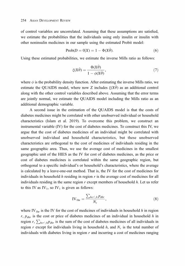
of control variables are uncorrelated. Assuming that these assumptions are satisfied,
we estimate the probabilities that the individuals using only insulin or insulin with
other noninsulin medicines in our sample using the estimated Probit model:
Prob(D ¼ 0jX) ¼ 1� �(Xθ̂): ð6ÞUsing these estimated probabilities, we estimate the inverse Mills ratio as follows:
�(Xθ̂) ¼ �(Xθ̂)
1� �(Xθ̂), ð7Þ
where � is the probability density function. After estimating the inverse Mills ratio, we
estimate the QUAIDS model, where now Z includes �(Xθ̂) as an additional control
along with the other control variables described above. Assuming that the error terms
are jointly normal, we estimate the QUAIDS model including the Mills ratio as an
additional demographic variable.
A second issue in the estimation of the QUAIDS model is that the costs of
diabetes medicines might be correlated with other unobserved individual or household
characteristics (Islam et al. 2019). To overcome this problem, we construct an
instrumental variable (IV) for the cost of diabetes medicines. To construct this IV, we
argue that the cost of diabetes medicines of an individual might be correlated with
unobserved individual and household characteristics, but these unobserved
characteristics are orthogonal to the cost of medicines of individuals residing in the
same geographic area. Thus, we use the average cost of medicines in the smallest
geographic unit of the HIES as the IV for cost of diabetes medicines, as the price or
cost of diabetes medicines is correlated within the same geographic region, but
orthogonal to a specific individual’s or household’s characteristics, where the average
is calculated by a leave-one-out method. That is, the IV for the cost of medicines for
individuals in household h residing in region r is the average cost of medicines for all
individuals residing in the same region r except members of household h. Let us refer
to this IV as IV1, so IV1 is given as follows:
IV1hr ¼P
h�r n h pdhrNr
, ð8Þ
where IV1hr is the IV for the cost of medicines of individuals in household h in region
r, pdhr is the cost or price of diabetes medicines of an individual in household h in
region r,P
h�r n hpdhr is the sum of the cost of diabetes medicines of all individuals in
region r except for individuals living in household h, and Nr is the total number of
individuals with diabetes living in region r and incurring a cost of medicines ranging
254 ASIAN DEVELOPMENT REVIEW
March 23, 2022 1:15:10pm WSPC/331-adr 2250009 ISSN: 0116-11052ndReading

from Tk436 to Tk1,930. Similarly, we construct an IV for the prices of food and
education.
Another issue in estimating the demand parameters is that error terms u may be
spatially correlated as costs of diabetes medicines are generally correlated with the
types of health care provider such as public hospitals, private hospitals, and
pharmacies, and we have certain types of health care providers in each region (Islam
et al. 2019). This may introduce heteroscedasticity in the QUAIDS model and hence
reduce the efficiency of the estimators. To eliminate the heteroscedasticity due to
spatial correlation in error terms u, we cluster the standard errors at the union or ward
level, which is the lowest administrative unit in Bangladesh.
E. Computing Counterfactual Price Changes
To determine the range of potential increases in the prices of insulin following
Bangladesh’s graduation from LDC, we use estimated demand elasticities to compute
the ranges of markups and marginal costs based on the current prices of insulin and
insulin market structure. Since the expenditure items in our QUAIDS model are
defined broadly (i.e., food, medicine, and education), it is expected that the price
elasticities of demand would be very low. Hence, it would be impossible to determine
the insulin prices under the monopoly market structure ensured by stronger IP laws as
a monopoly’s equilibrium output is always at the elastic part of the market demand
curve. To compute the counterfactual prices of insulin under monopoly market structure,
we need to estimate the slope of the demand function of insulin so that we can use this
slope to estimate the price elasticities of demand at different points on the demand curve.
This estimated elasticity is then used to derive the optimal monopoly markup. Here, we
assume that the market demand for insulin is linear in insulin prices and estimate this
linear demand function by estimating the following regression equation:
!2 ¼ ’0 þ ’1p2 þ ’2 �! þ Z 0�þ u, ð9Þ
where !2 is the household expenditure on insulin, p2 is the price of insulin faced by the
household, �! is the minimum level of income necessary to ensure a subsistence level of
food consumption for the household. �! is calculated by multiplying the household size
and the national lower poverty level income as reported in the final report of the 2016
HIES (BBS 2019); Z 0 is the vector of household and household head’s characteristics; uis the error term; and ’0, ’1, ’2, and � are parameters to be estimated. Here, the main
parameter of interest is’1, which then is used to calculate the slope of the insulin demand
THE SOCIAL COSTS OF SUCCESS 255
March 23, 2022 1:15:10pm WSPC/331-adr 2250009 ISSN: 0116-11052ndReading

curve with respect to insulin price as follows:
d!2
dp2¼ d(p2q2)
dp2¼ q2 þ p2
dq2dp2
¼ ’̂1,
�b ¼ dq2dp2
¼ ’̂1
�p2� �q2
�p2,
ð10Þ
where �b is the slope of the demand curve evaluated at the average price and quantity of
the insulin.We also verify the estimated slope of the inverse demand curve using the own
price elasticity of insulin demand obtained from our QUAIDS model as follows:
0 ¼ p2 þ q2dp2dq2
¼ 1þ 1E22
, ð11Þ
dp2dq2
¼ 1þ 1E22
� �p2�q2
¼ 1�b, ð12Þ
where we use the fact that at the midpoint of the demand curve, marginal revenue is 0.
Once we have the estimated slope of the insulin demand curve, we can estimate the price
elasticities of the insulin demand curve
E22 ¼ �bp2q2
: ð13Þ
Now, we can find the elasticities at different points of the demand curve. With these
estimated elasticities, we can find the optimal markup for the monopoly. In addition to
simulating the counterfactual markup and price under monopoly market structure, we
also use the average insulin price in Pakistan, where the pharmaceutical market is less
regulated and strong IP laws govern the market (Basant 2007). Nevertheless, most types
of insulin are very affordable in Pakistan compared to other South Asian countries. The
main reason that a stronger IPR regime did not lead to exorbitant price increases for
insulin in Pakistan is the provision of the insulin supply by the public sector (Ewen et al.
2019). The reasons that we choose current insulin prices in Pakistan as another
counterfactual price are as follows: (i) this provides an interesting scenario where strong
IP laws coexist with public sector participation, which enables greater access to insulin;
and (ii) the size and characteristics of the economy of Pakistan are comparable to those of
Bangladesh.
F. Welfare Analysis
To have insights into the welfare effects of a stronger IPR regime in post-LDC
Bangladesh under two counterfactual prices—simulated prices under monopoly
256 ASIAN DEVELOPMENT REVIEW
March 23, 2022 1:15:10pm WSPC/331-adr 2250009 ISSN: 0116-11052ndReading

market structure and prices in a less regulated neighboring country (Pakistan)—we use
several measures of welfare as elaborated by Araar and Verme (2016). Our first
measure is the consumer surplus (CS), defined as the difference between willingness to
pay and the market price of insulin. The measure of CS is given as follows:
CS ¼Z p2 0
p2D(p2)dp2, ð14Þ
where p2 and p2 0 are the current and counterfactual prices of insulin, D(p2) is the
demand function of insulin. Here, to estimate the CS we need to know the Marshallian
demand function D(p2). For a linear demand system and moderate change in prices,
CS can be estimated using the following equation:
CS ¼ �x2 Δp2(1þ 0:5E22Δp2): ð15ÞFor the problem concerned in this paper, the price changes could be significantly
higher and so the above formula will provide a highly overstated estimate for CS. Araar
and Verme (2016) derived an approximation CS formula for a large price change:
CS ¼ �x2 Δp2 1� 0:5Δp221þ Δp2
� �: ð16Þ
CS as a measure of welfare is somewhat restrictive as it assumes that the marginal utility
of real income is constant and there is no distributional effect of price changes. It also
captures only the partial equilibrium effect and does not perfectly measure the change in
welfare if the changes in prices are large. However, CS is a straightforward and easy-to-
estimate welfare measure, which would be a good standard to compare with other
measures of welfare. The next two welfare measures that we estimate are compensating
variation (CV) and equivalent variation (EV). These measures are defined as follows:
CV ¼ e(p2, v0)� e(p2 0 , v0) ¼
Z p2 0
p2h(p2, v
0)dp2, ð17Þ
EV ¼ e(p2, v1)� e(p2 0 , v1) ¼
Z p2 0
p2h(p2, v
1)dp2, ð18Þ
where v0 and v1 are levels of generic indirect utility before and after the implementation
of a stronger IPR regime, respectively, e(.) is the generic expenditure function, and h(.)
is the Hicksian demand function. Here, CV is the monetary compensation required to
bring the consumer back to the original utility level after the price change, and EV is the
monetary change required to obtain the same level of utility after the price change (Araar
and Verme 2016). One computational problem in calculating CVand EV is that we need
to know the indirect utility level before or after the changes in prices. One solution to
THE SOCIAL COSTS OF SUCCESS 257
March 23, 2022 1:15:11pm WSPC/331-adr 2250009 ISSN: 0116-11052ndReading

this computational problem is to derive CV and EV from CS as given in Chipman and
Moore (1980)
CV ¼ (1� e�CS=m)m, ð19ÞEV ¼ (eCS=m � 1)m, ð20Þ
where m is the income level. In addition to these measures of welfare, there are two
simple straightforward measures of welfare: Laspeyres Variation (LV), which is defined
as the exact change in income necessary to purchase the initial bundle of goods at prices
after and before the change in the IPR regime. LV is defined as follows:
LV ¼ e(p 02,X
0)� e(p2,X0), ð21Þ
where X 0 is the initial bundle of goods purchased before the change in prices. The
second measure is the Paasche Variation (PV), which is defined as the exact change in
income required to purchase the final bundle of goods at prices after and before the
change in the IPR regime. PV is given as follows:
PV ¼ e(p 02,X
1)� e(p2,X1), ð22Þ
where X 1 is the final bundle of goods purchased after the change in prices due to a
change in the IPR regime. To estimate LVor PV, we just need the information of quantity
purchased before or after the change in the policy regimes and the associated changes in
prices, whereas to estimate the other measures of welfare requires some knowledge or
assumptions on the demand function or the utility function.
V. Results
A. Price and Expenditure Elasticities
Table B1 in Appendix 2 reports the parameter estimates of our QUAIDS model.
The estimated uncompensated price elasticities and expenditure elasticities are
reported in Table 1. Here, all elasticities are the average elasticities across all
households in the sample. The price elasticities are denoted as Eij, where subscript i
denotes the expenditure on item i, and j denotes the price of item j. The estimate of
price elasticity of food, E11, is consistently estimated across different models; E11
ranges from 93.7% to 99.0% under different specifications. The price elasticities of
insulin have expected negative signs only under IV specification, and these vary from
258 ASIAN DEVELOPMENT REVIEW
March 23, 2022 1:15:11pm WSPC/331-adr 2250009 ISSN: 0116-11052ndReading

92.7% to 94.3%, whereas the price elasticities of education vary from 14.3% to 25.5%
under various specifications but are not statistically significant.
The cross-price elasticities show interesting demand patterns as well. The cross-
price elasticities between food and insulin (E12) or education (E13) are always negative
under all specifications and statistically different from zero. This indicates that
expenditure on food falls in response to an increase in the price of insulin or education.
However, the cross-price elasticities between insulin and food (E21) or education (E23)
are positive under IV specifications, which indicates that an increase in the price of
food or education may not lead to a decrease in demand for insulin.
B. Marginal Costs and Markups
Currently, the market for insulin in Bangladesh is oligopolistic. To find the
markups in this market, we assume that the marginal cost (MC) of producing insulin is
constant and the same for all producers. If there are n firms in the market with the same
Table 1. Uncompensated Price and Expenditure Elasticitiesof Major Expenditure Items in Bangladesh
Not Corrected Corrected
OLS IV OLS IV
Price elasticitiesE11 �0.988*** �0.945*** �0.990*** �0.937***E12 �0.103*** �0.004*** �0.106*** �0.004***E13 �0.071*** �0.054*** �0.072*** �0.060***E21 �0.043*** 0.621*** �0.042*** 0.563***E22 0.377*** �0.927*** 0.413*** �0.943***E23 0.120*** 0.107*** 0.125*** 0.090***E31 0.062*** �2.011*** 0.082*** �2.124***E32 �0.010 0.013 �0.010 0.003E33 �0.180 �0.255 �0.180 �0.143
Expenditure elasticitiesE1 1.162*** 1.003*** 1.168*** 1.001***E2 �0.454*** 0.203*** �0.495*** 0.289***E3 0.133 2.251*** 0.111 2.258***
IV ¼ instrumental variable, OLS ¼ ordinary least squares.Notes: Subscript 1 refers to food, subscript 2 is insulin, and subscript 3 iseducation. ***p < 0:01, **p < 0:05, *p < 0:1.Source: QUAIDS model estimates based on data from the BangladeshBureau of Statistics. 2019. Report on the Household Income andExpenditure Survey 2016. Dhaka: Statistics and Information Division,Ministry of Planning, Government of Bangladesh.
THE SOCIAL COSTS OF SUCCESS 259
March 23, 2022 1:15:12pm WSPC/331-adr 2250009 ISSN: 0116-11052ndReading

MC, c, the markup is defined as follows:
P� c
p¼ � 1
n
Q
P
dP
dQ¼ � 1
nED:
The current insulin market in Bangladesh is to some extent competitive. There are
seven domestic producers of insulin supplying 50 different insulin products in
Bangladesh (DGDA 2019). The differences in these products are in terms of dosages
size and the producers. In addition, there are six foreign producers, who have
registered a combined 65 insulin products in Bangladesh (DGDA 2019). The licenses
of products of two foreign producers expired in 2015 and early 2016.3 Hence, there are
now 11 suppliers of insulin in Bangladesh. Thus, the markup is given by the following
formula: 11þ 1
11*jE22 j
� �. The MCs are calculated using the bounds of insulin prices, which
is the amount paid by a household for 1 month of insulin supply. We use the maximum
retail prices reported by DGDA to estimate this monthly expenditure on insulin, which
is found to range from Tk436 to Tk1,925. The estimated markups and bounds of MC
of a 1-month insulin supply are reported in Table 2.
From Table 2, we can see that the current markups range from 1.107 to 1.109,
reflecting the fact that the current market is characterized by some competitive forces
as the markups are around 10% over the MC. The lower and upper bounds of MC
range from Tk393.24 to Tk1,740.73 and from Tk393.97 to Tk1,743.94, respectively.
These bounds reflect end user MCs rather than MCs at the production level.
3Eli Lilly & Company’s license in the US expired in May 2016. Lilly’s license in France expired inMay 2015. https://www.dgda.gov.bd/index.php/2013-03-31-05-16-29/registered-imported-drugs.
Table 2. Implied Markups and Marginal Costs of Insulin in Bangladesh underCurrent Market Structure (Tk)
Not Corrected Corrected
Lower Bound Upper Bound Lower Bound Upper Bound
Price elasticities �0.93 �0.93 �0.94 �0.94Markups 1.109 1.109 1.107 1.107Marginal costs 393.24 1,740.73 393.97 1,743.94
Tk ¼ Bangladesh taka.Source: Authors’ calculations based on data from the Bangladesh Bureau of Statistics. 2019.Report on the Household Income and Expenditure Survey 2016. Dhaka: Statistics andInformation Division, Ministry of Planning, Government of Bangladesh; and DirectorateGeneral of Drug Administration. “Registered Products.” Government of Bangladesh.http://www.dgda.gov.bd/index.php/manufacturers/allopathic (accessed 14 October 2019).
260 ASIAN DEVELOPMENT REVIEW
March 23, 2022 1:15:12pm WSPC/331-adr 2250009 ISSN: 0116-11052ndReading

Thus, these are the MCs of all value added of insulin production: from production to
final purchase by households.
C. Demand Function of Insulin and Counterfactual Prices
We estimate the insulin demand function as specified in regression equation (9)
using the IV for insulin prices. The result of the regression equation (9) is reported in
Table B3 in Appendix 2. The estimates of the coefficient of insulin price (p2IV) are
negative under the estimation strategies of not correcting and correcting for sample
selection bias. We use the estimate of the coefficient of p2IV in a regression corrected
for sample selection bias, and this estimate is ’̂1 ¼ �0:11. The estimated slope
coefficient, �b ¼ �0:00137, is given as follows:
�b ¼ dq2dp2
¼ ’̂1
�p2� �q2
�p2¼ ’̂1
�p2� �p2�q2
�p 22
¼ �0:11884:16
� 973:33884:162
¼ �0:00137,
where Tk973.33 is the average monthly household expenditure on insulin and
Tk884.16 is the average of monthly price of insulin. Now, the elasticity of insulin
demand at the average price and quantity of insulin is given as follows:
E22 ¼ �b�p
�q¼ �b
�p 2
�p�q¼ �0:00137� 884:162
973:33¼ �1:10:
Using this elasticity of insulin demand measured approximately at the midpoint of the
insulin demand curve, we can find the maximum markups:
1
1þ 1jE22j
!¼ jE22j
1þ jE22j¼ 11:01:
This markup shows that under an unregulated monopoly, the insulin price could be
more than 11 times higher than current insulin prices, where the current markup of
insulin in Bangladesh is about 1.1. Using the estimated markup under an unregulated
monopoly and the upper and lower bounds of MC as reported in Table 2, we estimate
maximum possible counterfactual prices of insulin, which are reported in Table 3.
These counterfactual prices show the most extreme situations of an increase in insulin
prices in Bangladesh following its graduation from LDC status and the enforcement
of strong IP laws. Thus, these provide some bounds on the prices of insulin in a
worst-case scenario.
For the Pakistan price counterfactual, we use the average insulin prices reported
in Ewen et al. (2019), where the insulin prices for several low- and middle-income
countries including Pakistan were surveyed in 2016. Since our sample is from the
THE SOCIAL COSTS OF SUCCESS 261
March 23, 2022 1:15:12pm WSPC/331-adr 2250009 ISSN: 0116-11052ndReading
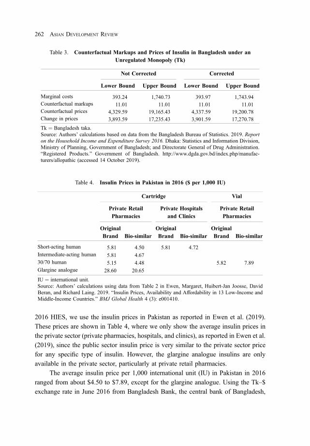
2016 HIES, we use the insulin prices in Pakistan as reported in Ewen et al. (2019).
These prices are shown in Table 4, where we only show the average insulin prices in
the private sector (private pharmacies, hospitals, and clinics), as reported in Ewen et al.
(2019), since the public sector insulin price is very similar to the private sector price
for any specific type of insulin. However, the glargine analogue insulins are only
available in the private sector, particularly at private retail pharmacies.
The average insulin price per 1,000 international unit (IU) in Pakistan in 2016
ranged from about $4.50 to $7.89, except for the glargine analogue. Using the Tk–$
exchange rate in June 2016 from Bangladesh Bank, the central bank of Bangladesh,
Table 3. Counterfactual Markups and Prices of Insulin in Bangladesh under anUnregulated Monopoly (Tk)
Not Corrected Corrected
Lower Bound Upper Bound Lower Bound Upper Bound
Marginal costs 393.24 1,740.73 393.97 1,743.94Counterfactual markups 11.01 11.01 11.01 11.01Counterfactual prices 4,329.59 19,165.43 4,337.59 19,200.78Change in prices 3,893.59 17,235.43 3,901.59 17,270.78
Tk ¼ Bangladesh taka.Source: Authors’ calculations based on data from the Bangladesh Bureau of Statistics. 2019. Reporton the Household Income and Expenditure Survey 2016. Dhaka: Statistics and Information Division,Ministry of Planning, Government of Bangladesh; and Directorate General of Drug Administration.“Registered Products.” Government of Bangladesh. http://www.dgda.gov.bd/index.php/manufac-turers/allopathic (accessed 14 October 2019).
Table 4. Insulin Prices in Pakistan in 2016 ($ per 1,000 IU)
Cartridge Vial
Private RetailPharmacies
Private Hospitalsand Clinics
Private RetailPharmacies
OriginalBrand Bio-similar
OriginalBrand Bio-similar
OriginalBrand Bio-similar
Short-acting human 5.81 4.50 5.81 4.72Intermediate-acting human 5.81 4.6730/70 human 5.15 4.48 5.82 7.89Glargine analogue 28.60 20.65
IU ¼ international unit.Source: Authors’ calculations using data from Table 2 in Ewen, Margaret, Huibert-Jan Joosse, DavidBeran, and Richard Laing. 2019. “Insulin Prices, Availability and Affordability in 13 Low-Income andMiddle-Income Countries.” BMJ Global Health 4 (3): e001410.
262 ASIAN DEVELOPMENT REVIEW
March 23, 2022 1:15:13pm WSPC/331-adr 2250009 ISSN: 0116-11052ndReading

these average prices correspond to Tk352.80–Tk618.58 per 1,000 IU, whereas the
average monthly cost of insulin per person in Bangladesh is about Tk884.16.4 Since
1,000 IU of insulin is approximately the monthly supply of insulin for an individual,
the average monthly insulin cost for most types of insulin is significantly higher in
Bangladesh than in Pakistan. However, average prices for long-acting insulins
such as glargine analogues range from $20.65 to $28.60, which corresponds to
Tk1,618.18–Tk2,246.16, higher than the average monthly insulin costs in Bangladesh.
Here, we use the price of the original brand of glargine analogues in Pakistan as the
counterfactual price of insulin in Bangladesh under stricter IP laws. To estimate the
upper bound of price gain and loss in welfare, we take the difference between this
price, Tk2,246.16, and the current monthly average cost of insulin per person in
Bangladesh, Tk8,84.16, which implies a potential 154% increase in the average
monthly cost of insulin in Bangladesh.
D. Welfare Analysis
The welfare estimates are reported in Table 5. The welfare loss estimates in this
table are aggregate national-level estimates. The welfare losses in the “Upper bound”
column correspond to upper bound price changes in columns 2 and 4 of Table 4.
Similarly, the welfare losses in columns 3 and 4 in Table 5 correspond to lower bound
price changes in columns 1 and 3 of Table 4. The welfare estimates in column 5 of
Table 5 are calculated for the counterfactual price increase from the average price of
Tk884.16. The welfare loss estimates in column 6 of Table 5 are calculated by using
the originator’s price of long-acting insulin glargine analogues in Pakistan. All these
estimates of welfare loss show the worst-case scenario, which entails maximum
welfare losses under an unregulated monopoly because of stronger IP laws after
Bangladesh’s graduation from LDC status.
The first row of Table 5 is the measure of aggregate increases in household
expenditures due to an increase in insulin prices following Bangladesh’s graduation
from LDC status. Here LV and PV measures are the same, as we use the same
composition of goods before and after changes in insulin prices. The upper bound of
the aggregate increase in household expenditure under an unregulated monopoly is
about $656 million per year, whereas the lower bound is about $148 million per year.
The aggregate increase in household expenditure would be significantly lower, about
4The Tk–$ exchange rate in June 2016 was 78.4. https://www.bb.org.bd/econdata/exchangerate.php.
THE SOCIAL COSTS OF SUCCESS 263
March 23, 2022 1:15:13pm WSPC/331-adr 2250009 ISSN: 0116-11052ndReading

Table
5.Annual
Agg
rega
teWelfare
Lossesin
Ban
glad
eshunder
anUnregu
latedMon
opolyan
dPak
istanPrice
Cou
nterfactual
Upper
Bou
nd
Low
erBou
nd
Not
Corrected
Corrected
Not
Corrected
Corrected
Average
Price
Cou
nterfactual
Pak
istanPrice
Cou
nterfactual
LV¼
PV
Tkmillion
51,347
.49
51,450
.48
11,599
.73
11,623
.54
26,367
.08
4,05
7.65
$million
654.94
656.27
147.96
148.26
336.31
51.76
CS
Tkmillion
25,675
.23
25,726
.73
5,80
1.35
5,81
3.26
13,185
.03
2,03
0.31
$million
327.49
328.15
74.00
74.15
168.18
25.90
CV
Tkmillion
31,883
.49
31,962
.69
6,07
1.70
6,08
4.74
14,662
.37
2,06
2.52
$million
406.68
407.69
77.45
77.61
187.02
26.31
EV
Tkmillion
21,385
.61
21,421
.22
5,55
2.47
5,56
3.38
11,961
.42
1,99
9.02
$million
272.78
273.23
70.82
70.96
152.57
25.50
CS¼
consum
ersurplus,
CV¼
compensating
variation,
EV¼
equivalent
variation,
LV¼
Laspeyres
Variatio
n,PV
¼Paasche
Variatio
n,Tk¼
Bangladeshtaka.
Sou
rce:
Autho
rs’calculations
basedon
data
from
theBangladeshBureauof
Statistics.20
19.Reporton
theHou
seho
ldIncomean
dExpenditure
Survey
2016
.Dhaka:StatisticsandInform
ationDivision,
Ministryof
Plann
ing,
Gov
ernm
entof
Bangladesh.
264 ASIAN DEVELOPMENT REVIEW
March 23, 2022 1:15:14pm WSPC/331-adr 2250009 ISSN: 0116-11052ndReading

$52 million per year if the insulin prices in Bangladesh stayed at a similar level to
insulin prices in Pakistan.
For an increase in the price of insulin, the relationship among losses in CS, CV,
and EV are as follows: CV > CS > EV. From Table 5, we can see that these
relationships are satisfied. From the figures in third (CV) and fourth (EV) rows in
Table 5, the annual aggregate loss in welfare under an unregulated monopoly will
range from $71 million to $407 million. However, under the Pakistan price
counterfactual, the annual loss in welfare would be around $26 million.
The welfare effect of an increase in insulin prices at the household level is in
Table 6, which reports the increase in household expenditure and the increase in
expenditure as a percentage of household average income per year for three
counterfactual scenarios: largest upper bound estimate (upper bound IV), smallest
lower bound estimate (lower bound OLS), and the Pakistan price counterfactual.
The annual welfare impacts of stronger IP laws could be from $51.8 million
across impacted households (Pakistan price counterfactual) to an upper bound of
$656.3 million under an unregulated monopoly (Table 6). According to a review of the
literature (Biswas et al. 2016), the incidence of people with diabetes in Bangladesh is
estimated to be between 4.5% and 35.0%, with the “pooled preference” being 7.4%.
The average number of people in a household in Bangladesh is 4.06 (BBS 2019). The
cost per impacted household per year would therefore range from $17.6 to $223.1,
which implies a 0.7% to about a 9.1% decline in affected household incomes.
E. Poverty Impact
An increase in the price of insulin because of stricter IP laws would also have a
significant impact on the poverty incidence for households that require access to
lifesaving insulin for the members of those households with diabetes. To show the
effect of a price rise in insulin on household poverty, we estimate the rate of poverty
for the households with members with diabetes, especially with members needing
insulin. Table 7 shows the absolute number of people and households and rates of
poverty under the upper and lower poverty lines at the national level, households with
persons having diabetes, and households with members requiring insulin.
Table 7 shows there are about 39.33 million households in Bangladesh, and out
of them, 12.89% fall below the lower poverty line and 24.28% fall below upper
poverty line.5 The corresponding poverty rates for households with at least one
5Lower and upper poverty line incomes are defined in BBS (2019).
THE SOCIAL COSTS OF SUCCESS 265
March 23, 2022 1:15:14pm WSPC/331-adr 2250009 ISSN: 0116-11052ndReading
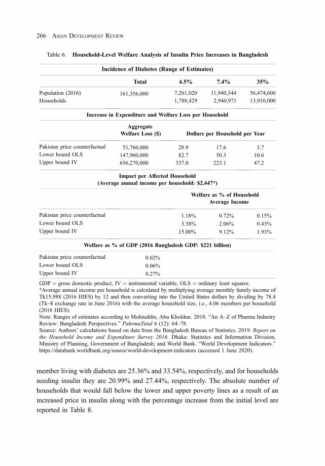
member living with diabetes are 25.36% and 33.54%, respectively, and for households
needing insulin they are 20.99% and 27.44%, respectively. The absolute number of
households that would fall below the lower and upper poverty lines as a result of an
increased price in insulin along with the percentage increase from the initial level are
reported in Table 8.
Table 6. Household-Level Welfare Analysis of Insulin Price Increases in Bangladesh
Incidence of Diabetes (Range of Estimates)
Total 4.5% 7.4% 35%
Population (2016) 161,356,000 7,261,020 11,940,344 56,474,600Households 1,788,429 2,940,971 13,910,000
Increase in Expenditure and Welfare Loss per Household
AggregateWelfare Loss ($) Dollars per Household per Year
Pakistan price counterfactual 51,760,000 28.9 17.6 3.7Lower bound OLS 147,960,000 82.7 50.3 10.6Upper bound IV 656,270,000 337.0 223.1 47.2
Impact per Affected Household(Average annual income per household: $2,447a)
Welfare as % of HouseholdAverage Income
Pakistan price counterfactual 1.18% 0.72% 0.15%Lower bound OLS 3.38% 2.06% 0.43%Upper bound IV 15.00% 9.12% 1.93%
Welfare as % of GDP (2016 Bangladesh GDP: $221 billion)
Pakistan price counterfactual 0.02%Lower bound OLS 0.06%Upper bound IV 0.27%
GDP ¼ gross domestic product, IV ¼ instrumental variable, OLS ¼ ordinary least squares.aAverage annual income per household is calculated by multiplying average monthly family income ofTk15,988 (2016 HIES) by 12 and then converting into the United States dollars by dividing by 78.4(Tk–$ exchange rate in June 2016) with the average household size, i.e., 4.06 members per household(2016 HIES).Note: Ranges of estimates according to Mohiuddin, Abu Kholdun. 2018. “An A–Z of Pharma IndustryReview: Bangladesh Perspectives.” PahrmaTutal 6 (12): 64–78.Source: Authors’ calculations based on data from the Bangladesh Bureau of Statistics. 2019. Report onthe Household Income and Expenditure Survey 2016. Dhaka: Statistics and Information Division,Ministry of Planning, Government of Bangladesh; and World Bank. “World Development Indicators.”https://databank.worldbank.org/source/world-development-indicators (accessed 1 June 2020).
266 ASIAN DEVELOPMENT REVIEW
March 23, 2022 1:15:14pm WSPC/331-adr 2250009 ISSN: 0116-11052ndReading

Poverty estimates in Table 8 are reported only for the upper bound and lower
bound of price change under an unregulated monopoly scenario, estimated using IVs
for prices with correction for sample selection bias and the price change under the
Pakistan counterfactual policy regime. The numbers of households that fall below the
lower poverty line are 5.2 million and 5.1 million for the upper and lower bounds of an
unregulated monopoly counterfactual scenario, respectively, which are about 3.0% and
0.8% higher than the initial level. For the Pakistan price counterfactual, the increase is
much smaller, with only about a 0.24% increase from the initial level of poverty.
Among all households with at least one member with diabetes, 0.27 million
households are estimated to be below the lower poverty line, which increases to 0.42
million, 0.30 million, and 0.28 million under each of the three counterfactual
scenarios, respectively. These increases represent a rise in poverty rates ranging from
4.61% to 58.27% from the current level of poverty for these households. Out of all
households that require insulin for one or more members, 0.08 million fall below the
lower poverty line, which increases by 194.51% to 0.23 million under the upper bound
and 49.06% to 0.12 million under the lower bound of an unregulated monopoly
counterfactual scenario. Under the Pakistan price counterfactual scenario, the number
of households that fall below the lower poverty line is 0.09 million, which is 15.40%
higher than the initial level. The pattern of increases in the poverty rates are similar
under the upper poverty line.
Table 9 reports the numbers of households that are below the lower and upper
poverty lines, and the percentage increase in poverty from the initial level of poverty
under the various counterfactual price increase scenarios. We also estimated the
poverty rates as a fraction of total households for three different aggregate levels.
After an increase in the insulin price under a stricter IPR regime, the fraction of
total households that fall below the lower poverty line ranges from 12.92% to 13.28%
Table 7. Initial Level of Poverty in Bangladesh
Lower Poverty Line Upper Poverty Line
TotalHouseholds(million)
Households inPoverty(million)
PovertyRate(%)
Householdsin Poverty(million)
PovertyRate(%)
1. National 39.33 5.07 12.89 9.55 24.282. Households with diabetes 1.05 0.27 25.36 0.35 33.543. Households needing insulin 0.38 0.08 20.99 0.10 27.44
Source: Authors’ calculations based on data from the Bangladesh Bureau of Statistics. 2019. Report onthe Household Income and Expenditure Survey 2016. Dhaka: Statistics and Information Division,Ministry of Planning, Government of Bangladesh.
THE SOCIAL COSTS OF SUCCESS 267
March 23, 2022 1:15:15pm WSPC/331-adr 2250009 ISSN: 0116-11052ndReading

Table8.
Pov
erty
Rates
inBan
glad
eshafteran
Increase
inInsulin
Prices
Hou
seholdsin
Hou
seholdsin
Pov
erty
after
aPrice
Increase
(million):
Increase
inHou
sehold
Pov
erty
Rates
(%):
Pov
erty
before
aPrice
Increase
Upper
Bou
nd
Low
erBou
nd
Pak
istan
Price
Upper
Bou
nd
Low
erBou
nd
Pak
istan
Price
(million)
Low
erPov
erty
Line
1.National
5.07
5.22
5.11
5.08
3.05
0.77
0.24
2.Hou
seho
ldswith
diabetes
0.27
0.42
0.30
0.28
58.27
14.69
4.61
3.Hou
seho
ldsneedinginsulin
0.08
0.23
0.12
0.09
194.51
49.06
15.40
Upper
Pov
erty
Line
1.National
9.55
9.69
9.58
9.57
1.45
0.36
0.18
2.Hou
seho
ldswith
diabetes
0.35
0.49
0.39
0.37
39.45
9.80
4.92
3.Hou
seho
ldsneedinginsulin
0.10
0.24
0.14
0.12
133.23
33.11
16.62
Sou
rce:Autho
rs’calculations
basedon
datafrom
theBangladeshBureauof
Statistics.20
19.Reporton
theHou
seho
ldIncome
andExpenditure
Survey
2016
.Dhaka:StatisticsandInform
ationDivision,
Ministryof
Plann
ing,
Gov
ernm
entof
Bangladesh.
268 ASIAN DEVELOPMENT REVIEW
March 23, 2022 1:15:15pm WSPC/331-adr 2250009 ISSN: 0116-11052ndReading

Table
9.Pov
erty
Rates
inBan
glad
eshbeforean
dafteran
Increase
inInsulin
Pricesan
dPercentage
Chan
ge
Hou
seholdPov
erty
Rates
after
Price
Increase
Percentage
PointIncrease
inHou
seholdPov
erty
Rates
Hou
seholdPov
erty
Ratebefore
Upper
Bou
nd
Low
erBou
nd
Pak
istan
Price
Upper
Bou
nd
Low
erBou
nd
Pak
istan
Price
Price
Increase
Low
erPov
erty
Line
1.National
12.89
13.28
12.99
12.92
0.39
0.10
0.03
2.Hou
seho
ldswith
diabetes
25.36
40.14
29.09
26.53
14.78
3.73
1.17
3.Hou
seho
ldsneedinginsulin
20.99
61.81
31.28
24.22
40.82
10.30
3.23
Upper
Pov
erty
Line
1.National
24.28
24.63
24.37
24.33
0.35
0.09
0.04
2.Hou
seho
ldswith
diabetes
33.54
46.78
36.83
35.20
13.23
3.29
1.65
3.Hou
seho
ldsneedinginsulin
27.44
64.01
36.53
32.01
36.56
9.09
4.56
Sou
rce:Autho
rs’calculations
basedon
datafrom
theBangladeshBureauof
Statistics.20
19.R
eporto
ntheHou
seho
ldIncomean
dExpenditure
Survey
2016
.Dhaka:StatisticsandInform
ationDivision,
Ministryof
Plann
ing,
Gov
ernm
entof
Bangladesh.
THE SOCIAL COSTS OF SUCCESS 269
March 23, 2022 1:15:16pm WSPC/331-adr 2250009 ISSN: 0116-11052ndReading

under these three counterfactual scenarios, with an increase in poverty rates ranging
from 0.03 percentage points to 0.39 percentage points. Similarly, among all the
households with at least one person with diabetes, the share of households that will be
under the lower poverty line increases from an initial 25.36% to 26.53%–40.14%, with
the increase in poverty rates ranging from 1.17 percentage points to 14.78 percentage
points. We can see a very substantial increase in household poverty among the
households needing insulin. Here, under the three different counterfactual scenarios,
the share of households that fall below the lower poverty line among all households
needing insulin range from 24.22% to 61.81% from an initial poverty rate of 20.99%,
which indicates an increase in poverty rates ranging from 3.23 percentage points to
40.82 percentage points for those households. We see a very similar pattern in
increased poverty rates when we use the upper poverty line instead of the lower
poverty line.
VI. Discussion and Conclusion
This paper is built on the previous theoretical and empirical insights to estimate
the potential impact of Bangladesh’s LDC graduation on its population living with
diabetes in general and insulin users in particular. To date, few if any studies deploy an
ex ante partial equilibrium framework that estimates price changes due to trade policy
change and then links those results to household behavior models and data. We model
and then estimate the potential impact of LDC graduation on the price of insulin in
Bangladesh and then link those price changes. Following those estimates, we calculate
demand elasticities and relate them to Bangladeshi household data to determine the
impacts of those potential price changes in household wealth.
Our findings have significant policy ramifications as well. Bangladesh has a
high incidence of diabetes and insulin users, as well as a fairly thriving domestic
industry that supplies those treatments to patients in need. We find that prices of
insulin would increase significantly in Bangladesh due to LDC graduation and the
subsequent requirement to comply with the IPR provisions of the WTO. What is
more, such price changes would also have significant welfare impacts for the
population. LDC graduation would trigger a significant jump in insulin prices that
could cause a 1%–15% decline in the welfare (i.e., an increase in expenditure) of
households with diabetes, increasing the poverty rate of households with diabetes by
54%–58% and of those needing insulin by 15%–195% unless policy adjustments
were carried out.
270 ASIAN DEVELOPMENT REVIEW
March 23, 2022 1:15:16pm WSPC/331-adr 2250009 ISSN: 0116-11052ndReading

Our estimates of the impact of an increase in insulin price under a stronger IPR
regime on household welfare and poverty has some important data limitations. These
limitations emanated from the lack of detailed expenditure information on medicines
by individuals with diabetes. The 2016 HIES of Bangladesh does not provide
disaggregated data on types of diabetic medicines, i.e., whether an individual with
diabetes needs insulin or noninsulin medicines, and it contains no information on the
quantity of medicines needed per day or per month. To construct the sample for our
analysis, we needed to infer the households needing insulin from the expenditure on
medicines for chronic disease reported in the 2016 HIES and compare this expenditure
to an interval constructed using administrative data on monthly insulin costs. It was
likely that there would be some households needing insulin but not included in our
sample if the household’s monthly expenditure on medicines fell below the lower
bound of the cost of insulin constructed using administrative data. Similarly, there
would be some households that do not need insulin but expenditure on medicines by
those households fell within the interval. In the prior scenario, our household welfare
and poverty estimates would be underestimated, and in the latter scenario, these would
be overestimated. Hence, without additional information on medicine expenditure by
the households with members living with diabetes, we could not determine the
direction of bias that our constructed sample may induce.
Another data limitation in the 2016 HIES is that it seems to underrepresent the
fraction of the population suffering from diabetes. In the final report, 186,078
individuals were included in the survey, but only 2,238 individuals were reported to be
living with diabetes, which is about 1.2% of the sample. However, it has been
estimated that about 10% of the population of Bangladesh are suffering from diabetes,
with half of them going undiagnosed (WHO 2016). Hence, we would expect about 5%
of the individuals in our sample to report a diagnosis of diabetes. The
underrepresentation of individuals with diabetes in the 2016 HIES would also cause
a downward bias in estimation. Thus, in this case, our estimated effects of an increase
in insulin price on households’ welfare and poverty are conservative estimates, which
signifies that the true welfare cost of a stricter IPR regime in Bangladesh after its
graduation from LDC status would be significantly higher.
That said, this paper should not be the last word on this subject for Bangladesh,
but rather it should start a discussion. As noted earlier, this analysis suffers from a lack
of data availability in a transparent manner. Better data collection and dissemination
will be paramount in achieving a better understanding of these issues in economics in
general and in Bangladesh in particular.
THE SOCIAL COSTS OF SUCCESS 271
March 23, 2022 1:15:16pm WSPC/331-adr 2250009 ISSN: 0116-11052ndReading

References
Abbott, Ryan B., Rania Bader, Lina Bajjali, Taher Abu ElSamen, Thamer Obeidat, HananSboul, Mustafa Shwayat, and Ibrahim Alabbadi. 2012. “The Price of Medicines inJordan: The Cost of Trade-Based Intellectual Property.” Journal of Generic Medicines9 (2): 75–85.
Akaleephan, Chutima, Suwit Wibulpolprasert, Rungpetch Sakulbumrungsil, Paithip Luan-gruangrong, Anchalee Jitraknathee, Achara Aeksaengsri, Siripa Udomaksorn, VirojTangcharoensathien, and Sripen Tantivess. 2009. “Extension of Market Exclusivity andIts Impact on the Accessibility to Essential Medicines, and Drug Expense in Thailand:Analysis of the Effect of TRIPs-Plus Proposal.” Health Policy 91 (2): 174–82.
Araar, Abdelkrim, and Paolo Verme. 2016. Prices and Welfare. Washington, DC: Poverty andEquity Global Practice Group, World Bank Group.
Baker, Brook K. 2016. “Trans-Pacific Partnership Provisions in Intellectual Property,Transparency, and Investment Chapters Threaten Access to Medicines in the US andElsewhere.” PLoS Medicine 13 (3): e1001970.
Bangladesh Bureau of Statistics. 2019. Report on the Household Income and ExpenditureSurvey 2016. Dhaka: Statistics and Information Division, Ministry of Planning,Government of Bangladesh.
Banks, James, Richard Blundell, and Arthur Lewbel. 1997. “Quadratic Engel Curves andConsumer Demand.” Review of Economics and Statistics 79 (1997): 527–39.
Basant, Rakesh. 2007. “Intellectual Property Rights Regimes: Comparison of Pharma Prices inIndia and Pakistan.” Economic and Political Weekly 42 (39): 3969–77.
Bhattacharya, Debapriya. 2009. “SABER.” http://saber.eaber.org/node/23153 (accessed 22January 2020).
Biswas, T., A. Islam, L. B. Rawal, and S. M. S. Islam. 2016. “Increasing Prevalence of Diabetesin Bangladesh: A Scoping Review.” Public Health 138 (2016): 4–11.
Chatterjee, Chirantan, Kensuke Kubo, and Viswanath Pingali. 2015. “The Consumer WelfareImplications of Governmental Policies and Firm Strategy in Markets for Medicines.”Journal of Health Economics 44 (2015): 255–73.
Chaudhuri, Shubham, Pinelopi K. Goldberg, and Panle Jia. 2006. “Estimating the Effects ofGlobal Patent Protection in Pharmaceuticals: A Case Study of Quinolones in India.”American Economic Review 96 (5): 1477–514.
Chaves, Gabriela, Walter Britto Gasper, and Marcela Fogaça Viera. 2017. “Mercosur–EU FreeTrade Agreement: Impact Analysis of TRIPS-Plus Measures Proposed by the EU onPublic Purchases and Domestic Production of HIV and Hepatitis C Medicines in Brazil.”Minist�erio da Saúde, Brazil.
Chipman, John S., and James C. Moore. 1980. “Compensating Variation, Consumer’s Surplus,and Welfare.” The American Economic Review 70 (5): 933–49.
Chowdhury, Alam Mohammad Aktarul. 2018. “Enforcement of Intellectual Property Rights inBangladesh: To What Extent Is It TRIPS-Responsive?” Beijing Law Review 9 (2019):425–38.
Deaton, Angus, and John Muellbauer. 1980. “An Almost Ideal Demand System.” TheAmerican Economic Review 70 (3): 312–26.
272 ASIAN DEVELOPMENT REVIEW
March 23, 2022 1:15:16pm WSPC/331-adr 2250009 ISSN: 0116-11052ndReading

Directorate General of Drug Administration. “Registered Products.” Government ofBangladesh. http://www.dgda.gotav.bd/index.php/manufacturers/allopathic (accessed 14October 2019).
Dutta, Antara. 2011. “From Free Entry to Patent Protection: Welfare Implications for the IndianPharmaceutical Industry.” The Review of Economics and Statistics 93 (1): 160–78.
Ewen, Margaret, Huibert-Jan Joosse, David Beran, and Richard Laing. 2019. “Insulin Prices,Availability and Affordability in 13 Low-Income and Middle-Income Countries.” BMJGlobal Health 4 (3): e001410.
Government of Bangladesh, Ministry of Health and Family Welfare. 2016. BangladeshNational Health Accounts, 1997–2015. Dhaka: Health Economics Unit.
Hasan, Md. Mehedi, Fariha Tasnim, Md. Tariqujjaman, and Sayem Ahmed. 2019.“Socioeconomic Inequalities of Undiagnosed Diabetes in a Resource-Poor Setting:Insights from the Cross-Sectional Bangladesh Demographic and Health Survey 2011.”International Journal of Environmental Research and Public Health 16 (1): 115.
IHME. 2019. “Bangladesh.” http://www.healthdata.org/bangladesh (accessed 5 March 2020).International Diabetes Federation. 2009. IDFDiabetes Atlas: Fourth Edition. https://diabetesatlas.
org/idfawp/resource-files/2006/07/IDF_diabetes_atlas_ fourth_edition.pdfInternational Household Survey Network. 2020. “Household Income and Expenditure Survey,
2016–2017.” Bangladesh Bureau of Statistics. https://catalog.ihsn.org/index.php/catalog/7399 (accessed 28 February 2021).
Islam, Md. Deen, Warren A. Kaplan, Danielle Trachtenberg, Rachel Thrasher, Kevin P.Gallagher, and Veronika J. Wirtz. 2019. “Impacts of Intellectual Property Provisions inTrade Treaties on Access to Medicine in Low and Middle Income Countries: ASystematic Review.” Globalization and Health 15 (1): 88.
Islam, Shariful Sheikh Mohammed, Andreas Lechner, Uta Ferrari, Michael Laxy, JochenSeissler, Jonathan Brown, Louis W. Niessen, and Rolf Holle. 2017. “Healthcare Use andExpenditure for Diabetes in Bangladesh.” BMJ Global Health 2 (1): e000023.
Islam, Sharmin, Aminur Rahman, and Abu Kholdun Al-Mahmood. 2018. “BangladeshPharmaceutical Industry: Perspective and the Prospects.” Bangladesh Journal of MedicalScience 17 (4): 519–25.
Islam, Sheikh Mohammed Shariful, Andreas Lechner, Uta Ferrari, Michael Laxy, JochenSeissler, Jonathan Brown, Louise W Niessen, and Rolf Holle. 2017. “Healthcare Use andExpenditure for Diabetes in Bangladesh.” BMJ Global Health 2 (1): e000033.
Kyle, Margaret, and Yi Qian. 2014. “Intellectual Property Rights and Access to Innovation:Evidence from TRIPS.” National Bureau of Economic Research Working Paper 20799.
Mohiuddin, Abu Kholdun. 2018. “An A–Z of Pharma Industry Review: BangladeshPerspectives.” PahrmaTutal 6 (12): 64–78.
. 2019. “Diabetes Fact: Bangladesh Perspective.” International Journal of DiabetesResearch 2 (1): 14–20.
National Institute of Diabetes and Digestive and Kidney Disease. Diabetes. https://www.niddk.nih.gov/health-information/diabetes (accessed 1 June 2020).
Poi, Brian P. 2002. “Dairy Policy and Consumer Welfare.” In Three Essays in AppliedEconometrics. Chapter II. Ann Arbor: Department of Economics, University ofMichigan.
THE SOCIAL COSTS OF SUCCESS 273
March 23, 2022 1:15:16pm WSPC/331-adr 2250009 ISSN: 0116-11052ndReading

. 2012. “Easy Demand-System Estimation with QUAIDS.” The Stata Journal 12 (3): 433–46.
Ray, Ranjan. 1983. “Measuring the Costs of Children: An Alternative Approach.” Journal ofPublic Economics 22 (1): 89–102.
Saeedi, Pouya, Inga Petersohn, Paraskevi Salpea, Belma Malanda, Suvi Karuranga, NigelUnwin, Stephen Colagiuri, Leonor Guariguata, Ayesha A. Motala, Katherine Ogurtsova,Jonathan E. Shaw, Dominic Bright, and Rhys Williams. 2019. “Global and RegionalDiabetes Prevalence Estimates for 2019 and Projections for 2030 and 2045: Results fromthe International Diabetes Federation Diabetes Atlas, 9th edition.” Diabetes Research andClinical Practice 157 (2019): 107843.
Shaffer, Ellen R., and Joseph E. Brenner. 2009. “A Trade Agreement’s Impact on Access toGeneric Drugs.” Health Affairs 28 (5): w957–w968.
Trachtenberg, Danielle, Warren A. Kaplan, Veronika J. Wirtz, and Kevin P. Gallagher. 2020.“The Effects of Trade Agreements on Imports of Biologics: Evidence from Chile.”Globalization and Development. doi: https://doi.org/10.1515/jgd-2019-0030.
United Nations. 2019. “Ex Ante Assessment of the Possible Impacts of the Graduation ofBangladesh from the Category of Least Developed Countries (LDCs).” https://www.un.org/development/desa/dpad/wp-content/uploads/sites/45/IA-Bangladesh-2019.pdf.
. 2020. “UN Office of the High Representative for the Least Developed Countries,Landlocked Developing Countries and Small Island Developing States.” http://unohrlls.org/about-ldcs/criteria-for-ldcs/.
. 2021. “Graduation of Bangladesh, Lao People’s Democratic Republic and Nepal from theLDC Category.” CDP News, November 24. https://www.un.org/development/desa/dpad/2021/graduation-of-bangladesh-lao-peoples-democratic-republic-and-nepal-from-the-ldc-category/.
World Bank. “World Development Indicators.” https://databank.worldbank.org/source/world-development-indicators (accessed 1 June 2020).
World Health Organization. 2015. Bangladesh Health System Review. Manila: Regional Officefor the Western Pacific.
. 2016. Diabetes Country Profiles: Bangladesh. https://www.who.int/diabetes/country-profiles/bgd en.pdf?ua=1.
. 2019. “Diabetes.” Factsheets, November 10. https://www.who.int/news-room/fact-sheets/detail/diabetes.
World Trade Organization. 2015. “General Council–Least Developed Country Members–Obligations under Article 70.8 and Article 70.9 of the TRIPS Agreement with Respect toPharmaceutical Product Patents.” 30 November. https://docs.wto.org/dol2fe/Pages/FE Search/FE S S006.aspx?Query=(%20@Symbol=%20(wt/l/971%20))&Langua-ge=ENGLISH&Context=FomerScriptedSearch&languageUIChanged=true#.
274 ASIAN DEVELOPMENT REVIEW
March 23, 2022 1:15:16pm WSPC/331-adr 2250009 ISSN: 0116-11052ndReading

Appendix 1. Summary Statistics
Table A1. Summary Statistics: Mean and Standard Deviation of Household andHousehold Head’s Characteristics
All Households with at Least OneMember with Diabetes Households Needing Insulin
Obs. Mean SD Obs. Mean SD
Household size 1,124 6.38 3.34 424 6.44 3.35Average age 1,124 35.03 12.24 424 35.15 11.59Head age 1,124 51.48 13.17 424 51.49 12.80Monthly income (Tk) 1,125 28,716.56 27,074.13 424 30,936.63 30,831.34Monthly food
expenditure (Tk)1,124 9,210.79 66,10.99 424 9,368.45 4,855.21
Monthly medicineexpenditure (Tk)
1,125 1,128.66 26,80.49 424 973.33 545.03
Monthly educationexpenditure (Tk)
1,015 1,562.88 2,673.55 383 1,786.54 3,034.72
Obs: ¼ observations, SD ¼ standard deviation, Tk = Bangladesh taka.Source: Authors’ calculations based on data from the Bangladesh Bureau of Statistics. 2019. Reporton the Household Income and Expenditure Survey 2016. Dhaka: Statistics and Information Division,Ministry of Planning, Government of Bangladesh.
Table A2. Summary Statistics: Proportions of Household andHousehold Head’s Characteristics
All with at Least OneMember with Diabetes
HouseholdsNeeding Insulin
Obs.Proportion
(%) Obs.Proportion
(%)
Location Rural 618 51.07 202 47.64Urban 592 48.93 222 52.36
House ownership Does not own 104 8.60 32 7.55Owns a house 1,106 91.40 392 92.45
Religion Non-Muslim 143 11.82 48 11.32Muslim 1,067 88.18 376 88.68
Members attending school 0 392 32.37 134 31.601 389 32.12 139 32.782 297 24.53 106 25.003 98 8.09 35 8.25More than 3 35 2.90 10 2.36
Continued.
THE SOCIAL COSTS OF SUCCESS 275
March 23, 2022 1:15:17pm WSPC/331-adr 2250009 ISSN: 0116-11052ndReading
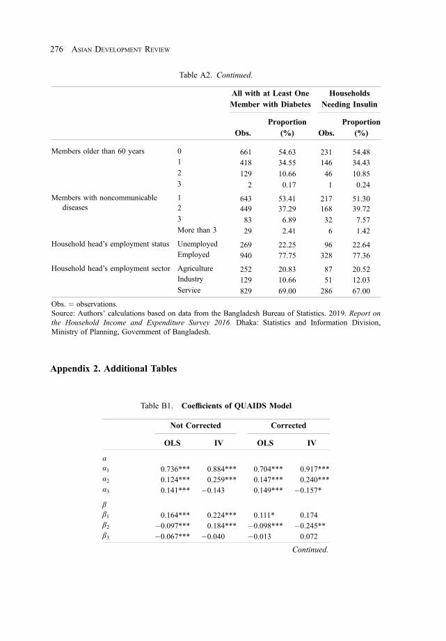
Appendix 2. Additional Tables
Table A2. Continued.
All with at Least OneMember with Diabetes
HouseholdsNeeding Insulin
Obs.Proportion
(%) Obs.Proportion
(%)
Members older than 60 years 0 661 54.63 231 54.481 418 34.55 146 34.432 129 10.66 46 10.853 2 0.17 1 0.24
Members with noncommunicablediseases
1 643 53.41 217 51.302 449 37.29 168 39.723 83 6.89 32 7.57More than 3 29 2.41 6 1.42
Household head’s employment status Unemployed 269 22.25 96 22.64Employed 940 77.75 328 77.36
Household head’s employment sector Agriculture 252 20.83 87 20.52Industry 129 10.66 51 12.03Service 829 69.00 286 67.00
Obs: ¼ observations.Source: Authors’ calculations based on data from the Bangladesh Bureau of Statistics. 2019. Report onthe Household Income and Expenditure Survey 2016. Dhaka: Statistics and Information Division,Ministry of Planning, Government of Bangladesh.
Table B1. Coefficients of QUAIDS Model
Not Corrected Corrected
OLS IV OLS IV
αα1 0.736*** 0.884*** 0.704*** 0.917***α2 0.124*** 0.259*** 0.147*** 0.240***α3 0.141*** �0.143 0.149*** �0.157*
ββ1 0.164*** 0.224*** 0.111* 0.174β2 �0.097*** 0.184*** �0.098*** �0.245**β3 �0.067*** �0.040 �0.013 0.072
Continued.
276 ASIAN DEVELOPMENT REVIEW
March 23, 2022 1:15:21pm WSPC/331-adr 2250009 ISSN: 0116-11052ndReading

Table B1. Continued.
Not Corrected Corrected
OLS IV OLS IV
γγ11 0.064*** 0.034 0.062*** 0.040γ21 �0.041*** 0.012 �0.040*** 0.010γ31 �0.023*** �0.046* �0.022*** �0.050**γ22 0.055*** �0.023* 0.055*** �0.022*γ32 �0.014*** 0.012* �0.015*** 0.011*γ33 0.036*** 0.034 0.036*** 0.039
�
�1 0.005*** �0.030*** 0.006*** �0.030***�2 �0.003*** 0.029*** �0.003*** 0.030***�3 �0.003* 0.002 �0.003** 0.001
ηη Hsize 1 0.001 0.018*** 0.003 0.021**η Hsize 2 0.001 �0.007** 0.000 �0.006*η Hsize 3 �0.003 �0.011** �0.003* �0.015**η AvgAge 1 �0.001** 0.001 �0.001* 0.002η AvgAge 2 0.000 �0.001 0.000 �0.001η AvgAge 3 0.001* �0.000 0.000** �0.001η NumSch 1 �0.011*** �0.050*** �0.012*** �0.047***η NumSch 2 �0.003** 0.011** �0.002 0.011***η NumSch 3 0.014*** 0.039*** 0.013*** 0.036***η old60 1 �0.002 �0.20** �0.004 �0.023**η old60 2 �0.001 0.007* 0.000 0.006η old60 3 0.003 0.012** 0.003 0.017**η NumNCD 1 0.018*** �0.002 0.017*** �0.003η NumNCD 2 �0.009*** 0.005 �0.008*** 0.006η NumNCD 3 �0.009*** �0.003 �0.008** �0.003η HeadAge 1 �0.000 �0.001 0.000 �0.001η HeadAge 2 �0.000 0.000 �0.000 0.000η HeadAge 3 0.000 0.001 0.000 0.001
η HeadEmpl 1 �0.007 �0.050*** �0.004 �0.055***η HeadEmpl 2 0.004 0.026*** 0.002 0.029***η HeadEmpl 3 0.004 0.024* 0.003 0.027**η HeadSector 1 �0.008 �0.017* �0.009 �0.019η HeadSector 2 0.005 0.010* 0.005 0.013**η HeadSector 3 0.003 0.007 0.004 0.006η HeadMuslim 1 �0.014 0.003 �0.012 0.010η HeadMuslim 2 0.012** �0.008 0.011** �0.008η HeadMuslim 3 0.002 0.005 0.001 �0.002η House 1 �0.035*** �0.019 �0.032*** �0.016
Continued.
THE SOCIAL COSTS OF SUCCESS 277
March 23, 2022 1:15:22pm WSPC/331-adr 2250009 ISSN: 0116-11052ndReading

Table B2. Suppliers of Insulin in Bangladesh
Suppliers of Insulin in Bangladesh
Domestic Producers (50 products) Import (65 products)
1. Advanced Chemical Industries Limited 1. Eli Lilly & Company, USA (License expired as of 2016)2. Aristopharma Limited 2. Lilly France S.A.S3. Beximco Pharmaceuticals Ltd. 3. Novo Nordisk A/S4. Drug International Ltd. 4. Novo Noris Producao Pharmaceutica do Brasil Ltd.
Brazil.5. Incepta Pharmaceuticals Ltd. 5. Novo Nordisk Production SAS (License expired
as of 2018)6. Popular Pharmaceuticals Ltd. 6. Sanofi Aventis Deutschland7. Square Pharmaceuticals Ltd.
Source: Government of Bangladesh, Directorate General of Drug Administration.
Table B1. Continued.
Not Corrected Corrected
OLS IV OLS IV
η House 2 0.017** �0.000 0.017** 0.005η House 3 0.018*** 0.019 0.015*** 0.011η Urban 1 �0.016*** �0.035** �0.015*** �0.031η Urban 2 0.002 �0.002 0.003 0.000η Urban 3 0.015*** 0.037*** 0.012*** 0.031*η IMR 1 0.027 0.019η IMR 2 0.008 0.028η IMR 3 �0.036 �0.047
�
� Hsize �0.019 1.230 0.001 0.290� AvgAge �0.006 0.298 �0.003 0.177� NumSch 0.035 �1.266* 0.011 �1.752� old60 0.018 �1.491 �0.006 �0.271� NumNCD 0.190** �0.531 0.126** �0.613� HeadAge �0.001 �0.056 0.000 �0.099� HeadEmpl �0.052 �0.393 �0.016 �1.958� HeadSector �0.069 �0.090 �0.047 �2.001� HeadMulim �0.163 7.168* �0.107 7.748*� house �0.321** 0.220 �0.233** �1.473� Urban �0.037 �1.653 �0.052 �1.832� IMR �0.310* 16.22*
IV ¼ instrumental variable, OLS ¼ ordinary least squares.Source: Authors’ calculations based on data from the Bangladesh Bureauof Statistics. 2019. Report on the Household Income and ExpenditureSurvey 2016. Dhaka: Statistics and Information Division, Ministry ofPlanning, Government of Bangladesh.
278 ASIAN DEVELOPMENT REVIEW
March 23, 2022 1:15:23pm WSPC/331-adr 2250009 ISSN: 0116-11052ndReading

Table B3. Estimates of Insulin Demand Equation
Dependent Variable is Total Expenditure on Insulin
Not Corrected Corrected
Coefficient SE Coefficient SE
p2IV �0.11 0.22 �0.112 0.22�! 0.03 0.02 0.027 0.02AvgAge 7.85* 4.29 7.803* 4.38NumSch �52.94* 32.05 �53.19 32.45old60 �48.42 36.22 �47.94 37.36NumNCD 74.04* 38.54 74.45* 39.34HeadAge 0.65 3.01 0.490 4.32HeadGender �172.700 109.90 �169.0 130.00HeadEduc 12.35 33.64 14.95 59.41HeadEmpl 186.90** 80.60 184.6** 91.51HeadSector 36.74 46.47 33.27 80.14Urban 106.30 78.48 106.5 78.65HeadMuslim 92.49 86.32 95.46 102.90House �28.37 102.40 �23.91 132.50IMR 76.30 1,436.70N 421 421
Adjusted R20.066 0.066
N ¼ number of observations, SE ¼ standard error.Source: Authors’ calculations based on data from the BangladeshBureau of Statistics. 2019. Report on the Household Income andExpenditure Survey 2016. Dhaka: Statistics and InformationDivision, Ministry of Planning, Government of Bangladesh.
THE SOCIAL COSTS OF SUCCESS 279
March 23, 2022 1:15:24pm WSPC/331-adr 2250009 ISSN: 0116-11052ndReading


Institutions and the Rate of Returnon Cattle: Evidence from Bangladesh
KAZI IQBAL, KAZI ALI TOUFIQUE,AND MD. WAHID FERDOUS IBON
¤
This study extends the recent debate on the rate of return on cattle rearing inIndia, triggered by Anagol, Etang, and Karlan (2017) and followed by others,to the Bangladeshi context and finds that the apparent paradox of widespreadcattle rearing despite negative returns in India is absent in Bangladesh. We usea nationally representative two-year panel data for rural Bangladesh and findthat the average and marginal returns on raising cows and bullocks are positiveand high in both 2011 and 2015. We show that appreciation of the value ofcattle is the major contributing factor to positive returns. The existence of cattlemarkets where cattle can be freely traded for slaughter, milk production, or forany other purpose—which is constrained to various degrees in India—is thekey to high and positive returns in Bangladesh.
Keywords: Bangladesh, livestock, poverty, rural development
JEL codes: C23, L25, O12, Q12
I. Introduction
Anagol, Etang, and Karlan (2017) unleashed a debate over raising livestock in
India. They used survey data collected from Uttar Pradesh to estimate returns from
raising livestock and found that the median return to cows was �7%, and 51% and
⁄Kazi Iqbal (corresponding author): Bangladesh Institute of Development Studies (BIDS), Dhaka,Bangladesh. E-mail: [email protected]; Kazi Ali Toufique (deceased): Bangladesh Institute ofDevelopment Studies (BIDS), Dhaka, Bangladesh; Md. Wahid Ferdous Ibon: Department of Economics,University of Dhaka, Bangladesh. E-mail: [email protected].
This is an Open Access article published by World Scientific Publishing Company. It is distributed underthe terms of the Creative Commons Attribution 3.0 International (CC BY 3.0) License which permits use,distribution and reproduction in any medium, provided the original work is properly cited.
March 23, 2022 1:08:05pm WSPC/331-adr 2250007 ISSN: 0116-11052ndReading
Asian Development Review, Vol. 39, No. 1, pp. 281–313DOI: 10.1142/S011611052250007X
© 2022 Asian Development Bank andAsian Development Bank Institute.

45% of households earned negative returns on cows and buffaloes, respectively.
When labor costs were included, they found that more than half of milk cows had
negative returns. This, they claimed, contradicts the fundamental tenets of capitalism
where activities generating negative returns would have been given up. They discussed
a comprehensive list of factors that could explain the puzzle of negative returns:
measurement errors, preference for illiquid savings, insurance, variation of returns
over the years, labor market failures, milk market failures, and social, cultural, and
religious values.
Two subsequent papers joined the debate and added some interesting
dimensions. Attanasio and Augsburg (2018) argued that the data used by Anagol,
Etang, and Karlan (2017) came from a drought year characterized by scarcity of fodder
and lower milk production, resulting in low returns. Attanasio and Augsburg used a
three-year panel data to show that returns were positive in normal years (good rain,
low fodder costs, and higher milk production because of better nutrition) and negative
in drought years (bad rain and high fodder costs). Subsequently, Gehrke and Grimm
(2018) joined the debate to check the generalizability of the results and introduced an
analysis of marginal returns and economies of scale. They also found that most
households operated at unprofitable levels and returns to livestock varied by quality of
cattle, size of stock, and annual rainfall. Those with cattle of better quality had higher
returns and those with a larger herd enjoyed economies of scale due to decreasing
labor costs. To summarize, the debate has generated four main results: returns to
raising livestock are predominantly negative, they vary from one year to another, there
are scale economies with larger farms showing diminishing costs, and cattle of better
quality generate higher returns.
This study contributes to the debate by extending the geographical horizon and
testing the results mentioned above in the context of livestock rearing in Bangladesh.
This shift in geographical focus from India to Bangladesh involves a shift in religious
and cultural beliefs that have relevance for the debate. There are no restrictions on
buying and selling of cows, slaughtering, movement across the country, or on the
consumption of beef in Bangladesh. Unrestricted and widespread markets for cattle
imply that they can be sold at any time in their life cycle, and their value as an asset is
not constrained by trading restrictions. Thus, Bangladesh provides a counterfactual to
India where most states have restrictive cattle trading and slaughtering policies.
We use household-level panel data from the Bangladesh Integrated Household
Survey (BIHS) of the International Food Policy Research Institute (IFPRI), which
is representative of the rural areas of all eight administrative divisions of the country.
For the sake of brevity and clarity, we combine survey years 2011 and 2015 for our
282 ASIAN DEVELOPMENT REVIEW
March 23, 2022 1:08:05pm WSPC/331-adr 2250007 ISSN: 0116-11052ndReading
main analysis. However, we also present results for 2011 and 2015 separately in the
online appendix to highlight year-specific characteristics.1
The key finding of this study is the predominance of positive and high rates of
return to raising cattle (i.e., large ruminants such as bullocks and cows) in
Bangladesh.2 We also find that the average annual return from raising livestock is
31.2% for the combined sample, with a higher return in 2015. These results are also
robust for small ruminants. Our data reveal that appreciation of the value of cattle is
the major contributing factor to large positive returns. Over a period of 12 months, the
value of cattle appreciated by 39%, and this figure is as high as 53% for households
that own only bullocks. In contrast, Anagol, Etang, and Karlan (2017) estimated that
the median value of cows depreciated by 3.1%, while Gehrke and Grimm (2018)
estimated a 40% depreciation in the value of cattle.3
We find that average returns tend to decrease with herd size, reaching a
maximum when herd size is equal to one. Thus, unlike India, there are diseconomies
of scale from livestock rearing in Bangladesh. BIHS data do not provide information
on the breed of the livestock but there is secondary evidence showing that, similar to
India, livestock of better variety generate higher returns in Bangladesh (Jabbar et al.
2005, Kabir and Talukder 1999, Gisby 2010).
Higher returns from raising livestock in Bangladesh are largely due to
appreciation of the market value of livestock. This is particularly true for bullocks
that are raised for their meat value. There is no reason to believe that Bangladeshi
farmers are more “rational” than Indian farmers or face more competitive markets for
milk, fodder, and other inputs and outputs. The difference lies in the cultural and
religious contexts that maximize the market value of cattle in Bangladesh but not in
India. Article 48 of the Constitution of India mandates the state to prohibit the
slaughter of cows and calves and other milk and draft cattle (Ministry of Law and
Justice 2020). Out of 29 states in India, 24 currently have various regulations
prohibiting the slaughter of cows. States such as Kerala, Meghalaya, Mizoram,
and Nagaland have no restrictions on cattle slaughtering. Other factors including
state-level politics may have also constrained the cattle market. For example, in both
1The online appendix can be accessed at: https://www.researchgate.net/publication/354776441_ONLINE_APPENDIX.
2Livestock includes cows (female) and bullocks (male) only. Buffaloes are not included becausethey represent only 6% of the cattle population of Bangladesh. We use the term cattle as consisting of cowsand bullocks only and use it interchangeably with the word livestock.
3The difference in depreciation rates of these two studies is largely driven by the nature of thesample, as the sample of Anagol, Etang, and Karlan (2017) includes a large number of heifers (Gehrke andGrimm 2018).
INSTITUTIONS AND THE RATE OF RETURN ON CATTLE 283
March 23, 2022 1:08:05pm WSPC/331-adr 2250007 ISSN: 0116-11052ndReading

Uttar Pradesh (surveyed by Anagol, Etang, and Karlan 2017) and Andhra Pradesh
(surveyed by Gehrke and Grimm 2018), slaughtering cows is banned, but bullocks and
buffaloes can be slaughtered upon obtaining a “fit-for-slaughter” certificate that the
animal is not economical or is not likely to become economical for the purpose of
breeding or draft/agricultural operations (Citizens for Justice and Peace 2018).
However, transportation of cattle within Uttar Pradesh and between this state and other
states (without permit) is forbidden, but not in Andhra Pradesh. This indicates a wide
variation in institutional setups across states, which may have adversely affected the
performance of the market for buying and selling livestock.
Our study has a bearing on the literature on anti-poverty programs based on asset
(livestock) transfers and the return on capital of microenterprises in developing
countries. There is a growing evidence that suggests that if livestock, generally cows
or goats, are given away to extremely poor households along with a set of
complementary inputs such as skills training, health support, consumption support,
etc., the beneficiaries tend to increase their labor supply and, as a result, their income
and assets likewise increase (Bandiera et al. 2017, Banerjee et al. 2015). In a recent
paper, Banerjee, Duflo, and Sharma (2020) found that such programs also have
substantial long-term impacts. Taking better advantage of opportunities to diversify
into more productive wage employment and migration has been found to contribute to
such successes. However, these studies could not separate the impact of livestock from
other inputs as the interventions were delivered as a bundle. Therefore, the rate of
return on livestock can be very high due to the presence of other complementary
inputs.
The rest of the paper is organized as follows. The next section describes the data
and presents relevant descriptive statistics. Revenue, costs, profit, and average and
marginal returns to raising livestock are estimated in Section III, while heterogeneity
in returns is analyzed in Section IV. We perform robustness checks in Section V.
We discuss overall findings in Section VI, and Section VII draws the conclusions.
II. Context, Data, and Descriptive Statistics
A. Livestock Sector in Bangladesh
The livestock sector plays an integral part of the rural economy of Bangladesh.
About 37.6% of rural households in Bangladesh had at least one livestock in 2015
(IFPRI 2015). It is estimated that about 20% of employment in the rural economy is
284 ASIAN DEVELOPMENT REVIEW
March 23, 2022 1:08:05pm WSPC/331-adr 2250007 ISSN: 0116-11052ndReading

directly associated with the livestock subsector, and this figure is about 50% when we
consider indirect employment (GOB 2018).
Though the livestock sector grew by 3.2% in 2016, its contribution to gross
domestic product (GDP) fell from 2.2% in 2008 to 1.7% in 2016 (GOB 2016).
The contribution of the livestock sector to the overall agriculture sector was almost
static at around 13% during the same period. The number of bovine populations
(cattle, buffalo, goat, and sheep) has increased since 1960, but their growth could not
match the growth of the human population (Huque and Huda 2016). As a result, the
per capita bovine population in Bangladesh declined from 0.4 in 1960 to 0.2 in 2018.
Meat consumption in Bangladesh steadily increased from 11.6 grams per person
per day (g/p/d) in 1995 to 18.6 g/p/d in 2010 (BBS 1995, BBS 2010a). Beef consumption
increased by about 11% between 2010 and 2016 (BBS 2016). Per capita milk
consumption in Bangladesh is about 126 milliliter per person per year which is
significantly lower than other countries in the region (Kabir, Islam, and Reza 2018).
According to the household income and expenditure survey (BBS 2010a), 79% of
Bangladeshi households eat meat no more than two days in a fortnight. Only about
63% of households drink milk and 60% eat eggs in a fortnight (Toufique and Belton
2014).
Existing studies estimating returns from livestock rearing in Bangladesh have
found them to be generally profitable. All the studies estimated returns without taking
into consideration appreciation or depreciation of livestock assets except for the study
undertaken by Gisby (2010).4
B. Data
There are several advantages of using the Bangladesh Integrated Household
Survey (BIHS of the International Food Policy Research Institute [IFPRI] dataset
[IFPRI 2011, IFPRI 2015]). First, the sample is nationally representative of rural
Bangladesh and representative of rural areas of each of the seven administrative
divisions of the country. Second, the BIHS conducted two rounds of surveys in 2011
and 2015 on the same households. We combine them to create household-level panel
data, which allow us to control household-level time-invariant heterogeneity in
estimating marginal returns. Third, since the objective of the survey is to study
agriculture, food security, nutrition, and poverty, detailed data are collected on
4Table A14 of the online appendix lists the names, data, methodology, and main findings of therelevant literature in the context of Bangladesh. Note that the appendix is available as an online supplementdue to space limitations of the journal.
INSTITUTIONS AND THE RATE OF RETURN ON CATTLE 285
March 23, 2022 1:08:05pm WSPC/331-adr 2250007 ISSN: 0116-11052ndReading

livestock raised by households. The survey contains information on livestock
ownership (large/small ruminants and poultry), including the livestock’s current and
last year’s values, revenues, and costs.
It is imperative to discuss whether the 2 sample years are normal years, as
year-specific shocks can influence the rate of return on cattle substantially. Data from the
World Bank’s Climate Change Knowledge Portal (2021) show that the average amounts
of rainfall in 2011 and 2015 were 233.2 and 212 millimeters, respectively. Note that
average rainfall for the period 1990–2015 was 194.8 millimeters, indicating that our
sample years experienced flood, particularly in 2011. However, our data show that only
48 households (4.5% of the working sample) in 2011 and 34 households (3.9% of the
working sample) in 2015 experienced crop loss due to floods. We found that farm
income as a share of total household incomewas 60% in both 2011 and 2015. Hence, the
loss of income due to flood was not significant in our sample. However, the floodwaters
may wash away haystacks and damage grass fields. The market demand for cattle and
milk may also decrease due to floods. But our data show that the rate of appreciation of
cattle value was higher in 2011 than in 2015 (44% versus 33%). However, other factors
such as higher fodder costs and wages for hired labor may lead to an underestimation of
costs to some extent in 2011. If this is the case, we may be estimating some lower
bounds of the rate of return on livestock rearing. This, in fact, corroborates our overall
results that the rate of return on livestock rearing is positive and high in Bangladesh.
The number of households included in the first (2011) and second rounds (2015)
of the BIHS was 4,423 and 4,419, respectively. Out of these households, 41.1%
(1,817) and 37.2% (1,643) owned cattle in the first and second rounds of the surveys,
respectively (Table 1). Farm animals in Bangladesh consist of cattle, buffalo, goat, and
sheep, but in this study, we only considered cattle, which consist of cows and
bullocks. As buffalo is not a common type of livestock in Bangladesh, we dropped
buffalo-owning households from the analysis.5
The BIHS data provide information at the household level only. The data record
the total number of cattle by type (cows, bullocks) for each household, and associated
revenues and costs are also presented in the aggregate. Information on cattle was
collected for the last 12 months in both survey rounds. The BIHS data recorded all
transactions in cattle that resulted in either depletion or accumulation of stock at the
end of the survey year.6
5In the agricultural census of 2008, only 0.7% of rural households reported owning buffaloes (BBS2010b). In the BIHS, only 20 households in 2011 and 10 in 2015 reported owning a buffalo.
6BIHS data provide two data points (beginning and end of the survey year) on size and value ofcattle stock in both rounds of surveys (2011 and 2015).
286 ASIAN DEVELOPMENT REVIEW
March 23, 2022 1:08:05pm WSPC/331-adr 2250007 ISSN: 0116-11052ndReading

The size of the herd can change from the initial period for the following reasons:
(i) sale of cattle, (ii) purchase of a cattle, (iii) exchange of cattle as gift, (iv) lease of
cattle from other households, (v) slaughter of cattle for consumption of meat, and (vi)
loss of cattle due to theft or death. We could only account for cattle sales (i) and loss of
cattle (vi) because the price of cattle sold and the value of cattle lost are reported in the
survey. For cases (ii) to (v), the information to calculate the rate of appreciation and
hence the rate of return on cattle is incomplete. Therefore, we drop cases (ii) to (v) in
our analysis, which leaves us with 1,065 and 884 households in 2011 and 2015,
respectively (Table 1).
To capture the heterogeneity of returns by gender of cattle, we divide all
households with livestock into three categories: (i) households with only bullocks, (ii)
households with only milk cows, and (iii) households with both bullocks and milk
cows (i.e., households with cattle of both gender). Note that Anagol, Etang, and Karlan
(2017) and Gehrke and Grimm (2018) considered milk cows and milk buffaloes only.
C. Descriptive Statistics
We first check whether the households omitted from our sample are different
from the sample households in a systematic way since we had to drop 41% and 46% of
cattle-owning households from our 2011 and 2015 sample, respectively, as shown in
Table 1. The table also shows the number and percentage of households with
livestock, households dropped from the sample, and households in the working sample
for each type of cattle. If the households were dropped in a systematic way, it would
create a selection bias in our sample. To this end, we report in Table 2 the distribution
of the four categories of households that were dropped from the sample due to
incomplete information on purchases, gifts, lease, and home consumption of cattle for
2011 and 2015. The table shows that purchases comprise about 60% of the dropped
sample in both years. The second-largest category at about 21%–23% is leasing. In the
sample of cattle-owning households, only 17% of the households that purchased in
2011 likewise purchased cattle in 2015. Hence, these are not the same households
purchasing cattle in both years. If they were the same households, one could argue that
these households always expand herd size and thus share some common
characteristics that have bearing on returns. This potential “systematic pattern”
could create a bias in our sample. Our data also show that the households that
purchased cattle come from different income groups. About 43% of the dropped
samples are from the first two quintiles of per capita expenditure. As we will see later,
average returns tend to be lower for these lower quintiles. Since the share of the
INSTITUTIONS AND THE RATE OF RETURN ON CATTLE 287
March 23, 2022 1:08:05pm WSPC/331-adr 2250007 ISSN: 0116-11052ndReading

Table
1.Number
ofHou
seholdswithLivestock,Hou
seholdsDropp
ed,an
dHou
seholdsin
WorkingSam
ple
byTyp
eof
Cattle
2011
2015
Hou
seholdswith
No.
ofHHswith
Livestock
No.
ofHHs
Dropped
No.
ofHHsin
WorkingSam
ple
No.
ofHHs
withLivestock
No.
ofHHs
Dropped
No.
ofHHsin
WorkingSam
ple
Onlybu
llocks
641
319
322
593
357
236
(35.27
)(42.42
)(30.23
)(36.09
)(47.0)
(26.70
)
Onlymilk
cows
569
188
381
495
185
310
(31.31
)(25.00
)(35.77
)(30.12
)(24.4)
(35.07
)
Bothbu
llocksandmilk
cows
607
245
362
555
217
338
(33.40
)(32.57
)(33.99
)(33.77
)(28.6)
(38.24
)
All
1,81
775
21,06
51,64
375
988
4(100
.00)
(100
.00)
(100
.00)
(100
.00)
(100
.00)
(100
.00)
HH¼
household.
Note:
The
numbers
inparenthesesarecolumnpercentagesandmay
notsum
upto
100du
eto
roun
ding
.Sou
rce:
Autho
rs’calculations
usingdata
from
theInternationalFoo
dPolicyResearchInstitu
te,“B
angladeshIntegrated
Hou
seho
ldSurvey(BIH
S)
2011–12
,”https://d
ataverse.harvard.edu
/dataset.xhtml?persistentId=hd
l:190
2.1/21
266and“B
angladeshIntegrated
Hou
seho
ldSurvey(BIH
S)20
15,”
https://d
ataverse.harvard.edu
/dataset.xhtml?persistentId=do
i:10.79
10/DVN/BXSYEL(bothaccessed
1June
2018
).
288 ASIAN DEVELOPMENT REVIEW
March 23, 2022 1:08:06pm WSPC/331-adr 2250007 ISSN: 0116-11052ndReading

Table2.
Distribution
ofHou
seholdsDropped
byReason
HHsDropped
Dueto
Incomplete
Inform
ationon
No.
ofHHs
Dropped
in20
11
Percentage
ofHHs
Dropp
edin
2011
(N¼
752)
No.
ofHHs
Dropped
in20
15
Percentage
ofHHs
Dropped
in20
15(N
¼75
9)
1Purchaseof
cattle
441
58.64
468
61.66
2Cattle
received
asgift
618.11
587.64
Cattle
givenas
gift
344.52
212.77
3Lease
ofcattlefrom
otherHHs
174
23.14
159
20.95
4Slaug
hter
ofcattleforow
nconsum
ption
425.59
536.98
Total
752
100.00
759
100.00
HH
¼ho
usehold,
N¼
numberof
households.
Sou
rce:Autho
rs’calculations
usingdatafrom
theInternationalF
oodPolicyResearchInstitu
te,“BangladeshIntegrated
Hou
seho
ldSurvey(BIH
S)
2011–12
,”https://d
ataverse.harvard.edu
/dataset.xhtml?persistentId=hd
l:190
2.1/21
266
and
“Bangladesh
Integrated
Hou
seho
ldSurvey
(BIH
S)
2015
,”https://d
ataverse.harvard.edu
/dataset.xhtml?persistentId=do
i:10.79
10/DVN/BXSYEL(bothaccessed
1June
2018
).
INSTITUTIONS AND THE RATE OF RETURN ON CATTLE 289
March 23, 2022 1:08:06pm WSPC/331-adr 2250007 ISSN: 0116-11052ndReading

dropped sample is not disproportionately higher in these lower quintiles, it lowers the
concern for overestimating the rate of return on cattle. The shares of gifts and home
consumption of cattle are both very low. Those who leased cattle are not owners, so we
drop this group from the sample.
We compare the characteristics of cattle-owning households that are included in
the sample with those that are dropped from the sample in Table 3. There is no
statistically significant difference between the working sample and the dropped
sample in per capita monthly expenditure. This suggests that the two groups are
similar in terms of income status. However, per capita food expenditure per month
was slightly lower in the working sample than the dropped sample in 2011.
The difference was 76 taka (Tk), which could buy about 2 kilograms of rice in 2011.
On the contrary, in 2015, per capita food expenditure was slightly higher for the
working sample at a difference of Tk59. Thus, this difference is not systematic over
the years. These random and meager differences are very unlikely to produce any
selection problems.
Table 3 also shows that the working sample is richer in landownerhip than the
dropped sample. This difference is driven by quintile 1 (lowest) and quintile 5
(highest) of the land distribution. Note that it is the homestead land that determines the
ownership and herd size of the cattle (Table A12 in online appendix). Since there is no
difference in homestead land between our working sample and the dropped sample, the
generalization of our results is less likely to suffer from a sample selection problem.
The fact that the household head is 2 years older than the dropped sample (48 versus
46) in 2015 is less likely to affect the generalization of results.
To further highlight that the working sample compares well with the dropped
sample in farming characteristics, we report the p-value of the mean differences in
Table 4. In particular, we focus on those variables that enter into the calculation of
returns. We observe that there is hardly any difference in the components of revenue
and costs in livestock rearing between these two samples in both years. There is no
statistically significant difference between these two samples in the case of revenues
from manure and milk, and costs of labor and fodder. The cost of fodder is slightly
higher for the working sample than the dropped sample, and the p-value of the mean
difference is 0.097 in 2015.
In short, the socioeconomic and the farming characteristics are very similar for
the working and dropped samples, lending support for the generalization of results of
the working sample. Note that we have a limited set of variables and there might still
be some systematic differences, but we cannot check for those. However, given the set
of variables we have, we are confident that there is no systematic selection bias.
290 ASIAN DEVELOPMENT REVIEW
March 23, 2022 1:08:06pm WSPC/331-adr 2250007 ISSN: 0116-11052ndReading

Table3.
Hou
seholdCharacteristicsof
CattleOwners:
WorkingSam
ple
vs.Dropped
Sam
ple
2011
2015
CattleOwners
(WorkingSam
ple)
CattleOwners
(Dropped
Sam
ple)Difference
inMean
CattleOwners
(WorkingSam
ple)
CattleOwners
(Dropped
Sam
ple)Difference
inMean
Mean
SD
Mean
SD
p-value
Mean
SD
Mean
SD
p-value
Maleho
useholdhead
0.93
0.26
0.92
0.26
0.67
80.92
0.27
0.91
0.27
0.96
9Age
ofho
useholdhead
45.97
13.17
45.03
13.19
0.13
548
.212
.88
45.89
12.8
0.00
0Hou
seho
ldsize
4.6
1.71
4.56
1.83
0.63
24.74
1.79
4.6
1.8
0.10
2Hou
seho
ldhead
isliterate
0.44
0.49
0.41
0.49
0.21
50.45
0.49
0.44
0.49
0.46
2Male–femaleratio
1.25
0.89
71.21
0.88
0.26
81.23
0.87
1.27
0.89
0.32
8Per
capita
food
expend
iture
(Tk,
mon
thly)
1,02
961
31,10
570
70.01
31,05
567
399
662
30.07
0Per
capita
totalexpend
iture
(Tk,
mon
thly)
2,42
72,35
42,53
92,25
20.31
02,51
42,37
52,37
53,24
60.31
8Hom
estead
land
owned(decim
al)
11.01
12.91
10.5
13.45
0.41
610
.41
12.07
9.8
11.54
0.29
7Total
land
owned(decim
al)
97.00
170.00
77.00
129.00
0.00
710
4.00
179.00
85.00
159.00
0.01
9Observatio
ns1,06
575
288
475
9
SD¼
standard
deviation,
Tk¼
Bangladeshtaka.
Notes:Allfigu
resarein
constant
2011
taka.$1
¼Tk7
4.2.
Sou
rce:
Autho
rs’calculations
usingdata
from
theInternationalFoo
dPolicyResearchInstitu
te,“B
angladeshIntegrated
Hou
seho
ldSurvey(BIH
S)20
11–12
,”https://d
ataverse.harvard.edu
/dataset.xhtml?persistentId=hd
l:190
2.1/21
266
and“B
angladesh
Integrated
Hou
seho
ldSurvey(BIH
S)20
15,”
https://d
ataverse.
harvard.edu/dataset.x
html?persistentId=do
i:10.79
10/DVN/BXSYEL(bothaccessed
1June
2018
).
INSTITUTIONS AND THE RATE OF RETURN ON CATTLE 291
March 23, 2022 1:08:07pm WSPC/331-adr 2250007 ISSN: 0116-11052ndReading

Table
4.Characteristicsof
CattleFarming:
Com
parison
betweenDropped
andWorkingSam
ples
WorkingSam
ple
Dropped
Sam
ple
MeanDifference
CattleFarmingVariables
NMean(Tk,yearly)
SD
NMean(Tk,yearly)
SD
p-value
2011
Milk
revenu
e48
210
,164
23,354
.60
286
8,83
6.00
4,27
5.63
0.38
5Manurerevenu
e1,05
31,97
42,19
0.70
670
1,83
0.00
2,44
5.60
0.10
7Fod
dercost
883
4,87
010
,880
.21
619
5,14
3.00
9,32
0.26
0.61
2Fam
ilylabo
rcost
1,05
56,97
45,37
1.44
714
6,76
8.21
4,95
4.18
0.41
5Fam
ilylabo
rcost:male
895
4,34
85,08
7.90
628
4,13
8.33
3,91
0.29
0.38
5Fam
ilylabo
rcost:female
994
3,48
72,25
4.42
679
3,28
9.59
2,82
0.85
0.113
Wagelabo
r23
8,75
115
,038
.26
712
,736
.36
16,739
.37
0.49
1Wagelabo
r:male
218,93
715
,293
.28
712
,736
.36
16,739
.37
0.52
3
2015
App
reciation
884
6,35
612
,276
.13
260
11,342
18,937
.60
0.64
4Manurerevenu
e76
51,54
01,69
2.97
400
1,59
82,93
4.97
0.64
3Fod
dercost
725
4,69
47,56
8.19
600
4,113
8,49
8.93
0.09
7Fam
ilylabo
rcost
882
3,86
42,02
6.66
732
3,79
62,119.95
0.25
8Fam
ilylabo
rcost:male
800
2,55
21,62
2.45
655
2,50
01,69
6.87
0.27
8Fam
ilylabo
rcost:female
846
1,61
499
4.75
710
1,54
595
9.92
0.08
5Wagelabo
r7
3,58
83,05
3.30
34,54
13,87
3.91
0.66
4Wagelabo
r:male
73,58
83,05
3.30
34,54
13,87
3.91
0.66
4
SD¼
standard
deviation,
Tk¼
Bangladeshtaka.
Notes:Allmon
etaryfigu
resarein
constant
2011
taka.$1
¼Tk7
4.2.
Nis
thenu
mberof
households
with
positiv
evalues
forvariou
scattle
farm
ingvariables.The
samplesize
offemalewagelabo
ristoosm
allto
estim
atethep-valueof
themeandifference.
Sou
rce:
Autho
rs’calculations
usingdata
from
theInternationalFoo
dPolicyResearchInstitu
te,“B
angladeshIntegrated
Hou
seho
ldSurvey
(BIH
S)20
11–12
,”https://d
ataverse.harvard.edu
/dataset.xhtml?persistentId=hd
l:190
2.1/21
266and“B
angladeshIntegrated
Hou
seho
ldSurvey
(BIH
S)20
15,”
https://d
ataverse.harvard.edu
/dataset.xhtml?persistentId=do
i:10.79
10/DVN/BXSYEL(bothaccessed
1June
2018
).
292 ASIAN DEVELOPMENT REVIEW
March 23, 2022 1:08:08pm WSPC/331-adr 2250007 ISSN: 0116-11052ndReading

Next, we present the main characteristics of cattle farming of the sample
households in Table 5.7 The BIHS collected information on the current value of
livestock as well as their value a year before as reported by respondents. The values of
the stock per household at the end of the reference periods were Tk33,810 in 2011 and
Tk37,089 in 2015, respectively, in real terms, and the average values of the stock at the
end of the reference period were Tk15,581 and Tk16,411, respectively. The increase in
average value of the stock may indicate that the quality of cattle increased between the
survey years. The herd size is highest for those with both milk cows and bullocks.
On the other hand, herd size is slightly higher for those with only bullocks than those
with only milk cows. This indicates that many households raise livestock to slaughter
for meat production. In both cases, the herd size increased during the survey periods.
The herd size of mixed farms slightly declined.
Table 5 also presents the components of revenues and costs. Note that average
appreciations (i.e., meat value), defined as the average of the change in the value of the
stock between the initial and terminal periods are reported in detail in Table 6. Average
revenue from selling milk increased between the survey years, by 6.4% in real terms
for households with positive milk revenue. However, the contribution of manure as a
source of revenue decreased over time. Fodder contributed the most in the cost of
rearing livestock in Bangladesh. Average fodder cost was about Tk4,870 in 2011 and
Tk4,694 in 2015 for households with positive fodder costs. The decrease in fodder
costs is not statistically significant. Wage labor was hired by only a few households.
Family labor was mostly employed in these farms. We observe that family labor costs
have declined in real terms and no clear explanation can be given. Female family
members worked more hours on cattle rearing than male members. In 2015, male
members spent about 368 hours compared to 417 hours by female members.
At the outset, it is important to note that we do not make the returns based on
imputed values of family labor salient in our discussion of results. There are two major
reasons, which are explained in the following. The explanation also sheds light on why
returns are consistently low and negative in most cases in 2011 while high and positive
in 2015 when we value family labor at market price.
First, the households in our sample are smallholders—the average cattle size is
about 2.2 in 2011 and 2.3 in 2015. Thus, the time that households spend per day to
take care of the cattle is also very low. Our data show that time spent by male members
of a household on livestock in a year is 368 hours, that is, about one hour per day.
7Note that we also present household characteristics of the cattle owners and nonowners in theonline appendix in Table A1.
INSTITUTIONS AND THE RATE OF RETURN ON CATTLE 293
March 23, 2022 1:08:08pm WSPC/331-adr 2250007 ISSN: 0116-11052ndReading

Table
5.Characteristicsof
CattleFarming,
2011
and20
15
2011
2015
MeanDifference
CattleFarmingVariables
NMean
SD
NMean
SD
p-value
Value
ofstockof
cattleperHH
(Tk)
1,06
533
,810
.00
29,547
.00
884
37,089
.00
30,294
.17
0.02
6Average
cattlevalue(Tk)*
1,06
515
,581
.00
8,44
4.29
884
16,411.00
8,94
1.44
0.03
5Herdsize:on
lybu
llocks
322
1.91
1.19
236
2.03
1.48
0.28
3Herdsize:on
lymilk
cows
381
1.72
1.00
310
1.91
1.39
0.03
7Herdsize:bo
thmilk
cowsandbu
llocks
362
2.87
1.66
338
2.73
1.52
0.25
0Herdsize:all
1,06
52.17
1.41
884
2.26
1.51
0.18
1Milk
revenu
e(Tk,
yearly)
482
10,164
.00
23,354
.60
486
10,811.00
18,462
.54
0.63
2Manurerevenu
e(Tk,
yearly)
1,05
31,97
4.00
2,19
0.70
765
1,54
0.00
1,69
2.97
0.00
0Revenue
from
calves
(Tk,
yearly)
391
8,46
7.00
3,08
8.34
327
8,28
8.00
3,06
0.95
0.43
6Fod
dercost(Tk,
yearly)
883
4,87
0.00
10,880
.21
725
4,69
4.00
6,56
8.19
0.70
3Value
ofcattlelost(Tk,
yearly)
1529
,833
.00
36,941
.88
616
,912
.00
15,183
.65
0.42
2Fam
ilylabo
rcost(Tk,
yearly)*
1,05
56,97
4.00
5,37
1.44
882
3,86
4.00
2,02
6.66
0.00
0Fam
ilylabo
rcost:male(Tk,
yearly)*
895
4,34
8.00
5,08
7.90
800
2,55
2.00
1,62
2.45
0.00
0Fam
ilylabo
rcost:female(Tk,
yearly)*
994
3,48
7.00
2,25
4.42
846
1,61
4.00
994.75
0.00
0Total
timespenton
livestock
inayear
(hou
rs)
1,06
066
7.00
488.86
883
794.00
397.72
0.00
0Malefamily
timespenton
livestock
inayear
(hou
rs)
895
367.00
425.53
884
368.00
273.54
0.93
8Fem
alefamily
timespenton
livestock
inayear
(hou
rs)
994
364.00
232.93
884
417.00
277.41
0.00
0Total
family
timespenton
livestock
inayear
(hou
rs)
1,05
565
5.00
465.82
882
788.00
395.40
0.00
0Hired
timespenton
livestock
inayear
(hou
rs)
2272
9.00
599.37
785
1.00
659.68
0.65
0
Con
tinued.
294 ASIAN DEVELOPMENT REVIEW
March 23, 2022 1:08:10pm WSPC/331-adr 2250007 ISSN: 0116-11052ndReading

Table
5.Con
tinued.
2011
2015
MeanDifference
CattleFarmingVariables
NMean
SD
NMean
SD
p-value
Num
berof
calves
391
1.18
0.43
327
1.15
0.43
0.43
6Total
valueof
cattlesold
(Tk,
yearly)
141
27,732
.00
19,846
.02
153
26,389
.00
25,062
.70
0.61
2Wagelabo
r(Tk,
yearly)
238,93
7.00
15,038
.26
73,58
8.00
3,05
3.30
0.38
0Wagelabo
r:male(Tk,
yearly)
218,75
1.00
15,293
.28
73,58
8.00
3,05
3.30
0.37
2Wagelabo
r:female(Tk,
yearly)
22,42
5.00
813.17
0...
...
...
*¼
calculated
values
(not
repo
rted
values),...¼
data
notavailable,
HH¼
household,
SD¼
standard
deviation,
Tk¼
Bangladeshtaka.
Notes:A
llmon
etaryfigu
resarein
constant
2011
taka.$
1¼
Tk7
4.2.
The
valueof
thestockof
cattleperho
useholdisdefinedas
thetotalv
alue
ofcattle
ownedby
allsampleho
useholds
dividedby
thenu
mberof
sampleho
useholds.Average
cattlevalueisdefinedas
thetotalvalueof
thestockof
cattle
ownedby
thesampleho
useholds
dividedby
thenu
mberof
cattle.
Nis
thenu
mberof
households
with
positiv
evalues
forvariou
scattlefarm
ing
variables.
Sou
rce:
Autho
rs’calculations
usingdata
from
theInternationalFoo
dPolicyResearchInstitu
te,“B
angladeshIntegrated
Hou
seho
ldSurvey(BIH
S)
2011–12
,”https://d
ataverse.harvard.edu
/dataset.xhtml?persistentId=hd
l:190
2.1/21
266and“B
angladeshIntegrated
Hou
seho
ldSurvey(BIH
S)20
15,”
https://d
ataverse.harvard.edu
/dataset.xhtml?persistentId=do
i:10.79
10/DVN/BXSYEL(bothaccessed
1June
2018
).
INSTITUTIONS AND THE RATE OF RETURN ON CATTLE 295
March 23, 2022 1:08:10pm WSPC/331-adr 2250007 ISSN: 0116-11052ndReading

Literature suggests that time spent on livestock does not hamper regular work in farm
or nonfarm employment. Typically, the time is spent on taking cattle to the grass field,
bathing, feeding, etc., which the male members do in between their regular work or
after work (Gisby 2010). Hence, the opportunity costs of time spent on livestock is
negligible. Gisby (2010, 22) noted “The majority of those looking after cattle stated
that they would be ‘idle’ in the absence of having to care for cattle.” The household
members do not have to give up any remunerated work time for taking care of cattle.
Hence, monetized family labor is negligible in our analysis.
Second, hourly wage of hired labor is what makes the returns in 2011
significantly lower than the returns in 2015. Note that male wage rates in 2011 and
2015 were Tk11.9 and Tk4.2 per hour, respectively. Female wage rate in 2011 was
Tk9.6 per hour. These lead to yearly labor costs of Tk8,751 in 2011 and only Tk3,588
in 2015 (Table 5). Thus, when we use these figures to impute the costs of family labor,
the figures for 2011 inflate. Our inspection of the data suggests that there are several
“large values” that are driving the very high wage rates in 2011. The standard
deviation of total wages in 2011 was Tk15,038 whereas it was only Tk3,053 in 2015.
We checked wage-related information from the BIHS employment module: the
average hourly wage in employment in livestock was about Tk4 in 2011 and Tk4.8 in
2015. This indicates that the hourly wage in 2015 is a more plausible figure than that in
2011. The survey of literature on Bangladesh (Table A14 in the online appendix) for
the period 2010–2014 suggests that hired labor costs were much lower than in the
BIHS data.8
III. Returns to Cattle Holding
The return to livestock comprises two parts: (i) the flow of profits from the sale of
livestock products such as milk or manure, and (ii) the appreciation or depreciation
of the value of livestock. We follow the empirical specification given by Gehrke and
Grimm (2018). Let the production function of a household from raising livestock be:
Q ¼ Af (K, L,X,F): ð1Þ
8Gisby (2010) found that monthly family labor cost (if paid for the opportunity cost of raising asingle livestock) varies from Tk108 to Tk295 based on cattle type and variety. Halim et al. (2010) recordeda family labor cost of Tk4,877 per year per cattle. Mondal, Sen, and Rayhan (2010) estimated an averagetotal labor (both family and hired) cost of Tk11.4 and Tk20.2 per cow per day for local-variety andcrossbred cows, respectively.
296 ASIAN DEVELOPMENT REVIEW
March 23, 2022 1:08:10pm WSPC/331-adr 2250007 ISSN: 0116-11052ndReading

In this production function,Q ¼ milk, calves, andmanure;K ¼ current/end period value
of cattle; L ¼ labor; X ¼ land; F ¼ fodder; and A ¼ household- and region-specific
characteristics that influence the total factor productivity (TFP) of the inputs. Gehrke
and Grimm (2018) lumped X and F together and noted that land entered into the
production function through F. Since we have data on homestead land, we treat X and
F separately. Note that in the case of bullocks, the production function becomes trivial
as Q includes only revenue from manure. The profit function is given by:
� ¼ P � Q� cK � wL� gF � rX � Sþ δK, ð2Þwhere P ¼ price of outputs; w ¼ wage rate (both market and imputed); g ¼ price of
fodder; r ¼ rent of land; c ¼ other costs associated with K (medical, purchase, or sale
of related costs, etc.); S is the value of cattle lost; and δ ¼ rate of appreciation/
depreciation.9 Following Gehrke and Grimm (2018), we assume the price of capital to
be zero. We also assume that the rental value of land, r, is equal to 0. We first calculate
the household-level annual profit and then estimate average and marginal returns of
raising livestock. The following equation shows the average return on raising livestock:
�
K¼ P � Q
K� c� wL
K� gF
K� S
Kþ δ: ð3Þ
Following Gehrke and Grimm (2018), we estimate marginal returns using both linear
production and Cobb–Douglas production technology, using pooled OLS and panel
fixed effects (FE). First, with the linear production function, we estimate profit (�it) as a
function of the value of herd size (value of the livestock, K) and several control variables
at the household level:
�it ¼ α0 þ α1 log (Kit)þ α2(Xit)þ eit, ð4Þwhere i and t stand for households and time, respectively. Xi includes labor cost,
homestead land owned, fodder cost, herd size, and a year dummy. α1 is the marginal
return of holding livestock of value K for a one-year period. Second, we use a
Cobb–Douglas production technology to estimate marginal return. The marginal return
of this type of production function is the first derivative of equation (2) with respect toK:
� 0(Kit) ¼ P � Q 0(Kit)� cþ δ: ð5Þ
9δ ¼ (K � K0)=K0, where K0 is the value of the cattle stock at the initial period and K is the endperiod value of the same stock. For households with constant herd sizes between the two survey periods,calculation of the rate of appreciation/depreciation is straightforward (δ ¼ (K � K0)=K0). In cases withnonconstant herd sizes and households with calves, calculation of δ involves several intermediate stepsdescribed in the online appendix.
INSTITUTIONS AND THE RATE OF RETURN ON CATTLE 297
March 23, 2022 1:08:10pm WSPC/331-adr 2250007 ISSN: 0116-11052ndReading

If Q is a Cobb–Douglas production function such that
Qit ¼ A � K α1it L
α2it F
α3it , ð6Þ
where all parameters lie strictly between 0 and 1. We get α1 from the following
logarithmic transformation of the production function in equation (6):
log (PQit) ¼ α0 þ α1 logKit þ α2 log Lit þ α3 logFit þ α4Xit þ 2it, ð7Þwhere Xit includes log of homestead land, herd size, and a year dummy. We then plug in
the estimated value of α1 into equation (5) and get the marginal return from raising
livestock in the following form:
� 0(Kit) ¼ P � α1 �Qit
Kit� cþ δ: ð8Þ
A. Appreciation and Depreciation
In Anagol, Etang, and Karlan (2017), the price of a cattle, P(t), is reported by the
farmer. They used self-reported values of dairy animals to establish a relationship
between cattle values and age. This helped them to estimate appreciation as the
difference in cattle values over a period of one year, P(t)� P(t � 1). On the other
hand, Attanasio and Augsburg (2018) could not estimate depreciation because their
data did not contain information on the age of livestock, although they had information
on the value of livestock. Gehrke and Grimm (2018) did not follow Anagol, Etang,
and Karlan (2017) on the estimation of appreciation or depreciation of cattle because
they also did not have information on age. Instead, Gehrke and Grimm (2018) used
information from secondary sources and assumed that a cow depreciates by 1,240
Indian rupees (�) (US$27) every year, and that the end-of-fertility value of a cow
is �1,400 (US$30), which is based on an annual depreciation of 20%.
The approach taken by these papers for estimating appreciation reflects the
institutional setup that exists in the respective Indian states: “Since cattle cannot be
sold for slaughter, this implies that the value of a cow will be zero once it is no longer
of reproductive age” (Gehrke and Grimm 2018, 682). This rationalized the use of age
as an appropriate indicator for estimating appreciation (Anagol, Etang, and Karlan
2017), the use of secondary sources of information (Gehrke and Grimm 2018), or
ignoring measurement of depreciation altogether (Attanasio and Augsburg 2018).
Our method of estimating appreciation is similar to Anagol, Etang, and Karlan
(2017) in the sense that we take the difference between initial and terminal values of
cattle as appreciation, and then divide the difference by the initial value to get the rate
of appreciation. The BIHS data include, for each year, the current value of cattle and
298 ASIAN DEVELOPMENT REVIEW
March 23, 2022 1:08:11pm WSPC/331-adr 2250007 ISSN: 0116-11052ndReading

their value in the previous 12 months, as reported by the respondents. This is
appropriate in the Bangladeshi context where there is no restriction on selling cattle for
slaughter. The value of livestock depends not only on age but also on other factors
such as weight of cattle, location, and time. Market conditions may also change
between the initial and terminal period, and the appreciation rate may reflect these
market conditions. These factors are incorporated by the respondents while reporting
the value of their cattle. The BIHS data do not present information on age, weight, or
breed of the cattle and hence we could not estimate the relationship between these
factors and the value of cattle. We would expect these to be incorporated by the
respondent while valuing the livestock. Dependence on self-reported values of cattle
likely involves overreporting by the sellers as they have private information on the
quality of the cattle that is not available to the buyers. This problem is less acute when
cattle are sold for slaughter, as weight is more visible than the potential milk
production of a cow. We also think that any bias that is generated from reported values
of cattle by the respondents is carried over to the next period and thus can cancel out
when estimating how much the cattle stock has appreciated. This asymmetric
information is not handled adequately in existing studies and this study is no
exception. As mentioned before, we have information on the value of cattle sold
during the reference period. We have considered that value as the end period value of
the cattle.
B. Revenue
The BIHS data provide information on three items of revenue: milk, manure, and
calves.
1. Milk and Manure
Households report value and quantity of milk and manure sold in the last 12
months. We consider net milk production by accounting for the amount of spoil.
We used two sets of prices to determine the value of milk. For households who sold
milk in the market, we estimated the price by dividing the value of the milk sold by the
quantity of milk sold. About 53% and 55% of households sold milk in the market in
2011 and 2015, respectively. For households that consumed all the milk they
produced, they provided information on the value of that milk consumed and this
allowed us to determine the market price. Though Anagol, Etang, and Karlan (2017)
mentioned that households may value their milk higher than the price it can fetch in
the market, we find that there is hardly any difference between the self-reported price
INSTITUTIONS AND THE RATE OF RETURN ON CATTLE 299
March 23, 2022 1:08:11pm WSPC/331-adr 2250007 ISSN: 0116-11052ndReading

and market price. This is true for the full sample as well as for all eight administrative
divisions in the country. The BIHS data also provide information on manure.
The BIHS data lumped together revenues from manure and milk by aggregating
small ruminants such as goat and sheep and large ruminants. It is therefore not possible
to separate milk and manure revenues for households that raise both cattle and small
ruminants. About a quarter of households who own cattle also have small ruminants.
However, milk revenues from small ruminants are very small: they comprise 6% and
9% of average milk revenues for 2011 and 2015, respectively. Small ruminants, on the
other hand, hardly have any relevance to manure revenue.
2. Calves
The BIHS data provide information on the number of calves born in the last
12-month period, but not calves’ market price. We take the calf price to be Tk7,151 in
both 2011 and 2015 from the data collected for the Final Impact Evaluation Survey of
the Second Participatory Livestock Development Project (BIDS 2010). We consider
the calves as a separate component of revenue in the return calculation; they are not
part of herd size.
C. Costs
Unlike revenue, cost data are presented by type of livestock. Three components
of costs are recorded: feed or fodder, medicine or treatment, and labor costs.
1. Fodder
Fodder is a major component of the costs of raising livestock in Bangladesh.
With the gradual diminishing of grazing grounds and other common property
resources, most of the cattle in Bangladesh are stall-fed. Common items of fodder are
straw, green grass, and concentrate. The BIHS data do not provide any information on
collected or home-produced fodder and report the value of purchased fodder only.
Halim et al. (2010) have found that home-produced and collected fodder comprise
about 20% of total purchased fodder when valued at market price. We used this
information to inflate fodder costs by 20% and estimate average and marginal returns.
2. Labor
The BIHS data provide labor use and labor cost information by gender as well by
source (family and hired). Labor use is presented as the number of hours spent on
300 ASIAN DEVELOPMENT REVIEW
March 23, 2022 1:08:11pm WSPC/331-adr 2250007 ISSN: 0116-11052ndReading

raising livestock. Family labor is unpaid but hired labor is paid, and the BIHS records
information on hired labor cost. About 98%–99% of labor time used in livestock
farming is provided by family labor. Thus, we present labor cost in two ways: (i) assume
it is 0 for family labor and (ii) monetize family labor. The process of monetizing family
labor is described in the online appendix. Table 6 presents the breakdown of costs and
revenue for three different types of households for the 2 years combined.
As is evident from Table 6, the highest stock appreciation is observed for the
households who only raise bullocks; within a year, the average value of their stock
increases by more than half, and this is true for both years (Tables A2 and A3 in the
online appendix). Relative appreciation is similar (higher for bullocks) to those found
by Gisby (2010) who found that bulls appreciated more than cows, both the local
variety (13% compared to 6%) as well as the crossbred variety (21% compared to 12%).
For the full sample, the average annual appreciation at the household level was 39%.
As expected, the share of milk revenue is highest for households with only milk
cows. Fodder and family labor are the major cost components for all household
categories. Cost and revenue components are similar in 2011 and 2015.
D. Profits and Average and Marginal Returns
Profit from raising livestock is positive (excluding family labor cost) in all
categories in the combined sample (Table 7) as well as for both 2011 and 2015
(Tables A4 and A5 in the online appendix). Once family labor is valued at market
price, profit decreases considerably and becomes negative for households with
bullocks only. The value of calves and the revenue from selling cattle (Table 5)
increase the profits for households with only milk cows and those selling cattle,
respectively.
Both average and marginal returns are positive for the combined sample in both
years except for the average return (with family labor) in 2011. For all household
categories together, the average return (without family labor) from holding cattle is
31.2%. Marginal return using the Cobb–Douglas production function is positive and
high at about 48% (Table 7).10 Intuitively, the annual return from investing an
additional one dollar to the existing stock is about 48 cents.11
10We are aware that the value of herd size (K) can be endogenous due to simultaneity bias. Higherprofit from livestock rearing can motivate households to raise certain breeds and thus affect the value of K.Due to lack of valid instruments, we did not consider instrumental variables estimation.
11See Table A10 of the online appendix for the regressions to estimate the marginal returns ofcapital stock.
INSTITUTIONS AND THE RATE OF RETURN ON CATTLE 301
March 23, 2022 1:08:11pm WSPC/331-adr 2250007 ISSN: 0116-11052ndReading

Table
6.Com
pon
ents
ofRevenuean
dCost(C
ombined
Tab
lefor20
11an
d20
15)
Revenue
Costs
Appreciation
Initial
Period
CattleValue
(K0)
EndPeriod
Cattle
Value
(K1)
(K1�K
0)*1
00=(K
0)Milk
(Tk)
Man
ure
(Tk)
Calf
(Tk)
Wag
eLab
or(Tk)
Fam
ilyLab
or(Tk)
Purchased
and
Non
purchased
Fod
der
Cost(Tk)
Medicine
andOther
Cost(Tk)
Valueof
Cattle
Lost(Tk)
Hou
seho
ldswith
only
bullo
cks(N
¼55
8)19
,184
29,351
53NA
1,39
6NA
545,13
03,88
429
254
9
Hou
seho
ldswith
only
milk
cows(N
¼69
1)21
,039
30,086
436,36
91,56
03,67
327
5,41
94,26
738
135
0
Hou
seho
ldswith
both
bullo
cksandmilk
cows(N
¼70
0)
34,022
42,187
248,21
82,00
04,97
524
05,94
15,89
751
30
Fullsample(N
¼1,94
9)24
,620
34,222
395,20
91,67
13,08
9111
5,52
44,74
340
328
1
N¼
numberof
households,NA
=no
tapplicable,Tk¼
Bangladeshtaka.
Notes:$1
¼Tk7
4.2.
App
reciation(depreciation)
istherealrateof
increase
(decrease)
ofthecattlestockin
12mon
ths.Allrevenu
eandcostcompo
nentsare
theaveragenu
mbers
forthesampleho
useholds
(N¼
1,94
9 ).Non
purchasedfodd
ercosthasbeen
assumed
as20
%of
thepu
rchasedfodd
ercost.
Sou
rce:Autho
rs’calculations
usingdatafrom
theInternationalFoo
dPolicyResearchInstitu
te,“BangladeshIntegrated
Hou
seho
ldSurvey(BIH
S)20
11–12
,”https://d
ataverse.harvard.edu
/dataset.xhtml?persistentId=hd
l:190
2.1/21
266and“B
angladeshIntegrated
Hou
seho
ldSurvey(BIH
S)20
15,”
https://d
ataverse.
harvard.edu/dataset.x
html?persistentId=do
i:10.79
10/DVN/BXSYEL(bothaccessed
1June
2018
).
302 ASIAN DEVELOPMENT REVIEW
March 23, 2022 1:08:11pm WSPC/331-adr 2250007 ISSN: 0116-11052ndReading

Table
7.Average
andMarginal
Returnsfrom
RaisingLivestock
(Com
bined
Tab
lefor20
11an
d20
15)
Total
Annual
Profit(Tk)
Average
Return
(%)
With
Fam
ilyLab
orWithou
tFam
ilyLab
orWithFam
ilyLab
orWithou
tFam
ilyLab
orMarginal
Return
Hou
seho
ldswith
only
bullo
cks
(N¼
558)
�3,101
2,02
8�1
8.22
8.28
0.54
Hou
seho
ldswith
only
milk
cows
(N¼
691)
5,67
311,092
13.79
40.09
0.54
Hou
seho
ldswith
both
bullo
cksand
milk
cows(N
¼70
0)8,21
814
,159
20.75
40.67
0.37
Fullsample(N
¼1,94
9)4,07
59,59
97.12
31.19
0.48
N¼
numberof
households,Tk¼
Bangladeshtaka.
Notes:$
1¼
Tk7
4.2.
“With
family
labo
r”im
pliesmon
etized
valueof
family
labo
r,and“w
ithou
tfam
ilylabo
r”im
plieson
lyhired
labo
rcosts.
Sou
rce:
Autho
rs’calculations
using
data
from
theInternationalFoo
dPolicy
Research
Institu
te,“B
angladesh
Integrated
Hou
seho
ldSurvey(BIH
S)20
11–12
,”https://d
ataverse.harvard.edu
/dataset.xhtml?persistentId=hd
l:190
2.1/21
266and“B
angla-
desh
Integrated
Hou
seho
ldSurvey(BIH
S)20
15,”
https://d
ataverse.harvard.edu
/dataset.xhtml?persistentId=do
i:10.79
10/DVN/
BXSYEL(bothaccessed
1June
2018
).
INSTITUTIONS AND THE RATE OF RETURN ON CATTLE 303
March 23, 2022 1:08:12pm WSPC/331-adr 2250007 ISSN: 0116-11052ndReading

IV. Heterogeneity in Average and Marginal Returns
In this section, we discuss the heterogeneity of returns from two aspects: (i) herd
size and (ii) household food expenditure. For the first aspect, we explore if there are
any economies of scale in herd size; and for the second, we check whether rates of
return change for different poverty groups as indicated by household food expenditure
quintiles (including home-produced food expenditure).
Table 8 shows that for both survey years combined, average return is maximized
at herd size one and minimized at herd size four when family labor cost is not
monetized. However, when we value family labor at market price, no systematic
patterns exist in the relationship between average returns and herd size. This is true for
2011 (Table A6 in the online appendix). But we find that even if we consider family
labor, we observe the highest average returns at herd size one in 2015 (Table A7 in the
online appendix). Thus, it appears that there are no economies of scale in raising
livestock in Bangladesh. To shed more light on this issue, we examine the sources of
the costs of rearing that can potentially lead to economies of scale and whether such
costs were incurred in large amounts in the context of rural Bangladesh. Cattle rearing
involves the following cost components: fodder, medicine, space, and hired labor to
take care of the cattle. Consider fodder and medicine first. The per unit cost (the cost
for one cow or bullock) of fodder and medicine is unlikely to vary much with herd size
since these costs are very specific to each animal. In the case of space in the homestead
where cattle are housed, there is scope for economies of scale. However, for a small
herd size, which is about 2.2 animals, additional cattle may cost little in terms of
Table 8. Herd Size and Returns (Combined Table for 2011 and 2015)
Herd Size
Average Valueof Total
Stock (Tk)
Average Returnwith FamilyLabor (%)
Average Returnwithout FamilyLabor (%)
MarginalReturn Observations
1 17,130 7.4 41.04 0.58 7422 15,804 7.97 29.62 0.48 6083 14,492 6.32 23.11 0.34 3174 14,839 2.4 17.62 0.47 152> 4 14,856 9.03 17.87 0.25 130
Tk ¼ Bangladesh taka.Note: $1 ¼ Tk74.2.Source: Authors’ calculations using data from the International Food Policy Research Institute,“Bangladesh Integrated Household Survey (BIHS) 2011–12,” https://dataverse.harvard.edu/dataset.xhtml?persistentId=hdl:1902.1/21266 and “Bangladesh Integrated Household Survey (BIHS) 2015,”https://dataverse.harvard.edu/dataset.xhtml?persistentId=doi:10.7910/DVN/BXSYEL (both accessed 1June 2018).
304 ASIAN DEVELOPMENT REVIEW
March 23, 2022 1:08:12pm WSPC/331-adr 2250007 ISSN: 0116-11052ndReading

extending the space or house. Moreover, this cost is a fixed cost, which is not
considered in the costing exercise. Hired labor is the potential source of economies of
scale—the average cost of taking care of the cattle may drop significantly with herd
size, particularly for smaller sizes. However, only 22 households in 2011 and 7
households in 2015 used hired labor for cattle rearing. Hence our finding of no
economies of scale in cattle rearing by smallholders is not implausible.
Poorer households raise more livestock. Table 9 shows that in the combined
sample, the incidence of livestock rearing by households in the bottom quintile (Q1) is
more than twice of those households in the top quintile (Q5). We find that although
poorer households raise more livestock, they earn a lower annual return than their
richer counterparts (Q4 and Q5). To examine further, we regress the incidence of cattle
rearing and herd size on the quintiles of food consumption, controlling for other
covariates. The results show that the lower quintiles are more likely to raise cattle and
have lower herd size. The results for 2011 and 2015 are reported in Tables A8 and A9
of the online appendix.
V. Robustness Check
Since we have dropped a large sample for which we could not calculate the
appreciation rate, we use the working sample’s average appreciation rates of cattle to
Table 9. Livestock Variables and Per Capita Food Expenditure Quintiles (Combined Tablefor 2011 and 2015)
Per CapitaFoodExpenditureQuintiles (Q)
% of HHswith
LivestockHerdSize
AverageValue ofTotal
Stock (Tk)
AverageReturnwithoutFamily
Labor (%)
AverageReturnwith
FamilyLabor (%)
MarginalReturn
Q1 56.70 2.31 14,298 28.10 4.14 0.46Q2 43.27 2.17 15,075 30.76 6.36 0.49Q3 36.01 2.20 15,220 27.92 3.45 0.45Q4 32.35 2.16 16,777 34.51 9.35 0.59Q5 27.32 2.21 18,421 34.67 12.32 0.39
Tk ¼ Bangladesh taka.Note: $1 ¼ Tk74.2.Source: Authors’ calculations using data from the International Food Policy Research Institute,“Bangladesh Integrated Household Survey (BIHS) 2011–12,” https://dataverse.harvard.edu/dataset.xhtml?persistentId=hdl:1902.1/21266 and “Bangladesh Integrated Household Survey (BIHS) 2015,”https://dataverse.harvard.edu/dataset.xhtml?persistentId=doi:10.7910/DVN/BXSYEL (both accessed 1June 2018).
INSTITUTIONS AND THE RATE OF RETURN ON CATTLE 305
March 23, 2022 1:08:13pm WSPC/331-adr 2250007 ISSN: 0116-11052ndReading

impute the rates for the dropped sample as a robustness check. These appreciation
rates are 0.4 for 2011 and 0.3 for 2015. With these imputed rates, the average returns
without monetizing family labor are 25.6% in 2011 and 36.8% in 2015 for the dropped
sample (Table A13 in the online appendix). These two rates compare very well with
the appreciation rates of the working sample for both years. The marginal returns of
livestock rearing for both working and dropped samples are also very similar.
In the context of rural Bangladesh, households depend less on the market
for fodder. We find that our results of high average returns are robust to accounting for
imputed fodder costs. All the above rates of returns we have discussed so far are for
large ruminants only. Since a large number of households are also raising small
ruminants (goats and sheep) along with large ones, the rate of return must also be high
for small ruminants. We find that the average returns from raising only small ruminants
are 26% and 35% in 2011 and 2015, respectively (Table A11 in the online appendix).
The marginal returns are also high at 42% and 53% in these 2 years.
The above exercises suggest that our estimates of returns from rearing livestock
are very robust.
VI. Discussion on the Debate
This paper is motivated by the debate triggered by Anagol, Etang, and Karlan
(2017) and the availability of the nationally representative BIHS data that contain
information on livestock holdings. This allowed us to estimate rates of return from
rearing livestock in rural Bangladesh and check whether these are similar to those
found in India. The estimation of positive and high rates of return kept us pondering
why, unlike India, this is the case in Bangladesh. We strongly believe that this is due to
two factors. First, a cow in Bangladesh has value not only for the capacity to produce
milk but also for producing meat for consumption. Second, markets for buying and
selling cattle for meat consumption freely exist that help farmers dispose of their cattle
whenever needed and for whatever purpose. As an asset, a cow is therefore more
liquid in Bangladesh than in India.
A milk cow has two main attributes: it provides milk, and it also provides meat.
A bull, on the other hand, has only one major attribute, that of providing meat.
The relevance of livestock as draft power has severely diminished over time in
Bangladesh due to the mechanization of agriculture, and other benefits such as manure
from livestock are minor. In India, livestock are raised mainly to produce milk, and
meat can be viewed as a by-product. This is not the case in Bangladesh where a cow
306 ASIAN DEVELOPMENT REVIEW
March 23, 2022 1:08:13pm WSPC/331-adr 2250007 ISSN: 0116-11052ndReading

can be sold not only for its milk but also for its meat. This is the basis of our
classification of households into three categories, those who own only bullocks and
only milk cows, and those who have both. About 35% of the households raise only
milk cows. About 27%–30% of the households rear only bullocks. Those who rear
only cows do so mainly because of milk, either for home consumption, to sell at the
market, or both. We do not have enough information about the extent of selling cows
for slaughter. A survey carried out by Toufique, Iqbal, and Ibon (2018) on the cattle
markets established for the sacrificial Eid-ul-Adha found that about 8% of the cattle
sold for slaughter are cows. A cow is least preferred because of the common
perception that a pregnant cow cannot be sacrificed, and buyers do not want to take the
risk of buying a cow. The BIHS data show that about 30% of cattle sold in a year
comprise cows. This figure includes cows bought for milk, but a part of it represents
those sold for meat. Thus, a cow can be sold at any time in its life and has value for both
milk and meat.
In both Uttar Pradesh and Andhra Pradesh, cows can never be slaughtered
irrespective of their age and therefore cows are traded only for their milk.12
The existence of a market for cattle, where they can be sold anytime either for milk or
meat or both, implies that the value of cattle is determined not only by age alone but
also by their breed (recognized by Anagol, Etang, and Karlan 2017), overall health,
buyers’ preference, condition of the market, etc. When a bull or cow can be bought for
slaughter, the value of the cattle includes the value of the meat, a component that is
largely missing in most Indian contexts. Since a cattle market for meat consumption
does not exist in many states in India or exist only for a limited type of cattle, such as
old, worn out, or unproductive cattle, the value of cattle is not maximized because the
meat value is almost zero.13 India’s beef industry is predominantly based on the
slaughtering of water buffaloes. According to the existing meat export policies in
India, the export of beef (meat of cows, oxen, and calves) is prohibited.
A reexamination of depreciation of the value of livestock by Anagol, Etang, and
Karlan (2017) justifiably used age as a determinant of the value of a cow in the context
of restrictions on slaughtering or meat consumption in most states in India. In a linear
depreciation method, as used by Gehrke and Grimm (2018), the value of livestock
always declines by a fixed amount each year as there is a finite period during which
holding livestock is useful. This observation leads Gehrke and Grimm (2018, 682) to
12In Andhra Pradesh, bullocks can be slaughtered when it is certified unproductive, normally at theage of 15.
13However, there is evidence that beef/buffalo meat consumption has increased among the Hindupopulation in India (See Bansal 2016, Sathyamala 2018).
INSTITUTIONS AND THE RATE OF RETURN ON CATTLE 307
March 23, 2022 1:08:13pm WSPC/331-adr 2250007 ISSN: 0116-11052ndReading

comment: “we assume that the market value of a cow approaches 0 with the end of
its fertility.”
When cattle can be slaughtered for meat consumption and there are competitive
markets for buying and selling cattle, the price of cattle can be considered as a more
reliable indicator of the current value of cattle. The cattle owner will likely sell,
ignoring distress sales, when the value of the cattle is highest, and this may depend on
many factors, although age and number of lactations continue to play a major role.
For example, in Bangladesh, cattle can fetch the highest value before the Eid-ul-Adha
when cattle are sacrificed for religious purposes. Many households buy and fatten
cattle to get the most of their investment from this occasion. Appreciation of buffaloes
is also estimated by using the same method. But since there are no restrictions on
transactions of buffaloes, including slaughtering them, age may not be the only
determinant of their value. In the case of buffaloes, weight is likely to be a better
determinant of asset value. We also observe a wide variation of values of both cows
and buffaloes for any given age.
The BIHS data include the value of cattle over a period of 1 year as reported by
the respondents. This helped us to estimate the appreciation or depreciation of cattle by
taking the price difference during this period. These values not only incorporate the
age of the cow but also the value of meat or other factors that are relevant to prices.
We find appreciation to be very high and mostly positive. For example, the price of
bullocks increased by more than half within a year. Such high appreciation is also
reported by Gisby (2010). Gisby (2010) estimated asset gain as measured by the
difference between buying and expected selling prices of cattle. For bullocks, they find
a monthly asset gain of approximately 13% for local-variety bulls and 22% for
crossbred bulls. The corresponding figures for cows are 6% and 12%, respectively.
We also notice that the rate of appreciation is very different in the two methods
used by Anagol, Etang, and Karlan (2017) and Gehrke and Grimm (2018). In Anagol,
Etang, and Karlan (2017), depreciation for the full sample is around 3.1% of the
median value of a cow. In the method used by Gehrke and Grimm (2018), cows
depreciate by 20% each year. In the full sample, depreciation is 40% of the value of the
cattle. Attanasio and Augsburg (2018, 318) consider appreciation and depreciation to
be a “minor source of costs, so the neglect is unlikely to introduce significant biases.”
Thus, there is a wide gap in the estimates of appreciation between Anagol, Etang, and
Karlan (2017) and Gehrke and Grimm (2018). The high incidence of negative returns
from rearing livestock was found both with relatively low depreciation (Anagol,
Etang, and Karlan 2017) as well as with relatively high depreciation (Gehrke and
Grimm 2018). On the other hand, looking across states in India, a lower incidence of
308 ASIAN DEVELOPMENT REVIEW
March 23, 2022 1:08:13pm WSPC/331-adr 2250007 ISSN: 0116-11052ndReading
negative returns can be expected in Andhra Pradesh than in Uttar Pradesh, because
rules on slaughtering cattle are less restrictive in Andhra Pradesh. We have already
mentioned that unproductive bullocks can be slaughtered in Andhra Pradesh, and there
are various formal and informal restrictions on the movement of cattle in Uttar
Pradesh. Besides, possession of beef is also illegal in Uttar Pradesh. The transport of
cattle is important because there are incentives to move cattle to states where cattle
trading and slaughtering are less restrictive. To cite Gehrke and Grimm (2018, 682),
“Of course, reports exist throughout the country of unproductive animals being sold
off to other states in which cattle slaughter is not prohibited.”
In the Indian context, various restrictions on slaughtering have strong
implications on returns to livestock. Negative returns imply that returns from the
sale of livestock products generally fail to account for the depreciation of livestock as
an asset. If various restrictions on livestock trading were absent or less restrained, we
could have observed relatively higher returns. Since cows cannot be slaughtered, a
farmer must retain relatively older cattle for some time as it is difficult to dispose of
them. For example, for a farm with 10 crossbred cows, the National Dairy
Development Board of India (NDDB 2019) has recommended that farmers dispose of
cows that have already had three lactation periods to maintain the productivity of the
herd.14 This also indicates that cows, even when they are allowed to be slaughtered
before they reach the age of 15 or beyond, are not that productive. Allowing cows to
be slaughtered even at the age of 15 helps farmers to get some revenue that can be used
to replenish the stock. The overall public opinion about slaughtering cows also affects
the price of cows, as traders find it difficult or risky to move cows across and within
states when there are strong restrictions against transporting them, such as in Uttar
Pradesh. The restrictions on slaughtering cows have already given rise to the problem
of stray cows. These are mostly cows abandoned by farmers as they become infertile
and hardly get any buyers. These problems are more acute in states with more
restrictive slaughtering rules. In Uttar Pradesh (more restrictive), 5.1% of cattle are
stray cattle compared to 0.4% in Andhra Pradesh (less restrictive).15 These restrictions
on cattle trade or movement surely create a black market for trading cows. This is
recognized by Gehrke and Grimm (2018, 682) but ignored. This suggests that farmers
can find an informal avenue to dispose of their cows, which may have somewhat
increased the rate of return.
14See http://www.dairyknowledge.in/content/10-crossbred-cow-farm (accessed 3 October 2019).15Indian Livestock Census 2012 figures cited in https://thewire.in/politics/modi-government-cow-
slaughter-stray-cattle (accessed 3 October 2019).
INSTITUTIONS AND THE RATE OF RETURN ON CATTLE 309
March 23, 2022 1:08:13pm WSPC/331-adr 2250007 ISSN: 0116-11052ndReading

VII. Conclusion
By using a nationally representative panel dataset for rural Bangladesh, this
paper finds that, unlike in India, the rates of return from raising cattle in Bangladesh
are high and positive. Positive rates of return in India are either explained by a good
year when fodder costs are low (Attanasio and Augsburg 2018) or by the existence of
economies of scale where households with larger herd sizes only get positive returns
(Gehrke and Grimm 2018). We have argued that positive and high rates of return in
Bangladesh are explained by the existence of a market for cattle in an institutional
setup where there is no moral or religious stigma attached to meat consumption or
trading. Existence of this market adds a new dimension to the relationship between age
and market value of cattle because cattle have value beyond milk and draft power. This
increases the extent of appreciation of cattle of Bangladesh. A market that is missing in
most states in India is present in Bangladesh, and this market increases the value of
livestock held by smallholders.
We find that the average rate of return on cattle rearing is about 31% and the
marginal return is about 48%. First, these findings are not at odds with the literature on
the rate of return on microenterprises (De Mel, McKenzie, and Woodruff 2008).16
We have also documented the rate of return on cattle found in other studies in
Bangladesh (Table A14 in the online appendix). Though the return figures in these
studies are accounting returns, they indicate a very high rate of return for cattle.
For example, Sarma, Raha, and Jørgensen (2014) found that the rate of return was
52% in the Pabna and Sirajganj districts. Earlier Jabbar et al. (2005) also estimated
44% and 55% returns for crossbred and local cows, respectively. Second, the high
interest rate on borrowing in the rural financial market also lends support to high
returns from cattle rearing. Rural finance in Bangladesh is dominated by microfinance
institutions and informal moneylenders. The effective rate of return on microcredit can
be as high as 43% (Faruqee and Khalily 2011). Borrowers also resort to moneylenders
for additional funds and the average annual interest rate of moneylenders was found to
be about 103% (Mallick 2012). In our sample, we find that 65% of households in 2011
and 70% of households in 2015 had outstanding loans with microfinance institutions
or other sources. Third, note that when we value family labor at market prices, the
average rate of return drops significantly. For example, in 2015, the average return is
23% when incorporating family labor and 39% without family labor. It is the
unaccounted family labor that makes the average return very high. This point is also
16De Mel, McKenzie, and Woodruff (2008) found a 6% rate of return per month in Sri Lanka.
310 ASIAN DEVELOPMENT REVIEW
March 23, 2022 1:08:13pm WSPC/331-adr 2250007 ISSN: 0116-11052ndReading

highlighted in the microfinance literature to explain higher repayment rates (Emran,
Morshed, and Stiglitz 2021).
Our findings have strong implications for livestock development and poverty
reduction in Bangladesh. Higher rates of return for livestock rearing indicate that there
is scope for further development of the livestock sector. Since rates of return are higher
for poorer households, the possibility to reduce poverty through livestock transfers
remains. There are, however, some worrying signs that justify caution. Though the
returns from livestock are high, they are declining. The poorest households have
reduced livestock rearing more than others, but the extent of livestock rearing for all
households has been falling. This may happen for factors that could not be analyzed
with available data. We think that inadequate livestock services, high costs of fodder,
and other factors could have set this trend. It should be emphasized that a successful
asset-transfer-based anti-poverty program in Bangladesh must be bundled with a
provision of livestock services and transfer of cash.
References
Anagol, Santosh, Alvin Etang, and Dean Karlan. 2017. “Continued Existence of CowsDisproves Central Tenets of Capitalism?” Economic Development and Cultural Change65 (4): 583–618.
Attanasio, Orazio, and Britta Augsburg. 2018. “Holy Cows or Cash Cows? The EconomicReturn to Livestock in Rural India.” Economic Development and Cultural Change 66 (2):307–30.
Banerjee, Abhijit, Esther Duflo, Nathanael Goldberg, Dean Karlan, Robert Osei, WilliamParienté, Jeremy Shapiro, Bram Thuysbaert, and Christopher Udry. 2015. “AMultifaceted Program Causes Lasting Progress for the Very Poor: Evidence from SixCountries.” Science 348 (6236): 1260799.
Bandiera, Oriana, Robin Burgess, Narayan Das, Selim Gulesci, Imran Rasul, and MunshiSulaiman. 2017. “Labor Markets and Poverty in Village Economies.” The QuarterlyJournal of Economics 132 (2): 811–70.
Banerjee, Abhijit, Esther Duflo, and Garima Sharma. 2020. “Long-term Effects of the Targetingthe Ultra Poor Program.” NBER Working Paper 28074, National Bureau of EconomicResearch, Cambridge, MA.
Bangladesh Bureau of Statistics (BBS). 1995. Household Income and Expenditure Survey1995, Ministry of Planning, Government of the People’s Republic of Bangladesh.
_____. 2010a. Household Income and Expenditure Survey 2010, Ministry of Planning,Government of the People’s Republic of Bangladesh.
_____. 2010b. Census of Agriculture 2008: Structure of Agricultural Holdings & LivestockPopulation, Volume 1. Ministry of Planning, Government of the People’s Republic ofBangladesh.
INSTITUTIONS AND THE RATE OF RETURN ON CATTLE 311
March 23, 2022 1:08:13pm WSPC/331-adr 2250007 ISSN: 0116-11052ndReading

_____. 2016. Household Income and Expenditure Survey 2016, Ministry of Planning,Government of the People’s Republic of Bangladesh.
Bangladesh Institute of Development Studies (BIDS). 2010. Final Impact Evaluation Survey ofSecond Participatory Livestock Development Project (PLDP-II). BIDS, Dhaka.
Bansal, Samrath. 2016. “More Indians Eating Beef, Buffalo Meat.” The Hindu. October 29.http://www.thehindu.com/news/national/%E2%80%98More-Indians-eating-beef-buffalo-meat%E2%80%99/article16085248.ece.
Citizens for Justice and Peace. 2018. “Cow Slaughter Prevention Laws in India.” https://cjp.org.in/cow-slaughter-prevention-laws-in-india/.
De Mel, Suresh, David McKenzie, and Christopher Woodruff. 2008. “Returns to Capital inMicroenterprises: Evidence from a Field Experiment.” The Quarterly Journal ofEconomics 123 (4): 1329–72.
Emran, M. Shahe, A. K. M. Mahbub Morshed, and Joseph E. Stiglitz. 2021. “Microfinance andMissing Markets.” Canadian Journal of Economics 54 (1): 34–67.
Faruqee, Rashid, and M. A. Baqui Khalily. 2011. “Interest Rates in Bangladesh MicrocreditMarket.” Institute of Microfinance Policy Paper, Dhaka, Bangladesh.
Gehrke, Esther, and Michael Grimm. 2018. “Do Cows Have Negative Returns? The EvidenceRevisited.” Economic Development and Cultural Change 66 (4): 673–707.
Gisby, Laura. 2010. “Relative Profitability of Crossbred versus Local Cattle Rearing UnderATP (DRAFT) Chars Livelihoods Programme.” Innovation, Monitoring, and LearningDivision, Government of the People’s Republic of Bangladesh.
Government of Bangladesh (GOB). 2016. “Bangladesh Economic Review.” EconomicAdvisor’s Wing, Finance Division, Ministry of Finance, Government of the People’sRepublic of Bangladesh.
_____. 2018. “Summary of Livestock Economy.” Department of Livestock Services (DLS),Government of the People’s Republic of Bangladesh.
Halim, M. A., M. A. Kashem, J. U. Ahmed, and M. Hossain. 2010. “Economic Analysis of RedChittagong Cattle Farming System in Some Selected Areas of Chittagong District.”Journal of the Bangladesh Agricultural University 8 (2): 271–76.
Huque, K. S., and N. Huda. 2016. “Agriculture Census-Based Dynamics of Changes inLivestock Farming Bangladesh—A Review.” Bangladesh Journal of Animal Science45 (1): 1–6.
International Food Policy Research Institute (IFPRI). 2011. “Bangladesh Integrated HouseholdSurvey (BIHS) 2011–12.” https://dataverse.harvard.edu/dataset.xhtml?persisten-tId=hdl:1902.1/21266 (accessed 1 June 2018).
_____. 2015. “Bangladesh Integrated Household Survey (BIHS) 2015.” https://dataverse.harvard.edu/dataset.xhtml?persistentId=doi:10.7910/DVN/BXSYEL (accessed 1 June2018).
Jabbar, Mohammad A., S. M. Fakhrul Islam, Christopher Delgado, Simeon Ehui, M. AminulIslam Akanada, M. I. Khan, and M. Kamruzzaman. 2005. “Policy and Scale FactorsInfluencing Efficiency in Dairy and Poultry Production in Bangladesh.” InternationalLivestock Research Institute (ILRI), Nairobi, Kenya; Systemwide Livestock Programme(SLP), Addis Ababa, Ethiopia; and Bangabandhu Sheikh Mujibur Rahman AgriculturalUniversity (BSMRAU), Salana, Gazipur, Bangladesh.
312 ASIAN DEVELOPMENT REVIEW
March 23, 2022 1:08:13pm WSPC/331-adr 2250007 ISSN: 0116-11052ndReading

Kabir, Abid Ul, Sirajul Islam, and Hasib Reza. 2018. “A Study on Milk Value Chains for PoorPeople in Bangladesh.” IDS Bulletin 49 (1).
Kabir, M. H., and R. K. Talukder. 1999. “Economics of Small-Scale Dairy Farmingin Bangladesh under the Government Support Programme.” Animal Bioscience 12 (3):429–34.
Mallick, Debdulal. 2012. “Microfinance and Moneylender Interest Rate: Evidence fromBangladesh.” World Development 40 (6): 1181–89.
Ministry of Law and Justice, Government of India. 2020. “The Constitution of India.” https://legislative.gov.in/constitution-of-india.
Mondal, R. K., S. Sen, and Shah Johir Rayhan. 2010. “A Comparative Economic Analysis ofLocal Breed and Cross Breed Milk Cow in a Selected Area of Bangladesh.” Journal ofScience Foundation 8 (1&2): 23–29.
National Dairy Development Board of India (NDDB). 2019. Dairy Knowledge Portal. http://www.dairyknowledge.in/content/10-crossbred-cow-farm (accessed 3 October 2019).
Sarma, P. K., S. K. Raha, and H. Jørgensen. 2014. “An Economic Analysis of Beef CattleFattening in Selected Areas of Pabna and Sirajganj Districts.” Journal of the BangladeshAgricultural University 12 (1): 127–34.
Sathyamala, C. 2018. “Meat-Eating in India: Whose Food, Whose Politics, and WhoseRights?” Policy Futures in Education 17 (7): 878–91.
Toufique, Kazi Ali, and Ben Belton. 2014. “Is Aquaculture Pro-Poor? Empirical Evidence ofImpacts on Fish Consumption in Bangladesh.” World Development 64: 609–20.
Toufique, Kazi Ali, Kazi Iqbal, and Wahid Ferdous Ibon. 2018. “Survey of Qurbani Cattle Hut-2018.” Bangladesh Institute of Development Studies, Dhaka.
World Bank. Climate Change Knowledge Portal. 2021. https://climateknowledgeportal.worldbank.org/download-data (accessed 1 January 2021).
INSTITUTIONS AND THE RATE OF RETURN ON CATTLE 313
March 23, 2022 4:06:54pm WSPC/331-adr 2250007 ISSN: 0116-11052ndReading


Impacts of Fuel Subsidy Rationalizationon Sectoral Output and Employment
in Malaysia
NOORASIAH SULAIMAN, MUKARAMAH HARUN,AND ARIEF ANSHORY YUSUF
¤
Large allocations for fuel subsidies have long put the Government ofMalaysia’s budget under great strain. Using a computable general equilibrium(CGE) model, this paper evaluates the impact of fuel subsidy rationalizationon sectoral output and employment. Employment is classified intooccupational categories and skill levels. Fuel subsidies were measuredusing the disaggregation of prices for petrol, diesel, and other fuel products.Findings show that removing fuel subsidies would hit economic performancethrough high input costs, specifically for industries closely attached to thepetroleum refinery sector. The manufacturing sector has the largest reductionin output and employment. Nevertheless, high- and medium-skilled laborforces experience increased demand. To increase economic efficiency, thesavings from the removal of fuel subsidies should be put toward policies suchas sales tax reduction. This study provides useful information for policymakers in evaluating or updating current subsidy policies to reduce economiclosses.
⁄Noorasiah Sulaiman (corresponding author): Center for Sustainable and Inclusive Development Studies,The National University of Malaysia. E-mail: [email protected]; Mukaramah Harun: Universiti UtaraMalaysia College of Business. E-mail: [email protected]; Arief Anshory Yusuf: Center forSustainable Development Goals Studies, Padjadjaran University. E-mail: [email protected] for this paper was supported by the Project of Economy and Environment Program for SoutheastAsia (EEPSEA-2011). We thank the managing editor and the anonymous referees for helpful commentsand suggestions. The Asian Development Bank recognizes “China” as the People’s Republic of China.
This is an Open Access article published by World Scientific Publishing Company. It is distributed underthe terms of the Creative Commons Attribution 3.0 International (CC BY 3.0) License which permits use,distribution and reproduction in any medium, provided the original work is properly cited.
March 23, 2022 1:10:17pm WSPC/331-adr 2250008 ISSN: 0116-11052ndReading
Asian Development Review, Vol. 39, No. 1, pp. 315–348DOI: 10.1142/S0116110522500081
© 2022 Asian Development Bank andAsian Development Bank Institute.

Keywords: computable general equilibrium model, employment, fuel subsidy,sectoral output, subsidy removal
JEL codes: H29, E23, E24, D58
I. Introduction
The high level of uncertainty over future global oil prices, which are more
influenced by international market conditions than domestic factors, places a domestic
economy in a very precarious position. An increase in fuel prices affects government
spending on fuel subsidies in many countries, including Malaysia. The latest data
reveal that government spending on fossil fuel subsidies has cost Southeast Asia
$17 billion (International Energy Agency 2017). The fuel subsidy has been identified
as the primary cause of Malaysia’s ballooning fiscal deficit, which threatens to make
the country’s economic position unsustainable (Economic Planning Unit [EPU] 2010).
Besides straining the budget, as the fuel subsidy continually raises the issue of
fiscal balance (Anand et al. 2013), the subsidy boosts the demand for fossil fuels and
discourages energy efficiency (Liu and Li 2011), leading to negative environmental
impacts (Li, Shi, and Bin 2017) and fuel smuggling (Asian Development Bank 2016).
Also, the fuel subsidy, which was primarily created to help the poor, has benefited the
wealthy population more. The poorest 20% of the population get only 7% of
the subsidy’s benefit, while the wealthiest 20% receive a disproportionate 43%
(del Granado, Coady, and Gillingham 2012).
Rapid industrialization has led to the domination of fuel usage in the industrial
sector, which has made Malaysia the third-largest energy consumer in Southeast Asia
(International Energy Agency 2015). Therefore, when the managed-float mechanism
for fuel prices comes into effect, fuel usage for all economic activities would be
based on market rates, which means those economic activities would be exposed to
high fluctuating costs. High-cost burdens those domestic sectors that are dependent
upon fuel and other energy products in their production processes. Thus, sectors
that are characterized by large shares of fuel-based inputs would be significantly
affected. Subsequently, decision-making concerning production activities will be
influenced too.
The impact of oil price hikes on commercial and industrial users includes
increased production costs (Middle East Economic Survey 2016). For example, in
Saudi Arabia, the Saudi Cement Company expected annual production costs to rise by
$18 million due to the removal of fuel subsidies (Trade Arabia 2015). Energy price
increases caused by subsidy reforms highlight that cost increases occur both directly
316 ASIAN DEVELOPMENT REVIEW
March 23, 2022 1:10:17pm WSPC/331-adr 2250008 ISSN: 0116-11052ndReading

and indirectly (Rentschler, Kornejew, and Bazilian 2017). Notably, energy-intensive
manufacturing firms experience substantial changes to their cost structures, with
adverse implications for profitability (Bazilian and Onyeji 2012).
Such implications can have knock-on effects on economic activity, employment,
and eventually on households (Kilian 2008). Although producers can pass on the
cost to their consumers, the output is reduced due to increased production costs.
Furthermore, employment decisions are impacted as high production costs lead to
reduced desirability for producing more output, which lowers the demand for
employment. Rentschler, Kornejew, and Bazilian (2017) highlight that cost increases
(both direct and indirect) do not necessarily reflect competitiveness losses since firms
have various ways to mitigate and pass on price shocks. Initially, high fuel prices are
often associated with low output and, in turn, low employment. Moreover, the high
costs of goods and services discourage spending by households and the government,
leading to lower economic growth.
Malaysia’s fiscal capacity runs at an unsustainable level as subsidies to maintain
low fuel prices constitute a huge portion of the government’s annual budget. The
country must run a fiscal deficit when excessive spending on subsidies has to support
rising fuel prices. When the crude oil price hovers between $65 and $85 per barrel
under normal circumstances, the estimated fuel subsidy is between 9 billion ringgit
(RM) and RM11 billion per annum (EPU 2008). When the crude oil price peaked in
2008 at more than $100 per barrel, the Malaysian government’s total fuel subsidy was
RM15 billion (EPU 2008).
Figure 1 shows that the petroleum subsidy comprised a large percentage of
public spending in Malaysia from 2004 to 2010, ranging from a low of 10.1% to a
high of 26.4% in 2008. It is more than the combined total spending on agriculture and
rural development, health, and housing, which are all critical to the country’s
development. The fiscal deficit, which was about 2.7% in 2007, climbed rapidly to
7.0% in 2009 as a result of the global oil price spike and its impact on the cost of fuel
subsidies (EPU 2010). The large substitution effect of the petroleum subsidy can be
seen by comparing it to other sectors. In other words, it indicates that a potentially high
amount of savings from a cut in the petroleum subsidy can be utilized for other policy
priorities that can have potentially more benefit for the Malaysian people.
Subsidy reforms and their impact have been thoroughly examined in developed
and developing countries (Clements et al. 2014). These studies have emphasized
welfare effects by looking at the distributional impact of fuel subsidy reform on
households. These investigations have been conducted in developing countries
(del Granado, Coady, and Gillingham 2012) such as Indonesia (Yusuf and
IMPACTS OF FUEL SUBSIDY RATIONALIZATION 317
March 23, 2022 1:10:17pm WSPC/331-adr 2250008 ISSN: 0116-11052ndReading

Resosudarmo 2008) and Malaysia (Solaymani and Kari 2014; Li, Shi, and Bin 2017).
Even though prior studies have investigated the potential adverse effects of fuel
subsidy reform on households, research on the energy industry’s impact is still
required. Hence, this study aims to analyze the impact of fuel subsidy removal on the
energy industry, specifically on sectoral output and employment (according to skill and
occupation), by considering macroeconomic performance.
This study contributes to the current literature based on three perspectives. First,
this study contributes via a comprehensive examination of the fuel subsidy removal’s
impact on the sectoral output and employment by classifying fuel into petrol
(gasoline), diesel, and other fuels. Next, by extending the impact on labor into
occupational categories and skill levels, this study also observes the impact of fuel
subsidy removal on aggregate employment according to occupations and skills.
The final aspect pertains to the model’s contribution via incorporating a detailed
description of the labor market’s structure in the economy through nine occupational
categories and three skill levels.
The remainder of this paper is structured as follows. Section II explains the
database and labor classifications applied in the model. Section III describes the
methodology, model validation, benchmark scenario, and simulations. Section IV
presents the results and discussion, and Section V concludes.
Figure 1. Petroleum Subsidy Expenditure as a Share of Total Government Spendingin Malaysia
Source: Ministry of Finance, Government of Malaysia. 2011. Malaysia Economic Reports 2004/05–2010/11.Putrajaya.
318 ASIAN DEVELOPMENT REVIEW
March 23, 2022 1:10:17pm WSPC/331-adr 2250008 ISSN: 0116-11052ndReading

II. Data
This study uses the 2005 Malaysia Input–Output (IO) Table consisting of 120
industries and commodities (Department of Statistics Malaysia 2010). We disaggregated
the subsector of petroleum refinery into three types of fuel commodities: petrol, diesel,
and other fuel products (liquified petroleum gas, coke, and gas), thus bringing the total to
122 industries (see Table A1 of the Appendix). The disaggregation is based on the
Malaysian Standard Industrial Classification (Department of Statistics Malaysia 2000),
while the fuel share is based on the National Energy Balance (Energy Commission
2005). The disaggregation is in line with the subsidy provided according to fuel products,
Table 1. Database of the Computable General Equilibrium Model
Sector
Producer Investor Household Export Government
Extension Matrix 1–122 1 1 1 1
Basic flows ofintermediateinputs,domestic
122� 122 V1dom V2dom V3dom V4dom V5dom
Basic flows ofintermediateinputs, import
122� 122 V1imp V2imp V3imp V4imp V5imp
Taxes 1� 122 V1tax V2tax V3tax V4tax V5tax
Labor Occupationalcategory
9� 122 V1lab
Skill levels 3� 122
Capital 1 V1cap
Land 1 V1lnd
Other costs 1 V1oct
V1dom ¼ domestic intermediate goods, V2dom ¼ domestic investment, V3dom ¼ household domesticconsumption, V4dom ¼ domestic production on export, V5dom ¼ domestic government expenditure,V1imp ¼ imported intermediate good, V2imp ¼ investment on imported capital, V3imp ¼ householdconsumption on import, V4imp ¼ imported goods, V5imp ¼ government expenditure on import,V1tax ¼ taxes on producer, V2tax ¼ taxes on investor, V3tax ¼ taxes on household, V4tax ¼ taxes onexport, V5tax ¼ taxes on government expenditure, V1lab ¼ labor, V1cap ¼ capital, V1lnd ¼ land, andV1oct ¼ other costs.Source: Noorasiah Sulaiman and Mukaramah Harun. 2015. “Valuing the Impact of RationalizingMalaysia’s Fuel Subsidies on its Macroeconomic Performance.” In Economy-Wide Analysis of ClimateChange in Southeast Asia: Impact, Mitigation and Trade-Off, edited by A.A. Yusuf, Arvin Hermanto, A.R.Irlan, K. Ahmad, N. Sulaiman, and M. Harun, pp. 146–201. Los Banos: WorldFish and Economy andEnvironment Program for Southeast Asia.
IMPACTS OF FUEL SUBSIDY RATIONALIZATION 319
March 23, 2022 1:10:20pm WSPC/331-adr 2250008 ISSN: 0116-11052ndReading

i.e., petrol for passenger vehicles, and diesel and other fuel products for non-passenger
vehicles.
Table 1 presents the database that comprises production, primary factors, and
final demand components, as well as detailed labor variables. The rows in the matrix
represent the supply side. In particular, the table presents linkages among economic
activities such as the relationships among production value, production cost, selling
price, market clearing conditions for the commodity, primary inputs, other macro
indicators, and the price index.
This study develops and includes an extension of the employment matrix,
according to occupations and skills in the Malaysia IO Table, to analyze the impact of
fuel subsidy removal on employment across subsectors. Employment data are obtained
from the Labour Force Survey 2005 (Department of Statistics Malaysia 2006).
As shown in Table 2, labor is classified into nine occupational categories and skill
levels based on the Malaysian Standard Classifications of Occupation (Ministry of
Human Resources 2008) and Sulaiman and Ismail (2019).
III. Methodology
The computable general equilibrium (CGE) model used in this study is based on
the generic (ORANI-G) CGE model developed by Horridge (2006). The programming
utilizes the General Equilibrium Modelling Package to analyze the impact of subsidy
removal on sectoral output and employment according to occupation and skill. In this
study, a static CGE model is developed, which includes the assumption that the
Table 2. Classification of Labor
Skill Level Occupational Category Job Description
High 1 Senior officials and managers2 Professionals
3 Technicians and associate professionals
Medium 4 Clerical workers5 Service workers
6 Skilled agriculture workers
7 Craft workers
8 Plant and machine operators
Low 9 Elementary workers
Source: Ministry of Human Resources, Government of Malaysia. 2008. MalaysiaStandard Classification of Occupations, 2nd Edition. Putrajaya.
320 ASIAN DEVELOPMENT REVIEW
March 23, 2022 1:10:20pm WSPC/331-adr 2250008 ISSN: 0116-11052ndReading

subsidy will be returned to the economy, so that aggregate employment remains
constant. Thus, the analysis focuses on the structural implications of subsidy removal
on sectoral output and employment growth.
The model is calibrated according to subsidy removal by fuel types, whereas
employment is based on occupation and skill. The inclusion of occupation and skill
into the Malaysia IO Table, and thus into the CGE model, allows the in-depth
realization of the impact of fuel subsidy removal on output and employment growth.
In analyzing the impact of the labor market in the CGE model, further assumptions are
made (Meagher, Adams, and Horridge 2000). The demand side of the labor market
assumes that labor by occupational type is demanded by industry according to constant
elasticity of substitution (CES) functions. Meanwhile, the supply side assumes that
labor is supplied according to the constant elasticity of transformation functions.
Thus, both labor demand and supply are supposed to be in equilibrium. Similar labor
skills are assumed substitutable among industries, and relative wage rates are assumed
to adjust to clear labor markets by occupation.
Since a fuel price increase is an endogenous variable, it would not directly affect
output and employment among industries. The subsidy’s removal would indirectly
affect production. As this study analyzes subsidy removal on fuel commodities, removal
of the subsidy would increase cost in terms of transportation due to diesel and other fuel
products used for non-passenger vehicles. Output and employment would remain high
in moderately competitive industries, with both falling in the least competitive ones.
The cost saving from subsidy removal is assumed as aggregate tax revenue from all
indirect taxes. The cost-saving return to households via cash transfer alleviates the
increased cost of living, specifically among low-income households. Household spending
would increase as a result of the cash transfer, resulting in higher aggregate demand.
Therefore, growth in aggregate demand would impact output and employment
among subsectors of the economy. The price elasticities of demand are expected not to
respond to fuel demand in the short run because the endogenous shock of the fuel price
increase has a smaller impact on demand for fuel products from economic subsectors
and households.
Nevertheless, demand for fuel can be elastic, as all inputs can be changed in the
long run. In developing countries, cash transfer programs are now more prevalent,
both as long-term poverty alleviation measures and to lessen the adverse effects of
certain types of reforms that may impact the poor. It has been successful to use these
transfers to reform fuel subsidies. Yusuf (2018) found that cash transfers funded by
cost savings in fuel subsidies minimize disparity in Indonesia more than other
approaches.
IMPACTS OF FUEL SUBSIDY RATIONALIZATION 321
March 23, 2022 1:10:20pm WSPC/331-adr 2250008 ISSN: 0116-11052ndReading

Figure 2 presents the production function of the model, based on a nested
production system. With the assumption of the CES functions, industries are supposed
to choose a mix of inputs that minimize production costs for their output level when
different CES production technologies are assumed. The industry’s output is classified
into domestic and export. Both require intermediate goods, primary factors, and other
costs in their production process.
Fuel subsidies are implemented into the model through net indirect taxes of fuel
products (petrol, diesel, and other fuels). Removal of the subsidy would result in
higher fuel prices that impact other sectors of the economy, especially those using fuel
more extensively. For household consumption, the model adopts the linear expenditure
system demand function derived from the maximization of a Klein–Rubin (1947)
utility function, which distinguishes between necessary and luxury demand goods
(Pollack and Wales 1992).
The next level of the primary-factor branch of the production nest consists of a
CES combination of labor, capital, and land. At the lowest level, the industry- and
occupation-specific labor demand are combined using a CES production technology to
Figure 2. Nested Production Structure
CES = constant elasticity of substitution.Source: Authors’ illustration.
322 ASIAN DEVELOPMENT REVIEW
March 23, 2022 1:10:20pm WSPC/331-adr 2250008 ISSN: 0116-11052ndReading

obtain the occupation-aggregated labor input. Labor by occupational categories is
represented by occupation 1 to occupation 9 and then classified into three skill levels.
The labor market extension in the CGE modeling techniques relies on the
strength of its capacity to consider available information on the structural linkages
between industries, occupations, and skills. Therefore, the model has a significant
feature of disaggregated employment into occupational categories and skill levels to
examine the impact of distributed labor demand and the output production across
industries by three types of fuel products.
A. Impacts of Fuel Subsidy Removal
The demand function is contingent on the impacts of energy disaggregated into
diesel, petrol, and other fuel. Specified as follows, the elasticity of demand in a
constant estimation with a range of parameters is
c ¼ b": ð1ÞTherefore, we can express that as
Δc ¼ "(B1 � B0): ð2ÞMeanwhile, the impact of household utilization is determined by the equation
Δc ¼ C1 � C0, ð3Þwhere Δc is the change in energy consumption when the fuel price increases; " is the
long-run price elasticity of energy demand; B0 and C0 indicate the price of energy and
its consumption before the subsidy removal policy, respectively. The B1 and C1 refer
to the price of energy and its consumption after the subsidy removal policy.
B. Employment Impacts
It is assumed that all production factors are variable. Producers can rent capital
and land in the agriculture sector. Intermediate inputs of capital and land are assumed
fixed between industries. Production specifications for the model are nested. Demand
for inputs for each industry ( j ) is determined by the cost-minimizing function subject
to Leontief ’s production function in equation (4). Inputs in the production structure
are composite commodities (i) (hþ 1, s), intermediate inputs, and other costs (hþ 2).
IMPACTS OF FUEL SUBSIDY RATIONALIZATION 323
March 23, 2022 1:10:22pm WSPC/331-adr 2250008 ISSN: 0116-11052ndReading

Therefore, the production function is
LeontiefI 1iyT 1iy
( )
¼ T 1j Aj, ð4Þ
where
I 1iy is an effective input for good i for current production in industry j,
Aj is the level of activity for industry j, and
T 1y and T 1
j are the coefficients for technological change.
Based on equation (5), composite commodity I 1iy is used in every industry with a
combination of export and import goods based on the CES technology. Primary input
I 1(hþ1, x)j also includes a combination of labor, capital, and land integrated based on the
CES technology. The CES technology refers to the combination of exported and
imported commodities, which explains that these two sources are imperfect substitutes
for input demand that vary according to relative price changes:
I 1iy ¼ CESx¼1, 2, 3I 1(hþ1, x)j
T 1(hþ1, x)j
( )
i ¼ 1, . . . , h (h is differential in production),
j ¼ 1, . . . , h (h is differential in industries):ð5Þ
The CES specification allows for an inter-labor replacement for the primary factors’
composite and intermediate inputs, depending on price changes relative to skill level.
In the input demand function, the production of each industry’s output level and the
input price (excluding the composite labor demand) are exogenous factors.
Consequently, minimizing costs can be solved with the input functions in the form
of percentage change by choosing the following equation:
I 1ij , I1(ix)j, I
1(hþ1, x)j, I
1(hþ1, 1, n)j: ð6Þ
To minimize,
Xh
i¼1
X2
x¼1
P1(ix)jI
1(ix)j þ
Xn
n¼1
P1(hþ1, 1, n)jI
1(hþ1, 1, n)j
þX3
x¼2
P1(hþ1, 1, x)jI
1(hþ1, 1, x)j þ P1
hþ2I1hþ2, j: (7)
I 1ij is the demand for effective intermediaries and primary inputs for industry j;
I 1(ix)j is the demand for intermediate inputs for import and export in industry j;
I 1(hþ1, x)j is the demand for primary factor input for industry j, including the capital,
labor, and L;
I 1(hþ1, 1, n)j is the demand for labor for types of skill levels for industry j;
324 ASIAN DEVELOPMENT REVIEW
March 23, 2022 1:10:23pm WSPC/331-adr 2250008 ISSN: 0116-11052ndReading
P1(ix)j is the price for the intermediate input of import and export;
P1(hþ1, 1, n)j is the price for the primary factor s for industry j; and
P1hþ2 is the price for other costs.
The function of demand for primary factors in equation (8) exhibits an increase
in industry j, following the average cost of labor, capital, and land, and causing
replacement factors:
I 1(hþ1, s)j ¼ yj � �1(hþ1, s)j p1
(hþ1, s) �X
x
F 1(hþ1, s)jp
1(hþ1, s)j
!
þ c1j þ c1hþ1, j
þ c1(hþ1, s)j �X
x
F 1(hþ1, s)c
1(hþ1, s)j): (8)
F 1(hþ1, s) is the share of labor, capital, and land for the payment of primary factor inputs
in industry j.
Equation (9) is a demand function of labor according to skill level. It also
includes changes in technical variables. In the absence of technological changes, an
increase in labor price for specific skills relative to other skilled labor costs will
increase the consumption of such labor more slowly than other labor:
I 1(hþ1, 1, r)j ¼ x(hþ1, 1)j � δ1(hþ1, 1, r)j p1(hþ1, 1, r)j �
X
r
F 1(hþ1, 1, r)jp
1(hþ1, 1, r)j
!
þ c1(hþ1, 1, r)j � �1(hþ1, 1)j c1(hþ1, 1, r)j �
X
r
F 1(hþ1, 1, r)jp
1(hþ1, 1, r)j
!
,
j ¼ 1, . . . , h: (9)
F 1(hþ1, r) is the share of costs for labor (at a skill or occupational level).
This can be explained as
F 1(hþ1, 1, r)j ¼
P1(hþ1, 1, r)jI
1(hþ1, 1, r)j
Pnr¼1 P
1(hþ1, 1, r)jI
1(hþ1, 1, r)j
: ð10Þ
δij denotes the elasticity of substitution between imported goods. Meanwhile, domestic
goods are the input for the production in industry j. Therefore, this specifies that if the
cost of any one source increases, it will cause a relative decrease in the input demand
of that particular source.
C. The Closure
The conditions give the closure of the model on the (i) government balance and
(ii) saving–investment balance. The government balance follows the condition that
IMPACTS OF FUEL SUBSIDY RATIONALIZATION 325
March 23, 2022 1:10:23pm WSPC/331-adr 2250008 ISSN: 0116-11052ndReading

saving is endogenously determined as the difference between the government’s
disposable income and total expenditure. The saving–investment balance condition
requires that investment is saving-driven, with gross fixed investment that derives
from the sum of aggregate saving. The real exchange rate can be flexible, while gross
saving and interest rates are fixed in nominal terms.
Government consumption and public transfers to households are fixed.
Furthermore, investment, the nominal exchange rate, government saving, and real
investment expenditure are also considered endogenous. Labor at three skill levels
and nine occupational types are mobile across subsectors, and capital supply is
exogenously fixed. Endogenous factor prices clear the corresponding labor and capital
markets, so there is no unemployment model. The model results must be considered
short term since the model is static with a fixed total factor supply.
D. Parameter and Model Validation
This study sets out the parameters of the model. The parameters are Armington
elasticities between domestic and imported commodities for different CES functions
for intermediate-use investment demand and household demand obtained from the
Global Trade Analysis Project (2008). The parameters also include commodity-
specific export elasticities, constant elasticity of transformation between domestic and
export supply commodities from the ORANI-G model (Horridge 2006), and the
elasticities of substitution between labor types by skill level utilized from the literature
(Meagher, Adams, and Horridge 2000). Sensitivity analysis is done for each elasticity
parameter, and the results show that the models are not sensitive to the value for
different parameters.
The model’s calibration is accomplished by a validation test to verify database
construction, specifying the equations and closure of the model. The model establishes
a validation test for the implementation of the CGE model (Horridge 2006). First, this
study has performed the nominal and real homogeneity tests. The test considers the
system of equations, and economic agents respond to the changes according to the
relative prices, not the absolute price level. The results imply that if all exogenous
nominal variables of the model change, then all endogenous nominal variables will
also change, while real variables remain unchanged. Likewise, if all real exogenous
variables of the model change, then all real endogenous variables will change, while
nominal variables remain unchanged.
Second, the model should pass a conditional balance equal to gross domestic
product (GDP) from the income and expenditure sides. Thus, the percentage changes
326 ASIAN DEVELOPMENT REVIEW
March 23, 2022 1:10:23pm WSPC/331-adr 2250008 ISSN: 0116-11052ndReading

in GDP are uniform. Third, the zero-profit condition test is performed with the total
cost of output equal to the total sale of commodities.
E. Benchmark Scenario and Simulations
The model simulation is outfitted with CES production and utility functions, with
indirect taxation affecting inputs, and consumption as the subsidy is removed through
the increase in prices. As an endogenous variable, the percentage change in prices can
be used to simulate the impacts of different policy scenarios in the CGE model
(Horridge 2006). Moreover, the endogenous variable of the price is used to determine
a subsidy removal on the fuel commodities.
For efficiency in fuel consumption and real cost for the industry, this study
developed a benchmark scenario used as a baseline for the model. The benchmark of
the scenario is based on the price increase for petrol and diesel from the Means of
Platts Singapore, which is a calculation of petrol prices done by a company based in
Singapore called Platts. The retail prices of petrol and diesel in Malaysia are
determined through the automatic price mechanism, ensuring that the difference
between retail and actual prices is borne by subsidies and sales tax exemptions
(EPU 2005).
In this study, we calculate the price changes in petrol and diesel as practiced in
Malaysia. As shown in Table A2 of the Appendix, the price increases in petrol and
diesel are considered as the base case and alternative scenarios. For petrol, the
subsidized rate is RM1.62 per liter. Without the subsidy, the actual cost would be
RM2.45 per liter. Hence, the government is bearing 83 sen: 59 sen in foregone taxes
and 24 sen in subsidies.1 On the other hand, the retail price is RM1.28 per liter for
diesel, but the actual cost is RM2.07 per liter. Thus, the subsidy is 59 sen per liter
with a foregone tax of 20 sen per liter. Besides, the unsubsidized price for other fuels
(e.g., liquified petroleum gas) is higher (i.e., RM2.39 per kilogram), but the retail price
is only RM1.45 per kilogram, and the subsidy is 94 sen (EPU 2005).
The level of price increase in fuel products affects government spending on
subsidies. Based on this situation, the fuel subsidy will be markedly higher, especially
when the fuel price per barrel has increased remarkably. The alternative scenario
considers the largest price increase to reflect the highest percentage when the subsidy
is removed. Table A2 of the Appendix shows that when the increase in fuel is larger
than $100 per barrel, the subsidized petrol and diesel are RM2.70 and RM2.58 per
1The Malaysian ringgit is divided into 100 sen.
IMPACTS OF FUEL SUBSIDY RATIONALIZATION 327
March 23, 2022 1:10:23pm WSPC/331-adr 2250008 ISSN: 0116-11052ndReading

liter, respectively, representing 30% and 40% of the subsidy removal. Table 3 presents
two scenarios that are examined in this study. In each scenario, three different
simulations are designed (i.e., for petrol, diesel, and other fuels). In the base case
scenario, the subsidy removal starts with a 10% increase in prices; the simulation of
fuel products can be seen in SIM1 (petrol), SIM2 (diesel), and SIM3 (other fuels). The
minimum 10% removal in subsidy per liter is chosen as the base model benchmark to
observe the general impact. It is represented by a minimum subsidy removal of 25 sen
per liter of fuel consumed for petrol, diesel, and other fuels.
Furthermore, it is crucial to examine the extent to which the policy instrument of
subsidy is fully removed to ensure a competitive market. Without the subsidies, the
prices for petrol and diesel are higher by 30% and 40%, respectively. Prices with those
subsidies correspond to the largest amount that the government commits for subsidies.
IV. Results and Discussion
The results on the impact of demand for labor are analyzed in two stages. First,
the macroeconomics scenario is discussed for the selection of macro variables. At the
macro level, by conducting each simulation, employment growth is determined
according to occupational categories and skill levels. At the sectoral level, labor is
Table 3. Subsidy Removal Simulations for Petrol, Diesel, and Other Fuels
Simulation Base Case Scenario Description
SIM1 f0tax_s(“C44aPetrol”) 25 sen per liter subsidy removal foris increased by 10% all users of petrol
SIM2 f0tax_s(“C44bDiesel”) 25 sen per liter subsidy removal foris increased by 10% all users of diesel
SIM3 f0tax_s(“C44cOthFuel”) 25 sen per liter subsidy removal foris increased by 10% all users of other fuel products
Simulation Alternative Scenario Description
SIM1 f0tax_s(“C44aPetrol”) RM1.32 per liter subsidyis increased by 30% removal for all users of petrol
SIM2 f0tax_s(“C44bDiesel”) RM1.70 per liter subsidy removalis increased by 40% for all users of diesel
SIM3 f0tax_s(“C44cOthFuel”) RM1.32 per liter subsidy removalis increased by 30% for all users of other fuel products
RM ¼ Malaysian ringgit, SIM ¼ simulation.Source: Authors’ calculations based on data from the Department of StatisticsMalaysia, Government of Malaysia. 2010. Malaysia Input–Output Tables 2005.Putrajaya.
328 ASIAN DEVELOPMENT REVIEW
March 23, 2022 1:10:24pm WSPC/331-adr 2250008 ISSN: 0116-11052ndReading

aggregated into the employment rate to determine the impact of subsidy removal on
employment growth. Similarly, at the subsector or industrial level, subsidy removal is
analyzed based on the type offuel product to examine the impact on employment and output
growth. Price elasticities of demand for fuels at the sectoral level are also estimated.
A. Key Results
Table 4 presents the base case scenario and the alternative scenario of subsidy
removal for selected macro variables and employment by occupation type and skill
level. The impacts of each scenario can be seen in the aggregate employment level by
occupational category and skill level. The base case scenario assumes a price increase
of 10% for each fuel commodity. In contrast, the alternative scenario is based on fuel
price increases of 30% (petrol) and 40% (diesel and other fuels). In both scenarios, the
results for all simulations (SIM1: petrol, SIM2: diesel, SIM3: other fuel products)
indicate that the price has increased for all users.
As the table shows, the fuel subsidy’s reduction by 10% of the fuel price
increase positively impacts macroeconomic variables for GDP, exports, and imports.
GDP (in real terms) increases by 0.05% for SIM1 and SIM2, whereas for SIM3, it
increases by 0.04%. Similar results are obtained for the alternative scenario, where the
subsidy reductions are 30% (petrol) and 40% (diesel and other fuels) of the fuel price
increase. GDP increases by 0.139% (SIM1), 0.185% (SIM2), and 0.119% (SIM3).
Likewise, the increase in exports rises from 0.244% with a 10% fuel subsidy reduction
to 0.721% with the fuel subsidy’s full removal (SIM1), from 0.258% to 1.007%
(SIM2), and from 0.205% to 0.608% (SIM3). The gain in imports also increases from
0.243% with a 10% fuel subsidy reduction to 0.73% with the fuel subsidy’s full
removal (SIM1), from 0.256% to 1.030% (SIM2), and from 0.204% to 0.613%
(SIM3). A similar study by Solaymani and Kari (2014) also found that removing
energy subsidies increases real GDP. However, total exports and imports decline,
which is the opposite of the results obtained from this study.
On the other hand, household consumption and government expenditure are
impacted negatively under the base case and the alternative scenarios. Household
consumption under a 10% fuel subsidy reduction falls by 0.035%, 0.036%, and
0.043% for SIM1, SIM2, and SIM3, respectively. Similarly, government expenditure
drops by 0.132%, 0.139%, and 0.111%, respectively. Nevertheless, both variables
show a larger contraction for the alternative scenario (full subsidy removal). The larger
decline in household consumption indicates that the cash transfer program does not
fully compensate for a higher cost of living due to the rising prices of goods and
services brought about by the increase in fuel prices.
IMPACTS OF FUEL SUBSIDY RATIONALIZATION 329
March 23, 2022 1:10:24pm WSPC/331-adr 2250008 ISSN: 0116-11052ndReading

Table
4.Key
ResultsforSelectedMacro
Variables(%
)
BaseCaseScenario
AlternativeScenario
Macroecon
omic
Variable
SIM
1SIM
2SIM
3SIM
1SIM
2SIM
3
GDP(real)
0.05
10.05
30.04
30.13
90.18
50.119
Hou
seho
ldexpend
iture
�0.035
�0.036
�0.029
�0.103
�0.143
�0.088
Gov
ernm
entexpend
iture
�0.132
�0.139
�0.111
�0.387
�0.537
�0.327
Exp
orts
0.24
40.25
80.20
50.72
11.00
70.60
8Im
ports
0.24
30.25
60.20
40.73
01.03
00.61
3
Skill
Level
Employm
entbyOccupation
High
1.Seniorofficialsandmanagers
0.17
00.18
00.14
30.50
60.71
00.42
72.
Professionals
0.16
40.17
30.13
80.48
70.68
20.41
0
3.Techn
icians
andassociate
profession
als
0.12
00.12
70.10
10.35
60.49
70.30
0
Total
0.45
40.48
00.38
21.34
91.88
91.13
4
Medium
4.Clericalworkers
0.15
80.16
70.13
30.46
90.65
70.39
65.
Service
workers
0.18
10.19
10.15
20.53
70.75
20.45
2
6.Skilledagricultu
reworkers
0.15
20.16
10.12
80.45
30.63
40.38
1
7.Craftworkers
0.12
60.13
30.10
60.37
30.52
10.31
4
8.Plant
andmachine
operators
0.119
0.12
60.10
00.35
20.49
20.29
7Total
0.73
60.77
80.61
92.18
43.05
61.52
6
Low
9.Elementary
workers
0.15
00.15
80.12
60.44
40.62
10.37
4
GDP¼
grossdo
mestic
prod
uct,SIM
¼simulation.
Sou
rce:Autho
rs’calculations
basedon
datafrom
theDepartm
entof
StatisticsMalaysia,Gov
ernm
entof
Malaysia.20
10.M
alaysia
Inpu
t–Outpu
tTables
2005
.Putrajaya.
330 ASIAN DEVELOPMENT REVIEW
March 23, 2022 1:10:25pm WSPC/331-adr 2250008 ISSN: 0116-11052ndReading

All results rely upon the assumption of providing extra revenue to households
through cash transfers to lower the cost of living. The results highlight that Malaysia’s
budget is distributing the cash transfers otherwise to other production factors.
A positive sign for real GDP implies that the fuel subsidy’s removal would reduce the
government’s budget and positively affect productive sectors. Specifically, the removal
of the diesel subsidy has a larger impact, as shown by SIM2, compared to the removal
of the subsidy for petrol (SIM1) and other fuels (SIM3).
Table 4 also shows that the aggregate demand for labor (the employment aspect)
has recorded positive signs by occupational categories and skill levels. In the base case
scenario, employment expansion for all types ranges from 0.100% to 0.191%; under
the alternative scenario, it ranges from 0.297% to 0.752%. Specifically, diesel subsidy
removal (SIM2) would significantly impact aggregate employment expansion for all
skill levels and occupational categories. Furthermore, the service worker category
experiences significant employment expansion.
B. Output and Employment Effects
Rationalizing fuel subsidies would have a significant impact on industries. In the
second stage of focusing on output and employment growth by type of industry, capital
growth and technical change are constant when production costs increase. With a
larger subsidy removal for fuel commodities, the additional cost to industry will
directly affect output and labor usage. On the other hand, an industry with a relatively
high rate of return will attract investment and enjoy a relatively high capital growth
rate. As a result, a relatively low percentage of employment growth is achieved for a
given rate of output growth. Also, for labor-intensive industries, employment
expansion will increase labor productivity.
Since this study concentrates on the mitigation scenario to see the maximum
impact of subsidy removal, the alternative scenario is given priority in the discussions.
Hence, the relative growth (both positive and negative) in the base case scenario
would always be a benchmark to examine the mitigation’s impact in general. Thus, the
relative growth rates in the alternative scenario are quite similar to those in the base
case scenario. For all simulations, subsidy removal shows a contraction in output and
employment for most of Malaysia’s economic subsectors. The output and employment
contractions range from 0.005% to 0.582% and from 0.011% to 3.951% for the base
case scenario. Moreover, the alternative scenario registers larger contractions from
0.025% to 2.425% for output and from 0.051% to 14.484% for employment.
Figure 3 presents the output and employment effects for each scenario according
to subsectors based on the findings for SIM1, SIM2, and SIM3. Within the agriculture
IMPACTS OF FUEL SUBSIDY RATIONALIZATION 331
March 23, 2022 1:10:25pm WSPC/331-adr 2250008 ISSN: 0116-11052ndReading

Figure 3. Agriculture Sector: Output and Employment
Source: Authors’ calculations based on data from the Department of Statistics Malaysia, Government of Malaysia.2010. Malaysia Input–Output Tables 2005. Putrajaya.
332 ASIAN DEVELOPMENT REVIEW
March 23, 2022 1:10:25pm WSPC/331-adr 2250008 ISSN: 0116-11052ndReading

sector, the oil palm subsector shows the largest contraction in output and a significant
reduction in employment for all the simulations in the base case scenario. Similar
results are obtained for the alternative scenario. All simulations have a larger impact
on output and employment, with the largest contraction belonging to SIM2 (petrol).
It shows a contraction of 1.141% for output and 2.505% for employment. However, the
forestry and logging subsector have the largest contractions in employment at 0.678%
(SIM1), 0.717% (SIM2), and 0.569% (SIM3). Thus, despite the adverse impact of
subsidy removal, there are also some positive impacts on output and employment.
A positive impact on output and employment can be seen in subsectors such as
vegetables, food crops, other agriculture, other livestock, paddy, fruits, poultry, and
rubber. For all simulations in the alternative scenario, the growth in output ranges from
0.029% to 1.721%, while employment growth ranges from 0.430% to 4.062%.
The findings indicate that employment growth is relatively larger than the output
growth for all simulations in the alternative scenario.
In Figure 4, all subsectors of the mining sector suffer from the fuel subsidy’s
removal. It highlights the marginal impact on output and employment ranging from
�0.635% to 0.617% and from �1.070% to 1.056%, respectively. The stone, clay, and
Figure 4. Mining Sector: Output and Employment
Source: Authors’ calculations based on data from the Department of Statistics Malaysia, Government of Malaysia.2010. Malaysia Input–Output Tables 2005. Putrajaya.
IMPACTS OF FUEL SUBSIDY RATIONALIZATION 333
March 23, 2022 1:10:31pm WSPC/331-adr 2250008 ISSN: 0116-11052ndReading

sand quarrying subsector is the most affected, followed by the metal ore and other
mining and quarrying subsectors. The alternative scenario shows a reduction in output
and employment from 0.012% to 1.282% and from 0.555% to 3.620%, respectively.
The construction sector’s residential and special trade work subsectors
experienced a smaller expansion in output and employment (Figure 5). In contrast,
the nonresidential and civil engineering subsector experienced a contraction in output
and employment, even though it was relatively small.
Figure 6 exhibits the impacts on output and employment among subsectors of
the manufacturing sector. For the alternative scenario, SIM1 shows output and
employment contractions of 1.732% and 10.721%, respectively. For SIM2, the
contractions are 2.425% and 14.484%, respectively; while for SIM3, they are 1.459%
and 9.501%, respectively. Under SIM1, the basic chemicals products; cement, lime,
and plaster; and sheet glass and glass products subsectors each have a reduction in
output ranging from 1.070% to 1.730%. SIM2 generates relatively larger output
contractions in these subsectors ranging from 1.144% to 2.425%, while SIM3’s
Figure 5. Construction Sector: Output and Employment
Source: Authors’ calculations based on data from the Department of Statistics Malaysia, Government of Malaysia.2010. Malaysia Input–Output Tables 2005. Putrajaya.
334 ASIAN DEVELOPMENT REVIEW
March 23, 2022 1:10:34pm WSPC/331-adr 2250008 ISSN: 0116-11052ndReading

Figure 6. Manufacturing Sector: Output and Employment
Source: Authors’ calculations based on data from the Department of Statistics Malaysia, Government of Malaysia.2010. Malaysia Input–Output Tables 2005. Putrajaya.
IMPACTS OF FUEL SUBSIDY RATIONALIZATION 335
March 23, 2022 1:10:38pm WSPC/331-adr 2250008 ISSN: 0116-11052ndReading

contractions range from 1.040% to 1.459%. In terms of employment, the contractions
range from 2.596% to 10.721% (SIM1), from 3.647% to 14.484% (SIM2), and from
2.184% to 9.501% (SIM3).
Expansions in output for all simulations of the alternative scenario were
registered for the following subsectors: semiconductor devices, tubes, and circuit
boards; TVs, radio receivers, transmitters, and associated goods; domestic appliances;
industrial machinery, measuring, checking, and industrial process equipment; soap,
perfumes, cleaning, and toilet preparations; office, accounting, and computing
machinery; electric lamps and lighting equipment; electrical machinery and apparatus;
and ship, boat building, and bicycles. These industries are all associated with
multinational companies and/or foreign direct investment. The output expansion was
largest for SIM2, ranging from 1.918% to 5.973%, followed by SIM1 (from 1.363% to
4.231%) and SIM3 (from 1.146% to 3.551%). The employment growth was largest for
SIM1, ranging from 5.024% to 9.827%, followed by SIM2 (from 7.034% to 13.906%)
and SIM3 (from 4.232% to 8.242%).
Fuel products show a significant contraction, both in output and employment,
particularly in the full subsidy removal (i.e., alternative) scenario. For both the base
case and full subsidy removal scenarios, the subsectors of petrol, diesel, and other fuel
products suffer large contractions in output and employment in each simulation.
Observing the full subsidy removal scenario, for SIM1, these industries experience
output reductions ranging from 0.856% to 1.177%, while for employment, the decline
ranges from 7.857% to 10.721%. SIM2 shows the largest effects, with contractions
ranging from 1.208% to 1.604% for output and from 11.002% to 14.484% for
employment. A similar result is obtained for SIM3, with output and employment
reductions ranging from 0.719% to 1.040% and from 6.618% to 9.501%, respectively.
Overall, these results imply that subsidy removal increases the price of fuels so that the
cost of production increases, indicating a decline in output and employment in fuel
product industries and among manufacturing subsectors.
Finally, for the service sector, subsectors closely related to petroleum refining
exhibit a larger impact on output and employment for all simulations in the alternative
scenario (Figure 7). The subsectors include other private services, restaurants, air
transport, land transport, port and airport operation, water transport, electricity and gas,
and waterworks. For those subsectors, output and employment decline under SIM1
from 0.323% to 1.585%, from 0.457% to 2.228% (SIM2), and from 0.271% to
1.333% (SIM3). Large declines are recorded in the output of other private services,
with contractions of 1.585% (SIM1), 2.228% (SIM2), and 1.333% (SIM3). Similarly,
for restaurants, the reductions in output are 1.277% (SIM1), 1.799% (SIM2), and
336 ASIAN DEVELOPMENT REVIEW
March 23, 2022 1:10:52pm WSPC/331-adr 2250008 ISSN: 0116-11052ndReading

Figure 7. Service Sector: Output and Employment (%)
Source: Authors’ calculations based on data from the Department of Statistics Malaysia, Government of Malaysia.2010. Malaysia Input–Output Tables 2005. Putrajaya.
IMPACTS OF FUEL SUBSIDY RATIONALIZATION 337
March 23, 2022 1:10:52pm WSPC/331-adr 2250008 ISSN: 0116-11052ndReading

1.333% (SIM3). Among the transportation sector, air transport and land transport are
the most affected subsectors in output reduction for all alternative scenarios in
this study.
Furthermore, all simulation results register even larger contractions in
employment. The subsectors of electricity and gas and waterworks register the largest
reductions in employment. For electricity and gas, the declines are 3.910% (SIM1),
5.472% (SIM2), and 3.297% (SIM3); while for waterworks, the reductions are 3.065%
(SIM1), 4.323% (SIM2), and 2.576% (SIM3) (Figure 7). The results are similar for the
subsectors of water transport, other public services, restaurant, air transport, real estate,
port and airport operation services, land transport and highways, and bridge and tunnel
operations, with each subsector experiencing a significant contraction in employment
for all simulations.
From the results obtained, a few inferences are formed. Based on the scenario
analysis, first, the findings reveal that SIM2 (diesel) has a larger impact on the output
and employment contraction than SIM1 and SIM3 for both the base case and
alternative scenarios. It is supported by the fact that the government-borne subsidy for
diesel is substantially larger than for petrol and other fuels. Specific subsectors,
especially those under the manufacturing sector, are affected the most when the
subsidy is removed. Notwithstanding, fuel subsidy reforms significantly influenced
sectoral output through increased production costs due to an increase in the prices of
intermediate inputs (Rentschler, Kornejew, and Bazilian 2017). Furthermore, the larger
contribution in both domestic and imported inputs shows that intermediate input is the
major component of total factor productivity growth for the manufacturing sector
(Sulaiman 2012). Also, the manufacturing sector is supported by upstreaming (as
consumers) and down-streaming industry (as suppliers) linkages (Sulaiman and Fauzi
2017), implying that those manufacturing subsectors deal with the transportation of
intermediate inputs and finished products from the supplier to the consumers.
Second, in general, both scenarios (base and alternative) indicated that all sectors
experience either a contraction or expansion in output and employment, particularly
both are larger for the manufacturing sector. A contraction in output usually reduces
the need for employment, and vice versa in the case of output and employment
expansion. The subsectors most influenced by multinational firms’ production
experience an increase in output and employment. As mentioned, the semiconductor
devices; tubes, circuit boards, TVs, radio receivers, and transmitters associated goods;
and measuring, checking, and industrial process equipment subsectors all have
substantial ties to foreign producers (i.e., multinational corporations). On the other
hand, output and employment contractions are experienced by local producers. Oil and
338 ASIAN DEVELOPMENT REVIEW
March 23, 2022 1:10:58pm WSPC/331-adr 2250008 ISSN: 0116-11052ndReading

fats; clay and ceramics; sheet glass and glass products; basic chemicals; and cement,
lime, and plaster are examples of locally produced goods. These findings are
corroborated by Sulaiman, Rashid, and Hamid (2012), who revealed that multinational
corporations are more efficient in utilizing both domestic and imported inputs than
local manufacturers.
Third, this study found a larger contraction in output for subsectors closely
related to the fuel sector, both in the manufacturing and service sectors. The findings
are comparable to that of an Indonesian study that reached the same conclusion (Yusuf
and Resosudarmo 2008). Furthermore, the study observed that fuel subsidy removal
tends to increase the price of industrial outputs that are highly dependent on fuel such
as in the transportation, energy, fishery, and industrial sectors. Increased production
costs result from rising oil prices for commercial and industrial customers (Middle
East Economic Survey 2016). Increases in energy prices from subsidy reforms result
in direct and indirect cost increases (Rentschler et al. 2017). Thus, subsectors that used
more energy, in particular, would have a significant impact on their cost structures
(Bazilian and Onyeji 2012).
Fourth, the alternative scenario shows the contraction in the employment rate is
greater than that in output. This finding is rational because firms will react by not
hiring new workers rather than reducing their production units. Thus, to cover the cost
of a price increase due to a subsidy removal, firms would prefer to minimize labor
compared to reducing the output produced, implying that the decline in the labor used
would adversely impact the output. Similarly, expansion in employment growth is
larger than the output growth even though it is not as big as the contraction, resulting
in a moderate impact on the distribution of employment across industries.
Such consequences may have repercussions for economic activity, jobs, and,
ultimately, households (Kilian 2008). Even though producers can pass on the cost
to their customers, the industry’s output is being reduced as production costs rise
(Harun et al. 2018). Therefore, employment decisions must be carefully considered
because high production costs reduce the desire to produce more output, depressing
the employment rate. According to Rentschler, Kornejew, and Bazilian (2017), cost
increases (both direct and indirect) may not indicate competitiveness losses because
firms have a variety of techniques to manage and pass on price shocks. Initially, high
fuel prices are often associated with lower output and, as a result, lower employment.
Furthermore, high prices for goods and services deter household and government
spending, resulting in slower economic growth.
Finally, based on the analysis presented, it is notable that when the revenues from
subsidy removal policies are channeled back into the economy via payments to
IMPACTS OF FUEL SUBSIDY RATIONALIZATION 339
March 23, 2022 1:10:58pm WSPC/331-adr 2250008 ISSN: 0116-11052ndReading

households, the resulting increase in demand will stimulate the economy. In Malaysia,
studies such as Solaymani and Kari (2014) and Loo and Harun (2020) identified the
harmful effects that would come from the implementation of the fuel subsidy reform
and urged for mitigating measures. The study found that the integration of a transfer of
government income to rural households would increase pro-poor growth and reduce
the negative impacts on all households’ real incomes with a slight improvement.
Specifically, Loo and Harun (2020) emphasized that (i) cash transfers are needed to
cope with the underlying high price resulting from the high fuel consumption price,
and (ii) the vulnerable—primarily low-income households and the poor—are the ones
hit hardest. Cash transfers are particularly preferable in the short term, where extended
time is needed for behavioral change, while developmental investments have
long-term benefits.
C. Sensitivity Analysis
Table 5 shows the price elasticity effects on fuel consumption estimates for the
whole economy, in which the elasticities range from �0.14 to �0.94. The ranges in
demand elasticity in key sectors are as follows: agriculture sector (�0.14 to �0.49),
mining sector (�0.43 to �0.44), manufacturing sector (�0.14 to �0.49), construction
sector (�0.46 to �0.63), and service sector (�0.35 to �0.94). It is not surprising that
demand in the agriculture and manufacturing sectors is relatively inelastic because
price elasticities could have been lower even for the long-run period, as revealed by
Bohi and Zimmerman (1994) and Graham and Glaister (2002).
Table 5. Elasticities of Demand for Fuel and Household Consumption
Price Elasticities ofDemand for Fuels
Expenditure Elasticitiesof Household Consumption
Sector Range Mean Value Range Mean Value
Agriculture �0.14 to �0.49 �0.27 0.32 to 1.15 0.63Mining �0.43 to �0.44 �0.44 1.01 to 1.04 1.03Construction �0.46 to �0.63 �0.58 0.28 to 0.63 1.34Manufacturing �0.14 to �0.49 �0.32 0.28 to 1.01 0.74Services �0.35 to �0.94 �0.56 0.47 to 0.87 1.28Total mean �0.40 0.89
Source: Authors’ calculations (using the Klein–Rubin utility function) based on datafrom the Department of Statistics Malaysia, Government of Malaysia. 2010. MalaysiaInput–Output Tables 2005. Putrajaya.
340 ASIAN DEVELOPMENT REVIEW
March 23, 2022 1:10:59pm WSPC/331-adr 2250008 ISSN: 0116-11052ndReading

However, prior studies found that long-run price elasticities tend to be much
higher than in the short run due to the three crucial conclusions on the sensitivity of
price changes on fuel demand in the long run (Graham and Glaister 2002, Plante
2014). First, behavioral responses to cost changes occur over time, implying demand
has a larger impact than short-run elasticity. Second, the range of responses included
changes by vehicle type and location decisions. Third, policy options are more
comprehensive in the long run.
Under the linear expenditure (Klein–Rubin) system, the elasticity of marginal
utility of income is estimated, which shows that the long-run household expenditure
elasticities for the whole economy are relatively larger, ranging from 0.28 to 1.15. In
contrast, the mean value ranges from 0.63 to 1.34. This result is in line with prior
studies that have reported income elasticity of fuel consumption in the range of 0.6–1.6
(Graham and Glaister 2002).
The subsidy removal minimizes deadweight losses in the economy by
incorporating an efficient fiscal policy to give a complete result (Plante 2014).
Remarkably, the Government of Malaysia has distributed the savings from
rationalizing fuel subsidies in the form of a direct cash assistance program to
low-income groups to mitigate fuel price increase (e-BR1M 2018). The program
provides RM500 ($159) in cash aid to households with a monthly income of RM3,000
($953) or below. Even though the cash transfer program is not a popular practice, it
can save about 70% of the government’s current expenses on fuel subsidies and benefit
low-income groups, while the benefits of fuel subsidies are biased toward high-income
groups.
V. Conclusions
The simulations investigate the impact of fuel price increases on macroeconomic
variables, sectoral outputs, and employment. In addition, the disaggregation of fuel
commodities into petrol, diesel, and other fuel products has enabled examining the
impact of price increases for these fuel commodities separately according to industry.
The subsidy removal and subsequent increase in fuel prices will reduce selected
sectors’ activities in the Malaysian economy. Still, a reduction in the general sales tax
has an expansionary impact on the broader segments of the economy. This effect will
more than compensate for the contractionary impact, resulting in a positive net gain for
the overall economy. On the other hand, removing fuel subsidies can have immediate
negative effects on macroeconomic indicators like GDP through an increase in the cost
IMPACTS OF FUEL SUBSIDY RATIONALIZATION 341
March 23, 2022 1:10:59pm WSPC/331-adr 2250008 ISSN: 0116-11052ndReading
of production, a rise in the consumer price index, and a reduction in employment.
Nevertheless, the net macroeconomic impact is positive when revenue from the
subsidy removal is given back to the economy through cuts in the general sales tax.
It indicates that the pre-reform fuel pricing policy has distorted resource allocation.
Therefore, a departure from such a policy reform would be the right move toward
having a more efficient economy.
The contraction in output is larger in the manufacturing sector due to increased
diesel prices versus petrol and other fuels. It is not surprising because a larger
proportion of the government’s fuel subsidy expenditure goes to diesel rather than
petrol and other fuels. However, negative impacts, such as increased production costs
due to higher fuel prices, would be more than offset by the positive impacts of
government revenue reallocation. Most subsectors exhibit a drop in output due to an
increase in the cost borne by all users. Some producers have no choice concerning the
consumption of petroleum products; they will not reduce their use and thus, their cost
of production will increase, resulting in contractions in industry output. Nonetheless,
some industries experience a positive impact on output and employment.
Furthermore, the distributional impacts across different types of labor vary and
are much larger than impacts on output. Hence, the results show that the effect of
subsidy removal would be felt much more by unskilled labor, such as service workers
and elementary workers, compared to skilled labor. On the other hand, the most
uniform impact across workers implies that the distributional impact of the reform
would be neutral. Under the subsidy rationalization program, the Government of
Malaysia has planned for a gradual subsidy removal for other subsidized items, primarily
food (e.g., wheat flour, cooking oil, sugar, and rice). This is because it accounts for a
sizable portion of the operating expenditure in Malaysia’s national budget.
An estimated RM25 billion worth of subsidies is allocated in the budget
annually, depending on price changes. The sugar subsidy was eliminated on
26 October 2013, and the rice subsidy was completely removed on 1 November
2015. On 1 November 2016, the government announced that the cooking oil subsidy
would be phased out (Ministry of Finance Malaysia 2018). All of these actions are part
of the subsidy rationalization program, necessitating further analysis and future
research.
This study, therefore, suggests that the design of subsidy removal has to include
mitigating measures that address the well-being of the Malaysian people, especially
from the perspective of employment. Awell-designed subsidy rationalization program
would not only increase the acceptance level of the reform but underpin sustainable
economic development. Regarding the fuel subsidy rationalization that has been
342 ASIAN DEVELOPMENT REVIEW
March 23, 2022 1:10:59pm WSPC/331-adr 2250008 ISSN: 0116-11052ndReading

focused on in this study, the integration of a cash transfer program would strengthen
economic performance by increasing real GDP growth, aggregate output, and
employment, and by improving the trade balance.
References
Anand, Rahul, David Coady, Mohammad Adil, Thakoor Vimal, and James P. Walsh. 2013.“The Fiscal and Welfare Impacts of Reforming Fuel Subsidies in India.” InternationalMonetary Fund Working Papers 13/128.
Asian Development Bank. 2016. “Fuel Smuggling: 12 Things to Know.” https://www.adb.org/news/features/fuel-smuggling-12-things-know (accessed 15 October 2019).
Bazilian, Morgan, and Ijeoma Onyeji. 2012. “Fossil Fuel Subsidy Removal and InadequatePublic Power Supply: Implications for Businesses.” Energy Policy 45 (C): 1–5.
Bohi, Douglas R., and Mary B. Zimmerman. 1994. “An Update on Econometrics Studies ofEnergy Demand.” Annual Review of Energy 9 (1): 105–54.
Clements, Benedict, David Coady, Stefania Fabrizio, Sanjeev Gupta, and Baoping Shang. 2014.“Energy Subsidies: How Large Are They and How Can they Be Reformed?” Economicsof Energy and Environmental Policy 3 (1): 1–17.
del Granado, Francisco J. A., David Coady, and Robert Gillingham. 2012. “The UnequalBenefits of Fuel Subsidies: A Review of Evidence for Developing Countries.” WorldDevelopment 40 (11): 2234–48.
Department of Statistics Malaysia, Government of Malaysia. 2000. Malaysian StandardIndustrial Classification. Putrajaya.
_____. 2006. Labour Force Survey 2005. Putrajaya._____. 2010. Malaysia Input–Output Tables 2005. Putrajaya.e-BR1M. 2018. Initial Portal. https://ebr1m.hasil.gov.my/ (accessed 23 January 2018).Economic Planning Unit, Prime Minister’s Office, Government of Malaysia. 2005.
Socioeconomic Indicators 2005. Putrajaya._____. 2008. Socioeconomic Indicators 2008. Putrajaya._____. 2010. Tenth Malaysia Plan 2011–2015. Putrajaya.Energy Commission, Ministry of Energy, Green Technology and Water, Government of
Malaysia. 2005. National Energy Balance. Putrajaya.Global Trade Analysis Project. 2008. “GTAP 7 Data Base.” Department of Agricultural
Economics, Purdue University. https://www.gtap.agecon.purdue.edu/databases/v7/(accessed 11 March 2016).
Graham, Danie J., and Stephen Glaister. 2002. “The Demand for Automobile Fuel: A Survey ofElasticities.” Journal of Transport Economics and Policy 36 (1): 1–25.
Harun, Mukaramah, Siti Hadijah Che Mat, Wan Roshidah Fadzim, Shazida Jan Mohd Khan,and Mohd Saifoul Zamzuri Noor. 2018. “The Effects of Fuel Subsidy Removal on InputCosts of Productions: Leontief Input–Output Price Model.” International Journal ofSupply Chain Management 7 (5): 529–34.
IMPACTS OF FUEL SUBSIDY RATIONALIZATION 343
March 23, 2022 1:10:59pm WSPC/331-adr 2250008 ISSN: 0116-11052ndReading

Horridge, Mark J. 2006. ORANI-G: A Generic Single-Country Computable GeneralEquilibrium Model. Centre for Policy Studies, Monash University.
International Energy Agency. 2015. Southeast Asia Energy Outlook 2015: World EnergyOutlook Special Report. Paris.
_____. 2017. Southeast Asia Energy Outlook 2017: World Energy Outlook 2017 SpecialReport. Paris.
Kilian, Lutz. 2008. “The Economic Effects of Energy Price Shocks.” Journal of EconomicLiterature 46 (4): 871–909.
Klein, Lawrence R., and H. Rubin. 1947. “A Constant Utility Index of the Cost of Living.”Review of Economic Studies 15 (2): 84–87.
Li, Yingzhu, Xunpeng Shi, and Su Bin. 2017. “Economic, Social, and Environmental Impactsof Fuel Subsidies: A Revisit of Malaysia.” Energy Policy 110 (C): 56–61.
Liu, Wei, and Hong Li. 2011. “Improving Energy Consumption Structure: A ComprehensiveAssessment of Fossil Energy Subsidies Reform in China.” Energy Policy 39 (7): 4134–43.
Loo, Sze Ying, and Mukaramah Harun. 2020. “The Assessment of Direct AgriculturalInvestment and Cash Transfer on Households in Malaysia: An Evidence of CompensationMechanism for Fuel Subsidy Removal.” International Journal of Business and Society21 (1): 300–12.
Meagher, Gerald A., Philip D. Adams, and Mark J. Horridge. 2000. “Applied GeneralEquilibrium Modeling and Labour Market Forecasting.” CoPS Working Paper No. IP-76.
Middle East Economic Survey. 2016. “Riyadh Cuts Fuel Subsidies, Petchem Producers Countthe Cost.” http://archives.mees.com/issues/1618/articles/53472.
Ministry of Finance, Government of Malaysia. 2011. Malaysia Economic Reports 2004/05–2010/11. Putrajaya.
_____. 2018. Estimated Federal Expenditure. http://www.treasury.gov.my/index.php/bajet/anggaran-perbelanjaan-persekutuan.html (accessed 22 January 2018).
Ministry of Human Resources, Government of Malaysia. 2008. Malaysia StandardClassification of Occupations, 2nd Edition. Putrajaya.
Plante, Michael. 2014. “The Long-Run Macroeconomic Impacts of Fuel Subsidies.” Journal ofDevelopment Economics 107 (C): 129–43.
Pollack, Robert A., and Terrence J. Wales. 1992. Demand System Specification and Estimation.New York: Oxford University Press.
Rentschler, Jun, Martin Kornejew, and Morgan Bazilian. 2017. “Fossil Fuel Subsidy Reformsand Their Impacts on Firms.” Energy Policy 108 (C): 617–23.
Solaymani, Saeed, and Fatimah Kari. 2014. “Impacts of Energy Subsidy Reform on theMalaysian Economy and Transportation Sector.” Energy Policy 70 (C): 115–25.
Sulaiman, Noorasiah. 2012. “An Input–Output Analysis of the Total Factor ProductivityGrowth of the Malaysian Manufacturing Sector, 1983–2005.” Jurnal Ekonomi Malaysia46 (1): 147–55.
Sulaiman, Noorasiah, and M. Ahmad Fauzi. 2017. “Identifying Key Sector of EmploymentPotential in Malaysia.” International Journal of Applied Business and EconomicResearch 15 (8): 577–93.
344 ASIAN DEVELOPMENT REVIEW
March 23, 2022 1:10:59pm WSPC/331-adr 2250008 ISSN: 0116-11052ndReading

Sulaiman, Noorasiah, and Rahmah Ismail. 2019. “Re-Aligning the Needs of Manpower for theVision 2020: The Case of the Manufacturing Sector in Malaysia.” International Journalof Business and Management Science 9 (3): 407–23.
Sulaiman, Noorasiah, Zakariah Rashid, and Khalid Hamid. 2012. “Productivity Improvement inthe Utilization of Domestic and Imported Inputs in Resource and Non-Resource-BasedIndustries: 1983–2005.” International Journal of Management Studies 19 (1): 87–114.
Trade Arabia. 2015. “Energy Price Hike to Cost Saudi Cement $18M.” http://www.tradearabia.com/news/CONS_297717.html.
Yusuf, Arief. 2018. “The Direct and Indirect Effect of Cash Transfers: The Case of Indonesia.”International Journal of Social Economics 45 (5): 793–807.
Yusuf, Arief, and Budy Resosudarmo. 2008. “Mitigating Distributional Impact of Fuel PricingReform: The Indonesian Experience.” ASEAN Economic Bulletin 25 (1): 32–47.
IMPACTS OF FUEL SUBSIDY RATIONALIZATION 345
March 23, 2022 1:10:59pm WSPC/331-adr 2250008 ISSN: 0116-11052ndReading

Appendix
TableA1.
Subsectorsof
theMalay
sian
Econom
y
No.
Sectoran
dSubsector
Agriculture
1Paddy
29Other
food
processing
60Rub
berprod
ucts
2Foo
dcrop
s30
Animal
feed
61Plastic
prod
ucts
3Vegetables
31Wineandspirits
62Sheet
glassandglassprod
ucts
4Fruits
32Softdrinks
63Clayandceramics
5Rub
ber
33Tob
acco
prod
ucts
64Cem
ent,lim
e,andplaster
6Oilpalm
34Yarnandcloth
65Con
creteandotherno
n-metallic
minerals
7Flower
plants
35Finishing
oftextiles
66Iron
andsteelprod
ucts
8Other
agricultu
re36
Other
textiles
67Basic
precious
andno
n-ferrou
smetals
9Pou
ltryfarm
ing
37Wearing
apparel
68Castin
gof
metals
10Other
livestock
38Leather
indu
stries
69Structuralmetal
prod
ucts
11Forestryandlogg
ing
39Foo
twear
70Other
fabricated
metal
prod
ucts
12Fishing
40Saw
millingandplaningof
woo
d71
Indu
strial
machinery
Mining
41Veneersheets,plyw
ood,
etc.
72General-purpo
semachinery
13Crude
oilandnaturalgas
42Builders’
carpentryandjoinery
73Special
purposemachinery
14Metal
oremining
43Woo
denandcane
containers
74Dom
estic
appliances
15Stone,clay,andsand
quarrying
44Other
woo
dprod
ucts
75Office,accoun
ting,
compu
tingmachinery
16Other
miningandqu
arrying
45Paper,paperprod
ucts,andfurnitu
re76
Electricalmachinery
andapparatus
Con
struction
46Pub
lishing
77Other
electrical
machinery
17Residential
47Printing
78Insulatedwires
andcables
18Non
-residential
48Petrolprod
ucts
79Electriclamps
andlig
htingequipm
ent
19Civilengineering
49Dieselprod
ucts
80Sem
i-cond
uctordevices,circuitbo
ards,etc.
20Special
tradeworks
50Other
fuel
prod
ucts
81TV,radioreceivers,transm
itters,etc.
Man
ufacturing
51Basic
chem
icals
82Medical,surgical
&orthop
edic
appliances
21Meatandmeatprod
uctio
n52
Fertilizers
83Measuring
,checking
,etc.
22Preservationof
seafoo
d53
Paintsandvarnishes
84Optical
instruments,etc.
23Preservationof
fruitsandvegetables
54Pharm
aceutical,chem
ical,etc.
85Watches
andclocks
Con
tinued.
346 ASIAN DEVELOPMENT REVIEW
March 23, 2022 1:11:01pm WSPC/331-adr 2250008 ISSN: 0116-11052ndReading

Table
A1.
Con
tinued.
No.
Sectoran
dSubsector
24Dairy
prod
uctio
n55
Soap,
perfum
es,cleaning
,etc.
86Motor
vehicles
25Oils
andfats
56Other
chem
ical
prod
ucts
87Motorcycles
26Grain
mills
57Tires
88Shipandbo
atbu
ilding,
bicycles,etc.
27Bakeryprod
ucts
58Rub
berprocessing
89Other
transportequipm
ent
28Con
fectionery
59Rub
berglov
es90
Other
manufacturing
91Recyclin
g10
1Portandairportop
erationservices
112
Researchanddevelopm
ent
Service
102
Highw
ay,bridge,andtunn
elop
eration
113
Professional
92Electricity
andgas
103
Com
mun
ication
114
Businessservices
93Waterworks
104
Banks
115
Pub
licadministration
94Who
lesale
andretailtrade
105
Financial
institu
tions
116
Edu
catio
n95
Accom
mod
ation
106
Insurance
117
Health
96Restaurants
107
Other
financialinstitu
tions
118
Defense
andpu
blic
order
97Landtransport
108
Realestate
119
Other
public
administration
98Water
transport
109
Ownershipof
dwellin
gs12
0Private
non-profi
tinstitu
tion
99Airtransport
110
Rentalandleasing
121
Amusem
entandrecreatio
nal
100
Rentalandleasing
111
Com
puterservices
122
Other
privateservices
Sou
rce:
Departm
entof
StatisticsMalaysia,
Gov
ernm
entof
Malaysia.
2010
.MalaysiaInpu
t–Outpu
tTables
2005
.Putrajaya.
IMPACTS OF FUEL SUBSIDY RATIONALIZATION 347
March 23, 2022 1:11:02pm WSPC/331-adr 2250008 ISSN: 0116-11052ndReading

Table A2. The Benchmark Scenario
Price Per Liter (RM)
July 2005 June 2008
No. Item Petrol Diesel Petrol Diesel
1 Product cost 2.13 2.10 4.28 4.252 Other costs 0.32 0.23 0.32 0.23
(i)þ Alpha 0.05 0.04 0.05 0.04(ii)þ Operational cost 0.10 0.10 0.10 0.10(iii)þ Oil company’s margin 0.05 0.02 0.05 0.02(iv)þ Fuel retailer’s margin 0.12 0.07 0.12 0.07
3 Actual price 2.45 2.33 4.60 4.484 Retail price 1.62 1.28 2.70 2.585 Taxþ subsidy (0.83) (1.05) (1.90) (1.90)
Sales tax foregone 0.58 0.20 0.59 0.20Subsidy 0.25 0.85 1.32 1.70
6 Price increase (%) 10.20 36.50 28.70 38.00Base case scenario 0.25� 10% 0.25� 10%
Alternative scenario 1.32� 30% 1.70� 40%
RM ¼ Malaysian ringgit.Notes:a. Product cost is based on average current Means of Platts Singaporeþ alpha (a constant: 5 sen for
petrol and 4 sen for diesel).b. Other costs are the summation of i, ii, iii, and iv, which are fixed elements.c. Actual price is obtained from product cost and other costs (aþ b).d. Retail price is obtained from actual price� (taxþ subsidy).e. Sales tax is obtained from actual price� subsidy.f. Subsidy per liter of petrol and diesel obtained in July 2005 and June 2008, respectively.g. Price increase is obtained from subsidy divided by actual price (a proportion of subsidy removed from
the actual price).Source: Authors’ calculations based on data from the Department of Statistics Malaysia, Government ofMalaysia. 2010. Malaysia Input–Output Tables 2005. Putrajaya.
348 ASIAN DEVELOPMENT REVIEW
March 23, 2022 1:11:03pm WSPC/331-adr 2250008 ISSN: 0116-11052ndReading
Vol. 39 No. 1 °c 2022, Asian Development Bank and Asian Development Bank Institute
Publication Stock No. JRN220114-2
Asian Development Review (ADR)
The Asian Development Review (ISSN 0116-1105, E-ISSN 1996-7241) is published twice a year (March,September) by World Scientific Publishing Co. Pte. Ltd., 5 Toh Tuck Link, Singapore 596224. A free electronicfull-text version of the Asian Development Review is available from World Scientific Publishing Co. Pte. Ltd.
The Asian Development Review is available under the Creative Commons Attribution 3.0 (CC BY 3.0) license:https://creativecommons.org/licenses/by/3.0. By using the content of this publication, you agree to be bound bythe terms of said license. This CC license does not apply to non-ADB and ADBI copyright materials in thispublication. If the material is attributed to another source, please contact the copyright owner or publisher of thatsource for permission to reproduce it. ADB, ADBI, and World Scientific Publishing Co. Pte. Ltd. cannot be heldliable for any claims that arise as a result of your use of the material. Please address inquiries to the PermissionsDepartment of World Scientific Publishing Co. Pte. Ltd at [email protected].
Subscriptions, changes of address, and single-copy orders should be addressed to Journal Department, WorldScientific Publishing Co. Pte. Ltd., 5 Toh Tuck Link, Singapore 596224, or 27 Warren Street, Suite 401-402,Hackensack, NJ 07601, USA, or 57 Shelton Street, Covent Garden, London WC2H 9HE, UK.
Typeset by Stallion Press
Email: [email protected]
March 23, 2022 7:06:08pm WSPC/ADB ISSN: XXXX-XXXX

World Scientific
Vol. 39 • N
o. 1 • M
arch 2022ISSN: 0116-1105
Asian Development ReviewThe Asian Development Review (ADR) is a professional journal that publishes research on development issues relevant to the Asia and Pacific region, specifically members of the Asian Development Bank. The ADR publishes high-quality empirical papers, survey articles, historical analyses, and policy-oriented work. The ADR bridges theoretical work and rigorous empirical studies that advance the understanding of Asia’s development; and it is open to discussions of alternative perspectives on all aspects of development, including globalization, inequality, structural transformation, and poverty. The ADR aims to disseminate the best research, with contributions from scholars in all fields, with the objective of providing the knowledge necessary for designing, implementing, and sustaining effective development policies. Its intended audience comprises a worldwide readership of economists and other social scientists.
Asian Development ReviewVolume 39 · Number 1 · March 2022Asian Development Review
MCI (P) 076/09/2021
Volume 39 2022 Number 1
Mini Symposium on Demographic Change andHuman Capital in Asia 1
Guest Editor: Isaac Ehrlich
A Cross-Country Comparison of Old-Age FinancialReadiness in Asian Countries versus the United States:The Case of Japan and the Republic of Korea 5
Isaac Ehrlich and Yong Yin
Educational Gradients in Disability among Asia’s FutureElderly: Projections for the Republic of Korea andSingapore 51
Cynthia Chen, Jue Tao Lim, Ngee Choon Chia, Daejung Kim,Haemi Park, Lijia Wang, Bryan Tysinger, Michelle Zhao,Alex R. Cook, Ming Zhe Chong, Jian-Min Yuan, Stefan Ma,Kelvin Bryan Tan, Tze Pin Ng, Koh Woon-Puay, Joanne Yoong,Jay Bhattacharya, and Karen Eggleston
Cognitive Functioning among Older Adults in Japan andOther Selected Asian Countries: In Search of a Better Wayto Remeasure Population Aging 91
Naohiro Ogawa, Taiyo Fukai, Norma Mansor, andNurul Diyana Kamarulzaman
Demographic Change, Economic Growth, and Old-AgeEconomic Security: Asia and the World 131
Andrew Mason, Sang-Hyop Lee, and Donghyun Park
Trends in Employment and Wages of Female and MaleWorkers in India: A Task-Content-Of-OccupationsApproach 169
Shruti Sharma
(Continued )
March 23, 2022 1:06:35pm WSPC/331-ADR content ISSN: 0116-1105FA1