arX

iv:h

ep-p

h/06

1027

4v3

16

Apr

200

8

Light Higgs Production in Hyperon Decay

Xiao-Gang He∗

Department of Physics and Center for Theoretical Sciences, National Taiwan University, Taipei.

Jusak Tandean†

Department of Mathematics/Physics/Computer Science,

University of La Verne, La Verne, CA 91750, USA

G. Valencia‡

Department of Physics and Astronomy,

Iowa State University, Ames, IA 50011, USA

(Dated: July 8, 2018)

AbstractA recent HyperCP observation of three events in the decay Σ+ → pµ+µ− is suggestive of a new particle

with mass 214.3MeV. In order to confront models that contain a light Higgs boson with this observation,

it is necessary to know the Higgs production rate in hyperon decay. The contribution to this rate from

penguin-like two-quark operators has been considered before and found to be too large. We point out that

there are additional four-quark contributions to this rate that could be comparable in size to the two-quark

contributions, and that could bring the total rate to the observed level in some models. To this effect we

implement the low-energy theorems that dictate the couplings of light Higgs bosons to hyperons at leading

order in chiral perturbation theory. We consider the cases of scalar and pseudoscalar Higgs bosons in

the standard model and in its two-Higgs-doublet extensions to illustrate the challenges posed by existing

experimental constraints and suggest possible avenues for models to satisfy them.

∗Electronic address: hexg@phys.ntu.edu.tw†Electronic address: jtandean@ulv.edu‡Electronic address: valencia@iastate.edu

1

I. INTRODUCTION

Three events for the decay mode Σ+ → pµ+µ− with a dimuon invariant mass of 214.3±0.5MeV

have been recently observed by the HyperCP Collaboration [1]. It is possible to account for theseevents within the standard model (SM) when long-distance contributions are properly included [2].

However, the probability of having all three events at the same dimuon mass in the SM is less thanone percent. This suggests a new-particle interpretation for the events, for which the branching

ratio is(

3.1+2.4−1.9 ± 1.5

)

× 10−8 [1].

This possibility has been explored to some extent in the literature, where it has been shown thatkaon decays place severe constraints on the couplings of the hypothetical new particle [3–5]. In

particular, it was found that the flavor-changing coupling of the new state, X , to d̄s has to be ofa pseudoscalar or axial-vector nature to explain why the state has not been seen in K → πµ+µ−.

At least one model containing a particle with these properties has appeared in the literature [6].

All these previous analyses of X considered only the effects of two-quark operators for d̄sX .

However, it is well known in the case of light-Higgs production in kaon decay that there are alsofour-quark operators that can contribute at the same level as the two-quark ones [7–10]. These

four-quark contributions are most conveniently described in chiral perturbation theory (χPT) whichimplements low-energy theorems governing the couplings of light (pseudo)scalars to hadrons. In this

paper we generalize existing studies appropriate for kaon decay to the case of hyperon decay. Thisallows us to discuss the production of light (pseudo)scalars in hyperon decay consistently, including

the effects of both the two- and four-quark operators with the aid of χPT. We consider the casesof scalar and pseudoscalar Higgs bosons in the SM and in the two-Higgs-doublet model (2HDM),

expressing our results in a form that can be easily applied to more complicated Higgs models.

This paper is organized as follows. We begin by collecting in Sec. II the existing constraints onlight Higgs bosons from kaon, B-meson, and hyperon decays if we interpret the HyperCP events

as being mediated by a light Higgs boson. In Secs. III and IV we compute the production rates in

both kaon and hyperon decays for a light scalar and pseudoscalar Higgs boson, respectively. Finallyin Sec. V we summarize our results and state our conclusions.

II. SUMMARY OF EXISTING CONSTRAINTS

In Ref. [3] we parameterized the possible couplings of the new particle, X , to d̄s and µ̄µ assuming

that it had definite parity. Whereas this is a reasonable assumption for the diagonal couplings ofX to fermions, it is not for its flavor-changing neutral couplings (FCNCs). Two-quark FCNCs are

predominantly induced by Higgs-penguin diagrams, which result in left- and right-handed couplings,implying that the scalar and pseudoscalar ones are present simultaneously. For this reason, we revisit

the existing constraints for X being a scalar particle, H, or a pseudoscalar particle, A, assumingthem to have two-fermion FCNCs described by

LHsd =gHv

[

ms d̄(1 + γ5)s + md d̄(1− γ5)s]

H + H.c. , (1a)

LAsd =igAv

[

ms d̄(1 + γ5)s − md d̄(1− γ5)s]

A + H.c. , (1b)

2

where the g’s are coupling constants, mq is a quark mass, and v = 2−1/4G−1/2F = 246GeV. In

addition, the diagonal couplings to charged leptons are assumed to have definite parity and be

proportional to the lepton mass,

LHℓ =gℓ mℓ

vℓ̄ℓH , LAℓ =

igℓmℓ

vℓ̄γ5ℓA . (2)

For a (pseudo)scalar of mass 214.3MeV, it is then natural to assume that the decay X → µ+µ−

will dominate over the other kinematically allowed modes: X → e+e−, νν̄, γγ. We will restrict

ourselves to this case, assuming that B(X → µ+µ−) ∼ 1. This is true, for example, for a lightSM Higgs boson where gℓ = 1, or for light pseudoscalars in the 2HDM types I and II, where

gℓ = cot β and − tan β, respectively. In all these cases decays, X → e+e− are suppressed at least

by (me/mµ)2 ∼ 10−5.

To be consistent with the HyperCP observation, X must be short-lived and decay inside thedetector. This is compatible with the estimate for the total width ΓA ∼ 10−7MeV [5] of a pseu-

doscalar particle, A. It was shown in Ref. [3] that the muon anomalous magnetic moment imposesthe constraint

|gℓ| <∼ 1.2 . (3)

A coupling satisfying this constraint implies a width

ΓA<∼ 3.7× 10−7 MeV , (4)

consistent with the observation. In contrast, the corresponding constraint for a scalar particle is|gℓ| <∼ 0.98, leading to a longer lifetime,

ΓH<∼ 6.9× 10−9 MeV . (5)

The estimated lifetime for the HyperCP particle is therefore consistent with that of a pseudoscalar

or scalar that decays predominantly into muons.

In addition to the two-quark contributions to the amplitudes for K → πH(A) and Σ+ → pH(A)induced by the interactions in Eq. (1), we will also include contributions arising from the usual SM

four-quark |∆S| = 1 operators, along with flavor-conserving couplings of H(A). We will adopt the

chiral-Lagrangian approach to evaluate the hadron-level interactions.

Later on we will discuss specific models and consider the bounds appropriate for them, includingall the relevant two- and four-quark contributions. It is useful to start with one example to illustrate

the ingredients needed to construct a model that can satisfy all the existing constraints. For thispurpose, we consider a pseudoscalar A with two-quark couplings as in Eq. (1b) supplemented with

simple parameterizations for the four-quark amplitudes for both kaon and hyperon decays. ForB-meson decay, we assume that the two-quark contribution completely dominates.

3

A. K → πA

Introducing the dimensionless quantity M4K for the four-quark contribution, we express the

amplitude for K± → π±A and its branching ratio, respectively, as

iM(K± → π±A) = gAm2

K −m2π

v− M4K

m2K

v,

B(K± → π±A) = 4.43× 108 |gA − 1.08M4K |2 . (6)

This mode is constrained by its nonobservation in the BNL E865 [11] or FNAL HyperCP [12]

measurements of K± → π±µ+µ−. It is also constrained by its nonobservation in the isospin-related mode KS → π0µ+µ− by CERN NA48 [13]. Of these three experiments, E865 had the best

statistics, collecting 430 events in K+ → π+µ+µ−. A new particle A of mass 214.3MeV wouldhave contributed only in their first dimuon-mass bin, where 0.21GeV < mµµ < 0.224GeV and

approximately 30 events were observed. To obtain a conservative bound, we assume that all the

events in the first bin are statistically Gaussian and can be attributed to the new particle (either ascalar or a pseudoscalar). Further assuming uniform acceptance, we obtain at 95% C.L.

B(K+ → π+X) <∼ 8.7× 10−9 . (7)

The NA48 Collaboration collected 6 events for KS → π0µ+µ− [13], and none of them have the

214.3-MeV invariant mass required if they originate from the new particle A. Using the KS fluxand the acceptance at lowmµµ in Ref. [13], we estimate a single event sensitivity of

(

5.3+0.6−0.4

)

×10−10.

With no events observed and Poisson statistics, this translates into the 95%-C.L. bound

B(KS → π0X) <∼ 1.8× 10−9 . (8)

We employ these bounds when we discuss specific models, but for now we use the E865 result in

Eq. (7), combined with Eq. (6), to find

|gA − 1.08M4K | <∼ 4.4× 10−9 . (9)

B. Σ+ → pA

In this case, we need two new dimensionless quantities A4 and B4 to parameterize the effect of

the four-quark operators, writing the amplitude as

M(Σ+ → pA) = ip̄(

ApA − BpAγ5)

Σ+ , (10a)

where

ApA = gAmΣ −mN

v+ A4

fπv

,

BpA = gA (D − F )mΣ +mN

v

m2K

m2K −m2

A

+ B4

fπv

, (10b)

4

the parameters D and F coming from a chiral Lagrangian to be discussed in a later section and

fπ = 92.4MeV being the pion-decay constant. The resulting branching ratio is

B(Σ+ → pA) = 1.91× 106 |gA + 0.36A4|2 + 4.84× 104 |gA + 0.14B4|2 (11)

with the choice D − F = 0.25. Combining the statistical and systematic errors of the HyperCPmeasurement [1] in quadrature, we require

B(Σ+ → pA) =(

3.1+2.8−2.4

)

× 10−8 , (12)

and therefore

|gA + 0.36A4| = (1.3± 0.6)× 10−7 , (13)

where we have used the larger of the errors in Eq. (12) and ignored the contribution from the

P-wave term in Eq. (11), assuming that B4<∼ A4. This assumption is satisfied by all the models

we discuss, but when checking a specific model, we do so without neglecting B4.

A comparison of Eqs. (9) and (13) shows why it is not possible to have a (pseudo)scalar with

penguin-like flavor-changing neutral couplings, as in Eq. (1), as an explanation for the HyperCP

result given the constraints from kaon decay. It also shows how this is no longer true if there arefour-quark contributions to the amplitudes that are comparable to the penguin amplitudes. In

particular, if we assume that in a given model gA, M4K , and A4 have comparable magnitudes, wesee that in order to satisfy both Eqs. (9) and (13) we need a cancelation between the two- and

four-quark contributions to the kaon amplitude that reduces them by a factor of about 20. As wewill show in later sections, this is possible in many models. For this cancelation to work, however,

gA and M4K must also have similar phases. As we will see, this is a requirement that is much harderto satisfy. In the simple models we consider in this paper, the phase of gA is much larger than the

phase of M4K so that the cancelation does not happen for the imaginary part.

C. b → sX

Finally we consider the constraints on the new particle from its nonobservation in B-meson

decay. In this case, the four-quark contributions are negligible, and we can neglect ms compared tomb. The Lagrangian for b → sX can then be expressed as

LXbs =g′mb

vs̄(

1 + γ5)

bX + H.c. , (14)

where g′ = g′H (ig′A) for X = H (A). This leads to the partial decay rate

Γ(b → sX) ≃ |g′|2 m3b

8πv2. (15)

Using for illustration mb = 4.3GeV and the B+ lifetime [14] results in

B(b → sX) = 1.3× 108 |g′|2 . (16)

One could obtain a similar number for b → dX .

5

The latest experimental average B(b → sµ+µ−) =(

4.27+1.23−1.22

)

×10−6 [14] covers the full kinematicrange for mµµ. To constrain g′, it is better to limit the comparison to the measured rate at the

lowest measured mµµ invariant-mass bin. BABAR quotes in Table II of Ref. [15]

B(b → sℓ+ℓ−)mℓ+ℓ−

∈[0.2GeV,1.0GeV] =(

0.08± 0.36+0.07−0.04

)

× 10−6 . (17)

This is an average for electrons and muons, but no noticeable difference between them was found.Belle quotes on Table IV of Ref. [16] the corresponding number

B(b → sℓ+ℓ−)mℓ+ℓ−

∈[0.2GeV,1.0GeV] =(

11.3± 4.8+4.6−2.7

)

× 10−7 . (18)

To be conservative, we constrain the Higgs coupling by requiring that the induced rate be belowthe 95%-C.L. upper-range of the measured b → sℓ+ℓ− rate in the lowest measured mµµ bin. Thus,

combining errors in quadrature for the more restrictive BABAR result gives

B(b → sℓ+ℓ−)mℓ+ℓ−

<1GeV<∼ 8.0× 10−7 (BABAR) (19)

and correspondingly

|g′| <∼ 7.8× 10−8 . (20)

The exclusive B → (K,K⋆)µ+µ− modes have been measured, but the resulting constraints are not

better than Eq. (20). This constraint, Eq. (20), is difficult to satisfy in models where gA and g′ arerelated by top-quark CKM angles, as happens in the simple models we consider here.

III. SCALAR HIGGS BOSON

In this section we discuss in detail the case of a light Higgs boson in the standard model and in

the two-Higgs-doublet model. We will use known low-energy theorems to implement the four-quarkcontributions to kaon and hyperon amplitudes.

A. Two-quark |∆S| = 1 interactions

The effective Lagrangian for the sdH coupling, where H is either the standard-model Higgsboson H0 or the lightest scalar Higgs-boson h0 in the 2HDM, has been much discussed in the

literature [7, 8, 17–19] and can be written as LHsd in Eq. (1a), where

gH =GF

4√2π2

∑

q=u,c,t

m2qV

∗qdVqs F (q) , (21)

with Vkl being the elements of the Cabibbo-Kobayashi-Maskawa (CKM) matrix and F (q) depending

on the model. In the SM, for a Higgs mass much smaller than the W mass,

F (q) = 3/4 , (22)

whereas in the 2HDM the expression for F (q) is much lengthier [18, 19].

6

Using CKM and mass parameters from Ref. [20], we find in the SM

gH = (−1.3 − 0.6i)× 10−6 , (23)

to be compared with Eqs. (9) and (13) above. Employing the expression for F (q) derived in Ref. [19],we obtain a similar number in the 2HDM type II, for instance,

gH = (5.0 + 1.9i)× 10−7 (24)

for the parameters

tan β ≃ 2.57 , sin(β − α) ≃ 0.149 , mH+ = 250 GeV , (25)

where tanβ is the ratio of vacuum expectation values of the two Higgs doublets, α the mixing angle

in the neutral-Higgs-boson mass matrix, and mH+ the mass of the charged Higgs bosons.1 We notethat the α and β values above satisfy the constraint sin2(β − α) < 0.06 from LEP [21]. We see

right away that gH can be in the right ball park to explain the HyperCP observation, Eq. (13), butconflicts with the kaon bound, Eq. (9).

To evaluate the hadronic amplitudes from this 2-quark contribution, we employ chiral perturba-

tion theory. Using the operator matching of Ref. [3], we write the lowest-order chiral realization ofLHsd as

LH = bD⟨

B̄ {hH, B}⟩

+ bF⟨

B̄ [hH, B ]⟩

+ b0 〈hH〉⟨

B̄B⟩

+ 12f 2B0 〈hH〉 + H.c. , (26)

where 〈· · · 〉 ≡ Tr(· · · ) in flavor-SU(3) space, f = fπ = 92.4MeV, and

hH = −2gH(

ξ†hMξ† + ξMhξ)Hv

, (27)

with h being a 3×3-matrix having elements hkl = δk2δ3l which selects out s → d transitions,

M = diag(m̂, m̂,ms) = diag(

m2π, m

2π, 2m

2K − m2

π

)

/(2B0) the quark-mass matrix in the isospin-symmetric limit mu = md = m̂, and the baryon and meson fields represented by the usual 3×3-

matrices B and Σ = ξξ = eiϕ/f , respectively.

To derive amplitudes, we also need the chiral Lagrangian for the strong interactions of the

hadrons [22, 23]. At leading order in the derivative and ms expansions, it can be written as

Ls =⟨

B̄ iγµ(

∂µB +[

Vµ, B])⟩

−m0

⟨

B̄B⟩

+D⟨

B̄γµγ5{

Aµ, B}⟩

+ F⟨

B̄γµγ5[

Aµ, B]⟩

+ bD⟨

B̄ {M+, B}⟩

+ bF⟨

B̄ [M+, B ]⟩

+ b0 〈M+〉⟨

B̄B⟩

+ 14f 2⟨

∂µΣ† ∂µΣ⟩

+ 12f 2B0 〈M+〉 , (28)

where Vµ = 12

(

ξ ∂µξ†+ ξ† ∂µξ)

, m0 is the baryon mass in the chiral limit, Aµ = i2

(

ξ ∂µξ†− ξ† ∂µξ)

,

and M+ = ξ†Mξ† + ξM †ξ, with further details being given in Ref. [3].

From LH and Ls, we derive the leading-order diagrams shown in Fig. 1 for Σ+ → pH, yieldingthe amplitude

M2q(Σ+ → pH) = gH

mΣ −mN

v

m2K

m2K −m2

π

p̄Σ+

− gH (D − F )mΣ +mN

v

m2K −m2

π

m2K −m2

H

p̄γ5Σ+ , (29)

1 We have also set κ = m2H+/m2

Win F (q), where κ is defined in Ref. [19].

7

Σ+

H

p

(a)

Σ+

K̄0

H

p

(b)

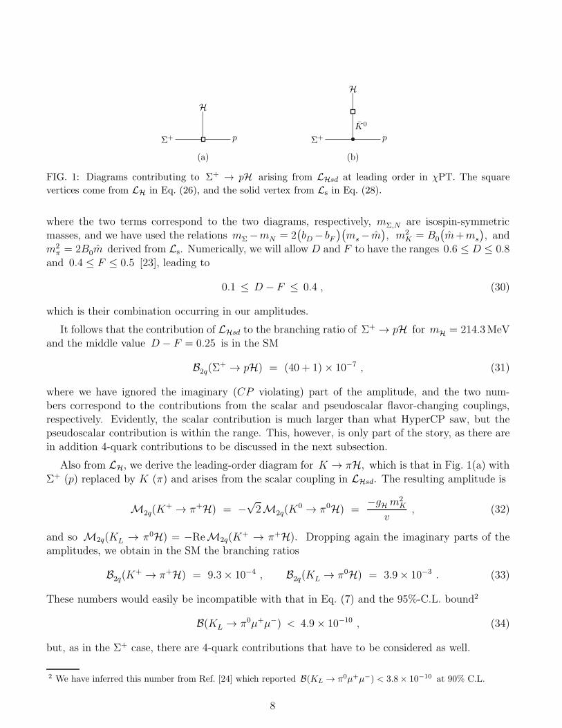
FIG. 1: Diagrams contributing to Σ+ → pH arising from LHsd at leading order in χPT. The square

vertices come from LH in Eq. (26), and the solid vertex from Ls in Eq. (28).

where the two terms correspond to the two diagrams, respectively, mΣ,N are isospin-symmetric

masses, and we have used the relations mΣ−mN = 2(

bD − bF)(

ms− m̂)

, m2K = B0

(

m̂+ms

)

, andm2

π = 2B0m̂ derived from Ls. Numerically, we will allow D and F to have the ranges 0.6 ≤ D ≤ 0.8

and 0.4 ≤ F ≤ 0.5 [23], leading to

0.1 ≤ D − F ≤ 0.4 , (30)

which is their combination occurring in our amplitudes.

It follows that the contribution of LHsd to the branching ratio of Σ+ → pH for mH = 214.3MeV

and the middle value D − F = 0.25 is in the SM

B2q(Σ+ → pH) = (40 + 1)× 10−7 , (31)

where we have ignored the imaginary (CP violating) part of the amplitude, and the two num-bers correspond to the contributions from the scalar and pseudoscalar flavor-changing couplings,

respectively. Evidently, the scalar contribution is much larger than what HyperCP saw, but thepseudoscalar contribution is within the range. This, however, is only part of the story, as there are

in addition 4-quark contributions to be discussed in the next subsection.

Also from LH, we derive the leading-order diagram for K → πH, which is that in Fig. 1(a) with

Σ+ (p) replaced by K (π) and arises from the scalar coupling in LHsd. The resulting amplitude is

M2q(K+ → π+H) = −

√2M2q(K

0 → π0H) =−gH m2

K

v, (32)

and so M2q(KL → π0H) = −ReM2q(K+ → π+H). Dropping again the imaginary parts of the

amplitudes, we obtain in the SM the branching ratios

B2q(K+ → π+H) = 9.3× 10−4 , B2q(KL → π0H) = 3.9× 10−3 . (33)

These numbers would easily be incompatible with that in Eq. (7) and the 95%-C.L. bound2

B(KL → π0µ+µ−) < 4.9× 10−10 , (34)

but, as in the Σ+ case, there are 4-quark contributions that have to be considered as well.

2 We have inferred this number from Ref. [24] which reported B(KL → π0µ+µ−) < 3.8× 10−10 at 90% C.L.

8

The situation is similar in the 2HDM. Adopting the real part of the coupling in Eq. (24), for

example, we find

B2q(Σ+ → pH) = (56 + 1)× 10−8 ,

B2q(K+ → π+H) = 1.3× 10−4 , B2q(KL → π0H) = 5.4× 10−4 . (35)

B. Four-quark |∆S| = 1 interactions

The hadronic interactions of a light Higgs-boson due to 4-quark |∆S| = 1 operators are best

accounted for in the chiral Lagrangian approach. The dominant contribution is generated by the|∆I| = 1

2component of the effective Hamiltonian transforming as (8L, 1R). The corresponding

Lagrangian at leading order is given by [23, 25].

Lw = hD

⟨

B̄{

ξ†hξ , B}⟩

+ hF

⟨

B̄[

ξ†hξ , B]⟩

+ γ8f2⟨

h ∂µΣ ∂µΣ†⟩

+ 2γ̃8f2B0

⟨

hξM+ξ†⟩

+ H.c. , (36)

where hD,F can be extracted from hyperon nonleptonic decays, γ8 = −7.8 × 10−8 from K → ππ,

the sign following from various predictions [7–9, 26], and γ̃8 is unknown as it does not contributeto any process with only kaons and pions.

The 4-quark |∆S| = 1 interactions of a light Higgs-boson H arises from its tree-level couplings

to quarks and W± bosons, as well as from its coupling to gluons induced by a triangle diagram with

heavy quarks in the loop. To obtain the relevant chiral Lagrangians, one starts with Ls,w above andfollows the prescription given in Refs. [7–9, 19]. The results are

LHs =

(

14c1 f

2⟨

∂µΣ† ∂µΣ⟩

+ 12c2 f

2B0 〈M+〉+ 12f 2B0

⟨

M̂+ −M+

⟩

) Hv

− k1m0

⟨

B̄B⟩ Hv

+ k2

(

bD⟨

B̄{

M̂+, B}⟩

+ bF⟨

B̄[

M̂+, B]⟩

+ b0⟨

M̂+

⟩ ⟨

B̄B⟩

) Hv

, (37)

LHw =

[

γ8 c3 f2⟨

h ∂µΣ ∂µΣ†⟩

+ 2γ̃8 c4 f2B0

⟨

hξM+ξ†⟩

+ 2γ̃8 f2B0

⟨

hξ(

M̂+ −M+

)

ξ†⟩

] Hv

+ k3(

hD

⟨

B̄{

ξ†hξ , B}⟩

+ hF

⟨

B̄[

ξ†hξ , B]⟩) H

v+ H.c. , (38)

where

c1 = 2kG , c2 = 3kG + 1 , c3 = 4kG − 2kW , c4 = 5kG − 2kW + 1 ,

k1 = kG , k2 = 1 , k3 = 3kG − 2kW ,

M̂+ = ξ†M̂ξ† + ξM̂ †ξ ,

(39)

with

kG =2(2ku + kd)

27, M̂ = diag

(

kum̂, kdm̂, kdms

)

, (40)

9

the expression for kG corresponding to 3 heavy and 3 light quarks. The parameters ku,d, kW , and

kG come from the couplings of H to light quarks, W±, and the gluons, respectively, and depend onthe model of the Higgs sector. Thus

ku = kd = kW = 1 in the SM , (41)

ku = kd =cosα

sin β, kW = sin(β − α) in the 2HDM I , (42)

ku =cosα

sin β, kd = − sinα

cos β, kW = sin(β − α) in the 2HDM II . (43)

The parameters c1,2,3,4 for the meson terms have already been obtained in the literature [7–9, 19, 27],whereas the new ones k1,2,3 follow from how the baryon parameters depend on masses: m0 ∼ Λ,

bD,F,0 ∼ 1, χ+ ∼ Λmq, and hD,F ∼ Λ3/m2W , where Λ is a QCD mass scale. Note that we work in

that basis in which the mass terms in the Lagrangians are not diagonal and must therefore includethe corresponding tadpole diagrams in our calculation.

For Σ+ → pH, we derive from L(H)s,w the diagrams shown in Fig. 2, finding

M4q(Σ+ → pH) = (kd − 3kG + 2kW )

hD − hF

vp̄Σ+

+ 4(kG − kW ) (D − F ) γ̃8mΣ +mN

v

m2K −m2

π

m2K −m2

H

p̄γ5Σ+ , (44)

where the first term comes from the upper three diagrams, which are at leading order, and the

second term results from the lower two diagrams, which are at next-to-leading order. Now, thecombination hD−hF also occurs in the amplitude for Σ+ → pπ0, which we write as

M(Σ+ → pπ0) = ip̄(

Apπ0 − Bpπ0γ5)

Σ+ , (45)

where from Ls,w

Apπ0 =−hD + hF

2 f, Bpπ0 = (D − F )

hD − hF

2 f

mΣ +mN

mΣ −mN

. (46)

Since from experiment [28]

Apπ0 = −3.25× 10−7 , Bpπ0 = 26.67× 10−7 , (47)

up to an overall sign, in our numerical evaluation of the 4-quark contributions to Σ+ → pH we willexplore different hD−hF values accordingly.

We can also derive from L(H)s,w the corresponding leading-order diagrams for K → πH, which are

the upper three in Fig. 2 with Σ+ (p) replaced by K (π) and yield

M4q

(

K+ → π+H)

=γ8v

[

2(kW − kG)(

m2K +m2

π −m2H

)

+ (kd − ku)m2π

]

+γ̃8v4(kG − kW )m2

K , (48)

M4q

(

K0 → π0H)

=γ8√2 v

[

2(kG − kW )(

m2K +m2

π −m2H

)

+ (ku − kd)m2

π m2K

m2K −m2

π

]

+γ̃8√2 v

[

4(kW − kG)m2K + (kd − ku)

m2π m

2K

m2K −m2

π

]

. (49)

10

Σ+

H

p Σ+

H

Σ+p Σ+

H

p p

Σ+

H

pK̄0

Σ+

H

pK̄0

K̄0

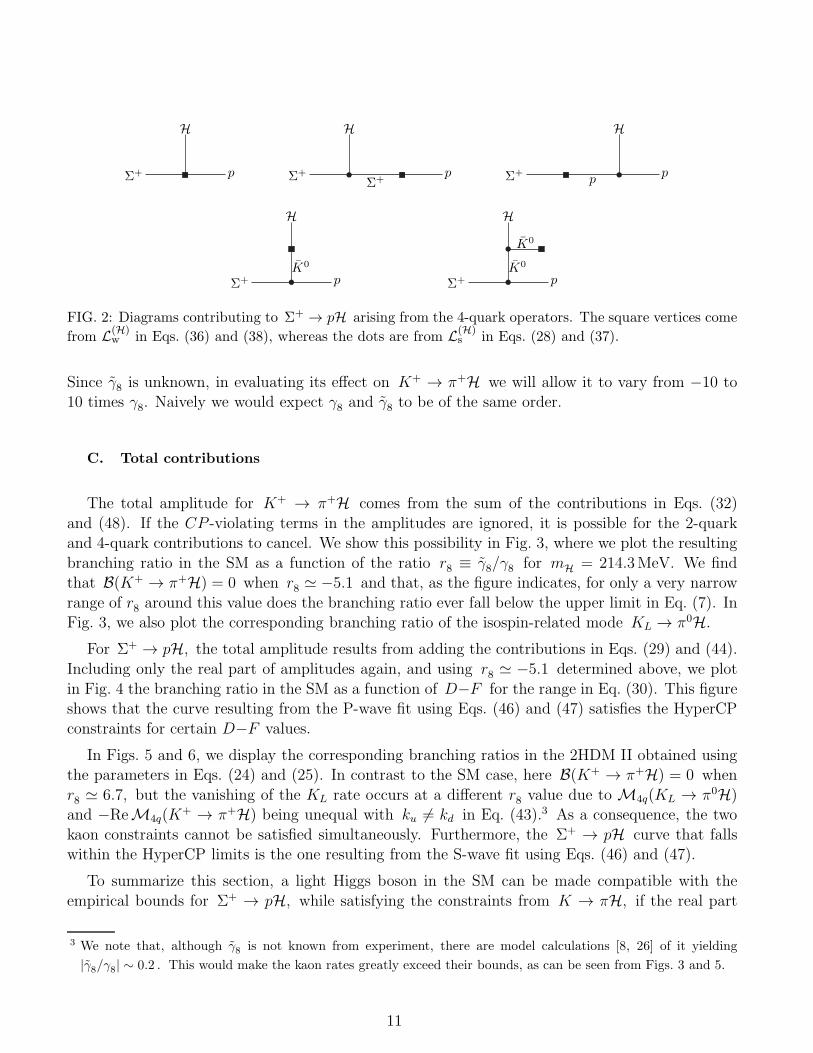
FIG. 2: Diagrams contributing to Σ+ → pH arising from the 4-quark operators. The square vertices come

from L(H)w in Eqs. (36) and (38), whereas the dots are from L(H)

s in Eqs. (28) and (37).

Since γ̃8 is unknown, in evaluating its effect on K+ → π+H we will allow it to vary from −10 to10 times γ8. Naively we would expect γ8 and γ̃8 to be of the same order.

C. Total contributions

The total amplitude for K+ → π+H comes from the sum of the contributions in Eqs. (32)

and (48). If the CP -violating terms in the amplitudes are ignored, it is possible for the 2-quarkand 4-quark contributions to cancel. We show this possibility in Fig. 3, where we plot the resulting

branching ratio in the SM as a function of the ratio r8 ≡ γ̃8/γ8 for mH = 214.3MeV. We findthat B(K+ → π+H) = 0 when r8 ≃ −5.1 and that, as the figure indicates, for only a very narrow

range of r8 around this value does the branching ratio ever fall below the upper limit in Eq. (7). InFig. 3, we also plot the corresponding branching ratio of the isospin-related mode KL → π0H.

For Σ+ → pH, the total amplitude results from adding the contributions in Eqs. (29) and (44).

Including only the real part of amplitudes again, and using r8 ≃ −5.1 determined above, we plot

in Fig. 4 the branching ratio in the SM as a function of D−F for the range in Eq. (30). This figureshows that the curve resulting from the P-wave fit using Eqs. (46) and (47) satisfies the HyperCP

constraints for certain D−F values.

In Figs. 5 and 6, we display the corresponding branching ratios in the 2HDM II obtained usingthe parameters in Eqs. (24) and (25). In contrast to the SM case, here B(K+ → π+H) = 0 when

r8 ≃ 6.7, but the vanishing of the KL rate occurs at a different r8 value due to M4q(KL → π0H)and −ReM4q(K

+ → π+H) being unequal with ku 6= kd in Eq. (43).3 As a consequence, the two

kaon constraints cannot be satisfied simultaneously. Furthermore, the Σ+ → pH curve that fallswithin the HyperCP limits is the one resulting from the S-wave fit using Eqs. (46) and (47).

To summarize this section, a light Higgs boson in the SM can be made compatible with the

empirical bounds for Σ+ → pH, while satisfying the constraints from K → πH, if the real part

3 We note that, although γ̃8 is not known from experiment, there are model calculations [8, 26] of it yielding

|γ̃8/γ8| ∼ 0.2 . This would make the kaon rates greatly exceed their bounds, as can be seen from Figs. 3 and 5.

11

-8 -6 -4 -2 0r8

10-3

10-5

10-7

10-9

BHK®ΠHL

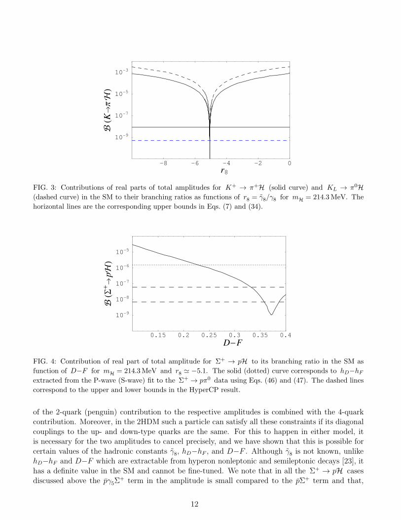
FIG. 3: Contributions of real parts of total amplitudes for K+ → π+H (solid curve) and KL → π0H(dashed curve) in the SM to their branching ratios as functions of r8 = γ̃8/γ8 for mH = 214.3MeV. The

horizontal lines are the corresponding upper bounds in Eqs. (7) and (34).

0.15 0.2 0.25 0.3 0.35 0.4D-F

10-5

10-6

10-7

10-8

10-9

BHS+®

pHL

FIG. 4: Contribution of real part of total amplitude for Σ+ → pH to its branching ratio in the SM as

function of D−F for mH = 214.3MeV and r8 ≃ −5.1. The solid (dotted) curve corresponds to hD−hFextracted from the P-wave (S-wave) fit to the Σ+ → pπ0 data using Eqs. (46) and (47). The dashed lines

correspond to the upper and lower bounds in the HyperCP result.

of the 2-quark (penguin) contribution to the respective amplitudes is combined with the 4-quarkcontribution. Moreover, in the 2HDM such a particle can satisfy all these constraints if its diagonal

couplings to the up- and down-type quarks are the same. For this to happen in either model, itis necessary for the two amplitudes to cancel precisely, and we have shown that this is possible for

certain values of the hadronic constants γ̃8, hD−hF , and D−F . Although γ̃8 is not known, unlikehD−hF and D−F which are extractable from hyperon nonleptonic and semileptonic decays [23], it

has a definite value in the SM and cannot be fine-tuned. We note that in all the Σ+ → pH casesdiscussed above the p̄γ5Σ

+ term in the amplitude is small compared to the p̄Σ+ term and that,

12

2 4 6 8 10r8

10-3

10-5

10-7

10-9

BHK®ΠHL

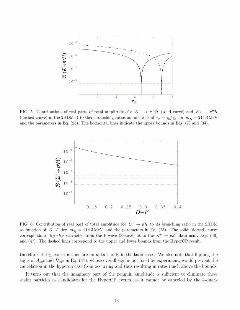
FIG. 5: Contributions of real parts of total amplitudes for K+ → π+H (solid curve) and KL → π0H(dashed curve) in the 2HDM II to their branching ratios as functions of r8 = γ̃8/γ8 for mH = 214.3MeV

and the parameters in Eq. (25). The horizontal lines indicate the upper bounds in Eqs. (7) and (34).

0.15 0.2 0.25 0.3 0.35 0.4D-F

10-5

10-6

10-7

10-8

10-9

BHS+®

pHL

FIG. 6: Contribution of real part of total amplitude for Σ+ → pH to its branching ratio in the 2HDM

as function of D−F for mH = 214.3MeV and the parameters in Eq. (25). The solid (dotted) curve

corresponds to hD−hF extracted from the P-wave (S-wave) fit to the Σ+ → pπ0 data using Eqs. (46)

and (47). The dashed lines correspond to the upper and lower bounds from the HyperCP result.

therefore, the γ̃8 contributions are important only in the kaon cases. We also note that flipping thesigns of Apπ0 and Bpπ0 in Eq. (47), whose overall sign is not fixed by experiment, would prevent the

cancelation in the hyperon case from occurring and thus resulting in rates much above the bounds.

It turns out that the imaginary part of the penguin amplitude is sufficient to eliminate thesescalar particles as candidates for the HyperCP events, as it cannot be canceled by the 4-quark

13

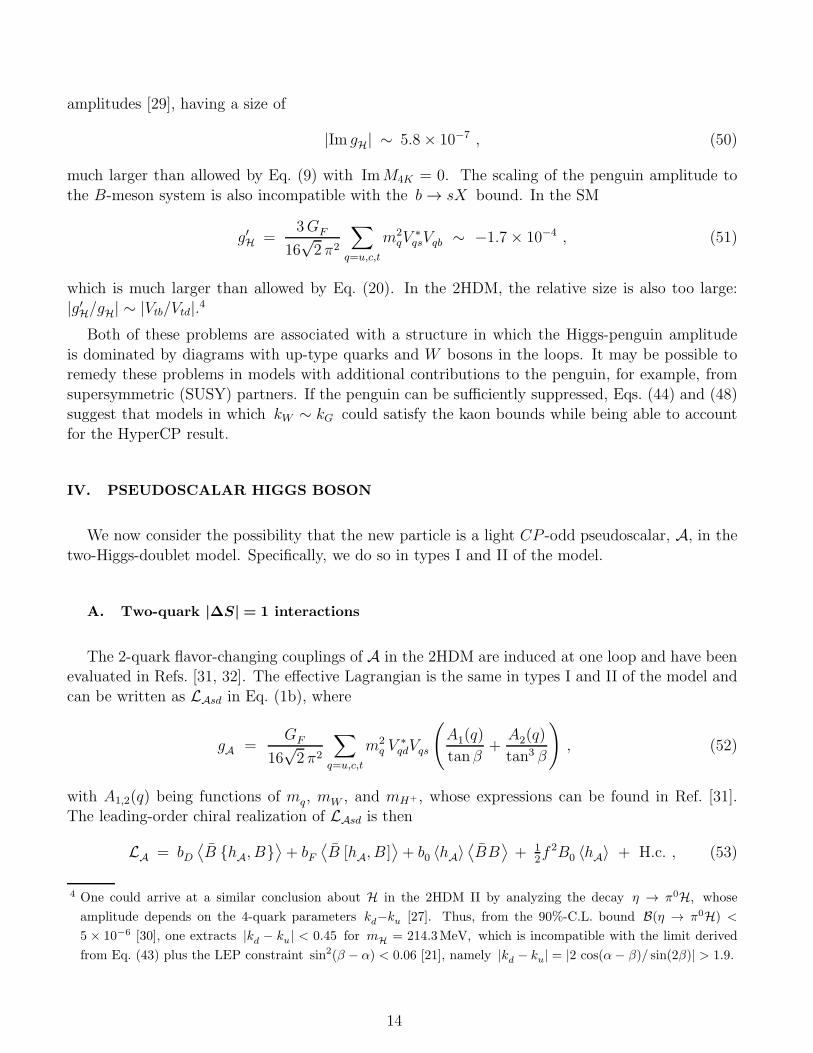
amplitudes [29], having a size of

|Im gH| ∼ 5.8× 10−7 , (50)

much larger than allowed by Eq. (9) with ImM4K = 0. The scaling of the penguin amplitude to

the B-meson system is also incompatible with the b → sX bound. In the SM

g′H =3GF

16√2 π2

∑

q=u,c,t

m2qV

∗qsVqb ∼ −1.7× 10−4 , (51)

which is much larger than allowed by Eq. (20). In the 2HDM, the relative size is also too large:|g′H/gH| ∼ |Vtb/Vtd|.4

Both of these problems are associated with a structure in which the Higgs-penguin amplitude

is dominated by diagrams with up-type quarks and W bosons in the loops. It may be possible toremedy these problems in models with additional contributions to the penguin, for example, from

supersymmetric (SUSY) partners. If the penguin can be sufficiently suppressed, Eqs. (44) and (48)suggest that models in which kW ∼ kG could satisfy the kaon bounds while being able to account

for the HyperCP result.

IV. PSEUDOSCALAR HIGGS BOSON

We now consider the possibility that the new particle is a light CP -odd pseudoscalar, A, in the

two-Higgs-doublet model. Specifically, we do so in types I and II of the model.

A. Two-quark |∆S| = 1 interactions

The 2-quark flavor-changing couplings of A in the 2HDM are induced at one loop and have beenevaluated in Refs. [31, 32]. The effective Lagrangian is the same in types I and II of the model and

can be written as LAsd in Eq. (1b), where

gA =GF

16√2 π2

∑

q=u,c,t

m2q V

∗qdVqs

(

A1(q)

tanβ+

A2(q)

tan3 β

)

, (52)

with A1,2(q) being functions of mq, mW , and mH+ , whose expressions can be found in Ref. [31].The leading-order chiral realization of LAsd is then

LA = bD⟨

B̄ {hA, B}⟩

+ bF⟨

B̄ [hA, B ]⟩

+ b0 〈hA〉⟨

B̄B⟩

+ 12f 2B0 〈hA〉 + H.c. , (53)

4 One could arrive at a similar conclusion about H in the 2HDM II by analyzing the decay η → π0H, whose

amplitude depends on the 4-quark parameters kd−ku [27]. Thus, from the 90%-C.L. bound B(η → π0H) <

5 × 10−6 [30], one extracts |kd− k

u| < 0.45 for mH = 214.3MeV, which is incompatible with the limit derived

from Eq. (43) plus the LEP constraint sin2(β − α) < 0.06 [21], namely |kd− ku| = |2 cos(α− β)/ sin(2β)| > 1.9.

14

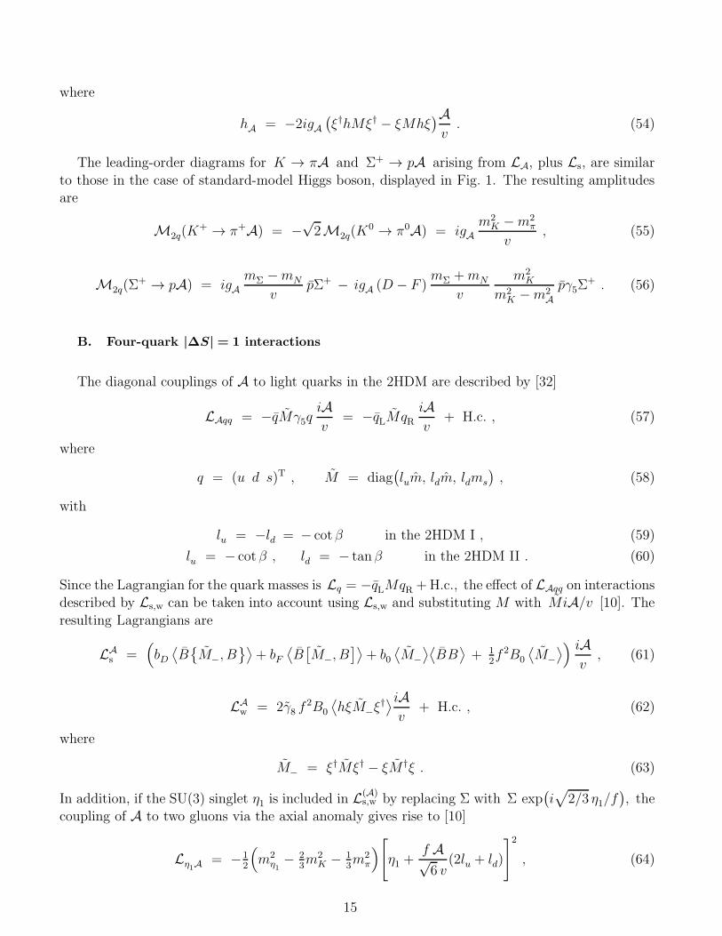
where

hA = −2igA(

ξ†hMξ† − ξMhξ)Av

. (54)

The leading-order diagrams for K → πA and Σ+ → pA arising from LA, plus Ls, are similar

to those in the case of standard-model Higgs boson, displayed in Fig. 1. The resulting amplitudesare

M2q(K+ → π+A) = −

√2M2q(K

0 → π0A) = igAm2

K −m2π

v, (55)

M2q(Σ+ → pA) = igA

mΣ −mN

vp̄Σ+ − igA (D − F )

mΣ +mN

v

m2K

m2K −m2

A

p̄γ5Σ+ . (56)

B. Four-quark |∆S| = 1 interactions

The diagonal couplings of A to light quarks in the 2HDM are described by [32]

LAqq = −q̄M̃γ5qiAv

= −q̄LM̃qRiAv

+ H.c. , (57)

where

q = (u d s)T , M̃ = diag(

lum̂, ldm̂, ldms

)

, (58)

with

lu = −ld = − cotβ in the 2HDM I , (59)

lu = − cotβ , ld = − tanβ in the 2HDM II . (60)

Since the Lagrangian for the quark masses is Lq = −q̄LMqR +H.c., the effect of LAqq on interactionsdescribed by Ls,w can be taken into account using Ls,w and substituting M with M̃iA/v [10]. The

resulting Lagrangians are

LAs =

(

bD⟨

B̄{

M̃−, B}⟩

+ bF⟨

B̄[

M̃−, B]⟩

+ b0⟨

M̃−

⟩⟨

B̄B⟩

+ 12f 2B0

⟨

M̃−

⟩

) iAv

, (61)

LAw = 2γ̃8 f

2B0

⟨

hξM̃−ξ†⟩iAv

+ H.c. , (62)

where

M̃− = ξ†M̃ξ† − ξM̃ †ξ . (63)

In addition, if the SU(3) singlet η1 is included in L(A)s,w by replacing Σ with Σ exp

(

i√

2/3 η1/f)

, thecoupling of A to two gluons via the axial anomaly gives rise to [10]

Lη1A = −1

2

(

m2η1− 2

3m2

K − 13m2

π

)

[

η1 +f A√6 v

(2lu + ld)

]2

, (64)

15

which modifies the η1-A mixing generated by LAs .

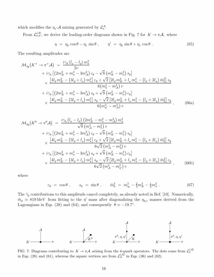
From L(A)s,w , we derive the leading-order diagrams shown in Fig. 7 for K → πA, where

η = η8 cos θ − η1 sin θ , η′ = η8 sin θ + η1 cos θ . (65)

The resulting amplitudes are

M4q

(

K+ → π+A)

=iγ8 (lu − ld)m

2π

2v

+ iγ8[(

2m2K +m2

π − 3m2A

)

cθ −√8(

m2K −m2

π

)

sθ]

×[

4ldm2K −

(

3ld + lu)

m2π

]

cθ +√2[

2ldm2K + lu m

2π −

(

ld + 2lu)

m̃20

]

sθ6(

m2η −m2

A

)

v

+ iγ8[(

2m2K +m2

π − 3m2A

)

sθ +√8(

m2K −m2

π

)

cθ]

×[

4ldm2K −

(

3ld + lu)

m2π

]

sθ −√2[

2ldm2K + lum

2π −

(

ld + 2lu)

m̃20

]

cθ6(

m2η′ −m2

A

)

v, (66a)

M4q

(

K0 → π0A)

=iγ8(

lu − ld) (

2m2K −m2

π −m2A

)

m2π√

8(

m2A −m2

π

)

v

+ iγ8[(

2m2K +m2

π − 3m2A

)

cθ −√8(

m2K −m2

π

)

sθ]

×[

4ldm2K −

(

3ld + lu)

m2π

]

cθ +√2[

2ldm2K + lu m

2π −

(

ld + 2lu)

m̃20

]

sθ

6√2(

m2A −m2

η

)

v

+ iγ8[(

2m2K +m2

π − 3m2A

)

sθ +√8(

m2K −m2

π

)

cθ]

×[

4ldm2K −

(

3ld + lu)

m2π

]

sθ −√2[

2ldm2K + lum

2π −

(

ld + 2lu)

m̃20

]

cθ

6√2(

m2A −m2

η′

)

v, (66b)

where

cθ = cos θ , sθ = sin θ , m̃20 = m2

η1− 2

3m2

K − 13m2

π . (67)

The γ̃8 contributions to this amplitude cancel completely, as already noted in Ref. [10]. Numerically,

m̃0 ≃ 819MeV from fitting to the η′ mass after diagonalizing the η8,1 masses derived from theLagrangians in Eqs. (28) and (64), and consequently θ ≃ −19.7◦.

K

A

π K

A

K0

π K

A

Kπ0, η, η′

π K

A

π0, η, η′

π

FIG. 7: Diagrams contributing to K → πA arising from the 4-quark operators. The dots come from L(A)s

in Eqs. (28) and (61), whereas the square vertices are from L(A)w in Eqs. (36) and (62).

16

The leading-order 4-quark contributions to Σ+ → pA arise from the diagrams in Fig. 8 and can

be expressed as

M4q(Σ+ → pA) = ip̄

(

ApA − BpAγ5)

Σ+ , (68)

where

ApA =f Apπ0

(

ld − lu)

m2π

2(

m2A −m2

π

)

v

+f Apπ0

{[

4ldm2K −

(

3ld + lu)

m2π

]

c2θ +√2[

2ldm2K + lu m

2π −

(

ld + 2lu)

m̃20

]

cθsθ}

2(

m2η −m2

A

)

v

+f Apπ0

{[

4ldm2K −

(

3ld + lu)

m2π

]

s2θ −√2[

2ldm2K + lum

2π −

(

ld + 2lu)

m̃20

]

cθsθ}

2(

m2η′ −m2

A

)

v, (69)

BpA =f Bpπ0

(

ld − lu)

m2π

2(

m2A −m2

π

)

v

+f Bpπ0

{[

4ldm2K −

(

3ld + lu)

m2π

]

c2θ +√2[

2ldm2K + lu m

2π −

(

ld + 2lu)

m̃20

]

cθsθ}

2(

m2η −m2

A

)

v

+f Bpπ0

{[

4ldm2K −

(

3ld + lu)

m2π

]

s2θ −√2[

2ldm2K + lum

2π −

(

ld + 2lu)

m̃20

]

cθsθ}

2(

m2η′ −m2

A

)

v, (70)

where Apπ0 and Bpπ0 are given in Eq. (46). We note that contributions with γ8 or γ̃8 appear onlyat next-to-leading order.

C. Total contributions

The total amplitudes for K → πA result from adding the contributions in Eqs. (55) and (66).

If the CP -violating terms in the amplitudes are ignored, it is possible for the 2-quark and 4-quarkcontributions to cancel. We show this possibility in Fig. 9, where we plot the resulting branching

ratios as functions of the charged-Higgs-boson mass for mA = 214.3MeV and different tan β valuesin the 2 versions of the 2HDM. The total amplitude for Σ+ → pA is the sum of the contributions

Σ+

A

p

π0, η, η′

Σ+

A

Σ+p

π0, η, η′

Σ+

A

p p

π0, η, η′

FIG. 8: Diagrams contributing to Σ+ → pA arising from the 4-quark operators. The square vertices come

from Lw in Eq. (36), whereas the dots are from the Lagrangians in Eqs. (28), (61), and (64).

17

265 270 275 280 285 290

mH+ HGeVL

10-9

10-8

10-7

BHK®ΠAL

2HDM I with tanΒ = 4

290 300 310 320 330

mH+ HGeVL

10-9

10-8

10-7

BHK®ΠAL

2HDM II with tanΒ = 0.9

FIG. 9: Contributions of real parts of total amplitudes for K+ → π+A (solid curve) and KS → π0A(dashed curve) in the 2HDM to their branching ratios as functions of charged-Higgs-boson mass for mA =

214.3MeV and tan β = 4 (0.9) in type I (II) of the model. The horizontal lines indicate the upper bounds

in Eqs. (7) and (8).

225 250 275 300 325 350 375 400

mH+ HGeVL

10-9

10-8

10-7

BHS+®

pAL

FIG. 10: Contribution of real part of total amplitude for Σ+ → pA to its branching ratio in the 2HDM I

(solid curve) and II (dotted curve) as function of charged-Higgs-boson mass for mA = 214.3MeV and

tan β = 4 (0.9) in type I (II). The dashed lines indicate the bounds from the HyperCP result.

in Eqs. (56) and (68). If the experimental values of Apπ0 and Bpπ0 in Eq. (47), as well as the middle

value D − F = 0.25, are used in the total amplitude, the resulting branching ratios in the 2HDMare displayed in Fig. 10.

We have found that only one of the kaon bounds can be satisfied if the HyperCP result isassumed to be mediated by A in the 2HDM. However, for certain tan β and mH+ values near

the ones indicated in Figs. 9 and 10, all the kaon and hyperon constraints can be nearly satisfiedsimultaneously. Part of the difficulty in satisfying all of the constraints lies with the vanishing

of the K+ and KS rates occurring at different mH+ values, which is due to M4q(KS → π0A) and−ReM4q(K

+ → π+A) being unequal with lu 6= ld in Eqs. (59) and (60). We note that the situation

is not much different if the signs of Apπ0 and Bpπ0 in Eq. (47) are both flipped.

To summarize this section, we have found that it is possible for the real part of the penguinamplitude to cancel against the 4-quark amplitude to approximately satisfy the kaon bounds while

18

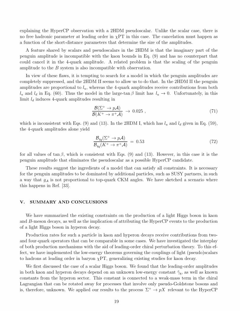
explaining the HyperCP observation with a 2HDM pseudoscalar. Unlike the scalar case, there is

no free hadronic parameter at leading order in χPT in this case. The cancelation must happen asa function of the short-distance parameters that determine the size of the amplitudes.

A feature shared by scalars and pseudoscalars in the 2HDM is that the imaginary part of the

penguin amplitude is incompatible with the kaon bounds in Eq. (9) and has no counterpart thatcould cancel it in the 4-quark amplitude. A related problem is that the scaling of the penguin

amplitude to the B system is also incompatible with observation.

In view of these flaws, it is tempting to search for a model in which the penguin amplitudes arecompletely suppressed, and the 2HDM II seems to allow us to do that. In the 2HDM II the penguin

amplitudes are proportional to lu, whereas the 4-quark amplitudes receive contributions from bothlu and ld in Eq. (60). Thus the model in the large-tanβ limit has lu → 0. Unfortunately, in this

limit ld induces 4-quark amplitudes resulting in

B(Σ+ → pA)

B(K+ → π+A)→ 0.025 , (71)

which is inconsistent with Eqs. (9) and (13). In the 2HDM I, which has lu and ld given in Eq. (59),the 4-quark amplitudes alone yield

B4q(Σ+ → pA)

B4q(K+ → π+A)

= 0.53 (72)

for all values of tan β, which is consistent with Eqs. (9) and (13). However, in this case it is thepenguin amplitude that eliminates the pseudoscalar as a possible HyperCP candidate.

These results suggest the ingredients of a model that can satisfy all constraints. It is necessaryfor the penguin amplitudes to be dominated by additional particles, such as SUSY partners, in such

a way that gA is not proportional to top-quark CKM angles. We have sketched a scenario wherethis happens in Ref. [33].

V. SUMMARY AND CONCLUSIONS

We have summarized the existing constraints on the production of a light Higgs boson in kaonand B-meson decays, as well as the implication of attributing the HyperCP events to the production

of a light Higgs boson in hyperon decay.

Production rates for such a particle in kaon and hyperon decays receive contributions from two-and four-quark operators that can be comparable in some cases. We have investigated the interplay

of both production mechanisms with the aid of leading-order chiral perturbation theory. To this ef-fect, we have implemented the low-energy theorems governing the couplings of light (pseudo)scalars

to hadrons at leading order in baryon χPT, generalizing existing studies for kaon decay.

We first discussed the case of a scalar Higgs boson. We found that the leading-order amplitudesin both kaon and hyperon decays depend on an unknown low-energy constant γ̃8, as well as known

constants from the hyperon sector. This constant is connected to a weak-mass term in the chiralLagrangian that can be rotated away for processes that involve only pseudo-Goldstone bosons and

is, therefore, unknown. We applied our results to the process Σ+ → pX relevant to the HyperCP

19

observation of Σ+ → pµ+µ−. We showed that the two-quark contributions in the SM and its

2HDM extensions are too large to explain the HyperCP observation. However, we also showedthat there can be cancelations between the CP -conserving two- and four-quark contributions to

this process that lead to a rate comparable in size to the HyperCP observation for both the SMand the 2HDM. Such cancelations occur for a certain range of known constants from the hyperon

sector, the effect of γ̃8 being small. In both cases, however, the two-quark penguin contributionhas an imaginary (CP violating) part that is too large to be compatible with the HyperCP result.

In the SM and in the 2HDM, the four-quark contributions have a CP -violating part that is muchsmaller than that of the penguin amplitude and hence these models are ruled out as explanations

for the HyperCP observation. More general models with additional CP -violating phases may beable to address this issue. In addition, in these models the scaling of the two-quark operator to the

B system is incompatible with the nonobservation of a light scalar in B decay.

We then discussed the case of a pseudoscalar Higgs boson in the 2HDM. In this case we computedthe leading-order amplitudes in χPT and included, as well, certain higher-order terms mediated by

the η′ state. The resulting amplitudes for both kaon and hyperon decays do not depend on any

unknown hadronic parameters. In particular, they do not depend on γ̃8, as observed in Ref. [10].We then applied our results to the Σ+ → pA process. Once again we found that the real part of

the amplitude can be consistent with the HyperCP observation for a certain range of parametersin the 2HDM (tanβ and mH+), but that the imaginary part of the penguin amplitude is too large.

The scaling of the two-quark operator to the B system also produces a B → XsA rate that is toolarge. Both of these problems can be solved in more general models that modify the phase and

scaling with CKM angles of the two-quark operator.

In conclusion, we have shown that it is possible to interpret the HyperCP observation as evidencefor a light Higgs boson, although it is not easy to arrange this in a model. Typical Higgs-penguin

operators have three problems:

(a) if they have the right size to fit the HyperCP observation, they induce K → πX at rates

larger than the existing bounds;

(b) if they are dominated by loop diagrams involving up-type quarks and W bosons, they have

a CP phase that is too large;

(c) if they are dominated by loop diagrams involving up-type quarks and W bosons, their scaling

to the B system is incompatible with the nonobservation of B → XsX .

We have found in this paper that (a) can be solved in some cases by the addition of the effects of

four-quark operators. We have suggested that more general models may be constructed to solve (b)and (c). To show that this is possible, we have constructed a specific example in Ref. [33].

Disregarding existing bounds from kaon and B-meson decays, we have shown that many light

Higgs bosons have couplings of the right size to explain the HyperCP observation. We think this issufficiently intriguing to warrant a revisiting of the kaon and B decay results. In particular, the B

factories are still operational and could reanalyze the very low mµµ invariant-mass region in theirmeasurements of B → Xsµ

+µ− modes. The NA48 experiment might also be able to revisit the

kaon modes.

20

Acknowledgments

The work of X.G.H. was supported in part by NSC and NCTS. The work of G.V. was supported

in part by DOE under contract number DE-FG02-01ER41155. We thank Laurence Littenberg andRainer Wanke for useful discussions on the kaon bounds and Soeren Prell for useful discussions on

the B bounds.

[1] H. Park et al. [HyperCP Collaboration], Phys. Rev. Lett. 94, 021801 (2005) [arXiv:hep-ex/0501014].

[2] X.G. He, J. Tandean, and G. Valencia, Phys. Rev. D 72, 074003 (2005) [arXiv:hep-ph/0506067].

[3] X.G. He, J. Tandean, and G. Valencia, Phys. Lett. B 631, 100 (2005) [arXiv:hep-ph/0509041].

[4] N.G. Deshpande, G. Eilam, and J. Jiang, Phys. Lett. B 632, 212 (2006) [arXiv:hep-ph/0509081].

[5] C.Q. Geng and Y.K. Hsiao, Phys. Lett. B 632, 215 (2006) [arXiv:hep-ph/0509175].

[6] D.S. Gorbunov and V.A. Rubakov, Phys. Rev. D 64, 054008 (2001) [arXiv:hep-ph/0012033]; ibid. 73,

035002 (2006) [arXiv:hep-ph/0509147]; S.V. Demidov and D.S. Gorbunov, arXiv:hep-ph/0610066.

[7] R.S. Chivukula and A.V. Manohar, Phys. Lett. B 207, 86 (1988) [Erratum-ibid. B 217, 568 (1989)];

[8] H.Leutwyler and M.A. Shifman, Nucl. Phys. B 343, 369 (1990);

[9] See for example, J.F. Gunion, H.E. Haber, G.L. Kane, and S. Dawson, SCIPP-89/13, and references

therein.

[10] B. Grzadkowski and J. Pawelczyk, Phys. Lett. B 300, 387 (1993).

[11] H. Ma et al. [E865 Collaboration], Phys. Rev. Lett. 84, 2580 (2000) [arXiv:hep-ex/9910047].

[12] H.K. Park et al. [HyperCP Collaboration], Phys. Rev. Lett. 88, 111801 (2002) [arXiv:hep-ex/0110033].

[13] J.R. Batley et al. [NA48/1 Collaboration], Phys. Lett. B 599, 197 (2004) [arXiv:hep-ex/0409011].

[14] E. Barberio et al. [The Heavy Flavor Averaging Group], arXiv:hep-ex/0603003.

[15] B. Aubert et al. [BABAR Collaboration], Phys. Rev. Lett. 93, 081802 (2004) [arXiv:hep-ex/0404006].

[16] M. Iwasaki et al. [Belle Collaboration], Phys. Rev. D 72, 092005 (2005) [arXiv:hep-ex/0503044].

[17] R.S. Willey and H.L. Yu, Phys. Rev. D 26, 3086 (1982); B. Grzadkowski and P. Krawczyk, Z. Phys. C

18, 43 (1983); A. Dedes, Mod. Phys. Lett. A 18, 2627 (2003) [arXiv:hep-ph/0309233], and references

therein.

[18] R.M. Barnett, G. Senjanovic, and D. Wyler, Phys. Rev. D 30, 1529 (1984); C.Q. Geng and J.N. Ng,

ibid. 39, 3330 (1989); M.E. Lautenbacher, Nucl. Phys. B 347, 120 (1990).

[19] S. Dawson, Nucl. Phys. B 339, 19 (1990).

[20] J. Charles et al. [CKMfitter Group], Eur. Phys. J. C 41, 1 (2005) [arXiv:hep-ph/0406184]. Updated

results used in this paper are from http://ckmfitter.in2p3.fr/, “Results as of FPCP 2006, Vancouver,

Canada”.

[21] G. Abbiendi et al. [OPAL Collaboration], Eur. Phys. J. C 40, 317 (2005) [arXiv:hep-ex/0408097].

[22] J. Gasser and H. Leutwyler, Annals Phys. 158, 142 (1984).

[23] J. Bijnens, H. Sonoda, and M.B. Wise, Nucl. Phys. B 261, 185 (1985); E. Jenkins and A.V. Manohar, in

Effective Field Theories of the Standard Model, edited by U.-G. Meissner (World Scientific, Singapore,

1992).

[24] A. Alavi-Harati et al. [KTEV Collaboration], Phys. Rev. Lett. 84, 5279 (2000) [arXiv:hep-ex/0001006].

[25] See, for example, J.F. Donoghue, E. Golowich, and B.R. Holstein, Dynamics of the Standard Model

(Cambridge University Press, Cambridge, 1992).

[26] J. Bijnens and J. Prades, JHEP 9901, 023 (1999) [arXiv:hep-ph/9811472].

21

[27] J. Prades and A. Pich, Phys. Lett. B 245, 117 (1990); A. Pich, J. Prades, and P. Yepes, Nucl. Phys.

B 388, 31 (1992).

[28] W.-M. Yao et al. [Particle Data Group], J. Phys. G 33, 1 (2006)

[29] H.Y. Cheng and H.L. Yu, Phys. Rev. D 40, 2980 (1989).

[30] R.I. Dzhelyadin et al., Phys. Lett. B 105, 239 (1981).

[31] J.M. Frere, J.A.M. Vermaseren, and M.B. Gavela, Phys. Lett. B 103 (1981) 129.

[32] L.J. Hall and M.B. Wise, Nucl. Phys. B 187, 397 (1981).

[33] X.G. He, J. Tandean, and G. Valencia, arXiv:hep-ph/0610362.

22