Artificial Intelligence in the Energy Industry - MDPI

Edited by

Artificial Intelligence in the Energy Industry

Ana-Belén Gil-GonzálezPrinted Edition of the Special Issue Published in Energies

www.mdpi.com/journal/energies

Artificial Intelligence in theEnergy Industry

Artificial Intelligence in theEnergy Industry

Editor

Ana-Belen Gil-Gonzalez

MDPI • Basel • Beijing • Wuhan • Barcelona • Belgrade • Manchester • Tokyo • Cluj • Tianjin

Editor


BISITE Research Group,

University of Salamanca,

Edificio Multiusos I+D+i,

Calle Espejo 2,

37007 Salamanca, Spain

Editorial Office

MDPI

St. Alban-Anlage 66

4052 Basel, Switzerland

This is a reprint of articles from the Special Issue published online in the open access journal Energies

(ISSN 1996-1073) (available at: https://www.mdpi.com/journal/energies/special issues/Artificial

Intelligence Energy Industry).

For citation purposes, cite each article independently as indicated on the article page online and as

indicated below:

LastName, A.A.; LastName, B.B.; LastName, C.C. Article Title. Journal Name Year, Volume Number,

Page Range.

ISBN 978-3-0365-4605-6 (Hbk)

ISBN 978-3-0365-4606-3 (PDF)

Cover image courtesy of Ana-Belen Gil-Gonzalez.

© 2022 by the authors. Articles in this book are Open Access and distributed under the Creative

Commons Attribution (CC BY) license, which allows users to download, copy and build upon

published articles, as long as the author and publisher are properly credited, which ensuresmaximum

dissemination and a wider impact of our publications.

The book as a whole is distributed byMDPI under the terms and conditions of the Creative Commons

license CC BY-NC-ND.

Contents

About the Editor . . . . . . . . . . . . . . . . . . . . . . . . . . . . . . . . . . . . . . . . . . . . . . vii

Preface to ”Artificial Intelligence in the Energy Industry” . . . . . . . . . . . . . . . . . . . . . . ix

Szabolcs Kovac, German Micha’conok, Igor Halenar and Pavel Vazan

Comparison of Heat Demand Prediction Using Wavelet Analysis and Neural Network for aDistrict Heating NetworkReprinted from: Energies 2021, 14, 1545, doi:10.3390/en14061545 . . . . . . . . . . . . . . . . . . . 1

Petros Koutroumpinas, Yu Zhang, Steve Wallis, Elizabeth Chang

An Artificial Intelligence Empowered Cyber Physical Ecosystem for Energy Efficiency andOccupation Health and SafetyReprinted from: Energies 2021, 14, 4214, doi:10.3390/en14144214 . . . . . . . . . . . . . . . . . . . 21

Mahmoud Abdelkader Bashery Abbass and Mohamed Hamdy

A Generic Pipeline for Machine Learning Users in Energy and Buildings DomainReprinted from: Energies 2021, 14, 5410, doi:10.3390/en14175410 . . . . . . . . . . . . . . . . . . . 35

Gustavo Carvalho Santos, Flavio Barboza, Antonio Claudio Paschoarelli Veiga and Mateus

Ferreira Silva

Forecasting Brazilian Ethanol Spot Prices Using LSTMReprinted from: Energies 2021, 14, 7987, doi:10.3390/en14237987 . . . . . . . . . . . . . . . . . . . 67

Pedro Macieira, Luis Gomes and Zita Vale

Energy Management Model for HVAC Control Supported by Reinforcement LearningReprinted from: Energies 2021, 14, 8210, doi:10.3390/en14248210 . . . . . . . . . . . . . . . . . . . 83

Amir Mortazavigazar, Nourehan Wahba, Paul Newsham, Maharti Triharta, Pufan Zheng,

Tracy Chen and Behzad Rismanchi

Application of Artificial Neural Networks for Virtual Energy AssessmentReprinted from: Energies 2021, 14, 8330, doi:10.3390/en14248330 . . . . . . . . . . . . . . . . . . . 97

Yeray Mezquita, Ana Belen Gil-Gonzalez, Angel Martın del Rey, Javier Prieto, Juan Manuel

Corchado

Towards a Blockchain-Based Peer-to-Peer Energy MarketplaceReprinted from: Energies 2022, 15, 3046, doi:10.3390/en15093046 . . . . . . . . . . . . . . . . . . . 115

v

About the Editor


Ana-Belen Gil-Gonzalez is Associate Professor at the Department of Computer Science and

Automatics at the University of Salamanca in the area of Computer Languages and Systems. She

holds a PhD in Computer Science and Automatics from the University of Salamanca, where she was

awarded in recognition of her extraordinary PhD work. She currently holds the position of Vice-Dean

of Teaching and Infrastructures of the Faculty of Science.

She works in the research group Bioinformatics, Intelligent Information Systems and Educational

Technology (BISITE). Her research focuses on the development of technological frameworks for

content retrieval, personalization and characterization in different domains and deepening its

representation, analysis and application of content. In these works, she applied artificial intelligence

techniques, multi-agent systems, data mining and Semantic Web for the retrieval and representation

of knowledge, as well as its application to different systems such as Recommender Systems, as well as

in applications related to Smartcities. A.B. Gil works on projects in the fields of Artificial Intelligence,

Machine Learning, Blockchain, IoT, Fog Computing, Edge Computing, Smart Cities, Smart Grids,

Sentiment Analysis, etc.

Her extensive experience with publication and dissemination of results is highlighted by

44 publications in international journals included in the Web of Science (WOS), of which 18 have

an impact factor, according to the JCR-SCI index. She is also co-author of more than 100 publications

in books and international peer-reviewed congresses of recognized prestige, some of them included in

the CORE and SCI rankings, among others. She has collaborated in various national and international

scientific committees while being active in the organization of numerous international scientific

congresses (PAAMS, CEDI, DCAI, etc.).

vii

Preface to ”Artificial Intelligence in the

Energy Industry”

Artificial intelligence is essential in all industrial environments. The energy industry is an area

that presents exceptional opportunities for development based on the use of artificial intelligence (AI).

In essence, AI provides a machine with the ability to learn and make decisions to solve problems or

optimize results toward meeting a goal. There are many decisions to be made in the energy sector

that require an early response and handling of a significant volume of data. Artificial intelligence can

optimally perform these important decisions where instantaneous collection and analysis of these

large volumes of data is required while processing as fast and efficiently as possible.

Smart grids carry electricity as well as data. In the case of intermittent and volatile energies, such

as solar and wind, it is more important than ever to effectively balance consumption and generation.

One of the hopes for artificial intelligence applied to the energy sector is that it will help us address

issues related to climate change, emission-reduction effects of technological progresses in industry,

energy balances, and environmental impacts, among others. One of the most basic applications of

AI in the energy sector is the use of machine learning in making generation systems more efficient,

improving the effectiveness of design technologies and creating energy-efficient objects.

The future of mobility is electric, which also poses new challenges. AI is being installed in

the electric vehicle sector within cars themselves for their management and to communicate data

that contribute to solving these challenges, in addition to outside the car to facilitate the effective

management of reports, intelligent mobility solutions, etc.

The application of AI to the energy industry sector is without a doubt unquestionable. Artificial

intelligence is beginning to be used in the energy sector and is already proving essential by providing

the industry and households with new information services for control over energy infrastructure,

optimizing generation, reducing consumption, or fighting climate change, which are only some

examples of its promising applications that are expected in the near future.

This book showcases all the various research approaches focused on the relationship between the

use of artificial intelligence and its direct application in the field of the energy sector, or so-called smart

energy. The different chapters address the high incidence of contributions from the perspective of

energy efficiency in energy management, production, and consumption. The use of AI will therefore

make it possible to produce, consume, and manage energy and energy products better, with fewer

resources and less environmental impact.


Editor

ix

energies

Article

Comparison of Heat Demand Prediction Using WaveletAnalysis and Neural Network for a District Heating Network

Szabolcs Kovác *, German Micha’conok, Igor Halenár and Pavel Važan

Citation: Kovác, S.; Micha’conok, G.;

Halenár, I.; Važan, P. Comparison of

Heat Demand Prediction Using

Wavelet Analysis and Neural

Network for a District Heating

Network. Energies 2021, 14, 1545.

https://doi.org/10.3390/en14061545

Academic Editor: Antonio Rosato

Received: 18 January 2021

Accepted: 8 March 2021

Published: 11 March 2021

Publisher’s Note: MDPI stays neutral

with regard to jurisdictional claims in

published maps and institutional affil-

iations.

Copyright: © 2021 by the authors.

Licensee MDPI, Basel, Switzerland.

This article is an open access article

distributed under the terms and

conditions of the Creative Commons

Attribution (CC BY) license (https://

creativecommons.org/licenses/by/

4.0/).

Institute of Applied Informatics, Automation and Mechatronics, Faculty of Materials and Science and Technologyin Trnava, Slovak University of Technology in Bratislava, 917 02 Trnava, Slovakia;[email protected] (G.M.); [email protected] (I.H.); [email protected] (P.V.)* Correspondence: [email protected]

Abstract: Short-Term Load Prediction (STLP) is an important part of energy planning. STLP is basedon the analysis of historical data such as outdoor temperature, heat load, heat consumer configuration,and the seasons. This research aims to forecast heat consumption during the winter heating season.By preprocessing and analyzing the data, we can determine the patterns in the data. The results ofthe data analysis make it possible to form learning algorithms for an artificial neural network (ANN).The biggest disadvantage of an ANN is the lack of precise guidelines for architectural design. Anotherdisadvantage is the presence of false information in the analyzed training data. False information isthe result of errors in measuring, collecting, and transferring data. Usually, trial error techniques areused to determine the number of hidden nodes. To compare prediction accuracy, several models havebeen proposed, including a conventional ANN and a wavelet ANN. In this research, the influence ofdifferent learning algorithms was also examined. The main differences were the training time andnumber of epochs. To improve the quality of the raw data and remove false information, the researchuses the technology of normalizing raw data. The basis of normalization was the technology of theZ-score of the data and determination of the energy-entropy ratio. The purpose of this research wasto compare the accuracy of various data processing and neural network training algorithms suitablefor use in data-driven (black box) modeling. For this research, we used a software application createdin the MATLAB environment. The app uses wavelet transforms to compare different heat demandprediction methods. The use of several wavelet transforms for various wavelet functions in theresearch allowed us to determine the best algorithm and method for predicting heat production.The results of the research show the need to normalize the raw data using wavelet transforms.The sequence of steps involves following milestones: normalization of initial data, wavelet analysisemploying quantitative criteria (energy, entropy, and energy-entropy ratio), optimization of ANNtraining with information energy–entropy ratio, ANN training with different training algorithms,and evaluation of obtained outputs using statistical methods. The developed application can serveas a control tool for dispatchers during planning.

Keywords: artificial neural networks; data analysis; signal decomposition; district heating; forecasting

1. Introduction

The application of new, progressive technologies to process control is the key to in-creasing productivity, quality, reliability, and safety [1]. The use of modern process controlmeans predictive control in the management process. It can be achieved by the implemen-tation of artificial intelligence in the control process, together with other data processingmethods. This article deals with the problem of short-time (1 h ahead) prediction of energyconsumption and planning in heat production, with a comparison of the effectiveness ofdifferent methods and algorithms.

Planning is the first phase and is often the most important in many areas. In thearea of heat production, the amount of energy produced depends on several variables.

Energies 2021, 14, 1545. https://doi.org/10.3390/en14061545 https://www.mdpi.com/journal/energies1

Energies 2021, 14, 1545

The most economical solution would be to produce as much as the demand. This isdifficult to achieve in heating systems due to many factors. First, to provide enough heatto the delivery point, it is necessary to produce more heat than is needed. For maximalproduction efficiency, it is important to make correct decisions. It is convenient to beable to forecast future states and make predictive decisions. The ability to predict is verybeneficial generally, such as in systems with high inertia. The control system of a thermalpower plant has large inertia in response to changes in the load on the part of customersand will therefore require accurate prediction of the production of the required powerand its distribution to individual positions. The current trend in the heating industry isthe transition from the third generation to the fourth generation which is characterizedby high efficiency, low heat losses, renewable and excess energy utilization. The fourthgeneration district heating system (DHS) also presents concept that uses low supplytemperature which significantly reduces DHS inertia. Transition to the fourth generationcan be achieved through the intelligent design of the network—implementing smartmeters, smart forecasting algorithm, etc. [2]. District heating is mainly influenced bythe demand that means accurate demand prediction is necessary. However, in order toensure the accuracy of the prediction, it is necessary to include the energy required bythe consumers. At present, the accuracy of the predicted behavior of energy consumers isprovided by mathematical models, operational statistics, and the experience of dispatchers.This places great demand on dispatcher skills in the production planning process. The useof artificial intelligence opens up new possibilities for improving the accuracy of thermalpower plant management and thus increasing the efficiency of energy production. Finally,the improvement of heat load prediction accuracy can ensure the comfort of users andimprove energy utilization. The central heating sector can play a significant role in reducingemissions [3] and has an influence on global climate change. It is, of course, also importantto consider the availability, environmental friendliness, and price of fuels and the heattransfer medium [4]. The heat consumption originates mainly from heat used for spaceheating and tap water heating. This combination leads to nonlinearity. It is confirmed thatneural networks have ability to solve nonlinearity, and their implementation is successfullyproven in many cases and described in many publications [5–7].

Besides neural networks, it is possible to use many other methods for short-termprediction. One of them is an application of wavelet transform to analyze data fromthe predicted process. The aim of this article is a comparison of the prediction accuracyof the mentioned methods. The source was data from the real environment of the heatproduction company for 2014-2015, with 2018 used for validation. The local heat plantuses the software TERMIS to optimize heat demand, and the control of the heating processis based on mathematical modeling and statistical methods. Although the data from theenvironment and heat production are stored in the database, the control of the heatingprocess does not use any method of prediction and is based on mathematical calculations.

The first step is to choose a proper neural network for the creation of the predictionmodel using data from the heating process. The next steps are the creation of a selectedneural network, identifying the data that will be intended for training, testing, and valida-tion, and realization of the learning process itself. After these steps, it is possible to create asoftware module for predictive control of the heating process.

Similarly, in the second part of this research, the wavelet transform is applied to rawdata. First, it is very important to choose a proper method of wavelet transform. Therefore,several wavelet transformations will be computed for different wavelet functions. Afterthese steps, it is possible to make a comparison of different prediction methods for thecontrol of the heating process to choose the best algorithm, whether a neural network or acombination of wavelet transform and neural network.

2. Related Work and Theoretical Basis

This section presents a brief description of the Discrete Wavelet Transform (DWT) andArtificial Neural Networks (ANN) that are used in this research.

2

Energies 2021, 14, 1545

2.1. Wavelet Theory and Multiresolution Analysis

Thanks to progress in computer science, there are many cases in which data from time-dependent processes in the physical world were processed using a computer system [8].There are many algorithms for the better understanding of these processes. The best knownand most used is Fourier transform (FT). For computer processing, FT is often paired withGabor transform, S-transformation, Hilbert transform, or Wavelet transform. In additionto the previously mentioned transformation methods, empirical mode decomposition(EMD) or ensemble empirical mode decomposition (EEMD) are used to solve similarsignal processing and surface reconstruction problems [9–11]. Wavelet transform andEMD/EEMD are relatively new. The main scope of this contribution is to use wavelettransformation for signal processing, prediction, and to improve the resolution of the datafrom the controlled process.

Thanks to the work of Meyer and Mallatt [12,13], wavelets have become widelyknown. Wavelet transform, thanks to its properties, is usable in many fields—mainlypicture and video processing [14–17], fault detection [18–20], diagnostics and research inmedicine [21,22], but also in many other fields [23–25].

Within the management of production processes, a common mathematical task is theprediction of the future state of a system based on known, recorded data. The wavelettransform is not mainly intended as a forecasting technique. It transforms a suspectedsignal into different levels of resolution and localizes a process in time and frequency. Evenso, there are a lot of papers in which it is used in the prediction process.

As we can see from the available literature, wavelet transformation is often used withother technologies, mainly in the process of prediction based on a known system state,data, and parameters from the past. The methods used for the computation of future statediffer, including different types of neural network, Nonlinear Least Squares AutoregressiveMoving Average (NLS-ARMA) [23,25], high-dimension space mapping [26,27], fractalprediction [28], grey prediction [29], etc. For example, Elarabi et al. [30] proposed anapproach that uses both DCT (Discrete Cosine Transform) and DWT (Discrete WaveletTransform) to enhance the intraprediction phase of H.264/AVC standard. The algorithmpresented in their research is designed for video processing software and, according tothe authors, extends the benefits of the wavelet-based compression technique to the speedof the FSF algorithm and forms an intraprediction algorithm that ensures a 51% drop inbit rate while keeping the same visual quality and peak signal-to-noise ratio (PSNR) ofthe original H.264/AVC intraprediction algorithm. A very interesting approach joiningwavelet decomposition and adaptive neuro-fuzzy inference system (ANFIS) for ship rollforecasting is described in the work of Li et al. [31].

Stefenon et al. [32] presented an approach to predict the failure of insulators in electricpower systems. In their work, they used a hybrid approach with wavelets and neuralnetworks to process data from the ultrasonic scan. Another use of the wavelet method isdescribed in the work of Prabhakar et al. [33]. They describe a combination of Fast Fouriertransform (FFT) together with Discrete Wavelet Transform and Discrete Shearlet Transformfor predicting surface roughness by milling. The predicted results of the hybrid modelwere better than the individual transform. The combination of wavelet transform andneural network for prediction is described by Zhang et al. [34]. The core of the article is thecreation of a power forecasting model based on dendritic neuron networks in combinationwith wavelet transform. For decomposing input data in the proposed model, Mallat’salgorithm, which is a fast Discrete Wavelet Transform (DWT), is used. The results show that,with the help of wavelet decomposition, together with various types of neural networks,the prediction process is faster and better compared to the results obtained by the otherthree conventional models for almost every error criterion.

Another case of joining neural networks with DWT is described in [35]. The articledescribes the proposal of a hybrid system for prediction that consists of a Long Short-TermMemory (LSTM) neural network and a wavelet module. Wavelet transform is used todecompose the data into a set of subseries, which appears to be very effective. El-Hendawi

3

Energies 2021, 14, 1545

and Wang [36] describe using a full wavelet packet transform model together with a neuralnetwork. Their proposed model is able to predict the electrical load. The model consists ofa wavelet packet transform module that is able to decompose a series of high-frequencycomponents into subseries of high and low frequencies. Subseries are fed into the neuralnetworks and the outputs of each neural networks are reconstructed, which is the forecastedload. The described approach is not sensitive to various conditions such as different daytypes (e.g., weekend, weekday, or holiday) or months. The authors also state that the modelcan reduce MAPE error by 20% compared to the conventional approach.

Similar problems are solved in [37–39]. Tayab et al. [39] propose using wavelet trans-form with classical feed-forward neural network for short-term forecasting of electricityload demand. Prediction in their work consists of using the best-basis stationary waveletpacket transform. The authors used a Harris hawks optimization to optimize the feed-forward neural network weights. The hybrid model achieved a more than 60% decreasein MAPE compared to SVM and a classical backpropagation neural network. More so-phisticated methods are described by Liu et al. [37]. The article predicts wind speed in awind power generation plant. The highlight is a conjunction of advanced neural networkmodels with wavelet packet decomposition (WPD). The authors developed a new hybridmodel to predict wind speed. The model is based on a WPD, convolutional neural network(CNN), and convolutional long short-term memory network (CNNLSTM). In the devel-oped WPD-CNNLSTM-CNN model, the WPD is used to decompose the original windspeed time series into various subseries. CNN with a 1D convolution operator is employedto predict the obtained high-frequency subseries and CNNLSTM is employed to completethe prediction of the low-frequency subseries.

The same or a very similar approach to signal processing via wavelet transformationis used in the work of Farhadi et al. [40]. They used a proven procedure of data processing,like other authors. This means that data from the manufacturing process retrieved viapiezoelectric sensors and microphones are processed with a combination of wavelet trans-form and neural network. All calculations are processed by a program written in MATLABsoftware. The type of neural network used is multilayer perceptron with a backpropagationlearning method.

Moreover, wavelet transform, in combination with other algorithms, can be used tofilter out noise or interference signals on the premise of ensuring an undistorted originaland adding the data prediction function in the data denoising process. Feng et al. [41]described a wavelet-based Kalman smoothing approach for oil well testing during thedata processing stage. To improve the dynamic prediction and data resolution, similarapproaches with the combination of Kalman prediction and wavelet transform can befound in [42,43]. There is the possibility to use a combination of DWT and other data filters.For example, the most often used method is the common and simple moving average (MA)method [44,45].

It is clear that the wavelet method (DWT) can be widely used for computer dataprocessing in many applications and many scientific fields, together with different tech-nologies, but mainly neural networks. Theory from the area of wavelet transformation iswell described in many works [46–49]. The DWT is considered a linear transformation forwhich wavelets are discretely sampled. Multiresolution analysis (MRA) and filter bankreconstruction are properties that confirm the wide range of applicability of DWT [50].The basis functions are derived from a mother wavelet ψ(x), by factors of dilation andtranslation [51].

ψa,b(x) =1√a

ψ

(x − b

a

)(1)

where a is the dilation factor and b represents the translation factor. The continuous wavelettransform of a function f(x) can be expressed as follows:

Fw(a, b) =1√a

∫ ∞

−∞f (x)ψ∗

(x − b

a

)dx (2)

4

Energies 2021, 14, 1545

where * represents the conjugate operator. The basis functions in (Equation (1)) are re-dundant when a and b are continuous, so it is possible to discretize a and b to form anorthonormal basis. One way of discretizing a and b is to let a = 2ˆp and b = 2pq. After this,(Equation (2)) can be expressed as follows:

ψa,b(x) = 2−p/2ψ∗(2−px − q)

(3)

where p and q are integers. Then, the wavelet transform in (Equation (3)) can be expressedas follows:

Fw(a, b) = 2−p/2∫ ∞

−∞f (x)ψ∗(2−px − q

)dx (4)

where p and q are set to be integers, and it is possible to call (Equation (2)) a wavelet series.It is clear from the representation that the wavelet transform contains both spatial andfrequency information. The wavelet transform is based on the concept of multiresolutionanalysis. That means the signal is decomposed into a series of subsignals and their asso-ciated detailed signals at different resolution levels. Generally, these subseries are calledapproximations (low frequencies) and details (high frequencies). The smooth subsignal(approximation) at level m can be reconstructed from the ith level smooth subsignal andthe associated m + 1 detailed signals.

Matlab software is often used for mathematical analysis [52]. Thanks to the number offunctions and features, it is suitable for wavelet decomposition, too. The wavelet problemis well managed by the wavelet toolbox.

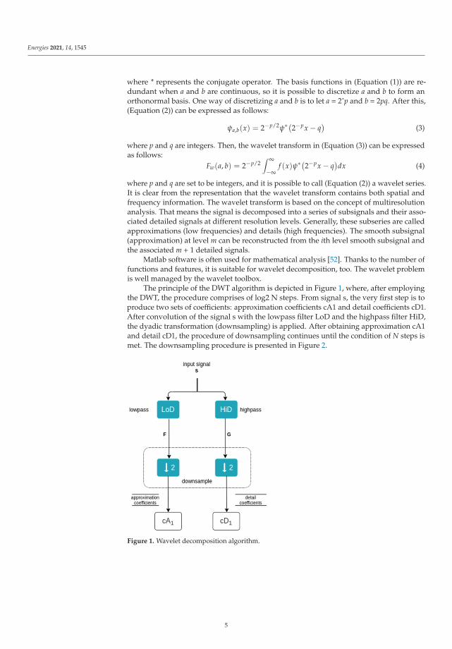
The principle of the DWT algorithm is depicted in Figure 1, where, after employingthe DWT, the procedure comprises of log2 N steps. From signal s, the very first step is toproduce two sets of coefficients: approximation coefficients cA1 and detail coefficients cD1.After convolution of the signal s with the lowpass filter LoD and the highpass filter HiD,the dyadic transformation (downsampling) is applied. After obtaining approximation cA1and detail cD1, the procedure of downsampling continues until the condition of N steps ismet. The downsampling procedure is presented in Figure 2.

Figure 1. Wavelet decomposition algorithm.

5

Energies 2021, 14, 1545

Figure 2. The 1D wavelet decomposition algorithm (wavedec function).

The decomposition was developed by Mallat [12]. DWT is commonly used for fastsignal extraction [34]. The decomposition process is iterative, which means that the ap-proximation component after iteration will be decomposed into several low-resolutioncomponents.

After the decomposition of the input signal s, we have the low-frequency coefficientcA1 and the high-frequency coefficient cD1 (see Figure 3). After the next decomposition ofcA1, high-frequency component cD2 and low-frequency component cA2 are gained. If thedecomposition process continues to level j = 3, in the last step coefficients cA3 and cD3are obtained from cA2. Coefficient cA1 can be reconstructed by cA2 and cD2; similarly,cA2 can be reconstructed by cA3 and cD3.

Figure 3. Three-level wavelet decomposition.

The wavelet transform is often used for data preparation for predictive systems witha neural network. In many cases, the type of neural network selected is very simple;oftentimes, a feedforward backpropagation neural network is used.

6

Energies 2021, 14, 1545

2.2. Artificial Neural Networks

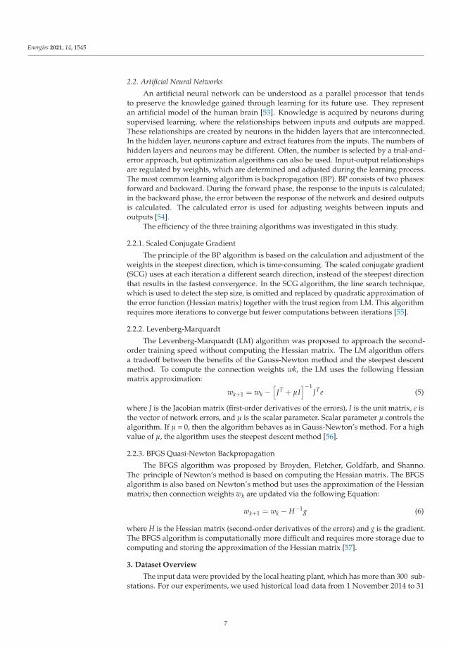
An artificial neural network can be understood as a parallel processor that tendsto preserve the knowledge gained through learning for its future use. They representan artificial model of the human brain [53]. Knowledge is acquired by neurons duringsupervised learning, where the relationships between inputs and outputs are mapped.These relationships are created by neurons in the hidden layers that are interconnected.In the hidden layer, neurons capture and extract features from the inputs. The numbers ofhidden layers and neurons may be different. Often, the number is selected by a trial-and-error approach, but optimization algorithms can also be used. Input-output relationshipsare regulated by weights, which are determined and adjusted during the learning process.The most common learning algorithm is backpropagation (BP). BP consists of two phases:forward and backward. During the forward phase, the response to the inputs is calculated;in the backward phase, the error between the response of the network and desired outputsis calculated. The calculated error is used for adjusting weights between inputs andoutputs [54].

The efficiency of the three training algorithms was investigated in this study.

2.2.1. Scaled Conjugate Gradient

The principle of the BP algorithm is based on the calculation and adjustment of theweights in the steepest direction, which is time-consuming. The scaled conjugate gradient(SCG) uses at each iteration a different search direction, instead of the steepest directionthat results in the fastest convergence. In the SCG algorithm, the line search technique,which is used to detect the step size, is omitted and replaced by quadratic approximation ofthe error function (Hessian matrix) together with the trust region from LM. This algorithmrequires more iterations to converge but fewer computations between iterations [55].

2.2.2. Levenberg-Marquardt

The Levenberg-Marquardt (LM) algorithm was proposed to approach the second-order training speed without computing the Hessian matrix. The LM algorithm offersa tradeoff between the benefits of the Gauss-Newton method and the steepest descentmethod. To compute the connection weights wk, the LM uses the following Hessianmatrix approximation:

wk+1 = wk −[

JT + μI]−1

JTe (5)

where J is the Jacobian matrix (first-order derivatives of the errors), I is the unit matrix, e isthe vector of network errors, and μ is the scalar parameter. Scalar parameter μ controls thealgorithm. If μ = 0, then the algorithm behaves as in Gauss-Newton’s method. For a highvalue of μ, the algorithm uses the steepest descent method [56].

2.2.3. BFGS Quasi-Newton Backpropagation

The BFGS algorithm was proposed by Broyden, Fletcher, Goldfarb, and Shanno.The principle of Newton’s method is based on computing the Hessian matrix. The BFGSalgorithm is also based on Newton’s method but uses the approximation of the Hessianmatrix; then connection weights wk are updated via the following Equation:

wk+1 = wk − H−1g (6)

where H is the Hessian matrix (second-order derivatives of the errors) and g is the gradient.The BFGS algorithm is computationally more difficult and requires more storage due tocomputing and storing the approximation of the Hessian matrix [57].

3. Dataset Overview

The input data were provided by the local heating plant, which has more than 300 sub-stations. For our experiments, we used historical load data from 1 November 2014 to 31

7

Energies 2021, 14, 1545

March 2015; for that period, we have a mixture of different data from various types ofweather (see Figure 4). This dataset is used for training and testing. The total load consistsof domestic hot water and the hot water used for central heating. The samples were loggedevery 10 min. Weather data were also collected from this heating plant. The units forload are in MW and for temperature in ◦C. Data were downloaded from SCADA in *.xlsxformat, and then the data were converted into a suitable format for further processing.A large heat load drop at the beginning of the series was caused by the beginning of theheating season. The statistical characteristics of the data used are presented in Table 1.

Figure 4. Heat consumption and outdoor temperature.

Table 1. Statistical characteristics of raw data.

Parameter Min Max Mean Std

Temperature (◦C) −8.93 18.47 5.27 4.52Load (MW) 0 74.04 32.34 8.92

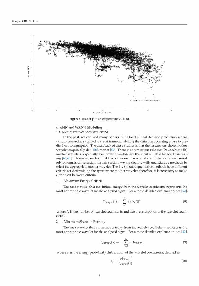
The scatter plot shown in Figure 5 shows the temperature and load dependency,as well as possible outliers. The presence of outliers can be explained by the fact that,during warmer days, the studied heat plant did not use the maximum power. That meansthat, during warmer periods, plants with less power were used.

Data preprocessing is necessary because all these data come from an industrial process,which is often full of errors such as missing data, noisy data, offset, etc. Missing data weresubstituted by the average of P−1 and P+1 values. Data normalization is a necessarystep to avoid node saturation, which could negatively affect the training phase. For datanormalization, we used Z score normalization:

Yi =Xi − X

σ(7)

where Yi is the normalized value, Xi is the actual value, X is the arithmetic mean, and σ isthe standard deviation.

8

Energies 2021, 14, 1545

Figure 5. Scatter plot of temperature vs. load.

4. ANN and WANN Modeling

4.1. Mother Wavelet Selection Criteria

In the past, we can find many papers in the field of heat demand prediction wherevarious researchers applied wavelet transform during the data preprocessing phase to pre-dict heat consumption. The drawback of these studies is that the researchers chose motherwavelet empirically db4 [58], morlet [59]. There is an unwritten rule that Daubechies (db)mother wavelets, especially low order db2–db4, are the most suitable for load forecast-ing [60,61]. However, each signal has a unique characteristic and therefore we cannotrely on empirical selection. In this section, we are dealing with quantitative methods toselect the appropriate mother wavelet. The investigated qualitative methods have differentcriteria for determining the appropriate mother wavelet; therefore, it is necessary to makea trade-off between criteria.

1. Maximum Energy Criteria

The base wavelet that maximizes energy from the wavelet coefficients represents themost appropriate wavelet for the analyzed signal. For a more detailed explanation, see [62].

Eenergy (s) =N

∑i=1

|wt(s, i)|2 (8)

where N is the number of wavelet coefficients and wt(s,i) corresponds to the wavelet coeffi-cients.

2. Minimum Shannon Entropy

The base wavelet that minimizes entropy from the wavelet coefficients represents themost appropriate wavelet for the analyzed signal. For a more detailed explanation, see [62].

Eentropy(s) = −N

∑i=1

pi· log2 pi (9)

where pi is the energy probability distribution of the wavelet coefficients, defined as

pi =|wt(s, i)|2Eenergy(s)

(10)

9

Energies 2021, 14, 1545

3. Energy-to-Shannon Entropy ratio

The base wavelet that has produced the maximum energy-to-Shannon entropy ratiowas selected to be the most appropriate wavelet for the analyzed signal [62]:

R(s) =Eenergy(s)

Eentropy(s)(11)

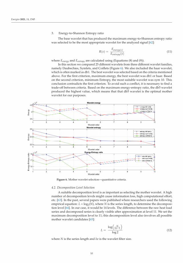
where Eenergy and Eentropy are calculated using (Equations (8) and (9)).In this section we compared 25 different wavelets from three different wavelet families,

namely Daubechies, Symlets, and Coiflets (Figure 6). We also included the haar wavelet,which is often marked as db1. The best wavelet was selected based on the criteria mentionedabove. For the first criterion, maximum energy, the best wavelet was db1 or haar. Basedon the second criterion, minimum Entropy, the most suitable wavelet was sym 10. Thisconclusion contradicts the first criterion. To avoid such a conflict, it is necessary to find atrade-off between criteria. Based on the maximum energy-entropy ratio, the db5 waveletproduced the highest value, which means that that db5 wavelet is the optimal motherwavelet for our purposes.

Figure 6. Mother wavelet selection—quantitative criteria.

4.2. Decomposition Level Selection

A suitable decomposition level is as important as selecting the mother wavelet. A highnumber of decomposition levels might cause information loss, high computational effort,etc. [63]. In the past, several papers were published where researchers used the followingempirical equation: L = log2(N), where N is the series length, to determine the decomposi-tion level [64]. In our case, it would be 14 levels. The difference between the raw heat loadseries and decomposed series is clearly visible after approximation at level 11. We set themaximum decomposition level to 11; this decomposition level also involves all possiblemother wavelet candidates [65]:

L =log

(N

lw−1

)log 2

(12)

where N is the series length and lw is the wavelet filter size.

10

Energies 2021, 14, 1545

We focused on a deeper analysis of the decomposed signal via the proposed methodby Sang [66]. This method is used to identify the true and noisy components of eachdecomposition level. The comparison of the energy of raw series and referenced noiseseries identified components that are close to or inside of the confidence interval of thereferenced noise series. In Figure 7, we can clearly identify the components (D1–D3) thatare likely to be noise. We suppose that the components above level D4 are true componentsof the signal. From this analysis, we propose two suitable decompositions at level 6 andlevel 9 by db5 mother wavelet.

Figure 7. Energy of subseries.

4.3. Building WANN and ANN Models

For an accurate forecast of heat consumption, it is necessary to make a detailedanalysis of the variables that influence heat consumption. Generally, energy consumptiondepends on many factors such as social and climate parameters, type of consumers, etc.Heat demand strongly depends on the outdoor temperature and other climate factors likehumidity, wind speed, and so on. Research papers from the past confirm that the strongestinfluence on demand is outdoor temperature [67]. That fact is also proven by a correlationanalysis between heat load and outdoor temperature, where the correlation coefficient is-0.78, which could be considered a strong relationship. Another good predictor is historicalload. It is likely that consumption the following day at the same time will be similar to theconsumption the day before. Significant lags were determined by autocorrelation analysis.Generally, heat load consumption also depends on the time of the day and day of the week.These factors could also increase the prediction accuracy. Table 2 shows the selected inputvariables for WANN.

Table 2. Selected input variables.

Input Number Input Name Value Calculation

1. Hour 0–23Timestamp2. Weekend 0–1

3. Day of the week 1–74. Temperature Various Exogenous5. Lagged load Various Endogenous + timestamp

11

Energies 2021, 14, 1545

1. Hour—To capture the cyclical behavior of the series, the hour variable was encodedvia sine and cosine transform:

Hsin =sin(2πh)

24(13)

Hcos =cos(2πh)

24(14)

Weekend—1 represents weekends and 0 represents weekdays.Day of the week (DoW)—determines the days of the week, where Mondays are marked

as 1 and Sundays as 7.

DOWsin =sin(2πdow)

7(15)

DOWcos =cos(2πdow)

7(16)

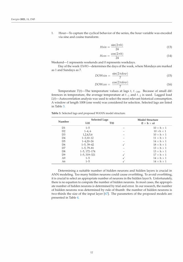
Temperature T(t)—The temperature values at lags t, t−144. Because of small dif-ferences in temperature, the average temperature at t−1 and t−2 is used. Lagged loadL(t)—Autocorrelation analysis was used to select the most relevant historical consumption.A window of length 1008 (one week) was considered for selection. Selected lags are listedin Table 3.

Table 3. Selected lags and proposed WANN model structure.

NumberSelected Lags Model Structure

(I × h × o)L(t) T(t)

D1 1–5 – 10 × h × 1D2 1–4, 6 – 10 ×h × 1D3 1,2,4,5,6 – 10 × h × 1D4 1–3,10–12 – 11 × h × 1D5 1–4,20–24 – 14 × h × 1D6 1–5, 39–42 � 18 × h × 1D7 1–5, 79–81 – 13 × h × 1D8 1–5, 172–174 – 13 × h × 1D9 1–5, 319–321 � 17 × h × 1A9 1–5 � 14 × h × 1A6 1–5 � 14 × h × 1

Determining a suitable number of hidden neurons and hidden layers is crucial inANN modeling. Too many hidden neurons could cause overfitting. To avoid overfitting,it is crucial to select an appropriate number of neurons in the hidden layer h. Unfortunately,there is no equation to compute the number of hidden neurons. In most cases, the appropri-ate number of hidden neurons is determined by trial and error. In our research, the numberof hidden neurons was determined by rule of thumb: the number of hidden neurons istwo-thirds the size of the input layer [67]. The parameters of the proposed models arepresented in Table 4.

12

Energies 2021, 14, 1545

Table 4. Parameters of proposed feedforward neural networks.

Model Parameter ValueBP

NN

and

WA

NN

Number of hidden layers 1

Number of neurons in hidden layer 21 for ANN modelsVarious for WANN; see Table 3

Number of output neurons 1Hidden layer activation function tansigOutput layer activation function purelin

Data set division train/test random 80/20 (%)Epochs 1000

Data normalization mapstd; see (Equation (7))Training algorithms trainlm, trainscg, trainbfg

Learning rate 0.001

WANNDecomposition level 6 and 9

Mother wavelet db5

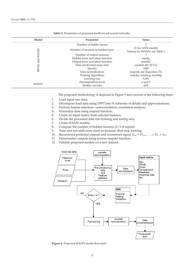
The proposed methodology is depicted in Figure 8 and consists of the following steps:

1. Load input raw data;2. Decompose load data using DWT into N subseries of details and approximations;3. Perform feature selection—autocorrelation, correlation analysis;4. Normalize data using mapstd function;5. Create an input matrix from selected features;6. Divide the processed data into training and testing sets;7. Create WANN models8. Compute the number of hidden neurons (2/3 of inputs)9. Train and test until error starts to increase, then stop training;10. Reconstruct predicted outputs and reconstruct signal Xrec = D1+, . . . ,+ Dn + An;11. Denormalize outputs using reverse mapstd function;12. Validate proposed models on a new dataset.

Figure 8. Proposed WANN model flowchart.

13

Energies 2021, 14, 1545

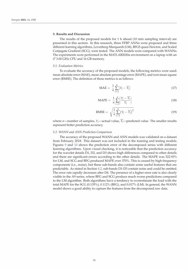
5. Results and Discussion

The results of the proposed models for 1 h ahead (10 min sampling interval) arepresented in this section. In this research, three FFBP ANNs were proposed and threedifferent learning algorithms, Levenberg-Marquardt (LM), BFGS quasi-Newton, and ScaledConjugate Gradient (SCG), were tested. The ANN models were compared with WANNs.The experiments were performed in the MATLAB2020a environment on a laptop with ani7 3.00 GHz CPU and 16 GB memory.

5.1. Evaluation Metrics

To evaluate the accuracy of the proposed models, the following metrics were used:mean absolute error (MAE), mean absolute percentage error (MAPE), and root mean squareerror (RMSE). The definition of these metrics is as follows:

MAE =1n

n

∑i=1

∣∣Yi − Yi∣∣ (17)

MAPE =1n

n

∑i=1

∣∣∣∣Yi − YiYi

∣∣∣∣ (18)

RMSE =

√1n

n

∑i=1

(Yi − Yi

)2 (19)

where n—number of samples, Yi—actual value, Yi—predicted value. The smaller resultsrepresent better prediction accuracy.

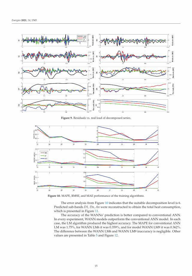
5.2. WANN and ANN Prediction Comparison

The accuracy of the proposed WANN and ANN models was validated on a datasetfrom February 2018. This dataset was not included in the training and testing models.Figures 9 and 10 shows the prediction error of the decomposed series with differentlearning algorithms. Upon visual checking, it is noticeable that the prediction accuracyfor the wavelet details D1, D2, and D3 shows high differences compared to other detailsand there are significant errors according to the other details. The MAPE was 322.93%for LM, and SCG and BFG produced MAPE over 370%. This is caused by high-frequencycomponents (i.e., noise), but these sub-bands also contain some useful features that arepredictable. As stated in Section 4.2, sub-bands D1-D3 contain noise and could be omitted.The error rate rapidly decreases after D4. The presence of a higher error rate is also clearlyvisible in the A9 series, where BFG and SCG produce much worse predictions comparedto the LM algorithm. Both algorithms have a tendency to overestimate the load with thetotal MAPE for the SCG (0.135%), 0.112% (BFG), and 0.017% (LM). In general, the WANNmodel shows a good ability to capture the features from the decomposed raw data.

14

Energies 2021, 14, 1545

Figure 9. Residuals vs. real load of decomposed series.

Figure 10. MAPE, RMSE, and MAE performance of the training algorithms.

The error analysis from Figure 10 indicates that the suitable decomposition level is 6.Predicted sub-bands D1, Dn, An were reconstructed to obtain the total heat consumption,which is presented in Figure 11.

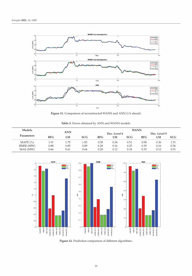
The accuracy of the WANNs’ prediction is better compared to conventional ANN.In every experiment, WANN models outperform the conventional ANN model. In eachcase, the LM algorithm produced the highest accuracy. The MAPE for conventional ANNLM was 1.75%, for WANN LM6 it was 0.359%, and for model WANN LM9 it was 0.362%.The difference between the WANN LM6 and WANN LM9 inaccuracy is negligible. Othervalues are presented in Table 5 and Figure 12.

15

Energies 2021, 14, 1545

Figure 11. Comparison of reconstructed WANN and ANN (1 h ahead).

Table 5. Errors obtained by ANN and WANN models.

ModelsANN

WANN

ParametersDec. Level 6 Dec. Level 9

BFG LM SCG BFG LM SCG BFG LM SCG

MAPE (%) 1.91 1.75 1.83 0.58 0.36 0.51 0.98 0.36 1.51RMSE (MW) 0.88 0.85 0.89 0.28 0.16 0.25 0.39 0.16 0.56MAE (MW) 0.66 0.61 0.64 0.20 0.12 0.18 0.33 0.12 0.51

Figure 12. Prediction comparison of different algorithms.

16

Energies 2021, 14, 1545

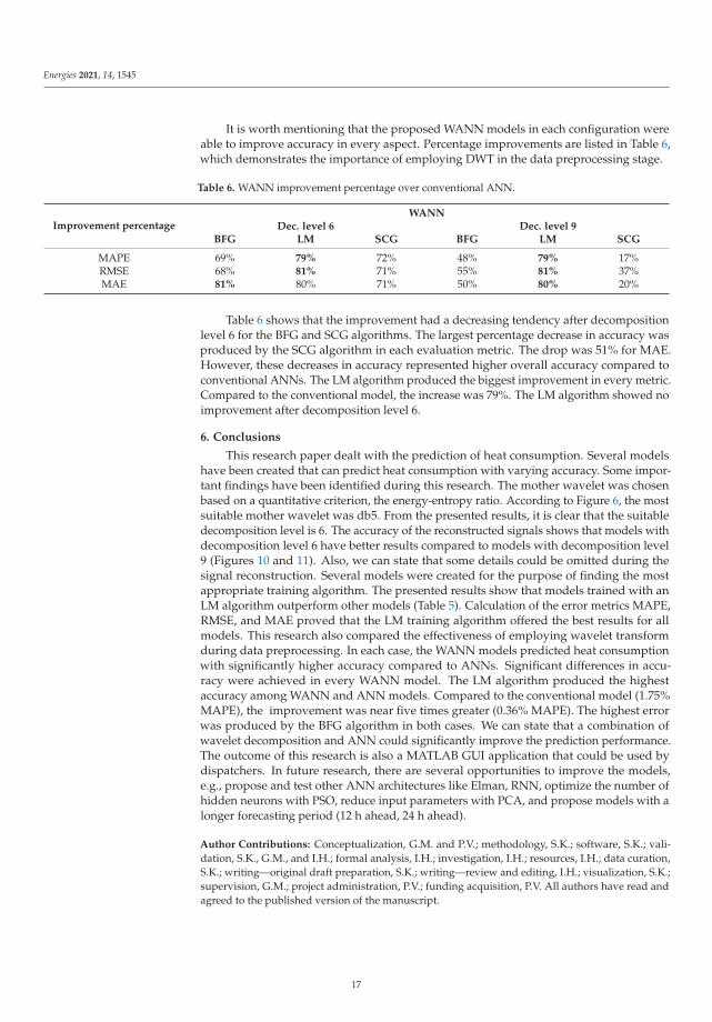
It is worth mentioning that the proposed WANN models in each configuration wereable to improve accuracy in every aspect. Percentage improvements are listed in Table 6,which demonstrates the importance of employing DWT in the data preprocessing stage.

Table 6. WANN improvement percentage over conventional ANN.

Improvement percentageWANN

Dec. level 6 Dec. level 9BFG LM SCG BFG LM SCG

MAPE 69% 79% 72% 48% 79% 17%RMSE 68% 81% 71% 55% 81% 37%MAE 81% 80% 71% 50% 80% 20%

Table 6 shows that the improvement had a decreasing tendency after decompositionlevel 6 for the BFG and SCG algorithms. The largest percentage decrease in accuracy wasproduced by the SCG algorithm in each evaluation metric. The drop was 51% for MAE.However, these decreases in accuracy represented higher overall accuracy compared toconventional ANNs. The LM algorithm produced the biggest improvement in every metric.Compared to the conventional model, the increase was 79%. The LM algorithm showed noimprovement after decomposition level 6.

6. Conclusions

This research paper dealt with the prediction of heat consumption. Several modelshave been created that can predict heat consumption with varying accuracy. Some impor-tant findings have been identified during this research. The mother wavelet was chosenbased on a quantitative criterion, the energy-entropy ratio. According to Figure 6, the mostsuitable mother wavelet was db5. From the presented results, it is clear that the suitabledecomposition level is 6. The accuracy of the reconstructed signals shows that models withdecomposition level 6 have better results compared to models with decomposition level9 (Figures 10 and 11). Also, we can state that some details could be omitted during thesignal reconstruction. Several models were created for the purpose of finding the mostappropriate training algorithm. The presented results show that models trained with anLM algorithm outperform other models (Table 5). Calculation of the error metrics MAPE,RMSE, and MAE proved that the LM training algorithm offered the best results for allmodels. This research also compared the effectiveness of employing wavelet transformduring data preprocessing. In each case, the WANN models predicted heat consumptionwith significantly higher accuracy compared to ANNs. Significant differences in accu-racy were achieved in every WANN model. The LM algorithm produced the highestaccuracy among WANN and ANN models. Compared to the conventional model (1.75%MAPE), the improvement was near five times greater (0.36% MAPE). The highest errorwas produced by the BFG algorithm in both cases. We can state that a combination ofwavelet decomposition and ANN could significantly improve the prediction performance.The outcome of this research is also a MATLAB GUI application that could be used bydispatchers. In future research, there are several opportunities to improve the models,e.g., propose and test other ANN architectures like Elman, RNN, optimize the number ofhidden neurons with PSO, reduce input parameters with PCA, and propose models with alonger forecasting period (12 h ahead, 24 h ahead).

Author Contributions: Conceptualization, G.M. and P.V.; methodology, S.K.; software, S.K.; vali-dation, S.K., G.M., and I.H.; formal analysis, I.H.; investigation, I.H.; resources, I.H.; data curation,S.K.; writing—original draft preparation, S.K.; writing—review and editing, I.H.; visualization, S.K.;supervision, G.M.; project administration, P.V.; funding acquisition, P.V. All authors have read andagreed to the published version of the manuscript.

17

Energies 2021, 14, 1545

Funding: This research was funded by Mladý výskumník, “Návrh neurónovej siete na predikciuspotreby tepla”; the Scientific Grant Agency of the Ministry of Education, Science, Research andSport of the Slovak Republic and the Slovak Academy of Sciences, grant number VEGA 1/0272/18,“Holistic approach of knowledge discovery from production data in compliance with Industry 4.0concept”; and the Scientific Grant Agency of the Ministry of Education, Science, Research and Sportof the Slovak Republic and the Slovak Academy of Sciences, grant number 1/0232/18, “Using themethods of multiobjective optimization in production processes control.”

Acknowledgments: We would like to thank BAT company for providing heat consumption dataand the anonymous reviewers for their comments, which improved the quality of the work. Thispublication is the results of the project ITMS 313011W988: “Research in the SANET network and possi-bilities of its further use and development” within the Operational Program Integrated Infrastructureco-financed by the ERDF.

Conflicts of Interest: The authors declare no conflict of interest.

References

1. Gabriska, D. Evaluation of the Level of Reliability in Hazardous Technological Processes. Appl. Sci. 2021, 11, 134. [CrossRef]2. Kurek, T.; Bielecki, A.; Swirski, K.; Wojdan, K.; Guzek, M.; Białek, J.; Brzozowski, R.; Serafin, R. Heat Demand forecasting

algorithm for a Warsaw district heating network. Energy 2021, 217. [CrossRef]3. Guo, B.; Cheng, L.; Xu, J.; Chen, L. Prediction of the Heat Load in Central Heating Systems Using GA-BP Algorithm. In Proceed-

ings of the International Conference on Computer Network, Electronic and Automation (ICCNEA 2017), Xi’an, China, 23–25September 2017; pp. 441–445. [CrossRef]

4. GRANRYD Eric. Refrigerating engineering; Royal Institute of Technology: Stockholm, Sweden, 2009; ISBN 978-91-7415-415-3.5. Panapakidis, I.P.; Dagoumas, A.S. Day-ahead natural gas demand forecasting based on the combination of wavelet transform

and ANFIS/genetic algorithm/neural network model. Energy 2017, 118, 231–245. [CrossRef]6. Yan, K.; Li, W.; Ji, Z.; Du, Y.; Qi, M. A Hybrid LSTM Neural Network for Energy Consumption Forecasting of Individual

Households. IEEE Access 2019, 7, 157633–157642. [CrossRef]7. Nemeth, M.; Borkin, D.; Michalconok, G. The comparison of machine-learning methods XGBoost and LightGBM to predict

energy development. In Proceedings of the Computational Statistics and Mathematical Modeling Methods in Intelligent Systems:Proceedings of 3rd Computational Methods in Systems and Software, Zlín, Czech Republic, 10–12 September 2019; Silhavy, R.,Silhavy, P., Prokopova, Z., Eds.; Springer: Cham/Basel Switzerland, 2019; Volume 2, pp. 208–215. [CrossRef]

8. Nemetova, A.; Borkin, D.; Michalconok, G. Comparison of methods for time series data analysis for further use of machinelearning algorithms. In Proceedings of the Computational Statistics and Mathematical Modeling Methods in Intelligent Systems:Proceedings of 3rd Computational Methods in Systems and Software, Zlín, Czech Republic, 10–12 September 2019; Silhavy, R.,Silhavy, P., Prokopova, Z., Eds.; Springer: Cham/Basel Switzerland, 2019; Volume 2, pp. 90–99. [CrossRef]

9. Lang, X.; Rehman, N.; Zhang, Y.; Xie, L.; Su, H. Median ensemble empirical mode decomposition. Signal Process. 2020, 176.[CrossRef]

10. Zuo, G.; Luo, J.; Wang, N.; Lian, Y.; He, X. Decomposition ensemble model based on variational mode decomposition and longshort-term memory for streamflow forecasting. J. Hydrol. 2020, 585. [CrossRef]

11. Yesilli, M.C.; Khasawneh, F.A.; Otto, A. On transfer learning for chatter detection in turning using wavelet packet transform andensemble empirical mode decomposition. Cirp J. Manuf. Sci. Technol. 2020, 28, 118–135. [CrossRef]

12. Mallat, S.G. A Theory for Multiresolution Signal Decomposition: The Wavelet Representation; Technical Report; University of Pennsyl-vania: Philadelphia, PA, USA, 1987.

13. Meyer, Y. Wavelets, Algorithms & Applications, 1st ed.; SIAM: Philadelphia, PA, USA, 1993.14. Sui, K.; Kim, H.G. Research on application of multimedia image processing technology based on wavelet transform. J. Image

Video Process. 2019, 24. [CrossRef]15. Mahesh, M.; Kumar, T.R.R.; Shoban Babu, B.; Saikrishna, J. Image Enhancement using Wavelet Fusion for Medical Image

Processing. Int. J. Eng. Adv. Technol. 2019, 9. [CrossRef]16. Shanmugapriya, K.; Priya, D.J.; Priya, N. Image Enhancement Techniques in Digital Image Processing. Int. J. Innov. Technol.

Explor. Eng. 2019, 8. [CrossRef]17. Kumar, K.; Mustafa, N.; Li, J.; Shaikh, R.A.; Khan, S.A.; Khan, A. Image edge detection scheme using wavelet transform.

In Proceedings of the International Computer Conference on Wavelet Active Media Technology and Information Processing(ICCWAMTIP 2014), Chengdu, China, 19–21 December 2014; pp. 261–265. [CrossRef]

18. Hashim, M.A.; Nasef, M.H.; Kabeel, A.E.; Ghazaly, N.M. Combustion fault detection technique of sparkignition engine based onwavelet packet transform and artificial neural network. Alex. Eng. J. 2020. [CrossRef]

19. Gharesi, N.; Mehdi Arefi, M.; Razavi-Farb, R.; Zarei, J.; Yin, S. A neuro-wavelet based approach for diagnosing bearing defects.Adv. Eng. Inform. 2020, 46. [CrossRef]

20. Kou, L.; Liu, C.; Cai, G.; Zhang, Z. Fault Diagnosis for Power Electronics Converters based on Deep Feedforward Network andWavelet Compression. Electr. Power Syst. Res. 2020, 185. [CrossRef]

18

Energies 2021, 14, 1545

21. Valizadeh, M.; Sohrabi, M.R.; Motiee, F. The application of continuous wavelet transform based on spectrophotometric methodand high-performance liquid chromatography for simultaneous determination ofanti-glaucoma drugs in eye drop. Spectrochim.Acta Part A Mol. Biomol. Spectrosc. 2020, 242. [CrossRef]

22. Gyorfi, Á.; Szilágyi, L.; Kovács, L. A Fully Automatic Procedure for Brain Tumor Segmentation from Multi-Spectral MRI RecordsUsing Ensemble Learning and Atlas-Based Data Enhancement. Appl. Sci. 2021, 11, 564. [CrossRef]

23. Akansu, A.N.; Serdijn, W.A.; Selesnick, W.I. Emerging applications of wavelets: A review. Phys. Commun. 2010, 3. [CrossRef]24. Zuo, H.; Chen, Y.; Jia, F. A new C0 layer wise wavelet finite element formulation for the static and free vibration analysis of

composite plates. Compos. Struct. 2020, 254. [CrossRef]25. Qin, Y.; Mao, Y.; Tang, B.; Wang, Y.; Chen, H. M-band flexible wavelet transform and its application to thefault diagnosis of

planetary gear transmission systems. Mech. Syst. Signal Process. 2019, 134. [CrossRef]26. Zhao, Z.; Wang, X.; Zhang, Y.; Gou, H.; Yang, F. Wind speed prediction based on wavelet analysis and time series method.

In Proceedings of the International Conference on Wavelet Analysis and Pattern Recognition (ICWAPR 2017), Ningbo, China,9–12 July 2017; pp. 23–27. [CrossRef]

27. Ren, P.; Xiang, Z.; Shangguan, R. Design and Simulation of a prediction algorithm based on wavelet support vector machine.In Proceedings of the Seventh International Conference on Natural Computation, Shanghai, China, 26–28 July 2011; pp. 208–211.[CrossRef]

28. Barthel, K.U.; Brandau, S.; Hermesmeier, W.; Heising, G. Zerotree wavelet coding using fractal prediction. In Proceedings of theInternational Conference on Image Processing (ICIP 1997), Santa Barbara, CA, USA, 26–29 October 1997; Volume 2, pp. 314–317.[CrossRef]

29. Yin, J.; Gao, C.; Wang, Y.; Wang, Y. Hyperspectral image classification using wavelet packet analysis and gray prediction model.In Proceedings of the International Conference on Image Analysis and Signal Processing (IASP 2010), Zhejiang, China, 9–11 April2010; pp. 322–326. [CrossRef]

30. Elarabi, T.; Sammoud, A.; Abdelgawad, A.; Li, X.; Bayoumi, M. Hybrid wavelet—DCT intra prediction for H.264/AVC interactiveencoder. In Proceedings of the IEEE China Summit & International Conference on Signal and Information Processing (ChinaSIP2014), Xi’an, China, 9–13 July 2014; pp. 281–285. [CrossRef]

31. Li, H.; Guo, C.; Yang, S.X.; Jin, H. Hybrid Model of WT and ANFIS and Its Application on Time Series Prediction of Ship RollMotion. In Proceedings of the Multiconference on Computational Engineering in Systems Applications (CESA 2006), Beijing,China, 4–6 October 2006; pp. 333–337. [CrossRef]

32. Stefenon, S.F.; Ribeiro, M.H.D.M.; Nied, A.; Mariani, V.C.; Coelho, L.D.S.; da Rocha, D.F.M.; Grebogi, R.B.; Ruano, A.E.D.B.Wavelet group method of data handling for fault prediction in electrical power insulators. Int. J. Electr. Power Energy Syst. 2020,123. [CrossRef]

33. Prabhakar, D.V.N.; Kumar, M.S.; Krishna, A.G. A Novel Hybrid Transform approach with integration of Fast Fourier, DiscreteWavelet and Discrete Shearlet Transforms for prediction of surface roughness on machined surfaces. Measurement 2020, 164.[CrossRef]

34. Zhang, T.; Chaofeng, L.; Fumin, M.; Zhao, K.; Wang, H.; O’Hare, G.M. A photovoltaic power forecasting model based on dendriticneuron networks with the aid of wavelet transform. Neurocomputing 2020, 397, 438–446. [CrossRef]

35. Chang, Z.; Zhang, Y.; Chen, W. Electricity price prediction based on hybrid model of Adam optimized LSTM neural network andwavelet transform. Energy 2019, 187. [CrossRef]

36. El-Hendawi, M.; Wang, Z. An ensemble method of full wavelet packet transform and neural network for short term electricalload forecasting. Electr. Power Syst. Res. 2020, 182. [CrossRef]

37. Liu, H.; Mi, X.; Li, Y. Smart deep learning based wind speed prediction model using wavelet packet decomposition, convolutionalneural network and convolutional long short term memory network. Energy Convers. Manag. 2018, 166, 120–131. [CrossRef]

38. Xia, C.; Zhang, M.; Cao, J. A hybrid application of soft computing methods with wavelet SVM and neural network to electricpower load forecasting. J. Electr. Syst. Inf. Technol. 2018, 5, 681–696. [CrossRef]

39. Bashir Tayab, U.; Zia, A.; Yang, F.; Lu, J.; Kashif, M. Short-term load forecasting for microgrid energy management system usinghybrid HHO-FNN model with best-basis stationary wavelet packet transform. Energy 2020, 203. [CrossRef]

40. Farhadi, M.; Abbaspour-Gilandeh, Y.; Mahmoudi, A.; Mari Maja, J. An Integrated System of Artificial Intelligence and SignalProcessing Techniques for the Sorting and Grading of Nuts. Appl. Sci. 2020, 10, 3315. [CrossRef]

41. Feng, X.; Feng, Q.; Li, S.; Hou, X.; Zhang, M.; Liu, S. Wavelet-Based Kalman Smoothing Method for Uncertain ParametersProcessing: Applications in Oil Well-Testing Data Denoising and Prediction. Sensors 2020, 20, 4541. [CrossRef]

42. Obidin, M.V.; Serebrovski, A.P. Signal denoising with the use of the wavelet transform and the Kalman filter. J. Commun. Technol.Electron. 2014, 59, 1440–1445. [CrossRef]

43. Li, Y.J.; Kokkinaki, A.; Darve, E.T.; Kitanidis, P.K. Smoothing-based compressed state Kalman filter for joint state-parameterestimation: Applications in reservoir characterization and CO2 storage monitoring. Water Resour. Res. 2017, 53, 7190–7207.[CrossRef]

44. Zhang, X.; Ni, W.; Liao, H.; Pohl, E.; Xu, P.; Zhang, W. Fusing moving average model and stationary wavelet decomposition forautomatic incident detection: Case study of Tokyo Expressway. J. Traffic Transp. Eng. 2014, 1, 404–414. [CrossRef]

45. Szi-Wen, C.; Hsiao-Chen, C.; Hsiao-Lung, C. A real-time QRS detection method based on moving-averaging incorporating withwavelet denoising. Comput. Methods Programs Biomed. 2006, 82, 187–195.

19

Energies 2021, 14, 1545

46. Akansu, A.N.; Haddad, R.A. Multiresolution Signal Decomposition: Transforms, Subbands, and Wavelets, 2nd ed.; Academic Press:San Diego, CA, USA, 2000.

47. Tan, L.; Jiang, J. Discrete Wavelet Transform. In Digital Signal Processing—Fundamentals and Applications, 3rd ed.; Elsevier:Amsterdam, The Netherlands, 2019; pp. 623–632.

48. Boashash, B. The Discrete Wavelet Transform. In Time-Frequency Signal Analysis and Processing—A Comprehensive Reference;Elsevier: Amsterdam, The Netherlands, 2016; pp. 141–142.

49. Loizou, C.P.; Pattichis, C.S.; D’hooge, J. Discrete Wavelet Transform. In Handbook of Speckle Filtering and Tracking in CardiovascularUltrasound Imaging and Video; Institution of Engineering and Technology: London, UK, 2018; pp. 174–177.

50. Bankman, I.N. Three-Dimensional Image Compression with Wavelet Transforms. In Handbook of Medical Image Processing andAnalysis, 2nd ed.; Elsevier: Amsterdam, The Netherlands, 2009; pp. 963–964.

51. MathWorks Wavedec. Available online: https://www.mathworks.com/help/wavelet/ref/wavedec.html (accessed on 1 Novem-ber 2020).

52. Freire, P.K.D.M.M.; Santos, C.A.G.; da Silva, G.B.L. Analysis of the use of discrete wavelet transforms coupled with ANN forshort-term streamflow forecasting. Appl. Soft Comput. 2019, 80, 494–505. [CrossRef]

53. Junior, L.A.; Souza, R.M.; Menezes, M.L.; Cassiano, K.M.; Pessanha, J.F.; Souza, R. Artificial Neural Network and WaveletDecomposition in the Forecast of Global Horizontal Solar Radiation. Pesqui. Oper. 2015, 35, 73–90. [CrossRef]

54. Moller, M.F. A scaled conjugate gradient algorithm for fast supervised learning. Neural Netw. 1993, 6, 525–533. [CrossRef]55. Rodrigues, F.; Cardeira, C.; Calado, J.M.F. The Daily and Hourly Energy Consumption and Load Forecasting Using Artificial

Neural Network Method: A case Study Using a Set of 93 Households in Portugal. Energy Procedia 2014, 62, 220–229. [CrossRef]56. Perera, A.; Azamathulla, H.; Rathnayake, U. Comparison of different Artificial Neural Network (ANN) training algorithm to

predict atmospheric temperature in Tabuk, Saudi Arabia. Mausam 2020, 25, 1–11.57. Gong, M.; Wang, J.; Bai, Y.; Li, B.; Zhang, L. Heat load prediction of residential buildings based on discrete wavelet transform and

tree-based ensemble learning. J. Build. Eng. 2020, 32. [CrossRef]58. Wang, M.; Qi, T. Application of wavelet neural network on thermal load forecasting. Int. J. Wirel. Mob. Comput. 2013, 6, 608–614.

[CrossRef]59. Amjady, N.; Keynia, F. Short-term load forecasting of power systems by combination of wavelet transform and neuro-

evolutionary algorithm. Energy 2009, 34, 46–57. [CrossRef]60. Bashir, Z.A.; El-Hawary, M.E. Applying wavelets to short-term load forecasting using PSO-based neural networks. IEEE Trans.

Power Syst. 2009, 24, 20–27. [CrossRef]61. Gao, R.X.; Yan, R. Wavelets: Theory and applications for manufacturing. Wavelets Theory Appl. Manuf. 2011, 165–187. [CrossRef]62. Tascikaraoglu, A.; Sanandaji, B.M.; Poolla, K.; Varaiya, P. Exploiting sparsity of interconnections in spatio-temporal wind speed

forecasting using Wavelet Transform. Appl. Energy 2016, 165, 735–747. [CrossRef]63. Daubechies, I. Ten Lectures on Wavelets, CBMS-NSF Regional Conference Series in Applied Mathematics; SIAM: Philadelphia, PA, USA,

1992.64. Freire, P.K.D.M.; Santos, C.A.G. Optimal level of wavelet decomposition for daily inflow forecasting. Earth Sci. Inf. 2020, 13,

1163–1173. [CrossRef]65. Sang, Y. A Practical Guide to Discrete Wavelet Decomposition of Hydrologic Time Series. Water Resour. Manag. 2012, 26,

3345–3365. [CrossRef]66. Yang, H.; Jin, S.; Feng, S.; Wang, B.; Zhang, F.; Che, J. Heat Load Forecasting of District Heating System Based on Numerical

Weather Prediction Model. In Proceedings of the 2nd International Forum on electrical Engineering and Automation (IFEEA2015), Guangzhou, China, 26–27 December 2015; pp. 1–5. [CrossRef]

67. Karsoliya, S.; Azad, M. Approximating Number of Hidden layer neurons in Multiple Hidden Layer BPNN Architecture. Int. J.Eng. Trends Technol. 2012, 3, 714–717.

20

energies

Article

An Artificial Intelligence Empowered Cyber Physical Ecosystemfor Energy Efficiency and Occupation Health and Safety

Petros Koutroumpinas 1, Yu Zhang 2,*, Steve Wallis 3 and Elizabeth Chang 2

Citation: Koutroumpinas, P.; Zhang,

Y.; Wallis, S.; Chang, E. An Artificial

Intelligence Empowered Cyber

Physical Ecosystem for Energy

Efficiency and Occupation Health

and Safety. Energies 2021, 14, 4214.

https://doi.org/10.3390/en14144214

Received: 17 April 2021

Accepted: 8 July 2021

Published: 12 July 2021




iations.








4.0/).

1 Faculty of Engineering, Monash University, Melbourne, VIC 3800, Australia; [email protected] School of Business, University of New South Wales, Canberra, ACT 2612, Australia; [email protected] Fleetwood Corporation Limited, Perth, WA 6004, Australia; [email protected]* Correspondence: [email protected]

Abstract: Reducing energy waste is one of the primary concerns facing Remote Industrial Plants(RIP) and, in particular, the accommodations and operational plants located in remote areas. Withthe COVID-19 pandemic continuing to attack the health of workforce, managing the balance betweenenergy efficiency and Occupation Health and Safety (OHS) in the workplace becomes another greatchallenge for the RIP. Maintaining this balance is difficult mainly because a full awareness of theOHS will generally consume more energy while reducing the energy cost may lead to a less effectiveOHS, and the existing literature has not seen a system that is designed for the RIPs to conserveenergy usage and improve workforce OHS simultaneously. To bridge this gap, in this paper, wepropose an AI Empowered Cyber Physical Ecosystem (AECPE) solution for the RIPs, which integratesCyber-Physical Systems (CPS), artificial intelligence, and mobile networks. The preliminary resultsof lab experiments and field tests proved that the AECPE was able to help industries reduce thecorporate annual energy cost that is worth millions of dollars, optimise the environmental conditions,and improve OHS for all workers and stakeholders. The implementation of the AECPE can resultin efficient energy usage, reduced wastage and emissions, environment-friendly operations, andimproved social reputation of the industries.

Keywords: cyber-physical system; ecosystem; remote industries; OHS; energy efficiency; smartmeter; artificial intelligence; COVID-19

1. Introduction

Maintaining a delicate balance between energy efficiency and Occupation Health andSafety (OHS) [1] has been a challenge facing large enterprises and particularly the RemoteIndustrial Plants (RIP), such as mining campsites and other resources industries and remoteindustrial facilities in regional and countryside areas. With extreme weather conditionsaround the world, energy powered air conditioning systems need to be properly managedin order to prevent uninhabitable situations from happening.

As examples: when the temperature outside of a mining campsite is around 40 ◦C, itcould exceed 50 ◦C indoors; one person working after hours turning on the entire site’sor building’s power and lights instead of the one specific spot that is needed; and mal-functioning air-conditioning units in an operational plant could lead all staff to experiencestress due to high or low temperatures. The extreme weather conditions require a constantsupply of energy with balanced heating or cooling to ensure that OHS standards are metfor the sake of all employees and visitors as well as stakeholders.

In addition, the challenge extends to the issues of appropriate lighting, ventilation,air-quality, and humidity control. Regardless of whether the majority of RIPs are reliant onfossil fuels to generate power and are off-site, off-grid with no electrical networks, or inthe city where the lights are on in continuous and constant mode. With massive energyconsumption, the difficulty lies in how to properly manage the energy cost whilst ensuringOHS conditions are optimal for the workforce.


Energies 2021, 14, 4214

In order to address the above issues and risks in the RIPs, this paper presents an AIEmpowered Cyber Physical Ecosystem (AECPE), which is a cost-effective, smart digitalecosystem solution that integrates Cyber-Physical Systems (CPS), mobile networks, andartificial intelligence. The AECPE is designed to intelligently provide personalised services,including a live-able temperature, refrigerating perishables, water temperature control,electrical appliances, lighting, ventilation, and room humidity, by detecting the occupancyof rooms or facilities and monitoring the habitable environments.

This differs from any existing CPS or Internet of Things (IoT) since its focus is onmaking the computing elements of the system coordinate more closely with the sensors andthe actuators to achieve a higher level of system intelligence and efficiency in monitoringand controlling the cyber and physical environments. In addition, the mobile networks andAI enable the system and devices to exchange information, analyse data and produce real-time energy usage and environmental awareness. The AECPE leverages communicationsamong sensors, smart meters, and AI modules through mobile networks to create a cyberphysical ecosystem that not only reduces electricity wastage and carbon emissions but alsofulfils OHS compliance at the same time.

The contribution of the proposed AECPE lies more towards its practical applicationsthan theoretical level, which is summarised from three aspects. Firstly, more OHS pro-file entries are considered in the AECPE since the system is designed for remote areaindustrial plants and accommodations, including indoor/outdoor and historical/forecasttemperature, lighting, air quality, ventilation, humidity, personal use preferences, andmovement from area to area. Secondly, the actuators are managed by machine-learningbased algorithms that require minimal human intervention, and that take into accountvaluable real data collected from test sites, such as user preferences, room occupancy andpersonal movement which can be used for not only maintaining the balance betweenenergy efficiency and OHS but also contact tracing to offer proactive responses duringthe COVID-19 pandemic. Finally, the ACEPE has been tested on real data in a real-lifeenvironment with highly demanding accommodation and a physically stressful outdoorenvironment, and the results have shown success in reducing the electricity consumptionwhile maintaining a user-friendly living environment.

The remainder of this paper is structured as follows. Section 2 presents the practicalissues facing the current industries and technologies. Section 3 introduces the frameworkof the proposed AECPE. Section 4 describes the design of the AECPE in detail, followed bythe prototype setup and field testing of the system in Section 5. Lastly, Section 6 presentsthe conclusions and directions for future study.

2. Related Work

2.1. Cyber-Physical Systems

A Cyber Physical System (CPS) is a system that provides new ways for humans tointeract with the cyber and the physical world [2]. A CPS generally contains two main parts.The first is real-time connectivity to the physical world allowing continual informationfeedback, and the second is intelligent data management and analytics. Instead of usinga two-part structure, a five-part structure of CPS was proposed [3]. They are (i) smartconnection, (ii) data-to-information conversion, (iii) a cyber level, (iv) cognition level, andfinally (v) configuration level. Each of these five sections will have subsections.

A smart connection should involve sensors and metering wireless networks and plugand play connectivity. This section does not have to be online if not necessary. A Zigbeeprotocol can be used for this section. Data analytics and desegregation will take part in thedata-to-information section. There are two choices of how to go about this. The analyticscan occur on-site where the data was collected or can be send to the cloud for the analyticsto occur there. On-site analytics require for there to be a server framework created on saidsite. On the other hand, for the data to be send to the cloud could put a strain on devices ifthey are running on a battery or could put excess strain on the bandwidth available.

22

Energies 2021, 14, 4214

In a case study, it was seen that the power draw of the CPS system could be reducedby up to 70% if the collected data were first compressed before being sent to the cloud [4].This promotes the idea that some amount of on-site pre-processing will have to occur. Thecyber level will allow for further analysis to occur and models to be created to be able toidentify similarities or variations within the incoming data. Next, the cognition level willallow the incoming data to be visualized for the user. Monitoring will play an importantrole in the future of CPS as it will enable real-time alerts and corrective actions dependingon what is needed by the system [5].

The final level is the configuration level, which includes a large amount of machinelearning algorithms so that the system can be self-adjustable, self-optimizing, and self-configuring. If the system can achieve these requirements, it will be able quickly adjust asthe system grows and become more complex throughout its operation. These five steps canact as a good road map in the future implementation of new Cyber Physical Systems [3] .

In terms of CPS applications, these have been used in many sectors, such as aviation,IT, transport, and medical fields. The medical field has seen multiple case studies. Onesuch study proposed the Medical Cyber Physical System or MCPS [6]. The main problemsthat a system like this would face are reliability, security, and safety requirements, whichrequire further human interactions to obtain the best use out of the system. The paperalso draws attention to the impact that cyber attacks can have as well as the need for acombined design methodology to resolve the design challenges of long-term learning andself-adaption of MCPS.

A further case study into the applications of CPS in the medical field was appliedin a house environment [7] to improve the quality of life for elderly patients or otherpatients. What they proposed was the application of a camera and sensor network for realtime surveillance of the patient to allow better and more efficient care. This would alsoallow real-time scheduling and management of resources—for example, the dispensingof medication. A point that this paper raised is aligned with another CPS research, whichclaimed that any lapses in the security and communication of the MCPS could put lives atrisk [6]. The MCPS was also used to control an Analgesic Infusion pump [8].

Their application used a spatio-temporal partial differential equation and a PKAmodel to determine the concentration of a medication in a patient’s blood stream. Ifthe concentration drops too low, then the pump will be told to increase the output ofmedication and vice versa if the concentration is too high. This way, if there is a highenough confidence in the system, the human error can be removed, and the response timeto the changes in concentration will be detected quicker by the software than by the humanuser, thus, improving the safety for the patient.

While CPS has been used as the framework to connect the cyber and physical worlds,many system control approaches have been proposed. An artificial bee colony optimisationalgorithm was proposed to simultaneously maximise comfort whilst minimising energyusage [9]. Fuzzy controllers were used in the system where the input for the controllerswas the difference between the input user parameters and the actual parameters, and theoutput is the required power to affect the conditions. This solution aims to address theComfort index, which applies on the suitability of environmental conditions for physicalactivity. Applying fuzzy logic for system control has become more common as the need forenergy saving is rising.

A fan coil unit was proposed as a way of transporting heat from the air into a coolantfluid [10]. In their experiment, the controlled variables were the room temperature andthe room humidity. It was shown that fuzzy controls successfully managed the previousvariables, whereas the Proportional Integral Derivative control failed to do so, which usesmore energy. It can also be used for multiple system control, such as managing the roomtemperature control whilst taking into account the dew point [11]. This study showed thatfuzzy logic was an easy way of solving this problem without getting too involved in thephysical variables. Fuzzy logic has been shown to be an effective solution when dealingwith a temperature control problem in certain situations.

23

Energies 2021, 14, 4214

However, fuzzy logic lacks the ability to make future predictions based on historicalinformation, such as how much energy will be used in the future leading to future costsbeing known. Machine learning, on the other hand, excels at this given that a large amountof data is collected and ready for use [12]. In our project, three years of room temperaturedata was collected and provided for experiments, and the outdoor daily temperature forthe region can also be accessed online [13], thus, making the machine learning a moreeffective solution than fuzzy logic for this situation.

2.2. Cyber Security

In any situation where a wireless connection is involved, cyber security is an issuethat has to be taken into account. Different types of attack can occur. A denial-of-service(DoS) attack involves rendering a service, a computer, or other devices unavailable to theintended users by overwhelming a targeted machine or service with requests until normalrequests cannot come through [14]. Sites, such as shopping centres, airports, universities,and other public locations, are vulnerable to these types of attacks due to their broadcastingnature [15].

These attacks can also slow down systems and make them use stale data [16]. In thiscase, it would drive up the energy usage as the optimisation algorithm relies on havingthe most current data. There is also a risk of the room not being at the correct temperaturewhen the worker arrives, which would be an OHS risk. A CPS could also face replayattacks, which involve an intercepted message being delayed or intercepted to misdirectthe receiver [17]. This attack could occur through the end sensors of the CPS, where thecollected data could be collected and then duplicated [18].

A possible way to combat this attack is to use a random authentication signal in thecontrol system [18] or encryption keys [17]. Another attack is a false data injection attack,which can happen in a power grid [19]. This attack also involves an attack on the sensors;however, in this case, it involves compromising the sensor reading in such a way thatundetected errors are introduced into the calculations of state variables and values [20].

2.3. Occupational Health and Safety

Occupational Health and Safety (OHS) is the study of workplace influences on healthand well-being, including identifying the environment and mechanism causes of imbal-ances related to human biological, chemical, and physical pollutants in the workplace andproviding a customised and occupational health and safety compliant environment forworkers, including remote operations. The Occupational Safety and Health Act and OHSrisk management supported by the Occupational Safety and Health Regulations in eachcountry are used to ensure that habitable conditions are met for the workers.

Occupational health is as important as physical health, and we developed mechanismsfor better occupational health using data captured through CPS devices to infer andidentify risk factors (i.e., stress, fatigue, and mental illness). There have been some studies,applications, and devices focusing on CPS (listed as follows); however, they all showedtheir limitations in considering the OHS.

• Smart metering from EKM Metering (US) and Meazon (EU) are great at monitoringenergy and water usage to extremely high accuracy but they do not offer services toimprove OHS [21].

• Paxton (UK) offers wireless door handles for access control but does not considerOHS [22].

• KBE, one of the world’s largest manufacturers for energy saving buildings, focusesonly on materials used for housing but not OHS [23].

• USA, China, and EU have worked on energy optimisation through the IoT coupledwith renewable energy for remote and rural communities to improve lifestyle throughenergy supply, but do not focus on the corporate social responsibility for OHS of theirworkers or tenants [24,25].

24

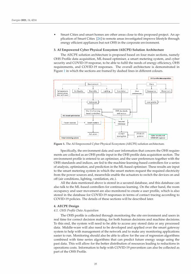
Energies 2021, 14, 4214

• Smart Cities and smart homes are other areas close to this proposed project. An ap-plication of Smart Cities [26] to remote areas investigated improve lifestyle throughenergy efficient appliances but not OHS in the corporate environment.

3. AI Empowered Cyber Physical Ecosystem (AECPE) Solution Architecture

The AECPE solution architecture is proposed based on four main sections, namelyOHS Profile data acquisition, ML-based optimiser, a smart metering system, and cybersecurity and COVID-19 response, to be able to fulfil the needs of energy efficiency, OHSrequirements, and COVID-19 responses. The overall architecture is demonstrated inFigure 1 in which the sections are framed by dashed lines in different colours.

Figure 1. The AI Empowered Cyber Physical Ecosystem (AECPE) solution architecture.

Specifically, the environment data and user information that concern the OHS require-ments are collected as an OHS profile input in the OHS profile data acquisition section. Theenvironment profile is entered to an optimiser, and the user preferences together with theOHS standards and indices, are fed to the machine-learning-based controllers for a seriesof analysis, optimisation, and prediction in the ML-based optimiser. These results are inputto the smart metering system in which the smart meters request the required electricityfrom the power sources and, meanwhile enable the actuators to switch the devices on andoff (air conditions, lighting, ventilation, etc.).

All the data mentioned above is stored in a secured database, and this database canalso talk to the ML-based controllers for continuous learning. On the other hand, the roomoccupancy and user movement are also monitored to create a user profile, which is alsostored in the database for COVID-19 responses in terms of contact tracing according toCOVID-19 policies. The details of these sections will be described later.

4. AECPE Design

4.1. OHS Profile Data Acquisition

The OHS profile is collected through monitoring the site environment and users inreal time for correct decision making, for both human decisions and machine decisions.To this end, the system will need to be able to access any stored data or any processeddata. Middle-ware will also need to be developed and applied over the smart gatewaysystem to help with management of the network and to make any monitoring applicationseasier to run. Monitoring should also be able to allow for the use of regression algorithmscombined with time series algorithms that can predict future energy usage using thepast data. This will allow for the better distribution of resources leading to reductions inoperations costs. Information to help with COVID-19 prevention can also be collected aspart of the OHS Profile.

25

Energies 2021, 14, 4214

The OHS profile includes indoor and outdoor temperature, as well as temperature inthe past and climate forecast for the near future, air quality, humidity, lighting, ventilation,personal user preferences, room occupancy, and user movement.

Having a room at a comfortable temperature is important, as heat stroke can occureasily in an environment that is under a near constant heat wave. A heat wave is definedas an area whose temperature over 32.2 ◦C for 3 days or more in a row, which is a criteriathat is met by the chosen site for multiple months every year [27]. Having this heat waveperiod greatly increases the risk of heat stroke occurring. Heat stroke is when the body’score temperature goes above 40 ◦C [27]. The risk of this occurring is even higher whenworkers return after a 10-h shift of physical labour. Where the temperature of the room iskept exactly will be subject to the user when they are in the room. This is done througheither the remote control of the air-conditioners for a one time change or by setting a newpermanent temperature through the app.

Another aspect that needs to be accounted for is the dew point and humidity of thearea, which changes greatly over time as there are large swings in the daily temperatureand the relative humidity. The dew-point must be precisely controlled. This is due to thefact that it has been observed (on site) that, if the temperature in the room is left beneaththe dew point, and moisture starts to build and mould can occur. If mould builds in a roomand it is not cleaned fast enough, it can cause permanent structural damage.

It can cost up to 2000 dollars to have mould cleaned, and it can render a block of fourapartments unlivable for up to 2 weeks. Therefore, whilst taking into account that thetemperature has to be kept cool enough to be lived in, the room also has to be allowed tobe heated above the dew point temperature long enough for moisture to evaporate to stopmould from forming. Controlling humidity will also help to ensure that the air quality inthe rooms is maintained at a good level.

The capture kit containing the sensors and actuators that allow OHS to be monitoredwas installed in the accommodation to start collecting data. This captured data plays acrucial role in delivering the balance between energy efficiency and OHS outcomes. Asecure communication between the sensors, the kit, and the cloud servers was establishedwith security mechanisms to maintain data security and to ensure the users’ privacy.

Sample temperature data from the whole site was collected by both indoor and out-door thermometers, including individual room thermometers and inbuilt air-conditioningthermometers as well as checked against online meteorological data for the region. Bothindoor and outdoor temperatures are required, as there is a tendency for the internal tem-perature to be higher than external temperatures. At higher temperatures, there is a strongcorrelation between the two temperatures [28] that is not there at lower temperatures.

As the site is located in a region that has average maximum temperatures reachingabove 30 ◦C for six months of the year and mid to high 20 ◦C for the other half year [29],this linear correlation occurs from when the temperature is greater than 12.7 ◦C, which iswell below even the average minimum temperature for the site. Collection and analysisof this data will lead to a better understanding of localised energy usage and OHS needs.The third stage will provide the roster and demographic data. This step also includespre-process data that includes data cleansing, data transformation, and labelling process.After pre-processing, data are fed into the AI and machine learning algorithms for analysis.

The overall data collection and analysis are demonstrated in Figure 2. This flowchartshows how incoming data from energy usage and sensor data is collected and processed,to generate reports and generate new commands to be able to run a more efficient site.

26

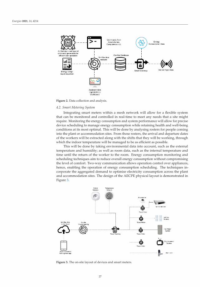
Energies 2021, 14, 4214

Figure 2. Data collection and analysis.

4.2. Smart Metering System

Integrating smart meters within a mesh network will allow for a flexible systemthat can be monitored and controlled in real-time to meet any needs that a site mightrequire. Monitoring the energy consumption and system performance will allow for precisedevice scheduling to manage energy consumption while retaining health and well-beingconditions at its most optimal. This will be done by analysing rosters for people cominginto the plant or accommodation sites. From those rosters, the arrival and departure datesof the workers will be extracted along with the shifts that they will be working, throughwhich the indoor temperature will be managed to be as efficient as possible.

This will be done by taking environmental data into account, such as the externaltemperature and humidity; as well as room data, such as the internal temperature andtime until the return of the worker to the room. Energy consumption monitoring andscheduling techniques aim to reduce overall energy consumption without compromisingthe level of comfort. Two-way communication allows operation control over appliances,hence, enabling the operation of energy consumption scheduling. The techniques in-corporate the aggregated demand to optimise electricity consumption across the plantand accommodation sites. The design of the AECPE physical layout is demonstrated inFigure 3.

Figure 3. The on-site layout of devices and smart meters.

27

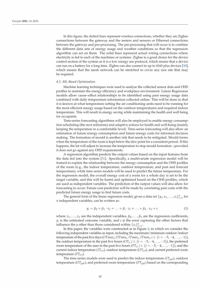
Energies 2021, 14, 4214

In this figure, the dotted lines represent wireless connections, whether they are Zigbeeconnections between the gateway and the meters and sensors or Ethernet connectionsbetween the gateway and pre-processing. The pre-processing that will occur is to combinethe different data sets of energy usage and weather conditions so that the regressionalgorithm can act on them. The solid lines represent actual wiring connections whereelectricity is fed to each of the machines or systems. Zigbee is a good choice for the devicecontrol section of the system as it is a low energy use protocol, which means that a devicecan run on a battery for a long time. Zigbee can also connect to up to 4160 plus devices [30],which means that the mesh network can be stretched to cover any size site that maybe required.

4.3. ML-Based Optimisation

Machine learning techniques were used to analyse the collected sensor data and OHSprofiles to maintain the energy efficiency and workplace environment. Linear Regressionmodels allow cause–effect relationships to be identified using past energy usage datacombined with daily temperature information collected online. This will be done so thatit is known at what temperature setting the air conditioning units need to be running forthe most efficient energy usage based on the outdoor temperatures and required indoortemperature. This will result in energy saving while maintaining the health and well beingfor occupants.

Time-series forecasting algorithms will also be employed to enable energy consump-tion scheduling (the next milestone) and adaptive actions for health and well-being (mainlykeeping the temperature to a comfortable level). Time-series forecasting will also allow anestimation of future energy consumption and future energy costs for informed decisionmaking. The formation of mould is another risk that needs to be mitigated. Mould formswhen the temperature of the room is kept below the dew point for a consistent period. If thishappens, the kit will adjust to increase the temperature to stop mould formation—providedit does not go against any OHS requirements.

A regression algorithm predicts the output values based on the input features fromthe data fed into the system [31]. Specifically, a multivariate regression model will betrained to explain the relationship between the energy consumption and the OHS profilesof the room (e.g., the indoor temperature, outdoor temperature, and past and forecasttemperature), while time series models will be used to predict the future temperature. Forthe regression model, the overall energy cost of a room for a whole day is set to be thetarget variable, and this will be learnt and optimised based on the OHS profiles, whichare used as independent variables. The prediction of the output values will also allow forforecasting to occur. Future cost prediction will be made by correlating past costs with thepredicted future energy usage to find future costs.

The general form of the linear regression model, given a data set {yi, x1, . . . , xi}ni=1 for

n independent variables, can be written as:

yi = β0 + β1 · x1 + . . . + βi · xi + . . . + βn · xn + ε (1)

where x1, . . . , xn are the independent variables, β0, . . . , βn are the regression coefficients,yi is the estimated outcome variable, and ε is the error capturing the other factors thatinfluence the y other than those considered within {xi}n

i=1.In this paper, the variables were constructed as in Figure 4, in which we consider the

following independent variables as input, including the maximum/minimum outdoor/indoortemperature of the past five days (OTmaxi, OTmini, ITmaxi, ITmini, i ∈ {i = −5,−4, . . . ,−1}),the outdoor temperature in the past five hours (OTj, j ∈ {i = −5,−4, . . . ,−1}), the preferredroom temperature of the user in the past five hours (PTj, j ∈ {i = −5,−4, . . . ,−1}), and thecurrent indoor temperature (ITcrt), outdoor temperature (OTcrt), and current preferred roomtemperature (PTcrt).

The time series models were used to predict the indoor temperature (ITpdt), outdoortemperature (OTpdt), and preferred room temperature (PTpdt) based on the corresponding

28

Energies 2021, 14, 4214

variables in the past days and hours. Lastly, all the collected and predicted data were fedinto a regression model as independent variables, and the dependent variable was theoverall energy cost of a room for a day, including the time when the room was used andnot used.

Figure 4. Machine learning models. The inputs and outputs of the models are in the rounded rectangles.

The cost prediction needs to give multiple estimates to account for a best to worstcase scenario depending on how much variation is in the previous values that were usedin the cost calculation. The aim is to set the ITcrt at a dynamic temperature to achieve theminimised Cost. In order to search for the optimised thermostat setback temperature foreach room, we used the historical outdoor temperature and initiated the ITcrt and PTcrtusing random numbers within a reasonable range to start up the training progress.

As for the ITcrt, it was set within a range from 17 to 33 ◦C, and the PTcrt was set within22 to 28 ◦C, because the historical data showed that most users set the air conditioner at22 to 28 ◦C after coming back to the room, and 5 extra degrees to both ends were extendedfor the air conditioner to handle extreme climates in the winter and summer. N, the numberof ITcrt, and M, the number of PTcrt, were randomly generated for initial training, and theroom occupation hours were also random numbers reflecting that the users could comeback to the room at any time of day. The room needed to reach the PTcrt within 20 minafter the PTcrt was set. Algorithm 1 summarises the details to search for the optimisedenergy cost.

Algorithm 1 Energy optimisation algorithmInput: OTmaxi, OTmini, ITmaxi, ITmini, OTj, PTj, ITcrt, OTcrt, PTcrt,

i ∈ {i = −5,−4, ...,−1}, j ∈ {i = −5,−4, ...,−1}Output: ITcrt, CostminParameter : β0, ..., βn

1 Initialise: ITcrt,p ← a, PTcrt,q ← b, a ∈ {17, ..., 33}, b ∈ {22, ..., 28}2 Train the regression model: Cost = β0 + β1 · OTmaxi + ... + βn · PTcrt + ε3 for p = 1 : N do4 for q = 1 : M do5 if Costm − Costm−1 ≤ 0 then6 return ITcrt,p7 Costmin ← Costm

8 return Costmin

4.4. Cyber Security and COVID-19 Response

In the AECPE, security is handled by a set of firewalls on top of the systems beingaccessible only via a VPN. For the moment, whilst the system is still in development andonly deployed very locally within one accommodation site, this security has proven tobe sufficient; however, it will need to be improved with a proper cyber threat responsesystem when it is ready to deploy to more locations. The security will mostly focus on theprotection of the end sensors/actuators as was outlined in the replay attack section.

29

Energies 2021, 14, 4214

As for the COVID-19 response, the movement of the people around the site can betracked using their ID cards when they tap them to gain access to their rooms and toother common facilities. In this way, if a case of COVID-19 is detected, this person’s closecontacts and the areas he or she has been in during any requested time period can bequickly queried via the system. The system can also be customised to include temperaturechecks to scan on the arrival of the workers and other random checks throughout theirtime on site.

A body temperature threshold (37.8 ◦C) will be set up to trigger the system to startrecording a person’s temperature, and an alarm will be sent to this person and campsitemanager if a body temperature above 38.28 ◦C [32] is detected; meanwhile, the user profile(movement and occupancy) of this person will be flagged in the system and ready toconduct contact tracing for a fast COVID-19 response.

5. Prototype Validation and Field Testing

5.1. AECPE Laboratory Prototype Setup

A prototype system was set up and tested in our lab environment in Australia. Fourdifferent devices were connected onto the system at the one time as demonstrated inFigure 5. The system could then measure how much electricity was being used and alsoprovided remote control of the devices. On a small scale, it was shown that the systemoperated as was expected. Further research will show if this control functionality can beused within the system when automated commands are given instead of user commands.It will also be interesting to determine to what extend feedback loops can be used andwhen a user needs to step in to give new commands.

Figure 5. The lab testing setup where four plugs and a gateway (on the right) are connected to alaptop, a screen, and two desk lamps. Their energy usage data was collected and remote control wasestablished over those devices.

5.2. AECPE Field Testing

We further conducted validation of the AECPE prototype in field testing in a largemining campsite provider and manager enterprise in West Australia. Specifically, thefeatures of continuously optimising energy usage and OHS awareness were tested in one ofthe campsites provided and managed by the enterprise. Since this campsite is composed ofa considerably large size of more than 1000 units meaning more than 3000 plus devices wereconnected, we also investigated the communication amongst sensors and smart meters, aswell as how much the mesh network could be stretched.

In the field testing, the AECPE mainly monitored workers in and out of miningcamp/room for the optimal use of electricity, and this was trialled in over 600 rooms inthe mining campsite. The preliminary results demonstrated that the energy costs could be

30

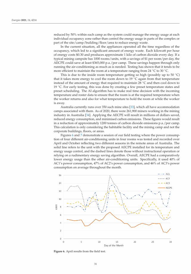
Energies 2021, 14, 4214

reduced by 50% within each camp as the system could manage the energy usage at eachindividual occupancy zone rather than control the energy usage in parts of the complex orpart of the site/camp/building/floor/area to reduce energy waste.

In the current situation, all the appliances operated all the time regardless of theoccupancy, which led to a significant amount of energy waste. Each kilowatt per hourof energy costs $0.30 and produces approximate 1 kilo of carbon dioxide every day. If atypical mining campsite has 1000 rooms/units, with a savings of $1 per room/per day, theAECPE could save at least $365,000 p.a./per camp. These savings happen through onlyrunning the air-conditioning as much as is needed. Testing has shown that it tends to bemore efficient to maintain the room at a temperature ranging from 24 ◦C to 30 ◦C.

This is due to the inside room temperature getting so high (possibly up to 50 ◦C)that it takes more energy to cool the room down to 19 ◦C again from that temperatureinstead of the amount of energy that required to maintain 28 ◦C and then cool down to19 ◦C. For early testing, this was done by creating a few preset temperature states andpreset scheduling. The AI algorithm has to make real time decision with the incomingtemperature and roster data to ensure that the room is at the required temperature whenthe worker returns and also for what temperature to hold the room at while the workeris away.

Australia currently runs over 350 such mine sites [33], which all have accommodationcamps associated with them. As of 2020, there were 261,900 miners working in the miningindustry in Australia [34]. Applying the AECPE will result in millions of dollars saved,reduced energy consumption, and minimised carbon emissions. These figures would resultin a reduction of approximately 1200 tonnes of carbon dioxide emissions p.a./per camp.This calculation is only considering the habitable facility and the mining camp and not thecorporate buildings, floors, or areas.

Figures 6 and 7 demonstrate a session of our field testing where the power consump-tion of four different air-conditioning units in four rooms was tested and recorded overApril and October reflecting two different seasons in the remote areas of Australia. Thesolid line refers to the unit with the proposed AECPE installed for its temperature andenergy usage control, and the dashed lines denote those without instructional operation orrelying on a rudimentary energy saving algorithm. Overall, AECPE had a comparativelylower energy usage than the other air-conditioning units. Specifically, it used 40% ofAC1’s power consumption, 47% of AC2’s power consumption, and 46% of AC3’s powerconsumption on average throughout the month.

Figure 6. April results from the field test.

31

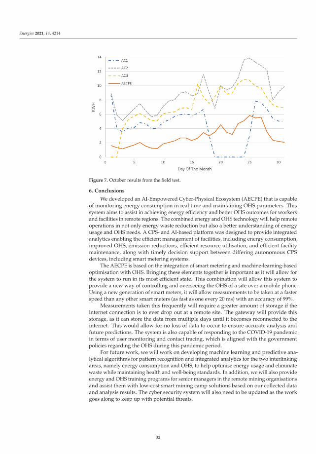
Energies 2021, 14, 4214

Figure 7. October results from the field test.

6. Conclusions

We developed an AI-Empowered Cyber-Physical Ecosystem (AECPE) that is capableof monitoring energy consumption in real time and maintaining OHS parameters. Thissystem aims to assist in achieving energy efficiency and better OHS outcomes for workersand facilities in remote regions. The combined energy and OHS technology will help remoteoperations in not only energy waste reduction but also a better understanding of energyusage and OHS needs. A CPS- and AI-based platform was designed to provide integratedanalytics enabling the efficient management of facilities, including energy consumption,improved OHS, emission reductions, efficient resource utilisation, and efficient facilitymaintenance, along with timely decision support between differing autonomous CPSdevices, including smart metering systems.

The AECPE is based on the integration of smart metering and machine-learning-basedoptimisation with OHS. Bringing these elements together is important as it will allow forthe system to run in its most efficient state. This combination will allow this system toprovide a new way of controlling and overseeing the OHS of a site over a mobile phone.Using a new generation of smart meters, it will allow measurements to be taken at a fasterspeed than any other smart meters (as fast as one every 20 ms) with an accuracy of 99%.

Measurements taken this frequently will require a greater amount of storage if theinternet connection is to ever drop out at a remote site. The gateway will provide thisstorage, as it can store the data from multiple days until it becomes reconnected to theinternet. This would allow for no loss of data to occur to ensure accurate analysis andfuture predictions. The system is also capable of responding to the COVID-19 pandemicin terms of user monitoring and contact tracing, which is aligned with the governmentpolicies regarding the OHS during this pandemic period.

For future work, we will work on developing machine learning and predictive ana-lytical algorithms for pattern recognition and integrated analytics for the two interlinkingareas, namely energy consumption and OHS, to help optimise energy usage and eliminatewaste while maintaining health and well-being standards. In addition, we will also provideenergy and OHS training programs for senior managers in the remote mining organisationsand assist them with low-cost smart mining camp solutions based on our collected dataand analysis results. The cyber security system will also need to be updated as the workgoes along to keep up with potential threats.

32

Energies 2021, 14, 4214

Author Contributions: Conceptualization: P.K., S.W. and E.C.; Methodology: P.K., Y.Z. and E.C.;Software: P.K.; Validation: P.K. and S.W.; Investigation: P.K. and Y.Z.; Resources: P.K., S.W. and E.C.;Writing—original draft preparation: P.K.; Writing—review and editing: P.K., Y.Z. and E.C.; Supervi-sion: Y.Z. and E.C. All authors have read and agreed to the published version of the manuscript.

Funding: This research received no external funding.


References

1. Stellman, J.M. Encyclopaedia of Occupational Health and Safety; International Labour Organization: Geneva, Switzerland, 1998;Volume 1.

2. Chang, E.; Gottwalt, F.; Zhang, Y. Cyber situational awareness for CPS, 5G and IoT. In Frontiers in Electronic Technologies; Springer:Singapore, 2017; pp. 147–161.

3. Lee, J.; Bagheri, B.; Kao, H.A. A cyber-physical systems architecture for industry 4.0-based manufacturing systems. Manuf. Lett.2015, 3, 18–23. [CrossRef]

4. Horcas, J.M.; Pinto, M.; Fuentes, L. Context-aware energy-efficient applications for cyber-physical systems. Ad Hoc Netw. 2019,82, 15–30. [CrossRef]

5. Bartocci, E.; Deshmukh, J.; Donzé, A.; Fainekos, G.; Maler, O.; Nickovic, D.; Sankaranarayanan, S. Specification-based monitoringof cyber-physical systems: A survey on theory, tools and applications. In Lectures on Runtime Verification; Springer: Cham,Switzerland, 2018; pp. 135–175.

6. Dey, N.; Ashour, A.S.; Shi, F.; Fong, S.J.; Tavares, J.M.R. Medical cyber-physical systems: A survey. J. Med. Syst. 2018, 42, 74.[CrossRef] [PubMed]

7. Wang, J.; Abid, H.; Lee, S.; Shu, L.; Xia, F. A secured health care application architecture for cyber-physical systems. arXiv 2011,arXiv:1201.0213.

8. Banerjee, A.; Gupta, S.K.; Fainekos, G.; Varsamopoulos, G. Towards modeling and analysis of cyber-physical medical systems. InProceedings of the 4th International Symposium on Applied Sciences in Biomedical and Communication Technologies, Barcelona,Spain, 26–29 October 2011; pp. 1–5.

9. Wahid, F.; Kim, D.H. An Efficient Approach for Energy Consumption Optimization and Management in Residential BuildingUsing Artificial Bee Colony and Fuzzy Logic. Math. Probl. Eng. 2016, 2016, 9104735. [CrossRef]

10. Attia, A.H.; Rezeka, S.F.; Saleh, A.M. Fuzzy logic control of air-conditioning system in residential buildings. Alex. Eng. J. 2015,54, 395–403. [CrossRef]

11. Patanaik, A. Fuzzy Logic Control of Air Conditioners; Indian Institute of Technology: Kharagpur, India, 2008.12. Kale, S.S.; Patil, P.S. Data mining technology with fuzzy logic, neural networks and machine learning for agriculture. In Data

Management, Analytics and Innovation; Springer: Singapore, 2019; pp. 79–87.13. Past Weather in Karratha, Western Australia, Australia. Available online: https://www.timeanddate.com/weather/australia/

karratha/historic (accessed on 4 June 2021).14. Hasbullah, H.; Soomro, I.A. Denial of service (DOS) attack and its possible solutions in VANET. Int. J. Electron. Commun. Eng.

2010, 4, 813–817.15. Bicakci, K.; Tavli, B. Denial-of-Service attacks and countermeasures in IEEE 802.11 wireless networks. Comput. Stand. Interfaces

2009, 31, 931–941. [CrossRef]16. Krotofil, M.; Cárdenas, A.A.; Manning, B.; Larsen, J. CPS: Driving Cyber-Physical Systems to Unsafe Operating Conditions by

Timing DoS Attacks on Sensor Signals. In Proceedings of the 30th Annual Computer Security Applications Conference (ACSAC ’14);Association for Computing Machinery: New York, NY, USA, 2014; pp. 146–155. [CrossRef]

17. Nagarsheth, P.; Khoury, E.; Patil, K.; Garland, M. Replay Attack Detection Using DNN for Channel Discrimination. In Proceedingsof the Interspeech 2017—18th Annual Conference of the International Speech Communication Association, Stockholm, Sweden,18–24 August 2017; pp. 97–101.

18. Hosseinzadeh, M.; Sinopoli, B.; Garone, E. Feasibility and Detection of Replay Attack in Networked Constrained Cyber-PhysicalSystems. In Proceedings of the 2019 57th Annual Allerton Conference on Communication, Control, and Computing (Allerton),Monticello, IL, USA, 24–27 September 2019; pp. 712–717. [CrossRef]

19. Liu, Y.; Ning, P.; Reiter, M.K. False Data Injection Attacks against State Estimation in Electric Power Grids. ACM Trans. Inf.Syst. Secur. 2011, 14. [CrossRef]

20. Ahmed, M.; Pathan, A.S.K. False data injection attack (FDIA): An overview and new metrics for fair evaluation of its countermea-sure. Complex Adapt. Syst. Model. 2020, 8. [CrossRef]

21. Mpelogianni, V.; Groumpos, P.; Tsipianitis, D.; Papagiannaki, A.; Gionas, J. Proactive Building Energy Management based onFuzzy Logic and Expert Intelligence. Inform. Intell. Syst. Appl. 2020, 1, 56–58. [CrossRef]

22. Paxton. Access Control. Available online: https://www.paxton-access.com/solutions/access-control/ (accessed on 8 April 2021).23. KBE Building Corporation. Available online: https://kbebuilding.com/portfolio/ (accessed on 8 April 2021).24. Zhang, Y.; Guo, Z.; Lv, J.; Liu, Y. A Framework for Smart Production-Logistics Systems Based on CPS and Industrial IoT.

IEEE Trans. Ind. Inform. 2018, 14, 4019–4032. [CrossRef]

33

Energies 2021, 14, 4214

25. Törngren, M.; Asplund, F.; Bensalem, S.; McDermid, J.; Passerone, R.; Pfeifer, H.; Sangiovanni-Vincentelli, A.; Schätz, B.Characterization, analysis, and recommendations for exploiting the opportunities of cyber-physical systems. In Cyber-PhysicalSystems; Elsevier: Amsterdam, The Netherlands, 2017; pp. 3–14.

26. Hernández-Muñoz, J.M.; Vercher, J.B.; Muñoz, L.; Galache, J.A.; Presser, M.; Gómez, L.A.H.; Pettersson, J. Smart cities at theforefront of the future internet. In Future Internet Assembly; Springer: Berlin/Heidelberg, Germany, 2011; pp. 447–462.

27. Bouchama, A.; Knochel, J.P. Heat Stroke. N. Engl. J. Med. 2002, 346, 1978–1988. [CrossRef] [PubMed]28. Nguyen, J.L.; Schwartz, J.; Dockery, D.W. The relationship between indoor and outdoor temperature, apparent temperature,

relative humidity, and absolute humidity. Indoor Air 2014, 24, 103–112. [CrossRef] [PubMed]29. Karratha Climate. Available online: https://en.climate-data.org/oceania/australia/western-australia/karratha-11105/ (accessed

on 29 May 2021).30. Zigbee Pro Best Practises. Available online: https://www.control4.com/docs/product/zigbee/best-practices/english/revision/

A/zigbee-best-practices-rev-a.pdf (accessed on 29 May 2021).31. Binder, J.J. On the use of the multivariate regression model in event studies. J. Account. Res. 1985, 23, 370–383. [CrossRef]32. What Temperature Is Considered a Fever? Available online: https://www.singlecare.com/blog/fever-temperature/ (accessed

on 14 June 2021).33. Australian Mineral Facts. Available online: https://www.ga.gov.au/education/classroom-resources/minerals-energy/

australian-mineral-facts#:~:text=Source%20Geoscience%20Australia.,from%20over%20350%20operating%20mines (accessedon 28 May 2021).

34. In Numbers: How Mining Came to be Australia’s Most Profitable Sector. Available online: https://www.mining-technology.com/features/in-numbers-how-mining-came-to-be-australias-most-profitable-sector/ (accessed on 28 May 2021).

34

energies

Article

A Generic Pipeline for Machine Learning Users in Energy andBuildings Domain

Mahmoud Abdelkader Bashery Abbass 1,* and Mohamed Hamdy 2

Citation: Abbass, M.A.B.; Hamdy, M.

A Generic Pipeline for Machine

Learning Users in Energy and

Buildings Domain. Energies 2021, 14,

5410. https://doi.org/10.3390/

en14175410

Academic Editors: Francesco Nocera

and Ana-Belén Gil-González

Received: 27 July 2021

Accepted: 29 August 2021

Published: 31 August 2021




iations.








4.0/).

1 Department of Mechanical Power Engineering, Helwan University, Cairo 11772, Egypt2 Department of Civil and Environmental Engineering, Norwegian University of Science and Technology,

7491 Trondheim, Norway; [email protected]* Correspondence: [email protected]

Abstract: One of the biggest problems in applying machine learning (ML) in the energy and buildingsfield is the lack of experience of ML users in implementing each ML algorithm in real-life applicationsthe right way, because each algorithm has prerequisites to be used and specific problems or appli-cations to be implemented. Hence, this paper introduces a generic pipeline to the ML users in thespecified field to guide them to select the best-fitting algorithm based on their particular applicationsand to help them to implement the selected algorithm correctly to achieve the best performance.The introduced pipeline is built on (1) reviewing the most popular trails to put ML pipelines for theenergy and building, with a declaration for each trial drawbacks to avoid it in the proposed pipeline;(2) reviewing the most popular ML algorithms in the energy and buildings field and linking themwith possible applications in the energy and buildings field in one layout; (3) a full description ofthe proposed pipeline by explaining the way of implementing it and its environmental impacts inimproving energy management systems for different countries; and (4) implementing the pipeline onreal data (CBECS) to prove its applicability.

Keywords: machine learning; benchmarking; prediction; pipeline; features; training; validation;tuning; evaluation and model verification

1. Introduction

Building energy benchmarking and prediction is a complex (i.e., multi-variant andnonlinear) problem. Building energy demands depend on many features such as climateconditions, characteristics of a building, and the type of equipment in the building. Thedemands include electrical and thermal (heating and cooling) loads. ML algorithms cansolve this type of problem as they automatically derive hidden patterns in the collected data.The patterns are then used to create the ML model, which generalizes real-life problems toprovide more well-informed and adaptive results.

There are a lot of ML algorithms that are used in the energy and buildings field, butthis paper explains the most popular algorithms that have dynamic behavior and are widelyused in the field. Dynamic behavior means the ability of an algorithm to solve differentproblems in different applications, and the ability of algorithm integration with otheralgorithms to improve overall performance. The paper focuses on four ML algorithms:(1) artificial neural networks (ANNs), (2) support vector machine (SVM), (3) Gaussianprocess regression (GPR) or Gaussian mixture models (GMM), and (4) clustering (such ask-means and k-shape clustering algorithms).

To identify the essential steps required for implementing the ML concepts in the energyand buildings field, previous trials must be reviewed. In 2014, Zhao mentioned a pipelinefor prediction energy values by split data into two data sets: (1) a training set that adjuststhe weights of the ML model and (2) a test set to evaluate the trained ML model, withoutany data preprocessing. This technique is not enough to overcome drawbacks of (1) dataquality such as missing values or outliers or noisy, and (2) overfitting training data because


Energies 2021, 14, 5410

of adjusting ML model on the same data set, as well as the loss of some data in the test setnot seen by the ML model [1]. In 2019, Tabrizchi, Javidi, and Amirzadeh Kim presented aprediction pipeline depending on the same two data sets but applying a cross-validationtechnique on the training data set to overcome the problem of overfitting. They proposed apipeline depending on the feedback or results from the model evaluation process to makean optimization process for model parameters and a feature selection process, which helpto reduce problem dimensionality without reducing ML model performance [2]. In 2019,Cai et al. declared the process of feature selection through a pipeline for the classificationprocess in a layer called feature engineering which has also feature an extraction process,and dealing with missing data and outliers’ values is also explained as a preprocessinglayer [3]. The importance of the feature selection process and the case that is used in to beeffective, is declared in the pipeline proposed in 2020 by Seyedzadeh et al., in addition to anexplanation of the feature extraction process, which is very important when the algorithmcannot perform automatic feature extraction during training [4].

On other hand, Somu, Raman, and Ramamritham, in 2021, mentioned adding a thirddata set called the validation data set that is used to overcome the overfitting problem ofML models, but the problem of losing some data points while making the test data setremains. In addition to adding a preprocess layer containing processes of increasing dataquality such as clean data from noise, missing values imputation, outlier detection, anddata normalization, the authors also mentioned different evaluation methods for predic-tion problems such as mean square error (MSE), root mean square error (RMSE), meanabsolute error (MAE), or mean absolute percentage error (MAPE). However, they added abenchmarking process as a feature extraction preprocess that integrates the clustering layerwith the prediction pipeline to decrease the complexity of the prediction process [5]. Thepreprocess layer and evaluation layer were proposed before by Fayaz and Kim in 2018, butnot in depth [6].

One of the trials of a general pipeline of ML algorithms was carried out by Liu et al.in 2019. The paper proposes different structures of pipelines, each one depending onthe ML algorithm used inside. The layers of the proposed pipelines are data collectionand preprocessing, training and evaluating models, and determining the best modelparameters and structure. The authors mentioned a very important layer that must befound in the pipeline, especially in the implementation of a real-life problem. This layeris called the verification layer, which is very important to measure the trained model’srobustness during operation. The weakness point of the proposed pipelines is that theauthors cannot make a general pipeline cover all the requirements of different algorithmsin different cases [7]. The trial of generating a general pipeline that suitable with differentML algorithms was performed by El-Gohary et al. in 2018. The pipeline deals with four MLalgorithms: Naive Bayes, SVM, Decision Trees, and Random Forest. The pipeline dependson layers of data preprocessing, feature extraction, principal component analysis, and anevaluation layer. The main drawback of this pipeline is that it depends on only one pathfor any real-life problem, which cannot be generalized in all cases, and the authors do notmention requirements or criteria of selecting each ML algorithm. In addition, putting theclassification process as a preprocessing layer to decrease prediction complexity means thatthe classification is an essential step [8]. In 2018, Saleh Seyedzadeh, Farzad Pour Rahimian,Ivan Glesk, and Marc Roper propose three pipelines: (1) a prediction pipeline dependingon splitting data to train and test data which make a feature extraction process dependingon the validation of model on test data, (2) a classification pipeline which depends onfeature selection as a preprocessor process before classification, and (3) a pipeline to selectthe most appropriate ML algorithm (ANN, SVM, GPR or GMM, k-mean, and k-shape)depending on the data set and requirements of each algorithm. The drawbacks of pipelinesare (1) neglecting the preprocessing process that must be performed to increase data quality,(2) depending on the simple technique of split data to train and test data, which cannotproduce a general model solution, (3) the third pipeline does not cover all ML algorithms’

36

Energies 2021, 14, 5410

requirements or data set cases, and (4) the authors cannot integrate the three pipelines intoone general pipeline [9].

After reviewing the previous trials to create a generic ML pipeline, the resultantpipeline consists of main three general steps: (1) the preprocessing steps, (2) the MLalgorithm selection, and (3) the ML model creation and implementation scientifically inreal life. The most complicated part of creating this pipeline is the interaction betweenthese three general steps (the main interactions come during ML selection procedures), sothe proposed pipeline overcomes all obstacles for ML users. The ML algorithm selectionstep represents the main source of interaction between the three main steps and is usuallydifficult (i.e., selecting the most appropriate ML algorithm for a specific application andimplementing it in real life) because it depends on many factors related to applications (e.g.,energy assessment and forecasting; prediction for buildings loads such as cooling or heatingor electricity; classification for buildings depending on energy consumption; modeling solarradiation; modeling and forecasting loads for air conditioning systems; simulating andcontrol for energy consumption systems; fault detection and diagnosis; and energy-saving,verification and retrofit studies) and factors related to data (e.g., data size, features size,data type (residential or non-residential data and time serious or not); degree of uncertaintyin data; and degree of complexity in data). After solving all interactions between thethree main steps, the final pipeline structure covers several factors including problemformulation, data collection and integration, data augmentation, feature engineering, datapreprocessing and visualization, different machine learning approaches with requirements,model training, model validation and tuning, model evaluation, and model verification.The generic ML pipeline will enhance the performance and organization of the reviewedML algorithms, because while working on ML problems, many steps are heavily repeated,and thus, putting these steps into one generic pipeline will ensure that the right algorithmsare deployed seamlessly, reducing the complexity of transferring ML models to real lifequickly and managing ML models easier.

The proposed paper consists of two main sections besides the introduction section.Section 2 explains each step of the proposed pipeline, with some previous cases demon-strated (i.e., the most popular ML algorithms and their applications used in the buildingenergy field and how each one is used to have most benefits). Section 3 implements thepipeline on CBECS data as an example to help ML users in using it.

2. The Essential Steps and Potential Improvements in ML Algorithms Implementation

There is a huge effort in the ML field to produce a general pipeline that covers all stepsneeded for algorithm implementation, but these efforts did not produce a robust pipelineto be used flexibly with different cases of data size, features size, data type, uncertaintyin data, and complexity in data. Therefore, this paper aims to produce a general pipelinesuitable for benchmarking and prediction in the building energy field.

Depending on the review of different pipelines resulting from previous trials, theproposed machine learning pipeline overcomes the drawbacks of each reviewed pipeline,explaining how to select and implement each machine learning approach on buildingenergy benchmarking and prediction problem in a sufficient way. There are essential stepsthat must be found in the pipeline, and these steps will be described one by one. In addition,each ML algorithm has requirements to be selected as a solution tool for a real-life problem.Based on results from existing works and reviewed pipelines for different applications, aPipeline is proposed to select and implement ML algorithms on real-life problems of theenergy and buildings field.

2.1. Problem Identification and Formulation

In the beginning, the real-life problem is identified as building energy consumptionbenchmarking and prediction. From there, we began problem formulation which includesarticulating the problem and converting it into an ML problem. Converting it to a machine

37

Energies 2021, 14, 5410

learning problem requires us to identify features that should be found in the data to predictaccurate output [10].

2.2. Data Collection, Analysis, and Preprocessing

Data have two elements: (1) a feature, which is an attribute that is used to help extractpatterns and predict future answers, and (2) a label, which is an answer that is wanted fromthe model to predict. The data are collected by answering problem formulation questions,then converting answers to features’ effect on output. After the problem is formulated, weneed to ensure that the data are formulated correctly for the ML algorithm and cleaned upin a way that will maximize the performance of the model. Thus, the step of data collection,preparation, and preprocessing is very important [11].

This step includes the following. (1) Data collection and integration ensures that rawdata are in one central, accessible place. The importance of this step appears when theresults of the evaluation metric on training and test data are low because the learningalgorithm did not have enough data to learn from. Thus, performance can be improved byusing the data augmentation technique which increases the amount of data. (2) Data pre-processing involves transforming raw data into an understandable format and extractingimportant features from the data. (3) Data visualization entails several things includinga programmatic analysis to give a quick sense of feature and label summaries, which iseffectively helping understand the data [12].

There is a relation between the selection process of the appropriate ML algorithmand the nature of collected data. This relation depends on many factors: (1) data size,(2) features size, (3) data type (residential or non-residential data and time serious or not),(4) degree of uncertainty in data, and (5) degree of complexity in data.

The ANN is the most flexible algorithm in the popular ML algorithms. It has a highdynamic power that resulting from the flexibility in performance control by using differenthyper-parameters values. The dynamics of ANN give this algorithm an advantage overother ML algorithms such as (1) handling huge data sizes in faster time with minimumcomputation power [13,14], (2) dealing with different data types by changing the type ofANN used (e.g., time serious data [13,15,16], annual commercial buildings’ data [17,18],and residential buildings’ data [19]), (3) it can overcome the complexity of data sets thathave a lot of features because it gives high weights for important features during training,and it can be integrated with feature selection or feature extraction concepts [16,20,21],(4) it is integrated with other ML algorithms in different ways to increase performance [22],and (5) it can train on noisy data sets by changing the sensitivity of the trained model tochanges of values [23] or use the Kalman filter [24] as preprocessing steps. The problemsthat keep ANN from an important role in the building energy field are that (1) ANNneeds an experience to deal with the hyper-parameters tuning process to deliver the bestperformance [13,25], (2) the difficulty of identifying the most appropriate sample size thatis suitable for real-life problems [25], and (3) decreasing prediction power with residentialbuildings’ data [18,26].

The ability of ANN algorithms to handle big data is declared in different applications.In 2010, Dombaycı et al. utilized a total of 35,070 hourly temperature data to estimatethe hourly energy consumption of a model house designed in Denizli, Turkey’s CentralAegean Region, for selecting appropriate and efficient heating and cooling equipment,with 26,310 h used for training and 8760 h used for testing. (The ANN model was trainedusing heating energy consumption data from 2004 to 2007 and evaluated using heatingenergy consumption data from 2008.) The result states that energy consumption levelsmay be predicted with a high degree of accuracy and that the ANN is extremely successfulwith large data sets [13]. In 2015, Antanasijevi et al. developed a new approach fordetermining the accuracy of a GRNN (general regression neural network) model appliedfor the prediction of EC (energy consumption) and GHG intensity of energy consumptionusing historical data from 2004 to 2012 for a set of 26 European countries (EU Members).The result states that the GRNN GHG intensity model is more accurate than the MLR

38

Energies 2021, 14, 5410

(multiple linear regression) and second-order and third-order non-linear MPR (multiplepolynomial regression) models that were evaluated [14].

The importance of preprocessing steps declared in some previous papers, such as thecomplexity that results from increasing the number of features, was discussed in 2015 byLi et al. while improving short-term building hourly electricity consumption prediction.They utilized principal component analysis (PCA) as an automated approach to reducethe ML problem complexity, and they said that this technique was able to fulfill twogoals (i.e., lowering ANN model complexity without compromising prediction accuracy)in only one automatic step [16]. In 2015, Platon, Dehkordi, and Martel used the samefeature selection technique (PCA) to select the most significant features from all studiedfeatures (i.e., only 10 significant features were selected out of the 22 available features)to develop hourly electricity predictive models based on ANN [15]. In 2006, Karatasou,Santamouris, and Geros explained the ability to improve ANN performance by usingstatistical analysis (e.g., hypothesis testing and information criteria) as a preprocessingstep before training to design an hourly building load predictor based on a feed-forwardartificial neural network (FFANN) [21]. The concept of preprocessing steps for ANNsmay depend on another ML concept that help in simplifying the process for complexproblems. In 2014, Du et al. employed a clustering method to aid ANN algorithms indetecting abnormalities in air handling units, which are common in commercial buildings(e.g., fixed biases, drifting biases, and complete failure of the sensors and chilled watervalve faults). For prior mistakes, the fault diagnosis tool for the HVAC system obtainedgood identification results [22].

The SVM algorithm is better than neural network algorithms, because of (1) the smallnumber of parameters compared to ANN and genetic programming [27,28], (2) the SVMsolution is unique and optimal because SVM can reach a global solution for problem [28,29],and (3) it can handle different types of data (e.g., time serious data [29], annual commercialbuildings’ data [18], and residential buildings’ data [30]). On the other hand, the SVMalgorithm cannot handle complex data that have too many features, so it is integratedwith feature selection methods to decrease the number of problem dimension spaces bydecreasing features [31]. In addition, it is not suitable for large data sets because thetraining process of SVM algorithms becomes very slow with a large amount of data, yetachieving good performance [28,29]. Sometimes, multi SVMs are used in parallel to reducethe computation time of large data [31,32].

The importance of preprocessing steps for SVM algorithms is greater than for ANNalgorithms because it cannot handle the complex ML problems that have many featuresand nonlinear relations. Thus, in 2012, Zhao and Magoulès used correlation analysis forfeature selection on complex data while assessing the energy demands of office buildingsto reduce the number of features for suggested algorithms. By manually computing thelinear correlation coefficients between characteristics and energy needs, the most significantfeatures with significant correlations were chosen [31].

The GPR or GMM algorithms are the best ones to deal with noisy data or uncertaintyin the data set. The reasons are as follows: (1) they overcome noisy measurements whichcome from sensors [33,34], (2) can extract complex patterns such as nonlinear and multi-variate relations between features [33], (3) can be integrated with other ML algorithms as apreprocessing step to remove uncertainty in the data set [35], and (4) give very efficientand robust predictions results even if with a small size of data [33,34]. The main drawbackof GPR or GMM algorithms is that they need high computation power and cost, especiallywith large data sizes [33].

Due to the ability of GPR and GMM algorithms to deal with complex ML problemsand noisy data, the preprocessing steps do not have an essential role with these algo-rithms during their implementation in complex applications. In 2012, Heo and Zavalademonstrated that these algorithms could capture complicated behavior (i.e., nonlinearities,multivariable interactions, and time correlations). Furthermore, because they were createdin a Bayesian environment, they have the potential to overcome problems of uncertainty,

39

Energies 2021, 14, 5410

but require a lot of computing power to accomplish these findings in a short amount oftime [33]. Moreover, the GPR and GMM algorithms can be used as a preprocessing step tofilter noisy data. In 2012, using these algorithms, Heo, Choudhary, and Augenbroe detecteduncertainty in buildings’ measurements to improve modeling and retrofit performancewhile creating a scalable, probabilistic methodology [35].

The clustering algorithms are very powerful because (1) they can handle differenttypes of data [36–38] and (2) propose a very powerful tool when integrated with predictionalgorithms that increase prediction performance [36,39]. However, they have drawbackssuch as (1) falling into the local minimum solution, especially the k-means algorithm, so itis recommended to iterate the clustering process to obtain the general solution; (2) theyare affected by high data complexity, so it is necessary to apply feature extraction, featureselection, and PCA as a preprocessing step [36,40]; (3) they are affected by data uncertainty,so it is necessary to integrate the Kalman filter or GPR or GMM as a preprocessing step [24];and (4) as the data size increases, the time of the iteration processes increases, too [38,40].

For increasing clustering algorithms’ performance in obtaining global solutions, theycan be integrated with preprocessing steps such as statistical analysis or feature selection inretrofit studies. In 2010, Gaitani et al. published an energy categorization tool for heatingschool buildings. Three steps were involved in the creation of the tool: (1) performingan extensive statistical analysis on the data, (2) applying PCA to select most significantfeatures, and (3) using k-means clustering technique to classify. The conclusions declarethat the proposed tool achieved very effective results because it used the two preprocessingmethods with clustering for energy-saving techniques [40]. One of the big advantages ofclustering algorithms is that they can be used as a preprocessing step for prediction modelsto increase performance. In 2017, Yang et al. demonstrated that combining the k-shapeclustering technique with the SVR model as a feature extraction phase to produce newfeatures from output clusters greatly improved the SVR model’s hourly and weekly energyconsumption forecasting accuracy [36].

2.3. ML Algorithm Selection

In general, determining which machine learning algorithm is the best is difficult. Asa result, it is critical to thoroughly examine the type of accessible or gathered data aswell as the application to select the most appropriate model. The ML algorithm selectionstep depends on many factors such as (1) application-type factors and (2) data factors.In this section, applications of four ML algorithms (i.e., ANN, SVM, GPR or GMM, andClustering K-Means or K-Shape) are explained to represent advantages, drawbacks, andpotential improvements for each algorithm to help ML users in the selection process forthe most appropriate algorithm during implementation in the field. After reviewing MLapplications, the ML users in the energy and buildings field can deduce that (1) ANNs are astrong tool for modeling and reliable prediction of building energy. They do, however, needa careful selection of network topology and fine tweaking of their many hyper-parametersfor training. Because ANN suffers from a local minimum issue, the models’ performancecannot be guaranteed. In addition, to obtain acceptable accuracy, ANN needs to be fedwith a sufficient number of samples. Simple MLR models may be able to outperformthem otherwise. As a result, ANN is best suited to engineers who are well-versed indeep learning and statistical modeling. We can also deduce that (2) SVM has been foundto outperform ANN in load forecasting and can construct models from small data and(3) GPR is utilized for model training with uncertainty assessments among ML approachesand other black-box methods. Uncertainty and sensitivity analysis for various machinelearning models have recently been presented and used. As a result, it is worthwhile todevote research resources to deploying these techniques for modeling construction underunclear data. Finally, we find that (4) in multi-dimensional energy assessment systems,k-means and k-shape are both highly efficient, with k-shape being used with time seriousdata and k-means being used with other data types. The popular applications of ML

40

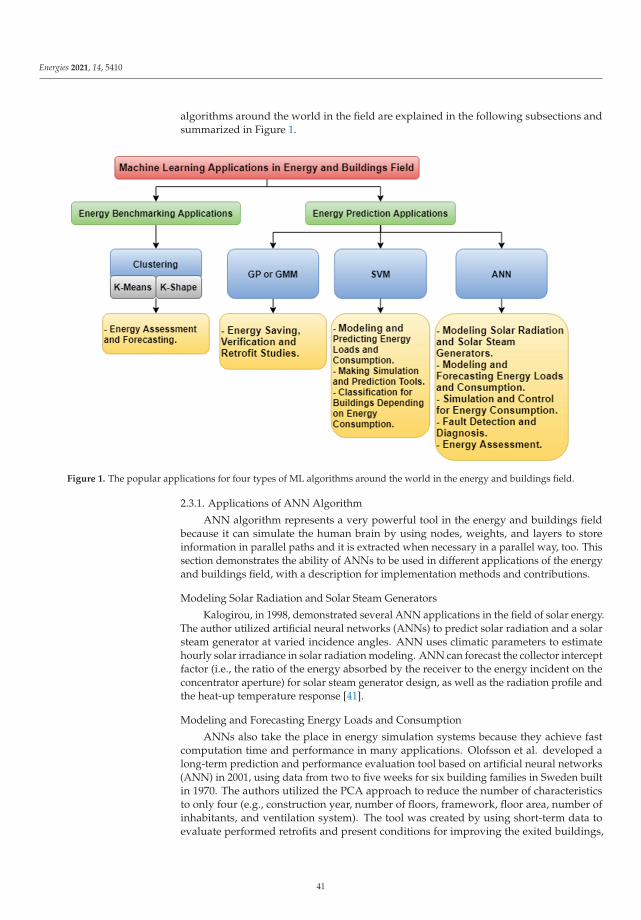
Energies 2021, 14, 5410

algorithms around the world in the field are explained in the following subsections andsummarized in Figure 1.

Figure 1. The popular applications for four types of ML algorithms around the world in the energy and buildings field.

2.3.1. Applications of ANN Algorithm

ANN algorithm represents a very powerful tool in the energy and buildings fieldbecause it can simulate the human brain by using nodes, weights, and layers to storeinformation in parallel paths and it is extracted when necessary in a parallel way, too. Thissection demonstrates the ability of ANNs to be used in different applications of the energyand buildings field, with a description for implementation methods and contributions.

Modeling Solar Radiation and Solar Steam Generators

Kalogirou, in 1998, demonstrated several ANN applications in the field of solar energy.The author utilized artificial neural networks (ANNs) to predict solar radiation and a solarsteam generator at varied incidence angles. ANN uses climatic parameters to estimatehourly solar irradiance in solar radiation modeling. ANN can forecast the collector interceptfactor (i.e., the ratio of the energy absorbed by the receiver to the energy incident on theconcentrator aperture) for solar steam generator design, as well as the radiation profile andthe heat-up temperature response [41].

Modeling and Forecasting Energy Loads and Consumption

ANNs also take the place in energy simulation systems because they achieve fastcomputation time and performance in many applications. Olofsson et al. developed along-term prediction and performance evaluation tool based on artificial neural networks(ANN) in 2001, using data from two to five weeks for six building families in Sweden builtin 1970. The authors utilized the PCA approach to reduce the number of characteristicsto only four (e.g., construction year, number of floors, framework, floor area, number ofinhabitants, and ventilation system). The tool was created by using short-term data toevaluate performed retrofits and present conditions for improving the exited buildings,

41

Energies 2021, 14, 5410

and made a long-term prediction for building energy consumption [20]. Ascione et al., in2017, studied the ability to create a building energy prediction tool with low computationalpower and high accuracy. The tool was constructed using data from office buildingserected in southern Italy between 1920 and 1970. Based on the ANN algorithm, the authorspresented two concepts of prediction tools: (1) used the existing data as it is, and (2) usedthe existing data but in the presence of energy retrofit measures. The proposed ANNs wereoptimized by “Simulation-based Large-scale sensitivity/uncertainty Analysis of BuildingEnergy performance” (SLABE). The performances of the networks were estimated by usingthe distributions of the relative error to compare ANNs’ outputs with EnergyPlus programtargets. The conclusion declares that the developed ANNs can replace standard buildingperformance simulation tools, thereby reducing computational effort and time [42]. Beccaliet al. studied EU non-residential building energy consumption in 2017 to develop anenergy evaluation tool based on two artificial neural networks (ANNs), the first of whichwas used to forecast actual energy consumption and the second of which was used to assesseconomic indicators. The authors used 151 existent buildings in four locations of southernItaly to assess the two ANNs. The conclusion states that the decision support tool based onANNs was able to forecast the energy performance of buildings quickly and accuratelyand that it was used to pick energy retrofit alternatives that can be implemented [43].

The ANNs’ flexibility is also declared in different applications when integrated withother optimization techniques to improve overall performance. Paudel et al. in 2014,integrated a pseudo-dynamic technique with an ANN model to make a daily short-termprediction for building heating demand. Because the hidden information in heating de-mand cannot be retrieved from climatic data by using ANN alone, the pseudo-dynamicapproach improved the overall performance of the ANN model by aspects of operationalheating power characteristics. The algorithm is used in the construction of French insti-tutions. The created dynamic model is resilient, according to the conclusion, and maybe utilized by energy service companies (ESCOs) in heat production dynamic controlsystems [44]. In 2017, Ascione et al. presented a detailed analysis and forecasting methodbased on ANN for cooling load of institutional building. For two years, data were collectedfrom three institutional buildings. Due to the nature of vacation times and universitytimetables, the research reveals a large variance in daily cooling loads energy consumption.The authors proposed dividing the data into groups based on vacation times and universitytimetables to solve the problem of variation and examine it. The conclusion states thatby adding categories’ numbers as a new input feature to the ANN algorithm, it was ableto improve predicting accuracy. Furthermore, by utilizing the Bayesian regularizationapproach for the hyper-parameters automated tuning process, the performance of ANNcan be most effective and rapid in computation time [45].

We can analyze the performance of the ANN algorithm declared in some previouspapers to highlight the advantages and drawbacks by comparing it with other ML algo-rithms in the energy and buildings field. In 2015, Platon, Dehkordi, and Martel presentedhourly electricity predictive models based on ANN and case-based reasoning (CBR) for aninstitutional building. The measured data from a Canadian institutional facility includedelements, such as weather information, that are relevant to the building’s operation. Toforecast power usage with a horizon of 1 to 6 h, the authors utilized principal componentanalysis to identify the most important characteristics (i.e., only 10 significant featureswere chosen out of 22 available features). The models’ prediction abilities were evaluated,and the ANN models regularly outperformed the CBR model, according to the results.Both the CBR and ANN models, on the other hand, had an error that was well within theASHRAE limits. To improve the CBR model’s performance, different approaches weretried: (1) varying the case similarity criterion and the number of previous instances used forprediction and (2) using automated optimization techniques on values’ weight. However,none of these techniques had a substantial impact on the CBR models’ performance [15].Edwards, New, and Parker, in 2012, sought to reduce difficulties such as a large number offeatures in the building characterization and prevent the problem of energy consumption

42

Energies 2021, 14, 5410

in the predesign stage. The scientists used sensor-collected energy usage data to conductstatistical analysis using several machine learning methods (e.g., feed-forward neuralnetwork, support vector regression, least squares support vector machine, a hierarchicalmixture of experts, and fuzzy c-means with feed-forward neural networks). To forecastnext hour energy usage, researchers compared several machine learning algorithms ontwo types of data: (1) data on commercial building consumption gathered hourly and(2) data on residential building consumption collected every 15 min. According to the find-ings of this comparison, ANN-based techniques perform better on commercial structures.However, results show that these methods perform poorly on residential data and thatleast squares support vector machines perform best on both, but with high computationcosts [18]. Kialashaki and Reisel, in 2013, created a hybrid method using artificial neu-ral networks (ANN) and multiple linear regression techniques to forecast future energyconsumption for residential buildings in the United States under various input scenarios(e.g., dwelling size, number of occupants, the efficiency of heating equipment and energyintensity). The authors describe how ANN’s effectiveness varies in residential structures inthe United States, especially with test data. As the ANN model prediction is dependent onthe cumulative trends of the various parameters, the reason for the variation in forecastenergy was the fluctuation induced by the economic recession [19].

Simulation and Control for Energy Consumption

The energy consumption for buildings can be enhanced and controlled easily byusing the ANN algorithm because it has the ability to deal with nonlinear equations insome applications. In 2015, Huang, Chen, and Hu proposed predictive control for anHVAC system to forecast an interior temperature by taking into account nonlinear buildingthermal dynamics (e.g., interaction between locations, noise in sensors, and delay time).Energy input from mechanical cooling, ventilation, weather, and convective heat transfersfor thermal coupling between locations are all features of the ANN input. The suggestedANN model incorporates the thermal interaction between zones, resulting in more accurateprediction results than a single zone model, according to the conclusion. This managementapproach resulted in a high level of building energy consumption control [23]. In 2016,Benedetti et al. presented an automatic tool based on ANN to control building energyconsumption and investigated the effect of the collected data period on the automaticutilization of such tools where a large amount of data is not always available in thereal world, so the minimum and maximum period of required data were identified toachieve reliable results. To determine the optimal ANN design for an energy consumptionmanagement tool, the authors used three alternative ANN architectures. Furthermore,because a large quantity of data is not always present in practice, a method is presented fordetermining the minimum time of data collection required to achieve accurate findingsand the maximum period of usefulness [46]. In 2017, Ahn, Cho, and Chung presenteda hybrid control approach on mass and temperature for supply air of heating system tominimize energy consumption. To understand the nonlinear relations between features andforecast or assess precise thermal, the suggested technique uses a mix of fuzzy inferencesystems and ANN. To assess supply air conditions for a heating season, the suggestedtechnique was compared to a basic thermostat on/off controller, and it was discoveredthat the ANN controller can reduce energy usage when compared to a simple thermostaton/off controller [47].

Fault Detection and Diagnosis

Time consumption problems during energy assessment and retrofit studies for build-ings vanish in some studies. Kalogirou et al. proposed a fault diagnostic prediction systemin 2008 that used temperature readings to identify problems in solar water heater compo-nents and forecast mistakes in collectors or pipe insulation. There were four elements tothe problem diagnosis system: (1) a data acquisition system measured temperatures infour locations of the solar water heater system and the mean value for a storage tank; (2) a

43

Energies 2021, 14, 5410

prediction module based on an artificial neural network (ANN) that was trained with fault-free system values obtained from a TRNSYS under the same meteorological conditions(e.g., Nicosia, Cyprus, and Paris, France), (3) the residual calculator takes measurementdata from the data collection system as well as error-free predictions from the predictionmodule, and (4) the diagnosis module detects a variety of defects, including collector faultsand insulation failures in the pipes linking the collection to the storage tank [48].

Energy Assessment

In 2013, Hong et al. studied the energy performance of schools (from 2008 to 2011) tocreate energy evaluations by combining statistical analysis with artificial neural networks(ANN) to evaluate the influence of each feature on energy and the relationship betweenthem. About 7700 schools were utilized in a rapid statistical study, and 465 schools wereinvestigated in depth using ANN to find variables that influenced school energy usagepatterns. The results declared that the non-domestic buildings must be re-classified be-cause of different reasons: (1) changes in the energy use pattern and (2) differences inenergy performance between primary and secondary schools such as a gradual increasein electricity consumption and a decrease in heating consumption in both. By comparingsimulation and engineering calculations, the authors noted the ability of ANN in energyassessment and the limitation in prediction [49]. Buratti, Barbanera, and Palladino devel-oped a verification tool based on ANN in 2014 to forecast energy consumption and assessbuilding performance by comparing it to energy certificates. The Umbria Region (centralItaly) acquired around 6500 energy certificates (2700 of which were self-declarations). Totrain the ANN, the authors utilized only right certificates recognized by comparing themto energy standards, and they created a new index called the neural energy performanceindex to describe the degree of accuracy and to identify the certificate’s precise controlneeds (NEPI) [50].

2.3.2. Applications of SVM Algorithm

The SVM algorithm represents the best alternative solution for the ANN algorithmin many applications of the energy and buildings field. SVMs have a low number ofhyper-parameters compared to ANN models, so they are easier to control and can betrained with small data sizes.

Modeling and Predicting Energy Loads and Consumption

The power and drawbacks of the SVM algorithm appeared in many applications ofthe field by comparing it with ANN models to solve the same problems. By using the SVMmethod for hourly cooling load forecast of an office building in Guangzhou, China, Li et al.demonstrated in 2009 that it is extremely successful, even with small data sets. The findingswere compared to those of backpropagation ANN to indicate that SVM outperformedANN in terms of accuracy and global solution. The input features were (1) outdoor drybulb temperature of the past 2 h and (2) solar radiation intensity of the past 1 h. The resultstates that the SVM algorithm performed as well as the ANN method in terms of speed andaccuracy, but with fewer data samples [28]. Using the least square support vector machine,Xuemei et al. increased the time efficiency required for hourly cooling load forecast in 2009(LSSVM). The authors compared the proposed approach to backpropagation ANNs toassess its performance. In the end, LSSVM outperformed backpropagation ANN in termsof accuracy and global solution, especially when the available training set is restricted. As aresult, LSSVM might be a viable option for predicting the cooling demand in a building [29].

After proofing the ability of SVM to replace ANN in different applications of the samefield, there are different papers applied the algorithm with some adjustments to overcomedrawbacks such as high time consumption when used with large data size. Hai XiangZhao et al. in 2009, studied the ability of SVM with the Gaussian kernel algorithm to dealwith large time series datasets and reduce the training time of predicting energy modelsby using a concept of parallel SVM algorithms. Results showed very good performance

44

Energies 2021, 14, 5410

in the prediction of energy consumption in multiple buildings based on large time seriesdatasets [32]. Zhao and Magoulès, in 2012, studied the ability to reduce time consumptionin SVM training with large data size by using radial and polynomial functions as a kernelfor parallel SVM algorithms to predict the energy consumption of office buildings. Thealgorithm feature selection is implemented on data by using correlation analysis for features.Using correlation analysis for features, the algorithm feature selection is implemented ondata. To compute the energy demands, the authors utilized simulated data from EnergyPlussoftware and manually selected features by computing correlation coefficients to reducethe number of features for the proposed algorithms [31].

Making Simulation and Prediction Tools

SVM algorithms can also outperform the ANN algorithm in dealing with residentialbuildings data for many cases such as energy prediction and creating tools. Jain et al., in2014, used a support vector regression (SVR) algorithm with sensor measurements fromresidential buildings to make energy predictions. The inputs feature during training were(e.g., weather, time of day, and previous energy consumption) from multi-family residentialbuilding data in New York City. The authors mentioned a paucity of research applyingmulti-family residential buildings. Thus, he expanded the study-to-study algorithm limita-tions by examining different time steps (i.e., 10 min, daily, and hourly) and different spatialcategories (i.e., by unit, by floor, and whole building). The conclusion declares that the SVRcould be used in energy prediction for residential buildings and the best prediction resultsoccurred at floor level in hourly intervals [30]. In 2008, Lai, Magoulès, and Lherminierutilized SVM to develop a simple and rapid method for predicting the electric energy con-sumption of residential buildings. The data include daily electricity usage for a year andthree months, as well as climatic data such as temperatures and humidity. For the learningstage, the authors utilized a year and two months, and for the prediction step, the authorsused the last month. The findings demonstrate that the model has high performance andthat the SVM tool may be utilized to conduct predictive modeling [51].

Classification for Buildings Depending on Energy Consumption

The SVM algorithm is very flexible to be integrated into existing systems on buildingenergy management. In 2010, Li, Bowers, and Schnier developed a daily power consump-tion management system for buildings based on detecting abnormal energy behavior andproviding the capacity to handle problems in real time to enable prediction and detectionof abnormal energy usage. The system consisted of the following steps: (1) outliers’ detec-tion in real time to identify abnormal energy use and delete it from further analysis, and(2) classifying based on the SVM-predicted daily electricity profile. The suggested systemwas computationally efficient and resilient enough to be incorporated into current buildingenergy management and alarm systems [52].

2.3.3. Applications of GPR or GMM AlgorithmEnergy Saving Verification and Retrofit Studies

Although the Gaussian-based algorithms need high computation power resources,they have a lot of advantages declared through implementation in some complicatedapplications which make them used in the field. In 2012, Heo and Zavala investigatedthe possibility of the GPR model to substitute a linear regression approach in energysavings, uncertainty measurements, and verification problems since it is highly powerfulin prediction, particularly with noisy data. The conclusion asserts that generalized linearmodels (GPR models) can represent complicated behavior (i.e., nonlinearities, multivariableinteractions, and time correlations). Furthermore, because they were created in a Bayesianenvironment, they can overcome difficulties of uncertainty [33].

These solution algorithms are best in the case of noisy data or probabilities and retrofitstudies to help decision makers in taking steps in improving countries. Furthermore, in2012, Heo, Choudhary, and Augenbroe presented a scalable, probabilistic methodology for

45

Energies 2021, 14, 5410

energy modeling based on Bayesian calibration (the same base for Gaussian models) toimprove modeling by detecting uncertainty in buildings models and aid in studying theprobability of building energy consumption improvements and retrofit performance. Thesuggested technique, according to the conclusion, may accurately assess energy retrofitchoices and promote risk-aware decision-making by clearly inspecting risks associatedwith each retrofit option [35].

The GPR and GMM algorithms can be integrated with other models to improveperformance even if the collected data are limited. In 2014 Burkhart, Heo, and Zavalautilized a GPR with a Monte Carlo expectation maximization (MCEM) model to copewith noisy data from sensors (e.g., weather, occupancy) and investigated the impact ofthe method on the quantity of necessary data from sensors during measurement andverification (M&V) stages. The GPR-MCEM model, according to the result, reached robustprediction levels when compared to conventional GPR alone, and may be utilized as amechanism to decrease data collection and sensor installation costs in M&V processes sinceit provides high performance with fewer data [34].

2.3.4. Applications of Clustering Algorithms (K-Means and K-Shape)Energy Assessment and Forecasting

The benchmarking process is very helpful in building energy assessment applications,especially when integrated with other algorithms to create energy assessment techniques.In 2007, Santamouris et al. developed an intelligent technique to cluster school buildingsas the first step in energy assessment procedures. Then, the output clusters used in theenergy performance studies specified the buildings’ rating and environmental impactof each cluster. The energy rating of the school buildings gives detailed information ontheir energy consumption and efficiency in comparison to other buildings of a similarkind, allowing for better intervention planning to enhance their energy performance. Theauthors created the technique in three steps: (1) energy consumption data were collectedfrom 320 schools in Greece, (2) fuzzy clustering techniques were used to make the energyrating scheme, and (3) 10 schools were selected and detailed analysis was performedfor energy efficiency, performance, and environmental impacts. The conclusion declaresthe ability of the used technique to identify and rate the existing school buildings andstudied the potential for energy and environmental improvements [39]. Gaitani et al.,in 2010, presented an energy classification tool for school buildings’ heating based ona k-means clustering technique with PCA to help decision makers in the schools ratingprocess and study probabilities of energy savings. The data used consisted of 1100 casesfrom secondary education school buildings in Greece, which represented 33% of the totalsecondary school sector, and included information such as energy consumption for spaceheating and lighting, building area, number of students and professors, a boiler installedpower, building manufacturing year, and operation schedule. The tool was created inthree steps: (1) an extensive statistical analysis on the data was performed, (2) PCA wasapplied to select the most significant features, and (3) a k-means clustering techniquewas used to classify. The results state that the categorization may be used to aid decisionmakers’ energy-saving strategies [40]. In 2017, Yang et al. proposed an energy clusteringmethod based on the k-shape algorithm for time series data, which can recognize patternsin time series data and categorize them using multi-dimensional space. The clustering wasperformed on data from 10 institutional buildings’ hourly and weekly energy usage usingthe k-shape method to find form patterns in time series data, which increased the accuracyof forecasting models. The conclusion declared that the proposed method could detectbuilding energy usage patterns in different time intervals effectively and also proved thatthe forecasting accuracy of the SVR model is significantly improved by integrating theclustering method with the SVR model [36].

These clustering algorithms also prove efficiency as an alternative solution for softwaresuch as the Energy Star program. In 2014, Gao and Malkawi proposed a benchmarkingtechnique based on the smart clustering concept, which classifies buildings’ energy based

46

Energies 2021, 14, 5410

on all features that have a relationship with energy consumption and groups buildings withthe most similarity of features into one cluster, implying that the problem of classifyingis multi-dimensional. The proposed methodology contains four steps: (1) data collection,(2) feature identification and selection, (3) selection for clustering algorithm depending oncollected data, and (4) buildings’ benchmarking concerning cluster group and centroid. Thefindings were compared to the Energy Star approach to show that the suggested strategycan give a more thorough approach to benchmarking, particularly with multi-dimensionalchallenges, inspiring a fresh viewpoint on building energy performance benchmarking [37].

The complexity of ML problems can be handled by the clustering algorithms, whichconvert the chaos data to more homogenous ones in simple iterative steps. Arambula Laraet al. in 2015, studied the European policy of energy saving and the Commission DelegatedRegulation (EU) 244/2012, which gave recommendations for some reference buildings tomake a compromise cost from expected improvements. The solution was found in the k-means clustering approach, which split huge data into tiny and homogeneous groups basedon building characteristics’ similarity, decreasing the complexity of energy optimizationand retrofits by reducing school buildings’ stock homogeneously. The data came from asample of roughly 60 schools in the region of Treviso in northern Italy, collected between2011 and 2012. The conclusion declares that this method could identify a small number ofparameters to assess the energy consumption for air heating and hot water production [38].

2.4. Model Training, Validation, and Tuning

This is an iterative process during the conversion of a solution that can be performedmany different times. Initially, upon training, the model will not achieve the results that areexpected. Thus, the tuning process is very important to evaluate model performance underdifferent values of hyper-parameters. During training, the machine learning algorithmupdates a set of numbers known as parameters or weights. The goal is to update modelparameters in the global solution direction which makes the predicted output as close aspossible to the true output (as seen in the data). This cannot be achieved in one iteration,because the model has not yet learned; it watches the weights and outputs from previousiterations and shifts the weights to a direction that lowers the error in the generated output.If the error in the output gradually decreases with each successive iteration, the model issaid to converge, and the training is considered successful. If, on the other hand, the errorseither increase or change randomly between iterations, the hyper-parameters of the modelneed to be tuned [12].

The most important thing in model performance is overfitting and underfitting. Theunderfitting problem means that the model performance is very low on the training data,and thus, the training model is unable to represent the data correctly. In underfittingproblems, the model could be very simple (the problem cannot be formulated well withenough features) to produce accurate outputs well, because of the inability to extractpatterns or relationships between input and output features for data. To overcome theunderfitting problem, there are different techniques: (1) reformulate the real-life problemby adding more effective features, (2) choose suitable preprocessing methods to solve datadrawbacks of missing or outlier values, and (3) decrease or change amount or type of modelregularization techniques such as dropout. The problem of overfitting is present when themodel performance is very high on training data but low on the validation or test data. Thereason for the overfitting problem is the inability of the model to attain the global solutionof the problem to cover all data sets. With low performance for unseen data, it makes senseto use fewer feature combinations and increase the amount of regularization [53].

There are several techniques to overcome overfitting and maximizing generalization.The most popular one is simple Hold-Out Validation. The simple hold-out techniquedepends on splitting data into multiple sets for training, validating, and testing models.Training data, which include both features and labels, feed into the model. The model isthen used to make predictions over the validation data set, which checks performance totune and change the model’s weights. Then, test data that only include features are used

47

Energies 2021, 14, 5410

to produce the labels. The performance of the model with the test data set is what we canreasonably expect to see in real life [13,54,55].

The problem of the hyper-parameters tuning process is mainly related to the MLalgorithm type. For the ANN algorithm, many papers discussed this problem duringthe implementation of different real-life problems and recommended using an automatictechnique in the tuning for a large number of ANN hyper-parameters because the ANNmodel has a lot of hyper-parameters.

González and Zamarreño, in 2005, studied the effect of hyper-parameters such as thenumber of neurons per layer and data size on the performance of ANN while creating analgorithm for short-term building load prediction. The authors mentioned difficulties inreaching the global solution because it related to large numbers of ANN hyper-parametersvalues [25]. Dombaycı et al. in 2010, studied the number of neurons per layer only as ahyper-parameter for an ANN model that was developed to make an hourly heating energyprediction in the design stage for a building to help in selecting appropriate and efficientheating and cooling equipment. The authors explained the complexity of tuning ANNhyper-parameters by using manual methods because of their large numbers [13]. One ofthe trials to overcome the problem of a large number of hyper-parameters was conducted in2015 by Li et al., who used particle swarm optimization technique in automatic ANN hyper-parameters tuning while improving the short-term building hourly electricity consumptionprediction and compared this method and simple ANN with manual tuning for hyper-parameters. The authors concluded that the automatic tuning process has a shorter trainingtime and higher performance than the manual method and the hybrid genetic algorithmmodel [16]. In 2017, Ascione et al. presented a solution for the same problem using theBayesian regularization technique for hyper-parameters’ automatic tuning while making adetailed analysis and forecasting method based on ANN for the cooling load of institutionalbuildings, and mentioned that the performance of ANN is the most effective and quick incomputing time by using this tuning technique [45].

Otherwise, the SVM algorithms are easily tuned and manually optimized. Theseadvantages appeared in many applications such as in 2009 when Zhijian Hou et al. studiedthe ability to replace huge numbers of trainable parameters for ANN by using radialfunction as a kernel for an SVM algorithm in an HVAC system energy prediction inNanzhou. The paper proved that the algorithm has fewer parameters to tune comparedwith ANN and is better than the ANN algorithm in forecasting [27].

2.5. Model Evaluation

The model evaluation is performing using test data to make sure that the required goalis achieved and to overcome the problem of over-fitting and under-fitting for the trainedmodel. If the trained model does not meet the required goal, it increases the required timeto re-validate the model and achieve goal. In this step, the feature engineer takes the roleto study data and features and find ways to improve the model, and the way that it isproduced. Once the retraining happens and the required goal is achieved, the model isdeployed to perform the best possible predictions on the unknown data to begin evaluatinghow the model responds in a non-training environment.

To evaluate the machine learning model, we need to know the type of ML problems,classification (such as benchmarking), or regression (such as prediction) problems. Thetype of machine learning problem will influence the type of metric used to evaluate themodel. We can start by looking at classification problems metrics. There are differenttypes of metrics to evaluate models: (1) accuracy, (2) precision, (3) recall, (4) F1 score (2*(re-call*precision)/(recall + precision)), and (5) area under the curve-receiver operator curve(AUC-ROC). To implement this metric method on the trained model, the model predictionsand the known target values are sent to the confusion matrix. A confusion matrix is thebuilding block for running these types of model evaluations for classification problems.Then, the predictions are returned, compared with the values of ground truth. Finally, theevaluation metric between predicted values and ground truth values is computed [56].

48

Energies 2021, 14, 5410

It is recommended in classification problems to use F1 as an evaluation metric becausethe F1 score combines precision and recall together to give one number to quantify theoverall performance of a particular ML algorithm. In addition, the F1 score should beused when the dataset has a class imbalance but we want to preserve the equality betweenprecision and recall.

In regression problems, there are other common metrics that we can use to evaluate themodel: (1) mean squared error and (2) R-squared. Mean squared error is very commonlyused. The difference between the prediction and actual value is calculated, that differenceis squared, and then all the squared differences for all the observations are summed up [16].

The other metric type is R-squared, which explains the fraction of variance accountedfor by the model. It is like a percentage, reporting a number from 0 to 1. When R-squaredis close to 1, this usually indicates that a lot of the variabilities in the data can be explainedby the model itself. The threshold for a good R-squared value depends on your machinelearning problem. In some machine learning problems, it is very difficult to achieve a highR-squared value. The high value of R-squared does not always represent strong modelperformance because R-squared is always increasing when more variables are added to themodel, which sometimes leads to overfitting [13]. To counter this potential issue, there isanother metric for model performance called the Adjusted R-squared value. The AdjustedR-squared has already taken care of the added effect for additional variables and it onlyincreases when the added variables have significant effects on the prediction. The adjustedR-squared adjusts the final value based on two factors: (1) the number of features and(2) the number of data points in the data. A recommendation, therefore, is to look at bothR-squared and Adjusted R-squared. This will ensure that the model is performing well butalso that there is not too much overfitting.

In the building energy prediction field, it is preferred to evaluate ANN using meanabsolute percentage error (MAPE) as a performance metric during model training. It isused in different applications in the same field and is proved to be very effective in theexamination of model quality during the prediction process [25].

The most recommended evaluation technique is the cross-validation method that wasused in 2006 by Karatasou, Santamouris, and Geros. They evaluated the hourly buildingsload predictor based on feed-forward artificial neural network (FFANN) by splitting thedata into many packages and looping them in the training process (i.e., each iteration in thetraining process carried out by using one of the packages as test data and others as trainingdata to cover all data samples without overfitting problems). In addition, the authorsdiscussed the cross-validation technique effect during training on the result of predictionand modeling and recommended this technique in such applications to achieve more robustmodels. The authors also discussed, the importance of attaining a more robust model byusing different types of data sets in the evaluation process (i.e., the model performance wasevaluated using two different data sets: (1) energy prediction shootout I contest and (2) anoffice building in Athens) [21]. Furthermore, one of the evaluation techniques was usedby Dombaycı et al. in 2010 while developing an hourly heating energy prediction modelbased on ANN for building. The total data of 35,070 h were split into two packages to trainand test the model: (1) the data from 2004 to 2007 (i.e., 26,310 data sample) used duringmodel training, and (2) the data of the year 2008 (i.e., 87,60 data sample) used in modeltesting or evaluating. The authors mentioned the importance of using test or unseen datato improve model performance in real life [13].

2.6. Model Verification

The verification of machine learning models’ robustness refers to checking modelsdeployed on a real-life problem to ensure that it adheres to these specifications and achievesthe target for a long run. A variety of machine learning models are also assessed accordingto how robust they are proven to be. This step must be performed frequently to make surethat the system is still working in high performance.

49

Energies 2021, 14, 5410

The evaluation step represents the base for verification steps during model deploy-ment. The more models are robust in the evaluation step, the easier the verification step,and results in real life will be better. The robustness or verification for any model is ex-amined firstly during the evaluation step by using unseen data or new data that differedfrom training data. Different types of data packages in many applications are used in theML model evaluation step, such as in the 2006 work Karatasou, Santamouris, and Geros,who evaluated the FFANN models by using two different data sets: (1) energy predictionshootout I contest, and (2) an office building in Athens. In addition, they trained models ondifferent time steps to identify limitations for models and create a robust hourly buildingsload predictor tool so that the FFANN can be deployed on different data sets and usedfor a long run [21]. Moreover, in 2015, Li et al. collected hourly data from two resources:(1) energy prediction shootout contest I, and (2) a campus building in east China; mean-ing that the data were collected from different locations all over the world to ensure thereliability and robustness of the model [16].

3. Discussion

As shown in Figure 2, the generic ML covers all required steps to use and deploythe ML algorithms (i.e., ANN, SVM, GPR or GMM, and k-mean or k-shape clustering)in the energy and buildings field. The pipeline starts with problem identification (i.e.,identify application type and specify the benchmarking and prediction problems). Then,this real-life problem must be converted to an ML problem in the problem formulationstep by identifying the related features. After that, the data scientists start in collectingthe data depending on the related features identified in the previous step and makesome statistical analysis and visualization to study the nature of collected data and theirdistribution (this step is very important to help data scientists in choosing the appropriatepreprocessing techniques).

Thereby, the data preprocessing step starts with answering some questions: (1) arethere too many features? If there are too many features, the features must be decreased byfeature selection (i.e., keeping only the most significant features that have a high effect onthe studied problem). If there are not too many features, the second question is (2) are theretoo few features? If the collected data have a small number of features that have nonlinearor deep interaction relationships, the data scientist must employ some feature extractiontechniques to increase the number of features and help the algorithm reach for a globalproblem solution during training. The third question concerns (3) noisy data. If the datacontain noise, the filtration must be carried out by Gaussian based models or the Kalmanfilter. The fourth question concerns (4) time series data. To identify the noise filter type, thisquestion must be answered to select between Gaussian-based models or the Kalman filter.The final step in preprocessing steps is solving problems of outliers and missing values.

Then, the most appropriate ML model must be selected. The selection depends on theML problem type (i.e., benchmarking or prediction) that is identified in the first step in theproposed pipeline. In addition, some questions must be answered to identify the algorithmtype. The first question concerns (1) time series data. If the data are time series, the k-shapeclustering algorithm is the best selection for benchmarking. If not, the k-means clusteringalgorithm is better. The second question concerns (2) very big data. If the data are very big,the ANN algorithm is the best solution for prediction problems. If not, the next questionconcerns (3) complex systems. If the data have nonlinear or deep interaction relationshipsbetween features, the GPR or GMM are the best solution models for prediction problems. Ifnot, the SVM model is better. After that, the labels from clustering is appended to the datain benchmarking to analyze the result, and the data must be normalized before training inprediction problems.

50

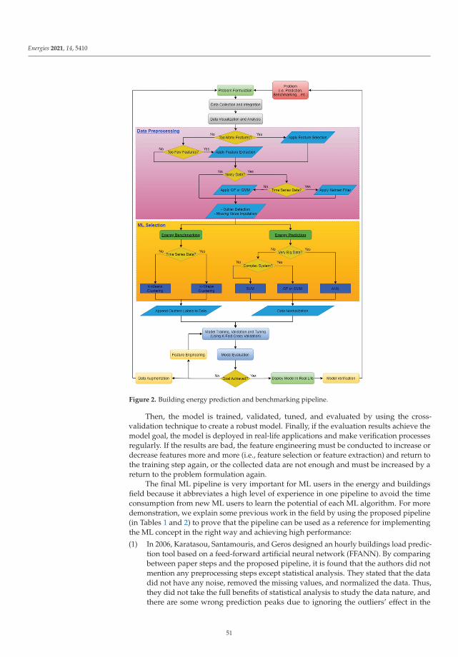
Energies 2021, 14, 5410

Figure 2. Building energy prediction and benchmarking pipeline.

Then, the model is trained, validated, tuned, and evaluated by using the cross-validation technique to create a robust model. Finally, if the evaluation results achieve themodel goal, the model is deployed in real-life applications and make verification processesregularly. If the results are bad, the feature engineering must be conducted to increase ordecrease features more and more (i.e., feature selection or feature extraction) and return tothe training step again, or the collected data are not enough and must be increased by areturn to the problem formulation again.

The final ML pipeline is very important for ML users in the energy and buildingsfield because it abbreviates a high level of experience in one pipeline to avoid the timeconsumption from new ML users to learn the potential of each ML algorithm. For moredemonstration, we explain some previous work in the field by using the proposed pipeline(in Tables 1 and 2) to prove that the pipeline can be used as a reference for implementingthe ML concept in the right way and achieving high performance:

(1) In 2006, Karatasou, Santamouris, and Geros designed an hourly buildings load predic-tion tool based on a feed-forward artificial neural network (FFANN). By comparingbetween paper steps and the proposed pipeline, it is found that the authors did notmention any preprocessing steps except statistical analysis. They stated that the datadid not have any noise, removed the missing values, and normalized the data. Thus,they did not take the full benefits of statistical analysis to study the data nature, andthere are some wrong prediction peaks due to ignoring the outliers’ effect in the

51

Energies 2021, 14, 5410

preprocessing data step. Because of the large data size and since the ML type is pre-diction, the selected algorithm was ANN, and they implemented the cross-validationtechnique to create a robust model. In addition, the ANN algorithm was evaluatedwith two different data sets to ensure robustness, but it is not enough because theevaluation would be better if performed on the same model structures with differentdata sets but with the same input features to increase reliability and robustness [21].

(2) Dombaycı et al., in 2010, developed an hourly heating energy prediction model basedon ANN to estimate energy in the design stage. The authors did not mention anypreprocessing steps, just normalization, because the user data were calculated, so theprobability of containing noise, missing values, and outliers is very small (this doesnot have the same worth of actual data). The ANN was used because the data arebig and the ML problem concerns prediction. The data were split to train and testsets, but this was not enough because the trained model could be more robust if thecross-validation technique was used in training and evaluation steps [13].

(3) Mena et al., in 2014, developed and assessed a short-term predictive ANN model ofelectricity demand. The authors manually reduced the number of features because thedata had a high number of features. Although the authors mentioned the outliers andnoise in the data, they did not apply any type of analysis to solve these two problemsin the data. In addition, the missing values in the data are kept as is and the authorsdepended on a manual method in splitting the data to skip missing values, which meansthe splitting blocks are imbalanced. Thus, the efforts made in the training and evaluationsteps to create a robust model are useless because the preprocessing steps are not wellperformed, so the results from the model have a relatively high mean error [57].

(4) In 2015, Li et al. improved the short-term hourly electricity consumption predictionof a building. The authors mentioned a large number of features, so they used anautomatic method of reducing features (PCA). However, the authors did not mentionanything about the missing values and outliers in the data. Because of the largedata size and since the ML type is prediction, the selected algorithm was ANN.The automatic tuning gives high prediction results, but it needs to integrate withcross-validation techniques to ensure the robustness and reliability of the model [16].

(5) In 2017, Yang et al. proposed an energy clustering and prediction method based onk-shape and SVM algorithms for time series data. The authors mentioned the noise in thedata but did not mention solving it. In addition, there was no mention of any techniqueto solve the problem of outliers and missing values. The data size is relatively high tobe used in SVM algorithms (the authors did not take into consideration the data sizewhen selecting the algorithm), and the authors extracted features to decrease complexityand effort during model training. Due to the huge data size, it is recommended to usedparallel SVM to reduce time or replace it directly with ANN [36].

(6) Heo and Zavala, in 2012, used the GPR model in energy savings and uncertainty mea-surements and verification problems. The authors did not use any feature extractionconcept, although they mentioned a high degree of complexity in the data due tonoise and nonlinear relationships. Moreover, they did not mention any technique todetect and solve the outliers and missing values problems. The data size is relativelylarge and since the authors did not mention time consumption in training, it may betoo large. Thus, it will be better to use the Gaussian model to remove noise only andcomplete the prediction by ANN or use ANN directly for all problems [33].

(7) In 2014, Gao and Malkawi proposed a benchmarking technique for building energybased on the k-means concept. The authors used the features selection techniquedue to the high number of features. The data contain outliers, but the authors didnot mention the technique to solve this. In addition, the imputation technique formissing values was not declared well, which greatly affected the k-means solution(the k-means has a high probability of falling into local minimum) [37].

52

Energies 2021, 14, 5410

Ta

ble

1.

Rev

iew

ofso

me

prev

ious

pape

rsco

mpa

ring

them

wit

hth

epr

opos

edM

Lpi

pelin

e.

Pre

pro

cess

ing

Qu

est

ion

sa

nd

Act

ion

sM

od

el

Se

lect

ion

Qu

est

ion

sa

nd

Act

ion

sM

od

el

Cre

ati

on

To

oM

an

yF

ea

ture

s?o

rT

oo

Fe

wF

ea

ture

s?

Ex

tra

cte

do

rS

ele

cte

dF

ea

ture

s

No

isy

Da

ta?

Tim

eS

eri

-o

us

Da

ta?

Ka

lma

no

rG

au

s-si

an

Fil

ters

Ou

tlie

rs’

Va

lue

sM

issi

ng

Va

lue

sB

en

chm

ark

ing

or

Pre

dic

tio

n?

Tim

eS

eri

-o

us

Da

ta?

Ve

ryB

igD

ata

?

Co

mp

lex

Sy

s-te

m?

Se

lect

ed

Alg

o-

rith

m?

Ap

pe

nd

Clu

ste

rsL

ab

els

toD

ata

?o

rN

orm

ali

ze

Da

ta?

Tra

inin

g,

Va

lid

ati

on

an

dT

un

ing

Ev

alu

ati

on

Not

aske

d—

–×

√—

–—

–re

mov

edpr

edic

tion

√√

Not

aske

dA

NN

norm

aliz

ed

App

lied

cros

s-va

lidat

ion

ontw

oda

tase

ts

Use

dtw

oda

tase

tsan

dtr

ied

diff

eren

tsa

mpl

esst

eps

[21]

Not

aske

d—

–×

√—

–—

–—

–pr

edic

tion

√√

Not

aske

dA

NN

norm

aliz

edSp

litda

tato

trai

nan

dte

stse

ts

Use

dte

stda

ta[1

3]

Too

man

yfe

atur

es

Sele

cted

feat

ures

usin

gco

rrel

atio

nbe

twee

nfe

atur

es

√√

—–

Kee

pas

itK

eep

asit

pred

icti

on√

√√

AN

Nno

rmal

ized

Split

data

totr

ain,

valid

ate,

and

test

sets

with

diff

eren

tsa

mpl

esst

eps

Use

dte

stda

taw

ith

diff

eren

tsa

mpl

esst

eps

[57]

Too

man

yfe

atur

es

Sele

cted

feat

ures

usin

gPC

A×

√—

–—

–—

–pr

edic

tion

√√

Not

aske

dA

NN

norm

aliz

ed

Split

data

totr

ain

and

test

wit

hau

tom

atic

tuni

ng(P

SO)

Use

dte

stda

ta[1

6]

Too

man

yfe

atur

es

Extr

acte

dfe

atur

esus

ing

k-sh

ape

clus

teri

ng

√√

—–

Filt

ered

Impu

ted

Benc

hmar

king

and

pred

icti

on√

Not

aske

dN

otas

ked

k-sh

ape

and

SVM

norm

aliz

edan

dap

pend

clus

ter

labe

ls

Split

data

totr

ain

and

test

and

appl

ied

cros

s-va

lidat

ion

Use

dte

stda

taw

ith

diff

eren

tsa

mpl

esst

eps

[36]

53

Energies 2021, 14, 5410

Ta

ble

1.

Con

t.

Pre

pro

cess

ing

Qu

est

ion

sa

nd

Act

ion

sM

od

el

Se

lect

ion

Qu

est

ion

sa

nd

Act

ion

sM

od

el

Cre

ati

on

To

oM

an

yF

ea

ture

s?o

rT

oo

Fe

wF

ea

ture

s?

Ex

tra

cte

do

rS

ele

cte

dF

ea

ture

s

No

isy

Da

ta?

Tim

eS

eri

-o

us

Da

ta?

Ka

lma

no

rG

au

s-si

an

Fil

ters

Ou

tlie

rs’

Va

lue

sM

issi

ng

Va

lue

sB

en

chm

ark

ing

or

Pre

dic

tio

n?

Tim

eS

eri

-o

us

Da

ta?

Ve

ryB

igD

ata

?

Co

mp

lex

Sy

s-te

m?

Se

lect

ed

Alg

o-

rith

m?

Ap

pe

nd

Clu

ste

rsL

ab

els

toD

ata

?o

rN

orm

ali

ze

Da

ta?

Tra

inin

g,

Va

lid

ati

on

an

dT

un

ing

Ev

alu

ati

on

Not

aske

d—

–√

√—

–—

–—

–pr

edic

tion

√√

√G

PRno

rmal

ized

Split

data

totr

ain

and

test

wit

hdi

ffer

ent

sam

ples

step

s

Use

dte

stda

taw

ith

diff

eren

tsa

mpl

esst

eps

[33]

Too

man

yfe

atur

es

Sele

cted

feat

ures

usin

gp-

valu

e

×√

—–

—–

repl

aced

Benc

hmar

king

×√

Not

aske

dk-

mea

nno

rmal

ized

App

lied

sim

ilari

tym

easu

reon

one

pack

age

data

Com

pare

resu

lts

wit

hEn

ergy

Star

soft

war

e

[37]

54

Energies 2021, 14, 5410

Ta

ble

2.

The

deta

ilsof

the

revi

ewed

pape

rsan

dth

eco

mm

ents

that

resu

ltfr

omco

mpa

riso

nw

ith

the

prop

osed

ML

pipe

line.

Mo

de

lT

arg

et

Da

taS

ou

rce

Da

taS

ize

Mo

de

lF

ea

ture

sS

ele

cte

dA

lgo

rith

m?

Be

stE

va

lua

tio

nR

esu

lts

Co

mm

en

tsa

nd

Ex

pe

cte

dIm

pro

ve

me

nts

Pred

ictH

ourl

yEn

ergy

Con

sum

ptio

n[2

1]

“Tw

odi

ffer

entd

ata

sets

prov

ided

from

two

diff

eren

tbui

ldin

gs:T

hefir

stse

tis

the

benc

hmar

kPR

OBE

N1,

and

com

esfr

omth

efir

sten

ergy

pred

icti

onco

ntes

t,th

eG

reat

Build

ing

Ener

gyPr

edic

tor

Shoo

tout

I,or

gani

zed

byA

SHR

AE

(dat

ase

tA)

&Th

ese

cond

data

setd

eriv

esfr

oman

offic

ebu

ildin

glo

cate

din

Ath

ens,

Gre

ece

(dat

ase

tB)”

data

setA

:ato

talo

f420

8ti

me

step

s,da

tase

tB:a

tota

lof8

280

tim

est

eps

data

setA

:“te

mpe

ratu

re,

sola

rra

diat

ion,

hum

idity

rati

oan

dw

ind

spee

d”da

tase

tB:“

ambi

ent

tem

pera

ture

,hum

idit

y,da

ily,w

eekl

yan

dye

arly

cycl

esth

eho

urof

day,

day

ofw

eek

and

day

ofye

ar”

AN

N

data

setA

:RM

Sis

15.2

5,M

APE

is1.

50,

CV

is2.

44an

dM

BEis

0.37

data

setB

:RM

Sis

1.13

,MA

PEis

2.64

,C

Vis

2.95

and

MBE

is–0

.03

The

rear

eso

me

wro

ngpr

edic

tion

peak

sdu

eto

igno

ring

the

effe

ctof

the

outl

iers

inpr

epro

cess

ing

data

step

,and

the

eval

uati

onw

ould

bebe

tter

ifca

rrie

dou

ton

the

sam

em

odel

stru

ctur

esw

ith

diff

eren

tdat

ase

tsbu

tw

ith

the

sam

ein

putf

eatu

res

toin

crea

sere

liabi

lity

and

robu

stne

ss.

55

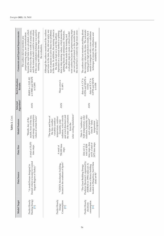
Energies 2021, 14, 5410

Ta

ble

2.

Con

t.

Mo

de

lT

arg

et

Da

taS

ou

rce

Da

taS

ize

Mo

de

lF

ea

ture

sS

ele

cte

dA

lgo

rith

m?

Be

stE

va

lua

tio

nR

esu

lts

Co

mm

en

tsa

nd

Ex

pe

cte

dIm

pro

ve

me

nts

Pred

ictH

ourl

yH

eati

ngEn

ergy

[13]

“Am

odel

hous

ede

sign

edin

Den

izli

whi

chis

loca

ted

inC

entr

alA

egea

nR

egio

nof

Turk

ey”

Ato

talo

f35,

070

tim

est

eps

“Mon

th,d

ayof

the

mon

th,h

our

ofth

eda

y,an

den

ergy

cons

umpt

ion

valu

esat

cert

ain

hour

s”

AN

NR

MSE

is1.

2125

,R2

is0.

9880

and

MA

PEis

0.20

81

The

auth

ordi

dno

tmen

tion

any

prep

roce

ssin

gst

eps,

just

norm

aliz

atio

nbe

caus

eth

eus

edda

taw

asca

lcul

ated

,whi

chdi

dno

thav

eth

esa

me

wor

thof

actu

alda

ta,

and

the

trai

ned

mod

elco

uld

bem

ore

robu

stif

the

cros

s-va

lidat

ion

tech

niqu

ew

asus

edin

trai

ning

and

diff

eren

ttim

est

eps

duri

ngth

eev

alua

tion

,

Pred

ictH

ourl

yEn

ergy

Con

sum

ptio

n[5

7]

“CIE

SOL

bioc

limat

icbu

ildin

g,lo

cate

din

the

sout

heas

tofS

pain

”

Ato

talo

f70

0,00

0ti

me

step

s

“The

type

and

hour

ofth

eda

y,w

eath

erva

riab

les

(out

door

tem

pera

ture

,out

door

hum

idit

y,so

lar

radi

atio

n,w

ind

velo

city

and

win

ddi

rect

ion)

and

the

stat

eof

the

actu

ator

sfr

omth

eso

lar

cool

ing

inst

alla

tion

”

AN

NM

ean

erro

ris

11.4

8%

Alt

houg

hth

eau

thor

sm

enti

oned

the

outl

iers

and

nois

ein

the

data

,the

ydi

dno

tapp

lyan

yty

peof

anal

ysis

toso

lve

thes

etw

opr

oble

ms

inth

eda

ta.I

nad

ditio

n,th

em

issi

ngva

lues

inth

eda

taar

eke

ptas

isan

dth

eau

thor

sde

pend

edon

am

anua

lmet

hod

insp

litti

ngda

tato

skip

mis

sing

valu

es,w

hich

mea

nsth

esp

litti

ngbl

ocks

are

imba

lanc

ed.T

here

fore

,th

eef

fort

sm

ade

inth

etr

aini

ngan

dev

alua

tion

step

sto

crea

tea

robu

stm

odel

wer

eus

eles

sbe

caus

eth

epr

epro

cess

ing

step

sar

eno

twel

lper

form

ed,s

oth

ere

sult

sfr

omth

em

odel

have

are

lati

vely

high

mea

ner

ror.

Pred

ictH

ourl

yel

ectr

icit

yco

nsum

ptio

n[1

6]

“The

Gre

atBu

ildin

gEn

ergy

Pred

icto

rSh

ooto

utI,

orga

nize

dby

ASH

RA

Ein

1990

s(d

ata

setA

)D

ata

from

alib

rary

build

ing

loca

ted

inH

angz

hou,

East

Chi

na(d

ata

setB

)”

data

setA

:ato

talo

f420

8ti

me

step

s,da

tase

tB:a

tota

lof

2472

tim

est

eps

Dat

aA

:“ou

tdoo

rdr

ybu

lbte

mpe

ratu

re,s

olar

radi

atio

n,hu

mid

ityra

tioan

dw

ind

spee

d”D

ata

B:“d

aily

tem

pera

ture

and

occu

panc

y”

AN

N

data

setA

:CV

is0.

0254

and

MA

PEis

0.01

62da

tase

tB:C

Vis

0.07

58an

dM

APE

is0.

058

The

auth

ors

did

notm

enti

onan

ythi

ngab

out

the

mis

sing

valu

esin

the

data

.The

auto

mat

ictu

ning

give

shi

ghpr

edic

tion

resu

lts,

buti

tne

eds

toin

tegr

ate

wit

ha

cros

s-va

lidat

ion

tech

niqu

eto

ensu

reth

ero

bust

ness

and

relia

bilit

yfo

rm

odel

.

56

Energies 2021, 14, 5410

Ta

ble

2.

Con

t.

Mo

de

lT

arg

et

Da

taS

ou

rce

Da

taS

ize

Mo

de

lF

ea

ture

sS

ele

cte

dA

lgo

rith

m?

Be

stE

va

lua

tio

nR

esu

lts

Co

mm

en

tsa

nd

Ex

pe

cte

dIm

pro

ve

me

nts

Benc

hmar

kan

dpr

edic

t(ho

urly

and

wee

kly)

Ener

gyco

nsum

ptio

n[3

6]

“10

inst

itut

iona

lbui

ldin

gsin

Sing

apor

e”

ato

talo

f122

days

for

each

build

ing

“Hou

rly

and

wee

kly

ener

gyco

nsum

ptio

n”k-

shap

ean

dSV

M

Res

pect

ive

MA

PEva

lues

are

15.3

6,9.

46,1

.033

1.23

,2.3

7,3.

66,0

.57,

54.1

1,3.

63,

4.46

for

the

ten

build

ings

The

auth

ors

men

tion

edth

eno

ise

inda

tabu

tdi

dno

tmen

tion

solv

ing

it.I

nad

diti

on,t

heou

tlie

rsan

dm

issi

ngva

lues

did

notm

enti

onso

lve

inth

ete

chni

que.

The

data

size

isre

lati

vely

high

tobe

used

inSV

Mal

gori

thm

s(t

heau

thor

sdi

dno

ttak

ein

toco

nsid

erat

ion

the

data

size

whe

nse

lect

ing

the

algo

rith

m),

and

the

auth

ors

extr

acte

dfe

atur

esto

decr

ease

com

plex

ity

and

effo

rt.T

hus,

itis

reco

mm

ende

dto

used

para

llelS

VM

tore

duce

tim

e.

Pred

ictD

aily

Ener

gyPe

rfor

man

ce[3

3]

“Rea

lwea

ther

data

inth

eC

hica

goar

ea”

ato

talo

f87

36ti

me

step

s

“Wea

ther

and

occu

panc

yle

vels

,and

the

mos

tco

mm

only

used

isou

tdoo

rdr

y-bu

lbai

rte

mpe

ratu

re”

GPR

SSE

isfr

om2.

7e5

to3.

6e6

and

tota

len

ergy

savi

ngs

pred

icti

oner

ror

isfr

om31

to41

.23

The

data

size

isre

lati

vely

larg

e,an

dth

eau

thor

sdi

dno

tmen

tion

time

cons

umpt

ion

intr

aini

ng,a

sit

may

beto

ola

rge.

The

refo

re,i

tw

illbe

bett

erto

use

the

Gau

ssia

nm

odel

tore

mov

eno

ise

only

and

com

plet

epr

edic

tion

byA

NN

orus

eA

NN

dire

ctly

for

allp

robl

ems.

Benc

hmar

kan

nual

Ener

gyPe

rfor

man

ce[3

7]

“com

mer

cial

build

ing

(CBE

CS

data

base

)”52

15sa

mpl

es

“Are

a,pe

rcen

thea

ted,

perc

entc

oole

d,w

all

mat

eria

ls,r

oofm

ater

ials

,w

indo

wm

ater

ials

,w

indo

wpe

rcen

t,sh

ape,

num

ber

offlo

ors,

cons

truc

tion

year

,w

eekl

yop

erat

ion

hour

s,oc

cupa

nts,

vari

able

air

volu

me,

heat

ing

unit

,co

olin

gun

it,ec

onom

izer

,re

frig

erat

ors,

num

ber

ofse

rver

s,of

fice

equi

pmen

t,he

atin

gan

dco

olin

gde

gree

day”

k-m

ean

Rat

iobe

twee

nac

tual

ener

gyin

dex

toce

ntro

idfo

rcl

uste

rin

rang

efr

om0.

96to

2.1

for

each

clus

ter

The

data

cont

ain

outli

ers,

butt

heau

thor

sdi

dno

tmen

tion

this

orth

ete

chni

que

toso

lve

this

.In

addi

tion

,the

impu

tati

onfo

rm

issi

ngva

lues

isno

tdec

lare

dw

ell.

The

eval

uati

onst

epis

carr

ied

outu

sing

aco

mpa

riso

nw

ith

Ener

gySt

arw

itho

utde

clar

atio

nof

any

appr

oach

toov

erco

me

the

loca

lmin

imum

solu

tion

ofth

ek-

mea

nal

gori

thm

.

57

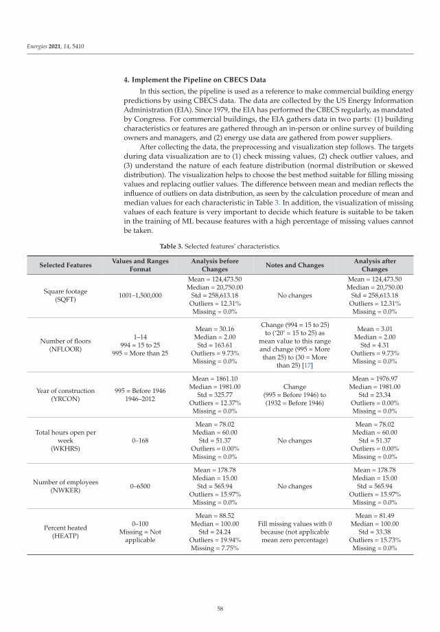
Energies 2021, 14, 5410

4. Implement the Pipeline on CBECS Data

In this section, the pipeline is used as a reference to make commercial building energypredictions by using CBECS data. The data are collected by the US Energy InformationAdministration (EIA). Since 1979, the EIA has performed the CBECS regularly, as mandatedby Congress. For commercial buildings, the EIA gathers data in two parts: (1) buildingcharacteristics or features are gathered through an in-person or online survey of buildingowners and managers, and (2) energy use data are gathered from power suppliers.

After collecting the data, the preprocessing and visualization step follows. The targetsduring data visualization are to (1) check missing values, (2) check outlier values, and(3) understand the nature of each feature distribution (normal distribution or skeweddistribution). The visualization helps to choose the best method suitable for filling missingvalues and replacing outlier values. The difference between mean and median reflects theinfluence of outliers on data distribution, as seen by the calculation procedure of mean andmedian values for each characteristic in Table 3. In addition, the visualization of missingvalues of each feature is very important to decide which feature is suitable to be takenin the training of ML because features with a high percentage of missing values cannotbe taken.

Table 3. Selected features’ characteristics.

Selected FeaturesValues and Ranges

FormatAnalysis before

ChangesNotes and Changes

Analysis afterChanges

Square footage(SQFT) 1001–1,500,000

Mean = 124,473.50Median = 20,750.00

Std = 258,613.18Outliers = 12.31%Missing = 0.0%

No changes

Mean = 124,473.50Median = 20,750.00

Std = 258,613.18Outliers = 12.31%Missing = 0.0%

Number of floors(NFLOOR)

1–14994 = 15 to 25

995 = More than 25

Mean = 30.16Median = 2.00Std = 163.61

Outliers = 9.73%Missing = 0.0%

Change (994 = 15 to 25)to (‘20’ = 15 to 25) as

mean value to this rangeand change (995 = Morethan 25) to (30 = More

than 25) [17]

Mean = 3.01Median = 2.00

Std = 4.31Outliers = 9.73%Missing = 0.0%

Year of construction(YRCON)

995 = Before 19461946–2012

Mean = 1861.10Median = 1981.00


Change(995 = Before 1946) to(1932 = Before 1946)

Mean = 1976.97Median = 1981.00


Total hours open perweek

(WKHRS)0–168

Mean = 78.02Median = 60.00


No changes

Mean = 78.02Median = 60.00


Number of employees(NWKER) 0–6500

Mean = 178.78Median = 15.00


No changes

Mean = 178.78Median = 15.00


Percent heated(HEATP)

0–100Missing = Not

applicable

Mean = 88.52Median = 100.00


Fill missing values with 0because (not applicablemean zero percentage)

Mean = 81.49Median = 100.00


58

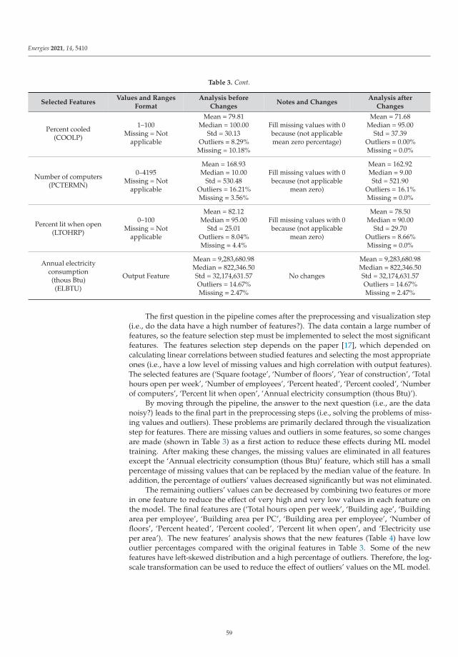
Energies 2021, 14, 5410

Table 3. Cont.

Selected FeaturesValues and Ranges

FormatAnalysis before

ChangesNotes and Changes

Analysis afterChanges

Percent cooled(COOLP)


applicable

Mean = 79.81Median = 100.00

Std = 30.13Outliers = 8.29%

Missing = 10.18%

Fill missing values with 0because (not applicablemean zero percentage)

Mean = 71.68Median = 95.00


Number of computers(PCTERMN)


applicable

Mean = 168.93Median = 10.00


Fill missing values with 0because (not applicable

mean zero)

Mean = 162.92Median = 9.00Std = 521.90

Outliers = 16.1%Missing = 0.0%

Percent lit when open(LTOHRP)


applicable

Mean = 82.12Median = 95.00


Fill missing values with 0because (not applicable

mean zero)

Mean = 78.50Median = 90.00


Annual electricityconsumption(thous Btu)(ELBTU)

Output Feature

Mean = 9,283,680.98Median = 822,346.50Std = 32,174,631.57Outliers = 14.67%Missing = 2.47%

No changes

Mean = 9,283,680.98Median = 822,346.50Std = 32,174,631.57Outliers = 14.67%Missing = 2.47%

The first question in the pipeline comes after the preprocessing and visualization step(i.e., do the data have a high number of features?). The data contain a large number offeatures, so the feature selection step must be implemented to select the most significantfeatures. The features selection step depends on the paper [17], which depended oncalculating linear correlations between studied features and selecting the most appropriateones (i.e., have a low level of missing values and high correlation with output features).The selected features are (‘Square footage’, ‘Number of floors’, ‘Year of construction’, ‘Totalhours open per week’, ‘Number of employees’, ‘Percent heated’, ‘Percent cooled’, ‘Numberof computers’, ‘Percent lit when open’, ‘Annual electricity consumption (thous Btu)’).

By moving through the pipeline, the answer to the next question (i.e., are the datanoisy?) leads to the final part in the preprocessing steps (i.e., solving the problems of miss-ing values and outliers). These problems are primarily declared through the visualizationstep for features. There are missing values and outliers in some features, so some changesare made (shown in Table 3) as a first action to reduce these effects during ML modeltraining. After making these changes, the missing values are eliminated in all featuresexcept the ‘Annual electricity consumption (thous Btu)’ feature, which still has a smallpercentage of missing values that can be replaced by the median value of the feature. Inaddition, the percentage of outliers’ values decreased significantly but was not eliminated.

The remaining outliers’ values can be decreased by combining two features or morein one feature to reduce the effect of very high and very low values in each feature onthe model. The final features are (‘Total hours open per week’, ‘Building age’, ‘Buildingarea per employee’, ‘Building area per PC’, ‘Building area per employee’, ‘Number offloors’, ‘Percent heated’, ‘Percent cooled’, ‘Percent lit when open’, and ‘Electricity useper area’). The new features’ analysis shows that the new features (Table 4) have lowoutlier percentages compared with the original features in Table 3. Some of the newfeatures have left-skewed distribution and a high percentage of outliers. Therefore, the log-scale transformation can be used to reduce the effect of outliers’ values on the ML model.

59

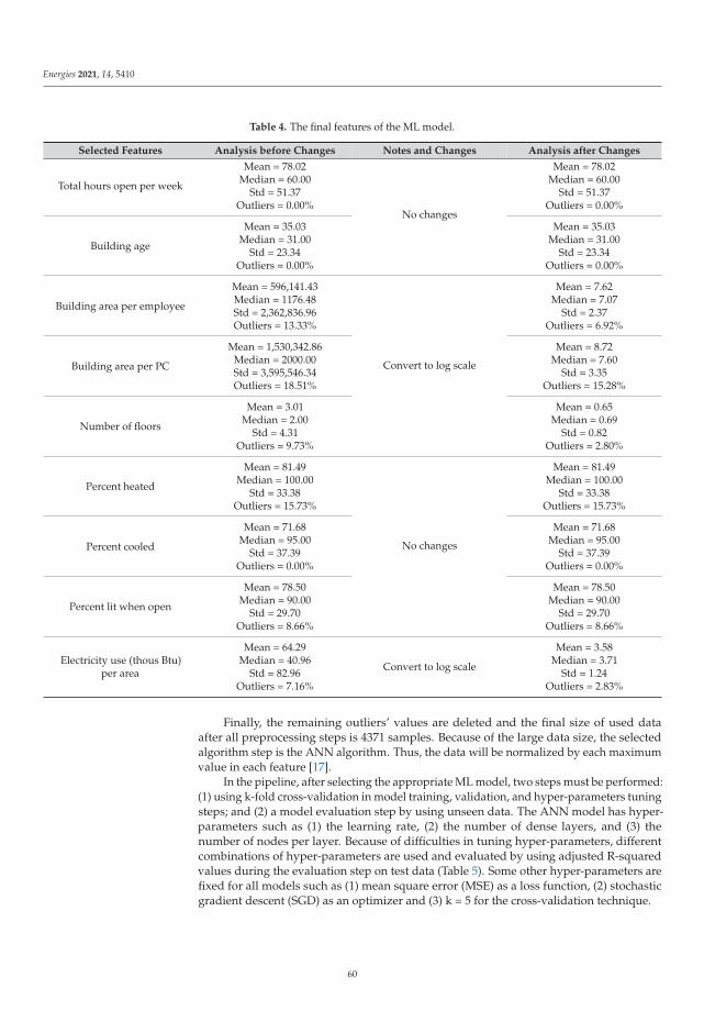
Energies 2021, 14, 5410

Table 4. The final features of the ML model.

Selected Features Analysis before Changes Notes and Changes Analysis after Changes

Total hours open per week

Mean = 78.02Median = 60.00


No changes

Mean = 78.02Median = 60.00


Building age

Mean = 35.03Median = 31.00


Mean = 35.03Median = 31.00


Building area per employee

Mean = 596,141.43Median = 1176.48Std = 2,362,836.96Outliers = 13.33%

Convert to log scale



Building area per PC

Mean = 1,530,342.86Median = 2000.00Std = 3,595,546.34Outliers = 18.51%



Number of floors





Percent heated

Mean = 81.49Median = 100.00

Std = 33.38Outliers = 15.73%

No changes

Mean = 81.49Median = 100.00

Std = 33.38Outliers = 15.73%

Percent cooled

Mean = 71.68Median = 95.00


Mean = 71.68Median = 95.00


Percent lit when open

Mean = 78.50Median = 90.00


Mean = 78.50Median = 90.00


Electricity use (thous Btu)per area

Mean = 64.29Median = 40.96


Convert to log scale



Finally, the remaining outliers’ values are deleted and the final size of used dataafter all preprocessing steps is 4371 samples. Because of the large data size, the selectedalgorithm step is the ANN algorithm. Thus, the data will be normalized by each maximumvalue in each feature [17].

In the pipeline, after selecting the appropriate ML model, two steps must be performed:(1) using k-fold cross-validation in model training, validation, and hyper-parameters tuningsteps; and (2) a model evaluation step by using unseen data. The ANN model has hyper-parameters such as (1) the learning rate, (2) the number of dense layers, and (3) thenumber of nodes per layer. Because of difficulties in tuning hyper-parameters, differentcombinations of hyper-parameters are used and evaluated by using adjusted R-squaredvalues during the evaluation step on test data (Table 5). Some other hyper-parameters arefixed for all models such as (1) mean square error (MSE) as a loss function, (2) stochasticgradient descent (SGD) as an optimizer and (3) k = 5 for the cross-validation technique.

60

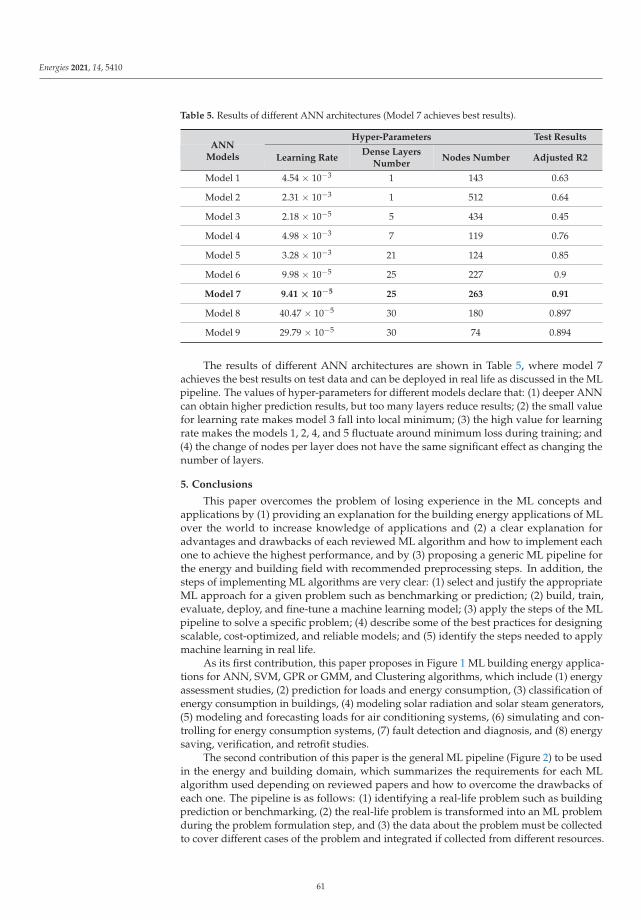
Energies 2021, 14, 5410

Table 5. Results of different ANN architectures (Model 7 achieves best results).

Hyper-Parameters Test ResultsANN

Models Learning RateDense Layers

NumberNodes Number Adjusted R2

Model 1 4.54 × 10−3 1 143 0.63

Model 2 2.31 × 10−3 1 512 0.64

Model 3 2.18 × 10−5 5 434 0.45

Model 4 4.98 × 10−3 7 119 0.76

Model 5 3.28 × 10−3 21 124 0.85

Model 6 9.98 × 10−5 25 227 0.9

Model 7 9.41 × 10−5 25 263 0.91

Model 8 40.47 × 10−5 30 180 0.897

Model 9 29.79 × 10−5 30 74 0.894

The results of different ANN architectures are shown in Table 5, where model 7achieves the best results on test data and can be deployed in real life as discussed in the MLpipeline. The values of hyper-parameters for different models declare that: (1) deeper ANNcan obtain higher prediction results, but too many layers reduce results; (2) the small valuefor learning rate makes model 3 fall into local minimum; (3) the high value for learningrate makes the models 1, 2, 4, and 5 fluctuate around minimum loss during training; and(4) the change of nodes per layer does not have the same significant effect as changing thenumber of layers.

5. Conclusions

This paper overcomes the problem of losing experience in the ML concepts andapplications by (1) providing an explanation for the building energy applications of MLover the world to increase knowledge of applications and (2) a clear explanation foradvantages and drawbacks of each reviewed ML algorithm and how to implement eachone to achieve the highest performance, and by (3) proposing a generic ML pipeline forthe energy and building field with recommended preprocessing steps. In addition, thesteps of implementing ML algorithms are very clear: (1) select and justify the appropriateML approach for a given problem such as benchmarking or prediction; (2) build, train,evaluate, deploy, and fine-tune a machine learning model; (3) apply the steps of the MLpipeline to solve a specific problem; (4) describe some of the best practices for designingscalable, cost-optimized, and reliable models; and (5) identify the steps needed to applymachine learning in real life.

As its first contribution, this paper proposes in Figure 1 ML building energy applica-tions for ANN, SVM, GPR or GMM, and Clustering algorithms, which include (1) energyassessment studies, (2) prediction for loads and energy consumption, (3) classification ofenergy consumption in buildings, (4) modeling solar radiation and solar steam generators,(5) modeling and forecasting loads for air conditioning systems, (6) simulating and con-trolling for energy consumption systems, (7) fault detection and diagnosis, and (8) energysaving, verification, and retrofit studies.

The second contribution of this paper is the general ML pipeline (Figure 2) to be usedin the energy and building domain, which summarizes the requirements for each MLalgorithm used depending on reviewed papers and how to overcome the drawbacks ofeach one. The pipeline is as follows: (1) identifying a real-life problem such as buildingprediction or benchmarking, (2) the real-life problem is transformed into an ML problemduring the problem formulation step, and (3) the data about the problem must be collectedto cover different cases of the problem and integrated if collected from different resources.

61

Energies 2021, 14, 5410

(4) The visualization step for the collected data helps to study the nature of problem by dataanalysis, answering some questions concerning data size, data features, correlation betweenfeatures, density distribution of data, mean, median, and mode of data and percentage ofnoise, missing values, and outliers. (5) The preprocessing step depends on the data analysisstep and is where the best technique of preparing data is selected and outliers and missingvalues are removed. (6) The selection of ML algorithms depends on the data analysis step toanswer the questions that identify the suitable algorithm for the problem. (7) The training,validation, and hyper-parameters’ tuning process must be carried out depending on k-foldcross validation to cover all data points without falling into the local minimum problem oroverfitting and underfitting problems. (8) The evaluation step is the key to knowing theoverall performance of the trained model. Finally, depending on the model evaluation,(9) we choose between implementing the model in real life and monitoring its performanceby a verification step, or rearranging the features and increasing the data sample.

The proposed pipeline lays out the main steps of evaluating any research in theenergy and buildings field to identify the value of new research. This approach willreconsider all previous papers in the field to repeat the previous work with a declarationfor implementation steps by using the ML pipeline to improve performance. In addition, itwill reduce the time required for any new ML user who does not have enough experiencein ML applications to enhance their work in a well-arranged pipeline. The contributionsof this paper are approved through implementing the ML pipeline on a real case study(i.e., CBECS data), which helps in creating a robust ANN model for a real-life problem andevaluating the performance for each hyper-parameter to achieve the best results. Duringimplementation, the pipeline represents an effective reference in handling one of the real-life problems (i.e., energy prediction for commercial buildings) and converting it to anML model scientifically. The implementation finds that many steps are heavily repeatedthroughout the solving of ML problems. Putting these steps in one generic pipeline todeploy the right algorithms seamlessly, reduce the complexity of quickly transferringML models into real life, and manage ML models easier increases the performance andorganization of creating a scientific model for real-life problems in a sufficient way.

This paper may be the basis for benchmarking in the field of energy and buildingsas well as for prediction software that need the user to select one application from theapplications list and upload just two files containing input data and output data. Then, thesoftware performs some statistical analysis to collect information about data such as datatype (i.e., categorical or numerical and time serious or not), size, most significant inputfeatures, degree of noise, and mean, median, percentage of missing values, and outliers.From the selected application and all calculated information, the software will detect thebest techniques required in each situation, choose algorithms, perform automatic training,tuning, and evaluation, and finally give the user the final model with its specifications file(i.e., model type and its inputs and outputs) to deploy it in real life. This future dream willdecrease the effort and time required by engineering to solve such problems. The softwaremay also have the energy certificates and regulations to conduct energy retrofit studiesfor users.

The dream of creating compatible software may have extended to other fields to createother versions; each one related to a specific field, but all are based on this ML pipeline.These types of software are very helpful nowadays to control our life more and more bymanaging real-life problems in some models in a fast, accurate, and scientific way.

Author Contributions: Conceptualization, M.A.B.A.; Formal analysis, M.A.B.A.; Investigation,M.A.B.A.; Methodology, M.A.B.A.; Software, M.A.B.A.; Supervision, M.H.; Validation, M.A.B.A.;Visualization, M.A.B.A.; Writing—original draft, M.A.B.A. Both authors have read and agreed to thepublished version of the manuscript.

Funding: The results are done by integrating graphical processing unit (NVIDA Tesla T4 GPU) withsupercomputer specifications (PowerEdge R7525 & 2 x 64-Core 2.45 GHz AMD EPYC 7763 64-CoreProcessor & 512 GB memory) of Norwegian University of Science and Technology (NTNU).

62

Energies 2021, 14, 5410

Institutional Review Board Statement: Not applicable.

Informed Consent Statement: Not applicable.

Data Availability Statement: https://www.eia.gov/consumption/commercial/.


References

1. Zhao, H. Artificial Intelligence Models for Large Scale Buildings Energy Consumption Analysis. Ph.D. Thesis, Ecole CentraleParis, Gif-sur-Yvette, France, 2014.

2. Tabrizchi, H.; Javidi, M.M.; Amirzadeh, V. Estimates of residential building energy consumption using a multi-verse optimizer-based support vector machine with k-fold cross-validation. Evol. Syst. 2019. [CrossRef]

3. Cai, H.; Shen, S.; Lin, Q.; Li, X.; Xiao, H. Predicting the energy consumption of residential buildings for regional electricitysupply-side and demand-side management. IEEE Access 2019, 7, 30386–30397. [CrossRef]

4. Seyedzadeh, S.; Rahimian, F.P.; Oliver, S.; Rodriguez, S.; Glesk, I. Machine learning modelling for predicting non-domesticbuildings energy performance: A model to support deep energy retrofit decision-making. Appl. Energy 2020, 279, 115908.[CrossRef]

5. Somu, N.; Raman, G.R.M.; Ramamritham, K. A deep learning framework for building energy consumption forecast. Renew.Sustain. Energy Rev. 2021, 137, 110591. [CrossRef]

6. Fayaz, M.; Kim, D. A Prediction Methodology of Energy Consumption Based on Deep Extreme Learning Machine and Compara-tive Analysis in Residential Buildings. Electronics 2018, 7, 222. [CrossRef]

7. Liu, Z.; Wu, D.; Liu, Y.; Han, Z.; Lun, L.; Gao, J.; Cao, G. Accuracy analyses and model comparison of machine learning adoptedin building energy consumption prediction. Energy Explor. Exploit. 2019, 37, 1426–1451. [CrossRef]

8. Wang, L.; El-Gohary, N.M. Machine-Learning-Based Model for Supporting Energy Performance Benchmarking for Office Buildings;Springer: Cham, Switzerland, 2018. [CrossRef]

9. Seyedzadeh, S.; Rahimian, F.P.; Glesk, I.; Roper, M. Machine learning for estimation of building energy consumption andperformance: A review. Vis. Eng. 2018, 6, 5. [CrossRef]

10. Shalev-Shwartz, S.; Ben-David, S. Understanding Machine Learning_From Theory to Algorithm. 2014. Available online: https://www.cs.huji.ac.il/~{}shais/UnderstandingMachineLearning/understanding-machine-learning-theory-algorithms.pdf (accessedon 30 August 2021).

11. Chao, W.-L. Machine Learning Tutorial. 2011. Available online: https://www.semanticscholar.org/paper/Machine-Learning-Tutorial-Chao/e74d94c407b599947f9e6262540b402c568674f6 (accessed on 30 August 2021).

12. Kirsch, J.H.A.D. IBM Machine Learning for Dummies. 2018. Available online: https://www.ibm.com/downloads/cas/GB8ZMQZ3 (accessed on 30 August 2021).

13. Dombaycı, Ö.A. The prediction of heating energy consumption in a model house by using artificial neural networks in Denizli–Turkey. Adv. Eng. Softw. 2010, 41, 141–147. [CrossRef]

14. Antanasijevic, D.; Pocajt, V.; Ristic, M.; Peric-Grujic, A. Modeling of energy consumption and related GHG (greenhouse gas)intensity and emissions in Europe using general regression neural networks. Energy 2015, 84, 816–824. [CrossRef]

15. Platon, R.; Dehkordi, V.R.; Martel, J. Hourly prediction of a building’s electricity consumption using case-based reasoning,artificial neural networks and principal component analysis. Energy Build. 2015, 92, 10–18. [CrossRef]

16. Li, K.; Hu, C.; Liu, G.; Xue, W. Building’s electricity consumption prediction using optimized artificial neural networks andprincipal component analysis. Energy Build. 2015, 108, 106–113. [CrossRef]

17. Yalcintas, M.; Aytun Ozturk, U. An energy benchmarking model based on artificial neural network method utilizing USCommercial Buildings Energy Consumption Survey (CBECS) database. Int. J. Energy Res. 2007, 31, 412–421. [CrossRef]

18. Edwards, R.E.; New, J.; Parker, L.E. Predicting future hourly residential electrical consumption: A machine learning case study.Energy Build. 2012, 49, 591–603. [CrossRef]

19. Kialashaki, A.; Reisel, J.R. Modeling of the energy demand of the residential sector in the United States using regression modelsand artificial neural networks. Appl. Energy 2013, 108, 271–280. [CrossRef]

20. Olofsson, T.; Andersson, S. Long-term energy demand predictions based on short-term measured data. Energy Build. 2001, 33,85–91. [CrossRef]

21. Karatasou, S.; Santamouris, M.; Geros, V. Modeling and predicting building’s energy use with artificial neural networks: Methodsand results. Energy Build. 2006, 38, 949–958. [CrossRef]

22. Du, Z.; Fan, B.; Jin, X.; Chi, J. Fault detection and diagnosis for buildings and HVAC systems using combined neural networksand subtractive clustering analysis. Build. Environ. 2014, 73, 1–11. [CrossRef]

23. Huang, H.; Chen, L.; Hu, E. A neural network-based multi-zone modelling approach for predictive control system design incommercial buildings. Energy Build. 2015, 97, 86–97. [CrossRef]

24. Pérez-Ortiz, J.A.; Gers, F.A.; Eck, D.; Schmidhuber, J. Kalman filters improve LSTM network performance in problems unsolvableby traditional recurrent nets. Neural Netw. 2003, 16, 241–250. [CrossRef]

25. González, P.A.; Zamarreño, J.M. Prediction of hourly energy consumption in buildings based on a feedback artificial neuralnetwork. Energy Build. 2005, 37, 595–601. [CrossRef]

63

Energies 2021, 14, 5410

26. Aydinalp, M.; Ismet Ugursal, V.; Fung, A.S. Modeling of the space and domestic hot-water heating energy-consumption in theresidential sector using neural networks. Appl. Energy 2004, 79, 159–178. [CrossRef]

27. Hou, Z.; Lian, Z. An application of support vector machines in cooling load prediction. In Proceedings of the 2009 InternationalWorkshop on Intelligent Systems and Applications, Wuhan, China, 23–24 May 2009.

28. Li, Q.; Meng, Q.; Cai, J.; Yoshino, H.; Mochida, A. Applying support vector machine to predict hourly cooling load in the building.Appl. Energy 2009, 86, 2249–2256. [CrossRef]

29. Li, X.; Lu, J.-H.; Ding, L.; Xu, G.; Li, J. Building Cooling Load Forecasting Model Based on LS-SVM. In Proceedings of the 2009Asia-Pacific Conference on Information Processing, Shenzhen, China, 18–19 July 2009; pp. 55–58.

30. Jain, R.K.; Smith, K.M.; Culligan, P.J.; Taylor, J.E. Forecasting energy consumption of multi-family residential buildings usingsupport vector regression: Investigating the impact of temporal and spatial monitoring granularity on performance accuracy.Appl. Energy 2014, 123, 168–178. [CrossRef]

31. Zhao, H.-X.; Magoulès, F. A review on the prediction of building energy consumption. Renew. Sustain. Energy Rev. 2012, 16,3586–3592. [CrossRef]

32. Zhao, H.X.; Magoulès, F. Parallel Support Vector Machines Applied to the Prediction of Multiple Buildings Energy Consumption.Algorithms Comput. Technol. 2009, 4, 231–249. [CrossRef]

33. Heo, Y.; Zavala, V.M. Gaussian process modeling for measurement and verification of building energy savings. Energy Build.2012, 53, 7–18. [CrossRef]

34. Burkhart, M.C.; Heo, Y.; Zavala, V.M. Measurement and verification of building systems under uncertain data: A Gaussianprocess modeling approach. Energy Build. 2014, 75, 189–198. [CrossRef]

35. Heo, Y.; Choudhary, R.; Augenbroe, G.A. Calibration of building energy models for retrofit analysis under uncertainty. EnergyBuild. 2012, 47, 550–560. [CrossRef]

36. Yang, J.; Ning, C.; Deb, C.; Zhang, F.; Cheong, D.; Lee, S.E.; Tham, K.W. k-Shape clustering algorithm for building energy usagepatterns analysis and forecasting model accuracy improvement. Energy Build. 2017, 146, 27–37. [CrossRef]

37. Gao, X.; Malkawi, A. A new methodology for building energy performance benchmarking: An approach based on intelligentclustering algorithm. Energy Build. 2014, 84, 607–616. [CrossRef]

38. Lara, R.A.; Pernigotto, G.; Cappelletti, F.; Romagnoni, P.; Gasparella, A. Energy audit of schools by means of cluster analysis.Energy Build. 2015, 95, 160–171. [CrossRef]

39. Santamouris, M.; Mihalakakou, G.; Patargias, P.; Gaitani, N.; Sfakianaki, K.; Papaglastra, M.; Zerefos, S. Using intelligentclustering techniques to classify the energy performance of school buildings. Energy Build. 2007, 39, 45–51. [CrossRef]

40. Gaitani, N.; Lehmann, C.; Santamouris, M.; Mihalakakou, G.; Patargias, P. Using principal component and cluster analysis in theheating evaluation of the school building sector. Appl. Energy 2010, 87, 2079–2086. [CrossRef]

41. Kalogirou, S.A. Applications of artificial neural networks in energy systems a review. Energy Convers. Manag. 1998, 40, 1073–1087.[CrossRef]

42. Ascione, F.; Bianco, N.; De Stasio, C.; Mauro, G.M.; Vanoli, G.P. Artificial neural networks to predict energy performance andretrofit scenarios for any member of a building category: A novel approach. Energy 2017, 118, 999–1017. [CrossRef]

43. Beccali, M.; Ciulla, G.; Brano, V.L.; Galatioto, A.; Bonomolo, M. Artificial neural network decision support tool for assessment ofthe energy performance and the refurbishment actions for the non-residential building stock in Southern Italy. Energy 2017, 137,1201–1218. [CrossRef]

44. Paudel, S.; Elmtiri, M.; Kling, W.L.; Le Corre, O.; Lacarrière, B. Pseudo dynamic transitional modeling of building heating energydemand using artificial neural network. Energy Build. 2014, 70, 81–93. [CrossRef]

45. Deb, C.; Eang, L.S.; Yang, J.; Santamouris, M. Forecasting diurnal cooling energy load for institutional buildings using ArtificialNeural Networks. Energy Build. 2016, 121, 284–297. [CrossRef]

46. Benedetti, M.; Cesarotti, V.; Introna, V.; Serranti, J. Energy consumption control automation using Artificial Neural Networks andadaptive algorithms: Proposal of a new methodology and case study. Appl. Energy 2016, 165, 60–71. [CrossRef]

47. Ahn, J.; Cho, S.; Chung, D.H. Analysis of energy and control efficiencies of fuzzy logic and artificial neural network technologiesin the heating energy supply system responding to the changes of user demands. Appl. Energy 2017, 190, 222–231. [CrossRef]

48. Kalogirou, S.; Lalot, S.; Florides, G.; Desmet, B. Development of a neural network-based fault diagnostic system for solar thermalapplications. Sol. Energy 2008, 82, 164–172. [CrossRef]

49. Hong, S.-M.; Paterson, G.; Mumovic, D.; Steadman, P. Improved benchmarking comparability for energy consumption in schools.Build. Res. Inf. 2013, 42, 47–61. [CrossRef]

50. Buratti, C.; Barbanera, M.; Palladino, D. An original tool for checking energy performance and certification of buildings by meansof Artificial Neural Networks. Appl. Energy 2014, 120, 125–132. [CrossRef]

51. Lai, F.; Magoulès, F.; Lherminier, F. Vapnik’s learning theory applied to energy consumption forecasts in residential buildings. Int.J. Comput. Math. 2008, 85, 1563–1588. [CrossRef]

52. Li, X.; Bowers, C.P.; Schnier, T. Classification of Energy Consumption in Buildings with Outlier Detection. IEEE Trans. Ind.Electron. 2010, 57, 3639–3644. [CrossRef]

53. Oladipupo, T. Types of Machine Learning Algorithms. New Adv. Mach. Learn. 2010, 3, 19–48.54. Wong, S.L.; Wan, K.K.W.; Lam, T.N.T. Artificial neural networks for energy analysis of office buildings with daylighting. Appl.

Energy 2010, 87, 551–557. [CrossRef]

64

Energies 2021, 14, 5410

55. Smola, A.; Vishwanathan, S.V.N. Introduction to Machine Learning; Cambridge University: Cambridge, UK, 2008.56. Deisenroth, M.P.; Faisal, A.A.; Ong, C.S. Mathematics for Machine Learning; Cambridge University Press: Cambridge, UK, 2020.57. Mena, R.; Rodríguez, F.; Castilla, M.; Arahal, M.R. A prediction model based on neural networks for the energy consumption of a

bioclimatic building. Energy Build. 2014, 82, 142–155. [CrossRef]

65

energies

Article

Forecasting Brazilian Ethanol Spot Prices Using LSTM

Gustavo Carvalho Santos 1,*,†, Flavio Barboza 2,*,†, Antônio Cláudio Paschoarelli Veiga 1,*,†,

and Mateus Ferreira Silva 3,*,†

Citation: Santos, G.C.; Barboza, F.;

Veiga, A.C.P.; Silva, M.F. Forecasting

Brazilian Ethanol Spot Prices Using

LSTM. Energies 2021, 14, 7987.

https://doi.org/10.3390/en14237987

Academic Editor: Ana-Belén

Gil-González

Received: 27 October 2021

Accepted: 22 November 2021

Published: 30 November 2021




iations.








4.0/).

1 Electrical Engineering School, Federal University of Uberlândia, Uberlândia 38408-100, Brazil2 School of Business and Management, Federal University of Uberlândia, Uberlândia 38408-100, Brazil3 School of Accounting, Federal University of Uberlândia, Uberlândia 38408-100, Brazil* Correspondence: [email protected] (G.C.S.); [email protected] (F.B.);

[email protected] (A.C.P.V.); [email protected] (M.F.S.); Tel.: +55-34-3230-9472 (F.B.)† These authors contributed equally to this work.

Abstract: Ethanol is one of the most used fuels in Brazil, which is the second-largest producer of thisbiofuel in the world. The uncertainty of price direction in the future increases the risk for agentsoperating in this market and can affect a dependent price chain, such as food and gasoline. This paperuses the architecture of recurrent neural networks—Long short-term memory (LSTM)—to predictBrazilian ethanol spot prices for three horizon-times (12, 6 and 3 months ahead). The proposed modelis compared to three benchmark algorithms: Random Forest, SVM Linear and RBF. We evaluatestatistical measures such as MSE (Mean Squared Error), MAPE (Mean Absolute Percentage Error),and accuracy to assess the algorithm robustness. Our findings suggest LSTM outperforms the othertechniques in regression, considering both MSE and MAPE but SVM Linear is better to identify pricetrends. Concerning predictions per se, all errors increase during the pandemic period, reinforcing thechallenge to identify patterns in crisis scenarios.

Keywords: price prediction; trend prediction; LSTM; SVM; Random Forest; MAPE; MSE; commod-ity price

1. Introduction

Ethanol has become an interesting alternative to fossil fuels in the world. In Brazil,this biofuel is widely used, and Brazilian production is the second largest in the world,behind only the United States. The importance of this biofuel in Brazil is because thecountry has succeeded in replacing oil with ethanol in 20% of the automotive fuel and thus80% of Brazilian cars can carry several mixtures of gasoline and ethanol. This substitutiontook place due to the fact the country was severely affected by the 1973 oil crisis, in whichthe local government invested in an ambitious program “Proalcool” for the production ofethanol as a substitute for gas [1].

The main form used in the global industry for the production of ethanol is alcoholicfermentation through a microbiological process [2]. In Brazil, the main raw material forthis process is sugarcane, where sugars are transformed into ethanol, energy, cell biomass,CO2 and other secondary products by yeast cells [3].

In terms of economic impact, the international market of ethanol produced in Brazilis expressive and widespread. According to government data [4], the local producersexport to more than 60 countries and imports to almost 20, and the country is among thetop 3 exporters of this commodity [5]. Moreover, the Energy Information Administration(EIA, [6]) reports the importance of the Brazil-US relationship, as well as highlights politicalaspects that influence transactions in these countries.

Some studies revealed ethanol prices can affect many products, mainly food andgasoline [7]. Besides, it is not difficult to find researchers that find contrary outlines. Forinstance, David et al. [8] evaluates the price transmission via cointegration among ethanol


Energies 2021, 14, 7987

and other commodities, especially coffee and Carpio [5] noticed the oil prices have affectedethanol prices when analysing more than 20 years. In addition, the volatility of spotprices encourages agents for hedging against market risk in the Brazilian and Americanmarkets [9].

The ethanol price is peculiar as long as it is not standardized for a global trade like oil,corn or coffee [5]. Although the spot price of ethanol in Brazil is given by the market, thereare timid financial devices on the local stock exchange, which leads many producers andconsumers to assume market risk. However, it has growth potential as renewable energybut also due to efficiency improvements in its production [10] and enormous current andfuture world necessity of energy [11]. Thus, as Brazil is one of the great markets [5,12], thebehavior of local price is an element to be observed around the world.

Another issue involved here is the complexity of this task. Predicting price is one ofthe greatest challenges in the financial environment. There are obvious reasons (the futureand dynamic nature) and methodologies employed for that. On the one hand, Statisticalmodelling needs to simplify the phenomena, when attempting to see linear structures.On the other hand, newer techniques arise from artificial intelligence development anddemonstrated interesting outcomes [11,13–15] when outperformed statistical ones in manycases, notably for complex backgrounds.

Based on that, our study intends to use artificial neural networks with LSTM archi-tecture to forecast the spot prices of the Brazilian market for this fuel based on sugar cane.To the best of our knowledge, this is the first study dedicated to forecast ethanol price.The results obtained in this paper demonstrate that it is possible to forecast ethanol pricesin Brazilian sight with a degree of correctness of direction between 68 and 80% for theperiods of 63, 125 and 252 working days (which is equivalent to 3, 6 and 12 months). Also,for validation of the algorithm, 3 models are compared to LSTM: Random Forest (RF),and Support Vector Machine (SVM)—with Linear and RBF kernels, since these techniqueshave shown satisfactory performance in the financial market contexts [13–15]. The modelrevealed interesting prediction power of the Brazilian biofuel price with a small error inperiods of low volatility but poor performance occurred during the pandemic caused byCOVID-19 due to the sharp drop of the commodity prices in this period.

This study contributes to the literature while it is the first study that examinesmachine learning models for forecasting Brazilian Ethanol, especially LSTM networks.The implemented algorithms can help practitioners to improve their performances, aswell as enable the application of advanced strategies for hedging portfolios, as well asspeculating ones.

The paper is organised in the following parts: In Section 2, we review related studies.Section 3 describes the proposed LSTM model and our methodology. The empirical resultsare presented in Section 4. The last part of the paper (Section 5) presents the concludingremarks and some recommendations.

2. Related Work

Several studies have been dedicated to applying statistical techniques in order tounderstand the behaviour of ethanol prices and establish dependency relationships indifferent markets. David et al. [9] used several tools such as Autoregressive IntegratedMoving Average, Autoregressive Fractional Integrated Moving Average, Detrended Fluc-tuation Analyzes and Hurst and Lyapunov exponents to investigate the mechanism ofethanol prices in Brazil in the period from 2010 to 2015. According to the author, resultsdemonstrate that the price of biofuel is antipersistent.

Bouri et al. [16] stated that the generalized autoregressive conditional heteroscedastic-ity (GARCH) models can incorporate structural breaks and improve the prediction of thevolatility of the ethanol market in the United States. They also noted that the influence ofgood and bad news is properly assessed under such breaks.

It is also possible to find in the literature numerous papers that study the relationshipbetween ethanol prices with other commodities: Carpio [5] relates the long-term and

68

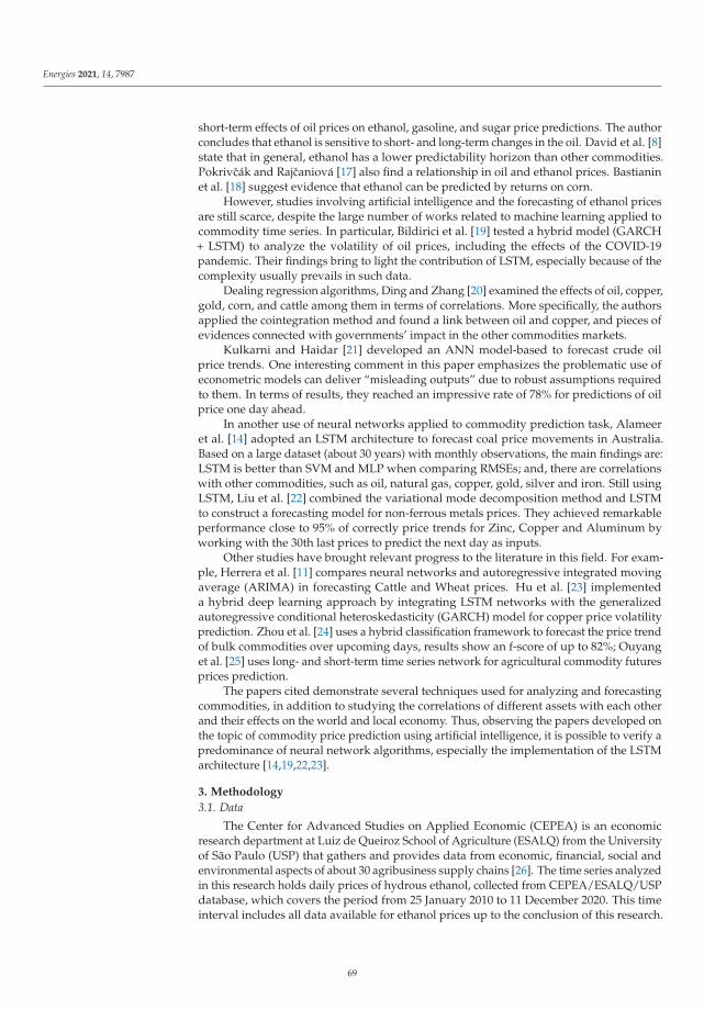
Energies 2021, 14, 7987

short-term effects of oil prices on ethanol, gasoline, and sugar price predictions. The authorconcludes that ethanol is sensitive to short- and long-term changes in the oil. David et al. [8]state that in general, ethanol has a lower predictability horizon than other commodities.Pokrivcák and Rajcaniová [17] also find a relationship in oil and ethanol prices. Bastianinet al. [18] suggest evidence that ethanol can be predicted by returns on corn.

However, studies involving artificial intelligence and the forecasting of ethanol pricesare still scarce, despite the large number of works related to machine learning applied tocommodity time series. In particular, Bildirici et al. [19] tested a hybrid model (GARCH+ LSTM) to analyze the volatility of oil prices, including the effects of the COVID-19pandemic. Their findings bring to light the contribution of LSTM, especially because of thecomplexity usually prevails in such data.

Dealing regression algorithms, Ding and Zhang [20] examined the effects of oil, copper,gold, corn, and cattle among them in terms of correlations. More specifically, the authorsapplied the cointegration method and found a link between oil and copper, and pieces ofevidences connected with governments’ impact in the other commodities markets.

Kulkarni and Haidar [21] developed an ANN model-based to forecast crude oilprice trends. One interesting comment in this paper emphasizes the problematic use ofeconometric models can deliver “misleading outputs” due to robust assumptions requiredto them. In terms of results, they reached an impressive rate of 78% for predictions of oilprice one day ahead.

In another use of neural networks applied to commodity prediction task, Alameeret al. [14] adopted an LSTM architecture to forecast coal price movements in Australia.Based on a large dataset (about 30 years) with monthly observations, the main findings are:LSTM is better than SVM and MLP when comparing RMSEs; and, there are correlationswith other commodities, such as oil, natural gas, copper, gold, silver and iron. Still usingLSTM, Liu et al. [22] combined the variational mode decomposition method and LSTMto construct a forecasting model for non-ferrous metals prices. They achieved remarkableperformance close to 95% of correctly price trends for Zinc, Copper and Aluminum byworking with the 30th last prices to predict the next day as inputs.

Other studies have brought relevant progress to the literature in this field. For exam-ple, Herrera et al. [11] compares neural networks and autoregressive integrated movingaverage (ARIMA) in forecasting Cattle and Wheat prices. Hu et al. [23] implementeda hybrid deep learning approach by integrating LSTM networks with the generalizedautoregressive conditional heteroskedasticity (GARCH) model for copper price volatilityprediction. Zhou et al. [24] uses a hybrid classification framework to forecast the price trendof bulk commodities over upcoming days, results show an f-score of up to 82%; Ouyanget al. [25] uses long- and short-term time series network for agricultural commodity futuresprices prediction.

The papers cited demonstrate several techniques used for analyzing and forecastingcommodities, in addition to studying the correlations of different assets with each otherand their effects on the world and local economy. Thus, observing the papers developed onthe topic of commodity price prediction using artificial intelligence, it is possible to verify apredominance of neural network algorithms, especially the implementation of the LSTMarchitecture [14,19,22,23].

3. Methodology

3.1. Data

The Center for Advanced Studies on Applied Economic (CEPEA) is an economicresearch department at Luiz de Queiroz School of Agriculture (ESALQ) from the Universityof São Paulo (USP) that gathers and provides data from economic, financial, social andenvironmental aspects of about 30 agribusiness supply chains [26]. The time series analyzedin this research holds daily prices of hydrous ethanol, collected from CEPEA/ESALQ/USPdatabase, which covers the period from 25 January 2010 to 11 December 2020. This timeinterval includes all data available for ethanol prices up to the conclusion of this research.

69

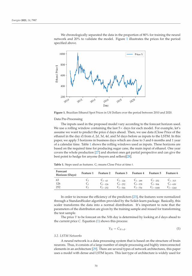
Energies 2021, 14, 7987

We chronologically separated the data in the proportion of 80% for training the neuralnetwork and 20% to validate the model. Figure 1 illustrates the prices for the periodspecified above.

Figure 1. Brazilian Ethanol Spot Prices in U$ Dollars over the period between 2010 and 2020.

Data Pre-Processing

The inputs used in the proposed model vary according to the forecast horizon used.We use a rolling window containing the last 5× days for each model. For example, let’sassume we want to predict the price d days ahead. Then, we use data (Close Price of theethanol in the day d) from d, 2d, 3d, 4d, and 5d days before as inputs to the LSTM. In thispaper, we apply 3 horizons in business days which are close to 3 and 6 months and 1 yearof a calendar time. Table 1 shows the rolling windows used as inputs. These horizons arebased on the required time for producing sugar cane, the main input of ethanol. One yearcovers the whole production [27] and shortest ones get partial perspective and can give thebest point to hedge for anyone (buyers and sellers)[28].

Table 1. Steps used as features. Ct means Close Price at time t.

ForecastHorizon (Days)

Feature 1 Feature 2 Feature 3 Feature 4 Feature 5 Feature 6

63 Ct Ct−63 Ct−126 Ct−189 Ct−252 Ct−315126 Ct Ct−126 Ct−252 Ct−378 Ct−504 Ct−630252 Ct Ct−252 Ct−504 Ct−756 Ct−1008 Ct−1260

In order to increase the efficiency of the predictors [23], the features were normalizedthrough a StandardScaler algorithm provided by the Scikit-learn package. Basically, thisscaler transforms the data into a normal distribution. It’s important to note that theparameters of the distribution are given by the training sample and reused for transformingthe test sample.

The price Y to be forecast on the Nth day is determined by looking at d days ahead tothe current price C. Equation (1) shows this process:

YN = CN+d. (1)

3.2. LSTM Networks

A neural network is a data processing system that is based on the structure of brainneurons. Thus, it consists of a large number of simple processing and highly interconnectedelements in an architecture [29]. There are several types of network architectures, this paperuses a model with dense and LSTM layers. This last type of architecture is widely used for

70

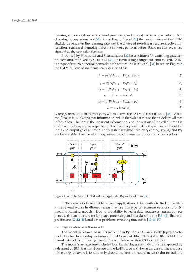
Energies 2021, 14, 7987

learning sequences (time series, word processing and others) and is very sensitive whenchoosing hyperparameters [30]. According to Breuel [31] the performance of the LSTMslightly depends on the learning rate and the choice of non-linear recurrent activationfunctions (tanh and sigmoid) make the network perform better. Based on that, we chosesigmoid as the activation function.

Proposed by Hochreiter and Schmidhuber [32] as a solution for vanishing gradientproblem and improved by Gers et al. [33] by introducing a forget gate into the cell, LSTMis a type of recurrent neural networks architecture. As in Yu et al. [34] based on Figure 2,the LSTM cell can be mathematically described as:

ft = σ(Wf ht−1 + Wf xt + b f ) (2)

it = σ(Wiht−1 + Wixt + bi) (3)

ct = σ(Wcht−1 + Wcxt + bc) (4)

ct = ft . ct−1 + it . ct (5)

ot = σ(Woht−1 + Woxt + bo) (6)

ht = ot . tanh(ct) (7)

where ft represents the forget gate, which allows the LSTM to reset its state [35]. Whenthe ft value is 1, it keeps that information, while the value 0 means that it deletes all thatinformation. The input, the recurrent information, and the output of the cell at time t isportrayed by xt, ht and yt respectively. The biases represented by b, it and ot represent theinput and output gates at time t. The cell state is symbolized by ct and Wi, Wc, Wo and Wfare the weights. The operator ‘·’ expresses the pointwise multiplication of two vectors.

Figure 2. Architecture of LSTM with a forget gate. Reproduced from [34].

LSTM networks have a wide range of applications. It is possible to find in the liter-ature several works in different areas that use this type of recurrent network to buildmachine learning models. Due to the ability to learn data sequences, numerous pa-pers use this architecture for language processing and text classification [36–41], financialpredictions [23,42–45], and other problems involving time series [19,46–50].

3.3. Proposed Model and Benchmarks

The model implemented in this work run in Python 3.8.6 (64-bit) with Jupyter Note-book. The hardware setup includes an Intel Core i5-4310u CPU 2.0GHz, 8GB RAM. Theneural network is built using Tensorflow with Keras version 2.3.1 as interface.

The model’s architecture includes four hidden layers with 64 units interspersed bya dropout of 20%, the first three are of the LSTM type and the last is dense. The purposeof the dropout layers is to randomly drop units from the neural network during training

71

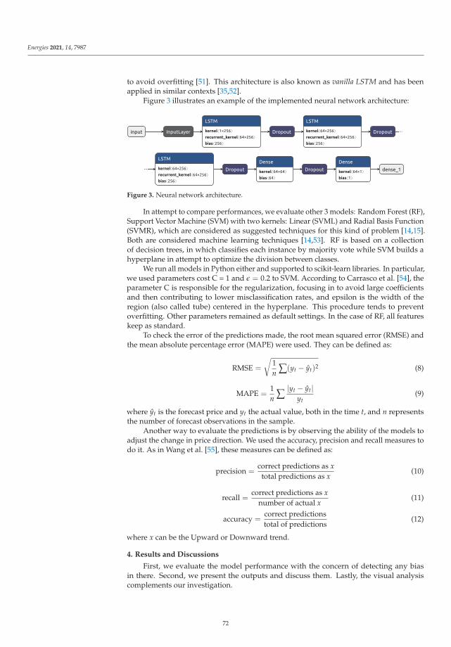
Energies 2021, 14, 7987

to avoid overfitting [51]. This architecture is also known as vanilla LSTM and has beenapplied in similar contexts [35,52].

Figure 3 illustrates an example of the implemented neural network architecture:

Figure 3. Neural network architecture.

In attempt to compare performances, we evaluate other 3 models: Random Forest (RF),Support Vector Machine (SVM) with two kernels: Linear (SVML) and Radial Basis Function(SVMR), which are considered as suggested techniques for this kind of problem [14,15].Both are considered machine learning techniques [14,53]. RF is based on a collectionof decision trees, in which classifies each instance by majority vote while SVM builds ahyperplane in attempt to optimize the division between classes.

We run all models in Python either and supported to scikit-learn libraries. In particular,we used parameters cost C = 1 and ε = 0.2 to SVM. According to Carrasco et al. [54], theparameter C is responsible for the regularization, focusing in to avoid large coefficientsand then contributing to lower misclassification rates, and epsilon is the width of theregion (also called tube) centered in the hyperplane. This procedure tends to preventoverfitting. Other parameters remained as default settings. In the case of RF, all featureskeep as standard.

To check the error of the predictions made, the root mean squared error (RMSE) andthe mean absolute percentage error (MAPE) were used. They can be defined as:

RMSE =

√1n ∑(yt − yt)2 (8)

MAPE =1n ∑

|yt − yt|yt

(9)

where yt is the forecast price and yt the actual value, both in the time t, and n representsthe number of forecast observations in the sample.

Another way to evaluate the predictions is by observing the ability of the models toadjust the change in price direction. We used the accuracy, precision and recall measures todo it. As in Wang et al. [55], these measures can be defined as:

precision =correct predictions as x

total predictions as x(10)

recall =correct predictions as x

number of actual x(11)

accuracy =correct predictionstotal of predictions

(12)

where x can be the Upward or Downward trend.

4. Results and Discussions

First, we evaluate the model performance with the concern of detecting any biasin there. Second, we present the outputs and discuss them. Lastly, the visual analysiscomplements our investigation.

72

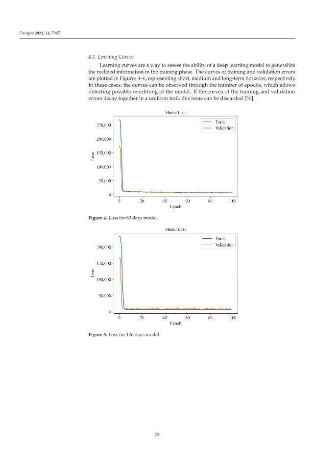
Energies 2021, 14, 7987

4.1. Learning Curves

Learning curves are a way to assess the ability of a deep learning model to generalizethe realized information in the training phase. The curves of training and validation errorsare plotted in Figures 4–6, representing short, medium and long-term horizons, respectively.In these cases, the curves can be observed through the number of epochs, which allowsdetecting possible overfitting of the model. If the curves of the training and validationerrors decay together in a uniform trail, this issue can be discarded [56].

Figure 4. Loss for 63 days model.


73

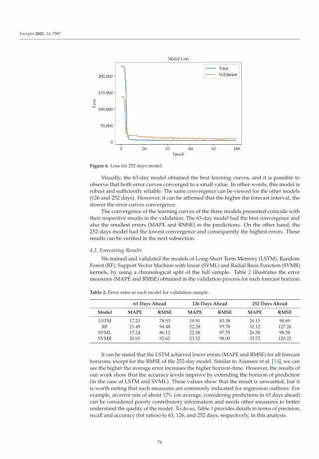
Energies 2021, 14, 7987


Visually, the 63-day model obtained the best learning curves, and it is possible toobserve that both error curves converged to a small value. In other words, this model isrobust and sufficiently reliable. The same convergence can be viewed for the other models(126 and 252 days). However, it can be affirmed that the higher the forecast interval, theslower the error curves convergence.

The convergence of the learning curves of the three models presented coincide withtheir respective results in the validation: The 63-day model had the best convergence andalso the smallest errors (MAPE and RMSE) in the predictions. On the other hand, the252-days model had the lowest convergence and consequently the highest errors. Theseresults can be verified in the next subsection.

4.2. Forecasting Results

We trained and validated the models of Long-Short Term Memory (LSTM), RandomForest (RF), Support Vector Machine with linear (SVML) and Radial Basis Function (SVMR)kernels, by using a chronological split of the full sample. Table 2 illustrates the errormeasures (MAPE and RMSE) obtained in the validation process for each forecast horizon.

Table 2. Error rates in each model for validation sample.

63 Days Ahead 126 Days Ahead 252 Days Ahead

Model MAPE RMSE MAPE RMSE MAPE RMSE

LSTM 17.23 78.53 19.91 83.38 26.15 98.69RF 21.49 94.48 22.28 95.78 32.12 127.26

SVML 17.24 86.12 22.58 97.55 26.58 98.58SVMR 20.65 92.62 23.32 98.00 33.72 120.22

It can be stated that the LSTM achieved lower errors (MAPE and RMSE) for all forecasthorizons, except for the RMSE of the 252-day model. Similar to Alameer et al. [14], we cansee the higher the average error increases the higher horizon-time. However, the results ofour work show that the accuracy levels improve by extending the horizon of prediction(in the case of LSTM and SVML). These values show that the result is unwanted, but itis worth noting that such measures are commonly indicated for regression outlines. Forexample, an error rate of about 17% (on average, considering predictions in 63 days ahead)can be considered poorly contributory information and needs other measures to betterunderstand the quality of the model. To do so, Table 3 provides details in terms of precision,recall and accuracy (hit ratios) to 63, 126, and 252 days, respectively, in this analysis.

74

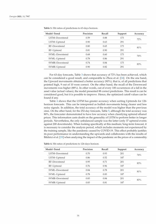
Energies 2021, 14, 7987

Table 3. Hit ratios of predictions to 63-days horizon.

Model–Trend Precision Recall Support Accuracy

LSTM–Downtrend 0.59 0.88 173 72%LSTM–Uptrend 0.90 0.63 291

RF–Downtrend 0.80 0.65 173 81%RF–Uptrend 0.81 0.90 291

SVML–Downtrend 0.68 0.60 173 74%SVML–Uptrend 0.78 0.86 291

SVMR–Downtrend 0.74 0.84 173 83%SVMR–Uptrend 0.90 0.82 291

For 63-day forecasts, Table 3 shows that accuracy of 72% has been achieved, whichcan be considered a good result, and comparable to Zhou et al. [24]. On the one hand,the Upward movements obtained a better accuracy (90%), that is, of all predictions thatpointed high, 9 out of 10 were correct. On the other hand, the recall of the Downwardmovements was higher (88%). In other words, out of every 100 occurrences of a fall in theasset value (actual values), the model presented 88 correct predictions. This result is can beconsidered good, but it is possible to improve. Hence, the optimized cutoff values can befound if any.

Table 4 shows that the LSTM has greater accuracy when sorting Uptrends for 126-horizon forecasts. This can be interpreted as bullish movements being clearer and lessnoisy signals. In addition, the total accuracy of the model was higher than the previousones. On the other hand, for the 252-day forecasts, Table 5, although the total accuracy was80%, the forecaster demonstrated to have low accuracy when classifying uptrend ethanolprices. This information casts doubt on the generality of LSTM to perform better in longerperiods. Nevertheless, the only unbalanced sample was the latter (only 37 uptrend eventsagainst 200 downtrends). When looking specifically at this medium/long-term forecast, itis necessary to consider the analysis period, which includes moments not experienced bythe training sample, like the pandemic caused by COVID-19. This effect probably justifiesits poor performance in understanding the upwards and collaborates with the results ofBildirici et al. [19] when analyzing the impact of the pandemic on the prices of a commodity.







75

Energies 2021, 14, 7987







In general, these results show to be different from the work of Kulkarni and Haidar [21],in which the accuracy of the forecasts decays with the enlargement of the forecast horizon.However, it is important to highlight that in the cited article the forecast periods are only 1,2 and 3 days. On the contrary, Bouri et al. [16] remind that the volatility (risk) perceived inperiods is lower, which has greater meaning and more corresponding to this study.

Comparing LSTM outlines with benchmarks, its error rates are better, except for RMSEin the longer horizon (SVML is slightly better). Based on that, we can consider LSTM as thebest predictor on a relative and regression basis. If we focus the analysis in the classificationreport, the findings are essentially unlike. LSTM presented just one single better indicator(recall in 63-day predictions, only bearing trends). Surprisingly, SVM achieved interestingperformance in all horizons. For 63-day predictions, SVMR was the most accurate with thehigher precision for uptrends. Curiously, the accuracy persisted to the mid-term horizonbut decrease in the long-term while SVML was the best and reported two higher ratios(precision for uptrends and recall for downtrends). The RF precision and recall deserve tobe emphasized. Except in the 252-day horizon, RF presented competitive ratios and moreaccurate than LSTM.

4.3. Visualising the Predictions

In the work of Bildirici et al. [19], it is possible to verify the impact of the COVID-19 pandemic on oil prices, in which the values suffered a great fall, affecting the entireinternational market. We can say the same for ethanol, as the big drop in prices alsooccurred. In addition, the author’s analysis that prices will return to their highest values—potentially causing inflation—may also be valid for ethanol.

Another important point is the impact of the pandemic on forecast errors. As it is anadverse and unpredictable event, the error rates (MAPE and RMSE) were greater in thisperiod compared to moments prior to the COVID-19 crisis.

Figures 7–9 illustrate the predictions of the algorithms versus the price verified in theanalyzed period.

76

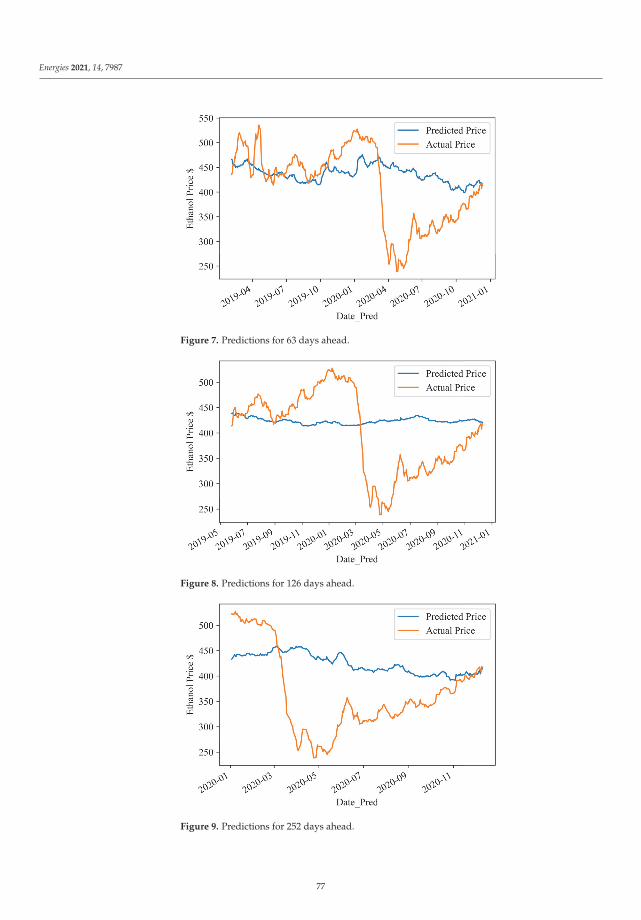
Energies 2021, 14, 7987

Figure 7. Predictions for 63 days ahead.



77

Energies 2021, 14, 7987

Furthermore, we can see that 63-days forecasts are relatively close to the actual pricebefore the most intense period of the pandemic (more specifically between March andSeptember of 2020) and, after that, recover similar performance. Thus, regarding regressionoutlines, there are evidences that incremental volatility could negatively interfere in thepredictions. Besides, it is hard to conclude for the price directions, as we found accuracyhigher than 80% for all the best predictors. The precision achieves values over 70%, exceptfor uptrend in 252-days, in which the test set is heavily unbalanced (only 37 upwardsagainst 200 downwards. Since the interval of time for predicting is relatively short (lessthan a year), these findings would be useful and sufficiently interesting for people whoneed or want to trade ethanol, whatever is the interest: hedge or speculation positions.

5. Conclusions

This paper presents a Brazilian spot ethanol price prediction model using artificialneural networks with the LSTM architecture and compared it to SVM and RF forecasts.The algorithms provide outlines for periods of 63, 126 and 252 business days. The resultsevaluated in this work show that it was possible to predict prices with a reasonable degreeof accuracy in market directions for all horizons used.

Tests to verify overfitting were performed using learning curves, and the modelsconverged in a satisfactory way, demonstrating a good fit of the neural network. Benchmarkresults show that LSTM produced the smallest regression errors (MAPE and RMSE).However, regarding the correctness of the direction in the predictions, other algorithmshad better accuracy for specific horizons.

SVML proved to be the best algorithm for detecting trends achieving good results forall forecast windows used. Still, LSTM also managed to achieve satisfactory results for allforecasts, unlike RF and SVMR which had poor results for the 252-day horizon.

It was possible to observe in the LSTM outcomes an increase in the accuracy ofthe algorithms in longer forecast horizons, 72%, 74%, and 80% for 63, 126, and 252-dayhorizons, respectively. However, the mean absolute percentage error (MAPE) of theforecasts increased: 17.2%, 19.9% and 26.1% for 3, 6 and 12 months respectively. The samewas found in the RMSE outputs. Furthermore, it is important to note that the COVID-19pandemic caused an unexpected drop in prices, increasing model errors.

The high degree of correctness of models in the direction of prices can be useful inthe development of new hedging strategies for market agents. In addition, it can helpproducers and cooperatives to protect their capital through planning that takes into accountthese forecasts.

This work contributes by demonstrating that LSTM networks are able to performefficiently when predicting ethanol prices, a biofuel widely used in Brazil and worldwide,which has the capacity to replace fossil energy sources.

Nevertheless, this paper has limitations: (i) despite of the satisfactory results, we builtmodels based on pure techniques, (ii) our research takes into account one single commoditywith prices traded in one country but these data can be exclusively found in Brazil (Top 3producer in the world) and there is no global market with standardized price for ethanol,(iii) potential effects (e.g., macroeconomic indicators) are not considered. However, theproposed (and best) model requires only historical values, and (iv) comparison withprevious results was impracticable since data, performance measures and horizons did notexist in the literature, what shows the pioneering of this study.

For future work, we can add hybrid models that mix different network architecturesand machine learning algorithms, such as Empirical Mode Decomposition. Thus, newfeatures can be implemented, such as endogenous variables (technical indicators) andexogenous variables (exchange rate, inflation and prices of other commodities).

78

Energies 2021, 14, 7987

Author Contributions: Conceptualization, G.C.S., F.B. and A.C.P.V.; methodology, G.C.S. and F.B.;software, G.C.S. and M.F.S.; validation, F.B. and A.C.P.V.; formal analysis, A.C.P.V.; investigation,G.C.S.; resources, A.C.P.V.; data curation, M.F.S.; writing—original draft preparation, G.C.S.; writing—review and editing, F.B. and A.C.P.V.; visualization, G.C.S. and M.F.S.; supervision, A.C.P.V.; projectadministration, F.B.; funding acquisition, G.C.S. and F.B. All authors have read and agreed to thepublished version of the manuscript.

Funding: This research was funded by Sapiens Agro, National Council for Scientific and Techno-logical Development (CNPq, grant number 438314/2018-2), Postgraduate Program in ElectricalEngineering of the Elec. Eng. School (PPGEELT–FEELT–UFU) and Postgraduate and Research Boardof the Federal University of Uberlândia (PROPP–UFU, process number 23117.079268/2021-03).



Data Availability Statement: Publicly available datasets were analyzed in this study. This data can befound here: https://www.cepea.esalq.usp.br/en/indicator/ethanol.aspx (accessed on 11 November2021). The predictions generated by the LSTM models can be accessed in the following repository:https://github.com/gustavocavsantos/Ethanol-Price-Predictions (accessed on 11 November 2021).


References

1. Goldemberg, J. The ethanol program in Brazil. Environ. Res. Lett. 2006, 1, 014008. [CrossRef]2. Silva, G.P.D.; Araújo, E.F.D.; Silva, D.O.; Guimarães, W.V. Ethanolic fermentation of sucrose, sugarcane juice and molasses by

Escherichia coli strain KO11 and Klebsiella oxytoca strain P2. Braz. J. Microbiol. 2005, 36, 395–404. [CrossRef]3. Lopes, M.L.; de Lima Paulillo, S.C.; Godoy, A.; Cherubin, R.A.; Lorenzi, M.S.; Giometti, F.H.C.; Bernardino, C.D.; de Amorim

Neto, H.B.; de Amorim, H.V. Ethanol production in Brazil: A bridge between science and industry. Braz. J. Microbiol. 2016,47, 64–76. [CrossRef] [PubMed]

4. Ministry of Agriculture, Fisheries and Supply—Ethanol Archives. Available online: https://www.gov.br/agricultura/pt-br/assuntos/sustentabilidade/agroenergia/arquivos-etanol-comercio-exterior-brasileiro/ (accessed on 11 November 2021).

5. Carpio, L.G.T. The effects of oil price volatility on ethanol, gasoline, and sugar price forecasts. Energy 2019, 181, 1012–1022.[CrossRef]

6. EIA—Today in Energy. Available online: https://www.eia.gov/todayinenergy/detail.php?id=47956 (accessed on 11 October2021).

7. Hira, A.; de Oliveira, L.G. No substitute for oil? How Brazil developed its ethanol industry. Energy Policy 2009, 37, 2450–2456.[CrossRef]

8. David, S.A.; Inácio, C.; Tenreiro Machado, J.A. Quantifying the predictability and efficiency of the cointegrated ethanol andagricultural commodities price series. Appl. Sci. 2019, 9, 5303. [CrossRef]

9. David, S.; Quintino, D.; Inacio, C.; Machado, J. Fractional dynamic behavior in ethanol prices series. J. Comput. Appl. Math. 2018,339, 85–93. [CrossRef]

10. Tapia Carpio, L.G.; Simone de Souza, F. Competition between second-generation ethanol and bioelectricity using the residualbiomass of sugarcane: Effects of uncertainty on the production mix. Molecules 2019, 24, 369. [CrossRef] [PubMed]

11. Herrera, G.P.; Constantino, M.; Tabak, B.M.; Pistori, H.; Su, J.J.; Naranpanawa, A. Long-term forecast of energy commoditiesprice using machine learning. Energy 2019, 179, 214–221. [CrossRef]

12. de Araujo, F.H.A.; Bejan, L.; Rosso, O.A.; Stosic, T. Permutation entropy and statistical complexity analysis of Brazilian agriculturalcommodities. Entropy 2019, 21, 1220. [CrossRef]

13. Barboza, F.; Kimura, H.; Altman, E. Machine learning models and bankruptcy prediction. Expert Syst. Appl. 2017, 83, 405–417.[CrossRef]

14. Alameer, Z.; Fathalla, A.; Li, K.; Ye, H.; Jianhua, Z. Multistep-ahead forecasting of coal prices using a hybrid deep learning model.Resour. Policy 2020, 65, 101588. [CrossRef]

15. Sun, W.; Zhang, J. Carbon Price Prediction Based on Ensemble Empirical Mode Decomposition and Extreme Learning MachineOptimized by Improved Bat Algorithm Considering Energy Price Factors. Energies 2020, 13, 3471. [CrossRef]

16. Bouri, E.; Dutta, A.; Saeed, T. Forecasting ethanol price volatility under structural breaks. Biofuels Bioprod. Biorefining 2021,15, 250–256. [CrossRef]

17. Pokrivcák, J.; Rajcaniová, M. Crude oil price variability and its impact on ethanol prices. Agric. Econ. 2011, 57, 394–403. [CrossRef]18. Bastianin, A.; Galeotti, M.; Manera, M. Ethanol and field crops: Is there a price connection? Food Policy 2016, 63, 53 – 61.

[CrossRef]19. Bildirici, M.; Guler Bayazit, N.; Ucan, Y. Analyzing Crude Oil Prices under the Impact of COVID-19 by Using LSTARGARCHLSTM.

Energies 2020, 13, 2980. [CrossRef]

79

Energies 2021, 14, 7987

20. Ding, S.; Zhang, Y. Cross market predictions for commodity prices. Econ. Model. 2020, 91, 455–462. [CrossRef]21. Kulkarni, S.; Haidar, I. Forecasting model for crude oil price using artificial neural networks and commodity futures prices. arXiv

2009, arXiv:0906.4838.22. Liu, Y.; Yang, C.; Huang, K.; Gui, W. Non-ferrous metals price forecasting based on variational mode decomposition and LSTM

network. Knowl.-Based Syst. 2020, 188, 105006. [CrossRef]23. Hu, Y.; Ni, J.; Wen, L. A hybrid deep learning approach by integrating LSTM-ANN networks with GARCH model for copper

price volatility prediction. Phys. A Stat. Mech. Its Appl. 2020, 557, 124907. [CrossRef]24. Zhou, B.; Zhao, S.; Chen, L.; Li, S.; Wu, Z.; Pan, G. Forecasting Price Trend of Bulk Commodities Leveraging Cross-Domain Open

Data Fusion. ACM Trans. Intell. Syst. Technol. 2020, 11, 1–26. [CrossRef]25. Ouyang, H.; Wei, X.; Wu, Q. Agricultural commodity futures prices prediction via long- and short-term time series network. J.

Appl. Econ. 2019, 22, 468–483. [CrossRef]26. CEPEA—Center for Advanced Studies on Applied Economics. Available online: https://www.cepea.esalq.usp.br/en/cepea-1.

aspx (accessed on 13 January 2021).27. Ariyawansha, T.; Abeyrathna, D.; Kulasekara, B.; Pottawela, D.; Kodithuwakku, D.; Ariyawansha, S.; Sewwandi, N.; Bandara, W.;

Ahamed, T.; Noguchi, R. A novel approach to minimize energy requirements and maximize biomass utilization of the sugarcaneharvesting system in Sri Lanka. Energies 2020, 13, 1497. [CrossRef]

28. Franken, J.R.; Parcell, J.L. Cash Ethanol Cross-Hedging Opportunities. J. Agric. Appl. Econ. 2003, 35, 510–516. [CrossRef]29. Uhrig, R.E. Introduction to artificial neural networks. In Proceedings of IECON’95-21st Annual Conference on IEEE Industrial

Electronics, Orlando, FL, USA, 6–10 November 1995; Volume 1, pp. 33–37.30. Nakisa, B.; Rastgoo, M.N.; Rakotonirainy, A.; Maire, F.; Chandran, V. Long Short Term Memory Hyperparameter Optimization

for a Neural Network Based Emotion Recognition Framework. IEEE Access 2018, 6, 49325–49338. [CrossRef]31. Breuel, T.M. Benchmarking of LSTM Networks. arXiv 2015, arXiv:1508.02774.32. Hochreiter, S.; Schmidhuber, J. Long Short-Term Memory. Neural Comput. 1997, 9, 1735–1780. [CrossRef]33. Gers, F.A.; Schmidhuber, J.; Cummins, F. Learning to Forget: Continual Prediction with LSTM. Neural Comput. 2000, 12, 2451–2471.

[CrossRef]34. Yu, Y.; Si, X.; Hu, C.; Zhang, J. A Review of Recurrent Neural Networks: LSTM Cells and Network Architectures. Neural Comput.

2019, 31, 1235–1270. [CrossRef]35. Greff, K.; Srivastava, R.K.; Koutník, J.; Steunebrink, B.R.; Schmidhuber, J. LSTM: A Search Space Odyssey. IEEE Trans. Neural

Netw. Learn. Syst. 2017, 28, 2222–2232. [CrossRef] [PubMed]36. Graves, A.; Fernández, S.; Schmidhuber, J. Bidirectional LSTM Networks for Improved Phoneme Classification and Recognition.

In Artificial Neural Networks: Formal Models and Their Applications—ICANN 2005; Duch, W., Kacprzyk, J., Oja, E., Zadrozny, S., Eds.;Springer: Berlin/Heidelberg, Germany, 2005; pp. 799–804.

37. Habibi, M.; Weber, L.; Neves, M.; Wiegandt, D.L.; Leser, U. Deep learning with word embeddings improves biomedical namedentity recognition. Bioinformatics 2017, 33, i37–i48. [CrossRef] [PubMed]

38. Zhou, C.; Sun, C.; Liu, Z.; Lau, F. A C-LSTM neural network for text classification. arXiv 2015, arXiv:1511.08630.39. Zhou, P.; Qi, Z.; Zheng, S.; Xu, J.; Bao, H.; Xu, B. Text classification improved by integrating bidirectional LSTM with two-

dimensional max pooling. arXiv 2016, arXiv:1611.06639.40. Liu, G.; Guo, J. Bidirectional LSTM with attention mechanism and convolutional layer for text classification. Neurocomputing

2019, 337, 325–338. [CrossRef]41. Sachan, D.S.; Zaheer, M.; Salakhutdinov, R. Revisiting lstm networks for semi-supervised text classification via mixed objective

function. In Proceedings of the AAAI Conference on Artificial Intelligence, Honolulu, HI, USA, 27 January–1 February 2019;Volume 33, pp. 6940–6948.

42. Bao, W.; Yue, J.; Rao, Y. A deep learning framework for financial time series using stacked autoencoders and long-short termmemory. PLoS ONE 2017, 12, e0180944. [CrossRef]

43. Siami-Namini, S.; Tavakoli, N.; Namin, A.S. A comparison of ARIMA and LSTM in forecasting time series. In Proceedings of the2018 17th IEEE International Conference on Machine Learning and Applications (ICMLA), Orlando, FL, USA, 17–20 December2018; pp. 1394–1401.

44. Moghar, A.; Hamiche, M. Stock market prediction using LSTM recurrent neural network. Procedia Comput. Sci. 2020, 170, 1168–1173. [CrossRef]

45. Tong, G.; Yin, Z. Adaptive Trading System of Assets for International Cooperation in Agricultural Finance Based on NeuralNetwork. Comput. Econ. 2021, 1–20. [CrossRef]

46. Karim, F.; Majumdar, S.; Darabi, H.; Chen, S. LSTM Fully Convolutional Networks for Time Series Classification. IEEE Access2018, 6, 1662–1669. [CrossRef]

47. Mahasseni, B.; Lam, M.; Todorovic, S. Unsupervised video summarization with adversarial lstm networks. In Proceedings of theIEEE conference on Computer Vision and Pattern Recognition, Honolulu, HI, USA, 21–26 July 2017; pp. 202–211.

48. Sønderby, S.K.; Sønderby, C.K.; Nielsen, H.; Winther, O. Convolutional LSTM networks for subcellular localization of proteins. InInternational Conference on Algorithms for Computational Biology; Springer: Cham, Switzerland, 2015; pp. 68–80.

80

Energies 2021, 14, 7987

49. Trinh, H.D.; Giupponi, L.; Dini, P. Mobile traffic prediction from raw data using LSTM networks. In Proceedings of the 2018 IEEE29th Annual International Symposium on Personal, Indoor and Mobile Radio Communications (PIMRC), Bologna, Italy, 9–12September 2018; pp. 1827–1832.

50. Ycart, A.; Benetos, E. A Study on LSTM Networks for Polyphonic Music Sequence Modelling. In Proceedings of the InternationalSociety for Music Information Retrieval Conference (ISMIR), Suzhou, China, 23–28 October 2017.

51. Srivastava, N.; Hinton, G.; Krizhevsky, A.; Sutskever, I.; Salakhutdinov, R. Dropout: A simple way to prevent neural networksfrom overfitting. J. Mach. Learn. Res. 2014, 15, 1929–1958.

52. Gers, F.A.; Schmidhuber, E. LSTM recurrent networks learn simple context-free and context-sensitive languages. IEEE Trans.Neural Netw. 2001, 12, 1333–1340. [CrossRef]

53. Herrera, G.P.; Constantino, M.; Tabak, B.M.; Pistori, H.; Su, J.J.; Naranpanawa, A. Data on forecasting energy prices using machinelearning. Data Brief 2019, 25, 104122. [CrossRef] [PubMed]

54. Carrasco, M.; López, J.; Maldonado, S. Epsilon-nonparallel support vector regression. Appl. Intell. 2019, 49, 4223–4236. [CrossRef]55. Wang, X.; Zhou, T.; Wang, X.; Fang, Y. Harshness-aware sentiment mining framework for product review. Expert Syst. Appl. 2022,

187, 115887. [CrossRef]56. Zhang, P.; Yin, Z.Y.; Zheng, Y.; Gao, F.P. A LSTM surrogate modelling approach for caisson foundations. Ocean Eng. 2020,

204, 107263. [CrossRef]

81

energies

Article

Energy Management Model for HVAC Control Supported byReinforcement Learning

Pedro Macieira, Luis Gomes and Zita Vale *

Citation: Macieira, P.; Gomes, L.;

Vale, Z. Energy Management Model

for HVAC Control Supported by

Reinforcement Learning. Energies

2021, 14, 8210. https://doi.org/

10.3390/en14248210

Academic Editors: Ana-Belén

Gil-González and Fabrizio Ascione

Received: 26 October 2021

Accepted: 3 December 2021

Published: 7 December 2021




iations.








4.0/).

GECAD—Research Group on Intelligent Engineering and Computing for Advanced Innovation andDevelopment, Polytechnic of Porto (P.PORTO), P-4200-072 Porto, Portugal; [email protected] (P.M.);[email protected] (L.G.)* Correspondence: [email protected]

Abstract: Heating, ventilating, and air conditioning (HVAC) units account for a significant con-sumption share in buildings, namely office buildings. Therefore, this paper addresses the possibilityof having an intelligent and more cost-effective solution for the management of HVAC units inoffice buildings. The method applied in this paper divides the addressed problem into three steps:(i) the continuous acquisition of data provided by an open-source building energy managementsystems, (ii) the proposed learning and predictive model able to predict if users will be working in agiven location, and (iii) the proposed decision model to manage the HVAC units according to theprediction of users, current environmental context, and current energy prices. The results show thatthe proposed predictive model was able to achieve a 93.8% accuracy and that the proposed decisiontree enabled the maintenance of users’ comfort. The results demonstrate that the proposed solutionis able to run in real-time in a real office building, making it a possible solution for smart buildings.

Keywords: building energy management systems; HVAC control; Internet of Things; occupancyprediction; reinforcement learning

1. Introduction

Smart grids enable the active participation of end-users and allow them to activelymanage their demand using demand-side management [1,2]. By managing home availableenergy resources and loads, the end-users are able to reduce energy costs [3], maximize theuse of renewable generation [4], participate in the smart grid [5], and transact energy withother end-users [6].

The ability to manage their own resources enables end-users to take control over theirfacilities and promote the dissemination of smart buildings [7]. Actions for demand-sidemanagement and for the active participation of end-users can also be achieved usinginternet of things (IoT) devices [8]. The possibilities of energy management are vast andthey represent a good opportunity for end-users to enable the reduction of energy costsand optimization of energy usage [9].

One of the biggest contributions to the energy consumption in buildings comes fromheating ventilating air conditioning (HVAC) systems [10]. Therefore, the control of HVACsystems is frequently found in the literature as a way to reduce energy costs and greenhousegas emissions [11,12]. The control of HVAC can also be used for the active participationof end-users in smart grids [13]. Because of their characteristic preconditioning time, i.e.,the preheating or cooling time of HVAC, the existing models for HVAC control usuallyresults in planned action ahead in time, demanding the use of prediction models to forecastcontexts. The use of prediction models, in smart grids, is common, in particular, to forecastthe consumption of end-user and individual loads, the generation of renewable resources,and the flexibility of end-users [14].

The optimization of HVAC systems, as any other electrical load placed in the end-userfacility, needs to consider the users’ preferences and needs [15]. It is then necessary to


Energies 2021, 14, 8210

balance the users’ comfort and the energy cost reduction. This is where prioritizationtechniques come in, allowing energy consumption to be reduced and avoiding unnecessaryelectricity expenses [16].

This paper proposes a novel model for HVAC control using a prediction reinforcementlearning algorithm and a decision tree for the consideration of building context, energycosts, and preconditioning time. The prediction model is used to predict occupancy inthe building ahead in time. The occupancy prediction is then used in a decision tree tocontrol of the HVAC units, considering the energy prices and the current temperature ofthe building. The proposed solution can intelligently control the HVAC units and promotethe reduction of energy costs.

The proposed solution, comprised of the prediction model and the decision tree, wasdeployed in a real office building using a building energy management system (BEMS)that was implemented based on the open-source platform Home Assistant (https://www.home-assistant.io/, accessed on 6 December 2021). This BEMS enabled the integration ofmultiple IoT devices and the implementation of the proposed models in a real building,allowing a continuous operation. The proposed solution addresses some of the limitationsthat were identified in the literature review, such as continuous learning, the considerationof several contexts in the building, and the users’ comfort.

This paper is structured as follows. After this first introductory section, related worksregarding the management of HVAC systems, namely occupancy-based solutions, arepresented in Section 2. In Section 3, several solutions to develop a BEMS are presentedand the proposed BEMS, based on Home Assistant, is described. Section 4 presents theproposed methodology including the prediction model and the decision tree. The resultsof the case study, using a real building, are described in Section 5. Section 6 presents thediscussion of results, while the main conclusions are presented in Section 6.

2. Related Works

The occupancy of the building and/or of different building zones can be used byenergy management systems to promote the contextual optimization of resources [15].The information regarding occupancy allows systems to better understand the buildingcontext and provide better resource optimization [17]. The exact occupation of the buildingand the location of people is hard to achieve, but estimates can be obtained using severaltechniques, using equipment already installed in the building or that requires new equip-ment to be installed [18]. In [19], a machine learning classification model is proposed forweek-ahead occupancy prediction using real-time smart meter data. Applied to HVACsystems, [20] proposed a control model based on students’ location inside auditoriums.This model uses Wi-Fi data to determine the number of connected devices and enables anoninvasive approach that does not require the installation of new equipment. In [21], amodel for HVAC control inside buildings is proposed using a rule-based approach sup-ported by a deep learning algorithm that predicts the preconditioning time. These solutionsaddress the prediction and identification of occupancy in buildings. However, they lackthe ability to consider multiple contexts. The contextual reinforcement learning predictivemodel proposed in this paper addresses the dynamics of the building usage consideringseveral contexts.

A reinforcement learning model for occupant behavior is proposed in [22] using aQ-learning model to allow automated control of the building’s thermostat. This work com-pared the prediction of the reinforcement learning model with an artificial neural network(ANN) prediction model. The results showed that the ANN had better results. In [23] theuse of reinforcement learning models to directly control the HVAC units demonstrated anincrease in energy costs, even when dealing with on/off control. However, the best resultswere achieved when the model was used to control five flow levels.

Other contextual data, beyond occupancy, can be used to control HVAC systems [24].A model for HVAC control considering not only the building occupancy but also thecharacterization of the building, namely the mean radiant temperature of building rooms

84

Energies 2021, 14, 8210

is proposed in [25]. In [26], it is proposed the use of IoT devices to obtain contextualinformation regarding outdoor temperature to improve the efficiency of HVAC controland achieve lower payback times, when compared to occupancy-based models. However,these solutions lack the ability to learn from historical data, and more importantly, theability to be able to continuously learn. The proposed solution addresses this limitation byconceiving a reinforcement learning model.

The control and management of HVAC systems are usually used in the energy do-main as a way to reduce energy costs [27], due to the high energy consumption of HVACequipment. A day-ahead HVAC control model for industrial buildings, to decrease en-ergy costs considering on-peak and off-peak tariffs and weather conditions, is proposedin [28]. A multiperiod optimization model for supervisory control and data acquisition(SCADA) systems is proposed in [29] to minimize energy costs while complying with usersconstraints. In [30], HVAC systems are controlled using market-based transactive controlsin commercial buildings to promote grid balance and stability. Although energy costs arean important aspect of the building, the user comfort needs to be considered, as well asthe building’s context. The proposed solution addresses the users’ comfort consideringahead HVAC control signals to prepare the building for the users’ arrival while trying tominimize energy costs. The context of the building is considered in the proposed solution,for instance, the HVAC units’ control considers the status of the windows.

The control of HVAC units can also be done to improve air quality. In [31], a computervision-based system is used to get the occupancy of a room and a neural network is usedto classify the users’ activities. This solution enables the prediction of CO2 levels andcontrols the HVAC unit to prevent potentially dangerous situations. In [32], a solutionfor commercial buildings is proposed where a scalable model, based on multiagent deepreinforcement learning, is used to minimize energy costs while considering user comfortand air quality.

More complex solutions can also be implemented to enable the combined managementof multi-HVAC systems. In [33], a data-driven mathematical model using contextual sensordata is used to optimize multi-HVAC systems that serve the same space. In [34], severaloptimization models are compared for multi-HVAC systems management considering theoutdoor temperature, building ambient temperature, and occupancy. The compared modelswere a multiobjective genetic algorithm, two nondominated sorting genetic algorithms, anoptimized multiobjective particle swarm optimization, a speed-constrained multi-objectiveparticle swarm optimization, and a random search. The authors were not able to identify aunique best solution but presented the benefits of each model.

3. Building Energy Management System Based on Home Assistant

A BEMS can be installed in a variety of ways, normally this is done using dedicated,commercial platforms such as DEXMA Energy Intelligence (https://www.dexma.com/,accessed on 6 December 2021) or Entronix (https://entronix.io/, accessed on 6 December2021). However, for the purposes of this paper, a home automation system was used,enabling the combination of Internet of Things (IoT) devices with the ability to gather dataand affect the environment around them with rules created by the user to manage thesmart home.

There are a variety of home automation system software solutions, both open andclosed source. The biggest open-source solutions available are:

• openHAB (https://www.openhab.org/, accessed on 6 December 2021), created byKai Kreuzer, which is built using Java and was initially released in 2010;

• Home Assistant, created by Paulus Schoutsen, based on Python and configurable withthe use of YAML files, which was first released in 2013;

• Domoticz (https://www.domoticz.com/, accessed on 6 December 2021), created byGizmocuz, is written in C++ and configurable with Blockly or Lua, and with the firstrelease date at the end of 2012.

85

Energies 2021, 14, 8210

There are also a wide variety of commercial closed source solutions, with the biggestones being owned by large players:

• Google Assistant (https://assistant.google.com/, accessed on 6 December 2021),Google’s solution for home assistant software, allows the use of Google Assistantsoftware together with Google Home devices to control a house with voice com-mands and using a graphical user interface (GUI). It also enables the customization ofautomation rules;

• Alexa (https://www.amazon.com/b?ie=UTF8&node=21576558011, accessed on 6December 2021), Amazon’s solution for home automation, works similarly to GoogleAssistant, by using an Alexa device to allow the user to control their smart home withvoice commands and with GUI;

• HomeKit (https://www.apple.com/ios/home/, accessed on 6 December 2021), de-veloped by Apple, allows users to integrate their houses with the Apple Ecosystem,allowing the use of voice commands through Siri but also providing a GUI for morepowerful smart home management.

For the purposes of this paper, Home Assistant was chosen due to its many advantagessuch as being open-source, easily customizable with simple YAML files, and the powerfulbut still simple set-up GUI.

First, some IoT devices were installed and configured in a docker containerized HomeAssistant installation, with their uses described in Table 1. The IoT devices integrated canbe seen as actuators and sensors, depending on the type of actions they allow. Additionallyto market-available IoT devices, the Home Assistant configuration also integrates a SCADAsystem, developed by the researchers of the authors’ research center, that was alreadypresent in the building. This SCADA system is represented in Table 1 as GECAD API. ThisAPI enables the reading of other IoT devices that are already integrated into the SCADAsystem by using REST-based HTTP requests. The last device identified in Table 1 is asimulated sensor that was integrated into Home Assistant as a file sensor, enabling thereading of a file and the publishing of that information. The file sensor is a dataset of realelectricity prices that were obtained from MIBEL, the Iberian electricity wholesale market.

Table 1. Devices configured for the Home Assistant installation.

Device Name Monitoring Data Actions

RM Pro + Any IR or RF signal Emission of IR or RF signalSonoff Pow R2 Current (A), power (W), voltage (V), load status (on/off) Turn on/off

D-Link DSP-W115 Load status (on/off) Turn on/offD-Link DSP-W215 Power (W), total power consumption (kWh), temperature (◦C) Turn on/offSonoff RF Bridge N/A N/A

Sonoff Sensor DW1 Door/window open triggered/A

GECAD API (REST Sensors)Exterior temperature (◦C)

Interior temperature of individual rooms (◦C)Light switch states (%)

N/A

File Sensor (JSON Source) Electricity price on a specific month, time, day, and hour(EUR/kWh) N/A

To manage the energy of a building in an intelligent way using Home Assistant,complex logic needs to be integrated. However, Home Assistant has some constraints,namely the fact that it is configured by YAML files, which can turn simple scripts into alarge amount of complex virtual sensors that are tightly interconnected and have little useoutside of single automation. This difficult the setting-up of the installation and makes itvery hard to share the logic with other Home Assistant installations.

To solve this issue, Pyscript (https://github.com/custom-components/pyscript, ac-cessed on 6 December 2021), an add-on to Home Assistant, has been used for the workpresented in this paper. This add-on can import standard Python libraries and interactwith Home Assistant triggers and events when IoT devices or Home Assistant itself create

86

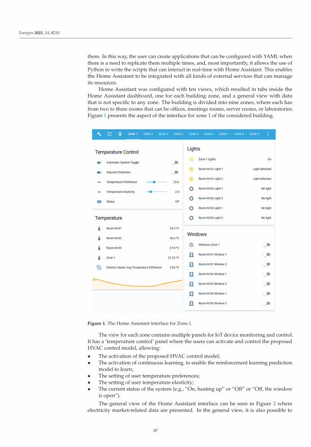
Energies 2021, 14, 8210

them. In this way, the user can create applications that can be configured with YAML whenthere is a need to replicate them multiple times, and, most importantly, it allows the use ofPython to write the scripts that can interact in real-time with Home Assistant. This enablesthe Home Assistant to be integrated with all kinds of external services that can manageits resources.

Home Assistant was configured with ten views, which resulted in tabs inside theHome Assistant dashboard, one for each building zone, and a general view with datathat is not specific to any zone. The building is divided into nine zones, where each hasfrom two to three rooms that can be offices, meetings rooms, server rooms, or laboratories.Figure 1 presents the aspect of the interface for zone 1 of the considered building.

Figure 1. The Home Assistant interface for Zone 1.

The view for each zone contains multiple panels for IoT device monitoring and control.It has a ‘temperature control’ panel where the users can activate and control the proposedHVAC control model, allowing:

• The activation of the proposed HVAC control model;• The activation of continuous learning, to enable the reinforcement learning prediction

model to learn;• The setting of user temperature preferences;• The setting of user temperature elasticity;• The current status of the system (e.g., “On, heating up” or “Off” or “Off, the window

is open”).

The general view of the Home Assistant interface can be seen in Figure 2 whereelectricity market-related data are presented. In the general view, it is also possible to

87

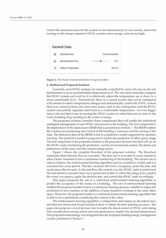
Energies 2021, 14, 8210

control the maximum price for the system to run autonomously, to save money, and avoidturning on the energy-expensive HVAC systems when energy costs are too high.

Figure 2. The Home Assistant interface for general data.

4. Method and Proposed Solution

Currently, most HVAC systems are manually controlled by users who are on-site andfind themselves at an uncomfortable temperature level. The user must manually configurethe HVAC system and wait for it to effectively adjust the temperature up or down to amore comfortable level. Alternatively, there is a central system that can be configuredwith sensors to detect temperature changes and automatically control the HVAC system.However, central systems also raise some issues, such as the waiting time until the HVACsystem successfully regulates itself back to a comfortable temperature. An even biggerissue is the fact that it may be turning the HVAC system on when there are no users in theroom/building, thus resulting in the waste of energy.

The proposed solution considers three components that will enable the individualintelligent management of each HVAC unit present in the building. The first component isthe deployment of the open-source BEMS that is presented in Section 3. The BEMS enablesthe continuous monitoring and control of the building’s resources and the storing of thedata. The historical data of the BEMS is fed to a predictive model supported by machinelearning. The predictive model is proposed to enable the prediction of office space usage.The last component of the proposed solution is the proposed decision tree that will act onthe HVAC units considering the prediction, current environmental context, the limits andpreferences of the users, and the current energy prices.

Figure 3 shows the complete flowchart of the proposed solution. The flowchartrepresents three threads that are executed. The first one is executed in every instant toallow Home Assistant to have continuous monitoring of the building. The second one isused to improve the reinforcement learning algorithm used as a predictive model, and it isexecuted once every period. This flow monitors the room’s occupancy, stores the data, andrecalculates the rewards. In the last flow, the control over the HVAC units is performed.The last thread is executed once every period and is able to collect the energy price, predictthe room’s occupancy, apply the decision tree, and control the HVAC units accordingly.

This paper proposes the use of a contextual reinforcement learning algorithm topredict the occupancy of the rooms of a building. The use of reinforcement learningenables the proposed model to have a continuous learning process, suitable to adjust theprediction to new routines or the addition of team members working in the same officespace. Moreover, the proposed model is a contextual reinforcement learning algorithm thatis able to have predictions considering the context of the office.

The reinforcement learning algorithm’s configuration and tuning are described and atest between linear and neural models is done to obtain the best learning accuracy. Thepaper also proposes a novel decision tree to enable the ahead control of HVAC units takinginto consideration energy prices and user preferences, namely the desired temperature.This proposed methodology was integrated into the proposed building energy managementsystem, presented in Section 3.

88

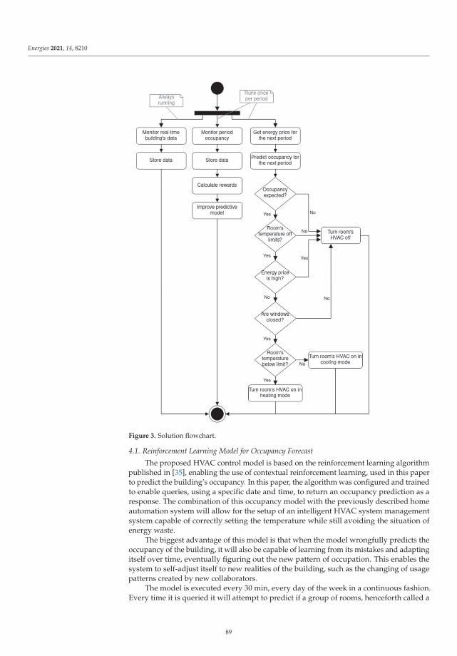
Energies 2021, 14, 8210

Figure 3. Solution flowchart.

4.1. Reinforcement Learning Model for Occupancy Forecast

The proposed HVAC control model is based on the reinforcement learning algorithmpublished in [35], enabling the use of contextual reinforcement learning, used in this paperto predict the building’s occupancy. In this paper, the algorithm was configured and trainedto enable queries, using a specific date and time, to return an occupancy prediction as aresponse. The combination of this occupancy model with the previously described homeautomation system will allow for the setup of an intelligent HVAC system managementsystem capable of correctly setting the temperature while still avoiding the situation ofenergy waste.

The biggest advantage of this model is that when the model wrongfully predicts theoccupancy of the building, it will also be capable of learning from its mistakes and adaptingitself over time, eventually figuring out the new pattern of occupation. This enables thesystem to self-adjust itself to new realities of the building, such as the changing of usagepatterns created by new collaborators.

The model is executed every 30 min, every day of the week in a continuous fashion.Every time it is queried it will attempt to predict if a group of rooms, henceforth called a

89

Energies 2021, 14, 8210

zone, will be occupied or not on the next 30 min period, thus giving ample time for theHVAC to adjust the room temperature, if needed.

4.2. Hyperparameter Tuning

After the initial training of the model, it was further refined with a process of hyper-parameter tuning. In this way, the model can achieve the highest possible accuracy scoreand the correct amount of learning/exploring so it can keep high accuracy scores in thefuture. For this, a specific set of parameters were tuned:

• The number of hidden layers of the neural model;• The size of each hidden layer;• The learning rate;• The decay of the learning rate;• A 0 and β 0 which are used to calculate the inverse γ and Gaussian inference used by

the model to perform exploration;• The λ prior.

4.3. Decision Tree

After the prediction of occupancy, a decision tree is used to identify the need forHVAC control. The decision tree is shown in Figure 3, being executed after the predictivemodel. There are three possible actions resulting from the decision tree: turn off the HVACunit of the room, turn it on in cooling mode, and turn it on in heating mode.

The decision tree is used to control the HVAC system considering several contextualvariables. The decision tree is applied 15 min ahead and during the targeted period,enabling a continuous monitoring and feedback loop between the context and the HVACcontrol. The decision tree was constructed to consider more parameters than just whetherthe zone will be occupied or not, taking into consideration:

• Current room temperature to check if there is even a need for the HVAC to be turnedon in the first place;

• If there are open windows which would represent a significant waste of energy due tothe outside–inside temperature differential;

• If the current electricity price is too high;• Whether it will turn the heating on or the cooling on.

The variables used in the decision tree are a combination of sensor data and userspecifications. The users of each office space are responsible to agree, converge, and definethe temperature comfortable limits. The building’s owner needs also to define the energyprice threshold used for the decision tree.

5. Case Study

The proposed solution was deployed in a multiple office building with IoT sensorsthat were configured with the used home automation software (i.e., Home Assistant). Thebuilding is organized into nine zones. The proposed HVAC model was tested on Zone1, which contains three office rooms named N101, N102, and N103. An overview of thefloorplan of the building and an aerial photo (Figure 4) demonstrates how the building islaid out.

5.1. Training Dataset

The dataset used to train the learning model consists of one-year data collected in 2019.The decision to use the year 2019 data is due to the SARS-CoV-2 restrictions that have beenin use since March 2020. In this way, during 2020 the building had usage patterns radicallydifferent from the ones occurring during a normal year. The structure of the dataset can beseen in Table 2.

90

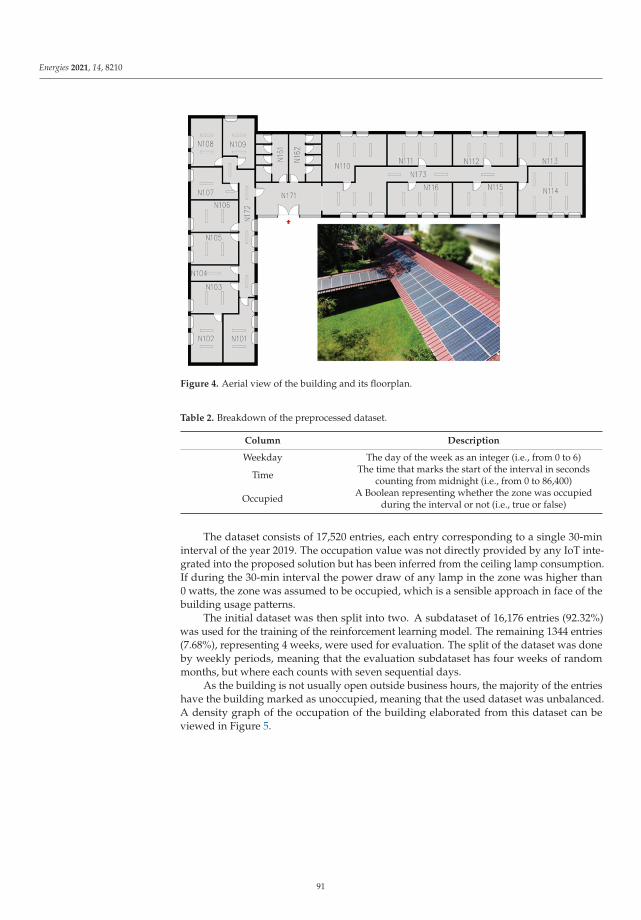
Energies 2021, 14, 8210

Figure 4. Aerial view of the building and its floorplan.

Table 2. Breakdown of the preprocessed dataset.

Column Description

Weekday The day of the week as an integer (i.e., from 0 to 6)

Time The time that marks the start of the interval in secondscounting from midnight (i.e., from 0 to 86,400)

Occupied A Boolean representing whether the zone was occupiedduring the interval or not (i.e., true or false)

The dataset consists of 17,520 entries, each entry corresponding to a single 30-mininterval of the year 2019. The occupation value was not directly provided by any IoT inte-grated into the proposed solution but has been inferred from the ceiling lamp consumption.If during the 30-min interval the power draw of any lamp in the zone was higher than0 watts, the zone was assumed to be occupied, which is a sensible approach in face of thebuilding usage patterns.

The initial dataset was then split into two. A subdataset of 16,176 entries (92.32%)was used for the training of the reinforcement learning model. The remaining 1344 entries(7.68%), representing 4 weeks, were used for evaluation. The split of the dataset was doneby weekly periods, meaning that the evaluation subdataset has four weeks of randommonths, but where each counts with seven sequential days.

As the building is not usually open outside business hours, the majority of the entrieshave the building marked as unoccupied, meaning that the used dataset was unbalanced.A density graph of the occupation of the building elaborated from this dataset can beviewed in Figure 5.

91

Energies 2021, 14, 8210

Figure 5. Occupancy graph of the building during 2019.

5.2. Forecast Errors Evaluation

Every time the model is executed, it takes in two input parameters, the current day ofthe week represented as an integer, ranging from 0 representing Monday to 6 representingSaturday, and the number of seconds that have passed since midnight of the current dayup until the desired 30-min prediction interval.

Two different models were evaluated based on [36]: a linear model that simplyattempted to regress the inputs and predict an output, and a more complex neural linearmodel that was able to learn a representation of the inputs and make a prediction based onthat representation.

92

Energies 2021, 14, 8210

The training dataset was used on both reinforcement learning models to compare andevaluate their results. This evaluation step allowed the identification of the model that bestperforms under our case study.

The linear model was faster to train but it was limited by its ability to representthe problem and accurately predict whether the zone would be occupied or not, mostlypredicting that it would be empty. Because an unbalanced dataset was used, the linearmodel managed to achieve an accuracy of around 68% as can be seen in its confusion matrixin Table 3. The neural linear model, using its default configuration of hyperparameters,was able to learn from the training dataset and achieve an accuracy of 92% (Table 4). Fromthis step forward, the linear model was discarded due to its low accuracy score and thefocus was set on improving the result of the neural linear model.

Table 3. Confusion matrix for the linear prediction model.

True LabelPredicted Label

Empty Zone Occupied Zone

Empty zone 855 64Occupied zone 373 80

Accuracy 68.15%

Table 4. Confusion matrix for the neural linear prediction model.

True LabelPredicted Label

Empty Zone Occupied Zone

Empty zone 873 46Occupied zone 60 393

Accuracy 92.27%

5.3. Hyperparameter Tuning Results

To tune the hyperparameters, Python’s Optuna library was used due to its flexibilityand learning curve, along with the ability to provide useful data and information at theend of a hyperparameter tuning session.

First, a selection of hyperparameters to tune was made, and then a range of appropriatevalues was chosen for each of the hyperparameters to be tuned. Then, using a loop, arandom combination of hyperparameters was chosen and the model was trained andevaluated. To avoid wasting time in nonviable trials, the algorithm continuously checksthe current accuracy and if it were lower than the average accuracy of the previous trialsthe entire trial would be pruned and the next trial starts.

In this case study, a hyperparameter tuning session with 500 trials was executed. Fromthe obtained results, more sensible ranges were defined to achieve more accurate models.After another 400 trials, the most accurate model to come out of the hyperparameter tuningsessions was able to achieve an accuracy of 93.8%.

The configuration with the best result uses a network with three hidden layers with26 nodes in the first and in the second layers, and with 12 nodes for the last layer. Thechosen network had a learning rate of 0.03473 and a lambda of 0.20787.

5.4. HVAC Control Test

The control of HVAC units was done using Broadlink RM pro devices that wereintegrated into the Home Assistant solution. The Broadlink RM pro devices were locatedin each room of the building in Figure 4. The control of HVAC units was done, by theproposed solution, considering the decision tree shown in Figure 3. The decision tree wascontinuously executed in the proposed BEMS. However, the prediction value was onlyupdated every 15 min and it considered the predicted presence of users for the next 15-min

93

Energies 2021, 14, 8210

period. Therefore, the control was done ahead of time, i.e., to prepare the room for the nextperiod by considering the time that HVAC units take to reach the desired temperature.

For this case study, the business day of Friday, 27 August 2021, was considered.Figure 6 shows the results for 24 h. The orange area represents the hours where users arepredicted to be inside the office N101, part of Zone 1. The case study data considered twotemperature limits of 25 and 23 ◦C, with a range of +3 ◦C, meaning that at the beginningof the day the temperature limit was from 25 ◦C to 28 ◦C, and it was changed to a limitbetween 23 ◦C and 26 ◦C. The energy threshold was set to 0.24 EUR/kWh.

Figure 6. HVAC control signals for N101 during 27 August 2021.

6. Discussion

The results shown in Figure 6 indicate that the HVAC unit of room N101 was turnedon seven times and turned off seven times over the 24 h. As can be seen, these actionshappen during the hours where the predictive model forecasts the presence of users insidethe office space of room N101, i.e., from 9:00 a.m. to 8:00 p.m. The turning on of theHVAC units also matched the increase of temperature above the upper user limit, whilethe turning off matched the below limit.

At 3:18 p.m., the user updated the temperature limit to a range between 23 ◦C and26 ◦C, changing the system performance. This action tested the system’s ability to adjust tothe users’ needs. However, as future improvement, the authors suggest the use of buildingthermal modeling to increase the intelligence of the management model.

The windows of room N101 were open between 4:07 p.m. and 4:45 p.m., leading toan early turn-off of the HVAC unit at 4:08 p.m. when the temperature was 24.93 ◦C (i.e.,1.93 ◦C above the lower limit of 23 ◦C). When the windows were closed, the HVAC almostimmediately started once again to decrease the room’s temperature.

The system demonstrated its ability to continuously manage the HVAC unit consid-ering the current context of the room while also considering the predictive data of theproposed model. The control of the temperature inside the room was not only made ac-cording to the current context. If the predictive model did not forecast the presence of usersduring the next period, no control would be made in the HVAC units. All control signals,to turn the unit on, were made because the predictive model forecasted the presence ofusers during the next period.

The BEMS, based on the open-source solution of Home Assistant, was able to providereal-time monitoring and control while providing historical data to train the reinforcementlearning algorithm. The proposed predictive model and the decision tree were deployedin BEMS using Python language and were able to cooperate with the BEMS to provide acontinuous intelligent operation without the need for manual actions.

94

Energies 2021, 14, 8210

7. Conclusions

This paper proposes a novel model for the control of HVAC units based on a predictionmodel and a decision tree. The control of the units is performed ahead of time to minimizethe units’ waiting times (i.e., the time they take to reach the desired temperature). Theprediction model uses a reinforcement algorithm that can provide continuous learningaccording to several contexts. The high accuracy of the model, 93.8%, demonstrates theability of such algorithms to be used in smart buildings to efficiently manage energy loadsand resources across different contexts.

Using the prediction result, a decision tree is proposed to consider the current contextand the predicted context, inside a building’s zone, to control the HVAC units. Theproposed model was tested and evaluated using real data from one year in an officebuilding. The validation of the proposed solution for 24 h is presented to demonstrate theuse of the proposed solution as a whole.

Moreover, the work described in the paper demonstrated the ability to have open-source-based automation solutions to deploy complex models of artificial intelligence andenergy management to operate in real-time and also ahead of time. This combination oftechnologies provides a complete tool to test and validate energy management models inreal buildings.

Author Contributions: Conceptualization, P.M., L.G. and Z.V.; methodology, P.M., L.G. and Z.V.;software, P.M.; validation, P.M. and L.G.; formal analysis, P.M. and L.G.; investigation, P.M.; resources,Z.V.; data curation, P.M.; writing—original draft preparation, P.M. and L.G.; writing—review andediting, L.G. and Z.V.; visualization, P.M. and L.G.; supervision, L.G. and Z.V.; project administra-tion, Z.V.; funding acquisition, Z.V. All authors have read and agreed to the published version ofthe manuscript.

Funding: The present work has received funding from European Regional Development Fundthrough COMPETE 2020—Operational Programme for Competitiveness and Internationalisationthrough the P2020 Project TIoCPS (ANI|P2020 POCI-01-0247-FEDER-046182), and has been devel-oped under the EUREKA—ITEA3 Project TIoCPS (ITEA-18008).

Institutional Review Board Statement: Not Applicable.

Informed Consent Statement: Not Applicable.

Data Availability Statement: Not Applicable.

Acknowledgments: The authors acknowledge the work facilities and equipment provided byGECAD research center (UIDB/00760/2020, UIDP/00760/2020) to the project team.


References

1. Lezama, F.; Soares, J.; Canizes, B.; Vale, Z. Flexibility management model of home appliances to support DSO requests in smartgrids. Sustain. Cities Soc. 2020, 55, 102048. [CrossRef]

2. Gazafroudi, A.S.; Soares, J.; Ghazvini, M.A.F.; Pinto, T.; Vale, Z.; Corchado, J.M. Stochastic interval-based optimal offering modelfor residential energy management systems by household owners. Int. J. Electr. Power Energy Syst. 2019, 105, 201–219. [CrossRef]

3. Yu, L.; Xie, W.; Xie, D.; Zou, Y.; Zhang, D.; Sun, Z.; Zhang, L.; Zhang, Y.; Jiang, T. Deep Reinforcement Learning for Smart HomeEnergy Management. IEEE Internet Things J. 2020, 7, 2751–2762. [CrossRef]

4. Liere-Netheler, I.; Schuldt, F.; von Maydell, K.; Agert, C. Simulation of Incidental Distributed Generation Curtailment to Maximizethe Integration of Renewable Energy Generation in Power Systems. Energies 2020, 13, 4173. [CrossRef]

5. Pinto, T.; Morais, H.; Sousa, T.M.; Sousa, T.; Vale, Z.; Praça, I.; Faia, R.; Pires, E.J.S. Adaptive Portfolio Optimization for MultipleElectricity Markets Participation. IEEE Trans. Neural Netw. Learn. Syst. 2016, 27, 1720–1733. [CrossRef]

6. Gomes, L.; Vale, Z.A.; Corchado, J.M. Multi-Agent Microgrid Management System for Single-Board Computers: A Case Study onPeer-to-Peer Energy Trading. IEEE Access 2020, 8, 64169–64183. [CrossRef]

7. Yu, L.; Qin, S.; Zhang, M.; Shen, C.; Jiang, T.; Guan, X. Deep Reinforcement Learning for Smart Building Energy Management: ASurvey. arXiv 2020, arXiv:2008.05074.

8. Gomes, L.; Ramos, C.; Jozi, A.; Serra, B.; Paiva, L.; Vale, Z. IoH: A Platform for the Intelligence of Home with a Context Awarenessand Ambient Intelligence Approach. Futur. Internet 2019, 11, 58. [CrossRef]

95

Energies 2021, 14, 8210

9. Djenouri, D.; Laidi, R.; Djenouri, Y.; Balasingham, I. Machine learning for smart building applications: Review and taxonomy.ACM Comput. Surv. 2019, 52, 1–36. [CrossRef]

10. Pérez-Lombard, L.; Ortiz, J.; Pout, C. A review on buildings energy consumption information. Energy Build. 2008, 40, 394–398.[CrossRef]

11. Esrafilian-Najafabadi, M.; Haghighat, F. Occupancy-based HVAC control systems in buildings: A state-of-the-art review. Build.Environ. 2021, 197, 107810. [CrossRef]

12. Gholamzadehmir, M.; Del Pero, C.; Buffa, S.; Fedrizzi, R.; Aste, N. Adaptive-predictive control strategy for HVAC systems insmart buildings—A review. Sustain. Cities Soc. 2020, 63, 102480. [CrossRef]

13. Adhikari, R.; Pipattanasomporn, M.; Rahman, S. An algorithm for optimal management of aggregated HVAC power demandusing smart thermostats. Appl. Energy 2018, 217, 166–177. [CrossRef]

14. Khalid, R.; Javaid, N. A survey on hyperparameters optimization algorithms of forecasting models in smart grid. Sustain. CitiesSoc. 2020, 61, 102275. [CrossRef]

15. Jung, W.; Jazizadeh, F. Human-in-the-loop HVAC operations: A quantitative review on occupancy, comfort, and energy-efficiencydimensions. Appl. Energy 2019, 239, 1471–1508. [CrossRef]

16. Gomes, L.; Spínola, J.; Vale, Z.; Corchado, J.M. Agent-based architecture for demand side management using real-time resources’priorities and a deterministic optimization algorithm. J. Clean. Prod. 2019, 241, 118154. [CrossRef]

17. Petrosanu, D.M.; Carutasu, G.; Carutasu, N.L.; Pîrjan, A. A review of the recent developments in integrating machine learningmodels with sensor devices in the smart buildings sector with a view to attaining enhanced sensing, energy efficiency, andoptimal building management. Energies 2019, 12, 4745. [CrossRef]

18. Ardakanian, O.; Bhattacharya, A.; Culler, D. Non-intrusive occupancy monitoring for energy conservation in commercialbuildings. Energy Build. 2018, 179, 311–323. [CrossRef]

19. Razavi, R.; Gharipour, A.; Fleury, M.; Akpan, I.J. Occupancy detection of residential buildings using smart meter data: Alarge-scale study. Energy Build. 2019, 183, 195–208. [CrossRef]

20. Simma, K.C.J.; Mammoli, A.; Bogus, S.M. Real-Time Occupancy Estimation Using WiFi Network to Optimize HVAC Operation.Procedia Comput. Sci. 2019, 155, 495–502. [CrossRef]

21. Esrafilian-Najafabadi, M.; Haghighat, F. Occupancy-based HVAC control using deep learning algorithms for estimating onlinepreconditioning time in residential buildings. Energy Build. 2021, 252, 111377. [CrossRef]

22. Deng, Z.; Chen, Q. Reinforcement learning of occupant behavior model for cross-building transfer learning to various HVACcontrol systems. Energy Build. 2021, 238, 110860. [CrossRef]

23. Wei, T.; Wang, Y.; Zhu, Q. Deep Reinforcement Learning for Building HVAC Control. In Proceedings of the 54th Annual DesignAutomation Conference, Austin, TX, USA, 18–22 June 2017. [CrossRef]

24. Escobar, L.M.; Aguilar, J.; Garces-Jimenez, A.; De Mesa, J.A.G.; Gomez-Pulido, J.M. Advanced fuzzy-logic-based context-drivencontrol for HVAC management systems in buildings. IEEE Access 2020, 8, 16111–16126. [CrossRef]

25. Lou, R.; Hallinan, K.P.; Huang, K.; Reissman, T. Smart Wifi Thermostat-Enabled Thermal Comfort Control in Residences.Sustainability 2020, 12, 1919. [CrossRef]

26. Wang, C.; Pattawi, K.; Lee, H. Energy saving impact of occupancy-driven thermostat for residential buildings. Energy Build. 2020,211, 109791. [CrossRef]

27. Yang, Y.; Hu, G.; Spanos, C.J. HVAC Energy Cost Optimization for a Multizone Building via a Decentralized Approach. IEEETrans. Autom. Sci. Eng. 2020, 17, 1950–1960. [CrossRef]

28. Khan, K.H.; Ryan, C.; Abebe, E. Day Ahead Scheduling to Optimize Industrial HVAC Energy Cost Based on Peak/OFF-PeakTariff and Weather Forecasting. IEEE Access 2017, 5, 21684–21693. [CrossRef]

29. Khorram, M.; Faria, P.; Abrishambaf, O.; Vale, Z. Air conditioner consumption optimization in an office building considering usercomfort. Energy Rep. 2020, 6, 120–126. [CrossRef]

30. Corbin, C.D.; Makhmalbaf, A.; Huang, S.; Mendon, V.V.; Zhao, M.; Somasundaram, S.; Liu, G.; Ngo, H.; Katipamula, S. TransactiveControl of Commercial Building HVAC Systems; Pacific Northwest National Lab.(PNNL): Richland, WA, USA, 2016.

31. Mutis, I.; Ambekar, A.; Joshi, V. Real-time space occupancy sensing and human motion analysis using deep learning for indoorair quality control. Autom. Constr. 2020, 116, 103237. [CrossRef]

32. Yu, L.; Sun, Y.; Xu, Z.; Shen, C.; Yue, D.; Jiang, T.; Guan, X. Multi-Agent Deep Reinforcement Learning for HVAC Control inCommercial Buildings. IEEE Trans. Smart Grid 2021, 12, 407–419. [CrossRef]

33. Aguilar, J.; Garcès-Jimènez, A.; Gallego-Salvador, N.; de Mesa, J.A.G.; Gomez-Pulido, J.M.; Garcìa-Tejedor, À.J. Autonomicmanagement architecture for multi-HVAC systems in smart buildings. IEEE Access 2019, 7, 123402–123415. [CrossRef]

34. Garces-Jimenez, A.; Gomez-Pulido, J.-M.; Gallego-Salvador, N.; Garcia-Tejedor, A.J. Genetic and Swarm Algorithms for Optimiz-ing the Control of Building HVAC Systems Using Real Data: A Comparative Study. Mathematics 2021, 9, 2181. [CrossRef]

35. Collier, M.; Llorens, H.U. Deep Contextual Multi-armed Bandits. arXiv 2018, arXiv:1807.09809.36. Riquelme, C.; Tucker, G.; Snoek, J. Deep Bayesian bandits showdown: An empirical comparison of Bayesian deep networks for

Thompson sampling. In Proceedings of the 6th International Conference on Learning Representations, ICLR 2018-ConferenceTrack Proceedings, Vancouver, BC, Canada, 30 April–3 May 2018.

96

energies

Article

Application of Artificial Neural Networks for VirtualEnergy Assessment

Amir Mortazavigazar 1,2, Nourehan Wahba 1, Paul Newsham 1,3, Maharti Triharta 1, Pufan Zheng 1, Tracy Chen 1

and Behzad Rismanchi 1,*

Citation: Mortazavigazar, A.; Wahba,

N.; Newsham, P.; Triharta, M.; Zheng,

P.; Chen, T.; Rismanchi, B.

Application of Artificial Neural

Networks for Virtual Energy

Assessment. Energies 2021, 14, 8330.

https://doi.org/10.3390/en14248330

Academic Editor:

Ana-Belén Gil-González

Received: 17 November 2021

Accepted: 8 December 2021

Published: 10 December 2021




iations.








4.0/).

1 Renewable Energy and Energy Efficiency Group, Department of Infrastructure Engineering,Melbourne School of Engineering, The University of Melbourne, Melbourne, VIC 3004, Australia;[email protected] (A.M.); [email protected] (N.W.);[email protected] (P.N.); [email protected] (M.T.);[email protected] (P.Z.); [email protected] (T.C.)

2 Virginia-Maryland College of Veterinary Medicine, Roanoke, VA 24060, USA3 Faculty of Business, UQ Business School, Economics & Law, University of Queensland,

Brisbane, QLD 4072, Australia* Correspondence: [email protected]

Abstract: A Virtual energy assessment (VEA) refers to the assessment of the energy flow in abuilding without physical data collection. It has been occasionally conducted before the COVID-19pandemic to residential and commercial buildings. However, there is no established frameworkmethod for conducting this type of energy assessment. The COVID-19 pandemic has catalysedthe implementation of remote energy assessments and remote facility management. In this paper,a novel framework for VEA is developed and tested on case study buildings at the University ofMelbourne. The proposed method is a hybrid of top-down and bottom-up approaches: gatheringthe general information of the building and the historical data, in addition to investigating andmodelling the electrical consumption with artificial neural network (ANN) with a projection of thefuture consumption. Through sensitivity analysis, the outdoor temperature was found to be the mostsensitive (influential) parameter to electrical consumption. The lockdown of the buildings providedinvaluable opportunities to assess electrical baseload with zero occupancies and usage of the building.Furthermore, comparison of the baseload with the consumption projection through ANN modellingaccurately quantifies the energy consumption attributed to occupation and operational use, referredto as ‘operational energy’ in this paper. Differentiation and quantification of the baseload andoperational energy may aid in energy conservation measures that specifically target to minimisethese two distinct energy consumptions.

Keywords: virtual energy assessment; artificial neural network; commercial buildings; energyefficiency; energy saving

1. Introduction

Energy efficiency is the hidden fuel for meeting the current global demand, yet itremains underutilised despite its proven potentials [1]. According to the 2018 InternationalEnergy Efficiency Scorecard Report [2], Australia has ranked 17th out of the top 25 countriesconsuming 78% of all energy on the planet, indicating its urgency to rally innovativeendeavour in the field of energy efficiency. In conjunction with the latter, the state ofVictoria’s Climate Change Act 2017 targets net-zero greenhouse gas emissions by 2050,which includes the transformation of the commercial building sector to encounter thepressure from a rapidly growing population to building emissions [3]. To reduce thegradual rise of building energy consumption, it is therefore critical to develop a holisticframework in identifying energy flow and waste within a building, replacing the traditionalperiodic walk-through energy audits. Furthermore, the gradual rise of energy cost has


Energies 2021, 14, 8330

propelled the urgencies of energy conservation and efficiency, which created a need forenergy audits to be conducted regularly in commercial and industrial sectors [4,5].

An energy audit is known as the first step to identify energy flow within a building,which helps to achieve energy savings, improve indoor user comfort and productivity, andreduce environmental impact [6]. This assessment can be used by large and small busi-nesses and even households to achieve higher energy efficiency improvements and carbonemissions reductions. A survey from the U.S. Energy Department shows that energy auditshave saved about 20% of energy for the commercial building as of 2020 and are expectedto reach 30% by 2030 with the utilisation of current technology. However, if emergingtechnologies are introduced, this number is expected to reach 55% within five years [7].Joshi [8] claims that a reduction in the amount of energy input can be achieved withoutreducing the level of useful output services, which leads to the implementation of energyconservation measures throughout a building’s lifecycle as an emerging response to therising energy consumption and carbon emissions of the global building sector. A traditionalenergy audit involves physical functional observation of the building, conducting a seriesof data acquisitions of onsite indoor quality parameters, and operational tests such as leaktests, infrared imaging, blower door tests, and equipment sub-metering (as defined by thestandards in [6]).

Traditional onsite energy audits require a substantial financial commitment of hu-man resources allocation, travelling times, and installation of instrumentation. In somecircumstances, overall implementation and the energy audit cost could exceed the potentialenergy saving cost. A traditional energy audit provides a periodic snapshot of the buildingenergy behaviour [9]. On the other hand, virtual energy assessment (VEA) does not involvea physical walk-around of the building and aims to cover the activities of the physicalenergy audit remotely without travelling time and allocation of physical auditor onsite [10].Conceivably VEA is a way to save time and cost and, more importantly, it has the potentialto provide a more frequent assessment of the building energy behaviour to the extent ofautonomous continuous assessment with machine learning. The concept of VEA is notentirely novel, it has been occasionally conducted before the COVID-19 pandemic in severalcases of residential and commercial buildings as summarised in Table 1. Literature reviewof building energy. However, it was not widely used as the preference of building ownerswas leaning towards the traditional energy audit [11]. The unprecedented time of theCOVID-19 pandemic has catalysed the application of VEA and provided the opportunitiesto unlock the market of VEA.

Energy modelling such as VEA can be conducted through two approaches: the bottom-up approach and the top-down approach [12]. The bottom-up approach entails thermalanalysis for an individual building, with data related to the building’s enclosure, schedules,external weather conditions, internal loads, and potential systems. A white-box model(a bottom-up approach) is commonly used for virtual energy assessments where thebuilding’s prediction relies on simplified heat balance calculations, aggregated weatherlibraries, fixed schedules, and thousands of building’s characteristics inputs. Consequently,inaccurate conclusions of energy efficiency can be reached, leading to a gap between thesimulated models and actual building interactions. Conversely, a black-box model (alsoa bottom-up approach) is based on the actual building’s energy consumption datasetsto provide insight into the existing building performance without extensive buildings’background and information needed. The artificial neural network (ANN) has been anoutperforming tool for VEAs [13].

98

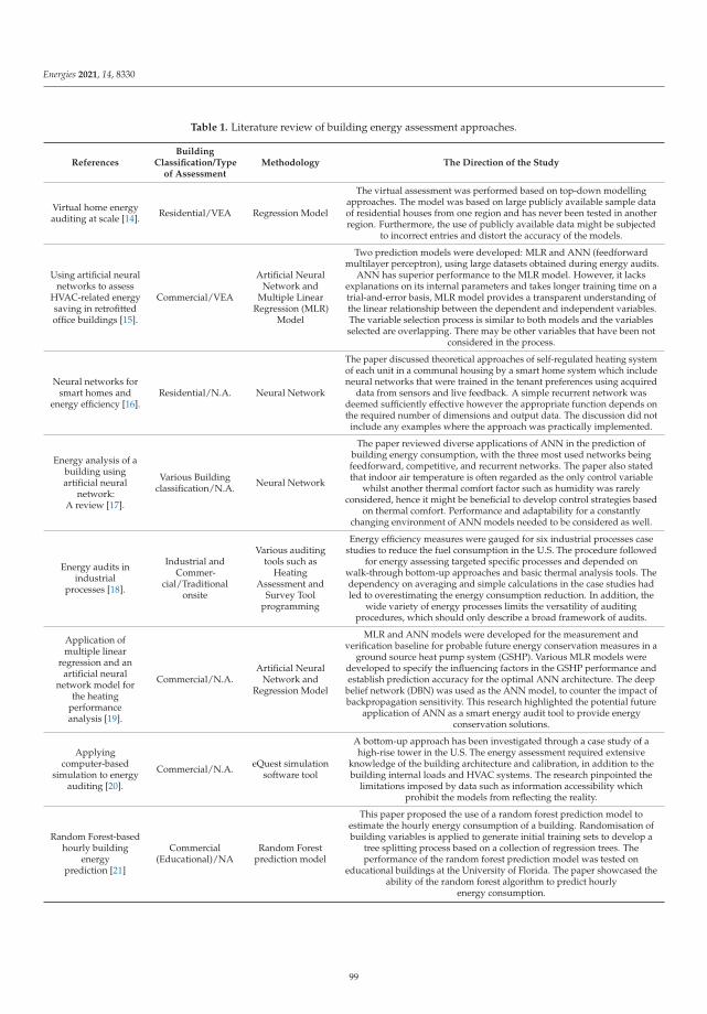
Energies 2021, 14, 8330

Table 1. Literature review of building energy assessment approaches.

ReferencesBuilding

Classification/Typeof Assessment

Methodology The Direction of the Study

Virtual home energyauditing at scale [14]. Residential/VEA Regression Model

The virtual assessment was performed based on top-down modellingapproaches. The model was based on large publicly available sample dataof residential houses from one region and has never been tested in anotherregion. Furthermore, the use of publicly available data might be subjected

to incorrect entries and distort the accuracy of the models.

Using artificial neuralnetworks to assess

HVAC-related energysaving in retrofittedoffice buildings [15].

Commercial/VEA

Artificial NeuralNetwork and

Multiple LinearRegression (MLR)

Model

Two prediction models were developed: MLR and ANN (feedforwardmultilayer perceptron), using large datasets obtained during energy audits.

ANN has superior performance to the MLR model. However, it lacksexplanations on its internal parameters and takes longer training time on atrial-and-error basis, MLR model provides a transparent understanding ofthe linear relationship between the dependent and independent variables.The variable selection process is similar to both models and the variablesselected are overlapping. There may be other variables that have been not

considered in the process.

Neural networks forsmart homes and

energy efficiency [16].Residential/N.A. Neural Network

The paper discussed theoretical approaches of self-regulated heating systemof each unit in a communal housing by a smart home system which includeneural networks that were trained in the tenant preferences using acquired

data from sensors and live feedback. A simple recurrent network wasdeemed sufficiently effective however the appropriate function depends onthe required number of dimensions and output data. The discussion did not

include any examples where the approach was practically implemented.

Energy analysis of abuilding usingartificial neural

network:A review [17].

Various Buildingclassification/N.A. Neural Network

The paper reviewed diverse applications of ANN in the prediction ofbuilding energy consumption, with the three most used networks beingfeedforward, competitive, and recurrent networks. The paper also statedthat indoor air temperature is often regarded as the only control variable

whilst another thermal comfort factor such as humidity was rarelyconsidered, hence it might be beneficial to develop control strategies based

on thermal comfort. Performance and adaptability for a constantlychanging environment of ANN models needed to be considered as well.

Energy audits inindustrial

processes [18].

Industrial andCommer-

cial/Traditionalonsite

Various auditingtools such as

HeatingAssessment and

Survey Toolprogramming

Energy efficiency measures were gauged for six industrial processes casestudies to reduce the fuel consumption in the U.S. The procedure followed

for energy assessing targeted specific processes and depended onwalk-through bottom-up approaches and basic thermal analysis tools. Thedependency on averaging and simple calculations in the case studies hadled to overestimating the energy consumption reduction. In addition, the

wide variety of energy processes limits the versatility of auditingprocedures, which should only describe a broad framework of audits.

Application ofmultiple linear

regression and anartificial neural

network model forthe heating

performanceanalysis [19].

Commercial/N.A.Artificial Neural

Network andRegression Model

MLR and ANN models were developed for the measurement andverification baseline for probable future energy conservation measures in a

ground source heat pump system (GSHP). Various MLR models weredeveloped to specify the influencing factors in the GSHP performance andestablish prediction accuracy for the optimal ANN architecture. The deep

belief network (DBN) was used as the ANN model, to counter the impact ofbackpropagation sensitivity. This research highlighted the potential future

application of ANN as a smart energy audit tool to provide energyconservation solutions.

Applyingcomputer-based

simulation to energyauditing [20].

Commercial/N.A. eQuest simulationsoftware tool

A bottom-up approach has been investigated through a case study of ahigh-rise tower in the U.S. The energy assessment required extensive

knowledge of the building architecture and calibration, in addition to thebuilding internal loads and HVAC systems. The research pinpointed the

limitations imposed by data such as information accessibility whichprohibit the models from reflecting the reality.

Random Forest-basedhourly building

energyprediction [21]

Commercial(Educational)/NA

Random Forestprediction model

This paper proposed the use of a random forest prediction model toestimate the hourly energy consumption of a building. Randomisation ofbuilding variables is applied to generate initial training sets to develop a

tree splitting process based on a collection of regression trees. Theperformance of the random forest prediction model was tested on

educational buildings at the University of Florida. The paper showcased theability of the random forest algorithm to predict hourly

energy consumption.

99

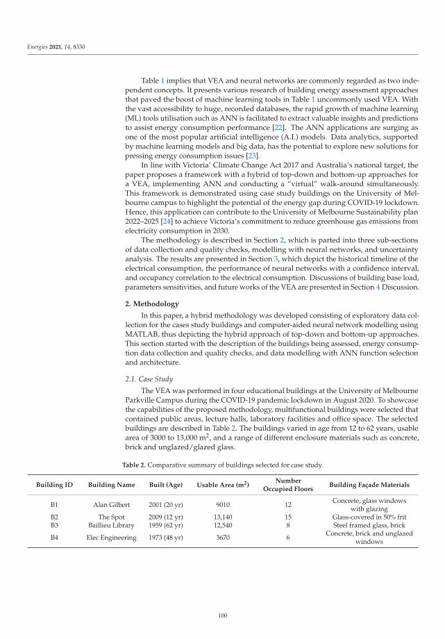
Energies 2021, 14, 8330

Table 1 implies that VEA and neural networks are commonly regarded as two inde-pendent concepts. It presents various research of building energy assessment approachesthat paved the boost of machine learning tools in Table 1 uncommonly used VEA. Withthe vast accessibility to huge, recorded databases, the rapid growth of machine learning(ML) tools utilisation such as ANN is facilitated to extract valuable insights and predictionsto assist energy consumption performance [22]. The ANN applications are surging asone of the most popular artificial intelligence (A.I.) models. Data analytics, supportedby machine learning models and big data, has the potential to explore new solutions forpressing energy consumption issues [23].

In line with Victoria’ Climate Change Act 2017 and Australia’s national target, thepaper proposes a framework with a hybrid of top-down and bottom-up approaches fora VEA, implementing ANN and conducting a “virtual” walk-around simultaneously.This framework is demonstrated using case study buildings on the University of Mel-bourne campus to highlight the potential of the energy gap during COVID-19 lockdown.Hence, this application can contribute to the University of Melbourne Sustainability plan2022–2025 [24] to achieve Victoria’s commitment to reduce greenhouse gas emissions fromelectricity consumption in 2030.

The methodology is described in Section 2, which is parted into three sub-sectionsof data collection and quality checks, modelling with neural networks, and uncertaintyanalysis. The results are presented in Section 3, which depict the historical timeline of theelectrical consumption, the performance of neural networks with a confidence interval,and occupancy correlation to the electrical consumption. Discussions of building base load,parameters sensitivities, and future works of the VEA are presented in Section 4 Discussion.

2. Methodology

In this paper, a hybrid methodology was developed consisting of exploratory data col-lection for the cases study buildings and computer-aided neural network modelling usingMATLAB, thus depicting the hybrid approach of top-down and bottom-up approaches.This section started with the description of the buildings being assessed, energy consump-tion data collection and quality checks, and data modelling with ANN function selectionand architecture.

2.1. Case Study

The VEA was performed in four educational buildings at the University of MelbourneParkville Campus during the COVID-19 pandemic lockdown in August 2020. To showcasethe capabilities of the proposed methodology, multifunctional buildings were selected thatcontained public areas, lecture halls, laboratory facilities and office space. The selectedbuildings are described in Table 2. The buildings varied in age from 12 to 62 years, usablearea of 3000 to 13,000 m2, and a range of different enclosure materials such as concrete,brick and unglazed/glazed glass.

Table 2. Comparative summary of buildings selected for case study.

Building ID Building Name Built (Age) Usable Area (m2)Number

Occupied FloorsBuilding Façade Materials

B1 Alan Gilbert 2001 (20 yr) 9010 12 Concrete, glass windowswith glazing

B2 The Spot 2009 (12 yr) 13,140 15 Glass-covered in 50% fritB3 Baillieu Library 1959 (62 yr) 12,540 8 Steel framed glass, brick

B4 Elec Engineering 1973 (48 yr) 3670 6 Concrete, brick and unglazedwindows

100

Energies 2021, 14, 8330

2.2. Virtual Energy Assessment2.2.1. Data Collection and Quality Checks

The case study buildings are equipped with a real-time energy monitoring platformthat is accessible through a secure web server. These energy data were collected for thecase study buildings for this study, as well as external weather conditions and occupancyrates. The external weather data were collected from the nearest weather station and theoccupancy rate was collected from the university security. All of the above-mentioneddata could be accessed for most of the new buildings and most of the existing buildingswhich have been upgraded with remote data access. The authors believe that the proposedmethodology is replicable to any building with such datasets. Abnormalities and outlierswere removed as part of the data quality checks.

Electrical consumption data was collected for a total load of each building separatelyusing Clariti. End-uses submetering was unavailable, with meter data representing thetotal load consumption. Fifteen minutes of load consumption was gathered from June 2015to January 2021, as the basis of the assessment. With the building closures due to COVID-19,the use of space and buildings’ layouts and building enclosure details were obtained fromfacility managers. Furthermore, the electrical consumption data were screened for outliers,the Clariti tool is very precise and for the cases, at hand, no outlier was detected.

Central to the building external conditions, 10 years of detailed meteorological datafrom the Australian Bureau of Meteorology in 15-min increments were procured fromthe nearest weather station. This data included temperature, humidity, rainfall, and solarirradiance. Online images of the sides and tops of the buildings were supplemented byusing tools such as Google Earth and Nearmap.

2.2.2. Variables Selection

To improve the learning efficiency and compilation of the ANN model, it was neces-sary to reduce the number of input data variables used to those that were most influentialof the energy use in each building. For instance, occupants’ behaviour is a typical key ele-ment of a building’s energy performance. In this paper, occupants’ behaviour informationwas scarce and limited to certain years, influencing its validity in the training process ofthe neural network; however, if available, it would have provided further fertile testinggrounds for the neural network’s ability to further detect the end-use energy performance.

2.2.3. Artificial Neural Network Modelling

The advent of ANN enables analysis from the complicated and large size of data,extracting patterns and trends to provide future projections with the potential to be trainedfor projections of unpredicted circumstances. It is currently widely used with applicationsranging from sales forecasting, web searching, to visual imaging. ANN model is a sim-plified version of a biological neural network that combines data and stores relationshipsbetween independent and dependent variables. The ANN can self-study the historical dataand users’ preferences, through training, to improve its accuracy of prediction. It can alsocontinue learning, which can be well adapted to a new environment [25]. Compared tosophisticated calculations of statistical models, the ANN model trains data for prediction,which is more suitable for a larger set of data [17].

As illustrated in Figure 1, a basic neural network consists of several connected nodes,or “neurons”, which produce a sequence of activation. Input neurons (in the input layer)are activated using an initialiser, while other neurons in hidden layers are activated throughweighted connections from previously activated neurons. After checking the outcomewith desired outputs, the neurons adjust their weight functions to get a more accurateresult [17]. This procedure is technically called “learning”. In general, the traditional-learning approach in a neural network requires significant amounts of data and long chainsof computational stages to obtain accurate results. To handle this obstacle, various othernetworks are developed to accurately assign the weight functions by adopting the trainingstages with an unsupervised learning technique.

101

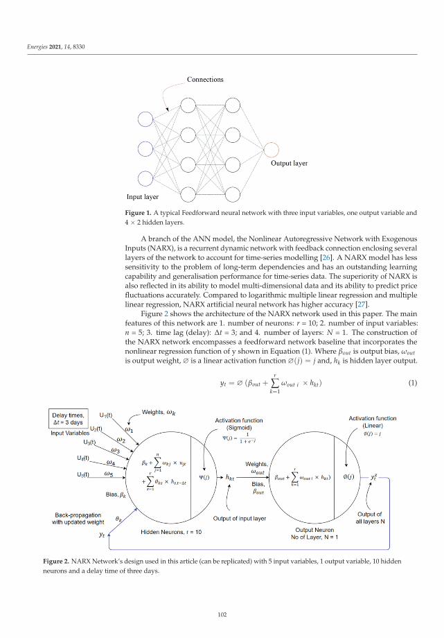
Energies 2021, 14, 8330

Figure 1. A typical Feedforward neural network with three input variables, one output variable and4 × 2 hidden layers.

A branch of the ANN model, the Nonlinear Autoregressive Network with ExogenousInputs (NARX), is a recurrent dynamic network with feedback connection enclosing severallayers of the network to account for time-series modelling [26]. A NARX model has lesssensitivity to the problem of long-term dependencies and has an outstanding learningcapability and generalisation performance for time-series data. The superiority of NARX isalso reflected in its ability to model multi-dimensional data and its ability to predict pricefluctuations accurately. Compared to logarithmic multiple linear regression and multiplelinear regression, NARX artificial neural network has higher accuracy [27].

Figure 2 shows the architecture of the NARX network used in this paper. The mainfeatures of this network are 1. number of neurons: r = 10; 2. number of input variables:n = 5; 3. time lag (delay): Δt = 3; and 4. number of layers: N = 1. The construction ofthe NARX network encompasses a feedforward network baseline that incorporates thenonlinear regression function of y shown in Equation (1). Where βout is output bias, ωoutis output weight, ∅ is a linear activation function ∅(j) = j and, hk is hidden layer output.

yt = ∅ (βout +r

∑k=1

ωout i × hkt) (1)

Figure 2. NARX Network’s design used in this article (can be replicated) with 5 input variables, 1 output variable, 10 hiddenneurons and a delay time of three days.

102

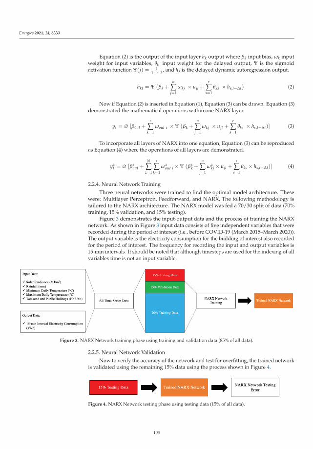
Energies 2021, 14, 8330

Equation (2) is the output of the input layer hk output where βk input bias, ωk inputweight for input variables, θk input weight for the delayed output, Ψ is the sigmoidactivation function Ψ(j) = 1

1+e−j , and hs is the delayed dynamic autoregression output.

hkt = Ψ (βk +n

∑j=1

ωkj × ujt +r

∑s=1

θks × hs,t−Δt) (2)

Now if Equation (2) is inserted in Equation (1), Equation (3) can be drawn. Equation (3)demonstrated the mathematical operations within one NARX layer.

yt = ∅ [βout +r

∑k=1

ωout i × Ψ (βk +n

∑j=1

ωkj × ujt +r

∑s=1

θks × hs,t−Δt)] (3)

To incorporate all layers of NARX into one equation, Equation (3) can be reproducedas Equation (4) where the operations of all layers are demonstrated.

yzt = ∅ [βz

out +N

∑z=1

r

∑k=1

ωzout i × Ψ (βz

k +n

∑j=1

ωzkj × ujt +

r

∑s=1

θks × hs,t−Δt)] (4)

2.2.4. Neural Network Training

Three neural networks were trained to find the optimal model architecture. Thesewere: Multilayer Perceptron, Feedforward, and NARX. The following methodology istailored to the NARX architecture. The NARX model was fed a 70/30 split of data (70%training, 15% validation, and 15% testing).

Figure 3 demonstrates the input-output data and the process of training the NARXnetwork. As shown in Figure 3 input data consists of five independent variables that wererecorded during the period of interest (i.e., before COVID-19 (March 2015–March 2020)).The output variable is the electricity consumption for the building of interest also recordedfor the period of interest. The frequency for recording the input and output variables is15-min intervals. It should be noted that although timesteps are used for the indexing of allvariables time is not an input variable.

Figure 3. NARX Network training phase using training and validation data (85% of all data).

2.2.5. Neural Network Validation

Now to verify the accuracy of the network and test for overfitting, the trained networkis validated using the remaining 15% data using the process shown in Figure 4.

Figure 4. NARX Network testing phase using testing data (15% of all data).

103

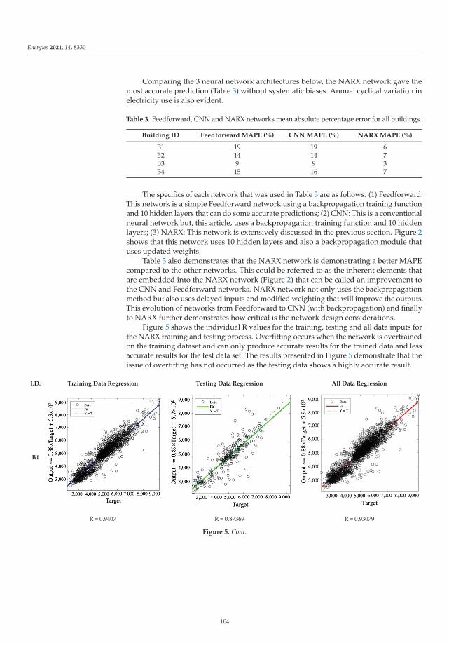
Energies 2021, 14, 8330

Comparing the 3 neural network architectures below, the NARX network gave themost accurate prediction (Table 3) without systematic biases. Annual cyclical variation inelectricity use is also evident.

Table 3. Feedforward, CNN and NARX networks mean absolute percentage error for all buildings.

Building ID Feedforward MAPE (%) CNN MAPE (%) NARX MAPE (%)

B1 19 19 6B2 14 14 7B3 9 9 3B4 15 16 7

The specifics of each network that was used in Table 3 are as follows: (1) Feedforward:This network is a simple Feedforward network using a backpropagation training functionand 10 hidden layers that can do some accurate predictions; (2) CNN: This is a conventionalneural network but, this article, uses a backpropagation training function and 10 hiddenlayers; (3) NARX: This network is extensively discussed in the previous section. Figure 2shows that this network uses 10 hidden layers and also a backpropagation module thatuses updated weights.

Table 3 also demonstrates that the NARX network is demonstrating a better MAPEcompared to the other networks. This could be referred to as the inherent elements thatare embedded into the NARX network (Figure 2) that can be called an improvement tothe CNN and Feedforward networks. NARX network not only uses the backpropagationmethod but also uses delayed inputs and modified weighting that will improve the outputs.This evolution of networks from Feedforward to CNN (with backpropagation) and finallyto NARX further demonstrates how critical is the network design considerations.

Figure 5 shows the individual R values for the training, testing and all data inputs forthe NARX training and testing process. Overfitting occurs when the network is overtrainedon the training dataset and can only produce accurate results for the trained data and lessaccurate results for the test data set. The results presented in Figure 5 demonstrate that theissue of overfitting has not occurred as the testing data shows a highly accurate result.

I.D. Training Data Regression Testing Data Regression All Data Regression

B1

R = 0.9407 R = 0.87369 R = 0.93079

Figure 5. Cont.

104

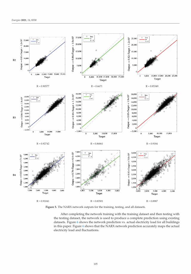
Energies 2021, 14, 8330

B2

R = 0.90577 R = 0.6671 R = 0.85349

B3

R = 0.92742 R = 0.86861 R = 0.9184

B4

R = 0.91041 R = 0.83501 R = 0.8987

Figure 5. The NARX network outputs for the training, testing, and all datasets.

After completing the network training with the training dataset and then testing withthe testing dataset, the network is used to produce a complete prediction using existingdatasets. Figure 6 shows the network prediction vs. actual electricity load for all buildingsin this paper. Figure 6 shows that the NARX network prediction accurately maps the actualelectricity load and fluctuations.

105

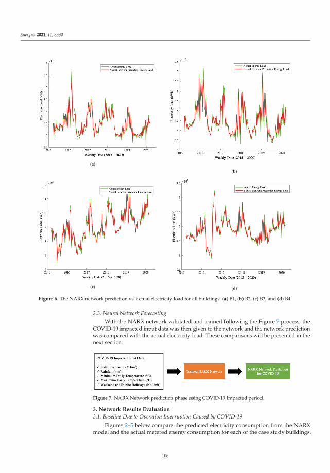
Energies 2021, 14, 8330

(a)

(b)

(c) (d)

Figure 6. The NARX network prediction vs. actual electricity load for all buildings. (a) B1, (b) B2, (c) B3, and (d) B4.

2.3. Neural Network Forecasting

With the NARX network validated and trained following the Figure 7 process, theCOVID-19 impacted input data was then given to the network and the network predictionwas compared with the actual electricity load. These comparisons will be presented in thenext section.

Figure 7. NARX Network prediction phase using COVID-19 impacted period.

3. Network Results Evaluation

3.1. Baseline Due to Operation Interruption Caused by COVID-19

Figures 2–5 below compare the predicted electricity consumption from the NARXmodel and the actual metered energy consumption for each of the case study buildings.

106

Energies 2021, 14, 8330

They include one year of regular operation leading to March 2020 for comparison ofthe COVID-19 impacted period from March 2020 to January 2021. The metered energyuse data from March 2020 to January 2021 show the reduction in electricity use in thebuildings during the period, and provide a better understanding of the base electrical loadof the buildings over a significant length of time whilst the city of Melbourne enduredtwo significant lockdowns due to health orders from the local spread of the COVID-19coronavirus:

• First lockdown: 17 March to 1 June 2020. Restriction “easing” began in Victoriaaccessed on 29 October 2021 (https://www.dhhs.vic.gov.au/coronavirus-update-victoria-1-june-2020), however, new outbreaks caused restrictions to reverse, andstarted tightening again on 22 June accessed on 29 October 2021 (https://www.dhhs.vic.gov.au/coronavirus-update-victoria-22-june-2020)

• Second lockdown: 8 July to 8 November 2020 accessed on 29 October 2021 (https://en.wikipedia.org/wiki/COVID-19_pandemic_in_Australia#Melbourne)

• Summer period: 30 November 2020, to 28 February 2021, accessed on 29 October 2021(https://www.unimelb.edu.au/dates/semester-dates)

• Staff and graduate students were beginning to return in late 2020, however, theUniversity did not re-open to students until 3 January 2021.

The impacts of these events were notable in the metered energy use (green) from17 March 2020, onward in the figures below, though not consistent for each buildingdepending on what activity remained throughout the lockdowns. For B1, B2, and B4(Figure 8 a, b and d respectively), between March 2020 and January 2021 the lower boundof the actual data is a strong measurement of the building baseload on evenings andweekends, and the upper bound was a strong indicator of the daytime building loadswithout added thermal load due to occupancy.

The situation was different for B3 (Library) (Figure 8c), which remained open withminimal staff to provide continued support to the university staff and students continuingworking and studying remotely during the study period. Electricity consumption waslower than predicted and irregular, but overall, due to the continued activity, there was nodefinitive measurement of the baseload captured for the library. During the break betweensemesters in July 2020, the library had higher than predicted electrical consumption, whichaligned with the short periods between the first and second lockdowns and the start of thesecond delayed semester of the 2020 school year, possibly due to the significant activitysurrounding planning for a full semester to be completed online due to the lockdown.

Some university services beyond libraries were open during the lockdowns, identifiedas essential services, albeit only for staff to be onsite for student support and filling studentrequests for pickup. Similarly, some faculties were also permitted to continue whereonline studies were not possible (e.g., medical, biological labs, etc.), but under strict healthprotocols as directed by the government of Victoria.

Overall, the amplitude of the metered energy use was decreased significantly betweendaytime peaks and baseload. The spread between the actual overnight vs. day baseloadis roughly 20% of the magnitude spread of the predicted electrical consumption (red),where the remaining 80% avoided electrical consumption could be attributed to the occupa-tion/operational use of the building. The offset between the lower bounds of the predictedand actual could be due to the additional thermal mass accumulation and additional HVACprograms during regular operation (with added plug loads).

Limited information was available from the university facilities departments for whatchanges were made to the building’s internal systems for energy savings (if at all) whenthe lockdown was initially announced in March 2020. Assumptions were made that B1,B2, and B4 had their HVAC systems put to holiday settings, and some IT systems suchas the A/V in the lecture halls were powered down. In September 2020, leading into thehotter summer weather in Melbourne, additional measures were taken to reduce HVACoperation by shutting curtains and minimising lighting demand to only safety/securityrequirements.

107

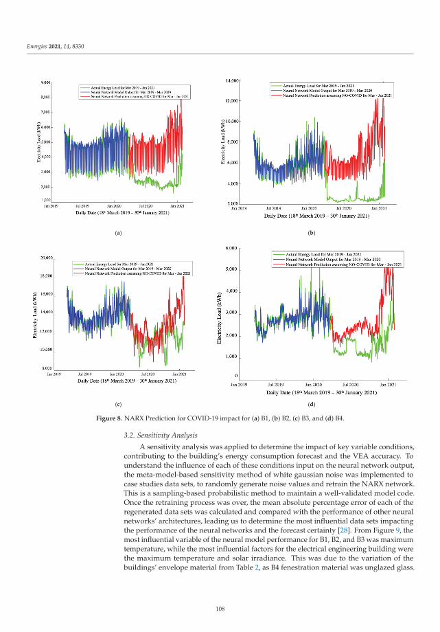
Energies 2021, 14, 8330

(a) (b)

(c) (d)

Figure 8. NARX Prediction for COVID-19 impact for (a) B1, (b) B2, (c) B3, and (d) B4.

3.2. Sensitivity Analysis

A sensitivity analysis was applied to determine the impact of key variable conditions,contributing to the building’s energy consumption forecast and the VEA accuracy. Tounderstand the influence of each of these conditions input on the neural network output,the meta-model-based sensitivity method of white gaussian noise was implemented tocase studies data sets, to randomly generate noise values and retrain the NARX network.This is a sampling-based probabilistic method to maintain a well-validated model code.Once the retraining process was over, the mean absolute percentage error of each of theregenerated data sets was calculated and compared with the performance of other neuralnetworks’ architectures, leading us to determine the most influential data sets impactingthe performance of the neural networks and the forecast certainty [28]. From Figure 9, themost influential variable of the neural model performance for B1, B2, and B3 was maximumtemperature, while the most influential factors for the electrical engineering building werethe maximum temperature and solar irradiance. This was due to the variation of thebuildings’ envelope material from Table 2, as B4 fenestration material was unglazed glass.

108

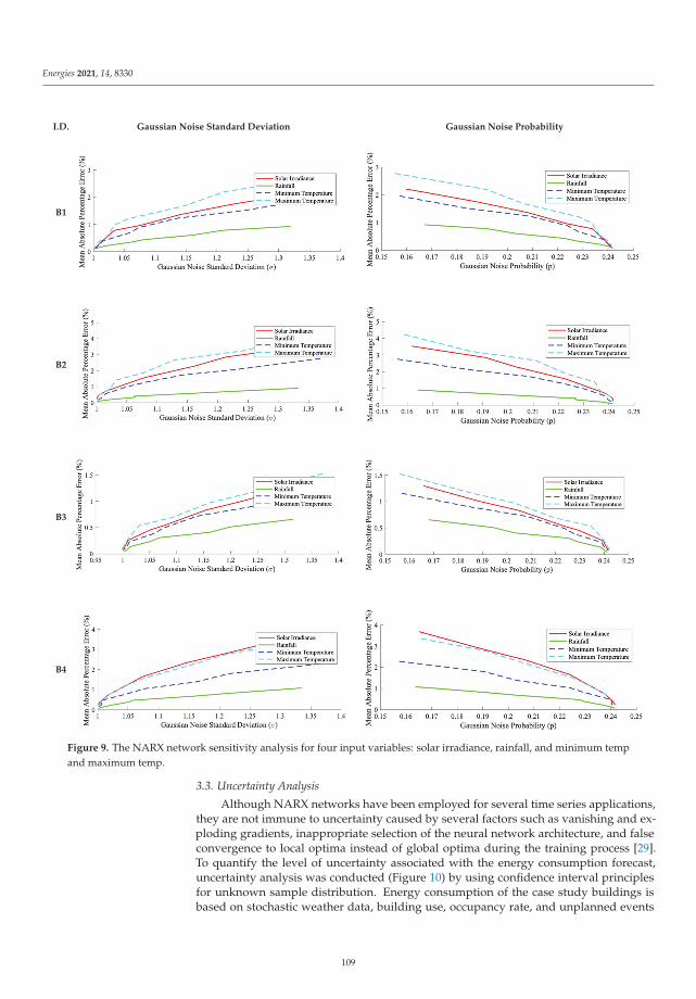
Energies 2021, 14, 8330

I.D. Gaussian Noise Standard Deviation Gaussian Noise Probability

B1

B2

B3

B4

Figure 9. The NARX network sensitivity analysis for four input variables: solar irradiance, rainfall, and minimum tempand maximum temp.

3.3. Uncertainty Analysis

Although NARX networks have been employed for several time series applications,they are not immune to uncertainty caused by several factors such as vanishing and ex-ploding gradients, inappropriate selection of the neural network architecture, and falseconvergence to local optima instead of global optima during the training process [29].To quantify the level of uncertainty associated with the energy consumption forecast,uncertainty analysis was conducted (Figure 10) by using confidence interval principlesfor unknown sample distribution. Energy consumption of the case study buildings isbased on stochastic weather data, building use, occupancy rate, and unplanned events

109

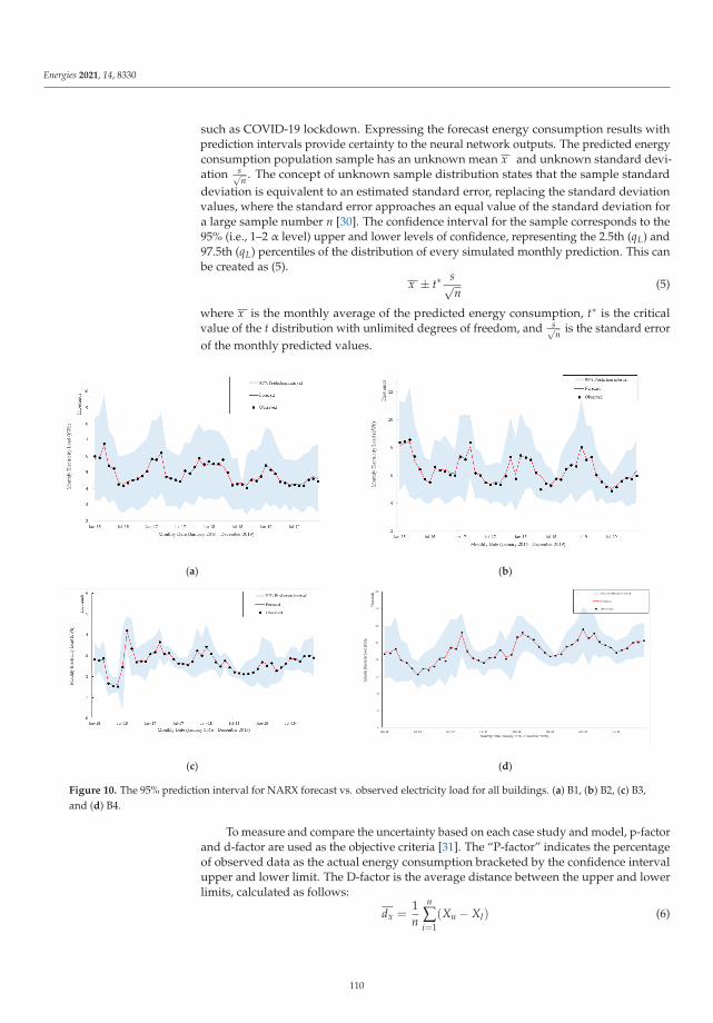
Energies 2021, 14, 8330

such as COVID-19 lockdown. Expressing the forecast energy consumption results withprediction intervals provide certainty to the neural network outputs. The predicted energyconsumption population sample has an unknown mean x and unknown standard devi-ation s√

n . The concept of unknown sample distribution states that the sample standarddeviation is equivalent to an estimated standard error, replacing the standard deviationvalues, where the standard error approaches an equal value of the standard deviation fora large sample number n [30]. The confidence interval for the sample corresponds to the95% (i.e., 1–2 α level) upper and lower levels of confidence, representing the 2.5th (qL) and97.5th (qL) percentiles of the distribution of every simulated monthly prediction. This canbe created as (5).

x ± t∗ s√n

(5)

where x is the monthly average of the predicted energy consumption, t∗ is the criticalvalue of the t distribution with unlimited degrees of freedom, and s√

n is the standard errorof the monthly predicted values.

(a)

(b)

(c)

(d)

Figure 10. The 95% prediction interval for NARX forecast vs. observed electricity load for all buildings. (a) B1, (b) B2, (c) B3,and (d) B4.

To measure and compare the uncertainty based on each case study and model, p-factorand d-factor are used as the objective criteria [31]. The “P-factor” indicates the percentageof observed data as the actual energy consumption bracketed by the confidence intervalupper and lower limit. The D-factor is the average distance between the upper and lowerlimits, calculated as follows:

dx =1n

n

∑i=1

(Xu − Xl) (6)

110

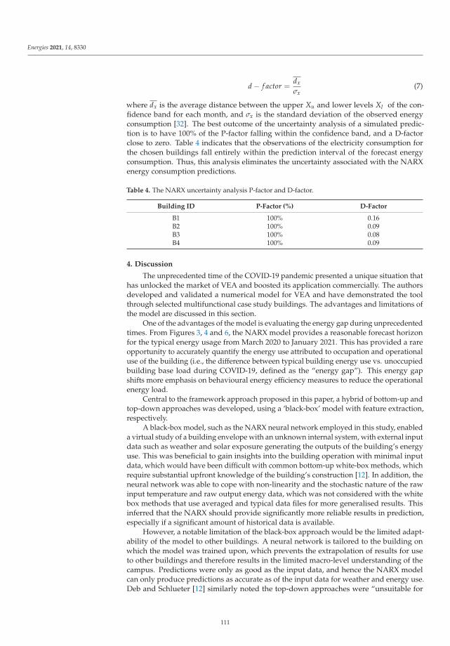
Energies 2021, 14, 8330

d − f actor =dx

σx(7)

where dx is the average distance between the upper Xu and lower levels Xl of the con-fidence band for each month, and σx is the standard deviation of the observed energyconsumption [32]. The best outcome of the uncertainty analysis of a simulated predic-tion is to have 100% of the P-factor falling within the confidence band, and a D-factorclose to zero. Table 4 indicates that the observations of the electricity consumption forthe chosen buildings fall entirely within the prediction interval of the forecast energyconsumption. Thus, this analysis eliminates the uncertainty associated with the NARXenergy consumption predictions.

Table 4. The NARX uncertainty analysis P-factor and D-factor.

Building ID P-Factor (%) D-Factor

B1 100% 0.16B2 100% 0.09B3 100% 0.08B4 100% 0.09

4. Discussion

The unprecedented time of the COVID-19 pandemic presented a unique situation thathas unlocked the market of VEA and boosted its application commercially. The authorsdeveloped and validated a numerical model for VEA and have demonstrated the toolthrough selected multifunctional case study buildings. The advantages and limitations ofthe model are discussed in this section.

One of the advantages of the model is evaluating the energy gap during unprecedentedtimes. From Figures 3, 4 and 6, the NARX model provides a reasonable forecast horizonfor the typical energy usage from March 2020 to January 2021. This has provided a rareopportunity to accurately quantify the energy use attributed to occupation and operationaluse of the building (i.e., the difference between typical building energy use vs. unoccupiedbuilding base load during COVID-19, defined as the “energy gap”). This energy gapshifts more emphasis on behavioural energy efficiency measures to reduce the operationalenergy load.

Central to the framework approach proposed in this paper, a hybrid of bottom-up andtop-down approaches was developed, using a ‘black-box’ model with feature extraction,respectively.

A black-box model, such as the NARX neural network employed in this study, enableda virtual study of a building envelope with an unknown internal system, with external inputdata such as weather and solar exposure generating the outputs of the building’s energyuse. This was beneficial to gain insights into the building operation with minimal inputdata, which would have been difficult with common bottom-up white-box methods, whichrequire substantial upfront knowledge of the building’s construction [12]. In addition, theneural network was able to cope with non-linearity and the stochastic nature of the rawinput temperature and raw output energy data, which was not considered with the whitebox methods that use averaged and typical data files for more generalised results. Thisinferred that the NARX should provide significantly more reliable results in prediction,especially if a significant amount of historical data is available.

However, a notable limitation of the black-box approach would be the limited adapt-ability of the model to other buildings. A neural network is tailored to the building onwhich the model was trained upon, which prevents the extrapolation of results for useto other buildings and therefore results in the limited macro-level understanding of thecampus. Predictions were only as good as the input data, and hence the NARX modelcan only produce predictions as accurate as of the input data for weather and energy use.Deb and Schlueter [12] similarly noted the top-down approaches were “unsuitable for

111

Energies 2021, 14, 8330

individual building retrofits”, hindering the proportioning of the total consumption intoenergy end uses.

The NARX model was supplemented by the top-down ‘feature extraction method’represented in the sensitivity analysis to determine the influential factors causing thevariations of energy consumption based on the case study buildings’ ages and envelopematerial. The sensitivity analysis prioritised the input data variables required in thedescription of the building energy consumption, as well as reducing the training time ofthe NARX model. In this study, the most influential variables to the buildings’ energyconsumption were hourly meteorological maximum temperature and solar irradiance, asshown earlier in Figure 9.

This combination of the two approaches has enabled the VEA to avoid the uncer-tainty inherited from the bottom-up aggregated simplified approaches and to gain anunderstanding of the interactions of the building beyond the black box limitations.

Further work could be conducted to examine the resiliency of each building, byexpanding the envelope of these influential variables to account for more extreme climatescenarios. This could provide valuable insight into how a building would react in itscurrent form in such scenarios and guide future retrofit priorities and design more tailoredand sustainable energy conservation measures.

5. Conclusions

The unprecedented time of the COVID-19 pandemic presented a unique situation thathas unlocked the market of VEA and boosted its application commercially. The authors de-veloped and validated a numerical model for VEA and have demonstrated the tool througha case study of multifunctional educational buildings. The advantages and limitations ofthe model have been elaborated in detail. The key opportunity presented was to evaluatethe “operational energy” over a significant amount of time which encompassed all four sea-sons in continuity (i.e., the difference between typical building energy use vs. unoccupiedbuilding base load during COVID-19 as demonstrated in [33]). In this paper, a combinationof bottom-up (‘black-box’ model) and top-down (‘feature extraction’) approaches wereemployed to conduct the VEA. This combination reduced the inherent uncertainty fromtypical bottom-up aggregated simplified approaches under similar data collection scenariosand provides meaningful insight into the behaviour of the building beyond employingonly the single ‘black-box’ methodology. A neural network model has limited applicabilitysince it is tailored using the data attributed to that specific building. Supplementing theNARX model with a separate top-down approach (i.e., the sensitivity analysis) identifiedthe most influential factors defining the variations of energy consumption, which not onlyoptimised model performance but provided insight for where to target ECM activity foreach building.

Author Contributions: Conceptualisation; B.R., A.M., P.N. and N.W., methodology; A.M., N.W., M.T.and P.N., software; A.M. and N.W., validation; B.R., A.M. and N.W., formal analysis; M.T., N.W.and P.N., investigation; A.M. and P.N., resources; A.M. and P.N., data curation; A.M., P.N. and P.Z.,writing—original draft; A.M., P.N., N.W., M.T., P.Z. and T.C., writing—review and editing; B.R. andN.W., visualization; A.M., M.T., N.W. and T.C., supervision; B.R. All authors have read and agreed tothe published version of the manuscript.

Funding: This research received no external funding.



Data Availability Statement: Data used in this article are publicly available through the University ofMelbourne Sustainable Campus initiative using Clariti. https://sustainablecampus.unimelb.edu.au,accessed on 1 May 2021.

Acknowledgments: This work was conducted within the Department of Infrastructure Engineeringas a part of the ongoing energy assessment of the university campus. The authors would like to

112

Energies 2021, 14, 8330

thank the University of Melbourne Campus Services for providing raw data for energy consumptionand occupancy density.


References

1. IEA. Net Zero by 2050; IEA: Paris, France, 2021. Available online: https://iea.blob.core.windows.net/assets/deebef5d-0c34-4539-9d0c-10b13d840027/NetZeroby2050-ARoadmapfortheGlobalEnergySector_CORR.pdf (accessed on 15 October 2021).

2. Castro-Alvarez, F.; Vaidyanathan, S.; Bastian, H.; King, J. The 2018 International Energy Efficiency Scorecard; American Council foran Energy-Efficient Economy: Washington, DC, USA, 2018.

3. Victoria, T.P.O. Climate Change Act 2017; Legislation Victoria, 2017. Available online: https://www.climatechange.vic.gov.au/legislation/climate-change-act-2017 (accessed on 15 October 2021).

4. Cronin, J.; Anandarajah, G.; Dessens, O. Climate change impacts on the energy system: A review of trends and gaps. Clim. Chang.2018, 151, 79–93. [CrossRef] [PubMed]

5. Akhmat, G.; Zaman, K.; Shukui, T.; Sajjad, F. Does energy consumption contribute to climate change? Evidence from majorregions of the world. Renew. Sustain. Energy Rev. 2014, 36, 123–134. [CrossRef]

6. Australia, S. Energy Audits Commercial Buildings AS/NZS 3598.1:2014; Standards Australia: Sydney, Australia, 2014.7. Austin, D. Addressing Market Barriers to Energy Efficiency in Buildings; Working Papers 43476; Congressional Budget Office: Wash-

ington, DC, USA, 2012. Available online: https://ideas.repec.org/p/cbo/wpaper/43476.html (accessed on 15 October 2021).8. Joshi, A.; Mundada, A.; Suryavanshi, Y.; Kurulekar, M.; Ranade, M.; Jadhav, S.; Patil, K.; Despande, Y. Performance Assessment of

Building by Virtual Energy Audit. In Proceedings of the 2018 International Conference and Utility Exhibition on Green Energyfor Sustainable Development (ICUE), Phuket, Thailand, 24–26 October 2018.

9. Glick, M.B.; Peppard, E.; Meguro, W. Analysis of Methodology for Scaling up Building Retrofits: Is There a Role for VirtualEnergy Audits?—A First Step in Hawai’i, USA. Energies 2021, 14, 5914. [CrossRef]

10. Cowan, J.; Pearson, R.; Sud, I. Procedures for Commercial Building Energy Audits; American Society of Heating; Ashrae: New York,NY, USA, 2004; ISBN 9781936504091. Available online: https://www.techstreet.com/standards/procedures-for-commercial-building-energy-audits-2nd-edition?product_id=1809206#product (accessed on 15 October 2021).

11. Avina, J.M.; Rottmayer, S.P. Virtual Audits: The Promise and The Reality. Energy Eng. 2016, 113, 34–52. [CrossRef]12. Deb, C.; Schlueter, A. Review of data-driven energy modelling techniques for building retrofit. Renew. Sustain. Energy Rev. 2021,

144, 110990. [CrossRef]13. Li, A.; Xiao, F.; Fan, C.; Hu, M. Development of an ANN-based building energy model for information-poor buildings using

transfer learning. Build. Simul. 2021, 14, 89–101. [CrossRef]14. Hosgör, E.; Fischbeck, P.S. Virtual home energy auditing at scale: Predicting residential energy efficiency using publicly available

data. Energy Build. 2015, 92, 67–80. [CrossRef]15. Deb, C.; Lee, S.E.; Santamouris, M. Using artificial neural networks to assess HVAC related energy saving in retrofitted office

buildings. Sol. Energy 2018, 163, 32–44. [CrossRef]16. Roessler, F.; Teich, T.; Franke, S. Neural Networks for Smart Homes and Energy Efficiency. In DAAAM International Scientific Book;

DAAAM International Publishing: Vienna, Austria, 2012; Chapter 26; pp. 305–314. [CrossRef]17. Kumar, R.; Aggarwal, R.K.; Sharma, J.D. Energy analysis of a building using artificial neural network: A review. Energy Build.

2013, 65, 352–358. [CrossRef]18. Kluczek, A.; Olszewski, P. Energy audits in industrial processes. J. Clean. Prod. 2017, 142, 3437–3453. [CrossRef]19. Park, S.K.; Moon, H.J.; Min, K.C.; Hwang, C.; Kim, S. Application of a multiple linear regression and an artificial neural network

model for the heating performance analysis and hourly prediction of a large-scale ground source heat pump system. Energy Build.2018, 165, 206–215. [CrossRef]

20. Zhu, Y. Applying computer-based simulation to energy auditing: A case study. Energy Build. 2006, 38, 421–428. [CrossRef]21. Wang, Z.; Wang, Y.; Zeng, R.; Srinivasan, R.S.; Ahrentzen, S. Random Forest based hourly building energy prediction. Energy

Build. 2018, 171, 11–25. [CrossRef]22. Sarker, I.H. Machine Learning: Algorithms, Real-World Applications and Research Directions. SN Comput. Sci. 2021, 2, 160.

[CrossRef]23. Koseleva, N.; Ropaite, G. Big Data in Building Energy Efficiency: Understanding of Big Data and Main Challenges. Procedia Eng.

2017, 172, 544–549. [CrossRef]24. University of Melbourne. Sustainability Report 2020; The University of Melbourne: Melbourne, Austria, 2017; p. 42.25. Kreider, J.F.; Claridge, D.E.; Curtiss, P.; Dodier, R.; Haberl, J.S.; Krarti, M. Building Energy Use Prediction and System Identification

Using Recurrent Neural Networks. J. Sol. Energy Eng. 1995, 117, 161–166. [CrossRef]26. Boussaada, Z.; Curea, O.; Remaci, A.; Camblong, H.; Meabet Bellaaj, N. A Nonlinear Autoregressive Exogenous (NARX) Neural

Network Model for the Prediction of the Daily Direct Solar Radiation. Energies 2018, 11, 620. [CrossRef]27. Azadeh, A.; Ghaderi, S.F.; Sohrabkhani, S. Forecasting electrical consumption by integration of Neural Network, time series and

ANOVA. Appl. Math. Comput. 2007, 186, 1753–1761. [CrossRef]28. Tian, W. A review of sensitivity analysis methods in building energy analysis. Renew. Sustain. Energy Rev. 2013, 20, 411–419.

[CrossRef]

113

Energies 2021, 14, 8330

29. Bhattacharyya, B.; Jacquelin, E.; Brizard, D. A Kriging-NARX Model for Uncertainty Quantification of Nonlinear StochasticDynamical Systems in Time Domain. J. Eng. Mech. 2020, 146, 04020070. [CrossRef]

30. Hayter, A.J. Simultaneous Confidence Intervals for Several Quantiles of an Unknown Distribution. Am. Stat. 2014, 68, 56–62.[CrossRef]

31. Mikayilov, F.; Johnson, C.; Van Genuchten, M. Estimating Uncertain Flow and Transport Parameters Using A SequentialUncertainty Fitting Procedure. Vadose Zone J. 2004, 3, 1340–1352.

32. Talebizadeh, M.; Moridnejad, A. Uncertainty analysis for the forecast of lake level fluctuations using ensembles of ANN andANFIS models. Expert Syst. Appl. 2011, 38, 4126–4135. [CrossRef]

33. Li, S.; Foliente, G.; Seo, S.; Rismanchi, B.; Aye, L. Multi-scale life cycle energy analysis of residential buildings in Victoria,Australia–A typology perspective. Build. Environ. 2021, 195, 107723. [CrossRef]

114

Citation: Mezquita, Y.; Gil-González,

A.B.; Martín del Rey, A.; Prieto, J.;

Corchado, J.M. Towards a

Blockchain-Based Peer-to-Peer

Energy Marketplace. Energies 2022,

15, 3046. https://doi.org/10.3390/

en15093046

Academic Editor: Mohamed

Benbouzid

Received: 3 March 2022

Accepted: 19 April 2022

Published: 21 April 2022




iations.








4.0/).

energies

Article

Towards a Blockchain-Based Peer-to-Peer Energy Marketplace

Yeray Mezquita 1,*, Ana Belén Gil-González 1, Angel Martín del Rey 2, Javier Prieto 1 and Juan Manuel Corchado 1

1 BISITE Research Group, University of Salamanca, 37007 Salamanca, Spain; [email protected] (A.B.G.-G.);[email protected] (J.P.); [email protected] (J.M.C.)

2 Department of Applied Mathematics, Institute of Fundamental Physics and Mathematics, University ofSalamanca, 37008 Salamanca, Spain; [email protected]

* Correspondence: [email protected]

Abstract: Blockchain technology is used as a distributed ledger to store and secure data and performtransactions between entities in smart grids. This paper proposes a platform based on blockchaintechnology and the multi-agent system paradigm to allow for the creation of an automated peer-to-peer electricity market in micro-grids. The use of a permissioned blockchain network has multiplebenefits as it reduces transaction costs and enables micro-transactions. Moreover, an improvementin security is obtained, eliminating the single point of failure in the control and management ofthe platform along with creating the possibility to trace back the actions of the participants and amechanism of identification. Furthermore, it provides the opportunity to create a decentralized anddemocratic energy market while complying with the current legislation and regulations on userprivacy and data protection by incorporating Zero-Knowledge Proof protocols and ring signatures.

Keywords: blockchain; energy market; multi-agent system; negotiation; distributed ledger technology

1. Introduction

The current traditional power grid is designed to transport energy over long distances.This characteristic of the traditional system implies that certain limitations exist, such asthe maximum voltage capacity supported by the distribution lines [1]. When this capacityis exceeded, the heat generated by a line can cause it to sag or break, resulting in powersupply instabilities such as phase and voltage fluctuations. Because the capacity of a linedepends on its length and the transmission voltage, one solution is to create shorter linesand distribute the functionalities of the current power grid in smaller smart networks.These networks are called smart micro-grids, which are a type of discrete energy systemthat includes appropriated energy sources as well as power loads that provide power toresidential, commercial, industrial, and governmental consumers. The main purpose ofsmart micro-grids is to provide affordable energy to areas independently of the main powersupply network while optimizing the transmission of the energy.

In the current context of energy generation, thanks to renewable sources such assolar or wind, and together with the emergence of a new type of actor that consumesand produces energy within the system—the so-called prosumers—micro-grids have thepotential to replace the traditional energy transmission system in the near future [2]. How-ever, the rise of smart micro-grids comes with some challenges that must be faced. Thesechallenges range from the vulnerability of platforms to DDOS attacks, to the emergenceof intermediaries that do not contribute to energy distribution but end up making it moreexpensive [3].

In the past, some authors have proposed strategies for energy management on micro-grid platforms. For example, in [4], the excess or shortage of energy could be compensatedby exchanging it with the utility grid or other external sources. However, that paper did notallow for direct energy exchange between individuals, nor did it allow for the automationand distribution of the platform. Without the use of blockchain technology, democratized


Energies 2022, 15, 3046

energy markets could not be created. A blockchain network acts as a reliable distributedledger that is governed by the platform and where information of value is stored. Thenetwork can be utilized to distribute the control and governance of the smart grid, alongwith the communication that is carried out within it, thus avoiding the single point offailure and eliminating those intermediaries that do not give any value to the platform.Moreover, blockchain technology (BT) provides a mechanism for protecting the actorsagainst identity theft by signing direct communications between peers [5].

After studying the literature on this topic, it was found that none of the works had beenable to propose a truly decentralized platform that enables peer-to-peer energy trading,automatically, and with dynamic prices. For this reason, we propose a distributed Multi-Agent System (MAS) based on blockchain technology to enable decentralized controlover a micro-grid platform that allows for an automated exchange of energy betweenits actors. In the proposed system, the MAS manages the workflow of the micro-grid,e.g., the negotiations between peers in the local market, or the correct balancing of theenergy network. By using a blockchain network, the control of the platform is distributedbetween the agents while the resilience of the communication channel between them isimproved. This allows for the deployment of a platform without a single point of failure.Moreover, existing research works do not take into consideration users’ anonymity andprivacy, something that we would also like to tackle with the proposed framework.

This paper shows a thorough study of the most important features of blockchaintechnology and smart micro-grids in Section 2. Section 3 studies how previous works inthe literature tackle the challenges of using blockchain technology in smart micro-grids.Furthermore, the section studies how automated negotiation between machines could beachieved and its viability. Section 4 describes the proposed platform, which is a combinationof a MAS and a blockchain network for improved decentralization, as well as the securityof the platform, along with the viability of the creation of a local automated energy marketthat optimizes the payoffs for the micro-grid stakeholders. Finally, Section 5 draws upconclusions and some final remarks on the conducted research.

Contributions

This work is relevant for designers, developers, and practitioners alike who are work-ing in the field of energy distribution and renewable energy adoption and who will getthe most benefits from the proposed framework. The main contributions of this paper areas follows:

• The design of a framework that will help developers to create new platforms that allowfor the appearance of automatic peer-to-peer energy markets with dynamic prices.

• The proposed framework also provides user flexibility in the negotiation algorithmsused. They will be able to implement the algorithm they want depending on theirneeds, with the only prerequisite being that the communications between agentsfollow the same ontology.

• The framework designed also provides anonymity to their users, complying with thecurrent data regulations.

• Following the proposed framework, the future platforms developed and deployedwill be more democratic and decentralized, thus eliminating the single point of failure.

2. Conceptual Foundations of Micro-Grid Platforms and Blockchain Technology

Traditional power grids deliver energy from a few central generators to a large numberof consumers. This creates a closed market in which energy prices are dictated in amonopolistic way. Sometimes, to avoid abusive pricing by companies towards consumers,states need to implement regulatory measures, with the European Union [6,7] being anexample in this case.

116

Energies 2022, 15, 3046

In the face of this monopolistic behavior, the literature has proposed the distributionof the traditional main grid into smaller micro-grids [2]. These micro-grids are comprisedof a set of loads and generators. The set of generators can be composed of individualhouses with solar panels on the roof. The entry of more entities into the energy marketreduces the risk of oligopolies and avoids the intervention of states by imposing the use ofregularization measures. This way, the energy market is converted into a more democraticmarket in which the offer and demand of energy will be the only factors that can regulatethe energy price.

Micro-grid platforms make use of a great number of Internet of Things (IoT) devicesthat exchange crucial information between them. The continuous communication betweenthe devices allows for the distribution of the management and control of any IoT platform.This helps with the optimization of the workflow of the system, but not without somedrawbacks [8].

• Heavy reliance on exchanged messages. Since each part of the system is controlledby an independent entity, the other entities have to trust the messages received tounderstand the system’s global state. If a malicious entity could somehow modifythe content of those messages, the proper functioning of the entire platform wouldbe compromised.

• Reliance on the truthfulness of the transmitted data. Entities of the platform have torely on the fact that the data transmitted have not been tampered with by the senderentity to make an unfair profit. In addition, it is a possibility that databases will beattacked in order to steal, modify, or delete sensitive information about the entitiesthat are taking part in the system’s workflow.

In the literature, the use of BT has been proposed to overcome the listed flaws of thiskind of platform. BT consists of a peer-to-peer (P2P) network of nodes, governed by a con-sensus algorithm that dictates how the information is stored within the network. This tech-nology allows for the creation of a distributed ledger where anything of value can be stored.

The use of a blockchain network within any IoT system makes it possible to distributethe process workflow while eliminating other centralized entities [8]. In addition, byeliminating the single point of failure factor of centralized platforms, protection againstsome traditional forms of cyberattacks is gained. In this way, the blockchain is used as abulletin where important information about the system is stored. Furthermore, the datastored within the blockchain network are kept in the same state after their storage, whichmeans that the information is tamper-proof [9].

Within a blockchain-based system, a cryptographic mechanism of pairs of asymmet-ric keys is used, which signs and encrypts the data transmitted. Hence, as long as theblockchain network is big enough, the consensus algorithm keeps the information in aconsistent state [10], the keys are not compromised, and the information transmitted andstored is secure from any attack, thus maintaining its integrity and authorship [11]. If thismechanism is also used in the exchange of messages between individuals of the system,then the messages are protected from being read and modified by unauthorized thirdparties [12].

A user needs to generate a random private key to make use of a blockchain protocol.This key is usually part of a cryptography mechanism that uses a key pair mechanism:the random private key mentioned and a public one derived from that. This public-keycryptography mechanism is used, not only because they allow for an efficient managementof the keys, but also because it is impossible for an attacker to obtain the private key evenwhen knowing the public one.

To interact with a blockchain protocol, an individual needs to generate at least onewallet address as an identifier. It is a three-step process, which starts with the generationof a random private key that only the owner should know. Then, through a one-wayalgorithmic transformation, the public key is obtained, which is shared with the networkand is used to verify the signatures made by the user with their private key. Finally, the

117

Energies 2022, 15, 3046

public key is hashed in order to obtain the wallet address to be used in the exchange ofvirtual assets between individuals within the blockchain protocol.

The process of exchanging assets is quite straightforward and shares the same steps asin every blockchain. Figure 1 illustrates how a user, Alice, wants to initiate a transactionwith Bob with 2 coins. To do that, Alice signs the transaction (Tx) with her private key andbroadcasts it in the network. Then, each node of the network verifies Alice’s signature withher public key, and if the check is correct and the transaction is proven to have come fromAlice, the network validates that she has the coins she wants to spend. If everything goeswell, the transaction will be added to the blockchain.

Figure 1. Example of the signature mechanism in a transaction.

2.1. Blockchain Consensus Algorithms

A consensus algorithm describes the mechanism that allows all agents in the systemto coordinate in a distributed environment. It constitutes the only source of truth. Thanksto the consensus algorithm employed by the network of nodes, it is possible to keepthe information stored and replicated in a consistent state. Among the functions of anyconsensus algorithm is ensuring that there is only one blockchain in the system, which canbe an issue when a part of the network accepts a blockchain while the remaining nodesaccept a different one (Fork). The consensus algorithm should enable the convergence ofthe chains into one as soon as possible. Moreover, it should offer resilience against attemptsby malicious actors to take over the network and guarantee that there will not be anyconsensus failure when nodes try to add new blocks of data to the blockchain. Keeping thedata stored in a blockchain makes it more difficult for attackers to take down the servicesof a system, and the attacker is forced to take down the majority of them to successfullyhack the data [8].

There is a great variety of consensus algorithms, including the Proof of Work (PoW),Proof of Stake (PoS), and Practical Byzantine Fault Tolerance (PBFT) (see Table 1), or anyof their variants that are the most widespread and have proven their effectiveness inpractice [13].

118

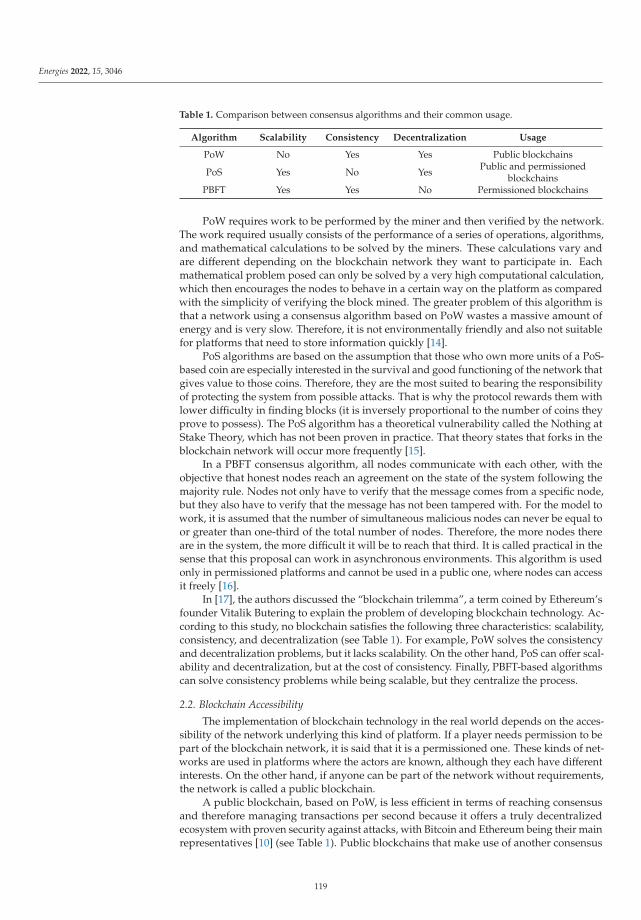
Energies 2022, 15, 3046

Table 1. Comparison between consensus algorithms and their common usage.

Algorithm Scalability Consistency Decentralization Usage

PoW No Yes Yes Public blockchains

PoS Yes No Yes Public and permissionedblockchains

PBFT Yes Yes No Permissioned blockchains

PoW requires work to be performed by the miner and then verified by the network.The work required usually consists of the performance of a series of operations, algorithms,and mathematical calculations to be solved by the miners. These calculations vary andare different depending on the blockchain network they want to participate in. Eachmathematical problem posed can only be solved by a very high computational calculation,which then encourages the nodes to behave in a certain way on the platform as comparedwith the simplicity of verifying the block mined. The greater problem of this algorithm isthat a network using a consensus algorithm based on PoW wastes a massive amount ofenergy and is very slow. Therefore, it is not environmentally friendly and also not suitablefor platforms that need to store information quickly [14].

PoS algorithms are based on the assumption that those who own more units of a PoS-based coin are especially interested in the survival and good functioning of the network thatgives value to those coins. Therefore, they are the most suited to bearing the responsibilityof protecting the system from possible attacks. That is why the protocol rewards them withlower difficulty in finding blocks (it is inversely proportional to the number of coins theyprove to possess). The PoS algorithm has a theoretical vulnerability called the Nothing atStake Theory, which has not been proven in practice. That theory states that forks in theblockchain network will occur more frequently [15].

In a PBFT consensus algorithm, all nodes communicate with each other, with theobjective that honest nodes reach an agreement on the state of the system following themajority rule. Nodes not only have to verify that the message comes from a specific node,but they also have to verify that the message has not been tampered with. For the model towork, it is assumed that the number of simultaneous malicious nodes can never be equal toor greater than one-third of the total number of nodes. Therefore, the more nodes thereare in the system, the more difficult it will be to reach that third. It is called practical in thesense that this proposal can work in asynchronous environments. This algorithm is usedonly in permissioned platforms and cannot be used in a public one, where nodes can accessit freely [16].

In [17], the authors discussed the “blockchain trilemma”, a term coined by Ethereum’sfounder Vitalik Butering to explain the problem of developing blockchain technology. Ac-cording to this study, no blockchain satisfies the following three characteristics: scalability,consistency, and decentralization (see Table 1). For example, PoW solves the consistencyand decentralization problems, but it lacks scalability. On the other hand, PoS can offer scal-ability and decentralization, but at the cost of consistency. Finally, PBFT-based algorithmscan solve consistency problems while being scalable, but they centralize the process.

2.2. Blockchain Accessibility

The implementation of blockchain technology in the real world depends on the acces-sibility of the network underlying this kind of platform. If a player needs permission to bepart of the blockchain network, it is said that it is a permissioned one. These kinds of net-works are used in platforms where the actors are known, although they each have differentinterests. On the other hand, if anyone can be part of the network without requirements,the network is called a public blockchain.

A public blockchain, based on PoW, is less efficient in terms of reaching consensusand therefore managing transactions per second because it offers a truly decentralizedecosystem with proven security against attacks, with Bitcoin and Ethereum being their mainrepresentatives [10] (see Table 1). Public blockchains that make use of another consensus

119

Energies 2022, 15, 3046

algorithm, such as PoS or any of its variants, are far more efficient, although they losesome consistency. Blockchain networks that use PBFT-based consensus algorithms couldonly be used in permissioned environments because they lose decentralization in favor ofscalability; to have consistency, it is required that the actors are known.

2.3. Smart Contracts

Another relevant aspect of some blockchain technologies is that they allow for thedeployment and execution of coded scripts called smart contracts. Those scripts, due to theimmutability feature of the blockchain technology, are considered self-enforcing and areused to automatize some processes, such as payments between entities within a platformthat would otherwise need human intervention and/or that of third parties [18]. The codeof smart contracts is transparent to the players that can make use of it, which means thatthey know the programmed clauses that rule it. Then, when those parties agree to use asmart contract, the workflow of the interactions between them is governed by the rulescoded in the smart contract, all without the need for human hands to verify the process [19].A smart contract ensures that the agreement will be carried out automatically when theconditions agreed upon are met [20].

3. Related Work on Micro-Grid Platforms Based on BT

Blockchain technology has been used to improve the performance of a broad rangeof platforms in today’s industries. The state of the art encompasses, to enumerate afew examples, the pharmaceutical industry [21,22], the agri-food sector [23,24] as well ashealthcare [8,25–27] and education services [28–30].

In this section, we will detail a small study on the state of the art related to the useof blockchain technology in the field of micro-grid platforms. Then, it will be followedby a study on the automatic negotiation algorithms that have been proposed in order tounderstand the requirements that need to be implemented in this type of platform.

3.1. Blockchain Technology and Micro-Grid Platforms

In the literature, we found some works that discussed the use of blockchain-based micro-grid platforms to create energy markets, focusing on specific characteristics such as the use ofcryptocurrencies, decentralization, security, privacy, and state estimations [12,31–34].

Pichler et al. [35] studied real-world use cases of platforms based on blockchaintechnology and whose aim was to allow for the direct exchange of energy between itsactors. The platforms studied have a general common aim: to create local markets basedon renewable energy communities. However, they share the same cons: they do not try tocreate an autonomous market, and they do not offer real anonymity and privacy to theirusers (see Table 2).

A working example is the Pylon network [36], a Spanish startup that makes use of itspermissioned blockchain-based Litecoin technology combined with a smart meter to certifyenergy flows and enable virtual transactions with the use of their own token. It makes useof a Proof of Cooperation (PoC) consensus algorithm, and its main aim is to create a neutraldatabase, one that is not governed by the companies that sell the energy,in order to helpthe user decide how to optimize the energy costs. They made their platform open sourceto receive help from the community in case any kind of improvement is needed for theirnetwork. In Slovenia, SunContract [37] has created a market for peer-to-peer transactionsof energy based on BT. They launched a crypto-asset within the Ethereum network inorder to use it in the exchange of energy between the entities that are participating in theplatform. On the other hand, there is Enosi [38], an Australian company whose aim issimilar to that of SunContract: to create a community of peers transacting energy directlybetween them. By using smart metering, they trace, match, and settle energy productionand consumption. Because of the platform, the producers can directly offer a price to theend consumer, with cheaper prices instead of the artificial ones that the power oligopolieshave in the traditional energy market.

120

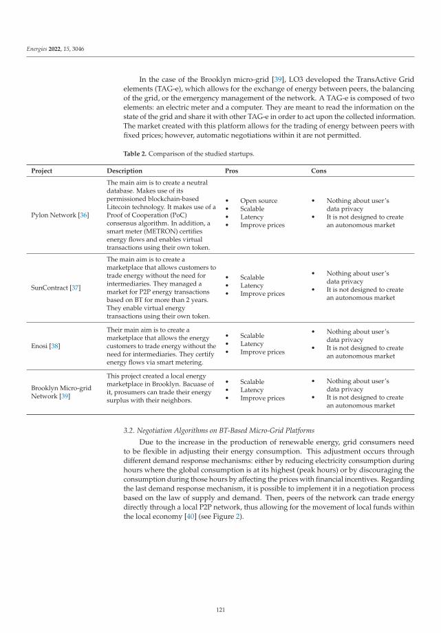
Energies 2022, 15, 3046

In the case of the Brooklyn micro-grid [39], LO3 developed the TransActive Gridelements (TAG-e), which allows for the exchange of energy between peers, the balancingof the grid, or the emergency management of the network. A TAG-e is composed of twoelements: an electric meter and a computer. They are meant to read the information on thestate of the grid and share it with other TAG-e in order to act upon the collected information.The market created with this platform allows for the trading of energy between peers withfixed prices; however, automatic negotiations within it are not permitted.

Table 2. Comparison of the studied startups.

Project Description Pros Cons

Pylon Network [36]

The main aim is to create a neutraldatabase. Makes use of itspermissioned blockchain-basedLitecoin technology. It makes use of aProof of Cooperation (PoC)consensus algorithm. In addition, asmart meter (METRON) certifiesenergy flows and enables virtualtransactions using their own token.

• Open source• Scalable• Latency• Improve prices

• Nothing about user’sdata privacy

• It is not designed to createan autonomous market

SunContract [37]

The main aim is to create amarketplace that allows customers totrade energy without the need forintermediaries. They managed amarket for P2P energy transactionsbased on BT for more than 2 years.They enable virtual energytransactions using their own token.

• Scalable• Latency• Improve prices



Enosi [38]

Their main aim is to create amarketplace that allows the energycustomers to trade energy without theneed for intermediaries. They certifyenergy flows via smart metering.




Brooklyn Micro-gridNetwork [39]

This project created a local energymarketplace in Brooklyn. Bacuase ofit, prosumers can trade their energysurplus with their neighbors.




3.2. Negotiation Algorithms on BT-Based Micro-Grid Platforms

Due to the increase in the production of renewable energy, grid consumers needto be flexible in adjusting their energy consumption. This adjustment occurs throughdifferent demand response mechanisms: either by reducing electricity consumption duringhours where the global consumption is at its highest (peak hours) or by discouraging theconsumption during those hours by affecting the prices with financial incentives. Regardingthe last demand response mechanism, it is possible to implement it in a negotiation processbased on the law of supply and demand. Then, peers of the network can trade energydirectly through a local P2P network, thus allowing for the movement of local funds withinthe local economy [40] (see Figure 2).

121

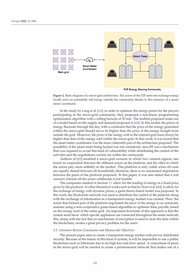
Energies 2022, 15, 3046

Figure 2. Basic diagram of a micro-grid architecture. The actors of the P2P network exchange energylocally and can potentially sell energy outside the community thanks to the existence of a smartmeter coordinator.

In the study by Long et al. [41], in order to optimize the energy prizes for the playersparticipating in the micro-grid community, they proposed a non-linear programmingoptimization algorithm with a rolling horizon of 30 min. The method proposed made useof a model based on the supply and demand proposed in [42]. In this model, the prices ofenergy fluctuate through the day, with a constraint that the price of the energy generatedwithin the micro-grid should never be higher than the price of the energy bought fromoutside the grid. Moreover, the prize of the energy sold to the external grid must always behigher than that of the energy sold within the micro-grid. In this work, it was found thatthe smart meter coordinator was the most vulnerable part of the architecture proposed. Thepossibility of the smart meter being hacked was not considered, since BT was a mechanismthat was required to avoid this kind of vulnerability while distributing the control of theactivities and the negotiations carried out within the community.

Authors of [43] modeled a micro-grid scenario in which two variants appear, onebased on cooperation between the different actors on the platform, and the other in whichthe actors play more selfishly in the market. This platform is only viable when all costsare equally shared between all households; therefore, there is no automated negotiationbetween the peers of the platform proposed. In this paper, it was also stated that a realscenario wherein all the actors collaborate is not feasible.

The companies studied in Section 3.1 allow for the trading of energy at a fixed pricegiven by the producer. In other theoretical works such as that by Noor et al. [44], to allow forthe exchange of energy with dynamic prizes, a game theory-based model was proposed. Inthis work, the blockchain network was used to distribute the control of the platform alongwith the exchange of information as a transparent energy market was created. Here, theactors that formed part of the platform negotiated the price of the energy in an automaticmanner using a non-cooperative game-based algorithm to optimize their payoffs, basedon the energy load of the entire grid. An important downside of this approach is that thesystem must know which specific appliances are connected throughout the entire network;this, along with the fact that no mechanism of encryption is used to store the data withinthe blockchain, creates a great privacy problem for the users.

3.3. Literature Review Conclusions and Manuscript Objectives

The present paper aims to create a transparent energy market with proven distributedsecurity. Because of the nature of this kind of system, it will be impossible to use a publicblockchain such as Ethereum due to its high fees and slow speed. A consortium of peersin the micro-grid will be needed to create a permissioned network that makes use of a

122

Energies 2022, 15, 3046

protocol such as PBFT, PoS, or dPOS, where it is assumed that all the network’s participantsare known and have the common goal of wanting the platform to work.

One of the features that the companies studied are lacking is the use of an automatic ne-gotiation between the players of each platform. Our model makes use of a non-cooperativegame between the consumers and producers that will regulate the energy market price inan autonomous way, thus allowing the stakeholders optimize their payoffs. Our modeland its interactions with the blockchain are thoroughly explained to help startups and en-trepreneurs to develop this kind of system. Furthermore, the scenario proposed in our workis based on a rolling horizon such as the one proposed by Long et al. [41], but with a timewindow of an hour to make the transactions more viable in the actual Ethereum network.

In the literature, compliance with the General Data Protection Regulation (GDPR) [45]has been found to be an important issue. Because of this, a careful selection of which dataare to be collected and stored in the public ledger is needed, as well as which data mustbe encrypted and hidden from unauthorized peers. Moreover, ensuring the integrity andauthenticity of the data is required by protecting it and the communication channels fromunauthorized users [35]. Another issue of the proposed platform is its heavy dependenceon the legislative framework of the country where it is to be installed. Laws that regulatethe transaction of renewable energy between peers within communities are needed, suchas in the case of Belgium, Greece, and Germany [35].

4. Proposed Architecture Design

In this section, we will describe the design of the proposed architecture, which aimsto: (i) decentralize the energy market, (ii) automate, as much as possible, the energymarket in small communities, (iii) and provide anonymity and privacy to its users. Inthe literature studied in the Section 3, there are working proposals that meet some of theabove-mentioned requirements, although not all of them together.

The proposed architecture will follow the paradigm of distributed Multi-Agent Sys-tems (MAS), which, in combination with blockchain technology, allows for the distributionof the processes and the control of the platform. The use of multi-agent systems waschosen because other works successfully achieved their main objective with the use of thisparadigm, with the optimization and decentralization of platforms of any kind [46]. In theproposed architecture, features from different works studied in the literature have been puttogether, thus enabling decentralized control over the platform without a single point offailure and allowing for a negotiation process between the peers of the network as well ascomplying with the GDPR.

• Through the MAS, the control and management of the micro-grid platform is achieved,along with the negotiation between peers for energy in the market. However, toachieve full decentralization of the platform, the use of a blockchain platform isrequired, in which the smart contracts deployed will be used by the agents in theworkflow of the platform. Thanks to this approach: (i) we will achieve a decentralizedplatform without a single point of failure; (ii) we will provide confidence to platformusers and agents that agreements would be enforced, and in case they are not, encour-age trust that the platform will compensate those who behave while punishing thoseagents who do not; and (iii) we will allow for the optimization of the prices of theenergy transacted within the platform, balancing them while maximizing the payoffsof each kind of actor involved.

• The smart meters read the energy consumed and/or produced by each household.They are connected to each independent house, representing a peer in the micro-grid network. Each smart meter is connected to the internet and interacts with theblockchain on behalf of the household. Moreover, the agent who negotiates with theirpeers to buy or sell energy should be deployed here or in a device connected to thesmart meter.

• The use of a blockchain network allows for the distribution of the communication andthe interactions between the agents of the platform. The network is used not only as a

123

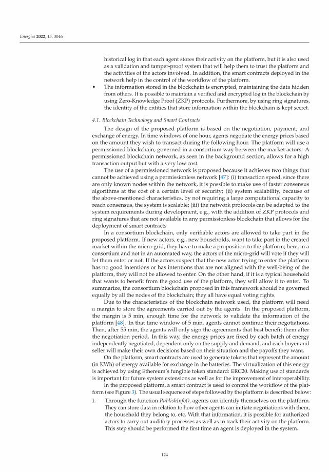
Energies 2022, 15, 3046

historical log in that each agent stores their activity on the platform, but it is also usedas a validation and tamper-proof system that will help them to trust the platform andthe activities of the actors involved. In addition, the smart contracts deployed in thenetwork help in the control of the workflow of the platform.

• The information stored in the blockchain is encrypted, maintaining the data hiddenfrom others. It is possible to maintain a verified and encrypted log in the blockchain byusing Zero-Knowledge Proof (ZKP) protocols. Furthermore, by using ring signatures,the identity of the entities that store information within the blockchain is kept secret.

4.1. Blockchain Technology and Smart Contracts

The design of the proposed platform is based on the negotiation, payment, andexchange of energy. In time windows of one hour, agents negotiate the energy prices basedon the amount they wish to transact during the following hour. The platform will use apermissioned blockchain, governed in a consortium way between the market actors. Apermissioned blockchain network, as seen in the background section, allows for a hightransaction output but with a very low cost.

The use of a permissioned network is proposed because it achieves two things thatcannot be achieved using a permissionless network [47]: (i) transaction speed, since thereare only known nodes within the network, it is possible to make use of faster consensusalgorithms at the cost of a certain level of security; (ii) system scalability, because ofthe above-mentioned characteristics, by not requiring a large computational capacity toreach consensus, the system is scalable; (iii) the network protocols can be adapted to thesystem requirements during development, e.g., with the addition of ZKP protocols andring signatures that are not available in any permissionless blockchain that allows for thedeployment of smart contracts.

In a consortium blockchain, only verifiable actors are allowed to take part in theproposed platform. If new actors, e.g., new households, want to take part in the createdmarket within the micro-grid, they have to make a proposition to the platform; here, in aconsortium and not in an automated way, the actors of the micro-grid will vote if they willlet them enter or not. If the actors suspect that the new actor trying to enter the platformhas no good intentions or has intentions that are not aligned with the well-being of theplatform, they will not be allowed to enter. On the other hand, if it is a typical householdthat wants to benefit from the good use of the platform, they will allow it to enter. Tosummarize, the consortium blockchain proposed in this framework should be governedequally by all the nodes of the blockchain; they all have equal voting rights.

Due to the characteristics of the blockchain network used, the platform will needa margin to store the agreements carried out by the agents. In the proposed platform,the margin is 5 min, enough time for the network to validate the information of theplatform [48]. In that time window of 5 min, agents cannot continue their negotiations.Then, after 55 min, the agents will only sign the agreements that best benefit them afterthe negotiation period. In this way, the energy prices are fixed by each batch of energyindependently negotiated, dependent only on the supply and demand, and each buyer andseller will make their own decisions based on their situation and the payoffs they want.

On the platform, smart contracts are used to generate tokens that represent the amount(in KWh) of energy available for exchange in the batteries. The virtualization of this energyis achieved by using Ethereum’s fungible token standard: ERC20. Making use of standardsis important for future system extensions as well as for the improvement of interoperability.

In the proposed platform, a smart contract is used to control the workflow of the plat-form (see Figure 3). The usual sequence of steps followed by the platform is described below:

1. Through the function PublishInfo(), agents can identify themselves on the platform.They can store data in relation to how other agents can initiate negotiations with them,the household they belong to, etc. With that information, it is possible for authorizedactors to carry out auditory processes as well as to track their activity on the platform.This step should be performed the first time an agent is deployed in the system.

124

Energies 2022, 15, 3046

2. To publish any energy offer on the platform, authors should call the function Make-Offer(). Agents can calculate the forecasted energy surplus that could be sold to the net-work and create an offer with the predicted amount of energy for the next time window.

3. When an agent predicts a need to buy energy for the next time window, it will need tocall the function GetOffers(). This function will return all the information related to theoffers published for the next time window. Then, the agent will start the negotiationprocess directly with all the publishers of offers.

4. During the negotiation process, the agents try to reach an equilibrium on the priceof the energy and the amount that must be bought. The price of the energy sold hasan upper constraint, which is the price of the energy bought from outside the grid.It also has a lower constraint, which is the minimum price needed to produce theenergy. Between those thresholds, agents have the autonomy to decide; they coulduse whatever negotiation algorithm they find more comfortable with as long as itexchanges messages following the ontology defined by the platform communications.The agents negotiate on the basis of different parameters such as the energy neededto buy or sell, the time left to finish the negotiation, the number of buyers or sellers,the amount of energy to be expected to generate or consume in the next time window,etc. When the last minutes of the negotiation are reached, each seller agent will startagreeing to sell the energy to those that offer the higher prices until the energy is allsold out. The buyer agents will do the opposite—they will buy at the lower pricesgiven by the sellers during their negotiation. Because of the constraints, it is ensuredthat all the energy will be sold out; no buyer will buy from the main grid while energyis still available within the system. Therefore, each agent should have a time out to getanswers from an offer. If they do not receive an answer during that time out, they willhave to drop the offer and try to reach an agreement with the next best offer on theirlist. This will ensure an equilibrium point while avoiding getting stuck in infinitewaiting periods.

5. After negotiating the price and the amount of energy to sell and to whom, the sellercan publish on the blockchain to whom, how much, and for how much they are sellingthe energy with the function AllowTransaction().

6. Finally, when the corresponding smart meters have detected the flow of energy to andfrom a house, automatic payments can be made by calling the function MakeTransaction().

For the platform to function optimally, the amount of energy available to exchangewithin the market must be auditable. A guarantee is needed that this energy exists onthe platform, so the smart meters in charge of reading this energy from the batteries andvirtualizing it into tokens for sale undergo periodic auditing processes to ensure its properfunctioning [47]. In addition, the smart meters are in charge of reading the energy flow inand out of the houses, another critical element for the proper functioning of the platform. Inthis sense, we call smart meters oracles, since they are in charge of virtualizing real-worlddata in smart contracts, a critical point of any platform based on blockchain and of which itis necessary to be very cautious [49].

Each agent of the platform interacting in one way or another with the blockchainnetwork needs to make use of a wallet. Some agents, such as those in charge of usingvirtual money in exchanges, need to obtain that money beforehand. For example, if ahousehold consumes more energy than it produces, it will need to put fiat money onthe platform; hence, a consortium of human agents and/or machines will be needed tovirtualize the money introduced and mint more tokens that represent it. In addition, theymust allow the withdrawal of real money when a user decides to take out part of the virtualmoney for use outside the platform.

125

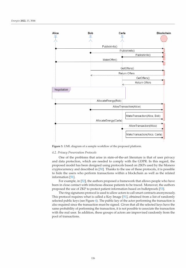
Energies 2022, 15, 3046

Figure 3. UML diagram of a sample workflow of the proposed platform.

4.2. Privacy Preservation Protocols

One of the problems that arise in state-of-the-art literature is that of user privacyand data protection, which are needed to comply with the GDPR. In this regard, theproposed model has been designed using protocols based on ZKPs used by the Monerocryptocurrency and described in [50]. Thanks to the use of these protocols, it is possibleto hide the users who perform transactions within a blockchain as well as the relatedinformation [51].

For example, in [52], the authors proposed a framework that allows people who havebeen in close contact with infectious disease patients to be traced. Moreover, the authorsproposed the use of ZKP to protect patient information based on bulletproofs [53].

The ring signatures protocol is used to allow actors to call smart contracts anonymously.This protocol requires what is called a Key Image [51], obtained from a list of randomlyselected public keys (see Figure 4). The public key of the actor performing the transaction isalso required since the transaction must be signed. Given that all the selected keys have thesame probability of performing the transaction, it is not possible to associate the transactionwith the real user. In addition, these groups of actors are improvised randomly from thepool of transactions.

126

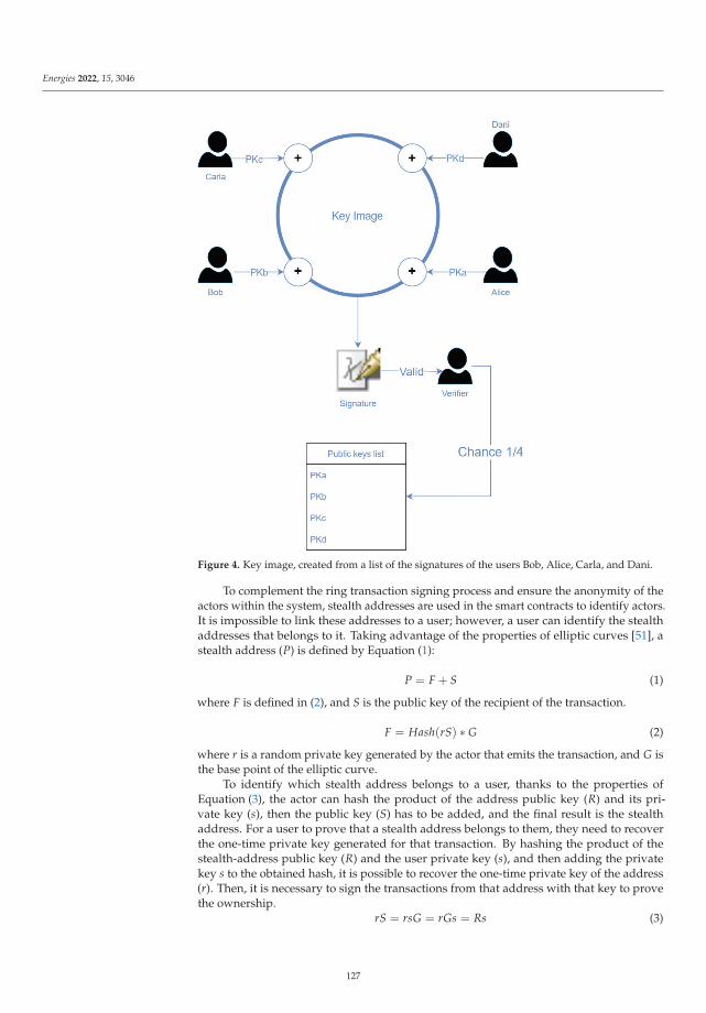
Energies 2022, 15, 3046

Figure 4. Key image, created from a list of the signatures of the users Bob, Alice, Carla, and Dani.

To complement the ring transaction signing process and ensure the anonymity of theactors within the system, stealth addresses are used in the smart contracts to identify actors.It is impossible to link these addresses to a user; however, a user can identify the stealthaddresses that belongs to it. Taking advantage of the properties of elliptic curves [51], astealth address (P) is defined by Equation (1):

P = F + S (1)

where F is defined in (2), and S is the public key of the recipient of the transaction.

F = Hash(rS) ∗ G (2)

where r is a random private key generated by the actor that emits the transaction, and G isthe base point of the elliptic curve.

To identify which stealth address belongs to a user, thanks to the properties ofEquation (3), the actor can hash the product of the address public key (R) and its pri-vate key (s), then the public key (S) has to be added, and the final result is the stealthaddress. For a user to prove that a stealth address belongs to them, they need to recoverthe one-time private key generated for that transaction. By hashing the product of thestealth-address public key (R) and the user private key (s), and then adding the privatekey s to the obtained hash, it is possible to recover the one-time private key of the address(r). Then, it is necessary to sign the transactions from that address with that key to provethe ownership.

rS = rsG = rGs = Rs (3)

127

Energies 2022, 15, 3046

where R is the public key of the randomly generated private key, and s is the private key ofthe transaction recipient.

The use of these protocols increases the need for the computational power of eachactor that makes use of them. In Figure 3, it is possible to study the number of times eachagent must write to the blockchain, thus making use of these protocols, within a systembased on the proposed framework. The agents only need to write the information in thefollowing cases:

1. When they are registered within the system and store information related to them. Inthe whole life cycle of the platform, this occurs once for each agent.

2. At the end of each hour, every agent writes in the blockchain the agreement reachedduring the negotiation process. For example, if Alice reaches an agreement withBob and Carla, then Alice will need to create two transactions. On the other hand,according to the example, Bob and Carla only need to create one each.

This step will depend on the number of agents involved, but with the time limitsproposed—from 5 to 10 min—in a permissioned blockchain, it is enough time to notovercharge the agents and their computational resources. Therefore, the performance willnot be affected when the system escalates.

4.3. Security Model

This section details the security assumptions made by the framework and how the datagenerated within the platform are treated. The implementation of blockchain technology inthis platform ensures the application of a secure identification protocol between the actors.Furthermore, the information stored is tamper-proof, and the smart contracts deployedallow for the decentralized control of the platform, ensuring that there will not be a singlepoint of failure that will be prone to attacks.

Regarding the storage of the generated data, which will be used to create the predic-tive models that will help with the proper functioning of the system, each actor will beresponsible for them. We assume that each actor is responsible for providing an accesspoint to their data so that they can control to whom they give access to the data. For eachhour, a batch can be created with the generated data, storing in the blockchain a hash ofsuch data that will help to verify that it has not been modified afterwards. The use ofauditability systems allows for the generation of data that can be trusted. Otherwise, itwould be impossible to know that the generated data has not been modified before thestorage of its hash in the blockchain [47].

As for the proposed privacy protocols, they ensure that the information stored in theblockchain cannot be read by third parties without permission, nor will it be possible toidentify or track user activity. This information that is stored is, for example, the energy bidsposted, the money paid for energy transactions, or the amount of energy transacted. Theonly vulnerability of this platform is when an attacker steals the keys of a user. However,this is not possible just by using the platform; it can only happen if the user is not carefulenough with the passwords used or with where the keys are stored.

In this work, we have made security assumptions that the network of blockchainnodes is large enough so that it is not easy to throw it from a typical Distributed Denialof Services (DDOS) attack. It has also been assumed that the actors that are part of theplatform benefit more from its proper functioning than from trying to sabotage it. Differentactors could collude with each other to achieve a greater benefit, but this scenario is notrealistic based on the study conducted by [43]. Having in mind the previous assumptions,we can thus say that the actors of the platform will benefit from the creation of this platformand the competition between them rather than in trying to sabotage the negotiation processand the well-being of the platform.

4.4. Multi-Agent System

This section will describe the MAS structure in detail. It is divided into four differentsubsystems, in which the agents are grouped according to their function within the platform

128

Energies 2022, 15, 3046

(see Figure 5). The following is a detailed description of the different subsystems and theagents that comprise them:

• Device Driver System (DDS). This system groups all the agents in charge of themanagement and control of the different smart devices of the platform (e.g., batteries,smart meters, PV panels). These agents are allowed to interact with the blockchainnetwork, so they also have an assigned wallet to identify and track their activitywithin the platform, thus helping in the auditing process. The agents in charge ofmonitoring the state of the PV panels (e.g., their energy production, the providedvoltage and current, and their active and reactive powers) are the PV agents (PVA).They store those data in the blockchain, which helps their owners to monitor themwhile also owning that information which they could sell in the future. The batteriesare monitored by agents called Battery State Agents (BSA). They store in the blockchaindata related to the state of a battery, its charge and discharge capability, and its currentstate of charge. The agent that stores the data related to the flow of current from or toa household is the Smart Meter Agent (SMA).

• Micro-grid Operator System (MGOS). In this system, all those agents that are respon-sible for monitoring, controlling, and managing the status and good credit of themicro-grid are grouped together. These agents are also connected to the blockchain,storing the relevant information that favors the traceability of the micro-grid moni-toring, flows of power to and from the utility network, the balance of the micro-gridpower, and the voltage level (Micro-grid Operator agent or MGO), or the energytransactions made from the grid to the micro-grid and vice versa (External Market In-teractor Agent or EMI). In addition, this system owns a series of batteries that improvethe balance of the grid load, governed by the State Of Charge agents (SOC). This partof the platform is economically maintained by the penalties of users who do not fulfilltheir part of the contracts and by the exchange of energy between the external gridand the micro-grid.

• Data Analytic System (DAS). This system is crucial for the platform as it is in chargeof grouping all those agents that are in charge of the data market and the creation ofpredictive models, which are required by the rest of the agents of the system to beable to infer the amount of energy they expect to obtain in the next hour, that whichthey could sell, and that which they will need to buy based on their past consumption.The agents in charge of reading the data provided by the other subsystems of theplatform on the blockchain and merging it with data coming from other external datasources are called Data Reader Agents (DRA). The agents that create and update newbehavioral models on demand are the Knowledge Extractor Agents (KEA). The agentsthat make predictions based on these models and the information extracted from theenvironment are the Forecasting Agents (FA). This subsystem benefits from the datamarket created with the addition of blockchain technology to the platform. As it hasbeen found in other works in the literature, it is also possible to improve the creationof the models with the use of blockchain technology by applying a federated learningframework similar to the one proposed in [54].

• Transaction Manager System (TMS). In this subsystem, all those agents that are respon-sible for the negotiation and exchange of energy within the micro-grid are grouped.These agents make use of the blockchain network to publish and search for energyoffers as well as register the agreements that take place. The agents in charge ofpublishing the offers are the Seller Agents (SA), while those who search for them inorder to buy are the Buyer Agents (BA). The agents in this system negotiate with eachother directly and make use of the DAS to estimate the energy they will need to buyand/or sell. As a way to improve the search process in the blockchain, a middlewarelayer could be used to optimize the search for information (offers in this case) withinthe blockchain, such as the one proposed in [55].

129

Energies 2022, 15, 3046

Figure 5. Proposed platform architecture.

4.5. Deployment of the Platform

In the proposed platform, there are three types of actors: consumers who receiveenergy that they buy from the grid, PV panels as producers that produce the energy anddump it into batteries, and batteries as prosumers who store and distribute the energy(e.g., consumed by their owners, or, if leftover, dumped into the micro-grid to make aprofit). There are also actors who are in charge of the good credit of the micro-grid andwho additionally make a profit by connecting it to the external grid. Finally, there are other

130

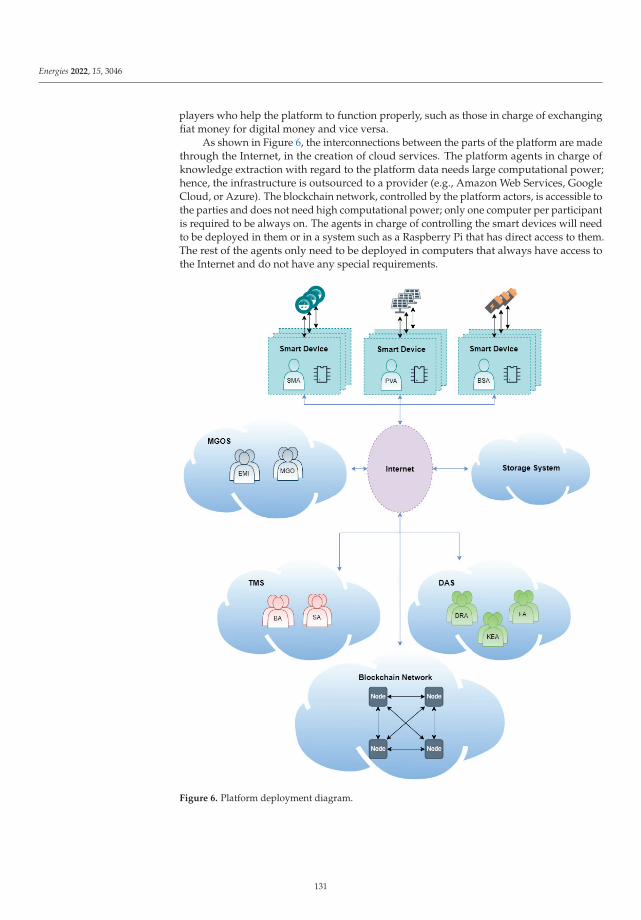
Energies 2022, 15, 3046

players who help the platform to function properly, such as those in charge of exchangingfiat money for digital money and vice versa.

As shown in Figure 6, the interconnections between the parts of the platform are madethrough the Internet, in the creation of cloud services. The platform agents in charge ofknowledge extraction with regard to the platform data needs large computational power;hence, the infrastructure is outsourced to a provider (e.g., Amazon Web Services, GoogleCloud, or Azure). The blockchain network, controlled by the platform actors, is accessible tothe parties and does not need high computational power; only one computer per participantis required to be always on. The agents in charge of controlling the smart devices will needto be deployed in them or in a system such as a Raspberry Pi that has direct access to them.The rest of the agents only need to be deployed in computers that always have access tothe Internet and do not have any special requirements.

Figure 6. Platform deployment diagram.

131

Energies 2022, 15, 3046

5. Conclusions and Future Work

This manuscript highlights and discusses concepts and technologies such as blockchain,smart micro-grids, and negotiation algorithms that have been applied to the energy market.Furthermore, this work elaborates on the proposal of an innovative high-technology-basedarchitecture of a fully distributed and autonomous smart micro-grid to support new formsof business in the smart energy market. With independent and dynamic pricing betweenthe transactors in the network, the proposal presented makes it possible to create a LocalEnergy Market (LEM) in order to achieve efficiency in the transmission and distribution ofenergy as compared to the traditional distribution model.

In the mentioned context, this paper has studied the implementation and developmentof smart micro-grids that would allow for the entrance of more entities, whose aim isself-consumption and making money with the excess energy generated, as competitors inthe energy market. If it is possible to introduce more actors into the power market that cancompete for revenue in the energy market, the regularization of prices is no longer necessary.Because the energy transactions between entities of a micro-grid that are closer to each otherare cheaper and better than those made between distant entities, the market law of supplyand demand would work, thus making their current regularization unnecessary. Finally,the use of ring signatures and ZKP protocols has been proposed to ensure the privacy ofthe users and the protection of the data stored within the platform, thus complying withthe GDPR.

In general terms, for future work, the designed proposal should be implemented as apilot project. This will allow for the design of ad hoc consensus algorithms for the energymarket. In this way, it will be possible to validate the proposed framework as a standardguideline for similar platforms. This will help to reduce development costs and encouragethe adoption of the system by companies and individuals.

Author Contributions: Funding acquisition, J.P. and J.M.C.; Investigation, Y.M.; Methodology,Y.M. and A.B.G.-G.; Project administration, Y.M.; Supervision, A.B.G.-G., A.M.d.R., J.P. and J.M.C.;Writing—original draft, Y.M. and A.B.G.-G.; Writing—review & editing, Y.M., A.B.G.-G. and A.M.d.R.All authors have read and agreed to the published version of the manuscript.

Funding: The research of Yeray Mezquita is supported by the pre-doctoral fellowship from theUniversity of Salamanca and co-funded by Banco Santander. Besides this work has been partiallysupported by the Institute for Business Competitiveness of Castilla y León, and the European RegionalDevelopment Fund under grant CCTT3/20/SA/0002 (AIR-SCity project).



Data Availability Statement: Not applicable.


References

1. Hirst, E.; Kirby, B. Transmission Planning for a Restructuring US Electricity Industry; Consulting in Electric-Industry Restructuring:Washington, DC, USA, 2001.

2. Fang, X.; Misra, S.; Xue, G.; Yang, D. Smart grid—The new and improved power grid: A survey. IEEE Commun. Surv. Tutor. 2011,14, 944–980. [CrossRef]

3. Memon, A.A.; Kauhaniemi, K. A critical review of AC Microgrid protection issues and available solutions. Electr. Power Syst. Res.2015, 129, 23–31. [CrossRef]

4. Bui, V.H.; Hussain, A.; Kim, H.M. A multiagent-based hierarchical energy management strategy for multi-microgrids consideringadjustable power and demand response. IEEE Trans. Smart Grid 2016, 9, 1323–1333. [CrossRef]

5. Tosh, D.K.; Shetty, S.; Liang, X.; Kamhoua, C.; Njilla, L. Consensus protocols for blockchain-based data provenance: Challengesand opportunities. In Proceedings of the 2017 IEEE 8th Annual Ubiquitous Computing, Electronics and Mobile CommunicationConference (UEMCON), New York, NY, USA, 19–21 October 2017; pp. 469–474.

6. Cameron, P.D.; Brothwood, M. Competition in Energy Markets: Law and Regulation in the European Union; Oxford University Press:Oxford, UK, 2002.

7. Von Danwitz, T. Regulation and Liberalization of the European Electricity Market-A German View. Energy 2006, 27, 423.

132

Energies 2022, 15, 3046

8. Mezquita, Y.; Casado-Vara, R.; González Briones, A.; Prieto, J.; Corchado, J.M. Blockchain-based architecture for the control oflogistics activities: Pharmaceutical utilities case study. Log. J. IGPL 2021, 29, 974–985. [CrossRef]

9. Liang, X.; Shetty, S.; Tosh, D.; Kamhoua, C.; Kwiat, K.; Njilla, L. Provchain: A blockchain-based data provenance architecture incloud environment with enhanced privacy and availability. In Proceedings of the 17th IEEE/ACM International Symposium onCluster, Cloud and Grid Computing, Madrid, Spain, 14–17 May 2017; pp. 468–477.

10. Buterin, V. Ethereum: Platform Review. In Opportunities and Challenges for Private and Consortium Blockchains; Availableonline: http://www.smallake.kr/wp-content/uploads/2016/06/314477721-Ethereum-Platform-Review-Opportunities-and-Challenges-for-Private-and-Consortium-Blockchains.pdf (accessed on 19 April 2022).

11. Huh, S.; Cho, S.; Kim, S. Managing IoT devices using blockchain platform. In Proceedings of the 2017 19th InternationalConference on Advanced Communication Technology (ICACT), Pyeongchang, Korea, 19–22 February 2017; pp. 464–467.

12. Dorri, A.; Kanhere, S.S.; Jurdak, R.; Gauravaram, P. Blockchain for IoT security and privacy: The case study of a smart home.In Proceedings of the 2017 IEEE International Conference on Pervasive Computing and Communications Workshops (PerComWorkshops), Kona, HI, USA, 13–17 March 2017; pp. 618–623.

13. Zheng, Z.; Xie, S.; Dai, H.; Chen, X.; Wang, H. An overview of blockchain technology: Architecture, consensus, and future trends.In Proceedings of the 2017 IEEE International Congress on Big Data (BigData Congress), Honolulu, HI, USA, 25–30 June 2017;pp. 557–564.

14. Beikverdi, A.; Song, J. Trend of centralization in Bitcoin’s distributed network. In Proceedings of the 2015 IEEE/ACIS 16thInternational Conference on Software Engineering, Artificial Intelligence, Networking and Parallel/Distributed Computing(SNPD), Takamatsu, Japan, 1–3 June 2015; pp. 1–6.

15. Martinez, J. Understanding Proof of Stake: The Nothing at Stake Theory. 2018. Available online: https://medium.com/coinmonks/understanding-proof-of-stake-the-nothing-at-stake-theory-1f0d71bc027 (accessed on 9 October 2019).

16. Witherspoon, Z. A Hitchhiker’s Guide to Consensus Algorithms. 2017. Available online: https://hackernoon.com/a-hitchhikers-guide-to-consensus-algorithms-d81aae3eb0e3 (accessed on 9 October 2019).

17. Abadi, J.; Brunnermeier, M. Blockchain Economics; Technical Report; National Bureau of Economic Research: Cambridge, MA,USA, 2018.

18. Sikorski, J.J.; Haughton, J.; Kraft, M. Blockchain technology in the chemical industry: Machine-to-machine electricity market.Appl. Energy 2017, 195, 234–246. [CrossRef]

19. Weber, I.; Xu, X.; Riveret, R.; Governatori, G.; Ponomarev, A.; Mendling, J. Untrusted business process monitoring and executionusing blockchain. In International Conference on Business Process Management; Springer: Berlin/Heidelberg, Germany, 2016;pp. 329–347.

20. Khaqqi, K.N.; Sikorski, J.J.; Hadinoto, K.; Kraft, M. Incorporating seller/buyer reputation-based system in blockchain-enabledemission trading application. Appl. Energy 2018, 209, 8–19. [CrossRef]

21. Schöner, M.M.; Kourouklis, D.; Sandner, P.; Gonzalez, E.; Förster, J. Blockchain Technology in the Pharmaceutical Industry; FrankfurtSchool Blockchain Center: Frankfurt, Germany, 2017.

22. Sylim, P.; Liu, F.; Marcelo, A.; Fontelo, P. Blockchain technology for detecting falsified and substandard drugs in distribution:Pharmaceutical supply chain intervention. JMIR Res. Protoc. 2018, 7, e10163. [CrossRef]

23. Galvez, J.F.; Mejuto, J.; Simal-Gandara, J. Future challenges on the use of blockchain for food traceability analysis. TrAC TrendsAnal. Chem. 2018, 107, 222–232. [CrossRef]

24. Kamath, R. Food traceability on blockchain: Walmart’s pork and mango pilots with IBM. J. Br. Blockchain Assoc. 2018, 1, 3712.[CrossRef]

25. Yue, X.; Wang, H.; Jin, D.; Li, M.; Jiang, W. Healthcare data gateways: Found healthcare intelligence on blockchain with novelprivacy risk control. J. Med. Syst. 2016, 40, 218. [CrossRef]

26. Mettler, M. Blockchain technology in healthcare: The revolution starts here. In Proceedings of the 2016 IEEE 18th InternationalConference on e-Health Networking, Applications and Services (Healthcom), Munich, Germany, 14–17 September 2016; pp. 1–3.

27. Ekblaw, A.; Azaria, A.; Halamka, J.D.; Lippman, A. A Case Study for Blockchain in Healthcare: “MedRec” prototype for electronichealth records and medical research data. In Proceedings of the IEEE Open & Big Data Conference, Vienna, Austria, 22–24August 2016; Volume 13, p. 13.

28. Turkanovic, M.; Hölbl, M.; Košic, K.; Hericko, M.; Kamišalic, A. EduCTX: A blockchain-based higher education credit platform.IEEE Access 2018, 6, 5112–5127. [CrossRef]

29. Grech, A.; Camilleri, A.F. Blockchain in Education. 2017. Available online: https://www.pedocs.de/volltexte/2018/15013/pdf/Grech_Camilleri_2017_Blockchain_in_Education.pdf (accessed on 19 April 2022).

30. Funk, E.; Riddell, J.; Ankel, F.; Cabrera, D. Blockchain technology: A data framework to improve validity, trust, and accountabilityof information exchange in health professions education. Acad. Med. 2018, 93, 1791–1794. [CrossRef]

31. Pop, C.; Cioara, T.; Antal, M.; Anghel, I.; Salomie, I.; Bertoncini, M. Blockchain based decentralized management of demandresponse programs in smart energy grids. Sensors 2018, 18, 162. [CrossRef]

32. Imbault, F.; Swiatek, M.; De Beaufort, R.; Plana, R. The green blockchain: Managing decentralized energy production andconsumption. In Proceedings of the 2017 IEEE International Conference on Environment and Electrical Engineering and 2017IEEE Industrial and Commercial Power Systems Europe (EEEIC/I&CPS Europe), Milan, Italy, 6 June 2017; pp. 1–5.

133

Energies 2022, 15, 3046

33. Aitzhan, N.Z.; Svetinovic, D. Security and privacy in decentralized energy trading through multi-signatures, blockchain andanonymous messaging streams. IEEE Trans. Dependable Secur. Comput. 2018, 15, 840–852. [CrossRef]

34. Mengelkamp, E.; Gärttner, J.; Rock, K.; Kessler, S.; Orsini, L.; Weinhardt, C. Designing microgrid energy markets: A case study:The Brooklyn Microgrid. Appl. Energy 2018, 210, 870–880. [CrossRef]

35. Pichler, M.; Meisel, M.; Goranovic, A.; Leonhartsberger, K.; Lettner, G.; Chasparis, G.; Vallant, H.; Marksteiner, S.; Bieser,H. Decentralized Energy Networks Based on Blockchain: Background, Overview and Concept Discussion. In Proceedingsof the International Conference on Business Information Systems, Colorado Springs, CO, USA, 8–10 June 2018; Springer:Berlin/Heidelberg, Germany, 2018; pp. 244–257.

36. Pylon Network Team. Pylon Network Whitepaper. The Energy Blockchain Platform. 2018. Available online: https://pylon-network.org/wp-content/uploads/2019/02/WhitePaper_PYLON_v2_ENGLISH-1.pdf (accessed on 6 November 2019).

37. Suncontract. Suncontract Whitepaper. An Energy Trading Platform that Utilises Blockchain Technology to Create A NewDisruptive Model for Buying and Selling Electricity. 2017. Available online: https://suncontract.org/wp-content/uploads/2020/12/whitepaper.pdf (accessed on 6 November 2019).

38. Aliyev, N.; Brooks, S.; Hale, M.; Hoy, S. Enosi Green Paper 2018. Available online: https://github.com/enosi/green-paper/blob/master/enosi-green-paper.pdf (accessed on 19 April 2022).

39. Goranovic, A.; Meisel, M.; Fotiadis, L.; Wilker, S.; Treytl, A.; Sauter, T. Blockchain applications in microgrids an overview ofcurrent projects and concepts. In Proceedings of the IECON 2017-43rd Annual Conference of the IEEE Industrial ElectronicsSociety, Beijing, China, 28 October–1 November 2017; pp. 6153–6158.

40. Koirala, B.P.; Koliou, E.; Friege, J.; Hakvoort, R.A.; Herder, P.M. Energetic communities for community energy: A review of keyissues and trends shaping integrated community energy systems. Renew. Sustain. Energy Rev. 2016, 56, 722–744. [CrossRef]

41. Long, C.; Wu, J.; Zhou, Y.; Jenkins, N. Peer-to-peer energy sharing through a two-stage aggregated battery control in a communityMicrogrid. Appl. Energy 2018, 226, 261–276. [CrossRef]

42. Liu, N.; Yu, X.; Wang, C.; Li, C.; Ma, L.; Lei, J. Energy-sharing model with price-based demand response for microgrids ofpeer-to-peer prosumers. IEEE Trans. Power Syst. 2017, 32, 3569–3583. [CrossRef]

43. van Leeuwen, G.; AlSkaif, T.; Gibescu, M.; van Sark, W. An integrated blockchain-based energy management platform withbilateral trading for microgrid communities. Appl. Energy 2020, 263, 114613. [CrossRef]

44. Noor, S.; Yang, W.; Guo, M.; van Dam, K.H.; Wang, X. Energy Demand Side Management within micro-grid networks enhancedby blockchain. Appl. Energy 2018, 228, 1385–1398. [CrossRef]

45. European Parliament and Council: Regulation on the Protection of Natural Persons with Regard to the Processing of PersonalData and on the Free Movement of Such Data, and Repealing Directive 95/46/EC (Data Protection Directive). 2016. Availableonline: https://eur-lex.europa.eu/legal-content/EN/TXT/PDF/?uri=CELEX:32016R0679&from=EN (accessed on 9 December2021).

46. Francisco, M.; Mezquita, Y.; Revollar, S.; Vega, P.; De Paz, J. Multi-agent distributed model predictive control with fuzzynegotiation. Expert Syst. Appl. 2019, 129, 68–83. [CrossRef]

47. Mezquita, Y.; Casado, R.; Gonzalez-Briones, A.; Prieto, J.; Corchado, J.M.; AETiC, A. Blockchain technology in IoT systems:Review of the challenges. Ann. Emerg. Technol. Comput. 2019, 3, 17–24. [CrossRef]

48. Combi, C. What Are Blockchain Confirmations and Why Do They Matter? 2017. Available online: https://coincentral.com/blockchain-confirmations/ (accessed on 19 April 2022).

49. Gatteschi, V.; Lamberti, F.; Demartini, C.; Pranteda, C.; Santamaría, V. Blockchain and smart contracts for insurance: Is thetechnology mature enough? Future Internet 2018, 10, 20. [CrossRef]

50. Van Saberhagen, N. CryptoNote v 2.0. 2013. Available online: https://www.getmonero.org/ru/resources/research-lab/pubs/whitepaper_annotated.pdf (accessed on 19 April 2022).

51. Roy Walker. The Battle for Blockchain Privacy: Monero. 2018. Available online: https://medium.com/all-things-venture-capital/privacy-protocol-analysis-monero-c116d7c2106f (accessed on 19 April 2022 ).

52. Peng, Z.; Xu, C.; Wang, H.; Huang, J.; Xu, J.; Chu, X. P2b-trace: Privacy-preserving blockchain-based contact tracing to combatpandemics. In Proceedings of the 2021 International Conference on Management of Data, Xi’an, China, 20–25 June 2021;pp. 2389–2393.

53. Bünz, B.; Bootle, J.; Boneh, D.; Poelstra, A.; Wuille, P.; Maxwell, G. Bulletproofs: Short proofs for confidential transactions andmore. In Proceedings of the 2018 IEEE Symposium on Security and Privacy (SP), San Francisco, CA, USA, 21–23 May 2018;pp. 315–334.

54. Peng, Z.; Xu, J.; Chu, X.; Gao, S.; Yao, Y.; Gu, R.; Tang, Y. VFChain: Enabling verifiable and auditable federated learning viablockchain systems. IEEE Trans. Netw. Sci. Eng. 2021, 9, 173–186. [CrossRef]

55. Wu, H.; Peng, Z.; Guo, S.; Yang, Y.; Xiao, B. VQL: Efficient and Verifiable Cloud Query Services for Blockchain Systems. IEEETrans. Parallel Distrib. Syst. 2021, 33, 1393–1406. [CrossRef]

134

MDPISt. Alban-Anlage 66

4052 BaselSwitzerland

Tel. +41 61 683 77 34Fax +41 61 302 89 18

www.mdpi.com

Energies Editorial OfficeE-mail: [email protected]

www.mdpi.com/journal/energies

ISBN 978-3-0365-4606-3

MDPI

St. Alban-Anlage 66

4052 Basel

Switzerland

Tel: +41 61 683 77 34

www.mdpi.com

Artificial Intelligence in the Energy Industry - MDPI

Documents

Transcript of Artificial Intelligence in the Energy Industry - MDPI