Arnold diffusion for smooth systems of two and ahalf degrees of freedom

V. Kaloshin∗, K. Zhang†

October 30, 2018

Dedicated to the memory of John Mather:a great mathematician and a remarkable person

Abstract

In the present paper we prove a strong form of Arnold diffusion. Let T2 bethe two torus and B2 be the unit ball around the origin in R2. Fix ρ > 0. Ourmain result says that for a “generic” time-periodic perturbation of an integrablesystem of two degrees of freedom

H0(p) + εH1(θ, p, t), θ ∈ T2, p ∈ B2, t ∈ T = R/Z,

with a strictly convex H0, there exists a ρ-dense orbit (θε, pε, t)(t) in T2×B2×T,namely, a ρ-neighborhood of the orbit contains T2 ×B2 × T.

Our proof is a combination of geometric and variational methods. Thefundamental elements of the construction are usage of crumpled normallyhyperbolic invariant cylinders from [13], flower and simple normally hyperbolicinvariant manifolds from as well as their kissing property at a strong doubleresonance. This allows us to build a “connected” net of 3-dimensional normallyhyperbolic invariant manifolds. To construct diffusing orbits along this net weemploy a version of Mather variational method [58] proposed by Bernard in[11]. This version is equipped with weak KAM theory [35].

∗University of Maryland at College Park (vadim.kaloshin gmail.com)†University of Toronto (kzhang math.utoronto.edu)

1

arX

iv:1

212.

1150

v3 [

mat

h.D

S] 8

Apr

201

8

Contents

1 Introduction 41.1 Statement of the result . . . . . . . . . . . . . . . . . . . . . . . . . . 51.2 Discussions of the result . . . . . . . . . . . . . . . . . . . . . . . . . 91.3 Scheme of diffusion . . . . . . . . . . . . . . . . . . . . . . . . . . . . 131.4 Three regimes of diffusion . . . . . . . . . . . . . . . . . . . . . . . . 16

2 Forcing relation 172.1 Sufficient condition for Arnold diffusion . . . . . . . . . . . . . . . . . 172.2 Diffusion mechanisms via forcing equivalence . . . . . . . . . . . . . . 192.3 Invariance under the symplectic coordinate changes . . . . . . . . . . 202.4 Normal hyperbolicity and Aubry-Mather type . . . . . . . . . . . . . 22

3 Normal forms and cohomology classes at single resonances 243.1 Resonant component and non-degeneracy conditions . . . . . . . . . . 243.2 Normal form . . . . . . . . . . . . . . . . . . . . . . . . . . . . . . . . 253.3 The resonant component . . . . . . . . . . . . . . . . . . . . . . . . . 29

4 Double resonance: geometric description 304.1 The slow system . . . . . . . . . . . . . . . . . . . . . . . . . . . . . 314.2 Non-degeneracy conditions for the slow system . . . . . . . . . . . . . 324.3 Normally hyperbolic cylinders . . . . . . . . . . . . . . . . . . . . . . 344.4 Local maps and global maps . . . . . . . . . . . . . . . . . . . . . . . 36

5 Double resonance: choice of cohomology and forcing equivalence 385.1 Choice of cohomologies for the slow system . . . . . . . . . . . . . . . 385.2 Aubry-Mather type at a double resonance . . . . . . . . . . . . . . . 415.3 Connecting to Γk1,k2 and ΓSRk1 . . . . . . . . . . . . . . . . . . . . . . 43

5.3.1 Connecting to the double resonance point . . . . . . . . . . . 435.3.2 Connecting single and double resonance . . . . . . . . . . . . 45

5.4 Jump from non-simple homology to simple homology . . . . . . . . . 475.5 Forcing equivalence at the double resonance . . . . . . . . . . . . . . 48

6 Weak KAM theory and forcing equivalence 496.1 Periodic Tonelli Hamiltonians . . . . . . . . . . . . . . . . . . . . . . 506.2 Weak KAM solution . . . . . . . . . . . . . . . . . . . . . . . . . . . 526.3 Pseudographs, Aubry, Mane and Mather sets . . . . . . . . . . . . . . 536.4 The dual setting, forward solutions . . . . . . . . . . . . . . . . . . . 546.5 Peierls barrier, static classes, elementary solutions . . . . . . . . . . . 55

2

6.6 The forcing relation . . . . . . . . . . . . . . . . . . . . . . . . . . . . 56

7 Perturbative Weak KAM theory 567.1 Semi-continuity . . . . . . . . . . . . . . . . . . . . . . . . . . . . . . 577.2 Continuity of the barrier function . . . . . . . . . . . . . . . . . . . . 597.3 Lipschitz estimates for nearly integrable systems . . . . . . . . . . . . 607.4 Estimates for nearly autonomous systems . . . . . . . . . . . . . . . . 617.5 Semi-concavity of viscosity solutions . . . . . . . . . . . . . . . . . . 63

8 Cohomology of Aubry-Mather type 658.1 Aubry-Mather type and diffusion mechanisms . . . . . . . . . . . . . 658.2 Weak KAM solutions are unstable manifolds . . . . . . . . . . . . . . 718.3 Regularity of the barrier functions . . . . . . . . . . . . . . . . . . . . 758.4 Bifurcation type . . . . . . . . . . . . . . . . . . . . . . . . . . . . . . 77

9 Aubry-Mather type at the single resonance 799.1 Normally hyperbolicity and localization of Aubry/Mane sets in the

single maximum case . . . . . . . . . . . . . . . . . . . . . . . . . . . 799.2 Aubry-Mather type at single resonance . . . . . . . . . . . . . . . . . 819.3 Bifurcations in the double maxima case . . . . . . . . . . . . . . . . . 829.4 Hyperbolic coordinates . . . . . . . . . . . . . . . . . . . . . . . . . . 849.5 Normally hyperbolic invariant cylinder . . . . . . . . . . . . . . . . . 869.6 Localization of the Aubry and Mane sets . . . . . . . . . . . . . . . . 89

10 Normally hyperbolic cylinders at double resonance 9110.1 Normal form near the hyperbolic fixed point . . . . . . . . . . . . . . 9110.2 Shil’nikov’s boundary value problem . . . . . . . . . . . . . . . . . . 9210.3 Properties of the local maps . . . . . . . . . . . . . . . . . . . . . . . 9510.4 Conley-McGehee isolating blocks . . . . . . . . . . . . . . . . . . . . 9910.5 Periodic orbit in simple homologies . . . . . . . . . . . . . . . . . . . 10010.6 Periodic orbits for non-simple homology . . . . . . . . . . . . . . . . 10310.7 Normally hyperbolic invariant cylinders for the slow mechanical system 10410.8 Cyclic concatenations of simple geodesics . . . . . . . . . . . . . . . . 105

11 Aubry-Mather type at the double resonance 10711.1 High energy case . . . . . . . . . . . . . . . . . . . . . . . . . . . . . 10711.2 Simple non-critical case . . . . . . . . . . . . . . . . . . . . . . . . . . 11011.3 Simple critical case . . . . . . . . . . . . . . . . . . . . . . . . . . . . 111

11.3.1 Proof of Aubry-Mather type using local coordinates . . . . . . 11111.3.2 Construction of the local coordinates . . . . . . . . . . . . . . 114

3

12 Forcing equivalence between kissing cylinders 11712.1 Variational problem for the slow mechanical system . . . . . . . . . . 11812.2 Variational problem for original coordinates . . . . . . . . . . . . . . 12112.3 Scaling limit of the barrier function . . . . . . . . . . . . . . . . . . . 12412.4 The jump mechanism . . . . . . . . . . . . . . . . . . . . . . . . . . . 125

A Generic properties of mechanical systems on the two-torus 129A.1 Generic properties of periodic orbits . . . . . . . . . . . . . . . . . . . 129A.2 Generic properties of minimal orbits . . . . . . . . . . . . . . . . . . . 135A.3 Non-degeneracy at high energy . . . . . . . . . . . . . . . . . . . . . 139A.4 Unique hyperbolic minimizer at very high energy . . . . . . . . . . . 141A.5 Proof of Proposition 4.5 . . . . . . . . . . . . . . . . . . . . . . . . . 143

B Derivation of the slow mechanical system 144B.1 Normal forms near double resonances . . . . . . . . . . . . . . . . . . 144B.2 Affine coordinate change, rescaling and energy reduction . . . . . . . 153B.3 Variational properties of the coordinate changes . . . . . . . . . . . . 158

C Variational aspects of the slow mechanical system 164C.1 Relation between the minimal geodesics and the Aubry sets . . . . . 164C.2 Characterization of the channel and the Aubry sets . . . . . . . . . . 167C.3 The width of the channel . . . . . . . . . . . . . . . . . . . . . . . . . 170C.4 The case E = 0 . . . . . . . . . . . . . . . . . . . . . . . . . . . . . . 172

D Notations 176D.1 Formulation of the main result . . . . . . . . . . . . . . . . . . . . . . 176D.2 Weak KAM and Mather theory . . . . . . . . . . . . . . . . . . . . . 177D.3 Single resonance . . . . . . . . . . . . . . . . . . . . . . . . . . . . . . 178D.4 Double resonance . . . . . . . . . . . . . . . . . . . . . . . . . . . . . 179

1 Introduction

The famous question called the ergodic hypothesis, formulated by Maxwell andBoltzmann, suggests that for a typical Hamiltonian on a typical energy surface all,but a set of zero measure of initial conditions, have trajectories dense in this energysurface. However, KAM theory showed that for an open set of (nearly integrable)Hamiltonian systems there is a set of initial conditions of positive measure with almostperiodic trajectories. This disproved the ergodic hypothesis and forced to reconsiderthe problem.

4

A quasi-ergodic hypothesis, proposed by Ehrenfest [34] and Birkhoff [17], asks if atypical Hamiltonian on a typical energy surface has a dense orbit. A definite answerwhether this statement is true or not is still far out of reach of modern dynamics.There was an attempt to prove this statement by E. Fermi [37], which failed (see [38]for a more detailed account). To simplify the problem, Arnold [4] asks:

Does there exist a real instability in many-dimensional problems of perturbationtheory when the invariant tori do not divide the phase space?

For nearly integrable systems of two degrees (resp. of one and a half) of freedomthe invariant tori do divide the phase space and an energy surface respectively. Thisimplies that instability do not occur. We solve a weaker version of this question forsystems with two and a half and 3 degrees of freedom. This corresponds autonomousperturbations of integrable systems with three degrees of freedom (resp. time-periodicperturbations of integrable systems with two degrees of freedom).

1.1 Statement of the result

Let (θ, p) ∈ T2 × B2 be the phase space of an integrable Hamiltonian system H0(p)with T2 being 2-dimensional torus T2 = R2/Z2 3 θ = (θ1, θ2) and B2 being the unitball around 0 in R2, p = (p1, p2) ∈ B2. H0 is assumed to be strictly convex with thefollowing uniform estimate: there exists D > 1 such that

D−1I ≤ ∂2ppH0 ≤ DI, |H0(0)|, ‖∂pH0(0)‖ ≤ D.

where I is the 2× 2 identity matrix.Consider a smooth time periodic perturbation

Hε(θ, p, t) = H0(p) + εH1(θ, p, t), t ∈ T = R/T.

We study Arnold diffusion for this system, namely,

topological instability in the p variable.

Arnold [5] proved existence of such orbits for an example and conjectured that theyexist for a typical perturbation (see e.g. [4, 6, 7]).

Denote Z3∗ = Z3 \ (0, 0, 1)Z, then integer relations k · (∂pH0, 1) = 0 with k =

(~k1, k0) ∈ Z3∗ and · being the inner product define a resonant submanifold. The strict

convexity of H0 implies that ∂pH0 : B2 −→ R2 is a diffeomorphism and each resonantline defines a smooth curve embedded into action space

Sk = p ∈ R2 : k · (∂pH0, 1) = 0.

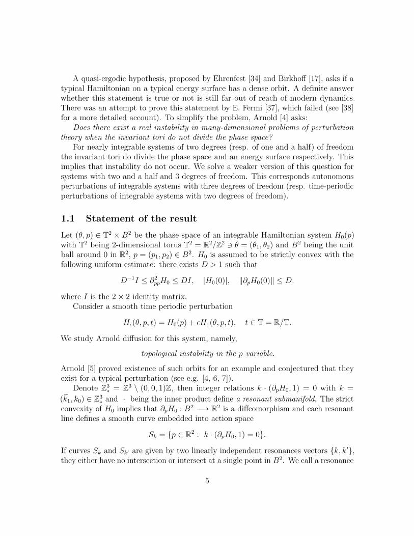
If curves Sk and Sk′ are given by two linearly independent resonances vectors k, k′,they either have no intersection or intersect at a single point in B2. We call a resonance

5

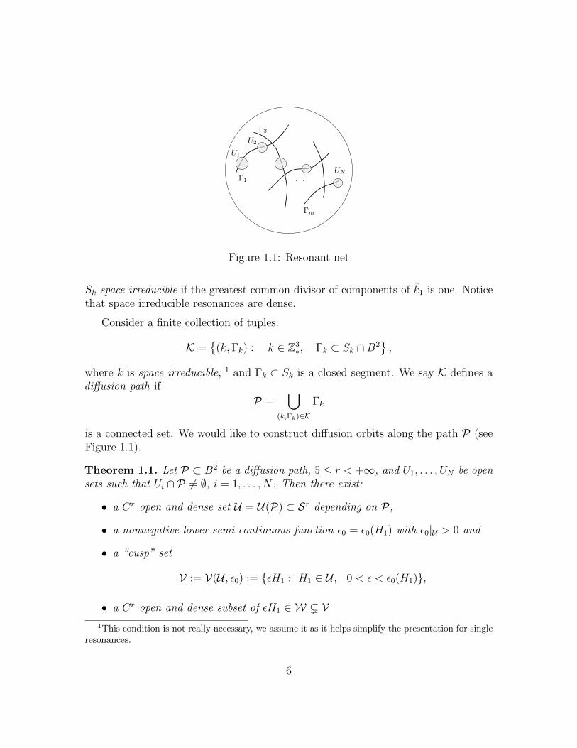
Figure 1.1: Resonant net

Sk space irreducible if the greatest common divisor of components of ~k1 is one. Noticethat space irreducible resonances are dense.

Consider a finite collection of tuples:

K =

(k,Γk) : k ∈ Z3∗, Γk ⊂ Sk ∩B2

,

where k is space irreducible, 1 and Γk ⊂ Sk is a closed segment. We say K defines adiffusion path if

P =⋃

(k,Γk)∈K

Γk

is a connected set. We would like to construct diffusion orbits along the path P (seeFigure 1.1).

Theorem 1.1. Let P ⊂ B2 be a diffusion path, 5 ≤ r < +∞, and U1, . . . , UN be opensets such that Ui ∩ P 6= ∅, i = 1, . . . , N . Then there exist:

• a Cr open and dense set U = U(P) ⊂ Sr depending on P,

• a nonnegative lower semi-continuous function ε0 = ε0(H1) with ε0|U > 0 and

• a “cusp” set

V := V(U , ε0) := εH1 : H1 ∈ U , 0 < ε < ε0(H1),

• a Cr open and dense subset of εH1 ∈ W ( V1This condition is not really necessary, we assume it as it helps simplify the presentation for single

resonances.

6

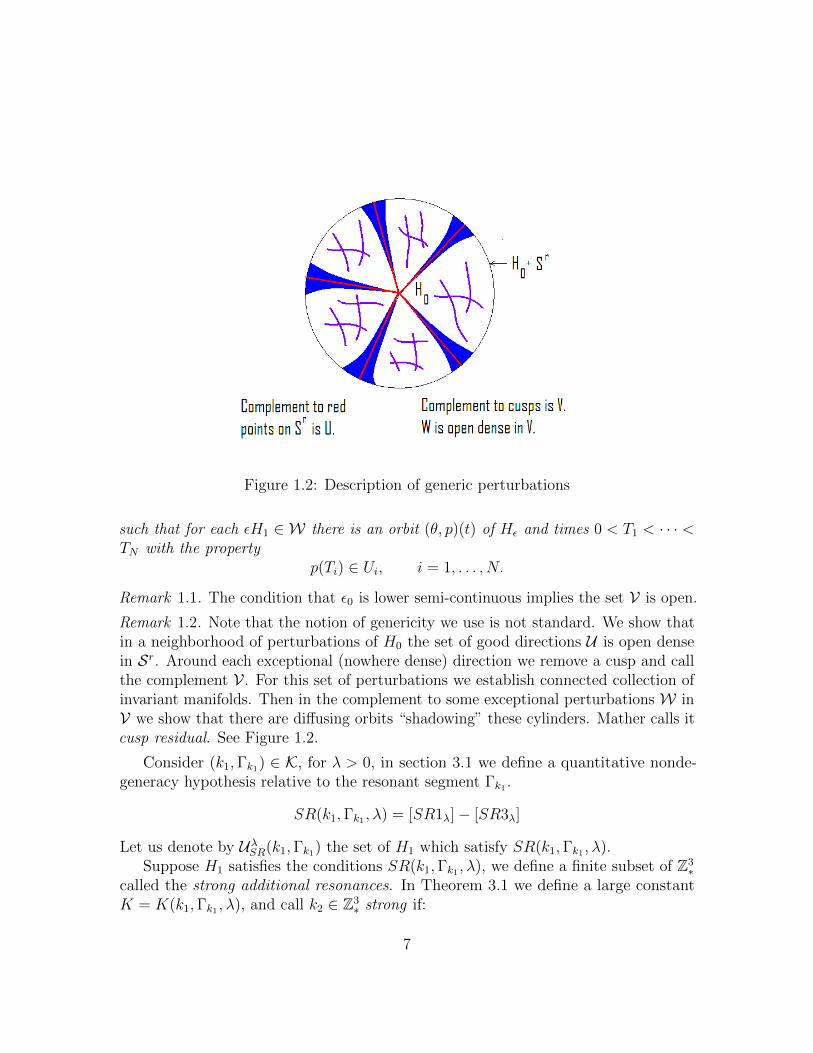
Figure 1.2: Description of generic perturbations

such that for each εH1 ∈ W there is an orbit (θ, p)(t) of Hε and times 0 < T1 < · · · <TN with the property

p(Ti) ∈ Ui, i = 1, . . . , N.

Remark 1.1. The condition that ε0 is lower semi-continuous implies the set V is open.

Remark 1.2. Note that the notion of genericity we use is not standard. We show thatin a neighborhood of perturbations of H0 the set of good directions U is open densein Sr. Around each exceptional (nowhere dense) direction we remove a cusp and callthe complement V . For this set of perturbations we establish connected collection ofinvariant manifolds. Then in the complement to some exceptional perturbations W inV we show that there are diffusing orbits “shadowing” these cylinders. Mather calls itcusp residual. See Figure 1.2.

Consider (k1,Γk1) ∈ K, for λ > 0, in section 3.1 we define a quantitative nonde-generacy hypothesis relative to the resonant segment Γk1 .

SR(k1,Γk1 , λ) = [SR1λ]− [SR3λ]

Let us denote by UλSR(k1,Γk1) the set of H1 which satisfy SR(k1,Γk1 , λ).Suppose H1 satisfies the conditions SR(k1,Γk1 , λ), we define a finite subset of Z3

∗called the strong additional resonances. In Theorem 3.1 we define a large constantK = K(k1,Γk1 , λ), and call k2 ∈ Z3

∗ strong if:

7

• either there is (k2,Γk2) ∈ K such that Γk1 ∩ Γk2 6= ∅;

• or |k2| ≤ K(k1,Γk1 , λ) and Sk2 ∩ Γk1 6= ∅.

We emphasize that strong additional resonances are taken from the set Z3∗, not just the

space irreducible ones. Denote the set of strong additional resonances Kst(k1,Γk1 , λ),If k2 is strong, then it defines a unique double resonance Γk1,k2 = Γk1 ∩ Sk2 .

For each double resonance Γk1,k2 , we associate non-resonance conditions of twotypes:

• high energy [DR1h]− [DR3h] (section 4.2),

• low energy [DR1c]− [DR4c] (section 4.2).

For each pair k2 ∈ Kst(k1,Γk1 , λ) consider the set of H1 which satisfy the aboveconditions and denote it by UDR(k1,Γk1 , k2).

Remark 1.3. All our non-degenerate conditions at a double resonance is stated relativeto a single resonance. Namely, the condition DR(k1,Γk1 , k2) may differ from thecondition DR(k2,Γk2 , k1).

The following theorem is immediate given that:

• (Proposition 3.2) Each UλSR(k1,Γk1) is open and the union⋃λ>0 UλSR(k1) is dense;

• (Proposition 4.3) The set UDR(k1,Γk1 , k2) is open and dense.

Theorem 1.2. The set

U = U(P) :=⋃λ>0

⋂(k1,Γk1 )∈K

UλSR(k1,Γk1) ∩⋂

k2∈Kst(k1,Γk1 ,λ)

UDR(k1,Γk1 , k2)

is open and dense in Sr.

As a corollary of Theorem 1.1, we obtain:

Theorem 1.3 (Almost Density Theorem). For any ρ > 0 there are

• an open dense set U = U(ρ) ⊂ Sr,

• a nonnegative lower semi–continuous function ε0 : Sr −→ R+ with ε0|U > 0,

• a cusp set V := V(U , ε0) := εH1 : H1 ∈ U , 0 < ε < ε0(H1),

• an open dense subset W ( V

8

all depending on ρ such that for any εH1 ∈ W there is a ρ–dense orbit on T2×B2×T.

Proof. Given a vector (ω, 1) ∈ R3, let us call ω being ρ-irrational if there exists T > 0such that t(ω, 1) : t ∈ [−T, T ] ⊂ T3 is ρ-dense, and let T (ω) be the smallest such T .Using the fact that p = O(ε), θ = ∇H0(p) +O(ε), there is ε0 > 0 depending on ρ andT (ω) such that if 0 < ε < ε0

B2ρ

(⋃t∈R

φtHε(θ0, p0, t0)

)⊃ T2 ×Bρ(p∗)× T,

for all p0 ∈ Bρ(p∗), (θ0, t0) ∈ T2 × T.

(1.1)

Any vector that is not ρ-irrational (called ρ-rational) must be resonant: namelyk · (ω, 1) = 0 for some k ∈ Z3

∗. Moreover, there are only finitely many resonances thatcorresponds to ρ-rational vectors. Since there are infinitely many space irreducibleresonances, there is a diffusion path P such consisting only of ρ/2-irrational resonances.Moreover, we may choose the path P to be ρ/2-dense in B2, since space irreducibleresonances are dense.

We now apply Theorem 1.1 to the path P, and pick pi, i = 1, . . . , N ∈ P suchthat (∇H0(pi), 1) is (ρ/2)−irrational, and such that

⋃ni=1Bρ/2(pi) ⊃ B2. According

to our theorem, there is an orbit whose p component visit every Bρ(pi). Then theorbit must be ρ−dense in view of (1.1).

1.2 Discussions of the result

Relation with Mather’s approach

Theorem 1.1 was announced by Mather in [60], where he proposed a plan to prove it.Some parts of the proof are written in [61]. Our work realizes Mather’s general planusing weak KAM theory and Hamiltonian point of view. New techniques and toolsare introduced, below we summarize them.

• We utilize Bernard’s forcing relation to simplify the construction of diffusionorbit. This allows a more Hamiltonian treatment of the variational concepts, andallows us to reduce the main theorem to local forcing equivalence of cohomologyclasses.

• We use Hamiltonian normal forms to construct a collection of normally hyperbolicinvariant cylinders along the chosen diffusion path. We obtain precise controlof the normal forms (via an anisotropic C2 norm) at both single and doubleresonances. Mather’s method uses mostly the Lagrangian point of view.

9

• We introduce the concept of Aubry-Mather type, which generalizes the workdone in Bernard–Kaloshin–Zhang [13] to a more abstract setting, applicable toboth single and double resonances. Heuristically, this means the Aubry setsbehaves like Aubry-Mather sets in twist maps. Our approach can be seen as ageneralization of the variational technique for a priori unstable systems from[11, 13, 25].

• One important obstacle is the problem of regularity of barrier functions (seesection 8.3), which outside of the realm of twist maps is difficult to overcome.Our definition of Aubry-Mather type allows proving this statement in a generalsetting. It is our understanding that Mather [55] handles this problem withoutproving existence of invariant cylinders.

• In a double resonance we also construct normally hyperbolic invariant cylinders.This leads to a fairly simple and explicit structure of minimal orbits near adouble resonance. In particular, in order to switch from one resonance to anotherwe need only one jump (see section 5.5 for the formulation of the statement).

• It is our understanding that Mather’s approach [55] requires an implicitly definednumber of jumps. His approach resembles his proof of existence of diffusingorbits for twist maps inside a Birkhoff region of instability [56].

Other results on apriori stable systems

In [23], Theorem 5.1 a weaker result to Theorem 1.1 is stated. The set of admissibleperturbations Ra in Theorem 5.1 is residual, while our set of admissible perturbationsU is open and dense. The size of admissible perturbation aP from Theorem 5.1 isanalog of ε0 in Theorem 1.1. Regularity of dependence of the size of admissibleperturbation aP on P is not discussed. Therefore, the genericity of perturbationsfrom Theorem 5.1 is up to the reader’s interpretation. Notice that the proof in [23] isvariational and, as well as our proof, fundamentally relies on Mather’s ideas.

In [53] (see also [42, 52]), Theorem 1 is nearly identical to Theorem 1.1. A slightdifference is a higher regularity requirement. This proof is geometrical and does notuse variational methods.

An earlier version of the current paper was available ([49]) since 2012, the currentversion is a thorough revision. We introduce a more general concept of Aubry-Mathertype, propose a different way to perform normal forms, and also use a different methodto handle the transition from single to double resonances.

In [45] we propose a way to prove Arnold diffusion in the same setting as in thepresent paper, namely, for generic time-periodic perturbations of integrable systemsof three degrees of freedom with strictly convex unperturbed H0. The key element

10

of the construction is to find a diffusion path such that at every strong resonancethe associated averaged mechanical system is dominant. For dominant systemswe introduce dimension reduction and prove existence of 3-dimensional normallyhyperbolic invariant cylinders. Moreover, we show existence of families of Aubry setsof Aubry-Mather type (see section 2.4 for a definition). Finally, we use these sets toconstruct diffusing orbits.

In [46] for dominant mechanical systems in any dimension we prove analogousstatement on existence of 3-dimensional cylinders carying a family of Aubry-Mathertype sets.

Autonomous version

Let n = 3, p = (p1, p2, p3) ∈ B3, and H0(p) be a strictly convex Hamiltonian. Fix

i ∈ 1, 2, 3 and a regular value a of H0. Since H0 is strictly convex, there is only

one critical value of H0. Consider a convex connected open set W in the region∂piH0 > ρ > 0 for some ρ > 0 and two open sets U and U ′ in W intersecting the same

energy surface Sa = H−10 (a). Then for a cusp generic (autonomous) perturbation

H0(p) + εH1(θ, p) there is an orbit (θε, pε)(t) on the energy surface Sa connecting Uwith U ′, namely, pε(0) ∈ U and pε(t) ∈ U ′ for some t = tε.

This can be shown using energy reduction to a time periodic system of two and ahalf degrees of freedom (see e.g. [8, Section 45]).

Generic instability of resonant totally elliptic points

In [47] stability of resonant totally elliptic fixed points of symplectic maps in dimension4 is studied. It is shown that generically a convex, resonant, totally elliptic point of asymplectic map is Lyapunov unstable.

Non-convex Hamiltonians

In the case the Hamiltonian H0 is non-convex or non-strictly convex for all p ∈ B2,for example, H0(p) = p2

1 + p32, the problem of global Arnold diffusion is wide open.

Some results for the Hamiltonian H0(p) = p21 − p2

2 are in [16, 20].To apply variational approach one faces another deep open problem of extending

Mather theory and weak KAM theory beyond convex Hamiltonians or developping anew technique to construct diffusing orbits.

11

Other diffusion mechanisms

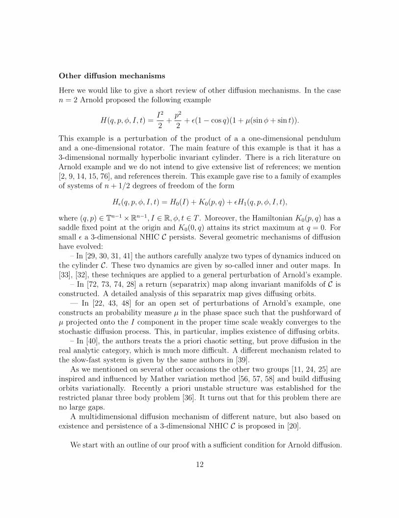
Here we would like to give a short review of other diffusion mechanisms. In the casen = 2 Arnold proposed the following example

H(q, p, φ, I, t) =I2

2+p2

2+ ε(1− cos q)(1 + µ(sinφ+ sin t)).

This example is a perturbation of the product of a a one-dimensional pendulumand a one-dimensional rotator. The main feature of this example is that it has a3-dimensional normally hyperbolic invariant cylinder. There is a rich literature onArnold example and we do not intend to give extensive list of references; we mention[2, 9, 14, 15, 76], and references therein. This example gave rise to a family of examplesof systems of n+ 1/2 degrees of freedom of the form

Hε(q, p, φ, I, t) = H0(I) +K0(p, q) + εH1(q, p, φ, I, t),

where (q, p) ∈ Tn−1×Rn−1, I ∈ R, φ, t ∈ T . Moreover, the Hamiltonian K0(p, q) has asaddle fixed point at the origin and K0(0, q) attains its strict maximum at q = 0. Forsmall ε a 3-dimensional NHIC C persists. Several geometric mechanisms of diffusionhave evolved:

– In [29, 30, 31, 41] the authors carefully analyze two types of dynamics induced onthe cylinder C. These two dynamics are given by so-called inner and outer maps. In[33], [32], these techniques are applied to a general perturbation of Arnold’s example.

– In [72, 73, 74, 28] a return (separatrix) map along invariant manifolds of C isconstructed. A detailed analysis of this separatrix map gives diffusing orbits.

— In [22, 43, 48] for an open set of perturbations of Arnold’s example, oneconstructs an probability measure µ in the phase space such that the pushforward ofµ projected onto the I component in the proper time scale weakly converges to thestochastic diffusion process. This, in particular, implies existence of diffusing orbits.

– In [40], the authors treats the a priori chaotic setting, but prove diffusion in thereal analytic category, which is much more difficult. A different mechanism related tothe slow-fast system is given by the same authors in [39].

As we mentioned on several other occasions the other two groups [11, 24, 25] areinspired and influenced by Mather variation method [56, 57, 58] and build diffusingorbits variationally. Recently a priori unstable structure was established for therestricted planar three body problem [36]. It turns out that for this problem there areno large gaps.

A multidimensional diffusion mechanism of different nature, but also based onexistence and persistence of a 3-dimensional NHIC C is proposed in [20].

We start with an outline of our proof with a sufficient condition for Arnold diffusion.

12

1.3 Scheme of diffusion

For all ε ≤ 1, the Hamiltonian Hε satisfy the Tonelli property of superlinearity, strictconvexity, and completeness (see Section 6). Mather theory ([35], [58]) implies thatfor each cohomology class c ∈ R2 ' H1(T2,R), the Hamiltonian Hε admits families ofinvariant sets of the Hamiltonian flow on T2 × R2 × T, called the Mather, Aubry, andMane sets, satisfying

MHε(c) ⊂ AHε(c) ⊂ NHε(c) ⊂ T2 ×BC√ε(c)× T,

where C is a constant depending only on D (see Corollary 7.7). We use M0Hε

(c),

A0Hε

(c) and N 0Hε

(c) to denote their intersection with the section t = 0, which areinvariant under the time-1-map. Throughout the paper, we may switch betweenthe two equivalent settings: either consider continuous invariant sets of the flow, ordiscrete invariant sets under the time-1-map.

Our main strategy is then to pick a subset Γ∗ ⊂ R2 of cohomologies very close tothe diffusion path P , then find an orbit that shadows a sequence of Aubry sets AHε(ci),i = 1, . . . , N , ci ∈ Γ∗. This requires the existence of non-degenerate heteroclinicconnections between the Aubry sets, the family of invariant sets with heteroclinicconnections is called a transition chain by Arnold [5]. To do this, we show that thecohomologies satisfy one of the four diffusion mechanisms.

We give a general introduction to these mechanisms below, and refer to Section2.1 for precise definitions.

Mather mechanism

For a twist map, it is known since Birkhoff that a region free of essential invariantcurves is unstable, namely there exists orbits that drifts from one boundary of theregion to another. Mather ([58]) gave a conceptual description of this phenomenon,and generalized it into higher dimension.

We say that the pair (Hε, c) satisfy the Mather mechanism if

πθN 0Hε(c) ⊂ T2

is contractible. (Note in the twist map case this means N 0(c) is not a rotational

invariant curve.) Mather proved that in this case, A0Hε

(c) admits a heteroclinic

connecting orbit to A0Hε

(c′) if c, c′ are close.

Arnold mechanism

In Arnold’s original paper [5], Arnold showed the existence of a family of invariant tori,whose own stable and unstable manifolds intersects transversally. In our setting, the

13

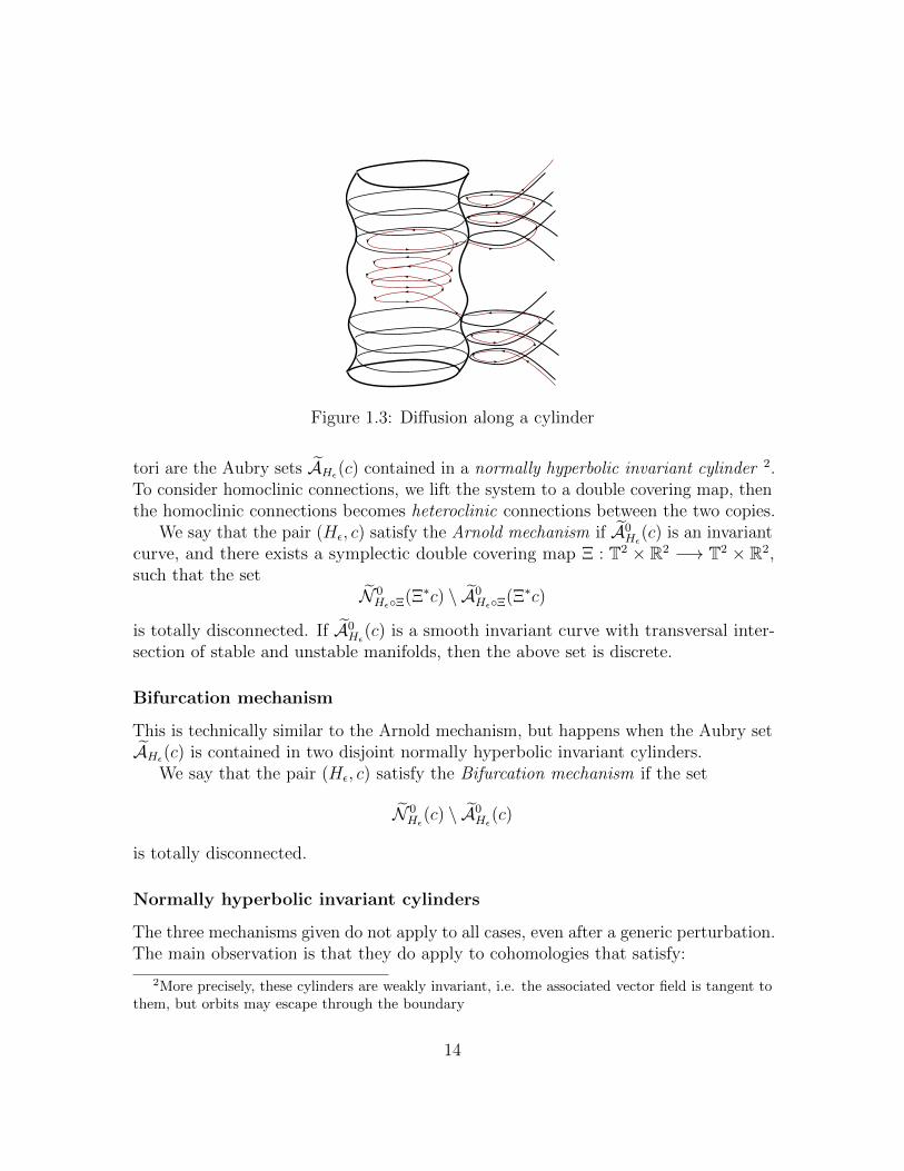
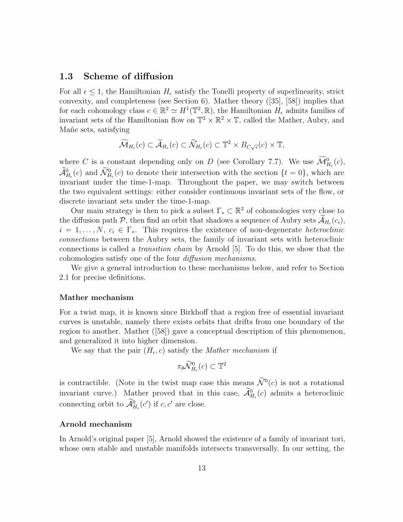
Figure 1.3: Diffusion along a cylinder

tori are the Aubry sets AHε(c) contained in a normally hyperbolic invariant cylinder 2.To consider homoclinic connections, we lift the system to a double covering map, thenthe homoclinic connections becomes heteroclinic connections between the two copies.

We say that the pair (Hε, c) satisfy the Arnold mechanism if A0Hε

(c) is an invariantcurve, and there exists a symplectic double covering map Ξ : T2 × R2 −→ T2 × R2,such that the set

N 0HεΞ(Ξ∗c) \ A0

HεΞ(Ξ∗c)

is totally disconnected. If A0Hε

(c) is a smooth invariant curve with transversal inter-section of stable and unstable manifolds, then the above set is discrete.

Bifurcation mechanism

This is technically similar to the Arnold mechanism, but happens when the Aubry setAHε(c) is contained in two disjoint normally hyperbolic invariant cylinders.

We say that the pair (Hε, c) satisfy the Bifurcation mechanism if the set

N 0Hε(c) \ A

0Hε(c)

is totally disconnected.

Normally hyperbolic invariant cylinders

The three mechanisms given do not apply to all cases, even after a generic perturbation.The main observation is that they do apply to cohomologies that satisfy:

2More precisely, these cylinders are weakly invariant, i.e. the associated vector field is tangent tothem, but orbits may escape through the boundary

14

1. (2D NHIC) The Aubry set A0Hε

(c) is contained in a two-dimensional normallyhyperbolic invariant cylinder.

2. (1D Graph Theorem) The Aubry set A0Hε

(c) is contained in a Lipschitz graphover the circle T.

In this case, we say that the pair (Hε, c) is of Aubry-Mather type.Under these assumptions, the Aubry set resembles the Aubry-Mather sets for twist

maps, and in particular, generically we have the following dichotomy: either πN 0Hε

(c)

is contractible, or A0Hε

(c) is a Lipschitz invariant curve. In the latter case, we can showthat Arnold mechanism applies after an additional perturbation. Since either Matheror Arnold mechanism applies, we conclude that A(c) is connected to A(c′) for c, c′

close. Moreover, this argument can be continued if c′ is also of Aubry-Mather type.Dynamically, the orbit is either diffusing along the heteroclinic orbits of invariantcurves, or diffusing in a Birkhoff region of instability within the cylinder. See Figure 1.3.We now briefly describe the non-degeneracy conditions.

While a cohomology of Aubry-Mather type is robust, namely it can be extendedalong a continuous curve, in a one-parameter family one may encounter a bifurcationwhere the Aubry set jumps from one cylinder to another one. At the bifurcation, theAubry set is contained in both cylinders. We say that the pair (Hε, c) if of BifurcationAubry-Mather type if the Aubry set is possibly contained in two cylinders.

Technically we have to involve a different bifurcation type, called asymmetricbifurcation type. This is very similar to the bifurcation Aubry-Mather type, the maindifference is on one side of the bifurcation, the Aubry set is a Aubry-Mather type setcontained in a invariant cylinder, while the other side we have a hyperbolic periodicorbit. This happens when we cross double resonance, see Definition 8.3.

Forcing relation

The rigorous formulation of the three diffusion mechanisms will be given using theconcept of forcing equivalence defined by Bernard in [11] (which is generalizationof a equivalence relation defined by Mather, see [58]). If c, c′ are forcing equivalent(denoted c a` c′), then there is a heteroclinic orbit connecting the associated Aubrysets. Moreover, there exists orbit shadowing an arbitrary sequence of cohomologies,as long as they are all equivalent. See Section 2.1 for more details.

The main theorem reduces to Theorem 2.1, which proves forcing equivalence of anet of cohomologies, called Γ∗. The set Γ∗ consists of finitely many smooth curves.On each of the smooth curves, we prove the cohomologies are of Aubry-Mather type,and therefore one of the three mechanisms apply.

We prove forcing equivalence of different connected components directly, using thedefinition of the forcing relation. We call this the Jump mechanism.

15

1.4 Three regimes of diffusion

Recall that our plan is to choose a net Γ∗ of cohomology classes, and prove theirforcing equivalence, by first proving they are of Aubry-Mather type or BifurcationAubry-Mather type. This is done in three distinct regimes.

Single resonance

Let (k1,Γk1) ∈ K be one of the single resonant component, and let Kst(k1,Γk1 , λ) bethe collection of the strong additional resonances. Then for p in a O(

√ε)-neighborhood

of the set

ΓSRk1 (M,λ) := Γk1 \

⋃k2∈Kst(k1,Γk1 ,λ)

BM√ε(Γk1,k2)

,

where M is a large parameter, the system admits the normal form

NSRε = H0 + εZ(θs, p) +O(εδ), (θs, θf , t) ∈ T3.

where how small δ is depends on how many double resonances we exclude. Under thenon-degeneracy conditions SR(k1,Γk1 , λ), the above system admits three dimensional(for the flow) normally hyperbolic invariant cylinders, and one can prove each c ∈ΓSRk1 (M,λ) is of AM or of Bifurcation AM type.

Double resonance, high energy

Let p0 = Γk1,k2 be a double resonance. On the set

BM√ε(p0), p0 = Γk1 ∩ Γk2 ,

we perform a normal form transformation, and then the p variable via I = (p−p0)/√ε.

One can show that the system is conjugate to:

1

β

(K(I)− U(ϕ) +O(

√ε)),

where K : R2 −→ R is a positive quadratic form and U : T2 −→ R, and β > 0 is aconstant depending only on k1, k2. The system Hs = K(I)− U(ϕ) is a two degrees offreedom mechanical system. Below we use the shifted energy E := Hs(ϕ, I)+minU(ϕ)as a parameter.

When the shifted energy E is not too close to 0, we are in the the high energyregime. By imposing the conditions [DR1h] − [DR3h], one shows existence of two-dimensional normally hyperbolic invariant cylinders associated to the shortest loopsfor the associated Jacobi metric, with the shifted energy as a parameter. This cylinderpersists under perturbation, and one can show that the associated cohomologies areof Aubry-Mather type.

16

Double resonance, low energy

As the energy decreases, the cylinder constructed in the high energy may not persist.Under the non-degeneracy conditions DR(k1, k2), we distinguish two separate cases:

1. Simple cylinder: in this case the cylinder extends across zero shifted energy tonegative shifted energy. In this case one can still show the associated cohomolo-gies are of Aubry-Mather type.

2. Non-simple cylinder: In this case the cylinder may be destroyed before theshifted energy becomes zero. However, we show the existence of two simplecylinders near the non-simple one, and one can “jump” from one cylinder toanother one.

This is the only case where the Jump mechanism is used.

2 Forcing relation

2.1 Sufficient condition for Arnold diffusion

Recall that we will utilize the concept of forcing equivalence, denoted c a` c′. Theactual definition will not be important for the current discussions, instead, we stateits main application to Arnold diffusion.

Proposition 2.1 ([11], Proposition 0.10). Let ciNi=1 be a sequence of cohomologyclasses which are forcing equivalent. For each i, let Ui be neighborhoods of the discreteMather sets M0

H(ci), then there is a trajectory of the Hamiltonian flowvisiting all thesets Ui.

Let σ > 0 and Vσ(H) denote the σ neighborhood of H in the space Cr(T2×B2×T)with respect to the natural Cr topology. The following statement is a “local” versionof our main theorem, where we state that given H1 ∈ U , we can:

(1) Choose ε0 to be locally constant on a neighborhood of H1;(2) Prove forcing equivalence on a residual subset of a neighborhood of Hε.

Theorem 2.1. Let P be a diffusion path and U1, . . . , UN be open sets intersecting P.Then there is and open and dense subset U(P) ⊂ Sr, and for each H1 ∈ U(P), thereare δ = δ(H0, H1) > 0, ε1 = ε1(H0, H1) > 0 such that for each

H ′1 ∈ Vδ(H1), 0 < ε < ε1,

17

there is a subset Γ∗(ε,H0, H′1) ⊂ R2 satisfying

Γ∗ = Γ∗(ε,H0, H′1) ∩ Ui 6= ∅, i = 1, . . . , N,

with the property that there is σ = σ(ε,H0, H′1) > 0, and a residual subset Rσ(H0 +

εH ′1) ⊂ Vσ(H0 + εH ′1), such that for each H ′ ∈ R, with respect to the Hamiltonian H ′,all the c ∈ Γ∗(ε,H0, H

′1) are forcing equivalent.

Proposition 2.1 and Theorem 2.1 imply our main theorem.

Proof of Theorem 1.1. First of all, let us define the lower semi-continuous function ε0.For each H1 ∈ U , define

εH12 (·) = ε1(H0, H1)1Vδ(H1)(·)

where 1V denote the indicator function of V . An indicator function of an open set islower semi-continuous by definition. For H1 ∈ Sr \ U , let εH1

2 ≡ 0. We then define

ε0(·) = supH1∈Sr

εH12 (·),

which is lower semi-continuous, being an (uncountable) supremum of lower semi-continuous function. Note that ε0 is positive on each H1 ∈ U since εH1

2 (H1) =ε1(H0, H1) > 0.

Consider now H1 ∈ U and 0 < ε < ε0(H1) as defined above. Let Γ∗(ε0, H0, H1) beas in Theorem 2.1. Let ci ∈ Ui ∩ Γ∗(ε,H0, H1). For any ‖H − H0‖Cr ≤ ε, there is

C > 0 depending only on D such that M0H(c) ⊂ T2×BC

√ε(c). As a result, reducing ε0

if necessary (note that minimum of an lower semi-continuous function and a constant

is still lower semi-continuous) , we have M0H(ci) ⊂ T2 × Ui. Since ci are all forcing

equivalent by Theorem 2.1, Proposition 2.1 implies the existence of an orbit visitingeach neighborhood T2 × Ui.

Since the above discussion applies to all H ∈ Rσ(H0 + εH1) where H1 ∈ U ,0 < ε < ε0(H1), we conclude that for a dense subset of V(U , ε0) (as defined inTheorem 1.1), there is an orbit visiting each T2 × Ui. Since this property is open dueto the smoothness of the flow, it holds on an open and dense subset W of V .

The set Γ∗(ε,H0, H1) will be chosen to be the union of finitely many smooth curves,and will coincide with P except on finitely many neighborhoods of size O(

√ε) of

strong double resonances.

18

2.2 Diffusion mechanisms via forcing equivalence

We reformulate the diffusion mechanisms introduced in Section 1.3 using forcingequivalence. We start with Mather mechanism.

Proposition 2.2 ([11], Theorem 0.11). Suppose

N 0H(c) is contractible. (Ma)

as a subset of T2, then there is σ > 0 such that c is forcing equivalent to all c′ ∈ Bσ(c).

To define the Arnold mechanism, we consider a finite covering of our space. Let

ξ : Tn −→ Tn

be a linear double covering map, for example: (θ1, θ2) 7→ (2θ1, θ2). Then ξ lifts to asymplectic map

Ξ : Tn × Rn −→ Tn × Rn, Ξ(θ, p) = (ξθ, ξ∗p),

where ξ∗(p) is defined by the relation ξ∗(p) · v = p · dξ(v) for all v ∈ R2. For example,if n = 2 and ξ(θ1, θ2) = (2θ1, θ2) we have ξ∗(p1, p2) = (p1/2, p2). This allows us toconsider the lifted Hamiltonian H Ξ.

Lemma 2.3. ([11], Section 7) We have

A0HΞ(ξ∗c) = Ξ−1A0

H(c), N 0HΞ(ξ∗c) ⊃ Ξ−1N 0

H(c).

Moreover, ξ∗c ` ξ∗c′ relative to H Ξ implies c ` c′ relative to H.

The Aubry set can be decomposed into disjoint invariant sets called static classes,which gives important insight into the structure of the Aubry set. In particular, whenthere is only one static class, then A0

H(c) = N 0H(c). In the case A0

H(c) 6= N 0H(c),

the difference N 0H(c) \ A0

H(c) consists of heteroclinic orbits from one static class

to another ([11]). Using Lemma 2.3, when A0H(c) = N 0

H(c), it may happen that

A0HΞ(ξ∗c) ( N 0

HΞ(ξ∗c), and the difference provides additional heterclinic orbits tothe Aubry set that is not contained in the Mane set before the lifting. This can beexploited to create diffusion orbits.

Proposition 2.4 ([11], Theorem 9.2, Proposition 7.3). Suppose, either:

A0H(c) has two static classes, and N 0

H(c) \ A0H(c) is totally disconnected, (Bif)

or:

A0H(c) has one static class, and N 0

HΞ(ξ∗c)\A0HΞ(ξ∗c) is totally disconnected. (Ar)

Then there is σ > 0 such that c is forcing equivalent to all c′ ∈ Bσ(c).

19

As implied by the labeling, the first item is called the bifurcation mechanism, andthe second the Arnold mechanism. We obtain the following immediate corollary:

Corollary 2.5 (Mather-Arnold mechanism). Suppose Γ ⊂ B2 is a continuous curve,and for each c ∈ Γ one of the diffusion mechanisms (Ma), (Bif), or (Ar) holds.Then all c ∈ Γ are forcing equivalent.

Recall that Γ∗(ε,H0, H1) can be chosen as a union of finitely many smooth curves.

• We will later show that for c ∈ Γ∗(ε,H0, H1) in Theorem 2.1, one of the twoapplies: Proposition 2.2 or Proposition 2.4.

As a result, each connected component of Γ∗(ε,H0, H1) consists of equivalent c’s.

• We prove the forcing equivalence between different connected components usingdirectly the definition of forcing relation. We call this the “jump” mechanism.

2.3 Invariance under the symplectic coordinate changes

A diffeomorphism Ψ = Ψ(θ, p) : Tn × Rn −→ Tn × Rn is called exact symplectic ifΨ∗λ − λ is an exact one-form, where λ =

∑ni=1 pidθi is the canonical form. We say

Φ : Tn × Rn × T −→ Tn × Rn × T is exact symplectic if

Φ(θ, p, t) = (Φ1(θ, p, t), t),

and there is E = E(θ, p, t), such that

Ψ(θ, p, t, E) = (Φ(θ, p, t), E + E(θ, p, t))

(called the autonomous extension of Φ) is exact symplectic. The new term E(θ, p, t)is defined up to adding a function f ′(t), where f(t) is periodic in t. Let us assume

E(0, 0, t) ≡ 0, therefore the choice of E is unique.Let H = H(θ, p, t), and Φ is exact symplectic with extension Ψ. Then for

G(θ, p, t, E) = H(θ, p, t) + E, we define

Φ∗H = Ψ∗H = G Ψ(θ, p, t, E)− E = H Φ + E(θ, p, t). (2.1)

The Aubry, Mather, Mane sets are invariant under exact symplectic coordinatechange in the following sense.

Proposition 2.6 ([10], [65]). Suppose H and Φ∗H are Tonelli, and let Ψ be theextension of Φ. Let (c, α) ∈ Rn × R ' H1(Tn × T,R), and let Ψ∗(c, α) = (c∗, α∗)

20

be the push forward of the cohomology class via the identification H1(T2 × T,R) 'H1(Tn × Rn × T× R,R). Then

α = αH(c) ⇐⇒ α∗ = αΦ∗H(c∗).

Let us denote(Φ∗Hc, α

∗) = Ψ∗(c, αH(c)),

then

MH(c) = Φ(MΦ∗H(Φ∗Hc)

), AH(c) = Φ

(AΦ∗H(Φ∗Hc)

), NH(c) = Φ

(NΦ∗H(Φ∗Hc)

).

Note in the particular case when Φ is homotopic to identity, Φ∗Hc = c and αΦ∗H(c) =αH(c).

Lemma 2.7. Let Φ be an exact symplectic coordinate change. The tuple (H, c) satisfies(Bif) or (Ar) if and only if (Φ∗H,Φ∗Hc) satisfies the same conditions. The property

(Ma) with the additional condition that A0H(c) = N 0

H(c) is also invariant under exactsymplectic coordinate changes.

Proof. Since our symplectic coordinate changes are always identity in the t components,the invariance of Aubry and Mane sets imply the invariance of their zero section underthe map Φ(·, ·, 0). The invariance of (Bif) follows. For the invariance of (Ma), note

that due to the graph property, A0H(c) is contractible in T2 × R2 if and only if A0

H(c)is contractible in T2. Therefore the contractibility of Aubry set is invariant, and sincethe Aubry set coincide with the Mane set by assumption, (Ma) is invariant.

For (Ar), let Ψ be the extension of Φ, and let us extend Ξ trivially to Tn×Rn×Tor Tn × Rn × R without changing its name. Let Φ1 be an exact symplectic changehomotopic to Φ, with extension Ψ1, such that

Φ Ξ = Ξ Φ1, Ψ Ξ = Ξ Ψ1.

Let us note Ξ∗c, defined as the push forward of H1(Tn × Rn × T× R,R) under theidentification with H1(Tn × T,R), is identical to ξ∗c. We have:

Ψ∗1(Ξ∗c, αHΞ(Ξ∗c)) = Ψ∗1Ξ∗(c, αH(c)) = Ξ∗Ψ∗(c, αH(c)).

Since Ξ is independent of t, Ξ∗ is identity in the last component. We conclude that(Φ1)∗HΞ Ξ∗c = Ξ∗(Φ∗Hc). Moreover,

(Φ Ξ)∗H = (Φ∗H) Ξ, (Ξ Φ1)∗H = Φ∗1(H Ξ).

Then

Φ1

(N(ΦΞ)∗H((Φ Ξ)∗Hc)

)= Φ1

(NΦ∗1(HΞ)((Φ1)∗HΞ Ξ∗c)

)= NHΞ(Ξ∗c)

21

andΦ1

(Ξ−1NΦ∗H(Φ∗Hc)

)= Ξ−1Φ

(Ξ−1NΦ∗H(Φ∗Hc)

)= Ξ−1

(NH(c)

),

therefore

Φ1

(N(Φ∗H)Ξ(Ξ∗(Φ∗Hc)) \ Ξ−1NΦ∗H(Φ∗Hc)

)= NHΞ(Ξ∗c) \ Ξ−1NH(c).

This implies invariance of (Ar) after considering the zero section of the above equality.

Our definition of exact symplectic coordinate change for time-periodic systemis somewhat restrictive, and in particular, it does not apply directly to the linearcoordinate change performed at the double resonance. In that setting, we will proveinvariance of Mather, Aubry and Mane set directly.

2.4 Normal hyperbolicity and Aubry-Mather type

Call a two dymensional normally hyperbolic invariant cylinder symplectic if therestriction of the canonical form for this cylinder is non-degenerate on the domain ofdefinition. Loosely speaking, a pair (H∗, c∗) is called of Aubry-Mather type (AM typefor short, refer to Definition 8.1 for details) if:

1. The discrete Aubry set A0H∗(c∗) is contained in two dimensional normally hyper-

bolic invariant cylinder, the restriction of the symplectic form is non-degenerateon the cylinder.

2. There is σ > 0 such that the following holds for c ∈ Bσ(c∗) and H ∈ Vσ(H∗) :

(a) The discrete Aubry set satisfies the graph property under the local coordi-nates of the cylinder.

(b) When the Aubry set is an invariant graph, then locally the unstable manifoldof the Aubry set is a graph over the configuration space T2.

This definition gives an abstract version of the setting seen in the a priori unstablesystems.

Theorem 2.2 (See Theorem 8.1). Suppose H∗ ∈ Cr, r ≥ 2 and (H∗, c∗) is of Aubry-Mather type, Γ ⊂ R2 is a smooth curve containing c∗ in the relative interior. Thenthere is σ > 0 such that for all c ∈ Bσ(c∗) ∩ Γ, the following dichotomy holds for aCr-residual subset of H ∈ Vσ(H∗):

1. Either the projected Mane set N 0H(c) is contractible as a subset of T2 (Mather

mechanism (Ma));

22

2. Or there is a finite covering map Ξ such that the set

N 0HΞ(ξ∗c) \ Ξ−1N 0

H(c)

is totally disconnected (Arnold mechanism (Ar)).

We say (H∗, c∗) is of bifurcation Aubry-Mather type if there exists two normallyhyperbolic invariant cylinders, such that the local Aubry set restricted to each cylindersatisfy the conditions of Aubry-Mather type. The precise definition is given inDefinition 8.2.

We will also consider a particular (and simpler) bifurcation. We say (H∗, c∗) is ofasymmetric bifurcation type if there exists one normally hyperbolic invariant cylinder,and a hyperbolic periodic orbit, such that the Aubry set is either contained in the unionof the cylinder (and of Aubry-Mather type), and the periodic orbit, see Definition 8.3.

We state the consequence of these definitions in terms of diffusion.

Theorem 2.3 (See Theorem 8.2). Suppose H∗ ∈ Cr, r ≥ 2 and (H∗, c∗) is ofbifurcation Aubry-Mather type or asymmetric bifurcation type, and Γ ⊂ R2 is a smoothcurve containing c∗ in the relative interior. Then there is σ > 0 and an open anddense subset R ⊂ Vσ(H∗) such that for each H ∈ R and each c ∈ Γ ∩ Bσ(c∗), (Bif)holds on at most finitely many c’s, and for all other c’s either (Ma) or (Ar) holds.

The following Proposition is a direct consequence of Theorem 2.2 and Theorem 2.3.

Proposition 2.8. Suppose Γ ⊂ B2 is a piecewise smooth curve of cohomologies suchthat for each c ∈ Γ, such that the pair (H∗, c) is of Aubry-Mather type, bifurcationAM type or asymmetric bifurcation type. Then there is σ > 0 and a residual subsetRσ(H∗) ⊂ Vσ(H∗), such that either (Ma), (Bif), or (Ar) holds for each H ∈ Rσ(H∗)and each c ∈ Γ.

Proof. For a piecewise smooth Γ =⋃mi=1 Γi, we can extend each Γi to Γ′i smoothly,

such that Γi is contained in the relative interior of Γ′i. We then apply Theorem 2.2 andTheorem 2.3 to each c ∈ Γi relative to the smooth curve Γ′i, to get the conclusion of ourproposition for c′ ∈ Bσ(c)(c), and H ∈ Rσ(c)(H∗) ⊂ Vσ(c)(H∗). The proposition thenfollows by considering a finite covering of Γ by Bσ(cj)(cj), and taking finite intersectionof residual subsets Rσ(cj)(H∗).

We now describe the selection of cohomologies and prove AM type in each of thetwo regimes. Single resonance is covered in Section 3, and double resonance is splitinto two sections, Section 4 covers the geometrical part, while Section 5 covers thevariational part.

23

3 Normal forms and cohomology classes at single

resonances

3.1 Resonant component and non-degeneracy conditions

Let (k1,Γk1) ∈ K be a resonant segment in the diffusion path. Define the resonantcomponent of H1 relative to the single resonance k1 as follows:

[H1]k1(θ, p, t) =∑k∈k1Z

hk(p)e2πik·(θ,t),

where hk are the Fourier coefficients of H1(θ, p, t). Since [H1]k1 only depends on thevariables k1 · (θ, t) and p, we define

Zk1 : T× R2 −→ R, Zk1(k1 · (θ, t), p) = [H1]k1(θ, p, t).

For p0 ∈ Γk, define the following conditions:

[SR1λ] For all p ∈ Bλ(p0), the function Zk1(·, p) achieves a global maximum at θs∗(p) ∈ T,and

Zk1(θs, p)− Zk1(θs∗(p), p) < λd(θs, θs∗(p))

2.

[SR2λ] For all p ∈ Bλ(p0), there exists two local maxima θs1(p) and θs2(p) of the functionZk1(., p) in Tn−1 satisfying

∂2θsZk1(θ

s1(p), p) < λI , ∂2

θsZk1(θs2(p), p) < λI,

Zk1(θs, p) < maxZk1(θ

f1 (p), p), Zk1(θ

f2 (p), p) − λ

(mind(θs − θs1), d(θs − θs2)

)2.

Definition 3.1. We say that H1 satisfy the condition SR(k1,Γk1 , λ) if for eachp0 ∈ Γk1 , at least one of [SR1λ] and [SR2λ] holds for the function Zk1(θ

s, p).

Proposition 3.2. The set of H1 ∈ Sr such that SR(k1,Γk1 , λ) holds for some λ > 0is open and dense.

Proof. It suffices to show that a generic one-parameter family f(x, a), x ∈ T, a ∈[a1, a2] the function f(·, a) has unique non-degenerate maximum, with the exceptionof up to finitely many a’s for which there are two non-degenerate maxima. We canfirst show that the following property is open and dense: any local maxima in xis non-degenerate (∂2

xxf(x) < 0). The main observation is that it’s implied by aco-dimension two condition: we require whenever ∂xf = 0, and ∂xxf = 0, we have∂xxxf 6= 0. Then any degenerate critical point cannot be a maxima.

We obtain a finite family of local minima. We then can “slide” them against eachother so that they intersect transversally.

24

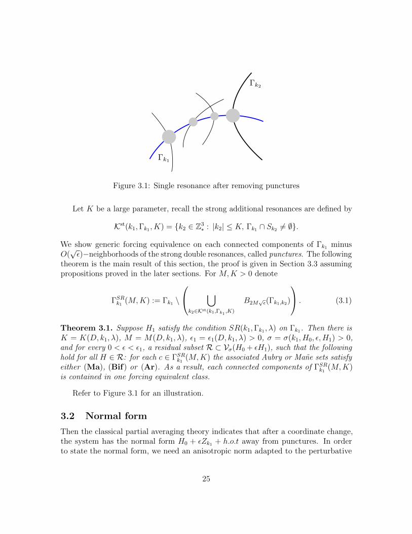
Figure 3.1: Single resonance after removing punctures

Let K be a large parameter, recall the strong additional resonances are defined by

Kst(k1,Γk1 , K) = k2 ∈ Z3∗ : |k2| ≤ K, Γk1 ∩ Sk2 6= ∅.

We show generic forcing equivalence on each connected components of Γk1 minusO(√ε)−neighborhoods of the strong double resonances, called punctures. The following

theorem is the main result of this section, the proof is given in Section 3.3 assumingpropositions proved in the later sections. For M,K > 0 denote

ΓSRk1 (M,K) := Γk1 \

⋃k2∈Kst(k1,Γk1 ,K)

B2M√ε(Γk1,k2)

. (3.1)

Theorem 3.1. Suppose H1 satisfy the condition SR(k1,Γk1 , λ) on Γk1. Then there isK = K(D, k1, λ), M = M(D, k1, λ), ε1 = ε1(D, k1, λ) > 0, σ = σ(k1, H0, ε,H1) > 0,and for every 0 < ε < ε1, a residual subset R ⊂ Vσ(H0 + εH1), such that the followinghold for all H ∈ R: for each c ∈ ΓSRk1 (M,K) the associated Aubry or Mane sets satisfyeither (Ma), (Bif) or (Ar). As a result, each connected components of ΓSRk1 (M,K)is contained in one forcing equivalent class.

Refer to Figure 3.1 for an illustration.

3.2 Normal form

Then the classical partial averaging theory indicates that after a coordinate change,the system has the normal form H0 + εZk1 + h.o.t away from punctures. In orderto state the normal form, we need an anisotropic norm adapted to the perturbative

25

nature of the system. Define

‖H1(θ, p, t)‖CrI = sup|α|+|β|≤r

ε|β|2 sup

∣∣∂α(θ,t)∂βpH1(θ, p, t)∣∣ , (3.2)

where α ∈ (Z+)3, β ∈ (Z+)2 are multi-indices and | · | denote the sum of the indices.The rescaled norm is similar to Cr norm, but replace the p derivatives by the derivativesin I = p/

√ε, hence the name.

Theorem 3.2 (See end of this section). With the notations above there is C =C(D, k1) > 1 such that the following hold. Let δ > 0 be a small parameter and setK = 1/δ2 and M = K2. Then for any c ∈ ΓSRk1 (M,K) there exists pc ∈ Γk1 such that

c ∈ BCK√ε/2(pc), (3.3)

and an C∞ exact symplectic coordinate change homotopic to the identity

Φε : T2 ×BCK√ε/2(pc)× T −→ T2 ×BCK

√ε(pc)× T

such that:

1.(Φε)

∗H = H0 + ε[H1]k1 + εR, ‖R‖C2I≤ Cδ. (3.4)

2. ‖Πθ(Φε − Id)‖C2I≤ Cδ4 and ‖Πp(Φε − Id)‖C2

I≤ Cδ4

√ε.

Here the C2I norm is evaluated on the set T2 ×BCK

√ε/2(pc)× T.

Remark 3.1. The C∞ coordinate change is obtained by approximating a coordinatechange that is only Cr−1, see Appendix B.1. The reason this can be done is that weonly need C2 estimates of the coordinate change.

We use the idea of Lochak (see for example [51]) to cover the action space withdouble resonances. A double resonance p0 = Sk1 ∩ Sk2 corresponds to a periodic orbitof the unperturbed system H0. More precisely, we have ω0 = Ω0(p0) := ∇H0(p0)which satisfies R(ω, 1) ∩ Z3 6= ∅. Denote by Tω0 = mint > 0 : t(ω0, 1) ∈ Z3 theminimal period.

The resonant lattice for p0 is Λ = SpanRk1, k2∩Z3, and the resonant componentis

[H1]k1,k2 =∑k∈Λ

hk(p)e2πik·(θ,t).

We have the following general normal form theorem, the proof is given at the endof Section B.1.

26

Proposition 3.3. Let p0 = Γk1,k2 , T = Tω0(p0). Then for a parameter C1 > 1, thereexists C = C(r, C1) > 1, ε0 = ε0(r) > 0 such that if K1 > C satisfies

T <C1

K21

√ε,

then for each 0 < ε < ε0 there exists a C∞ exact symplectic map

Φ : T2 ×BK1√ε/2 × T −→ T2 ×BK1

√ε × T

such that(Φ)∗Hε = H0 + ε[H1]k1,k2 + εR1,

where‖R1‖C2

I≤ CK−1

1 ,

and‖Πθ(Φ− Id)‖C2

I≤ CK−2

1 , ‖Πp(Φ− Id)‖C2I≤ CK−2

1

√ε.

Let us denote Λ1 = SpanRk1 ∩ Z3 and Λ2 = SpanRk1, k2 ∩ Z3.

Lemma 3.4. There is an absolute constant C > 0 such that if

min|k| : k ∈ Λ2 \ Λ1 ≥ K > 0,

we have‖[H1]k1,k2 − [H1]k1‖C2 ≤ CK−

12 .

Proof. First let us note that there is an absolute constant C > 0 such that for eachtwo dimensional lattice Λ ⊂ Z3, we have∑

k∈Λ\0

|k|−2− 12 < C.

To see this, we can bound the sum above using the integral∫|z|≥1, z∈SpanRΛ

|z|−2− 12dA.

Then using the fact that ‖hk‖C2 ≤ |k|2−r‖H1‖Cr , we have

‖[H1]k1,k2 − [H1]‖C2 ≤∑

k∈Λ2\Λ1

|k|2−r ≤ K−12

∑k∈Λ2\0

|k|2+ 12−r < CK−

12 .

The following lemma is an easy consequence of the Dirichlet theorem (see [51]).

27

Lemma 3.5. There is C = C(D, k1) > 0 such that for each Q1 > 1 and each c ∈ Sk1,there is a double resonance p0 with Tω0 < CQ1, and ‖c − p0‖ < C(Tω0Q1)

−1, whereω0 = ∇H0(p0).

Proof of Theorem 3.2. Denote τ = K2√ε. First we apply Lemma 3.5 using the pa-

rameter Q1 = Cτ−1, then each c ∈ Sk1 is contained in the τT (pc)

≤ K2√ε neighborhood

of a double resonance pc, whose period T (ωc) is at most CQ1, ωc = ∇H0(pc). Notethat for c in the set (3.1) (with M = K2), we have

pc /∈ Kst(k1,Γk1 , K).

Let pc = Γk1,k2 , necessarily Λ2 \ Λ1 (see Lemma 3.4) contains only vectors larger thanK, in this case we have Tωc ≥ C−1K where C may depend on k1. This lead to abetter estimate

‖pc − c‖ ≤K2√ε

Tωc≤ CK

√ε.

Moreover, from Lemma 3.4,

‖[H1]k1,k2 − [H1]k1‖C2 < CK−12 .

Let K1 = CK, we have Tωc ≤ CK2√ε

= C3

K21

√ε, therefore Proposition 3.3 applies with

the parameter C1 = C3 and K1 = CK, we obtain, for a different constant C2

‖R1‖C2I≤ C2K

−11 = C2C

−1K−1,

thereforeHε Φ = H0 + ε[H1]k1 + εR,

where

‖R‖C2I

= ‖ε([H1]k1,k2 − [H1]k1) + εR1‖C2I≤ C2C

−1K−1 + CK−12 ≤ 2CK−

12

if K is large enough. Moreover,

‖Πθ(Φ− Id)‖C2I≤ C2K

−21 ≤ K−2 ≤ C2δ

4,

‖Πp(Φ− Id)‖C2I≤ C2K

−21

√ε ≤ C2δ

4√ε.

28

3.3 The resonant component

Using the fact that k1 = (k11, k

01) ∈ Z2 × Z is space irreducible, there is k2 = (k1

2, k02)

such that BT0 :=

[k1

1

k12

]∈ SL(2,Z). 3 Define:

B =

(k1)T

(k2)T[0 0 1

] ∈ SL(3,Z),

and

ΦL(θ, p, t) = (θs, θf , ps, pf , t),

θsθft

= B

[θt

],

[ps

pf

]= (BT

0 )−1p.

One verifies that ΦL is a linear exact symplectic coordinate change. Note thatθs = k1 · (θ, t) and [H1]k1 ΦL depends only on θs, ps, pf . Let us write

Nε = (Φ∗εHε) ΦL = H0(ps, pf ) + εZ(θs, ps, pf ) + εR(θs, θf , ps, pf , t), (3.5)

where we abused notation by keeping the name of H0 and R after the coordinatechange. Let us also abuse notation by writing θ = (θs, θf) and p = (ps, pf). Let usnote that Nε is defined on the set

T2 ×BK1√ε(p1)× T, where K1 =

2K

‖B−1‖, p1 = (BT

0 )−1 p0.

and the resonant segment Γk1 is represented by Γs = p : ∂psH0 = 0 in the newcoordinates.

Let us consider the following set:

R(ε, δ, p1) =Nε = H0 + εZ(θs, p) + εR(θ, p, t), ‖R‖C2

I (T2×BK1√ε(p1)×T) < δ

.

We show that the system Nε admits a three dimensional normally hyperbolicinvariant cylinder of the type

(θs, pf ) = (Θs, P s)(θf , pf , t).

and if we consider the discrete Aubry set, it is a graph over θf component. The detailswill be given in Section 9, here we state the consequences of those results:

3This is the only part where the space irreducibility of resonance is used.

29

Proposition 3.6 (See Theorem 9.3). Assume that Z(θs, p) satisfies condition [SR1λ]at p1 ∈ Γs. Then there is δ0, ε0 > 0 depending on D,λ such that if 0 < ε < ε0 and0 < δ < δ0, for each N ∈ R(ε, δ, p1), each c ∈ BK1

√ε/2(p1) ∩ Γs the pair (N, c) is of

Aubry-Mather type.

Proposition 3.7 (See Theorem 9.4). Consider Nε as in Proposition 3.6, and assumethat Z(θs, p) satisfies condition [SR2λ] at p2 ∈ Γs. Then there is δ0, ε0 > 0 dependingon D,λ such that if 0 < ε < ε0 and 0 < δ < δ0, there is an open and dense subsetR1 ⊂ R(ε, δ, p1), such that each c ∈ BK1

√ε/2(p1) ∩ Γs the pair (N, c) is of bifurcation

Aubry-Mather type.

Proof of Theorem 3.1. Choose K0 = 1/δ0. Let Γ be a connected component of (3.1),and consider c0 ∈ Γ. Then there is p0 ∈ Γk such that c0 ∈ BK2

√ε/2(p0) (this is possible

by choosing Q large in (3.3)), where K2 = K/‖B−1‖2. After the coordinate change, cis mapped to c1 = (MT

0 )−1(c) which is contained in BK1/2(p1) with K1 = K/‖B−1‖.We now apply either Proposition 3.6 or 3.7 depending on the condition, and concludethat on the curve BK1

√ε/2(p1)∩Γs, each c is of Aubry-Mather or bifurcation AM type,

relative to Nε. We now apply Proposition 2.8, to conclude that to conclude that either(Ma), (Bif), or (Ar) holds for each c ∈ BK1

√ε/2(p1) ∩ Γs, on a Cr-residual subset

Rσ(Nε) of N ∈ Vσ(Nε), for some σ > 0.We now revert the coordinate change. The fact that the coordinate change is

C∞ implies the mapping Hε 7→ (ΦL Φε)∗Hε =: Φ∗Hε is a homeomorphism between

Cr spaces, and in particular, open neighborhoods and residual subsets are preservedbetween coordinate changes. As a result, there is σ′ > 0 and a residual subsetRσ′(Hε) of Vσ′(Hε), such that H ∈ Rσ′(Hε) implies Φ∗Hε ∈ Rσ(Nε). Then Lemma 2.7(invariance of diffusion mechanism under symplectic coordinate changes) implies foreach c ∈ BK2

√ε/2(p0) ∩ Γ, and for each H ∈ Rσ′(Hε), one of (Ma), (Bif), or (Ar)

hold.We now apply the above argument to each c ∈ Γ, and establish (Ma), (Bif), or

(Ar) for an neighborhood Bσ(c)(c) of c, on a Cr residual subset Rc of Vσ(c)(H). Bycompactness, Γ can be covered by finitely many Bσ(ci)(ci)’s, then by taking intersectionsover Rci , we conclude that our conditions hold on all c ∈ Γ, over a residual subset ofVσ0(Hε), where σ0 = minσ(ci). The theorem follows.

4 Double resonance: geometric description

In this section we describe the non-degeneracy condition at the double resonance. Wethen describe the normally hyperbolic cylinders in this regime. In next section, wewill return to variational setting, define the cohomology classes and prove their forcingequivalence.

30

4.1 The slow system

We now consider one of the strong double resonance. Let k ∈ Kst(k1,Γ, K), anddenote p0 = Γk1,k, and ω0 = ∇H0(p). Define

Λ = SpanRk1, k ∩ Z3,

and choose k2 ∈ Z3∗ such that Λ = SpanZk1, k2. It is always possible to choose

|k2| ≤ |k1|+K.Given H1 =

∑k∈Z3 hk(p)e

2πik·(θ,t), we define

[H1]Λ =∑k∈Λ

hk(p)e2πik·(θ,t).

Then after a symplectic coordinate change defined on the set K√ε (see Theorem B.1),

the system has the normal form:

Nε = Φ∗εHε = H0 + ε[H1]Λ +O(ε32 ).

The system is conjugate to a two degrees of freedom mechanical system after acoordinate change and an energy reduction. The details are given in Appendix B,here we give a brief description. Let k3 ∈ Z3 be such that

BT =[k1 k2 k3

]∈ SL(3,Z).

To define a symplectic coordinate change, we consider the corresponding autonomoussystem Nε(θ, p, t) + E, and consider the coordinate change

(θ, p, t, E) = ΦL(ϕ, I, τ, F ),[θt

]= B−1

[ϕ

τ/√ε

],

[p− p0

E +H0(p0)

]= BT

[√εIεF

].

(4.1)

One checks that(T2 × R2 × T× R, dθ ∧ dp+ dt ∧ dE

)ΦL−→(T2 × R2 × T× R,

1√ε(dϕ ∧ dI + dτ ∧ dF )

)is an exact symplectic coordinate change. The transformed Hamiltonian (Nε +E)ΦL

is no longer Tonelli in the standard sense, however by using a standard energy reductionon the energy level 0, with τ as the new time takes the system to

1

β

(K(I)− U0(ϕ) +

√εP (ϕ, I, τ)

), ϕ ∈ T2, I ∈ R2, τ ∈

√εT,

31

where

β = k3 · (ω0, 1), K(I) =1

2

(B0∂

2ppH0(p0)BT

0

), B0 =

[kT1kT2

],

andU(k1 · (θ, t), k2 · (θ, t)) = −[H1]Λ(θ, p0, t).

The systemHs(ϕ, I) = K(I)− U(ϕ) = K − U (4.2)

is called the slow mechanical system, and the non-degeneracy conditions at the doubleresonance p0 is stated for this system.

4.2 Non-degeneracy conditions for the slow system

We consider the (shifted) energy as a parameter. For each E > 0, by the Maupertuisprinciple, the Hamiltonian dynamics on the energy surface SE := (ϕ, I) : Hs(ϕ, I) +minU(ϕ) = E, is the time change of the geodesic flow for the Jacobi metric

gE(ϕ)(v) = 2(E + U(ϕ))K−1(v),

where K−1(v) = 12

(∂2IIK)

−1v · v is the Lagrangian associated to the Hamiltonian

K(I).We will be interested in a special homology class h = (0, 1) ∈ Z2 ' H1(T2,Z).

They represent classes of the original system satisfying k1 · (θ, 1) = 0, i.e. orbits thattravel close to the resonance Γk1 . We assume the following non-degeneracy conditions:

[DR1h] For each E ∈ (0,∞), each shortest closed geodesic (called a loop) of gE in thehomology class h is a hyperbolic orbit of the geodesic flow.

[DR2h] At all but finitely many bifurcation values, there is only one gE-shortest loop.At each bifurcation value E, there are exactly two shortest gE loops denoted γEhand γEh .

[DR3h] At bifurcation value E∗,

d(`E(γEh ))

dE|E=E∗ 6=

d(`E(γEh ))

dE|E=E∗ ,

where lE denote the gE length of a loop.

We now discuss the conditions at the critical shifted energy E = 0. The Jacobimetric g0 becomes degenerate at one point ϕ∗ = argminϕU(ϕ). By performing atranslation, we may assume ϕ∗ = 0. Let γ0

h be a shortest loop of g0 in the homologyh. Consider the following cases:

32

1. 0 ∈ γ0h and γ0

h is not self-intersecting. Call such homology class h simple criticaland the corresponding geodesic γ0

h simple loop.

2. 0 ∈ γ0h and γ0

h is self-intersecting. Call such homology class h non-simple andthe corresponding geodesic γ0

h non-simple.

3. 0 6∈ γ0h, then γ0

h is a regular geodesic. Call such homology class h simplenon-critical.

Mather [63] proved that generically only these three cases occur (see below for theprecise claim).

Lemma 4.1. Let h be a non-simple homology class. Then for a generic potential Uthe curve γ0

h is the concatenation of of two simple loops, possibly with multiplicities.More precisely, given h ∈ H1(T2,Z) generically there are simple homology classesh1, h2 ∈ H1(Ts,Z) and integers n1, n2 ∈ Z+ such that the corresponding minimalgeodesics γ0

h1and γ0

h2are simple and h = n1h1 + n2h2.

We call γ0h extensible if there exists a family of shortest curves γEh converging to it

in the Hausdorff topology. Consider the lift of γEh to the universal cover R2, then asE −→ 0 it converges to a periodic curve in R2 consists of concatenation of γ0

h1and

γ0h2

. Let (σ1, . . . , σn) ∈ 0, 1N be the order that γ0hi

are traced.

Lemma 4.2 (See Section 10.8). Assume that γ0h is extensible, then the sequence

(σn, . . . , σn), as described, is uniquely determined up to cyclic permutation. We write

γEh −→ γ0hσ1∗ · · · ∗ γ0

hσn, as E −→ 0.

We note that (0, 0) is a fixed point of the Hamiltonian flow Hs(ϕ, I) which ishyperbolic if ∂2

θθU(0) > 0. Any simple g0–shortest loop corresponds to a homoclinicorbit of the fixed point (0, 0). We impose the following non-degeneracy conditions:

[DR1c] (0, 0) is a hyperbolic fixed point with distinct eigenvalues −λ2 < −λ1 < 0 <λ1 < λ2. Let v±1 , v

±2 be the eigendirections for ±λ1, ±λ2.

[DR2c] There is a unique g0–shortest loop in the homology h. If it is non-simple, thenit is the concatenation of two simple loops γ0

h1and γ0

h2.

[DR3c] If γ0h is simple critical, then it is not tangent to the 〈v+

2 , v−2 〉 plane. If γ0

h isnon-simple, then each of γ0

h1and γ0

h2are not tangent to the 〈v+

2 , v−2 〉 plane.

[DR4c] – If γ0h is simple non-critical, then γ0

h is hyperbolic.

– If γ0h is simple critical, then γ0

h is non-degenerate in the sense that it is thetransversal intersection of the stable and unstable manifolds of (0, 0).

33

– If γ0h is non-simple, then each of γ0

h1and γ0

h2is non-degenerate.

The genericity of these conditions are summarized in the following statement.

Proposition 4.3. The conditions [DR1h −DR3h] and [DR1c −DR4c] hold on anopen and sense set of potentials U ∈ Cr(T2), for r ≥ 2.

4.3 Normally hyperbolic cylinders

Conditions [DR1h]− [DR3h] ensures that for each E0 > 0, the set⋃E∈(E0−δ,E0+δ)

ηEh

is a normally hyperbolic invariant cylinder. This cylinder does not necessarily extendto the shifted energy E = 0. The following statement ensures existence of cylindersnear critical energy, using the conditions [DR1c]− [DR4c].

Recall that γ0h is a shortest curve in the critical energy. The corresponding set in

the phase space is called η0h. Due to the symmetry of the system, we also have the

shortest curve γ0−h which coincide with γ0

h but has a different orientation.

Theorem 4.1 (See Section 10). Suppose that Hs satisfies conditions [DR1c]−[DR4c] 4.

1. If γ0h is simple, then there is e > 0 depending on Hs such that:

(a) For each 0 < E < e, there exist periodic orbits ηEh and ηE−h, such that theprojections γEh −→ γ0

h and γE−h −→ γ0−h in the Hausdorff topology.

(b) For each −e < E < 0, there exists a periodic orbit ηEc which shadows theconcatenation of η0

h and η0−h.

Then the union ⋃0<E<e

(ηEh ∪ ηE−h

)∪ η0

h ∪ η0−h ∪

⋃−e<E<0

ηEc

is a C1 normally hyperbolic invariant manifold containing the homoclinics η0±h.

2. If γ0h is non-simple: Let σ1, . . . , σn be the sequence determined in Lemma 4.2,

[DR1c]− [DR4c] ensures γ0h is extensible. More precisely, there is e > 0 such that

for each 0 < E < e, there is a periodic orbit γEh such that γEh −→ γ0hσ1∗ · · · ∗γ0

hσn.

Moreover, each γEh is hyperbolic.

34

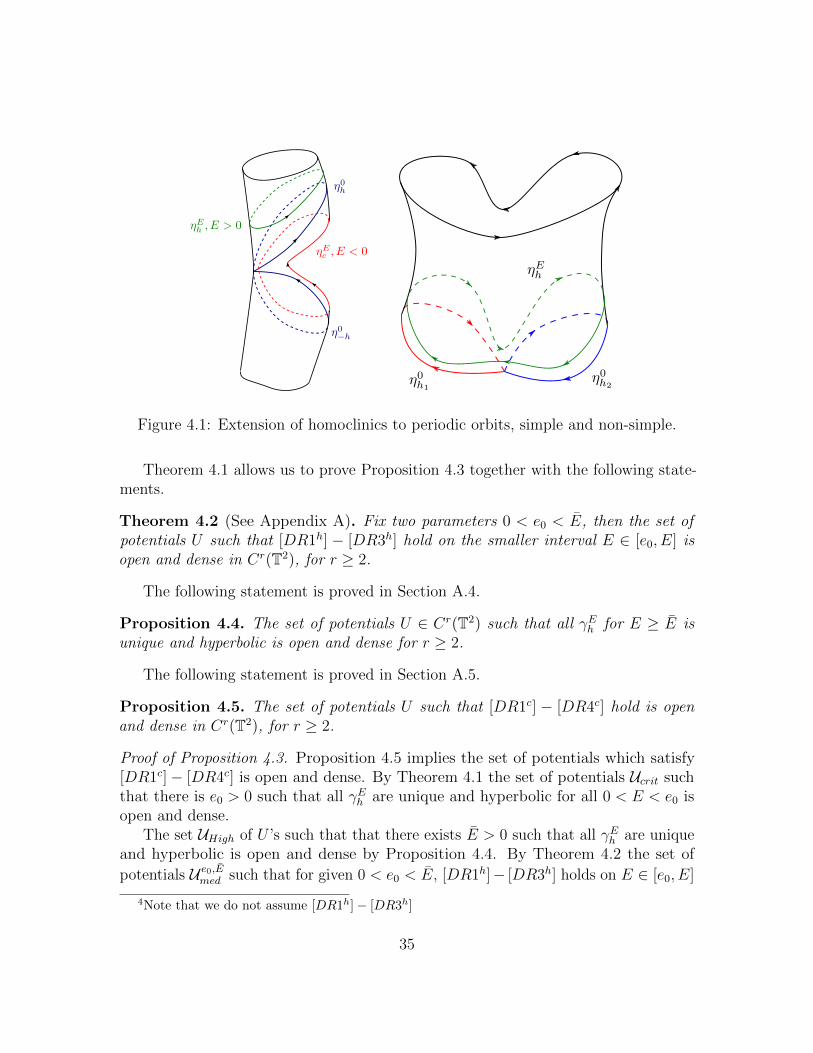
Figure 4.1: Extension of homoclinics to periodic orbits, simple and non-simple.

Theorem 4.1 allows us to prove Proposition 4.3 together with the following state-ments.

Theorem 4.2 (See Appendix A). Fix two parameters 0 < e0 < E, then the set ofpotentials U such that [DR1h] − [DR3h] hold on the smaller interval E ∈ [e0, E] isopen and dense in Cr(T2), for r ≥ 2.

The following statement is proved in Section A.4.

Proposition 4.4. The set of potentials U ∈ Cr(T2) such that all γEh for E ≥ E isunique and hyperbolic is open and dense for r ≥ 2.

The following statement is proved in Section A.5.

Proposition 4.5. The set of potentials U such that [DR1c] − [DR4c] hold is openand dense in Cr(T2), for r ≥ 2.

Proof of Proposition 4.3. Proposition 4.5 implies the set of potentials which satisfy[DR1c]− [DR4c] is open and dense. By Theorem 4.1 the set of potentials Ucrit suchthat there is e0 > 0 such that all γEh are unique and hyperbolic for all 0 < E < e0 isopen and dense.

The set UHigh of U ’s such that that there exists E > 0 such that all γEh are uniqueand hyperbolic is open and dense by Proposition 4.4. By Theorem 4.2 the set of

potentials U e0,Emed such that for given 0 < e0 < E, [DR1h]− [DR3h] holds on E ∈ [e0, E]

4Note that we do not assume [DR1h]− [DR3h]

35

is also open and dense. As a result the set of potentials, where [DR1h]− [DR3h] holdson E ∈ (0,∞) is

Ucrit ∩⋃

0<e0<E

U e0,Emed ∩ Uhigh

which is open and dense.

Diffusion across a double resonance: a geometric description

The diffusion across a double resonance may be described heuristically as follows:

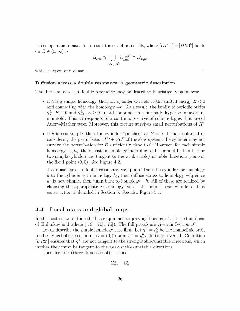
• If h is a simple homology, then the cylinder extends to the shifted energy E < 0and connecting with the homology −h. As a result, the family of periodic orbitsγEh , E ≥ 0 and γE−h, E ≥ 0 are all contained in a normally hyperbolic invariantmanifold. This corresponds to a continuous curve of cohomologies that are ofAubry-Mather type. Moreover, this picture survives small perturbations of Hs.

• If h is non-simple, then the cylinder “pinches” at E = 0. In particular, afterconsidering the perturbation Hs +

√εP of the slow system, the cylinder may not

survive the perturbation for E sufficiently close to 0. However, for each simplehomology h1, h2, there exists a simple cylinder due to Theorem 4.1, item 1. Thetwo simple cylinders are tangent to the weak stable/unstable directions plane atthe fixed point (0, 0). See Figure 4.2.

To diffuse across a double resonance, we “jump” from the cylinder for homologyh to the cylinder with homology h1, then diffuse across to homology −h1 sinceh1 is now simple, then jump back to homology −h. All of these are realized bychoosing the appropriate cohomology curves the lie on these cylinders. Thisconstruction is detailed in Section 5. See also Figure 5.1.

4.4 Local maps and global maps

In this section we outline the basic approach to proving Theorem 4.1, based on ideasof Shil’nikov and others ([18], [70], [75]). The full proofs are given in Section 10.

Let us describe the simple homology case first. Let η+ = η0h be the homoclinic orbit

to the hyperbolic fixed point O = (0, 0), and η− = η0−h its time-reversal. Condition

[DR2c] ensures that η± are not tangent to the strong stable/unstable directions, whichimplies they must be tangent to the weak stable/unstable directions.

Consider four (three dimensional) sections

Σu±, Σs

±

36

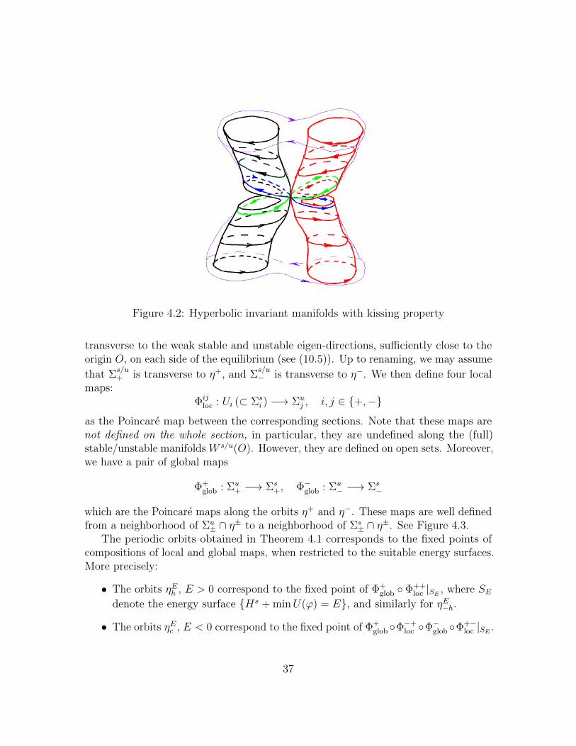
Figure 4.2: Hyperbolic invariant manifolds with kissing property

transverse to the weak stable and unstable eigen-directions, sufficiently close to theorigin O, on each side of the equilibrium (see (10.5)). Up to renaming, we may assume

that Σs/u+ is transverse to η+, and Σ

s/u− is transverse to η−. We then define four local

maps:Φij

loc : Ui (⊂ Σsi ) −→ Σu

j , i, j ∈ +,−

as the Poincare map between the corresponding sections. Note that these maps arenot defined on the whole section, in particular, they are undefined along the (full)stable/unstable manifolds W s/u(O). However, they are defined on open sets. Moreover,we have a pair of global maps

Φ+glob : Σu

+ −→ Σs+, Φ−glob : Σu

− −→ Σs−

which are the Poincare maps along the orbits η+ and η−. These maps are well definedfrom a neighborhood of Σu

± ∩ η± to a neighborhood of Σs± ∩ η±. See Figure 4.3.

The periodic orbits obtained in Theorem 4.1 corresponds to the fixed points ofcompositions of local and global maps, when restricted to the suitable energy surfaces.More precisely:

• The orbits ηEh , E > 0 correspond to the fixed point of Φ+glob Φ++

loc |SE , where SEdenote the energy surface Hs + minU(ϕ) = E, and similarly for ηE−h.

• The orbits ηEc , E < 0 correspond to the fixed point of Φ+glob Φ−+

loc Φ−glob Φ+−loc |SE .

37

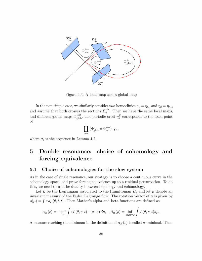
Figure 4.3: A local map and a global map

In the non-simple case, we similarly consider two homoclinics η1 = ηh1 and η2 = ηh2 ,

and assume that both crosses the sections Σs/u+ . Then we have the same local maps,

and different global maps Φ1/2glob. The periodic orbit ηEh corresponds to the fixed point

of1∏i=n

(Φσi

glob Φ++loc

)|SE ,

where σi is the sequence in Lemma 4.2.

5 Double resonance: choice of cohomology and

forcing equivalence

5.1 Choice of cohomologies for the slow system

As in the case of single resonance, our strategy is to choose a continuous curve in thecohomology space, and prove forcing equivalence up to a residual perturbation. To dothis, we need to use the duality between homology and cohomology.

Let L be the Lagrangian associated to the Hamiltonian H, and let µ denote aninvariant measure of the Euler–Lagrange flow. The rotation vector of µ is given byρ(µ) =

∫v dµ(θ, t, t). Then Mather’s alpha and beta functions are defined as:

αH(c) = − infµ

∫(L(θ, v, t)− c · v) dµ, βH(ρ) = inf

ρ(µ)=ρ

∫L(θ, v, t)dµ.

A measure reaching the minimum in the definition of αH(c) is called c−minimal. Then

38

α and β are both convex and Fenchel dual of each other:

βH(ρ) = supρ · c− αH(c).

The Legendre-Fenchel transform of β is defined as

LFβH (ρ) = c ∈ R2 : βH(ρ) = ρ · c− αH(c).

Geometrically,

LFβH (ρ) = conv c : there is a c-minimal µ such that ρ(µ) = ρ

where conv denotes the convex hull.Let γEh be a shortest loop for the Jacobi metric gE. Let T (γEh ) denotes its period

under the Hamiltonian flow, and if γEh is unique, we define

λEh = 1/T (γEh ).

If Hs satisfies [DR1h]− [DR3h], then there are at most finitely many E’s such thatthere are two shortest loops γEh and γEh . We will show that the set LFβHs (λEh h) =LFβHs (λEh h), and, therefore, the set LFβsH (λEh h) is independent of the choice of γEh .

Each LFβsH (λEh h) is a segment of nonzero length parallel to h⊥, and dependscontinuously on E. We call the union⋃

E>0

LFβHs (λEh h) (5.1)

the channel associated to the homology h, and we will choose a curve of cohomologiesin the interior of this channel. The channel is connected at the bottom to the setLFβH (0), which is a convex set with non-empty interior. The following propositionsummarizes the channel picture and the relation to the Aubry sets.

Proposition 5.1 (See Section C). Assume that Hs satisfies the conditions [DR1h −DR3h] and [DR1c −DR4c]. Then each LFβHs (λEh h) is a segment of non-zero lengthorthogonal to h, which varies continuously with respect to E.

For E > 0, let ch : (0, E] −→ H1(Ts,R) be a C1 function such that ch(E) is in therelative interior of LFβH (λEh h). The following hold.

1. If E is not a bifurcation energy, then AHs(ch(E)) = γEh .

2. If E is a bifurcation energy, AHs(ch(E)) = γEh ∪ γEh .

3. If h is simple, then the limit limE−→0 LFβHs (λEh h) contains a segment of non-zero width. We assume, in addition, that ch(0) is in the relative interior of thissegment.

39

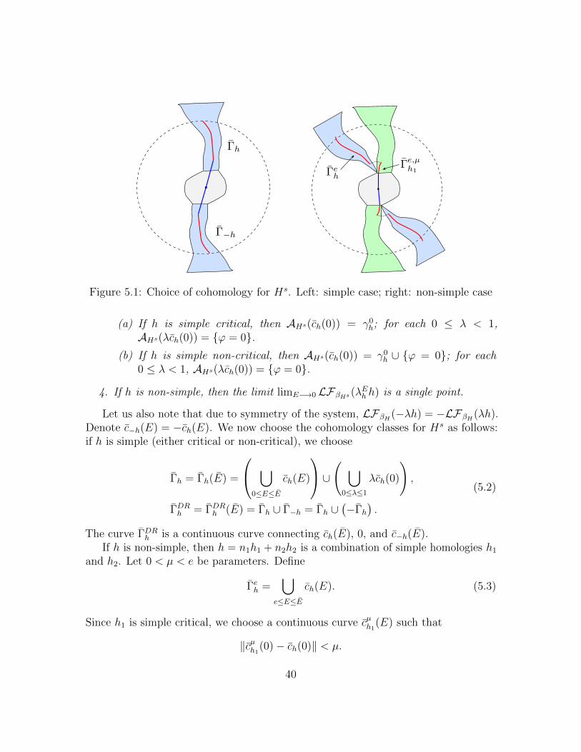
Figure 5.1: Choice of cohomology for Hs. Left: simple case; right: non-simple case

(a) If h is simple critical, then AHs(ch(0)) = γ0h; for each 0 ≤ λ < 1,

AHs(λch(0)) = ϕ = 0.(b) If h is simple non-critical, then AHs(ch(0)) = γ0

h ∪ ϕ = 0; for each0 ≤ λ < 1, AHs(λch(0)) = ϕ = 0.

4. If h is non-simple, then the limit limE−→0 LFβHs (λEh h) is a single point.

Let us also note that due to symmetry of the system, LFβH (−λh) = −LFβH (λh).Denote c−h(E) = −ch(E). We now choose the cohomology classes for Hs as follows:if h is simple (either critical or non-critical), we choose

Γh = Γh(E) =

⋃0≤E≤E

ch(E)

∪( ⋃0≤λ≤1

λch(0)

),

ΓDRh = ΓDRh (E) = Γh ∪ Γ−h = Γh ∪(−Γh

).

(5.2)

The curve ΓDRh is a continuous curve connecting ch(E), 0, and c−h(E).If h is non-simple, then h = n1h1 + n2h2 is a combination of simple homologies h1

and h2. Let 0 < µ < e be parameters. Define

Γeh =⋃

e≤E≤E

ch(E). (5.3)

Since h1 is simple critical, we choose a continuous curve cµh1(E) such that

‖cµh1(0)− ch(0)‖ < µ.

40

We then define

Γe,µh1 =

( ⋃0≤E≤e+µ

cµh1(E)

)∪

( ⋃0≤λ≤1

λch1(0)

). (5.4)

Γe,µh1 is a continuous curve connecting cµh1(e+ µ) with 0 (see Fig. 5.1, right). We thendefine

Γh = Γeh ∪ Γe,µh1 , ΓDRh = Γh ∪ Γ−h. (5.5)

Let us note that the set ΓDRh consists of three connected component, Γeh, Γe−h andΓe,µh1 ∪Γe,µ−h1 . Since the mechanisms we described so far can only prove forcing equivalencealong a connected set, we will use a different mechanism called “jump” to prove forcing-equivalence of different connected components.

5.2 Aubry-Mather type at a double resonance

Proposition 5.2. Suppose Hs = K(I)− U(ϕ) satisfies the non-degeneracy assump-tions. Given C > 0, there is ε0, δ > 0 depending on Hs and C such that for each0 < ε < ε0, if U ′ ∈ Vδ(U) and ‖P‖C2 < C, then for

Hsε =

1

β

(K(I)− U ′(ϕ) +

√εP (ϕ, I, τ)

).

each c ∈ ΓDRh is of one of fours types: Aubry-Mather type, bifurcation Aubry-Mather

type, asymmetric bifurcation type, or AHsε

is a hyperbolic periodic orbit. Note that thisapplies to all types of homologies: simple critical, simple non-critical, and non-simple.

Proof. We prove our proposition by referring to technical statement proved in latersections.

(1) Simple, critical homology. Denote c0 = ch(0). Theorem 11.3 states that thereexists ε0, ε, δ > 0 such that for all 0 < ε < ε0, U

′ ∈ Vδ(U), and c ∈ Be(c0), the pairHsε , c is of Aubry-Mather type. The same theorem also states Hs

ε , λc0 for 0 ≤ λ ≤ 1 isof Aubry-Mather type. This covers the cohomologies:

c ∈⋃

0≤E≤e

ch(E) ∪⋃

0≤λ≤1

λch(0).

The cohomologies⋃e≤E≤E ch(E), is covered in Theorem 11.1, which states that for

each e > 0, for there is ε, δ as in our proposition, such that with respect to Hsε , the

cohomology ch(E), E ≥ e is of Aubry-Mather type if γEh is the unique shortest curve,and of bifurcation Aubry-Mather type if there are two shortest curves. As a result, allcohomologies in Γh are of AM or bifurcation AM type, and by symmetry, so does Γ−h.This proves our proposition in the simple homology case, see (5.2).

41

(2) Non-simple homology. In the non-simple case. the cohomology curve Γh is thedisjoint union of two parts, namely

Γeh =⋃

e≤E≤E

ch(E), Γe,µh1 =

( ⋃0≤E≤e+µ

cµh1(E)

)∪

( ⋃0≤λ≤1

λch1(0)

).

We note that h1 is a simple homology and therefore each c ∈ Γe,µh1 are of AM typein the same way as in case (1). On the other hand, each homology in Γeh is of AMor bifurcation AM type since Theorem 11.1 applies the same way to simple andnon-simple homology. We conclude that our Proposition holds in the non-simple case.

(3) Simple, non-critical homology. The high energy case follows from Theorem 11.1in the same way as before. The critical energy follows from Theorem 11.2, the maindifference is that the critical energy is an asymmetric bifurcation (see Definition 8.3).For c = λch(0) where 0 ≤ λ < 1, the Aubry set is a single periodic orbit as aperturbation of the hyperbolic fixed point (0, 0).

Corollary 5.3. Suppose Hsε is from Proposition 5.2, then there is σ > 0 and a

residual subset R of Vσ(Hsε ), such that if H ′ ∈ R, then each c ∈ ΓDRh satisfies one of

the diffusion mechanisms (Ma), (Bif) and (Ar).

Proof. Note that Proposition 2.8 applies when c is either Aubry-Mather type, bifurca-tion Aubry-Mather type, asymmetric bifurcation type. Then Using Proposition 5.2,we only need to show the same conclusion hold if we add a fourth case, when theAubry set is a single hyperbolic periodic orbit. However, in this case, N 0 = A0 isdiscrete, so (Ma) applies.

We now revert to the original coordinate system. Denote p0 = Γk1,k2 the doubleresonance point. For a given cohomology class c ∈ R2, we consider the pair c, α definedby the equality [

c− p0

−α +H0(p0)

]= MT

[c√ε

αHsε(c) ε

](5.6)

then α = αNε(c) (compare to (4.1)). If (5.6) is satisfied, we denote

(c,−α) = Φ∗L(c, αHsε(c)), c = Φ∗L,Hs

ε(c).

Moreover, let us consider the autonomous version of the Aubry set:

AHsε+F (c) = (ϕ, I, τ,−Hε

s(ϕ, I, τ)) : (ϕ, I, τ) ∈ AHsε(c),

and similarly define M and N . Then by Proposition B.7

AHε+E(c) = ΦL

(AHs

ε+F (c)), NHε+E(c) = ΦL

(NHs

ε+F (c)). (5.7)

42

Proposition 5.4. Suppose c, c are related by (5.6). Then with respect to Nε, c satisfiesone of the diffusion mechanisms (Ma), (Bif) and (Ar) if and only if c does the samewith respect to Hs

ε .

Proof. The main issue here is that (Ma), (Bif) and (Ar) are defined for the zero

section A0 and N 0, but the symplectic coordinate change ΦL does not preserve the zerosection. However, the property that there exists a global section of the Hamiltonianflow such that one of (Ma), (Bif) or (Ar) applies to the intersection of A or N withthe section, is invariant under the coordinate change ΦL, due to (5.7). Since any twoglobal sections are related by the Poincare map, any topological properties of invariantsets are equivalent across different sections.

5.3 Connecting to Γk1,k2 and ΓSRk1At this point it is natural to consider the cohomology class

Φ∗L,Hsε

(ΓDRh

):= πc

(Φ∗L(c, αHs

ε(c)) : c ∈ ΓDRh

)(5.8)

(see (5.6)) where πc denote the projection (c,−α) 7→ c ∈ R2. We note that α isautomatically determined by c via the relation α = αNε(c) = αHε(c).

We would like to choose the cohomology Φ∗L,Hsε

(ΓDRh

)for the original system, but

due to the ε dependence of the map, the new set does not necessarily contain the doubleresonance point Γk1,k2 , nor does it connect to the cohomology ΓSRk1 already chosen atsingle resonance. To solve this problem, we will add three pieces of “connectors” tothe set: Γcon

0 is used to connect to Γk1,k2 , and Γcon± to connect to ΓSRk1,k2 . Then

ΓDRk1,k2(ε,H1) = Φ∗L,Hsε

(ΓDRh

)∪ Γcon

0 ∪ Γcon− ∪ Γcon

+ . (5.9)

See Figure 5.2.

5.3.1 Connecting to the double resonance point

We define

c0 = Γk1,k2 , cε0 = Φ∗L,Hsε(0, αHs

ε(0)), Γcon

0 =⋃

s∈[0,1]

sc0 + (1− s)cε0

and define h to be the homology class corresponding to k1.Notice that we add a small segment to connect directly to Γk1,k2 .

Proposition 5.5. Suppose H1 satisfies the satisfies the conditions [DR1h −DR3h]and [DR1c − DR4c] at the double resonance Γk1,k2 relative to Γk1. Then there is

43

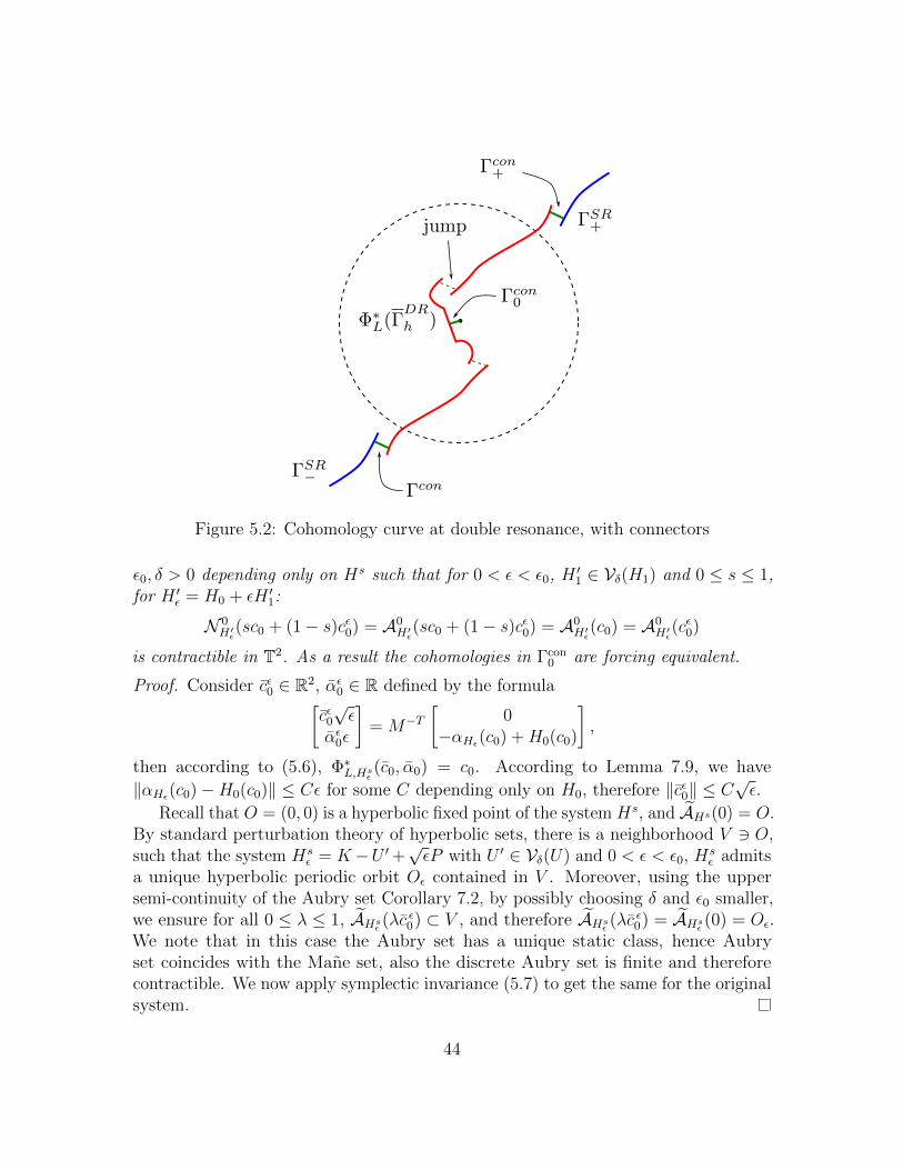
Figure 5.2: Cohomology curve at double resonance, with connectors

ε0, δ > 0 depending only on Hs such that for 0 < ε < ε0, H ′1 ∈ Vδ(H1) and 0 ≤ s ≤ 1,for H ′ε = H0 + εH ′1:

N 0H′ε

(sc0 + (1− s)cε0) = A0H′ε

(sc0 + (1− s)cε0) = A0H′ε

(c0) = A0H′ε

(cε0)

is contractible in T2. As a result the cohomologies in Γcon0 are forcing equivalent.

Proof. Consider cε0 ∈ R2, αε0 ∈ R defined by the formula[cε0√ε

αε0ε

]= M−T

[0

−αHε(c0) +H0(c0)

],

then according to (5.6), Φ∗L,Hsε(c0, α0) = c0. According to Lemma 7.9, we have

‖αHε(c0)−H0(c0)‖ ≤ Cε for some C depending only on H0, therefore ‖cε0‖ ≤ C√ε.

Recall that O = (0, 0) is a hyperbolic fixed point of the system Hs, and AHs(0) = O.By standard perturbation theory of hyperbolic sets, there is a neighborhood V 3 O,such that the system Hs

ε = K−U ′+√εP with U ′ ∈ Vδ(U) and 0 < ε < ε0, Hs

ε admitsa unique hyperbolic periodic orbit Oε contained in V . Moreover, using the uppersemi-continuity of the Aubry set Corollary 7.2, by possibly choosing δ and ε0 smaller,we ensure for all 0 ≤ λ ≤ 1, AHs

ε(λc ε0) ⊂ V , and therefore AHs

ε(λc ε0) = AHs

ε(0) = Oε.

We note that in this case the Aubry set has a unique static class, hence Aubryset coincides with the Mane set, also the discrete Aubry set is finite and thereforecontractible. We now apply symplectic invariance (5.7) to get the same for the originalsystem.

44

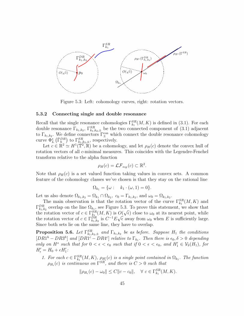
Figure 5.3: Left: cohomology curves, right: rotation vectors.

5.3.2 Connecting single and double resonance

Recall that the single resonance cohomologies ΓSRk1 (M,K) is defined in (3.1). For eachdouble resonance Γk1,k2 , ΓSRk1,k2,± be the two connected component of (3.1) adjacentto Γk1,k2 . We define connectors Γcon

± which connect the double resonance cohomologycurve Φ∗L

(ΓDRh

)to ΓSRk1,k2,±, respectively.

Let c ∈ R2 ' H1(T2,R) be a cohomology, and let ρH(c) denote the convex hull ofrotation vectors of all c-minimal measures. This coincides with the Legendre-Fencheltransform relative to the alpha function

ρH(c) = LFαH (c) ⊂ R2.

Note that ρH(c) is a set valued function taking values in convex sets. A commonfeature of the cohomology classes we’ve chosen is that they stay on the rational line

Ωk1 = ω : k1 · (ω, 1) = 0.Let us also denote Ωk1,k2 = Ωk1 ∩ Ωk2 , c0 = Γk1,k2 , and ω0 = Ωk1,k2 .

The main observation is that the rotation vector of the curve ΓSRk1 (M,K) andΓDRk1,k2 overlap on the line Ωk1 , see Figure 5.3. To prove this statement, we show thatthe rotation vector of c ∈ ΓSRk1 (M,K) is O(

√ε) close to ω0 at its nearest point, while

the rotation vector of c ∈ ΓDRk1,k2 is C−1E√ε away from ω0 when E is sufficiently large.

Since both sets lie on the same line, they have to overlap.

Proposition 5.6. Let ΓSRk1,k2,± and Γk1,k2 be as before. Suppose H1 the conditions

[DR1h−DR3h] and [DR1c−DR4c] relative to Γk1. Then there is ε0, δ > 0 dependingonly on Hs such that for 0 < ε < ε0 such that if 0 < ε < ε0, and H ′1 ∈ Vδ(H1), forH ′ε = H0 + εH ′1:

1. For each c ∈ ΓSRk1 (M,K), ρH′ε(c) is a single point contained in Ωk1. The functionρHε(c) is continuous on ΓSR, and there is C > 0 such that

‖ρHε(c)− ω0‖ ≤ C‖c− c0‖, ∀ c ∈ ΓSRk1 (M,K).

45

2. Let ch(E) = Φ∗L (ch(E)) ∈ ΓDRk1,k2. Then each ρH′ε(ch(E)) is a single point con-tained in Ωk1, and there are C,E0 > 0 such that

‖ρH′ε(ch(E))− ω0‖ ≥ C−1E√ε, E ≥ E0.

As a result, there exists E > 0 such that for E > E, the rotation vectors ρH′ε(ch(E))coincide with one of ρH′ε(Γ

SRk1,k2,±), see Figure 5.3. Similarly, for E sufficiently large,

the rotation vectors ρH′ε(c−h(E)) coincide with one of ρH′ε(ΓSRk1,k2,±) (which are not

covered in the first case).

Proof. In the single resonance regime, after a linear coordinate change (Section 3.3)the system is converted to H0 + εZ(θs, p) + εR(θs, θf , ps, pf , t), where the invariantcylinder is given by (θs, ps) = (Θs, P s)(θf , pf , t), and the Aubry set for any c ∈ Γs =(∂pH0(0), 1) · (1, 0, 0) = 0 is a graph over (θf , t) (see Theorem 9.1, Theorem 9.2)This implies that any c admits a unique rotation vector, as different rotation vectorswill resulting in intersecting minimizing orbits, which violates the graph theorem.By reverting the coordinate change, we also obtain ρHε(c) ∈ Ωk1 . We then applyCorollary 7.8, to get (in general)

‖ρHε(c)−∇H0(c)‖ ≤ C√ε,

while‖∇H0(c)− ω0‖ = ‖∇H0(c)−∇H0(c0)‖ ≤ C‖c− c0‖

and recall that ‖c− c0‖ ≥ K√ε for any c ∈ ΓSRk1 , item (1) follows.

In the double resonance case, the cohomology curve ch(E) at high energy areof Aubry-Mather type corresponding to the homology class h = (1, 0). The samearguments as in the single resonance case implies ρHs

ε(c) is unique, and contained in

the line ω1 = 0. Again by reverting the coordinate change, we obtain the desiredproperty for ρH−ε(c). For the in equality, note that if any point (ϕ, I, t) in the Aubry

set AHsε(c) satisfies Hs(ϕ, I) ≥ E0, we have K(I) ≥ Hs(ϕ, I)− ‖U‖C0 ≥ 1

2Hs(ϕ, I) if

E0 ≥ 2‖U‖C0 . As a result

min(ϕ,I,τ)∈AHsε (ch(E))

‖I‖ ≥ C−1 min(ϕ,I,τ)∈AHsε (ch(E))

√K(I) ≥ C−1

√E

for a suitable C > 1. Reverting the coordinate change ΦL implies

min(θ,p,t)∈AHε (ch(E))

‖p− p0‖ ≥ C−1‖I‖√ε ≥ C−1

√E√ε.

Finally, we apply Corollary 7.8 again to get our inequality.

We have the following lemma:

46

Lemma 5.7 ([54], Proposition 6). Let c1, c2 ∈ H1(T2,R) and ρ ∈ H1(T2,R) satisfyρH(c1) = ρH(c2) = ρ, and both c1, c2 lie in the relative interior of LFβH (ρ). Then

AH(c1) = AH(c2).

Proposition 5.8. Suppose H1 satisfies the conditions [DR1h −DR3h] and [DR1c −DR4c] relative to Γk1. Then there is ε0, δ > 0 depending only on Hs such that for0 < ε < ε0 and a residual subset Rδ(H1) of Vδ(H1), for each H ′1 ∈ Rδ(H1), there isc±1 ∈ ΓSRk1 (M,K) and c±2 ∈ ΓDRk1,k2, such that for all 0 ≤ λ ≤ 1 and H ′ε = H0 + εH ′1

N 0H′ε

(λc±1 + (1− λ)c±2 ) = A0H′ε

(λc±1 + (1− λ)c±2 ) = A0H′ε

(c±1 ) = A0H′ε

(c±2 )

is contractible in T2. As the result both cohomology curves

Γcon+ =

⋃s∈[0,1]

sc+1 + (1− s)c+

2 , Γcon− =

⋃s∈[0,1]

sc−1 + (1− s)c−2

are contained in a single forcing equivalent class.

Proof. Proposition 5.6 implies the curves ρHε(ΓSRk1

) and ρHε(ΓDRk1,k2

) overlap on aninterval contained in Ωk1 , for all H ′1 ∈ Vδ(H1). In particular, there must be c1 ∈ ΓSRk1and c2 ∈ ΓDRk1,k2 where they both have rational rotation vectors. We now assumethat H ′ε = H0 + εH ′1 satisfies the residual condition that all Aubry sets with rationalrotation vector is supported on a hyperbolic periodic orbit, in this setting A = N ,c1, c2 are contained in the relative interior of LFβ(ρ). Lemma 5.7 now implies all theAubry sets AHε(λc1 + (1− λ)c2), 0 ≤ λ ≤ 1 coincide, which implies (Ma) applies tothe whole segment. The proposition follows.

5.4 Jump from non-simple homology to simple homology

As described, when h is not a simple homology, the cohomology class ΓDRk1,k2 as chosenis not connected. More precisely, ΓDRk1,k2 consists of three connected components (seealso (5.3) and (5.9)):

Φ∗LΓeh ∪ Γcon+ , Φ∗LΓe−h ∪ Γcon

− , Φ∗L(Γe,µh1 ∪ Γe,µ−h1

)∪ Γcon

0 .

We will show forcing equivalence of the components by the following:

Theorem 5.1 (Section 12). Suppose the slow system Hs satisfies the conditions[DR1c] − [DR4c], and that the associated homology h = n1h1 + n2h2 is non-simple.Then there exists e, µ, ε0, δ > 0 depending on Hs, such that there is a residual subsetRδ(H1) of Vδ(H1), and for each H ′1 ∈ Rδ(H1), there is E1, E1 ∈ (e, e+ µ) such that

Φ∗L (ch(E1)) , Φ∗L(cµh1(E2)

)are forcing equivalent, with respect to H0 + εH ′1. The same conclusions apply whenh, h1 are replaced with −h,−h1.

See the dashed line in Figure 5.2.

47

5.5 Forcing equivalence at the double resonance

We summarize all of our constructions in the following theorem.

Theorem 5.2. Suppose H1 satisfies all non-degeneracy conditions of Γk1 and Γk1,k2.Then there is ε1 = ε1(H0, H1) > 0, δ = δ(H0, H1) > 0, such that for all H ′1 ∈ Vδ(H1),and 0 < ε < ε1, there is a subset ΓDRk1,k2 = ΓDRk1,k2(H0, H

′1, ε) satisfying:

1. Γk1,k2 ⊂ ΓDRk1,k2;

2. ΓDRk1,k2 intersects both ΓSRk1,k2,+ and ΓSRk1,k2,−;

there is σ = σ(H0, H1, ε) > 0 and a residual subset Rσ(H0 + εH ′1) of Vσ(H0 + εH ′1),such that for all H ∈ R(H0 + εH ′1), all of ΓDRk1,k2 are forcing equivalent.

Proof. The two properties of ΓDRk1,k2 hold by construction. During the proof, we saya property hold “after a residual perturbation” if it holds on an residual subset ofa neighborhood of the corresponding Hamiltonian. Note that if several propertieseach hold after a residual perturbation, then they hold simultaneously after a residualperturbation. Moreover, if a property holds after a residual perturbation, and isinvariant under coordinate changes, then it also holds in the new coordinate after aresidual perturbation, provided the coordinate change is smooth enough. This is thecase for our system since all coordinate changes are C∞.

Let δ be the smallest parameter depending on Hs such that all of Corollary 5.3,Proposition 5.5 and Proposition 5.8 holds.

Let δ1 = δ1(H0, H1) be such that for any H ′1 ∈ Vδ1(H1), the associated slow systemis in Vδ(Hs). Then for 0 < ε < ε0, Lemma B.5 implies the system H0 + εH ′1 is reducedto a system (Gs +

√εP )/β satisfying the conclusions of Corollary 5.3. Moreover, by

Proposition 5.4, relative to the the normal form system Nε, one of the three diffusionmechanisms hold for Φ∗L(ΓDRh ), after taking a residual perturbation. By Lemma 2.7,the same holds for relative to the original system H0 + εH ′1.

Recall that (see 5.9) ΓDRk1,k2 consists of the set Φ∗L(ΓDRh ) and the connector sets Γcon0

and Γcon± . Proposition 5.5 and 5.8 implies forcing equivalence of the connectors after a

residual perturbation. This implies each connected component of ΓDRk1,k2 are forcingequivalent.

Finally, Theorem 5.1 implies all three components of ΓDRk1,k2 are equivalent to eachother after a residual perturbation.

Assuming all the propositions and theorems formulated thus far, we prove Theo-rem 2.1 which implies our main theorem.

48

Proof of Theorem 2.1. Let H1 ∈ U , which means that H1 satisfies SR(k1, λ) forsome λ > 0 and all k1 ∈ K, and that for all the strong double resonances k2 ∈⋃k1∈K

⋃Kst(k1,Γk1 , λ), H1 satisfies the non-degeneracy conditions DR(k1,Γk1 , k2).

For each k1, Theorem 3.1 applies. Therefore, there exists εk11 (H0, λ) > 0 such thatthe theorem applies for each H0 + εH1 with 0 < ε < ε1. Since SR(k1,Γk1 , λ) is anopen condition, there exists δk1 = δk1(H0, H1) such that the conclusion of the theoremto all H ′1 ∈ Vδk1 (H1).

For each k1, k2, the conclusion of Theorem 5.2 holds to all H ′1 ∈ Vδk1,k2 (H1) and0 < ε < εk1,k21 (H0, H1). Define

ε1(H0, H1) = min

mink1,k2

εk1,k21 ,mink1

εk11

, δ(H0, H1) = min

mink1,k2

δk1,k2 ,mink1

δk1.

Then the conclusion of both theorems apply to H ′1 ∈ Vδ(H1) and 0 < ε < ε1.Define

Γ∗(H0, H′1, ε) =

⋃k1∈K

ΓSRk1 ∪⋃

k2∈Kst(k1,λ)

ΓDRk1,k2

.

For each single resonance k1, the union

ΓSR∗ (k1) = ΓSRk1 ∪⋃

k2∈Kst(k1,λ)

ΓDRk1,k2

are contained in a single equivalent class, since each ΓDRk1,k2 are forcing equivalent, andthey connect all the disconnected pieces from ΓSRk1 . If two single resonances Γk1 andΓk′1 intersect at Γk1,k′1 , then ΓSR∗ (k1) and ΓSR∗ (k′1) also intersect at Γk1,k′1 , since Γk1,k′1 iscontained in both ΓDRk1,k′1

and ΓDRk′1,k1. As a result, the entire Γ∗(H0, H

′1, ε) is contained

in a single forcing equivalent class.Finally, if U1, . . . , UN are open sets which intersect P , by setting ε0 small enough,

they also intersect⋃k1∈K ΓSRk1 , since the said union is obtained from P by removing

finitely many neighborhoods of size O(√ε). Therefore, U1, . . . , UN also intersect

Γ∗(H0, H′1, ε).

6 Weak KAM theory and forcing equivalence

In this section we give an introduction to weak KAM theory and forcing relation.Most of the presentation follow [11] and [35].

The forcing relation is introduced by Bernard ([11]). It generalizes a similarequivalence relation defined by Mather ([58]), using the point of view of Fathi ([35]),see also [50]. This approach frees us from needing to construct a variational principle

49

for the global diffusion orbit, as the approaches in [57, 56, 59, 60, 24, 25] requires.Another advantage is that Mather’s approach works only on continuous curves ofcohomologies, as the his definition is local. The forcing relation allows disconnectedpieces of cohomology as long as we prove the forcing relation by definition, enablingthe jump mechanism.

6.1 Periodic Tonelli Hamiltonians

A C2 HamiltonianH : Tn × Rn × R −→ R

is called (time-periodic) Tonelli if it satisfies:

1. (Periodicity) There is 0 < $ = $ H such that H(θ, p, t+$ ) = H(θ, p, t).

2. (Convexity) ∂2ppH(x, p, t) is strictly positive definite as a quadratic form.

3. (Superlinearity) lim‖p‖−→∞H(x, p, t)/‖p‖ −→ ∞.

4. (Completeness) The Hamiltonian vector field generates a complete flow onTn × Rn. We denote by φs,tH the flow from time s to time t, and by φH the flowφ0,1H .

We will denote by

L = LH(θ, v, t) = supp · v −H(θ, p, t)

its Legendre transform. For the most part, we will restrict to Hamiltonians with$ = 1, namely, defined on Tn × Rn × T, but near double resonances we need toconsider Hamiltonians that are

√ε−periodic.

It is helpful to consider a family of Hamiltonians which satisfy these propertiesuniformly. For D > 0, consider

H(D) =H ∈ C2(Tn × Rn × R) :

$ H ≤ 1, D−1I ≤ ∂2ppH ≤ DI, ‖H(·, 0)‖C0 , ‖∂pH(·, 0)‖C0 ≤ D.

We then check that each H ∈ H(D) is Tonelli, and it satisfy a list of uniform estimatescalled uniform family in [11]. In particular, if H0 ∈ H(D), then Hε ∈ H(2D) for allε ≤ ε0 = ε0(D).

Given C > 0, we say a function u : Rn −→ R is C semi-concave if for every x ∈ Rn,there is a linear function lx : Rn −→ R, such that

u(y)− u(x) ≤ lx(y − x) + C‖y − x‖2, y ∈ Rn.

50

The linear form lx is called a super-differential at x. The set of all super-differentials atx is denoted ∂+u(x). It is easy to see if u is differentiable at x, then ∂+u(x) = du(x).A function u : Tn −→ R is semi-concave if it’s semi-concave as a function on Rn.

Lemma 6.1. ([11]) If u : Tn −→ R is C semi-concave, then it is C√n–Lipschitz.

The super-differential set ∂+u(x) ⊂ ‖p‖ ≤ C√n.

Given s < t ∈ R, x, y ∈ Tn, we define the Lagrangian action

A(x, s, y, t) = infγ(s)=x, γ(t)=y

∫ t

s

LH(γ(τ), γ(τ), τ)dτ, (6.1)

where the infimum is taken over all absolutely continuous γ. We outline a series ofuseful results:

Proposition 6.2. Let H ∈ H(D), then:

1. (Tonelli Theorem) ([57], Appendix 2) The infimum in (6.1) is always reached.It is then C2, which solves the Euler-Lagrange equation. Such a γ is called aminimizer.

2. (A priori compactness) ([11], Section B.2) Let δ > 0, then there is a constantCδ > 0 depending only on δ and D, such that for t− s > δ, any minimizer ofA(s, x, t, y) satisfies ‖γ‖ ≤ Cδ.

3. (Uniform semi-concavity) ([11], Theorem B.7, see also Proposition 7.12) Fort − s > δ, the function A(s, x; t, y) is Cδ semi-concave in (x, s) and (y, t).Moreover, if γ : [s, t] −→ Tn is a minimizer, then

(p(s),−H(γ(s), p(s), s)) ∈ −∂+(x,s)A(x, s, y, t),

(p(t),−H(γ(t), p(t), t)) ∈ −∂+(y,t)A(x, s, y, t),

(6.2)

where p(τ) = ∂vLH(γ(τ), γ(τ), τ).

Remark 6.1. For item 3 of Proposition 6.2, [11] only treated the semi-concavity in x.A proof that also include time-dependence can be obtained from Proposition 7.12 bychoosing a non-small ε.

For each c ∈ Rn, define

LH,c(θ, v, t) = LH(θ, v, t)− c · v,

and denote AH,c = ALH,c . Then (6.2) becomes

(p(t)− c,−H(γ(t), p(t), t)) ∈ ∂(y,t)AH,c(x, s, y, t)

and similarly for s.

51

6.2 Weak KAM solution

We now define the (continuous) Lax-Oleinik semi-group T s,tc : C(Tn) −→ C(Tn) viathe formula

T s,tc u(x) = minz∈Tnu(z) + AH,c(z, s;x, t) .

For a $ -periodic Hamiltonian, the associated discrete semi-group is generated by theoperator: Tcu = T 0,$

c u.

Lemma 6.3. Let uζζ∈Z be a (possibly uncountable) family of C-semi-concave func-tions Tn −→ R, and v = inf uζ is bounded, then infζ∈Z uζ is also C semi-concave.

Moreover, suppose for x0 ∈ Z, the infimum v(x0) is reached at uζ0(x0), then∂+uζ0(x0) = ∂+v(x0).

Using Proposition 6.2, the functions T nη u are C semi-concave with the constantdepending only on uniform family.

Proposition 6.4 (Mane’s critical value, see [11], Proposition 3.1). There is a uniqueα ∈ R such that T nc u(x) + nα stays bounded for all n ∈ N. This value coincides withMather’s alpha function:

αH(c) = − infµ

∫LH,c(θ, v, t)dµ(θ, v, t)

(6.3)

where the infimum is taken over all invariant probability measure of the Euler-Lagrangeflow on Tn × Rn × T$ .

Let us also point out an alternative definition of the alpha function (see [71]),namely, we can replace the class of minimal measures with the class of closed measures,which satisfies ∫

df(θ, t) · (v, 1)dµ(θ, v, t) = 0

for every C1 function f : Tn × R −→ R satisfying f(θ, t+$) = f(θ, t).A function w : Tn × T$ −→ R is called a weak KAM solution if

T s,tc w(·, s) + αH(c)(t− s) = w(·, t), s < t ∈ R,

i.e. the family w(·, t) is invariant under the semi-group up to a linear drift. Thefunction u(θ) = w(θ, 0) is then a fixed point of the operator Tc +$αH(c).

Proposition 6.5 (Existence of weak KAM solution, [11], Proposition 3.2). For c ∈ Rn

and u0 ∈ C(Tn), the function

w(θ, t) = lim infN−→−∞

(T t−N$ ,tc u0 +N$α(c)), N ∈ N

is a $ -periodic weak KAM solution.

52

The following is a easy consequence of Lemma 6.3.

Lemma 6.6. Weak KAM solutions are uniformly semi-concave over all H ∈ H(D).

A function w : Tn × R −→ R is called dominated by LH,c, α if

w(y, t)− w(x, s) ≤ AH,c(x, s, y, t) + (t− s)α, x, y ∈ Tn, t < s.

γ : I −→ Tn, where I is an interval in R is called calibrated by w if

w(γ(t), t)− w(γ(s), s) = AH,c(x, s, y, t) + (t− s)α.

Proposition 6.7 ([35], Proposition 4.1.8). w : Tn×R −→ R is a weak KAM solutionif and only if it is dominated by Lc, αH(c) and for every (y, t) there is a calibratedcurve γ : (−∞, t] −→ Tn such that γ(t) = y.

6.3 Pseudographs, Aubry, Mane and Mather sets

Let u : Tn −→ R be semi-concave. By the Radamacher theorem, u is differentiablealmost everywhere. For c ∈ Rn, we define the (overlapping) psudograph

Gc,u = Gc,H,u = (x, c+∇u(x)), ∇u(x) exists .

In the one-dimensional case, at every discontinuity of the function du(x), the left limitis larger than the right limit. In the time-dependent setting if w : Tn × R −→ R issemi-concave, we write

Gc,w = (x, c+ ∂xu(x, t), t) : ∂xu exists.

The evolution by the Lax-Oleinik semi-group generates an evolution operator onthe psudograph. The following statement outline its relation with the Hamiltoniandynamics.

Proposition 6.8 ([11]). For each s < t, we have

Gc,T s,tc u ⊂ φs,tH (Gc,u) ,

here φs,tH denotes the Hamiltonian flow.

Corollary 6.9. Suppose w(θ, t) is a (time-periodic) weak KAM solution of LH,c, then(φs,tH)−1 Gc,w(·,t) ⊂ Gc,w(·,s).

In particular, (φ−1H )Gc,u ⊂ Gc,u, where u = w(·, 0) and φH = φ0,$

H is the associateddiscrete dynamics.

53

Let w = w(θ, t) be a continuous weak KAM solution for Lc. Then Corollary 6.9implies the set

Gc,w =

(θ, p) : (θ, p) ∈ Gc,w(·,t)

is backward invariant under the flow φs,tH . We then define

I(c, w) =

(θ, p, t) : (θ, p) ∈

⋂s<t

(φs,tH)−1 Gc,w(·,t)

,

in other words, I(c, w) is the invariant set generated by the family of psudographsGc,w(·,t), in the extended phase space Tn × Rn × T$.

The Aubry and Mane sets admit the following equivalent definitions:

A(c) =⋂w

I(c, w), N (c) =⋃w

I(c, w),

where w : Tn × R −→ T$ is taken over all Lc continuous-time weak KAM solutions.The Mather set M(c) is then the support of all φs,tH invariant measures contained in

A(c). Note that if we consider a discrete weak KAM solution u : Tn −→ R, then the

analogous definitions give us A0 and N 0.

6.4 The dual setting, forward solutions

There is a dual setting which corresponds to forward dynamics (as apposed to thebackward invariant sets obtained before). Define

T s,tc u(x) = maxzu(z)− Ac(x, s; z, t) ,

and note the following:

1. α = αH(c) is the unique number such that a weak KAM solution may exist.

2. −T s,tc u are uniformly semi-concave (if t− s > τ), fixed points of T s,tc − α exists,and are called forward weak KAM solution.

3. For a semi-concave function u, we define Gc,u = (θ, c+∇xu(θ)), and call it ananti-overlapping psudographs.

4. Analogs of the previous section apply with appropriate changes.

Let w(θ, t) be a weak KAM solution for LH,c, and w+ a forward weak KAMsolution. We say that w,w+ are conjugate if they coincide on the set MH(c).

Proposition 6.10 ([35], Theorem 5.1.2). For each weak KAM solution w, there existsa forward solution w+ conjugate to w satisfying w+ ≥ w, and

I(c, w) = I(c, w+) = I(c, w, w+) := (x, c+ ∂xw(x, t), t) : w(x, t) = w+(x, t).

54

6.5 Peierls barrier, static classes, elementary solutions

We define

hH,c(x, s, y, t) = lim infN−→∞

AH,c(x, s, y, t+N$ ) +N$αH(c)

called the Peirels barrier by Mather ([58]). The projected Aubry set AH(c) has thefollowing alternative characterization:

AH(c) = (x, s) ∈ Tn × T$ : hH,c(x, s, x, s) = 0.

We will also consider the discrete barrier:

hH,c(x, y) = hH,c(x, 0, y, 0), (6.4)

then A0H(c) = x : hH,c(x, x) = 0.

On the set AH(c) we define the Mather semi-distance:

d(x, s, y, t) = hH,c(x, s, y, t) + hH,c(y, t, x, s),

then the condition d(x, s, y, t) = 0 defines an equivalence relation (x, s) ∼ (y, t) onAH(c). The equivalence classes of this relation are called the static classes. LetS ⊂ AH(c) be a static class, it corresponds uniquely to an invariant set in the phasespace:

S = π−1(x,t)

∣∣∣AH(c)

S.

For (ζ, τ) ∈ S, the functionhH,c(ζ, τ, ·, ·)

is a weak KAM solution for LH,c, called the elementary solution. The elementarysolution is independent of the choice of (ζ, τ) ∈ S, up to an additive constant.

We have the following useful statements concerning elementary solutions.

Proposition 6.11. 1. (Representation formula, see [35], Theorem 8.6.1 and [27],Theorem 7) Let w(x, t) be an LH,c weak KAM solution. Then

w(x, t) = min(ζ,τ)∈AH(c)

w(ζ, τ) + hH,c(ζ, τ, x, t).

2. (See [11], Proposition 4.3) Every orbit in the Mane set NH(c) is a heteroclinic

orbit between two static classes S1, S2. We have AH(c) = NH(c) if and only if

AH(c) has only one static class.

55

6.6 The forcing relation

Definition 6.12. Let u : Tn −→ R be semi-concave, and N ∈ N. We say thatGc,u `N c′, if there exists a semi-concave function v : Tn −→ R such that

Gc′,v ⊂N⋃k=0

φkH (Gc,u) .

We say the c ` c′ if there exists N ∈ N such that

Gc,u `N c′

for every psudograph Gc,u. We say c a` c′ if c ` c′ and c′ ` c.

In view of Proposition 6.8, we always have c ` c. The relation is transitive bydefinition. Therefore a` defines an equivalence relation.

We summarize the property of the forcing relation below.

• (Proposition 2.1)

Let ciNi=1 be a sequence of cohomology classes which are forcing equivalent.

For each i, let Ui be neighborhoods of the discrete Mather sets M0H(ci), then

there is a trajectory of the Hamiltonian flow φt of H visiting all the sets Ui.

• (Mather mechanism, Proposition 2.2)

Suppose N 0H(c) is contractible as a subset of T2, then there is σ > 0 such that c

is forcing equivalent to all c′ ∈ Bσ(c).

• (Arnold and Bifurcation mechanism, Proposition 2.4)

Suppose, either: A0H(c) has only two static classes and N 0

H(c) \ A0H(c) is totally

disconnected, or A0H(c) has only one static class, and there is a symplectic double

covering map ξ such that N 0HΞ(ξ∗c) \Ξ−1N 0

H is totally disconnected, then thereis σ > 0 such that c is forcing equivalent to all c′ ∈ Bσ(c).

7 Perturbative Weak KAM theory

By perturbative weak KAM theory, we mean two things:

• How do the weak KAM solutions and the Mather, Aubry, Mane sets respond tolimits of the Hamiltonian;

56

• How do the weak KAM solutions change when we perturb a system, in particular,what happens when we perturb (1) completely integrable systems, and (2)autonomous systems.

In this section, we state and prove results in both aspects, as a technical tool forproving forcing equivalence.

7.1 Semi-continuity

Let H(D) be the uniform family defined before, note that they are periodic of period0 < $ H ≤ 1, but not necessarily of the same period. It is known that in the case thatall periods are fixed at 1, the weak KAM solutions are upper semi-continuous (seeprecise statements below) under C2 convergence over compact sets ([12]). The resultsgeneralize to the case when the periods are not the same, as we now show.

Let us remark that if Hn ∈ H(D) is a family of Hamiltonians, and Hn −→ Huniformly over compact sets on Tn × Rn × R, then H is necessarily periodic of someperiod, and therefore H ∈ H(D).

We define the upper limit lim sup for a sequence of sets An to be the set of allaccumulation points of all sequences xn ∈ An.

Lemma 7.1 ([12], Lemma 7). Suppose Hamiltonians Hk ∈ H(D), k ∈ N are afamily of periodic Tonelli Hamiltonians. Suppose Hn −→ H in C2 over compact sets,ck −→ c ∈ Rn, then αHk(ck) −→ αH(c). If wk : Tn × R −→ R is a sequence of weakKAM solution of Hk, ck which converges uniformly to w : Rn × R −→ R, then w is aweak KAM solution of H, c.

Moreover, we have

lim supk−→∞

Gck,Hk,wk ⊂ Gc,H,w, lim supk−→∞

IHk(ck, wk) ⊂ IH(c, w), lim supk−→∞

NHk(ck) ⊂ NH(c).

Proof. The proof is an elaboration of [12], Lemma 7. First, note that if Hk ∈ H andck uniformly bounded, then αHk(ck) is uniformly bounded ((6.3)). By restricting to asubsequence, we may assume αHk(ck) −→ α ∈ R. Then taking limit in

wk(γ(t), t)− wk(γ(s), s) ≤∫ t

s

LHk(γ(τ), γ(τ), τ)− ck · γ(τ) + αHk(ck) dτ

we obtain

w(γ(t), t)− w(γ(s), s) ≤∫ t

s

LH(γ(τ), γ(τ), τ)− c · γ(τ) + α dτ,

implying α ≥ αH(c), using the definition of the α-function (6.3).

57

Now given x ∈ Tn, t ∈ R, let γk : (−∞, t] −→ Td be a LHk,ck , wk calibrated curve,then Proposition 6.2 implies γk are uniformly Lipschitz. Then γk has a subsequencethat converges in C1

loc to a limit γ(t), which is LH,c + α, u calibrated. This impliesboth αH(c) = α and that u is a H, c weak KAM solution.

We now prove the “moreover” part. Denote

Gk = Gck,Hk,wk , G = Gc,H,w Ik = IH(ckwk), I = IH(c, w).

then if (xk, pk, tk) ∈ Gk, then there exists LHk,ck , wk calibrated curves γk : (−∞, tk] −→Td with γk(tk) = xk and ∂pHk(xk, pk, tk) = γn. Then by the same argument, afterrestricting to a subsequence, γn converges in C1

loc to γ : (−∞, t] −→ Td, and γ is aLH,c, w calibrated curve. This implies (t, x, p) ∈ G.

For the set I, let us prove for each fixed T , we have

lim supn−→∞

φ−THk Gk ⊂ φ−TH G.

Indeed, for any (xk, pk, tk) ∈ φ−THk Gck,Hk,wk , there exists LHk,ck , wk calibrated curves

γ : (−∞, tk + T ] −→ Td such that γ(tk) = xk, ∂pHk(xk, pk, tk) = γk(tk). Then exactlythe same argument as before implies γn accumulates to a LH,c, u calibrated curveγ : (−∞, t+ T ) −→ Td, and implying (t, x, p) ∈ Φ−TH G. We obtain

lim supn−→∞

In ⊂ I.

Finally, since

NHk(ck) =⋃w

IH(ck, w),

where the union is over all LHk,ck weak KAM solutions. For (xk, pk, tk) ∈ NHk(ck),there exists uk such that (xk, pk, tk) ∈ Gck,Hk,uk . Since all wk are equi-continuous andequi-bounded (see e.g. (A.3), [11]), there exists a subsequence that converges to uuniformly on the interval Td × [0, K]. Since all wk’s are periodic with period boundedby 1, this implies wk −→ w on Td × R as well. We then apply the semi-continuity ofG sets to get semi-continuity of N .

The theory built in [12] allows one to pass from semi-continuity of pseudographsto semi-continuity of Aubry set under a condition called the coincidence hypothesis. Asufficient condition for this hypothesis is when the Aubry set has finitely many staticclasses.

Corollary 7.2. Suppose AH(c) has at most finitely many static classes. Then ifHn ∈ H(D) C2 converges to H over compact sets, and cn −→ c, we have

lim supn−→∞

AHn(cn) ⊂ AH(c)

as subsets of Tn × Rn × R.

58

Proof. The proof follows in the same way as the proof of Theorem 1 in [12]. We alsorefer to [46], Section 6.2 where this is carried out in detail.

7.2 Continuity of the barrier function

In general, the barrier function hH,c may be discontinuous with respect to H and c.However, the continuity properties hold in the particular case when the limiting Aubryset contains only one static class.

Proposition 7.3. Assume that a sequence Hk ∈ H(D) converges to H in C2 overcompact sets, and ck −→ c ∈ Rn. Assume that the projected Aubry set AH(c) containsat a unique static class. Let (xk, sk) ∈ AHk(ck) with (xk, sk) −→ (x, s), then the barrierfunctions hHk,ck(xk, sk; ·, ·) converges to hH,c(x, s; ·, ·) uniformly.

Similarly, for (yk, tk) ∈ AHk(ck) and (yk, tk) −→ (y, t), the barrier functionshHk,ck(·, ·; yk, tk) converges to hH,c(·, ·; y, t) uniformly.

Proposition 7.4. Assume that a sequence Hn converges to H in C2 over compactsets, ck −→ c ∈ Rn and the Aubry set AH(c) contains a unique static class.

1. For any (x, s) ∈ AH(c) we have

limn−→∞

sup(y,t)∈M×T

|hHk,ck(xk, sk; y, t)− hH,c(x, s; y, t)| = 0

uniformly over (xk, sk) ∈ AHk(ck) and (y, t) ∈M × R.

2. For any lk ∈ ∂+y hHk,ck(xk, sk; y, t) and lk −→ l, we have l ∈ ∂+

y hH,c(x, s; y, t).Moreover, the convergence is uniform in the sense that

limn−→∞

inflk∈∂+y hHk,ck (xk,sk;y,t)

d(lk, ∂+y hH,c(x, s; y, t)) = 0

uniformly in (x, s) ∈ AH(c), (xk, sk) ∈ AHk(ck).

The following statement follows easily from the representation formula (Proposi-tion 6.11).

Lemma 7.5. Assume that AH(c) has a unique static class. Let (x1, t1) ∈ AH(c), thenany weak KAM solution differs from hH,c(x1, t1; ·, ·) by a constant.

Proof of Proposition 7.3. We prove the second statement. By Proposition 6.2, allfunctions hHk,ck(xk, sk; ·, ·) are uniformly semi-concave, and hence equi-continuous. ByArzela-Ascoli, any subsequence contains a uniformly convergent subsequence, whoselimit is

hH,c(x, s; ·, ·) + C

59

due to Lemma 7.1 and Lemma 7.5. Moreover,

hH,c(xk, sk;x, s) −→ hH,c(x, s;x, s) = 0,

so C = 0. It follows that hHk,ck(xk, sk; ·, ·) converges to hH,c(x, s; ·, ·) uniformly.Statement 1 follows from the definition of the projected Aubry set

AH(c) = (x, s) ∈M × T : hH,c(x, s;x, s) = 0

and statement 2.

Proof of Proposition 7.4. Part 1. We argue by contradiction. Assume that there existδ > 0, and by restricting to a subsequence,

infC∈R

sup(y,t)

|hHk,ck(xk, sk, y, t)− hH,c(x, s, y, t)− C| > δ.

By compactness, and by restricting to a subsequence again, we may assume that(xk, sk) −→ (x∗, s∗), (yk, tk) −→ (y, t). Using Proposition 7.3, take limit as n −→∞,we have

sup(y,t)

|hH,c(x∗, s∗, y, t)− hH,c(x, s, y, t)| > δ.

By Lemma 7.5, the left hand side is 0, which is a contradiction.Part 2. hHk,ck(xk, sk, ·, t) converges to hH,c(x, s, ·, t) uniformly. Convergence of

super-differentials follows directly from Proposition 6.2. It suffices to prove uniformity.Assume, by contradiction, that by restricting to a subsequence, we have (xk, sk) −→(x, s) ∈ AH(c), lk ∈ ∂+

y hHk,ck(xk, sk, y, t) and (x, s) ∈ AH(c) such that

limn−→∞

lk /∈ ∂+y hH,c(x, s, y, t).

By Proposition 6.2, ln −→ l ∈ ∂+y hH,c(x

∗, s∗, y, t), but we also have ∂+y hH,c(x, s, y, t) =

∂+y hH,c(x

∗, s∗, y, t) since the functions differ by a constant using Lemma 7.5. This is acontradiction.

7.3 Lipschitz estimates for nearly integrable systems

In this section we record uniform estimates for the nearly integrable system

Hε = H0(p) + εH1(θ, p, t), (θ, p, t) ∈ Tn × Rn × T,

with the assumptions H0 ∈ H(D), ‖H1‖C2 ≤ 1.

Proposition 7.6 (Proposition 4.3, [13]). For Hε as given, for any c ∈ Rn, any LHε,cweak KAM solution u(x, t) is 6D

√ε−semi-concave and 6D

√dε−Lipschitz in x.

60

Corollary 7.7. For any LHε,c weak KAM solution u : Tn×T −→ R, let γ(−∞, t0] −→Tn be a calibrated curve. Then for any t ∈ (−∞, t0),

p(t) := ∂vLHε(γ(t), γ(t), t)

satisfies ‖p(t)− c‖ ≤ 6D√nε.

Moreover, any (x, p, t) ∈ NHε(c) satisfies the same estimate ‖p− c‖ ≤ 6D√nε.

Proof. p(t)− c is a super gradient of u(·, t) at γ(t). The conclusion follows from the

fact that u(·, t) is 6D√nε–Lipschitz. The statement for N follows from the fact that

any (x, p, t) ∈ G ⊂ N is the end point of a calibrated curve.

Corollary 7.8. Let µ be any c-minimal measure of Hε, then there is C > 0 dependingonly on H0 such that

‖ρ(µ)−∇H0(c)‖ ≤ C√ε.

Proof. Recall that µ is a measure on Tn×Rn×R, invariant under the Euler-Lagrangeflow. By considering the Legendre transform L, we obtain

ρ(µ) =

∫vdµ(θ, v, t) =

∫∂pHε(θ, p, t)dL∗µ(θ, p, t).

By Corollary 7.7, we have ∂pHε(θ, p, t) = ∇H0(c) +O(√ε) for all

(θ, p, t) ∈ suppL∗µ ⊂ AHε(c),

therefore, ρ(µ) = ∇H0(c) +O(√ε).

7.4 Estimates for nearly autonomous systems

The goal of this section is to derive a special Lipshitz estimate of weak KAM solutionsfor perturbations of autonomous systems. More precisely, consider

Hε(x, p, t) = H1(x, p) + εH2(x, p, t).

Assume that H1 ∈ H(D/2) and ‖H2‖C2 = 1. Then for ε small enough all Hε ∈ H(D).Let Lε denote the associated Lagrangian.

We first state an estimate for the alpha function.

Lemma 7.9. There is C > 0 depending only on ‖H1‖C2 and D, such that

‖αHε(c)− αH1(c)‖ < Cε.

61

Proof. Let C always denote a generic constant depending on ‖H1‖C2 . Let L1 be theLagrangian for H1, then ‖Lε − L1‖C0 ≤ Cε. As a result, the functionals∫

(Lε − c · v)dµ,

∫(L− c · v)dµ,

defined on the space of closed probability measures, differ by at most Cε. The lemmafollows immediately using the closed measure version for the definition of the alphafunction, see Section 6.2.

Let u(x, t) be a weak KAM solution to Lε− c · v, and w(x, t) a forward weak KAMsolution conjugate to u. Recall that

Iu,w(c) = argmin(x,t)(u− w), Iu,w(c) = (x, t, c+ dxu(x, t)) : (x, t) ∈ Iu,w.

Theorem 7.1. Let u,w be conjugate pair of weak KAM solutions to Lε − c · v, thenthere is C depending only D and ‖c‖ such that

|Hε(x1, p1, t1)−Hε(x2, p2, t2)| ≤ C√ε ‖(x2 − x1, t2 − t1)‖, (xi, pi, ti) ∈ Iu,w.

In particular, the above estimates holds on the Aubry set ALε(c).

The proof relies on semi-concavity of weak KAM solution, following Fathi ([35]).However to get an improved estimate we need a notion of semi-concavity that is“stronger” in the t direction.

Let Ω ⊂ Rn be an open convex set. Let A be a symmetric n× n matrix. We saythat f : Ω −→ R is A-semi-concave if for each x ∈ Rn, there is lx ∈ Rn such that

f(y)− f(x)− lx · (y − x) ≤ 1

2A(y − x)2, x, y ∈ Ω

where Ax2 denotes Ax · x. These definitions generalizes the standard semi-concavity,as A-semi-concave functions are 1

2‖A‖-semi-concave. We say f is A-semi-convex if −f

is A-semi-concave. The following lemma follows from a direct computation.

Lemma 7.10. f is A-semi-concave if and only if fA(x) = f(x)− 12Ax2 is concave.

The following lemma is proved in [77].

Lemma 7.11 (See [77], Lemma 3.2). Suppose f : Rn −→ R is B-semi-concave andg : Rn −→ R is (−A)-semi-convex, and S = B − A is positive definite. Supposef(x) ≥ g(x) and M is the set on which f − g reaches its minimum.

Then for all x1, x2 ∈M , we have

‖df(x2)− df(x1)− 1

2(A+B)(x2 − x1)‖S−1 ≤ 1

2‖x2 − x1‖S,

where ‖x‖S =√Sx2.

62

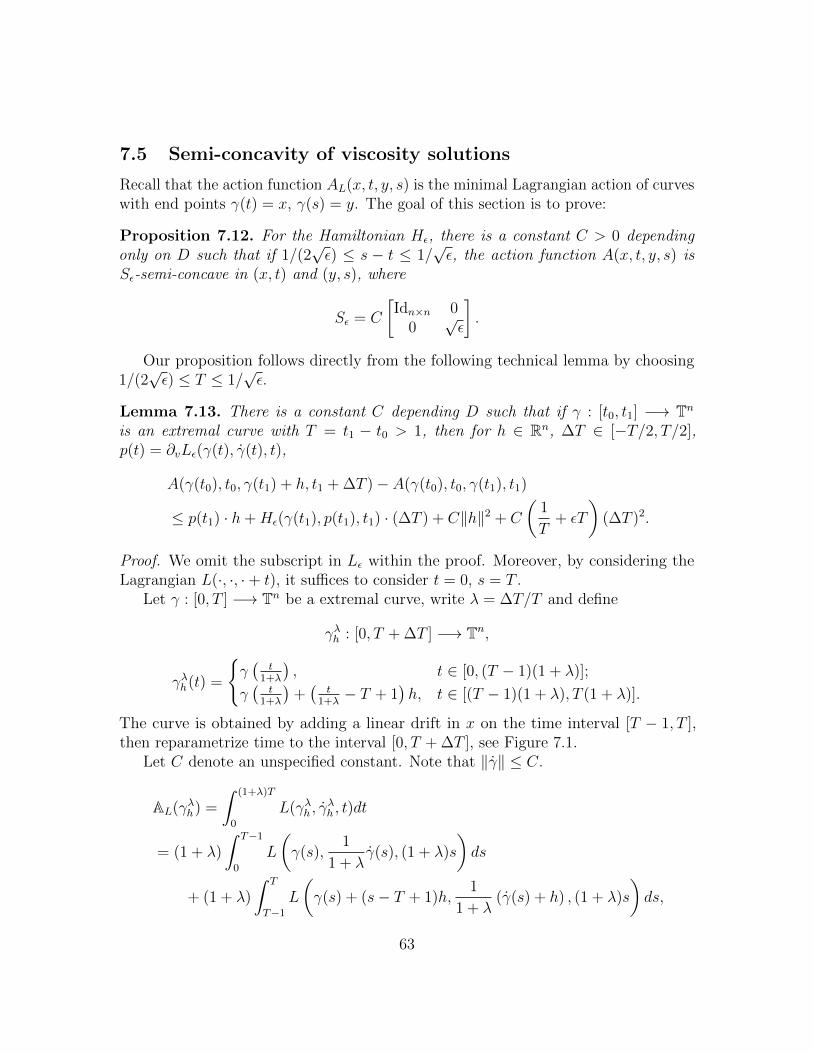
7.5 Semi-concavity of viscosity solutions

Recall that the action function AL(x, t, y, s) is the minimal Lagrangian action of curveswith end points γ(t) = x, γ(s) = y. The goal of this section is to prove:

Proposition 7.12. For the Hamiltonian Hε, there is a constant C > 0 dependingonly on D such that if 1/(2

√ε) ≤ s − t ≤ 1/

√ε, the action function A(x, t, y, s) is

Sε-semi-concave in (x, t) and (y, s), where

Sε = C

[Idn×n 0

0√ε

].

Our proposition follows directly from the following technical lemma by choosing1/(2√ε) ≤ T ≤ 1/

√ε.

Lemma 7.13. There is a constant C depending D such that if γ : [t0, t1] −→ Tnis an extremal curve with T = t1 − t0 > 1, then for h ∈ Rn, ∆T ∈ [−T/2, T/2],p(t) = ∂vLε(γ(t), γ(t), t),

A(γ(t0), t0, γ(t1) + h, t1 + ∆T )− A(γ(t0), t0, γ(t1), t1)

≤ p(t1) · h+Hε(γ(t1), p(t1), t1) · (∆T ) + C‖h‖2 + C

(1

T+ εT

)(∆T )2.

Proof. We omit the subscript in Lε within the proof. Moreover, by considering theLagrangian L(·, ·, ·+ t), it suffices to consider t = 0, s = T .

Let γ : [0, T ] −→ Tn be a extremal curve, write λ = ∆T/T and define

γλh : [0, T + ∆T ] −→ Tn,

γλh(t) =

γ(

t1+λ

), t ∈ [0, (T − 1)(1 + λ)];

γ(

t1+λ

)+(

t1+λ− T + 1

)h, t ∈ [(T − 1)(1 + λ), T (1 + λ)].

The curve is obtained by adding a linear drift in x on the time interval [T − 1, T ],then reparametrize time to the interval [0, T + ∆T ], see Figure 7.1.

Let C denote an unspecified constant. Note that ‖γ‖ ≤ C.

AL(γλh) =

∫ (1+λ)T

0

L(γλh , γλh , t)dt

= (1 + λ)

∫ T−1

0

L

(γ(s),

1

1 + λγ(s), (1 + λ)s

)ds

+ (1 + λ)

∫ T

T−1

L

(γ(s) + (s− T + 1)h,

1

1 + λ(γ(s) + h) , (1 + λ)s

)ds,

63

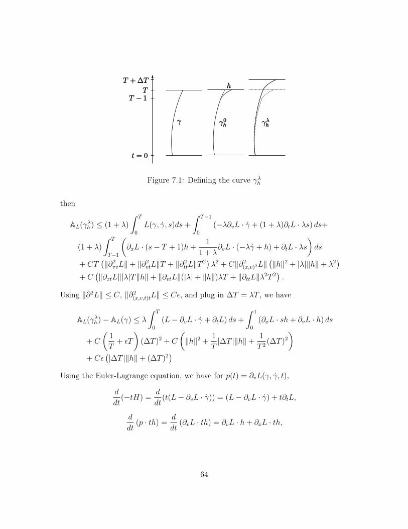
Figure 7.1: Defining the curve γλh

then

AL(γλh) ≤ (1 + λ)

∫ T

0

L(γ, γ, s)ds+

∫ T−1

0

(−λ∂vL · γ + (1 + λ)∂tL · λs) ds+

(1 + λ)

∫ T

T−1

(∂xL · (s− T + 1)h+

1

1 + λ∂vL · (−λγ + h) + ∂tL · λs

)ds

+ CT(‖∂2

vvL‖+ ‖∂2vtL‖T + ‖∂2

ttL‖T 2)λ2 + C‖∂2

(x,v)2L‖(‖h‖2 + |λ|‖h‖+ λ2

)+ C

(‖∂xtL‖|λ|T‖h‖+ ‖∂vtL‖(|λ|+ ‖h‖)λT + ‖∂ttL‖λ2T 2

).

Using ‖∂2L‖ ≤ C, ‖∂2(x,v,t)tL‖ ≤ Cε, and plug in ∆T = λT , we have

AL(γλh)− AL(γ) ≤ λ

∫ T

0

(L− ∂vL · γ + ∂tL) ds+

∫ 1

0

(∂xL · sh+ ∂vL · h) ds

+ C

(1

T+ εT

)(∆T )2 + C

(‖h‖2 +

1

T|∆T |‖h‖+

1

T 2(∆T )2

)+ Cε

(|∆T |‖h‖+ (∆T )2

)Using the Euler-Lagrange equation, we have for p(t) = ∂vL(γ, γ, t),

d

dt(−tH) =

d

dt(t(L− ∂vL · γ)) = (L− ∂vL · γ) + t∂tL,

d

dt(p · th) =

d

dt(∂vL · th) = ∂vL · h+ ∂xL · th,

64

we get

AL(γλh)− AL(γ) ≤ λ(−tH)∣∣∣T0

+ (p(T − 1 + t) · ht)∣∣∣10

+ C‖h2‖+ C

(1

T+ ε

)|∆T |‖h‖+ C

(1

T+ εT

)(∆T )2

≤ H(γ(T ), p(T ), T )(∆T ) + p(T ) · h+ 2C‖h‖2 + 2C

(1

T+ εT

)(∆T )2.

Let u(x, t) be a weak KAM solution to Lε− c · v, and w(x, t) a forward weak KAMsolution conjugate to u. Then Proposition 7.12 implies that u is Sε-semi-concave,while w is (−Sε)-semi-convex.

Proof of Theorem 7.1. Note that for each (x, p, t) ∈ Iu,w, −H(x, p, t) + αLε(c) =∂tu(x, t). Apply Proposition 7.12 and Lemma 7.11, we obtain∥∥∥∥[ p2 − p1

H(x2, p2, t2)−H(x1, p1, t1)

]−[C(x2 − x1)C√ε(t2 − t1)

]∥∥∥∥S−1ε

≤∥∥∥∥[x2 − x1

t2 − t1

]∥∥∥∥Sε

,

therefore1√ε|H(x2, p2, t2)−H(x1, p1, t1)− C

√ε(t2 − t1)|

≤ C‖x2 − x1‖+ C‖t2 − t1‖,the proposition follows.

8 Cohomology of Aubry-Mather type

8.1 Aubry-Mather type and diffusion mechanisms

LetH : Tn × Rn × T −→ R

be a Cr Tonelli Hamiltonian with r ≥ 2 contained in the family H(D).

Definition 8.1. We say that the pair (H∗, c∗) is of Aubry-Mather type if it satisfiesthe following conditions:

1. There is an embedding

χ : T× (−1, 1) −→ Tn × Rn,

65

such that C(H) = χ(T × (−1, 1)) is a normally hyperbolic weakly invariantcylinder under the time-1-map ΦH . We require C(H) is symplectic, i.e. therestriction of the symplectic form ω to C is non-degenerate.

2. There is σ > 0, such that the following holds for all

Vσ(H∗) := ‖H −H∗‖C2 < σ , Bσ(c∗) := ‖c− c∗‖ < σ.

(We then say that the property below holds robustly at (H∗, c∗).)

(a) The discrete Aubry set A0(c) ⊂ C(H). Moreover, the pull back of theAubry set is contained in a Lipschitz graph, namely, the map

πx : χ−1A0H(c) ⊂ T× (−1, 1) −→ T

is bi-Lipschitz.

(b) If χ−1A0H(c) projects onto T, then there is a neighborhood V 0 of A0

H(c)

such that the strong unstable manifold W u(A0H(c)) ∩ π−1

θ V 0 is a Lipschitzgraph over the θ component.

If (H∗, c∗) is of Aubry-Mather type, let h ∈ Zn ' H1(Tn,Z) be the homology classof the curve χ(T× 0).Remark 8.1. The definition of Aubry-Mather type includes a much simpler case, thatis when the Aubry set AH(c) is a hyperbolic periodic orbit, still contained in a NHIC C.

The condition 2(a) is satisfied since A0H(c) is discrete. Condition (b) is vacuous since

the χ−1A0H(c) never projects onto T. This holds, in particular, at double resonance

when the energy is critical.

Definition 8.2. We say that the pair (H∗, c∗) is of bifurcation Aubry-Mather type ifthere exist σ > 0 and open sets V1, V2 ⊂ Tn with V1 ∩ V2 = ∅, and a smooth bumpfunction

f : Tn −→ [0, 1], f |V1 = 0, f |V2 = 1,

such that for all c ∈ Bσ(c∗) and H ∈ Vσ(H∗):

1. Each of the Hamiltonians H1 = H − f and H2 = H − (1− f) satisfies

AH1(c) ⊂ V1 × T, AH2(c) ⊂ V2 × T.

It follows that AH1(c), AH2(c) are both invariant sets of H, called the localAubry sets.

66

2. (H1, c∗) (resp. (H2, c∗)) are of Aubry-Mather type, with the invariant cylindersC1 and C2. Moreover, they have the same homology class h.

3. The Aubry setAH(c) ⊂ AH1(c) ∪ AH2(c).

According to item (3) above, the Aubry set AH(c) may be contained in one of thelocal component, or both.

There is another type of bifurcation which happens at double resonance, when thehomology h is simple non-critical (i.e. the shortest geodesic loop does not contain thesaddle fixed point). We call this an asymmetric bifurcation.

Definition 8.3. We say that the pair (H∗, c∗) is of asymmetric bifurcation type ifthere exist σ > 0 and open sets V1, V2 ⊂ Tn with V1 ∩ V2 = ∅, and a smooth bumpfunction

f : Tn −→ [0, 1], f |V1 = 0, f |V2 = 1,

such that for all c ∈ Bσ(c∗) and H ∈ Vσ(H∗):

1. Item 1 of Definition 8.2 holds.

2. (H1, c∗) is of Aubry-Mather type, with the invariant cylinder C1. The Aubry set

AH2(c∗) is a single hyperbolic periodic orbit.

3. The Aubry setAH(c) ⊂ AH1(c) ∪ AH2(c).

Theorem 8.1. Suppose a pair (H∗, c∗) is of Aubry-Mather type, and let Γ 3 c∗ be asmooth curve in R2. Then there are σ1, σ2 > 0 such that for all c ∈ Γ1 := Bσ1(c∗) ∩ Γ,we have the following dichotomy for a residual subset of H ∈ Vσ(H∗):

1. The projected Mane set N 0H(c) is contractible as a subset of Tn;

2. There is a double covering map Ξ such that the set

N 0HΞ(ξ∗c) \ Ξ−1N 0

H(c)

is totally disconnected.

Theorem 8.2. Suppose (H∗, c∗) is of either

• bifurcation AM type, or

• asymmetric bifurcation type,

67

and c∗ ∈ Γ, where Γ is a smooth curve in R2, then there is σ > 0 and an open anddense subset R ⊂ Vσ(H∗) such that for c ∈ Bσ(c∗) ∩ Γ and H ∈ R, either:

1. A0H(c) has a unique static class, and one of the following holds.

(a) The projected Mane set N 0H(c) is contractible as a subset of Tn;

(b) There is a double covering map Ξ such that the set

N 0HΞ(ξ∗c) \ Ξ−1N 0

H(c)

is totally disconnected.

2. Or A0H(c) has two static classes, and

N 0H(c) \ A0

H(c)

is a discrete set.

Analogous result in the a priori unstable setting is due to Mather and Cheng-Yan([24], [25]). Our definition is more general and applies, as will be seen, to both singleand double resonant settings. The prove is base on the result of [13], which applies toour setting with appropriate changes. Here we describe the changes needed for theproof in [13] to apply.

If (c∗, H∗) is of Aubry-Mather type, let h ∈ Zn ' H1(Tn,Z) be its homology class.

Then any minimal measure contained in A0(c) must have rotation vector λh, λ ∈ R.Moreover, similar to the case of twist map, all such measures has the same rotationvector λh. We say the rotation vector is rational/irrational if λ is rational/irrational.

The following proposition is a consequence of the Hamiltonian Kupka-Smaletheorem, see for example [69].

Proposition 8.4. There are σ1, σ2 > 0, and a residual subset R1 of the ball Vσ2(H∗),such that for all c ∈ Γ1 := Bσ1(c

∗) ∩ Γ, H ∈ R1, if c has rational rotation vector, then

πχ−1A0(c) 6= T.

Let 1 ≤ j ≤ n be such that ej ∦ h, define the covering map ξ : Tn −→ Tn by

ξ(θ1, · · · , θn) = (θ1, · · · , 2θj, · · · , θn).

• For H ∈ R1, define

Γ∗(H) = c ∈ Γ1 : πχ−1(N 0H(c)) = T. (8.1)

Proposition 8.4 implies that each c ∈ Γ∗(H) has an irrational rotation vector,and the Aubry set has a unique static class, and A0

H(c) = N 0H(c). Each Γ∗(H)

is compact due to upper semi-continuity of the Mane set.

68

• For H ∈ R1 and c ∈ Γ∗(H), the lifted Aubry set A0HΞ(ξ∗c) = Ξ−1AH(c) has

two static classes, denote them S1, S2 (and projections S1,S2).

We have the decomposition

N 0HΞ(ξ∗c) = S1 ∪ S2 ∪ H12 ∪ H21,

where Hij consists of heteroclinic orbits from Si to Sj . We will use the notation

Si(H, c), H(H, c) to show dependence on the pair (H, c), and Hij for projection

of Hij.

• For H ∈ R1 and c ∈ Γ∗(H), consider the (discrete) Peierl’s barrier (see (6.4))

h(ζ1, ·), h(ζ2, ·), h(·, ζ1), h(·, ζ2), ζi ∈ Si, i = 1, 2,

where h = hHΞ, ξ∗c. These functions are independent of the choice of ζi exceptfor an additive constant. We define

b−H,c(θ) = h(ζ1, θ) + h(θ, ζ2)− h(ζ1, ζ2)

and b+H,c by switching ζ1, ζ2. The functions b±H,c are non-negative and vanish on

H12 ∪ S1 ∪ S2 and H21 ∪ S1 ∪ S2, respectively.

• Consider small neighborhoods V1, V2 of S1(H∗, c∗),S2(H∗, c∗), and define K =Tn \ (V1 ∪ V2). By semi-continuity of the Aubry set, for sufficiently small σ1, σ2,K is disjoint from Si(H, c) for all c ∈ Γ1 and H ∈ R1. Moreover, π−1K intersect

every orbit of H12(H, c) and H12(H, c).

Lemma 8.5 ([13], Lemma 5.2). For each (H, c) ∈ R1 × Γ1, the set

NHΞ(ξ∗c) \ Ξ−1NH(c)

is totally disconnected if and only if

NHΞ(ξ∗c) ∩K = (H12 ∪H21) ∩K

is totally disconnected.

We will show that the set of H ∈ R1 with the following property contains a denseGδ set: for each c ∈ Γ∗(H), NHΞ(ξ∗c) ∩ K is totally disconnected. The followinglemma implies the Gδ property.

Lemma 8.6 ([13], Lemma 5.3). Let K ⊂ Tn be compact, then the set of H ∈ R1 suchthat for all c ∈ Γ∗(N), the set NHΞ(ξ∗c) is totally disconnected, is a Gδ set.

69

The following proposition allows local perturbations of b±H,c simultaneously for allc’s in a small ball. Let Bσ(x) denote the ball of radius σ at x in a metric space.

Proposition 8.7 ([13], Proposition 5.2). Let H∗ ∈ R1, c∗ ∈ Γ∗(H), and K ∩AHΞ(ξ∗c) = ∅. Then there is σ > 0 such that for all

H ∈ R1 ∩Bσ(H∗), θ0 ∈ K ∩H12(H∗, c∗), ϕ ∈ Crc (Bσ(θ0)) with ‖ϕ‖Cr < σ,

there is a Hamiltonian Hϕ such that:

1. For all c ∈ Bσ(c∗), the Aubry sets AHϕΞ(ξ∗c) coincides with AHΞ(ξ∗c) with thesame static classes. In particular, Bσ(c∗) ∩ Γ∗(H) = Bσ(c∗) ∩ Γ∗(Hϕ).

2. For all c ∈ Bσ(c0) ∩ Γ∗(H), there exists a constant e ∈ R such that

b+Hϕ,c

(θ) = b+H,c(θ) + ϕ(θ) + e, θ ∈ Bσ(θ0). (8.2)

The same holds for θ0 ∈ K ∩ H21(H∗, c∗), with b+ replaced with b− in (8.2).Moreover, for each H ∈ R1 ∩Bσ(H∗), ‖Hϕ −H‖Cr −→ 0 when ‖ϕ‖Cr −→ 0.

We will use Proposition 8.7 to locally perturb the functions b+H,c, therefore, per-

turbingH12(H, c) ∩Bσ(θ0) = argmin b+

H,c ∩Bσ(θ0).

Similarly for b−. However, as observed by Mather and Cheng-Yan, this requiresadditional information on how b±H,c depends on c.

Proposition 8.8 (Section 8.3). There is β > 0 such that each H ∈ R1, the mapsc 7→ b±H,c from Γ∗(H) to C0(Tn,R) are β-Holder.

As a result, the set b±H,c : c ∈ Γ∗(N) has Hausdorff dimension at most 1/β inC0(Tn,R). The following lemma allows us to take advantage of this fact.

Lemma 8.9 ([13], Lemma 5.6). Let F ⊂ C0([−1, 1]n,R) be a compact set of finiteHausdorff dimension. The following property is satisfied on a residual set of functionsϕ ∈ Cr(Rn,R) (with the uniform Cr norm):

For each f ∈ F , the set of minima of the function f + ϕ on [−1, 1]n is totallydisconnected.

As a consequence, for each open neighborhood Ω of [−1, 1]n in Rn, there existsarbitrarily Cr-small compactly supported functions ϕ : Ω −→ R satisfying this property.

Proof of Theorem 8.1. Let (H∗, c∗) be of Aubry-Mather type, and let σ > 0 be asin Definition 8.1. Let K be as in Lemma 8.5 and denote Γ1 = Bσ(c∗) ∩ Γ. LetR2 ⊂ R1 ∩ Vσ(H∗) be the set of Hamiltonians such that for all c ∈ Γ1 ∩ Γ∗(H), the

70

set N 0HΞ(ξ∗c) \ N 0

H(c) is totally disconnected. According to Lemma 8.6, this set isGδ, we will to show that it is dense on Vσ2(H∗) for some 0 < σ2 < σ.

Consider c ∈ Γ1 ∩ Γ∗(H∗), let σc > 0 be small enough so that Proposition 8.7

applies to to the pair (H∗, c) on the set K. For each θ0 ∈ N 0H∗Ξ(ξ∗c) ∩K, define

Dσc(θ0) = θ : maxi|θi − θi0| ≤ σc/(2

√n) ⊂ Bσc(θ0).

Proposition 8.8 implies that the family of functions the family of functions

b±H,c, c ∈ Γ1 ∩ Γ∗(N)

has Hausdorff dimension at most 1/β, therefore we can apply Lemma 8.9 on the cubeDσc(θ0) for each H ∈ R1. We find arbitrarily small functions ϕ compactly supportedin Dσc(θ0) and such that each of the functions

b±N,c + ϕ, c ∈ Γ1 ∩ Γ∗(N)

have a totally disconnected set of minima in Dσc(θ0). We then apply Proposition 8.7to get Hamiltonians Hϕ approximating H. We obtain:

• The set of Hamiltonians H such that NHΞ(ξ∗c)∩Dσc(θ0) is totally disconnectedfor each c ∈ Γ∗(H) is dense in R1 ∩ Vσc(H∗). By Lemma 8.6, it is also Gδ,therefore residual.

Since K is compact, there is a finite cover K ⊂⋃ki=1Dσi(θi), such hat

• For a residual set Ri(c) of H ∈ Bσc(H∗), the set NHΞ(ξ∗c) ∩Dσc(θi) is totallydisconnected for all i = 1, . . . , k and c ∈ Γ∗(H).

Take Rc =⋂iRi, then for H ∈ Rc, the set NHΞ(ξ∗c) ∩K is totally disconnected.

Finally, we consider a finite covering Γ1 ⊂⋃j Bσcj

(cj) and repeat the above argument.

The next two sections are dedicated to proving Proposition 8.8.

8.2 Weak KAM solutions are unstable manifolds

An important consequence of the Aubry-Mather type is that the local unstable manifoldcoincide with an elementary weak KAM solution.

Proposition 8.10. Suppose (H∗, c∗) is of Aubry-Mather type. Then for each (H, c) ∈Vσ(H∗)×Bσ(c∗) such that χ−1A0

H(c) projects onto T, we have

W u(A0H(c)) ∩ π−1

θ V 0 = (θ, c+∇u(θ)) : θ ∈ V 0,

where u(θ) = hH,c(ζ, θ) for some ζ ∈ A0H(c).

71

Proposition 8.10 follows from the following general statement (for the continuousAubry sets).

Lemma 8.11. Assume that:

1. AH(c) is a partially hyperbolic set of the dynamics.

2. There is a neighborhood V ⊃ AH(c) ⊂ Tn × T such that (strong) unstable

manifold W u(AH(c)) ∩ π−1(θ,t)V is a Lipschitz graph over V ⊂ Tn × T.

Then there is a function u : V −→ R solving the Hamilton-Jacobi equation

ut +H(θ, c+∇u, t) = αH(c),

and (θ,∇u(θ, t), t) = W u(AH(c)) for all (θ, t) ∈ V .

Assume, in addition, that AH(c) has a unique static class. Then there is C ∈ Rand (ζ, τ) ∈ AH(c) such that

u(θ, t) = hH,c(ζ, τ, θ, t) + C, (θ, t) ∈ V.

The idea of the Lemma is that the unstable manifold is a backward invariantLagrangian manifold, which can be used to construct a solution of the Hamilton-Jacobiequation. The proof is a standard application of the method of characteristics.

Proof. By considering the Hamiltonian H(θ, c+ p)− α instead of H, we can alwaysassume c = 0 and αH(c) = 0.

let z = zϑ,s ∈ Tn × Rn × T be the unique point such that z ∈ W u(AH(c)) and

π(x,t)z = (ϑ, s) (Since W u(AH(c)) is locally a graph over (θ, t)), and let γϑ,s, pϑ,s :

(−∞, s] −→ Tn × Rn be the backward orbit of z. Let z′ = z′ϑ,s ∈ AH(c) be theunique such point with zϑ,s ∈ W u(z′ϑ,s), and let γ′ϑ,s, p

′ϑ,s : (−∞, s] −→ Tn×Rn be the

backward orbit of z′. See Figure 8.1.Let w be an arbitrary weak KAM solution for H at cohomology 0. We then define

uT (ϑ, s) = w(γ′ϑ,s(−T ),−T ) +

∫ 0

−TL(dγϑ,s(t))dt,

where dγ(t) = (γ, γ, t). Note that

uT (ϑ, s) =

∫ 0

−TL(dγϑ,s(t))− L(dγ′ϑ,s(t))dt+ w(γ′ϑ,s(−T ),−T ) +

∫−TL(dγ′ϑ,s(t))dt

=

∫ 0

−TL(dγϑ,s(t))− L(dγ′ϑ,s(t))dt+ w(γ′ϑ,s(s), s),

72

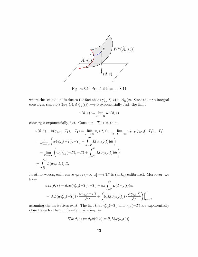
Figure 8.1: Proof of Lemma 8.11

where the second line is due to the fact that (γ′ϑ,s(t), t) ∈ AH(c). Since the first integralconverges since dist(dγz(t), dγ

′ϑ,s(t)) −→ 0 exponentially fast, the limit

u(ϑ, s) := limT−→∞

uT (ϑ, s)

converges exponentially fast. Consider −T1 < s, then

u(ϑ, s)− u(γϑ,s(−T1),−T1) = limT−→∞

uT (ϑ, s)− limT−T1−→∞

uT−T1(γϑ,s(−T1),−T1)

= limT−→∞

(w(γ′ϑ,s(−T ),−T ) +

∫ 0

−TL(dγϑ,s(t))dt

)− lim

T−→∞

(w(γ′ϑ,s(−T ),−T ) +

∫ T1

−TL(dγϑ,s(t))dt

)=

∫ T

T1

L(dγϑ,s(t))dt.

In other words, each curve γϑ,s : (−∞, s] −→ Tn is (u, Lc)-calibrated. Moreover, wehave

dϑu(ϑ, s) = dϑw(γ′ϑ,s(−T ),−T ) + dϑ

∫ 0

−TL(dγϑ,s(t))dt

= ∂vL(dγ′ϑ,s(−T )) ·∂γ′ϑ,s(−T )

∂ϑ+

(∂vL(dγϑ,s(t)) ·

∂γϑ,s(t)

∂ϑ

)∣∣∣0t=−T

,

assuming the derivatives exist. The fact that γ′ϑ,s(−T ) and γϑ,s(−T ) are exponentiallyclose to each other uniformly in ϑ, s implies

∇u(ϑ, s) := dϑu(ϑ, s) = ∂vL(dγϑ,s(0)),

73

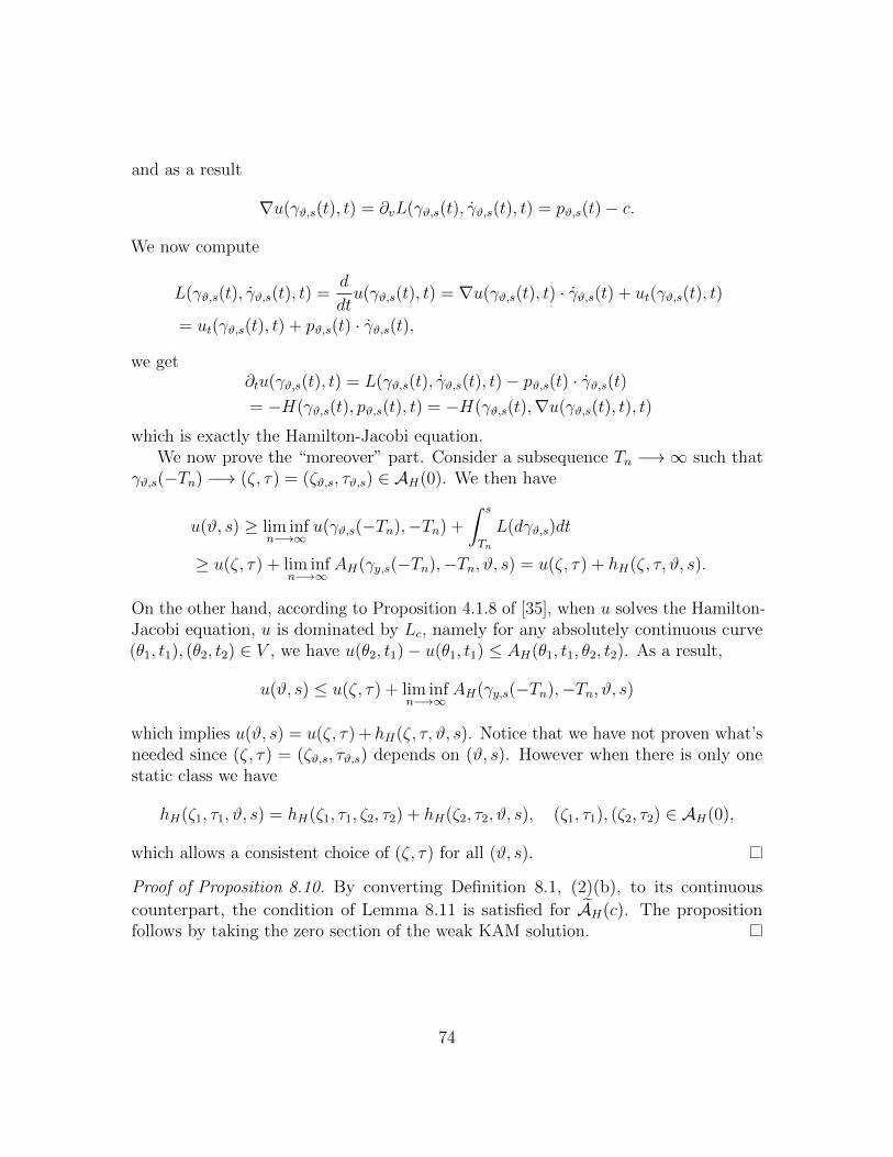
and as a result

∇u(γϑ,s(t), t) = ∂vL(γϑ,s(t), γϑ,s(t), t) = pϑ,s(t)− c.

We now compute

L(γϑ,s(t), γϑ,s(t), t) =d

dtu(γϑ,s(t), t) = ∇u(γϑ,s(t), t) · γϑ,s(t) + ut(γϑ,s(t), t)

= ut(γϑ,s(t), t) + pϑ,s(t) · γϑ,s(t),

we get∂tu(γϑ,s(t), t) = L(γϑ,s(t), γϑ,s(t), t)− pϑ,s(t) · γϑ,s(t)= −H(γϑ,s(t), pϑ,s(t), t) = −H(γϑ,s(t),∇u(γϑ,s(t), t), t)

which is exactly the Hamilton-Jacobi equation.We now prove the “moreover” part. Consider a subsequence Tn −→∞ such that

γϑ,s(−Tn) −→ (ζ, τ) = (ζϑ,s, τϑ,s) ∈ AH(0). We then have

u(ϑ, s) ≥ lim infn−→∞

u(γϑ,s(−Tn),−Tn) +

∫ s

Tn

L(dγϑ,s)dt

≥ u(ζ, τ) + lim infn−→∞

AH(γy,s(−Tn),−Tn, ϑ, s) = u(ζ, τ) + hH(ζ, τ, ϑ, s).

On the other hand, according to Proposition 4.1.8 of [35], when u solves the Hamilton-Jacobi equation, u is dominated by Lc, namely for any absolutely continuous curve(θ1, t1), (θ2, t2) ∈ V , we have u(θ2, t1)− u(θ1, t1) ≤ AH(θ1, t1, θ2, t2). As a result,

u(ϑ, s) ≤ u(ζ, τ) + lim infn−→∞

AH(γy,s(−Tn),−Tn, ϑ, s)

which implies u(ϑ, s) = u(ζ, τ) + hH(ζ, τ, ϑ, s). Notice that we have not proven what’sneeded since (ζ, τ) = (ζϑ,s, τϑ,s) depends on (ϑ, s). However when there is only onestatic class we have

hH(ζ1, τ1, ϑ, s) = hH(ζ1, τ1, ζ2, τ2) + hH(ζ2, τ2, ϑ, s), (ζ1, τ1), (ζ2, τ2) ∈ AH(0),

which allows a consistent choice of (ζ, τ) for all (ϑ, s).

Proof of Proposition 8.10. By converting Definition 8.1, (2)(b), to its continuous

counterpart, the condition of Lemma 8.11 is satisfied for AH(c). The propositionfollows by taking the zero section of the weak KAM solution.

74

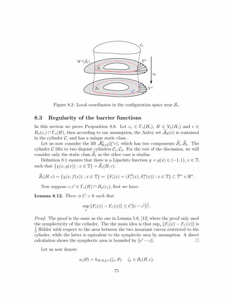
Figure 8.2: Local coordinates in the configuration space near S1.

8.3 Regularity of the barrier functions

In this section we prove Proposition 8.8. Let c∗ ∈ Γ∗(H∗), H ∈ Vσ(H∗) and c ∈Bσ(c∗) ∩ Γ∗(H), then according to our assumption, the Aubry set AH(c) is containedin the cylinder C, and has a unique static class.

Let us now consider the lift A0HΞ(ξ∗c), which has two components S1, S2. The

cylinder C lifts to two disjoint cylinders C1, C2. For the rest of the discussion, we willconsider only the static class S1 as the other case is similar.

Definition 8.1 ensures that there is a Lipschitz function y = g(x) ∈ (−1, 1), x ∈ T,

such that χ(x, g(x)) : x ∈ T = S1(H, c).

S1(H, c) = χ(x, f(x)) : x ∈ T =: Fc(x) = (F θc (x), F p

c (x)) : x ∈ T ⊂ Tn × Rn.

Now suppose c, c′ ∈ Γ∗(H) ∩Bσ(c∗), first we have:

Lemma 8.12. There is C > 0 such that

supx‖Fc(x)− Fc′(x)‖ ≤ C‖c− c′‖

12 .

Proof. The proof is the same as the one in Lemma 5.8, [13] where the proof only usedthe symplecticity of the cylinder. The the main idea is that supx ‖Fc(x)− Fc′(x)‖ is12

Holder with respect to the area between the two invariant curves restricted to thecylinder, while the latter is equivalent to the symplectic area by assumption. A directcalculation shows the symplectic area is bounded by ‖c′ − c‖.

Let us now denote

uc(θ) = hHΞ,ξ∗c(ζ1, θ), ζ1 ∈ S1(H, c).

75

Before moving forward, we define a convenient local coordinate system near S1. Ac-cording to Proposition 8.10, the graph (θ,∇uc(θ)) locally coincides with W u(S1(H, c)).

The (strong) unstable bundle Eu(z) of z ∈ S1(H, c) is tangent to W u(S1(H, c)) at

every point, and transverse to the tangent cone of S1(H, c). Since W u(S1(H, c)) is aLipschitz graph over Tn, the projection Nu(z) := dπθE

u(z) forms a non-zero section

of the normal bundle to S1(H, c) = πθS1(H, c) within the configuration space Tn. Bychoosing an orthonormal basis e1(z), · · · , en−1(z), Nu(z) naturally defines a coordinatesystem (xf , xs) ∈ T× Rn−1 on the tubular neighborhood of S1:

ι(xf , xs) = F θc (xf ) +

n−1∑i=1

ei(Fθc (xf ))xsi .

See Figure 8.2. We note that the coordinate system is only Holder since the unstablebundle is only Holder a priori. Therefore, we consider C∞ functions that approximateF θc and ei in the C0 sense, th new coordinate system is still well defined near S1, and

the xs coordinate projects onto the unstable direction. In the sequel, we fix such acoordinate system using W u(S1(H∗, c∗)). Due to semi-continuity, for (H, c) close to(H∗, c∗), the coordinate system is defined in a neighborhood of S1(H, c).

By assumption, the foliation to W u(S1(H, c)), c ∈ Γ∗(H) by strong unstablemanifold is β0-Holder for some β0 > 0 (see [68]). As a result, we obtain the followingregularity:

Lemma 8.13. There is σ > 0 such that for H ∈ Vσ(H∗), c, c′ ∈ Γ∗(H) ∩ Bσ(c∗),θ ∈ Bσ(S1(H, c∗)), there is β > 0, C1 > 0, C2 ∈ R such that

1. |∇uc(θ)−∇uc′(θ)| ≤ C1 ‖c− c′‖β;

2. |uc(θ)− uc′(θ)− C2| ≤ C1 ‖c− c′‖β.

Moreover, the same holds with S1 replaced with S2.

Proof. The proof is essentially the same as Lemma 5.9 in [13]. Let σ1 be small enoughsuch that the local coordinates (xf , xs) is defined for |xs| < σ. We then consider theweak KAM solution uc ι(xf , xs) instead, which we still denote as uc(x

f , xs), abusingthe notation.

Let |xs| < σ1, let y = (xf , xs,∇uc(xf , xs)), and let z ∈ S1(H, c) be such thaty ∈ W u(z). We then define z′ ∈ S1(H, c) be the unique such point with xf (z′) = xf (z).Finally define y′ ∈ W u(z′) be such that xs(y′) = xs(y), which is possible since W u(z′)is a graph over the xs coordinates. See Figure 8.3.

We note that within the center unstable manifold W u(C1), the NHIC C1 on onehand, and xs = xs(y) on the other hand serves as two transversals to the strong

76

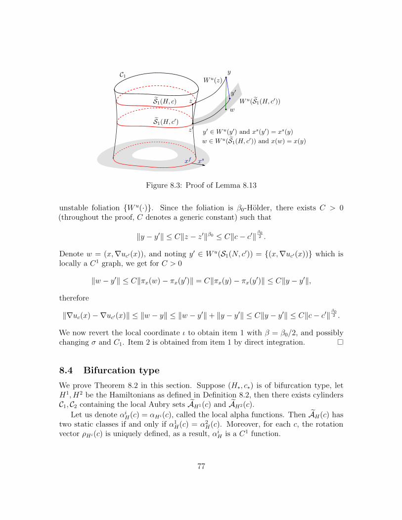
Figure 8.3: Proof of Lemma 8.13

unstable foliation W u(·). Since the foliation is β0-Holder, there exists C > 0(throughout the proof, C denotes a generic constant) such that

‖y − y′‖ ≤ C‖z − z′‖β0 ≤ C‖c− c′‖β02 .

Denote w = (x,∇uc′(x)), and noting y′ ∈ W u(S1(N, c′)) = (x,∇uc′(x)) which is

locally a C1 graph, we get for C > 0

‖w − y′‖ ≤ C‖πx(w)− πx(y′)‖ = C‖πx(y)− πx(y′)‖ ≤ C‖y − y′‖,

therefore

‖∇uc(x)−∇uc′(x)‖ ≤ ‖w − y‖ ≤ ‖w − y′‖+ ‖y − y′‖ ≤ C‖y − y′‖ ≤ C‖c− c′‖β02 .

We now revert the local coordinate ι to obtain item 1 with β = β0/2, and possiblychanging σ and C1. Item 2 is obtained from item 1 by direct integration.

8.4 Bifurcation type

We prove Theorem 8.2 in this section. Suppose (H∗, c∗) is of bifurcation type, letH1, H2 be the Hamiltonians as defined in Definition 8.2, then there exists cylindersC1, C2 containing the local Aubry sets AH1(c) and AH2(c).

Let us denote αiH(c) = αHi(c), called the local alpha functions. Then AH(c) hastwo static classes if and only if α1

H(c) = α2H(c). Moreover, for each c, the rotation

vector ρHi(c) is uniquely defined, as a result, αiH is a C1 function.

77

Proposition 8.14. Let H∗, c∗ be of bifurcation AM type. There is σ > 0 such thatfor an open and dense subset of H ∈ Vσ(H∗), such that there are at most finite manyc ∈ Bσ(c∗) ∩ Γ for which α1

H(c) = α2H(c).

For each such (bifurcation) c, we have A0H1(c), A0

H2(c) are both supported on

hyperbolic periodic orbits. Moreover, N 0H(c) \ A0

H(c) is a discrete set.

Proof. Let σ be as in Definition 8.2. For the rest of the proof, we refer to Bσ(c∗) ∩ Γas Γ to simplify notations.

Consider the family of Hamiltonians Hλ = H(θ, p, t)−λf (f is the mollifier functionin Definition 8.2). Then we have

α1Hλ

(c) = α1H(c) + λ, α2

Hλ(c) = α2

H(c).

By Sard’s theorem, there exists a full Lebesgue measure set E of regular values λ ofthe function α1

H − α2H , which implies for λ ∈ E, 0 is a regular value of α1

Hλ− α2

Hλ(c)

which implies the equation has only finitely many solutions on Γ, and at each solution,α1 and α2 has different derivatives when restricted to Γ. Note that this property isopen in H, which implies the claim of our proposition is an open property. We onlyneed to prove density.

Let ci(λ) ∈ Γ, i = 1, · · · , N be the set on which α1Hλ

= α2Hλ

, then since ddλα1Hλ

(ci) 6=ddλα2Hλ

(ci), each ci(λ) is locally a monontone function in λ.We now impose the assumption that H is a Kupka-Smale system, namely, all

periodic orbits are non-degenerate. Then in this setting, all invariant measures ofrational rotation vectors are supported on hyperbolic periodic orbits, by a furtherperturbation, we can ensure for each c there is only one minimal periodic orbit. Sincethe Aubry set is upper semi-continuous when there is only one static class, and thehyperbolic periodic orbit is structurally stable, we obtain that each hyperbolic periodicorbit is the Aubry set for an open set of c’s. Let us denote by R(H,Γ) the set of all

c ∈ Γ such that A0H(c) is a hyperbolic periodic orbit, then R(H1,Γ) and R(H2,Γ)

are both open and dense in Γ. Then for each ci, there is di > 0 and an open andsense subset of λ ∈ Bdi(0) such that ci(λ) ∈ R(H1,Γ) ∩ R(H2,Γ). Let d = min di,then there is an open and dense set of λ ∈ Bd(0) such that for all i = 1, · · · , N ,

ci(λ) ∈ R(Γ). For these ci’s, A0H1(ci), A0

H2(ci) are both hyperbolic periodic orbits.Using the Kupka-Smale theorem again, it is an open and dense property such thatthe stable and unstable manifolds of A0

H1(ci) and A0H2(ci) intersect transversally. Due

to dimension considerations, the intersection is a discrete set. Since each orbit inNH(ci)\AH(ci) is a heteroclinic orbit between A0

H1(ci) and A0H2(ci), it is also a discrete

set.We have now proven the claim of our proposition holds for an arbitrarily small

perturbation Hλ of H, and hence is dense on Vσ(H∗).

78

An analogous statement holds for the asymmetric bifurcation case:

Proposition 8.15. Let H∗, c∗ be of asymmetric bifurcation type, then there is σ > 0such that for an open and of H ∈ Vσ(H∗), such that there a unique c ∈ Bσ(c∗) ∩ Γ for

which α1H(c) = α2

H(c). Moreover, at such (bifurcation) c, we have A0H1(c), A0

H2(c) are

both supported on hyperbolic periodic orbits. Moreover, N 0H(c) \ A0

H(c) is a discreteset.

Proof. The proof is nearly identical to Proposition 8.14 with the simplification thatfor σ small enough, AH2(c) is always the same hyperbolic periodic orbit, and αH2(c)is a linear function. Since αH1(c) is convex on Γ, there is at most one bifurcation. Therest of the proof is identical.

Proof of Theorem 8.2. Case 1 : Let H∗, c∗ be of bifurcation AM type, and let σ > 0be such that Proposition 8.14 holds on a open and dense subset R1 of Vσ(H∗). Thenon Γ ∩Bσ(c∗) there are at most finitely many bifurcations ci, i = 1, · · · , N . Moreover,for each bifurcation value ci, there is σi > 0 such that for c ∈ Bσi(ci), the localAubry sets are hyperbolic periodic orbits. This means that for each (non-bifurcation)

c ∈ Bσi(ci) \ ci, the sets N 0H(c) = A0

H(c) are contractible (in fact finite). At the

bifurcation values, the set N 0H(ci) \ A0

H(ci) is discrete.We now consider the set (

Γ ∩Bσ(c∗))\

N⋃i=1

Bσi(ci)

which is compact with finitely many connected components. On each of the componentsA0H(c) has a unique static class. We apply Theorem 8.1 to get there is σ′ > 0 such

that the dichotomy of Theorem 8.1 holds for a residual subset R2 of H ∈ Vσ′(H∗) oneach of the connected components. The theorem follows by taking the intersection ofR1 and R2 as well as the smaller value of σ and σ′.

Case 2 : If (H∗, c∗) is of asymmetric bifurcation type, the proof is the same withProposition 8.15 replacing Proposition 8.14.

9 Aubry-Mather type at the single resonance

9.1 Normally hyperbolicity and localization of Aubry/Manesets in the single maximum case

In this section we consider the Hamiltonian system

Nε = H0(p) + εZ(θs, p) + εR(θ, p, t),

79

where θ = (θs, θf) ∈ Tn−1 × T and p = (ps, pf) ∈ Rn−1 × R. Consider the resonantcurve

Γ = p ∈ Bn : ∂psH0(p) = 0 = p∗(pf ) = (ps∗(pf ), pf ) : pf ∈ [a−, a+].

We first consider the case where p ∈ Γ satisfy the condition [SR1λ], namely foreach p ∈ Bλ(p0) ∩ Γ, Z(θs, p∗(p

f )) has a unique global maximum at θs∗(pf ), and

D−1I ≤ ∂2ppH0 ≤ DI, ‖Z‖C3 ≤ 1, λI ≤ −∂2

θsθsZ(θs∗(pf ), p∗(p

f )) ≤ λI,

and that for K > 0, and p0 = p∗(a0) ∈ Γ,

‖R‖C2I (Tn×BK√ε(p0)×T) ≤ δ,

note that we are using the rescaled norm C2I (see (3.2)). We then set K1 = K/D and

consider the local segment

Γ(ε, p0) = p∗(pf ) : pf ∈ [a0 −K1

√ε, a0 +K1

√ε] ⊂ Γ ∩BK

√ε(p0),

which is contained in Bλ(p0) ∩ Γ if ε0 is small enough depending on K. Throughoutthis section, we write f = O(g) if |f | ≤ C|g| for C > 0 that may depend only on D, λand n.

Theorem 9.1 (Proof in Section 9.4 and Section 9.5, see also [13], Theorem 3.1).Assume that K1 > 2. There is δ0, ε0 > 0 and C = C(D,λ, n) > 1, such that if0 < δ < δ0 and 0 < ε < maxε0,

√δ, there is a C2 map

(Θs, P s)(θf , pf , t) : T× [a0 −K1

√ε/2, a0 +K1

√ε/2]× T −→ Tn−1 × Rn−1,

such that C = (θs, ps) = (Θs, P s)(θf , pf , t) is weakly invariant in the sense that thevector field is tangent to C. C is contained in the set

V = (θ, p, t) : ‖θs − θs∗(pf )‖ ≤ C−1, ‖ps − ps∗(pf )‖ ≤ C−1

and it contains all the invariant set contained in V . Moreover, we have∥∥Θs(θf , pf , t)− θs∗(pf )∥∥ ≤ Cδ,

∥∥P s(θf , pf , t)− ps∗(pf )∥∥ ≤ Cδ

√ε,

‖∂pfΘs‖ ≤ C√δ/ε, ‖∂(θf ,t)Θ

s‖ ≤ C√ε, ‖∂pfP s‖ ≤ C, ‖∂(θf ,t)P

s‖ ≤ C√ε.

The cylinder C is normally hyperbolic with its stable/unstable bundle projects onto theθs direction.

80

Theorem 9.2 (Proof is in Section 9.6, see also [13], Theorem 4.1, Theorem 4.2).There is δ0 = δ0(λ, n,D) > 0 and ε0 = ε0(λ, n,D, δ) such that if 0 < δ < δ0 and0 < ε < ε0, the Mane set of the cohomology c satisfies

NNε(c) ⊂ Bδ1/5(θs∗)× T×B√ε·δ1/16 × T ⊂ Tn−1 × T× Rn × T.

If u is a weak KAM solution of Nε at c, then the set I(u, c) ⊂ Tn × Rn is containedin a 18

√Dε−Lipschitz graph above Tn.

The theorems as stated are analogous to the cited theorems in [13]. The maindifference is that we now assume the much weaker assumption ‖R‖C2

I≤ δ. Nevertheless,

we now check that the method in [13] applies in the same way, and leading to theestimates as stated.

9.2 Aubry-Mather type at single resonance

Theorem 9.3. Let c = p∗(pf) with pf ∈ [a0 −K1

√ε/4, a0 +K1

√ε/4], there there is

ε0, δ0 > 0 such that for Nε = H0 + εZ + εR with 0 < ε < ε0 and δ < δ0, then Nε, c isof Aubry-Mather type with the hyperbolic cylinder given by the embedding

χ(θf , pf ) = (Θs, P s)(θf , pf , 0)

where Θs, P s is from Theorem 9.1.

We need the following statement.

Lemma 9.1 ([13], Proposition 4.11). Let u be a (discrete) weak KAM solution forNε at cohomology c, let

Gc,u = (θ, c+∇u(θ))

be the associated pseudograph. Then there is C > 0 depending only on n,D such thatfor any k ≥ 1/

√ε, (θ1, p1), (θ2, p2) ∈ φ−kGc,u, we have

‖p2 − p1‖ ≤ C√ε‖θ2 − θ1‖.

We prove Theorem 9.3 assuming Theorem 9.1 and 9.2.

Proof of Theorem 9.3. Let us denote C the cylinder in Theorem 9.1 and C0 = C ∩t =0.

Let δ0, ε0 be small enough such that Theorem 9.1 and 9.2 applies for 0 < ε < ε0 and0 < δ < δ0. In particular, these statements holds on a open set Nε and c, as required byDefinition 8.1. The embedding as described is a weakly normally hyperbolic invariant

81

cylinder. Moreover, Theorem 9.1 implies that for any two tangent vectors v, v′ ∈ TzC0,we have |dΘs ∧ dP s(v, v′)| ≤ C

√δ|dθf ∧ dpf (v, v′)|, and therefore for δ small enough∣∣(dΘs ∧ dP s + dθf ∧ dpf )(v, v′)

∣∣ ≥ (1− C√δ) ≥ 1

2|dθf ∧ dpf (v, v′)|.

Since the form dθf ∧ dpf is non-degenerate on C0, the symplectic form dθs ∧ dpf +dθf ∧ dpf is non-degenerate when restricted to C0.

Theorem 9.2 implies that for δ small enough, the Mane set NNε(c) is containedin the neighborhood V described in Theorem 9.1. Since the Mane set is invariant, itmust be contained in the cylinder C. Therefore A0

Nε(c) ⊂ N 0

Nε(c) ⊂ C0.

We now show thta A0Nε

is a Lipschitz graph over θf . Let (θ1, p1), (θ2, p2) ∈ A0Nε

(c),then by Theorem 9.2 we have

‖p2 − p1‖ ≤ 18D√ε‖θ2 − θ1‖ ≤ 18D

√ε(‖θs2 − θs1‖+ ‖θf2 − θ

f1‖).

By Theorem 9.1,

‖θs2 − θs1‖ ≤ C(1 +√δ/ε)

(‖θf2 − θ

f1‖+ ‖p2 − p1‖

). (9.1)

Combine everything, we get for some constant C1 depending on n,D,(1− C1(

√ε+√δ))‖p2 − p1‖ ≤ C1(

√ε+√δ)‖θf2 − θ

f1‖.

Which implies ‖p2 − p1‖ ≤ ‖θf2 − θf1‖ if δ, ε is small enough depending only on C1.

Combine with (9.1) we get ‖(θ2, p2)− (θ1, p1)‖ ≤ 2‖θf2 − θf1‖ if ε, δ is small enough.

Finally, let u be a weak KAM solution for Nε at cohomology c, and assume thatA0Nε

(c) projects onto θf component. Since the strong unstable manifolds depends C1

on the base point, the unstable manifold W u(A0H(c)) is a Lipschitz manifold. Moreover,

since the strong unstable direction projects onto the θs direction, W u(A0H(c)) is locally

a graph over θ = (θf , θs). This verifies (2)(b) of Definition 8.1. We have verified allconditions in Definition 8.1 and therefore Nε, c is of Aubry-Mather type.

9.3 Bifurcations in the double maxima case

In this section we assume that for the Hamiltonian

Nε = H0 + εZ + εR,

where Z satisfies the condition [SR2λ], namely for all p ∈ Bλ(p0)∩ Γ, there exists twolocal maxima θs1(p) and θs2(p) of the function Z(., p) in Tn−1 satisfying

∂2θsZ(θs1(p), p) < λI , ∂2

θsZ(θs2(p), p) < λI,

Z(θs, p) < maxZ(θf1 (p), p), Z(θf2 (p), p) − λ(

mind(θs − θs1), d(θs − θs2))2.

82

Let f : Tn−1 −→ R be a bump function satisfying the following conditions:

f |Bλ(θs1(p0)) = 0, f |Bλ(θs2(p0)) = 1,

and 0 ≤ f ≤ 1 otherwise. Define

Z1 = Z − f, Z2 = Z − (1− f),

then Z1(·, p0) has a unique maximum at θs1(p0), while Z2(·, p0) has a unique maximumat θs2(p0). There is κ > 0 depending only on λ such that the same holds for p ∈ Bκ(p0).To the Hamiltonian

N iε = N + εZi + εR, i = 1, 2

we may apply Theorem 9.1 and 9.2 to obtain existence of the NHIC Ci which containsthe local Aubry sets Ai(c) for c ∈ Bκ/2(p0). Morevoer, we may define the local alphafunctions αi(c) = αN i

ε(c) similar to Section 8.4. The cohomology c ∈ Γ ∩Bκ/2(p0) is

of bifurcation type if and only if α1(c) = α2(c), and is of Aubry-Mather type if andonly if α1(c) 6= α2(c).

Moreover, in this case we have the following analog of Theorem 9.2.

Theorem 9.4 (Proof is in Section 9.6, see also [13], Theorem 4.5). If δ = δ(λ, n,D) > 0is small enough and if ε < ε0 = ε0(λ, n,D, δ) is small enough, for c ∈ Bκ/2(p0) ∩ Γ theAubry set at cohomology c of the Hamiltonian Nε satisfies

A(c) ⊂(B(θs1, δ

1/5) ∪B(θs2, δ1/5))× T×B(c,

√εδ1/16)× T ⊂ Tn−1 × T× Rn × T.

If, moreover, the projection θs(A0(c)) ⊂ Tn−1 is contained in one of the (disjoint)balls B(θsi , δ

1/5), then the projection θs(N 0(c)) ⊂ Tn−1 of the Man set is contained inthe same ball B(θsi , δ

1/5).

Theorem 9.5. Suppose Z satisfies condition SR2λ at p = c∗. Then there existsε0, δ0 > 0, such that if 0 < ε < ε0 and 0 < δ < δ0, such that if Nε = H0 + εZ + εRwith ‖R‖C2

I< δ, Nε, c∗ is of bifurcation Aubry-Mather type.

Proof. Let V1 = Bλ(θs1(p0))×T ⊂ Tn−1 ×T, and V2 = Bλ(θs2(p0))×T. We check thatthe functions N1

ε and N2ε both satisfies the conditions of Theorem 9.3, and as a result,

conditions (1) and (2) of Definition 8.2 are satisfied. It suffices to check item (3).

83

9.4 Hyperbolic coordinates

The Hamiltonian flow admits the following equation of motion :

θs = ∂psH0 + ε∂psZ + ε∂psR

ps = −ε∂θsZ − ε∂θsRθf = ∂pfH0 + ε∂pfZ + ε∂pfR

pf = −ε∂θfRt = 1

. (9.2)

The Hamiltonian structure of the flow is not used in the following proof.The system (9.2) is a perturbation of

θs = ∂psH0, ps = −ε∂θsZ, θf = ∂pfH0, pf = 0, t = 1

which admits a normally hyperbolic invariant cylinder

(θs∗(pf ), θf , ps∗(pf ), pf , t) : θf , t ∈ T, .

SetB(pf ) := ∂2

pspsH0(p∗(pf )), A(pf ) := −∂2

θsθsZ(θs∗(pf ), p∗(p

f )),

then as in [13], there is a positive definite matrix T (pf ) such that

Λ(pf ) = T (pf )A(pf )T (pf ) = T−1(pf )B(pf )T−1(pf ).

We lift the equation to the universal cover, and consider the change of variable

x = T−1(pf )(θs − θs∗(pf )) + ε−1/2T (pf )(ps − ps∗(pf ))y = T−1(pf )(θs − θs∗(pf ))− ε−1/2T (pf )(ps − ps∗(pf )),I = ε−1/2(pf − a0), Θ = γθf ,

(9.3)

where 0 < γ < 1 is a parameter to be determined.

Lemma 9.2 ([13], Lemma 3.1, Lemma 3.2). For each pf ∈ [a−, a+], we have Λ(pf ) ≥√λ/DI. We also have the following estimates:

‖T‖C2 , ‖T−1‖C2 , ‖∂pf θs∗‖C0 , ‖ps∗‖C2 = O(1), ‖θs−θs∗‖C0 ≤ O(ρ), ‖ps−ps∗‖C0 ≤ O(√ερ),

where ρ = max‖x‖, ‖y‖.

Note we are using the regular C2 norm in Lemma 9.2 since T depends only on H0

and Z which are bounded in the regular norm.

84

Lemma 9.3. The equation of motion in the new variables takes the form

x =√εΛ(a0 +

√εI)x+

√εO(δ + ρ2), y = −

√εΛ(a0 +

√εI)y +

√εO(δ + ρ2),

and I = O(√εδ).

Proof. The last equation is straight forward. We only prove the equation for x as thecalculations for y are the same. In the original coordinates, we have

θs = B(pf )(ps − ps∗(pf )) +O(‖ps − ps∗(pf )‖2) +O(δ√ε),

ps = εA(pf )(θs − θs∗(pf )) +O(ε‖θs − θs∗(pf )‖2) +O(εδ),

where we used ‖∂pR‖ = ε−12‖∂IR‖ = O(ε−

12 δ). Differentiate (9.3), use pf = O(εδ),

Lemma 9.2, we get

x = T−1θs + ε−12T ps +O(

√εδ)

=√εT−1BT−1 · ε−

12T (ps − ps∗(pf )) +

√εTAT · T−1(θs − θs∗) +O(

√εδ +

√ερ2)

=√εΛ(pf )x+

√εO(δ + ρ2).

Lemma 9.4. Suppose√ε ≤ δ, then in the new coordinates (x, y,Θ, I, t) the linearized

system is given by

L =

√εΛ 0 0 0 00 −

√εΛ 0 0 0

0 0 0 0 00 0 0 0 00 0 0 0 0

+√εO(δγ−1 + ρ+ γ),

where ρ = max‖x‖, ‖y‖.Proof. In the original coordinates, the linearized equation is given by the matrix

L =

O(√εδ) B +O(δ) O(

√εδ) ∂2

pfpsH0 +O(δ) 0

εA+O(ερ) O(√εδ) 0 O(

√εδ) 0

O(√εδ) O(1) O(

√εδ) O(1) 0

0 O(√εδ) 0 O(

√εδ) 0

0 0 0 0 0

+O(εδ).

The coordinate change matrix is

[∂(θs, ps, θf , pf , t)

∂(x, y,Θ, I, t)

]=

T/2 T/2 0 O(

√ε) 0√

εT−1/2 −√εT−1/2 0

√ε∂pfp

s∗ +O(ερ) 0

0 0 γ−1 0 00 0 0

√ε 0

0 0 0 0 1

.

85

The product is

L

[∂(θs, ps, θf , pf , t)

∂(x, y,Θ, I, t)

]= O(εδγ−1 + ερ)+

√εBT−1/2 +O(

√εδ) −

√εBT−1/2 +O(

√εδ) O(

√εδγ−1) O(

√εδ) 0

εAT/2 εAT/2 0 0 0O(√ε) O(

√ε) O(

√εδγ−1) O(

√ε) 0

0 0 0 0 00 0 0 0 0

.Most of the computations are straightforward, with the exception of the fourth row,first column, which contains the following cancellation:

∂2pspfH0∂pfp

s∗ + ∂2

pfpfH0 = ∂pf(∂pfH0(p∗(p

f )))

= 0

since ∂pfH0(p∗(pf )) = 0 for every pf by definition.

The differential of the inverse coordinate change is

[∂(x, y,Θ, I, t)

∂(θs, ps, θf , pf , t)

]=

T−1 ε−1/2T 0 O(ε−1/2λ−1/4) 0T−1 −ε−1/2T 0 O(ε−1/2λ−1/4) 0

0 0 γ 0 00 0 0 ε−1/2 00 0 0 0 1

.Finally, the new matrix of the linearized equation is

L =

[∂(x, y,Θ, I, t)

∂(θs, ps, θf , pf , t)

]L

[∂(θs, ps, θf , pf , t)

∂(x, y,Θ, I, t)

]

= O(√ε(δγ−1 + ρ)) +

√εΛ 0 0 0 00 −

√εΛ 0 0 0

O(√εγ) O(

√εγ) O(

√εγ) 0 0

0 0 0 0 00 0 0 0 0

.

9.5 Normally hyperbolic invariant cylinder

We state the following abstract statement for existence of normally hyperbolic invariantmanifolds, given in [13].

86

Let F : Rn −→ Rn be a C1 vector field. We split the space Rn as Rnu ×Rns ×Rnc ,and denote by z = (u, s, c) the points of Rn. We denote by (Fu, Fs, Fc) the componentsof F :

F (x) = (Fu(z), Fs(z), Fc(z)).

We study the flow of F in the domain

Ω = Bu ×Bs × Ωc

where Bu and Bs are the open Euclidean balls of radius ru and rs in Rnu and Rns ,and Ωc = Ωc1 × Rc2 is a convex open subset of Rnc . We denote by

L(z) = dF (z) =

Luu(z) Lus(z) Luc(z)Lsu(z) Lss(z) Lsc(z)Lcu(z) Lcs(z) Lcc(z)

the linearized vector field at point z. We assume that ‖L(z)‖ is bounded on Ω, whichimplies that each trajectory of F is defined until it leaves Ω. We denote by W c(F, ω)the union of all full orbits contained in Ω, W sc(F,Ω) the set of points whose positiveorbit remains inside Ω, and by W uc(F,Ω) the set of points whose negative orbitremains inside Ω.

Let us further consider a positive parameter b > 0, and consider the set Ωc2b =

Bb(Ωc2) and Ωc

b = Ωc1 × Ωc2b .

Proposition 9.5 ([13], Proposition A.6). Let F : Rnu×Rns×Ωcb −→ Rnu×Rns×Rnc

be a C2 vector field. Assume that there exists α,m, σ > 0 such that

• Fu(u, s, c) · u > 0 on ∂Bu × Bs × Ωcb.

• Fs(u, s, c) · s < 0 on Bu × ∂Bs × Ωcb.

• Luu(z) > αI, Lss(z) 6 −αI for each x ∈ Ωb in the sense of quadratic forms.

• ‖Lus(z)‖+‖Luc(z)‖+‖Lss(z)‖+‖Lsc(z)‖+‖Lcu(z)‖+‖Lcs(z)‖+‖Lcc(z)‖ 6 mfor each x ∈ Ωb.

• ‖Lus(z)‖+ ‖Luc(z)‖+ ‖Lss(z)‖+ ‖Lsc(z)‖+ ‖Lcu(z)‖+ ‖Lcs(z)‖+ ‖Lcc(z)‖+2‖Fc2(z)‖/b 6 m for each z ∈ Ωb − Ω.

Assume furthermore that

K :=m

α− 2m6

1

8,

then there exist C2 maps

wsc : Bs × Ωcb −→ Bu, wuc : Bu × Ωc

b −→ Bs, wc : Ωcb −→ Bu ×Bs

87

satisfying the estimates

‖dwsc‖ 6 K, ‖dwuc‖ 6 K, ‖dwc‖ 6 2K,

the graphs of which respectively contain W sc(F,Ω),W uc(F,Ω),W c(F,Ω). Moreover,the graphs of the restrictions of wsc, wuc and wc to, respectively, Bs×Ωc, Bu×Ωc andΩc, are tangent to the flow.

There exists an invariant C1 foliation of the graph of wuc whose leaves are graphsof K-Lipschitz maps above Bu. The set W uc(F,Ω) is a union of leaves : it has thestructure of an invariant C1 lamination. Two points x, x′ belong to the same leaf ofthis lamination if and only if d(x(t), x′(t))etα/4 is bounded on R−.

If in addition there exists a group G of translations of Rnc1 such that F (id ⊗id⊗ g ⊗ id) = F for each g ∈ G, then the maps w∗ can be chosen such that

wsc (id⊗ g ⊗ id) = wsc, wuc (id⊗ g ⊗ id) = wuc, wc (g ⊗ id) = wc (9.4)

for each g ∈ G. The lamination is also translation invariant.

Proof of Theorem 9.1. Consider the equation of Nε in the (x, y, θf , pf , t) coordinates,and set Bu = ‖x‖ < ρ, Bs = ‖y‖ < ρ, Ωc2 = ‖If‖ ≤ K1/2, Ωc1 = (θf , t)with the group translation Z2, α =

√λ/4D, b = 1 < K1/2. Note that our choice of b

implies Ωc2b ⊂ ‖If‖ < K1. We fix γ =

√δ

According to Lemma 9.2 and Lemma 9.3, we have for ‖x‖ = ρ,

x · x ≥√εαρ2 − ρ

√εO(δ + ρ2) =

√ερ(ρ−O(δ + ρ2)

)> 0

as long as ρ ≥ Cδ for C large enough. This verifies the first bullet point assumption.The second assumption is verified in the same way.

By Lemma 9.4, we have for C1 > 1 depending on λ,D, n,

‖Lus(z)‖+ ‖Luc(z)‖+ ‖Lss(z)‖+ ‖Lsc(z)‖+ ‖Lcu(z)‖+ ‖Lcs(z)‖+ ‖Lcc(z)‖=√εO(δγ−1 + ρ+ γ) ≤ C1

√ε(√δ + ρ) =: m/2,

and Luu ≥ (2α−m)I ≥ αI as long as m < α. This is possible as long as ε, δ, ρ < C−11 <

α. Finally, we check that if z ∈ Ωb \Ω, ‖Fc2(z)‖ = O(√εδ) ≤ C1

√ε(√δ + ρ)/2 = m/4

if C1 is chosen large enough. These estimates ensure all the bullet point conditionsare satisfied. By choosing C1 even smaller, we can ensure m < α/10 which impliesK = m/(α− 2m) ≤ 1/8.

To summarize, we have shown all conditions of Proposition 9.5 is satisfied if0 < ε < C−1

1 , 0 < δ < C−11 , Cδ ≤ ρ ≤ C−1

1 . We apply the Proposition twice, once forρ = C−1

1 and once for ρ = Cδ. The first application shows the invariant cylinder is

88

the maximal invariant set in the set Ωc = ‖x‖, ‖y‖ ≤ C−11 . The second application

shows that the cylinder is in fact contained in the set ‖x‖, ‖y‖ ≤ Cδ. Moreover, inthe second application, we get the estimate m = O(

√εδ), which allows the estimate

K = O(√εδ).

We now return to the original coordinates using the formula

Θs(θf , pf , t) = θs∗(pf ) +

1

2T (pf ) · (wcu + wcs)(γθ

f , a0 + ε−1/2pf , t)

P s(θf , pf , t) = ps∗(pf ) +

√ε

2T−1(pf ) · (wcu − wcs)(γθf , a0 + ε−1/2pf , t).

(9.5)

All the estimates stated in Theorem 9.1 follow directly from these expressions, andfrom the fact that ‖x‖, ‖y‖ ≤ Cδ, ‖dwc‖ 6 2K = O(

√εδ).

9.6 Localization of the Aubry and Mane sets

Let D1 = 2D, the Hamiltonian Nε satisfies the following estimates if δ is small enoughdepending only on D:

D−11 I ≤ ∂2

ppNε ≤ DI, ‖∂2θpNε‖ ≤ 2

√ε, ‖∂2

θθNε‖ ≤ 3ε.

Let L(θ, p, t) be the Lagrangian associated to Nε, and L0 the Lagrangian of H0.

Lemma 9.6. The following estimates holds for the Lagrangian L.

1. ([13], Lemma 4.1) For K > 0, the image of the set Tn × BK√ε × T under the

diffeomorphism ∂pNε contains the set Tn ×BK1√ε(c)× T, where K1 = K/(4D1).

2. ([13], Lemma 4.2) The estimates

‖∂2θvL‖C0 ≤ 2D1

√ε, ‖∂2

θθL‖C0 ≤ 3ε

holds on Tn ×BK1√ε(c)× T.

3. ([13], Lemma 4.3) For v ∈ BK1√ε(c), we have

|L(θ, v, t)− (L0(v)− εZ(θs, c)) | ≤ 2εδ.

4. ([13], Lemma 4.4) The alpha function αNε(c) satisfies

|αNε(c)− (H0(c) + εmaxZ(·, c))| ≤ 2εδ.

89

5. ([13], Lemma 4.5) There is C > 1 depending only on D such that if ε < C−1δ,we have the estimates

L(θ, v, t)− c · v + α(c) > ‖v − ∂H0(c)‖2/(4D1)− εZc(θs)− 4εδ (9.6)

L(θ, v, t)− c · v + α(c) 6 D1‖v − ∂H0(c)‖2 − εZc(θs) + 4εδ (9.7)

for each (θ, v, t) ∈ Tn × Rn × R, where Zc(θs) := Z(θs, c)−maxθs Z(θs, c).

Proof. We remark that in [13] it is assumed that ‖∂2θpNε‖ ≤ 2ε instead of 2

√ε as

we assumed. However the same calculations as given in the cited lemmas proveLemma 9.6, once appropriate changes are made.

Proposition 9.7. For each c ∈ Rn, the weak KAM solution u of cohomology c is3√D1ε/2−semi-concave.

Proof of Theorem 9.2. The proofs of Theorem 4.1 and 4.2 in [13] replies on theestimates (3)(4)(5) in Lemma 9.6, as well as Proposition 9.7. We have arrived at thesame estimates using weaker assumption, the only change is we replaced the constantD with D1 = 2D. The rest of the proofs are exactly identical.

Proof of Theorem 9.4. This is similar to Theorem 9.2. The proof of Theorem 4.5, [13]applies once we taking into account Lemma 9.6 and Proposition 9.7.

90

10 Normally hyperbolic cylinders at double reso-

nance

We prove Theorem 4.1 in these sections. Recall that the theorem deals with two cases:

1. (Simple critical homology) In this case we show the homoclinic curve η0±h can

be extended to periodic orbits both in positive and negative energy. The unionof these periodic orbits form a C1 normally hyperbolic invariant manifold.

2. (Non-simple homology) In this case we show that for positive energy, there existsperiodic orbits shadowing η0

h1and η0

h2in a particular order.

Our strategy is to prove existence of these periodic orbits as hyperbolic fixed points ofcomposition of local and global maps. A main technical tool to prove existence anduniqueness of these fixed points is the Conley-McGehee isolation block ([66]). Theplan of this section is as follows.

In section 10.1 we state a standard normal from near the hyperbolic fixed point.In section 10.2 we study the property of the Shil’nikov boundary value problem.In section 10.3, we apply results of Section 10.2 to establish strong hyperbolicity of

the local map Φ∗loc as well as existence of unstable cones. Since the global maps Φ∗globhave bounded time, they have bounded norms and the linearization of the propercompositions Φ∗globΦ

∗loc are dominated by the local component.

In section 10.4 we give definition and derive simple properties of isolating blocksof Conley-McGehee [66].

In section 10.5, under non-degeneracy conditions [DR1c]− [DR4c], we constructisolating blocks for the proper compositions of Φ∗globΦ

∗loc.

In section 10.6 we extend this analysis to Φ∗globΦ∗loc · · ·Φ∗globΦ∗loc. This would imply

existence of families of shadowing orbits in non-simple case.In section 10.7 we complete the proof of Theorem 4.1 by showing that periodic

orbits constructed in the previous two sections, forms a normally hyperbolic invariantcylinder. Moreover, they coincide with the shortest geodesics for the Jacobi metric.

In Section 10.8 we prove Lemma 4.2 which describes in the non-simple case, theorder at which the simple periodic orbits are shadowed.

10.1 Normal form near the hyperbolic fixed point

We describe a normal form near the hyperbolic fixed point (assumed to be (0, 0)) ofthe slow Hamiltonian Hs : T2 × R2 −→ R. For the rest of this section, we drop thesuperscript s to abbreviate notations. In a neighborhood of the origin, there exists a a

91

symplectic linear change of coordinates under which the system has the normal form

H(u1, u2, s1, s2) = λ1s1u1 + λ2s2u2 +O3(s, u).

Here s = (s1, s2), u = (u1, u2), and On(s, u) stands for a function bounded by C|(s, u)|n.By taking a standard straightening coordinate change, we get:

Lemma 10.1. After an Cr−1 symplectic coordinate change Φ, the Hamiltonian takesthe form

N = H Φ = λ1s1u1 + λ2s2u2 +∑i,j=1,2

siujO1(s, u),

and the equation is [su

]=

[−Λs+ sO1(s, u)Λu+ uO1(s, u)

], (10.1)

where Λ = diagλ1, λ2.

Proof. Since (0, 0) is a hyperbolic fixed point, for sufficiently small r > 0, thereexists stable manifold W s = (u = U(s), |s| ≤ r and unstable manifold W u = s =S(u), |u| ≤ r containing the origin. All points on W s converges to (0, 0) exponentiallyin forward time, while all points on W u converges to (0, 0) exponentially in backwardtime. These manifolds are Lagrangian; as a consequence, the change of coordinatess′ = s − S(u), u′ = u − U(s′) = u − U(s − S(u)) is symplectic. Under the newcoordinates, we have that W s = u′ = 0 and W u = s′ = 0. We abuse notation andkeep using (s, u) to denote the new coordinate system.

Under the new coordinate system, the Hamiltonian has the form

H(s, u) = λ1s1u1 + λ2s2u2 +H1(s, u),

where H(s, u) = O3(s, u) and H1(s, u)|s=0 = H1(s, u)|u=0 = 0. The Hamiltonian andthe vector field takes the desired form under this coordinate.

10.2 Shil’nikov’s boundary value problem

Recall the definition of the local map (Section 4.4). We will define the sections Σs± to

be a subset of the section s1 = ±δ, and the sections Σu± to be contained in u1 = ±δ.

In this section, we study the properties of the local map via the Shil’nikov boundaryvalue problem.

Proposition 10.2 (Shil’nikov [70], Lemma 2.1, 2.2, 2.3). There exists C > 0, δ0 > 0and T0 > 0 such that for each 0 < δ < δ0, any sin = (sin1 , s

in2 ), uout = (uout1 , uout2 ) with

‖(s, u)‖ ≤ δ and any large T > T0, there exists a unique solution (sT , uT ) : [0, T ] −→

92

BCδ of the system (10.1) with the property sT (0) = sin and uT (T ) = uout. Moreover,we have

‖sT (t)‖ ≤ Cδe−λ1t/2, ‖uT (t)‖ ≤ Cδe−λ1(T−t)/2,

and ∥∥∥∥∂sT (t)

∂sin

∥∥∥∥+

∥∥∥∥∂uT (t)

∂sin

∥∥∥∥ ≤ Ce−λ1t/2,

∥∥∥∥∂sT (t)

∂uout

∥∥∥∥+

∥∥∥∥∂uT (t)

∂uout

∥∥∥∥ ≤ Ce−λ1(T−t)/2.

Consider the space of all smooth curves (s, u) : [0, T ] −→ BCδ, define a map

Corollary 10.3. Let (sT , uT ) be the solution in Proposition 10.2 with fixed boundaryvalues sin, uout. Then∥∥∥∥ d

dT(sT (t), uT (t))

∥∥∥∥ ≤ Ce−λ1(T−t)/2,

∥∥∥∥ d

dT(sT (T − t), uT (T − t))

∥∥∥∥ ≤ Ce−λ1t/2,

(10.2)and

d

dτ

∣∣∣τ=T

(sτ (T ), uτ (T )) = −XN(sT (T ), uT (T )) +O(e−λ1T/2),

d

dτ

∣∣∣τ=T

(sτ (T − τ), uτ (T − τ)) = XN(sT (0), uT (0)) +O(e−λ1T/2),

(10.3)

where XN denote the Hamiltonian vector field of N .

Proof. Consider two solutions (sT1 , uT1) and (sT2 , uT2) of the boundary value problem,we extend the definition of the solutions to R by solving the ODE. We note that(sT1 , uT1) : [0, T2] −→ R4 satisfies the boundary condition sin and uT1(T2) on [0, T2],and by Corollary 10.3,∥∥(sT1 , uT1)(t)− (sT2 , uT2)(t)

∥∥ ≤ Ceλ1(T2−t)/2‖uT1(T2)− uout‖.

Note that

limT2−→T1

uT1(T2)− uout

T2 − T1

= limT2−→T1

uT1(T2)− uT1(T1)

T2 − T1

=d

dt

∣∣∣t=T1

uT1(t),

and as a result, ∥∥∥∥ d

dT

∣∣∣T=T1

(sT , uT )(t)

∥∥∥∥ ≤ Ceλ1(T1−t).

This proves the first half of (10.2) while the second half is similar.For (10.3), note

d

dτ

∣∣∣τ=T

(sτ (T ), uτ (T )) =d

dτ

∣∣∣τ=T

(sτ (τ), uτ (τ))− d

dτ

∣∣∣τ=T

(sT (τ), uT (τ)),

the first half of (10.3) follows. The second half is similar.

93

Let (vs1 , vs2 , vu1 , vu2) denote the coordinates for the tangent space induced by(s1, s2, u1, u2). For K > 0 and x ∈ Br, we define the strong unstable cone by

CuK(x) = K2|vu2 |2 > |vu1|2 + |vs1|2 + |vs2|2 (10.4)

and the strong stable cone to be

CsK = K2|vs2|2 > |vs1|2 + |vu1|2 + |vu2|2.

The following statement follows from the hyperbolicity of the fixed point O viastandard techniques.

Lemma 10.4 (See for example, [44]). For any 0 < κ < λ2−λ1, there exists δ = δ(κ,K)and C = C(κ,K) > 1 such that the following holds:

• If φt(x) ∈ B4δ(O) for 0 ≤ t ≤ t0, then Dφt(CuK(x)) ⊂ Cu

K(φt(x)) for all0 ≤ t ≤ t0. Furthermore, for any v ∈ Cu

K(x),

|Dφt(x)v| ≥ C−1e(λ2−κ)t, 0 ≤ t ≤ t0.

• If φ−t(x) ∈ B4δ(O) for 0 ≤ t ≤ t0, then Dφ−t(CsK(x)) ⊂ Cs

K(φ−t(x)) for all0 ≤ t ≤ t0. Furthermore, for any v ∈ Cs

K(x),

|Dφ−t(x)v| ≥ C−1e(λ2−κ)t, 0 ≤ t ≤ t0.

Lemma 10.5. For any κ > 0 there is δ0 > 0 such that for any 0 < δ ≤ δ0,|sin1 | = |uout1 | = δ, and |sin2 |, |uout2 | ≤ κλ1δ/(2λ2), we have∣∣∣∣ ddT uT2 (0)

∣∣∣∣ ≤ κ

∣∣∣∣ ddT uT1 (0)

∣∣∣∣ , ∣∣∣∣ ddT sT2 (T )

∣∣∣∣ ≤ κ

∣∣∣∣ ddT sT1 (T )

∣∣∣∣ .Moreover, by integrating in T , we get

|uT2 (0)| ≤ κ|uT1 (0)|, |sT2 (T )| ≤ κ|sT1 (T )|.

Proof. Given κ > 0 we can choose δ0 small enough such that the backward flow Dφ−tpreserves the cone

(CuK)c = ‖vu2‖ ≤ K−1‖(vs1 , vs2 , vu1)‖,

where K = κ−1. Note that

d

dT(sT (0), uT (0)) = Dφ−T

d

dτ

∣∣∣τ=T

(sτ (T ), uτ (T )).

94

Since the vector

d

dτ

∣∣∣τ=T

(sτ (T ), uτ (T )) = −XN(sT (T ), uT (T )) +O(e−λ1T/2)

= (λ1sT1 (T ), λ2s

T2 (T ), λ1u

T1 (T ), λ2u

T2 (T )) +O(δ2) +O(e−λ1T/2)

= (0, 0, λ1δ, λ2uout2 ) +O(δ2) +O(e−λ1T/2) ∈ (Cu

K)c

if |uout2 | ≤ κλ1δ/(2λ2), δ is small and T large enough. It follows that ddT

(sT (0), uT (0)) ∈(Cu

K)c. Keep in mind that ddTsT (0) = 0, the first half of our estimate follows. The

second half is proven in a symmetric way.

10.3 Properties of the local maps

Recall that γ+ is a non-degenerate homoclinic orbit, and γ− is its time-reversal. Letus define

Σs+ = (δ, s2, u1, u1) : |s2|, |u1|, |u2| ≤ δ,

Σu+ = (s1, s2, δ, u1) : |s2|, |u1|, |u2| ≤ δ.

(10.5)

Denote q+ = γ+ ∩ s1 = δ = (σ, s+2 , 0, 0), and p+ = γ+ ∩ u1 = δ = (0, 0, δ, u+

2 ).Let κ > 0 be a parameter to be defined in Proposition 10.6. Since γ+ is tangent tothe s1, u1 axes, we can choose δ > 0 such that |s+

2 |, |u+2 | < κδ, therefore q+, p+ are

contained Σs+ and Σu

+ respectively. Define

ls = (δ, s2, 0, 0) : −κδ ≤ s2 ≤ κδ ⊂ W s(O) ∩ Σs+,

lu = (0, 0, δ, u2) : −κδ ≤ u2 ≤ κδ ⊂ W u(O) ∩ Σu+.

LetΣs,E

+ = Σs+ ∩ N(s, u) = E, Σu,E

+ = Σu+ ∩ N(s, u) = E

be restriction of the sections to an energy E close to 0. We would like to study thedomain of the restricted local map Φ++

loc : Σs,E+ −→ Σu,E

+ .A rectangle R is a diffeomorphic image of the Euclidean rectangle in R2. Let us

label the vertices by 1, 2, 3, 4 in clockwise order, and call the four sides l12, l34, l14, l23.

Proposition 10.6. There is e, κ > 0 such that for each 0 < E < e, there is a rectangleR++(E) ⊂ Σs,E

+ with sides lij(E), such that:

1. Φ++loc is well defined on R++(E), and its image Φ++

loc (R++(E)) is also a rectangle,it’s four sides denoted l′ij(E).

2. As E −→ 0, both l12(E) and l34(E) converges to lu in Hausdorff metric. Similarly,both l′14(E) and l′23(E) converges to lu.

95

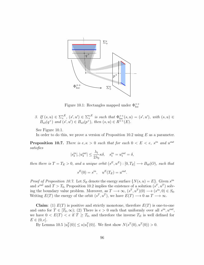
Figure 10.1: Rectangles mapped under Φ++loc

3. If (s, u) ∈ Σs,E+ , (s′, u′) ∈ Σu,E

+ is such that Φ++loc (s, u) = (s′, u′), with (s, u) ∈

Bκδ(q+) and (s′, u′) ∈ Bκδ(p

+), then (s, u) ∈ R++(E).

See Figure 10.1.In order to do this, we prove a version of Proposition 10.2 using E as a parameter.

Proposition 10.7. There is e, κ > 0 such that for each 0 < E < e, sin and uout

satisfies

|sin2 |, |uout2 | ≤λ1

2λ2

κδ, sin1 = uout1 = δ,

then there is T = TE > 0, and a unique orbit (sE, uE) : [0, TE] −→ B4δ(O), such that

sE(0) = sin, uE(TE) = uout.

Proof of Proposition 10.7. Let SE denote the energy surface N(s, u) = E. Given sin

and sout and T > T0, Proposition 10.2 implies the existence of a solution (sT , uT ) solv-ing the boundary value problem. Moreover, as T −→∞, (sT , uT )(0) −→ (sin, 0) ∈ S0.Writing E(T ) the energy of the orbit (sT , uT ), we have E(T ) −→ 0 as T −→∞.

Claim: (1) E(T ) is positive and strictly monotone, therefore E(T ) is one-to-oneand onto for T ∈ [T0,∞); (2) There is e > 0 such that uniformly over all sin, uout,we have 0 < E(T ) < e if T ≥ T0, and therefore the inverse TE is well defined forE ∈ (0, e].

By Lemma 10.5 |uT2 (0)| ≤ κ|uT1 (0)|. We first show N(sT (0), uT (0)) > 0.

96

Let us consider the energy function N(s1, u1, s2, u2) = λ1s1u1 + λ2s2u2 +H1(s, u)with H1|s=0 = H1|u=0 = 0. Recall that the section Σ+ = (s, u) : s1 = δ, |(s, u)| ≤ δ.We consider the submanifold Σ ∩ N(s, u) = 0. Since

∂u1N(δ, u1, s2, u2) = λ1δ + ∂u1H1 = λ1δ +O(δ2) > 0,

by implicit function theorem, for |(s, u)| ≤ δ the surface Σ ∩ N = 0 is given by agraph u1 = uc1(s2, u2). We conclude that Σ is divided by the graph u1 = uc1(s2, u2)into two components, and:

• N(s, u) > 0 whenever u1 > uc1(s2, u2), and N(s, u) < 0 when u1 < uc1(s2, u2).

Moreover, uc1|u2=0 = 0, and by differentiating the implicit function, we get |∂u2uc1| ≤ Cwhere C is a constant depending on ‖N‖C2 . Therefore |uc1(s2, u2)| ≤ C|u2|. Thisimplies if (δ, u1, s2, u2) ∈ Σ satisfies u1 > C|u2| ≥ |uc1|, we have N(δ, u1, s2, u2) > 0. Inparticular, this is satisfied for (sT (0), uT (0)) if κ < C−1.

E(T ) is a continuous function defined on T ≥ T0, and limT−→∞E(T ) = 0. Wenow prove that it is monotone. Using Lemma 10.5,

d

dTE(T ) =

d

dTN(sT (0), uT (0)) = ∇N ·

(0, 0,

d

dTuT1 (0),

d

dTuT2 (0)

)= (λ1s

in1 +O2(s, u))

d

dTuT1 (0) + (λ2s

in2 +O2(s, u))

d

dTuT2 (0) 6= 0

if κ is sufficiently small. Since we have proved E(T ) > 0, claim (1) follows. Finally,Proposition 10.2 implies

0 < E(T ) ≤ Cδ2e−λ1T/2,

claim (2) follows.

Proof of Proposition 10.6. Let κ > 0 be small enough such that Proposition 10.7applies, and let us rename λ1κ/(2λ2) into κ. Consider two parameters a ∈ [−κδ, κδ]and b ∈ [−κδ, κδ], and then there exist unique orbits sEa,b solving the boundary valueproblem

sEa,b(0) = (δ, a), sEa,b(Ta,b(E)) = (δ, b),

then

R++(E) =

(sEa,b(0), uEa,b(0)) : a, b ∈ [δ/2, δ/2],

Φ++loc

(R++(E)

)=

(sEa,b(Ta,b(E)), uEa,b(Ta,b(E))) : a, b ∈ [δ/2, δ/2].

Note that two sides of the rectangle R++(E) are graphs over s2 ∈ [−κδ, κδ], sincethe u1, u2 component converge to 0 exponentially fast as T −→ ∞ (and E −→ 0),

97

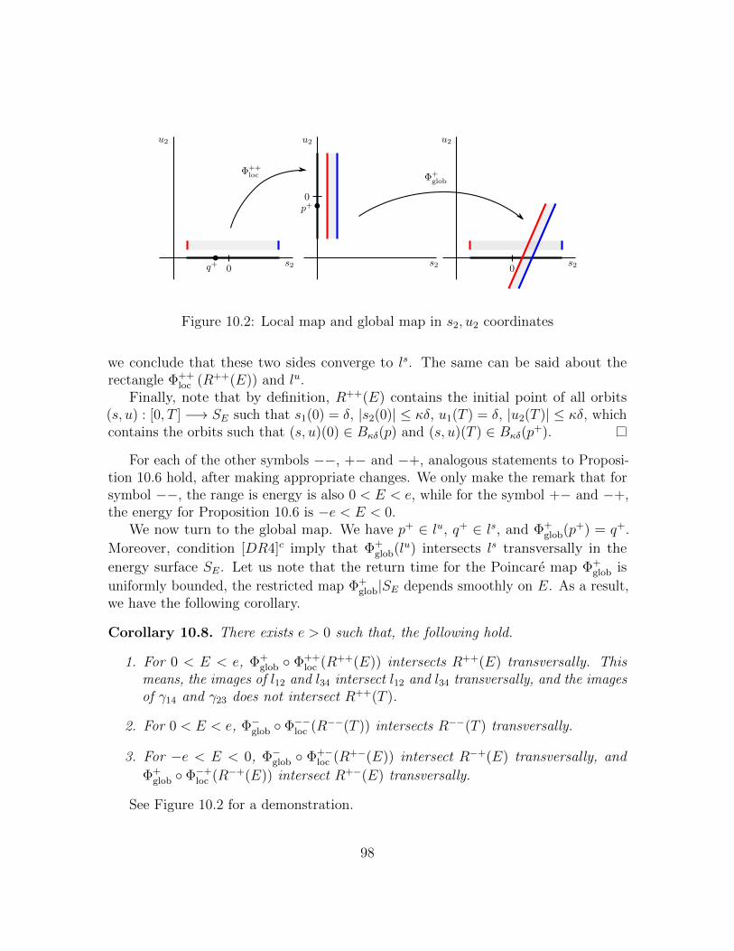
Figure 10.2: Local map and global map in s2, u2 coordinates

we conclude that these two sides converge to ls. The same can be said about therectangle Φ++

loc (R++(E)) and lu.Finally, note that by definition, R++(E) contains the initial point of all orbits

(s, u) : [0, T ] −→ SE such that s1(0) = δ, |s2(0)| ≤ κδ, u1(T ) = δ, |u2(T )| ≤ κδ, whichcontains the orbits such that (s, u)(0) ∈ Bκδ(p) and (s, u)(T ) ∈ Bκδ(p

+).

For each of the other symbols −−, +− and −+, analogous statements to Proposi-tion 10.6 hold, after making appropriate changes. We only make the remark that forsymbol −−, the range is energy is also 0 < E < e, while for the symbol +− and −+,the energy for Proposition 10.6 is −e < E < 0.

We now turn to the global map. We have p+ ∈ lu, q+ ∈ ls, and Φ+glob(p+) = q+.

Moreover, condition [DR4]c imply that Φ+glob(lu) intersects ls transversally in the

energy surface SE. Let us note that the return time for the Poincare map Φ+glob is

uniformly bounded, the restricted map Φ+glob|SE depends smoothly on E. As a result,

we have the following corollary.

Corollary 10.8. There exists e > 0 such that, the following hold.

1. For 0 < E < e, Φ+glob Φ++

loc (R++(E)) intersects R++(E) transversally. Thismeans, the images of l12 and l34 intersect l12 and l34 transversally, and the imagesof γ14 and γ23 does not intersect R++(T ).

2. For 0 < E < e, Φ−glob Φ−−loc (R−−(T )) intersects R−−(T ) transversally.

3. For −e < E < 0, Φ−glob Φ+−loc (R+−(E)) intersect R−+(E) transversally, and

Φ+glob Φ−+

loc (R−+(E)) intersect R+−(E) transversally.

See Figure 10.2 for a demonstration.

98

10.4 Conley-McGehee isolating blocks

The rectangles as constructed form isolation blocks of Conley and McGehee ([66]).A rectangle R = I1 × I2 ⊂ Rd × Rk, I1 = ‖x1‖ ≤ 1, I2 = ‖x2‖ ≤ 1 is called

an isolating block for the C1 diffeomorphism Φ, if the following hold:

1. The projection of Φ(R) to the first component covers I1.

2. Φ|I1 × ∂I2 is homotopically equivalent to the identity restricted on the setI1 × (Rk \ int I2).

If R is an isolating block of Φ, then the set

W+ = x ∈ R : Φk(x) ∈ R, k ≥ 0

(resp. W− = x ∈ R : Φ−k(x) ∈ R, k ≥ 0)

projects onto I1 (resp. onto I2) (see [66]). If some additional cone conditions aresatisfied, then W+ and W− are in fact C1 graphs. Note that in this case, W+ ∩W−

is the unique fixed point of Φ on R.As usual, we denote by Cu

K(x) = c‖v1‖ ≤ ‖v2‖ the unstable cone at x. Wedenote by πCu

K(x) the set x+CuK(x), which corresponds to the projection of the cone

CuK(x) from the tangent space to the base set. The stable cones are defined similarly.

Let U ⊂ Rd × Rk be an open set and Φ : U −→ Rd × Rk a C1 map. Denote DΦx thelinearization of Φ at x.

C1. DΦx preserves the cone field CuK(x), and there exists Λ > 1 such that ‖DΦ(v)‖ ≥

Λ‖v‖ for any v ∈ CuK(x).

C2. Φ preserves the projected restricted cone field πCuK , i.e., for any x ∈ U ,

Φ(U ∩ πCuK(x)) ⊂ Cu

K(Φ(x)) ∩ Φ(U).

C3. If y ∈ πCuK(x) ∩ U , then ‖Φ(y)− Φ(x)‖ ≥ Λ‖y − x‖.

The unstable cone condition guarantees that any forward invariant set is contained ina Lipschitz graph.

Proposition 10.9 (See [66]). Assume that Φ and U satisfies [C1]-[C3], then anyforward invariant set W ⊂ U is contained in a Lipschitz graph over Rk (the stabledirection).

99

Similarly, we can define the conditions [C1]-[C3] for the inverse map and thestable cone, and refer to them as “stable [C1]-[C3]” conditions. Note that if Φ and Usatisfies both the isolating block condition and the stable/unstable cone conditions,then W+ and W− are transversal Lipschitz graphs. In particular, there exists a uniqueintersection, which is the unique fixed point of Φ on R. We summarize as follows.

Corollary 10.10. Assume that Φ and U satisfies the isolating block condition, andthat Φ and U (resp. Φ−1 and U ∩Φ(U)) satisfies the unstable (resp. stable) conditions[C1]-[C3]. Then Φ has a unique hyperbolic fixed point in U .

10.5 Periodic orbit in simple homologies

We now apply the isolating block construction to the maps and rectangles obtained inCorollary 10.8.

Proposition 10.11. There exists e > 0 such that the following hold.

• For 0 < E < e, Φ+glob Φ++

loc has a unique fixed point p+(E) on Σs+ ∩R++(E);

• For 0 < E < e, Φ−glob Φ−−loc has a unique fixed point p−(E) on Σs− ∩R−−(E);

• For −e < E < 0: Φ+glob Φ−+

loc Φ−glob Φ+−loc has a unique fixed point pc(E) on

R+−(E) ∩ (Φ−glob Φ+−loc )−1(R−+(E)).

To prove Proposition 10.11, we notice that the rectangle R++(T ) has C1 sides,and there exists a C1 change of coordinates turning it to a standard rectangle. It’seasy to see that the isolating block conditions are satisfied for the following maps andrectangles:

Φ+glob Φ++

loc and R++(E), Φ−glob Φ−−loc and R−−(E),

Φ+glob Φ−+

loc Φ−glob Φ+−loc and (Φ−glob Φ+−

loc )−1R−+(E) ∩R+−(E).

It suffices to prove the stable and unstable cone conditions [C1]-[C3] for the corre-sponding return map and rectangles. Given z = (s, u) ∈ SE, let us define the restrictedcones

Cu,EK (z) = Cu

K ∩ TzSE, Cs,EK = Cs

K ∩ TzSE.

Lemma 10.12. For each orbit (s, u)(t) associated to orbits of the local map, therestricted cones Cu,E

K and Cs,EK are non-empty.

100

Proof. We only prove the statement for Cu,EK since the stable one is completely

symmetric. Moreover, observe that if we prove the cone Cu,EK is non-empty at (s, u)(0),

the same holds for the entire orbit, since the unstable cone is invariant under theforward dynamics.

Note that

∇N = (λ1u1 + uO1, λ2u2 + uO1, λ1s1 + sO1, λ2s2 + sO1),

and ‖u(0)‖ is exponentially small in T , we have ∇N ∼ (0, 0, λ1s1, λ2s2). Since|s2| ≤ δ = |s1| on Σs

+, we have the angle between ∇N and u1 axis is boundedfrom below. As a consequence, there exists K > 0, such that Cu,K has nonemptyintersection with the tangent direction of SE (which is orthogonal to ∇N). The lemmafollows.

We will only prove the [C1]-[C3] conditions conditions for the unstable cone Cu, cE ,

the map Φ+glob Φ++

loc and the rectangle R++(T ); the proof for the other cases can beobtained by making obvious changes to the case covered.

Lemma 10.13. There exists T0 > 0 and c > 0 such that the following hold. Assumethat U ⊂ Σs

+ ∩Br is a connected open set on which the local map Φ++loc is defined, and

for each x ∈ U ,inft ≥ 0 : ϕt(x) ∈ Σu

+ ≥ T0.

Then the map D(Φ+glob Φ++

loc ) preserves the cone field CuK, and the inverse D(Φ+

glob Φ++

loc )−1 preserves the non-empty CsK. Moreover, the projected cones πCu

K ∩ U andπCs

K ∩ V are preserved by Φ+glob Φ++

loc and its inverse, where V = Φ+glob Φ++

loc (U).The same set of conclusions hold for the restricted version. Namely, we can replace

CuK and Cs

K with Cu,EK and Cs,E

K , and U with U ∩ SE.

Recall that lu 3 p+ is the intersection of the unstable manifold W u(O) with thesection Σu

+. Let T u be the tangent vector to lu at p+, and T s the tangent vector toT s at q+. We will show that if Φ++

loc |SE(x) = y, then the image of the unstable coneDΦ++

loc (x)CuK is very close to T u. This happens because the flow of tangent vector is

very close to that of a linear flow.Assume that φt is a flow on Rd × Rk, and xt is a trajectory of the flow. Let

v(t) = (v1(t), v2(t)) be a solution of the variational equation, i.e. v(t) = Dφt(xt)v(0).

Lemma 10.14. With the above notations assume that there exists b2 > 0, b1 < b2

and σ, δ > 0 such that the variational equation

v(t) =

[A(t) B(t)C(t) D(t)

] [v1(t)v2(t)

]

101

satisfy A ≤ b1I and D ≥ b2I as quadratic forms, and ‖B‖ ≤ σ, ‖C‖ ≤ δ.Then for any c > 0 and κ > 0, there exists δ0 > 0 such that if 0 < δ, σ < δ0, we

have(Dφt)C

uK ⊂ Cu,βt , βt = ce−(b2−b1−κ)t + σ/(b2 − b1 − κ).

Proof. Denote γ0 = c. The invariance of the cone field is equivalent to

d

dt

(β2t 〈v2(t), v2(t)〉 − 〈v1(t), v1(t)〉

)≥ 0.

Compute the derivatives using the variational equation, apply the norm bounds andthe cone condition, we obtain

2βt (β′t + (b2 − δβt − b1)βt − σ) ‖v2‖2 ≥ 0.

We assume that βt ≤ 2γ0, then for sufficiently small δ0, δβt ≤ κ. Denote b3 = b2−b1−κand let βt solve the differential equation

β′t = −b3βt + σ.

It’s clear that the inequality is satisfied for our choice of βt. Solve the differentialequation for βt and the lemma follows.

Proof of Lemma 10.13. We will only prove the unstable version. By Assumption 4,there exists c > 0 such that DΦ+

glob(q+)T uu(q+) ⊂ CuK(p+). Note that as T0 −→ ∞,

the neighborhood U shrinks to p+ and V shrinks to q+. Hence there exists β > 0 andT0 > 0 such that DΦ+

glob(y)Cu, β(y) ⊂ CuK for all y ∈ V .

Let (s, u)(t)0≤t≤T be the trajectory from x to y. By Proposition 10.2, we have‖s‖ ≤ e−λ1T/4 for all T/2 ≤ t ≤ T . It follows that the matrix for the variationalequation[

A(t) B(t)C(t) D(t)

]=

[− diagλ1, λ2+O(s) O(s)

O(u) diagλ1, λ2+O(u)

](10.6)

satisfies A ≤ −(λ1 − κ)I, D ≥ (λ1 − κ)I, ‖C‖ = O(δ) and ‖B‖ = O(e−(λ1−κ)T/2). Asbefore Cu

K(x) = ‖vs‖ ≤ c‖vu‖, Lemma 10.14 implies

DφT (x)CuK(x) ⊂ Cu,βT (y),

where βT = O(e−λ′T/2) and λ′ = minλ2 − λ1 − κ, λ1 − κ. Finally, note that

DφT (x)CuK(x) and DΦ++

loc (x)CuK(x) differs by the differential of the local Poincare map

near y. Since near y we have |s| = O(e−(λ1−κ)T ), using the equation of motion, thePoincare map is exponentially close to identity on the (s1, s2) components, and is

102

exponentially close to a projection to u2 on the (u1, u2) components. It follows thatthe cone Cu, βT is mapped by the Poincar’e map into a strong unstable cone withexponentially small size. In particular, for T ≥ T0, we have

DΦ++loc (x)Cu

K(x) ⊂ Cu, β(y),

and the first part of the lemma follows. To prove the restricted version we follow thesame arguments.

Conditions [C1]-[C3] follows, and this concludes the proof of Proposition 10.11.

10.6 Periodic orbits for non-simple homology

In the case of the non-simple homology, there exist two rectangles R1 and R2, whoseimages under Φglob Φloc intersect themselves transversally, providing a “horseshoe”type picture.

Proposition 10.15. There exists e > 0 such that the following hold:

1. For all 0 < E ≤ e, there exist rectangles R1(E), R2(E) ∈ Σs,E+ such that for

i = 1, 2, Φiglob Φ++

loc (Ri) intersects both R1(E) and R2(E) transversally.

2. Given σ = (σ1, · · · , σn), there exists a unique fixed point pσ(E) of

1∏i=n

(Φσi

glob Φ++loc

)|Rσi (E) (10.7)

on the set Rσ1(E).

3. The curve pσ(E) is a C1 graph over the u1 component with uniformly boundedderivatives. Furthermore, pσ(E) approaches pσ1 and for each 1 ≤ j ≤ n− 1,

1∏i=j

(Φσi

glob Φ++loc

)(pσ(E))

approaches pσj+1 as E −→ 0.

The proof is analogous to that of Proposition 10.11 and we omit it.

103

10.7 Normally hyperbolic invariant cylinders for the slow me-chanical system

We prove Theorem 4.1 in this section.

Proof. Non-simple case. If the homology h is non-simple, then h = n1h1 + n2h2

with h1, h2 being simple homologies. Let (σ1, . . . , σn) be the sequence determinedby Lemma 4.2. Apply Proposition 10.15, we obtain the fixed points pσ(E) for all0 < E < e. The fixed points corresponds to hyperbolic periodic orbits that we call ηEh .Let γEh be the projection of ηEh to the configuration space, we now prove that theymust be identical to the shortest curve in Jacobi metric gE, after a reparametrization.According to the condition [DR3c], γ0

h is the unique shortest curve for the Jacobi

metric g0, and there exist c0 such that η0h = AHs(c0) = NHs(c0). Any gE shortest

curve γ′E corresponds to Aubry set of cohomology cE, which lifts to an orbit η′E inphase space. Using semi-continuity, η′E must be contained in a neighborhood of η0

h inthe phase space. In particular, it must intersect the sections Σs

+ and Σu+ sufficiently

close to q+ and p+. According to Proposition 10.7, item 3, the intersection with Σs+

must be contained in the rectangle R++(E). Since the fixed point pσ(E) is the uniquefixed point for the map (10.7), we conclude that η′E = ηEh .

Simple critical case. The existence the periodic orbits follows from Proposition 10.11in the same way as the non-simple case. Also, by the same reasoning, we know thatthe orbits ηEh , ηE−h must coincide with the minimal geodesics of the Jacobi metric. Itsuffices to show that

M =⋃

0<E<e

(ηEh ∪ ηE−h

)∪ η0

h ∪ η0−h ∪

⋃−e<E<0

ηEc

form a C1 normally hyperbolic invariant cylinder.Denote

l+(p+) = p+(E)0<E≤E0 , l+(p−) = p−(E)0<E≤E0 ,

l+(q+) = Φ++loc (l+(p+)) and l+(q−) = Φ−−loc (l+(q−)). Note that the superscript of l

indicates positive energy instead of the signature of the homoclinics. We denote

l−(p+) = pc(E)−E0≤E<0

l−(q−) = Φ+−loc (l−(p+)), l−(p−) = Φ−glob(l−(q−)) and l−(q+) = Φ−+

loc (l−(p−)). Anillustration of M the curves l± are included in Figure 10.3.

l(p+) and l(p−) are both graphs over the u1 variable. By considering the image⋃t>0 φt(l(p

+)) and⋃t>0 φt(l(q

+)), using Lemma 10.5, the projection of M to s1u1

plane contains a neighborhood of 0. Standard cone arguments implies it must be aLipschitz graph over s1u1 near 0. Finally, standard arguments in partial hyperbolicity

104

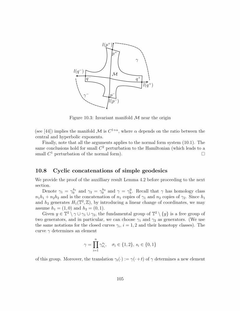
l(p−)

p+

l(p+)

q+

l(q+)

p−

q−l(q−)

γ

γ−

M

Figure 10.3: Invariant manifold M near the origin

(see [44]) implies the manifold M is C1+α, where α depends on the ratio between thecentral and hyperbolic exponents.

Finally, note that all the arguments applies to the normal form system (10.1). Thesame conclusions hold for small C2 perturbation to the Hamiltonian (which leads to asmall C1 perturbation of the normal form).

10.8 Cyclic concatenations of simple geodesics

We provide the proof of the auxilliary result Lemma 4.2 before proceeding to the nextsection.

Denote γ1 = γh10 and γ2 = γh20 and γ = γ0h. Recall that γ has homology class

n1h1 + n2h2 and is the concatenation of n1 copies of γ1 and n2 copies of γ2. Since h1

and h2 generates H1(T2,Z), by introducing a linear change of coordinates, we mayassume h1 = (1, 0) and h2 = (0, 1).

Given y ∈ T2 \ γ ∪ γ1 ∪ γ2, the fundamental group of T2 \ y is a free group oftwo generators, and in particular, we can choose γ1 and γ2 as generators. (We usethe same notations for the closed curves γi, i = 1, 2 and their homotopy classes). Thecurve γ determines an element

γ =n∏i=1

γsiσi , σi ∈ 1, 2, si ∈ 0, 1

of this group. Moreover, the translation γt(·) := γ(·+ t) of γ determines a new element

105

by cyclic translation, i.e.,

γt =n∏i=1

γsi+mσi+m, m ∈ Z,

where the sequences σi and si are extended periodically. We claim the following:There exists a unique (up to translation) periodic sequence σi such that γ =∏n

i=1 γσi+m for some m ∈ Z, independent of the choice of y. Note that in particular,all si = 1.

The proof of this claim is split into two steps.Step 1. Let γn1/n2(t) = γ(0) + (n1/n2, 1)t, t ∈ R. We will show that γ is

homotopic (along non-self-intersecting curves) to γn1/n2 . To see this, we lift bothcurves to the universal cover with the notations γ and γn1/n2 . Let p.q ∈ Z be suchthat pn1 − qn2 = 1 and define

T γ(t) = γ(t) + (p, q).

As T generates all integer translations of γ, γ is non-self-intersecting if and onlyif T γ ∩ γ = ∅. Define the homotopy γλ = λγ + (1 − λ)γn1/n2 , it suffices to proveT γλ ∩ γλ = ∅. Take an additional coordinate change[

xy

]7→[n1 pn2 q

]−1 [xy

],

then under the new coordinates T γ(t) = γ(t) + (1, 0).Under the new coordinates, T γ ∩ γ = ∅ if and only if any two points on the same

horizontal line has distance less than 1. The same property carries over to γλ for0 ≤ λ < 1, hence T γλ ∩ γλ = ∅.

Step 2. By step 1, it suffices to prove that γ = γn1/n2 defines unique sequencesσi and si. Since γn1/n2 is increasing in both coordinates, we have si = 1 for all i.Moreover, choosing a different y is equivalent to shifting the generators γ1 and γ2.Since the translation of the generators is homotopic to identity, the homotopy class isnot affected. This concludes the proof of Lemma 4.2.

106

11 Aubry-Mather type at the double resonance

We consider the systemHs(ϕ, I) = K(I)− U(ϕ).

Given the homology h ∈ H1(T2,Z), there is a curve ch : (0, E] −→ H1(T2,R) suchthat ch(E). There are two regimes, the “high energy regime”, where we consider thecohomologies ch(E) with e ≤ E ≤ E where e is a small parameter; and the criticalregime, where c is in a small neighborhood of ch(0).

11.1 High energy case

First we consider the “non-critical energy case”, and show that the cohomologies aschosen are of Aubry-Mather type. For each E > 0, there are two possible behavior:

1. The Aubry set AHs(ch(E)) = γEh , where γEh is the unique shortest geodesic inhomology E. Let us denote the corresponding Hamiltonian orbit ηEh = (ϕ, I) :[0, TE] −→ T2 × R2.

2. (Bifurcation) The Aubry set AHs(ch(E)) = γEh ∪ γEh , where γEh , γEh are the two

shortest geodesic in homology E. Let us denote the corresponding Hamiltonianorbit ηEh , η

Eh .

Theorem 11.1. Given any e > 0, there is ε0, δ > 0 depending only on Hs and e suchthat the following holds for all 0 < ε < ε0 and all U ′ ∈ Vδ(U) (in the space Cr(T2)),the Hamiltonian

Hsε (ϕ, I, τ) = K(I)− U ′(ϕ) +

√εP, ‖P‖C2 ≤ 1,

satisfies the following properties:

1. Suppose E ≥ e is such that AHs(ch(E)) is a unique hyperbolic orbit, then(Hs

ε , cH(E)) is of Aubry-Mather type.

2. Suppose E ≥ e is such that AHs(ch(E)) is the union of two hyperbolic orbits,then (Hs

ε , ch(E)) is of bifurcation Aubry-Mather type.

We first discuss the non-bifurcation case, and the bifurcation case will be a simplecorollary.

Given E0 ≥ 0, denote c0 = ch(E0). Suppose AHs(c0) = γEh consists of a uniqueshortest curve, then there exists E1 < E0 < E2 such that each ηEh for E ∈ (E1, E2) isa hyperbolic periodic orbit. Then

C0 =⋃

E∈(E1,E2)

ηEh ⊂ T2 × R2

107

is a normally hyperbolic invariant cylinder. In order to give a proper parametrizationfor C0, we consider a transversal section to ηE0

h , which is also transversal to ηEh ,E ∈ (E1, E2) if E1, E2 are close enough to E0. Denote zE = ηEh ∩ Σ, then ZE,E ∈ (E1, E2) is a smooth function of E. We now define

χ : T× (E1, E2) −→ T2 × R2, χ(s, E) = φsTEHs (zE), (11.1)

where φtHs is the Hamiltonian flow of Hs and TE is the period of ηEh .

Lemma 11.1. There is δ > 0 depending on K,U,E1, E2 such that for all U ′ ∈ Vδ(U)and Hs = K − U ′, χ is a smooth embedding and χ(T × (E1, E2)) = C0. C0 isnormally hyperbolic, and for each E, W u(ηEh ) is a smooth graph over θ component ona neighborhood of γEh .

Proof. The fact that γEh is a unique non-degenerate shortest geodesic is robust, there-fore χ is well defined for all U ′ ∈ Vδ(U), where δ depends on K,U,E1, E2.

The fact that χ is smooth and that the image is C0 follows directly from definition.Since Hs(χ(s, E)) = E by definition, have ∇Hs(χ(s, E)) · ∂Eχ(s, E) = 1. On theother hand, ∂sχ(s, E) = XHs(χ(s, E)), where XHs is the Hamiltonian vector field ofHs. Since ∇Hs ·XHs = 0, we conclude that ∂sχ, ∂Eχ are linearly independent over(s, E) ∈ T× [E1, E2].

To see that the local stable-unstable manifolds are graphs over the θ component,we invoke the concept of Green bundles G±. These invariant bundles are defined forall orbits of the Aubry sets, and are Lipschitz graphs over the θ components. TheLipschitz constant is uniform over all E > 0. According to [3], for hyperbolic periodicorbits, the bundle G− is the sum of the vector field direction and the unstable direction.As a result, the unstable bundle of ηEh projects onto a bundle transversal to γEh , andthe unstable manifold projects onto the θ component.

We now consider the Hamiltonian

Hsε (ϕ, I, τ) = Hs(ϕ, I) +

√εP (ϕ, I, τ), ϕ ∈ T2, I ∈ R2, τ ∈ T√ε. (11.2)

Proposition 11.2. Given any κ > 0, 0 < e < E there is ε0 > 0 depending onHs, e, κ and κ > 0 depending only on Hs, e; such that for all E0 ∈ [e, E], there isE1 < E0 < E2, such that for all 0 < ε < ε0, there is an embedding

χε(x, y, τ) : T× (E1, E2)× T√ε −→ T2 × R2 × T√ε, πτχε = id

such that Cε is a weakly invariant normally hyperbolic cylinder for the Hamiltonianflow of Hs

ε (see (11.2)). Moreover, we have

‖χε(ϕ, I, τ)− χ0(ϕ, I)‖C1 < κ,

108

and Cε contains all the invariant sets in

V = Bκ(C0)× T√ε.

Since ‖√εP‖C2 ≤

√ε, this is a regular perturbation of the vector field, compared

to the singular perturbation we see in Section 9. The proof follows from standardtheory, see for example [68], [29].

We will denote by χ0ε(x, y) = χε(ϕ, I, 0) the zero-section of the embedding, and

χ0ε (T× (E1, E2)) = C0

ε

which is invariant under the time-√ε map φ = φ

√ε

Hsε.

We have the following Lipschitz estimate for weak KAM solutions of Hsε .

Proposition 11.3 (Follows from Theorem 7.1). Given R > 0, there is C > 0depending only on ‖∂2K‖, ‖Hs‖C2 and R, such that if u is any weak KAM solutionof Hs

ε at cohomology c with ‖c‖ ≤ R, then for any

(ϕ1, I1), (ϕ2, I2) ∈ I(c, u) =⋂n∈N

φ−n (Gc,u) ,

we have|Hs(ϕ1, I1)−Hs(ϕ2, I2)| ≤ Cε

14‖ϕ1 − ϕ2‖.

As a result, the same Lipschitz property holds on the sets I(c, u), A0Hsε.

Proof of Theorem 11.1. Part (1): Let c0 = ch(E0), and γE0h is the unique shortest

curve, we show (Hεs, c0) is of AM type. By Proposition 11.2, for sufficiently small ε, we

have NHsε(c0) ⊂ Bκ(C0)× T√ε. Due to semi-continuity, the same holds for c ∈ Bσ(c0)

for some σ > 0. As a result, AHsε(c) ⊂ AHs

ε(c) ⊂ Cε.

We now prove the graph property. Suppose

(x1, y1), (x2, y2) ∈ (χ0ε)−1(A0

Hsε(c))

where c ∈ Bσ(c0). Observe that Hs χ0(x, y) = y. Then due to Proposition 11.3,

‖Hs χ0ε(x, y)− y‖C1 = ‖Hs χ0

ε −Hs χ0‖ ≤ ‖Hs‖C2‖χ0ε − χ0‖C1 ≤ Cδ,

where C will be used to denote a generic constant. We have

‖y2 − y1‖ ≤ ‖Hs χ0ε(x2, y2)−Hs χ0

ε(x1, y1)‖+ Cδ‖(x2 − x1, y2 − y1)‖≤ Cε

14‖πϕ χ0

ε(x2, y2)− πϕ χ0ε(x1, y1)‖+ Cδ‖(x2 − x1, y2 − y1)‖

≤ C(δ + ε14 )‖(x2 − x1, y2 − y1)‖

(11.3)

109

For ε, δ small enough, we have ‖y2 − y1‖ ≤ 2C(δ + ε14 )‖x2 − x1‖.

Finally, assume that (χ0ε)−1A0

Hsε(c) project onto the x component, we will show that

W u(A0Hsε(c)) is a graph over the θ component. According to Lemma 11.1, W u(A0

Hs(c))is a smooth graph over θ component, and the projection of the unstable bundle isnormal to γEh . Let us note that (11.3) implies A0

Hsε

is close to A0Hs(c) in Lipschitz norm,

and the unstable bundle depends smoothly on perturbation. Therefore the unstablebundle of A0

Hsε(c) is also transversal to AHs

ε(c), implying (2)(b) of Definition 8.1.

Part (2): Suppose c0 = ch(E0) is such that AHs(c) = γE0h ∪ γ

E0h are two shortest

curves. Let V1, V2 be neighborhoods of γE0 , γE0 such that πϕηE ⊂ V1, πϕη

E ⊂ V2 forall E ∈ (E0 − δ, E0 + δ), and let

f : Tn −→ [0, 1], f |V1 = 0, f |V2 = 1,

be a smooth bump function. Then for

H1 = Hs − f, H2 = Hs − (1− f),

AH1(c0) = γE0 and AH2(c0) = γE0 . We then apply part (1) to obtain that for eachi = 1, 2, H i +

√εP, c0 is of Aubry-Mather type. This implies Hs

ε , c0 is of bifurcationAubry-Mather type (see Definition 8.2).

11.2 Simple non-critical case

Suppose h is a simple non-critical homology, which means that for the energy E = 0,there is a unique shortest curve γ0

h in the homology h corresponding to a hyperbolicperiodic orbit η0

h of the Hamiltonian system. In this case, however, we have, forc0 = ch(0)

AHs(c0) = γ0h ∪O,

where O is the origin (which is where U attains its minimum). If we consider V1, V2

disjoint open sets containing γ0h and 0 respectively, and define the local Aubry sets

AH1(c) and AH2(c). It follows that AH1(c) = γ0h and AH2(c) = O.

Theorem 11.2. Suppose h is simple non-critical, and let c0 = ch(0). Then there isε0, δ > 0 depending only on K,U such that for 0 < ε < ε0 and U ′ ∈ Vδ(U), for

Hsε = K(I)− U ′(ϕ) +

√εP, ‖P‖C2 ≤ 1,

the pair (Hsε , c0) is of asymmetric bifurcation type.

Proof. The fact that H1, c0 is of Aubry-Mather type follows the same proof as Theo-rem 11.1. On the other hand, AHs(c0) is a hyperbolic periodic orbit, which is robustunder perturbation. Therefore Definition 8.3 is satisfied.

110

11.3 Simple critical case

11.3.1 Proof of Aubry-Mather type using local coordinates

Theorem 11.3. Suppose h ∈ H1(T2,Z) is a simple homology for Hs, and considerthe cohomology class c0 = ch(0). Then there exists ε0, e, δ > 0 depending only onHs, h such that for each 0 < ε < ε0, U ′ ∈ Vδ(U) and c ∈ Be(c0), the pair (Hs

ε , c) is ofAubry-Mather type.

Moreover, the same holds for (Hs, λc) for all 0 ≤ λ ≤ 1.

We have the following (See Section 10):

• η0h = AHs(c0) contains the hyperbolic fixed point (0, 0), and is a homoclinic orbit

to (0, 0).

• (0, 0) admits eigenvectors −λ2 < −λ1 < λ1 < λ2. Let vs/u1 and v

s/u2 denote the

eigendirections of the eigenvalues ±λ1,±λ2. Let Inv(ϕ, I) = (ϕ,−I) denote theinvolution of the Hamiltonian system. Since the flow is time-reversible, we haveInv(vsi ) = ±vui , i = 1, 2. Without loss of generality, we assume Inv(vsi ) = vui . Asresult, there exists vi, wi ∈ R2 such that

vsi = (vi, wi), vui = (vi,−wi), i = 1, 2.

• There is a C1 normally hyperbolic invariant manifold M containing η0h. In

particular, M must contain (0, 0) and it’s tangent to the plane Spanvs1, vu1 =Rv1 ⊕ Rw1 ⊂ R2 × R2 at (0, 0).

The projection πϕη0h = γ0

h then is a C1 curve in T2, since 0 ∈ T2 is the onlypossible discontinuity of the tangent direction, but at 0 the curve is tangent tov1 = πϕv

s1 = πϕv

u1 . Let πv1 : R4 −→ R and πw1 : R4 −→ R be the orthogonal

projections to v1, w1 directions.

We also need the following analog of Lemma 11.1.

Lemma 11.4. W u(η0h) is a Lipschitz graph over θ component on a neighborhood of

γ0h.

Proof. In the proof of Lemma 11.1, the Lipschitz constant of the Green bundles isuniform over all energy E. The lemma follows by taking limit E −→ 0 in the space ofLipschitz graphs.

We require a suitable parametrization of the cylinder C(Hs) near the homoclinicη0h. An illustration of the parametrization is given in Figure 11.1.

111

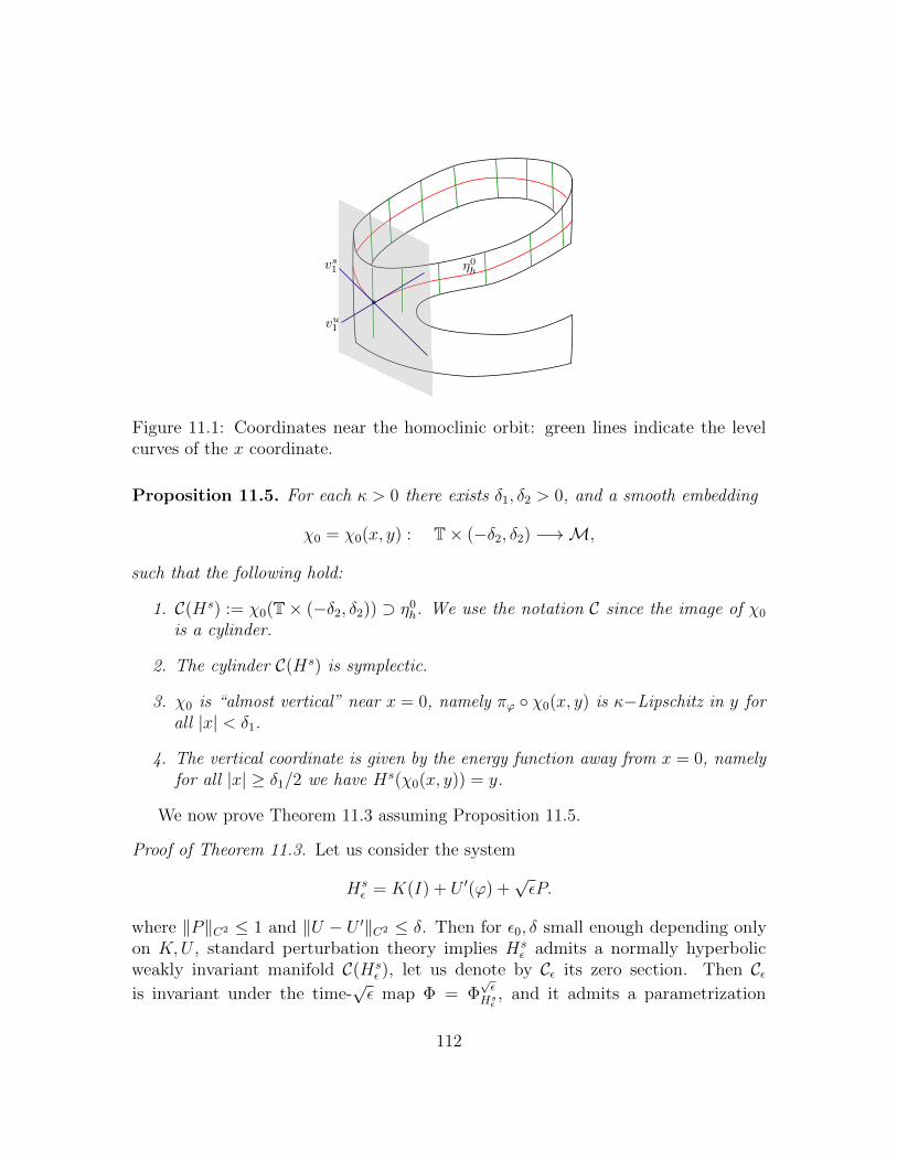
Figure 11.1: Coordinates near the homoclinic orbit: green lines indicate the levelcurves of the x coordinate.

Proposition 11.5. For each κ > 0 there exists δ1, δ2 > 0, and a smooth embedding

χ0 = χ0(x, y) : T× (−δ2, δ2) −→M,

such that the following hold:

1. C(Hs) := χ0(T× (−δ2, δ2)) ⊃ η0h. We use the notation C since the image of χ0

is a cylinder.

2. The cylinder C(Hs) is symplectic.

3. χ0 is “almost vertical” near x = 0, namely πϕ χ0(x, y) is κ−Lipschitz in y forall |x| < δ1.

4. The vertical coordinate is given by the energy function away from x = 0, namelyfor all |x| ≥ δ1/2 we have Hs(χ0(x, y)) = y.

We now prove Theorem 11.3 assuming Proposition 11.5.

Proof of Theorem 11.3. Let us consider the system

Hsε = K(I) + U ′(ϕ) +

√εP.

where ‖P‖C2 ≤ 1 and ‖U − U ′‖C2 ≤ δ. Then for ε0, δ small enough depending onlyon K,U , standard perturbation theory implies Hs

ε admits a normally hyperbolicweakly invariant manifold C(Hs

ε ), let us denote by Cε its zero section. Then Cεis invariant under the time-

√ε map Φ = Φ

√ε

Hsε, and it admits a parametrization

112

χε : T × (−δ2, δ2) −→ Cε, and ‖χε − χ0‖C1 = o(1) as ε, δ −→ 0. The cylinder issymplectic since symplecticity is open under perturbations. Moreover, for e > 0small enough, the set NHs(c) ⊂ C(Hs) for all c ∈ Be(c0), and since N is upper

semi-continuous under Hamiltonian pertubations, NHsε(c) is close to C(Hs

ε ) for smallε. Since C(Hs

ε ) contains all the invariant sets in its neighborhood, we conclude that

AHsε(c) ⊂ NHs

ε(c) ⊂ C(Hs

ε ).

We now show χ−1ε AHs

ε(c) is a Lipschitz graph for c ∈ Be(c0). Let (ϕi, Ii) = χε(xi, yi),

i = 1, 2 be two points in AHsε(c).

The proof consists of two cases. In the first case we use the almost verticality ofthe cylinder, and the idea is similar to the proof of Theorem 9.3. In the second casewe use the strong Lipschitz estimate for the energy Hs, and the idea is similar to theproof of Theorem 11.1.

Case 1. |x1|, |x2| < δ1. In this case, we apply the a priori Lipschitz estimates forthe Aubry sets: there is C > 0 depending only ∂2K, ‖Hs‖C2 such that

‖I2 − I1‖ ≤ C‖ϕ2 − ϕ1‖.

Let κ be as in Proposition 11.5, and let ε0 be small enough such that πϕχε(x, y) is2κ-Lipschitz in y. Since χ0 is an embedding, there is C > 1 depending only on Hs

such that for all ε0 small enough,

‖ϕ2 − ϕ1‖+ ‖I2 − I1‖ ≥ C−1 (‖x2 − x1‖+ ‖y2 − y1‖) .

Let (ϕ3, I3) = χε(x2, y1), then

‖ϕ3 − ϕ2‖ ≤ ‖χε(x2, y1)− χε(x2, y2)‖ ≤ 2κ‖y2 − y1‖,

‖ϕ3 − ϕ1‖ ≤ ‖χε(x2, y1)− χε(x1, y1)‖ ≤ C‖x2 − x1‖,

combine all estimates, we get

C−1 (‖x2 − x1‖+ ‖y2 − y1‖) ≤ (1 + C)‖ϕ2 − ϕ1‖≤ (1 + C) (2κ‖y2 − y1‖+ C‖x2 − x1‖) ,

or (C−1 − 2(1 + C)κ

)‖y2 − y1‖ ≤

(C−1 + (1 + C)C

)‖x2 − x1‖

which is what we need if κ < 1/(4C(1 + C)).Case 2. |x1|, |x2| > δ1/2. In this case we apply Proposition 11.3, to get

‖Hs(ϕ2, I2)−Hs(ϕ1, I1)‖ ≤ Cε14‖ϕ2 − ϕ1‖.

113

Assume that ε is small enough such that ‖χε − χ0‖C1 < κ. Then a computation

identical to (11.3) implies ‖y2 − y1‖ ≤ 2C(κ + ε14 )‖x2 − x1‖ if ε, κ is small enough

depending only on C.We obtain the Lipschitz property of χ−1

ε A0Hsε(c) after combining the two cases.

Finally, we show W u(A0Hsε(c)) is a graph over ϕ when χ−1

ε A0Hsε(c) projects onto the

x component. It suffices to check that the unstable bundle Eu is uniformly transverseto the projection A0

Hsε(c). In case 1, the almost verticality of the cylinder implies

A0Hsε(c) differs from AHs(c0) = γ0

h by O(κ) in Lipschitz norm. Given that the tangent

vector of γ0h is close to the weak directions v

s/u1 in case 1, while the projection of

Eu is close to vs/u2 , the desired transversality holds. In case 2, similar to the proof

of Theorem 11.1, AHsε(c) is also close to AHs(c0) in Lipschitz norm (for a different

reason, i.e (11.3)). The claim follows, similar to the proof of Theorem 11.1, usingLemma 11.4.

11.3.2 Construction of the local coordinates

This is done separately near the hyperbolic fixed point (local) and away from it(global). Furthermore, the local coordinate requires a preliminary step.

Lemma 11.6. For each κ > 0 there is δ > 0, and a smooth embedding

χpre = χpre(x, y) : (−δ, δ)× (−δ, δ) −→M∩B2δ(0, 0) ⊂ T2 × R2,

satisfying‖χpre (πv1 , πw1)− id‖C1 < κ. (11.4)

There is 0 < δ1 < δ such that the curve χ−1preη

0h ∩ π−1

x (−δ1, δ1) is given by a Lipschitzgraph (x, g(x)) : x ∈ (−δ1, δ1).Proof. The existence of the local coordinate follows from T(0,0)M = Rv1 ⊕ Rw1, thefact that M is C1, and the implicit function theorem. Since γ0

h = πϕη0h is a C1 curve

tangent to v1 at 0 ∈ T2, γ0h can be reparametrized using its projection to v1 direction.

Since η0h is a Lipschitz graph over γ0

h, the second claim follows.

Lemma 11.7. For each κ > 0 there is δ1 > δ2 > 0, a smooth embedding

χloc = χloc(x, y) : (−δ1, δ1)× (−δ1, δ1) −→M∩B2δ(0, 0),

a neighborhood V of the local homoclinic η0h ∩ π−1

x (−δ1, δ1) on which the cylinder is“almost vertical” in the sense that there is C > 0 such that

πϕχloc(x, y) is Cκ− Lipschitz in y.

The pull back χ−1locη

0h ∩ π−1

x (−δ1, δ1) is a Lipschitz graph over x, and in addition,

Hs(χloc(x, y)) = y, for all δ1/2 < |x| < δ1, |y| < δ2. (11.5)

114

The manifold χloc (−δ1, δ1)× (−δ1, δ1)) is symplectic.

Proof. First we show the image of χpre is symplectic. To see this, note that Hs(ϕ, I) =12AI · I − 1

2Bϕ · ϕ + O3(I, ϕ), where A = ∂2

IIK and B = ∂2ϕϕU(0) are both positive

definite. Moreover, we have λ1w1 = Av1 and λ1v1 = Bw1. From (11.4), we have

∂xχpre(x, y) = v1 +O(κ), ∂yχpre(x, y) = w1 +O(κ),

As a result, let ω be the standard symplectic form, we have

ω(∂xχpre, ∂yχpre) = ω((v1, 0), (0, w1)) +O(κ) = λ1v1 · Av1 +O(κ)

is uniformly bounded away from 0 if κ is small enough.Let δ, δ1, χpre and g be from Lemma 11.6. We claim that after possibly shrinking δ1,

there is δ2 > 0 and C > 1 such that for all (x, g(x) + y) ∈ R2, |y| < δ2, δ1/2 < |x| < δ1

we haveCδ1 > |∂y (Hs χpre(x, g(x) + y)) | > C−1δ1 > 0.

We will only prove it for the case δ1/2 < x < δ as the other half is symmetric.

Since η0h is tangent to the stable/unstable vectors v

s/u1 , we have

χpre(x, g(x)) = xvu1 +O(x2) = x(v1, w1) +O(x2),

χpre(x, g(x) + y) = x(v1, w1) +O(x2) +O(y), x > 0.

We have

∂y (Hs χpre(x, g(x) + y)) =(x(Bv1, Aw1) +O(x2) +O(y)

)· (w1 +O(κ))

= xAw1 · w1 +O(x2) +O(y) +O(κ(|x|+ |y|))≥ 4C−1δ1 +O(x2) +O(y) +O(κ(|x|+ |y|)) > C−1δ1,

if 8C−1 = ‖Aw1 · w1‖, δ1/2 < x < δ1, δ1 < C−1, |y| < δ2 < C−1δ1, and κ < C−1/2.The upper bound can be obtained similarly. This proves our claim.

We consider the function

F = F (x, y) =δ−1

1

∂y (Hs χpre(x, g(x) + y)), δ1/2 < |x| < δ1, |y| < δ2.

and for each fixed x, let YF (x, y) denote the solution to the ODE

d

dyYF = F (x, y), YF (0) = g(x),

then ∂yHs χpre(x, YF (x, y)) = 1, therefore Hs χpre(x, YF (x, y)) = y.

115

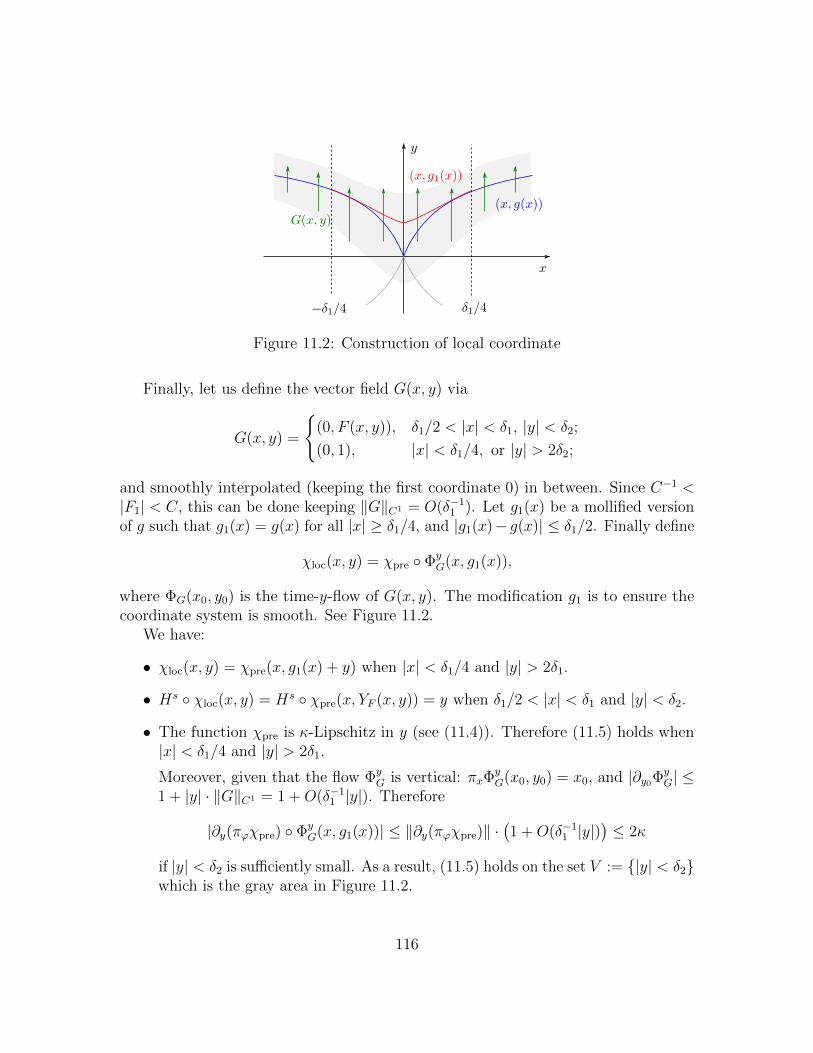
Figure 11.2: Construction of local coordinate

Finally, let us define the vector field G(x, y) via

G(x, y) =

(0, F (x, y)), δ1/2 < |x| < δ1, |y| < δ2;

(0, 1), |x| < δ1/4, or |y| > 2δ2;

and smoothly interpolated (keeping the first coordinate 0) in between. Since C−1 <|F1| < C, this can be done keeping ‖G‖C1 = O(δ−1

1 ). Let g1(x) be a mollified versionof g such that g1(x) = g(x) for all |x| ≥ δ1/4, and |g1(x)− g(x)| ≤ δ1/2. Finally define

χloc(x, y) = χpre ΦyG(x, g1(x)),

where ΦG(x0, y0) is the time-y-flow of G(x, y). The modification g1 is to ensure thecoordinate system is smooth. See Figure 11.2.

We have:

• χloc(x, y) = χpre(x, g1(x) + y) when |x| < δ1/4 and |y| > 2δ1.

• Hs χloc(x, y) = Hs χpre(x, YF (x, y)) = y when δ1/2 < |x| < δ1 and |y| < δ2.

• The function χpre is κ-Lipschitz in y (see (11.4)). Therefore (11.5) holds when|x| < δ1/4 and |y| > 2δ1.

Moreover, given that the flow ΦyG is vertical: πxΦ

yG(x0, y0) = x0, and |∂y0Φ

yG| ≤

1 + |y| · ‖G‖C1 = 1 +O(δ−11 |y|). Therefore

|∂y(πϕχpre) ΦyG(x, g1(x))| ≤ ‖∂y(πϕχpre)‖ ·

(1 +O(δ−1

1 |y|))≤ 2κ

if |y| < δ2 is sufficiently small. As a result, (11.5) holds on the set V := |y| < δ2which is the gray area in Figure 11.2.

116

• The curve η0h = χpre(x, g(x)) : |x| < δ1 coincide with χloc(x, 0) when |x| ≥ δ1/4

and coincides with χloc(x, y − g1(x) + g(x)) when |x| ≤ δ1/4, and therefore is aLipschitz graph under χ−1

loc .

Proof of Proposition 11.5. Consider the χloc coordinate system as constructed. Byconstruction, the sections Σ± = χloc(|y| ≤ δ2, x = ±δ1) are transversal to theHamiltonian flow, and therefore there is a Poincare map Φ : Σ+ −→ Σ−. Moreover,we must have χ−1

loc Φ χloc(δ1, y) = (−δ1, y), since the flow preserves energy. Let T (y)denote the time it takes for φtHs to flow from χloc(δ1, y) to χloc(−δ1, y).

We now define

χ(x, y) =

χloc(x, y), 0 ≤ x < δ1;

χloc(x− 1, y), 1− δ1 ≤ x ≤ 1;

φs(x,y)Hs (δ1, y), s(x, y) = x−δ1

1−2δ1T (y), δ1 ≤ x ≤ 1− δ1.

Then χ(x, y) is an embedding T× (−δ2, δ2) −→ T2 × R2 satisfying item (1)(3)(4) ofProposition 11.5.

It remains to prove (2), namely symplecticity. For |x| ≤ δ1, this is coveredin Proposition 11.5. For |x| ≥ δ1, note that the tangent plane to the cylinderis spanned by two vector fields, one being XHs and the other is ∂yχ. We haveω(XH , ∂yχ) = ∇H · ∂yχ = 1 by construction, therefore the manifold is symplectic.

12 Forcing equivalence between kissing cylinders

In this section we prove Theorem 5.1. We assume that h is a non-simple homologyclass which satisfies h = n1h1 + n2h2, where h1, h2 are simple homologies. They areassociated with curves ch(E) and cµh1(E) in the corresponding channels, where weassume ∥∥ch(0)− cµh1(0)

∥∥ < µ.

Our goal is to prove forcing equivalence of the cohomologies Φ∗L(ch(E1)) and Φ∗L(cµh1(E2))for some E1, E2 ∈ (e, e+ µ), where e > 0 is sufficiently small.

We will construct a variational problem which proves forcing equivalence for theoriginal Hamiltonian Hε using definition (Definition 6.12). The proof consists of foursteps.

1. We construct a special variational problem for the slow mechanical system Hs.A solution of this variational problem is an orbit “jumping” from one homologyclass h to the other h1. The same can be done with h and h1 switched.

117

2. We modify this variational problem for the fast time-periodic perturbation of Hs,i.e. for the perturbed slow system Hs

ε (ϕs, Is, τ) = K(Is)−U(ϕs)+

√εP (ϕs, Is, τ)

with τ ∈√εT. This is achieved by applying the perturbative results established

in Section 7.

Recall the original Hamiltonian system Hε near a double resonance can bebrought to a normal form Nε = Hε Φε and this normal form, in turn, is relatedto the perturbed slow system through coordinate change and energy reduction(see section B). The variational problem for Hs

ε can then be converted to avariational problem for the original Hε.

3. Using this variational problem we prove forcing relation between ch(E1) andcµh1(E2).

12.1 Variational problem for the slow mechanical system

The slow system is given by Hs(ϕ, I) = K(I) − U(ϕ) where we assumed that theminimum of U is achieved at 0. Given m ∈ T2, a > 0 and a unit vector ω ∈ R2, define

S(m, a, ω) = m+ λω : λ ∈ (−a, a).

S(m, a, ω) is a line segment in T2 and we will refer to it as a section (see Figure 12.1).Given c1, c2 ∈ R2, we say that c1, c2 has a non-degenerate connection for Hs, at

the section S(m, a, ω) ∈ T2, such that the following conditions hold.

[N1A] 5

(c1 − c2) ⊥ S, αH(c1) = αH(c2).

[N2a] There exists a compact set K ⊂ S0 such that for all x ∈ AH(c1) and z ∈ AH(c2),the minimum of the variational problem

miny∈ShHs,c1(x, y) + hHs,c2(y, z)

is never achieved outside of K.

[N3A] Suppose the above minimum is achieved at y0, let p1−c1 be any super-differentialof hHs,c1(x, ·) at y0, and −p2 + c2 a super-differential of hHs,c2(·, z) at y0, then

∂pHs(y0, pi) · S⊥, i = 1, 2

have the same signs, here S⊥ denote a normal vector to S.

5The “A” in [N1A]-[N3A] stands for “autonomous”.

118

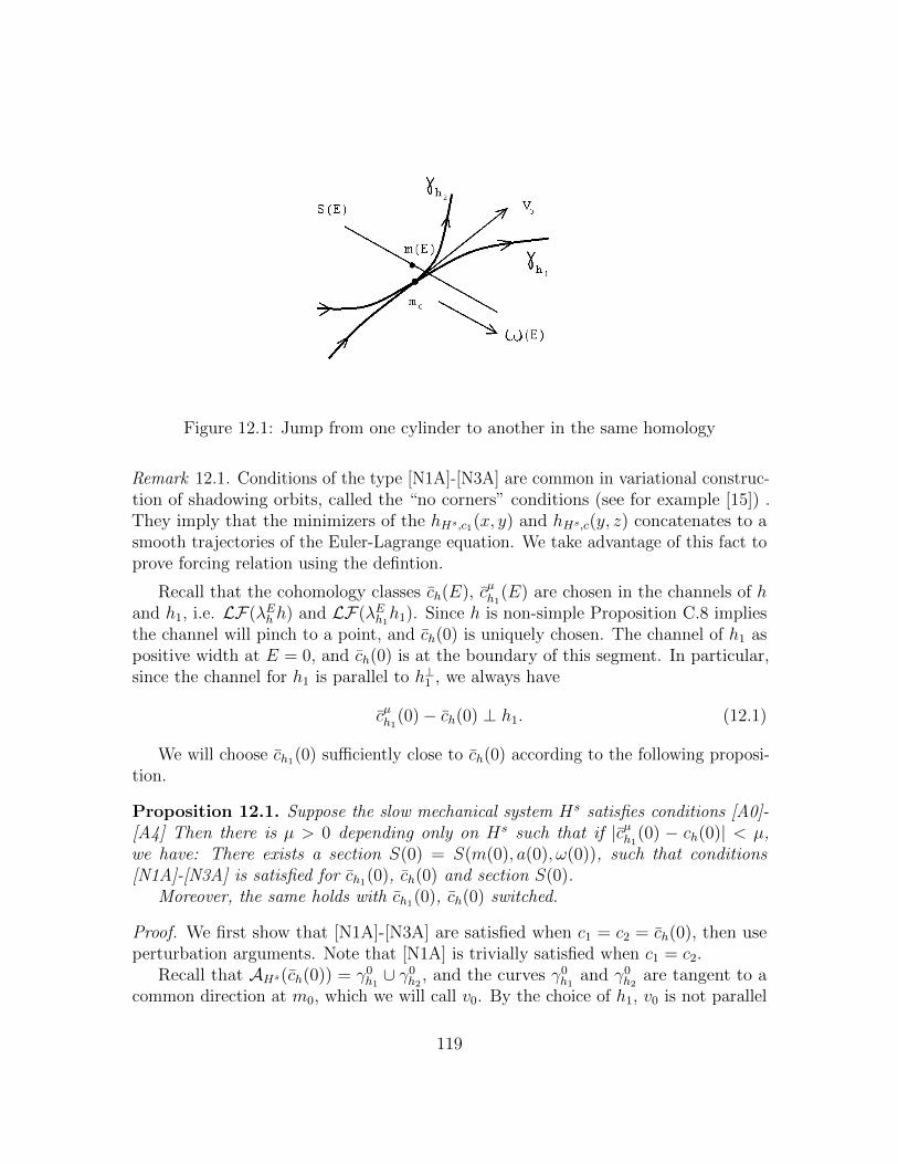
Figure 12.1: Jump from one cylinder to another in the same homology

Remark 12.1. Conditions of the type [N1A]-[N3A] are common in variational construc-tion of shadowing orbits, called the “no corners” conditions (see for example [15]) .They imply that the minimizers of the hHs,c1(x, y) and hHs,c(y, z) concatenates to asmooth trajectories of the Euler-Lagrange equation. We take advantage of this fact toprove forcing relation using the defintion.

Recall that the cohomology classes ch(E), cµh1(E) are chosen in the channels of hand h1, i.e. LF(λEh h) and LF(λEh1h1). Since h is non-simple Proposition C.8 impliesthe channel will pinch to a point, and ch(0) is uniquely chosen. The channel of h1 aspositive width at E = 0, and ch(0) is at the boundary of this segment. In particular,since the channel for h1 is parallel to h⊥1 , we always have

cµh1(0)− ch(0) ⊥ h1. (12.1)

We will choose ch1(0) sufficiently close to ch(0) according to the following proposi-tion.

Proposition 12.1. Suppose the slow mechanical system Hs satisfies conditions [A0]-[A4] Then there is µ > 0 depending only on Hs such that if |cµh1(0) − ch(0)| < µ,we have: There exists a section S(0) = S(m(0), a(0), ω(0)), such that conditions[N1A]-[N3A] is satisfied for ch1(0), ch(0) and section S(0).

Moreover, the same holds with ch1(0), ch(0) switched.

Proof. We first show that [N1A]-[N3A] are satisfied when c1 = c2 = ch(0), then useperturbation arguments. Note that [N1A] is trivially satisfied when c1 = c2.

Recall that AHs(ch(0)) = γ0h1∪ γ0

h2, and the curves γ0

h1and γ0

h2are tangent to a

common direction at m0, which we will call v0. By the choice of h1, v0 is not parallel

119

to h1. We now choose ω(0) = h1‖h1‖ , m(0) sufficiently close to 0, and a(0) = a > 0, such

that S(m(0), ω(0), a(0)) intersect AHs(ch(0)) transversally and is disjoint from 0 (seeFigure 12.1).

The Aubry set AHs(ch(0)) supports a unique minimal measure, and therefore hasa unique static class. Since for any x, z ∈ AHs(ch(0)), the function

hch(0)(x, ·) + hch(0)(·, z)

reaches its global minimal at NHs(ch(0)), which coincides with AHs(ch(0)). Hence theminimum in

miny∈S(0)

hch(0)(x, y) + hch(0)(y, z)

(12.2)

is reached at S(0) ∩ AHs(ch(0)), which is compactly contained in S(0). This implies[N2a] is satisfied for c1 = c2 = ch(0) along the section S(0).

Moreover, for any y0 reaching the minimum in (12.2), then according to the aboveanalyis y0 also reaches the global minimum of hch(0)(x, ·) + hch(0)(·, z). Then usingProposition 6.2, the associated super-gradients p1 − ch(0) and −p2 + ch(0) (in [N3A])satisfies p1 = p2, and ∂pH

s(y0, p1) = ∂pHs(y0, p2) is the velocity of the unique backward

minimizer at y0. To show that [N3A] holds, we only need to show ∂pHs(y0, p1) 6= 0.

This is the case because 0 is the only equilibrium in AHs(ch(0)), and S(0) is disjointfrom 0.

We now perturb c1 away from ch(0) while keeping c2 = ch(0). We choose c1 = cµh1(0)at the bottom of the h1 channel, then (12.1) and ω(0) = h1 means [N1A] is still satisfied.Proposition 7.4 implies that [N2a] and [N3A] are both robust under the perturbationof c1, therefore [N1A]-[N3A] holds if ‖ch1(0)− ch(0)‖ is small enough.

To prove the same with ch1(0), ch(0) switched, we perform the same perturbationargument keeping c1 = ch(0) and c2 = ch1(0).

We now perform one more step of perturbation by taking E > 0.

Proposition 12.2. Suppose the slow mechanical system Hs satisfies conditions[DR1c] − [DR4c], then there exists e > 0 such that the following hold. For each0 ≤ E ≤ e, there exists a section S(E) := S(m(E), a(E), ω(E)), with S(E) −→ S(0)in Hausdorff distance, and the condition [N1A]-[N3A] are satisfied for cµh1(E), ch(E)at S(E).

Moreover, the same conditions are satisfied with ch(E) and cµh1(E) switched.

Proof of Proposition 12.2. Since the Aubry sets AHs(ch1(0)) and AHs(ch(0)) has aunique static class, Proposition 7.4 implies that [N2a] and [N3A] are both robustunder the perturbation of c1 and c2. As a result, it suffices to construct a sectionS(E) = S(m(E), ω(E), a(E)) such that [N1A] holds, and S(E) −→ S(0) as E −→ 0.

120

To do this, we choose ω(E) to be a unit vector orthogonal to ch1(E)− ch(E), andby continuity of the functions c, ω(E) −→ ω(0) as E −→ 0. Since αHs(ch1(E)) =αHs(ch(E)) = E, [N1A] is satisfied. We then choose m(E) = m(0) and a(E) = a(0).Clearly S(E) −→ S(0) in Hausdorff metric. The proposition follows.

12.2 Variational problem for original coordinates

The original Hamiltonian Hε is reduced via coordinate change, and time change, to

Hsε (ϕ

s, Is, τ) = K(Is)− U(ϕs) +√ε P (ϕs, Is, τ),

with ‖P‖C2 ≤ C1, see Section B.2. The system Hsε is defined on T2 × R2 × R, but is√

ε periodic in τ , i.e. it is a periodic Tonelli Hamiltonian introduced in Section 6.1.Denote

√εT = R/(

√εZ), then Hs

ε projects to T2 × R2 ×√εT.

We now define a variational problem for the perturbed system. First, we willadjust the cohomologies so that they have the same alpha function.

Lemma 12.3. Fix e > 0. There exists C > 0, and ε0 > 0 depending only on K(I),‖U‖C0 and e such that for any e

3≤ E ≤ 2e

3and 0 ≤ ε ≤ ε0, there exists 0 < Eε < e

such thatαHs

ε(ch(E)) = αµHs

ε(ch1(E

ε)), |E − Eε| ≤ C√ε.

Proof. We note that αHs(ch(E)) = E = αHs(cµh1(E). By Lemma 7.9,∥∥αHsε(ch(E))− E

∥∥ , ∥∥αHsε(cµh1(E))− E

∥∥ ≤ C√ε.

The Lemma easily follows if we choose ε0 such that e > 3C√ε0.

We define a section Sε(E) = S(m(E), a(E), ωε(E)), by keeping m(E), a(E) thesame as before, with ωε(E) to be a unit vector orthogonal to ch(E) − cµh1(E

ε). Itis natural to study the extended section Sε ×

√εT ⊂ T2 ×

√εT, and condition [N1]

becomes [c1 − c2

−αHsε(c1) + αHs

ε(c2)

]⊥ Sε ×

√εT,

and the variational problem for [N2] is: For (x, 0) ∈ AHsε(ch(E)) and (z, 0) ∈

AHsε(cµh1(E

ε)), consider the minimization

min(y,t)∈Sε×

√εT

hHs

ε ,ch(E)(x, 0; y, t) + hHsε ,c

µh1

(Eε)(y, t; z, 0). (12.3)

We will not, however, study conditions [N1]-[N3] for Hsε directly. Instead, we

transform the cohomology ch(E) and ch1(Eε), the section Sε×

√εT, and the variational

problem (12.3) directly to the original system Hε.

121

Recall that the original Hamiltonian Hε can be brought into a normal form systemNε. Nε is related to Hs

ε via the coordinate ΦL, and an energy reduction, see section B.2.Denote

Φ1L(ϕ, τ) = B−1

[ϕ

τ/√ε

],(Φ1L

)−1(θ, t) =

[1 00√ε

]B

[θt

],

this is the angular component of the affine coordinate change ΦL (see (B.16)). The3× 3 matrix B is defined in (B.9).

Given c ∈ R2, we define

cε = p0 +BT0

[ √εc

−εαHsε(c)

](12.4)

where B0 is the first two rows of B, given precisely by kT1 , kT2 . According to Proposi-tion B.7, we have[

cε − p0

−αHε(cε) +H0(p0)

]= BT

[ √ε c

−ε αHsε(c)

]= Φ∗L(c, αHs(c)), (12.5)

where Φ∗L is from (5.8), and coincide with the action component of ΦL. In particular,(12.4) is the first row of (12.5). Let us denote the cohomologies cεh(E) and cεh1(E) theimage of c = ch(E) and c = ceh1(E) under (12.4).

We define a section Σ = Σ(θ0, a,Ω, l) ⊂ T2 × T (for the original HamiltonianHε : T2 × R2 × T −→ R) by

Σ(θ0, a,Ω, l) = (θ0 + λΩ + lt, t) ∈ T2 × T : −a < λ < a, t ∈ T, (12.6)

whereΩ ∈ R3, l ∈ Z3.

The section S(m, a, ω)×√εT ⊂ T2 ×

√εT is mapped under Φ1

L to Σ(θ0, a,Ω, l) with

θ0 = B−1

[m0

]∈ T3, Ω = B−1

[ω0

]∈ R3, l = B−1

001

∈ Z3. (12.7)

Note that for (cεi , αHε(cεi)) = Φ∗L(ci, αHs

ε(ci)), i = 1, 2, using (12.4) and Σ = Φ1

L(S ×√εT), we have[

c1 − c2

−αHsε(c1) + αHs

ε(c2)

]⊥ S ×

√εT⇐⇒

[cε1 − cε2

−αHε(cε1) + αHε(cε2)

]⊥ Σ (12.8)

We say that c1, c2 ∈ R2 has non-degnerate connection along a section Σ(θ, a,Ω, l),if the following conditions hold.

122

[N1] We have [c1 − c2

−αHε(c1) + αHε(c2)

]⊥ Σ.

[N2] There exists compact set K ⊂ Σ such that: for each (x, 0) ∈ AHε(c1) and(z, 0) ∈ AHε(c2), the minimum in

min(y,t)∈Σ

hHε,c1(x, 0; y, t) + hHε,c2(y, t; z, 0)

is never achieved outside of K.

[N3] Assume that the minimum [N2] is reached at (y0, t0), and let p1−c1 and −p2 +c2

be any super-differentials of hc1(x, 0; ·, t) and hc2(·, t0; z, 0) respectively. Then

(∂pH(y0, p1, t0), 1) · Σ⊥, (∂pH(y0, p2, t0), 1) · Σ⊥

have the same signs, where Σ⊥ is a normal vector to Σ.

Proposition 12.4. Consider cεh(E), cεh1(E) be defined from ch(E), ch1(E) using (12.4).Let Eε be as in Lemma 12.3, and let the section Sε(E) be as in (12.3), and the sectionΣε(E) be obtained from Sε(E)×

√εT via (12.7).

Then for each 0 < ε < ε0, we have

cεh(E), cεh1(Eε),Σε(E)

satisfies [N1]-[N3]. Moreover, the same holds with cεh(E) and cεh1(Eε) switched.

The following statement is a direct application of Theorem 12.1 which holds forgeneral Tonelli Hamiltonians.

Proposition 12.5. Assume that the conclusions of Proposition 12.4 hold. In addition,assume that both AHε(cεh(E)) and AHε(cεh1(E

ε)) admits a unique static class. Then

ch(E) a` ce,µh1 (Eε).

Proof of Theorem 5.1. By Proposition 12.4, for the system Hε, which is a perturbationof Hε, all conditions of Proposition 12.5 are satisfied, except the condition of uniquenessof static classes. For this we consider again the residual condition that all rationalminimal periodic orbits are hyperbolic, and has transversal homoclinic and heteroclinicintersections. Under this condition all cohomologies ch(E) and ce,µh1 (E) has uniquestatic class (using the fact that they are of Aubry-Mather type).

We prove Proposition 12.4 in section 12.3 and Proposition 12.5 in section 12.4.

123

12.3 Scaling limit of the barrier function

In this section we prove Proposition 12.4. Using the choice of the cohomology classesand the sections, together with (12.8), we get [N1] is satisfied for cεh(E), cεh1(E

ε), andΣε(E). It suffices to prove [N2] and [N3]. We will show that the variational problemin [N2] is a scaling limit of the variational problem (12.3).

Proposition 12.6. The family of functions hHε,ch(E)(χE,ε, 0; ·, t)/

√ε is uniformly

semi-concave, and

limε−→0+

sup(θ,t)∈T2×T

∣∣∣hHε,cεh(E)(χE,ε, 0; θ, t)/

√ε− hHs,ch(E)(x

E, B0

[θt

])∣∣∣ = 0.

uniformly over

(χE,ε, 0) ∈ AHε(ch(E)), (xE, 0) ∈ AHε(ch(E)).

The same conclusions apply to the barrier function hHε,ceh1 (E)(·, ·; ξE,ε, 0)/√ε.

Proof. The uniform semi-concavity of barrier functions follows from Proposition 7.6.Moreover, according to Proposition B.7, item 2, the families of functions

hHε,cεh(E)(χE,ε, 0; θ, t)/

√ε, hHs

ε ,ch(E)

(Φ1LS(χE,ε, 0); Φ1

LS(θ, t))

share the same limit points as ε −→ 0. Moreover, Proposition B.7, item 3 impliesΦ1LS(χE,ε, 0) ∈ AHs

ε(ch(E)).

The functions Hsε form a uniform family of periodic Hamiltonians, and Hs

ε −→ Hs

in C2(T2 × R2 × R). By construction, AHs(ch(E)) has unique static class, thereforeProposition 7.4 applies, and for any (xE, 0) ∈ AHs(ch(E)),

hHsε ,ch(E)

(Φ1LS(χE,ε, 0);ϕ, τ)

)−→ hHs,ch(E)

(xE, 0;ϕ, τ

)uniformly. Finally, noticing

Φ1L(θ, t) =

[Id 00√ε

]B

[θt

]=

[Id 00√ε

] [B0

kT3

] [θt

]−→

B0

[θt

]0

(12.9)

as ε −→ 0, we obtain the desired limit. The case for hHε,ceh1 (E)(·, ·; ξE,ε, 0)/√ε is

symmetric and we omit it.

124

Proof of Proposition 12.4. Condition [N1] is satisfied by the choice of section. Observethat

B0Σε(E) =

[Id 00 0

]BΣε(E) =

[Id 00 0

]BB−1

[Id 0

0√ε−1

](Sε(E)×

√εT)

=

[Id 00 0

](Sε(E)×

√εT) = Sε(E).

Since Sε(E) −→ S(E) as E −→ 0, combine with Proposition 12.2 we get [N2] stillholds for 0 ≤ ε < ε0, with ε0 depending only on Hs. [N3] follows from the samelimiting argument and we omit it.

12.4 The jump mechanism

In this section we show that [N1]-[N3] condition combined with uniqueness of staticclass imply c1 ` c2, which is Proposition 12.5. The discussions here apply to generalToneli Hamiltonians. Denote

AH,c(x, s, y, t) = AH,c(x, s, y, t) + αH(c)(t− s).

The subscript H may be omitted.

Theorem 12.1. Assume that c1, c2 and Σ satisfies the conditions [N1]-[N3], and inaddition,

AH(c1), AH(c2)

both have unique static class, then the following hold.

1. (interior minimum) There exists N < N ′,M < M ′ ∈ N and a compact setK ′ ⊂ Σ, such that for any semi-concave function u on T2, the minimum in

v(z) := minu(x) + Ac1(x, 0; y, t+ n) + Ac2(y, t+ n; z, n+m), (12.10)

where the minimum is taken in

x ∈ T2, (y, t) ∈ Σ, N ≤ n ≤ N ′, M ≤ m ≤M ′,

is never achieved for (y, t) /∈ K ′.

2. (no corner) Assume the minimum in (12.10) is achieved at (y, t) = (y0, t0),(n,m) = (n0,m0), and the minimizing curves are γ1 : [0, t0 + n0] −→ T2 andγ2 : [t0 + n0, t0 + n0 + m0] −→ T2. Then γ1 and γ2 connect to an orbit of theEuler-Lagrange equation, i.e.

γ1(t0 + n0) = γ2(t0 + n0).

125

3. (connecting orbits) The function v is semi-concave, and its associated pseudo-graph satisfies

Gc2,v ⊂⋃

0≤t≤N ′+M ′φtGc1,u.

As a consequence,c1 ` c2.

Remark 12.2. We only need item 3 of the theorem for our purpose, the first twoitems are stated to illuminate the idea. Item 1 can be seen as a finite time version ofthe variational problem in [N2]. It holds for sufficiently large M , N , due to uniformconvergence of the Lax-Oleinik semi-group. Item 2 implies the minimizers concatenateto a real orbit of the system, which is crucial in proving item 3.

Lemma 12.7. 1. Let u be a continuous function on T2. The limit

limN−→∞

limN ′−→∞

minx∈T2, N≤n≤N ′

u(x) + Ac(x, 0; y, t+ n) =

= minx∈Du(x) + hc(x, 0; y, t)

is uniform in u and (y, t).

2. The limitlim

N−→∞lim

N ′−→∞min

N≤n≤N ′Ac(y, t; z, n) = hc(y, t; z, 0)

is uniform in y, t, z.

Proof. The proof of the first item is similar to the proof of Proposition 6.3 of [11]with some auxiliary facts proven in Appendix A there. The proof of the second itemis similar to that of Proposition 6.1 from [11].

In both cases the action function, defined in (2.4) and (6.1) of [11], is restrictedto have integer time increment. For non-integer time increments the same argumentapplies.

Using the representation formula (Proposition 6.11) and Lemma 7.5, we have thefollowing characterization of the barrier functions.

Lemma 12.8. Assume that A(c) has only one static class. For each point (y, t) ∈T2 × T and each z ∈ T2

1. there exists x0 ∈ T2 and x1 ∈ A(c) such that

minx∈T2

u(x) + hc(x, 0; y, t) = u(x0) + hc(x0, 0;x1, 0) + hc(x1, 0; y, t).

126

2. there exists z1 ∈ A(c) such that

hc(y, t; z, 0) = hc(y, t; z1, 0) + hc(z1, 0; z, 0).

Proof of Theorem 12.1. According to Lemma 12.7, (12.10) converges uniformly asN,M −→∞ to

minx,y,tu(x) + hc1(x, 0; y, t) + hc2(y, t; z, 0),

which is equal to

min(y,t)u(x0) + hc1(x0, 0;x1, 0) + hc1(x1, 0; y, t) + hc2(y, t; z1, 0) + hc2(z1, 0; z, 0)

= min(y,t)const+ hc1(x1, 0; y, t) + hc2(y, t; z1, 0) + hc2(z1, 0; z, 0).

by Lemma 12.8. Since the above variational problem has a interior minimum due tocondition N2, by uniform convergence, the finite-time variational problem (12.10) alsohas an interior minimum for sufficiently large N,M .

We now prove the second conclusion. Let γ1 and γ2 be the minimizers forAc1(x0, 0; y0, t0 + n0) and Ac2(y0, t0 + n0; z, n0 + m0), and let p1 and p2 be the as-sociated momentum, we will show that

p1(t0 + n0) = p2(t0 + n0),

which implies γ1(t0 + n0) = γ2(t0 + n0). To abbreviate notations, we write p01 =

p1(t0 + n0) and p02 = p2(t0 + n0)for the rest of the proof.

Note that

u1(x0) + Ac1(x0, 0; y0, t0 + n0) = minx∈T2u1(x) + Ac1(x, 0; y0, t0 + n0).

By semi-concavity, the function u1(x) + Ac1(x, 0; y0, t0 + n0) is differentiable at x0 andthe derivative vanishes. By Proposition 6.2 part 3,

dxu(x0) = p1(0)− c1. (12.11)

By a similar reasoning, we have

Ac1(x0, 0; y0, t0 + n0) + Ac2(y0, t0 + n0; z, n0 +m0)

= min(y,t)∈Σ

Ac1(x0, 0; y, t+ n0) + Ac2(y, t+ n0; z, n0 +m0). (12.12)

By Proposition 6.2, we know

(p01 − c1, αH(c1)−H(y0, t0, p

10)), (−p0

2 + c1,−αH(c2) +H(y0, t0, p20)).

127

are super-differentials of Ac1(x0, 0; y0, t0 +n0) and Ac2(y0, t0 +n0; z, n0 +m0) at (y0, t0 +n0), since the minimum in (12.12) is obtained inside of Σ, we have

(p01 − p0

2,−H(y0, t0, p01 +H(y0, t0, p

02)) + (−c1 + c2, αH(c1)− αH(c2))

is orthogonal to Σ. Since the second term is orthogonal to Σ by [N1], we obtain

(p01 − p0

2,−H(y0, t0, p01) +H(y0, t0, p

02)) ∈ RΣ⊥.

We proceed to prove p01 = p0

2.Write Σ⊥ = (v, w) ∈ R2 × R, then there exists λ0 such that

p01 − p0

2 = λ0v, −H(y0, t0, p01) +H(y0, t0, p

02) = λ0w.

Definef(λ) = H(y0, t0, p

01 + λv)−H(y0, t0, p1) + λw,

then f(λ0) = 0. Since f(λ) is a strictly convex on R, there are at most two solutions,one of them is λ = 0. Suppose there is a nonzero solution λ0, then f ′(0) and f ′(λ0)must have different signs. Since

f ′(0) = (∂pH(y0, t0, p01), 1) · (v, w), f ′(λ0) = (∂pH(y0, t0, p

02), 1) · (v, w),

have the same signs from [N3], we get a contradiction. As a result, 0 is the only solutionto f(λ) = 0, indicating p0

1 = p02. Moreover, this implies p0

1 = p02 is uniquely defined

and the functions Ac1(x0, 0; ·, ·), Ac2(·, ·; z0, n0 +m0) are differentiable at (y0, t0 + n0).As a consequence, (γ1, p1) and (γ2, p2) connect as a solution of the Hamiltonian

flow. Using (12.11), we have

φn0+m0(x0, dux(x0) + c1) = (z, p2(n0 +m0)).

Note that p2(n0 +m0)− c2 is a super-differential to v at z. If v is differentiable at z,then p2 = dv(z) + c2. This implies

Gc2,v ⊂⋃

0≤t≤N ′+M ′φtGc1,u

and the forcing relation.

128

A Generic properties of mechanical systems on

the two-torus

Most of this section is devoted to proving Theorem 4.2. At the end of the sectionwe prove Proposition 4.5. This states that the minimal shortest curves in a fixedhomology class h is generically hyperbolic, with finitely many bifurcations. To achievethis, we study generic properties of non-degenerate orbits. It is well known thatminimal non-degenerate orbits must be hyperbolic.

The proof of Theorem 4.2 consists of three parts.

1. In section A.1, we prove a Kupka-Smale-like theorem about non-degeneracyof periodic orbits. For a fixed energy surface, generically, all periodic orbitsare non-degenerate. This fails for an interval of energies. We show that whiledegenerate periodic orbits exists, there are only finitely many of them. Moreover,there could be only a particular type of bifurcation for any family of periodicorbits crossing a degeneracy.

2. In section A.2, we show that a non-degenerate locally minimal orbit is alwayshyperbolic. Using part I, we show that for each energy, the globally minimalorbits is chosen from a finite family of hyperbolic locally minimal orbits.

3. In section A.3, we finish the proof by proving the finite local families obtainedfrom part II are “in general position”, and therefore there are at most two globalminimizers for each energy.

A.1 Generic properties of periodic orbits

We simplify notations and drop the supscript “s” from the notation of the slowmechanical system. Moreover, we treat U as a parameter, and write

HU(ϕ, I) = K(I)− U(ϕ), ϕ ∈ T2, I ∈ R2, U ∈ Cr(T2). (A.1)

We shall use U as an infinite-dimensional parameter. As before K is a kinetic energyand it is fixed. Denote by Gr = Cr(T2) the space of potentials, x denotes (ϕ, I), Wdenotes T2 × R2, and either φUt or Φ(·, t, U) denotes the flow of (A.1). We will useχU(x) = (∂K, ∂U)(x) to denote the Hamiltonian vector field of HU and use SE todenote the energy surface HU = E. We may drop the superscript U when there isno confusion.

By the invariance of the energy surface, the differential map DxφUt defines a map

DxφUt (x) : TxSH(x) −→ TφUt (x)SH(x).

129

Since the vector field χ(x) is invariant under the flow, Dxφ induces a factor map

DxφUt (x) : TxSH(x)/Rχ(x) −→ TφUt (x)SH(x)/Rχ(φt(x)).

Given U0 ∈ Gr, x0 ∈ W and t0 ∈ R, let

V = V (x0)× (t0 − a, t0 + a)× V (U0)

be a neighborhood of (x0, t0, U0), V (x0, t0) of (x0, t0), and V (φU0t0 (x0)) a neighborhood

of φU0t0 (x0), such that

φUt (x) ∈ V (φU0t0 (x0)), (x, t, U) ∈ V .

By fixing the local coordinates on V (x0) and V (φUt0(xx)), we define

DxΦ : V −→ Sp(2),

where DxΦ(x, t, U) is the 2× 2 symplectic matrix associated to DxϕUt (x) under the

local coordinates. The definition depends on the choice of coordinates.Let φU0

t (x0) be a periodic orbit with minimal period t0. The periodic orbit is

non-degenerate if and only if 1 is not an eigenvalue of DxΦ(x0, t0, U0) 6. Furthermore,we identify two types of degeneracies:

1. A degenerate periodic orbit (x0, t0, U0) is of type I if DxΦ(x0, t0, U0) = Id, theidentity matrix;

2. It is of type II if DxΦ(x0, t0, U0) is conjugate to the matrix [1, µ; 0, 1] for µ 6= 0.

Denote

N =

[1 µ0 1

]: µ ∈ R \ 0

, O(N) = BAB−1 : A ∈ N,B ∈ Sp(2).

Then (x0, t0, U0) is of type II if and only if DxΦ(x0, t0, U0) ∈ O(N).

Lemma A.1. The set O(N) is a 2–dimensional submanifold of Sp(2).

Proof. Any matrix in O(N) can be expressed by[a bc d

] [1 µ0 1

] [d −b−c a

]=

[1− acµ a2µ−c2µ 1− acµ

],

6Note that we are interested in non-degeneracy for minimal period of periodic orbits only. As theresult eigenvalues given by exp(2π i p/q) with integer p, q 6= 0 are allowed

130

where ad− bc = 1 and µ 6= 0. Write α = a2µ and β = acµ, we can express any matrixin O(N) by [

1− β α1− β2/α 1− β

]. (A.2)

The standard Kupka-Smale theorem (see [67], [69]) no longer holds for an intervalof energies. Generically, periodic orbits appear in one-parameter families and maycontain degenerate ones. However, while degenerate periodic orbits may appear,generically, a family of periodic orbits crosses the degeneracy “transversally”. This ismade precise in the following theorem.

Theorem A.1. There exists residual subset of potentials G ′ of Gr, such that for allU ∈ G ′, the following hold:

1. The set of periodic orbits for φUt form a submanifold of dimension 2. Since aperiodic orbit itself is a 1-dimensional manifold, distinct periodic orbits formone-parameter families.

2. There is no degenerate periodic orbits of type I.

3. The set of periodic orbits of type II form a 1-dimensional manifold. Factoringout the flow direction, the set of type II degenerate orbits are isolated.

4. For U0 ∈ Gr, let ΛU0 ⊂ W × R+ denote the set of periodic orbits for φUt , andΛU0N ⊂ ΛU0 denote the set of type II degenerate ones. Then for any (x0, t0) ∈ ΛU0

N ,let V (x0, t0) be a neighborhood of (x0, t0). Then

DxΦ|U=U0 : ΛU0 ∩ V (x0, t0) −→ Sp(2)

is transversal to O(N) ⊂ Sp(2).

Remark A.1. Statement 4 of the theorem can be interpreted in the following way. LetA(λ) be the differential of the Poincare return map on associated with a family ofperiodic orbits. Then if A(λ0) ∈ O(N), then the tangent vector A′(λ0) is transversalto O(N).

We can improve the set G ′ to an open and dense set, if there is a lower and upperbound on the minimal period.

Corollary A.2. 1. Given 0 < T0 < T1, there exists an open and dense subsetG ′ ⊂ Gr, such that the set of periodic orbits with minimal period in [T0, T1]satisfies the conclusions of Theorem A.1.

131

2. For any U0 ∈ G ′, there are at most finitely many type II degenerate periodicorbits. Moreover, there exists a neighbourhood V (U0) of U0, such that the setof type II degenerate periodic orbits depends smoothly on U . (This means thenumber of such periodic orbits is constant on V (U0), and each periodic orbitdepends smoothly on U .)

We defineF : W × R+ × Gr −→ W ×W, (A.3)

F (x, t, U) = (x,Φ(x, t, U)).

F is a Cr−1−map of Banach manifolds. Define the diagonal set by ∆ = (x, x) ⊂W×W . Then φU0

t (x0) is an period orbit of period t0 if and only if (x0, t0, U0) ∈ F−1∆.

Proposition A.3. Assume that (x0, t0, U0) ∈ F−1∆ or, equivalently, x0 is periodicorbit of period t0 for HU and that t0 is the minimal period, then there exists aneighborhood V of (x0, t0, U0) such that the map

dπ⊥∆D(x,t,U)F : T(x,t,U)(W × R+ × Gr) −→ TF (x,t,U)(W ×W )/T∆

has co-rank 1 for each (x, t, U) ∈ V, where dπ⊥∆T (W ×W ) −→ T (W ×W )/T∆ is thestandard projection along T∆.

Remark A.2. If the aforementioned map has full rank, then the map is called transversalto ∆ at (x0, t0, U0). However, the transversality condition fails for our map.

Given δU ∈ Gr, the directional derivative DUΦ · δU is defined as follows∂∂ε|ε=0Φ(x, t, U+εδU). The differential DUΦ then defines a map from TGr to TΦ(x,t,U)W .

The following hold for this differential map:

Lemma A.4. [67] Assume that there exists ε > 0 such that the orbit of x has noself-intersection for the time interval (ε, τ − ε), then the map

DUΦ(x, τ, U) : Gr −→ TΦ(x,τ,U)W

generates a subspace orthogonal to the gradient ∇HU (Φ(x, τ, U)) and the Hamiltonianvector field χU(Φ(x, τ, U)) of HU .

Proof. We refer to [67], Lemma 16 and 17. We note that while the proof was writtenfor a periodic orbit of minimal period τ , the proof holds for non-self-intersectingorbit.

Proof of Proposition A.3. We note that if φUt (x) is a periodic orbit of minimalperiod τ , then the orbit φU ′t (x′) satisfies the assumptions of Lemma A.4. It followsthat the matrix

dπ⊥∆ DUF =[DxΦ− I DtΦ DUΦ

]132

has co-rank 1, since the last two component generates the subspace

Image (DUΦ) + RχU ,

which is a subspace complementary to ∇HU .

Proposition A.3 allows us to apply the constant rank theorem in Banach spaces.

Proposition A.5. The set F−1∆ as a subset of a Banach space is a submanifoldof codimension 2n − 1. If r ≥ 4, then for generic U ∈ Gr, F−1∆ ∩ π−1

U U is a2-dimensional manifold.

Proof. We note that the kernel and cokernel of the map dπDUF has finite codimension,hence the constant rank theorem (see [1], Theorem 2.5.15) applies. As a consequence,we may assume that locally, ∆ = ∆1 × (−a, a) and that the map π1 F has full rank.Since the dimension of ∆1 is 2n− 1, F−1∆ is a submanifold of codimension 2n− 1.The second claim follows from Sard’s theorem.

Denote Λ = F−1∆. On a neighbourhood V of each (x0, t0, U0) ∈ Λ, we define themap

DxΦ : Λ ∩ V −→ Sp(2), DxΦ(x, t, U) = DφUt (x). (A.4)

First we refer to the following lemma of Oliveira:

Lemma A.6 ([67], Theorem 18). For each (x0, t0, U0) ∈ Λ such that t0 is the minimal

period, let G be the set of tangent vectors in T(x0,t0,U0)Λ of the form (0, 0, V ). Thenthe map

DUDxΦ : G −→ TDxΦ(x0,t0,U0)Sp(2)

has full rank.

Corollary A.7. The map (A.4) is transversal to the submanifold Id and O(N) ofSp(2).

Denote

ΛId = Λ ∩ DxΦ)−1(Id) and ΛN = Λ ∩ DxΦ)−1(O(N)).

Note that the expression is well defined because both preimages are defined independentof local coordinate changes.

Proof of Theorem A.1. The first statement of the theorem follows from Proposi-tion A.5.

133

As the subset Id has codimension 3 in Sp(2), ΛId has codimension 3 in Λ, andhence has codimension 2n+ 2 in W ×R+×Gr. By Sard’s lemma, for a generic U ∈ Gr,the set ΛId ∩ π−1

U is empty. This proves the second statement of the theorem.Since the set O(N) has codimension 1, ΛN has codimension 1 in Λ, and hence has

codimension 2n in W ×R+×Gr. As a consequence, generically, the set ΛUN = ΛN ∩π−1

U

has dimension 1. This proves the third statement.Fix U0 ∈ G ′, the set ΛU0 = Λ ∩ π−1

U (U0) has dimension 2, while ΛU0N ⊂ ΛU0 has

dimension 1. It follows that at any (x0, t0) ∈ ΛU0N , there exists a tangent vector

(δx, δt) ∈ T(x0,t0)ΛU0 \ T(x0,t0)Λ

U0N

such that(δx, δt, 0) ∈ T(x0,t0,U0)Λ \ T(x0,t0,U0)ΛN .

It follows that

D(x,t)DxΦ|U=U0(x0, t0) = D(x,t,U)DxΦ(x0, t0, U0) · (δx, δt, 0)

is not tangent to O(N). Since O(N) has codimension 1, this implies that the map

DxΦ|U=U0 is transversal to O(N). This proves the fourth statement.

Proof of Corollary A.2. If a potential U ∈ G ′, then by Theorem A.1 conditions 1–4are satisfied. In particular, all periodic orbits are either non-degenerate or degeneratesatisfying conditions 3 and 4. Non-degenerate periodic orbits of period bounded bothfrom zero and infinity form a compact set. Therefore, they stay non-degenerate for allpotential Cr-close to U . By condition 3 degenerate periodic orbits are isolated. Thisimplies that there are finitely many of them. Condition 4 is a transversality condition,which is Cr open for each degenerate orbit.

Fix U ∈ G ′ as in Corollary A.2. It follows that periodic orbits of φUt for one-parameter families. We now discuss the generic bifurcation of such a family at adegenerate periodic or

Proposition A.8. Let (xλ, tλ) be a family of periodic orbits such that (x0, λ0) is

degenerate. The one side of λ = λ0, the matrix DxφUtλ

(xλ) has a pair of distinct realeigenvalues; on the other side of λ = λ0, it has a pair of complex eigenvalues.

Proof. Write A(λ) = DxφUtλ

(xλ) for short. By choosing a proper local coordin we mayassume that A(λ0) = [1, µ; 0, 1]. The tangent space to Sp(2) at [1, µ; 0, 1] is givenby the set of traceless matrices [a, b; c,−a]. Using (A.2), we have a basis of the tangspace to O(N) to [1, µ; 0, 1] is given by[

0 1−β2/α2 0

]and

[−1 0−2β/α −1

].

134

An orthogonal matrix to this space, using the inner product tr(ATB), is given by[0, 0; 1, 0]. As a consequence, a matrix [a, b; c,−a] is transversal to O(N) if and only ifc 6= 0.

The eigenvalues of the matrix[1 + ah µ+ bhch 1− ah

]are given by λ = 1 ±

√a2h2 − bch2 − µch. Using µ 6= 0 and c 6= 0 we obtain that

a2h2 − bch2 − µch changes sign at h = 0. This proves our proposition.

A.2 Generic properties of minimal orbits

In this section, we analyze properties of families of minimal orbits. It is well knownthat a non-degenerate minimizing geodesic is hyperbolic. However, we have shown inthe previous section that degenerate ones do exist. The main idea is when one extenda family of hyperbolic minimal orbits, the family must terminate at a degenerateorbit of type II. We then can “slide” different families against each other so that thedegenerate orbit is never the shortest.

Let dE denote the metric derived from the Riemannian metric gE(ϕ, v) = 2(E +U(ϕ))K−1(v). We define the arclength of any continuous curve γ : [t, s] −→ T2 by

lE(γ) = supN−1∑i=0

dE(γ(ti), γ(ti+1)),

where the supremum is taken over all partitions [ti, ti+1]N−1i=0 of [t, s]. A curve γ is

called rectifiable if lE(γ) is finite.A curve γ : [a, b] −→ T2 is called piecewise regular, if it is piecewise C1 and

γ(t) 6= 0 for all t ∈ [a, b]. A piecewise regular curve is always rectifiable.A closed curve γ is called a (gE, h) minimizer We write

lE(h) = infξ∈CEh

lE(ξ),

where CEh denote the set of all piecewise regular closed curves with homology h ∈H1(T2,Z). A curve realizing the infimum is the shortest geodesic curve in the homologyh, which we will also refer to as a global (gE, h)-minimizer.

It is well known that for any E > −minϕ U(ϕ), a global gE−minimizer is a closedgE−geodesic. Hence, it corresponds to a periodic orbit of the Hamiltonian flow.

It will also be convenient to consider the local minimizers. Let V ⊂ T2 be an openset, a closed continuous curve γ : [a, b] −→ V is a local minimizer if

lE(γ) = infξ∈CEh ,ξ⊂V

lE(ξ). (A.5)

135

Since γ b V , there is an open set V1 such that γ b V1 b V2. Then by modifying themetric outside of V1, we can ensure that γ is a global minimizer of the new metric.

Proposition A.9. Assume that γ is a (gE, h) (local) minimizer, and assume that theassociated Hamiltonian periodic orbit η is nondegenerate. Then η is hyperbolic.

An orbit (θ, p)(t), t ∈ R of the Hamiltonian flow is called dis-conjugate if

DφsV(x(t), p(t)) t V(x(t+ s), p(t+ s)), t, s ∈ R, V(x, p) = 0 × R2.

Let γ : [0, T ] −→ T2 be a (gE, h) minimizer, let η : R −→ T2 × R2 be the associatedperiodic Hamiltonian orbit. Then:

Lemma A.10 ([21, 3]). η is minimizing and disconjugate. Its differential mapDφs(η(t)) admits a 2−dimensional invariant bundle (and the associated Poincare mappreserves a 1-dimensional bundle).

Proof of Proposition A.9. A non-degenerate periodic orbit η : [0, T ] −→ T2×R2 eitheris hyperbolic or the associated Poincare map has eigenvalues on the unit circle. Inthis case the Poincare map does not preserve any one-dimensional subspace, whichcontradicts with Lemma A.10.

Theorem A.2. Given 0 < e < E, there exists an open and dense subset G ′ of Gr, suchthat for each U ∈ G ′, the Hamiltonian H(ϕ, I) = K(I)− U(ϕ) satisfies the followingstatements. There exists finitely many smooth families of local minimizers

ξEj , aj − σ ≤ E ≤ bj + σ, j = 1, · · · , N,

and σ > 0, with the following properties.

1. All ξEj for aj − σ ≤ E ≤ bj + σ are hyperbolic.

2.⋃j[aj, bj] ⊃ [E0, E].

3. For each E0 ≤ E ≤ E, any global minimizer is contained in the set of all ξEj ’ssuch that E ∈ [aj, bj].

Proof of Theorem A.2, occupies the rest of this section.

Lemma A.11. Assume that γE0 is a hyperbolic local (ρE0 , h)−minimizer. The follow-ing hold.

1. There exists a neighbourhood V of γE0, such that γE0 is the unique local (gE, h)-minimizer on V .

136

2. There exists δ > 0 such that for any U ′ ∈ Cr(T2) with ‖U − U ′‖C2 ≤ δ and|E ′ − E0| ≤ δ, the Hamiltonian H ′(ϕ, I) = K(I) − U ′(ϕ) admits a hyperboliclocal minimizer in V .

3. There exists δ > 0 and a smooth family γE ⊂ V , E0 − δ ≤ E ≤ E0 + δ, suchthat each of them is a hyperbolic local minimizer.

Proof. Let ηE0 denote the Hamiltonian orbit of γE0 . Inverse function theorem impliesthat if ηE0 is hyperbolic, then it is locally unique, and it uniquely extends to hyperbolicperiodic orbit ηE,U ′ if E is close to E0 and U ′ is close to U . Let γE be the projectionof ηE, then they must be the unique local minimizers.

We now use the information obtained to classify the set of global minimizers.

• Consider the Hamiltonian H(ϕ, I) = K(I)−U(ϕ)+minϕ U(ϕ). For 0 < E0 < E,it is easy to see that any periodic orbit in the energy E0 ≤ E ≤ E has a lowerbound and upper bound on the minimal period, which depends only on E0 andE. Hence, Corollary A.2 applies. In particular, there are only finitely manydegenerate periodic orbits and the number of them is constant under smallperturbation of U .

• By the previous item, all but finitely many global minimizers are nondegenerate,hence hyperbolic by Proposition A.9.

• Since a global minimizer is always a local minimizer, using Lemma A.11, itextends to a smooth one parameter family of local minimizers. The extensioncan be continued until either the orbit is no-longer locally minimizing, or if theorbit becomes degenerate. Once a local minimizer becomes degenerate, thisfamily can no longer be extended as local minimizers as by Proposition A.8, itmust bifurcate to a periodic orbit of complex eigenvalues.

• It is well known that for a fixed energy, any two global minimizers do not cross(see for example, [64]). We can locally extend the global minimizers for a smallinterval of energy without them crossing.

• There are at most finitely many families of local minimizers, because they areisolated and do not accumulate (Lemma A.11).

• There are at most finitely many energies on which the global minimizer may bea degenerate periodic orbit.

We have proved the following statement.

137

Proposition A.12. Given 0 < e < E, there exists an open and dense subset G ′ of Gr,such that for each U ∈ G ′, for the Hamiltonian H(ϕ, I) = K(I)− U(ϕ) + minϕ U(ϕ),such that the following hold.

1. There are at most finitely many (maybe none) isolated global minimizers γEj ,dj ,

j = 1, · · · ,M .

2. There are finitely many smooth families of local minimizers

γEj , aj ≤ E ≤ bj, j = 1, · · · , N,

with [e, E] ⊃⋃

[aj, bj], such that γEj are hyperbolic for aj < E < bj. The set γEjfor E = aj, bj may be hyperbolic or degenerate.

3. For a fixed energy surface E, the sets γE,dj and⋃aj≤E≤bj γ

Ej are pairwise

disjoint.

4. For each e ≤ E ≤ E, the global minimizer is chosen among the set of all γcj ,dj

with E = cj, or one of the local minimizers γEj with E ∈ [aj, bj].

Proof of Theorem A.2. We first show that the set of potentials U satisfying the conclu-sion of Theorem A.2 is open. By Lemma A.11,the family of local minimizers persistsunder small perturbation of the potential U . It suffices to show that for sufficientlysmall perturbation of U satisfying the conclusion, the global minimizer is still takenat one of the local families. Assume, by contradiction, that there is a sequence Unapproaching U , and for each Hn = K − Un, there is some global minimizer γEnn notfrom these families. By picking a subsequence, we can assume that it converges toa closed curve γ∗, which belong one of the local families γEj . Using local uniquenessfrom Lemma A.11, γEnn must belong to one of the local families as well. This is acontradiction.

To prove density, it suffices to prove that for a potential U satisfying the conclusionof Proposition A.12, we can make an arbitrarily small perturbation, such that thereare no degenerate global minimizers.

Our strategy is to eliminate the degenerate global minimizers one by one using asequence of perturbations. Suppose γdE is an isolated degenerate minimizer. Then by([26], proof of Theorem D, page 40-42), there is a perturbation δU with the propertythat: δU ≥ 0, U |γdE = 0, such that γdE is still a global minimizer, but the associatedHamiltonian orbit ηdE becomes hyperbolic (i.e. the perturbation keeps the orbit ηdEintact but changes it’s linearization). This perturbation strictly decreases the numberof of isolated degenerate minimizers by 1.

Suppose γdE is the terminal point of one of the local families γEj : E ∈ [aj, bj],let’s say γdE = γEj (bj). Then since claim γEj can not be extended to E > bj, the

138

global minimizer for E ∈ (bj, bj + δ) must be contained in a different local branch, sayγEi : E ∈ [ai, bi]. In particular, γEi (bj) is another global minimizer.

Let V be an neighborhood of γEjj , such that V is disjoint from the set of other

global minimizers with the same energy. For δ > 0 we define Uδ : T2 −→ R such thatUδ|γ

Ejj = δ and suppUδ ⊂ V . Let Hδ = K − U − Uδ, and let lE,δ be the perturbed

length function. We have

lEj ,δ(γEjj ) =

∫γEjj

√2(Ej + U + δ)K > lEj(γ

Ejj ) = lEj(h) = lEj ,δ(h).

As a consequence, γEjj is no longer a global minimizer for the perturbed system.

Moreover, for sufficiently small δ, no new degenerate global minimizer can be created.Hence the perturbation has decreased the number of degenerate global minimizersstrictly. By repeating this process finitely many times, we can eliminate all degenerateglobal minimizers.

A.3 Non-degeneracy at high energy

In this section we complete the proof of Theorem 4.2. This amounts to proving thatfinite local families of local minimizers, obtained from the previous section, are “ingeneral position”.

We assume that the potential U0 ∈ Gr satisfies the conclusions of Theorem A.2.Let γE,Uj denote the branches of local minimizers from Theorem A.2, where we havemade the dependence on U explicit. There exists an neighbourhood V (U0) of U0, suchthat the local branches γE,Uj are defined for E ∈ [aj − σ/2, bj + σ/2] and U ∈ V (U0).

Define a set of functions

fj : [aj − σ/2, bj + σ/2]× V (U0) −→ R, fj(E,U) = lE(γE,Uj ).

Then γE,Ui is a global minimizer if and only if

fi(E,U) = fmin(E,U) := minjfj(E,U),

where the minimum is taken over all j’s such that E ∈ [aj, bj].The following proposition implies Theorem 4.2.

Proposition A.13. There exists an open and dense subset V ′ of V (U0) such that forevery U ∈ V ′, the following hold:

1. For each E ∈ [E0, E], there at at most two j’s such that fj(E,U) = fmin(E,U);

139

2. There are at most finitely many E ∈ [E0, E] such that there are two j’s withfj(E,U) = fmin(E,U);

3. For any E ∈ [E0, E] and j1, j2 be such that fj1(E,U) = fj2(E,U) = fmin(E,U);we have

∂

∂Efj1(E,U) 6= ∂

∂Efj2(E,U).

Proof. We first note that it suffices to prove the theorem under the additional assump-tion that all functions fj’s are defined on the same interval (a, b) with fmin(E,U) =minj fj(E,U). Indeed, we may partition [E0, E] into finitely many intervals, on whichthe number of local branches is constant, and prove proposition on each interval.

We define a map

f = (f1, · · · , fN) : (a, b)× V (U0) −→ RN ,

and subsets

∆i1,i2,i3 = (x1, · · · , xn);xi1 = xi2 = xi3, 1 ≤ i1 < i2 < i3 ≤ N,

∆i1,i2 = (x1, · · · , xn);xi1 = xi2, 1 ≤ i1 < i2 ≤ N

of RN × RN . We also write fU(E) = f(E,U). The following two claims imply ourproposition:

1. For an open and dense set of U ∈ V (U0), for all 1 ≤ i1 < i2 < i3 ≤ N , the set(fU)−1∆i1,i2,i3 is empty.

2. For an open and dense set of U ∈ V (U0), and all 1 ≤ i1 < i2 ≤ N , the mapfU : (a, b) −→ RN is transversal to the submanifold ∆i1,i2 .

Indeed, the first claim imply the first statement of our proposition. It follows fromour second claim that there are at most finitely many points in (fU)−1∆i1,i2 , whichimplies the second statement. Furthermore, using the second claim, we have for anyE ∈ (fU )−1∆i1,i2 , the subspace (DfU (E))R is transversal to T∆i1,i2 . This implies thethird statement of our proposition.

For a fixed energy E and (v1, · · · , vN) ∈ RN , let δU : T2 −→ R be such thatδU(ϕ) = vj on an open neighbourhood of γEj for each j = 1, · · ·N . Let lE,ε and γE,εj

denote the arclength and local minimizer corresponding to the potential U + εδU . Forany ϕ in a neighbourhood of γEj , we have

E + U(ϕ) + δU(ϕ) = E + U(ϕ) + εvj,

hence for sufficiently small ε > 0, ξE,εj = ξE+εvjj .

140

The directional derivative

DUf(E,U) · δU =d

dε

∣∣∣ε=0lE,ε(ξ

E,εj ) =

d

dε

∣∣∣ε=0lE+εvj(ξ

E+εvjj ) =

∂

∂Efj(E,U)vj.

It follows from a direct computation that each fj is strictly increasing in E and thederivative in E never vanishes. As a consequence, we can choose (v1, · · · , vN) in sucha way, that DUf(E,U) · δU takes any given vector in RN . This implies the map

DUf : (a, b)× TV (U0) −→ RN

has full rank at any (E,U). As a consequence, f is transversal to any ∆i1,i2,i3 and∆i1,i2 . Using Sard’s lemma, we obtain that for a generic U , the image of fU is disjointfrom ∆i1,i2,i3 and that fU is transversal to ∆i1,i2 .

A.4 Unique hyperbolic minimizer at very high energy

In this section we prove Proposition 4.4, namely for the mechanical system

Hs(ϕ, I) = K(I) + U(ϕ),

the shortest loop in the homology h ∈ H1(T2,Z) for Jacobi metric gE(ϕ, v) = 2(E +U(ϕ))K−1(v), where K−1(v) is the Legendre dual of K. Since the metrics

gE(ϕ, v) = 2(1 + E−1U(ϕ))K−1(√Ev), gE(ϕ, v) = 2(1 + E−1U(ϕ))K−1(v)

differ by a constant multiple, it suffices to study the shortest loops for the metric gE.Denote δ = E−1, this is then equivalent to study the mechanical system

Hδ(ϕ, I) = K(I) + δU(ϕ)

with energy E = 1. Without loss of generality, we may assume h = (1, 0). Let us write

U(ϕ) = U1(ϕ1) + U2(ϕ1, ϕ2),

where∫ 1

0U2(ϕ1, s)ds = 0. We will show an averaging effect that eliminates U2.

Let us denote by ρ0 the unique positive number such that K−1(ρ0h) = 1, and letc0 = ∂K−1(ρ0h).

Lemma A.14. There is C > 1 depending only on ‖∂2K‖, ‖∂2K−1‖ such that thenthe associated Hamiltonian orbit η1

h = (ϕ, I)(t) satisfies

‖ϕ− ρ0h‖, ‖I − c0‖ ≤ Cδ.

141

Proof. Let us note the shortest curve γ1h corresponds to the orbit η1

h = (ϕh, Ih) of theHamiltonian Hδ, satisfying ϕh(T ) = ϕh(0) + h. Note:

1. ϕh(t) = δ∇U(ϕh(t)) = O(δ),

2. Since the energy is 1, K(Ih(t)) = 1 + O(δ), K−1(ϕh(t)) = K−1(∂IK(Ih(t))) =K(Ih(t)) = 1 +O(δ);

The first item implies ϕh(t) = 1Th + O(δ), when combined with the second item,

implies ϕh(t) = ρ0h+O(δ). apply ∂K−1, we get Ih(t) = c0 +O(δ).

Note that the condition ∂K(I) = ρh corresponds precisely to the resonance segmentΓ = I ∈ R2, ∂K(I) · (1, 0) = 0, in other words, we are in precisely the same situationas in single resonance. In fact, since there are fewer degree of freedom, the normalform is much stronger.

Proposition A.15. For any M > 0, there is δ0 = δ0(K,M) and C = C(K,M) > 0such that for every Hδ with 0 < δ < δ0, there is a C∞ coordinate change Φ homotopicto identity such that

Hδ Φ = K(I) + δU1(ϕ1) + δR(ϕ),

with ‖R‖C2I≤√δ, and ‖πθ(Φ − Id)‖C2 ≤ Cδ and ‖πp(Φ − Id)‖C2 ≤ Cδ, where the

norms are measured on the set I ∈ BM√δ(c0).

If U1(ϕ1) has a unique non-degenerate minimum at ϕ1 = ϕ∗1, and satisfies

U(ϕ1)− U(ϕ∗1) ≥ λ‖ϕ1 − ϕ∗1‖2.

Then by choosing δ0 = δ0(K,M, λ) > 0 smaller, the system Hδ Φ has a normallyhyperbolic invariant cylinder C given by

(ϕ1, I1) = (F (ϕ2, I2) + ϕ∗1, G(ϕ2, I2)), ϕ2 ∈ T, I2 ∈ Γ ∩BM√δ(c0),

satisfying ‖F‖C0 ≤ Cκ, ‖G‖C0 ≤ Cκ√δ. C contains all the invariant sets in

‖ϕ1 − ϕ∗1‖ < C−1, dist(I,Γ ∩BM√δ) < C−1.

The minimal periodic orbit η1h is contained in C and is a graph over ϕ2. It is

therefore unique and hyperbolic.

Proof. The first part is very similar to Theorem 3.2, but in the much simpler case oftwo-degrees of freedom. In this case, we can give out the coordinate change explicitly.Define

W (ϕ1, ϕ2) = ρ−10

∫ 1

0

sU2(ϕ1, ϕ2 + s)ds,

142

note that W is well defined on T2 due to∫ 1

0U2(ϕ1, s)ds = 0. Note that ∂ϕ2W = ρ−1

0 U2.Consider the coordinate change I 7→ I + δ∇W . Then the new Hamiltonian is

K(I + δ∇W )− δU1 − δU2

= K(I) + δ∂K(I) · ∇W − δU1 − δU2 + δ2K(∇W )

= K(I)− δU1 + δ(ρ0h · ∇W − U2) + δ2K(∇W ) + δ(∂K(I)− ρ0h) · ∇W.

The main observation is that the second term in the last equality vanishes, the thirdterm is O(δ2) in C2 norm, and the last term is O(δ

32 ) in C2

I norm.The other parts of the proposition is identical to Theorem 9.1 and Theorem 9.2,

and are omitted.

Proposition 4.4 follows immdediately from the above proposition.

A.5 Proof of Proposition 4.5

We prove Proposition 4.5, namely non-degenerate conditions [DR1c]− [DR4c]. Thisconsists of two steps consisting of two localized perturbations of the potential U .

First, we perturb U near the origin to achieve properties [DR1c] − [DR2c]. LetW ′ be a ρ-neighborhood of the origin in R2 for small enough ρ > 0 so that it does notintersect sections Σs

± and Σu±. Consider ξ(ϕ) a C∞-bump function so that ξ(ϕ) ≡ 1 for

|ϕ| < ρ/2 and ξ(ϕ) ≡ 0 for |ϕ| > ρ. Let Qζ(ϕ) =∑ζijϕiϕj be a symmetric quadratic

form. Consider Uζ(ϕ) = U(ϕ) + ξ(ϕ)(Qζ(θ) + ζ0). In W ′ × R2 we can diagonalizeboth: the quadratic form K(p) = 〈Ap, p〉 and the Hessian ∂2U(0). Explicit calculationshows that choosing properly ζ one can make the minimum of U at 0 being uniqueand eigenvalues to be distinct.

Suppose now that conditions [DR1c] − [DR2c] hold. Fix a point θ∗ ∈ γ+ at adistance of order of one from the origin. In particular, it is away from sections Σs

±.Let W ′′ be its small neighborhood so that intersects only one homoclinic γ+. Denotewu = W u ∩ Σu

+ an unstable curve on the exit section Σu+ and ws = W s ∩ Σs

+ a stablecurve on the enter section Σs

+. Denote on wu (resp. ws) the point of intersectionΣu

+ (resp. Σs+) with strong stable direction qss (resp. quu). Recall that q+ (resp. p+)

denotes the point of intersection of γ+ with Σu+ (resp. Σs

+). We also denote by T uu(q+)(resp. T ss(p+)) subspaces the tangent to wu (resp. ws) at the corresponding points.The critical energy surface H = K − U = 0 is denoted by S0. In order to satisfyconditions [DR3c]− [DR4c] the global map Φ+

glob has to satisfy

• Φ+globw

u ∩ ws 6= qss and (Φ+glob)

−1(ws) ∩ wu 6= quu.

• DΦ+glob(q+)|TS0T

uu(q+) t T ss(p+), DΦ−glob(q−)|TS0Tuu(q−) t T ss(p−).

143

The first condition can also be viewed as a property of the restriction of Φ+glob|S0 .

Notice that Φ+glob, restricted to S0, is a 2-dimensional map.

Consider perturbations δU ∈ Gr of the potential U localized in W ′′. By LemmaA.4 the differential map DUΦ generates a subspace orthogonal to the gradient ∇HU

and the Hamiltonian vector field χU (·) of HU . Notice that when we restrict Φ+glob onto

Σu+ ∩ S0 we factor out ∇HU and χU(·). Both conditions on Φ+

glob (resp. DΦ+glob|S0)

are non-equality conditions on images and preimages for a 2-dimensional map. Thus,these conditions can be satisfies by Lemma A.4.

B Derivation of the slow mechanical system

In this section we derive the slow mechanical system. The discussions here applies toarbitrary degrees of freedom, and indeed we will consider

Hε(θ, p, t) = H0(p) + εH1(θ, p, t), θ ∈ Tn, p ∈ Rn, t ∈ T,

and let p0 ∈ Rn be an n−resonance, namely, there are linearly independent k1, · · · , kn ∈Zn+1 such that

ki · (∂H0(p0), 1), i = 1, · · · , n.Since the resonance depends only on the hyperplane containing k1, · · · , kn, we maychoose k1, · · · , kn to be irreducible, namely

SpanZk1, · · · , kn = SpanRk1, · · · , kn ∩ Zn+1.

Results in this section applies to the rest of the paper by restricting n = 2.First, we will reduce the system near an n−resonance to a normal form. After

that, we perform a coordinate change on the extended phase space, and an energyreduction to reveal the slow system.

In section B.1, we describe a resonant normal form.In section B.2, we describe the affine coordinate change and the rescaling, revealing

the slow system.In section B.3 we discuss variational properties of these coordinate changes.

B.1 Normal forms near double resonances

Write ω0 := ∂pH0(p0), then the orbit (ω0, 1) t is periodic. Let

T = inft>0t(ω0, 1) ∈ Z3

be the minimal period, then there exists a constant T∗ = T∗(k1, · · · , kn) > 0, suchthat T ≤ T∗(k1, · · · , kn).

144

Given a function f : Tn × Rn × T −→ R, we define

[f ]ω0(θ, p, t) =1

T

∫ T

0

f(θ + ω0s, p, t+ s)ds.

[f ]ω0 corresponds to the resonant component related to the double resonance.Writing H1(θ, p, t) =

∑k∈Zn hk(p)e

2πik·(θ,t), and let Λ = SpanZk1, · · · , kn ⊂ Zn,then

[H1]ω0(θ, p, t) =∑k∈Λ

hk(p)e2πik·(θ,t).

We define a rescaled differential in the action variable by

∂If(θ, p, t) =√ε∂pf(θ, p, t), (B.1)

and use the notation CrI to denote the Cr norm with ∂p replaced by ∂I . For a vector

or a matrix valued function, we take the Cr (or CrI ) norm to be the sum of the norm

of all elements. Let Bnr (p) denote the r-neighborhood of p0 in Rn.

Theorem B.1. Assume that r ≥ 5. Then for any M1 > 0, there exists ε0 = ε0 > 0,C1 > 1 depending only on ‖H0‖Cr , T∗(k1, · · · , kn), n,M1 such that for any 0 < ε < ε0,there exists a C∞ symplectic coordinate change

Φε : Tn ×BnM1√ε(p0)× T −→ Tn ×Bn

2M1√ε(p0)× T,

which is the identity in the t component, such that

Nε(θ, p, t) := Hε Φε(θ, p, t) = H0(p) + εZ(θ, p, t) + εZ1(θ, p, t, ε)7 + εR(θ, p, t, ε),

where Z = [H1]ω0, [Z1]ω0 = Z1, and

‖Z1‖C2I≤ C1

√ε, ‖R‖C2

I≤ C1ε

32 , (B.2)

and‖Φε − Id‖C2

I≤ C1ε.

Moreover, Φε admits the following extensions:

1. Φε can be extended to Tn × Rn × T such that Φε is identity outside of Tn ×U4M1

√ε(p0)× T.

2. The extension in item 1 can be further extended to Φε(θ, p, t, E) on Tn×Rn×T×R,such that

Φε(θ, p, t, E) = (Φε(θ, p, t), E + E(θ, p, t)),

and Φε is exact symplectic.

7formally speaking this term contains two terms of the averaging expansion

145

3. ‖Φε − Id‖C2I≤ C1ε holds.

Remark B.1. • Our normal form is related to the classical “partial averaging”,see, for example expansion (6.5) in [2, Section 6.1.2]. Our goal here is to obtainprecise control of the norms with minimal regularity assumptions. In particular,the norm estimate of Φε− Id is stronger than the usual results, and is needed inthe proof of Proposition B.8.

• It is possible to lower the regularity assumption to r ≥ 4, and use the weakerestimate ‖R‖C2

I≤ C1ε. This, however, requires more technical discussions in the

next few sections, and we choose to avoid it.

• Due to existence of the extension, we consider Nε = Hε Φε as defined on all ofTn × Rn × T, however, the normal form only holds on the local neighborhood.

The rest of this section is dedicated to proving Theorem B.1. Denote Πθ(θ, p, t) =θ, Πp(θ, p, t) = p the natural projections. For a map Φ : Tn×U ×T −→ Tn×Rn×T,which is the identity in the last component, denote Φ = (Φθ,Φp, Id), where Φθ = Πθ Φand Φp = Πp Φ.

Lemma B.1. We have the following properties of the rescaled norm.

1. ‖f‖CrI ≤ ‖f‖Cr , ‖f‖Cr ≤ ε−r/2‖f‖CrI .

2. ‖∂θf‖Cr−1I≤ ‖f‖CrI , ‖∂pf‖Cr−1

I≤ 1√

ε‖f‖CrI .

3. There exists cr,n > 1 such that ‖fg‖CrI ≤ cr,n ‖f‖CrI ‖g‖CrI .

4. Let Φ be as before, and Id denote the identity map. There exists cr,n > 1 suchthat if

max‖Πθ (Φ− Id)‖CrI , ‖Πp(Φ− Id)‖CrI /√ε < 1

we have‖f Φ‖CrI ≤ cr,n‖f‖CrI .

Proof. The first two conclusions follow directly from definition. For the third conclu-sion, we have ‖f‖Cr = ‖f‖CrI , where

f(θ, I) = f(θ,√εI).

The conclusion then follows from properties of the Cr−norm.For the fourth conclusion, we note

f Φ = f Φ,

146

where f is as before, and Φ(θ, I) = (Φθ(θ,√εI),Φp(θ,

√εI)/√ε). Moreover, let us

denote Ψ = Φ− Id, and note that Ψ = Φ− Id. Then there exists c > 0 dependingonly on dimension that

‖DΦ‖Cr−1 ≤ c+ ‖D(Φ− Id)‖Cr−1 ≤ c+ max‖ΠθΨ‖Cr , ‖ΠpΨ‖Cr≤ c+ max‖Πθ (Φ− Id)‖CrI , ‖Πp(Φ− Id)‖CrI /

√ε ≤ c+ 1,

By the Faa-di Bruno formula, there exists dr > 0 such that

‖f Φ‖CrI = ‖f Φ‖Cr ≤ dr‖f‖Cr(

1 + ‖DΦ‖rCr−1

)≤ dr‖f‖CrI (1 + (c+ 1)r) ≤ cr,n‖f‖CrI

where cr,n = dr(1 + (c+ 1)r).

For ρ > 0, denoteDρ = Tn × Uρ(p0)× T× R.

We require another lemma for estimating the norm of a Hamiltonian coordinatechange. This is an adaptation of Lemma 3.15 from [31].

Lemma B.2. For 0 < ρ′ < ρ < ρ0, r ≥ 4, 2 ≤ ` ≤ r − 1, ε > 0 small enough, and aCr Hamiltonian G : Dρ0 −→ R, let ΦG

t denote the Hamiltonian flow defined by G.Let cr,n > 1 be the constant from item 4, Lemma B.1. Assume that

1√ε‖G‖Cl+1

I<

1

cr,n√ε

min√

ε, ρ− ρ′,

then for 0 ≤ t ≤ 1, the flow ΦGt is well defined from Dρ′ to Dρ. Moreover,

‖Πθ(ΦGt − Id)‖ClI ≤ cr,n‖∂pG‖ClI , ‖Πp(Φ

Gt − Id)‖ClI ≤ cr,n‖∂θG‖ClI . (B.3)

Proof. Define

At = max0≤τ≤t

‖Πθ(Φ

Gτ − Id)‖ClI ,

1√ε‖Πp(Φ

Gτ − Id)‖ClI

.

Let t0 be the largest t ∈ [0, 1] such that the following conditions hold.

(a) At ≤ 1.

(b) ΦG−t(Dρ) ⊃ Dρ′ , in other words, ΦG

t : Dρ′ −→ Dρ is well defined.

147

We first show (B.3) holds on 0 ≤ t ≤ t0, then we show t0 = 1.By Lemma B.1, item 4, we have

∥∥Πθ

(ΦGt − Id

)∥∥ClI≤∫ t

0

∥∥∂pG ΦGτ

∥∥ClIdτ ≤ cr,n‖∂pG‖ClI

and ∥∥Πp

(ΦGt − Id

)∥∥ClI≤∫ t

0

∥∥∂θG ΦGτ

∥∥ClIdτ ≤ cr,n‖∂θG‖ClI .

We now show t0 = 1. By the estimates obtained,

At0 ≤ cr,n max‖∂pG‖ClI ,1√ε‖∂θG‖ClI ≤

cr,n√ε‖G‖Cl+1

I< 1.

Moreover, we have

‖Πp

(ΦGt0− Id

)‖ClI ≤ cr,n‖∂θG‖ClI <

√εcr,n√ε‖G‖Cl+1

I< ρ− ρ′,

implying Φ−t0Dρ ) Dρ′ . If t0 6= 1, we can extend conditions (a) and (b) to t > t0,contradicting the maximality of t0.

We now state our main technical lemma, which is an adaptation of an inductivelemma due to Bounemoura.

Lemma B.3. There exists a constant K > 2 depending only on r such that thefollowing hold. Assume the parameters r ≥ 4, ρ > 0, µ > 0 satisfy

0 < ε ≤ µ2, KTµ < min

1

4,

ρ

2(r − 2)√ε

.

Assume that

H : Tn × Uρ(p0)× T× R −→ R, H(θ, p, t, E) = l + g0 + f0,

where l(p, E) = (ω0, 1) · (p, E) is linear, g0, f0 are Cr and depend only on (θ, p, t), and

‖g0‖CrI ≤√εµ, ‖f0‖CrI (ρ0) ≤ ε, ‖∂pf0‖Cr−1

I≤ ε. (B.4)

Then for j ∈ 1, · · · , r − 2 and ρj = ρ − j ρ2(r−2)

> ρ/2, there exists a collection of

Cr−j–symplectic maps Φj : Dρj −→ Dρ, of the special form

Φj(θ, p, t, E) = (Θ(θ, p, t), P (θ, p, t), t, E + E(θ, p, t)).

148

The maps Φj have the properties

‖Πθ(Φj − Id)‖Cr−jI (Dρj ) ≤ jKj+1(Tµ)2, ‖Πp(Φj − Id)‖Cr−jI (Dρj ) ≤ jKj(Tµ)√ε,

(B.5)and

H Φj = l + gj + fj,

for each j ∈ 1, · · · , r − 2 satisfying gj = gj−1 + [fj−1]ω0 and

‖gj‖Cr−j(Dρj ) ≤ (2− 2−j)√εµ, ‖fj‖Cr−j(Dρj ) ≤ (KTµ)j ε. (B.6)

Proof. The proof is an adaptation of the proof of Proposition 3.2, [19], page 9.Following [19], we define

χj =1

T

∫ T

0

s(fj − [fj]ω0)(θ + ω0s, p, t+ s)ds, (B.7)

Φ0 = Id, andΦj+1 = Φj Φ

χj1 ,

where Φχjs is the time-s map of the Hamiltonian flow of χj.

Using the fact that χj is independent of E, we have the map Φχj := Φχj1 is

independent of E in the (θ, p, t) components. Furthermore, Φχj is the identity inthe t component, and ΠEΦχj − E is independent of E. Hence Φj takes the specialformat described in the lemma. The special form of Φj implies that gj and fj are alsoindependent of E, allowing the induction to continue.

First of all, assuming the step j of the induction is complete, we prove the normestimate (B.5). Using (B.6),

‖[fj]ω0‖Cr−jI≤ ‖fj‖Cr−jI

≤ (KTµ)jε, ‖χj‖Cr−jI≤ 2T‖fj‖Cr−jI

< 2T (KTµ)jε.

We will choose K such that K ≥ 2cr,n. Then

1√ε‖χj‖Cr−jI

≤ 1

cr,n(2Tcr,n

√ε)(KTµ)j ≤ 1

cr,n(KTµ)j+1 <

1

cr,nmax1

4,

ρ

2√ε(r − 2)

,

(B.8)therefore Lemma B.2 applies with ρ = ρj, ρ

′ = ρj+1, G = χj.For j ≥ 1, using the inductive assumption and cr,n > 1,

‖∂pχj‖Cr−j−1I

≤ 1√ε‖χj‖Cr−jI

≤ (KTµ)j+1,

while for j = 0, the initial assumption on f0 implies

‖∂pχ0‖Cr−1I≤ 2T‖∂pf0‖Cr−1

I≤ 2Tε ≤ 2Tµ2 <

1

cr,n(KTµ)2,

149

since T ≥ 1 and K ≥ 2cr,n. Apply Lemma B.2, we get Φχj are well defined maps fromDρj+1

to Dρj , and

‖Πθ(Φχj − Id)‖Cr−j−1

I≤ cr,n‖∂pχj‖Cr−j−1

I≤ (KTµ)2,

‖Πp(Φχj − Id)‖Cr−j−1

I≤ cr,n‖∂θχj‖Cr−j−1

I≤ cr,n‖χj‖Cr−jI

< (KTµ)j+1√ε

using (B.8). Since Φ1 = Φχ0

1 , we obtain (B.5) for j = 1.For each j ≥ 2, using the bound on Φχj − Id above, Lemma B.1, item 4 applies

for Φ = Φχj . Then

‖Πθ(Φj−1 − Id) Φχj−1‖Cr−ji≤ cr,n‖Πθ(Φj−1 − Id)‖.

We have

‖Πθ(Φj − Id)‖Cr−jI

= ‖Πθ(Φj−1 Φχj−1 − Φχj−1 + Φχj−1 − Id)‖Cr−jI

≤ ‖Πθ(Φj−1 − Id) Φχj−1‖Cr−jI+ ‖Πθ(Φ

χj−1 − Id)‖Cr−jI

≤ cr,n‖Πθ(Φj−1 − Id)‖Cr−jI+ ‖Πθ(Φ

χj−1 − Id)‖Cr−jI

≤j−1∑i=0

cj−i−1r,n ‖Πθ(Φ

χi − Id)‖Cr−i−1I

< jKj−1(KTµ)2,

noting cr,n < K and ‖Π(Φχj − Id)‖Cr−j−1r

≤ (KTµ)2.By the same reasoning, we get

‖Πp(Φj − Id)‖Cr−jI≤

j−1∑i=0

cj−i−1r,n ‖Πp(Φ

χi − Id)‖Cr−i−1I

≤ jKj−1(KTµ)√ε.

We now proceed with the induction in j. The inductive assumption (B.6) holdsfor j = 0 due to (B.4), which is in fact stronger. For the inductive step, define

gj+1 = gj + [fj]ω0 .

Since ‖fj‖Cr−jI≤ (KTµ)jε < 4−j

√εµ, we get

‖gj+1‖Cr−j−1I

≤ ‖gj‖Cr−jI+ ‖fj‖Cr−jI

≤ (2− 2−j + 4−j)√εµ < (2− 2j+1)

√εµ.

By a standard computation,

fj+1 =

∫ 1

0

f sj , χj Φχjs ds,

150

where f sj = gj + sfj + (1− s)[fj]ω0 . Estimate (B.6) implies ‖f sj ‖Cr−jI≤ 3‖gj‖Cr−jI

≤6√εµ. Using Lemma B.1, items 2 and 3, there exists an absolute constant d > 1 such

that for any f, g ∈ C l(Dρ), we have

‖f, g‖ClI = ‖∂θf · ∂pg + ∂pf · ∂θg‖ClI ≤d√ε‖f‖Cl+1

I‖g‖Cl+1

I.

Therefore

‖f sj , χj‖Cr−j−1I

≤ d√ε‖f sj ‖Cr−jI

‖χj‖Cr−jI

≤ d√ε· 3√εµ · 2T‖fj‖Cr−jI

≤ (6dTµ)(KTµ)jε.

Furthermore, by Lemma B.1, items 4,

‖fj+1‖Cr−j−1I

≤ max0≤s≤1

‖f sj , χj Φχjs ‖Cr−j−1

I≤ cr,n max

0≤s≤1‖f sj , χj‖Cr−j−1

I

≤ (6cr,nd)Tµ(KTµ)jε ≤ (KTµ)j+1ε

if we choose K ≥ 6cr,nd. The induction is complete.

Proof of Theorem B.1. First, we show that We write

H(θ, p, t, E) = Hε(θ, p, t)−H0(p0) + E = l + g0 + f0,

where l(p, E) = (ω0, 1) · (p, E),

g0(θ, p, t) = H0(p)−H0(p0)− ω0 · p

and f0 = εH1.Define ρ = 2M1

√ε. we have the following estimates: ∂θg0 = 0,

‖∂pg0‖C0 = ‖∂pH0(p)− ∂pH0(p0)‖C0 ≤ ‖H0‖C2 · ρ = 2‖H0‖C2M1

√ε

and ‖∂jpjg0‖C0 ≤ ‖H0‖C1+j for all j ≥ 2. Then for some C1 > 1 depending on H0, H1,

‖∂pg0‖Cr−1I (Dρ) ≤ max

j≥1(√ε)j−1‖∂j

pjg0‖C0 ≤ C1M1

√ε.

On the other hand, using ‖f‖CrI ≤ ‖f‖Cr , we have

‖f0‖CrI (Dρ) ≤ C1ε, ‖∂pf0‖Cr−1I (Dρ) ≤ C2ε.

151

Choose µ = C1M1

√ε ≥

√ε, we have

‖g0‖CrI ≤ max‖∂θg0‖Cr−1I (Dρ),

√ε‖∂pg0‖Cr−1

I (Dρ) ≤ C1M1ε =√εµ,

and ‖f0‖CrI (Dρ), ‖∂pf0‖Cr−1I (Dρ) ≤

√εµ. By choosing ε sufficiently small, we ensure

KTµ = KTC1M1

√ε < min1

4,

ρ

2(r − 2)√ε = min1

4,

2E

2(r − 2).

The conditions of Lemma B.3 are satisfied with these parameters and we apply thelemma with j = 3. There exists a map Φ3 : Dρ/2 −→ Dρ,

‖Φ3 − Id‖C2I (Dρ/2) ≤ max2K3(Tµ)2, 2K2(Tµ)

√ε ≤ C2ε

for some C2 > 1 depending on T, C1,M1. Moreover,

H Φ3 = l + g0 + [f0]ω0 + [f1]ω0 + [f2]ω0 + f3,

with‖[f1]ω0‖C2

I (Dρ/2) ≤ (KTµ)√εµ ≤ C3ε

32 ,

‖[f2]‖C2I (Dρ/2) ≤ (KTµ)2

√εµ ≤ C3ε

2,

‖[f3]‖C2I (Dρ/2) ≤ (KTµ)3

√εµ ≤ C3ε

52 ,

for some C3 depending on T, C1,M1. Using l + g0 = H0(p) + E − H0(p0), defineεZ = [f0]ω0 , εZ1 = [f1 + f2]ω0 , and εR = f3, we obtain

(Hε + E) Φ2 = H0 + εZ + εZ1 + εR + E

with the desired estimates and constant C1 = maxC2, C3. Finally, we defineΦε(θ, p, t) = Φ3(θ, p, t, E). This is well defined since Φ3 is independent of E.

We now use a smooth approximation technique to show the normal form Φ can betaken to be C∞. Using standard techniques, for every σ > 0, there is C = C(r) > 0such that there is C∞ functions H ′0(p) and H ′1(θ, p, t) satisfying:

‖H0 −H ′0‖C2 ≤ σ, ‖H1 −H ′1‖C2 ≤ σ, ‖H0‖Cr , ‖H1‖Cr ≤ C.

Note that the estimates of the normal form depends on the Cr norm of the smoothapproximation. We apply the above procedure to H ′0+εH ′1, and obtain a C∞ coordinatechange Φ′ such that

(H ′0 + εH ′1 + E) Φ′ = H0 + εZ ′ + εZ ′1 + εR′.

152

We have ‖εZ ′ − εZ‖C2 ≤ ε‖H1 −H ′1‖C2 < εσ and ‖Z ′1‖C2I≤ Cε, ‖R‖C2

I≤ Cε

32 . We

now compute

(H0 + εH1 + E) Φ′

= H0 + εZ + εZ ′1 + +εR′ + (H0 −H ′0) Φ′ + ε(H1 −H ′1) Φ′ + ε(Z ′ − Z).

The last three terms are bounded in C2I norms by C

√ε−2σ. To ensure the remainder

is small we can take σ = ε4.

The normal form lemma stated here also applies to double resonances with longperiod, which then combined with the idea of Lochak, can be used to study singleresonance. This is Proposition 3.3, which we prove here.

Proof of Proposition 3.3. As in the proof of Theorem B.1, we apply the Lemma B.3to l + g0 + f0 where l + g0 = H0 + E and f0 = εH1. Choose ρ = K1

√ε, then

‖g0‖CrI ≤ CK1

√ε, ‖f0‖CrI ≤ ε, ‖∂pf0‖Cr−1

I≤ ε

where C depends on r, n, ‖H0‖Cr . Choose

µ = CK1

√ε,

by assumption T ≤ C1/(K21

√ε), then KTµ ≤ (KCC1)K

−11 . The condition of

Lemma B.3 is satisfied if K1 is sufficiently large. We apply Lemma B.3 with j = 1,the conclusion is

‖Πθ(Φ− Id)‖Cr−1I≤ K2(KCC1)2K−2

1 , ‖Πp(Φ− Id)‖Cr−1I≤ K(KCC1)K−1

1

√ε.

and‖f1‖Cr−j ≤ (KCC1)K−1

1 ε.

We can also apply the same smooth approximation to upgrade the coordinate changeto C∞.

B.2 Affine coordinate change, rescaling and energy reduction

Definition of the slow system. Recall that an n-tuple of vectors k1, · · · , kn ∈ Zn+1

defines an irreducible lattice, if the lattice Λ = 〈k1, · · · , kn〉Z is not contained in anylattice of the same rank or, equivalently, 〈k1, · · · , kn〉R ∩ Zn+1 = Λ. Let B0 be then× (n+ 1) matrix whose rows are vectors kT1 , · · · , kTn from Zn+1, and let kn+1 ∈ Zn+1

be such that

B :=

kT1...

kTn+1

∈ SL(n+ 1,Z). (B.9)

153

Such a kn+1 exists if and only if k1, · · · , kn is irreducible. By possibly changing thesigns of the rows of B, we ensure

β := kn+1 · (ω0, 1) > 0 (B.10)

In particular, we have

B

[ω0

1

]=

[0β

]. (B.11)

Let A0 = ∂2ppH0(p0), we define

K(I) =1

2

(B0A0B

T0

)I · I, I ∈ Rn (B.12)

and U(ϕ), ϕ ∈ Tn by the relation

U(k1 · (θ, t), · · · , kn · (θ, t)) = −Z(θ, p0, t). (B.13)

Consider the corresponding autonomous system

Gε(θ, p, t, E) = Nε + E,

We show that Gε can be reduced to

Hsε (ϕ, I, τ) =

1

β

(K(I)− U(ϕ) +

√εP (ϕ, I, τ, ε)

), ϕ ∈ Tn, I ∈ Rn, τ ∈

√εT,

(B.14)with a coordinate change and an energy reduction. See Proposition B.6.

Linear and rescaling coordinate change. Our coordinate change is a combina-tion of a linear and a rescaling coordinate change. Namely, we have

(θ, p, t, E) = Φ1(ϕ, ps, s, pf ) :

[θt

]= B−1

[ϕs

],

[p− p0

E +H0(p0)

]= BT

[ps

pf

],

(ϕ, ps, s, pf ) = Φ2(ϕ, I, τ, F ) = (ϕ,√εI, τ/

√ε, εF ).

We then have

ΦL = Φ1 Φ2 : (ϕ, I, τ, F ) ∈ Tn × Rn ×√εT× R 7→ (θ, p, t, E) (B.15)

by the formula[θt

]= B−1

[ϕ

τ/√ε

],

[p− p0

E +H0(p0)

]=√εBT

[I√εF

]. (B.16)

154

Given any M1 > 0, there exists CB > 1 such that

‖(I,√εF )‖ < C−1

B M1 ⊂ ΦL

(‖(p− p0, E +H0(p0))‖ <

√εM1

)⊂ ‖(I,

√εF )‖ < CBM1 .

(B.17)

Define

Gsε(ϕ, I, τ, F ) =

1√εGε ΦL,

then the Hamiltonian flows of Gsε and Gε are conjugate via ΦL. This can be seen from

the equivalence of the following Hamiltonian systems:

(Gε, dθ ∧ dp+ dt ∧ dE) ∼ (Gε ΦL,√ε(dϕ ∧ dI + dτ ∧ dF ))

∼(

1√εGε ΦL, dϕ ∧ dI + dτ ∧ dF

)We have the following lemma.

Lemma B.4. Assume that Nε satisfies (B.2) on DM1√ε. Then there exists CB > 1

and C1 = C1(H0, C,M) such that

Gsε =√ε(K(I)− U(ϕ) + (β +

√ε l(I, F )) · F +

√εP1(ϕ, I, τ, F, ε)

), (B.18)

where β = kn+1 · (ω(p0), 1), and

‖l‖C2 , ‖P1‖C2 ≤ C1,

with the norm taken on the set

‖(I,√εF )‖ < C−1

B M1. (B.19)

Proof of Lemma B.4. Due to (B.17), GεΦL is defined on the ‖(I,√εF )‖ < C−1

B M1.Consider the expansion of Nε from Theorem B.1

Nε(θ, p, t) := Hε Φε(θ, p, t) = H0(p) + εZ(θ, p, t) + εZ1 + εR.

Denote

A = ∂2(H0(p) + E)(p0,−H0(p0)) =

[∂2ppH0(p0) 0

0 0

],

where H0(p) +E is a function of p and E. Expanding H0(p) +E to the third order at(p0,−H0(p0)), and Z(·, p) to the first order at p0, we have

Gε =

[ω0

1

]·[

p− p0

E +H0(p0)

]+

1

2A

[pE

]·[pE

]+ εZ(θ, p0, t) + H0 + εZ1 + εR,

155

with

H0 = H0(p)−H0(p0)−ω(p0)·(p−p0)−1

2A

[pE

]·[pE

], Z1 = Z(θ, p, t)−Z(θ, p0, t)+Z1.

On the set ‖p−p0‖ ≤M1

√ε and |E+H0(p)| ≤M1

√ε, for some C = C(H0, C,M1),

we have‖H0‖C2

I≤ Cε

32 , ‖Z1‖C2

I≤ C√ε, ‖R‖C2

I≤ Cε

32 .

From (B.16) we have U(ϕ1, · · · , ϕn) = −Z(θ, p0, t), and from (B.11),

(ω0, 1) · (p− p0, E +H0(p0)) = (0, β) · (√εI, εF ) = εβF,

we get

Gε ΦL =

ε

(1

2BABT

[I√εF

]·[I√εF

]+ βF − U(ϕ) + (H0/ε+ Z1 +R) ΦL

). (B.20)

Finally, note K(I) = 12BABT

[I0

]·[I0

], and define

l(I, F ) · F = BABT

[I0

]·[

0√εF

]+

1

2BABT

[0√εF

]·[

0√εF

],

√εP = (H0 + εZ1 +R) ΦL,

then (B.18) follows directly from (B.20) and definition of ΦL. It is also clear from thedefinition that l(I, F )/

√ε has bounded C2 norm on the set ‖I‖, ‖

√εF‖ ≤ C−1

B M.For the norm estimates, we note the coordinate change Φ1 increase C2 norm by a

factor CB depending only on B. Note that Z1 depends only on k1 ·(θ, t), · · · , kn ·(θ, t), p,Z1 depends only on ϕ, I, F (and not in τ). As a result, using the definition of therescaled norm (B.1), we have

‖(H0/ε+ Z1) ΦL‖C2 ≤ ‖(H0/ε+ Z1) Φ1(ϕ,√εI, εF )‖C2

I

≤ ‖(H0/ε+ Z1) Φ1‖C2 ≤ CBC√ε.

For terms depending on τ , we have

‖R ΦL‖C2 = ‖R Φ1(ϕ, τ/√ε,√εI, εF )‖C2 ≤ CB(

√ε)−2‖R‖C2

I≤ CBC

√ε,

where we used (B.2). The C2-norm estimate of P follows from estimates on C2I norms

of H0, Z1, R.

156

Reduction on energy surface We perform a standard reduction on the energysurface Gs

ε = 0, with τ as the new time, obtaining a time-periodic system.

Lemma B.5. Assume that conclusions of Lemma B.4 hold on the set ‖(I,√εF )‖ <

M2. Then there exists ε0 = ε0(H0, C1,M2), C3 = C2(H0, C1,M2, U) > 0, such thatfor any 0 < ε < ε0, there is a function

Hsε : Tn ×Bn

M2(0)×

√εT −→ R

uniquely solving the equation

Gsε(ϕ, I, τ,−Hs

ε ) = 0

on the set ‖(I,√εF )‖ ≤M2. Moreover, Hs

ε has the form (B.14), i.e.

Hsε (ϕ, I, τ) =

1

β

(K(I)− U(ϕ) +

√εP (ϕ, I, τ, ε)

)where ‖P‖C2 ≤ C3.

In particular, Hsε −→ Hs/β uniformly in C2(T2 × R2 × R).

Proof of Lemma B.5. We can choose ε0 such that for any 0 < ε < ε0

∂

∂F(Gs

ε) >β

2> 0

on ‖(I,√εF )‖ ≤ M2. Therefore, Hs

ε exists by the implicit function theorem.Moreover, there exists a constant C ′, depending on H0 and U , but independent of ε,such that ‖Hs

ε ‖C2 ≤ C ′.Let Q = Hs

ε − 1β(K(I)−U(ϕ)) = Hs

ε −Hs, then ‖Q‖C2 ≤ ‖Hs‖C2 +C ′. We know

0 = Gsε(ϕ, I, τ,−Q−Hs)

=√ε(−βQ+

√εl(I,Q+Hs)(Q+Hs) +

√εP1(ϕ, I, τ, Q+Hs, ε)

)=:√ε(−βQ+

√εP2(ϕ, I, τ, Q+Hs, ε)).

Therefore,

Q =

√ε

βP2(ϕ, I, τ, Q+Hs, ε).

To solve this implicit equation notice that there exists C ′′ > 0 depending only on C1,Hs such that ‖P2‖C2 ≤ C ′′. Application of the Faa-di Bruno formula show that forsome C > 0 depending only on n we have

‖Q‖C2 =

√ε

β‖P2(ϕ, I, τ, Q+Hs, ε)‖C2 ≤

√εCC ′′‖Q‖2

C2 ≤√εCC ′′(‖Hs‖C2 + C ′),

and the lemma follows.

157

We haveGsε(ϕ, I, τ, F ) = 0, ⇐⇒ Hs

ε + F = 0. (B.21)

The following Proposition follows from the standard energy reduction (see forexample [8]).

Proposition B.6. Assume the conclusions of Theorem B.1 hold on the set

DM1 := ‖(p− p0, H +H0(p0)‖ < M1

√ε

for sufficently large M1 depending only on H0. Then for M3 = C−2B M1, 0 < ε <

ε0(H0, C1,M1), the following are equivalent:

1. The curve (θ, t, p, E)(t) is an orbit of Nε(θ, p, t) + E inside DM1.

2. The curve (ϕ, τ, I, F )(t) = ΦL(θ, t, p, E)(t) is the time change of an orbit ofN sε (ϕ, I, τ) + F , with τ as the new time.

B.3 Variational properties of the coordinate changes

We have made two reductions: The normal form

Hε(θ, p, t) −→ Nε(θ, p, t) = Hε Φε,

and the coordinate change with time change

Nε(θ, p, t) + E −→ Hsε (ϕ, I, τ) + F.

In this section, we discuss the effect of these reductions on the Lagrangian, barrierfunction, and the Mather, Aubry, Mane sets. The main conclusion of this section isthe following proposition, which follows directly from Propositions B.8 and B.9 below.

Proposition B.7. For M1 large enough depending only on H0, k1, · · · , kn, n, thereexist C2 > 1 and ε0 > 0 depending on H0, k1, · · · , kn, n,M1, such that the followinghold for any 0 < ε < ε0.

1. For M ′ = C−2B M1/2 (see (B.19)), and ‖c− p0‖ ≤ M ′√ε and α = αHε(c), let c

and α satisfy [c− p0

−α +H0(p0)

]= BT

[√ε c−ε α

],

then αHsε(c) = α.

158

2. Let c, αNε(c), c, αHsε(c) satisfy the relation in item 1, and suppose (ϕi, ti) ∈ Tn×T,

(ϕi, τi) ∈ Tn ×√εT, i = 1, 2 satisfies[

θiti

]= B−1

[ϕi

τi/√ε

]mod Zn × Z,

then|hHε,c(θ1, t1; θ2, t2)−

√εhHs

ε ,c(ϕ1, τ1;ϕ2, τ2)| ≤ Cε.

3. Let c, αHε(c), c, αHsε(c) be as before, then

MHsε(c) = ΦL Φε(MHε(c)), AHs

ε(c) = ΦL Φε(AHε(c)), NHs

ε(c) = ΦL Φε(NHε(c)).

Recall that Φε can be extended to the whole phase space, and Nε = Hε Φε isconsidered as a function on Tn × Rn × T.

Proposition B.8. In the setup of Proposition B.7 there exists C3 > 1 depending onH0, k1, · · · , kn, n,M1 such that we have the following relation.

1. αHε(c) = αNε(c), Φε MHε(c) = MNε(c), Φε AHε(c) = ANε(c), Φε NHε(c) =

NNε(c).

2. |AHε,c(θ1, t1; θ2, t2)− ANε,c(θ1, t1; θ2, t2)| ≤ C3ε.

3. |hHε,c(θ1, t1; θ2, t2)− hNε,c(θ1, t1; θ2, t2)| ≤ C3ε.

Proof of Proposition B.8. The symplectic invariance of the alpha function and theMather, Aubry and Mane sets follows from exactness Φε (see [10]). In order to getthe quantitative estimate of action, we need more detailed estimates.

Writing Φε(θ, p, t, E) = (Θ, P, t,ΦE), from Theorem B.1 and using the rescalednorm (B.1), we have

‖Φε − Id‖C0 ≤ C1ε, ‖Φε − Id‖C1 ≤ C1

√ε

Denote E = ΦE − E. By exactness of Φε, we have there exists a function S :Tn × Rn × T× R −→ R such that

PdΘ + ΦEdt− (pdθ+Edt) = PdΘ− pdθ+ Edt = dS(θ, p, t, E) = dS(θ, p, t) (B.22)

In particular, given a curve (θ, p, t, E)(t), t ∈ [t1, t2] with Nε + E = 0, we have for

(Θ, P, t,ΦE)(t) = Φε(θ, p, t, E) (and hence Hε(Θ, P, t) + ΦE = 0), we apply (B.22) to

159

the tangent vector of the curve to get

d

dtS(θ, p, t, E) = P · Θ + ΦE − (p · θ + E)

= P · Θ−Hε(Θ, P, t)− (p · θ −Nε(θ, p, t))

= LHε(Θ, Θ, t)− LNε(θ, θ, t)

As a result, ∫ t2

t1

(LHε(Θ, Θ, t)− c · Θ

)dt−

∫ t2

t1

(LNε(θ, θ, t)− c · θ

)dt

=(S(θ, p, t, E)− c · (Θ− θ)

)∣∣∣t2t1,

(B.23)

where Θ, θ are lifts of Θ(t), θ(t) to the universal cover. Moreover, from

‖Φε − id‖C0 ≤ C1ε,

we get Θ− θ is a well defined vector function on Tn × BM1(p0)n × T. In particular,

we hve Θ− θ = Θ− θ.We now estimate the C0−norm of S. Write S0 = p · (Θ− θ), using (B.22) we have

dS = (P − p)dΘ + pd(Θ− θ) + Edt = (P − p)dΘ + dS0 − (Θ− θ)dp+ Edt.

Since ‖Θ− θ‖C0 , ‖P − p‖C0 , ‖E‖C0 = ‖ΦE −E‖C0 ≤ C1ε, we have ‖dS‖C0 ≤ C1ε, and‖S − S(0)‖C0 ≤ C ′ε for some C ′ depending on C1.

We now conclude that the integral in (B.23) is bounded by C ′ε. Apply this estimateto a minimizer, we have

|ANε,c(θ(t1), t1; θ(t2), t2)− AHε,c(Θ(t1), t1; Θ(t2), t2))| ≤ C ′ε.

Since ‖Φε− Id‖C0 ≤ C1ε, we have ‖θ(ti)−Θ(ti)‖ ≤ C1ε, i = 1, 2. The estimate followsfrom the Lipschitz property of AH,c.

Taking limit, we obtain the estimate for the barrier hH,c.

We now study the relation between Nε and Hsε . We extend the definition of Hs

ε toTn × Rn × R such that the

√εP term is supported on the set ‖(I,

√εF )‖ < 2M2.

Proposition B.9. Assume the conclusions of Theorem B.1 hold on the set

‖(p− p0, H +H0(p0)‖ < M1

√ε

for sufficently large M1 depending only on H0. Then for M3 = C−2B M1, we have:

160

1. Let (θ, p, t, E) satisfies ‖(p− p0, E +H0(p0))‖ < M3, Nε(θ, p, t) + E = 0, and

(ϕ, I, τ, F ) = ΦL(θ, p, t, E).

Let LNε and LHsε

be the Lagrangians for Nε and Hsε . Then for

v = ∂pNε(θ, p, t),

[vs

vf

]= B

[v1

],

we have

LNε(θ, v, t)− p0 · v +H0(p0) = εvfLHsε

(ϕ,

1√ε

vs

vf, s√ε

).

2. Suppose (c, α), (c, α) ∈ Rn × R satisfies ‖c− p0‖ ≤ M3

2

√ε and[

c− p0

−α +H0(p0)

]= BT

[√εcεα

],

then α = αNε(c) if and only if α = αHsε(c).

3. Let c, αNε(c), c, αHsε(c) satisfies the relation in item 2, and suppose (ϕi, ti) ∈

Tn × T, (ϕi, τi) ∈ Tn ×√εT, i = 1, 2 satisfies[

θiti

]= B−1

[ϕi

τi/√ε

]mod Zn × Z,

thenhNε,c(θ1, t1; θ2, t2) =

√εhHs

ε ,c(ϕ1, τ1;ϕ2, τ2).

4. Let c, αNε(c), c, αHsε(c) be as before, then

MHsε(c) = ΦL(MNε(c)), AHs

ε(c) = ΦL(ANε(c)), NHs

ε(c) = ΦL(NNε(c))

Proof of Proposition B.9. The choice of M3 is to ensure that for M2 = C−1B M1 as in

Lemma B.4,

ΦL(‖(p− p0, E +H0(p0))‖ < M3) ⊂ ‖(I,√εF )‖ < M2.

Item 1. Recall that Gε = Hε + E, and

LNε − p0 · v +H0(p0) = supp(p− p0) · v −Nε(θ, p, t) +H0(p0)

= supp,E(p− p0, E +H0(p0)) · (v, 1) : Nε(θ, p, t) + E = 0 ,

(B.24)

161

where the supremum is acheived at a unique point since Hε + E ≤ 0 is a strictlyconvex set. Let us denote Lp0Nε = LNε − p0 · v +H0(p0).

Continuing from (B.24) and using (B.16), we get

Lp0Nε(θ, v, t) = sup

(BT )−1

[p− p0

E +H0(p0)

]·B[v1

]: Gε(θ, p, t, E) = 0

= sup

√ε(I,√εF ) · (vs, vf ) : Gs

ε(ϕ, I, τ, F ) = 0

=√ε sup

(I, F ) · (vs, vf

√ε) : Hs

ε (ϕ, I, τ) + F = 0,

= εvf sup

(I, F ) · (vs/(vf√ε), 1) : Hs

ε (ϕ, I, τ) + F = 0

= εvfLHsε(ϕ, vs/(vf

√ε), τ).

Item 2. We first derive a relation between the integrals of the Lagrangians. Let(θ, p, t, E)(t), t ∈ [t1, t2] be a solution to Nε + E with

Nε + E = 0 and ‖(p− p0, E +H0(p0))‖ < M1

√ε.

Let (ϕ, I, τ, F )(t) = Φ−1L (θ, p, t, E)(t). Then from (B.16),[ϕ

τ/√ε

]= B

[θ1

]:=

[vs

vf

](t),

dϕ

dτ=

vs√εvf

.

From item 1 we get∫ t2

t1

Lp0Nε(θ, θ, t)dt =

∫ t2

t1

εvf (t)LHsε

(ϕ, vs/(vf

√ε), τ

)dt

=

∫ τ2

τ1

εvf (τ)LHsε(ϕ(τ),

dϕ

dτ(τ), τ)

dt

dτ(τ)dτ =

√ε

∫ τ2

τ1

LHsε(ϕ,

dϕ

dτ, τ)dτ.

Let θ(t) be a lift of θ(t) to the universal cover and ϕ(t), τ(t) be a lift of (ϕ(t), τ(t)).Then [

ϕ(t)τ(t)/

√ε

]= B

[θ(t)t

]+ const.

162

Given any (c,−α) ∈ Rn × R, we have∫ t2

t1

(LNε(θ, θ, t)− c · θ + α

)dt

=

∫ t2

t1

Lp0Nε(θ, θ, t)dt− (c− p0,−α +H0(p0)) ·(

(θ(t2)− θ(t1), t2 − t1))

=√ε

∫ τ2

τ1

LHsεdτ − (BT )−1

[c− p0

−α +H0(p0)

]·B[θ(t2)− θ(t1)t2 − t1

]=√ε

∫ τ2

τ1

LHsεdτ − (

√εc,−εα) · (ϕ(τ2)− ϕ(τ1), (τ2 − τ1)/

√ε)

=√ε

∫ τ2

τ1

(LHs

ε− c · dϕ

dτ+ α

)(ϕ,

dϕ

dτ, τ)dτ.

(B.25)

We now prove Item 2. Suppose α = αNε(c), let (θ, p, t, E)(t), t ∈ [−∞,∞) bean orbit in the Mane set NNε(c). Then there exists C∗ > 0 such that we have‖p(t) − c‖ ≤ C∗

√ε, by Proposition 7.6. Since ‖c − p0‖ ≤ M3

√ε/2, with M3 large

enough, we have ‖p(t)− p0‖ ≤M3

√ε for all t.

Moreover, using the fact that the orbit is semi-static, we have

−C ≤∫ T

0

(LNε − c · v + α) (θ(t), θ(t), t)dt ≤ C.

From (B.25), we get

−C ≤∫ τ(T )

τ(0)

(LHs

ε− c · v + α

)dτ ≤ C

for all T > 0. This implies α is Mane critical for c.As a result, we obtain that α is Mane critical for LNε−c·v implies α is Mane critical

for LHsε− c · v. Moreover the converse is true by reversing the above computations.

Item 3. We apply (B.25) to any one-sided minimizer of hNε,c(θ1, t1; θ2, t2), and usethe localization of calibrated orbits.

Item 4. (B.25) implies that an orbit (θ, p, t, E)(t) is semi-static for LNε,c implies(ϕ, I, τ, F ) = Φ−1

L (θ, p, t, E) is a reparametrization of a semi-static orbit of LHsε ,c. The

converse also holds. This implies the relation between Mane sets. The same appliesto Aubry sets. We note that the Mather set is precisely the support of all invariantmeasures contained in the Aubry set, and therefore is also invariant.

163

C Variational aspects of the slow mechanical sys-

tem

In this section we study the variational properties of the slow mechanical system

Hs(ϕ, I) = K(I)− U(ϕ),

with minU = U(0) = 0.The main goal of this section is to derive some properties of the “channel”⋃

E>0 LFβ(λEh h), and information about the Aubry sets for c ∈ LFβ(λEh h). Moreprecisely, we prove Proposition 5.1 and justify the picture Figure 5.1.

• In section C.1, we show that each LFβ(λEh h) is an segment parallel to h⊥.

• In section C.2, we provide a characterization of the segment, and provideinformation about the Aubry sets.

• In section C.3, we provide a condition for the “width” of the channel to benon-zero.

• In section C.4, we discuss the limit of the set LFβ(λEh h) as E −→ 0 whichcorresponds to the “bottom” of the channel.

We drop all supscripts “s” to simplify the notations. The results proved in thissection are mostly contained in [62] in some form. Here we reformulate some of themfor our purpose and also provide some different proofs.

C.1 Relation between the minimal geodesics and the Aubrysets

Assume that H(ϕ, I) satisfies the conditions [DR1h]− [DR3h] and [DR1c]− [DR4c].Then for E 6= Ej, 1 ≤ j ≤ N − 1, there exists a unique shortest geodesic γEh forthe metric gE in the homology h. For the bifurcation values E = Ej, there are twoshortest geodesics γEh and γEh .

The function lE(h) denotes the length of the shortest gE−geodesic in homologyh. By Lemma C.2 the length function lE(h) is continuous and strictly increasing inE ≥ 0. It is easy to see that it is positive homogeneous (lE(nh) = nlE(h), n ∈ N) andsub-additive (lE(h1 + h2) ≤ lE(h1) + lE(h2)) in h.

Assume that the curves γEh are parametrized using the Maupertuis principle,namely, it is the projection of the associated Hamiltonian orbit. Let T (γEh ) be theperiod under this parametrization, and write λ(γEh ) = 1/(T (γEh )).

164

We pick another vector h ∈ H1(T2,Z) such that h, h form a basis of H1(T2,Z) andfor the dual basis h∗, h∗ in H1(T2,R) we have 〈h, h∗〉 = 0. We denote h∗ by h⊥ toemphasise the latter fact.

The main result of this section is:

Theorem C.1. 1. For E = Ej,

LFβ(λ(γEh ) · h) = LFβ(λ(γEh ) · h).

As a consequence, write λEh = λ(γEh ), then the set LFβ(λEh h) is well defined (thedefinition is independent of the choice of γEh ).

2. For each E > 0, there exists −∞ ≤ a−E(h) ≤ a+E(h) ≤ ∞ such that

LFβ(λEh h) = lE(h)h∗ + [a−E(h), a+E(h)] h⊥.

Moreover, the set function [a−E, a+E] is upper semi-continuous in E.

3. For each c ∈ LFβ(λEh h), E 6= Ej, there is a unique c−minimal measure supportedon γEh .

4. For each c ∈ LFβ(λEjh h), there are two c−minimal measures supported on γ

Ejh

and c.

5. For E > 0, assume that the torus T2 is not completely foliated by shortest closedgE−geodesics in the homology h, then a+

E(h)− a−E(h) > 0 and the channel hasnon-zero width.

Assume that γ is a geodesic parametrized according to the Maupertuis principle.First, we note the following useful relation.

L(γ, γ) + E = 2(E + U(γ)) =√gE(γ, γ), (C.1)

where L denote the associated Lagrangian.According to [21], the minimal measures for L is in one-to-one correspondence

with the minimal measures of 12gE(ϕ, v). On the other hand, any minimal measure

12gE with a rational rotation number is supported on closed geodesic. The following

lemma characterizes minimal measures supported on a closed geodesic.

Lemma C.1. 1. Assume that c ∈ H1(T2,R) is such that αH(c) = E > 0. Thenfor any h ∈ H1(T2,Z),

lE(h)− 〈c, h〉 ≥ 0.

165

2. Let γ be a closed geodesic of gE, E > 0, with [γ] = h ∈ H1(T2,Z). Let µ be theinvariant measure supported on the periodic orbit associated to γ. Then givenc ∈ H1(T2,R) with αHs(c) = E,

µ is c−minimal if and only if lE(h)− 〈c, h〉 = 0. (C.2)

3. Let γ be a closed geodesic gE, E ≥ 0, with [γ] = h ∈ H1(T2,Z) and αHs(c) = E.Then γ ⊂ AHs(c) if and only if (C.2) holds.

Proof. Let γ be a closed geodesic of gE, E > 0, with [γ] = h. Assume that with theMaupertuis parametrization, the periodic of γ is T . Let µ be the associated invariantmeasure, then ρ(µ) = h/T . Assume that α(c) = E, by definition, we have∫

Ldµ+ E ≥ β(h/T ) + α(c) ≥ 〈c, h/T 〉.

By (C.1), we have∫Ldµ+ E =

1

T

∫ T

0

(L+ E)(dγ) =1

T

∫ T

0

√gE(dγ) = lE(γ)/T.

Combine the two expressions, we have lE(γ) − 〈c, h〉 ≥ 0. By choosing γ such thatlE(γ) = lE(h), statement 1 follows.

To prove statement 2, notice that if µ is c−minimal, then α(c) = E and theequality ∫

Ldµ+ E = 〈c, h/T 〉

holds. Equality (C.2) follows from the same calculation as statement 1.For E > 0, γ ⊂ AHs(c) if an only if γ is a minimal measure. Hence we only need

to prove statement 3 for E = 0. In this case, γ can be parametrized as a homoclinicorbit. γ ⊂ AHs(c) if and only if∫ ∞

−∞(L− c · v + α(c))(dγ) = 0.

Since ∫ ∞−∞

(L− c · v + α(c))(dγ) =

∫ ∞−∞

(L+ E)(dγ)− 〈c, h〉 = lE(h)− 〈c, h〉,

the statement follows.

166

Proof of Theorem C.1, item 1-4. By Lemma C.1, if there are two shortest geodesicsγEh and γEh for gE, for any c, the invariant measure supported on γEh is c− minimal ifand only if the measure on γEh is c−minimal. This implies statement 1.

Statement 2 follows from the fact that LFβ(λEh h) is a closed convex set, and (C.2).Statement 3 and 4 follows directly from Lemma C.1. Item 5 is proved in Proposi-

tion C.7.

We also record the following consequence of Theorem 4.1.

Lemma C.2. The period TE := T (γEh ) and action lEh as functions of E are strictlymonotone for E > 0.

Proof. Let γEh be a minimal geodesic of gE, then for any E ′ < E we have

lE′(h) ≤∫ √

gE′(γEh ) <

∫ √gE(γEg ) = lE(h),

therefore lE(h) is strictly monotone.To prove strict monotonicity of TE application of Theorem C.1 part 2 gives

LFβ(h/TE) · h = lEh h∗ · h,

where h∗ · h > 0. Since LFβ(h/TE) are distinct for different E, TE 6= TE′ for E 6= E ′,proving strict monotonicity.

C.2 Characterization of the channel and the Aubry sets

In this section we provide a precise characterization of the set

LFβ(λEh h) = lE(h)h∗ + [a−E(h), a+E(h)]h⊥.

For each E > 0, define

d±E(h) = ± infn−→∞

(lE(nh± h)− lE(nh)),

where h, h is a basis in H1(T 2,R) and the dual of h satisfies 〈h∗, h〉 = 0 so we denoteit h⊥. Note that the sequence lE(nh ± h) − lE(nh) is decreasing, so the infimumcoincides with the limit. We will omit dependence on h when it is not important.

Lemma C.3. The function d±E(h) is continuous in E > 0.

167

Proof. From the sub-linearity of lE(h), we get,

−lE(h) ≤ lE(nh± h)− lE(nh) ≤ lE(h),

as a result, the family lE(nh± h)− lE(nh) as a function of E ∈ [E1, E2] ⊂ (0,∞) isequi-continuous and equi-bounded. Then there exists a subsequence such that

limn−→∞

lE(nh± h)− lE(nh) = d+E(h)

uniformly. This implies d+E(h) is continuous. The same argument works for d−E(h).

Proposition C.4. For each E > 0, we have

d±E(h) = a±E(h).

Proof. We first showd−E(h) ≤ a−E(h) ≤ a+

E(h) ≤ d+E(h).

Omit dependence on h. Denote c+ = lE(h)h∗+a+Eh⊥, by definition, lE(h)−〈c+, h〉 = 0.

By Lemma C.1, statement 1, for n ∈ N,

0 ≤ lE(nh+ h)− 〈c+, nh+ h〉 = lE(nh+ h)− nlE(h)− 〈c+, h〉= lE(nh+ h)− nlE(h)− a+

E.

Take infimum in n, we have d+E − a

+E ≥ 0. Perform the same calculation with nh+ h

replaced by nh− h, we obtain 0 ≤ lE(nh− h)− nlE(h) + a−E, hence a−E − d−E ≥ 0.

We now prove the opposite direction. Take any c ∈ lE(h)h∗ + [d−E, d+E]h⊥, we first

show that α(c) = E.Take ρ ∈ Qh + Qh, then any invariant measure µ with rotation number ρ is

supported on some [γ] = m1h+m2h with m1,m2 ∈ Z. Let T denote the period, byLemma C.5 below,

β(ρ) + E = lE(m1h+m2h)/T ≥ 〈c,m1h+m2h〉/T = 〈c, ρ〉.

Since β is continuous, we have α(c) = sup〈c, ρ〉 − β(ρ) ≤ E, where the supremum istaken over all rational ρ’s. Since the equality is achieved at ρ = h, we conclude thatα(c) = E.

By Lemma C.1, statement 2, the measure supported on γEh is c−minimal, andhence c ∈ LFβ(λEh h).

Recall h, h form a basis in H1(T 2,Z) and the dual of h is perpendicular to h anddenoted by h⊥.

168

Lemma C.5. For any c ∈ lE(h)h∗ + [d−E, d+E]h⊥ and m1,m2 ∈ Z, we have

lE(m1h+m2h)− 〈c,m1h+m2h〉 ≥ 0.

Moreover, if c ∈ lE(h)h∗ + (d−E, d+E)h⊥ and m1,m2 6= 0, there exists a > 0 such that

lE(m1h+m2h)− 〈c,m1h+m2h〉 > a > 0.

Proof. The inequality for m1 = 0 or m2 = 0 follows from positive homogeneity of lE.We now assume m1,m0.

If m2 > 0, for a sufficiently large n ∈ N, have

lE(m1h+m2h)− 〈c,m1h+m2h〉= lE(m1h+m2h) + lE((nm2 −m1)h)− 〈c, nm2h+m2h〉≥ lE(m2(nh+ h))− 〈c,m2(nh+ h) = m2(lE(nh+ h)− 〈c, nh+ h〉)≥ lE(nh+ h)− 〈c, nh+ h〉.

SincelE(nh+ h)− 〈c, nh+ h〉 = lE(nh+ h)− nlE(h)− 〈c, h〉,

for c ∈ lE(h)h∗ + (d−E, d+E)h⊥, then there exists a > 0 such that for sufficiently large n,

limn−→∞

lE(nh+ h)− nlE(h)− 〈c, h〉 > a.

For m2 < 0, we replace the term (nm2 −m1)h with (−nm2 −m1)h in the abovecalculation.

We have the following characterization of the Aubry sets for the cohomologiescontained in the channel.

Proposition C.6. For any E > 0 and c ∈ lE(h)h∗ + (d−E, d+E)h⊥, we have

AHs(c) = γEh

if E is not a bifurcation value and

AHs(c) = γEh ∪ γEh

if E is a bifurcation value.

Proof. We first consider the case when E is not a bifurcation value. Since γEh isthe unique closed shortest geodesic, if AHs(c) ⊇ γEh , it must contain an infiniteorbit γ+. Moreover, as γEh supports the unique minimal measure, the orbit γ+ must

169

be biasumptotic to γEh . As a consequence, there exists Tn, T′n −→ ∞ such that

γ+(−Tn)− γ+(T ′n) −→ 0. By closing this orbit using a geodesic, we obtain a closedpiece-wise geodesic curve γn. Moreover, since γ+ has no self-intersection, we canarrange it such that γn also have no self-intersection. We have∫

(L− c · v + α(c))(dγn) =

∫(L+ E)(dγn)− 〈c, [γn]〉 = lE(γn)− 〈c, [γn]〉.

By the definition of the Aubry set, and take limit as n −→∞, we have

limn−→∞

lE(γn)− 〈c, [γn]〉 = 0.

Since γn has no self intersection, we have [γn] is irreducible. However, this contradictsto the strict inequality obtained in Lemma C.5.

We now consider the case when E is a bifurcation value, and there are two shortestgeodesics γEh and γEh . Assume by contradiction that AHs(c) ⊇ γEh ∪ γEh . For mechanicalsystems on T2, the Aubry set satisfies an ordering property. As a consequence, theremust exist two infinite orbits γ+

1 and γ+2 contained in the Aubry set, where γ+

1 is forwardasymptotic to γEh and backward asymptotic to γEh , and γ+

2 is forward asymptotic toγEh and backward asymptotic to γEh . Then there exists Tn, T

′n, Sn, S

′n −→∞ such that

γ+1 (T ′n)− γ+

2 (−Sn), γ+2 (S ′n)− γ+

1 (−Tn) −→ 0

as n −→ ∞. The curves γ+1,2, γ

Eh , γEh are all disjoint on T2. Similar to the previous

case, we can construct a piecewise geodesic, non-self-intersecting closed curve γn with

limn−→∞

∫(L− c · v + α(c))(dγn) = 0.

This, however, lead to a contradiction for the same reason as the first case.

C.3 The width of the channel

We show that under our assumptions, the “width” of the channel

d+E(h)− d−E(h) = inf

n∈N(lE(nh+ h)− lE(nh)) + inf

n∈N(lE(nh− h)− lE(nh)),

is non-zero.The following statement is a small modification of a theorem of Mather (see [62]),

we provide a proof using our language.

Proposition C.7. For E > 0, assume that the torus T2 is not completely foliated byshortest closed gE−geodesics in the homology h. Then

d+E(h)− d−E(h) > 0.

170

Remark C.1. This is the last item of Theorem C.1.

Proof. Let M denote the union of all shortest closed gE−geodesics in the homologyh. We will show that M 6= T2 implies d+

E(h)− d−E(h) > 0. Omit h dependence. Forn ∈ N, denote

dn = (lE(nh+ h)− lE(nh)) + (lE(nh− h)− lE(nh)).

Assume by contradiction that inf dn = lim dn > 0.Let γ0 be a shortest geodesic in homology h. We denote γ0 its lift to the universal

cover, and use “≤γ” to denote the order on γ defined by the flow. Let γ1 and γ2 beshortest curves in the homology nh+ h and nh− h respectively, and let T1 and T2 betheir periods. γi depends on n but we will not write it down explicitly.

Let γi, i = 0, 1, 2 denote a lift of γi to the universal cover. Using the standardcurve shortening lemma in Riemmanian geometry, it’s easy to see that γi and γj mayintersect at most once. Let a ∈ γ0 ∩ γ1 and lift it to the universal cover withoutchanging its name. Let b ∈ γ0 ∩ γ2, and we choose a lift in γ0 by the largest elementsuch that b ≤ a. We now choose the lifts γi of γi, i = 1, 2, by the relations γ1(0) = aand γ2(T2) = b.

We have for 1 ≤ k ≤ 2n, γ2(T2) + kh > γ1(0) and

γ2(0) + kh = b− (nh− h) + kh ≤γ0 a+ nh+ h = γ1(T1).

As a consequence, γ2 + kh and γ1 has a unique intersection. Let

xk = (γ2 + kh) ∩ γ1, xk = (γ2 + kh) ∩ (γ1 − h).

We have xk is in increasing order on γ1 and xk is in decreasing order after projectionto γ2 (see Figure C.1) . Define

γ∗k = (γ2 + kh)|[xk, xk] ∗ γ1|[xk, xk+1],

and let γ∗k be its projection to T2. We have [γk] = h and

2n∑k=1

lE(γ∗k) = lE(γ1) + lE(γ2).

Using lE(γk) ≥ lE(h) and lE(γ1) + lE(γ2) ≤ 2nlE(h) + dn, we obtain

lE(h) ≤ lE(γk) ≤ lE(h) + dn.

Any connected component in the completement of M is diffeomorphic to anannulus. Pick one such annulus, and let b > 0 denote the distance between its

171

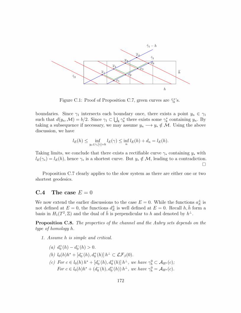
Figure C.1: Proof of Proposition C.7, green curves are γ∗k’s.

boundaries. Since γ1 intersects each boundary once, there exists a point yn ∈ γ1

such that d(yn,M) = b/2. Since γ1 ⊂⋃k γ∗k there exists some γ∗k containing yn. By

taking a subsequence if necessary, we may assume yn −→ y∗ /∈M. Using the abovediscussion, we have

lE(h) ≤ infy∗∈γ,[γ]=h

lE(γ) ≤ infnlE(h) + dn = lE(h).

Taking limits, we conclude that there exists a rectifiable curve γ∗ containing y∗ withlE(γ∗) = lE(h), hence γ∗ is a shortest curve. But y∗ /∈M, leading to a contradiction.

Proposition C.7 clearly applies to the slow system as there are either one or twoshortest geodesics.

C.4 The case E = 0

We now extend the earlier discussions to the case E = 0. While the functions a±E isnot defined at E = 0, the functions d±E is well defined at E = 0. Recall h, h form abasis in H1(T 2,Z) and the dual of h is perpendicular to h and denoted by h⊥.

Proposition C.8. The properties of the channel and the Aubry sets depends on thetype of homology h.

1. Assume h is simple and critical.

(a) d+0 (h)− d−0 (h) > 0.

(b) l0(h)h∗ + [d−0 (h), d+0 (h)]h⊥ ⊂ LFβ(0).

(c) For c ∈ l0(h)h∗ + [d−0 (h), d+0 (h)]h⊥, we have γ0

h ⊂ AHs(c);

For c ∈ l0(h)h∗ + (d−0 (h), d+0 (h))h⊥, we have γ0

h = AHs(c).

172

2. Assume h is simple and non-critical.

(a) d+0 (h)− d−0 (h) > 0.

(b) l0(h)h∗ + [d−0 (h), d+0 (h)]h⊥ ⊂ LFβ(0).

(c) For c ∈ l0(h)h∗ + [d−0 (h), d+0 (h)]h⊥, we have γ0

h ∪ 0 ⊂ AHs(c);

For c ∈ l0(h)h∗ + (d−0 (h), d+0 (h))h⊥, we have γ0

h ∪ 0 = AHs(c).

(d) The functions d±E(h) is right-continuous at E = 0.

3. Assume h is non-simple and h = n1h1 + n2h2, with h1, h2 simple.

(a) d+0 (h) = d−0 (h). Moreover, let c∗(h) = lE(h1)h

∗1 + lE(h2)h

∗2, where (h∗1, h

∗2)

is the dual basis to (h1, h2), then

c∗ = lE(h)h∗ + d±0 (h)h⊥,

where h⊥ is a unit vector perpendicular to h.

(b) γ0h1∪ γ0

h2= AHs(c∗).

(c) d+0 (h1)− d−0 (h1) > 0 with

lE(h1)h∗1 + d+0 (h1)h∗2 = c∗.

Before proving Proposition C.8, we first explain how the proof of Proposition C.7can be adapted to work even for E = 0.

Lemma C.9. Assume that there is a unique g0−shortest geodesic in the homology h.Then

d+0 (h)− d−0 (h) > 0.

Proof. We will try to adapt the proof of Proposition C.7. Let γ0, γ1 and γ2 be shortestgeodesics in homologies h, nh+ h and nh− h, respectively. We choose an arbitraryparametrization for γi on [0, T ]. Note that the parametrization is only continuous ingeneral.

The proof of Proposition C.7 relies only on the property that lifted shortestgeodesics intersects at most once. For E = 0, we will rely on a weaker property.

Let γi be the lifts to the universal cover R2. The degenerate point 0 lifts to theinteger lattice Z2. Since g0 is a Riemannian metric away from the integers, using theshortening argument, we have: if γi intersect γj at more than one point, then eitherthe intersections occur only at integer points, or the two curve coincide on a segmentwith integer end points.

Let a0 ∈ γ0 ∩ γ1 and let γ0 and γ1 be lifts with γ0(0) = γ1(0) = a0. If a /∈ Z2,then it is the only intersection between the two curves. If a0 ∈ Z2, we define a′0

173

to be the largest intersection between γ0|[0, T ) and γ1 according to the order on γ0.a′0 is necessarily an integer point, and since a′0 ∈ γ0, there exists n1 < n such thata′0 − a0 = n0h. Moreover, using the fact that γ0 is minimizing, we have

l0(γ0|[a0, a′0]) = l0(γ1|[a0, a

′0]).

We now apply a similar argument to γ0 + h and γ1. Let a1 = γ0(T ) + h = γ1(T ) andlet a′1 be the smallest intersection between γ0|(0, T ] and γ1. Then there exists n1 ∈ N,n0 + n1 < n, such that a1 − a′1 = n1h. Moreover,

l0((γ0 + h)|[a′1, a1]) = l0(γ1|[a′1, a1]).

Let η1 = γ1|[a′0, a′1] and η1 be its projection. We have [η] = (n−n0−n1)h+h =: m1h+h,and

l0(η1)−m1l0(h) = l0(γ1)− nl0(h).

The curve η1 has the property that it intersects γ0 only once. Apply the same argumentto γ2, we obtain a curve η2 with [η2] = m2h− h, and

l0(η2)−m2l0(h) = l0(γ2)− nl0(h).

To proceed as in the proof of Proposition C.7, we show that if η1 and η2 are liftsof η1 and η2 with the property that

η1(0), η2(T ) ∈ γ0(t), η1(T ), η2(0) ∈ γ0(t) + h,

then η1 and η2 intersects only once. Indeed, there are no integer points between γ0

and γ0 + h.We have

l0(η1)−m1l0(h) + l0(η2)−m2l0(h) = dn,

where dn is as defined in Proposition C.7. Assume inf dn = 0, proceed as in the proofof Proposition C.7, we obtain curves [γk] = h, positive distance away from γ0, suchthat

l0(h) ≤ l0(γk) ≤ l0(h) + dn.

This leads to a contradiction.

Proof of Proposition C.8. Case 1, h is simple and critical.(a) This follows from Lemma C.9.(b) We note that Lemma C.5 depends only on positive homogeinity and sub-

additivity of lE(h), and hence applies even when E = 0. We obtain for c ∈ l0(h)h∗ +[d−0 (h), d+

0 (h)]h∗

l0(h′)− 〈c, h′〉 ≥ 0, ∀h′ ∈ H1(T2,Z2).

174

Since lE(h) is strictly increasing, we obtain lE(h′) − 〈c, h′〉 > 0 for E > 0. ByLemma C.1, there are no c−minimal measures with energy E > 0. As a consequence,α(c) = 0. Since 0 is a c−minimal measure with rotation number 0, we concludel0(h)h∗ + [d−0 (h), d+

0 (h)]h∗ ⊂ LFβ(0).(c) Since we proved α(c) = 0, the first conclusion follows from Lemma C.1. For

the second conclusion, we verify that the proof of Proposition C.6 for non-bifurcationval applies to this case.

(d) The set function [d−E(h), d+E(h)] is upper semi-continuous at E = 0 from the

right, by definition We will show that it is continuous. Assume by contradiction that

[lim infE−→0+

d−E(h), lim supE−→0+

d+E(h)] ( [d−0 (h), d+

0 (h)].

Then there exists c ∈ l0(h)h∗ + (d−0 (h), d+0 (h))h∗ and

c(E) /∈ lE(h)h∗ + [d−E(h), d+E(h)]h⊥

such that c(E) −→ c. By part (c), the Aubry set AHs(c) supports a unique minimalmeasure. By Proposition 7.3, the Aubry set is upper semi-continuous in c. Henceany limit point of AHs(c(E)) as E −→ 0 is in AHs(c). This implies that AHs(c(E))approaches γEh as E −→ 0. Since γEh is the unique closed geodesic in a neighbourhood

of itself, we conclude that AHs(c(E)) = γEh for sufficiently small E. But this contradictswith c(E) /∈ lE(h)h∗ + [d−E(h), d+

E(h)]h⊥

Case 2, h is simple and non-critical.(a) This follows from Lemma C.9.(b) The proof is identical to case 1.(c) For the first conclusion, we can directly verify that γ0

h ⊂ AHs(c) and 0 ⊂AHs(c). For the second conclusion, we note that proof of Proposition C.6 for bifurcationvalues applies to this case.

Case 3, h is non-simple with h = n1h1 + n2h2.(a) Assume that h = m1h1 + m2h2 for some m1,m2 ∈ Z. For sufficiently large

n ∈ N, we have nh± h ∈ Nh1 + Nh2. As a consequence,

l0(nh± h)− l0(nh)

= (nn1 ±m1)l0(h1) + (nn2 ±m2)l0(h2)− (nn1l0(h1) + nn2l0(h2))

= ±m1l0(h1)±m2l0(h2).

We obtain d+0 (h)− d−0 (h) = 0 by definition.

We check directly thatl0(h)− 〈c∗, h〉 = 0.

175

Since l0(h)h∗ + d−0 (h)h⊥ = l0(h)h∗ + d+0 (h)h⊥ is the unique c with this property. The

second claim follows.(b) We note that any connected component of the complement to γ0

h1∪ γ0

h2is

contractible. If AHs(c) has other components, the only possibility is a contractibleorbit bi-asymp to 0. However, such an orbit can never be minimal, as the fixedpoint 0 has smaller action.

(c) The statement d+0 (h1) − d−0 (h1) > 0 follows from part 1(a). for the second

claim, we compute

d+0 (h1) = inf

nl0(nh1 + h2)− l0(nh2) = l0(h2)

and the claim follows.

Acknowledgment

V.K. has been partially supported of the NSF grant DMS-1402164 and enjoyed thehospitality of the ETH Institute for Theoretical Studies. He has been partiallysupported by the Dr. Max Rssler, the Walter Haefner Foundation and the ETHZurich Foundation. K.Z. is supported by the NSERC Discovery grant, referencenumber 436169-2013, and thank the hospitality of the Institute for Theoretical Studiesfor visiting in 2017. During the spring semester of 2012 the authors visited theInstitute for Advanced Study. They acknowledge hospitality and a highly stimulatingresearch atmosphere. The authors are grateful to John Mather for numerous inspiringdiscussions. The course of lectures Mather gave in the spring of 2009 was very helpfulfor the authors. The authors thank Abed Bounemoura and Chong-Qing Cheng forhelpful comments on preliminary versions of this paper. Bounemoura pointed out someerrors related to normal forms and Cheng on error related to total disconnectednessof Mane sets. The authors are thankful to Giovanni Forni for helpful remarks onexposition.

D Notations

We provide a list of notations for the reader’s convenience.

D.1 Formulation of the main result

(θ, p, t) A point in the phase space T2 × R2 × T.φs,tH The Hamiltonian flow for an non-autonomous Hamiltonian.ΦtH The Hamiltonian flow for an autonomous Hamiltonian.

176

Hε = H0 + εH1 Nearly integrable system.D A fixed constant controlling the norm and convexity of H0.Z3∗ = Z3 \ (0, 0, 1)Z Set of integer vectors defining a resonance relation.

k = (k1, k2, k0) Resonance vectors, contained in Z3∗.

Sk Single resonance surface in the action space given by k ∈ Z3∗.

Γk Singe resonance segment, a closed segment contained in Sk.Sk1,k2 Double resonance point in the action space given by k1, k2 ∈

Z3∗.

Sr The unit sphere of the Cr functions.P Diffusion path consisting of segments of single resonance

segments.K = (k,Γk) Collection of resonances and resonance segments making up

a diffusion path.U = U(P) An open and dense set in Sr defining the “non-degenerate

perturbations” relative to a diffusion path.UλSR(k1,Γk1) Set of H1 ∈ Sr satisfying the quantitative non-resonance

conditions [SR1λ]− [SR3λ] relative to the resonant segment(k1,Γk1).

UDR(k1, k2) Set of H1 ∈ Sr satisfying the non-degeneracy conditions[DR1h]− [DR3h] and [DR1c]− [DR4c].

V = V(U , ε0) A “cusp” set of perturbations, equal to εH1 : H1 ∈ U , 0 <ε < ε0(H1).

Kst(k1,Γk1 , λ) Set of strong additional resonances relative to the resonancesegment Γk1 , for an perturbation H1 ∈ UλSR(k1,Γk1).

Bσ Ball in Euclidean space Rn.Vrσ,Vσ Ball in the functional space Cr. When supscript is not

indicated, then stands for Cr where r is from the maintheorem.

D.2 Weak KAM and Mather theory

$ = $(H) The period of a time periodic Hamiltonian, i.e. H(θ, p, t+$) = H(θ, p, t).

T$ = R/($Z) Torus with period $.H = H(D) A family of Hamiltonians satisfying uniform conditions de-

pending on the parameter D > 1.L = LH The Lagrangian of H.LH,c The “penalized” Lagrangian LH(θ, v, t)− c · v.AH,c(x, s, y, t) The minimal action for the Lagrangian LH,c.αH(c), αL(c) Mather’s alpha function.

177

βH(ρ), βL(ρ) Mather’s beta function.hH,c(x, s, y, t) The time dependent Peierl’s barrier function.hH,c(x, y) The discrete Peierl’s barrier function, equal to hH,c(x, 0, y, 0).dH,c(x, s, y, t) Mather’s semi-distanceT s,tc u(x) Lax-Oleinik semi-group defined on Tn.∂+u(x) The supergradient of a semi-concave function at x.Gc,w, w = w(θ, t) The time-dependent pseudograph as a subset of Tn×Rn×R,

or Tn × Rn × T$.

I(c, w) The maximum invariant set contained in the psudographGc,w.

MH(c), AH(c), NH(c) The continuous (Hamiltonian) Mather, Aubry and Mane set,defined on Tn × Rn × T$(H).

M0H(c), A0

H(c), N 0H(c) The discrete (Hamiltonian) Mather, Aubry and Mane set,

defined on Tn × Rn, invariant under the map φH = φ$(H)H .

S(H, c) A static class of the Aubry set AH(c).c ` c′ The forcing relation.c a` c′ The forcing equivalence relation.

D.3 Single resonance

[H1]k1 The average of H1 relative to the resonance k1.[H1]k1,k2 The average of H1 relative to the double resoannce k1, k2.Φε The averaging coordinate change at single resonance.Nε Normal form under the coordinate change. Same notation

is used at double resonance.Zk1(θ

s, p, t) The resonant component of H1 relative to the resonance k1.R(θ, p, t) The remainder in the single resonance normal form.Kst(k1,Γk1 , K) Set of strong additional resonance k2 intersecting Γk1 with

norm at most K, plus any resonances in the diffusion paththat intersect Γk1 .

ΓSRk1 The punctured resonance segment after removing O(√ε)

neighborhoods of strong double resonances.‖ · ‖CrI The rescaled Cr norm where the derivatives in the action

variable are rescaled by√ε.

Tω The period of the rational vector (ω, 1) ∈ R3.B ∈ SL(3,Z) An integer matrix defining the linear coordinate change

relative to a double resonance k1, k2.

178

(θs, θf , ps, pf , t) The coordinate at single resonance after taking a linearcoordinate change. The resonance becomes (1, 0, 0) · (ω, 1) =0 in this coordinate.

(Θs, P s)(θf , pf , t) Normally hyperbolic invariant cylinder for the single resonantnormal form, parametrized using the (θf , pf , t) variables.

D.4 Double resonance

Φε The averaging coordinate change at double resonance.Nε The normal form at double resonance.ΦL The linear coordinate change corresponding to the double

resonance k1, k2.K(I) The kinetic energy of the slow mechanical system.U(ϕ) The potential function of the slow mechanical system.gE The Jacobi metric at energy E of the slow mechanical system.h A homology class in H1(T2,Z).γEh Shortest curves of the Jacobi metric in homology class h.ηEh The Hamiltonian periodic orbit corresponding to the geodesic

γEh .

Φijloc, i, j ∈ +,− Local maps near the saddle fixed point of Hs.

Φglob Global map along a homoclinic orbit η of Hs.ch(E) Curve of cohomologies chosen in the channel of h.Γh Choice of cohomologies along the homology h.Γeh In the non-simple case, choice of cohomology curve above

energy e.Γe,µh1 In the non-simple case, choice of cohomology along the

adjacent simple homology h1.Φ∗L The relation between cohomology class and alpha function

after the coordinate change ΦL.Φ∗L,Hs

εThe relation between the cohomology classes for the coor-dinate change ΦL. Depends on the alpha function of thesystem Hs

ε .ΓDRk1,k2 The choice of cohomology classes at a double resonance

k1, k2.

179

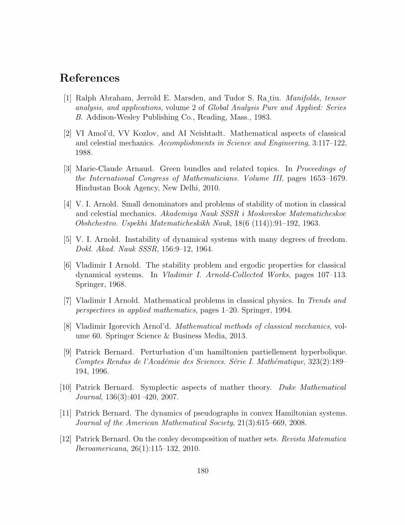
References

[1] Ralph Abraham, Jerrold E. Marsden, and Tudor S. Ra¸tiu. Manifolds, tensoranalysis, and applications, volume 2 of Global Analysis Pure and Applied: SeriesB. Addison-Wesley Publishing Co., Reading, Mass., 1983.

[2] VI Amol’d, VV Kozlov, and AI Neishtadt. Mathematical aspects of classicaland celestial mechanics. Accomplishments in Science and Engineering, 3:117–122,1988.

[3] Marie-Claude Arnaud. Green bundles and related topics. In Proceedings ofthe International Congress of Mathematicians. Volume III, pages 1653–1679.Hindustan Book Agency, New Delhi, 2010.

[4] V. I. Arnold. Small denominators and problems of stability of motion in classicaland celestial mechanics. Akademiya Nauk SSSR i Moskovskoe MatematicheskoeObshchestvo. Uspekhi Matematicheskikh Nauk, 18(6 (114)):91–192, 1963.

[5] V. I. Arnold. Instability of dynamical systems with many degrees of freedom.Dokl. Akad. Nauk SSSR, 156:9–12, 1964.

[6] Vladimir I Arnold. The stability problem and ergodic properties for classicaldynamical systems. In Vladimir I. Arnold-Collected Works, pages 107–113.Springer, 1968.

[7] Vladimir I Arnold. Mathematical problems in classical physics. In Trends andperspectives in applied mathematics, pages 1–20. Springer, 1994.

[8] Vladimir Igorevich Arnol’d. Mathematical methods of classical mechanics, vol-ume 60. Springer Science & Business Media, 2013.

[9] Patrick Bernard. Perturbation d’un hamiltonien partiellement hyperbolique.Comptes Rendus de l’Academie des Sciences. Serie I. Mathematique, 323(2):189–194, 1996.

[10] Patrick Bernard. Symplectic aspects of mather theory. Duke MathematicalJournal, 136(3):401–420, 2007.

[11] Patrick Bernard. The dynamics of pseudographs in convex Hamiltonian systems.Journal of the American Mathematical Society, 21(3):615–669, 2008.

[12] Patrick Bernard. On the conley decomposition of mather sets. Revista MatematicaIberoamericana, 26(1):115–132, 2010.

180

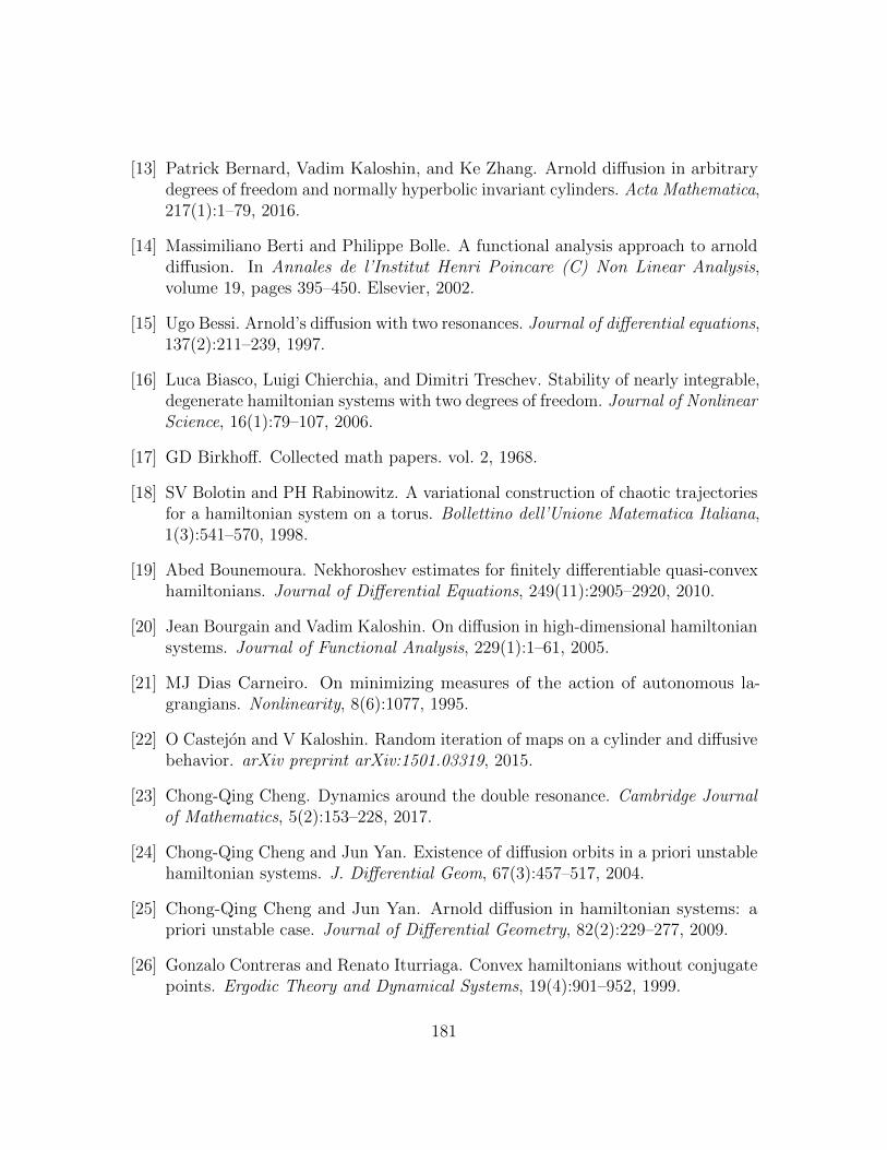
[13] Patrick Bernard, Vadim Kaloshin, and Ke Zhang. Arnold diffusion in arbitrarydegrees of freedom and normally hyperbolic invariant cylinders. Acta Mathematica,217(1):1–79, 2016.

[14] Massimiliano Berti and Philippe Bolle. A functional analysis approach to arnolddiffusion. In Annales de l’Institut Henri Poincare (C) Non Linear Analysis,volume 19, pages 395–450. Elsevier, 2002.

[15] Ugo Bessi. Arnold’s diffusion with two resonances. Journal of differential equations,137(2):211–239, 1997.

[16] Luca Biasco, Luigi Chierchia, and Dimitri Treschev. Stability of nearly integrable,degenerate hamiltonian systems with two degrees of freedom. Journal of NonlinearScience, 16(1):79–107, 2006.

[17] GD Birkhoff. Collected math papers. vol. 2, 1968.

[18] SV Bolotin and PH Rabinowitz. A variational construction of chaotic trajectoriesfor a hamiltonian system on a torus. Bollettino dell’Unione Matematica Italiana,1(3):541–570, 1998.

[19] Abed Bounemoura. Nekhoroshev estimates for finitely differentiable quasi-convexhamiltonians. Journal of Differential Equations, 249(11):2905–2920, 2010.

[20] Jean Bourgain and Vadim Kaloshin. On diffusion in high-dimensional hamiltoniansystems. Journal of Functional Analysis, 229(1):1–61, 2005.

[21] MJ Dias Carneiro. On minimizing measures of the action of autonomous la-grangians. Nonlinearity, 8(6):1077, 1995.

[22] O Castejon and V Kaloshin. Random iteration of maps on a cylinder and diffusivebehavior. arXiv preprint arXiv:1501.03319, 2015.

[23] Chong-Qing Cheng. Dynamics around the double resonance. Cambridge Journalof Mathematics, 5(2):153–228, 2017.

[24] Chong-Qing Cheng and Jun Yan. Existence of diffusion orbits in a priori unstablehamiltonian systems. J. Differential Geom, 67(3):457–517, 2004.

[25] Chong-Qing Cheng and Jun Yan. Arnold diffusion in hamiltonian systems: apriori unstable case. Journal of Differential Geometry, 82(2):229–277, 2009.

[26] Gonzalo Contreras and Renato Iturriaga. Convex hamiltonians without conjugatepoints. Ergodic Theory and Dynamical Systems, 19(4):901–952, 1999.

181

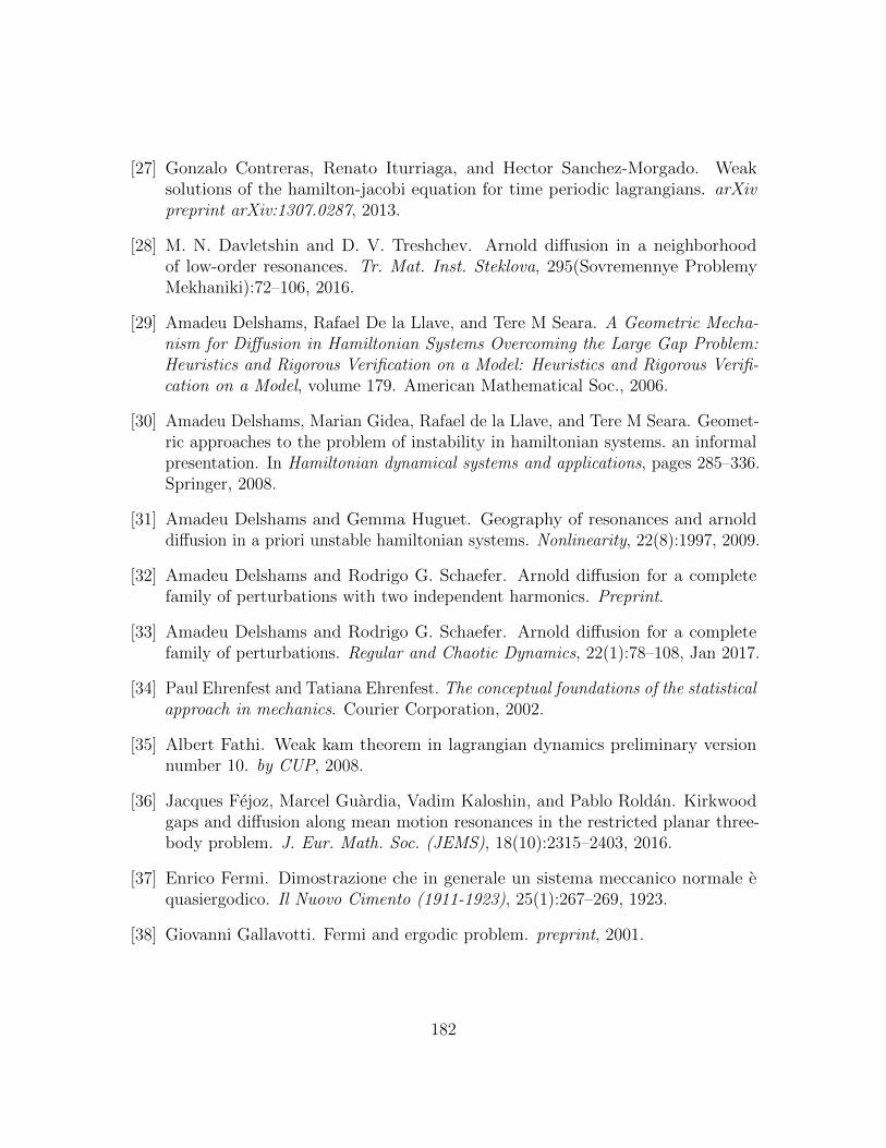
[27] Gonzalo Contreras, Renato Iturriaga, and Hector Sanchez-Morgado. Weaksolutions of the hamilton-jacobi equation for time periodic lagrangians. arXivpreprint arXiv:1307.0287, 2013.

[28] M. N. Davletshin and D. V. Treshchev. Arnold diffusion in a neighborhoodof low-order resonances. Tr. Mat. Inst. Steklova, 295(Sovremennye ProblemyMekhaniki):72–106, 2016.

[29] Amadeu Delshams, Rafael De la Llave, and Tere M Seara. A Geometric Mecha-nism for Diffusion in Hamiltonian Systems Overcoming the Large Gap Problem:Heuristics and Rigorous Verification on a Model: Heuristics and Rigorous Verifi-cation on a Model, volume 179. American Mathematical Soc., 2006.

[30] Amadeu Delshams, Marian Gidea, Rafael de la Llave, and Tere M Seara. Geomet-ric approaches to the problem of instability in hamiltonian systems. an informalpresentation. In Hamiltonian dynamical systems and applications, pages 285–336.Springer, 2008.

[31] Amadeu Delshams and Gemma Huguet. Geography of resonances and arnolddiffusion in a priori unstable hamiltonian systems. Nonlinearity, 22(8):1997, 2009.

[32] Amadeu Delshams and Rodrigo G. Schaefer. Arnold diffusion for a completefamily of perturbations with two independent harmonics. Preprint.

[33] Amadeu Delshams and Rodrigo G. Schaefer. Arnold diffusion for a completefamily of perturbations. Regular and Chaotic Dynamics, 22(1):78–108, Jan 2017.

[34] Paul Ehrenfest and Tatiana Ehrenfest. The conceptual foundations of the statisticalapproach in mechanics. Courier Corporation, 2002.

[35] Albert Fathi. Weak kam theorem in lagrangian dynamics preliminary versionnumber 10. by CUP, 2008.

[36] Jacques Fejoz, Marcel Guardia, Vadim Kaloshin, and Pablo Roldan. Kirkwoodgaps and diffusion along mean motion resonances in the restricted planar three-body problem. J. Eur. Math. Soc. (JEMS), 18(10):2315–2403, 2016.

[37] Enrico Fermi. Dimostrazione che in generale un sistema meccanico normale equasiergodico. Il Nuovo Cimento (1911-1923), 25(1):267–269, 1923.

[38] Giovanni Gallavotti. Fermi and ergodic problem. preprint, 2001.

182

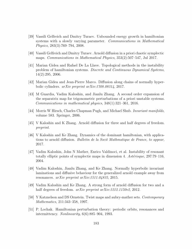
[39] Vassili Gelfreich and Dmitry Turaev. Unbounded energy growth in hamiltoniansystems with a slowly varying parameter. Communications in MathematicalPhysics, 283(3):769–794, 2008.

[40] Vassili Gelfreich and Dmitry Turaev. Arnold diffusion in a priori chaotic symplecticmaps. Communications in Mathematical Physics, 353(2):507–547, Jul 2017.

[41] Marian Gidea and Rafael De La Llave. Topological methods in the instabilityproblem of hamiltonian systems. Discrete and Continuous Dynamical Systems,14(2):295, 2006.

[42] Marian Gidea and Jean-Pierre Marco. Diffusion along chains of normally hyper-bolic cylinders. arXiv preprint arXiv:1708.08314, 2017.

[43] M Guardia, Vadim Kaloshin, and Jianlu Zhang. A second order expansion ofthe separatrix map for trigonometric perturbations of a priori unstable systems.Communications in mathematical physics, 348(1):321–361, 2016.

[44] Morris W Hirsch, Charles Chapman Pugh, and Michael Shub. Invariant manifolds,volume 583. Springer, 2006.

[45] V Kaloshin and K Zhang. Arnold diffusion for three and half degrees of freedom.preprint.

[46] V Kaloshin and Ke Zhang. Dynamics of the dominant hamiltonian, with applica-tions to arnold diffusion. Bulletin de la Socit Mathmatique de France, to appear,2017.

[47] Vadim Kaloshin, John N Mather, Enrico Valdinoci, et al. Instability of resonanttotally elliptic points of symplectie maps in dimension 4. Asterisque, 297:79–116,2004.

[48] Vadim Kaloshin, Jianlu Zhang, and Ke Zhang. Normally hyperbolic invariantlaminations and diffusive behaviour for the generalized arnold example away fromresonances. arXiv preprint arXiv:1511.04835, 2015.

[49] Vadim Kaloshin and Ke Zhang. A strong form of arnold diffusion for two and ahalf degrees of freedom. arXiv preprint arXiv:1212.1150v2, 2012.

[50] Y Katznelson and DS Ornstein. Twist maps and aubry-mather sets. ContemporaryMathematics, 211:343–358, 1997.

[51] P. Lochak. Hamiltonian perturbation theory: periodic orbits, resonances andintermittency. Nonlinearity, 6(6):885–904, 1993.

183

[52] Jean-Pierre Marco. Chains of compact cylinders for cusp-generic nearly integrableconvex systems on A3. arXiv preprint arXiv:1602.02399, 2016.

[53] JP Marco. Arnold diffusion for cusp-generic nearly integrable convex systems onA3. Preprint available at https://arxiv. org/abs/1602.02403, 2016.

[54] Daniel Massart. On aubry sets and mathers action functional. Israel Journal ofMathematics, 134(1):157–171, 2003.

[55] John Mather. Personal communication.

[56] John Mather. Variational construction of trajectories for time periodic lagrangiansystems on the two torus. preprint, 1996.

[57] John N Mather. Action minimizing invariant measures for positive definitelagrangian systems. Mathematische Zeitschrift, 207(1):169–207, 1991.

[58] John N Mather. Variational construction of orbits of twist diffeomorphisms.Journal of the American Mathematical Society, 4(2):207–263, 1991.

[59] John N Mather. Total disconnectedness of the quotient aubry set in low dimensions.Communications on pure and applied mathematics, 56(8):1178–1183, 2003.

[60] John N Mather. Arnold diffusion. i: Announcement of results. Journal ofMathematical Sciences, 124(5):5275–5289, 2004.

[61] John N Mather. Arnold diffusion. ii. preprint, pages 1–185, 2008.

[62] John N Mather. Order structure on action minimizing orbits. Symplectic topologyand measure preserving dynamical systems, 512:41, 2010.

[63] John N Mather. Shortest curves associated to a degenerate jacobi metric on t2.Progress in variational methods, Nankai Ser. Pure Appl. Math. Theoret. Phys., 7,World Sci. Publ., Hackensack, NJ, 2011., 7:126–168, 2010.

[64] John N Mather and Giovanni Forni. Action minimizing orbits in hamiltomiansystems. In Transition to chaos in classical and quantum mechanics, pages 92–186.Springer, 1994.

[65] Marco Mazzucchelli and Alfonso Sorrentino. Remarks on the symplectic invarianceof Aubry-Mather sets. Comptes Rendus Mathematique. Academie des Sciences.Paris, 354(4):419–423, 2016.

[66] Richard McGehee. The stable manifold theorem via an isolating block. InSymposium on Ordinary Differential Equations, pages 135–144. Springer, 1973.

184

[67] Elismar R Oliveira. On generic properties of lagrangians on surfaces: the kupka-smale theorem. Discrete Contin. Dyn. Syst., 21(2):551–569, 2008.

[68] Charles Pugh, Michael Shub, and Amie Wilkinson. Holder foliations. DukeMathematical Journal, 86(3):517–546, 1997.

[69] Ludovic Rifford and Rafael O Ruggiero. Generic properties of closed orbits ofhamiltonian flows from mane’s viewpoint. International Mathematics ResearchNotices, 2012(22):5246–5265, 2011.

[70] Leonid Pavlovich Shilnikov. On a Poincare–Birkhoff problem. MatematicheskiiSbornik, 116(3):378–397, 1967.

[71] Alfonso Sorrentino. Action-minimizing Methods in Hamiltonian Dynamics (MN-50): An Introduction to Aubry-Mather Theory. Princeton University Press, 2015.

[72] D Treschev. Multidimensional symplectic separatrix maps. Journal of NonlinearScience, 12(1):27–58, 2002.

[73] D Treschev. Evolution of slow variables in a priori unstable hamiltonian systems.Nonlinearity, 17(5):1803, 2004.

[74] D Treschev. Arnold diffusion far from strong resonances in multidimensional apriori unstable hamiltonian systems. Nonlinearity, 25(9):2717, 2012.

[75] D Turaev and L Shilnikov. On the hamiltonian-systems with homoclinic curvesfor a saddle. Doklady Akademii Nauk USSR, 304(4):811–814, 1989.

[76] Ke Zhang. Speed of arnold diffusion for analytic hamiltonian systems. Inventionesmathematicae, 186(2):255–290, 2011.

[77] Ke Zhang. On the tangent cones of Aubry sets. Annales de la Facult des Sciencesde Toulouse, to appear, 2017.

185