Are returns to public investment lower in less-favored rural areas?: an empirical analysis of India

ARE RETURNS TO PUBLIC INVESTMENT LOWERIN LESS-FAVORED RURAL AREAS? AN EMPIRICAL

ANALYSIS OF INDIA

Shenggen Fan and Peter Hazell

EPTD DISCUSSION PAPER NO. 43

Environment and Production Technology Division

International Food Policy Research Institute2033 K Street, N.W.

Washington, D.C. 20006 U.S.A.

May 1999

EPTD Discussion Papers contain preliminary material and research results, and are circulatedprior to a full peer review in order to stimulate discussion and critical comment. It is expected thatmost Discussion Papers will eventually be published in some other form, and that their content mayalso be revised.

ABSTRACT

Developing countries allocate scarce government funds to investments in rural areas

to achieve the twin goals of agricultural growth and poverty alleviation. Choices have to

be made between different types of investments, especially infrastructure, human capital

and agricultural research, and between different types of agricultural regions, e.g.,

irrigated and high- and low-potential rainfed areas. This paper develops an econometric

approach and provides empirical evidence on the impact of government investments in

rural India using district-level data. While irrigated areas played a key role in agricultural

growth during the Green Revolution era, our results show that it is now the rainfed areas,

including many less-favored areas that offer the most growth for an additional unit of

investment. Moreover, investments in rainfed areas have a much larger impact on poverty

alleviation, making this a win-win development strategy. These results have important

policy implications, and challenge conventional thinking that public investments in rural

India should always be targeted to irrigated and other high-potential areas.

i

CONTENTS

1. Introduction . . . . . . . . . . . . . . . . . . . . . . . . . . . . . . . . . . . . . . . . . . . . . . . . . . . . . . . 1

2. Classification of Indian Agroecological Zones . . . . . . . . . . . . . . . . . . . . . . . . . . . . . . 5

3. Technologies and Infrastructure . . . . . . . . . . . . . . . . . . . . . . . . . . . . . . . . . . . . . . . . 6

4. Production and Productivity Growth . . . . . . . . . . . . . . . . . . . . . . . . . . . . . . . . . . . . 11

5. Rural Poverty . . . . . . . . . . . . . . . . . . . . . . . . . . . . . . . . . . . . . . . . . . . . . . . . . . . . . 15

6. Effects of Infrastructure and Technologies on Production and Rural Poverty . . . . . 17Conceptual Framework . . . . . . . . . . . . . . . . . . . . . . . . . . . . . . . . . . . . . . . . . . . 18Estimates of the Production and Poverty Equations . . . . . . . . . . . . . . . . . . . . . . 22Marginal Returns of Infrastructure and Technologies . . . . . . . . . . . . . . . . . . . . . 29

7. Conclusions . . . . . . . . . . . . . . . . . . . . . . . . . . . . . . . . . . . . . . . . . . . . . . . . . . . . . . 31

References . . . . . . . . . . . . . . . . . . . . . . . . . . . . . . . . . . . . . . . . . . . . . . . . . . . . . . . . . . 34

Shenggen Fan and Peter Hazell are Senior Research Fellow and Director,*

respectively, Environment and Production Technology Division, International Food PolicyResearch Institute, Washington, D.C.

ARE RETURNS TO PUBLIC INVESTMENT LOWER IN LESS-FAVOREDRURAL AREAS? AN EMPIRICAL ANALYSIS OF INDIA

Shenggen Fan and Peter Hazell*

1. INTRODUCTION

Past agricultural development strategies have emphasized irrigated agriculture and

“high-potential” rainfed lands in an attempt to increase food production and stimulate

economic growth. This strategy has been very successful in many countries and was

responsible for the Green Revolution. At the same time, however, large areas of less-

favored lands have been neglected and lag behind in their economic development. These

lands are characterized by lower agricultural potential, often because of poorer soils,

shorter growing seasons, and lower and uncertain rainfall, but also because past neglect

has left them with limited infrastructure and poor access to markets. Despite some out-

migration to more rapidly growing areas, population size continues to grow in many less-

favored areas, and this growth has not been matched by increases in yields. The result is

worsening poverty and food insecurity problems, which in turn is contributing to the

widespread degradation of natural resources (e.g., mining of soil fertility, soil erosion,

deforestation, and loss of biodiversity) as people seek to expand the cropped area. The

severity of these problems has now reached the point where some governments and

donors are spending more resources on crisis relief than development in these areas

2

An environmental goal could be added as a third dimension to this argument. 1

Unfortunately, we do not have any relevant environmental data for India and hence have

(Owens and Hoddinott 1999).

Less-favored lands are extensive in the developing world. According to a report

prepared by the Technical Advisory Committee of the CGIAR, “marginal” and sparsely

populated arid lands account for 75 percent and 85 percent, respectively, of the total

agricultural area in Asia and Sub-Saharan Africa (CGIAR 1998). Their shares in total

agricultural production are lower but still large. In China and India, for example, we

estimate that less-favored lands account for about one-third and 40 percent of total

agricultural output, respectively. Globally, some 500 million poor people live in less-

favored lands (Hazell and Garrett 1996).

It is becoming increasingly clear that, on poverty and environmental grounds alone,

more attention will have to be given to less-favored lands in setting priorities for policy

and public investments. This leads to two important questions: 1) How much public

investment can be justified in less-favored areas compared to higher-potential areas; and,

2) How should those funds be allocated among different types of investments? Both

questions are especially germane at a time when many governments are having to cut their

total expenditure and need to allocate resources more efficiently.

The amount of public investment that can be justified in any region should depend

on the net social returns that are realized through productivity growth and poverty

reduction. While “win-win” investments are usually more desirable, an investment that

involves some tradeoff between these two social goals may also be attractive providing

any sacrifice of one goal is adequately compensated by gains on the other goal.1

3

had to limit our analysis to growth and poverty.

Conventional wisdom suggests that the productivity returns to investment are

highest in irrigated and high-potential rainfed lands, and that growth in these areas also has

substantial “trickle-down” benefits for the poor, including those residing in less-favored

areas. Even though investing in less-favored lands might have a greater direct impact on

the poor living in those areas, it is argued that investments in high-potential areas give

higher social returns for a nation. The logic behind this position is as follows. Investment

in high-potential areas generates more agricultural output and higher economic growth at

lower cost than in less-favored areas. Faster economic growth leads to more employment

and higher wages nationally, and greater agricultural output leads to lower food prices,

both of which are beneficial to the poor. Less-favored areas will benefit from cheaper

food, from increased market opportunities for growth, and from new opportunities for

workers to migrate to more productive jobs in the high-potential areas and in towns.

Fewer people will try to live in less-favored lands, and this will help reduce environmental

degradation and increase per capita earnings. Migrants may also send remittances back to

less-favored areas, further increasing per capita incomes there, especially for the poor.

Many of the expected benefits arising from rapid agricultural growth in high-

potential areas have been confirmed (Pinstrup-Andersen and Hazell 1985). Nevertheless,

the rationale for neglecting less-favored areas is being increasingly challenged by: a) the

failure of past patterns of agricultural growth to resolve growing poverty and food

insecurity problems in many less-favored areas; b) increasing evidence of stagnating levels

of productivity growth in many high-potential areas (Pingali and Rosegrant 1998); and c)

4

The data used in this study were compiled from published statistical materials by2

Drs. S. Thorat and T. Haque.

emerging evidence that the right kinds of investments can increase agricultural

productivity to much higher levels than previously thought in some less-favored lands

(Scherr and Hazell 1994). It now seems plausible that increased public investment in

many less-favored areas may have the potential to generate competitive if not greater

agricultural growth on the margin than comparable investments in many high-potential

areas, and have a greater impact on the rural poor living in less-favored areas. If so, then

additional investments in less-favored areas may actually give higher aggregate social

returns to a nation than additional investments in high-potential areas. In fact, they might

even offer win-win possibilities.

This paper uses district level data from India for the period 1970 to 1994 to

estimate the relative returns to public investments in irrigated and high- and low-potential

rainfed areas. In the process, we also obtain important insights about the returns to2

different kinds of public investments within each type of area. India is a good case study

because past public investments have been biased towards high-potential areas, and the

remarkable productivity gains achieved in those areas (which led to national food

surpluses) can now be juxtaposed against the lagging productivity, and widespread

poverty and food insecurity that exists in many less-favored rainfed areas. The results

provide strong support for our hypothesis that greater levels of investment in less-favored

lands are now warranted.

The paper is organized as follows. In the next section, we briefly overview the

characteristics of the major agroecological zones in Indian agriculture, and present our

5

This classification of rainfed and irrigated areas is similar to that used by the3

Ministry of Agriculture of India which, for the purpose of watershed development,considers rainfed areas to be those with less than 30 percent of their crop area underirrigation at the time of initiation of the program. But the Ministry of Agriculture’sclassification is only applied in recent years, whereas we take averages for 1970 to 1994.

definitions of rainfed and irrigated areas, and of low- and high-potential rainfed areas. In

the third section, we review recent trends in the development of technologies and rural

infrastructure by type of area, much of which has been publicly funded. The fourth section

analyzes the corresponding trends in agricultural production and productivity growth,

while the fifth section describes changes in rural poverty. In section six, we develop an

econometric model to analyze and measure the effects of improved technologies and

increased infrastructure on agricultural production growth and poverty reduction, and

estimate results for irrigated and low- and high-potential rainfed areas in India. The final

section discusses the implications of our results for investment priorities in India and other

developing countries.

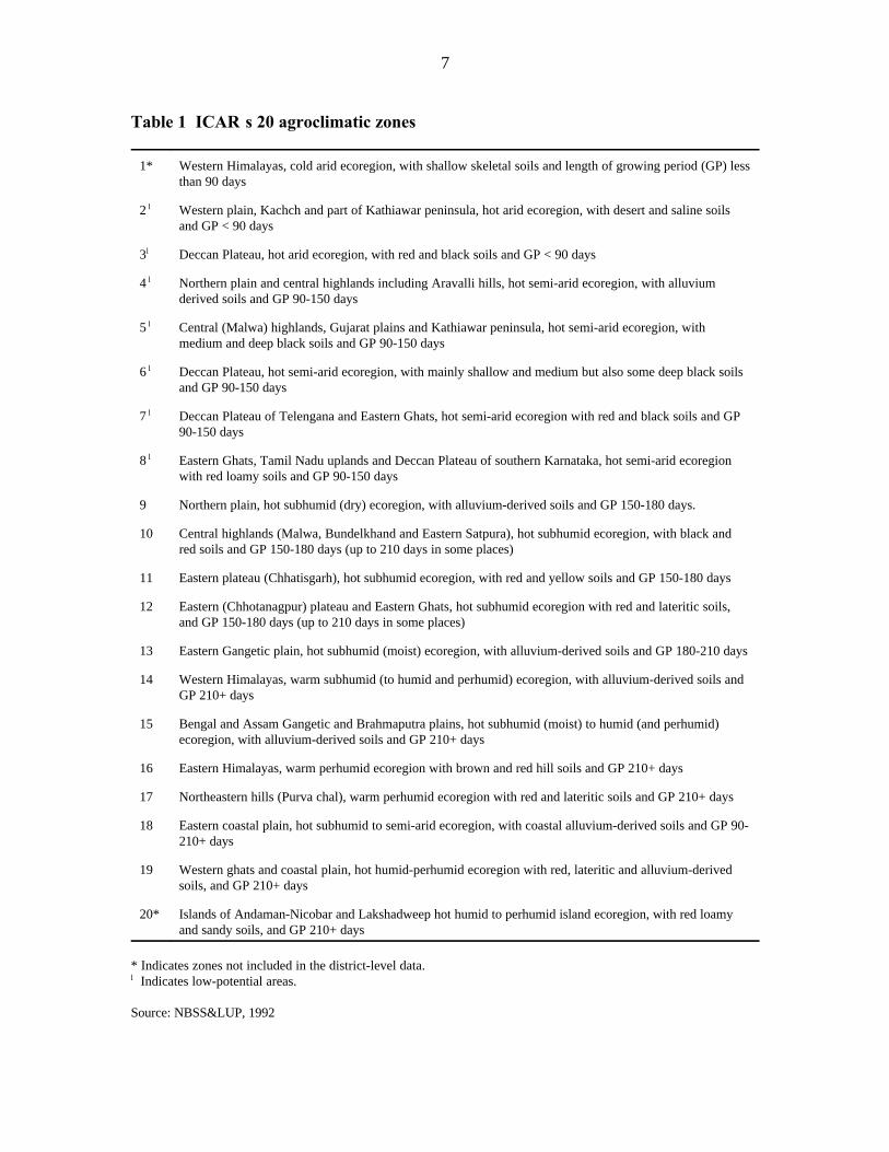
2. CLASSIFICATION OF INDIAN AGROECOLOGICAL ZONES

We classify districts as irrigated if more than 25 percent of the cropped area

(averaged from 1970 to 1995) is irrigated, and as rainfed if the irrigated share is less than

25 percent. We further subdivide rainfed areas into high- and low-potential areas3

according to their agroecological characteristics. There have been several attempts to

define agroecological zones in India. In this study we use a classification scheme

developed by the Indian Council of Agricultural Research (ICAR), which divides India

into 20 agroecological zones based on soils and climate (NBSS&LUP 1992). The district

6

High-yielding varieties (also referred to as modern varieties) are those released by4

the Indian national agricultural research system and the international agricultural researchcenters. The yields of these varieties are substantially higher than those of traditionalvarieties when grown under irrigated conditions with fertilizer.

data available to us cover 18 of these 20 zones. One of the excluded zones is in the

Himalayas, and the other is in the Andaman, Nicobar and Lakshadweep Islands. These are

minor zones in terms of their agricultural production and rural population size. Table 1

presents some distinguishing features of each zone. Rainfed districts in zones 2 to 8 are

considered low-potential areas in this study because of their poor soils, short growing

seasons, and low rainfall. Rainfed districts in zones 9 to 19 are considered high-potential

because these zones have better soils, longer growing seasons, and higher rainfall.

Defined in this way, irrigated and high- and low-potential rainfed areas account for 48, 17,

and 35 percent of the total cropped area, and 56, 17, and 27 percent of total agricultural

output, respectively.

3. TECHNOLOGIES AND INFRASTRUCTURE

One of the most significant changes in Indian agriculture in recent decades has

been the widespread adoption of high-yielding varieties (Figure 1). This has been a 4

major engine of growth in agricultural production and factor productivity. In 1970, the

area under high-yielding varieties as a share of the total cropped area was still low,

7

Table 1 ICAR’s 20 agroclimatic zones

1* Western Himalayas, cold arid ecoregion, with shallow skeletal soils and length of growing period (GP) lessthan 90 days

2 Western plain, Kachch and part of Kathiawar peninsula, hot arid ecoregion, with desert and saline soils l

and GP < 90 days

3 Deccan Plateau, hot arid ecoregion, with red and black soils and GP < 90 daysl

4 Northern plain and central highlands including Aravalli hills, hot semi-arid ecoregion, with alluvium l

derived soils and GP 90-150 days

5 Central (Malwa) highlands, Gujarat plains and Kathiawar peninsula, hot semi-arid ecoregion, with l

medium and deep black soils and GP 90-150 days

6 Deccan Plateau, hot semi-arid ecoregion, with mainly shallow and medium but also some deep black soils l

and GP 90-150 days

7 Deccan Plateau of Telengana and Eastern Ghats, hot semi-arid ecoregion with red and black soils and GP l

90-150 days

8 Eastern Ghats, Tamil Nadu uplands and Deccan Plateau of southern Karnataka, hot semi-arid ecoregion l

with red loamy soils and GP 90-150 days

9 Northern plain, hot subhumid (dry) ecoregion, with alluvium-derived soils and GP 150-180 days.

10 Central highlands (Malwa, Bundelkhand and Eastern Satpura), hot subhumid ecoregion, with black andred soils and GP 150-180 days (up to 210 days in some places)

11 Eastern plateau (Chhatisgarh), hot subhumid ecoregion, with red and yellow soils and GP 150-180 days

12 Eastern (Chhotanagpur) plateau and Eastern Ghats, hot subhumid ecoregion with red and lateritic soils,and GP 150-180 days (up to 210 days in some places)

13 Eastern Gangetic plain, hot subhumid (moist) ecoregion, with alluvium-derived soils and GP 180-210 days

14 Western Himalayas, warm subhumid (to humid and perhumid) ecoregion, with alluvium-derived soils andGP 210+ days

15 Bengal and Assam Gangetic and Brahmaputra plains, hot subhumid (moist) to humid (and perhumid)ecoregion, with alluvium-derived soils and GP 210+ days

16 Eastern Himalayas, warm perhumid ecoregion with brown and red hill soils and GP 210+ days

17 Northeastern hills (Purva chal), warm perhumid ecoregion with red and lateritic soils and GP 210+ days

18 Eastern coastal plain, hot subhumid to semi-arid ecoregion, with coastal alluvium-derived soils and GP 90-210+ days

19 Western ghats and coastal plain, hot humid-perhumid ecoregion with red, lateritic and alluvium-derivedsoils, and GP 210+ days

20* Islands of Andaman-Nicobar and Lakshadweep hot humid to perhumid island ecoregion, with red loamyand sandy soils, and GP 210+ days

* Indicates zones not included in the district-level data. Indicates low-potential areas.l

Source: NBSS&LUP, 1992

1970 1975 1980 1985 19900

102030405060708090

100

Kg

per

Ha

IrrigatedHigh P. RainfedLow P. Rainfed

Fertilizer Application

1970 1975 1980 1985 1990 19950

5

10

15

20

25

30

35

40

Per

cent

age


Areas under Public Irrigation

1970 1975 1980 1985 1990 19950

10

20

30

40

50

60

70

Per

cent

age


High-yielding Varieties

1970 1975 1980 1985 1990 19950

5

10

15

20

25

30

35

40

Per

cent

age


Areas under Private Irrigation

8

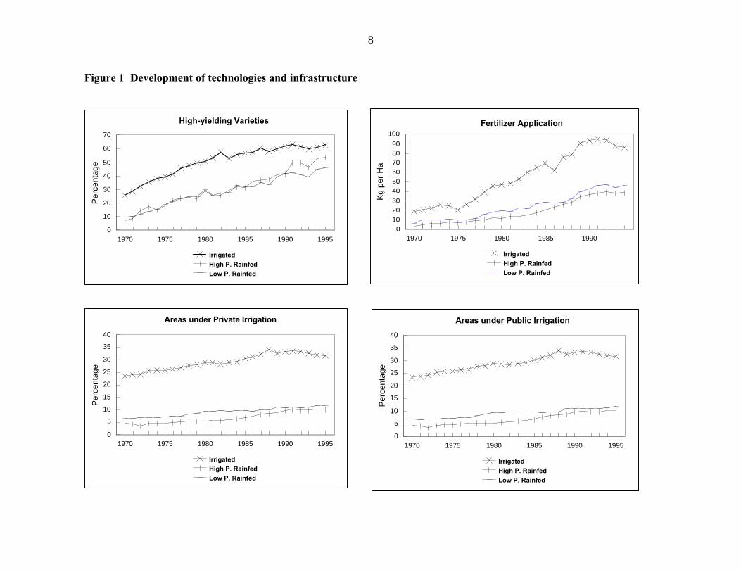
Figure 1 Development of technologies and infrastructure

9

though higher in irrigated than in high- or low-potential rainfed areas (26 verses 7 and 10

percent, respectively). These shares have since grown significantly, and the gap between

rainfed and irrigated areas has also narrowed. By 1995, high-yielding varieties were

planted on about 60 percent of the total cropped area in irrigated areas, and 50 and 40

percent, respectively, in high and low-potential rainfed areas. The share is still increasing

in rainfed areas, but growth has been flat in irrigated areas since the late 1980s.

Since high-yielding varieties require higher applications of fertilizer to realize their

yield potential, fertilizer application in Indian agriculture has also increased rapidly since

1970 (Figure 1). On a per hectare basis, fertilizer use increased from 19 kg in 1970 to

over 90 kg in the 1990s in irrigated areas. It also grew rapidly in high- and low-potential

rainfed areas (from 3 kg and 7 kg in 1970 to 38 kg and 46 kg, respectively, by 1995), but

is still less than half the rate used in irrigated areas.

Irrigation, another important growth factor in Indian agriculture, has also increased

steadily over the years, but with considerable regional variation (Figure 1). We have

disaggregated the total irrigated area into canal and private irrigation. Canal irrigation is

nearly all provided by the public sector, while private irrigation (tanks, wells, and tube

wells) is mainly the result of farmers’ private investment. In irrigated areas, more than 60

percent of the cropped area was irrigated in 1995, compared to only 20-24 percent in

rainfed areas. More than half of the irrigated area is under private irrigation in all three

types of areas, and the share of private irrigation has been increasing.

Another significant achievement in recent decades has been the increase in the

literacy rate of the rural population (Figure 2). Initially highest in the low-potential

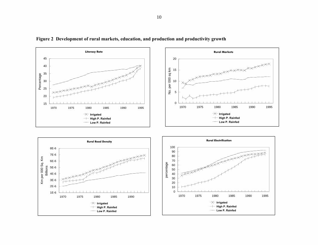
1970 1975 1980 1985 1990 1995

15

20

25

30

35

40

45

Per

cent

age


Literacy Rate

1970 1975 1980 1985 1990 19950

10

20

30

40

50

60

70

80

90

100

perc

enta

ge


Rural Electrification

1970 1975 1980 1985 1990 19950

5

10

15

20

No.

per

000

sq

km


Rural Markets

1970 1975 1980 1985 19901E-6

2E-6

3E-6

4E-6

5E-6

6E-6

7E-6

8E-6

Bill

ions

Km

per

000

Sq.

Km


Rural Road Density

10

Figure 2 Development of rural markets, education, and production and productivity growth

11

rainfed areas, it has increased and converged to about 40 percent in all types of areas.

Rural markets (including both secondary and principal markets), measured as the

number of regulated agricultural markets per thousand square kilometers of geographic

area, increased in all three types of areas between 1970 and 1994. But the density in

rainfed areas is still much lower than in irrigated areas, and it remains particularly sparse in

the low-potential rainfed areas (Figure 2).

The road density in irrigated areas, measured as the length of roads in kilometers

per thousand square kilometers of geographic area, increased from 3,145 in 1970 to 6,926

in 1995; a growth rate of 3.3 percent a year (Figure 2). The road density in high-potential

rainfed areas is now approaching the level of irrigated areas, but the road density in low-

potential rainfed areas is 40 percent lower.

The percentage of villages electrified has also increased substantially since 1970

(Figure 2). Most of the increase occurred during the 1980s, and further growth has been

modest since then. Moreover, while high-potential rainfed areas initially lagged irrigated

and low-potential rainfed areas, all three types of areas now have most of their villages

electrified.

4. PRODUCTION AND PRODUCTIVITY GROWTH

As a result of the rapid adoption of new technologies and increases in rural

infrastructure, agricultural production and factor productivity have grown rapidly in Indian

agriculture in recent decades (Table 2). Five major crops (rice, wheat, sorghum, pearl

millet, and maize), fourteen minor crops (barley, cotton, groundnut, other grain,

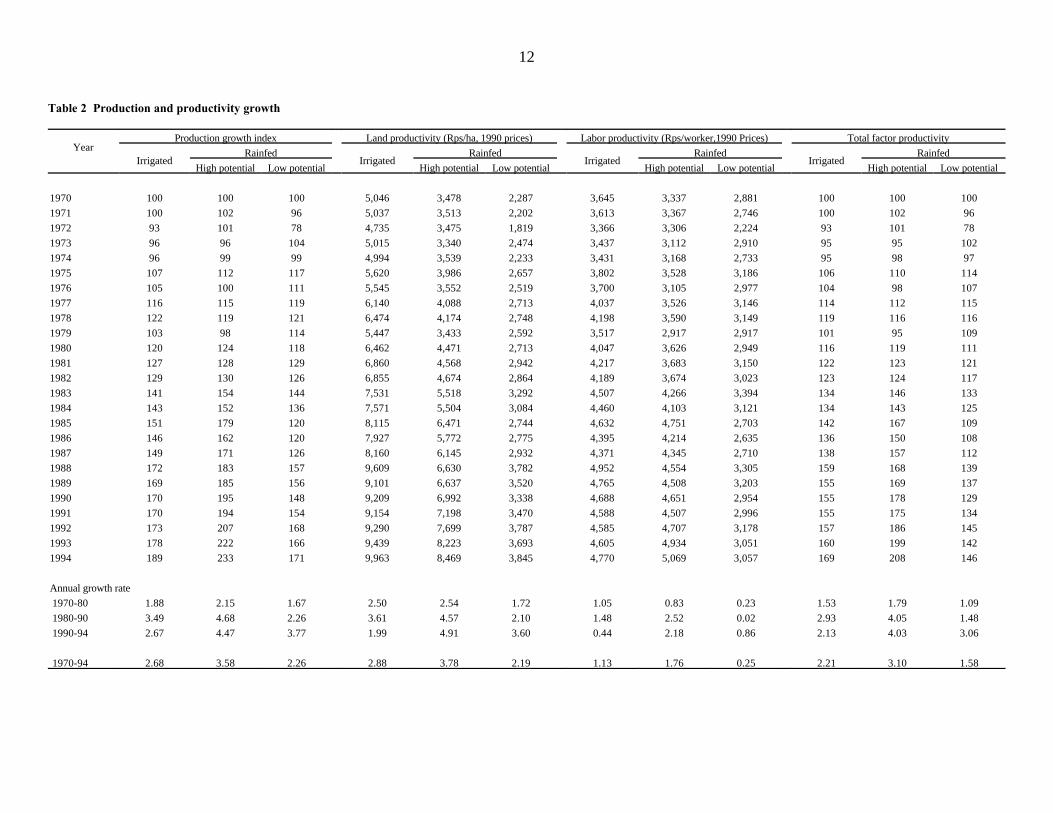
12

Table 2 Production and productivity growth

Year

Production growth index Land productivity (Rps/ha, 1990 prices) Labor productivity (Rps/worker,1990 Prices) Total factor productivity

Irrigated Irrigated Irrigated IrrigatedRainfed Rainfed Rainfed Rainfed

High potential Low potential High potential Low potential High potential Low potential High potential Low potential

1970 100 100 100 5,046 3,478 2,287 3,645 3,337 2,881 100 100 100

1971 100 102 96 5,037 3,513 2,202 3,613 3,367 2,746 100 102 96

1972 93 101 78 4,735 3,475 1,819 3,366 3,306 2,224 93 101 78

1973 96 96 104 5,015 3,340 2,474 3,437 3,112 2,910 95 95 102

1974 96 99 99 4,994 3,539 2,233 3,431 3,168 2,733 95 98 97

1975 107 112 117 5,620 3,986 2,657 3,802 3,528 3,186 106 110 114

1976 105 100 111 5,545 3,552 2,519 3,700 3,105 2,977 104 98 107

1977 116 115 119 6,140 4,088 2,713 4,037 3,526 3,146 114 112 115

1978 122 119 121 6,474 4,174 2,748 4,198 3,590 3,149 119 116 116

1979 103 98 114 5,447 3,433 2,592 3,517 2,917 2,917 101 95 109

1980 120 124 118 6,462 4,471 2,713 4,047 3,626 2,949 116 119 111

1981 127 128 129 6,860 4,568 2,942 4,217 3,683 3,150 122 123 121

1982 129 130 126 6,855 4,674 2,864 4,189 3,674 3,023 123 124 117

1983 141 154 144 7,531 5,518 3,292 4,507 4,266 3,394 134 146 133

1984 143 152 136 7,571 5,504 3,084 4,460 4,103 3,121 134 143 125

1985 151 179 120 8,115 6,471 2,744 4,632 4,751 2,703 142 167 109

1986 146 162 120 7,927 5,772 2,775 4,395 4,214 2,635 136 150 108

1987 149 171 126 8,160 6,145 2,932 4,371 4,345 2,710 138 157 112

1988 172 183 157 9,609 6,630 3,782 4,952 4,554 3,305 159 168 139

1989 169 185 156 9,101 6,637 3,520 4,765 4,508 3,203 155 169 137

1990 170 195 148 9,209 6,992 3,338 4,688 4,651 2,954 155 178 129

1991 170 194 154 9,154 7,198 3,470 4,588 4,507 2,996 155 175 134

1992 173 207 168 9,290 7,699 3,787 4,585 4,707 3,178 157 186 145

1993 178 222 166 9,439 8,223 3,693 4,605 4,934 3,051 160 199 142

1994 189 233 171 9,963 8,469 3,845 4,770 5,069 3,057 169 208 146

Annual growth rate

1970-80 1.88 2.15 1.67 2.50 2.54 1.72 1.05 0.83 0.23 1.53 1.79 1.09

1980-90 3.49 4.68 2.26 3.61 4.57 2.10 1.48 2.52 0.02 2.93 4.05 1.48

1990-94 2.67 4.47 3.77 1.99 4.91 3.60 0.44 2.18 0.86 2.13 4.03 3.06

1970-94 2.68 3.58 2.26 2.88 3.78 2.19 1.13 1.76 0.25 2.21 3.10 1.58

lnYIt'ji1/2((Si, t%Si, t&1)(ln(Yi, t/Yi, t&1),

13

(1)

The formula for the index of aggregate production is:5

where lnYI is the log of the production index at time t, S and S are output I’st I, t i, t-1

share in total production value at time t and t-1, respectively; and Y and Y are i,t i, t-1

quantities of output I at time t and t-1, respectively. Farm prices are used tocalculate the weights of each crop in the value of total production. Unliketraditional measures of production growth which use constant output prices, theTornqvist-Theil index (a discrete approximation to the Divisia index) is desirablebecause of its invariance property: if nothing real has changed (e.g., the only inputquantity changes involve movements along an unchanged isoquant) then the indexitself is unchanged (Diewert 1976; Lau 1979).

other pulses, potato, rapeseed, mustard, sesame, sugar, tobacco, soybeans, jute, and

sunflower), and three major livestock products (milk, chicken, and sheep and goat meat)

are included in our measure of total output. Unlike traditional measures of aggregate

production which use constant output prices, we use the more appropriate Tornqvist-Theil

index (a discrete approximation to the Divisia index).5

For the period 1970 to 1994, agricultural production grew fastest in the high-

potential rainfed areas (3.58 percent per year), followed by irrigated areas (2.68 percent)

and then low-potential rainfed areas (2.26 percent). This may reflect a catching-up effect,

since irrigated production grew rapidly prior to 1970 as a result of the Green Revolution,

and the use of HYVs and fertilizers spread more slowly to rainfed areas. Production

growth in irrigated and high-potential rainfed areas slowed in the early 1990s, whereas it

increased in the low-potential rainfed areas to 3.77 percent per year, more than double the

rate of growth achieved in the 1970s.

Land productivity, measured as the gross value of output in rupees (1990 prices)

14

per hectare of net cropped area, also grew fastest on average in the high-potential rainfed

areas, but the most rapid growth in these areas occurred after 1980 when it increased to

nearly 5 percent per year (Table 2). Average growth in land productivity has also been

quite high in irrigated areas (2.88 percent per year since 1970), though it slowed to less

than 2 percent per year after 1990. In contrast, low-potential rainfed areas experienced

the slowest average growth in land productivity between 1970 and 1990, but growth has

accelerated to 3.6 percent per year since then. Land productivity remains more than twice

as high in irrigated and high-potential rainfed areas than in low-potential areas, and this

gap has widened since 1970.

Growth in labor productivity has been consistently low in all types of Indian

agriculture since 1970, averaging only 1.13, 1.76 and 0.25 percent per year in irrigated

and high- and low-potential rainfed areas, respectively (Table 2). It has accelerated a little

in the low-potential rainfed areas since 1990 (but only to 0.86 percent per year), but has

slowed in irrigated and high-potential rainfed areas. Given that the welfare of the rural

poor can be expected to be closely linked to labor productivity in agriculture, these trends

should be a matter of considerable concern to Indian policymakers.

Total factor productivity (TFP), a measure of the return to all direct and indirect

inputs used in agriculture, grew fastest in high-potential rainfed areas during 1970-1994

(3.1 percent per year), followed by irrigated areas (2.21 percent per year) and then low-

lnTFPt'3i1/2((Si, t%Si, t&1)(ln(Yi, t/Yi, t&1)&3i1/2((Wi, t%Wi, t&1)(ln(Xi, t/Xi, t&1)

15

A Tornqvist-Theil index is used to aggregate both inputs and outputs. 6

Specifically,

where lnTFP is the log of the total factor productivity index; W and W are costt i,t i,t-1

shares of input I in total cost at time t and t-1, respectively; and X and X arei,t i,t-1

quantities of input I at time t and t-1, respectively. Five inputs (labor, land,fertilizer, tractors and buffalo) are included. Labor input is measured as the totalnumber of male and female workers employed in agriculture at the end of each year;land is measured as gross cropped area; fertilizer input is measured as the totalamount of nitrogen, phosphate, and potassium used; tractor input is measured as thenumber of four-wheel tractors; and bullock input is measured as the number of adultbullocks. The wage rate for agricultural labor is used as the price of labor; rentalrates of tractors and bullocks are used for their respective prices; and the fertilizerprice is calculated as a weighted average of the prices of nitrogen, phosphate, andpotassium. The land price is measured as the residual of total revenue net ofmeasured costs for labor, fertilizer, tractors, and bullocks.

potential rainfed areas at 1.58 percent per year (Table 2). TFP growth has slowed in6

irrigated areas since 1990, remained unchanged at nearly 4 percent per year in high-

potential rainfed areas, and accelerated to 3.06 percent per year in low-potential rainfed

areas.

5. RURAL POVERTY

Although the literature on poverty and its links to agricultural growth is extensive

for India, there has been little work on how these relationships are affected at a

disaggregated level by differences in the characteristics of different agro-ecological zones

(Dreza and Srinivasan are an exception) (Ahluwalia 1978; Mellor and Desai 1985; Ghose

1989; Gaiha 1989; Bell and Rich 1994; Ravallion and Datt 1995; Datt and Ravallion 1997

and 1998; Dreze and Srinivasan 1997).

16

We aggregated the available poverty data by agroecological zone into our three7

land types using rural populations as weights. Since agroclimatic zones are moreaggregated than districts (an agroclimatic zone usually consists of 5-10 districts), wedefine agroclimatic zones as rainfed if less than 40 percent of the total cropped area isirrigated, and as irrigated if the irrigated share is more than 40 percent. Rural poverty wasestimated on the basis of consumer expenditure surveys carried out by the NationalSample Survey Organization (NSSO).

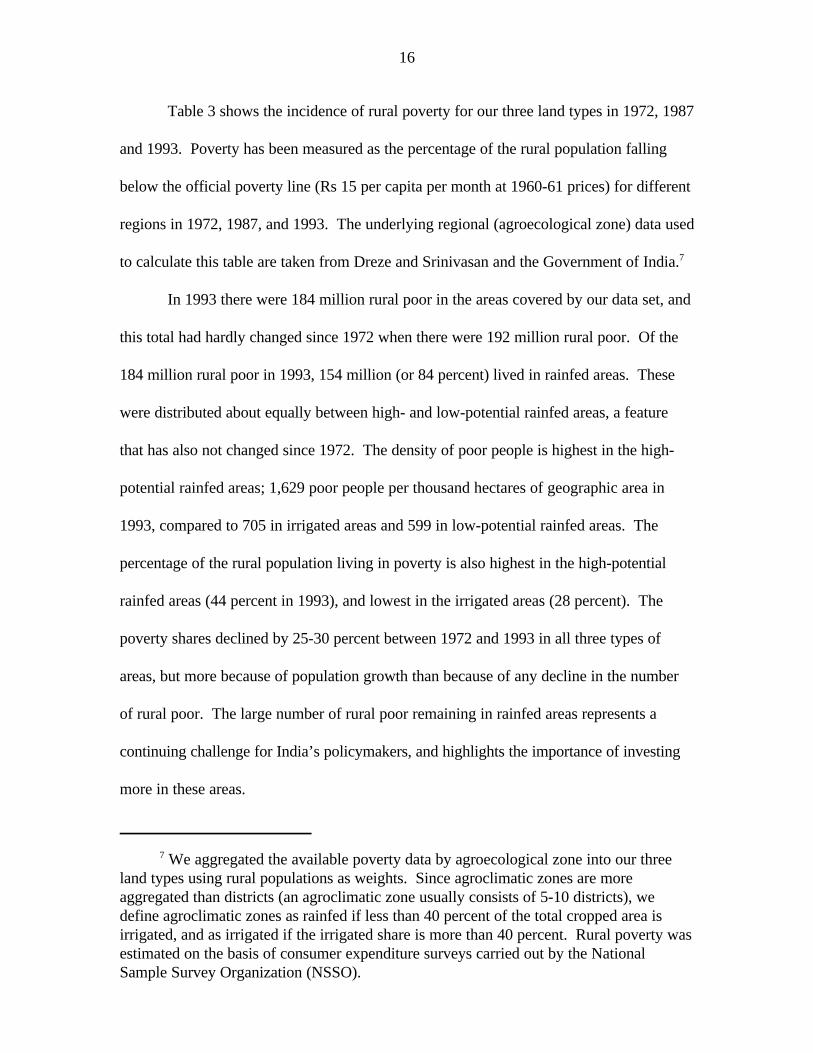
Table 3 shows the incidence of rural poverty for our three land types in 1972, 1987

and 1993. Poverty has been measured as the percentage of the rural population falling

below the official poverty line (Rs 15 per capita per month at 1960-61 prices) for different

regions in 1972, 1987, and 1993. The underlying regional (agroecological zone) data used

to calculate this table are taken from Dreze and Srinivasan and the Government of India.7

In 1993 there were 184 million rural poor in the areas covered by our data set, and

this total had hardly changed since 1972 when there were 192 million rural poor. Of the

184 million rural poor in 1993, 154 million (or 84 percent) lived in rainfed areas. These

were distributed about equally between high- and low-potential rainfed areas, a feature

that has also not changed since 1972. The density of poor people is highest in the high-

potential rainfed areas; 1,629 poor people per thousand hectares of geographic area in

1993, compared to 705 in irrigated areas and 599 in low-potential rainfed areas. The

percentage of the rural population living in poverty is also highest in the high-potential

rainfed areas (44 percent in 1993), and lowest in the irrigated areas (28 percent). The

poverty shares declined by 25-30 percent between 1972 and 1993 in all three types of

areas, but more because of population growth than because of any decline in the number

of rural poor. The large number of rural poor remaining in rainfed areas represents a

continuing challenge for India’s policymakers, and highlights the importance of investing

more in these areas.

17

Table 3 Poverty changes by type of region, rural India

Irrigatedareas

Rainfed areas

Total High potential Low potential

Percentage of poor 1972 39 52 59 47in total population(%)

1987 32 46 48 44

1993 28 39 44 36

Number of poor 1972 37 155 80 75(millions) 1987 35 167 79 88

1993 30 154 78 76

Number of poor perthousand hectaresgeographic areas(millions)

1972 862 880 1,680 583

1987 813 951 1,660 688

1993 705 878 1,629 599

Sources: Authors’ calculation based on data from Dreze and Srinivasan (1996) and theGovernment of India.

Notes: Only 47 agroclimatic zones (of total 65) are included in the calculation due to dataunavailability. An agroclimatic zone is defined as rainfed if less than 40 percent of the totalcropped areas is irrigated, and as irrigated if irrigated share is over 40 percent.

6. EFFECTS OF INFRASTRUCTURE AND TECHNOLOGIES ONPRODUCTION AND RURAL POVERTY

In this section, we analyze how technologies and rural infrastructure have

contributed to production growth and poverty reduction in irrigated and high- and low-

potential rainfed areas.

CONCEPTUAL FRAMEWORK

The conceptual model for our econometric analysis is given by equations (1) to

18

Using cross-section data from a survey of rural households in West Bengal, India,8

Mukhopadhaya found that farmers’ decision to adopt new technology depend mainly onthe quality of their land, irrigation, and profitability (Mukhopadhyay1994).

The interaction between education and technological change during the Green9

Revolution in rural India was recognized by A. Foster and M. Rosenzweig (1996). In ourmodel, we attempt to model the effects of education and infrastructure development on

(7). Equation (1) is the production function. The dependent variable is agricultural

output (Y ), while explanatory variables include traditional farm inputs such as labori,t

(LABOR ), land (LAND ), fertilizer (FERT ), machinery (MACH ), and draft animalsi, t i,t i,t i,t

(ANIMAL ); technology inputs like the percentage of HYVs in total cropped areai,t

(HYV ), the percentage of the total cropped area that is under canal irrigation (GIRRI )i,t i,t

and private irrigation (PIRRI ); infrastructure variables such as road density (ROAD ),i,t i,t

development of rural markets (MKT ), and rural electrification (ELECT ); literacy rate ofi,t i,t

the rural population (LITE ); and a time trend variable that is intended to capture anyi,t

time-related changes that are not captured by other variables. The subscripts i and t

represent districts and years, respectively. Our list of technology and infrastructure

variables is incomplete, but these are key ones for which we have district level data. Due

to the endogeneity of HYVs and irrigation variables in the production function, these

variables are also modeled as endogenous variables in equations (2), (3) and (4). The8

explanatory variables are lagged output prices (ATT ), measured as the previous five-yeari,t

moving average of agricultural prices divided by a relevant GNP deflator, and other social

and infrastructure variables like rural education and road density. The estimation of these

equations also enables us to measure the indirect impact of rural infrastructure and

education on agricultural production through improved technologies.9

19

production directly and indirectly through the adoption of new technologies such as theuse of HYVs and private irrigation.

A. Sen (1997) argued that the real explanation for the rise in agricultural wages10

lies in the rapid growth of rural nonagricultural employment. However, the developmentof rural nonagricultural employment depends largely on the development of ruralinfrastructure. Including the infrastructure variables in the wage equation captures thedirect impact of improved infrastructure on wage increases.

Poverty (defined as the percentage of the rural population living below the official

poverty line) is modeled in equation (5) as a function of agricultural production, wages (a

weighted average of the daily agricultural wages for male and female workers deflated by

the CPI for agricultural labor), and a terms of trade variable (TT) measured as the

agricultural GDP deflator divided by the non-agricultural GDP deflator. Increases in

agricultural output or wages should help the poor to increase their incomes, and hence

reduce poverty. Improvements in the terms of trade for agriculture can be expected to

benefit farmers, but by raising the price of food they can also increase poverty in the short

run, particularly among the landless and small farmers who are net purchasers of food.

However, in the long run, improvements in the terms of trade for agriculture should lead

to greater investment in irrigation and HYVs (see equations 2, 3 and 4) which in turn can

be beneficial to the poor.

Equation (6) models wages as a function of agricultural output, roads,

electrification, and rural literacy. All four variables are expected to contribute to higher

wages. Roads have an indirect impact on wages through agricultural growth (equation 1),

but may also contribute directly by promoting growth of the rural nonfarm economy (not

modeled explicitly here) and through enhancing commuting opportunities.10

20

The agricultural terms of trade is modeled in equation (7) at the district level. They

are expected to decline with increases in agricultural production at the national and district

levels. National agricultural output is included to capture downward pressure on prices

arising from increases in output anywhere in India. We initially included some demand

side variables in the equation (population size and per capita income), but these turned out

not to be statistically significant and were dropped from the model.

As specified above, estimation biases could arise if government investments in

technology and rural infrastructure are systematically targeted to different kinds of regions

(e.g., if government gives higher priority to high-potential areas). In this case, the

investment variables may be correlated with the error terms in the production and poverty

equations (Binswanger, Rosenzweig, and Khandker 1993). We do not have enough

exogenous variables to fully resolve this problem, and have attempted to reduce the size of

the possible estimation biases by including annual rainfall in many of the equations. We

expect rainfall to act as a proxy for agricultural potential, which is presumed to drive any

selection bias in government decisions. We also added district dummies in all equations to

capture any remaining fixed effects of agroecological characteristics.

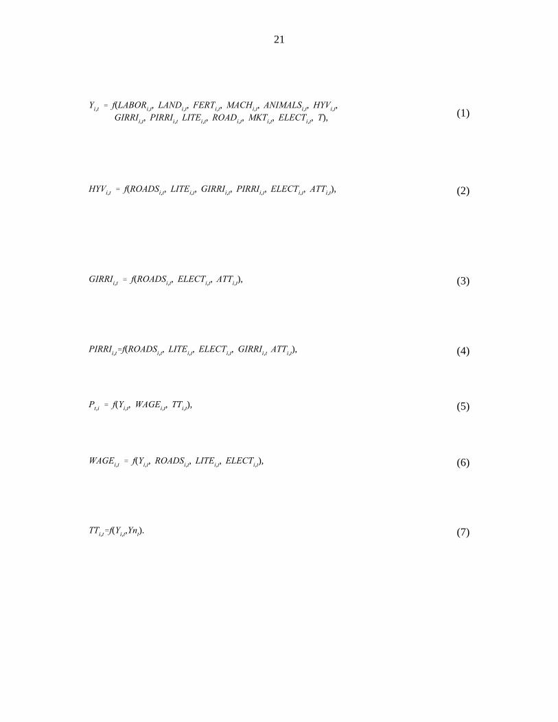
Yi,t ' f(LABORi,t, LANDi,t, FERTi,t, MACHi,t, ANIMALSi,t, HYVi,t,GIRRIi,t, PIRRIi,t LITEi,t, ROADi,t, MKTi,t, ELECTi,t, T),

WAGEi,t ' f(Yi,t, ROADSi,t, LITEi,t, ELECTi,t),

HYVi,t ' f(ROADSi,t, LITEi,t, GIRRIi,t, PIRRIi,t, ELECTi,t, ATTi,t),

GIRRIi,t ' f(ROADSi,t, ELECTi,t, ATTi,t),

PIRRIi,t'f(ROADSi,t, LITEi,t, ELECTi,t, GIRRIi,t ATTi,t),

TTi,t'f(Yi,t,Ynt).

Pt,i ' f(Yi,t, WAGEi,t, TTi,t),

21

(1)

(6)

(2)

(3)

(4)

(7)

(5)

gijt'Djgijt&1%eijt,

22

For more information about the specification of serial correlation in an equation11

system, and its estimation, refer to pages 81 and 113 of Baltagi (1995).

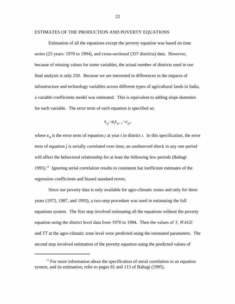
ESTIMATES OF THE PRODUCTION AND POVERTY EQUATIONS

Estimation of all the equations except the poverty equation was based on time

series (25 years: 1970 to 1994), and cross-sectional (337 districts) data. However,

because of missing values for some variables, the actual number of districts used in our

final analysis is only 250. Because we are interested in differences in the impacts of

infrastructure and technology variables across different types of agricultural lands in India,

a variable coefficients model was estimated. This is equivalent to adding slope dummies

for each variable. The error term of each equation is specified as:

where g is the error term of equation j at year t in district i. In this specification, the errorijt

term of equation j is serially correlated over time; an unobserved shock in any one period

will affect the behavioral relationship for at least the following few periods (Baltagi

1995). Ignoring serial correlation results in consistent but inefficient estimates of the11

regression coefficients and biased standard errors.

Since our poverty data is only available for agro-climatic zones and only for three

years (1972, 1987, and 1993), a two-step procedure was used in estimating the full

equations system. The first step involved estimating all the equations without the poverty

equation using the district level data from 1970 to 1994. Then the values of Y, WAGE

and TT at the agro-climatic zone level were predicted using the estimated parameters. The

second step involved estimation of the poverty equation using the predicted values of

23

independent variables at the agro-climatic zone level using the available poverty data for

1972, 1987 and 1993. Both linear and double-log forms of the equations were estimated.

However, we only report the results of the double-log specification since these gave

superior fits and had more statistically significant coefficients. As such, all the coefficients

are in elasticity form.

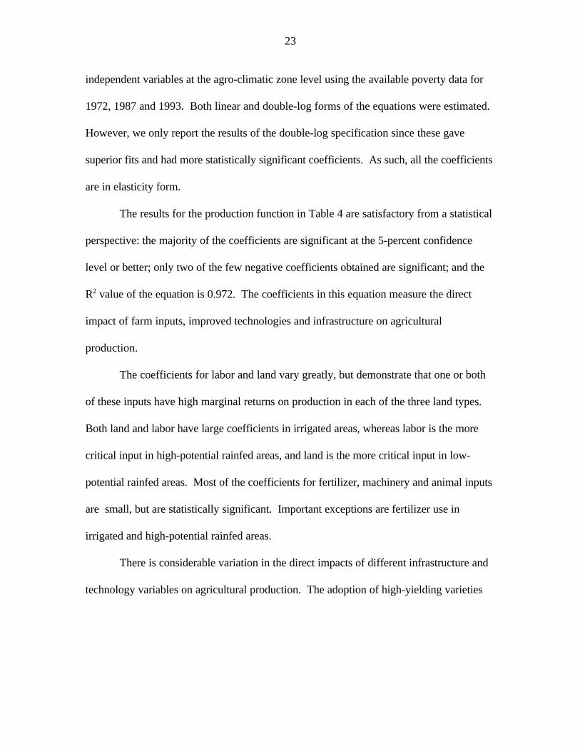
The results for the production function in Table 4 are satisfactory from a statistical

perspective: the majority of the coefficients are significant at the 5-percent confidence

level or better; only two of the few negative coefficients obtained are significant; and the

R value of the equation is 0.972. The coefficients in this equation measure the direct2

impact of farm inputs, improved technologies and infrastructure on agricultural

production.

The coefficients for labor and land vary greatly, but demonstrate that one or both

of these inputs have high marginal returns on production in each of the three land types.

Both land and labor have large coefficients in irrigated areas, whereas labor is the more

critical input in high-potential rainfed areas, and land is the more critical input in low-

potential rainfed areas. Most of the coefficients for fertilizer, machinery and animal inputs

are small, but are statistically significant. Important exceptions are fertilizer use in

irrigated and high-potential rainfed areas.

There is considerable variation in the direct impacts of different infrastructure and

technology variables on agricultural production. The adoption of high-yielding varieties

24

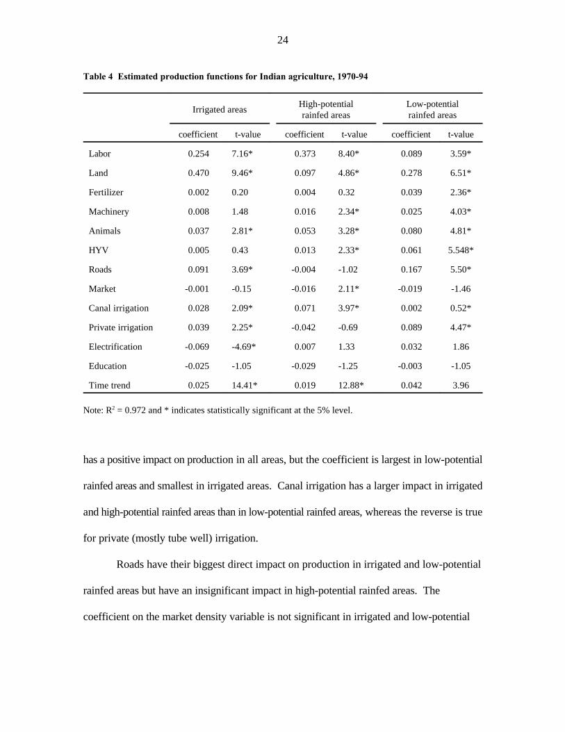
Table 4 Estimated production functions for Indian agriculture, 1970-94

Irrigated areasHigh-potential Low-potentialrainfed areas rainfed areas

coefficient t-value coefficient t-value coefficient t-value

Labor 0.254 7.16* 0.373 8.40* 0.089 3.59*

Land 0.470 9.46* 0.097 4.86* 0.278 6.51*

Fertilizer 0.002 0.20 0.004 0.32 0.039 2.36*

Machinery 0.008 1.48 0.016 2.34* 0.025 4.03*

Animals 0.037 2.81* 0.053 3.28* 0.080 4.81*

HYV 0.005 0.43 0.013 2.33* 0.061 5.548*

Roads 0.091 3.69* -0.004 -1.02 0.167 5.50*

Market -0.001 -0.15 -0.016 2.11* -0.019 -1.46

Canal irrigation 0.028 2.09* 0.071 3.97* 0.002 0.52*

Private irrigation 0.039 2.25* -0.042 -0.69 0.089 4.47*

Electrification -0.069 -4.69* 0.007 1.33 0.032 1.86

Education -0.025 -1.05 -0.029 -1.25 -0.003 -1.05

Time trend 0.025 14.41* 0.019 12.88* 0.042 3.96

Note: R = 0.972 and * indicates statistically significant at the 5% level.2

has a positive impact on production in all areas, but the coefficient is largest in low-potential

rainfed areas and smallest in irrigated areas. Canal irrigation has a larger impact in irrigated

and high-potential rainfed areas than in low-potential rainfed areas, whereas the reverse is true

for private (mostly tube well) irrigation.

Roads have their biggest direct impact on production in irrigated and low-potential

rainfed areas but have an insignificant impact in high-potential rainfed areas. The

coefficient on the market density variable is not significant in irrigated and low-potential

25

rainfed areas, but is positive and very significant in high-potential rainfed areas. Rural

electrification only has a positive and statistically significant coefficient in low- potential

rainfed areas. The direct impacts of education are not statistically significant in any of the

three regions. The positive and statistically significant coefficients for the time trend

variable suggest that there are important but missing technology and infrastructure

variables in the model. These may include the impacts of agricultural research not

captured by the HYV variable (e.g., research on improved husbandry practices), and

agricultural extension and technical education for farmer.

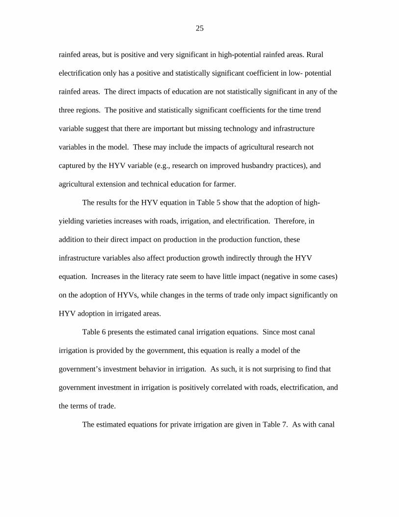
The results for the HYV equation in Table 5 show that the adoption of high-

yielding varieties increases with roads, irrigation, and electrification. Therefore, in

addition to their direct impact on production in the production function, these

infrastructure variables also affect production growth indirectly through the HYV

equation. Increases in the literacy rate seem to have little impact (negative in some cases)

on the adoption of HYVs, while changes in the terms of trade only impact significantly on

HYV adoption in irrigated areas.

Table 6 presents the estimated canal irrigation equations. Since most canal

irrigation is provided by the government, this equation is really a model of the

government’s investment behavior in irrigation. As such, it is not surprising to find that

government investment in irrigation is positively correlated with roads, electrification, and

the terms of trade.

The estimated equations for private irrigation are given in Table 7. As with canal

26

Table 5 Estimated equation for high-yielding varieties in India



Roads -0.074 -1.70 0.274 3.77* 0.258 3.51*

Canal irrigation 0.182 7.22* -0.068 -1.68 0.014 2.89*

Private irrigation 0.087 2.64* 0.338 7.55* 0.205 5.44*

Electrification 0.110 4.37* 0.020 1.98* 0.050 2.58*

Education -0.261 -5.92* 0.267 1.88 -0.334 -6.23*

Terms of Trade 0.141 2.70* -0.127 0.57 -0.160 -1.10


Table 6 Estimated canal irrigation equations for India



Roads 0.164 4.62* 0.298 6.84* 0.657 13.26*


Terms of Trade .053 1.13 -0.160 1.25 0.198 3.03*


Table 7 Estimated private irrigation equations for India



Roads 0.101 3.69* 0.05 2.40* -0.13 1.78


Canal Irrigation 0.221 12.18* 0.580 26.36* 0.310 16.58*

Education 0.101 3.27* 0.278 6.58* 0.539 11.62*

Terms of Trade 0.024 0.74 -0.070 -0.64 0.059 1.95*


irrigation, private investment in irrigation increases with roads, electrification, and the

27

The evidence from Tables 4 to 7 show that education and electrification have little12

direct impact on production growth, but they affects production mainly through theadoption of HYVs and improved irrigation.

The correlation between the change in the terms of trade and rural poverty was13

also found by Misra and Hazell (1996).

terms of trade. In addition, government investment in canal irrigation is complementary to

private irrigation investment in all three types of areas; it raises the groundwater level

which makes tubewell investments more profitable. Government investment in irrigation

not only affects agricultural production directly, but also enhances production indirectly

through greater use of high-yielding varieties, and by encouraging greater private

investment in irrigation. Literacy also has a large and significant impact on private

irrigation.12

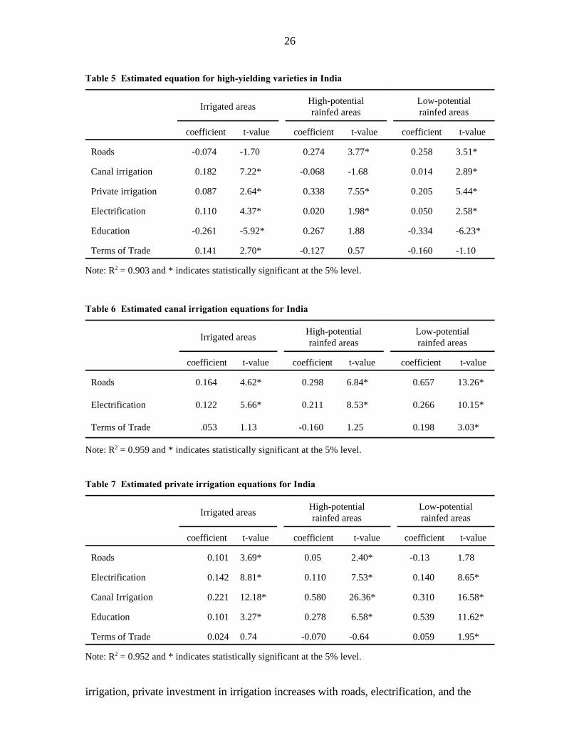
The coefficients of the poverty equation in Table 8 are all signed according to

expectations. Higher production growth and higher wages both contribute to reductions

in rural poverty (hence the negative signs), while increases in the agricultural terms of

trade are harmful to the poor in the short run.13

Table 8 Estimated poverty equations for India



Production growth -0.160 -1.83 -0.170 -1.75 -0.310 -2.18*

Wage -0.157 -1.99* -0.161 -2.01* -0.022 -1.41

Terms of Trade 0.258 1.48 0.268 1.41 0.123 1.97*

R = 0.757 and * indicates statistically significant at the 5% level.2

Table 9 presents the estimated coefficients for the wage equations. With only one

exception (literacy in low-potential rainfed areas), increases in agricultural production,

28

roads, education and rural electrification all have a positive and statistically significant

impact on wages. However, increases in the agricultural terms of trade have a negative

impact on real wages in the short run.

Table 9 Estimated wage equations for India



Production growth 0.201 9.91* 0.050 5.63* 0.101 6.36*

Roads 0.098 4.47* 0.097 4.46* 0.248 8.77*

Education 0.103 4.36* 0.233 7.50* -0.03 -1.09


Terms of Trade -0.190 -7.25* -0.160 -6.35* -0.371 -11.55*


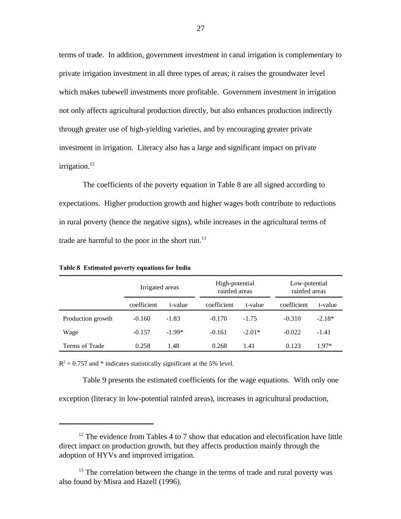
The estimated terms of trade equations in Table 10 show that increases in local and

national agricultural production both contribute to lower real prices for farmers. Markets

apparently do work despite the heavy intervention policies of the government during much

of the period analyzed.

Table 10 Estimated terms of trade equations for India



District production -0.134 -8.29* -0.018 -4.11* 0.005 1.80growth

National production -0.208 -8.07* -0.104 -5.78* -0.258 -9.56*growth


29

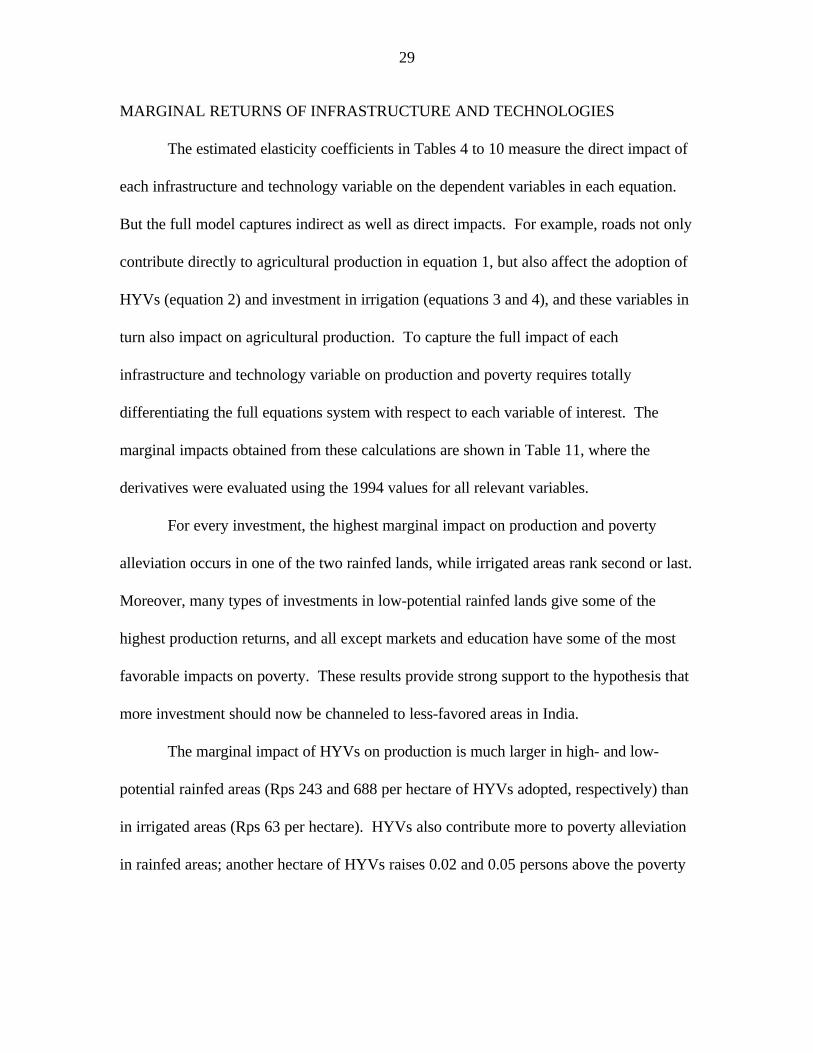
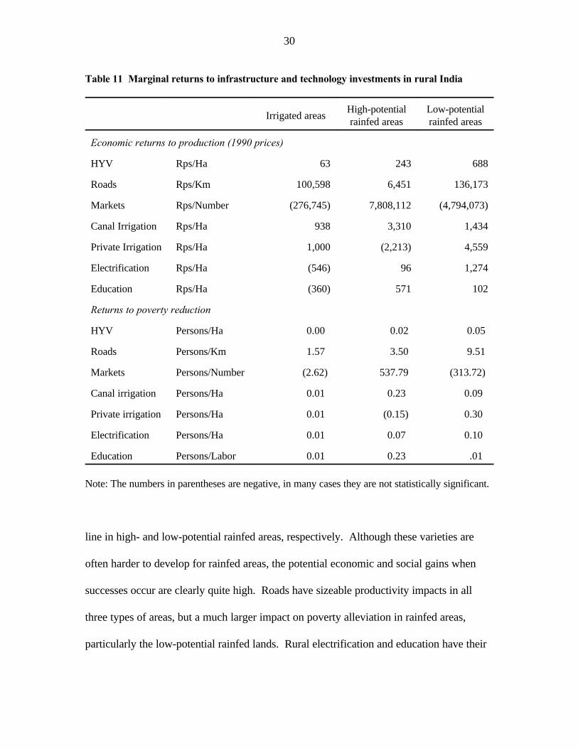
MARGINAL RETURNS OF INFRASTRUCTURE AND TECHNOLOGIES

The estimated elasticity coefficients in Tables 4 to 10 measure the direct impact of

each infrastructure and technology variable on the dependent variables in each equation.

But the full model captures indirect as well as direct impacts. For example, roads not only

contribute directly to agricultural production in equation 1, but also affect the adoption of

HYVs (equation 2) and investment in irrigation (equations 3 and 4), and these variables in

turn also impact on agricultural production. To capture the full impact of each

infrastructure and technology variable on production and poverty requires totally

differentiating the full equations system with respect to each variable of interest. The

marginal impacts obtained from these calculations are shown in Table 11, where the

derivatives were evaluated using the 1994 values for all relevant variables.

For every investment, the highest marginal impact on production and poverty

alleviation occurs in one of the two rainfed lands, while irrigated areas rank second or last.

Moreover, many types of investments in low-potential rainfed lands give some of the

highest production returns, and all except markets and education have some of the most

favorable impacts on poverty. These results provide strong support to the hypothesis that

more investment should now be channeled to less-favored areas in India.

The marginal impact of HYVs on production is much larger in high- and low-

potential rainfed areas (Rps 243 and 688 per hectare of HYVs adopted, respectively) than

in irrigated areas (Rps 63 per hectare). HYVs also contribute more to poverty alleviation

in rainfed areas; another hectare of HYVs raises 0.02 and 0.05 persons above the poverty

30

Table 11 Marginal returns to infrastructure and technology investments in rural India


Economic returns to production (1990 prices)

HYV Rps/Ha 63 243 688

Roads Rps/Km 100,598 6,451 136,173

Markets Rps/Number (276,745) 7,808,112 (4,794,073)

Canal Irrigation Rps/Ha 938 3,310 1,434

Private Irrigation Rps/Ha 1,000 (2,213) 4,559

Electrification Rps/Ha (546) 96 1,274

Education Rps/Ha (360) 571 102

Returns to poverty reduction

HYV Persons/Ha 0.00 0.02 0.05

Roads Persons/Km 1.57 3.50 9.51

Markets Persons/Number (2.62) 537.79 (313.72)

Canal irrigation Persons/Ha 0.01 0.23 0.09

Private irrigation Persons/Ha 0.01 (0.15) 0.30

Electrification Persons/Ha 0.01 0.07 0.10

Education Persons/Labor 0.01 0.23 .01

Note: The numbers in parentheses are negative, in many cases they are not statistically significant.

line in high- and low-potential rainfed areas, respectively. Although these varieties are

often harder to develop for rainfed areas, the potential economic and social gains when

successes occur are clearly quite high. Roads have sizeable productivity impacts in all

three types of areas, but a much larger impact on poverty alleviation in rainfed areas,

particularly the low-potential rainfed lands. Rural electrification and education have their

31

biggest productivity impacts in rainfed areas, and they also impact favorable on the poor in

these areas. Their impacts in irrigated areas are very small. Canal irrigation has its biggest

productivity and poverty impacts in high-potential rainfed areas, while private irrigation

has its biggest impacts in low-potential rainfed areas. Market development has a huge

marginal impact on production and poverty alleviation in the high-potential rainfed areas,

but not in irrigated and low-potential rainfed areas.

It should be noted that the marginal impacts of different investments reported

above are gross of their costs. It could be argued that some investments are more

expensive to undertake in less-favored areas, because of their diverse and generally less

favorable agroecological conditions. For example, the development of HYVs may be

more difficult for less-favored areas, and their widespread adoption may be more

constrained by the diversity of growing conditions. Investments in roads and other

infrastructure may also be more costly in many less-favored lands because of difficult

topographical conditions, or remoteness from major population centers or markets. Data

that we have obtained at the state level for India suggest that the unit costs of key

investments are not all that different across states, despite considerable diversity in the

proportions of their irrigated and rainfed areas (Fan, Hazell, and Thorat 1998).

7. CONCLUSIONS

In order to promote economic growth and to redress poverty, policymakers in

developing countries will need to promote agricultural intensification for both high- and

low-potential regions. This dual strategy will be particularly challenging if government

32

budgets for investment in agriculture and rural areas continue to remain tight, and striking

the right investment balance between irrigated and rainfed regions, and between high and

low-potential rainfed areas will be particularly important. Investments in irrigated and

high-potential rainfed areas cannot be neglected because these areas still provide much of

the food needed to keep prices low, and to feed growing livestock and urban populations.

On the other hand, the poverty, food security and environmental problems of many

low-potential areas are likely to remain serious in the decades ahead as populations

continue to grow. While out-migration and economic diversification should become

increasingly important in the development of most low-potential areas, agricultural

intensification will often offer the only viable way of raising incomes and creating

employment on the scale required in the near future. Even when the investments needed

to achieve this growth yield lower economic returns than investments in high-potential

areas, they might still be justified on the basis of their significant social benefits in the form

of poverty alleviation and improved environmental management. Moreover, with

worsening income disparities between many high- and low-potential areas, policymakers

are likely to come under increasing pressure to invest more in low-potential areas.

The size of the potential tradeoffs between investing in high- and low-potential

areas have yet to be widely quantified, and it is possible that they may be changing.

Productivity levels in many high-potential areas have reached a plateau, while at the same

time recent agricultural research in some low-potential rainfed areas is suggesting new

avenues for increasing their productivity. Our analysis of investments in irrigated and

high- and low-potential rainfed areas in India suggests that investments in rural

33

infrastructure, agricultural technology and human capital are now at least as productive in

many rainfed areas as in irrigated areas, and they have a much larger impact on poverty.

These results raise the tantalizing possibility that greater public investment in some low-

potential areas could actually offer a “win-win” strategy for addressing productivity and

poverty problems.

The successful development of less-favored lands will require new and improved

approaches, particularly for agricultural intensification (Hazell and Fan 1998). These will

require stronger partnerships than needed in high-potential areas between agricultural

researchers and other agents of change, including local organizations, farmers, community

leaders, nongovernmental organizations, national policymakers and donors. It will also

require time and innovation; new approaches will need to be developed and tried on a

small scale before they are scaled up, and their testing will take time to assess and

evaluate, particularly given the noise introduced by climatic variability. All this will

require patience and perseverence on the part of policymakers and donors, perhaps more

than the current aid culture allows.

34

REFERENCES

Ahluwalia, M. 1978. Rural poverty and agricultural performance in India. Journal ofDevelopment Studies 14: 298-323.

Baltagi, B. 1995. Econometric analysis of panel data. New York: John Wiley & Sons.

Bell, C., and R. Rich. 1994. Rural poverty and aggregate agricultural performance inpost independence India. Oxford Bulletin of Economics and Statistics 56.

Binswanger, H., M. Rosenzweig, and S. Khandker. 1993. How infrastructure andfinancial institutions affect agricultural output and investment in India Journal ofDevelopment Economics 41 (99): 337-66.

Consultative Group on International Agricultural Research. 1998. CGIAR Study onMarginal Lands. Technical Advisory Committee. Washington, D.C.: CGIAR.

Datt, G., and M. Ravallion. 1997. Why have some Indian states performed better thanothers at reducing rural poverty? FCND Discussion Paper No. 26. InternationalFood Policy Research Institute, Washington, D.C.

Datt, G., and M. Ravallion. 1998. Farm productivity and rural poverty in India. Journalof Development Studies 34: 62-85.

Diewert, W. 1976. Exact and superlative index numbers. Journal of Econometrics 4:115-46.

Dreze, J., and P. Srinivasan. 1996. Poverty in India: Regional estimates, 1987-8. DelhiSchool of Economics and Indira Gandhi Institute of Development Research. Mimeo.

Fan, S., P. Hazell, and S. Thorat. 1998. Government spending, growth, and poverty: Ananalysis of interlinkages in rural India. EPTD Discussion Paper No. 33,International Food Policy Research Institute, Washington, D.C.

Foster, A., and M. Rosenzweig. 1996. Technical change and human-capital returns andinvestments: Evidence from the Green Revolution. American Economic Review 86:931-53.

Gaiha, R. 1989. Poverty, agricultural production and prices in rural India - Areformation. Cambridge Journal of Economics 13: 333-352.

Ghose, A. 1989. Rural poverty and relative prices in India. Cambridge Journal ofEconomics 13: 307-331.

35

Hayami, Y., and V. Ruttan. 1985. Agricultural development: An internationalperspective. Baltimore, Md.: Johns Hopkins University Press.

Hazell, P., and S. Fan. 1998. Balancing regional development priorities to achievesustainable and equitable agricultural growth. Paper prepared for the AAEAInternational Conference on Agricultural Intensification, Economic Developmentand the Environment, July 31 - August 1, Salt Lake City, Ut.

Hazell, P., and J. Garrett. 1996. Reducing poverty and protecting the environment. Theoverlooked potential of less-favored lands. 2020 Brief 39. Washington, D.C.:International Food Policy Research Institute.

Lau, L. 1979. On exact numbers. Review of Economics and Statistics 61: 73-82.

Mellor, J., and G. Desai, eds. 1985. Rural poverty, agricultural production, and prices: Areexamination. In Agricultural Change and Rural Poverty. Baltimore, Md.,U.S.A.: Johns Hopkins University Press.

Misra, V. and P. Hazell. 1996. Terms of trade, rural poverty, technology and investment:the Indian experience, 1952-53 to 1990-91. Economic and Political Weekly 31:A2-A13.

Mukhopadhyay, S. 1994. Adapting household behavior to agricultural technology inWest Bengal, India: Wage labor, fertility and child schooling determinants.Economic Development and Cultural Change 43: 91-115.

NBSS&LUP. 1992. Agro-ecological regions of India, 2 ed. NBSS Publication No. 24. nd

Nagpur: National Bureau of Soil Survey and Land Use Planning, and New Delhi:Oxford and IBH.

Owens, T., and J. Hoddinott. 1999. Investing in development or investing in relief:Quantifying the poverty tradeoffs using Zimbabwe household panel data. Washington, D.C.: International Food Policy Research Institute.

Pingali, P., and M. Rosegrant. 1998. Intensive food systems in Asia: Can the degradationproblems be reversed? Paper presented at the pre-conference workshop“Agricultural Intensification, Economic Development and the Environment” of theAnnual Meeting of the American Agricultural Economics Association held in SaltLake City, Utah, July 31-August 1.

Pinstrup-Andersen, P., and P. Hazell. 1985. The impact of the green revolution andprospects for the future. Food Reviews International 1 (1).

36

Ravallion, M., and G. Datt. 1995. Growth and poverty in rural India. World Bank PolicyResearch Working Paper. Washington, D.C: World Bank.

Scherr, S., and P. Hazell. 1994. Sustainable agricultural development strategies in fragilelands. EPTD Discussion Paper No. 1, International Food Policy ResearchInstitute,Washington, D.C.

Sen, A. 1997. Structural adjustment and rural poverty: Variables that really matter. InGrowth, employment and poverty: Change and continuity in Rural India, ed. G.Chadha and A. Sharma. New Delhi: Vikas Publishing House.

Are returns to public investment lower in less-favored rural areas?: an empirical analysis of India

Documents

Transcript of Are returns to public investment lower in less-favored rural areas?: an empirical analysis of India