ArcFuels User Guide and Tutorial: for Use with ArcGIS 9®

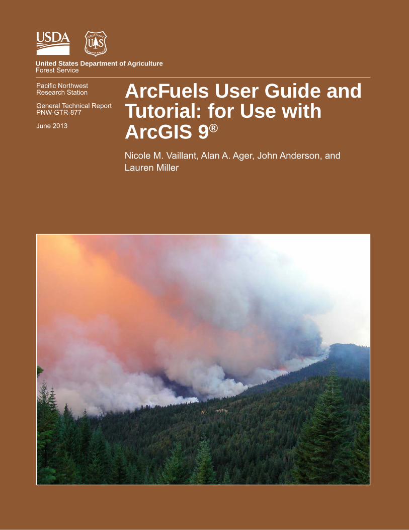
Pacific Northwest Research Station

General Technical Report PNW-GTR-877

June 2013

ArcFuels User Guide and Tutorial: for Use with ArcGIS 9®

Nicole M. Vaillant, Alan A. Ager, John Anderson, and Lauren Miller

DEPAR TMENT OF AGRICULT URE

United States Department of AgricultureForest Service

AuthorsNicole M. Vaillant is a fire ecologist and Alan A. Ager is an operations research analyst, U.S. Department of Agriculture, Forest Service, Pacific Northwest Research Station, Western Wildlands Environmental Threat Assessment Center, 3160 NE 3rd Street, Prineville, OR 97754; John Anderson is a lead programmer, BalanceTech, 534 Fairview Avenue, Missoula, MT 59801; and Lauren Miller is a fire and fuels specialist, U.S. Department of Agriculture, Forest Service, Deschutes National Forest, 63095 Deschutes Market Road, Bend, OR 97701.

Cover photograph by Tom Iraci.

The Forest Service of the U.S. Department of Agriculture is dedicated to the principle of multiple use management of the Nation’s forest resources for sustained yields of wood, water, forage, wildlife, and recreation. Through forestry research, cooperation with the States and private forest owners, and management of the National Forests and National Grasslands, it strives—as directed by Congress—to provide increasingly greater service to a growing Nation.

The U.S. Department of Agriculture (USDA) prohibits discrimination in all its programs and activities on the basis of race, color, national origin, sex, religion, age, disability, sexual orientation, marital status, family status, status as a parent (in education and training programs and activities), because all or part of an individual’s income is derived from any public assistance program, or retaliation. (Not all prohibited bases apply to all programs or activities.)

If you require this information in alternative format (Braille, large print, audiotape, etc.), contact the USDA’s TARGET Center at (202) 720-2600 (Voice or TDD).

If you require information about this program, activity, or facility in a language other than English, contact the agency office responsible for the program or activity, or any USDA office.

To file a complaint alleging discrimination, write USDA, Director, Office of Civil Rights, 1400 Independence Avenue, S.W., Washington, D.C. 20250-9410, or call toll free, (866) 632-9992 (Voice). TDD users can contact USDA through local relay or the Federal relay at (800) 877-8339 (TDD) or (866) 377-8642 (relay voice users). You may use USDA Program Discrimination Complaint Forms AD-3027 or AD-3027s (Spanish) which can be found at: http://www.ascr.usda.gov/complaint_filing_cust.html or upon request from a local Forest Service office. USDA is an equal opportunity provider and employer.

AbstractVaillant, Nicole M.; Ager, Alan A.; Anderson, John; Miller, Lauren. 2013.

ArcFuels User Guide and Tutorial: for use with ArcGIS 9. Gen. Tech. Rep. PNW-GTR-877. Portland, OR: U.S. Department of Agriculture, Forest Service, Pacific Northwest Research Station. 256 p.

Fuel management planning can be a complex problem that is assisted by fire behavior modeling and geospatial analyses. Fuel management often is a particularly complicated process in which the benefits and potential impacts of fuel treatments need to be demonstrated in the context of land management goals and public expec-tations. Fire intensity, likelihood, and effects can be analyzed for multiple treatment alternatives. Depending on the goal, the effect of treatments on wildfire impacts can be considered at multiple scales, from a single forest stand or planning unit to a watershed to a national forest to the Nation as a whole.

The fuel treatment planning process is complicated by the lack of data assimila-tion among fire behavior models and by weak linkages to geographic information systems, corporate data, and desktop office software. ArcFuels is a streamlined fuel management planning and wildfire risk assessment system. ArcFuels creates a trans-scale (stand to large landscape) interface to apply various forest growth and fire behavior models within an ArcGIS® platform to design and test fuel treatment alternatives. It eliminates a number of tedious data transformations and repetitive processes that have plagued the fire operations and research communities as they apply the models to solve fuel management problems.

This User Guide and Tutorial includes an overview of ArcFuels and its func-tionality, a tutorial highlighting all the tools within ArcFuels, and fuel treatment planning scenarios. There is also a section for obtaining, formatting, and setting up ArcFuels for use with your own data. It is assumed that the reader has basic famil-iarity with the Forest Vegatetion Simulator (forest growth and yield program) and FlamMap (landscape fire behavior model).

Keywords: ArcGIS, fire behavior models, forest growth models, fuel treatment planning, wildfire hazard, wildfire risk.

Contents

Chapter 1 1 What is ArcFuels? 2 Modeling Fuel Treatments With FFE-FVS 4 Simulating Landscape Fire Behavior and Fuel Treatments 5 Burn Probability Modeling and Risk Analysis 6 Fuel Treatment Impacts on Carbon

Chapter 2 7 Getting Started 7 Purpose of the User Guide and Tutorial 7 User Guide and Tutorial Conventions 8 System Requirements 8 ArcFuels Download and Installation Instructions 10 Mt. Emily Demonstration Data 12 Setting up ArcFuels With the Mt. Emily Demonstration Data 17 Start-up Errors 17 Visual Basic editor window— 18 Missing buttons—

Chapter 3 19 ArcFuels Tool Overview 20 Stand and Select Stand 20 Set Stand Options— 23 View FVS I/O— 24 SVS— 24 Select Stand— 24 Cell Data 25 Landscape 25 Assign Prescriptions to Landscape— 27 Simulate Landscape Treatments— 31 Build FlamMap Landscape— 34 GNN to LCP Process— 36 Landscape Treatment Designer (LTD)— 37 Wildfire Models 37 Behave Calculator— 38 Modify Grid Values 39 Conversion 40 Convert Ascii to Grid— 40 Batch Convert Ascii to Grid—

42 Convert XY Text to Shapefile— 42 Batch Convert XY Text to Shapefile— 43 Copy Attributes to Spreadsheet— 44 Projects and Files 44 Manage Projects— 44 File Explorer— 44 File Janitor— 45 ArcFuels Help

Chapter 4 46 ArcFuels Tool Tutorial 46 Stand and Select Stand 46 Exercise 4-1: Running FVS and SVS for an untreated stand— 51 Exercise 4-2: Creating NEXUS input files— 55 Exercise 4-3: Running a combination treatment (thinning and prescribed fire) followed by a wildfire in FVS— 59 Exercise 4-4: Using FVS to create treatment adjustment factors for grid data— 60 Exercise 4-5: Fine tuning treatment prescriptions using the Treatment Analysis tab— 63 Exercise 4-6: Comparing treatment prescriptions using the Compare Treatments tab— 66 Exercise 4-7: Opening FVS output files— 70 Cell Data 70 Exercise 4-8: Cell data information— 70 Landscape 71 Exercise 4-9: Assigning FVS prescriptions by selecting individual stands— 72 Exercise 4-10: Assign FVS prescriptions to ArcGIS-selected features— 76 Exercise 4-11: Assign prescriptions with a treatment grid— 78 Exercise 4-12: Running FVS for the no-treatment alternative— 81 Exercise 4-13: Simulating landscape treatments in FVS to create an ideal landscape for the TOM in FlamMap— 83 Exercise 4-14: Simulating landscape treatments in FVS only to stands with prescriptions— 85 Exercise 4-15: Using the Treatment Analysis tab to vary a single parameter— 89 Exercise 4-16: Comparing carbon offsets between treatment alternatives— 91 Exercise 4-17: Joining FVS outputs to the stand polygon— 93 Exercise 4-18: Build the no-treatment alternative LCP using inventory data run through FVS—

97 Exercise 4-19: Build the WUI treatment alternative LCP using inventory data run through FVS— 99 Exercise 4-20: Build the no-treatment alternative LCP using grid data— 101 Exercise 4-21: Build a treatment alternative LCP using treatment adjustment factors and grid data— 106 Exercise 4-22: Build an LCP using multiple grid sources— 109 Wildfire Models 110 Exercise 4-23: Using the Behave Calculator— 111 Modify Grid Values 111 Exercise 4-24: Globally update a fuel model— 113 Exercise 4-25: Globally update a fuel model and clip the extent— 115 Exercise 4-26: Update fuel models only within a recent fire— 117 Conversion 117 Exercise 4-27: Convert a single ASCII file to a grid— 119 Exercise 4-28: Batch convert ASCII files to grids— 121 Exercise 4-29: Convert a single XY file to a shapefile— 122 Exercise 4-30: Batch convert XY text files to shapefiles— 124 Exercise 4-31: Copy shapefile attributes to spreadsheet—

Chapter 5 125 Introduction to the Forest Vegetation Simulator (FVS) 125 FVS Program Overview 126 FVS Extensions 127 FVS Variants 128 FVS Input Data 128 FVS data sources— 128 FVS database table linkages— 128 Example FVS keywords for fuel treatments— 129 Thinning keywords— 129 FFE specific keywords— 130 Other useful keywords— 130 FVS Output Description and Units 137 Using the FVS Parallel Processing Extension (PPE)

Chapter 6 139 Introduction to Fire Behavior Modeling With FlamMap3 139 FlamMap3 Overview 140 Input data— 142 Getting Started With FlamMap3 142 Opening FlamMap3— 143 Loading an LCP file—

143 Changing the display and/or units of a theme— 146 Saving a theme for further mapping and analysis in ArcGIS— 146 Creating a FlamMap3 run— 152 FlamMap3 Tutorial 153 Exercise 6-1: Running FlamMap3 to produce basic fire behavior outputs— 157 Exercise 6-2: Running FlamMap3 to produce minimum travel time (MTT) outputs for a single ignition— 161 Exercise 6-3: Running FlamMap3 to produce burn probability for random ignitions— 164 Exercise 6-4: Running the treatment optimization model (TOM) in FlamMap3—

Chapter 7 170 Fuel Treatment Planning Scenarios Using ArcFuels 171 Evaluating Wildfire Hazard 172 Step 1: Acquire existing condition data and update if necessary— 172 Step 2: Run FlamMap3 to obtain flame length and crown fire activity— 172 Step 3: Create a wildfire hazard map— 177 Step 4: Summarize wildfire hazard— 179 Wildfire Risk Assessment: Creating a Wildfire Exposure Scatter Plot 181 Step 1: Acquire existing condition data and update if necessary— 181 Step 2: Run FlamMap3 to obtain flame length and burn probability— 182 Step 3: Summarize fire behavior values by forest type— 184 Step 4: Create the wildfire risk scatter plot— 186 Designing Landscape Level Fuel Treatment Alternatives By Using Wildfire Exposure With FVS Data 186 Step 1: Acquire existing condition data and update if necessary— 186 Step 2: Run FlamMap3 fire behavior runs for the existing conditions— 190 Step 3: Create a wildfire exposure map to design fuel treatment alternatives— 204 Step 4: Run FlamMap3 fire behavior runs for the treatment alternatives— 204 Step 5: Assess the effectiveness of the fuel treatment alternatives— 206 Designing Landscape Level Fuel Treatment Alternatives By Using TOM with Grid and FVS Data 206 Step 1: Acquire existing condition data and update if necessary— 207 Step 2: Run the Treatment Optimization Model in FlamMap3— 207 Step 3: Use the TOM treatment grid and FVS/FFE-FVS to develop a fuel treatment alternative in ArcFuels—

219 Step 4: Run FlamMap3 fire behavior runs for the treatment alternatives— 223 Step 5: Assess the effectiveness of the treatment alternatives— 228 Designing Landscape Level Fuel Treatment Alternatives By Using a Preexisting Plan With Grid Data 229 Step 1: Acquire existing condition data and update if necessary— 229 Step 2: “Implement” the preexisting fuel treat alternatives— 235 Step 3: Run FlamMap3 for fire behavior— 237 Step 4: Assess the effectiveness of the treatment alternatives—

Chapter 8 244 Running ArcFuels With Your Data 244 Grid Data 245 Grid data list— 246 LANDFIRE grid data— 246 Inventory Data for FVS 246 FVS-ready databases— 247 Creating your own FVS database— 248 Spatial linkage between FVS database and stands— 249 Setting Up ArcFuels With Your Data 250 Acknowledgments 250 Metric Equivalents 251 Literature Cited

1

ArcFuels User Guide and Tutorial: for Use with ArcGIS 9

What is ArcFuels?ArcFuels is a library of ArcGIS®1 macros (programs) developed to streamline fire behavior modeling and spatial analyses for fuel treatment planning at the landscape scale. ArcFuels macros are executed via a custom toolbar in ArcMap®. ArcFuels was programmed in the Visual Basic for Applications (VBA) development environ-ment and incorporated into ArcMap. The macros link (1) key wildfire behavior models, (2) fuels and vegetation data, (3) Microsoft Office®, and (4) ArcGIS. ArcFuels exists as an ArcMap project file (.mxd) that is linked with a Microsoft Access® projects database.

ArcFuels is used to rapidly design and test fuel treatments at the stand-to-landscape scales via linkages to forest vegetation growth and visualization models, stand-level fire behavior models, landscape-level fire behavior models, and fire-effects models, within a spatial interface (table 1-1). The ArcMap framework helps users incorporate data from a variety of sources to address project-specific issues that typify many fuel treatment projects.

ArcFuels provides a logical flow from stand to landscape analyses of vegetation, fuel, and fire behavior, using a number of different models (table 1-1) and a simple user interface within ArcMap (fig. 1-1). ArcFuels was built to accommodate both ArcGIS grid data and forest inventory data. The specific functionality of ArcFuels includes: 1. An interactive system within ArcMap to simulate fuel treatment prescrip-

tions with the Fire and Fuels Extension to the Forest Vegetation Simulator (FFE-FVS) (Rebain 2010).

2. Automated generation of Microsoft Excel® workbooks and Stand Visualization System (SVS) (McGaughey 1997) images showing how fuel treatments change wildfire behavior and stand conditions over time after FFE-FVS modeling.

3. Scale-up of stand-specific treatments to simulate landscape changes in veg-etation and fuel from proposed management activities.

4. Pre- and postprocessing of files for FlamMap (Finney 2006) to simulate landscape-scale fire behavior and to measure fuel treatment performance in terms of wildfire probabilities, spread rates, and fireline intensity.

5. The ability to easily modify and reevaluate fuel treatment scenarios.6. Viewing and analyzing spatial fire behavior outputs in ArcMap.

1 The use of trade or firm names in this publication is for reader information and does not imply endorsement by the U.S. Department of Agriculture of any product or service.

Chapter 1

ArcFuels is used to rapidly design and test fuel treatments at the stand-to-landscape scales via linkages to forest vegetation growth and visualization models, stand-level fire behavior models, landscape-level fire behavior models, and fire-effects models, within a spatial interface.

2

GENERAL TECHNICAL REPORT PNW-GTR-877

ArcFuels can be used for both project planning and fuel management research. There are four major applications explained in this manual, which appear in order of increasing complexity: (1) modeling fuel treatments with FFE-FVS, (2) simulat-ing landscape-level fire behavior and fuel treatments, (3) using burn probability modeling and risk exposure analysis to measure the performance of fuel treat-ments, and (4) fuel treatment impacts on carbon offsets. These individual areas are described below.

Modeling Fuel Treatments With FFE-FVSArcFuels adds a spatial context to FFE-FVS and facilitates its application for both stand and landscape modeling of fuel treatments. Stand-level analysis with FFE-FVS typically involves simulating activities like thinning, and surface fuel treatments such as pile burning, mastication, or broadcast burns, and examining the changes to fire behavior and effects such as tree mortality. At the stand level, the intention is that users will have access to digital orthophotos to see the vegetation in stands (delineated by an ArcGIS stand polygon layer) and be able to point and click on individual stands to run FFE-FVS and SVS. When this is completed, ArcFuels

Table 1-1—Description of forest growth and fire behavior models linked to ArcFuels

Model Description Linkage within ArcFuels

Forest Vegetation Individual-tree, distance-independent Calls the program, creates input data, Simulator (FVS) growth and yield model processes output data, and allows (Crookston and Dixon 2005) interaction in executionStand Visualization System Generates graphics depicting Calls the program; creates input data (SVS) (McGaughey 1997) stand conditions Fire and Fuels Extension to FVS Stand-level simulations of fuel Calls the program, creates input data, (FFE-FVS) (Reabin 2010) dynamics, potential fire behavior processes output data, and allows and fire effects over time interaction in executionNEXUS (Scott 1999) Stand-level spreadsheet that links Calls the program; creates input data surface and crown fire prediction models BehavePlus (Heinsch Stand-level fire behavior, fire effects, and Calls the program and Andrews 2010) fire environment modeling systemBehavePlus Stand-level fire behavior, fire effects, and Fully integrated (Behave Calculator in (SURFACE module) fire environment modeling system Wildfire Models tool)FlamMap (Finney 2006) Landscape-level fire behavior mapping Calls the program; creates input data, and analysis program processes output dataFire Area Simulator Landscape-level fire spread simulator Calls the program; creates input data, (FARSITE) (Finney 1998) processes output dataFirst Order Fire Effects Stand-level first order fire effects Calls the program Model (FOFEM) modeling system (Reinhardt et al. 1997) Source: Adapted from table 1 in Ager et al. (2012).

3


Inve

ntor

y da

ta

(i.e.

,FS

Veg

)

Pre

scrip

tion

deve

lopm

ent

FVS

-FFE

mod

elin

g

SV

S v

isua

lizat

ion

Arc

GIS

eva

luat

ion

Mod

ify g

rid v

alue

s

Arc

GIS

grid

s (i.

e., L

AN

DFI

RE

)P

re-p

lann

ed

alte

rnat

ives

Flam

Map

Tr

eatm

ent

Opt

imiz

atio

n M

odel

(TO

M)

Land

scap

e Tr

eatm

ent

Des

igne

r (LT

D)

LCP

cre

atio

n

Fire

beh

avio

r m

odel

ing

(Fla

mM

ap)

Pos

t-pro

cess

ing/

an

alys

is o

f fire

m

odel

out

puts

Land

scap

e-le

vel

Dat

a c

ritiq

ue/u

pdat

eFu

el tr

eatm

ent

plan

ning

Dat

a ac

quis

ition

Exis

ting

cond

ition

sFu

el tr

eatm

ent

effe

ctiv

enes

s

Fire

haz

ard/

risk

asse

ssm

ent

SV

S v

isua

lizat

ion

Sta

nd-l

evel

Land

scap

e-le

vel

Sta

nd-le

vel

Land

scap

e-le

vel

FFE

-FV

S m

odel

ing

SV

S v

isua

lizat

ion

Sta

nd-le

vel

Land

scap

e-le

vel

FFE

-FV

S m

odel

ing

Sta

nd-l

evel

LCP

cre

atio

n

Fire

beh

avio

r m

odel

ing

(Fla

mM

ap)

Pos

t-pro

cess

ing/

an

alys

is o

f fire

m

odel

out

puts

FFE

-FV

S m

odel

ing

Sta

nd-l

evel

LCP

cre

atio

n

Fire

beh

avio

r m

odel

ing

(Fla

mM

ap)

Land

scap

e-le

vel

Pos

t-pro

cess

ing/

an

alys

is o

f fire

m

odel

out

puts

Oth

er

Figu

re 1

-1—

Arc

Fuel

s wor

k flo

w im

age.

Gra

y bo

xes a

re sp

ecifi

c to

Arc

Fuel

s fun

ctio

nalit

y.

4


generates an Excel workbook with FFE-FVS outputs and graphs generated in each worksheet. At the landscape scale, modeled outputs are written to an Access database. The selection of which stands are run through FFE-FVS is user defined and can range from a single stand to the entire landscape. Additionally, ArcFuels makes it possible to build landscape files (LCPs) from the FFE-FVS outputs for fire behavior modeling in FlamMap to test treatment alternatives with wildfires.

Much of stand-level modeling involves validating data and iteratively examin-ing different treatment combinations on a suite of stands that collectively comprise a coordinated landscape fuel treatment strategy. Direct links to the prescription files (keyword component files, KCPs) allows efficient editing of the keywords, making easy comparisons possible. The validation or assessment of fuel treatment prescription(s) at the stand level can also be applied to larger landscapes to develop landscape-level treatment alternatives. Posttreatment stand development and fuel dynamics can be used to determine retreatment frequency over time.

In addition to running FFE-FVS for a single prescription, ArcFuels has the ability to analyze treatment prescriptions by altering a single keyword parameter over set step amounts. This provides a way to explore how different fuel treatment prescriptions affect fire behavior and effects. ArcFuels will batch process the runs and generate an Excel workbook (with graphs) for a single stand, or generate an Access database for multiple stands. The process is useful for uncovering thres-holds and other nonlinear outcomes. An example of a threshold would be determining the intensity of tree thinning required to result in potential flame lengths of less than 4 ft.

In addition to fire behavior and fire effects, it is possible to complete ancil-lary analyses using FFE-FVS for other factors such as wildlife habitat and carbon sequestration.

Simulating Landscape Fire Behavior and Fuel TreatmentsLandscape analysis of fuel treatment scenarios examines the aggregate effect of all treatments on potential wildfire behavior (Collins et al. 2010). The spatial arrange-ment, unit size, and total area treated are of importance to fuel treatment effective-ness (Finney 2001, 2007; Finney et al. 2007). The concept of strategically placing fuel treatments to block the progression of wildfire was demonstrated in simulation studies by Finney (2001, 2007). In simulated simplistic landscapes, treatments located in a staggered, overlapping pattern perpendicular to the prevailing wind are most effective at reducing rates of spread (Finney 2001). This theory was put into practice by planners in the Pacific Southwest Region of the Forest Service as a key component of their collaborative “Fireshed Assessment” process (Bahro et al.

5


2007), and ArcFuels became the analytical engine for this process. The Forest Ser-vice created a national program to promote wider application of the concept (Gercke and Stewart 2006) and facilitate the use of an automated treatment optimization model (TOM) (Finney 2007) developed for FlamMap. The TOM system located treatments to block the fastest routes of travel and maximize the reduction in spread rate across a landscape per area treated.

Regardless of the fuel treatment plan, fuel treatments can be simulated at the landscape scale in three ways in ArcFuels: (1) simulating all stands through FFE-FVS with treatment prescription(s), (2) using appropriate stand-level FFE-FVS runs to determine treatment adjustment factors to alter grid data to represent posttreat-ment conditions, or (3) using treatment adjustment factors determined from experi-ence or direct monitoring to represent posttreatment conditions. Within ArcFuels, it is possible to store the treatment adjustment factors and then apply the changes to select locations in the landscape in a single step.

Ultimately, outputs from treatment and no-treatment alternatives can be compiled and formatted to feed directly into the spatial fire modeling programs FARSITE and FlamMap. FlamMap is a widely used landscape-level fire behavior model for analyzing fuel treatments. ArcFuels streamlines the preparation of LCPs which characterize the fuel environment; they can be created using ArcFuels from grid data (such as LANDFIRE) (Rollins 2009), from FFE-FVS simulations, or from multiple sources. ArcFuels also provides tools for quick postprocessing of modeled fire behavior outputs to analyze treatment effects in ArcGIS.

Burn Probability Modeling and Risk AnalysisThe incorporation of the minimum travel time (MTT) (Finney 2002) fire spread algorithm into FlamMap makes it feasible to rapidly simulate thousands of fires that can then be used to generate burn probability maps. These burn probability maps can be compared for different management scenarios at large scales. Prior to this method, fire likelihood for fuel treatment projects was quantified with relatively few (<10) predetermined ignition locations.

Burn probability coupled with simulated flame length can be used to complete a type of wildfire risk assessment called a “wildfire exposure analysis”. The outputs can be used to create matrices to categorize the landscape based on likelihood of a fire occurring (burn probability) and potential intensity (flame length). This categorization can highlight “hot spots” in the landscape for fuel treatment plan-ning. The outputs can also be used to create risk scatter plots to assess differences in exposure between and among values. Such an analysis was completed by Ager et al. (2010) to analyze tradeoffs between preserving large trees and protecting the wildland-urban interface.

6


Fuel Treatment Impacts on CarbonAnalyzing carbon dynamics with fire behavior models like the FFE-FVS has become a common fire modeling exercise and has been motivated by questions about carbon impacts from fuel management programs (Hurteau et al. 2008, North et al. 2009, Reinhardt and Holsinger 2010). The potential carbon impact from fuel treatments is dependent on the distribution of carbon in different pools (live, dead, surface, canopy, etc.) and the contribution of the pools to fire behavior. Fuel management activities differentially affect carbon pools depending on the type of treatment, and can result in emissions from both underburning and the wood manu-facturing process. Both positive (Finkral and Evans 2008) and negative (Mitchell et al. 2009, Reinhardt and Holsinger 2010) carbon impacts from fuel treatments have been reported.

ArcFuels enhances the postprocessing of carbon outputs generated by FFE-FVS. At the stand level, ArcFuels automates the process of comparing carbon pools before and after treatment or among two treatment alternatives. The offset calcula-tion involves accounting for carbon removed from the site and fixed in building products, as well as adding emissions from logging residue to the emissions pool. At the landscape level, the carbon offset can be automatically calculated for two landscapes. The offset is calculated for both emissions (carbon released from fire and nonmerchantable materials removed during treatment) and total carbon stock (live and dead overstory and understory vegetation, surface fuels, and live and dead roots).

7


Getting StartedPurpose of the User Guide and TutorialThe purpose of this document is to highlight the functionality of ArcFuels and teach the user how to proficiently use all the tools in ArcFuels. Because ArcFuels leverages other programs such as ArcGIS, FlamMap, FVS, SVS, Excel, and Access the user is assumed to have some familiarity with these programs. The User Guide and Tutorial will teach basic functionality of these auxiliary programs with respect to use with ArcFuels but does not include all aspects of those programs. For extra guidance with ArcGIS please refer to the downloadable supplemental guide “GIS Tips and Tricks,” available from the ArcFuels Web site (http://www.fs.fed.us/wwetac/arcfuels/).

User Guide and Tutorial ConventionsThis User Guide and Tutorial employs the following conventions:1. Reference to sections within the User Guide and Tutorial are in bold italic

text. For example, “See the Start-up Errors section below if ArcFuels does not open properly.”

2. Menu selections, buttons, form names, and tab names are in bold text. For example, “Select the Wildfire Models button, then select FlamMap from the drop-down list.

3. Text within forms or tabs is shown in italics. For example, “Select elevation from the Stand Polygon Layer drop-down list.”

4. Preexisting data, either within the demonstration data or data created dur-ing a prior exercise, are underlined. For example, “Select elevation from the Stand Polygon Layer drop-down list.”

5. Commands or text you type from the keyboard are shown in quotation marks. For example, “Enter ‘fm_8’ in the text box to name the new grid you are creating.”

6. “Click” refers to pressing the primary mouse button (usually the left mouse button).

7. “Double-click” refers to pressing the primary mouse button twice.8. “Right-click” refers to clicking the secondary mouse button.9. When a string of steps is used, they are in bold text and connected with an

arrow (). For example, “Add the GIS layer file for the demonstration data in ArcMap (FileAdd Data).”

10. Keyboard combinations are shown separated by a hyphen (-); this means that both keys need to be pressed in unison for the function to work. For example, “The VBA editor can be opened by pressing Alt-F11.”

Chapter 2

The purpose of this document is to highlight the functionality of ArcFuels and teach the user how to proficiently use all the tools in ArcFuels.

8


11. Capitalization is used to emphasize important steps. For example, “MAKE SURE THE FOLDERS ARE NOT FURTHER NESTED.”

System RequirementsTo run ArcFuels, the following programs must be installed on your computer:

• ArcMap version 9.1, 9.2, 9.3, or 9.3.1 with the Spatial Analyst Extension• ArcCatalog• Microsoft Office Excel• Microsoft Office Access• Notepad, WordPad, or another text editing program.

ArcFuels Download and Installation InstructionsThe ArcFuels toolbar is distributed in an ArcMap project file (*.mxd). There is no installation program for ArcFuels (you do not need administrative privileges on your computer). The download site contains a complete set of demonstration data and a set of programs needed for demonstration purposes.1. Create a directory C:\arcfuels and download the following files from the

ArcFuels Web site: http://www.fs.fed.us/wwetac/arcfuels/. • arcfuels9x.mxd—ArcMap project file for use with ArcGIS 9.1, 9.3, 9.3,

or 9.3.1 with ArcFuels macros (i.e., toolbar buttons). • arcfuels_projects.mdb—The Access database stores information

about data and program directories and paths. • data.zip—This zip folder includes demonstration data for the Mt.

Emily project area and will be used throughout the User Guide and Tutorial exercises.

• programs.zip—This zip folder contains a selected set of FVS/FFE-FVS (Forest Vegetation Simulator/Fire and Fuels Extension to FVS) executables, the SVS (Stand Visualization System), and FlamMap3 pro-gram files. All of these are needed to complete the exercises in the User Guide and Tutorial.

• docs.zip—This zip folder is an optional download. It contains support-ing literature about the programs and relevant scientific publications.

• extra_programs.zip—This zip folder is an optional download. It con-tains additional fire behavior models: FARSITE (Fire Area Simulator), NEXUS, FOFEM (First Order Fire Effects Model) and BehavePlus.

• exercise_outputs.zip—This zip folder is an optional download. It con-tains the outputs for all exercises in the User Guide and Tutorial.

2. Unzip the data.zip and programs.zip into to the C:\arcfuels folder. If extra_programs.zip, docs.zip, and exercise_outputs.zip were downloaded, also

The ArcFuels toolbar is distributed in an ArcMap project file. There is no installation program for ArcFuels.

9


unzip them into to the C:\arcfuels folder. Unzipping will create several subfolders containing data files and programs (fig. 2-1). MAKE SURE THE FOLDERS ARE NOT FURTHER NESTED. For example, the path to the data folder should be C:\arcfuels\data.

3. Create a folder C:\arcfuels\outputs, which will be the default location for all outputs created during the exercises.

Figure 2-1—Data structure (A) and directory set up (B) for ArcFuels. Ensure the data, outputs, and programs folders are not further nested in other folders.

C:\arcfuels\data

Input data(fuel grids,

stand polygon, resources at

risk, etc.)

C:\arcfuels\programs

FlamMapKCP

FVSbin (FVS, FFE-FVS, SVS)

C:\arcfuels\outputs

Output data (LCPs, grids, FVS

runs, etc.)

C:\arcfuels\extra_programs

NEXUSFARSITEFOFEM

BehavePlus

C:\arcfuels\docs

Useful documentation

and publications

C:\arcfuels

arcfuels9x.mxdarcfuels_projects.mdb

10


Other directory structures and names can be used for ArcFuels, providing that the defaults are changed accordingly in the projects database. This is discussed in subsequent sections. ArcFuels will run from any directory.

The demonstration program set includes FlamMap, SVS, and FVS. These programs are provided in the C:\arcfuels\programs folder and are for demonstration purposes only. You should eventually go to the respective Web sites and download the most recent version. Fire behavior programs such as FlamMap and FARSITE are available at http://www.fire.org; FVS is located at http://www.fs.fed.us/fmsc/fvs/software/.

Only the Blue Mountain (BM) variant of FVS is included in the programs folder because it corresponds to the Mt. Emily study area. Documentation about the BM variant is included in the docs folder. FVS contains many variants across the United States; if you are using your own data, refer to the FVS Web page (http://www.fs.fed.us/fmsc/fvs/) and download the correct variant files.

Many of the routines in ArcFuels use database fieldnames to retrieve data from Access databases. The code is case sensitive, using lowercase as the convention, with few exceptions. IF YOU BUILD YOUR OWN DATABASES, USE THE DEMONSTRATION VERSIONS AS TEMPLATES.

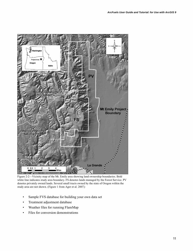
Mt. Emily Demonstration DataThe supplied demonstration data are for the Mt. Emily wildland-urban interface in northeastern Oregon (fig. 2-2). The Mt. Emily area is immediately north of La Grande, Oregon, and encloses 40,385 ac, 58 percent of which are federally man-aged lands. About 30,300 ac of the area are forested based on a 10 percent canopy closure definition. The forest composition ranges from dry forests of ponderosa pine to cold forests dominated by subalpine fir and Engelmann spruce, and a transition zone containing grand fir, Douglas-fir, and western larch (Ager et al. 2010). The Mt. Emily study area is composed of 1,081 stands (polygons).

A full set of demonstration data is available for completing the exercises within this User Guide and Tutorial. Data include:

• Geospatial data (see table 2-1 for a full list)• Database with forest inventory data

TIP: ArcFuels will not work properly if the folders are further nested. For example, the path to the data folder should be: C:\arcfuels\data NOT C:\arcfuels\data\data. All references to finding data and linkages among programs rely on proper initial setup.

11


Figure 2-2—Vicinity map of the Mt. Emily area showing land ownership boundaries. Bold white line indicates study area boundary. FS denotes lands managed by the Forest Service. PV denotes privately owned lands. Several small tracts owned by the state of Oregon within the study area are not shown. (Figure 1 from Ager et al. 2007.)

• Sample FVS database for building your own data set• Treatment adjustment database • Weather files for running FlamMap• Files for conversion demonstrations

12


Setting Up ArcFuels With the Mt. Emily Demonstration Data1. Start ArcMap by double-clicking the arcfuels9x.mxd. See the Start-up

Errors section below if ArcFuels does not open properly.a. The Project Manager form will appear (fig. 2-3). In the Current

Project textbox, select mtemily from the drop-down list.

i. The Project Manager form includes four separate tabs (described below) and contains information on folders, files, geographic infor-mation system (GIS) data, and programs for specific projects. This information is stored in the arcfuels_projects.mdb.

2. Click Close to close the form.3. Add the GIS layer file (fig. 2-4) for the demonstration data in ArcMap

(ArcMap MenuFileAdd Data) by navigating to Demo_data.lyr in the C:\arcfuels\data folder.

4. Click the Projects and Files button on the ArcFuels toolbar, then select Manage Projects from the drop-down list to reopen the Manage Projects form.

Table 2-1—Spatial data included within the demonstration data folder

Data type Name Units Description

grid lf_fbfm40 n/a Scott and Burgan (2005) fire behavior fuel modelgrid lf_cc % Canopy cover grid lf_ch m*10 Canopy height grid lf_cbh m*10 Canopy base height grid lf_cbd kg/m3*10 Canopy bulk densitygrid elevation m Elevationgrid aspect azimuth Aspectgrid slope degrees Slopegrid hillshade n/a Shaded relief of the study areagrid subarea n/a Smaller sub-area within the study areagrid fire n/a Hypothetical past firegrid lynx n/a Hypothetical Canada lynx habitatgrid trt_type n/a Hypothetical fuel treatment typegrid trt_location n/a Hypothetical fuel treatment locationgrid ideal_trt n/a Hypothetical ideal treatment locationsSID mt_em.sid n/a NAIP imagery of the study areapolygon mt_emily_stands n/a Mt. Emily standspolygon lynx_habitat n/a Hypothetical Canada lynx habitatpolygon treatment_units n/a Hypothetical fuel treatment planpoint structures n/a Individual structures within the study areaSource: The “lf” data were downloaded from LANDFIRE (http://www.landfire.gov) and are the Refresh 2008 (LF_1.1.0) data.

13


Figure 2-3–Project Manager form with the mtemily project selected.

Figure 2-4—Mt. Emily project area with satellite imagery in the background and the stand polygon outlines in the foreground.

14


Figure 2-5—Layers tab filled out properly in the Project Manager form for use with the demonstration data.

5. Select the Layers tab (fig. 2-5).a. The Layers tab is where the stand polygon layer and associated stand

grid layer are stored for use with FVS runs. In addition, the grids used to build landscape files are stored, which are required when using the Cell Data tool.

b. Ensure that the ArcGIS layers autopopulated in the correct boxes. If not, use the drop-down lists to select the correct layers.

6. Select the Programs tab (fig. 2-6).a. The Programs tab contains the paths to the executable files for exter-

nal programs linked to ArcFuels. For more information about the pro-grams, refer to table 1-1.

b. Check that the paths to FVS, SVS, and FlamMap are correct. If not, navigate to the versions of the programs downloaded from the Web site (which will be in C:\arcfuels\programs) or to the location on your computer. If the paths to the other programs are populated and you did not download the extra programs, it is okay to leave them that way; ArcFuels will function properly without these paths populated.

15


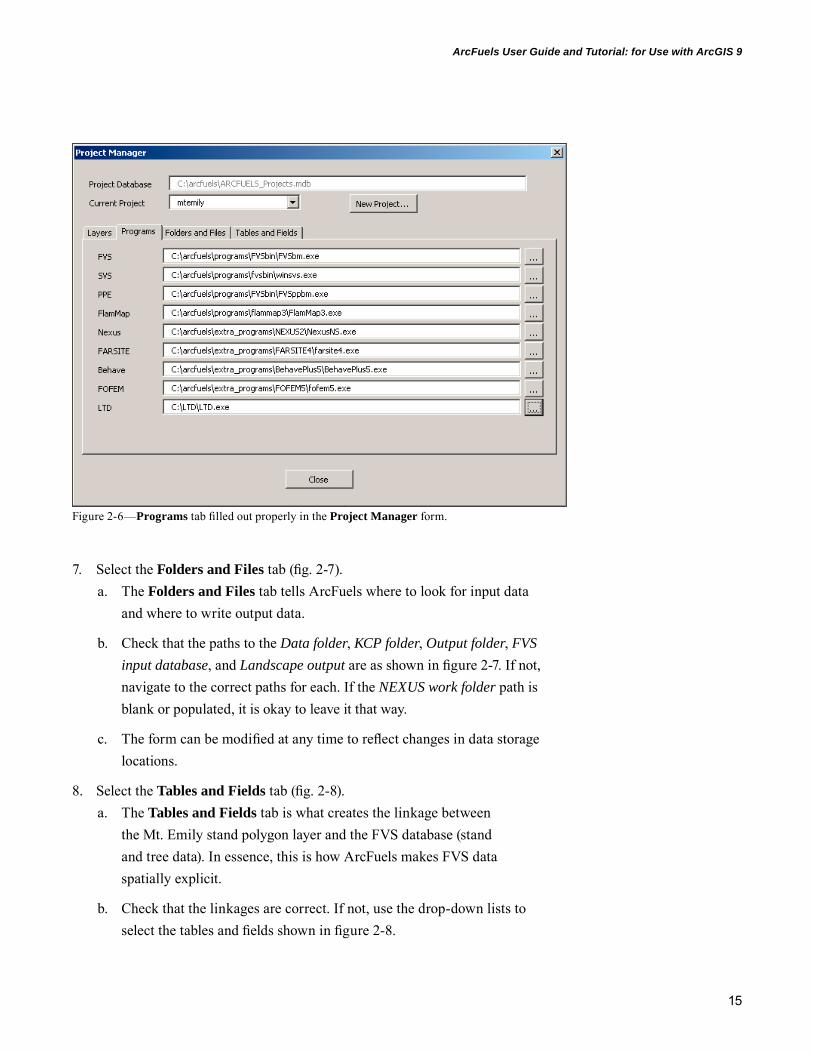
Figure 2-6—Programs tab filled out properly in the Project Manager form.

7. Select the Folders and Files tab (fig. 2-7).a. The Folders and Files tab tells ArcFuels where to look for input data

and where to write output data.

b. Check that the paths to the Data folder, KCP folder, Output folder, FVS input database, and Landscape output are as shown in figure 2-7. If not, navigate to the correct paths for each. If the NEXUS work folder path is blank or populated, it is okay to leave it that way.

c. The form can be modified at any time to reflect changes in data storage locations.

8. Select the Tables and Fields tab (fig. 2-8).a. The Tables and Fields tab is what creates the linkage between

the Mt. Emily stand polygon layer and the FVS database (stand and tree data). In essence, this is how ArcFuels makes FVS data spatially explicit.

b. Check that the linkages are correct. If not, use the drop-down lists to select the tables and fields shown in figure 2-8.

16


Figure 2-8—Tables and Fields tab filled out properly in the Project Manager form.

Figure 2-7—Folders and Files tab filled out properly in the Project Manager form.

17


Figure 2-9—Visual Basic editor window showing the RunReset process for troubleshooting.

Start-Up ErrorsVisual Basic editor window—If an error is generated by the ArcFuels macros, the VBA editor will open and the offending code will be highlighted in yellow. Click RunReset on the main menu (fig. 2-9) and FileExit to close the VBA editor and return to ArcMap to resume the session. The blue square below Run will also reset the project. The VBA editor can be opened by pressing Alt-F11. Most errors generated by ArcFuels are caused by incorrect pathnames and fieldnames in the project database.

If you are using ArcFuels on a non-Forest Service computer and get an error at startup, you will probably need to edit the VBA references. In the VBA editor, go to ToolsReferences. Look through the list of references that have check marks (these are at the top of the list) for ones that say MISSING. If you find any, write down the complete name and click to remove the check mark. Then scroll down the list of unchecked references (these are in alphabetical order) for one with the same name but a different number. For example, if you found “Microsoft ADO Ext. 2.8 for DDL and Security (MISSING)” with a check mark, you might find “Microsoft ADO Ext. 2.7 for DDL and Security” lower in the list. Click on this reference to put a check mark next to it. Note that you may need to save and/or restart ArcMap for these changes to take effect.

18


Missing buttons—When you open ArcFuels, if a few of the buttons on the toolbar are “[Missing]” and you get an error window opening, this means that ArcGIS was not installed prop-erly (fig.2-10). You will need to repair or reinstall ArcGIS.

Figure 2-10—Missing buttons in the ArcFuels toolbar means that ArcGIS was installed incorrectly and needs to be repaired or reinstalled.

19


ArcFuels Tool OverviewAs mentioned, ArcFuels is a library of ArcGIS macros developed to streamline fire behavior modeling and spatial analyses for fuel treatment planning where ArcFuels macros are executed via a custom toolbar in ArcMap (fig. 3-1, table 3-1).

The toolbar consists of a number of buttons, many with multiple options found in drop-down lists and sometimes multiple tabs in the associated forms. The ArcFuels toolbar also has two buttons, Select Stand and Cell Data which are used to select a polygon (stand) or a grid cell from data loaded into your ArcMap table of contents.

The functionality of each button will be described in the following sections, from left to right across the toolbar, with exercises for each.

Figure 3-1—ArcFuels toolbar.

Table 3-1—Summary of ArcFuels tool bar functionality

Button Description

Stand Set up options for FVS/FFE-FVS. Includes applying fuel treatment prescriptions, treatment analysis, and treatment comparison tools. External linkage to open SVS.Select Stand Toggle button to select individual stands within the landscape to run FVS/FFE-FVS.Cell Data Toggle button to quickly view values associated with the FARSITE grid sandwich.Landscape Multiple functions: (1) apply prescriptions to the landscape, (2) set up and running of FVS/FFE-FVS, as well a treatment analysis, and carbon offset calculations at the landscape scale, (3) create landscape files from FVS data, grid data, or multiple sources, and (4) external linkage to the Landscape Treatment Designer (LTD).Wildfire External linkage to open select fire behavior models. Internally coded Models version of BehavePlus ("Behave Calculator") for quick stand-level comparisons of fire behavior.Modify Grid Tool that allows for modification of grid values across the Values whole landscape or for user-defined portions.Conversion Single and batch conversion of point data to shapefiles and ASCII files to grids, and direct export of polygon attributes to Excel.Projects and Location of linkage information between ArcFuels linked programs, Files GIS layers, GIS layers and FVS databases, and input and output data folders.ArcFuels ArcFuels version information. HelpSource: Adapted from table 3 in Ager et al. (2011).

Chapter 3

The ArcFuels toolbar consists of a number of buttons, many with multiple options found in drop-down lists and sometimes multiple tabs in the associated forms.

20


Stand and Select StandThe Stand and Select Stand buttons are used in tandem to run FVS/FFE-FVS stand-level functionality in ArcFuels. The Stand button has a drop-down list with three options, Set Stand Options, View FVS I/O, and SVS (fig. 3-2). The Set Stand Options form is where FVS options are set up. With this you can set the number of cycles to run, apply prescriptions, fine-tune prescriptions, and compare prescriptions for individual stands. The View FVS I/O form links to the FVS out file, FVS key file and Excel spreadsheet (if created) for the most recent FVS run. The SVS option opens the Stand Visualization System program.

Set Stand Options—The Set Stand Options form has four tabs that are used to set up and run FVS. • The Point&Click Options tab (fig. 3-3) is where

FVS outputs are selected. ArcFuels is unique in that you can simultaneously run FVS, create and open SVS files, and export the FVS data to an Excel workbook with graphs of key attributes. The ability to write NEXUS output files for fire behavior modeling outside of ArcFuels in another option. Finally, an insect risk report can be cre-ated when coupled with the insectrisks.kcp sup-plied in the C:\arcfuels\programs\kcp folder.

• The FVS Options tab (fig. 3-4) is where the number of cycles and time steps for FVS runs and the fuel model set(s) that FVS/FFE-FVS will use are specified. Treatment prescriptions can be selected by choosing KCP files or using fields in the database that have the KCP files listed. Other hard-wired options include the generation of a cut list, the ability to pause the FVS run at the end for debugging, and the option to override the FEE-FVS fuel model selections with others in the input database. The FVS Keyword Guide (Van Dyck and Smith-Mateja 2000) can also be opened with the View Keyword Guide button on the form to aid in KCP development.

• The Treatment Analysis tab (fig. 3-5) allows a single parameter to be varied within a KCP to test the effects on modeled outputs such as stand structure or fire behavior. This is very useful when trying to determine how intensely to thin a stand or to see the effects of varying windspeed or fine dead fuel moisture on projected fire behavior.

Figure 3-2—Stand and Select Stand buttons on the ArcFuels toolbar. These buttons are used together to do much of the stand-level forest growth, fuel treatment prescription testing, and fire behavior modeling within ArcFuels.

The Stand and Select Stand buttons are used in tandem to run FVS/FFE-FVS stand-level functionality in ArcFuels.

21


Figure 3-3—The Point&Click Options tab of the Stand-Select Mode Options form is used to select outputs when running FVS through ArcFuels.

Figure3-4—The FVS Options tab of the Stand-Select Mode Options form is where options for the stand level FVS runs are specified.

22


• The Compare Treatments tab (fig. 3-6) allows for direct comparison of two treatment alternatives. When this tab is used, comparison graphs are created within the Excel workbook when the create graphs option is turned on.

Figure 3-5—The Treatment Analysis tab of the Stand-Select Mode Options form is used to test the affect of varying a single prescription parameter at a time on modeled forest structure and fire behavior and effects.

23


Figure 3-6—The Compare Treatments tab of the Stand-Select Mode Options form is used to compare two treatment alternatives.

View FVS I/O—The View FVS I/O (fig. 3-7) form is used to quickly reopen and review FVS files from the latest run, as well as open the outputs folder. The FVS outfile (*.out) is a text file containing all the outputs from an FVS run. The FVS key file (*.key) is a keyword record file that FVS reads to complete a run and includes information on the location of the stand and tree data, specifics on run duration, and prescriptions applied. The FVS spreadsheet (*.xls) contains the same information as the FVS outfile in tabular form. The File Explorer button opens the ArcFuels outputs folder.

24


SVS—The SVS option in the Stand drop-down list opens the Stand Visualization System program. Once it is open, you will need to navigate to an SVS file previously created.

Select Stand—The Select Stand button is a toggle button much like the information button in Arc-Map and is used to run FVS for the stand selected. It can be turned off by selecting another button in ArcMap such as Select Features or Select Elements.

Cell DataThe Cell Data button is used much like the Identify button in ArcMap. It will show the values of the eight layers that make up the FlamMap “grid sandwich” (or landscape file, LCP) when the grid layers are loaded into ArcMap and linked through the Manage Projects form (fig. 3-8). For information about LCPs, see the Introduction to Mod-eling Fire Behavior in FlamMap3 section. The Cell Data button can be turned off by selecting another button in ArcMap such as Select Features or Select Elements.

Figure 3-7—The FVS Outputs form quickly opens files associated with the latest FVS run.

Figure 3-8—The Cell Data form displays the values for the eight grid layers added to ArcMap and assigned in the Project Manager form. Canopy is canopy cover, Height is canopy height, CBH is canopy base height, and CBD is canopy bulk density.

The Cell Data button will show the values of the eight layers that make up the FlamMap “grid sandwich” (or Landscape file, LCP)

25


LandscapeThe Landscape button has five associated options (fig. 3-9). The Assign Prescriptions to Landscape form allows the user to assign and store KCP prescriptions to stands for use with the Simulate Landscape Treatments form. The Simulate Landscape Treatments form is where a user can run FVS/FFE-FVS for a landscape. ArcFuels has a compact interface to FVS/FFE-FVS that can be used to run the models in a spatial context by linking FVS data to a stand polygon layer in ArcMap. With the Build FlamMap Landscape and GNN to LCP Process forms, LCPs can be built from a number of data sources including FVS databases, grid data such as LANDFIRE, Gradient Nearest Neighbor (GNN) (Ohmann and Gregory 2002) data, or multiple-grid data sets. Finally, the Landscape Treatment Designer (LTD) program (Ager et al. 2012) is used to design fuel treatment plans using an attributed stand shapefile. Attributes from FVS/FFE-FVS are often used to populate the stand shapefile for LTD.

The user is assumed to have some familiarity with FVS/FFE-FVS and Flam-Map before proceeding with the exercises in this section. If not, please review the Introduction to the Forest Vegetation Simulator (FVS) and Introduction to Modeling Fire Behavior in FlamMap3 sections.

Assign Prescriptions to Landscape—The Assign Prescriptions to Landscape form (fig. 3-10) allows the user to assign FVS/FFE-FVS KCP prescriptions to stands and store them in the FVS database for use with the Simulate Landscape Treatments form to run FVS. There are three methods for assigning prescriptions to stands: • Method A: By selecting individual stands using the Select Stand tool.• Method B: By selecting groups of stands using ArcMap (also known as

ArcSelected stands).• Method C: Using an integer grid consisting of only 0s and 1s, where 1 indi-

cates the need for a treatment and 0 is no-treatment needed.

Figure 3-9—Landscape button with the associated drop-down list from the ArcFuels toolbar.

The Landscape button has options for assigning FVS/FFE-FVS prescription across the landscape, running FVS/FFE-FVS for the landscape, building LCPs, and running the Landscape Treatment Designer program.

26


ArcFuels stores stand prescriptions in the stands data table within the Mt_Emily_Database.mdb (fig. 3-11). Preexisting fields are supplied with the demonstra-tion data, but more can be added. Records are populated with the name of the KCP for each stand using the Assign Prescriptions to Landscape tools. When running FVS/FFE-FVS at the stand or landscape level, ArcFuels can use these populated prescriptions. If you want to add your own prescription columns to the stands table, the new columns need to be the same format to work. Also, new column names cannot contain spaces or special characters other than an underscore.

Figure 3-10—Assign Prescriptions tab of Landscape Treatment Design form.

27


Simulate Landscape Treatments—The Simulate Landscape Treatments form has four tabs, all related to running FVS for a single stand to an entire landscape. • The Run FVS tab offers a compact FVS interface with many options (fig.

3-12). You can run a single stand, a set number of stands, ArcMap selected stands, only stands with prescriptions, or all the stands. Prescriptions can be applied to all stands or to select stands by linking to the prescription field in the input database (see the Assign Prescriptions to Landscape section to learn how). The number of FVS cycles and years is set with this form. In addition to the ability to write and use KCPs, some helpful FFE-FVS/FVS functions are included: fuel model selection, carbon reports, turning off the FFE-FVS reports, including a West-wide insect KCP, and generating a cutlist.▪ Advanced users can also run the Parallel Processing Extension (PPE) to

FVS through this tab. Running PPE is not covered in this guide. More information about the program can be found on the FVS Web site and within the User’s Guide to the Parallel Processing Extension of the Prognosis Model (Crookston and Stage 1991) which can be found in the optional docs download (C:/arcfuels/docs).

• The Treatment Analysis tab (fig. 3-13) has four methods for analyzing treatment effects on stand characteristics and modeled fire behavior and effects.▪ Method 1 is similar to the Treatment Analysis tab in the Stand tool,

where a single parameter within the prescription file is varied in a step-wise fashion.

Figure 3-11—Linkage between individual stands and the FVS database.

28


▪ Method 2 substitutes a single-value-based prescription with “<_>” inside a command indicating the value to be altered. The minimum and maximum values and the step amount are specified by the user. See the flameadjust.kcp for an example.

▪ Method 3 and Method 4 are primarily used in the research field of quantitative wildfire risk and are not demonstrated in the User Guide and Tutorial.

Figure 3-12—Run FVS tab of the Simulate Landscape Treatments form.

29


• The Compare Treatments tab (fig. 3-14) calculates the carbon offset (tons) between two landscapes (typically an untreated and treated) for a given year. The calculations subtract Scenario A from Scenario B (i.e., treated – untreated). For this to work, the Carbon Reports option must be selected on the Run FVS tab for both scenarios.• Carbon offset from change in emissions is the difference in carbon

emissions (defined as the carbon released from fire and the nonmerchantable carbon removed (tons) via treatment) between the two scenarios.

Figure 3-13—Treatment Analysis tab within the Simulate Landscape Treatments form.

30


• Carbon offset from change in stock is the difference in total stand carbon (live and dead overstory, understory, surface fuels, and below-ground roots) including merchantable carbon stored (tons) between the two scenarios.

• Total carbon offset is the Carbon offset from change in stock minus the Carbon offset from change in emissions.

For more information about the carbon submodel to FVS, see the FFE-FVS guide (Rebain 2010) supplied in the optional docs download (C:\arcfuels\docs). • The Join FVS Outputs to Polygons tab (fig. 3-15) joins FVS/FFE-FVS

outputs from any table in the FVS output database for a given year to the stand polygon layer.

Figure 3-14—Compare Treatments tab within the Simulate Landscape Treatments form.

31


Build FlamMap Landscape—Running FlamMap or FARSITE, two commonly used fire behavior modeling programs, requires an LCP. An LCPs is a binary file containing a compilation or “sandwich” of ASCII data, including slope, elevation, aspect, surface fuel model, canopy height, canopy cover, canopy bulk density, and canopy base height. In addi-tion to building LCPs from a variety of data sources, ArcFuels also has the ability to reduce the analysis area based on another grid or coordinates, quickly apply treatments, and export the ASCIIs and grids. The Build FlamMap Landscape form has three options for building LCPs specific to the input data available.

Figure 3-15—Join FVS Outputs to Polygons tab within the Simulate Landscape Treatments form.

32


• The Using FVS Database tab (fig. 3-16) couples the ArcGIS grids for topography (elevation, slope, and aspect) with an FVS/FFE-FVS output database using a stand identification grid to spatially apply the FVS out-puts. Treatments can be applied by using a second FVS/FFE-FVS output database containing only treated stands. The values associated with the treated stands replace the untreated values. If the FFE-FVS fuel model selection is not desired, an ArcGIS grid layer can be used instead.

• The Using ArcGIS Grid Data tab (fig. 3-17) builds LCP files from ArcGIS grids. This eliminates the need to export the grids as ASCII files, which is required for creating LCPs in FlamMap and FARSITE. Treatments can also be rapidly applied using a treatment adjustments database coupled with grids indicating location and type of treatment.

Figure 3-16—Using FVS Database tab within the Build FlamMap Landscape form.

33


• The Using Multiple Sources tab (fig. 3-18) allows the user to mix and match grids from varying data sources (LANDFIRE and FVS) or mosaic together multiple grids of different spatial extent into one seamless layer for any given data set needed to create an LCP. It is even possible for the grids to have different units, but they must be the same resolution, and projection, and be snapped.

Figure 3-17—Using ArcGIS Grid Data tab within the Build FlamMap Landscape form.

34


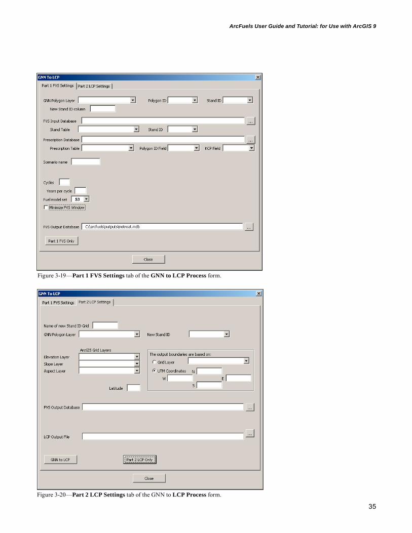
GNN to LCP Process—The GNN to LCP Process form (figs. 3-19 and 3-20) is another option for building the LCP file; with this option, GNN data are used. The GNN data are 30 m by 30 m grid data that link to FVS data, much like the link between FVS and stand polygon data. GNN data are available only in the Pacific Northwest and the northern extent of California (Klamath National Forest). This process is broken into two steps; part one runs FVS for the GNN data, and part two builds the LCP. Because the dem-onstration data does not include GNN data this process will be explained but no exercises are included.

The Part 1 FVS Settings tab (fig. 3-19) is where the settings for an FVS run are defined. The input data include a polygon layer version of the GNN grid with an attribute that links to the FVS database (i.e., StandID), and an FVS input database that coincides with the GNN data. A prescription database may also be used that includes a field with assigned prescriptions (this may be the same database as the FVS input data). The number of cycles, years per cycle, and fuel model set are also defined with this form.

Figure 3-18—Using Multiple Sources tab within the Build FlamMap Landscape form.

35


Figure 3-19—Part 1 FVS Settings tab of the GNN to LCP Process form.

Figure 3-20—Part 2 LCP Settings tab of the GNN to LCP Process form.

36


The Part 2 LCP Settings tab (fig. 3-20) uses the GNN polygon layer and FVS output database created in Part 1 FVS Settings in addition to elevation, slope, and aspect grids to build the LCP.

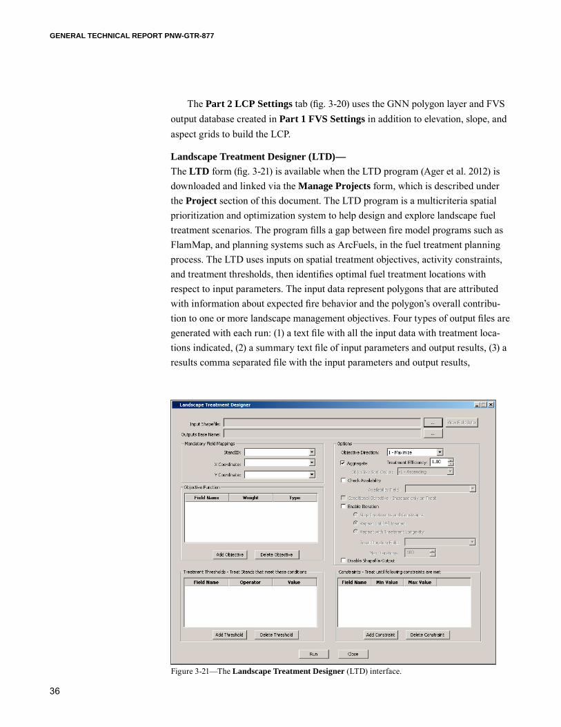
Landscape Treatment Designer (LTD)—The LTD form (fig. 3-21) is available when the LTD program (Ager et al. 2012) is downloaded and linked via the Manage Projects form, which is described under the Project section of this document. The LTD program is a multicriteria spatial prioritization and optimization system to help design and explore landscape fuel treatment scenarios. The program fills a gap between fire model programs such as FlamMap, and planning systems such as ArcFuels, in the fuel treatment planning process. The LTD uses inputs on spatial treatment objectives, activity constraints, and treatment thresholds, then identifies optimal fuel treatment locations with respect to input parameters. The input data represent polygons that are attributed with information about expected fire behavior and the polygon’s overall contribu-tion to one or more landscape management objectives. Four types of output files are generated with each run: (1) a text file with all the input data with treatment loca-tions indicated, (2) a summary text file of input parameters and output results, (3) a results comma separated file with the input parameters and output results,

Figure 3-21—The Landscape Treatment Designer (LTD) interface.

37


and (4) a shapefile with an attribute table that identifies patch locations and stands selected for treatments. For more detailed information about the LTD, refer to Ager et al. (2012).

Wildfire ModelsArcFuels creates links to select fire behavior models (NEXUS, FARSITE, FlamMap, Behave, and FOFEM) and opens the programs for use outside of ArcFuels (fig. 3-22). In addition to linking to external programs, ArcFuels also has the Behave Calculator, which runs through ArcFuels.

The location of the models’ executables are set using the Programs tab in the Project Manager form, which is described in the Setting up ArcFuels with Mt. Emily Demonstration Data section at the beginning of the User Guide and Tutorial.

Behave Calculator—The Behave Calculator (fig. 3-23) is hardwired into ArcFuels and uses the same equations as the SURFACE module in Behave Plus. The Behave Calculator can be used to quickly assess changes to modeled surface fire rate of spread and flame length from changes to fuel model, slope, fuel moisture, and/or windspeed inputs.

Figure 3-22—Wildfire Models button with the associated drop-down list from the ArcFuels toolbar.

Figure 3-23—Behave Calculator form.

ArcFuels creates links to select fire behavior models (NEXUS, FARSITE, FlamMap, Behave, and FOFEM) and opens the programs for use outside of ArcFuels.

38


Modify Grid ValuesAfter critiquing data for accuracy (informally, on-the-ground, using the Stratton (2009) methodology, or otherwise), it is most likely that some modifications will be required to reflect local knowledge of fuel models and fire behavior, recent manage-ment activities, recent wildfires, etc. It is important to document changes, as well as make changes incrementally, to make it easier to see the effect of the changes and backtrack, if necessary. Realize, however, that when modeling landscape-level fire behavior, there will be some error in the data.

With ArcFuels, complex grid value replacements are easily made on the indi-vidual grid layers, rather than on the landscape file. Tools such as the FARSITE landscape calculator and the WFDSS landscape editor are available to make changes on the landscape file, but are generally limited to simple changes (Stratton 2009).

Within ArcFuels the Modify Grid Values form (fig. 3-24) is available to update or correct grid data. When the tool is used, both a projected grid file and an ASCII file are created. The changes can be made to either floating point or integer data. Options for changing data include:• Which pixels to apply the changes to spatially

▪ Apply to all pixels: global change all pixels, or▪ Apply to selected pixels: change some pixels based on another

grid layer.• The extent of the output data

▪ The same as the input data—default option,▪ The same as another grid layer—smaller extent, or▪ Manually restricted—using UTM coordinates of a smaller extent.

This function pairs extremely well with the ArcMap Raster Calculator (ArcToolboxSpatial AnalystRaster Calculator). For example, with the Raster Calculator, you can create new 0/1 grids based on specific criteria (e.g., all burn-able fuels, slopes > 30 percent, south aspects, etc.) and then use ArcFuels to make changes within these areas. This eliminates several steps and reduces the number of files you need to keep track of and organize.

With ArcFuels, complex grid value replacements are easily made on the individual grid layers, rather than on the landscape file, to update grids to reflect recent management activities, recent wildfires, etc.

39


ConversionThe Conversion button has five associated options (fig. 3-25). The Convert Ascii to Grid and Batch Convert Ascii to Grid converts ASCII files into grids, and the Convert XY Text to Shapefile and Batch Convert XY Text to Shapefile converts XY text files into shapefiles. The conversion can be done for a single file or for multiple files at once (batch). The files are also projected and mapped in the same process. Additionally, it is possible to copy the attributes of a polygon layer directly into an Excel spreadsheet using the Copy Attributes to Spreadsheet form.

The conversion of ASCII files to grids allows for post-processing and analysis of fire modeled outputs created in FlamMap. The conversion of XY text files can be used to import data with X and Y coordinates information, such as fire ignition location, plot location data, etc.

Figure 3-24—Modify Grid Values form.

Figure 3-25—Conversion button with the associated drop-down list from the ArcFuels toolbar.

The conversion forms are used to efficiently post-process simulated wildfire behavior outputs for further analysis in ArcMap.

40


Convert Ascii to Grid—The Convert Ascii Grid File form (fig. 3-26) combines two ArcGIS processing steps into one. It converts an integer or floating point ASCII file into a grid, and it defines the spatial reference at the same time. The user has the option of where to output the grid file and what to name it. Being able to name the grid file is helpful when the ASCII name exceeds the 13-character grid name limit. Finally, the user has the option of adding the grid file to ArcMap.

Figure 3-26—Convert Ascii Grid File form used to convert a single file at a time.

Batch Convert Ascii to Grid—The batch Convert Ascii Grid Files form (fig. 3-27) combines many ArcGIS processing steps into one. It converts integer or floating point ASCII files into grids and it defines the spatial reference at the same time. Typically this would need to be completed separately for each ASCII file in ArcMap. In addition, the user has the option of adding the grid files to ArcMap.

41


Figure 3-27—Convert Ascii Grid Files form used to convert multiple files at once.

42


Figure 3-28—Convert XY File form used to convert a single file at a time.

Batch Convert XY Text to Shapefiles—The batch Convert XY Text to Shapefiles form (fig. 3-29) combines many ArcGIS processing steps into one. It converts multiple XY text files into events files, then exports them as shapefiles with defined spatial reference. The X-coordinate and Y-coordinate field names can be the default XPos, YPos, X, Y, or anything else using the Other option. There is also an option for batch exporting FSim (Finney et al. 2011) fire size list files, which are used for quantitative risk assessments with Fire Program Analysis (FPA) data. See FPA (http://www.fpa.nifc.gov/) for more information about the FSim program and outputs. Finally, the user has the option of adding the shapefile to ArcMap.

Convert XY Text to Shapefile—The Convert XY File form (fig. 3-28) combines two ArcGIS processing steps into one. It converts an XY text file into an events file, then exports it as a shapefile with defined spatial reference. The X-coordinate and Y-coordinate field names can be the default XPos, YPos, X,Y, or anything else using the Other option. Finally, the user has the option of adding the shapefile to ArcMap.

43


Figure 3-29—Convert XY Text to Shapefiles form used to convert multiple files at once.

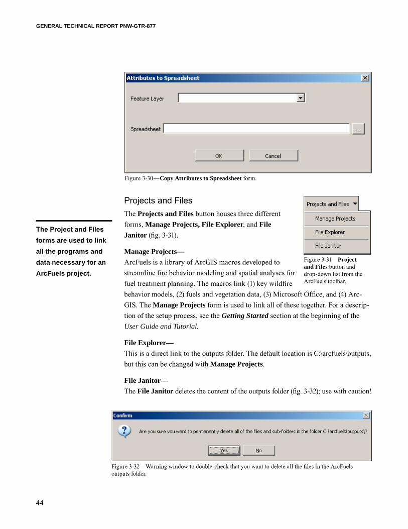
Copy Attributes to Spreadsheet—The Copy Attributes to Spreadsheet form (fig. 3-30) does just what it says; it copies the attributes table from a shapefile into Excel and opens the workbook.

44


Projects and FilesThe Projects and Files button houses three different forms, Manage Projects, File Explorer, and File Janitor (fig. 3-31).

Manage Projects—ArcFuels is a library of ArcGIS macros developed to streamline fire behavior modeling and spatial analyses for fuel treatment planning. The macros link (1) key wildfire behavior models, (2) fuels and vegetation data, (3) Microsoft Office, and (4) Arc-GIS. The Manage Projects form is used to link all of these together. For a descrip-tion of the setup process, see the Getting Started section at the beginning of the User Guide and Tutorial.

File Explorer—This is a direct link to the outputs folder. The default location is C:\arcfuels\outputs, but this can be changed with Manage Projects.

File Janitor—The File Janitor deletes the content of the outputs folder (fig. 3-32); use with caution!

Figure 3-30—Copy Attributes to Spreadsheet form.

Figure 3-31—Project and Files button and drop-down list from the ArcFuels toolbar.

Figure 3-32—Warning window to double-check that you want to delete all the files in the ArcFuels outputs folder.

The Project and Files forms are used to link all the programs and data necessary for an ArcFuels project.

45


ArcFuels HelpThe ArcFuels Help button (fig. 3-33) About ArcFuels option opens a new window with the version date (fig. 3-34) of the arcfuels9x.mxd.

The program is updated periodically; please visit http://www.fs.fed.us/wwetac/arcfuels/ for the most recent version if you are having problems with any ArcFuels functionality.

Figure 3-33—The Arc-Fuels Help button with the drop-down list from the ArcFuels toolbar.

Figure 3-34—ArcFuels version date.

46


ArcFuels Tool TutorialThis section will demonstrate the functionality of all the tools within ArcFuels through exercises using the demonstration data. If you have not set up ArcFuels for use with the demonstration data, please see the Getting Started section for detailed instructions.

Stand and Select StandExercises 4-1 through 4-7 will highlight many of the functionalities of the Stand and Select Stand tools. If you are unfamiliar with FVS, read the Introduction to the Forest Vegetation Simulator (FVS) section before starting these exercises.

Exercise 4-1: Running FVS and SVS for an untreated stand—1. Click the Stand button on the ArcFuels toolbar, then select Set Stand

Options from the drop-down list. 2. Select the Point&Click Options tab (fig. 4-1).

a. Select View Outputs in SVS, Generate Spreadsheet, Generate Spreadsheet Graphs, and Open Spreadsheet options by clicking in the box to the left of each.

3. Select the FVS Options tab (fig. 4-2).

Figure 4-1—Set up for the Point&Click Options tab of the Stand-Select Mode Options form.

Chapter 4

Running individual stands through FVS/FFE-FVS is streamlined in ArcFuels. Many of fire and fuel treatment FFE outputs are automatically created and output into an Excel workbook with values graphed, making it easy to evaluate a completed run.

47


a. Input Database: if the Project Manager is set up correctly, the C:\arc-fuels\data\Mt_Emily_Database.mdb will be selected. If it is blank or incorrect, go to the Projects and Files Manage Projects form and correct the path.

b. Cycles: type “10” in the text box.

c. Years per cycle: type “1” in the text box.

d. Fuel model set: select 53 from the drop-down list.

i. This is used to tell FVS which fuel model set to use: Anderson 1982 (13), Scott and Burgan 2005 (40), or both (53).

4. Click Close to close the form to apply and save your inputs for the tabs. 5. Click the Select Stands button on the ArcFuels toolbar.

a. This is a toggle button; once it is pressed, ArcMap responds in the same manner as using the ArcMap Identify function until the active function in ArcMap is changed (e.g., the Select or Pan tool).

b. The map image area is now active, and ArcMap will attempt to retrieve the standid from the mt_emily_stands layer (which spatially links the

Figure 4-2—FVS Options tab set up of the Stand-Select Mode Options form.

48


FVS data to individual stands within Mt. Emily) and then run the stand data through FVS/FFE-FVS.

6. Click on a forested polygon in the stand layer to execute an FVS run (fig.4-3).

Figure 4-3—Stand polygon (A) and the FVS run window (B) for stand number 794. The selected stand is outlined in turquoise; the rest of the visible stands are outlined in black. The Mt. Emily NAIP image is below the stand polygon layer.

TROUBLESHOOTING: If FVS does not execute or executes incorrectly, open the Project Manager form and check the directory settings. A warning window may open telling you what folders are not linked correctly (fig. 4-4).

Figure 4-4—ArcFuels warning window indicating that the outputs folder is not found.

TROUBLESHOOTING: If ArcFuels opens the FVS.out file, then FVS was terminated abnormally and there is an error in the run.

7. After FVS finishes, SVS will open.a. Page through the SVS images for each cycle by clicking the Next but-

ton on the bottom right of the SVS window (fig. 4-5).

49


8. Close SVS (FileExit). 9. An Excel workbook was created and opened (fig. 4-6). The workbook has

multiple spreadsheets, some with graphs of the FVS outputs. For more information including units for all tables, see the Introduction to the Forest Vegetation Simulator (FVS) section. Below is a list of possible spread-sheets within the Excel workbook.• FVS_Cases—information about the stand and the run you completed.

• FVS_StrClass—stand structure class by stratum.

• FVS_PotFire—potential fire behavior, fire effects, and fuel models.

• FVS_Fuels—fuel loading and consumption.

• FVS_Carbon—above and belowground live and dead carbon loading.

• FVS_Hrv_Carbon—harvest carbon products, energy, and emissions.

• FVS_Summary—stand characteristics.

• FVS_Compute—canopy characteristics used for fire modeling and flame length.

Figure 4-5—SVS image of stand 794 during the first year. To see later years, click Next in the bottom-right corner.

50


• FVS_BurnReport—fuel moistures and resulting fire behavior (pro-duced only when a fire is simulated).

• FVS_Consumption—consumption of all fuel types (produced only when a fire is simulated).

• FVS_Mortality—mortality by size class and species (produced only when a fire is simulated).

• InsectRisk—risk value associated with western spruce budworm, fir engraver, mountain pine beetle, spruce beetle, and Douglas-fir tussock moth (produced only when the Insect Risk Report is selected on the Point&Click Options tab).

• FVS_Treelist—the cutlist for trees removed during silvicultural activi-ties such as a thin (produced only when a thinning activity is initiated and the Generate cut lists option is selected on the FVS Options tab).

Figure 4-6—Excel spreadsheet showing the potential fire report outputs (FVS_PotFire) from an FVS run of stand 794, including the autogenerated graphs. The pictured graph shows the predicted surface fire flame length (ft) under severe weather conditions over time (from 2000 through 2009).

51


• FVS_Compare_Carbon—a bar chart comparison of carbon pools before and after treatment and before and after a wildfire with the off-set as well (produced only when using the Compare Treatments tab).

10. Go to the FVS_Compute spreadsheet in the Excel workbook (you might have to scroll to the right to see the tab). The CANOPY (canopy cover, per-centage), FML (fuel model), HTT (stand height, ft), HTLIVE (height to live crown, ft), CBD (canopy bulk density, kg/m3), and YR (year) columns can be used to create landscape files required to run FlamMap. This process will be described later.

TIP: If your SVS window does not display the same as figure 4-5, you can change the settings in SVS, SVS options Screen layouts 0 3-view layout.

TIP: If you try to rerun a stand and still have the Excel work-book open, a warning window (fig. 4-7) will open, not allowing you to proceed until Excel is closed.

Figure 4-7—Warning window when attempting to rerun FVS for a stand with Excel spreadsheet open.

Exercise 4-2: Creating NEXUS input files—This exercise will show you how to create NEXUS input files by using FVS to process stands. This will work only if you either have NEXUS installed on your machine and the path is set up correctly in the Project Manager form or you downloaded and unzipped the extra programs folder.

For more information about NEXUS, refer to the programs help guide. This exer-cise will not explain how to run the program.1. Click the Stand button on the ArcFuels toolbar, then select Set Stand


a. Select the Generate NEXUS Inputs option by clicking in the box to the left.

ArcFuels can be used to create input files for NEXUS from FVS/FFE-FVS runs.

52


b. A new form for setting the NEXUS input parameters will open (fig. 4-9).

c. Simulation Type: select conifer from the drop-down list.

d. Wind reduction factor: type “0.1” in the text box.

e. ROS multiplier: type “1” in the text box.

f. Load and Depth multiplier: type “1” in the text box.

g. Fireline Intensity multiplier: type “1” in the text box.

h. 1 hr moisture: type “3” in the text box.

i. 10 hr moisture: type “4” in the text box.

j. 100 hr moisture: type “6” in the text box.

k. Herbaceous: type “30” in the text box.

l. Woody: type “60” in the text box.

Figure 4-9—NEXUS Inputs form, used to set the simulation parameters for NEXUS runs in addition to the fuels information created in FFE-FVS to run NEXUS.

Figure 4-8—Point&Click Options tab of the Stand-Select Mode Options form for generating NEXUS outputs.

53


m. Avail. Canopy load: type “1” in the text box.

n. Foliar Moisture Content: type “100” in the text box.

o. Shrub Transition Flame Length: type “1” in the text box.

p. Open Windspeed: type “15” in the text box.

q. Wind direction: type “225” in the text box.

r. Click Continue to close the form.

3. Select the FVS Options tab (fig. 4-2).a. Input Database: the C:\arcfuels\data\Mt_Emily_Database.mdb will be

autopopulated.




4. Click Close to close the form to apply and save your inputs for the tabs. 5. Click the Select Stands button on the ArcFuels toolbar, if not already

turned on. 6. Click on a forested polygon in the stand layer to execute an FVS run.

a. Once FVS has completed, NEXUS will open (fig. 4-10) with the data from the first simulation year loaded, which is 2000 for this exercise.

b. All of the NEXUS files are written to the outputs folder for all years run in FVS (2000 through 2009 for this exercise). They are saved as *.scn files with a naming convention of stand number_year. For example, the NEXUS input file for stand 794 for 2005 is named 794_2005.scn.

7. Close NEXUS (File Exit).

54


Figu

re 4

-10—

NEX

US

inte

rfac

e w

ith th

e da

ta lo

aded

for t

he fi

rst F

VS

sim

ulat

ion

year

(200

0).

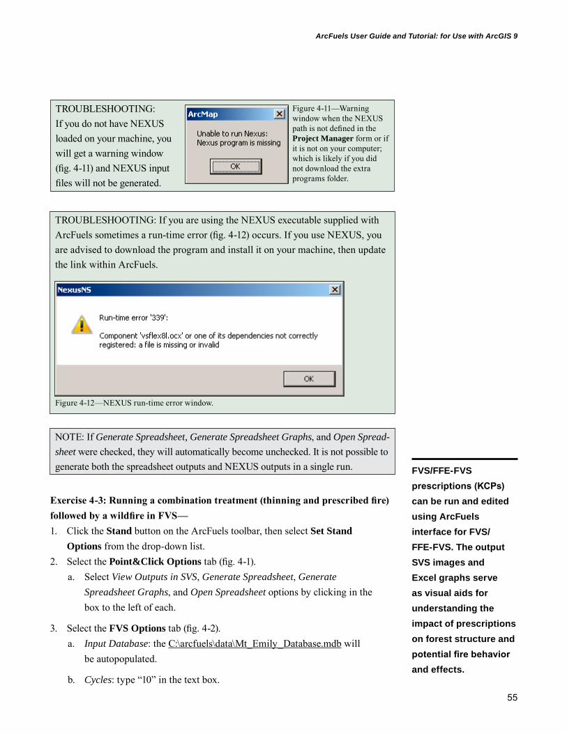
55


Exercise 4-3: Running a combination treatment (thinning and prescribed fire) followed by a wildfire in FVS—1. Click the Stand button on the ArcFuels toolbar, then select Set Stand


a. Select View Outputs in SVS, Generate Spreadsheet, Generate Spreadsheet Graphs, and Open Spreadsheet options by clicking in the box to the left of each.

3. Select the FVS Options tab (fig. 4-2).a. Input Database: the C:\arcfuels\data\Mt_Emily_Database.mdb will

be autopopulated.


NOTE: If Generate Spreadsheet, Generate Spreadsheet Graphs, and Open Spread-sheet were checked, they will automatically become unchecked. It is not possible to generate both the spreadsheet outputs and NEXUS outputs in a single run.

TROUBLESHOOTING: If you are using the NEXUS executable supplied with ArcFuels sometimes a run-time error (fig. 4-12) occurs. If you use NEXUS, you are advised to download the program and install it on your machine, then update the link within ArcFuels.

Figure 4-12—NEXUS run-time error window.

TROUBLESHOOTING: If you do not have NEXUS loaded on your machine, you will get a warning window (fig. 4-11) and NEXUS input files will not be generated.

Figure 4-11—Warning window when the NEXUS path is not defined in the Project Manager form or if it is not on your computer; which is likely if you did not download the extra programs folder.

FVS/FFE-FVS prescriptions (KCPs) can be run and edited using ArcFuels interface for FVS/FFE-FVS. The output SVS images and Excel graphs serve as visual aids for understanding the impact of prescriptions on forest structure and potential fire behavior and effects.

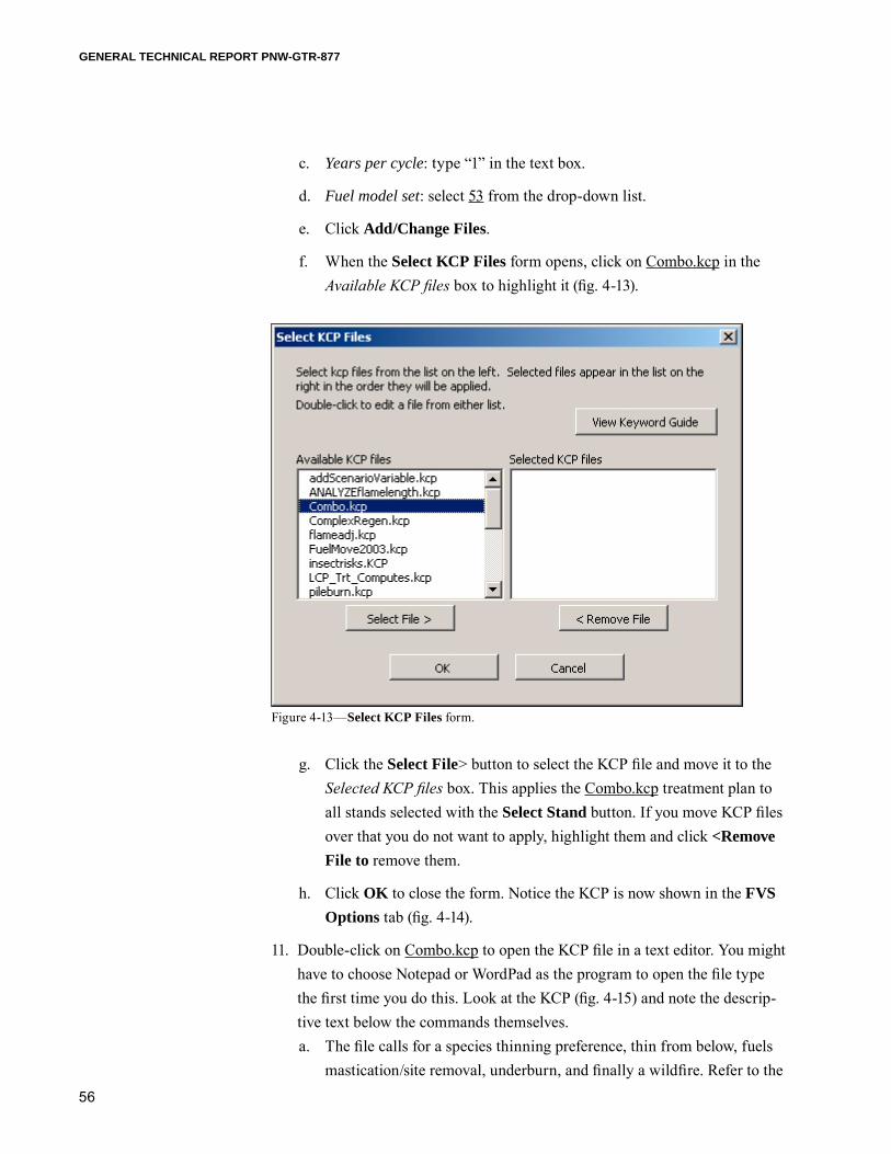
56




e. Click Add/Change Files.

f. When the Select KCP Files form opens, click on Combo.kcp in the Available KCP files box to highlight it (fig. 4-13).

Figure 4-13—Select KCP Files form.

g. Click the Select File> button to select the KCP file and move it to the Selected KCP files box. This applies the Combo.kcp treatment plan to all stands selected with the Select Stand button. If you move KCP files over that you do not want to apply, highlight them and click <Remove File to remove them.

h. Click OK to close the form. Notice the KCP is now shown in the FVS Options tab (fig. 4-14).

11. Double-click on Combo.kcp to open the KCP file in a text editor. You might have to choose Notepad or WordPad as the program to open the file type the first time you do this. Look at the KCP (fig. 4-15) and note the descrip-tive text below the commands themselves. a. The file calls for a species thinning preference, thin from below, fuels

mastication/site removal, underburn, and finally a wildfire. Refer to the

57


Figure 4-14—FVS Options tab with the Combo.kcp file loaded.

Figure 4-15—Combo.kcp file contents. This KCP is thinning the stand and removing activity fuels in 2003, simulating a prescribed burn in 2004, then a wildfire in 2007.

FVS Keyword Guide (Van Dyck and Smith-Mateja 2000) for detailed information on the keyword options.

b. The KCP can be edited and saved as the same file or as a new name at this time but the field position is important. Pay attention when you save the file—Notepad and WordPad will add a TXT extension if you save it as a text file and this will cause problems later in FVS. If you saved the file under a new name you will need to add the .kcp exten-sion, but if you maintained the same name you are ready to proceed.

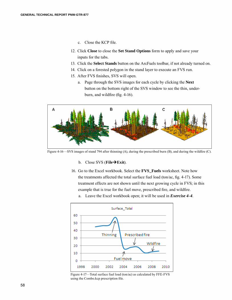
58


c. Close the KCP file.

12. Click Close to close the Set Stand Options form to apply and save your inputs for the tabs.

13. Click the Select Stands button on the ArcFuels toolbar, if not already turned on.14. Click on a forested polygon in the stand layer to execute an FVS run. 15. After FVS finishes, SVS will open.

a. Page through the SVS images for each cycle by clicking the Next button on the bottom right of the SVS window to see the thin, under-burn, and wildfire (fig. 4-16).

Figure 4-16—SVS images of stand 794 after thinning (A), during the prescribed burn (B), and during the wildfire (C).

Figure 4-17—Total surface fuel load (ton/ac) as calculated by FFE-FVS using the Combo.kcp prescription file.

b. Close SVS (FileExit).

16. Go to the Excel workbook. Select the FVS_Fuels worksheet. Note how the treatments affected the total surface fuel load (ton/ac, fig. 4-17). Some treatment effects are not shown until the next growing cycle in FVS; in this example that is true for the fuel move, prescribed fire, and wildfire.a. Leave the Excel workbook open; it will be used in Exercise 4-4.

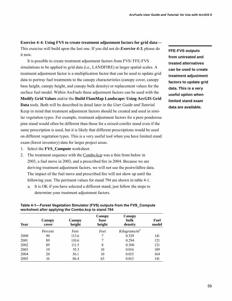
59


Exercise 4-4: Using FVS to create treatment adjustment factors for grid data—This exercise will build upon the last one. If you did not do Exercise 4-3, please do it now.

It is possible to create treatment adjustment factors from FVS/ FFE-FVS simulations to be applied to grid data (i.e., LANDFIRE) at larger spatial scales. A treatment adjustment factor is a multiplication factor that can be used to update grid data to portray fuel treatments to the canopy characteristics (canopy cover, canopy base height, canopy height, and canopy bulk density) or replacement values for the surface fuel model. Within ArcFuels these adjustment factors can be used with the Modify Grid Values and/or the Build FlamMap Landscape: Using ArcGIS Grid Data tools. Both will be described in detail later in the User Guide and Tutorial. Keep in mind that treatment adjustment factors should be created and used in simi-lar vegetation types. For example, treatment adjustment factors for a pure ponderosa pine stand would often be different than those for a mixed-conifer stand even if the same prescription is used, but it is likely that different prescriptions would be used on different vegetation types. This is a very useful tool when you have limited stand exam (forest inventory) data for larger project areas.1. Select the FVS_Compute worksheet.2. The treatment sequence with the Combo.kcp was a thin from below in

2003, a fuel move in 2003, and a prescribed fire in 2004. Because we are deriving treatment adjustment factors, we will not use the postwildfire data. The impact of the fuel move and prescribed fire will not show up until the following year. The pertinent values for stand 794 are shown in table 4-1. a. It is OK if you have selected a different stand; just follow the steps to

determine your treatment adjustment factors.

Table 4-1—Forest Vegetation Simulator (FVS) outputs from the FVS_Compute worksheet after applying the Combo.kcp to stand 794

Canopy Canopy Canopy Canopy base bulk Fuel Year cover height height density model

Percent Feet Feet Kilograms/m3 2000 90 113.6 7 0.329 1412001 89 110.6 7 0.294 1212002 89 111.5 8 0.300 1212003 19 55.3 10 0.014 1892004 20 56.1 10 0.015 1642005 16 86.4 63 0.013 141

FFE-FVS outputs from untreated and treated alternatives can be used to create treatment adjustment factors to update grid data. This is a very useful option when limited stand exam data are available.

60


3. Because the Combo.kcp is a multistepped prescription, it is possible to cre-ate treatment adjustment factors for individual parts or for the treatment as a whole. The process is the same for both. We will look at the impact of thinning only.a. Owing to thinning, canopy cover was reduced from 89 percent in 2002

to 19 percent in 2003, which is a 79 percent reduction.

i. To calculate the treatment adjustment factor, the formula is 1 minus the pretreatment value (89 percent) minus the posttreatment value (19 percent) divided by the pretreatment value (19 percent) which would by typed in as “=1-((89-19)/89)” in Excel and is equal to 0.21.

ii. Because you are reducing canopy cover by 79 percent, the adjust-ment factor would be 0.21. This is because you are retaining 21 percent of the original canopy cover after treatment.

b. The same process can be done for canopy height, canopy base height, and canopy bulk density.

i. The adjustment factors are 0.49 for canopy height, 1.25 for canopy base height, and 0.05 for canopy bulk density.

c. The thinning treatment changed the fuel model from 141 (GS1-low load, dry climate grass-shrub) to 189 (TL9-very high load broadleaf lit-ter) because of the increased surface fuel loads from the thinning.

4. Close the Excel workbook.

Exercise 4-5: Fine tuning treatment prescriptions using the Treatment Analysis tab—The Treatment Analysis tab provides a way to analyze a range of treatment intensities to find the optimal prescription. When the Treatment Analysis tab is used, only the line in the KCP file that is varied is applied to the stand. For instance, suppose you are interested in finding a thinning intensity that achieves a specific fire behavior, such as flame length or fire type, and you are also concerned about total stand carbon.1. Click the Stand button on the ArcFuels toolbar, then select Set Stand


a. Select Generate Spreadsheet, Generate Spreadsheet Graphs, and Open Spreadsheet options by clicking in the box to the left of each.

The Treatment Analysis tab provides a way to analyze a range of treatment intensities to find the optimal prescription.

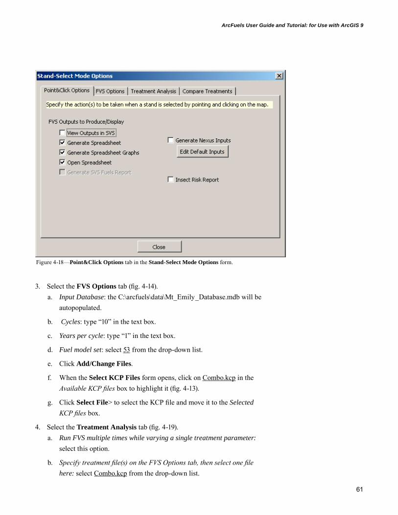
61


3. Select the FVS Options tab (fig. 4-14).a. Input Database: the C:\arcfuels\data\Mt_Emily_Database.mdb will be

autopopulated.




e. Click Add/Change Files.

f. When the Select KCP Files form opens, click on Combo.kcp in the Available KCP files box to highlight it (fig. 4-13).

g. Click Select File> to select the KCP file and move it to the Selected KCP files box.

4. Select the Treatment Analysis tab (fig. 4-19).a. Run FVS multiple times while varying a single treatment parameter:

select this option.

b. Specify treatment file(s) on the FVS Options tab, then select one file here: select Combo.kcp from the drop-down list.

Figure 4-18—Point&Click Options tab in the Stand-Select Mode Options form.

62


c. Select the line containing the variable to be analyzed: select the line that starts with ThinBBA from the drop-down list. ThinBBA is the thinning keyword.

d. Variable Parameter: select 2 from the drop-down list. This is the parameter associated with basal area; the 2 corresponds to the basal area portion of the keyword line.

e. Minimum value: type “10” in the text box. This is the minimum basal area the stand will be thinned to for the run.

f. Maximum value: type “130” in the text box. This is the maximum basal area the stand will be thinned to for the run.

g. Step amount: type “20” in the text box. This is the step amount for altering basal area (i.e., basal area will be thinned to 10, 30, 50 ft2/ac, etc.).

h. Click Close to close the form to apply and save your inputs for the tabs.

5. Click the Select Stands button on the ArcFuels toolbar, if not already turned on.

Figure 4-19—Treatment Analysis tab of the Stand-Select Mode Options form. Basal area is thinned incrementally from 10 ft2/ac to 130 ft2/ac in 20 ft2/ac steps to see the effect on stand struc-ture and fire behavior.

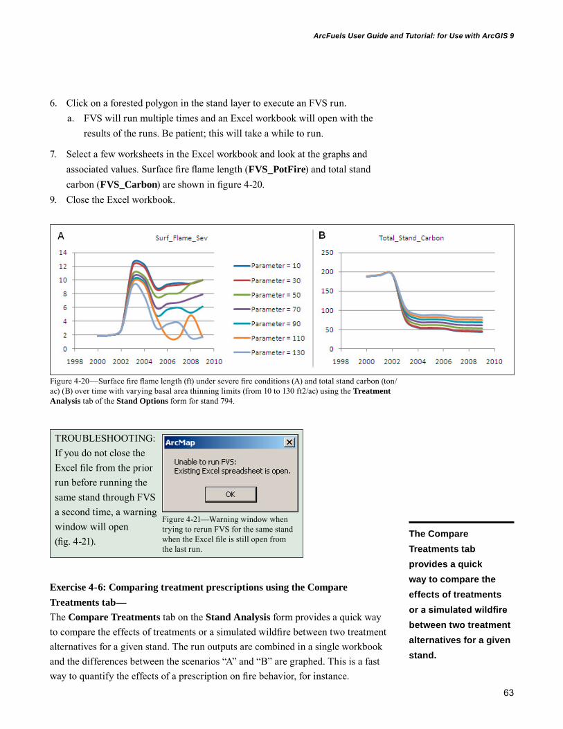
63


6. Click on a forested polygon in the stand layer to execute an FVS run. a. FVS will run multiple times and an Excel workbook will open with the

results of the runs. Be patient; this will take a while to run.

7. Select a few worksheets in the Excel workbook and look at the graphs and associated values. Surface fire flame length (FVS_PotFire) and total stand carbon (FVS_Carbon) are shown in figure 4-20.


Figure 4-20—Surface fire flame length (ft) under severe fire conditions (A) and total stand carbon (ton/ac) (B) over time with varying basal area thinning limits (from 10 to 130 ft2/ac) using the Treatment Analysis tab of the Stand Options form for stand 794.

TROUBLESHOOTING: If you do not close the Excel file from the prior run before running the same stand through FVS a second time, a warning window will open (fig. 4-21).

Figure 4-21—Warning window when trying to rerun FVS for the same stand when the Excel file is still open from the last run.

Exercise 4-6: Comparing treatment prescriptions using the Compare Treatments tab—The Compare Treatments tab on the Stand Analysis form provides a quick way to compare the effects of treatments or a simulated wildfire between two treatment alternatives for a given stand. The run outputs are combined in a single workbook and the differences between the scenarios “A” and “B” are graphed. This is a fast way to quantify the effects of a prescription on fire behavior, for instance.

The Compare Treatments tab provides a quick way to compare the effects of treatments or a simulated wildfire between two treatment alternatives for a given stand.

64


The following process simulates the effects of wildfire on a treated (Combo.kcp) and untreated stand (Wildfire2007.kcp). Specifically, the spreadsheet outputs calculate the difference between the two scenarios. 1. Click the Stand button on the ArcFuels toolbar, then select Set Stand


a. Select Generate Spreadsheet, Generate Spreadsheet Graphs, and Open Spreadsheet options by clicking in the box to the left of each.

3. Select the Compare Treatments tab (fig. 4-22).a. Run FVS with two different treatment scenarios and compare the

results: select this option.

b. Input Database: the C:\arcfuels\data\Mt_Emily_Database.mdb will be autopopulated.

c. Click Add/Change Files under Treatment Prescription A.

i. When the Select KCP Files form opens, click on Wildfire2007.kcp in the Available KCP files box to highlight it. KCP files are listed alphabetically.

Figure 4-22—Compare Treatments tab of the Stand-Select Mode Options form showing the two prescriptions to be compared. Treatment prescription A is a wildfire in 2007, and treatment prescrip-tion B is a thinning, followed by a fuel move and prescribed burn, then the same wildfire as in A.

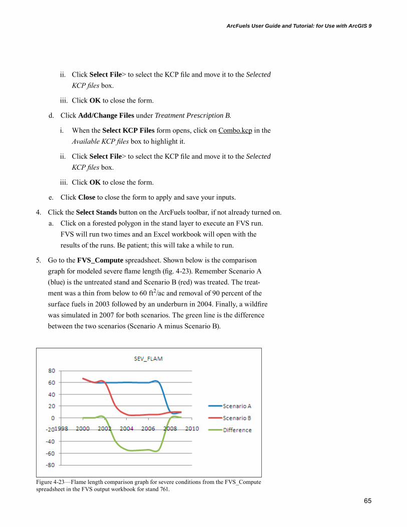
65


ii. Click Select File> to select the KCP file and move it to the Selected KCP files box.

iii. Click OK to close the form.

d. Click Add/Change Files under Treatment Prescription B.

i. When the Select KCP Files form opens, click on Combo.kcp in the Available KCP files box to highlight it.

ii. Click Select File> to select the KCP file and move it to the Selected KCP files box.

iii. Click OK to close the form.

e. Click Close to close the form to apply and save your inputs.

4. Click the Select Stands button on the ArcFuels toolbar, if not already turned on.a. Click on a forested polygon in the stand layer to execute an FVS run.

FVS will run two times and an Excel workbook will open with the results of the runs. Be patient; this will take a while to run.

5. Go to the FVS_Compute spreadsheet. Shown below is the comparison graph for modeled severe flame length (fig. 4-23). Remember Scenario A (blue) is the untreated stand and Scenario B (red) was treated. The treat-ment was a thin from below to 60 ft2/ac and removal of 90 percent of the surface fuels in 2003 followed by an underburn in 2004. Finally, a wildfire was simulated in 2007 for both scenarios. The green line is the difference between the two scenarios (Scenario A minus Scenario B).

Figure 4-23—Flame length comparison graph for severe conditions from the FVS_Compute spreadsheet in the FVS output workbook for stand 761.

66


6. Go to the FVS_Compare_Carbon spreadsheet. This is a new addition that is available only with the Compare Treatments tab in the Set Stand Options form. It shows the carbon pools for the treated (Scenario B) and untreated (Scenario A) scenarios before and after the wildfire in 2007 as well as an offset column (fig. 4-24).


Figure 4-24—Carbon comparison for stand 761 treated and untreated before and after the simulated wildfire. The graph is created as part of the Compare Treatments tab in the Set Stand Options form and can be found on the FVS_Compare_Carbon spreadsheet.

Exercise 4-7: Opening FVS output files—1. Click the Stand button on the ArcFuels toolbar, then select View FVS I/O

from the drop-down list.2. Click the Open FVS Outfile button on the FVS Outputs form (fig. 4-25).

a. This will open the FVS out file (fig. 4-26), which contains all the infor-mation that ArcFuels writes to the Excel workbook.

b. Close the FVS out file.

FVS/FEE-FVS output files can be opened via the ArcFuels toolbar.

67


Figure 4-25—FVS Ouputs form with the FVS files associated with the most recent FVS run (stand 761) loaded.

Figure 4-26—Example FVS out file.

3. Click the Open FVS Key File button on the FVS Outputs form (fig. 4-25).a. This will open the FVS key (fig. 4-27) file, which contains the informa-

tion that tells FVS what to do, where to look for stand and tree data, and what outputs to generate based on the options and KCPs selected for the last run.

b. Close the FVS key file.

68


Figure 4-27—Example FVS key file.

4. Click the Open FVS Spreadsheet button on the FVS Outputs form (fig. 4-25).a. This opens the Excel workbook created during the last FVS run. If you

did not select Generate Spreadsheet in the Point&Click Options tab of the Set Stand Options form, this option will not be available.

b. Close the Excel workbook.

5. Click the File Explorer button on the FVS Outputs form (fig. 4-25).a. This opens a new file explorer window for the ArcFuels outputs folder.

b. Close the folder.

6. Click Close to close the FVS Outputs form.

69


TROUBLESHOOTING: The first time you try and open an FVS out or FVS key file a window might open asking what program to use (fig. 4-29). These files can be opened with NotePad, WordPad, or any other text editing program.

TROUBLESHOOTING: If you try to re-open an open Excel workbook you will get a warning window from Excel stating that the file is already in use (fig. 4-28). Click cancel to close the window and go to the already open file.

Figure 4-28—Warning window when trying to rerun FVS for the same stand when the Excel file is still open from the last run.

Figure 4-29—Window asking what program to use to open the FVS out or FVS key files.

70


Cell DataThe Cell Data button is similar to the information button in ArcMap where it displays information about data. The Cell Data button in ArcFuels automatically displays data for the eight grid layers used to build a landscape file.

Exercise 4-8: Cell data information—1. Click the Cell Data button on

the ArcFuels toolbar to “turn on” the tool.

2. Click anywhere within the Mt. Emily study area.

3. This opens the Cell Data window with the information for all eight grids at the point selected (fig. 4-30). a. The data displayed is for

the grid layers loaded into the Layers tab of the Project Manager form described in Setting Up ArcFuels with Mt. Emily Demonstration Data.

4. Close the Cell Data window by clicking on the X in the upper right hand corner.

LandscapeExercises 4-9 through 4-11 will demonstrate how to assign FVS prescriptions to selected stands in the landscape by using the Assign Prescriptions to Landscape form. Exercises 4-12 through 4-16 will demonstrate how to run FVS at the land-scape scale, including applying treatments, completing a treatment analysis, and comparing carbon pools for different treatment alternatives using the Simulate Landscape Treatments form. Exercise 4-17 shows how to join FVS outputs to the stand polygon. Exercises 4-18 through 4-22 will demonstrate how to build Flam-Map/FARSITE landscape files (LCPs) from FVS databases, grid data, and multiple grid sources using the Build FlamMap Landscape form.

Figure 4-30—The Cell Data tool displays the values for the eight grid layers added to ArcMap and assigned in the Project Manager. Canopy is canopy cover height is canopy height, CBH is canopy base height, and CBD is canopy bulk density.

NOTE: The units are those of the input grid data. For the demonstration data: elevation (m), slope (degrees), aspect (degrees), fuel model (n/a), canopy (percent), height (m*10), CBH (m*10), and CBD (kg/m3*100).

The Cell Data button in ArcFuels automatically displays data for the eight grid layers used to build a landscape file.

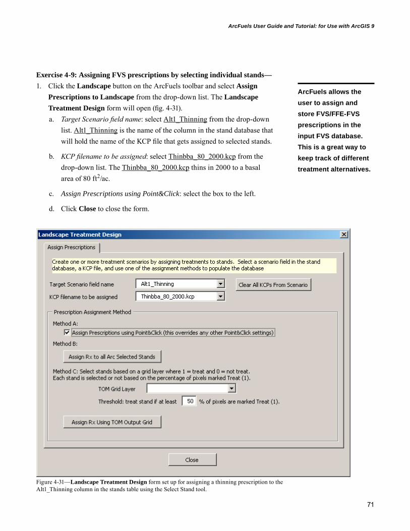
71


Exercise 4-9: Assigning FVS prescriptions by selecting individual stands—1. Click the Landscape button on the ArcFuels toolbar and select Assign

Prescriptions to Landscape from the drop-down list. The Landscape Treatment Design form will open (fig. 4-31).a. Target Scenario field name: select Alt1_Thinning from the drop-down

list. Alt1_Thinning is the name of the column in the stand database that will hold the name of the KCP file that gets assigned to selected stands.

b. KCP filename to be assigned: select Thinbba_80_2000.kcp from the drop-down list. The Thinbba_80_2000.kcp thins in 2000 to a basal area of 80 ft2/ac.

c. Assign Prescriptions using Point&Click: select the box to the left.

d. Click Close to close the form.

Figure 4-31—Landscape Treatment Design form set up for assigning a thinning prescription to the Alt1_Thinning column in the stands table using the Select Stand tool.

ArcFuels allows the user to assign and store FVS/FFE-FVS prescriptions in the input FVS database. This is a great way to keep track of different treatment alternatives.

72


2. Click the Select Stand button on the ArcFuels toolbar and point and click on a few densely forested stands.a. Click Yes to each of the Confirm windows that open after selecting

stands (fig. 4-32).

3. Open the Mt_Emily_Database.mdb in the data folder, then open the stands table.a. Sort in descending order the Alt1_Thinning column to see how the

KCP is stored (fig. 4-33).

b. Close the database when you are done.

Exercise 4-10: Assign FVS prescriptions to ArcGIS-selected features—This option is used in conjunction with ArcMap. Prescriptions can be assigned to ArcSelected stands. Stands can be selected based on location or attribute. The example below uses ArcSelected stands selected by proximity to structures in the wildland-urban interface.1. In ArcMap, open the Select by Location tool (ArcMap

toolbarSelectionSelect By Location…). The Select By Location form will open (fig. 4-34).

Figure 4-32—Confirm window that checks to see if you really want to apply the prescription to the selected stand. The example shown is for applying the Thibba_80_2000.kcp to stand 590.

Figure 4-33—Thnbba_80_2000.kcp assignments in the Alt1_Thinning column of the stands table in the Mt_Emily_Database file.

73


a. I want to: select Select features from from the drop-down list.

b. the following layer(s): check the box to the left of mt_emily_stands.

c. that: select are within a distance of from the drop-down list.

d. the features in the layer: select structures from the drop-down list.

e. Apply a buffer to the features in structures: check the box to the left.

f. of: type in “0.5” and then select Miles from the drop-down list.

g. Click OK to apply the selection. This will select all stands within one-half mile of each structure (fig. 4-35).

Figure 4-34—ArcMap Select By Location form set up to select stands within one-half mile of structures in the Mt. Emily wildland-urban interface.

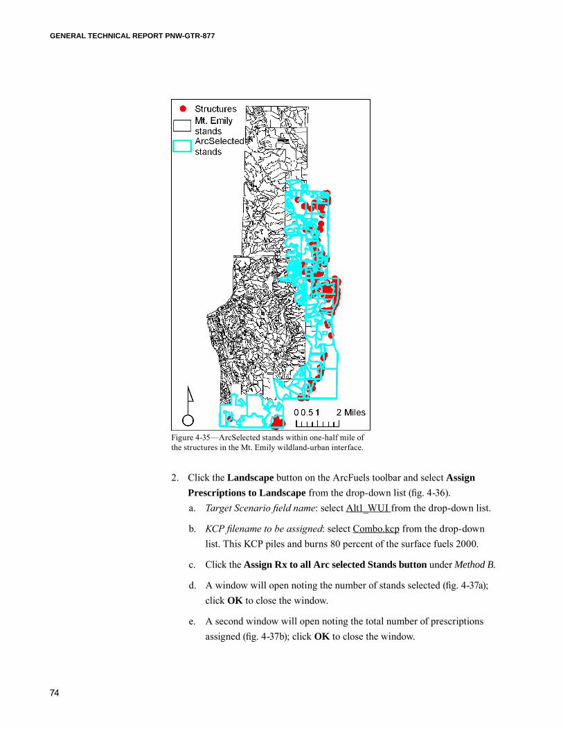
74


2. Click the Landscape button on the ArcFuels toolbar and select Assign Prescriptions to Landscape from the drop-down list (fig. 4-36). a. Target Scenario field name: select Alt1_WUI from the drop-down list.

b. KCP filename to be assigned: select Combo.kcp from the drop-down list. This KCP piles and burns 80 percent of the surface fuels 2000.

c. Click the Assign Rx to all Arc selected Stands button under Method B.

d. A window will open noting the number of stands selected (fig. 4-37a); click OK to close the window.

e. A second window will open noting the total number of prescriptions assigned (fig. 4-37b); click OK to close the window.

Figure 4-35—ArcSelected stands within one-half mile of the structures in the Mt. Emily wildland-urban interface.

75


Figure 4-36—Landscape Treatment Design form set up to assign a combined thinning, surface fuel treatment, and underburn prescription to stands within one-half mile of structures in the Mt. Emily wildland-urban interface.

Figure 4-37—Arc Map window indicating the number of ArcSelected stands (A) and that treatments have been assigned (B).

76


3. Open the Mt_Emily_Database.mdb in the data folder, then open the stands table to see how the prescriptions were assigned in the Alt1_WUI column. Close the database when you are done.

Exercise 4-11: Assign prescriptions with a treatment grid—Using a treatment grid is an efficient way to assign prescriptions to stands. The tool requires a 0/1 grid where 1 indicates treatments should be applied. Because grid cells are square, and polygons are not typically, the tool also allows you to decide how much of the polygon must be represented by a value of 1 in the grid.

Although this function was designed specifically to be used with the Treatment Grid created by running the treatment optimization model (TOM) in FlamMap (see the Introduction to Modeling Fire Behavior in FlamMap for more information about TOM) it can be used with other 0/1 grids. For example, the function pairs extremely well with the Raster Calculator (ArcToolBoxSpatial AnalystRaster Calculator) within ArcMap. With the Raster Calculator you can create new grids based on criteria (e.g., all burnable fuels, slopes > 30 percent, south aspects, etc.) and then use ArcFuels to make changes within these areas. The grids created in the Raster Calculator default to 0/1 values. This eliminates several steps and reduces the number of files you need to keep track of and organize.1. Look at the ideal_trt grid in ArcMap. Stands that are gray have a grid value

of 0, meaning that they are not available for treatment; stands that are black have a grid value of 1 and are available to be treated (fig. 4-38). The black area accounts for about 66 percent of the landscape.

2. Click the Landscape button on the ArcFuels toolbar and select Assign Prescriptions to Landscape from the drop-down list. The Landscape Treatment Design form will open (fig. 4-39).a. Target Scenario field name: select

Alt1_TOM from the drop-down list.

b. KCP filename to be assigned: select Combo.kcp from the drop-down list.

c. TOM Grid Layer: select the ideal_trt grid from the drop-down list (under Method C).

¸ 0 1 20.5 Miles

0-no1-yes

Ideal treatment locations

Figure 4-38—Ideal treatment grid (ideal_trt) where gray is not available for treatment and black is available.

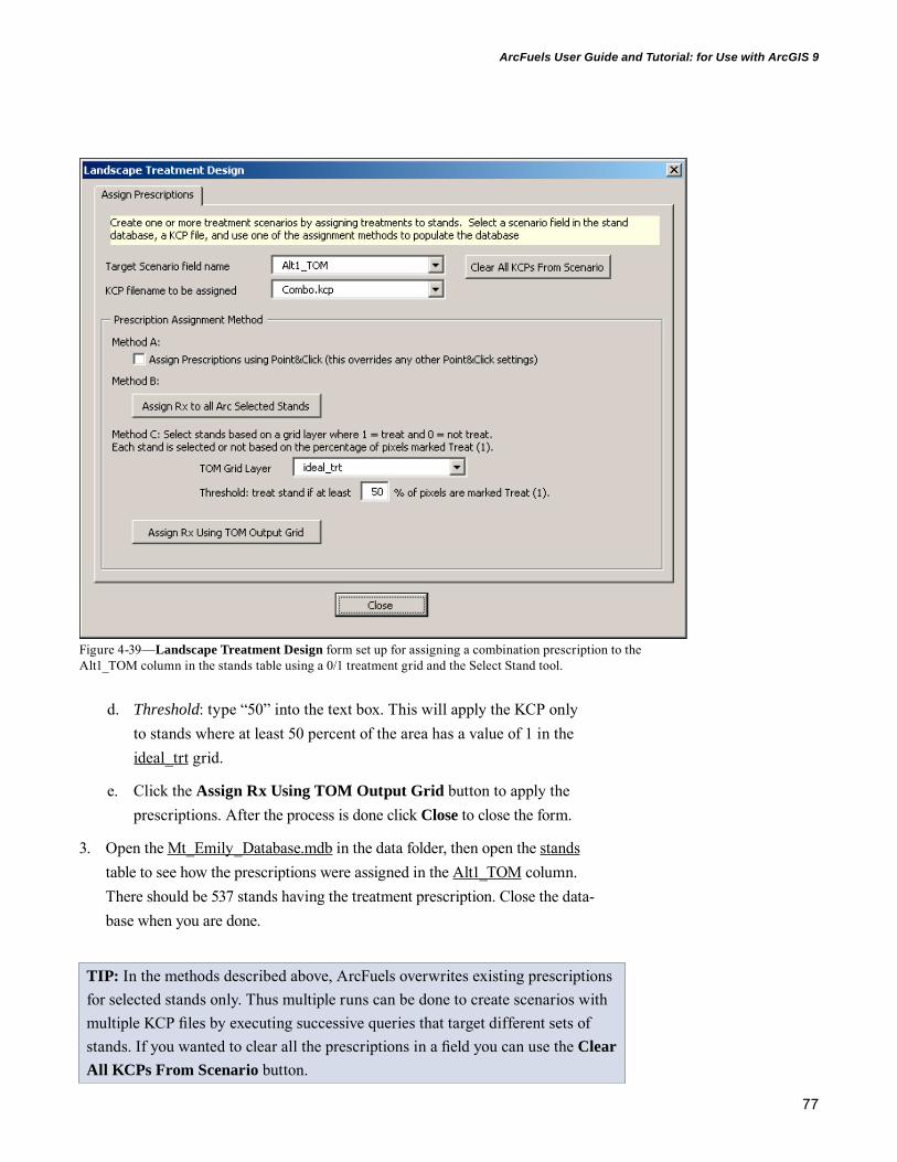
77


d. Threshold: type “50” into the text box. This will apply the KCP only to stands where at least 50 percent of the area has a value of 1 in the ideal_trt grid.

e. Click the Assign Rx Using TOM Output Grid button to apply the prescriptions. After the process is done click Close to close the form.

3. Open the Mt_Emily_Database.mdb in the data folder, then open the stands table to see how the prescriptions were assigned in the Alt1_TOM column. There should be 537 stands having the treatment prescription. Close the data-base when you are done.

TIP: In the methods described above, ArcFuels overwrites existing prescriptions for selected stands only. Thus multiple runs can be done to create scenarios with multiple KCP files by executing successive queries that target different sets of stands. If you wanted to clear all the prescriptions in a field you can use the Clear All KCPs From Scenario button.

Figure 4-39—Landscape Treatment Design form set up for assigning a combination prescription to the Alt1_TOM column in the stands table using a 0/1 treatment grid and the Select Stand tool.

78


Exercise 4-12: Running FVS for the no-treatment alternative—In this exercise, we will run all the stands through FVS to create the no-treatment alternative with a wildfire simulated in 2007, using the Wildfire2007.kcp. We will run the simulation for 10 years in 1-year increments (2000 through 2009). 1. Click the Landscape button on the ArcFuels toolbar, then select Simulate

Landscape Treatment from the drop-down list. 2. Select the Run FVS tab (fig. 4-40).

a. Input Database: the default database Mt_Emily_Database.mdb is set using the Project Manager.

b. Stand Table: keep the default, stands, which is set using the Project Manager.

Figure 4-40—The Run FVS tab set up to run FVS for all stands to create the no-treatment alternative with a wildfire simulated in 2007.

FVS/FFE-FVS can be run at the landscape scale within ArcFuels. Because ArcFuels makes FVS/FFE-FVS spatially explicit the user can run stands a variety of ways including those selected in ArcMap.

79


c. Stand ID: keep the default, Stand_ID, which is set using the Project Manager.

d. Output Database: keep the default database name, notreat.mdb, which is set using the Project Manager.

e. Scenario name: type “nt” in the text box to the right; this will then autopopulate the Key file and Out file text boxes. The “nt” refers to the no-treatment alternative.

f. Stand selection: select the radio button to the left of Run all Stands. We want to run all the stands in the Mt. Emily area.

i. When working with large data sets or testing new prescription files, you are advised to run a smaller number of stands using the Run first XXX stands option.

g. Prescription Source: click the Add/Change Files button and select the Wildfire2007.kcp from the Select KCP Files form (fig. 4-13). This function is the same as was completed for running single stands in Exercise 4-3.

h. Options/Outputs: for this run we will be running 10 one-year cycles, allowing fuel models to be selected from both sources, and we will be creating carbon reports.

i. Cycles: type“10” in the text box.

ii. Years per cycle: type “1” into the text box.

iii. Fuel model set: select 53 from the drop-down list.

iv. Check Execute, Overwrite DB and Carbon Report; make sure the rest are unchecked.

v. Scenario Index: type “1” into the box

i. Click the Run FVS button to start the FVS simulation. Depending on your computer, this should take 5 to 15 minutes.

j. When FVS is done running, double-click the text C:\arcfuels\outputs\notreat.mdb in the Output Database text box to open the output data-base (fig. 4-41), and then browse the various FVS output tables. For a description of the tables see Exercise 4-1.

80


NOTE: Because a prescription (KCP) is being applied to all the stands, it is recom-mended that you first run a few stands through using the Run first “xx” stands option first to check for errors (see the TIP below) and review the output database.

TROUBLESHOOTING: If FVS experiences a termination code and closes or if you terminate a run, a warning window (fig. 4-42) will pop up and the FVS out file will automati-cally open. Look through the FVS out file to identify the error.

Figure 4-41—FVS output database with all the tables created on the left hand side of the window, and the FVS_Carbon table open.

Figure 4-42—Abnormal FVS termination warning window.

81


Exercise 4-13: Simulating landscape treatments in FVS to create an ideal land-scape for the TOM in FlamMap—This exercise will create a potential treatment alternative that can be used to create the ideal landscape for use with the TOM in FlamMap3 (refer to the Introduction to Modeling Fire Behavior in FlamMap3 section for more information). A combina-tion prescription including a thinning, surface fuel treatment, and underburn was assigned to stands using the ideal_trt grid in Exercise 4-11.1. Click the Landscape button on the ArcFuels toolbar, then select Simulate





d. Output Database: use the navigation button to create a new output database named “Alt1_TOM.”

e. Scenario name: type “tom” in the text box to the right.

TIP: You can open the FVS input and output databases from the Run FVS tab by double-clicking on the text box next to each.

TIP: The Scan for Errors button on the Run FVS tab checks the FVS output file for any errors that may have occurred during the run (fig. 4-43). The most common errors happen when a KPC is not written correctly. A window will open letting you know that there either were no errors or what the error was and where to find it.

Figure 4-43—FVS Error Scan windows for no errors or for an error. The FVS error code number can be looked up in the FVS Essentials Guide (Dixon 2003).

82


f. Stand selection: select the radio button to the left of Run all Stands. We want to run all the stands in the Mt. Emily area.

g. Prescription Source: click the Add/Change Fields button and select the Alt1_TOM field using the Select KCP Fields form that opens. This is similar to selecting a KCP file.

h. Options/Outputs: for this run, we will be running 10 one-year cycles, allowing fuel models to be selected from both sources, and we will be creating carbon reports.

Figure 4-44—The Run FVS tab set up to run FVS for all stands to create the TOM alternative. The Combo.kcp was assigned to all stands requiring treatment in the Alt1_TOM field of the stands table in the Mt_Emily_Database file in Exercise 4-11.

83


i. Cycles: type “10” in the text box.



iv. Check Execute, Overwrite DB and Carbon Report; make sure the rest are unchecked.

v. Scenario Index: type “1” into the box.

i. Click Run FVS to start the FVS simulation. Depending on your com-puter, this should take 5 to 15 minutes.

j. When FVS is done running, double-click the text C:\arcfuels\outputs\Alt1_TOM.mdb in the Output Database text box to open the output database, and browse the various FVS output tables. For a description of the tables see Exercise 4-1.

Exercise 4-14: Simulating landscape treatments in FVS only to stands with prescriptions—This exercise will use FVS to simulate only the stands with the Combo.kcp prescrip-tion assigned to the Alt1_WUI column (field) in the stands table of the Mt_Emily_Database.mdb. The Combo.kcp prescription was assigned to all stands within one-half mile of the structures of the wildland-urban interface in Exercise 4-10.1. Click the Landscape button on the ArcFuels toolbar, then select Simulate





d. Output Database: use the navigation button to create a new output database named “Alt1_WUI.”

e. Scenario name: type “wui” in the text box to the right.

f. Stand selection: select the radio button to the left of Run stands with prescriptions.

To save time it is possible to only run stands with prescriptions assigned through FVS/FFE-FVS. The resulting output database can be coupled with an output database including all stands (untreated) in the landscape to build a treated LCP using ArcFuels.

84


i. If a no-treatment alternative has already been run, time can be saved by running only the stands with prescriptions. The two data-bases can be merged to create a FlamMap landscape file (LCP) using ArcFuels.

g. Prescription Source: click on the Add/Change Fields button and select the Alt1_WUI field using the Select KCP Fields form that opens. This is similar to selecting a KCP file.

i. Remove the Alt1_TOM prescription field if it is still loaded.

Figure 4-45—The Run FVS tab set up to run FVS only for stands with prescriptions assigned to create a WUI treatment alternative. The pileburn.kcp was assigned to all stands requiring treatment in the Alt1_WUI field of the stands table in the Mt_Emily_Database file in Exercise 4-10.

85



i. Cycles: type”10” in the text box.



iv. Check Execute, Overwrite DB and Carbon Report, and make sure the rest are unchecked.

v. Scenario Index: type “1” into the text box.

i. Click the Run FVS button to start the FVS simulation. Depending on your computer, this should take 5 to 15 minutes.

j. When FVS is done running, double-click the text C:\arcfuels\outputs\Alt1_WUI.mdb in the Output Database text box to open the output database, and browse the various FVS output tables. For a description of the tables, see Exercise 4-1.

Exercise 4-15: Using the Treatment Analysis tab to vary a single parameter—Method 1 of the Treatment Analysis tab in the Simulate Landscape Treatments form is simlar to the Treatment Analysis tab in the Set Stand Options form (see Exercise 4-5). Two main differences exist: the option here can run multiple stands at once, and when running the tool at the landscape scale the outputs are written to an Access database rather than an Excel workbook. For example, you are interested in finding a thinning intensity that reduces canopy bulk density below a set thresh-old (0.1 kg/m3) because crown fire is unlikely to occur below that level (Agee 1996).1. Click the Landscape button on the ArcFuels toolbar, then select Simulate




NOTE: The same results could be obtained by first selecting the stands within one-half mile of the structures in ArcMap, then selecting the Combo.kcp as the Prescription Source, then selecting Run ArcMap Selected Stands.

Similar to stand functionality, FVS/FFS-FVS prescriptions can be analyzed for an entire landscape or select stands to fine tune prescriptions.

86



d. Output Database: use the navigation button to create a new output database named “Combo_BA_Analysis.mdb.”

e. Scenario name: type “ba” in the text box to the right.

f. Stand selection: select the radio button to the left of Run first stands and type “50” into the text box.

Figure 4-46—The Run FVS tab set up to run FVS to analyze the effect of varying thinning intensities.

87


g. Prescription Source: click the Add/Change Files button and select the Combo.kcp field using the Select KCP Files form that opens. Remove old fields, e.g., Alt1_WUI, if they are still loaded.


i. Cycles: type “10” in the text box.



iv. Check Execute, and make sure the rest are unchecked.

v. Scenario Index: type “1” into the box.

3. Select the Treatment Analysis tab (fig. 4-47).a. Specify treatment file(s) on the Run FVS tab, then select one here:

select the Combo.kcp from the drop-down list.

b. Method 1: select the radio button to the left of this option.

i. Select the line containing the variable to be analyzed: select the line with the ThinBBA keyword from the drop-down list. This is the keyword that triggers a thin from below. The text boxes below the line will autopopulate (fig. 4-47).

ii. Variable parameter: select 2 from the drop-down list because this corresponds to the basal area.

iii. Minimum Value: type “50” into the text box. This is the minimum basal area value for thinning.

iv. Maximum Value: type “100” into the text box. This is the maximum basal area value for thinning.

v. Step Amount: type “10” into the text box. This is the step amount for thinning (i.e., basal area will be thinned to 50, 60, 70 ft2/ac, etc.)

c. Click the Run FVS Analysis button to start the FVS simulation. This will run FVS six times, once for each time step. Depending on your computer, this should take about 5 to 10 minutes.

88


d. When FVS is done running, double-click the text C:\arcfuels\outputs\Combo_BA_Analysis.mdb in the Output Database text box to open the output database, and then open the FVS_Compute table and scroll all the way to the right. Notice the appended THINBBA2 column (fig. 4-48). The basal area thinning factor associated with the runs is appended to this table for further analysis. The value can be added to other tables by doing a query function in the database.

Figure 4-47—Treatment Analysis tab set up to vary basal area thinning intensities from 50 to 100 ft2/ac in 10-ft2/ac increments.

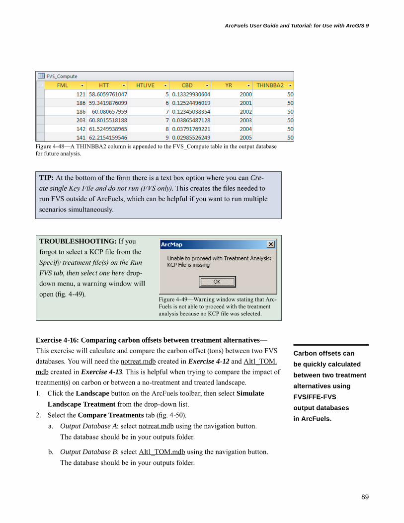
89


Exercise 4-16: Comparing carbon offsets between treatment alternatives—This exercise will calculate and compare the carbon offset (tons) between two FVS databases. You will need the notreat.mdb created in Exercise 4-12 and Alt1_TOM.mdb created in Exercise 4-13. This is helpful when trying to compare the impact of treatment(s) on carbon or between a no-treatment and treated landscape. 1. Click the Landscape button on the ArcFuels toolbar, then select Simulate

Landscape Treatment from the drop-down list. 2. Select the Compare Treatments tab (fig. 4-50).

a. Output Database A: select notreat.mdb using the navigation button. The database should be in your outputs folder.

b. Output Database B: select Alt1_TOM.mdb using the navigation button. The database should be in your outputs folder.

TIP: At the bottom of the form there is a text box option where you can Cre-ate single Key File and do not run (FVS only). This creates the files needed to run FVS outside of ArcFuels, which can be helpful if you want to run multiple scenarios simultaneously.

TROUBLESHOOTING: If you forgot to select a KCP file from the Specify treatment file(s) on the Run FVS tab, then select one here drop-down menu, a warning window will open (fig. 4-49).

Figure 4-48—A THINBBA2 column is appended to the FVS_Compute table in the output database for future analysis.

Figure 4-49—Warning window stating that Arc-Fuels is not able to proceed with the treatment analysis because no KCP file was selected.

Carbon offsets can be quickly calculated between two treatment alternatives using FVS/FFE-FVS output databases in ArcFuels.

90


c. Year of interest: type “2007” in the text box. A wildfire was initiated in both the no-treatment and TOM alternatives in 2007.

d. Click the Calculate Carbon Offset button.

e. The Carbon Offset from change in emission, Carbon offset from change in stock, and Total carbon offset have been calculated between the two treatment scenario databases.

Figure 4-50—Compare Treatments tab in the Simulate Landscape Treatments form set up to compare the total carbon offset between untreated and treated scenarios after a wildfire in 2007.

91


i. The difference is Alt1_TOM minus notreat. The TOM treat-ment resulted in a total carbon offset of 1,486 tons of carbon. In other words, the treated landscape retained more carbon than the untreated landscape after a simulated wildfire in 2007.

Exercise 4-17: Joining FVS outputs to the stand polygon—Because FVS runs often include multiple simulation years it is not possible to join the outputs to the stand shapefile using ArcMap. This tool allows you to join data from any year within an FVS output table to the Mt. Emily stands shapefile. This is quite helpful for visualizing the FVS runs on the landscape.1. Click the Landscape button on the ArcFuels toolbar, then select Simulate

Landscape Treatment from the drop-down list. 2. Select the Join FVS Outputs to Polygons tab (fig. 4-51).

a. FVS Output Database: select notreat.mdb using the navigation button. The database should be in your outputs folder.

b. Table to Join from FVS output DB: select FVS_Summary from the drop-down list.

c. Year to Join: select 2005 from the drop-down list.

d. Click the Do Join button.

e. Click OK when the confirmation windows (fig. 4-52) open.

f. Click Close to close the form and return to ArcMap.

3. Open the attributes table of mt_emily_stands and scroll to the right; note the joined data.

4. To visualize the output data change the symbology of the mt_emily_stands polygon to show trees per acre (TPA, fig. 4-53). a. Right-click on the mt_emily_stands polygon in the ArcMap table

of contents then PropertiesSymbologyQuantities Graduated Colors.

i. The Value should be TPA, then select 6 from the Classes drop-down menu.

ii. Click the Classify button to open the Classification form.

iii. Select Manual from the Method drop-down menu and set the break values according to figure 4-53.

iv. Click OK to close the Classification form.

ArcFuels allows the user to join values within an FVS/FFE-FVS database to a stand shapefile in ArcMap. The resulting maps can be used to highlight various metrics such as tree density, basal area, or potential fire behavier for any year modeled.

92


v. Click OK again to close the Layer Properties form.

b. This can also be completed for the TOM treatment alternative as shown in figure 4-53b if you so choose.

Figure 4-51—Join FVS Outputs to Polygons tab in the Simulate Landscape Treatments form set up to join the FVS_Summary data for 2005.

Figure 4-52—Confirmation windows that appear after a join is initiated.

BA

93


Exercise 4-18: Build the no-treatment alternative LCP using inventory data run through FVS—This exercise will demonstrate how to build an LCP from an FVS output database. The notreat.mdb, created in Exercise 4-12, will be used in conjunction with the slope, aspect, elevation, and stands grids. 1. Click the Landscape button on the ArcFuels toolbar, then select Build

FlamMap Landscape from the drop-down list. 2. Select the Using FVS Database tab (fig. 4-54).

a. Elevation: select elevation from the drop-down list.

b. Slope: select slope from the drop-down list.

c. Aspect: select aspect from the drop-down list.

d. Stand ID Grid: select stands from the drop-down list.

e. Latitude: type “45” into the text box.

f. The output boundaries are based on: select the Grid Layer radio but-ton, then select the stands grid from the drop-down list.

NOTE: It is not possible to do multiple joins at once using this tool. The most recent join will replace any past joins, even if the Remove Joins button is not used.

Figure 4-53—Maps of trees per acre for the untreated (A) and TOM treatment (B) alternatives.

A B

5 100

100 250

250 500500 1,000

1,000

5<_

_

_

_

>

Trees per acre

ArcFuels can build landscape files (LCPs) from FVS/FFE-FVS output databases using the default FVS-Compute table created.

94


g. FVS Output Database: select the notreat.mdb from the outputs folder using the navigation button.

h. Output Table: select FVS_Compute from the drop-down list.

i. Stand ID Field: select StandID from the drop-down list.

j. Year: select 2005 from the drop-down list.

k. Scenario: select 1 from the drop-down list.

l. Fuel model: select FML from the drop-down list.

m. Canopy Cover: select CANOPY from the drop-down list.

n. Canopy Height: select HTT from the drop-down list.

o. Canopy Base Height: select HTLIVE from the drop-down list.

p. Canopy Bulk Density: select CBD from the drop-down list.

q. Apply Treatments: make sure this box is not checked.

Figure 4-54—Using FVS Database tab set up to create a no-treatment LCP from the FVS run for 2005.

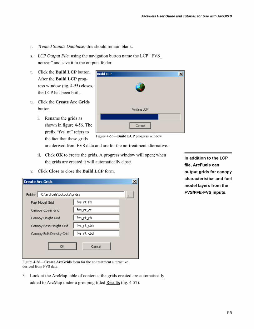
95


r. Treated Stands Database: this should remain blank.

s. LCP Output File: using the navigation button name the LCP “FVS_notreat” and save it to the outputs folder.

t. Click the Build LCP button. After the Build LCP prog-ress window (fig. 4-55) closes, the LCP has been built.

u. Click the Create Arc Grids button.

i. Rename the grids as shown in figure 4-56. The prefix “fvs_nt” refers to the fact that these grids are derived from FVS data and are for the no-treatment alternative.

ii. Click OK to create the grids. A progress window will open; when the grids are created it will automatically close.

v. Click Close to close the Build LCP form.

3. Look at the ArcMap table of contents; the grids created are automatically added to ArcMap under a grouping titled Results (fig. 4-57).

Figure 4-55—Build LCP progress window.

Figure 4-56—Create ArcGrids form for the no treatment alternative derived from FVS data.

In addition to the LCP file, ArcFuels can output grids for canopy characteristics and fuel model layers from the FVS/FFE-FVS inputs.

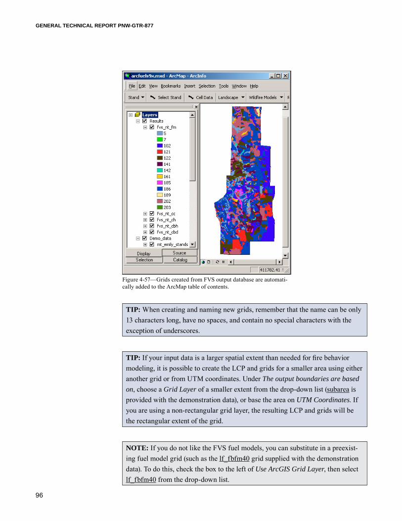
96


Figure 4-57—Grids created from FVS output database are automati-cally added to the ArcMap table of contents.

TIP: When creating and naming new grids, remember that the name can be only 13 characters long, have no spaces, and contain no special characters with the exception of underscores.

TIP: If your input data is a larger spatial extent than needed for fire behavior modeling, it is possible to create the LCP and grids for a smaller area using either another grid or from UTM coordinates. Under The output boundaries are based on, choose a Grid Layer of a smaller extent from the drop-down list (subarea is provided with the demonstration data), or base the area on UTM Coordinates. If you are using a non-rectangular grid layer, the resulting LCP and grids will be the rectangular extent of the grid.

NOTE: If you do not like the FVS fuel models, you can substitute in a preexist-ing fuel model grid (such as the lf_fbfm40 grid supplied with the demonstration data). To do this, check the box to the left of Use ArcGIS Grid Layer, then select lf_fbfm40 from the drop-down list.

97


Exercise 4-19: Build the WUI treatment alternative LCP using inventory data run through FVS—To eliminate the need to resimulate the entire landscape with each treatment scenario, it is possible to combine a no-treatment landscape output with the simula-tion outputs from only the treated stands to create a hybrid landscape file. In other words, FVS outputs for the treated stands replace the FVS outputs for the no-treat-ment alternative for the stands that are treated. If relatively few stands are treated, the process of creating several treatment scenarios is accelerated. This exercise will demonstrate how to build a treatment alternative LCP (and grids) using both a no-treatment FVS output database and a wildland-urban interface treatment alternative FVS output database that contains only treated stands. This exercise uses the FVS output databases from Exercises 4-12 and 4-14.1. Click the Landscape button on the ArcFuels toolbar, then select Build

FlamMap Landscape from the drop-down list. 2. Select the Using FVS Database tab (fig. 4-58).

Figure 4-58—Using FVS Database tab set up to create a WUI treatment alternative LCP.

ArcFuels can combine two FVS/FFE-FVS databases to build an LCP file. The first is the untreated database where all stands are modeled, and the second is the post-treatment database where only those stands requiring treatment are included.

98


















q. Apply Treatments: check the box to the left.

r. Treated Stands Database: navigate to and select the Alt1_WUI.mdb in the outputs folder.

s. LCP Output File: using the navigation button, name the LCP “FVS_WUItreat” and save it to the outputs folder.

t. Click the Build LCP button.

u. Click the Create Arc Grids button.

i. Rename the grids as shown in figure 4-59. The prefix “fvs_wui” refers to the fact that these grids are derived from FVS data and are for the WUI treatment alternative.

ii. Click OK to create the grids.

v. Click Close to close the Build LCP form.

99


3. Return to ArcMap and look at the fuel model layer; notice where it changed. The fuel model layer can often be the easiest layer to verify treatments occurred where envisioned.

Exercise 4-20: Build the no-treatment alternative LCP using grid data—This exercise will demonstrate how to build a no-treatment LCP from grid data. The supplied LANDFIRE data will be used. 1. Click the Landscape button on the ArcFuels toolbar, then select Build

FlamMap Landscape from the drop-down list. 2. Select the Using AcGIS Grid Data tab (fig. 4-60).

a. Elevation: select elevation and meters from the drop-down lists.

b. Slope: select slope and degrees from the drop-down lists.


d. Distance Units: select meters from the drop-down list.


f. The output boundaries are based on: select the Grid Layer radio button, then select elevation from the drop-down list.

g. Apply Treatment Adjustments: leave this box unchecked.

Figure 4-59—Create ArcGrids form to create the WUI treat-ment alternative grids.

NOTE: It is also possible to repeat Exercise 4-19 with an FVS database that contains all stands treated and untreated together. An example of this type of database (Alt1_TOM) was created in Exercise 4-13.

ArcFuels can be used to build LCPs from grid data. This saves time when the user would otherwise need to export the individual layers as ASCII files to build the LCP FlamMap.

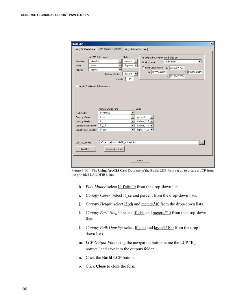
100


h. Fuel Model: select lf_fbfm40 from the drop-down list.

i. Canopy Cover: select lf_cc and percent from the drop-down lists.

j. Canopy Height: select lf_ch and meters,*10 from the drop-down lists.

k. Canopy Base Height: select lf_cbh and meters,*10 from the drop-down lists.

l. Canopy Bulk Density: select lf_cbd and kg/m3,*100 from the drop-down lists.

m. LCP Output File: using the navigation button name the LCP “lf_notreat” and save it to the outputs folder.

n. Click the Build LCP button.

o. Click Close to close the form.

Figure 4-60—The Using ArcGIS Grid Data tab of the Build LCP form set up to create a LCP from the provided LANDFIRE data.

101


Exercise 4-21: Build a treatment alternative LCP using treatment adjustment factors and grid data—This exercise will demonstrate how to build an LCP and grids for a treatment alternative using the current conditions LANDFIRE grids, treatment location (trt_location), and treatment type (trt_type) grids along with a treatment adjust-ments database (Treatment_adjustments.mdb). The supplied treatment location and treatment types treat about 20 percent of the landscape and were designed to target preservation of large trees (Ager et al. 2010).

ArcFuels modifies grid data and creates new grids and LCP files by using an Access “lookup” table (fig. 4-62), which stores the replacements (e.g., change fuel model to 8 within unit 5) or adjustments (e.g., increase canopy base height by 30 percent, decrease canopy bulk density by 20 percent within unit 3) desired.

Determining how to adjust canopy characteristic grids can be completed by running prescriptions FVS through ArcFuels (Exercise 4-4) FVS can also predict fuel models under changed stand conditions. However, expert knowledge of the

TROUBLESHOOTING: If you do not have the full path in the LCP Output File text box, you will get an error window stating there was an error generating the LCP file (fig. 4-61).

TIP: If your input data is a larger spatial extent than needed for fire behavior modeling, it is possible to create the LCP and grids for a smaller area by using either another grid or from UTM coordinates. Under The output boundaries are based on, choose a Grid Layer of a smaller extent from the drop-down list (subarea is provided with the demonstration data), or base the area on UTM Coordinates. If you are using a non-rectangular grid layer, the resulting LCP and grids will be the rectangular extent of the grid.

NOTE: Knowing the units of the input data and correctly assigning them in the Using ArcGIS Grid Data form is very important when building LCPs. Improper units can drastically alter fire model outputs.

Figure 4-61—When the full path is not included, the LCP will not be built and an error window will open.

Posttreatment LCP(s) can be rapidly built by updating values in the existing conditions grids using treatment location and type grids along with treatment adjustment factor(s) in ArcFuels.

102


on-the-ground conditions should be used in conjunction with these data. Note that shrub dynamics are not a part of FFE-FVS; fuel models are predicted based on the data collected by standard forest inventory plots. Alternatively, adjustments can be derived from monitoring data of treated areas that represent the posttreatment conditions desired, or may come from a specific treatment prescription (i.e., canopy cover will be reduced to 40 percent and canopy base height will be lifted to 6 ft).

ArcFuels multiplies the adjustment factor numbers by the existing condi-tion values or replaces them. For example, treatment type 1 reduces canopy bulk density and canopy cover by 50 percent (multiplies the existing condition by 0.5) and increases canopy base height and canopy height by 80 percent (multiplies the existing condition by 1.8) and 30 percent (multiplies the existing condition by 1.3), respectively. In this example, under treatment type 1, fuel models will be changed (replaced) to 181.

The flowchart below (fig. 4-63) is a visual depiction of the relationship between the treatment type and location grids and the treatment adjustments table within the treatment adjustments database. This system allows for pixel-level (versus entire stand) manipulation of the grid data, allowing a single stand to receive different intensities of treatment.1. Click the Landscape button on the ArcFuels toolbar, then select Build

FlamMap Landscape from the drop-down list. 2. Select the Using AcGIS Grid Data tab (fig. 4-64).






f. The output boundaries are based on: select the Grid Layer radio button, then select elevation from the drop-down list.

Figure 4-62—Example treatment adjustments table within the treatment adjustments database.

103


Figure 4-63—Flow chart of how the treatment adjustment grids and factors work together to create a treatment alternative.

Treated LCP and fuel grids

Grid of treatment type pixels.1 in yellow = heavy thin with under burn2 in green = underburn only3 in blue = light thin with underburn

0 1 1 1 2 2 2 0 0 0 0 0 0 1 1 2 2 2 3 0 0 0 0 0 0 1 1 1 3 1 3 0 0 0 0 0 0 0 0 0 0 0 3 2 2 1 0 0 0 0 0 0 0 0 0 0 1 1 1 0

Grid of treatment location pixels.Non-zero value in red = apply treatment, zero in black = no treatment.

Treatments can be identified by any non-zero value.

0 1 1 1 1 1 1 0 0 0 0 0 0 1 1 1 1 1 1 0 0 0 0 0 0 1 1 1 1 1 1 0 0 0 0 0 0 0 0 0 0 0 1 1 1 1 0 0 0 0 0 0 0 0 0 0 1 1 1 0

Treatment adjustments table within the treatment adjustments database.

Untreated fuel grids

104


g. Apply Treatment Adjustments: check the box to the left. This will make more options available.

i. Treatment Type Database: navigate to and select the Treatment_adjustments.mdb in the data folder using the navigation button.

ii. Treatment Location Grid: select trt_location from the drop-down list.

iii. Treatment Type Grid: select trt_type from the drop-down list.

iv. Treatment Adjustment Table: select example_treatment_adjustment from the drop-down list.

v. Treatment Type ID Field: select treat_type from the drop-down list.

h. Fuel Model: select lf_fbfm40 and fm_adj from the drop-down lists.

i. Canopy Cover: select lf_cc, percent, and cc_adj from the drop-down lists.

Figure 4-64—The Using ArcGIS Grid Data tab of the Build LCP form set up to create a treat-ment alternative with the provided LANDFIRE data and treatment adjustment database.

105


j. Canopy Height: select lf_ch, meters,*10, and ch_adj from the drop-down lists.

k. Canopy Base Height: select lf_cbh, meters,*10, and cbh_adj from the drop-down lists.

l. Canopy Bulk Density: select lf_cbd, kg/m3,*100, and cbd_adj from the drop-down lists.

m. LCP Output File: using the navigation button name the LCP “lf_treat20” and save it to the outputs folder.


o. Click the Create Arc Grids button.

i. Rename the grids as shown in figure 4-65. The prefix “lf_trt20” refers to the fact that these grids are derived from LANDFIRE data (lf) and are for a treatment scenario (treat) that treated 20 percent (20) of the landscape.

ii. Click OK to create the grids.

Figure 4-65—Create ArcGrids form to create the treatment alternative grids.

p. Click Close to close the Build LCP form.

3. Look at the grids added to the ArcMap table of contents; they will be under a new Results group. Note how they have changed to represent treatment when compared to the input grids. It is a good idea to check the created grids before modeling fire behavior with the LCP to be sure treatments were applied as you envisioned.

106


Exercise 4-22: Build an LCP using multiple grid sources—Building an LCP from multiple grid sources within ArcFuels is a time-saving tool that allows you to mosaic multiple grid layers together and create an LCP in a single step. This tool might be used if you have smaller extent grid layers that represent update conditions owing to recent management or disturbance. Or when creating landscape files for fire behavior simulations it is preferred to have a rectangular extent; stand inventory data often are not rectangular in extent, so this tool is a quick way to mosaic in LANDFIRE (or other grid data) to make the LCP rectangu-lar. This is true with the demonstration data.

This exercise will use the no-treatment grids created from FVS data in Exercise 4-19 and the supplied LANDFIRE grid data.1. If not already loaded in ArcMap, add the fvs_nt_fm, fvs_nt_cc, fvs_nt_

cbh, fvs_nt_ch, and fvs_nt_cbd layers created in Exercise 4-19. 2. Click the Landscape button on the ArcFuels toolbar, then select Build

FlamMap Landscape from the drop-down list. 3. Select the Using Multiple Sources tab (fig. 4-66).

Figure 4-66—Using Multiple Sources tab set up to create a no-treatment LCP from the FVS run for 2005 and the LANDFIRE data.

ArcFuels can be used to create LCPs from multiple grids. The grids can be of various extents and units but must be the same resolution.

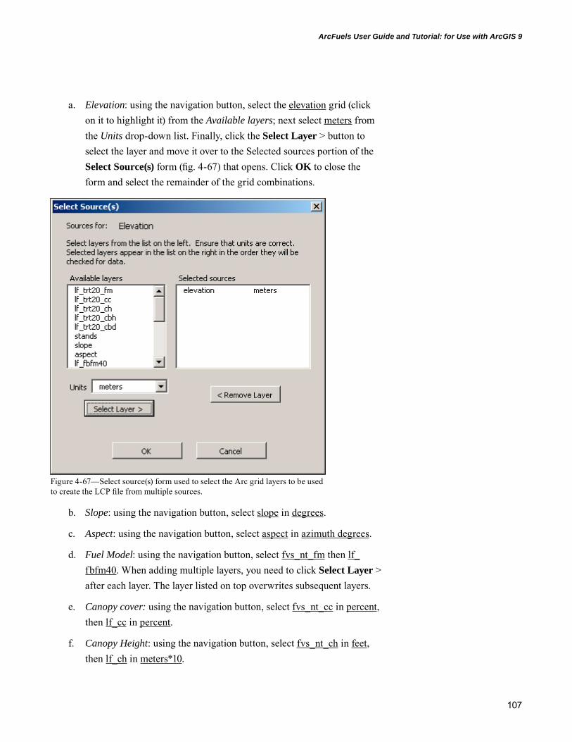
107


a. Elevation: using the navigation button, select the elevation grid (click on it to highlight it) from the Available layers; next select meters from the Units drop-down list. Finally, click the Select Layer > button to select the layer and move it over to the Selected sources portion of the Select Source(s) form (fig. 4-67) that opens. Click OK to close the form and select the remainder of the grid combinations.

b. Slope: using the navigation button, select slope in degrees.

c. Aspect: using the navigation button, select aspect in azimuth degrees.

d. Fuel Model: using the navigation button, select fvs_nt_fm then lf_fbfm40. When adding multiple layers, you need to click Select Layer > after each layer. The layer listed on top overwrites subsequent layers.

e. Canopy cover: using the navigation button, select fvs_nt_cc in percent, then lf_cc in percent.

f. Canopy Height: using the navigation button, select fvs_nt_ch in feet, then lf_ch in meters*10.

Figure 4-67—Select source(s) form used to select the Arc grid layers to be used to create the LCP file from multiple sources.

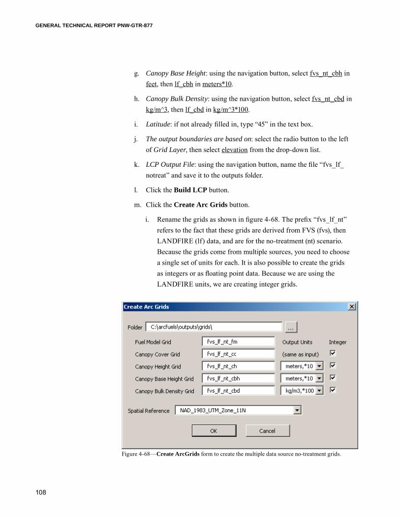
108


g. Canopy Base Height: using the navigation button, select fvs_nt_cbh in feet, then lf_cbh in meters*10.

h. Canopy Bulk Density: using the navigation button, select fvs_nt_cbd in kg/m^3, then lf_cbd in kg/m^3*100.

i. Latitude: if not already filled in, type “45” in the text box.

j. The output boundaries are based on: select the radio button to the left of Grid Layer, then select elevation from the drop-down list.

k. LCP Output File: using the navigation button, name the file “fvs_lf_notreat” and save it to the outputs folder.

l. Click the Build LCP button.

m. Click the Create Arc Grids button.

i. Rename the grids as shown in figure 4-68. The prefix “fvs_lf_nt” refers to the fact that these grids are derived from FVS (fvs), then LANDFIRE (lf) data, and are for the no-treatment (nt) scenario. Because the grids come from multiple sources, you need to choose a single set of units for each. It is also possible to create the grids as integers or as floating point data. Because we are using the LANDFIRE units, we are creating integer grids.

Figure 4-68—Create ArcGrids form to create the multiple data source no-treatment grids.

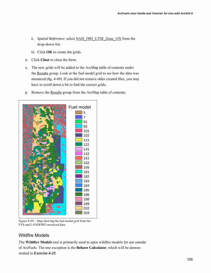
109


ii. Spatial Reference: select NAD_1983_UTM_Zone_11N from the drop-down list.

iii. Click OK to create the grids.

n. Click Close to close the form.

o. The new grids will be added to the ArcMap table of contents under the Results group. Look at the fuel model grid to see how the data was mosaiced (fig. 4-69). If you did not remove older created files, you may have to scroll down a bit to find the correct grids.

p. Remove the Results group from the ArcMap table of contents.

Figure 4-69—Map showing the fuel model grid from the FVS and LANDFIRE mosaiced data.

Fuel model579193101102121122141142161162165181182183184185186188189202203

Wildfire ModelsThe Wildfire Models tool is primarily used to open wildfire models for use outside of ArcFuels. The one exception is the Behave Calculator, which will be demon-strated in Exercise 4-23.

110


Exercise 4-23: Using the Behave Calculator—In this exercise we will run the Behave Calculator for a number of different midflame windspeeds to see the impact on surface fire behavior. 1. Click the Wildfire Models button on the ArcFuels toolbar, then select

Behave Calculator from the drop-down list (fig. 4-70).

a. Fuel model: select TL5 High load, conifer litter from the drop-down list.

b. Slope percent: type “0” in the text box.

c. 1 hr fuel moisture: type “9” in the text box.

d. 10 hr fuel moisture: type “10” in the text box.

e. 100 hr fuel moisture: type “11” in the text box.

f. Herbaceous: type “120” in the text box.

g. Woody: type “150” in the text box.

h. Midflame windspeed: this is the parameter that will be varied; start with 0 mph and incrementally increase it to 10 mph in 2-mph steps

i. Click the Run Behave Calculations button to calculate flame length and rate of spread.

j. Repeat the process, changing the Midflame windspeed in 2-mph increments to fill out table 4-2.

Figure 4-70—Behave Calculator form set up for the first Behave run.

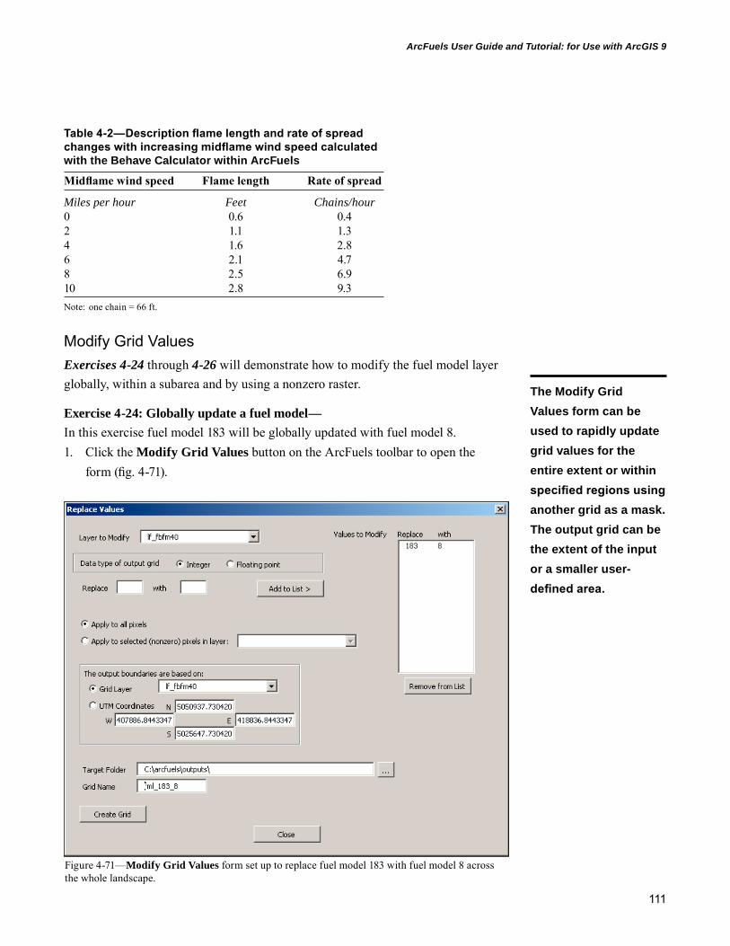
111


Modify Grid ValuesExercises 4-24 through 4-26 will demonstrate how to modify the fuel model layer globally, within a subarea and by using a nonzero raster.

Exercise 4-24: Globally update a fuel model—In this exercise fuel model 183 will be globally updated with fuel model 8.1. Click the Modify Grid Values button on the ArcFuels toolbar to open the

form (fig. 4-71).

Figure 4-71—Modify Grid Values form set up to replace fuel model 183 with fuel model 8 across the whole landscape.

Table 4-2—Description flame length and rate of spread changes with increasing midflame wind speed calculated with the Behave Calculator within ArcFuels

Midflame wind speed Flame length Rate of spread

Miles per hour Feet Chains/hour0 0.6 0.42 1.1 1.34 1.6 2.86 2.1 4.78 2.5 6.910 2.8 9.3Note: one chain = 66 ft.

The Modify Grid Values form can be used to rapidly update grid values for the entire extent or within specified regions using another grid as a mask. The output grid can be the extent of the input or a smaller user-defined area.

112


a. Layer to Modify: select lf_fbfm40 from the drop-down list.

b. Data type of output grid: select the radio button next to Integer.

c. Replace “183” with “8” by typing the values in the appropriate boxes and then click Add to List> to move the change to the Values to Modify box.

i. To remove values from the list, click on the one you would like to remove to highlight it and then click Remove from List.

d. Select the radio button to the left of Apply to all pixels.

e. The output boundaries are based on: select the radio button to the left of Grid Layer and then select lfrr_fbfm40 from the drop-down list.

f. Target Folder: using the navigation button, select the outputs folder (this is the default).

g. Grid Name: type “fml_183_8” in the text box.

h. Click the Create Grid button and then Close once ArcFuels has com-pleted processing.

2. The modified grid will automatically be added to your ArcMap and will show up under a new subheading entitled Modified Results (fig. 4-72).

A B Fuel Model8

91

93

99

101

102

121

122

142

161

162

163

165

181

182

184

185

186

188

183

Figure 4-72—The original LANDFIRE fuel model grid (A) and the modified fuel model grid where fuel model 183 was universally changed to fuel model 8 (B).

113


TIP: ArcFuels will not let you proceed if you forget to add your changes to the list by clicking the Add to List> (fig. 4-73).

Figure 4-73—Warning window alerting you that you did not enter values to modify the grid.

Figure 4-74—Modify Grid Values form set up to replace fuel model 165 with fuel model 5 in a smaller subarea.

Exercise 4-25: Globally update a fuel model and clip the extent—This example will demonstrate how to update the fuel model in a smaller subarea, and only export the newly created grid to that extent. This tool will always output the rectangular extent of the smaller subarea grid used, even if it is not rectangular.1. Click the Modify Grid Values button on the ArcFuels toolbar to open the

form (fig. 4-74).a. Layer to Modify: select lf_fbfm40 from the drop-down list.


c. Replace “165” with “5” by typing the values in the appropriate boxes and then click Add to List> to move the change to the Values to Modify box.

114


d. Select the radio button to the left of Apply to all pixels.

e. The output boundaries are based on: select the radio button to the left of Grid Layer and then select subarea from the drop-down list.

f. Target Folder: using the navigation button, select the outputs folder (this should be the default).

g. Grid Name: type “fml_sub_165_5” in the text box.


i. Look at the new fuel model grid (fig. 4-75) to see the change and smaller extent.

TIP: ArcFuels will ask if you want to overwrite an existing grid data set before proceeding if you forget to change the Grid Name or want to replace an existing grid (fig. 4-76).

Figure 4-75—Modified fuel model grid for a smaller subarea.

Figure 4-76—Warning window alerting that you did not create a new grid name.

Fuel Model

91

93

99

101

102

121

122

142

161

162

185

186

188

183

5

115


Exercise 4-26: Update fuel models only within a recent fire—This example will demonstrate how to update the fuel model within a recent fire boundary only and still output a grid of the full extent. The fuel model changes are hypothetical and are used to demonstrate how to modify multiple fuel models in a single step.1. Click the Modify Grid Values button on the ArcFuels toolbar to open the

form (fig. 4-77).a. Layer to Modify: select lf_fbfm40 from the drop-down list.


c. Replace “161”, “165”, “183”, “185”, and “188” with “181” by typing the values in the appropriate text boxes and then clicking Add to List> to move the change to the Values to Modify box for each. Repeat the steps to change “102” and “122” to “101.”

d. Select the radio button to the left of Apply to selected (nonzero) pixels in layer: and then select fire from the drop-down list.

Figure 4-77—Modify Grid Values form set up to replace fuel models to represent changes from a recent wildfire.

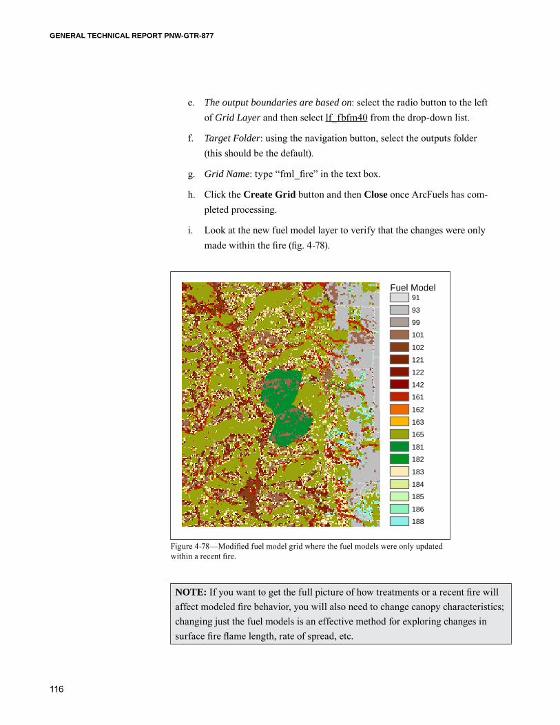
116


e. The output boundaries are based on: select the radio button to the left of Grid Layer and then select lf_fbfm40 from the drop-down list.

f. Target Folder: using the navigation button, select the outputs folder (this should be the default).

g. Grid Name: type “fml_fire” in the text box.


i. Look at the new fuel model layer to verify that the changes were only made within the fire (fig. 4-78).

NOTE: If you want to get the full picture of how treatments or a recent fire will affect modeled fire behavior, you will also need to change canopy characteristics; changing just the fuel models is an effective method for exploring changes in surface fire flame length, rate of spread, etc.

Fuel Model91

93

99

101

102

121

122

142

161

162

163

165

181

182

183

184

185

186

188

Figure 4-78—Modified fuel model grid where the fuel models were only updated within a recent fire.

117


ConversionExercises 4-27 through 4-31 will demonstrate how to single and batch convert ASCII files to grids, XY text files to shapefiles, and how to export the attributes of a shapefile to Excel.

Exercise 4-27: Convert a single ASCII file to a grid—In this exercise, a no-treatment burn probability ASCII created in FlamMap will be converted to a grid.1. Click the Conversion button on the ArcFuels toolbar, then select Convert

Ascii to Grid from the drop-down list (fig. 4-79).a. Ascii Grid File: navigate to and select the NOTRT_BP.asc file located

in the data folder.

b. Target Folder: navigate to and select the outputs folder (this is the default).

c. Grid Name: type “notrt_bp” in the text box.

d. Data type: select the radio button to the left of Floating point. Floating point was selected because burn probability is a value between 0 and 1. If integer was selected the converted grid would have a value of 0.

e. Spatial Reference: select NAD_1983_UTM_Zone_11N from the drop-down list.

f. Check the box to the left of Add Grid to Map.

g. Click OK.

Figure 4-79—Convert Ascii Grid File form set up to convert a no-treat burn probability file.

The ASCII conversion forms allow a user to rapidly post-process many of the FlamMap outputs.

118


2. When the conversion is done, the form will automatically close. The con-verted grid (fig. 4-80) will be added to the ArcMap table of contents under a new grouping named Conversion Results.

Figure 4-80—No-treatment burn probability grid modeled in FlamMap3 using an FVS-derived LCP.

TIP: Although ASCII file types can have more than 13 characters, grid names cannot. Additionally, do not use any or special characters in your grid name other than under-scores and no spaces. ArcFuels will not convert the ASCII files if either of these are the case (fig. 4-81).

Burn probabilityHigh : 0.462

Low : 0

Figure 4-81—Warning window when the grid name is too long.

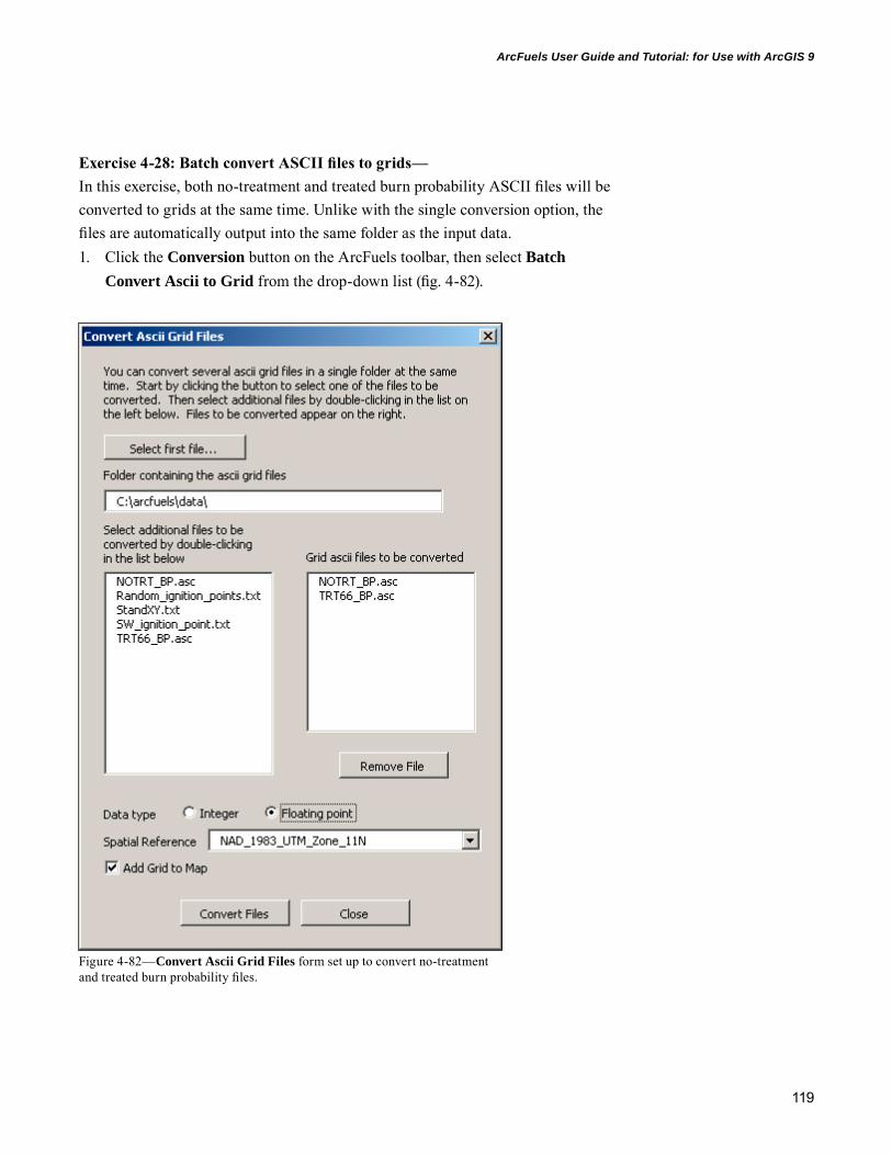
119


Exercise 4-28: Batch convert ASCII files to grids—In this exercise, both no-treatment and treated burn probability ASCII files will be converted to grids at the same time. Unlike with the single conversion option, the files are automatically output into the same folder as the input data.1. Click the Conversion button on the ArcFuels toolbar, then select Batch

Convert Ascii to Grid from the drop-down list (fig. 4-82).

Figure 4-82—Convert Ascii Grid Files form set up to convert no-treatment and treated burn probability files.

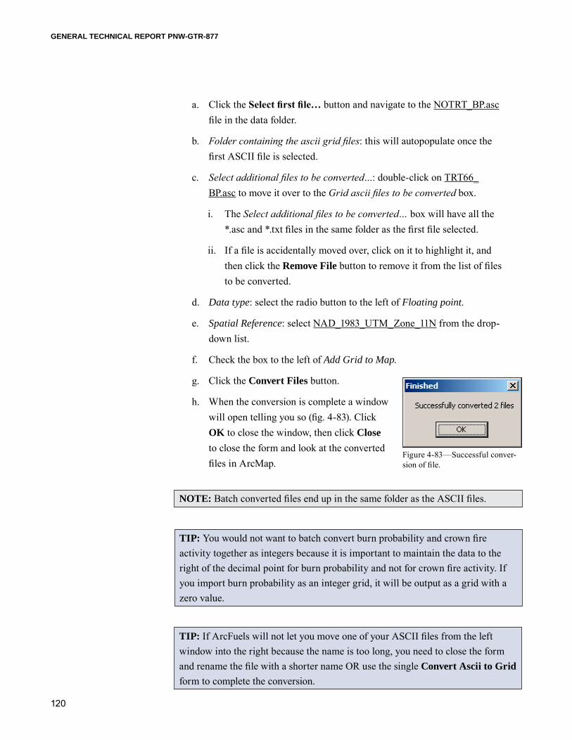
120


a. Click the Select first file… button and navigate to the NOTRT_BP.asc file in the data folder.

b. Folder containing the ascii grid files: this will autopopulate once the first ASCII file is selected.

c. Select additional files to be converted…: double-click on TRT66_BP.asc to move it over to the Grid ascii files to be converted box.

i. The Select additional files to be converted… box will have all the *.asc and *.txt files in the same folder as the first file selected.

ii. If a file is accidentally moved over, click on it to highlight it, and then click the Remove File button to remove it from the list of files to be converted.

d. Data type: select the radio button to the left of Floating point.


f. Check the box to the left of Add Grid to Map.

g. Click the Convert Files button.

h. When the conversion is complete a window will open telling you so (fig. 4-83). Click OK to close the window, then click Close to close the form and look at the converted files in ArcMap.

NOTE: Batch converted files end up in the same folder as the ASCII files.

TIP: You would not want to batch convert burn probability and crown fire activity together as integers because it is important to maintain the data to the right of the decimal point for burn probability and not for crown fire activity. If you import burn probability as an integer grid, it will be output as a grid with a zero value.

TIP: If ArcFuels will not let you move one of your ASCII files from the left window into the right because the name is too long, you need to close the form and rename the file with a shorter name OR use the single Convert Ascii to Grid form to complete the conversion.

Figure 4-83—Successful conver-sion of file.

121


Exercise 4-29: Convert a single XY file to a shapefile—In this exercise, a list of centroid points (geometric center) for each stand in the Mt. Emily area will be converted to a shapefile.1. Click the Conversion button on the ArcFuels toolbar, then select Convert

XY Text to Shapefile from the drop-down list (fig. 4-85).

TIP: If the grid already exists in the folder you are trying to convert to, a warning window (fig. 4-84) will open asking if you would like to replace the existing grid.

Figure 4-84—Replace existing grid warning window.

Figure 4-85—Convert XY File form set up to convert a text list of stand centroid points to a shapefile.

a. XY Text File: navigate to and select the StandXY.txt file in the data folder.

b. X and Y column names: select the radio button to the left of X, Y.

c. Spatial Reference: select NAD_1983_UTM_Zone_11N from the drop-down list.

d. Check the box to the left of Add Shape File to Map.

e. Click OK.

The XY file conversion forms can be used to quickly convert and add point location data to ArcMap.

122


f. When the conversion is complete, the form will close and the shapefile will be placed under the Conversion Results grouping in the ArcMap table of contents.

TIP: The Convert XY Text to Shapefile and Batch Convert XY Text to Shapefile forms can be used only with files that are delaminated with commas (fig. 4-86), not tabs.

Figure 4-86—Comma separated text file for conversion to shapefile.

Exercise 4-30: Batch convert XY text files to shapefiles—In this exercise, two additional XY text files will be batch converted to shapefiles. This includes a hypothetical single-fire ignition point and multiple randomly located fire ignition points. 1. Click the Conversion button on the ArcFuels toolbar, then select Batch

Convert XY Text to Shapefile from the drop-down list (fig. 4-87). a. Click the Select first file… button and navigate to the Random_igni-

tion_points.txt file in the data folder.

b. Folder containing the ascii grid files: this will autopopulate once the first text file is selected.

c. Select additional files to be converted…: double-click on SW_ignition_point.txt to move it over to the XY test files to be converted box.

i. The Select additional files to be converted… box will have all the *.txt files in the same folder as the first file selected.

ii. If a file is accidentally moved over, click on it to highlight it, and then click Remove File to remove it from the list of files to be con-verted.

d. X and Y column names: select the radio button to the left of XPos, YPos.


123


f. Check the box to the left of Add Shape File to Map.

g. Click the Convert Files button.

h. When the conversion is complete, a window will open telling you so. Click OK to close the window, then click Close to close the form and look at the converted files in ArcMap.

Figure 4-87—Convert XY File form set up to convert the remaining XY text files to shapefiles.

124


Exercise 4-31: Copy shapefile attributes to spreadsheet—This tool allows the attributes table information from a shapefile to be directly exported into Excel. 1. Click the Conversion button on the ArcFuels toolbar, then select Copy

Attributes to Spreadsheet from the drop-down list (fig. 4-89).a. Feature Layer: select mt_emily_stands from the drop-down list.

b. Spreadsheet: navigate to the outputs folder and name the file “mt_emily_stands_attributes.”

c. Click OK. The Excel workbook will open. Click Yes if you get a Microsoft Windows warning window.

Figure 4-89—Attributes to Spreadsheet form set up to copy the attributes of the Mt. Emily stand polygon layer to an Excel workbook.

TIP: If the file(s) has already been converted you will get a series of error message (fig. 4-88) and ArcFuels will not convert the file(s).

Figure 4-88—Error window when trying to convert to a shapefile that already exists.

125


Introduction to the Forest Vegetation Simulator (FVS)This section is meant to be a brief introduction to FVS and FFE-FVS. For more thorough tutorials, webinars, and information about FVS training courses, please visit the FVS Web page (http://www.fs.fed.us/fmsc/fvs/training/index.shtml).

The Forest Vegetation Simulator typically is run through the Suppose graphical user interface (http://www.fs.fed.us/fmsc/fvs/software/suppose.php) with specific text file inputs. However, FVS has also been linked to other software such as Access. ArcFuels has leveraged these links and created a different interface for run-ning FVS with a spatial component. The ArcFuels interface and tutorials are found in the ArcFuels Tools section of this User Guide and Tutorial. A Suppose tutorial will not be included; rather, the User Guide and Tutorial includes general informa-tion about FVS and FFE-FVS.

FVS Program OverviewThe Forest Vegetation Simulator is an individual tree, distance independent, growth and yield model that is used to model forest stand dynamics overtime (Crookston and Dixon 2005). The FVS is used extensively in the United States by federal agencies, private landholders, and universities. The FVS and the available exten-sions (see below for a complete list) are used to summarize current stand conditions, model future stand conditions, simulate silvicultural prescriptions including costs associated, model fuel treatment prescriptions, model wildfire events, determine suitability of wildlife habitat, estimate insect hazard, predict change under future climate scenarios, and much more.

Within FVS, the stand is the basic unit of management; however, many thou-sands of stands can be run through the model. Tree growth and mortality can be run hundreds of years into the future with FVS (the limit in ArcFuels is 49 years).

The FVS starts by reading stand and tree data, then calibrates based on the input data and reports on initial conditions (i.e., tree density, fuel loading, etc.) for each stand (fig. 5-1). Next, treatment prescriptions or other management activities are read into the program and applied at the appropriate time. The stand is grown forward accounting for mortality and regeneration. Metrics related to the treatments applied and stand structure information are output. If more than one stand is run through FVS, this process repeats until all stands have been simulated.

Chapter 5

The FVS and the available extensions are used to summarize current stand conditions, model future stand conditions, simulate silvicultural prescriptions including costs associated, model fuel treatment prescriptions, model wildfire events, determine suitability of wildlife habitat, estimate insect hazard, predict change under future climate scenarios, and much more.

126


FVS ExtensionsIn addition to the FVS base model, there are many extensions available for use with FVS. The extensions include:

• Cover and shrubs• Economics extension• Regeneration and establishment• Fire and fuels extension (FFE)• Parallel processing extension (PPE)• Douglas-fir beetle• Douglas-fir tussock moth• Dwarf mistletoe• Mountain pine beetle• White pine blister rust impact• Western root disease• Western spruce budworm• Climate extension

Figure 5-1—Simplified FVS program flow for a FFE-FVS fuel treatment run.

127


The only extensions available for all variants (described below) are the eco-nomics extension and the fire and fuels extension. The ArcFuels User Guide and Tutorial only includes the use of the fire and fuels extension. To learn more about the other extensions go to: http://www.fs.fed.us/fmsc/fvs/whatis/index.shtml.

FVS VariantsTree growth, mortality, and volume equations differ within FVS based on the dominant tree species within 20 regions of the United States (fig. 5-2). Each of these regions is called a variant. Within each variant, only specific tree species, habitat types, dominant vegetation groups, etc. are available and applicable. In addition to unique growth, mortality, and volume equations within FVS, equations specific to extensions differ. For example, in FFE moderate and extreme fuel moisture condi-tions differ among variants to best represent the fire environment for the geographic location.

The demonstration data included with the ArcFuels download includes the Blue Mountain (BM) variant. Before working with your FVS data in ArcFuels, be sure to download the proper variant file.

Figure 5-2—Map of FVS variants from the FVS Web page http://www.fs.fed.us/fmsc/fvs/whatis/index.shtml.

128


FVS Input DataFVS data sources—FVS requires information about the stand and/or plot and the trees within. At a minimum, stand information must include a unique identifier, the area of the stand, the inventory year, topographic information (slope, aspect, elevation), inverse plot size (for smaller trees), the diameter at breast height (DBH) breakpoint between small and large trees, basal area factor, and the number of plots. Plot information includes the same, minus the number of plots. Tree information must include a unique identifier, species, DBH, history (live or dead code), and number of trees represented by the species-DBH-mortality combination. However, the more infor-mation supplied, the more accurate the modeled outputs will be. For a full list of all the input data possible, see the FVS Essentials Guide (Dixon 2003).

Data can be obtained through Forest Inventory Analysis (FIA) and the FSVeg database for national forest lands (http://www.fs.fed.us/fmsc/fvs/software/data.shtml), or field inventory.

FVS database table linkages—An example database has been supplied with the demonstration data (Example_FVS_input_database.mdb) that includes both the FSVeg data tables and additional tables for the minimum data required. For more information see the Creating your own FVS database portion of the Running ArcFuels With Your Data section of the User Guide and Tutorial.

Example FVS keywords for fuel treatments—A keyword system is used to communicate the information to be used by FVS as well as determine the treatment prescriptions and outputs to be generated. A single keyword record consists of the keyword itself and the associated parameters. Multiple keywords can be strung together in a KCP file. Suppose (the FVS GUI interface) can be used to generate the keyword files needed or the supplied KCP files can be altered with a text editing program.

There are some rules to creating keyword files that need to be known. The keyword always begins in the first column of the keyword record and up to seven additional parameter fields on the record may be used. The number is dependent on the keyword itself. Each parameter field consists of 10 columns. Depending on the type (alphabetic or numeric) or if a decimal point is included, the location of the parameter matters within the 10-column field. If integer values are used (no period), they must be right-justified.

A few useful FVS keywords for fuel treatments are described below for dem-onstration purposes. Users should read the FVS Keyword Guide (Van Dyck and

At a minimum, stand information must include a unique identifier, the area of the stand, the inventory year, topographic information, inverse plot size, the diameter at breast height breakpoint between small and large trees, basal area factor, and the number of plots. Tree information must include a unique identifier, species, DBH, history, and number of trees represented by the species-DBH-mortality combination.

129


Smith-Mateja 2000), FFE-FVS Manual (Rebain 2010), and FVS Event Monitor Guide (Crookston 1990) for a complete explanation.

Thinning keywords—THINSDI thins to a stand density index (SDI) target. In the example below, all species in the stand were thinned from below to 35 percent of the residual SDI and the cutting efficiency is 90 percent with no diameter limits.THINSDI 2000 . 35 0.90 0 0 999.0 1THINBBA thins from below to a desired basal area. In the example below, all species in the stand were thinned from below in 2000 to 150 ft2/ac throughout all diameter and height ranges at 95 percent efficiency. ThinBBA 2000 150 0.95 0 999.0 0 999.0SPECPREF sets a removal preference, by species, for subsequent simulated thin-ning. This affects the order in which trees are selected for removal when a harvest is implemented. Positive values favor removal and negative values favor retention. For example, the keyword set below sets a removal priority to three tree species. These priorities favor retention of ponderosa pine (PP), Douglas-fir (DF), and western larch (WL) whenever a thinning is implemented. The retention priorities are weighted such that PP is most heavily favored for retention, followed by DF, followed by WL. SPECPREF 0 PP - 100SPECPREF 0 DF -50SPECPREF 0 WL -20

FFE specific keywords—FMIN signals the start of the FFE keywords and END signals the end of the FFE keywords. All other FFE keywords must appear between the FMIN-END pair. You may code several FMIN-END pairs and you may have one or many FFE keywords between each pair.

FUELMOVE keyword moves dead and downed fuel between fuel size classes to simulate fuel treatments. The following set of FUELMOVE keywords removes from the stand 90 percent of fuels from size classes 3, 4, and 5 in 2002.

FUELMOVE 2002 3 0 0 0.9 999 0

FUELMOVE 2002 4 0 0 0.9 999 0

FUELMOVE 2002 5 0 0 0.9 999 0

MOISTURE is used to set the moisture levels for each fuel size class. If this keyword is used, the user must specify moisture levels for all size classes (there are no defaults). When the MOISTURE keyword is used, it overrides the moisture

130


category from the SIMFIRE keyword. In the example below, the fuel moisture is set for 2007. One-hr fuel moisture is 3 percent, 10-hr is 4 percent, 100-hr is 6 percent, 1000-hr is 7 percent, duff is 20 percent, live herbaceous is 60 percent, and live woody is 90 percent.

MOISTURE 2007 3 4 6 7 20 60 90

SIMFIRE signals that a fire and its effects should be simulated. The following SIMFIRE keyword invokes a fall fire in 2003, with dry fuel conditions, 8 mph windspeed, and air temperature of 70 ˚F where the whole stand is burned and mortality is calculated.

SIMFIRE 2003 8 1 70 1 100 4

Other useful keywords—COMPUTE allows you to define up to 200 variables expressed as functions of Event Monitor variables, constants, and variables previously defined using the COMPUTE feature. The COMPUTE option can be scheduled for specific years, and the value of variables may depend on an event.SPMCDBH returns to the user one of the following: trees per acre, basal area, total cubic volume, merchantable cubic foot volume, total board foot volume, quadratic mean diameter, average height, percentage of cover, average mistletoe rating, stand density index, species-specific average diameter growth per acre, tree value class, tree status, or range of diameter and height. The example below returns the quadratic mean diameter of recent mortality trees that are at least 10 in DBH and at least 40 ft tall.SPMCDBH(5,0,0,10,999,40,999,1)

FVS Output Description and UnitsArcFuels has many hardwired keywords included in every FVS simulation. Some of these can be turned on or turned off by setting the FVS options within the appropri-ate form. For more information about the forms and options, see the ArcFuels Tools section. Tables 5-1 through 5-10 contain all the output units for hardwired results tables from FVS runs. For units specific to other keywords, see the FVS literature.

ArcFuels has many hardwired keywords included in every FVS simulation. Some of these can be turned on or turned off by setting the FVS options within the appropriate form.

131


Table 5-1—Output units for the FVS_Cases table

Metric Description Units

Stand_CN Stand_CN from FVS database n/aStandID Stand ID from FVS database n/aMgmtID Management ID from FVS database n/aKeywordFile Location of output keyword file n/aSamplingWt Area of stand-from FVS database acVariant FVS variant used n/aRunDateTime Time and date of FVS run n/a

Table 5-2—Output units for the FVS_Summary table


Age Stand age yrTpa Tree density trees/acBA Basal area ft2/acSDI Stand density index n/aCCF Crown competition factor percentTopHt Top height ftQMD Quadratic mean diameter inTCuFt Total cubic feet ft3/acMCuFt Merchantable cubic feet ft3/acBdFt Board foot volume n/aRTpa Tree density removed trees/acRTCuFt Total cubic feet removed ft3/acRMCuFt Merchantable cubic feet removed ft3/acRBdFt Total board feet removed n/aATBA Basal area, after treatment ft2/acATSDI Stand density index, after treatment n/aATCCF Crown competition factor, after treatment percentATTopHt Top height, after treatment ftATQMD Quadratic mean diameter, after treatment inchesPrdLen Period length yearsAcc Accretion ft3/ac/yrMort Mortality ft3/ac/yrMAI Stand mean annual increment n/aForTyp Forest type n/aSizeCls Stand size class n/aStkCls Stand stocking class n/a

132


Table 5-3—Output units for the FVS_StrClass (structure class) table


Removal_Code Removal code n/aStratum_X_DBH Nominal diameter at breast height, Stratum X inStratum_X_Nom_Ht Height of the tallest tree, Stratum X ftStratum_X_Lg_Ht Nominal height of trees, Stratum X ftStratum_X_Sm_Ht Height of the shortest tree, Stratum X ftStratum_X_Crown_Base Canopy base height, Stratum X ftStratum_X_Crown_Cover Canopy cover, Stratum X percentStratum_X_Species_X Primary species, Stratum X n/aStratum_X_Species_2 Secondary species, Stratum X n/aStratum_X_Status_Code Status, Stratum X n/aNumber_of_Strata Number of valid strata n/aTotal_Cover Total canopy cover in all strata percentStructure_Class Structure class: ground (BG), stand initiation (SI), n/a stem exclusion (SE), understory reinitiation (UR), young forest multistrata (YM), old forest single stratum (OS), or old forest multistrata (OM)

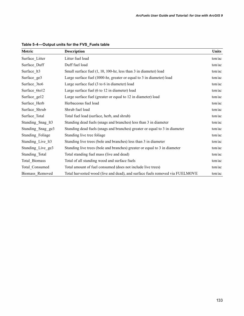
133


Table 5-4—Output units for the FVS_Fuels table


Surface_Litter Litter fuel load ton/acSurface_Duff Duff fuel load ton/acSurface_lt3 Small surface fuel (1, 10, 100-hr, less than 3 in diameter) load ton/acSurface_ge3 Large surface fuel (1000-hr, greater or equal to 3 in diameter) load ton/acSurface_3to6 Large surface fuel (3 to 6 in diameter) load ton/acSurface_6to12 Large surface fuel (6 to 12 in diameter) load ton/acSurface_ge12 Large surface fuel (greater or equal to 12 in diameter) load ton/acSurface_Herb Herbaceous fuel load ton/acSurface_Shrub Shrub fuel load ton/acSurface_Total Total fuel load (surface, herb, and shrub) ton/acStanding_Snag_lt3 Standing dead fuels (snags and branches) less than 3 in diameter ton/acStanding_Snag_ge3 Standing dead fuels (snags and branches) greater or equal to 3 in diameter ton/acStanding_Foliage Standing live tree foliage ton/acStanding_Live_lt3 Standing live trees (bole and branches) less than 3 in diameter ton/acStanding_Live_ge3 Standing live trees (bole and branches) greater or equal to 3 in diameter ton/acStanding_Total Total standing fuel mass (live and dead) ton/acTotal_Biomass Total of all standing wood and surface fuels ton/acTotal_Consumed Total amount of fuel consumed (does not include live trees) ton/acBiomass_Removed Total harvested wood (live and dead), and surface fuels removed via FUELMOVE ton/ac

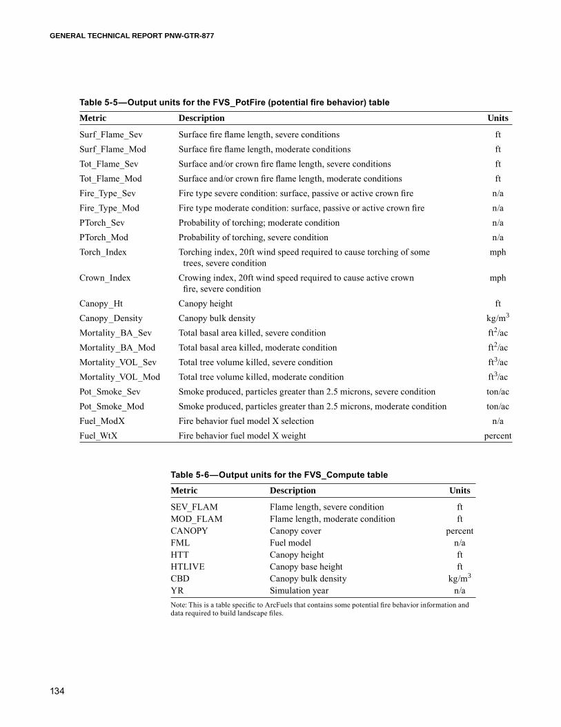
134


Table 5-5—Output units for the FVS_PotFire (potential fire behavior) table


Surf_Flame_Sev Surface fire flame length, severe conditions ftSurf_Flame_Mod Surface fire flame length, moderate conditions ftTot_Flame_Sev Surface and/or crown fire flame length, severe conditions ftTot_Flame_Mod Surface and/or crown fire flame length, moderate conditions ftFire_Type_Sev Fire type severe condition: surface, passive or active crown fire n/aFire_Type_Mod Fire type moderate condition: surface, passive or active crown fire n/aPTorch_Sev Probability of torching; moderate condition n/aPTorch_Mod Probability of torching, severe condition n/aTorch_Index Torching index, 20ft wind speed required to cause torching of some mph trees, severe conditionCrown_Index Crowing index, 20ft wind speed required to cause active crown mph fire, severe conditionCanopy_Ht Canopy height ftCanopy_Density Canopy bulk density kg/m3

Mortality_BA_Sev Total basal area killed, severe condition ft2/acMortality_BA_Mod Total basal area killed, moderate condition ft2/acMortality_VOL_Sev Total tree volume killed, severe condition ft3/acMortality_VOL_Mod Total tree volume killed, moderate condition ft3/acPot_Smoke_Sev Smoke produced, particles greater than 2.5 microns, severe condition ton/acPot_Smoke_Mod Smoke produced, particles greater than 2.5 microns, moderate condition ton/acFuel_ModX Fire behavior fuel model X selection n/aFuel_WtX Fire behavior fuel model X weight percent

Table 5-6—Output units for the FVS_Compute table


SEV_FLAM Flame length, severe condition ftMOD_FLAM Flame length, moderate condition ftCANOPY Canopy cover percentFML Fuel model n/aHTT Canopy height ftHTLIVE Canopy base height ftCBD Canopy bulk density kg/m3

YR Simulation year n/aNote: This is a table specific to ArcFuels that contains some potential fire behavior information and data required to build landscape files.

135


Table 5-7—Output units for the FVS_BurnReport table (produced only when a fire is simulated)


One_Hr_Moisture 1-hr time lag fuel moisture percentTen_Hr_Moisture 10-hr time lag fuel moisture percentHundred_Hr_Moisture 100-hr time lag fuel moisture percentThousand_Hr_Moisture 1,000-hr time lag fuel moisture percentDuff_Moisture Duff moisture percentLive_Woody_Moisture Live woody plant moisture percentLive_Herb_Moisture Live herbaceous plant moisture percentMidflame_Wind Midflame wind speed based on 20 ft mph wind input and canopy coverSlope Slope of the stand percentFlame_length Flame length used to calculate mortality ftScorch_height Scorch height based on the flame length ftFire_Type Fire type: surface fire, passive crown fire, n/a or active crown fireFuelModlX Fire behavior fuel model X selection n/aWeightX Fire behavior fuel model X weight percent

Table 5-8—Output units for the FVS_Consumption table (fuel consumption from fire, produced only when a fire is simulated)


Min_Soil_Exp Mineral soil exposure percentLitter_Consumption Litter consumed ton/acDuff_Consumption Duff consumed ton/acConsumption_lt3 1, 10, and 100-hr fuels consumed ton/acConsumption_ge3 Large surface fuels (greater or equal to 3 in diameter) ton/ac consumed in the simulated fireConsumption_3to6 Large surface fuels (3 to 6 in diameter) consumed ton/acConsumption_6to12 Large surface fuels (6 to 12 in diameter) consumed ton/acConsumption_ge12 Large surface fuels (greater or equal to 12 in diameter) ton/ac consumedConsumption_Herb_Shrub Herbs and shrubs consumed ton/acConsumption_Crowns Tree crowns consumed from scorching ton/acTotal_Consumption Total all fuel types consumed ton/acPercent_Consumption_Duff Duff consumed percentPercent_Consumption_ge3 Large surface fuels greater or equal to 3 in diameter) percent consumedPercent_Trees_Crowning Crown fraction burned: surface fire = 0; active crown percent fire = 100; passive crown fire is between 0 and 100Smoke_Production_25 Smoke produced, particles greater than 2.5 ton/ac microns (PM2.5)Smoke_Production_10 Smoke produced, particles greater than 10 ton/ac microns (PM10)

136


Table 5-9—Output units for the FVS_Mortality table (tree mortality from fire, produced only when a fire is simulated)


Species Two letter tree species code n/aKilled_class1 Trees killed by fire in class 1 (default 0 to 5 in DBH) trees/acTotal_class1 Trees before fire in class 1 (default 0 to 5 in DBH) trees/acKilled_class2 Trees killed by fire in class 2 (default 5 to 10 in DBH) trees/acTotal_class2 Trees before fire in class 2 (default 5 to 10 in DBH) trees/acKilled_class3 Trees killed by fire in class 3 (default 10 to 20 in DBH) trees/acTotal_class3 Trees before fire in class 3 (default 10 to 20 in DBH) trees/acKilled_class4 Trees killed by fire class 4 (default 20 to 30 in DBH) trees/acTotal_class4 Trees before fire in class 4 (default 20 to 30 in DBH) trees/acKilled_class5 Trees killed by fire in class 5 (default 30 to 40 in DBH) trees/acTotal_class5 Trees before fire in class 5 (default 30 to 40 in DBH) trees/acKilled_class6 Trees killed by fire in class 6 (default 40 to 50 in DBH) trees/acTotal_class6 Trees before fire in class 6 (default 40 to 50 in DBH) trees/acKilled_class7 Trees killed by fire in class 7 (default greater or equal to 50 in DBH) trees/acTotal_class7 Trees before fire in class 7 (default greater or equal to 50 in DBH) trees/acBakill Total basal area killed by fire ft2/acVolkill Total tree volume killed by fire ft3/acNote: DBH=diameter at breast height

Table 5-10—Output units for the FVS_Carbon and FVS_Hrv_Carbon (harvested) carbon (C) tables


Aboveground_Total_Live Total aboveground live tree C ton/acAboveground_Merch_Live Total aboveground merchantable tree C ton/acBelowground_Live Total belowground live C (roots) ton/acBelowground_Dead Total belowground dead C (roots) ton/acStanding_Dead Total aboveground dead tree C ton/acForest_Down_Dead_Wood Total down dead woody fuel (1, 10, 100, 1,000-hr) C ton/acForest_Floor Total litter and duff C ton/acForest_Shrub_Herb Total herb and shrub C ton/acTotal_Stand_Carbon Total stand C—all live and dead pools ton/acTotal_Removed_Carbon Total C removed by treatment ton/acCarbon_Released_From_Fire C in fuel consumed by fire ton/acProducts Merchantable C stored in products ton/acLandfill Merchantable C stored in landfills ton/acEnergy Merchantable C emitted with energy capture ton/acEmissions Merchantable C emitted without energy capture ton/acMerch_Carbon_Stored Merchantable C stored—products and landfill ton/acMerch_Carbon_Removed Merchantable C removed ton/ac

137


Using the FVS Parallel Processing Extension (PPE)The FVS Parallel Processing Extension (PPE) (Crookston and Stage 1991) is a useful extension for landscape planning with FVS. It simulates multiple stands in a parallel fashion, i.e., the simulation is completed for all stands each time period before cycling to the next time period. The PPE can model multiple, spatially explicit treatment constraints and priorities at the stand scale for a given landscape.

For example, suppose a comparison is desired of two treatment strategies, one in which stands are selected for treatment based on their tree density, and one based on proximity to structures. Suppose also that six treatment levels are desired where 0, 5, 10, 20, 30, and 40 percent of the landscape is treated. These scenarios are simulated with the MSPOLICY keyword to set the priority treatment vari-able and the total treatment constraint. The priority variable can be an FVS event monitor variable or a variable read from the stand database. Sample priority data are included in the stand database in the homedens field. To read the variable into an FVS run, add the ReadVariablesFromStandDatabase.kcp file in the PPE folder in the KCP folder within the programs folder of the demonstration data. The KCP file reads the homedens variable from the stand input table and sets an FVS compute table equal to the variable. The contents of the file are as follows:DatabaseDSNINC:\arcfuels\data\Mt_Emily_Database.mdbSQLIN 1SELECT homedens FROM standsWHERE stand_cn = ‘percentstand_cn percent’EndSQLThe subsequent commands make a compute variable to echo the database contents into the FVS output database.COMPUTE 0hdens = homedensEND

On the ArcFuels Simulate Landscape Treatments form, enter “hdens” into the priority text box and set the proportion to 0.2. With the number of stands set to 200, click the Run PPE button. The resulting run will treat 20 percent of the landscape (about 200 stands) and prioritize the treatments according to the distance to homes.

138


To use an event monitor variable as the treatment priority, declare the variable in a COMPUTE variable, i.e., make a new variable and set it equal to a predefined FVS event monitor variable. The statement below defines and sets the variable CBSDI to the values of the FVS variable BSDI, which is the before-thin stand density index. COMPUTE 0CBSDI= BSDIEND

It is also possible to create more elaborate treatment priority schemes using external programs. Coding a ‘1’ in the last field of the MSPOLICY field instructs FVS-PPE to stop execution at each cycle and execute a user-supplied program called “computepriority.” FVS-PPE expects this latter program to generate an ASCII file containing treatment priorities. Prior to stopping, the user can write the current state of FVS variables to an Access database to be read by “computeprior-ity.” An example application of this system can be found in Finney et al. (2007).

139


Introduction to Fire Behavior Modeling With FlamMap3This section is meant to be a brief introduction FlamMap3. There are many func-tions within FlamMap3 that will not be discussed. The purpose is to have the user gain a foundation in FlamMap3 skills for use with ArcFuels. For more thorough tutorials, download the program and help file from the FlamMap3 Web site (http://www.firemodels.org/index.php/national-systems/flammap).

FlamMap3 OverviewFlamMap3 (Finney 2006) is a spatially explicit landscape fire behavior mapping and modeling system that describes potential fire behavior with a constant fire environment (static weather and fuel moisture). The fact that the fire environment is held constant makes FlamMap3 the ideal tool for landscape-level fire behavior assessment for fuel treatment planning. It is possible to see the effect of changes to fuels on fire behavior without the additional unknown of weather effects.

FlamMap3 has two methods of modeling potential fire behavior: basic fire behavior and minimum travel time (MTT) (Finney 2002). In the first type of simulation, basic fire behavior is calculated by independently burning each pixel on the landscape. Primary modeled outputs include rate of spread, flame length, fireline intensity, and crown fire activity. In the second type of simulation, discrete wildfire(s) are simulated using the two-dimensional MTT fire growth algorithm. Minimum travel time calculations assume independence of fire behavior among neighboring cells but are dependent on the ignition locations, resolution of calcula-tions, and simulation time. The MTT algorithm replicates fire growth by Huygens’ principle, in which the growth and behavior of the fire edge is modeled as a vector or wave front (Knight and Coleman 1993). This method results in less distortion of fire shape and response to temporally varying conditions than techniques that model fire growth from cell-to-cell on a gridded landscape (Finney 2002). Specifi-cally, a rectangular lattice of a defined resolution (preferably scaled to the input data) is used to determine fire spread or travel time between each node (cell size based on the input variables), fuel moisture, windspeed, and wind direction. In addition to the fire spread, fire behavior is stored for each node (Finney 2002). Minimum travel time is determined starting at the ignition location for all adjacent nodes until the minimum cumulative travel time is determined. Primary outputs for a single fire are rate of spread, arrival time, fire intensity, and flow paths. When multiple random fires are ignited, the only output available is burn probability.

Both basic fire behavior and MTT calculations are derived from the same lin-eage of systems that model one-dimensional behavior as part of a spreading line fire

Chapter 6

FlamMap3 is a spatially explicit landscape fire behavior mapping and modeling system that describes potential fire behavior with a constant fire environment. The fact that the fire environment is held constant makes FlamMap3 the ideal tool for landscape-level fire behavior assessment for fuel treatment planning.

140


(Albini 1976; Anderson et al. 1982; Rothermel 1972, 1991; Van Wagner 1977, 1993). For more detailed information about the calculations, see the FlamMap3 help guide.

In addition to the fire behavior outputs, FlamMap3 also has the TOM (Finney 2007). The TOM utilizes MTT fire behavior calculations, predetermined fire igni-tion (point, line or area), fuel moisture and wind information, and two LCPs. The first LCP represents the current conditions, and the second an “ideal” landscape. The ideal landscape represents posttreatment conditions, with treatments occurring wherever they are possible (not just desired). The TOM then simulates fire across both landscapes and places treatment block (user-defined size) in the most optimal location to slow fire spread. The output is a treatment grid consisting of 0s and 1s with the most optimal treatment pattern given the availability to be treated and the proportion of land allowed to be treated.

As with any modeling system, there are known limitations with FlamMap3 (Cruz and Alexander 2010). Having an understanding of these limitations is impor-tant before using any model.

Input data—FlamMap3 requires a landscape (LCP) file, fuel moisture file (FMS), and wind-speed and wind direction information to run. Additional optional files include a custom fuel model file (FMD), wind vector files (direction and speed), foliar moisture content, and weather (WTR) and wind (WND) files for fuel moisture conditioning.

The LCP is a binary file that contains spatially explicit information about the topography and fuel characteristics of a landscape (fig. 6-1). The LCP is composed of five layers at a minimum (elevation, slope, aspect, fuel model, and canopy cover) and ideally 8 (addition of canopy base height, canopy height, and canopy bulk den-sity), and infrequently 10 (addition of duff loading and course woody fuels). This LCP file is identical to the one used in FARSITE. It is possible to create the LCP in both FARSITE and FlamMap3, but this will not be discussed. Rather see the sec-tion Build FlamMap Landscape to learn how to build the LCP using ArcFuels.

Windspeed and wind direction will depend on the fire scenario desired. Winds can blow either uphill (based on the input topographic themes in the LCP) or from a set direction (e.g., from the southwest). Windspeed can be selected using a program such as FireFamilyPlus (Bradshaw and Tirmenstein 2009) to characterize a given percentile condition, or can be determined using expert opinion. To use wind vec-tors, an external program such as WindNinja (Forthofer et al. 2009) (http://www.firemodels.org/index.php/research-systems/windninja) needs to be run to create the direction and speed ASCII files that FlamMap3 will use to create the wind grids.

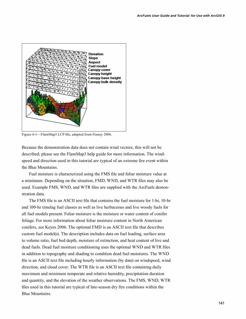
141


Because the demonstration data does not contain wind vectors, this will not be described; please see the FlamMap3 help guide for more information. The wind-speed and direction used in this tutorial are typical of an extreme fire event within the Blue Mountains.

Fuel moisture is characterized using the FMS file and foliar moisture value at a minimum. Depending on the situation, FMD, WND, and WTR files may also be used. Example FMS, WND, and WTR files are supplied with the ArcFuels demon-stration data.

The FMS file is an ASCII text file that contains the fuel moisture for 1-hr, 10-hr and 100-hr timelag fuel classes as well as live herbaceous and live woody fuels for all fuel models present. Foliar moisture is the moisture or water content of conifer foliage. For more information about foliar moisture content in North American conifers, see Keyes 2006. The optional FMD is an ASCII text file that describes custom fuel model(s). The description includes data on fuel loading, surface area to volume ratio, fuel bed depth, moisture of extinction, and heat content of live and dead fuels. Dead fuel moisture conditioning uses the optional WND and WTR files in addition to topography and shading to condition dead fuel moistures. The WND file is an ASCII text file including hourly information (by date) on windspeed, wind direction, and cloud cover. The WTR file is an ASCII text file containing daily maximum and minimum temperate and relative humidity, precipitation duration and quantity, and the elevation of the weather observations. The FMS, WND, WTR files used in this tutorial are typical of late-season dry fire conditions within the Blue Mountains.

Figure 6-1—FlamMap3 LCP file, adapted from Finney 2006.

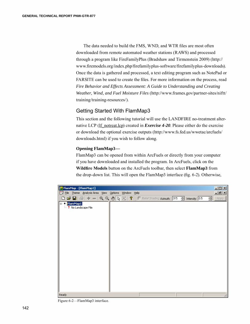
142


The data needed to build the FMS, WND, and WTR files are most often downloaded from remote automated weather stations (RAWS) and processed through a program like FireFamilyPlus (Bradshaw and Tirmenstein 2009) (http://www.firemodels.org/index.php/firefamilyplus-software/firefamilyplus-downloads). Once the data is gathered and processed, a text editing program such as NotePad or FARSITE can be used to create the files. For more information on the process, read Fire Behavior and Effects Assessment: A Guide to Understanding and Creating Weather, Wind, and Fuel Moisture Files (http://www.frames.gov/partner-sites/niftt/training/training-resources/).

Getting Started With FlamMap3This section and the following tutorial will use the LANDFIRE no-treatment alter-native LCP (lf_notreat.lcp) created in Exercise 4-20. Please either do the exercise or download the optional exercise outputs (http://www.fs.fed.us/wwetac/arcfuels/downloads.html) if you wish to follow along.

Opening FlamMap3—FlamMap3 can be opened from within ArcFuels or directly from your computer if you have downloaded and installed the program. In ArcFuels, click on the Wildfire Models button on the ArcFuels toolbar, then select FlamMap3 from the drop-down list. This will open the FlamMap3 interface (fig. 6-2). Otherwise,

Figure 6-2—FlamMap3 interface.

143


open FlamMap3 from the shortcut icon on your desktop or from StartAll ProgramsFlamMap3 FlamMap3.

The left pane is called the “tree” pane and the right is the “display” pane (fig. 6-2). Within the tree pane each “section” is indicated by a diamond to the left of the text, and each section can be expanded using the boxed “+” symbol, or collapsed using the boxed “-” symbol when there are multiple data layers or options within a section.

Loading an LCP file—There are a three ways to load LCP files into FlamMap3: 1. Via the main toolbar ThemeFARSITE Landscape File, then navigate to

a preexisting LCP,2. Double-click ? No Landscape File in the tree pane, then navigate to a pre-

existing LCP, or3. In the tree pane, right-click ? No Landscape FileOpen, then navigate to

a preexisting LCP.Load the lf_notreat.lcp file from the outputs folder (C:/arcfuels/outputs). Note

that there are now more sections in the tree pane. The Themes section includes all the layers within the loaded LCP file. FlamMap3 automatically expands this section and has the fuel model layer displayed. The layer shown in the display pane is the active theme selected, which is indicated by the landscape icon to the left of the name; the non-active themes have a magnifying glass to the left (fig. 6-3). To change the active theme, click on the magnifying glass or name of the theme you would like displayed.

Changing the display and/or units of a theme—Changing the display and/or unit of a theme is useful for better understanding your data. This is most beneficial after completing a FlamMap3 run.

There are a couple of ways to open the Create/Modify Legend window, which is where you can change the display of a theme and also change the units. We will use the Fuel Model theme to demonstrate.1. Right-click on the theme name in the tree pane to open a new menu, then

select Properties, or2. Double-click on the theme name in the tree pane, which opens a new

Legend window (fig. 6-4) and click on the theme name up top.

Open the Create/Modify Legend window (fig. 6-5). There are many parts to the window, which are each described as follows:

144


• Theme: this is the theme you are changing.

• Units: the available units are listed in the drop-down list.

• Decimal Places: the number of deci-mal places used to categorize and dis-play the data.

• Number of Classes: you can choose the number of classes in which you would like your data to be displayed.

• Variable Type: this will depend on the data type; most will be Continuous Scale.

• Color Ramp: all the options are shown in the drop-down list.

Figure 6-4—Legend window for the fuel model theme.

Figure 6-3—No-treatment alternative LCP loaded.

145


• Predefined Legend: if there are common preexisting options, they will be in the drop-down list. It is also possible to create and save custom ones; see the FlamMap3 guide for more information.

• You can also insert, append, delete and sort classes using the Insert Class, Append Class, Delete Class, and Sort Classes buttons.

To make the changes, you must click the Apply button next to the change selected and then click OK at the bottom of the screen.

Figure 6-5—Create/Modify Legend window for the fuel model.

146


Saving a theme for further mapping and analysis in ArcGIS—Saving the individual themes is necessary for further mapping and analysis in ArcMap. As with changing the display and units, this is more important for fire modeled outputs than the input LCP file themes. FlamMap3 has a known bug and does not always reopen saved FlamMap3 runs; saving individual themes you would like to retain is very important.

To save a theme, right-click on the theme name in the tree pane and then select Save As from the new menu. A Save As window will open where you can navigate to the location where you would like to save the file, name the file, and choose the file type (ASCII, BMP, JPEG, GIF, TIFF, PNG). The default is an ASCII file that can be easily converted to a grid using ArcFuels.

Creating a FlamMap3 run—There are three ways to start a new run:1. Via the main toolbar Analysis AreNew Run, 2. Double-click Runs in the tree pane, or3. In the tree pane, right-click RunsNew Run.

This will add a New Run theme to the Runs section in the tree pane.

The FlamMap3 Runs window consists of four tabs: Inputs, Fire Behavior Outputs, Minimum Travel Time, and Treatment Optimization.

The Inputs tab (fig. 6-6) is where a run can be named, fuel moisture files are loaded, wind information is input, canopy characteristics are defined, and fuel moisture settings are defined.

A fuel moisture file must be loaded to run FlamMap3. In addition, if custom fuel models are used in the theme, a custom fuel model file must also be used. The pencil icon to the right of the files can be used to open a loaded file, verify the contents, update the file as needed, and save the file.

Winds can be blowing uphill at a user-defined speed, be out of a set direction based on azimuth, or be defined using wind vectors.

If your landscape file does not have information about the canopy height, canopy base height and/or canopy bulk density, you can define a single constant value for the entire landscape under the Canopy Characteristics heading. It is

TIP: If you change the display of a theme using a Predefined Legend the data saved will still be continuous, not categorical, however, the units of the Predefined Legend will be maintained.

Saving the individual themes is necessary for further mapping and analysis in ArcMap.

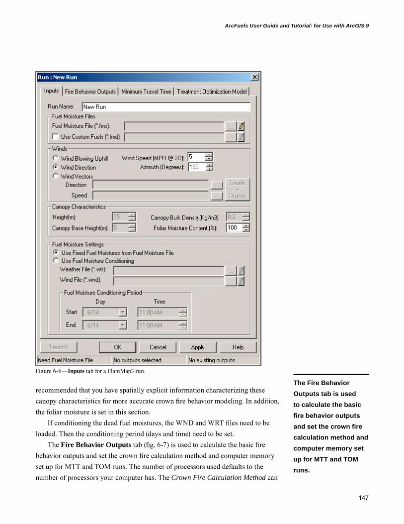
147


recommended that you have spatially explicit information characterizing these canopy characteristics for more accurate crown fire behavior modeling. In addition, the foliar moisture is set in this section.

If conditioning the dead fuel moistures, the WND and WRT files need to be loaded. Then the conditioning period (days and time) need to be set.

The Fire Behavior Outputs tab (fig. 6-7) is used to calculate the basic fire behavior outputs and set the crown fire calculation method and computer memory set up for MTT and TOM runs. The number of processors used defaults to the number of processors your computer has. The Crown Fire Calculation Method can

Figure 6-6—Inputs tab for a FlamMap3 run.

The Fire Behavior Outputs tab is used to calculate the basic fire behavior outputs and set the crown fire calculation method and computer memory set up for MTT and TOM runs.

148


be set based on Finney (1998), methods, which are identical to FARSITE, or Scott and Reinhardt (2001) methods. When you are using the Finney (1998) method, it is recommended that canopy bulk density values derived using a 15 ft running mean window (Scott and Reinhardt 2001), as is the case with FFE-FVS, be doubled. The other differences have to do with how active and passive crown fire spread are mod-eled. Active crown fire is reduced to account for spotting being modeled separately with the Finney (1998) method and passive crown fire is scaled to the crown fraction burned using the Scott and Reinhardt (2001) method. Fire behavior output grids are listed and described in table 6-1.

Figure 6-7—Fire Behavior Outputs tab for a FlamMap3 run.

149


The Minimum Travel Time tab (fig. 6-8) is used to calculate the MTT fire behavior outputs. Depending on the type of ignition used, a set ignition (created within FlamMap3 or in ArcMap and loaded) versus random ignitions, the available outputs will differ. When random ignitions are used, only a burn probability grid is created, and when a set ignition is used, all other output grids (table 6-2) are available except burn probability. The rotation direction for node lattice depends on the wind direction specified on the Inputs tab. Resolution of calculations dictates how often the calculations are completed, and what the output resolution of the grids selected will be. It is advised that the user choose a multiple of the input resolution (i.e., if the input grid resolution is 30 m, then choose 30 m, 60 m, 90 m, etc., for the calculations). Simulation time can be set for a defined time (often a single burn period such as 6 hr or 360 min) or left to run until every pixel has burned. The interval for the minimum travel paths controls how FlamMap3 outputs the major paths.

Table 6-1—Basic fire behavior output grids from FlamMap3

Output grid Possible units Description

Fireline intensity kW/m, BTU/ft/sec Rate of heat energy released per unit time per unit length of fire frontRate of spread m/min, ft/min, chains/hr Horizontal distance that the flame zone moves per unit of timeFlame length m, ft Distance from the ground at the leading edge of the flame to tip of the flameHeat/unit area kJ/m2, BTU/ft2 Total amount of heat released per unit area as the flaming front of the fire passesHorizontal movement m/min, ft/min, chains/hr The rate of spread (slope basis) transformed to a horizontal projectionMidflame windspeed k/hr, mph The speed of the wind measured at the midpoint of the flamesSpread vectors n/a A combination of the Maximum Spread Direction and Rate of Spread grids displayed as an arrowCrown fire activity categorical Fire type: 0 = no fire; 1 = surface fire; 2 = passive crown fire; 3 = active crown fireSolar radiation W/m2 The amount of sunlight exposed to the fuels1-hr fuel moisture fraction Moisture content of 1-hr timelag fuels (fuels smaller than ¼ in in diameter including the litter layer)10-hr fuel moisture fraction Moisture content of 10-hr timelag fuels (fuels greater than ¼-in but less than 1 in in diameter)

The Minimum Travel Time tab is used to calculate the MTT fire behavior outputs. Depending on the type of ignition used, a set ignition (created within FlamMap3 or in ArcMap and loaded) versus random ignitions, the available outputs will differ.

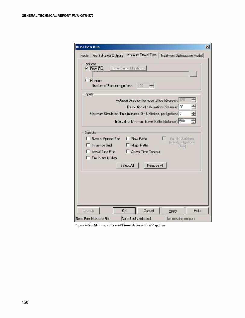
150


Figure 6-8—Minimum Travel Time tab for a FlamMap3 run.

151


Table 6-2—Minimum travel time (MTT) outputs

Output Possible units Description

Rate of spread grid m/min, ft/min, chains/hr Spread rate of the fire as it encountered each node along the minimum travel time pathInfluence grid n/a Logarithm of the number of nodes burning as a result of burning through that particular nodeArrival time grid min The elapsed time when the fire arrived at each node–fire progressionFire intensity map kW/m, BTU/ft/sec Fireline intensity of each node burned by the fire as it follows the minimum travel time pathFlow paths n/a Minimum travel time pathways among all nodesMajor paths n/a Flow paths identified at the user-specified interval for MTT flowArrival time contour n/a Contour representation of the MTT Arrival Time grid (default contour interval is the maximum value of the MTT Arrival Time grid divided by 10)Burn probability fraction Fraction of the number of fires that encountered each node

The Treatment Optimization Model tab (fig. 6-9) is used to determine the optimal fuel treatment pattern to slow the forward progression of fire by using existing conditions and ideal landscape for a defined fire ignition. Inputs include a fire ignition (created in FlamMap3 or ArcMap), resolution of calculations (see the MTT tab), the ideal landscape, and treatment specifications. Maximum treatment dimension is the maximum linear dimension of any treatment allowed. The number of iterations/treatment level sets the number of iterations for the model to run; more iterations increase computing time for minimal benefits. The treatment fraction is the fraction of the entire landscape, not just the available lands that can be treated. Outputs include the treatment opportunities grid (a positive value indicates that the ideal landscape has a slower rate of spread, and a 0 is no difference) and the treat-ment grid (a 0/1 grid identifies where TOM suggests treatments). In addition, the same outputs as the MTT (table 6-2) calculations are available.

The Treatment Optimization Model tab is used to determine the optimal fuel treatment pattern to slow the forward progression of fire by using existing conditions and ideal landscape for a defined fire ignition.

152


FlamMap3 TutorialIn this tutorial, we will cover some of the basics within FlamMap3. The outputs will be used in the Fuel Treatment Planning Scenarios with ArcFuels section of the User Guide and Tutorial. Exercises in the FlamMap3 tutorial will cover how to do basic fire behavior modeling (Exercise 6-1), MTT modeling (Exercises 6-2 and 6-3), and TOM modeling (Exercise 6-4). It will also teach how to change the properties of the display and how to export the modeled outputs for further analysis and mapping within ArcMap. As mentioned, this is not an all-inclusive tutorial; it is highly recommended that you complete the tutorial provided with the FlamMap3 program to learn all the functionality within the program.

Figure 6-9—Treatment Optimization Model tab for a FlamMap3 run.

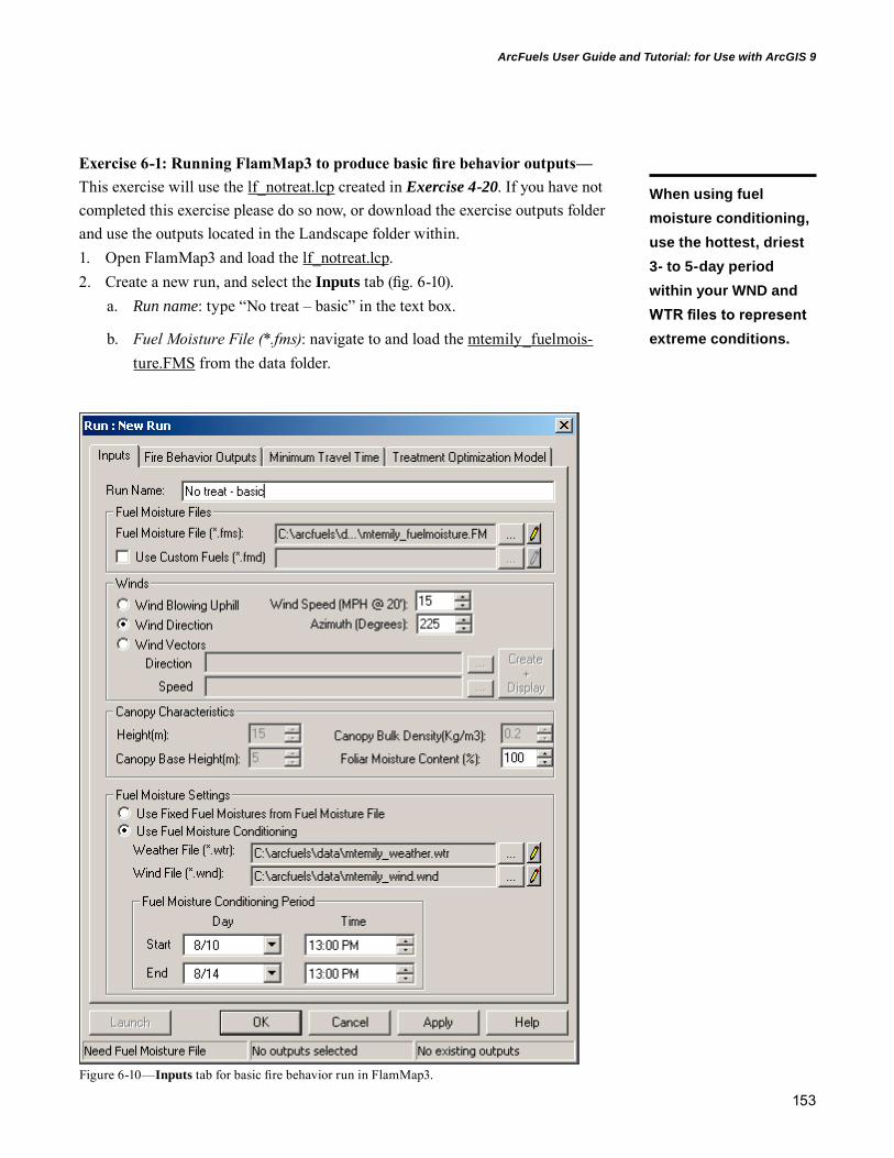
153


Exercise 6-1: Running FlamMap3 to produce basic fire behavior outputs—This exercise will use the lf_notreat.lcp created in Exercise 4-20. If you have not completed this exercise please do so now, or download the exercise outputs folder and use the outputs located in the Landscape folder within.1. Open FlamMap3 and load the lf_notreat.lcp.2. Create a new run, and select the Inputs tab (fig. 6-10).

a. Run name: type “No treat – basic” in the text box.

b. Fuel Moisture File (*.fms): navigate to and load the mtemily_fuelmois-ture.FMS from the data folder.

Figure 6-10—Inputs tab for basic fire behavior run in FlamMap3.

When using fuel moisture conditioning, use the hottest, driest 3- to 5-day period within your WND and WTR files to represent extreme conditions.

154


i. Click on the pencil button to view the FMS file. The fuel moistures are characteristic of very low conditions as defined by Scott and Burgan (2005).

c. Select the radio button to the left of Wind Direction.

i. Windspeed (MPH @20’): type “15” in the text box.

ii. Azimuth (Degrees): type “225” in the text box.

d. Foliar Moisture Content (%): type “100” in the text box.

e. Select the radio button to the left of Use Fuel Moisture Conditioning.

i. Weather file (*.wtr): navigate to and load the mtemily_weather.wtr from the data folder.

ii. Wind file (*.wnd): navigate to and load the mtemily_wind.wnd from the data folder.

iii. Fuel Moisture Conditioning Period: set the Start date to “8/10” and the End date to “8/14.” Set the Start and End times to “13:00 PM.”

f. Click Apply.

3. Select the Fire Behavior Outputs tab (fig. 6-11).a. Processor Usage and Memory/Disk Usage: leave the default values in

place.

b. Output Grids: click Select All to check the boxes next to all the out-puts.

c. Crown Fire Calculation Method: select the radio button to the left of Scott/Reinhardt (2001).

d. Options: select the radio button to the left of Relative Spread Direction From Maximum which is the default.

e. Click Apply and then click Launch.

4. A FlamMap3 Progress window will appear and indicate when the run is complete (fig. 6-12). Click OK to close the window. Click OK again to close the Run form.

5. Note in the tree pane under the No treat–basic section that all the outputs have been added (fig. 6-13). Note that the Spread Vectors theme has a blue check next to it rather than a magnifying glass. This means the theme is a vector (line or shapefile) rather than a grid theme.

155


Figure 6-11—Fire Behavior Outputs tab for basic fire behavior run in FlamMap3.

Figure 6-12—FlamMap3 Progress window.

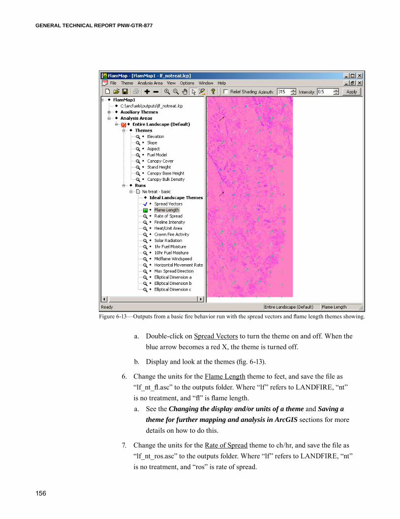
156


a. Double-click on Spread Vectors to turn the theme on and off. When the blue arrow becomes a red X, the theme is turned off.

b. Display and look at the themes (fig. 6-13).

6. Change the units for the Flame Length theme to feet, and save the file as “lf_nt_fl.asc” to the outputs folder. Where “lf” refers to LANDFIRE, “nt” is no treatment, and “fl” is flame length.a. See the Changing the display and/or units of a theme and Saving a

theme for further mapping and analysis in ArcGIS sections for more details on how to do this.

7. Change the units for the Rate of Spread theme to ch/hr, and save the file as “lf_nt_ros.asc” to the outputs folder. Where “lf” refers to LANDFIRE, “nt” is no treatment, and “ros” is rate of spread.

Figure 6-13—Outputs from a basic fire behavior run with the spread vectors and flame length themes showing.

157


8. Save the Crown Fire Activity theme as “lf_nt_cfa.asc” to the outputs folder. Where “lf” refers to LANDFIRE, “nt” is no treatment, and “cfa” is crown fire activity.

Exercise 6-2: Running FlamMap3 to produce minimum travel time (MTT) outputs for a single ignition—This exercise will use the lf_notreat.lcp created in Exercise 4-20. If you have not completed this exercise, do so now, or download the exercise outputs folder and use the outputs located in the Landscape folder within.

To run MTT, a fire ignition is needed (this can be a point, line, or area). This exercise will demonstrate how to create an ignition in FlamMap3 and how to use it for the MTT run.

Select the drip torch button on the FlamMap3 menu bar. The drip torch button is a toggle button and remains activated until you select another button such as the arrow button on the toolbar. This is similar to the pan tool in ArcMap, or the Select Stand button in ArcFuels. You know it is activated when you mouse over the map and you see a drip torch. Play around a bit to get the feeling.

• A left-click of the mouse followed by a right-click of the mouse will put down a point ignition. This can be repeated to have multiple point ignitions.

• Successive left-clicks will create a segmented line ignition connecting the points on the map where you clicked.

• Successive left-clicks followed by a right-click will create and area ignition, connecting the points with a line, and then connecting the first and last click location.

• Two successive left-clicks with the mouse followed by a right-click will create a single line.

You can manage the ignitions by going to OptionsIgnitions. Clear all your ignitions before proceeding.1. Create any ignition you would like (point, line, or area). Then save the igni-

tion (OptionsIgnitions Save to File) as a shapefile in your outputs folder. Name the shapefile “ignition.”

TIP: The default modeled fire behavior units are metric (e.g., m, kW/m, k/hr). If you would like to save the themes in English units (e.g., ft, mph) you need to change the units before you save the theme.

158


2. Create a new run, and select the Inputs tab (see fig. 6-10 for basic set up minus the name).a. Run name: type “No treat – MTT” in the text box.









iii. Fuel Moisture Conditioning Period set the Start date to “8/10” and the End date to “8/14.” Set the Start and End times to “13:00 PM.”

f. Click Apply.

3. Select the Fire Behavior Outputs tab.a. Processor Usage and Memory/Disk Usage: leave the default values in

place.

b. Crown Fire Calculation Method: select the radio button to the left of Scott/Reinhardt (2001).

c. Click Apply.

4. Select the Minimum Travel Time tab (fig. 6-14).a. Select the radio button to the left of From File. Then either click Load

Current Ignitions or use the navigation button to select the ignition.shp just created.

b. Resolution of calculations (distance): type “90” in the text box. Remember that this should always be a multiple of the input data reso-lution.

c. Maximum Simulation Time: type “0” in the text box. This allows the whole landscape to burn.

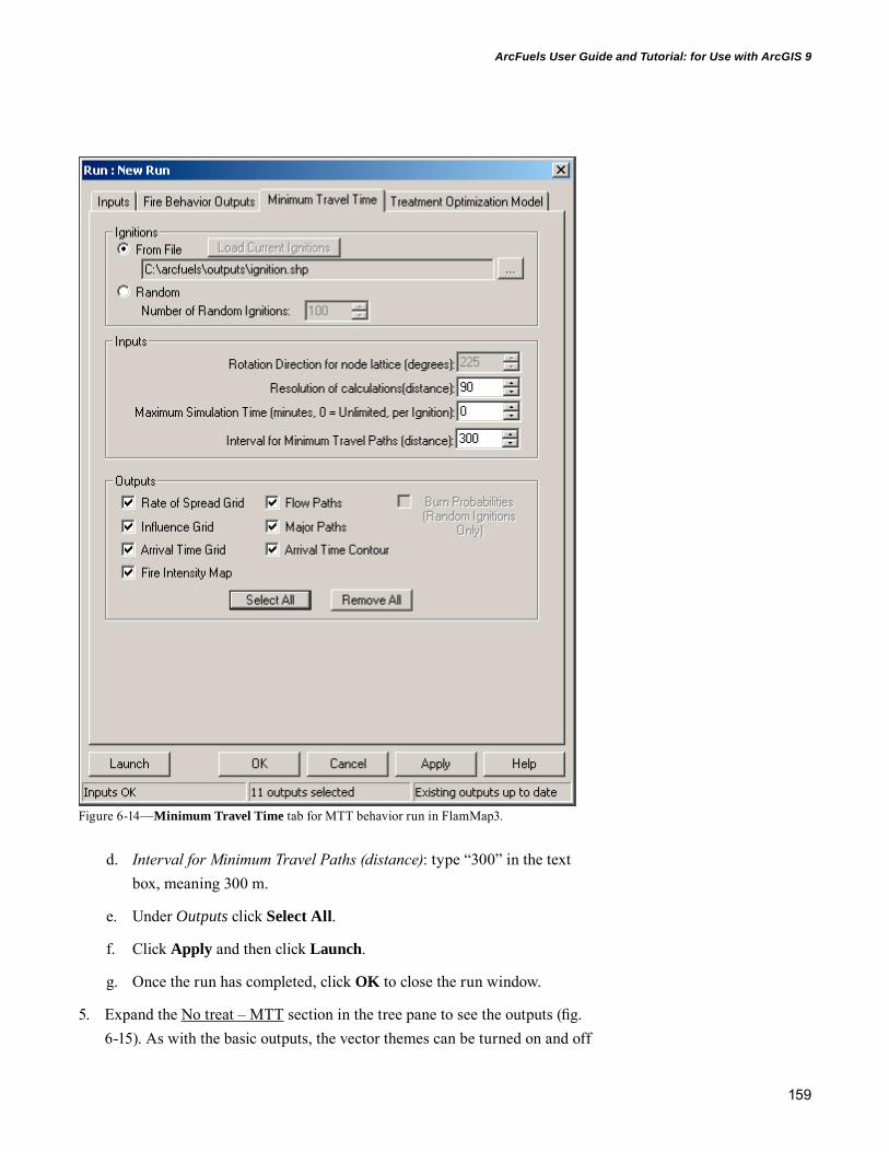
159


d. Interval for Minimum Travel Paths (distance): type “300” in the text box, meaning 300 m.

e. Under Outputs click Select All.

f. Click Apply and then click Launch.

g. Once the run has completed, click OK to close the run window.

5. Expand the No treat – MTT section in the tree pane to see the outputs (fig. 6-15). As with the basic outputs, the vector themes can be turned on and off

Figure 6-14—Minimum Travel Time tab for MTT behavior run in FlamMap3.

160


by double-clicking the blue check and the other themes can be viewed by clicking on their names.

6. Turn on the MTT Flow Paths and the MTT Major Paths.a. The paths are vector outputs of the minimum travel time between

nodes (the distance is user-defined). The flow paths are all the points from node to node, whereas the major paths are only the most signifi-cant fire spread pathways. If the resolution of the calculations is small, the flow paths can be overwhelming.

b. Save the MTT Major Paths as “lf_nt_mtt_major_paths.shp” to the out-puts folder.

Figure 6-15—MTT fire behavior outputs with MTT ROS shown in the display pane of FlamMap3.

161


The MTT major flow paths can be brought into ArcMap for a look at the effect of fuel treatments on the paths. The MTT major and flow paths are valuable outputs for comparing the effectiveness of fuel treat-ments (fig. 6-16). The paths are a good way to visualize what the fuel treatments do to the forward progression of fire. Figure 6-16 shows that the treatments that are narrow (perpendicular) to the fire spread are virtually ineffective at slowing the fire, whereas wider treat-ments often stop the fire progression quickly. To create a map similar to figure 6-16, a second MTT run in FlamMap needs to be completed with the lf_rt20.lcp created in Exercise 4-21.

Exercise 6-3: Running FlamMap3 to produce burn probability for random ignitions—In this exercise, MTT will be used again but this time with randomly placed ignitions to create a burn probability map. This exercise will use the lf_notreat.lcp created in Exercise 4-20. If you have not completed this exercise, do so now, or download the exercise outputs folder and use the outputs located in the Landscape folder within.1. Create a new run, and select the Inputs tab (see fig. 6-10 for basic set up

minus the name).a. Run name: type “No treat – MTT BP” in the text box.


0 0.5 10.25 Miles ¸No treatment MTT major flowpathsTreatment units

Posttreatment MTT major flowpaths

Figure 6-16—MTT fire Major Paths for the no-treatment alterna-tive (blue) and posttreatment alternative (red) with the treatment units in gray. This is one way to see how treatment units affect fire spread. As the flow paths reach the treatment units posttreat-ment, they typically stop at the edge of the unit or find a different path through. Narrower treatment units are not as effective at stopping or slowing the forward progression of the fire.

The MTT major and flow paths are valuable outputs for comparing the effectiveness of fuel treatments. The paths are a good way to visualize what the fuel treatments do to the forward progression of fire.

162










f. Click Apply.


place.


c. Click Apply.

3. Select the Minimum Travel Time tab (fig. 6-17).a. Select the radio button to the left of Random and then type “2500” in

the text box to the left of Number of Random Ignitions.

b. Resolution of calculations (distance): type “90” in the text box.

c. Maximum Simulation Time: type “480” in the text box; 480 min is equivalent to 8 hrs, which is a single burn period or fire day.

d. Interval for Minimum Travel Paths (distance): type “300” in the text box. This is the default value.

e. Click Apply and then click Launch. This will take about 30 min to complete.

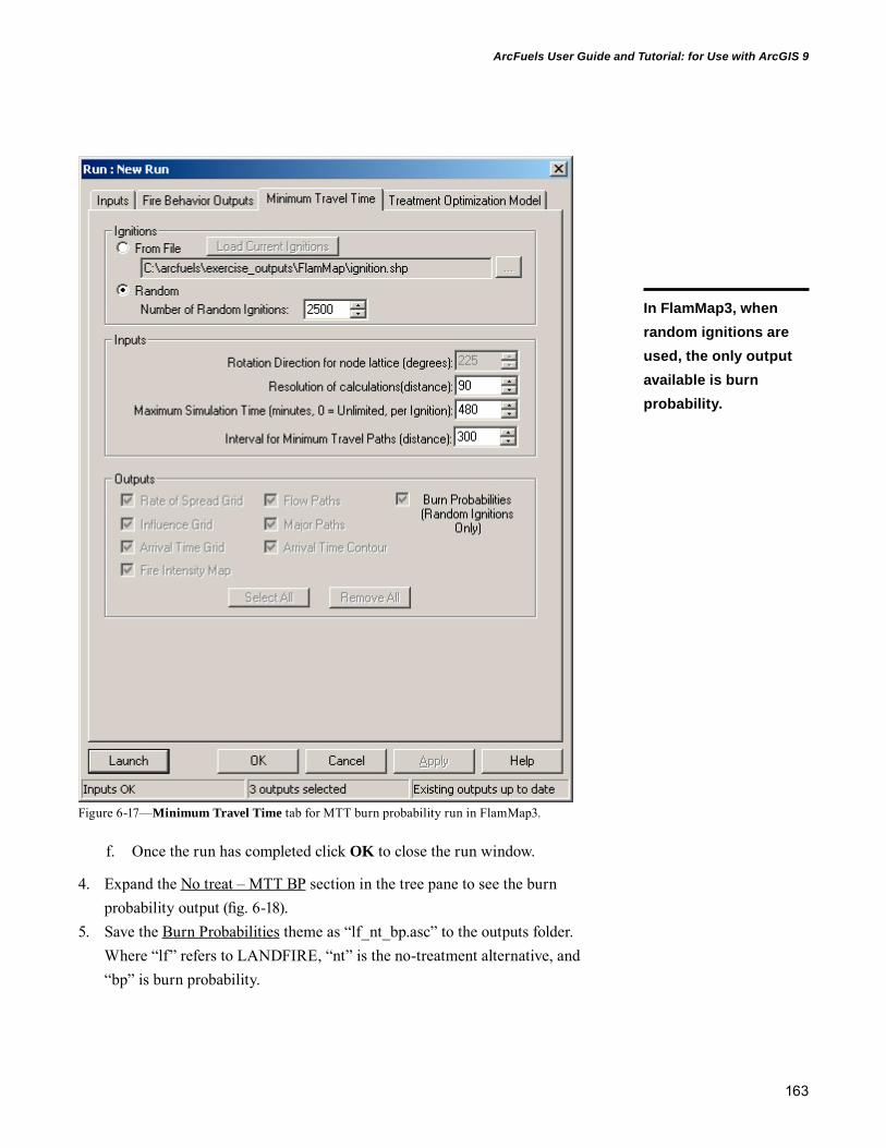
163


f. Once the run has completed click OK to close the run window.

4. Expand the No treat – MTT BP section in the tree pane to see the burn probability output (fig. 6-18).

5. Save the Burn Probabilities theme as “lf_nt_bp.asc” to the outputs folder. Where “lf” refers to LANDFIRE, “nt” is the no-treatment alternative, and “bp” is burn probability.

Figure 6-17—Minimum Travel Time tab for MTT burn probability run in FlamMap3.

In FlamMap3, when random ignitions are used, the only output available is burn probability.

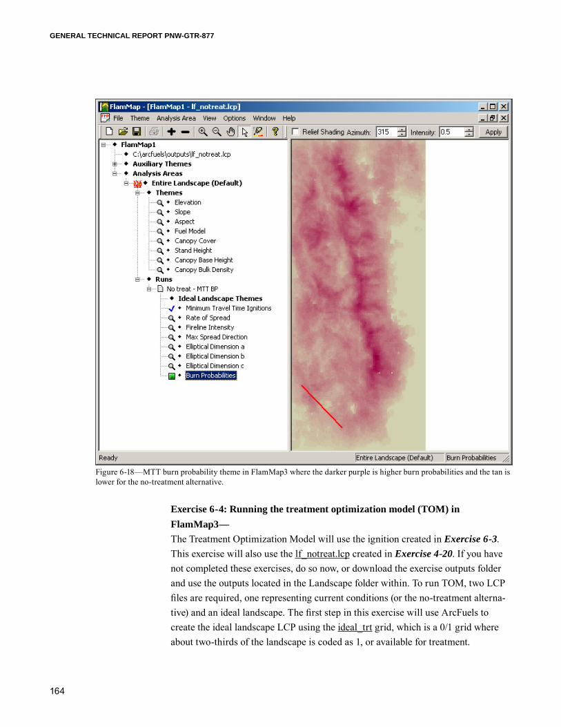
164


Exercise 6-4: Running the treatment optimization model (TOM) in FlamMap3—The Treatment Optimization Model will use the ignition created in Exercise 6-3. This exercise will also use the lf_notreat.lcp created in Exercise 4-20. If you have not completed these exercises, do so now, or download the exercise outputs folder and use the outputs located in the Landscape folder within. To run TOM, two LCP files are required, one representing current conditions (or the no-treatment alterna-tive) and an ideal landscape. The first step in this exercise will use ArcFuels to create the ideal landscape LCP using the ideal_trt grid, which is a 0/1 grid where about two-thirds of the landscape is coded as 1, or available for treatment.

Figure 6-18—MTT burn probability theme in FlamMap3 where the darker purple is higher burn probabilities and the tan is lower for the no-treatment alternative.

165


1. Open ArcFuels and load the demonstration data layer. Click the Land-scape button on the ArcFuels toolbar, then select Build FlamMap Landscape from the drop-down list. Select the Using ArcGIS Grid Data tab (fig. 6-19).

Figure 6-19—Using ArcGIS Grid Data tab setup to create the ideal landscape LCP from LANDFIRE data.






166


f. The output boundaries are based on: select the Grid Layer radio but-ton, then select elevation from the drop-down list.



ii. Treatment Location Grid: select ideal_trt from the drop-down menu.

iii. Treatment Type Grid: select ideal_trt from the drop-down menu.

iv. Treatment Adjustment Table: select example_treatment_adjustment from the drop-down menu.

v. Treatment Type ID Field: select treat_type from the drop-down menu.

h. Fuel model: select lf_fbfm40 and fm_adj from the drop-down lists.





m. LCP Output File: using the navigation button name the LCP “lf_ideal_treat” and save it in the outputs folder.


o. Click Close to close the Build LCP form.

2. Open FlamMap3 and load the lf_notreat.lcp if not already loaded. Create a new run, and select the Inputs tab (see fig. 6-10 for basic setup minus the name). a. Run name: type “TOM” in the text box.

167











f. Click Apply.


place.


c. Click Apply.

4. Select the Treatment Optimization tab (fig. 6-20).a. Ignition file: use the navigation button to select ignition.shp from the

outputs folder.


c. Ideal Landscape: use the navigation button to select lf_ideal_treat.lcp from the outputs folder.

d. Maximum Treatment Dimension (m): type “300” in the text box; this is the default value.

168


e. Iterations/Treatment Level (1-5): type “1” in the text box; this is the default value.

f. Treatment Fraction: type “0.2” in the text box; this is the default value. According to the FlamMap3 help guide, this value should be between 0.1 and 0.3 to optimally place treatments. It has been found that values below 0.05 do not change enough of the landscape and values above 0.5 are no better than random.

Figure 6-20—Treatment Optimization Tab set up.

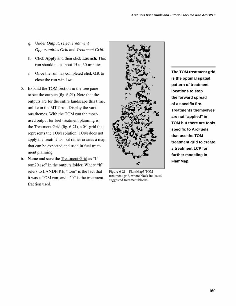
169


g. Under Output, select Treatment Opportunities Grid and Treatment Grid.

h. Click Apply and then click Launch. This run should take about 15 to 30 minutes.

i. Once the run has completed click OK to close the run window.

5. Expand the TOM section in the tree pane to see the outputs (fig. 6-21). Note that the outputs are for the entire landscape this time, unlike in the MTT run. Display the vari-ous themes. With the TOM run the most-used output for fuel treatment planning is the Treatment Grid (fig. 6-21), a 0/1 grid that represents the TOM solution. TOM does not apply the treatments, but rather creates a map that can be exported and used in fuel treat-ment planning.

6. Name and save the Treatment Grid as “lf_tom20.asc” in the outputs folder. Where “lf” refers to LANDFIRE, “tom” is the fact that it was a TOM run, and “20” is the treatment fraction used.

Figure 6-21—FlamMap3 TOM treatment grid, where black indicates suggested treatment blocks.

The TOM treatment grid is the optimal spatial pattern of treatment locations to stop the forward spread of a specific fire. Treatments themselves are not “applied” in TOM but there are tools specific to ArcFuels that use the TOM treatment grid to create a treatment LCP for further modeling in FlamMap.

170


Fuel Treatment Planning Scenarios Using ArcFuelsThis section contains fuel treatment planning scenarios to highlight the use of ArcFuels. The scenarios are meant to serve as a foundation for planning documents (such as fire and fuels specialist reports for an environmental impact statement (EIS) or environmental assessment (EA)). Figure 7-1 is a simplistic flow chart of the fuel treatment planning process. ArcFuels was designed to assist in the middle processes: designing the no-treatment alternative, designing fuel treatment alternative(s), and analyzing the effects of the fuel treatment alternatives. The scenarios provided highlight the uses of ArcFuels in conjunction with other programs such as Flam-Map3, ArcGIS, Excel, and Access to complete these processes. The scenarios are not all-inclusive but should provide a good foundation for fuel treatment planning.

The following scenarios will use outputs created in the Tools and Introduction to Fire Behavior Modeling with FlamMap3 sections of this User Guide and Tuto-rial. If you have not completed the exercises you may do them when referred to or download the optional exercise outputs from http://www.fs.fed.us/wwetac/arcfuels/downloads.html.

Figure 7-1—Simplistic flow chart of fuel management planning process. ArcFuels was designed to assist the middle processes: designing the no-treatment alternative, designing fuel treatment alternative(s), and analyzing the effects of the fuel treatment alternatives.

Chapter 7

Pre-planningAcquire data and verify for accuracy

Design the no-treatment alternativeUpdate data as needed

Analyze to identify problem areas

Design fuel treatment alternative(s)Locate fuel treatment units or use pre-de�ned plans

Analyze the e�ects of the fuel treatment alternatives

Wild�re hazard and risk assessements, e�ectson values at risk, forest health, etc.

Complete planning documents

The scenarios provided highlight the uses of ArcFuels in conjunction with other programs such as FlamMap3, ArcGIS, Excel, and Access to complete these processes. The scenarios are not all-inclusive but should provide a good foundation for fuel treatment planning.

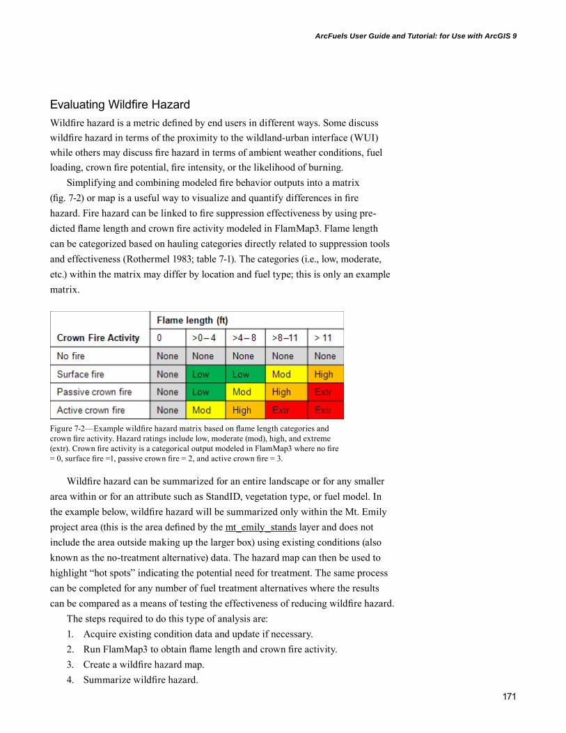
171


Evaluating Wildfire HazardWildfire hazard is a metric defined by end users in different ways. Some discuss wildfire hazard in terms of the proximity to the wildland-urban interface (WUI) while others may discuss fire hazard in terms of ambient weather conditions, fuel loading, crown fire potential, fire intensity, or the likelihood of burning.

Simplifying and combining modeled fire behavior outputs into a matrix (fig. 7-2) or map is a useful way to visualize and quantify differences in fire hazard. Fire hazard can be linked to fire suppression effectiveness by using pre-dicted flame length and crown fire activity modeled in FlamMap3. Flame length can be categorized based on hauling categories directly related to suppression tools and effectiveness (Rothermel 1983; table 7-1). The categories (i.e., low, moderate, etc.) within the matrix may differ by location and fuel type; this is only an example matrix.

Figure 7-2—Example wildfire hazard matrix based on flame length categories and crown fire activity. Hazard ratings include low, moderate (mod), high, and extreme (extr). Crown fire activity is a categorical output modeled in FlamMap3 where no fire = 0, surface fire =1, passive crown fire = 2, and active crown fire = 3.

Wildfire hazard can be summarized for an entire landscape or for any smaller area within or for an attribute such as StandID, vegetation type, or fuel model. In the example below, wildfire hazard will be summarized only within the Mt. Emily project area (this is the area defined by the mt_emily_stands layer and does not include the area outside making up the larger box) using existing conditions (also known as the no-treatment alternative) data. The hazard map can then be used to highlight “hot spots” indicating the potential need for treatment. The same process can be completed for any number of fuel treatment alternatives where the results can be compared as a means of testing the effectiveness of reducing wildfire hazard.

The steps required to do this type of analysis are:1. Acquire existing condition data and update if necessary.2. Run FlamMap3 to obtain flame length and crown fire activity.3. Create a wildfire hazard map.4. Summarize wildfire hazard.

172


The following example will complete the above steps with fire-modeled outputs (Exercise 6-1) for the no-treatment alternative (Exercise 4-20). If you have not done the exercises, please do so now, or use the files in the exercise outputs folder. The example will build upon skills gained in the ArcFuels Tools and Introduction to Fire Behavior Modeling with FlamMap sections; please refer back to these sections for more detail about the forms or processes mentioned.

Step 1: Acquire existing condition data and update if necessary—The supplied LANDFIRE data will be used. For this scenario, they are assumed to be accurate and not in need of updating.

Step 2: Run FlamMap3 to obtain flame length and crown fire activity—Before FlamMap3 can be run, the input LCP file must be built. The existing condi-tions LCP (lf_notreat.lcp) built in Exercise 4-20 from LANDFIRE data will be used in FlamMap3.

FlamMap3 was run to characterize flame length and crown fire activity for the no-treatment alternative (lf_nt_fl.asc and lf_nt_cfa.asc) in Exercise 6-1.

Step 3: Create a wildfire hazard map—In this step, flame length will be reclassified based on the hauling chart values (table 7-1). Next, the reclassified flame length and crown fire activity grids will be combined to create a hazard grid using the hazard matrix (fig. 7-2).

Table 7-1—Hauling category table adapted from Rothermel (1983), which related flame length to fire suppression effectiveness

Flame length Fireline intensity Description

Feet Btu/fs/s<4 <100 Fires can generally be attacked at the head or flanks by persons using hand tools. Hand line should hold the fire.4–8 100–500 Fires are too intense for direct attack on the head by persons using hand tools. Hand line cannot be relied on to hold fire. Equipment such as dozers, pumpers, and fire-retardant aircraft can be effective.8–11 500–1,000 Fires may present serious control problems—torching out, crowning, and spotting. Control efforts at the fire head will probably be ineffective.>11 >1,000 Crowning, spotting, and major fire runs are probable. Control efforts at head of fire are ineffective.

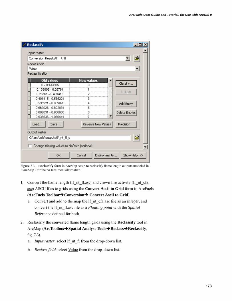
173


1. Convert the flame length (lf_nt_fl.asc) and crown fire activity (lf_nt_cfa.asc) ASCII files to grids using the Convert Ascii to Grid form in ArcFuels (ArcFuels ToolbarConversion Convert Ascii to Grid).a. Convert and add to the map the lf_nt_cfa.asc file as an Integer, and

convert the lf_nt_fl.asc file as a Floating point with the Spatial Reference defined for both.

2. Reclassify the converted flame length grids using the Reclassify tool in ArcMap (ArcToolboxSpatial Analyst ToolsReclassReclassify, fig. 7-3).a. Input raster: select lf_nt_fl from the drop-down list.

b. Reclass field: select Value from the drop-down list.

Figure 7-3—Reclassify form in ArcMap setup to reclassify flame length outputs modeled in FlamMap3 for the no-treatment alternative.

174


c. Click the Classify button to open the Classification form (fig. 7-4).

i. Method: select Equal Interval from the drop-down list to change the number of Classes.

ii. Classes: select 5 from the drop-down list.

iii. Break values: highlight the values and type in “0,” “4,” “8,” and “11” for the first 4 values; leave the last value as it appears. After this is done, the Method will default to Manual (fig. 7-4).

iv. Click OK to apply the changes and return to the Reclassify form.

d. Set the New values to be the upper end (highest amount within its range of flame heights) of the Old values, which correlates to the flame length categories used in the prior step (fig. 7-5).

Figure 7-4—Classification form set up to reclassify flame length into five categories.

Changing the display to the categories desired does not change the values in the grid. The Classify tool is used to change the values and create a new grid.

175


e. Output raster: name the out-put raster “lf_nt_fl_c” and save it in the outputs folder. The “c” at the end signifies this is a classified version of the flame length output.

f. Click OK to close the Reclassify form and complete the reclassification.

3. Combine the reclassified flame length and crown fire activ-ity grids using the Combine tool (ArcToolboxSpatial Analyst ToolsLocalCombine, fig. 7-6).a. Input rasters: select lf_nt_fl_c and lf_nt_cfa from the drop-down list.

b. Output raster: name the grid “lf_nt_haz” and save it in the outputs folder. The “haz” at the end indicates that this is the hazard grid.

Figure 7-5—New values for reclassification of flame length.

TIP: If your maximum flame length value is around 40 instead of about 140, you saved the output in meters instead of feet. Redo Exercise 6-1 and be sure to change your units to feet before saving the ASCII file.

Figure 7-6—Combine form in ArcMap used to combine the categorized flame length and crown fire activity grids.

176


c. To only include areas within the Mt. Emily area, click the Environments… button on the Combine form, expand >>Raster Analysis Settings and under Mask select stands from the drop-down list. Click OK to apply the changes.

i. If this step is not completed the join will be of the entire rectangu-lar extent of the LANDFIRE data.

d. Click OK to complete the combine.

4. Open the attributes table for lf_nt_haz and add a new text field (Attributes Table OptionsAdd Field…) named “HAZARD.”a. Use the Field Calculator (right-click on the HAZARD heading, then

select Field Calculator from the menu) to type the values identified in your hazard matrix shown in figure 7-2 (fig. 7-7 shows this step com-pleted). This can be done one field at a time, or for multiple fields.

Figure 7-7—Attributes table for the lf_nt_haz grid with the added hazard field filled in.

TIP: When you are using the Field Calculator, text entries must be enclosed in quotations (e.g., “LOW”).

TIP: The Field Calculator can be used to assign values to one or more fields at a time. If no fields are selected, the change will be applied to all; if fields are selected the change will be applied only to the selected field(s).

NOTE: This can also be completed with the Editor tool in ArcMap.

177


5. In ArcMap, change the display of lf_nt_haz to show the hazard field (fig. 7-8a).a. Right-click on the grid name

in the table of contents, select Properties from the list, and select the Symbology tab.

b. Show: select Unique Values from the options in the box.

c. Value field: select HAZARD from the drop-down list.

d. Set NONE to be black, LOW to be green, MODERATE to be yellow, HIGH to be orange, and EXTREME to be red to match that of the haz-ard matrix (fig. 7-2).

e. Click OK to close the form.

If you were starting to plan fuel treatment locations and you only have exist-ing conditions data, you can create a hazard map to identify places of high hazard to use in the planning process. Just because a location has elevated hazard does not mean it needs to be treated; based on vegetation type or fire regime grouping it might be fine if it burns at a higher intensity. However, if high hazard is also coupled with high likelihood of burning or is near or within an area with highly valued resources, it might be more important to treat a given area. These methods can be repeated for any number of fuel treatment alternatives for comparison. Figure 7-8 displays wildfire hazard for the no-treatment alternative created in the steps above and an alternative in which 20 percent of the landscape was treated.

Step 4: Summarize wildfire hazard—Maps are useful aids for visualizing the impact of fuel treatment alternatives on fire hazard. However, for reports and documents, the change often needs to be quanti-fied. There are many ways to summarize the data. Below is one example using the Summary option available within the attributes table. For comparison, the no-treatment alternative is compared to one in which 20 percent of the landscape was treated; however, only the no-treatment alternative is demonstrated. 1. Open the lf_nt_haz attributes table. Right-click on the HAZARD column

and select Summarize... from the menu (fig. 7-9).

Figure 7-8—Wildfire hazard maps for the no-treat-ment (A) and treat 20 percent (B) alternatives.

0 42mi

A BNo treatment Treat 20 percent

Hazard classesNoneLowModerate

HighExtreme

Maps are useful aids for visualizing the impact of fuel treatment alternatives on fire hazard. However, for reports and documents, the change often needs to be quantified.

178


a. Select the field to summarize: select HAZARD from the drop-down list.

b. Choose one or more summary statistics to be included in the output table: expand COUNT, then select Sum from the options.

c. Specify output table: name the output table “HazardArea.dbf” and save it in the outputs folder.

d. Click OK to complete the summary.

e. When the Summarize Completed window opens, click No.

2. Open the HazardArea.dbf file with Excel (fig. 7-10). HAZARD is the haz-ard classes, Cnt_HAZARD is the number of times that hazard class was assigned, and Sum_COUNT is the number of 30 m pixels that are within the hazard category. To calculate area in acres, multiply Sum_COUNT by 0. 0.222394, because each pixel is 900 m2 (30 m by 30 m pixel) and 1 m2 is equal to 0.0002471044 ac (table 7-2).

Figure 7-9—Summarize form set to calculate area by hazard class.

179


About half of the Mt. Emily landscape was categorized as extreme hazard. The map can be used in conjunction with other data such as forest type, values at risk, road networks, etc., to devise treatment alternatives to reduce the landscape hazard.

NOTE: To summarize for other attributes such as StandID or fuel model, the Combine tool would need to be used to combine the flame length, crown fire activity, and another grid (i.e., stands or lf_fbfm40 for existing conditions or lf_trt_fm for the treat 20 percent alternative) before the Summary is completed. For more help with GIS download and use, the GIS Tips and Tricks Guide avail-able at http://www.fs.fed.us/wwetac/arcfuels/downloads.html.

Figure 7-10—Hazard Area table where the values counts of 30 m pixels.

Table 7-2—Wildfire hazard comparison for the Mt. Emily project area for the no-treatment and treat 20 percent alternatives

Hazard No treatment Treat 20 percent

Acres Percent Acres PercentNone 3,718 9 3,718 9Low 12,172 30 18,401 46Moderate 2,313 6 2,035 5High 3,094 8 2,672 7Extreme 19,076 47 13,565 33Total 40,373 100 40,373 100

Wildfire Risk Assessment: Creating a Wildfire Exposure Scatter PlotWildfire risk is the likelihood of a fire occurring, the associated fire behavior when a fire occurs, and the effects of the fire (Calkin et al. 2010, Finney 2005, Scott 2006). Although the effects can be both positive and negative, in the field of wildfire risk the benefits are most often not considered. Wildfire risk mitigation is achieved when any of the three aspects (likelihood, behavior, or effects) are reduced.

Burn probability modeling represents a major advancement in wildfire behavior modeling compared to previous methods, such as those in which fire likelihood was quantified with relatively few (<10) predetermined ignition locations. Now

A wildfire risk assessment has two major components. A wildfire exposure analysis considers the likelihood of a fire occurring and the associated fire behavior related to a highly valued resource. A wildfire effects analysis also considers the likelihood and behavior of a fire in addition to the effect of the fire on a highly valued resource.

180


thousands of fires can be simulated relatively quickly. Burn probability (BP) is an estimate of the likelihood of a pixel burning given a single random ignition in the landscape and is calculated as:

BP = F/nwhere F is the number of times a pixel burns and n is the number of fires simulated.

Wildfire risk assessments are becoming more common in the research and management communities. When fire effects are not quantified but are summarized with respect to any resource or value of interest the assessment is called a “wildfire exposure analysis.” If no values or resources are considered, this is called a “proba-bilistic wildfire hazard assessment.” Probabilistic wildfire hazard (combination of burn probability and flame length) is most often mapped and summarized by location or area (fig. 7-11). Scatter plots (fig. 7-12) can be created to visualize differ-ences in wildfire exposure for individual resources (e.g., forest stands, structures, or values at risk), and can be used to compare the effects of fuel treatment alterna-tives on wildfire exposure. They can be created from point data (e.g., structure location) or from area data (e.g., forest type). When using area data, fire behavior information must first be summarized (e.g., average value for the polygon). Figure 7-12 (Ager et al. 2010) is an example of a wildfire exposure scatter plot for struc-tures within the Mt. Emily area. The scatter plots highlight changes in wildfire exposure for two treatment priorities, one to preserve large trees (SDEN) and the other to protect structures (RDEN), for three treatment intensities (treating 0, 20, and 66 percent, respectively).

Figure 7-11—Maps of probabilistic wildfire hazard for the no-treatment (A) and treat 20 percent (B) fuel treatment scenarios and a sampleprobabilistic wildfire hazard matrix (C).

181


Because the mechanics behind creating wildfire hazard maps and summariz-ing wildfire hazard are the same for probabilistic wildfire hazard, they will not be demonstrated in this section. The example below will demonstrate the creation of a wildfire risk scatter plot using the no-treatment alternative; the same steps and processes can be completed for treatment alternatives for comparisons of fuel treat-ment effectiveness.

The steps required to do this type of analysis are:1. Acquire existing condition data and update if necessary.2. Run FlamMap3 fire behavior runs for the no-treatment alternative.3. Summarize fire behavior values by forest type.4. Create the scatter plot.The following example will complete the above steps with fire-modeled out-

puts (Exercises 6-1 and 6-3) for the no-treatment alternative (Exercise 4-20). If you have not done the exercises, please do so now, or use the files in the optional exercise outputs folder. The scatter plot will show the change in wildfire exposure for forest types within the landscape before and after treatment.

Step 1: Acquire existing condition data and update if necessary—The supplied LANDFIRE data will be used. For this scenario, they are assumed to be accurate and not in need of updating.

Step 2: Run FlamMap3 to obtain flame length and burn probability—Before FlamMap3 can be run, the input LCP file must be built. The existing condi-tions LCP (lf_notreat.lcp) built in Exercise 4-20 from LANDFIRE data will be used in FlamMap3.

Figure 7-12—Expected flame length and burn probability scatter plots showing values for individual structures. The stand density (SDEN) and residential density (RDEN) priorities for the no treatment, 20 percent area treated, and 66 percent area treated are plotted. Points are averages of all pixels within a 45.7 m radius around each structure (figure 12 from Ager et al. 2010).

Scatter plots of burn probability and flame length can be used to visualize the wildfire exposure of individual points or area units on a landscape.

182


FlamMap3 was run to characterize flame length and burn probability for the no-treatment alternative (lf_nt_fl.asc and lf_nt_bp.asc) in Exercise 6-1 and 6-3.

Step 3: Summarize fire behavior values by forest type—To do this, first a grid of forest types needs to be created using the ArcMap Polygon to Raster tool. Then the Zonal Statistics as Table tool in ArcMap will be used to summarize burn probability and flame length by forest type.1. Batch convert the flame length and burn probability ASCII files to grids

using the Batch Convert Ascii to Grid form in ArcFuels (ArcFuels ToolbarConversion Batch Convert Ascii to Grid).a. Convert the lf_nt_fl.asc and lf_nt_bp.asc files as a Floating point with

the Spatial Reference defined for both. The lf_nt_fl.asc was converted in the Evaluating Wildfire Hazard scenario; a replacement warning window will open if you completed that scenario.

2. Create a forest type grid using the Polygon to Raster tool (ArcToolbox Conversion ToolsTo RasterPolygon to Raster, fig. 7-13).a. Input Features: select mt_emily_stands from the drop-down list.

b. Value field: select ForestType from the drop-down list.

c. Output Raster Dataset: save the grid as “forest_type” in the outputs folder.

d. Cell assignment type (optional): keep the default CELL_CENTER.

Figure 7-13—Polygon to Raster form set up to convert the forest type attribute of the stands polygon to a grid file.

183


e. Priority field (optional): keep the default NONE.

f. Cellsize (optional): type “30” in the text box.

g. Click the Environments… button to open the Environments Settings form.

i. Expand the General Settings option.

ii. Snap Raster: select stands from the drop-down list. You might have to scroll down to find this setting.

iii. Click OK to close the Environments Settings form.

iv. Click OK to create the forest_type grid.

3. Complete summary statistics of burn probability by forest type using the Zonal Statistics as Table tool in ArcMap (ArcToolboxSpatial Analyst ToolsZonal Zonal Statistics as Table, fig. 7-14).a. Input raster or feature zone data: select forest_type from the drop-

down list.

b. Zone field: select FORESTTYPE from the drop-down list.

c. Input value raster: select lf_nt_bp from the drop-down list.

d. Output Table: save the table as “lf_nt_bp_fortype_zonal” in the out-puts folder.

e. Click OK to complete the process.

Figure 7-14—Zonal Statistics as Table form set to summarize burn probability by forest type.

184


4. Repeat step 3 with the lf_nt_fl grid, saving the output table as “lf_nt_fl_for-type_zonal” in the outputs folder.

Step 4: Create the wildfire risk scatter plot—1. Open the lf_nt_bp_fortype_zonal table (fig. 7-15). You will need switch to

the Source tab at the bottom of the table of contents in ArcMap to see it, then right-click and chose Open. Within the table, burn probability values have been summarized (i.e., minimum, maximum, range) by forest type.

Figure 7-15—Zonal statistics table for forest type and burn probability.

Figure 7-16—Excel workbook with zonal statistics outputs filled in for both the no-treatment and treatment alternatives where about 20 percent of the landscape was treated.

2. Open the lf_nt_fl_fortype_zonal table to see the flame length summarization.3. Create a new Excel workbook called “ForestTypeScatterPlot.xlxs” in the

outputs folder. The information that will need to be copied into an Excel spreadsheet is FORESTTYPE and MEAN for burn probability and flame length (fig. 7-16).

185


a. There are a number of ways to complete this; you can copy and paste individual cells from the zonal statistics table, type the values into the Excel spreadsheet, or export the zonal statistics table as a *.dbf file and open it with Excel.

4. In Excel, insert an XY scatter chart (Excel RibbonInsertScatter Scatter with only Markers). a. The x-axis values are burn probability and the y-axis values flame

length (fig. 7-17a).

b. To get markers for each forest type, each forest type will need to be an individual series. To change the series within a chart, right-click in the chart and select Select Data from the menu and Add a new series.

i. Series name: type “Grand fir” in the text box.

ii. Series X values: select cell of the Nt BP value for Grand fir. In fig-ure 7-16, this would be B2.

iii. Series Y values: select cell of the Nt FL value for Grand fir. In fig-ure 7-16, this would be C2.

iv. Repeat for all the forest types.

Figure 7-17—Scatter plot of wildfire exposure for forest types for the no-treatment (A) and treat 20 percent (B) fuel treatment alternatives.

Wildfire exposure was reduced by the fuel treatment alternative as can be seen by the points shifting down and to the left relative to the no-treatment values

186


The same process can be replicated for treatment alternatives for a comparison of wildfire exposure before and after treatment (fig. 7-17). Forest types lower and to the left (i.e., nonforested) have lower wildfire exposure than those in the upper righthand corner (i.e., lodgepole pine and subalpine fir) (fig 7-17b).

Designing Landscape Level Fuel Treatment Alternatives By Using Wildfire Exposure With FVS DataA wildfire exposure assessment of current conditions coupled with other informa-tion can be a good start for fuel treatment planning. This scenario will build fuel treatment alternatives based on probabilistic wildfire hazard for the entire landscape and wildfire exposure of the various forest types. Finally, the effectiveness of the fuel treatment alternatives will be tested.

The steps required to do this type of analysis are:1. Acquire existing condition data and update if necessary.

2. Run FlamMap3 fire behavior runs for the existing conditions.

3. Create a wildfire exposure map to design fuel treatment alternatives.

4. Run FlamMap3 fire behavior runs for the treatment alternatives.

5. Assess the effectiveness of the fuel treatment alternatives.

The following scenario will complete the above steps using a landscape file comprised of FVS run values surrounded by LANDFIRE grids to model fire behavior.

Step 1: Acquire existing condition data and update if necessary—The data supplied by LANDFIRE, Mt_Emily_Database.mdb, and the mt_emily_stands.shp are assumed to be accurate and not in need of updating.

Step 2: Run FlamMap3 fire behavior runs for the existing conditions—Before FlamMap3 can be run, the input LCP file must be built. The existing conditions LCP (fvs_lf_notreat.lcp) built in Exercise 4-22 from LANDFIRE and FFE-FVS data will be used in FlamMap3. FlamMap3 will be run to output crown fire activity, flame length, and burn probability. Rather than doing separate runs for flame length and crown fire activity and then burn probability, both can be run at once in FlamMap3.1. Open FlamMap3, load the fvs_lf_notreat.lcp, and create a new run.2. Select the Inputs tab (fig. 7-18).

a. Run name: type “Wildfire Exposure Alt” in the text box.

This scenario will require many steps within ArcMap. There are several ways to accomplish the steps provided. If you are more comfortable with another method, please do what you know.

187







Figure 7-18— Inputs tab for a wildfire exposure run.

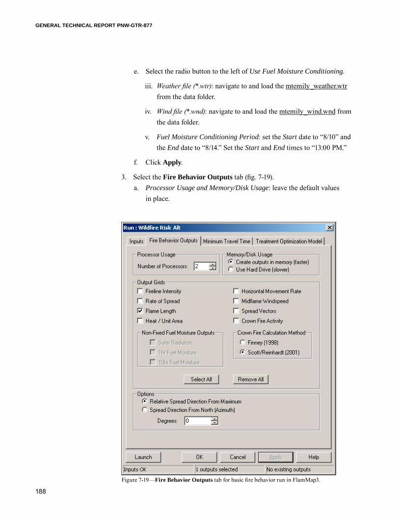
188



iii. Weather file (*.wtr): navigate to and load the mtemily_weather.wtr from the data folder.

iv. Wind file (*.wnd): navigate to and load the mtemily_wind.wnd from the data folder.

v. Fuel Moisture Conditioning Period: set the Start date to “8/10” and the End date to “8/14.” Set the Start and End times to “13:00 PM.”

f. Click Apply.

3. Select the Fire Behavior Outputs tab (fig. 7-19).a. Processor Usage and Memory/Disk Usage: leave the default values

in place.

Figure 7-19—Fire Behavior Outputs tab for basic fire behavior run in FlamMap3.

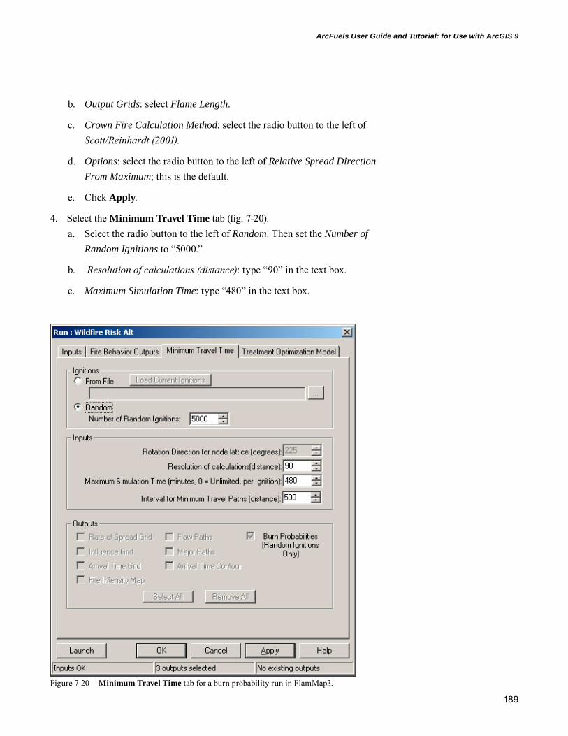
189


b. Output Grids: select Flame Length.


d. Options: select the radio button to the left of Relative Spread Direction From Maximum; this is the default.

e. Click Apply.

4. Select the Minimum Travel Time tab (fig. 7-20).a. Select the radio button to the left of Random. Then set the Number of

Random Ignitions to “5000.”


c. Maximum Simulation Time: type “480” in the text box.

Figure 7-20—Minimum Travel Time tab for a burn probability run in FlamMap3.

190


d. Interval for Minimum Travel Paths (distance): type “500” in the text box; this is the default.

e. Click Apply and then click Launch. This might take 30–60 minutes depending on your computer.

f. Once the run has completed, click OK to close the run window.

5. Name the output ASCII files as “fvs_nt_fl” and “fvs_nt_bp” for flame length (change the units to ft) exposure and burn probability, respectively, and save them in the outputs folder.

Step 3: Create a wildfire exposure map to design fuel treatment alternatives—In this step, a wildfire exposure map will be created from the flame length and burn probability outputs from FlamMap3. The process is similar to creating a wildfire hazard map. Once the map is created, it will be used to create two treatment alternatives.

• Alternative 1 will treat all forested areas of moderate, high, and extreme wildfire exposure, which is about 30 percent of the landscape.

• Alternative 2 will treat all forested areas with high and extreme wild-fire exposure, which is about 15 percent of the landscape.

1. If not already in the ArcMap table of contents, add the forest_type grid. This was created in Wildfire risk assessment–Creating scatter plots and was saved in the outputs folder.

2. Convert the flame length and burn probability ASCII files to grids using the Batch Convert Ascii to Grid form in ArcFuels (ArcFuels ToolbarConversion Batch Convert Ascii to Grid).a. Convert and add to the map the fvs_nt_fl.asc and fvs_nt_bp.asc files as

Floating point with the Spatial Reference defined for both.

3. Reclassify flame length based on the hauling chart values (table 7-1) using the Reclassify tool in ArcMap (ArcToolboxSpatial Analyst Tools ReclassReclassify, fig. 7-21). a. Input raster: select fvs_nt_fl from the drop-down list.



i. Method: select Equal Interval from the drop-down list to change the number of Classes.

191



iii. Break values: highlight the values and type in “0,” “4,” “8,” and “11” for the first 4 values; leave the last value as it appears. After this is done, the Method will default to Manual (fig. 7-4).

iv. Click OK to apply the changes and return to the Reclassify form.

d. Set the New values to be the upper end (highest amount within its range of flame lengths) of the Old values, which correlates to the flame length categories used in the prior step (fig. 7-21).

e. Output raster: name the output raster “fvs_nt_fl_c” and save it in the outputs folder. The “c” at the end signifies that this is a classified ver-sion of the flame length output.

f. Click OK to close the Reclassify form and complete the reclassification.

Figure 7-21—Reclassify form set up to reclassify flame length into categories.

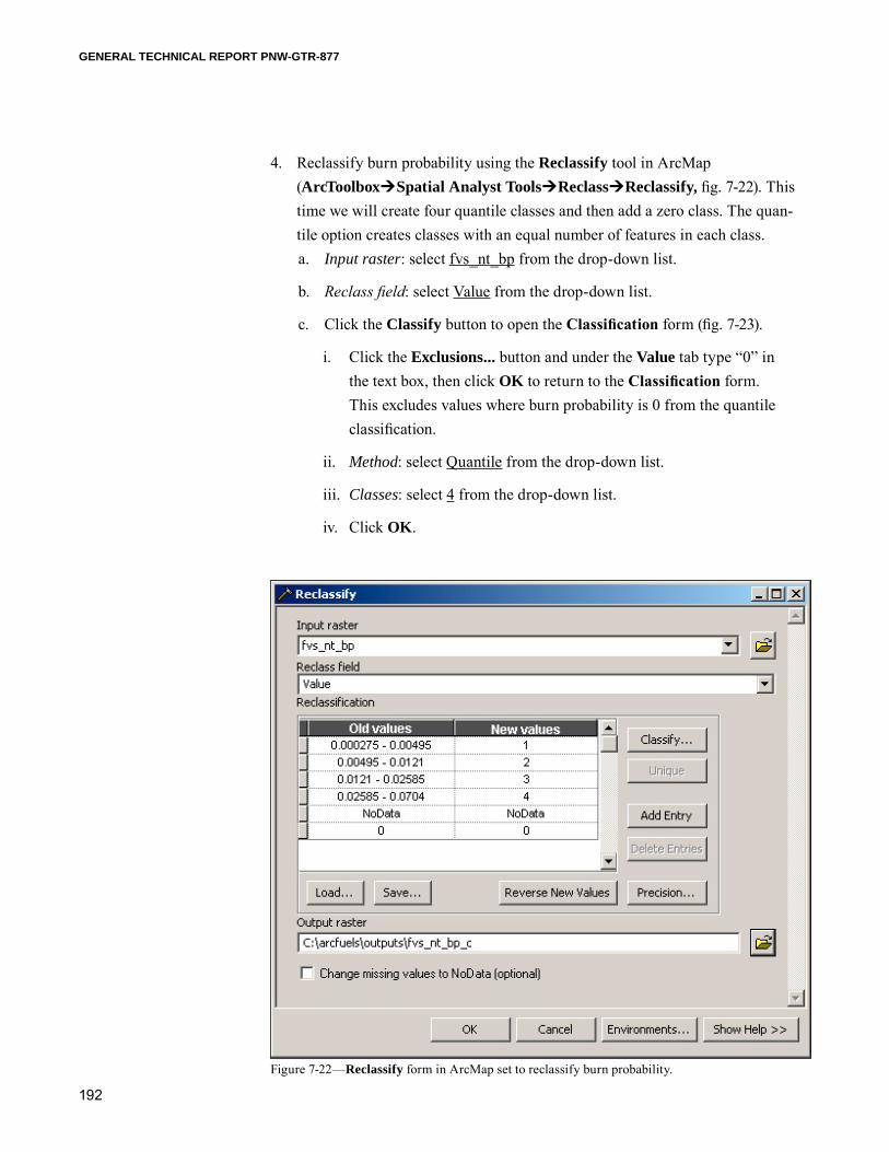
192


4. Reclassify burn probability using the Reclassify tool in ArcMap (ArcToolboxSpatial Analyst ToolsReclassReclassify, fig. 7-22). This time we will create four quantile classes and then add a zero class. The quan-tile option creates classes with an equal number of features in each class. a. Input raster: select fvs_nt_bp from the drop-down list.



i. Click the Exclusions... button and under the Value tab type “0” in the text box, then click OK to return to the Classification form. This excludes values where burn probability is 0 from the quantile classification.

ii. Method: select Quantile from the drop-down list.

iii. Classes: select 4 from the drop-down list.

iv. Click OK.

Figure 7-22—Reclassify form in ArcMap set to reclassify burn probability.

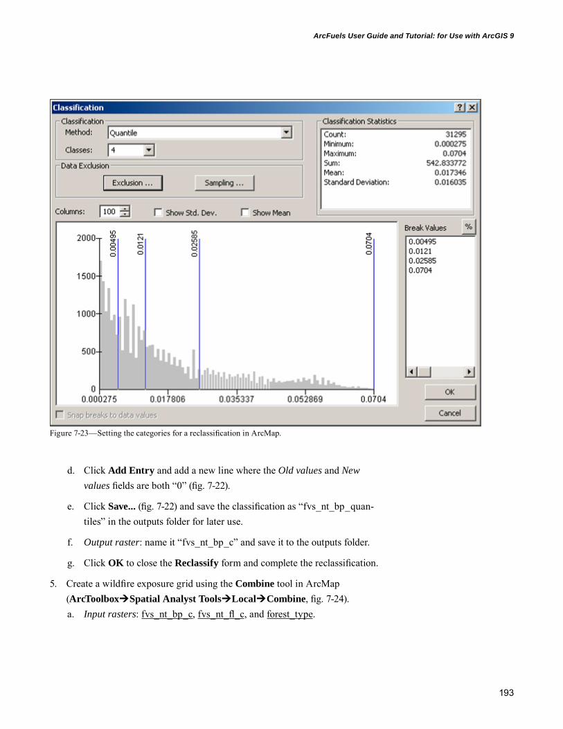
193


d. Click Add Entry and add a new line where the Old values and New values fields are both “0” (fig. 7-22).

e. Click Save... (fig. 7-22) and save the classification as “fvs_nt_bp_quan-tiles” in the outputs folder for later use.

f. Output raster: name it “fvs_nt_bp_c” and save it to the outputs folder.

g. Click OK to close the Reclassify form and complete the reclassification.

5. Create a wildfire exposure grid using the Combine tool in ArcMap (ArcToolboxSpatial Analyst ToolsLocalCombine, fig. 7-24).a. Input rasters: fvs_nt_bp_c, fvs_nt_fl_c, and forest_type.

Figure 7-23—Setting the categories for a reclassification in ArcMap.

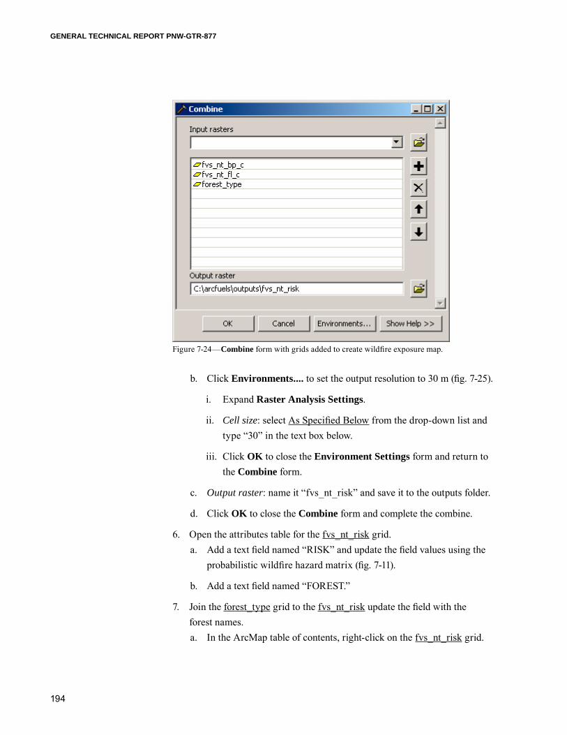
194


b. Click Environments.... to set the output resolution to 30 m (fig. 7-25).

i. Expand Raster Analysis Settings.

ii. Cell size: select As Specified Below from the drop-down list and type “30” in the text box below.

iii. Click OK to close the Environment Settings form and return to the Combine form.

c. Output raster: name it “fvs_nt_risk” and save it to the outputs folder.

d. Click OK to close the Combine form and complete the combine.

6. Open the attributes table for the fvs_nt_risk grid. a. Add a text field named “RISK” and update the field values using the

probabilistic wildfire hazard matrix (fig. 7-11).

b. Add a text field named “FOREST.”

7. Join the forest_type grid to the fvs_nt_risk update the field with the forest names. a. In the ArcMap table of contents, right-click on the fvs_nt_risk grid.

Figure 7-24—Combine form with grids added to create wildfire exposure map.

195


b. Select Joins and RelatesJoin to open the Join Data form (fig. 7-26).

i. What do you want to join to this layer: select Join attributes from a table from the drop-down list.

ii. 1. Choose the field in this layer that the join will be based on: select FOREST_TYPE from the drop-down list.

iii. 2. Choose the table to join to this layer, or load the table from disk: select forest_type from the drop-down list.

iv. 3. Choose the field in the bale to base the join on: select VALUE from the drop-down list.

v. Join Options: select the radio button to the left of Keep all records.

vi. Click OK to complete the join.

Figure 7-25—Environment Settings form specifying the output grid resolution.

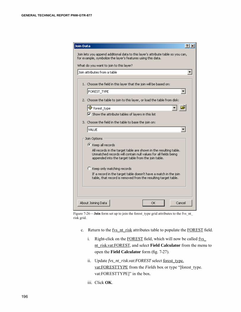
196


c. Return to the fvs_nt_risk attributes table to populate the FOREST field.

i. Right-click on the FOREST field, which will now be called fvs_nt_risk.vat:FOREST, and select Field Calculator from the menu to open the Field Calculator form (fig. 7-27).

ii. Update fvs_nt_risk.vat:FOREST select forest_type.vat:FORESTTYPE from the Fields box or type “[forest_type.vat:FORESTTYPE]” in the box.

iii. Click OK.

Figure 7-26—Join form set up to join the forest_type grid attributes to the fvs_nt_risk grid.

197


8. Remove the join (right-click on fvs_nt_expos and select Joins and RelatesRemove Join(s)Remove All Joins).

9. In ArcMap, change the display of lf_nt_expos to show the EXPOSURE field (fig. 7-28). a. Right-click on the grid name in the table of contents, select Properties

from the list, and select the Symbology tab.

b. Show: select Unique Values from the options in the box.

c. Value field: select EXPOSURE from the drop-down list.

d. Set NONE to be black, LOW to be green, MODERATE to be yellow, HIGH to be orange, and EXTREME to be red to match that of the risk matrix (fig. 7-11).

e. Click OK to close the form.

Figure 7-27—Field Calculator form updating the forest type name field.

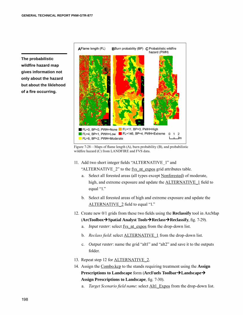
198


11. Add two short integer fields “ALTERNATIVE_1” and “ALTERNATIVE_2” to the fvs_nt_expos grid attributes table. a. Select all forested areas (all types except Nonforested) of moderate,

high, and extreme exposure and update the ALTERNATIVE_1 field to equal “1.”

b. Select all forested areas of high and extreme exposure and update the ALTERNATIVE_2 field to equal “1.”

12. Create new 0/1 grids from these two fields using the Reclassify tool in ArcMap (ArcToolboxSpatial Analyst ToolsReclassReclassify, fig. 7-29). a. Input raster: select fvs_nt_expos from the drop-down list.

b. Reclass field: select ALTERNATIVE_1 from the drop-down list.

c. Output raster: name the grid “alt1” and “alt2” and save it to the outputs folder.

13. Repeat step 12 for ALTERNATIVE_2.14. Assign the Combo.kcp to the stands requiring treatment using the Assign

Prescriptions to Landscape form (ArcFuels ToolbarLandscape Assign Prescriptions to Landscape, fig. 7-30). a. Target Scenario field name: select Alt1_Expos from the drop-down list.

Figure 7-28—Maps of flame length (A), burn probability (B), and probabilistic wildfire hazard (C) from LANDFIRE and FVS data.

The probabilistic wildfire hazard map gives information not only about the hazard but about the liklehood of a fire occurring.

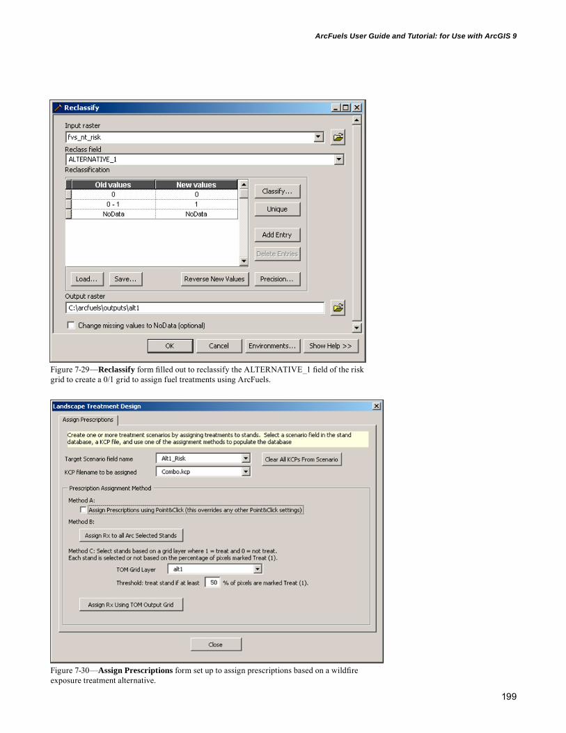
199


Figure 7-29—Reclassify form filled out to reclassify the ALTERNATIVE_1 field of the risk grid to create a 0/1 grid to assign fuel treatments using ArcFuels.

Figure 7-30—Assign Prescriptions form set up to assign prescriptions based on a wildfire exposure treatment alternative.

200


b. Click Clear All KCPs From Scenario.

c. KCP filename to be assigned: select Combo.kcp from the drop-down list.

d. TOM Grid Layer: select alt1 from the drop-down list.

e. Threshold: treat stand if at least.... percent of pixels are marked treat: type “50” in the text box.

f. Click Assign Rx Using TOM Output Grid.

15. Repeat step 14 with the Alt2_Risk field and the alt2 grid.16. Run FVS for the stands with treatments using the treatment field for both

alternatives using the Run FVS form in ArcFuels (ArcFuels Toolbar LandscapeSimulate Landscape TreatmentsRun FVS, fig. 7-31). a. Input Database: the default database Mt_Emily_Database.mdb.

b. Stand Table: keep the default, stands.

c. Stand ID: keep the default, Stand_ID.

d. Output Database: use the navigation button to create a new output database named”Alt1_Risk.”

e. Scenario name: type “risk1” in the text box to the right.


g. Prescription Source: click on the Add/Change Fields button and select the Alt1_Risk field using the Select KCP Fields form that opens.

h. Cycles: type”10” in the text box.

i. Years per cycle: type “1” into the text box.

j. Fuel model set: select 53 from the drop-down list.

k. Check Execute, Overwrite DB, and make sure the rest are unchecked.

l. Scenario Index: type “1” into the text box.

m. Click the Run FVS button to start the FVS simulation. Depending on your computer, this should take about 15 minutes.

17. Repeat step 16 for Alt2_Risk.18. Create grids for both treatment alternatives Using FVS Database

form in ArcFuels (ArcFuels ToolbarLandscapeBuild FlamMap LandscapeUsing FVS Database, fig. 7-32).

201







Figure 7-31—FVS run window set to run only stands with prescriptions for the Alt1_Risk alternative.

202











Figure 7-32—Creating treated grids from two FVS databases for the Alt1_Risk alternative.

203




q. Apply Treatments: check the box to the left.

r. Treated Stands Database: navigate to and select the Alt1_Risk.mdb in the outputs folder.

s. Click Create Arc Grids.

i. Use “alt1_xxx” where xxx is cc, ch, cbh, cbd, or fm to name the new grids.

19. Repeat step 18 for Alt2_Risk.20. Create an LCP with LANDFIRE and FVS treated data for the risk treatment

alternative with the Using Multiple Sources form in ArcFuels (ArcFuels Toolbar LandscapeBuild FlamMap LandscapeUsing Multiple Sources, fig. 7-33).

Figure 7-33—Building a landscape file from FVS and LANDFIRE data.

204


a. Slope: using the navigation button, select slope in degrees.

b. Aspect: using the navigation button, select aspect in azimuth degrees.

c. Fuel Model: using the navigation button, select alt1_fm then lf_fbfm40.

d. Canopy cover: using the navigation button, select alt1_cc in percent then lf_cc in percent.

e. Canopy Height: using the navigation button, select alt1_ch in feet then lf_ch in meters*10.

f. Canopy Base Height: using the navigation button, select alt1_cbh in feet then lf_cbh in meters*10.

g. Canopy Bulk Density: using the navigation button, select alt1_cbd in kg/m^3 then lf_cbd in kg/m^3*100.

h. Latitude: type “45” in the text box.

i. The output boundaries are based on: select the radio button to the left of Grid Layer, then select elevation from the drop-down list.

j. LCP Output File: using the navigation button name the file “Alt1_Risk.lcp.”

k. Click the Build LCP button.

21. Repeat step 20 for Alt2_Risk

Step 4: Run FlamMap3 fire behavior runs for the treatment alternatives—Run FlamMap3 using the same settings as Step 2 with the Alt1_Expos.lcp and Alt2_Risk.lcp LCPs built in Step 3.

Step 5: Assess the effectiveness of the fuel treatment alternatives—To assess the effectiveness of the fuel treatment alternatives, run FlamMap3, create exposure maps and summarize the data (fig. 7-34 and 7-35; table 7-3). For an example of how to create a wildfire exposure map, see Step 3. For an example of how to summarize by wildfire exposure category, refer to the Evaluating Wildfire Hazard section. For an example of how to create a scatter plot, refer to the Wildfire Risk Assessment: Creating a Wildfire Exposure Scatter Plot section.

Were the fuel treatment alternatives effective? Are there other areas that might benefit from treatment? Or perhaps using different fuel treatment prescrip-tions for different forest types (see the nonforested point in the scatter) would be more effective?

Remember that the fuel treatment alternatives were based on risk and forest type only. If your objective was to protect lynx habitat or WUI, are the treatment alternatives still effective?

205


Figure 7-34—Wildfire probabilistic wildfire hazard (PWH) maps for the three fuel treatment alternatives.

Figure 7-35—Scatter plots by forest type for the three fuel treatment alternatives.

Table 7-3—Wildfire exposure comparison for the existing conditions, alternative 1 and alternative 2 for the entire landscape

Exposure No treatment Alternative 1 Alternative 2

Acres Percent Acres Percent Acres PercentNone 0 0 0 0 0 0Low 18,967 47 26,634 66 25,424 63Mod 7,264 18 3,228 8 5,650 14High 4,843 12 3,228 8 3,228 8Ext 8,878 22 6,860 17 6,053 15

Grand f ir Nonforested Douglas-f irPonderosa pine Western larch Subalpine f irLodgepole pine Engelmann spruce

a) No treatment b) Alternative 1 c) Alternative 2

0

5

10

15

20

25

0.000 0.010 0.020

Flam

e le

ngth

(ft)

Burn probability

0

5

10

15

20

25

0.000 0.010 0.020

Flam

e le

ngth

(ft)

Burn probability

0

5

10

15

20

25

0.000 0.010 0.020

Flam

e le

ngth

(ft)

Burn probability

Engelmann spruce-subalpine fir

Once maps are created they can be further analyzed in ArcMap. One useful step might be differencing the maps to see where the exposure increased or decreased as a result of treatment.

206


Designing Landscape Level Fuel Treatment Alternatives By Using TOM With Grid and FVS Data As mentioned, the TOM in FlamMap3 locates treatments to block the fastest routes of travel and maximize the reduction in spread rate across a landscape per area treated. Because TOM uses an ideal landscape to define where treatments are allowed to occur, the output treatment grid can be used without having to further limit treatment area. However, there are a couple of limitations that should be shared: (1) the TOM treatment grid does often have single pixel (grid cell) treat-ment units that would not be practical to implement in the real world and should be scrutinized, and (2) the TOM treatment grid is designed for a single potential problem fire under specific fire weather conditions. Given the known limitations, TOM is a great tool to use as starting point for fuel treatment planning. However, without further editing, the TOM treatment grid might not be realistic. That said, the following scenario will be using the TOM treatment grid to locate stands need-ing treatment, then FVS to develop treatment adjustment factors.


2. Run the Treatment Optimization Model in FlamMap3.

3. Use the treatment grid and FVS/FFE-FVS to develop fuel treatment alternatives in ArcFuels.

4. Run FlamMap3 fire behavior runs for the treatment alternatives.

5. Assess the effectiveness of the treatment alternatives.

The following scenario will complete the above steps using LANDFIRE grids to create the no-treatment alternative and ideal landscape LCP files for TOM modeling in FlamMap3. Tree list data will be run through FVS to determine treat-ment adjustment factors to be applied based on forest types. Landscape files will be built for two fuel treatment alternatives and a risk assessment will be completed to compare the no-treatment alternative to the two TOM treatment alternatives.

Step 1: Acquire existing condition data and update if necessary—The data supplied by LANDFIRE are assumed to be accurate and not in need of updating. The supplied FVS data is also assumed to be accurate.

NOTE: The values in table 7-3 and scatter plots in figure 7-35 will be slightly different for each run because no burn probability runs are exactly the same.

When limited FVS data are available, they can be used to create treatment adjustment factors to update grid data. More often than not, FVS data will not be available for every stand in your landscape.

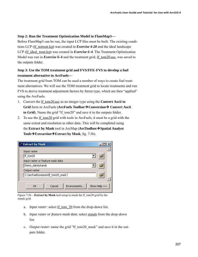
207


Step 2: Run the Treatment Optimization Model in FlamMap3—Before FlamMap3 can be run, the input LCP files must be built. The existing condi-tions LCP (lf_notreat.lcp) was created in Exercise 4-20 and the ideal landscape LCP (lf_ideal_treat.lcp) was created in Exercise 6-4. The Treatment Optimization Model was run in Exercise 6-4 and the treatment grid, lf_tom20.asc, was saved to the outputs folder.

Step 3: Use the TOM treatment grid and FVS/FFE-FVS to develop a fuel treatment alternative in ArcFuels—The treatment grid from TOM can be used a number of ways to create fuel treat-ment alternatives. We will use the TOM treatment grid to locate treatments and run FVS to derive treatment adjustment factors by forest type, which are then “applied” using the ArcFuels.1. Convert the lf_tom20.asc as an integer type using the Convert Ascii to

Grid form in ArcFuels (ArcFuels ToolbarConversion Convert Ascii to Grid). Name the grid “lf_tom20” and save it in the outputs folder.

2. To use the lf_tom20 grid with tools in ArcFuels, it must be a grid with the same extent and resolution as other data. This will be completed using the Extract by Mask tool in ArcMap (ArcToolboxSpatial Analyst ToolsExtractionExtract by Mask, fig. 7-36).

Figure 7-36—Extract by Mask tool setup to mask the lf_tom20 grid by the stands grid.

a. Input raster: select lf_tom_20 from the drop-down list.

b. Input raster or feature mask data: select stands from the drop-down list.

c. Output raster: name the grid “lf_tom20_mask” and save it in the out-puts folder.

208


d. Set the output resolution to 30 m (Environments...Raster Analysis Settings, fig. 7-25).

i. Cell size: select As Specified Below from the drop-down list and type “30” in the text box below.

ii. Click OK to save and apply the changes.

e. Click OK to create the new grid.

3. Assign prescriptions to stands where at least 33 percent of a stand is marked as “treated” by TOM (ArcFuels ToolbarLandscapeAssign Prescriptions to Landscape, fig. 7-37).a. Target Scenario field name: select Alt1_TOM from the drop-down list.

b. Click Clear All KCPs From Scenario.

c. KCP filename to be assigned: select Combo.kcp from the drop-down list.

d. TOM Grid Layer: select lf_tom20_mask from the drop-down list.

Figure 7-37—Assign Prescriptions form setup to assign the Combo.kcp to stands where at least 33 percent was chosen as needing treatment in TOM.

209


e. Threshold: treat stand if at least.... percent of pixels are marked treat: type “33” in the text box.

f. Click Assign Rx Using TOM Output Grid.

4. Run FVS for the stands with treatments using the treatment field using the Run FVS form in ArcFuels (ArcFuels ToolbarLandscape Simulate Landscape TreatmentsRun FVS, fig. 7-38).

Figure 7-38—FVS run tab set to run only stands with prescriptions for the Alt1_TOM alternative.

210


a. Input Database: the default database Mt_Emily_Database.mdb.

b. Stand Table: keep the default, stands.

c. Stand ID: keep the default, Stand_ID.

d. Output Database: use the navigation button to create a new output database named”Alt1_TOM.”

e. Scenario name: type “tom1” in the text box to the right.


g. Prescription Source: click on the Add/Change Fields button and select the Alt1_TOM field using the Select KCP Fields form that opens.

h. Cycles: type”10” in the text box.

i. Years per cycle: type “1” into the text box.

j. Fuel model set: select 53 from the drop-down list.

k. Check Execute, Overwrite DB, and make sure the rest are unchecked.

l. Scenario Index: type “1” into the text box.

m. Click the Run FVS button to start the FVS simulation. Depending on your computer, this should take about 15 minutes.

5. Join the FVS_Compute table from the Alt1_TOM.mdb to the mt_emily_stands shapefile for 2005 using the Join FVS Outputs to Polygons form in ArcFuels (ArcFuels ToolbarLandscapeSimulate Landscape TreatmentsJoin FVS Outputs to Polygons, fig. 7-39).

6. Open the mt_emily_stands attribute table and select all stands where joined data is not <Null> (ArcMapSelectionSelect By Attributes). These are the stands that received treatment. There should be 241 stands selected (fig. 7-40).

7. Run summary statistics on the treated stands to find the pretreatment average values for canopy cover, canopy height, canopy base height, and canopy bulk density by forest type using the Summary Statistics tool in ArcMap (ArcToolboxAnalysis ToolsStatisticsSummary Statistics, fig. 7-41).a. Input Table: select mt_emily_stands from the drop-down list.

b. Output Table: name the table “mt_emily_stands_notreat_stats.dbf” and save it in the outputs folder.

211


Figure 7-39—Joining FVS outputs to the Mt. Emily stands polygon.

Figure 7-40—ArcSelected stands that had at least 33 percent of their area needing treatment according to TOM.

212


c. Statistics Field(s): select FVS_Compute2005.CANOPY, FVS_Compute2005.HTT, FVS_Compute2005.HTLIVE, and FVS_Compute2005.CBD from the drop-down list.

d. Statistic Type: select MEAN from the drop-down list for each Field. Click in the box to get the drop-down list to show.

e. Case field (optional): select mt_emily_stands.ForestType from the drop-down list.

f. Click OK to complete the summary statistics.

8. Remove the join using the Join FVS Outputs to Polygons form in ArcFuels (ArcFuels ToolbarLandscapeSimulate Landscape TreatmentsJoin FVS Outputs to Polygons, fig. 7-39).

9. Join the FVS_Compute table from the notreat.mdb to the mt_emily_stands shapefile for 2005 using the Join FVS Outputs to Polygons form in ArcFuels (ArcFuels ToolbarLandscapeSimulate Landscape TreatmentsJoin FVS Outputs to Polygons).

Figure 7-41—Summary Statistics form to calculate the mean canopy characteristics by forest type.

213


10. Repeat step 7 for the notreat.mdb, naming the output “mt_emily_stands_untreated_statistics.dbf” and saving it to the outputs folder.

11. Using the File Explorer in ArcFuels (ArcFuels ToolbarProjects and FilesFile Explorer) open the outputs folder.

12. Open the mt_emily_stands_notreat_statistics.dbf and mt_emily_stands_treat_statistics.dbf files with Excel. Note that the headers were truncated (fig. 7-42). They are in the order selected in the Summary Statistics form: MEAN_FVS_C is canopy cover (CANOPY), MEAN_FVS_1 is canopy height (HTT), MEAN_FVS_2 is canopy base height (HTLIVE), and MEAN_FVS_3 is canopy bulk density (CBD).

13. Create a new Excel workbook named “ForestTypeTreatmentAdjustments” in the outputs folder.a. Copy and paste the untreated and treated tables into the new work-

book and relabel the columns (see step 12). Label each table so that you know which is which.

14. Within the Excel workbook, calculate the forest specific treatment adjust-ment factors. a. Adjustment factors can be replacements or multiplication factors. In

this example, multiplication factors will be calculated. The formula for calculating the adjustment factors is: 1-((no-treatment – treated) / no treatment).

b. For an example of how to do this, see Exercise 4-4.

15. Open the Treatment_adjustments.mdb in the data folder, copy and paste the example_treatment_adjustment table into the same Access database, and rename the table “forest_type.”

Figure 7-42—Untreated summary statistics table opened in Excel.

214


a. Right-click on the table name and select Copy from the menu.

b. Right-click below the table name and select Paste from the menu. Rename it when the Paste Table As window opens.

16. Open the new forest_type table. a. Delete the old data by highlighting all the data lines and pressing

Delete on your keyboard.

b. Add a new text field named “forest_type_name.”

i. With the table open, switch to Design View (Access Ribbon ViewsDesign View).

ii. Under Field Name add a new line called “forest_type_name” (fig. 7-43).

Figure 7-43—Adding a text field to the Access data table.

c. Switch back to the Datasheet View (Access RibbonViews Datasheet View). When prompted to save the changes, click Yes.

d. Type the adjustment values into the table. Update the fm_adj to “181” for all forest types. Because the forest_type grid has a 0 value for the grand fir forest type we need to assign new values to the forest types to be able to use ArcFuels tools. Renumber treat_type based on number-ing forest types alphabetically (i.e., Douglas-fir = 1, Englemann spruce = 2, etc., fig. 7-44).

17. Close the Treatment_adjustments.mdb database.

NOTE: The same process can be run when limited stand data is available. It is not necessary to have tree list data for every stand in the landscape to derive treatment adjustment factors. However, a sufficient sample should be available to represent the variance within a given landscape, forest type, etc.

215


18. Combine the lf_tom20_mask and forest_type grids using the Combine tool (ArcToolboxSpatial Analyst ToolsLocalCombine, fig. 7-45).a. Input rasters: lf_tom20_mask and forest_type.

b. Set the output resolution to 30 m (Environments...Raster Analysis Settings, fig. 7-25).

i. Cell size: select As Specified Below from the drop-down list and type “30” in the text box below.

c. Name the Output raster “tom_forest” and save it to the outputs folder

Figure 7-44—Forest specific treatment adjustment factors.

Figure 7-45—Combine from set to for combining the forest type and TOM grids.

After treatment adjustment factors are calculated, verify that the values are realistic. Is an 808 percent increase in canopy base height accurate for posttreatment in Engelmann spruce?

216


19. Open the attributes table for tom_forest and add a text field named “FOREST.”

20. Join the forest_type grid to the tom_forest grid to update the FOREST_NAME field with the forest names. In the ArcMap table of contents, right-click on the tom_forest grid.a. Select Joins and Relates from the menu.

b. Select Join and fill out as shown in figure 7-26.

c. Click OK.

21. Return to the tom_forest attributes table to populate the FOREST field. a. Right-click on the FOREST field, which will now be called tom_forest.

vat:FOREST, and select Field Calculator from the menu to open the Field Calculator form (fig. 7-27)

i. Update tom_ forest.vat:FOREST select forest_type.vat:FORESTTYPE from the Fields box or type “[forest_type.vat:FORESTTYPE]” in the box.

ii. Click OK.

b. Add a short integer field named “TREAT_TYPE.”

i. If LF_TOM20 has a value of 1 then update the TREAT_TYPE field with the new forest appropriate treat_type values from forest_type stand table of the Treatment_adjustments.mdb database (fig. 7-44).

ii. If LF_TOM20 has a value of 0 then update the TREAT_TYPE field with a 0.

22. Remove the join (right-click on tom_forestJoins and RelatesRemove Join(s)Remove All Joins).

23. Create a new treatment type grid from the tom_forest grid using the Reclassify tool (ArcToolboxSpatial Analyst Tools ReclassReclassify, fig. 7-46). a. Input raster: select tom_forest from the drop-down list.

b. Reclass field: select TREAT_TYPE from the drop-down list.

c. Reclassification: have the new classes match the old classes.

d. Output raster: name the new grid “tom_trt_type” and save it to the outputs folder.

Look at the new treatment grid in ArcMap (fig. 7-47).

217


Figure 7-46—Reclassify form to create the treatment type grid for use with ArcFuels.

Figure 7-47—Forest specific treatment plan based on TOM run completed in FlamMap3.

0 52.5mi ¸

0 - No treatment1 - Douglas-fir2 - Engelmann spruce3 - Englemann spruce-subalpine fir4 - Grand fir5 - Lodgepole pine6 - Nonforested7 - Ponderosa pine8 - Subalpine fir9 - Western larch

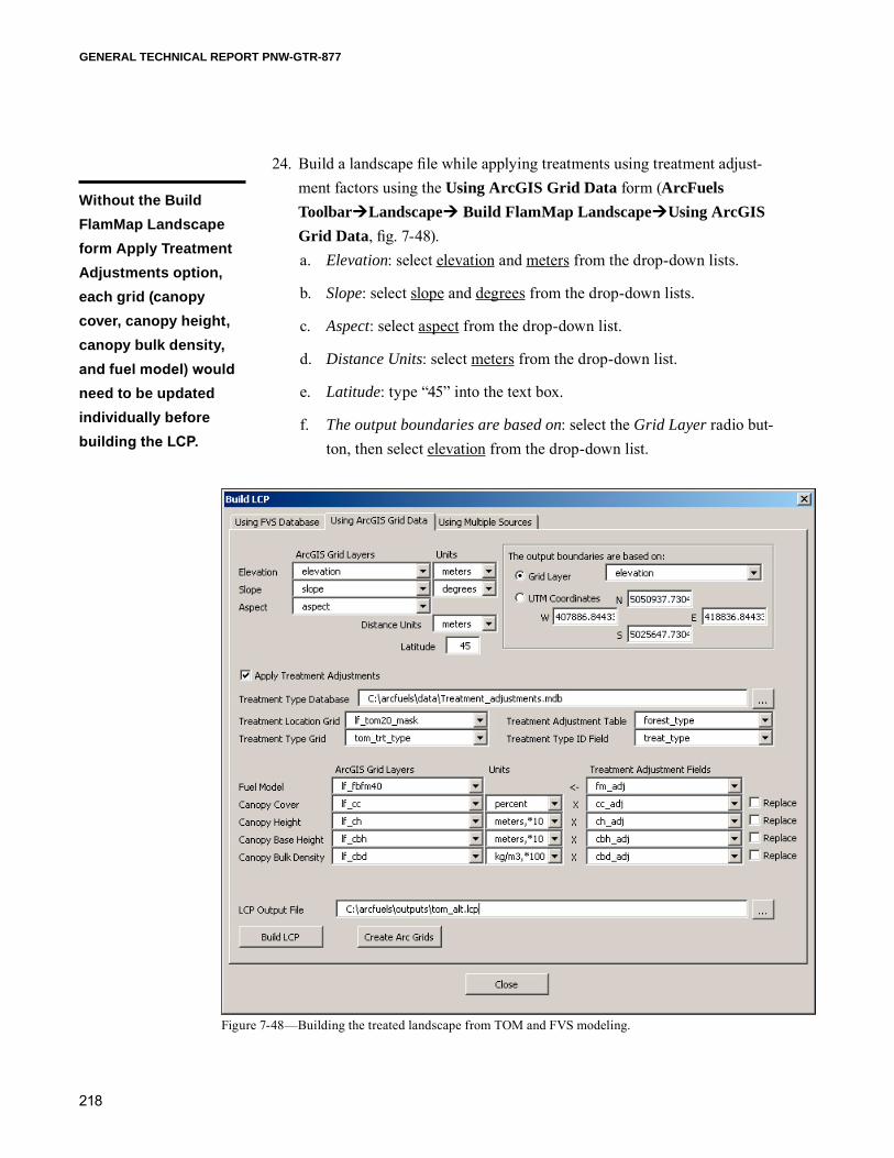
218


24. Build a landscape file while applying treatments using treatment adjust-ment factors using the Using ArcGIS Grid Data form (ArcFuels ToolbarLandscape Build FlamMap LandscapeUsing ArcGIS Grid Data, fig. 7-48).a. Elevation: select elevation and meters from the drop-down lists.






Figure 7-48—Building the treated landscape from TOM and FVS modeling.

Without the Build FlamMap Landscape form Apply Treatment Adjustments option, each grid (canopy cover, canopy height, canopy bulk density, and fuel model) would need to be updated individually before building the LCP.

219




ii. Treatment Location Grid: select lf_tom20_mask from the drop-down list.

iii. Treatment Type Grid: select tom_trt_type from the drop-down list.

iv. Treatment Adjustment Table: select forest_type from the drop-down list.







m. LCP Output File: using the navigation button name the LCP “tom_alt.”

n. Click Build LCP.

TROUBLESHOOTING: If you get an error message stating that the cell sizes do not match (fig. 7-49), check the properties of the Treatment Location and Treatment Type Grids. Chances are that one is 90 m and needs to be 30 m; both must be 30 m.

Figure 7-49—LCP building error window.

Step 4: Run FlamMap3 fire behavior runs for the treatment alternatives—In this step, FlamMap3 will be run for both the no-treatment and the TOM-derived alternatives. The same line ignition from the TOM run (Exercise 6-4) in Flam-Map3 will be used to run MTT. In addition the no-treatment alternative LCP (lf_notreat.lcp) will be used (created in Exercise 4-20).

220


1. Open FlamMap3 and load the lf_notreat.lcp. Create a new run, and select the Inputs tab (fig. 7-50). a. Run name: type “No treat MTT” in the text box.





Figure 7-50—FlamMap3 Inputs tab for the no-treatment alternative.

221







f. Click Apply.


place.


c. Click Apply.

3. Select the Minimum Travel Time tab (fig. 7-51).a. Ignitions: load the ignition.shp file from the outputs folder.

b. Resolution of calculations: type “90” in the text box.


d. Interval for Minimum Travel Paths: type “500” in the text box.

e. Outputs: select Rate of Spread Grid, Arrival Time Grid, Fire Intensity Map, and Major Paths.

f. Click Apply, then Launch.

4. Save the outputs.a. Save the MTT Major Paths as “tom_nt_mtt_paths.shp” in the outputs

folder.

b. Change the units for the MTT FLI Map to BTU/ft/sec and save it as “tom_nt_fli.asc” in the outputs folder.

c. Contour the MTT Arrival Time to create a progression map.

i. To contour, right-click on the theme in the pane and select Contour from the menu.

222


ii. Contour interval: set the interval to 480. This is 8 hr or 1 day.

iii. Minimum Distance between points on a contour line: set the dis-tance to 90. This is the default and is equal to the resolution used in the FlamMap3 run.

iv. Click OK.

v. Expand Auxiliary Themes, then expand Contours. The created con-tour will be there. Save the contour file as “tom_nt_contour480.shp.”

5. Repeat steps 1 through 4 with the tom_alt.lcp saving the outputs as “tom_alt_.....”

Figure 7-51—FlamMap3 Minimum Travel Time tab for the no-treatment alternative.

223


Step 5: Assess the effectiveness of the treatment alternatives—To assess the effectiveness of the TOM treatment alternative, we will create two maps, one with the MTT travel paths and the treatment units, and another with the fire progression (contours) and treatment units. Next we will summarize fire sever-ity using fireline intensity inside and outside of treatment units based on hauling chart (table 7-1) categories.1. Add the tom_nt_mtt_paths.shp, tom_alt_mtt_paths.shp, tom_nt_con-

tour480.shp, and tom_alt_contour480.shp layers from FlamMap3 to ArcMap from the outputs folder.a. The outputs saved from FlamMap3 do not contain projection informa-

tion; a warning window will open (fig. 7-52). Click OK.

Figure 7-52—Unknown Spatial Reference window from ArcMap.

2. Define the projection (NAD_1983_UTM_Zone_11N) of all four newly added FlamMap3 layers in ArcMap (ArcToolboxData Management ToolsProjections and TransformationsDefine Projection).

3. Display the MTT treatment paths over the tom_trt_type grid (fig. 7-53). Zoom into and out of different areas. Did the treatments affect fire spread?

4. Display the fire progression contours over the tom_trt_type grid (fig. 7-54). Did the treatments slow the daily fire spread?

5. Batch convert the tom_nt_fli.asc and tom_alt_fli.asc as integer types while defining the projection using the Batch Convert Ascii to Grid form (ArcFuels ToolbarConversion Batch Convert Ascii to Grid).

224


6. Reclassify tom_nt_fli according to the hauling chart (ArcFuels Toolbar Spatial Analyst ToolsReclassReclassify, table 7-1; fig. 7-55).a. Input raster: select tom_nt_fli from the drop-down list.

b. Reclass field: select VALUE from the drop-down list.

c. Reclassification: click Classify... to open the Classification form (fig. 7-56).

i. Method: select Equal Interval from the drop-down list.

Figure 7-53—Minimum Travel Time paths for the no-treatment and TOM treatment alternatives over the treatment units for the whole landscape (A), and then zoomed in to show the differences between the no-treatment (B) and TOM alternative (C) for the same area.FlamMap MTT travel

paths show how the fire moves across the landscape. When they are overlayed on treatment units, you can see the effect of the planned treatment alternatives on fire spread.

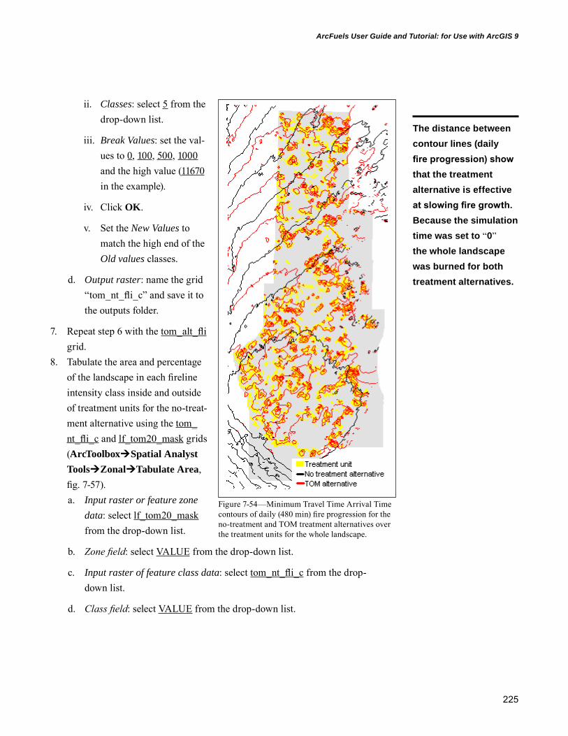
225



iii. Break Values: set the val-ues to 0, 100, 500, 1000 and the high value (11670 in the example).

iv. Click OK.

v. Set the New Values to match the high end of the Old values classes.

d. Output raster: name the grid “tom_nt_fli_c” and save it to the outputs folder.

7. Repeat step 6 with the tom_alt_fli grid.

8. Tabulate the area and percentage of the landscape in each fireline intensity class inside and outside of treatment units for the no-treat-ment alternative using the tom_nt_fli_c and lf_tom20_mask grids (ArcToolboxSpatial Analyst ToolsZonalTabulate Area, fig. 7-57).a. Input raster or feature zone

data: select lf_tom20_mask from the drop-down list.

b. Zone field: select VALUE from the drop-down list.

c. Input raster of feature class data: select tom_nt_fli_c from the drop-down list.

d. Class field: select VALUE from the drop-down list.

Figure 7-54—Minimum Travel Time Arrival Time contours of daily (480 min) fire progression for the no-treatment and TOM treatment alternatives over the treatment units for the whole landscape.

The distance between contour lines (daily fire progression) show that the treatment alternative is effective at slowing fire growth. Because the simulation time was set to “0” the whole landscape was burned for both treatment alternatives.

226


Figure 7-55—Reclassify form filled out to reclassify fireline intensity based on hauling chart values.

Figure 7-56—Reclassify form used to set the number of classes and associated values.

227


e. Output table: name the output “tom_nt_fli_area” and save it to the out-puts folder.

f. Processing cell size (optional): leave the default “90,” which is the same resolution as the fireline intensity grid.

9. Repeat step 8 with tom_alt_fli_c and lf_tom20_mask grids.10. Open the tom_nt_fli_area and tom_alt_fli_area tables (fig. 7-58). You will

need to go to the Source tab in the ArcMap table of contents to see the new tables. The area units are m2 and the row with VALUE equal to 0 are out-side of treatment units and VALUE equal to 1 are inside. The VALUE_xx columns are the fireline intensity categories where _xx is 0, 100, etc. relat-ing to the reclassification classes.

Figure 7-57—Tabulate area tool from ArcMap setup to calculate the area inside and outside of treatment units for each fireline intensity category.

Figure 7-58—Tabulate area table with the area (m2) inside (1) and outside (0) treatment units for fireline intensity classes based on the hauling chart (VALUE_X).

228


11. Fill out table 7-4 with the values from tom_nt_fli_area and tom_alt_fli_area and calculate percentages.Because we used the MTT fireline intensity rather than the basic fire behavior

fireline intensity, fire was modeled across the landscape from the ignition line. Modeling fire spread allows us to see how the fuel treatments affected fire behavior inside and outside of treatments.

Designing Landscape Level Fuel Treatment Alternatives By Using a Pre-existing Plan With Grid DataFuel treatment alternatives are often designed by planning teams. The treatment locations and changes are known and it is up to the fuels specialist to use this data to complete fire behavior modeling to compare the treatment alternatives for specialist reports, NEPA and EA documents, etc.


2. “Implement” the preexisting fuel treat alternative.

3. Run FlamMap3 for fire behavior.

4. Assess the effectiveness of the treatment alternatives.

The following scenario will complete the above steps using LANDFIRE grids to create the no-treatment and treated alternatives for fire behavior modeling in FlamMap3.

Table 7-4—Area (m2) and total landscape percentage by fireline intensity class inside and outside of treatment units as well as for the landscape as a whole for the no-treatment and TOM alternatives

Fireline intensity class

Alternative Location 0 >0–100 100–500 500–1,000 >1,000

Square Percent Square Percent Square Percent Square Percent Square Percent meters meters meters meters metersNo-treatment Inside 900 0 738,900 5 985,500 6 56880 3 2,092,500 13 Outside 900 0 3,112,200 19 342,9900 21 1418400 9 4,005,900 24 Landscape 1,800 0 3,851,100 24 4415,400 27 198720 12 6,098,400 37

TOM alternative Inside 490,500 3 3,870,900 24 41,400 0 0 0 0 0 Outside 1,800 0 3,933,000 24 3,713,400 23 1,614,600 10 2,705,400 17 Landscape 492,300 3 7,803,900 48 3,754,800 23 1,614,600 10 2,705,400 17

NOTE: If you wanted to see the affect by treatment type, the Tabulate Area form could have been used with the tom_treat_type grid rather than the lf_tom20_mask grid.

By using MTT the effect of treatments on fire behavior outside of the treatment units can be analyzed; this is not true of the basic fire behavior outputs.

229


Step 1: Acquire existing condition data and update if necessary—The data supplied by LANDFIRE are assumed to be accurate and not in need of updating.

Step 2: “Implement” the preexisting fuel treat alternatives—The supplied treatment_units shapefile will be used in this exercise. It contains four fuel treatment alternatives: AltA_Low, AltB_Low, AltA_Mod, and AltB_Mod. The “Low” alternatives both treat about 20 percent of the landscape, and the “Mod” alternatives treat about 40 percent of the landscape. The primary goal of alternative A is to treat within the wildlands and alternative B is to protect the WUI. The treat-ment types within each alternative include hand thin and pile burn, mastication, prescribed fire, thin from below, thin from below and burn, and commercial thin (fig. 7-59).

Figure 7-59—Hypothetical fuel treatment alternatives for Mt. Emily.

Your silvicultualist ran FFE-FVS from some stand exams that were representa-tive of your project area and supplied you with information on how to alter the current conditions to represent posttreatment conditions (table 7-5).

You, the fuels specialist, then assigned fuel models that would represent post-treatment conditions (table 7-6). The first step in this process will be to create a treatment adjustments table. Once the table is created, treatment location and type grids will be built for each alternative. Then the treatment adjustments table and locations grids will be used to build landscape files for each alternative for use in FlamMap3.

Quite often the location and the type of treatment to be implemented is predetermined. ArcFuels can be used to “implement” preplanned treatment alternatives.

230


1. Export the treatment_units attributes to Excel using the Copy Attributes to Spreadsheet form in ArcFuels (ArcFuelsConversionCopy Attributes to Spreadsheet). a. Name the file “treatment_units.xls” and save it to the outputs folder.

b. If a warning window opens about the version of Excel, click Yes.

2. With treatment_units.xls open, add treatment adjustment fields for each alternative (fig. 7-60).a. The headers are Alow_xx, Blow_xx, Amod_xx, and Bmod_xx, where

xx is: cc, ch, cbh, cbd, and fm.

Table 7-5—Fuel treatment effects on canopy characteristics for various fuel treatment types

Canopy Canopy Treatment type Canopy cover Canopy height base height bulk density

Hand thin and Reduce 5% No change 6 ft No change pile burnPrescribed burn Reduce 10% No change 10 ft Reduce 10%Mastication Reduce 15% No change 10 ft Reduce 15%Thin from below Reduce 25% No change 15 ft Reduce 20%Thin from below Reduce 35% No change 20 ft Reduce 25% and burnCommercial thin Reduce 50% Reduce 20% 6 ft Reduce 60%

Table 7-6—Posttreatment fuel model assignments

Treatment type Fuel model

Hand thin and pile burn TL8 (188) – long-needle litterPrescribed burn TL1 (181) – low load compact conifer litterMastication SB1 (201) – low load activity fuelThin from below TU1 (161) – low load, dry climate timber-grass-shrubThin from below and burn TL1 (181) – low load compact conifer litterCommercial thin GS1 (121) – low load, dry climate grass-shrub

Figure 7-60—Excel worksheet with treatment adjustments for the four fuel treatment alternatives; only the AltA low treat-ment adjustments are shown in the figure.

231


b. Using tables 7-5 and 7-6, update the appropriate fields with the adjustments.

i. For canopy cover, canopy height, and canopy bulk density, the changes will be multiplication factors. So a reduction of 10 percent is a multiplication factor of 0.90.

ii. For canopy base height and fuel model, the changes are replace-ments. The LANDFIRE units for canopy base height are m*10; the replacement values need to be in the correct units. For example, hand thin and pile burn result in a canopy base height of 6 ft which is equivalent to 1.83 m, so the replacement value will be 18.

iii. Leave the fields blank that are not treated.

3. Open the Treatment_adjustments.mdb database in the data folder.a. Copy and paste the example_treatment adjustments data table and

rename it “AltA_Low.”

b. Copy and paste the corresponding columns from treatment_units.xls into the data table (fig. 7-61). Only copy the fields where adjustment factors were required. For this alternative that is 214 stands.

Figure 7-61—Treatment adjustments table for the AltA Low alternative.

i. The treat_type column in the Mt_Emily_Alts is the StandID field in treatment_units.xls.

ii. When the Access window opens asking if you are sure you want to paste the records, click Yes. As verification that you are pasting them all it should be 214 records.

c. Close the Access database.

4. Repeat step 3 for the remaining alternatives.

232


5. Select stands with treatments from the AltA_Low field in the treatment_units shapefile.

6. Create a treatment location and type grid from the selected stands using the Polygon to Raster tool in ArcMap (ArcToolboxConversion ToolsTo RasterPolygon to Raster, fig. 7-62).

Figure 7-62—Polygon to Raster form used to create the AltA Low treatment alternative.

a. Input Features: select treatment_units from the drop-down list.

b. Value field: select StandID from the drop-down list.

c. Output Raster Dataset: name the grid “alta_low” and save it to the out-puts folder.

d. Cell assignment type (optional): select CELL_CENTER from the drop-down list.

e. Priority field: select NONE from the drop-down list.

f. Cellsize: type “30” in the text box.

NOTE: The treatment adjustments data table can be created a number of ways. For example, the process can be done within Access using queries to update the treatment adjustments by treatment type for each alternative. Or the adjustments fields can be added to the attributes table in ArcMap and then exported as a *.dbf file opened in Excel and copied into Access.

233


g. Click on Environments....

i. Expand the General Settings option.

ii. Scroll down to Snap Raster and select stands from the drop-down list.

iii. Click OK to return to the Polygon to Raster form.

h. Click OK to create the grid.

7. Repeat steps 5 and 6 for the remaining alternatives.8. Build the LCP for the Alt A Low alternative using the treatment adjust-

ments database, the treatment type and location grid, and the existing conditions LANDFIRE data using the Using ArcGIS Grid Data form in ArcFuels (ArcFuelsLandscapeBuild FlamMap Landscape Using ArcGIS Grid Data, fig. 7-63).

Figure 7-63—Using ArcGIS Grid Data form from ArcFuels setup to build the AltA Low fuel treatment alternative LCP.

234










ii. Treatment Location Grid: select alta_low from the drop-down list.

iii. Treatment Type Grid: select alta_low from the drop-down list.

iv. Treatment Adjustment Table: select AltA_Low from the drop- down list.





k. Canopy Base Height: select lf_cbh, meters,*10, and cbh_adj from the drop-down lists and select Replace.


m. LCP Output File: using the navigation button name the LCP “Alt_A_Low.”

n. Click Build LCP.

9. Repeat step 8 for the remaining three treatment alternatives.

Although not demonstrated, outputting the treated grid files is smart for archiving data for the treatment alternatives.

235


Step 3: Run FlamMap3 for fire behavior—For fuel treatment effectiveness, hazard and burn probability will be summarized and mapped for each alternative including the no-treatment alternative. All five treatment alternatives will be run through FlamMap3 to output flame length, crown fire activity, and burn probability.1. Open FlamMap3 and load the lf_notreat.lcp. Create a new run and select

the Inputs tab (fig. 7-64). a. Run name: type “Mt. Emily No Action” in the text box.


Figure 7-64—FlamMap3 Inputs tab for the no-treatment alternative.

236



iii. Windspeed (MPH @20’): type “15” in the text box.

iv. Azimuth (Degrees): type “225” in the text box.



iv. Weather file (*.wtr): navigate to and load the mtemily_weather.wtr from the data folder.

v. Wind file (*.wnd): navigate to and load the mtemily_wind.wnd from the data folder.

vi. Fuel Moisture Conditioning Period: set the Start date to “8/10” and the End date to “8/14.” Set the Start and End times to “13:00 PM.”

f. Click Apply.


place.

b. Output grids: select Flame Length and Crown Fire Activity.


d. Options: select the radio button to the left of Relative Spread Direction From Maximum.

e. Click Apply.

3. Select the Minimum Travel Time tab.a. Ignitions: select the radio button to the left of Random.

i. Number of Random Ignitions: type “2500” in the text box.

b. Resolution of calculations: type “90” in the text box.


d. Interval for Minimum Travel Paths: type “500” in the text box.

e. Click Apply and then click Launch. Depending on your computer, this should take 30 to 60 minutes.

237


4. Save the outputs.a. Save the MTT Burn Probability as “no_act_bp.asc” in the outputs

folder.

b. Save the Crown Fire Activity as “no act_cfa.asc” in the outputs folder.

c. Change the units on Flame Length to feet and save it as “no_act_fl.asc” in the outputs folder.

5. Repeat steps 1–4 with Alt_A_Low.lcp, Alt_B_Low.lcp, Alt_A_Mod.lcp, and Alt_B_Mod.lcp, saving the outputs as “a_low_...,” “b_low_...,” “a_mod_...,” and “b_mod_...,” respectively.

Step 4: Assess the effectiveness of the treatment alternatives—For fuel treatment effectiveness, hazard and burn probability will be summarized and mapped for each alternative including the no-treatment alternative for the Mt. Emily project area as a whole. We will use a different wildfire hazard matrix this round with only three categories: low, medium, and high (table 7-7), and three classes of burn probability: low, medium, and high.1. Batch convert the crown fire activity ASCIIs as Integer data types and then

batch convert flame length and burn probability ASCIIs as Floating point data types while defining the projection using the Batch Convert Ascii to Grid form in ArcFuels (ArcFuels ToolbarConversion Batch Convert Ascii to Grid).

2. Reclassify no_act_fl (ArcFuels ToolbarSpatial Analyst Tools ReclassReclassify, table 7-7; fig. 7-65).a. Input raster: select no_act_fl from the drop-down list.


c. Reclassification: click Classify... to open the Classification form (fig. 7-66).

i. Method: select Equal Interval from the drop-down list.


iii. Break Values: set the values to 4, 8, 11, and 139.

iv. Click OK.

d. Set the New Values to match the high end of the Old values classes.

e. Output raster: name the grid “no_act_fl_c” and save it to the outputs folder.

3. Repeat step 2 with the remaining four flame length grids.

238


Figure 7-65—Reclassify form filled out to reclassify flame length.

Figure 7-66—Classification form used to set the number of classes and associated values.

239


4. Reclassify no_act_bp (ArcFuels ToolbarSpatial Analyst Tools ReclassReclassify, fig. 7-67).a. Input raster: select no_act_bp from the drop-down list.


c. Reclassification: click Classify... to open the Classification form.

i. Method: select Quantile from the drop-down list. Quanitles are cat-egories with equal numbers of data.


iii. Click OK.

d. Click Save... and save the quantile classification as “no_act_bp_quan-tile” in the outputs folder for use with the remaining burn probability grids.

e. Output raster: name the grid “no_act_bp_c” and save it to the outputs folder.

Figure 7-67—Reclassify form filled out to reclassify fireline intensity based on hauling chart values.

240


5. Repeat steps 4a and b with the remaining four burn probability grids. However, click Load... and select no_act_bp_quantile to reuse the same classes as the no-action alternative to keep the classification the same for all grids.

6. Combine the reclassified flame length and burn probability grids and the crown fire activity grid using the Combine tool in ArcMap (ArcToolboxSpatial Analyst ToolsLocalCombine, fig. 7-68).a. Input rasters: select no_act_fl_c, no_act_bp_c and no_act_cfa from the

drop-down list.

b. Output raster: name the grid “no_act_combo” and save it in the out-puts folder. The “combo” at the end indicates this is the combined grid.

c. To include only areas within the Mt. Emily area and set the cell size, click Environments… and expand >>Raster Analysis Settings.

i. Cell Size: select As specified below from the drop-down list and type “30” in the text box below.

ii. Mask: select stands from the drop-down list.

iii. Click OK to apply the changes.

d. Click OK to complete the combine.

Figure 7-68—Combine form in ArcMap used to combine the reclassifed flame length and burn probability and crown fire activity grids.

241


7. Open the attributes table for no_act_combo and add a text field (OptionsAdd Field) named “BP_HAZ.”a. Using the Field Calculator (right-click on the BP_HAZ column and

select Field Calculator from the menu), update the fields based on the burn probability categories (low = 1, medium = 2, and high = 3) and hazard (see table 7-7). For example, burn probability class 1, crown fire activity class 1 and flame length class 4 would be “low-low” (fig. 7-69).

Table 7-7—Wildfire hazard matrix for the Mt. Emily fuel treatment project

Flame Surface Passive Active length fire (0–1) crown fire (2) crown fire (3)

0–4 Low Low High4–8 Low Medium High8–11 Medium Medium High11+ Medium High High

Figure 7-69—Attributes table with the burn probability and hazard (BP_HAZ) data populated.

8. Summarize the cell counts by BP_HAZ class. a. Open the attributes table for no_act_combo; right-click on the BP_

HAZ column and select Summarize (fig. 7-70).

i. Select a field to summarize: select BP_HAZ from the drop-down list.

ii. Choose one or more summary statistics to be included in the output table: expand COUNT and select Sum from the options.

iii. Specify output table: name the table “no_act_bp_haz.dbf” and save it in the outputs folder.

9. Repeat steps 6 through 8 with the remaining grids.

242


Figure 7-70—Summarize window set to sum the grid cells by burn probability and hazard classes.

Table 7-8—Area (ac) by treatment alternative for burn probability and hazard

Burn No AltA probability Hazard action Low AltB Low AltA Mod AltB Mod

Acres Acres Acres Acres AcresLow Low 452 1169 1184 2269 196 Medium 34 124 92 257 603 High 145 481 237 549 506Medium Low 506 745 547 492 310 Medium 196 256 777 74 1159 High 603 964 2 401 630High Low 630 83 373 0 34 Medium 310 36 189 0 145 High 1159 181 636 1 452

Pixel counts can be used to calculate percentages of the landscape rather than multiplying by a conversion factor to calculate acreage.

243


10. Open no_act_bp_haz.dbf with Excel. BP_HAZ is the burn probability and hazard classes, Cnt_BP_HAZ is the number of times that class was assigned, and Sum_COUNT is the number of 30 m pixels that are within the hazard category. To calculate area in acres, multiply Sum_COUNT by 0.0222394, because each pixel is 900 m2 (30 m by 30 m pixel) and 1 m2 is equal to 0.0002471044 ac.a. Once the acres are calculated, fill out table 7-8.

11. Repeat step 10 with the remaining summaries.Based on table 7-8, the AltA Mod alternative was the most effective at reduc-

ing burn probability and wildfire hazard. However, all four alternatives did reduce wildfire exposure compared to the no-action alternative.

244


Running ArcFuels With Your DataArcFuels can be utilized with grid data, forest inventory data, or both. This sec-tion will explain where data can be obtained for your project area, how to format inventory data to run through FVS, and how to set up the Project Manager and ArcFuels folders for projects.

Grid DataGrid data are becoming more readily available for the United States. The LAND-FIRE project (Rollins 2009) has 30-m resolution fuels, topographic, and vegetation data for the entire country. Lemma has created gradient nearest neighbor (GNN) data for the Pacific Northwest (Ohmann and Gregory 2002). The Wildland Fire Decision Support System (WFDSS) has grid data for land administered by the Forest Service. In addition, many forests derive grid data through cross-walking vegetation to fuels using field inventory data and remotely sensed data (such as LiDAR imagery and aerial photographs).

Regardless of the source of data used, a thorough critique is necessary, espe-cially if the data will be used at the project-level. It is most likely that the data you use will, at minimum, need to be updated for recent management activities or recent wildfires. Establishing when and how your data were created, what sources were used to create the data (e.g., year of satellite imagery, vegetation layers, etc.), and whether it has been reviewed by managers will help you determine what level of critique and update is necessary. For example, your data could have been created in 2006, but based on 2004 satellite imagery. Spending time researching these details will save you time in the long run. Stratton (2009) has written a general technical report that provides a comprehensive approach for critiquing data as well as several suggestions on how to make modest and more complex changes to LCP files or the individual grid components using various applications. The Modify Grid Values tool within ArcFuels can be used to make simple modifications to grid data and the Apply Treatment Adjustments option in the Using ArcGIS Grid Data tab of the Build FlamMap Landscapes form can be used to make complicated modifications that are not discussed in Stratton (2009).

ALL PROJECT DATA HAS TO HAVE THE SAME RESOLUTION (CELL SIZE), SPATIAL REFERENCE (E.G., PROJECTION), AND BE SNAPPED TOGETHER (ALL THE CELLS LINED UP, FIG. 8-1). This is very important, if any of the data is projected differently or is lacking spatial reference ArcFuels will not work. In addition, if data is not snapped together (fig. 8-1) ArcFuels will not work properly. Unlike other systems, the data do not all need to be the same patial extent.

Chapter 8

ArcFuels can be used with grid only data, FVS data with topography grids only, or both data sources.

For ArcFuels to function properly, all grid data must be snapped, have the same resolution, and be the same projection.

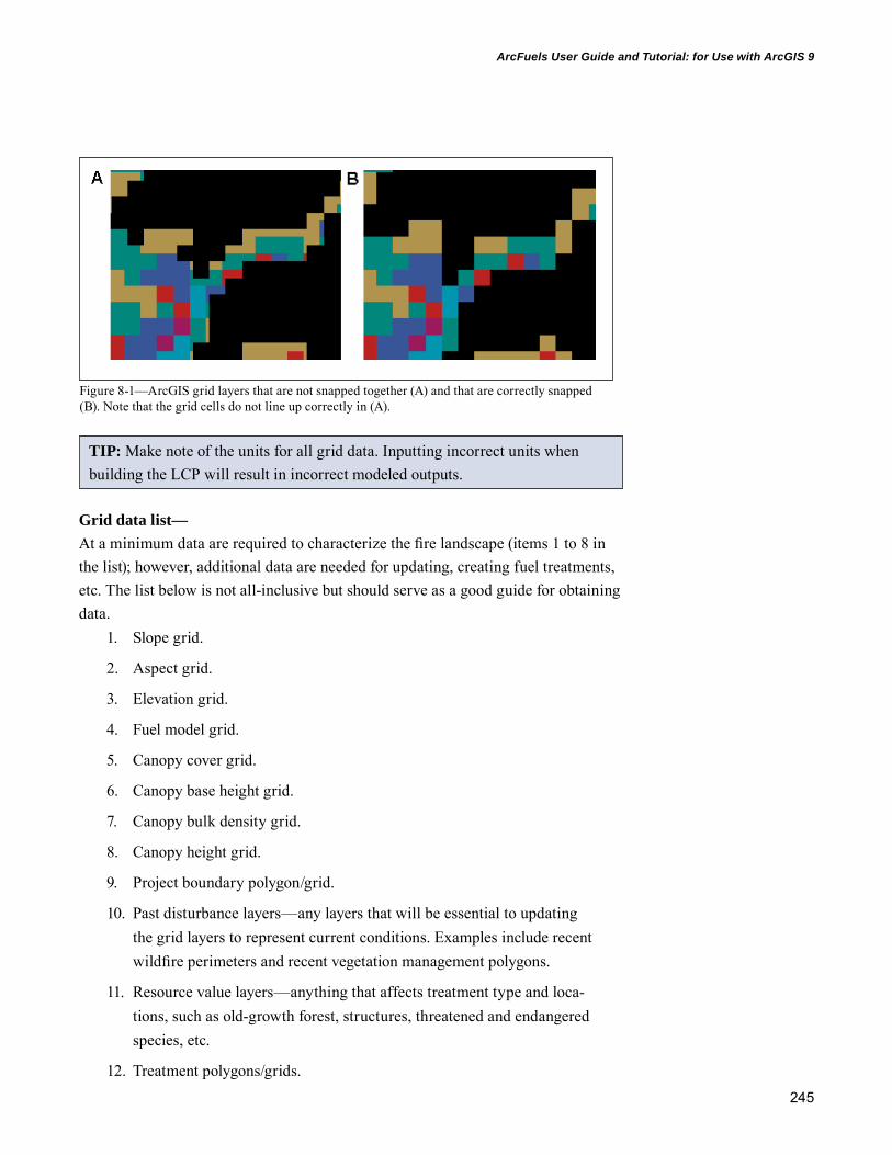
245


Figure 8-1—ArcGIS grid layers that are not snapped together (A) and that are correctly snapped (B). Note that the grid cells do not line up correctly in (A).

Grid data list—At a minimum data are required to characterize the fire landscape (items 1 to 8 in the list); however, additional data are needed for updating, creating fuel treatments, etc. The list below is not all-inclusive but should serve as a good guide for obtaining data.

1. Slope grid.

2. Aspect grid.

3. Elevation grid.

4. Fuel model grid.

5. Canopy cover grid.

6. Canopy base height grid.

7. Canopy bulk density grid.

8. Canopy height grid.

9. Project boundary polygon/grid.

10. Past disturbance layers—any layers that will be essential to updating the grid layers to represent current conditions. Examples include recent wildfire perimeters and recent vegetation management polygons.

11. Resource value layers—anything that affects treatment type and loca-tions, such as old-growth forest, structures, threatened and endangered species, etc.

12. Treatment polygons/grids.

TIP: Make note of the units for all grid data. Inputting incorrect units when building the LCP will result in incorrect modeled outputs.

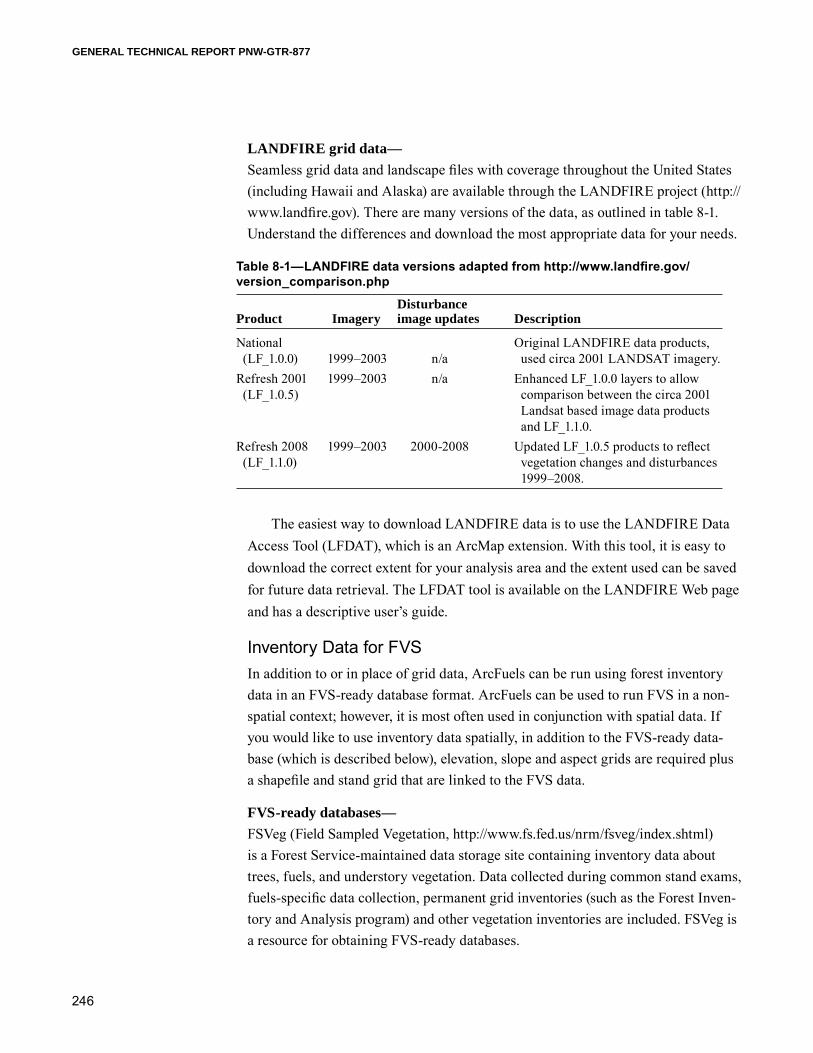
246


LANDFIRE grid data—Seamless grid data and landscape files with coverage throughout the United States (including Hawaii and Alaska) are available through the LANDFIRE project (http://www.landfire.gov). There are many versions of the data, as outlined in table 8-1. Understand the differences and download the most appropriate data for your needs.

Table 8-1—LANDFIRE data versions adapted from http://www.landfire.gov/version_comparison.php

Disturbance Product Imagery image updates Description

National Original LANDFIRE data products, (LF_1.0.0) 1999–2003 n/a used circa 2001 LANDSAT imagery.Refresh 2001 1999–2003 n/a Enhanced LF_1.0.0 layers to allow (LF_1.0.5) comparison between the circa 2001 Landsat based image data products and LF_1.1.0.Refresh 2008 1999–2003 2000-2008 Updated LF_1.0.5 products to reflect (LF_1.1.0) vegetation changes and disturbances 1999–2008.

The easiest way to download LANDFIRE data is to use the LANDFIRE Data Access Tool (LFDAT), which is an ArcMap extension. With this tool, it is easy to download the correct extent for your analysis area and the extent used can be saved for future data retrieval. The LFDAT tool is available on the LANDFIRE Web page and has a descriptive user’s guide.

Inventory Data for FVSIn addition to or in place of grid data, ArcFuels can be run using forest inventory data in an FVS-ready database format. ArcFuels can be used to run FVS in a non-spatial context; however, it is most often used in conjunction with spatial data. If you would like to use inventory data spatially, in addition to the FVS-ready data-base (which is described below), elevation, slope and aspect grids are required plus a shapefile and stand grid that are linked to the FVS data.

FVS-ready databases—FSVeg (Field Sampled Vegetation, http://www.fs.fed.us/nrm/fsveg/index.shtml) is a Forest Service-maintained data storage site containing inventory data about trees, fuels, and understory vegetation. Data collected during common stand exams, fuels-specific data collection, permanent grid inventories (such as the Forest Inven-tory and Analysis program) and other vegetation inventories are included. FSVeg is a resource for obtaining FVS-ready databases.

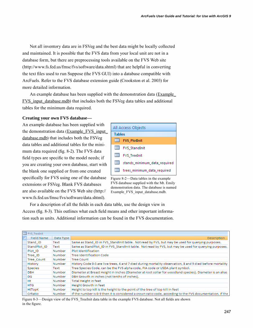
247


Not all inventory data are in FSVeg and the best data might be locally collected and maintained. It is possible that the FVS data from your local unit are not in a database form, but there are preprocessing tools available on the FVS Web site (http://www.fs.fed.us/fmsc/fvs/software/data.shtml) that are helpful in converting the text files used to run Suppose (the FVS GUI) into a database compatible with ArcFuels. Refer to the FVS database extension guide (Crookston et al. 2003) for more detailed information.

An example database has been supplied with the demonstration data (Example_FVS_input_database.mdb) that includes both the FSVeg data tables and additional tables for the minimum data required.

Creating your own FVS database—An example database has been supplied with the demonstration data (Example_FVS_input_database.mdb) that includes both the FSVeg data tables and additional tables for the mini-mum data required (fig. 8-2). The FVS data field types are specific to the model needs; if you are creating your own database, start with the blank one supplied or from one created specifically for FVS using one of the database extensions or FSVeg. Blank FVS databases are also available on the FVS Web site (http://www.fs.fed.us/fmsc/fvs/software/data.shtml).

For a description of all the fields in each data table, use the design view in Access (fig. 8-3). This outlines what each field means and other important informa-tion such as units. Additional information can be found in the FVS documentation.

Figure 8-2—Data tables in the example FVS database supplied with the Mt. Emily demonstration data. The database is named Example_FVS_input_database.mdb.

Figure 8-3—Design view of the FVS_TreeInit data table in the example FVS database. Not all fields are shown in the figure.

248


The stand, optional plot, and tree data tables are all linked through a unique stand identifier, STAND_ID. This linkage is necessary when building your own database. Table 8-2 is a simplistic view of this linkage.

Table 8-2—Stand, plot, and tree data table linkage example

FVS_StandInit FVS_PlotInit FVS_TreeInit

STAND_ID NUM_PLOTS STAND_ID PLOT_ID STAND_ID PLOT_ID TREE_ID 1 3 1 1 1 1 100 1 2 1 1 101 1 3 1 2 200 1 2 201 1 2 202 1 3 301Note: All records in the stand, plot, and tree tables must be linked by a unique identifier (STAND_ID) for each stand. There can be multiple plots per stand and multiple trees per plot.

Spatial linkage between FVS database and stands—This is often the hardest part for getting your data to work in ArcFuels. Regard-less of the source of the FVS database obtained, properly linking the database to the stand polygon layer (and stand grid) is critical. There must be a relationship between the polygon identifier and the FVS stand table variable (STAND_ID). If data exist for every polygon, there will be a unique stand and tree list for every stand within the polygon (a one-to-one relationship). This is the case with the demonstration data (fig. 8-4). If imputation (i.e., Most Similar Neighbor (MSN), or Gradient Nearest Neighbor (GNN)) is used, a single stand and associated treelist will be used for multiple polygons (one-to-many relationship).

NO MATTER WHAT THE RELATIONSHIP (ONE-TO-ONE OR ONE-TO-MANY), THERE MUST BE A FIELD IN THE STAND POLYGON (AND THE VALUE FIELD OF THE STAND GRID) THAT IS IDENTI-CAL TO THE FVS TABLES. IT IS HIGHLY RECOMMENDED THAT THIS BE THE STAND_ID FIELD.

For future sorting and joining, it is recommended that a second stand iden-tification field be added to the FVS data tables that is equal to the Stand_ID but is numeric. In the demonstration data (Mt_Emily_Database.mdb), this is the Stand_ID_NUM field.

NOTE: FSVeg databases include a field named “GIS_LINK” in the FVS_Stan-dInit table. This link does not work in ArcFuels because the field is not also present in the FVS_PlotInit and FVS_TreesInint tables.

Spatially linking the FVS-ready database to the stand shapefile is one of the hardest steps in the data preparation phase. The link (i.e., STAND_ID) must be identical in the shapefile and FVS-data tables.

249


Setting Up ArcFuels With Your DataWhen setting up ArcFuels with your own data, it is recommended that you place your data and outputs folder within the same parent ArcFuels folder (i.e., C:/arcfu-els/mydata and C:/arcfuels/myoutputs). Because the majority of programs are the same, you can use the existing ArcFuels programs and extra_programs folders. One important note is that you must download the proper FVS variant file when using the FVS functionality in ArcFuels. These can be found at the FVS Web site (http://www.fs.fed.us/fmsc/fvs/software/variantinstaller.php).

Once your data are loaded into a new arcfuels9x.mxd, save it with your project name. Go to Projects and Files on the ArcFuels toolbar and select Manage Proj-ects from the drop-down list. Create a new project by clicking the New Project but-ton. Then fill out the tabs accordingly. For a refresher, see the Setting up ArcFuels with the Mt. Emily Demonstration Data section in this user guide.

Figure 8-4—Linkage between the GIS stand polygon layer and the FVS stand and tree data tables. All three are linked by a unique stand identification number. Having the imagery behind the stand polygon layer is a useful visual when looking at stand and tree data tables. In this example, stand 392 is densely stocked as can be seen by the 10 tree list entries and 428 trees compared to stand 423 with two tree list entries and two trees.

250


AcknowledgmentsWe acknowledge the Joint Fire Sciences Program (JFSP 03-4-1-04) and the Western Wildlands Environmental Threat Assessment Center for supplying much of the funding to develop and maintain ArcFuels. We thank the following people for development and testing: Dana Simon, Geoff Babb, Bridgett Naylor, Berni Bahro, Joe Sherlock, Deana Wall, and Nathan Amboy. We thank Michelle Day, Deana Wall, Carol Ewell, Brandon Collins, and Phil Bowden for numerous edits to this User Guide and Tutorial in its many iterations.

Metric EquivalentsWhen you know: Multiply by: To find:Inches (in) 2.54 CentimetersFeet (ft) 0.305 MetersMiles 1.609 KilometersMiles per hour (mph) 0.447 Meters per secondSquare feet (ft2) 0.0929 Square metersAcres (ac) 0.405 HectaresTons per acre (t/ac) 2.24 Tonnes or megagrams per hectareTrees per acre 2.24 Trees per hectarePounds (lb) 0.454 KilogramCubic feet (ft3) 0.283 Cubic meters

251


Literature CitedAgee, J.K. 1996. The influence of forest structure on fire behavior. In: Proceedings

of the 17th annual forest vegetation management conference. Redding, CA: Forest Vegetation Management Conference: 52–68.

Agee, J.K. 1998. The landscape ecology of western forest fire regimes. Northwest Science. 72: 24–34.

Ager, A.A.; McMahan, A.J.; Barrett, J.J.; McHugh, C.W. 2007. A simulation study of thinning and fuel treatments on a wildland–urban interface in eastern Oregon, USA. Landscape and Urban Planning. 80: 292–300.

Ager, A.A., Vaillant, N.M.; Finney, M.A. 2010. A comparison of landscape fuel treatment strategies to mitigate wildland fire risk in the urban interface and preserve old forest structure. Forest Ecology and Management. 259: 1556–1570.

Ager, A.A.; Vaillant, N.M.; Finney, M.A. 2011. Integration of fire behavior modeling tools and GIS for wildland fire risk assessment and fuel management planning. Journal of Combustion. Article ID 572452. 19 p.

Ager, A.A.; Vaillant, N.M.; Owens, D.E.; Brittain S.; Hamann, J. 2012. Overview and example application of the Landscape Treatment Designer. Gen. Tech. Rep. PNW-GTR-859. Portland, OR: U.S. Department of Agriculture, Forest Service, Pacific Northwest Research Station. 11 p.

Albini, F.A. 1976. Estimating wildfire behavior and effects. Gen. Tech. Rep. INT-GTR-30. Ogden, UT: U.S. Department of Agriculture, Forest Service, Intermountain Forest and Range Experiment Station. 92 p.

Anderson, D.H.; Catchpole, E.A.; DeMestre, N.J.; Parkes, T. 1982. Modeling the spread of grass fires. Journal of the Australian Mathematical Society (Series B). 23: 451–466.

Anderson, H.E. 1982. Aids to determining fuel models for estimating fire behavior. Gen. Tech. Rep. INT-GTR-122. Ogden, UT: U.S. Department of Agriculture, Forest Service, Intermountain Forest and Range Experiment Station. 22 p.

Bahro, B.; Barber, K.H.; Sherlock, J.W.; Yasuda, D.A. 2007. Stewardship and fireshed assessment: a process for designing a landscape fuel treatment strategy. In: Restoring fire-adapted ecosystems: proceedings of the 2005 national silviculture workshop. Gen. Tech. Rep. PSW-GTR-203. Albany, CA: U.S. Department of Agriculture, Forest Service, Pacific Southwest Research Station. 306 p.

252


Bradshaw, L.S.; Tirmenstein, D. 2009 (draft). FireFamilyPlus user’s guide, version 4.1. Internal report. Fort Collins, CO: U.S. Department of Agriculture, Forest Service, Rocky Mountain Research Station. 282 p.

Calkin, D.E.; Ager, A.A.; Gilbertson-Day, J., eds. 2010. Wildfire risk and hazard: Procedures for the first approximation. Gen. Tech. Rep. RMRS-GTR-235. Fort Collins, CO: U.S. Department of Agriculture, Forest Service, Rocky Mountain Research Station. 62 p.

Collins, B.M.; Stephens,S.L.; Moghaddas, J.J.; Battles, J. 2010. Challenges and approaches in planning fuel treatments across fire-excluded forested landscapes. Journal of Forestry. 108: 24–31.

Crookston, N.L. 1990. User’s guide to the event monitor: part of Prognosis Model version 6. Gen. Tech. Rep. INT-GTR-275. Ogden, UT: U.S. Department of Agriculture, Forest Service, Intermountain Research Station. 21 p.

Crookston, N.L; Dixon, G.E. 2005. The forest vegetation simulator: a review of its structure, content, applications. Computers and Electronics in Agriculture. 49: 60–80.

Crookston, N.L.; Gammel, D.L.; Rebain, S.; Robinson, D.; Keyser, C. 2003 (revised August 2011). Users guide to the database extension of the Forest Vegetation Simulator Version 2.0. Internal report. Fort Collins, CO: U.S. Department of Agriculture, Forest Service, Forest Management Service Center. 56 p. http://www.fs.fed.us/fmsc/ftp/fvs/docs/gtr/DBSUserGuide.pdf. (30 August 2012).

Crookston, N.L.; Stage, A.R. 1991. User’s guide to the Parallel Processing Extension of the Prognosis Model. Gen. Tech. Rep. INT-GTR-281. Ogden, UT: U.S. Department of Agriculture, Forest Service, Intermountain Research Station. 88 p.

Cruz M.G.; Alexander M.E. 2010. Assessing crown fire potential in coniferous forests of western North America: a critique of current approaches and recent simulation studies. International Journal of Wildland Fire. 19: 377–398.

Dixon, G.E. 2003 (revised August 2011). Essential FVS: a user’s guide to the Forest Vegetation Simulator. Internal report. Fort Collins, CO: U.S. Department of Agriculture, Forest Service, Forest Management Service Center. 246 p. http://www.fs.fed.us/fmsc/ftp/fvs/docs/gtr/EssentialFVS.pdf. (31 October 2012).

253


Finkral, A.J.; Evans, A.M. 2008. The effects of a thinning treatment on carbon stocks in a northern Arizona ponderosa pine forest. Forest Ecology and Management. 255: 2743–2750.

Finney, M.A. 1998. FARSITE: fire area simulator-model development and evaluation. Res. Pap. RMRS-RP-4. Ogden, UT: U.S. Department of Agriculture, Forest Service, Rocky Mountain Research Station. 47 p.

Finney, M.A. 2001. Design of regular landscape fuel treatment patterns for modifying fire growth and behavior. Forest Science. 47(2): 219–228.

Finney, M.A. 2002. Fire growth using minimum travel time methods. Canadian Journal of Forest Research. 32: 1420–1424.

Finney, M.A. 2005. The challenge of quantitative risk assessment for wildland fire. Forest Ecology and Management. 211: 97–108.

Finney, M.A. 2006. An overview of FlamMap fire modeling capabilities. In: Andrews, P.L.; Butler, B.W. comps., 2006. Fuels management—how to measure success: conference proceedings. Proceedings RMRS-P-41. Fort Collins, CO: U.S. Department of Agriculture, Forest Service, Rocky Mountain Research Station: 213–220.

Finney, M.A. 2007. A computational method for optimizing fuel treatment locations. International Journal of Wildland Fire. 16: 702–711.

Finney, M.A.; McHugh, C.W.; Grenfell, I.C.; Riley, K.L.; Short, K.C. 2011. A simulation of probabilistic wildfire risk components for the continental United States. Stochastic Environmental Research and Risk Assessment. 25: 973–1000.

Finney, M.A.; Seli, R.; McHugh, C.; Ager, A.A.; Bahro, B.; Agee, J. 2007. Simulation of long-term landscape-level fuel treatment effects on large wildfires. International Journal of Wildland Fire. 16: 712–727.

Forthofer, J.; Shannon, K.; Butler, B. 2009. Simulating diurnally driven slope winds with WindNinja. In: Proceedings of 8th Symposium on Fire and Forest Meteorology. Boston, MA: American Meteorological Society: 4.4.

Gercke, G.; Stewart, S. 2006. Strategic placement of treatments (SPOTS): maximizing the effectiveness of fuel and vegetation treatments on problem fire behavior and effects. In: Andrews, P.L.; Butler, B.W. comps., 2006. Fuels management—how to measure success: conference proceedings. Proceedings RMRS-P-41. Fort Collins, CO: U.S. Department of Agriculture, Forest Service, Rocky Mountain Research Station: 185–192.

254


Heinsch, F.A.; Andrews, P.L. 2010. BehavePlus fire modeling system, version 5.0: design and features. Gen. Tech. Rep. RMRS-GTR-249. Fort Collins, CO: U.S. Department of Agriculture, Forest Service, Rocky Mountain Research Station. 111 p.

Hurteau, M.D.; Koch, G.W.; Hungate, B.A. 2008. Carbon protection and fire risk reduction: toward a full accounting of forest carbon offsets. Frontiers in Ecology and the Environment. 6: 493–498.

Keyes, C.R. 2006. Role of foliar moisture content in the silvicultural management of forest fuels. Western Journal of Applied Forestry. 21(4): 228–231.

Knight, I.; Coleman, J. 1993. A fire perimeter expansion algorithm based on Huygens’ wavelet propagation. International Journal of Wildland Fire. 3: 73–84.

McGaughey, R. 1997. Visualizing forest stand dynamics using the Stand Visualization System. In: Proceedings of the American Congress on Surveying and Mapping. American Society of Photogrammetry and Remote Sensing. 4: 248–257.

Mitchell, S.R.; Harmon, M.E.; O’Connell, K.E.B. 2009. Forest fuel reduction alters fire severity and long-term carbon storage in three Pacific Northwest ecosystems. Ecological Applications. 19: 643–655.

North, M.; Hurteau, M.; Innes, J. 2009. Fire suppression and fuels treatment effects on mixed-conifer carbon stocks and emissions. Ecological Applications. 19: 1385–1396.

Ohmann, J.L.; Gregory, M.J. 2002. Predictive mapping of forest composition and structure with direct gradient analysis and nearest neighbor imputation in coastal Oregon, U.S.A. Canadian Journal of Forest Research. 32: 725–741.

Rebain, S.A. comp., 2010 (revised October 2012). The Fire and Fuels Extension to the Forest Vegetation Simulator: updated model documentation. Internal report. Fort Collins, CO: U.S. Department of Agriculture, Forest Service, Forest Management Service Center. 396 p. http://www.fs.fed.us/fmsc/ftp/fvs/docs/gtr/FFEguide.pdf. (16 October 2012).

Reinhardt E.; Holsinger L. 2010. Effects of fuel treatments on carbon-disturbance relationships in forests of the northern Rocky Mountains. Forest Ecology and Management. 259: 1427–1435.

255


Reinhardt, E.D.; Keane R.E.; Brown J.K. 1997. First Order Fire Effects Model: FOFEM 4.0, user’s guide. Gen. Tech. Rep. INT-GTR-344. Ogden, UT: U.S. Department of Agriculture, Forest Service, Intermountain Research Station. 65 p.

Rollins, M.G. 2009. LANDFIRE: a nationally consistent vegetation, wildland fire, and fuel assessment. International Journal of Wildland Fire. 18(3): 235–249.

Rothermel, R.C. 1972. A mathematical model for predicting fire spread in wildland fuels. Res. Pap. INT-115. Ogden, UT: U.S. Department of Agriculture, Forest Service, Intermountain Forest and Range Experiment Station. 40 p.

Rothermel, R.C. 1983. How to predict the spread and intensity of forest and range fires. Res. Pap. INT-143. Ogden, UT: U.S. Department of Agriculture, Forest Service, Intermountain Forest and Range Experiment Station. 161 p.

Rothermel, R.C. 1991. Predicting behavior and size of crown fires in the Northern Rocky Mountains. Res. Pap. INT-438. Ogden, UT: U.S. Department of Agriculture, Forest Service, Intermountain Forest and Range Experiment Station. 46 p.

Scott, J.H. 1999. NEXUS: A system for assessing crown fire hazard. Fire Management Notes. 59: 21–24.

Scott, J.H. 2006. An analytical framework for quantifying wildland fire risk and treatment benefit. In: Andrews, P.L.; Butler, B.W. comps., 2006. Fuels management—how to measure success: conference proceedings. Proceedings RMRS-P-41. Fort Collins, CO: U.S. Department of Agriculture, Forest Service, Rocky Mountain Research Station: 169–184.

Scott, J.E.; Burgan, R.E. 2005. Standard fire behavior fuel models: a comprehensive set for use with Rothermel’s surface fire spread model. Gen. Tech. Rep. RMRS-GTR-153, Fort Collins, CO: U.S. Department of Agriculture, Forest Service, Rocky Mountain Research Station. 72 p.

Scott, J.H.; Reinhardt, E.D. 2001. Assessing crown fire potential by linking models of surface and crown fire behavior. Res. Pap. RMRS-29. Fort Collins, CO: U.S. Department of Agriculture, Forest Service, Rocky Mountain Research Station. 59 p.

Stratton, R.D. 2009. Guidebook on LANDFIRE fuels data acquisition, critique, modification, maintenance, and model calibration. Gen. Tech. Rep. RMRS-GTR-220. Fort Collins, CO: U.S. Department of Agriculture, Forest Service, Rocky Mountain Research Station. 54 p.

256


Van Dyck, M.G.; Smith-Mateja, E.E., comps. 2000 (revised September 2012). Keyword reference guide for the Forest Vegetation Simulator. Internal report. Fort Collins, CO: U.S. Department of Agriculture, Forest Service, Forest Management Service Center. 119 p. http://www.fs.fed.us/fmsc/ftp/fvs/docs/gtr/keyword.pdf. (10 September 2012).

Van Wagner, C.E. 1977. Conditions for the start and spread of crown fire. Canadian Journal of Forest Research. 7: 23–34.

Van Wagner, C.E. 1993. Prediction of crown fire behavior in two stands of jack pine. Canadian Journal of Forest Research. 23: 442–449.

Pacific Northwest Research Station

Web site http://www.fs.fed.us/pnw/Telephone (503) 808-2592Publication requests (503) 808-2138FAX (503) 808-2130E-mail [email protected] address Publications Distribution Pacific Northwest Research Station P.O. Box 3890 Portland, OR 97208-3890

U.S. Department of Agriculture Pacific Northwest Research Station 333 SW First Avenue P.O. Box 3890 Portland, OR 97208-3890

Official Business Penalty for Private Use, $300

ArcFuels User Guide and Tutorial: for Use with ArcGIS 9®

Documents

Transcript of ArcFuels User Guide and Tutorial: for Use with ArcGIS 9®