water

Article

Influence of Land Use Change on Hydrological Cycle:Application of SWAT to Su-Mi-Huai Area inBeijing, China

Linlin Zhang 1 , Caiyuan Wang 2, Guixing Liang 3, Yali Cui 1,* and Qiulan Zhang 1

1 Beijing Key Laboratory of Water Resources and Environmental Engineering, School of Water Resources andEnvironment, China University of Geosciences, Beijing 100083, China; lilizhang@cugb.edu.cn (L.Z.);qlzhang919@cugb.edu.cn (Q.Z.)

2 Department of Hydrological Monitoring Management, Beijing Hydrological Center, Beijing 100089, China;wangcaiyuan555@163.com

3 Shallow Geothermal Energy Research Center, Beijing Geothermal Research Institute, Beijing 102218, China;cugblgx@163.com

* Correspondence: cuiyl@cugb.edu.cn

Received: 29 September 2020; Accepted: 10 November 2020; Published: 12 November 2020

Abstract: The human activities and urbanization process have changed the underlying surface ofurban areas, which would affect the recharge of groundwater through rainfall infiltration and mayfurther influence the groundwater environment. Accordingly, it is imperative to investigate thevariation of hydrological cycle under the condition of underlying surface change. Based on thehigh-precision remote sensing data of 2000, 2005, 2010 and 2015, and Soil and Water AssessmentTool (SWAT) model, this work firstly studied the land use change and the corresponding changes inrunoff generation mechanism and rainfall infiltration coefficient in Su-Mi-Huai area, Beijing, China.Meanwhile, SWAT-MODFLOW semi-loose coupling model was applied to analyze the water balancein the study area in typical hydrological years. The results showed that the area of the constructionland (urban and rural residential land) increased by 1.04 times from 2000 to 2015, which is mainlyattributed to the conversion of cultivated land to construction land in the plain area. This changecaused the runoff in the area to increase by 7 × 106 m3, the runoff coefficient increased by 17.9%,and the precipitation infiltration coefficient was less than the empirical value determined by lithology.Compared with 2000, the average annual precipitation infiltration coefficient in 2018 decreased by 6.5%.Under the influence of urbanization process, the maximum reduction rate of precipitation infiltrationrecharge is up to 38%. The study investigated the response of surface runoff and precipitationinfiltration recharge to land use change, which can provide helps for water resources managers tocoordinate the relationship between land use change and rational water resources planning.

Keywords: land use change; precipitation infiltration coefficient; SWAT model; runoff

1. Introduction

Groundwater is an extremely precious natural resource. It plays a key role in the hydrologiccycle, ecological and geological environment as well as economic and social development [1,2]. As animportant part of water resources, groundwater is preferred to be used for water supply than surfacewater due to its characteristics of wide distribution, strong storage capacity, good water quality andeasy development [3,4]. Precipitation infiltration is the main natural recharge source of groundwater.In recent years, the development of urbanization in Beijing, China, has greatly changed the underlyingsurface conditions. The land hardening and vadose thickening brought about by this change makethe recharge amount of groundwater obtained from precipitation infiltration decrease continuously.

Water 2020, 12, 3164; doi:10.3390/w12113164 www.mdpi.com/journal/water

Water 2020, 12, 3164 2 of 17

However, in order to meet the economic development as well as the production and living needs,the exploitation of groundwater is still increasing year by year. To ensure the sustainable developmentof the city, it is urgent to evaluate the land use change on precipitation infiltration coefficient, runoff andgroundwater in this case.

In the application of groundwater modeling, the precipitation infiltration recharge is determinedaccording to the total precipitation and the precipitation infiltration recharge coefficient (α) in acertain area [5,6]. The coefficient mainly depends on the lithology, structure and thickness of thevadose zone as well as the land surface slope [7–9]. The natural amplitude of phreatic water level,lysimeter observation, isotope analysis, equilibrium method, chloride tracer and numerical simulationare usually used to calculate α [10–14]. With the rapid economic and social development in recentyears, a variety of human activities (such as the acceleration of urbanization process) have contributedto significant changes in land use and land cover, which directly affect the underlying surface of thebasin [15], and then changes the rainfall infiltration process.

Recently, researches about the influences of the land use change are abundant, including climatechange [16], hydrology and solute budgets [17], streamflow [18], and soil chemical attributes [19].By analyzing the characteristics of climate change (including spatial distribution and temporal trendof precipitation and temperature) and land use/cover change in Yunnan Province, China during1961–2011, Shi and Chen [16] concluded that the close relationships of the built-up land with theannual temperature and precipitation changes might be attributed to the developments of urbanization.Based on the lithology of unsaturated zone and the depth to groundwater table in different periods,Meng et al. [6] discussed the temporal and spatial evolution characteristics of precipitation infiltrationrecharge in the North China Plain in recent 50 years. The study showed that with the increase ofwater table depth, the precipitation infiltration recharge coefficient increased and reached the peakvalue at a particular depth (the optimal depth of different lithology is 3 to 6 m). Cherubin et al. [19]conducted the investigation on the effects of land use change on Brazilian tropical soil chemicalattributes, indicating that long-term land use change from natural ecosystems to extensive pasturedecreases available P, S, Ca, Mg and B contents, and land use change from pasture to sugarcane willlead to increase of nutrients levels and reduction of soil acidity. However, in the area where thegroundwater recharge is dominated by the rainfall infiltration, the investigations on the impact ofland use change on rainfall infiltration recharge remain limited. Therefore, it is important to study thevariation of rainfall infiltration coefficient under the condition of underlying surface change.

The Soil and Water Assessment Tool (SWAT) model can comprehensively consider soil, land use,vegetation, land surface slope, meteorology, reservoir and runoff information to simulate differenthydrological cycle processes. Jin et al. [20] improved SWAT model to solve the problem that SWATcould not reflect the land use change during the simulation period. The improved SWAT model canuse land use data year by year, and the simulation effect is better than SWAT Model in the HeiheRiver basin in China where land use and cover change greatly. SWAT model uses land use datain the modeling process, which will affect hydrological processes such as evapotranspiration andgroundwater recharge [20]. SWAT model has certain advantages in the calculation of groundwaterrecharge resources under the condition of underlying surface change. Based on the SWAT hydrologicalmodel, Mohamed et al. [21] simulated the responses of streamflow and baseflow to climate and landuse change in the Upper West Branch DuPage River basin in Illinois and the Walzem River Basin inTexas, respectively. The modeling results show that changes in streamflow and baseflow in the latterwatershed seem to be more affected by urbanization than by climate change. Zhang et al. [22] appliedthe improved SWAT model to simulate the impact of different land use changes on water balancein the North Johnston River catchment in eastern Australia, showing that urbanization will increasesurface runoff. The change of underlying surface will lead to the increase of surface runoff and thedecrease of precipitation infiltration recharge, causing the decrease of groundwater recharge amount.Correspondingly, the groundwater level will continue to drop when the groundwater exploitationremains unchanged or continues to increase. In this case, it may lead to surface subsidence and other

Water 2020, 12, 3164 3 of 17

geological hazards, threaten ecological security, water resources security [23–25]. Thus, it is necessaryto study the effect of land use change on the rule of runoff, rainfall infiltration coefficient and rainfallinfiltration recharge, so as to reasonably plan the relationship between land use and water resources inthe context of the social and economic development.

In order to evaluate the influence of underlying surface change on the hydrological cycle, we firstlyanalyzed the land use change in different periods of the study area, the Su-Mi-Huai District inBeijing, China, and used SWAT model to discuss the influence of underlying surface change onrunoff mechanism and rainfall infiltration coefficient. Secondly, the semi-loose coupling model wasestablished by MODFLOW and SWAT, and the results of this model were used to compare the influenceof the water balance in the study area before and after land use changes in typical years. This studycould provide guidance for the rational planning of land use, the correct prediction of urban watersituation and the rational planning of water resources in areas with rapid urbanization.

2. Methodology

2.1. Study Area

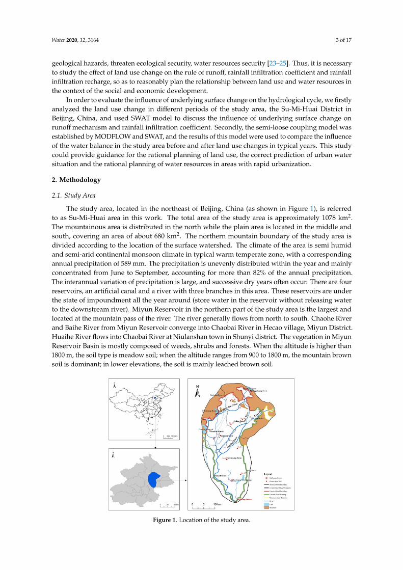
The study area, located in the northeast of Beijing, China (as shown in Figure 1), is referredto as Su-Mi-Huai area in this work. The total area of the study area is approximately 1078 km2.The mountainous area is distributed in the north while the plain area is located in the middle andsouth, covering an area of about 680 km2. The northern mountain boundary of the study area isdivided according to the location of the surface watershed. The climate of the area is semi humidand semi-arid continental monsoon climate in typical warm temperate zone, with a correspondingannual precipitation of 589 mm. The precipitation is unevenly distributed within the year and mainlyconcentrated from June to September, accounting for more than 82% of the annual precipitation.The interannual variation of precipitation is large, and successive dry years often occur. There are fourreservoirs, an artificial canal and a river with three branches in this area. These reservoirs are underthe state of impoundment all the year around (store water in the reservoir without releasing waterto the downstream river). Miyun Reservoir in the northern part of the study area is the largest andlocated at the mountain pass of the river. The river generally flows from north to south. Chaohe Riverand Baihe River from Miyun Reservoir converge into Chaobai River in Hecao village, Miyun District.Huaihe River flows into Chaobai River at Niulanshan town in Shunyi district. The vegetation in MiyunReservoir Basin is mostly composed of weeds, shrubs and forests. When the altitude is higher than1800 m, the soil type is meadow soil; when the altitude ranges from 900 to 1800 m, the mountain brownsoil is dominant; in lower elevations, the soil is mainly leached brown soil.

Water 2020, 12, x FOR PEER REVIEW 3 of 18

rainfall infiltration coefficient and rainfall infiltration recharge, so as to reasonably plan the relationship between land use and water resources in the context of the social and economic development.

In order to evaluate the influence of underlying surface change on the hydrological cycle, we firstly analyzed the land use change in different periods of the study area, the Su-Mi-Huai District in Beijing, China, and used SWAT model to discuss the influence of underlying surface change on runoff mechanism and rainfall infiltration coefficient. Secondly, the semi-loose coupling model was established by MODFLOW and SWAT, and the results of this model were used to compare the influence of the water balance in the study area before and after land use changes in typical years. This study could provide guidance for the rational planning of land use, the correct prediction of urban water situation and the rational planning of water resources in areas with rapid urbanization.

2. Methodology

2.1. Study Area

The study area, located in the northeast of Beijing, China (as shown in Figure 1), is referred to as Su-Mi-Huai area in this work. The total area of the study area is approximately 1078 km2. The mountainous area is distributed in the north while the plain area is located in the middle and south, covering an area of about 680 km2. The northern mountain boundary of the study area is divided according to the location of the surface watershed. The climate of the area is semi humid and semi-arid continental monsoon climate in typical warm temperate zone, with a corresponding annual precipitation of 589 mm. The precipitation is unevenly distributed within the year and mainly concentrated from June to September, accounting for more than 82% of the annual precipitation. The interannual variation of precipitation is large, and successive dry years often occur. There are four reservoirs, an artificial canal and a river with three branches in this area. These reservoirs are under the state of impoundment all the year around (store water in the reservoir without releasing water to the downstream river). Miyun Reservoir in the northern part of the study area is the largest and located at the mountain pass of the river. The river generally flows from north to south. Chaohe River and Baihe River from Miyun Reservoir converge into Chaobai River in Hecao village, Miyun District. Huaihe River flows into Chaobai River at Niulanshan town in Shunyi district. The vegetation in Miyun Reservoir Basin is mostly composed of weeds, shrubs and forests. When the altitude is higher than 1800 m, the soil type is meadow soil; when the altitude ranges from 900 to 1800 m, the mountain brown soil is dominant; in lower elevations, the soil is mainly leached brown soil.

Figure 1. Location of the study area. Figure 1. Location of the study area.

Water 2020, 12, 3164 4 of 17

This area is one of the main water sources in Beijing. The groundwater in the plain area ismainly pore water in loose rock, while in mountain area it is dominated by fissure water in bedrock.From piedmont to plain, the aquifer changes from single layer to multi-layer. The groundwater inthe area is mainly supplied by precipitation infiltration. Artificial exploitation is almost the only wayof groundwater discharge. In recent years, the overexploitation of groundwater resources led to theincrease of the groundwater depth and the thickness of the vadose zone and the change of underlyingsurface conditions. At the same time, the original overflow zone disappears. The groundwater depthis greater than the evaporation limit (4 m), which means that there is no phreatic water evaporationwhen the water level is lower than 4 m [26].

2.2. Water Balance Modeling

2.2.1. SWAT Model

The input data needed for SWAT model are mainly divided into two categories: spatial dataand attribute data are shown in Table 1. The former includes the digital elevation model (DEM),land use and soil type, while the latter includes hydrological data, meteorological data (daily rainfall,daily average wind speed, daily relative humidity, solar radiation and daily maximum and minimumtemperature) [27,28]. Among them, DEM data is used to (1) generate river network, (2) determinewatershed outlet and (3) divide sub-basin. The hydrological response unit (HRU) is generated by usingthe superimposition of the land use type map, soil type distribution map and slope data. Soil data isused to calculate and create the soil databases needed for the SWAT model.

Table 1. Data items in the study.

Method Data Type Scale Year

SWATModel

Spatial DataDEM 1 90 × 90 m

Land Use Map 2 1000 × 1000 m 2010Soil Type Map 3 1000 × 1000 m 2015

AttributeData 4

Meteorological Data Diurnal Scale 2000–2016Reservoir Data Monthly Scale 2000–2016

Runoff Data Monthly Scale 2000–2016

Land UseAnalysis Landsat 8 Remote Sensing Image 2 30 × 30 m 2000, 2005, 2010,

2015, 20181 The data set is provided by Geospatial Data Cloud site, Computer Network Information Center, Chinese Academyof Sciences. (http://www.gscloud.cn). 2 The data set is provided by Data Center for Resources and EnvironmentalSciences, Chinese Academy of Sciences (RESDC) (http://www.resdc.cn). 3 The data set is provided by Food andAgriculture Organization of the United Nations (FAO) (http://www.fao.org). 4 The data set is provided by BeijingHydrological Center, China.

The groundwater recharge in SWAT model is calculated by the Green and Ampt formula [29].The Soil Conservation Service (SCS) runoff curve method is used to estimate surface runoff in SWATmodel. The SCS calculation formula [30] is as follows:

Qsur f =

(Rday − 0.2S

)2

Rday + 0.8S(1)

where Qsur f is the cumulative runoff (mm), Rday is the rainfall depth of one day (mm), S is retentionparameters (mm). Only when Rday > 0.2S, surface runoff is generated.

We processed the remote sensing image data (Table 1) of different periods to get the land usetransfer matrix applied in land use analysis. The specific measures are as follows: firstly, we openthe land use map of two periods in ARCGIS at the same time and fuse the two maps according tothe land use field. Then, the land use maps of the two periods are superimposed and cross analyzedto obtain the intersection layer. We assign values to the attribute table of the intersection layer and

Water 2020, 12, 3164 5 of 17

calculate its area and then export the attribute table. Finally, we open the attribute table through Excel,and perform the Pivot Table and Pivot Chart operations to get the land use transfer matrix [31].

2.2.2. SWAT-MODFLOW Coupling

MODFLOW Model

MODFLOW is a three-dimensional, physically based, distributed finite-difference groundwatermodel for variably saturated subsurface systems [32]. In MODFLOW, if the change of water density isnot considered, the three-dimensional flow of groundwater in porous media can be expressed by thefollowing partial differential equation:

Ss∂h∂t

=∂∂x

(Kx∂h∂x

)+

∂∂y

(Ky∂h∂y

)+∂∂z

(Kz∂h∂z

)+ W x, y, z ∈ Ω, t ≥ 0 (2)

where Ss is water storage rate of water bearing medium (1/m), h is water level elevation of aquifer (m),Kx, Ky, Kz is the permeability coefficient of x, y and z directions respectively (m/d), W is the source andsink term of aquifer (1/d).

MODFLOW software has a main program and several relatively independent subprograms.Each subroutine has several modules, and each module completes part of the numerical simulation.This modular structure is quite conducive to the increase and decrease of data and the establishment oflater coupling model. In this study, the optimized RCH subprogram package and the newly developedRAW (recharge and well) subprogram by Han et al. [33] are selected to process the source and sink data.These two subroutines are the principle of area data processing. Precipitation infiltration recharge,agricultural irrigation supply and partial mining are carried out in the form of area. In the simulation,the study area can be divided into different sub regions to deal with the related recharge and discharge.This method is helpful to use them to process the replenishment and discharge data, and to replace thewater supplied to aquifer in SWAT model with the same areal distribution.

The Semi-loose Coupling

This work mainly uses three parts to complete the semi loose coupling of surface water andgroundwater: (1) surface water runoff model based on SWAT2005 software, (2) groundwater flowmodel based on MODFLOW-2005 and (3) semi-loose coupling model of surface water and groundwaterbased on GIS platform for data transmission. The process of establishing SWAT-MODFLOW semi-loosecoupling model is described as follows: (1) the groundwater recharge in the plain area calculated bySWAT model is used to replace the rainfall infiltration amount in MODFLOW model, (2) the optimizedRCH sub-package is selected to deal with precipitation infiltration recharge and (3) it is substitutedinto model as the area recharge item. In addition, the MODFLOW model’s lateral recharge in thepiedmont area is replaced by the mountainous aquifer recharge calculated using the SWAT model,and the recharge is substituted into the model in the form of well (WELL).

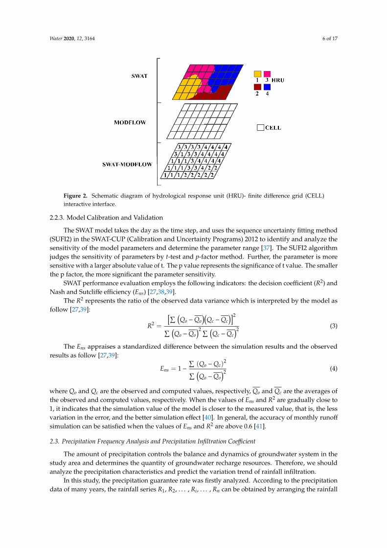
The key problem in the establishment of semi-loose coupling model is that the basic calculationunit of MODFLOW model is finite difference grid (CELL), which has spatial information. The basiccalculation unit of SWAT model is hydrological response unit (HRU), which is the basis of modelsimulation calculation [34,35]. Each HRU represents the combination of specific land use, soil type andslope in the watershed. They have vector information, but their data cannot be directly transferredto the grid (CELL). For this reason, we established an interactive interface of HRU-CELL throughARCGIS software [36]. The specific situation is shown in Figure 2. Through this interactive interface,each hydrological response unit corresponds to one or more grids, and the values on each HRUare transferred to the corresponding CELL, that is, the semi-loose coupling of SWAT-MODFLOWis realized.

Water 2020, 12, 3164 6 of 17Water 2020, 12, x FOR PEER REVIEW 6 of 18

Figure 2. Schematic diagram of hydrological response unit (HRU)- finite difference grid (CELL) interactive interface.

2.2.3. Model Calibration and Validation

The SWAT model takes the day as the time step, and uses the sequence uncertainty fitting method (SUFI2) in the SWAT-CUP (Calibration and Uncertainty Programs) 2012 to identify and analyze the sensitivity of the model parameters and determine the parameter range [37]. The SUFI2 algorithm judges the sensitivity of parameters by t-test and p-factor method. Further, the parameter is more sensitive with a larger absolute value of t. The p value represents the significance of t value. The smaller the p factor, the more significant the parameter sensitivity.

SWAT performance evaluation employs the following indicators: the decision coefficient (𝑅 ) and Nash and Sutcliffe efficiency (𝐸 ) [27,38,39].

The 𝑅 represents the ratio of the observed data variance which is interpreted by the model as follow [27,39]: 𝑅 = ∑ 𝑄 − 𝑄 𝑄 − 𝑄∑ 𝑄 − 𝑄 ∑ 𝑄 − 𝑄 (3)

The 𝐸 appraises a standardized difference between the simulation results and the observed results as follow [27,39]: 𝐸 = 1 − ∑ 𝑄 − 𝑄∑ 𝑄 − 𝑄 (4)

where 𝑄 and 𝑄 are the observed and computed values, respectively, 𝑄 and 𝑄 are the averages of the observed and computed values, respectively. When the values of 𝐸 and 𝑅 are gradually close to 1, it indicates that the simulation value of the model is closer to the measured value, that is, the less variation in the error, and the better simulation effect [40]. In general, the accuracy of monthly runoff simulation can be satisfied when the values of 𝐸 and 𝑅 are above 0.6 [41].

2.3. Precipitation Frequency Analysis and Precipitation Infiltration Coefficient

The amount of precipitation controls the balance and dynamics of groundwater system in the study area and determines the quantity of groundwater recharge resources. Therefore, we should analyze the precipitation characteristics and predict the variation trend of rainfall infiltration.

In this study, the precipitation guarantee rate was firstly analyzed. According to the precipitation data of many years, the rainfall series 𝑅 , 𝑅 , …, 𝑅 , …, 𝑅 can be obtained by arranging the rainfall from large to small. The guarantee rate 𝑃 (cumulative frequency) of precipitation 𝑅 is defined as follows:

Figure 2. Schematic diagram of hydrological response unit (HRU)- finite difference grid (CELL)interactive interface.

2.2.3. Model Calibration and Validation

The SWAT model takes the day as the time step, and uses the sequence uncertainty fitting method(SUFI2) in the SWAT-CUP (Calibration and Uncertainty Programs) 2012 to identify and analyze thesensitivity of the model parameters and determine the parameter range [37]. The SUFI2 algorithmjudges the sensitivity of parameters by t-test and p-factor method. Further, the parameter is moresensitive with a larger absolute value of t. The p value represents the significance of t value. The smallerthe p factor, the more significant the parameter sensitivity.

SWAT performance evaluation employs the following indicators: the decision coefficient (R2) andNash and Sutcliffe efficiency (Ens) [27,38,39].

The R2 represents the ratio of the observed data variance which is interpreted by the model asfollow [27,39]:

R2 =

[∑ (Qo −Qo

)(Qc −Qc

)]2

∑ (Qo −Qo

)2 ∑ (Qc −Qc

)2 (3)

The Ens appraises a standardized difference between the simulation results and the observedresults as follow [27,39]:

Ens = 1−∑

(Qo −Qc)2∑ (

Qo −Qo)2 (4)

where Qo and Qc are the observed and computed values, respectively, Qo and Qc are the averages ofthe observed and computed values, respectively. When the values of Ens and R2 are gradually close to1, it indicates that the simulation value of the model is closer to the measured value, that is, the lessvariation in the error, and the better simulation effect [40]. In general, the accuracy of monthly runoff

simulation can be satisfied when the values of Ens and R2 are above 0.6 [41].

2.3. Precipitation Frequency Analysis and Precipitation Infiltration Coefficient

The amount of precipitation controls the balance and dynamics of groundwater system in thestudy area and determines the quantity of groundwater recharge resources. Therefore, we shouldanalyze the precipitation characteristics and predict the variation trend of rainfall infiltration.

In this study, the precipitation guarantee rate was firstly analyzed. According to the precipitationdata of many years, the rainfall series R1, R2, . . . , Ri, . . . , Rn can be obtained by arranging the rainfall

Water 2020, 12, 3164 7 of 17

from large to small. The guarantee rate Pi (cumulative frequency) of precipitation Ri is defined asfollows:

Pi =i

n + 1(5)

where Pi is greater than or equal to the frequency of occurrence of precipitation Ri, i is the serial numberof precipitations in order of magnitude, n is the number of years of statistics.

Precipitation infiltration coefficient is the ratio of precipitation recharge to precipitation.This coefficient is an important hydrological parameter in the study of groundwater resourcesestimation and mutual transformation between atmospheric water, surface water and groundwater.

The precipitation infiltration recharge coefficient changes greatly due to the comprehensiveinfluence of natural factors and human factors. The annual precipitation infiltration coefficient can becalculated as follows [42]:

α =PERCPREC

(6)

where α is precipitation infiltration coefficient, PERC is groundwater recharge (mm), PREC isprecipitation (mm). The empirical value of the precipitation infiltration coefficient is determined byprevious studies based on factors such as the lithology, structure and thickness of the unsaturatedzone [7–9].

3. Results and Discussion

3.1. The Results of Model Calibration and Validation

SuZhuang station, a hydrological observation station in the study area, is selected to calibratethe runoff parameters based on the monthly measured runoff. The SuZhuang station is located at thedownstream outlet of the basin, which can reflect the runoff from the entire watershed to the outlet.The runoff data of this station is provided by Beijing Hydrological Center, China. The collected runoff

data is divided into two parts: the first part (from January 2000 to December 2012) is used for modelcalibration, and the second part (from January 2013 to December 2016) is used for model validation.The comparison of simulated and observed monthly streamflow during calibration and validationperiods is shown in Figure 3. During the calibration period, the values of R2 and Ens are 0.64 and 0.60,respectively. During the validation period, the values of R2 and Ens are 0.78 and 0.70, respectively.The values of R2 and Ens in the calibration period and the validation period are both greater than0.6, which meets the accuracy requirements, indicating that the calculation results of SWAT modelare reliable.

The results of MODFLOW model and SWAT-MODFLOW model have been presented in ourprevious study, which indicate that the simulation results of models are reliable [43].

3.2. Influence of Underlying Surface Change on Precipitation Infiltration Coefficient

3.2.1. Analysis on Land Use Change

In order to fully demonstrate the direction of land type transfer and supplementary sources,we used the land use transfer matrix to conduct the research. Table 2 shows the land use transfermatrix of the study area from 2000 to 2015. It can be seen that there are eight types of land use in thestudy area, mainly including cultivated land, woodland, rural area and urban area.

From 2000 to 2015, the area of cultivated land in the study region decreased by 22.85%.Rural residential land increased by 44.22%. The area of urban residential land has become 2.81 timesthe area of the same land type in 2000.

Rural residential land and urban residential land are mainly converted from cultivated land.The area of grassland, woodland and waters decreased to varying degrees, and the percentage ofreduction was 44.2%, 11.5% and 19.1%, respectively. The expansion of land used for urban construction

Water 2020, 12, 3164 8 of 17

in the study area is more significant, which is mainly manifested in the increase of urban and ruralresidential land and the decrease of arable land.

Water 2020, 12, x FOR PEER REVIEW 8 of 18

Figure 3. Runoff fitting diagram of SuZhuang station, adapted from our previous study [43].

3.2. Influence of Underlying Surface Change on Precipitation Infiltration Coefficient

3.2.1. Analysis on Land Use Change

In order to fully demonstrate the direction of land type transfer and supplementary sources, we used the land use transfer matrix to conduct the research. Table 2 shows the land use transfer matrix of the study area from 2000 to 2015. It can be seen that there are eight types of land use in the study area, mainly including cultivated land, woodland, rural area and urban area.

From 2000 to 2015, the area of cultivated land in the study region decreased by 22.85%. Rural residential land increased by 44.22%. The area of urban residential land has become 2.81 times the area of the same land type in 2000.

Rural residential land and urban residential land are mainly converted from cultivated land. The area of grassland, woodland and waters decreased to varying degrees, and the percentage of reduction was 44.2%, 11.5% and 19.1%, respectively. The expansion of land used for urban construction in the study area is more significant, which is mainly manifested in the increase of urban and rural residential land and the decrease of arable land.

Figure 3. Runoff fitting diagram of SuZhuang station, adapted from our previous study [43].

Table 2. Land use transfer matrix of the study area from 2000 to 2015 (Unit: km2).

Land Use Types2015

Grassland UrbanArea

CultivatedLand

TrafficLand Woodland Rural

Area Waters Total

2000

Grassland 9.50 0.29 3.07 4.30 1.03 0.58 1.13 19.90UrbanArea 0.01 34.39 0.21 0.00 0.02 0.00 0.29 34.92

CultivatedLand 0.58 55.32 317.24 12.68 11.15 67.28 6.58 470.84

TrafficLand 0.34 13.55 3.89 4.54 1.12 4.85 0.42 28.72

Woodland 0.40 6.53 17.69 5.35 157.10 6.12 2.78 195.97Bare Land 0.00 0.07 0.01 0.00 0.06 0.00 0.00 0.15

RuralArea 0.16 15.81 12.04 2.46 2.31 77.06 0.29 110.12

Waters 0.02 7.11 9.08 2.64 0.71 2.94 34.95 57.45Total 11.02 133.07 363.23 31.96 173.51 158.83 46.45 918.06

3.2.2. Influence of Land Use Change on Precipitation Infiltration Coefficient

Spatial Variation Analysis of Precipitation Infiltration Coefficient

Figure 4 shows the land use types of the study area in 2000 and 2015, the zoning of the empiricalvalue of precipitation infiltration coefficient in plain area and the rainfall infiltration coefficient zoningof the study area based on SWAT surface runoff simulation calculation using the land use map of 2015.

As the process of urbanization accelerates, land use types have changed, and the precipitationinfiltration coefficient will also change accordingly. Figure 4b,d shows that the precipitation infiltrationcoefficient calculated by SWAT model is smaller than the empirical value of precipitation infiltrationcoefficient in plain area. In the mountainous area, the rainfall infiltration coefficient calculated by SWATmodel is greater than 0.33. The maximum range of precipitation infiltration coefficient obtained bythe two methods is in the northern plain area, but the maximum range of empirical value is 0.01–0.17larger than the SWAT calculation result.

Water 2020, 12, 3164 9 of 17

Water 2020, 12, x FOR PEER REVIEW 9 of 18

Table 2. Land use transfer matrix of the study area from 2000 to 2015 (Unit: km2).

Land Use Types 2015

Grassland Urban Area

Cultivated Land

Traffic Land Woodland Rural

Area Waters Total

2000

Grassland 9.50 0.29 3.07 4.30 1.03 0.58 1.13 19.90 Urban Area

0.01 34.39 0.21 0.00 0.02 0.00 0.29 34.92

Cultivated Land

0.58 55.32 317.24 12.68 11.15 67.28 6.58 470.84

Traffic Land

0.34 13.55 3.89 4.54 1.12 4.85 0.42 28.72

Woodland 0.40 6.53 17.69 5.35 157.10 6.12 2.78 195.97 Bare Land 0.00 0.07 0.01 0.00 0.06 0.00 0.00 0.15

Rural Area

0.16 15.81 12.04 2.46 2.31 77.06 0.29 110.12

Waters 0.02 7.11 9.08 2.64 0.71 2.94 34.95 57.45 Total 11.02 133.07 363.23 31.96 173.51 158.83 46.45 918.06

3.2.2. Influence of Land Use Change on Precipitation Infiltration Coefficient

Spatial Variation Analysis of Precipitation Infiltration Coefficient

Figure 4 shows the land use types of the study area in 2000 and 2015, the zoning of the empirical value of precipitation infiltration coefficient in plain area and the rainfall infiltration coefficient zoning of the study area based on SWAT surface runoff simulation calculation using the land use map of 2015.

As the process of urbanization accelerates, land use types have changed, and the precipitation infiltration coefficient will also change accordingly. Figure 4b,d shows that the precipitation infiltration coefficient calculated by SWAT model is smaller than the empirical value of precipitation infiltration coefficient in plain area. In the mountainous area, the rainfall infiltration coefficient calculated by SWAT model is greater than 0.33. The maximum range of precipitation infiltration coefficient obtained by the two methods is in the northern plain area, but the maximum range of empirical value is 0.01–0.17 larger than the SWAT calculation result.

(a) (b)

Water 2020, 12, x FOR PEER REVIEW 10 of 18

(c) (d)

Figure 4. (a) The land use type in 2000; (b) Empirical value of the partition map of precipitation infiltration coefficient; (c) The land use types in 2015; (d) The partition map of precipitation infiltration coefficient calculated by Soil and Water Assessment Tool (SWAT) model.

As shown in Figure 4b, the areas with large empirical value of precipitation infiltration recharge coefficients are concentrated in the upper part of the alluvial fan, where the lithology is mainly gravel and coarse sand and the precipitation infiltration coefficient ranges from 0.56 to 0.65. The precipitation infiltration coefficient in the middle part of the plain area is greater than 0.33, while it is less than 0.33 in the northern mountain and the downstream boundary. In 2000, the land use types in the study area were relatively primitive, and large-scale urbanization had not started. As it can be seen from Figure 4a, the main land use type of the plain area was cultivated land, accounting for 69.24% of the plain area. Rural and urban residential areas accounted for 16.19% and 5.14% of the plain area, respectively. The woodland is mainly distributed in the northern mountainous area, accounting for 21.35% of the total area.

According to the Table 2 and Figure 4c,d, the proportion of cultivated land, the main land use type in the region, decreased from 51.29% to 39.56% by 2015 due to the acceleration of urbanization. In the plain area of the upper reaches of the river, the precipitation infiltration coefficient of the area with more cultivated land is relatively large, ranging between 0.48 and 0.55, less than the empirical value of precipitation coefficient.

Compared with the land-use type maps in Figure 4, it can be clearly seen that rural residential area and urban residential area have increased significantly. In the areas where urban residential land increased (such as the western, northeastern and southwestern riverside areas of the study area), the precipitation infiltration coefficient decreased 0.18–0.44. The precipitation infiltration coefficient of the concentrated area of urban residential land in the study area is generally less than 0.32 due to the ground hardening caused by urbanization.

Time Variation Analysis of Precipitation Infiltration Coefficient

Figure 5 shows the change of land use type area in the four periods of 2000–2005, 2005–2010, 2010–2015 and 2015–2018. Based on the land use data in 2000, 2005, 2010, 2015 and 2018, the annual precipitation infiltration coefficients of these years are calculated by SWAT model. Figure 6 presents the area changes of the main land use types in the five periods as well as the corresponding annual precipitation infiltration coefficient.

Figure 4. (a) The land use type in 2000; (b) Empirical value of the partition map of precipitationinfiltration coefficient; (c) The land use types in 2015; (d) The partition map of precipitation infiltrationcoefficient calculated by Soil and Water Assessment Tool (SWAT) model.

As shown in Figure 4b, the areas with large empirical value of precipitation infiltration rechargecoefficients are concentrated in the upper part of the alluvial fan, where the lithology is mainly graveland coarse sand and the precipitation infiltration coefficient ranges from 0.56 to 0.65. The precipitationinfiltration coefficient in the middle part of the plain area is greater than 0.33, while it is less than 0.33in the northern mountain and the downstream boundary. In 2000, the land use types in the studyarea were relatively primitive, and large-scale urbanization had not started. As it can be seen fromFigure 4a, the main land use type of the plain area was cultivated land, accounting for 69.24% ofthe plain area. Rural and urban residential areas accounted for 16.19% and 5.14% of the plain area,respectively. The woodland is mainly distributed in the northern mountainous area, accounting for21.35% of the total area.

Water 2020, 12, 3164 10 of 17

According to the Table 2 and Figure 4c,d, the proportion of cultivated land, the main land usetype in the region, decreased from 51.29% to 39.56% by 2015 due to the acceleration of urbanization.In the plain area of the upper reaches of the river, the precipitation infiltration coefficient of the areawith more cultivated land is relatively large, ranging between 0.48 and 0.55, less than the empiricalvalue of precipitation coefficient.

Compared with the land-use type maps in Figure 4, it can be clearly seen that rural residentialarea and urban residential area have increased significantly. In the areas where urban residentialland increased (such as the western, northeastern and southwestern riverside areas of the study area),the precipitation infiltration coefficient decreased 0.18–0.44. The precipitation infiltration coefficient ofthe concentrated area of urban residential land in the study area is generally less than 0.32 due to theground hardening caused by urbanization.

Time Variation Analysis of Precipitation Infiltration Coefficient

Figure 5 shows the change of land use type area in the four periods of 2000–2005, 2005–2010,2010–2015 and 2015–2018. Based on the land use data in 2000, 2005, 2010, 2015 and 2018, the annualprecipitation infiltration coefficients of these years are calculated by SWAT model. Figure 6 presentsthe area changes of the main land use types in the five periods as well as the corresponding annualprecipitation infiltration coefficient.

According to the analysis of Figure 6, from 2000 to 2018, the average annual precipitation infiltrationcoefficient shows a decreasing trend with the change of land use, which is negatively correlated with thechange of construction land area (urban area and rural area), but positively correlated with the changeof cultivated land area. From 2000 to 2018, the average annual precipitation infiltration coefficientdecreased by 6.5%. During the years from 2000 to 2005, the average annual precipitation coefficientdecreased significantly, by 3.4%. During this period, the area of construction land increased, such asurban area, rural area and traffic land, which increased by 41.3%, 13.1% and 25.5%, respectively.

3.3. Influence of Land Use Change on Hydrological Cycle

3.3.1. Runoff Generation

In this section, the land use data of 2000, 2005, 2010 and 2015 were used to analyze the change ofsurface runoff in the study area. It can be found from Figure 7 that the simulated surface runoff yieldunder the four land use types has the same change trend, and the runoff yield fluctuates with rainfall.In 2012, the surface runoff was the largest, ranging from 82 × 106 m3 to 94 × 106 m3. The surfacerunoff in 2003 and 2009 was the smallest, ranging from 22 × 106 m3 to 28 × 106 m3. According tothe precipitation histogram, the year with the largest precipitation is 2012, and the year with theminimum precipitation is 2003 and 2009. The peak and valley values of runoff are the same as thoseof precipitation.

The runoff coefficient is the ratio of surface runoff to rainfall. It can comprehensively reflectthe influence of natural geographical factors on the relationship between precipitation and runoff.The average annual runoff and runoff coefficient under each land use scenario are calculated. The annualaverage value of surface runoff in the study area is increasing continuously. The average runoff

coefficient in 2015 was 17.9% higher than 2000.From 2000 to 2005, the change range of land use was the largest, and the annual increment of

surface runoff was the largest, which was 5 × 106 m3. Comparing each year’s surface production flowand annual average surface production flow under the four phases of land use, the changes are thesame, both showing an increasing trend. The added value is the largest during the period of the fastestland use change (2000–2005). From 2000 to 2015, when the land use type changed from cultivated landto construction land, the runoff coefficient increased with the increase of average runoff yield, and theincrease rate of runoff coefficient was greater than that of surface runoff.

Water 2020, 12, 3164 11 of 17Water 2020, 12, x FOR PEER REVIEW 11 of 18

Figure 5. The change area of each land use type in four periods.

Figure 6. The variation trend of land use types and the change chart of annual precipitation infiltration coefficient under land use scenarios in different periods.

According to the analysis of Figure 6, from 2000 to 2018, the average annual precipitation infiltration coefficient shows a decreasing trend with the change of land use, which is negatively correlated with the change of construction land area (urban area and rural area), but positively correlated with the change of cultivated land area. From 2000 to 2018, the average annual precipitation infiltration coefficient decreased by 6.5%. During the years from 2000 to 2005, the average annual precipitation coefficient decreased significantly, by 3.4%. During this period, the area of construction land increased, such as urban area, rural area and traffic land, which increased by41.3%, 13.1% and 25.5%, respectively.

Figure 5. The change area of each land use type in four periods.

Water 2020, 12, x FOR PEER REVIEW 11 of 18

Figure 5. The change area of each land use type in four periods.

Figure 6. The variation trend of land use types and the change chart of annual precipitation infiltration coefficient under land use scenarios in different periods.

According to the analysis of Figure 6, from 2000 to 2018, the average annual precipitation infiltration coefficient shows a decreasing trend with the change of land use, which is negatively correlated with the change of construction land area (urban area and rural area), but positively correlated with the change of cultivated land area. From 2000 to 2018, the average annual precipitation infiltration coefficient decreased by 6.5%. During the years from 2000 to 2005, the average annual precipitation coefficient decreased significantly, by 3.4%. During this period, the area of construction land increased, such as urban area, rural area and traffic land, which increased by41.3%, 13.1% and 25.5%, respectively.

Figure 6. The variation trend of land use types and the change chart of annual precipitation infiltrationcoefficient under land use scenarios in different periods.

Water 2020, 12, 3164 12 of 17

Water 2020, 12, x FOR PEER REVIEW 12 of 18

3.3. Influence of Land Use Change on Hydrological Cycle

3.3.1. Runoff Generation

In this section, the land use data of 2000, 2005, 2010 and 2015 were used to analyze the change of surface runoff in the study area. It can be found from Figure 7 that the simulated surface runoff yield under the four land use types has the same change trend, and the runoff yield fluctuates with rainfall. In 2012, the surface runoff was the largest, ranging from 82 × 106 m3 to 94 × 106 m3. The surface runoff in 2003 and 2009 was the smallest, ranging from 22 × 106 m3 to 28 × 106 m3. According to the precipitation histogram, the year with the largest precipitation is 2012, and the year with the minimum precipitation is 2003 and 2009. The peak and valley values of runoff are the same as those of precipitation.

Figure 7. Variation of surface runoff in the Su-Mi-Huai region during 2000–2016 under four land use types.

The runoff coefficient is the ratio of surface runoff to rainfall. It can comprehensively reflect the influence of natural geographical factors on the relationship between precipitation and runoff. The average annual runoff and runoff coefficient under each land use scenario are calculated. The annual average value of surface runoff in the study area is increasing continuously. The average runoff coefficient in 2015 was 17.9% higher than 2000.

From 2000 to 2005, the change range of land use was the largest, and the annual increment of surface runoff was the largest, which was 5 × 106 m3. Comparing each year’s surface production flow and annual average surface production flow under the four phases of land use, the changes are the same, both showing an increasing trend. The added value is the largest during the period of the fastest land use change (2000–2005). From 2000 to 2015, when the land use type changed from cultivated land to construction land, the runoff coefficient increased with the increase of average runoff yield, and the increase rate of runoff coefficient was greater than that of surface runoff.

3.3.2. Analysis of Water Balance in Typical Years

In this study, we used the rainfall series data from 1956 to 2016 to calculate the guarantee rate of each year (Appendix A) and count the frequency of precipitation during this period (Table 3). It can be seen that the extremely dry year is 2000 (the guarantee rate is 95%) in which, the rainfall is 313.9 mm. The general dry year is 2013 (the guarantee rate is 75%), and the corresponding rainfall is 465.4 mm. The normal year is 1970 (the guarantee rate is 50%), the simulation period representative year is

Figure 7. Variation of surface runoff in the Su-Mi-Huai region during 2000–2016 under four landuse types.

3.3.2. Analysis of Water Balance in Typical Years

In this study, we used the rainfall series data from 1956 to 2016 to calculate the guarantee rate ofeach year (Appendix A) and count the frequency of precipitation during this period (Table 3). It can beseen that the extremely dry year is 2000 (the guarantee rate is 95%) in which, the rainfall is 313.9 mm.The general dry year is 2013 (the guarantee rate is 75%), and the corresponding rainfall is 465.4 mm.The normal year is 1970 (the guarantee rate is 50%), the simulation period representative year is 2010,the rainfall is 555.7 mm. The rainy year is 2012 (the guarantee rate is 15%), the rainfall is 753.6 mm,and the statistical annual average rainfall is 588.8 mm.

Table 3. Statistics of precipitation frequency from 1956 to 2016.

Precipitation Frequency Typical Year(mm)

>1000 1 1959900–1000 2 1956, 1969800–900 3 1964, 1994700–800 8 2005, 2012600–700 13 2008, 2016500–600 13 2009, 2010400–500 16 2007, 2013300–400 5 2000, 2003

The water balance of representative years is selected in this section to study the impact of landuse change on the overall water balance in the study area. As shown in Table 4, the phreatic aquiferwater equilibria of the study area in three characteristic years before and after land use change areselected, which are calculated by MODFLOW model and SWAT-MODFLOW semi-loose couplingmodel [43] respectively.

In the rainy year, the calculated precipitation infiltration replenishment after considering the landuse change is less than the calculation result when the land use change is not considered, and thereduction rate is 16.5%. In the normal year, under the condition of land use change, the amount ofprecipitation infiltration recharge decreased by 33.6%. In the dry year, under the condition of land usechange, the amount of precipitation infiltration recharge decreased by 38%.

Water 2020, 12, 3164 13 of 17

Table 4. Water balance of phreatic aquifer in typical years (Unit: 106 m3).

Equilibrium Term

Rainy Year Normal Year Dry Year2012 2010 2013

BeforeChange

AfterChange

BeforeChange

AfterChange

BeforeChange

AfterChange

Recharge

Precipitation Infiltration 263 220 180 119 175 109Agricultural Irrigation Supply 22 22 27 27 22 22

Irrigation Supply of Canal System 6 6 8 8 6 6Pipe Leakage Supply 67 67 67 67 67 67

Lateral Recharge in Piedmont 52 81 39 45 51 48Boundary Lateral Inflow Recharge 20 24 17 21 21 25

Subtotal 430 419 338 286 343 277

Discharge

Exploitation 429 429 424 424 339 339Boundary Lateral Outflow 0.1 0.09 0.2 0.14 0.1 0.07

Lateral Outflow Between Layers 15 9 18 12 7 3Subtotal 445 439 442 436 346 342

TotalDifference −15 −19 −104 −150 −3 −65

Vertical Exchange Capacity −174 −177 −185 −186 −133 −131

In the rainy year, the calculated precipitation infiltration replenishment after considering the landuse change is less than the calculation result when the land use change is not considered, and thereduction rate is 16.5%. In the normal year, under the condition of land use change, the amount ofprecipitation infiltration recharge decreased by 33.6%. In the dry year, under the condition of land usechange, the amount of precipitation infiltration recharge decreased by 38%.

The results show that the impact of land use change on water balance is mainly reflected inthe aspect of precipitation infiltration recharge [44,45]. Land hardening leads to a decrease in theamount of groundwater recharge by precipitation infiltration, which is especially obvious in the year ofdecreasing atmospheric precipitation, that is, the response in dry year is stronger than that in normalyear, and the response in rainy year is the weakest. Although the investigation conducted in this workis based on a small-scale model, its results are similar to those obtained from large-scale studies [44–46].Urbanization increases runoff and reduces groundwater recharge, posting a challenge for catchmentmanagement. The study on the change of flood peak in river urban agglomeration [47,48] and thechange of regional climate [49,50] are related to the rapid urban growth. Groundwater is very importantfor irrigation and global food security. When the supply of groundwater is reduced, the groundwaterlevel drop caused by irrigation cannot be replenished in time, which will affect the aquatic ecologyof rivers [51]. Accordingly, it is important to reasonably plan the land use of a town even a region,and comprehensively consider its impact on runoff and groundwater infiltration.

The methodology used in this work can quantify the influence of land use change on hydrologicalcycle in a watershed, including precipitation infiltration coefficient, surface runoff and water balance,which is helpful to provide guidance for water resource management. It is different from the qualitativeunderstanding obtained by remote sensing data or other traditional methods, that is, the logarithmicrelationship between urbanization rate and runoff [52]. In areas strongly affected by human activities,it may not be realistic to obtain detailed hydrological parameters to establish a full coupling modelof surface-water and groundwater for water resources evaluation and hydrological process research.The combination of the remote sensing data, SWAT model and MODFLOW model make it possible.The application of this comprehensive method in Su-Mi-Huai area demonstrates the simulation resultsare credible. Specifically, the remote sensing data of different periods were used to calculate the degreeof urbanization construction and the transformation of land use types. The SWAT and MODFLOWmodel are semi loosely coupled to quantify the amount of water resources affected by land use change.In order to ensure the sustainable development of an area, we should not only balance the relationshipbetween urban development and water resources allocation but also consider the effect of urbanizationon hydrological cycle. Certainly, this requires the coordinated planning and joint efforts of landplanning, water resources management and other departments.

Water 2020, 12, 3164 14 of 17

4. Conclusions

Based on the Landsat 8 high-precision remote sensing data and the SWAT hydrological model,this study analyzes the change law of the falling water infiltration coefficient and surface runoff in thestudy area under the land use change scenario and analyzes the effect of land use change on the waterbalance of the study area using the MODFLOW model. The conclusions as follows are reached.

From 2000 to 2015, the land use change was mainly manifested in the transformation fromcultivated land to urban and rural residential land in Su-Mi-Huai area in Beijing, China.

By 2015, the precipitation infiltration coefficient value in the area is smaller than its empirical value.In the area of increasing urban residential land, the precipitation infiltration coefficient decreased by0.18–0.44. From 2000 to 2018, the average annual precipitation infiltration coefficient in the study areahas gradually decreased, which is positively correlated with the change of cultivated land area andnegatively correlated with the change of construction land.

Under the conditions of land use from 2000 to 2015, the annual average value of surface runoff

and the runoff coefficient in the area showed an increasing trend. During the period of the fastest landuse change (2000–2005), the increase values of surface runoff and annual average surface runoff of eachyear are the largest.

Changes in land use mainly reduce precipitation infiltration replenishment. In the dry year,precipitation infiltration recharge has the strongest response to land use changes, with a reduction rateof 38%.

This study examined the influence of hydrology cycle due to the land use change primarily causedby urbanization. The current study provides useful implications for the rational management of waterresources under the situation of land use change caused by urbanization. The sustainable developmentof cities must consider the impact of land use change on the hydrological cycle and find a reasonablebalance between urban planning and water resources management.

Author Contributions: Conceptualization, L.Z., G.L. and Y.C.; methodology, L.Z., C.W. and Y.C.; data curation,L.Z., Q.Z. and G.L.; formal analysis, L.Z. and Y.C.; writing—original draft preparation, L.Z.; writing—review andediting, L.Z., C.W., G.L., Y.C. and Q.Z. All authors have read and agreed to the published version of the manuscript.

Funding: This research was funded by the Special Foundation for the Basic Resources Survey Program of theMinistry of Science and Technology, China, grant number [2017FY100405] and the project of “Investigationand evaluation of water resources in Beijing—Study on the conversion relationship between surface water andgroundwater” in cooperation with Beijing Hydrological Center, China.

Acknowledgments: We would like to thank the Beijing Hydrological Center for providing the meteorological andrunoff data, and the observed data of groundwater level.

Conflicts of Interest: The authors declare no conflict of interest.

Appendix A

In this study, we used the rainfall series data from 1956 to 2016 to calculate the guarantee rate ofeach year, which is shown in Table A1.

Water 2020, 12, 3164 15 of 17

Table A1. Statistical table of annual rainfall guarantee rate of SuZhuang station.

SerialNumber Year Precipitation

(mm)Guarantee

RateSerial

Number Year Precipitation(mm)

GuaranteeRate

1 1959 1041.3 1.61% 32 1974 561.5 51.61%2 1956 997.5 3.23% 33 2010 555.7 53.23%3 1969 907.5 4.84% 34 1976 548.9 54.84%4 1994 875.1 6.45% 35 1989 529.0 56.45%5 1964 811.2 8.06% 36 2009 524.4 58.06%6 1990 809.8 9.68% 37 1966 523.1 59.68%7 1979 797.1 11.29% 38 1982 523.0 61.29%8 1973 753.6 12.90% 39 2004 508.2 62.90%9 2012 753.6 14.52% 40 1996 505.9 64.52%10 2005 744.9 16.13% 41 1988 497.3 66.13%11 1958 743.6 17.74% 42 1968 491.7 67.74%12 2011 742.8 19.35% 43 1963 491.2 69.35%13 1987 713.0 20.97% 44 2007 487.0 70.97%14 1998 709.8 22.58% 45 1971 483.8 72.58%15 2015 692.2 24.19% 46 1983 476.1 74.19%16 1991 691.4 25.81% 47 2013 465.4 75.81%17 1978 676.3 27.42% 48 2006 465.2 77.42%18 1977 676.2 29.03% 49 1972 455.6 79.03%19 2016 676.1 30.65% 50 2002 451.3 80.65%20 1957 661.8 32.26% 51 1975 437.2 82.26%21 1967 660.2 33.87% 52 1993 437.2 83.87%22 2008 652.0 35.48% 53 1960 420.9 85.48%23 1995 637.0 37.10% 54 2001 417.3 87.10%24 1985 631.8 38.71% 55 2014 414.2 88.71%25 1992 615.4 40.32% 56 1980 402.4 90.32%26 1986 609.1 41.94% 57 2003 387.8 91.94%27 1962 605.0 43.55% 58 1981 347.1 93.55%28 1984 578.7 45.16% 59 2000 313.9 95.16%29 1997 577.8 46.77% 60 1965 305.8 96.77%30 1961 576.0 48.39% 61 1999 304.7 98.39%31 1970 567.4 50.00% Annual average precipitation: 588.82 mm

References

1. Andreas, N.C. Groundwater and its economic nature. Q. J. Eng. Geol. Hydrogeol. 2019, 53, 176–188. [CrossRef]2. Gleeson, T. Global groundwater sustainability. Ground Water. 2020, 58, 484–485. [CrossRef] [PubMed]3. Zhao, H.; Gao, L.; Dong, S.F. Tasks of groundwater management and conservation recently in China.

China Water Resour. 2013, 1, 22–25. (In Chinese)4. Qiao, W.; Howard, K.W.F.; Li, W.; Zhang, S.; Zhang, X.; Niu, Y. Coordinated exploitation of both coal and

deep groundwater resources. Environ. Earth Sci. 2020, 79, 120. [CrossRef]5. Xu, K. Analysis on relationship between the precipitation & groundwater replenishment. Ground Water 2004,

26, 272–274. (In Chinese)6. Meng, S.; Liu, J.; Zhang, Z.; Lei, T.; Qian, Y.; Li, Y. Spatiotemporal evolution characteristics study on the

precipitation infiltration recharge over the past 50 years in the North China Plain. J. Earth Sci. 2015, 26,416–424. [CrossRef]

7. Qi, Z.; Zhou, J.; Ji, Y.; Sun, Y.; Wang, Z.; Zheng, Y. Research on the precipitation infiltration recharge law inarid area based on long series observation data. J. Water Resour. Water Eng. 2019, 30, 124–133. (In Chinese)

8. Min, Z.; Meng, J.; Xiu, W.; Zhong, Z. Analysis of precipitation recharge using observed data of lysimeter.Geol. Sci. Technol. Inf. 2002, 21, 37–40. (In Chinese)

9. Yang, X. Analysis on change rule of the precipitation infiltration compensating coefficient by lysimeter.J. Water Resour. Water Eng. 2009, 20, 150–152. (In Chinese)

Water 2020, 12, 3164 16 of 17

10. Strobach, E.; Harris, B.D.; Dupuis, J.C.; Kepic, A.W. Time-lapse borehole radar for monitoring rainfallinfiltration through podosol horizons in a sandy vadose zone. Water Resour. Res. 2014, 50, 2140–2163.[CrossRef]

11. Song, B.; Zha, Y.; Yang, J. An analysis of groundwater recharge from precipitation and irrigation based onRoss numerical models. China Rural Water Hydropower 2012, 9, 55–59. (In Chinese)

12. Wang, F.; Liao, Z. Study of the precipitation infiltration recharge with the D. 18O isotopes peak displacementmethod. J. Jilin Univ. 2007, 37, 284–287. (In Chinese)

13. Healy, R.W.; Cook, P.G. Using groundwater levels to estimate recharge. Hydrogeol. J. 2002, 10, 91–109.[CrossRef]

14. Scanlon, B.R. Evaluation of liquid and vapor water flow in desert soils based on chlorine 36 and tritiumtracers and nonisothermal flow simulations. Water Resour. Res. 1992, 28. [CrossRef]

15. Gao, Y.; Chen, J.; Luo, H.; Wang, H. Prediction of hydrological responses to land use change. Sci. Total Environ.2020, 708, 134998. [CrossRef]

16. Shi, H.; Chen, J. Characteristics of climate change and its relationship with land use/cover change in YunnanProvince, China. Int. J. Clim. 2018, 38, 2520–2537. [CrossRef]

17. Germer, S.; Neill, C.; Vetter, T.; Joaquin, C.; Krusche, A.V.; Elsenbeer, H. Implications of long-term land-usechange for the hydrology and solute budgets of small catchments in Amazonia. J. Hydrol. 2009, 364, 349–363.[CrossRef]

18. Gupta, S.C.; Kessler, A.C.; Brown, M.K.; Zvomuya, F. Climate and agricultural land use change impacts onstreamflow in the upper midwestern United States. Water Resour. Res. 2015, 51, 5301–5317. [CrossRef]

19. Cherubin, M.R.; Franco, A.L.C.; Cerri, C.E.P.; Oliveira, D.; Davies, C.A.; Cerri, C.C. Sugarcane expansion inBrazilian tropical soil-Effects of land use change on soil chemical attributes. Agric. Ecosyst. Environ. 2015,211, 173–184. [CrossRef]

20. Jin, X.; Jin, Y.; Yang, D.X. Improved SWAT and its application to a region with severe land use/land coverchanges. J. Geo-Inf. Sci. 2018, 20, 1064–1073. (In Chinese)

21. Aboelnour, M.; Gitau, M.W.; Engel, B.A. A comparison of streamflow and baseflow responses to land-usechange and the variation in climate parameters using SWAT. Water 2020, 12, 191. [CrossRef]

22. Zhang, H.; Wang, B.; Liu, D.; Zhang, M.; Yu, Q. Using an improved swat model to simulate hydrologicalresponses to land use change: A case study of a catchment in tropical Australia. J. Hydrol. 2020, 585, 124822.[CrossRef]

23. Mohseni, N.; Sepehr, A.; Hosseinzadeh, S.R.; Golzarian, M.R.; Shabani, F. Variations in spatial patterns ofsoil–vegetation properties over subsidence-related ground fissures at an arid ecotone in northeastern Iran.Environ. Earth Sci. 2017, 76, 234. [CrossRef]

24. Kerrou, J.; Renard, P.; Tarhouni, J. Status of the Korba groundwater resources (Tunisia): Observations andthree-dimensional modelling of seawater intrusion. Hydrogeol. J. 2020, 18, 1173–1190. [CrossRef]

25. Sun, X.; Peng, J.; Cui, X.; Jiang, Z. Relationship between ground fissures, groundwater exploration and landsubsidence in Taiyuan basin. Chin. J. Geol. Hazard Control 2016, 27, 91–98. (In Chinese)

26. Zhang, A. Groundwater in Beijing; China Land Press: Beijing, China, 2008; p. 58.27. Zhao, Z.; Wang, H.; Bai, Q.; Wu, Y.; Wang, C. Quantitative analysis of the effects of natural and human factors

on a hydrological system in Zhangweinan Canal Basin. Water 2020, 12, 186. [CrossRef]28. Gao, F.; Feng, G.; Han, M.; Dash, P.; Liu, C. Assessment of surface water resources in the big sunflower river

watershed using coupled SWAT-MODFLOW model. Water 2019, 11, 528. [CrossRef]29. Bauwe, A.; Kahle, P.; Lennartz, B. Hydrologic evaluation of the curve number and Green and Ampt infiltration

methods by applying Hooghoudt and Kirkham tile drain equations using SWAT. J. Hydrol. 2016, 537, 311–321.[CrossRef]

30. Neitsch, S.L.; Arnold, J.G.; Kiniry, J.R. Soil and Water Assessment Tool Theoretical Documentation Version 2009;Texas Water Resources Institute: Temple, TX, USA, 2011.

31. Zhang, J.; Li, J.; Yin, B.; Gao, Y.; Liu, X. Evaluation of land use change of Jungar Banner based on land usetransfer matrix. Bull. Soil Water Conserv. 2018, 38, 131–134. (In Chinese)

32. Bailey, R.T.; Wible, T.C.; Arabi, M.; Records, R.M.; Ditty, J. Assessing regional-scale spatio-temporal patternsof groundwater-surface water interactions using a coupled SWAT-MODFLOW model. Hydrol. Process. 2016,30, 4420–4433. [CrossRef]

Water 2020, 12, 3164 17 of 17

33. Han, Z.; Shao, J.; Cui, Y.; Cheng, T.; Yang, C. Preprocessing optimization of groundwater flow model basedon MODFLOW. J. Jilin Univ. 2014, 44, 1290–1296. (In Chinese)

34. Chu, J.; Zhang, C.; Zhou, H. Research and Application of Interface and Frame Structure of SWAT andMODFLOW Models Coupling. Prog. Geol. 2011, 30, 335–342. (In Chinese)

35. Zhang, X.; Mao, Y.; Dong, J.; Li, Z. A coupled model simulation and application of SWAT-MODFLOW.Water Resour. Prot. 2010, 26, 49–52. (In Chinese)

36. Kim, N.W.; Chung, I.M.; Won, Y.S.; Arnold, J.G. Development and application of the integratedSWAT–MODFLOW model. J. Hydrol. 2008, 356, 1–16. [CrossRef]

37. Liu, W. Hydrological Simulation and Runoff Response Analysis Based on SWAT Model: A Case Study ofWeihe River in Guanzhong Area. Ph.D. Thesis, Northwest University, Xi’an, China, 2014. (In Chinese).

38. Nash, J.E.; Sutcliffe, J.V. River flow forecasting through conceptual models—A discussion of principles.J. Hydrol. 1970, 10, 282–290. [CrossRef]

39. Mendona, F.; Oliveira, R.P.D.; Lollo, D. Effects of land use changes on streamflow and sediment yield inAtibaia River Basin-SP, Brazil. Water 2020, 12, 1711. [CrossRef]

40. Krause, P.; Boyle, D.P.; Base, F. Comparison of different efficiency criteria for hydrological model assessment.Adv. Geosci. 2005, 5, 89–97. [CrossRef]

41. Ramanarayanan, T.S.; Williams, J.R.; Dugas, W.A.; Hauck, L.M.; McFarland, A.M.S. Using APEX to identifyalternative practices for animal waste management: Part II. Model application. Paper number 972209.In Proceedings of the American Society of Agricultural Engineers Annual International Meeting, Minneapolis,MN, USA, 10–14 August 1997.

42. Jin, G.; Wang, J.; Zheng, S.; Song, J. Measurement and estimation of the parameters for groundwater resourcescomputation. Adv. Water Sci. 1997, 8, 16–24. (In Chinese)

43. Zhang, L.; Cui, Y.; Liang, G.; Liang, L.; Wang, X. Application of SWAT-MODFLOW coupling model ingroundwater balance analysis. South-to-North Water Transf. Water Sci. Technol. 2020, 18, 176–183. (In Chinese)

44. Pan, Y.; Gong, H.; Zhou, D.; Li, X.; Nakagoshi, N. Impact of land use change on groundwater recharge inGuishui River Basin, China. Chin. Geogr. Sci. 2011, 21, 734–743. [CrossRef]

45. Adhikari, R.K.; Mohanasundaram, S.; Shrestha, S. Impacts of land-use changes on the groundwater rechargein the Ho Chi Minh city, Vietnam. Environ. Res. 2020, 185, 109440. [CrossRef] [PubMed]

46. Sertel, E.; Imamoglu, M.Z.; Cuceloglu, G.; Erturk, A. Impacts of land cover/use changes on hydrologicalprocesses in a rapidly urbanizing mid-latitude water supply catchment. Water 2019, 11, 1075. [CrossRef]

47. Nigussie, T.A.; Altunkaynak, A. Assessing the hydrological response of Ayamama watershed fromurbanization predicted under various landuse policy scenarios. Water Resour. Manag. 2016, 30, 3427–3441.[CrossRef]

48. Gao, Y.; Yuan, Y.; Wang, H.; Schmidt, A.R.; Wang, K.; Ye, L. Examining the effects of urban agglomerationpolders on flood events in Qinhuai River Basin, China with HEC-HMS model. Water Sci. Technol. 2017, 75,2130–2138. [CrossRef]

49. Carlson, T.N.; Arthur, S.T. The impact of land use-land cover changes due to urbanization on surfacemicroclimate and hydrology: A satellite perspective. Glob. Planet. Chang. 2000, 25, 49–65. [CrossRef]

50. H uff, F.A.; Changnon, S.A. Climatological assessment of urban effects on precipitation at St. Louis.J. Appl. Meteorol. 1972, 11, 823–842. [CrossRef]

51. Graaf, I.E.M.D.; Gleeson, T.; Beek, L.P.H.R.V.; Sutanudjaja, E.H.; Bierkens, M.F.P. Environmental flow limitsto global groundwater pumping. Nature 2019, 574, 90–94. [CrossRef]

52. Liu, Y.; Xu, Y.; Shi, Y. Hydrological effects of urbanization in the qinhuai river basin, China. In Proceedingsof the Engineering, International Conference on Modern Hydraulic Engineering (CMHE), Nanjing, China,9–11 March 2012.

Publisher’s Note: MDPI stays neutral with regard to jurisdictional claims in published maps and institutionalaffiliations.

© 2020 by the authors. Licensee MDPI, Basel, Switzerland. This article is an open accessarticle distributed under the terms and conditions of the Creative Commons Attribution(CC BY) license (http://creativecommons.org/licenses/by/4.0/).