EURASIP Journal on Applied Signal Processing 2003:8, 766–779c© 2003 Hindawi Publishing Corporation

Application of Evolution Strategies to the Designof Tracking Filters with a Large Numberof Specifications

Jesus Garcıa HerreroDepartamento de Informatica, Escuela Politecnica Superior (EPS), Universidad Carlos III de Madrid, 28911 Leganes, Madrid, SpainEmail: jgherrer@inf.uc3m.es

Juan A. Besada PortasDepartamento de Senales, Sistemas y Radiocomunicaciones, ETSI Telecomunicacion,Universidad Politecnica de Madrid, 28040 Madrid, SpainEmail: besada@grpss.ssr.upm.es

Antonio Berlanga de JesusDepartamento de Informatica, EPS, Universidad Carlos III de Madrid, 28911 Leganes, Madrid, SpainEmail: aberlan@ia.uc3m.es

Jose M. Molina LopezDepartamento de Informatica, EPS, Universidad Carlos III de Madrid, 28911 Leganes, Madrid, SpainEmail: molina@ia.uc3m.es

Gonzalo de Miguel VelaDepartamento de Senales, Sistemas y Radiocomunicaciones, ETSI Telecomunicacion,Universidad Politecnica de Madrid, 28040 Madrid, SpainEmail: gonzalo@grpss.ssr.upm.es

Jose R. Casar CorrederaDepartamento de Senales, Sistemas y Radiocomunicaciones, ETSI Telecomunicacion,Universidad Politecnica de Madrid, 28040 Madrid, SpainEmail: jramon@grpss.ssr.upm.es

Received 28 June 2002 and in revised form 14 February 2003

This paper describes the application of evolution strategies to the design of interacting multiple model (IMM) tracking filters inorder to fulfill a large table of performance specifications. These specifications define the desired filter performance in a thoroughset of selected test scenarios, for different figures of merit and input conditions, imposing hundreds of performance goals. Thedesign problem is stated as a numeric search in the filter parameters space to attain all specifications or at least minimize, ina compromise, the excess over some specifications as much as possible, applying global optimization techniques coming fromevolutionary computation field. Besides, a new methodology is proposed to integrate specifications in a fitness function able toeffectively guide the search to suitable solutions. The method has been applied to the design of an IMM tracker for a real-worldcivil air traffic control application: the accomplishment of specifications defined for the future European ARTAS system.

Keywords and phrases: evolution strategies, radar tracking filters, multicriteria optimization.

1. INTRODUCTION

A tracking filter has the double goal of reducing measure-ment noise and consistently predicting future values of sig-nal. This kind of problems has efficient solutions in the case

of stationary signals, but solutions for nonstationary prob-lems are not so consolidated yet. This is the case in the fieldwe are dealing with in this paper, tracking aircraft trajectoriesfrom radar measurements in air traffic control (ATC) appli-cations.

Evolution Strategies to Design Tracking Filters 767

The design of tracking filters for the ATC problem de-mands complex algorithms, like the modern interactingmultiple model (IMM) filter [1]. These algorithms dependon a high number of parameters (seven in the IMM de-sign presented here) which must be adjusted in order toachieve, as much as possible, the desired tracking filter per-formance. IMM has proven certainly satisfactory perfor-mance for tracking maneuvering targets, in relation to pre-vious approaches. However, the relation between its inputparameters and final performance is far from clear due tostrongly nonlinear interactions among all parameters. There-fore, no direct design methodology has been proposed togenerate the best solution for a specific application to date,apart from manual parameterization and evaluation withsimulation.

Besides, real-world applications of tracking filters forATC usually address performance specifications defined overan exhaustive set of realistic operational scenarios and cov-ering a number of conflicting figures of merit. These twocharacteristics, large table of specifications and applicationof complex algorithms, make the design of modern trackingfilter a very complex problem.

In this paper, the authors expose a new methodology todesign and adjust tracking filters for ATC applications basedon the use of evolution strategies (ES) as an optimizationproblem over a customized cost function (fitness function).The method has been demonstrated by the design of a real-world engineering application: a modern ATC system pro-moted by EUROCONTROL for Europe, the ARTAS system.Due to the high dimensionality of parameters’ space and thelarge number of defined constrains (the operational scenar-ios and performance figures sum up to 264 specifications forARTAS), an automatic procedure to search and tune the fi-nal solution is mandatory. Classical techniques, such as thosebased on gradient descent, were discarded due to the highnumber of local minima presented by the fitness function.ES have been selected for this problem due to their high ro-bustness and immunity to local extremes/discontinuities inthe fitness function.

However, the selection of a fitness function taking ac-count of all specifications is not so direct since all of themshould be simultaneously considered to guide the search.The performance of ES has been analyzed in previous worksfor sets of test functions, but its application to a real en-gineering problem with hundreds of specifications, wherethe fitness landscape’s properties are not well known, isa harder task. A procedure has been proposed to buildthis function, exploiting specific knowledge about the do-main. Objectives with similar behavior in the search aregrouped first to select the worst cases for each group, andthen combine all of them in the final cost function. Re-sults show that this procedure is able to find acceptable solu-tions lowering the excess over some specifications as much aspossible.

The paper starts by presenting the design performanceconstrains for ATC problems in Section 2 (particularizedfor an industrial application, the ARTAS system) and a de-scription of the IMM algorithm in Section 3. In Section 4,

we explain the proposed optimization method based onES. Finally, Sections 5 and 6 are aimed at discussing op-timization results and characteristics of solutions minimiz-ing the fitness function, and summarizing the main conclu-sions.

2. SPECIFICATIONS FOR TRACKER MODULEOF ARTAS SYSTEM

ARTAS [2] is the concept of a Europe-wide distributedsurveillance system developed by EUROCONTROL, relyingon the implementation of interoperable units coordinatedtogether. Each ARTAS unit will be in charge of processing allsurveillance data reports (i.e., primary and secondary radarreports, ADS reports, etc.) to form a good estimate of thecurrent air traffic situation in its responsibility volume.

Each of the ARTAS units should fulfill a set of well de-fined interoperability requirements to ensure a very highquality of the assessed air situation that will be delivered tothe rest of the units. ARTAS defines, with a highly detailedlevel, the required performance for all components, and es-pecially for the tracker systems which process radar data.To do this, it considers that the worst case of track perfor-mance will be expected in the case that a tracker receivesonly monoradar data, while other cases of fusion with extradata situations lead to relatively better performance. There-fore, the main emphasis is given to this monoradar case,leaving the definition of performance for other cases as amatter of specifying improvement factors. The most impor-tant aspect considered for tracker quality definition is thespecification of track output quality in a set of well-definedrepresentative input conditions. These conditions are clas-sified with respect to radar and aircraft characteristics be-cause of the very different behavior of any tracker for vary-ing input conditions. Radar parameters represent the accu-racy and quality of available data, while target conditionsare the distance and orientation of the flight with respectto radar, motion state of aircraft (uniform velocity, turn-ing, accelerating), and specific values of speed and acceler-ation.

Since it would not be possible to specify the performancefor all possible input situations, which would require anenormous amount of figures, an area is defined in which theperformance is described by a limited amount of parametersand some simple relations. Besides, since ARTAS will pro-vide radar data processing basically for the control of civilaircraft, the specifications consider the most representativesituations and the upper and lower limits of speed and accel-erations in these conditions. ARTAS differentiates scenariosfor two basic types of controlled areas in ATC terminal ma-neuvering area (TMA), covered by sensors with shorter re-fresh period (4 seconds), moderate range (up to 80 nauticalmiles or NM), and enroute area, and by sensors with longerperiod (12 seconds) and larger coverage (up to 230 NM). Wehave considered in this study the enroute area since the dif-ficulty is higher to achieve the performance figures specifiedin this situation, being the design process for other situationscompletely similar.

768 EURASIP Journal on Applied Signal Processing

Out of all possible combinations, ARTAS has carriedout a choice containing the most important and realisticallyworst cases. It comprises a number of simple input scenar-ios on which the nominal track quality requirements are de-fined. The methodology specified for this evaluation is basedon Monte Carlo simulation with the input parameters (radarand trajectory parameters) particularized for each scenario.The trajectories in different scenarios vary in the followingfeatures:

(i) orientation with respect to the radar (radial or tangen-tial starting courses, starting at a short, medium, ormaximum range);

(ii) sequence of different modes of flight (uniform, turns,and longitudinal accelerations);

(iii) values of accelerations (upper and lower limits);(iv) values of speeds (upper and lower limits).

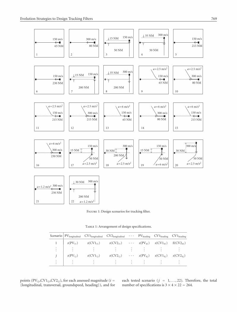
There are eight specified simple scenarios with uniformmotion, and twelve complex scenarios including initializa-tion with uniform motion, transition to transversal maneu-ver, and a second transition to come back to uniform motion.When the target is far enough from the radar, a pure radialapproach to the radar leads to the worst case for transver-sal and heading errors during maneuver transitions, since az-imuth error (much higher than radial error) is projected overthese components. With a similar reasoning, a pure tangen-tial approach is the worst case for longitudinal and ground-speed errors during maneuvers. So, the scenarios basicallycontain these two types of situations, varying in distance, ve-locities, and acceleration magnitudes. The authors have con-sidered a couple of scenarios with longitudinal maneuvers al-though ARTAS does not specify performance for that type ofsituations. The reason for this is that these operations ap-pear in civil operations (especially in the TMAs) and thefilter is conceived to operate in real conditions. Otherwise,the resulting tracking filter could be overfitted to transver-sal maneuvers, but developing undesirable systematic errorswith longitudinal maneuvers. The specifications for longitu-dinal scenarios were obtained extrapolating the ARTAS re-lations for the new input conditions. The resulting 22 sce-narios, to be taken into account in the design of tracking fil-ter are shown in Figure 1 (a circle represents radar positionand a square the initial position of target trajectory). Sincethe specifications depend tightly on the input conditions,there is no a priori worst case scenario whose attainmentwould guarantee all cases, but all of them have to be consid-ered simultaneously in the design process. It must be takeninto account that the design of tracker will be done con-sidering that all requirements will be met without interme-diate adaptation of the tracker parameters once the trackerhas been tuned for the typical radar characteristics and con-trolled volume (in this case, enroute area). The design willprovide a single set of parameters that would allow the fil-ter to accomplish all the specifications in all the scenariosconsidered.

For each of these scenarios, the performance of thetracker should approach listed performance goal values un-

der the defined conditions. The accuracy requirements areexpressed as a function of several input parameters depend-ing on each specific-tested scenario: groundspeed, range, ori-entation of the trajectory with respect to the radar (radialand tangential projection of velocity heading), magnitude ofthe transversal acceleration, and magnitude of the ground-speed change. There are four quality parameters in whichthe requirements are defined: two for position (errors mea-sured along and across trajectory direction, resp., longitu-dinal and transversal errors) and velocity (errors expressedin the groundspeed and heading components). All of themare expressed with the root mean square errors (RMSE), es-timated by means of Monte Carlo simulation. Similarly, ac-curacy requirements are also defined for vertical coordinates,but this work will address only the 2D (horizontal) filtering,although similar ideas could be used for the design of a ver-tical tracker.

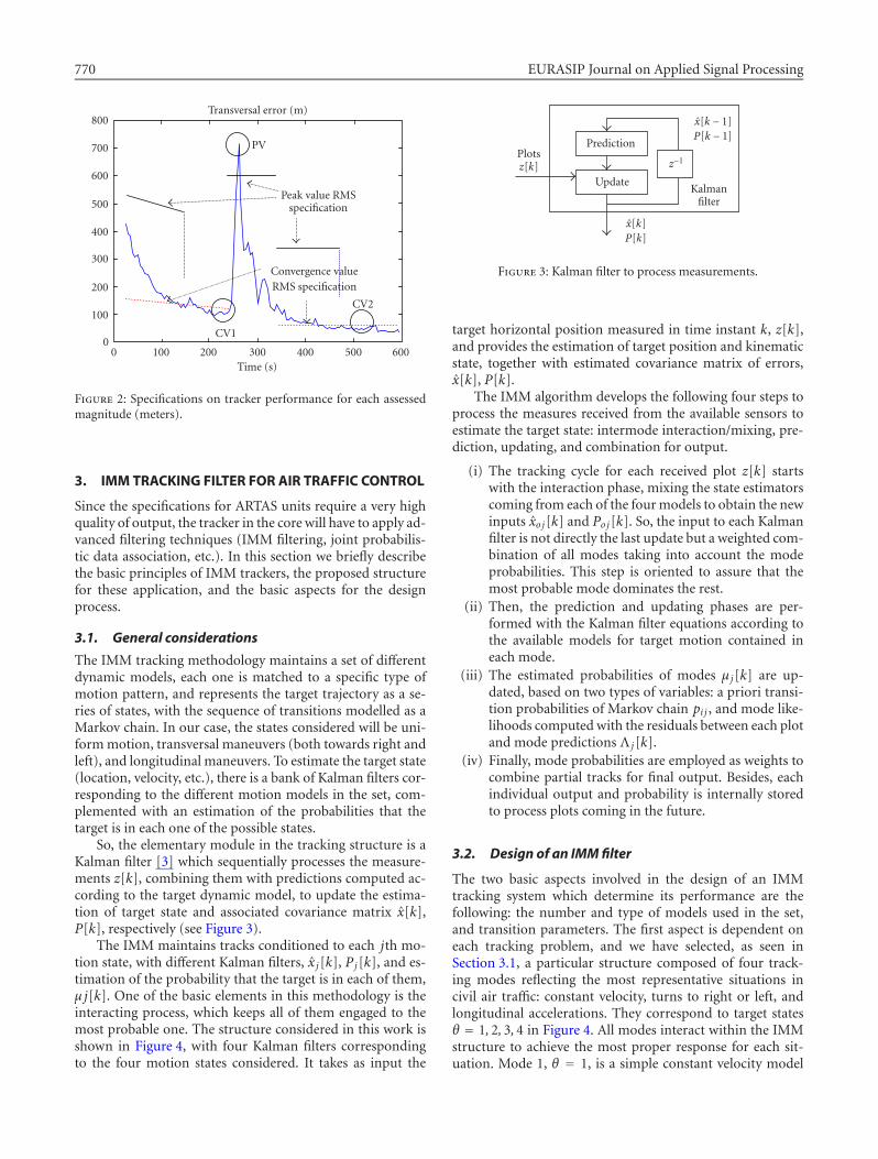
There are three basic parameters characterizing the de-sired shape of the RMS functions: peak value (RMSpv), con-vergence value (RMScv), and time period of RMS conver-gence to a certain level close to the final convergence value(RMSpv + c∗RMSpv). These values are specified for differ-ent situations: initialization, transition from uniform motionto turn, and transition to come back from turn to uniformmotion. Therefore, for each type of situation, the specifi-cations are particularized according to the target evolution,defining a bounding mask for each magnitude and scenario.An example is indicated in Figure 2, with the transversal er-ror obtained through simulation and the ARTAS boundingmask for the scenario 10. Instead of measuring performancealong the whole trajectory in each scenario, only some inter-est points in the aircraft trajectory will be assessed to guar-antee that the measured performance attains the boundingmask: convergence RMSE in rectilinear motion before andafter maneuver segments (CV1 and CV2), and maximumRMSE during maneuver (PV).

The design of a tracking filter aims at attaining a sat-isfactory trade-off among all specifications. The quality ofthe design will be evaluated by means of simulation over22 test scenarios, producing several types of trade-offs tobe considered. First, the different transitions in modes offlight (uniform and maneuvers) impose a trade-off betweensteady-state smoothing and peak error during maneuvers,which always lead to conflicting requirements (the higher thesmoothing factor the higher the filter error during transi-tions and vice versa). This is considered with the three rep-resentative values for each scenario and magnitude: CV1,CV2, and PV. Secondly, each one of the magnitudes eval-uated (transversal, longitudinal, heading and groundspeedRMS errors) could individually shift the design towards dif-ferent solutions, and so all magnitudes must be consideredat the same time to arrive to a certain compromise. Fi-nally, different design scenarios impose harder conditionsfor different magnitudes (radial trajectories for transversaland heading errors, etc.) so that all scenarios should betaken into account. In Table 1, we indicate the arrangementof specifications as they will be considered in the design.Specifications s(·) are particularized for the three evaluation

Evolution Strategies to Design Tracking Filters 769

1

150 m/s

65 NM

2

300 m/s

80 NM

3

150 m/s15 NM

50 NM

4

300 m/s35 NM

50 NM

5

150 m/s

215 NM

6

150 m/s

230 NM

7

150 m/s15 NM

200 NM8

300 m/s35 NM

200 NM9

150 m/s

65 NM

a=2.5 m/s2

10

300 m/s

80 NM

a=2.5 m/s2

11

150 m/s

215 NM

a=2.5 m/s2

12

300 m/s

215 NM

a=2.5 m/s2

13

150 m/s

65 NM

a=6 m/s2

14

300 m/s

80 NM

a=6 m/s2

15

150 m/s

215 NM

a=6 m/s2

16

300 m/s

230 NM

a=6 m/s2

17

150 m/s

15 NM

50 NM

a=2.5 m/s218

300 m/s

200 NM

30 NM

a=2.5 m/s219

150 m/s

50 NM

15 NM

a=6 m/s220

300 m/s

50 NM

30 NM

a=2.5 m/s2

21

300 m/s

230 NM

a=1.2 m/s2

22

300 m/s30 NM

200 NM

a=1.2 m/s2

Figure 1: Design scenarios for tracking filter.

Table 1: Arrangement of design specifications.

Scenario PVlongitudinal CV1longitudinal CV2longitudinal · · · PVheading CV1heading CV1heading

1 s(PV11) s(CV111) s(CV211) · · · s(PV41) s(CV141) S(CV241)...

......

......

......

...

j s(PV1 j) s(CV11 j) s(CV21 j) · · · s(PV4 j) s(CV14 j) s(CV24 j)...

......

......

......

...

points (PVi j ,CV1i j ,CV2i j), for each assessed magnitude (i ={longitudinal, transversal, groundspeed, heading}), and for

each tested scenario ( j = 1, . . . , 22). Therefore, the totalnumber of specifications is 3× 4× 22 = 264.

770 EURASIP Journal on Applied Signal Processing

PV

CV1

CV2

0 100 200 300 400 500 600Time (s)

0

100

200

300

400

500

600

700

800Transversal error (m)

Peak value RMSspecification

Convergence valueRMS specification

Figure 2: Specifications on tracker performance for each assessedmagnitude (meters).

3. IMM TRACKING FILTER FOR AIR TRAFFIC CONTROL

Since the specifications for ARTAS units require a very highquality of output, the tracker in the core will have to apply ad-vanced filtering techniques (IMM filtering, joint probabilis-tic data association, etc.). In this section we briefly describethe basic principles of IMM trackers, the proposed structurefor these application, and the basic aspects for the designprocess.

3.1. General considerations

The IMM tracking methodology maintains a set of differentdynamic models, each one is matched to a specific type ofmotion pattern, and represents the target trajectory as a se-ries of states, with the sequence of transitions modelled as aMarkov chain. In our case, the states considered will be uni-form motion, transversal maneuvers (both towards right andleft), and longitudinal maneuvers. To estimate the target state(location, velocity, etc.), there is a bank of Kalman filters cor-responding to the different motion models in the set, com-plemented with an estimation of the probabilities that thetarget is in each one of the possible states.

So, the elementary module in the tracking structure is aKalman filter [3] which sequentially processes the measure-ments z[k], combining them with predictions computed ac-cording to the target dynamic model, to update the estima-tion of target state and associated covariance matrix x[k],P[k], respectively (see Figure 3).

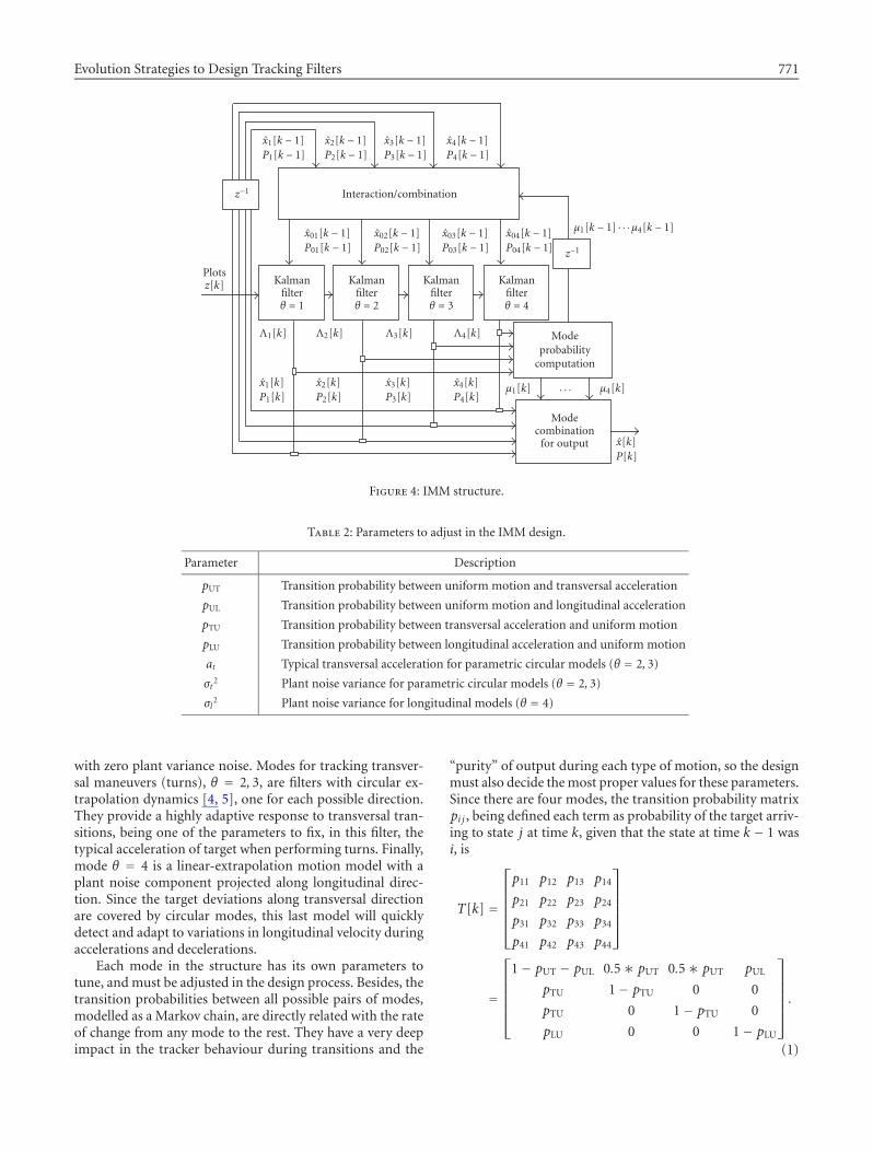
The IMM maintains tracks conditioned to each jth mo-tion state, with different Kalman filters, x j[k], Pj[k], and es-timation of the probability that the target is in each of them,µ j[k]. One of the basic elements in this methodology is theinteracting process, which keeps all of them engaged to themost probable one. The structure considered in this work isshown in Figure 4, with four Kalman filters correspondingto the four motion states considered. It takes as input the

Plotsz[k]

Prediction

UpdateKalman

filter

x[k − 1]P[k − 1]

z−1

x[k]P[k]

Figure 3: Kalman filter to process measurements.

target horizontal position measured in time instant k, z[k],and provides the estimation of target position and kinematicstate, together with estimated covariance matrix of errors,x[k], P[k].

The IMM algorithm develops the following four steps toprocess the measures received from the available sensors toestimate the target state: intermode interaction/mixing, pre-diction, updating, and combination for output.

(i) The tracking cycle for each received plot z[k] startswith the interaction phase, mixing the state estimatorscoming from each of the four models to obtain the newinputs xo j[k] and Poj[k]. So, the input to each Kalmanfilter is not directly the last update but a weighted com-bination of all modes taking into account the modeprobabilities. This step is oriented to assure that themost probable mode dominates the rest.

(ii) Then, the prediction and updating phases are per-formed with the Kalman filter equations according tothe available models for target motion contained ineach mode.

(iii) The estimated probabilities of modes µj[k] are up-dated, based on two types of variables: a priori transi-tion probabilities of Markov chain pi j , and mode like-lihoods computed with the residuals between each plotand mode predictions Λ j[k].

(iv) Finally, mode probabilities are employed as weights tocombine partial tracks for final output. Besides, eachindividual output and probability is internally storedto process plots coming in the future.

3.2. Design of an IMM filter

The two basic aspects involved in the design of an IMMtracking system which determine its performance are thefollowing: the number and type of models used in the set,and transition parameters. The first aspect is dependent oneach tracking problem, and we have selected, as seen inSection 3.1, a particular structure composed of four track-ing modes reflecting the most representative situations incivil air traffic: constant velocity, turns to right or left, andlongitudinal accelerations. They correspond to target statesθ = 1, 2, 3, 4 in Figure 4. All modes interact within the IMMstructure to achieve the most proper response for each sit-uation. Mode 1, θ = 1, is a simple constant velocity model

Evolution Strategies to Design Tracking Filters 771

Plotsz[k]

x1[k − 1]P1[k − 1]

x2[k − 1]P2[k − 1]

x3[k − 1]P3[k − 1]

x4[k − 1]P4[k − 1]

z−1 Interaction/combination

x01[k − 1]P01[k − 1]

x02[k − 1]P02[k − 1]

x03[k − 1]P03[k − 1]

x04[k − 1]P04[k − 1] z−1

µ1[k − 1] · · · µ4[k − 1]

Kalmanfilterθ = 1

Kalmanfilterθ = 2

Kalmanfilterθ = 3

Kalmanfilterθ = 4

Λ1[k] Λ2[k] Λ3[k] Λ4[k]

x1[k]P1[k]

x2[k]P2[k]

x3[k]P3[k]

x4[k]P4[k]

µ1[k] · · · µ4[k]

Modeprobability

computation

Modecombination

for output x[k]P[k]

Figure 4: IMM structure.

Table 2: Parameters to adjust in the IMM design.

Parameter Description

pUT Transition probability between uniform motion and transversal acceleration

pUL Transition probability between uniform motion and longitudinal acceleration

pTU Transition probability between transversal acceleration and uniform motion

pLU Transition probability between longitudinal acceleration and uniform motion

at Typical transversal acceleration for parametric circular models (θ = 2, 3)

σt2 Plant noise variance for parametric circular models (θ = 2, 3)

σl2 Plant noise variance for longitudinal models (θ = 4)

with zero plant variance noise. Modes for tracking transver-sal maneuvers (turns), θ = 2, 3, are filters with circular ex-trapolation dynamics [4, 5], one for each possible direction.They provide a highly adaptive response to transversal tran-sitions, being one of the parameters to fix, in this filter, thetypical acceleration of target when performing turns. Finally,mode θ = 4 is a linear-extrapolation motion model with aplant noise component projected along longitudinal direc-tion. Since the target deviations along transversal directionare covered by circular modes, this last model will quicklydetect and adapt to variations in longitudinal velocity duringaccelerations and decelerations.

Each mode in the structure has its own parameters totune, and must be adjusted in the design process. Besides, thetransition probabilities between all possible pairs of modes,modelled as a Markov chain, are directly related with the rateof change from any mode to the rest. They have a very deepimpact in the tracker behaviour during transitions and the

“purity” of output during each type of motion, so the designmust also decide the most proper values for these parameters.Since there are four modes, the transition probability matrixpi j , being defined each term as probability of the target arriv-ing to state j at time k, given that the state at time k − 1 wasi, is

T[k] =

p11 p12 p13 p14

p21 p22 p23 p24

p31 p32 p33 p34

p41 p42 p43 p44

=

1− pUT − pUL 0.5∗ pUT 0.5∗ pUT pUL

pTU 1− pTU 0 0

pTU 0 1− pTU 0

pLU 0 0 1− pLU

.

(1)

772 EURASIP Journal on Applied Signal Processing

The number of parameters have been simplified by consider-ing only as possible transitions between uniform motion andthe rest of modes. The parameters pUT, pUL are the probabili-ties of starting transversal and longitudinal maneuvers, givenan aircraft at uniform motion, while the parameters pTU, pLU

are the probabilities of transitions to uniform motion, giventhat the aircraft is performing, respectively, transversal andlongitudinal maneuvers.

It is important to notice that all parameters, those ineach particular model plus transition probabilities in Markovchain, are completely coupled through the IMM algorithmsince partial outputs from each mode are combined andfeedback all modes. So, there is a strongly nonlinear inter-action between them, making the adjusting process certainlydifficult. The whole set of parameters in the tracking struc-ture is summarized in Table 2.

4. DESIGN OF FILTER PARAMETERS

The design of the particular IMM tracking structure ad-dressed in this work, stated as adjusting the seven numericinput parameters to fit filter performance within ARTASspecifications, can be generally considered as a numerical op-timization problem. We are searching for the proper combi-nation of real input parameters that minimizes a real func-tion assessing the quality of solutions as a cost f : V ⊂R7 → R. The final design solution −→xd ∈ V should be aglobal minimum of f , which means that f (−→xd) ≤ f (−→x ) forany −→x ∈ V ⊂ R7. The subspace V stands for the regionof feasible solutions, defined as those vectors representinga valid IMM filter: parameters for probabilities must fall inthe interval [0, 1] and parameters for variances must be pos-itive. These are the only constraints to be accomplished bysolutions during the search. Performance specifications arenot considered as constraints here, but they will be used aspenalty terms in the objective cost function. The cost wouldachieve a minimum value of zero only in the ideal case of asolution accomplishing all specifications, grading the rest ofpossible cases with a positive global cost function that will bedetailed later.

4.1. Evolution strategies

In numeric optimization problems, when f is a smooth,low-dimensional function, there are an available numberof classic optimization methods. The best case is for low-dimensional analytical functions, where solutions can be an-alytically determined or found with simple sampling meth-ods. If partial derivatives of function with respect to inputparameters are available, gradient-descent methods could beused to find the directions leading to a minimum. However,these gradient-descent methods quickly converge and stop atlocal minima, so additional steps must be added to find theglobal minimum. For instance, with a moderated number ofglobal minima, we could run several gradient-descent solversto find the best solution. The problem is that the numberof similar local minima increases exponentially with dimen-sionality, making these types of solvers unfeasible. In our par-ticular case, besides a high-dimensional input space causing

multimodal dependence, we do not have an analytical func-tion to optimize. It is the result of a complex and exhaus-tive evaluation process implying the simulation and perfor-mance assessment of tracking structure on the whole set of22 scenarios defined. The evaluation of a single point in theinput space requires several minutes of CPU time (PentiumIII, 700 MHz). Besides, the evaluation of quality after all sim-ulations is not direct but it should take into account systemperformance in all scenarios and magnitudes in comparisonwith the whole table of specifications. As we will see later,multiple specifications (or objectives) will increase the num-ber of solutions with similar performance, increasing there-fore the complexity of the search.

For complex domains, evolutionary algorithms haveproven to be robust and efficient stochastic optimizationmethods, combining properties of volume and path-orientedsearching techniques. ES [6] are the evolutionary algorithmsspecifically conceived for numerical optimization, and havebeen successfully applied to engineering optimization prob-lems with real-valued vector representations [7]. They com-bine a search process which randomly scans the feasible re-gion (exploration) and local optimization along certain paths(exploitation), achieving very acceptable rates of robustnessand efficiency. Each solution to the problem is defined as anindividual in a population, codifying each individual with acouple of real-valued vectors: the searched parameters and astandard deviation of each parameter used in the search pro-cess. In this specific problem, one individual will representthe set of dynamic parameters in the IMM structure, as in-dicated in Table 2, (x1, . . . , x7), and their corresponding stan-dard deviations (σ1, . . . , σ7).

The optimization search basically consists in evolving apopulation of individuals in order to find better solutions.The computational procedure of ES can be summarized inthe following steps, according to the named “µ + λ” strategydefined by Back and Schwefel [8], and particularized for ourproblem:

(1) generate an initial population with µ individuals uni-formly distributed on the search space V ;

(2) evaluate the objective value for each individual in pop-ulation f (−→xi ), i = 1, . . . , µ;

(3) Select the best parents in population to generate a setof λ new individuals, by means of genetic operatorsof recombination and mutation. In this case, recombi-nation follows a canonical discrete recombination [6],and mutation is carried out as follows:

σ ′i = σi exp{N(0,∆σ)

},

x′i = xi + N(0, σ ′i

),

(2)

where x′i and σ ′i are the mutated values and N(0, σ)stands for a normal distribution with zero mean andvariance σ2;

(4) calculate the objective value of the generated offspringf (−→xi ), i = 1, . . . , λ, and select the best µ individuals ofthis new set containing parents and children to formthe next generation;

Evolution Strategies to Design Tracking Filters 773

(5) Stop if the halting criterion is satisfied. Otherwise, goto step (3).

We have implemented ES for this problem with a size of50 + 30 individuals and mutation factor ∆σ = 0.9. Thefitness function will directly depend on the differences be-tween RMS values of errors, evaluated through Monte Carlosimulation, and ARTAS specifications for all scenarios andmagnitudes, as will be detailed next. It is important to no-tice that simulations are carried out using common randomnumbers to evaluate all individuals in all generations, en-hancing system comparison within the optimization loop. Inother words, the noise samples used to simulate all scenar-ios in the RMS evaluation are the same for each individualin order to exploit the advantages coming from the use ofa deterministic fitness function. Besides, the number of it-erations was selected to guarantee that confidence intervalsof estimated figures were short in relation to the estimatedvalues.

A basic aspect to achieve successful optimization in anyevolutionary algorithm is the control of diversity, but thisappropriateness will depend on the problem landscape. If apopulation converges to a particular point in a search spacetoo fast in relation to the roughness of its landscape, it isvery probable that it will end in a local minimum. On thecontrary, a too slow convergence will require a large com-putational effort to find the solution. ES give the higher im-portance to the mutation operator, achieving the interestingproperty of being “self-adaptive” in the sizes of steps carriedout during mutation, as indicated in step (3) of the algo-rithm above. Before selecting an algorithm for optimization,it is interesting to consider the point of view of the “no freelunch” (NFL) theorem [9], which asserts that no optimiza-tion procedure is better than a random search if the perfor-mance measurement consists in averaging arbitrary fitnessfunctions. The performance of ES has been widely analyzedunder a set of well-known test functions [8, 10]. They areartificial analytical functions used as benchmarks for com-parison of representative properties of optimization tech-niques, such as convergence velocity under unimodal land-scapes, robustness with multimodality, nonlinearity, con-straints, presence of flat plateaus at different heights, and soforth. However, the performance on these test functions can-not be directly extrapolated to real engineering applications.The application of ES to a new problem, such as our com-plex IMM design against multiple specifications where thelandscape properties are not known (it is not known evenif there is a global minimum or not), is a challenge open toresearch.

4.2. Multiobjective optimization

The selection of the proper fitness function for this applica-tion is the problem-dependent feature with the highest im-pact on the algorithm (higher than the ES parameters suchas population size or mutation factor). Really, we should re-gard this design as a multiobjective optimization problem,where each individual objective is the minimization of differ-ence between desired specification and assessed performance

in each specific figure of merit. When a problem involves si-multaneous optimization of multiple, usually conflicting ob-jectives (or criteria), the goal is not so clear as in the case ofsingle-objective optimization. The presence of different ob-jectives generates a set of alternative solutions, defined asPareto-optimal solutions [11]. The presence of conflictingmultiple objectives leads to the fact that different solutionscannot be directly compared and ranked to determine thebest one, but the concept of domination appears for com-parisons. A solution −→x1 is dominated by a second one −→x2 if−→x2 is better than −→x1 simultaneously in all objective functionsconsidered. In any other case, they could not be strictly com-pared. Taking into account this concept of domination, aPareto-optimal set P is defined as the set of solutions suchthat there exists no solution in the search space dominatingany member in P.

Some multiobjective optimization techniques have thedouble goal of guiding the search towards the global Pareto-optimal set and at the same time covering as many solutionsas possible. There are several proposed evolutionary methods[12] that address this goal by maintaining a population di-versity to cover the whole Pareto front. This fact implies firstthe enlargement of population size and then specific proce-dures to guarantee guiding the search to the desired optimalset with a well-distributed sample of the front. Among theseprocedures, we can mention methods, such as selection byaggregation and so forth, switching the objectives during theselection phase to decide which individuals will appear in themating pool. Zitzler et al. [12] analyze and compare, oversome standard test analytical functions, some of the mostoutstanding multiobjective evolutionary algorithms.

From the authors point of view, the peculiarities of theproblem dealt with, namely, the complexity and computa-tional cost of evaluation function together with the consid-erable number of specifications, preclude the application oftechniques to derive the whole Pareto set. We have consid-ered a weighting sum on partial goals to build a global fitnessfunction:

Minimize−→xM∑i=1

wi fi(−→x ). (3)

As indicated by Deb [11], this type of approaches withweighted sums converge to particular solutions of Paretofront, corresponding to the tangential point in the directiondefined by the vector of weights. The general idea is illus-trated in Figure 5 for a simplified case with only two objectivefunctions f1 and f2. The shaded area is an example of finiteimage set of the feasible region by objective functions f1 andf2, being the set of nondominated solutions (Pareto front, P)represented with a bold line. No solution in the image set hassimultaneously lower values in f1 and f2 than any point inP. A pair of weights define a direction for search in space ofobjective functions, leading to the tangential point for eachsolution.

However, a large number of specifications will make theweighted summation cumbersome, being difficult that allobjectives are simultaneously considered to guide the search.

774 EURASIP Journal on Applied Signal Processing

f2

Minimum ofw1 f1 + w2 f2

f1Minimum ofw′

1 f1 + w′2 f2

Pareto-optimal front

Figure 5: Solutions with a weighted sum method.

In our specific problem, we should fix a weighting vectorwith 264 components. A variation is proposed to reduce thenumber of objectives in the sum by exploiting knowledgeabout the problem. Basically, objectives with similar behav-ior are grouped to select a “representative” per group, theone with the worst value, so that it guarantees that all ob-jectives in the group are represented in the final function. Ifwe consider Table 1 with the whole set of specifications, weare going to select the worst case for each column, leavingonly 12 terms in the summation. It is important to notice thatthis maximum operation will break the linearity of functionwith respect to objectives and will make the landscape de-pend on each specific input vector. A trajectory of solutionsin the search process may jump along different goal functionsif the scenarios with the worst case change. The justificationcomes from the fact that each magnitude has certain depen-dence with the input parameters similar in all scenarios, so asingle representative is enough to be considered in the opti-mization. Besides, the selection of the worst case assures thatif the method can satisfy that term, all the scenarios will besimultaneously accomplished.

Taking into account this consideration, the fitness func-tion, which assesses the quality of a solution as the degreeof attainment performance figures with respect to specifica-tions, is presented next. The following details have also beenconsidered.

(i) It assesses the excess over the specification for eachperformance figure, penalizing a solution as the er-ror increases, but once the error is below the speci-fication, the cost is zero. This is so because there isno additional advantage if the RMSE decreases moreafter the required values are attained. This is imple-mented for each magnitude by means of the expres-sion R(pi − s(pi)), where pi is the ith performance fig-ure (RMSE), s(pi) the specification, and R(·) the rampfunction:

R(x) =x, x > 0,

0, x ≤ 0.(4)

(ii) Different physical magnitudes (errors in position,heading, and groundspeed) have the same importance,

0 20 40 60 80 100 120 140Generations

0

5

10

15

20

Fitn

ess

20 40 60 80 100 120 140

250

200

150

100

50

Exc

ess

over

spec

ifica

tion

s

Figure 6: Evolution of fitness and performance in each specific ob-jective.

and so are normalized with the specification value,defining a partial cost for ith figure,

ci = R(pi − s(pi)

pi

). (5)

(iii) In order to add some flexibility in the trade-off be-tween maneuver and uniform motion performances,weighting factors αt are included. They allow us to varythe priority of these performance figures, in the casewhere all of them cannot be attained at the same time,defining therefore a cost per jth scenario,

c(s j) = 4∑

i=1

{αPVR

(PVi j − s

(PVi j

)(PVi j

))

+ αCV1R

(CV1i j − s

(CV1i j

)s(CV1i j

))

+ αCV2R

(CV2i j − s

(CV2i j

)s(CV2i j

))}

,

(6)

where the subindex i represents each interest mag-nitude (longitudinal, transversal, groundspeed, andheading) and j the scenario index.

(iv) Finally, considering the set E of all the scenarios wherethe performance figures are evaluated (in our example,the 22 scenarios indicated in Figure 1), the worst casescenario is j, for each figure of merit and selected time

Evolution Strategies to Design Tracking Filters 775

0 50 100 150 200 250 300 350 400 450Time

0

100

200

300

400

500

600

700Longitudinal error (m)

0 50 100 150 200 250 300 350 400 450Time

100

200

300

400

500

600

700

800

900

1000

1100Transversal error (m)

50 100 150 200 250 300 350 400Time

0

2

4

6

8

10

12

14

16

Groundspeed error (m)

0 50 100 150 200 250 300 350 400 450Time

0

2

4

6

8

10

12

14

16

18

20Heading error (m)

Figure 7: Performance and ARTAS specifications for scenario 12.

instant (PV, CV1, and CV2). Therefore, the final goalfunction to be minimized is as follows:

4∑i=1

{αPV max

j∈E

[R

(PVi j − s

(PVi j

)(PVi j

))]

+ αCV1 maxj∈E

[R

(CV1i j − s

(CV1i j

)s(CV1i j

))]

+ αCV2 maxj∈E

[R

(CV2i j − s

(CV2i j

)s(CV2i j

))]}

.

(7)

So, this function considers the relative excesses overspecifications for all performance figures, each one as-sessed in the worst case scenario.

5. RESULTS

In this section, the results obtained along the optimizationprocess to adjust the filter parameters according to ARTAS

specifications are presented and analyzed. They have beenobtained particularizing expression (6) to the case of a weightof 1 for all magnitudes αPV = αCV1 = αCV2 = 1.

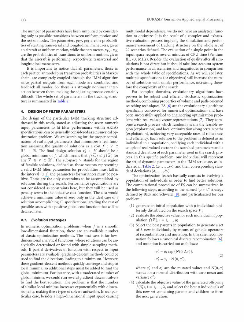
First, Figure 6 summarizes the evolution of best individ-ual in the population (the one with the lowest value of fit-ness), indicating graphically the accomplishment of specifi-cations along the generations. Each design objective is pre-sented by a row in the diagram, while the best individual foreach generation appears in each column. The grey level ofposition (i, j) in the image indicates the quality of the fittingto the ith specification of the best individual for the jth gen-eration. The grey level represents linearly the relative excessover the restriction (no excess is presented as white, 100%or higher excess as black), which is the partial cost functionrelated with this constraint. Therefore, a completely whitecolumn means that the optimization process has found aset of parameters able to fulfil all design restrictions, whilea complete white row means that all best individuals in thisoptimization exercise are able to fulfil the specification for

776 EURASIP Journal on Applied Signal Processing

0 50 100 150 200 250 300 350Time

0

50

100

150

200

250

300

350Longitudinal error (m)

0 50 100 150 200 250 300 350Time

50

100

150

200

250

300

350

400

450

500Transversal error (m)

0 50 100 150 200 250 300 350Time

0

1

2

3

4

5

6

7

8

Groundspeed error (m)

0 50 100 150 200 250 300 350Time

0

5

10

15

20

25

30Heading error (m)

Figure 8: Performance and ARTAS specifications for scenario 13.

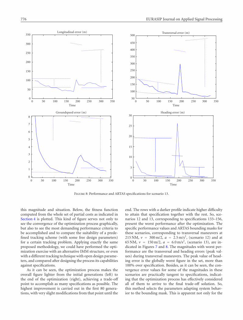
this magnitude and situation. Below, the fitness functioncomputed from the whole set of partial costs as indicated inSection 4 is plotted. This kind of figure serves not only tosee the convergence of the optimization process graphically,but also to see the most demanding performance criteria tobe accomplished and to compare the suitability of a prede-fined tracking scheme (with some free design parameters)for a certain tracking problem. Applying exactly the sameproposed methodology, we could have performed the opti-mization exercise with an alternative IMM structure, or evenwith a different tracking technique with open design parame-ters, and compared after designing the process its capabilitiesagainst specifications.

As it can be seen, the optimization process makes theoverall figure lighter from the initial generations (left) tothe end of the optimization (right), achieving a trade-offpoint to accomplish as many specifications as possible. Thehighest improvement is carried out in the first 80 genera-tions, with very slight modifications from that point until the

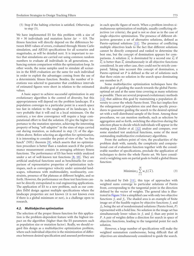
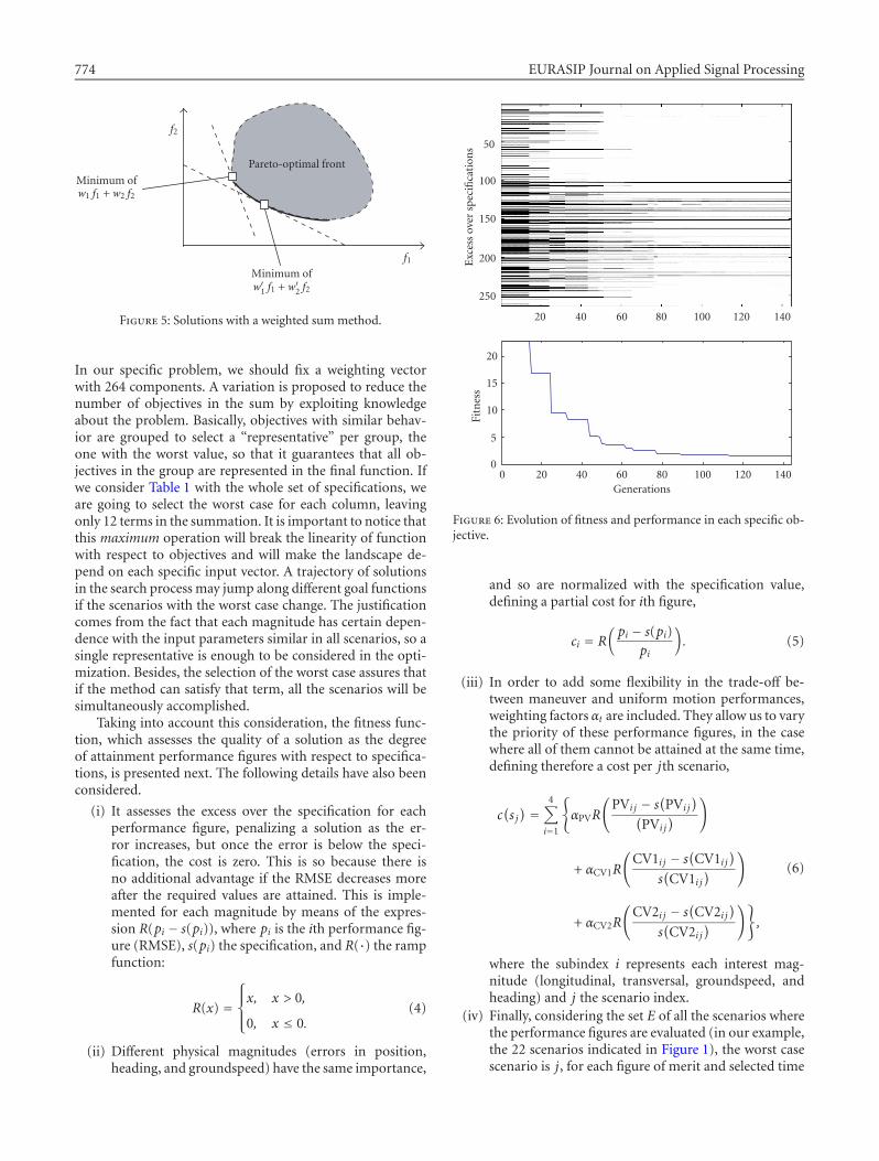
end. The rows with a darker profile indicate higher difficultyto attain that specification together with the rest. So, sce-narios 12 and 13, corresponding to specifications 133–156,present the worst performance after the optimization. Thespecific performance values and ARTAS bounding masks forthese scenarios, corresponding to transversal maneuvers at215 NM, v = 300 m/2, a = 2.5 m/s2, (scenario 12) and at65 NM, v = 150 m/2, a = 6.0 m/s2, (scenario 13), are in-dicated in Figures 7 and 8. The magnitudes with worst per-formance are the transversal and heading errors (peak val-ues) during transversal maneuvers. The peak value of head-ing error is the globally worst figure in the set, more than100% over specification. Besides, as it can be seen, the con-vergence error values for some of the magnitudes in thesescenarios are practically tangent to specifications, indicat-ing that the optimization process has effectively consideredall of them to arrive to the final trade-off solution. So,this method selects the parameters adapting system behav-ior to the bounding mask. This is apparent not only for the

Evolution Strategies to Design Tracking Filters 777

1 2 3 4 5 6 7 8 9 10Runs

250

200

150

100

50

Exc

ess

over

spec

ifica

tion

s

1 2 3 4 5 6 7 8 9 10Runs

1.651.7

1.751.8

1.851.9

1.952

2.05

2.1

Fitn

ess

Figure 9: Evolution of fitness and performance in each specific ob-jective.

presented scenarios with worst cases but for all design sce-narios as well.

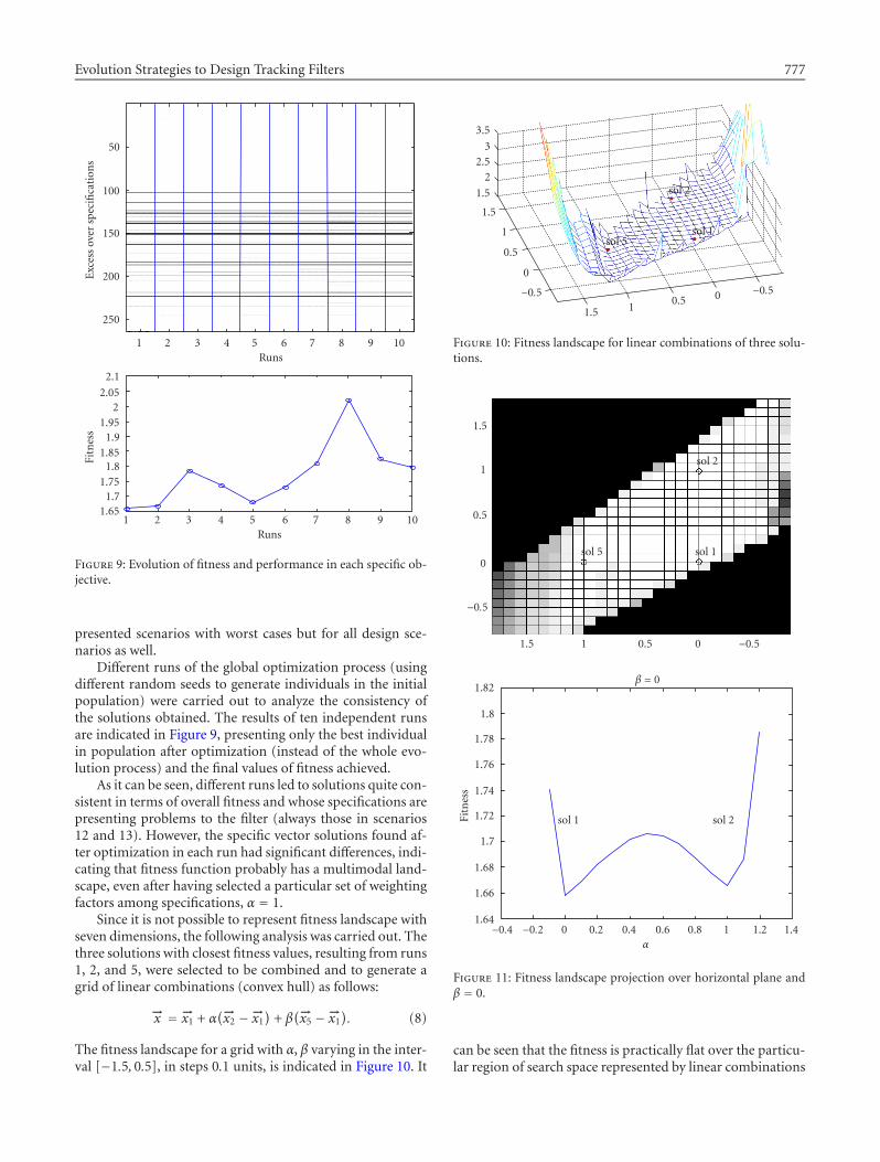
Different runs of the global optimization process (usingdifferent random seeds to generate individuals in the initialpopulation) were carried out to analyze the consistency ofthe solutions obtained. The results of ten independent runsare indicated in Figure 9, presenting only the best individualin population after optimization (instead of the whole evo-lution process) and the final values of fitness achieved.

As it can be seen, different runs led to solutions quite con-sistent in terms of overall fitness and whose specifications arepresenting problems to the filter (always those in scenarios12 and 13). However, the specific vector solutions found af-ter optimization in each run had significant differences, indi-cating that fitness function probably has a multimodal land-scape, even after having selected a particular set of weightingfactors among specifications, α = 1.

Since it is not possible to represent fitness landscape withseven dimensions, the following analysis was carried out. Thethree solutions with closest fitness values, resulting from runs1, 2, and 5, were selected to be combined and to generate agrid of linear combinations (convex hull) as follows:

−→x = −→x1 + α(−→x2 −−→x1

)+ β

(−→x5 −−→x1). (8)

The fitness landscape for a grid with α, β varying in the inter-val [−1.5, 0.5], in steps 0.1 units, is indicated in Figure 10. It

1.5 10.5 0 −0.5

1.5

1

0.5

0

−0.5

1.5

22.5

3

3.5

sol 1

sol 2

sol 5

Figure 10: Fitness landscape for linear combinations of three solu-tions.

1.5 1 0.5 0 −0.5

−0.5

0

0.5

1

1.5

sol 1

sol 2

sol 5

−0.4 −0.2 0 0.2 0.4 0.6 0.8 1 1.2 1.4α

1.64

1.66

1.68

1.7

1.72

1.74

1.76

1.78

1.8

1.82

Fitn

ess

β = 0

sol 1 sol 2

Figure 11: Fitness landscape projection over horizontal plane andβ = 0.

can be seen that the fitness is practically flat over the particu-lar region of search space represented by linear combinations

778 EURASIP Journal on Applied Signal Processing

−0.4 −0.2 0 0.2 0.4 0.6 0.8 1 1.2 1.4β

1.6

1.8

2

2.2

2.4

2.6

2.8

3

Fitn

ess

α = 0

sol 1sol 5

−0.5 0 0.5 1 1.5 2α

1.6

1.7

1.8

1.9

2

2.1

2.2

2.3

2.4

2.5

Fitn

ess

β = 1 − α

sol 5 sol 2

Figure 12: Fitness landscape projection over plane and α = 0, β = 1− α.

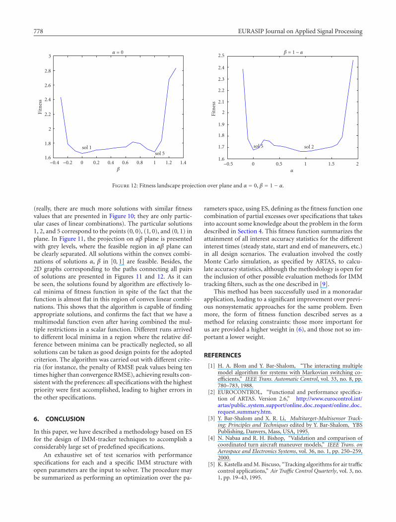
(really, there are much more solutions with similar fitnessvalues that are presented in Figure 10; they are only partic-ular cases of linear combinations). The particular solutions1, 2, and 5 correspond to the points (0, 0), (1, 0), and (0, 1) inplane. In Figure 11, the projection on αβ plane is presentedwith grey levels, where the feasible region in αβ plane canbe clearly separated. All solutions within the convex combi-nations of solutions α, β in [0, 1] are feasible. Besides, the2D graphs corresponding to the paths connecting all pairsof solutions are presented in Figures 11 and 12. As it canbe seen, the solutions found by algorithm are effectively lo-cal minima of fitness function in spite of the fact that thefunction is almost flat in this region of convex linear combi-nations. This shows that the algorithm is capable of findingappropriate solutions, and confirms the fact that we have amultimodal function even after having combined the mul-tiple restrictions in a scalar function. Different runs arrivedto different local minima in a region where the relative dif-ference between minima can be practically neglected, so allsolutions can be taken as good design points for the adoptedcriterion. The algorithm was carried out with different crite-ria (for instance, the penalty of RMSE peak values being tentimes higher than convergence RMSE), achieving results con-sistent with the preferences: all specifications with the highestpriority were first accomplished, leading to higher errors inthe other specifications.

6. CONCLUSION

In this paper, we have described a methodology based on ESfor the design of IMM-tracker techniques to accomplish aconsiderably large set of predefined specifications.

An exhaustive set of test scenarios with performancespecifications for each and a specific IMM structure withopen parameters are the input to solver. The procedure maybe summarized as performing an optimization over the pa-

rameters space, using ES, defining as the fitness function onecombination of partial excesses over specifications that takesinto account some knowledge about the problem in the formdescribed in Section 4. This fitness function summarizes theattainment of all interest accuracy statistics for the differentinterest times (steady state, start and end of maneuvers, etc.)in all design scenarios. The evaluation involved the costlyMonte Carlo simulation, as specified by ARTAS, to calcu-late accuracy statistics, although the methodology is open forthe inclusion of other possible evaluation methods for IMMtracking filters, such as the one described in [9].

This method has been successfully used in a monoradarapplication, leading to a significant improvement over previ-ous nonsystematic approaches for the same problem. Evenmore, the form of fitness function described serves as amethod for relaxing constraints: those more important forus are provided a higher weight in (6), and those not so im-portant a lower weight.

REFERENCES

[1] H. A. Blom and Y. Bar-Shalom, “The interacting multiplemodel algorithm for systems with Markovian switching co-efficients,” IEEE Trans. Automatic Control, vol. 33, no. 8, pp.780–783, 1988.

[2] EUROCONTROL, “Functional and performance specifica-tion of ARTAS. Version 2.6,” http://www.eurocontrol.int/artas/public system support/online doc request/online docrequest summary.htm.

[3] Y. Bar-Shalom and X. R. Li, Multitarget-Multisensor Track-ing: Principles and Techniques edited by Y. Bar-Shalom, YBSPublishing, Danvers, Mass, USA, 1995.

[4] N. Nabaa and R. H. Bishop, “Validation and comparison ofcoordinated turn aircraft maneuver models,” IEEE Trans. onAerospace and Electronics Systems, vol. 36, no. 1, pp. 250–259,2000.

[5] K. Kastella and M. Biscuso, “Tracking algorithms for air trafficcontrol applications,” Air Traffic Control Quarterly, vol. 3, no.1, pp. 19–43, 1995.

Evolution Strategies to Design Tracking Filters 779

[6] H. P. Schwefel, Numerical Optimisation of Computer Models,John Wiley & Sons, New York, NY, USA, 1981.

[7] I. Rechenberg, “Evolution strategy: Nature’s way of optimiza-tion,” in Optimization: Methods and Applications, Possibilitiesand Limitations, H. W. Bergmann, Ed., Lecture Notes in En-gineering, pp. 106–126, Springer, Berlin, Germany, 1989.

[8] T. Back, Evolutionary Algorithms in Theory and Practice, Ox-ford University Press, New York, NY, USA, 1996.

[9] D. H. Wolpert and W. G. Macready, “No-free-lunch theoremsfor optimization,” IEEE Trans. on Evolutionary Computation,vol. 1, no. 1, pp. 67–82, 1997.

[10] K. Ohkura, Y. Matsumura, and K. Ueda, “Robust evolutionstrategies,” Applied Intelligence, vol. 15, no. 3, pp. 153–169,2001.

[11] K. Deb, “Evolutionary algorithms for multi-criterion opti-mization in engineering design,” in Evolutionary Algorithms inEngineering and Computer Science, John Wiley & Sons, Chich-ester, UK, 1999, Chapter 8.

[12] E. Zitzler, K. Deb, and L. Thiele, “Comparison of multiobjec-tive evolutionary algorithms: Empirical results,” EvolutionaryComputation, vol. 8, no. 2, pp. 173–195, 2000.

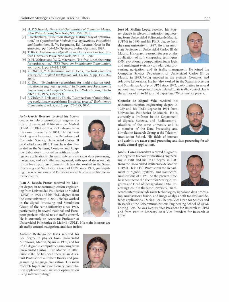
Jesus Garcıa Herrero received his Masterdegree in telecommunication engineeringfrom Universidad Politecnica de Madrid(UPM) in 1996 and his Ph.D. degree fromthe same university in 2001. He has beenworking as a Lecturer at the Department ofComputer Science, Universidad Carlos IIIde Madrid, since 2000. There, he is also inte-grated in the Systems, Complex and Adap-tive Laboratory, involved in artificial intel-ligence applications. His main interests are radar data processing,navigation, and air traffic management, with special stress on datafusion for airport environments. He has also worked in the SignalProcessing and Simulation Group of UPM since 1995, participat-ing in several national and European research projects related to airtraffic control.

Juan A. Besada Portas received his Mas-ter degree in telecommunication engineer-ing from Universidad Politecnica de Madrid(UPM) in 1996 and his Ph.D. degree fromthe same university in 2001. He has workedin the Signal Processing and SimulationGroup of the same university since 1995,participating in several national and Euro-pean projects related to air traffic control.He is currently an Associate Professor atUniversidad Politecnica de Madrid (UPM). His main interests areair traffic control, navigation, and data fusion.

Antonio Berlanga de Jesus received hisB.S. degree in physics from UniversidadAutonoma, Madrid, Spain in 1995, and hisPh.D. degree in computer engineering fromUniversidad Carlos III de Madrid in 2000.Since 2002, he has been there as an Assis-tant Professor of automata theory and pro-gramming language translation. His mainresearch topics are evolutionary computa-tion applications and network optimizationusing soft computing.

Jose M. Molina Lopez received his Mas-ter degree in telecommunication engineer-ing from Universidad Politecnica de Madrid(UPM) in 1993 and his Ph.D. degree fromthe same university in 1997. He is an Asso-ciate Professor at Universidad Carlos III deMadrid. His current research focuses on theapplication of soft computing techniques(NN, evolutionary computation, fuzzy logicand multiagent systems) to radar data pro-cessing, navigation, and air traffic management. He joined theComputer Science Department of Universidad Carlos III deMadrid in 1993, being enrolled in the Systems, Complex, andAdaptive Laboratory. He has also worked in the Signal Processingand Simulation Group of UPM since 1992, participating in severalnational and European projects related to air traffic control. He isthe author of up to 10 journal papers and 70 conference papers.

Gonzalo de Miguel Vela received histelecommunication engineering degree in1989 and his Ph.D. degree in 1994 fromUniversidad Politecnica de Madrid. He iscurrently a Professor in the Departmentof Signals, Systems, and Radiocommu-nications of the same university and isa member of the Data Processing andSimulation Research Group at the Telecom-munication School. His fields of interestand activity are radar signal processing and data processing for airtraffic control applications.

Jose R. Casar Corredera received his gradu-ate degree in telecommunications engineer-ing in 1981 and his Ph.D. degree in 1983from the Universidad Politecnica de Madrid(UPM). He is a Full Professor in the Depart-ment of Signals, Systems, and Radiocom-munications of UPM. At the present time,he is Adjunct to the Rector for Strategic Pro-grams and Head of the Signal and Data Pro-cessing Group at the same university. His re-search interests include radar technologies, signal and data process-ing, multisensory fusion, and image analysis both for civil and de-fence applications. During 1993, he was Vice Dean for Studies andResearch at the Telecommunications Engineering School of UPM.During 1995, he was Deputy Vice President for Research at UPMand from 1996 to February 2000 Vice President for Research atUPM.

Photograph © Turisme de Barcelona / J. Trullàs

Preliminary call for papers

The 2011 European Signal Processing Conference (EUSIPCO 2011) is thenineteenth in a series of conferences promoted by the European Association forSignal Processing (EURASIP, www.eurasip.org). This year edition will take placein Barcelona, capital city of Catalonia (Spain), and will be jointly organized by theCentre Tecnològic de Telecomunicacions de Catalunya (CTTC) and theUniversitat Politècnica de Catalunya (UPC).EUSIPCO 2011 will focus on key aspects of signal processing theory and

li ti li t d b l A t f b i i ill b b d lit

Organizing Committee

Honorary ChairMiguel A. Lagunas (CTTC)

General ChairAna I. Pérez Neira (UPC)

General Vice ChairCarles Antón Haro (CTTC)

Technical Program ChairXavier Mestre (CTTC)

Technical Program Co Chairsapplications as listed below. Acceptance of submissions will be based on quality,relevance and originality. Accepted papers will be published in the EUSIPCOproceedings and presented during the conference. Paper submissions, proposalsfor tutorials and proposals for special sessions are invited in, but not limited to,the following areas of interest.

Areas of Interest

• Audio and electro acoustics.• Design, implementation, and applications of signal processing systems.

l d l d d

Technical Program Co ChairsJavier Hernando (UPC)Montserrat Pardàs (UPC)

Plenary TalksFerran Marqués (UPC)Yonina Eldar (Technion)

Special SessionsIgnacio Santamaría (Unversidadde Cantabria)Mats Bengtsson (KTH)

FinancesMontserrat Nájar (UPC)• Multimedia signal processing and coding.

• Image and multidimensional signal processing.• Signal detection and estimation.• Sensor array and multi channel signal processing.• Sensor fusion in networked systems.• Signal processing for communications.• Medical imaging and image analysis.• Non stationary, non linear and non Gaussian signal processing.

Submissions

Montserrat Nájar (UPC)

TutorialsDaniel P. Palomar(Hong Kong UST)Beatrice Pesquet Popescu (ENST)

PublicityStephan Pfletschinger (CTTC)Mònica Navarro (CTTC)

PublicationsAntonio Pascual (UPC)Carles Fernández (CTTC)

I d i l Li i & E hibiSubmissions

Procedures to submit a paper and proposals for special sessions and tutorials willbe detailed at www.eusipco2011.org. Submitted papers must be camera ready, nomore than 5 pages long, and conforming to the standard specified on theEUSIPCO 2011 web site. First authors who are registered students can participatein the best student paper competition.

Important Deadlines:

P l f i l i 15 D 2010

Industrial Liaison & ExhibitsAngeliki Alexiou(University of Piraeus)Albert Sitjà (CTTC)

International LiaisonJu Liu (Shandong University China)Jinhong Yuan (UNSW Australia)Tamas Sziranyi (SZTAKI Hungary)Rich Stern (CMU USA)Ricardo L. de Queiroz (UNB Brazil)

Webpage: www.eusipco2011.org

Proposals for special sessions 15 Dec 2010Proposals for tutorials 18 Feb 2011Electronic submission of full papers 21 Feb 2011Notification of acceptance 23 May 2011Submission of camera ready papers 6 Jun 2011