Application of Dynamic Programming for the Analysis of Complex Water Resources Systems:

A Case Study on the Mahaweli River Basin Development in Sri Lanka

Ontvangen

U Q -CARDEX

0000 0489

BibJUOlHJbUv

EA£JPBOUWUNIVERSHEEt

Promotoren: Dr.-Ing. J.J. Bogardi Hoogleraar in de Hydrologie, Hydraulica en Kwantitatief Waterbeheer

Dr. P. van Beek Hoogleraar in de Operationele Analyse

M.D.U.P. Kularathna

Application of Dynamic Programming for the Analysis of Complex Water Resources Systems:

A Case Study on the Mahaweli River Basin Development in Sri Lanka

Proefschrift ter verkrijging van de graad van doctor in de landbouw- en milieuwetenschappen op gezag van de rector magnificus, dr. H.C. van der Plas, in het openbaar te verdedigen op vrijdag 12 juni 1992 des namiddags te half twee in de Aula van de Landbouwuniversiteit te Wageningen

To my parents

^O2TX>I \siH

Statements

1. Due to the uncertain conditions under which the actual operation of water resources systems takes place, flexibility of operation is an important aspect which should not be left aside in any operational study.

This thesis.

2. Methodology for formulating long-term operation policies of water resources systems need more attention than their short-term counterparts.

This thesis.

3. In contrast to the optimization models, simulation models can best be employed to assess the performance of a system if the operation policies have been predetermined. This would permit a detailed investigation of the resulting operation pattern and subsequent improvements to the operation policies which are derived by optimization models that include much less details of the system than the simulation models.

This thesis.

4. "Objectives" are often noncommensurate, even in a simple one-man enterprise.

5. Irrigation in Sri Lanka is a long-practised art using the traditional tank-irrigation systems. This vast experience should be integrated in the future development of Sri Lankas water resources systems.

6. An approximate answer to the right question is better than the right answer to a wrong question.

7. To effectively contribute to research, one should not only know how much one knows, but also how much one has yet to learn.

8. Technology must always be appropriate to the country's needs and circumstances. There is a great need for development of such appropriate technology, and also for guidance on ways of selecting the most cost-effective mixture of conventional and new technology.

WMO/UNESCO (199D. Report on Water Resources Assessment, p. 47.

9. The communication and cooperation between the universities and the practitioners need to be improved, in order to narrow the existing gap between theory and practice in the field of water resources management.

W S /

10. In all scientific research, the researcher may or may not find what he/she is looking for. Indeed his/her hypothesis may be demolished. But he/she is certain to learn something, which may be and often is more important than what he/she had hoped to learn.

Robert Heinlein, in: Richard Boyle (1991), The Serendipity Factor, Serendib (The Magazine of Air Lanka1). Vol. 10, No. 4.

11. The environmental impacts of large scale water resources developments have to be carefully investigated in the planning stage, as those impacts are often irreversible.

12. The Forest, With endless life-giving qualities, It protects all living beings And provides shelter Even to those who destroy it with an axe.

The Lord Buddha.

M.D.U.P. Kularathna Application of Dynamic Programming for the Analysis of Complex Water Resources Systems: A Case Study on the Mahaweli River Basin Development in Sri Lanka Wageningen, 12* June 1992

Abstract

Kularathna, M.D.U.P. (1992), Application of Dynamic Programming for the Analysis of Complex Water Resources Systems: A Case Study on the Mahaweli River Basin Development in Sri Lanka, Doctoral Dissertation, Wageningen Agricultural University, Wageningen, The Netherlands, (xviii) + 163 pp., 32 Figures, 32 Tables (Summary and Conclusions in English and Dutch)

The technique of Stochastic Dynamic Programming (SDP) is ideally suited for operation policy analyses of water resources systems. However SDP has a major drawback which is appropriately termed as its "curse of dimensionality".

Aggregation/Disaggregation techniques based on SDP and simulation are presented to analyze a complex water resources system. The system under consideration serves two major purposes: hydropower generation and irrigation. The identification of subsystems by their functional and physical characteristics was an important first step in the analysis. Subsequently each subsystem is represented by a hypothetical composite reservoir to arrive at an operation policy for the interface point of the subsystems. A more detailed analysis which considers the real configurations of the subsystems is performed by following this operation policy of the interface point. Two approaches: sequential optimization and iterative optimization are presented. In these approaches, each subsystem is individually analyzed using two-reservoir SDP models.

The applicability of an Implicit Stochastic Approach in which the operation of the system is optimized for a number of deterministic hydrologic data series is also investigated. To complement the aggregation technique of the Composite Reservoir, subsequent disaggregation techniques are proposed. Three different techniques: (1) A statistical disaggregation, (2) An optimization/simulation-based technique, and (3) The disaggregation of the composite policy in the actual operation by incorporating a single-time-step optimization are tested.

The accuracy of the sequential and iterative optimization approaches are evaluated by applying them to a subsystem of three reservoirs in a cascade for which the deterministic optimum pattern is also determined by an Incremental Dynamic Programming (IDP) model. In the case of the Implicit Stochastic Approach, the results are compared with the results of the explicit SDP approach and the deterministic optimum operation pattern, in addition to the historical operation pattern of the system. The results of the Composite Policy Disaggregation techniques are compared to the results obtained by real multireservoir optimizations carried out by the use of explicit SDP models.

Samenvatting

Kularathna, M.D.U.P. (1992), Application of Dynamic Programming for the Analysis of Complex Water Resources Systems: A Case Study on the Mahaweli River Basin Development in Sri Lanka, proefschrift, Landbouwuniversiteit Wageningen, Wageningen, Nederland, (xviii) + 163 pp., 32 figuren, 32 tabellen. (Samenvatting en Conclusies in Engels en Nederlands)

De techniek Stochastic Dynamic Programming (SDP) is zeer geschikt voor analyse van beheer van water systemen. SDP heeft echter een belangrijk knelpunt, welke wordt aangeduid met haar 'curse of dimensionality'.

Aggregatie/disaggregatie technieken, gebaseerd op SDP, worden gepresenteerd ten einde complexe water systemen te analyseren. Het beschouwde systeem heeft twee belangrijke functies : waterkracht opwekking en irrigatie. Een eerste belangrijke stap in de analyse was de identificatie van subsystemen op grand van hun functionele en fysische eigenschappen. Vervolgens werd ieder subsysteem gemodelleerd door een hypothetisch samengesteld reservoir, om zo tot een optimaal beheer voor de verbindingspunten tussen de subsystemen te komen. Daarna werd een meer gedetailleerde analyse uitgevoerd, uitgaande van de werkelijke configuratie van de subsystemen en het eerder gevonden beheer op de verbindingspunten. Twee benaderingen worden beschreven: sequentiele en iteratieve optimalisatie. In deze benaderingen wordt ieder subsysteem individueel geanalyseerd als SDP modellen bestaande uit twee reservoirs.

De toepasbaarheid van een impliciete stochastische benadering, waarbij het systeem geoptimaliseerd wordt voor een aantal deterministische hydrologische reeksen, is ook onderzocht. Ter aanvulling van de aggregatie techniek van het samengestelde reservoir worden disaggregatie technieken voorgesteld. Drie technieken worden getest: (1) een statistische disaggregatie techniek, (2) een techniek gebaseerd op optimalisatie/simulatie en (3) disaggregatie van het huidige, samengestelde beleid door optimalisatie per enkele tijdstap.

De nauwkeurigheid van de sequentiele en iteratieve optimalisatie methoden worden geevalueerd door hen toe te passen op een systeem van drie reservoirs in serie, waarvoor ook met behulp van Incremental Dynamic Programming (IDP) het deterministische optimale beheer werd bepaald. De resultaten van de impliciete stochastische methode worden vergeleken met de resultaten van de expliciete SDP methode, met het deterministisch optimale beheer, en met het historische beheer van het systeem. De resultaten van de disaggregatie technieken voor samengesteld beheer worden vergeleken met de resultaten die verkregen door met behulp van SDP een systeem van meerdere reservoirs te optimaliseren.

V I

Acknowledgements

The author wishes to express his gratitude to Prof. Dr.-Ing. J.J. Bogardi and Prof. Dr. P. van Beek for giving him the opportunity to carry out the present study under their guidance. Their constructive criticisms and continued encouragements during the course of this study were invaluable. The help given in many ways by Prof. Bogardi during the last five years is gratefully acknowledged, although the author feels that it is insufficient to express his gratitude in a few words or sentences.

It is with gratitude the author acknowledges the guidance given by Prof. R. Harboe at the Asian Institute of Technology in Thailand (AIT). Author is thankful to dr.ir. M.A.J, van Montfort [Department of Mathematics, Wageningen Agricultural University (WAU), The Netherlands] not only for reviewing the dissertation, but also for the kind assistance given in the subsequent modifications. Thanks are due to Prof, dr.ir. R.A. Feddes (WAU), Prof. L. Somlyody (International Institute for Applied Systems Analysis, Austria) and Prof. ir. W.A. Segeren (International Institute for Hydraulic and Environmental Engineering, The Netherlands) for serving as the members of the examination committee.

The author appreciates the assistance given to him by Mr. L.U. Weerakoon [former Director, Water Management Secretariat (WMS) of the Mahaweli Authority of Sri Lanka] for collecting the data needed for this study. The help given by Mr. C. Hewavisenthi and Mr. Ratnayake (Water Resources Engineers of WMS) for the data collection is heartily acknowledged. A sincere word of thanks goes to Dr. C. Kariyawasam (University of Moratuwa, Sri Lanka) for the encouragements and guidance given since the authors undergraduate career.

The financial assistance received from the Wageningen Agricultural University (through the Ph.D fellowship) as well as from the Deutsche Gesellschaft fiir Technische Zusammenarbeit GTZ GmbH of Germany (through the project "Improved Large Scale Water Resources Development Planning" at the Water Resources Engineering Division of AIT) is gratefully acknowledged.

Author wishes to thank the staff of the Department of Hydrology, Soil Physics and Hydraulics of the WAU for their cooperation. Special thanks are due to the Secretary of the Department Ms. J.M.H. Hofs for her continued assistance, Mr. A. van't Veer for his drawings, Ir. P.M.M. Warmerdam for all his help in administrative matters, and Ir. J.C. van Dam and drs. P.J.J.F. Torfs for assisting with the Dutch terminology.

The author is indebted to his family members in Sri Lanka; for their patience, love and encouragements during the years of absence from home. Last but not least an affectionate expression of appreciation to Pushpa, for her assistance and encouragements, despite the many sacrifices she had to make during the difficult period of author's research.

V I I

About the Author

Maddumage Don Udayananda Pushpakumara Kularathna was born at Induruwa in Sri Lanka on December 25th, 1960. In 1984, he received his degree in Civil Engineering from the University of Moratuwa in Sri Lanka. After working as an Instructor at the University of Moratuwa for 4 months, he joined the National Water Supply and Drainage Board of Sri Lanka as a Civil Engineer.

He entered the Asian Institute of Technology (AIT) in Thailand in 1987, and received the degree of master of engineering in August 1988, specializing in the field of water resources engineering. Subsequently he worked as a Research Associate in the Division of Water Resources Engineering at AIT until February 1989.

His Ph.D study at Wageningen Agricultural University (WAU) was started in March 1989. In September 1989 he returned to AIT and continued his research while working as a Research Associate. His present research was continued under the supervision of Prof. Dr.-Ing. J.J. Bogardi, Prof. Dr. P. van Beek (Wageningen Agricultural University) and Prof. R. Harboe (Asian Institute of Technology).

He returned to Wageningen in June 1991, to finalize his Ph.D thesis. In June 1991 he attended the International Postgraduate Course on "Decision Support Techniques for Integrated Water Resources Management" held in Wageningen, organized by the International Training Centre of the WAU. He joined the Water Resources Project of the International Institute for Applied Systems Analysis (IIASA) in Austria as a Research Scholar in March 1992.

His permanent address is: "Wasantha" Kaballagoda Horana Sri Lanka.

v m

Table of Contents

ABSTRACT v

SAMENVATTING vi

LIST OF TABLES xiii

LIST OF FIGURES xv

LIST OF ABBREVIATIONS xvii

LIST OF LOCAL NAMES xviii

1 INTRODUCTION 1

1.1 Water Resources Systems Analysis 1 1.2 Mathematical Models in Water Resources Systems Analysis 2

1.3 Operational Management of Water Resources Systems 3

2 DESCRIPTION OF THE CASE STUDY SYSTEM 5

2.1 General 5 2.2 Mahaweli Water Resources Development Scheme 7 2.3 Components of the Macrosystem and Microsystem of the

Mahaweli Water Resources Development Scheme 8 2.4 The Present Status of the Irrigation Development in Sri Lanka 10 2.5 Power Supply System in Sri Lanka 10 2.6 Management Structure for the Operation of Mahaweli System 14

2.6.1 Different Agencies and their Role in the Mahaweli Development Scheme 14

2.6.2 Current Operating Procedures 16 3 OUTLINE OF THE STUDY 21

3.1 Objectives 21 3.2 Scope of the Study 22

3.2.1 Estimation of Irrigation Water Demands 22 3.2.2 Estimation of the Diversion Water Requirements

from the Macrosystem 23 3.2.3 Analysis of the Macrosystem 24

3.2.3.1 Analysis of the Macrosystem using a Three-Composite-Reservoir Representation 24

I X

3.2.3.2 Formulation of Reservoir Operation Policies by Sequential Optimization 25

3.2.3.3 Formulation of Reservoir Operation Policies by Iterative Optimization 25

3.2.3.4 Analysis of the Victoria-Randenigala-Rantembe Subsystem by an Implicit Stochastic Approach 26

3.2.3.5 Performance of the Composite-Reservoir and the Disaggregation of Composite Operation Policies 26

4 LITERATURE REVIEW 30

4.1 Operation Policy for a Reservoir System 30 4.2 Operation Policy Analyses 31 4.3 Applicability of Dynamic Programming in Water Resources

Systems Analysis (Comparison with Linear Programming and Non-linear Programming) 32

4.4 Reservoir Operation Models Based on Deterministic Dynamic Programming 34

4.5 Stochastic Optimization 36 4.5.1 Stochastic Dynamic Programming (SDP) Models

for the Optimization of Reservoir Operation 37 4.5.2 Different Versions of Stochastic Dynamic Programming 39 4.5.3 Disaggregation/Aggregation Techniques Based

on Dynamic Programming 41 4.5.4 Implicit Stochastic Models for the Operational

Optimization of Reservoir Systems 43 4.6 Simulation Techniques 43 4.7 Multicriterion Decision Making (MCDM) Techniques 44

4.7.1 Outranking Type of MCDM Techniques 45 4.7.2 Distance-Based MCDM Techniques 45 4.7.3 Value or Utility Type of MCDM Techniques 46 4.7.4 Direction-Based MCDM Techniques 46 4.7.5 Mixed Type of MCDM Techniques 46

4.8 Disaggregation Models in Stochastic Hydrology 47 4.9 Techniques/Models Selected for the Present Study 50

5 THEORETICAL CONSIDERATIONS 52

5.1 Computational Procedure of Irrigation Demand Model 53 5.1.1 Consumptive Use 53 5.1.2 Effective Rainfall 54 5.1.3 Field Water Requirements 54

5.1.3.1 Field Water Requirements of Paddy 56 5.1.3.2 Field Water Requirements of Upland Crops 57

5.1.4 Minimum Flow Factor 58 5.1.5 Monthly Demand Coefficients and Project Requirements 59 5.1.6 Return Flow 60

5.2 Microsystem Simulation Model 61 5.3 Stochastic Dynamic Programming Models for the Optimization of

Reservoir Operation 67 5.3.1 Discretization of Inflows and Storages 68 5.3.2 Description of the Optimization Process 68 5.3.3 Test of Convergence of SDP Procedure 69 5.3.4 SDP Model for Two Reservoirs in Series (The Tandem System) 69

5.4 Macrosystem Reservoir Simulation Models 75 5.5 Incremental Dynamic Programming (IDP) 77

5.5.1 Model Formulation 77 5.5.2 Construction of Corridors for a

Two State Variable IDP Model 79 5.5.3 Tests for Convergence 79

5.6 Composite Reservoir Model Formulation 81 5.7 Compromise Programming 84 5.8 LAST Statistical Disaggregation Package 85

6 DATA AVAILABILITY 89

6.1 System Characteristics 89 6.2 Hydrological Data 90 6.3 Agricultural and Meteorological Data 90 6.4 Miscellaneous Data 91

7 ANALYSIS AND RESULTS 92

7.1 General 92 7.2 Three-Composite-Reservoir IDP Model 95 7.3 Two-Reservoir SDP Models 112 7.4 Sequential Optimization SDP/Simulation Model 117 7.5 Iterative Optimization SDP/Simulation Model 123 7.6 Implicit Stochastic Dynamic Programming Analysis 127

7.6.1 Generation of Synthetic Streamflow Data 127 7.6.2 Optimization of the System Operation 128 7.6.3 Regression Analysis 130

7.7 Disaggregation of Composite Operation Policies 135 7.7.1 Statistical Disaggregation of Composite Policies 136 7.7.2 Disaggregation of Composite-Policies by

an Optimization/Simulation Based Approach 140 7.7.3 Use of a Single-Time-Step Optimization Model

to Disaggregate the Composite Policy 140

8 ACCURACY OF THE RESULTS 144

8.1 Accuracy of Sequential and Iterative Optimization Approaches 144

X I

8.2 Possible Improvement in the Operation by Incorporating

an Interpolation for the Target Storage 147

9 CONCLUSIONS AND RECOMMENDATIONS 149

9.1 Conclusions 149

9.2 Recommendations for Further Research 152

CONCLUSIES EN AANBEVELINGEN 153

Conclusies 153 Aanbevelingen Voor Toekomstig Onderzoek 156

10 REFERENCES 157

X I I

List of Tables

2.1 Existing, On-going and Potential Irrigation Areas (in ha) under the Mahaweli Development Scheme 12

2.2 Principal Features of the Existing and Proposed Reservoirs/Power Plants of the System 13

3.1 Techniques Used for The Different Analytical Approaches of This Study 29

5.1 Calculation of Weighted Crop Coefficients, Percolation Rates and Land Preparation Requirements 58

5.2 Symbols Used in the Flow Diagram for the Irrigation Reservoir (Tank) Simulation Subprogram 66

7.1 Results of the Three-Composite-Reservoir IDP Model 104 7.2 Sensitivity Analysis Results of the

Three-Composite-Reservoir IDP Model 110 7.3 Sets of Weights for Performance Criteria 110 7.4 Results of the Compromise Programming Analysis Performed on

the Results of Three-Composite-Reservoir IDP Model 111 7.5 A SDP-Based Operation Policy for the Victoria and

Randenigala Reservoirs for the Month of October 114 7.6 Inflow Class Discretization of the Operation Policy of Table 7.5 115 7.7 Storage Classes of the Operation Policy of Table 7.5 116 7.8 Simulation Results of the Victoria-Randenigala-Rantembe

Reservoir-Subsystem According to SDP-Based Policies 116 7.9 Results of the Sequential Optimization Model

(Objective Function: Max. Energy Generation) 121 7.10 Results of the Sequential Optimization Model

(Objective Function: Min. Squared Deviation of Supply from the Demand) 122

7.11 Results of the Compromise Programming Analysis Performed on the Results of Sequential Optimization Approach 122

7.12 Results of the Iterative Optimization Model 126 7.13 Results of the Compromise programming Analysis Performed on the

Results of Iterative and Sequential Optimization Approaches 127 7.14 Means and Standard Deviations of Original and Generated Data

of the Implicit Stochastic Approach 129 7.15 Lag-0 Correlation Coefficients of Original and Generated Data

of the Implicit Stochastic Approach 130 7.16 Combinations of Variables Selected for Regression Analysis

of the Implicit Stochastic Approach 131 7.17 Regression Coefficients - Victoria Reservoir

(Implicit Stochastic Approach) 134

x m

7.18 Regression Coefficients - Randenigala Reservoir (Implicit Stochastic Approach) 134

7.19 Summary Comparison of the Performance of Implicit SDP-based Operation with that of the Explicit SDP-based Operation, Deterministic Optimum and Historical Operation 135

7.20 Comparison of the Simulated Performance of Victoria+Randenigala (V+R) Composite Reservoir with that of the Real Victoria and Randenigala (V&R) Two-Reservoir System 136

7.21 Means and Standard Deviations of Original and Generated Data of the Statistical Disaggregation Approach (Objective Function: Max. Energy Generation) 138

7.22 Means and Standard Deviations of Original and Generated Data of the Statistical Disaggregation Approach (Objective Function: Min. Squared Deviation of Water Supply from the irrigation Demand) 139

7.23 Regression Coefficients - Victoria Reservoir (Statistical Disaggregation of Composite-Policy) 142

7.24 Regression Coefficients - Randenigala Reservoir (Statistical Disaggregation of Composite-Policy) 142

7.25 Comparison of the Results of the Composite-Policy-Disaggregation Approaches 143

8.1 Simulation Results Based on the Joint Optimization of Kotmale and V+R Composite Reservoirs 146

8.2 Comparison of the Performance of the Sequential and Iterative Optimization Models with the Deterministic Optimum 148

x iv

List of Figures

2.1 Map of the Mahaweli Water Resources System 6 2.2 Schematic Diagram of the Macrosystem 9 2.3 Schematic Representation of the Water Conveyance System 11 2.4 Organizational Structure for the Management

of the Mahaweli System (Source: Weerakoon, 1989) 19 2.5 Reservoir Zone Representation of the ACRES

Reservoir Simulation Program (ARSP) (Source: Weerakoon, 1989) 20 3.1 Scope of the Study 28 5.1 General Structure of the Irrigation Demand Model (ACRES, 1985) 55 5.2 Staggering of Land Preparation and Planting 57 5.3 General Structure of the Microsystem Simulation Model 63 5.4 Flow Diagram for the Irrigation Reservoir (Tank) Simulation

Subprogram of the Microsystem Simulation Model 65 5.5 System Configuration Selected for the

Description of the SDP Algorithm 72 5.6 Graphical Display of the Indices Used

in the SDP Model Description 72 5.7 Flow Diagram for the Stochastic Dynamic Programming Model 74 5.8 General Structure of the Macrosystem Simulation

Models (Example of a Two-Reservoir System) 76 5.9 Incremental Dynamic Programming Algorithm

(Source: Nandalal, 1986) 78 5.10 Construction of the Corridor for Incremental Dynamic Programming

(Example of a Single-Reservoir Optimization) (Source: Budhakooncharoen, 1990) 80

5.11 Composite Representation of a Serially Linked Two-Reservoir System 82

5.12 Structure of Staged Disaggregation Employed in LAST Package (Adopted from Grygier and Stedinger, 1988) 88

7.1 Cropping Patterns 93 7.2 Calibration of Caledonia+Talawakelle (C+K) Composite Reservoir

(Objective Function: Minimization of the Squared Deviation of Water Supply from the Irrigation Demand) 97

7.3 Calibration of Victoria+Randenigala (V+R) Composite Reservoir (Objective Function: Minimization of the Squared Deviation of Water Supply from the Irrigation Demand) 98

7.4 Calibration of Bowatenne+Moragahakanda (B+M) Composite Reservoir (Objective Function: Minimization of the Squared Deviation of Water Supply from the Irrigation Demand) 99

7.5 Real and Composite Configurations of the Macrosystem 100

xv

7.6 Monthly Diversions at Polgolla (October-March) (Results of Three-Composite-Reservoir IDP Model) 105

7.7 Monthly Diversions at Polgolla (April-September) (Results of Three-Composite-Reservoir IDP Model) 106

7.8 Plot of Inflow vs Diversion at Polgolla (Results of the Three-Composite-Reservoir IDP Model) 107

7.9 Polgolla Diversion Policy Prespecified for the Sensitivity Analysis 109

7.10 General Structure of the Iterative Optimization Model 125 7.11 Schematic Diagram of Victoria-Randenigala-Rantembe

Reservoir Subsystem 128 7.12 Operation Rule Curves of Victoria and Randenigala Reservoirs

(Source: JICA, 1989) 133 8.1 The Kotmale-Victoria-Randenigala (KVR) Reservoir System 145 8.2 The Simplified Configuration of the KVR Reservoir System 145

xv i

List of Abbreviations

AMDP = Accelerated Mahaweli Development Program ARSP = ACRES Reservoir Simulation Program B+M = Bowatenne + Moragahakanda B&M = Bowatenne and Moragahakanda °C = Degrees Celsius C+K = Caledonia + Kotmale C&K = Caledonia and Kotmale CEB = Ceylon Electricity Board CP = Compromise Programming CTK = Caledonia, Talawakelle and Kotmale DDDP = Discrete Differential Dynamic Programming DM = Decision Maker DP = Dynamic Programming El.m = Elevation in metres FAO = Food and Agricultural Organization GWh = Giga watt hours ha = hectares (10000 square metres) HAO&M= Headworks Administration, Operation and maintenance Division HCP = Hydrologic Crash Program ID = Irrigation Department IDM = Irrigation Demand Model IDP = Incremental Dynamic Programming KVR = Kotmale - Victoria -Randenigala LECO = Lanka Electric Company LP = Linear Programming m = Metres MASL = Mahaweli Authority of Sri Lanka MCDM = MultiCriterion Decision Making MCM = Million Cubic Metres MDB = Mahaweli Development Board of Sri Lanka MEA = Mahaweli Economic Agency mm = Millimetres mo = Month MW = Mega Watts NCP = North Central Province NLP = Non Linear Programming OF = Objective Function PPP = Policy Planning Panel SDP = Stochastic Dynamic Programming SOP = Seasonal Operation Plans Sq.km = Square kilometres

x v i 1

TWL = Tail Water Level UBM = Ukuwela, Bowatenne and Moragahakanda UNDP = United Nations Development Programme V+R = Victoria + Randenigala V&R = Victoria and Randenigala VRR = Victoria, Randenigala and Rantembe WL = Water Level WMP = Water Management Panel WMS = Water Management Secretariat

List of Local Names

Anicut = A diversion structure built across a stream to divert water for irrigation purposes

Ganga = River Maha = The (major) cultivation season from October to March Oya = Creek Tank = A reservoir built for irrigation purposes Yala = The (minor) cultivation season from April to September

x v i 11

1 Introduction

The rapid growth of population, together with the extension of irrigated agriculture and industrial development, are stressing the quantity and quality aspects of the natural water resources systems. Because of the increasing problems it has been realized that a "use and discard" philosophy can no longer be followed either with water resources or any other natural resources. As a result, the need for a consistent management of water resources has become evident. The increasing scale and complexity of water resources management has led to the identification of its different steps, namely: assessment, planning, design, implementation, operation and maintenance of water resources systems. While the last three terms are self-explanatory, the demarcation between the terms "assessment", "planning" and "design" needs some explanation. In the context of water resources management, "assessment" basically interprets the assessment of available water resources, uses, present and future demands, disasters, economy, technical options etc. "Planning" implies the process of siting, scaling, sizing, selecting, sequencing and scheduling of the components of a water resources system. The structural design, costing etc fall under the "design" stage (Bogardi, 1987).

1.1 Water Resources Systems Analysis

Systems analysis techniques are being increasingly adopted for the planning and operation of engineering systems. Systems analysis may be defined as an analysis that helps a decision maker to identify and select a preferred course of action among several feasible alternatives. It is a logical and sequential approach wherein assumptions, objectives, and criteria are clearly specified at the outset. It can significantly aid a decision maker to arrive at better decisions by broadening his information base, by providing a better understanding of the system and interlinkages of the various subsystems. This is done by predicting the consequences of several alternative courses of action, or by selecting a suitable course of action that will accomplish a prescribed result. Even though the application of sophisticated systems analysis techniques to the management of water resources systems is of comparatively recent origin, the study and use of models probably antedates recorded

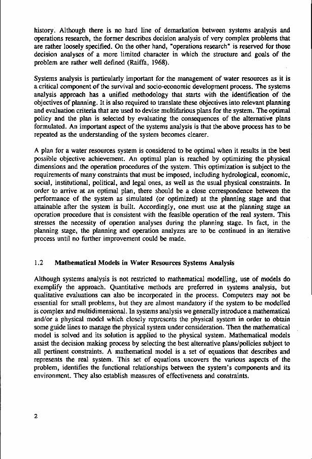
history. Although there is no hard line of demarkation between systems analysis and operations research, the former describes decision analysis of very complex problems that are rather loosely specified. On the other hand, "operations research" is reserved for those decision analyses of a more limited character in which the structure and goals of the problem are rather well defined (Raiffa, 1968).

Systems analysis is particularly important for the management of water resources as it is a critical component of the survival and socio-economic development process. The systems analysis approach has a unified methodology that starts with the identification of the objectives of planning. It is also required to translate these objectives into relevant planning and evaluation criteria that are used to devise multifarious plans for the system. The optimal policy and the plan is selected by evaluating the consequences of the alternative plans formulated. An important aspect of the systems analysis is that the above process has to be repeated as the understanding of the system becomes clearer.

A plan for a water resources system is considered to be optimal when it results in the best possible objective achievement. An optimal plan is reached by optimizing the physical dimensions and the operation procedures of the system. This optimization is subject to the requirements of many constraints that must be imposed, including hydrological, economic, social, institutional, political, and legal ones, as well as the usual physical constraints. In order to arrive at an optimal plan, there should be a close correspondence between the performance of the system as simulated (or optimized) at the planning stage and that attainable after the system is built. Accordingly, one must use at the planning stage an operation procedure that is consistent with the feasible operation of the real system. This stresses the necessity of operation analyses during the planning stage. In fact, in the planning stage, the planning and operation analyzes are to be continued in an iterative process until no further improvement could be made.

1.2 Mathematical Models in Water Resources Systems Analysis

Although systems analysis is not restricted to mathematical modelling, use of models do exemplify the approach. Quantitative methods are preferred in systems analysis, but qualitative evaluations can also be incorporated in the process. Computers may not be essential for small problems, but they are almost mandatory if the system to be modelled is complex and multidimensional. In systems analysis we generally introduce a mathematical and/or a physical model which closely represents the physical system in order to obtain some guide lines to manage the physical system under consideration. Then the mathematical model is solved and its solution is applied to the physical system. Mathematical models assist the decision making process by selecting the best alternative plans/policies subject to all pertinent constraints. A mathematical model is a set of equations that describes and represents the real system. This set of equations uncovers the various aspects of the problem, identifies the functional relationships between the system's components and its environment. They also establish measures of effectiveness and constraints.

However it must be emphasized that the real life issues are extremely complex. They are not always quantifiable and commensurate. Many implications and uncertain assumptions may be necessary to construct models and a great deal must be simplified and left out of active consideration. Intuition and judgement alone decide whether some factors are important or whether others can be safely ignored, at least in the first approximation. This emphasizes the proven fact that systems analysis cannot replace experience. In fact systems analysis has to be combined with experience.

Solutions to the mathematical models used in systems analysis are often obtained through one of the two solution strategies: optimization and simulation. The area of operations research include a variety of quantitative methods that can be used for analyzing water resources systems.

1.3 Operational Management of Water Resources Systems

The physical dimensions of any system determined at the planning and design stages of the system undoubtedly add to the returns brought about by the system. The determination of physical dimensions is accomplished in the planning stage of a system. Equally or even more important is the determination of operating policies to be used as guidelines for operating the system components. However the operation policies which are frequently formulated without explicit knowledge of the future consequences of such policies have often resulted in less than the most efficient allocation and use of the water resources.

As water resources systems become more complex, it becomes apparent that operation procedures consist of several kinds of decisions. Storage and release of water must be apportioned among reservoirs, purposes and time periods. Concern may also be directed in special cases to depth-layers of reservoirs in order to provide water of required quality. The operation procedures are sequential decision problems having consequences that extend over a considerable period of time. However these consequences are not exactly predictable, but depend also on the original decision. Uncertainty associated with the future inflows add up to the complexity of the decision problem. In cases where hydropower generation is involved, the decision problem becomes nonlinear due to the fact that the energy generation is a nonlinear function of the flow through power turbines and reservoir head.

Operation of a water resources system can be classified into short-term and long-term operations. For short-term operation (hourly or daily) one may regard both the water demand and the water inflow as deterministic. The most recent hydrological forecasts of the demands and inflows are usually incorporated in the short-term deterministic optimization. For the long-term operation (monthly or annual) the stochastic nature of inflows have to be considered. Methodology for formulating long-term operation policies need more attention than their short-term counterparts due to the equal importance of the long-term operation policies in both the planning and operation stages of a system. Nevertheless, formulation of a short-term operation policy requires a predetermined long-term operation policy which should specify the limits within which the short-term operation should take place.

There exists a wide variety of techniques that can be applied to solve the operation problem of water resources systems. Water resources systems are characterised by the size of the decision problem even in the case of a single reservoir optimization. This is mainly due to the large number of decisions that are to be taken in an uncertain environment. Multipurpose systems tend to increase the size of the problem by another dimension. With the advancement of computers the solution procedures are becoming more sophisticated. Even then the ever increasing complexity of water resources systems exert a great challenge to the systems analyst in selecting the appropriate tools for solving water resources problems. The selection of the algorithm appropriate for a particular situation depends on the type of problem in hand. The capabilities and limitations of the different solution techniques suggest that a combination of the available techniques might offer the best solution strategy.

Due to the uncertain conditions under which the actual operation of water resources systems take place, flexibility of operation is an important aspect which should not be left aside in any operational study. The solution to an operational problem should be a robust one which can tackle the multitude of operational conditions. At the same time, it should also be simple and flexible enough to be used by the system operators who are not supposed to be deprived of the guidance provided by the optimal solution specially after the situations in which a deviation from the prespecified optimal operation is implemented.

2 Description of the Case Study System

2.1 General

The Mahaweli Water Resources Development Scheme which is the project under consideration in this study is a multipurpose water resources scheme that harnesses the hydroelectric and irrigation potential of the Mahaweli Ganga (River) in Sri Lanka.

Sri Lanka is an island with an agriculture-dominated national economy. Agriculture contributed to about 27% of gross domestic products and employed about 45% of the total work force in 1987. It is expected that agriculture will continue to concentrate on the staples and provide the principal support for the national revenue. Hydropower is also an essentially valuable resource in Sri Lanka, since coal and petroleum resources have not yet been found in the island. Therefore the Government of Sri Lanka has been paying attention to the systematic development of land and water resources to prepare for the future economic development. Water resources development is therefore one of the most important aspects in this regard.

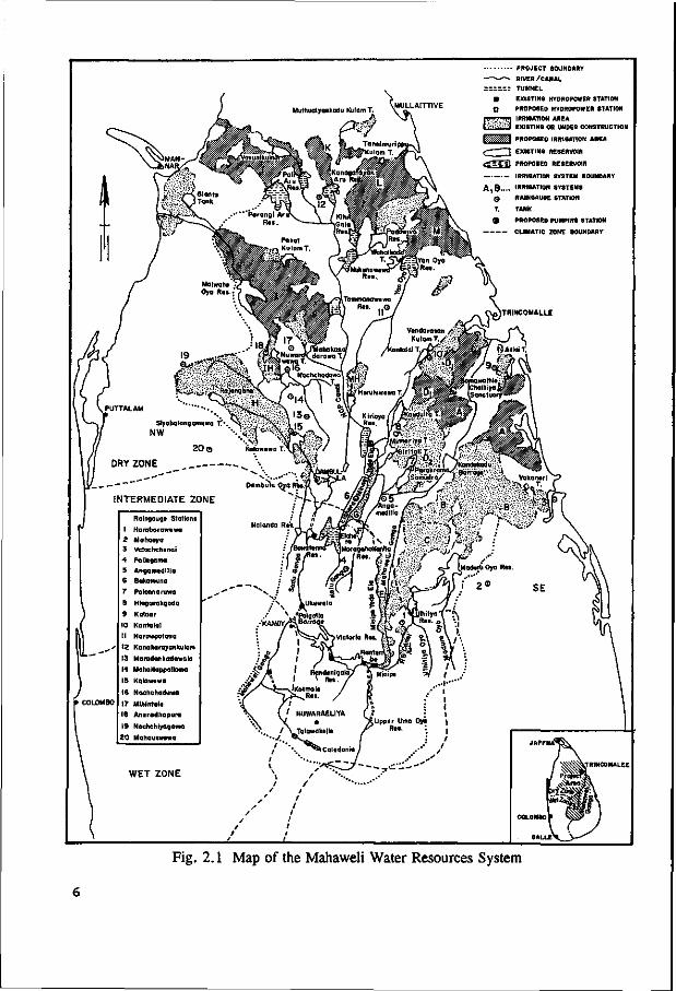
The island has an area of 65,000 square kilometres. The south-central part of the island consists of hills and mountains which culminate at 2,500 meters above sea level. The coastal plain, rather narrow on the west, east and south, broadens out to a vast tract in the north. Temperatures are very even throughout the year. Mean temperatures are high on the coast (ranging from 27 to 28 °C); in the hills they fall off at a steady rate of 1 °C for each 165 m in rise. The climatological conditions in Sri Lanka are dominated by two monsoons. The southwest monsoon or 'Yala' season (April to September) and the northeast monsoon or 'Maha' season (October to March). Due partly to the screening effect of the mountains, rainfall is very unevenly distributed over the island and is subject to large seasonal variations. The strong influence of the central hills along with the other factors lead to the subdivision of the country into three climatic zones; wet, intermediate and dry as shown in Fig. 2.1. Annual average rainfall varies from below 1,000 mm in the driest zone to over 5,000 mm at certain places on the southwest slopes of the hills.

PROJECT BOUNDARY

-——• RIVER /CANAL

.---Z TUNNEL

• EXISTING HYDROPOWER STATION

O PROPOSED HYDROPOWER STATION

IRRBATION AREA

EXISTING OR UNDER CONSTRUCTION

PROPOSED IRRIGATION AREA

EXISTING RESERVOIR

PROPOSED RESERVOIR

IRRIGATION SYSTEM BOUNDARY

A , B — IRRIGATION SYSTEMS

Q RAINGAU8E STATION

T. TANK

9 PROPOSED PUMPING STATION

CLIMATIC ZONE BOUNDARY

1 2 3 4

9 6

7

B

9

10 II

12

13

K

15

16

ir IB

19

20

Raingaugt Stations

Horaborawftwa Mohaoya Valochchmai Polls ga ma

Angamedilla Bakamuna

Polonnaruwa

Hlngurakgoda

Kalaar

Kantalai

Horowpotana

Kana karayankulam

Marodonkadawala

Mahailuppalkuna

Kalawtwa

Nachchaduwa

Mihintal*

Anuradhapura

Nochehlyagama

Mahautmwa

WET ZONE

Fig. 2.1 Map of the Mahaweli Water Resources System

The wet zone, corresponding roughly to the southwest quadrant of the island, covers about 30 % of the land area of Sri Lanka but includes more than three quarters of its total population. In the dry zone, irrigation is essential for cultivation in the Yala season and some supplemental irrigation is necessary for Maha season. Irrigation in Sri Lanka is a long-practised art using the traditional tank (reservoir built for irrigation purposes) irrigation systems. Traditional irrigation systems are based on storage tanks designed to supplement irrigation water to Maha crops, and to store residual water for the limited Yala season cropping. There are over 25,000 such schemes scattered all over the island, a major part of them in the dry zone. The responsibilities of operation and maintenance of these schemes are borne by the farmers, and only the major headworks and canals come under the governments purview. Dry zone of Sri Lanka was once (several centuries ago) agriculturally developed and contained the main population centres of the island. Circumstances not very well understood (in which wars played a great part) led progressively to the complete abandonment of this zone which reverted to the jungle.

Having the population pressure upon land in the wet zone becoming excessive, attempts have been made to redevelop the once prosperous dry zone. The waters which flow through this zone from the mountains to the sea and the good soils they could fertilize represent for Sri Lanka an important yet largely untapped resource. The systematic development of these important natural resources along with industrialization is the main economic development theme of the country at present.

2.2 Mahaweli Water Resources Development Scheme

Being Sri Lanka's longest and most important river, the importance of Mahaweli river is basically due to the fact that it originates in the wettest part of Sri Lanka in the central highlands and flows through the driest uninhabited fertile plains of the country. The copious flows of Mahaweli which fall through so many hundreds of meters before being discharged to the sea has a very high hydropower potential. Mahaweli development scheme has been based on using the naturally diverse flow pattern of the Mahaweli river, regulated where necessary with storage reservoirs, to satisfy irrigation demands in the dry zone of the country. Hydroelectric energy can be generated at storage dams and along some of the diversion routes. There is a number of reservoirs which are already constructed within the Mahaweli development scheme. Some more are planned to be built in the near future. Those would provide sufficient storage to regulate river flows, and to generate hydropower at a steady rate.

2.3 Components of the Macrosystem and Microsystem of the Mahaweli Water Resources Development Scheme

Mahaweli Development Scheme comprises of a complex network of regulating reservoirs and diversion structures built on the main stem of the Mahaweli river as well as on its tributaries and diversion routes. The system can be subdivided into two interlinked parts, identified as macrosystem and microsystem.

The main reservoir system, power plants and the other regulating structures situated on the major rivers can be grouped together as the macrosystem. The irrigation systems with their irrigation tanks (reservoirs built for irrigation purposes) and the conveyance facilities starting from the diversion points of the major rivers up to the field level comprise the microsystem.

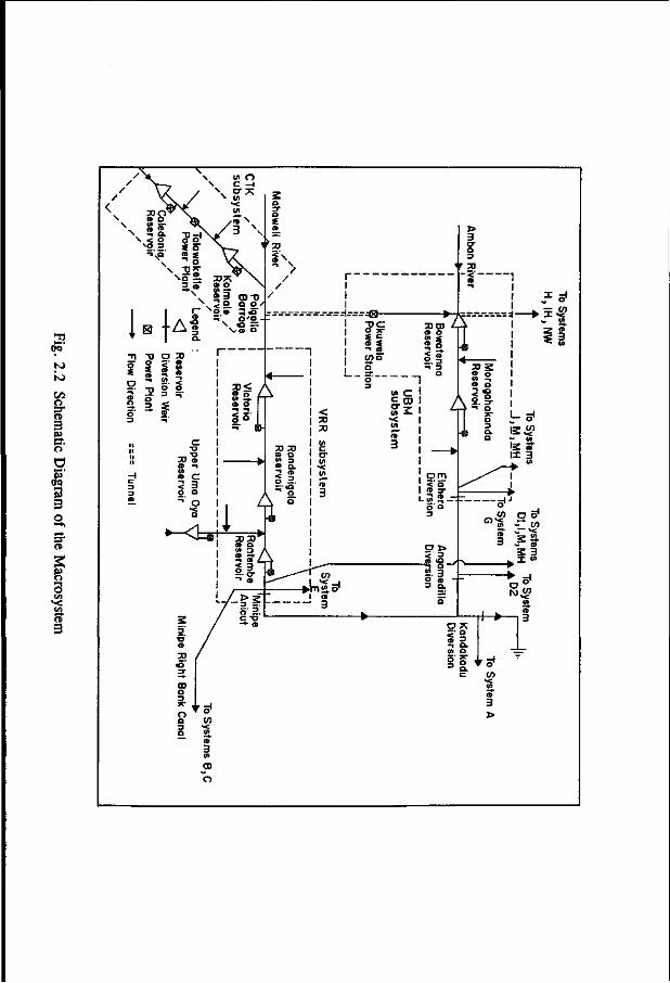
The system configuration considered in this study is expected to be the ultimate system configuration of the Mahaweli development scheme. As the schematic diagram of the macrosystem in Fig. 2.2 illustrates, there are three reservoirs on the main stem of Mahaweli river namely Victoria, Randenigala and Rantembe reservoirs. Each of these reservoirs has a power plant as well. These reservoirs are already in operation and they serve the purposes of power generation and flow regulation for irrigation. Caledonia, Talawakelle and Kotmale reservoirs are located on Kotmale Oya (Creek), a major tributary of the Mahaweli river. Kotmale reservoir and its power plant is presently under operation. Caledonia and Talawakelle reservoirs and the associated power plants are planned additions for the near future. Downstream of the Kotmale reservoir is the Polgolla barrage which plays a vital role in this water resource system. It is used for an interbasin water transfer from the Mahaweli river to the adjacent Amban Ganga basin via a diversion tunnel. The diverted water is used to generate power at a power station at Ukuwela before being collected in Bowatenne reservoir. Bowatenne reservoir is used as a regulating reservoir for diverting irrigation water to irrigation systems H, IH and NW while serving the purpose of power generation by downstream discharges. Moragahakanda reservoir which is located downstream of Bowatenne is also a multipurpose structure which serves the purposes of hydropower generation and flow regulation for irrigation. Ukuwela and Bowatenne structures are presently in operation, and the Moragahakanda reservoir is to be constructed. As the schematic diagram of the whole system in Fig. 2.3 indicates, the major diversion points of the system are Polgolla, Bowatenne, Elahera, Angamedilla, Minipe and Kandakadu. All of them are presently under operation. However most of them are presently operated at a below-capacity level as the microsystems are not fully completed at this stage.

The water remaining after diversion to system G at Elahera is planned to be collected at a pond at Kiri Oya before being sent to the northern part of the country via the North Central Province (NCP) canal. NCP canal would serve the irrigation systems I, MH, J,K,L and M. However the development of the irrigation systems J,K and L has been found uneconomical at present. Due to this reason these irrigation systems were excluded from the present analysis. Angamedilla diversion is used to divert waters to system D2.

21

q3' J° to

C/5 o ST n 3 S-o' a &' 3 3 o

8

3

U} 2 . » * o

V ™2 CD-O, v< 9. o o /

f~ N 0 ID 2.5"

f I =:' 2

H I

*-<bs

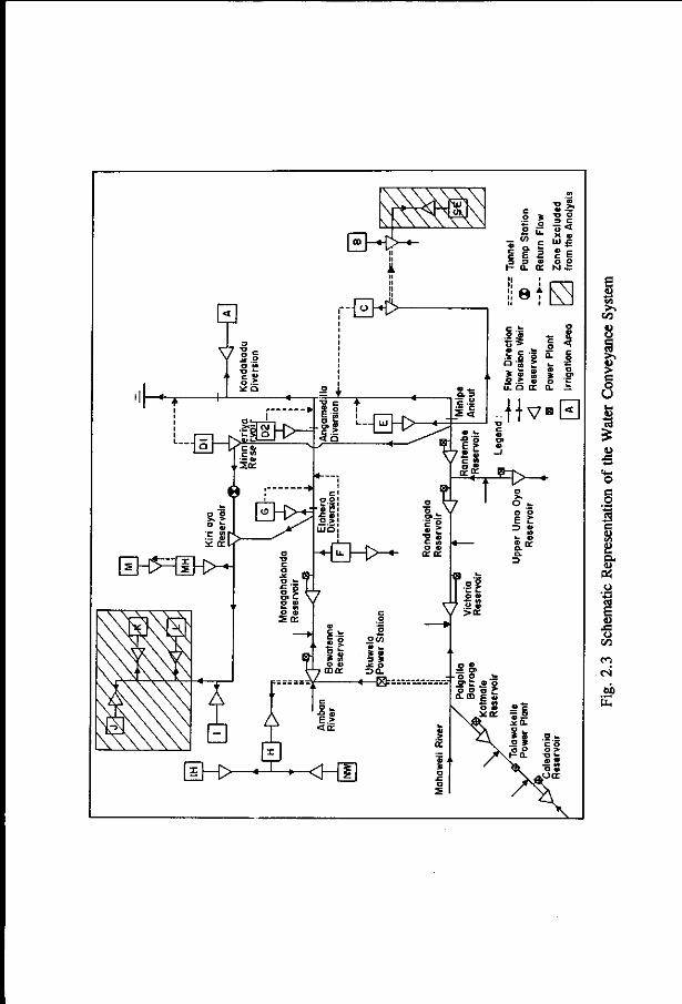
The anicut at Minipe diverts water both to the right and left bank canals in order to fulfil requirements of systems B, C, SE and E respectively. System SE also will not be developed in the near future, as it is found uneconomical. A canal which connects Minipe and Minneriya reservoir is envisaged to feed the system Dl also from the water available at Minipe. A pumping station planned at Minneriya reservoir would pump the waters of Minneriya reservoir to Kiri Oya which will in turn feed the NCP canal. Kandakadu diversion structure serves system A which is the most downstream irrigation system of the Mahaweli Development Scheme.

2.4 The present Status of the Irrigation Development in Sri Lanka

In the whole country, the total wet paddy area is about 500,000 ha (in net area) comprising 210,000 ha of major irrigation schemes, 115,000 ha of minor irrigation schemes and 175,000 ha of rain-fed paddy areas. Due to lack of irrigation water in the dry season, rice production is still vulnerable to weather conditions. The government of Sri Lanka wishes to maximize the irrigation area with reliable water supply and to increase cropping intensity in the existing irrigation areas.

About 135,000 ha of agricultural lands are currently irrigated with the water of the Mahaweli Ganga, the Amban Ganga and local catchment areas under the Accelerated Mahaweli Development Programme (AMDP) implemented in 1977. The existing, on-going and potential irrigation areas of the Mahaweli Development Scheme are presented in Table 2.1.

2.5 Power Supply System in Sri Lanka

The entire public power supply system is managed and operated by the Ceylon Electricity Board (CEB), which is the statutory body of the Government. CEB supplies electrical power to consumers both directly and indirectly through the Lanka Electricity Company (LECO). CEB owns power plants of 1,165 MW in total installed capacity, consisting of 965 MW of hydropower plants and 200 MW of thermal power plants. Hydropower plants can generate 3,682 GWh under normal hydrological conditions. The annual energy demand in the CEB system was around 3,300 GWh and the peak demand was 620 MW in 1989. The future demand is expected to grow at about 9% per annum (JICA, 1989), so additional installations of power plants will be required annually.

Hydropower development was expedited to eliminate the shortage of electric power in 1960s. Based on the UNDP/FAO master plan, Ukuwela and Bowatenne hydropower stations were constructed in 1976 and 1981 respectively. In 1977, the Government revised the master plan to accelerate the Mahaweli Development Programme (AMDP). According to AMDP, hydropower in recent years has been developed as a component of multipurpose dam development: the Kotmale, Victoria, Randenigala multipurpose dams which were constructed in the early 1980s. The Rantembe hydropower station also was commissioned in 1990. The principal features of the existing and proposed hydropower plants and reservoirs of the Mahaweli Development Scheme is presented in Table 2.2.

10

E B >. oo

u > c o U

c o a c 0 .

a) E <u

J= o 00 en

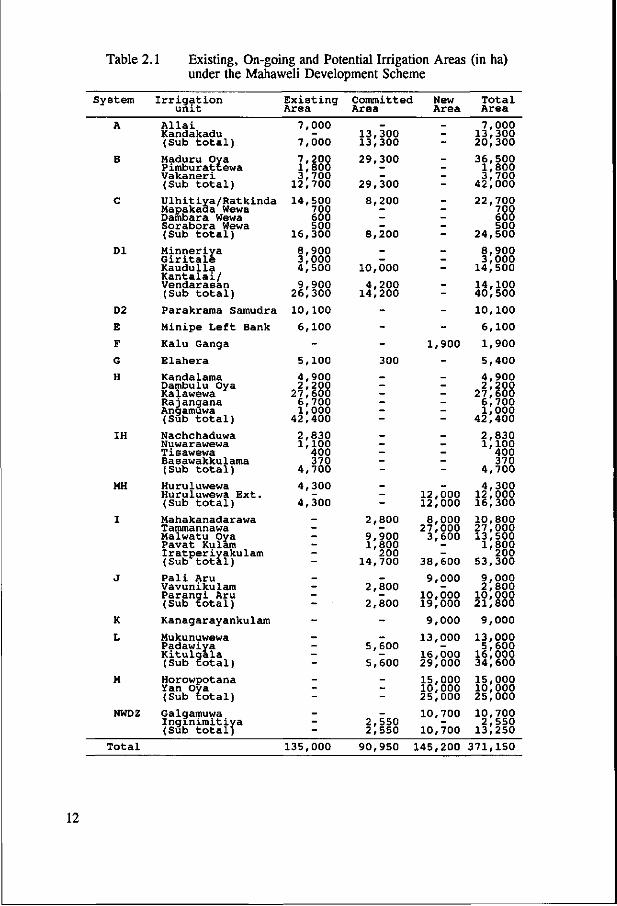
Table 2.1 Existing, On-going and Potential Irrigation Areas (in ha) under the Mahaweli Development Scheme

System Irrigation unit

Existing Area

Committed Area

New Area

Total Area

A Allai 7,000 Kandakadu - 13,300 (Sub total) 7,000 13,300

B Maduru Ova 7,200 29,300 Pimburattewa 1,800 Vakaneri 3,700 (Sub total) 12,700 29,300

C Ulhitiya/Ratkinda 14,500 8,200 Mapakada Wewa 700 Dambara Wewa 600 - -Sorabora Wewa 500 (Sub total) 16,300 8,200

Dl Minneriya 8,900 Giritale 3,000 Kaudulla 4,500 10,000 Kantalai/ Vendarasan 9,900 4,200 (Sub total) 26,300 14,200

D2 Parakrama Samudra 10,100

E Minipe Left Bank 6,100

F Kalu Ganga - - 1,900

G Elahera 5,100 300

H Kandalama 4,900 Dambulu Oya 2,200 Kalawewa 27,600 Raj angaria 6,700 Angamuwa 1,000 (Sub total) 42,400

IH Nachchaduwa 2,830 Nuwarawewa 1,100 Tisawewa 400 Basawakkulama 370 (Sub total) 4,700

MH Huruluwewa 4,300 Huruluwewa Ext. - - 12,000 (Sub total) 4,300 - 12,000

I Mahakanadarawa - 2,800 8,000 Tammannawa - - 27,000 Malwatu Oya - 9,900 3,600 Pavat Kulam - 1,800 Iratperiyakulam - 200 (Sub total) - 14,700 38,600

J Pali Aru - - 9,000 Vavunikulam - 2,800 Parangi Aru - - 10,000 (Sub total) - 2,800 19,000

K Kanagarayankulam - - 9,000

L Mukunuwewa - - 13,000 Padawiya - 5,600 Kitulgala - - 16,000 (Sub total) - 5,600 29,000

M Horowpotana - - 15,000 Yan Oya - - 10,000 (Sub total) - - 25,000

NWDZ Galgamuwa - - 10,700 Inginimitiya - 2,550 (Sub total) - 2,550 10,700

7,000 13,300 20,300

36,500 1,800 3,700

42,000

22,700 700 600 500

24,500

8,900 3,000

14,500

14 40

10

4 2

27 6 1

42

2 1

4 12 16

10 27 13

1

53

9 2

10 21

13 5

16 34

15 10 25

10 2

13

100 500

100

100

900

400

900 200 600 700 000 400

830 100 400 370 700

300 000 300

800 000 500 800 200 300

000 800 000 800

000

000 600 000 600

000 000 000

700 550 250

Total 135,000 90,950 145,200 371,150

12

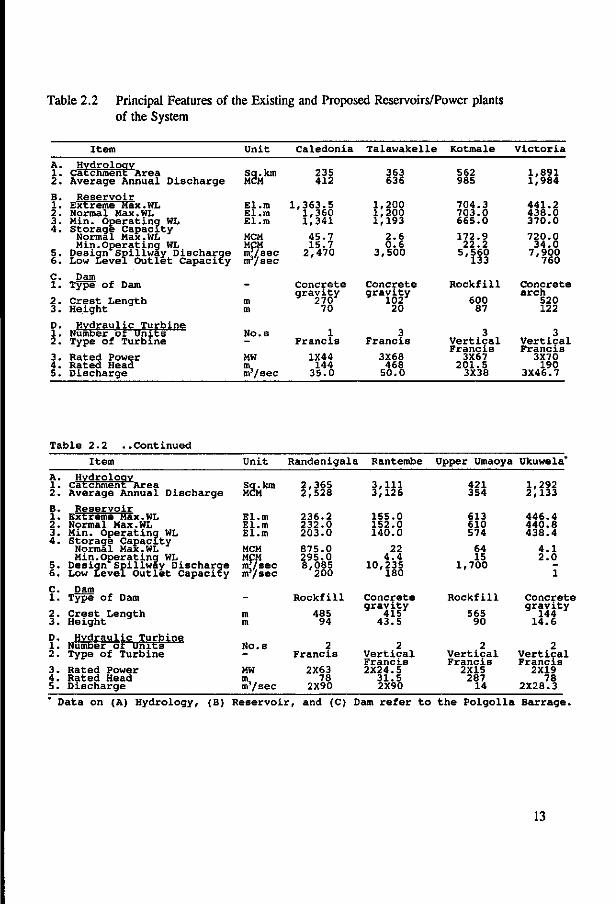
Table 2.2 Principal Features of the Existing and Proposed Reservoirs/Power plants of the System

A. 1. 2.

R. 1. 2. 3. 4.

5. 6.

C. 1.

2. 3.

D. 1. 2.

3. 4. 5.

Item

Hvdroloov Catchment Area Average Annual Discharge

Reservoir Extreme Max.WL Normal Max.WL Min. Operating WL Storage Capacity

Normal Max.WL Min.Operating WL

Design Spillway Discharge Low Level Outlet Capacity

Dam Type of Dam

Crest Length Height

Hvdraulic Turbine Number or Units Type of Turbine

Rated Power Rated Head Discharge

Unit

Sg.km MCM

El.m El.m El.m

MCM MCM m,/sec tir/sec

~ m m

No.s -MW m nr/sec

Caledonia

235 412

1,363.5 1,360 l|341

45.7 15.7

2,470

Concrete gravity

270 70

1 Francis

1X44 144

35.0

Talawakelle

363 636

1,200 1,200 1,193

2.6 0.6

3,500

Concrete gravity

102 20

3 Francis

3X68 468

50.0

Kotmale

562 985

704.3 703.0 665.0

172.9 22.2

5,560 133

Rockfill

600 87

3 Vertical Francis

3X67 201.5

3X38

Victoria

1,891 1,984

441.2 438.0 370.0

720.0 34.0

7,900 760

Concrete arch

520 122

3 Vertical Francis

3X70 190

3X46.7

Table 2.2 ..Continued

A. 1. 2.

B. 1. 2. 3. 4.

b. 6.

C. 1.

2. 3.

D. 1. 2.

3. 4. 5.

Item

Hydroloav Catcnment Area Average Annual Discharge

Reservoir Extreme Max.WL Normal Max.WL Min. Operating WL Storage Capacity

Normal Max.WL Min.Operating WL

Design Spillway Discharge Low Level Outlet Capacity

Dam Type or Dam

Crest Length Height

Hvdraulic Turbine Number ot units Type of Turbine

Rated Power Rated Head Discharge

Unit

Sg.km MCM

El.m El.m El.m

MCM MCM m,/sec m /sec

~ m m

No.s

MW m m /sec

Randenigala

2,365 2,528

236.2 232.0 203.0

875.0 295.0 8,085

200

Rockfill

485 94

2 Francis

2X63 78

2X90

Rantembe

3,111 3,126

155.0 152.0 140.0

22 4.4

10,235 180

Concrete gravity

415 43.5

2 Vertical Francis 2X24.5

31.5 2X90

Upper Umaoya

421 354

613 610 574

64 15

1,700

Rockfill

565 90

2 Vertical Francis

2X15 287

14

Ukuwela"

1,292 2,133

446.4 440.8 438.4

4.1 2.0

— 1

Concrete gravity

144 14.6

2 Vertical Francis

2X19 78

2X28.3

Data on (A) Hydrology, (B) Reservoir, and (C) Dam refer to the Polgolla Barrage.

13

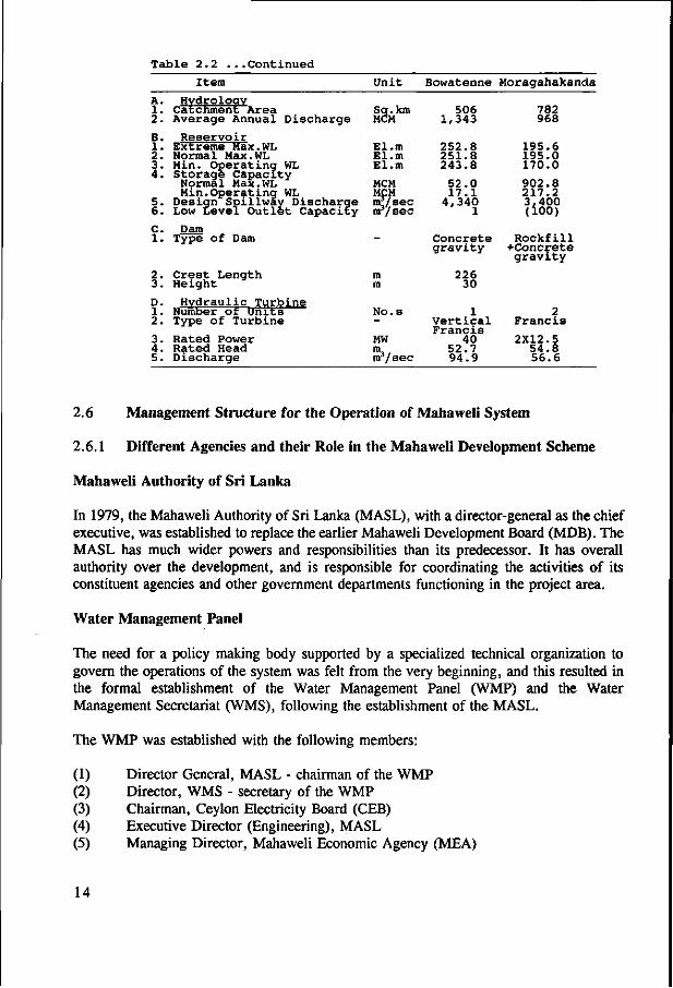
Table 2.2 .Continued

Item Unit Bowatenne Moragahakanda Hydrology

:atc A . • . , . _ • _ • . . 1. Catchment Area 2. Average Annual Discharge

B. Reservoir 1. Extreme Max.WL 2. Normal Max.WL 3. Min. Operating WL 4. Storage Capacity

Normal Max.WL Min.Operating WL

5. Design Spillway Discharge 6. Low Level Outlet Capacity

C. Dam 1. Type of Dam

2. Crest Length 3. Height D. Hydraulie Turbine 1. Number or units 2. Type of Turbine

3. Rated Power 4. Rated Head 5. Discharge

Sq.km So.. MCM

El.m El.m El.m

MCM MCM m,/sec nr/sec

m m

No.s

MW m m /sec

506 1,343

2 5 2 . 8 2 5 1 . 8 2 4 3 . 8

5 2 . 0 1 7 . 1

4 , 3 4 0

Concrete gravity

226 30

Vertical Francis

40 52.7 94.9

782 968

195.6 195.0 170.0

902.8 217.2 3,400 (iOQ)

Rockfill +Concrete

gravity

Francis

2X12.5 54.8 56.6

2.6 Management Structure for the Operation of Mahaweli System

2.6.1 Different Agencies and their Role in the Mahaweli Development Scheme

Mahaweli Authority of Sri Lanka

In 1979, the Mahaweli Authority of Sri Lanka (MASL), with a director-general as the chief executive, was established to replace the earlier Mahaweli Development Board (MDB). The MASL has much wider powers and responsibilities than its predecessor. It has overall authority over the development, and is responsible for coordinating the activities of its constituent agencies and other government departments functioning in the project area.

Water Management Panel

The need for a policy making body supported by a specialized technical organization to govern the operations of the system was felt from the very beginning, and this resulted in the formal establishment of the Water Management Panel (WMP) and the Water Management Secretariat (WMS), following the establishment of the MASL.

The WMP was established with the following members:

(1) Director General, MASL - chairman of the WMP (2) Director, WMS - secretary of the WMP (3) Chairman, Ceylon Electricity Board (CEB) (4) Executive Director (Engineering), MASL (5) Managing Director, Mahaweli Economic Agency (MEA)

14

(6) Secretary, Ministry of Agricultural Development and Research (7) Secretary, Ministry of Lands and Land Development (8) Director of Irrigation (9) Director of Agriculture (10) Government Agents of the administrative districts benefited by the Mahaweli

project.

The principal function of the WMP was to govern the management of the water resources of the Mahaweli system to achieve optimum benefits. The WMP would make operational policy decisions and set overall cultivation programs for the irrigated areas served by the project. This was accomplished mainly through convening two formal meetings per year, prior to the Maha and Yala seasons.

Policy Planning Panel

Decision making at WMP meetings is by consensus, rather than by vote. This approach worked well in the early days when contentious water management issues were primarily related to allocation of scarce water resources among competing irrigation areas (Weerakoon, 1989). However, with more complex power irrigation trade-off questions surfacing after the construction of Victoria and Randenigala reservoirs, the Government felt that a smaller interministerial policy planning panel at national level should be established to examine such issues and lay down broad operation policies, particularly as it was felt that the constitution of the WMP was weighed in favour of irrigation interests.

The Policy Planning Panel (PPP) for the Mahaweli system was established in 1986 with the following membership, which was considered a more balanced representation of the irrigation and power interests.

(1) Secretary, Ministry of Finance and Planning (Chairman) (2) Secretary, Ministry of Mahaweli Development (3) Secretary, Ministry of Power and Energy (4) Secretary, Ministry of Lands and Land Development (5) Secretary, Ministry of Industries (6) Additional General Manager (Generation), CEB (7) Government Agent, Anuradhapura District

The PPP is now vested with the responsibility for establishing operation policies for the Mahaweli system as well as for the long term planning of the Mahaweli Complex Development. This has eroded the policy making role of the WMP, which functions now in an operational capacity within the broad policy guide lines as established by the PPP. The Director General of MASL is usually associated as an invitee in the deliberations of the PPP. The Director of WMS functions as the Secretary of both the PPP and the WMP, and this helps to maintain the necessary communication link between the two panels.

15

Water Management Secretariat (WMS)

The WMS, which is a technically specialized unit of the MASL services both the WMP and the PPP. It provides information and recommendations to the two panels to assist in reaching policy and operational decisions. Although it is administratively a part of the MASL, the operation planning and coordinating responsibilities of the WMS extend to the other operating agencies as well.

Operating Responsibilities

The agencies involved in the Mahaweli system operations are the following.

(1) Headworks Administration, Operation and Maintenance (HAO&M) Division (2) Ceylon Electricity Board (CEB) (3) Mahaweli Economic Agency (MEA) (4) Irrigation Department (ID).

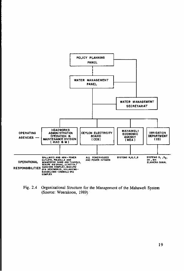
The organizational structure for Mahaweli operations is shown in Fig. 2.4. The WMS has the responsibility of coordinating the operational activities of these agencies.

2.6.2 Current Operating Procedures

Operating Philosophy

In the Mahaweli project the two major uses of water are irrigation and hydropower generation. These uses are to a large extent compatible, but conflicts arise because of the need to divert some Mahaweli Ganga flows away from the path of the maximum generating head to serve irrigation needs in the other areas.

Basically, the operations in the Mahaweli system are geared to generate maximum economic benefits from the limited water resource, taking also into consideration the socio-economic impact of irrigation cutbacks and power cuts. Under the operating guide lines developed, the minimum possible flows are diverted at Polgolla, sufficient only to meet the net requirements of the Amban Ganga irrigation areas. Once these needs are met, operations aim at maximizing power benefits. Rule curves have been developed for all the major tanks too, with the objective of maximizing use of local inflows and minimizing irrigation demand on the macrosystem.

Seasonal Operating Plans

The operation of the whole Mahaweli system is based on Seasonal Operating Plans (SOP) prepared twice each year to project system operations over the forthcoming cultivation season. Each SOP covers a 6-month period, October-March and April-September, corresponding to the two cultivation seasons Maha (major) and Yala (minor) respectively. The SOP is prepared by the WMS with the assistance of the operating agencies, which supply relevant data and information regarding the proposed cropping patterns and schedules, national power and energy demand, plant availability etc. The SOP gives the

16

projected reservoir releases, diversions, tank storages, irrigation issues, energy generation etc for both average and dry hydrological conditions based on the results of mathematical simulations covering a period of 36 years for which hydrological data are available.

Two mathematical models developed by Acres International Ltd. of Canada, who served as general consultants to the WMS, are used in the simulation studies. They are:

(1) The Irrigation Demand Model (IDM), and (2) The Acres Reservoir Simulation Program (ARSP)

The IDM computes on a monthly basis the irrigation demands (as at the tank outlet) for each irrigation scheme on the basis of relevant parameters like evapotranspiration, percolation losses, land preparation requirements, distribution and field application efficiencies, effective rainfall etc. These irrigation demands and the CEB's energy demand are used in the ARSP for simulating system performance. If the initial studies indicate that the objectives cannot be met with an acceptable degree of reliability, then the irrigation extents are reduced or power generation priorities reallocated in consultation with the agencies concerned till the required reliability for both power and irrigation is met. The SOP is then discussed and approved with any necessary modifications at a WMP meeting held prior to the cultivation. Some members of Parliament too make it a point to attend these meetings, where they seek to obtain maximum irrigation benefits for their respective constituencies, many of which are heavily dependent on the Mahaweli for economic sustenance. Issues that cannot be resolved at the WMP meetings are referred to the PPP.

Acres Reservoir Simulation Program (ARSP)

This is a planning oriented, flexible, simulation model using a monthly time step. In each time step of the simulation a single-time-step optimization is performed based on a network flow solution technique known as the Out-of-kilter algorithm. It is a very efficient algorithm for solving minimum cost flow problems (Murty, 1976). One of the principal features of the Out-of-kilter algorithm is the representation of the system as a set of nodes and connecting arcs in a capacitated network form. In the water resources system, which is represented by a flow network, the junctions and control points, such as reservoirs, are represented as nodes. The natural or man-made channels that connect the junctions are represented by arcs.

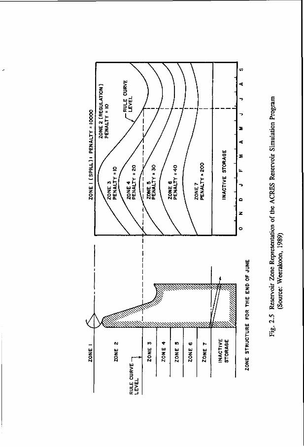
This network solution technique requires that channel flow constraints and reservoir storages be assigned relative penalties. In the case of reservoir storage, discrete intervals or zones of storage volumes are defined. As shown in Fig. 2.5, each zone has a specified upper and lower boundary and a user assigned cost or penalty that represents the relative value of water stored in that zone. Flow constraints are represented by a number of flow elements or "arcs". As in the case of storage, each flow arc has an upper and lower bound and a user-specified cost or penalty associated with flow in that arc. A single channel can have a number of arcs representing the full range of channel flow capability. In addition, arcs are also used to define storage changes in reservoirs. The capacitated network model which is solved by the Out-of-kilter algorithm is stated in mathematical form as (Wagner, 1975; Sigvaldason, 1976):

17

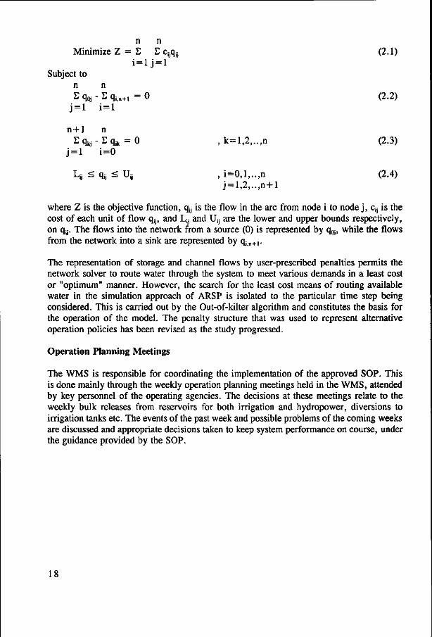
n n Minimize Z = £ E c^j (2.1)

i = l j = l Subject to

n n E qpj - E qi,.+i = 0 (2.2)

j = l i= l

n+1 n Eq ) t j-Eq i k = 0 , k=l,2,..,n (2.3)

j = l i=0

Lij =S q« ^ Us , i=0,l,..,n (2.4) j = l,2,..,n + l

where Z is the objective function, q is the flow in the arc from node i to node j , c is the cost of each unit of flow q , and L;j and Uy are the lower and upper bounds respectively, on qy. The flows into the network from a source (0) is represented by q , while the flows from the network into a sink are represented by q^+i.

The representation of storage and channel flows by user-prescribed penalties permits the network solver to route water through the system to meet various demands in a least cost or "optimum" manner. However, the search for the least cost means of routing available water in the simulation approach of ARSP is isolated to the particular time step being considered. This is carried out by the Out-of-kilter algorithm and constitutes the basis for the operation of the model. The penalty structure that was used to represent alternative operation policies has been revised as the study progressed.

Operation Planning Meetings

The WMS is responsible for coordinating the implementation of the approved SOP. This is done mainly through the weekly operation planning meetings held in the WMS, attended by key personnel of the operating agencies. The decisions at these meetings relate to the weekly bulk releases from reservoirs for both irrigation and hydropower, diversions to irrigation tanks etc. The events of the past week and possible problems of the coming weeks are discussed and appropriate decisions taken to keep system performance on course, under the guidance provided by the SOP.

18

POLICY PLANNING

PANEL

WATER MANAGEMENT PANEL

OPERATING

AGENCIES -

WATER MANAGEMENT

SECRETARIAT

HEAOWORKS ADMINISTRATION

OPERATION 8 MAINTENANCE DIVISION

( HAO a M )

CEYLON ELECTRICITY BOARD (CEB)

MAHAWELI ECONOMIC

AGENCY ( M E A )

IRRIGATION DEPARTMENT

( ID)

SPILLWAYS AND NON- POWER OUTLETS, POLGOLLA AND

OPERATIONAL BOWATENNE DAMS AND TUNNELS, MINIPE RB CANAL, ULHITIYA/

DCCDOMCIRII ITICC RATKINDA COMPLEX, MADURU nc .orUN9IOIL . IUCO 0 Y A HEADWORKS, KALAWEWA-

KANDALAMA- DAMBULU OYA COMPLEX

ALL POWERHOUSES AND POWER INTAKES

SYSTEMS H,6 ,C,B SYSTEMS D, , D 2 ,

ELAHERA CANAL

Fig. 2.4 Organizational Structure for the Management of the Mahaweli System (Source: Weerakoon, 1989)

19

6 2

OH

C

o

on

00 W OS U <

c o <S ON

c °° 4} CT\

8 e rv C

SB o a

" " 2 IN oh

a 3 O

on

3 Outline of the Study

3.1 Objectives

The aim of this case study is the formulation of a detailed set of guide lines for operating the macrosystem of the Mahaweli water resources system. Operation of the Mahaweli water resources system is presently supported by the Acres Reservoir Simulation Program (ARSP), which was introduced in section 2.6.2. In the actual operation, the weekly Operation Planning Meetings (Section 2.6.2) play an important role. The single-time-step optimization employed in the ARSP makes the long-term optimality of the resulting operation questionable. Also, the outcome of the simulation approach is largely dependent on the penalty structure used in the model. The operational guidance that can be practically obtained by this model is a partial one, covering a few possible operational and hydrological scenarios.

The present study employs the optimization technique of Stochastic Dynamic Programming (SDP) to formulate optimal operation policies. Although the SDP replaces the trial-and-error-search of the optimal course of action of simulation techniques, an SDP-based operation policy is always assessed by a subsequent simulation using available or generated data. An operation policy formulated by Stochastic dynamic Programming (SDP) indicates the optimal end-of-the-period state or the optimal release volumes as a function of the initial state of the system and the subsequent or previous hydrologic outcomes. It indicates the optimal decisions that corresponds to the whole range of feasible states of a system. This type of a policy is quite useful over the traditional operation policies derived by simulation based techniques or by intuition. The traditional operation policies mostly cover a certain range of operation patterns which are commonly experienced. In contrast, an SDP-based operation policy covers the entire feasible set of policy options.

However, SDP has certain shortcomings. The most critical one being the excessive computational requirement of a conventional SDP model (termed as "curse of dimensionality"). Practically, a conventional SDP model can only be used to analyze a two-reservoir system, even with a limited number of state discretization levels. The computational load of a SDP model increases dramatically with the increase of the number of reservoirs or with the number of discretizations. This excludes the possibility of using

21

a conventional SDP model straightforward for analyzing a reservoir system consisting of more than two reservoirs.

In order to circumvent the dimensionality problems inherent to SDP, several disaggregation and aggregation techniques based on SDP are proposed and their applicability is justified. Certain preliminary stages of the analysis are aided also by the technique of Incremental Dynamic Programming (IDP) within the deterministic context. The performance of the derived policies are assessed by simulating the system operation using the derived policies. Mahaweli system serves the purposes of hydropower generation and irrigation. Correspondingly, two different objective functions were considered in the analysis. Maximization of the expected energy generation was one of them, while the other objective function minimizes the expected sum of squared deviations of the irrigation water supply from the demand.

Subsequent to an aggregation procedure, it is of utmost importance to develop a suitable disaggregation technique to define the operation policies of the individual system components. In the case of the aggregation procedure of 'composite reservoir' presented in Section 5.6, three different techniques for the disaggregation are also proposed and investigated. The uncertainty of the hydrological outcomes is explicitly incorporated in the SDP models developed for this study. However the applicability of an implicit stochastic approach to derive optimal operation policy for a multireservoir system is also investigated.

3.2 Scope of the Study

This section contains a brief description of the methodology presented in the subsequent chapters. A flow diagram of the research conducted is displayed in Fig. 3.1. Table 3.1 presents the techniques used in the different analytical approaches of this study.

3.2.1 Estimation of Irrigation Water Demands

Mahaweli water resources system serves two major purposes: hydropower generation and irrigation. The increasing power demand of Sri Lanka has to be primarily satisfied by hydropower plants. However, due to the limited availability of water resources that can be developed for hydropower generation, a number of thermal power plants has been planned for the near future. Energy that can be produced by hydropower plants signify a saving of the high operation and maintenance cost of the thermal power plants. Therefore it can be assumed that the total energy production of the Mahaweli system can be used to satisfy the increasing energy demands.

The upper limits of the irrigation water requirements are however constrained by the availability of lands and the feasibility of their development. Within-year distribution of irrigation water requirements is more pronounced unlike that of the energy demand. Among other factors, cropping calendar and the variation of the rainfall have a significant effect on the within-year distribution of irrigation water demands. The determination of monthly irrigation water demands of each irrigation area is therefore an important first step in the operational optimization of this system. The irrigation water demand model documented in

22

Section 5.1 serves this purpose. It estimates the monthly irrigation water requirements of each of the 14 irrigation areas considered in the analysis. The computation is performed for a period of 37 years for which rainfall data are available. Model input includes the crop data, water use efficiencies and losses, and monthly rainfall data. This model also computes the return flows from the irrigation area corresponding to 100% irrigation. These theoretical return flow values are later used to compute the actual return flows in the cases of under-irrigation.

3.2.2 Estimation of the Diversion Water Requirements from the Macrosystem

This study is focused on the optimization of the operation of the macrosystem components. It is therefore necessary to express the irrigation water demands of the individual irrigation areas in terms of the aggregated monthly water demands at the interface(s) between the macro and micro systems. These water demands exist at the five diversion points (Bowatenne, Elahera, Angamedilla, Minipe, and Kandakadu) which diverts water from the macrosystem to the microsystem.

In order to assess the water demands at these locations, the integrated operation of the microsystem is simulated. Due to the complexity of the microsystem's conveyance system and storage reservoir (referred to as irrigation 'tank') network, a simplified microsystem configuration is assumed. In the simplified configuration each irrigation area is assumed to possess only one hypothetical composite tank. The storage capacity of a composite tank is equivalent to the aggregated storage capacity of the real tanks within the area. ACRES (1985) also used the composite representation of tanks successfully in their studies of operation policy options for a part of the Mahaweli system. The simplified system configuration selected for the present study is displayed schematically in Fig. 2.3.

The simulation of the microsystem was performed by the microsystem simulation model (Section 5.2) developed in this study. It estimates the monthly diversion requirements at the five diversion points by simulating the integrated operation of the microsystem. The input data requirements of the microsystem simulation model are:

(1) Monthly irrigation demands of each irrigation area over the 37-year-period (estimated by the irrigation water demand model)

(2) Data related to the assumed composite storage of each irrigation area

(3) Evaporation data and conveyance loss factors

(4) Rainfall-runoff models to estimate the local inflows to irrigation (composite) tanks

(5) Weighted monthly rainfall values for each irrigation area for the period of 37 years.

(6) Monthly flows at the 5 diversion points of the macrosystem over the 37-year-period.

23

3.2.3 Analysis of the Macrosystem

The optimization techniques used in this study are based on Dynamic Programming (DP). DP has significant advantages over the other optimization techniques that can be used for water resources systems analysis. However the computational load in solving a DP formulation of a water resources problem increases exponentially with the increase of the number of system components. Therefore excessive amounts of computer time and computer memory are inevitably needed. This difficulty is circumvented in the present study by using several aggregation and disaggregation techniques. In the first place, the macrosystem is considered as comprised of three interlinked reservoir-subsystems. These subsystems are namely:

(1) Caledonia-Talawakelle-Kotmale (2) Victoria-Randenigala-Rantembe (3) Ukuwela-Bowatenne-Moragahakanda

Polgolla barrage is the common interface point of these subsystems. After determining the optimal operation pattern at this interface point, the three interconnected subsystems can be individually optimized to yield a satisfactory operation policy for the whole system. This is done by optimizing the operation of the individual subsystems subject to the condition that the optimal operation pattern of the interface point is followed. Although the union of the individual optima of a set of interdependent subsystems is not equivalent to the global optimum of the whole system, the guidance given by the optimum operation pattern at the interface point leads the solution to a satisfactory "near optimal" one.

The following input data are required to perform an operational optimization of the macrosystem.

(1) Reservoir/power plant data

(2) Historical monthly incremental1 inflows of each reservoir

(3) Losses

(4) Diversion demands computed from the microsystem simulation model

3.2.3.1 Analysis of the Macrosystem using a Three-Composite-Reservoir Representation

The determination of the optimal operation pattern of Polgolla barrage requires the consideration of all three subsystems of the macrosystem simultaneously. In order to have a computationally manageable system configuration, each of the three reservoir subsystems are represented by hypothetical composite reservoirs. As described in Section 7.2, this

'The total inflow to a reservoir consists of the incremental inflow that originates in its local catchment and the regulated releases of any upstream reservoirs.

24

transforms the whole system into a simplified system consisting of only three composite reservoirs.

However, each of the three composite reservoirs need to be formulated in such a way that they represent the performance of the real multireservoir subsystem fairly well. To achieve this similarity of performance, the performance of the assumed composite reservoir formulations are individually calibrated against that of the real configurations. For this purpose, each subsystem is first optimized using a multireservoir optimization model that considers the real configuration of the subsystem. The resulting optimal operation patterns are compared with those of the corresponding composite reservoir optimization models. The parameters used to formulate the composite reservoirs are changed iteratively so as to obtain a similarity of performance with the multireservoir models on monthly and annual scales. The performance criteria considered were the energy generation and the downstream releases.

After the formulation of the three composite reservoirs, the operation of the resulting three-composite-reservoir configuration is optimized using the technique of Incremental Dynamic Programming (IDP). In this optimization model, the monthly volume of water diverted at Polgolla is considered as a decision variable, in addition to the monthly release decisions of each composite reservoir and the monthly diversion decisions at Bowatenne, Elahera and Minipe. The storage volumes of the three reservoirs form the state space.

3.2.3.2 Formulation of Reservoir Operation Policies by Sequential Optimization

After determining the diversion pattern at Polgolla, the operation policies of the individual reservoirs can be formulated. This is first accomplished by analyzing the three subsystems sequentially, while following the optimal diversion policy of the diversion structure at Polgolla. The sequential optimization is initiated with the optimization of the uppermost Caledonia-Talawakelle-Kotmale reservoir subsystem using SDP. Resulting operation policy is used to simulate the operation of the subsystem over the period for which streamflow data are available. The simulation provides the values of inflows that enter the downstream subsystems. Subsequently the two downstream subsystems are individually optimized using SDP. Formulated policies are assessed by simulating the system operation using historical inflows. In order to determine the best set of operation policies, this analysis is performed using different combinations of objective functions and constraints that are applicable.

3.2.3.3 Formulation of Reservoir Operation Policies by Iterative Optimization

In the iterative optimization, the operation of the subsystems are optimized using SDP starting with the two downstream subsystems. In this approach, the simulated water shortages of the two downstream subsystems are considered as demands from the upstream subsystem. On the other hand, in the sequential optimization approach, the optimal flow pattern at the interface point (Polgolla Barrage) obtained by the preliminary three-composite-reservoir model is considered as demands from the upstream system. Due to this reason the sequential optimization starts with the uppermost subsystem, while the iterative optimization starts with the two downstream subsystems. When the operations of the downstream subsystems are simulated according to the SDP-based optimal policies

25

formulated using the incremental inflows, the resulting operation pattern yields two time series of water shortage for the two downstream subsystems. These shortages are then considered as demands from the upstream subsystem. Subsequently the operation of the upstream subsystem is optimized and simulated. The resulting releases of the simulation are used to update the previously used inflows to the downstream subsystems. The process is repeated until a convergence to a constant system return is obtained. As in the case of the sequential optimization, the analysis is conducted for different combinations of objective functions and constraints.

3.2.3.4 Analysis of the Victoria-Randenigala-Rantembe Subsystem by an Implicit Stochastic Approach

The SDP models used in the sequential and iterative optimizations include an explicit incorporation of the hydrologic uncertainty. This is one of the facts that contributes to the dimensionality of SDP models. An implicit stochastic dynamic programming approach reduces the dimensionality of the problem, but with an increase of the computational efforts. Applicability of an implicit SDP approach is tested for the operational optimization of the Victoria-Randenigala-Rantembe subsystem. The implicit stochastic approach consists of generating synthetic streamflow sequences followed by deterministic optimization of the system operation for each of these synthetic streamflow sequences. The optimal operation policy is then formulated by a regression analysis which covers the different optimal operation patterns obtained by using different streamflow sequences. In this regression analysis it was attempted to establish the relationship of the optimal operation decisions with the state of the system for each month separately. The deterministic optimum operation patterns predetermined for the known streamflow sequences provide the values of the set of operational decisions and the states of the system.

3.2.3.5 Performance of the Composite-Reservoir and the Disaggregation of Composite Operation Policies

Formulation of a hypothetical composite reservoir instead of a multireservoir system is one of the possible ways of analyzing a multireservoir system. However, subsequent decomposition of the operation policy derived for the composite reservoir into those of the individual reservoirs is an important task. Three methods to decompose the operation policy derived for Victoria-Randenigala composite reservoir into those of the individual reservoirs are tested. They are:

(1) Decomposition by an optimization/simulation based process

In this approach, the aim is to reproduce the operation pattern obtained using the composite representation in the real system. An iterative optimization/simulation-based process is used to obtain an operation which converges to that of the composite reservoir's operation.

26

(2) Decomposition by statistical disaggregation

The statistical relationship that exist between the composite reservoir's optimal operation pattern and the actual historical operation pattern of the reservoir system is used to disaggregate the composite operation policy. The optimal operation pattern of the composite reservoir is determined by a simulation which is performed according to its optimal operation policies. On the other hand, the actual historical operation pattern reflects the past experience obtained from the system operation. The decomposition is approached by using a statistical disaggregation model to generate the operation patterns of the individual reservoirs.

(3) Decomposition of the composite policy during each time step of the operation

A single time-step optimization model is used to determine the release volumes of different system components. The optimization is performed subject to the long-term operation guide lines set by the composite operation policy.

27

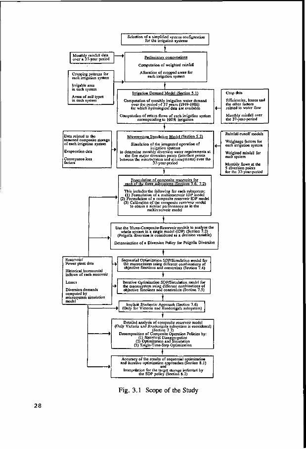
Monthly rainfall data over a 3 7-year-period

Cropping patterns for each irrigation system

Irrigable area in each system

Areas of soil types in each system

Selection of a simplified system configuration for the irrigation systems

Preliminary computations

Computation of weighted rainfall

Allocation of cropped areas for each irrigation system

Irrigation Demand Model (Section 5.1)

Computation of monthly irrigation water demand over the period of 37 years (1949-1986) for which hydrologicaf data are available

Computation of relum flows of each irrigation system corresponding to 100% irrigation

Crop data

Efficiencies, losses and the other factors related to water flow

Monthly rainfall over the 3 7-y car-period

Data related to the assumed composite storage of each irrigation system

Evaporation data

Conveyance loss factors

Microsystem.,Simulation Model (Section 5.2)

Simulation of the integrated operation of irrigation systems

to determine monthly diversion water requirements at the five major diversion points (interface points

between the macrosystem and microsystems) over the 37-ycar-period

Formulation of composite reservoirs for eachof the three subsystems (Sections 5.6" 1.2)

This includes the following for each subsystem: (1) Formulation of a mullireservoir IDP model

(2) Formulation of a composite reservoir IDP model (3) Calibration of the composite reservoir model

to obtain a similar performance as in the multirescrvoir model

Use the Three-Composite-Rcservoir models to analyze the whole system in a single model (IDP) (Section 7.2)

(Polgolla diversion is considered as a decision variable)

Determination of a Diversion Policy for Polgolla Diversion

Reservoir/ Power plant data

Historical incremental inflows of each reservoir

Losses

Diversion demands computed by microsystem simulation model

Sequential Optimization SDP/Simulation model for the macrosystem using different combinations of objective functions and constraints (Section 7.4)

Iterative Optimization SDP/Simulation model for the macrosystem using different combinations of objective functions and constraints (Section 7.5)

Implicit Stochastic Approach (Section 7.6) - • (Only for Victoria and Randcnigala subsystem)

T Detailed analysis of composite reservoir model

(Only Victoria ana Randcnigala subsystem is considered) (Section 7.7)

Decomposition of Composite Operation Policies by: (1) Statistical Disaggregation

(2) Optimization ana Simulation (3) Single-Time-Step Optimization

Accuracy of the results of sequential optimization and iterative optimization approaches (Section 8.1)

and Interpolation for the target storage indicated by

the SDP policy (Section 8.2)

Rainfall-runoff models

Wcighlagc factors for each irrigation system

Weighted rainfall for each system

Monthly flows at the 5 diversion points for the 37-year-period

Fig. 3.1 Scope of the Study

28

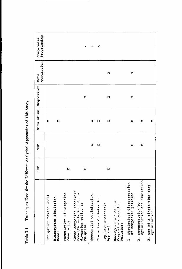
X! X

>> 3

J5

3 o h i ex OH

<

13 e < c o>

c o -rl 01 01 CI u tn (U PS

C o •P 0

rH 3 e

-rl

a w

a. o

X X

Q <u

•8

u 3 ST

'S

^H

ai T J 0

s T 1 C id

ft <]>

a c 0

• r |

• P id

0< - r l

Li l-i

M

c 0

- r l

• p IS

r H 3

e • - i

w e 01

• P 01 > 1

01 0 rH u ai O T3

•rl 0

a x

01 • p • r l 01

0 p. ft 0

u HH 0

c 0

- r l

4->

m ,-H 3 ft VI

0 to

01 Vi

• r l 0

> u (1) 01 01 VI

VI •rl 01 0 s. > +) VI 01 >H 01 O -P 01 IS VI c 1 O > i 01 •<-< o 4J .p -rl • H U H J 1 H O O 3 OH

a e e vi c 0 0 0 O fL4 -r| 1 - - U) 01 H VI 01 01 01

id ^H r H 0

m Vl -O > rH £ 0 - 1 0 EH g -O OH

c 0 • r l

• P id N

- r l

fi • r l

•p H i

o r H id

• r l • P C 01 3

re 01

w

c 0

• r l

• p id N

• r l

ft - r l

•P P . O

01

> •H •P id VI 01

4J M

<> - r l

• P 10 <d

J3 t )

0 • P </l

•p J S •H Cl

• r i r H

O 01

0 Vl

a a f= H

a <

ai a c +J 0

- r | <H -P 0 n)

VI C 01 0 OH

•rl 0 • P •rl 01 01 4J O - r l Pt 01

e o

•• 01

a> • r |

0

o a-ri 0 B 0) 0

r H

0 a o a,

c 0

- r |

• P i d Cn 01 oi at VI ~H o> o Ol ' r l Id rH 01 O

•rl 0J •a 1

01 ^ -P id -H O 01

•rl 0 4J OH 01 S

•rl 0 •P o id 4J <t-t W 0

• r-i

c 0 • r l

4 J id

r H 3

e - r l

oi

r t - O J3 C

id

c 0 c •rl 0 +1 -r| •rl .P la id 0 N CU-rl

e e 0 -rl O -P 01 OH Q 0

• CM

O H

01 • p 01 1

01

e - r |

• P 1 01

•-I

o> c c -rl 0 01 -rl

- P id id

N >H -r|

o e • r |

01 -P oi a 3 0

• f O

4 Literature Review

This Chapter contains a review of the mathematical models and techniques applied to the quantitative management of water resources systems. In general, quantitative analyses of existing reservoir systems are reviewed. Two of the other areas that are of considerable importance to the water resources systems analyst i.e. water quality aspects and capacity expansion are not included this selected review.

4.1 Operation Policy for a Reservoir System

A variety of operation policies are in use at the present time. These operation policies vary from those that only define each reservoir's ideal pool level, or target level (and provide no information or guidance on what to do if maintaining those levels becomes impractical or impossible), to those that define very precisely how much water should be withdrawn or released at every control structure for all possible combinations of hydrologic and reservoir storage conditions.

Ideal storage volumes of single reservoirs are typically defined by "rule curves". They define the desired storage volumes, reservoir releases and/or diversion quantities for each time step of the year. Most often they are based on historical operation practice sometimes supplemented by the results of simulation studies. Having only these target volumes for each reservoir, the operator has to decide on the appropriate action to be taken when it is not possible to maintain these ideal levels.

For multireservoir systems consisting of single purpose water supply reservoirs, the following simple operation rules have generally been adopted:

1. Reservoirs in Series - For such systems the downstream reservoirs are depleted before using upstream reservoir water to meet downstream demands. This procedure ensures maximum use of available storage and that no unnecessary lower reservoir spilling will occur.

30

2. Reservoirs in Parallel - Two procedures are commonly used. One involves discharging water first from reservoirs with relatively larger drainage areas (or potential inflows) per unit storage volume capacity. This procedure is valid only when the runoff per unit area is essentially the same in each reservoir's watershed. Discharging water first from the reservoir having the largest drainage area to storage volume capacity ratio will usually result in a reasonable conservation of water. Another, and more precise procedure involves drawing in tandem from each reservoir. This requires monitoring storage volumes and estimating future inflows. Such a policy minimizes expected water wastage (Loucks et al.,1979).

For multipurpose reservoirs, or for single purpose reservoirs involving recreation or hydropower, operation policies and associated rule curves commonly define the desired storage volumes and discharges at any time of the year as a function of one or more components of: existing storage volumes, the time of the year, the expected inflows, and the demand for water or hydropower. While approximate methods (based on simulation) for determining these operation policies and rule curves have been used in the past (Beard, 1976), research continues towards finding improved methodologies.

4.2 Operation Policy Analyses

Over the past several decades, increasing attention has been given to the use of mathematical models for deriving operation policies for multireservoir systems. As a result, there are now available a variety of methods for analyzing the operation of multireservoir systems used to satisfy collective water-based needs of river basins. These techniques can be used in the selection of those alternatives that best satisfy the different objectives. In general these techniques can be classified into two groups, optimization models and simulation models. Both group of models complements each other. While simulation is an effective means of analyzing the consequences of various proposed management plans and for indicating where marginal improvements in design or operation policy might be made, the technique is not very effective in selecting the best alternative operation policy from the set of all possible alternatives. Usually there are just too many alternatives to be simulated and compared. For this reason optimization models (aggregated and detailed) are often used to indicate which alternatives are most likely to be better than the others.

Optimization models can eliminate the clearly undesirable alternatives, and those alternatives that appear to be most promising can then be further analyzed and improved using simulation techniques. In general, the available optimization methods can be classified as Linear Programming (LP), Dynamic Programming (DP), and Nonlinear Programming (NLP). Yeh (1985) reviewed the state-of-the-art of the mathematical models developed for reservoir operations.

31

4.3 Applicability of Dynamic Programming in Water Resources Systems Analysis (Comparison with Linear Programming and Nonlinear Programming)

Dynamic Programming, a method formulated by Bellman (1957), is a procedure for optimizing a multistage decision process. DP is used extensively in the optimization of the operation of water resources systems. The popularity and success of this method can be attributed to the fact that the multistage decision making behaviour coupled with nonlinear features which characterize a large number of water resources systems can be translated into a dynamic programming approach.

The fact that most of the functions encountered in water resources systems are nonlinear has been the main obstacle in using Linear Programming for water resources management problems. However a nonlinear problem can be handled by linearization techniques with a drastic increase of the number of variables. Nevertheless the degree of reliability depends on the degree of approximation required in the optimization process.

In hydropower optimization problems, the nonlinear hydroelectric production function has the form

E = E(Q,H) = 7*Q*H*t*e (4.1)

in which the produced energy (E) is a function of discharge (Q), generating head (H), and of efficiency (e) multiplied by the specific weight of water (7) and the duration of the time period (t). The nonlinearity that arise from the multiplication of the two decision variables (Q and H) have to be removed in order to use an LP formulation. The simplest way of linearization is to assume a constant value for the head (H) and the efficiency (e). With this approximation an LP problem can be formulated and solved. The obtained solution is used to update the assumed values. This iterative procedure is repeated until the difference between the assumption and the LP solution is less than the required accuracy (Reznicek etal., 1990).

The linearization algorithm developed by Grygier (1983) uses a more sophisticated linearization procedure. The energy equation (4.1) can be written in the following form:

E = ERF*Q*t (4.2)

where ERF stands for energy rate function and is expresses as

ERF = 7*H*e (4.3)

The assumption is that ERF is only a function of the head, that is, of the storage and that it is not dependent on the release. Furthermore, it is assumed that the value of the ERF during the time step can be approximated by taking the average of the function value for the initial and final storage. The approach of Grygier (1983) further requires that the first-order Taylor expansion of the ERF around the estimated initial and final storage values be considered together with an approximation for the linearization introduced by Loucks et. al (1981).

32

Reznicek et al (1990) developed a new algorithm named energy management by successive linear programming (EMSLP) to optimize a hydropower system operation. The EMSLP algorithm is based on the work of Grygier (1983) and has two iteration levels: at the first level a stable solution is sought, and at the second the interior of the feasible region is searched to improve the objective function value whenever it decreases between two iterations of the first level. The EMSLP algorithm has been tested using the Manitoba Hydro system data applied to a single reservoir. To evaluate the performance of the algorithm a comparison has been made only with the presently used approach which uses a constant plant head from one iteration to the other. Reznicek et al. (1990) concluded that their EMSLP approach approximates the hydro production function more efficiently than the constant head approach.

Reznicek et al. (1992) presented the GEMSLP model which is a modification of the previous EMSLP model. The GEMSLP model has the capability to take into account the multivariate character of the ERF incorporating the dependence on discharge and storage. Two ways have been investigated to approximate the ERF; an integral regression analysis and a separate analysis of significant relationships. This model also has been compared only with the results of the presently used "constant head" technique. Although the results are found to be satisfactory, Reznicek et al. (1992) indicated that an application of GEMSLP to a multireservoir, high power plant head is necessary to assess the practical value of the model.

The LP model for the problem of operating a single reservoir presented by Gablinger and Loucks (1970) contained 2000 equations and 15,000 variables and required more than two hours of IBM 360/65 computer time. For a three-reservoir system, the model of Roefs and Bodin (1970) required more than 20 hours of IBM 360/50 time and still had not converged to an optimal solution. In a stochastic LP model, discretization of state variables creates an increase of computational load along with the further boom of variables. Even in the case of deterministic LP, the operation during the entire period has to be considered simultaneously, thereby increasing the dimensions of the problem as the length of the period is increased. Thus, the use of LP is limited only to relatively simple problems.

As Yeh (1985) has explained, nonlinear programming is not popular in water resources systems analysis due to the fact that the optimization process is usually inefficient and takes up a large amount of computer time and memory when compared to the other methods. The mathematics involved in the nonlinear models are much more complicated than in the linear case and cannot explicitly accommodate the stochastic nature of the system.

DP is extensively used in water resources problems due to the fact that problems with a large number of decision variables could frequently be decomposed into a sequence of subproblems (a sequence of decision stages) having one or few decision variables at each stage. In a DP formulation, the series of subproblems is solved recursively. The solution procedure of DP is based on Bellman's principle of optimality (Bellman, 1957). It states that an optimal policy has the property that irrespective of the initial state and initial stage, the remaining decisions must constitute an optimal policy with regard to the initial state and stage. The recursive solution of a DP problem can be achieved by proceeding either backward or forward through the decision stages. Where there is no special reason for

33

choosing either backward or forward formulation, the backward recurrence is normally used. The procedure of making first a backward and then a forward pass is convenient especially in problems involving time, as it gives the optimal policy in the chronological order. In stochastic problems backward recurrence is essential, since each stage depends on the results of the former stage. However forward recurrence has advantages when a deterministic problem has to be solved several times with different planning horizons. This may occur because a plan is periodically reviewed or where the appropriate horizon is unknown and a sensitivity analysis is undertaken. The procedure can be extended forward in time without repeating previous calculations.

It is not unusual to find that a problem can be formulated for solution by DP in more than one way. For example, decision stages may represent different points in time or in space. However, to decompose a general problem into stages with decisions required at each stage, the value of every stage should satisfy the separability condition and the monotonicity condition (Nemhauser, 1966). The validity of DP regarding separability can be extended by an appropriate choice of stage and state. For example, reservoir inflows are defined as states in addition to reservoir storage when the inflows are markovian rather than random in the transition equation.

However, the main drawback of a DP approach is the drastic increase of the computational load and the computer memory requirement which result as the number of state variables increases. This is appropriately termed as the "curse of dimensionality" associated with Dynamic Programming.

4.4 Reservoir Operation Models Based on Deterministic Dynamic Programming

Hall and Buras (1961) were the first ones to apply dynamic programming techniques for optimizing the design of water resources systems. A problem of capacity allocation among a number of reservoir sites was solved using DP. A loss function was used to measure the cost and benefit of capacity allocation to different sites. It was also shown how the decision problem of allocating water at a given reservoir site among various users (flood control, recreation, irrigation) can also be formulated as a DP problem. Thus DP is used in the construction of single-stage loss functions themselves.

Meier and Beightler (1967) illustrated methods for optimizing branched multistage systems in water resources planning. Nonserial river basin systems were decomposed into equivalent serial systems amenable to analysis by the dynamic programming method.

Hall and Shepard (1967) developed a DP-LP technique for optimizing a reservoir system in which the multiple reservoir system is decomposed into a master-problem and subproblems. The master-problem could be seen as a system coordinating agency and the subproblems as single reservoir managers. In that work the subproblems were solved by DP. The schedule of releases and energy production were reported to the system coordinating agency which was modelled by LP.

34

Larson (1968) introduced the concept of Incremental Dynamic Programming (IDP), putting DP into an iterative context. IDP uses the incremental concept for the state variables. Only a limited state space is considered for a given iteration run. It starts with a feasible initial solution which can be visualized as a trajectory along the subsequent stages. Traditional DP is then applied in the neighbourhood of this trajectory. At the end of each iteration step an improved trajectory is obtained, which is used as the trial trajectory for the next iteration step.

Computer time and memory requirements are vastly reduced by considering only a limited state space. However the major setback of using this technique is its possibility to end up at a local optimum. (Turgeon, 1982). That can be avoided by starting with large increments to define the imaginary corridor around the actual trajectory and reducing them gradually as the iteration proceeds. Another way to avoid getting trapped at a local optimum is to repeat the iteration with different initial conditions. Finally both approaches i.e. varying increments and different starting solutions can be coupled (Nandalal, 1986).

Heidari et al. (1971) systematized the use of incremental dynamic programming and referred to as Discrete Differential Dynamic Programming (DDDP). Nopmongkol and Askew (1976) analyzed the difference between IDP and DDDP and concluded that DDDP is the generalization of IDP.

Trott and Yeh (1973) developed a method to determine the optimal planning of a reservoir system with cascade and parallel connections. The policy was obtained by decomposing the original problem into a series of subproblems of one state variable each and by applying Bellman's method of successive approximations in such a manner that the series of optimizations over the subproblems converge to a solution of the original problem. Each sub-problem was analyzed using the DDDP technique of Heidari.

Murray and Yakowitz (1979) developed a successive approximation dynamic programming technique using differential dynamic programming principles, constraining a sequential decision variable as applicable to multireservoir control problems in some cases. This approach is known as the Constrained Differential Dynamic Programming (CDDP) algorithm.

Yakowitz (1982) reviewed the DP models for water resources applications. Apart from reservoir operation analysis, the models reviewed include aqueduct design, irrigation system control, project development and water quality maintenance.

Harboe (1987) applied DP to a system of reservoirs in which low-flow augmentation was the main purpose. The objective function used in the optimization is to maximize the minimum flow. A sequential optimization starting from the upstream and considering one reservoir at a time is employed. The optimum results of one reservoir are used as the inputs to the downstream reservoir. The local optimum obtained was very close to the global optimum due to the high cross-correlation among monthly flows at different locations in the basin.

35

4.5 Stochastic Optimization

Deterministic optimization models are often inadequate for effective water resources systems analysis due to the uncertainties inherent in the prediction of hydrologic, economic, and other factors. The general form of an optimization problem is:

maximize f(X) , X' = (X, ,X2).. ,X„)

subject to g,(X) = Bi ,X,=(XI,X„..,X11) (4.4)

i = l,2,..,m

in which the vector X contains the decision variables X( whose values define a particular plan and operation policy. Uncertainty may arise in the objective function f(.), one or more constraint functions g|(.), or right-hand-side values B;.

The uncertainty that affects the problem's objective function f(X) and not related to the constraints gj(X)=B, can arise from imprecise knowledge of the value of the future benefits and costs resulting from alternative decisions. Such uncertainty can often be handled by substitution of the expected value for the uncertain net benefit function. Use of the expected value of the objective is satisfactory if the alternatives are not too extreme in terms of the objective values so that the expected value can be substituted for the expected utility of a decision.

Uncertainty in the constraints g;(X)=Bi can be handled in different ways. If the uncertainty is small it may be satisfactory to use the expected values of both sides of the constraint, as in many deterministic optimization problems. However the substitution of expected value for random quantities is unacceptable when large variation in some quantities will result in significant violation of the constraints.

Alternatively, an explicit description of the uncertainty in the constraints can be included in the optimization model, allowing the decision variables to depend on the values of various random variables. This allows the constraints to be met for different values of the random variables and allows the operation policy to exploit the availability of extra resources. Uncertainty in the constraints can be modelled in different ways, depending on the optimization technique. Conventional stochastic dynamic programming can be used to study complicated situations as long as few state variables are required. Stochastic linear programming techniques require more restrictive assumptions concerning the structure of the uncertainty. Solution of stochastic problems using LP can be performed in two ways. They are the use of a large number variables to account for alternative possible scenarios, or the use of chance constraints. The former one restricts the possible number of scenarios to only a few, in order to reduce the number of variables. When only the right-hand side B( of one or more inequality constraints is random, chance constraints can be formulated that define the probability p that the constraint can fail. Thus instead of specifying that

36

g,(X)<E[By for those constraints in which Bj is random, a chance constraint

Pr[gi(X)<B;] > 1-p, (4.5)

can be defined, indicating that the constraint can be violated no more than 100pj% of the time. This can be converted into deterministic equivalents if the probability distribution function Fj(bi) is known (bj) represents a possible realization of the random variable Bj). For a particular decision, this can be expressed as:

gi(X) < b>i> (4.6)

where the quantity F{l(pD is expressed as b^P.

Dupacova et al. (1991) adopted chance constraints in analyzing a small-size water resources system in Eastern Czechoslovakia. They also analyzed the same system using an alternative model which included a penalty function for the underachievement of the objective. With regard to the chance constrained model they concluded that the probabilities considered in the model have to be carefully chosen in order to avoid conservative results. This is due to the pessimism inherent in the chance constraint models which is a result of modelling scarce resources and high demands to set the targets. The consistent joint occurrence is not only unlikely, but basically negates the proven fact that consumption can be reduced by rationing etc in face of supply shortage often without disastrous consequences. The "penalty" models cannot however be applied in the real life situations for the simple reason that the result would be too sensitive to the unknown (often approximated) penalty function.

4.5.1 Stochastic dynamic programming (SDP) Models for the Optimization of Reservoir Operation

The methods reviewed so far are employed in predominantly deterministic decision environments. Streamflows are taken to be equal to the mean seasonal inflow or from a historical critical period. In reality, however, virtually all hydrological model parameters are uncertain. In the following, several methodologies which can be used for planning purposes when particular parameters such as inflows are considered to be uncertain will be reviewed.

Stochastic nature of the inflows can be handled by two approaches; an implicit or an explicit stochastic approach. In the implicit approach, a time series model is used to generate a number of synthetic inflow sequences. The system is optimized for each streamflow sequence and the operating rules are found by multiple regression. During the optimization the synthetic data series are considered as deterministic ones.

Although the implicit approach can be easily adopted for single reservoir optimization, numerous difficulties are encountered in applying it to multireservoir systems. Difficulty of obtaining a computationally manageable algorithm which derives the optimal results

'£[Bi] indicates the expectation of the random variable Bj

37

becomes much more severe when the streamflows into each reservoir are interdependent. In such a situation, complicated synthetic streamflow generating models are to be used, to obtain the cross-correlated streamflows into each of the reservoirs.

Implicit approach optimizes the system operation under a large number of streamflow sequences, at the expense of computer time. It is therefore employed only for long range planning purposes. The explicit approach considers the probability distribution of the inflows rather than specific flow sequences. This approach generates an operation policy comprising of storage targets or release decisions for every possible reservoir storage and inflow states in each month, rather than a mere single schedule of reservoir releases.

Butcher (1971) used explicit stochastic dynamic programming to determine the optimal operation policy for a multipurpose reservoir. The optimal policy is expressed in terms of the state of the reservoir indicated by the storage volume and the streamflow in the preceding month.

Loucks et al. (1981) presented a stochastic dynamic programming model with its application to a single reservoir. In this example only two periods, each period having only two possible discrete inflows and two initial storages have been considered.

Stedinger, Sule and Loucks (1984) developed a stochastic dynamic programming model which employs the best forecast of the current period's inflow to define the reservoir release policy and to calculate the expected benefit from future operations. Use of the best inflow forecast as a hydrologic state variable, instead of the inflow of the preceding period resulted in substantial improvements in simulated reservoir operations with derived stationary reservoir operation policies.

Bogardi et al. (1988a) investigated the impact of varying number of storage and inflow classes upon the operational performance of SDP for both single and multi-unit reservoir systems. The results indicated that by simply increasing the number of storage classes beyond certain limits the system performance would not improve much. These results comply with the "Law of diminishing returns". Emphasis should rather be placed on the "synchronization" of the number and size of storage and inflow classes, in order to check whether any improvement could be obtained.

Shrestha (1987) applied SDP to derive optimal operation policies for different configurations of a hydropower system which was in the planning stage. Simulation of the system operation is carried out based on the SDP-based optimum policy to evaluate the system performance. Finally the optimum system configuration is selected by comparing the performance values obtained for the different configurations.

Laabs and Harboe (1988) presented three models based on DP including a deterministic model, an independent probability model and a markov model for finding Pareto-optimal operation rules for a single multipurpose reservoir. In the independent probability model, the inflow probabilities of each time step are considered. Inflow transitional probabilities are considered in the markov model. The markov model included several objective functions and weights for each objective as needed in a compromise programming analysis

38

of multiobjective decision making. A number of Pareto-optimal operation rules were generated. The final selection of the optimal policy can be done only after simulations with these operation rules have been performed and a multiobjective selection criterion is applied to the results.

Shrestha et al. (1990) studied the effect of the number of discrete characteristic states and the impact of varying the definition of these characteristic states on SDP model performance. Four real world cases have been analyzed from different hydrological regimes. It has been found that varying the definition of inflow state discretization renders only marginal changes in the model performance. The factors which could have a direct bearing on the adequate level of storage state discretization are identified as: the hydrologic regime in which the system is located (due to the differences in inflow state distribution), the type of system constraints and the degree of severeness of system constraints.

4.5.2 Different Versions of Stochastic Dynamic Programming

Four categories of SDP models (Huang, 1989; Huang et al., 1991) and their characteristics are briefly described in the following.

Assume that the objective function in SDP is the maximization of the expected system performance. Let Bkilt be the value of system performance associated with an initial reservoir storage volume (k), an inflow (i), a release (r) leading to a final storage volume (1) in time step t. Furthermore, define ft(k,i) as the total expected value of the system performance with n periods to go (while at the beginning of the time step t). Then the backward recursive relationships can be generated by

f\(k,i) = Maximize [Bkilt + E Pijt+1*f,1,+1(lj)] (4.7)

1 J for all n,k,i,t; 1 feasible

where t refers to the within-year period and n to the total number of periods from the actual stage until the end of the time horizon. They are also graphically displayed in Fig. 5.6 under the detailed description of a SDP model presented in Section 5.3.4. The indices k and i are indicating state variables while state 1 (the initial storage state for the next time step) is the decision variable. Pjjt+1 is the inflow transitional probability specifying the conditional probability that the next inflow state in period t+1 is at state j , given the current inflow in period t is at state i.

If the correlation between two consecutive inflows is not significant, i.e., the current inflow is nearly independent of the previous inflow, then the probability distribution of the inflow can be considered as an unconditional one. Equation 4.7 yields

f\(k,i) = Maximize [Bkilt + E P/^f ' .+.Oj)] (4.8) 1 J

for all n,k,i,t; 1 feasible

39

The optimal operation policies related to Equations 4.7 and 4.8 are functions of the initial reservoir storage and the unknown inflow during the time step considered. In practical situations, streamflow forecasts regarding the reservoir inflow during the stage are needed for on-line operation.

On the other hand, if the optimal operation policy is considered as a function of initial storage and the previous inflow, instead of the current inflow, streamflow forecasts may be avoided. By specifying P^ as the inflow transition probability that the inflow state of the current period t is at state j , given the previous inflow in period t-1 was at state i, the backward recursive function becomes

f\(k,i) = Maximize (EP^PV + f^.OJ)]} (4.9) r j

for all n,k,i,t; r feasible where r is the release decision of the time step t.

In case of independence between two consecutive inflows, Equation 4.9 then reduces to contain only a single state variable (storage) without the consideration of inflow, known as a probabilistic model which is expressed as follows.

ft(k) = Maximize { E P ^ , , + f"-'1+1(l)]} (4.10) r j

for all n,k,t; r feasible

Note that for Equations 4.7 and 4.8 the decision variable is defined as the final storage state (1) while the Equations 4.9 and 4.10 indicate the possibility of using the release (r) as the decision variable.

Huang (1989) concluded that the SDP model with initial reservoir storage and past inflow as state variables (Equation 4.9) appears to be the best one among all SDP models. Huang (1989) also indicated that this conclusion might not be universal under different hydrological regimes, but depends upon the characteristics of the particular water resources system.

However, it is not reasonable to assume that the forecasts can be avoided or neglected by considering the previous month's inflows in SDP. It is simply too dangerous to neglect forecasts in the actual operation of any reservoir. The use of the current month's inflow in the SDP model results in the best policy under the condition of perfect forecasts. This means that the performance under the resulting policy indicates the upper bound attainable using a SDP-based policy. The performance will only be deteriorated due to the inaccuracy of the forecast. Should the forecast found to be inaccurate, the policy formulated with the current month's inflow still can indicate the alternative action to be taken during the course of the time step considered. On the contrary, the operator will have no guidance for such an action in the case of a policy based on the previous month's inflow.

40

4.5.3 Disaggregation/Aggregation Techniques Based on Dynamic Programming

As indicated previously, dynamic programming algorithm suffer from the "curse of dimensionality". It was shown by Bogardi and Nandalal(1988) that the maximum number of reservoirs that can be handled in a conventional SDP model is limited to two, without exceeding the practical limits of computer memory and computer time requirements. However the computational requirements of such a model well exceed those limits, upon a slight increase of the number of inflow and/or storage discretization levels of reservoirs.

The computational requirements can be substantially reduced by disaggregation/aggregation techniques which can be described under the general headings of mathematical disaggregation and physical disaggregation. Commonly both procedures are used, each to a degree depending on the circumstances. Mathematical disaggregation is based on constructing a suitable mathematical model representing the entire physical system to be considered. In general, the interactions between the mathematically disaggregated subproblems will appear in the set of internal constraints which limit the feasible decision sets. Rogers et al. (1991) reviewed the recent theory and applications of mathematical aggregation and disaggregation techniques in optimization. Their review covered methodologies in which the optimization problems are solved by (1) combining data, (2) using an auxiliary model (or models) which is reduced in size and/or complexity relative to the original model, and (3) analyzing the results of the auxiliary model in terms of the original model.

The second approach which is the physical disaggregation differs from mathematical disaggregation only in the point at which one begins. In physical disaggregation the complex system is first divided into sub-units on the basis of the physical or functional characteristics, then the mathematical models are prepared, rather than vice versa.

Physical disaggregation itself may have a number of basic approaches. One of the more useful of these for water resources is the identification of subsystems by their functions or purposes within the large system. Frequently this allows disaggregation of objectives and objective functions as well as of the interactions. This is particularly useful for multiple-objective systems that are usually encountered in water resources planning or management. Some objectives dominate certain subsystems but are essentially negligible for others. Frequently this eliminates serious problems of attempting to commensurate fundamentally different (noncommensurate) objectives at all levels.

The problem of the optimal operation of a multireservoir system can be simplified also by transforming the problem into three subproblems. The first is to formulate a single equivalent reservoir representing the multireservoir system. The second is to determine the optimal operation of such single reservoir. The third is to disaggregate such optimal operation into the operation of the original multireservoir system. According to Salas and Hall (1983), attempts to use aggregation procedures for solving multireservoir systems began in 1951 with the work of Morlat. Since then extensive studies have been made directed to better approaching the three subproblems mentioned above.

41

A composite model for multireservoir hydroelectric power systems is constructed by Arvanitidis and Rosing (1970) for studying the monthly decision concerning total hydropower generation. Their composite model is based on a single measure "potential energy" which is indicative of the systems generating capability. This results in a one dam representation of the multireservoir system which in effect receives, stores and releases potential energy, in a statistical model for the potential energy inflow and in a generation function which relates potential energy related to actual electric power generated. The analytical technique used was SDP. Their model is most applicable when the sequence of monthly decisions on total energy generation is of greater economic significance than the allocation of the total output among various hydropower plants.

Turgeon (1980) proposed two methods which use dynamic programming to determine optimal operation policies of multireservoir systems with stochastic inflows. The first, called the one-at-a-time method, consists in breaking up the original multivariable problem into a series of one state variable subproblems that are solved by dynamic programming. The final result is an optimal local feedback operation policy for each reservoir. The second method, called the aggregation decomposition method consists in breaking up the original n state variable problem into n stochastic problems of two state variables that are solved by dynamic programming. The final result is a suboptimal global feed back operation policy for the system of n reservoirs.

Turgeon (1981) presented a decomposition method for the long term scheduling of reservoirs in series. The method consists of rewriting the stochastic nonlinear optimization problem of n state variables as n-1 problems of two state variables which are solved by dynamic programming. The reservoir release policy obtained by this method is a function of the water content of the reservoir and of the total amount of potential energy stored in the downstream reservoirs.

However, in the above approaches, along with the reduction of dimensionality the complexity of the approaches has been correspondingly increased.

A heuristic iterative technique based upon SDP for the analysis of the operation of a multireservoir system was presented by Tai and Goulter (1987). The technique is initiated using historical inflow data for the downstream reservoir. At each iteration the optimal policy for the downstream unit are used to estimate targets for the operation of upstream reservoirs. New input inflows to the downstream reservoir are then obtained by running the historical inflow record through the optimal policies for the upstream reservoirs. These flows are then used to develop a new operation policy for the downstream reservoir and hence set new targets for the upstream reservoirs. The process is continued until the operation policies for each reservoir provide the same overall system benefit for two successive iterations. This convergence is approximately equivalent to convergence in the operation policies of the reservoirs, i.e. having the operation policy for each of the reservoirs unchanged from one iteration to the next.

42

4.5.4 Implicit Stochastic Models for the Operational Optimization of Reservoir Systems

These are the models which optimize returns for stochastic hydrologic sequences assuming that these sequences are known a priori. Some early developments in this area were conducted by Hall (1964) and Hall and Buras (1961). Their models were solved using DP methods. Young (1966,1967) extended the results of these earlier investigations. His approach included streamflow synthesis, deterministic optimization (again with the use of DP) and regression analyses. The regression analyses were used to define release values in terms of storage levels and previous inflow rates. The data used for the regression analyses were derived from the sequence of computed responses obtained from the optimization model.

Although Young's work was directed at analyzing only a single reservoir, it was considered that the "implicit stochastic" approach would be superior to the "explicit stochastic" approach for multireservoir systems. For the implicit approach, the computational effort in optimization is directly proportional to the number of reservoirs in the system. Computing time grows exponentially with the conventional explicit approach.

The sampling stochastic dynamic programming approach (SSDP), first used by Araujo and Terry (1974) for the operation of a hydro system can also be categorized as an implicit stochastic approach. SSDP was used by Dias et al. (1985) for the optimization of flood control and power generation requirements in a multipurpose reservoir. With SSDP, one selects a large number of possible streamflow scenarios for the system to describe the joint distribution of reservoir inflows. Kelman et al (1990) included the best inflow forecast as a hydrologic state variable in the SSDP algorithm. In their approach, a historical time series of streamflow forecasts was employed to develop the required conditional probability distributions.

There are, however, certain theoretical questions which still remain unanswered in using an implicit approach. For example, the form of the equation (which independent variables should be included and how they should be treated) for regression analysis is open to question. An implicit stochastic approach would not be the appropriate technique particularly for a multireservoir system, due to the complexity of streamflow data generation process.

4.6 Simulation Techniques

Simulation is a modelling technique which is used to approximate the behaviour of a system, representing all the characteristics of the system largely by mathematical equations. A simulation model provides the response of the system for certain inputs which includes operation rules so that it enables a decision maker to examine the consequences of various scenarios of an existing system or of a new system to be constructed. Since simulation models do not define the optimum policy or procedure to be used directly, it is necessary to use a trial-and-error procedure to search for an optimal or near optimal solution. To achieve this, it may be necessary to perform a large number of simulation runs which can

43

of course be computationally prohibitive.

Simulation models, however, have certain other advantages. They usually permit more detailed representation of different parts of the system. They also allow added flexibility in deriving responses which cannot always be readily defined in economic terms (recreational benefits, preservation of fish and wild life etc.). Finally, they provide an effective focus for dialogue with system operators (the principles of simulation modelling can usually be understood more easily than those of the optimization modelling).

A mathematical simulation model for assessing alternative policies of operation of a 48-reservoir system was developed by Sigvaldason (1976). In every time step of the simulation process, a single time-step optimization is performed to route water through the system in an optimum manner. Every reservoir was subdivided into five storage zones (which were variable in a temporal sense). A time-based rule curve was also prescribed to represent ideal reservoir operation. Ranges were described for channel flows, which were dependent on water based needs. 'Penalty coefficients' were assigned to those variables which represented deviations from ideal conditions. Different operation policies were simulated by altering relative values of these coefficients. The development and use of the model were simplified by representing the entire reservoir system in a 'capacitated network' form and deriving optimum solutions for individual time periods with the 'out-of-kilter' algorithm. Besides being computationally efficient this algorithm simplified the model development and permitted flexibility in readily using the model for a wide range of reservoir configurations and operating policies. This methodology has been used by ACRES (1985) in the studies of operating policy options for the Mahaweli water resources system.

In contrast to the optimization models, simulation models can best be employed to assess the performance of a system, if the operation policies have been predetermined. This would permit a detailed investigation of the resulting operation pattern and subsequent improvements to the operation policies which are derived by optimization models that include much less details of the system than the simulation models.

4.7 Multicriterion Decision Making (MCDM) Techniques

The planning and operation of water resources systems are usually multiobjective decision problems. Often, the trade-offs must be considered between two or more objectives. These objectives may fall under the broad categories of economic, social, environmental, political and in some cases international as well. To reflect the trade-off or compromise between the conflicting interests or objectives, several promising scientific tools are available. The outcome of the analysis is a compromise solution or a "satisfactum" rather than an "optimum". These techniques also apply to problems in which trade-offs are made among various purposes.

The use of a Multicriterion Decision Making (MCDM) technique is needed in the present study in order to select the most satisfactory operation policy among a number of alternatives. These DP-based operation policies are evaluated by several different performance criteria. These performance criteria can be considered as the measures of

44

different "objectives" in the MCDM process.

In a MCDM approach, one chooses a "noninferior" solution also referred to as a "Pareto optimal", "nondominated" or an "efficient" solution. With this solution, no improvement may be obtained in any objective achievement without causing a simultaneous degradation in at least one of the other objectives. The solution of the MCDM problem which is the best compromise solution of the problem belongs to this "noninferior" set of solutions. The term "ideal point" has been used to describe a measure of goal attainment that the decision maker would like to achieve. To qualify for a MCDM analysis, these levels specified for goals are such that they cannot be achieved simultaneously for all the objectives. Otherwise, a trade-off is not required. In other words, an ideal point is located outside the feasible region. If each objective is optimized without regard to the other objectives, the point in the decision space which is having these optimal values is called the ideal point.

There are many possible classification schemes for MCDM problems (Duckstein, 1989). The classification of Duckstein (1989) identifies five categories of MCDM techniques. They are:

(1) Outranking type of techniques (2) Distance-based techniques (3) Value or utility type of techniques (4) Direction-based techniques (5) Mixed type of techniques

4.7.1 Outranking Type of MCDM Techniques

These techniques use outranking relationships among alternatives to select the most satisfying alternative. An outranking relation is conceived to represent the preference ordering of a finite set of alternatives. Four different preference relations between alternatives can be recognized: a strict preference, indifference, weak preference and incomparability (Haimes et al.,1984)

Outranking techniques constitute excellent tools for the design of reservoir schemes under conflicting objectives. The key element of such schemes is a table of alternatives versus criteria; the criteria may include non-numerical measures, in which case techniques that can handle such non-numerical criteria should be selected for use.

4.7.2 Distance-Based MCDM Techniques

Some MCDM techniques are based on the concept of distance to arrive at the most satisfying solution. This distance is not limited to the geometric sense of distance between two points. Rather distance in this case is used as a proxy measure for human preference (Zeleny, 1973, 1982). This concept of distance is therefore, used for the purpose of determining solutions in reference to some point in the decision space. (Duckstein, 1989)

45

There are several distance-based techniques developed to date. Generally, the solution procedure in these techniques proceeds by first defining some reference point which is mostly an infeasible alternative that one relates the solution one desires to achieve. One major difference among the techniques that belong to this group is the way they relate to the reference point. Compromise Programming (CP) identifies the feasible solution that is closest to the reference point which is known in this case as the ideal solution (Zeleny, 1973, 1974, 1982; Yu, 1973). Distance-based techniques have the advantage that they are simple to understand and implement.

4.7.3 Value or Utility Type of MCDM Techniques

Many MCDM procedures are based on the preference orders of the decision maker, which is assumed to be known (Szidarovszky et al., 1986) and on the hypothesis that the Decision Maker (DM)'s preference structure can be formally and mathematically represented by his/her value if the problem is deterministic, or utility function especially if there is any risk involved in the problem.

The value or utility type of techniques are certainly well adapted to the modelling and resolving of conflicts in reservoir management. (Krzysztofowicz and Duckstein, 1979). In principle, they provide a complete ordering of the set of nondominated (pareto optimal) alternatives. The nondominated alternative which yields the highest utility is then taken to be the most satisficing solution. Yet the utility functions are very difficult to formulate and their development for water resources development has been meagre. (Goodman, 1984)

4.7.4 Direction-based MCDM Techniques

Most interactive schemes include a step during which the decision maker is asked to state a preferred direction for the search for a compromise solution. Techniques such as evolutionary SEMOPS (Bogardi et al, 1988b, 1988c) belong to this category. The direction based techniques are recommended whenever a decision maker is willing to provide information for a directional search for a "satisfactum". Their use for conflict resolution needs further investigation. (Duckstein, 1989)

4.7.5 Mixed Type of MCDM Techniques

Apart from the above four types of MCDM techniques, there are a large number of miscellaneous techniques that cannot be placed under any one category. Many of them, however, can be considered as generating techniques. According to Goicoechea et al. (1982) a generating technique considers the vector of objective functions in a decision problem and uses this vector to identify and generate the subset of nondominated solutions in the feasible region. In doing so, these techniques identify a set of nondominated solutions to help the DM gain insight into the physical realities of the problem under consideration.

If a finite set of distinct alternatives is used, then most multiobjective programming methods fall through. On the other hand, the use of the techniques such as CP may be promoted. (Duckstein, 1989).

46

4.8 Disaggregation Models in Stochastic Hydrology

The aggregation techniques that can be used to facilitate the operational optimization of water resources systems is followed by a need for a disaggregation process. The representation of a number of reservoirs in a system as a single hypothetical composite reservoir is one of the most suitable aggregation techniques. The composite reservoir circumvents the dimensionality problems in analyzing multireservoir water resources systems. However the optimum operation policy that is derived for a composite reservoir configuration needs to be translated (decomposed) into that of the real individual reservoirs. For this purpose, a variety of techniques can be used. The principle of decomposition shall be to identify the individual reservoir operation patterns that closely resembles the global optimum operation pattern derived using composite representation. The statistical relationships that exist among the operation patterns of composite and individual reservoirs provide the basis for a statistical disaggregation approach of this study.

The historical operation pattern of the reservoir system can provide a reasonable basis for the operation pattern of the individual reservoirs. The optimum operation pattern of the composite reservoir can be determined by a simulation performed according to the SDP-based operation policy of the composite reservoir. The resulting inflow, release and storage time series of the composite reservoir and the corresponding actual operation details of the individual reservoirs can be used to implement the disaggregation of composite reservoir operation pattern to that of the individual reservoirs.

Disaggregation modelling is a process by which lower level (eg. monthly, weekly) time series are generated dependent on a higher level (eg. annual) time series already available. It is one of the several approaches that have been reported for the analysis of hydrological time series (Hipel, 1985). In disaggregation (DA) procedure, the independent series which are stationary, e.g. the annual series are generated first by a suitable model such as a fractional noise process or an autoregressive process, and then the seasonal series are generated by disaggregating the independent time series preserving both long and short term variance and covariance properties of the hydrologic process. The DA model may be temporal or spatial depending upon whether the disaggregation of time series is in time domain or in space domain respectively. Hence, disaggregation of annual streamflows to generate seasonal (say monthly) streamflows is an example of temporal disaggregation and that of total flow of a river basin into the individual tributary flows is an example of spatial disaggregation.

It is experienced that when sequences corresponding to a certain level of aggregation are generated with autoregressive models, relevant statistics of higher levels of aggregation are not necessarily preserved. The fractional noise models are applicable only to stationary processes and thus cannot be adapted to the seasonally varying processes occurring within the year. Disaggregation modelling overcomes the difficulties in both the fractional noise and autoregressive models.

Literature review in the development of disaggregation models shows that the basic model was first proposed by Valencia and Schaake (1973). This contribution was referred by some authors as a significant bench mark in the literature of hydrologic time series. The model

47

developed for generating multiple hydrologic time series preserved both long term and short term variance and covariance properties, including seasonal variation. The disaggregation model proposed by them maintains relevant statistics at all levels of aggregation owing to the fact that the general model preserves all linear relationships between variables at successive levels of aggregation. This model was successfully used for rainfall generation in Puerto Rico, for streamflow generation in Argentina and the United States and for the generation of hourly water demands in the Boston water distribution system.

In this model, the data within a given year preserve the statistics for all levels of aggregation. However they are linked with the past only through the statistics at the yearly level. Mejia and Rousselle (1976) extended the disaggregation model proposed by Valencia and Schaake (1973) in order to include linkage with the past at all levels of aggregation. The model was tested on 24 years of hydrologic information for two stations located in the watershed of the North River.

The application of disaggregating modelling to multistation, multiyear synthesis of hydrologic time series is presented by Tao and Delleur (1976). The model developed not only preserves the long-term and short-term properties of the time series but also the cross-covariances between the stations. The model which is a generalized disaggregation model based on the procedure proposed by Valencia and Schaake (1973), has the following two advantages over the latter: (1) It requires no data transformation on the original observed time series for the removal of within-the-year cyclicities; therefore this model is free from any possible error or bias in the preservation of seasonal cyclicities introduced by the data transformation. (2) The model is not only capable of disaggregating the lower-level events from the higher-level events of the same kind but also has the merit of generating the lower-level events from the higher-level events of different kinds (e.g., disaggregating annual rainfall volumes into monthly run-off volumes). The model was applied to 36 rainfall, run-off, and rainfall-run-off sequences in the lower Ohio and upper Mississippi River basins. The properties (i.e., the moments - the means, the variances, the auto and co-variances) of the generated data series showed excellent agreement with those of the historical observed data series.

Hoshi and Burges (1979) proposed a disaggregation model called Hoshi-Burges (HB) model. The model which is an alternative model for Mejia and Rousselle (MR) model, ensures the preservation of correlation between seasons in successive water years. The HB model achieves the result by simultaneously disaggregating two successive annual events.

Methods for the preservation of skewness in linear disaggregation schemes are reviewed by Todini (1980). As discussed earlier, Hoshi and Burges (1979) approached the problem by employing transformations and using various disaggregation schemes in the transformed space. However, this means that the linear additive property which is one of the main attributes of the original linear disaggregation schemes of Valencia and Schaake (1973) is apparently lost. The preservation of skewness for the extended model by Mejia and Rousselle (1976) is also presented. Besides the author has also proposed the use of standardized variables of annual and seasonal flow vectors. The applicability of proposed methodology is testified by generating streamflow for the Nile river at Aswan. The 100 annual historic as well as the same length of generated series are disaggregated to generate

48

monthly series. The distributions of average statistics of generated and historic monthly flows have shown the similar pattern.

Stedinger and Vogel (1984) discussed why the extended model of Valencia and Schaake (1973) by Mejia and Rousselle (1976) fails to reproduce the anticipated variances and covariances of the disaggregated flows. Examination of the causes of failure reveals the constraint imposed by the disaggregation framework on the lagged covariances of the disaggregation flows (i.e. the parameter estimators are not self-consistent). The authors presented a class of disaggregation models which within the disaggregation framework, can reproduce the covariances of the disaggregated flow vectors (seasonal or basin flows at individual sites), their covariances with the upper level flows (annual or aggregated basin flows), and reasonable approximations to the lagged covariances of the disaggregated series.

A note of caution in using disaggregation models has also been cited. The disaggregation models can reproduce some lagged covariances while they do not or cannot reproduce others, hence care must be taken to insure that a model's parameters are estimated using appropriate equations. If care is not exercised, then one may implicitly assume that some historical statistics will be reproduced when that is not the case. This illustrates a difference in the requirements which should be imposed on models to be used for prediction, forecasting, and control and those to be used for stochastic streamflow generation. When developing equations for prediction, one generally assumes that historical relationships among the explanatory variables will persist. However, when generating streamflows or other stochastic sequences, the only characteristics of the real system which will be reproduced in the selected generated series are those reproduced by the generating model and its parameters. Thus, special care should be taken to insure that models used for stochastic streamflow generation and statistics used to estimate the model's parameters are self-consistent.

The Valencia and Schaake's basic models of multisite, multiseason disaggregation models can have an excessive number of parameters because of the many cross correlations that they attempt to reproduce. This has led to the use of the staged disaggregation models in which the higher level flows are disaggregated to lower level flows in a number of steps, say from annual to seasonal, seasonal to monthly and monthly to weekly.

Lane and Frevert (1989) developed a comprehensive multisite stochastic streamflow package, called LAST. The condensed LAST model reproduces the concurrent and lag-1 monthly correlations among the monthly flows, and the correlations between the monthly and annual flows.

LAST package disaggregates key station annual flows to substation annual flows and then disaggregates jointly substation annual flows in different groups to seasonal (or monthly) flows for stations in that group. This explicitly models the cross correlations among annual flows in different groups, but not the cross correlations of the seasonal flows. It is to be noted that the term "seasonal" is used here as a general term which also represents monthly values. The essential attributes of the approach used in LAST package are as follows:

49

(1) Ability to preserve year-to-year serial correlations with a multilag linear autoregressive model in addition to seasonal serial correlations.

(2) Ability to preserve cross correlations on an annual basis.

(3) Ability to generate "key" stations and to disaggregate those values into component substations on an annual basis.

(4) Ability to likewise disaggregate annual values into seasonal values preserving both serial correlations and cross correlations between variables on a seasonal basis.

(5) Ability to generate annual and seasonal values which come from distributions statistically indistinguishable from those observed historically. The transformation of the data to a normal form is done by a trial-and-error procedure, with the use of cumulative probability distribution plots.

4.9 Techniques/Models Selected for the Present Study

In the following, the selected modules of the analysis are summarized.

Irrigation demand Computation The irrigation demand model of ACRES (1985) that has been calibrated for modelling Mahaweli irrigation systems is selected for this purpose.

Optimization of Reservoir Operation In order to derive long-term optimal operation policies of reservoirs, SDP is employed. Its suitability over the other available techniques is discussed in Sections 4.3 and 4.5. The SDP model formulation selected was the one that contain the initial reservoir storage and the inflow during the current time step as state variables (Equation 4.7). The basis for this selection is presented in Section 4.5.2. The technique of Incremental Dynamic Programming (IDP) is used to determine the deterministic optimum reservoir operation pattern for a known time period. IDP, while possessing all the advantages of DP, reduces the dimensionality of the problem by an iterative search of the optimum solution over a limited state space at each iteration step (Section 4.4).

Simulation Techniques Simulation models are employed to assess the performance of the SDP-based reservoir operation policies. The determination of the water requirements of the microsystem is also achieved by simulating the integrated operation of the irrigation areas within the microsystem.

Aggregation/Disaggregation Techniques In this study, both mathematical and physical aggregation/disaggregation techniques are used. The implicit stochastic technique (Sections 3.2.3.4 and 7.6) can be termed as a mathematical disaggregation approach, while the composite reservoir technique (Sections 3.2.3.1, 5.6 and 7.2) is a physical aggregation approach. The sequential optimization (Sections 3.2.3.2 and 7.4), and iterative optimization (Sections 3.2.3.3 and 7.5) are physical disaggregation approaches. The use of the aggregation/disaggregation techniques are essential to reduce the computational load of the

50

analysis to a manageable level.

MultiCriterion Decision Making Techniques The use of a MCDM technique in this study is to select the most satisfactory alternative operation pattern out of a discrete set of alternatives each having a number of performance criteria. Value or utility type of techniques are not appropriate for this task, due to the difficulty of formulating the preference structures. Analysis of a set of predefined alternatives does not fall under the category of direction based techniques in which the alternative solutions are generated in the process. Due to the same reason, most of the mixed type of techniques are also not appropriate. From the two remaining types (outranking type and distance based type), the distance based technique of Compromise Programming (CP) is selected, although certain other MCDM techniques may also be applicable.

Statistical Disaggregation The LAST statistical disaggregation package (Lane and Frevert, 1989) was used for this purpose. Being a comprehensive statistical package, it allows the determination of the statistical properties of the available data, the data generation by statistical disaggregation, and the checking of the generated data.

51

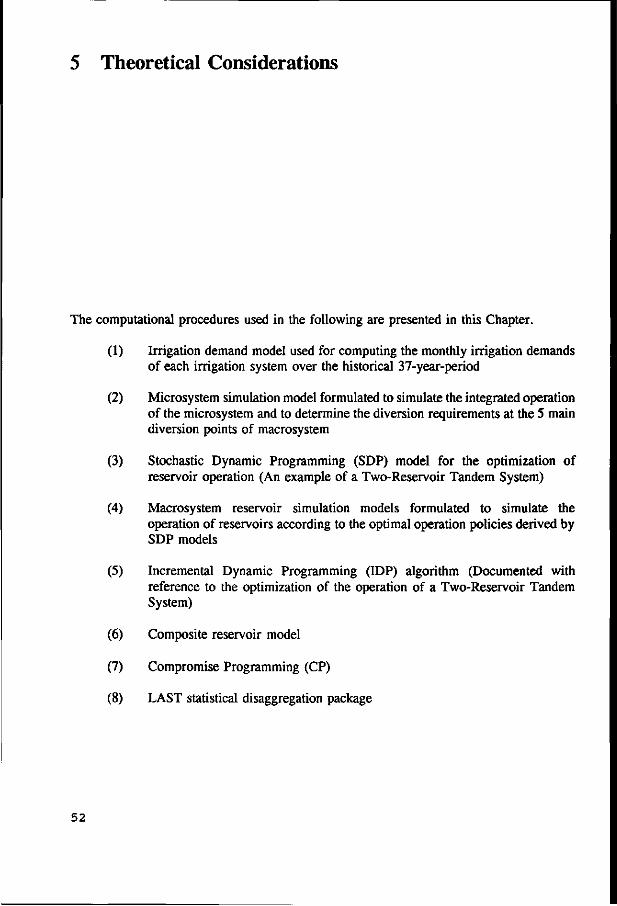
5 Theoretical Considerations

The computational procedures used in the following are presented in this Chapter.

(1) Irrigation demand model used for computing the monthly irrigation demands of each irrigation system over the historical 37-year-period

(2) Microsystem simulation model formulated to simulate the integrated operation of the microsystem and to determine the diversion requirements at the 5 main diversion points of macrosystem

(3) Stochastic Dynamic Programming (SDP) model for the optimization of reservoir operation (An example of a Two-Reservoir Tandem System)

(4) Macrosystem reservoir simulation models formulated to simulate the operation of reservoirs according to the optimal operation policies derived by SDP models

(5) Incremental Dynamic Programming (IDP) algorithm (Documented with reference to the optimization of the operation of a Two-Reservoir Tandem System)

(6) Composite reservoir model

(7) Compromise Programming (CP)

(8) LAST statistical disaggregation package

52

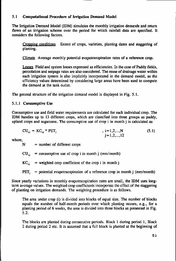
S.l Computational Procedure of Irrigation Demand Model

The Irrigation Demand Model (IDM) simulates the monthly irrigation demands and return flows of an irrigation scheme over the period for which rainfall data are specified. It considers the following factors.

Cropping conditions Extent of crops, varieties, planting dates and staggering of planting.

Climate Average monthly potential evapotranspiration rates of a reference crop.

Losses Field and system losses expressed as efficiencies. In the case of Paddy fields, percolation and seepage rates are also considered. The reuse of drainage water within each irrigation system is also implicitly incorporated in the demand model, as the efficiency values determined by considering large areas have been used to compute the demand at the tank outlet.

The general structure of the irrigation demand model is displayed in Fig. 5.1.

5.1.1 Consumptive Use

Consumptive use and field water requirements are calculated for each individual crop. The IDM handles up to 13 different crops, which are classified into three groups as paddy, upland crops and sugarcane. The consumptive use of crop i in month j is calculated as

CUsj = KCg * PETj , i = l,2,..,N (5.1) j = l,2,..,12

where, N = number of different crops

CUjj = consumptive use of crop i in month j (mm/month)

KCj j = weighted crop coefficient of the crop i in month j

PETj = potential evapotranspiration of a reference crop in month j (mm/month)

Since yearly variations in monthly evapotranspiration rates are small, the IDM uses long-term average values. The weighted crop coefficients incorporate the effect of the staggering of planting on irrigation demands. The weighting procedure is as follows.

The area under crop (i) is divided into blocks of equal size. The number of blocks equals the number of half-month periods over which planting occurs, e.g., for a planting period of 6 weeks, the area is divided into three blocks as presented in Fig. 5.2.

The blocks are planted during consecutive periods. Block 1 during period 1, Block 2 during period 2 etc. It is assumed that a full block is planted at the beginning of

53

each period. Staggering within the block is not considered.

The weighted monthly crop coefficient is the average of the coefficients in all blocks. The procedure is demonstrated in Table 5.1.

5.1.2 Effective Rainfall

For paddy, monthly effective rainfall is estimated by an equation proposed by the Land Use Division (LUD) of the irrigation department of Sri Lanka.

EFRj = 0.67 (Rainj - 25) , j = l,2,..,12 (5.2)

where EFRj = effective rainfall in month j (mm/month)

Rainj = observed rainfall in month j (mm/month)

In using the Equation (5.2), the effective rainfall has to be limited to a maximum of 225 mm/month (Joshua, 1977). The above equation is applied to the growing season, when the fields are flooded, and also to the land preparation period. In fact, the relationship between rainfall and land preparation requirements is more complicated due to the following:

Rainfall before the land preparation period increases the moisture content of the topsoil and, in heavy clay soils, it causes cracks to close. Because the fields are dry, runoff is very low.

Rainfall conditions since the previous harvest determine the position of the groundwater table. Particularly in lighter soils, the depth to the groundwater table is one of the main factors that determines the land preparation requirement at the beginning of the season.

Modelling of these processes might be useful for detailed studies of small areas, but is not practical for larger areas.

For upland crops, the effective rainfall is estimated by the USDA method (Dastagne, 1974).

5.1.3 Field Water Requirements

The IDM uses two methods to calculate field water requirements. The requirements of paddy are computed by accounting for the water balance of a paddy basin. The net demand for a paddy crop is the amount of water required to raise the water table to the desired level. This amount is the sum of the field losses (percolation and seepage) and the consumptive use, minus the effective rainfall since the previous irrigation. Thus, the field requirement includes unavoidable losses that have already occurred.

54

Start

Segment 1 Specifications

Data statements

Segment 2 Input general data

Names of crops Crop coefficients Field efficiencies Number of crops

Segment 3 Input specific data

Return flow factors Minimum flow factors Monthly distrib: coeff:s

Percolation rates Land preparation req:

Pre-irrigation

Segment 4 Read crop data and

calculate coefficients

Read crops, planting dates, staggering, crop areas,

Compute weighted crop coefficients, land preparation and percolation.

Segment 5 Compute basic requirements

Read evapotranspiration Set coefficients to calendar

months Compute crop requirements

segment 6 Compute effective rainfall

Read rainfall data Compute effective rainfall

for Paddy and upland crops

Segment 7 Compute project requirements

and return flows

Compute field water req: Compute total requirement

Compute return flows

Segment 8 Print results

Fig. 5.1 General Structure of the Irrigation Demand Model (ACRES, 1985)

55

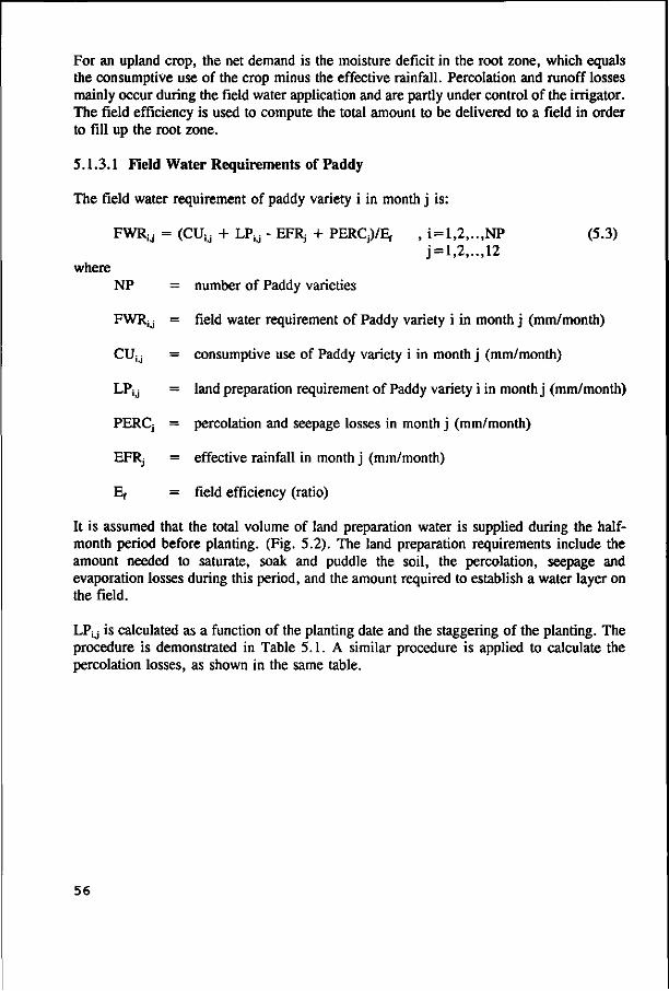
For an upland crop, the net demand is the moisture deficit in the root zone, which equals the consumptive use of the crop minus the effective rainfall. Percolation and runoff losses mainly occur during the field water application and are partly under control of the irrigator. The field efficiency is used to compute the total amount to be delivered to a field in order to fill up the root zone.

5.1.3.1 Field Water Requirements of Paddy

The field water requirement of paddy variety i in month j is:

FWR;J = (CUij + LPy - EFRj + PERC^/E, , i=l,2,..,NP (5.3) j = l,2,..,12

where NP = number of Paddy varieties

FWRjj = field water requirement of Paddy variety i in month j (mm/month)

CUjj = consumptive use of Paddy variety i in month j (mm/month)

LPjj = land preparation requirement of Paddy variety i in month j (mm/month)

PERCj = percolation and seepage losses in month j (mm/month)

EFRj = effective rainfall in month j (mm/month)

Ef = field efficiency (ratio)

It is assumed that the total volume of land preparation water is supplied during the half-month period before planting. (Fig. 5.2). The land preparation requirements include the amount needed to saturate, soak and puddle the soil, the percolation, seepage and evaporation losses during this period, and the amount required to establish a water layer on the field.

LPg is calculated as a function of the planting date and the staggering of the planting. The procedure is demonstrated in Table 5.1. A similar procedure is applied to calculate the percolation losses, as shown in the same table.

56

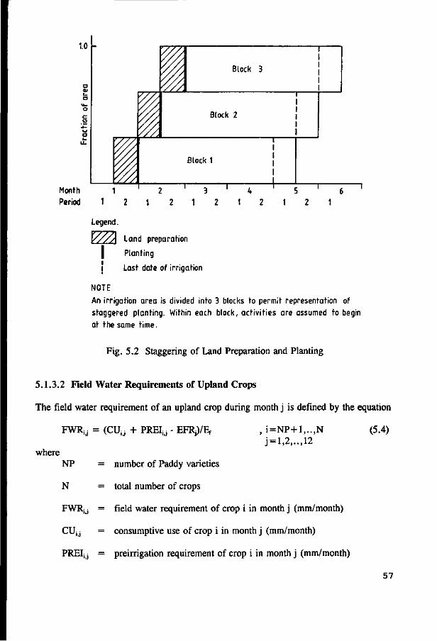
1.0

Block 3

Block 2

Block 1

T i T Month 1 " 2 3 ' 4

Period 1 2 1 2 1 2 1 2

5

1 2

Legend.

V/A\ Land preparation

I Planting

j Last date of irrigation

NOTE

An irrigation area is divided into 3 blocks to permit representation of

staggered planting. Within each block, activities are assumed to begin

at the same time.

Fig. 5.2 Staggering of Land Preparation and Planting

5.1.3.2 Field Water Requirements of Upland Crops

The field water requirement of an upland crop during month j is defined by the equation

FWRjj = (CUjj + PREIjj - EFRj)/Ef

where

, i =NP+ l , . . ,N j = l,2,..,12

(5.4)

NP = number of Paddy varieties

N = total number of crops

FWR^ = field water requirement of crop i in month j (mm/month)

CUjj = consumptive use of crop i in month j (mm/month)

PREIjj = preirrigation requirement of crop i in month j (mm/month)

57

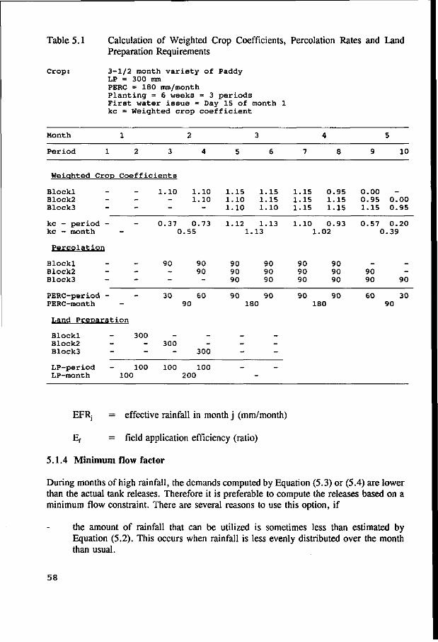
Table 5.1 Calculation of Weighted Crop Coefficients, Percolation Rates and Land Preparation Requirements

Crop: 3-1/2 month variety of Paddy LP = 300 mm PERC = 180 mm/month Planting = 6 weeks = 3 periods First water issue = Day 15 of month 1 kc = Weighted crop coefficient

Month

Period 1

Weiahted Crop

Blockl Block2 Block3

kc - period -kc - month

Percolation

Blockl Block2 Block3

PERC-period -PERC-month

Land Preoarat

Blockl Block2 Block3

LP-period -LP-month

1

2 3

Coefficients

-

-

_

-

Lon

300

100 100

1.10

2

4

1.10 1.10

0.37 0.73 0.55

90

30

300

100

90 90

60 90

300

100 200

5

1.15 1.10 1.10

1.12 1

90 90 90

3

6

1.15 1.15 1.10

1.13 13

90 90 90

90 90 180

-

-

-

-

7

1.15 1.15 1.15

1.10 1

90 90 90

4

8

0.95 1.15 1.15

0.93 .02

90 90 90

90 90 180

9

0.00 0.95 1.15

5

10

0.00 0.95

0.57 0.20 0.39

90 90

60

90

30 90

EFRj = effective rainfall in month j (mm/month)

Ef = field application efficiency (ratio)

5.1.4 Minimum flow factor

During months of high rainfall, the demands computed by Equation (5.3) or (5.4) are lower than the actual tank releases. Therefore it is preferable to compute the releases based on a minimum flow constraint. There are several reasons to use this option, if

the amount of rainfall that can be utilized is sometimes less than estimated by Equation (5.2). This occurs when rainfall is less evenly distributed over the month than usual.

58

the system response to rainfall may not be efficient due to the drop of efficiency during wet periods

a minimum flow is normally maintained in the system to supply domestic or other uses

during wet periods the efficiencies drop, but adjustments would inflate demands in dry periods

excess water is available under such conditions and no need is perceived by operational staff to reduce releases.

The minimum flow is calculated as

FWRy = PP * (CUy + PERq) , j = 1,2,.., 12 (5.5)

where PP = minimum flow factor.

A minimum flow factor of 0.25 has been found to be necessary by comparing theoretical demands with the actual tank releases in representative areas (ACRES, 1985).

5.1.5 Monthly Demand Coefficients and Project Requirements

The monthly project or diversion requirements are calculated using the formula

N TlRj = E (FWRy * Ay) * 10"5/ES , j = l,2,..,12 (5.6)

i = l where

TIRj = total project requirement in month j (MCM/month)

FWRy = field water requirement of crop i in month j (mm/month)

Ay = area under crop i in month j (ha)

Es = system efficiency (ratio)

N = number of crops

The total seasonal irrigation demands computed with average efficiencies generally provide a satisfactory estimate of the total issues during a season. Since efficiencies and losses vary during the season, actual and theoretical monthly issues will differ. To correct this shortcoming of the model, the MDF has been introduced.

TIRCj = MDFj * TIRj , j = 1,2,.., 12 (5.7)

59

where

TIRCj = corrected project requirement in month j (MCM/month)

MDFj = monthly distribution factor

TIRj = requirements as computed by Equation 5.6 (MCM/month)

The use of the MDF should not change the computed total issues during the season.

n n E TIRCj = E TIRj (5.8)

j=m j=m where

m = first month of the season n = last month of the season

Assessment of reliable records (ACRES, 1985) has indicated that MDF values should vary from 1.1 to 1.5 during the land preparation period, reduce to 0.8 during most of the growing season, and increase to about 2.5 during the last month of the season, when the theoretical demand is low. Actual values should be adjusted to ensure that the total seasonal demand computed using the MDF's is equal to the total demand computed without them. Thus, the MDF's alter the pattern of the water release, but do not alter the total seasonal demand.

5.1.6 Return Flow

The return flow estimates are necessary in the simulation of the integrated operation of the microsystem (Section 5.2). The theoretical return flow from an irrigation area is defined as the amount of water that is not used by the crops or vegetation. For the case of 100% supply of the irrigation requirement, the theoretical return flow can be expressed as,

N TRFCj = TIRj + E(RAINj - CUij - LPiJ)*Aij*10-5 (5.9)

i= l ' ' , j = l,2,..,12 where

N = number of crops

TRFCj = theoretical return flow from cropped areas (MCM/month)

The actual return flow is normally less than the theoretical flow. The actual flows are estimated using a monthly return flow factor.

RFj = RFFj * (TRFUj + TRFCj) , j = l,2,..,12 (5.10) where

RFj = return flow in month j (MCM/month)

60

RFFj = return flow factor for month j

TRFUj = theoretical return flow from uncropped areas (MCM/month)

5.2 Microsystem Simulation Model

Mahaweli water resources system has a complex network of reservoirs and irrigation tanks (reservoirs built alone for irrigation purposes). After a study of the conveyance system and the future development plans, a simplified system configuration was selected so as to minimize the deviation from the real distribution system. The diagram displayed in Fig. 2.3 is a simplified configuration for the system. Each irrigation system is considered as having a single composite tank with a storage equal to the total storage available within the irrigation system. This was necessary due to the fact that each irrigation system has a large number of minor tanks interconnected in a complex network which practically exclude the possibility of modelling all of them individually.

The microsystem simulation model is a water balance simulation model which was formulated to simulate the operation of all the irrigation systems of Mahaweli system simultaneously. This model can be run in two different modes, either to estimate the diversion requirements at major diversion points, or to simulate the operation of irrigation systems for predetermined inflows at the diversion points. The following can be taken into account in this simulation model.

(a) Weightages for supplying water to each irrigation system.

(b) Operation rule curves (upper and lower rule curves) for the composite tank in each irrigation system.

(c) Return flows.

(d) Conveyance losses.

(e) Reduction of irrigation area in case of water shortages occurring after the start of the season.

The simulation model utilizes the available flows for a historical 37-year period at 5 main diversion points: Bowatenne, Elahera, Angamedilla, Minipe and Kandakadu. The 5 diversion points mentioned above are regarded as the interface points between the macro-system and the irrigation systems (microsystem). Simulation is done on monthly basis, taking into account the two different seasons of the year. Results of the simulation include operational details of each irrigation system as well as that of the diversion points. Actual diversion requirements for the 37 year period are also determined by the simulation model.

61

Data requirements of the microsystem simulation model are:

(a) Monthly irrigation water demands of each irrigation system for the period of 37 years considered. (Estimated by the irrigation demand model).

(b) Weighted monthly rainfall of each irrigation catchment for the period of 37 years.

(c) Return flows which corresponds to 100% irrigation of each irrigation system. (Estimated by the irrigation water demand model)

(d) Data related to the assumed composite tanks, and conveyance canal capacities.

(e) Rule curves (upper and lower) for the composite tanks of each irrigation system (defined according to the presently used rule curves of real irrigation tanks in the vicinity). As displayed in Fig. 5.4, no release is made when the tank level is lower than that specified by the lower rule curve. In the range in between the two rule curves, releases are made to satisfy the demands; subject to the minimum final level specified by the lower rule curve.

(f) Rainfall-runoff regression coefficients for each of the irrigation catchments.

(g) Conveyance and evaporation losses.

(h) Available flows at 5 main diversion points.

(i) Weightage factors assigned for supplying water to each irrigation system.

Flow diagrams for the microsystem simulation model and its tank-simulation subprogram are shown in Figs. 5.3 and 5.4 respectively. The symbols used in the flow diagram for the tank-simulation subprogram are described in Table 5.2.

62

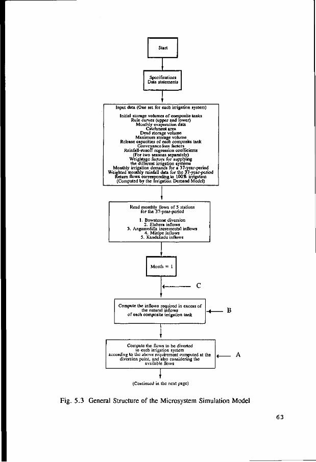
Start

1

Specifications Data statements

1

Input data (One set for each irrigation system)

Initial storage volumes of composite tanks Rule curves (upper and lower)

Monthly evaporation data Catchment area

Dead storage volume Maximum storage volume

Release capacities of each composite tank Conveyance loss factors

Rainfall-runoff regression coefficients (For two seasons separately)

Weightage factors for supplying the different irrigation systems

Monthly irrigation demands for a 37-year-period Weighted monthly rainfall data for the 37-year-period

Return flows corresponding to 100% irrigation (Computed by the Irrigation Demand Model)

Read monthly flows of 5 stations for the 3 7-y ear-period

1. Bowatennc diversion 2. Elahera inflows

3. Angamedilla incremental inflows 4. Minipe inflows

5. Kandakadu inflows

Month - 1

Compute the inflows required in excess of the natural inflows

of each composite irrigation tank B

Compute the flows to be diverted to each irrigation system

according to the above requirement computed at the diversion point, and also considering the

available flows

(Continued in the next page)

Fig. 5.3 General Structure of the Microsystem Simulation Model

63

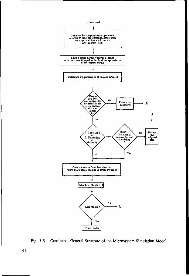
..Continued

Simulate the composite tank operations in order to meet the demands, considering

the upper and lower rule curves (Sub Program 'RES')

Set the initial storage volumes of tanks in the next month equal to the final storage volumes

of the current month

Determine the percentage of demand satisfied

Yes

Compute return flows based on the return flows corresponding to 100% irrigation

•-c

Fig. 5.3 ...Continued. General Structure of the Microsystem Simulation Model

64

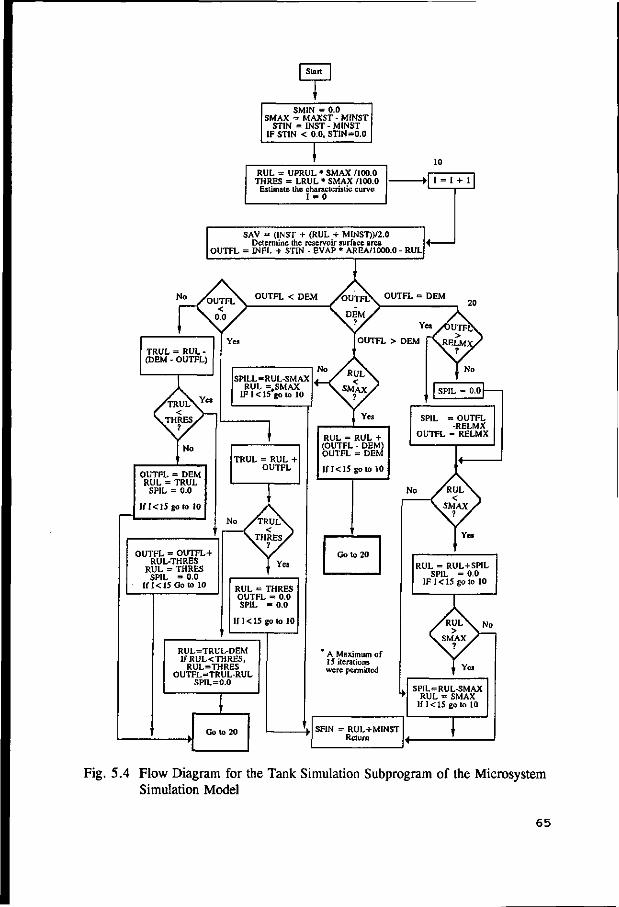
SMIN = 0.0 SMAX = MAXST - M1NST

STIN = INST - MINST IF STIN < 0.0, STIN=0.0

RUL = UPRUL » SMAX /100.0 THRES = LRUL * SMAX /100.0 Estimate the characteristic curve

I = 0

• 1 = 1 + 1

SAV = (INST + (RUL + MINST))/2.0 Determine the reservoir surface area

OUTFL = INFL + STIN - EVAP * AREA/1000.0 - RUL

OUTFL < DEM /OUTFLV OUTFL = DEM

TRUL = RUL-(DEM - OUTFL)

OUTFL = DEM RUL = TRUL SPIL = 0.0

If K15goto 10

SPILL=RUL-SMAX RUL =,SMAX

IF K15 goto 10

TRUL = RUL + OUTFL

OUTFL = OUTFL+ RUL-THRES

RUL = THRES SPIL = 0.0

If 1< 15 Go to 10

OUTFL > DEM

SPIL = 0.0

RUL = RUL + (OUTFL - DEM) OUTFL = DEM

If K 15 go to 10

RUL=TRUL-DEM If RUL<THRES,

RUL=THRES OUTFL=TRUL-RUL

SPIL =0.0

Go to 20

SPIL = OUTFL -RELMX

OUTFL = RELMX

Fig. 5.4 Flow Diagram for the Tank Simulation Subprogram of the Microsystem Simulation Model

65

Table 5.2 Symbols Used in the Flow-Diagram for the Irrigation Reservoir (Tank) Simulation Subprogram

Symbol Description

MAXST maximum storage capacity of the tank (in MCM)

MINST minimum (dead) storage volume of the tank (in MCM)

SMAX active storage capacity (in MCM)

INST total storage volume at the beginning of the month (in MCM)

STIN active storage volume at the beginning of the month (in MCM)

INFL inflow to the tank during the month (in MCM)

UPRUL upper rule curve level as a % of the active storage

LRUL lower rule curve level as a % of the active storage

RUL active storage volume indicated by the upper rule curve (in MCM)

THRES active storage volume indicated by the lower rule curve (in MCM)

SAV average storage volume within the month (in MCM)

EVAP volume of water evaporated from the tank during the month (in MCM)

AREA average water surface area of the tank within the month (in Sq.km)

OUTFL tank release during the month (in MCM)

RELMX maximum release capacity (in MCM/month)

DEM irrigation water demand during the month (in MCM)

SPIL volume of water spilled during the month (in MCM)

SFIN final total storage volume at the end of the month (in MCM)

TRUL a (temporary) variable used to denote the active storage volume (in MCM)

66

5.3 Stochastic Dynamic Programming Models for the Optimization of Reservoir Operation

The future states or outcomes of any stochastic process such as rainfalls and streamflows cannot be predicted with certainty. However, based on past performance the probability associated with any particular outcome may be estimated. Hydrologic uncertainty of streamflows is explicitly taken into consideration in the explicit SDP models developed for this study. These models incorporate discrete probability distributions in the optimization process. They describe the extent of the uncertainty of future occurrences of streamflows and the correlation of streamflows in time and space that are present in any river basin.

Assuming that the unconditional steady state probability distributions for monthly streamflows are not changing from one year to the next, a Markov chain could be defined for each month's streamflow. Since there are 12 months in a year there would be 12 Markov chains, the elements of which could be denoted as P1^ the probability of occurrence of a streamflow class j in month (t+1) given a streamflow state i in month t.

In the models developed for this study, first order (lag one) Markov chains are used to estimate the discrete conditional (transition) probabilities in order to represent the stochasticity inherent in the streamflows. Discrete transition probabilities are estimated for a number of representative inflow values for each month, using the available historical streamflow records.

DP by its definition decomposes a problem having a large number of decisions to a number of problems (stages) having one or few decisions each. In a DP formulation of a water resources allocation problem, time periods are often considered as stages. The stored volumes of water in the reservoirs at the beginning of the time periods represent the state of the system. The decisions to be taken at each stage are the quantities of water to be released. That can be implicitly identified by specifying the storage volumes at the next stage, (identifying the storage volumes at the end of the time step considered). In order to incorporate the markovian nature of the streamflow, it is also defined as a state variable in SDP formulations. Therefore a SDP formulation of a water resources problem will have a two-dimensional state variable consisting of the storage volumes and the inflows to the reservoirs.

The use of DP requires the discretization of the state variables and representation of them by a finite number of characteristic values. The sets of characteristic (representative) storage volumes and streamflows are chosen so that the entire ranges of possible storage volumes and streamflows are considered. The characteristic streamflows can be found by partitioning the range of streamflows into intervals. For this study, the average of the historical inflows that occurred within an interval is chosen as that interval's characteristic value. This value represents the entire interval in the subsequent computations.

67

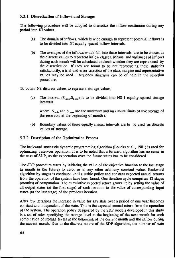
5.3.1 Discretization of Inflows and Storages

The following procedure will be adopted to discretize the inflow continuum during any period into NI values.

(a) The domain of inflows, which is wide enough to represent potential inflows is to be divided into NI equally spaced inflow intervals.

(b) The averages of the inflows which fall into these intervals are to be chosen as the discrete values to represent inflow classes. Means and variances of inflows during each month will be calculated to check whether they are reproduced by the discretization. If they are found to be not reproducing these statistics satisfactorily, a trial-and-error selection of the class margins and representative values may be used. Frequency diagrams can be of help in the selection procedure.

To obtain NS discrete values to represent storage values,

(a) The interval (Stmin,S,max) is to be divided into NS-1 equally spaced storage intervals.

where, S, min and St,max are the minimum and maximum limits of live storage of the reservoir at the beginning of month t.

(b) Boundary values of these equally spaced intervals are to be used as discrete values of storage.

5.3.2 Description of the Optimization Process

The backward stochastic dynamic programming algorithm (Loucks et al., 1981) is used for optimizing reservoir operation. It is to be noted that a forward algorithm has no sense in the case of SDP, as the expectation over the future states has to be considered.

The SDP procedure starts by initiating the value of the objective function at the last stage (a month in the future) to zero, or to any other arbitrary constant value. Backward algorithm by stages is continued until a stable policy and constant expected annual returns from the operation of the system have been found. One iteration cycle comprises 12 stages (months) of computation. The cumulative expected return grows up by setting the value of all output states (at the first stage) of each iteration to the value of corresponding input states (at the last stage) of the previous iteration.

After few iterations the increase in value for any state over a period of one year becomes constant and independent of the state. This is the expected annual return from the operation of the system. The operation policy designated by the SDP models developed in this study is a set of rules specifying the storage level at the beginning of the next month for each combination of storage levels at the beginning of the current month and the inflow during the current month. Due to the discrete nature of the SDP algorithm, the number of state

68

transformations in any stage show an exponential growth with the increase of the number of state variables. A polynomial growth of the number of state transformations at each stage can be noted with the increase of the number of state discretizations. This is reflected in the excessive computer time and memory requirements necessary to run a SDP model with a comparatively fine discretization of state variables.

5.3.3 Test of convergence of SDP procedure

There are two criteria which determine the convergence.

(1) The stabilization of the expected annual increment of the optimum value obtained by Bellman's recursive formula (Loucks et al., 1981)

(2) Stabilization of the operation policy. (Chow et al., 1975)

The two convergence criteria are briefly described in the following.

During the continued backward computation of the SDP algorithm, the optimum expected return for all possible initial states will be determined for each stage (month). When the expected return for a period of one year becomes constant for all state transformations in each stage (month), the convergence criterion of constant expected annual objective achievement is satisfied.

At each stage (month) of the SDP algorithm, an operation policy for that stage is determined. After continuing backward computation for a couple of years, a stable operation policy can be obtained. This implies that the operation policy for a specific month will not change from year to year. When this condition is reached the convergence criterion of stabilization of the operation policy is achieved.

5.3.4 SDP Model for Two Reservoirs in Series (The Tandem System)

To describe the applicability of SDP for optimizing the operation of multi-unit reservoir systems, the SDP model for a serially-linked two-reservoir system is presented in the following. The system configuration selected for this documentation is displayed in Fig. 5.5.

Assuming an objective to maximize the expected annual energy generation, the objective function for the optimization of the system can be mathematically expressed by the following.

T 2 Maximize E {E [ETEPJ} (5.11)

t = l i = l where,

TEP; t = the energy generation by the power plant i at stage t of the operation period (in GWh)

= 9.8 * Rit * (ELu-DWLit) * e/3600 GWh , i = l,2 ; t=l,2,..,T

69

Rj t = release from reservoir i during month t (in MCM)

ELj t = average water surface elevation of the reservoir i during month t (in metres)

= SMS* + Siit+1)/2] , i = l ,2 ; t=l ,2 , . . ,T

Sj t = storage in reservoir i at the beginning of month t (in MCM)

SEj = represents the relationship between the water surface elevation and the storage volume (characteristic curve) of reservoir i

DWLj t = average downstream water level of power plant i during the month t (in metres)

= max [TWL„ EL,J , i = l ; t=l,2,..,T

TWL2 , i=2 ; t=l,2,..,T

TWL; = normal tail water level of power plant i (in metres)

e = overall efficiency of the power plant (0.75 was used)

E = denotes the expectation

T = number of periods within the annual cycle = 12 This optimization is subject to the constraints on reservoir storages and releases. The storages of the reservoirs during any stage must be within the limits of minimum and maximum live storage capacity.

SMINit< Sit < SMAXit , i = l,2 (5.12) t=l,2,..,12

where, SMIN|, = minimum storage of reservoir i at the beginning of month t (in MCM)

SMAXj, = maximum storage of reservoir i at the beginning of month t (in MCM)

The releases from each reservoir are subject to the constraints of maximum and minimum limits. This is due to the maximum capacities of outlets and the compulsory releases, if any.

RMINit < Rit < RMAXit , i = l,2 (5.13) t=l,2,..,12

where, RMIN;, = minimum release from reservoir i during month t (in MCM)

RMAXj t = maximum release from reservoir i during month t (in MCM)

70

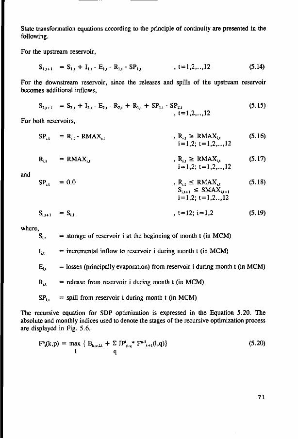
State transformation equations according to the principle of continuity are presented in the following.

For the upstream reservoir,

Si,«+i = S,,t + IM - E,,, - R u - SP,,, , t= l ,2 , . . ,12 (5.14)

For the downstream reservoir, since the releases and spills of the upstream reservoir becomes additional inflows,

S2,t+i = S2>t + I2,t - Ejt - R2,t + Ri,t + SP l i t" SP2,t (5.15) , t = l , 2 , . . , 12

For both reservoirs,

SP j t = R i t -RMAX i t , R i t > R M A X i t (5.16) i= l ,2 ; t= l ,2 , ' . . ,12

and

R i t =RMAX U , Rit > RMAXit (5.17) i = l ,2; t=l ,2, ' . . ,12

SP i t = 0 . 0 , Ru < RMAXit (5.18) Si,'t+1 < SMAXijt+I

i = l,2; t= l ,2 . . ,12

Si>t+, = S U , t = 1 2 ; i = l , 2 (5.19)

where,

Siit = storage of reservoir i at the beginning of month t (in MCM)

Ii>t = incremental inflow to reservoir i during month t (in MCM)

Ejit = losses (principally evaporation) from reservoir i during month t (in MCM)

Rijt = release from reservoir i during month t (in MCM)

SP i t = spill from reservoir i during month t (in MCM)

The recursive equation for SDP optimization is expressed in the Equation 5.20. The absolute and monthly indices used to denote the stages of the recursive optimization process are displayed in Fig. 5.6.

F \ (k ,p) = max { Bk ,p ,u + E JP<p.q* F"' l +1(l ,q)} (5.20)

1 q

7 1

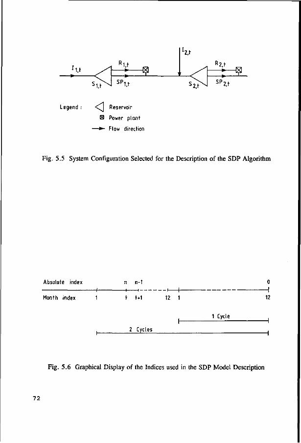
u <v

' U

-§_ SP

u

l2.t

'2,t

R2,t

SP 2,t

Legend : < \ j Reservoir

E3 Power plant

—•- Flow direction

Fig. 5.5 System Configuration Selected for the Description of the SDP Algorithm

Absolute index

Month index

n n-1

—i 1 - -

t r+1 - i r-12 1 12

1 Cycle

2 Cycles

Fig. 5.6 Graphical Display of the Indices used in the SDP Model Description

72

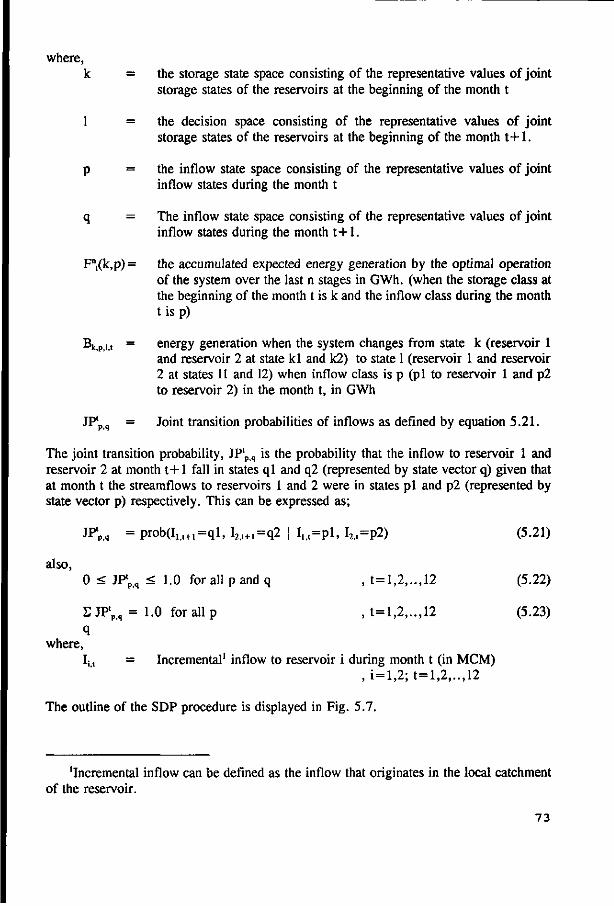
where, k = the storage state space consisting of the representative values of joint

storage states of the reservoirs at the beginning of the month t

1 = the decision space consisting of the representative values of joint storage states of the reservoirs at the beginning of the month t+1.

p = the inflow state space consisting of the representative values of joint inflow states during the month t

q = The inflow state space consisting of the representative values of joint inflow states during the month t+1.

Fn,(k,p) = the accumulated expected energy generation by the optimal operation of the system over the last n stages in GWh. (when the storage class at the beginning of the month t is k and the inflow class during the month t isp)

Bk,P,i,t = energy generation when the system changes from state k (reservoir 1

and reservoir 2 at state kl and k2) to state 1 (reservoir 1 and reservoir 2 at states 11 and 12) when inflow class is p (pi to reservoir 1 and p2 to reservoir 2) in the month t, in GWh

JP'p, = Joint transition probabilities of inflows as defined by equation 5.21.

The joint transition probability, JPlp q is the probability that the inflow to reservoir 1 and

reservoir 2 at month t+1 fall in states ql and q2 (represented by state vector q) given that at month t the streamflows to reservoirs 1 and 2 were in states pi and p2 (represented by state vector p) respectively. This can be expressed as;

JP'p,q = prob(Iu+1=ql, I2,t+1=q2 | I u =pl , I2,,=p2) (5.21)

also, 0 < JP'p,q < 1.0 for all p and q , t=l,2,..,12 (5.22)

EJP'p,,, = 1.0 for all p , t=l,2,..,12 (5.23) q

where, Ij, = Incremental1 inflow to reservoir i during month t (in MCM)

, i=l ,2; t=l ,2 , . . ,12

The outline of the SDP procedure is displayed in Fig. 5.7.

'Incremental inflow can be defined as the inflow that originates in the local catchment of the reservoir.

73

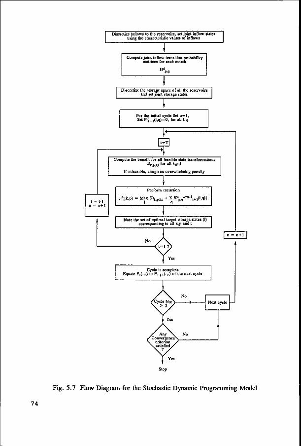
Disciclize inflows to Ihe reservoirs, set joint inflow states using the characteristic values of inflows

Compute joint inflow transition probability matrices for each month

Discretize the storage space of all the reservoirs and set joint storage states

For the initial cycle Set n = 1, ~ F°l+l(lIq)=0, foralll.q Set

t = T

Compute the benefit for all feasible state transformations ^k,p,l,i *°r a^ k'P'l

If infeasible, assign an overwhelming penalty

t = t-1 n = n+1

Perform recursion

F,(k,p) = Max {Bkp?M + E JP,Piq*F°-'l+1(l,q)}

Note the set of optimal target storage states (I) corresponding to all k,p and t

No

Yes

Cycle is complete Equate F,(.,.) to FT+1(.,.) of the next cycle

Next cycle —

Fig. 5.7 Flow Diagram for the Stochastic Dynamic Programming Model

74

5.4 Macrosystem Reservoir Simulation Models

The SDP based optimization models developed for this study require the subsystems be simulated according to the operation policy derived by SDP. In the sequential and iterative optimization models (Sections 7.4 and 7.5), the simulated output of the upstream subsystem is used as inputs for the downstream subsystem. In addition, the iterative optimization proceeds by considering the simulated water shortages of the downstream subsystems as demands from the upstream subsystem. Nevertheless, reservoir simulation is necessary to assess the performance of an operation policy. These simulation models are formulated to simulate reservoir operation over the historical 37-year-period for which hydrological data are available. In the simulation process, the SDP-based operation policy is used to identify the target storage volume at the end of each time period (month) as a function of the present state of the system. The present state of the system is defined by the initial storage volume at the beginning of the month and the inflow volume during the month. Since the simulation was performed with the same historical inflow data as used to derive the policy, no inflow forecasting was needed. The main data input requirements of a macrosystem simulation model are:

(1) Monthly hydrological data over the historical 37-year-period

(2) Operation policy derived by SDP based optimization

(3) Reservoir and power plant characteristics

(4) Losses

When the simulated output of the model (according to the SDP-based policy) fails to satisfy the downstream irrigation water demand, the policy is over-ruled by simulating a larger release from the reservoir system. This is done by lowering the level of downstream reservoir first. Upstream reservoirs are lowered only if the downstream reservoir is at the minimum operation level.

Results of simulation models include monthly operational details of each reservoir in the system, hydropower generation, and monthly river flows at different locations. A flow diagram for macrosystem reservoir simulation models is presented in Fig. 5.8.

75

Reduce the target storage of downstream reservoir (STOF2)

Read data

Reservoir and power plant characteristics Historical streamflows

SDP-based operation policy Losses

Initial storage volumes of reservoirs

Fig. 5.8 General Structure of the Macrosystem Simulation Models (Example of a Two-Reservoir System)

76

5.5 Incremental Dynamic Programming (IDP)

Incremental Dynamic Programming (IDP) (Larson, 1968) is a deterministic optimization algorithm which has a considerably less computational requirement than traditional DP. In the iterative procedure of IDP, a limited state space is considered for a given iteration run. The general scheme of IDP procedure is represented by the flow diagram in Fig. 5.9. The IDP procedure starts with an initial feasible solution, which can be visualized in the case of a reservoir system as a trajectory of the feasible storage states along the subsequent stages (time periods). Only an imaginary corridor around the initial feasible solution is considered as the feasible state space to derive an improved solution (a new trajectory of the state vector along the time periods). A corridor is then defined around the new trajectory and the procedure repeated (iteration) until a prespecified convergence criterion is satisfied. This completes one cycle of the IDP algorithm. It is to be indicated that IDP needs the initial and final stages of the system to be known. Those stages are not changed during the iteration.

In the next cycle, a corridor of a lesser width is considered around the optimal solution of the previous cycle and the iterations will be repeated. Thus, the term "iteration" is used to define the optimization process within a cycle using a fixed corridor width whereas the corridor width is reduced from one cycle to the next.

For each iteration of a cycle, the optimal trajectory within a given corridor and its return are determined by the conventional DP methodology. A new iteration is needed if the convergence criterion is not satisfied. The number of cycles for the entire procedure and the allowable maximum number of iterations per cycle are to be prespecified.

5.5.1 Model Formulation

The model formulation is documented with reference to a serially linked two-reservoir system. Some modifications are required in modelling the other configurations which are analyzed in this study.

Assuming an objective function to maximize the total energy generation for a specific time period, the DP recursive equation which is used to determine the deterministic optimum solution within each corridor can be expressed as,

F't+1(St+1) = max { TEPA,St+1) + F*t(SJ} , t=l,2,..N (5.24) R,

where, TEPt(S„Sl+1) = energy generation of the system when the states at stages t and t+1

are S, and S,+1 respectively.

R, = the release decision associated with the state transformation from St to St+1.

N = number of stages

77

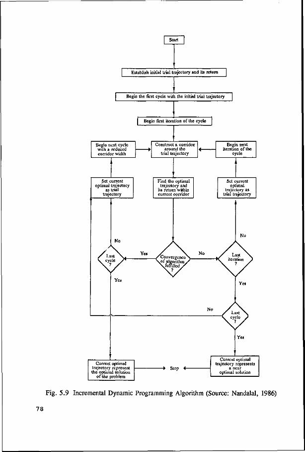
Start

Establish initial trial trajectory and its return

Begin the first cycle with the initial trial trajectory

Begin first iteration of the cycle

Begin next cycle with a reduced corridor width

Construct a corridor around the

trial trajectory

Set current optimal trajectory

as trial trajectory

Begin next iteration of the

cycle

Find the optimal trajectory and

its return within current corridor

Set current optimal

trajectory as trial trajectory

Current optimal trajectory represent the optimal solution

of the problem

-> Stop +-

Current optimal trajectory represents

a near optimal solution

Fig. 5.9 Incremental Dynamic Programming Algorithm (Source: Nandalal, 1986)

78

F*t+1(St+1) is the maximum total of the objective function value from stage 1 to stage t+1, when the state at stage t+1 is St+1.

In the case of a two serially linked reservoir system, this optimization is subject to a similar set of constraints as described under 5.3.4. However the optimization is carried out deterministically. It is to be noted that a forward algorithm of DP technique has been used in this IDP model whereas a backward algorithm has been used in the SDP models.

5.5.2 Construction of Corridors for a Two State Variable IDP Model

A corridor composed of three values of the state variable is constructed around the initial trajectory whenever possible. In general, the corridor is defined symmetrically around the trial trajectory of state variables as described in the following. For a two-reservoir system, the state of the system in stage t is defined by the storage volumes of the two reservoirs at the beginning of the period t (Sh, S2t). Then the 3 boundary points of the corridor with regard to slt can be defined as: (su- Delta,), sIt, and (s„+ Delta,). Similarly, the 3 boundary points for s2t can also be defined as (s2l- Delta2), s2t, (s2t+ Delta2), where Delta, and Delta2 are the corridor half-widths for state variables 1 and 2 respectively. These imply the identification of 9 points in the two dimensional storage space. However, asymmetrical corridors may result if the boundaries of the corridors exceed the minimum or maximum limits of live storage capacities. Larger corridor widths are used for the initial cycles, which ensure that the optimal trajectories are obtained within a small number of iterations. Since the initial trajectory for any later cycle is the optimal trajectory for its preceding cycle and thus closer to the optimality than the initial one, smaller corridor widths can be used for later cycles to search for the optimal trajectory. In this study, the corridor widths were halved after each cycle.

After the construction of a corridor around the trial trajectory, the optimal trajectory and the corresponding objective function value within the corridor should be sought. This is to be done by means of a conventional dynamic programming algorithm however restricting the computations of the state transformations only to those values of the state variables defined by the corridor. The potential state transformations and the procedure for constructing corridor for a single reservoir optimization which has only one state variable, is displayed in Fig. 5.10.

5.5.3 Tests for convergence

As indicated previously, the optimal trajectory for a given corridor width will be obtained iteratively. The improvement of the return from trajectories of subsequent iterations decrease as the iterations progress. The convergence criterion can be expressed as,

iF'i-FV.I 5i = , i=l ,2, . . . , I (5.25)

IF' .-F'ol

79

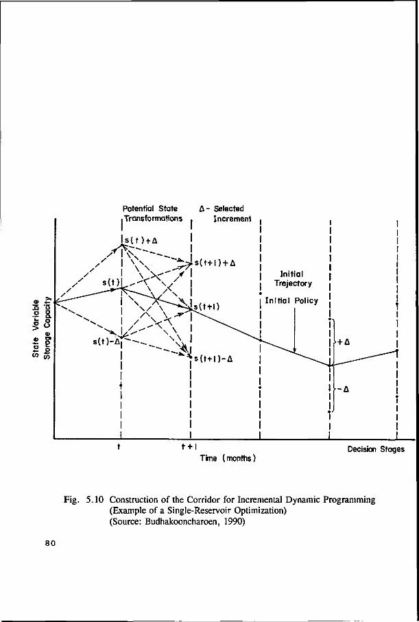
« . Q O

3 <1> O

w

>. u X o o IB o>

OT

Potential State A - Selected

.Transformations . Increment

l s ( t ) + A

/ I Y \ t,>ls(t+l)+A Initial Trajectory

Ini t ial Policy

t + l Time (months)

Decision Stages

Fig. 5.10 Construction of the Corridor for Incremental Dynamic Programming (Example of a Single-Reservoir Optimization) (Source: Budhakooncharoen, 1990)

8 0

where, F'j = the return from the optimal trajectory for the i-th iteration of a given

cycle, (i=0,1,2....)

I = maximum number of iterations per cycle

If, during any of the intermediate cycles, the iterative process yields a value of 5j which does not represent a significant improvement in the return; that is

Si < e , i = l,2,...,I (5.26)

the computational cycle will be terminated. The next cycle starts with a smaller (half size) corridor considered around the optimal trajectory of the completed cycle. After the final iteration of each cycle the following test will be made in order to determine the convergence of the algorithm toward the optimal solution.

IF;-vi X > (5.27) V

where, F*j = the return from the optimal trajectory for the j-th cycle, (j = 1,2,3,...)

X is an arbitrary convergence criterion, which terminates the IDP procedure once the above criterion is satisfied. The trajectory which yields the optimum return is identified as the solution of the optimization problem. In the present study, e and X were assigned the values of 0.001 and 0.0001 respectively.

5.6 Composite Reservoir Model Formulation

Formulation of a hypothetical composite reservoir instead of the real multireservoir configuration is a convenient method to circumvent the "curse of dimensionality" of a DP-based operational optimization model. Composite representation of a serially linked two-reservoir system is displayed in Fig. 5.11. The fundamental idea behind the formulation of a hypothetical composite reservoir instead of the consideration of A and B reservoirs as individual units is to reduce the number of state variables and thereby reduce the computer memory requirements. Thus a larger part of the system can be handled in a single SDP model. The Composite Reservoir Concept can be presented by the following simplifications.

Q'c = Q'. + 0 * Q'b , t = l , 2 , . . ,N (5.28)

Sc = Sa + Sb , t= l ,2 , . . ,N (5.29) where,

Qlc = inflow to the composite reservoir in stage t (in MCM)

Ql« Q'b = inflows to reservoirs A and B in stage t (in MCM)

81

OQ Ob

Reservoir A

t °u Reservoir B

(a) Real Configuration

(Qa + B * Q b ) composite Reservoir

Hypothetical Run-of-the-River Power Plant ( I - P ) Qb

(b) Hypothetical Composite Configuration

Legend :

• Flow Direction

< J Reservoir

G3 Power Plant

Fig. 5.11 Composite Representation of a Serially Linked Two-Reservoir System

82

)3 = fraction of reservoir B ' s inflow assumed to be regulated by the

composi te reservoir

S c = composi te reservoirs active s torage capacity (in M C M )

Sa , Sb = active s torage capacities of reservoirs A and B respectively.

N = number of stages

The justification of the above formulation is presented as follows.

Since the inflow to A is regulated by both reservoirs, the inflows to A a re assumed to be completely passing through the composite reservoir as well . Incremental inflows to B a re regulated only by the reservoir B . Therefore in the composi te formulation only a fraction of the incremental inflows to B will be considered to pass through the composi te reservoir . The fraction 0 is justified due to the reason that out of the total s torage (S„ + Sb) of composi te reservoir the inflow component of B is regulated only by a partial s torage vo lume equal to the s torage of reservoir B .

According to the above formulation, the total inflow to the composite reservoir will be Q'a + P*Qb- However the real total inflow volume of A and B reservoirs is Q, + Q\. The leftover vo lume of water is therefore considered to be added to the downstream of the composi te reservoir through a hypothetical hydropower plant which has a generating head proport ional to the head of the composite reservoir during the particular t ime period. This will represent the fact that all the releases of reservoir B are passed through the power plant , however subject to the l imitations of the turbine capacities.

The A + B Composi te reservoir has to b e formulated in such a way that it represents the performance of the real multireservoir subsystem fairly accurately. T o achieve this similarity of the output, the performance of the assumed composi te reservoir formulation is calibrated against that of the real configuration. The calibration is performed by formulating two optimization models . The first model considers the real multireservoir configuration of the reservoir system, while the second model uses the composi te configuration. Optimal operation pattern obtained by the multireservoir formulation are compared with that obtained by the composite reservoir optimization model formulation. A t r ial-and-error p rocedure is used to determine the parameters of the composi te reservoir so as to obtain a similar performance to that of the multireservoir model . The model parameters include the inflow factor (/?), the head factor (ji)1 and the elevation-storage-area relationships of the composite reservoir. In the t r ial-and-error estimation of the parameters , the optimization of the composite reservoir operation is repeated by changing its parameters until the results of the Composi te Optimization closely follows that of the Mult ireservoir Optimization. The comparison of the operation patterns a re based on the monthly and annual energy / release plots of the two cases.

'Generat ing head of the hypothetical power plant = ju.head of the composi te reservoir

83

5.7 Compromise Programming

Evaluation of the operation policies derived in this study is performed by simulating the system performance in accordance with the derived policies. A number of performance criteria are used in the selection of the most promising policy out of a set of alternatives. For this task, a MultiCriterion Decision Making (MCDM) technique is the most appropriate technique.

Compromise Programming (CP) is used in this study to determine the best compromise alternative out of a set of alternatives each having a number of performance criteria. Being a distance-based MCDM technique, it looks for the best compromise solution that would result in the minimum weighted deviation from the ideal solution. The ideal solution with regard to a specific performance criterion (i) corresponds to the optimal value of that single criterion achieved by one of the different alternatives j , j = l,..m. In compromise programming what is of interest is the comparison of different efficient points (fs, j = l,...,m) from the ideal solution which is the point of reference. Given an ideal point fj", the distance of the various points fy from this ideal, given n performance parameters measured along n coordinates, can be generalized into the following expression.

L>G) = [Ewip|fi*-f»lP]"p , j = l,2,..,m (5.30)

where i

Lp(j) = the distance measure for alternative j from the ideal point (to be minimized over j to find the most satisfactory alternative)

Wj = weighting factor for objective i

fy = value of objective i (performance parameter i) attained by alternative j

fj* = preferred (ideal) value of objective i [can be chosen equal to maXj(=max f ) or min i(=min i j) accordingly]

j j

p = parameter which reflects the attitude of the decision maker towards

evaluating the deviations from the ideal point.

For p approaching oo, the distance measure reduces to the following expression:

L„(j) = max [w j l f i * - f ^ ] , j = l , 2 , . . . ,m (5.31) i

This is because the relative contribution of the largest deviation when raised to a large exponent would be extremely larger than all the rest combined, and thus dominates the distance determination. Therefore the solution corresponds to the min-max decision. When objectives are of different dimensions, the distance measure needs to be corrected to make the individual objectives mutually commensurable. It is therefore necessary to use relative

84

rather than absolute deviations. This can be represented by the following expression.

Lp(j) = [Ew,-" f* - f

max: - min;

"]"" , j = l,2,..,m (5.32)

5.8 LAST Statistical Disaggregation Package

The LAST statistical disaggregation package developed by Lane and Frevert (1989) for the generation of hydrological data is selected for use in the disaggregation of composite operation policies. As introduced in Section 4.8, the statistical relationships that exist among the optimum composite operation pattern and the real multireservoir operation patterns can be exploited for this purpose.

A broad overview of the LAST model is presented in the following. The main characteristic of this approach which differentiates it from other widely used approaches is the use of "key stations" and "sub stations". Key stations are stations of major importance, usually stations indicative of large portions of the basin whose flows are actually the summation of several substations. Key stations are analyzed and generated totally separate from the substations. Substations are analyzed and generated taking into account the intercorrelations between key and substations.

In general, there are two purposes of having key stations and substations rather than having all stations as key stations. One is simply to reduce the number of parameters. The second purpose is that several stations whose values essentially add up to the value of a single station may be generated in a manner which preserves the statistical properties of both the sum (key station) and of the individual substations. This is done by generating substation data depending on the selected key station(s). In this way, the substations may be generated subject to the constraint that they add together properly to give a reasonable hydrologic trace at the key stations. The structure of staged disaggregation procedure employed in LAST model is displayed in Fig. 5.12.

The steps involved in using this model are as follows:

(1) Decide upon the basic structure of the stochastic model (2) Normalize the data (3) Estimate the parameters for each generation group (4) Generate data (5) Analyze and check the generated data

In the following, the various aspects of the approach used in the LAST model are discussed in the logical order that they would normally be performed.

(1) Structure the problem Key stations must be identified and grouped for calculation purposes. Substation generation groups must also be identified along with the groupings to be used in disaggregation of annual data into seasonal data.

85

(2) Transformation of data to normal Through the use of appropriate transformations, it is possible to change the basic data set into a set of data on which the normal probability distribution applies. The reduction of data to normally distributed data is necessary at this stage to ensure that the generated data will adequately follow the observed distribution and will reproduce the statistics accurately. The statistics that can be preserved by the LAST package include the lag-1 serial correlations and lag-0 cross correlations of the seasonal values and the lag-1 and lag-2 serial and cross correlations of the annual values. The data transformations will be performed both on the annual and on the seasonal data.

(3) Estimation of parameters for the generation of annual values at the key stations Once the data have been normalized, the next step is to undertake the task of estimating the parameters needed for generating values on an annual basis at key stations.

(4) Estimation of parameters for the disaggregation of annual values at key stations into annual value at substations The disaggregation process proposed by Valencia and Schaake (1973), which is designed for disaggregation of annual data into seasonal data, provides the incentive for the approach taken here. The disaggregation approach used here while similar to that of Valencia and Schaake (1973) is applied for entirely different purpose.

(5) Estimation of parameters for the disaggregation of annual values into seasonal Cor monthly) values The disaggregation process of Valencia and Schaake (1973) which was extended by Mejia and Rousselle (1976) provides the basis for the approach taken here.

This approach will automatically preserve the variations of the seasonal serial correlation within the year and also allows for the use of different numbers of seasons within the year. It is not confined to monthly subdivisions. The fact that normalized data are used at this point permits the use of differing distributions for each season of the year. Since the data being used are transformed, the seasonal data will not sum exactly to the values generated for the annual data. The difference, while expected to be negligible in effect, are eliminated by adjusting the generated data to ensure that the seasonal values sum exactly to the annual values.

(6) Generation of synthetic data Once all the parameters have been estimated, the generation of synthetic data may be performed using these parameters.

(7) Checking of synthetic data At least initially with each new application, the generated data should be examined to ensure that the desired statistics have been adequately preserved and that the generated values appear reasonable. Moments, crossing properties, the marginal distributions, help in this examination. In addition to calculating various statistics, plots will aid in this task.

86

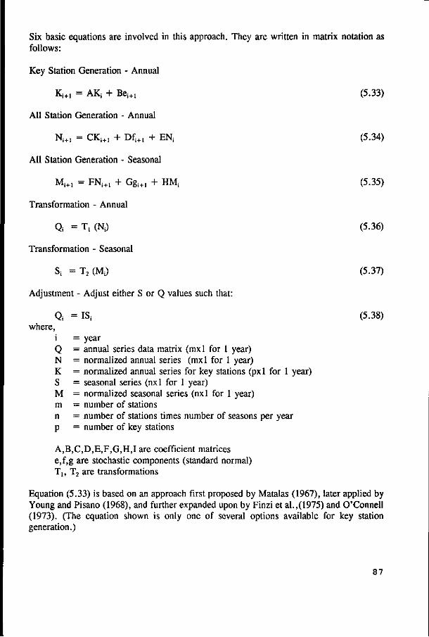
Six basic equations are involved in this approach. They are written in matrix notation as follows:

Key Station Generation - Annual

Ki+1 = AK; + Bei+1 (5.33)

All Station Generation - Annual

Ni+1 = CKi+1 + Dfi+1 + EN; (5.34)

All Station Generation - Seasonal

Mi+1 = FNi+1 + Ggi+1 + HM; (5.35)

Transformation - Annual

Q; =T,(N i) (5.36)

Transformation - Seasonal

Si =T2(Mi) (5.37)

Adjustment - Adjust either S or Q values such that:

Qi =ISi (5.38) where,

i = year Q = annual series data matrix (mxl for 1 year) N = normalized annual series (mxl for 1 year) K = normalized annual series for key stations (pxl for 1 year) S = seasonal series (nxl for 1 year) M = normalized seasonal series (nxl for 1 year) m = number of stations n = number of stations times number of seasons per year p = number of key stations

A,B,C,D,E,F,G,H,I are coefficient matrices e,f,g are stochastic components (standard normal) T,, T2 are transformations

Equation (5.33) is based on an approach first proposed by Matalas (1967), later applied by Young and Pisano (1968), and further expanded upon by Finzi et al.,(1975) and O'Connell (1973). (The equation shown is only one of several options available for key station generation.)

87

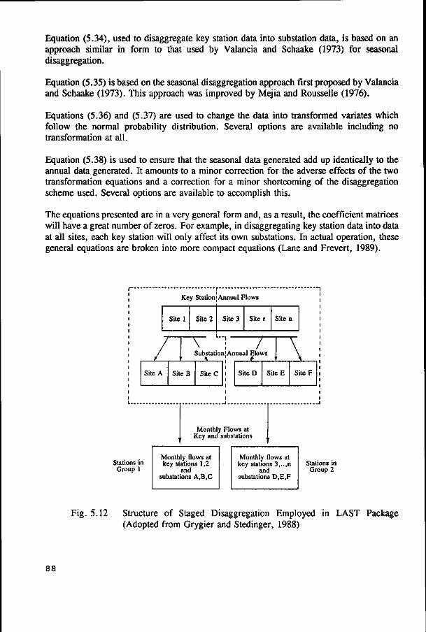
Equation (5.34), used to disaggregate key station data into substation data, is based on an approach similar in form to that used by Valancia and Schaake (1973) for seasonal disaggregation.

Equation (5.35) is based on the seasonal disaggregation approach first proposed by Valancia and Schaake (1973). This approach was improved by Mejia and Rousselle (1976).

Equations (5.36) and (5.37) are used to change the data into transformed variates which follow the normal probability distribution. Several options are available including no transformation at all.

Equation (5.38) is used to ensure that the seasonal data generated add up identically to the annual data generated. It amounts to a minor correction for the adverse effects of the two transformation equations and a correction for a minor shortcoming of the disaggregation scheme used. Several options are available to accomplish this.

The equations presented are in a very general form and, as a result, the coefficient matrices will have a great number of zeros. For example, in disaggregating key station data into data at all sites, each key station will only affect its own substations. In actual operation, these general equations are broken into more compact equations (Lane and Frevert, 1989).

Key Station'Annual Flows

Site 1 Site 2 Site 3 Siter Siten

/I Site A

\ Substation

SiteB Site C

T [Annual Flows

Site D SileE SiteF

L J . .

Monthly Flows at Key and substations

Stations in Group 1

Monthly flows at key stations 1,2

and substations A,B.C

Monthly flows at key stations 3,..,n

and substations D.E.F

Stations in Group 2

Fig. 5.12 Structure of Staged Disaggregation Employed in LAST Package (Adopted from Grygier and Stedinger, 1988)

88

6 Data Availability

The data collected for this study can be broadly categorized into the following.

(a) System characteristics (b) Hydrological data (c) Agricultural and meteorological data (d) Miscellaneous data

6.1 System Characteristics

The general characteristics of macro (main stream) and micro (irrigation) systems were collected from the Water Management Secretariat of Sri Lanka (WMS), which is the technically specialized agency to formulate operational decisions for the Mahaweli water resources system. Principal water levels, reservoir characteristics, monthly gross/net evaporation and seepage loss data were collected for the main reservoirs and irrigation tanks. Characteristics of power plants and the present operation rules of the reservoirs were also collected. Seepage from the main reservoirs has been ignored, since these dams are located in steep-sided valleys with exposed bedrock, and have grout curtains to minimize losses. Although subsequent studies may assist in refining the estimates of seepage, little effect is likely to result from such a refinement.

The natural canals, tunnels and canals that comprise the Mahaweli system have constraints such as capacity limitations, losses and minimum flow requirements. Most of these data were extracted from the WMS and compared with the other agencies responsible for operating the structures concerned.

89

6.2 Hydrological Data

Monthly rainfall data of 20 raingauge stations for a period of 37 years (1949 to 1985) in the Mahaweli irrigation areas were collected from WMS. These data have been recorded by the Meteorology Department of Sri Lanka which maintains records of about 500 ordinary raingauges and 22 automatic rainfall recorders distributed all over the island. The maintenance of these stations are being done by various institutions like Irrigation Department, Agriculture Department and Forest Department of Sri Lanka. Although the recording of daily rainfall had been commenced about 100 years ago, most of the streamflow measurements are only 40 years old. Streamflow data of about 75 gauging stations in Sri Lanka are maintained by the Hydrology Division of the Irrigation Department. Most of these stations are equipped with staff gauges and current meters. Station crew consists of 4 to 5 labourers with a hydrological field assistant in charge. However some stations are manned by a senior labourer under the supervision of a hydrological field assistant. Observing hourly gauge readings and development of rating curves are the main responsibilities of the station crew. These hourly gauge returns are submitted to the head office at the end of every month after which the daily and monthly discharges are computed.

Considerable effort has been made since 1979 to improve the reliability of flow estimates in the Mahaweli and the other main power generating complex of the country: the Kastlreigh-Maussakelle (K-M) complex. The Hydrologic Crash Program (HCP) which began in 1979 and was completed in late 1984 has resulted in major revisions to previously collected data. The HCP had as its main objective the metering of medium and high flows at existing hydrometeorological stations, and the checking and upgrading of existing hydrological data, based on the new flow metering data. The program was directed at medium and high flows, since the lack of cableways previously prevented measurements from being taken under these conditions.

The HCP program has concentrated on the main Mahaweli and K-M complexes, thereby leaving the quality of data representing inflow to the irrigation tanks still suspect. Rainfall-Runoff correlation studies had been carried out to provide a reasonable basis for estimating local inflows to the tanks. Second and third degree polynomial equations have been fitted to the rainfall-runoff relationships of the two seasons of the year; Yala and Maha separately. Second degree polynomials had been ultimately adopted for use in estimating the missing data.

6.3 Agricultural and Meteorological Data

These include crop types, cropping patterns, crop calendars, irrigable areas, crop coefficients, land preparation requirements, efficiency of irrigation systems, accepted operational practices and average monthly evapotranspiration of a reference crop.

A substantial part of these data were obtained from the work done by the Japanese International Cooperation Agency (1989) on the agricultural developments under the Mahaweli scheme. The visits to the irrigation schemes and the discussions with the

90

operational staff and the farmers were also useful, although this study is not aimed at micro level system management.

6.4 Miscellaneous Data

These include the organizational setup for system operation and maintenance, decision structure, flow of information and the present techniques applied. These were obtained from the WMS and during the discussions with officials of Mahaweli Economic Agency, Mahaweli Engineering and Construction Agency, Irrigation Department and the Headworks Administration and Operation Agency of Mahaweli Authority of Sri Lanka.

9 1

7 Analysis and Results

7.1 General

The Mahaweli water resources system is presently in the development stage. Therefore the system configuration and also the operation procedures change gradually. The system configuration considered in this study is expected to be the future configuration of the system. The operation policy analysis of the macrosystem as envisaged in this study require an estimation of micro system water demands as the first step of the analysis. These demands are to be estimated for an adequate time period upon which the operation policy analysis is to be performed. The historical monthly hydrological data necessary for this study are available for a period of 37 years from 1949-1985. Monthly time steps are considered throughout the analysis.

There are five major points in the macrosystem where the water demands exist for the purpose of supplying the microsystem irrigation areas. As shown in Fig. 2.2, these diversion structures are located at Bowatenne, Elahera, Angamedilla, Minipe and Kandakadu. In order to determine these diversion water demands, it is first required to assess the irrigation water demands of the individual irrigation areas. Subsequently the operation of the whole microsystem consisting of 14 irrigation areas and their water storage/conveyance system can be simulated to determine the diversion requirements.

Irrigation water demands of each irrigation area Monthly irrigation water demand time series were estimated based on the cropping patterns presented in Fig. 7.1. The computation was done for the period of 37 years (1949-1985) for which historical rainfall data were available. The irrigation demand model (IDM) used for this purpose is documented in Chapter 5.1. IDM also computes the return flow time series from an area corresponding to 100% irrigation.

Diversion water demands from the macrosystem Having determined the irrigation water demands and return flows of each irrigation area, the integrated operation of irrigation areas were simulated in order to obtain the diversion water requirements from the macrosystem. As the Mahaweli microsystem has a complex network of irrigation tanks (irrigation reservoirs), the analysis required the representation of microsystem in a simplified form.

92

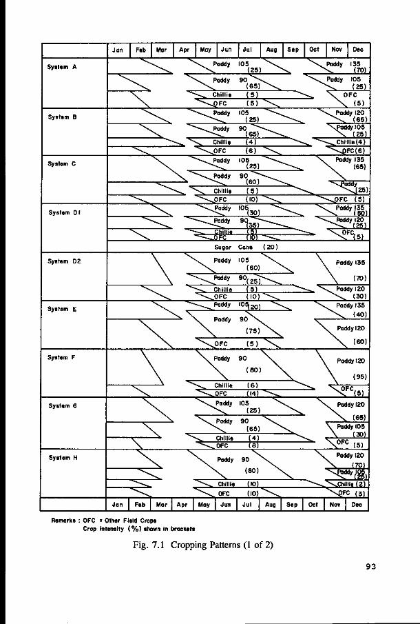
Remarks : OFC = Other Field Crops Crop intensity (%) shown in brackets

Fig. 7.1 Cropping Patterns (1 of 2)

93

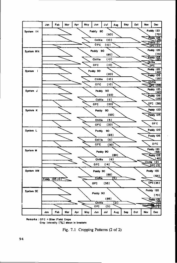
Remarks : OFC = Other Field Craps Crop intensity (%) shown in brockets

Fig. 7.1 Cropping Patterns (2 of 2)

94

This simplification was achieved by assuming that each irrigation area has only one storage reservoir with a storage capacity equivalent to the total storage capacity available within the area. The composite representation of irrigation reservoirs has also been successfully applied by ACRES (1985) in their studies of operating policy options for a part of the Mahaweli system analyzed in the present study. The simplified system configuration selected for the present study is displayed schematically in Fig. 2.3. The diversion water demands from the macrosystem are estimated by considering this configuration of the microsystem in the microsystem simulation model.

The SDP-based models described in the subsequent chapters of this study aim at optimizing subsystems of the macrosystem individually, in order to mitigate computational burden. To obtain a solution which is close to the global optimum, it is required that the optimum operation pattern (diversion policy) at the common interface point of the subsystems be determined beforehand. In Mahaweli system, three interconnected subsystems could be identified. They are:

(1) Caledonia-Talawakelle-Kotmale (CTK) reservoir subsystem

(2) Ukuwela-Bowatenne-Moragahakanda (UBM) subsystem

(3) Victoria-Randenigala-Rantembe (VRR) subsystem

The particular reason for identifying these three subsystems is that they reduce the number of interface points to a minimum of only one while forming computationally manageable subsystems. Polgolla diversion structure acts as the interface point of these three subsystems. Hence the determination of the optimum diversion strategy for Polgolla diversion structure is of utmost importance for the present study. It is also an important operational decision to be made in the actual system operation as well.

In this study, the operation of the upper Uma Oya reservoir (Fig. 2.2) was optimized independently of the other system components. The optimum release pattern obtained by simulating the operation of this reservoir was considered throughout the study as a part of the incremental inflows to Rantembe.

7.2 Three-Composite-Reservoir IDP Model

In the determination of the optimum diversion policy at Polgolla, it is required to consider the effects of all three subsystems jointly. However, the consideration of the real multireservoir configuration is impractical due to the dimensionality of the problem (Section 4.3). Therefore a composite representation of each subsystem was used to circumvent the computational difficulties of the analysis. This approach converts the real multireservoir configuration into a three-reservoir system consisting of only three composite reservoirs interlinked at a common point. The common point in the three-composite-reservoir corresponds to the Polgolla barrage in reality.

95

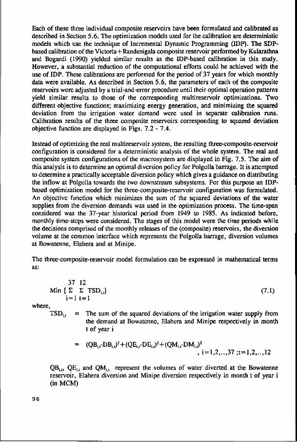
Each of these three individual composite reservoirs have been formulated and calibrated as described in Section 5.6. The optimization models used for the calibration are deterministic models which use the technique of Incremental Dynamic Programming (IDP). The SDP-based calibration of the Victoria+Randenigala composite reservoir performed by Kularathna and Bogardi (1990) yielded similar results as the IDP-based calibration in this study. However, a substantial reduction of the computational efforts could be achieved with the use of IDP. These calibrations are performed for the period of 37 years for which monthly data were available. As described in Section 5.6, the parameters of each of the composite reservoirs were adjusted by a trial-and-error procedure until their optimal operation patterns yield similar results to those of the corresponding multireservoir optimizations. Two different objective functions; maximizing energy generation, and minimizing the squared deviation from the irrigation water demand were used in separate calibration runs. Calibration results of the three composite reservoirs corresponding to squared deviation objective function are displayed in Figs. 7.2 - 7.4.

Instead of optimizing the real multireservoir system, the resulting three-composite-reservoir configuration is considered for a deterministic analysis of the whole system. The real and composite system configurations of the macrosystem are displayed in Fig. 7.5. The aim of this analysis is to determine an optimal diversion policy for Polgolla barrage. It is attempted to determine a practically acceptable diversion policy which gives a guidance on distributing the inflow at Polgolla towards the two downstream subsystems. For this purpose an IDP-based optimization model for the three-composite-reservoir configuration was formulated. An objective function which minimizes the sum of the squared deviations of the water supplies from the diversion demands was used in the optimization process. The time-span considered was the 37-year historical period from 1949 to 1985. As indicated before, monthly time-steps were considered. The stages of this model were the time periods while the decisions comprised of the monthly releases of the (composite) reservoirs, the diversion volume at the common interface which represents the Polgolla barrage, diversion volumes at Bowatenne, Elahera and at Minipe.

The three-composite-reservoir model formulation can be expressed in mathematical terms as:

37 12 Min { E E TSDit} (7.1)

i = l t = l where,

TSDj, = The sum of the squared deviations of the irrigation water supply from the demand at Bowatenne, Elahera and Minipe respectively in month t of year i

= (QVDBJ 2 + (QE^-DEi,,)2+(QMi>t-DMi>t)2

, i=l,2,. . ,37;t=l,2,. . ,12

QBj t, QE;, and QMj t represent the volumes of water diverted at the Bowatenne reservoir, Elahera diversion and Minipe diversion respectively in month t of year i (in MCM)

96

(a) Comparison of Annual Energy

1600

1400

1200

1000

u

w r-l

a 3

800

600

400

200

*• Two reservoirs + Composite reservoir

10 20 30 Year

(b) Comparison of Annual Flows at Polgolla

2

r-l

o i-C

o

•u

I-I

r-l

El <

JJUU

3000

2500

2000

1500

1000

500

0

l A t I K 1

Jfp^^^^ 1 I

* Two reservoirs + Composite reservoir

i i i

20 30 Year

Fig. 7.2 Calibration of Caledonia+Kotmale (C+K) Composite Reservoir (Objective Function: Minimization of the Squared Deviation of Water Supply from the Irrigation Demand)

97

(a) Comparison of Annual Energy

60 U 01 C W

to

3

2000

1500

1000

500

6000

5000

p. •r-l Ci

4-1

o r-l

j~4

3 C C <

4000

3000

2000

1000

j |£VJ

+ ft

•W .!/>• -• \ 1 / ^ - *

V + V/

* Two r e s e r v o i r s + Composite r e s e r v o i r

i i i

f

10 20 30 Year

(b) Comparison of Annual Flows at Minipe

+ Two reservoirs + Composite reservoir

10 20 30 Year

Fig. 7.3 Calibration of Victoria+Randenigala (V+R) Composite Reservoir (Objective Function: Minimization of the Squared Deviation of Water Supply from the Irrigation Demand)

98

(a) Comparison of Annual Energy

400

>-< 0) G w r-H

<

300

200

100

4S^^iV

1

* Two r e s e r v o i r s + Composite r eserv

• i

foir

h\-

10 20 30 Year

(b) Comparison of Annual Flows at Elahera

M

^ 1500 w •u

o Si 1000 i-H

3 500

0

— / 1

/W*v / 1 W\

1

+4. ~k

\ ^ % ^ " ^ ^ ^

• Two reservoirs + Composite reservoir

i i

20 30 Year

Fig. 7.4 Calibration of Bowatenne+Moragahakanda (B+M) Composite Reservoir (Objective Function: Minimization of the Squared Deviation of Water Supply from the Irrigation Demand)

99

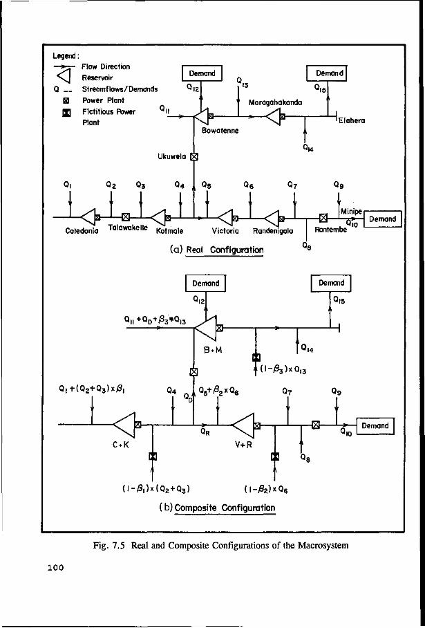
Legend:

>^ Flow Direction

\ J Reservoir

Q Streamf lows/Demands ^12

E9 Power Plant

JQ Fictitious Power

Plant

Demand

Oil f>

13

Demand

"15 Moragahakanda

Bowatenne

1 Elahera

Ukuwela ^

Q2 Q3 Q4 1 Q5

v

<K <KI-<>-

Q9

Caledonia T a l a w a k e l l e Kotmale Victoria Randenigala -B-

Minipe

Rantembe '10

Demand

(a) Real Configuration

Demand

'12

Q|t + Q D

+ /33*QI3 >.

Demand

$

QitfQg+Qslx/S, Q4

<t C*K

a-

AV^2 x Q 6

[ ]

•<I5

0.4

• ( l - £ 3 ) x Q 1 3

Q7 Q9

QR a-V+R

E]

HB-'10

Demand

[ ] Q

( l - j 3 l ) x { Q 2 + Q3) (1 -yS2) x Q6

(b) Composite Configuration

Fig. 7.5 Real and Composite Configurations of the Macrosystem

100

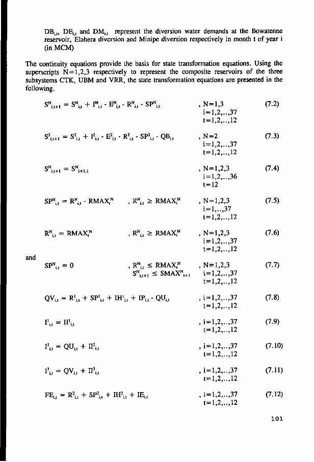
DBit, DEit and DMit represent the diversion water demands at the Bowatenne reservoir, Elahera diversion and Minipe diversion respectively in month t of year i (in MCM)

The continuity equations provide the basis for state transformation equations. Using the superscripts N=1,2,3 respectively to represent the composite reservoirs of the three subsystems CTK, UBM and VRR, the state transformation equations are presented in the following.

ON — QN i TN pN p N QpN a i,t+l — ° i,t T l i,t c i,t R i,t o r i,t

S\,+, = S\ t + I \ t - E\, - R\ t - SP\ t - QB,,,

oN _ cN ° i,t+l — ° i + 1,1

SpN ( = RN.^ . R M A X N , RN. ( > RMAXtN

and

RNit = RMAX,N

SPNi,, = 0

, RNit > RMAXt

N

, RNit < RMAX,N

SNit+1 < SMAXN

t.

QVU = R1;,, + SP'U + IHS,, + IP,, - QUU

I2i,, = QUiit + H\ t

I3i,t = QViit + I l \ t

FEU = R\ t + SP\, + IH2U + IEU

, N=l,3 i=l,2,..,37 t=l,2,..,12

, N=2 i=l,2,..,37 t=l,2,..,12

, N=l,2,3 i = l,2,..,36 t=12

, N=l,2,3 i = l,..,37 t=l,2,..,12

, N=l,2,3 i=l,2,..,37 t=l,2,..,12

,N=1,2,3 i=l,2,..,37 t=l,2,..,12

, i=l,2,. . ,37 t=l,2,..,12

, i = l,2,..,37 t=l,2,..,12

, i = l,2,..,37 t=l,2,..,12

, i = l,2,..,37 t=l,2,..,12

, i=l,2,. . ,37 t=l,2,..,12

(7.2)

(7.3)

(7.4)

(7.5)

(7.6)

(7.7)

(7.8)

(7.9)

(7.10)

(7.11)

(7.12)

101

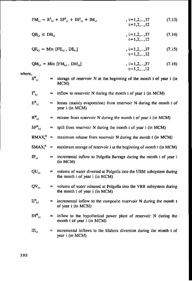
, i = l,2,. t=l,2,.

, i = l,2,. t=l ,2, .

, i=l ,2, . t=l ,2, .

, i = l,2,. t=l ,2, .

.,37

.,12

.,37

.,12

.,37

.,12

.,37

.,12

(7.13)

(7.14)

(7.15)

(7.16)

FMU = R\ t + SP\, + IH3U + IMit

QBM < DBi>t

QE;,t = Min {FEi,, , DEi>t}

QMU = Min {FMit , DMit}

where, SNj, = storage of reservoir N at the beginning of the month t of year i (in

MCM)

INi t = inflow to reservoir N during the month t of year i (in MCM)

EN; t = losses (mainly evaporation) from reservoir N during the month t of

year i (in MCM)

RN; t = release from reservoir N during the month t of year i (in MCM)

SPNj t = spill from reservoir N during the month t of year i (in MCM)

RMAX,N = maximum release from reservoir N during the month t (in MCM)

SMAXtN = maximum storage of reservoir i at the beginning of month t (in MCM)

IPj t = incremental inflow to Polgolla Barrage during the month t of year i (in MCM)

QUj t = volume of water diverted at Polgolla into the UBM subsystem during the month t of year i (in MCM)

QVj t = volume of water released at Polgolla into the VRR subsystem during the month t of year i (in MCM)

IINi t = incremental inflow to the composite reservoir N during the month t of year i (in MCM)

IHNit = inflow to the hypothetical power plant of reservoir N during the

month t of year i (in MCM)

IEit = incremental inflows to the Elahera diversion during the month t of year i (in MCM)

102

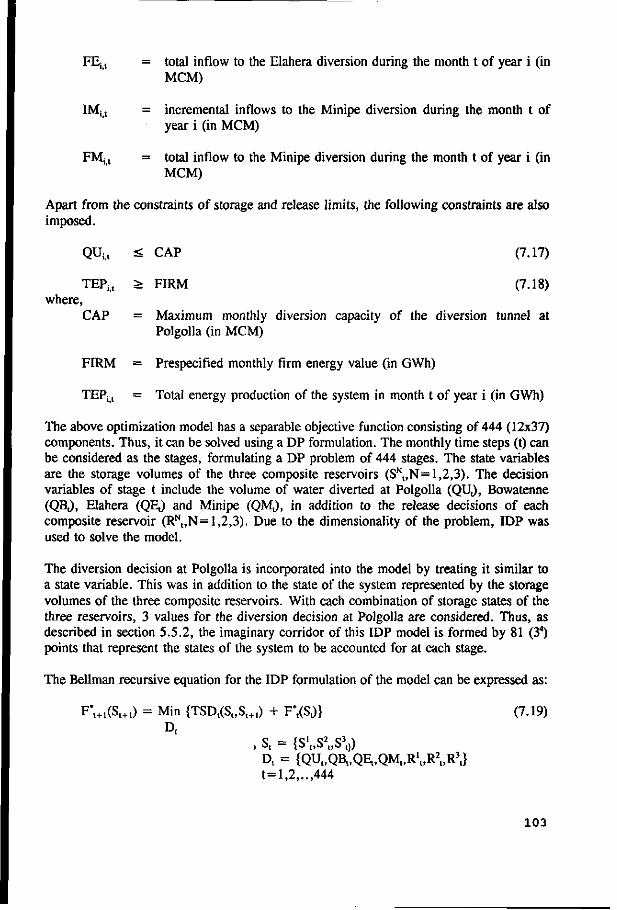
FEj t = total inflow to the Elahera diversion during the month t of year i (in MCM)

IMj, = incremental inflows to the Minipe diversion during the month t of year i (in MCM)

FMj t = total inflow to the Minipe diversion during the month t of year i (in MCM)

Apart from the constraints of storage and release limits, the following constraints are also imposed.

QUU < CAP (7.17)

TEPit > FIRM (7.18) where,

CAP = Maximum monthly diversion capacity of the diversion tunnel at Polgolla (in MCM)

FIRM = Prespecified monthly firm energy value (in GWh)

TEPj t = Total energy production of the system in month t of year i (in GWh)

The above optimization model has a separable objective function consisting of 444 (12x37) components. Thus, it can be solved using a DP formulation. The monthly time steps (t) can be considered as the stages, formulating a DP problem of 444 stages. The state variables are the storage volumes of the three composite reservoirs (SN

t,N= 1,2,3). The decision variables of stage t include the volume of water diverted at Polgolla (QUJ, Bowatenne (QB,), Elahera (QEJ and Minipe (QM,), in addition to the release decisions of each composite reservoir (RN„N= 1,2,3). Due to the dimensionality of the problem, IDP was used to solve the model.

The diversion decision at Polgolla is incorporated into the model by treating it similar to a state variable. This was in addition to the state of the system represented by the storage volumes of the three composite reservoirs. With each combination of storage states of the three reservoirs, 3 values for the diversion decision at Polgolla are considered. Thus, as described in section 5.5.2, the imaginary corridor of this IDP model is formed by 81 (34) points that represent the states of the system to be accounted for at each stage.

The Bellman recursive equation for the IDP formulation of the model can be expressed as:

F*t+1(St+1) = Min {TSD,(S,,Sl+0 + F'.CSJ} (7.19)

, 5>t = (J> i,o „ o ,})

Dt = {QU„QBl,QEt,QM1,R\,R2t,R

3t}

t= 1,2,..,444

103

where, S, = the state of the system at stage t

TSDt(S„St+1) = the squared deviation of the irrigation water supply from the demands during stage t

Dt = The decisions associated with the state transformation from S, to Sl+,

F*t+1(S,+1) = the minimum total of the objective function value from stage 1 to stage t+1, when the state at stage t+1 is St+,

Due to the large number of discrete state transformations that has to be considered at each stage, it was not possible to consider the entire 37-year period in a single optimization run. Instead, the 37-year period was divided into eleven 3-year periods and one 4-year period. It was assumed that the composite reservoirs are half-full at the beginning and at the end of each of these 12 periods. The model was run on an ordinary personnel computer which has a RAM of 640 Kb, considering 5 different values of maximum diversion capacities at Polgolla. Diversion capacities of 40%, 50%, 60%, 80% and 100% of the capacity of the diversion tunnel were considered. The aggregated results of the analysis are presented in Table 7.1.

Table 7.1 Results of the Three-composite-reservoir

D i v e r s i o n Average c a p a c i t y annua l

a t e n e r g y P o l g o l l a g e n e r a -

- t i o n

(MCM/mo) (GWh)

60 2 6 8 9 . 7 8 75 2 6 6 3 . 8 4 89 2 6 4 5 . 5 6

119 2 6 2 7 . 0 5 149 2 6 1 7 . 3 0

Annual f i rm e n e r g y

(GWH)

8 6 5 . 2 9 2 6 . 4 8 7 0 . 0 8 7 6 . 0 8 5 4 . 4

Average annua l w a t e r s h o r t a g e a t Min ipe (MCM)

4 7 . 0 0 4 5 . 2 2 4 4 . 8 7 4 4 . 6 1 4 4 . 9 0

IDP model

Average annua l w a t e r s h o r t a g e a t Bowatenne (MCM)

8 1 . 4 1 6 6 . 7 5 5 4 . 4 4 5 1 . 1 1 4 9 . 9 2

Average annua l w a t e r s h o r t a g e a t E l a h e r a (MCM)

0 . 0 0 . 0 0 . 0 0 . 0 0 . 0

Having found several time series of diversion vs inflow at Polgolla, an attempt was made to fit a regression formula for those two variables. However it was found that their relationship could not be adequately represented by a regression formula. The reason for that can be explained by referring to the Figs. 7.6, 7.7 and 7.8. The monthly diversions at Polgolla obtained from the results of Three-composite-reservoir IDP model are displayed in Figs. 7.6 and 7.7. These correspond to the model run with a maximum diversion capacity of 75 MCM per month. The plot of the monthly inflow at Polgolla vs diversion obtained using the three-composite-reservoir model is displayed in Fig. 7.8.

104

(a) October (b) November

0 10 20 30 40 Year

8o (c) December

10 20 Year

80 (e1) February

10 20 30 40 Year

c o •i-i to u <u .5 a

80

60

40

20

1 1 I 1 ±. i l l ) 1 1 1 1 1 1 1 1 1 1 1 1 . inn i i

a o

•H in U <D

80

60

40

20

0 10 20 30 Year

(d) January

40

10 20 30 40 Year

(f) March

10 20 30 40 Year

Fig. 7.6 Monthly Diversions at Polgolla (October-March) (Results of Three-Composite-Reservoir IDP Model)

105

(a) April 80

(b) May

80

a g 60

0 10 20 30 40 Year

(e) August

M <u >

•r-l

40

20

0 10 20 30 40 Year

£ 6 0 o a c o

•H 40 to

n 0)

> 20

"ti . 1 1 1 1 1 1 1 I 1 j l l l l

• •

V 10 20

Year (d) July

30 40

80

a a1 60 a o

S 40 > o

10 20 30 40 Year

(f) September

20

0 10 20 30 40 Year

Fig. 7.7 Monthly Diversions at Polgolla (April-September) (Results of Three-Composite-Reservoir IDP Model)

106

S1

~ j bo

2

3

O

< en

< ft

O 3

T3

00*

o

f t

3" ft

O o 3 "8

ft ft 3 o

O

8.

Diversion a t Polgolla (MCM) S3

o o o Ui

o O o

S3 . O O

5 3 rt cr i-1

3 l-h

4>-. TJ O o o I-1

00 O

+ + +

+

+

+

K o S

o . o

00 o O-

+ $

+ +

i * * t t +

+ 1 + +

+ t + + + !

+ + +

± + + ± + + + + +

+

+ +

+ + +

+ +

+

*ia +

+

+ + +

+

+

+

* *

$ *

+

+

+

+ + + +

+ ::

+

+

+ +

+ +

oo o

The wide variation of the diversion volume despite the large number of cases where the diversion volume reaches the upper limit refer to a poor correlation between the two variables. In order to determine the best diversion policy at Polgolla barrage, a diversion policy which has a close resemblance to the diversion pattern obtained by the three-composite-reservoir model was employed. Fig. 7.9 displays the diversion policy considered for further analysis.

Fig. 7.9 indicates a minimum downstream release volume at Polgolla. The part of the available inflow which is in excess of this minimum release is to be diverted to the Amban Ganga basin. A maximum limit for this diversion is also specified. Any excess over the maximum possible diversion at Polgolla is to be spilled downstream into the VRR subsystem. In this diversion policy, the best values for the minimum release volume and the maximum limit on the diversion are to be determined.

The best values for these parameters were estimated by performing a sensitivity analysis using the three-composite-reservoir IDP model. In the sensitivity analysis, several different combinations of the two parameters were used to prespecify several independent diversion policies. With each of these diversion policies, the three-composite-reservoir IDP model was run using the available historical records. As the diversion volume is no longer a decision variable, the number of states that had to be considered in each stage of this model was 27 (33). Due to the reduced computational load, this model could be run by dividing the 37-year time series into three 9-year periods and one 10-year period. For each of these 10 periods, it was assumed that the composite reservoirs are half-full at the beginning and also at the end.

Results of the sensitivity analysis done with 15 different combinations of minimum release and diversion capacities at Polgolla are presented in Table 7.2. It was necessary to use a multicriterion decision making technique to select the best alternative combination. The technique of Compromise Programming (CP) described in Section 5.7 was used for this purpose. This CP analysis was done with different sets of weight factors for the four performance criteria. The sets of weights are presented in Table 7.3. Results of the CP analysis are presented in Table 7.4. With an exponent of p=1, the CP technique evaluates all the deviations of a specific performance criterion from the ideal with an equal importance. CP results corresponding to an exponent of p=2 penalizes the large deviations from the ideal more than the smaller deviations. The case of p= <» corresponds to a "min-max" criteria in which the minimum deviation out of the set of alternatives with largest deviations is identified as the compromise solution. CP results corresponding to p=2 of Table 7.4 indicate that the alternatives 5,6,8 and 9 are having the least deviations from the ideal solutions. These correspond to maximum monthly diversion capacities of 75 and 89 MCM at Polgolla. Therefore in further analysis of the system using stochastic optimization models, maximum diversion capacities of only 75 and 89 MCM are taken into account.

108

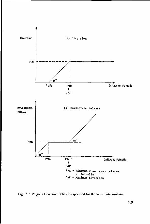
Diversion

CAP

PMR

(a) D ive r s ion

PMR +

CAP

Inflow to Polgolla

Downstream Release

PMR

(b) Downstream Re lease

Inflow to Polgolla

PMR = Minimum downstream r e l e a s e a t P o l go l l a

CAP = Maximum d i v e r s i o n

Fig. 7.9 Polgolla Diversion Policy Prespecified for the Sensitivity Analysis

109

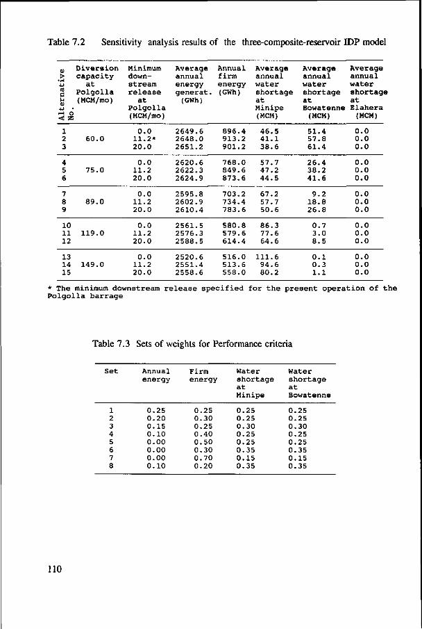
Table 7.2 Sensitivity analysis results of the three-composite-reservoir IDP model

01

> 4-1

a u 4J • r-l o < !S

1 2 3

4 5 6

7 8 9

10 11 12

13 14 15

Diversion capacity

at Polgolla (MCM/mo)

60.0

75.0

89.0

119.0

149.0

Minimum down­stream release

at Polgolla (MCM/mo)

0.0 11.2* 20.0

0.0 11.2 20.0

0.0 11.2 20.0

0.0 11.2 20.0

0.0 11.2 20.0

Average annual energy generat.

(GWh)

2649.6 2648.0 2651.2

2620.6 2622.3 2624.9

2595.8 2602.9 2610.4

2561.5 2576.3 2588.5

2520.6 2551.4 2558.6

Annual firm energy (GWh)

896.4 913.2 901.2

768.0 849.6 873.6

703.2 734.4 783.6

580.8 579.6 614.4

516.0 513.6 558.0

Average annual water shortage at Minipe (MCM)

46.5 41.1 38.6

57.7 47.2 44.5

67.2 57.7 50.6

86.3 77.6 64.6

111.6 94.6 80.2

Average annual water shortage at Bowatenne

(MCM)

51.4 57.8 61.4

26.4 38.2 41.6

9.2 18.8 26.8

0.7 3.0 8.5

0.1 0.3 1.1

Average annual water shortage at Elahera

(MCM)

0.0 0.0 0.0

0.0 0.0 0.0

0.0 0.0 0.0

0.0 0.0 0.0

0.0 0.0 0.0

* The minimum downstream release specified for the present operation of the Polgolla barrage

Table 7.3 Sets of weights for Performance criteria

Set

1 2 3 4 5 6 7 8

Annual energy

0.25 0.20 0.15 0.10 0.00 0.00 0.00 0.10

Firm energy

0.25 0.30 0.25 0.40 0.50 0.30 0.70 0.20

Water shortage at Minipe

0.25 0.25 0.30 0.25 0.25 0.35 0.15 0.35

Water shortage at Bowatenne

0.25 0.25 0.30 0.25 0.25 0.35 0.15 0.35

110

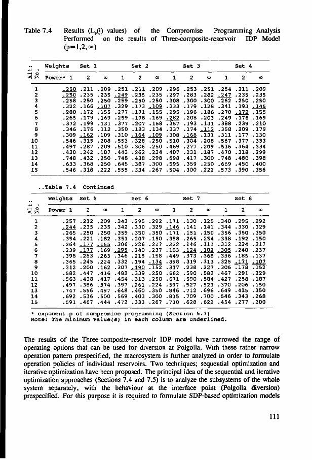
Table 7.4 Results (Lp(j) values) of the Compromise Programming Analysis Performed on the results of Three-composite-reservoir IDP Model (p=l,2,oo)

4-1 • r-l O

< 53

1 2 3 4 5 6 7 8 9

10 11 12 13 14 15

.

.. r-j O

l 2 3 4 5 6 7 8 9

10 11 12 13 14 15

Weights

Power* 1

.250

.250

.258

.322

.280

.265

.372

.346

.309

.546

.497

.430

.748

.633

.546

.Table 7.4

Weights

Power 1

.257

.244

.265

.354

.264

.239

.398

.365

.312

.582

.563

.497

.747

.692

.591

Set 1

2

.211

.235

.250

.166

.172

.179

.199

.176

.162

.315

.287

.242

.432

.368

.318

GO

.209

.235

.250

.107

.155

.169

.131

.112

.109

.208

.209

.187

.250

.250

.222

Continuec

Set 5

2

.212

.235

.250

.221

.177

.177

.283

.245

.200

.447

.438

.386

.556

.536

.467

00

.209

.235

.250

.182

.155

.169

.263

.224

.162

.416

.417

.374

.497

.500

.444

1

.251

.249

.259

.329

.277

.259

.377

.350

.310

.553

.510

.443

.748

.645

.555

1

.343

.342

.359

.351

.306

.295

.346

.332

.307

.482

.454

.397

.648

.569

.472

Set 2

2

.211

.235

.250

.173

.171

.178

.207

.183

.164

.328

.306

.262

.438

.387

.334

Set 6

2

.295

.330

.350

.207

.226

.240

.215

.194

.190

.339

.313

.261

.460

.403

.333

00

.209

.235

.250

.109

.155

.169

.158

.134

.109

.250

.250

.224

.298

.300

.267

00

.292

.329

.350

.150

.217

.237

.158

.134

.152

.250

.250

.224

.350

.300

.267

1

.296

.297

.308

.333

.295

.282

.357

.337

.308

.510

.469

.407

.698

.595

.504

1

.171

.146

.171

.358

.222

.183

.449

.398

.317

.682

.671

.597

.846

.815

.710

Set 3

2

.253

.283

.300

.179

.196

.208

.193

.174

.168

.304

.277

.231

.417

.359

.300

Set 7

2

.130

.141

.151

.265

.146

.124

.373

.319

.238

.590

.590

.527

.712

.709

.628

00

.251

.282

.300

.128

.186

.203

.131

.112

.131

.208

.209

.187

.300

.250

.222

00

.125

.141

.150

.254

.111

.102

.368

.313

.227

.582

.584

.523

.696

.700

.622

1

.254

.247

.262

.341

.270

.249

.388

.358

.311

.567

.536

.470

.748

.669

.573

1

.340

.344

.356

.338

.312

.305

.336

.325

.306

.467

.427

.370

.649

.546

.454

Set A

2

.211

.235

.250

.193

.172

.176

.239

.209

.177

.377

.364

.318

.480

.450

.390

Set 8

2

.295

.330

.350

.192

.224

.240

.185

.171

.178

.291

.258

.206

.415

.343

.277

00

.209

.235

.250

.145

.155

.169

.210

.179

.130

.333

.334

.299

.398

.400

.356

00

.292

.329

.350

.150

.217

.237

.137

.107

.152

.229

.187

.150

.350

.268

.200

* exponent p of compromise programming (Section 5.7) Note: The minimum value(s) in each column are underlined.

The results of the Three-composite-reservoir IDP model have narrowed the range of operating options that can be used for diversion at Polgolla. With these rather narrow operation pattern prespecified, the macrosystem is further analyzed in order to formulate operation policies of individual reservoirs. Two techniques; sequential optimization and iterative optimization have been proposed. The principal idea of the sequential and iterative optimization approaches (Sections 7.4 and 7.5) is to analyze the subsystems of the whole system separately, with the behaviour at the interface point (Polgolla diversion) prespecified. For this purpose it is required to formulate SDP-based optimization models

111

for the individual multiunit subsystems. The assessment of the SDP model formulated for the VRR subsystem is presented in Section 7.3.

7.3 Two-Reservoir SDP Models

In order to analyze the subsystems of the macrosystem, two-reservoir SDP models which are computationally manageable with commonly available computers were formulated (Harboe et al., 1991). The Victoria-Randenigala-Rantembe reservoir subsystem is chosen to test the developed model. Rantembe reservoir, due to its negligible storage capacity, is treated as a run-of-the-river power plant in this analysis. Nandalal (1986) has shown the validity of this simplification by proving that the consideration of Rantembe as the third reservoir would have only a marginal influence on the system output. The basic two-reservoir SDP model is documented in Chapter 5.3.4. Two different model formulations were considered. The first one has an objective function to maximize the expected energy generation (OF1). The second formulation has an objective function to minimize the expected sum of squared deviation of the flows at Minipe from the Minipe demands (OF2). The analysis is based on historical (37-year-long) monthly streamflow data at each reservoir and at Minipe diversion. In both of the cases, no demand constraints were considered in order to permit a comparison with an IDP-based deterministic optimum. In the case of the deterministic optimum solution, it was found that a feasible solution does not exist when the available demand series is considered as constraints. Therefore the SDP-based optimizations also were performed without demand constraints.

This optimization model produces an output consisting of 12 operation policy tables for the 12 months of the year. They specify the optimal target storage level at the end of the month as a function of the initial storage levels and the current inflows during the month. As an example, the operation policy table obtained with the OF1 using 4 inflow classes and 7 storage classes for each reservoir is displayed in Table 7.5. The numerical values used to identify the different inflow and storage levels are presented in Tables 7.6 and 7.7 respectively.

The system performance was simulated separately according to the different SDP-based operation policies derived using different state discretization levels. The performance indicators used to assess the simulated operation are the following:

(1) Average annual energy generation (2) Annual firm energy (3) Average annual water shortage (4) Probability of failure months (The probability that the demand cannot be satisfied as

a result of a reservoir level being lower than or equal to the minimum operation level.)

The simulation results are summarized in Table 7.8. Results of the deterministic optimum operation pattern for the two objectives are also included. The tabulated computer time is for the IBM 3083 mainframe computer at the Asian Institute of Technology in Thailand.

112

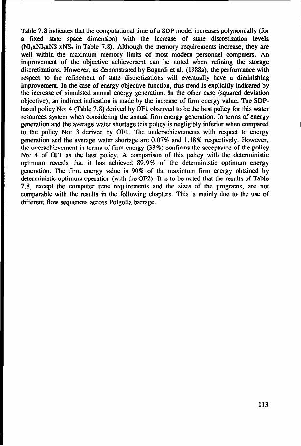
Table 7.8 indicates that the computational time of a SDP model increases polynomially (for a fixed state space dimension) with the increase of state discretization levels (N^XNIJXNS^NSJ in Table 7.8). Although the memory requirements increase, they are well within the maximum memory limits of most modern personnel computers. An improvement of the objective achievement can be noted when refining the storage discretizations. However, as demonstrated by Bogardi et al. (1988a), the performance with respect to the refinement of state discretizations will eventually have a diminishing improvement. In the case of energy objective function, this trend is explicitly indicated by the increase of simulated annual energy generation. In the other case (squared deviation objective), an indirect indication is made by the increase of firm energy value. The SDP-based policy No: 4 (Table 7.8) derived by OF1 observed to be the best policy for this water resources system when considering the annual firm energy generation. In terms of energy generation and the average water shortage this policy is negligibly inferior when compared to the policy No: 3 derived by OF1. The underachievements with respect to energy generation and the average water shortage are 0.07% and 1.18% respectively. However, the overachievement in terms of firm energy (33%) confirms the acceptance of the policy No: 4 of OF1 as the best policy. A comparison of this policy with the deterministic optimum reveals that it has achieved 89.9% of the deterministic optimum energy generation. The firm energy value is 90% of the maximum firm energy obtained by deterministic optimum operation (with the OF2). It is to be noted that the results of Table 7.8, except the computer time requirements and the sizes of the programs, are not comparable with the results in the following chapters. This is mainly due to the use of different flow sequences across Polgolla barrage.

113

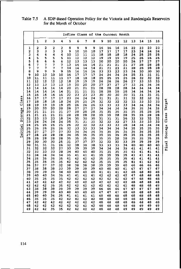
Table 7.5 A SDP-Based Operation Policy for the Victoria and Randenigala Reservoirs for the Month of October

CO CO CD

O

CD 60

U O

CO

I-l

cd J-J .,-1 C 1—1

1 2 3 4 5 6 7 8 9

10 11 12 13 14 15 16 17 18 19 20 21 22 23 24 25 26 27 28 29 30 31 32 33 34 35 36 37 38 39 40 41 42 43 44 45 46 47 48 49

1

2 3 4 5 6 7 7 9

10 11 12 13 14 14 16 17 18 19 20 21 21 23 24 25 26 27 28 28 30 31 32 33 34 35 35 37 38 39 40 35 42 42 38 39 40 35 42 42 42

2

2 3 4 5 6 7 7 9

10 11 12 13 14 14 16 17 18 19 20 21 21 23 24 25 26 27 28 28 30 31 32 33 34 35 35 37 38 39 40 35 42 42 38 39 40 35 42 42 42

3

2 3 4 5 6 7 7 9

10 11 12 13 14 14 16 17 18 19 20 21 21 23 24 25 26 27 28 28 30 31 32 33 34 35 35 37 38 39 34 35 42 35 38 39 34 35 42 42 35

Inflow CI

4

2 3 4 5 6 7 7 9

10 11 12 13 14 14 16 17 18 19 20 21 21 18 24 25 26 27 28 28 25 26 27 28 34 35 35 32 33 34 35 35 42 35 39 40 35 42 42 42 35

5

8 9

10 11 12 13 14 15 16 17 18 19 20 21 22 23 24 25 26 27 28 24 25 26 32 33 34 35 31 32 33 34 35 41 42 38 39 40 41 42 42 42 39 40 41 42 42 42 42

6

9 10 11 12 13 14 14 16 17 18 19 20 21 21 23 24 25 26 27 28 28 30 31 32 33 34 35 35 37 38 39 40 41 42 42 38 39 40 41 42 42 42 39 40 41 42 42 42 42

ass

7

9 10 11 12 13 14 14 16 17 18 19 20 21 21 23 24 25 26 27 28 28 30 31 32 33 34 35 35 37 38 39 40 41 42 42 38 39 40 41 42 42 42 39 40 41 42 42 42 42

of the Current Month

8

9 10 11 12 13 14 14 16 17 18 19 20 21 21 23 24 25 26 27 28 28 30 31 32 33 34 35 35 37 38 39 40 41 42 42 38 39 40 41 42 42 42 39 40 41 42 42 42 42

9

16 17 18 19 20 21 21 23 24 25 26 27 28 28 30 31 32 33 34 35 35 31 32 33 34 35 35 35 32 33 34 35 35 35 35 39 40 41 42 42 42 42 46 47 48 48 48 48 48

10

16 17 18 19 20 21 21 23 24 25 26 27 28 28 30 31 32 33 34 35 35 31 32 33 34 35 35 35 32 33 34 35 35 35 35 39 40 41 42 42 42 42 46 47 48 48 48 48 48

11

16 17 18 19 20 21 21 23 24 25 26 27 28 28 30 31 32 33 34 35 28 31 32 33 34 35 35 28 32 33 34 35 35 35 35 39 40 41 42 42 42 42 46 47 48 48 48 48 48

12

16 17 18 19 20 21 21 23 24 25 26 27 28 28 30 31 32 33 34 35 28 26 27 28 34 35 35 28 33 34 35 35 35 35 35 40 41 42 42 42 42 42 47 48 48 48 48 48 49

13

22 23 24 25 26 27 28 24 25 26 27 33 34 34 31 32 33 34 35 35 35 32 33 34 35 35 35 35 39 40 41 41 41 41 41 46 47 48 47 47 48 48 47 48 48 48 48 48 49

14

23 24 25 26 27 28 28 30 31 32 33 34 34 34 31 32 33 34 35 35 35 32 33 34 35 35 35 35 39 40 41 41 41 41 41 46 47 48 48 48 48 48 47 48 48 48 48 49 49

15

23 24 25 26 27 28 28 30 31 32 33 34 34 34 31 32 33 34 34 28 28 32 33 34 35 35 35 35 39 40 41 41 41 41 42 46 47 48 48 48 48 48 47 48 48 48 48 49 49

16

23 24 25 26 27 28 28 30 31 32 33 34 34 34 31 32 33 34 35 28 28 32 33 34 35 35 35 35 39 40 41 41 41 41 42 46 47 48 48 48 48 49 48 48 48 48 48 49 49

114

Table 7.6 Inflow Class Discretization of the Operation Policy of Table 7.5

Inf low C l a s s

1

2

3

4

5

6

7

8

9

10

11

12

13

14

15

16

V R

V R

V R

V R

V R

V R

V R

V R

V R

V R

V R

V R

V R

V R

V R

V R

Oc t

93 .5 24 .9

93 .5 4 3 . 1

93 .5 65 .3

93 .5 89 .7

176.2 24 .9

176.2 4 3 . 1

176.2 65 .3

176.2 89 .7

304.5 24 .9

304 .5 4 3 . 1

304.5 65 .3

304.5 89 .7

402.4 24 .9

402.4 4 3 . 1

402.4 65 .3

402.4 89 .7

Nov

155 .1 32 .0

155 .1 68 .2

155 .1 98.2

155 .1 141.2

279.2 32 .0

279.2 68.2

279.2 98.2

279.2 141.2

429.7 32 .0

429.7 68.2

429.7 98 .2

429.7 141.2

Dec

146.2 76 .8

146.2 161.9

146.2 295.2

146.2 447.0

381.8 76 .8

381.8 161.9

381.8 295.2

381.8 447.0

710.2 76 .8

710.2 161.9

710.2 295.2

710.2 447.0

657.51113.9 32 .0 76 .8

657.51113.9 68.2 161.9

657.51113.9 98 .2 295.2

657.51113.9 141.2 447.0

J a n

67.2 61 .0

67.2 118.0

67.2 177.6

67.2 255.7

200.5 61 .0

200.5 118.0

200.5 177.6

200.5 255.7

313.0 61.0

313.0 118.0

313.0 177.6

313.0 255.7

485 .1 61 .0

485 .1 118.0

485 .1 177.6

485 .1 255.7

Feb

34.7 24 .7

34.7 89 .9

34 .7 157.5

34 .7 248.0

106.2 24.7

106.2 89 .9

106.2 157.5

106.2 248.0

169.9 24.7

169.9 89 .9

169.9 157.5

169.9 248.0

287.2 24 .7

287.2 89 .9

287.2 157.5

287.2 248.0

Mar

25.6 13.5

25 .6 36 .3

25 .6 71 .1

25 .6 106 .1

48 .4 13.5

48 .4 36 .3

48 .4 71 .1

48 .4 106.1

75 .6 13.5

75 .6 36 .3

75 .6 71 .1

75.6 106 .1

110.9 13.5

110.9 36 .3

110.9 71 .1

110.9 106.1

Apr

41.2 12.7

41 .2 26 .8

41 .2 43 .0

41 .2 59.7

80 .9 12.7

80 .9 26 .8

80 .9 43 .0

80 .9 59.7

131.0 12.7

131.0 26 .8

131.0 43 .0

131.0 59.7

195.7 12.7

195.7 26 .8

195.7 43 .0

195.7 59.7

May

47.0 14 .0

47 .0 33.9

47 .0 66 . 1

47 .0 96 .3

166.7 14.0

166.7 33.9

166.7 66 .1

166.7 96 .3

260.5 14 .0

260 .5 33 .9

260 .5 66 . 1

260.5 96 .3

376.9 14.0

376.9 33.9

376.9 66 . 1

376.9 96 .3

J u n

87 .5 10 .6

87 .5 24 .2

87 .5 39 .8

87 .5 67 .6

280 .8 10 .6

280 .8 24 .2

280 .8 39 .8

280.8 67 .6

440 .1 10.6

4 40 . 1 24 .2

440 .1 39 .8

440 .1 67 .6

723.9 10 .6

723.9 24.2

723.9 39 .8

723.9 67 .6

J u l

79.3 8 .3

79 .3 21 .8

79 .3 38 .0

79 .3 54.9

223.4 8 .3

223.4 21 .8

223.4 38 .0

223.4 54 .9

312 .1 8 .3

312 .1 21 .8

312 .1 38 .0

312 .1 54.9

500.3 8 .3

500.3 21 .8

500.3 38 .0

500.3 54.9

Aug

102.7 10.7

102.7 22 .5

102.7 34 .5

102.7 58.2

236 .6 10 .7

236 .6 22 .5

236 .6 34 .5

236 .6 58.2

365.7 10.7

365 .7 22 .5

365.7 34 .5

365.7 58 .2

542.6 10.7

542.6 22 .5

542.6 34 .5

542.6 58.2

Sep

99 .3 8 .6

99 .3 23 .7

99 .3 43 . 1

99 .3 57 .1

261.2 8 .6

261.2 23 .7

261.2 43 . 1

261.2 57 . 1

422.4 8.6

422.4 23 .7

422.4 43 . 1

422.4 57 .1

687.3 8 .6

687.3 23 .7

687.3 4 3 . 1

687.3 57 . 1

V S R indicate the inflows of Victoria and Randenigala reservoirs respectively

115

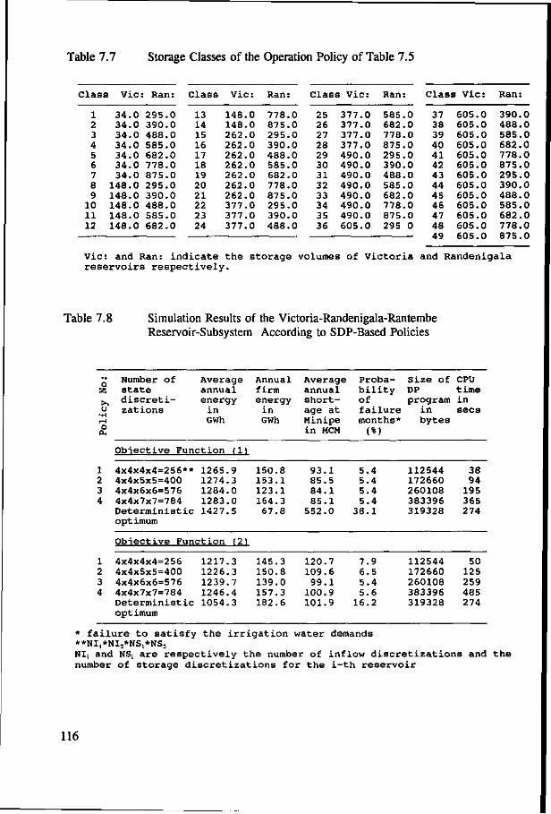
Table 7.7 Storage Classes of the Operation Policy of Table 7.5

Clas

1 2 3 4 5 6 7 8 9

10 11 12

s Vic

34.0 34.0 34.0 34.0 34.0 34.0 34.0

148.0 148.0 148.0 148.0 148.0

Ran:

295.0 390.0 488.0 585.0 682.0 778.0 875.0 295.0 390.0 488.0 585.0 682.0

Class

13 14 15 16 17 18 19 20 21 22 23 24

Vic:

148.0 148.0 262.0 262.0 262.0 262.0 262.0 262.0 262.0 377.0 377.0 377.0

Ran:

778.0 875.0 295.0 390.0 488.0 585.0 682.0 778.0 875.0 295.0 390.0 488.0

Class Vic:

25 26 27 28 29 30 31 32 33 34 35 36

377.0 377.0 377.0 377.0 490.0 490.0 490.0 490.0 490.0 490.0 490.0 605.0

Ran:

585.0 682.0 778.0 875.0 295.0 390.0 488.0 585.0 682.0 778.0 875.0 295 0

Class Vic:

37 38 39 40 41 42 43 44 45 46 47 48 49

605.0 605.0 605.0 605.0 605.0 605.0 605.0 605.0 605.0 605.0 605.0 605.0 605.0

Ran:

390.0 488.0 585.0 682.0 778.0 875.0 295.0 390.0 488.0 585.0 682.0 778.0 875.0

Vic: and Ran: indicate the storage volumes of Victoria and Randenigala reservoirs respectively.

Table 7.8 Simulation Results of the Victoria-Randenigala-Rantembe Reservoir-Subsystem According to SDP-Based Policies

a > i

o I—1

o

1 2 3 4

1 2 3 4

Number of state discreti­zations

Average annual energy

in GWh

Obiective Function (11

4x4x4x4=256** 4x4x5x5=400 4x4x6x6=576 4x4x7x7=784 Deterministic opt imum

1265.9 1274.3 1284.0 1283.0 1427.5

Obiective Function 12)

4x4x4x4=256 4x4x5x5=400 4x4x6x6=576 4x4x7x7=784 Deterministic optimum

1217.3 1226.3 1239.7 1246.4 1054.3

Annual firm energy

in GWh

150.8 153.1 123.1 164.3 67.8

145.3 150.8 139.0 157.3 182.6

Average annual short­age at Minipe in MCM

93.1 85.5 84.1 85.1

552.0

120.7 109.6 99.1

100.9 101.9

Proba­bility of failure months* (%)

5.4 5.4 5.4 5.4

38.1

7.9 6.5 5.4 5.6

16.2

Size of DP program

in bytes

112544 172660 260108 383396 319328

112544 172660 260108 383396 319328

CPU time in sees

38 94

195 365 274

50 125 259 485 274

* failure to satisfy the irrigation water demands **NI,*NI2*NS1*NS2 NI; and NSS are respectively the number of inflow discretizations and the number of storage discretizations for the i-th reservoir

116

7.4 Sequential Optimization SDP/simulation model

Sequential optimization is initiated with the optimization of the uppermost reservoir subsystem which consists of Caledonia, Talawakelle and Kotmale reservoirs. For this optimization, the SDP model described in Chapter 5.3 is used with the necessary modifications. The power plant of Talawakelle reservoir is considered as a run-of-the-river power plant due to the small storage capacity of Talawakelle reservoir. Simulation of the operation of the same subsystem using available historical monthly streamflow records is carried out according to the operation policies derived by optimization. The optimal diversion policy of the Polgolla barrage as described in section 7.2 is also followed. Therefore, in addition to the operation pattern of the reservoir subsystem, the monthly diversions and releases at Polgolla can be determined. The diversions and releases so determined become the upstream inflows to Ukuwela-Bowatenne-Moragahakanda and Victoria-Randenigala-Rantembe reservoir subsystems respectively.

The operation of the two downstream reservoir-subsystems are then optimized individually considering inflows contributed by Polgolla barrage in addition to the inflows within the respective subsystems. In the optimization of Victoria-Randenigala-Rantembe subsystem, Rantembe power plant is considered as a run-of-the-river power plant due to the small storage capacity of Rantembe reservoir. After formulating operation policies by optimization, the operation of two downstream subsystems are then simulated independently using available historical flow records. This simulation is carried out according to the operation policies derived by the optimization models.

The mathematical formulation of the sequential optimization approach (consisting of three SDP-based optimization models) is presented in the following. An objective function which maximizes the expected energy generation is assumed. Using the usual notation (Section 5.3.4) and the superscripts N= 1,2 and 3 respectively to represent the CTK, UBM and VRR subsystems, and the subscripts i = 1,2,3 to represent the three reservoirs/power plants (starting from the upstream) in each subsystem,

For the CTK subsystem.

T 3 Maximize E {E (E TEPit)} (7.20)

t = l i = l where,

TEPit = 9.8 * R'it * (EL'it - DWL'it) * e /3600 GWh , i=1,2,3 t=l,2,..,12

The state transformation equation for the Caledonia reservoir can be expressed as:

S\,,+1 = S\,, + I1,,, - E \ , - R\,t - SP'U , t=l,2,..,12 (7.21)

For the assumed run-of-the-river power plant at Talawakelle,

R!2,« = R'i.t + SP'U + I'2, , t=l,2,. . ,12 (7.22)

117

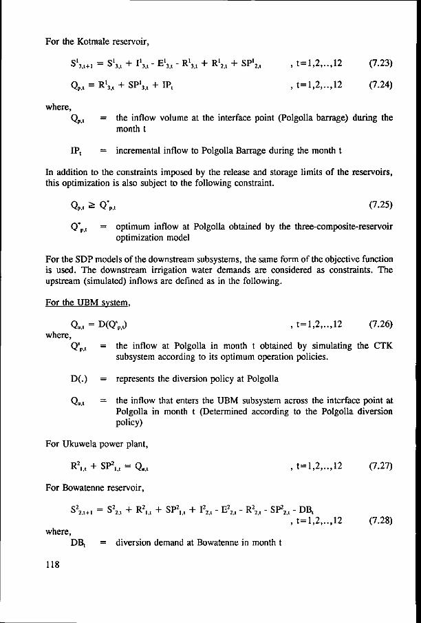
For the Kotmale reservoir,

S V i = S'j,, + I*3,t - E'3,t - R's,, + R'2,, + SP'2,t , t=l,2,..,12 (7.23)

Qp., = R'j,, + SP'j., + IP, , t=l,2,. . ,12 (7.24)

where, Qp t = the inflow volume at the interface point (Polgolla barrage) during the

month t

IP, = incremental inflow to Polgolla Barrage during the month t

In addition to the constraints imposed by the release and storage limits of the reservoirs, this optimization is also subject to the following constraint.

QP,, ^ Q*P,t (7-25)

Q*P,I = optimum inflow at Polgolla obtained by the three-composite-reservoir

optimization model

For the SDP models of the downstream subsystems, the same form of the objective function is used. The downstream irrigation water demands are considered as constraints. The upstream (simulated) inflows are defined as in the following.

For the UBM system.

Qu, = D(Qsp,J , t=l,2,..,12 (7.26)

where, Qs

pt = the inflow at Polgolla in month t obtained by simulating the CTK subsystem according to its optimum operation policies.

D(.) = represents the diversion policy at Polgolla

Qu t = the inflow that enters the UBM subsystem across the interface point at Polgolla in month t (Determined according to the Polgolla diversion policy)

For Ukuwela power plant,

R2,,, + SP2M = QM , t=l,2,. . ,12 (7.27)

For Bowatenne reservoir,

S 2,t+l = S 2,i + R 1,1 + SP i , + I 2,t " E 2,t - R 2,t " S r 2,t " Dl$t , t=l,2,. . ,12 (7.28)

where, DBt = diversion demand at Bowatenne in month t

118

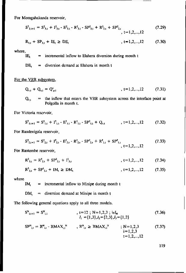
For Moragahakanda reservoir,

S 3,t+l = S 3>t + I 3,1 - E 3 1 - R 3 t - SP 3 , + R 2,t + SP 2,t (7.29)

, t=l,2,. . ,12

R3,, + SP3,, + IE, > DE, , t=l,2,..,12 (7.30)

where, IE, = incremental inflow to Elahera diversion during month t DE, = diversion demand at Elahera in month t

For the VRR subsystem.

Qv,, + Qu,t = QsP,t , t=l,2,.. ,12 (7.31)

Qv, = the inflow that enters the VRR subsystem across the interface point at Polgolla in month t.

For Victoria reservoir,

S \ l + , = S3,,, + I3U - E3,,, - R3,,, - SP3,,, + Q¥il , t=l,2,..,12 (7.32)

For Randenigala reservoir,

S 2,t+l = S 2,1 + I 2,t " E 2,1 " R 2,t " SP 2,t + R l,t + SP j , (7.33) , t=l,2,.. ,12

For Rantembe reservoir,

R33,, = R32,, + SP32,t + I33,t , t=l,2,.. ,12 (7.34)

R33, + SP3

3, + IM, > DM, , t=l,2,..,12 (7.35)

where

IM, = incremental inflow to Minipe during month t

DM, = diversion demand at Minipe in month t

The following general equations apply to all three models.

SNU+1 = SN

U , t=12 ; N=1,2,3 ; ie/N (7.36) h ={l,3},/2 = {2,3},/3 = {l,2}

SPNit = RN

it - RMAXitN , RN

it > RMAXitN ; N=l,2,3 (7.37)

i=l,2,3 t=l,2,..,12

119

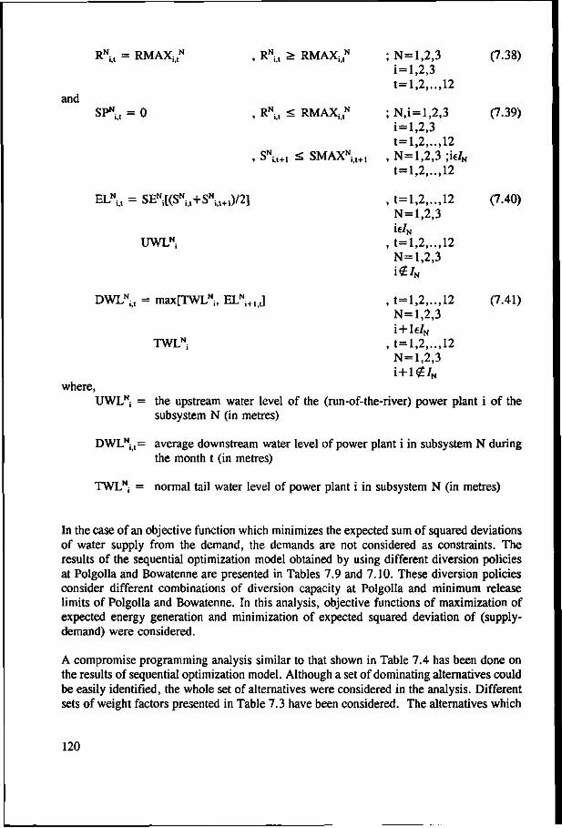
and

RNi>t = RMAXit

N

SP i,, = 0

, RNit > RMAXit

N ; N = 1,2,3 i=l,2,3

, RNi>t < RMAXit

N ;

, S\t+l < SMAXN;,t+I ,

ELNi>t = SEN

i[(SN

i,l+SNu+1)/2]

UWLNj

DWLNi>t = maxtTWL^, ELN

i+1 J

TWLN;

where,

(7.38)

(7.39)

= 1,2,..,12

N,i=l,2,3 = 1,2,3 = 1,2,..,12

N= 1,2,3 ;ie/N

= 1,2,..,12

= 1,2,..,12 (7.40) N=l,2,3 e/N

= 1,2,..,12 N=l,2,3 €IN

= 1,2,.. ,12 (7.41) N=l,2,3 + l6/N

= 1,2,..,12 N=l,2,3 i + l g / N

UWLNi = the upstream water level of the (run-of-the-river) power plant i of the subsystem N (in metres)

DWLNit= average downstream water level of power plant i in subsystem N during

the month t (in metres)

TWLN( = normal tail water level of power plant i in subsystem N (in metres)

In the case of an objective function which minimizes the expected sum of squared deviations of water supply from the demand, the demands are not considered as constraints. The results of the sequential optimization model obtained by using different diversion policies at Polgolla and Bowatenne are presented in Tables 7.9 and 7.10. These diversion policies consider different combinations of diversion capacity at Polgolla and minimum release limits of Polgolla and Bowatenne. In this analysis, objective functions of maximization of expected energy generation and minimization of expected squared deviation of (supply-demand) were considered.

A compromise programming analysis similar to that shown in Table 7.4 has been done on the results of sequential optimization model. Although a set of dominating alternatives could be easily identified, the whole set of alternatives were considered in the analysis. Different sets of weight factors presented in Table 7.3 have been considered. The alternatives which

120

ranked the 1st, 2nd and the 3rd positions in the CP analysis are presented with the corresponding weights in Table 7.11.

It can be seen from the results of Table 7.11 that the alternative 2 has ranked to the 1" position except when the weight set 7 was used. However the weight set 7 refer to a large importance of the firm energy generation when compared to the irrigation water shortages, which is not the case for the Mahaweli water resources system. Table 7.11 also indicates that the results obtained by using energy objective have outperformed those obtained by using squared deviation objective.

Table 7.9 Results of the Sequential Optimization Model (Objective Function: Energy Generation)

Max.

<u >

.r-| 4-1 m G

4J ..

< S3

1 2 3 4 5 6 7 8 9

10 11 12

13 14 15 16 17 18 19 20 21 22 23 24

Polgolla Bowatenne minimum release

(MCM)

Polgolla

0.0

11.2

20.0

30.0

Polgolla

0.0

11.2

20.0

30.0

minimum release

(MCM)

Diversion Pol

0.0 10.0 21.0

0.0 10.0 21.0 0.0

10.0 21.0

0.0 10.0 20.0

Diversion Pol

0.0 10.0 21.0

0.0 10.0 21.0

0.0 10.0 21.0

0.0 10.0 20.0

Average annual energy

generation (GWh)

Ley: Divert

2853.6 2852.8 2847.1 2849.7 2849.8 2843.5 2859.1 2859.5 2854.4 2865.0 2864.8 2860.4

Ley: Divert

2804.2 2804.9 2803.9 2814.9 2816.1 2817.6 2810.5 2812.4 2814.4 2815.2 2817.2 2813.5

Total annual

firm energy (GWh)

upto a

625.0 636.2 650.8 579.7 594.0 604.1 557.8 577.0 593.6 534.6 551.9 570.2

upto a

543.4 551.4 563.8 528.2 546.6 565.6 506.9 522.0 543.3 516.5 532.2 551.8

Average annual water

shortage at

Minipe (MCM)

maximum of

97.8 97.8 97.8 92.8 92.8 92.8 84.7 84.7 84.7 80.6 80.6 80.6

maximum of

114.2 114.2 114.2 102.9 102.9 102.9 99.7 99.7 99.7 89.3 89.3 89.3

Average annual water

shortage at

Bowatenne (MCM)

75 MCM

0.5 2.8

26.0 5.0

12.3 34.7 16.8 20.2 47.5 24.6 34.7 66.0

89 MCM

4.3 10.3 17.0 14.8 21.2 30.1 22.8 32.0 46.3 36.3 51.9 67.7

121

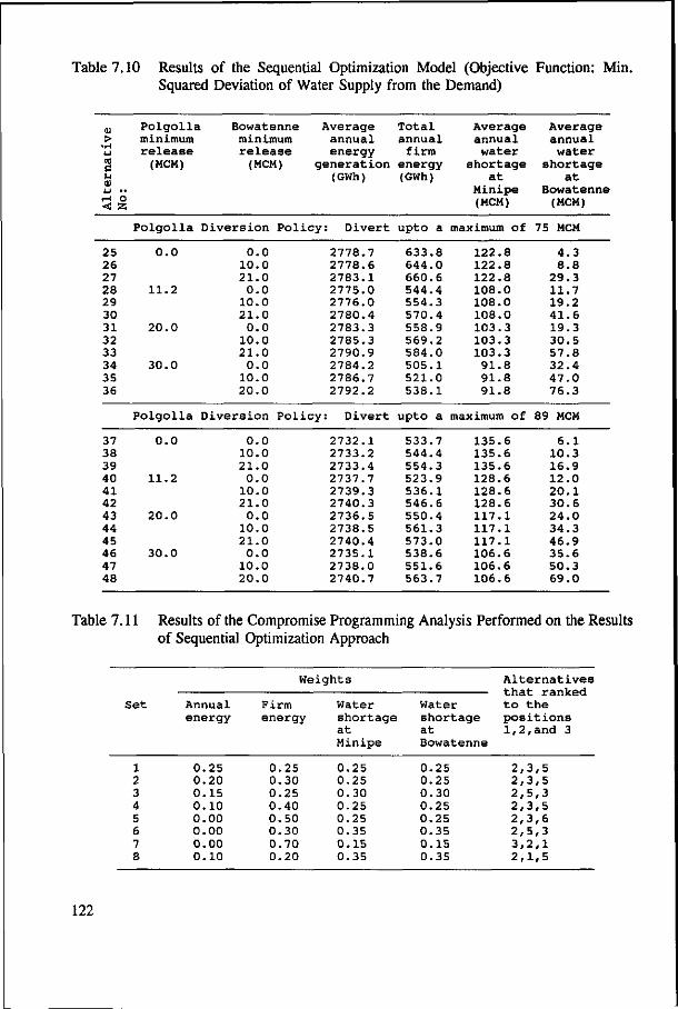
Table 7.10 Results of the Sequential Optimization Model (Objective Function: Min. Squared Deviation of Water Supply from the Demand)

(U > 4-1

a M

j-i ••

i-l o <d 85

25 26 27 28 29 30 31 32 33 34 35 36

37 38 39 40 41 42 43 44 45 46 47 48

Polgolla Bowatenne minimum release

(MCM)

Polgolla

0.0

11.2

20.0

30.0

Polgolla

0.0

11.2

20.0

30.0

minimum release

(MCiV

Diversion

0.0 10.0 21.0

0.0 10.0 21.0

0.0 10.0 21.0

0.0 10.0 20.0

Diversion

0.0 10.0 21.0

0.0 10.0 21.0

0.0 10.0 21.0 0.0

10.0 20.0

)

Average annual energy

generation (GWh)

Policy: Divert

2778.7 2778.6 2783.1 2775.0 2776.0 2780.4 2783.3 2785.3 2790.9 2784.2 2786.7 2792.2

Policy: Divert

2732.1 2733.2 2733.4 2737.7 2739.3 2740.3 2736.5 2738.5 2740.4 2735.1 2738.0 2740.7

Total annual

firm energy (GWh)

upto a

633.8 644.0 660.6 544.4 554.3 570.4 558.9 569.2 584.0 505.1 521.0 538.1

upto a

533.7 544.4 554.3 523.9 536.1 546.6 550.4 561.3 573.0 538.6 551.6 563.7

Average annual water

shortage at

Minipe (MCM)

maximum of

122.8 122.8 122.8 108.0 108.0 108.0 103.3 103.3 103.3 91.8 91.8 91.8

maximum of

135.6 135.6 135.6 128.6 128.6 128.6 117.1 117.1 117.1 106.6 106.6 106.6

Average annual water

shortage at

Bowatenne (MCM)

75 MCM

4.3 8.8

29.3 11.7 19.2 41.6 19.3 30.5 57.8 32.4 47.0 76.3

89 MCM

6.1 10.3 16.9 12.0 20.1 30.6 24.0 34.3 46.9 35.6 50.3 69.0

Table 7.11 Results of the Compromise Programming Analysis Performed on the Results of Sequential Optimization Approach

Annual energy

0.25 0.20 0.15 0.10 0.00 0.00

Weights

Firm energy

0.25 0.30 0.25 0.40 0.50 0.30

Water shortage at Minipe

0.25 0.25 0.30 0.25 0.25 0.35

Water shortage at Bowatenne

0.25 0.25 0.30 0.25 0.25 0.35

Alternatives that ranked to the positions 1,2,and 3

2,3,5 2,3,5 2,5,3 2,3,5 2,3,6 2,5,3

set

2 3 4 5 6 7 0 .00 0 .70 0 .15 0 .15 3 , 2 , 1 8 0 .10 0 .20 0 .35 0 .35 2 , 1 , 5

122

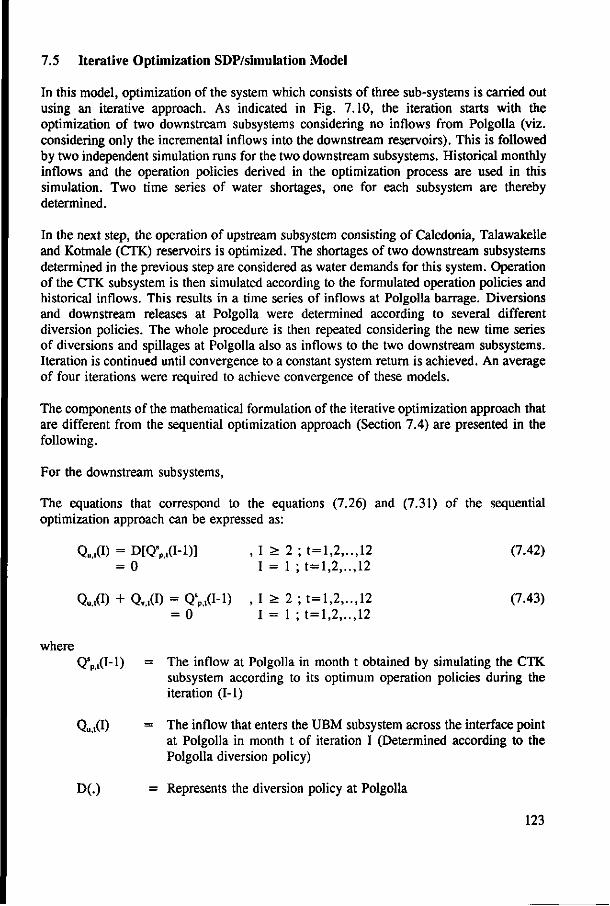
7.5 Iterative Optimization SDP/simulation Model

In this model, optimization of the system which consists of three sub-systems is carried out using an iterative approach. As indicated in Fig. 7.10, the iteration starts with the optimization of two downstream subsystems considering no inflows from Polgolla (viz. considering only the incremental inflows into the downstream reservoirs). This is followed by two independent simulation runs for the two downstream subsystems. Historical monthly inflows and the operation policies derived in the optimization process are used in this simulation. Two time series of water shortages, one for each subsystem are thereby determined.

In the next step, the operation of upstream subsystem consisting of Caledonia, Talawakelle and Kotmale (CTK) reservoirs is optimized. The shortages of two downstream subsystems determined in the previous step are considered as water demands for this system. Operation of the CTK subsystem is then simulated according to the formulated operation policies and historical inflows. This results in a time series of inflows at Polgolla barrage. Diversions and downstream releases at Polgolla were determined according to several different diversion policies. The whole procedure is then repeated considering the new time series of diversions and spillages at Polgolla also as inflows to the two downstream subsystems. Iteration is continued until convergence to a constant system return is achieved. An average of four iterations were required to achieve convergence of these models.

The components of the mathematical formulation of the iterative optimization approach that are different from the sequential optimization approach (Section 7.4) are presented in the following.

For the downstream subsystems,

The equations that correspond to the equations (7.26) and (7.31) of the sequential optimization approach can be expressed as:

QUI) = D[Qsp,t(M)] , 1 ^ 2 ; t=l,2,..,12 (7.42)

= 0 1 = 1 ; t=l,2,..,12

Q«.,(I) + QUI) = QU1"1) , 1 ^ 2 ; t=l,2,..,12 (7.43) = 0 i = l ; t=l,2,..,12

where Q5

p,(I-l) = The inflow at Polgolla in month t obtained by simulating the CTK subsystem according to its optimum operation policies during the iteration (1-1)

Qu,t(I) = Tne inflow that enters the UBM subsystem across the interface point at Polgolla in month t of iteration I (Determined according to the Polgolla diversion policy)

D(.) = Represents the diversion policy at Polgolla

123

Qv ,(I) = The inflow that enters the VRR subsystem across the interface point at Polgolla in month t of iteration I (Determined according to the Polgolla diversion policy)

For the upstream subsystem, the demand constraint that corresponds to the Equation (7.25) of the sequential optimization can be expressed as:

Qp,t(I) > SHsu,t(I) + SHs

vl(I) for all I , t= 1,2,.., 12 (7.44)

where,

SHSU ,(I) and SHS

V ,(I) are the Water shortage at month t obtained by simulating the operation of the UBM and VRR subsystems according to their optimal operation policies during the Ith iteration.

The same formulation except the demand constraints is applicable when considering the objective function of minimization of the squared deviation of water supply from the demand. The results of the iterative optimization obtained using several different diversion policies for Polgolla diversion are presented in Table 7.12.

It is observed that the alternative solutions 53,54 and 56 of the iterative optimization are not practically acceptable as they are associated with very high water shortages at Bowatenne. The results of a compromise programming analysis performed on the results of iterative and sequential approaches are presented in Table 7.13.

The results of Table 7.13 also indicate the suitability of an objective function which maximizes the expected annual energy generation, to formulate operation policies for this particular system. The results obtained by using a diversion policy which diverts water at Polgolla according to the average annual shortages of the downstream subsystems are found to be inferior to those corresponding to the optimal diversion policy of Fig. 7.9.

If the weight sets 4,5 and 7 are excluded from consideration (since they do not properly represent the importance of the performance criteria of Mahaweli system), the alternatives 2 and 8 can be selected as the most satisfactory ones. Although the alternative 8 slightly outperforms 2 in terms of the average annual energy generation (an increase of 0.2%) and in terms of the average annual water shortage at Minipe (a decrease of 13.4%), the high water shortage at Bowatenne (an increase of 620%) and the low firm energy generation (a decrease of 9.3%) make it inferior to alternative 2.

124

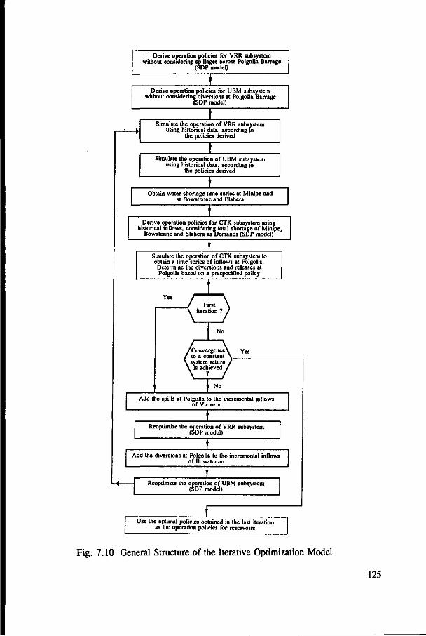
Derive operation policies for VRR subsystem without considering spillages across Polgolla Barrage

(SDP model)

Derive operation policies for UBM subsystem without considering diversions at Polgolla Barrage

(SDP model)

Simulate the operation of VRR subsystem using historical data, according to

the policies derived

Simulate the operation of UBM subsystem using historical data, according to

the policies derived

Obtain water shortage time scries at Minipe and at Bowatenne and Elahcra

Derive operation policies for CTK subsystem using historical inflows, considering total shortage of Minipe,

Bowatenne and Elahera as Demands (SDP model)

Simulate the operation of CTK subsystem to obtain a time series of inflows at Polgolla. Determine the diversions and releases at Polgolla based on a prespecified policy

Rcoplimize the operation of VRR subsystem (SDP model)

Add the diversions at Polgolla to the incremental inflows of Bowatenne

Reoptimize the operation of UBM subsystem (SDP model)

Use the optimal policies obtained in the last iteration as the operation policies for reservoirs

Fig. 7.10 General Structure of the Iterative Optimization Model

125

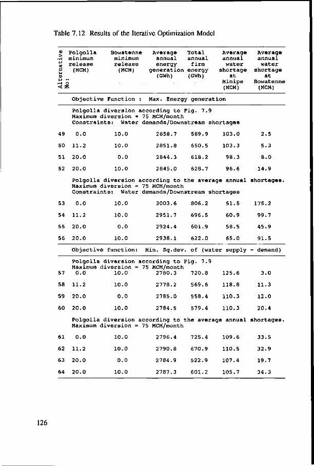
Table 7.12 Results of the Iterative Optimization Model

Average Total Average Average annual annual annual annual energy firm water water

generation energy shortage shortage (GWh) (GWh) at at

Minipe Bowatenne (MCM) (MCM)

Objective Function : Max. Energy generation

Polgolla diversion according to Fig. 7.9 Maximum diversion = 75 MCM/month Constraints: Water demands/Downstream shortages

jjj Polgolla •H minimum ^ release p (MCM)

4J ..

.-1 o < S5

Bowatenne minimum release

(MCM)

49

50

51

52

0.0

11.2

20.0

20.0

10.0

10.0

0.0

10.0

2858.7

2851.8

2844.3

2845.0

589.9

650.5

618.2

628.7

103.0

103.3

98.3

96.6

2.5

5.3

8.0

14.9

Polgolla diversion according to the average annual shortages. Maximum diversion = 75 MCM/month Constraints: Water demands/Downstream shortages

53

54

55

56

57

58

59

60

0.0

11.2

20.0

20.0

Objective

Polgolla Maximum d

0.0

11.2

20.0

20.0

10.0

10.0

0.0

10.0

function:

diversion iversion =

10.0

10.0

0.0

10.0

3003.6

2951.7

2924.4

2938.1

Min. Sq.dev.

according to F 75 MCM/month

2780.3

2778.2

2785.0

2784.5

806.2

696.5

601.9

622.0

51.5

60.9

58.5

65.0

of (water supply

ig. 7.9

720.8

569.6

558.4

579.4

125.6

118.8

110.3

110.3

175.2

99.7

45.9

91.5

- demand)

3.0

11.3

12.0

20.4

Polgolla diversion according to the average annual shortages. Maximum diversion = 75 MCM/month

61

62

63

64

0.0

11.2

20.0

20.0

10.0

10.0

0.0

10.0

2796.4

2790.8

2784.9

2787.3

725.4

670.9

522.9

601.2

109.6

110.5

107.4

105.7

33.5

32.9

19.7

34.3

126

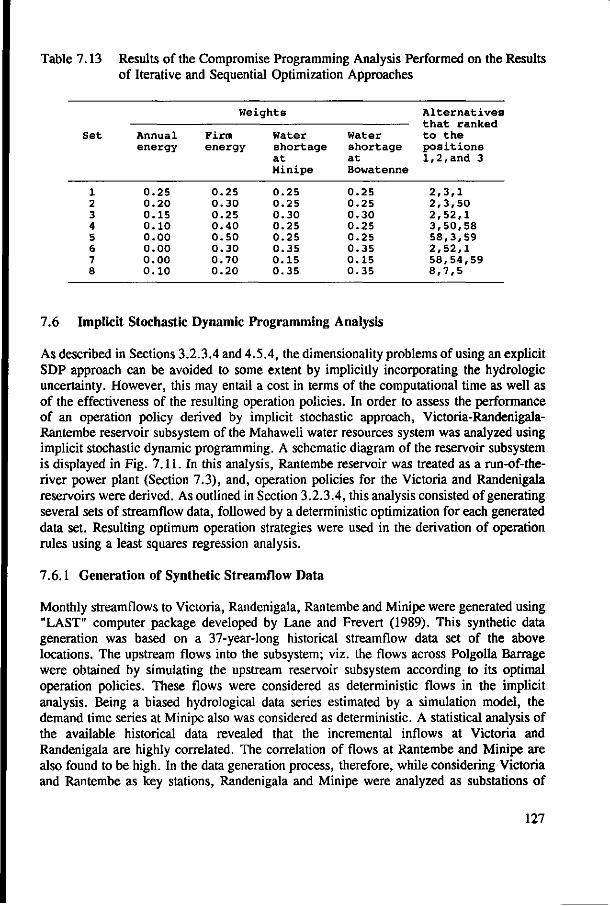
Table 7.13 Results of the Compromise Programming Analysis Performed on the Results of Iterative and Sequential Optimization Approaches

set

1 2 3 4 5 6 7 8

Annual energy

0.25 0.20 0.15 0.10 0.00 0.00 0.00 0.10

We

Firm energy

0.25 0.30 0.25 0.40 0.50 0.30 0.70 0.20

ights

Water shortage at Minipe

0.25 0.25 0.30 0.25 0.25 0.35 0.15 0.35

Water shortage at Bowatenne

0.25 0.25 0.30 0.25 0.25 0.35 0.15 0.35

Alternatives that ranked to the positions 1,2,and 3

2,3,1 2,3,50 2,52,1 3,50,58 58,3,59 2,52,1 58,54,59 8,7,5

7.6 Implicit Stochastic Dynamic Programming Analysis

As described in Sections 3.2.3.4 and 4.5.4, the dimensionality problems of using an explicit SDP approach can be avoided to some extent by implicitly incorporating the hydrologic uncertainty. However, this may entail a cost in terms of the computational time as well as of the effectiveness of the resulting operation policies. In order to assess the performance of an operation policy derived by implicit stochastic approach, Victoria-Randenigala-Rantembe reservoir subsystem of the Mahaweli water resources system was analyzed using implicit stochastic dynamic programming. A schematic diagram of the reservoir subsystem is displayed in Fig. 7.11. In this analysis, Rantembe reservoir was treated as a run-of-the-river power plant (Section 7.3), and, operation policies for the Victoria and Randenigala reservoirs were derived. As outlined in Section 3.2.3.4, this analysis consisted of generating several sets of streamflow data, followed by a deterministic optimization for each generated data set. Resulting optimum operation strategies were used in the derivation of operation rules using a least squares regression analysis.

7.6.1 Generation of Synthetic Streamflow Data

Monthly streamflows to Victoria, Randenigala, Rantembe and Minipe were generated using "LAST" computer package developed by Lane and Frevert (1989). This synthetic data generation was based on a 37-year-long historical streamflow data set of the above locations. The upstream flows into the subsystem; viz. the flows across Polgolla Barrage were obtained by simulating the upstream reservoir subsystem according to its optimal operation policies. These flows were considered as deterministic flows in the implicit analysis. Being a biased hydrological data series estimated by a simulation model, the demand time series at Minipe also was considered as deterministic. A statistical analysis of the available historical data revealed that the incremental inflows at Victoria and Randenigala are highly correlated. The correlation of flows at Rantembe and Minipe are also found to be high. In the data generation process, therefore, while considering Victoria and Rantembe as key stations, Randenigala and Minipe were analyzed as substations of

127

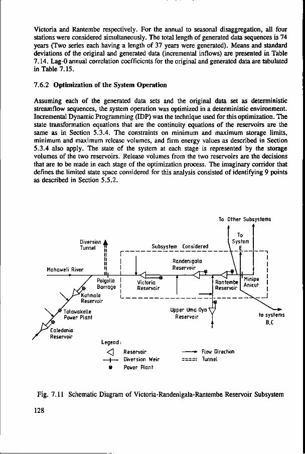
Victoria and Rantembe respectively. For the annual to seasonal disaggregation, all four stations were considered simultaneously. The total length of generated data sequences is 74 years (Two series each having a length of 37 years were generated). Means and standard deviations of the original and generated data (incremental inflows) are presented in Table 7.14. Lag-0 annual correlation coefficients for the original and generated data are tabulated in Table 7.15.

7.6.2 Optimization of the System Operation

Assuming each of the generated data sets and the original data set as deterministic streamflow sequences, the system operation was optimized in a deterministic environment. Incremental Dynamic Programming (IDP) was the technique used for this optimization. The state transformation equations that are the continuity equations of the reservoirs are the same as in Section 5.3.4. The constraints on minimum and maximum storage limits, minimum and maximum release volumes, and firm energy values as described in Section 5.3.4 also apply. The state of the system at each stage is represented by the storage volumes of the two reservoirs. Release volumes from the two reservoirs are the decisions that are to be made in each stage of the optimization process. The imaginary corridor that defines the limited state space considered for this analysis consisted of identifying 9 points as described in Section 5.5.2.

To Other Subsystems

Diversion • Tunnel

Mahaweli River

II II II II II

A-

Subsystem Considered

Potgolla Barrage

Kotmale Reservoir

<fc Victoria Reservoir

Talawakelle Power Plant-

Caledonia Reservoir

Legend:

< ] Reservoir — | — Diversion Weir

B Power Plant

Randenigala Reservoir

Upper Urn a Oya ' Reservoir

Rantembe Reservoir

to systems B.C

Flow Direction Tunnel

Fig. 7.11 Schematic Diagram of Victoria-Randenigala-Rantembe Reservoir Subsystem

128

r-

c ID

o r H

C «

c

- H

M O

CM

c

e ID

o r-1 IB c

•H 00

•H M

o

c 9 O

,_, c

— 1 (0

e •H 00

•H H

o

eg

C 0)

C m O

« C

- w M

• H M

O

to

o

m -a-o

in •a-

o

CO

r

-* -a--a-

-a--a-

CM

m -a-

•a-•a-

C O -a-

C O C O

•a-

C O r-l

•*

C O t o

m

C O C O

tO

o

C n

£

o

00 rH

O

-* o

CM

O

CM CO

o

CO r-.

O)

Ol

o CM

C O O l

o C M

CO

en

m

o e g

CM CM

o C O

C O

o CM C O

o o CM C O

> ID

Q •o +1 CO

o

o

CD to

o

lO

o

(0

CO ID

m CO

m

CM C O

to

0 > C O

CO

to

rH

(O

CO

m C O

to o

m

p*.

CO o r-4

S 4)

£

> o z

CM

O

-* CM

O

m C M

O

o o CM

i-H

CM

>n

o rH

CM

tO (O

to to

CO

to CM

ID ID

to CO

00 to

10

-a-

o m

CO

CO

CM

> O

• a

to

o O)

o

o

O

•a-00

o

s o

•a-o

o p-*

CO

CO CO

00

r-l r-l

O) r-l

CM

o CO

o CM

CO o

ID O r H

m

o

-3-

m r-.

§ (V

£

«

o u>

o

m CO

o

O) CO

o

CM

CO tO

rH

CO

to •a-

m O)

»n m

HT

O

to «n

•a-o

o CO

to en

0 1

•a-

r-l 1 0

0 1 t o

CO

o> C O

> Q

•a +J

to

CM 00

o

to

o

CO

o

to ID

to CO

CO

o oi

O)

m 00

Ol

CM CM

o m m o r-l

rH to

CO o

Ol

a» CO

to o

to CO

00 CO

»n C O

c n 0)

£

CO

o

O) CM

o

o •a-

o

O)

to to

CO

m

-a-

o t o

t o m

ID

r«*

m Ol

CM

O) CO

CO 10

•a-o

to

•a-C O

CO

•a-en

I-I

t o

> 0)

Q

• a

w

CM <0

O

01

m o

O)

m o

to o

to

10

I D to

•a-CO

CO to

CO -a-

o

to to

o

to CO

•n

O)

-a-

to CO

CM

«n -a-

o

c ID

V

CM C O

o

C O

CM

o

C O t o

o

CM

i-H CO

to m

•9 m

rH tn

CO CO

•* en

CO CO

o

CO CM

r»»

O) CO

CM to

•a-

O) CM

m

a • a -P w

t o -a-

o

CO

o

o

-a-O)

r* • *

CM C O

-3-

C O t o

m •a-

to o

CO CO

o CO CM

CO

to CM

00 r-l

-a-CO

•a-

CM

O) CO

Ol CM

s

CM

o

r*

o

CM

o

CO

00

•a-o

rH

m

o CM

rH 00

CO CO

rH

P^ CO

CM tM

•a-o

o C M

m o t o r H

C O -a-

CM

> a

o

CM

m o

CM

o

t o C M

(0

CM en

C O

m

C O

-a--a-m

rH

rH CO

01 Ol

to CM

Ol

m e g

•a-CM

-a-

m o

o

CM

o •a-

<D

M

CO CM

o

CO

o

CM CM

o

ID CM

CM

00 10

£

•a-CM

CM CM

CO

•a-o N

1 0 I D

01

t o

•a-

m r H

m CO

CM

CM CO

ID CM

CO <0

CM CM

> o

»n

o

•a-

o

O l

•a-o

C O

m

CO

o «n

o

CM o O l t o

en en

CM

00 Ol

CM

CO CO

rH to

en CM

•a-

to -a-

CM

m

c ©

& S

to

o

CO

o

m r H

o

in

i-»

rH

CM

m •a-

o m m

CO CO

Ol to

o t o

o C M

-a-o

o C M

en

t o -a-

t o O l

o C O

en m

to to

> CD

a • o

w

Ol CM

O

CO CM

o

CO CM

O

m

CO to

to

CM to

to

CM CO

ID CO

CO rH

m

m

to

ID

CM CO

-a1

CO -a-

CO

•a-

o

C M

m

<D

§

o rH

O

00 o

o

Ol

o o

CM t o

to

r H t o

to

rH

tD

o O l

•a-

CM C O

•a-r H

o> CO

CM rH

CM -a-

m t o

00

t o C O

r

m C O

> Q

•a to

CO

o

CM

O

O CO

o

CO

CO to

2 CM to

rH to

CM CO

•a-m

CM

CM

CO

C O o

o CM

I D

»n

I-*

00

O l •a-

C O

m

r-l

at o o

t o

o o

t o o o

C O

m m

m CO

**

CO

m

to m •a-

to N

01

CO

m rH rH

to 00

o to

o

CM

o

CO CM

> 9

Q

• o

C O

C M C M

o

r H

CM

o

C M C M

o

-a-

CO

C M o

o t o

CM CM

o C O

CO

CM

Ol

o C M

•a-O l

o C M

CM t o

o t o

CO

o «n

t o C O

C M

m

ID

H O

1

ID O

o

to

o o

m o o

m o to

C O C O

CO

to

•a-

CO

-r H •a-

o

m

C M r H

Pv

O

rH

C O 0 >

o -a-

•a-(0

CO to

> e o •o CO

in o CM rH

o o

CO O) CM O

o o

m ID CM o o o

m co rH ©

O CO •a-

•a -a-o> m

rv m CO

CM 01 O Ol

en m CO

00 CO m co

to to CM rH

m CM to Ol rH CO CM rH

Ol P^ CO rH

CM rH

CO ST Ol Ol

00 rH •9 CO

r%. Ol -a- o

m a-

m -a-o o> (*» P-*

• * C O

> o

Q

£ co a 0 w

Table 7.15 Lag-0 Correlation Coefficients of Annual Data of the Implicit Stochastic Approach

1. Original Data

2

3

Victoria

Victoria 1.00 Randenigala Rantembe Minipe

. Generated Data Set 1

Victoria

Victoria 1.00 Randenigala Rantembe Minipe

. Generated Data Set 2

Victoria

Victoria 1.00 Randenigala Rantembe Minipe

Randenigala

0.97 1.00

Randenigala

0.94 1.00

Randenigala

0.97 1.00

Rantembe

0.58 0.60 1.00

Rantembe

0.62 0.57 1.00

Rantembe

0.60 0.61 1.00

Minipe

0.58 0.61 0.98 1.00

Minipe

0.59 0.59 0.92 1.00

Minipe

0.60 0.63 0.97 1.00

Two different objective functions, namely maximization of energy generation and minimization of squared deviation of the water supply from the irrigation demand were considered for the optimization. However, the downstream water demands were not considered as constraints due to the fact that the solution became infeasible when this specific demand series was considered as constraints. Instead, feasible firm energy constraints which were selected by trial-and-error were imposed for both optimizations. These firm energy values were selected by gradually increasing the firm energy constraints of each reservoir until the solution became infeasible.

7.6.3 Regression Analysis

Having formulated the deterministic optimum operation pattern for each streamflow sequence, a least square multiple regression analysis was performed (for the 12 months separately) to formulate an operation rule for the system operation. Thirty five combinations of independent variables were considered in a preliminary regression analysis in order to determine the significant variables to formulate an operation policy. These independent variables include initial reservoir storages, inflows of reservoirs corresponding to the current and previous months, and irrigation water demand as linear terms. Their cross

130

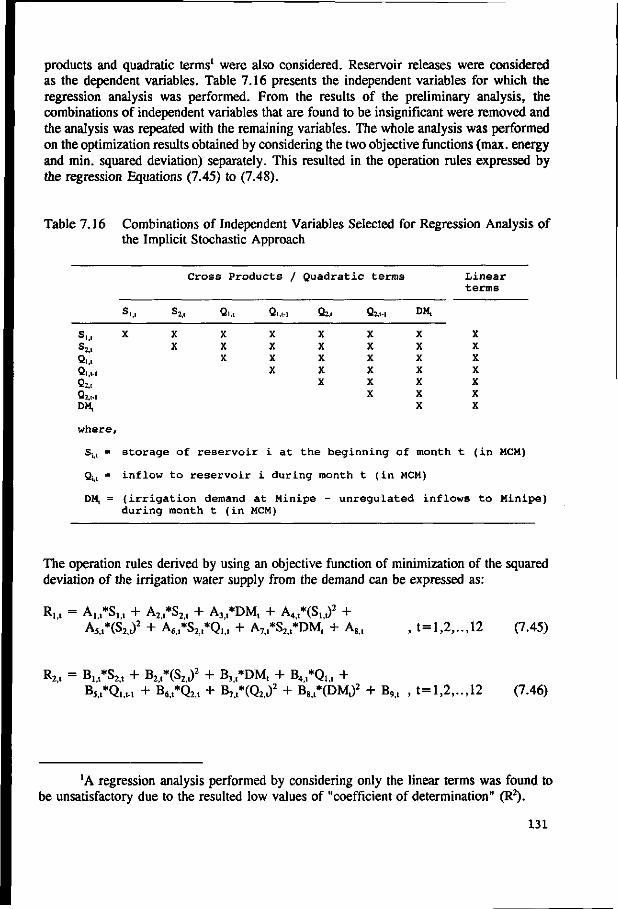
products and quadratic terms1 were also considered. Reservoir releases were considered as the dependent variables. Table 7.16 presents the independent variables for which the regression analysis was performed. From the results of the preliminary analysis, the combinations of independent variables that are found to be insignificant were removed and the analysis was repeated with the remaining variables. The whole analysis was performed on the optimization results obtained by considering the two objective functions (max. energy and min. squared deviation) separately. This resulted in the operation rules expressed by the regression Equations (7.45) to (7.48).

Table 7.16 Combinations of Independent Variables Selected for Regression Analysis of the Implicit Stochastic Approach

s...

2... Q,.,., 0-2,, 0.2,,., DM,

where,

SM =

CM =

DM, =

s...

X

Cross Products /

S2.. Q1.1 Q1..-1

X X X X X X

X X X

storage of reservoir i at

inflow to reservoir i duri

Quadratic terms

Q2,. Q2..-1

X X X X X X X X X X

X

the beginning

ng month t (in

of

DM,

X X X X X X X

month

MCM)

(irrigation demand at Minipe - unregulated in during month t (in MCM)

Linear terms

X X X X X X X

t (in MCM)

flows to Minip

The operation rules derived by using an objective function of minimization of the squared deviation of the irrigation water supply from the demand can be expressed as:

Ri.t = Alit*S1>t + A2/S2,t + A3,t*DM, + A4,t*(S,,,)2 + A5,,*(S2,,)

2 + A6,t*S2,t*QM + A7,l*S2j,*DMt + Ag-I , t=l,2,. . ,12 (7.45)

R2,t = Bu*S2>t + B2,t*(S2,,)2 + B3,t*DMt + B4>l*Q1>t +

B5/Q1.M + B6,t*Q2,t + B7,t*(Q2,1)2 + Bs^DM,)2 + B9>t , t=l,2,..,12 (7.46)

'A regression analysis performed by considering only the linear terms was found to be unsatisfactory due to the resulted low values of "coefficient of determination" (R2).

131

where, Ri>t = release from the reservoir i during month t (in MCM) (i=1 and 2 indicate the

Victoria and Randenigala reservoirs respectively)

Ait, i=l,2,..,8 ; t=l,2,..,12 and Bit, i=l,2,..,9 ; t=l,2,..,12 are regression coefficients.

With the use of an objective function of maximization of energy generation, the following regression equations have been obtained.

R... = CM*SU + C2?1*QM + CVQ,,,., + C4,t*DMt + Cj/CS,.,)2 + C6,,*Slit*Qu + C1A*SU*Q1M + CM*QM*DMt + C9,t , t=l,2,..,12 (7.47)

R2,, = DM*SU + D2,t*QM + D3,t*Q2,t + D4,t*DMt + D5,t*(S,,,)2 + D6,t*(Q,,,)2 + Dr/S./Q,. , + Dg/S1.,*Q2pl + D9,t*QM*DMt + Dm (7.48)

, t=l,2,. . ,12

Cit, i=l,2,..,9 ; t=l,2,..,12 and Dit, i = l,2,..,10 ; t=l,2,..,12 are regression coefficients.

The estimated regression coefficients of equations (7.45) to (7.48) are presented in Tables 7.17 and 7.18. Corresponding 'coefficients of determination' are also included in the same Tables. According to the operation rules of equations (7.45) - (7.48), the system operation was simulated. The simulated system performance obtained by to these implicit SDP-based operation rules are compared with the simulation performed according to the explicit SDP-based operation policies and also with the deterministic optimum operation and the historical1 operation, in Table 7.19.

In Table 7.19, the results of the IDP models indicate the upper bounds on the objective achievements for the particular historical data set. In the case of the squared deviation objective, the objective achievement is indirectly indicated by the firm energy generation. An explicit indication in terms of the annual energy generation is made in the case of the energy objective. Table 7.19 shows that the explicit SDP-based operation policy formulated by using energy objective [alternative (5)] outperforms the implicit SDP-based operations (1) and (4). Although (1) is preferable in terms of the probability of failure, (5) outranks (1) when considering the other three performance criteria, specially the firm energy generation. It can be seen that the historical operation obtained by simulating the system using the present rule curves (displayed in Fig. 7.12) indicates lower annual energy and firm energy values, although the historical operation has been slightly better in terms of the water shortage and the probability of failure months.

'Historical operation refers to the results of a simulation performed using the historical data by following the present rule curves of the reservoirs.

132

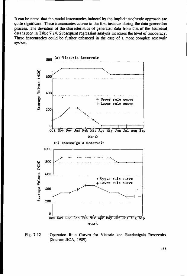
It can be noted that the model inaccuracies induced by the implicit stochastic approach are quite significant. These inaccuracies accrue in the first instance during the data generation process. The deviation of the characteristics of generated data from that of the historical data is seen in Table 7.14. Subsequent regression analysis increases the level of inaccuracy. These inaccuracies could be further enhanced in the case of a more complex reservoir system.

3 0)

I 1-1 o > <u 60 n) U O

800

600

400

200

0

(a) Victoria Reservoir

x —

-*- Upper rule curve + Lower rule curve

Oct Nov Dec Jan Feb Mar Apr May Jun Jul Aug Sep

Month

(b) Randenigala Reservoir

1000

w 200

0

-*- Upper rule curve + Lower rule curve

1 I I L_ _ l I L_ Oct Nov Dec Jan Feb Mar Apr May Jun J u l Aug Sep

Month

Fig. 7.12 Operation Rule Curves for Victoria and Randenigala Reservoirs (Source: JICA, 1989)

133

Table 7.17

Oct Nov Dec J a n Feb Mar Apr May J u n J u l Aug Sep

Oc t Nov Dec J a n Feb Mar Apr May J un J u l Aug Sep

A,,

Regression Coefficients - Victoria Reservoir (Implicit Stochastic Approach)

A,,

Objective Funct 0.004

-0.214 -0.188 -0.419 -0.420 -0.117 0.140

-0.028 0.032

-0.210 -0.189 -0.329

c,,

-1.047 0.015

-0.087 -0.443 -0.657 -0.778 -1.644 -2.404 -1.777 -1.945 -1.455 -1.967

= 2 . .

A,,

ion: Min 1.445 0.838 0.646 0.459 0.919 1.361 1.100 1.289 0.036 0.963 0.734 0.817

c„

Objective Function: Max 0.425

-0.903 -3.637 -3.523 2.364

-17.150 -0.319 0.093

-1.706 -3 .371 -0 .941 2.918

-1 .151 0.460

-1.416 -2.415 0.498

-37.910 4.585

-1.966 -1.543 -2.025 -0.433 -0 .921

1.162 0.855 2.441 1.044 0.544

-2.416 35.947 0.342 0.778

-1.344 -0.208 -0.553

A., A,, A.,

. Souared Deviation 0.000 0.000 0.000 0.001 0.000 0.000 0.000 0.000 0.000 0.001 0.001 0.001

C4J

0.002 0.000 0.000 0.000 0.001 0.001 0.001 0.002 0.001 0.002 0.001 0.001

c,,

. Enerxv Gener 0.423 0.497 0.036 0.003

-0.049 0.002 0.035

-0.064 -0.103 -0.250 0.207 0.148

-0.001 0.001 0.003 0.002

-0.001 0.011 0.001

-0.001 0.001 0.001 0.000

-0.003

0.001 0.001 0.001 0.001 0.001 0.001 0.001 0.001 0.001 0.001 0.000 0.001

c«.,

at ion 0.003 0.001 0.003 0.005 0.000 0.054

-0.005 0.004 0.003 0.004 0.002 0.003

A,,

-0.003 -0 .001 -0 .001 -0 .001 -0.001 -0.002 -0 .001 -0.002 0.001

-0.001 0.000

-0.001

c„

-0.002 -0.001 -0.003 -0.001 -0.001 0.003

-0.050 -0 .001 -0.001 0.002 0.000 0.001

A.,

241.28 -28.82 -9.14

129.70 202.36 194.99 362.24 511.31 450.62 539.96 402.50 564.45

c,.

-0.001 -0.002 0.000 0.000 0.000 -0.000 0.000 0.001 0.000 0.001

-0.001 -0.001

R»

0.70 0.70 0.62 0.66 0.80 0.75 0.81 0.64 0.69 0.69 0.75 0.75

c,.

90.33 83.17

1012.28 1342.45 1021.74 6377.74 -548.32 709.63 957.26

1939.93 552.85

-308.94

R2

0 0 0 0 0 0 0 0 0 0 0 0

82 79 73 89 88 70 86 69 92 88 87 82

Table 7.18 Regression Coefficients - Randenigala Reservoir (Implicit Stochastic Approach)

Oct Nov Dec J a n Feb Mar Apr May J u n J u l Aug Sep

Oc t Nov Dec J a n Feb Mar Apr May J un J u l Aug Sep

B,,

O b j e c t 0 . 087 0 . 324 0 . 1 1 3 0 . 0 0 1 0 . 2 8 3 0 . 534 0 . 427 0 . 184 0 . 1 7 5 0 . 0 5 2 0 . 037 0 . 007

D,,

B„

l v e F u n c t 0 . 000 0 . 0 00 0 . 000 0 . 0 00 0 . 000 0 . 000 0 . 0 00 0 . 000 0 . 0 00 0 . 000 0 . 0 00 0 . 000

D»,

B„

i o n : Min - 2 . 0 3 9 - 1 . 0 8 0

0 . 392 0 . 6 2 2 0 . 297

- 0 . 0 9 8 0 . 7 1 8 0 . 907 0 . 9 0 8 0 . 2 5 2 1 .401 1 .576

D,,

O b j e c t i v e F u n c t i o n : Max - 0 . 2 5 9

1 .390 - 4 . 8 6 1 1 1 . 324 - 5 . 7 9 1 1 7 . 448

1 . 381 - 3 . 3 6 1 - 1 . 3 8 5

0 . 6 3 6 - 0 . 9 3 0

0 . 6 0 8

1 .009 5 . 0 4 5

- 1 . 2 3 2 - 5 . 0 9 4 - 1 . 7 0 6

- 3 0 . 7 4 2 9 0 . 9 5 0 -- 3 . 8 4 0

0 . 8 1 9 0 . 2 5 3 0 . 7 4 9

- 1 . 7 6 2

- 1 . 2 5 2 - 1 . 3 5 0 - 0 . 5 2 8 - 1 . 6 7 9 - 0 . 1 8 8

- 2 3 . 2 4 2 1 15 . 187

1 1 . 438 4 . 4 3 9 2 . 9 5 2

- 1 . 6 0 9 0 . 6 3 1

B,,, Bs., B.,

. S o u a r ed D e v i a t i o n 0 . 2 2 9 0 . 100 0 . 1 8 2

- 0 . 0 8 0 0 . 1 2 3 0 . 4 10 0 . 2 4 5 0 . 0 2 9 0 . 0 5 1 0 . 0 6 9 0 . 0 6 6

- 0 . 0 6 0

D4J

0 . 1 1 9 0 . 153 0 . 120 0 . 237 0 . 164 0 . 220 0 . 868 0 . 530 0 . 1 5 2 0 . 067 0 . 137 0 . 1 7 9

D..,

- 0 . 0 5 5 - 0 . 3 0 5 - 0 . 5 3 8

0 . 7 7 5 0 . 553 0 . 144 1 .761 0 . 4 65 3 . 6 96 2 . 474 3 . 6 0 1 3 .714

D«

. EnerRV G e n e r a t i o n 0 . 908 0 . 3 2 2 0 . 108

- 0 . 0 9 3 - 0 . 0 5 0

0 . 0 0 6 0 . 0 6 5

- 0 . 0 8 5 0 . 013

- 0 . 1 3 8 0 . 184 0 . 036

- 0 . 0 0 1 - 0 . 0 0 0

0 . 004 0 . 007 0 . 0 05 0 . 0 1 2 0 . 0 0 1 0 . 0 0 1 0 . 0 0 1

- 0 . 0 0 1 0 . 0 00

- 0 . 0 0 2

- 0 . 0 0 1 - 0 . 0 0 3

0 . 000 0 . 0 0 1 0 . 0 0 2

- 0 . 0 0 1 - 0 . 0 0 2

0 . 000 - 0 . 0 0 1 - 0 . 0 0 2 - 0 . 0 0 1

0 . 000

B„

0 . 004 0 . 004 0 . 0 0 1

- 0 . 0 0 2 - 0 . 0 0 2

0 . 003 - 0 . 0 1 6 - 0 . 0 0 1 - 0 . 0 5 0 - 0 . 0 1 5 - 0 . 0 4 1 - 0 . 0 2 8

D,.,

0 . 0 0 2 - 0 . 0 0 4

0 . 0 0 3 0 . 0 0 8 0 . 003 0 . 044

- 0 . 1 2 4 0 . 006 0 . 0 0 1 0 . 0 0 2 0 . 0 0 1 0 . 004

B.,

0 . 0 05 0 . 004 0 . 0 0 1 0 . 0 0 1 0 . 0 0 2 0 . 004

- 0 . 0 0 2 0 . 000 0 . 0 00 0 . 0 0 1

- 0 . 0 0 1 - 0 . 0 0 1

D.,

0 . 0 0 3 0 . 0 0 3 0 . 0 0 2 0 . 004 0 . 0 0 2 0 . 034 0 . 1 6 1

- 0 . 0 1 5 - 0 . 0 0 5 - 0 . 0 0 3

0 . 0 0 3 0 . 0 0 2

B„

4 2 7 . 5 6 1 0 9 . 4 1 - 1 1 . 8 5 - 6 6 . 8 6 - 7 0 . 5 8 - 8 5 . 9 2

- 1 9 4 . 8 6 - 3 9 . 8 8 - 4 6 . 8 2

8 6 . 0 5 - 8 4 . 1 7 - 8 2 . 7 3

D.,

- 0 . 0 0 3 - 0 . 0 0 1

0 . 000 0 . 0 0 1 0 . 000 0 . 000 0 . 000 0 . 0 0 1 0 . 000 0 . 000 0 . 0 00

- 0 . 0 0 1

R*

0 . 4 1 0 . 7 3 0 . 7 9 0 . 6 3 0 . 77 0 . 8 1 0 . 7 9 0 . 9 1 0 . 7 5 0 . 6 1 0 . 84 0 . 8 8

D,.,

2 4 3 . 3 5 - 9 8 7 . 0 1 1 618 . 88 4 4 4 3 . 8 9 1 760 . 92 6 4 7 0 . 5 9

- 1 3 2 5 . 4 2 1852 .40

4 93 . 50 3 01 . 00 5 5 2 . 2 3 5 30 . 58

0 0 0 0 0 0 0 0 0 0 0 0

R!

86 83 76 97 97 87 91 75 94 90 90 84

134

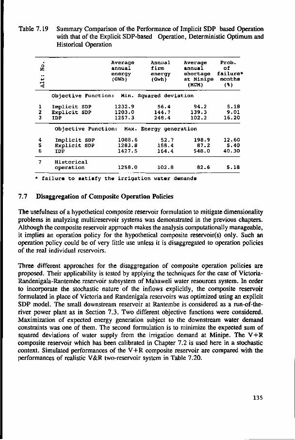
Table 7.19 Summary Comparison of the Performance of Implicit SDP based Operation with that of the Explicit SDP-based Operation, Deterministic Optimum and Historical Operation

o a

<!

1 2 3

4 5 6

7

Average annual energy (GWh)

Annual firm energy (Gwh)

Average annual shortage at Minipe

(MCM)

Objective Function: Min. Squared deviation

Implicit SDP 1232.9 56.4 94.2 Explicit SDP 1203.0 144.7 139.3 IDP 1257.3 248.4 102.2

Objective Function: Max.

Implicit SDP 1088.6 Explicit SDP 1283.8 IDP 1427.5

Historical operation 1258.0

Energy generation

52.7 198.9 158.4 87.2 164.4 548.0

102.8 82.6

Prob. of

failure* months (%)

5.18 9.01

16.20

12.60 5.40

40.30

5.18

* failure to satisfy the irrigation water demands

7.7 Disaggregation of Composite Operation Policies

The usefulness of a hypothetical composite reservoir formulation to mitigate dimensionality problems in analyzing multireservoir systems was demonstrated in the previous chapters. Although the composite reservoir approach makes the analysis computationally manageable, it implies an operation policy for the hypothetical composite reservoir(s) only. Such an operation policy could be of very little use unless it is disaggregated to operation policies of the real individual reservoirs.

Three different approaches for the disaggregation of composite operation policies are proposed. Their applicability is tested by applying the techniques for the case of Victoria-Randenigala-Rantembe reservoir subsystem of Mahaweli water resources system. In order to incorporate the stochastic nature of the inflows explicitly, the composite reservoir formulated in place of Victoria and Randenigala reservoirs was optimized using an explicit SDP model. The small downstream reservoir at Rantembe is considered as a run-of-the-river power plant as in Section 7.3. Two different objective functions were considered. Maximization of expected energy generation subject to the downstream water demand constraints was one of them. The second formulation is to minimize the expected sum of squared deviations of water supply from the irrigation demand at Minipe. The V+R composite reservoir which has been calibrated in Chapter 7.2 is used here in a stochastic context. Simulated performances of the V+R composite reservoir are compared with the performances of realistic V&R two-reservoir system in Table 7.20.

135

Table 7.20 Comparison of the Simulated Performance of Victoria+Randenigala (V+R) Composite Reservoir with that of the Real Victoria and Randenigala (V&R) Two-Reservoir System

Objective function/ constraints

Max.Energy; Demands at Minipe and firm energy constraints

Min. Squared deviation of supply-demand at Minipe; firm energy constraints

Configu--ration

V+R Composite

V&R Two-res:

V+R Composite

V&R Two-res:

Average annual energy (GWh)

1280.9

1263.6

1271.9

1203.0

Annual firm energy (GWh)

75.0

161.9

62.5

144.7

Average annual shortage at Minipe (MCM)

106.3

104.1

107.3

139.3

Proba--bility

of failure* months(%)

5.6

5.4

5.6

9.0

* failure to satisfy the irrigation water demands

The three disaggregation approaches proposed for disaggregating composite policies are:

(1) Statistical disaggregation of composite policies

(2) Disaggregation by an optimization/simulation based approach

(3) Use of a deterministic optimization model in each time interval of the operation.

7.7.1 Statistical Disaggregation of Composite Policies

The statistical disaggregation model of Lane and Frevert (1989) generates seasonal flows by disaggregating annual flows to seasonal values. In this approach, key stations (stations of major importance) are used to generate key and substation flows, preserving the intercorrelations between key and substations. This model preserves serial and cross correlations between variables on annual as well as on seasonal basis.

In this study, the 'LAST' statistical disaggregation package originally formulated for hydrologic data generation is applied for reservoir operation. It is used to determine the optimum operation of individual reservoirs based on the operation of a hypothetical composite reservoir. The composite reservoir can be considered as a key station, while the individual reservoirs correspond to the substations.

Simulating the operation of composite reservoir using historic streamflow data according to the SDP based policy, the optimum operation pattern for the composite reservoir is obtained (A sequence of monthly storage volumes during the period for which the historical data are available). This optimum operation pattern, together with the composite-inflows are treated

136

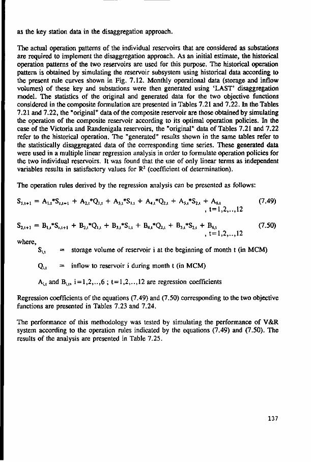
as the key station data in the disaggregation approach.

The actual operation patterns of the individual reservoirs that are considered as substations are required to implement the disaggregation approach. As an initial estimate, the historical operation patterns of the two reservoirs are used for this purpose. The historical operation pattern is obtained by simulating the reservoir subsystem using historical data according to the present rule curves shown in Fig. 7.12. Monthly operational data (storage and inflow volumes) of these key and substations were then generated using 'LAST' disaggregation model. The statistics of the original and generated data for the two objective functions considered in the composite formulation are presented in Tables 7.21 and 7.22. In the Tables 7.21 and 7.22, the "original" data of the composite reservoir are those obtained by simulating the operation of the composite reservoir according to its optimal operation policies. In the case of the Victoria and Randenigala reservoirs, the "original" data of Tables 7.21 and 7.22 refer to the historical operation. The "generated" results shown in the same tables refer to the statistically disaggregated data of the corresponding time series. These generated data were used in a multiple linear regression analysis in order to formulate operation policies for the two individual reservoirs. It was found that the use of only linear terms as independent variables results in satisfactory values for R2 (coefficient of determination).

The operation rules derived by the regression analysis can be presented as follows:

S,,,+i = A,,t*Sc,t+1 + A2,,*Q,,t + Aj/S,,, + A4jt*Q2,, + A5>t*S2,t + A6,t (7.49) , t=l,2,. . ,12

S2,t+. = BU*SM+1 + B2it*QM + B 3 /SM + B4,t*Q2,t + B5,t*S2,t + B6,t (7.50) , t=l,2,.. ,12

where, Sj, = storage volume of reservoir i at the beginning of month t (in MCM)

Qi, = inflow to reservoir i during month t (in MCM)

Ait and Bjt, i=l,2,..,6 ; t= 1,2,.., 12 are regression coefficients

Regression coefficients of the equations (7.49) and (7.50) corresponding to the two objective functions are presented in Tables 7.23 and 7.24.

The performance of this methodology was tested by simulating the performance of V&R system according to the operation rules indicated by the equations (7.49) and (7.50). The results of the analysis are presented in Table 7.25.

137

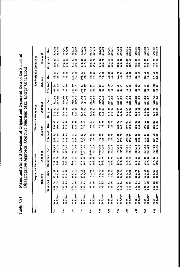
<1 r-'

1

c CD

o

a) C

-iH M>

• H ( 4

o

a 0

o

c i H 0 0

•w u o

c a

a C

• • H

CO • H M

O

C (V

CD

a G

• H 0 0

• H u o

c

<a c

• H 0 0

- H M

O

r - t <o C

• H 0 0

• H H

O

CO m

co

t n

o

CO m m

<r m

CO

•a-

t n

i n

t n - a

CO

n ro

CO «n O l

p i

CO t o O l

o 0 0

( O n . p i

o o •a-t n

CO

CO CM

p i

•a-o

CO

C

© Z

O

CO CO

o m O ]

OJ Ol

o t O O J

p i p i

m OJ

t n o>

o O J

CO t O

CO m OJ

OJ CO

O J CO OJ

•a-

-a-( D r H

CO I D

O

CD m

CO O J

( 0

CD CO

CO CO

I D r H

CO o

t O

> eg

P •a * >

o t o

CO O) •a-

CO m

OJ

t n

CO t o

m n

n ( O

CO n

OJ o

t o i-i m

o p i

t n

t o

•a-

OJ

CO n

p i p i OJ

r H CO

»n t n n

GO m

0 0

n

0 0 n ol

0 0 CO

CO

CO

§ a

> o z

CO CO

m O J CO

o O )

m p i OJ

CO CO

O J CO

t o t o

CO CO

t n o

t n O l

CO t o

P i OJ OJ

t o 0 0

CO OJ r H

m

r H -a-r H

o •3 -

p i CO CO

o t o

0 0 CO CO

en

CO

CO

CO •a-

> a •o CO

CO r - l

OJ t n t n

CO t o

CO r H t o

CO p i

O J O l

o CO

o OJ

o CO

t n to >n

CO t o

-a-CO

CO CO

t o o OJ

p i CO

to r H OJ

•a-p i

CO CO CO

o o

OJ t o CO

o p i

OJ t o OJ

r H CO

OJ

OJ

§ 0J

Z

a

p i CO

OJ •a-CO

• n OJ

oo CO O J

CO

o o CO

• a -o

o 0 0

o

CO CO OJ

o r H

o OJ OJ

0 0 0 0

O J

p i t o

p i CO

OJ o p i CO

CO

t n CO

-a-

O J

OO t n

t o t n

OJ OJ OJ

> CO

Q

* o +J W

CO 0 0

O ] OJ t o

t o 0 0

0 0 p i ( O

OJ r H

m o

t o

CO o

<n o

CO CO «n

0) Ol •a-

t o

-a

CO r H

CO m

p *

CO 0 0

m O J o

OJ OJ

CO

I - I

CO r H

CO t o

0 0 -a-p i t o

8 Z

t o O l

o CO

t o

p i p i OJ

-a

0 0 tn

CO CO

CO t o

CO CO

0 0 CO

p * o

m 0 0 w-i

CO OJ

t o p*

CO

m O )

o o

o •a-

r H i H

CO o • a -

CO

o o o 1-1

t o

OJ r H

> a

•d CO

t o -a

CO t o

CO

o CO t o

( O t n

t o m

t o CO

»n

CO

i H CO <n

»n -a1

o

t o

o OJ

t o t o

m C M

t o t o

CO OJ

-a-

o

O l m

CO p v

CO t o

CO

•a-t o

CO

OJ

m

• a CO o l

0 0

CO t o OJ

CO

•a-m

CO OJ

m <n

t n to

en 0 0

p*. CO

0 0 0 0

O l CO

o m

o - a

t n

CO CO

p ^ en CO

»n r - l

t o CO CO

-a-p *

p v

o CO

r H 0 0

> CO

Q

• o • P CO

CO CO

O J CO to

CO

CO p ^ t o

CO CO

t n CO

t o OJ

OJ •a-

CO «n m

t o o

m CO m

• a -CO

CO -a-

oo 0 0

OJ •a-

CO CO

t o CO o r - l

O * CO

CO r H r H

t n P *

m t o

CO OJ

m * n

c (0 eg

u nt

0 0 CO

p * O J

t o P-.

o «n OJ

t o -a

CO •a-

CO

OJ OJ

o

m

OJ

ro OJ

O l

O l

CO

<n r o

• a -p * .

CO O l

m m

CO o •a-

•a-•a-

t o CO CO

CO -a-

-a-t n

t n CO

CO CO

> Q

* o ±> t o

•a-o

o Ol t o

o CO

-a m t o

t o r H

t o O J

CO CO

»n O l

o

•a-ro t n

»n m

t o P v

r o OJ

-a -t o

t o OJ

t o

ro

t n ro CO

m

m OJ o

CO ro

to p *

r H O l

CO p *

0

r l

-a

0 0

O J

t o CO

t o CO O l

o

O l

CO • a -

t n

CO CO

•a--a -O l

OJ »n

•a-O J

m p%

en OJ

CO p *

ro

CO OJ

O l CO CO

t n P v

•a-CO CO

O l CO

-a-CO

t o OJ

ro *a

> 0)

Q

•6 - P CO

CO CO

•a-m

t o

t o «n

t o p-

en O l

CO

p * OJ

CO

t o o >n

CO

CO •a-t n

CO CO

O l O l r H

t o t o

r-« r H r H

•a-CO

CO p * p ^

r>» •a -

•a1

t n 0 0

CO t o

p * CO r H

CO m

o CO r H

CO

O J 0 0

0 0 •a-OJ

t o o

m ro OJ

p-» o

ro

•a-o

o O l

o m

CO 0 0 OJ

CO

<o p i O l

£ 0 0 r H r H

CO

•a-o

•a-m

t o Ol ro

m

CO CO CO

o

to OJ

t o

3 > CD

Q

* o • P CO

CO -a-

ro m «n

CO OJ

CO to m

o o

t o r H

-a-t o

t o r H

CO •a-

0 0 -a

-a-t o

m

o CO

p » o O l

Ol t o •a-o O J

•a-CO

CO •a-

t o CO

m

CO

ro p».

m r H OJ

t o OJ

O J

O J

£

CO

§

•->

OJ CO

m p i

p i

CO OJ

CD

O

CO

OJ

CO ro

t n m Ol

t o

CO

OJ

o 0 0

O l CO

- a o

t o t o r H

•a-ro

CO • H CO

en

p i CO ro

O l

CO CO

m 0 0

0 0 t o r H

> O

Q

•a

CO

to o

o m m

o o

t n t o t n

t o CO

o O J

0 0 o

o O J

CO CO

en o »n

OJ t o

CO CO

o o

o t n O J

p i CO

CO OJ OJ

r*.

CO

0 0

en

CO p i CO

t o p i

CO m CM

t o

OJ CO OJ

S z

3

OJ

t o CO OJ

o CO

-a t o Ol

t n t o

•a-

r H

CO

m

r H

CO o

•a-r o OJ

o

CO CO OJ

t o r o

OJ

O l

o CO

o m r H

r o p i

•a-OJ CO

CO t n

OJ t o ro

o i - i O l OJ

0 0

t o t n r H

> 0

Q

•a + J CO

CO CO

o O J m

ro CO

t o

t n

Ol -a-

OJ OJ

•a-CO

o O J

CO 0 0

p i CO «n

p i ro

•a--a t n

Ol r H

t o o OJ

•a-o

t o

OJ

OJ t o -a-o CO

t n CO

CO t n 0 0

t n t n

t o

O J

p i t o

m OJ OJ

i CO

Z

0 0

O J -a-

t o OJ

m p i

p i O l

r H r H

O J

t n i-t

O l

o

-a-N O l

o en

t o

OJ

ro 0 0

O J

p i CO

t n ro

r o CO

-a-

CO

CO r H

P i

t o

•a-o

ro CM t-H

en OJ

CO ro

> a •6 - P to

CO o CO P i

t o CO to tn <n o )

r H p i t o ro

ro t o t n r i . m o j

O J • »

-a- m m r H O J O J

e n p i CO « H

r H *8-OJ r H

to tn t n co

0 0 P i •a- co m o i

co en P i 0 0

0 0 O I -a - o j t n o j

t o t o CO 0 0

O P i OJ r H

CO <t

•a to CO r H oo m r H r H

CO t o t n r H

P i t o e n s r P i t o

r o p i r H e n

P i CO - a - e n 0 0 CO

p i n . t o r o

r o o r H 0 0 O l r H

r o o t o P i

co to co m

> Q

§ *o Z CO

« CO

"8

3 " * <Z) o « 5 •B .9 °> «5 .22

3 1 e • u c 0 58

§ §

.5 c (Q-

•Ctt. s O <u E <*- > £ O ' B ' O Ui & g

C y .a O g u .»-. c -S

Ifi •§ < §

.2 tL cd Q .

si S o j

C/3 "O

a

c o r-t vf C O

T-t m

CM -a-m eN

O N m eg

CO o m to m eg

o m rv co

m ID •a- eg

co in «-t O)

-a- o •a- e g

«n co C O CD

c o pv *-* -a-*n eg

m eg -a- C O

•-• e g C O C O m eg

co co en eg

•a- o m rv eg *-t

r-l O l

rv co co o i D « H e g « H

O ) C D pv C D

eg co pv o CD eg

C D vT c o o i

O O l rv e g

t D . H

-a- CD

eg o rv pv e g ^ H

-a- co o © <J- L O

C O t H e g r-i

pv

-a-

O l

-a-

C O

eg •a-m

•a-o

-a-pv

rv

C D

C O

co C O

eg m

o pv

•a-•a-

rv

eg

e g

O l pv

pv

eg

co C D

o C O CO

C O C O

C O C O C D

C O

C D

pv

eg

C O

en C O i-i C O

eg C O

CO r-l C O

o O )

m r» eg

r-l

o C O

to C D

C O C O

C O

ro

o *n CM

C O

to

pv eg eg

C O Pv

m eg

m

•a-

m o O ) C O e g

eg

-a-rv eg

o

C O C O

O l pv

O l

0 1 C O

m m

C O C D

o> r-l t o

C O O l

eg

o ro

o eg r-l

•a-eg

o rv m

C O C D

•a-oi m

rv m m o eg

Pv

O l

C D

eg

C O

m

rv

o CO

m

•a-O )

C D

eg

C O

eg

eg

N o

-a1

C O

m eg

C O C O e g

C D

rv r v

•a-o

o C O

tn CO

r-l

•a-eg

o r-1

o eg CM

C O C O

o C O

pv

C O

C O

eg eg

eg C O e g

m C O

eg O) eg

o C O

C O

to

to m eg eg eg

C O

m C O N C O

to C O

C O

pv

to

r-l

-* •n o

to

C O O

O ) C O

•a-

m

CD eg

•a-r-t to

co

eg

C O i n

pv r-l

m C O

C O

oi

C O

m o o

r-l •-i

eg to

C O •a-

p-» to

CN

O o C O

C O

eg

eg o o C O

en C O

C O C O

to

O l

Pv

o m C O

PN.

o C D

C O

m O )

o> -a-

C O

C N eg

m e g C O

Pv

-a1

o i H

Pv

e g

0 >

to

O)

m m C O C O

co o C O

m

C O C O

pv m

C O

m C O m

m •a-o C O

m

C O C O

m eg

C D to

m CN

C O C O

o> m o

flO o CN

-a-C O

eg O)

CD

o C O

0 1

CN

C O 1**

O ) C D

rg

•a-C O

p*. m

C O

eg

m m

C O

C O O l

pv C O

C O C O

-a-CD

eg m

o

pv m

-a •a-CO CO

C O

o

IN

o

C O P-.

o Ol

C O

-a-

Pv C O C O

C O

C O

to

eg C O

•a-C O

m C O

C D

eg

C O

eg

IN C O

m C D

o m O l m

co eg

o m

C O C O

eg -a-

o

C O to 0 )

C O C O

eg C O o

eg

C O C O

eg

C O C O

m I N

C O

o m eg

C O C O

•a-•a-

p ^ C O

eg eg

C O C O

•a-i H eg

C O e g

eg

eg

o m C O C O

C O

eg

m C O

P-* e g C O

C O C O

C D e g C O

to m C O

m

m O l

C O C O

C D O l

•a-eg to

o O l

-a-m C O

C O C O

C O

eg

O l

m C M

CM O )

m C O m

C D

m

O l

C O C D

C O CM

C D

O l 0 1

i n C O C O

m

o CM O l

eg o

C O pv

eg

C O P-

m

m eg

C D O l

C D C O

rg

to o C O

C O

-a1

«n

O 01

C O -a-eg

eg m m •a-eg

o -a-

o> CM

C O pv

C O

o C O

o C O

CO

o o C O

C O

eg

•a1

C O

C O CN

C O

-a-

C O

o m m m

C O

C O

m

a o o C O

C O O l

eg

m

o

m

•a-O l

O l •a-m

C O C O

C O

CN

to C O

P-*

m C O C O C D

o pv

•a-C O pv

o

O l C O r-l

C O

m o C O

O l

<n •n eg

to

o m C O C N

*a-m

O )

-a1

o

o C M

C O m

O l C O CM

C O

to

CM

o C M

C O CM

O l

•a-o F-4

O l C O

•a-m C M

m C O

C D m CM

to C O

C O

s

o

C O i n

O l

eg

C O to m

C M C O

C O

-a-C O

C O l-l

O l

m C O •a-

•a-C O

i-H

m

to o

o

eg

CM CO

•a-o CM

•n C D

o pv to

C O C O

m o

C O p ^

C O

CM

C D

eg

eg

eg

•a-

O l C O e g

r*.

O l C M

C M C O

-

0 1 C O

C M

m

m CM

C O

C O

•a1

C M

C O •a-

O l

C O

o C O C O

•a-C O

C M •a-< M

O

m p ^ C O CM

o> C O

to Ol t-i

C O

C O C O

CM C O

O l m m

o o m to m

o -a-o eg

C O

o o C M

C M

C O

•n

eg to

C O C O

m

a C O -a-CM

C O

C O

CM C M

m C O C M Pv

a-o

-a-C O rv

r-l

to

m eg

t-i

to

eg C O eg

C O

to •a-eg

o C O

-a-C O e g

O l

rv

m

C O

m i H

eg

C O •a-eg

o

C O C O CM

C O C O

eg

o C O

o m I-I

m o m N C O C O

C O

eg

-a-C M

C O eg eg

C O

C O

»n

eg CO

CO eg <n

C O O l

C O

m

O l O l

C M

vT O l

o CM

P v

C O

-a-m

r v C O

•a-•a-m

o m

CM

•a-o C O

C M

m to

C O i-H r v

m

P v

C O r v

rv

C O

C M eg

Pv

t o

m eg eg

O l

«n O ) • » C M

m Pv

rv eg

-a-

3

m

C M

r H

C O C O

eg

o Ol

to

eg

C O O l

C O

eg

(V,

C O

m C O

•a-Ol

C O m CM

C O C M

C O C O

eg

C O C O

C O C M

0 1

CM

O l C O

o m * m «n «* -a- CD m CM

•n rv ( O C O

co to >n rv tn CM

eg eg CO o

CM eg

o> rv CO r-t

CM r-t

T-I PV

m co rv oi tn co m eg

O l O l

rv co

co eg v T CM m eg

O l i H

to -a-

r v T* oi to

oi -a-v T C O

O l i-H

co tn

co m m co

C O C O O C O r v CM

-a- co O l C O

•a- p v CM co rv eg

«n T H C M O l

O l O l o t o C M T H

C O o C O Pv

O l C O o i m

CN CN

U

(0 TJ

S W S W S W S W CO 4 J

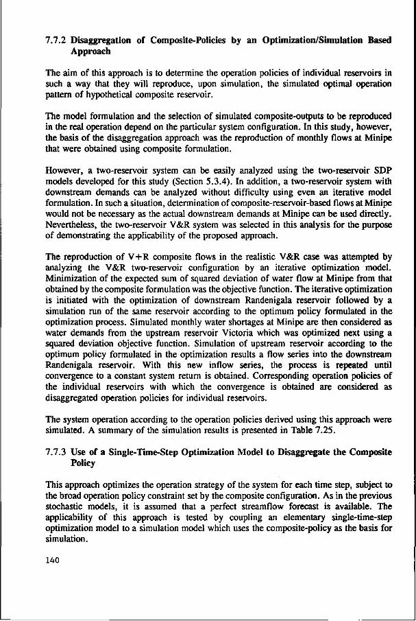
7.7.2 Disaggregation of Composite-Policies by an Optimization/Simulation Based Approach

The aim of this approach is to determine the operation policies of individual reservoirs in such a way that they will reproduce, upon simulation, the simulated optimal operation pattern of hypothetical composite reservoir.

The model formulation and the selection of simulated composite-outputs to be reproduced in the real operation depend on the particular system configuration. In this study, however, the basis of the disaggregation approach was the reproduction of monthly flows at Minipe that were obtained using composite formulation.

However, a two-reservoir system can be easily analyzed using the two-reservoir SDP models developed for this study (Section 5.3.4). In addition, a two-reservoir system with downstream demands can be analyzed without difficulty using even an iterative model formulation. In such a situation, determination of composite-reservoir-based flows at Minipe would not be necessary as the actual downstream demands at Minipe can be used directly. Nevertheless, the two-reservoir V&R system was selected in this analysis for the purpose of demonstrating the applicability of the proposed approach.

The reproduction of V+R composite flows in the realistic V&R case was attempted by analyzing the V&R two-reservoir configuration by an iterative optimization model. Minimization of the expected sum of squared deviation of water flow at Minipe from that obtained by the composite formulation was the objective function. The iterative optimization is initiated with the optimization of downstream Randenigala reservoir followed by a simulation run of the same reservoir according to the optimum policy formulated in the optimization process. Simulated monthly water shortages at Minipe are then considered as water demands from the upstream reservoir Victoria which was optimized next using a squared deviation objective function. Simulation of upstream reservoir according to the optimum policy formulated in the optimization results a flow series into the downstream Randenigala reservoir. With this new inflow series, the process is repeated until convergence to a constant system return is obtained. Corresponding operation policies of the individual reservoirs with which the convergence is obtained are considered as disaggregated operation policies for individual reservoirs.

The system operation according to the operation policies derived using this approach were simulated. A summary of the simulation results is presented in Table 7.25.

7.7.3 Use of a Single-Time-Step Optimization Model to Disaggregate the Composite Policy

This approach optimizes the operation strategy of the system for each time step, subject to the broad operation policy constraint set by the composite configuration. As in the previous stochastic models, it is assumed that a perfect streamflow forecast is available. The applicability of this approach is tested by coupling an elementary single-time-step optimization model to a simulation model which uses the composite-policy as the basis for simulation.

140

The deterministic optimization model formulation is presented in the following. Optimization for each of the fixed monthly time intervals (t) is attempted by using two different objective functions. The elementary optimization procedure used here is to evaluate all feasible discrete combinations of decisions for each month separately. For each month of the total simulation period of 37 years,

2 (1) MaxZ t= E (TEPit) , t=l,2,..,12 (7.51)

i= l

(2) Min Z, = (7.52)

where, TEPU

Si j i ,t+i

S max i,t+l —

^2,1+1

, t=l,2,.. ,12

energy generation of the reservoir i during month t (in GWh)

storage volume of reservoir i at the beginning of month t+1 (in MCM)

maximum storage capacity of reservoir i at the beginning of month t+1 (in MCM)

minimum storage capacity of reservoir i at the beginning of month t+1 (in MCM)

Subject to:

1 Scl+1 - (Sit+1 + S2,t+i) |

TEPM > FIRMiit

< 5 , t= l ,2 , .

, t= l ,2 , . i=l ,2

.,12

.,12

(7.53)

(7.54)

where,

""0,1+1

TEPi>t =

FIRMit =

the allowable deviation from the prespecified composite-policy (in MCM)

storage volume of composite reservoir at the beginning of month t+1 (in MCM) (specified by the composite-policy)

energy generation at reservoir i during month t (in GWh)

firm energy generation of reservoir i during month t (in GWh)

In addition, the constraints on reservoir storage and release volumes as well as the continuity equations presented in equations (5.12) to (5.19) also apply. Composite policies derived by the two different model formulations described in Section 7.7 are separately used in the analysis. Results of the simulations performed using this technique are also presented in Table 7.25.

141

Table 7.23 Regression Coefficients - Victoria Reservoir (Statistical Disaggregation of Composite-Policy)

Oct Nov Dec Jan Feb Mar Apr May Jun Jul Aug Sep

Oct Nov Dec Jan Feb Mar Apr May Jun Jul Aug Sep

A.J

Objective 0.14

-0.01 -0.01 0.03 0.11

-0.02 -0.14 -0.02 0.12 0.02 0.07 0.46

Objective 0.19

-0.05 -0.00 0.04 0.07

-0.02 -0.13 0.05 0.15 0.02 0.08 0.54

A,j

function: 0.06 0.01 0.15

-0.16 0.22 0.44 0.71 0.10

-0.07 0.24 0.10

-0.14

Function: 0.03 0.05 0.10

-0.26 0.00 0.32 0.91 0.09

-0.09 0.23 0.11

-0.21

A.J ^

Max. Energy generation 0.86 0.96 0.80 0.88 0.78 1.13 1.14 0.84 0.84 0.49 0.93 0.26

Min. Squared 0.90 0.99 0.82 0.85 0.73 1.12 1.11 0.87 0.80 0.57 0.B7 0.24

0.52 0.39

-0.06 0.36 0.10

-0.06 -0.29 -0.21 3.60

-1.91 3.34 1.37

Deviation 0.55 0.40

-0.02 0.47 0.16 0.04

-0.66 -0.33 4.24

-1.28 2.39 1.69

A>J

-0.05 -0.01 -0.02 0.03 0.09 0.01 0.15 0.04

-0.08 0.40

-0.09 0.04

-0.08 -0.01 -0.04 0.05 0.17 0.02 0.16

-0.04 -0.02 0.33

-0.01 0.07

A.J

-37.39 47.97

137.64 -5.31

-80.77 -108.32 -126.58

42.12 7.37

27.88 -53.39 -18.15

-55.22 51.19

133.37 -9.84

-49.65 -105.18 -130.78

33.43 -14.98 28.49

-41.41 -20.32

R!

0.95 0.97 0.94 0.93 0.94 0.97 0.97 0.94 0.88 0.87 0.91 0.64

0.94 0.97 0.94 0.94 0.92 0.97 0.97 0.94 0.88 0.88 0.90 0.44

Table 7.24 Regression Coefficients - Randenigala Reservoir (Statistical Disaggregation of Composite-Policy)

Oct Nov Dec Jan Feb Mar Apr May Jun Jul Aug Sep

Oct Nov Dec Jan Feb Mar Apr May Jun Jul Aug Sep

B.J

Objective 0.06 0.06

-0.06 0.00 0.00

-0.01 0.10 0.16 0.01 0.14 0.08 0.45

Objective 0.06 0.09

-0.03 0.01 0.01 0.05 0.14 0.29 0.03 0.21 0.11 0.58

B > j

Function: 0.61 0.62 0.55 0.08 0.68 1.22 1.04 0.15 0.33 0.07 0.28 0.03

Function: 0.58 0.54 0.46 0.04 0.61 0.97 0.92 0.19 0.38 0.05 0.18

-0.03

B.o

Max. Energy 0.27 0.23 0.55 0.26 0.08 0.07 0.19 0.28 0.22 0.17 0.26

-0.03 Min. Squared

0.30 0.27 0.55 0.24 0.04 0.01 0.12 0.25 0.31 0.10 0.20 0.04

K generation

0.74 0.88

-0.23 0.23

-0.03 -0.63 0.91 1.79 0.72 0.79 1.20 1.12

Deviation 0.81 1.04

-0.13 0.30 0.00

-0.53 1.07 1.31 0.50 0.79 1.41 1.11

B»o

0.70 0.70 0.56 0.79 0.83 0.85 0.67 0.59 0.61 0.66 0.66 0.34

0.68 0.69 0.51 0.81 0.86 0.85 0.72 0.59 0.52 0.71 0.72 0.31

B.j

-240.24 -180.41 -19.19 -45.12 10.77 11.91

-134.91 -105.90

21.63 -75.08 -96.01 -34.91

-233.98 -202.55 -20.65 -51.75 15.27 3.59

-145.86 -145.25

4.04 -98.64 -90.18 -87.15

R>

0.94 0.93 0.92 0.96 0.94 0.95 0.92 0.86 0.87 0.93 0.91 0.64

0.94 0.93 0.92 0.97 0.95 0.95 0.92 0.88 0.87 0.93 0.92 0.63

142

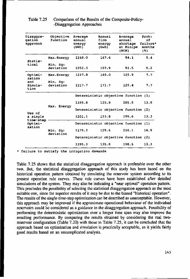
Table 7.25 Comparison of the Results of the Composite-Policy--Disaggregation Approaches

Disaggre- Objective Average Annual gation function annual firm approach energy energy

(GWh) (Gwh)

Average Prob: annual of shortage failure* at Minipe months (MCM) (%)

Statis­tical

Max.Energy

Min. Sq: deviation

1248.0

1252.3

167.6

157.9

94.1

91.5

5.4

5.2

Max. Energy

Optimi- Max.Energy 1217.8 165.0 125.9 7.7 zation and Min. Sg: Simula- deviation 1217.7 171.7 125.4 7.7 tion

Deterministic objective function (1)

1185.8 125.8 205.5 13.9

Deterministic objective function (2)

1201.1 123.8 199.6 13.3

Deterministic objective function (1)

1179.3 129.6 216.1 14.9

Deterministic objective function (2)

1195.3 135.8 198.5 13.3

Use of a single time-step Optimi­zation

Min. Sq: deviation

* failure to satisfy the irrigation demands

Table 7.25 shows that the statistical disaggregation approach is preferable over the other two. But, the statistical disaggregation approach of this study has been based on the historical operation pattern obtained by simulating the reservoir system according to its present operation rule curves. These rule curves have been established after detailed simulations of the system. They may also be indicating a "near optimal" operation pattern. This precludes the possibility of selecting the statistical disaggregation approach as the most suitable one, since the superior results of it may be due to the biased "historical operation". The results of the single-time-step optimization can be described as unacceptable. However, this approach may be improved if the approximate operational behaviour of the individual reservoirs could be considered as a guidance in the disaggregation approach. Possibility of performing the deterministic optimization over a longer time span may also improve the resulting performance. By comparing the results obtained by considering the real two-reservoir configuration (Table 7.20) with those in Table 7.25, it can be concluded that the approach based on optimization and simulation is practically acceptable, as it yields fairly good results based on an uncomplicated analysis.

143

8 Accuracy of the Results

8.1 Accuracy of Sequential and Iterative Optimization Approaches

The accuracy of the sequential and iterative optimization processes are evaluated by applying them to a smaller reservoir system which is a subsystem of the Mahaweli water resources system. The system considered consists of four reservoirs namely Kotmale, Victoria, Randenigala and Rantembe. The system can be scaled down to a three-reservoir system by considering the Rantembe reservoir as a run-of-the-river power plant. (Nandalal, 1986). The monthly streamflow data and the irrigation water demands used for the analysis in Chapter 7 are used for this analysis, while the diversion demands at Polgolla were prespecified approximately. The effect of the upstream Caledonia and Talawakelle reservoirs that are not considered in this system is incorporated partly by considering an increased storage capacity for the Kotmale reservoir. The system configuration selected for this analysis is displayed in Fig. 8.1.

This system can be considered as comprised of two subsystems which are the Victoria-Randenigala-Rantembe subsystem and the Kotmale subsystem. As in Chapter 7, the common interface point of the two subsystems is the Polgolla barrage. The optimal flow pattern at the interface point can be determined by formulating mathematical models that consider the joint operation of Kotmale and Victoria+Randenigala (V+R) Composite reservoirs. The simplified system configuration consisting of the Kotmale and V+R composite reservoirs is displayed in Fig. 8.2. Operational analysis of this composite configuration was performed by formulating a SDP-based optimization model and a simulation model. The operation policies that are derived by the SDP model are used to simulate the system operation using the 37-year-long monthly streamflow and demand data.

Two different objective functions, namely maximization of the energy generation and the minimization of the squared deviation of the water supply from the irrigation demand are considered. In addition to the constraints imposed by the physical characteristics and continuity of flow, the firm energy and the diversion demands at Polgolla are considered as constraints. The results of this analysis are presented in Table 8.1.

144

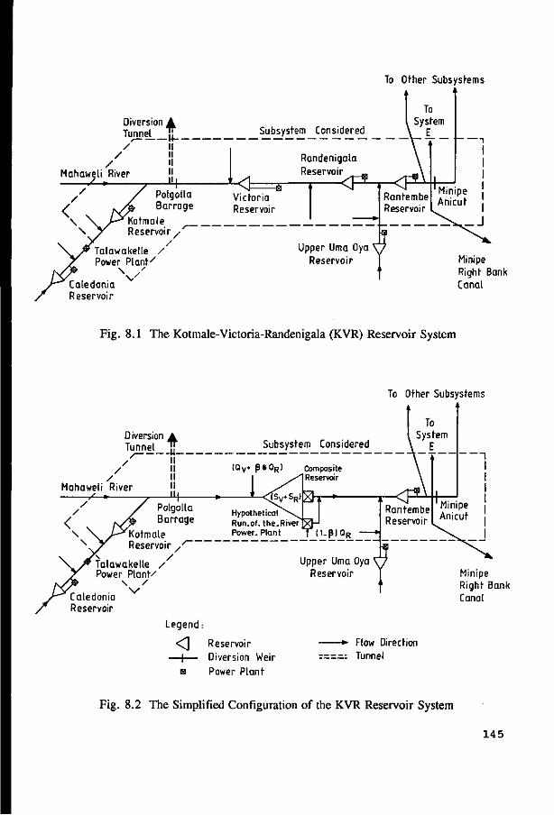
To Other Subsystems

Diversion A

Minipe Right Bank Canal

Fig. 8.1 The Kotmale-Victoria-Randenigala (KVR) Reservoir System

To Other Subsystems

Diversion • Tunnel_ TJ_

Mahaweli River / - \

Polgolla Barrage

Kotmale Reservoir /

/ ^ ~ /

Talawakelle / Power Plant/

\ / Caledonia Reservoir

Subsystem Considered

(Qv* P * O R ) Composite Reservoir

"* *—<$fv,SR]

Hypothetical Run.of. the.River Power. Plant

Upper Uma Oya Reservoir Minipe

Right Bank Canal

Legend:

<^\ Reservoir — | — Diversion Weir

H Power Plant

-*• Flow Direction ===== Tunnel

Fig. 8.2 The Simplified Configuration of the KVR Reservoir System

145

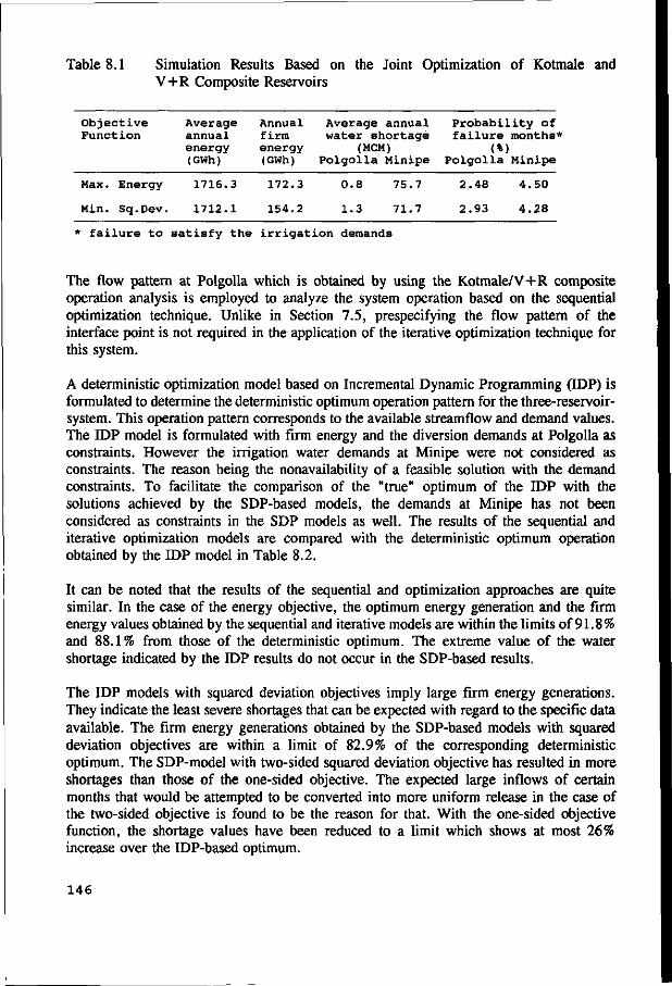
Table 8.1 Simulation Results Based on the Joint Optimization of Kotmale and V+R Composite Reservoirs

Objective Function

Average Annual annual firm energy energy (GWh) (GWh)

Average annual Probability of water shortage failure months*

(MCM) (%) Polgolla Minipe Polgolla Minipe

Max. Energy

Min. Sq.Dev.

1716.3

1712.1

172.3

154.2

0.8

1.3

75.7

71.7

2.48

2.93

4.50

4.28

* failure to satisfy the irrigation demands

The flow pattern at Polgolla which is obtained by using the Kotmale/V+R composite operation analysis is employed to analyze the system operation based on the sequential optimization technique. Unlike in Section 7.5, prespecifying the flow pattern of the interface point is not required in the application of the iterative optimization technique for this system.

A deterministic optimization model based on Incremental Dynamic Programming (IDP) is formulated to determine the deterministic optimum operation pattern for the three-reservoir-system. This operation pattern corresponds to the available streamflow and demand values. The IDP model is formulated with firm energy and the diversion demands at Polgolla as constraints. However the irrigation water demands at Minipe were not considered as constraints. The reason being the nonavailability of a feasible solution with the demand constraints. To facilitate the comparison of the "true" optimum of the IDP with the solutions achieved by the SDP-based models, the demands at Minipe has not been considered as constraints in the SDP models as well. The results of the sequential and iterative optimization models are compared with the deterministic optimum operation obtained by the IDP model in Table 8.2.

It can be noted that the results of the sequential and optimization approaches are quite similar. In the case of the energy objective, the optimum energy generation and the firm energy values obtained by the sequential and iterative models are within the limits of 91.8% and 88.1% from those of the deterministic optimum. The extreme value of the water shortage indicated by the IDP results do not occur in the SDP-based results.

The IDP models with squared deviation objectives imply large firm energy generations. They indicate the least severe shortages that can be expected with regard to the specific data available. The firm energy generations obtained by the SDP-based models with squared deviation objectives are within a limit of 82.9% of the corresponding deterministic optimum. The SDP-model with two-sided squared deviation objective has resulted in more shortages than those of the one-sided objective. The expected large inflows of certain months that would be attempted to be converted into more uniform release in the case of the two-sided objective is found to be the reason for that. With the one-sided objective function, the shortage values have been reduced to a limit which shows at most 26% increase over the IDP-based optimum.

146

8.2 Possible Improvement in the Operation by Incorporating an Interpolation for the Target Storage

The SDP-based operation policies formulated in this study indicate the final storage volume of a reservoir as a function of the initial storage volume and the current inflow. They correspond to a discrete set of predefined storage and inflow values. These are the values that are used as representative values (Section 5.3.1) in the SDP-based optimization process. In the actual operation, an interpolation can be employed to arrive at an operation policy decision that corresponds to a different combination of initial storage and current inflow.

The effect of using a linear interpolation on the final storage decision is assessed by simulating the KVR system according to the operation policies formulated in Section 8.1. The results are tabulated in Table 8.2. It can be seen that the performances with and without interpolations do not differ much in this particular example. However substantially different results can be anticipated in cases where relatively rough state discretizations are employed. In the present analysis, the storage spaces of the Victoria and Randenigala reservoirs were discretized into 49 joint classes. Similarly, the inflows were discretized into 16 joint classes. For the Kotmale reservoir, 20 storage classes and 8 inflow classes were considered.

There are disadvantages of using a linear interpolation. It does not assure differentiability (or smoothness, in a geometric context) of the interpolating function at the class limits. Furthermore, to achieve an accurate interpolation, the size of the classes need to be reduced, which is not practical with SDP. In cases where a relatively rough state discretization is used, the cubic spline interpolation can be used to obtain a better approximation for the target storage. It uses cubic polynomials to ensure a better approximation of a continuously differentiable function on each sub-interval (Burden et al.,1978).

147

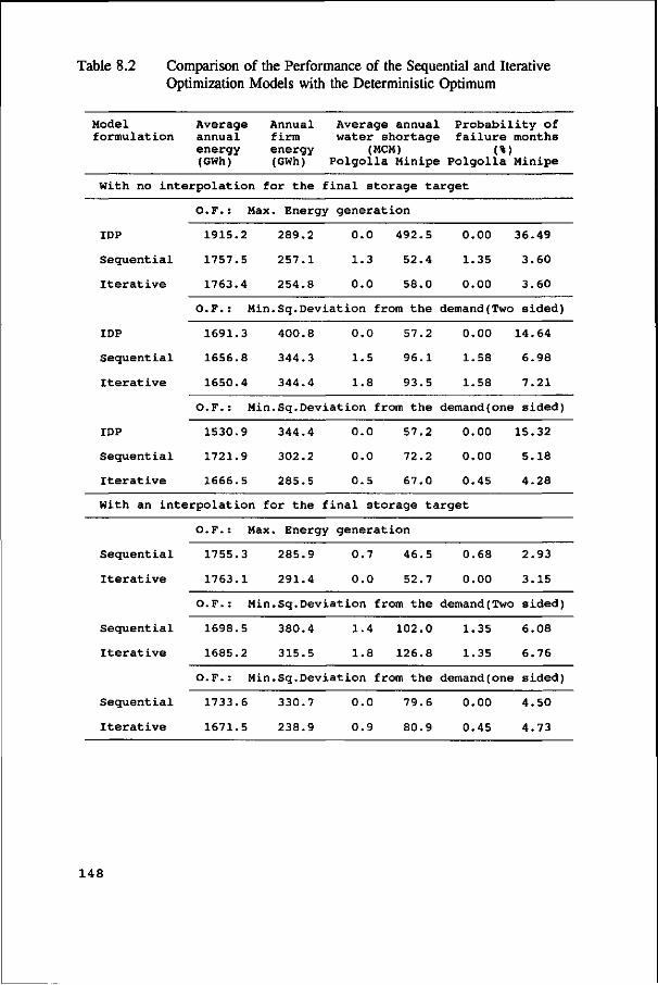
Table 8.2 Comparison of the Performance of the Sequential and Iterative Optimization Models with the Deterministic Optimum

Model formulation

Average Annual Average annual annual firm water shortage energy energy (MCM) (GWh) (GWh) Polgolla Minipe

Probabil failure

(%) Polgolla

ity of months

Minipe

With no interpolation for the final storage target

IDP

Sequential

Iterative

IDP

Sequential

Iterative

IDP

Sequential

Iterative

O.F.: Max. Energy generation

1915.2 289.2 0.0 492.5

1757.5 257.1 1.3 52.4

1763.4 254.8 0.0 58.0

O.F.: Min.Sq.Deviation from the

1691.3 400.8 0.0 57.2

1656.8 344.3 1.5 96.1

1650.4 344.4 1.8 93.5

O.F.: Min.Sq.Deviation from the

1530.9 344.4 0.0 57.2

1721.9 302.2 0.0 72.2

1666.5 285.5 0.5 67.0

0.00

1.35

0.00

demand(Two

0.00

1.58

1.58

demand(one

0.00

0.00

0.45

36.49

3.60

3.60

sided)

14.64

6.98

7.21

sided)

15.32

5.18

4.28

With an interpolation for the final storage target

Sequential

Iterative

Sequential

Iterative

Sequential

Iterative

O.F.: Max. Energy generation

1755.3 285.9 0.7 46.5

1763.1 291.4 0.0 52.7

O.F.: Min.Sq.Deviation from the

1698.5 380.4 1.4 102.0

1685.2 315.5 1.8 126.8

O.F.: Min.Sq.Deviation from the

1733.6 330.7 0.0 79.6

1671.5 238.9 0.9 80.9

0.68

0.00

demand(Two

1.35

1.35

demand(one

0.00

0.45

2.93

3.15

sided)

6.08

6.76

sided)

4.50

4.73

148

9 Conclusions and Recommendations

9.1 Conclusions

The analysis in this study was aimed at determining the macro system (reservoir system located on the major rivers) operation policies of the Mahaweli water resources system. It was assumed that the present operation practices of the micro (irrigation) system would not be changed. On this assumption, the micro system water demands have been estimated. Subsequently a two-stage approach was used to formulate operation policies for the macro system components. Referring to the organizational structure for Mahaweli Operations presented in Fig. 2.4, it can be stated that the present study is carried out from the view­point of the Water Management Secretariat (WMS) of Sri Lanka. WMS is the technically specialized agency that assists the decision making process for the Mahaweli Operation.

In the two-stage approach, the macro system is visualized as comprising of three subsystems interconnected at a common interface point which is the Polgolla Barrage (Fig. 2.2). Each of the subsystems so identified were represented by hypothetical composite reservoirs. The resulting three-composite-reservoir configuration was employed to arrive at an operation guide-line for the interface point of the subsystems. This operation policy is followed in a more detailed analysis which considers the real configurations of each of the three subsystems individually.

The use of a hypothetical composite reservoir instead of a multireservoir configuration was found to be a convenient technique in analyzing an otherwise computationally unmanageable system. The composite reservoir formulations of this study were calibrated in a deterministic environment. The composite reservoir formulations of Kularathna and Bogardi (1990) and Bogardi et al. (1990b) were calibrated in stochastic environments. The final results of the two approaches were found to be similar. The deterministic calibration has the advantage that it requires considerably less time. Also, the outputs of the deterministic optimization models used for this purpose directly identify the corresponding optimal operation patterns. On the other hand, the output of a stochastic optimization model has to be subsequently used in a simulation in order to determine the corresponding operation pattern.

149

The use of an objective function which minimizes the sum of squared deviations from the micro system water demand was necessary in the preliminary analysis due to several reasons. The Mahaweli system bears an important objective of meeting the irrigation water demands with the best fit. A "deviation" type of an objective function best represents this objective. It is also recognized that the large deviations from the demands produce more adverse effects on irrigation areas. This implies the suitability of a squared deviation objective function. The use of an objective function which maximizes the energy output would route water through the path with the maximum generating head. This would lead to the release of a large quantity of flow at the Polgolla barrage into the Victoria-Randenigala-Rantembe subsystem. It is theoretically possible to use the energy objective together with the downstream irrigation demands as constraints. However, this is not practical in a deterministic optimization problem, due to the nonavailability of a feasible solution when high demand constraints are imposed. Instead, the approach considered in this study was to use a squared deviation objective function together with a firm energy value as a constraint. This firm energy level was determined by trial-and-error so as not to lead the solution to an infeasible one. (The firm energy constraint was increased gradually, so that it over-rules the objective achievement until a level is reached beyond which there is no feasible solution).

The analysis of the system considering the predetermined optimal diversion policy at Polgolla is done by two different approaches: sequential and iterative optimizations. These approaches use two-reservoir SDP models to analyze each of the subsystems individually. The two-reservoir SDP models formulated in this study show a substantial improvement over those models documented in the recent literature. These SDP models occupy a computer memory of approximately 384 Kb (corresponding to 49 joint storage classes and 16 joint inflow classes of the two reservoirs). Further refinement of the storage discretization may improve the resulting performance up to a certain limit. However the refinement of inflow discretization beyond a certain limit would lead to a deterioration of policies due to the large number of possible "0" values in the transitional probability matrices. These values may lead the subsequent SDP optimization results to be "trapped" at certain states, or to alternate between the states, depending on the structure of the transitional probability matrices (Wagner, 1975). One way of reducing the number of these "0" values is the use of synthetic streamflow data for estimating the probability matrices. This would provide a sufficient number of data points to estimate the required probabilities.

The comparison of the performance of the SDP-based optimization with the deterministic optimum found by IDP (Sections 7.3 and 8.1) reveals that the SDP-based solution avoids extreme results. This is basically due to the expectation-oriented nature of the SDP algorithm. Although this behaviour leads to a long-term optimal operation, it makes the SDP-based policies unsuitable for extreme situations. In such cases, the long-term operation guide-line provided by the SDP may be switched to a short-term emergency mode (Bogardi etal., 1990a).

When the optimal diversion policy at Polgolla is followed, the results of the iterative optimization were found to be similar to those of the sequential optimization approach. The importance of the predetermined optimal diversion policy at Polgolla is reflected in the deteriorated results of the iterative optimization with a different (non optimal) diversion

150

policy. The results of the alternative solutions 53-56 and 61-64 of Table 7.12 were obtained by using a diversion policy which proportions the diversions and releases at Polgolla according to the average annual shortages of the two downstream subsystems. These lead to extreme results that are practically unacceptable.

The accuracy of the SDP-based aggregation/disaggregation techniques for analyzing a multireservoir system has been assessed in Section 8.1. Comparison of the "true" optimum results obtained by the deterministic optimization with the SDP-based performance imply that they are similar. One more factor which makes the SDP-based aggregation/disaggregation techniques suitable for analyzing multireservoir systems can be noted here. The use of SDP for the optimization of multireservoir systems is usually made without considering the cross correlation of the various natural flows into the system. This is done in order to reduce the dimensionality of the problem. Only the serial correlation of the flows are incorporated in the form of a Markov Chain. Explicit incorporation of the cross correlation of the inflows would increase the number of state variables by one more dimension. Therefore, the cross correlation of inflows can best be handled by a separation of optimization and streamflow synthesis (as in the implicit stochastic approach) or by an aggregation/disaggregation methodology.

A comparison of an implicit stochastic approach with the explicit SDP-based results and the deterministic optimum operation is made in Section 7.6. For the particular system considered, an explicit SDP-based policy was found to be the best operation policy. The analysis in Section 7.6 reveals that an implicit stochastic approach could be very inaccurate especially in the case of a complex multireservoir water resources system. This is basically due to two reasons. (1) The associated multi-site data generation process would be quite complex. (2) The selection of the variables that has to be considered in the regression analysis impose another inaccuracy. This is due to the essential trading-off of the statistical acceptance of the variables with the practical applicability of the resulting operation policies.

The applicability of the composite reservoir concept leads to the search for techniques that can disaggregate the operation policies derived by using a composite representation. The statistical disaggregation approach presented in Section 7.7.1 can be viewed as a method that combines theory and practice. This is because the disaggregation process thereof is based on the available historical operation pattern of the system. However, the results of Table 7.25 should not be misinterpreted to conclude that the statistical disaggregation technique outperforms the other two techniques that are proposed. This is due to the reason that the present operation pattern which was used to arrive at this solution is also a "near optimal" solution. The present operation pattern was determined by simulating the system performance according to the rule curves of the reservoirs. It can be stated that the approach based on the optimization and simulation is also an adequate way of disaggregating the composite policies. The results of the method of single-time-step optimization do not prove that this method is suitable in its present form. However, this method may be improved either by performing the optimization over a longer time horizon, or by prespecifying an acceptable joint operation pattern to supplement the disaggregation approach.

1 5 1

9.2 Recommendations for Further Research

Throughout this study, a time step of one month was considered as a reasonable compromise between model accuracy and computer time requirements. Due to the considerable storage available in the main reservoir and irrigation tanks, monthly time steps would be sufficient except in the cases of extreme situations. The present operation practice of the Mahaweli system is to have weekly Operation Planning Meetings (Section 2.6.2) to make the short-term decisions based on the long-term operation policy. This process can be aided by an interactive short-term decision making model that could provide more information during the weekly meetings. The input data for such model may include flow forecasts, the current state of the reservoir system, the long-term operation policies and appropriate objective function(s). Incorporation of a multiobjective decision making process into this interactive model of the system would also be convenient.

The Incremental Dynamic Programming models of this study employed a "corridor" comprising of three values of each state variable. For a two state variable case, the corridor has a square grid pattern, while it is a spatial pattern (in the form of a cube) for a problem of three state variables. This increases the computational requirements of an IDP model with a large number of stages. Possibility of designing a corridor that contains a less number of grid points (not necessarily having the square or spatial patterns used in this study) would substantially reduce this problem. Continuation of the research on IDP to include risk/reliability aspects is also recommended.

In the actual operation of a water resources system, some performance criteria that are not explicitly incorporated in the present optimization models have a great importance. These criteria include the length of water shortage periods, frequency of shortage periods in addition to the reliability of system performance. Attempts to formulate methodologies that can incorporate these criteria into the optimization process would be a suitable area for future research. Similarly, the effect of the model parameters (in terms of the objective function, constraints etc.) on the unmodelled performance criteria needs to be studied.

The effect of the simplified aggregation/decomposition techniques on the performance criteria such as reliability require the attention of future research. It can be either in the form of incorporating these criteria during the model simplification, or in the form of a detailed investigation of the simplifying techniques on the performance of different water resources systems.

Further research is also needed to extend the applicability of the aggregation/disaggregation techniques to analyze water resources systems consisting of more units, and also to analyze different configurations.

Consideration of the water quality in the operational management of water resources systems is becoming increasingly important. Even though the quantity of available water may be sufficient, its quality may impose severe restrictions on the intended uses. Therefore, it would be necessary to incorporate water quality aspects in the formulation of reservoir operation policies. Further research is needed in this area, in order to handle the increased complexity resulting from the increased number of state variables.

152

Conclusies en Aanbevelingen

Conclusies

Het doel van dit onderzoek was het bepalen van optimaal beheer van het macrosysteem (bestaande uit de grote reservoirs van de Mahaweli rivier en zijn toevoerwegen) van het Mahaweli water systeem. Aangenomen werd dat de huidige waterverdeling in het micro (irrigatie) systeem ongewijzigd blijft. Er werd een twee-staps benadering gebruikt om het beheer voor de componenten van het macrosysteem te formuleren. Verwijzend naar het organisatieschema voor het Mahaweli beheer in figuur 2.4, kan gesteld worden dat de huidige studie is uitgevoerd vanuit het gezichtspunt van het 'Water Management Secretariat (WMS)' van Sri Lanka. WMS is een technisch gespecialiseerde orgaan dat het besluitvormingsproces voor het Mahaweli beheer ondersteund.

In de twee-staps benadering wordt het macrosysteem geschematiseerd als bestaande uit drie subsystemen welke met elkaar verbonden zijn door een gemeenschappelijk verbindingspunt (Polgolla Barrage). Ieder van de subsystemen werd gemodelleerd door een hypothetisch samengesteld reservoir. De resulterende configuratie werd gebruikt om een globaal beleid voor beheer van het verbindingspunt op te stellen. In de tweede stap is dit beheersbeleid onderwerp van een meer gedetailleerde analyse, waarbij de werkelijke configuraties van de drie subsystemen in beschouwing wordt genomen.

Het gebruik van het hypothetische, samengestelde reservoir in plaats van een configuratie met afzonderlijke reservoirs, bleek een doeltreffende techniek te zijn in het analyseren van een anderszins rekenkundig onbeheersbaar systeem. De systeemkenmerken van het samengestelde reservoir werden gecalibreerd op optimalisaties met deterministische invoer. Eerder was dezelfde calibratie uitgevoerd op optimalisaties met stochastische invoer (zie Kularathna en Bogardi, 1990 en Bogardi e.a., 1990b). De resultaten van beide calibraties waren vergelijkbaar. De deterministische calibratie heeft het voordeel dat het aanzienlijk sneller is. Bovendien maakt de uitvoer van de deterministische optimalisatie het direct mogelijk het corresponderende optimale beheerspatroon vast te stellen. De uitvoer van een stochastisch optimalisatie kan slechts indirect, via een simulatie, gebruikt worden om het optimale beheerspatroon vast te stellen.

153

In de vooranalyse was het gebruik van een doelfunctie die de som van de kwadratische afwijkingen van de vraag van het microsysteem minimaliseerde noodzakelijk om verschillende redenen. Het Mahaweli systeem heeft als eerste doel tegemoet te komen aan de irrigatiebehoeften. Dit verantwoord de keuze van een doelfunctie waarin die "afwijkingen" voorkomen. Er dient rekening te worden gehouden met het feit dat grotere afwijkingen van de waterbehoefte een groter negatief effect hebben. Dit maakt de doelfunctie met gekwadrateerde afwijkingen geschikt. Het gebruik van een doelfunctie welke de energieproductie maximaliseert, zou het water leiden door dat pad dat de grootste drukhoogten zou genereren. Dit zou bij de Polgolla dam resulteren in het leiden van grote hoeveelheden water door het Victoria-Randenigale-Rantembe subsysteem (zie Figuur 2.2). Theoretisch is het mogelijk de energiewensen te beschouwen met de benedenstroomse irrigatiebehoeften als randvoorwaarden. Dit is echter niet praktisch in een deterministisch optimalisatie probleem aangezien er geen mogelijke oplossing bestaat indien er grote irrigatie waterbehoeften bestaan. In plaats daarvan wordt in deze studie een kleinste kwadraten doelfunctie voor irrigatie waterbehoeften gebruikt met een minimale energieproductie als randvoorwaarde. De minimale energieproductie werd met "trial and error" zodanig bepaald, dat oplossing van het kleinste kwadraten criterium mogelijk was.

De analyse van het systeem met het vastgestelde optimale water verdelingsbeleid bij Polgolla, is op twee manieren uitgevoerd: sequentieel en iteratief. Beide benaderingen stellen de subsystemen voor als SDP modellen van twee reservoirs. De in deze studie gebruikte modellen geven een substantiate verbetering te zien ten opzichte van SDP modellen in recente literatuur. De gebruikte SDP modellen nemen een computer geheugen in van ± 384 Kb (overeenkomend met 49 joint storage classes en 16 joint inflow classes van de twee reservoirs). Verdere verfijning van de discretisatie van de opslag kan de resultaten enigszins verbeteren. Echter, de verfijning van de discretisatie van de instroming voorbij een zekere grens, leidt tot slechtere resultaten door een groot aantal mogelijke nul waarden in de overgangsmatrices. De nul waarden kunnen ertoe leiden dat de SDP optimalisatie wordt "gevangen" in zekere toestanden, of oscilleert tussen bepaalde toestanden, afhankelijk van de structuur van de overgangsmatrices (Wagner, 1975).

Vergelijking van de resultaten van de SDP-optimalisatie met het deterministische optimum bepaald met IDP (Secties 7.3 en 8.1) tonen aan dat de oplossing gebaseerd op SDP extreme resultaten vermijdt. Dit komt door het verwachting-georienteerde karakter van het SDP algoritme. Hoewel dit gedrag leidt tot beheer dat optimaal is op lange termijn, maakt het SDP ongeschikt voor extreme situaties. In extreme situaties kan het lange termijn beheer, zoals verkregen door SDP, worden vervangen door een calamiteiten mode voor korte termijn (Bogardi et al., 1990).

Indien de optimale waterverdeling bij Polgolla wordt gehanteerd, zijn de resultaten van de iteratieve optimalisatie gelijk aan die van de sequentiele optimalisatie. Het belang van de vooraf vastgestelde optimale waterverdeling bij Polgolla komt tot uiting in de slechtere resultaten van de iteratieve optimalisatie met een afwijkende waterverdeling.De alternatieve oplossingen 53-56 en 61-64 van Tabel 7.12 werden verkregen door het water bij Polgolla te verdelen overeenkomstig de gemiddelde jaarlijkse tekorten van de benedenstroomse subsystemen. Dit resulteert o.a. in onacceptabel hoge water tekorten.

154

De geschiktheid van de aggregatie/disaggregatie technieken gebaseerd op SDP voor het analyseren van een multi-reservoir systeem, wordt besproken in Sectie 8.1. Het "ware optimum", verkregen door de deterministische optimalisatie, is vergelijkbaar met de resultaten van de SDP optimalisatie. Een extra factor, welke de SDP aggregatie/disaggregatie technieken geschikt maken om multi-reservoir systemen te analyseren, kan hier worden opgemerkt. Bij gebruik van SDP optimalisatie voor multi-reservoir systemen worden gewoonlijkde kruiscorrelaties tussen de verschillende natuurlijke waterstromen die het systeem binnen komen, niet in beschouwing genomen. Dit wordt gedaan om de dimensie van het probleem te reduceren. Alleen de autocorrelatie wordt in rekening gebracht, in vorm van een Markov Chain. Expliciet in rekening brengen van de kruiscorrelatie voor de instroming zou het aantal toestandsvariabelen met een extra dimensie vergroten. De kruiscorrelatie van ingaande stromen kan dan ook het beste worden benadert door afzonderlijke optimalisatie en synthese van stromingen (zoals in de impliciete stochastische benadering) of door een aggregatie/disaggregatie methode.

In Sectie 7.6 wordt een vergelijking gemaakt tussen een impliciete stochastische benadering gebaseerd op SDP resultaten en het deterministische optimale beheer. Voor het beschouwde systeem bleek een expliciet, op SDP gebaseerd beleid, het beste te zijn. De analyse in Sectie 7.6 wijst uit dat de impliciete stochastische benadering zeer onnauwkeurig kan zijn, vooral in geval van complexe, multi-reservoir systemen. Dit komt voornamelijk door twee redenen. (1) Het benodigde data generatie proces voor verschillende reservoirs is complex. (2) De selectie van variabelen in de regressie analyse, veroorzaakt extra onnauwkeurigheid. Dit wordt veroorzaakt door een "trade-off tussen de statistische acceptatie van variabelen enerzijds en de praktische toepasbaarheid van het daaruit volgende beheer anderzijds.

De geschiktheid van het samengesteld reservoir concept leidt tot het zoeken naar technieken die de beheersmaatregelen, afgeleid voor samengestelde reservoirs, kunnen disaggregeren. De statistische disaggregatie methode die is beschreven in Sectie 7.7.1, kan worden beschouwd als een methode die theorie en praktijk combineert. Het betreffende disaggregatie proces is namelijk gebaseerd op de beschikbare beheersmaatregelen van het systeem in het verleden. Het is echter verkeerd uit de resultaten van Tabel 7.25 concluderen dat de statistische disaggregatie techniek beter is dan de twee andere voorgestelde methoden. In dit geval was deze techniek beter omdat het huidige beheersbeleid, dat werd gebruikt om de statistische disaggregatie techniek toe te passen, dicht bij de "optimale" oplossing ligt. De huidige beheersmaatregelen zijn bepaald door het systeem te simuleren met behulp van de "rule curves" van de reservoirs. Men kan stellen dat de techniek gebaseerd op optimalisatie en simulatie ook een geschikte manier is om het samengestelde beheer te disaggregeren. De resultaten verkregen met een enkelvoudige tijdstap optimalisatie tonen niet aan dat deze methode in zijn huidige vorm geschikt is. Deze methode kan echter verbeterd worden of door de optimalisatie te laten gebeuren over een langere tijdshorizon, of door een acceptabel gecombineerd beheer voor te schrijven als aanvulling van de disaggregatie benadering.

155

Aanbevelingen voor toekomstig onderzoek

In deze studie werd de tijdstap van een maand beschouwd als een redelijk compromis tussen model nauwkeurigheid en benodigde computertijd. Wegens de aanzienlijke opslag die beschikbaar is in het hoofdreservoir en de irrigatietanks zullen, met uitzondering van extreme situaties, maandelijks tijdstappen voldoende zijn. In het Mahaweli systeem is men gewend om wekelijks Operation Planning Meetings te beleggen, ten einde korte termijn beslissingen te nemen met als basis het lange termijn beheersbeleid. Deze vergaderingen kunnen worden ondersteund door een interactief model voor korte termijn besluiten. De invoer gegevens voor zo'n model kunnen o.a. bevatten afvoervoorspellingen, de actuele toestand van het reservoir systeem, het lange termijn beleid en geschikte doelfunctie(s). Opname van een Multiobjective Decision Making routine die gebruik maakt resultaten van het interactieve model, kan ook waardevol zijn.

De Incremental Dynamic Programming modellen in deze studie gebruiken een "corridor" welke drie waarden voor iedere toestandsvariabele kan bevatten. Indien slechts twee waarden worden toegestaan heeft de corridor een vierkant grid patroon, terwijl drie waarden een ruimtelijk, kubisch patroon doen ontstaan. De sterke toename van het aantal mogelijkheden veroorzaakt een evenredige toename van de computer tijd van het IDP model. Een corridor dat minder grid punten bevat (niet noodzakelijkerwijs de twee- en drie-dimensionale patronen gebruikt in deze studie) zou aan dit probleem tegemoet komen. Vervolg onderzoek aan IDP modellen ten einde betrouwbaarheidsaspecten toe te voegen, wordt ook aan bevolen.

In het werkelijke beheer van het water systeem kunnen sommige criteria, die niet expliciet opgenomen zijn in de huidige optimalisatie modellen, van groot belang zijn. Voorbeelden zijn de lengte van de periode met watertekort, de frequentie van droogteperioden en de betrouwbaarheid van het systeem. Een geschikt terrein voor toekomstig onderzoek is het opnemen van deze criteria in het optimalisatie proces. Ook de effecten van model parameters (in termen van doelfunctie, randvoorwaarde(n), etc.) op de nog niet opgenomen criteria, dient onderzocht te worden.

Ten slotte vraagt het effect van de vereenvoudigde aggregatie/disaggregatie technieken op systeemkenmerken, zoals betrouwbaarheid, om nader onderzoek. Dit kan worden gedaan door deze criteria direct tijdens de model vereenvoudiging mee te nemen, of door gedetailleerd onderzoek van de vereenvoudigingstechnieken op het gedrag van verschillende water systemen.

Verder onderzoek is ook nodig om de toepasbaarheid van de aggregatie/disaggregatie techniek uit te breiden naar systemen bestaande uit meerdere eenheden en verschillende configuraties.

Beschouwingen over waterkwaliteit worden steeds belangrijker binnen het operationele waterbeheer. Ook al is er genoeg water aanwezig, dan nog kan de kwaliteit ervan ernstige beperkingen aan het gebruik ervan opleggen. Daarom is het belangrijk om kwaliteitsaspecten mee te nemen in de formulering van reservoirbeheer. De grotere complexiteit, als gevolg van het toegenomen aantal toestandsvariabelen, maakt verder onderzoek op dit gebied nodig.

156

10 References

ACRES International Limited (1985), Mahaweli Water Resources Management Project-Studies of Operating Policy Options. Nigara Falls, Canada.

Araujo, A.R. and L.A. Terry (1974), Operation of a Hydrothermal System, Brazil Journal of Electrical Energy.

Arvanitidis, N.V. and J. Rosing (1970), Optimal Operation of Multireservoir Systems Using a Composite Representation, IEEE Proceedings on Power Apparatus and Systems. Vol. 89, No. 2, pp. 327-335.

Beard, L.R. (1976), Flood Control by Reservoirs, Hydrologic Engineering Methods for Water Resources Development. Vol. 7, U.S. Army Corps of Engineers, Hydrologic Engineering Centre, Davis, California.

Bellman, R. (1957), Dynamic Programming. Princeton University Press, Princeton, New Jersey.

Bogardi, J.J. (1987), System Design in Water Resources Development, Lecture Notes. ATT, Bangkok, Thailand.

Bogardi, J.J. and K.D.W. Nandalal (1988) Dynamic Programming Based Joint Operation Policy for the Victoria and Randenigala Reservoirs in Sri Lanka, Proceedings. VI th IWRA World Congress on Water Resources, Vol. JJ, Ottawa, Canada.

Bogardi J.J., S. Budhakooncharoen, D.L. Shrestha and K.D.W. Nandalal (1988a) Effect of State Space and Inflow Discretization on Stochastic Dynamic Programming-Based Reservoir Operation Rules and System Performance, Proceedings. VI Congress, Asian-Pacific Division, International Association of Hydraulic Research, Kyoto, Japan, Vol. I, pp. 429-436.

157

Bogardi, J.J., S. Budhakooncharoen, L. Duckstein and A.A. Sutanto (1988b), Evolutionary Interactive MCDM for Discrete Water Resources Systems Planning, Proceedings. Vmth Interactive Conference on MCDM, August 21-26, Manchester, England.

Bogardi, J.J. et al. (1988c), Improved Large Scale Water Resources Development Planning, Progress Report. Water Resources Engineering Division, AIT, Bangkok, Thailand.

Bogardi, J.J., W-C. Huang and R. Harboe (1990a), On-line Operation of a Multipurpose Reservoir During Typhoon Occurrence, Proceedings. International Symposium on Tropical Hydrology and Fourth Carribean Islands Water Resources Congress, July 23-27, San Juan, Puerto Rico.

Bogardi, J.J., M.D.U.P. Kularathna and R. Harboe (1990b), Approximate Techniques in the Operational Optimization of the Mahaweli Reservoir System in Sri Lanka, Proceedings. International Symposium on Tropical Hydrology and Fourth Carribean Islands Water Resources Congress, July 23-27, San Juan, Puerto Rico.

Budhkooncharoen, S. (1990), Interactive Multi-Objective Decision Making in Reservoir Operation, D.Eng. thesis. AIT, Bangkok, Thailand.

Burden, R.L., J.D. Faires and A.C. Reynolds (1978), Numerical Analysis. Prindle, Weber and Schmidt, Boston, Massachusetts, pp. 107-119.

Butcher, W.S. (1971), Stochastic Dynamic Programming for Optimum Reservoir Operation, Water Resources Bulletin. Vol. 7, No. 1, pp. 115-123.

Chow, V.T., D.H. Kim, D.R. Maidment and T.L. Ula (1975), A Scheme for Stochastic State Variable Water Resources System Optimization, Report No. 105. University of Illinois and Urbana Champaign Water Resources Centre, Illinois.

Dastagne, N.G. (1974), Effective Rainfall in Irrigated Agriculture, Irrigation and Drainage Paper 25. FAO, Rome.

Dias, N.L.C., M.V.F. Pereira, and J. Kelman (1985), Optimization of Flood Control and Power Generation Requirements in a Multipurpose Reservoir, Paper Presented at the Symposium on Planning and Operation of Electric Energy Systems. International Federation of Automatic Control, Rio de Janeiro, Brazil.

Duckstein, L. (1989), Conflicts in Reservoir Management: Modelling and Reduction by Multiobjective Analysis, Proceedings. International Seminar-Workshop on Conflict Analysis in Reservoir Management, AIT, Bangkok, Thailand.

Dupacova, J., A. Gaivoronski, Z. Kos and T. Szantai (1991), Stochastic Programming in Water Management: A Case Study and a Comparison of Solution Techniques, European Journal of Operational Research, Elsevier Science Publishers (North Holland), Vol. 52, pp. 28-44.

158

FAO (1968), Mahaweli Ganga Irrigation and Hydropower survey. Government Press, Ceylon.

Finzi, G., E. Todini, and J.R. Wallis (1975), Comment Upon Multivariate Synthetic Hydrology, Water Resources Research. Vol. 11, No. 6, pp. 844-850.

Gablinger, M. and D.P. Loucks (1970), Markov Models for Flow Regulation, ASCE Journal of Hydraulics Division. Vol. 96, HY1, pp. 165-181.

Goicoechea, A., D.H. Hansen and L. Duckstein (1982), Multiobjective Decision Analysis with Engineering and Business Applications. John Wiley and Sons Inc., New York.

Goodman, A.S. (1984), Principles of Water Resources Planning. Prentice Hall Inc., Englewood Cliffs, New Jersey.

Grygier, J.C. (1983) Optimal Monthly Operation of Hydrosystems, Ph.D. thesis. Cornell University, Ithaca, New York.

Grygier J. C , and J.R. Stedinger (1988), Condensed Disaggregation Procedures and Conservation Corrections for Stochastic Hydrology, Water Resources Research. Vol. 24, No. 10, pp. 1574-1584.

Haimes, Y.Y., and D.S. Alle (1984), Multiobjective Analysis in Water Resources. American Association of Civil Engineering, New York.

Hall, W.A. (1964), Optimal Design of a Multipurpose Reservoir, ASCE Journal of the Hydraulics Division. Vol. 90, No. HY4, pp. 141-149.

Hall, W.A. and N. Buras (1961), Dynamic Programming Approach for Water Resources Development, Journal of Geophysical Research. Vol. 66, No. 2, pp. 517-521.

Hall, W.A., and R.W. Shephard (1967), Optimum Operation for Planning of a Complex Water Resources System, Technical Report 122 (UCLA-ENG 67-54). Water Resources Centre, School of Engineering and Applied Science, University of California, Los Angeles.

Harboe, R. (1987), Application of Optimization Models to Synthetic Hydrologic Samples, Proceedings. International Symposium on Water for the Future, April 6-11, Rome, Italy.

Harboe, R., M.D.U.P. Kularathna and J.J. Bogardi (1991), Stochastic Dynamic Programming for Operation of Two Reservoirs, Proceedings. International Hydrology and Water Resources Symposium, October 2-4, Perth, Western Australia.

Heidari, M., V.T. Chow, P.C. Kokotovic and D.D. Meredith (1971), Discrete Differential Dynamic Programming Approach to Water Resources Optimization, Water Resources Research. Vol.7, No.2, pp. 273-282.

159

Hipel K. W. (1985), Time Series Analysis in Perspective, Water Resources Bulletin. Vol. 21, No. 4, pp. 609-624.

Hoshi, K. and S. J. Burges (1979), Disaggregation of Streamflow Volumes, Journal of the Hydraulic Division. Vol. 105, No. HY1, pp. 27-41.

Huang, W-C. (1989), Multiobjective Decision Making in the On-Line Operation of a Multipurpose Reservoir, D.Eng. thesis. AIT, Bangkok, Thailand.

Huang, W-C, R. Harboe and J.J. Bogardi (1991), Testing Stochastic Dynamic Programming Models Conditioned on Observed or Forecasted Inflows, Journal of Water Resources Planning and Management. Vol. 117, No. 1, pp. 28-36.

Japanese International Corporation Agency (1989), The Study on Extension of The Moragahakanda Agricultural Development Project. Vol I & II.

Joshua, W.D. (1977), Irrigation Requirements and Water Management for Rice at the Farm Level. Irrigation Department, Colombo, Sri Lanka.

Kelman, J., J.R. Stedinger, L.A. Cooper, E.Hsu, and S-Q Yuan (1990) Sampling Stochastic Dynamic Programming Applied to Reservoir Operation, Water Resources Research. Vol. 26, No. 3, pp. 447-454.

Krzysztofowicz, R. and L. Duckstein (1979), Preference Criterion for Flood Control Under Uncertainty, Water Resources Research. Vol. 15, No. 3, pp. 513-520.

Kularathna, M.D.U.P. and J.J. Bogardi (1990), Simplified System Configurations for Stochastic Dynamic Programming Based Optimization of Multireservoir Systems, Water Resources Systems Application, edited by S.P.Simonovic et al., Proceedings of the International Symposium on Water Resources Systems Application, June 12-19, University of Manitoba, Canada.

Laabs, H., and R. Harboe (1988), Generation of Operating Rules with Stochastic Dynamic Programming and Multiple Objectives, Water Resources Management. Vol. 2, No. 4, pp. 221-227.

Lane W.L. and D.K. Frevert (1989), Applied Stochastic Techniques. User Manual. Bureau of Reclamation, Engineering and Research Centre, Denver, Colorado.

Larson, R.E. (1968), State Incremental Dynamic Programming. American Elsevier Publishing Company, New York.

Loucks, D.P. and O.T. Sigvaldason (1979), Operations Research in Multiple-Reservoir Operation, Proceedings. ORAGWA International Conference, November 25-29, Jerusalem.

Loucks, D.P., J.R. Stedinger and D.A. Haith (1981), Water Resource Systems Planning and Analysis. Princeton Hall Inc., Englewood Cliffs, New Jersey.

160

Matalas, N.C. (1967), Mathematical Assessment of Synthetic Hydrology, Water Resources Research. Vol. 3, No. 4, pp. 937-947.

Meier, W.L. and C.S. Beightler (1967), An Optimization Method for Branching Multistage Water Resources Systems, Water Resources Research. Vol.3, No.3, pp. 645-652.

Mejia J. M., and J. Rousselle (1976), Disaggregation Models in Hydrology Revisited, Water Resources Research. Vol. 12, No. 2, pp. 185-186.

Morlat, G. (1951), Sur La Consigne De'explotaton Optimum Pes Reservoir Saisonniers. La Houille Blanche, pp. 497-509.

Murray, D.M. and S.J. Yakowitz (1979), Constrained Differential Dynamic Programming and Its Application to Multireservoir Control, Water Resources Research. Vol. 15, No.5, pp.1017- 1027.

Murty, K. (1976), Linear and Combinatorial Programming. John Wiley and Sons Inc., New York, pp. 168-381.

Nandalal, K.D.W. (1986), Operation Policies for Two Multipurpose Reservoirs of the Mahaweli Development Scheme in Sri Lanka, M.Eng Thesis No. WA-86-9. AIT, Bangkok, Thailand.

Nemhauser, G.L. (1966), Introduction to Dynamic Programming. John Wiley, New York.

Nopmongcol, P., and A.J. Askew (1976), Multi-Level Incremental Dynamic Programming, Water Resources Research. Vol. 12, No. 6, pp. 1291-1297.

O'Connel, P.E. (1973), Multivariate Synthetic Hydrology: A Correction, Journal of Hydraulics Division. ASCE, Vol. 99, pp. 2392-2396.

Raiffa, H. (1968), Decision Analysis Introductory Lectures on Choices Under Uncertainty. Addison-Wesley, Reading, Massachusetts.

Reznicek, K.K. and S.P. Simonovic (1990), An Improved Algorithm for Hydropower Optimization, Water Resources Research. Vol. 26, No. 2, pp. 189-198.

Reznicek K.K. and S.P. Simonovic (1992), Issues in Hydropower Modelling using the GEMSLP Algorithm, Journal of Water Resources Planning and Management. Vol. 118, No. 1, pp. 54-70.

Roefs, T.G., and L.D. Bodin (1970), Multireservoir Operation Studies, Water Resources Research. Vol. 6, No. 2, pp. 410-420.

Rogers, D.F., R.D. Plante, R.T. Wong and J.R. Evans (1991), Aggregation and Disaggregation Techniques and Methodology in Optimization, Operations Research. Vol. 39, No. 4, pp. 553-582.

161

Salas, J.D. and W.A. Hall (1983), Disaggregation and Aggregation of Water Systems, Operation of Complex Water Systems, edited by Guggino, E., G. Rossi and D. Hendricks, Martinus Nijhoff, The Hague, The Netherlands, pp.35-60.

Shrestha, D.L. (1987), Optimal Hydropower System Configuration Considering Operational Aspects, M.Eng. thesis. AIT, Bangkok, Thailand.

Shrestha, D.L., J.J. Bogardi, and G.N. Paudyal (1990), Evaluating Alternative State Space Discretization in Stochastic Dynamic Programming for Reservoir Operation Studies, Water Resources System Application, edited by S.P.Simonovic et al., University of Manitoba, Canada, pp. 378-387.

Sigvaldason, O.T. (1976), A Simulation Model for Operating a Multipurpose Multireservoir System, Water Resources Research. Vol.12, No.2, pp.263-278.

Stedinger, J.R., B.F. Sule and D.P. Loucks (1984), Stochastic Dynamic Programming Models for Reservoir Operation Optimization, Water Resources Research. Vol. 20,No. 11, pp.1499-1505.

Stedinger J. R., and R. M. Vogel (1984), Disaggregation Procedures for Generating Serially Correlated Flow Vectors, Water Resources Research. Vol. 20, No. 1, pp. 47-56.

Szidarovszky, F., M.E. Gershon and L. Duckstein (1986), Techniques for Multiobjective Decision Making in Systems Management. Elsevier Publications, Amsterdam, The Netherlands.

Tai, F.K., and I.C. Goulter (1987), A Stochastic Dynamic Programming Based Approach to the Operation of a Multireservoir System , Water Resources Bulletin. AWWA, Vol. 23, No. 3, pp. 371-377.

Tao P. C , and J. W. Delleur (1976), Multistation, Multiyear Synthesis of Hydrologic Time Series by Disaggregation, Water Resources Research. Vol. 12, No. 6, pp. 1303-1312.

Todini E. (1980), The Preservation of Skewness in Linear Disaggregation Schemes, Journal of Hydrology. Vol. 47, pp. 199-214.

Trott, W.J. and W. Yeh (1973), Optimization of Multireservoir Systems, Journal of Hydraulic Division. ASCE, Vol.99, HY10, pp. 1865-1883.

Turgeon, A. (1980), Optimal Operation of Multireservoir Power Systems with Stochastic Inflows, Water Resources research. Vol.16, No.2, pp. 275-283.

Turgeon, A. (1981), A Decomposition Method for the Long Term Scheduling of Reservoirs in Series, Water Resources Research. Vol.17, No.6, pp. 1565-1570.

162

Turgeon, A. (1982), Incremental Dynamic Programming May Yield Nonoptimal Solutions, Water Resources Research. Vol. 18, No. 6, pp. 1599-1604.

Valencia D. R., and J. C. Schaake, Jr. (1973), Disaggregation Processes in Stochastic Hydrology, Water Resources Research. Vol.9, No. 3, pp. 580-585.

Wagner, H.M. (1975), Principles of Operations Research. Prentice Hall Inc., London, pp. 747-774.

Weerakoon, L.U. (1989), Conflict Management in the Operation of the Mahaweli Project in Sri Lanka, Proceedings. Seminar-Workshop on Conflict Analysis in Reservoir Management, AIT, Bangkok, Thailand, pp.445-453.

Yakowitz, S. (1982), Dynamic Programming Applications in Water Resources, Water Resources Research, Vol. 18, No. 4, pp. 673-696.

Yeh, W.G. (1985), Reservoir Management and Operation Models: A State-of-the-Art review, Water Resources Research. Vol.21, No. 12, pp. 1797-1818.

Young, G.K. (1966), Techniques for Finding Reservoir Operation Rules, Ph.D. Thesis. Harvard University, Cambridge, Massachusetts.

Young, G.K. (1967), Finding Reservoir Operation Rules, ASCE Journal of the Hydraulics Division.. Vol. 93, HY6, pp.297-321.

Young, G.K. and W.C. Pisano (1968), Operation Hydrology Using Residuals, Journal of the Hydraulics Division. ASCE, Vol. 94, No. 4, pp. 909-923.

Yu, P.L. (1973), Introduction to Domination Structure in Multi-Criteria Decision Problems, Multiple Criteria Decision Making, edited by Cochrane, J.L. and M. Zeleny, University of South Carolina Press.

Zeleny, M. (1973), Compromise Programming in Multiple Criteria Decision Making. University of South Carolina Press, U.S.A.

Zeleny, M. (1974), Linear Multiobjective Programming. Springer Verlag, Berlin.

Zeleny, M. (1982), Multiple Criteria Decision Making. MacGraw Hill, New York.

163