aplicación de cromatografía/espectrometría
268
Universitat Jaume I Departament de Química Física i Analítica Institut Universitari de Plaguicides i Aigües APLICACIÓN DE CROMATOGRAFÍA/ESPECTROMETRÍA DE MASAS (GC-MS Y LC-MS) A LA DETERMINACIÓN DE RESIDUOS DE CONTAMINANTES ORGÁNICOS EN SEGURIDAD ALIMENTARIA Y ACUICULTURA MARINA Tesis Doctoral MERCEDES BARREDA PORTALÉS 2011
-
Upload
khangminh22 -
Category
Documents
-
view
1 -
download
0
Transcript of aplicación de cromatografía/espectrometría

Universitat Jaume I
Departament de Química Física i Analítica
Institut Universitari de Plaguicides i Aigües
APLICACIÓN DE CROMATOGRAFÍA/ESPECTROMETRÍA
DE MASAS (GC-MS Y LC-MS) A LA DETERMINACIÓN DE
RESIDUOS DE CONTAMINANTES ORGÁNICOS
EN SEGURIDAD ALIMENTARIA Y ACUICULTURA MARINA
Tesis Doctoral
MERCEDES BARREDA PORTALÉS
2011


Dr. Félix Hernández Hernández, Catedrático de Química Analítica, y Dr. Roque
Serrano Gallego, Profesor Titular de Química Analítica, de la Universitat Jaume I de
Castelló,
CERTIFICAN: que la Tesis Doctoral “Aplicación de cromatografía/espectrometría de
masas (GC-MS y LC-MS) a la determinación de residuos de contaminantes orgánicos en
seguridad alimentaria y acuicultura marina” ha sido desarrollada bajo su dirección, en el
Instituto Universitario de Plaguicidas y Aguas, Departamento de Química Física i
Analítica de la Universitat Jaume I de Castelló, por Mercedes Barreda Portalés.
Lo que certificamos para los efectos oportunos en Castelló de la Plana, a 21 de Febrero de
2011.
Fdo. Dr.Félix Hernández Hernández Fdo. Dr. Roque Serrano Gallego


Esta Tesis ha sido realizada, y consecuentemente será defendida, con el propósito
de obtener el título de Doctorado en Química de la Universitat Jaume I.
Previamente a la defensa de la Tesis Doctoral, este trabajo ha sido evaluado por
tres censores independientes directamente relacionados con el área de investigación:
Dr. Ramón J. Barrio Díez-Caballero, Catedrático de Universidad, Departamento
de Química Analítica, Universidad del País Vasco, UPV/EHU.
Dr. Jordi Mañes i Vinuesa, Catedrático de Nutrició i Bromatologia, Departament
de Medicina Preventiva i Salut Pública, Universitat de València.
Dr. Juan Carlos Navarro Tárrega, Investigador Científico, Instituto de
Acuicultura de Torre de la Sal, Consejo Superior de Investigaciones Científicas
(CSIC).


Als meus pares
Als meus germans, Ivana i Jose
A Pedro
A Laia
I com no, a tots vosaltres (família, companys, amics.
Tots els que d´una manera o altra heu estat sempre
ahí durant tot el procés d´aquest treball)
Gràcies a tots per tot.
Mercedes


RESUMEN
En la presente Tesis Doctoral se ha estudiado el potencial analítico del
acoplamiento cromatografía-espectrometría de masas con empleo de diferentes
analizadores, en el campo del análisis de residuos de plaguicidas. Dependiendo del
problema analítico abordado se han desarrollado aplicaciones empleando la técnica LC-
MS/MS o GC-MS(MS). Todos los métodos de análisis desarrollados se han validado
siguiendo los criterios de calidad recogidos en las guías europeas, desde el punto de vista
cualitativo y cuantitativo, con el fin de que los datos obtenidos sean altamente fiables.
La investigación realizada en esta Tesis Doctoral se estructura en dos grandes
bloques. Esta estructura se ha elegido para agrupar los trabajos según el campo de
aplicación y el tipo de muestras estudiadas. En el Bloque 1 se han desarrollado
aplicaciones para el análisis de residuos de plaguicidas en muestras vegetales. En el
primero de los trabajos se desarrolla metodología multiresidual empleando la técnica de
LC-MS/MS con analizador de triple cuadrupolo para la determinación de 52 compuestos
con características físico-químicas muy diversas en 4 matrices vegetales. El criterio
general para la selección de los analitos ha sido su dificultad para los análisis por GC. El
segundo de los trabajos explora las ventajas obtenidas en el anterior análisis multiresidual
al emplear la técnica UHPLC-MS/MS (QqQ). Este primer bloque termina con el
desarrollo de un método capaz de determinar, conjuntamente, dos fungicidas
problemáticos desde el punto de vista analítico: captan y folpet, dada su inestabilidad
química y térmica. Para ello, se ha usado GC-MS con analizador de cuadrupolo simple.
En el Bloque 2, se emplea la técnica GC-MS con analizador de cuadrupolo simple
y GC-MS/MS con analizador de trampa de iones para la determinación de plaguicidas
organoclorados (OCs) y bifenilos policlorados (PCBs) en muestras procedentes de la
acuicultura marina, como son los piensos utilizados en piscicultura así como diversos
tejidos de los peces cultivados. En el segundo de los trabajos de este bloque se aplica la
metodología analítica desarrollada para evaluar las diferencias en los niveles de

concentración así como en el perfil de los contaminantes en peces cultivados y salvajes
procedentes de la costa de Castellón. Por último, se ha realizado un estudio del crustáceo,
Artemia sp, de gran interés en la acuicultura por servir de alimento para larvas de peces.
En concreto se ha evaluado el efecto barrera del corion de Artemia sp en la exposición de
este organismo al insecticida clorpirifos, por ser ampliamente empleado en nuestra
agricultura.

ÍNDICE GENERAL
OBJETIVOS Y PLAN DE TRABAJO...................................................................... 1
INTRODUCCIÓN GENERAL................................................................................. 9
BLOQUE 1. APLICACIÓN DE TÉCNICAS CROMATOGRÁFICAS
ACOPLADAS A ESPECTROMETRÍA DE MASAS PARA LA
DETERMINACIÓN DE RESIDUOS DE PLAGUICIDAS EN MUESTRAS
VEGETALES
1.1. Métodos multiresiduales para la determinación de residuos de plaguicidas en
alimentos de origen vegetal basados en HPLC y/o UHPLC acopladas a
espectrometría de masas en tándem (analizador de triple cuadrupolo)............... 41
1.1.1. Introducción........................................................................................ 43
1.1.2. Artículo científico 1............................................................................. 47
Multiresidue liquid chromatography tandem mass spectrometry
determination of 52 non gas chromatography–amenable pesticides and
metabolites in different food commodities.
Journal of Chromatography A (2006) 1109, 242-252
1.1.3. Artículo científico 2............................................................................. 71
Multiresidue pesticide analysis of fruits by ultra-performance liquid
chromatography tandem mass spectrometry
Analytical and Bioanalytical Chemistry (2007) 389, 1765-1771
1.1.4. Discusión de los resultados obtenidos……………………………… 87
1.1.5. Referencias...........................................................................................
101
1.2. Aplicación de cromatografía de gases acoplada a espectrometría de masas para
la determinación de plaguicidas problemáticos en muestras vegetales................ 105
1.2.1. Introducción........................................................................................ 107
1.2.2. Artículo científico 3………………………………………………… 111
Residue determination of captan and folpet in vegetable samples by gas
chromatography/negative chemical ionization-mass spectrometry
Journal of AOAC International (2006) Vol 89, No.4, 1080-1087
1.2.3. Discusión de los resultados obtenidos……………………………… 131
1.2.4. Referencias………………………………………………………….. 137
BLOQUE 2. Determinación de contaminantes orgánicos en muestras procedentes
de acuicultura marina mediante cromatografía de gases acoplada a espectrometría
de masas
2.1. Estudio de los niveles de compuestos organoclorados (plaguicidas y PCBs) en
peces (salvajes y cultivados) mediante cromatografía de gases acoplada a
espectrometría de masas en tándem ................................................................... 143
2.1.1. Introducción........................................................................................ 145
2.1.2. Artículo científico 4........................................................................... 151
Determination of low concentrations of organochlorine pesticides and
PCBs in fish feed and fish tissues from aquaculture activities by gas
chromatography with tandem mass spectrometry
Journal of Separation Science (2003) 26, 75-86
2.1.3. Artículo científico 5............................................................................ 177
Investigating the presence of organochlorine pesticides and polychlorinated
biphenyls in wild and farmed gilthead sea bream (Sparus aurata) from the
Western Mediterranean sea
Marine Pollution Bulletin (2008) 56, 963-972
2.1.4. Discusión de los resultados obtenidos................................................ 201
2.1.5. Referencias.......................................................................................... 208
2.2. Estudio del comportamiento del insecticida organofosforado clorpirifos en
quistes de Artemia (Artemia sp). Efectos sobre la biología (eclosión y
supervivencia)...................................................................................................... 215
2.2.1. Introducción........................................................................................ 217
2.2.2. Artículo científico 6............................................................................ 221
Assessment of the efficacy of Artemia sp (crustacea) cysts chorion as
barrier to chlorpyrifos (organophosphorus pesticide) exposure. Effect of
hatching and survival.
Science of the Total Environment (2006) 366, 148-153
2.2.3. Discusión de los resultados obtenidos................................................ 237
2.2.4. Referencias.......................................................................................... 241
CONCLUSIONES....................................................................................................... 243
RELACIÓN DE ARTÍCULOS CIENTÍFICOS.......................................................... 249


OBJETIVOS Y PLAN DE TRABAJO


Objetivos y plan de trabajo 3
OBJETIVOS
El objetivo principal de la presente Tesis Doctoral es la aplicación de técnicas
cromatográficas acopladas a espectrometría de masas, empleando distintos analizadores,
para desarrollar, validar y aplicar metodología analítica que resulte útil y eficaz para el
análisis de contaminantes orgánicos en diferentes matrices de interés alimentario.
El trabajo se divide en dos grandes bloques, que se diferencian principalmente por
la naturaleza de las matrices tratadas. En el Bloque 1 se aplican técnicas cromatográficas
acopladas a espectrometría de masas para la determinación de residuos de plaguicidas en
muestras de origen vegetal, eligiendo entre LC-MS/MS (UHPLC-MS/MS) o GC-MS en
función de los compuestos a determinar. En el Bloque 2 se desarrollan métodos para la
determinación de contaminantes orgánicos apolares en muestras procedentes de la
acuicultura marina mediante GC-MS/MS.
Toda la metodología desarrollada se ha validado atendiendo a los criterios
establecidos en las guías europeas de control de análisis de residuos de plaguicidas, para
así asegurar la calidad de los resultados obtenidos.
Los trabajos incluidos en cada uno de los bloques se han llevado a cabo atendiendo
a unos objetivos específicos, que se detallan a continuación.
1. Desarrollo y validación de metodología analítica basada en LC-MS/MS con
analizador QqQ para la determinación multiresidual de plaguicidas, que no
resultan fáciles de determinar mediante GC-MS, en vegetales haciendo uso de
SPE como técnica de purificación y preconcentración.
2. Estudio preliminar para evaluar el potencial de la técnica UHPLC-MS/MS en el
análisis multiresiduo de plaguicidas.
Objetivos y plan de trabajo 4
3. Desarrollo y validación de metodología analítica basada en GC-MS para la
determinación de los fungicidas captan y folpet en muestras vegetales
procedentes de cultivos menores, como caqui y coliflor, teniendo en cuenta su
difícil determinación analítica debido a su baja estabilidad, tanto térmica como
en solución acuosa.
4. Análisis de muestras vegetales procedentes de ensayos de campo realizados con
los fungicidas captan y folpet, para la obtención de curvas de disipación, en
estudios de residuos realizados en cumplimiento con los principios de las
Buenas Prácticas de Laboratorio.
5. Desarrollo y validación de metodología analítica basada en GC-MS/MS para la
determinación de bajos niveles de contaminantes orgánicos (plaguicidas
organoclorados y PCBs) en piensos utilizados en piscicultura y en productos
procedentes de la acuicultura marina, prestando una especial atención a las
etapas de purificación debido al elevado contenido lipídico que presentan este
tipo de matrices.
6. Análisis de muestras reales de pienso empleado en actividades acuícolas.
Análisis de diferentes tejidos de peces, tanto cultivados en piscifactoría como de
origen salvaje.
7. Estudio comparativo de los niveles de concentración y perfil de plaguicidas
organoclorados y PCBs presentes en peces salvajes y cultivados procedentes de
las Costas de Castellón.
8. Estudio de la exposición del crustáceo, Artemia sp, al insecticida clorpirifos.
Determinación de la viabilidad y supervivencia de quistes y adultos de Artemia
sp a diferentes niveles de concentración de clorpirifos en el medio.

Objetivos y plan de trabajo 5
9. Estudio de la eficacia del corion de los quistes (formas de resistencia) de
Artemia sp como barrera protectora frente a la penetración del insecticida
organofosforado clorpirifos.

Objetivos y plan de trabajo 6
PLAN DE TRABAJO
El plan de trabajo seguido en la presente Tesis Doctoral se ha desarrollado según
el siguiente esquema:
1. Revisión bibliográfica sobre los métodos de análisis existentes para la
determinación multiresidual de plaguicidas en muestras vegetales mediante LC-
MS/MS.
2. Selección de compuestos a estudiar, en función de las dificultades que presenten
para su análisis mediante GC-MS.
3. Optimización de las condiciones de MS mediante infusión de patrones para
establecer el ion precursor de cada compuesto y sus correspondientes iones
producto para así poder determinar las transiciones SRM más adecuadas.
4. Selección de transiciones SRM adicionales para poder aplicar un método de
confirmación en la determinación multiresidual mediante LC-MS/MS.
5. Optimización de la separación cromatográfica (HPLC) mediante inyección de
patrones.
6. Estudio del efecto matriz en muestras vegetales mediante el análisis de patrones
en solvente y en extractos de muestras fortificados al mismo nivel de
concentración.
7. Aplicación de extracción en fase sólida como etapa de purificación y
preconcentración de los extractos vegetales.
8. Validación de la metodología desarrollada estudiando los parámetros indicados
en las guías europeas (SANCO): linealidad, especificidad, exactitud y precisión.
9. Aplicación de la metodología LC-MS/MS desarrollada al análisis de muestras
reales teniendo en cuenta criterios de control de calidad.

Objetivos y plan de trabajo 7
10. Re-evaluación y adecuación de las condiciones cromatográficas y de MS,
desarrolladas para el método anterior, usando la técnica UHPLC-MS/MS.
11. Validación de metodología UHPLC-MS/MS desarrollada en matrices vegetales
y comparación de resultados obtenidos mediante las técnicas HPLC-MS/MS y
UHPLC-MS/MS.
12. Evaluación del modo ionización química como alternativa al uso de impacto
electrónico en GC-MS, para mejorar la sensibilidad y selectividad en la
determinación de plaguicidas problemáticos, como son captan y folpet.
13. Estudio de métodos de inyección en GC, uso de distintos aditivos y procesos
SPE para minimizar los problemas de degradación de los fungicidas, captan y
folpet.
14. Validación de la metodología GC(NCI)-MS desarrollada para la determinación
de captan y folpet y análisis de muestras reales procedentes de ensayos de
campo.
15. Revisión bibliográfica sobre métodos más recientes de análisis para la
determinación de compuestos organoclorados en organismos marinos y
productos procedentes de la acuicultura marina, prestando especial atención a
las etapas de purificación empleadas en estos métodos.
16. Optimización de las variables cromatográficas y de MS, mediante inyección de
patrones y de extractos de muestras, con el fin de estudiar el efecto matriz
existente en el análisis de muestras de origen marino mediante GC-MS.
17. Validación del método GC-(IT)MS/MS desarrollado y análisis de muestras de
dorada salvajes y de muestras procedentes de acuicultura marina.

Objetivos y plan de trabajo 8
18. Optimización de la determinación del insecticida organofosforado clorpirifos
mediante GC-MS en los diferentes estadíos de desarrollo del crustáceo Artemia
sp.
19. Estudio del efecto barrera del corion sobre la acumulación del insecticida
organoclorado clorpirifos en el embrión del quiste Artemia sp. A partir de estos
experimentos, estudio de variables de relevancia en la supervivencia de la
especie, como el porcentaje de eclosión y la supervivencia de las larvas
expuestas

INTRODUCCIÓN GENERAL


Introducción general 11
Los plaguicidas son productos químicos que se han desarrollado con la finalidad de
prevenir, destruir, repeler o mitigar cualquier tipo de plaga que afecte a cultivos agrícolas,
horticultura, ganadería, higiene pública y en menor medida, al uso doméstico (Marrs,
1993). Estas sustancias proporcionan a los cultivos protección frente al ataque de plagas y
son aplicadas en muy diversos estadíos de los cultivos, tanto durante su crecimiento como
después de la cosecha para preservar la calidad de los productos durante la etapa de
almacenamiento.
Dentro de los plaguicidas, se incluyen cientos de ingredientes activos que
comprenden muchas familias distintas (Soler et al, 2008), como los insecticidas,
herbicidas, fungicidas, rodenticidas, nematicidas, molusquicidas y acaricidas. Todos ellos
presentan características físico-químicas muy diversas y grandes diferencias en polaridad,
volatilidad y persistencia. No se incluyen dentro de la definición de plaguicida los
medicamentos y productos farmacéuticos, puesto que éstos están destinados a combatir
parásitos internos (Barberá, 1989). Tampoco están incluidos, dentro del término
plaguicida, los bifenilos policlorados (PCBs) que son una serie de compuestos orgánicos
procedentes de combustiones incompletas y de la síntesis de otros compuestos orgánicos

Introducción general 12
con características de elevada persistencia y liposolubilidad, semejantes a las de los
plaguicidas organoclorados.
Los plaguicidas fueron introducidos a escala mundial, de modo masivo, en la
década de los 40, coincidiendo con la obtención de los primeros compuestos orgánicos
sintéticos. Estos compuestos, contrariamente a lo que ocurre con los plaguicidas
inorgánicos, penetran a través de los tejidos de las plantas, con lo que su actuación es
mucho más efectiva. En la década de los 60 se empieza a reconocer que un solo
plaguicida es, muchas veces, incapaz de eliminar las especies causantes de una plaga,
aceptándose el hecho de que una plaga puede volverse resistente a los efectos de un
plaguicida después de una exposición más o menos prolongada a su acción. Esto provoca
la aparición en el mercado, en las décadas posteriores, de nuevas generaciones de
compuestos con el fin de combatir las plagas resistentes (Doménech, 1994).
Sin embargo, el uso de plaguicidas no produce sólo beneficios, sino que plantea
una serie de problemas debido a su demostrada toxicidad para especies que no son su
objetivo y a la bioacumulación en organismos vivos. Muchas veces presentan
neurotoxicidad, mutagénesis, carcinogenia y actividad hormonal, lo que obliga a un
estudio exhaustivo de cada una de las nuevas sustancias que aparecen en el mercado.
Durante muchos años se han venido realizando prácticas agrícolas con un elevado, a
veces desproporcionado, uso de estos productos en todo el planeta. Estas malas prácticas
se han traducido, en ocasiones, en concentraciones de contaminantes en todos los
compartimentos del Medio Ambiente (agua, aire, suelo…) (Kuster et al, 2006; El-
Shahawi et al, 2010) generando problemas tanto ambientales como de salud pública,
puesto que existe la posibilidad de contaminación directa de productos de consumo
humano, como alimentos y aguas. Por estos motivos se les da un carácter prioritario como
contaminante a controlar según la Unión Europea (EU, http:// ec.europa.eu/ food/ plant/
protection/ pesticides/ index-en. htm; Directiva 2008/15/CE) y la Agencia de Protección
del Medio Ambiente (EPA) (http:// www.epa.gov/ pesticides/ regulating/index.htm).

Introducción general 13
En los últimos años, la Química Analítica ha experimentado un gran desarrollo y se
ha producido una mejora en las técnicas y métodos de análisis de residuos de plaguicidas
debido, en gran parte, a la preocupación mostrada por la comunidad científica acerca de
los posibles efectos adversos asociados a la presencia de estos compuestos en el Medio
Ambiente (van Leeuwen et al, 2008). En cuanto a los productos destinados al consumo se
ha puesto, en las últimas décadas, especial énfasis a nivel internacional (Codex
Alimentarius Commission) y europeo (EU Commission) en el desarrollo de una serie de
normativas y legislación que garantice la seguridad para los consumidores
(http://ec.europa.eu/food/plant/protection/resources/publications-en.htm). Se establece la
necesidad de disponer de métodos capaces de determinar el límite máximo de residuo
(LMR) (Hiemstra et al, 2007), que define el límite legal permitido de plaguicida en
productos de origen alimentario (expresado en mg de plaguicida por Kg de producto)
(SANCO/10684/2009; SANCO/3029/99; SANCO 825/00; Reglamento (CE) Nº
396/2005). Con respecto a ésto, hay que mencionar que estos documentos se han
convertido en una herramienta de consulta muy útil para los laboratorios de análisis en
temas de seguridad alimentaria, ya que incluyen las definiciones y descripción de los
requisitos necesarios para el análisis en cuanto a identificación y detección de compuestos
preestablecidos (target) (Malik et al, 2010).

Introducción general 14
A. TÉCNICAS CROMATOGRÁFICAS PARA ANÁLISIS
DE RESIDUOS DE PLAGUICIDAS
Los métodos de análisis de residuos de plaguicidas (ARP) han sufrido enormes
cambios en las últimas décadas. Durante muchos años, la mayor parte de estos análisis se
han realizado empleando la técnica de cromatografía de gases (GC) acoplada a detectores
de captura de electrones (ECD), nitrógeno-fósforo (NPD) y fotométrico de llama (FPD).
Las aplicaciones que se llevaban a cabo mediante cromatografía líquida (LC) eran menos
habituales debido a que los detectores habitualmente utilizados de ultravioleta (UV),
diodos y fluorescencia presentaban una menor sensibilidad y selectividad que los
empleados en GC. El desarrollo que ha experimentado la espectrometría de masas (MS)
ha supuesto una revolución en este campo, de modo que, hoy en día, no puede concebirse
el ARP sin el uso del acoplamiento cromatografía/espectrometría de masas. Actualmente,
pueden alcanzarse a detectar con relativa facilidad niveles de concentración por debajo de
partes por billón (ppb) e incluso partes por trillón (ppt) (Koester, 2005). El uso de MS
como técnica de detección aporta a los métodos una sensibilidad y poder de confirmación
mucho más elevados, que no era posible conseguir con los detectores tradicionales. Todo
esto hace que MS sea una herramienta analítica imprescindible que se ha ligado, de forma
rutinaria, a las determinaciones realizadas por GC y LC (Alder et al, 2006).
La cromatografía de gases es una técnica de separación que resulta adecuada para
la determinación de compuestos orgánicos apolares, volátiles y térmicamente estables,
mientras que la cromatografía de líquidos se emplea para el análisis de compuestos con
carácter polar (incluso compuestos iónicos), con una volatilidad baja y termolábiles. La
cromatografía de líquidos también resulta adecuada para la determinación de metabolitos
o productos de transformación (TPs) debido a que suelen tener un carácter más polar que
sus compuestos de partida (Reemstma, 2003; Hernández et al, 2004). Muchos de estos
compuestos se han venido analizando mediante GC-MS pero haciendo uso de métodos
que requieren tratamientos de muestra complejos, con reacciones de derivatización, para
así conseguir modificar las características de los compuestos y hacerlos aptos para el uso

Introducción general 15
de esta técnica. En los últimos años, el elevado número de citas reportadas en la
bibliografía (Greulich et al, 2008; Richardson, 2008; Petrovic et al, 2010; Richardson,
2010) demuestra que existe una preferencia en el empleo de LC-MS en detrimento del
uso de GC-MS, debido principalmente a que los métodos basados en LC-MS suelen
incluir un menor tratamiento de muestra dando lugar a métodos de análisis más sencillos
(Hernández et al, 2001; Sancho et al, 2004; Grimalt et al, 2007; Marín et al, 2009). En el
caso concreto del análisis de aguas, pueden incluso realizarse inyecciones directas de las
muestras sin necesidad de ningún tratamiento previo gracias a la elevada sensibilidad y
selectividad alcanzada por LC-MS/MS (Marín et al, 2006 a; Marín et al, 2006 b; Greulich
et al, 2008). Teniendo en cuenta que los plaguicidas presentan propiedades físico-
químicas muy diversas, con grandes diferencias en la polaridad, volatilidad y persistencia,
las técnicas GC y LC son consideradas complementarias, y ambas son necesarias para la
determinación de residuos de plaguicidas en todo tipo de matrices (Careri et al, 2002;
Soler et al, 2008). Así pues, siempre existirán situaciones en las que por la naturaleza de
los compuestos a tratar será necesario el empleo de la técnica GC-MS (Alder et al, 2006).
La aplicación de MS, especialmente tándem MS (MS/MS) en el análisis de
residuos de plaguicidas ha supuesto un gran progreso en los últimos años. Las técnicas
GC-MS/MS y LC-MS/MS son posiblemente las más adecuadas en el momento actual
para la determinación de plaguicidas y sus productos de transformación (TPs). Así,
existen métodos modernos que aplican una sola extracción para las muestras seguida de
un análisis complementario por LC-MS/MS y por GC-MS/MS (Lehotay et al, 2005; Mol
et al, 2007; Pihlström et al, 2007). De este modo, en un solo método se puede incluir un
mayor número de compuestos. A modo de ejemplo, se podría citar el método para 309
plaguicidas en varias matrices de origen vegetal desarrollado en la National Food
Administration, Suecia (Pihlström et al, 2007), que emplea la técnica de LC-MS/MS
(tanto en modo positivo como negativo) para la determinación de 187 analitos, mientras
que los restantes 122 son determinados mediante la técnica GC-MS/MS. También hay
que mencionar el método QuEChERS (Quick, Easy, Cheap, Effective, Rugged and Safe)
(Lehotay et al, 2005) que permite la determinación de 229 plaguicidas, en dos matrices

Introducción general 16
vegetales (lechuga y naranja), empleando las técnicas de GC-MS/MS y LC-MS/MS. El
método QuEChERS se basa en una extracción de la muestra con acetonitrilo, seguida de
una partición líquido-líquido (ELL) adicionando NaCl y MgSO4. Como método de
purificación se realiza una extracción en fase sólida dispersiva (SPDE) que emplea una
amina primaria/secundaria (PSA) como fase estacionaria.

Introducción general 17
B. ESPECTROMETRÍA DE MASAS
Los espectrómetros de masas se pueden clasificar según el modo en que separan
los iones generados en la fuente de ionización en función de su relación masa/carga (m/z),
es decir, en función del analizador de masa que posean. Se van a comentar a
continuación, muy brevemente, las características principales de los analizadores más
empleados en el campo de análisis de contaminantes orgánicos: cuadrupolo simple (Q),
tiempo de vuelo (TOF), triple cuadrupolo (QqQ) y trampa de iones cuadrupolar (ITQ).
Para una descripción más detallada se puede hacer uso de obras específicas, como de
Hoffmann (2002), Niessen (2006 a) y Dass (2007).
Cuadrupolo simple (Q)
El analizador Q consiste en cuatro cilindros metálicos dispuestos paralelamente dos
a dos. Los cilindros opuestos están conectados entre sí eléctricamente y a éstos se les
aplica un voltaje de radiofrecuencia (RF) determinado, de modo que solo los iones con
una determinada relación m/z alcanzan al detector, mientras que el resto de iones que no
responden a las RF proporcionadas presentan trayectorias inestables y colisionan con los
cilindros, siendo expulsados. Esto permite la selección de un cierto número de iones o de
un ion en particular mediante variación de los voltajes RF.
Figura 1. Esquema de un cuadrupolo lineal

Introducción general 18
Los analizadores Q permiten dos modos de trabajo. En modo full scan se obtiene el
espectro completo con resolución de un Dalton (Da) del analito de una forma
reproducible. Este modo de trabajo proporciona información cualitativa de utilidad,
aunque ofrece poca sensibilidad. Para mejorar esta desventaja existe la posibilidad de
trabajar en modo Selected Ion Monitoring (SIM), donde el Q actúa de filtro de los iones
para unas m/z concretas. De este modo se produce un aumento de la selectividad y
sensibilidad en el análisis y resulta un modo de trabajo ideal para el análisis cuantitativo
de los analitos en modo target (preseleccionados con anterioridad). Tradicionalmente, se
trata del analizador más ampliamente utilizado para determinar contaminantes orgánicos
en todo tipo de matrices (Lehotay et al, 2002; Santos et al, 2003; Jakubowska et al, 2009),
aunque debido a las desventajas que presenta en cuanto a baja sensibilidad y poca
discriminación entre analitos e interferentes de la matriz a niveles de concentración muy
bajos, se opta por sustituirla empleando técnicas cromatográficas de tándem MS.
Tiempo de vuelo (TOF)
El analizador TOF separa los iones en función del tiempo que tardan en atravesar
un tubo de vuelo de longitud conocida. Este tiempo depende de la relación m/z porque los
iones menos pesados llegarán más rápidamente al detector que aquellos que presentan
una relación m/z de valor más alto. Los equipos que emplean este tipo de analizadores
permiten la medición de la masa exacta de los iones detectados debido a la elevada
resolución que alcanzan estos equipos. Solo permite trabajar en modo full scan por lo que
presenta un elevado poder de trabajo en modo cualitativo y resulta ideal para análisis tipo
post-target y non-target (aplicable para análisis de búsqueda de desconocidos). Los
instrumentos más modernos han mejorado el rango lineal de modo que empiezan a
aparecer aplicaciones cuantitativas.

Introducción general 19
Figura 2. Esquema de espectrómetro TOF con reflectrón
B.1. Espectrometría de masas en tándem (MS/MS)
La posibilidad de acoplamiento de dos analizadores de masa aumenta el potencial
de las técnicas aplicadas. De este modo, la espectrometría de masas en tándem (MS/MS)
conlleva dos o más etapas de análisis separadas por una reacción o paso de
fragmentación. En la primera, se produce la selección de un ion precursor seguida de una
ionización de las moléculas mediante un proceso de disociación o por medio de una
reacción química. En una segunda etapa se lleva a cabo el análisis de los iones producto
obtenidos del proceso de fragmentación. Presenta una serie de ventajas frente al MS
simple como la reducción del ruido de fondo (S/N) debido a la elevada especificidad. El
MS/MS consigue que los instrumentos posean una gran selectividad que hace que no sea
necesaria una completa resolución cromatográfica entre los analitos y los componentes de
la matriz, de modo que es posible desarrollar tratamientos con menos pasos dando lugar a
métodos más simples (Garrido Frenich et al, 2008). Existen dos configuraciones para este
modo de trabajo, tándem en espacio y tándem en tiempo. La primera presenta un
analizador distinto e independiente en diferentes localizaciones del instrumento. En esta

Introducción general 20
clase de analizadores híbridos se encuentran el de triple cuadrupolo (QqQ) y
acoplamiento cuadrupolo-TOF (QTOF). En los analizadores de tándem en tiempo, los
distintos procesos que ocurren en el analizador tienen lugar en el mismo espacio pero los
procesos suceden en distintos tiempos durante el análisis. El ejemplo de este tipo de
analizadores es la trampa de iones (IT).
Triple cuadrupolo (QqQ)
Este tipo de analizador es el más empleado para análisis cuantitativo. Proporciona
una información adicional que se obtiene de la fragmentación de los iones generados en
el proceso de ionización. Esta fragmentación se consigue mediante un proceso
denominado disociación inducida por colisión (CID), que hace que el ion precursor
colisione con moléculas de gas inerte (nitrógeno o argón) dando lugar a fragmentos más
pequeños que conforman los iones producto. Estos fragmentos varían en función de la
estructura del analito, de ahí la información útil para la elucidación estructural que se
obtiene con la técnica MS/MS. Para poder realizar MS/MS en este tipo de analizadores se
acoplan tres cuadrupolos simples distribuidos secuencialmente (Figura 3).
En Q1 se aísla y selecciona un ion con m/z determinada (ion precursor) y se
acelera el ion o iones hacia q2 que actúa como celda de colisión en la que tiene lugar el
proceso CID descrito. Estos iones se transmiten de q2 a Q3 donde se realiza un barrido o
selección de los iones producto generados. Los cuadrupolos Q1 y Q3 tienen la función de
resolver masas. La geometría de la celda de colisión suele ser hexapolar u octapolar
debido a que estos diseños hacen que la transmisión de los iones producto de q2 a Q3 sea
más eficaz.
El analizador QqQ puede trabajar en distintos modos, tanto en modo MS (como si
de un Q simple se tratara) como en modo MS/MS. Cuando trabaja en modo MS/MS se
pueden realizar barrido de iones precursores (precursor ion scan), barrido de iones
producto (product ion scan), de pérdidas neutras (neutral loss scan) y monitorización de
una transición concreta (Selected Reaction Monitoring, SRM) (Dass C., 2007), siendo
éste último el más común y el empleado en esta Tesis Doctoral. Cuando un QqQ trabaja

Introducción general 21
en modo SRM, Q1 proporciona un determinado ion precursor y Q3 un ion producto,
generándose así una transición específica.
Figura 3. Esquema de un analizador de QqQ en modo SRM
Este modo de trabajo presenta una elevada sensibilidad y selectividad debido a que
durante todo el proceso del análisis se está midiendo una o varias transiciones específicas
por lo que resulta el más adecuado para el análisis de contaminantes a nivel de trazas.
Una de las ventajas de trabajar en modo SRM es la posibilidad de usar tiempos de dwell
muy bajos y así poder incluir en un solo método un gran número de transiciones,
facilitando el desarrollo de métodos multiresiduales que permiten realizar
simultáneamente el screening, cuantificación y confirmación de los analitos. La principal
desventaja de este modo de adquisición es que no se obtiene el espectro completo, de
modo que solo es útil para análisis tipo pre-target. El analizador QqQ es ampliamente
utilizado tanto en el campo GC-MS/MS como en LC-MS/MS, tal y como se comentará
más adelante en el Apartado 1.1.1.
Fuente
Q1 Selección
Ion Precursor
q2
Celda colisión
Q3 Selección
Ion Producto Detector

Introducción general 22
Trampa de iones cuadrupolar (ITQ)
Las trampas de iones (IT) están formadas por tres electrodos. Uno de ellos con
forma de anillo que se encuentra situado entre dos electrodos hiperbólicos. En este tipo de
analizadores, como se comentó con anterioridad, los procesos de aislamiento del ion
precursor, fragmentación y análisis de los iones producto tienen lugar en un mismo
espacio pero a distintos tiempos. Se crea una diferencia de potencial (ddp) oscilante entre
los electrodos que establece la creación de un campo eléctrico. Todos los iones que llenan
la trampa estabilizan sus trayectorias y el voltaje que existe en la IT va aumentándose
hasta alcanzar un valor crítico (qz) que produce la desestabilización de una trayectoria de
modo que el ion abandona la trampa. Este proceso se realiza ordenadamente según el
valor ascendente de m/z. La ventaja principal de este analizador es que es capaz de
multiplicar los estadíos de análisis del MS y obtener espectros de iones producto MS/MS
y MSn (debido a la preselección y análisis de los fragmentos inducidos). De este modo se
permite la elucidación estructural de compuestos a expensas de no disponer de valores de
masa exacta. Adicionalmente, resaltar que una de las ventajas más interesantes de los
analizadores IT, es su mayor sensibilidad cuando se trabaja en modo scan, especialmente
comparando con los analizadores QqQ. Los analizadores ITQ son empleados en muy
diversos campos de análisis, como el alimentario (Arrebola et al, 2003; Garrido Frenich et
al, 2008), ambiental (Guardia et al, 2006; Ruiz-Gil et al, 2008) y biológico (de Saeger et
al, 2005; Gómara et al, 2006).
Figura 4. Esquema de un analizador de trampa de iones

Introducción general 23
A modo de resumen se presenta en la Tabla 1 las principales aplicaciones, así
como los modos de trabajo y técnicas en las que principalmente se hace uso de los
analizadores que se han comentado con anterioridad en el presente apartado.
Tabla 1. Resumen de las características de aplicación de los analizadores comentados
Analizador Modo trabajo Aplicación Técnica
Cuadrupolo simple (Q)
scan cualitativa
GC-MS/MS
SIM cuantitativa
Triple cuadrupolo (QqQ) SRM cuantitativa
GC-MS/MS
LC-MS/MS
Trampa iones (IT) scan
cualitativa GC-MS/MS
LC-MS/MS cuantitativa
Tiempo de vuelo (TOF)
Espectro completo,
masa exacta
cualitativa
GC-MS/MS
LC-MS/MS

Introducción general 24
C. ANÁLISIS DE RESIDUOS DE PLAGUICIDAS EN
MUESTRAS DE INTERÉS ALIMENTARIO
El procedimiento global para la determinación de plaguicidas en muestras de
carácter complejo, como pueden ser las muestras de interés alimentario, incluye
diferentes etapas: (i) tratamiento de muestra; (ii) purificación de los extractos obtenidos;
(iii) determinación analítica mediante técnicas cromatográficas. Todas estas etapas son de
especial importancia para poder generar metodología analítica que resulte robusta y
fiable.
(i) tratamiento de muestra que variará dependiendo del tipo de matriz, los
analitos objeto de estudio y la técnica de determinación que se va a aplicar.
Generalmente, un tratamiento de muestra general consta de una extracción sólido-líquido
(o líquido-líquido (ELL)) con disolvente orgánico o mezcla de disolventes, que se eligen
dependiendo del tipo de problema analítico que se tiene que abordar. La extracción,
generalmente, se realiza mediante homogeneización del disolvente y la muestra mediante
un sistema manual o automático de agitación-homogeneización. También pueden
emplearse sistemas de extracción como la extracción con fluidos supercríticos (SFE),
extracción con Soxhlet, extracción mediante uso de microondas (MAE), extracción en
solvente acelerada (ASE), entre otros (van Leeuwen et al, 2008). Para terminar,
mencionar que también existen métodos basados en la adsorción de los analitos en
superficies sólidas como los basados en técnicas de extracción en fase sólida (SPE),
microextracción en fase sólida (SPME), extracción en fase sólida dispersiva (SPDE), o
extracción mediante adsorción en stir-bar (SBSE) (Fernández Moreno et al, 2008).
En esta etapa del análisis pueden existir etapas de pre-concentración que intenten
mejorar la sensibilidad del análisis (típico en análisis realizados mediante GC-MS).
(ii) purificación de los extractos obtenidos. Las interferencias ocasionadas por la
matriz, conocidas como efecto matriz son uno de los principales inconvenientes que
presentan los métodos de análisis tanto para GC como LC. Este efecto matriz depende de

Introducción general 25
la combinación analito-muestra. Aunque los métodos basados en MS y MS/MS tienen
una elevada selectividad, en muestras especialmente complejas puede haber componentes
de la matriz coextraídos presentes en la muestra inyectada que causen problemas de
cuantificación si coeluyen con el analito. También pueden existir componentes de la
matriz que pueden competir con el analito en el proceso de ionización alterando la
eficacia de la formación de los iones (Qu et al, 2001; Garrido Frenich et al, 2009).
El efecto matriz se traduce en una supresión (o exaltación, en menor número de
casos) de la señal que conlleva una disminución de la sensibilidad y un empeoramiento de
los límites de detección y hace que peligre la correcta cuantificación de los analitos. Los
métodos de purificación se aplican para eliminar sustancias interferentes y minimizar el
efecto matriz, pero también pueden emplearse para mejorar los límites de detección,
debido a la pre-concentración de los extractos más limpios normalmente asociada a la
etapa de purificación.
Para hacer frente a los problemas ocasionados por el efecto matriz se pueden
emplear dos tipos de estrategias distintas, unas que compensan los efectos ocasionados
por la existencia de matriz empleando métodos de calibración adecuados, aunque también
es posible emplear estrategias que eliminen los interferentes, previa determinación
analítica, mediante etapas de purificación o clean-up (Garrido-Frenich et al, 2009).
Entre las estrategias que compensan la existencia del efecto matriz, se pueden
distinguir:
a. Uso de patrones en solvente, mediante empleo de factores de corrección para
transformar los resultados y de esta forma contrarrestar los efectos de la matriz.
También es posible emplear aditivos o protectores de analito que se añaden a
los patrones preparados en solvente e impiden el efecto matriz bloqueando los
sitios activos del inyector.
b. Uso de patrones preparados en matriz, mediante calibrados preparados en
matriz blanco, o aplicando el método de adiciones estándar.

Introducción general 26
- Calibrado en matriz. Haciendo uso de este método de compensación, todos los
analitos sufren por igual el efecto matriz tanto en las muestras analizadas como
en los patrones de la curva de calibración, por lo que la cuantificación se realiza
teniendo en cuenta este efecto. Tiene como inconveniente que la preparación
resulta más laboriosa que para patrones en solvente y que no existe siempre
matriz blanco disponible, que sea representativa (como ocurre en los casos de
análisis de muestras ambientales) para la preparación de los calibrados. En el
análisis de muestras vegetales, las muestras blanco se pueden obtener a partir de
ensayos de campo con muestras control o puede seleccionarse una matriz
representativa procedente de agricultura biológica dentro de un grupo de
matrices (las matrices están clasificadas según las guías SANCO
(SANCO/10684/2009) en cuatro grupos que son: elevado contenido en agua,
elevada acidez, elevado contenido graso y cultivos secos o cereales. (Garrido
Frenich et al, 2009)).
- Método de las adiciones standard. Resulta una forma de trabajo útil cuando no
existe matriz blanco disponible. Como inconveniente se puede indicar que es
muy tedioso ya que es necesario un mayor número de inyecciones por muestra
y, además, para poder realizar las adiciones correctamente, es necesario hacer,
una previsión del nivel de concentración del residuo que se espera obtener.
c. Uso de patrones internos. Su uso es el más aconsejable puesto que minimiza las
etapas de pre-tratamiento de las muestras, permitiendo incluso la inyección
directa de algunos tipos de muestras como es el caso de muestras de agua. El
compuesto utilizado como patrón interno debe tener estructura y tiempo de
retención similares a las del analito para que la ionización afecte por igual a los
interferentes de la matriz, al analito y al propio patrón interno (de aquí la
dificultad que existe en su empleo para métodos multiresiduales). La
circunstancia ideal es el empleo del mismo compuesto a analizar, pero marcado
isotópicamente, aunque tiene la limitación de que no existe disponibilidad

Introducción general 27
comercial para todos los compuestos y, en el caso de que existan, suelen ser
sustancias con un coste muy elevado.
d. Dilución de las muestras. Se emplea cuando no existe un patrón interno
adecuado o tampoco es posible realizar un calibrado en matriz porque no existe
muestra blanco. Para poder efectuar estas etapas de dilución es necesario que la
sensibilidad del analito no sea un problema, ya que los interferentes producidos
por la matriz se minimizan al diluir los extractos en el mismo solvente en que
han sido preparados los patrones.
Por otro lado, están las estrategias que eliminan los interferentes previa inyección
de los extractos en los sistemas cromatográficos. En estos métodos, la cantidad de matriz
que se introduce en el sistema se reduce de modo que se minimiza el daño instrumental
que producen los interferentes (Hajšlová et al, 2003, Niessen et al, 2006 b). Muchos
laboratorios tienden a evitar, en la medida de lo posible, estas etapas extra en los métodos
ya que son tediosas y consumen una cantidad de tiempo considerable. Además, al elevar
el número de etapas del procedimiento es mayor el riesgo de pérdida de analitos o
contaminación de las muestras. De todos modos, en muchos procedimientos de análisis
de muestras complejas como pueden ser los vegetales o las muestras con elevado
contenido en grasa, como los organismos marinos y sus derivados, estas etapas son de
vital importancia y la aplicación de procedimientos de purificación adicionales es
necesaria. Los más aplicados suelen ser la cromatografia de permeación en gel (GPC) y/o
extracción en fase sólida (SPE).
La GPC es un método de purificación basado en la separación de los componentes
del extracto por tamaño mediante paso de la muestra a través de un gel polimérico
poroso. Este procedimiento de purificación elimina muchos tipos de interferentes como
lípidos, proteínas, polímeros, componentes celulares, entre otros y es apropiado para todo
tipo de analitos. El problema que presenta la GPC en el análisis de extractos con elevado
contenido graso es que a menudo es necesario aplicar un segundo proceso de GPC o una

Introducción general 28
etapa adicional de SPE para eliminar lípidos residuales u otros componentes de la matriz
(Patel et al, 2005).
En cuanto a los procesos de purificación basados en SPE, éstos se basan en el
fraccionamiento de los analitos e interferentes presentes en el extracto mediante retención
y posterior elución selectiva del sorbente sólido empleando diferentes disolventes.
Existen multitud de sorbentes sólidos que se seleccionan dependiendo del problema
analítico al que hay que dar solución. En la Tabla 2 se muestra una clasificación de los
tipos de sorbentes existentes. Unos son de aplicación general, puesto que son aptos para
una gran variedad de compuestos, y son ampliamente utilizados en muchas aplicaciones,
como es el caso de los sorbentes polares o de fase normal (sílica, alúmina, florisil), las
resinas poliméricas apolares (PS-DVB, poliestireno-divinilbenzeno) o los de relleno de
base sílica o de fase reversa (C18, C8, C2). También existen numerosos sorbentes que
tienen una elevada especificidad, que son empleados en casos más particulares. Dentro de
este grupo de sorbentes, están los de intercambio iónico, los inmunosorbentes o los
polímeros de impresión molecular (MIPs), entre otros. (Winefordner, 2003).

Introducción general 29
Tabla 2: Clasificación de los tipos de sorbente más empleados en procedimientos de SPE
Uso Sorbente Tipos
General Polar Sílica (SiO2)x, Alúmina (Al2O3), Florisil
(MgSiO3)
Polimérico PS-DVB
Relleno base sílica Octadecil, C18; octil, C8, etil, C2, ciclohexil…
Carbón grafitizado GCBs , PGCs
Resinas poliméricas Acetil PS-DVB, benzoil PS-DVB…
Específico Intercambio iónico Contienen aminas primarias/secundarias,
ácidos carboxílicos, ácidos sulfónicos…
Inmunosorbentes
MIPs
(iii) determinación analítica mediante técnicas cromatográficas. Durante esta
etapa es necesario optimizar las condiciones cromatográficas y del sistema de detección
con el objetivo de obtener una separación satisfactoria entre los componentes de la matriz
y los analitos y así obtener una respuesta apropiada en el sistema. Como se ha comentado
anteriormente, en las determinaciones de plaguicidas y sus TPs realizadas tanto por LC
como por GC, se prefieren los acoplamientos que emplean un sistema de detección de
MS, especialmente de MS/MS. El uso de MS/MS hace que la especificidad del análisis
sea muy elevada, de modo que se aumenta la selectividad y sensibilidad del método. El
empleo de esta técnica resulta de gran utilidad en los análisis a nivel de trazas debido a
que permite realizar de modo simultáneo la identificación, cuantificación, e incluso
confirmación de los analitos estudiados.

Introducción general 30
En la presente Tesis Doctoral se han empleado tanto la técnica de análisis de GC-
MS/MS como LC-MS/MS, haciendo uso de diferentes analizadores.
En el caso de las aplicaciones desarrolladas para análisis de contaminantes en
muestras vegetales (Bloque 1) se ha desarrollado metodología multiresidual y se han
empleado las técnicas de LC-MS/MS y UHPLC-MS/MS con analizador QqQ (Artículos
científicos 1 y 2). En el caso particular de la determinación de los compuestos
problemáticos captan y folpet se empleó la técnica GC-MS con analizador Q simple
(Artículo científico 3).
En el Bloque 2 los métodos desarrollados para la determinación de plaguicidas
organoclorados (OCs) y bifenilos policlorados (PCBs) en muestras con origen en la
acuicultura, en concreto para los piensos empleados en la alimentación de los peces
cultivados y para los tejidos de estos peces, se empleó la técnica GC-MS con analizador
de Q simple y GC-MS/MS con analizador de ITQ (Artículo científico 4). También se ha
empleado esta técnica, en el Artículo científico 5, para evaluar los patrones de
contaminación en peces de origen salvaje y cultivados, capturados en el Mediterráneo. En
el Artículo científico 6 se hace uso de la técnica GC-MS para evaluar el efecto protector
del corion durante la exposición de los quistes de Artemia sp al compuesto clorpirifos.
Esta variedad de técnicas y analizadores empleados viene a corroborar el
comentario realizado anteriormente sobre la no universalidad en el uso de una sola
técnica cromatográfica ni en el empleo de un único analizador. En el campo del análisis
de residuos de plaguicidas resulta necesario combinar técnicas y analizadores distintos
dependiendo del tipo de estudio analítico al que hay que dar solución.

Introducción general 31
D. REFERENCIAS
Alder L., Greulich K., Kempe G., Vieth B. (2006). “Residue analysis of 500 high priority
pesticides: Better by GC-MS or LC-MS/MS?”. Mass Spectrometry Reviews 25,
838-865.
Arrebola F.J., Martínez Vidal J.L., Mateu-Sánchez M., Álvarez-Castellón F.J. (2003).
“Determination of 81 multiclass pesticides in fresh foodstuffs by a single injection
analysis using gas chromatography-chemical ionization and electron ionization
tandem mass spectrometry”. Analytica Chimica Acta 484, 167-180.
Barberá C. (1989). “Plaguicidas Agrícolas”. Ediciones Omega, 4ª edición, Barcelona.
Careri M, Bianchi F., Corradini C. (2002). “Recent advances in the application of mass
spectrometry in food-related analysis”. Journal of Chromatography A 970, 3-64.
Dass C. (2007). “Fundamentals of Contemporary Mass Spectrometry. Chapter 4:
Tandem Mass Spectrometry”. Wiley Interscience Series on Mass Spectrometry.
de Hoffmann de E. , Stroobant V. (2002). “Mass Spectrometry. Principles and
applications”. 2nd
Edition. John Wiley & Sons.
de Saeger S., Sergeant H., Piette M., Bruneel N., van de Voorde W., van Peteghem C.
(2005). “Monitoring of polycholrinated biphenyls in Belgian human adipose tissue
samples”. Chemosphere 58, 953-960.
Directiva 2008/15/CE del Parlamento Europeo y del Consejo de 16 de diciembre de 2008
relativa a las normas de calidad ambiental en el ámbito de la política de aguas.
Diario Oficial de la Unión Europea 24.12.2008.
Doménech X. (1994). “El Impacto ambiental de los residuos”. 2ª edición. Ediciones
Miraguano .

Introducción general 32
El-Shahawi M.S., Hamza A., Bashammakh A.S. Al-Saggaf W.T. (2010). “An overview
on the accumulation, distribution, transformation, toxicity and analytical methods
for the monitoring of persistent organic pollutants”. Talanta 80, 1587-1597.
Fernández Moreno J.L., Garrido Frenich A., Plaza Bolaños P., Martínez Vidal J.L.
(2008). “Multiresidue method for the analysis of more tan 140 pesticide residues in
fruits and vegetables by gas chromatography coupled to triple quadrupole mass
spectrometry”. Journal of Mass Spectrometry 43, 1235-1254.
Garrido Frenich A., Plaza-Bolaños P., Martínez Vidal J.L. (2008). “Comparison of
tandem-in-space and tandem-in-time mass spectrometry in gas chromatography
determination of pesticides: application to simple and complex food samples”.
Journal of Chromatography A 1203, 229-238.
Garrido Frenich A., Martínez Vidal J.L., Fernández Moreno J.L., Romero-González R.
(2009). “Compensation for matrix effects in gas chromatography-tandem mass
spectrometry using a single point standard addition”. Journal of Chromatography
A 1216, 4798-4808.
Gómara B., Herrero L., Bordajandi L.R., González M.J. (2006). “Quantitative analysis of
polybrominated diphenyl ethers in adipose tissue, human serum and foodstuff
samples by gas chromatography with ion trap tandem mass spectrometry and
isotope dilution”. Rapid Communications in Mass Spectrometry 20, 69-74.
Greulich K., Alder L. (2008). “Fast multiresidue screening of 300 pesticides in water for
human consumption by LC-MS/MS”. Analytical and Bioanalytical Chemistry 391,
183-197.
Grimalt S., Pozo O.J., Sancho J.V., Hernández F. (2007). “Use of liquid chromatography
coupled to Quadrupole Time-of-Flight mass spectrometry to investigate pesticide
residues in fruits”. Analytical Chemistry 79 (7), 2833-2843.

Introducción general 33
Guardia Rubio M., Ruiz Medina A., Molina Díaz A., Fernández de Córdova M.L. (2006).
“Determination of pesticides in washing waters of olive processing by gas
chromatography-tandem mass spectrometry”. Journal of Separation Science 29,
1578-1586.
Hajšlová J., Zrostlíková J. (2003). “Matrix effects in (ultra)trace analysis of pesticide
residues in food and biotic matrices”. Journal of Chromatography A 1000, 181-
197.
Hernández F., Sancho J.V., Pozo O.J., Lara A., Pitarch E. (2001). “Rapid direct
determination of pesticides and metabolites in environmental water samples at sub-
ppb level by on line solid phase extraction-liquid chromatography-electrospray
tandem mass spectrometry”. Journal of Chromatography A 939, 1-11.
Hernández F., Ibáñez M., Sancho J.V., Pozo O.J. (2004). “Comparison of different mass
spectrometric techniques combined with liquid chromatography for confirmation of
pesticides in environmental water based on the use of identification points”.
Analytical Chemistry 76, 4349-4357.
Hiemstra M., de Kok A. ( 2007). “ Comprehensive multi-residue method for the target
analysis of pesticides in crops using liquid chromatography-tandem mass
spectrometry”. Journal of Chromatography A 1154, 3-25.
Jakubowska N., Zygmunt B., Polkowska Z., Zabiegala B., Namieśnik J. (2009). “Sample
preparation for gas chromatographic determination of halogenated volatile
organic compounds in environmental and biological samples”. Journal of
Chromatography A 1216, 422-441.
Koester C.J. (2005). “Trends in Environmental Analysis”. Analytical Chemistry 77,
3737-3754.
Introducción general 34
Kuster M., López de Alda M., Barceló D. (2006). “Analysis of pesticides in water by
liquid chromatography-tandem mass spectrometric techniques”. Mass
Spectrometry Reviews 25, 900-916.
Lehotay S.J., Hajšlová J. (2002). “Application of gas chromatography in food analysis”.
Trends in Analytical Chemistry 21, 686-697.
Lehotay S.J., de Kok A., Hiemstra M., van Bodegraven P. (2005). “Validation of a fast
and easy method for the determination of residues from 229 pesticides in fruits and
vegetables using gas and liquid chromatography and mass spectrometric
detection”. Journal of AOAC International 88, 595-614.
Marrs T.C. (1993). “Organophosphate poisoning”. Pharmacology and Therapeutics
58(1), 51-66.
Malik A. K., Blasco C. Picó Y. (2010). “Liquid chromatography-mass spectrometry in
food safety”. Journal of Chromatography A 1217, 4018-4040.
Marín J.M., Sancho J.V., Pozo O.J., López F.J., Hernández F. (2006 a). “Quantification
and confirmation of anionic, cationic and neutral pesticides and transformation
products in water by on-line solid phase extraction liquid chromatography-tandem
mass spectrometry”. Journal of Chromatography A 1133, 204-214.
Marín J.M., Pozo O.J., Sancho J.V., Pitarch E., López F.J., Hernández F. (2006 b).
“Study of different atmospheric-pressure interfaces for LC-MS/MS determination
of acrylamide in water at sub-ppb levels”. Journal of Mass Spectrometry 41, 1041-
1048.
Marín J.M., Gracia-Lor E., Sancho J.V., López F.J., Hernández F. (2009). “Application of
ultra-high-pressure liquid chromatography-tandem mass spectrometry to the
determination of multiclass pesticides in environmental and wastewater samples:
Study of matrix effects”. Journal of Chromatography A 1216, 1410-1420.

Introducción general 35
Mol H.G., Rooseboom A., van Dam R., Roding M., Arondeus K., Sunarto S. (2007).
“Modification and re-validation of the ethyl acetate-based multi-residue method
for pesticide in produce”. Analytical and Bioanalytical Chemistry 389, 1715-1754.
Niessen W.M.A. (2006 a). “Liquid Chromatography Mass Spectrometry”.Third Edition.
Chromatographic Science Series 97. Ed. Marcel Dekker.
Niessen W.M.A., Manini P., Andreoli R. (2006 b). “Matrix effects in quantitative
pesticide analysis using liquid-chromatography-mass spectrometry”. Mass
Spectrometry Reviews 25, 881-899.
Patel K., Fussell R.J., Hetmanski M., Goodall D.M., Keely B.J. (2005). “Evaluation of
gas chromatography-tandem quadrupole mass spectrometry for the determination
of organochlorine pesticides in fats and oils”. Journal of Chromatography A 1068,
289-296.
Petrovic M., Farré M., López de Alda M., Pérez S., Postigo C., Köck M., Radjenovic J.,
Gros M., Barceló D. (2010). “Recent trends in the liquid chromatography-mass
spectrometry analysis of organic contaminants in environmental samples”. Journal
of Chromatography A 1217, 4004-4017.
Pihlström T, Blomkvist G., Friman P. ,Pagard U., Österdahl B-G. (2007). “Analysis of
pesticide residues in fruit and vegetables with ethyl acetate extraction using gas
and liquid chromatography with tandem mass spectrometric detection”. Analytical
and Bioanalytical Chemistry 389, 1773-1789.
Qu J., Wang Y., Luo G. (2001). “Determination of scutellarin in Erigeron breviscapus
extract by liquid chromatography-tandem mass spectrometry”. Journal of
Chromatography A 919 (2), 437-441.
Reglamento (CE) Nº 396/2005 del Parlamento Europeo y del Consejo de 23 de Febrero
de 2005 relativo a los límites máximos de residuos de plaguicidas en alimentos y

Introducción general 36
piensos de origen vegetal y animal y que modifica la Directiva 91/414/CEE del
Consejo. Diario Oficial de la Unión Europea. Septiembre 2008.
Reemstma T. (2003). “Liquid chromatography-mass spectrometry and strategies for
trace-level analysis of polar organic pollutants”. Journal of Chomatography A
1000, 477-501.
Richardson S.D. (2008). “Environmental Mass Spectrometry: Emerging Contaminants
and Current Issues”. Analytical Chemistry 80, 4373-4402.
Richardson S.D. (2010). “Environmental Mass Spectrometry: Emerging Contaminants
and Current Issues”. Analytical Chemistry, 82, 4742-4774.
Ruiz-Gil L., Romero-González R., Garrido Frenich A., Martínez Vidal J.L. (2008).
“Determination of pesticides in water samples by solid phase extraction and gas
chromatography tandem mass spectrometry”. Journal of Separation Science 31,
151-161.
Sancho J.V., Pozo O., Hernández F. (2004). “Liquid chromatography and tandem Mass
Spectrometry: a powerful approach for the sensitive and rapid multiclass
determination of pesticides and transformation products in water”. The Analyst
129, 38-44.
SANCO/10684/2009. “Method validation and quality control procedures for pesticide
residues analysis in food and feed”. European Commission. Directorate General
Health and Consumer Protection.
SANCO/3029/99. “Residues Guidance for generating and reporting methods of analysis
in support of pre-registration data requirements for Annex II (part A, Section 4)
and Annex III (part A, Section 5) of Directive 91/414”. European Commission.
Directorate General Health and Consumer Protection.
SANCO 825/00.“Guidance document on residue analytical methods”. European
Commission. Directorate General Health and Consumer Protection. Rev.7

Introducción general 37
Santos F.J., Galcerán M.T. (2003). “Modern developments in gas chromatography-mass
spectrometry-based environmental analysis”. Journal of Chromatography A 1000,
125-151.
Soler C., Mañes J., Picó Y. (2008). “The role of the liquid chromatography- mass
spectrometry in pesticide residue determination in food”. Critical Reviews in
Analytical Chemistry 38, 93-117.
van Leeuwen S.P.J., de Boer J. (2008). “Advances in the gas chromatographic
determination of persistent organic pollutants in the aquatic environment”. Journal
of Chromatography A 1186, 161-182.
Winefordner J.D. (2003). “Chemical Analysis: A series of monographs on Analytical
Chemistry and its applications. Sample preparation techniques in Analytical
Chemistry”. Wiley Interscience

Introducción general 38

BLOQUE 1:
Aplicación de técnicas cromatográficas
acopladas a espectrometría de masas para la
determinación de residuos de plaguicidas
en muestras vegetales

1.1. Métodos multiresiduales para la determinación de residuos de plaguicidas en
alimentos de origen vegetal basados en HPLC y/o UHPLC acopladas a espectrometría
de masas en tándem (analizador de triple cuadrupolo, QqQ)
1.1.1. INTRODUCCIÓN
1.1.2. ARTÍCULO CIENTÍFICO 1
Multiresidue liquid chromatography tandem mass spectrometry
determination of 52 non gas chromatography–amenable pesticides and
metabolites in different food commodities.
Journal of Chromatography A. (2006). 1109, 242-252
1.1.3. ARTÍCULO CIENTÍFICO 2
Multiresidue pesticide analysis of fruits by ultra-performance liquid
chromatography tandem mass spectrometry
Analytical and Bioanalytical Chemistry. (2007). 389,1765-1771
1.1.4. DISCUSIÓN DE LOS RESULTADOS OBTENIDOS
1.1.5. REFERENCIAS


Determinación de plaguicidas en muestras vegetales 43
1.1.1. INTRODUCCIÓN
Los métodos multiresiduo para la determinación de contaminantes basados en
MS/MS deberían ser capaces de detectar el mayor número posible de compuestos a nivel
de trazas de un modo rápido y fiable (Hajšlová et al, 1998; Hiemstra et al, 2007), así
como disponer de un amplio ámbito de aplicación debido a la diversidad de matrices a
tratar. La excelente selectividad y sensibilidad que se consigue con el empleo de MS/MS
hace que esta técnica sea atractiva para la cuantificación y correcta identificación de los
compuestos detectados en las muestras. Los métodos analíticos desarrollados deben ser
capaces de cuantificar y confirmar de modo inequívoco los contaminantes presentes en
las muestras. El elevado número de plaguicidas existentes hace necesaria la
determinación simultánea de varios compuestos en un solo análisis mediante métodos
multiresiduales (MRM). Hasta ahora, estos métodos no incluían más de unas decenas de
analitos, pero con el desarrollo de los instrumentos de QqQ de nueva generación, el
número de compuestos target puede superar fácilmente los 100 ó 200.

Determinación de plaguicidas en muestras vegetales 44
El desarrollo de un MRM conlleva una serie de dificultades: (i) la inclusión en un
solo método de análisis de pesticidas con propiedades físico-químicas muy diversas y
distintas polaridades, ya que pueden encontrarse en las muestras en forma neutra,
aniónica o catiónica, (ii) la posible presencia de productos de transformación (TPs) que
suelen ser más polares que aquellos productos de los que provienen, (iii) la complejidad y
diversidad de las matrices objeto de análisis, ya que éstas pueden ser de muchos tipos:
aguas (Greulich et al, 2008), suelos (Fenoll et al, 2009), productos vegetales (Okihashi et
al, 2007; Pihlström et al, 2007; Fernández-Moreno, 2008; Lehotay et al, 2010), alimentos
(Leandro et al, 2005; Wang et al, 2009) y (iv) los bajos niveles máximos de concentración
requeridos por la legislación.
Debido a que en este tipo de análisis la respuesta debe ser lo más rápida posible es
deseable la aplicación de métodos de screening que permiten descartar en un solo análisis
las muestras con niveles de residuos no detectables (negativas) de aquellas en las que se
detectan posibles contaminantes que será necesario confirmar y/o cuantificar en un
posterior análisis. Los métodos analíticos desarrollados en esta Tesis, e incluidos como
Artículos científicos en este bloque, podrían ser considerados, como de screening rápido
que permiten descartar, en un primer análisis, las muestras negativas, aunque en el
Artículo científico 1 se indica la estrategia empleada para crear un método de
confirmación para el análisis de las muestras positivas.
Así pues para el análisis completo de las muestras, incluyendo la cuantificación y
confirmación, serían necesarias dos inyecciones. En la primera inyección, se emplea una
sola transición (Q), la más selectiva posible para cada compuesto, que proporciona la
información de si los compuestos target se encuentran en la muestra por encima de un
nivel de concentración establecido a priori (Garrido Frenich et al, 2005). Una vez
realizado este screening, sólo las muestras con un resultado positivo deben re-analizarse
para confirmar la identidad del compuesto detectado en un segundo método que contiene
transiciones SRM adicionales (q) para cada uno de los compuestos analizados. De este
modo, se obtienen las relaciones Q/q para los analitos estudiados, que se comparan con
los obtenidos para los patrones, pudiendo calcular las desviaciones entre éstos y

Determinación de plaguicidas en muestras vegetales 45
evaluarlas según los criterios de las diferentes guías de confirmación (FDA, 2001; EU
2002/657/EC; WADA, 2004). El hecho de aplicar un método de screening y otro de
confirmación, favorece al adquirir sólo una transición para cada compuesto, que se pueda
monitorizar un número mayor de plaguicidas en el método sin repercutir en la calidad de
los datos obtenidos en cuanto a sensibilidad y forma de pico, puesto que al disminuir el
número de iones que el instrumento debe medir de modo secuencial se puede obtener un
mayor número de puntos para una óptima definición del pico cromatográfico. Por otro
lado, en el método confirmativo se puede incluir un elevado número de transiciones para
una mejor confirmación de los analitos detectados, ya que el análisis estaría focalizado en
unos pocos plaguicidas, que pudieran estar presentes en la muestra.
Aunque la tendencia en los últimos años es la aplicación de métodos de control de
contaminantes basados en LC-MS/MS y/o GC-MS/MS en modo SRM, cabe señalar que
no siempre es posible el uso de estos métodos, puesto que existen compuestos con
características especiales que requieren de métodos individuales para su análisis, como
más adelante se comentará en el Apartado 1.2.
Los trabajos que se presentan en este bloque aportan un método capaz de
determinar un número considerable de compuestos de muy diversas familias en matrices
vegetales de interés alimentario. Los plaguicidas incluidos en el método se han
seleccionado por las dificultades, ya conocidas, de su determinación mediante GC. En el
Artículo científico 1 se muestra la optimización de las condiciones referentes al método
cromatográfico, parámetros del MS, así como el tratamiento de las distintas muestras para
así abarcar la totalidad del proceso analitico. Una vez optimizados todos los parámetros,
se realiza la validación del método atendiendo a las directrices marcadas por la Guía
Europea SANCO (SANCO/10476/2003) para así asegurar la calidad del procedimiento
analítico desarrollado.
En el Artículo científico 2 se muestra la aplicación de una metodología semejante,
pero haciendo uso ahora de la técnica de cromatografía líquida de ultra resolución
(UHPLC), para así poder comprobar las ventajas que ofrece esta técnica.

Determinación de plaguicidas en muestras vegetales 46
UHPLC es una técnica de separación cromatográfica que ha sido desarrollada en
los últimos años con el fin de desarrollar métodos más rápidos, sensibles y selectivos.
Esta técnica consigue una mejora tecnológica respecto a la técnica HPLC, basada a
grandes rasgos, en el empleo de columnas de fase estacionaria con relleno de partículas
porosas con un diámetro inferior a 2 µm y sistemas capaces de soportar las elevadas
presiones generadas (Mellors, 2004; Neue, 2005; Swartz, 2005). Las elevadas
velocidades lineales a las que trabaja UHPLC permiten obtener picos cromatográficos
más estrechos (con anchuras entre 2-8 s), un aumento en la resolución de los picos y una
mejora en la sensibilidad y selectividad de los métodos, que puede traducirse en una
disminución del efecto matriz habitualmente presente en la técnica de LC-MS/MS. El
empleo de UHPLC hace necesario disponer de analizadores de masas capaces de
aumentar la rapidez en la adquisición mediante la aplicación de tiempos de dwell más
bajos (5 ms) que en los equipos convencionales de HPLC-MS/MS para no desmejorar la
resolución de los picos cromatográficos. Haciendo uso de esta técnica se consigue reducir
el tiempo de análisis multiresiduo a unos minutos o menos sin perjudicar la calidad de los
datos generados ni la separación de los compuestos (Wren et al, 2006; Richardson, 2010).
En los últimos años, existen múltiples referencias sobre el empleo de esta técnica en muy
diversos campos de aplicación como análisis de alimentos, muestras medioambientales,
fluidos biológicos, extractos de origen vegetal (Beltrán et al, 2009; Bijlsma et al, 2009;
Ibáñez et al, 2009; Gracia-Lor et al, 2010; Grimalt et al, 2010; Guillarme et al, 2010).

1.1.2. ARTÍCULO CIENTÍFICO 1
Multiresidue liquid chromatography tandem mass spectrometry determination of 52
non gas chromatography–amenable pesticides and metabolites in different food
commodities
F. Hernández , O.J. Pozo, J.V. Sancho, L. Bijlsma, M. Barreda, E. Pitarch
Journal of Chromatography A. (2006). 1109, 242-252


Hernández et al. J. Chromatogr. A (2006). 1109, 242-252 49
Multiresidue liquid chromatography tandem mass spectrometry
determination of 52 non gas chromatography-amenable pesticides
and metabolites in different food commodities
F. Hernández, O.J. Pozo, J.V. Sancho, L. Bijlsma, M. Barreda and E. Pitarch
Research Institute for Pesticides and Water, University Jaume I, Castellón, Spain
Abstract
A multiresidue method is developed for the screening, quantification and confirmation of
43 pesticides, belonging to different chemical families of insecticides, acaricides, fungicides,
herbicides and plant growth regulators, and 9 pesticide metabolites in four fruit and vegetable
matrices. Pesticide residues are extracted from the samples with MeOH:H2O (80:20, v/v)
0.1% HCOOH, and then a cleanup step using OASIS HLB SPE cartridges is applied. The
SPE eluate is concentrated and the final volume adjusted to 1 mL with MeOH:H2O (10:90,
v/v) before injection into LC–MS/MS. Analyses are performed using electrospray ionization
(ESI) and triple quadrupole (QqQ) analyzer. The method has been validated based on the
SANCO European Guidelines for representative samples that were chosen to study the
influence of different matrices: high water content (tomato), high acidic content (lemon), high
sugar content (raisin) and high lipidic content (avocado). Special attention has been given to
minimize the degradation of some pesticides into their metabolites and the losses observed in
the evaporation step. Under the optimized conditions, the recoveries were, with a few
exceptions, in the range 70–110% with satisfactory precision (CV ≤ 15%). The quantification
of analytes was carried out using the most sensitive transition for every compound and by
―matrix-matched‖ standards calibration. The method can be used for the accurate
determination of 52 pesticides and metabolites in one single determination step at the
0.01 mg/kg level. Confirmation of residues detected in samples is performed by an
independent injection into the LC–MS/MS system by acquiring additional MS/MS transitions
to that used for quantification. The acquisition of the highest number of available transitions
is suggested for unequivocal confirmation of the analyte.
Keywords: Pesticides; Metabolites; Multiresidue analysis; Food analysis; LC–MS/MS; SPE

Hernández et al. J. Chromatogr. A (2006). 1109, 242-252 50
1. Introduction
The application of multiresidue methods for pesticides determination in foodstuff is
normally preferred in most of laboratories due to the simplicity of determining several
pesticides after a single extraction, facilitating the demands of more efficient and rapid
monitoring. The multiresidue determination of pesticides in vegetable and fruit samples has
been traditionally carried out by gas chromatography (GC), normally coupled to mass
spectrometry (MS), due to its excellent characteristics of efficient chromatographic
separation, sensitivity and confirmation power based on electron impact (EI) ionization mass
spectra.
Until now, the majority of pesticides investigated in food samples have been insecticides,
acaricides and fungicides, which normally are GC amenable. However, an important amount
of well-known and frequently used pesticides is gradually being retired in the EU as a
consequence of the Council Directive 91/414/EEC [1] concerning the placing of plant
protection products on the market. Thus, new active ingredients are being developed in the
last decennia, with physico-chemical characteristics that fit better with liquid chromatography
(LC) analysis. Liquid chromatography mass spectrometry (LC–MS) allows the rapid and
efficient determination of many compounds that have been scarcely investigated in food until
now, or determined with some difficulties by using laborious and time-consuming GC or
conventional LC procedures. Additionally, LC–MS is an appropriate technique for the residue
determination of herbicides and most of pesticide metabolites, together with some groups of
compounds such as insecticides of natural origin, like abamectin, azadiractin or spinosad [2],
[3] and [4]. Although GC–MS and LC–MS are complementary techniques, there is a clear
trend nowadays to increase the number of applications of LC–MS in pesticide residue
analysis (PRA), both in specific/individual and in multiresidue methods.
More recently, LC tandem mass spectrometry (LC–MS/MS) is becoming a powerful tool
for PRA in a variety of complex matrices, due to its inherent advantages: selectivity and
sensitivity are notably improved, the sample pre-treatment steps can be minimized, and
reliable quantification and confirmation can be easily achieved at the low concentration levels
required. After the first publications in PRA using this technique, dated in the early 2000s [5]
and [6], several multiresidue LC–MS/MS methods in food commodities have been described
[7], [8], [9], [10], [11], [12], [13], [14] and [15], very few in comparison to the extended

Hernández et al. J. Chromatogr. A (2006). 1109, 242-252 51
scientific literature on GC–MS in this field. In the last 2 years, some LC–MS/MS methods
have been developed for the determination of more than 50 multi-class pesticides in fruits and
vegetables [16], [17], [18], [19] and [20]. These papers illustrate the great potential of this
technique in PRA that starts to be comparable to GC–MS in its scope and application range.
However, there are still some lacks and problematic aspects in relation to both quantitative
and confirmative applications, which have to be still evaluated in order to consolidate this
technique and to get a realistic overview of its application potentiality.
The use of LC–MS/MS for quantitative purposes can be hampered by the presence of co-
eluting matrix compounds, which might interfere the ionization of the target analytes (ion
enhancement or suppression) [21] and [22]. Besides, its application is restricted to compounds
that are ionized in atmospheric pressure ionization (API) interfaces (the most widely used)
and the fragmentation is usually more limited compared to EI used in GC–MS. Other
important aspect is the need of unequivocal confirmation of the analytes detected in samples.
The confirmation of positive findings is required, specially in violative cases, i.e. where the
analyte concentration is above the maximum residue level (MRL). Different approaches can
be used for confirmation, all of them based on the collection of analyte mass information. One
of the most frequently criterium used is based on the collection of identification points (IPs),
which are obtained depending on the mass analyzer used. According to the EU Decision [23],
the minimum number of IPs needed for confirmation of positive findings can be achieved by
the acquisition of two transitions in tandem MS methods using low resolution instruments as
QqQ. This decision was actually defined for organic contaminants in animal food, but it is
also being applied to other fields, such as environmental, due to the absence of unified criteria
to perform confirmation [24]. In this way, false positives might be reported if only one
transition is acquired [25], making necessary the use of two or more transitions for
confirmation. Despite this recommendation, the confirmation of analytes detected has been
scarcely treated in the LC–MS/MS methods proposed for multiresidue determination of
pesticides in vegetables and fruits. Some software limitations have been reported, which
hampered the acquisition of two transitions [19], and very few authors included the
acquisition of two transitions in a second injection for the confirmation of positive findings
[16].

Hernández et al. J. Chromatogr. A (2006). 1109, 242-252 52
In this paper, a rapid multiresidue method is developed by LC–MS/MS with electrospray
interface (ESI), using a cleanup step based on off-line solid phase extraction (SPE) to improve
the method robustness for a variety of sample matrices. The procedure has been applied to the
screening, quantification and unequivocal confirmation of 52 multi-class pesticides and
metabolites in four foodstuff matrices (lemon, raisin, tomato and avocado). Analytes have
been chosen as being representative of compounds with physico-chemical properties that do
not fit well with GC analysis (polarity, volatility, easy thermal degradation, etc.). Sample
matrices are representative of a variety of fruits and vegetables with regard to their pH or
water, lipid or sugar contents, based on the recommendation of SANCO European Guidelines
[26] for developing multiresidue methods in PRA.
2. Experimental
2.1. Reagents and chemicals
Pesticides reference standards were purchased from Dr. Ehrenstorfer (Augsburg,
Germany) or Riedel-de Haën (Seelze, Germany). HPLC-grade acetone, acetonitrile, methanol
(MeOH), methyl tert buthyl ether (MTBE) and analytical-grade formic acid (HCOOH,
content >98%) were purchased from Scharlab (Barcelona, Spain). HPLC-grade water was
obtained by purifying demineralized water in a Nanopure II system (Barnstead, Newton, MA,
USA).
Standard stock solutions were prepared dissolving 50 mg, accurately weighted, in
100 mL of HPLC grade organic solvent obtaining a final concentration of 500 μg/mL. For
LC–MS analysis and sample fortification, the stock solutions were mixed and diluted with
methanol (0.1% HCOOH) or HPLC-grade water. For infusion experiments, standards were
prepared in acetonitrile/H2O (50:50, v/v) 0.1% HCOOH.
Disposable solid-phase extraction (SPE) cartridges containing 200 mg of a copolymer
designed to have a Hydrophilic–Lipophilic Balance (Oasis HLB, 30 μm) were obtained from
Waters (Milford, MA, USA).

Hernández et al. J. Chromatogr. A (2006). 1109, 242-252 53
2.2. Liquid chromatography
A high-performance liquid chromatography (HPLC) system Waters Alliance 2695
(Waters, Milford) was interfaced to a Quattro Micro triple quadrupole mass spectrometer
(Waters, Manchester, UK). Chromatographic separation was achieved using an Atlantis C18
5 μm particle size analytical column 2.1 mm × 100 mm from Waters, at a flow-rate of
200 μl/min with mobile phases consisting of methanol—0.01% HCOOH and water—0.01%
HCOOH.
2.3. Mass spectrometry
A Quattro Micro API mass spectrometer with an orthogonal Z-Spray-electrospray
interface (Waters) was used. Drying gas as well as nebulizing gas was nitrogen generated
from high purity nitrogen generator NM30LA Gas Station from Peak Scientific (Inchinnan,
Scotland). For ESI, the desolvation gas flow and cone gas flow were selected approximately
to 600 and 60 L/h, respectively. Infusion experiments were performed using the built-in
syringe pump, directly connected to the interface, at a flow rate of 10 μL/min.
For operation in MS/MS mode, collision gas was Argon 99.995% (Carburos Metálicos,
Valencia, Spain) with a pressure of 6 × 10⁻³
mbar in the collision cell. Capillary voltages of
3.5 kV were used in the positive ionization mode. The interface temperature was set to 350 °C
and the source temperature to 120 °C. Dwell times of 0.1 s/scan were selected. A solvent
delay of 2.5 min was chosen in order to have an additional clean-up using the built-in divert
valve controlled by the Masslynx NT v. 4.0 software. The application manager Quanlynx was
used to process the quantitative data obtained from the calibration standards and from the
samples.
2.4. Sample procedure
For the development of a multiresidue method applicable to a variety of vegetable
matrices, four types of food commodities were selected: lemon (high acidity), raisin (high
sugar content), tomato (high water content) and avocado (high lipid content). The samples
were purchased from an organic farming grocery.
Samples (with the exception of raisin) were cut into small pieces without any pre-
treatment, such as washing or removing their peel, and were triturated. A 20 g portion of

Hernández et al. J. Chromatogr. A (2006). 1109, 242-252 54
homogenized sample was accurately weighed (precision of 0.1 mg) and mixed with 60 mL
MeOH:H2O (80:20, v/v) 0.1% HCOOH. The mixture was extracted for 2 min with a high-
speed Ultra-Turrax T25 blender (Janke & Kunkel GmbH & Co., Staufen, Germany) at
8000 rpm and the entire extract was filtered through a filter paper (raisin and avocado samples
were filtered under vacuum); the solid material was washed and the filtrate was diluted with
MeOH:H2O (80:20, v/v) 0.1% HCOOH to a final volume of 100 mL. Afterwards, the extract
was eight fold diluted with LC-grade water (0.1% HCOOH), taking an aliquot of 2.5 mL and
diluting to 20 mL. Then, 5 mL of the diluted extract was passed through a solid phase
extraction cartridge.
The SPE cartridges were preconditioned with 5 mL of MeOH, 5 mL of MeOH:MTBE
(10:90, v/v) 0.1% HCOOH, 5 mL of MeOH 0.1% HCOOH and finally 5 mL of acidified
water (0.1% HCOOH). After loading the sample, the cartridge was dried by passing air for
approximately 1 h and they were eluted by means of gravity with 5 mL of MeOH:MTBE
(10:90, v/v) 0.1% HCOOH. Then, 0.5 mL of water was added and the extract was evaporated
under a gentle nitrogen stream at 40 °C until 0.5 mL, adjusting the final volume to 1 mL with
MeOH:H2O (10:90, v/v). Finally, the compounds were determined by injecting a 20 μL
aliquot into the LC–MS/MS system.
2.5. LC procedure
For all sample extracts, the mobile phase used was methanol–water (both 0.01%
HCOOH) gradient in which the percentage of methanol was changed linearly as follows:
0 min, 5%; 1 min, 5%; 8.5 min, 50%; 25 min, 90%; 28 min, 90%; and 29 min, 5%.
2.6. Validation study
The validation study was carried out based on the European SANCO guidelines [26], and
the method was tested to assess for sensitivity, mean recovery (as a measure of trueness),
precision and specificity. This requires performing recovery experiments with spiked blank
samples to estimate the accuracy of the method. A minimum of five replicates is required (to
check also precision) at both the reporting limit (to check the sensitivity), and at least another
higher level.

Hernández et al. J. Chromatogr. A (2006). 1109, 242-252 55
Linearity was studied using matrix-matched calibrations by analyzing in triplicate six
concentration levels, between 10 and 500 ng/mL
Mean recoveries and precision (repeatability, expressed as coefficient of variation (in %)
were determined by analyzing spiked tomato, lemon, raisin and avocado samples in
quintuplicate at two spiking levels each, 0.01 and 0.1 mg/kg.
The limit of quantification (LOQ) was established as the lowest concentration assayed,
which gave satisfactory recovery (70–110%) and precision (<20% RSD).
2.7. Confirmation
The potential to confirm positive findings by the developed method was studied by a
second injection under the chromatographic conditions described above. Individual MS/MS
methods including the highest number of available transitions for each analyte were
developed and used for confirmation purposes. Then, an independent confirmation injection
was performed for every analyte. Blank and spiked samples at different levels were injected
using individual confirmatory methods. The minimum analyte concentration able to be
confirmed was predicted by comparison of ion ratios obtained for every transition selected.
3. Results and discussion
3.1. Pesticide selection
In this work, we initially selected 60 non-easily GC-amenable compounds to be
investigated. The high multiresiduality and multiclass character expected for the analytical
method made that the initial list of candidates included compounds with quite distinct
physico-chemical characteristics, from anionic to cationic compounds, from small to high
molecular weight, and from highly polar to non-polar molecules. The analytes selected
included 26 insecticides/acaricides, 13 fungicides, 11 herbicides, 1 plant growth regulator and
9 metabolites. They belonged to quite different chemical families, as N-methyl carbamates,
sulfonylureas, phenylureas, strobilurines, fenoxiacids, organophosphorus, benzomidazoles,
neonicotinoids, macrocyclic lactones, and others.
Two of the compounds selected were discarded without performing previous experiments
as their determination did not fit within a multiresidue/multiclass analytical approach: (a)
fosetyl, as it was the only analyte present as an anionic form and it would require a specific

Hernández et al. J. Chromatogr. A (2006). 1109, 242-252 56
method, e.g. based on ion pairing chromatography with TBA[27], and (b) abamectin, as it is a
non-easily ionisable molecule in API and it would require adduct formation, e.g. with Li+,
Na+ or NH4
+ for a robust and sensitive determination [3]. After a few preliminary
experiments, formetanate and dithianon were also removed from the list of candidates as they
were found to be non-easily ESI ionisable. Regarding formetanate, low sensitivity and poor
chromatography was observed. In the case of dithianon, the use of APCI in negative mode
was found to be much more appropriate than ESI. Therefore, in our work we developed
analytical methodology for the multi-residue determination of the remaining 56 pesticides in
food based on the use of ESI LC–MS/MS with QqQ analyzer.
However, four of the analytes were present as cationic forms. They were three quats
(diquat, paraquat and clormequat), and also cyromazine, that was protonated under the
experimental conditions selected (extraction in acidic medium). The simultaneous
multiresidue determination of these cationic analytes together with the rest of pesticides was
not feasible, both from the sample preparation point of view and also because of
chromatographic optimization reasons. Therefore, the analytical approach used in our work
was the development of two multiresidue LC–MS/MS methods: one for the determination of
52 pesticides (including 9 metabolites among of them), and the other for the determination of
three quats and cyromazine. The last analyte, together with its main metabolite melamine, has
already been satisfactorily determined in our laboratory by ion pairing LC coupled to MS/MS
in chard samples [28]. In this paper, we present the results for the multiresidue method
developed for 52 pesticides, while the development of the method for the remaining four
cationic compounds is under study at present.
3.2. MS optimization
Individual standard solutions of 2 μg/mL were prepared in acetonitrile/H2O (50:50) 0.1%
HCOOH for MS optimization by infusion experiments. The full-scan mass spectra and the
MS/MS spectra were acquired in order to obtain the maximum number of available transitions
for each compound. The best results in terms of sensitivity were always obtained with ESI in
the positive ionization mode, using the [M + H]+ as precursor ion in the 90% of the cases
studied. Working in selected reaction monitoring (SRM), the most sensitive transition was
selected for quantification in the screening method whereas the rest ones available were taken

Hernández et al. J. Chromatogr. A (2006). 1109, 242-252 57
as confirmation transitions. As an example, Fig. 1 shows the results obtained for three
selected compounds, carbendazim and diuron (precursor ion [M + H]+) as well as oxamyl
(precursor ion [M + Na]+). It is pointed out the amount of information obtained in the case of
carbendazim, where a high number of transitions could be monitored, using both the
protonated ion (m/z 192) and an ion-source fragment (m/z 160) as precursor ions. Oxamyl,
together with aldicarb and its sulfone and sulfoxide metabolites, and 3-hydroxycarbofuran,
where the only ones monitored by selecting the sodium adduct as precursor ion. It can also be
pointed out, that diuron could easily be confirmed by monitoring the transition 233 > 46,
where the abundant product ion with low m/z 46 was selected. This illustrates the advantage
of using QqQ as there were no restrictions regarding the m/z of the fragment ions in contrast
to quadrupole ion trap analyzers. Table 1 shows the MS/MS transitions selected for screening
and quantification together with the optimized parameters for all the compounds studied.
Table 2 shows the different MS/MS transitions chosen to perform confirmation of suspected
positive samples for four selected pesticides.

Hernández et al. J. Chromatogr. A (2006). 1109, 242-252 58
Fig. 1. Full scan and MS/MS spectra corresponding to different collision energies optimized for (A)
carbendazim at 30 V, (B) carbendazim at 55 V, (C) oxamyl at 25 V and (D) diuron at 35 V.
m/z50 100 150 200 250
%
0
100
%
0
100
%
0
100
%
0
100
%
0
100
INF0007 1 (0.314) Daughters of 192ES+ 2.15e7160
132105
92
INF0006 1 (0.314) Daughters of 192ES+ 4.78e7160
132
INF0004 1 (0.314) Daughters of 192ES+ 7.32e7160
INF0003 1 (0.314) Daughters of 192ES+ 4.77e7192
160
INF0001 1 (0.314) Scan ES+ 2.76e8192
100 160133m/z
50 100 150 200 250
%
0
100
%
0
100
%
0
100
%
0
100
%
0
100
INF0013 1 (0.314) Daughters of 160ES+ 4.17e765
105132
INF0012 1 (0.314) Daughters of 160ES+ 3.60e765 105
132
INF0011 1 (0.314) Daughters of 160ES+ 3.30e7132105
9264 160
INF0010 1 (0.314) Daughters of 160ES+ 6.95e7160
13210592
INF0009 1 (0.314) Scan ES+ 1.12e9160
m/z50 100 150 200 250
%
0
100
%
0
100
%
0
100
%
0
100
%
0
100
INF0079 1 (0.203) Daughters of 242ES+ 2.22e772
INF0078 1 (0.203) Daughters of 242ES+ 2.36e772
INF0077 1 (0.203) Daughters of 242ES+ 1.80e7242
72121
INF0076 1 (0.203) Daughters of 242ES+ 3.22e7242
INF0075 1 (0.203) Scan ES+ 14e8242
214 m/z50 100 150 200 250
%
0
100
%
0
100
%
0
100
%
0
100
%
0
100
INF0038 1 (0.203) Daughters of 233ES+ 1.29e772
46
INF0037 1 (0.203) Daughters of 233ES+ 1.42e772
46 233
INF0036 1 (0.203) Daughters of 233ES+ 9.82e6233
7246
INF0035 1 (0.203) Daughters of 233ES+ 1.63e7233
INF0034 1 (0.203) Scan ES+ 9.83e7233
158m/z
50 100 150 200 250
%
0
100
%
0
100
%
0
100
%
0
100
%
0
100
INF0038 1 (0.203) Daughters of 233ES+ 1.29e772
46
INF0037 1 (0.203) Daughters of 233ES+ 1.42e772
46 233
INF0036 1 (0.203) Daughters of 233ES+ 9.82e6233
7246
INF0035 1 (0.203) Daughters of 233ES+ 1.63e7233
INF0034 1 (0.203) Scan ES+ 9.83e7233
158
m/z50 100 150 200 250
%
0
100
%
0
100
%
0
100
%
0
100
%
0
100
INF0007 1 (0.314) Daughters of 192ES+ 2.15e7160
132105
92
INF0006 1 (0.314) Daughters of 192ES+ 4.78e7160
132
INF0004 1 (0.314) Daughters of 192ES+ 7.32e7160
INF0003 1 (0.314) Daughters of 192ES+ 4.77e7192
160
INF0001 1 (0.314) Scan ES+ 2.76e8192
100 160133m/z
50 100 150 200 250
%
0
100
%
0
100
%
m/z50 100 150 200 250
%
0
100
%
0
100
%
0
100
%
0
100
%
0
100
INF0007 1 (0.314) Daughters of 192ES+ 2.15e7
0
100
%
0
100
%
0
100
INF0007 1 (0.314) Daughters of 192ES+ 2.15e7160
132105
92
INF0006 1 (0.314) Daughters of 192ES+ 4.78e7
160132
10592
INF0006 1 (0.314) Daughters of 192ES+ 4.78e7160
132
INF0004 1 (0.314) Daughters of 192ES+ 7.32e7
160
132
INF0004 1 (0.314) Daughters of 192ES+ 7.32e7160
INF0003 1 (0.314) Daughters of 192ES+ 4.77e7
160
INF0003 1 (0.314) Daughters of 192ES+ 4.77e7192
160
INF0001 1 (0.314) Scan ES+ 2.76e8
192160
INF0001 1 (0.314) Scan ES+ 2.76e8192
100 160133m/z
50 100 150 200 250
%
0
100
%
0
100
%
0
100
%
0
100
%
0
100
INF0013 1 (0.314) Daughters of 160ES+ 4.17e765
105132
INF0012 1 (0.314) Daughters of 160ES+ 3.60e765 105
132
INF0011 1 (0.314) Daughters of 160ES+ 3.30e7132105
9264 160
INF0010 1 (0.314) Daughters of 160ES+ 6.95e7160
13210592
INF0009 1 (0.314) Scan ES+ 1.12e9160
m/z50 100 150 200 250
%
0
100
%
0
100
%
0
100
%
0
100
%
0
100
INF0079 1 (0.203) Daughters of 242ES+ 2.22e772
INF0078 1 (0.203) Daughters of 242ES+ 2.36e772
INF0077 1 (0.203) Daughters of 242ES+ 1.80e7242
72121
INF0076 1 (0.203) Daughters of 242ES+ 3.22e7242
INF0075 1 (0.203) Scan ES+ 14e8242
214m/z
50 100 150 200 250
%
0
100
%
0
100
%
0
100
%
0
100
%
0
100
INF0079 1 (0.203) Daughters of 242ES+ 2.22e772
INF0078 1 (0.203) Daughters of 242ES+ 2.36e772
INF0077 1 (0.203) Daughters of 242ES+ 1.80e7242
72121
INF0076 1 (0.203) Daughters of 242ES+ 3.22e7242
INF0075 1 (0.203) Scan ES+ 14e8242
214 m/z50 100 150 200 250
%
0
100
%
0
100
%
0
100
%
0
100
%
0
100
INF0038 1 (0.203) Daughters of 233ES+ 1.29e772
46
INF0037 1 (0.203) Daughters of 233ES+ 1.42e772
46 233
INF0036 1 (0.203) Daughters of 233ES+ 9.82e6233
7246
INF0035 1 (0.203) Daughters of 233ES+ 1.63e7233
INF0034 1 (0.203) Scan ES+ 9.83e7233
158m/z
50 100 150 200 250
%
0
100
%
0
100
%
0
100
%
0
100
%
0
100
INF0038 1 (0.203) Daughters of 233ES+ 1.29e772
46
INF0037 1 (0.203) Daughters of 233ES+ 1.42e772
46 233
INF0036 1 (0.203) Daughters of 233ES+ 9.82e6233
7246
INF0035 1 (0.203) Daughters of 233ES+ 1.63e7233
INF0034 1 (0.203) Scan ES+ 9.83e7233
158
30eV
25eV
15eV
10eV
30eV
35eV
30eV
25eV
20eV
55eV
20eV
15eV
10eV
5eV
25eV
20eV
15eV
10eV
5eV
25eV
(A) (B)
(C) (D)
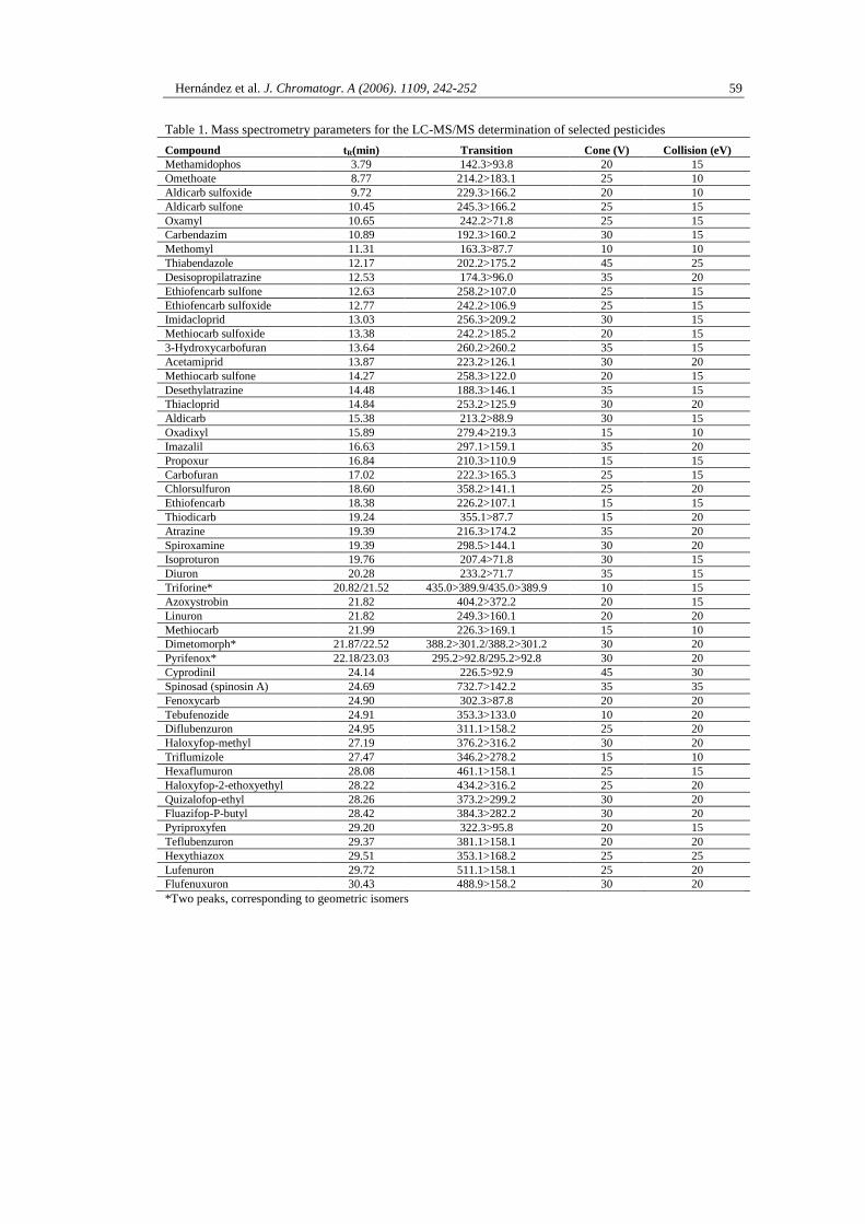
Hernández et al. J. Chromatogr. A (2006). 1109, 242-252 59
Table 1. Mass spectrometry parameters for the LC-MS/MS determination of selected pesticides
Compound tR(min) Transition Cone (V) Collision (eV)
Methamidophos 3.79 142.3>93.8 20 15
Omethoate 8.77 214.2>183.1 25 10
Aldicarb sulfoxide 9.72 229.3>166.2 20 10
Aldicarb sulfone 10.45 245.3>166.2 25 15
Oxamyl 10.65 242.2>71.8 25 15
Carbendazim 10.89 192.3>160.2 30 15
Methomyl 11.31 163.3>87.7 10 10
Thiabendazole 12.17 202.2>175.2 45 25
Desisopropilatrazine 12.53 174.3>96.0 35 20
Ethiofencarb sulfone 12.63 258.2>107.0 25 15
Ethiofencarb sulfoxide 12.77 242.2>106.9 25 15
Imidacloprid 13.03 256.3>209.2 30 15
Methiocarb sulfoxide 13.38 242.2>185.2 20 15
3-Hydroxycarbofuran 13.64 260.2>260.2 35 15
Acetamiprid 13.87 223.2>126.1 30 20
Methiocarb sulfone 14.27 258.3>122.0 20 15
Desethylatrazine 14.48 188.3>146.1 35 15
Thiacloprid 14.84 253.2>125.9 30 20
Aldicarb 15.38 213.2>88.9 30 15
Oxadixyl 15.89 279.4>219.3 15 10
Imazalil 16.63 297.1>159.1 35 20
Propoxur 16.84 210.3>110.9 15 15
Carbofuran 17.02 222.3>165.3 25 15
Chlorsulfuron 18.60 358.2>141.1 25 20
Ethiofencarb 18.38 226.2>107.1 15 15
Thiodicarb 19.24 355.1>87.7 15 20
Atrazine 19.39 216.3>174.2 35 20
Spiroxamine 19.39 298.5>144.1 30 20
Isoproturon 19.76 207.4>71.8 30 15
Diuron 20.28 233.2>71.7 35 15
Triforine* 20.82/21.52 435.0>389.9/435.0>389.9 10 15
Azoxystrobin 21.82 404.2>372.2 20 15
Linuron 21.82 249.3>160.1 20 20
Methiocarb 21.99 226.3>169.1 15 10
Dimetomorph* 21.87/22.52 388.2>301.2/388.2>301.2 30 20
Pyrifenox* 22.18/23.03 295.2>92.8/295.2>92.8 30 20
Cyprodinil 24.14 226.5>92.9 45 30
Spinosad (spinosin A) 24.69 732.7>142.2 35 35
Fenoxycarb 24.90 302.3>87.8 20 20
Tebufenozide 24.91 353.3>133.0 10 20
Diflubenzuron 24.95 311.1>158.2 25 20
Haloxyfop-methyl 27.19 376.2>316.2 30 20
Triflumizole 27.47 346.2>278.2 15 10
Hexaflumuron 28.08 461.1>158.1 25 15
Haloxyfop-2-ethoxyethyl 28.22 434.2>316.2 25 20
Quizalofop-ethyl 28.26 373.2>299.2 30 20
Fluazifop-P-butyl 28.42 384.3>282.2 30 20
Pyriproxyfen 29.20 322.3>95.8 20 15
Teflubenzuron 29.37 381.1>158.1 20 20
Hexythiazox 29.51 353.1>168.2 25 25
Lufenuron 29.72 511.1>158.1 25 20
Flufenuxuron 30.43 488.9>158.2 30 20
*Two peaks, corresponding to geometric isomers

Hernández et al. J. Chromatogr. A (2006). 1109, 242-252 60
Table 2. Mass spectrometry parameters for the LC–MS/MS confirmation of carbendazim, carbofuran,
thiodicarb and fenoxycarb
Precursor ion
(m/z)
Cone voltage (V) Product ion
(m/z)
Collision energy
(eV)
Relative abundance
(%)
Carbendazim
192a 30a 160a 15a 100
132 30 19
105 35 14
92 35 7
90 40 7
65 45 8
160 55 132 20 91
105 25 63
92 25 32
90 30 35
65 35 43
Carbofuran
222a 25a 165a 15a 100
123 20 95
91 35 6
54 25 9
165 45 123 15 67
54 15 7
Thiodicarb
355a 15a 88a 20a 100
108 15 54
149 10 18
163 10 22
Fenoxycarb
302a 20a 88a 20a 100
43 35 8
116 10 99
256 15 16 a Quantification transition.
3.3. LC optimization
Regarding to LC separation, the gradient was optimized in order to render a rough
separation between the 52 selected analytes, obtaining less than 10 compounds monitored
simultaneously per a 3–4 min time window. In this way, using a dwell time of 0.1 s per
transition, we obtained satisfactory peak shape for all analytes. Distributing the analytes along
30 overlapping functions allowed us to center the chromatographic peak in the time window,
minimizing the risk of peak loss due to unexpected slight changes in retention time. The
retention times are shown in Table 1 and they corresponded to analytes from high polarities,
as metamidophos (tR = 3.8 min) to non-polar, as flufenoxuron (tR = 30.4 min). The gradient

Hernández et al. J. Chromatogr. A (2006). 1109, 242-252 61
used (see Section 2) gave satisfactory separation and also resolved adequately geometric
isomers present for three analytes, triforine, dimetomorph and pyrifenox.
3.4. Sample treatment optimization
The general analytical methodology applied for sample preparation was a conventional
extraction with organic solvent followed by extract purification with SPE.
In the SPE step, Oasis HLB cartridges were selected due to their reversed-phase
capabilities combined with a special polar-hook for enhanced capture of polar analytes and
excellent wettability. Due to the high polarity of some compounds, 200 mg sorbent was
selected to minimize breakthrough. The loading of cartridges was performed using aqueous
standard solutions containing 20% of different organic solvents (acetonitrile, acetone and
MeOH). After selecting MeOH, which gave the minimum breakthrough, different percentage
of MeOH were studied, obtaining the best results for 10% MeOH.
The extraction step was not thoroughly optimized and it was performed using a mixture
MeOH:H2O, (80:20, v/v) for all samples selected. As the initial sample extract contained high
percentage of MeOH, a dilution step was required before loading the sample onto the
cartridge. An eight-fold dilution factor was selected to decrease the methanol content down to
10% in order to minimize breakthrough for the most polar analytes in the subsequent SPE
cleanup step. This sample dilution together with the effectiveness of Oasis HLB clean up was
an efficient way to homogenize samples from different origin, minimizing the possible
variability between samples, which can compromise the quantification as observed by Jansson
et al. [18]. In addition, the volume adjustment of sample extract up to 100 mL MeOH:H2O
(80:20, v/v) and the subsequent eight-fold dilution with water of an aliquot minimized
possible variations in matrix water content.
Several problems were observed along sample treatment, such as the degradation of
some analytes (aldicarb, ethiofencarb and methiocarb), partial losses during the evaporation
step for the late eluting compounds and the not complete SPE elution for spiroxamine. The
degradation of carbamates was not observed by Jansson et al. [18] which used ethyl acetate
for extraction; therefore, this degradation might be associated to the use of methanol as
extracting solvent. This problem was minimized by acidification of the extraction solvent,
which also served to improve the SPE elution of spiroxamine. Finally, partial losses were

Hernández et al. J. Chromatogr. A (2006). 1109, 242-252 62
observed when the SPE eluate (MTBE/MeOH 0.1% HCOOH, 9:1) was evaporated to dryness
at 40 °C under a gentle nitrogen stream. This effect has been scarcely reported until now
despite the common use of a evaporation step in previously reported methods. In our case,
losses were observed mainly for the ten late-eluting analytes (see Table 1). The addition of
0.5 mL of water as a holder before evaporation, allowed us to minimize these problems.
3.5. Validation
The method developed was validated for the four matrices studied in this work: raisin,
tomato, avocado and lemon. The validation scheme followed was based on the SANCO
European Guidelines [26].
Matrix-matched calibration curves prepared in every type of sample showed good
linearity between 10 and 500 ng/mL, with a correlation coefficient ≥0.99. The specificity of
the method was tested by the analysis of blank samples. The absence of any chromatographic
peak in every matrix, at the same retention times as target pesticides, indicated that there were
no matrix compounds that might give a false positive signal in these blank samples. However,
in real unknown samples, the risk of reporting false positives still exits and an additional
confirmation step would be necessary.
The accuracy of the method was estimated by means of recovery experiments at two
concentration levels (0.01 and 0.1 mg/kg). All experiments were carried out in quintuplicate
at each level (Table 3). For all matrices, the results obtained for most of the compounds were
satisfactory, with recoveries between 70–110% and coefficients of variation (CV) below 15%.
Only three pesticides presented lower recoveries in the four matrices studied: the high polar
methamidophos, due to the breakthrough in the SPE process, and aldicarb and ethiofencarb
owing to their partial degradation during sample pre-treatment.
As it can be observed in Table 3, several of the less polar compounds (the late eluting
analytes) showed low recoveries (<60%) mainly in avocado samples, probably due to its high
lipid content which makes more difficult to extract this type of pesticide from the sample with
the used mixture (MeOH:H2O, 80:20, v/v). The poor recoveries for some less polar analytes
also illustrate the difficulties of development a unique multiresidue method for the
determination of a number of pesticides with a wide range of polarities. For those compounds
with poor recoveries, the method could be used for screening and confirmation of all analytes

Hernández et al. J. Chromatogr. A (2006). 1109, 242-252 63
in all matrices. But, even quantification would be feasible in the light of the satisfactory
precision by applying the adequate correction factors. The lowest level validated, i.e.
0.01 mg/kg, was taken as the LOQ value.
As an example, Fig. 2 shows the LC–MS/MS chromatograms for ten representative
analytes with quite different polarities at the LOQ level in lemon sample. It can be observed
the excellent sensitivity for all these compounds and some interesting aspects of the
developed method, such as the detection of methamidophos at the 0.01 mg/kg level despite its
low recovery or the chromatographic resolution of the two isomers of triforine.
In relation to quantification, several experiments were also performed to check for matrix
interferences. After the sample treatment performed, no significant matrix effects were
observed for any of the vegetable matrices analysed. In spite of this, we preferred to perform
the quantification using calibration with matrix-matched standards to prevent slight variations
in the MS signal for some analytes and unexpected enhancement or signal suppressions in real
samples.
According to our data, the LC–MS/MS method developed allows the rapid screening and
quantification of 52 pesticides and metabolites in a variety of food matrices. These results are
in the line of others reported in recent methods published in the literature [16], [17], [18], [19]
and [20] and confirm that LC–MS/MS is an attractive and powerful technique for the
quantitative determination of pesticide residues.

Hernández et al. J. Chromatogr. A (2006). 1109, 242-252 64
Table 3. Mean recoveries and coefficients of variation in brackets (n=5) obtained after
applying the LC-MS/MS procedure to different samples spiked at two concentration levels.
Compound Tomato Lemon Raisin Avocado
0.01
mg/kg
0.1
mg/kg
0.01
mg/kg
0.1
mg/kg
0.01
mg/kg
0.1
mg/kg
0.01
mg/kg
0.1
mg/kg
Methamidophos 33 (11) 38 (11) 23 (9) 35 (7) 40 (10) 28 (14) 41 (8) 42 (4)
Omethoate 93 (6) 91 (8) 87 (8) 89 (4) 81 (8) 67 (5) 81 (4) 84 (4)
Aldicarb sulfoxide 131 (7) 119 (8) 95 (7) 103 (2) 99 (11) 98 (13) 107 (5) 111 (6)
Aldicarb sulfone 96 (9) 97 (7) 85 (8) 85 (7) 90 (15) 76 (11) 87 (6) 92 (13)
Oxamyl 94 (8) 94 (4) 89 (6) 86 (3) 88 (4) 76 (7) 87 (6) 90 (8)
Carbendazim 96 (6) 87 (7) 82 (6) 82 (2) 89 (6) 72 (9) 85 (9) 84 (8)
Methomyl 94 (12) 85 (4) 81 (12) 85 (5) 80 (7) 63 (3) 105 (4) 90 (11)
Thiabendazole 95 (8) 103 (7) 85 (6) 85 (6) 84 (11) 70 (6) 75 (6) 133 (5)
Desisopropilatrazine 88 (10) 86 (6) 81 (8) 87 (7) 84 (4) 70 (8) 80 (11) 90 (5)
Ethiofencarb sulfone 130 (9) 101 (6) 87 (8) 88 (6) 93 (7) 75 (6) 86 (8) 84 (9)
Ethiofencarb sulfoxide 115 (10) 119 (6) 109 (9) 105 (5) 107 (10) 97 (6) 89 (5) 91 (5)
Imidacloprid 96 (14) 87 (7) 100 (11) 93 (4) 88 (11) 67 (4) 87 (9) 88 (4)
Methiocarb sulfoxide 104 (11) 92 (6) 94 (8) 90 (2) 95 (7) 74 (6) 85 (10) 85 (3)
3-Hydroxycarbofuran 89 (15) 92 (6) 86 (16) 87 (7) 103 (16) 75 (15) 92 (11) 79 (8)
Acetamiprid 95 (6) 87 (6) 93 (6) 87 (2) 90 (4) 72 (4) 84 (2) 84 (5)
Methiocarb sulfone 96 (4) 90 (5) 92 (10) 87 (3) 91 (7) 77 (4) 87 (10) 84 (5)
Desethylatrazine 83 (11) 83 (5) 84 (5) 84 (6) 106 (11) 73 (5) 93 (24) 87 (7)
Thiacloprid 95 (14) 87 (5) 89 (7) 88 (4) 88 (6) 73 (6) 84 (5) 85 (7)
Aldicarb 31 (16) 45 (4) 58 (8) 71 (4) 58 (10) 42 (9) 60 (10) 61 (7)
Oxadixyl 89 (11) 80 (6) 96 (11) 92 (8) 89 (6) 76 (7) 90 (8) 92 (4)
Imazalil 95 (12) 74 (6) 106 (6) 83 (11) 84 (5) 66 (5) 85 (14) 75 (6)
Propoxur 76 (12) 72 (10) 83 (6) 84 (7) 77 (8) 60 (7) 78 (12) 74 (6)
Carbofuran 81 (11) 75 (6) 90 (5) 85 (4) 82 (8) 67 (5) 81 (6) 79 (6)
Chlorsulfuron 43 (11) 58 (7) 115 (2) 83 (4) 80 (8) 84 (4) 88 (5) 88 (7)
Ethiofencarb 31 (6) 23 (5) 106 (4) 38 (8) 27 (15) 13 (13) 47 (13) 34 (9)
Thiodicarb 85 (13) 61 (8) 76 (7) 63 (6) 95 (5) 75 (5) 72 (9) 66 (10)
Spiroxamine 72 (7) 64 (6) 83 (5) 89 (6) 82 (6) 73 (5) 85 (7) 82 (6)
Atrazine 81 (5) 78 (3) 84 (3) 85 (4) 86 (3) 71 (6) 83 (4) 85 (7)
Isoproturon 87 (8) 81 (1) 90 (5) 87 (3) 88 (7) 73 (5) 87 (7) 86 (4)
Diuron 95 (15) 82 (4) 88 (7) 87 (5) 91 (9) 72 (6) 88 (10) 86 (5)
Triforine 1 58 (15) 71 (10) 75 (14) 82 (6) 91 (15) 75 (7) 86 (9) 89 (5)
Triforine 2 84 (14) 74 (11) 88 (19) 83 (9) 98 (13) 75 (6) 81 (8) 84 (4)
Azoxystrobin 95 (7) 83 (5) 95 (5) 88 (4) 94 (8) 76 (6) 94 (7) 87 (2)
Dimethomorph 1 108 (15) 92 (4) 111 (7) 103 (4) 105 (5) 86 (7) 100 (6) 96 (1)
Dimethomorph 2 101 (10) 76 (4) 93 (6) 83 (4) 91 (7) 73 (6) 90 (7) 84 (3)
Linuron 86 (12) 75 (6) 94 (7) 86 (5) 85 (9) 71 (5) 78 (13) 77 (3)
Methiocarb 81 (8) 73 (8) 92 (7) 85 (5) 83 (5) 68 (7) 80 (9) 77 (2)
Pyrifenox 1 86 (11) 76 (5) 83 (4) 79 (7) 79 (5) 68 (5) 79 (8) 78 (3)
Pyrifenox 2 86 (6) 75 (6) 87 (4) 83 (6) 82 (10) 71 (4) 83 (5) 77 (4)
Cyprodinil 86 (9) 74 (7) 88 (4) 82 (7) 84 (8) 73 (1) 50 (7) 55 (5)
Spinosad (spinosin A) 137 (8) 67 (20) 113 (12) 99 (7) 86 (12) 68 (12) 122 (2) 89 (4)
Fenoxycarb 89 (5) 76 (2) 101 (6) 90 (2) 88 (9) 86 (7) 47 (15) 64 (9)
Tebufenozide 104 (14) 77 (4) 100 (15) 85 (11) 91 (6) 80 (4) 92 (6) 84 (3)
Diflubenzuron 101 (12) 77 (3) 101 (13) 88 (4) 82 (14) 83 (9) 60 (18) 64 (9)
Haloxyfop-methyl 85 (3) 71 (11) 90 (8) 89 (2) 86 (11) 78 (7) 37 (23) 48 (10)
Triflumizole 12 (15) 30 (10) 14 (18) 79 (8) 71 (14) 98 (6) 20 (16) 72 (6)
Hexaflumuron 50 (30) 55 (20) 129 (15) 120 (9) 92 (15) 125 (9) 96 (12) 57 (7)
Haloxyfop-2-ethoxyethyl 101 (5) 74 (10) 100 (6) 97 (3) 78 (16) 80 (8) 48 (9) 49 (8)
Fluazifop-P-butyl 98 (10) 64 (14) 131 (6) 108 (5) 102 (3) 95 (10) 56 (11) 48 (8)
Quizalofop-ethyl 78 (12) 67 (8) 91 (4) 92 (2) 74 (5) 86 (9) 29 (14) 39 (7)
Pyriproxyfen 53 (21) 60 (13) 74 (12) 83 (4) 72 (6) 85 (10) 14 (15) 38 (4)
Lufenuron 102 (15) 45 (11) 146 (6) 113 (7) 111 (12) 112 (13) 128 (14) 72 (7)
Teflubenzuron 70 (9) 69 (6) 96 (16) 100 (9) 78 (16) 94 (6) 121 (12) 46 (7)
Hexythiazox 66 (13) 56 (3) 92 (8) 101 (7) 74 (7) 102 (14) 19 (35) 38 (6)
Flufenoxuron 101 (10) 43 (10) 117 (7) 105 (10) 122 (28) 108 (17) 77 (22) 57 (3)

Hernández et al. J. Chromatogr. A (2006). 1109, 242-252 65
Fig. 2. LC–MS/MS chromatograms for ten representative pesticides studied in lemon spiked at
0.01 mg/kg.
Time5.00 10.00 15.00
%
0
100
PRE678 1: MRM of 1 Channel ES+ 142.3 > 93.8
3.00e3
Time5.00 10.00 15.00
%
0
100
PRE687 1: MRM of 1 Channel ES+ 142.3 > 93.8
3.00e3Area
3.7294.2
Time5.00 10.00 15.00
%
0
100
PRE691 1: MRM of 1 Channel ES+ 142.3 > 93.8
3.00e3Area
3.66516.6
Time5.00 10.00 15.00
%
0
100
PRE691 2: MRM of 1 Channel ES+ 214.2 > 183.1
5.00e3Area
8.33500.8
Time5.00 10.00 15.00
%
0
100
PRE687 2: MRM of 1 Channel ES+ 214.2 > 183.1
5.00e3Area
8.33332.3
Time5.00 10.00 15.00
%
0
100
PRE678 2: MRM of 1 Channel ES+ 214.2 > 183.1
5.00e3
Time10.00 20.00
%
0
100
PRE691 6: MRM of 4 Channels ES+ 258.2 > 107
2.00e3Area
12.27171.4
Time10.00 20.00
%
0
100
PRE687 6: MRM of 4 Channels ES+ 258.2 > 107
2.00e3Area
12.22117.6
Time10.00 20.00
%
0
100
PRE678 6: MRM of 4 Channels ES+ 258.2 > 107
2.00e3
13.86
Time10.00 20.00
%
0
100
PRE691 6: MRM of 4 Channels ES+ 242.2 > 106.9
8.00e3Area
12.42806.9
Time10.00 20.00
%
0
100
PRE687 6: MRM of 4 Channels ES+ 242.2 > 106.9
8.00e3Area
12.38603.9
Time10.00 20.00
%
0
100
PRE678 6: MRM of 4 Channels ES+ 242.2 > 106.9
8.00e3
Time10.00 20.00
%
0
100
PRE691 7: MRM of 3 Channels ES+ 260.2 > 260.2
1.20e4Area13.33
1025.3
Time10.00 20.00
%
0
100
PRE687 7: MRM of 3 Channels ES+ 260.2 > 260.2
1.20e4Area13.33
924.0
Time10.00 20.00
%
0
100
PRE691 13: MRM of 2 Channels ES+ 226.2 > 107.1
5.00e3Area
17.92465.8
Time10.00 20.00
%
0
100
PRE687 13: MRM of 2 Channels ES+ 226.2 > 107.1
5.00e3Area
17.93175.0
Time10.00 20.00
%0
100
PRE678 13: MRM of 2 Channels ES+ 226.2 > 107.1
5.00e3
Time20.00 30.00
%
0
100
PRE691 17: MRM of 1 Channel ES+ 435 > 389.9
250Area21.02
34.720.2932.6
Time20.00 30.00
%
0
100
PRE687 17: MRM of 1 Channel ES+ 435 > 389.9
250Area
20.3722.4
20.9818.2
Time20.00 30.00
%
0
100
PRE678 17: MRM of 1 Channel ES+ 435 > 389.9
250
21.2920.37
Time20.00 30.00
%
0
100
PRE691 23: MRM of 1 Channel ES+ 732.7 > 142.2
4.00e3Area
24.312230.0
Time20.00 30.00
%
0
100
PRE687 23: MRM of 1 Channel ES+ 732.7 > 142.2
4.00e3Area
24.452000.6
Time20.00 30.00
%
0
100
PRE678 23: MRM of 1 Channel ES+ 732.7 > 142.2
4.00e3
Time20.00 30.00
%
0
100
PRE691 27: MRM of 4 Channels ES+ 373.2 > 299.2
1.10e4Area
27.801138.3
Time20.00 30.00
%
0
100
PRE687 27: MRM of 4 Channels ES+ 373.2 > 299.2
1.10e4Area
27.80754.8
Time20.00 30.00
%
0
100
PRE678 27: MRM of 4 Channels ES+ 373.2 > 299.2
1.10e4
Time20.00 30.00
%
0
100
PRE691 30: MRM of 1 Channel ES+ 488.9 > 158.2
1.50e3Area
29.96118.1
Time20.00 30.00
%
0
100
PRE687 30: MRM of 1 Channel ES+ 488.9 > 158.2
1.50e3Area
29.96155.9
Time20.00 30.00
%
0
100
PRE678 30: MRM of 1 Channel ES+ 488.9 > 158.2
1.50e3Area
30.0136.6
Time10.00 20.00
%
0
100
PRE678 7: MRM of 3 Channels ES+ 260.2 > 260.2
1.20e4
13.73
Methamidophos
Omethoate
Ethiofencarb sulfoxide
Ethiofencarb sulfone
3-Hydroxy Carbofuran
Ethiofencarb
Triforine
Spinosad
Quizalofop-ethyl
Flufenoxuron
1.5 ng/mL matrix-matched
standard
Lemon spiked 0.01 mg/Kg
(final extract 1.2 ng/mL) Blank lemon

Hernández et al. J. Chromatogr. A (2006). 1109, 242-252 66
3.6. Confirmation
Despite the high specificity of LC–MS/MS, there is still a risk of reporting false positives
when analyzing real samples owing to the acquisition of only one MS/MS transition. The
complexity of vegetable matrices might make feasible the occurrence of other compounds
sharing the same precursor and product ion with a similar retention time. Moreover, the
absence of any peak in a specific blank sample cannot be taken as an unequivocal way to
discard false positive findings due to high variability observed even in a same type of sample
[18]. The confirmation of positive findings is needed mainly in violative cases, i.e. samples
where the analyte concentration is above the MRL.
The acquisition of at least two transitions is required for reliable confirmation and it has
been proved as a good approach for this purpose [16]. The confirmation performed in this
way usually requires an additional injection due to the high number of transitions needed for
the simultaneous quantification and confirmation. This was our case, where the simultaneous
acquisition of two transitions for each compound would lead to a method monitoring more
than hundred transitions, which would reduce the number of points per peak leading to
unsatisfactory peak shapes. This limitation might be overcome by the use of new generation
instruments, which can reduce the dwell time for each transition without any loss in
sensitivity allowing to increase the number of transitions acquired simultaneously.
The acquisition of two transitions allows reaching four or five IPs, which is accepted as
sufficient for the confirmation of registered and even banned compounds [23]. However, if
one of the transitions is interfered by a matrix component, the calculated ion ratio in the
sample would be different to that of the reference standard making the confirmation
troublesome. This situation is undoubtedly minimized by the acquisition of more transitions,
if available. Therefore, we decided to use the maximum number of available transitions for
each compound in order to have an ultimate confirmation of the presence of the analyte. Thus,
the cone voltage and collision energy were optimized for each available transition, generating
a specific confirmation method for each selected compound. As an example, Fig. 1A and B
show the optimization of fragmentation for carbendazim. From these data a confirmatory
method for this analyte was set up as can be seen in Table 2. This is one of the most favorable
cases, where up to 11 transitions could be optimized including 5 obtained from an in-source
fragment (used a parent ion) at m/z 160.

Hernández et al. J. Chromatogr. A (2006). 1109, 242-252 67
Fig. 3 shows the chromatograms for a blank raisin sample spiked at 0.01 mg/kg level
with carbendazim. Despite the low abundance for some selected confirmatory transitions
(<10%), the high sensitivity of the method allowed the detection of all selected transitions
even at this low concentration level. Additionally, the ion ratios calculated for the spiked
sample were similar to those of the reference standard at all concentrations checked. Thus, the
presence of carbendazim residues can be easily and unequivocally confirmed by a second
injection reaching a number of IPs as high as 18.5, even at the LOQ level.
Fig. 3. LC–MS/MS chromatograms obtained from a blank raisin sample spiked at 0.01 mg/kg level with
carbendazim. (A) Chromatograms corresponding to SRM optimized with cone value of 30 V. (B)
Chromatograms corresponding to SRM optimized with cone value of 55 V (* used for quantification).
Obviously, not all the analytes presented so abundant fragmentation as carbendazim.
Thus, fenoxycarb presented lower fragmentation and only four transitions could be monitored
in the confirmatory method (see Table 2). Although four transitions allowed us to reach seven
IPs, the lower abundance for two of them hindered the ultimate confirmation of fenoxycarb at
low concentration levels. However, for most of selected analytes, we optimized at least four
transitions, making their confirmation extremely confident.
Time10.00 12.00
%
0
100
10.00 12.00
%
0
100
10.00 12.00
%
0
100
10.00 12.00
%
0
100
10.00 12.00
%
0
100
10.00 12.00
%
0
100
CONF0007 1: MRM of 11 Channels ES+ 192.3 > 160.2
4.54e3Area
10.20669.1
CONF0007 1: MRM of 11 Channels ES+ 192.3 > 132.1
746Area
10.22100.3
CONF0007 1: MRM of 11 Channels ES+ 192.3 > 105
685Area
10.2281.2
CONF0007 1: MRM of 11 Channels ES+ 192.3 > 92
227Area
10.2033.4
CONF0007 1: MRM of 11 Channels ES+ 192.3 > 90
383Area
10.2242.2
CONF0007 1: MRM of 11 Channels ES+ 192.3 > 65
550Area
10.2267.9
30V
Time10.00 12.00
%
0
100
10.00 12.00
%
0
100
10.00 12.00%
0
100
10.00 12.00
%
0
100
10.00 12.00
%
0
100
CONF0007 1: MRM of 11 Channels ES+ 160.2 > 132.1
4.07e3Area
10.22546.9
CONF0007 1: MRM of 11 Channels ES+ 160.2 > 105
2.49e3Area
10.22371.2
CONF0007 1: MRM of 11 Channels ES+ 160.2 > 92
1.42e3Area
10.22207.5
CONF0007 1: MRM of 11 Channels ES+ 160.2 > 90
1.48e3Area
10.24224.7
CONF0007 1: MRM of 11 Channels ES+ 160.2 > 65
2.12e3Area
10.22295.5
55V
(A) (B)
*

Hernández et al. J. Chromatogr. A (2006). 1109, 242-252 68
The only analyte that could not be confirmed was 3-hydroxycarbofuran, as its [M + Na]+
precursor ion did not present any abundant selective fragment. With the aim to confirm this
type of analytes, ammonium acetate could be added into the mobile phase in order to promote
the [M + H]+ or [M + NH4]
+ formation, favoring its fragmentation and the number of
available transitions.
4. Conclusions
A multiresidue method has been developed for the reliable screening, quantification and
confirmation of 52 pesticides and metabolites in different food commodities by LC–MS/MS
using a triple quadrupole analyzer. The procedure, based on a SPE step using Oasis HLB
cartridges previously to the determination by LC–MS/MS, has been validated based on the
SANCO European Guidelines for representative species from different commodity groups
(tomato, lemon, raisin and avocado), obtaining satisfactory accuracy and precision for most of
analyte/matrix combinations. A value of 0.01 mg/kg has been established as LOQ (the lowest
concentration level fully validated using the overall analytical procedure), although several
pesticides could be quantified at lower levels if required.
The proposed LC–MS/MS methodology allows the simultaneous determination of
pesticides and their metabolites of very different chemical families and physico-chemical
properties in one single determination step, monitoring the most sensitive transition for every
compound. Confirmation of pesticides detected in samples is performed by an independent
second injection into the LC–MS/MS system by acquiring the highest number of MS/MS
transitions available.
As a result of its high sensitivity and selectivity, LC–MS/MS has shown its strong
potential in the field of pesticide residue analysis. This technique is gaining interest and
popularity within this field as a powerful analytical tool in multiresidue methods. A drastic
growth in the applications and on the use of LC–MS/MS in pesticide residue laboratories is
expected in the near future.

Hernández et al. J. Chromatogr. A (2006). 1109, 242-252 69
Acknowledgements
The Quattro Micro LC–MS/MS was funded by the European Union (Fondos Feder-
Reino de España, Ministerio de Ciencia y Tecnología, Ref: UNJM-E004). This work forms a
part of the project ―Determination of pesticide residues in fruit and vegetables‖ developed
with the financial support of Waters Cromatografía S.A. (Barcelona, Spain).
References
[1] Directive 91/414/EEC, Off. J. Eur. Commun., 14 July 1991.
[2] O.J. Pozo, J.M. Marin, J.V. Sancho and F. Hernández, J. Chromatogr. A 992 (2003), p.
133.
[3] S. Grimalt, O.J. Pozo, J.M. Marín, J.V. Sancho and F. Hernández, J. Am. Soc. Mass
Spectrom. 16 (2005), p. 1619.
[4] D.A. Schwedler, A.D. Thomas and L.T. Yeh, J. Agric. Food Chem. 48 (2000), p. 5138.
[5] A.C. Hogenboom, M.P. Hofman, S.J. Kok, W.M.A. Niessen and U.A.T. Brinkman, J.
Chromatogr. A 892 (2000), p. 379.
[6] K. Bester, G. Bordin, A. Rodriguez, H. Schimmel, J. Pauwels and G. van Vyncht,
Fresenius J. Anal. Chem. 371 (2001), p. 550.
[7] D. Perret, A. Gentili, S. Marchese, M. Sergi and G. D’Ascenzo, J. AOAC Int. 85 (2002), p.
724.
[8] M.J. Taylor, K. Hunter, K.B. Hunter, D. Lindsay and S.L. Bouhellec, J. Chromatogr. A
982 (2002), p. 225.
[9] H.G.J. Mol, R.C.J. van Dam and O.M. Steijger, J. Chromatogr. A 1015 (2003), p. 119.
[10] A. Garrido, J.L. Martínez, T. López, S. Cortés and I. Martínez, J. Chromatogr. A 1048
(2004), p. 199.
[11] A. Aguera, S. López, A.R. Fernández-Alba, M. Contreras, J. Crespo and L. Piedra, J.
Chromatogr. A 1045 (2004), p. 125.
[12] K. Granby, J.H. Andersen and H.B. Christensen, Anal. Chim. Acta 520 (2004), p. 165.
[13] T. Zamora, O.J. Pozo, F. López and F. Hernández, J. Chromatogr. A 1045 (2004), p.
137.
[14] A. Sannino, L. Bolzoni and M. Bandini, J. Chromatogr. A 1036 (2004), p. 161.
[15] S.J. Lehotay, K. Mastovska and S.J. Yun, J. AOAC Int. 88 (2005), p. 630.
Hernández et al. J. Chromatogr. A (2006). 1109, 242-252 70
[16] D. Ortelli, P. Edder and C. Corvi, Anal. Chim. Acta 520 (2004), p. 33.
[17] L. Alder, S. Luderitz, K. Lindtner and H.J. Stan, J. Chromatogr. A 1058 (2004), p. 67.
[18] C. Jansson, T. Pihlström, B.-G. Österdahl and K.E. Markides, J. Chromatogr. A 1023
(2004), p. 93.
[19] C.L. Hetherton, M.D. Sykes, R.J. Fussell and D.M. Goodall, Rapid Commun. Mass
Spectrom. 18 (2004), p. 2443.
[20] S.J. Lehotay, A. de Kok, M. Hiemstra and P. van Bodegraven, J. AOAC Int. 88 (2005), p.
595.
[21] B.K. Matuszewski, M.L. Constanzer and C.M. Chvez-Eng, Anal. Chem. 70 (1998), p.
882.
[22] J.V. Sancho, O.J. Pozo, F.J. López and F. Hernández, Rapid Commun. Mass Spectrom.
16 (2002), p. 639.
[23] European Commission Decision 2002/657/EC, Off. J. Eur. Commun., 21 August 2002.
[24] F. Hernández, M. Ibáñez, J.V. Sancho and O.J. Pozo, Anal. Chem. 76 (2004), p. 4349.
[25] F. Hernández, O.J. Pozo, J.V. Sancho, F.J. López, J.M. Marín and M. Ibáñez, Trends
Anal. Chem. 24 (2005), p. 596.
[26] European Comission, directorate General Health and Consumer Protection, Comission
working document SANCO/10476/2003, Quality Control Procedures for Pesticide
Residues Analysis, 5 February 2004.
[27] F. Hernández, J.V. Sancho, O. Pozo, C. Villaplana, M. Ibáñez and S. Grimalt, J. AOAC
Int. 86 (2003), p. 832.
[28] J.V. Sancho, M. Ibáñez, S. Grimalt, O. Pozo and F. Hernández, Anal. Chim. Acta 530
(2005), p. 237.
Presented at the 1st International Workshop on Liquid Chromatography-Tandem Mass Spectrometry
for Screening and Trace Level Quantitation in Environmental and Food Samples, Barcelona,
Spain, 20–21 June 2005.

1.1.3. ARTÍCULO CIENTÍFICO 2
Multiresidue pesticide analysis of fruits by ultra-performance liquid chromatography
tandem mass spectrometry
O.J. Pozo, M. Barreda, J.V. Sancho, F. Hernández, J. Ll. Lliberia, M.A. Cortés, B. Bagó
Analytical and Bioanalytical Chemistry. (2007). 389, 1795-1771


Pozo et al. Anal. Bioanal. Chem. (2007). 389, 1765-1771 73
Multiresidue pesticide analysis of fruits by ultra-performance
liquid chromatography tandem mass spectrometry
Pozo, O.J.a , Barreda, M.a , Sancho, J.V.a , Hernández, F.a , Ll Lliberia, J.b , Cortés, M.A.b , Bagó, B.b
a Research Institute for Pesticides and Water, University Jaume I, Castellón, Spain
b Waters Corporation, Spain, Parc Tecnològic del Vallès, Ronda de Can Fatjó, 7-A,
08290 Cerdanyola del Vallès,
Abstract
Ultra-performance liquid chromatography coupled to tandem mass spectrometry (UPLC–
MS–MS) has been used for screening and quantification of 32 pesticides and metabolites in
two fruit matrices. The compounds investigated belonged to different chemical families of
insecticides, acaricides, fungicides, and herbicides; several metabolites were also included.
Quantification was conducted using matrix-matched standards calibration; response was a
linear function of concentration in the range tested (10–500 ng mL−1
). The method was
validated with blank samples of lemon and raisin spiked at 0.01 and 0.1 mg kg−1
, and
recoveries were satisfactory, between 70 and 110%, for most of the pesticides tested and
relative standard deviations were below 15% (n = 5 at each spiking level). Excellent
sensitivity resulted in limits of detection for all compounds well below 0.01 mg kg−1
, with the
limit of quantification being validated at 0.01 mg kg−1
. The UPLC system generates narrow
peaks (approx. 5 s), thus increasing peak height and improving sensitivity. This improved
separation efficiency facilitates adequate resolution not only of the analytes but also of matrix
interferences compared with conventional HPLC. The method developed could also resolve
some geometric isomers. The main advantage of this approach is the high sample throughput
achieved because of the short analysis time, which enables satisfactory separation of all the
compounds in less than 5 min per sample.
Keywords: UPLC, Pesticides, Metabolites, Multiresidue analysis, Tandem mass
spectrometry, Fruits

Pozo et al. Anal. Bioanal. Chem. (2007). 389, 1765-1771 74
Introduction
In recent years LC tandem mass spectrometry (LC–MS–MS) has become a powerful tool
for pesticide-residue analysis (PRA) in a variety of complex matrices, because of its already
known advantages—high selectivity and sensitivity, substantial reduction of sample-treatment
steps compared with other, more conventional, techniques, for example GC–MS, LC–UV, or
LC–FD, and reliable quantification and confirmation at the low concentrations required [1–4].
There is a growing demand for high sample throughput, so some strategies have been
developed to reduce separation time without compromising separation quality and the
quantity of the analytical data generated [5, 6]. In this way, some technological developments
have been introduced to achieve these objectives, and systems using smaller stationary phase
particles (<1.7 μm), different bridging structure of the column packing and high-pressure
systems have become commercially available. This new technology has been called ultra-
performance liquid chromatography (UPLC) [7–9]. It uses higher linear velocities, and
therefore faster run times, and increased sensitivity and improved peak resolution are
achieved, which are of particular interest in the analysis of complex matrices [5, 10]. The only
requirement when coupling to tandem mass spectrometry is to achieve rapid data acquisition,
so the improved resolution is not degraded.
Although UPLC technology was launched only recently, many applications can be found
in the literature, which illustrates the interest in this technique. These applications have
covered different fields, for example pharmaceutical analysis [11, 12] and drug metabolism,
in which identification of metabolites is rather complicated because it involves analysis of
analytes at low concentration in complex matrices, for example biological fluids [13–15].
Petrovic et al. [16] recently showed the advantages of use of UPLC in combination with
tandem MS for environmental analysis of pharmaceuticals—screening and confirmation of 29
analytes in wastewater samples could be achieved in merely ten minutes. This high sample
throughput has also been proved for PRA in water [17]—nine priority pesticides were
separated in less than ten minutes. Pesticide residue analysis in food can also benefit from the
high sample throughput attainable by UPLC methods, keeping the high multi-residue

Pozo et al. Anal. Bioanal. Chem. (2007). 389, 1765-1771 75
capability required for such applications; this was recently demonstrated in two studies
comparing UPLC and LC for PRA in baby foods [6, 18].
The objective of the work discussed in this paper was to perform a preliminary study to
evaluate the potential of UPLC in combination with MS–MS in PRA. Two fruit samples
(lemon and raisin) were chosen and a multiresidue method was used for screening and
quantification of 35 multi-class pesticides and metabolites. The analytes were chosen from
compounds with physicochemical properties incompatible with GC analysis (high polarity,
low volatility, readily thermally degraded).
Experimental
Reagents and chemicals
Pesticides were selected as a variety of multiclass compounds from different families and
as insecticides, acaricides, fungicides, and herbicides. Several relevant metabolites were also
included in the study. Reference standards were purchased from Dr Ehrenstorfer (Augsburg,
Germany) or Riedel–de Haën (Seelze, Germany). HPLC-grade acetone, acetonitrile, methanol
(MeOH), methyl tert-butyl ether (MTBE) and analytical-grade formic acid (HCOOH, content
>98%) were purchased from Scharlab (Barcelona, Spain). HPLC-grade water was obtained by
purifying demineralized water in a Nanopure II system (Barnstead, Newton, MA, USA).
Standard stock solutions were prepared dissolving 50 mg, accurately weighed, in 100 mL
HPLC-grade organic solvent to furnish a final concentration of 500 μg mL−1
. For UPLC–MS
analysis and sample fortification the stock solutions were mixed and diluted with methanol
(0.1% HCOOH) or HPLC-grade water.
Disposable solid-phase extraction (SPE) cartridges containing 200 mg of a copolymer
designed to have a hydrophilic–lipophilic balance (Oasis HLB, 30 μm) were obtained from
Waters (Milford, MA, USA).

Pozo et al. Anal. Bioanal. Chem. (2007). 389, 1765-1771 76
Ultra-performance liquid chromatography
A Waters (Milford, MA, USA) Acquity ultra-performance liquid chromatography
(UPLC) system was interfaced to a triple-quadrupole mass spectrometer (LC–MS–MS).
Chromatographic separation was achieved on a 2.1 mm × 100 mm, 1.7 μm particle size,
Acquity BEH C18 analytical column (Waters). The mobile phase was a gradient prepared from
0.01% HCOOH methanol and 0.01% HCOOH water in which the amount of methanol was
changed linearly as follows: 0 min, 5%; 0.5 min, 5%; 1.8 min, 50%; 4.6 min, 90%; 5.1 min,
90%; and 5.3 min, 5% until 6 min. The flow-rate was 0.6 mL min−1
.
Mass spectrometry
A Waters (Manchester, UK) Quattro Premier mass spectrometer with an orthogonal Z-
Spray-electrospray interface was used. Drying gas and nebulizing gas was nitrogen Alfagaz
B50 (99.999%) from Air Liquide (Madrid, Spain). Desolvation gas flow and cone gas flow
were 650 and 60 L h−1
, respectively.
For operation in MS–MS mode the collision gas was argon C50 (99.999%) from Air
Liquide at a pressure of 6 × 10⁻³
mbar in the collision cell. A capillary potential of 3.5 kV was
used in positive ionization mode. The desolvation temperature was set to 350 °C and the
source temperature to 120 °C. Dwell times of 50 ms were selected. The system was controlled
by Masslynx software (version 4.1). The application manager Quanlynx was used to process
the quantitative data obtained from the calibration standards and from the samples.
Sample procedure
For development of the method two fruit matrices were selected—lemon and raisin.
Samples were purchased from an organic farming grocery.
The sample-treatment procedure has previously been used in our laboratory and is
described elsewhere [4]. Briefly, samples were cut into small pieces and chopped and 20 g
was extracted with MeOH–H2O, 80:20 (v/v) containing 0.1% HCOOH. The extract was
filtered and conveniently diluted, and an aliquot of the diluted extract was passed through a

Pozo et al. Anal. Bioanal. Chem. (2007). 389, 1765-1771 77
polymeric Oasis HLB SPE cartridge. Analysis was performed by injecting 20 μL into the
UPLC–MS–MS system.
Validation study
The validation study was performed on the basis of the European SANCO guideline [19].
Analytical characteristics evaluated were sensitivity, mean recovery (as a measure of
accuracy), precision (expressed as repeatability), and specificity. With this objective, recovery
experiments with spiked blank lemon and raisin samples were performed at two
concentrations. Five replicates were used for each sample matrix and at each spiking level
(0.01 and 0.1 mg kg−1
). Linearity was studied using matrix-matched standards, analyzing each
of them in triplicate at six concentrations between 0.5 and 30 ng mL−1
.
The limit of quantification (LOQ) was established as the lowest concentration tested for
which recovery and precision were satisfactory (70–110% and < 20% RSD, respectively) in
accordance with the criteria established for analysis of pesticide residues in foods [19].
Results and discussion
MS optimization
Individual standard solutions (2 μg mL−1
) were prepared in acetonitrile–H2O, 50:50
containing 0.1% HCOOH for MS optimization. Both full-scan and MS–MS spectra were
acquired to obtain information about the maximum number of transitions available for each
compound. Typically, the quantification transition was selected to achieve maximum
sensitivity, i.e. selecting the most sensitive but also trying to avoid transitions generated by
general, non-specific, losses, for example M−H2O or M−CO2, to improve selectivity. All the
compounds were determined with the ESI in positive-ion mode. The most sensitive results
were always obtained by using [M + H]+ as the precursor ion.
Table 1 shows the MS–MS transitions selected for screening and quantification, with the
most relevant MS settings used for the compounds investigated in this work.

Pozo et al. Anal. Bioanal. Chem. (2007). 389, 1765-1771 78
Table 1. Mass spectrometry conditions for the UPLC-MS-MS determination of the pesticides
Compound tR (min) Precursor ion Product ion Cone (V) Collision
(eV)
Aldicarb sulfoxide 1.25 229 166 20 10
Aldicarb sulfone 1.34 245 166 25 15
Oxamyl 1.39 242 72 25 15
Carbendazim 1.50 192 160 30 15
Methomyl 1.39 163 88 10 10
Thiabendazol 1.64 202 175 45 25
DIA 1.60 174 96 35 20
Imidacloprid 1.72 256 209 30 15
Methiocarb sulfoxide 1.79 242 185 20 15
Acetamiprid 1.86 223 126 30 20
Methiocarb sulfone 1.91 258 122 20 15
DEA 1.96 188 146 35 15
Thiacloprid 1.98 253 126 30 20
Aldicarb 2.08 213 89 30 15
Oxadixyl 2.17 279 219 15 10
Imazalil 2.59 297 159 35 20
Propoxur 2.28 210 111 15 15
Carbofuran 2.31 222 165 25 15
Chlorsulfuron 2.42 358 141 25 20
Thiodicarb 2.47 355 88 15 20
Spiroxamine 3.10 298 144 30 20
Atrazine 2.59 216 174 35 20
Isoproturon 2.66 207 72 30 15
Diuron 2.69 233 72 35 15
Azoxystrobin 2.94 404 372 20 15
Dimetomorpha 3.01/3.14 388 301 30 20
Methiocarb 2.94 226 169 15 10
Pyrifenoxa 3.00/3.10 295 93 30 20
Cyprodinil 3.29 226 93 30 20
Spinosad 3.86 732.4 142 35 35
Fenoxycarb 3.51 302 88 20 20
Tebufonozide 3.48 353 133 10 20
Haloxyfop-methyl 3.90 376 316 30 20
aTwo peaks corresponding to geometric isomers

Pozo et al. Anal. Bioanal. Chem. (2007). 389, 1765-1771 79
Method development and validation
The main objective of this work was to perform a preliminary study to evaluate the
potential of UPLC in combination to tandem MS for multiresidue pesticide analysis in
complex samples. Considering the advantages of this technology, it was expected that a rapid
method, with improved sensitivity and possibly selectivity, would be developed.
The optimized method led to superb resolution between the analytes selected. Use of the
UPLC system enabled analysis of 32 pesticides in less than 5 min (Table 1 and Fig. 1). The
peaks were very narrow (approx. 5 s), in comparison with conventional HPLC, with good
shape, despite the low dwell time selected. This short analysis time results in a method with
high sample throughput.
Fig. 1 UPLC–MS–MS chromatograms obtained from six representative pesticides: (a) blank sample (b)
sample spiked at 0.01 mg kg−1
(1.25 ng mL−1
in the final extract) (c) matrix-matched standard (1.5 ng
mL−1
)
b ca
Carbendazim
Imidacloprid
Oxadixyl
Carbofuran
Atrazine
Tebufonozide
Time0.00 1.00 2.00 3.00 4.00 5.00
%
0
100
4: MRM of 5 Channels ES+192 > 160
2.00e4Area
1.50
935.8
Time0.00 1.00 2.00 3.00 4.00 5.00
%
0
100
4: MRM of 5 Channels ES+192 > 160
2.00e4Area
Time0.00 1.00 2.00 3.00 4.00 5.00
%
0
100
5: MRM of 2 Channels ES+256 > 209
1.50e3Area
Time0.00 1.00 2.00 3.00 4.00 5.00
%
0
100
8: MRM of 2 Channels ES+279 > 219
8.00e3Area
Time0.00 1.00 2.00 3.00 4.00 5.00
%
0
100
9: MRM of 2 Channels ES+222 > 165
9.50e3Area
Time0.00 1.00 2.00 3.00 4.00 5.00
%
0
100
11: MRM of 4 Channels ES+216 > 174
1.25e4Area
Time0.00 1.00 2.00 3.00 4.00 5.00
%
0
100
16: MRM of 3 Channels ES+353 > 133
9.00e3Area
Time0.00 1.00 2.00 3.00 4.00 5.00
%
0
100
5: MRM of 2 Channels ES+256 > 209
1.50e3Area
1.74
47.8
Time0.00 1.00 2.00 3.00 4.00 5.00
%
0
100
8: MRM of 2 Channels ES+279 > 219
8.00e3Area
2.17170.8
Time0.00 1.00 2.00 3.00 4.00 5.00
%
0
100
9: MRM of 2 Channels ES+222 > 165
9.50e3Area
2.30
339.5
Time0.00 1.00 2.00 3.00 4.00 5.00
%
0
100
11: MRM of 4 Channels ES+216 > 174
1.25e4Area
2.59562.9
Time0.00 1.00 2.00 3.00 4.00 5.00
%
0
100
16: MRM of 3 Channels ES+353 > 133
9.00e3Area3.49
232.4
Time0.00 1.00 2.00 3.00 4.00 5.00
%
0
100
4: MRM of 5 Channels ES+192 > 160
2.00e4Area
1.49
900.8
Time0.00 1.00 2.00 3.00 4.00 5.00
%
0
100
5: MRM of 2 Channels ES+256 > 209
1.50e3Area
1.72
69.7
Time0.00 1.00 2.00 3.00 4.00 5.00
%
0
100
9: MRM of 2 Channels ES+222 > 165
9.50e3Area
2.31
356.3
Time0.00 1.00 2.00 3.00 4.00 5.00
%
0
100
11: MRM of 4 Channels ES+216 > 174
1.25e4Area
2.59587.1
Time0.00 1.00 2.00 3.00 4.00 5.00
%
0
100
16: MRM of 3 Channels ES+353 > 133
9.00e3Area
3.48252.9
R A
I S
I N
2.17166.6
Time0.00 1.00 2.00 3.00 4.00 5.00
%
0
100
8: MRM of 2 Channels ES+
279 > 219
8.00e3
Area
Time0.00 1.00 2.00 3.00 4.00 5.00
%
0
100279 > 219
8.00e3
Area
Carbendazim
Imidacloprid
Oxadixyl
Carbofuran
Atrazine
Tebufonozide
Time0.00 1.00 2.00 3.00 4.00 5.00
%
0
100
4: MRM of 5 Channels ES+192 > 160
2.00e4Area
Time0.00 1.00 2.00 3.00 4.00 5.00
%
0
100
4: MRM of 5 Channels ES+192 > 160
2.00e4Area
1.50
935.8
Time0.00 1.00 2.00 3.00 4.00 5.00
%
0
100
4: MRM of 5 Channels ES+192 > 160
2.00e4Area
Time0.00 1.00 2.00 3.00 4.00 5.00
%
0
100
4: MRM of 5 Channels ES+192 > 160
2.00e4Area
Time0.00 1.00 2.00 3.00 4.00 5.00
%
0
100
4: MRM of 5 Channels ES+192 > 160
2.00e4Area
Time0.00 1.00 2.00 3.00 4.00 5.00
%
0
100
5: MRM of 2 Channels ES+256 > 209
1.50e3Area
Time0.00 1.00 2.00 3.00 4.00 5.00
%
0
100
5: MRM of 2 Channels ES+256 > 209
1.50e3Area
Time0.00 1.00 2.00 3.00 4.00 5.00
%
0
100
8: MRM of 2 Channels ES+279 > 219
8.00e3Area
Time0.00 1.00 2.00 3.00 4.00 5.00
%
0
100
8: MRM of 2 Channels ES+279 > 219
8.00e3Area
Time0.00 1.00 2.00 3.00 4.00 5.00
%
0
100
8: MRM of 2 Channels ES+279 > 219
8.00e3Area
Time0.00 1.00 2.00 3.00 4.00 5.00
%
0
100
9: MRM of 2 Channels ES+222 > 165
9.50e3Area
Time0.00 1.00 2.00 3.00 4.00 5.00
%
0
100
9: MRM of 2 Channels ES+222 > 165
9.50e3Area
Time0.00 1.00 2.00 3.00 4.00 5.00
%
0
100
9: MRM of 2 Channels ES+222 > 165
9.50e3Area
Time0.00 1.00 2.00 3.00 4.00 5.00
%
0
100
11: MRM of 4 Channels ES+216 > 174
1.25e4Area
Time0.00 1.00 2.00 3.00 4.00 5.00
%
0
100
11: MRM of 4 Channels ES+216 > 174
1.25e4Area
Time0.00 1.00 2.00 3.00 4.00 5.00
%
0
100
16: MRM of 3 Channels ES+353 > 133
9.00e3Area
Time0.00 1.00 2.00 3.00 4.00 5.00
%
0
100
16: MRM of 3 Channels ES+353 > 133
9.00e3Area
Time0.00 1.00 2.00 3.00 4.00 5.00
%
0
100
16: MRM of 3 Channels ES+353 > 133
9.00e3Area
Time0.00 1.00 2.00 3.00 4.00 5.00
%
0
100
16: MRM of 3 Channels ES+353 > 133
9.00e3Area
Time0.00 1.00 2.00 3.00 4.00 5.00
%
0
100
5: MRM of 2 Channels ES+256 > 209
1.50e3Area
Time0.00 1.00 2.00 3.00 4.00 5.00
%
0
100
5: MRM of 2 Channels ES+256 > 209
1.50e3Area
1.74
47.8
Time0.00 1.00 2.00 3.00 4.00 5.00
%
0
100
8: MRM of 2 Channels ES+279 > 219
8.00e3Area
Time0.00 1.00 2.00 3.00 4.00 5.00
%
0
100
8: MRM of 2 Channels ES+279 > 219
8.00e3Area
2.17170.8
Time0.00 1.00 2.00 3.00 4.00 5.00
%
0
100
9: MRM of 2 Channels ES+222 > 165
9.50e3Area
2.30
339.5
Time0.00 1.00 2.00 3.00 4.00 5.00
%
0
100
11: MRM of 4 Channels ES+216 > 174
1.25e4Area
Time0.00 1.00 2.00 3.00 4.00 5.00
%
0
100
11: MRM of 4 Channels ES+216 > 174
1.25e4Area
2.59562.9
Time0.00 1.00 2.00 3.00 4.00 5.00
%
0
100
16: MRM of 3 Channels ES+353 > 133
9.00e3Area
Time0.00 1.00 2.00 3.00 4.00 5.00
%
0
100
16: MRM of 3 Channels ES+353 > 133
9.00e3Area3.49
232.4
Time0.00 1.00 2.00 3.00 4.00 5.00
%
0
100
4: MRM of 5 Channels ES+192 > 160
2.00e4Area
Time0.00 1.00 2.00 3.00 4.00 5.00
%
0
100
4: MRM of 5 Channels ES+192 > 160
2.00e4Area
1.49
900.8
Time0.00 1.00 2.00 3.00 4.00 5.00
%
0
100
5: MRM of 2 Channels ES+256 > 209
1.50e3Area
1.72
69.7
Time0.00 1.00 2.00 3.00 4.00 5.00
%
0
100
9: MRM of 2 Channels ES+222 > 165
9.50e3Area
Time0.00 1.00 2.00 3.00 4.00 5.00
%
0
100
9: MRM of 2 Channels ES+222 > 165
9.50e3Area
2.31
356.3
Time0.00 1.00 2.00 3.00 4.00 5.00
%
0
100
11: MRM of 4 Channels ES+216 > 174
1.25e4Area
Time0.00 1.00 2.00 3.00 4.00 5.00
%
0
100
11: MRM of 4 Channels ES+216 > 174
1.25e4Area
2.59587.1
Time0.00 1.00 2.00 3.00 4.00 5.00
%
0
100
16: MRM of 3 Channels ES+353 > 133
9.00e3Area
Time0.00 1.00 2.00 3.00 4.00 5.00
%
0
100
16: MRM of 3 Channels ES+353 > 133
9.00e3Area
3.48252.9
R A
I S
I N
2.17166.6
Time0.00 1.00 2.00 3.00 4.00 5.00
%
0
100
8: MRM of 2 Channels ES+
279 > 219
8.00e3
Area
Time0.00 1.00 2.00 3.00 4.00 5.00
%
0
100279 > 219
8.00e3
Area

Pozo et al. Anal. Bioanal. Chem. (2007). 389, 1765-1771 80
Fig. 1 ( continued)
Different dwell times were tested between 10 and 100 ms. When 100 ms was used the
number of data points acquired was not enough to define a good chromatographic peak. When
the dwell time was 10 ms all the compounds could be acquired in one time window only but
with increased background noise. As a compromise which enabled all the compounds studied
to be distributed along several acquisition functions, 50 ms was finally selected. Distributing
the analytes into 20 overlapping functions (each approx. 0.6 min wide) enabled us to centre
the chromatographic peak in the time window to minimize the risk of peak loss because of to
unexpected slight changes in retention time.
Figure 2 shows the separation efficiency achievable by UPLC which revealed, for
example, that a peak observed in blank lemon when screening for diuron was not a real
positive but an interfering compound present in the lemon matrix. In fact, when lemon was
b ca
Time0.00 1.00 2.00 3.00 4.00 5.00
%
0
100
4: MRM of 5 Channels ES+192 > 160
2.00e4Area
Time0.00 1.00 2.00 3.00 4.00 5.00
%
0
100
5: MRM of 2 Channels ES+256 > 209
1.50e3Area
Time0.00 1.00 2.00 3.00 4.00 5.00
%
0
100
8: MRM of 2 Channels ES+279 > 219
8.00e3Area
Time0.00 1.00 2.00 3.00 4.00 5.00
%
0
100
9: MRM of 2 Channels ES+222 > 165
9.50e3Area
Time0.00 1.00 2.00 3.00 4.00 5.00
%
0
100
11: MRM of 4 Channels ES+216 > 174
1.25e4Area
Time0.00 1.00 2.00 3.00 4.00 5.00
%
0
100
16: MRM of 3 Channels ES+353 > 133
9.00e3Area
Time0.00 1.00 2.00 3.00 4.00 5.00
%
0
100
4: MRM of 5 Channels ES+192 > 160
2.00e4Area1.50
624.2
Time0.00 1.00 2.00 3.00 4.00 5.00
%
0
100
5: MRM of 2 Channels ES+256 > 209
1.50e3Area
1.7329.0
Time0.00 1.00 2.00 3.00 4.00 5.00
%
0
100
8: MRM of 2 Channels ES+279 > 219
8.00e3Area2.17
129.5
Time0.00 1.00 2.00 3.00 4.00 5.00
%
0
100
9: MRM of 2 Channels ES+222 > 165
9.50e3Area2.30
195.1
Time0.00 1.00 2.00 3.00 4.00 5.00
%
0
100
11: MRM of 4 Channels ES+216 > 174
1.25e4Area2.59
342.2
Time0.00 1.00 2.00 3.00 4.00 5.00
%
0
100
16: MRM of 3 Channels ES+353 > 133
9.00e3Area
3.49
182.0
Time0.00 1.00 2.00 3.00 4.00 5.00
%
0
100
4: MRM of 5 Channels ES+
192 > 1602.00e4
Area
1.50
780.4
Time0.00 1.00 2.00 3.00 4.00 5.00
%
0
100
5: MRM of 2 Channels ES+256 > 209
1.50e3Area
1.72
30.5
Time0.00 1.00 2.00 3.00 4.00 5.00
%
0
100
8: MRM of 2 Channels ES+279 > 219
8.00e3Area
2.17
170.1
Time0.00 1.00 2.00 3.00 4.00 5.00
%
0
100
9: MRM of 2 Channels ES+222 > 165
9.50e3Area
2.30
275.3
Time0.00 1.00 2.00 3.00 4.00 5.00
%
0
100
11: MRM of 4 Channels ES+216 > 174
1.25e4Area
2.59
411.9
Time0.00 1.00 2.00 3.00 4.00 5.00
%
0
100
16: MRM of 3 Channels ES+353 > 133
9.00e3Area
3.49145.9
Carbendazim
Imidacloprid
Oxadixyl
Carbofuran
Atrazine
Tebufonozide
L E
M
O
N
Time0.00 1.00 2.00 3.00 4.00 5.00
%
0
100
4: MRM of 5 Channels ES+192 > 160
2.00e4Area
Time0.00 1.00 2.00 3.00 4.00 5.00
%
0
100
4: MRM of 5 Channels ES+192 > 160
2.00e4Area
Time0.00 1.00 2.00 3.00 4.00 5.00
%
0
100
5: MRM of 2 Channels ES+256 > 209
1.50e3Area
Time0.00 1.00 2.00 3.00 4.00 5.00
%
0
100
8: MRM of 2 Channels ES+279 > 219
8.00e3Area
Time0.00 1.00 2.00 3.00 4.00 5.00
%
0
100
8: MRM of 2 Channels ES+279 > 219
8.00e3Area
Time0.00 1.00 2.00 3.00 4.00 5.00
%
0
100
9: MRM of 2 Channels ES+222 > 165
9.50e3Area
Time0.00 1.00 2.00 3.00 4.00 5.00
%
0
100
11: MRM of 4 Channels ES+216 > 174
1.25e4Area
Time0.00 1.00 2.00 3.00 4.00 5.00
%
0
100
11: MRM of 4 Channels ES+216 > 174
1.25e4Area
Time0.00 1.00 2.00 3.00 4.00 5.00
%
0
100
16: MRM of 3 Channels ES+353 > 133
9.00e3Area
Time0.00 1.00 2.00 3.00 4.00 5.00
%
0
100
16: MRM of 3 Channels ES+353 > 133
9.00e3Area
Time0.00 1.00 2.00 3.00 4.00 5.00
%
0
100
4: MRM of 5 Channels ES+192 > 160
2.00e4Area
Time0.00 1.00 2.00 3.00 4.00 5.00
%
0
100
4: MRM of 5 Channels ES+192 > 160
2.00e4Area1.50
624.2
Time0.00 1.00 2.00 3.00 4.00 5.00
%
0
100
5: MRM of 2 Channels ES+256 > 209
1.50e3Area
1.7329.0
Time0.00 1.00 2.00 3.00 4.00 5.00
%
0
100
8: MRM of 2 Channels ES+279 > 219
8.00e3Area
Time0.00 1.00 2.00 3.00 4.00 5.00
%
0
100
8: MRM of 2 Channels ES+279 > 219
8.00e3Area2.17
129.5
Time0.00 1.00 2.00 3.00 4.00 5.00
%
0
100
9: MRM of 2 Channels ES+222 > 165
9.50e3Area
Time0.00 1.00 2.00 3.00 4.00 5.00
%
0
100
9: MRM of 2 Channels ES+222 > 165
9.50e3Area2.30
195.1
Time0.00 1.00 2.00 3.00 4.00 5.00
%
0
100
11: MRM of 4 Channels ES+216 > 174
1.25e4Area
Time0.00 1.00 2.00 3.00 4.00 5.00
%
0
100
11: MRM of 4 Channels ES+216 > 174
1.25e4Area2.59
342.2
Time0.00 1.00 2.00 3.00 4.00 5.00
%
0
100
16: MRM of 3 Channels ES+353 > 133
9.00e3Area
Time0.00 1.00 2.00 3.00 4.00 5.00
%
0
100
16: MRM of 3 Channels ES+353 > 133
9.00e3Area
3.49
182.0
Time0.00 1.00 2.00 3.00 4.00 5.00
%
0
100
4: MRM of 5 Channels ES+
192 > 1602.00e4
Area
1.50
780.4
Time0.00 1.00 2.00 3.00 4.00 5.00
%
0
100
5: MRM of 2 Channels ES+256 > 209
1.50e3Area
1.72
30.5
Time0.00 1.00 2.00 3.00 4.00 5.00
%
0
100
8: MRM of 2 Channels ES+279 > 219
8.00e3Area
Time0.00 1.00 2.00 3.00 4.00 5.00
%
0
100
8: MRM of 2 Channels ES+279 > 219
8.00e3Area
2.17
170.1
Time0.00 1.00 2.00 3.00 4.00 5.00
%
0
100
9: MRM of 2 Channels ES+222 > 165
9.50e3Area
2.30
275.3
Time0.00 1.00 2.00 3.00 4.00 5.00
%
0
100
11: MRM of 4 Channels ES+216 > 174
1.25e4Area
Time0.00 1.00 2.00 3.00 4.00 5.00
%
0
100
11: MRM of 4 Channels ES+216 > 174
1.25e4Area
2.59
411.9
Time0.00 1.00 2.00 3.00 4.00 5.00
%
0
100
16: MRM of 3 Channels ES+353 > 133
9.00e3Area
Time0.00 1.00 2.00 3.00 4.00 5.00
%
0
100
16: MRM of 3 Channels ES+353 > 133
9.00e3Area
3.49145.9
Carbendazim
Imidacloprid
Oxadixyl
Carbofuran
Atrazine
Tebufonozide
L E
M
O
N

Pozo et al. Anal. Bioanal. Chem. (2007). 389, 1765-1771 81
spiked, UPLC could resolve this interference from the diuron peak. This was not observed
when HPLC was used, although this interferent did not affect quantification, because matrix-
matched standard calibration was used [4]. The optimized gradient also adequately resolved
the geometric isomers of dimetomorph and pyrifenox (Table 1).
Fig. 2 UPLC–MS–MS chromatograms obtained from: (a) lemon spiked with diuron at 0.01 mg kg−1
(top) and blank lemon (bottom); (b) raisin spiked with diuron at 0.01 mg kg−1
(top) and blank raisin
(bottom)
In relation to quantification, several experiments were performed to check for matrix
effects. Our results showed that after the sample treatment performed, including SPE clean-
up, no significant matrix effects were observed for any pesticide–matrix combination.
Although standards in solvent could, in principle, be used for quantification, we preferred to
perform quantification using calibration with matrix-matched standards to prevent slight
variations in the MS signal for some analytes and unexpected enhancement or suppression of
Time1.50 2.00 2.50 3.00 3.50
%
0
10011: MRM of 4 Channels ES+
233 > 71.92.20e3
Area
2.69
95.4
Time1.50 2.00 2.50 3.00 3.50
%
0
10011: MRM of 4 Channels ES+
233 > 71.92.20e3
Area
2.69
121.9
Time2.00 2.50 3.00 3.50
%100
11: MRM of 4 Channels ES+ 233 > 71.9
2.20e3Area
2.69
2.64
b
1.500
a
1.50 2.00 2.50 3.00 3.50Time
%
0
100
11: MRM of 4 Channels ES+ 233 > 71.9
3.65e32.64

Pozo et al. Anal. Bioanal. Chem. (2007). 389, 1765-1771 82
the signal from real samples. The ready availability of blank samples from organic farming
grocery also made it easy to apply this approach, which is more problematic in other fields,
for example environmental analysis, when finding a representative blank with matrix
composition similar to that of samples is often troublesome.
Matrix-matched calibration plots were highly linear between 0.5 and 30 ng mL−1
, with
correlation coefficients > 0.99 for both lemon and raisin matrices. The specificity of the
method was tested by analysis of blank samples. The absence of any chromatographic peak in
every matrix, at exactly the same retention time as target pesticides, indicated there were no
matrix compounds that might give a false positive signal in these samples.
The accuracy of the method was estimated by means of recovery experiments at two
spiking levels (0.01 and 0.1 mg kg−1
). All experiments were performed in quintuplicate at
each level (Table 2). Most recoveries were satisfactory, with mean values ranging from 70 to
110%, and coefficients of variation (CV) below 15%. Lower recoveries were observed for
haloxyfop-methyl in lemon, possibly because of losses as a result of breakthrough during the
SPE process, and for aldicarb, surely as a consequence of its partial degradation during
sample pre-treatment. The latter explanation is supported by the observation that recovery of
its metabolite (aldicarb sulfoxide) was notably higher than expected.

Pozo et al. Anal. Bioanal. Chem. (2007). 389, 1765-1771 83
Table 2 Mean recoveries and coefficients of variation (in parentheses; n = 5) after application of
UPLC–MS–MS to different samples spiked at two concentrations
Compound Lemon Raisin
0.01 mg/kg 0.1 mg/kg 0.01 mg/kg 0.1 mg/kg
Aldicarb sulfoxide 126(17) 150(3) 159(19) 158(4)
Aldicarb sulfone 84(10) 74(4) 115(13) 112(3)
Oxamyl 80(12) 96(5) 112(13) 113(6)
Carbendazim 82(12) 94(3) 107(9) 98(3)
Methomyl 78(13) 96(6) 119(8) 117(2)
Thiabendazol 70(12) 87(2) 97(9) 76(3)
DIA 77(16) 86(3) 99(15) 80(7)
Imidacloprid 106(20) 82(10) 87(15) 82(6)
Methiocarb sulfoxide 84(7) 89(5) 95(12) 115(1)
Acetamiprid 90(7) 97(3) 97(6) 83(3)
Methiocarb sulfone 72(6) 84(4) 104(18) 96(5)
DEA 82(17) 84(4) 101(13) 95(3)
Thiacloprid 83(16) 93(3) 94(13) 75(2)
Aldicarb 41(19) 52(15) 67(17) 40(21)
Oxadixyl 84(8) 95(3) 100(12) 86(3)
Imazalil 70(15) 76(3) 101(16) 91(4)
Propoxur 76(6) 91(2) 89(10) 96(2)
Carbofuran 75(6) 86(2) 94(13) 87(1)
Chlorsulfuron 103(23) 85(8) 108(16) 105(10)
Thiodicarb 80(11) 77(3) 86(15) 88(3)
Spiroxamine 70(13) 70(1) 86(12) 94(1)
Atrazine 81(10) 97(3) 97(13) 91(2)
Isoproturon 71(8) 80(3) 85(7) 89(2)
Diuron 72(8) 73(4) 97(10) 85(6)
Azoxystrobin 76(11) 76(3) 90(3) 96(1)
Dimetomorph 1 77(23) 71(5) 104(18) 100(8)
Dimetomorph 2 86(10) 72(3) 92(16) 97(6)
Methiocarb 76(11) 76(3) 90(3) 97(3)
Pyrifenox 1 80(19) 75(4) 89(17) 87(5)
Pyrifenox 2 75(14) 75(3) 97(16) 85(3)
Cyprodinil 72(16) 70(7) 93(14) 96(3)
Spinosad 62(12) 73(11) 116(11) 97(9)
Fenoxycarb 94(20) 70(3) 94(14) 105(10)
Tebufonozide 73(4) 70(4) 93(12) 99(1)
Haloxyfop-methyl 45(22) 51(12) 77(18) 90(9)

Pozo et al. Anal. Bioanal. Chem. (2007). 389, 1765-1771 84
The lowest concentration that was validated for the samples with satisfactory recovery
and precision, 0.01 mg kg−1
, was taken as the LOQ of the method. Figure 1 shows UPLC–
MS–MS chromatograms obtained for six representative analytes, distributed along the
chromatogram, for raisin and lemon, both spiked at the LOQ level. It is apparent all the
analytes are separated in less than 4 min with typical peak widths of 5 s. From these narrow
peaks, limits of detection well below 0.01 mg kg−1
can be easily estimated; values of
approximately 1 μg kg−1
are achieved for most pesticides.
Only one SRM transition (Q) has been used in this work; this enables rapid screening and
quantification of low levels of analyte. Confirmation of positives in real samples would
require acquiring, at least, one additional SRM transition (q) per analyte and the evaluation of
Q/q ratio deviation in relation to a reference standard. The method proposed should be seen as
a rapid screening that enables discarding of negative samples.
Conclusions
Use of ultra-performance liquid chromatography coupled with tandem mass spectrometry
enabled the development of a rapid multiresidue method for screening and quantification of
32 pesticides and metabolites in fruit samples. Owing to the high sensitivity of the method it
could be satisfactorily validated at the 0.01 mg kg−1
level, which was the LOQ objective in
this work. From the data available, however, it is predicted that this value could, if required,
be reduced for most of the compounds investigated. The main advantage of using UPLC is its
excellent chromatographic separation efficiency, which enables analysis to be performed with
very short chromatographic runs (less than 5 min per sample to determine 32 pesticides).
High sample throughput can therefore be achieved (more than 240 injections per day), which
is useful in monitoring food programs in which a large number of samples is normally
analyzed.
The UPLC–MS–MS method proposed in this paper could be easily upgraded to
determine more compounds by selecting lower dwell times to maintain adequate peak shape.
Confirmation of positive findings could be achieved simultaneously with the screening and
quantification if, at least, two SRM transitions were taken for each compound. Acquiring as
Pozo et al. Anal. Bioanal. Chem. (2007). 389, 1765-1771 85
many MS–MS transitions as possible for each analyte is, however, recommended to improve
reliability when confirming the identity of the compounds detected in samples [20, 21].
Acknowledgements Authors acknowledge Waters Cromatografía S.A. for technical and
financial support.
References
1. Alder L, Greulich K, Kempe G, Vieth B (2006) Mass Spectrom Rev 25:838–865
2. Picó Y, Font G, Ruiz MJ, Fernández M (2006) Mass Spectrom Rev 25:917–960
3. Lehotay SJ, de Kok A, Hiemstra M, van Bodegraven P (2005) J AOAC Int 88:595–614
4. Hernández F, Pozo OJ, Sancho JV, Bijlsma R, Barreda M, Pitarch E (2006) J Chromatogr
A 1109:242–252
5. Wren S, Tchelitcheff P (2006) J Chromatogr A 1119:140–146
6. Kovalczuk T, Jech M, Poustka J, Hajšlová J (2006) Anal Chim Acta 577:8–17
7. Neue U (2005) J Chromatogr A 1079:153–161
8. Swartz ME (2005) J Liq Chromatogr Related Technol 28:1253–1263
9. Nováková L, Matysová L, Solich P (2006) Talanta 68:908–918
10. Apollonio LG, Whittall IR, Pianca DJ, Kyd JM, Maher WA (2006) Rapid Commun Mass
Spectrom 20:2259–2264
11. Li R, Dong L, Huang J (2005) Anal Chim Acta 546:167–173
12. Wren S, Tchelitcheff P (2006) J Pharm Biomed Anal 40:571–580
13. Castro-Pérez J, Plumb R, Granger J, Beattie I, Joncour K, Wright A (2005) Rapid
Commun Mass Spectrom 19:843–848
14. Dear GJ, James AD, Sarda S (2006) Rapid Commun Mass Spectrom 20:1351–1360
15. O’Connor D, Mortishire-Smith R, Morrison D, Davies A, Dominguez M (2006) Rapid
Commun Mass Spectrom 20:851–857
16. Petrovic M, Gros M, Barcelo D (2006) J Chromatogr A 1124:68–81

Pozo et al. Anal. Bioanal. Chem. (2007). 389, 1765-1771 86
17. Mezcua M, Agüera A, Lliberia JL, Cortés MA, Bagó B, Fernández-Alba AR (2006) J
Chromatogr A 1109:222–227
18. Leandro CC, Hancock P, Fussell RJ, Keely BJ (2006) J Chromatogr A 1103:94–101
19. Guidance document on residue analytical methods SANCO 825/00 rev7, 17/03/2004, 15
p, European Commission
20. http://ec.europa.eu/food/plant/protection/resources/guide_doc_825-00_rev7_en.pdf
21. Pozo OJ, Sancho JV, Ibáñez M, Hernández F, Niessen WMA (2006) Trends Anal Chem
25:1030–1042

Determinación de plaguicidas en muestras vegetales 87
1.1.4. DISCUSIÓN DE LOS RESULTADOS OBTENIDOS
El proyecto objeto de esta investigación surge por la colaboración de nuestro
laboratorio con la empresa Waters ® con el fin de desarrollar un método analítico para
matrices vegetales capaz de monitorizar y cuantificar plaguicidas de muy diversa
naturaleza en un mismo análisis. Se buscaba, a su vez, que fueran compuestos que
presentaran una dificultad expresa en el análisis mediante cromatografía de gases.
Las matrices vegetales empleadas se seleccionaron de modo que tuvieran
características bien diferenciadas entre sí. Así, se escogieron como representativas las
siguientes: tomate por su elevado contenido en agua, limón por su acidez, aguacate por el
contenido en grasa, y pasas por los azúcares que poseen.
En cuanto a la selección de los plaguicidas objeto de análisis, se hizo un especial
hincapié en que pertenecieran a familias distintas de compuestos y también que fueran
moléculas con diferentes propiedades físico-químicas, que estuvieran en un rango de peso
molecular variado, con polaridades muy diversas (se escogieron moléculas de polaridad
elevada hasta llegar a moléculas relativamente apolares). Todas estas consideraciones
hacen que la creación de un único método analítico, tanto de tratamiento de muestra como
de determinación cromatográfica, sea dificultosa. La primera selección de compuestos
incluía 60 plaguicidas distribuidos entre las familias que se muestran en la Tabla 1.

Determinación de plaguicidas en muestras vegetales 88
Tabla 1: Clasificación de los compuestos incluidos en el proyecto
INSECTICIDAS/ACARICIDAS (26)
Lactonas macrocíclicas
Abamectina Spinosad
Carbamato
Aldicarb Propoxur Fenoxycarb
Ethiofencarb Thiodicarb Methiocarb
Methomyl Carbofuran Oxamyl
Derivado de la hidracida
Tebufenozide
Mímicos de la hormona juvenil
Pyriproxyfen
Neonicotinoide
Acetamiprid Thiacloprid Imidacloprid
Benzoilurea
Diflubenzuron Teflubenzuron Lufenuron
Hexaflumuron Flufenoxuron
Organofosforado
Methamidophos Omethoate
Formamidina
Formeanate
Regulador del crecimiento
Hexythiazox
Triazina
Ciromazina
FUNGICIDAS (13)
Estrobilurina
Azoxystrobin
Benzimidazol
Carbendazima Thiabendazol
Conazol
Imazalil Triflumizol
Anilida, Oxazol
Oxadixyl
Piridina
Pyrifenox
Amida
Triforine
Sin clasificar
Spiroxamina
Pirimidina
Cyprodinil
Morfolina
Dimetomorf
Quinona
Ditianon

Determinación de plaguicidas en muestras vegetales 89
HERBICIDAS (11)
Sulfonilurea
Clorosulfuron
Fenilurea
Diuron Linuron Isoproturon
Amina cuaternaria
Diquat Paraquat
Aryloxiphenoxy propionic
Haloxyfop-methyl Haloxyfop-2-ethoxyethyl Quizalofop-ethyl
Fluazipop-P-buthyl
Triazina
Atrazina
REGULADOR DEL CRECIMIENTO (1)
Amina cuaternaria
Clormequat
METABOLITOS (9)
Aldicarb sulfona Aldicarb
Aldicarb sulfoxido Aldicarb
Des-isopropilatrazina Atrazina y otras triazinas
Desetilatrazina Atrazina
Ethiofencarb sulfona Ethiofencarb
Ethiofencarb sulfoxido Ethiofencarb
Methiocarb sulfona Methiocarb
Methiocarb sulfoxido Methiocarb
3-hidroxicarbofuran Carbofuran
Una vez realizada la primera selección, se descartaron varios compuestos debido a
los resultados obtenidos en investigaciones anteriores, realizadas en nuestro laboratorio, y
que demostraban que no todos ellos eran factibles de ser incluidos en un método
multiresidual, pues se necesita hacer uso de métodos individuales adecuados a sus
características especiales (Ver Apartado 1.2.). Un ejemplo de esto es el fosetyl, que por
sus características ácidas se encuentra en forma aniónica en las muestras de modo que
requiere de una cromatografía con formación de pares iónicos para una correcta retención
y determinación cromatográfica (Hernández et al, 2003). También se descartó la inclusión
de la abamectina, pues se trata de un compuesto que no es fácilmente ionizable en modo
electrospray (ESI), que necesita de la formación de aductos con sales de amonio o litio
para favorecer su ionización en esta fuente (Grimalt et al, 2005). Se descartó también la
inclusión en el método multirresidual del grupo de las sales de amonio cuaternarias
(clormequat, diquat y paraquat) debido a su carácter catiónico, y también de la
ciromazina, por tratarse de un compuesto que requiere, de nuevo, la formación de pares
iónicos para una correcta cromatografía (Sancho et al, 2005). Después de realizar algunos
ensayos previos se descartaron 2 compuestos más: el ditianon, por ser un compuesto que

Determinación de plaguicidas en muestras vegetales 90
no se ioniza con facilidad en la fuente de ESI, y el formetanate, por presentar una mala
retención cromatográfica y muy baja sensibilidad. Para el análisis de estos dos
compuestos se considera que es más conveniente el empleo de la fuente de APCI.
Una vez descartados los 8 compuestos comentados, estuvimos en condiciones de
empezar a optimizar las variables cromatográficas y espectrométricas para desarrollar un
único método MRM con el uso de la misma fuente de ionización (ESI) para todos los
analitos. Para ello, se infusionaron patrones individuales de cada plaguicida con el
objetivo de obtener los espectros en modo full scan y MS/MS de cada uno de los
compuestos y se recabó información sobre el mayor número posible de transiciones, para
así disponer de la máxima información de cada compuesto y poder realizar un segundo
análisis de confirmación en caso necesario. Se empleó la transición más sensible para la
cuantificación y las restantes se emplearon para la confirmación de los analitos. Los iones
precursores seleccionados fueron en el 90% de los casos el [M+H]+, mientras que para los
compuestos oxamilo, aldicarb (y su correspondiente sulfona y sulfóxido) y también para
el 3-hidroxicarbofuran fueron los iones sodiados, [M+Na]+. Se descartó, en lo posible, el
uso de transiciones poco específicas, como es el caso de las pérdidas de agua [M-H2O] o
CO2 [M-CO2].
La separación cromatográfica se realizó haciendo uso de una columna Atlantis C18
(Waters). Los detalles del método cromatográfico aparecen en el Apartado 2.5 del
Artículo científico 1. El método desarrollado permitió la separación de los 52
compuestos estudiados haciendo uso de 30 funciones de adquisición que se solapan en el
tiempo, consiguiendo que el pico cromatográfico quede centrado en mitad de la función
de adquisición y así se evite la pérdida del analito si existiera una inesperada fluctuación
en el tiempo de retención. En cada una de las funciones se incluyeron como máximo 4
compuestos, y se puso la restricción de que no se midieran más de 10 compuestos
simultáneamente para tener la mayor sensibilidad posible en todos los casos. Se empleó
un tiempo de dwell de 100 ms con el que se obtuvieron suficientes puntos
cromatográficos para tener una buena forma de pico para todos los compuestos. En la

Determinación de plaguicidas en muestras vegetales 91
Figura 1 se muestra una captura de pantalla en la que aparecen las distintas funciones del
método anteriormente mencionadas.
Figura 1: Captura de pantalla del método de masas empleado en la determinación analítica en el que
aparece la distribución de las 30 funciones de adquisición.

Determinación de plaguicidas en muestras vegetales 92
Cabe destacar que el gradiente empleado en el método cromatográfico permitió la
resolución de los isómeros geométricos de varios compuestos: triforine, dimetomorf y
pyrifenox (ver Figura 2).
Figura 2: Cromatograma correspondiente a un patrón de dimetomorf. Se observan dos picos debido a la
resolución cromatográfica de los isómeros geométricos del compuesto.
El procedimiento desarrollado se basa en una extracción convencional con
disolvente orgánico seguida de una etapa de purificación mediante SPE, tal como se
detalla en el Apartado 2.4 del Artículo científico 1.
Para la etapa de SPE se escogieron los cartuchos Oasis HLB (Waters) debido a que
la fase reversa con características hidrofílicas-lipofílicas resultó adecuada para todos los
compuestos. Además, cabe esperar que no se obtengan recuperaciones bajas debidas a la
actividad no deseada de los silanoles, el secado de los sorbentes, las limitaciones de pH, y
la degradación de los metabolitos y los compuestos polares. La variedad de compuestos
incluidos en el método y la diversidad de las matrices hizo aconsejable la utilización de
estos cartuchos, que presentan un amplio rango de aplicación. Una vez seleccionado el
tipo de cartucho a emplear se escogieron los de 200 mg de fase para evitar al máximo las
pérdidas por breakthrough. Se realizaron pruebas con diferentes disolventes orgánicos
para optimizar la etapa de carga del extracto de muestra. Se probaron extractos con un
min21.50 22.00 22.50 23.00 23.50
%
0
100
F22:MRM of 1 channel,ES+388.2 > 301.2
2.237e+00522.51
21.85
22855.53

Determinación de plaguicidas en muestras vegetales 93
contenido orgánico del 20% en acetona, acetonitrilo y metanol, obteniéndose los mejores
resultados para el extracto en metanol puesto que las pérdidas por breakthrough para los
compuestos más polares fueron menores, tal como puede observarse en la Figura 3.
Figura 3: Recuperaciones obtenidas para los 15 compuestos más polares según el uso de diferentes
disolventes orgánicos (20% en todos los casos) en la etapa de carga del cartucho de SPE.
Una vez seleccionado el metanol, como disolvente del extracto, se optimizó el
porcentaje de disolvente orgánico para tener las menores pérdidas posibles por
breakthrough para los compuestos más polares. Se hicieron pruebas con carga de 5, 10 y
20% de metanol (Figura 4). Se consideró como óptima la carga en el cartucho de un
extracto con un 10% de contenido máximo en metanol.
Figura 4: Resultados de recuperación para los 7 compuestos más polares al variar el porcentaje de
MeOH en la carga del cartucho de SPE.
0
20
40
60
80
100
120
1 2 3 4 5 6 7 8 9 10 11 12 1314 1 2 3 4 5 6 7 8 9 10 11 12 13 14 1 2 3 4 5 6 7 8 9 10 11 12 13 14
Compound
Reco
very
(%)
Metanol Acetona Acetonitrilo
0
20
40
60
80
100
120
1 2 3 4 5 6 7 1 2 3 4 5 6 7 1 2 3 4 5 6 7
Compound
Recovery
(%
)
5% MeOH 10% MeOH 20% MeOH

Determinación de plaguicidas en muestras vegetales 94
Se observaron problemas de degradación en los carbamatos, que no habían sido
recogidos en la bibliografía por otros autores, como Jansson (2008), por lo que se asoció
al uso del metanol como disolvente de extracción. Como puede observarse en la Figura
5, en el caso del ethiofencarb, existe una disminución de la señal cuando se compara un
patrón en solvente frente a un patrón sometido al proceso de extracción. Si esta misma
comparación se realiza para un patrón de ethiofencarb sulfóxido, el efecto observado es
inverso, la señal aumenta para el patrón sometido al proceso de extracción. Esto sugiere
que el disolvente empleado en la extracción produce una oxidación del ethiofencarb para
dar ethiofencarb sulfóxido y justificaría las bajas recuperaciones obtenidas para este
compuesto así como el elevado valor que se tiene para su correspondiente sulfóxido y
sulfona. Para minimizar este efecto se optó por acidificar el disolvente de extracción,
consiguiéndose de este modo una estabilización de la señal, tal como se observa en la
Figura 6.
Figura 5: Cromatograma LC-MS/MS correspondiente a un patrón en solvente (izquierda) y después del
procedimiento de extracción (derecha) de ethiofencarb (abajo) y ethiofencarb sulfóxido (arriba).
CH2 S
CH2CH3
OC
O
N
H
H3CO
CH2 S
CH2CH3
OC
O
N
H
H3C
min12.00 13.00
%
0
100
F7:MRM of 4 channels,ES+
242.2 > 106.91.808e+005
12.4433093.28
min17.00 17.50 18.00 18.50
%
0
100
F14:MRM of 2 channels,ES+226.2 > 107.1
1.947e+00517.82
40353.20
min12.00 13.00
%
0
100
F7:MRM of 4 channels,ES+242.2 > 106.9
2.721e+00512.46
51259.29
min17.00 17.50 18.00 18.50
%
0
100
F14:MRM of 2 channels,ES+226.2 > 107.1
1.349e+00517.86
28313.54
Ethiofencarb sulfoxide
Ethiofencarb
Patrón en solvente Patrón tras proceso extracción
Area=33000
Area=40000
Area=52000
Area=28000

Determinación de plaguicidas en muestras vegetales 95
Figura 6: Inyecciones consecutivas (n=5) de un patrón de methiocarb sulfona preparado en metanol y
del mismo compuesto preparado en metanol acidificado.
También se observaron, para algunos compuestos, problemas de recuperación que
pudieron ser asociados a la etapa final de evaporación de los extractos. Estos problemas
de degradación en la etapa de evaporación eran más evidentes para los diez compuestos
más apolares. Se pudieron solventar (Figura 7), añadiendo previamente a la evaporación
un volumen conocido de agua que actuaba como protector de los analitos.
0
5000
10000
15000
20000
25000
30000
0 1 2 3 4 5 6
InyecciónR
esp
uest
a
MeOH/H2O acidificado
CH3
S
H3C
O C N
OH
CH3
CH3
OO MeOH/H2O
Methiocarb sulfona
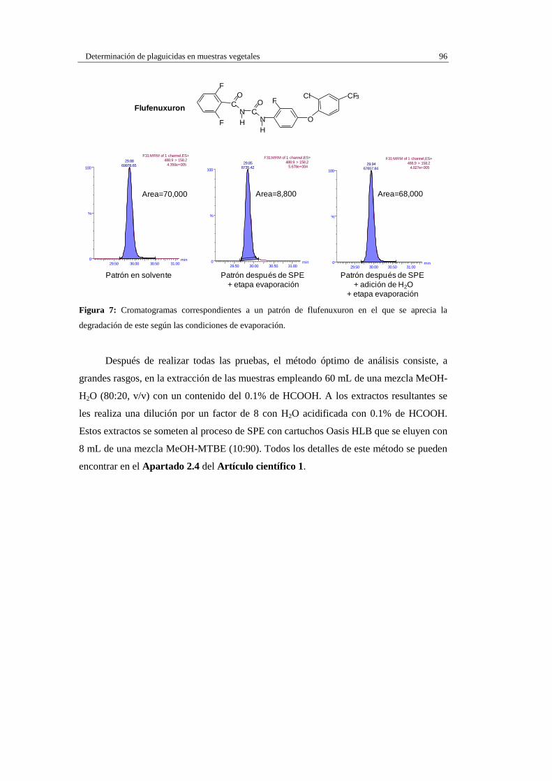
Determinación de plaguicidas en muestras vegetales 96
Figura 7: Cromatogramas correspondientes a un patrón de flufenuxuron en el que se aprecia la
degradación de este según las condiciones de evaporación.
Después de realizar todas las pruebas, el método óptimo de análisis consiste, a
grandes rasgos, en la extracción de las muestras empleando 60 mL de una mezcla MeOH-
H2O (80:20, v/v) con un contenido del 0.1% de HCOOH. A los extractos resultantes se
les realiza una dilución por un factor de 8 con H2O acidificada con 0.1% de HCOOH.
Estos extractos se someten al proceso de SPE con cartuchos Oasis HLB que se eluyen con
8 mL de una mezcla MeOH-MTBE (10:90). Todos los detalles de este método se pueden
encontrar en el Apartado 2.4 del Artículo científico 1.
Patrón en solvente
min29.50 30.00 30.50 31.00
%
0
100
F31:MRM of 1 channel,ES+488.9 > 158.2
4.350e+00529.88
69978.65
Area=70,000
min29.50 30.00 30.50 31.00
%
0
100
F31:MRM of 1 channel,ES+488.9 > 158.2
5.678e+00429.85
8735.42
min29.50 30.00 30.50 31.00
%
0
100
F31:MRM of 1 channel,ES+488.9 > 158.2
4.027e+00529.94
67657.84
Area=8,800 Area=68,000
Patrón después de SPE
+ etapa evaporación
Patrón después de SPE
+ adición de H2O
+ etapa evaporación
C
F
F
N
O
C
H N
O
H
O
FCl CF3
Flufenuxuron

Determinación de plaguicidas en muestras vegetales 97
Validación del método analítico
Una vez optimizadas las variables experimentales que afectan al método, se realizó
la validación del mismo, siguiendo las directivas de las guías europeas
(SANCO/10476/2003), considerando como parámetros esenciales el rango de linealidad,
la exactitud y la precisión, así como la especificidad del método. La cuantificación se
realizó mediante calibrado en matriz a pesar de haber comprobado que el efecto matriz
después del tratamiento de muestra realizado era irrelevante. Aún así, se empleó este tipo
de calibrado para prevenir cualquier variación en la señal que se pudiera producir con el
cambio de alguna característica de las muestras (cambio de variedad, grado de
madurez…) en el análisis de muestras reales. Los resultados obtenidos para la linealidad
y especificidad fueron satisfactorios. La exactitud y precisión se evaluaron mediante
ensayos de recuperación, cuyos resultados se pueden observar en la Tabla 3 del Artículo
científico 1 y, de un modo más esquemático, en la Figura 8, presentada a continuación.
Las recuperaciones se encuentran dentro del rango 70-120% para la mayoría de los
compuestos analizados. Los únicos compuestos que presentan resultados no satisfactorios
para todas las matrices estudiadas son methamidophos, aldicarb y ethiofencarb. Se
observa, por otro lado, que las matrices en las que se obtienen más resultados fuera del
rango satisfactorio son tomate y aguacate. En el caso concreto de aguacate, se observa
que los resultados menos satisfactorios se producen en los compuestos más apolares,
probablemente debido a que el porcentaje de disolvente orgánico, empleado en la
extracción, no es del todo adecuado para extraer estos compuestos en esta matriz con
elevado contenido de lípidos. La dificultad de obtener resultados óptimos para todos los
analitos incluidos en un método MRM, debido a las grandes diferencias en sus
propiedades físico-químicas, ya ha sido mencionada en la bibliografía (Hajšlová et al,
1998).

Determinación de plaguicidas en muestras vegetales 98
Figura 8: Resultados de recuperación para las 4 matrices objeto de estudio. En rojo se muestran los
compuestos cuyo valor de recuperación queda fuera de los límites considerados aceptables.
Como ya se ha comentado anteriormente, en el método MRM solo se adquiere una
transición por compuesto, empleada para la cuantificación. La confirmación de los
analitos se realiza en una segunda inyección del extracto adquiriendo todas las
transiciones MS/MS que, para tal fin, se obtuvieron en las experiencias de infusión
realizadas durante la optimización del método.
0%
20%
40%
60%
80%
100%
120%
140%
Meth
am
ido
pho
s
Ald
icarb
Lufe
nuro
n
Recupera
ció
n(%
)
Limón (recuperación media)
0%
20%
40%
60%
80%
100%
120%
140%R
ecupera
ció
n (%
)Tomate (recuperación media)
Recupera
ció
n (%
)
0%
20%
40%
60%
80%
100%
120%
140%Aguacate (recuperación media)
0%
20%
40%
60%
80%
100%
120%
140%
Meth
am
ido
pho
s
Ald
icarb
Eth
iofe
ncarb
Recupera
ció
n(%
)
Pasa (recuperación media)

Determinación de plaguicidas en muestras vegetales 99
En el Artículo científico 2 se realiza un estudio para evaluar las ventajas que
puede aportar el empleo de la técnica UHPLC-MS/MS en el análisis de plaguicidas en
matrices vegetales. El estudio se realiza aplicando el mismo procedimiento desarrollado
en el Artículo científico 1 para dos de las matrices anteriormente estudiadas: limón y
pasas. A la vista de los resultados obtenidos en el Artículo científico 1 se redujo el
número de compuestos de 52 a 35, porque se descartaron aquellos que habían dado
resultados poco satisfactorios en la validación.
Se reoptimizaron las condiciones cromatográficas, acorde a las características de
UHPLC-MS/MS. Se consiguieron separar los 35 compuestos empleando 20 funciones de
adquisición de no más de 30 s cada una, en las que el pico cromatográfico queda centrado
en la función para prevenir posibles pérdidas de éstos por fluctuaciones inesperadas,
como ya se comentó con anterioridad.
El tiempo de dwell fue de 50 ms, de modo que todos los picos disponen de un
número de puntos adecuado para una buena definición, así como una adecuada relación
S/N. Se realizaron pruebas con diferentes tiempos de dwell, entre 100 ms (típicamente
empleado en HPLC-MS/MS) y 10 ms. Con dwell de 100 ms, los picos cromatográficos
no estaban bien definidos puesto que no se realizaba la adquisición de suficientes puntos.
Sin embargo, cuando el tiempo de dwell se bajaba hasta 10 ms, aunque todos los
compuestos podían ser adquiridos dentro de una misma función, se producía un aumento
notable del ruido de fondo de modo que la sensibilidad del método se veía perjudicada.
Aplicando UHPLC-MS/MS se consigue la correcta separación y cuantificación de
todos los compuestos en un tiempo inferior a 4 minutos (frente a los 31 minutos del
método HPLC-MS/MS), con picos con una anchura aproximada de 5 s. Este método es
capaz de resolver isómeros geométricos (caso del dimetomorph y pyrifenox). Además, se
observó que la técnica UHPLC fue capaz de resolver el pico de un interferente, causado
por la matriz de limón, del analito (diuron), que en el método de HPLC no se había
observado (Figura 2, Artículo científico 2).

Determinación de plaguicidas en muestras vegetales 100
Este método también fue validado siguiendo los mismos criterios, descritos
anteriormente. Los resultados, satisfactorios para la mayor parte de los compuestos, se
muestran en la Tabla 2 del Artículo científico 2.
Así pues, se comprobó que haciendo uso de la técnica UHPLC-MS/MS se consigue
una mejora en cuanto a la separación de los analitos y tiempo de análisis con respecto al
método anterior desarrollado basado en HPLC-MS/MS.

Determinación de plaguicidas en muestras vegetales 101
1.1.5. REFERENCIAS
Beltrán E., Ibáñez M., Sancho J.V., Hernández F. (2009). ” Determination of mycotoxins
in different food commodities by ultra-high-pressure liquid chromatography
coupled to triple quadrupole mass spectrometry”. Rapid Communications in Mass
Spectrometry 23 (12), 1801-1809.
Bijlsma, L., Sancho J.V., Pitarch E., Ibáñez M., Hernández F. (2009). “Simultaneous
ultra-high-pressure liquid chromatography-tandem mass spectrometry
determination of amphetamine and amphetamine-like stimulants, cocaine and its
metabolites, and a cannabis metabolite in surface water and urban wastewater”.
Journal of Chromatography A 1216 (15), 3078-3089.
European Commision Decision 2002/657/EC, implementing Council Directive 96/23/EC
concerning the performance of analytical methods and the interpretation of results.
Official Journal of European Communities 2002, L221,8.
European Commision, directorate General Health and Consumer Protection, Commision
working document SANCO/10476/2003. “Quality Control Procedures for
Pesticide Residues Analysis”. 5th February 2004.
FDA. (2001). “Guidance for Industry: Mass Spectrometry for confirmation of the identity
of animal drugs residues”. Draft Guidance 118, Food and Drug Administration.
Fenoll J., Hellín P., Martínez C.M., Flores P. (2009). “Multiresidue analysis of pesticides
in soil by high-performance liquid chromatography with tandem mass
spectrometry”. Journal of AOAC International 92 (5), 1566-1575.
Fernández-Moreno J.L., Garrido Frenich A., Plaza-Bolaños P., Martínez Vidal J.L.
(2008). “Multiresidue method for the analysis of more than 140 pesticide residues
in fruits and vegetables by gas chromatography coupled to triple quadrupole mass
spectrometry”. Journal of Mass Spectrometry 43, 1235-1254.

Determinación de plaguicidas en muestras vegetales 102
Garrido Frenich A., González- Rodríguez M.J., Arrebola F.J., Martínez Vidal J.L. (2005).
“ Potential of gas chromatography–triple quadrupole mass spectrometry in
vanguard and rearguard methods of pesticide residues in vegetables”. Analytical
Chemistry 77, 4640-4648.
Gracia-Lor E., Sancho J.V., Hernández F. (2010). " Simultaneous determination of acidic,
neutral and basic pharmaceuticals in urban wastewater by ultra high-pressure
liquid chromatography-tandem mass spectrometry”. Journal of Chromatography A
1217 (5), 622-632.
Greulich A., Alder L. (2008). “Fast multiresidue screening of 300 pesticides in water for
human consumption by LC-MS/MS”. Analytical and Bioanalytical Chemistry 391,
183-197.
Grimalt S., Pozo O.J., Marín J.M., Sancho J.V., Hernández F. (2005). “Evaluation of
different quantitative approaches for the determination of non easily ionizable
molecules by different atmospheric pressure interfaces used in liquid
chromatography tandem mass spectrometry: Abamectin as case of study” Journal
of the American Society for Mass Spectrometry 16 (10), 1619-1630.
Grimalt S., Sancho J.V., Pozo O.J., Hernández F. (2010). “ Quantification, confirmation
and screening capability of UHPLC coupled to triple quadrupole and hybrid
quadrupole time-of-flight mass spectrometry in pesticide residue analysis”. Journal
of Mass Spectrometry 45 (4), 421-436.
Guillarme D., Schappler J., Rudaz S., Veuthey J. (2010). “Coupling ultra-high-pressure
liquid chromatography with mass spectrometry”.Trends in Analytical Chemistry
29, 15-27.
Hajšlová J., Holadová K., Kocourek V., Poustka J., Godula M., Cuhra P., Kempný M.
(1998). “Matrix-induced effects: a critical point in the gas chromatographic
analysis of pesticide residues”. Journal of Chromatography A 800, 283-295.

Determinación de plaguicidas en muestras vegetales 103
Hernández F., Sancho J.V., Pozo O.J., Villaplana C., Ibáñez M., Grimalt S. (2003)
“Rapid determination of Fosetyl-Aluminum residues in lettuce by liquid
chromatography/electrospray tandem mass spectrometry”. Journal of AOAC
International 86 (4), 832-838.
Hiemstra M., de Kok A. ( 2007). “ Comprehensive multi-residue method for the target
analysis of pesticides in crops using liquid chromatography-tandem mass
spectrometry”. Journal of Chromatography A 1154, 3-25.
Ibáñez M., Guerrero C, Sancho J.V., Hernández F. (2009). “Screening of antibiotics in
surface and wastewater samples by ultra-high-pressure liquid chromatography
coupled to hybrid quadrupole time-of-flight mass spectrometry” Journal of
Chromatography A 1216, 2529–2539.
Jansson C., Pihlström T., Österdahl B.-G., Markides K.E. (2008). “A new multi-residue
method for analysis of pesticide residues in fruit and vegetables using liquid
chromatography with tandem mass spectrometric detection”. Journal of
Chromatography A 1023 (1), 93-104.
Leandro C.C., Fussell R.J., Keely B.J. (2005). ”Determination of priority pesticides in
baby foods by gas chromatography tandem quadrupole mass spectrometry”.
Journal of Chromatography A 1085 (2), 207-212.
Lehotay S.J., Son K.A., Kwon H., Koesukwiwat U., Fu W., Maštovska K., Hoh E.,
Leepipatpiboon N. (2010). “Comparison of QuEChERS sample preparation
methods for the analysis of pesticide residues in fruit and vegetables”. Journal of
Chromatography A 1217, 2548-2560.
Mellors J.S., Jorgeson J.W. (2004). “Use of 1.5µm porous ethyl-bridged hybrid particles
as a stationary phase support for reversed-phase ultra high-pressure liquid-
chromatography”. Analytical Chemistry 75, 5441-5450.

Determinación de plaguicidas en muestras vegetales 104
Neue U.D. (2005). “Theory of peak capacity in gradient elution”. Journal of
Chromatography A 1079,153–161.
Okihashi M., Takatori S., Kitagawa Y., Tanaka Y. (2007). “Simultaneous analysis of 260
pesticide residues in agricultural products by gas chromatography/triple
quadrupole mass spectrometry”. Journal of AOAC International 90, 1165-1179.
Pihlström T., Blomkvist G., Friman P. ,Pagard U., Österdahl B-G. (2007). “Analysis of
pesticide residues in fruit and vegetables with ethyl acetate extraction using gas
and liquid chromatography with tandem mass spectrometric detection”. Analytical
and Bioanalytical Chemistry 389, 1773-1789.
Richardson S. (2010). “ Environmental Mass Spectrometry: Emerging contaminants and
current issues”. Analytical Chemistry 82, 4742-4774.
Sancho J.V., Ibáñez M., Grimalt S., Pozo O.J., Hernández F. (2005). “Residue
determination of cyromazine and its metabolite melamine in chard samples by ion-
pair liquid chromatography coupled to electrospray tandem mass spectrometry”.
Analytica Chimica Acta 530 (2), 237-243.
Swartz M.E. (2005). “UPLC: An introduction and review”. Journal of Liquid
Chromatography and Related Technologies 28, 1253–1263.
WADA. (2004). “Identification criteria for qualitative analysis”. Technical Document
TD2003IDCR 1.2.
Wang J., Leung D. (2009). “Determination of 142 pesticides in fruit- and vegetable-
based infant foods by liquid chromatography/electrospray ionization-tandem mass
spectrometry and estimation of measurement uncertainty”. Journal of AOAC
International 92 (1), 279-301.
Wren S., Tchelitcheff P. (2006).”Use of ultra-performance liquid chromatography in
pharmaceutical development”. Journal of Chromatography A 1119, 140-146.

1.2. Aplicación de cromatografía de gases acoplada a espectrometría de masas para la
determinación de plaguicidas problemáticos en muestras vegetales
1.2.1. INTRODUCCIÓN
1.2.2. ARTÍCULO CIENTÍFICO 3
Residue determination of captan and folpet in vegetable samples by gas
chromatography/negative chemical ionization-mass spectrometry
Journal of AOAC International. (2006). Vol 89, No. 4, 1080-1087
1.2.3. DISCUSIÓN DE RESULTADOS OBTENIDOS
1.2.4. REFERENCIAS


Determinación de plaguicidas en muestras vegetales 107
1.2.1. INTRODUCCIÓN
Captan, [(N-(trichloromethylthio)cyclohex-4-ene-1,2-dicarboximide] y folpet [N-
(trichloromethylthio)phthalimide] son dos fungicidas que pertenecen a la familia de las
ftalimidas. Estos compuestos actúan por medio de reacciones con los grupos tiol y
deshabilitan los procesos metabólicos que permiten la división celular y los procesos de
respiración de un amplio espectro de microorganismos, proporcionando acciones
curativas o de protección a las plantas. El captan es empleado en agricultura puesto que
favorece el crecimiento sano de las hojas, proveyendo a éstas de más superficie
fotosintética. El empleo de este fungicida hace que se obtenga una mayor producción de
carbohidratos en las plantas, que conlleva una mayor calidad de los frutos. También
puede tener usos post-cosecha, ya que es un producto que favorece la conservación de la
fruta en las etapas de almacenamiento y transporte. A su vez, es un compuesto empleado,
también, para el tratamiento de semillas, puesto que aporta protección adecuada contra

Determinación de plaguicidas en muestras vegetales 108
procesos denominados del “mal del complejo de hongos del suelo” y sobre aquellos
hongos que se encuentren normalmente en las semillas (Fernández-Cruz et al, 2006).
Por su parte, el folpet también favorece el crecimiento sano de las hojas. Se emplea
como fungicida en bayas, flores, plantas ornamentales, cultivos de diversas frutas y
verduras, y en tratamientos de semillas. También tiene otros usos fuera del campo de la
agricultura en el que se emplea como fungicida en pinturas y plásticos para tratamientos
estructurales de diversas superficies o construcciones.
A pesar de los avances que se han registrado en los últimos años en tratamiento de
muestra e instrumentación, las características físico químicas especiales de algunos
pesticidas hacen que la inclusión de éstos en métodos multiresiduales sea prácticamente
imposible, puesto que los resultados obtenidos al aplicar los métodos MRM desarrollados
no son satisfactorios. Esto hace que resulte necesario desarrollar métodos individuales
con tratamiento de muestra o condiciones cromatográficas específicas que se adecúen a
sus características especiales. Como ejemplos de estos compuestos, que no resultan
factibles de ser incluidos en métodos MRM, pueden citarse en el campo de LC-MS, el
fosetyl-aluminio (Hernández et al, 2003), etefón (Marín et al, 2006), melamina y su
producto de transformación ciromazina (Sancho et al, 2005) y el glifosato (Ibáñez et al,
2005). En el campo de GC-MS, mencionaríamos algunos compuestos a modo de ejemplo,
como son captan, folpet (que nos ocupan en este Apartado), captafol, clorotalonil, dicofol
y el grupo de los ditiocarbamatos. En el caso de captan y folpet, su determinación resulta
especialmente problemática debido a su inestabilidad química y térmica.
El objetivo del trabajo presentado en el Artículo científico 3 es desarrollar un
nuevo método capaz de determinar conjuntamente los fungicidas captan y folpet, debido
a las exigencias de la definición de residuo para estos compuestos (Real Decreto
280/1994), en matrices vegetales procedentes de cultivos menores que resultan de
especial interés para la agricultura española. Se muestra la optimización de las
condiciones referentes al método cromatográfico, parámetros de MS, así como del
tratamiento de las distintas muestras a analizar. Una vez optimizados todos los

Determinación de plaguicidas en muestras vegetales 109
parámetros, se realiza la validación del método atendiendo a las directrices marcadas por
la Guía Europea SANCO (SANCO/10476/2003) para así asegurar la calidad del
procedimiento analítico desarrollado. También se realiza el análisis de muestras reales
procedentes de estudios de campo realizados por el Instituto Nacional de Investigación y
Tecnología Agraria y Alimentaria (INIA) con el objetivo de establecer los LMR para
estos dos fungicidas en las matrices de caqui y coliflor. Todos estos análisis se han
realizado en cumplimiento de los principios establecidos por las Buenas Prácticas de
Laboratorio (BPL).

Determinación de plaguicidas en muestras vegetales 110

1.2.2. ARTÍCULO CIENTÍFICO 3
Residue determination of captan and folpet in vegetable samples by gas
chromatography/negative chemical ionization-mass spectrometry
M.Barreda, F.J. López, M. Villarroya, J. Beltran, J.M. García-Baudín,F. Hernández
Journal of AOAC International. (2006). Vol 89, No. 4, 1080-1087


Barreda et al. J. of AOAC Int.. (2006). 89 (4), 1080-1087 113
Residue Determination of Captan and Folpet in Vegetable
Samples by Gas Chromatography/Negative Chemical Ionization–
Mass Spectrometry
Mercedes Barredaa, Francisco J. Lópeza, Mercedes Villarroyab, Joaquim Beltrana,
Jose María García-Baudínb, Felix Hernándeza
a Universidad Jaume I, Research Institute for Pesticides and Water, 12071, Castellón, Spain
b Instituto Nacional de Investigación y Tecnología Agraria y Alimentaria (INIA), Departamento de
Protección Vegetal,Carretera de la Coruña Km 7.5, 28040 Madrid, Spain
Abstract
A gas chromatography/negative chemical ionization-mass spectrometry (GC/NCI-MS)
method has been developed for the simultaneous determination of the fungicides captan and
folpet in khaki (persimmon; flesh and peel) and cauliflower. Samples were extracted with
acetone in the presence of 0.1 M zinc acetate solution in order to avoid degradation of
fungicides and were purified using solid-phase extraction with divinylbenzene polymeric
cartridges. Purified extracts were evaporated and dissolved in hexane prior to injection into
the GC/NCI-MS system. Isotope-labeled captan and folpet were used as surrogate/internal
standards, and quantification was performed using matrix-matched calibration. The method
showed linear response in the concentration range tested (50–2500 ng/mL). The method was
fully validated with untreated blank samples of khaki (flesh and peel) and cauliflower spiked
at 0.05 and 0.5 mg/kg. Satisfactory recoveries between 82 and 106% and relative standard
deviations lower than 11% in all cases (n = 5) were obtained. The limit of detection for both
compounds were estimated to be 0.01 mg/kg. The developed method has been applied to
treated and untreated samples collected from residue trials.

Barreda et al. J. of AOAC Int.. (2006). 89 (4), 1080-1087 114
Captan [(N-(trichloromethylthio)cyclohex-4-ene-1,2- dicarboximide] is a fungicide of
the phthalimide group (N-trihalomethylthio derivative) with protective and curative action by
inhibiting some process of respiration and metabolism of fungi as a nonspecific thiol reactant.
Captan is widely used inmany countries around theworld. In Spain, it is applied for the
control of anthracnose, brown rot, and scab in fruit trees and for the control of anthracnose,
Botrytis spp., and mildew in vegetables. Folpet [N-(trichloromethylthio) phthalimide] is also a
fungicide of the phthalimide group with protective action by inhibiting respiration as a
nonspecific thiol reactant, and it is used for control of mildew, leaf spot diseases, scab, etc., in
several crops (1–3).
Determination of captan and folpet residues in plant materials is usually performed by
gas chromatography (GC) using electron capture detector (ECD; 2, 4–6) or mass spectrometry
(MS) detection, which is used for confirmation (7, 8) or quantification (9–11).
Most of references dealing with GC/MS analysis described use electron impact
(EI)mode (7–10), although GC/MS in the chemical ionization (CI) mode (12–14) has been
used to determine these pesticides in vegetable samples. Typically, chromatograms obtained
using GC/CI-MS are cleaner due to the minimization of background interferences and
because there is less chance for interferences from ions derived from the sample matrix than
when using EI.
Folpet has been usually determined by GC, although liquid chromatography (LC/MS)
with atmospheric pressure chemical ionization (APCI) has also led to satisfactory results for
its residue determination in some crops (14).
There is a shortage of specific analytical methods for captan and folpet determination
(2, 4, 10, 15, 16) because most references deal with multiresidue methods (MRM) based on
GC/MS. Surprisingly, satisfactory recoveries have been reported in several multiresidue,
multiclass methods, in spite of obvious analytical problems for captan and folpet. Lehotay et
al. (17) summarized their wide experience with these analytes, considering them as
problematic pesticides that easily degrade during sample preparation, GC injection, and/or in
solution. Thus, it is not surprising that <70% recoveries were obtained for these analytes.
Several problems have been described for the determination of captan and folpet by
different authors, which illustrates the difficulties involved in the determination of these
compounds at the residue level. The main problems deal with the degradation and instability

Barreda et al. J. of AOAC Int.. (2006). 89 (4), 1080-1087 115
of these compounds due to the N-trihalomethylthio functional group. The instability can be
due to several factors: (1) instability due to sunlight (15), which degrades folpet by a first-
order kinetics with a half-time (t1/2) of approximately 19 days to unknown products that are
not assignable to phthalimide, phthalamic, and phthalic acids (the same behavior is supposed
for captan). (2) effect of different solvents, including variability due to the lot. Maštovská and
Lehotay (18) have recently studied the effect of different solvents in the analysis of several
pesticides, including the group of N-trihalomethylthio fungicides. Among others, the stability
of captan and folpet under different conditions was discussed, and important factors were
found to be the light, pH, and GC conditions. (3) Hydrolysis of captan and folpet in aqueous
media depending on the pH has been reported by several authors (2, 15). Thus, a pH-
dependent pseudo-first-order rate reaction for captan in water was reported for a pH range
between 2 and 6. For alkaline hydrolysis (pH between 7 and 9), a second-order rate reaction
was found. Besides, it is already known that at basic pH in certain solvent and matrix
environments, captan and folpet degrade to the corresponding phthalimides (19). (4) Captan
degradation under certain GC conditions has also been reported (16). The same problem may
occur for folpet, so LC methods might be more convenient for this compound. Noticing the
possibility of degradation during the sample preparation or GC analysis, GC-amenable
degradation products were monitored to help with the identification. Their presence was taken
as indicative of parent compounds (9).
The Instituto Nacional de Investigación y Tecnología Agraria y Alimentaria (INIA) has
performed several residue trials for captan in 2 minor crops that are of special interest in
Spain, khaki (persimmon Diospyros kaki L.f.) and cauliflower (Brassica oleracea convar.
Botrytis L.), in order to establish the maximum residue level (MRL) for this fungicide.
Because the residue amount for captan in fruits and vegetables is given as the sum of captan +
folpet, the application of reliable analytical methodology for the simultaneous determination
of both captan and folpet was necessary. Besides, the chromatographic response detected in
the developed method should be truly due to the analyte included in the residue definition,
rather than to a degradation product generated during the analytical process (20).
Given the well-documented problems of lack of stability of captan and folpet under
typical GC temperature conditions and the degradation processes observed in some
aqueous/organic solutions, the aim of this work was to develop a sensitive and reliable

Barreda et al. J. of AOAC Int.. (2006). 89 (4), 1080-1087 116
analytical GC/MS method for determination of these problematic compounds in khaki (flesh
and peel) and cauliflower. The proposed method has been validated in compliance with good
laboratory practices (GLP) and following the European SANCO guidelines (20, 21).
Experimental
Reagents and Chemicals
(a) Pesticide standards.—98–99.5% purity captan and folpet reference standards were
purchased from Dr. Ehrenstorfer (Promochem, Wesel, Germany). Individual stock solutions
(ca 500 µg/mL) were prepared by dissolving the standards in acetone and then stored at –
20ºC. Working standard solutions of pesticide mixtures for sample fortification and
calibration were prepared by diluting stock solutions in acetone and then stored at 4ºC.
(b) Internal standards.—Captan-D6 and folpet-D4 (Dr. Ehrenstorfer) were used as
surrogate/internal standards. Individual stock and working solutions of labeled standards were
prepared by diluting commercially available standards (ca 100 µg/mL) in acetone and stored
at –20ºC.
(c) Acetone, hexane, and dichloromethane.—Ultratrace analysis quality (Scharlab,
Barcelona, Spain).
(d) Zinc acetate dihydrated.—Extra pure grade (Scharlab).
(e) Water.—HPLC grade; obtained by purifying demineralized water in a Nanopure II
System (Barnstead, Newton, MA).
(f) Solid-phase extraction (SPE) cartridges.—Supelclean EnviChrom P (500 mg, 6
mL; Supelco, Bellefonte, PA).
Samples
Fresh khaki and cauliflower samples from field residue trials were collected by INIA.
Peel and flesh were separated manually in khaki samples. All samples (khaki peel, khaki
flesh, and cauliflower) were throughly triturated using a K55 Homogenizer (Dito Sama,
Aubussen, France) and stored at –20ºC. Homogenized blank samples from untreated plots
were used for method validation and preparation of quality control (QC) samples.
GC Analysis
Chromatographic analysis was performed using an Agilent 6890 Series gas
chromatograph equipped with a CIS-4 programmed temperature vaporizer (PTV) injector

Barreda et al. J. of AOAC Int.. (2006). 89 (4), 1080-1087 117
(Gerstel GmbH & Co. KG, Mülheim an der Ruhr, Germany), a Multipurpose SamplerMPS2
(GerstelGmbH&Co. KG), and a single quadrupole mass spectrometer (Model No. 5973N;
Agilent Technologies, Wilmington, DE) working in the negative chemical ionization (NCI)
mode using methane as the reagent gas. The injector temperature program started at 40ºC, and
then it was raised at 10ºC/s to 150ºC (0.5min).The oven temperature was programmed as
follows: 90ºC (1min), 30ºC/min to 200ºC, 4ºC/min to 250ºC, and a final hold for 4.83 min.
Pulsed splitless injections were done with an initial pressure of 25.0 psi (1.5 min) and a
constant pressure of 8.74 psi for the rest of the analysis using a CIS4 glass liner baffled and
deactivated (Gerstel GmbH & Co. KG). Asimple volume of 2 µL was injected onto a 30 m ×
0.25 mm id, 0.25 µm HP-5MS (5% phenyl methyl siloxane) column (J&W Scientific, Folson,
CA). Heliumwas used as the carrier gas.
MS Analysis
Experimental MS parameters were the following: source and transfer line temperatures
150 and 250ºC, respectively; electronmultiplier potential 3000 V; andmultiplier gain 2732.
Ions selected from NCI-MS spectra for quantification were m/z 150 (captan), 156 (captan-D6),
146 (folpet), and 150 (folpet-D4).
Sample Preparation
Homogenized sample (20 g cauliflower or khaki flesh and 10 g khaki peel) was
accurately weighed, and 10 mL 0.1 M zinc acetate dihydrate solution (15mLfor cauliflower in
order to cover completely the whole sample) and 1 mL of mixed solution of internal standards
(500 ng/mL) were added. The sample was extracted with 60 mL acetone for 2 min using a
high-speed blender (Ultraturrax T25, Janke & Kunkel, Staufen, Germany) at 8000 rpm. The
entire extract was passed through filter paper and washed with 25 mL acetone, and the final
volume was adjusted to 100 mL with acetone. Then, the raw acetone extract was diluted 5-
fold with water (i.e., a 20 mL aliquot was diluted to 100 mL with HPLC water).
The diluted extract (100 mL) was passed through an SPE cartridge previously
conditioned by passing 4mL acetone and 4 mLwater. The cartridges were dried by passing
nitrogen for 30 min, and then they were eluted with 8 mL dichloromethane. The eluate was
evaporated to dryness under a gentle nitrogen stream at 40ºC, and the residue was dissolved in
1 mL hexane. Finally, a 2 µL aliquot was injected into the GC/MS system. Captan and folpet
quantification was performed by the internal standard method using their respective labeled

Barreda et al. J. of AOAC Int.. (2006). 89 (4), 1080-1087 118
internal standards (captan-D6 and folpet-D4). Calibration was performed with matrix-matched
standards prepared from a blank matrix.
Validation Study
The analytical method developed was fully validated for the vegetable matrixes
studied: peel khaki, flesh khaki, and cauliflower. The matrix-matched calibration curve was
obtained by analyzing in triplicate 8 standard solutions at concentrations between 50 and 2500
ng/mL for both fungicides. Matrix-matched standards were prepared using blank untreated
samples that were extracted accordingly to the sample preparation procedure. After extraction,
1 mL of the internal standard solution (100 ng/mL) and 1 mL of different standard solutions
of captan and folpet were added to 20 mL of blank raw extract, diluting finally with water to
100 mL. Then, the diluted extract was submitted to SPE as indicated above.
The selectivity of the method was evaluated by injecting in turn a procedure blank;
peel and flesh khaki and cauliflower blank samples; and blank samples spiked at the lowest
fortification level assayed (i.e., 0.05 mg/kg). The response obtained for the blank samples
should not exceed 30% of the response corresponding to the limit of quantification (LOQ).
The accuracy of the method was estimated by means of recovery experiments, which
were performed at 2 concentration levels (0.05 and 0.5 mg/kg). All experiments were carried
out with 5 replicates. Fortification of samples was performed by delivering appropriate
volumes of mixed standard solutions in acetone to blank samples. The spiked samples were
then equilibrated for 1 h prior to the extraction procedure. Precision of the method
(repeatability) was evaluated within the same day at each recovery level, and it was calculated
in terms of relative standard deviation (RSD) for 5 replicates.
The limit of detection (LOD), defined as the minimum concentration or mass of the
analyte that can be detected with acceptable certainty but not quantifiable with acceptable
precision, was estimated as the quantity of analyte that generated a response 3 times greater
than the noise level (20). It was estimated from the chromatogram corresponding to the lowest
point used in the matrix-matched calibration.
The LOQ was established as the lowest concentration that was validated in the samples
with acceptable recoveries (between 70 and 110%) and precision (lower than 15%; 20).

Barreda et al. J. of AOAC Int.. (2006). 89 (4), 1080-1087 119
Results and Discussion
According to our experience, we can corroborate that stability and degradation
problems for captan and folpet exist, and they depend in a great deal on minor changes in the
experimental conditions. The effects on method robustness lead to satisfactory recoveries in a
set of experiments while in others the results are unsatisfactory with unacceptable, high RSD
values. We studied in depth the analytical parameters that could affect this problematic
determination. Not only were MS conditions studied and optimized but also, and particular,
GC and sample preparation conditions in order to develop a robust method that could be used
to measure their residues in selected minor crops and to establish the MRLs in this type of
vegetable matrix.
Method Optimization
Chromatographic and MS conditions.—According to the literature available, the first
approach used for the determination of captan and folpet was based on the use of GC/MS in
the EI mode (70 eV). Chromatographic conditions used were similar to those described in
other papers (7–9). From these preliminary experiments, it seemed evident that captan and
folpet were degraded both by chemical processes (when dissolved in methanol) and/or by
thermal degradation (when heated to 250ºC in the gas chromatograph injection port). In both
cases, captan and folpet were degraded to their correspondent phthalimides according to the
reactions shown in Figure 1, which fit with the mass spectra obtained after injection of
standards under these conditions.
Figure 1: Structures for captan and folpet and their corresponding phthalimides (PHI) (main
degradation products)
S CCl3 + CCl3S
OH 2
+H2OH + CCl3SHON
O
O
N
O
O
N
O
O
O
O
S CCl3 + CCl3S
OH 2
+H2OH + CCl3SHON
O
O
N
O
N
O
CAPTAN
FO LPET
CAPTAN PHI
FO LPET PHI
S CCl3 + CCl3S
OH 2
+H2OH + CCl3SHON
O
O
N
O
O
N
O
O
S CCl3 + CCl3S
OH 2
+H2O+H2OH + CCl3SHON
O
O
N
O
O
N
O
O
O
O
S CCl3 + CCl3S
OH 2
+H2OH + CCl3SHON
O
O
N
O
N
O
S CCl3 + CCl3S
OH 2
+H2O+H2OH + CCl3SHON
O
O
N
O
N
O
CAPTAN
FO LPET
CAPTAN PHI
FO LPET PHI

Barreda et al. J. of AOAC Int.. (2006). 89 (4), 1080-1087 120
As a consequence, all pesticide standard solutions (stock and working solutions) were
prepared in acetone, and the effect of the injection port temperature (working in the splitless
mode) was studied. Repeated injections of a mixed standard of captan and folpet at 2.5 µg/mL
using different injection temperatures (150–250ºC) were made. Chromatograms obtained
showed that at higher temperatures peaks for captan and folpet still could be observed, but the
corresponding phthalimides were also present. With decreasing injection temperature,
degradation of pesticides became negligible, and it was not observed at 150ºC (Figure 2).
Figure 2: Effect of GC injection temperature on captan and folpet degradation. GC/EI-
MS chromatograms [total ion current (TIC)] for captan and folpet standard solutions
(2.5 µg/mL) with an injection temperature of 250ºC (A) and 150ºC (B). At the bottom,
the full-scan spectra confirming the peak identity of (1) captan, (2) folpet, (1´) captan
PHI, and (2´) folpet PHI.
6.00 7.00 8.00 9.00 10.00 11.00 12.00 13.00 14.00
100000
200000
300000
400000
500000
600000
700000
800000
900000
Time-->
Abundance
TIC: 0201001.D
B
(1)
(2)
5.00 6.00 7.00 8.00 9.00 10.00 11.00 12.00 13.00 14.00
50000
100000
150000
200000
250000
300000
350000
400000
450000
Time-->
Abundance
TIC: 0201001.D
A
(2´)(1´)
(1)
(2)
6.00 7.00 8.00 9.00 10.00 11.00 12.00 13.00 14.00
100000
200000
300000
400000
500000
600000
700000
800000
900000
Time-->
Abundance
TIC: 0201001.D
B
(1)
(2)
6.00 7.00 8.00 9.00 10.00 11.00 12.00 13.00 14.00
100000
200000
300000
400000
500000
600000
700000
800000
900000
Time-->
Abundance
TIC: 0201001.D
B
6.00 7.00 8.00 9.00 10.00 11.00 12.00 13.00 14.00
100000
200000
300000
400000
500000
600000
700000
800000
900000
Time-->
Abundance
TIC: 0201001.D
6.00 7.00 8.00 9.00 10.00 11.00 12.00 13.00 14.00
100000
200000
300000
400000
500000
600000
700000
800000
900000
Time-->
Abundance
TIC: 0201001.D
B
(1)
(2)
5.00 6.00 7.00 8.00 9.00 10.00 11.00 12.00 13.00 14.00
50000
100000
150000
200000
250000
300000
350000
400000
450000
Time-->
Abundance
TIC: 0201001.D
A
(2´)(1´)
(1)
(2)
5.00 6.00 7.00 8.00 9.00 10.00 11.00 12.00 13.00 14.00
50000
100000
150000
200000
250000
300000
350000
400000
450000
Time-->
Abundance
TIC: 0201001.D
5.00 6.00 7.00 8.00 9.00 10.00 11.00 12.00 13.00 14.00
50000
100000
150000
200000
250000
300000
350000
400000
450000
Time-->
Abundance
TIC: 0201001.D
A
(2´)(1´)
(1)
(2)
20 40 60 80 100 120 140 160 180 200 220 240 260 280 300
0
2000
4000
6000
8000
m/z-->
Abundance
79
149
10726439
121
13453 182 236
26
66 29993 20412 165
(1)
20 40 60 80 100 120 140 160 180 200 220 240 260 280 300
0
2000
4000
6000
8000
m/z-->
Abundance
104
76
260117 130
50
178147
90 2972326338 20016226 282213
(2)
30 40 50 60 70 80 90 100 110 120 130 140 150 160 170 180 190 200 2100
2000
4000
6000
8000
m/z-->
Abundance
147
76 104
50
38 66
90 122
(2´)
40 60 80 100 120 140 160 180 200 220 240 260 280 300 320 340
0
2000
4000
6000
8000
m/z-->
Abundance
79
151
51
12265 96 136
(1´)
20 40 60 80 100 120 140 160 180 200 220 240 260 280 300
0
2000
4000
6000
8000
m/z-->
Abundance
79
149
10726439
121
13453 182 236
26
66 29993 20412 165
(1)
20 40 60 80 100 120 140 160 180 200 220 240 260 280 300
0
2000
4000
6000
8000
m/z-->
Abundance
79
149
10726439
121
13453 182 236
26
66 29993 20412 165
(1)
20 40 60 80 100 120 140 160 180 200 220 240 260 280 300
0
2000
4000
6000
8000
m/z-->
Abundance
104
76
260117 130
50
178147
90 2972326338 20016226 282213
(2)
20 40 60 80 100 120 140 160 180 200 220 240 260 280 300
0
2000
4000
6000
8000
m/z-->
Abundance
104
76
260117 130
50
178147
90 2972326338 20016226 282213
(2)
30 40 50 60 70 80 90 100 110 120 130 140 150 160 170 180 190 200 2100
2000
4000
6000
8000
m/z-->
Abundance
147
76 104
50
38 66
90 122
(2´)
30 40 50 60 70 80 90 100 110 120 130 140 150 160 170 180 190 200 2100
2000
4000
6000
8000
m/z-->
Abundance
147
76 104
50
38 66
90 122
(2´)
40 60 80 100 120 140 160 180 200 220 240 260 280 300 320 340
0
2000
4000
6000
8000
m/z-->
Abundance
79
151
51
12265 96 136
(1´)
40 60 80 100 120 140 160 180 200 220 240 260 280 300 320 340
0
2000
4000
6000
8000
m/z-->
Abundance
79
151
51
12265 96 136
(1´)

Barreda et al. J. of AOAC Int.. (2006). 89 (4), 1080-1087 121
Even with injection at 150ºC, several problems still remained, mainly the poor
repeatability of standard injections that led to RSD around 20% (n = 10), which was
unacceptable. Precision was improved by using a pulsed splitless injection mode (initial
pressure 25 psi, initial time 1.5 min, then constant pressure at 8.8 psi), which lowered the
RSD to around 10% (n = 10). The pressure pulse used allowed a quicker and more efficient
transfer of the analytes to the chromatographic column, thereby decreasing thermal
degradation and improving repeatability. In a latter experiment, the chromatographic
systemwas equipped with a PTV injector that was operated in the pulsed-splitless mode (vent
valve closed during injection) at an initial temperature of 40ºC (obtained with a Peltier
cooling system) and then, immediately after injection, heated at 10ºC/s until 150ºC. Using this
system, we obtained the recognized advantages of PTV injection regarding the adequate
transfer of thermally unstable compounds without (or with negligible) degradation in the
injection step (11, 13). The use of PTV injection was found to be the most convenient option
and led to satisfactory results in terms of repeatability.
Once the injection conditions were optimized for both captan and folpet, the sensitivity
was still not sufficient to achieve the required LOQ, which was initially established at 0.05
mg/kg for the vegetable matrixes studied. Considering the chemical structures of these
pesticides, the use of NCI seemed to be an attractive option in order to improve the signal-to-
noise ratio. Optimum conditions for NCI-MS using methane were selected according to the
information provided by the GC/MS instrument (see Experimental). Using NCI, the
sensitivity of the GC/MS determination was increased by a factor of 15 compared to EI
(Figure 3).

Barreda et al. J. of AOAC Int.. (2006). 89 (4), 1080-1087 122
Figure 3: GC/EI-MS (A) and GC/NCI-MS (B) chromatograms (TIC) with the
corresponding full-scan spectra of captan (1) and folpet (2) standard solutions (500 ng/mL).
See the abundance response.
6.00 7.00 8.00 9.00 10.00 11.00 12.00 13.00 14.00
60008000
10000
12000
14000
1600018000
2000022000
24000
26000
2800030000
32000
Time-->
Abundance
TIC: 0501022.D
A
6.00 7.00 8.00 9.00 10.00 11.00 12.00 13.00 14.00
60008000
10000
12000
14000
1600018000
2000022000
24000
26000
2800030000
32000
Time-->
Abundance
TIC: 0501022.D
A
6.00 7.00 8.00 9.00 10.00 11.00 12.00 13.00 14.00
60008000
10000
12000
14000
1600018000
2000022000
24000
26000
2800030000
32000
Time-->
Abundance
TIC: 0501022.D
6.00 7.00 8.00 9.00 10.00 11.00 12.00 13.00 14.00
60008000
10000
12000
14000
1600018000
2000022000
24000
26000
2800030000
32000
Time-->
Abundance
TIC: 0501022.D
A(1)
(2)
6.00 7.00 8.00 9.00 10.00 11.00 12.00 13.00 14.00
60008000
10000
12000
14000
1600018000
2000022000
24000
26000
2800030000
32000
Time-->
Abundance
TIC: 0501022.D
A
6.00 7.00 8.00 9.00 10.00 11.00 12.00 13.00 14.00
60008000
10000
12000
14000
1600018000
2000022000
24000
26000
2800030000
32000
Time-->
Abundance
TIC: 0501022.D
6.00 7.00 8.00 9.00 10.00 11.00 12.00 13.00 14.00
60008000
10000
12000
14000
1600018000
2000022000
24000
26000
2800030000
32000
Time-->
Abundance
TIC: 0501022.D
A(1)
(2)
6.00 7.00 8.00 9.00 10.00 11.00 12.00 13.00 14.00
50000
100000
150000
200000
250000
300000
350000
400000
450000
500000
Time-->
Abundance
TIC: 0601001.D
B
6.00 7.00 8.00 9.00 10.00 11.00 12.00 13.00 14.00
50000
100000
150000
200000
250000
300000
350000
400000
450000
500000
Time-->
Abundance
TIC: 0601001.D
B
6.00 7.00 8.00 9.00 10.00 11.00 12.00 13.00 14.00
50000
100000
150000
200000
250000
300000
350000
400000
450000
500000
Time-->
Abundance
TIC: 0601001.D
6.00 7.00 8.00 9.00 10.00 11.00 12.00 13.00 14.00
50000
100000
150000
200000
250000
300000
350000
400000
450000
500000
Time-->
Abundance
TIC: 0601001.D
B
(2)
(1)
6.00 7.00 8.00 9.00 10.00 11.00 12.00 13.00 14.00
50000
100000
150000
200000
250000
300000
350000
400000
450000
500000
Time-->
Abundance
TIC: 0601001.D
B
6.00 7.00 8.00 9.00 10.00 11.00 12.00 13.00 14.00
50000
100000
150000
200000
250000
300000
350000
400000
450000
500000
Time-->
Abundance
TIC: 0601001.D
6.00 7.00 8.00 9.00 10.00 11.00 12.00 13.00 14.00
50000
100000
150000
200000
250000
300000
350000
400000
450000
500000
Time-->
Abundance
TIC: 0601001.D
B
(2)
(1)
146 147 148 149 150 151 152 153 154 155 156 157
40
80
120
160
200
240
280
m/z-->
AbundanceScan1165 (12.048min): 0701009.D
147156146
146 147 148 149 150 151 152 153 154 155 156 157
40
80
120
160
200
240
280
m/z-->
AbundanceScan1165 (12.048min): 0701009.D150
147156146
146 147 148 149 150 151 152 153 154 155 156 157
40
80
120
160
200
240
280
m/z-->
AbundanceScan1194 (12.272min): 0701009.D
147
156150
146 147 148 149 150 151 152 153 154 155 156 157
40
80
120
160
200
240
280
m/z-->
AbundanceScan1194 (12.272min): 0701009.D
147
146
156150
(1) (2)
6.00 7.00 8.00 9.00 10.00 11.00 12.00 13.00 14.00
60008000
10000
12000
14000
1600018000
2000022000
24000
26000
2800030000
32000
Time-->
Abundance
TIC: 0501022.D
A
6.00 7.00 8.00 9.00 10.00 11.00 12.00 13.00 14.00
60008000
10000
12000
14000
1600018000
2000022000
24000
26000
2800030000
32000
Time-->
Abundance
TIC: 0501022.D
A
6.00 7.00 8.00 9.00 10.00 11.00 12.00 13.00 14.00
60008000
10000
12000
14000
1600018000
2000022000
24000
26000
2800030000
32000
Time-->
Abundance
TIC: 0501022.D
6.00 7.00 8.00 9.00 10.00 11.00 12.00 13.00 14.00
60008000
10000
12000
14000
1600018000
2000022000
24000
26000
2800030000
32000
Time-->
Abundance
TIC: 0501022.D
A(1)
(2)
6.00 7.00 8.00 9.00 10.00 11.00 12.00 13.00 14.00
60008000
10000
12000
14000
1600018000
2000022000
24000
26000
2800030000
32000
Time-->
Abundance
TIC: 0501022.D
A
6.00 7.00 8.00 9.00 10.00 11.00 12.00 13.00 14.00
60008000
10000
12000
14000
1600018000
2000022000
24000
26000
2800030000
32000
Time-->
Abundance
TIC: 0501022.D
6.00 7.00 8.00 9.00 10.00 11.00 12.00 13.00 14.00
60008000
10000
12000
14000
1600018000
2000022000
24000
26000
2800030000
32000
Time-->
Abundance
TIC: 0501022.D
A(1)
(2)
6.00 7.00 8.00 9.00 10.00 11.00 12.00 13.00 14.00
60008000
10000
12000
14000
1600018000
2000022000
24000
26000
2800030000
32000
Time-->
Abundance
TIC: 0501022.D
6.00 7.00 8.00 9.00 10.00 11.00 12.00 13.00 14.00
60008000
10000
12000
14000
1600018000
2000022000
24000
26000
2800030000
32000
Time-->
Abundance
TIC: 0501022.D
A
6.00 7.00 8.00 9.00 10.00 11.00 12.00 13.00 14.00
60008000
10000
12000
14000
1600018000
2000022000
24000
26000
2800030000
32000
Time-->
Abundance
TIC: 0501022.D
6.00 7.00 8.00 9.00 10.00 11.00 12.00 13.00 14.00
60008000
10000
12000
14000
1600018000
2000022000
24000
26000
2800030000
32000
Time-->
Abundance
TIC: 0501022.D
A(1)
(2)
6.00 7.00 8.00 9.00 10.00 11.00 12.00 13.00 14.00
50000
100000
150000
200000
250000
300000
350000
400000
450000
500000
Time-->
Abundance
TIC: 0601001.D
B
6.00 7.00 8.00 9.00 10.00 11.00 12.00 13.00 14.00
50000
100000
150000
200000
250000
300000
350000
400000
450000
500000
Time-->
Abundance
TIC: 0601001.D
B
6.00 7.00 8.00 9.00 10.00 11.00 12.00 13.00 14.00
50000
100000
150000
200000
250000
300000
350000
400000
450000
500000
Time-->
Abundance
TIC: 0601001.D
6.00 7.00 8.00 9.00 10.00 11.00 12.00 13.00 14.00
50000
100000
150000
200000
250000
300000
350000
400000
450000
500000
Time-->
Abundance
TIC: 0601001.D
B
(2)
(1)
6.00 7.00 8.00 9.00 10.00 11.00 12.00 13.00 14.00
50000
100000
150000
200000
250000
300000
350000
400000
450000
500000
Time-->
Abundance
TIC: 0601001.D
B
6.00 7.00 8.00 9.00 10.00 11.00 12.00 13.00 14.00
50000
100000
150000
200000
250000
300000
350000
400000
450000
500000
Time-->
Abundance
TIC: 0601001.D
6.00 7.00 8.00 9.00 10.00 11.00 12.00 13.00 14.00
50000
100000
150000
200000
250000
300000
350000
400000
450000
500000
Time-->
Abundance
TIC: 0601001.D
B
(2)
(1)
6.00 7.00 8.00 9.00 10.00 11.00 12.00 13.00 14.00
50000
100000
150000
200000
250000
300000
350000
400000
450000
500000
Time-->
Abundance
TIC: 0601001.D
6.00 7.00 8.00 9.00 10.00 11.00 12.00 13.00 14.00
50000
100000
150000
200000
250000
300000
350000
400000
450000
500000
Time-->
Abundance
TIC: 0601001.D
B
6.00 7.00 8.00 9.00 10.00 11.00 12.00 13.00 14.00
50000
100000
150000
200000
250000
300000
350000
400000
450000
500000
Time-->
Abundance
TIC: 0601001.D
6.00 7.00 8.00 9.00 10.00 11.00 12.00 13.00 14.00
50000
100000
150000
200000
250000
300000
350000
400000
450000
500000
Time-->
Abundance
TIC: 0601001.D
B
(2)
(1)
146 147 148 149 150 151 152 153 154 155 156 157
40
80
120
160
200
240
280
m/z-->
AbundanceScan1165 (12.048min): 0701009.D
147156146
146 147 148 149 150 151 152 153 154 155 156 157
40
80
120
160
200
240
280
m/z-->
AbundanceScan1165 (12.048min): 0701009.D150
147156146
146 147 148 149 150 151 152 153 154 155 156 157
40
80
120
160
200
240
280
m/z-->
AbundanceScan1194 (12.272min): 0701009.D
147
156150
146 147 148 149 150 151 152 153 154 155 156 157
40
80
120
160
200
240
280
m/z-->
AbundanceScan1194 (12.272min): 0701009.D
147
146
156150
(1) (2)
146 147 148 149 150 151 152 153 154 155 156 157
40
80
120
160
200
240
280
m/z-->
AbundanceScan1165 (12.048min): 0701009.D
147156146
146 147 148 149 150 151 152 153 154 155 156 157
40
80
120
160
200
240
280
m/z-->
AbundanceScan1165 (12.048min): 0701009.D150
147156146
146 147 148 149 150 151 152 153 154 155 156 157
40
80
120
160
200
240
280
m/z-->
AbundanceScan1194 (12.272min): 0701009.D
147
156150
146 147 148 149 150 151 152 153 154 155 156 157
40
80
120
160
200
240
280
m/z-->
AbundanceScan1194 (12.272min): 0701009.D
147
146
156150
(1) (2)

Barreda et al. J. of AOAC Int.. (2006). 89 (4), 1080-1087 123
Sample preparation.—The sample preparation step also proved to be critical for the
accurate determination of residues of captan and folpet in vegetables. First, an extraction with
acetone (blending) followed by extract purification by liquid–liquid extraction (LLE) in a 3-
phase system of acetone–water–dichloromethane was studied. Unsatisfactory results were
obtained due to the well-described problems associated to LLE (22). The production of
emulsions that could not be properly eliminated led to low recoveries, especially when
dealing with khaki flesh extracts. As an alternative, the use of SPE was tested as a cleanup
procedure. Preliminary experiments, carried out with standard solutions in hexane using silica
gel cartridges, led to poor recoveries for both compounds, probably due to their chemical
characteristics. Because the sample extract solvent was acetone with a high water content, the
use of divinylbenzene polymeric cartridges was chosen as a better option after dilution of the
acetone extract with HPLC grade water. The optimization of the SPE step was first carried out
with standards in aqueous solutions considering several parameters: percentage of acetone in
the extract (10 and 20% of acetone in water); eluting solvent (hexane and dichloromethane);
maintaining a fixed cartridge mass (500 mg) and type (Supelclean ENVI-Chrom P SPE
Tubes, 6mL); sample volume (100 mL of acetone extract diluted with water); and elution
volume (8 mL).
No differences were observed when using 10 or 20% acetone in the diluted extracts.
Thus, 20% acetone was selected because better sensitivity could be achieved as a result of the
lower dilution factor. This acetone percentage was reached by diluting 20 mL of the acetone
sample extract to 100 mL with water. The use of dichloromethane as the eluting solvent led to
better recoveries (nearly 100%) than hexane (50–80%).
After the sample treatment for standards was optimized, it was applied to spiked
samples (khaki and cauliflower), but the recoveries obtained were low (about 40%). Similar
results have been reported by Tonogai et al. (23), who suggested that low recoveries for these
pesticides were not related to the extraction methodology but the degradation of analytes
during the spiking step. These authors recommended the addition of zinc acetate to the sample
in order to avoid degradation of captan and folpet. Therefore, we added zinc acetate dihydrate
solution (0.1M) to the homogenized sample immediately before spiking the sample with the
pesticide standard solutions (prepared in acetone; Figure 4).

Barreda et al. J. of AOAC Int.. (2006). 89 (4), 1080-1087 124
Figure 4: Effect of zinc acetate on captan and folpet degradation. Chromatograms
(TIC) for khaki flesh samples spiked with captan (1) and folpet (2) obtained in the
EI mode without adding 0.1 M zinc acetate to the sample extract (A) and with
addition of 0.1 M zinc (B). See the abundance response.
Unfortunately, the samples were chopped immediately when arriving at the laboratory,
so the effect of adding zinc acetate before/during chopping could not be evaluated. To avoid
possible degradation during sample preparation, it is best to add the preservative during the
chopping process, as in the Japanese official analytical method for captan, captafol, and folpet
in fruits and vegetables (24). Under these conditions, and using the recommended procedure
indicated in the Sample Preparation section above, the recoveries of the overall analytical
procedure were satisfactory. The use of labeled internal standards allowed us to improve the
8.50 9.00 9.50 10.00 10.50 11.00 11.50 12.00 12.50
100000
200000
300000
400000
500000
600000
700000
800000
900000
1000000
1100000
Time-->
AbundanceTIC: 1301018.D
8.50 9.00 9.50 10.00 10.50 11.00 11.50 12.00 12.50
200000
400000
600000
800000
1000000
1200000
1400000
1600000
1800000
2000000
2200000
2400000
Time-->
Abundance
TIC: 1501020.D
(1)
(2)
A
B(1)
(2)
8.50 9.00 9.50 10.00 10.50 11.00 11.50 12.00 12.50
100000
200000
300000
400000
500000
600000
700000
800000
900000
1000000
1100000
Time-->
AbundanceTIC: 1301018.D
8.50 9.00 9.50 10.00 10.50 11.00 11.50 12.00 12.50
100000
200000
300000
400000
500000
600000
700000
800000
900000
1000000
1100000
Time-->
AbundanceTIC: 1301018.D
8.50 9.00 9.50 10.00 10.50 11.00 11.50 12.00 12.50
200000
400000
600000
800000
1000000
1200000
1400000
1600000
1800000
2000000
2200000
2400000
Time-->
Abundance
TIC: 1501020.D
8.50 9.00 9.50 10.00 10.50 11.00 11.50 12.00 12.50
200000
400000
600000
800000
1000000
1200000
1400000
1600000
1800000
2000000
2200000
2400000
Time-->
Abundance
TIC: 1501020.D
(1)
(2)
A
B(1)
(2)
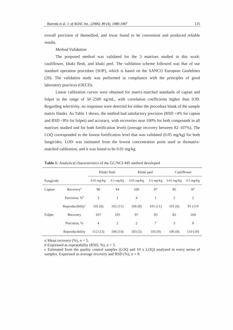
Barreda et al. J. of AOAC Int.. (2006). 89 (4), 1080-1087 125
overall precision of themethod, and itwas found to be convenient and produced reliable
results.
Method Validation
The proposed method was validated for the 3 matrixes studied in this work:
cauliflower, khaki flesh, and khaki peel. The validation scheme followed was that of our
standard operation procedure (SOP), which is based on the SANCO European Guidelines
(20). The validation study was performed in compliance with the principles of good
laboratory practices (OECD).
Linear calibration curves were obtained for matrix-matched standards of captan and
folpet in the range of 50–2500 ng/mL, with correlation coefficients higher than 0.99.
Regarding selectivity, no responses were detected for either the procedure blank of the sample
matrix blanks. As Table 1 shows, the method had satisfactory precision (RSD <4% for captan
and RSD <8% for folpet) and accuracy, with recoveries near 100% for both compounds in all
matrixes studied and for both fortification levels (average recovery between 82–107%). The
LOQ corresponded to the lowest fortification level that was validated (0.05 mg/kg) for both
fungicides. LOD was estimated from the lowest concentration point used in thematrix-
matched calibration, and it was found to be 0.01 mg/kg.
Table 1: Analytical characteristics of the GC/NCI-MS method developed
Khaki flesh Khaki peel Cauliflower
Fungicide 0.05 mg/Kg 0.5 mg/Kg 0.05 mg/Kg 0.5 mg/Kg 0.05 mg/Kg 0.5 mg/Kg
Captan Recoverya 98 94 100 97 85 87
Precision, %b 3 1 4 1 2 2
Reproducibilityc 102 (6) 102 (11) 106 (8) 101 (11) 101 (6) 91 (119
Folpet Recovery 107 105 97 93 82 104
Precision, % 4 2 2 7 3 8
Reproducibility 112 (13) 106 (14) 103 (5) 105 (9) 106 (8) 110 (10)
a Mean recovery (%), n = 5.
b Expressed as repeatability (RSD, %), n = 5.
c Estimated from the quality control samples (LOQ and 10 x LOQ) analyzed in every series of
samples. Expressed as average recovery and RSD (%), n = 8.

Barreda et al. J. of AOAC Int.. (2006). 89 (4), 1080-1087 126
Analysis of Real Samples
Once the method was validated, it was applied to the analysis of 56 khaki (28 peel and
28 flesh) and 28 cauliflower samples from different field residue trials carried out by INIA. In
spite of the residue definition (captan + folpet), folpet was not detected in any sample because
the test item applied in the field studies was a captan-formulated product. Every 4 samples (8
injections as every sample was injected in duplicate), 2 QC samples (1 at the LOQ level and
the other at 10 × LOQ) were included in the analysis sequence. Satisfactory QC recoveries
were obtained, showing the robustness of the method during several days of analysis (see
Table 1). Figure 5 shows selected chromatograms for all of the matrixes analyzed. As
expected, captan was not detected in samples from untreated plots, and the results in treated
samples were in accordance with the postharvest intervals in the experiments corresponding
to dissipation curves. Average residues (mg/kg) in samples collected at harvestwere 0.13
(khaki flesh), 5.75 (khaki peel), and 0.23 (cauliflower).
Figure 5: GC/NCI-MS chromatograms (TIC) obtained in the analysis of treated
samples from field residue trials: (A) cauliflower, (B) khaki peel, and (C) khaki
flesh. The peak marked ―*‖ corresponds to folpet-D4. Both captan-D6 (m/z 156) and
folpet-D4 (m/z 150) were added as surrogates in the analysis of real samples. The ion
selected for monitoring folpet-D4 was the same as for captan (m/z 150).
100
300
500
700
900
1100
1300
1500
1700
1900
100
300
500
700
900
1100
1300
1500
1700
1900
Abundance
CAPTAN
*
1000
2000
3000
4000
5000
6000
7000
8000
9000
Abundance
1000
2000
3000
4000
5000
6000
7000
8000
9000
CAPTAN
*
200
600
1000
1400
1800
2200
2600
3000
200
600
1000
1400
1800
2200
2600
3000
Abundance
*
CAPTAN
100
200
300
400
500
600
700
Abundance
100
200
300
400
500
600
700
CAPTAN D-6
100
200
300
400
500
600
700
800
900
1000
1100
1200
Abundance
100
200
300
400
500
600
700
800
900
1000
1100
1200
CAPTAN D-6
100
200
300
400
500
600
700
800
100
200
300
400
500
600
700
800
Abundance
CAPTAN D-6
A
B
C
100
300
500
700
900
1100
1300
1500
1700
1900
100
300
500
700
900
1100
1300
1500
1700
1900
Abundance
CAPTAN
*
100
300
500
700
900
1100
1300
1500
1700
1900
100
300
500
700
900
1100
1300
1500
1700
1900
Abundance
CAPTAN
*
1000
2000
3000
4000
5000
6000
7000
8000
9000
Abundance
1000
2000
3000
4000
5000
6000
7000
8000
9000
CAPTAN
*
1000
2000
3000
4000
5000
6000
7000
8000
9000
Abundance
1000
2000
3000
4000
5000
6000
7000
8000
9000
CAPTAN
*
200
600
1000
1400
1800
2200
2600
3000
200
600
1000
1400
1800
2200
2600
3000
Abundance
*
CAPTAN
200
600
1000
1400
1800
2200
2600
3000
200
600
1000
1400
1800
2200
2600
3000
Abundance
*
CAPTAN
100
200
300
400
500
600
700
Abundance
100
200
300
400
500
600
700
CAPTAN D-6
100
200
300
400
500
600
700
Abundance
100
200
300
400
500
600
700
CAPTAN D-6
100
200
300
400
500
600
700
800
900
1000
1100
1200
Abundance
100
200
300
400
500
600
700
800
900
1000
1100
1200
CAPTAN D-6
100
200
300
400
500
600
700
800
900
1000
1100
1200
Abundance
100
200
300
400
500
600
700
800
900
1000
1100
1200
CAPTAN D-6
100
200
300
400
500
600
700
800
100
200
300
400
500
600
700
800
Abundance
CAPTAN D-6
100
200
300
400
500
600
700
800
100
200
300
400
500
600
700
800
Abundance
CAPTAN D-6
A
B
C

Barreda et al. J. of AOAC Int.. (2006). 89 (4), 1080-1087 127
Conclusions
This work has shown the difficulties associated with the residue determination of
captan and folpet in vegetables, mainly due to the degradation of these compounds during the
analytical procedure. The use of GC with conventional injection facilitated thermal
degradation of the pesticides in the injector. In the method developed, the use of PTV
injection allowed the accurate determination of both compounds by GC/MS without thermal
degradation. As well, the use of the NCI-MS mode increased the sensitivity of the method
compared with the EI mode, providing the sensitivity required to easily reach the required
LOQ (0.05 mg/kg). Additionally, it was necessary to add the preservative zinc acetate to the
samples in order to avoid degradation of the fungicides during the extraction process.
The method developed allowed the simultaneous residue determination of captan and
folpet in the 3 vegetable matrixes studied (khaki flesh and peel and cauliflower) with
satisfactory recoveries and precision. It has been applied to the analysis of khaki and
cauliflower samples from residue trials, proving its robustness and adequacy for establishing
the MRLs in these minor crops.

Barreda et al. J. of AOAC Int.. (2006). 89 (4), 1080-1087 128
References
(1) British Crop Protection Council (1997) The Pesticide Manual, 11th Ed., C.D.S.
Tomlin (Ed.), Farnham, UK
(2) Frank, R., Northover, J., & Braun, H.E. (1985) J. Agric. Food Chem. 33, 514–518
(3) U.S. Environment Protection Agency (1999) Prevention Pesticides and Toxic
Substances (7508C), EPA-738-F99-015 and EPA-738-F99-016
(4) Cabras, P., Angioni, A., Caboni, P., Garau, V.L.,Melis,M., Pirisi, F.M.,&Cabitza, F.
(2000) J. Agric. Food Chem. 48, 915–916
(5) Kiigemagi, U., Inman, R.D., Mellenthin, W.M., & Deinzer, M.L. (1991) J. Agric.
Food Chem. 39, 400–403
(6) Sannino, A., Bandini, M., & Bolzoni, L. (1999) J. AOAC Int. 82, 1229–1238
(7) Columé, A., Cárdenas, S., Gallego, M., & Valcárcel, M. (2001) Anal. Chim. Acta.
436, 153–162
(8) Taube, J., Vorkamp, K., Förster, M., & Herrmann, R. (2002) Chemosphere 49,
1357–1365
(9) Štajnbaher, D., & Zupan_i_-Kralj, L. (2003) J. Chromatogr. A 1015, 185–198
(10) Angioni, A., Garau, V.L., Aguilera del Real, A., Melis, M., Minelli, E.V.,
Tuberoso, C., & Cabras, P. (2003) J. Agric. Food Chem. 51, 6761–6766
(11) Mattern, G.C., Singer, G.M., Louis, J., Robson, M., & Rosen, J.D. (1990) J. Agric.
Food Chem. 38, 402–407
(12) Niessner, G., Buchberger, W., & Eckerstorfer, R. (1999) J. Chromatogr. A 846,
341–348
(13) Mattern, G.C., Liu, C.H., Louis, J.B., & Rosen, J.D. (1991) J. Agric. Food Chem.
39, 700–704
(14) Gimeno, R.A., Aguilar, C., Marcé, R.M., & Borrull, F. (2001) J. Chromatogr. A
915, 139–147
(15) Cabras, P., Angioni, A., Garau, V.L., Melis, M., Pirisi, F.M., Farris, G.A., Sotgiu,
C., & Minelli, E.V. (1997) J. Agric. Food Chem. 45, 476–479
(16) Büttler, B., & Hörmann, W.D. (1981) J. Agric. Food Chem. 29, 257–260
(17) Lehotay, S.J., Kok, A., Hiemstra, M., & van Bodegraven, P. (2005) J. AOAC Int.
88, 595–614

Barreda et al. J. of AOAC Int.. (2006). 89 (4), 1080-1087 129
(18) Maštovská, K., & Lehotay, S.J. (2004) J. Chromatogr. A 1040, 259–272
(19) Lehotay, S.J., Maštovská, K., & Lightfield, A.R. (2005) J. AOAC Int. 88, 615–629
(20) Quality Control Procedures for Pesticide Residue (2004) European Comission,
Directorate General Health and Consumer Protection, Commission Working
Document SANCO/10476/2003
(21) Residues: Guidance for Generating and Reporting Methods of Analysis in Support
of Preregistration Data Requirements, Annex II and Annex III of Directive 91/414
(2000) European Comission, Directorate General Health and Consumer
Protection, Comission Working Document SANCO/3029/99
(22) Official Methods of Analysis (2000) 17th Ed., W. Horwitz (Ed.), AOAC
INTERNATIONAL, Gaithersburg, MD, Chapter 10, p. 5
(23) Tonogai, Y., Tsumura, Y., Nakamura, Y., Matsuki, H., & Ito, Y. (1992) Jpn. J.
Toxicol. Environ. Health 38, 270–281
(24) Japanese Official Analytical Method for Captan, Captafol, and Folpet in Fruits
and Vegetables (November 2005) (in Japanese)
http://www.mhlw.go.jp/topics/bukyoku/iyaku/syoku-anzen/zanryu3/2-045.html

Barreda et al. J. of AOAC Int.. (2006). 89 (4), 1080-1087 130

Determinación de plaguicidas en muestras vegetales 131
1.2.3. DISCUSIÓN DE LOS RESULTADOS OBTENIDOS
El principal problema al que hubo que hacer frente en el presente estudio fueron los
problemas de estabilidad que presentaron los fungicidas estudiados, lo cual está bien
documentado en la bibliografía (Cabras et al, 1997; Štajnbaher et al, 2003; Lehotay et al,
2005; Bailey et al, 2007). Resulta necesario resolver estos problemas si atendemos a la
definición de residuo de estos compuestos, ya que la respuesta final en el análisis de
captan y folpet debe ser procedente de los compuestos originales y no de sus productos de
degradación (SANCO/10476/2003). Aunque existen métodos en la bibliografía en los que
se determinan estos compuestos (incluso forman parte de métodos multiresiduo) y en más
de una ocasión no se reportan problemas asociados a su análisis, obteniendo buenos
resultados de recuperación. Sin embargo, al examinar los trabajos se observa que los
resultados reportados corresponden generalmente a los productos de degradación del
captan y folpet que son los que realmente se determinan en los métodos basados en GC.
Las primeras experiencias que se realizaron fueron para desarrollar y optimizar el
método cromatográfico. Se inyectaron patrones individuales de cada uno de los
compuestos haciendo uso de GC-MS en modo EI para así obtener los espectros en modo
full scan. Estas experiencias se realizaron empleando unas condiciones típicas de GC
como son una energía de 70 eV y una inyección tipo splitless con una temperatura del
inyector de 250ºC. En esta primera aproximación ya se pudo observar la degradación
debida a la alta temperatura del inyector, pues los cromatogramas obtenidos presentaban
picos correspondientes a los productos de degradación de los compuestos, sus ftalimidas
(Figura 2 del Artículo científico 3). Para evitar estos problemas de degradación térmica,
se realizaron diferentes pruebas disminuyendo la temperatura del inyector hasta 150ºC. A
esta temperatura ya no se observaron en el cromatograma los picos correspondientes a los
productos de degradación de los analitos, por lo que se consideró como temperatura
óptima de inyección. Al comprobar la reproducibilidad de los resultados inyectando el
mismo patrón 10 veces seguidas se observó que no era adecuada ya que la desviación
standard era demasiado elevada. Por ello, se cambió el modo de inyección (splitless), y se

Determinación de plaguicidas en muestras vegetales 132
optó por el empleo de un pulso de presión, de modo que la transferencia de los analitos a
la cabeza de columna se realizase de una manera más rápida y eficaz, minimizando
también el tiempo de residencia de los analitos en el inyector. De este modo, se evitaban
también los problemas de degradación térmica que se han comentado anteriormente.
Llegados a este punto, los problemas de degradación térmica parecían estar solventados.
No obstante, se pudo emplear un inyector PTV (Programmable Temperature
Vaporization) recientemente adquirido en nuestro laboratorio, capaz de realizar una
inyección inicialmente en frío (T=40ºC), mediante un sistema de enfriamiento tipo
Peltier, aumentando la temperatura rápidamente, (v=10ºC/s), hasta llegar a 150ºC. Este
modo de inyección fue considerado el más adecuado para solventar los problemas de
inestabilidad térmica y reproducibilidad que se habían presentado. También, puesto que
los compuestos marcados isotópicamente de estos analitos se encontraron disponibles
comercialmente, se decidió emplearlos como patrones internos, de modo que ayudaron a
mejorar la precisión del método.
Aparte de los problemas de degradación térmica ya comentados, también se hizo
patente la degradación química de los compuestos al emplear metanol como disolvente de
preparación de los patrones, dando lugar a la obtención de picos cromatográficos de las
ftalimidas correspondientes. Finalmente, el disolvente escogido para la preparación de los
patrones fue acetona. Por ello, se descartó el uso de metanol en cualquier paso del
procedimiento analítico para así evitar la degradación química observada.
Para la optimización del método se realizaron pruebas de extracción en pulpa de
caqui empleando diferentes disolventes orgánicos o mezclas de éstos, como son acetona,
hexano, mezclas acetona:hexano y mezclas acetonitrilo:agua. Se pretendía desarrollar un
método que consistiera en una extracción con disolvente orgánico seguida de una etapa de
purificación basada en partición líquido-líquido, pero ninguna de las pruebas realizadas
dio resultados satisfactorios debido a la formación de emulsiones como consecuencia de
la naturaleza y composición de la matriz estudiada. Así pues, se optó por realizar pruebas
basándose en una extracción con disolvente orgánico (acetona) seguida de una etapa de
SPE.

Determinación de plaguicidas en muestras vegetales 133
Para la optimización de la etapa de SPE se realizaron experiencias preliminares
empleando cartuchos de sílica en los que se cargaron disoluciones patrón preparadas en
hexano. Los resultados obtenidos no fueron satisfactorios para ninguno de los dos
compuestos en ninguna de las variaciones ensayadas. Se optó por cambiar el tipo de
sorbente escogiendo cartuchos de tipo polimérico, en concreto con fase divinilbenceno ya
que este tipo de resina en comparación con la sílica presenta una mayor capacidad de
retención de compuestos con carácter hidrofóbico, y tiene menor limitación en cuanto al
pH de los extractos (Winefordner, 2003). Este tipo de sorbente también resultaba
adecuado y compatible con el disolvente de extracción escogido (acetona) y con el
elevado contenido en agua que presentaban los extractos de muestra. Se escogieron como
condiciones fijas el tipo de sorbente (Supelclean ENVI-Chrom P SPE, SUPELCO) y la
cantidad de éste, 500mg. También se mantuvieron como valores fijos el volumen de
muestra (100 mL de extracto de acetona diluido con agua) y el volumen de disolvente de
elución. Para optimizar la etapa de carga, se probaron extractos con contenido orgánico
del 10% y del 20% en acetona. No se observaron diferencias considerables en los
resultados obtenidos al emplear los diferentes porcentajes de acetona, por lo que se
descartaron posibles pérdidas por breakthrough y se escogió el del 20% ya que suponía
un factor de dilución menor de los extractos, con la consecuente mejora en la sensibilidad
del método. También se realizaron ensayos evaluando diferentes disolventes de elución.
Se realizaron pruebas con diclorometano y hexano, obteniendo mejores resultados al
emplear el primero.
Una vez optimizada la etapa de extracción con patrones, se reprodujeron las
condiciones con las matrices objeto de estudio, (pulpa de caqui, piel de caqui y coliflor).
Se fortificaron alícuotas de extractos de muestras a los niveles de LOQ y 10 LOQ y se
aplicó el método desarrollado y probado satisfactoriamente para patrones. Las
recuperaciones no superaron el 40% en ninguna de las réplicas analizadas. De este modo,
se comprobó que los analitos al entrar en contacto con la matriz sufrían una importante
degradación, tal como indican algunos autores (Alary et al, 1995; Akiyawa et al, 1998)
pues las bajas recuperaciones obtenidas al analizar estos fungicidas no se debían a

Determinación de plaguicidas en muestras vegetales 134
problemas en la metodología de extracción, sino a la degradación sufrida por contacto
con la matriz procesada. Esta degradación podría ser solventada mediante el empleo a lo
largo del proceso de analisis de ciertas sustancias que actúan como protectores de los
analitos. Esta estrategia es empleada para minimizar los efectos de degradación que
ocurren en algunos métodos de GC, de modo que los protectores añadidos compiten con
el analito, de forma eficaz, ocupando los sitios activos presentes en los sistemas de
inyección de GC (Anastassiades et al, 2003; Maštovska et al, 2005). Tonogai et al (1992)
mencionan que ciertos componentes presentes en la matriz ocasionan la degradación de
captan, folpet y captafol obteniendo para éstos unas recuperaciones muy bajas. Estos
autores proponen un método de purificación que consiste en adicionar, previo tratamiento
de la muestra, una cantidad de acetato de zinc de modo que produce un precipitado que
reduce la cantidad de ciertos componentes de la matriz y elimina los ácidos grasos
presentes en la muestra. Se optó por realizar un ensayo que consistió en la adición de
acetato de zinc 0.1 M a muestras fortificadas. Pasado un tiempo de contacto de una hora
entre el analito y la matriz se realizó la extracción anteriormente optimizada para las
muestras. Se observó que la adición de acetato de zinc hizo que las recuperaciones fueran
satisfactorias, estando entre los límites de 70-110% establecidos por las guías
(SANCO/10476/2003).
Así pues, el método de análisis definitivo para los compuestos captan y folpet en
las tres matrices estudiadas consiste en la extracción-homogeneización de las muestras
con 60 mL de acetona, previa adición de 10 mL de acetato de zinc 0.1 M y 1 mL de la
mezcla de patrones marcados de captan y folpet (captan-D6 y folpet-D4). El extracto
resultante después de filtrar se enrasa a 100 mL con acetona, tomando posteriormente una
alícuota, que se diluye por un factor de cinco con H2O. El extracto diluido se somete al
proceso de SPE optimizado anteriormente. Se pueden encontrar los detalles de este
método en el apartado de “Preparación de muestra” del Artículo científico 3.

Determinación de plaguicidas en muestras vegetales 135
Validación del método analítico
Una vez optimizadas las variables experimentales que afectan al método, se realizó
la validación del mismo, siguiendo las directrices de las guías europeas
(SANCO/10476/2003), para las tres matrices estudiadas (coliflor, pulpa y piel de caqui),
considerando como parámetros esenciales el rango de linealidad, estudiado entre 50-2500
ng·mL-1
, la exactitud y la precisión, que se evaluaron mediante ensayos de recuperación a
los niveles 0.05 mg·kg-1
y 0.5 mg·kg-1
. Los resultados se pueden observar en la Tabla 1
del Artículo científico 3. También se estudió la especificidad del método, preparando un
blanco de procedimiento, muestras blanco de las matrices estudiadas y muestras
fortificadas al nivel más bajo validado y comprobando que la respuesta del blanco no
supere el 30% de la respuesta obtenida para el LOQ. La cuantificación se realizó con
curva de calibrado preparada en matriz utilizando extracto blanco procedente de muestras
no tratadas.
Los resultados obtenidos para la linealidad y especificidad fueron satisfactorios.
Las recuperaciones calculadas en los ensayos de exactitud y precisión se encuentran
dentro del rango 70-120% con RSD menores al 15%.
Análisis de muestras reales
El método desarrollado se aplicó al análisis de muestras reales procedentes de
ensayos de residuos en campo que formaban parte de un estudio BPL. En concreto se
analizaron 56 muestras de caqui (28 de pulpa y 28 de piel) y 28 muestras de coliflor
procedentes de varios ensayos de campo realizados por el INIA. Los resultados obtenidos
en el análisis de estas muestras no se pueden reportar en esta Memoria debido a la
clausula de confidencialidad que existe en este tipo de estudios. No obstante, cabe indicar
que con los datos generados en nuestro laboratorio se han podido proponer, por parte del
Ministerio de Agricultura, límites máximos de residuos (LMRs) para cultivos menores,
como el caqui y la coliflor.
En cada secuencia de muestras analizadas se incluyeron muestras control de
calidad (QC) para evaluar el buen funcionamiento del método. Los resultados de

Determinación de plaguicidas en muestras vegetales 136
recuperación para los QC fueron satisfactorios en todos los casos. En la Figura 5 del
Artículo científico 3 se pueden ver los cromatogramas GC-NCI-MS obtenidos para una
muestra positiva de cada una de las tres matrices estudiadas. Se observa la existencia de
los picos cromatográficos de captan, así como los correspondientes a los dos patrones
internos (captan-D6 y folpet-D4), añadidos para mejorar la robustez y exactitud del
método. Cabe mencionar que en ninguna de las muestras analizadas se detectó la
presencia de folpet. Esto se justifica debido a que el producto formulado aplicado en los
ensayos de campo solo contenía captan en su composición.

Determinación de plaguicidas en muestras vegetales 137
1.2.4 REFERENCIAS
Alary J., Bescos D., Monge M.C., de Brauwer l., Bories G.F. (1995). “Laboratory
simulation of captan residues degradation during apple processing”. Food
Chemistry 54(2), 205-211.
Anastassiades M., Maštovska K., Lehotay S.J. (2003). “Evaluation of analyte protectants
to improve gas chromatographic analysis of pesticides”. Journal of
Chromatography A 1015, 163-184.
Akiyawa Y., Yoshioka N., Tsuji M. (1998). “Studies on pesticide degradation products
in pesticide residue analysis”. Journal of Food Hygienic Society of Japan 39(5),
303-309.
Bailey R., Belzer W. (2007). “Large volume cold on-column injection for gas
chromatography-negative chemical ionization-mass spectrometry analysis of
selected pesticides in air samples”. Journal of Agricultural and Food Chemistry
55(4), 1150-1155.
Cabras P., Angioni A., Garau V.L., Melis M., Pirisi F.M., Farris G.A., Sotgiu C., Minelli
E.V. (1997). “Persistence and metabolism of folpet in grapes and wine”. Journal
of Agricultural and Food Chemistry 45, 476-479.
Fernández-Cruz M.L., Barreda M., Villarroya M., Peruga A., Llanos S., García-Baudín
J.M. (2006). “Captan and Fenitrothion dissipation in field-treated cauliflowers
and effect of household processing”. Pest Management Science 62, 637-645.
Hernández F., Sancho J.V., Pozo Ó.J., Villaplana C., Ibáñez M., Grimalt S. (2003).
“Rapid determination of Fosetyl-Aluminum residues in lettuce by liquid
chromatography/electrospray tandem mass spectrometry”. Journal of AOAC
International 86 (4), 832-838.

Determinación de plaguicidas en muestras vegetales 138
Ibáñez M., Pozo, O.J., Sancho, J.V., L pe , F.J., ern nde , F. (2005). “Residue
determination of glyphosate, glufosinate and aminomethylphosphonic acid in water
and soil samples by liquid chromatography coupled to electrospray tandem mass
spectrometry”. Journal of Chromatography A 1081 (2), 145-155.
Lehotay S.J., Kok A., Hiemstra M., van Bodegraven P. (2005). “Validation of a fast and
easy method for the determination of residues from 229 pesticides in fruits and
vegetables using gas and liquid chromatography and mass spectrometric
detection”. Journal of AOAC International 88, 595-614.
Marín J.M., Pozo Ó.J., Beltrán J., Hernández F. (2006) “An ion-pairing liquid
chromatography/tandem mass spectrometric method for the determination of
ethephon residues in vegetables”. Rapid Communications in Mass Spectrometry
20 (3), 419-426.
Maštovska K., Lehotay S.J., Anastassiades M. (2005). “Combination of analyte
protectants to overcome matrix effects in routine GC analysis of pesticide residues
in food matrixes”. Analytical Chemistry 77, 8129-8137.
Real Decreto 280/1994, de 18 de febrero, por el que se establecen los limites máximos de
residuos de plaguicidas y su control en determinados productos de origen vegetal.
(BOE núm. 53 de 3 de marzo).
Sancho J.V., Ibáñez M., Grimalt S., Pozo Ó.J., Hernández F. (2005). “Residue
determination of cyromazine and its metabolite melamine in chard samples by ion-
pair liquid chromatography coupled to electrospray tandem mass spectrometry”.
Analytica Chimica Acta 530 (2), 237-243.
“Quality Control Procedures for Pesticide Residue Analysis”. (2004). European
Commission, Directorate General Health and Consumer Protection, Commission
Working Document SANCO/10476/2003.

Determinación de plaguicidas en muestras vegetales 139
Štajnbaher D., Zupančič-Kralj L. (2003). “Multiresidue method for determination of 90
pesticides in fresh fruits and vegetables using solid-phase extraction and gas
chromatography-mass spectrometry”. Journal of Chromatography A 1015, 185-
198.
Tonogai, Y., Tsumura, Y., Nakamura, Y., Matsuki, H. & Ito, Y. (1992). “Studies on
simultaneous determination of 12 kinds of fungicides containing unstable captan,
captafol etc. In preparation of test solution”. Japanese Journal. Toxicology
Environmental Health 38, 270–281.
Winefordner J.D. (2003). “Chemical Analysis: A Series of Monographs on Analytical
Chemistry and its Applications. Sample Preparation Techniques in Analytical
Chemistry”. Wiley Interscience.

Determinación de plaguicidas en muestras vegetales 140

BLOQUE 2:
Determinación de contaminantes orgánicos
en muestras procedentes de acuicultura
marina mediante cromatografía de gases
acoplada a espectrometría de masas


2.1. Estudio de los niveles de compuestos organoclorados (plaguicidas y PCBs) en peces
(salvajes y cultivados) mediante cromatografía de gases acoplada a espectrometría de masas
en tándem
2.1.1. INTRODUCCIÓN
2.1.2. ARTÍCULO CIENTÍFICO 4
Determination of low concentrations of organochlorine pesticides and PCBs in fish
feed and fish tissues from aquaculture activities by gas chromatography with
tandem mass spectrometry
Journal of Separation Science. (2003). 26, 75-86
2.1.3. ARTÍCULO CIENTÍFICO 5
Investigating the presence of organochlorine pesticides and polychlorinated
biphenyls in wild and farmed gilthead sea bream (Sparus aurata) from the Western
Mediterranean sea
Marine Pollution Bulletin. (2008). 56, 963-972
2.1.4. DISCUSIÓN DE LOS RESULTADOS OBTENIDOS
2.1.5. REFERENCIAS


Determinación de contaminantes en muestras procedentes de la acuicultura 145
2.1.1. INTRODUCCIÓN
Los contaminantes orgánicos persistentes (COPs) son compuestos químicos
procedentes de actividades humanas diversas, incluyendo las agrícolas, urbanas e
industriales. Estos contaminantes se han producido en grandes cantidades durante ciertos
periodos de tiempo y debido a su producción, uso y escasa degradación se encuentran
presentes desde hace décadas en el medio ambiente. Los COPs se pueden clasificar,
según los acuerdos adoptados en el Convenio de Estocolmo, en varias familias de
compuestos: 8 plaguicidas organoclorados (dieldrin, endrin, aldrin, chlordane,
heptachlor, DDT y sus derivados, mirex y toxafeno), varias familias de compuestos
generados de forma no intencionada (hexaclorobenceno y bifenilos policlorados (PCBs)),
así como dibenzoparadioxinas (PCDDs), dibenzofuranos policlorados (PCDFs). Además
de todos estos compuestos mencionados existen otros muchos que se encuentran
pendientes de inclusión en la lista de contaminantes orgánicos persistentes que
continuamente emergen de la industria química, cuyo destino final es el medio ambiente
y, en especial, el medio marino. Estos compuestos se detallan en la lista de contaminantes

Determinación de contaminantes en muestras procedentes de la acuicultura 146
orgánicos persistentes registrados en el Programa de Naciones Unidas para el Medio
Ambiente (PNUMA) bajo el Convenio de Estocolmo (van Leeuwen et al, 2008; Plan
Nacional aplicación Convenio de Estocolmo, 2004), que busca la identificación y
regulación global de estos compuestos, prioritarios desde el punto de vista
medioambiental, ya que cumplen los cuatro criterios básicos exigidos: persistencia en el
ambiente, bioacumulación, toxicidad y transporte a grandes distancias (Rodan et al, 1999;
Brown et al, 2008).
Los COPs son introducidas en el Medio Ambiente a través de distintas fuentes y
son transportados a través de diferentes vías, como pueden ser el aire, el agua o las
especies migratorias, hasta alcanzar su compartimento final en el ecosistema. Los
contaminantes organoclorados se encuentran, a pesar de que su uso está prohibido o en
casos excepcionales restringido, ampliamente distribuidos por todas las latitudes, desde
los trópicos hasta el Ártico y la Antártida (Hernández et al, 2000; Pandit et al, 2001;
Hoekstra et al, 2003; Bocquene et al, 2005; Yang et al, 2007). Estos compuestos
presentan una elevada tendencia a incorporarse en el compartimento biótico del
ecosistema, debido a su elevada lipofilia, y permanecen en él durante largos periodos de
tiempo como consecuencia de su lenta degradación; además, la mayoría de ellos son
semivolátiles y presentan una alta toxicidad crónica (Schüürmann et al, 1998; Mackay et
al, 2001; Breivik et al, 2002).
El transporte de los compuestos orgánicos persistentes se produce tanto por la
atmósfera como a través de los océanos. Éstos últimos juegan un papel importante en el
control del transporte medioambiental y posterior destino de los contaminantes, tanto a
nivel local como a escala global (Dachs et al, 2002). Wania y Mackay (1996) sugirieron
que la temperatura tiene un papel importante en el transporte y posterior deposición de los
COPs en los océanos ya que la mayoría son semivolátiles, por lo que en su transporte se
produce una deposición repetida desde la atmósfera al agua y una nueva movilización a la
atmósfera. Estos fenómenos son los que hacen que exista una vía de entrada de
compuestos que han sido generados a largas distancias y depositados en zonas remotas
como ocurre en las zonas polares, mientras que otros compuestos menos volátiles son

Determinación de contaminantes en muestras procedentes de la acuicultura 147
depositados cerca de sus fuentes de emisión. De todos modos, solo una fracción muy
pequeña de la cantidad total de contaminante se encuentra en la atmósfera, ya que los
océanos y otras masas de agua, así como el compartimento terrestre, son medios de
almacenaje que se encuentran en contínuo intercambio con la atmósfera. Los océanos son
una gran reserva de estos compuestos, donde se encuentran cantidades mucho más
elevadas que en el aire (Burkow et al, 2000; Jurado et al, 2004).
La procedencia de una gran parte de los contaminantes que llegan a los ecosistemas
acuáticos es a través de descargas directas, debido a procesos hidrogeológicos, como la
lixiviación de suelos contaminados, o a la deposición debida al transporte atmosférico
(Jacobs et al, 2002). En el medio marino estos contaminantes sufren una redistribución
entre sus distintos compartimentos: el agua, los sedimentos, el aire circundante y los
componentes bióticos del sistema, las plantas y los animales (Edwards, 1978).
Los COPs son compuestos perdurables en el medio marino y que, como se ha
indicado anteriormente, debido a su estructura y a su carácter lipofílico son capaces de
acumularse en la fracción lipídica de los organismos vivos. La presencia continuada de
estos contaminantes en el medio ambiente, es también consecuencia de su larga vida
media así como de ser contínuo vertido en el medio ambiente marino (Ozmen et al,
2008).
En cuanto a los mecanismos de acumulación de estos compuestos en los
organismos acuáticos, pueden ser muy diversos, siendo los más frecuentes la difusión
pasiva del agua a través de las agallas o de los tejidos epiteliales (bioconcentración), a
través de la ingestión de partículas suspendidas contaminadas o, en mayor proporción
(90%), por la ingesta de alimento contaminado (bioacumulación) (van der Oost et al,
2003). La bioacumulación se ve afectada por numerosos procesos biológicos como son la
respiración, la habilidad de los organismos tanto de ingerir como de eliminar los
compuestos, la fase de desove y el crecimiento de la especie. Las propiedades físico-
químicas de los contaminantes también influyen en sus procesos de acumulación en los
distintos organismos, puesto que se caracterizan por presentar una baja solubilidad en

Determinación de contaminantes en muestras procedentes de la acuicultura 148
agua y una alta solubilidad en los lípidos, que aumenta, en el caso de los organoclorados,
con el aumento de la cloración de los compuestos (Loizeau et al, 2001 a; Perugini et al,
2004). La biomagnificación hace referencia a la totalidad de los procesos por los cuales
aumenta la concentración en los tejidos de un compuesto bioacumulado a medida que éste
pasa a través de dos o más niveles tróficos (Brungs y Mount, 1978). La biomagnificación
está limitada a compuestos que tengan gran persistencia en el medio y una lenta
degradación, como es el caso de los DDTs y sus derivados y los PCBs. Sin embargo, la
mayoría de plaguicidas no son biomagnificados en un grado tan elevado debido a su
menor tiempo de vida media.
Se han realizado algunos estudios que demuestran que la ingesta de alimentos es la
mayor fuente de acumulación de los OCs y PCBs en los organismos marinos (Thomann
et al, 1984; Loizeau et al 2001 a, b), si bien también pueden acumular estas sustancias del
ambiente que les rodea. Así pues, el uso de los piensos empleados en la acuicultura puede
tener una gran influencia en el nivel de contaminantes en los peces cultivados (de Boer et
al, 1991; Easton et al, 2002; Serrano et al, 2003; Antunes et al, 2004).
Son varios los factores que explican el almacenamiento y eliminación de los
contaminantes en los organismos marinos: el hábitat, los factores fisiológicos, el
contenido lipídico, el origen geográfico y el comportamiento de alimentación (Perugini et
al, 2004). Algunos autores han comprobado el aumento de concentración de compuestos
organoclorados en la cadena trófica formada desde los crustáceos a los peces, de forma
que esto soporta la hipótesis sobre la importancia de la contaminación adquirida a través
de la dieta (Borga et al, 2001), que hace que los niveles de concentración en los
individuos de la parte más alta de la cadena trófica sean mucho más elevados. (Loizeau et
al, 2001 b).
Las actividades enmarcadas en la acuicultura marina crean una cadena trófica
artificial cuyo último eslabón es el hombre. A través de esta cadena trófica, los
compuestos organoclorados pueden bioacumularse y biomagnificarse presentando un
riesgo potencial para la salud pública. La ingesta de alimentos de origen marino, tanto de

Determinación de contaminantes en muestras procedentes de la acuicultura 149
origen salvaje como cultivado, parece ser la principal vía de entrada de estos
contaminantes en el cuerpo humano, los cuales se encuentran a concentraciones notables
en los tejidos grasos y en los fluidos de la población (Hernández et al, 2002 a; Pitarch et
al, 2003; Hernández et al, 2005). De hecho, el consumo de alimentos de origen marino
parece ser la principal vía de exposición no ocupacional de estos contaminantes en
comparación con otras vías de contaminación como son el contacto dérmico o la
inhalación de estos compuestos (Bordajandi et al, 2006). Algunas investigaciones
recientes sugieren que la presencia de organoclorados y PCBs en el pescado puede
contrarrestar los beneficios saludables que produce en el sistema cardiovascular la
elevada cantidad de aceite omega 3 presente en la parte grasa de los pescados (Hites et al,
2004; Carubelli et al, 2007).
Los piensos utilizados en la piscicultura marina contienen un elevado porcentaje de
aceites y proteínas de origen marino, los cuales se obtienen a partir de los recursos
pesqueros de dos zonas, principalmente, cono sur Americano (costas de Chile y Perú) y
Atlantico Norte. Como consecuencia, la pesca utilizada para la elaboración de los piensos
presenta un típico perfil de contaminación según su procedencia, el cual se traslada
después al resto de la cadena trófica que surge de la acuicultura marina.
La concentración de contaminantes persistentes en el pienso empleado en
acuicultura puede disminuirse si se reformula su composición empleando para su
preparación aceites vegetales y materias primas de origen marino pero procedentes de
zonas menos contaminadas. A su vez, las características nutritivas de estos piensos
pueden mejorarse haciendo uso de materias primas con una composición en ácidos grasos
que se asemeje lo máximo posible a la dieta natural (Nácher et al, 2009; Saera-Vila et al,
2009).
La acuicultura y la pesca extractiva son dos actividades complementarias que
deben hacer frente al reto de la creciente demanda de productos pesqueros, ya que la
pesca extractiva no puede cubrirla en su totalidad debido a las limitaciones de la

Determinación de contaminantes en muestras procedentes de la acuicultura 150
producción natural, que se ha visto superada en muchas ocasiones, provocando la
sobreexplotación de los caladeros.
Los trabajos del Bloque 2 surgen como respuesta al interés que presenta el ARP en
los productos procedentes de la acuicultura marina, así como el estudio del
comportamiento de estos compuestos en el ecosistema marino.
En concreto, el objetivo perseguido es el desarrollo de metodología analítica
multiresidual que permita la determinación de bajos niveles de plaguicidas
organoclorados y bifenilos policlorados en los piensos utilizados en piscicultura así como
en los tejidos de los peces cultivados, de una forma fiable y precisa (Artículo científico
4).
Se ha prestado especial atención a la etapa de purificación de los extractos, debido
a la problemática que presenta el análisis de muestras con un elevado contenido lipídico
(hasta un 19% de lípidos en peso húmedo en los piensos).
Además, se ha optimizado la detección mediante GC-MS/MS con analizador de
trampa de iones en los diferentes tipos de muestras consideradas.
Por último, la metodología analítica desarrollada se ha validado y aplicado al
estudio de los niveles de contaminantes organoclorados tanto en peces cultivados como
salvajes procedentes de la costa de Castellón, con el objetivo de discernir posibles
diferencias en los niveles de concentración y en el perfil de contaminación en ambos tipos
de pesca (Artículo científico 5).

2.1.2. ARTÍCULO CIENTÍFICO 4
Determination of low concentrations of organochlorine pesticides and PCBs in fish
feed and fish tissues from aquaculture activities by gas chromatography with tandem
mass spectrometry
R. Serrano, M. Barreda, E. Pitarch, F. Hernández
Journal of Separation Science. (2003). 26, 75-86


Serrano et al. J. Sep. Sci.. (2003). 26, 75-86 153
Determination of low concentrations of organochlorine
pesticides and PCBs in fish feed and fish tissues from aquaculture
activities by gas chromatography with tandem mass spectrometry
Roque Serrano, Mercedes Barreda, Elena Pitarch, Félix Hernández
Analytical Chemistry. Dept. Experimental Sciences.
University Jaume I. 12004. Castellón. Spain.
Abstract
A sensitive and rapid multiresidual method has been developed for the determination of
organochlorine compounds in fish feed and fish tissues. The method is based on automated
off-line normal-phase liquid chromatography (NPLC) clean-up prior to GC-MS/MS. Analytes
are extracted by refluxing in n-hexane and fats present in the hexanic extracts are removed by
automated NPLC, using n-hexane and ethyl acetate as mobile phase. Both NPLC and acid
digestion with sulphuric acid have been evaluated as clean up techniques for the analysis of
these kinds of fatty samples. Thus, acid digestion is recommended before NPLC when large
amounts of fat are present in the extracts. Purified extracts are then analysed by GC- MS/MS
(electron impact, EI) using extracted ion mode. The high efficiency in the elimination of fats
from the extracts together with optimised MS/MS detection leads to high sensitivity in the
multiresidue determination of analytes, reaching limits of detection at the sub-ppb level in this
type of fatty samples (up to 19% lipids fresh weight). The developed procedure represents an
improvement over current methodologies for the analysis of organochlorine compounds
(OCs) in fatty samples as regards to solvent consumption and automation, allowing the
application of automated off-line NPLC (26 min per sample) prior to GC determination.
Besides, changes of solvent are not necessary during analysis. The application of the
developed procedure to real world samples of fish feed and cultured fish revealed the
presence of HCB, DDTs and PCBs at ng·g-1
levels.
Keywords: organochlorine compounds, fatty samples, gas chromatography, tandem mass
spectrometry.
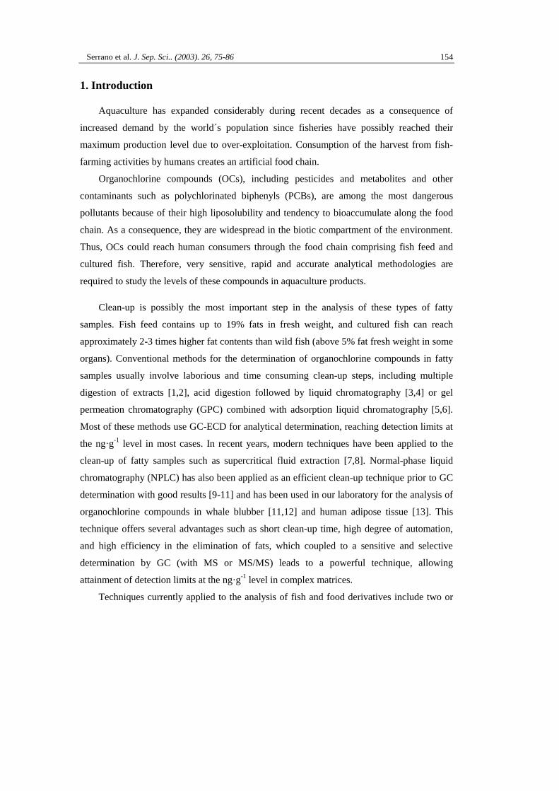
Serrano et al. J. Sep. Sci.. (2003). 26, 75-86 154
1. Introduction
Aquaculture has expanded considerably during recent decades as a consequence of
increased demand by the world´s population since fisheries have possibly reached their
maximum production level due to over-exploitation. Consumption of the harvest from fish-
farming activities by humans creates an artificial food chain.
Organochlorine compounds (OCs), including pesticides and metabolites and other
contaminants such as polychlorinated biphenyls (PCBs), are among the most dangerous
pollutants because of their high liposolubility and tendency to bioaccumulate along the food
chain. As a consequence, they are widespread in the biotic compartment of the environment.
Thus, OCs could reach human consumers through the food chain comprising fish feed and
cultured fish. Therefore, very sensitive, rapid and accurate analytical methodologies are
required to study the levels of these compounds in aquaculture products.
Clean-up is possibly the most important step in the analysis of these types of fatty
samples. Fish feed contains up to 19% fats in fresh weight, and cultured fish can reach
approximately 2-3 times higher fat contents than wild fish (above 5% fat fresh weight in some
organs). Conventional methods for the determination of organochlorine compounds in fatty
samples usually involve laborious and time consuming clean-up steps, including multiple
digestion of extracts [1,2], acid digestion followed by liquid chromatography [3,4] or gel
permeation chromatography (GPC) combined with adsorption liquid chromatography [5,6].
Most of these methods use GC-ECD for analytical determination, reaching detection limits at
the ng·g-1
level in most cases. In recent years, modern techniques have been applied to the
clean-up of fatty samples such as supercritical fluid extraction [7,8]. Normal-phase liquid
chromatography (NPLC) has also been applied as an efficient clean-up technique prior to GC
determination with good results [9-11] and has been used in our laboratory for the analysis of
organochlorine compounds in whale blubber [11,12] and human adipose tissue [13]. This
technique offers several advantages such as short clean-up time, high degree of automation,
and high efficiency in the elimination of fats, which coupled to a sensitive and selective
determination by GC (with MS or MS/MS) leads to a powerful technique, allowing
attainment of detection limits at the ng·g-1
level in complex matrices.
Techniques currently applied to the analysis of fish and food derivatives include two or

Serrano et al. J. Sep. Sci.. (2003). 26, 75-86 155
more clean-up steps and GC-ECD detection, reaching limits of detection around 10 ng·g-1
[14-16], embracing in some cases traditional techniques as acid digestion with sulphuric acid
due to its high efficiency in elimination of fats, both directly [17,18] or through impregnation
of the silica layer in adsorption column chromatography [19].
The aim of this work is to develop sensitive and rapid multiresidual analytical
methodology for the determination of organochlorine pesticides and PCB residues in fish feed
and fish tissues that allows attainment of low limits of detection by means of an efficient
clean-up step and GC-MS/MS (EI) detection. Both, NPLC and sulphuric acid clean-up are
evaluated for their efficiency in elimination of fats in order to develop an accurate procedure
able to detect residues below ng·g-1
in this type of difficult matrices characterised by their high
fat content. Gas chromatography coupled with mass spectrometry (MS/MS, EI) has been
optimised for the analytical determination of organochlorine compounds to allow the
unequivocal identification of the analytes and the high selectivity and sensitivity required in
ecotoxicological and environmental studies.
2. Material and Methods
2.1. Reagents
DDTs (p,p’-DDT, p,p’-DDE, p,p’-DDD), HCB, aldrin, heptachlor, heptachlor epoxide,
lindane, mirex, metoxychlor, endosulfan ( and isomers), ensodulfan sulphate, endosulfan
ether and PCBs (IUPAC nº 28, 52, 101, 118, 138, 153, 180) were included in this study. In
addition, chlorfenson was used as internal standard in the validation study. Reference
materials of pesticides and metabolites from Dr S. Ehrenstorfer (Promochem, Wesel,
Germany) with a purity 97-99.7% were used for the preparation of stock solutions by
dissolving in acetone. These stock solutions (around 500 µg·mL-1
) were stored in a freezer at -
20°C. Working solutions of pesticides for sample fortification and for injection in the LC and
the GC systems were prepared by diluting stock solutions in n-hexane. Acetone residues were
eliminated from working and standard solutions by evaporation at 40°C under N2 stream.
PCB mix 3 standard from Dr S. Ehrenstorfer (10 g·mL-1
in isooctane) was used for single
quantitation of PCBs congeners IUPAC nº 28, 52, 101, 118, 138, 153, 180. Working solutions
were prepared by dilution in n-hexane

Serrano et al. J. Sep. Sci.. (2003). 26, 75-86 156
Three labelled internal standards were used: HCB-13
C6, 2,2’,3,4,4’,5’-
hexachlorobyphenyl-13
C12 (PCB 138) (Cambridge Isotope Labs, Inc. Andover, MA) and p,p’-
DDE D8 (Dr Ehrenstorfer). Working solutions of labelled standards (ca. 1 µg·mL-1
) were
prepared by dilution of commercial solution with hexane and stored at 4 °C.
Ethyl acetate and n-hexane Ultratrace quality and sulphuric acid 95-98% were purchased
from Scharlab (Barcelona, Spain). Anhydrous sodium sulphate for pesticide residue analysis
(Baker, Deventer, Holland) was dried for 18 hours at 300°C before use.
2.2. Samples
Pools of samples of fish feed and fish tissues from cultured Sparus aurata were used for
the method validation. Real world samples of fish feed and fish tissues (white and red muscle
and liver) from aquaculture activities were stored at - 20°C until analysis.
2.3. LC instrumentation
A schematic representation of the LC system is shown in Figure 1. It was constructed
with the following equipment: LC Pump: Master 305 piston pump, Gilson (Middleton, USA);
Valve: 6 way high-pressure valve VICI Valco (Europe Instruments, Schenkon, Switzerland),
electronically controlled; Sampler: injection valve Rheodyne (Cotati, CA, USA) with 1.0-ml
loop; Column: 150 x 3.9 mm ID packed with Novapack 4 µm silica (Waters, Milford, MA,
USA); Fraction collector: Gilson FC 203B (Middleton, USA); Mobile phases: n-hexane and
ethyl acetate; Flow rate: 1 mL·min-1
.

Serrano et al. J. Sep. Sci.. (2003). 26, 75-86 157
Figure 1. Scheme of the automated NPLC system used in this work.
2.4. GC instrumentation
GC-MS/MS was performed using an ion trap mass spectrometer (Finnigan GCQ, Austin,
Texas, USA) operating in the electron impact ionisation mode (EI) at an electron energy of 70
eV and an emission current of 250 µA. The GC 8000 Top (CE Instruments, Milan, Italy) was
equipped with an AS 800 autosampler. The injector temperature was 240°C. The oven
temperature was programmed as follows: 90°C (4 min), 30°·min-1
to 180°C, 4°·min-1
to
270°C, 30º·min-1
to 300ºC with a final hold for 3.5 min. Splitless injections (3 mm ID glass
liner) of 2 µl were performed using a fused silica DB-5MS capillary column coated with
cross-linked 5% phenyl methyl siloxane with a length of 30 m x 0.25 mm ID. and a film
thickness of 0.25 µm. Helium was applied as carrier gas at a flow of 1 mL·min-1
.
Experimental mass spectrometer parameters are the following: the source and transfer
line temperatures were 220ºC and 275ºC, respectively; the electron multiplier potential was
1550 V and the multiplier gain was 3.2E5; the values of automatic gain control (AGC) target
and trap offset were 50 and 10, respectively. Extracted ions selected from EI-MS/MS spectra
used for quantitation are indicated in Table 1.
LOOP1 ml
PUMP
WasteSample Injection
(controller)
mobile phase
150x3.9 mm i.d., 4µm silica Novapack
COLLECTOR
FRACTIONSGC
MS/MS
Waste
LOOP4 ml
ethyl acetate
reservoir
LC column
Injection valve 6-way high pressure valve
load position
inject position

Serrano et al. J. Sep. Sci.. (2003). 26, 75-86 158
2.5. Validation study
Statistical validation of the method was performed in our own laboratory. The following
parameters were evaluated:
Linearity: the calibration curve for MSD was obtained by analysing standard solutions in
triplicate at 8 concentrations between 0.5 and 1000 ng·mL-1
.
Accuracy: the accuracy was estimated by means of recovery experiments, analysing
representative samples (n=6) fortified at three concentrations levels (75, 25 and 5 ng·g-1
, fresh
weight). The Standard Additions Method was applied for quantitation of HCB, DDTs and
PCBs as they were present in all the blank samples studied.
Precision: the precision of the method was determined as the repeatability of the recoveries
(n=6) at each fortification level, within and between days.
Selectivity: the selectivity of the method was based on the appropriate selection of ions for the
detection of each analyte by mass spectrometry extracted ion mode.
Limit of detection: the LOD was obtained when the signal was three times the background
noise in the chromatogram at 4 ng·g-1
.

Serrano et al. J. Sep. Sci.. (2003). 26, 75-86 159
Table 1. Program used for MS/MS detection of the compounds studied in this paper and extracted ions
selected from EI-MS/MS spectra for quantitation. OC pesticides and PCB were analysed with different
MS/MS programs.
Compound Parent
ion
Time
(min)
Window Mass
range
Voltage
(V)
Rt a)
(min)
Extracted ions
selected
HCB 288 3.50 10 170-295 3.50 7.31 214, 249
HCB-13C6 288 3.50 10 170-295 3.50 7.31 220, 225
Lindane 219 7.50 5 140-225 1.05 7.85 181, 183
Endosulfan ether 241 8.40 8 165-245 1.56 8.84 204-208, 237-241
Heptachlor 337 9.25 8 200-345 1.50 9.56 265
Aldrin 293 10.30 10 145-300 1.75 10.57 220
Heptachlor epoxide 355 11.30 8 175-360 1.60 11.80 265
α-Endosulfan 241 12.65 8 165-245 2.50 12.99 170, 172, 204-208
p,p’-DDE 250 13.60 8 145-260 3.00 13.82 176
p,p’-DDE-D8 250 13.60 8 145-260 3.00 13.82 183, 184
β-Endosulfan 241 14.60 8 165-245 2.50 15.02 170, 172, 204-208
p,p’-DDD 235 15.20 8 160-240 1.30 15.44 165, 199
Endosulfan sulphate 289 16.47 8 175-295 1.60 16.63 217, 219, 251-255
p,p’-DDT 235 16.75 8 160-240 1.70 16.83 165, 199
Metoxychlor 227 18.00 4 110-230 1.50 19.21 152, 169
Mirex 272 20.00 8 200-280 1.50 20.5 237
PCB 28 258 3.50 4 140-262 2.00 9.16 186
PCB 52 292 9.80 4 180-295 1.50 10.09 220, 222
PCB 101 326 11.50 4 170-330 2.00 12.85 254, 256
PCB 118 326 11.50 4 170-330 2.00 15.09 254, 256
PCB 153 360 15.60 8 200-380 1.75 15.93 288, 290
PCB 138 360 15.60 8 200-380 1.75 16.99 288, 290
PCB 138-13C12 372 15.60 8 200-280 1.75 16.99 302, 337, 372, 374
PCB 180 396 18.50 8 220-402 2.25 19.66 322,324,326
a) Rt: retention time

Serrano et al. J. Sep. Sci.. (2003). 26, 75-86 160
2.6. Procedure
2.6.1. Sample preparation and extraction
Samples were thawed at room temperature. Approximately 8 g of fish tissues or fish feed
were chopped and homogenised in a mortar with the amount of anhydrous sodium sulphate
necessary to remove water. Refluxing in n-hexane for 4 hours effected extraction. After
filtration (0.45 µm), the extract was pre-concentrated using a Kuderna-Danish apparatus until
ca. 2 ml. The final residue was adjusted to 2 ml with n-hexane (4 g sample per mL hexane).
2.6.2. Recommended clean-up procedure
For the analysis of fish tissues, including white and red muscle and liver, 1 mL of the
hexanic extract (4 g sample·mL-1
) was injected into the LC system using the 6-way injection
valve (IV). The mobile phase (n-hexane) was set at a flow rate of 1 mL·min-1
. The modifier
solvent (ethyl acetate) was loaded in a 25 mL syringe used as reservoir (see Figure 1) that fill
the 4-mL loop mounted on the HPV1 valve by gravity (ca. 2 mL·min-1
) and was introduced
into the column at 16 min of elution. LC fractions of 1 mL were first collected in order to
know both the fat and pesticide elution patterns after the LC clean-up. Finally, analytes eluted
as follows: DDTs, PCBs, mirex, aldrin, heptachlor, -endosulfan, HCB and lindane between
0-12 minutes (Fraction A), -endosulfan, endosulfan sulphate, endosulfan ether, metoxychlor
and heptachlor epoxide between 12-18 minutes (Fraction B). The silica gel column was
regenerated by 4 mL ethyl acetate flush step at 20 minutes. The volume of the fractions
collected was adjusted at 1 mL under N2 stream at 40°C.
The elution pattern of pesticides and lipids was reproducible during at least two months
of routine analysis. The overall procedure was controlled from the LC pump programming the
times of valve activation (Figure 1).
In order to reach detection levels as low as possible in the analysis of fish feed, first, acid
digestion was applied to the hexanic extracts (4 g of fish feed per mL hexane), in order to
remove most of the fats. Hexanic extracts were digested with two volumes of H2SO4 by
shaking for 3 min in a Vortex. The operation was repeated three times. The hexanic phases
obtained were combined and adjusted to the appropriate volume (4 g·mL-1
) at 40°C under
gentle N2 stream. 1-mL of the cleaned up hexanic extract was injected into the LC system,

Serrano et al. J. Sep. Sci.. (2003). 26, 75-86 161
using n-hexane as mobile phase (flow: 1 mL·min-1
) and a pulse of 4-mL ethyl acetate at 16
min of elution.
Figure 2 shows a scheme of the overall analytical procedure.
f.m. hexane
LC- clean up
GC-MS/MS
1 ml
N 2 stream , 40°C
(2:1, v/v) x3
Purified Extract
2 ml
f.m. hexane
16’ ethyl acetate
LC- clean up
Fraction 1-12 ml
DDTs , PCBs , HCB
mirex , heptachlor
+ chopped
+ 20 g Na 2 SO 4
+ 100 ml n- hexane
+ reflux 4 hours
H 2 SO 4
fish tissues fish foods 1 ml
1 ml 1 ml
8 g sample
Extract + solid particles
Filtration 0.45 µm
Extract
Pre - concentration
Kuderna - Danish
Extract 2 ml
Fraction A (1-12 ml )
DDTs , PCBs , HCB
mirex , heptachlor , aldrin
Fraction B (12-18 ml )
hep - epoxi , lindane ,
endosulfan and metabolites ,
metoxychlor
Figure 2. Scheme of the overall analytical procedure applied for the determination of organochlorine
compounds in fish food and fish muscle.

Serrano et al. J. Sep. Sci.. (2003). 26, 75-86 162
2.6.3. GC analysis
1-mL portions of the fat-free LC fractions containing the analytes were injected in the
GC system using MS/MS (EI) detection. Linearity of response was proved in a concentration
range from 0.5 to 1000 ng·mL-1
. In the validation study, chlorfenson was used as internal
standard. MS/MS (EI) was also used as confirmation of analytes detected in real samples.
2.6.4. Determination of the fat
The total fat content in the sample extracts was determined by gravimetry, evaporating at
95°C until constant weight. However, the low amount of fat in the LC fractions necessitated
the use of a colorimetric method for the determination of fat at µg level. The colorimetric
method used for total lipids determination is based on the sulphophosphovainillin reactivity
[20]. Triacylglyceride calibration solution (Sigma, St Louis, Missouri, USA) was used as
standard. The calibration curve was plotted between 125 and 1000 µg. The LOD was found to
be 33 µg.
3. Results and Discussion
3.1. MS/MS optimisation
The MS/MS method applied uses EI ionization mode with automatic gain control (AGC),
which is characteristic of ion trap MS analyzer. MS/MS detection was performed by isolation
of the corresponding selected parent ion for each compound inside the trap followed by
application of an adequate excitation voltage for its subsequent fragmentation. Parent ions
were selected from the EI spectra taking into account aspects as high m/z values but also the
peak abundance as well as the chromatographic signal obtained after its isolation in the ion
trap. Daughter ions obtained were scanned over a characteristic mass range leading to the
MS/MS spectrum. The object was to generate MS/MS spectra where the parent ions were, at
least, 10-20% of base peak.
In this paper, two MS/MS methods were used, divided into five and fourteen acquisition
segments for PCBs and OC compounds, respectively (PCB 101 and 118, and PCB 153 and
138 into the same segment). Three values of the trapping parameter q (0.45, 0.35 and 0.25)

Serrano et al. J. Sep. Sci.. (2003). 26, 75-86 163
were investigated. The higher response for most compounds were obtained with q = 0.45, so
this value was selected for the method. Then, isolation and excitation conditions were
optimised and selected in order to obtain characteristic MS/MS spectra with fragmentation
patterns rich enough to allow the accurate identification of analytes detected.
Table 1 shows the conditions corresponding to the optimised MS/MS method. The
highest isolation windows (10 m/z units) used corresponded to HCB and p,p’-DDE as labelled
HCB-13
C6 and 4,4’-DDE D8 were also included in these segments. Selection of the precursor
ion and window was undertaken in order to keep an isolation mass range as short as possible,
including the pesticide as well as the isotopically labelled compound. In the segment
corresponding to the determination of PCB 138 and PCB 138 13
C12, it was not feasible to
select a single scan for their fragmentation because the difference was 12 units of m/z and the
highest window of m/z allowed by the system was 5 units. The software of the instrument
allows us to programme different scans (acquisition of dates) in the same time-window, thus
for PCB 153 and 138 a scan with the precursor ion 360 was selected, and for PCB 138 13
C12
another scan using 372 as precursor ion was selected, all of them in the fourth segment.
Extracted ions selected from EI-MS/MS spectra for quantitation are indicated in Table 1.
3.2. Study of clean up step
First, normal phase liquid chromatography and acid digestion with sulphuric acid were
assayed separately in order to determine their efficiency in the elimination of fat present in
hexanic extracts from both fish feed and fish tissues.
3.2.1. NPLC clean up
Our laboratory has previously used NPLC as a clean-up technique, obtaining satisfactory
results for marine organisms [10, 11]. The application of this technique removed more than
90% of fats in the extracts, allowing their direct injection in the GC system as the amount of
fat injected onto the capillary GC columns was below the maximum recommended for this
type of column (600 ng) [10, 21]. In the present work, LC fractions obtained after processing
4 g·mL-1
fish feed contained excessive amount of lipids for their injection in GC system
(more than 1000 ng of fats per µL purified extract) due to the high fat content present in the
samples (16-19% of fat fresh weight). Assays were repeated processing 1 g of sample per mL

Serrano et al. J. Sep. Sci.. (2003). 26, 75-86 164
hexane. In this case, the fat remaining in the purified extract (around 300 ng·µL-1
) allowed
their injection into GC.
On the other hand, the application of normal phase LC clean-up to fish muscle and liver
extracts (4 g of sample per mL hexane) allowed their injection into GC system as a
consequence of the lower content of fat present in this type of samples (around 5%). Figure 3
shows extracted ion GC-MS/MS chromatograms corresponding to fish muscle samples
(Sparus aurata) fortified at 4 ng·g-1
and underlines the absence of interferences and the high
S/N obtained.
Figure 3.Extracted ion GC-MS/MS chromatograms corresponding to fish muscle samples (Sparus
aurata) fortified at 4 ng·g-1
2 6 10 14 18 22 26 30
Time (min)
0
20
40
60
80
100
Re
lative
Abu
nd
an
ce
p,p’-DDE
4 8 12 16 20 24 28
Time (min)
0
20
40
60
80
100
Re
lative
Abu
nd
an
ce
lindane
2 6 10 14 18 22 26 30Time (min)
0
20
40
60
80
100
Re
lative
Abu
nd
an
ce
HCB
0 5 10 15 20 25 30 35
Time (min)
0
20
40
60
80
100
Re
lative
Abu
nd
an
ce PCB 101
PCB 118
10 12 14 16 18 20 22 24 26
Time (min)
010
40
60
80
100
Re
lative
Abu
nd
an
ce
-endosulfan
0 5 10 15 20 25 30 35Time (min)
0
20
40
60
80
100
Re
lative
Abu
nd
an
ce
PCB 180
Serrano et al. J. Sep. Sci.. (2003). 26, 75-86 165
3.2.2. Acid digestion clean up
Sulphuric digestion was assayed for fish feed as the high lipid content rendered the
application of NPLC clean-up inefficient. Data obtained showed that 99.5% of fats were
removed by using sulphuric acid clean-up in extracts containing 4 g of sample per mL hexane.
However, the amount of lipids remaining in the purified extracts (640 µg·mL-1
, approximately
1300 ng of fat in 2 µL of injection volume) was higher than the maximum recommended for
injection in capillary GC columns. Additionally, acid digestion did not allow the analysis of
acid labile compounds.
3.2.3. Acid digestion plus NPLC clean up
As a consequence of the previous assays, the two clean-up techniques were combined in
order to allow the processing of a sufficient amount of fish feed sample to attain the low
limits of detection required.
Results obtained by applying first acid digestion and then NPLC showed the high
efficiency of this combined clean-up, there remaining less than 200 µg of fat per mL hexane
in LC-fractions (introduction of less than 600 ng in the 2 µL injected into the GC system) on
using extracts of 4 g of sample per mL hexane. As a consequence of the efficiency of
purification of the extracts, GC chromatograms obtained presented a high S/N ratio leading to
low limits of detection.
3.3. Analytical parameters
Table 2 shows the slopes of the direct calibration curve and the standard addition method
for those analytes detected in the “blank” samples of fish feed and fish muscle used for the
validation study. Values obtained proved the absence of important matrix effects in the
determination of HCB, DDTs and PCBs in both, fish feed and muscle, as concentrations
calculated by direct calibration and standard addition method were similar in all cases.
Therefore, quantitation of fortified samples used in the validation study was carried out by
direct calibration, substracting the area of the peaks of the analytes detected in the blank
sample and using chlorfenson as internal standard.
The LOD was obtained when the signal was three times the background noise in the

Serrano et al. J. Sep. Sci.. (2003). 26, 75-86 166
chromatogram at the lowest concentration assayed (4 ng·g-1
). The LOQ was considered as
three times the LOD calculated in the validation study. The lowest concentration assayed in
recovery experiments was 5 ng·g-1
, as fortification levels below 5 ng·g-1
were not investigated
due to the presence of most analytes in the “blank” samples at concentration levels below 10
ng·g-1
(see Table 2).

Serrano et al. J. Sep. Sci.. (2003). 26, 75-86 167
D
irec
t ca
lib
rati
on
S
tan
da
rd a
dd
itio
ns
S
tan
da
rds
in h
exa
ne
fi
sh f
oo
d
m
usc
le
Co
mp
ou
nd
sl
op
e
r2
sl
op
e
r2
DC
a)
SA
b)
sl
op
e
r2
DC
a)
SA
b)
HC
B
0.0
17
0
.99
0
.01
5
0.9
955
1.0
8
0.4
8
-
- nd
nd
p,p
´-D
DD
0
.13
5
0.9
972
0
.12
1
0.9
996
4.2
7
4.7
1
0
.12
3
0.9
995
d
d
p,p
´-D
DE
0
.11
9
0.9
997
0
.12
8
0.9
95
8.3
8
.21
0
.12
2
0.9
952
1.3
2
1.2
1
p,p
´-D
DT
0
.08
2
0.9
99
0
.09
3
0.9
997
d
d
0
.08
3
0.9
957
d
d
PC
B 2
8
0.1
75
0.9
8
0
.18
3
0.9
997
d
d
0
.18
8
0.9
999
d
d
PC
B 5
2
0.3
17
0.9
976
0
.28
1
0.9
999
0.8
9
1.0
0.3
02
0.9
924
d
d
PC
B 1
01
0.1
21
0.9
907
0
.13
2
0.9
988
3.0
6
3.0
2
0
.11
2
0.9
923
d
d
PC
B 1
18
0.2
02
0.9
999
0
.19
0
0.9
984
1.7
0
1.7
6
0
.17
2
0.9
96
d
d
PC
B 1
53
0.2
85
0.9
93
0
.31
2
0.9
974
3.2
2
3.3
5
0
.28
0
0.9
965
d
d
PC
B 1
38
0.2
83
0.9
9
0
.27
0
0.9
971
3.4
5
3.0
4
0
.30
1
0.9
959
d
d
PC
B 1
80
0.2
86
0
.99
7
0
.29
8
0.9
96
0.5
5
0.4
7
0
.28
1
0.9
958
d
d
Ta
ble
2. C
om
par
iso
n o
f sl
op
es a
nd
con
cen
trat
ion
fou
nd
(n
g·g
-1)
in t
he
fish
fee
d s
imp
le u
sed f
or
val
idat
ion
stu
dy
usi
ng
dir
ect
cali
bra
tio
n a
nd s
tan
dar
d a
dd
itio
n m
eth
od
(ca
lib
rati
on r
ang
e 5
-75
ng
·g-1
).
d:
det
ecte
d b
elo
w l
imit
of
qu
anti
fica
tio
n;
nd
: n
on
det
ecte
d
a)
DC
: co
nce
ntr
atio
n f
ou
nd
by
dir
ect
cali
bra
tio
n
b)
SA
: co
nce
ntr
atio
n f
ou
nd
by
sta
nd
ard
add
itio
n

Serrano et al. J. Sep. Sci.. (2003). 26, 75-86 168
3.3.1.Fish feed
The overall analytical procedure, including reflux in hexane for the extraction of OCs,
evaporation by Kuderna-Danish, combined clean-up by means of acid digestion and
automated NPLC, and final determination by GC-MS/MS (EI), was applied to fish feed
samples fortified at 75, 25 and 5 ng·g-1
(fresh weight). Table 3 shows quantitative recoveries
(between 80-120% for the majority of compounds and fortification levels) and a precision
between days below 10% at the highest level of fortification and below 18% at the lowest
level assayed (5 ng·g-1
). Precision within days was similar to between days. Limits of
detection were below 1 ng·g-1
, except for heptachlor and p,p’-DDD.
Table 3. Mean recoveries (%) and relative standard deviations between days (in brackets) after
application of the overall analytical procedure to fortified fish feed samples (n=6). LOD in ng·g-1
fresh
weight.
Fortification level (ng·g-1
) LOD ng·g-1
75 25 5
HCB 85 (10) 98 (12) 80 (13) 0.3
Heptachlor 76 (7) 89 (14) 86 (18) 1.0
Mirex 121 (10) 110 (8) 116 (14) 0.5
p,p’-DDD 95 (6) 90 (10) 86 (8) 1.1
p,p’-DDE 88 (7) 86 (11) 79 (6) 0.5
p,p’-DDT 92 (7) 83 (15) 80 (12) 0.4
PCB 28 78 (7) 89 (15) 86 (15) 0.1
PCB 52 84 (5) 97 (12) 87 (10) 0.2
PCB 101 97 (8) 86 (14) 90 (10) 0.4
PCB 118 94 (6) 105 (8) 84 (11) 0.4
PCB 153 111 (7) 80 (15) 77 (17) 0.4
PCB 138 114 (7) 82 (13) 79 (15) 0.4
PCB 180 120 (8) 89 (12) 91 (17) 0.1
Non-recovered analytes, which were destroyed or lost during the sulphuric acid treatment
(metoxychlor, endosulfan and metabolites, aldrin, heptachlor epoxide, lindane) were
determined by applying only NPLC in the clean-up step of hexanic extracts containing 1 g of
sample per mL hexane. Recoveries were between 87 and 102%, with precision between days
lower than 13 % in all cases. However, limits of detection were around 10-fold higher (1-10
ng·g-1
) due to the lower amount of sample processed.
Serrano et al. J. Sep. Sci.. (2003). 26, 75-86 169
3.3.2.Fish tissues
Table 4 shows the recoveries obtained after the application of the method to the
determination of OCs in fish muscle and fish liver fortified samples (reflux in hexane,
automated NPLC clean-up and GC-MS/MS determination). The majority of recoveries at all
fortification levels were between 80 and 110%, with very few exceptions. Precision was better
than 15% and around this value at the lowest fortification level (5 ng·g-1
).
The limits of detection were below 1 ng·g-1
(except for endosulfan ether, 1.5 ng·g-1
) for
the analysis of fish muscle, and below 2 ng·g-1
for liver.
As Tables 3 and 4 show, all compounds were quantitatively recovered at the lowest level
of fortification assayed. Consequently, the method can be applied satisfactorily to
concentration levels as low as 5 ng·g-1
. As regards analysis time, after the extraction step
(simultaneous refluxing of a number of samples for 4 hours), sample preparation is simpler
and faster than by other methods available in the literature. For example, fish food acid
digestion can be carried out for 6 samples in around 2 hours and the subsequent treatment is
fully automated (LC clean-up and GC coupled off line).
3.4. Application to real-world samples
The analytical methodology developed in this work was applied to the analysis of fish
feed samples used in aquaculture during 2000-01 and tissues from cultured fish (weight: 224
10 g; length: 25 1 cm) from commercial markets. Fish feed is triturated fish (from
Moroccan coastal waters) blended with fish oils.
Although satisfactory analytical parameters were obtained in the validated procedure, 50
ng of isotopically labelled standards were added before the extraction as surrogate internal
standards for quality control in the analysis of real samples, rendering the use of chlorfenson
as internal standard unnecessary. Labelled standards used were HCB-13
C6 (for HCB, lindane,
endosulfan-ether; heptachlor, aldrin, heptachlor epoxide and -endosulfan), p,p’-DDE-D8 (for
p,p’-DDE, β-endosulfan, p,p’-DDD, endosulfan sulphate, p,p’-DDT, metoxychlor and mirex)
and PCB 138-13
C12 for PCBs.

Serrano et al. J. Sep. Sci.. (2003). 26, 75-86 170
Table 4. Mean recoveries (%) and relative standard deviations (in brackets) after application of the
overall analytical procedure to fortified fish muscle and fish liver samples. LOD in ng·g-1
fresh weight.
Fish muscle Fish liver
75 ng·g-1 25 ng·g-1 5 ng·g-1 LOD ng·g-1 5 ng·g-1 LOD ng·g-1
HCB 81 (12) 84 (14) 88 (11) 0.5 85 (15) 0.2
Lindane 104 (7) 91 (13) 75 (14) 0.8 85 (13) 0.1
Endosulfan ether 103 (11) 82 (10) 112 (10) 1.5 102 (12) 1.0
Heptachlor 88 (10) 93 (11) 84 (14) 0.4 90 (15) 0.5
Aldrin 97 (5) 92 (11) 88 (9) 0.5 96 (11) 0.5
Heptachlor epoxide 107 (7) 102 (12) 87 (11) 0.7 78 (13) 0.2
α-Endosulfan 104 (4) 101 (9) 88 (16) 0.5 94 (14) 1.2
p,p’-DDE 92 (9) 98 (4) 92 (10) 0.3 94 (10) 0.4
β-Endosulfan 103 (12) 96 (13) 81 (10) 0.5 85 (16) 1.5
p,p’-DDD 90 (8) 99 (7) 81 (11) 0.4 88 (15) 0.4
Endosulfan sulphate 80 (12) 86 (11) 87 (15) 0.5 81 (14) 1.0
p,p’-DDT 93 (6) 96 (11) 82 (13) 0.5 79 (17) 1.3
Metoxychlor 94 (6) 101 (13) 90 (11) 0.4 97 (10) 1.0
Mirex 90 (15) 103 (7) 91 (13) 0.2 90 (9) 0.1
PCB 28 113 (9) 108 (11) 86 (10) 0.4 85 (11) 0.4
PCB 52 102 (12) 114 (8) 97 (9) 0.5 99 (13) 1.4
PCB 101 97 (7) 71 (11) 83 (12) 0.4 81 (15) 0.2
PCB 118 82 (14) 84 (10) 83 (12) 0.8 93 (15) 0.3
PCB 153 95 (8) 91 (5) 78 (12) 0.3 71 (17) 0.1
PCB 138 88 (11) 91 (5) 79 (10) 0.5 75 (12) 0.2
PCB 180 85 (15) 93 (4) 95 (16) 0.4 93 (13) 0.1
The results obtained are shown in Table 5. Fish feed samples analysed contained
appreciable amounts of HCB, DDTs and all PCB congeners studied. The highest
concentrations corresponded to PCB 153 and 138, and to the main metabolite of DDT, i.e.
p,p’-DDE. On the other hand, all the DDTs and PCBs investigated were detected at low ng·g-1
levels in muscle and liver samples from cultured fish (Sparus aurata) obtained from markets.
In the fish tissues samples, the highest concentrations corresponded generally to p,p’-DDE
and PCB 153.

Serrano et al. J. Sep. Sci.. (2003). 26, 75-86 171
Table 5. Concentrations of organochlorine compounds detected in real world samples of fish
feeds and cultured fish tissues (Sparus aurata) from aquaculture activities during 2000-01.
Concentration (ng·g-1 fresh weight)
Fish feed Cultured fish
Compound White muscle Red muscle Liver
n a) 6b) 3 3 3
HCB 3.7 (16) nd, nd, nd d, d, d nd, nd, nd
p,p’-DDD 9.8 (13) d, d, d 2.3, 2.3, 2.7 1.3, 1.4, 1.2
p,p’-DDE 40.9 (9) 1.3, 1.2, 1.5 5.2, 5.8, 5.4 2.2, 2.4, 2.3
p,p’-DDT 28.5 (17) d, d. nd d, d, d d, d, d
PCB 28 7.8 (10) d, d, d d, d, d d, d, d
PCB 52 14.5 (17) d, d, d d, d, d d, d, d
PCB 101 37.9 (9) d, d, d 2.8, 2.5, 2.3 12.8, d, nd
PCB 118 17.1 (20) d, d, d 2.4, d, d 14.6, d, nd
PCB 153 57.2 (8) d, d, d 1.2, 1.0, 1.3 1.1, 1.0, 1.0
PCB 138 51.4 (4) d, d, d d, d, d 3.2, d, d
PCB 180 4.4 (14) d, d, d d, d, d 2.5, d, d
a) n = number of samples analysed. Every sample was a pool of 2-4 individuals
b) mean concentration and relative standard deviation in brackets
d= detected, nd= non detected,
As an example, Figure 4 and Figure 5 show the GC-MS/MS chromatograms obtained
after the application of the developed procedures to the analysis of fish feed (Figure 4) and
fish liver (Figure 5). As can be observed, the spectrum of each peak obtained by MS/MS
confirms the identity of the organochlorine compounds detected in the samples.

Serrano et al. J. Sep. Sci.. (2003). 26, 75-86 172
A
B
10 12 14 16 18 20 22 Time (min)
0
20
40
60
80
100
PCB 28 (3Cl)
PCB 52 (4Cl)
PCB 101 (5Cl)
PCB 118 (5Cl)
PCB 153 (6Cl)
PCB 138 (6Cl)
PCB 180 (7Cl)
160 180 200 220 240 m/z0
20
40
60
80
100 186
150
188258
256
220 240 260 280 m/z0
20
40
60
80
100220
222
257
3Cl
4Cl
250 270 290 310 m/z0
20
40
60
80
100256
291 326
5Cl
6Cl
320 340 360 380 m/z0
20
40
60
80
100 324
326
394
396
7Cl
200 240 280 320 360 m/z0
20
40
60
80
100290
288
360
292
362358
Figure 4. GC-MS/MS chromatograms of a fish food sample analysed, and MS/MS spectra of the
compounds detected. A- organochlorine pesticides (extracted ion). B- PCBs (total ion current).
5 10 15 Time (min)2520
HCB
p,p’-DDT
p,p’-DDD
p,p’-DDE
170 190 210 230 250 270 2900
20
40
60
80
100214
248.6
177 216 251 282
160 180 200 220 240
165
199237
200
150 170 190 210 230 2500
20
40
60
80
100
176
246
150177 211
0
20
40
60
80
100

Serrano et al. J. Sep. Sci.. (2003). 26, 75-86 173
A
B
4 6 8 10 12 14 16 18 20 22 24 26 28 30 32Time (min)
0
10
20
30
40
50
60
70
80
90
100
RelativeAbundanc
e
140 150 160 170 180 190 200 210m/z
0
20
40
60
80
100
186
151
PCB 28
(3Cl)
3Cl
PCB 52
(4Cl)
180 190 200 210 220 230 240 250 260 270 280 290
m/z
0
20
40
60
80
100220
2224Cl
PCB 101
(5Cl) PCB 118(5Cl)
PCB 153
(6Cl)
PCB 138
(6Cl)
PCB 180
(7Cl)240 260 280 300 320 340 360 380 400
m/z0
20
40
60
80
100
324
326
322
328
180 200 220 240 260 280 300m/z
0
20
40
60
80
100
254
2565Cl
6Cl
200 220 240 260 280 300 320 340 360 380m/z
0
20
40
60
80
100
290
288
360292
364358
7Cl
Figure 5. GC-MS/MS chromatograms for a fish liver sample analysed (Sparus aurata) and
MS/MS spectra of the compounds detected. A- organochlorine pesticides (extracted ion). B-
PCBs (total ion current).
10.5 11.5 12.5 13.5 14.5 15.5 16.5 17.5 18.5 19.5 20.5
Time (min)
0
10
20
30
40
50
60
70
80
90
100
Re
lative
Ab
un
da
nce p,p’-DDE
160 170 180 190 200 210 220 230 240
m/z
0
20
40
60
80
100
Re
lative
Ab
un
da
nce 165.0
199.0 237.1
150160170180190200210
m/z
0
20
40
60
80
100
Re
lative
Ab
un
da
nce
176.0
150.0 211.0
14.5 15.5 16.5 17.5 18.5 19.5 20.5
Time (min)
10
20
30
40
50
60
70
80
90
100
Re
lative
Ab
un
da
nce
p,p’-DDD
p,p’-DDT
0

Serrano et al. J. Sep. Sci.. (2003). 26, 75-86 174
4. Concluding remarks
It can be concluded that application of the optimised method for MS/MS detection
(extract ion mode) to extracts of fatty samples purified by automated NPLC allowed the
unequivocal identification of the analytes and to reach limits of detection below ng·g-1
.
As a consequence of the results obtained in the analysis of real samples, more data are
needed in order to trace the behaviour of the organochlorine compounds through the marine
food chain of wild and cultured products, in order to foresee risks to the human population,
the final fate of these contaminants.
Acknowledgments
We thank the Generalitat Valenciana (Conselleria de Cultura y Educación, Project
GV00-019-2) for their financial support of this study.
References
[1] M. Blanchard, M.J. Teil, A.M. Carru, A. Chesterikoff, M. Chevrenil, Wat. Res. 1997,
31(6), 1455-1461.
[2] H. Yamada, K. Takayanagi, T. Masahiro, H. Tagata, K. Ikeda, Environ. Pollut. 1997,
96(2), 217-226.
[3] S. Focardi, C. Fossi, C. Leonzio, S. Corsolni, O. Parra, Environ. Monitor. Asses.
1996. 43, 73-92.
[4] M.N. Jacobs, P.A. Johnston, C.L. Wyatt, D. Santillo, M.C. French, Int. J. Environ.
Pollut. 1997. 8, 74-92.
[5] P.J. Marquis, R.L. Hanson, M.L. Larsen, W.M. DeVita, B.C. Butterworth, D.W.
Kuehl, Chemosphere. 1994. 29, 509-521.
[6] L. Brown, Arch. Environ. Contam. Toxicol. 1997. 33, 357-368.
[7] J.H. Wang, Q. Xu, K. Jiao, J. Chromatogr. A. 1998, 818(1), 138-143.
[8] M.L. Hopper, J. Chromatogr. A. 1999. 840(1), 93-105.
[9] G.R. van der Hoff, A.C. van Beuzekom, V.A. Brinkman, R.A. Bauman, P. van
Zoonen, J. Chromatogr. A. 1996, 754(1-2), 487-496.
[10] F. Hernández, R. Serrano, E. Pitarch, F.J. López, Anal. Chim. Acta. 1998, 374, 215-
229.
Serrano et al. J. Sep. Sci.. (2003). 26, 75-86 175
[11] R. Serrano, F.J. López, F. Hernández, J. Chromatogr. A. 1999, 855, 633-643.
[12] F. Hernández, R. Serrano, A.F. Roig-Navarro, Y. Martínez-Bravo, F.J. López, Mar.
Pollut. Bull. 2000, 40 (5), 426-433.
[13] F. Hernandez, E. Pitarch, R. Serrano, J.V. Gaspar, N. Olea, J. Anal. Toxicol. 2002,
(in press).
[14] C.R. Santerre, R. Ingram, G.W. Lewis, J.T. Davis, L.G. Lane, R.M. Grodner, C.I.
Wei, P.B. Bush, D.H. Xu, J. Shelton, E.G. Alley, J.M. Hinshaw, J. Food Science.
2000, 65(2), 231-235.
[15] D. Berglund, P. Larsson, G. Ewald, L. Okla, Can J. Fish Aquat. Sci. 2000, 57,1160-
1168.
[16] K.A. Kidd, H.A. Bootsma, R.H. Nesslein, D.C.G. Muir, R.E. Hecky, Environ. Sci.
Technol. 2001, 35, 14-20.
[17] M. Solé, C. Porte, D. Barcelo, J. Albaiges, Mar. Pollut. Bull. 2000, 40(9), 746-753.
[18] K. Borga, G.W. Gabrielsen, J.V. Skaare, Env. Pollut. 2001, 113, 187-198.
[19] G. Asmund, M. Cleemann, Sci. Total Environ. 2000, 245: 203-219.
[20] N. Zöllner, K.Z Kirsch, Ges. Exp. Med. 1962, 135: 545-548.
[21] K. Grob, I. Kalin, A. Artho, J. High Resolut. Chromatogr. 1991, 14: 373-376.

Serrano et al. J. Sep. Sci.. (2003). 26, 75-86 176

2.1.3. ARTÍCULO CIENTÍFICO 5
Investigating the presence of organochlorine pesticides and polychlorinated biphenyls
in wild and farmed gilthead sea bream (Sparus aurata) from the Western Mediterranean
sea
R. Serrano, M. Barreda, M.A. Blanes
Marine Pollution Bulletin. (2008). 56, 963-972


Serrano et al. Mar. Poll.Bull. (2008). 56, 963-972 179
Investigating the presence of organochlorine pesticides and
polychlorinated biphenyls in wild and farmed gilthead sea bream
(Sparus aurata) from the Western Mediterranean sea
Roque Serrano, Mercedes Barreda and Miguel A. Blanes
Research Institute for Pesticides and Water (IUPA), Avda Sos Baynat, s/n.
University Jaume I, 12071 Castellón, Spain
Abstract
The presence of organochlorine pesticides and polychlorinated biphenyls in wild and
farmed gilthead sea bream (Sparus aurata) from the Western Mediterranean, Spain, is
investigated. These pollutants were determined in white and red muscle and liver by gas
chromatography coupled to tandem mass spectrometry. Contaminant profiles present in both
wild and farmed fish tissues include DDTs, PCBs and HCB. The highest concentrations of
contaminants were found in liver, and an increase in pollutant levels was observed in autumn,
before spawning. This fact is explained in light of increased food intake when sea water
temperatures increase. Gilthead sea bream from Western Mediterranean populations showed
significantly higher concentrations of DDTs and PCBs than farmed fish from the same area.
This fact is attributed to the low level of organochlorine contaminants present in fish feed
supplied to the cultured fish. The diet is highlighted as an important factor in understanding
differences observed in organochlorine pollutants levels of fish tissues.
Keywords: Organochlorine pesticides; Polychlorinated biphenyls; Wild fish; Farmed fish; Western
Mediterranean; Gilthead sea bream

Serrano et al. Mar. Poll.Bull. (2008). 56, 963-972 180
1. Introduction
Marine aquaculture has seen strong development in the last few decades as a
consequence of increased fish consumption by the world population and decreasing wild
stocks. Fish culture has also increased in the Western Mediterranean, where it is mainly
focused on two species: gilthead sea bream (Sparus aurata) and sea bass (Dicentrarchus
labrax). Fish culture operates in parallel to traditional fisheries and nowadays both cultured
and wild fish are important components of the Mediterranean diet.
Polychlorinated biphenyls (PCB) and organochlorine pesticides (OCP) are non-polar,
highly lipophilic and persistent, ubiquitous environmental pollutants. Both are classified as
persistent organic pollutants (POP) and are present in the contamination pattern of marine
environments world-wide. Organochlorine compounds (OC) are dangerous pollutants due to
their toxicity and stability, long biological half life and high liposolubility. These factors
result in high bioaccumulation and biomagnification in the food chain, involving a wide range
of trophic levels (Borga et al., 2001; Kidd et al., 2001; Serrano et al., 2003 a; Hoekstra et al.,
2003 and Konwick et al., 2006).
As the human population is at the top of the artificial food chain that arises from
aquaculture activities (composed of fish feed and farmed fish), a possible source of
accumulation of OC in human beings exists. In fact, dietary intake, especially of marine
organisms, is considered the most important source of OC in humans (Bjerregard et al., 2001;
Johansen et al., 2004; Naso et al., 2005 and Bordajandi et al., 2006) and as a consequence,
organochlorine compounds are frequently detected in human lipid tissues and fluids of people
who have consumed seafood (Porta et al., 1999; Hernández et al., 2002a; Hernández et al.,
2002b; Pitarch et al., 2003; Cruz et al., 2003; De Felip et al., 2004; De Saeger et al., 2005 and
Withcomb et al., 2005).
Previous works have detected these pollutants in fish feed used in aquaculture and in
cultured fish (Santerre et al., 2000; Easton et al., 2002 and Serrano et al., 2003a). Specifically,
fish feed used in fish production on the Spanish Mediterranean Coast has been analysed by
(Serrano et al., 2003 a) and (Serrano et al., 2003 b) who found appreciable concentrations of
DDTs and PCBs.

Serrano et al. Mar. Poll.Bull. (2008). 56, 963-972 181
Recently a controversy has arisen from the study carried out by Hites et al. (2004) on OC
levels in farmed and wild salmon. Results of this study showed that concentrations of OC
pollutants were significantly higher in farmed salmon than in wild salmon.
The high load of pollutants, including organochlorine compounds, in farmed salmon was
also highlighted in a preliminary study performed by Easton et al. (2002). The feed used in
the culture of these carnivorous fish was identified as the main source of organic persistent
pollutants.
In this paper the levels of PCB and OCP in wild and cultured sea bream from the
Western Mediterranean are investigated. Specimens were collected over two years (2001 and
2002) before and after spawning (autumn and winter, respectively). Liver, white muscle and
red muscle were analysed using gas chromatography (GC) coupled to tandem mass
spectrometry (MS/MS), after automated purification of sample extracts by normal phase
liquid chromatography (NPLC). Data obtained from wild and cultured fish are compared to
provide information on possible differences in their organochlorine levels, and to assist with
information that may impact on public health.
2. Materials and methods
2.1. Samples
Authentic samples of wild and cultured gilthead sea bream (S. aurata) came from
populations located off the Castellon Coast (Spanish Mediterranean Coast) (Fig. 1) either
from trawl catch, or from sea cage farms located in the same area (around longitude 0°
latitude 40°N). They were purchased from commercial markets, dissected, the target tissues
separated, and stored at −20 °C until analysis. The development state of oocytes was checked
in each sample. Samples were collected in winter (after spawning) and autumn (before
spawning) in both 2001 and 2002. The composite samples were made up of three individual
specimens (female specimens around 500 g) that were pooled in order to obtain homogeneous
composite samples of each tissue studied. At each sampling time, three composite samples
were prepared, and all were analysed in triplicate.

Serrano et al. Mar. Poll.Bull. (2008). 56, 963-972 182
Fig. 1. Comparison between organochlorine compounds concentrations in liver from wild and cultured
gilthead sea bream from the Western Mediterranean area. ■ Average concentrations corresponding to
the analysis of composite samples (n = 3) 2001. □ id 2002. Signify differences between wild and farmed
fish * p < 0.05;
** p < 0.01.

Serrano et al. Mar. Poll.Bull. (2008). 56, 963-972 183
2.2. Analytical methodology
Organochlorine compounds, including pesticides and derivatives (DDTs – p,p′-DDT,
p,p′-DDE, p,p′-DDD –, HCB, heptachlor, heptachlor epoxide, lindane, mirex, metoxychlor,
endosulfan (α and β isomers), endosulfan sulphate and endosulfan ether) and the
polychlorinated biphenyls usually used as indicators IUPAC No. 28, 52, 101, 118, 138, 153,
180, were determined in fish tissues (white and red muscle, and liver) following the method
described by Serrano et al. (2003 b).
In brief, extraction from muscle and liver was carried out by refluxing ca. 8 g
homogenized thawed sample in n-hexane for 4 h. Clean up of fish extracts was performed by
HPLC, injecting 1 mL hexanic extract (4 g sample per mL) into an HPLC system using a
silica-gel column. LC system used is composed by an LC Pump Master 305 piston pump,
Gilson (Middleton, USA), with a column 150 × 3.9 mm i.d. packed with 4 μm silica
Novapack (Waters, Milford, MA, USA); mobile phases were n-hexane and ethyl acetate for
column regeneration after a clean up cycle; flow rate was 1 ml min−1
. Analysis of the fat-free
LC fractions collected was performed by gas chromatography with tandem mass spectrometry
(GC–MS/MS) using an ion trap mass spectrometer (Finnigan GCQ, Austin, Texas, USA)
operating in the electron impact ionisation mode (EI). The GC 8000 Top (CE Instruments,
Milan, Italy) was equipped with an AS 800 autosampler. The oven temperature was
programmed as follows: 90 °C (4 min), 30 °C to 180 °C min−1
, 4 °C to 270 °C min−1
, 30 °C to
300 °C min−1
with a final hold for 3.5 min. Splitless injections (3 mm i.d. glass liner) of 2 μl
were performed using a fused silica DB-5MS capillary column coated with cross-linked 5%
phenyl methyl siloxane with a length of 30 m × 0.25 mm i.d. and a film thickness of 0.25 μm.
Helium was applied as carrier gas at a flow of 1 ml min−1
. The injector temperature was
240 °C. Experimental mass spectrometer conditions are listed in Table 1 (more details
reported in Serrano et al., 2003 b).

Serrano et al. Mar. Poll.Bull. (2008). 56, 963-972 184
Table 1. Program used for MS/MS detection of PCB and OC and extracted ions selected for quantitative
determination
Compound Parent
ion
Time
(min) Window Mass range Voltage (V)
Rta
(min)
Extracted ions
selected
HCB 288b 3.50 10 170–295 3.50 7.31 214, 249
HCB-13C6d 288b 3.50 10 170–295 3.50 7.31 220, 225
Lindane 219 7.50 5 140–225 1.05 7.85 181, 183
Endosulfan ether 241 8.40 8 165–245 1.56 8.84 204–208, 237–241
Heptachlor 337 9.25 8 200–345 1.50 9.56 265
Heptachlor epoxide 355 11.30 8 175–360 1.60 11.80 265
α-Endosulfan 241 12.65 8 165–245 2.50 12.99 170, 172, 204–208
p,p′-DDE 250c 13.60 8 145–260 3.00 13.82 176
p,p′-DDE-D8d 250c 13.60 8 145–260 3.00 13.82 183, 184
β-Endosulfan 241 14.60 8 165–245 2.50 15.02 170, 172, 204–208
p,p′-DDD 235 15.20 8 160–240 1.30 15.44 165, 199
Endosulfan sulphate 289 16.47 8 175–295 1.60 16.63 217, 219, 251–255
p,p′-DDT 235 16.75 8 160–240 1.70 16.83 165, 199
Metoxychlor 227 18.00 4 110–230 1.50 19.21 152, 169
Mirex 272 20.00 8 200–280 1.50 20.5 237
PCB 28 258 3.50 4 140–262 2.00 9.16 186
PCB 52 292 9.80 4 180–295 1.50 10.09 220, 222
PCB 101 326 11.50 4 170–330 2.00 12.85 254, 256
PCB 118 326 11.50 4 170–330 2.00 15.09 254, 256
PCB 153 360 15.60 8 200–380 1.75 15.93 288, 290
PCB 138-13C12d 372 15.60 8 200–280 1.75 16.99 302, 337, 372, 374
PCB 138 360 15.60 8 200–380 1.75 16.99 288, 290
PCB 180 396 18.50 8 220–402 2.25 19.66 322, 324, 326
OC and PCB were analysed with different MS/MS programs. The isotopic labelled compounds used as surrogate
internal standards (modified from Serrano et al., 2003b) are shown in italic letters. a Rt: retention time.
b The total m/z range selected to carry out fragmentation (283–293) covers the individual parent ions of HCB (284)
and HCB 13C6 (290). c The total m/z range selected to carry out fragmentation (245–255) covers the individual parent ions of p,p′-DDE
(246) and p,p′-DDE D8 (254). d Isotopically labelled compounds used as surrogate internal standards.

Serrano et al. Mar. Poll.Bull. (2008). 56, 963-972 185
The analytical method applied showed excellent sensitivity and selectivity, as a
consequence of the use of tandem mass spectrometry. It was satisfactorily validated by
recovery experiments down to 5 ng g−1
. Lower spiked levels were not checked due to the
presence of DDTs and PCBs in the “blank” samples and the background levels found in all
fish analysed. However, the powerful analytical characteristics of GC–MS/MS together with
the efficiency of the HPLC clean up in removing fat allowed us to detect the analytes at
concentrations as low as 0.1 ng g−1
(estimated as the limit of detection, except for endosulfan
ether, 0.2 ng g−1
). The limit of quantification was estimated as three times the detection limit
(i.e. nine times the background noise in the chromatograms), resulting in values of 0.3 ng g−1
,
except for endosulfan ether (0.6 ng g−1
). All analytes detected in the samples were confirmed
by tandem mass spectrometry.
In regard to fish feed, an additional clean up step with concentrated sulphuric acid was
necessary prior to normal phase HPLC clean up as a consequence of its high lipid content
(around 20% fresh weight) (Serrano et al., 2003 b). Limits of detection were below 1 ng g−1
,
except for heptachlor and p,p′-DDD. Analytes lost or destroyed in the acid treatment were
analysed applying only normal phase HPLC clean up, with limits of detection around
10 ng g−1
, due to the lower amount of sample processed.
For quality control of real sample analysis, 50 ng of isotopically labelled standards were
added before extraction as surrogates. Labelled standards used were HCB-13
C6 (for the
determination of HCB, lindane, endosulfan ether, heptachlor, heptachlor epoxide, and α-
endosulfan); p,p′ DDE-D8 (for DDTs, β-endosulfan, endosulfan sulfate, metoxychlor, and
mirex), and PCB138-13
C12 (for PCBs).
Biomagnification factors (BMF) were calculated as the ratio between lipid-based
concentrations of organochlorine compounds in fish tissues and fish feed (Serrano et al., 2003
a) using data obtained before and after spawning (autumn and winter, respectively).
2.2.1. Determination of fat
The total fat content in the sample extracts was determined gravimetrically after
evaporation at 95ºC to constant weight.

Serrano et al. Mar. Poll.Bull. (2008). 56, 963-972 186
2.2.2. Data analysis
OC concentrations in tissues are expressed on a fresh weight and lipid weight basis
(ng g−1
fresh weight and ng g−1
lipid weight). Data were converted to log (ng g−1
lipid weight
+1) to correct for the dependence between arithmetic means and standard deviations.
Homoscedasticity of variances was tested by means of Barlett′s test (p < 0.05). Levels of OC
in wild and cultured fish tissues were compared by t-Student test. All the statistical tests were
conducted using STATGRAPHICS Version 7.0 (Statistical Graphics Corporation).
3. Results
3.1. Seasonal and tissue variation of PCB and OC concentration
The analysis of liver and muscle from wild, commercially caught, gilthead sea bream
showed the presence of p,p′-DDT, p,p′-DDE, p,p′-DDD, HCB, lindane and all the PCBs
studied (Table 2). The highest concentrations corresponded to the sum of DDTs (especially
p,p′-DDE) and the biphenyls with a higher degree of chlorine substitution (PCBs number 118,
138, 153, 180).
With regard to the presence of OC and PCB in muscle, white muscle presented low
levels of DDTs, and PCBs were detected at concentrations below the limit of quantification
(Table 2). Red muscle showed higher levels of contaminants than white muscle over winter,
although both muscle tissues did not present significant seasonal variations. In contrast to
muscle tissues, liver clearly presented higher concentrations of pollutants in autumn (Table 2
and Table 3).

Serrano et al. Mar. Poll.Bull. (2008). 56, 963-972 187
C
once
ntr
atio
n r
ange
(ng g
-1 l
ipid
wei
ght)
a
L
iver
R
ed m
usc
le
Whit
e m
usc
le
W
inte
r
Autu
mn
W
inte
r
Autu
mn
W
inte
r
Autu
mn
2
00
1
20
02
20
01
20
02
20
01
20
02
20
01
20
02
20
01
20
02
20
01
20
02
p,p
´-D
DE
1
32
-23
3
54
.3-2
56
58
8-1
058
91
5-1
158
32
1-4
36
28
6-3
48
17
6-2
54
13
4-4
01
13
.2-7
1.6
3
5.5
-58
.6
13
0-1
68
82
.5-1
68
p,p
´-D
DD
6
3.3
-11
6
42
.6-8
9.2
3
22
-41
5
22
6-3
16
48
.2-9
84
67
.8-1
24
69
.4-1
21
88
.5-1
30
19
.8-3
1.5
2
8.5
-32
.6
56
-10
2
42
.0-1
01
p,p
´-D
DT
1
7.5
-88
.1
10
.8-9
8.6
1
14
-17
5
48
.2-1
14
41
.5-6
8.6
2
8.5
-50
.5
82
.2-1
31
10
2-1
29
19
.8-3
2.2
1
2.1
-35
.5
61
.3-8
6.5
6
1.3
-86
.5
HC
B
24
.0-9
6.8
1
0.8
-33
0
d-2
0.4
1
8.5
-28
.3
65
.2-1
02
46
.5-1
73
d-8
.4
d-1
1.0
-
- -
-
Lin
dan
e
- -
- -
19
.8-3
6.2
2
7.1
-37
.3
- -
- -
- -
PC
B 2
8
d
d
d
d
16
.5-3
6.5
1
2.6
-31
.7
d
d
d
d
- -
PC
B 5
2
d
d
d
d
29
.2-5
2.4
3
7.4
-48
.6
- -
d
d
- -
PC
B 1
01
d
d
26
8-3
43
18
7-2
25
45
.3-6
6.8
5
8.6
-71
.6
19
.4-3
6.9
9
.0-4
1.2
d
d
d
d
PC
B 1
18
12
.8-1
01
8.1
-85
.6
50
6-6
53
54
9-8
76
60
.2-7
9.0
5
1.8
-64
.3
26
.3-4
4.2
1
9.2
-37
.0
d
d
d
d
PC
B 1
53
88
.8-1
23
97
.3-1
59
65
5-7
90
55
9-1
282
77
.6-1
24
86
.2-1
04
22
6-3
12
18
5-4
01
d
d
d
d
PC
B 1
38
70
.6-1
36
52
.3-9
4.5
3
23
-42
8
25
9-3
90
21
.5-5
8.7
3
9.2
-56
.2
78
.6-1
02
12
.5-1
21
d
d
d
d
PC
B 1
80
55
.0-8
5.8
4
4.2
-34
6
23
5-2
80
24
5-4
31
8.3
-40
.3
4.6
-24
.6
14
2-2
02
12
4-2
48
d
d
d
d
Ta
ble
2.
An
nu
al r
ang
e o
f o
rgan
och
lori
ne
com
po
un
ds
con
cen
trat
ion
s (n
g g
-1 l
ipid
wei
gh
t) i
n w
ild
co
mm
erci
al g
ilth
ead
sea
bre
am l
iver
fro
mm
th
e
Wes
tern
Med
iter
ran
ean
are
a
-: n
ot
det
ecte
d;
d:
det
ecte
d a
t a
con
cen
trat
ion
lev
el b
etw
een
LO
D a
nd
LO
Q.
a Av
erag
e v
alu
es, n
=3
.

Serrano et al. Mar. Poll.Bull. (2008). 56, 963-972 188
Table 3. Sum of concentrations of DDTs (p,p′-DDT, p,p′-DDD and p,p′-DDE), PCBs, other
organochlorine pesticides and total of pollutants quantified in the samples analysed in this work.
Liver Red muscle White muscle
Winter Autumn Winter Autumn Winter Autumn
Sum of concentrations (ng g-1
fresh weight (ng g-1
lipid based))
2001
Wild fish
DDTs 15 (303) 84 (1395) 7.6 (950) 3.1 (307) 16 (527) 17 (418)
PCBs 16 (312) 133 (2217) d d 11 (358) 23 (584)
Others 2.5 (50) d - - 3.2 (107) d
Total 33 (665) 217 (3618) 7.6 (950) 3.1 (307) 30 (9929) 40 (1005)
Farmed fish
DDTs 7.9 (99) 50 (552) 1.4 (69) 1.8 (61) 8.8 (161) 16 (271)
PCBs 13 (158) 96 (1073) d 2.2 (73) 3.7 (67) 34 (566)
Others d - - - 0.8 (15) -
Total 21 (258) 146 (1626) 1.4 (69) 4.0 (134) 13 (243) 50 (837)
Sum of concentrations (ng g-1
fresh weight (ng g-1
lipid based))
2002
Wild fish
DDTs 10 (260) 69 (1383) 8 (995) 2.7 (270) 14 (460) 19 (468)
PCBs 15 (387) 117 (2342) d d 11 (352) 23 (589)
Others 5 (125) 6.5 (13) - - 4.2 (139) d
Total 31 (772) 187 (3738) 8 (995) 2.7 (270) 28 (951) 42 (1061)
Farmed fish
Jan Oct Jan Oct Jan Oct
DDTs 6.3 (79) 47 (518) 8.7 (58) 1.9 (62) 8.7 (158) 18 (304)
PCBs 6.5 (81) 11 (125) d 2.1 (72) 3 (54) 39 (647)
Others - - - - 1.3 (23) -
Total 13 (159) 58 (643) 8.7 (58) 4.0 (134) 13 (236) 57 (951)
(d: detected; –: not detected).

Serrano et al. Mar. Poll.Bull. (2008). 56, 963-972 189
3.2. Comparison between PCB and OCP levels in wild and farmed fish
The comparison between PCB and OCP levels in tissues of wild and farmed fish can be
seen in Fig. 1, Fig. 2 and Fig. 3. PCB and OCP concentrations in the tissues analysed were
higher in wild than in farmed fish for most of the samples collected. The differences observed
were statistically significant (t-Student test, p < 0.01 and p < 0.05) for DDTs and PCBs
quantified in liver, especially in autumn (Fig. 1). Red and white muscle generally presented
the same tendency as that of liver (Fig. 2 and Fig. 3), except for PCB congeners 138 and 153
in white muscle which presented higher concentrations in farmed fish in winter. The highest
concentration levels in both wild and farmed fish correspond to p,p′-DDE followed by PCB
153, and none of the individual data exceeded 1.2 μg g−1
(lipid based) using average values.
Table 3 shows the sum of concentrations of DDTs, PCBs and other organochlorine pesticides
detected in the samples analysed, as well as the total load of organochlorine pollutants in wild
and farmed specimens expressed on fresh weight and on a lipid basis. As can be observed, the
results obtained showed a higher load of organochlorine contaminants in wild fish than in
farmed fish.
Table 4 shows the organochlorine pollutants determined in fish feed batches purchased
during 2001–2002. As can be seen, the load of organochlorine compounds in the fish feed
supplied to farmed fish in the Western Mediterranean confirms the low levels found in other
studies (Serrano et al., 2003 a and Serrano et al., 2003 b).

Serrano et al. Mar. Poll.Bull. (2008). 56, 963-972 190
Fig. 2. Comparison between organochlorine compounds concentrations in red muscle from wild and
cultured gilthead sea bream from the Western Mediterranean area. ■ Average concentrations
corresponding to the analysis of composite samples (n = 3) 2001. □ id 2002. Signify differences
between wild and farmed fish * p < 0.05;
** p < 0.01.

Serrano et al. Mar. Poll.Bull. (2008). 56, 963-972 191
Fig. 3. Comparison between organochlorine compounds concentrations in white muscle from wild and
cultured gilthead sea bream from the Western Mediterranean area. ■ Average concentrations
corresponding to the analysis of composite samples (n = 3) 2001. □ id 2002. Signify differences
between wild and farmed fish * p < 0.05;
** p < 0.01.

Serrano et al. Mar. Poll.Bull. (2008). 56, 963-972 192
Table 4. Concentrations of organochlorine compounds (ng g−1
fresh weight and lipid weight) in fish
feed batches supplied to fish during 2001–2002
Compound Concentration of organochlorine pollutants
Fresh weight (ng g−1) Lipid weight (ng g−1)
Mean s.d. Mean s.d.
p,p′-DDE 5.3 1.0 57.3 10.7
p,p′-DDD 1.6 0.2 17.3 1.9
p,p′-DDT 1.2 0.2 12.7 2.3
HCB 0.9 0.3 10.1 3.1
Lindane 0.3 0.0 3.3 0.2
PCB 28 d – d –
PCB 52 0.5 0.1 5.7 1.5
PCB 101 1.2 0.3 12.8 3.2
PCB 118 1.4 0.3 15.3 3.4
PCB 153 2.6 0.3 28.2 3.6
PCB 138 1.2 0.2 12.7 2.3
PCB 180 0.9 0.1 10.1 1.2
∑ OCs 9.1 1.1 97.4 11.6
∑ PCBs 7.9 0.6 84.8 6.6
∑ Total 17.0 1.2 182.2 13.3
a Mean of six batches supplied to farmed fish during 2001–2002.
Biomagnification factors (BMF) were calculated for each tissue and season in wild and
farmed fish (Table 5).
Table 5. Biomagnification factors (BMF) calculated for the tissues studied before and after spawning
(average values from 2001 to 2002)
Autumn Winter
Liver 6.2 1.4
Red muscle 4.9 1.3
White muscle 0.7 0.3

Serrano et al. Mar. Poll.Bull. (2008). 56, 963-972 193
4. Discussion
4.1. Seasonal and tissue variation of PCB and OC concentration
The profile of contaminants determined in the samples studied are in agreement with the
contamination pattern observed in marine ecosystems around the world, as pointed out by
several authors (Borga et al., 2001; Hernández et al., 2000; Ueno et al., 2003; Naso et al.,
2005 and Johnson et al., 2007).
Seasonal changes observed in the concentrations of organochlorine compounds could be
explained in light of the biological cycle. Wild gilthead sea bream normally lives in a marine
environment where temperatures range from 11 °C (winter) to 23 °C (late summer), without
any apparent problems (Gallardo et al., 2003). On the Western Mediterranean Coast, sea
water temperature varies within that range. The uptake of food increases from winter to
autumn when seawater temperatures increase. The most obvious effect of this increased food
intake is the accumulation of lipids before the spawning season, and the risk of associated
increased uptake of non-polar pollutants.
It is known that factors such as diet lipid level (Hemre and Sandness, 1999), ration level
(Hillestad et al., 1998 and Johansson et al., 1995] and the weight of the fish (Lie et al., 1990)
increase the body lipid composition and, consequently can account for an increase in the
accumulation of lipophilic contaminants. Recently, Zhou et al. (2007) have found significant
correlations between DDTs and OCPs concentrations and lipid content in different fish.
Nevertheless, Antunes and Gil (2004) describe that normalized data for lipid weight reduced
differences found between organochlorine concentrations in wild and farmed sea bass, but
cannot explain the differences between two different farms in dry weight concentrations of
contaminants. Our results support the hypothesis that considers lipid storage as the carrier of
hydrophobic contaminants, as the highest concentrations of organochlorines in liver, the main
target organ of lipid storage in Sparid fish, coincide with the increasing of sea water
temperatures on the Spanish Mediterranean Coast. In contrast the load of organochlorine
contaminants is lower in winter when the food uptake decreases due to the low temperatures.
Seasonal variations detected could not be explained in this case by different lipid contents in
liver during the year, as concentrations were normalized for lipid content. Fresh weight
concentrations of pollutants follow the same profile (Table 3).

Serrano et al. Mar. Poll.Bull. (2008). 56, 963-972 194
4.2. Comparison between PCB and OCP levels in wild and farmed fish
Conversely to our study, a recent paper from Antunes and Gil (2004) pointed out that
wild sea bass (D. labrax) collected from the Northern Portuguese Coast showed lower fresh
weight concentrations of PCB and DDT than fish from farms sited in the same area. The
authors suggested the commercial diet as a source of PCB.
Several data on the presence of xenobiotics in cultured fish have been recently reported.
Santerre et al. (2000) noticed a contrast in contaminant levels between aquaculture products
and wild fish. The results of the analysis of farmed channel catfish, rainbow trout and red
swamp crayfish from Southern USA sources revealed absence or low levels of OC, and were
lower than the concentration levels reported in wild fish. However, Easton et al. (2002)
assessed the risk of the organochlorine contaminants in wild and farmed salmon, indicating
higher levels of PCB and OC in cultured fish as a consequence of the presence of these
contaminants in fish feed. This fact has been confirmed in a recent study carried out by Hites
et al. (2004), also suggesting the feed fish consume as the cause of the high levels of
contaminants in farmed salmon, especially in Northern Europe. In these samples, the levels of
organic compounds were higher than those found in farmed fish from North and South
America.
The feed used in the culture of carnivorous fish is identified as the main source of
organic persistent contaminants, a fact that was supported by the concentrations found in the
samples analysed (up to 90 ng g−1
total PCBs), especially in Northern Europe farms (Hites et
al., 2004). Possibly, the high concentrations found in this fish feed are a consequence of the
raw material used in its manufacture (fish from the North Sea, a highly polluted marine area).
In fact, Antunes and Gil (2004) have noticed relationship between PCB profiles presented in
farmed fish and their diets.
With regard to gilthead sea bream from the Western Spanish Mediterranean Coast, feed
used in these farms is made from fish landed on the South American Coast (Chile, Peru).
These fish are processed (chopped and dried) and mixed with fish oils to provide enrichment
in essential fatty acids (ω3). In according with our previous results on fish feed (Serrano et al.,
2003 a), levels of contaminants in the feed supplied to the farmed fish studied in this paper,
manufacturing feeds from fish from South America fishing areas would result in low PCB and

Serrano et al. Mar. Poll.Bull. (2008). 56, 963-972 195
OCP content (Table 4), and consequently in the final aquaculture product as well, as the main
organochlorine input for farmed fish appears to be the feed.
Biomagnification factors (BMF) calculated for each tissue and season in wild and farmed
fish (Table 5) show values close to 1 in winter, similar to BMF calculated for cultured sea
bass at 12 and 24 months of fist feeding (Serrano et al., 2003 a). BMF in autumn are clearly
higher, especially in liver and red muscle, tissues with high metabolic activity, that would be
due to the increasing food uptake in this season, supporting the idea that lipid metabolism is
related to non-polar pollutant accumulation in fish.
It is interesting to remark that the lowest contaminants levels have been found in white
muscle, the part of the fish usually consumed, minimizing the human health risk. Fresh
weight concentrations of pollutants in muscle tissues, the edible part of fish or carcase, are
below 10 ng g−1
in both wild and farmed fish.
In the light of data available and recognising the difficulties for accurate comparison
between different studies performed on OC and PCB contents in wild and farmed fish (e.g.
peculiarities of the different species and habitats, proper characterization of fish feed,
concentrations expressed in different units), it can be deduced that the load of organochlorine
pollutants in fish tissues is related to seasonal changes in the feeding behaviour of these
marine organisms. The diet is highlighted as an important factor in understanding the different
levels found of organochlorine pollutants in wild and farmed fish tissues.
Acknowledgment
We thank the Generalitat Valenciana (Conselleria de Cultura y Educación, Project
GV00-019-2) for financial support of this study.
Serrano et al. Mar. Poll.Bull. (2008). 56, 963-972 196
References
Antunes and Gil, 2004 P. Antunes and O. Gil, PCB and DDT contamination in cultivated and
wild sea bass from Ria Aveiro, Portugal, Chemosphere 54 (2004), pp. 1503–1507.
Bjerregard et al., 2001 P. Bjerregard, E. Dewailly, P. Ayotte, T. Parrs, L. Ferron and G.J.
Mulvad, Exposure of Inuit in Greenland to organochlorines through the marine diet,
Toxicology and Environmental Health 62 (2001), pp. 69–81.
Bordajandi et al., 2006 L.R. Bordajandi, I. Martín, E. Abad, J. Rivera and M.J. Gonzalez,
Organochlorine compounds (PCBs, PCDDs and PCDFs) in sea fish and seafood from the
Spain Atlantic Southwest coast, Chemosphere 64 (2006), pp. 1450–1457.
Borga et al., 2001 K. Borga, G.W. Gabrielsen and J.U. Skaare, Biomagnification of
organochlorines along a Barents Sea food chain, Environmental Pollution 113 (2001),
pp. 187–198.
Cruz et al., 2003 S. Cruz, C. Lino and M.I. Silveira, Evaluation of organochlorine pesticide
residues in human serum from an urban and two rural populations in Portugal, Science of
the Total Environment 317 (2003), pp. 23–35.
De Felip et al., 2004 E. De Felip, A. Di Domenico, R. Miniero and L. Silvestroni,
Polychlorobiphenyls and other organochlorine compounds in human follicular fluid,
Chemosphere 54 (2004), pp. 1445–1449.
De Saeger et al., 2005 S. De Saeger, H. Sergeant, M. Piette, N. Bruneel, W. Van de Voorde
and C. Van Peteghem, Monitoring of polychlorinated biphenyls in Belgian human
adipose tissue samples, Chemosphere 58 (2005), pp. 953–960.
Easton et al., 2002 M.D.L. Easton, D. Luszniak and E. Von der Geest, Preliminary
examination of contaminant loadings in farmed salmon, wild salmon and commercial
salmon feed, Chemosphere 46 (2002), pp. 1053–1074.
Gallardo et al., 2003 M.A. Gallardo, M. Sala-Rabanal, A. Ibarz, F. Padrós, J. Blasco, J.
Fernández-Borrás and J. Sánchez, Functional alterations associated with “winter
syndrome” in gilthead sea bream (Sparus aurata), Aquaculture 223 (2003), pp. 15–27.
Hemre and Sandness, 1999 G.I. Hemre and K. Sandness, Effect of dietary lipid level on
muscle composition in Atlantic salmon Salmo salar, Aquaculture Nutrition 5 (1999), pp.
9–16.

Serrano et al. Mar. Poll.Bull. (2008). 56, 963-972 197
Hernández et al., 2000 F. Hernández, R. Serrano, F. Roig-Navarro, Y. Martinez-Bravo and
F.J. López, Persistent organochlorines and organophosphorus compounds and heavy
elements in common whale (Balaenoptera physalus) from the western Mediterranean
sea, Marine Pollution Bulletin 40 (2000), pp. 426–433.
Hernández et al., 2002a F. Hernández, E. Pitarch, R. Serrano, J.V. Gaspar and N. Olea,
Multiresidue determination of endosulfan and metabolic derivatives in human adipose
tissue using automated liquid chromatography clean up and gas chromatography
analysis, Journal of Analytical Toxicology 26 (2002), pp. 94–103.
Hernández et al., 2002b F. Hernández, E. Pitarch, R. Serrano and C. Guerrero, Determination
of organochlorine compounds in human adipose tissue using automated liquid
chromatographic clean up and gas chromatography–tandem mass spectrometry,
Chromatographia 55 (2002), pp. 715–722.
Hillestad et al., 1998 M. Hillestad, F. Johnsen, E. Austreng and T. Asgard, Long-term effects
of dietary fat level and feeding rate on growth, feed utilization and carcass quality of
Atlantic salmon, Aquaculture Nutrition 4 (1998), pp. 89–97.
Hites et al., 2004 R.A. Hites, J.A. Foran, D.O. Carpenter, M.C. Hamilton, B.A. Knuth and S.J.
Schwager, Global assessment of organic contaminants in farmed salmon, Science 303
(2004), pp. 226–229.
Hoekstra et al., 2003 P.F. Hoekstra, T.M. O′Hara, A.T. Fisk, K. Borga, K.R. Solomon and
D.C.G. Muir, Trophic transfer of persistent organochlorine contaminants (OCs) within an
Artic marine food web from the southern Beaufort–Chukchi Seas, Environmental
Pollution 124 (2003), pp. 509–522. Johansen et al., 2004 P. Johansen, D. Muir, G.
Asmund and F. Riget, Human exposure to contaminants in the traditional Greenland diet,
Science of the Total Environment 331 (2004), pp. 189–206.
Johansson et al., 1995 L. Johansson, A. Kiessling, T. Asgard and L. Berglund, Effects of
ration level in rainbow trout, Oncorhynchus mykiss, (Walbaum), on sensory
characteristics, lipid content and fatty acid composition, Aquaculture Nutrition 1 (1995),
pp. 59–66.
Johnson et al., 2007 L.L. Johnson, G.M. Ylitalo, C.A. Sloan, B.F. Anulacion, A.N. Kagley,
M.R. Arkoosh, T.A. Lundrigan, K. Larson, M. Siipola and T.K. Collier, Persistent

Serrano et al. Mar. Poll.Bull. (2008). 56, 963-972 198
organic pollutants in outmigrant juvenile chinook salmon from the Lower Columbia
Estuary, USA, Science of the Total Environment 374 (2007), pp. 342–366.
Kidd et al., 2001 K.A. Kidd, H.A. Bootsma, R.H. Hesslein, D.C.G. Muir and R.E. Hecky,
Biomagnification of DDT through the benthic and pelagic food webs of Lake Malawi,
East Africa: importance of trophic level and carbon source, Environmental Science and
Technology 35 (2001), pp. 14–20.
Konwick et al., 2006 B.J. Konwick, A.W. Garrison, M.C. Black, J.K. Avants and A.T. Fisk,
Bioaccumulation, biotransformation and metabolite formation of fibronil and chiral
legacy pesticides in rainbow trout, Environmental Science and Technology 40 (2006), pp.
2930–2936.
Lie et al., 1990 O. Lie, G.I. Hemre and G. Lambertsen, A comparison of the composition of
cultured and wild caught European eel (Anguilla anguilla), particularly regarding lipids,
Fiskeridirektorates Skrifter, Serie Ernaering 2 (1990), pp. 3–11.
Naso et al., 2005 B. Naso, D. Perrone, M.C. Ferrante, M. Bilancione and A. Lucisano,
Persistent organic pollutants in edible marine species from the Gulf of Naples, Southern
Italy, Science of the Total Environment 343 (2005), pp. 83–95.
Pitarch et al., 2003 E. Pitarch, R. Serrano, F.J. López and F. Hernández, Rapid multiresidue
determination of organochlorine and organophosphorus compounds in human serum by
solid phase extraction and gas chromatography coupled to tandem mass spectrometry,
Analytical and Bioanalytical Chemistry 376 (2003), pp. 189–197.
Porta et al., 1999 M. Porta, N. Malats, M. Jariod, J.O. Grimalt, J. Rifá, A. Carrato, L. Guarner,
A. Salas, M. Santiago-Silva, J.M. Corominas, M. Andreu and F.X. Real, Serum
concentrations of OC compounds and K-ras mutations in exocrine pancreatic cancer, The
Lancet 354 (1999), pp. 21–25.
Santerre et al., 2000 C.R. Santerre, R. Ingram, G.W. Lewis, J.T. Davis, L.G. Lane, R.M.
Grodner, C.-I. Wei, P.B. Bush, D.H. Xu, J. Shelton, E.G. Alley and J.M. Hinshaw,
Organochlorines, organophosphates and pyrethroids in channel catfish, rainbow trout,
and red swamp crayfish from aquaculture facilities, Food Chemistry and Toxicology 65
(2000), pp. 231–235.
Serrano et al., 2003 a R. Serrano, A. Simal-Julian, E. Pitarch, F. Hernández, I. Varo and J.C.
Navarro, Biomagnification study on organochlorine compounds in marine aquaculture:

Serrano et al. Mar. Poll.Bull. (2008). 56, 963-972 199
the sea bass (Dicentrarchus labrax) as a model, Environmental Science and Technology
37 (2003), pp. 3375–3381.
Serrano et al., 2003 b R. Serrano, M. Barreda, E. Pitarch and F. Hernández, Determination of
low concentrations of organochlorine pesticides and PCBs in fish feed and fish tissues
from aquaculture activities by gas chromatography with tandem mass spectrometry,
Journal of Separation Science 26 (2003), pp. 75–86.
Ueno et al., 2003 D. Ueno, S. Ionue, K. Ikeda, H. Tanaka, H. Yamada and S. Tanabe, Specific
accumulation of polychlorinated biphenyls and organochlorine pesticides in Japanese
common squid as a bioindicator, Environmental Pollution 125 (2003), pp. 227–235.
Withcomb et al., 2005 B.W. Withcomb, E.F. Schisterman, G.M. Buck, J.M. Weiner, H.
Greicerstein and P.J. Kostiniak, Relative concentrations of organochlorines in adipose
tissue and serum among reproductive age women, Environmental Toxicology and
Pharmacology 19 (2005), pp. 203–213.
Zhou et al., 2007 R. Zhou, L. Zhu and Q. Kong, Persistent chlorinated pesticides in fish
species from Qiantang River in East China, Chemosphere 68 (2007), pp. 838–847.

Serrano et al. Mar. Poll.Bull. (2008). 56, 963-972 200

Determinación de contaminantes en muestras procedentes de la acuicultura 201
2.1.4. DISCUSIÓN DE LOS RESULTADOS OBTENIDOS
En una primera fase, se ha desarrollado un método eficiente y sensible, que permite
alcanzar bajos límites de detección a pesar de la complejidad de las matrices estudiadas,
con un alto contenido lipídico (Artículo científico 4). Las muestras biológicas grasas son
una de las matrices que más dificultades crean en la determinación de residuos de
plaguicidas. Esto se debe a que en la fase de extracción, junto con los plaguicidas, se
extraen gran cantidad de compuestos, como los lípidos, que pueden interferir en la
determinación analítica o simplemente deteriorar los equipos instrumentales (columnas y
detectores del sistema cromatográfico). Así, para el análisis de residuos de plaguicidas, es
necesario la eliminación de los compuestos interferentes presentes en los extractos
(especialmente grasas co-extraídas) haciendo uso de métodos eficaces de purificación.
La técnica empleada para la determinación instrumental de los compuestos
considerados (plaguicidas organoclorados y sus derivados y PCBs) es la GC-MS/MS con
un analizador de trampa de iones (IT) en modo impacto electrónico (EI). Esta técnica
permite alcanzar una elevada selectividad, así como la confirmación fiable de los analitos
junto a unos límites de detección bajos, adecuados para la caracterización del perfil de
contaminación de las muestras exigido en estudios de carácter ecotoxicológico y
ambiental. Usando columnas cromatográficas capilares, el nivel de grasa inyectado no
debería ser superior a 600 ng por inyección, por lo que se requieren métodos de
purificación con una elevada eficacia en la eliminación de las grasas. Las muestras de
organismos marinos analizadas presentan un alto contenido en grasas, tanto neutras
(colesterol y sus ésteres, ceras, triglicéridos) como polares (fosfolípidos) (Serrano, 1990).
En la presente investigación se han utilizado dos técnicas de purificación: la
cromatografía líquida en fase normal (NPLC), que permite un alto grado de
automatización, y el tradicional tratamiento ácido con H2SO4 concentrado.
Se ha estudiado la eficacia de los dos métodos de purificación mediante su
aplicación a extractos hexánicos conteniendo 4 gramos de muestra fresca por mililitro.

Determinación de contaminantes en muestras procedentes de la acuicultura 202
Los resultados obtenidos mostraron que NPLC es capaz de purificar muestras con
contenidos de grasa de, aproximadamente, un 5 % en peso fresco, como es el caso de los
tejidos musculares de pescado. Sin embargo, esta técnica no consigue una purificación
suficiente en extractos de muestras más problemáticas como los piensos utilizados en
piscicultura, con un contenido graso del 20%. En estos casos, sólo cuando la
concentración del extracto se bajó hasta 1 g de muestra por mL se pudo rebajar el nivel de
grasa en el extracto purificado lo suficiente como para ser inyectado en el sistema
cromatográfico. Sin embargo, esto impediría alcanzar límites de detección por debajo de
ng·g-1
de compuesto OC en pienso, objetivo de esta parte del trabajo.
La aplicación del tratamiento ácido como método de purificación de los extractos
de pienso demostró la destrucción de más del 99% de las grasas presentes, pero, aún así,
el contenido graso del extracto purificado fue excesivo para su inyección en el sistema
cromatográfico. Por otra parte, un inconveniente del tratamiento ácido es la degradación
de algunos de los analitos estudiados, lo que ocurre con metoxiclor, endosulfan y sus
metabolitos, aldrin, heptacloro-epóxido y lindano (Hernández et al, 2002 b).
Finalmente, puesto que ninguno de los dos métodos de purificación por separado
proporcionó resultados totalmente satisfactorios, se optó por combinar ambos métodos,
realizando primero el tratamiento por digestión ácida seguido del clean-up por NPLC.
Los resultados obtenidos al aplicar este proceso de purificación combinado a extractos de
pienso (4 g de muestra por mL de disolvente) mostraron que la cantidad de grasa en las
fracciones de LC obtenidas fue inferior a 200 µg·mL-1
, por lo que su inyección en la
columna de gases fue viable (en una inyección de 1µL en el sistema GC-MS, la cantidad
estimada de grasa sería de 200 ng). La eficacia de estos procedimientos de purificación
ensayados hizo que los cromatogramas obtenidos presentaran una relación señal-ruido
(S/N) elevada y unos límites de detección muy bajos.
Para evaluar la fiabilidad de los procedimientos de análisis desarrollados se realizó
una validación en la que se estimaron los siguientes parámetros: linealidad, efecto matriz,
exactitud y precisión, límite de cuantificación y límite de detección, según las
recomendaciones de la guía SANCO/825/00.

Determinación de contaminantes en muestras procedentes de la acuicultura 203
La respuesta fue lineal para los compuestos estudiados en todo el rango de
concentración ensayado (0.5-1000 µg·mL-1
), con coeficientes de correlación mayores a
0.999 y niveles de significación de la regresión altamente favorables, no observándose
tendencias significativas en los residuos.
El efecto matriz se estudió por comparación de las pendientes mediante calibración
directa y las obtenidas por el método de las adiciones estándar. Para la mayoría de los
casos, las concentraciones resultantes mediante calibrado directo y adiciones estándar
fueron similares por lo que se comprobó la ausencia de efecto matriz, lo que es indicativo
de la eficiente purificación llevada a cabo. El método de adiciones estándar sólo se pudo
llevar a cabo en pienso y tejido muscular de pescado y no para hígado debido a la
pequeña cantidad de muestra de la que se dispuso.
Los estudios de recuperación se realizaron para los tres tipos de muestras
estudiados. Se ensayaron tres niveles de fortificación en el caso de músculo y pienso (5,
25 y 75 ng·g-1
), mientras que para hígado sólo se estudió el nivel de 5 ng·g-1
. Los valores
de recuperación obtenidos oscilaron entre 70-120% con una desviación estándar inferior
al 20%. La precisión se evaluó en estos mismos ensayos obteniéndose resultados
similares tanto en los ensayos de precisión intermedia como en los de repetibilidad
(Tabla 4 del Artículo científico 4).
Los límites de detección del método se calcularon como la concentración
correspondiente a un pico tres veces mayor al ruido de fondo. Para su obtención se realizó
el análisis de 10 réplicas de una muestra fortificada al nivel más bajo ensayado, 5 ng·g-1
.
No se pudo realizar a un nivel de concentración más bajo debido a la no disponibilidad de
muestras blanco ya que todas las muestras estudiadas contenían varios de los analitos.
Puesto que el nivel más bajo validado fue el de 5 ng·g-1
, éste se consideró como el
LOQ objetivo, que se estableció como la concentración más baja de analito para la cual el
método fue validado satisfactoriamente. Los analitos no resistentes al ataque ácido se
determinaron en extractos 4 veces más diluidos purificados únicamente mediante NPLC,
lo que condujo a límites de detección de 1 ng·g-1
. En el caso de las muestras de músculo

Determinación de contaminantes en muestras procedentes de la acuicultura 204
de pescado, los niveles de detección fueron de alrededor de 0.1 ng·g-1
, lo que permitió la
detección de los contaminantes resistentes al tratamiento ácido presentes en las muestras
a niveles de sub-ppb.
Los procedimientos desarrollados mejoran, en general, las metodologías analíticas
existentes para el análisis de compuestos organoclorados en muestras con alto contenido
de grasas en cuanto a límites de detección y de cuantificación gracias, por un lado, a la
eficacia de la etapa de purificación de los extractos, lo que permite la obtención de
óptimos resultados, así como a la determinación mediante GC-MS/MS, por otro lado.
El método desarrollado se aplicó al estudio de los niveles de contaminantes
organoclorados presentes en peces salvajes y cultivados procedentes de las Costas de
Castellón, concretamente en especies de interés comercial en la zona, como son la dorada
(Sparus aurata), y la lubina (Dicentrarchus labrax), que son parte importante de la dieta
mediterránea del área (Artículo científico 5).
Actualmente, este tema crea cierta polémica, especialmente entre la piscicultura
nórdica y norteamericana, dedicada a los salmónidos, y la mediterránea que, como se ha
indicado, se dedica principalmente al cultivo de dorada y lubina. Mientras los salmónidos
cultivados presentan niveles de contaminación alarmantes en algunos casos (Hites et al,
2004), los productos de la acuicultura mediterránea presentan una mejor calidad, incluso
frente a especies salvajes.
Para la obtención de datos representativos se muestrearon especímenes
recolectados en dos periodos relevantes de su ciclo biológico, como son el otoño, por
producirse el desove de los peces y presentar éstos una mayor acumulación de lípidos
debido al aumento en la ingesta de alimento que se ha producido en los meses anteriores,
y el invierno, por ser la etapa posterior a estos fenómenos biológicos. Esto se realizó
durante dos años consecutivos (2001-2002). Los resultados obtenidos para cada muestra,
compuesta de tres especímenes, se presentaron individualmente (n=6). Este diseño en el
muestreo nos permitió comprobar los cambios debidos al ciclo biológico y a los posibles
cambios climáticos anuales.

Determinación de contaminantes en muestras procedentes de la acuicultura 205
A su vez, se diseccionó cada una de las muestras extrayendo diferentes tejidos; dos
tipos de músculo (blanco y rojo) e hígado, con el objeto de conocer la distribución de los
contaminantes en los diferentes tejidos del pez. Se estudiaron estos tejidos debido a las
diferencias en composición lipídica y a la importancia que presentan algunos de ellos, en
la dieta humana puesto que normalmente sólo se consume el filete (músculo) del pescado.
Los resultados obtenidos en el análisis de los diferentes tejidos mostraron la
presencia de p,p´-DDT, p,p´-DDE, p,p´-DDD, HCB, lindano y todos los congéneres
seleccionados para los PCBs. El perfil de contaminación coincide con el encontrado por
otros autores en el compartimento biótico del ecosistema marino por todo el mundo
(Deudero et al, 2007). Los niveles más altos correspondieron a compuestos de la familia
de los DDTs, en especial el p,p´-DDE (hasta 1158 ng·g-1
, peso lipídico (p.l.) en hígado),
junto con los congéneres de PCBs con mayor nivel de cloración, como son los PCBs 118,
138, 153 y 180 (hasta 1282 ng·g-,1 p.l.).
Si se realiza una comparación de nivel de contaminantes según los distintos tejidos,
se observa que en el músculo blanco los niveles de concentración son los más bajos,
estando siempre por debajo del límite de cuantificación, tanto para DDTs como para
PCBs. Los niveles de contaminantes en el músculo rojo son más altos que en el blanco,
como cabría esperar si se tiene en cuenta que la cantidad de grasa es mayor que la del
músculo blanco en el que existen mayor número de lípidos pero de tipo estructural. Así
pues, el almacenaje lipídico que se observa en las muestras conlleva un almacenamiento
de contaminantes. Esto se pone de especial manifiesto cuando se tienen en cuenta los
resultados obtenidos para el hígado, ya que la concentración de compuestos
organoclorados en este órgano es mucho más elevada que en otros tejidos de los peces.
De esta forma, se puede considerar al hígado como el principal órgano diana para estos
contaminantes. En resumen, los tejidos más grasos presentaron concentraciones más altas
de contaminantes, siguiendo la secuencia hígado > músculo rojo > músculo blanco, tal
como otros autores han encontrado (Blanes et al, 2009).

Determinación de contaminantes en muestras procedentes de la acuicultura 206
En cuanto a la variación estacional, se verificó que la concentración más elevada de
contaminantes coincide con el otoño, tras un periodo estival en el que sube la temperatura
del agua y se produce un aumento de la ingesta, en preparación de la etapa de puesta en
Noviembre-Diciembre. Tras el desove y la llegada de las temperaturas más bajas, la
ingesta baja, lo que coincide con los niveles más bajos de contaminantes encontrados en
los diferentes tejidos.
Como consecuencia de estas variaciones estacionales, los valores de
biomagnificación calculados a partir de los niveles de contaminantes en el pienso y en los
peces cultivados mostraron valores cercanos a 1 en invierno y mucho más elevados en
otoño, sobre todo en los órganos o tejidos con mayor actividad metabólica, como el
hígado y el músculo rojo. A su vez, en esta estación el valor de biomagnificación para el
músculo blanco es muy bajo (0.7), como consecuencia de las bajas temperaturas que se
producen en el agua y la disminución en la ingesta de comida. Este dato es sumamente
positivo puesto que como ya se ha mencionado, el músculo es generalmente la parte
comestible del pescado.
Cabe destacar que la variación de las concentraciones de contaminantes de una
estación a otra no se pueden explicar como resultado de la variación en el contenido
lipídico de los diferentes tejidos, puesto que los resultados están normalizados en base al
contenido graso. Aunque si se tienen en cuenta los datos referidos a peso fresco, se
observa que éstos siguieron la misma tendencia.
Finalmente, la comparación de los niveles de contaminantes en doradas salvajes y
cultivadas mostró que las primeras presentaron en otoño valores significativamente más
altos que las cultivadas. Este hecho está en contradicción con otros trabajos realizados en
salmónidos (Easton et al, 2002; Hites et al, 2004), e incluso con algún trabajo con
especies templadas (Antunes et al, 2004). Sin embargo, estudios posteriores (Serrano et
al, 2008 a; Blanes et al, 2009) confirman los resultados obtenidos en el presente trabajo.
Las causas de estas diferencias tienen dos posibles explicaciones. Por una parte, el
pienso utilizado en la cría de salmónidos contiene un mayor porcentaje de aceite de

Determinación de contaminantes en muestras procedentes de la acuicultura 207
pescado y de otros derivados marinos (alrededor de un 5%) en comparación con los
piensos utilizados en piscicultura mediterránea. Los derivados marinos utilizados en la
fabricación de los piensos son la principal fuente de contaminantes organoclorados que
aparecen en los piensos y que acaban acumulándose en los tejidos de los peces cultivados
(Nácher et al, 2009; Serrano et al, 2008 a). Por otra parte, los derivados marinos
utilizados en la mayoría de granjas situadas en la costa mediterránea proceden del cono
sur americano, con niveles de compuestos organoclorados más bajos en comparación con
los procedentes del Atlántico norte (Nácher et al, 2009; Serrano et al, 2008 b).
El análisis de los datos, al comparar los niveles de contaminantes en peces de
origen salvaje y de origen cultivado, demuestra que la carga de contaminantes en peces
salvajes es mayor que la que existe en peces cultivados para la mayoría de las muestras
analizadas. Estos datos están en concordancia con los bajos niveles de contaminación
obtenidos para los piensos que se han empleado en la alimentación de las muestras
cultivadas objeto de estudio.
Podemos concluir que en el presente trabajo se demuestra la calidad de los
productos de la acuicultura mediterránea, especialmente de la piscicultura dedicada al
cultivo de dorada y lubina, como consecuencia de la utilización de piensos de alta calidad
respecto a la presencia de contaminantes organoclorados, lo que redunda en la
disminución de riesgos para la Salud Pública.

Determinación de contaminantes en muestras procedentes de la acuicultura 208
2.1.5. REFERENCIAS
Antunes P., Gil O. (2004). “PCB and DDT contamination in cultivated and wild sea bass
from Ria de Aveiro, Portugal”. Chemosphere 54, 1503-1507.
Blanes M.A., Serrano R., López F.J. (2009). “Seasonal trends and tissue distribution of
organochlorine pollutants in wild and farmed gilthead sea bream (Sparus aurata)
from the western Mediterranean sea and their relationship with environmental and
biological factors”. Archives of Environmental Contamination and Toxicology
57(1), 133-144.
Bocquene G., Franco A. (2005) “Pesticide contamination of the coastline of Martinique”.
Marine Pollution Bulletin 51, 612-619.
Bordajandi L.R, Martín I., Abad E., Rivera J., González M.J. (2006). “Organochlorine
compounds (PCBs, PCDDs and PCDFs) in seafish and seafood from Spanish
Atlantic Southwest Coast”. Chemosphere 64, 1450-1457.
Borga K., Gabrelsen G.W., Skaare J.U. (2001). “Biomagnification of organochlorines
along a Barents Sea food chain”. Environmental Pollution 113, 187-198.
Breivik K., Alcock R. (2002). “Emission imposible? The challenge of quantifying sources
and releases of POPs into the environment”. Environment International 28, 137-
138.
Brown T.N., Wania F. (2008). “Screening chemicals for the potential to be persistent
organic pollutants: A case study of Arctic contaminants”. Environmental Science
Technology 42, 5202-5209.
Brungs W.A., Mount D.I. (1978). “Introduction to the discussion of the use of aquatic
toxicity test for evaluation of the effects of toxic substances. Estimating the Hazard
of Chemical Substances to Aquatic Life”. Cairns J., Dickson K.L., Maki A.W.
(eds). ASTM STP 657, pp. 15-26, American Society for Testing and Materials,
Philadelphia.

Determinación de contaminantes en muestras procedentes de la acuicultura 209
Burkow I.C., Kallenborn R. (2000). “Sources and transport of persistent pollutants to the
Arctic”. Toxicology Letters 112-113, 87-92.
Carubelli G., Fanelli R., Mariani G.,Nichetti S., Crosa G., Calamari D., Fattore E. (2007).
“PCB contamination in farmed and wild sea bass (Dicentrarchus labrax) from a
coastal wetland area in central Italy”. Chemosphere 68, 1630-1635.
Dachs J., Lohmann R., Ockenden W.A., Méjanelle L., Eisenreich S.J., Jones K.C. (2002).
“Oceanic biogeochemical controls on global dynamics of persistent organic
pollutants”. Environmental Science Technology 36, 4229-4237.
de Boer J., Pieters H. (1991). “Dietary accumulation of polychlorinated biphenyls,
chlorinated pesticides and mercury by cultivated eels, Anguilla anguilla L.”.
Aquaculture Fishery Management 22, 329-334.
Deudero S., Box A., March D., Valencia J.M., Grau A.M., Tintore J., Benedicto J. (2007)
“Organic compounds temporal trends in some invertebrate species from the
Balearics, Western Mediterranean”. Chemosphere 68, 1650–1659.
Easton M.D.L., Luszniak D., Von der Geest E. (2002). “Preliminary examination of
contaminants loadings in farmed salmon and comercial salmon feed”.
Chemosphere 46, 1053-1074.
Edwards C.A. (1978). “Occurrence and persistence of pesticides in the physical
environment and occurrence and persistence of pesticides in the biota”. Persistent
Pesticides in the Environment, 2nd
ed. 1-104, C.R.C. Press, Ohio.
European Commission, Directorate General Health and Consumer Protection, Residues:
Guidance document on residue analytical methods. Document SANCO/825/00 rev.
7th
Hernández F., Serrano R., Roig-Navarro A.F., Martínez-Bravo Y., López F.J. (2000).
“Persistent organochlorines and organophosphorus compounds and heavy metals

Determinación de contaminantes en muestras procedentes de la acuicultura 210
in common whale (Balaenoptera physalus) from the western Mediterranean Sea”.
Marine Pollution Bulletin 40, 426-433.
Hernández F, Pitarch E., Serrano R., Guerrero C. (2002 a). “Determination of
organochlorine compounds in human adipose tissue using automated liquid
chromatographic clean up and gas chromatography-tandem mass spectrometry”.
Chromatographia 55 (11-12), 715-722.
Hernández F., Pitarch E., Serrano R., Gaspar, J.V., Olea, N. (2002 b). “Multiresidue
determination of endosulfan and metabolic derivatives in human adipose tissue
using automated liquid chromatographic cleanup and gas chromatographic
analysis”. Journal of Analytical Toxicology 26 (2), 94-103
Hernández F., Portolés T., Pitarch E., López F.J., Beltrán J. (2005). “Potential of gas
chromatography coupled to triple quadrupole mass spectrometry for quantification
and confirmation of organohalogen xenoestrogen compounds in human breast
tissues”. Analytical Chemistry, 77, 7662-7672.
Hites R., Foran J.A., Schwager S.J., Knuth B.A., Hamilton M.C., Carpenter D.O. (2004).
“Global assessment of polybrominated diphenyl ethers in farmed and wild
salmon”. Environmental Science Technology 38, 4945-4949.
Hoekstra P.F., O´Hara T.M., Fisk A.T., Borga K., Solomon K.R., Muir D.C.G. (2003).
“Trophic transfer of persistet organochlorine contaminants (OCs) within an Artic
marine food web from the southern Beaufort-Chukchi Seas”. Environmental
Pollution 124, 509-522.
Jacobs M.N., Covaci A., Scchepens P. (2002). “Investigation of selected persisitent
organic pollutants in farmed Atlantic salmon (Salmo salar), salmon aquaculture
feed, and fish oil components of the feed”. Environmental Science Technology 36,
2797-2805.

Determinación de contaminantes en muestras procedentes de la acuicultura 211
Jurado E., Lohmann R., Meijer S., Jones k.C., Dachs J. (2004). “Latitudinal and seasonal
capacity of the surface oceans as a reservoir of polychlorinated biphenyls”
Environmental Pollution 128, 149-162.
Loizeau V., Abarnou A., Menesguen A. (2001 a). “A steady-state model of PCB
Bioaccumulation in the Sea Bass (Dicentrarchus labrax) food web from the Seine
Estuary, France”. Estuaries 24, 1074-1087.
Loizeau V., Abarnou A., Cugier P., Jaouen-Madoulet A., Le Guellec A., Menesguen A.
(2001 b). “A model of PCB Bioaccumulation in the Sea Bass Food Web from the
Seine Estuary (Eastern English Channel)”. Marine Pollution Bulletin 43 (7-12),
242-255.
Mackay D., Webster E., Beyer A., Matthies M., Wania F. (2001). “Defining the
bioaccumulation, persistence, and transport attributes of priority chemicals”. ACS
Symposium Series Vol: 773, 14-28.
Nácher-Mestre J., Serrano R., Benedito-Palos L., Navarro J.C., López F.J., Pérez-Sánchez
J. (2009). “Effect of fish oil replacement and re-feeding on the bioaccumulation of
organochlorine compounds in gilthead sea bream (Sparus aurata L.) of market
size”. Chemosphere 76, 811-817.
Ozmen M., Ayas Z., Güngördü A., Ekmekci G.F., Yerli S. (2008). “Ecotoxicological
assessment of water pollution in Sariyar Dam Lake, Turkey”. Ecotoxicology and
Environmental Safety 70, 163-173.
Pandit G.G., Mohan Rao A.M., Jha S.K., Krishnamoorthy T.M., Kale S.P., Raghu K.,
Murthy N.B.K. (2001). “Monitoring of organochlorine pesticide residues in the
Indian marine environment”. Chemosphere 44, 301-305.
Perugini M., Cavaliere M., Giammarino A., Mazzone P., Olivieri V., Amorena M.
(2004). “Levels of polychlorinated biphenyls and organochlorine pesticides in

Determinación de contaminantes en muestras procedentes de la acuicultura 212
some edible marine organisms from the Central Adriatic Sea”. Chemosphere 57,
391-400.
Pitarch E., Serrano R., López F.J., Hernández F. (2003). “Rapid multiresidue
determination of organochlorine and organophosphorus compounds in human
serum by solid phase extraction and gas chromatography coupled to tandem mass
spectrometry”. Analytical and Bioanalytical Chemistry 376, 189-197.
Plan nacional de aplicación Convenio de Estocolmo y el Reglamento 850/2004, sobre
Contaminantes Orgánicos Persistentes. (2004). Subdirección General de Calidad
del Aire y Prevención de Riesgos del Ministerio de Medio Ambiente.
Rodan B., Pennington D.W., Eckley N., Boethling R.S. (1999). “Screening for persistent
organic pollutants: Techniques to provide a scientific basis for POPs criteria in
international negotiations”. Environmental Science Technology 33, 3482-3488
Saera-Vila A., Benedito-Palos L., Sitjà-Bobadilla A., Nácher-Mestre J., Serrano R.,
Kaushik S., Pérez-Sánchez J. (2009). “Assessment of the health and antioxidant
trade-off in gilthead sea bream (Sparus aurata L.) fed alternative diets with low
levels of contaminants”. Aquaculture 87, 87-95.
Schüürmann G., Markert B. (eds). (1998). “Ecotoxicology: Ecological Fundamentals,
Chemical exposure, and Biological Effects”. Wiley.
Serrano R. (1990). “Análisis de residuos de plaguicidas organofosforados en organismos
marinos: Estudio de la etapa de purificación. Aplicación a estudios de
bioconcentración”. Tesis Doctoral. Universitat Jaume I.
Serrano R., Barreda M., Pitarch E., Hernández F. (2003). “Determination of low
concentrations of organochlorine pesticides and PCBs in fish tissues from
aquaculture activities by gas chromatography with tandem mass spectrometry”.
Journal of Separation Science 26, 75-86.

Determinación de contaminantes en muestras procedentes de la acuicultura 213
Serrano R., Blanes M.A., López F.J. (2008 a) “Biomagnification of organochlorine
pollutants in farmed and wild gilthead sea bream (Sparus aurata) and stable
isotope characterization of the trophic chains”. Science of the Total Environment
389, 340-349.
Serrano R., Nácher-Mestre J., Benedito-Palos L., Pérez-Sánchez J. (2008 b) “Sea bream
toxicology”. En: http//www.aquamax.org.
Thomann R.V., Conolly J.P. (1984). “Model of PCB in the Lake Michigan lake trout food
chain”. Environmental Science Technology 18, 65-71.
van der Oost R., Beyer J., Vermeulen N.P.E. (2003). “Fish bioaccumulation and
biomarkers in environmental risk assessment: a review”. Environmental
Toxicology and Pharmacology 13, 57-149.
van Leeuwen S.P.J., de Boer J. (2008). “Advances in the gas chromatpgraphic
determination of persistent organic pollutants in the aquatic environment”. Journal
of Chromatography A 1186, 161-182.
Yang R., Yao T., Xu B., Jiang G., Xin X. (2007). “Accumulation features of
organochlorine pesticides and heavy metals in fish from high mountain lakes and
Lhasa River in the Tibetan Plateau”. Environmental International 33, 151-156.
Wania F., Mackay D. (1996). “Tracking the distribution of persistent organic pollutants”.
Environmental Science and Technology 30, 390A-6A.

Determinación de contaminantes en muestras procedentes de la acuicultura 214
2.2. Estudio del comportamiento del insecticida organofosforado clorpirifos en quistes
de Artemia (Artemia sp). Efectos sobre la biología (eclosión y supervivencia)
2.2.1. INTRODUCCIÓN
2.2.2. ARTÍCULO CIENTÍFICO 6
Assessment of the efficacy of Artemia sp (Crustacea) cysts chorion as barrier
to chlorpyrifos (organophosphorus pesticide) exposure. Effect of hatching
and survival
Science of the Total Environment. (2006). 366, 148-153
2.2.3. DISCUSIÓN DE LOS RESULTADOS OBTENIDOS
2.2.4. REFERENCIAS


Determinación de contaminantes en muestras procedentes de la acuicultura 217
2.2.1. INTRODUCCIÓN
El género Artemia (Crustacea, Branqueópoda, Anostraca), está compuesto por
diferentes cepas, repartidas por todo el mundo, que prosperan en lagos salados en los que
es capaz de soportar condiciones ambientales severas como son valores de salinidad de
más de 200 gramos por litro. Estos monocrustáceos son capaces de reproducirse tanto por
vía sexual como partenogenética. Una característica importante del ciclo de vida de la
Artemia es que, bajo condiciones ambientales adversas, el modo de reproducción puede
cambiar de ovoviviparismo a oviparismo, de modo que se producen quistes de resistencia
que son embriones en diapausa cubiertos por una envoltura característica que les confiere
protección. Los quistes preservan a los embriones en un estado de gástrula todo el tiempo
que éstos están en estado seco o sometidos a condiciones anóxicas. Una vez hidratados,
los embriones retoman su desarrollo dando lugar a un estadio larvario. Debido a su
tamaño uniforme y apropiado y a la buena palatabilidad, los nauplios son ampliamente
usados como alimento en la acuicultura de larvas de peces y crustáceos.
Los ambientes habitados por la Artemia son aguas salinas poco profundas que
frecuentemente se encuentran localizadas cerca de zonas agrícolas. Los pesticidas

Determinación de contaminantes en muestras procedentes de la acuicultura 218
organofosforados son ampliamente empleados en muchos cultivos, de modo que pueden
resultar una amenaza para las poblaciones de Artemia debido a la toxicidad que presentan
para especies non-target y a su capacidad de bioacumulación. Este hecho es de vital
importancia debido a que los pesticidas acumulados en los tejidos de Artemia pueden
alcanzar los productos de la acuicultura a través de la cadena trófica artificial creada, en
la que este organismo es uno de sus eslabones.
La Artemia fue propuesta como un organismo de ensayo para bioanálisis por
Michael et al (1956). El uso de los quistes y de los nauplios elimina la necesidad de
mantener cultivos de organismos de ensayo. Sin embargo, el uso de quistes se ha
considerado poco ventajoso dada la incapacidad de alterar o perturbar el desarrollo de los
embriones, ya que el corion hace que los embriones sean impermeables a casi todos los
compuestos externos.
El quiste de Artemia es un embrión en estado de blástula o gástrula incipiente
protegido por el corion. Después de una desecación efectiva, presenta una forma
semiesférica, con un hemisferio casi completamente invaginado en el otro. Cuando se
hidrata recupera su forma totalmente esférica.
Los quistes son emitidos por las hembras adultas en condiciones críticas para la
supervivencia de la población como son la falta de alimento, elevadas salinidades,
deficiencias en niveles de oxígeno, entre otras, que pueden darse en los lagos salados y
explotaciones salinas donde habitan.
El corion ofrece una importante protección a los quistes de Artemia: gran tolerancia
a bajas y altas temperaturas, resistencia a la acción de disolventes orgánicos, protección
ante radiaciones, resistencia a la ruptura mecánica, etc. Además, el corion presenta gran
higroscopicidad, de tal forma que es capaz de captar el agua del ambiente hasta un 200%
de su peso, proceso de hidratación tras el cual el quiste pierde flotabilidad y se reinicia el
metabolismo que culminará con la rotura del corion y salida al exterior del nauplio.

Determinación de contaminantes en muestras procedentes de la acuicultura 219
El desarrollo de preemergencia parte, como antes se ha indicado, del estado de
blástula o gástrula, llegando hasta el nauplio parcialmente formado o prenauplio. A partir
de entonces, durante el desarrollo emergente, se forma el nauplio estado larvario I que ya
nace nadando libremente en el medio. Tras la primera muda accede al estado larvario II,
en el que ya empieza a capturar alimento exteno, y con el que se entra a las formas
metanaupliares que darán paso a las fases juveniles y adultas.
La Artemia habita exclusivamente ecosistemas hipersalinos, caracterizados por su
escasa diversidad biológica y por la ausencia de predadores. Los hábitats naturales
comprenden salinas y lagos salados, temporales y permanentes, situados en zonas
costeras o en entornos continentales.
Según las diferentes especies, la temperatura, la calidad del agua y otros factores, el
desarrollo de la Artemia podrá darse dentro de los siguientes tiempos:
Este monocrustáceo se caracteriza por soportar un gran intervalo de salinidad
comprendido entre 10-20 g/L y más de 300 g/L debido a su gran capacidad de
osmorregulación. También es capaz de habitar salmueras con una composición iónica
completamente distinta a la existente en los medios marinos.
La Artemia es un crustáceo filtrador pasivo que basa su alimentación en la captura
de bacterias, algas unicelulares y otros seres vivos del medio en el que vive. Se considera
que es un ser filtrador simple, obligado y no selectivo, que ingiere partículas en un
tamaño de 1 a 50 µm. De todos modos, se conoce que es capaz de modificar su
comportamiento alimenticio dependiendo del hábitat en el que se encuentre.
1 2 3 4 5 6
QUISTE QUISTE 12 H 18-20 H
ECLOSIÓN
20-22 H
ECLOSIÓN
22-24 H
ECLOSIÓN
NAUPLIO
ARTEMIA

Determinación de contaminantes en muestras procedentes de la acuicultura 220
Los quistes de Artemia proceden de poblaciones silvestres desarrolladas en
ecosistemas naturales que, en algunos casos, pueden estar intervenidos por la actividad
humana como es el caso de las lagunas saladas o salinas dedicadas a la extracción de sal.
En los lagos, lagunas o salinas en que se desarrollan las poblaciones de Artemia, los
quistes flotantes son empujados por el oleaje y los vientos dominantes hacia las orillas.
Allí se acumulan en capas de varios centímetros de espesor, ocupando a veces grandes
extensiones. La constancia de los vientos facilita la acumulación en la superficie de
salmuera o en las orillas, desde donde se procede a su recogida.
El objetivo de este trabajo fue el de obtener información acerca del efecto protector
del corion frente a la exposición de los quistes a la acción de un pesticida
organofosforado como es el clorpirifos mediante experiencias de hidratación e
incubación. Para ello, se realizaron ensayos con quistes enteros y descapsulados que
fueron expuestos al pesticida y se estudió la incubación y supervivencia de los nauplios.
También se determinó la concentración de clorpirifos en los quistes expuestos durante el
periodo de hidratación. Los quistes fueron recogidos en la Laguna de la Mata (Torrevieja,
Alicante) y se procesaron y guardaron deshidratados en el banco de quistes del Instituto
de Acuicultura de Torre de la Sal (Castellón). La determinación de clorpirifos se lleva a
cabo por GC-MS previa purificación de los extractos de la muestra mediante NPLC.

2.1.2. ARTÍCULO CIENTÍFICO 6
Assessment of the efficacy of Artemia sp (Crustacea) cysts chorion as barrier to
chlorpyrifos (organophosphorus pesticide) exposure. Effect on hatching and
survival
I. Varó, F. Amat, J.C. Navarro, M. Barreda, E. Pitarch, R. Serrano
Science of the Total Environment. (2006). 366, 148-153


Varó et al. Sci. Total Environm. (2006). 366, 148-153 223
Assessment of the efficacy of Artemia sp (Crustacea) cysts
chorion as barrier to chlorpyrifos (organophosphorus pesticide)
exposure. Effect on hatching and survival
I. Varóa, F. Amatb, J.C. Navarrob, M. Barredac, E. Pitarchc and R. Serranoc
aDepartamento Biología Funcional y Antropología Física, Facultad de Ciencias Biológicas,
Universitat de València, C/ Dr. Moliner 50, 46100 Burjassot, Valencia, Spain
bInstituto de Acuicultura de Torre de la Sal (C.S.I.C.), 12595 Ribera de Cabanes, Castellón, Spain
cAnalytical Chemistry, Department of Experimental Sciences,
University Jaume I, P.O. Box 224, 12080 Castellón, Spain
Abstract
In order to reveal the efficacy of the Artemia cysts chorion as barrier to the
organophosphorus pesticide chlorpyrifos, whole and decapsulated cysts have been exposed to
10 mg L− 1
chlorpyrifos in sea water during hydration and hatching phase, separately. The
concentration of chlorpyrifos in capsulated and decapsulated cysts after exposure has been
determined in order to elucidate the efficacy of chorion as protection to the embryo.
The results obtained demonstrate the ability of the cysts chorion to obstruct the pass of
chlorpyrifos molecules through this protection structure. Thus, the concentration of
chlorpyrifos in exposed decapsulated cysts is higher than in exposed whole cysts. Moreover,
after removing the chorion of exposed cysts, the concentration of chlorpyrifos in the embryo
was lower than that of cysts exposed, what would demonstrate the retention of chlorpyrifos
molecules by the shell.
Hatching was not severely affected by exposure to the insecticide whereas survival at 44
h of the nauplii exposed to chlorpyrifos was significantly different from the controls. Survival
of nauplii hatched from exposed decapsulated cysts was higher than that from those hatched
from exposed whole cysts, probably because of the lower vitality of the latter, due to
depletion of energy reserves during hatching.
Keywords: Artemia; Cysts chorion; Organophosphorus pesticides; Chlorpyrifos
Varó et al. Sci. Total Environm. (2006). 366, 148-153 224
1. Introduction
The brine shrimp Artemia is a small crustacean that thrives in salt ponds where it can
stand severe environmental conditions such as water salinity values over 200 g L− 1
. The
genus Artemia is able to undergo bisexual and parthenogenetic reproduction. One remarkable
characteristic of the life cycle of Artemia is that, under adverse environmental conditions, the
reproduction mode switches from ovoviviparity to oviparity, producing resistant cysts which
are embryos in diapause covered by a characteristic shell or chorion that confers protection.
Cysts preserve the embryo in gastrula stage as long as they are kept dry or under anoxic
conditions. Upon hydration, the embryos resume their development giving rise to a naupliar
larval stage. Due to their uniform appropriate size, lack of escape response and good
palatability, nauplii are widely used as larval feed in fish and crustacean aquaculture (Léger et
al., 1986).
The environments inhabited by Artemia are coastal and inland shallow saline water
bodies which frequently are located close to agricultural areas. Organophosphorus pesticides
are widely used in farms and, therefore, could be a threat to Artemia populations due to their
toxicity to non-target species and to their bioaccumulation ability (Varó et al., 1998, Varó et
al., 2000 and Varó et al., 2002).This fact is of great concern since pesticides accumulated in
Artemia tissues can reach aquaculture products via the artificial food chain in which Artemia
is one of the links.
Artemia has been proposed as a test organism for bioassays by Michael et al. (1956). The
use of the cysts and nauplii eliminates the necessity of maintaining cultures of test organisms.
However, the use of cysts has also been regarded as disadvantageous given the relative
inability to alter or disrupt the development of the embryos since the chorion makes the
embryo impervious to nearly all external compounds (Rafiee et al., 1986).
The aim of the present work was to obtain information on the protective effect of the
chorion during the exposure of cysts, throughout hydration and hatching, to the
organophosphorous pesticide chlorpyrifos. Whole and decapsulated (de-shelled) cysts were
exposed to the pesticide and the hatching and survival of the resulting nauplii was monitored.
The concentration of chlorpyrifos in cysts (whole and decapsulated) exposed to chlorpyrifos
during the hydration period was also determined.
Varó et al. Sci. Total Environm. (2006). 366, 148-153 225
2. Materials and methods
2.1. Origin and processing of the cysts
Cysts of the Artemia parthenogentic population (diploid) from the Laguna de la Mata
(Torrevieja, Alicante, Spain) were used. They were collected in 1988, processed and kept
dehydrated, at 4 °C in the dark, in the cyst bank of the Instituto de Acuicultura de Torre de la
Sal.
Previous to the experiment, the cysts were kept in an oven at 40 °C during 48 h to reduce
the potential moisture acquired during their storage.
A subsample of the original cysts was decapsulated, eliminating the chorion with a
solution of sodium hypochlorite (Bruggeman et al., 1979 and Lavens and Sorgeloos, 1987).
These decapsulated cysts were adequately washed with freshwater, and the potential rests of
hypochloride were neutralized with a 0.1 N solution of HCl. They were then washed again
with distilled water, and kept in saturated brine (temporal dehydration), in the fridge (4 °C)
during one week.
2.2. Treatment and hatching of whole cysts
Triplicate aliquotes of 100 mg of cysts were allocated in a thermostatic bath (28 °C), in
cilindroconical glass recipients filled with 1 L of filtered (1 μm) sea water (35 g L− 1
). Each
recipient was supplied with gentle aeration from the bottom. The following treatments were
assayed:
- Control: cysts in sea water.
- Treatment with chlorpyrifos during hydration and hatching phase: same as above plus
chlorpyrifos (stock solution dissolved in acetone) added at 10 mg L− 1
.This concentration is
within values found in estuarine ecosystems like the river Ebro delta (Tarragona, Spain) after
agricultural application of organophosphorous pesticides (Serrano et al., unpublished results).
- Treatment with chlorpyrifos during hydration: same as treatment with chlorpyrifos but
only during 8 h (Hontoria, 1990). After this time, cysts were washed during 5 min with
abundant freshwater and placed in recipients with clean sea water.

Varó et al. Sci. Total Environm. (2006). 366, 148-153 226
Chlorpyrifos standard (purity 99%) for cyst exposure and analytical procedures was
purchased from Dr. Ehrenstorfer Reference Materials (Germany). Chlorpyrifos was dissolved
and delivered in 250 mL acetone.
Chlorpyrifos concentration in water was determined at the end of each experiment.
2.3. Treatment and hatching of decapsulated cysts
Two hundred mg aliquots of blotted dry decapsulated cysts (per triplicate) were used.
Blotted dry decapsulated cysts weigh twice as much as dry whole cysts, so this amount was
estimated to contain a similar amount of cysts than 100 mg of dry whole cysts. The treatments
were the same as those described for the whole cysts except for the fact that the decapsulated
cysts, exposed to chlorpyrifos and subsequently washed, were only hydrated for 2 h, which is
the calculated hydration time for the decapsulated cysts of this strain (Hontoria, 1990).
2.4. Hatching efficiency and survival
After 20 h of hydration, 5 mL samples of each treatment were taken, and the number of
embryos or vesiculated (“umbrella stage”) prenaupliae and hatched nauplii was counted. The
result was extrapolated to 1 g of cysts (hatching efficiency). The same procedure was carried
out at 22, 25, 28, 31 and 44 h.
After the third control (25 h), when the availability of newly hatched nauplii was assured,
groups of 50 nauplii from each treatment were isolated and placed in multiwell plates (6 wells
per plate, 2 plates per treatment) in sea water. The plates were kept in the dark at 24 °C, and
survival was estimated after 48 h.
2.5. Samples for the analysis of chlorpyrifos in the cysts
One g of non-decapsulated (whole) cysts (per triplicate) were hydrated in filtered (1 μm)
sea water with 10 mg L− 1
of chlorpyrifos during 8 h. After this time, the cysts were
decapsulated and stored for analysis.
The same treatment was repeated with previously decapsulated cysts hydrated for 2 h and
then washed and stored for analysis.

Varó et al. Sci. Total Environm. (2006). 366, 148-153 227
Besides, 15 mL of filtered sea water (control) and the same amount of 10 mg L− 1
chlorpyrifos treated sea water, before and after the hydration of the whole and decapsulated
cysts, were sampled to monitor nominal and actual chlorpyrifos concentrations. Actual values
varied within 20% of nominal ones.
All the samples were frozen and stored at − 20 °C until they were analyzed.
2.6. Analytical
Chlorpyrifos was determined in Artemia cysts following the method described in
Hernández et al. (1998).
Briefly, samples were thawed at room temperature. Two g of cysts were pooled and
homogenized with 30 g anhydrous sodium sulphate and 1 g Celite, and extracted with 150 ml
of acetonitrile:acetone (90 : 10; v/v) in a high speed blender during 3 min (Ultraturrax T 25,
Janke and Kunkel, Germany).
After two-step filtration (first with gentle vacuum and second by gravity), the extract was
pre-concentrated by means of a Kuderna–Danish until ca. 5 ml, and evaporated to dryness
under a gentle nitrogen stream at 40 °C. The final residue was dissolved in 2 ml of n-hexane.
Clean up of the hexanic extract was carried out by normal phase liquid chromatography using
a silicagel column in order to remove most of the fats. Analysis of the fat-free extracts was
performed by gas chromatography with mass spectrometry (details in Hernández et al., 1998).
The analytical method applied to cysts showed recoveries of 90% at concentrations of 50
ng g− 1
, with a relative standard deviation of 10%. The method showed good sensitivity and
selectivity as a consequence of the use of mass spectrometry. The limit of quantitation,
considered as the lowest concentration level validated in spiked samples with satisfactory
recovery and precision, was 50 ng g− 1
, and the limit of detection was estimated in 10 ng g− 1
.
The determination of chlorpyrifos in sea water was performed as follows: a liquid : liquid
extraction with dichloromethane (100 + 50 + 50 mL) was applied to extract chlorpyrifos from
sea water. Water residues in the extract were eliminated with anhydrous sodium sulfate
(pesticide residue analysis quality, Baker). After pre-concentration with Kuderna Danish, the
extract was dried under gentle nitrogen stream and dissolved in n-hexane for detection with
Gas Chromatography (GC) (Hernández et al., 1993). The recovery of chlorpyrifos from sea
Varó et al. Sci. Total Environm. (2006). 366, 148-153 228
water spiked at 1 mg L− 1
was 90% with a relative standard deviation of 6%. Limits of
detection were found to be 0.03 μg L− 1
.
2.7. Data analysis
Comparison of means was carried out using Student t-test (groups of 2) and ANOVA.
Survival results failed normality and homoscedasticity tests even after log or arcsine
transformation and data were compared using Kruskall Wallis test.
3. Results and discussion
Fig. 1 shows the effect of chlorpyrifos on the hatching of the Artemia cysts. It can be
observed that neither whole cysts nor decapsulated cysts present differences on hatching rate
and efficiency. The synchronicity of hatching among controls and treatments was high. In
deep study on the hatching efficiency at 44 h by means of ANOVA only reveals significant
differences between the controls and exposed whole cysts at α ≤ 0.05, but not at α ≤ 0.01.
Decapsulated cysts did not show significant differences respect the controls (α ≤ 0.14).
Direct observation of the nauplii hatched from cysts exposed to chlorpyrifos either during
hydration or during the whole hatching process, showed conspicuous restricted movement in
comparison to the controls.
Restricted movement has been described as a criterion to test the effect of toxicants on
adult Artemia (Michael et al., 1956), and has also been reported by Go et al. (1990) in nauplii
exposed to inorganic mercury. Concentrations as low as 0.01 μmol L− 1
delayed development
without affecting the final number of developed brine shrimp. Higher concentrations had a
more dramatic effect inhibiting development and complete hatching. Hatched nauplii also
displayed deformities. These authors pointed out that the mercury does not exert any
influence upon development until the cyst shell is open, thus suggesting a protective or barrier
effect of the chorion.

Varó et al. Sci. Total Environm. (2006). 366, 148-153 229
Fig. 1. Hatching of whole and decapsulated Artemia cysts exposed to
chlorpyrifos during the hydration period (Hydration) or during the entire
hatching time (Hatching). Error bars are 1 standard deviation (n = 3).
In fact, hatchability seems also to be linked to the kind of toxic used. Kuwabara et al.
(1980) examined the hatchability of Artemia cysts submitted to several lipophilic compounds
and reported that not all the pesticides had an effect on hatchability. Besides, the same
authors, concluded that heavy metals affect the hatchability of Artemia at lower concentration
than that of pesticides.
Fig. 2 shows the survival of the nauplii hatched from whole and decapsulated cysts
exposed to chlorpyrifos either during the hydration process or during the whole hatching time.
The nauplii hatched from decapsulated cysts showed higher survival as compared to that of
nauplii hatched from whole cysts, the differences being more apparent in the nauplii of both
groups of treated cysts. Exposure of the cysts to the pesticide significantly decreased

Varó et al. Sci. Total Environm. (2006). 366, 148-153 230
(Kruskall Wallis α ≤ 0.05) the survival of the nauplii. This was more evident in nauplii from
exposed whole cysts.
When exposing Artemia cysts and cucumber seeds to alcohols, Smith and Siegel (1975)
found that the hatching of the cysts and the germination of the seeds are processes less
susceptible to the effects of the alcohols than the normal growth and development of the
organisms. In fact, these authors relate the permeation capacity of the alcohol to its
hydrocarbon chain length. Absolute methanol penetrates rapidly and ethanol penetrates
slowly. However, these authors discarded a molecular sieve effect and suggested that
methanol, which is similar to water in many of its characteristics could partially solvate the
proteins of the membranes and produce configurational changes and exposure of lipids.
Although in general the effect of chlorpyrifos on the naupliar survival was more apparent
in nauplii exposed for longer time to the toxicant, i.e., fully exposed as compared to exposed
only during hydration, clearly higher survival was found in nauplii hatched from exposed
decapsulated cysts.
Fig. 2. Survival of Artemia nauplii hatched from whole and
decapsulated Artemia cysts exposed to chlorpyrifos during the
hydration period (Hydration) or during the entire hatching time
(Hatching). Error bars are 1 standard deviation (n = 3).

Varó et al. Sci. Total Environm. (2006). 366, 148-153 231
The transition from the encysted embryo to the free swimming nauplius is critical in
terms of development (Clegg and Conte, 1980) and is energetically demanding (Vanhaecke et
al., 1983), in such a way that hatchability increases from 1.8% to 23%, together with higher
naupliar dry weights, have been reported for cysts of some strains after decapsulation
(Bruggeman et al., 1980 and Vanhaecke and Sorgeloos, 1983). Thus, we hypothesize that,
aside from the fact that decapsulted cysts incorporate more pesticide, the benefits from
decapsulation overcome the toxicological effect of the pesticide. The nervous system
disruption effects of the neurotoxic pesticide chlorpyrifos take place in the free swimming
nauplii rather than in the embryo, and thus, weaker nauplii hatched from whole cysts may be
more prone to the toxic effects of chlorpyrifos than stronger nauplii hatched from
decapsulated cysts.
Our results on the concentration of chlorpyrifos in whole, and decapsulated cysts, and in
whole cysts decapsulated just after hydration, show that the chorion effectively acts as a
barrier retaining the majority of the toxicant. This is clear from the results shown in Fig. 3.
After hydration, the pesticide was found in much higher concentration in decapsulated cysts
than in whole cysts. When comparing the pesticide concentration of exposed whole cysts with
that of exposed cysts decapsulated after hydration, significant differences were found (t-test,
α ≤ 0.05). By comparing the means, it was possible to determine that about 67% of the total
pesticide detected in the cysts was retained in the chorion.

Varó et al. Sci. Total Environm. (2006). 366, 148-153 232
Fig. 3. Concentration of chlorpyrifos during hydration in: A)
whole Artemia cysts and whole Artemia cysts hydrated in
chlorpyrifos and then decapsulated, and B) decapsulated Artemia
cysts. Error bars are 1 standard deviation (n = 3).
Sarabia et al. (1998) found no differences in hatching among cysts exposed to several
mercury concentrations and controls, and found similar results with cysts exposed to
cadmium. On the contrary Bagshaw et al. (1986) reported complete arrest of emergence in
cysts exposed to the same or lower cadmium concentrations, and Rafiee et al. (1986) showed
that pre-nauplius larvae prior to hatching are more sensitive to cadmium than are hatched

Varó et al. Sci. Total Environm. (2006). 366, 148-153 233
nauplii. These last authors also showed that zinc parallels the effects of cadmium although at
a lesser extent at equal concentrations. As discussed by Sarabia et al. (2003) it is then possible
that differences in cyst structure, metabolism, and physiology among species can account for
these different results. Many previous works on ecotoxicology using Artemia cysts and
nauplii as test organisms have been carried out without paying attention to the species or
strain of Artemia used, and this information can be very important for the correct
interpretation of the results. In fact the studies mentioned above were carried out using
different Artemia strains and it is well known that different strains have different chorion
thickness (range from 5 to 11 μm, Vanhaecke and Sorgeloos, 1980). The chorion thickness of
the cysts of the Artemia strains used by Bagshaw et al. (1986) and Rafiee et al. (1986),
measures around 7 μm (Vanhaecke and Sorgeloos, 1980), whereas a value of 5 μm is reported
by Hontoria (1990) for the cysts of the strain used by Sarabia et al. (1998) in their study.
These cysts are the same used in the present work.
This may support the fact that the chorion, acting as a barrier, can account for differences
in the effects on hatching found in Artemia exposed to the same kind of toxic compounds
since breaking thinner chorions at hatching should be less energetically demanding.
However, chain length and permeation through the chorion do not seem to be the only
explanations for the toxicological effect of chemicals on Artemia cysts. In our study, no clear
differences in hatchability were found between exposed whole cysts and decapsulated ones,
so the mode of action (toxicity mechanism) of the toxicant should also play a leading role
besides any barrier effect of the chorion. Migliore et al., 1993 and Migliore et al., 1997 tested
the toxicity of sulphadimethoxine and of two antibiotics, Bacitracin and Flumequin, on cysts.
Bacitracin and sulphadimethoxine depressed hatching and had toxicological effects on
nauplii, whereas Flumequine mainly affected pigmentation without depressing hatching.

Varó et al. Sci. Total Environm. (2006). 366, 148-153 234
4. Conclusions
The chorion of the Artemia cysts acts as a barrier slowing down the entry of chlorpyrifos
into the embryo. Chlorpyrifos has little effect on hatching but affects free swimming nauplii
survival. In view of these results and taking into account the specific mechanisms of
toxicological activity of the different xenobiotics in test, decapsulation of the cysts should be
considered when performing toxicological assays with Artemia.
References
J.C. Bagshaw, P. Rafiee, Ch.O. Matthews and T.H. MacRae, Cadmium and zinc reversibly
arrest development of Artemia larvae, Bull Environ Comtam Toxicol 37 (1986), pp. 289–
296.
E. Bruggeman, M. Baeza-Mesa, E. Bossuyt and P. Sorgeloos, Improvements in the
decapsulation of Artemia cysts. In: E. Styczynska-Jurewicz, T. Backiel, E. Jaspers and G.
Persoone, Editors, Cultivation of fish fry and its live food, Special Publication vol. 4,
European Mariculture Society, Bredene (1979) 534 pp..
E. Bruggeman, P. Sorgeloos and P. Vanhaecke, Improvements in the decapsulation technique
of Artemia cysts. In: G. Persoone, P. Sorgeloos, O. Roels and E. Jaspers, Editors, The
brine shrimp Artemia vol. 3. Ecology, culturing, use in aquaculture, Universa Press,
Wetteren (1980), pp. 261–269.
J.S. Clegg and F.P. Conte, A review of the cellular and developmental biology of Artemia. In:
G. Persoone, P. Sorgeloos, O. Roels and E. Jaspers, Editors, The brine shrimp Artemia.
Physiology, biochemistry, molecular biology, Universa Press, Wetteren (1980), pp. 11–
54.
E.C. Go, A.S. Pandey and TH. MacRae, Effect of inorganic mercury on the emergence and
hatching of the brine shrimp Artemia franciscana, Mar Biol 107 (1990), pp. 93–102.
F. Hernández, I. Morell, J. Beltrán and F.J. López, Multiresidue procedure for the análisis of
pesticides in groundwater. Application to samples from the Comunidad Valenciana,
Spain, Chromatographia 37 (1993), pp. 303–312. View Record in Scopus | Cited By in
Scopus (24)

Varó et al. Sci. Total Environm. (2006). 366, 148-153 235
F. Hernández, R. Serrano, E. Pitarch and F.J. Lopez, Automated sample clean-up procedure
for organophosphorus pesticides in several aquatic organisms using normal phase liquid
chromatography, Anal Chim Acta 374 (1998), pp. 215–229.
Hontoria, F. Caracterización de tres poblaciones originarias del área levantina española del
crustáceo branquiópodo Artemia. Aplicación en acuicultura. Ph. D. Thesis. University of
Barcelona; 1990. 326 pp.
K. Kuwabara, A. Nakamura and T. Kashimoto, Effect of petroleum oil, pesticides, PCBs and
other environmental contaminants on the hatchability of Artemia salina dry eggs, Bull
Environ Contam Toxicol 25 (1980), pp. 69–74.
P. Lavens and P. Sorgeloos, The cryptobiotic state of Artemia cysts, its diapause deactivation
and hatching: a review. In: P. Sorgeloos, D.A. Bengtson, W. Decleir and E. Jaspers,
Editors, Artemia research and its applications. Ecology, culturing, use in aquaculture,
Universa Press, Wetteren (1987), pp. 27–63.
Ph. Léger, D.A. Bengtson, K.L. Simpson and P. Sorgeloos, The use and nutritional value of
Artemia as a food source. In: E. Barnes, Editor, Oceanogr Mar Biol Ann Rev vol. 24,
Aberdeen University Press, Aberdeen (1986), pp. 521–623.
A.S. Michael, C.G. Thompson and M. Abramovitz, Artemia salina as a test organism for
bioassay, Science 123 (1956), p. 464.
L. Migliore, G. Brambilla, A. Grassitellis and G. Dojmi di Delupis, Toxicity and
bioaccumulation of sulphadimethoxine in Artemia (Crustacea, Anostraca), Int J Salt Lake
Res 2 (1993), pp. 141–152.
L. Migliore, C. Civitareale, G. Brambilla and G.D. Didelupis, Toxicity of several important
agricultural antibiotics to Artemia, Water Res 31 (1997), pp. 1801–1806.
P. Rafiee, C.O. Matthews, J.C. Bagshaw and T.H. MacRae, Reversible arrest of Artemia
development by cadmium, Can J Zool 64 (1986), pp. 1633–1641.
R. Sarabia, A. Torreblanca, J.J. Del Ramo and J. Diaz-Mayans, Effects of low mercury
concentration exposure on hatching, growth and survival in the Artemia strain La Mata
parthenogenetic diploid, Comp Biochem Physiol PA 120 (1998), pp. 93–97.
R. Sarabia, J. Del Ramo, J. Díaz-Mayans and A. Torreblanca, Developmental and
reproductive effects of low cadmium concentration on Artemia parthenogenetica, J
Environ Sci Health 38 (2003), pp. 1065–1071.

Varó et al. Sci. Total Environm. (2006). 366, 148-153 236
C.W. Smith and S.M. Siegel, Differential permeability of Artemia cysts and cucumber seeds
by alcohols, J Histochem Cytochem 23 (1975), pp. 80–83.
P. Vanhaecke and P. Sorgeloos, International study on Artemia. IV. The biometrics of
Artemia strains from different geographical origin. In: G. Persoone, P. Sorgeloos, O.
Roels and E. Jaspers, Editors, The brine shrimp Artemia. Ecology, culturing, use in
aquaculture, Universa Press, Wetteren (1980), pp. 395–405.
P. Vanhaecke and P. Sorgeloos, International study on Artemia. XIX. Hatching data for ten
commercial sources of brine shrimp cysts and re-evaluation of the “hatching efficiency”
concept, Aquaculture 30 (1983), pp. 43–52.
P. Vanhaecke, P. Lavens and P. Sorgeloos, International study on Artemia. XVII. Energy
consumption in cysts and early larval stages of various geographical strains of Artemia,
Ann Soc R Zool Belg 113 (1983), pp. 155–164.
I. Varó, R. Serrano, J.C. Navarro, F.J. López and F. Amat, Acute lethal toxicity of the
organophosphorus pesticide chlorpyrifos to different species and strains of Artemia, Bull
Environ Contam Toxicol 61 (1998), pp. 778–785.
I. Varó, R. Serrano, E. Pitarch, F. Amat, F.J. López and J.C. Navarro, Toxicity and
bioconcentration of chlorpyrifos in aquatic organisms: Artemia parthenogenetica
(Crustacea), Gambusia affinis, and Aphanius iberus (Pisces), Bull Environ Comtam
Toxicol 65 (2000), pp. 623–630.
I. Varó, R. Serrano, E. Pitarch, F. Amat, F.J. López and J.C. Navarro, Bioaccumulation of
chlorpyrifos through an experimental food chain: study of protein HSP70 as biomarker of
sublethal stress in fish, Arch Environ Contam Toxicol 42 (2002), pp. 229–235.

Determinación de contaminantes en muestras procedentes de la acuicultura 237
2.2.3. DISCUSIÓN DE LOS RESULTADOS OBTENIDOS
Con el objetivo de obtener información sobre el posible efecto protector del corion
frente a la exposición de los quistes de Artemia a contaminantes presentes en su hábitat,
se ha aplicado un diseño experimental basado en la exposición de quistes enteros y
descapsulados al plaguicida organofosforado clorpirifos. Este insecticida se ha tomado
como modelo debido a su amplio uso en la agricultura valenciana. A partir de estos
experimentos se han determinado variables de relevancia en la supervivencia de la
especie, como el porcentaje de eclosión y la supervivencia de las larvas expuestas.
Asimismo, se ha determinado la concentración de clorpirifos en quistes expuestos al
plaguicida, tanto enteros como descapsulados.
En la presente investigación, la concentración a la que se han expuesto los quistes
(10 mg·L-1
clorpirifos) es sensiblemente mayor a las concentraciones encontradas en las
aguas del Delta del Ebro en diferentes campañas de muestreo, la cual es un indicador de
la presencia de clorpirifos en el hábitat de las poblaciones de Artemia, aunque sólo en
momentos puntuales. Sin embargo, es de esperar que la concentración presente después
de aplicaciones agrícolas o vertidos ilegales pueda ser bastante más alta. Estos hechos
avalan la presente investigación y justifican el estudio del efecto de contaminantes
tóxicos sobre la supervivencia de las poblaciones de microcrústaceos, uno de los primeros
eslabones de la cadena trófica en hábitats muy valiosos desde el punto de vista ecológico,
como es el Delta del Ebro.
Los diferentes tipos de muestras (quistes de Artemia y aguas marinas) se
procesaron y determinaron según la metodología descrita en el Apartado 2.6 del
Artículo científico 6, desarrollada en una investigación realizada con anterioridad en
nuestro laboratorio con diferentes tipos de organismos acuáticos (Hernández et al, 1998).
La validación del método GC-MS aplicado dio unos resultados de recuperación a nivel de
LOQ (50 ng·g-1
) de 90% con una RSD no superior al 10%, para el tratamiento de los
quistes de Artemia. El LOD se estimó en 10 ng·g-1
. En el caso de las aguas marinas se

Determinación de contaminantes en muestras procedentes de la acuicultura 238
obtuvo una recuperación de 90% con una RSD menor al 6%, el valor establecido para el
LOQ fue de 10 ng·L-1
y el LOD se estimó en 0.03 µg·L-1
.
La comparación de los porcentajes de eclosión obtenidos en los diferentes
tratamientos (control, tratamiento con 10 mg·L-1
de clorpirifos durante la hidratación de
los quistes) muestra que no se observan diferencias significativas (p<0.01) (Figura 1,
Artículo científico 6). Sin embargo, sí que se observaron restricciones en el movimiento
de los grupos expuestos, lo que puede ser crítico en la supervivencia de los individuos.
Este efecto subletal ha sido descrito previamente como criterio para comprobar el efecto
de tóxicos en adultos de Artemia (Michael et al, 1956) y ha sido utilizado por Go et al
(1990) en nauplii expuestos a mercurio inorgánico. Es muy interesante el hecho de que en
este mismo estudio, no se observó ningún efecto sobre el desarrollo de los embriones
expuestos a mercurio hasta que el quiste se abrió, lo que sugirió que el corion actuaba
como una barrera frente a los efectos tóxicos del metal (Go et al, 1990).
Respecto a la supervivencia de los nauplii, se observó que los eclosionados a partir
de quistes descapsulados presentaron mayor supervivencia que los procedentes de quistes
enteros en los grupos expuestos (Figura 2, Artículo científico 6).
A la vista de estos resultados se establece la hipótesis de que, a pesar de que los
quistes descapsulados incorporan más pesticidas, los beneficios de la descapsulación son
superiores respecto al efecto tóxico del plaguicida. El plaguicida clorpirifos afecta al
sistema neurológico del nauplius nadador con mayor virulencia que al embrión. La
transición desde el embrión enquistado a nauplius es un paso crítico en el desarrollo de
Artemia (Clegg y Conte, 1980), lo que hace que sea muy importante el posible efecto de
los contaminantes en estos estadíos del desarrollo. Los Nauplii debilitados, eclosionados
de quistes enteros, parecen ser más propensos al tóxico que nauplii sanos de quistes
descapsulados, lo cual explicaría los resultados obtenidos.
Los resultados obtenidos al analizar quistes enteros, descapsulados, y
descapsulados después de la fase de hidratación, demuestran claramente que el corion
actúa como una barrera que retiene la mayor parte del tóxico, evitando su llegada al

Determinación de contaminantes en muestras procedentes de la acuicultura 239
embrión. En efecto, después de la hidratación, la concentración de clorpirifos fue mucho
mayor en los quistes enteros que en los descapsulados después de la deshidratación
(Figura 3, Artículo científico 6). Comparando las concentraciones encontradas en ambas
muestras, se puede deducir que aproximadamente el 67% del plaguicida no atraviesa el
corion, quedándose retenido en él.
Desde el punto de vista evolutivo, los resultados obtenidos sugieren que el corion
actuaría como barrera, reteniendo compuestos que pudieran ser perjudiciales para el
embrión durante su desarrollo, y no sólo como parte de un germen perdurable ante
sequías o condiciones naturales adversas.
Los resultados obtenidos por otros investigadores con diferentes tipos de
contaminantes no son homogéneos. Mientras Sarabia et al (1998, 2003) no encuentran
efectos sobre la eclosión de quistes expuestos a mercurio y cadmio, Bagshaw et al (1986)
informaron años antes de la ausencia de eclosión provocada por cadmio en
concentraciones similares. Asimismo, Rafiee et al (1986) mostraron el efecto del cadmio
y el zinc en las larvas después de la eclosión. Estas contradicciones fueron justificadas
por Sarabia et al (2003) como consecuencia de diferencias en la estructura del corion
entre especies y cepas.
Muchas de las investigaciones en el campo de la ecotóxicología llevadas a cabo
con quistes y larvas de Artemia no han tenido en cuenta las diferentes cepas utilizadas y
esta información puede ser muy importante para la interpretación de los resultados. De
hecho, es conocido que diferentes razas de Artemia tienen diferentes grosores de corion
(de 5 a 11 µm, Vanhaecke y Sorgeloos, 1980). Además, varios trabajos han demostrado
las diferencias de respuesta de diferentes cepas de Artemia al efecto de tóxicos como el
clorpirifos (Varó et al, 1997, 1998, 2000).
Estos hechos apoyan la idea de que puede haber diferencias en el porcentaje de
eclosión y de supervivencia larvaria expuestos a la misma clase de tóxicos, ya que del
grosor del corion depende tanto el nivel de protección ante los tóxicos como la cantidad

Determinación de contaminantes en muestras procedentes de la acuicultura 240
de energía necesaria para la eclosión, lo cual, a la vista de los resultados obtenidos en este
trabajo, es crucial para la supervivencia de los nauplii nadadores.
Por otra parte, los mecanismos de toxicidad de los diferentes tipos de tóxicos
también pueden hacer variar considerablemente los efectos sobre la eclosión, como
demostraron con diferentes antibióticos Migliore et al (1993, 1997)
La presente investigación aporta información relevante sobre aspectos
ecotóxicológicos de Artemia, necesarios en el estado actual del tema debido a la
complejidad de la especie, lo que provoca contradicciones entre diferentes estudios. Los
resultados obtenidos revelan que el corion de los quistes de Artemia actúa como una
barrera, reteniendo la mayor parte de clorpirifos presente en el medio, impidiendo su
llegada al embrión. Esto minimiza el efecto tóxico de este insecticida en la eclosión, pero
afecta a la supervivencia de las larvas después de ésta.

Determinación de contaminantes en muestras procedentes de la acuicultura 241
2.2.4. REFERERENCIAS
Bagshaw J.C., Rafiee P., Matthews Ch.O., MacRae T.H. (1986). “Cadmium and zinc
reversibly arrest development of Artemia larvae”. Bulletin of Environmental
Contamination and Toxicology 37, 289–96.
Clegg J.S., Conte F.P. (1980). “A review of the cellular and developmental biology of
Artemia”. In: Persoone G., Sorgeloos P., Roels O., Jaspers E., editors. “The brine
shrimp Artemia. Physiology, biochemistry, molecular biology”. Wetteren:
Universa Press, p. 11–54.
Go E.C., Pandey A.S., MacRae T.H. (1990). “Effect of inorganic mercury on the
emergence and hatching of the brine shrimp Artemia franciscana”. Marine
Biology 107, 93-102.
Hernández F., Serrano R., Pitarch E., López F.J. (1998). “Automated sample clean-up
procedure for organophosphorus pesticides in several aquatic organisms using
normal phase liquid chromatography”. Analytica Chimica Acta 374, 215–229.
Michael A.S., Thompson C.G., Abramovitz M. (1956). “Artemia salina as a test
organism for bioassay”. Science 123, 464.
Migliore L., Brambilla G., Grassitellis A., Dojmi di Delupis G. (1993). “Toxicity and
bioaccumulation of sulphadimethoxine in Artemia (Crustacea, Anostraca)”.
International Journal of Salt Lake Research 2, 141–52.
Migliore L., Civitareale C., Brambilla G., Didelupis G.D. (1997). “Toxicity of several
important agricultural antibiotics to Artemia”. Water Research 31, 1801–1806.
Rafiee P., Matthews C.O., Bagshaw J.C., MacRae T.H. (1986). “Reversible arrest of
Artemia development by cadmium”. Canadian Journal of Zoology 64, 1633–41.
Sarabia R., Torreblanca A., del Ramo J.J., Díaz-Mayans J. (1998). “Effects of low
mercury concentration exposure on hatching, growth and survival in the Artemia

Determinación de contaminantes en muestras procedentes de la acuicultura 242
strain La Mata parthenogenetic diploid”. Comparative Biochemistry and
Physiology Part A 120, 93–97.
Sarabia R., del Ramo J., Díaz-Mayans J., Torreblanca A. (2003). “Developmental and
reproductive effects of low cadmium concentration on Artemia parthenogenetica”.
Journal of Environmental Science and Health 38, 1065–71.
Vanhaecke P., Sorgeloos P. (1980). “International study on Artemia. IV. The biometrics
of Artemia strains from different geographical origin”. In: Persoone G., Sorgeloos
P., Roels O., Jaspers E., editors. “The brine shrimp Artemia. Ecology, culturing,
use in aquaculture”. Wetteren: Universa Press, p. 395–405.
Varo, I., Taylor, A.C., Ferrando, M.D. (1997). “Effect of endosulfan pesticide on the
oxygen consumption rates of nauplii of different Spanish strains of Artemia”.
Journal of Environmental Science and Health 32, 363-375.
Varó, I. Serrano, R. Navarro, J.C. López, F.J., Amat F. (1998). “Acute lethal toxicity of
the organophosphorus pesticide chlorpyrifos to different species and strains of
Artemia”. Bulletin of Environmental Contamination and Toxicology 61,778-785.
Varó I., Serrano R., Pitarch E., Amat F., López F.J., Navarro J.C. (2000). “Toxicity and
bioconcentration of chlorpyrifos in aquatic organisms: Artemia parthenogenetica
(Crustacea), Gambusia affinis and Aphanius iberus (Pisces)”. Bulletin of
Environmental Contamination and Toxicology 65, 623-630.

CONCLUSIONES


Conclusiones 245
La conclusión general de la presente Tesis Doctoral es que las técnicas
cromatográficas (tanto LC como GC) acopladas a espectrometría de masas, especialmente
tándem MS (MS/MS) resultan ser muy eficaces y adecuadas para la determinación de
residuos de plaguicidas y sus productos de transformación (TPs) en matrices de interés
alimentario, debido a que aportan una sensibilidad y poder de confirmación muy
elevados, que no es posible conseguir con los detectores tradicionales. También queda
reflejada la complementariedad de las técnicas de análisis GC y LC debido al amplio
abanico de problemas analíticos que se pueden abordar y a la naturaleza de los
compuestos tratados.
De los trabajos presentados en esta Tesis Doctoral se pueden extraer las siguientes
conclusiones específicas:
1. La técnica LC-MS/MS resulta de especial interés en el campo de análisis de
residuos de plaguicidas debido a su elevada sensibilidad y selectividad,
particularmente en el caso de compuestos de polaridad media-alta. Es una
técnica altamente versátil y eficiente para métodos multiresiduo, como puede
observarse en la bibliografía reportada en la última década.
2. La técnica LC-MS/MS con analizador QqQ permite la determinación
simultánea de múltiples compuestos pertenecientes a familias químicas muy
diversas, y también de sus metabolitos (TPs), tal como se ha comprobado en
esta Tesis con el método desarrollado para 52 compuestos en diversas matrices
vegetales.
3. El empleo de LC-MS/MS con analizador QqQ permite la adquisición
simultánea de varias transiciones SRM para cada compuesto, de modo que en
una sola inyección es posible cuantificar y confirmar su presencia en las
muestras analizadas a niveles muy bajos.
4. La técnica UHPLC supone una mejora sobre LC ya que consigue reducir
considerablemente el tiempo empleado en la determinación con una adecuada

Conclusiones 246
separación cromatográfica de los compuestos, debido a la elevada resolución
que se consigue empleando esta innovadora técnica gracias al uso de partículas
de 1.7 µm en la fase estacionaria.
5. La menor anchura de los picos conseguidos con UHPLC requiere del uso de un
sistema de detección lo suficientemente rápido como para no comprometer la
resolución conseguida. En el caso de análisis MS/MS implica el uso de
instrumentos que permitan reducir el valor de tiempo de dwell (1-5 ms) sin
perjudicar sus características analíticas (sensibilidad).
6. El método GC-MS desarrollado para el análisis de los analitos problemáticos
captan y folpet permite su determinación simultánea en las tres matrices
vegetales estudiadas (coliflor, pulpa y piel de caqui). Además, los iones
medidos en el análisis son procedentes de los compuestos originales y no de sus
correspondientes productos de degradación, como ocurre en otros métodos de
análisis reportados en la bibliografía.
7. Se ha dado solución a los problemas de degradación típicamente observados en
la determinación de los fungicidas captan y folpet. El empleo de sustancias
químicas que actúan como protectores de los analitos (acetato de cinc, en este
caso) permite minimizar e incluso evitar los problemas de degradación que
surgen del contacto de la matriz con estos analitos durante la etapa de
extracción. El control de la temperatura y modo de inyección, mediante empleo
de un sistema PTV, hace, así mismo, que la degradación térmica sufrida por
captan y folpet en el sistema de inyección de GC se vea minimizada.
8. En cuanto al análisis de organismos marinos, el método de purificación
aplicado, basado en NPLC automatizada combinado con tratamiento ácido, es
altamente eficaz en la eliminación del alto contenido graso presente en los
extractos, previamente a la medida mediante GC-MS.

Conclusiones 247
9. La técnica GC-MS/MS con analizador IT se ha mostrado muy adecuada para la
identificación y cuantificación de plaguicidas organoclorados y PCBs en
muestras de interés en acuicultura, como son piensos para peces y organismos
marinos, con un alto contenido en grasa. Previa purificación mediante NPLC
automatizada, se obtienen cromatogramas con una elevada relación S/N y se
alcanzan LOD del orden de pocos ng·g-1
, que resultan adecuados para este tipo
de análisis.
10. La metodología desarrollada en esta Tesis se ha aplicado al estudio de
contaminantes organoclorados y PCBs en peces salvajes y cultivados de la zona
Mediterránea, en concreto dorada (Sparus aurata). Los análisis realizados han
mostrado la presencia de estos contaminantes en concentraciones apreciables.
11. Los niveles de contaminantes presentes en tejidos de peces son mayores en los
tejidos con más contenido graso, siguiendo, de modo general, la secuencia:
hígado > músculo rojo > músculo blanco.
12. Los niveles de concentración de contaminantes en peces varían según la
estación del año estudiada, siendo la carga de contaminante mayor en otoño y
reduciéndose en verano, lo que podría ser consecuencia de una mayor ingesta de
alimento para afrontar la etapa de desove.
13. Parece existir una mayor carga de contaminantes en los peces de origen salvaje
en comparación con los cultivados debido, en parte, a que las materias primas
de los piensos empleados en la alimentación de estas especies mediterráneas son
de elevada calidad, con un bajo contenido en contaminantes.
14. La exposición de los nauplius (larvas) de Artemia al insecticida
organofosforado clorpirifos afecta a su supervivencia. El corion de los quistes
de Artemia actúa como barrera protectora impidiendo, en parte, la entrada de
clorpirifos en el embrión. Los quistes de Artemia deberían ser descapsulados
(eliminación del corion) para su uso en tests de toxicidad.

Conclusiones 248
15. La metodología analítica desarrollada y empleada en esta Tesis Doctoral se ha
validado de acuerdo con las recomendaciones recogidas en las guías europeas
(principalmente, Guías SANCO) considerando como parámetros esenciales:
linealidad, especificidad, exactitud y precisión, límite de cuantificación y límite
de detección.

RELACIÓN DE ARTÍCULOS CIENTÍFICOS


Artículos científicos 251
ARTÍCULOS CIENTÍFICOS PRESENTADOS
ARTÍCULO 1
Multiresidue liquid chromatography tandem mass spectrometry determination of
52 non gas chromatography–amenable pesticides and metabolites in different
food commodities
F. Hernández , O.J. Pozo, J.V. Sancho, L. Bijlsma, M. Barreda, E. Pitarch
Journal of Chromatography A (2006) 1109, 242-252
ARTÍCULO 2
Multiresidue pesticide analysis of fruits by ultra-performance liquid
chromatography tandem mass spectrometry
O.J. Pozo, M. Barreda, J.V. Sancho, F. Hernández, J. Ll.Lliberia, M.A. Cortés, B. Bagó
Analytical and Bioanalytical Chemistry (2007) 389,1765-1771
ARTÍCULO 3
Residue determination of captan and folpet in vegetable samples by gas
chromatography/negative chemical ionization-mass spectrometry
M.Barreda, F.J. López, M. Villarroya, J. Beltran, J.M. García-Baudín, F. Hernández
Journal of AOAC International (2006) Vol 89, No. 4, 1080-1087
ARTÍCULO 4
Determination of low concentrations of organochlorine pesticides and PCBs in
fish feed and fish tissues from aquaculture activities by gas chromatography with
tandem mass spectrometry
R. Serrano, M. Barreda, E. Pitarch, F. Hernández
Journal of Separation Science (2003) 26, 75-86

Artículos científicos 252
ARTÍCULO 5
Investigating the presence of organochlorine pesticides and polychlorinated
biphenyls in wild and farmed gilthead sea bream (Sparus aurata) from the
Western Mediterranean sea
R. Serrano, M. Barreda, M.A. Blanes
Marine Pollution Bulletin (2008) 56, 963-972
ARTÍCULO 6
Assessment of the efficacy of Artemia sp (Crustacea) cysts chorion as barrier to
chlorpyrifos (organophosphorus pesticide) exposure. Effect on hatching and
survival
I. Varó, F. Amat, J.C. Navarro, M. Barreda, E. Pitarch, R. Serrano,
Science of the Total Environment (2006) 366, 148-153

Artículos científicos 253
ARTÍCULOS CIENTÍFICOS RELACIONADOS
Captan and fenitrothion dissipation in field-treated cauliflowers and effect of
household processing
María L. Fernández-Cruz, Mercedes Barreda, Mercedes Villarroya, Arantzazu Peruga,
Susana Llanos and José M. García-Baudín
Pest Management Science (2006) 62:637-645.

Artículos científicos 254