Apache Impala Reference - Cloudera documentation
95
Cloudera Runtime 7.2.8 Apache Impala Reference Date published: 2019-11-01 Date modified: 2021-03-25 https://docs.cloudera.com/
-
Upload
khangminh22 -
Category
Documents
-
view
1 -
download
0
Transcript of Apache Impala Reference - Cloudera documentation

Cloudera Runtime 7.2.8
Apache Impala ReferenceDate published: 2019-11-01Date modified: 2021-03-25
https://docs.cloudera.com/

Legal Notice
© Cloudera Inc. 2021. All rights reserved.
The documentation is and contains Cloudera proprietary information protected by copyright and other intellectual propertyrights. No license under copyright or any other intellectual property right is granted herein.
Copyright information for Cloudera software may be found within the documentation accompanying each component in aparticular release.
Cloudera software includes software from various open source or other third party projects, and may be released under theApache Software License 2.0 (“ASLv2”), the Affero General Public License version 3 (AGPLv3), or other license terms.Other software included may be released under the terms of alternative open source licenses. Please review the license andnotice files accompanying the software for additional licensing information.
Please visit the Cloudera software product page for more information on Cloudera software. For more information onCloudera support services, please visit either the Support or Sales page. Feel free to contact us directly to discuss yourspecific needs.
Cloudera reserves the right to change any products at any time, and without notice. Cloudera assumes no responsibility norliability arising from the use of products, except as expressly agreed to in writing by Cloudera.
Cloudera, Cloudera Altus, HUE, Impala, Cloudera Impala, and other Cloudera marks are registered or unregisteredtrademarks in the United States and other countries. All other trademarks are the property of their respective owners.
Disclaimer: EXCEPT AS EXPRESSLY PROVIDED IN A WRITTEN AGREEMENT WITH CLOUDERA,CLOUDERA DOES NOT MAKE NOR GIVE ANY REPRESENTATION, WARRANTY, NOR COVENANT OFANY KIND, WHETHER EXPRESS OR IMPLIED, IN CONNECTION WITH CLOUDERA TECHNOLOGY ORRELATED SUPPORT PROVIDED IN CONNECTION THEREWITH. CLOUDERA DOES NOT WARRANT THATCLOUDERA PRODUCTS NOR SOFTWARE WILL OPERATE UNINTERRUPTED NOR THAT IT WILL BEFREE FROM DEFECTS NOR ERRORS, THAT IT WILL PROTECT YOUR DATA FROM LOSS, CORRUPTIONNOR UNAVAILABILITY, NOR THAT IT WILL MEET ALL OF CUSTOMER’S BUSINESS REQUIREMENTS.WITHOUT LIMITING THE FOREGOING, AND TO THE MAXIMUM EXTENT PERMITTED BY APPLICABLELAW, CLOUDERA EXPRESSLY DISCLAIMS ANY AND ALL IMPLIED WARRANTIES, INCLUDING, BUT NOTLIMITED TO IMPLIED WARRANTIES OF MERCHANTABILITY, QUALITY, NON-INFRINGEMENT, TITLE, ANDFITNESS FOR A PARTICULAR PURPOSE AND ANY REPRESENTATION, WARRANTY, OR COVENANT BASEDON COURSE OF DEALING OR USAGE IN TRADE.

Cloudera Runtime | Contents | iii
Contents
Performance Considerations................................................................................... 5Performance Best Practices.................................................................................................................................. 5Query Join Performance....................................................................................................................................... 7Table and Column Statistics.................................................................................................................................8
Generating Table and Column Statistics................................................................................................20Runtime Filtering................................................................................................................................................23Partitioning.......................................................................................................................................................... 26
Partition Pruning for Queries................................................................................................................. 29HDFS Caching....................................................................................................................................................32HDFS Block Skew............................................................................................................................................. 36Understanding Performance using EXPLAIN Plan........................................................................................... 37Understanding Performance using SUMMARY Report....................................................................................38Understanding Performance using Query Profile.............................................................................................. 39
Scalability Considerations......................................................................................40Scaling Limits and Guidelines........................................................................................................................... 45Dedicated Coordinator........................................................................................................................................ 46
Hadoop File Formats Support.............................................................................. 50Using Text Data Files........................................................................................................................................ 51Using Parquet Data Files....................................................................................................................................54Using ORC Data Files........................................................................................................................................62Using Avro Data Files........................................................................................................................................63Using RCFile Data Files.................................................................................................................................... 67Using SequenceFile Data Files.......................................................................................................................... 67
Storage Systems Supports......................................................................................68Impala with HDFS..............................................................................................................................................68Impala with Kudu............................................................................................................................................... 70
Configuring for Kudu Tables................................................................................................................. 71Impala DDL for Kudu............................................................................................................................71Impala DML for Kudu Tables............................................................................................................... 76
Impala with HBase............................................................................................................................................. 78Impala with Azure Data Lake Store (ADLS).................................................................................................... 81Impala with Amazon S3.....................................................................................................................................84
Specifying Impala Credentials to Access S3......................................................................................... 88
Ports Used by Impala.............................................................................................88
Migration Guide......................................................................................................89
Setting up Data Cache for Remote Reads........................................................... 93

Managing Metadata in Impala..............................................................................94
On-demand Metadata.............................................................................................94
SQL transactions in Impala.................................................................................. 95

Cloudera Runtime Performance Considerations
Performance Considerations
The following sections explain the factors affecting the performance of Impala features, and procedures for tuning,monitoring, and benchmarking Impala queries and other SQL operations.
Performance Best PracticesUse the performance guidelines and best practices during planning, experimentation, and performance tuning for anImpala-enabled cluster.
Choose the appropriate file format for the data
Typically, for large volumes of data (multiple gigabytes per table or partition), the Parquet file format performs bestbecause of its combination of columnar storage layout, large I/O request size, and compression and encoding.
Note: For smaller volumes of data, a few gigabytes or less for each table or partition, you might not seesignificant performance differences between file formats. At small data volumes, reduced I/O from anefficient compressed file format can be counterbalanced by reduced opportunity for parallel execution. Whenplanning for a production deployment or conducting benchmarks, always use realistic data volumes to get atrue picture of performance and scalability.
Avoid data ingestion processes that produce many small files
When producing data files outside of Impala, prefer either text format or Avro, where you can build up the files rowby row. Once the data is in Impala, you can convert it to the more efficient Parquet format and split into multiple datafiles using a single INSERT ... SELECT statement. Or, if you have the infrastructure to produce multi-megabyteParquet files as part of your data preparation process, do that and skip the conversion step inside Impala.
Always use INSERT ... SELECT to copy significant volumes of data from table to table within Impala. AvoidINSERT ... VALUES for any substantial volume of data or performance-critical tables, because each suchstatement produces a separate tiny data file.
For example, if you have thousands of partitions in a Parquet table, each with less than 256 MB of data, considerpartitioning in a less granular way, such as by year / month rather than year / month / day. If an inefficient dataingestion process produces thousands of data files in the same table or partition, consider compacting the data byperforming an INSERT ... SELECT to copy all the data to a different table; the data will be reorganized into asmaller number of larger files by this process.
Choose partitioning granularity based on actual data volume
Partitioning is a technique that physically divides the data based on values of one or more columns, such as by year,month, day, region, city, section of a web site, and so on. When you issue queries that request a specific value orrange of values for the partition key columns, Impala can avoid reading the irrelevant data, potentially yielding a hugesavings in disk I/O.
When deciding which column(s) to use for partitioning, choose the right level of granularity. For example, should youpartition by year, month, and day, or only by year and month? Choose a partitioning strategy that puts at least 256MB of data in each partition, to take advantage of HDFS bulk I/O and Impala distributed queries.
Over-partitioning can also cause query planning to take longer than necessary, as Impala prunes the unnecessarypartitions. Ideally, keep the number of partitions in the table under 30 thousand.
When preparing data files to go in a partition directory, create several large files rather than many small ones. If youreceive data in the form of many small files and have no control over the input format, consider using the INSERT ... SELECT syntax to copy data from one table or partition to another, which compacts the files into a relativelysmall number (based on the number of nodes in the cluster).
5
Cloudera Runtime Performance Considerations
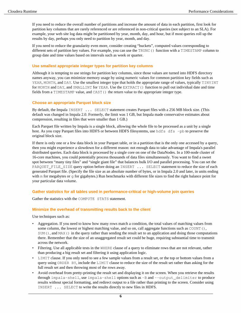
If you need to reduce the overall number of partitions and increase the amount of data in each partition, first look forpartition key columns that are rarely referenced or are referenced in non-critical queries (not subject to an SLA). Forexample, your web site log data might be partitioned by year, month, day, and hour, but if most queries roll up theresults by day, perhaps you only need to partition by year, month, and day.
If you need to reduce the granularity even more, consider creating “buckets”, computed values corresponding todifferent sets of partition key values. For example, you can use the TRUNC() function with a TIMESTAMP column togroup date and time values based on intervals such as week or quarter.
Use smallest appropriate integer types for partition key columns
Although it is tempting to use strings for partition key columns, since those values are turned into HDFS directorynames anyway, you can minimize memory usage by using numeric values for common partition key fields such asYEAR, MONTH, and DAY. Use the smallest integer type that holds the appropriate range of values, typically TINYINTfor MONTH and DAY, and SMALLINT for YEAR. Use the EXTRACT() function to pull out individual date and timefields from a TIMESTAMP value, and CAST() the return value to the appropriate integer type.
Choose an appropriate Parquet block size
By default, the Impala INSERT ... SELECT statement creates Parquet files with a 256 MB block size. (Thisdefault was changed in Impala 2.0. Formerly, the limit was 1 GB, but Impala made conservative estimates aboutcompression, resulting in files that were smaller than 1 GB.)
Each Parquet file written by Impala is a single block, allowing the whole file to be processed as a unit by a singlehost. As you copy Parquet files into HDFS or between HDFS filesystems, use hdfs dfs -pb to preserve theoriginal block size.
If there is only one or a few data block in your Parquet table, or in a partition that is the only one accessed by a query,then you might experience a slowdown for a different reason: not enough data to take advantage of Impala's paralleldistributed queries. Each data block is processed by a single core on one of the DataNodes. In a 100-node cluster of16-core machines, you could potentially process thousands of data files simultaneously. You want to find a sweetspot between “many tiny files” and “single giant file” that balances bulk I/O and parallel processing. You can set thePARQUET_FILE_SIZE query option before doing an INSERT ... SELECT statement to reduce the size of eachgenerated Parquet file. (Specify the file size as an absolute number of bytes, or in Impala 2.0 and later, in units endingwith m for megabytes or g for gigabytes.) Run benchmarks with different file sizes to find the right balance point foryour particular data volume.
Gather statistics for all tables used in performance-critical or high-volume join queries
Gather the statistics with the COMPUTE STATS statement.
Minimize the overhead of transmitting results back to the client
Use techniques such as:
• Aggregation. If you need to know how many rows match a condition, the total values of matching values fromsome column, the lowest or highest matching value, and so on, call aggregate functions such as COUNT(),SUM(), and MAX() in the query rather than sending the result set to an application and doing those computationsthere. Remember that the size of an unaggregated result set could be huge, requiring substantial time to transmitacross the network.
• Filtering. Use all applicable tests in the WHERE clause of a query to eliminate rows that are not relevant, ratherthan producing a big result set and filtering it using application logic.
• LIMIT clause. If you only need to see a few sample values from a result set, or the top or bottom values from aquery using ORDER BY, include the LIMIT clause to reduce the size of the result set rather than asking for thefull result set and then throwing most of the rows away.
• Avoid overhead from pretty-printing the result set and displaying it on the screen. When you retrieve the resultsthrough impala-shell, use impala-shell options such as -B and --output_delimiter to produceresults without special formatting, and redirect output to a file rather than printing to the screen. Consider usingINSERT ... SELECT to write the results directly to new files in HDFS.
6

Cloudera Runtime Performance Considerations
Verify that your queries are planned in an efficient logical manner
Examine the EXPLAIN plan for a query before actually running it.
Verify performance characteristics of queries
Verify that the low-level aspects of I/O, memory usage, network bandwidth, CPU utilization, and so on are withinexpected ranges by examining the query profile for a query after running it.
Hotspot analysis
In the context of Impala, a hotspot is defined as “an Impala daemon that for a single query or a workload is spendinga far greater amount of time processing data relative to its neighbours”.
Before discussing the options to tackle this issue, some background is first required to understand how this problemcan occur.
By default, the scheduling of scan based plan fragments is deterministic. This means that for multiple queries needingto read the same block of data, the same node will be picked to host the scan. The default scheduling logic doesnot take into account node workload from prior queries. The complexity of materializing a tuple depends on a fewfactors, namely: decoding and decompression. If the tuples are densely packed into data pages due to good encoding/compression ratios, there will be more work required when reconstructing the data. Each compression codec offersdifferent performance tradeoffs and should be considered before writing the data. Due to the deterministic nature ofthe scheduler, single nodes can become bottlenecks for highly concurrent queries that use the same tables.
If, for example, a Parquet based dataset is tiny, e.g. a small dimension table, such that it fits into a single HDFS block(Impala by default will create 256 MB blocks when Parquet is used, each containing a single row group) then thereare a number of options that can be considered to resolve the potential scheduling hotspots when querying this data:
• Te scheduler’s deterministic behaviour can be changed using the following query options: REPLICA_PREFERENCE and RANDOM_REPLICA.
• HDFS caching can be used to cache block replicas. This will cause the Impala scheduler to randomly pick a nodethat is hosting a cached block replica for the scan. Note, although HDFS caching has benefits, it serves only tohelp with the reading of raw block data and not cached tuple data, but with the right number of cached replicas (bydefault, HDFS only caches one replica), even load distribution can be achieved for smaller datasets.
• Do not compress the table data. The uncompressed table data spans more nodes and eliminates skew caused bycompression.
• Reduce the Parquet file size via the PARQUET_FILE_SIZE query option when writing the table data. Using thisapproach the data will span more nodes. However it’s not recommended to drop the size below 32 MB.
Query Join PerformanceJoins are the main class of queries that you can tune at the SQL level.
Queries involving join operations often require more tuning than queries that refer to only one table. The maximumsize of the result set from a join query is the product of the number of rows in all the joined tables. When joiningseveral tables with millions or billions of rows, any missed opportunity to filter the result set, or other inefficiency inthe query, could lead to an operation that does not finish in a practical time and has to be cancelled.
The simplest technique for tuning an Impala join query is to collect statistics on each table involved in the joinusing the COMPUTE STATS statement, and then to let Impala automatically optimize the query based on thesize of each table, number of distinct values of each column, and so on. For accurate statistics about each table,issue the COMPUTE STATS statement after loading the data into that table, and again if the amount of data changessubstantially due to operations, such as INSERT, LOAD DATA, or adding a partition.
If statistics are not available for all the tables in the join query, or if Impala chooses a join order that is not the mostefficient, you can override the automatic join order optimization by specifying the STRAIGHT_JOIN keywordimmediately after the SELECT and any DISTINCT or ALL keywords. In this case, Impala uses the order the tablesappear in the query to guide how the joins are processed.
7

Cloudera Runtime Performance Considerations
When you use the STRAIGHT_JOIN technique, you must order the tables in the join query manually instead ofrelying on the Impala optimizer. The optimizer uses sophisticated techniques to estimate the size of the result set ateach stage of the join. For manual ordering, use this heuristic approach to start with, and then experiment to fine-tunethe order:
• Specify the largest table first. This table is read from disk by each Impala node and so its size is not significant interms of memory usage during the query.
• Next, specify the smallest table. The contents of the second, third, and so on tables are all transmitted across thenetwork. You want to minimize the size of the result set from each subsequent stage of the join query. The mostlikely approach involves joining a small table first, so that the result set remains small even as subsequent largertables are processed.
• Join the next smallest table, then the next smallest, and so on.
For example, if you had tables BIG, MEDIUM, SMALL, and TINY, the logical join order to try would be BIG, TINY,SMALL, MEDIUM.
The terms “largest” and “smallest” refers to the size of the intermediate result set based on the number of rows andcolumns from each table that are part of the result set. For example, if you join one table sales with another tablecustomers, a query might find results from 100 different customers who made a total of 5000 purchases. In thatcase, you would specify SELECT ... FROM sales JOIN customers ..., putting customers on theright side because it is smaller in the context of this query.
The Impala query planner chooses between different techniques for performing join queries, depending on theabsolute and relative sizes of the tables. Broadcast joins are the default, where the right-hand table is considered to besmaller than the left-hand table, and its contents are sent to all the other nodes involved in the query. The alternativetechnique is known as a partitioned join (not related to a partitioned table), which is more suitable for large tablesof roughly equal size. With this technique, portions of each table are sent to appropriate other nodes where thosesubsets of rows can be processed in parallel. The choice of broadcast or partitioned join also depends on statisticsbeing available for all tables in the join, gathered by the COMPUTE STATS statement.
To see which join strategy is used for a particular query, issue an EXPLAIN statement for the query. If you find that aquery uses a broadcast join when you know through benchmarking that a partitioned join would be more efficient, orvice versa, add a hint to the query to specify the precise join mechanism to use.
How Joins Are Processed when Statistics Are Unavailable
If table or column statistics are not available for some tables in a join, Impala still reorders the tables using theinformation that is available. Tables with statistics are placed on the left side of the join order, in descending orderof cost based on overall size and cardinality. Tables without statistics are treated as zero-size, that is, they are alwaysplaced on the right side of the join order.
Overriding Join Reordering with STRAIGHT_JOIN
If an Impala join query is inefficient because of outdated statistics or unexpected data distribution, you can keepImpala from reordering the joined tables by using the STRAIGHT_JOIN keyword immediately after the SELECTand any DISTINCT or ALL keywords. The STRAIGHT_JOIN keyword turns off the reordering of join clauses thatImpala does internally, and produces a plan that relies on the join clauses being ordered optimally in the query text.
Note: The STRAIGHT_JOIN hint affects the join order of table references in the query block containingthe hint. It does not affect the join order of nested queries, such as views, inline views, or WHERE-clausesubqueries. To use this hint for performance tuning of complex queries, apply the hint to all query blocks thatneed a fixed join order.
Table and Column StatisticsImpala can do better optimization for complex or multi-table queries when it has access to statistics about the volumeof data and how the values are distributed. Impala uses this information to help parallelize and distribute the workfor a query. For example, optimizing join queries requires a way of determining if one table is “bigger” than another,
8

Cloudera Runtime Performance Considerations
which is a function of the number of rows and the average row size for each table. This topic described the categoriesof statistics Impala can work with, and how to produce them and keep them up to date.
Overview of table statistics
The Impala query planner can make use of statistics about entire tables and partitions. This information includesphysical characteristics such as the number of rows, number of data files, the total size of the data files, and thefile format. For partitioned tables, the numbers are calculated per partition, and as totals for the whole table. Thismetadata is stored in the Metastore database, and can be updated by either Impala or Hive.
If a number is not available, the value -1 is used as a placeholder. Some numbers, such as number and total sizesof data files, are always kept up to date because they can be calculated cheaply, as part of gathering HDFS blockmetadata.
The following example shows table stats for an unpartitioned Parquet table. The values for the number and sizes offiles are always available. Initially, the number of rows is not known, because it requires a potentially expensive scanthrough the entire table, and so that value is displayed as -1. The COMPUTE STATS statement fills in any unknowntable stats values.
show table stats parquet_snappy;+-------+--------+---------+--------------+-------------------+---------+-------------------+...| #Rows | #Files | Size | Bytes Cached | Cache Replication | Format | Incremental stats |...+-------+--------+---------+--------------+-------------------+---------+-------------------+...| -1 | 96 | 23.35GB | NOT CACHED | NOT CACHED | PARQUET | false |...+-------+--------+---------+--------------+-------------------+---------+-------------------+...
compute stats parquet_snappy;+-----------------------------------------+| summary |+-----------------------------------------+| Updated 1 partition(s) and 6 column(s). |+-----------------------------------------+
show table stats parquet_snappy;+------------+--------+---------+--------------+-------------------+---------+-------------------+...| #Rows | #Files | Size | Bytes Cached | Cache Replication | Format | Incremental stats |...+------------+--------+---------+--------------+-------------------+---------+-------------------+...| 1000000000 | 96 | 23.35GB | NOT CACHED | NOT CACHED | PARQUET | false |...+------------+--------+---------+--------------+-------------------+---------+-------------------+...
To check that table statistics are available for a table, and see the details of those statistics, use the statement SHOW TABLE STATS table_name.
Overview of Column Statistics
The Impala query planner can make use of statistics about individual columns when that metadata is available inthe metastore database. This technique is most valuable for columns compared across tables in join queries, to helpestimate how many rows the query will retrieve from each table. These statistics are also important for correlatedsubqueries using the EXISTS or IN operators, which are processed internally the same way as join queries.
9
Cloudera Runtime Performance Considerations
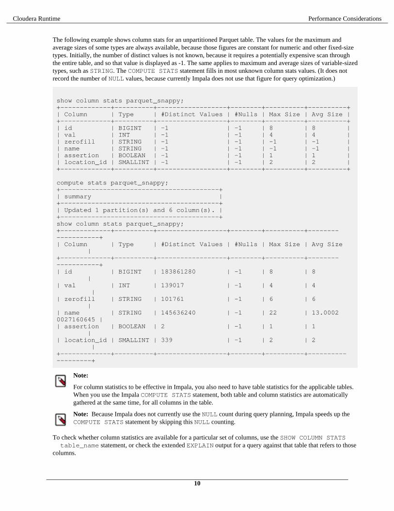
The following example shows column stats for an unpartitioned Parquet table. The values for the maximum andaverage sizes of some types are always available, because those figures are constant for numeric and other fixed-sizetypes. Initially, the number of distinct values is not known, because it requires a potentially expensive scan throughthe entire table, and so that value is displayed as -1. The same applies to maximum and average sizes of variable-sizedtypes, such as STRING. The COMPUTE STATS statement fills in most unknown column stats values. (It does notrecord the number of NULL values, because currently Impala does not use that figure for query optimization.)
show column stats parquet_snappy;+-------------+----------+------------------+--------+----------+----------+| Column | Type | #Distinct Values | #Nulls | Max Size | Avg Size |+-------------+----------+------------------+--------+----------+----------+| id | BIGINT | -1 | -1 | 8 | 8 || val | INT | -1 | -1 | 4 | 4 || zerofill | STRING | -1 | -1 | -1 | -1 || name | STRING | -1 | -1 | -1 | -1 || assertion | BOOLEAN | -1 | -1 | 1 | 1 || location_id | SMALLINT | -1 | -1 | 2 | 2 |+-------------+----------+------------------+--------+----------+----------+
compute stats parquet_snappy;+-----------------------------------------+| summary |+-----------------------------------------+| Updated 1 partition(s) and 6 column(s). |+-----------------------------------------+show column stats parquet_snappy;+-------------+----------+------------------+--------+----------+-------------------+| Column | Type | #Distinct Values | #Nulls | Max Size | Avg Size |+-------------+----------+------------------+--------+----------+-------------------+| id | BIGINT | 183861280 | -1 | 8 | 8 || val | INT | 139017 | -1 | 4 | 4 || zerofill | STRING | 101761 | -1 | 6 | 6 || name | STRING | 145636240 | -1 | 22 | 13.00020027160645 || assertion | BOOLEAN | 2 | -1 | 1 | 1 || location_id | SMALLINT | 339 | -1 | 2 | 2 |+-------------+----------+------------------+--------+----------+-------------------+
Note:
For column statistics to be effective in Impala, you also need to have table statistics for the applicable tables.When you use the Impala COMPUTE STATS statement, both table and column statistics are automaticallygathered at the same time, for all columns in the table.
Note: Because Impala does not currently use the NULL count during query planning, Impala speeds up theCOMPUTE STATS statement by skipping this NULL counting.
To check whether column statistics are available for a particular set of columns, use the SHOW COLUMN STATS table_name statement, or check the extended EXPLAIN output for a query against that table that refers to thosecolumns.
10

Cloudera Runtime Performance Considerations
How Table and Column Statistics Work for Partitioned Tables
When you use Impala for “big data”, you are highly likely to use partitioning for your biggest tables, the onesrepresenting data that can be logically divided based on dates, geographic regions, or similar criteria. The table andcolumn statistics are especially useful for optimizing queries on such tables. For example, a query involving one yearmight involve substantially more or less data than a query involving a different year, or a range of several years. Eachquery might be optimized differently as a result.
The following examples show how table and column stats work with a partitioned table. The table for this exampleis partitioned by year, month, and day. For simplicity, the sample data consists of 5 partitions, all from the same yearand month. Table stats are collected independently for each partition. (In fact, the SHOW PARTITIONS statementdisplays exactly the same information as SHOW TABLE STATS for a partitioned table.) Column stats apply to theentire table, not to individual partitions. Because the partition key column values are represented as HDFS directories,their characteristics are typically known in advance, even when the values for non-key columns are shown as -1.
show partitions year_month_day;+-------+-------+-----+-------+--------+---------+--------------+-------------------+---------+...| year | month | day | #Rows | #Files | Size | Bytes Cached | Cache Replication | Format |...+-------+-------+-----+-------+--------+---------+--------------+-------------------+---------+...| 2013 | 12 | 1 | -1 | 1 | 2.51MB | NOT CACHED | NOT CACHED | PARQUET |...| 2013 | 12 | 2 | -1 | 1 | 2.53MB | NOT CACHED | NOT CACHED | PARQUET |...| 2013 | 12 | 3 | -1 | 1 | 2.52MB | NOT CACHED | NOT CACHED | PARQUET |...| 2013 | 12 | 4 | -1 | 1 | 2.51MB | NOT CACHED | NOT CACHED | PARQUET |...| 2013 | 12 | 5 | -1 | 1 | 2.52MB | NOT CACHED | NOT CACHED | PARQUET |...| Total | | | -1 | 5 | 12.58MB | 0B | | |...+-------+-------+-----+-------+--------+---------+--------------+-------------------+---------+...
show table stats year_month_day;+-------+-------+-----+-------+--------+---------+--------------+-------------------+---------+...| year | month | day | #Rows | #Files | Size | Bytes Cached | Cache Replication | Format |...+-------+-------+-----+-------+--------+---------+--------------+-------------------+---------+...| 2013 | 12 | 1 | -1 | 1 | 2.51MB | NOT CACHED | NOT CACHED | PARQUET |...| 2013 | 12 | 2 | -1 | 1 | 2.53MB | NOT CACHED | NOT CACHED | PARQUET |...| 2013 | 12 | 3 | -1 | 1 | 2.52MB | NOT CACHED | NOT CACHED | PARQUET |...| 2013 | 12 | 4 | -1 | 1 | 2.51MB | NOT CACHED | NOT CACHED | PARQUET |...| 2013 | 12 | 5 | -1 | 1 | 2.52MB | NOT CACHED | NOT CACHED | PARQUET |...| Total | | | -1 | 5 | 12.58MB | 0B | | |...+-------+-------+-----+-------+--------+---------+--------------+-------------------+---------+...
show column stats year_month_day;+-----------+---------+------------------+--------+----------+----------+| Column | Type | #Distinct Values | #Nulls | Max Size | Avg Size |
11

Cloudera Runtime Performance Considerations
+-----------+---------+------------------+--------+----------+----------+| id | INT | -1 | -1 | 4 | 4 || val | INT | -1 | -1 | 4 | 4 || zfill | STRING | -1 | -1 | -1 | -1 || name | STRING | -1 | -1 | -1 | -1 || assertion | BOOLEAN | -1 | -1 | 1 | 1 || year | INT | 1 | 0 | 4 | 4 || month | INT | 1 | 0 | 4 | 4 || day | INT | 5 | 0 | 4 | 4 |+-----------+---------+------------------+--------+----------+----------+
compute stats year_month_day;+-----------------------------------------+| summary |+-----------------------------------------+| Updated 5 partition(s) and 5 column(s). |+-----------------------------------------+
show table stats year_month_day;+-------+-------+-----+--------+--------+---------+--------------+-------------------+---------+...| year | month | day | #Rows | #Files | Size | Bytes Cached | Cache Replication | Format |...+-------+-------+-----+--------+--------+---------+--------------+-------------------+---------+...| 2013 | 12 | 1 | 93606 | 1 | 2.51MB | NOT CACHED | NOT CACHED | PARQUET |...| 2013 | 12 | 2 | 94158 | 1 | 2.53MB | NOT CACHED | NOT CACHED | PARQUET |...| 2013 | 12 | 3 | 94122 | 1 | 2.52MB | NOT CACHED | NOT CACHED | PARQUET |...| 2013 | 12 | 4 | 93559 | 1 | 2.51MB | NOT CACHED | NOT CACHED | PARQUET |...| 2013 | 12 | 5 | 93845 | 1 | 2.52MB | NOT CACHED | NOT CACHED | PARQUET |...| Total | | | 469290 | 5 | 12.58MB | 0B | | |...+-------+-------+-----+--------+--------+---------+--------------+-------------------+---------+...
show column stats year_month_day;+-----------+---------+------------------+--------+----------+-------------------+| Column | Type | #Distinct Values | #Nulls | Max Size | Avg Size |+-----------+---------+------------------+--------+----------+-------------------+| id | INT | 511129 | -1 | 4 | 4 || val | INT | 364853 | -1 | 4 | 4 || zfill | STRING | 311430 | -1 | 6 | 6 || name | STRING | 471975 | -1 | 22 | 13.00160026550293 || assertion | BOOLEAN | 2 | -1 | 1 | 1 || year | INT | 1 | 0 | 4 | 4 || month | INT | 1 | 0 | 4 | 4 || day | INT | 5 | 0 | 4 | 4 |
12

Cloudera Runtime Performance Considerations
+-----------+---------+------------------+--------+----------+-------------------+
If you run the Hive statement ANALYZE TABLE COMPUTE STATISTICS FOR COLUMNS, Impala can only usethe resulting column statistics if the table is unpartitioned. Impala cannot use Hive-generated column statistics for apartitioned table.
Detecting Missing Statistics
You can check whether a specific table has statistics using the SHOW TABLE STATS statement (for any table) orthe SHOW PARTITIONS statement (for a partitioned table). Both statements display the same information. If a tableor a partition does not have any statistics, the #Rows field contains -1. Once you compute statistics for the table orpartition, the #Rows field changes to an accurate value.
The following example shows a table that initially does not have any statistics. The SHOW TABLE STATS statementdisplays different values for #Rows before and after the COMPUTE STATS operation.
[localhost:21000] > create table no_stats (x int);[localhost:21000] > show table stats no_stats;+-------+--------+------+--------------+--------+-------------------+| #Rows | #Files | Size | Bytes Cached | Format | Incremental stats |+-------+--------+------+--------------+--------+-------------------+| -1 | 0 | 0B | NOT CACHED | TEXT | false |+-------+--------+------+--------------+--------+-------------------+[localhost:21000] > compute stats no_stats;+-----------------------------------------+| summary |+-----------------------------------------+| Updated 1 partition(s) and 1 column(s). |+-----------------------------------------+[localhost:21000] > show table stats no_stats;+-------+--------+------+--------------+--------+-------------------+| #Rows | #Files | Size | Bytes Cached | Format | Incremental stats |+-------+--------+------+--------------+--------+-------------------+| 0 | 0 | 0B | NOT CACHED | TEXT | false |+-------+--------+------+--------------+--------+-------------------+
The following example shows a similar progression with a partitioned table. Initially, #Rows is -1. After a COMPUTE STATS operation, #Rows changes to an accurate value. Any newly added partition starts with no statistics,meaning that you must collect statistics after adding a new partition.
[localhost:21000] > create table no_stats_partitioned (x int) partitioned by (year smallint);[localhost:21000] > show table stats no_stats_partitioned;+-------+-------+--------+------+--------------+--------+-------------------+| year | #Rows | #Files | Size | Bytes Cached | Format | Incremental stats |+-------+-------+--------+------+--------------+--------+-------------------+| Total | -1 | 0 | 0B | 0B | | |+-------+-------+--------+------+--------------+--------+-------------------+[localhost:21000] > show partitions no_stats_partitioned;+-------+-------+--------+------+--------------+--------+-------------------+| year | #Rows | #Files | Size | Bytes Cached | Format | Incremental stats |+-------+-------+--------+------+--------------+--------+-------------------+
13

Cloudera Runtime Performance Considerations
| Total | -1 | 0 | 0B | 0B | | |+-------+-------+--------+------+--------------+--------+-------------------+[localhost:21000] > alter table no_stats_partitioned add partition (year=2013);[localhost:21000] > compute stats no_stats_partitioned;+-----------------------------------------+| summary |+-----------------------------------------+| Updated 1 partition(s) and 1 column(s). |+-----------------------------------------+[localhost:21000] > alter table no_stats_partitioned add partition (year=2014);[localhost:21000] > show partitions no_stats_partitioned;+-------+-------+--------+------+--------------+--------+-------------------+| year | #Rows | #Files | Size | Bytes Cached | Format | Incremental stats |+-------+-------+--------+------+--------------+--------+-------------------+| 2013 | 0 | 0 | 0B | NOT CACHED | TEXT | false || 2014 | -1 | 0 | 0B | NOT CACHED | TEXT | false || Total | 0 | 0 | 0B | 0B | | |+-------+-------+--------+------+--------------+--------+-------------------+
Note: Because the default COMPUTE STATS statement creates and updates statistics for all partitions in atable, if you expect to frequently add new partitions, use the COMPUTE INCREMENTAL STATS syntaxinstead, which lets you compute stats for a single specified partition, or only for those partitions that do notalready have incremental stats.
If checking each individual table is impractical, due to a large number of tables or views that hide the underlying basetables, you can also check for missing statistics for a particular query. Use the EXPLAIN statement to preview queryefficiency before actually running the query. Use the query profile output available through the PROFILE commandin impala-shell or the web UI to verify query execution and timing after running the query. Both the EXPLAIN plan and the PROFILE output display a warning if any tables or partitions involved in the query do not havestatistics.
[localhost:21000] > create table no_stats (x int);[localhost:21000] > explain select count(*) from no_stats;+------------------------------------------------------------------------------------+| Explain String |+------------------------------------------------------------------------------------+| Estimated Per-Host Requirements: Memory=10.00MB VCores=1 || WARNING: The following tables are missing relevant table and/or column statistics. || incremental_stats.no_stats || || 03:AGGREGATE [FINALIZE] || | output: count:merge(*) |
14

Cloudera Runtime Performance Considerations
| | || 02:EXCHANGE [UNPARTITIONED] || | || 01:AGGREGATE || | output: count(*) || | || 00:SCAN HDFS [incremental_stats.no_stats] || partitions=1/1 files=0 size=0B |+------------------------------------------------------------------------------------+
Because Impala uses the partition pruning technique when possible to only evaluate certain partitions, if you have apartitioned table with statistics for some partitions and not others, whether or not the EXPLAIN statement shows thewarning depends on the actual partitions used by the query. For example, you might see warnings or not for differentqueries against the same table:
-- No warning because all the partitions for the year 2012 have stats.EXPLAIN SELECT ... FROM t1 WHERE year = 2012;
-- Missing stats warning because one or more partitions in this range-- do not have stats.EXPLAIN SELECT ... FROM t1 WHERE year BETWEEN 2006 AND 2009;
To confirm if any partitions at all in the table are missing statistics, you might explain a query that scans the entiretable, such as SELECT COUNT(*) FROM table_name.
Manually Setting Table Statistics with ALTER TABLE
The most crucial piece of data in all the statistics is the number of rows in the table (for an unpartitioned orpartitioned table) and for each partition (for a partitioned table). The COMPUTE STATS statement alwaysgathers statistics about all columns, as well as overall table statistics. If it is not practical to do a full COMPUTE STATS or COMPUTE INCREMENTAL STATS operation after adding a partition or inserting data, or if you cansee that Impala would produce a more efficient plan if the number of rows was different, you can manually set thenumber of rows through an ALTER TABLE statement:
-- Set total number of rows. Applies to both unpartitioned and partitioned tables.alter table table_name set tblproperties('numRows'='new_value', 'STATS_GENERATED_VIA_STATS_TASK'='true');
-- Set total number of rows for a specific partition. Applies to partitioned tables only.-- You must specify all the partition key columns in the PARTITION clause.alter table table_name partition (keycol1=val1,keycol2=val2...) set tblproperties('numRows'='new_value', 'STATS_GENERATED_VIA_STATS_TASK'='true');
This statement avoids re-scanning any data files. For example:
alter table analysis_data set tblproperties('numRows'='1001000000', 'STATS_GENERATED_VIA_STATS_TASK'='true');
15
Cloudera Runtime Performance Considerations
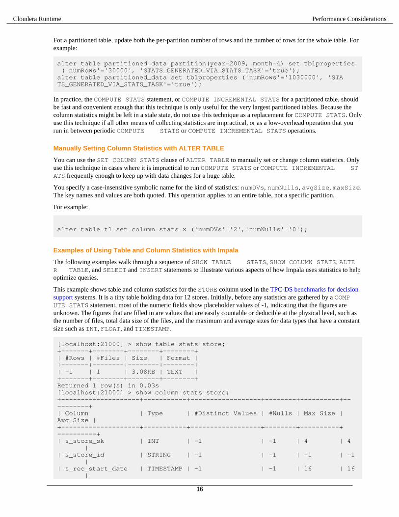
For a partitioned table, update both the per-partition number of rows and the number of rows for the whole table. Forexample:
alter table partitioned_data partition(year=2009, month=4) set tblproperties ('numRows'='30000', 'STATS_GENERATED_VIA_STATS_TASK'='true');alter table partitioned_data set tblproperties ('numRows'='1030000', 'STATS_GENERATED_VIA_STATS_TASK'='true');
In practice, the COMPUTE STATS statement, or COMPUTE INCREMENTAL STATS for a partitioned table, shouldbe fast and convenient enough that this technique is only useful for the very largest partitioned tables. Because thecolumn statistics might be left in a stale state, do not use this technique as a replacement for COMPUTE STATS. Onlyuse this technique if all other means of collecting statistics are impractical, or as a low-overhead operation that yourun in between periodic COMPUTE STATS or COMPUTE INCREMENTAL STATS operations.
Manually Setting Column Statistics with ALTER TABLE
You can use the SET COLUMN STATS clause of ALTER TABLE to manually set or change column statistics. Onlyuse this technique in cases where it is impractical to run COMPUTE STATS or COMPUTE INCREMENTAL STATS frequently enough to keep up with data changes for a huge table.
You specify a case-insensitive symbolic name for the kind of statistics: numDVs, numNulls, avgSize, maxSize.The key names and values are both quoted. This operation applies to an entire table, not a specific partition.
For example:
alter table t1 set column stats x ('numDVs'='2','numNulls'='0');
Examples of Using Table and Column Statistics with Impala
The following examples walk through a sequence of SHOW TABLE STATS, SHOW COLUMN STATS, ALTER TABLE, and SELECT and INSERT statements to illustrate various aspects of how Impala uses statistics to helpoptimize queries.
This example shows table and column statistics for the STORE column used in the TPC-DS benchmarks for decisionsupport systems. It is a tiny table holding data for 12 stores. Initially, before any statistics are gathered by a COMPUTE STATS statement, most of the numeric fields show placeholder values of -1, indicating that the figures areunknown. The figures that are filled in are values that are easily countable or deducible at the physical level, such asthe number of files, total data size of the files, and the maximum and average sizes for data types that have a constantsize such as INT, FLOAT, and TIMESTAMP.
[localhost:21000] > show table stats store;+-------+--------+--------+--------+| #Rows | #Files | Size | Format |+-------+--------+--------+--------+| -1 | 1 | 3.08KB | TEXT |+-------+--------+--------+--------+Returned 1 row(s) in 0.03s[localhost:21000] > show column stats store;+--------------------+-----------+------------------+--------+----------+----------+| Column | Type | #Distinct Values | #Nulls | Max Size | Avg Size |+--------------------+-----------+------------------+--------+----------+----------+| s_store_sk | INT | -1 | -1 | 4 | 4 || s_store_id | STRING | -1 | -1 | -1 | -1 || s_rec_start_date | TIMESTAMP | -1 | -1 | 16 | 16 |
16

Cloudera Runtime Performance Considerations
| s_rec_end_date | TIMESTAMP | -1 | -1 | 16 | 16 || s_closed_date_sk | INT | -1 | -1 | 4 | 4 || s_store_name | STRING | -1 | -1 | -1 | -1 || s_number_employees | INT | -1 | -1 | 4 | 4 || s_floor_space | INT | -1 | -1 | 4 | 4 || s_hours | STRING | -1 | -1 | -1 | -1 || s_manager | STRING | -1 | -1 | -1 | -1 || s_market_id | INT | -1 | -1 | 4 | 4 || s_geography_class | STRING | -1 | -1 | -1 | -1 || s_market_desc | STRING | -1 | -1 | -1 | -1 || s_market_manager | STRING | -1 | -1 | -1 | -1 || s_division_id | INT | -1 | -1 | 4 | 4 || s_division_name | STRING | -1 | -1 | -1 | -1 || s_company_id | INT | -1 | -1 | 4 | 4 || s_company_name | STRING | -1 | -1 | -1 | -1 || s_street_number | STRING | -1 | -1 | -1 | -1 || s_street_name | STRING | -1 | -1 | -1 | -1 || s_street_type | STRING | -1 | -1 | -1 | -1 || s_suite_number | STRING | -1 | -1 | -1 | -1 || s_city | STRING | -1 | -1 | -1 | -1 || s_county | STRING | -1 | -1 | -1 | -1 || s_state | STRING | -1 | -1 | -1 | -1 || s_zip | STRING | -1 | -1 | -1 | -1 || s_country | STRING | -1 | -1 | -1 | -1 || s_gmt_offset | FLOAT | -1 | -1 | 4 | 4 || s_tax_percentage | FLOAT | -1 | -1 | 4 | 4 |+--------------------+-----------+------------------+--------+----------+----------+Returned 29 row(s) in 0.04s
With the Hive ANALYZE TABLE statement for column statistics, you had to specify each column for which togather statistics. The Impala COMPUTE STATS statement automatically gathers statistics for all columns, becauseit reads through the entire table relatively quickly and can efficiently compute the values for all the columns. Thisexample shows how after running the COMPUTE STATS statement, statistics are filled in for both the table and all itscolumns:
[localhost:21000] > compute stats store;
17
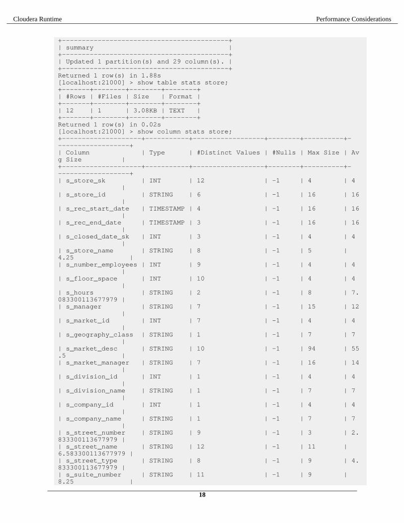
Cloudera Runtime Performance Considerations
+------------------------------------------+| summary |+------------------------------------------+| Updated 1 partition(s) and 29 column(s). |+------------------------------------------+Returned 1 row(s) in 1.88s[localhost:21000] > show table stats store;+-------+--------+--------+--------+| #Rows | #Files | Size | Format |+-------+--------+--------+--------+| 12 | 1 | 3.08KB | TEXT |+-------+--------+--------+--------+Returned 1 row(s) in 0.02s[localhost:21000] > show column stats store;+--------------------+-----------+------------------+--------+----------+-------------------+| Column | Type | #Distinct Values | #Nulls | Max Size | Avg Size |+--------------------+-----------+------------------+--------+----------+-------------------+| s_store_sk | INT | 12 | -1 | 4 | 4 || s_store_id | STRING | 6 | -1 | 16 | 16 || s_rec_start_date | TIMESTAMP | 4 | -1 | 16 | 16 || s_rec_end_date | TIMESTAMP | 3 | -1 | 16 | 16 || s_closed_date_sk | INT | 3 | -1 | 4 | 4 || s_store_name | STRING | 8 | -1 | 5 | 4.25 || s_number_employees | INT | 9 | -1 | 4 | 4 || s_floor_space | INT | 10 | -1 | 4 | 4 || s_hours | STRING | 2 | -1 | 8 | 7.083300113677979 || s_manager | STRING | 7 | -1 | 15 | 12 || s_market_id | INT | 7 | -1 | 4 | 4 || s_geography_class | STRING | 1 | -1 | 7 | 7 || s_market_desc | STRING | 10 | -1 | 94 | 55.5 || s_market_manager | STRING | 7 | -1 | 16 | 14 || s_division_id | INT | 1 | -1 | 4 | 4 || s_division_name | STRING | 1 | -1 | 7 | 7 || s_company_id | INT | 1 | -1 | 4 | 4 || s_company_name | STRING | 1 | -1 | 7 | 7 || s_street_number | STRING | 9 | -1 | 3 | 2.833300113677979 || s_street_name | STRING | 12 | -1 | 11 | 6.583300113677979 || s_street_type | STRING | 8 | -1 | 9 | 4.833300113677979 || s_suite_number | STRING | 11 | -1 | 9 | 8.25 |
18

Cloudera Runtime Performance Considerations
| s_city | STRING | 2 | -1 | 8 | 6.5 || s_county | STRING | 1 | -1 | 17 | 17 || s_state | STRING | 1 | -1 | 2 | 2 || s_zip | STRING | 2 | -1 | 5 | 5 || s_country | STRING | 1 | -1 | 13 | 13 || s_gmt_offset | FLOAT | 1 | -1 | 4 | 4 || s_tax_percentage | FLOAT | 5 | -1 | 4 | 4 |+--------------------+-----------+------------------+--------+----------+-------------------+Returned 29 row(s) in 0.04s
The following example shows how statistics are represented for a partitioned table. In this case, we have set up a tableto hold the world's most trivial census data, a single STRING field, partitioned by a YEAR column. The table statisticsinclude a separate entry for each partition, plus final totals for the numeric fields. The column statistics include someeasily deducible facts for the partitioning column, such as the number of distinct values (the number of partitionsubdirectories).
localhost:21000] > describe census;+------+----------+---------+| name | type | comment |+------+----------+---------+| name | string | || year | smallint | |+------+----------+---------+Returned 2 row(s) in 0.02s[localhost:21000] > show table stats census;+-------+-------+--------+------+---------+| year | #Rows | #Files | Size | Format |+-------+-------+--------+------+---------+| 2000 | -1 | 0 | 0B | TEXT || 2004 | -1 | 0 | 0B | TEXT || 2008 | -1 | 0 | 0B | TEXT || 2010 | -1 | 0 | 0B | TEXT || 2011 | 0 | 1 | 22B | TEXT || 2012 | -1 | 1 | 22B | TEXT || 2013 | -1 | 1 | 231B | PARQUET || Total | 0 | 3 | 275B | |+-------+-------+--------+------+---------+Returned 8 row(s) in 0.02s[localhost:21000] > show column stats census;+--------+----------+------------------+--------+----------+----------+| Column | Type | #Distinct Values | #Nulls | Max Size | Avg Size |+--------+----------+------------------+--------+----------+----------+| name | STRING | -1 | -1 | -1 | -1 || year | SMALLINT | 7 | -1 | 2 | 2 |+--------+----------+------------------+--------+----------+----------+Returned 2 row(s) in 0.02s
The following example shows how the statistics are filled in by a COMPUTE STATS statement in Impala.
[localhost:21000] > compute stats census;+-----------------------------------------+| summary |+-----------------------------------------+| Updated 3 partition(s) and 1 column(s). |
19

Cloudera Runtime Performance Considerations
+-----------------------------------------+Returned 1 row(s) in 2.16s[localhost:21000] > show table stats census;+-------+-------+--------+------+---------+| year | #Rows | #Files | Size | Format |+-------+-------+--------+------+---------+| 2000 | -1 | 0 | 0B | TEXT || 2004 | -1 | 0 | 0B | TEXT || 2008 | -1 | 0 | 0B | TEXT || 2010 | -1 | 0 | 0B | TEXT || 2011 | 4 | 1 | 22B | TEXT || 2012 | 4 | 1 | 22B | TEXT || 2013 | 1 | 1 | 231B | PARQUET || Total | 9 | 3 | 275B | |+-------+-------+--------+------+---------+Returned 8 row(s) in 0.02s[localhost:21000] > show column stats census;+--------+----------+------------------+--------+----------+----------+| Column | Type | #Distinct Values | #Nulls | Max Size | Avg Size |+--------+----------+------------------+--------+----------+----------+| name | STRING | 4 | -1 | 5 | 4.5 || year | SMALLINT | 7 | -1 | 2 | 2 |+--------+----------+------------------+--------+----------+----------+Returned 2 row(s) in 0.02s
You can see how Impala executes a query differently in each case by observing the EXPLAIN output before and aftercollecting statistics. Measure the before and after query times, and examine the throughput numbers in before andafter SUMMARY or PROFILE output, to verify how much the improved plan speeds up performance.
Generating Table and Column StatisticsUse the COMPUTE STATS statement to collect table and column statistics. The COMPUTE STATS variants offerdifferent tradeoffs between computation cost, staleness, and maintenance workflows.
Important:
For a particular table, use either COMPUTE STATS or COMPUTE INCREMENTAL STATS, but nevercombine the two or alternate between them. If you switch from COMPUTE STATS to COMPUTE INCREMENTAL STATS during the lifetime of a table, or vice versa, drop all statistics by running DROP STATS before making the switch.
COMPUTE STATS
The COMPUTE STATS command collects and sets the table-level and partition-level row counts as well as allcolumn statistics for a given table. The collection process is CPU-intensive and can take a long time to complete forvery large tables.
To speed up COMPUTE STATS consider the following options which can be combined.
• Limit the number of columns for which statistics are collected to increase the efficiency of COMPUTE STATS.Queries benefit from statistics for those columns involved in filters, join conditions, group by or partition byclauses. Other columns are good candidates to exclude from COMPUTE STATS. This feature is available sinceImpala 2.12.
• Set the MT_DOP query option to use more threads within each participating impalad to compute the statisticsfaster - but not more efficiently. Note that computing stats on a large table with a high MT_DOP value cannegatively affect other queries running at the same time if the COMPUTE STATS claims most CPU cycles.
• Consider the experimental extrapolation and sampling features (see below) to further increase the efficiency ofcomputing stats.
COMPUTE STATS is intended to be run periodically, e.g. weekly, or on-demand when the contents of a table havechanged significantly. Due to the high resource utilization and long response time of tCOMPUTE STATS, it is mostpractical to run it in a scheduled maintenance window where the Impala cluster is idle enough to accommodate
20
Cloudera Runtime Performance Considerations
the expensive operation. The degree of change that qualifies as “significant” depends on the query workload, buttypically, if 30% of the rows have changed then it is recommended to recompute statistics.
If you reload a complete new set of data for a table, but the number of rows and number of distinct values for eachcolumn is relatively unchanged from before, you do not need to recompute stats for the table.
Extrapolation and Sampling
Impala supports extrapolation and sampling to alleviate the following common issues for computing and maintainingstatistics on very large tables:
• Newly added partitions do not have row count statistics. Table scans that only access those new partitionsare treated as not having stats. Similarly, table scans that access both new and old partitions estimate the scancardinality based on those old partitions that have stats, and the new partitions without stats are treated as having 0rows.
• The row counts of existing partitions become stale when data is added or dropped.• Computing stats for tables with a 100,000 or more partitions might fail or be very slow due to the high cost of
updating the partition metadata in the Hive Metastore.• With transient compute resources it is important to minimize the time from starting a new cluster to successfully
running queries. Since the cluster might be relatively short-lived, users might prefer to quickly collect stats thatare "good enough" as opposed to spending a lot of time and resources on computing full-fidelity stats.
For very large tables, it is often wasteful or impractical to run a full COMPUTE STATS to address the scenarios aboveon a frequent basis.
The sampling feature makes COMPUTE STATS more efficient by processing a fraction of the table data, and theextrapolation feature aims to reduce the frequency at which COMPUTE STATS needs to be re-run by estimating therow count of new and modified partitions.
The sampling and extrapolation features are disabled by default. They can be enabled globally or for specific tables,as follows.
• Set the impalad start-up configuration --enable_stats_extrapolation to enable the features globally.• To enable them only for a specific table, set the impala.enable.stats.extrapolation table property to
true for the table. The table-level property overrides the global setting, so it is also possible to enable samplingand extrapolation globally, but disable it for specific tables by setting the table property to false. For example:
ALTER TABLE mytable test_table SET TBLPROPERTIES("impala.enable.stats.extrapolation"="true");
Note: Why are these features experimental? Due to their probabilistic nature it is possible that these featuresperform pathologically poorly on tables with extreme data/file/size distributions. Since it is not feasible forus to test all possible scenarios we only cautiously advertise these new capabilities. That said, the featureshave been thoroughly tested and are considered functionally stable. If you decide to give these features a try,please tell us about your experience at [email protected]! We rely on user feedback to guide futureimprovements in statistics collection.
Stats Extrapolation
The main idea of stats extrapolation is to estimate the row count of new and modified partitionsbased on the result of the last COMPUTE STATS. Enabling stats extrapolation changes the behaviorof COMPUTE STATS, as well as the cardinality estimation of table scans. COMPUTE STATSno longer computes and stores per-partition row counts, and instead, only computes a table-levelrow count together with the total number of file bytes in the table at that time. No partition metadatais modified. The input cardinality of a table scan is estimated by converting the data volume ofrelevant partitions to a row count, based on the table-level row count and file bytes statistics. It isassumed that within the same table, different sets of files with the same data volume correspond tothe similar number of rows on average. With extrapolation enabled, the scan cardinality estimationignores per-partition row counts. It only relies on the table-level statistics and the scanned datavolume.
21
Cloudera Runtime Performance Considerations
The SHOW TABLE STATS and EXPLAIN commands distinguish between row counts stored in theHive Metastore, and the row counts extrapolated based on the above process.
Sampling
A TABLESAMPLE clause may be added to COMPUTE STATS to limit the percentage of data to beprocessed. The final statistics are obtained by extrapolating the statistics from the data sample overthe entire table. The extrapolated statistics are stored in the Hive Metastore, just as if no samplingwas used. The following example runs COMPUTE STATS over a 10 percent data sample.
COMPUTE STATS test_table TABLESAMPLE SYSTEM(10) ;
We have found that a 10 percent sampling rate typically offers a good tradeoff between statisticsaccuracy and execution cost. A sampling rate well below 10 percent has shown poor results and isnot recommended.
Important: Sampling-based techniques sacrifice result accuracy for executionefficiency, so your mileage may vary for different tables and columns depending ontheir data distribution. The extrapolation procedure Impala uses for estimating thenumber of distinct values per column is inherently non-detetministic, so your resultsmay even vary between runs of COMPUTE STATS TABLESAMPLE, even ifno data has changed.
COMPUTE INCREMENTAL STATS
In Impala 2.1.0 and higher, you can use the COMPUTE INCREMENTAL STATS and DROP INCREMENTALSTATS commands. The INCREMENTAL clauses work with incremental statistics, a specialized feature for partitionedtables.
When you compute incremental statistics for a partitioned table, by default Impala only processes those partitions thatdo not yet have incremental statistics. By processing only newly added partitions, you can keep statistics up to datewithout incurring the overhead of reprocessing the entire table each time.
You can also compute or drop statistics for a specified subset of partitions by including a PARTITION clause in theCOMPUTE INCREMENTAL STATS or DROP INCREMENTAL STATS statement.
Important:
When you run COMPUTE INCREMENTAL STATS on a table for the first time, the statistics arecomputed again from scratch regardless of whether the table already has statistics. Therefore, expect a one-time resource-intensive operation for scanning the entire table when running COMPUTE INCREMENTAL STATS for the first time on a given table.
The metadata for incremental statistics is handled differently from the original style of statistics:
• Issuing a COMPUTE INCREMENTAL STATS without a partition clause causes Impala to compute incrementalstats for all partitions that do not already have incremental stats. This might be the entire table when running thecommand for the first time, but subsequent runs should only update new partitions. You can force updating apartition that already has incremental stats by issuing a DROP INCREMENTAL STATS before running COMPUTE INCREMENTAL STATS.
• The SHOW TABLE STATS and SHOW PARTITIONS statements now include an additional columnshowing whether incremental statistics are available for each column. A partition could already be covered by theoriginal type of statistics based on a prior COMPUTE STATS statement, as indicated by a value other than -1under the #Rows column. Impala query planning uses either kind of statistics when available.
• COMPUTE INCREMENTAL STATS takes more time than COMPUTE STATS for the same volume of data.Therefore it is most suitable for tables with large data volume where new partitions are added frequently, makingit impractical to run a full COMPUTE STATS operation for each new partition. For unpartitioned tables, orpartitioned tables that are loaded once and not updated with new partitions, use the original COMPUTE STATSsyntax.
• COMPUTE INCREMENTAL STATS uses some memory in the catalogd process, proportional to the numberof partitions and number of columns in the applicable table. The memory overhead is approximately 400 bytes for
22
Cloudera Runtime Performance Considerations
each column in each partition. This memory is reserved in the catalogd daemon, the statestored daemon,and in each instance of the impalad daemon.
• In cases where new files are added to an existing partition, issue a REFRESH statement for the table, followedby a DROP INCREMENTAL STATS and COMPUTE INCREMENTAL STATS sequence for the changedpartition.
• The DROP INCREMENTAL STATS statement operates only on a single partition at a time. To remove statistics(whether incremental or not) from all partitions of a table, issue a DROP STATS statement with no INCREMENTAL or PARTITION clauses.
The following considerations apply to incremental statistics when the structure of an existing table is changed (knownas schema evolution):
• If you use an ALTER TABLE statement to drop a column, the existing statistics remain valid and COMPUTE INCREMENTAL STATS does not rescan any partitions.
• If you use an ALTER TABLE statement to add a column, Impala rescans all partitions and fills in the appropriatecolumn-level values the next time you run COMPUTE INCREMENTAL STATS.
• If you use an ALTER TABLE statement to change the data type of a column, Impala rescans all partitions and fillsin the appropriate column-level values the next time you run COMPUTE INCREMENTAL STATS.
• If you use an ALTER TABLE statement to change the file format of a table, the existing statistics remain validand a subsequent COMPUTE INCREMENTAL STATS does not rescan any partitions.
Runtime FilteringRuntime filtering is a wide-ranging optimization feature available in Impala. When only a fraction of the datain a table is needed for a query against a partitioned table or to evaluate a join condition, Impala determines theappropriate conditions while the query is running, and broadcasts that information to all the impalad nodes thatare reading the table so that they can avoid unnecessary I/O to read partition data, and avoid unnecessary networktransmission by sending only the subset of rows that match the join keys across the network.
Runtime filtering is primarily used:
• To optimize queries against large partitioned tables (under the name dynamic partition pruning)• To optimize joins of large tables
The following terms are used in this topic to describe runtime filtering.plan fragment
Impala decomposes each query into smaller units of work that are distributed across the cluster.Wherever possible, a data block is read, filtered, and aggregated by plan fragments executing on thesame host. For some operations, such as joins and combining intermediate results into a final resultset, data is transmitted across the network from one Impala daemon to another.
SCAN and HASH JOIN plan nodes
In the Impala query plan, a scan node performs the I/O to read from the underlying data files.Although this is an expensive operation from the traditional database perspective, Hadoop clustersand Impala are optimized to do this kind of I/O in a highly parallel fashion. The major potentialcost savings come from using the columnar Parquet format (where Impala can avoid reading datafor unneeded columns) and partitioned tables (where Impala can avoid reading data for unneededpartitions).
Most Impala joins use the hash join mechanism. (It is only fairly recently that Impala started usingthe nested-loop join technique, for certain kinds of non-equijoin queries.) In a hash join, whenevaluating join conditions from two tables, Impala constructs a hash table in memory with all thedifferent column values from the table on one side of the join. Then, for each row from the table onthe other side of the join, Impala tests whether the relevant column values are in this hash table ornot.
hash join
23

Cloudera Runtime Performance Considerations
In a hash join, when evaluating join conditions from two tables, Impala constructs a hash table inmemory with all the different column values from the table on one side of the join. Then, for eachrow from the table on the other side of the join, Impala tests whether the relevant column values arein this hash table or not.
• A hash join node constructs such an in-memory hash table, then performs the comparisons toidentify which rows match the relevant join conditions and should be included in the result set(or at least sent on to the subsequent intermediate stage of query processing). Because someof the input for a hash join might be transmitted across the network from another host, it isespecially important from a performance perspective to prune out ahead of time any data that isknown to be irrelevant.
The more distinct values are in the columns used as join keys, the larger the in-memory hashtable and thus the more memory required to process the query.
broadcast join vs shuffle join
In a broadcast join, the table from one side of the join (typically the smaller table) is sent in itsentirety to all the hosts involved in the query. Then each host can compare its portion of the datafrom the other (larger) table against the full set of possible join keys. In a shuffle join, there isno obvious “smaller” table, and so the contents of both tables are divided up, and correspondingportions of the data are transmitted to each host involved in the query.
A shuffle join is sometimes referred to in Impala as a partitioned join.
build and probe phases
When Impala processes a join query, the build phase is where the rows containing the join keycolumns, typically for the smaller table, are transmitted across the network and built into an in-memory hash table data structure on one or more destination nodes. The probe phase is where datais read locally (typically from the larger table) and the join key columns are compared to the valuesin the in-memory hash table. The corresponding input sources (tables, subqueries, and so on) forthese phases are referred to as the build side and the probe side.
Runtime Filters
The filter that is transmitted between plan fragments is essentially a list of values for join key columns. When this listof values is transmitted in time to a scan node, Impala can filter out non-matching values immediately after readingthem, rather than transmitting the raw data to another host to compare against the in-memory hash table on that host.
Impala supports the following types of filters based on the payload:
• Bloom filter: For HDFS-based tables, the Bloom filter uses a probability-based algorithm to determine all possiblematching values. The probability-based aspects means that the filter might include some non-matching values, butif so, that does not cause any inaccuracy in the final results.
• Min-max filter: The filter is a data structure representing a minimum and maximum value. These filters are passedto Kudu to reduce the number of rows returned to Impala when scanning the probe side of the join. This filtercurrently only applies to Kudu tables.
Based on how filters from all join instances are aggregated, each of the above filters can be categorized as one of thefollowing:
• Broadcast filter: A broadcast filter reflects the complete list of relevant values and can be immediately evaluatedby a scan node.
Broadcast filters are also classified as local or global. With a local broadcast filter, the information in the filteris used by a subsequent query fragment that is running on the same host that produced the filter. A non-localbroadcast filter must be transmitted across the network to a query fragment that is running on a different host.Impala designates 3 hosts to each produce non-local broadcast filters, to guard against the possibility of a singleslow host taking too long. Depending on the setting of the RUNTIME_FILTER_MODE query option (LOCALor GLOBAL), Impala either uses a conservative optimization strategy where filters are only consumed on thesame host that produced them, or a more aggressive strategy where filters are eligible to be transmitted across thenetwork. The default for runtime filtering is the GLOBAL setting.
24

Cloudera Runtime Performance Considerations
• Partitioned filter: A partitioned filter reflects only the values processed by one host in the cluster; all thepartitioned filters must be combined into one (by the coordinator node) before the scan nodes can use the results toaccurately filter the data as it is read from storage.
File Format Considerations for Runtime Filtering
Parquet tables get the most benefit from the runtime filtering optimizations. Runtime filtering can speed up joinqueries against partitioned or unpartitioned Parquet tables, and single-table queries against partitioned Parquet tables.
For other file formats (text, Avro, RCFile, and SequenceFile), runtime filtering speeds up queries against partitionedtables only. Because partitioned tables can use a mixture of formats, Impala produces the filters in all cases, even ifthey are not ultimately used to optimize the query.
Wait Intervals for Runtime Filters
Because it takes time to produce runtime filters, especially for partitioned filters that must be combined by thecoordinator node, there is a time interval above which it is more efficient for the scan nodes to go ahead and constructtheir intermediate result sets, even if that intermediate data is larger than optimal. If it only takes a few seconds toproduce the filters, it is worth the extra time if pruning the unnecessary data can save minutes in the overall querytime. You can specify the maximum wait time in milliseconds using the RUNTIME_FILTER_WAIT_TIME_MSquery option.
By default, each scan node waits for up to 1 second (1000 milliseconds) for filters to arrive. If all filters have notarrived within the specified interval, the scan node proceeds, using whatever filters did arrive to help avoid readingunnecessary data. If a filter arrives after the scan node begins reading data, the scan node applies that filter to the datathat is read after the filter arrives, but not to the data that was already read.
If the cluster is relatively busy and your workload contains many resource-intensive or long-running queries, considerincreasing the wait time so that complicated queries do not miss opportunities for optimization. If the cluster is lightlyloaded and your workload contains many small queries taking only a few seconds, consider decreasing the wait timeto avoid the 1 second delay for each query.
Query Options for Runtime Filtering
The following query options control runtime filtering.
• RUNTIME_FILTER_MODE
This query option controls how extensively the filters are transmitted between hosts. By default, it is set to thehighest level (GLOBAL).
• The other query options are tuning knobs that you typically only adjust after doing performance testing, and thatyou might want to change only for the duration of a single expensive query.
• MAX_NUM_RUNTIME_FILTERS
• DISABLE_ROW_RUNTIME_FILTERING
• RUNTIME_FILTER_MAX_SIZE
• RUNTIME_FILTER_MIN_SIZE
• RUNTIME_BLOOM_FILTER_SIZE
Runtime Filtering and Query Plans
In the same way the query plan displayed by the EXPLAIN statement includes information about predicates used byeach plan fragment, it also includes annotations showing whether a plan fragment produces or consumes a runtimefilter.
• A plan fragment that produces a filter includes an annotation such as runtime filters: filter_id <- table.column
• A plan fragment that consumes a filter includes an annotation such as runtime filters: filter_id -> table.column
25
Cloudera Runtime Performance Considerations
Setting the query option EXPLAIN_LEVEL=2 adds additional annotations showing the type of the filter:
• filter_id[bloom] (for HDFS-based tables)• filter_id[min_max] (for Kudu tables)
The query profile (displayed by the PROFILE command in impala-shell) contains both the EXPLAIN plan andmore detailed information about the internal workings of the query. The profile output includes the Filter routing table section with information about each filter based on its ID.
Tuning and Troubleshooting Queries that Use Runtime Filtering
These tuning and troubleshooting procedures apply to queries that are resource-intensive enough, long-runningenough, and frequent enough that you can devote special attention to optimizing them individually.
Use the EXPLAIN statement and examine the runtime filters: lines to determine whether runtime filters arebeing applied to the WHERE predicates and join clauses that you expect. For example, runtime filtering does not applyto queries that use the nested loop join mechanism due to non-equijoin operators.
Make sure statistics are up-to-date for all tables involved in the queries. Use the COMPUTE STATS statement afterloading data into non-partitioned tables, and COMPUTE INCREMENTAL STATS after adding new partitions topartitioned tables.
If join queries involving large tables use unique columns as the join keys, for example joining a primary key columnwith a foreign key column, the overhead of producing and transmitting the filter might outweigh the performancebenefit because not much data could be pruned during the early stages of the query. For such queries, consider settingthe query option RUNTIME_FILTER_MODE=OFF.
PartitioningUse partitioning to speed up queries that retrieve data based on values from one or more columns.
Partitioning is a technique for physically dividing the data during loading based on values from one or more columns.For example, with a school_records table partitioned on a year column, there is a separate data directory foreach different year value, and all the data for that year is stored in a data file in that directory. A query that includesa WHERE condition such as YEAR=1966, YEAR IN (1989,1999), or YEAR BETWEEN 1984 AND 1989can examine only the data files from the appropriate directory or directories, greatly reducing the amount of data toread and test.
Parquet is a popular format for partitioned Impala tables because it is well suited to handle huge data volumes.
You can add, drop, set the expected file format, or set the HDFS location of the data files for individual partitionswithin an Impala table.
When to Use Partitioned Tables
Partitioning is typically appropriate for:
• Tables that are very large, where reading the entire data set takes an impractical amount of time.• Tables that are always or almost always queried with conditions on the partitioning columns. In our example of
a table partitioned by year, SELECT COUNT(*) FROM school_records WHERE year = 1985is efficient, only examining a small fraction of the data; but SELECT COUNT(*) FROM school_recordshas to process a separate data file for each year, resulting in more overall work than in an unpartitioned table. Youwould probably not partition this way if you frequently queried the table based on last name, student ID, and so onwithout testing the year.
• Columns that have reasonable cardinality (number of different values). If a column only has a small number ofvalues, for example Male or Female, you do not gain much efficiency by eliminating only about 50% of thedata to read for each query. If a column has only a few rows matching each value, the number of directories toprocess can become a limiting factor, and the data file in each directory could be too small to take advantage ofthe Hadoop mechanism for transmitting data in multi-megabyte blocks. For example, you might partition census
26

Cloudera Runtime Performance Considerations
data by year, store sales data by year and month, and web traffic data by year, month, and day. (Some users withhigh volumes of incoming data might even partition down to the individual hour and minute.)
• Data that already passes through an extract, transform, and load (ETL) pipeline. The values of the partitioningcolumns are stripped from the original data files and represented by directory names, so loading data into apartitioned table involves some sort of transformation or preprocessing.
SQL Statement for Partitioned Tables
In terms of Impala SQL syntax, partitioning affects these statements:
• CREATE TABLE: You specify a PARTITIONED BY clause when creating the table to identify names anddata types of the partitioning columns. These columns are not included in the main list of columns for the table.
• CREATE TABLE AS SELECT: Use the PARTITIONED BY clause to create a partitioned table, copy datainto it, and create new partitions based on the values in the inserted data.
• ALTER TABLE: Add or drop partitions, to work with different portions of a huge data set. You can designate theHDFS directory that holds the data files for a specific partition. With data partitioned by date values, you might“age out” data that is no longer relevant.
If you are creating a partition for the first time and specifying its location, for maximum efficiency, use a singleALTER TABLE statement including both the ADD PARTITION and LOCATIONclauses, rather than separatestatements with ADD PARTITION and SET LOCATION clauses.
• INSERT: When you insert data into a partitioned table, you identify the partitioning columns. One or morevalues from each inserted row are not stored in data files, but instead determine the directory where that rowvalue is stored. You can also specify which partition to load a set of data into, with INSERT OVERWRITEstatements; you can replace the contents of a specific partition but you cannot append data to a specific partition.
By default, if an INSERT statement creates any new subdirectories underneath a partitioned table, thosesubdirectories are assigned default HDFS permissions for the impala user. To make each subdirectory have thesame permissions as its parent directory in HDFS, specify the ##insert_inherit_permissions startupoption for the Impala Daemon.
• Although the syntax of the SELECT statement is the same whether or not the table is partitioned, the way queriesinteract with partitioned tables can have a dramatic impact on performance and scalability. The mechanism thatlets queries skip certain partitions during a query is known as partition pruning.
• SHOW PARTITIONS: Displays information about each partition in a table.
Static and Dynamic Partitioning Clauses
Specifying all the partition columns in a SQL statement is called static partitioning, because the statement affects asingle predictable partition. For example, you use static partitioning with an ALTER TABLE statement that affectsonly one partition, or with an INSERT statement that inserts all values into the same partition:
INSERT INTO t1 PARTITION(x=10, y='a') SELECT c1 FROM some_other_table;
When you specify some partition key columns in an INSERT statement, but leave out the values, Impala determineswhich partition to insert. This technique is called dynamic partitioning.
INTSERT INTO t1 PARTITION(x, y='b') SELECT c1, c2 FROM some_other_table;-- Create new partition if necessary based on variable year, month, and day; insert a single value.INSERT INTO weather PARTITION (year, month, day) SELECT 'cloudy',2014,4,21;-- Create new partition if necessary for specified year and month but variable day; insert a single value.INSERT INTO weather PARTITION (year=2014, month=04, day) SELECT 'sunny',22;
The more key columns you specify in the PARTITION clause, the fewer columns you need in the SELECT list. Thetrailing columns in the SELECT list are substituted in order for the partition key columns with no specified value.
27

Cloudera Runtime Performance Considerations
Refreshing a Single Partition
The REFRESH statement is typically used with partitioned tables when new data files are loaded into a partition bysome non-Impala mechanism, such as a Hive or Spark job. The REFRESH statement makes Impala aware of the newdata files so that they can be used in Impala queries. Because partitioned tables typically contain a high volume ofdata, the REFRESH operation for a full partitioned table can take significant time.
You can include a PARTITION (partition_spec) clause in the REFRESH statement so that only a singlepartition is refreshed. For example, REFRESH big_table PARTITION (year=2017, month=9, day=30). The partition spec must include all the partition key columns.
Partition Key Columns
The columns you choose as the partition keys should be ones that are frequently used to filter query results inimportant, large-scale queries. Popular examples are some combination of year, month, and day when the data hasassociated time values, and geographic region when the data is associated with some place.
• For time-based data, split out the separate parts into their own columns, because Impala cannot partition based ona TIMESTAMP column.
• The data type of the partition columns does not have a significant effect on the storage required, because thevalues from those columns are not stored in the data files, rather they are represented as strings inside HDFSdirectory names.
• You can enable the OPTIMIZE_PARTITION_KEY_SCANS query option to speed up queries that only refer topartition key columns, such as SELECT MAX(year). This setting is not enabled by default because the querybehavior is slightly different if the table contains partition directories without actual data inside.
• All the partition key columns must be scalar types.• When Impala queries data stored in HDFS, it is most efficient to use multi-megabyte files to take advantage of
the HDFS block size. For Parquet tables, the block size (and ideal size of the data files) is 256 MB.. Therefore,avoid specifying too many partition key columns, which could result in individual partitions containing only smallamounts of data. For example, if you receive 1 GB of data per day, you might partition by year, month, and day;while if you receive 5 GB of data per minute, you might partition by year, month, day, hour, and minute. If youhave data with a geographic component, you might partition based on postal code if you have many megabytes ofdata for each postal code, but if not, you might partition by some larger region such as city, state, or country. state
If you frequently run aggregate functions such as MIN(), MAX(), and COUNT(DISTINCT) on partition keycolumns, consider enabling the OPTIMIZE_PARTITION_KEY_SCANS query option, which optimizes suchqueries.
Setting Different File Formats for Partitions in a Table
Partitioned tables have the flexibility to use different file formats for different partitions. For example, if youoriginally received data in text format, then received new data in RCFile format, and eventually began receiving datain Parquet format, all that data could reside in the same table for queries. You just need to ensure that the table isstructured so that the data files that use different file formats reside in separate partitions.
For example, here is how you might switch from text to Parquet data as you receive data for different years:
[localhost:21000] > CREATE TABLE census (name STRING) PARTITIONED BY (year SMALLINT);[localhost:21000] > ALTER TABLE census ADD PARTITION (year=2012); -- Text format;[localhost:21000] > ALTER TABLE census ADD PARTITION (year=2013); -- Text format switches to Parquet before data loaded;[localhost:21000] > ALTER TABLE census PARTITION (year=2013) SET FILEFORMAT PARQUET;
[localhost:21000] > INSERT INTO census PARTITION (year=2012) VALUES ('Smith'),('Jones'),('Lee'),('Singh');[localhost:21000] > INSERT INTO census PARTITION (year=2013) VALUES ('Flores'),('Bogomolov'),('Cooper'),('Appiah');
28

Cloudera Runtime Performance Considerations
At this point, the HDFS directory for year=2012 contains a text-format data file, while the HDFS directory foryear=2013 contains a Parquet data file. As always, when loading non-trivial data, you would use INSERT ... SELECT or LOAD DATA to import data in large batches, rather than INSERT ... VALUES which producessmall files that are inefficient for real-world queries.
For other file types that Impala cannot create natively, you can switch into Hive and issue the ALTER TABLE ... SET FILEFORMAT statements and INSERT or LOAD DATA statements there. After switching back to Impala,issue a REFRESH table_name statement so that Impala recognizes any partitions or new data added through Hive.
Dropping Partitions
What happens to the data files when a partition is dropped depends on whether the partitioned table is designated asinternal or external. For an internal (managed) table, the data files are deleted. For example, if data in the partitionedtable is a copy of raw data files stored elsewhere, you might save disk space by dropping older partitions that are nolonger required for reporting, knowing that the original data is still available if needed later. For an external table, thedata files are left alone. For example, dropping a partition without deleting the associated files lets Impala considera smaller set of partitions, improving query efficiency and reducing overhead for DDL operations on the table; if thedata is needed again later, you can add the partition again.
Using Partitioning with Kudu Tables
Kudu tables use a more fine-grained partitioning scheme than tables containing HDFS data files. You specify a PARTITION BY clause with the CREATE TABLE statement to identify how to divide the values from the partition keycolumns.
Keeping Statistics Up to Date for Partitioned Tables
Because the COMPUTE STATS statement can be resource-intensive to run on a partitioned table as new partitions areadded, Impala includes a variation of this statement that allows computing statistics on a per-partition basis such thatstats can be incrementally updated when new partitions are added.
The COMPUTE INCREMENTAL STATS variation computes statistics only for partitions that were added or changedsince the last COMPUTE INCREMENTAL STATS statement, rather than the entire table. It is typically used for tableswhere a full COMPUTE STATS operation takes too long to be practical each time a partition is added or dropped.
Partition Pruning for QueriesPartition pruning refers to the mechanism where a query can skip reading the data files corresponding to one or morepartitions.
If you can arrange for queries to prune large numbers of unnecessary partitions from the query execution plan, thequeries use fewer resources and are thus proportionally faster and more scalable.
For example, if a table is partitioned by columns YEAR, MONTH, and DAY, then WHERE clauses such as WHERE year = 2013, WHERE year < 2010, or WHERE year BETWEEN 1995 AND 1998 allow Impala toskip the data files in all partitions outside the specified range. Likewise, WHERE year = 2013 AND month BETWEEN 1 AND 3 could prune even more partitions, reading the data files for only a portion of one year.
If a view applies to a partitioned table, any partition pruning considers the clauses on both the original query and anyadditional WHERE predicates in the query that refers to the view.
In queries involving both analytic functions and partitioned tables, partition pruning only occurs for columnsnamed in the PARTITION BY clause of the analytic function call. For example, if an analytic function queryhas a clause such as WHERE year=2016, the way to make the query prune all other YEAR partitions is toinclude PARTITION BY year in the analytic function call; for example, OVER (PARTITION BY year,other_columns other_analytic_clauses).
29

Cloudera Runtime Performance Considerations
Checking if Partition Pruning Happens for a Query
To check the effectiveness of partition pruning for a query, check the EXPLAIN output for the query before runningit. For example, this example shows a table with 3 partitions, where the query only reads 1 of them. The notation#partitions=1/3 in the EXPLAIN plan confirms that Impala can do the appropriate partition pruning.
[localhost:21000] > INSERT INTO census PARTITION (year=2010) VALUES ('Smith'),('Jones');[localhost:21000] > INSERT INTO census PARTITION (year=2011) VALUES ('Smith'),('Jones'),('Doe');[localhost:21000] > INSERT INTO census PARTITION (year=2012) VALUES ('Smith'),('Doe');[localhost:21000] > EXPLAIN select name from census where year=2010;+------------------------------------------------------------------+| Explain String |+------------------------------------------------------------------+| PLAN FRAGMENT 1 || PARTITION: RANDOM || || STREAM DATA SINK || EXCHANGE ID: 1 || UNPARTITIONED || || 0:SCAN HDFS || table=predicate_propagation.census #partitions=1/3 size=12B |+------------------------------------------------------------------+
For a report of the volume of data that was actually read and processed at each stage of the query, check the output ofthe SUMMARY command immediately after running the query. For a more detailed analysis, look at the output of thePROFILE command; it includes this same summary report near the start of the profile output.
Predicate Propagation
Impala can do partition pruning in cases where the partition key column is not directly compared to a constant. Usingthe predicate propagation technique, Impala applies the transitive property to other parts of the WHERE clause.
In this example, the census table includes another column indicating when the data was collected, which happensin 10-year intervals. Even though the query does not compare the partition key column (YEAR) to a constant value,Impala can deduce that only the partition YEAR=2010 is required, and again only reads 1 out of 3 partitions.
[localhost:21000] > CREATE TABLE census (name STRING, census_year INT) PARTITIONED BY (year INT);[localhost:21000] > INSERT INTO census PARTITION (year=2010) VALUES ('Smith',2010),('Jones',2010);[localhost:21000] > INSERT INTO census PARTITION (year=2011) VALUES ('Smith',2020),('Jones',2020),('Doe',2020);[localhost:21000] > INSERT INTO census PARTITION (year=2012) VALUES ('Smith',2020),('Doe',2020);[localhost:21000] > [localhost:21000] > EXPLAIN select name from census where year = census_year and census_year=2010;+------------------------------------------------------------------+| Explain String |+------------------------------------------------------------------+| PLAN FRAGMENT 1 || PARTITION: RANDOM || || STREAM DATA SINK || EXCHANGE ID: 1 || UNPARTITIONED || || 0:SCAN HDFS |
30

Cloudera Runtime Performance Considerations
| table=predicate_propagation.census #partitions=1/3 size=22B || predicates: census_year = 2010, year = census_year |+------------------------------------------------------------------+
Dynamic Partition Pruning
Impala supports two types of partition pruning.
• Static partition pruning: The conditions in the WHERE clause are analyzed to determine in advance whichpartitions can be safely skipped.
• Dynamic partition pruning: Information about the partitions is collected during the query execution, and Impalaprunes unnecessary partitions. The information is not available in advance before runtime.
For example, if partition key columns are compared to literal values in a WHERE clause, Impala can perform staticpartition pruning during the planning phase to only read the relevant partitions:
-- The query only needs to read 3 partitions whose key values are known ahead of time.-- That's static partition pruning.SELECT COUNT(*) FROM sales_table WHERE year IN (2005, 2010, 2015);
Dynamic partition pruning involves using information only available at run time, such as the result of a subquery. Thefollowing example shows a simple dynamic partition pruning.
CREATE TABLE yy (s STRING) PARTITIONED BY (year INT);INSERT INTO yy PARTITION (year) VALUES ('1999', 1999), ('2000', 2000), ('2001', 2001), ('2010', 2010), ('2018', 2018);COMPUTE STATS yy;
CREATE TABLE yy2 (s STRING, year INT);INSERT INTO yy2 VALUES ('1999', 1999), ('2000', 2000), ('2001', 2001);COMPUTE STATS yy2;-- The following query reads an unknown number of partitions, whose key values-- are only known at run time. The runtime filters line shows the-- information used in query fragment 02 to decide which partitions to skip.
EXPLAIN SELECT s FROM yy WHERE year IN (SELECT year FROM yy2);+--------------------------------------------------------------------------+| PLAN-ROOT SINK || | || 04:EXCHANGE [UNPARTITIONED] || | || 02:HASH JOIN [LEFT SEMI JOIN, BROADCAST] || | hash predicates: year = year || | runtime filters: RF000 <- year || | || |--03:EXCHANGE [BROADCAST] || | | || | 01:SCAN HDFS [default.yy2] || | partitions=1/1 files=1 size=620B || | || 00:SCAN HDFS [default.yy] || partitions=5/5 files=5 size=1.71KB || runtime filters: RF000 -> year |+--------------------------------------------------------------------------+
SELECT s FROM yy WHERE year IN (SELECT year FROM yy2); -- Returns 3 rows from yy
31

Cloudera Runtime Performance Considerations
PROFILE;
In the above example, Impala evaluates the subquery, sends the subquery results to all Impala nodes participatingin the query, and then each impalad daemon uses the dynamic partition pruning optimization to read only thepartitions with the relevant key values.
The output query plan from the EXPLAIN statement shows that runtime filters are enabled. The plan also shows thatit expects to read all 5 partitions of the yy table, indicating that static partition pruning will not happen.
The Filter summary in the PROFILE output shows that the scan node filtered out based on a runtime filter ofdynamic partition pruning.
Filter 0 (1.00 MB): - Files processed: 3 - Files rejected: 1 (1) - Files total: 3 (3)
Dynamic partition pruning is especially effective for queries involving joins of several large partitioned tables.Evaluating the ON clauses of the join predicates might normally require reading data from all partitions of certaintables. If the WHERE clauses of the query refer to the partition key columns, Impala can now often skip reading manyof the partitions while evaluating the ON clauses. The dynamic partition pruning optimization reduces the amount of I/O and the amount of intermediate data stored and transmitted across the network during the query.
Dynamic partition pruning is part of the runtime filtering feature, which applies to other kinds of queries in additionto queries against partitioned tables.
HDFS CachingImpala can use the HDFS caching feature to make more effective use of RAM so that repeated queries can takeadvantage of data “pinned” in memory regardless of how much data is processed overall.
The HDFS caching feature lets you designate a subset of frequently accessed data to be pinned permanently inmemory, remaining in the cache across multiple queries and never being evicted. This technique is suitable for tablesor partitions that are frequently accessed and are small enough to fit entirely within the HDFS memory cache. Forexample, you might designate several dimension tables to be pinned in the cache, to speed up many different joinqueries that reference them. Or in a partitioned table, you might pin a partition holding data from the most recenttime period because that data will be queried intensively; then when the next set of data arrives, you could unpin theprevious partition and pin the partition holding the new data.
The performance gain comes from two aspects:
• Reading from RAM instead of disk• Accessing the data straight from the cache area instead of copying from one RAM area to another
This yields further performance improvement over the standard OS caching mechanism, which still results inmemory-to-memory copying of cached data. Because accessing HDFS cached data avoids a memory-to-memorycopy operation, queries involving cached data require less memory on the Impala side than the equivalent querieson uncached data.
Due to a limitation of HDFS, zero-copy reads are not supported with encryption. Cloudera recommends not usingHDFS caching for Impala data files in encryption zones. The queries fall back to the normal read path during queryexecution, which might cause some performance overhead.
Because this Impala performance feature relies on HDFS infrastructure, it only applies to Impala tables that useHDFS data files. HDFS caching for Impala does not apply to HBase tables, S3 tables, Kudu tables, or Isilon tables.
32

Cloudera Runtime Performance Considerations
Using HDFS Caching for Impala Tables and Partitions
Begin by choosing which tables or partitions to cache. For example, these might be lookup tables that are accessed bymany different join queries, or partitions corresponding to the most recent time period that are analyzed by differentreports or ad-hoc queries.
In your SQL statements, you specify logical divisions such as tables and partitions to be cached. Impala translatesthese requests into HDFS-level directives that apply to particular directories and files. For example, given apartitioned table CENSUS with a partition key column YEAR, you could choose to cache all or part of the data asfollows.
-- Cache the entire table (all partitions).ALTER TABLE census SET CACHED IN 'pool_name';
-- Remove the entire table from the cache.ALTER TABLE census SET UNCACHED;-- Cache a portion of the table (a single partition).-- If the table is partitioned by multiple columns (such as year, month, day),-- the ALTER TABLE command must specify values for all those columns.ALTER TABLE census PARTITION (year=1960) SET CACHED IN 'pool_name';
-- Cache the data from one partition on up to 4 hosts, to minimize CPU load on any-- single host when the same data block is processed multiple times.ALTER TABLE census PARTITION (year=1970) SET CACHED IN 'pool_name' WITH REPLICATION = 4;
-- At each stage, check the volume of cached data.-- For large tables or partitions, the background loading might take some time,-- so you might have to wait and reissue the statement until all the data-- has finished being loaded into the cache.SHOW TABLE STATS census;+-------+-------+--------+------+--------------+--------+| year | #Rows | #Files | Size | Bytes Cached | Format |+-------+-------+--------+------+--------------+--------+| 1900 | -1 | 1 | 11B | NOT CACHED | TEXT || 1940 | -1 | 1 | 11B | NOT CACHED | TEXT || 1960 | -1 | 1 | 11B | 11B | TEXT || 1970 | -1 | 1 | 11B | NOT CACHED | TEXT || Total | -1 | 4 | 44B | 11B | |+-------+-------+--------+------+--------------+--------+
CREATE TABLE and ALTER TABLE considerations:
The HDFS caching feature affects the Impala CREATE TABLE statement as follows:
• You can put a CACHED IN 'pool_name' clause and optionally a WITH REPLICATION = number_of_hosts clause at the end of a CREATE TABLE statement to automatically cache the entirecontents of the table, including any partitions added later.
The pool_name is a pool that you previously set up with the hdfs cacheadmin command in HDFS.• Once a table is designated for HDFS caching through the CREATE TABLE statement, if new partitions are
added later through ALTER TABLE ... ADD PARTITION statements, the data in those new partitions isautomatically cached in the same pool.
• If you want to perform repetitive queries on a subset of data from a large table, and it is not practical to designatethe entire table or specific partitions for HDFS caching, you can create a new cached table with just a subset of thedata by using CREATE TABLE ... CACHED IN 'pool_name' AS SELECT ... WHERE .... When you are finished with generating reports from this subset of data, drop the table and both the data filesand the data cached in RAM are automatically deleted.
33

Cloudera Runtime Performance Considerations
• If you have designated a table or partition as cached through the CREATE TABLE or ALTER TABLE statements,subsequent attempts to relocate the table or partition through an ALTER TABLE ... SET LOCATIONstatement will fail. You must issue an ALTER TABLE ... SET UNCACHED statement for the table orpartition first. Otherwise, Impala would lose track of some cached data files and have no way to uncache themlater.
• The optional WITH REPLICATION clause for CREATE TABLE and ALTER TABLE lets you specify areplication factor, the number of hosts on which to cache the same data blocks. When Impala processes a cacheddata block, where the cache replication factor is greater than 1, Impala randomly selects a host that has a cachedcopy of that data block. This optimization avoids excessive CPU usage on a single host when the same cacheddata block is processed multiple times. Cloudera recommends specifying a value greater than or equal to theHDFS block replication factor.
INSERT and LOAD DATA considerations:
• When HDFS caching is enabled for a table or partition, new data files are cached automatically when they areadded to the appropriate directory in HDFS, without the need for a REFRESH statement in Impala. Impalaautomatically performs a REFRESH once the new data is loaded into the HDFS cache.
• If you perform an INSERT or LOAD DATA through Hive, Impala only recognizes the new data files after aREFRESH table_name statement in Impala.
• If the cache pool is entirely full, or becomes full before all the requested data can be cached, the Impala DDLstatement returns an error. This is to avoid situations where only some of the requested data could be cached.
DROP TABLE and ALTER TABLE DROP PARTITION considerations:
The HDFS caching feature interacts with the Impala DROP TABLE and ALTER TABLE ... DROP PARTITION statements as follows:
• When you issue a DROP TABLE or ALTER TABLE ... DROP PARTITION for a table that is entirelycached, or has some partitions cached, the DROP TABLE succeeds and all the cache directives Impala submittedfor that table are removed from the HDFS cache system.
• The underlying data files are removed if the dropped table is an internal table, or the dropped partition is in itsdefault location underneath an internal table. The data files are left alone if the dropped table is an external table,or if the dropped partition is in a non-default location.
• If you drop an HDFS cache pool through the hdfs cacheadmin command, all the Impala data files arepreserved, just no longer cached. After a subsequent REFRESH, SHOW TABLE STATS reports 0 bytes cachedfor each associated Impala table or partition.
• If you designated the data files as cached through the hdfs cacheadmin command, and the data files are leftbehind as described in the previous item, the data files remain cached.
Impala only removes the cache directives submitted by Impala through the CREATE TABLE or ALTER TABLE statements.
• One file can have multiple redundant cache directives. The directives all have unique IDs, and owners so that thesystem can tell them apart.
SHOW TABLE STATS and SHOW PARTITIONS considerations:
For each table or partition, the SHOW TABLE STATS or SHOW PARTITIONS statement displays the number ofbytes currently cached by the HDFS caching feature.
A value of 0, or a smaller number than the overall size of the table or partition, indicates that the cache request hasbeen submitted but the data has not been entirely loaded into memory yet.
If there are no cache directives in place for that table or partition, the result set displays NOT CACHED.
SELECT considerations:
The Impala HDFS caching feature interacts with the SELECT statement and query performance as follows:
• Impala automatically reads from memory any data that has been designated as cached and actually loaded into theHDFS cache. (It could take some time after the initial request to fully populate the cache for a table with large sizeor many partitions.)
34
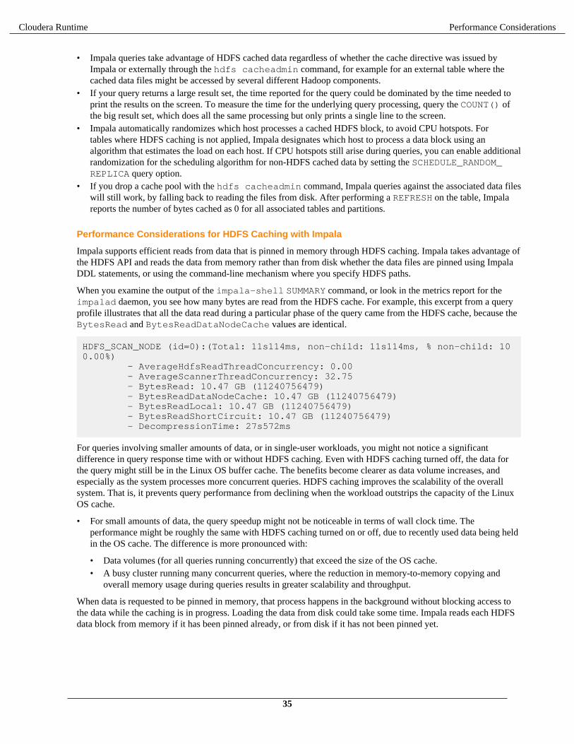
Cloudera Runtime Performance Considerations
• Impala queries take advantage of HDFS cached data regardless of whether the cache directive was issued byImpala or externally through the hdfs cacheadmin command, for example for an external table where thecached data files might be accessed by several different Hadoop components.
• If your query returns a large result set, the time reported for the query could be dominated by the time needed toprint the results on the screen. To measure the time for the underlying query processing, query the COUNT() ofthe big result set, which does all the same processing but only prints a single line to the screen.
• Impala automatically randomizes which host processes a cached HDFS block, to avoid CPU hotspots. Fortables where HDFS caching is not applied, Impala designates which host to process a data block using analgorithm that estimates the load on each host. If CPU hotspots still arise during queries, you can enable additionalrandomization for the scheduling algorithm for non-HDFS cached data by setting the SCHEDULE_RANDOM_REPLICA query option.
• If you drop a cache pool with the hdfs cacheadmin command, Impala queries against the associated data fileswill still work, by falling back to reading the files from disk. After performing a REFRESH on the table, Impalareports the number of bytes cached as 0 for all associated tables and partitions.
Performance Considerations for HDFS Caching with Impala
Impala supports efficient reads from data that is pinned in memory through HDFS caching. Impala takes advantage ofthe HDFS API and reads the data from memory rather than from disk whether the data files are pinned using ImpalaDDL statements, or using the command-line mechanism where you specify HDFS paths.
When you examine the output of the impala-shell SUMMARY command, or look in the metrics report for theimpalad daemon, you see how many bytes are read from the HDFS cache. For example, this excerpt from a queryprofile illustrates that all the data read during a particular phase of the query came from the HDFS cache, because theBytesRead and BytesReadDataNodeCache values are identical.
HDFS_SCAN_NODE (id=0):(Total: 11s114ms, non-child: 11s114ms, % non-child: 100.00%) - AverageHdfsReadThreadConcurrency: 0.00 - AverageScannerThreadConcurrency: 32.75 - BytesRead: 10.47 GB (11240756479) - BytesReadDataNodeCache: 10.47 GB (11240756479) - BytesReadLocal: 10.47 GB (11240756479) - BytesReadShortCircuit: 10.47 GB (11240756479) - DecompressionTime: 27s572ms
For queries involving smaller amounts of data, or in single-user workloads, you might not notice a significantdifference in query response time with or without HDFS caching. Even with HDFS caching turned off, the data forthe query might still be in the Linux OS buffer cache. The benefits become clearer as data volume increases, andespecially as the system processes more concurrent queries. HDFS caching improves the scalability of the overallsystem. That is, it prevents query performance from declining when the workload outstrips the capacity of the LinuxOS cache.
• For small amounts of data, the query speedup might not be noticeable in terms of wall clock time. Theperformance might be roughly the same with HDFS caching turned on or off, due to recently used data being heldin the OS cache. The difference is more pronounced with:
• Data volumes (for all queries running concurrently) that exceed the size of the OS cache.• A busy cluster running many concurrent queries, where the reduction in memory-to-memory copying and
overall memory usage during queries results in greater scalability and throughput.
When data is requested to be pinned in memory, that process happens in the background without blocking access tothe data while the caching is in progress. Loading the data from disk could take some time. Impala reads each HDFSdata block from memory if it has been pinned already, or from disk if it has not been pinned yet.
35
Cloudera Runtime Performance Considerations
Memory Considerations
The amount of data that you can pin on each node through the HDFS caching mechanism is subject to a quota that isenforced by the underlying HDFS service. Before requesting to pin an Impala table or partition in memory, check thatits size does not exceed this quota.
Note: Because the HDFS cache consists of combined memory from all the DataNodes in the cluster, cachedtables or partitions can be bigger than the amount of HDFS cache memory on any single host.
The Impala HDFS caching feature interacts with the Impala memory limits as follows:
• The maximum size of each HDFS cache pool is specified externally to Impala, through the hdfs cacheadmincommand.
• All the memory used for HDFS caching is separate from the impalad daemon address space and does not counttowards the limits of the --mem_limit startup option, MEM_LIMIT query option, or further limits imposedthrough YARN resource management or the Linux cgroups mechanism.
HDFS Block SkewFor best performance of Impala parallel queries, the work is divided equally across hosts in the cluster, and all hoststake approximately equal time to finish their work. If one host takes substantially longer than others, the extra timeneeded for the slow host can become the dominant factor in query performance. Therefore, one of the first steps inperformance tuning for Impala is to detect and correct such conditions.
The main cause of uneven performance that you can correct within Impala is skew in the number of HDFS datablocks processed by each host, where some hosts process substantially more data blocks than others. This conditioncan occur because of uneven distribution of the data values themselves, for example causing certain data files orpartitions to be large while others are very small. (Although it is possible to have unevenly distributed data withoutany problems with the distribution of HDFS blocks.) Block skew could also be due to the underlying block allocationpolicies within HDFS, the replication factor of the data files, and the way that Impala chooses the host to process eachdata block.
The most convenient way to detect block skew, or slow-host issues in general, is to examine the “executive summary”information from the query profile after running a query:
• In impala-shell, issue the SUMMARY command immediately after the query is complete, to see just thesummary information. If you detect issues involving skew, you might switch to issuing the PROFILE command,which displays the summary information followed by a detailed performance analysis.
• In the Cloudera Manager interface or the Impala debug web UI, click on the Profile link associated with the queryafter it is complete. The executive summary information is displayed early in the profile output.
For each phase of the query, you see an Avg Time and a Max Time value, along with #Hosts indicating how manyhosts are involved in that query phase. For all the phases with #Hosts greater than one, look for cases where themaximum time is substantially greater than the average time. Focus on the phases that took the longest, for example,those taking multiple seconds rather than milliseconds or microseconds.
If you detect that some hosts take longer than others, first rule out non-Impala causes. One reason that some hostscould be slower than others is if those hosts have less capacity than the others, or if they are substantially busier dueto unevenly distributed non-Impala workloads:
• For clusters running Impala, keep the relative capacities of all hosts roughly equal. Any cost savings fromincluding some underpowered hosts in the cluster will likely be outweighed by poor or uneven performance, andthe time spent diagnosing performance issues.
• If non-Impala workloads cause slowdowns on some hosts but not others, use the appropriate load-balancingtechniques for the non-Impala components to smooth out the load across the cluster.
If the hosts on your cluster are evenly powered and evenly loaded, examine the detailed profile output to determinewhich host is taking longer than others for the query phase in question. Examine how many bytes are processedduring that phase on that host, how much memory is used, and how many bytes are transmitted across the network.
36

Cloudera Runtime Performance Considerations
The most common symptom is a higher number of bytes read on one host than others, due to one host being requestedto process a higher number of HDFS data blocks. This condition is more likely to occur when the number of blocksaccessed by the query is relatively small. For example, if you have a 10-node cluster and the query processes 10HDFS blocks, each node might not process exactly one block. If one node sits idle while another node processes twoblocks, the query could take twice as long as if the data was perfectly distributed.
Possible solutions in this case include:
• If the query is artificially small, perhaps for benchmarking purposes, scale it up to process a larger data set.For example, if some nodes read 10 HDFS data blocks while others read 11, the overall effect of the unevendistribution is much lower than when some nodes did twice as much work as others. As a guideline, aim for a“sweet spot” where each node reads 2 GB or more from HDFS per query. Queries that process lower volumesthan that could experience inconsistent performance that smooths out as queries become more data-intensive.
• If the query processes only a few large blocks, so that many nodes sit idle and cannot help to parallelize the query,consider reducing the overall block size. For example, you might adjust the PARQUET_FILE_SIZE query optionbefore copying or converting data into a Parquet table. Or you might adjust the granularity of data files producedearlier in the ETL pipeline by non-Impala components. In Impala 2.0 and later, the default Parquet block size is256 MB, reduced from 1 GB, to improve parallelism for common cluster sizes and data volumes.
• Reduce the amount of compression applied to the data. For text data files, the highest degree of compression(gzip) produces unsplittable files that are more difficult for Impala to process in parallel, and require extramemory during processing to hold the compressed and uncompressed data simultaneously. For binary formatssuch as Parquet and Avro, compression can result in fewer data blocks overall, but remember that when queriesprocess relatively few blocks, there is less opportunity for parallel execution and many nodes in the clustermight sit idle. Note that when Impala writes Parquet data with the query option COMPRESSION_CODEC=NONEenabled, the data is still typically compact due to the encoding schemes used by Parquet, independent of the finalcompression step.
Understanding Performance using EXPLAIN PlanTo understand the high-level performance considerations for Impala queries, read the output of the EXPLAINstatement for the query. You can get the EXPLAIN plan without actually running the query itself.
The EXPLAIN statement gives you an outline of the logical steps that a query will perform, such as how the workwill be distributed among the nodes and how intermediate results will be combined to produce the final result set.You can see these details before actually running the query. You can use this information to check that the query willnot operate in some very unexpected or inefficient way.
Read the EXPLAIN plan from bottom to top:
• The last part of the plan shows the low-level details such as the expected amount of data that will be read, whereyou can judge the effectiveness of your partitioning strategy and estimate how long it will take to scan a tablebased on total data size and the size of the cluster.
• As you work your way up, next you see the operations that will be parallelized and performed on each Impalanode.
• At the higher levels, you see how data flows when intermediate result sets are combined and transmitted from onenode to another.
• The EXPLAIN_LEVEL query option lets you customize how much detail to show in the EXPLAIN plandepending on whether you are doing high-level or low-level tuning, dealing with logical or physical aspects of thequery.
Read the EXPLAIN plan from bottom to top:
• The last part of the plan shows the low-level details such as the expected amount of data that will be read, whereyou can judge the effectiveness of your partitioning strategy and estimate how long it will take to scan a tablebased on total data size and the size of the cluster.
• As you work your way up, next you see the operations that will be parallelized and performed on each Impalanode.
37

Cloudera Runtime Performance Considerations
• At the higher levels, you see how data flows when intermediate result sets are combined and transmitted from onenode to another.
• The EXPLAIN_LEVEL query option lets you customize how much detail to show in the EXPLAIN plandepending on whether you are doing high-level or low-level tuning, dealing with logical or physical aspects of thequery.
The example below shows how the standard EXPLAIN output moves from the lowest (physical) level to the higher(logical) levels. The query begins by scanning a certain amount of data; each node performs an aggregation operation(evaluating COUNT(*)) on some subset of data that is local to that node; the intermediate results are transmitted backto the coordinator node (labelled here as the EXCHANGE node); lastly, the intermediate results are summed to displaythe final result.
[impalad-host:21000] > EXPLAIN select count(*) from customer_address;+----------------------------------------------------------+| Explain String |+----------------------------------------------------------+| Estimated Per-Host Requirements: Memory=42.00MB VCores=1 || || 03:AGGREGATE [MERGE FINALIZE] || | output: sum(count(*)) || | || 02:EXCHANGE [PARTITION=UNPARTITIONED] || | || 01:AGGREGATE || | output: count(*) || | || 00:SCAN HDFS [default.customer_address] || partitions=1/1 size=5.25MB |+----------------------------------------------------------+
The EXPLAIN plan is also printed at the beginning of the query PROFILE report to provide convenience inexamining both the logical and physical aspects of the query side-by-side.
The amount of detail displayed in the EXPLAIN output is controlled by the EXPLAIN_LEVEL query option. Youcustomize how much detail to show in the EXPLAIN plan depending on whether you are doing high-level or low-level tuning, dealing with logical or physical aspects of the query. You typically increase this setting from standard to extended when double-checking the presence of table and column statistics during performance tuning, orwhen estimating query resource usage in conjunction with the resource management features.
Understanding Performance using SUMMARY ReportFor an overview of the physical performance characteristics for a query, issue the SUMMARY command in impala-shell immediately after executing a query. This condensed information shows which phases of execution took themost time, and how the estimates for memory usage and number of rows at each phase compare to the actual values.
Like the EXPLAIN plan, it is easy to see potential performance bottlenecks in the SUMMARY report. Like the PROFILE output, the SUMMARY report is available after the query is run, and it displays actual timing statistics.
The SUMMARY report is also printed at the beginning of the query profile report described in the PROFILE output, forconvenience in examining high-level and low-level aspects of the query side-by-side.
When the MT_DOP query option is set to a value larger than 0, the #Inst column in the output shows the number offragment instances. Impala decomposes each query into smaller units of work that are distributed across the cluster,and these units are referred as fragments.
When the MT_DOP query option is set to 0, the #Inst column in the output shows the same value as the #Hostscolumn, since there is exactly one fragment for each host.
For example, here is a query involving an aggregate function on a single-node. The different stages of the query andtheir timings are shown (rolled up for all nodes), along with estimated and actual values used in planning the query.In this case, the AVG() function is computed for a subset of data on each node (stage 01) and then the aggregated
38

Cloudera Runtime Performance Considerations
results from all nodes are combined at the end (stage 03). You can see which stages took the most time, and whetherany estimates were substantially different than the actual data distribution. (When examining the time values, be sureto consider the suffixes such as us for microseconds and ms for milliseconds, rather than just looking for the largestnumbers.)
> SELECT AVG(ss_sales_price) FROM store_sales WHERE ss_coupon_amt = 0;> SUMMARY;+--------------+--------+--------+----------+----------+-------+------------+----------+---------------+-----------------+| Operator | #Hosts | #Inst | Avg Time | Max Time | #Rows | Est. #Rows | Peak Mem | Est. Peak Mem | Detail |+--------------+--------+--------+----------+----------+-------+------------+----------+---------------+-----------------+| 03:AGGREGATE | 1 | 1 | 1.03ms | 1.03ms | 1 | 1 | 48.00 KB | -1 B | MERGE FINALIZE || 02:EXCHANGE | 1 | 1 | 0ns | 0ns | 1 | 1 | 0 B | -1 B | UNPARTITIONED || 01:AGGREGATE | 1 | 1 |30.79ms | 30.79ms | 1 | 1 | 80.00 KB | 10.00 MB | || 00:SCAN HDFS | 1 | 1 | 5.45s | 5.45s | 2.21M | -1 | 64.05 MB | 432.00 MB | tpc.store_sales |+--------------+--------+--------+----------+----------+-------+------------+----------+---------------+-----------------+
Notice how the longest initial phase of the query is measured in seconds (s), while later phases working on smallerintermediate results are measured in milliseconds (ms) or even nanoseconds (ns).
Understanding Performance using Query ProfileTo understand the detailed performance characteristics for a query, issue the PROFILE command in impala-shell immediately after executing a query. This low-level information includes physical details about memory,CPU, I/O, and network usage, and thus is only available after the query is actually run.
The PROFILE command, available in impala-shell, produces a detailed low-level report showing how a querywas executed. Unlike the EXPLAIN plan, this information is only available after the query has finished. It showsphysical details such as the number of bytes read, maximum memory usage, and so on for each node. You can usethis information to determine if the query is I/O-bound or CPU-bound, whether some network condition is imposing abottleneck, whether a slowdown is affecting some nodes but not others, and to check that recommended configurationsettings such as short-circuit local reads are in effect.
By default, time values in the profile output reflect the wall-clock time taken by an operation. For values denotingsystem time or user time, the measurement unit is reflected in the metric name, such as ScannerThreadsSysTime or ScannerThreadsUserTime. For example, a multi-threaded I/O operation might show a small figurefor wall-clock time, while the corresponding system time is larger, representing the sum of the CPU time taken byeach thread. Or a wall-clock time figure might be larger because it counts time spent waiting, while the correspondingsystem and user time figures only measure the time while the operation is actively using CPU cycles.
The EXPLAIN plan is also printed at the beginning of the query profile report, for convenience in examining boththe logical and physical aspects of the query side-by-side. The EXPLAIN_LEVEL query option also controls theverbosity of the EXPLAIN output printed by the PROFILE command.
The Per Node Profiles section in the profile output includes the following metrics that can be controlled by theRESOURCE_TRACE_RATIO query option.
• CpuIoWaitPercentage
• CpuSysPercentage
• CpuUserPercentage
• HostDiskReadThroughput: All data read by the host as part of the execution of this query (spilling), by theHDFS data node, and by other processes running on the same system.
39

Cloudera Runtime Scalability Considerations
• HostDiskWriteThroughput: All data written by the host as part of the execution of this query (spilling), bythe HDFS data node, and by other processes running on the same system.
• HostNetworkRx: All data received by the host as part of the execution of this query, other queries, and otherprocesses running on the same system.
• HostNetworkTx: All data transmitted by the host as part of the execution of this query, other queries, and otherprocesses running on the same system.
Until this release, the impala-shell 'profile' command only returns the profile for the most recent profile attempt.There was no option to get the original query profile (the profile of the first query attempt that failed) from theimpala-shell. This release added support for returning both the original and retried profiles for a retried query.
impala-shell has been modified and the 'profile' command has a new set of options. The syntax is now:
PROFILE [ALL | LATEST | ORIGINAL]
If you specify 'ALL', both the latest and original profiles are printed. When you specify 'LATEST', only the latestprofile is printed. If 'ORIGINAL' is specified, only the original profile is printed. The default behavior is equivalent tospecifying 'LATEST'.
Note: Support for this has only been added to HS2 given that Beeswax is being deprecated soon. The new'profile' options have no affect when the Beeswax protocol is used.
Scalability Considerations
The size of your cluster and the volume of data influences query performance. Typically, adding more clustercapacity reduces problems due to memory limits or disk throughput. On the other hand, larger clusters are more likelyto have other kinds of scalability issues, such as a single slow node that causes performance problems for queries.
Impact of Many Tables or Partitions on Impala Catalog Performance and Memory Usage
Because Hadoop I/O is optimized for reading and writing large files, Impala is optimized for tables containingrelatively few, large data files. Schemas containing thousands of tables, or tables containing thousands of partitions,can encounter performance issues during startup or during DDL operations such as ALTER TABLE statements.
Scalability Considerations for the Impala StateStore
If it takes a very long time for a cluster to start up with the message, This Impala daemon is not ready to accept user requests, the StateStore might be taking too long to send the entire catalog topic tothe cluster. In this case, consider setting the Load Catalog in Background field to false in your Catalog Serviceconfiguration. This setting stops the StateStore from loading the entire catalog into memory at cluster startup. Instead,metadata for each table is loaded when the table is accessed for the first time.
Effect of Buffer Pool on Memory Usage
Most of the memory needed is reserved at the beginning of the query, avoiding cases where a query might run for along time before failing with an out-of-memory error. The actual memory estimates and memory buffers are typicallysmaller than before, so that more queries can run concurrently or process larger volumes of data than previously.
Increase the MAX_ROW_SIZE query option setting when querying tables with columns containing long strings, manycolumns, or other combinations of factors that produce very large rows. If Impala encounters rows that are too largeto process with the default query option settings, the query fails with an error message suggesting to increase theMAX_ROW_SIZE setting.
SQL Operations that Spill to Disk
Certain memory-intensive operations write temporary data to disk (known as spilling to disk) when Impala is close toexceeding its memory limit on a particular host.
40

Cloudera Runtime Scalability Considerations
What kinds of queries might spill to disk:
Several SQL clauses and constructs require memory allocations that could trigger spilling to disk:
• when a query uses a GROUP BY clause for columns with millions or billions of distinct values, Impala keeps asimilar number of temporary results in memory, to accumulate the aggregate results for each value in the group.
• When large tables are joined together, Impala keeps the values of the join columns from one table in memory, tocompare them to incoming values from the other table.
• When a large result set is sorted by the ORDER BY clause, each node sorts its portion of the result set in memory.• The DISTINCT and UNION operators build in-memory data structures to represent all values found so far, to
eliminate duplicates as the query progresses.
When the spill-to-disk feature is activated for a join node within a query, Impala does not produce any runtime filtersfor that join operation on that host. Other join nodes within the query are not affected.
The amount data depends on the portion of the data being handled by that host, and thus the operator may end upconsuming different amounts of memory on different hosts.
How Impala handles scratch disk space for spilling:
Impala uses intermediate files during large sorts, joins, aggregations, or analytic function operations The files areremoved when the operation finishes. By default, intermediate files are stored in the directory /tmp/impala-scratch.
You can specify locations of the intermediate files in one of the following ways:
• By starting the impalad daemon with the ##scratch_dirs="path_to_directory" configurationoption.
• By specifying a different location in the Cloudera Manager in the Impala Daemon Scratch Directories field.
With either option above:
• You can specify a single directory or a comma-separated list of directories.• You can specify an optional a capacity quota per scratch directory using the colon (:) as the delimiter.
The capacity quota of -1 or 0 is the same as no quota for the directory.• The scratch directories must be on the local filesystem, not in HDFS.• You might specify different directory paths for different hosts, depending on the capacity and speed of the
available storage devices.
If there is less than 1 GB free on the filesystem where that directory resides, Impala still runs, but writes a warningmessage to its log.
Impala successfully starts (with a warning written to the log) if it cannot create or read and write files in one of thescratch directories.
The following are examples for specifying scratch directories.
Config option Description
--scratch_dirs=/dir1,/dir2 Use /dir1 and /dir2 as scratch directories with no capacity quota.
--scratch_dirs=/dir1,/dir2:25G Use /dir1 and /dir2 as scratch directories with no capacity quota on /dir1 and the 25GB quota on /dir2.
--scratch_dirs=/dir1:5MB,/dir2 Use /dir1 and /dir2 as scratch directories with the capacity quota of5MB on /dir1 and no quota on /dir2.
--scratch_dirs=/dir1:-1,/dir2:0 Use /dir1 and /dir2 as scratch directories with no capacity quota.
Allocation from a scratch directory will fail if the specified limit for the directory is exceeded.
If Impala encounters an error reading or writing files in a scratch directory during a query, Impala logs the error, andthe query fails.
Memory usage for SQL operators:
41

Cloudera Runtime Scalability Considerations
The memory required to spill to disk is reserved up front, and you can examine it in the EXPLAIN plan when theEXPLAIN_LEVEL query option is set to 2 or higher.
If an operator accumulates more data than can fit in the reserved memory, it can either reserve more memory tocontinue processing data in memory or start spilling data to temporary scratch files on disk. Thus, operators withspill-to-disk support can adapt to different memory constraints by using however much memory is available to speedup execution, yet tolerate low memory conditions by spilling data to disk.
The amount of data depends on the portion of the data being handled by that host, and thus the operator may end upconsuming different amounts of memory on different hosts.
Avoiding queries that spill to disk:
Because the extra I/O can impose significant performance overhead on these types of queries, try to avoid thissituation by using the following steps:
1. Detect how often queries spill to disk, and how much temporary data is written. Refer to the following sources:
• The output of the PROFILE command in the impala-shell interpreter. This data shows the memory usagefor each host and in total across the cluster. The WriteIoBytes counter reports how much data was writtento disk for each operator during the query.
• In Impala Queries in Cloudera Manager, you can see the peak memory usage for a query, combined across allnodes in the cluster.
• In the Queries tab in the Impala debug web user interface, select the query to examine and click thecorresponding Profile link. This data breaks down the memory usage for a single host within the cluster, thehost whose web interface you are connected to.
2. Use one or more techniques to reduce the possibility of the queries spilling to disk:
• Increase the Impala memory limit if practical. For example, using the SET MEM_LIMIT SQL statement,increase the available memory by more than the amount of temporary data written to disk on a particular node.
• Increase the number of nodes in the cluster, to increase the aggregate memory available to Impala and reducethe amount of memory required on each node.
• On a cluster with resources shared between Impala and other Hadoop components, use resource managementfeatures to allocate more memory for Impala.
• If the memory pressure is due to running many concurrent queries rather than a few memory-intensive ones,consider using the Impala admission control feature to lower the limit on the number of concurrent queries. Byspacing out the most resource-intensive queries, you can avoid spikes in memory usage and improve overallresponse times.
• Tune the queries with the highest memory requirements, using one or more of the following techniques:
• Run the COMPUTE STATS statement for all tables involved in large-scale joins and aggregation queries.• Minimize your use of STRING columns in join columns. Prefer numeric values instead.• Examine the EXPLAIN plan to understand the execution strategy being used for the most resource-
intensive queries.• If Impala still chooses a suboptimal execution strategy even with statistics available, or if it is impractical
to keep the statistics up to date for huge or rapidly changing tables, add hints to the most resource-intensivequeries to select the right execution strategy.
• If your queries experience substantial performance overhead due to spilling, enable the DISABLE_UNSAFE_SPILLS query option. This option prevents queries whose memory usage is likely to be exorbitant fromspilling to disk. As you tune problematic queries using the preceding steps, fewer and fewer will be cancelledby this option setting.
When to use DISABLE_UNSAFE_SPILLS:
The DISABLE_UNSAFE_SPILLS query option is suitable for an environment with ad hoc queries whoseperformance characteristics and memory usage are not known in advance. It prevents “worst-case scenario” queriesthat use large amounts of memory unnecessarily. Thus, you might turn this option on within a session whiledeveloping new SQL code, even though it is turned off for existing applications.
42
Cloudera Runtime Scalability Considerations
Organizations where table and column statistics are generally up-to-date might leave this option turned on all thetime, again to avoid worst-case scenarios for untested queries or if a problem in the ETL pipeline results in a tablewith no statistics. Turning on DISABLE_UNSAFE_SPILLS lets you “fail fast” in this case and immediately gatherstatistics or tune the problematic queries.
Some organizations might leave this option turned off. For example, you might have tables large enough that theCOMPUTE STATS takes substantial time to run, making it impractical to re-run after loading new data. If youhave examined the EXPLAIN plans of your queries and know that they are operating efficiently, you might leaveDISABLE_UNSAFE_SPILLS turned off. In that case, you know that any queries that spill will not go overboardwith their memory consumption.
Limits on Query Size and Complexity
There are hard-coded limits on the maximum size and complexity of queries. Currently, the maximum number ofexpressions in a query is 2000. You might exceed the limits with large or deeply nested queries produced by businessintelligence tools or other query generators.
If you have the ability to customize such queries or the query generation logic that produces them, replace sequencesof repetitive expressions with single operators such as IN or BETWEEN that can represent multiple values or ranges.For example, instead of a large number of OR clauses:
WHERE val = 1 OR val = 2 OR val = 6 OR val = 100 ...
use a single IN clause:
WHERE val IN (1,2,6,100,...)
Scalability Considerations for Impala I/O
Impala parallelizes its I/O operations aggressively, therefore the more disks you can attach to each host, the better.Impala retrieves data from disk so quickly using bulk read operations on large blocks, that most queries are CPU-bound rather than I/O-bound.
Because the kind of sequential scanning typically done by Impala queries does not benefit much from the random-access capabilities of SSDs, spinning disks typically provide the most cost-effective kind of storage for Impala data,with little or no performance penalty as compared to SSDs.
Resource management features such as YARN, Llama, and admission control typically constrain the amount ofmemory, CPU, or overall number of queries in a high-concurrency environment. Currently, there is no throttlingmechanism for Impala I/O.
Scalability Considerations for Table Layout
Due to the overhead of retrieving and updating table metadata in the Metastore database, try to limit the number ofcolumns in a table to a maximum of approximately 2000. Although Impala can handle wider tables than this, theMetastore overhead can become significant, leading to query performance that is slower than expected based on theactual data volume.
To minimize overhead related to the Metastore database and Impala query planning, try to limit the number ofpartitions for any partitioned table to a few tens of thousands.
If the volume of data within a table makes it impractical to run exploratory queries, consider using the TABLESAMPLE clause to limit query processing to only a percentage of data within the table. This technique reduces theoverhead for query startup, I/O to read the data, and the amount of network, CPU, and memory needed to processintermediate results during the query.
Kerberos-Related Network Overhead for Large Clusters
When Impala starts up, or after each kinit refresh, Impala sends a number of simultaneous requests to the KDC.For a cluster with 100 hosts, the KDC might be able to process all the requests within roughly 5 seconds. For a cluster
43

Cloudera Runtime Scalability Considerations
with 1000 hosts, the time to process the requests would be roughly 500 seconds. Impala also makes a number of DNSrequests at the same time as these Kerberos-related requests.
While these authentication requests are being processed, any submitted Impala queries will fail. During this period,the KDC and DNS may be slow to respond to requests from components other than Impala, so other secure servicesmight be affected temporarily.
Avoiding CPU Hotspots for HDFS Cached Data
You can use the HDFS caching feature to reduce I/O and memory-to-memory copying for frequently accessed tablesor partitions.
To avoid hotspots, include the WITH REPLICATION clause with the CREATE TABLE or ALTER TABLEstatements for tables that use HDFS caching. This clause allows more than one host to cache the relevant data blocks,so the CPU load can be shared, reducing the load on any one host.
The work for HDFS cached data is divided better among all the hosts that have cached replicas for a particular datablock. When more than one host has a cached replica for a data block, Impala assigns the work of processing thatblock to whichever host has done the least work (in terms of number of bytes read) for the current query. If hotspotspersist even with this load-based scheduling algorithm, you can enable the query option SCHEDULE_RANDOM_REPLICA=TRUE to further distribute the CPU load. This setting causes Impala to randomly pick a host to process a cacheddata block if the scheduling algorithm encounters a tie when deciding which host has done the least work.
Scalability Considerations for File Handle Caching
One scalability aspect that affects heavily loaded clusters is the load on the metadata layer from looking up the detailsas each file is opened. On HDFS, that can lead to increased load on the NameNode, and on object stores such as S3 orABFS, this can lead to an excessive number of metadata requests. For example, a query that does a full table scan ona partitioned table may need to read thousands of partitions, each partition containing multiple data files. Accessingeach column of a Parquet file also involves a separate “open” call, further increasing the load on the NameNode. HighNameNode overhead can add startup time (that is, increase latency) to Impala queries, and reduce overall throughputfor non-Impala workloads that also require accessing HDFS files.
You can reduce the number of calls made to your file system's metadata layer by enabling the file handle cachingfeature. Data files that are accessed by different queries, or even multiple times within the same query, can beaccessed without a new “open” call and without fetching the file details multiple times.
Impala supports file handle caching for the following file systems:
• HDFS
The cache_remote_file_handles flag controls local and remote file handle caching for an impalad. It isrecommended that you use the default value of true as this caching prevents your NameNode from overloadingwhen your cluster has many remote HDFS reads.
• S3
The cache_s3_file_handles impalad flag controls the S3 file handle caching. The feature is enabled bydefault with the flag set to true.
• ABFS
The cache_abfs_file_handles impalad flag controls the ABFS file handle caching. The feature isenabled by default with the flag set to true.
The feature is enabled by default with 20,000 file handles to be cached. To change the value, set the configurationoption Maximum Cached File Handles (max_cached_file_handles) to a non-zero value for each Impaladaemon (impalad). From the initial default value of 20000, adjust upward if NameNode request load is stillsignificant, or downward if it is more important to reduce the extra memory usage on each host. Each cache entryconsumes 6 KB, meaning that caching 20,000 file handles requires up to 120 MB on each Impala executor. The exactmemory usage varies depending on how many file handles have actually been cached; memory is freed as file handlesare evicted from the cache.
44
Cloudera Runtime Scalability Considerations
If a manual operation moves a file to the trashcan while the file handle is cached, Impala still accesses the contentsof that file. This is a change from prior behavior. Previously, accessing a file that was in the trashcan would cause anerror. This behavior only applies to non-Impala methods of removing files, not the Impala mechanisms such as TRUNCATE TABLE or DROP TABLE.
If files are removed, replaced, or appended by operations outside of Impala, the way to bring the file information upto date is to run the REFRESH statement on the table.
File handle cache entries are evicted as the cache fills up, or based on a timeout period when they have not beenaccessed for some time.
To evaluate the effectiveness of file handle caching for a particular workload, issue the PROFILE statement inimpala-shell or examine query profiles in the Impala Web UI. Look for the ratio of CachedFileHandlesHitCount (ideally, should be high) to CachedFileHandlesMissCount (ideally, should be low). Beforestarting any evaluation, run several representative queries to “warm up” the cache because the first time each data fileis accessed is always recorded as a cache miss.
To see metrics about file handle caching for each impalad instance, examine the following fields on the /metricspage in the Impala Web UI:
• impala-server.io.mgr.cached-file-handles-miss-count• impala-server.io.mgr.num-cached-file-handles
Scaling Limits and GuidelinesConsider and respect the scalability limitations provided in this topic in order to achieve optimal scalability andperformance in Impala. For example, while you might be able to create a table with 2000 columns, you willexperience performance problems while querying the table. This topic does not cover functional limitations in Impala.
Unless noted otherwise, the limits listed in this topic were tested and certified.
The limits noted as "generally safe" are not certified, but recommended as generally safe. A safe range is not a hardlimit as unforeseen errors or troubles in your particular environment can affect the range.
Deployment Limits
• Number of Impalad Executors: 150 nodes• Number of Impalad Coordinators: 1 coordinator for at most every 50 executors
Data Storage Limits
There are no hard limits for the following, but you will experience gradual performance degradation as you increasethese numbers.
• Number of databases• Number of tables - total, per database• Number of partitions - total, per table• Number of files - total, per table, per table per partition• Number of views - total, per database• Number of user-defined functions - total, per database• Parquet
• Number of columns per row group• Number of row groups per block• Number of HDFS blocks per file
45

Cloudera Runtime Scalability Considerations
Schema Design Limits
• Number of columns
• 300 for Kudu tables• 1000 for other types of tables
Security Limits
• Number of roles: 10,000
Query Limits - Compile Time
• Maximum number of columns in a query, included in a SELECT list, INSERT, and in an expression: no limit• Number of tables referenced: no limit• Number of plan nodes: no limit• Number of plan fragments: no limit• Depth of expression tree: 1000 hard limit• Width of expression tree: 10,000 hard limit
• Codegen: Very deeply nested expressions within queries can exceed internal Impala limits, leading to excessivememory usage. Setting the query option disable_codegen=true may reduce the impact, at a cost of longerquery runtime.
Dedicated CoordinatorWhen scalability bottlenecks occur, you can assign one dedicated role to each Impala daemon host, either as acoordinator or as an executor, to address the issues.
Each host that runs the Impala Daemon acts as both a coordinator and as an executor, by default, managing metadatacaching, query compilation, and query execution. In this configuration, Impala clients can connect to any Impaladaemon and send query requests.
During highly concurrent workloads for large-scale queries, the dual roles can cause scalability issues because:
• The extra work required for a host to act as the coordinator could interfere with its capacity to perform otherwork for the later phases of the query. For example, coordinators can experience significant network and CPUoverhead with queries containing a large number of query fragments. Each coordinator caches metadata for alltable partitions and data files, which requires coordinators to be configured with a large JVM heap. Executor-only Impala daemons should be configured with the default JVM heaps, which leaves more memory available toprocess joins, aggregations, and other operations performed by query executors.
• Having a large number of hosts act as coordinators can cause unnecessary network overhead, or even timeouterrors, as each of those hosts communicates with the StateStore daemon for metadata updates.
• The "soft limits" imposed by the admission control feature are more likely to be exceeded when there are a largenumber of heavily loaded hosts acting as coordinators.
The following factors can further exacerbate the above issues:
• High number of concurrent query fragments due to query concurrency and/or query complexity• Large metadata topic size related to the number of partitions/files/blocks• High number of coordinator nodes• High number of coordinators used in the same resource pool
If such scalability bottlenecks occur, you can assign one dedicated role to each Impala daemon host, either as acoordinator or as an executor, to address the issues.
• All explicit or load-balanced client connections must go to the coordinator hosts. These hosts perform the networkcommunication to keep metadata up-to-date and route query results to the appropriate clients. The dedicated
46
Cloudera Runtime Scalability Considerations
coordinator hosts do not participate in I/O-intensive operations such as scans, and CPU-intensive operations suchas aggregations.
• The executor hosts perform the intensive I/O, CPU, and memory operations that make up the bulk of the work foreach query. The executors do communicate with the Statestored daemon for membership status, but the dedicatedexecutor hosts do not process the final result sets for queries.
Using dedicated coordinators offers the following benefits:
• Reduces memory usage by limiting the number of Impala nodes that need to cache metadata.• Provides better concurrency by avoiding coordinator bottleneck.• Eliminates query over-admission.• Reduces resource, especially network, utilization on the StateStore daemon by limiting metadata broadcast to a
subset of nodes.• Improves reliability and performance for highly concurrent workloads by reducing workload stress on
coordinators. Dedicated coordinators require 50% or fewer connections and threads.• Reduces the number of explicit metadata refreshes required.• Improves diagnosability if a bottleneck or other performance issue arises on a specific host, you can narrow down
the cause more easily because each host is dedicated to specific operations within the overall Impala workload.
In this configuration with dedicated coordinators / executors, you cannot connect to the dedicated executor hoststhrough clients such as impala-shell or business intelligence tools as only the coordinator nodes support clientconnections.
Determining the Optimal Number of Dedicated Coordinators
You should have the smallest number of coordinators that will still satisfy your workload requirements in a cluster. Arough estimation is 1 coordinator for every 50 executors.
To maintain a healthy state and optimal performance, it is recommended that you keep the peak utilization of allresources used by Impala, including CPU, the number of threads, the number of connections, and RPCs, under 80%.
Consider the following factors to determine the right number of coordinators in your cluster:
• What is the number of concurrent queries?• What percentage of the workload is DDL?• What is the average query resource usage at the various stages (merge, runtime filter, result set size, etc.)?• How many Impala Daemons (impalad) is in the cluster?• Is there a high availability requirement?• Compute/storage capacity reduction factor
Start with the below set of steps to determine the initial number of coordinators:
1. If your cluster has less than 10 nodes, we recommend that you configure one dedicated coordinator. Deploythe dedicated coordinator on a DataNode to avoid losing storage capacity. In most of the cases, one dedicatedcoordinator is enough to support all workloads on a cluster.
2. Add more coordinators if the dedicated coordinator CPU or network peak utilization is 80% or higher. You mightneed 1 coordinator for every 50 executors.
3. If the Impala service is shared by multiple workgroups with a dynamic resource pool assigned, use onecoordinator per pool to avoid admission control over admission.
4. If high availability is required, double the number of coordinators. One set as an active set and the other as abackup set.
Advance Tuning
Use the following guidelines to further tune the throughput and stability.
1. The concurrency of DML statements does not typically depend on the number of coordinators or size of thecluster. Queries that return large result sets (10,000+ rows) consume more CPU and memory resources on thecoordinator. Add one or two coordinators if the workload has many such queries.
47

Cloudera Runtime Scalability Considerations
2. DDL queries, excluding COMPUTE STATS and CREATE TABLE AS SELECT, are executed only oncoordinators. If your workload contains many DDL queries running concurrently, you could add one coordinator.
3. The CPU contention on coordinators can slow down query executions when concurrency is high, especially forvery short queries (<10s). Add more coordinators to avoid CPU contention.
4. On a large cluster with 50+ nodes, the number of network connections from a coordinator to executors can growquickly as query complexity increases. The growth is much greater on coordinators than executors. Add a fewmore coordinators if workloads are complex, i.e. (an average number of fragments * number of Impalad) > 500,but with the low memory/CPU usage to share the load. Watch IMPALA-4603 and IMPALA-7213 to track theprogress on fixing this issue.
5. When using multiple coordinators for DML statements, divide queries to different groups (number of groups =number of coordinators). Configure a separate dynamic resource pool for each group and direct each group ofquery requests to a specific coordinator. This is to avoid query over admission.
6. The front-end connection requirement is not a factor in determining the number of dedicated coordinators.Consider setting up a connection pool at the client side instead of adding coordinators. For a short-term solution,you could increase the value of fe_service_threads on coordinators to allow more client connections.
7. In general, you should have a very small number of coordinators so storage capacity reduction is not a concern.On a very small cluster (less than 10 nodes), deploy a dedicated coordinator on a DataNode to avoid storagecapacity reduction.
Estimating Coordinator Resource Usage
Resource Safe range Notes / CM tsquery to monitor
Memory (Max JVM heap setting +
query concurrency *
query mem_limit)
<=
80% of Impala process memory allocation
Memory usage:
SELECT mem_rss WHERE entityName ="Coordinator Instance ID" AND category =ROLE
JVM heap usage (metadata cache):
SELECTimpala_jvm_heap_current_usage_bytesWHERE entityName = "Coordinator InstanceID" AND category = ROLE (only in release5.15 and above)
TCP Connection Incoming + outgoing < 16K Incoming connection usage:
SELECTthrift_server_backend_connections_in_useWHERE entityName = "Coordinator InstanceID" AND category = ROLE
Outgoing connection usage:
SELECTbackends_client_cache_clients_in_useWHERE entityName = "Coordinator InstanceID" AND category = ROLE
Threads < 32K SELECT thread_manager_running_threadsWHERE entityName = "Coordinator InstanceID" AND category = ROLE
48

Cloudera Runtime Scalability Considerations
CPU Concurrency =
non-DDL query concurrency <=
number of virtual cores allocated to Impala pernode
CPU usage estimation should be based on howmany cores are allocated to Impala per node,not a sum of all cores of the cluster.
It is recommended that concurrency shouldnot be more than the number of virtual coresallocated to Impala per node.
Query concurrency:
SELECTtotal_impala_num_queries_registered_across_impaladsWHERE entityName = "IMPALA-1" ANDcategory = SERVICE
If usage of any of the above resources exceeds the safe range, add one more coordinator.
Monitoring Coordinator Resource Usage
Using Cloudera Manager, monitor the coordinator resource usage to understand your workload and adjust the numberof coordinators according to the guidelines above. The available options are:
• Impala Queries tab: Monitor such attributes as DDL queries and Rows produced.• Custom charts: Monitor activities, such as query complexity which is an average fragment count per query (total
fragments / total queries).• tsquery: Build the custom charts to monitor and estimate the amount of resource the coordinator needs.
The following are sample queries for common resource usage monitoring. Replace entityName values with yourcoordinator instance id.
Per coordinator tsquery
Resource Usage Tsquery
Memory usage SELECT impala_memory_total_used, mem_tracker_process_limitWHERE entityName = "Coordinator Instance ID" AND category =ROLE
JVM heap usage (metadata cache) SELECT impala_jvm_heap_current_usage_bytes WHERE entityName= "Coordinator Instance ID" AND category = ROLE (only in release5.15 and above)
CPU usage SELECT cpu_user_rate / getHostFact(numCores, 1) * 100,cpu_system_rate / getHostFact(numCores, 1) * 100 WHEREentityName="Coordinator Instance ID"
Network usage (host level) SELECT total_bytes_receive_rate_across_network_interfaces,total_bytes_transmit_rate_across_network_interfaces WHEREentityName="Coordinator Instance ID"
Incoming connection usage SELECT thrift_server_backend_connections_in_use WHEREentityName = "Coordinator Instance ID" AND category = ROLE
Outgoing connection usage SELECT backends_client_cache_clients_in_use WHERE entityName= "Coordinator Instance ID" AND category = ROLE
Thread usage SELECT thread_manager_running_threads WHERE entityName ="Coordinator Instance ID" AND category = ROLE
Cluster wide tsquery
Resource usage Tsquery
Front-end connection usage SELECTtotal_thrift_server_beeswax_frontend_connections_in_use_across_impalads,total_thrift_server_hiveserver2_frontend_connections_in_use_across_impalads
Query concurrency SELECT total_impala_num_queries_registered_across_impaladsWHERE entityName = "IMPALA-1" AND category = SERVICE
49

Cloudera Runtime Hadoop File Formats Support
Related InformationManaging Metadata in Impala
Hadoop File Formats Support
Impala supports a number of file formats used in Apache Hadoop.
Impala can load and query data files produced by other Hadoop components such as Spark, and data files producedby Impala can be used by other components also. The following sections discuss the procedures, limitations, andperformance considerations for using each file format with Impala.
The file format used for an Impala table has significant performance consequences. Some file formats includecompression support that affects the size of data on the disk and, consequently, the amount of I/O and CPU resourcesrequired to deserialize data. The amounts of I/O and CPU resources required can be a limiting factor in queryperformance since querying often begins with moving and decompressing data. To reduce the potential impact of thispart of the process, data is often compressed. By compressing data, a smaller total number of bytes are transferredfrom disk to memory. This reduces the amount of time taken to transfer the data, but a tradeoff occurs when the CPUdecompresses the content.
For the file formats that Impala cannot write to, create the table from within Impala whenever possible and insert datausing another component such as Hive or Spark. See the table below for specific file formats.
The following table lists the file formats that Impala supports.
File Type Format Compression Codecs Impala Can CREATE? Impala Can INSERT?
Parquet Structured Snappy, gzip, zstd, LZ4;currently Snappy bydefault
Yes. Yes.
CREATE TABLE, INSERT, LOAD DATA, and query.
ORC Structured gzip, Snappy, LZ4;currently gzip by default
Yes. By default, ORC reads are enabledin Impala
3.4.0 and higher. To disable, set--enable_orc_scanner to false whenstarting the cluster.
No.
Import data by using LOAD DATA ondata files already in the right format, oruse INSERT in Hive followed by REFRESH table_name in Impala.
Text Unstructured bzip2, deflate, gzip,Snappy,zstd
Yes.
CREATE TABLE with no STORED AS clause.
The default file format is uncompressedtext, with values separated by ASCII0x01 characters (typically represented asCtrl-A).
Yes if uncompressed.
CREATE TABLE, INSERT, LOAD DATA, and query.
No if compressed.
If other kinds of compression are used,you must load data through LOAD DATA, Hive, or manually in HDFS.
Avro Structured Snappy, gzip, deflate Yes. No.
Import data by using LOAD DATA ondata files already in the right format, oruse INSERT in Hive followed by REFRESH table_name in Impala.
RCFile Structured Snappy, gzip, deflate,bzip2
Yes. No.
Import data by using LOAD DATA ondata files already in the right format, oruse INSERT in Hive followed by REFRESH table_name in Impala.
50

Cloudera Runtime Hadoop File Formats Support
File Type Format Compression Codecs Impala Can CREATE? Impala Can INSERT?
SequenceFile Structured Snappy, gzip, deflate,bzip2
Yes. No.
Import data by using LOAD DATA ondata files already in the right format, oruse INSERT in Hive followed by REFRESH table_name in Impala.
Impala supports the following compression codecs:
Snappy
Recommended for its effective balance between compression ratio and decompression speed.Snappy compression is very fast, but gzip provides greater space savings. Supported for text, RC,Sequence, and Avro files in Impala 2.0 and higher.
Gzip
Recommended when achieving the highest level of compression (and therefore greatest disk-spacesavings) is desired. Supported for text, RC, Sequence and Avro files in Impala 2.0 and higher.
Deflate
Supported for AVRO, RC, Sequence, and text files.
Bzip2
Supported for text, RC, and Sequence files in Impala 2.0 and higher.
Zstd
For Parquet and text files only.
Lz4
For Parquet files only.
Choosing the File Format for a Table
Different file formats and compression codecs work better for different data sets. Choosing the proper format foryour data can yield performance improvements. Use the following considerations to decide which combination of fileformat and compression to use for a particular table.
• If you are working with existing files that are already in a supported file format, use the same format for theImpala table if performance is acceptable. If the original format does not yield acceptable query performance orresource usage, consider creating a new Impala table with different file format or compression characteristics, anddoing a one-time conversion by rewriting the data to the new table.
• Text files are convenient to produce through many different tools and are human-readable for ease of verificationand debugging. Those characteristics are why text is the default format for an Impala CREATE TABLE statement.However, when performance and resource usage are the primary considerations, use one of the structured fileformats that include metadata and built-in compression.
A typical workflow might involve bringing data into an Impala table by copying CSV or TSV files into theappropriate data directory, and then using the INSERT ... SELECT syntax to rewrite the data into atable using a different, more compact file format.
Using Text Data FilesImpala supports using text files as the storage format for input and output. Text files are a convenient format to usefor interchange with other applications or scripts that produce or read delimited text files, such as CSV or TSV withcommas or tabs for delimiters.
51

Cloudera Runtime Hadoop File Formats Support
Text files are flexible in their column definitions. For example, a text file could have more fields than the Impalatable, and those extra fields are ignored during queries. Or it could have fewer fields than the Impala table, and thosemissing fields are treated as NULL values in queries.
You could have fields that were treated as numbers or timestamps in a table, then use ALTER TABLE ... REPLACE COLUMNS to switch them to strings, or the reverse.
Creating Text Tables
You can create tables with specific separator characters to import text files in familiar formats such as CSV, TSV, orpipe-separated with the FIELDS TERMINATED BY clause preceded by the ROW FORMAT DELIMITED clause.For example:
CREATE TABLE tsv(id INT, s STRING, n INT, t TIMESTAMP, b BOOLEAN) ROW FORMAT DELIMITED FIELDS TERMINATED BY '\t';
You can specify a delimiter character '\0' to use the ASCII 0 (nul) character for text tables.
You can also use these tables to produce output data files, by copying data into them through the INSERT ... SELECT syntax and then extracting the data files from the Impala data directory.
The data files created by any INSERT statements uses the Ctrl-A character (hex 01) as a separator between eachcolumn value.
Issue a DESCRIBE FORMATTED table_name statement to see the details of how each table is representedinternally in Impala.
Complex type considerations: Although you can create tables in this file format using the complex types (ARRAY,STRUCT, and MAP), currently, Impala cannot query these types in text tables.
Data Files for Text Tables
When Impala queries a table with data in text format, it consults all the data files in the data directory for that table,with some exceptions:
• Impala ignores any hidden files, that is, files whose names start with a dot or an underscore.• Impala queries ignore files with extensions commonly used for temporary work files by Hadoop tools. Any files
with extensions .tmp or .copying are not considered part of the Impala table. The suffix matching is case-insensitive, so for example Impala ignores both .copying and .COPYING suffixes.
• Impala uses suffixes to recognize when text data files are compressed text. For Impala to recognize thecompressed text files, they must have the appropriate file extension corresponding to the compression codec,either .bz2, .gz, .snappy, or .zst, .deflate. The extensions can be in uppercase or lowercase.
• Otherwise, the file names are not significant. When you put files into an HDFS directory through ETL jobs, orpoint Impala to an existing HDFS directory with the CREATE EXTERNAL TABLE statement, or move datafiles under external control with the LOAD DATA statement, Impala preserves the original filenames.
An INSERT ... SELECT statement produces one data file from each node that processes the SELECT part of thestatement. An INSERT ... VALUES statement produces a separate data file for each statement; because Impala ismore efficient querying a small number of huge files than a large number of tiny files, the INSERT ... VALUESsyntax is not recommended for loading a substantial volume of data. If you find yourself with a table that is inefficientdue to too many small data files, reorganize the data into a few large files by doing INSERT ... SELECT totransfer the data to a new table.
Do not surround string values with quotation marks in text data files that you construct. If you need to include theseparator character inside a field value, for example to put a string value with a comma inside a CSV-format data file,specify an escape character on the CREATE TABLE statement with the ESCAPED BY clause, and insert thatcharacter immediately before any separator characters that need escaping.
Special values within text data files:
52

Cloudera Runtime Hadoop File Formats Support
• Impala recognizes the literal strings inf for infinity and nan for “Not a Number”, for FLOAT and DOUBLEcolumns.
• Impala recognizes the literal string \N to represent NULL. When using Sqoop, specify the options --null-non-string and --null-string to ensure all NULL values are represented correctly in the Sqoop outputfiles. \N needs to be escaped as in the below example:
--null-string '\\N' --null-non-string '\\N'
• By default, Sqoop writes NULL values using the string null, which causes a conversion error when such rowsare evaluated by Impala. (A workaround for existing tables and data files is to change the table properties throughALTER TABLE name SET TBLPROPERTIES("serialization.null.format"="null").)
• Impala can optionally skip an arbitrary number of header lines from text input files on HDFS based on the skip.header.line.count value in the TBLPROPERTIES field of the table metadata.
Loading Data into Text Tables
To load an existing text file into an Impala text table, use the LOAD DATA statement and specify the path of the filein HDFS. That file is moved into the appropriate Impala data directory.
To load multiple existing text files into an Impala text table, use the LOAD DATA statement and specify the HDFSpath of the directory containing the files. All non-hidden files are moved into the appropriate Impala data directory.
Use the DESCRIBE FORMATTED statement to see the HDFS directory where the data files are stored, then useLinux commands such as hdfs dfs -ls hdfs_directory and hdfs dfs -cat hdfs_file to displaythe contents of an Impala-created text file.
When you create a text file for use with an Impala text table, specify \N to represent a NULL value.
If a text file has fewer fields than the columns in the corresponding Impala table, all the corresponding columns areset to NULL when the data in that file is read by an Impala query.
If a text file has more fields than the columns in the corresponding Impala table, the extra fields are ignored when thedata in that file is read by an Impala query.
You can also use manual HDFS operations such as hdfs dfs -put or hdfs dfs -cp to put data files inthe data directory for an Impala table. When you copy or move new data files into the HDFS directory for the Impalatable, issue a REFRESH table_name statement in impala-shell before issuing the next query against thattable, to make Impala recognize the newly added files.
Query Performance for Text Tables
Data stored in text format is relatively bulky, and not as efficient to query as binary formats such as Parquet. For thetables used in your most performance-critical queries, look into using more efficient alternate file formats.
For frequently queried data, you might load the original text data files into one Impala table, then use an INSERTstatement to transfer the data to another table that uses the Parquet file format. The data is converted automatically asit is stored in the destination table.
For more compact data. consider using text data compressed in the gzip, bzip2, or Snappy formats. However, thesecompressed formats are not “splittable” so there is less opportunity for Impala to parallelize queries on them. Youalso have the choice to convert the data to Parquet using an INSERT ... SELECT statement to copy the originaldata into a Parquet table.
Using bzip2, deflate, gzip, Snappy-Compressed, or zstd Text Files
Impala supports using text data files that employ bzip2, deflate, gzip, Snappy, or zstd compression. Thesecompression types are primarily for convenience within an existing ETL pipeline rather than maximum performance.Although it requires less I/O to read compressed text than the equivalent uncompressed text, files compressed bythese codecs are not “splittable” and therefore cannot take full advantage of the Impala parallel query capability.Impala can read compressed text files written by Hive.
53
Cloudera Runtime Hadoop File Formats Support
As each Snappy-compressed file is processed, the node doing the work reads the entire file into memory and thendecompresses it. Therefore, the node must have enough memory to hold both the compressed and uncompressed datafrom the text file. The memory required to hold the uncompressed data is difficult to estimate in advance, potentiallycausing problems on systems with low memory limits or with resource management enabled. This memory overheadis reduced for bzip2-, deflate-, gzip-, and zstd-compressed text files. The compressed data is decompressed as it isread, rather than all at once.
To create a table to hold compressed text, create a text table with no special compression options. Specify thedelimiter and escape character if required, using the ROW FORMAT clause.
Because Impala can query compressed text files but currently cannot write them, produce the compressed text filesoutside Impala and use the LOAD DATA statement, manual HDFS commands to move them to the appropriate Impaladata directory. (Or, you can use CREATE EXTERNAL TABLE and point the LOCATION attribute at a directorycontaining existing compressed text files.)
Using Parquet Data FilesImpala allows you to create, manage, and query Parquet tables. Parquet is a column-oriented binary file formatintended to be highly efficient for the types of large-scale queries.
Parquet is suitable for queries scanning particular columns within a table, for example, to query “wide” tables withmany columns, or to perform aggregation operations such as SUM() and AVG() that need to process most or all ofthe values from a column.
Each Parquet data file written by Impala contains the values for a set of rows (referred to as the “row group”). Withina data file, the values from each column are organized so that they are all adjacent, enabling good compression forthe values from that column. Queries against a Parquet table can retrieve and analyze these values from any columnquickly and with minimal I/O.
Creating Parquet Tables
To create a table in the Parquet format, use the STORED AS PARQUET clause in the CREATE TABLE statement.For example:
CREATE TABLE parquet_table_name (x INT, y STRING) STORED AS PARQUET;
Or, to clone the column names and data types of an existing table, use the LIKE with the STORED AS PARQUETclause. For example:
CREATE TABLE parquet_table_name LIKE other_table_name STORED AS PARQUET;
You can derive column definitions from a raw Parquet data file, even without an existing Impala table. For example,you can create an external table pointing to an HDFS directory, and base the column definitions on one of the files inthat directory:
CREATE EXTERNAL TABLE ingest_existing_files LIKE PARQUET '/user/etl/destination/datafile1.dat' STORED AS PARQUET LOCATION '/user/etl/destination';
Or, you can refer to an existing data file and create a new empty table with suitable column definitions. Then you canuse INSERT to create new data files or LOAD DATA to transfer existing data files into the new table.
CREATE TABLE columns_from_data_file LIKE PARQUET '/user/etl/destination/datafile1.dat' STORED AS PARQUET;
54

Cloudera Runtime Hadoop File Formats Support
In this example, the new table is partitioned by year, month, and day. These partition key columns are not part of thedata file, so you specify them in the CREATE TABLE statement:
CREATE TABLE columns_from_data_file LIKE PARQUET '/user/etl/destination/datafile1.dat' PARTITION (year INT, month TINYINT, day TINYINT) STORED AS PARQUET;
If the Parquet table has a different number of columns or different column names than the other table, specify thenames of columns from the other table rather than * in the SELECT statement.
Data Type Considerations for Parquet Tables
The Parquet format defines a set of data types whose names differ from the names of the corresponding Impala datatypes. If you are preparing Parquet files using other Hadoop components such as Pig or MapReduce, you mightneed to work with the type names defined by Parquet. The following tables list the Parquet-defined types and theequivalent types in Impala.
Primitive types
Parquet type Impala type
BINARY STRING
BOOLEAN BOOLEAN
DOUBLE DOUBLE
FLOAT FLOAT
INT32 INT
INT64 BIGINT
INT96 TIMESTAMP
Logical types
Parquet uses type annotations to extend the types that it can store, by specifying how the primitive types should beinterpreted.
Parquet primitive type and annotation Impala type
BINARY annotated with the UTF8 OriginalType STRING
BINARY annotated with the STRING LogicalType STRING
BINARY annotated with the ENUM OriginalType STRING
BINARY annotated with the DECIMAL OriginalType DECIMAL
INT64 annotated with the TIMESTAMP_MILLISOriginalType
TIMESTAMP
or
BIGINT (for backward compatibility)
INT64 annotated with the TIMESTAMP_MICROSOriginalType
TIMESTAMP
or
BIGINT (for backward compatibility)
INT64 annotated with the TIMESTAMP LogicalType TIMESTAMP
or
55

Cloudera Runtime Hadoop File Formats Support
Parquet primitive type and annotation Impala type
BIGINT (for backward compatibility)
Complex types:
Impala only supports queries against the complex types (ARRAY, MAP, and STRUCT) in Parquet tables.
Loading Data into Parquet Tables
Choose from the following process to load data into Parquet tables based on whether the original data is already in anImpala table, or exists as raw data files outside Impala.
If you already have data in an Impala or Hive table, perhaps in a different file format or partitioning scheme:
• Transfer the data to a Parquet table using the Impala INSERT...SELECT statement.
For example:
INSERT OVERWRITE TABLE parquet_table_name SELECT * FROM other_table_name;
You can convert, filter, repartition, and do other things to the data as part of this same INSERT statement.
When inserting into partitioned tables, especially using the Parquet file format, you can include a hint in the INSERT statement to fine-tune the overall performance of the operation and its resource usage.
Any INSERT statement for a Parquet table requires enough free space in the HDFS filesystem to write one block.Because Parquet data files use a block size of 1 GB by default, an INSERT might fail (even for a very small amountof data) if your HDFS is running low on space.
Avoid the INSERT...VALUES syntax for Parquet tables, because INSERT...VALUES produces a separate tinydata file for each INSERT...VALUES statement, and the strength of Parquet is in its handling of data (compressing,parallelizing, and so on) in large chunks.
If you have one or more Parquet data files produced outside of Impala, you can quickly make the data query-ablethrough Impala by one of the following methods:
• The LOAD DATA statement moves a single data file or a directory full of data files into the data directory for anImpala table. It does no validation or conversion of the data.
The original data files must be somewhere in HDFS, not the local filesystem.• The CREATE TABLE statement with the LOCATION clause creates a table where the data continues to reside
outside the Impala data directory.
The original data files must be somewhere in HDFS, not the local filesystem.
For extra safety, if the data is intended to be long-lived and reused by other applications, you can use the CREATEEXTERNAL TABLE syntax so that the data files are not deleted by an Impala DROP TABLE statement.
• If the Parquet table already exists, you can copy Parquet data files directly into it using the hadoop distcp -pb command, then use the REFRESH statement to make Impala recognize the newly added data.
You must preserve the block size of the Parquet data files by using the hadoop distcp -pb commandrather than a -put or -cp operation on the Parquet files.
56

Cloudera Runtime Hadoop File Formats Support
Note:
Currently, Impala always decodes the column data in Parquet files based on the ordinal position of thecolumns, not by looking up the position of each column based on its name. Parquet files produced outsideof Impala must write column data in the same order as the columns are declared in the Impala table. Anyoptional columns that are omitted from the data files must be the rightmost columns in the Impala tabledefinition.
If you created compressed Parquet files through some tool other than Impala, make sure that any compressioncodecs are supported in Parquet by Impala. For example, Impala does not currently support LZO compressionin Parquet files. Also doublecheck that you used any recommended compatibility settings in the other tool,such as spark.sql.parquet.binaryAsString when writing Parquet files through Spark.
Recent versions of Sqoop can produce Parquet output files using the --as-parquetfile option.
If the data exists outside Impala and is in some other format, combine both of the preceding techniques. First, usea LOAD DATA or CREATE EXTERNAL TABLE ... LOCATION statement to bring the data into an Impalatable that uses the appropriate file format. Then, use an INSERT...SELECT statement to copy the data to theParquet table, converting to Parquet format as part of the process.
Loading data into Parquet tables is a memory-intensive operation, because the incoming data is buffered until itreaches one data block in size, then that chunk of data is organized and compressed in memory before being writtenout. The memory consumption can be larger when inserting data into partitioned Parquet tables, because a separatedata file is written for each combination of partition key column values, potentially requiring several large chunks tobe manipulated in memory at once.
When inserting into a partitioned Parquet table, Impala redistributes the data among the nodes to reduce memoryconsumption. You might still need to temporarily increase the memory dedicated to Impala during the insertoperation, or break up the load operation into several INSERT statements, or both.
Query Performance for Parquet Tables
Query performance for Parquet tables depends on the number of columns needed to process the SELECT list andWHERE clauses of the query, the way data is divided into large data files with block size equal to file size, thereduction in I/O by reading the data for each column in compressed format, which data files can be skipped (forpartitioned tables), and the CPU overhead of decompressing the data for each column.
For example, the following is an efficient query for a Parquet table:
SELECT AVG(income) FROM census_data WHERE state = 'CA';
The query processes only 2 columns out of a large number of total columns. If the table is partitioned by the STATEcolumn, it is even more efficient because the query only has to read and decode 1 column from each data file, and itcan read only the data files in the partition directory for the state 'CA', skipping the data files for all the other states,which will be physically located in other directories.
The following is a relatively inefficient query for a Parquet table:
SELECT * FROM census_data;
Impala would have to read the entire contents of each large data file, and decompress the contents of each columnfor each row group, negating the I/O optimizations of the column-oriented format. This query might still be fasterfor a Parquet table than a table with some other file format, but it does not take advantage of the unique strengths ofParquet data files.
Impala can optimize queries on Parquet tables, especially join queries, better when statistics are available for allthe tables. Issue the COMPUTE STATS statement for each table after substantial amounts of data are loaded into orappended to it.
The runtime filtering feature works best with Parquet tables. The per-row filtering aspect only applies to Parquettables.
57
Cloudera Runtime Hadoop File Formats Support
Impala queries are optimized for files stored in Amazon S3. For Impala tables that use the Parquet file formats, thePARQUET_OBJECT_STORE_SPLIT_SIZE query option determines how Impala divides the I/O work of readingthe data files. By default, this value is 256 MB. Impala parallelizes S3 read operations on the files as if they weremade up of 256 MB blocks to match the row group size produced by Impala.
Parquet files written by Impala include embedded metadata specifying the minimum and maximum values for eachcolumn, within each row group and each data page within the row group. Impala-written Parquet files typicallycontain a single row group; a row group can contain many data pages. Impala uses this information (currently, onlythe metadata for each row group) when reading each Parquet data file during a query, to quickly determine whethereach row group within the file potentially includes any rows that match the conditions in the WHERE clause.
For example, if the column X within a particular Parquet file has a minimum value of 1 and a maximum value of 100,then a query including the clause WHERE x > 200 can quickly determine that it is safe to skip that particularfile, instead of scanning all the associated column values.
This optimization technique is especially effective for tables that use the SORT BY clause for the columns mostfrequently checked in WHERE clauses, because any INSERT operation on such tables produces Parquet data files withrelatively narrow ranges of column values within each file.
To disable Impala from writing the Parquet page index when creating Parquet files, set the PARQUET_WRITE_PAGE_INDEX query option to FALSE.
Partitioning for Parquet Tables
Partitioning is an important performance technique for Impala generally. This section explains some of theperformance considerations for partitioned Parquet tables.
The Parquet file format is ideal for tables containing many columns, where most queries only refer to a small subsetof the columns. The physical layout of Parquet data files lets Impala read only a small fraction of the data for manyqueries. The performance benefits of this approach are amplified when you use Parquet tables in combination withpartitioning. Impala can skip the data files for certain partitions entirely, based on the comparisons in the WHEREclause that refer to the partition key columns. For example, queries on partitioned tables often analyze data for timeintervals based on columns such as YEAR, MONTH, and/or DAY, or for geographic regions.
As Parquet data files use a large block size, when deciding how finely to partition the data, try to find a granularitywhere each partition contains 256 MB or more of data, rather than creating a large number of smaller files splitamong many partitions.
Inserting into a partitioned Parquet table can be a resource-intensive operation, because each Impala node couldpotentially be writing a separate data file to HDFS for each combination of different values for the partition keycolumns. The large number of simultaneous open files could exceed the HDFS “transceivers” limit. To avoidexceeding this limit, consider the following techniques:
• Load different subsets of data using separate INSERT statements with specific values for the PARTITION clause,such as PARTITION (year=2010).
• Increase the “transceivers” value for HDFS, sometimes spelled “xcievers” (sic). The property value in the hdfs-site.xml configuration file is dfs.datanode.max.transfer.threads.
For example, if you were loading 12 years of data partitioned by year, month, and day, even a value of 4096 mightnot be high enough.
• Use the COMPUTE STATS statement to collect column statistics on the source table from which data is beingcopied, so that the Impala query can estimate the number of different values in the partition key columns anddistribute the work accordingly.
Enabling Compression for Parquet Tables
When Impala writes Parquet data files using the INSERT statement, the underlying compression is controlled by theCOMPRESSION_CODEC query option. The allowed values for this query option are snappy (the default), gzip,zstd, lz4, and none, the compression codecs that Impala supports for Parquet.
Snappy
58
Cloudera Runtime Hadoop File Formats Support
By default, the underlying data files for a Parquet table are compressed with Snappy. Thecombination of fast compression and decompression makes it a good choice for many data sets.
GZip
If you need more intensive compression (at the expense of more CPU cycles for uncompressingduring queries), set the COMPRESSION_CODEC query option to gzip before inserting the data.
Zstd
Zstd is a real-time compression algorithm offering a tradeoff between speed and ratio ofcompression. Compression levels from 1 up to 22 are supported. The lower the level, the faster thespeed at the cost of compression ratio.
Lz4
Lz4 is a lossless compression algorithm providing extremely fast and scalable compression anddecompression.
None
If your data compresses very poorly, or you want to avoid the CPU overhead of compression anddecompression entirely, set the COMPRESSION_CODEC query option to none before inserting thedata.
The actual compression ratios, and relative insert and query speeds, will vary depending on the characteristics of theactual data.
Because Parquet data files are typically large, each directory will have a different number of data files and the rowgroups will be arranged differently.
At the same time, the less aggressive the compression, the faster the data can be decompressed.
For example, using a table with a billion rows, switching from Snappy to GZip compression shrinks the data by anadditional 40% or so, while switching from Snappy compression to no compression expands the data also by about40%. A query that evaluates all the values for a particular column runs faster with no compression than with Snappycompression, and faster with Snappy compression than with Gzip compression.
The data files using the various compression codecs are all compatible with each other for read operations. Themetadata about the compression format is written into each data file, and can be decoded during queries regardless ofthe COMPRESSION_CODEC setting in effect at the time.
Exchanging Parquet Data Files with Other Cloudera Components
You can read and write Parquet data files from other Cloudera components, such as Hive.
Impala supports the scalar data types that you can encode in a Parquet data file, but not composite or nested typessuch as maps or arrays. Impala can query Parquet data files that include composite or nested types, as long as thequery only refers to columns with scalar types.
If you copy Parquet data files between nodes, or even between different directories on the same node, make sureto preserve the block size by using the command hadoop distcp -pb. To verify that the block size waspreserved, issue the command hdfs fsck -blocks HDFS_path_of_impala_table_dir and checkthat the average block size is at or near 256 MB (or whatever other size is defined by the PARQUET_FILE_SIZEquery option).. (The hadoop distcp operation typically leaves some directories behind, with names matching_distcp_logs_*, that you can delete from the destination directory afterward.)
Issue the command hadoop distcp for details about distcp command syntax.
Impala can query Parquet files that use the PLAIN, PLAIN_DICTIONARY, BIT_PACKED, and RLE encodings.As of CDP 7.2.8, Impala supports decodingRLE_DICTIONARY encoded pages. This encoding is identical to thealready-supported PLAIN_DICTIONARY encoding but the PLAIN enum value is used for the dictionary pages andthe RLE_DICTIONARY enum value is used for the data pages. When creating files outside of Impala for use byImpala, make sure to use one of the supported encodings.
In particular, for MapReduce jobs, parquet.writer.version must not be defined (especially as PARQUET_2_0) for writing the configurations of Parquet MR jobs.
59

Cloudera Runtime Hadoop File Formats Support
Data using the version 2.0 of Parquet writer might not be consumable by Impala, due to use of the RLE_DICTIONARY encoding.
Use the default version of the Parquet writer and refrain from overriding the default writer version by setting theparquet.writer.version property or via WriterVersion.PARQUET_2_0 in the Parquet API.
How Parquet Data Files Are Organized
Although Parquet is a column-oriented file format, Parquet keeps all the data for a row within the same data file, toensure that the columns for a row are always available on the same node for processing. Parquet sets a large HDFSblock size and a matching maximum data file size to ensure that I/O and network transfer requests apply to largebatches of data.
Within that data file, the data for a set of rows is rearranged so that all the values from the first column are organizedin one contiguous block, then all the values from the second column, and so on. Putting the values from the samecolumn next to each other lets Impala use effective compression techniques on the values in that column.
Note:
Impala INSERT statements write Parquet data files using an HDFS block size that matches the data file size,to ensure that each data file is represented by a single HDFS block, and the entire file can be processed on asingle node without requiring any remote reads.
If you create Parquet data files outside of Impala, such as through a MapReduce or Pig job, ensure thatthe HDFS block size is greater than or equal to the file size, so that the “one file per block” relationship ismaintained. Set the dfs.block.size or the dfs.blocksize property large enough that each file fitswithin a single HDFS block, even if that size is larger than the normal HDFS block size.
If the block size is reset to a lower value during a file copy, you will see lower performance for queriesinvolving those files, and the PROFILE statement will reveal that some I/O is being done suboptimally,through remote reads.
When Impala retrieves or tests the data for a particular column, it opens all the data files, but only reads the portionof each file containing the values for that column. The column values are stored consecutively, minimizing the I/O required to process the values within a single column. If other columns are named in the SELECT list or WHEREclauses, the data for all columns in the same row is available within that same data file.
If an INSERT statement brings in less than one Parquet block's worth of data, the resulting data file is smaller thanideal. Thus, if you do split up an ETL job to use multiple INSERT statements, try to keep the volume of data for eachINSERT statement to approximately 256 MB, or a multiple of 256 MB.
RLE and Dictionary Encoding for Parquet Data Files
Parquet uses some automatic compression techniques, such as run-length encoding (RLE) and dictionary encoding,based on analysis of the actual data values. Once the data values are encoded in a compact form, the encoded data canoptionally be further compressed using a compression algorithm. Parquet data files created by Impala can use Snappy,GZip, or no compression; the Parquet spec also allows LZO compression, but currently Impala does not support LZO-compressed Parquet files.
RLE and dictionary encoding are compression techniques that Impala applies automatically to groups of Parquet datavalues, in addition to any Snappy or GZip compression applied to the entire data files. These automatic optimizationscan save you time and planning that are normally needed for a traditional data warehouse. For example, dictionaryencoding reduces the need to create numeric IDs as abbreviations for longer string values.
Run-length encoding condenses sequences of repeated data values. For example, if many consecutive rows all containthe same value for a country code, those repeating values can be represented by the value followed by a count of howmany times it appears consecutively.
Dictionary encoding takes the different values present in a column, and represents each one in compact 2-byte formrather than the original value, which could be several bytes. (Additional compression is applied to the compactedvalues, for extra space savings.) This type of encoding applies when the number of different values for a column isless than 2**16 (16,384). It does not apply to columns of data type BOOLEAN, which are already very short. TIME
60
Cloudera Runtime Hadoop File Formats Support
STAMP columns sometimes have a unique value for each row, in which case they can quickly exceed the 2**16limit on distinct values. The 2**16 limit on different values within a column is reset for each data file, so if severaldifferent data files each contained 10,000 different city names, the city name column in each data file could still becondensed using dictionary encoding.
Compacting Data Files for Parquet Tables
If you reuse existing table structures or ETL processes for Parquet tables, you might encounter a “many small files”situation, which is suboptimal for query efficiency.
Here are techniques to help you produce large data files in Parquet INSERT operations, and to compact existing too-small data files:
• When inserting into a partitioned Parquet table, use statically partitioned INSERT statements where the partitionkey values are specified as constant values. Ideally, use a separate INSERT statement for each partition.
• You might set the NUM_NODES option to 1 briefly, during INSERT or CREATE TABLE AS SELECTstatements. Normally, those statements produce one or more data files per data node. If the write operationinvolves small amounts of data, a Parquet table, and/or a partitioned table, the default behavior could producemany small files when intuitively you might expect only a single output file. SET NUM_NODES=1 turns off the“distributed” aspect of the write operation, making it more likely to produce only one or a few data files.
• Be prepared to reduce the number of partition key columns from what you are used to with traditional analyticdatabase systems.
• Do not expect Impala-written Parquet files to fill up the entire Parquet block size. Impala estimates on theconservative side when figuring out how much data to write to each Parquet file. Typically, the of uncompresseddata in memory is substantially reduced on disk by the compression and encoding techniques in the Parquetfile format. The final data file size varies depending on the compressibility of the data. Therefore, it is not anindication of a problem if 256 MB of text data is turned into 2 Parquet data files, each less than 256 MB.
• If you accidentally end up with a table with many small data files, consider using one or more of the precedingtechniques and copying all the data into a new Parquet table, either through CREATE TABLE AS SELECT orINSERT ... SELECT statements.
To avoid rewriting queries to change table names, you can adopt a convention of always running importantqueries against a view. Changing the view definition immediately switches any subsequent queries to use the newunderlying tables:
Schema Evolution for Parquet Tables
Schema evolution refers to using the statement ALTER TABLE ... REPLACE COLUMNS to change thenames, data type, or number of columns in a table. You can perform schema evolution for Parquet tables as follows:
• The Impala ALTER TABLE statement never changes any data files in the tables. From the Impala side, schemaevolution involves interpreting the same data files in terms of a new table definition. Some types of schemachanges make sense and are represented correctly. Other types of changes cannot be represented in a sensible way,and produce special result values or conversion errors during queries.
• The INSERT statement always creates data using the latest table definition. You might end up with data files withdifferent numbers of columns or internal data representations if you do a sequence of INSERT and ALTER TABLE ... REPLACE COLUMNS statements.
• If you use ALTER TABLE ... REPLACE COLUMNS to define additional columns at the end, when theoriginal data files are used in a query, these final columns are considered to be all NULL values.
• If you use ALTER TABLE ... REPLACE COLUMNS to define fewer columns than before, when the originaldata files are used in a query, the unused columns still present in the data file are ignored.
61

Cloudera Runtime Hadoop File Formats Support
• Parquet represents the TINYINT, SMALLINT, and INT types the same internally, all stored in 32-bit integers.
• That means it is easy to promote a TINYINT column to SMALLINT or INT, or a SMALLINT column to INT.The numbers are represented exactly the same in the data file, and the columns being promoted would notcontain any out-of-range values.
• If you change any of these column types to a smaller type, any values that are out-of-range for the new typeare returned incorrectly, typically as negative numbers.
• You cannot change a TINYINT, SMALLINT, or INT column to BIGINT, or the other way around. Althoughthe ALTER TABLE succeeds, any attempt to query those columns results in conversion errors.
• Any other type conversion for columns produces a conversion error during queries. For example, INT toSTRING, FLOAT to DOUBLE, TIMESTAMP to STRING, DECIMAL(9,0) to DECIMAL(5,2), and so on.
You might find that you have Parquet files where the columns do not line up in the same order as in your Impalatable. For example, you might have a Parquet file that was part of a table with columns C1,C2,C3,C4, and now youwant to reuse the same Parquet file in a table with columns C4,C2. By default, Impala expects the columns in thedata file to appear in the same order as the columns defined for the table, making it impractical to do some kinds offile reuse or schema evolution.
The query option PARQUET_FALLBACK_SCHEMA_RESOLUTION=name lets Impala resolve columns by name,and therefore handle out-of-order or extra columns in the data file.
Using ORC Data FilesImpala can read ORC data files.
Disabling ORC reads
By default, ORC reads are enabled in Impala 3.4.0. To disable the support of ORC data files:
1. In Cloudera Manager, navigate to Clusters > Impala.2. In the Configuration tab, set --enable_orc_scanner=false in the Impala Command Line Argument
Advanced Configuration Snippet (Safety Valve)field.
To enable ORC reads, set the property to true.3. Restart the cluster.
Creating ORC Tables and Loading Data
To create a table in the ORC format, use the STORED AS ORC clause in the CREATE TABLE statement.
Because Impala can query ORC tables but cannot currently write to, after creating ORC tables, use the Hive shell toload the data.
After loading data into a table through Hive or other mechanism outside of Impala, issue a REFRESH table_name statement the next time you connect to the Impala node, before querying the table, to make Impalarecognize the new data.
For example, here is how you might create some ORC tables in Impala (by specifying the columns explicitly, orcloning the structure of another table), load data through Hive, and query them through Impala:
$ impala-shell -i localhost[localhost:21000] default> CREATE TABLE orc_table (x INT) STORED AS ORC;[localhost:21000] default> CREATE TABLE orc_clone LIKE some_other_table STORED AS ORC;[localhost:21000] default> quit;
$ hivehive> INSERT INTO TABLE orc_table SELECT x FROM some_other_table;3 Rows loaded to orc_tableTime taken: 4.169 seconds
62

Cloudera Runtime Hadoop File Formats Support
hive> quit;$ impala-shell -i localhost[localhost:21000] default> -- Make Impala recognize the data loaded through Hive;[localhost:21000] default> REFRESH orc_table;[localhost:21000] default> SELECT * FROM orc_table;
Fetched 3 row(s) in 0.11s
Data Type Considerations for ORC Tables
The ORC format defines a set of data types whose names differ from the names of the corresponding Impala datatypes. If you are preparing ORC files using other Hadoop components such as Pig or MapReduce, you might need towork with the type names defined by ORC. The following figure lists the ORC-defined types and the equivalent typesin Impala.
Primitive types:
ORC type Impala type
BINARY STRING
BOOLEAN BOOLEAN
DOUBLE DOUBLE
FLOAT FLOAT
TINYINT TINYINT
SMALLINT SMALLINT
INT INT
BIGINT BIGINT
TIMESTAMP TIMESTAMP
DATE Not supported
Complex types:
Impala supports the complex types ARRAY, STRUCT, and MAP in ORC files. Because Impala has better performanceon Parquet than ORC, if you plan to use complex types, become familiar with the performance and storage aspects ofParquet first.
Enabling Compression for ORC Tables
ORC tables are in ZLIB (Deflate in Impala) compression by default. The supported compressions for ORC tables areNONE, ZLIB, and SNAPPY.
Set the compression when you load ORC tables in Hive.
Using Avro Data FilesImpala supports creating and querying Avro tables. You need to use Hive to insert data into Avro tables.
Creating Avro Tables
To create a new table using the Avro file format, use the STORED AS AVRO clause in the CREATE TABLEstatement. If you create the table through Impala, you must include column definitions that match the fields specifiedin the Avro schema. With Hive, you can omit the columns and just specify the Avro schema.
63

Cloudera Runtime Hadoop File Formats Support
The following examples demonstrate creating an Avro table in Impala, using either an inline column specification orone taken from a JSON file stored in HDFS:
[localhost:21000] > CREATE TABLE avro_only_sql_columns > (col1 BOOLEAN, col2 INT) > STORED AS AVRO;
[localhost:21000] > CREATE TABLE impala_avro_table > (col1 BOOLEAN, col2 INT) > STORED AS AVRO > TBLPROPERTIES ('avro.schema.literal'='{ > "name": "my_record", > "type": "record", > "fields": [ > {"name":"col1", "type":"boolean"}, > {"name":"col2", "type":"int"}]}');[localhost:21000] > CREATE TABLE avro_examples_of_all_types (col1 BOOLEAN, col2 INT) > STORED AS AVRO > TBLPROPERTIES ('avro.schema.url'='hdfs://localhost:8020/avro_schemas/alltypes.json');
Each field of the record becomes a column of the table. Note that any other information, such as the record name, isignored.
Note: For nullable Avro columns, make sure to put the "null" entry before the actual type name. InImpala, all columns are nullable; Impala currently does not have a NOT NULL clause. Any non-nullableproperty is only enforced on the Avro side.
If you create the table through Hive, switch back to impala-shell and issue an INVALIDATE METADATAtable_name statement. Then you can run queries for that table through impala-shell.
In rare instances, a mismatch could occur between the Avro schema and the column definitions in the Metastoredatabase. Impala checks for such inconsistencies during a CREATE TABLE statement and each time it loads themetadata for a table (for example, after INVALIDATE METADATA). Impala uses the following rules to determinehow to treat mismatching columns, a process known as schema reconciliation:
• If there is a mismatch in the number of columns, Impala uses the column definitions from the Avro schema.• If there is a mismatch in column name or type, Impala uses the column definition from the Avro schema. Because
a CHAR or VARCHAR column in Impala maps to an Avro STRING, this case is not considered a mismatch and thecolumn is preserved as CHAR or VARCHAR in the reconciled schema.
• An Impala TIMESTAMP column definition maps to an Avro STRING and is presented as a STRING in thereconciled schema, because Avro has no binary TIMESTAMP representation.
Specifying the Avro Schema through JSON:
While you can embed a schema directly in your CREATE TABLE statement, as shown above, column widthrestrictions in the Hive Metastore limit the length of schema you can specify. If you encounter problems with longschema literals, try storing your schema as a JSON file in HDFS instead. Specify your schema in HDFS using tableproperties in the following format using the avro.schema.url in TBLPROPERTIES clause.
TBLPROPERTIES ('avro.schema.url'='hdfs//your-name-node:port/path/to/schema.json');
Data Type Considerations for Avro Tables
The Avro format defines a set of data types whose names differ from the names of the corresponding Impala datatypes. If you are preparing Avro files using other Hadoop components such as Pig or MapReduce, you might need to
64
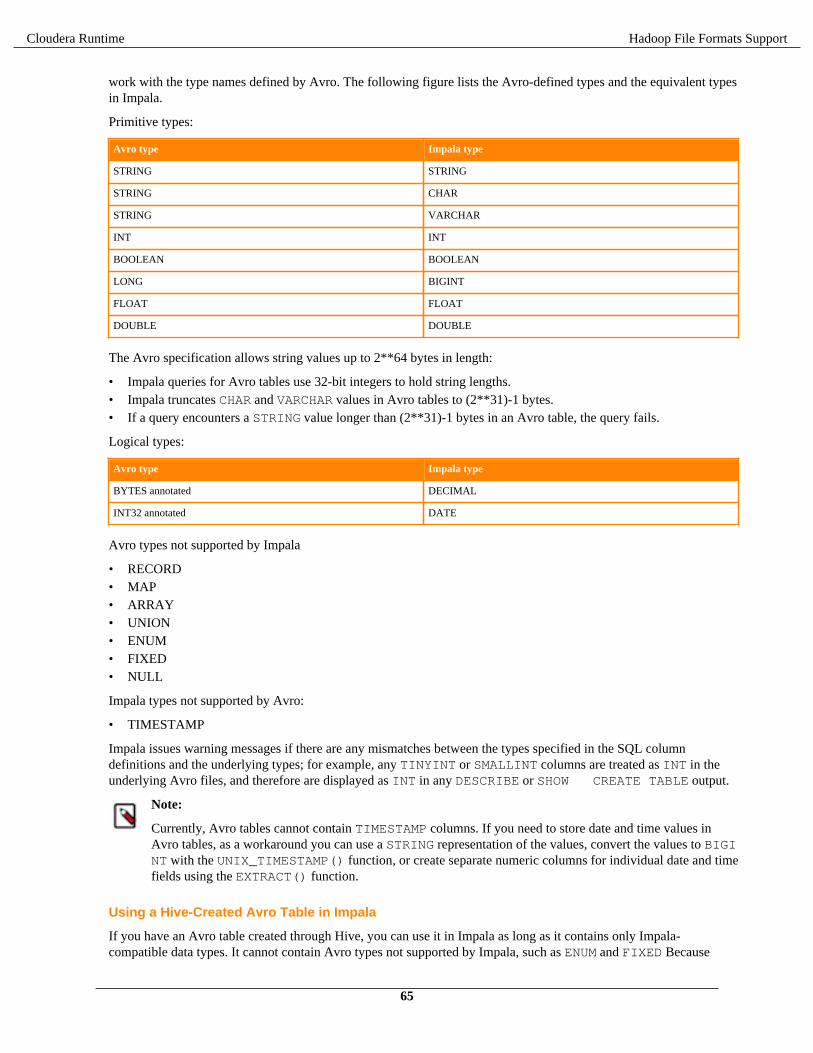
Cloudera Runtime Hadoop File Formats Support
work with the type names defined by Avro. The following figure lists the Avro-defined types and the equivalent typesin Impala.
Primitive types:
Avro type Impala type
STRING STRING
STRING CHAR
STRING VARCHAR
INT INT
BOOLEAN BOOLEAN
LONG BIGINT
FLOAT FLOAT
DOUBLE DOUBLE
The Avro specification allows string values up to 2**64 bytes in length:
• Impala queries for Avro tables use 32-bit integers to hold string lengths.• Impala truncates CHAR and VARCHAR values in Avro tables to (2**31)-1 bytes.• If a query encounters a STRING value longer than (2**31)-1 bytes in an Avro table, the query fails.
Logical types:
Avro type Impala type
BYTES annotated DECIMAL
INT32 annotated DATE
Avro types not supported by Impala
• RECORD• MAP• ARRAY• UNION• ENUM• FIXED• NULL
Impala types not supported by Avro:
• TIMESTAMP
Impala issues warning messages if there are any mismatches between the types specified in the SQL columndefinitions and the underlying types; for example, any TINYINT or SMALLINT columns are treated as INT in theunderlying Avro files, and therefore are displayed as INT in any DESCRIBE or SHOW CREATE TABLE output.
Note:
Currently, Avro tables cannot contain TIMESTAMP columns. If you need to store date and time values inAvro tables, as a workaround you can use a STRING representation of the values, convert the values to BIGINT with the UNIX_TIMESTAMP() function, or create separate numeric columns for individual date and timefields using the EXTRACT() function.
Using a Hive-Created Avro Table in Impala
If you have an Avro table created through Hive, you can use it in Impala as long as it contains only Impala-compatible data types. It cannot contain Avro types not supported by Impala, such as ENUM and FIXED Because
65

Cloudera Runtime Hadoop File Formats Support
Impala and Hive share the same metastore database, Impala can directly access the table definitions and data fortables that were created in Hive.
If you create an Avro table in Hive, issue an INVALIDATE METADATA in Impala. This is a one-time operationto make Impala aware of the new table. You can issue the statement while connected to any Impala node, and thecatalog service broadcasts the change to all other Impala nodes.
If you load new data into an Avro table through Hive, either through a Hive LOAD DATA or INSERT statement, orby manually copying or moving files into the data directory for the table, issue a REFRESH table_name statementthe next time you connect to Impala through impala-shell.
If you issue the LOAD DATA statement through Impala, you do not need a REFRESH afterward.
Impala only supports fields of type BOOLEAN, INT, LONG, FLOAT, DOUBLE, and STRING, or unions of these typeswith null, for example, ["string", "null"]. Unions with null essentially create a nullable type.
Loading Data into Avro Tables
Currently, Impala cannot write Avro data files. Therefore, an Avro table cannot be used as the destination of anImpala INSERT statement or CREATE TABLE AS SELECT.
To copy data from another table, issue any INSERT statements through Hive.
After loading data into a table through Hive or other mechanism outside of Impala, issue a REFRESH table_name statement the next time you connect to the Impala node, before querying the table, to make Impalarecognize the new data.
If you already have data files in Avro format, you can also issue LOAD DATA in either Impala or Hive. Impala canmove existing Avro data files into an Avro table, it just cannot create new Avro data files.
Enabling Compression for Avro Tables
To enable compression for Avro tables, specify settings in the Hive shell to enable compression and to specify acodec, then issue a CREATE TABLE statement as in the preceding examples. Impala supports the snappy anddeflate codecs for Avro tables.
For example:
hive> set hive.exec.compress.output=true;hive> set avro.output.codec=snappy;
Handling Avro Schema Evolution
Impala can handle with Avro data files that employ schema evolution, where different data files within the same tableuse slightly different type definitions. (You would perform the schema evolution operation by issuing an ALTER TABLE statement in the Hive shell.) The old and new types for any changed columns must be compatible, for example acolumn might start as an INT and later change to a BIGINT or FLOAT.
As with any other tables where the definitions are changed or data is added outside of the current impalad node,ensure that Impala loads the latest metadata for the table if the Avro schema is modified through Hive. Issue a REFRESH table_name or INVALIDATE METADATA table_name statement. REFRESH reloads themetadata immediately, INVALIDATE METADATA reloads the metadata the next time the table is accessed.
When Avro data files or columns are not consulted during a query, Impala does not check for consistency. Thus,if you issue SELECT c1, c2 FROM t1, Impala does not return any error if the column c3 changed in anincompatible way. If a query retrieves data from some partitions but not others, Impala does not check the data filesfor the unused partitions.
In the Hive DDL statements, you can specify an avro.schema.literal table property (if the schema definitionis short) or an avro.schema.url property (if the schema definition is long, or to allow convenient editing for thedefinition).
66

Cloudera Runtime Hadoop File Formats Support
Query Performance for Avro Tables
In general, expect query performance with Avro tables to be faster than with tables using text data, but slower thanwith Parquet tables.
Using RCFile Data FilesImpala supports creating and querying RCFile tables.
Creating RCFile Tables and Loading Data
To create a table in the RCFile format, use the STORED AS RCFILE clause in the CREATE TABLE statement.
Because Impala can query RCFile tables but cannot currently write to, after creating RCFile tables, use the Hive shellto load the data.
After loading data into a table through Hive or other mechanism outside of Impala, issue a REFRESH table_name statement the next time you connect to the Impala node, before querying the table, to make Impalarecognize the new data.
Query Performance for RCFile Tables
In general, expect query performance with RCFile tables to be faster than with tables using text data, but slower thanwith Parquet tables.
Enabling Compression for RCFile Tables
You may want to enable compression on existing tables. Enabling compression provides performance gains in mostcases and is supported for RCFile tables.
The compression type is specified in the SET mapred.output.compression.codec command.
For example, to enable Snappy compression, you would specify the following additional settings when loading datathrough the Hive shell.
SET mapred.output.compression.codec=org.apache.hadoop.io.compress.SnappyCodec;
Using SequenceFile Data FilesImpala supports creating and querying SequenceFile tables.
Creating SequenceFile Tables and Loading Data
To create a table in the SequenceFile format, use the STORED AS SEQUENCEFILE clause in the CREATE TABLE statement.
Because Impala can query SequenceFile tables but cannot currently write to, after creating SequenceFile tables, usethe Hive shell to load the data.
After loading data into a table through Hive or other mechanism outside of Impala, issue a REFRESH table_name statement the next time you connect to the Impala node, before querying the table, to make Impalarecognize the new data.
Enabling Compression for SequenceFile Tables
You may want to enable compression on existing tables. Enabling compression provides performance gains in mostcases and is supported for SequenceFile tables.
67

Cloudera Runtime Storage Systems Supports
The compression type is specified in the SET mapred.output.compression.codec command.
For example, to enable Snappy compression, you would specify the following additional settings when loading datathrough the Hive shell.
SET mapred.output.compression.codec=org.apache.hadoop.io.compress.SnappyCodec;
Query Performance for SequenceFile Tables
In general, expect query performance with SequenceFile tables to be faster than with tables using text data, but slowerthan with Parquet tables.
Storage Systems Supports
This section describes the storage systems that Impala supports.
Impala with HDFS
Although Impala typically works well with many large files in an HDFS storage system, there are times when youmight perform some file cleanup to reclaim space, or advise developers on techniques to minimize space consumptionand file duplication.
• Use compact binary file formats where practical. Numeric and time-based data in particular can be stored in morecompact form in binary data files. Depending on the file format, various compression and encoding featurescan reduce file size even further. You can specify the STORED AS clause as part of the CREATE TABLEstatement, or ALTER TABLE with the SET FILEFORMAT clause for an existing table or partition within apartitioned table.
• You manage underlying data files differently depending on whether the corresponding Impala table is defined asan internal or external table:
• Use the DESCRIBE FORMATTED statement to check if a particular table is internal (managed by Impala) orexternal, and to see the physical location of the data files in HDFS.
• For Impala-managed (“internal”) tables, use DROP TABLE statements to remove data files.• For tables not managed by Impala (“external”) tables, use appropriate HDFS-related commands such as hado
op fs, hdfs dfs, or distcp, to create, move, copy, or delete files within HDFS directories that areaccessible by the impala user. Issue a REFRESH table_name statement after adding or removing anyfiles from the data directory of an external table.
• Use external tables to reference HDFS data files in their original location. With this technique, you avoidcopying the files, and you can map more than one Impala table to the same set of data files. When you drop theImpala table, the data files are left undisturbed.
• Use the LOAD DATA statement to move HDFS files into the data directory for an Impala table from insideImpala, without the need to specify the HDFS path of the destination directory. This technique works for bothinternal and external tables.
• Make sure that the HDFS trashcan is configured correctly. When you remove files from HDFS, the space mightnot be reclaimed for use by other files until sometime later, when the trashcan is emptied.
• Drop all tables in a database before dropping the database itself.• If an INSERT statement encounters an error, and you see a directory named .impala_insert_staging or
_impala_insert_staging left behind in the data directory for the table, it might contain temporary datafiles taking up space in HDFS. You might be able to salvage these data files.
For example, delete those files through commands such as hadoop fs or hdfs dfs to reclaim spacebefore re-trying the INSERT. Issue DESCRIBE FORMATTED table_name to see the HDFS path whereyou can check for temporary files.
68

Cloudera Runtime Storage Systems Supports
Configuring Scratch Space for Spilling to Disk
Impala uses intermediate files during large sorts, joins, aggregations, or analytic function operations The files areremoved when the operation finishes. By default, intermediate files are stored in the directory /tmp/impala-scratch.
You can specify locations of the intermediate files in one of the following ways:
• By starting the impalad daemon with the ##scratch_dirs="path_to_directory" configurationoption.
• By specifying a different location in the Cloudera Manager in the Impala Daemon Scratch Directories field.
With either option above:
• You can specify a single directory or a comma-separated list of directories.• You can specify an optional a capacity quota per scratch directory using the colon (:) as the delimiter.
The capacity quota of -1 or 0 is the same as no quota for the directory.• The scratch directories must be on the local filesystem, not in HDFS.• You might specify different directory paths for different hosts, depending on the capacity and speed of the
available storage devices.
If there is less than 1 GB free on the filesystem where that directory resides, Impala still runs, but writes a warningmessage to its log.
Impala successfully starts (with a warning written to the log) if it cannot create or read and write files in one of thescratch directories.
The following are examples for specifying scratch directories.
Config option Description
--scratch_dirs=/dir1,/dir2 Use /dir1 and /dir2 as scratch directories with no capacity quota.
--scratch_dirs=/dir1,/dir2:25G Use /dir1 and /dir2 as scratch directories with no capacity quota on /dir1 and the 25GB quota on /dir2.
--scratch_dirs=/dir1:5MB,/dir2 Use /dir1 and /dir2 as scratch directories with the capacity quota of5MB on /dir1 and no quota on /dir2.
--scratch_dirs=/dir1:-1,/dir2:0 Use /dir1 and /dir2 as scratch directories with no capacity quota.
Allocation from a scratch directory will fail if the specified limit for the directory is exceeded.
If Impala encounters an error reading or writing files in a scratch directory during a query, Impala logs the error, andthe query fails.
Increasing Scratch Capacity
You can compress the data spilled to disk to increase the effective scratch capacity. You typically more thandouble capacity using compression and reduce spilling to disk. Use the --disk_spill_compression_codec and –-disk_spill_punch_holes startup options. The --disk_spill_compression_codec takes any value supported by theCOMPRESSION_CODEC query option. The value is not case-sensitive. A value of ZSTD or LZ4 is recommended(default is NONE).
For example:
--disk_spill_compression_codec=LZ4--disk_spill_punch_holes=true
If you set --disk_spill_compression_codec to a value other than NONE, you must set --disk_spill_punch_holes to true.
The hole punching feature supported by many file systems is used to reclaim space in scratch files during execution ofa query that spills to disk. This results in lower scratch space requirements in many cases, especially when combined
69

Cloudera Runtime Storage Systems Supports
with disk spill compression. When this option is not enabled, scratch space is still recycled by a query, but lesseffectively in many cases.
You can specify a compression level for ZSTD only. For example:
--disk_spill_compression_codec=ZSTD:10--disk_spill_punch_holes=true
Compression levels from 1 up to 22 (default 3) are supported for ZSTD. The lower the compression level, the fasterthe speed at the cost of compression ratio.
Impala with KuduYou can use Impala to query tables stored by Apache Kudu. This capability allows convenient access to a storagesystem that is tuned for different kinds of workloads than the default with Impala.
By default, Impala tables are stored on HDFS. HDFS files are ideal for bulk loads (append operations) and queriesusing full-table scans, but do not support in-place updates or deletes. Kudu is an alternative storage engine used byImpala which can do both in-place updates (for mixed read/write workloads) and fast scans (for data-warehouse/analytic operations). Using Kudu tables with Impala can simplify the ETL pipeline by avoiding extra steps tosegregate and reorganize newly arrived data.
The underlying storage is managed and organized by Kudu, not represented as HDFS data files.
The combination of Kudu and Impala works best for tables where scan performance is important, but data arrivescontinuously, in small batches, or needs to be updated without being completely replaced. HDFS-backed tables canrequire substantial overhead to replace or reorganize data files as new data arrives. Impala can perform efficientlookups and scans within Kudu tables, and Impala can also perform update or delete operations efficiently. You canalso use the Kudu Java, C++, and Python APIs to do ingestion or transformation operations outside of Impala, andImpala can query the current data at any time.
With HDFS-backed tables, you are typically concerned with the number of DataNodes in the cluster, how many andhow large HDFS data files are read during a query, and therefore the amount of work performed by each DataNodeand the network communication to combine intermediate results and produce the final result set.
Certain Impala SQL statements and clauses, such as DELETE, UPDATE, UPSERT, and PRIMARY KEY work onlywith Kudu tables.
Other statements and clauses, such as LOAD DATA, TRUNCATE TABLE, and INSERT OVERWRITE, are notapplicable to Kudu tables.
Query performance for Kudu tables
For queries involving Kudu tables, Impala can delegate much of the work of filtering the result set to Kudu, avoidingsome of the I/O involved in full table scans of tables containing HDFS data files. This type of optimization isespecially effective for partitioned Kudu tables, where the Impala query WHERE clause refers to one or more primarykey columns that are also used as partition key columns. For example, if a partitioned Kudu table uses a HASH clausefor col1 and a RANGE clause for col2, a query using a clause such as WHERE col1 IN (1,2,3) AND col2 > 100 can determine exactly which tablet servers contain relevant data, and therefore parallelize the queryefficiently.
Impala can push down additional information to optimize join queries involving Kudu tables. If the join clausecontains predicates of the form column = expression, after Impala constructs a hash table of possiblematching values for the join columns from the bigger table (either an HDFS table or a Kudu table), Impala can “pushdown” the minimum and maximum matching column values to Kudu, so that Kudu can more efficiently locatematching rows in the second (smaller) table. These min/max filters are affected by the RUNTIME_FILTER_MODE,RUNTIME_FILTER_WAIT_TIME_MS, and DISABLE_ROW_RUNTIME_FILTERING query options; the min/maxfilters are not affected by the RUNTIME_BLOOM_FILTER_SIZE, RUNTIME_FILTER_MIN_SIZE, RUNTIME_FILTER_MAX_SIZE, and MAX_NUM_RUNTIME_FILTERS query options.
70

Cloudera Runtime Storage Systems Supports
The TABLESAMPLE clause of the SELECT statement does not apply to a table reference derived from a view, asubquery, or anything other than a real base table. This clause only works for tables backed by HDFS or HDFS-likedata files, therefore it does not apply to Kudu tables.
Configuring for Kudu TablesThe Kudu configuration property must be set for Impala to connect to the appropriate Kudu server.
Procedure
1. In Cloudera Manager, navigate to Clusters > Impala Service.
2. In the Configuration tab, specify the Kudu service you want to use in the Kudu Service field.
Typically, the required value for this setting is kudu_host:7051. In a high-availability Kudu deployment,specify the names of multiple Kudu hosts separated by commas.
3. If the Kudu Service field is not set, you can still associate the appropriate value for each table by specifying aTBLPROPERTIES('kudu.master_addresses') clause in the CREATE TABLE statement or changingthe TBLPROPERTIES('kudu.master_addresses') value with an ALTER TABLE statement.
Impala DDL for KuduYou can use the Impala CREATE TABLE and ALTER TABLE statements to create and fine-tune the characteristicsof Kudu tables. Impala supports specific features and properties that only apply to Kudu tables.
To create a Kudu table, use the STORED AS KUDU clause in the CREATE TABLE statement.
The column list in a CREATE TABLE statement can include the following attributes, which only apply to Kudutables:
PRIMARY KEY| [NOT] NULL| ENCODING codec| COMPRESSION algorithm| DEFAULT constant_expression| BLOCK_SIZE number
PRIMARY KEY Attribute
The primary key for a Kudu table is a column, or set of columns, that uniquely identifies every row. The primary keyvalue also is used as the natural sort order for the values from the table.
The notion of primary key only applies to Kudu tables. Every Kudu table requires a primary key.
Because all of the primary key columns must have non-null values, specifying a column in the PRIMARY KEYclause implicitly adds the NOT NULL attribute to that column.
The primary key columns must be the first ones specified in the CREATE TABLE statement.
When the primary key is a single column, you can specify the PRIMARY KEY attribute either inline in a singlecolumn definition, or as a separate clause at the end of the column list.
For example:
CREATE TABLE pk_inline( col1 BIGINT PRIMARY KEY, col2 STRING, col3 BOOLEAN) PARTITION BY HASH(col1) PARTITIONS 2 STORED AS KUDU;
CREATE TABLE pk_at_end
71

Cloudera Runtime Storage Systems Supports
( col1 BIGINT, col2 STRING, col3 BOOLEAN, PRIMARY KEY (col1)) PARTITION BY HASH(col1) PARTITIONS 2 STORED AS KUDU;
If the primary key consists of more than one column, you must specify the primary key using a separate entry in thecolumn list.
CREATE TABLE pk_multiple_columns( col1 BIGINT, col2 STRING, col3 BOOLEAN, PRIMARY KEY (col1, col2)) PARTITION BY HASH(col2) PARTITIONS 2 STORED AS KUDU;
The contents of the primary key columns cannot be changed by an UPDATE or UPSERT statement.
Including too many columns in the primary key (more than 5 or 6) can reduce the performance of write operations.Therefore, pick the most selective and most frequently tested non-null columns for the primary key specification. If acolumn must always have a value, but that value might change later, leave it out of the primary key and use a NOT NULL clause for that column instead.
NULL | NOT NULL Attribute
For Kudu tables, you can specify which columns can contain nulls or not. This constraint offers an extra level ofconsistency enforcement for Kudu tables. If an application requires a field to always be specified, include a NOT NULL clause in the corresponding column definition, and Kudu prevents rows from being inserted with a NULL inthat column.
For example, a table containing geographic information might require the latitude and longitude coordinates to alwaysbe specified. Other attributes might be allowed to be NULL. For example, a location might not have a designatedplace name, its altitude might be unimportant, and its population might be initially unknown, to be filled in later.
For non-Kudu tables, Impala allows any column to contain NULL values, because it is not practical to enforce a “notnull” constraint on HDFS data files that could be prepared using external tools and ETL processes.
CREATE TABLE required_columns( id BIGINT PRIMARY KEY, latitude DOUBLE NOT NULL, longitude DOUBLE NOT NULL, place_name STRING, altitude DOUBLE, population BIGINT) PARTITION BY HASH(id) PARTITIONS 2 STORED AS KUDU;
During performance optimization, Kudu can use the knowledge that nulls are not allowed to skip certain checkson each input row, speeding up queries and join operations. Therefore, specify NOT NULL constraints whenappropriate.
The NULL clause is the default condition for all columns that are not part of the primary key. You can omit it, orspecify it to clarify that you have made a conscious design decision to allow nulls in a column.
Because primary key columns cannot contain any NULL values, the NOT NULL clause is not required for the primarykey columns, but you might still specify it to make your code self-describing.
72

Cloudera Runtime Storage Systems Supports
DEFAULT Attribute
You can specify a default value for columns in Kudu tables. The default value can be any constant expression, forexample, a combination of literal values, arithmetic and string operations. It cannot contain references to columns ornon-deterministic function calls.
The following example shows different kinds of expressions for the DEFAULT clause. The requirement to use aconstant value means that you can fill in a placeholder value such as NULL, empty string, 0, -1, 'N/A' and so on,but you cannot reference functions or column names. Therefore, you cannot use DEFAULT to do things such asautomatically making an uppercase copy of a string value, storing Boolean values based on tests of other columns, oradd or subtract one from another column representing a sequence number.
CREATE TABLE default_vals( id BIGINT PRIMARY KEY, name STRING NOT NULL DEFAULT 'unknown', address STRING DEFAULT upper('no fixed address'), age INT DEFAULT -1, earthling BOOLEAN DEFAULT TRUE, planet_of_origin STRING DEFAULT 'Earth', optional_col STRING DEFAULT NULL) PARTITION BY HASH(id) PARTITIONS 2 STORED AS KUDU;
Note:
When designing an entirely new schema, prefer to use NULL as the placeholder for any unknown ormissing values, because that is the universal convention among database systems. Null values can be storedefficiently, and easily checked with the IS NULL or IS NOT NULL operators. The DEFAULT attributeis appropriate when ingesting data that already has an established convention for representing unknown ormissing values, or where the vast majority of rows have some common non-null value.
ENCODING Attribute
Each column in a Kudu table can optionally use an encoding, a low-overhead form of compression that reduces thesize on disk, then requires additional CPU cycles to reconstruct the original values during queries. Typically, highlycompressible data benefits from the reduced I/O to read the data back from disk.
The encoding keywords that Impala recognizes are:
• AUTO_ENCODING: Use the default encoding based on the column type, which are bitshuffle for the numeric typecolumns and dictionary for the string type columns.
• PLAIN_ENCODING: Leave the value in its original binary format.• RLE: Compress repeated values (when sorted in primary key order) by including a count.• DICT_ENCODING: When the number of different string values is low, replace the original string with a numeric
ID.• BIT_SHUFFLE: Rearrange the bits of the values to efficiently compress sequences of values that are identical or
vary only slightly based on primary key order. The resulting encoded data is also compressed with LZ4.• PREFIX_ENCODING: Compress common prefixes in string values; mainly for use internally within Kudu.
COMPRESSION Attribute
You can specify a compression algorithm to use for each column in a Kudu table. This attribute imposes more CPUoverhead when retrieving the values than the ENCODING attribute does. Therefore, use it primarily for columns withlong strings that do not benefit much from the less-expensive ENCODING attribute.
The choices for COMPRESSION are LZ4, SNAPPY, and ZLIB.
73
Cloudera Runtime Storage Systems Supports
Note:
Columns that use the BITSHUFFLE encoding are already compressed using LZ4, and so typically do notneed any additional COMPRESSION attribute.
BLOCK_SIZE Attribute
Although Kudu does not use HDFS files internally, and thus is not affected by the HDFS block size, it does have anunderlying unit of I/O called the block size. The BLOCK_SIZE attribute lets you set the block size for any column.
The block size attribute is a relatively advanced feature. This is an unsupported feature and is consideredexperimental.
Kudu Replication Factor
By default, Kudu tables created through Impala use a tablet replication factor of 3. To change the replication factorfor a Kudu table, specify the replication factor using the TBLPROPERTIES in the CREATE TABLE statement asbelow where n is the replication factor you want to use:
TBLPROPERTIES ('kudu.num_tablet_replicas' = 'n')
The number of replicas for a Kudu table must be odd.
Altering the kudu.num_tablet_replicas property after table creation currently has no effect.
How Impala Handles Kudu Metadata
Much of the metadata for Kudu tables is handled by the underlying storage layer. Kudu tables have less relianceon the Metastore database, and require less metadata caching on the Impala side. For example, information aboutpartitions in Kudu tables is managed by Kudu, and Impala does not cache any block locality metadata for Kudutables.
The REFRESH and INVALIDATE METADATA statements are needed less frequently for Kudu tables than forHDFS-backed tables. Neither statement is needed when data is added to, removed, or updated in a Kudu table, even ifthe changes are made directly to Kudu through a client program using the Kudu API.
Run REFRESH table_name or INVALIDATE METADATA table_name for a Kudu table only after making achange to the Kudu table schema, such as adding or dropping a column.
Because Kudu manages the metadata for its own tables separately from the Metastore database, there is a tablename stored in the Metastore database for Impala to use, and a table name on the Kudu side, and these names can bemodified independently through ALTER TABLE statements.
To avoid potential name conflicts, the prefix impala:: and the Impala database name are encoded into theunderlying Kudu table name.
Partitioning for Kudu TablesKudu tables use special mechanisms to distribute data among the underlying tablet servers. Although referred aspartitioned tables, they are distinguished from traditional Impala partitioned tables with the different syntax in CREATE TABLE statement.
Kudu tables use PARTITION BY, HASH, RANGE, and range specification clauses rather than the PARTITIONED BY clause for HDFS-backed tables, which specifies only a column name and creates a new partition for each differentvalue.
To see the current partitioning scheme for a Kudu table, you can use the SHOW CREATE TABLE statement or theSHOW PARTITIONS statement. The CREATE TABLE syntax displayed by this statement includes all the hash,range, or both clauses that reflect the original table structure plus any subsequent ALTER TABLE statements thatchanged the table structure.
To see the underlying buckets and partitions for a Kudu table, use the SHOW TABLE STATS or SHOW PARTITIONS statement.
74

Cloudera Runtime Storage Systems Supports
Hash Partitioning
Hash partitioning is the simplest type of partitioning for Kudu tables. For hash-partitioned Kudu tables, insertedrows are divided up between a fixed number of “buckets” by applying a hash function to the values of the columnsspecified in the HASH clause. Hashing ensures that rows with similar values are evenly distributed, instead ofclumping together all in the same bucket. Spreading new rows across the buckets this way lets insertion operationswork in parallel across multiple tablet servers. Separating the hashed values can impose additional overhead onqueries, where queries with range-based predicates might have to read multiple tablets to retrieve all the relevantvalues.
-- 1M rows with 50 hash partitions = approximately 20,000 rows per partition.-- The values in each partition are not sequential, but rather based on a hash function.-- Rows 1, 99999, and 123456 might be in the same partition.CREATE TABLE million_rows (id string primary key, s string) PARTITION BY HASH(id) PARTITIONS 50 STORED AS KUDU;
-- Because the ID values are unique, we expect the rows to be roughly-- evenly distributed between the buckets in the destination table.INSERT INTO million_rows SELECT * FROM billion_rows ORDER BY id LIMIT 1e6;
The largest number of buckets that you can create with a PARTITIONS clause varies depending on the number oftablet servers in the cluster, while the smallest is 2. For large tables, prefer to use roughly 10 partitions per server inthe cluster.
Range Partitioning
Range partitioning lets you specify partitioning precisely, based on single values or ranges of values within oneor more columns. You add one or more RANGE clauses to the CREATE TABLE statement, following thePARTITION BY clause. The RANGE clause includes a combination of constant expressions, VALUE or VALUESkeywords, and comparison operators.
CREATE TABLE t1 (id STRING PRIMARY KEY, s STRING) PARTITION BY RANGE (PARTITION 'a' <= VALUES < '{', PARTITION 'A' <= VALUES < '[', PARTITION VALUES = '00000') STORED AS KUDU;
Note:
When defining ranges, be careful to avoid “fencepost errors” where values at the extreme ends might beincluded or omitted by accident. For example, in the tables defined in the preceding code listings, the range "a" <= VALUES < "{" ensures that any values starting with z, such as za or zzz or zzz-ZZZ, are all included, by using a less-than operator for the smallest value after all the values starting with z.
For range-partitioned Kudu tables, an appropriate range must exist before a data value can be created in the table.Any INSERT, UPDATE, or UPSERT statements fail if they try to create column values that fall outside the specifiedranges. The error checking for ranges is performed on the Kudu side. Impala passes the specified range information toKudu, and passes back any error or warning if the ranges are not valid. (A nonsensical range specification causes anerror for a DDL statement, but only a warning for a DML statement.)
Partition ranges can be non-contiguous:
PARTITION BY RANGE (year) (PARTITION 1885 <= VALUES <= 1889, PARTITION 1893 <= VALUES <= 1897)
75

Cloudera Runtime Storage Systems Supports
The ALTER TABLE statement with the ADD PARTITION or DROP PARTITION clauses can be used to addor remove ranges from an existing Kudu table.
ALTER TABLE foo ADD PARTITION 30 <= VALUES < 50;ALTER TABLE foo DROP PARTITION 1 <= VALUES < 5;
When a range is added, the new range must not overlap with any of the previous ranges; that is, it can only fill in gapswithin the previous ranges.
When a range is removed, all the associated rows in the table are deleted regardless whether the table is internal orexternal.
Kudu tables can also use a combination of hash and range partitioning. For example:
PARTITION BY HASH (school) PARTITIONS 10, RANGE (letter_grade) (PARTITION VALUE = 'A', PARTITION VALUE = 'B', PARTITION VALUE = 'C', PARTITION VALUE = 'D', PARTITION VALUE = 'F')
Impala DML for Kudu TablesIn DML statements, Impala supports specific features and properties that only apply to Kudu tables.
The UPDATE and DELETE statements let you modify data within Kudu tables without rewriting substantial amountsof table data.
The UPSERT statement acts as a combination of INSERT and UPDATE, inserting rows where the primary key doesnot already exist, and updating the non-primary key columns where the primary key does already exist in the table.
The INSERT statement for Kudu tables honors the unique and NOT NULL requirements for the primary keycolumns.
Because Impala and Kudu do not support transactions, the effects of any INSERT, UPDATE, or DELETE statementare immediately visible. For example, you cannot do a sequence of UPDATE statements and only make the changesvisible after all the statements are finished. Also, if a DML statement fails partway through, any rows that werealready inserted, deleted, or changed remain in the table; there is no rollback mechanism to undo the changes.
In particular, an INSERT ... SELECT statement that refers to the table being inserted into might insert more rowsthan expected, because the SELECT part of the statement sees some of the new rows being inserted and processesthem again.
Query hints:
The INSERT or UPSERT operations into Kudu tables automatically add an exchange and a sort node to the plan thatpartitions and sorts the rows according to the partitioning/primary key scheme of the target table (unless the numberof rows to be inserted is small enough to trigger single node execution). Since Kudu partitions and sorts rows onwrite, pre-partitioning and sorting takes some of the load off of Kudu and helps large INSERT operations to completewithout timing out. However, this default behavior may slow down the end-to-end performance of the INSERT orUPSERT operations.
You can use the /* +NOCLUSTERED */ and /* +NOSHUFFLE */ hints together to disable partitioningand sorting before the rows are sent to Kudu. Additionally, since sorting may consume a large amount of memory,consider setting the MEM_LIMIT query option for those queries.
Loading Data into Kudu Tables
Kudu tables are well-suited to use cases where data arrives continuously, in small or moderate volumes. To bring datainto Kudu tables, use the Impala INSERT and UPSERT statements.
The LOAD DATA statement does not support Kudu tables.
76

Cloudera Runtime Storage Systems Supports
Because Kudu manages its own storage layer that is optimized for smaller block sizes than HDFS, and performs itsown housekeeping to keep data evenly distributed, it is not subject to the “many small files” issue and does not needexplicit reorganization and compaction as the data grows over time.
The partitions within a Kudu table can be specified to cover a variety of possible data distributions, instead ofhardcoding a new partition for each new day, hour, and so on, which can lead to inefficient, hard-to-scale, and hard-to-manage partition schemes with HDFS tables.
Your strategy for performing ETL or bulk updates on Kudu tables should take into account the limitations onconsistency for DML operations.
• The INSERT, UPDATE, and UPSERT operations should produce an identical result even when executed multipletimes.
• If a bulk operation is in danger of exceeding capacity limits due to timeouts or high memory usage, split it into aseries of smaller operations.
• Avoid running concurrent ETL operations where the end results depend on precise ordering. In particular, donot rely on an INSERT ... SELECT statement that selects from the same table into which it is inserting,unless you include extra conditions in the WHERE clause to avoid reading the newly inserted rows within the samestatement.
• Because relationships between tables cannot be enforced by Impala and Kudu, and cannot be committed or rolledback together, do not expect transactional semantics for multi-table operations.
Consistency Considerations for Kudu Tables
Kudu tables have consistency characteristics such as uniqueness, controlled by the primary key columns and non-nullable columns. The emphasis for consistency is on preventing duplicate or incomplete data from being stored in atable.
Currently, Kudu does not enforce strong consistency for order of operations, total success or total failure of a multi-row statement, or data that is read while a write operation is in progress. Changes are applied atomically to each row,but not applied as a single unit to all rows affected by a multi-row DML statement. That is, Kudu does not currentlyhave atomic multi-row statements or isolation between statements.
If some rows are rejected during a DML operation because of a mismatch with duplicate primary key values, NOT NULL constraints, and so on, the statement succeeds with a warning. Impala still inserts, deletes, or updates the otherrows that are not affected by the constraint violation.
Consequently, the number of rows affected by a DML operation on a Kudu table might be different than you expect.
Because there is no strong consistency guarantee for information being inserted into, deleted from, or updated acrossmultiple tables simultaneously, consider denormalizing the data where practical. That is, if you run separate INSERT statements to insert related rows into two different tables, one INSERT might fail while the other succeeds,leaving the data in an inconsistent state. Even if both inserts succeed, a join query might happen during the intervalbetween the completion of the first and second statements, and the query would encounter incomplete inconsistentdata. Denormalizing the data into a single wide table can reduce the possibility of inconsistency due to multi-tableoperations.
Information about the number of rows affected by a DML operation is reported in impala-shell output, and inthe PROFILE output, but is not currently reported to HiveServer2 clients such as JDBC or ODBC applications.
Handling Date, Time, or Timestamp Data with Kudu
You can include TIMESTAMP columns in Kudu tables. The behavior of TIMESTAMP for Kudu tables has somespecial considerations:
• Any nanoseconds in the original 96-bit value produced by Impala are not stored, because Kudu represents date/time columns using 64-bit values. The nanosecond portion of the value is rounded, not truncated. Therefore, aTIMESTAMP value that you store in a Kudu table might not be bit-for-bit identical to the value returned by aquery.
• The conversion between the Impala 96-bit representation and the Kudu 64-bit representation introduces someperformance overhead when reading or writing TIMESTAMP columns. You can minimize the overhead during
77

Cloudera Runtime Storage Systems Supports
writes by performing inserts through the Kudu API. Because the overhead during reads applies to each query, youmight continue to use a BIGINT column to represent date/time values in performance-critical applications.
• The Impala TIMESTAMP type has a narrower range for years than the underlying Kudu data type. Impala canrepresent years 1400-9999. If year values outside this range are written to a Kudu table by a non-Impala client,Impala returns NULL by default when reading those TIMESTAMP values during a query. Or, if the ABORT_ON_ERROR query option is enabled, the query fails when it encounters a value with an out-of-range year.
Impala with HBaseYou can use Impala to query data residing in HBase tables, a key-value data store where the value consists of multiplefields. The key is mapped to one column in the Impala table, and the various fields of the value are mapped to theother columns in the Impala table.
HBase tables are the best suited in Impala in the following use cases.
• Storing rapidly incrementing counters, such as how many times a web page has been viewed, or on a socialnetwork, how many connections a user has or how many votes a post received.
The append-only storage mechanism of HBase is efficient for writing each change to disk, and a query alwaysreturns the latest value. An application could query specific totals like these from HBase, and combine the resultswith a broader set of data queried from Impala.
• Storing very wide tables in HBase.
Wide tables have many columns, possibly thousands, typically recording many attributes for an important subjectsuch as a user of an online service. These tables are also often sparse, that is, most of the columns values areNULL, 0, false, empty string, or other blank or placeholder value. (For example, any particular web site usermight have never used some site feature, filled in a certain field in their profile, visited a particular part of the site,and so on.) A typical query against this kind of table is to look up a single row to retrieve all the information abouta specific subject, rather than summing, averaging, or filtering millions of rows as in typical Impala-managedtables.
HBase works out of the box with Impala. There is no mandatory configuration needed to use these two componentstogether.
For efficient queries, use WHERE clauses to find a single key value or a range of key values wherever practical, bytesting the Impala column corresponding to the HBase row key. Avoid queries that do full-table scans, which areefficient for regular Impala tables but inefficient in HBase.
To work with an HBase table from Impala, ensure that the impala user has read/write privileges for the HBasetable, using the GRANT command in the HBase shell.
Creating HBase Tables for Impala
You create the tables on the Impala side using the Hive shell, because the Impala CREATE TABLE statementcurrently does not support custom SerDes and some other syntax needed for HBase tables.
• You create the new table as an HBase table using the STORED BY 'org.apache.hadoop.hive.hbase.HBaseStorageHandler' clause on the Hive CREATE TABLE statement.
• You map these specially created tables to corresponding tables that exist in HBase, with the clause TBLPROPERTIES("hbase.table.name" = "table_name_in_hbase") on the Hive CREATE TABLEstatement.
• You define the column corresponding to the HBase row key as a string with the #string keyword, or map it to aSTRING column.
• After creating a new table through Hive, issue the INVALIDATE METADATA statement in Impala to makeImpala aware of the new table.
Because Impala and Hive share the same Metastore database, once you create the table in Hive, you can query orinsert into it through Impala.
78
Cloudera Runtime Storage Systems Supports
Supported Data Types for HBase Columns
HBase does not enforce any typing for the key or value fields. All the type enforcement is done on the Impala side.
HBase row key
When creating the table through the Hive shell, use the STRING data type for the column thatcorresponds to the HBase row key.
For best performance of Impala queries against HBase tables, most queries will performcomparisons in the WHERE clause against the column that corresponds to the HBase row key.
Impala can translate predicates (through operators such as =, <, and BETWEEN) against this columninto fast lookups in HBase, but this optimization (“predicate pushdown”) only works when thatcolumn is defined as STRING.
HBase numeric column
Define HBase numeric columns as the binary data type in Hive CREATE TABLE statement usingthe #binary (#b) keyword.
Defining numeric columns as binary can reduce the overall data volume in the HBase tables.
Impala also supports reading and writing to columns that are defined in the Hive CREATE TABLE statement usingbinary data types , represented in the Hive table definition using the #binary keyword, often abbreviated as #b.
Loading Data into HBase Tables
The Impala INSERT statement supports HBase tables. The INSERT ... VALUES syntax is ideally suited toHBase tables, because inserting a single row is an efficient operation for an HBase table.
When you use the INSERT ... SELECT syntax, the result in the HBase table could be fewer rows than youexpect. HBase only stores the most recent version of each unique row key, so if an INSERT ... SELECTstatement copies over multiple rows containing the same value for the key column, subsequent queries will onlyreturn one row with each key column value.
Successive INSERT statements using the same value for the key column achieves the same result as UPDATE.
Examples of Querying HBase Tables from Impala
The following examples create an HBase table with four column families, create a corresponding table through Hive,then insert and query the table through Impala.
In HBase, create a table. Table names are quoted in the CREATE statement in HBase.
hbase(main):001:0> CREATE 'hbasealltypessmall', 'boolsCF', 'intsCF', 'floatsCF', 'stringsCF'
Issue the following CREATE TABLE statement in the Hive shell.
This example creates an external table mapped to the HBase table, usable by both Impala and Hive. It is defined as anexternal table so that when dropped by Impala or Hive, the original HBase table is not touched at all.
The WITH SERDEPROPERTIES clause specifies that the first column (ID) represents the row key, and mapsthe remaining columns of the SQL table to HBase column families. The mapping relies on the ordinal order of thecolumns in the table, not the column names in the CREATE TABLE statement. The first column is defined to be thelookup key; the STRING data type produces the fastest key-based lookups for HBase tables.
Note: For Impala with HBase tables, the most important aspect to ensure good performance is to use a STRING column as the row key, as shown in this example.
hive> CREATE EXTERNAL TABLE hbasestringids ( > id string, > bool_col boolean, > tinyint_col tinyint,
79

Cloudera Runtime Storage Systems Supports
> smallint_col smallint, > int_col int, > bigint_col bigint, > float_col float, > double_col double, > date_string_col string, > string_col string, > timestamp_col timestamp) > STORED BY 'org.apache.hadoop.hive.hbase.HBaseStorageHandler' > WITH SERDEPROPERTIES ( > "hbase.columns.mapping" = > ":key,boolsCF:bool_col,intsCF:tinyint_col,intsCF:smallint_col,intsCF:int_col,intsCF:\ > bigint_col,floatsCF:float_col,floatsCF:double_col,stringsCF:date_string_col,\ > stringsCF:string_col,stringsCF:timestamp_col" > ) > TBLPROPERTIES("hbase.table.name" = "hbasealltypessmall");
Once you have established the mapping to an HBase table, you can issue DML statements and queries from Impala.The following example shows a series of INSERT statements followed by a query. The ideal kind of query from aperformance standpoint retrieves a row from the table based on a row key mapped to a string column.
The INVALIDATE METADATA statement makes the table created through Hive visible to Impala.
[impala] > INVALIDATE METADATA hbasestringids;
[impala] > INSERT INTO hbasestringids VALUES ('0001',true,3.141,9.94,1234567,32768,4000,76,'2014-12-31','Hello world',NOW());
[impala] > IMSERT INTO hbasestringids VALUES ('0002',false,2.004,6.196,1500,8000,129,127,'2014-01-01','Foo bar',NOW());
[impala] > SELECT * FROM hbasestringids WHERE id = '0001';+------+----------+------------+-------------------+------------+---------+--------------+-------------+-----------------+-------------+-------------------------------+| id | bool_col | double_col | float_col | bigint_col | int_col | smallint_col | tinyint_col | date_string_col | string_col | timestamp_col |+------+----------+------------+-------------------+------------+---------+--------------+-------------+-----------------+-------------+-------------------------------+| 0001 | true | 3.141 | 9.939999580383301 | 1234567 | 32768 | 4000 | 76 | 2014-12-31 | Hello world | 2015-02-10 16:36:59.764838000 |+------+----------+------------+-------------------+------------+---------+--------------+-------------+-----------------+-------------+-------------------------------+
Performance Considerations for the Impala-HBase Integration
Impala uses the HBase client API via Java Native Interface (JNI) to query data stored in HBase. This querying doesnot read HFiles directly. The extra communication overhead makes it important to choose what data to store in HBaseor in HDFS, and construct efficient queries that can retrieve the HBase data efficiently:
• Use HBase table for queries that return a single row or a small range of rows, not queries that perform a full tablescan of an entire table. (If a query has a HBase table and no WHERE clause referencing that table, that is a strongindicator that it is an inefficient query for an HBase table.)
• HBase may offer acceptable performance for storing small dimension tables where the table is small enoughthat executing a full table scan for every query is efficient enough. However, Kudu is almost always a superior
80

Cloudera Runtime Storage Systems Supports
alternative for storing dimension tables. HDFS tables are also appropriate for dimension tables that do not need tosupport update queries, delete queries or insert queries with small numbers of rows.
Query predicates are applied to row keys as start and stop keys, thereby limiting the scope of a particular lookup. Ifrow keys are not mapped to string columns, then ordering is typically incorrect and comparison operations do notwork. For example, if row keys are not mapped to string columns, evaluating for greater than (>) or less than (<)cannot be completed.
Predicates on non-key columns can be sent to HBase to scan as SingleColumnValueFilters, providing someperformance gains. In such a case, HBase returns fewer rows than if those same predicates were applied using Impala.While there is some improvement, it is not as great when start and stop rows are used. This is because the numberof rows that HBase must examine is not limited as it is when start and stop rows are used. As long as the row keypredicate only applies to a single row, HBase will locate and return that row. Conversely, if a non-key predicate isused, even if it only applies to a single row, HBase must still scan the entire table to find the correct result.
Limitations and Restrictions of the Impala and HBase Integration
The Impala integration with HBase has the following limitations and restrictions, some inherited from the integrationbetween HBase and Hive, and some unique to Impala:
• If you issue a DROP TABLE for an internal (Impala-managed) table that is mapped to an HBase table, theunderlying table is not removed in HBase. The Hive DROP TABLE statement removes the HBase table inthis case.
• The INSERT OVERWRITE statement is not available for HBase tables. You can insert new data, or modify anexisting row by inserting a new row with the same key value, but not replace the entire contents of the table. Youcan do an INSERT OVERWRITE in Hive if you need this capability.
• If you issue a CREATE TABLE LIKE statement for a table mapped to an HBase table, the new table is also anHBase table, but inherits the same underlying HBase table name as the original. The new table is effectively analias for the old one, not a new table with identical column structure. Avoid using CREATE TABLE LIKE forHBase tables, to avoid any confusion.
• Copying data into an HBase table using the Impala INSERT ... SELECT syntax might produce fewernew rows than are in the query result set. If the result set contains multiple rows with the same value for the keycolumn, each row supercedes any previous rows with the same key value. Because the order of the inserted rowsis unpredictable, you cannot rely on this technique to preserve the “latest” version of a particular key value.
• The LOAD DATA statement cannot be used with HBase tables.• The TABLESAMPLE clause of the SELECT statement does not suppport HBase tables.
Impala with Azure Data Lake Store (ADLS)You can use Impala to query data residing on the Azure Data Lake Store (ADLS) filesystem and Azure Blob FileSystem (ABFS). This capability allows convenient access to a storage system that is remotely managed, accessiblefrom anywhere, and integrated with various cloud-based services.
Impala can query files in any supported file format from ADLS. The ADLS storage location can be for an entire tableor individual partitions in a partitioned table.
The default Impala tables use data files stored on HDFS, which are ideal for bulk loads and queries using full-tablescans. In contrast, queries against ADLS data are less performant, making ADLS suitable for holding “cold” datathat is only queried occasionally, while more frequently accessed “hot” data resides in HDFS. In a partitioned table,you can set the LOCATION attribute for individual partitions to put some partitions on HDFS and others on ADLS,typically depending on the age of the data.
Impala requires that the default filesystem for the cluster be HDFS. You cannot use ADLS as the only filesystem inthe cluster.
To be able to access ADLS, first set up an Azure account, configure an ADLS store, and configure your cluster withappropriate credentials.
81

Cloudera Runtime Storage Systems Supports
Creating Impala Databases, Tables, and Partitions for Data Stored on ADLS
To create a table that resides on ADLS, specify the ADLS details in the LOCATION clause of the CREATE TABLE or ALTER TABLE statement. The syntax for the LOCATION clause is:
• For ADLS Gen1:
LOCATION 'adl://account.azuredatalakestore.net/path/file'
• For ADLS Gen2:
LOCATION 'abfs://[email protected]/path/file'
or
LOCATION 'abfss://[email protected]/path/file'
container denotes the parent location that holds the files and folders, which is the Containers in the Azure StorageBlobs service.
account is the name given for your storage account.
Any reference to an ADLS location must be fully qualified. (This rule applies when ADLS is not designated as thedefault filesystem.)
Once a table or partition is designated as residing on ADLS, the SELECT statement transparently accesses the datafiles from the appropriate storage layer.
ALTER TABLE can also set the LOCATION property for an individual partition so that some data in a table resideson ADLS and other data in the same table resides on HDFS.
Note:
By default, TLS is enabled both with abfs:// and abfss://.
When you set the fs.azure.always.use.https=false property, TLS is disabled with abfs://,and TLS is enabled with abfss://
For a partitioned table, either specify a separate LOCATION clause for each new partition, or specify a base LOCATION for the table and set up a directory structure in ADLS to mirror the way Impala partitioned tables are structuredin HDFS.
Although, strictly speaking, ADLS filenames do not have directory paths, Impala treats ADLS filenames with /characters the same as HDFS pathnames that include directories.
To point a nonpartitioned table or an individual partition at ADLS, specify a single directory path in ADLS, whichcould be any arbitrary directory.
To replicate the structure of an entire Impala partitioned table or database in ADLS requires more care, withdirectories and subdirectories nested and named to match the equivalent directory tree in HDFS. Consider setting upan empty staging area if necessary in HDFS, and recording the complete directory structure so that you can replicateit in ADLS.
For example, the following session creates a partitioned table where only a single partition resides on ADLS. Thepartitions for years 2013 and 2014 are located on HDFS. The partition for year 2015 includes a LOCATION attributewith an adl:// URL, and so refers to data residing on ADLS, under a specific path underneath the store impalademo.
CREATE TABLE mostly_on_hdfs (x INT) PARTITIONED BY (year INT);ALTER TABLE mostly_on_hdfs ADD PARTITION (year=2013);ALTER TABLE mostly_on_hdfs ADD PARTITION (year=2014);ALTER TABLE mostly_on_hdfs ADD PARTITION (year=2015) LOCATION 'adl://impalademo.azuredatalakestore.net/dir1/dir2/dir3/t1';
82

Cloudera Runtime Storage Systems Supports
When working with multiple tables with data files stored in ADLS, you can create a database with the LOCATIONattribute pointing to an ADLS path. Specify a URL of the form as shown above. Any tables created inside thatdatabase automatically create directories underneath the one specified by the database LOCATION attribute.
Use the standard ADLS file upload methods to actually put the data files into the right locations. You can also putthe directory paths and data files in place before creating the associated Impala databases or tables, and Impalaautomatically uses the data from the appropriate location after the associated databases and tables are created.
You can switch whether an existing table or partition points to data in HDFS or ADLS. For example, if you have anImpala table or partition pointing to data files in HDFS or ADLS, and you later transfer those data files to the otherfilesystem, use an ALTER TABLE statement to adjust the LOCATION attribute of the corresponding table or partitionto reflect that change. This location-switching technique is not practical for entire databases that have a custom LOCATION attribute.
You cannot use the ALTER TABLE ... SET CACHED statement for tables or partitions that are located in ADLS.
Internal and External Tables Located on ADLS
Just as with tables located on HDFS storage, you can designate ADLS-based tables as either internal (managed byImpala) or external, by using the syntax CREATE TABLE or CREATE EXTERNAL TABLE respectively.
When you drop an internal table, the files associated with the table are removed, even if they are on ADLS storage.When you drop an external table, the files associated with the table are left alone, and are still available for access byother tools or components.
If the data on ADLS is intended to be long-lived and accessed by other tools in addition to Impala, create anyassociated ADLS tables with the CREATE EXTERNAL TABLE syntax, so that the files are not deleted from ADLSwhen the table is dropped.
If the data on ADLS is only needed for querying by Impala and can be safely discarded once the Impala workflow iscomplete, create the associated ADLS tables using the CREATE TABLE syntax so that dropping the table also deletesthe corresponding data files on ADLS.
Loading Data into ADLS for Impala Queries
If your ETL pipeline involves moving data into ADLS and then querying through Impala, you can either use ImpalaDML statements to create, move, or copy the data, or use the same data loading techniques as you would for non-Impala data.
Using Impala DML Statements for ADLS Data:
The Impala DML statements (INSERT, LOAD DATA, and CREATE TABLE AS SELECT) can write data into atable or partition that resides in the Azure Data Lake Store (ADLS) or ADLS Gen2.
Manually Loading Data into Impala Tables on ADLS:
You can use the Microsoft-provided methods to bring data files into ADLS for querying through Impala. See theMicrosoft ADLS documentation for details.
After you upload data files to a location already mapped to an Impala table or partition, or if you delete files in ADLSfrom such a location, issue the REFRESH statement to make Impala aware of the new set of data files.
Running and Queries for Data Stored on ADLS
Once the appropriate LOCATION attributes are set up at the table or partition level, you query data stored in ADLSthe same as data stored on HDFS or in HBase:
• Queries against ADLS data support all the same file formats as for HDFS data.• Tables can be unpartitioned or partitioned. For partitioned tables, either manually construct paths in ADLS
corresponding to the HDFS directories representing partition key values, or use ALTER TABLE ... ADD PARTITION to set up the appropriate paths in ADLS.
• HDFS, Kudu, and HBase tables can be joined to ADLS tables, or ADLS tables can be joined with each other.
83

Cloudera Runtime Storage Systems Supports
• Authorization to control access to databases, tables, or columns works the same whether the data is in HDFS or inADLS.
• The catalogd daemon caches metadata for both HDFS and ADLS tables. Use REFRESH and INVALIDATE METADATA for ADLS tables in the same situations where you would issue those statements for HDFS tables.
• Queries against ADLS tables are subject to the same kinds of admission control and resource management asHDFS tables.
• Metadata about ADLS tables is stored in the same Metastore database as for HDFS tables.• You can set up views referring to ADLS tables, the same as for HDFS tables.• The COMPUTE STATS, SHOW TABLE STATS, and SHOW COLUMN STATS statements support ADLS
tables.
Query Performance for ADLS Data
Although Impala queries for data stored in ADLS might be less performant than queries against the equivalent datastored in HDFS, you can still do some tuning. Here are techniques you can use to interpret explain plans and profilesfor queries against ADLS data, and tips to achieve the best performance possible for such queries.
All else being equal, performance is expected to be lower for queries running against data on ADLS rather thanHDFS. The actual mechanics of the SELECT statement are somewhat different when the data is in ADLS. Althoughthe work is still distributed across the datanodes of the cluster, Impala might parallelize the work for a distributedquery differently for data on HDFS and ADLS. ADLS does not have the same block notion as HDFS, so Impalauses heuristics to determine how to split up large ADLS files for processing in parallel. Because all hosts can accessany ADLS data file with equal efficiency, the distribution of work might be different than for HDFS data, where thedata blocks are physically read using short-circuit local reads by hosts that contain the appropriate block replicas.Although the I/O to read the ADLS data might be spread evenly across the hosts of the cluster, the fact that all datais initially retrieved across the network means that the overall query performance is likely to be lower for ADLS datathan for HDFS data.
Because data files written to ADLS do not have a default block size the way HDFS data files do, any Impala INSERTor CREATE TABLE AS SELECT statements use the PARQUET_FILE_SIZE query option setting to definethe size of Parquet data files. (Using a large block size is more important for Parquet tables than for tables that useother file formats.)
When optimizing aspects of for complex queries such as the join order, Impala treats tables on HDFS and ADLS thesame way.
In query profile reports, the numbers for BytesReadLocal, BytesReadShortCircuit, BytesReadDataNodeCached, and BytesReadRemoteUnexpected are blank because those metrics come from HDFS.
All the I/O for ADLS tables involves remote reads, and they will appear as “remote read” operations in the queryprofile.
Impala with Amazon S3You can use Impala to query data residing on the Amazon S3 object store. This capability allows convenient accessto a storage system that is remotely managed, accessible from anywhere, and integrated with various cloud-basedservices.
Impala can query files in any supported file format from S3. The S3 storage location can be for an entire table, orindividual partitions in a partitioned table.
Best Practices for Using Impala with S3
The following guidelines summarize the best practices described in the rest of this topic:
• Any reference to an S3 location must be fully qualified when S3 is not designated as the default storage, forexample, s3a:://[s3-bucket-name].
• Set the fs.s3a.connection.maximum safety valve setting, to 1500 for impalad.
84
Cloudera Runtime Storage Systems Supports
• Set the fs.s3a.block.size safety valve setting to 134217728 (128 MB in bytes) if most Parquet filesqueried by Impala were written by Hive or ParquetMR jobs.
• Set the PARQUET_OBJECT_STORE_SPLIT_SIZE query option to 268435456 (256 MB in bytes) if mostParquet files queried by Impala were written by Impala.
• DROP TABLE .. PURGE is much faster than the default DROP TABLE. The same applies to ALTER TABLE ... DROP PARTITION PURGE versus the default DROP PARTITION operation. However, due tothe eventually consistent nature of S3, the files for that table or partition could remain for some unbounded timewhen using PURGE. The default DROP TABLE/PARTITION is slow because Impala copies the files to theS3A trashcan, and Impala waits until all the data is moved. DROP TABLE/PARTITION .. PURGE is afast delete operation, and the Impala statement finishes quickly even though the change might not have propagatedfully throughout S3.
• INSERT statements are faster than INSERT OVERWRITE for S3. The S3_SKIP_INSERT_STAGINGquery option, which is set to true by default, skips the staging step for regular INSERT (but not INSERT OVERWRITE). This makes the operation much faster, but consistency is not guaranteed: if a node fails duringexecution, the table could end up with inconsistent data. Set this option to false if stronger consistency isrequired, but this setting will make the INSERT operations slower.
• For Impala-ACID tables, both INSERT and INSERT OVERWRITE tables for S3 are fast, regardless of thesetting of S3_SKIP_INSERT_STAGING. Plus, consistency is guaranteed with ACID tables.
• Enable data cache for remote reads.• Enable S3Guard in your cluster for data consistency.• Too many files in a table can make metadata loading and updating slow in S3. If too many requests are made to
S3, S3 has a back-off mechanism and responds slower than usual.
• If you have many small files due to over-granular partitioning, configure partitions with many megabytes ofdata so that even a query against a single partition can be parallelized effectively.
• If you have many small files because of many small INSERT queries, use bulk INSERTs so that more data iswritten to fewer files.
Creating Impala Databases, Tables, and Partitions for Data Stored in S3
To create a table that resides in S3, run the CREATE TABLE or ALTER TABLE statement with the LOCATIONclause.
ALTER TABLE can set the LOCATION property for an individual partition, so that some data in a table resides in S3and other data in the same table resides on HDFS.
The syntax for the LOCATION clause is:
LOCATION 's3a://bucket_name/path/to/file'
The file system prefix is always s3a://. Impala does not support the s3:// or s3n:// prefixes.
For a partitioned table, either specify a separate LOCATION clause for each new partition, or specify a base LOCATION for the table and set up a directory structure in S3 to mirror the way Impala partitioned tables are structured inS3.
You point a nonpartitioned table or an individual partition at S3 by specifying a single directory path in S3, whichcould be any arbitrary directory. To replicate the structure of an entire Impala partitioned table or database in S3requires more care, with directories and subdirectories nested and named to match the equivalent directory treein HDFS. Consider setting up an empty staging area if necessary in HDFS, and recording the complete directorystructure so that you can replicate it in S3.
When working with multiple tables with data files stored in S3, you can create a database with a LOCATION attributepointing to an S3 path. Specify a URL of the form s3a://bucket/root/path/for/database for the LOCATION attribute of the database. Any tables created inside that database automatically create directories underneath theone specified by the database LOCATION attribute.
The following example creates a table with one partition for the year 2017 resides on HDFS and one partition for theyear 2018 resides in S3.
85

Cloudera Runtime Storage Systems Supports
The partition for year 2018 includes a LOCATION attribute with an s3a:// URL, and so refers to data residing inS3, under a specific path underneath the bucket impala-demo.
CREATE TABLE mostly_on_hdfs (x int) PARTITIONED BY (year INT);ALTER TABLE mostly_on_hdfs ADD PARTITION (year=2017);ALTER TABLE mostly_on_hdfs ADD PARTITION (year=2018) LOCATION 's3a://impala-demo/dir1/dir2/dir3/t1';
The following session creates a database and two partitioned tables residing entirely in S3, one partitioned by a singlecolumn and the other partitioned by multiple columns.
• Because a LOCATION attribute with an s3a:// URL is specified for the database, the tables inside that databaseare automatically created in S3 underneath the database directory.
• To see the names of the associated subdirectories, including the partition key values, use an S3 client tool toexamine how the directory structure is organized in S3.
CREATE DATABASE db_on_s3 LOCATION 's3a://impala-demo/dir1/dir2/dir3';CREATE TABLE partitioned_multiple_keys (x INT) PARTITIONED BY (year SMALLINT, month TINYINT, day TINYINT);ALTER TABLE partitioned_multiple_keys ADD PARTITION (year=2015,month=1,day=1);ALTER TABLE partitioned_multiple_keys ADD PARTITION (year=2015,month=1,day=31);
!hdfs dfs -ls -R s3a://impala-demo/dir1/dir2/dir32015-03-17 13:56:34 0 dir1/dir2/dir3/2015-03-17 16:47:13 0 dir1/dir2/dir3/partitioned_multiple_keys/2015-03-17 16:47:44 0 dir1/dir2/dir3/partitioned_multiple_keys/year=2015/month=1/day=1/2015-03-17 16:47:50 0 dir1/dir2/dir3/partitioned_multiple_keys/year=2015/month=1/day=31/
The CREATE DATABASE and CREATE TABLE statements create the associated directory paths if they do notalready exist. You can specify multiple levels of directories, and the CREATE statement creates all appropriate levels,similar to using mkdir -p.
Use the standard S3 file upload methods to put the actual data files into the right locations. You can also putthe directory paths and data files in place before creating the associated Impala databases or tables, and Impalaautomatically uses the data from the appropriate location after the associated databases and tables are created.
Use the ALTER TABLE statement with the LOCATION clause to switch whether an existing table or partition pointsto data in HDFS or S3. For example, if you have an Impala table or partition pointing to data files in HDFS or S3, andyou later transfer those data files to the other filesystem, use the ALTER TABLE statement to adjust the LOCATIONattribute of the corresponding table or partition to reflect that change.
Internal and External Tables Located in S3
Just as with tables located on HDFS storage, you can designate S3-based tables as either internal (managed byImpala) or external with the CREATE TABLE or CREATE EXTERNAL TABLE statement respectively.
When you drop an internal table, the files associated with the table are removed, even if they are in S3 storage. Whenyou drop an external table, the files associated with the table are left alone, and are still available for access by othertools or components.
If the data in S3 is intended to be long-lived and accessed by other tools in addition to Impala, create any associatedS3 tables with the CREATE EXTERNAL TABLE statement, so that the files are not deleted from S3 when the table isdropped.
If the data in S3 is only needed for querying by Impala and can be safely discarded once the Impala workflow iscomplete, create the associated S3 tables using the CREATE TABLE statement, so that dropping the table also deletesthe corresponding data files in S3.
86

Cloudera Runtime Storage Systems Supports
Loading Data into S3 for Impala Queries
If your ETL pipeline involves moving data into S3 and then querying through Impala, you can either use ImpalaDML statements to create, move, or copy the data, or use the same data loading techniques as you would for non-Impala data.
Using Impala DML Statements for S3 Data:
Impala DML statements (INSERT, LOAD DATA, and CREATE TABLE AS SELECT) can write data into a tableor partition that resides in S3.
Because of differences between S3 and traditional filesystems, DML operations for S3 tables can take longer than fortables on HDFS. For example, both the LOAD DATA statement and the final stage of the INSERT and CREATETABLE AS SELECT statements involve moving files from one directory to another. (In the case of INSERT andCREATE TABLE AS SELECT, the files are moved from a temporary staging directory to the final destinationdirectory.) Because S3 does not support a “rename” operation for existing objects, in these cases, Impala copies thedata files from one location to another and then removes the original files.
Manually Loading Data into Impala Tables in S3:
You can use the Amazon-provided methods to bring data files into S3 for querying through Impala.
After you upload data files to a location already mapped to an Impala table or partition, or if you delete files in S3from such a location outside of Impala, issue the REFRESH statement to make Impala aware of the new set of datafiles.
Running and Tuning Impala Queries for Data Stored in S3
Once a table or partition is designated as residing in S3, the SELECT statement transparently accesses the data filesfrom the appropriate storage layer.
• Queries against S3 data support all the same file formats as HDFS data.• Tables can be unpartitioned or partitioned. For partitioned tables, either manually construct paths in S3 based on
partition key values, or use ALTER TABLE ... ADD PARTITION to set up the appropriate paths in S3.• HDFS and HBase tables can be joined to S3 tables, or S3 tables can be joined with each other.• Authorization to control access to databases, tables, or columns works the same whether the data is in HDFS or in
S3.• The Catalog Server (catalogd) daemon caches metadata for both HDFS and S3 tables.• Queries against S3 tables are subject to the same kinds of admission control and resource management as HDFS
tables.• Metadata about S3 tables is stored in the same Metastore database as for HDFS tables.• You can set up views referring to S3 tables.• The COMPUTE STATS, SHOW TABLE STATS, and SHOW COLUMN STATS statements work for S3
tables.
Query Performance for S3
All else being equal, performance is expected to be lower for queries running against data in S3 than HDFS. Theactual mechanics of the SELECT statement are different when the data is in S3. Although the work is still distributedacross the DataNodes of the cluster, Impala might parallelize the work for a distributed query differently for data onHDFS and S3.
S3 does not have the same block notion as HDFS, so Impala uses heuristics to determine how to split up large S3 filesfor processing in parallel. Because all hosts can access any S3 data file with equal efficiency, the distribution of workmight be different than for HDFS data, where the data blocks are physically read using short-circuit local reads byhosts that contain the appropriate block replicas. Although the I/O to read the S3 data might be spread evenly acrossthe hosts of the cluster, the fact that all data is initially retrieved across the network means that the overall queryperformance is likely to be lower for S3 data than for HDFS data.
Use the PARQUET_OBJECT_STORE_SPLIT_SIZE query option to control the Parquet-specific split size. Thedefault value is 256 MB.
87

Cloudera Runtime Ports Used by Impala
When optimizing aspects of complex queries such as the join order, Impala treats tables on HDFS and S3 the sameway. Therefore, follow all the same tuning recommendations for S3 tables as for HDFS ones, such as using the COMPUTE STATS statement to help Impala construct accurate estimates of row counts and cardinality.
In query profile reports, the numbers for BytesReadLocal, BytesReadShortCircuit, BytesReadDataNodeCached, and BytesReadRemoteUnexpected are blank because those metrics come from HDFS. Bydefinition, all the I/O for S3 tables involves remote reads.
Restrictions on Impala Support for S3
The following restrictions apply when using Impala with S3:
• Impala does not support the old s3:// block-based and s3n:// filesystem schemes, and it only supports s3a://.
• Although S3 is often used to store JSON-formatted data, the current Impala support for S3 does not includedirectly querying JSON data. For Impala queries, use data files in one of the file formats listed in Hadoop FileFormats Support on page 50. If you have data in JSON format, you can prepare a flattened version of that datafor querying by Impala as part of your ETL cycle.
• You cannot use the ALTER TABLE ... SET CACHED statement for tables or partitions that are located in S3.
Specifying Impala Credentials to Access S3Specify an Impala credential to access data in Amazon S3.
Procedure
1. In Cloudera Manager, navigate to Administration > External Accounts.
2. In the AWS Credentials tab, click Add Access Key Credentials.
3. Enter a Name of your choosing for this account.
4. Enter the AWS Access Key ID.
5. Enter the AWS Secret Key.
6. Click Add.
7. Click Save to finish adding the AWS Credential.
8. Select Cluster Access to S3.
Ports Used by Impala
Impala uses the TCP ports listed in the following table.
Before deploying Impala, ensure these ports are open on each system. You can use the corresponding settings inCloudera Manager to overwrite the default port numbers.
Scope Cloudera Manager Setting / Startup Flag DefaultPort
Comment
Impala Daemon Impala Daemon Frontend Port
--beeswax_port
21000 Port on which Beeswax client requests are servedby Impala Daemons.
Impala Daemon Impala Daemon Frontend Port
--hs2_port
21050 Port on which HiveServer2 client requests areserved by Impala Daemons.
Impala Daemon Impala Daemon Backend Port
--be_port
22000 Internal use only. Impala daemons use this port tocommunicate with each other.
Impala Daemon StateStoreSubscriber Service Port
--state_store_subscriber_port
23000 Internal use only. Impala daemons listen on thisport for updates from the StateStore daemon.
88

Cloudera Runtime Migration Guide
Scope Cloudera Manager Setting / Startup Flag DefaultPort
Comment
Catalog Daemon StateStoreSubscriber Service Port
--state_store_subscriber_port
23020 Internal use only. The catalog daemon listens onthis port for updates from the StateStore daemon.
Impala Daemon Impala Daemon HTTP Server Port
--webserver_port
25000 Impala debug Web UI for administrators tomonitor and troubleshoot.
Impala StateStore Daemon StateStore HTTP Server Port
--webserver_port
25010 StateStore debug Web UI for administrators tomonitor and troubleshoot.
Impala Catalog Daemon Catalog HTTP Server Port
--webserver_port
25020 Catalog Server debug Web UI for administratorsto monitor and troubleshoot.
Impala StateStore Daemon StateStore Service Port
--state_store_port
24000 Internal use only. The StateStore daemon listenson this port for registration/unregistrationrequests.
Impala Catalog Daemon Catalog Service Port
--catalog_service_port
26000 Internal use only. The catalog service uses thisport to communicate with the Impala daemons.
Impala Daemon KRPC Port
--krpc_port
27000 Internal use only. Impala daemons use this portfor KRPC based communication with each other.
Impala Daemon HiveServer2 HTTP Port
--hs2_http_port
28000 Used to transmit commands and receive resultsby client applications over HTTP via theHiveServer2 protocol.
Related InformationStarting and Stopping Impala
Migration Guide
This topic describes the important differences between Impala in CDH and Impala in CDP. These changes weremade in CDP for the optimal interoperability between Hive and Impala for the improved user experience. Review thechanges before you migrate your Impala workload from CDH to CDP.
Default Value Changes in Configuration Options
Configuration Option Scope Default in CDH 6.x Default in CDP
DEFAULT_FILE_FORMAT Query TEXT PARQUET
hms_event_polling_interval_s Catalogd 0 2
ENABLE_ORC_SCANNER Query TRUE FALSE
use_local_catalog Coordinator / Catalogd false true
catalog_topic_mode Coordinator full minimal
New Configuration Options
Configuration Option Scope Default Value
default_transactional_type Coordinator insert_only
DEFAULT_TRANSACTIONAL_TYPE Query insert_only
disable_hdfs_num_rows_estimate Impalad false
disconnected_session_timeout Coordinator 900
89
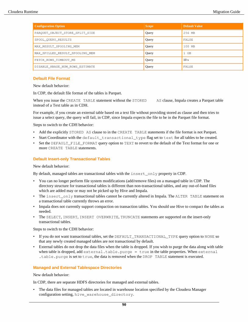
Cloudera Runtime Migration Guide
Configuration Option Scope Default Value
PARQUET_OBJECT_STORE_SPLIT_SIZE Query 256 MB
SPOOL_QUERY_RESULTS Query FALSE
MAX_RESULT_SPOOLING_MEM Query 100 MB
MAX_SPILLED_RESULT_SPOOLING_MEM Query 1 GB
FETCH_ROWS_TIMEOUT_MS Query 10 s
DISABLE_HBASE_NUM_ROWS_ESTIMATE Query FALSE
Default File Format
New default behavior:
In CDP, the default file format of the tables is Parquet.
When you issue the CREATE TABLE statement without the STORED AS clause, Impala creates a Parquet tableinstead of a Text table as in CDH.
For example, if you create an external table based on a text file without providing stored as clause and then tries toissue a select query, the query will fail, in CDP, since Impala expects the file to be in the Parquet file format.
Steps to switch to the CDH behavior:
• Add the explicitly STORED AS clause to in the CREATE TABLE statements if the file format is not Parquet.• Start Coordinator with the default_transactional_type flag set to text for all tables to be created.• Set the DEFAULT_FILE_FORMAT query option to TEXT to revert to the default of the Text format for one or
more CREATE TABLE statements.
Default Insert-only Transactional Tables
New default behavior:
By default, managed tables are transactional tables with the insert_only property in CDP.
• You can no longer perform file system modifications (add/remove files) on a managed table in CDP. Thedirectory structure for transactional tables is different than non-transactional tables, and any out-of-band fileswhich are added may or may not be picked up by Hive and Impala.
• The insert_only transactional tables cannot be currently altered in Impala. The ALTER TABLE statement ona transactional table currently throws an error.
• Impala does not currently support compaction on transaction tables. You should use Hive to compact the tables asneeded.
• The SELECT, INSERT, INSERT OVERWRITE, TRUNCATE statements are supported on the insert-onlytransactional tables.
Steps to switch to the CDH behavior:
• If you do not want transactional tables, set the DEFAULT_TRANSACTIONAL_TYPE query option to NONE sothat any newly created managed tables are not transactional by default.
• External tables do not drop the data files when the table is dropped. If you wish to purge the data along with tablewhen table is dropped, add external.table.purge = true in the table properties. When external.table.purge is set to true, the data is removed when the DROP TABLE statement is executed.
Managed and External Tablespace Directories
New default behavior:
In CDP, there are separate HDFS directories for managed and external tables.
• The data files for managed tables are located in warehouse location specified by the Cloudera Managerconfiguration setting, hive_warehouse_directory.
90
Cloudera Runtime Migration Guide
• The data files for external tables are located in warehouse location specified by the Cloudera Managerconfiguration setting, hive_warehouse_external_directory.
If you perform file system level operations for adding/removing files on the table, you need to consider if its anexternal table or managed table to find the location of the table directory.
Steps to switch to the CDH behavior:
Check the output of the DESCRIBE FORMATTED command to find the table location.
Hive Default File Format Interoperability
New default behavior:
The managed tables created by Hive are of ORC file format, by default, and support full transactional capabilities.If you create a table without specifying the STROED AS clause and load data from Hive, then such tables are notreadable or writable by Impala.
Steps to switch to the CDH behavior:
• You must use the STORED AS PARQUET clause when you create tables in Hive if you want interoperabilitywith Impala on those tables.
• If you want to change this default file format at the system level, in the Hive_on_Tez service configuration inCloudera Manager, set the hive_default_fileformat_managed field to parquet.
Statistics Interoperability Between Hive and Impala
New default behavior:
Statistics for tables are engine specific, namely, Hive or Impala, so that each engine could use its own statistics andnot overwrite the statistics generated by the other engine.
When you issue the COMPUTE STATS statement on Impala, you need to issue the corresponding statement on Hiveto ensure both Hive and Impala statistics are accurate.
Impala COMPUTE STATS command does not overwrite the Hive stats for the same table.
Steps to switch to the CDH behavior:
There is no workaround.
ORC Table Support Disabled
New default behavior:
ORC table support is disabled by default. The CDH queries against ORC tables will fail in CDP.
Steps to switch to the CDH behavior:
Set the query option ENABLE_ORC_SCANNER to TRUE to re-enable ORC table support.
Note that this option does not work on a full transactional ORC table, and the queries will still return an error.
Reconnect to HS2 Session
New default behavior:
Clients can disconnect from Impala while keeping the session running. Clients can reconnect to the same session bypresenting the session_token. By default, disconnected sessions are terminated after 15 min.
• Your end users will not notice a difference in behaviour.• If clients are disconnected without the driver explicitly closing the session (e.g. because of a network fault),
disconnected sessions and the queries associated with them may remain open and continue consuming resourcesuntil the disconnected session is timed out. Administrators may notice these disconnected sessions and/or theassociated resource consumption.
91
Cloudera Runtime Migration Guide
Steps to switch to the CDH behavior:
You can adjust the --disconnected_session_timeout flag to a lower value so that disconnected sessionsare cleaned up more quickly.
Automatic Row Count Estimation when Statistics Are Not Present
New default behavior:
If there are no statistics available on a table, Impala will try to estimate the cardinality by estimating the size of tablebased on the number of rows in the table. This behavior is turned on by default and should result in better plans formost cases when stats are not present.
For some edge cases, it is possible that Impala will generate a bad plan (when compared to the same query in CDH)when the statistics are not present on that table and could negatively affect the query performance.
Steps to switch to the CDH behavior:
Set the DISABLE_HDFS_NUM_ROWS_ESTIMATE query option to TRUE to disable this optimization.
Metadata V2
All catalog metadata improvements are enabled by default in CDP, resulting in many performance and scalabilityimprovements, such as reduced memory footprint on coordinators and automatic cache eviction.
See Impala Metadata Management for the details about catalog improvements.
Amazon EC2 Instances
Impala Data Hub clusters in CDP are created using the Data Mart cluster type. The recommended EC2 instance typefor Impala Data Mart Data Hub clusters is r5d.2xlarge. This instance type provides a good balance of memory vsCPU and also includes fast ephemeral SSD storage which is used by Impala data cache and spill.
When provisioning a Data Mart Data Hub cluster with the Cluster Definition option in the UI (or the --cluster-definition-name option in the CLI), the r5d.2xlarge instance type will be selected by default.
If you choose the Custom option to provision a cluster with the Data Mart blueprint, you should explicitly specify ther5d.2xlarge instance type since this isn’t the default type for Custom clusters.
Impala DWX clusters use the r5d.2xlarge instance type for executor instances and it’s not possible to override this.
Authorization Support by Ranger
In CDP, Ranger is the authorization provider for Impala.
New behavior:
• The CREATE ROLE, GRANT ROLE, SHOW ROLE statements are not supported as Ranger currently does notsupport roles.
• When a particular resource is renamed, currently, the policy is not automatically transferred to the newly renamedresource.
• SHOW GRANT with an invalid user/group does not return an error.
The following table lists the different access type requirements to run SQL statements in Hive and Impala.
SQL Statement Impala Access Requirement Hive Access Requirement
DESCRIBE view VIEW_METADATA on the underlying tables SELECT on the view
ALTER TABLE RENAME
ALTER VIEW RENAME
ALL on the target table / view
ALTER on the source table / view
ALTER on the source table / view
SHOW DATABASES
SHOW TABLES
VIEW_METADATA USE
92
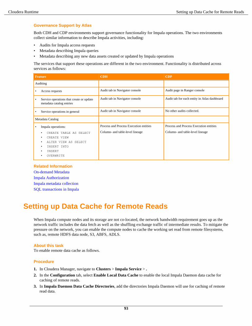
Cloudera Runtime Setting up Data Cache for Remote Reads
Governance Support by Atlas
Both CDH and CDP environments support governance functionality for Impala operations. The two environmentscollect similar information to describe Impala activities, including:
• Audits for Impala access requests• Metadata describing Impala queries• Metadata describing any new data assets created or updated by Impala operations
The services that support these operations are different in the two environment. Functionality is distributed acrossservices as follows:
Feature CDH CDP
Auditing
• Access requests Audit tab in Navigator console Audit page in Ranger console
• Service operations that create or updatemetadata catalog entries
Audit tab in Navigator console Audit tab for each entity in Atlas dashboard
• Service operations in general Audit tab in Navigator console No other audits collected.
Metadata Catalog
• Impala operations:
• CREATE TABLE AS SELECT
• CREATE VIEW
• ALTER VIEW AS SELECT
• INSERT INTO
• INSERT
• OVERWRITE
Process and Process Execution entities
Column- and table-level lineage
Process and Process Execution entities
Column- and table-level lineage
Related InformationOn-demand Metadata
Impala Authorization
Impala metadata collection
SQL transactions in Impala
Setting up Data Cache for Remote Reads
When Impala compute nodes and its storage are not co-located, the network bandwidth requirement goes up as thenetwork traffic includes the data fetch as well as the shuffling exchange traffic of intermediate results. To mitigate thepressure on the network, you can enable the compute nodes to cache the working set read from remote filesystems,such as, remote HDFS data node, S3, ABFS, ADLS.
About this taskTo enable remote data cache as follows.
Procedure
1. In Cloudera Manager, navigate to Clusters > Impala Service > .
2. In the Configuration tab, select Enable Local Data Cache to enable the local Impala Daemon data cache forcaching of remote reads.
3. In Impala Daemon Data Cache Directories, add the directories Impala Daemon will use for caching of remoteread data.
93

Cloudera Runtime Managing Metadata in Impala
4. In Impala Daemon Data Cache Per Directory Capacity, specify the maximum amount of local disk spaceImpala will use per daemon in each of the configured directrories for caching of remote read data.
5. Click Save Changes and restart the Impala service.
Managing Metadata in Impala
This section describes various knobs you can use to control how Impala manages its metadata in order to improveperformance and scalability.
On-demand Metadata
With the on-demand metadata feature, the Impala coordinators pull metadata as needed from catalogd and cache itlocally. The cached metadata gets evicted automatically under memory pressure.
The granularity of on-demand metadata fetches is at the partition level between the coordinator and catalogd.Common use cases like add/drop partitions do not trigger unnecessary serialization/deserialization of large metadata.
The feature can be used in either of the following modes.Metadata on-demand mode
In this mode, all coordinators use the metadata on-demand.
Set the following on catalogd:
--catalog_topic_mode=minimal
Set the following on all impalad coordinators:
--use_local_catalog=true
Mixed mode
In this mode, only some coordinators are enabled to use the metadata on-demand.
We recommend that you use the mixed mode only for testing local catalog’s impact on heap usage.
Set the following on catalogd:
--catalog_topic_mode=mixed
Set the following on impalad coordinators with metdadata on-demand:
--use_local_catalog=true
Limitation:
HDFS caching is not supported in On-demand metadata mode coordinators.
Note:
In Impala 3.4.0 and above, global INVALIDATE METADATA statement is supported when On-demandfeature is enabled.
INVALIDATE METADATA Usage Notes:
To return accurate query results, Impala needs to keep the metadata current for the databases and tables queried.Through "automatic invalidation" or "HMS event polling" support, Impala automatically picks up most changes inmetadata from the underlying systems. However there are some scenarios where you might need to run INVALIDATE METADATA or REFRESH.
94

Cloudera Runtime SQL transactions in Impala
• if some other entity modifies information used by Impala in the metastore, the information cached by Impala mustbe updated via INVALIDATE METADATA or REFRESH,
• if you have "local catalog" enabled without "HMS event polling" and need to pick up metadata changes that weredone outside of Impala in Hive and other Hive client, such as SparkSQL,
• and so on.
• Note: As this is a very expensive operation compared to the incremental metadata update done by theREFRESH statement, when possible, prefer REFRESH rather than INVALIDATE METADATA.
SQL transactions in Impala
A transaction is a single logical operation on the data. Impala supports transactions that satisfy a level of consistencythat improves the integrity and reliability of the data before and after a transaction.
Specifically, Impala provides atomicity and isolation of insert operations on transactional tables. A single table insertis either committed in full or not committed, and the results of the insert operation are not visible to other queryoperations until the operation is committed.
For single table, the inserts are ordered, so if Impala doesn't see a committed insert, it won't see any insert committedafter it.
For insert-only transactional tables, you can perform the following statements: CREATE TABLE, DROP TABLE,TRUNCATE, INSERT, SELECT
All transactions in Impala automatically commit at the end of the statement. Currently, Impala does not support multi-statement transactions.
Insert-only tables must be the managed and file-format based tables, such as Parquet, Avro, and text.
Note: Impala does not support changing transactional properties of tables. For example, you cannot alter atransactional table to a non-transactional table.
95