1

Analyzing the Structure and Evolution of MassiveTelecom Graphs

Amit A. Nanavati, Rahul Singh, Dipanjan Chakraborty, Koustuv Dasgupta (Member, IEEE), Sougata Mukherjea,Gautam Das, Siva Gurumurthy, Anupam Joshi (Senior Member, IEEE)

Abstract— With ever growing competition in telecommunica-tions markets, operators have to increasingly rely on businessintelligence to offer the right incentives to their customers.Existing approaches for telecom business intelligence have almostsolely focused on the individual behavior of customers. In thispaper, we use the Call Detail Records of a mobile operator toconstruct Call graphs, that is, graphs induced by people callingeach other. We determine the structural properties of thesegraphs and also introduce theTreasure-Huntmodel to describethe shape of mobile call graphs. We also determine how thestructure of these call graphs evolve over time. Finally, sinceShort Messaging Service (SMS) is becoming a preferred modeof communication among many sections of the society we alsostudy the properties of the SMS graph. Our analysis indicatesseveral interesting similarities as well as differences between theSMS graph and the corresponding call graph. We believe thatour analysis techniques can allow telecom operators to betterunderstand the social behavior of their customers, and potentiallyprovide major insights for designing effective incentives.

Index Terms— Telecom Call Data Records, Graph Algorithms,Social Network Analysis

I. INTRODUCTION

As Mobile Telecom penetration is increasing, and even ap-proaching saturation in many geographies, the focus is shiftingfrom customer acquisition to customer retention. It has been esti-mated that it is much cheaper to retain an existing customer thanto acquire a new one [3], [13]. To maintain profitability, telecomservice providers must controlchurn, the loss of subscribers whoswitch from one carrier to another. However, as the telecommuni-cations markets grow more and more competitive, it is very easyfor a consumer to churn because of low barriers to switchingproviders. In order to retain customers, the operators have tooffer the right incentives, adopt the right marketing strategies,and place their network assets appropriately. To succeed in thisgoal, optimizing marketing expenditure and improved targetingare critical requirements.

Retrieving information from call graphs (where people are thenodes and calls are the edges) obtained from the Call DetailRecords (CDRs) can provide major business insights to MobileTelecom operators for designing effective strategies. A CDRcontains various details pertaining to each call: who called whom,when was it made, how long it lasted, etc. Graph theoreticinformation from call graphs can allow service providers tobetter understand the underlying behavior of users, in a local aswell as global context, in order to design incentives to increasesubscriber loyalty and prevent/reduce churn. For example, if thecall graph is disconnected into many small components thenblanket advertising may be more appropriate asword-of-mouthspreading is impossible. Similarly, the presence of cliques orbipartite cores, which implies the presence of communities, canbe utilized to improve group targeting and retention.

In this paper we present an analysis of the CDRs of one ofthe largest Telecom operators in the world. Previously, a fewexperiments on call graphs of stationary telephone networks hadbeen undertaken to determine parameters like cliques [1] anddegree distributions [2]. However, to the best of our knowledge,this is the first study that attempts to discover and characterizea broad set of structural properties of mobile call graphs. Inparticular, we report findings on various topological properties ofthese massive call graphs, including degree distributions, stronglyconnected components, and cliques. The presence of power lawdistributions is ubiquitous in many parameters of the call graph,a typical signature of its scale-free structure. Further, we observeinteresting similarities and differences with respect to commonlystudied networks like the WWW graph [21].

One of our primary motivations has been to characterize theshape of call graphs imposed by cellular phone users. For this,we utilize the technique that has been used to arrive at the Bow-Tie model for WWW graphs [6] and then conduct additionalexperiments using novel techniques in order to reveal the finerstructure of the graphs. An interesting revelation is that, whereasmost existing graphs (hence their models) are based on the nodedistributions in the components of the graph, our call graphs arebetter characterised by theedgedistributions among the variouscomponents. We introduce theTreasure-Huntmodel, an edgedistribution based model, to characterise our mobile call graphs.The techniques proposed herein are general enough to be appliedto the analysis of any network, and may be particularly relevantfor social networks.

Although several studies on the structure and properties ofdifferent types of networks have been reported in the literaturemost of them are restricted to the analysis of a static snapshotof the network. A temporal analysis of a network to determinehow it evolves over time can be very insightful. Such a studyis difficult for most real-world networks since it is difficult toobtain information about the arrival of each node and edge intothe network. However since the CDRs record the time for allcalls, temporal analysis of the Telecom Call graphs is feasible.In this paper we take snapshots of the call graphs at differenttime segments and analyze how the various parameters of thecall graphs change over time.

In several geographies and among many segments of customers,Short Messaging Services (SMS) has become very popular and isa preferred medium of communication. The Call Detail Recordsmaintain the details of all the SMSes and it is possible to createthe SMS graph from the CDRs. In this paper we also analyze thisgraph and try to determine its correlation with the Call graph. Ouranalysis seems to indicate that the SMS graph is moresocial thanthe Call graph. As far as we know this is the first study that triesto determine the characteristics of the SMS graph. We believethat insights from the analysis can enable the Telecom operators

2

understand an important segment of its customers who utilizeSMS as a communication medium.

In summary, the contributions of this paper are as follows:• We study a broad set of parameters that reveal various

structural properties of mobile call graphs.• We describe novel techniques to determine the shape of large

graphs• We introduce theTreasure-Huntmodel, an edge distribution

based model, possibly the first topological model for mobilecall graphs.

• We present a temporal analysis of mobile call graphs tounderstand how the various parameters of the graph evolveover time.

• We extend our analysis to SMS graphs and try to correlatethe properties between SMS and Call graphs.

• We make a conscious effort to emphasize the practicalimplications of our findings in a way that can providebusiness insights and design strategies for mobile Telecomoperators.

The rest of the paper is organized as follows. The next sectioncites related work. In Section III, we describe our data sets andthe techniques for sampling data sources and creation of thecall graphs. Various characteristics providing critical insights inthe call graphs are presented in Section IV. We then introducea framework to get the finer level details of the topology inSection V. In Section VI we present a temporal analysis of thecall graphs and Section VII extends the analysis to SMS graphs.Finally, we conclude the paper with Section VIII.

II. BACKGROUND AND RELATED WORK

Massive graphs originating from different sources like WWW,Internet topology, Email graphs and Biological networks havedrawn the attention of a plethora of researchers [21], [12], [7].These graphs pose interesting challenges in terms of scalability,choice of parameters used to characterize them, and finally thetechniques used for interpreting the graph structure. Even thoughmany theoretical studies are available which characterize thegraphs based on various parameters like size, density, degreedistribution, clustering coefficient and connected components,practical interpretation and utilization of those parameters (andresults) are still lacking.

In the recent times, there is a lot of interest in studying World-wide Web and Internet graphs. [14] showed that the degreedistribution of the internet follow a Power law. Both [4] and [18]suggest that thein andout degrees of vertices on the Web graphalso exhibit power laws. Moreover, [4] has shown that most pairsof pages on the Web are separated by a handful of links, almostalways under 20. This is viewed by some as a “small world”phenomenon. On-line friendship networks also exhibit the small-world phenomenon [20]. Our analysis reveals evidence of smallworld phenomenon in mobile graphs also.

Determining groups of related pages in such networks isanother interesting problem. For example, [18] showed thatbipartite cores in the Web graph represent implicitly definedcommunities. A related area of research is the determination ofthe importance of pages (nodes) in the Web graph. The mostwell-known technique isPage Rank[5] which has been used veryeffectively to rank the results in Google search engine. Anothertechnique of finding the important pages in a WWW collectionhas been developed by [15] who defined two types of scores for

Web pages which pertain to a certain topic:authority and hubscores. We also try to identify communities and important mobilenumbers from the Telecom graphs.

Yet another body of work has been undertaken to determinetopological model of the WWW graph. [6] showed that the Webhas aBow-Tiestructure. This work outlines a general model butdoes not expose further details of the component structures. TheDaisy model [11] is an attempt to further refine the WWW bow-tie model. Researchers have also tried to determine models for theInternet topology. The Jellyfish model [24] was one of the firstin this direction. The Medusa model [8] is yet another model forthe Internet topology which was derived using a technique calledk-core decomposition. In this paper we introduce a model forTelecom graphs.

Although real-world graphs are evolving over time most ofthe analysis reported in the literature have been done on staticgraphs. Recently, structural properties of different snapshots of theWWW graph has been reported in [22]. [19] showed that Citationgraphs exhibit densification and shrinking diameters over time andpresented a generative model called theForest Fire modelforcapturing this phenomenon. On the other hand, the emergence ofbursty communities in the blogspace was identified in [16]. Thestructure and evolution of two Online Social Network maintainedby Yahoo has been reported in [17].

One of the first studies on call graph was performed on a graphof landline phones made on1-day consisting of approximately 53million nodes and 170 million edges [1]. The graph was foundto be disconnected with 3.7 million separate components, mostof them being pairs of telephones that called only each other. Agiant component consisting of80% of the total nodes was found.The diameter of this giant component was20. [2] experimentedwith the call graph of long-distance telephone traffic. The actualcall graph showed that the degree sequence was not quite aperfect power law, and the authors introduced a unique class ofrandom graphs with a power law degree sequence, calledα-βgraphs to capture the distribution. In this paper we present deeperinsights on the characteristics of Telecom call and SMS graphsto compliment the earlier studies.

In terms of business strategy design for telecommunicationindustry, many existing techniques exist based on mining of userprofiles [13] as well as application of machine learning methods[3]. Most of these rely on the individual calling patterns ofbehaviors. We believe that structural findings from call graphs canaugment and strengthen business intelligence directed towards thecritical problems of customer targeting, campaign managementand churn prevention.

III. D ATA SOURCES ANDPREPROCESSING

A Call Detail Record (CDR) contains all the details pertainingto a call such as the time, duration, origin, destination, etc. ofthe call. The CDRs are collected at Base stations and generallystored in a Data Warehouse. In this paper we analyze the CDRs ofone of the largest mobile operator in India. Not surprisingly, fora large country like India with a significant mobile penetration,more than a billion calls are made every month, and the datastorage runs into terabytes.

A call graphG is a pair〈V (G), E(G))〉, whereV (G) is a non-empty finite set of vertices (mobile users), andE(G) is a finite setof vertex-pairs fromV (G) (mobile calls). Ifu andv are vertices

3

1

10

100

1000

10000

100000

1e+06

1 10 100 1000

No. of nodes

Indegree of nodes

�

- Region ��Region

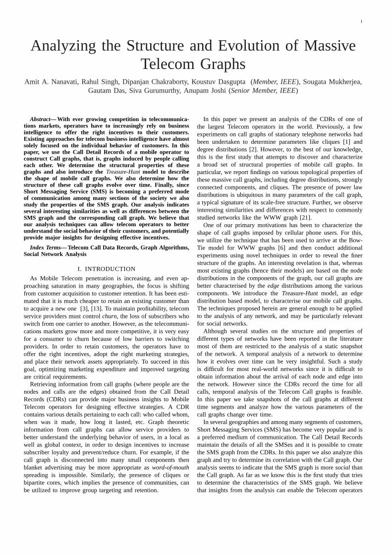
Fig. 1. In-degree distribution for regionsB andC (γin is 2.85924 and2.89961)

1

10

100

1000

10000

100000

1e+06

1 10 100 1000 10000 100000 1e+06

No. o

f n

od

es

Outdegree of nodes

�

- Region � - Region

Fig. 2. Out-degree distribution for regionsB andC (γout is 1.71374 and1.70808)

TABLE I

DETAILS OF DATA SET USED

Region Nodes Edges Period Avg. Deg. Type

A-Region 224418 1816285 1 month 16.19 DirectedB-Region 1250656 4514528 1 week 7.22 DirectedC-Region 989573 4313797 1 week 8.72 DirectedD-Region 407332 1456645 1 month 7.15 Directed

of G, then an edge〈u, v〉 is said to exist ifu callsv. Such a graphcan be easily constructed from the CDRs.

To get the actual graph, we had to query the Data warehouseand extract the best sample that would reflect the global callingpattern. The data set has the following characteristics:

• This study was done for a single mobile operator in India.• The mobile operator has broken the country into several

region-wise circles. For our study, we analyzed the callingpatterns of four circles; two of these circles were largemetropolitan cities and two were states with a mixture ofrural and urban population. These regions are in differentareas of India and are also culturally diverse with differentlocal languages.

• The study was done for intra-region calls, and does notinclude long distance or international calls.

• For two of the regions, we collected all the calls made ina week, and for the other two, we collected all the callsmade in a month. Interestingly, despite the durational andgeographical differences, many parameters for these fourregions are consistent with each other.

• Further, very short duration calls (less than 10 seconds) havebeen ignored as missed calls and wrong calls since they mayyield incorrect results. (However in many countries some ofthese missed calls may be used to convey pre-determinedmessages and are therefore socially relevant).

• Multiple calls between any two user or nodes is treated asa single edge. The resulting graph isdirected simple graphwith no self-loops or multiple edges.

Table I shows the details of the data set used in this paper.While two call graphs have been generated for the span of1

month (A andD), the two are generated from call details recordsof 1 week (B and C). Some basic graph properties such as thenumber of nodesn (also referred to asgraph size) and thenumberof links m are reported. TheAverage node degreeis definedas k̄ = 2m/n.

IV. STRUCTURAL PROPERTIES OF CALL GRAPHS

In this section we analyse the structural properties of callgraphs. Our analysis is based on a set of graph metrics that havebeen traditionally used to characterise large networks. In manycases, we use existing tools [10], [9], [23] for computing theseparameters.

A. Degree Distributions

Distributions of degree gives information which average degreecannot, i.e. the number of nodesn(d) of each degreed in thegraph. We define this property asnode degree distribution( P (d) = n(d)/n). The degree distributionP (d) for directednetworks splits in two separate functions, the in-degree distri-butionP (din) and the out-degree distributionP (dout), which aremeasured separately as the probabilities of havingdin incominglinks anddout outgoing links, respectively.

In Figure 1 and Figure 2, we report the behavior of the in-degree and out-degree distributions in log-log scale. We provideddegree distribution results for regionsB and C only becausethey are the largest ones and other two regionsA andD wereshowing similar results. Observing both in-degree and out-degreedistributions, the call graph topology is found to be characterizedby presence of a highly heterogeneous topology, with degreedistributions characterized by wide variability and heavy tails.Observing log-log plots, we can see that degree distributions fitwell to power law distributions.

The in-degree distribution exhibits a heavy-tailed form approxi-mated by a power-law behaviorP (din) ∼ d−γin

in , and the value ofthe exponent ofγ is between 2 and 3, very much like the WWWgraph [6]. However, in the case of the out-degree distribution, theexponent is less than 2, very much unlike both the WWW as wellas the Email graph.The parameters of the four regions are ratherclose despite their geographic, cultural, and duration (1 week fortwo regions vs. 1 month for the other two) differences. The degreedistributions imply that there are very few nodes that have veryhigh in-degree or out-degree and therefore may be suitable forindividual targeting by a telecom service provider.

B. Neighbourhood Distribution

The neighbourhood function,N(h) for a graph also called hop-plot [14], is the number of pairs of nodes within a specified dis-tance, for all distancesh. The individual neighbourhood functionfor u at h is the number of nodes at distanceh or less fromu. Itcan be computed as

4

1e+06

1e+07

1e+08

1e+09

1e+10

1e+11

1e+12

1 10

Pa

irs o

f n

od

es w

ith

in o

r e

qu

al to

�

Number of hops �

�-Region�-Region�-Region�-Region

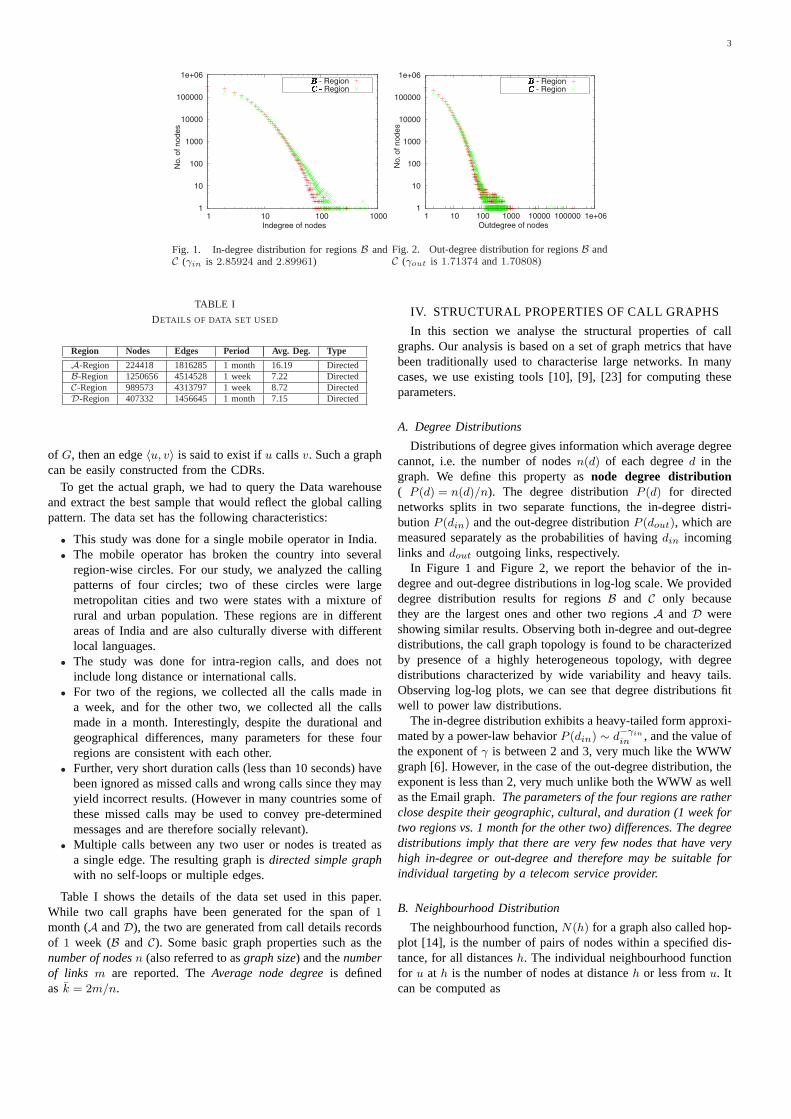
Fig. 3. Neighbourhood function distributions for all regions

TABLE II

HOP EXPONENT AND EFFECTIVE DIAMETER VALUES(C IS THE CONSTANT

FOR THE LINEAR EQUATION FIT IN LOG-LOG SCALE FOR THE EQUATION

N(h) ∝ hH)

Region H C δeffA 4.53 14 8.10177B 4.53 14 13.9314C 5.52 14 8.07642D 4.94 13 8.93613

follows:

IN(u, h) = |{v : v ∈ V, dist(u, v) 6 h}|.

The neighbourhood functionN(h) is the number of pairs of nodeswithin distanceh, and is defined:N(h) =

Pu∈V IN(u, h). The

neighbourhood function provides us ways to compare call graphsin terms of hop-exponent, distance distribution, and effectivediameter.

We calculated the neighbourhood function for call graphs usingthe ANF tool [23]. The plot of the neighbourhood function for allhop for all the regions are shown in the Figure 3. Also,N(h) ∝hH, whereH is thehop exponent.

There are three interesting observations about the hop exponentthat make it an appealing metric. First, if the power-law holds,the neighbourhood function will have a linear section with slopeH when viewed in log-log scale. Second, the hop exponent is,informally, the intrinsic dimensionality of the graph. For example,a cycle has a hop exponent of1 while a grid has a hop exponentof 2. Third, if two graphs have different hop exponents, there isno way that they could be structurally similar [23].

We computed thehop-exponentusing linear fit on the neigh-bourhood function distribution shown in Figure 3. The hopexponents of the 4 regions are reported in the Table II. Weconsistently found hop exponent close to4 and5 in the Telecomgraphs. The only other real-world graphs whose hop exponents weknow are Int-11-97, Int-04-98, Int-12-98 and Rout-95 with hopexponents 4.62, 4.71, 4.86, 2.83 respectively [14].This suggeststhat our mobile telecom graphs are structurally asdenseasthose of the Internet graphs. Interestingly, even though the graphof regionsA and B differ considerably in parameters such asaverage degree, number of nodes and edges(Table I), their hopexponents are similar ( 3).

Effective diameter gives us another parameter for effectivemeasurement of the compactness of the network. For a call graphof N nodes withE edges, we can compute effective diameter

based upon the equation [14]:

δeff =

�N2

N + 2E

�1/H

The effective diameter of a network isδeff if any two nodesare within δeff hops from each otherwith a high probability.The effective diameter for all the four regions are given in theTable II; the maximum value is13. This provides evidence ofsmall-world phenomenon in mobile call graphs since most pairsof nodes (phone numbers) are separated by a handful of edges(calls). We believe that this phenomenon can be further exploitedto identify (social) communities.

0

100000

200000

300000

400000

500000

600000

3 4 5 6 7 8 9 10 11 12 13 14 15 16 17 18 19 20

Num

ber

of N

odes

Clique Size

A-RegionB-RegionC-RegionD-Region

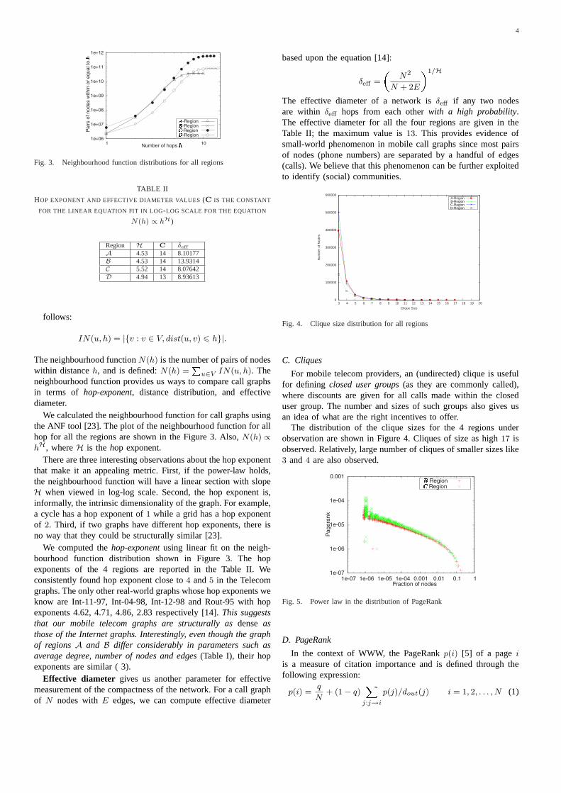
Fig. 4. Clique size distribution for all regions

C. Cliques

For mobile telecom providers, an (undirected) clique is usefulfor defining closed user groups(as they are commonly called),where discounts are given for all calls made within the closeduser group. The number and sizes of such groups also gives usan idea of what are the right incentives to offer.

The distribution of the clique sizes for the 4 regions underobservation are shown in Figure 4. Cliques of size as high17 isobserved. Relatively, large number of cliques of smaller sizes like3 and4 are also observed.

1e-07

1e-06

1e-05

1e-04

0.001

1e-07 1e-06 1e-05 1e-04 0.001 0.01 0.1 1

Pa

ge

ran

k

Fraction of nodes

� Region� Region

Fig. 5. Power law in the distribution of PageRank

D. PageRank

In the context of WWW, the PageRankp(i) [5] of a pagei

is a measure of citation importance and is defined through thefollowing expression:

p(i) =q

N+ (1− q)

Xj:j→i

p(j)/dout(j) i = 1, 2, . . . , N (1)

5

1

10

100

1000

10000

100000

1e+06

1 10 100 1000 10000 100000 1e+06

Nu

mb

er

of

SC

C

Size of SCC

�-Region �-Region �-Region �-Region

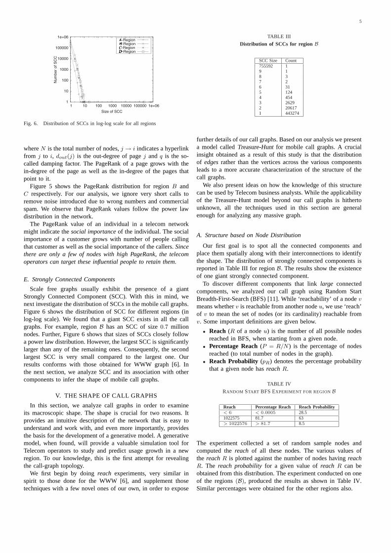
Fig. 6. Distribution of SCCs in log-log scale for all regions

whereN is the total number of nodes,j → i indicates a hyperlinkfrom j to i, dout(j) is the out-degree of pagej and q is the so-called damping factor. The PageRank of a page grows with thein-degree of the page as well as the in-degree of the pages thatpoint to it.

Figure 5 shows the PageRank distribution for regionB andC respectively. For our analysis, we ignore very short calls toremove noise introduced due to wrong numbers and commercialspam. We observe that PageRank values follow the power lawdistribution in the network.

The PageRank value of an individual in a telecom networkmight indicate thesocial importanceof the individual. The socialimportance of a customer grows with number of people callingthat customer as well as the social importance of the callers.Sincethere are only a few of nodes with high PageRank, the telecomoperators can target these influential people to retain them.

E. Strongly Connected Components

Scale free graphs usually exhibit the presence of a giantStrongly Connected Component (SCC). With this in mind, wenext investigate the distribution of SCCs in the mobile call graphs.Figure 6 shows the distribution of SCC for different regions (inlog-log scale). We found that a giant SCC exists in all the callgraphs. For example, regionB has an SCC of size0.7 millionnodes. Further, Figure 6 shows that sizes of SCCs closely followa power law distribution. However, the largest SCC is significantlylarger than any of the remaining ones. Consequently, the secondlargest SCC is very small compared to the largest one. Ourresults conforms with those obtained for WWW graph [6]. Inthe next section, we analyze SCC and its association with othercomponents to infer the shape of mobile call graphs.

V. THE SHAPE OF CALL GRAPHS

In this section, we analyze call graphs in order to examineits macroscopic shape. The shape is crucial for two reasons. Itprovides an intuitive description of the network that is easy tounderstand and work with, and even more importantly, providesthe basis for the development of a generative model. A generativemodel, when found, will provide a valuable simulation tool forTelecom operators to study and predict usage growth in a newregion. To our knowledge, this is the first attempt for revealingthe call-graph topology.

We first begin by doingreach experiments, very similar inspirit to those done for the WWW [6], and supplement thosetechniques with a few novel ones of our own, in order to expose

TABLE III

Distribution of SCCs for region B

SCC Size Count755592 19 18 37 26 315 1244 4543 26292 206171 443274

further details of our call graphs. Based on our analysis we presenta model calledTreasure-Huntfor mobile call graphs. A crucialinsight obtained as a result of this study is that the distributionof edgesrather than the vertices across the various componentsleads to a more accurate characterization of the structure of thecall graphs.

We also present ideas on how the knowledge of this structurecan be used by Telecom business analysts. While the applicabilityof the Treasure-Hunt model beyond our call graphs is hithertounknown, all the techniques used in this section are generalenough for analyzing any massive graph.

A. Structure based on Node Distribution

Our first goal is to spot all the connected components andplace them spatially along with their interconnections to identifythe shape. The distribution of strongly connected components isreported in Table III for regionB. The results show the existenceof one giant strongly connected component.

To discover different components that linklarge connectedcomponents, we analyzed our call graph using Random StartBreadth-First-Search (BFS) [11]. While ‘reachability’ of a nodev

means whetherv is reachable from another nodeu, we use ‘reach’of v to mean the set of nodes (or its cardinality) reachable fromv. Some important definitions are given below.

• Reach (R of a nodeu) is the number of all possible nodesreached in BFS, when starting from a given node.

• Percentage Reach(P = R/N ) is the percentage of nodesreached (to total number of nodes in the graph).

• Reach Probability (pR) denotes the percentage probabilitythat a given node hasreachR.

TABLE IV

RANDOM START BFS EXPERIMENT FOR REGIONB

Reach Percentage Reach Reach Probability< 6 < 0.0005 28.51022575 81.7 63> 1022576 > 81.7 8.5

The experiment collected a set of random sample nodes andcomputed thereach of all these nodes. The various values ofthe reachR is plotted against the number of nodes havingreachR. The reach probability for a given value ofreach R can beobtained from this distribution. The experiment conducted on oneof the regions(B), produced the results as shown in Table IV.Similar percentages were obtained for the other regions also.

6

IN OUTSCC

Tendrils

Tubes

Disconnected Components

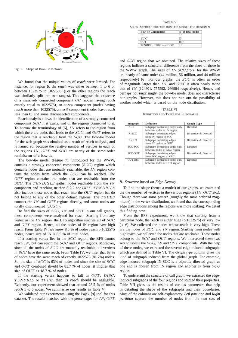
Fig. 7. Shape of Bow-Tie Network

We found that the unique values ofreach were limited. Forinstance, for regionB, the reach was either between 1 to 6 orbetween 1022575 to 1022586. (For the other regions the reachwas similarly split into two ranges). This suggests the existenceof a massively connected componentCC (nodes havingreachexactly equal to 1022575), anentry component (nodes havingreachmore than 1022575), anexit component (nodes havereachless than 6) and some disconnected components.

Reach analysis allows the identification of a strongly connectedcomponentSCC if it exists, and of the regions connected to it.To borrow the terminology of [6],IN refers to the region fromwhich there are paths that leads to theSCC, andOUT refers tothe region that is reachable from theSCC. The Bow-tie modelfor the web graph was obtained as a result of reach analysis, andis named so, because the relative number of vertices in each ofthe regionsIN , OUT and SCC are nearly of the same orderreminiscent of a bow-tie.

The bow-tie model (Figure 7), introduced for the WWW,contains a strongly connected component(SCC) region whichcontains nodes that are mutually reachable, theIN region con-tains the nodes from which theSCC can be reached. TheOUT region contains the nodes that are reachable from theSCC. The TENDRILS gather nodes reachable from theIN

component and reaching neitherSCC nor OUT . TENDRILS

also include those nodes that reach into theOUT region but donot belong to any of the other defined regions. TheTUBES

connect theIN and OUT regions directly, and some nodes aretotally disconnected(DISC).

To find the sizes ofSCC, IN and OUT in our call graphs,these components were analyzed for reach. Starting from anyvertex in theIN region, the BFS algorithm reaches all ofSCC

and OUT region. Hence, all the nodes of IN region have highreach. From Table IV, we know 8.5 % of nodes reach>1022575nodes, hence size of IN is 8.5 % of total nodes.

If a starting vertex lies in theSCC region, the BFS cannotreachIN , but can reach theSCC andOUT regions. Moreover,since all the nodes ofSCC are mutually reachable, all verticesin SCC have the same reach. From Table IV, we infer that 63 %of nodes have the same reach of exactly 1022575 (81.7%) nodes.So, the size ofSCC is 63% of nodes and since the size ofSCC

and OUT combined should be 81.7 % of nodes, it implies thatsize ofOUT as 18.7 % of nodes.

If the starting vertex happens to fall inOUT , DISC,TENDRIL or TUBE, then its reach should be negligible.Evidently, our experiment showed that around 28.5 % of nodesreach1 to 6 nodes. We summarize our results in Table V.

We validated our experiments using the Pajek [9] tool for thisdata set. The results matched with the percentages forIN , OUT

TABLE V

SIZES INFERRED FOR THEBOW-TIE MODEL FOR REGIONBBow-tie Component % of total nodesIN 8.5SCC 63OUT 18.7TENDRIL, TUBE and DISC 9.8

and SCC region that we obtained. The relative sizes of theseregions indicate a structural difference from the sizes of those inthe WWW graph. The sizes ofIN ,SCC,OUT for the WWWare nearly of same order (44 million, 56 million, and 44 millionrespectively) [6]. For our graphs, theSCC is often an orderof magnitude larger thanIN , and OUT is often nearly twicethat of IN (124801, 755592, 266984 respectively). Hence, andperhaps not surprisingly, the bow-tie model does not characteriseour graphs. However, this does not rule out the possibility ofanother model which is based on the node distribution.

TABLE VI

DEFINITION AND TYPES FORSUBGRAPHS

Subgraph Definition Graph TypeIN-IN Subgraph containing edges only Directed

between nodes of IN regionIN-SCC Subgraph consisting edges Bi-partitie & Directed

from IN region to SCCIN-OUT Subgraph consisting edges Bi-partitie & Directed

from IN region to OUTSCC-SCC Subgraph containing edges only Directed

between nodes of SCC regionSCC-OUT Subgraph consisting edges Bi-partitie & Directed

from SCC region to OUTOUT-OUT Subgraph containing edges only Directed

between nodes of OUT region

B. Structure based on Edge Density

To find the shape (hence a model) of our graphs, we examinedthe the number of vertices in the various regions (IN, OUT ,etc.).Though there was some pattern (roughly the same order of mag-nitude) in the vertex distribution, we found that the correspondingedge distributions among the regions was more striking. We detailthis finding now.

From the BFS experiment, we know that starting from aparticular node, the reach is either huge (>1022575) or very low(< 6). We collected the nodes whose reach is very high. Theseare the nodes ofSCC and IN region. Starting from nodes withhigh reach, we collected the nodes that are reachable. These nodesbelong to theSCC andOUT regions. We intersected these twosets to isolate theSCC, IN andOUT components. With the helpof these nodes, we extracted the several edge-induced subgraphswhich are defined in Table VI. TheGraph typecolumn gives thekind of subgraph induced from the global graph. For example,edge induced subgraph IN-SCC is a bipartite directed graph asone end is chosen from IN region and another is fromSCC

region.To understand the structure of call graph, we extracted the edge-

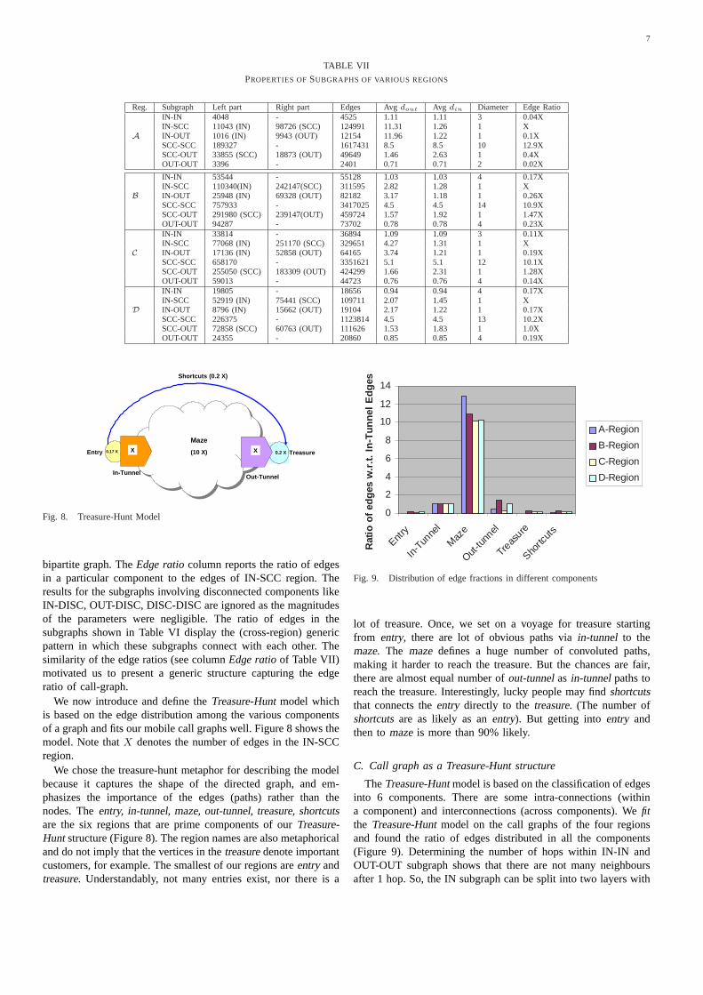
induced subgraphs of the four regions and studied their properties.Table VII gives us the results of various parameters that helpin detailing the shape of the subgraphs and their boundaries.Most of the columns are self-explanatory.Left partitionandRightpartition capture the number of nodes from the two sets of

7

TABLE VII

PROPERTIES OFSUBGRAPHS OF VARIOUS REGIONS

Reg. Subgraph Left part Right part Edges Avg dout Avg din Diameter Edge RatioIN-IN 4048 - 4525 1.11 1.11 3 0.04XIN-SCC 11043 (IN) 98726 (SCC) 124991 11.31 1.26 1 X

A IN-OUT 1016 (IN) 9943 (OUT) 12154 11.96 1.22 1 0.1XSCC-SCC 189327 - 1617431 8.5 8.5 10 12.9XSCC-OUT 33855 (SCC) 18873 (OUT) 49649 1.46 2.63 1 0.4XOUT-OUT 3396 - 2401 0.71 0.71 2 0.02X

IN-IN 53544 - 55128 1.03 1.03 4 0.17XIN-SCC 110340(IN) 242147(SCC) 311595 2.82 1.28 1 X

B IN-OUT 25948 (IN) 69328 (OUT) 82182 3.17 1.18 1 0.26XSCC-SCC 757933 - 3417025 4.5 4.5 14 10.9XSCC-OUT 291980 (SCC) 239147(OUT) 459724 1.57 1.92 1 1.47XOUT-OUT 94287 - 73702 0.78 0.78 4 0.23XIN-IN 33814 - 36894 1.09 1.09 3 0.11XIN-SCC 77068 (IN) 251170 (SCC) 329651 4.27 1.31 1 X

C IN-OUT 17136 (IN) 52858 (OUT) 64165 3.74 1.21 1 0.19XSCC-SCC 658170 - 3351621 5.1 5.1 12 10.1XSCC-OUT 255050 (SCC) 183309 (OUT) 424299 1.66 2.31 1 1.28XOUT-OUT 59013 - 44723 0.76 0.76 4 0.14XIN-IN 19805 - 18656 0.94 0.94 4 0.17XIN-SCC 52919 (IN) 75441 (SCC) 109711 2.07 1.45 1 X

D IN-OUT 8796 (IN) 15662 (OUT) 19104 2.17 1.22 1 0.17XSCC-SCC 226375 - 1123814 4.5 4.5 13 10.2XSCC-OUT 72858 (SCC) 60763 (OUT) 111626 1.53 1.83 1 1.0XOUT-OUT 24355 - 20860 0.85 0.85 4 0.19X

Shortcuts

Out-TunnelIn-Tunnel

Maze

Entry Treasure(10 X) X0.17 X 0.2 XX

(0.2 X)

Fig. 8. Treasure-Hunt Model

bipartite graph. TheEdge ratiocolumn reports the ratio of edgesin a particular component to the edges of IN-SCC region. Theresults for the subgraphs involving disconnected components likeIN-DISC, OUT-DISC, DISC-DISC are ignored as the magnitudesof the parameters were negligible. The ratio of edges in thesubgraphs shown in Table VI display the (cross-region) genericpattern in which these subgraphs connect with each other. Thesimilarity of the edge ratios (see columnEdge ratioof Table VII)motivated us to present a generic structure capturing the edgeratio of call-graph.

We now introduce and define theTreasure-Huntmodel whichis based on the edge distribution among the various componentsof a graph and fits our mobile call graphs well. Figure 8 shows themodel. Note thatX denotes the number of edges in the IN-SCCregion.

We chose the treasure-hunt metaphor for describing the modelbecause it captures the shape of the directed graph, and em-phasizes the importance of the edges (paths) rather than thenodes. Theentry, in-tunnel, maze, out-tunnel, treasure, shortcutsare the six regions that are prime components of ourTreasure-Hunt structure (Figure 8). The region names are also metaphoricaland do not imply that the vertices in thetreasuredenote importantcustomers, for example. The smallest of our regions areentryandtreasure. Understandably, not many entries exist, nor there is a

0

2

4

6

8

10

12

14

Entry

In-T

unne

l

Maz

e

Out-tu

nnel

Treas

ure

Shortc

uts

Rat

io o

f ed

ges

w.r

.t.

In-T

un

nel

Ed

ges

A-Region

B-Region

C-Region

D-Region

Fig. 9. Distribution of edge fractions in different components

lot of treasure. Once, we set on a voyage for treasure startingfrom entry, there are lot of obvious paths viain-tunnel to themaze. The maze defines a huge number of convoluted paths,making it harder to reach the treasure. But the chances are fair,there are almost equal number ofout-tunnelas in-tunnelpaths toreach the treasure. Interestingly, lucky people may findshortcutsthat connects theentry directly to thetreasure. (The number ofshortcutsare as likely as anentry). But getting intoentry andthen tomazeis more than 90% likely.

C. Call graph as a Treasure-Hunt structure

TheTreasure-Huntmodel is based on the classification of edgesinto 6 components. There are some intra-connections (withina component) and interconnections (across components). Wefitthe Treasure-Huntmodel on the call graphs of the four regionsand found the ratio of edges distributed in all the components(Figure 9). Determining the number of hops within IN-IN andOUT-OUT subgraph shows that there are not many neighboursafter 1 hop. So, the IN subgraph can be split into two layers with

8

one of them connectingSCC, and another which connects toitself. Thus, the nodes of IN region split into two layers asentryand in-tunnelregion inTreasure-Huntmodel. Similarly, the OUTregion is separated into theout-tunneland thetreasure.

To fit regionB to the Treasure-Huntmodel, the edge inducedsubgraphs IN-IN, IN-SCC, SCC-SCC, SCC-OUT, OUT-OUTand IN-OUT can be mapped toentry, in-tunnel, maze, out-tunnel,treasure, andshortcutsrespectively. Theedge ratiocolumnof Table VII gives the relative magnitude of the edges of eachcomponent with respect to thein-tunnel. The shape is conclusiveasentry is 0.16 timesin-tunnelandmazeis almost 10 times thein-tunnel. The out-tunnelis similar in size asin-tunnel, whereastreasureis relatively the smallest and almost in the same orderas entry. The shortcutsare paths that directly connectentry totreasure; they are also smaller in magnitude and of the same orderas theentry.

We tried to fit the other regions (A, C,D) (see other edgeratios in Table VII) and found that they fit theTreasure-Huntmodel quite closely. TheTreasure-Huntmodel brings to light thefact that often the edges rather than the nodes of graphs mightfollow a pattern, as our call graphs indicate.There are severalimplications of the results we obtain through path based modelof the call graph. It provides telecom operators with insights onhow a certain new serviceroll-out might be propagated in thenetwork. For example, the propagation chances would be higherif they target nodes with greater reach (belonging to theEntryand In-Tunnel regions). Similarly, customers can be segmentedbased on their placement in the structure.

VI. TEMPORAL ANALYSIS

In this section we discuss temporal analysis of the call graphs.We studied how some of the structural properties of these callgraphs vary with time. For regionsB and C for which we hadone week’s data we looked at the cumulative call data records ateach of the seven days. For regionsA andD for which we hadone month’s data we looked at seven time points at intervals offour days each. Note that the analysis was done using the CDRsfrom a period in which there was no celebrations or special eventsto ensure that the snapshot reflected the normal calling patternsof the customers.

A. Degree Distributions

The changes in the degree distribution of the graphs over timemay yield some insights into the evolution of call graphs. Forinstance, it might be interesting to find out how the number ofnodes with high in-degree and high out-degree changes with time.

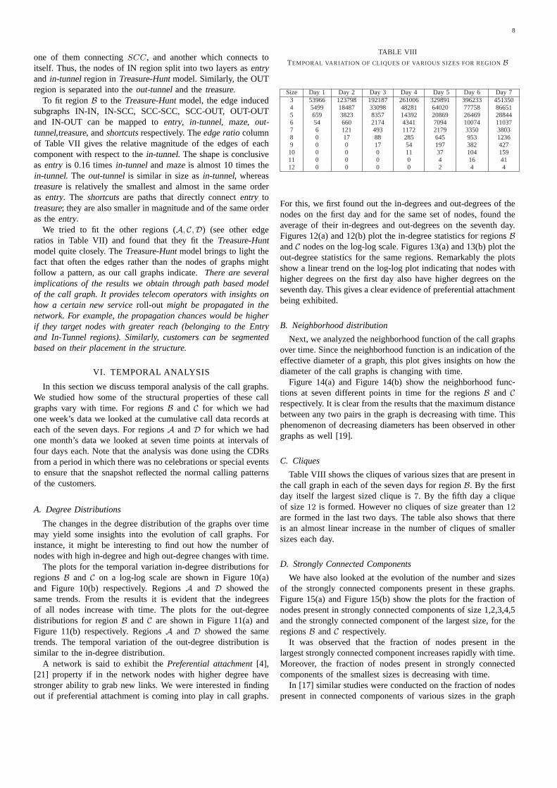
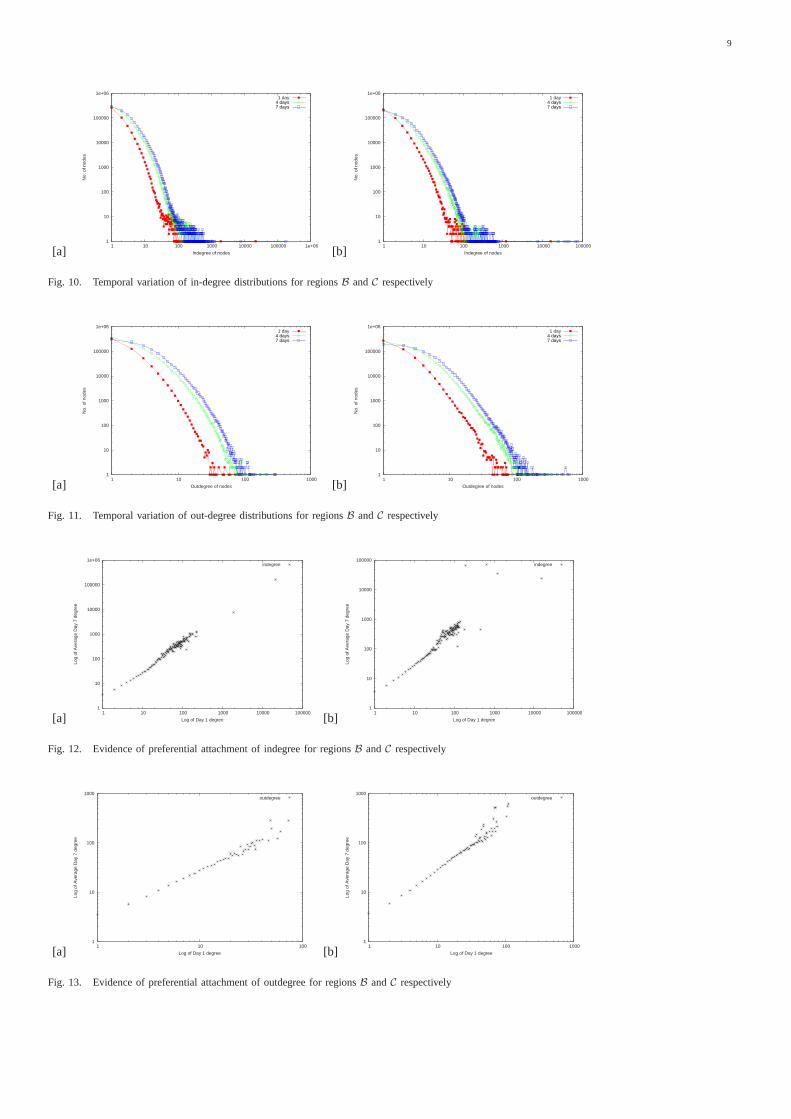
The plots for the temporal variation in-degree distributions forregionsB and C on a log-log scale are shown in Figure 10(a)and Figure 10(b) respectively. RegionsA and D showed thesame trends. From the results it is evident that the indegreesof all nodes increase with time. The plots for the out-degreedistributions for regionB and C are shown in Figure 11(a) andFigure 11(b) respectively. RegionsA and D showed the sametrends. The temporal variation of the out-degree distribution issimilar to the in-degree distribution.

A network is said to exhibit thePreferential attachment[4],[21] property if in the network nodes with higher degree havestronger ability to grab new links. We were interested in findingout if preferential attachment is coming into play in call graphs.

TABLE VIII

TEMPORAL VARIATION OF CLIQUES OF VARIOUS SIZES FOR REGIONB

Size Day 1 Day 2 Day 3 Day 4 Day 5 Day 6 Day 73 53966 123798 192187 261006 329891 396233 4513504 5499 18487 33098 48281 64020 77758 866515 659 3823 8357 14392 20869 26469 288446 54 660 2174 4341 7094 10074 110377 6 121 493 1172 2179 3350 38038 0 17 88 285 645 953 12369 0 0 17 54 197 382 42710 0 0 0 11 37 104 15911 0 0 0 0 4 16 4112 0 0 0 0 2 4 4

For this, we first found out the in-degrees and out-degrees of thenodes on the first day and for the same set of nodes, found theaverage of their in-degrees and out-degrees on the seventh day.Figures 12(a) and 12(b) plot the in-degree statistics for regionsBandC nodes on the log-log scale. Figures 13(a) and 13(b) plot theout-degree statistics for the same regions. Remarkably the plotsshow a linear trend on the log-log plot indicating that nodes withhigher degrees on the first day also have higher degrees on theseventh day. This gives a clear evidence of preferential attachmentbeing exhibited.

B. Neighborhood distribution

Next, we analyzed the neighborhood function of the call graphsover time. Since the neighborhood function is an indication of theeffective diameter of a graph, this plot gives insights on how thediameter of the call graphs is changing with time.

Figure 14(a) and Figure 14(b) show the neighborhood func-tions at seven different points in time for the regionsB and Crespectively. It is clear from the results that the maximum distancebetween any two pairs in the graph is decreasing with time. Thisphenomenon of decreasing diameters has been observed in othergraphs as well [19].

C. Cliques

Table VIII shows the cliques of various sizes that are present inthe call graph in each of the seven days for regionB. By the firstday itself the largest sized clique is7. By the fifth day a cliqueof size12 is formed. However no cliques of size greater than12

are formed in the last two days. The table also shows that thereis an almost linear increase in the number of cliques of smallersizes each day.

D. Strongly Connected Components

We have also looked at the evolution of the number and sizesof the strongly connected components present in these graphs.Figure 15(a) and Figure 15(b) show the plots for the fraction ofnodes present in strongly connected components of size 1,2,3,4,5and the strongly connected component of the largest size, for theregionsB andC respectively.

It was observed that the fraction of nodes present in thelargest strongly connected component increases rapidly with time.Moreover, the fraction of nodes present in strongly connectedcomponents of the smallest sizes is decreasing with time.

In [17] similar studies were conducted on the fraction of nodespresent in connected components of various sizes in the graph

9

[a] 1

10

100

1000

10000

100000

1e+06

1 10 100 1000 10000 100000 1e+06

No.

of n

odes

Indegree of nodes

1 day4 days7 days

[b] 1

10

100

1000

10000

100000

1e+06

1 10 100 1000 10000 100000

No.

of n

odes

Indegree of nodes

1 day4 days7 days

Fig. 10. Temporal variation of in-degree distributions for regionsB andC respectively

[a] 1

10

100

1000

10000

100000

1e+06

1 10 100 1000

No.

of n

odes

Outdegree of nodes

1 day4 days7 days

[b] 1

10

100

1000

10000

100000

1e+06

1 10 100 1000

No.

of n

odes

Outdegree of nodes

1 day4 days7 days

Fig. 11. Temporal variation of out-degree distributions for regionsB andC respectively

[a] 1

10

100

1000

10000

100000

1e+06

1 10 100 1000 10000 100000

Log

of A

vera

ge D

ay 7

deg

ree

Log of Day 1 degree

indegree

[b] 1

10

100

1000

10000

100000

1 10 100 1000 10000 100000

Log

of A

vera

ge D

ay 7

deg

ree

Log of Day 1 degree

indegree

Fig. 12. Evidence of preferential attachment of indegree for regionsB andC respectively

[a] 1

10

100

1000

1 10 100

Log

of A

vera

ge D

ay 7

deg

ree

Log of Day 1 degree

outdegree

[b] 1

10

100

1000

1 10 100 1000

Log

of A

vera

ge D

ay 7

deg

ree

Log of Day 1 degree

outdegree

Fig. 13. Evidence of preferential attachment of outdegree for regionsB andC respectively

10

[a] 1e+06

1e+07

1e+08

1e+09

1e+10

1e+11

1e+12

0 5 10 15 20 25

Log

of N

umbe

r of

Pai

rs w

ithin

that

dis

tanc

e

Distance between the pairs

1 day2 days3 days4 days5 days6 days7 days

[b] 1e+06

1e+07

1e+08

1e+09

1e+10

1e+11

1e+12

0 5 10 15 20 25

Log

of N

umbe

r of

Pai

rs w

ithin

that

dis

tanc

e

Distance between the pairs

1 day2 days3 days4 days5 days6 days7 days

Fig. 14. Temporal variation of neighborhood function distributions for regionsB andC respectively

[a] 1e-04

0.001

0.01

0.1

1

1 2 3 4 5 6 7

Log

of F

ract

ion

of N

odes

in C

ompo

nent

of t

his

size

Day t

1 sized component2 sized component3 sized component 4 sized component 5 sized component Largest Component

[b] 1e-04

0.001

0.01

0.1

1

1 2 3 4 5 6 7

Log

of F

ract

ion

of N

odes

in C

ompo

nent

of t

his

size

Day t

1 sized component2 sized component3 sized component 4 sized component 5 sized component Largest Component

Fig. 15. Temporal variation of the fraction of nodes in strongly connected components of various sizes for regionsB andC respectively

structure of social networking sites Flickr and Yahoo! 360. Ananalysis of these graphs revealed that the fraction of nodes in allcomponents was continuously increasing. However, call graphsseem to show a tendency of greater accumulation into a singlestrongly connected component over time by taking in nodes fromthe smaller components.

E. TheTreasure-Huntmodel

It would be interesting to determine how theTreasure-Huntmodel that we proposed earlier for call graphs evolves over time.Therefore we fitted theTreasure-Huntmodel on the graph as itstood at various points of time. Figure 16(a) and Figure 16(b)show the edges present in the various components of theTreasure-Hunt model at seven points of time for the regionsB and Crespectively. It is interesting to note the striking similarity in thetwo plots in spite of them belonging to different regions. Someof the trends that are evident from these plots are:

• The number of edges in the maze increase very rapidly. Thisobservation should be expected since we had earlier observedthat the percentage of nodes in the strongly connectedcomponent was increasing.

• The sizes of the in-tunnel and out-tunnel are also increasing.However the increase is not as rapid as in the case of themaze.

• The sizes of the treasure and entry components are decreas-ing. Hence the increase in maze is coming at the expense ofthe treasure and entry becoming smaller. The maze is gettingbulkier by sucking in edges from the side components i.e.the entry on the one end and the treasure on the other end.

TABLE IX

DISTRIBUTION OF NEW NODES TO VARIOUS COMPONENTS OF THE

BOW-TIE MODEL FOR REGIONB

Day Fraction of new Fraction of new Fraction of newNumber nodes in IN nodes in SCC nodes in OUT

2 0.300206 0.0777751 0.1500143 0.324856 0.07414 0.1733764 0.334607 0.0742626 0.1844465 0.361123 0.0812633 0.2132246 0.36397 0.0869003 0.225477 0.346742 0.0855269 0.233377

• The number of shortcuts remains almost constant with time.

While studying theTreasure-Huntmodel we had noticed thatthe ratio of edges in various components with respect to theedges in the in-tunnel component were surprisingly similar fordifferent regions. We wanted to determine how this ratio changeswith time. Figure 17(a) and Figure 17(b) show the values ofthe ratio of edges in various components to the edges in the in-tunnel component at seven points in time. As expected these plotsindicate that:

• The fraction of edges in the maze is increasing.• The fraction of edges in entry and treasure are decreasing• The fraction of edges in shortcuts and out-tunnel remain

almost constant.

1) Densification in the Treasure-Hunt model:Figures 16 and17 show that the maze, entry and treasure component sizesare flattening. We also observed that the size of the maze iscontinuously increasing while the size of the entry and treasure

11

[a] 10000

100000

1e+06

1e+07

1 2 3 4 5 6 7

Log

of N

umbe

r of

Edg

es a

t day

t

Day t

entryin-tunnel

mazeout-tunnelshortcutstreasure

[b] 10000

100000

1e+06

1e+07

1 2 3 4 5 6 7

Log

of N

umbe

r of

Edg

es a

t day

t

Day t

entryin-tunnel

mazeout-tunnelshortcutstreasure

Fig. 16. Temporal variation of the edges in the variousTreasure-Huntcomponents for regionsB andC respectively

[a] 0.1

1

10

1 2 3 4 5 6 7

Log

of R

atio

of E

dges

w.r

.t In

-Tun

nel e

dges

at d

ay t

Day t

entryin-tunnel

mazeout-tunnelshortcutstreasure

[b] 0.01

0.1

1

10

1 2 3 4 5 6 7

Log

of R

atio

of E

dges

w.r

.t In

-Tun

nel e

dges

at d

ay t

Day t

entryin-tunnel

mazeout-tunnelshortcutstreasure

Fig. 17. Temporal variation of the edge ratios of the different components of theTreasure-Huntw.r.t. the In-tunnel for regionsB andC respectively

is continuously decreasing. A natural question to ask is whetherthe graphs shall continue to preserve the ratios of theTreasure-Hunt model or will the continued densification lead the variouscomponents to collapse into a single large maze.

Each day of the analysis new nodes are added to the Call graph.Table IX shows the fraction of the new nodes that went into thethree bow-tie regions IN, SCC and OUT for regionB. It is clearfrom the table that a large portion of these new nodes are goinginto the IN and OUT regions. This indicates that the tremendousincrease in the maze is primarily because of older nodes fromthe other regions being pulled into the maze and not due to theaddition of new nodes. The pattern of new nodes coming into theIN and SCC regions also validates the observed calling behaviorin the society. The new people who join the network initiallymake or receive a few calls and hence are part of the IN or theOUT region. Over time they make and receive more calls thuspulling them into the SCC. The constantly high influx of newnodes into the IN and the OUT regions suggests against the totalvanishing of the treasure and entry regions.

Another important point that should be noted is that in thecurrent study, due to the shorter interval of analysis, we donot consider the deletion of old edges. Over a period of verylong intervals, the call graph accumulates a number of edgeswhich have become stale (no call has been made between thecorresponding nodes for a long time). Filtering the call graphto select only edges which correspond to sufficiently frequentand recent calls before analyzing the call graph may give betterinsights.

If the densification disturbs the ratios in theTreasure-Hunt

TABLE X

DETAILS OF DATA SET USED FORCALL AND SMS GRAPH COMPARISON.

Region Nodes Edges Period Avg. Deg. Type

B-Region Call Graph 2324556 6875678 1 week 2.96 Dir.B-Region SMS Graph 1162457 2237482 1 week 1.92 Dir.

model, how can we explain the findings of Section V-B whichshowed that the various regions which were analysed overdifferent periods of time have the same ratios? One plausibleexplanation is the following: One common feature in these graphsis the order of the number of edges. Since theTreasure-Huntmodel is an edge based model, it is an indication of the fact thatthe ratios are a function of the number of edges in the graph.

VII. SMS GRAPH ANALYSIS

In the previous sections we have concentrated on analyzingthe graph induced by voice calls made between mobiles within aparticular region. Short Messaging Service (SMS) is very popularin certain geographies and among some customer segments. TheCall Detail Records contain information of all the SMSes thatare sent and the SMS graph can be extracted from the CDRs. Inthis section we analyze SMS graph and compare and contrast thestructural properties of SMS and Call graphs.

A. Data Sources

We studied the structural properties of the Call and the SMSgraph for the same region over the same period of time. We

12

selected regionB for this set of experiments. Table X shows thedetails for the data set used for the experiments which will bereported hereafter.

It is interesting to note that for the same period of time thenumber of edges in the SMS graph are only one-third of thenumber of edges present in the call graph. Similarly the numberof nodes is only half of those in the call graph. This indicatesthat a large number of mobile phone users only make voice calls.

B. Structural Properties

In this section we will analyze the SMS graph for someinsightful structural properties. In order to compare how theseproperties differ with respect to the call graphs we will also studythe same properties for the call graph.

1) Reciprocity: The reciprocity of a directed graph is definedas the fraction of the total edges such that if(a, b) is an edgein the graph then(b, a) is also an edge in the graph. From theperspective of Telecom graphs, pairs of nodes which have edges inboth directions may be an indication of greater social ties betweenthose nodes as compared to pairs which have only an one-wayedge. We found out the reciprocity of the call graph to be 0.3while that of the SMS graph was almost double with a value of0.6. This is an important observation and indicates that there isa greater fraction of social edges in SMS graph as compared tocall graphs. It is interesting to note that the reciprocity of twoSocial Networking Web sites were found to be around 0.7 and0.84 [17].

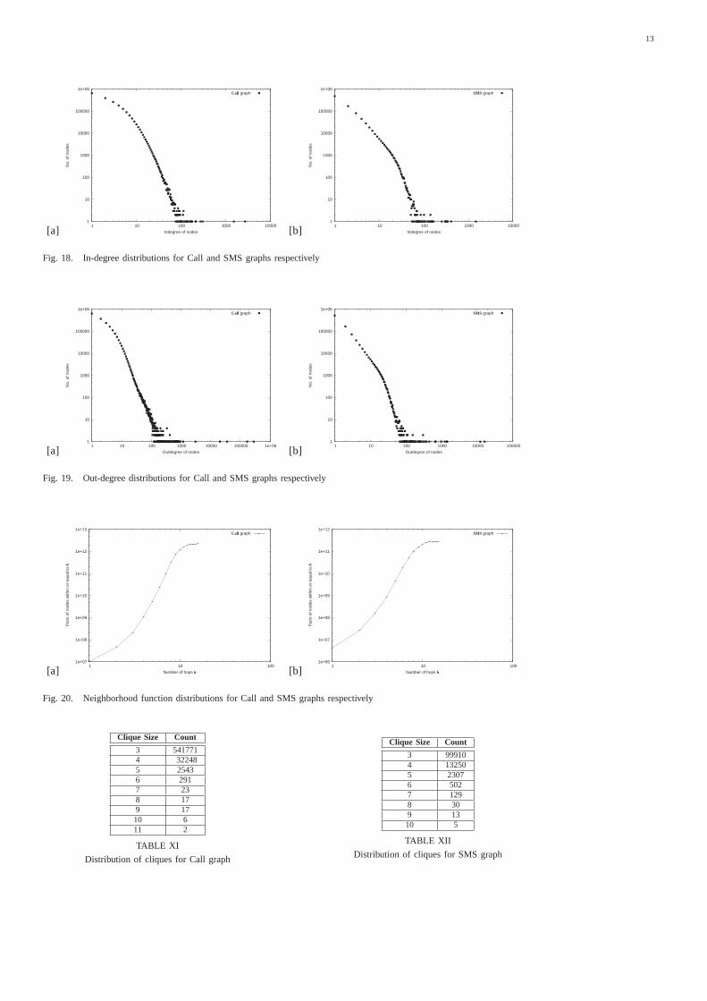
2) Degree Distributions:Figure 18(a) and Figure 18(b) showthe in-degree distribution for the call and SMS graphs whileFigure 19(a) and Figure 19(b) show the out-degree distributionfor the graphs

The power-law behavior is apparent for the Call graphs. How-ever for the SMS graph the in-degree and out-degree distributionsdo not show a marked power-law behavior. The SMS in-degreeand out-degree distributions consist of two different regions oflinear growth. A sudden kink where the two linear regions meetis evident in both the plots. Thus the degree distributions of SMSgraphs are different from many networks that has been studied inthe literature.

3) Neighborhood Distribution:Figure 20(a) and Figure 20(b)show the neighbourhood function distributions for the call andSMS graphs The neighborhood function plots for both the graphsappear similar. This indicates that the diameters of both the callgraph and the SMS graph are almost the same.

4) Cliques: Table XI and Table XII give the number of cliquespresent in the call graph and SMS graph respectively. The numberof smaller size cliques is higher in the Call graph. This is to beexpected since the Call graph has a higher number of nodes andedges. However it is very interesting to note the number of highersized cliques (of size 6,7,8) are higher in the SMS graph in-spiteof that graph having only one-third the number of edges in thecall graph.

This observation leads to the inference that there are somecliques where the participating members only send SMSes toone another and do not make calls. Such kind of a behavioralpattern may be indicative of a group of people with commoninterests where the members send bulk SMSes (jokes, etc.) toall the other members of the clique for instance. This statisticsindicates that Telecom Operators need to analyze the SMS graphs

also to identify an important segment of customer communitieswho may not be discovered by Call graph analysis.

TABLE XVI

RATIO OF EDGES OFCALL AND SMS GRAPH FOR THE DIFFERENT

TREASUREHUNT SUBGRAPHS

Subgraph Graph type Call Graph SMS Graph RatioEdges Edges

IN-IN Directed 113541 35832 3.17IN-SCC Bi-partitie & Directed 877417 110280 7.96IN-OUT Bi-partitie & Directed 203335 12879 15.79SCC-SCC Directed 4444481 1466544 3.03SCC-OUT Bi-partitie & Directed 861238 157932 5.45OUT-OUT Directed 138177 73619 1.88DISC Directed 237489 380396 0.62TOTAL Directed 6875678 2237482 3.07

5) Strongly Connected Components:Table XIII and Table XIVgive the number of strongly connected components present in theSMS graph and the call graph respectively. The tables show thenumber of strongly connected components present of each sizeand also the fraction of the total nodes that are present in thestrongly connected components of that size.

For the call graph the largest strongly connected componentcomprises more than of half the nodes. Apart from this largeststrongly connected component, the call graph has strongly con-nected components of only 10 other sizes and the size of thesecond largest strongly connected component is only 11. On theother hand, Table XIII reveals that the there are a large numberof nodes which are present in the smaller strongly connectedcomponents in the case of the SMS graph. This graph also has onevery large strongly connected component which contains about37% of the nodes.

This analysis gives an indication of the fact that the SMS graphis composed of a number of small islands which are stronglyconnected. This may be due to the fact that during SMSing thepeople are often part of a community which has lesser linksoutside.

C. TheTreasure-HuntModel

We tried to fit theTreasure-Huntmodel on the SMS graph.Table XV gives the details of the various components of the modelfound in the call graph and the SMS graph. On the other handTable XVI gives the ratio of edges in the call graph compared tothe SMS graph for the various subgraphs of the Treasure Hunt.

The call graph has three times the number of edges than theSMS graph. The ratio of edges for theIN-IN and SCC-SCCsubgraphs of the call graph to the SMS graph is also threetimes. On the other hand the ratios of the edges in the subgraphsIN-SCC, IN-OUT and SCC-OUTof the call graph to the SMSgraph are higher. Note that these subgraphs are bipartitite andthus have edges in one direction only. Since the SMS graphhas higher reciprocity, the proportion of such edges are lower.On the other hand the SMS graph has more edges inDISC,the disconnected components. This is also to be expected sincewe have observed that the SMS graph has many disconnectedislands. In fact, despite having fewer edges, it has a higher numberof cliques, SCCs, disconnected components, and smaller sizedbipartite components, which indicate more reciprocity.Therefore,the SMS graph follows the Treasure-Hunt Model but with ahigher reciprocity.

13

[a] 1

10

100

1000

10000

100000

1e+06

1 10 100 1000 10000

No.

of n

odes

Indegree of nodes

Call graph

[b] 1

10

100

1000

10000

100000

1e+06

1 10 100 1000 10000

No.

of n

odes

Indegree of nodes

SMS graph

Fig. 18. In-degree distributions for Call and SMS graphs respectively

[a] 1

10

100

1000

10000

100000

1e+06

1 10 100 1000 10000 100000 1e+06

No.

of n

odes

Outdegree of nodes

Call graph

[b] 1

10

100

1000

10000

100000

1e+06

1 10 100 1000 10000 100000

No.

of n

odes

Outdegree of nodes

SMS graph

Fig. 19. Out-degree distributions for Call and SMS graphs respectively

[a] 1e+07

1e+08

1e+09

1e+10

1e+11

1e+12

1e+13

1 10 100

Pai

rs o

f nod

es w

ithin

or

equa

l to

h

Number of hops h

Call graph

[b] 1e+06

1e+07

1e+08

1e+09

1e+10

1e+11

1e+12

1 10 100

Pai

rs o

f nod

es w

ithin

or

equa

l to

h

Number of hops h

SMS graph

Fig. 20. Neighborhood function distributions for Call and SMS graphs respectively

Clique Size Count

3 5417714 322485 25436 2917 238 179 1710 611 2

TABLE XI

Distribution of cliques for Call graph

Clique Size Count

3 999104 132505 23076 5027 1298 309 1310 5

TABLE XII

Distribution of cliques for SMS graph

14

Size Count Node Fraction

439444 1 0.3780322 2 3.78509e-0521 1 1.80652e-0520 1 1.72049e-0518 1 1.54844e-0517 3 4.38726e-0516 2 2.75279e-0515 5 0.00017893112 17 0.0001754911 40 0.00037850910 45 0.0003871119 92 0.0007122848 146 0.001004777 259 0.001559636 520 0.002683975 1077 0.004632434 2719 0.009356043 8580 0.02214282 40828 0.07024431 590696 0.508144

TABLE XIII

Distribution of SCCs for SMS graph

Size Count Nodes Fraction

1235077 1 0.53131711 1 4.73209e-0610 1 4.3019e-068 6 2.06491e-057 11 3.31246e-056 79 0.000203915 217 0.0004667564 919 0.001581383 4737 0.006113432 33224 0.02858521 1003439 0.431669

TABLE XIV

Distribution of SCCs for Call graph

TABLE XV

PROPERTIES OFTREASURE-HUNT SUBGRAPHS OF THE CALL AND THESMS GRAPHS

Type Subgraph Left Part Right part Edges Avg dout Avg din Diameter Edge RatioCALL IN-IN 101367 - 113541 1.1201 1.1201 4 0.13X

IN-SCC 331109 (IN) 502152 (SCC) 877417 2.64993 1.74731 1 XIN-OUT 70083 (IN) 145850 (OUT) 203335 2.90135 1.39414 1 0.23X

SCC-SCC 1235221 - 4444481 3.59813 3.59813 15 5.06XSCC-OUT 500900 (SCC) 478196 (OUT) 861238 1.71938 1.80101 1 0.98XOUT-OUT 173089 - 138177 0.7983 0.7983 4 0.16X

SMS IN-IN 35649 - 35832 1.00513 1.00513 6 0.32XIN-SCC 94707 (IN) 75475 (SCC) 110280 1.16443 1.46115 1 XIN-OUT 10304 (IN) 11436 (OUT) 12879 1.2499 1.12618 1 0.12X

SCC-SCC 440085 - 1466544 3.33241 3.33241 16 13.3XSCC-OUT 79844 (SCC) 135698 (OUT) 157932 1.97801 1.16385 1 1.43XOUT-OUT 73190 - 73610 1.00574 1.00574 5 0.67X

TABLE XVII

L INEAR CORRELATION COEFFICIENTS BETWEENCALL AND SMSGRAPHS

SMS Graph Variable Call Graph Variable Coefficient

Outdegree Indegree 0.0179568Outdegree Outdegree 0.974498Indegree Indegree 0.206114Indegree Outdegree 0.154815Pagerank Pagerank 0.131639

D. Correlation between SMS and Call Graphs

We studied if there was some correlation between the in-degree,out-degree and pagerank of nodes in the call graph, and thesevalues for the same nodes in the SMS graph. Table XVII showsthe linear correlation coefficient values observed for variouspairs of variables studied. For conducting these experiments wesegregated the nodes which were common in both the graphs. Thenumber of such nodes was 1035025, which is almost the sameas the number of nodes in the SMS graph (1162457). Howeverthis number is less than half of the total nodes in the call graph(2324556); as we have already seen, there exist a large numberof nodes which are only present in the call graph and not in theSMS graph.

Table XVII shows that the out-degrees of the two graphs areremarkably correlated. This indicates that people who make a lot

of calls also sends many SMSes. However indegree and pagerankdo not seem to be correlated. There may be a lot of nodes in theSMS graph which have incoming edges in the call graph, fromnodes which are not present in the SMS graph, making themhave a high in-degree in the call graph but not the SMS graph.On the other hand some nodes have a high in-degree in the SMSgraph but not in the call graph.This statistics again emphasizesthe point made earlier that Telecom Operators need to analyzethe SMS graphs also to identify important segments of customerswho may not be discovered by call graph analysis.

VIII. C ONCLUSIONS

Over the years, a number of important graph metrics have beenproposed to analyze and compare the structure of arbitrary graphs.This paper uses a series of graph structural properties that canbe employed in a more systematic approach to analyze networktopologies. We used a carefully chosen set of parameter whichreveal mostly connectivity directed characteristics and used themon Call and SMS graphs of a mobile operator. Such metrics canbe employed by business strategy planner involved in the telecomdomain. We hope that our methods will enable a more rigorousand consistent method of analyzing the telecom graphs andalso enable researchers and business community to gain insightinto the graphs. These results can significantly affect businessstrategies. Therefore, at present we are currently collaborating

15

with the marketing department of the Telecom Service providerto derive deeper business insights from the results.

The shapes of the call graph of four disparate regions are ingood agreement with theTreasure-Huntmodel. Although this ispromising, only further studies with more call graphs from othercountries can serve to verify or refute this model. In fact it willbe interesting to determine whether the properties of the Call andSMS graphs determined in our study hold in other geographiesand cultures as well.

Our analysis indicates that there are some similarities as welldifferences between the call and SMS graphs. The SMS graphseems to be moresocial with a higher value of reciprocity. Webelieve that the Telecom operators need to analyze both thesegraphs to gain complete understanding of its customer base.

Our temporal analysis highlights interesting insights on howthe graphs evolve over time. In the future we plan to study theevolution of the graphs for a longer period of time. A problemworthy of consideration is to find a generative model for thesetelecom graphs, if one exists. If found, it is likely to offer deepinsights into how a mobile operator’s customer base evolves withtime.

REFERENCES

[1] J. Abello, P. M. Pardalos, and M. G. C. Resende. On MaximumClique Problems in Very Large Graphs. In J. Abello and J. Vitter,editors,External Memory Algorithms (DIMACS Series), pages 119–130.American Mathematical Society, 1999.

[2] William Aiello, Fan Chung, and Linyuan Lu. A Random Graph Modelfor Massive Graphs. InProceedings of the Thirty-second annual ACMsymposium on Theory of Computing, pages 171–180, May 2000.

[3] Wai Ho Au Chan and K. C. C. Xin Yao. A Novel EvolutionaryData Mining Algorithm with applications to Churn Prediction.IEEETransaction on Evolutionary Computation, 7(6):532– 545, Dec 2003.

[4] A. L. Barabasi and Reka Albert. Emergence of Scaling in RandomNetworks. Science, 286:509–512, October 1999.

[5] Sergey Brin and Lawrence Page. The Anatomy of a large-scale Hy-pertextual Web Search Engine.Proceedings of the Eighth InternationalConference on the World Wide Web/Computer Networks, 30(1–7):107–117, 1998.

[6] A. Z. Broder, R. Kumar, F. Maghoul, P. Raghavan, S. Rajagopalan,R. Stata, A. Tomkins, and J. L. Wiener. Graph Structure in the Web. InProceedings of the Ninth International Conference on the World WideWeb/ Computer Networks, volume 33, pages 309–320, 2000.

[7] G. Caldarelli.Scale-Free Networks. Oxford University Press, 2007.[8] Shai Carmi, Shlomo Havlin, Scott Kirkpatrick, Yuval Shavitt, and Eran

Shir. MEDUSA - New Model of Internet Topology Using k-shellDecomposition. InProceedings of the International Workshop andConference on Network Science (NetSci), 2006.

[9] W. de Nooy, A. Mrvar, and Batagelj. V.Exploratory Social NetworkAnalysis with Pajek. Cambridge University Press, 2005.

[10] D. Donato, L. Laura, S. Leonardi, and S. Millozzi. Large scale propertiesof the Webgraph.The European Physical Journal B, 38:239–243, 2004.

[11] D. Donato, S. Leonardi, S. Millozzi, and P. Tsaparas. Mining the InnerStructure of the Web Graph. InEighth International Workshop on theWeb and Databases, 2005.

[12] S. Dorogovtsev and J. Mendes.Evolution of Networks: From BiologicalNets to the Internet and the WWW. Oxford University Press, 2000.

[13] T. Euler. Churn Prediction in Telecommunications Using MiningMart.In Proceedings of the Workshop on Data Mining and Business (DMBiz),2005.

[14] M. Faloutsos, P. Faloutsos, and C. Faloutsos. On Power-law Relation-ships of the Internet Topology. InProceedings of ACM SIGCOMMConference on Applications, Technologies, Architectures, and Protocolsfor Computer Communications, pages 251–262, 1999.

[15] J. Kleinberg. Authoritative Sources in a Hyperlinked Environment. InJournal of ACM, volume 46, 1999.

[16] Ravi Kumar, Jasmine Novak, Prabhakar Raghavan, and AndrewTomkins. Structure and Evolution of Blogspace.Communications ofthe ACM, 47(12):35–39, 2004.

[17] Ravi Kumar, Jasmine Novak, and Andrew Tomkins. Structure andEvolution of Online Social Networks. InProceeding of the Twelfth ACMInternational Conference on Knowledge Discovery and Data Mining(SIGKDD), August 2006.

[18] Ravi Kumar, Prabhakar Raghavan, Sridhar Rajagopalan, and AndrewTomkins. Trawling the Web for emerging Cyber-communities. InProceedings of the Eighth International Conference on World Wide Web,pages 1481–1493, 1999.

[19] Jure Leskovec, Jon Kleinberg, and Christos Faloutsos. Graphs over time:Densification laws, Shrinking diameters and possible explanations. InProceeding of the Eleventh ACM International Conference on Knowl-edge Discovery and Data Mining (SIGKDD), pages 177–187, 2005.

[20] D. Liben-Nowell, J. Novak, R. Kumar, P. Raghavan, and A. Tomkins.Geographic Routing in Social Networks.PNAS, 102(33):11623–11628,2005.

[21] M. E. J. Newman. The Structure and Function of Complex Networks.SIAM Review, 45:167, 2003.

[22] A. Ntoulas, J. Cho, and C. Olston. Whats new on the Web? Theevolution of Web from a Search Engine perspective. InProceedingsof the Thirteenth International Conference on World Wide Web, pages1–12, 2004.

[23] Christopher R. Palmer, Phillip B. Gibbons, and Christos Faloutsos. ANF:a Fast and Scalable Tool for Data Mining in Massive Graphs. InProceeding of the Eighth ACM International Conference on KnowledgeDiscovery and Data Mining (SIGKDD), pages 81–90, 2002.

[24] G. Siganos, S. Tauro, and M. Faloutsos. Jellyfish: A Conceptual Modelfor the AS Internet Topology.Journal of Communications and Networks,8(3):339–350, September 2006.

Amit Anil Nanavati is a Research Staff Memberin IBM India Research Lab, New Delhi, India. Hegraduated from Louisiana State University, BatonRouge with M.S. (1994) and Ph.D. in ComputerScience (Distributed Computing) in 1996, and witha B.E. in Computer Science from M.S. Universityof Baroda in 1989. Prior to IBM Research, heworked for Netscape Communications (1996-2000).His recent research focus has been on mobile andpervasive computing and information mining andretrieval, as applied to Telecom service provider

settings and is currently working on solutions for emerging economies. Heis particularly interested in applications of graph theory in various domains.His other interests include speech in mobile and pervasive environments andtheory and modelling of systems. Before completing his Ph.D., he spent asummer at the Jet Propulsion Laboratory, Caltech, NASA. He can be reachedat namit@in.ibm.com.

Rahul Singh received the B.Tech. degree fromthe Indian Institute of Technology at Guwahati in2005. From 2005 to 2006, he worked at the Or-acle Development Center in Bangalore, India asmember of technical staff. In 2006, he joined IBMIndia Research Lab at New Delhi as a technicalstaff member. He is currently in the first year ofhis PhD in Computer Science at the University ofMassachusetts, Amherst. His area of research ismachine learning, data mining and applications ofthe above to large-scale systems. He can be reached

at rahul@cs.umass.edu.

16

Dipanjan Chakraborty is a Research Staff Memberat IBM India Research Lab. He received his Ph.D.in Computer Science from University of Maryland,Baltimore County (UMBC) in 2004. His reserachis in the areas of mobile and pervasive comput-ing environments, next generation network protocolsand management, peer-to-peer systems with specialinterests in the fields of service discovery, infor-mation aggregation and composition, ad-hoc/sensornetworks and application-centric routing. He is alsoworking in the area of business process management.

His thesis is in the area of service discovery and composition for pervasiveenvironments. He received a fellowship grant from IBM during the 3 yearsof his Ph.D candidacy. He can be reached at cdipanjan@in.ibm.com.

Koustuv Dasgupta is a Researcher at the IBMIndia Research Lab, New Delhi, India. Koustuvreceived his Ph.D. in Computer Science from theUniversity of Maryland Baltimore County in May,2003, and his B.Engg. in Computer Science andEngineering from Jadavpur University, India in July1997. At IBM, for the past four years, he hasbeen working on and leading projects on telecominfrastructure and middleware, including algorithmsand architectures for advanced SIP-based presencein converged networks, context-sensitive middleware

technologies, and next-generation IMS-based service delivery platforms. Hisresearch interests further span a wide range of networked computer systemsincluding Internet-scale systems, QoS-aware storage systems, wireless sensornetworks, and enterprise grids. Koustuv is a member of ACM and IEEE. Hecan be reached at kdasgupta@in.ibm.com.

Sougata Mukherjea is a Research Staff Memberand Manager of the Telecom Research InnovationCenter in IBM India Research Lab. He receivedhis Bachelors from Jadavpur University, Calcutta,MS from Northeastern University, Boston and PhDfrom Georgia Institute of Technology, Atlanta (all inComputer Science). Before joining IBM, he held re-search and software architect positions in companiesin Silicon Valley (California) including NEC USA,Inktomi and BEA Systems. His research interestsinclude Middleware technologies and its applications

to Telecom, Data Analysis, Information Retrieval and Visualization. He hasseveral patents and publications in reputed Computer Science conferences andjournals in these research areas. He can be reached at smukherj@in.ibm.com.

Gautam Das received B. Tech. degree in Com-puter Science and Engineering from Indian Insti-tute of Technology Guwahati in 2005. From 2005to 2006, he worked at IBM India Research Lab,New Delhi. Currently, he is a second year MastersStudent at University of Massachusetts Amherst inthe ECE Department. His research interests includeproduct optimization based on data analytics, so-cial network analysis, mining and characterizationof user generated content. He can be reached atgdas@ecs.umass.edu.

Siva Gurumurthy received B. Tech. degree in Com-puter Science and Engineering from Indian Instituteof Technology Guwahati in 2005. He had pursuedone year research training from IBM India ResearchLab. Currently, he is a second year Masters Studentat University of Massachusetts Amherst in the ECEDepartment. His research interests include largescale data analysis such as web graph, call graphand social network analysis. He can be reached atshiva@gmail.com.

Anupam Joshi is a Professor of Computer Scienceand Electrical Engineering at UMBC. Earlier, he wasan Assistant Professor in the CECS department atthe University of Missouri, Columbia. He obtaineda B. Tech degree in Electrical Engineering fromIIT Delhi in 1989, and a Masters and Ph.D. inComputer Science from Purdue University in 1991and 1993 respectively. His research interests are inthe broad area of networked computing and intelli-gent systems. His primary focus has been on datamanagement and security for mobile, pervasive, and

sensor systems. He has created agent based middleware to support discovery,composition, and secure access of services/data over both infrastructure basedand ad-hoc wireless networks, as well as systems that integrate sensors withthe grid. He is also interested in Semantic Web, Social Media, and Data/WebMining, where he has worked on creating personalized and secure web spacesusing a combination of agents, policies, and soft computing.

He has published over 150 technical papers, and has obtained researchsupport from NSF, NASA, DARPA, DoD, IBM, LMCO, AetherSystens, HP,AT&T and Intel. He has presented tutorials in conferences, served as guesteditor for special issues for VLDB J., Comm. ACM etc., and served as anAssociate Editor of IEEE Transactions of Fuzzy Systems from 99-03. Hecurrently serves on the editorial board of the Intl. J. Semantic Web andInformation Systems. At UMBC, Joshi teaches courses in Operating Systems,Mobile Computing, Networking, Security, and Web Mining. He is a memberof IEEE, IEEE-CS, and ACM. He can be reached at joshi@cs.umbc.edu.