PATTERN RULES, PATTERNS, AND GRAPHS:

ANALYZING GRADE 6 STUDENTS’ LEARNING OF LINEAR FUNCTIONS

THROUGH THE PROCESSES OF WEBBING, SITUATED ABSTRACTIONS, AND

CONVERGENT CONCEPTUAL CHANGE

By

Ruth A. Beatty

A thesis submitted for the degree of Doctor of Philosophy

Department of Human Development and Applied Psychology Ontario Institute for Studies in Education of the

University of Toronto

© Copyright by Ruth A. Beatty, 2010

ii

PATTERN RULES, PATTERNS, AND GRAPHS: ANALYZING GRADE 6 STUDENTS’ LEARNING OF LINEAR FUNCTIONS THROUGH THE PROCESSES OF WEBBING,

SITUATED ABSTRACTION, AND CONVERGENT CONCEPTUAL CHANGE Doctor of Philosophy, 2010

Ruth A. Beatty Department of Human Development and Applied Psychology

University of Toronto

Abstract

The purpose of this study, based on the third year of a three-year research study, was to

examine Grade 6 students’ previously developed abilities to integrate their understanding of

geometric growing patterns with graphic representations as a means of further developing

their conception of linear relationships. In addition, I included an investigation to determine

whether the students’ understanding of linear relationships of positive values could be

extended to support their understanding of negative numbers. The theoretical approach to the

microgenetic analyses I conducted is based on Noss & Hoyles’ notion of situated

abstractions, which can be defined as the development of successive approximation of

formal mathematical knowledge in individuals. I also looked to Roschelle’s work on

collaborative conceptual change, which allowed me to examine and document successive

mathematical abstractions at a whole-class level. I documented in detail the development of

ten grade 6 students’ understanding of linear relationships as they engaged in seven

experimental lessons. The results show that these learners were all able to grasp the

connections among multiple representations of linear relationships. The students were also

able to use their grasp of pattern sequences, graphs and tables of value to work out how to

operate with negative numbers, both as the multiplier and as the additive constant. As a

contribution to research methodology, the use of two analytical frameworks provides a

model of how frameworks can be used to make sense of data and in particular to pinpoint the

interplay between individual and collective actions and understanding.

iii

Acknowledgements

I am so grateful for all of the people in my life who have supported this endeavour. I

wish to thank:

Dr. Joan Moss. You and I have travelled such a long way. Thank you for your

kindness, your energy, warmth, humour, intelligence, and enthusiasm. Thank you for

allowing me to believe in myself. It has been such pleasure learning from you, and working

with you.

Dr. Carolyn Kieran. You are the Queen of Algebra. Thank you for your ongoing

support, your generosity of time and your continued interest in this work.

Dr. David Pimm. Thank you for being such an outstanding mentor and friend, and for

the long conversations as I attempted to formulate and articulate my thoughts. Thank you for

always providing new and intriguing perspectives!

Dr. Earl Woodruff, for having the courage to read both my M.A. final work, and the

PhD beast!

Dr. Eunice Jang. Your sparkling brilliance lights up everyone around you. Thank you

for making me think about concepts and issues outside of my obsession.

Dr. John Mason. Thank you for your continued interest in this work, and for your

insightful analysis and constructive feedback. Thank you for opening the door to new

interpretations.

Dr. Cathy Bruce. For always being at the end of an email, for your ongoing support,

encouragement and friendship. Thank you for being spectacular!

To Kate Taylor, without whom none of this work would have been possible. You are

a gifted teacher – thank you for making this study so successful.

iv

To my amazing support network, without whom this would not have been possible.

To my Thesis Defense Team: Monique Herbert; Saad Chahine; Tomoko Arimura; and

Olessya Falunchuk. Thank you for keeping me sane! Thanks for your support, kindness and

friendship, for taking care of minor details (like arranging the data projector!) and for

prepping me for the defense. Thank you to OISE friends who have journeyed with me: Toni

Doyle, Jing Zhang, Sejal Patel, Dawn Pollon, Kathleen Hipfner-Boucher, Bev Caswell, and

Liz Rentzelos. A very special thank you to Christine Davidson, friend and editor

extraordinaire, who has gotten all of us through!

To Anne McGuire and Sonia Satov for their tireless support (1,0,0,0,1,1,0 etc)

generosity, and unbounded intellectual energy!

“The girls at the back” Julie McDonnell, Aislinn Smail, Corey Berry and Christy

Johnson who have helped me maintain a sense of humour and balance through this process.

Thank you all for the joy and love you bring to my life.

To Lakehead friends Frances Helyar, Lex Scully, Yvette DeBeer, Daphne Bonar,

Linda Rodenburg, Bruce Boyes, and Sonia Mastrangelo.

Thank you to friends and colleagues who have supported all of my work in “real”

schools! Pat Milot, Glynnis Flemming, Sue Wilson, Sean Hanna, Tara Flynn, Rich

McPhearson, Richard Gallant, Dr. John Ross, Myrna Ingalls, Judy Dussiaume, Greg Clark,

Ross Issenegger. Special thanks to Elizabeth Morley and Richard Messina and all of the

amazing teachers and principals I have had the privilege to work with over the past several

years. And thank you to all the students I had the good fortune to work with – you are the

inspiration for all of us and I am so grateful for your honesty, enthusiasm, and brilliance.

v

Finally to my family, Ralph Beatty, Eileen Beatty, Stephen Beatty, Rafe Beatty,

Olivia Beatty, Jack Beatty and Finn Beatty. Thank you for giving me a solid base from which

to aim as high as possible. I love you all.

vi

!"#$%&'(&)'*+%*+,!

"#$%&"'% (((((((((((((((((((((((((((((((((((((((((((((((((((((((((((((((((((((((((((((((((((((((((((((((((((((((((((((((((((((((((((((((((((((((((((((((((((((((((((((((((((((((((((((((((((( ))!

"'*+,-./01/2/+%$((((((((((((((((((((((((((((((((((((((((((((((((((((((((((((((((((((((((((((((((((((((((((((((((((((((((((((((((((((((((((((((((((((((((((((((((((((((((( )))!

.3$%!,4!%"#./$ ((((((((((((((((((((((((((((((((((((((((((((((((((((((((((((((((((((((((((((((((((((((((((((((((((((((((((((((((((((((((((((((((((((((((((((((((((((((((((((((((((((((((((5!

.3$%!,4!4316&/$ ((((((((((((((((((((((((((((((((((((((((((((((((((((((((((((((((((((((((((((((((((((((((((((((((((((((((((((((((((((((((((((((((((((((((((((((((((((((((((((((((((((( 5))!

7(!3+%&,06'%3,+ (((((((((((((((((((((((((((((((((((((((((((((((((((((((((((((((((((((((((((((((((((((((((((((((((((((((((((((((((((((((((((((((((((((((((((((((((((((((((((((((((((( 7!7(7!/"&.8!".1/#&"((((((((((((((((((((((((((((((((((((((((((((((((((((((((((((((((((((((((((((((((((((((((((((((((((((((((((((((((((((((((((((((((((((((((((((((((((((((((((((((((((((((((((((((((7!7(9!3+%/&:&/%"%3,+$!,4!;/"&.8!".1/#&"< ((((((((((((((((((((((((((((((((((((((((((((((((((((((((((((((((((((((((((((((((((((((((((((((((((((((((((((((((((((((((((9!7(=!28!:&/>3,6$!&/$/"&'? (((((((((((((((((((((((((((((((((((((((((((((((((((((((((((((((((((((((((((((((((((((((((((((((((((((((((((((((((((((((((((((((((((((((((((((((((((((((((((((@!7(A!03$$/&%"%3,+!$%608 (((((((((((((((((((((((((((((((((((((((((((((((((((((((((((((((((((((((((((((((((((((((((((((((((((((((((((((((((((((((((((((((((((((((((((((((((((((((((((((((((((B!7(C!,>/&>3/-!,4!03$$/&%"%3,+!'?":%/&$ (((((((((((((((((((((((((((((((((((((((((((((((((((((((((((((((((((((((((((((((((((((((((((((((((((((((((((((((((((((((( 7D!

9(!&/>3/-!,4!%?/!.3%/&"%6&/(((((((((((((((((((((((((((((((((((((((((((((((((((((((((((((((((((((((((((((((((((((((((((((((((((((((((((((((((((((((((((((((((((((7=!9(7!%?/!$%608!,4!.3+/"&!&/."%3,+$?3:$!"+0!+/1"%3>/!+62#/&$((((((((((((((((((((((((((((((((((((((((((((((((((((((((((((((((((( 7=!9(7(7!!"#$%&'()$*+$,-.#/0$0#,/&-*.%"-1%222222222222222222222222222222222222222222222222222222222222222222222222222222222222222222222222222222222222222222222234$9(7(9!5-++-6',&-#%$7-&"$80/1"-6/,$0#10#%#.&/&-*.%$*+$,-.#/0$0#,/&-*.%"-1%2222222222222222222222222222222222222222222222222239$9(7(=!:*,;-.8$,-.#/0$#<'/&-*.% 222222222222222222222222222222222222222222222222222222222222222222222222222222222222222222222222222222222222222222222222222222222222223=$

9(9!%?/!$%608!,4!+/1"%3>/!+62#/&$((((((((((((((((((((((((((((((((((((((((((((((((((((((((((((((((((((((((((((((((((((((((((((((((((((((((((((((((((((((((((((((((((( 7E!9(=!$,'3,F'6.%6&".!:/&$:/'%3>/$!,4!./"&+3+1((((((((((((((((((((((((((((((((((((((((((((((((((((((((((((((((((((((((((((((((((((((((((((((((((((((((((( 99!9(=(7!:*6-*>6',&'0/,-%? 2222222222222222222222222222222222222222222222222222222222222222222222222222222222222222222222222222222222222222222222222222222222222222222222222222@@$9(=(9!:-&'/&#($,#/0.-.822222222222222222222222222222222222222222222222222222222222222222222222222222222222222222222222222222222222222222222222222222222222222222222222222222@4$9(=(=!A#BB-.8$/.($%-&'/&#($/B%&0/6&-*.222222222222222222222222222222222222222222222222222222222222222222222222222222222222222222222222222222222222222222@C$9(=(A!A#BB-.8 2222222222222222222222222222222222222222222222222222222222222222222222222222222222222222222222222222222222222222222222222222222222222222222222222222222222222222222222@=$9(=(C!:-&'/&#($/B%&0/6&-*. 2222222222222222222222222222222222222222222222222222222222222222222222222222222222222222222222222222222222222222222222222222222222222222222222@D$9(=(@!E*.;#08#.&$6*.6#1&'/,$6"/.8#2222222222222222222222222222222222222222222222222222222222222222222222222222222222222222222222222222222222222222222222222@F$

=(!,>/&>3/-!,4!:&/>3,6$!8/"&$G!&/$/"&'?!"+0!&/$6.%$ (((((((((((((((((((((((((((((((((((((((((((((((((((((((((((((((((((((((=9!=(7!8/"&!,+/H!1&"0/!4,6&!$%608((((((((((((((((((((((((((((((((((((((((((((((((((((((((((((((((((((((((((((((((((((((((((((((((((((((((((((((((((((((((((((((((((((((((((((( ==!=(7(7!G.%&0'6&-*.22222222222222222222222222222222222222222222222222222222222222222222222222222222222222222222222222222222222222222222222222222222222222222222222222222222222222222244$=(7(9!H#%',&% 222222222222222222222222222222222222222222222222222222222222222222222222222222222222222222222222222222222222222222222222222222222222222222222222222222222222222222222222224D$

9(@!8/"&!%-,H!1&"0/!43>/!$%608 ((((((((((((((((((((((((((((((((((((((((((((((((((((((((((((((((((((((((((((((((((((((((((((((((((((((((((((((((((((((((((((((((((((((((((((( =E!=(9(7!G.%&0'6&-*.2222222222222222222222222222222222222222222222222222222222222222222222222222222222222222222222222222222222222222222222222222222222222222222222222222222222222222224D$=(9(9!H#%',&% 222222222222222222222222222222222222222222222222222222222222222222222222222222222222222222222222222222222222222222222222222222222222222222222222222222222222222222222222229@$

=(=!$622"&8!,4!:"$%!&/$/"&'?((((((((((((((((((((((((((((((((((((((((((((((((((((((((((((((((((((((((((((((((((((((((((((((((((((((((((((((((((((((((((((((((((((((((((((((( A9!

A(!0/>/.,:2/+%!,4!%?/!%?3&0!8/"&!./$$,+!$/I6/+'/ ((((((((((((((((((((((((((((((((((((((((((((((((((((((((((((((((((((((((((((AA!A(7!%?/!./$$,+!$/I6/+'/ ((((((((((((((((((((((((((((((((((((((((((((((((((((((((((((((((((((((((((((((((((((((((((((((((((((((((((((((((((((((((((((((((((((((((((((((((((((((((((((( AC!A(9!./$$,+!7J!2"*3+1!',++/'%3,+$!"2,+1!&/:&/$/+%"%3,+$(((((((((((((((((((((((((((((((((((((((((((((((((((((((((((((((((((((((((( AE!A(9(7!I#%%*.$3 222222222222222222222222222222222222222222222222222222222222222222222222222222222222222222222222222222222222222222222222222222222222222222222222222222222222222222222229D$

A(=!./$$,+$!9FAJ!/K:.,&3+1!.3+/"&!&6./$!%?"%!?">/!3+%/&$/'%3+1!%&/+0!.3+/$ ((((((((((((((((((((((((((((((( AB!A(=(7!I#%%*.$@ 222222222222222222222222222222222222222222222222222222222222222222222222222222222222222222222222222222222222222222222222222222222222222222222222222222222222222222222229F$A(=(9!I#%%*.$4 22222222222222222222222222222222222222222222222222222222222222222222222222222222222222222222222222222222222222222222222222222222222222222222222222222222222222222222222C3$A(=(=!I#%%*.$9 22222222222222222222222222222222222222222222222222222222222222222222222222222222222222222222222222222222222222222222222222222222222222222222222222222222222222222222222C@$

A(A!./$$,+$!CFEJ!3+',&:,&"%3+1!+/1"%3>/!+62#/&$!((((((((((((((((((((((((((((((((((((((((((((((((((((((((((((((((((((((((((((((((((((((((((((((( C=!A(A(7!I#%%*.$C 22222222222222222222222222222222222222222222222222222222222222222222222222222222222222222222222222222222222222222222222222222222222222222222222222222222222222222222222C9$A(A(9!I#%%*.$= 22222222222222222222222222222222222222222222222222222222222222222222222222222222222222222222222222222222222222222222222222222222222222222222222222222222222222222222222C9$A(A(=!I#%%*.$D 22222222222222222222222222222222222222222222222222222222222222222222222222222222222222222222222222222222222222222222222222222222222222222222222222222222222222222222222CC$

A(C!$622"&8!,4!3+$%&6'%3,+".!0/$31+!(((((((((((((((((((((((((((((((((((((((((((((((((((((((((((((((((((((((((((((((((((((((((((((((((((((((((((((((((((((((((((( CE!

vii

A(@!$622"&8!,4!03$$/&%"%3,+!&"%3,+"./!"+0!?8:,%?/$/$!(((((((((((((((((((((((((((((((((((((((((((((((((((((((((((((((((((((((((((((( CL!A(E!&/$/"&'?!I6/$%3,+$! (((((((((((((((((((((((((((((((((((((((((((((((((((((((((((((((((((((((((((((((((((((((((((((((((((((((((((((((((((((((((((((((((((((((((((((((((((((((((((((( @D!

C(!2/%?,0,.,18 ((((((((((((((((((((((((((((((((((((((((((((((((((((((((((((((((((((((((((((((((((((((((((((((((((((((((((((((((((((((((((((((((((((((((((((((((((((((((((((((((((@9!C(7!0/$'&3:%3,+!,4!%?/!,>/&"..!&/$/"&'?!3+>/$%31"%3,+((((((((((((((((((((((((((((((((((((((((((((((((((((((((((((((((((((((((((((((((( @=!C(9!$"2:.3+1!:&,'/06&/$ ((((((((((((((((((((((((((((((((((((((((((((((((((((((((((((((((((((((((((((((((((((((((((((((((((((((((((((((((((((((((((((((((((((((((((((((((((((((((((( @A!C(=!$%60/+%!:&,43./$(((((((((((((((((((((((((((((((((((((((((((((((((((((((((((((((((((((((((((((((((((((((((((((((((((((((((((((((((((((((((((((((((((((((((((((((((((((((((((((((((((((( @C!C(A!0"%"!',../'%/0!:&3,&!%,!"+0!"4%/&!./$$,+!32:./2/+%"%3,+(((((((((((((((((((((((((((((((((((((((((((((((((((((((((((((( @@!C(A(7!J0#K1*%&$80/1"-.8$?#/%'0# 2222222222222222222222222222222222222222222222222222222222222222222222222222222222222222222222222222222222222222222222222222222==$C(A(9!J0#K1*%&$-.&#0;-#7%$7-&"$%#,#6&#($"-8"$/.($,*7$/6"-#;-.8$%&'(#.&% 22222222222222222222222222222222222222222222222=D$

C(C!0"%"!',./'%/0!06&3+1!./$$,+!32:./2/+%"%3,+(((((((((((((((((((((((((((((((((((((((((((((((((((((((((((((((((((((((((((((((((((((((((((((( @L!C(C(7!L-(#*&/1#($6,/%%0**?$*B%#0;/&-*.$(/&/ 222222222222222222222222222222222222222222222222222222222222222222222222222222222222222222222222222222=M$C(C(9!E,/%%0**?$B/%#($%&'(#.&$-.&#0;-#7% 22222222222222222222222222222222222222222222222222222222222222222222222222222222222222222222222222222222222222=F$C(C(=!N&"#0$(/&/ 222222222222222222222222222222222222222222222222222222222222222222222222222222222222222222222222222222222222222222222222222222222222222222222222222222222222222222=F$

C(@!0"%"!"+".8$3$(((((((((((((((((((((((((((((((((((((((((((((((((((((((((((((((((((((((((((((((((((((((((((((((((((((((((((((((((((((((((((((((((((((((((((((((((((((((((((((((((((((((((((((( @B!C(@(7!O'/,-&/&-;#$/./,)%-%$10*6#('0#% 22222222222222222222222222222222222222222222222222222222222222222222222222222222222222222222222222222222222222222222222=F$C(@(9!O'/.&-&/&-;#$/./,)%-%$10*6#('0#% 22222222222222222222222222222222222222222222222222222222222222222222222222222222222222222222222222222222222222222222D3$C(@(=!P-Q#($/./,)%-%$10*6#('0#% 2222222222222222222222222222222222222222222222222222222222222222222222222222222222222222222222222222222222222222222222222222222222D3$

C(E!/%?3'".!',+$30/&"%3,+$! (((((((((((((((((((((((((((((((((((((((((((((((((((((((((((((((((((((((((((((((((((((((((((((((((((((((((((((((((((((((((((((((((((((((((((((((((((( E9!

@(!'?":%/&!$3KJ!&/$/"&'?!I6/$%3,+!,+/!&/$6.%$ ((((((((((((((((((((((((((((((((((((((((((((((((((((((((((((((((((((((((((((((((((((((((E=!@(7!:"&%!,+/!M!',++/'%3,+$!"2,+1!&/:&/$/+%"%3,+$!,4!.3+/"&!&/."%3,+$?3:$((((((((((((((((((((((((((((( EC!@(7(7!I#%%*.$323 2222222222222222222222222222222222222222222222222222222222222222222222222222222222222222222222222222222222222222222222222222222222222222222222222222222222222222222DC$@(7(9!I#%%*.$32@ 2222222222222222222222222222222222222222222222222222222222222222222222222222222222222222222222222222222222222222222222222222222222222222222222222222222222222222222MR$@(7(=!I#%%*.$324 2222222222222222222222222222222222222222222222222222222222222222222222222222222222222222222222222222222222222222222222222222222222222222222222222222222222222222222M=$@(7(A!S0*'1$%-&'/&#($/B%&0/6&-*.%$+*0$1/0&$*.#22222222222222222222222222222222222222222222222222222222222222222222222222222222222222222222222222222MF$

@(9!:"&%!%-,!M!&6./$!-3%?!3+%/&$/'%3+1!%&/+0!.3+/$ ((((((((((((((((((((((((((((((((((((((((((((((((((((((((((((((((((((((((((((((((((((((((( B=!@(9(7!I#%%*.$@23 2222222222222222222222222222222222222222222222222222222222222222222222222222222222222222222222222222222222222222222222222222222222222222222222222222222222222222222F3$@(9(9!I#%%*.$@2@ 2222222222222222222222222222222222222222222222222222222222222222222222222222222222222222222222222222222222222222222222222222222222222222222222222222222222222222222FD$@(9(=!I#%%*.$@24 2222222222222222222222222222222222222222222222222222222222222222222222222222222222222222222222222222222222222222222222222222222222222222222222222222222222222222 3R@$@(9(A!I#%%*.$423 2222222222222222222222222222222222222222222222222222222222222222222222222222222222222222222222222222222222222222222222222222222222222222222222222222222222222222 3RM$@(9(C!I#%%*.$42@ 2222222222222222222222222222222222222222222222222222222222222222222222222222222222222222222222222222222222222222222222222222222222222222222222222222222222222222 334$@(9(@!I#%%*.$923 2222222222222222222222222222222222222222222222222222222222222222222222222222222222222222222222222222222222222222222222222222222222222222222222222222222222222222 33D$@(9(E!I#%%*.$92@ 2222222222222222222222222222222222222222222222222222222222222222222222222222222222222222222222222222222222222222222222222222222222222222222222222222222222222222 33M$@(9(L!I#%%*.$924 2222222222222222222222222222222222222222222222222222222222222222222222222222222222222222222222222222222222222222222222222222222222222222222222222222222222222222 3@4$@(9(B!:'??/0)$*+$,#%%*.%$3$&*$922222222222222222222222222222222222222222222222222222222222222222222222222222222222222222222222222222222222222222222222222222222 3@C$

@(=!:"&%!%?&//!M!+/1"%3>/!+62#/&$H!:"%%/&+!&6./$!"+0!1&":?$((((((((((((((((((((((((((((((((((((((((((((((((((((((((((((( 79L!@(=(7!I#%%*.$C23 2222222222222222222222222222222222222222222222222222222222222222222222222222222222222222222222222222222222222222222222222222222222222222222222222222222222222222 3@M$@(=(9!I#%%*.$=23 2222222222222222222222222222222222222222222222222222222222222222222222222222222222222222222222222222222222222222222222222222222222222222222222222222222222222222 39R$@(=(=!I#%%*.$=2@ 2222222222222222222222222222222222222222222222222222222222222222222222222222222222222222222222222222222222222222222222222222222222222222222222222222222222222222 3C3$@(=(A!I#%%*.$=24 2222222222222222222222222222222222222222222222222222222222222222222222222222222222222222222222222222222222222222222222222222222222222222222222222222222222222222 3C3$@(=(C!I#%%*.$D23 2222222222222222222222222222222222222222222222222222222222222222222222222222222222222222222222222222222222222222222222222222222222222222222222222222222222222222 3CM$@(=(@!I#%%*.$D2@ 2222222222222222222222222222222222222222222222222222222222222222222222222222222222222222222222222222222222222222222222222222222222222222222222222222222222222222 3DR$A(=(E!:'??/0)$*+$,#%%*.%$C$&*$D22222222222222222222222222222222222222222222222222222222222222222222222222222222222222222222222222222222222222222222222222222222 3D3$

E(!'?":%/&!$/>/+J!&/$/"&'?!I6/$%3,+!%-,!&/$6.%$ ((((((((((((((((((((((((((((((((((((((((((((((((((((((((((((((((((((((((((((7EC!E(7!:"&%!,+/M!%?/!2/"+3+1!,4!%?/!:,3+%!,4!3+%/&$/'%3,+ (((((((((((((((((((((((((((((((((((((((((((((((((((((((((((((((((((((((((((( 7EC!E(7(7!S0/1"-6/,$0#10#%#.&/&-*.% 2222222222222222222222222222222222222222222222222222222222222222222222222222222222222222222222222222222222222222222222222222222 3DD$E(7(9!!/B,#%$*+$;/,'#%22222222222222222222222222222222222222222222222222222222222222222222222222222222222222222222222222222222222222222222222222222222222222222222222222222 3FD$E(7(=!T<'/&-*.%22222222222222222222222222222222222222222222222222222222222222222222222222222222222222222222222222222222222222222222222222222222222222222222222222222222222222222 @RF$E(7(A!:'??/0)$U$-.&#0%#6&-.8$&0#.($,-.#%2222222222222222222222222222222222222222222222222222222222222222222222222222222222222222222222222222222222222 @3F$

E(9!:"&%!%-,M!+/1"%3>/!+62#/&$ ((((((((((((((((((((((((((((((((((((((((((((((((((((((((((((((((((((((((((((((((((((((((((((((((((((((((((((((((((((((((((((((((((((( 997!E(9(7!V./0)$/.($B-./0)$W,-?-&#($?',&-1,-6/&-;#X$'.(#0%&/.(-.8$*+$.#8/&-;-&) 222222222222222222222222222222222222 @@4$

viii

E(9(9!V./0)Y$B-./0)Y$/.($?',&-1,-6/&-;#$'.(#0%&/.(-.8$*+$.#8/&-;-&) 222222222222222222222222222222222222222222222222222222 @4D$E(9(=!:'??/0)$U$.#8/&-;#$.'?B#0%222222222222222222222222222222222222222222222222222222222222222222222222222222222222222222222222222222222222222222222222 @CF$

L(!'?":%/&!/31?%J!&/$/"&'?!I6/$%3,+!%?&//!&/$6.%$(((((((((((((((((((((((((((((((((((((((((((((((((((((((((((((((((((((((((9@D!L(7!:"&%!,+/!M!3+%/&$/'%3+1!%&/+0!.3+/$ (((((((((((((((((((((((((((((((((((((((((((((((((((((((((((((((((((((((((((((((((((((((((((((((((((((((((((((((((((( 9@D!L(9!:"&%!%-,!M!+/1"%3>/!+62#/&$ (((((((((((((((((((((((((((((((((((((((((((((((((((((((((((((((((((((((((((((((((((((((((((((((((((((((((((((((((((((((((((((((((((( 9@=!

B(!'?":%/&!+3+/J!&/$/"&'?!I6/$%3,+!4,6&!&/$6.%$ ((((((((((((((((((((((((((((((((((((((((((((((((((((((((((((((((((((((((((((((9@@!B(7!:"&%!,+/M6+0/&$%"+03+1!1&":?3'".!&/:&/$/+%"%3,+$!,4!.3+/"&!&/."%3,+$?3:$! ((((((((((( 9@E!B(7(7!J0#$&#%&$0#%',&%2222222222222222222222222222222222222222222222222222222222222222222222222222222222222222222222222222222222222222222222222222222222222222222222222222222 @=D$B(7(9!:'??/0)$*+$10#$&#%&$0#%',&%22222222222222222222222222222222222222222222222222222222222222222222222222222222222222222222222222222222222222222222222222222 @=F$B(7(=!J0#$&#%&$-.&#0;-#7% 22222222222222222222222222222222222222222222222222222222222222222222222222222222222222222222222222222222222222222222222222222222222222222222222 @D3$B(7(A!J*%&$&#%&$0#%',&% 22222222222222222222222222222222222222222222222222222222222222222222222222222222222222222222222222222222222222222222222222222222222222222222222222222 @D9$B(7(C!:'??/0)$*+$1*%&$&#%&$0#%',&%222222222222222222222222222222222222222222222222222222222222222222222222222222222222222222222222222222222222222222222222222 @DC$B(7(@!J*%&$&#%&$-.&#0;-#7% 222222222222222222222222222222222222222222222222222222222222222222222222222222222222222222222222222222222222222222222222222222222222222222222 @DD$B(7(E!J0#$&*$1*%&$%6*0#$6*?1/0-%*.%222222222222222222222222222222222222222222222222222222222222222222222222222222222222222222222222222222222222222222222222 @MR$B(7(L!:'??/0)$*+$0#%',&%$1/0&$*.#222222222222222222222222222222222222222222222222222222222222222222222222222222222222222222222222222222222222222222222222222 @M@$

B(9!:"&%!%-,M6+0/&$%"+03+1!+/1"%3>/!+62#/&$! (((((((((((((((((((((((((((((((((((((((((((((((((((((((((((((((((((((((((((((((((((((((((((((( 9L9!B(9(7!$N.#$(-?#.%-*./,$'.(#0%&/.(-.8 222222222222222222222222222222222222222222222222222222222222222222222222222222222222222222222222222222222222222222 @M4$B(9(9!$H',#%$7-&"$/$1*%-&-;#$?',&-1,-#0$/.($/$.#8/&-;#$6*.%&/.& 22222222222222222222222222222222222222222222222222222222222222222 @M9$B(9(=!H',#%$7-&"$/$.#8/&-;#$?',&-1,-#0$/.($/$1*%-&-;#$6*.%&/.& 222222222222222222222222222222222222222222222222222222222222222222 @MM$B(9(A!V./0)$*0$B-./0)$6*.6#1&-*.$*+$.#8/&-;-&) 2222222222222222222222222222222222222222222222222222222222222222222222222222222222222222222222222 @MF$B(9(C!I-.#/0$?*(#,K/0#/$?*(#,$*+$*1#0/&-*.%$7-&"$.#8/&-;#$.'?B#0%222222222222222222222222222222222222222222222222222 @F3$B(9(@!Z0#/$?*(#,$%-&'/&#($/B%&0/6&-*.%22222222222222222222222222222222222222222222222222222222222222222222222222222222222222222222222222222222222222222 @F4$B(9(E!:'??/0)$*+$0#%',&%$1/0&$&7* 22222222222222222222222222222222222222222222222222222222222222222222222222222222222222222222222222222222222222222222222222 @F=$

7D(!'?":%/&!%/+J!03$'6$$3,+((((((((((((((((((((((((((((((((((((((((((((((((((((((((((((((((((((((((((((((((((((((((((((((((((((((((((((((((((((((((((((((((((((9BE!7D(7!',+%/+%!6+0/&$%"+03+1! ((((((((((((((((((((((((((((((((((((((((((((((((((((((((((((((((((((((((((((((((((((((((((((((((((((((((((((((((((((((((((((((((((((((((((((( 9BE!7D(7(7!!"#$/(;/.&/8#%$*+$%&/0&-.8$7-&"$,-.#/0$80*7-.8$1/&&#0.%22222222222222222222222222222222222222222222222222222222222222 @FD$7D(7(9!S0/1"-6/,$0#10#%#.&/&-*.%$*+$,-.#/0$0#,/&-*.%"-1%222222222222222222222222222222222222222222222222222222222222222222222222222222 @FM$7D(7(=!:*,;-.8$,-.#/0$#<'/&-*.%222222222222222222222222222222222222222222222222222222222222222222222222222222222222222222222222222222222222222222222222222222222 4R3$7D(7(A!G?1,-6/&-*.%$-.$&#0?%$*+$&#/6"-.8$/.($,#/0.-.8$.#8/&-;#$.'?B#0% 22222222222222222222222222222222222222222222 4R@$

7D(9!4&"2/-,&*$!4,&!"+".8$3$!,4!$%60/+%!6+0/&$%"+03+1((((((((((((((((((((((((((((((((((((((((((((((((((((((((((((((((((((((( =D@!7D(9(7!E*.;#08#.&$6*.6#1&'/,$6"/.8#$U$&"#$%*6-/,,)$6*.%&0'6&#($./&'0#$*+$,#/0.-.82222222222222222222222 4RD$7D(9(9!A#BB-.8 2222222222222222222222222222222222222222222222222222222222222222222222222222222222222222222222222222222222222222222222222222222222222222222222222222222222222222 43R$7D(9(=!G.(-;-('/,$%-&'/&#($/B%&0/6&-*.%22222222222222222222222222222222222222222222222222222222222222222222222222222222222222222222222222222222222222222 433$

7D(=!6%3.3N3+1!%-,!4&"2/-,&*$!%,!%&"'*!$%60/+%!./"&+3+1 ((((((((((((((((((((((((((((((((((((((((((((((((((((((((((((((((((( =7A!7D(A!46%6&/!03&/'%3,+$ ((((((((((((((((((((((((((((((((((((((((((((((((((((((((((((((((((((((((((((((((((((((((((((((((((((((((((((((((((((((((((((((((((((((((((((((((((((((((((((( =7C!7D(C!03443'6.%3/$((((((((((((((((((((((((((((((((((((((((((((((((((((((((((((((((((((((((((((((((((((((((((((((((((((((((((((((((((((((((((((((((((((((((((((((((((((((((((((((((((((((((((((( =7E!7D(@!.323%"%3,+$(((((((((((((((((((((((((((((((((((((((((((((((((((((((((((((((((((((((((((((((((((((((((((((((((((((((((((((((((((((((((((((((((((((((((((((((((((((((((((((((((((((((((((((( =7L!

"::/+03K!"!-/##3+1!"+0!$3%6"%/0!"#$%&"'%3,+((((((((((((((((((((((((((((((((((((((((((((((((((((((((((((((((((((((((((((((((((((==7!

"::/+03K!#!:&/O:,$%!$6&>/8 ((((((((((((((((((((((((((((((((((((((((((((((((((((((((((((((((((((((((((((((((((((((((((((((((((((((((((((((((((((((((((((((((((==9!

"::/+03K!'!./$$,+$!7FE((((((((((((((((((((((((((((((((((((((((((((((((((((((((((((((((((((((((((((((((((((((((((((((((((((((((((((((((((((((((((((((((((((((((((((((((=AD!

ix

List of Tables

Table Page Number 1. NCTM topic strands for early algebra 3 2. Kaput’s forms of algebraic reasoning 5 3. Study foci of the first 2 years of my research 9 4. Examples of webbing/situated abstraction from a previous

study 28

5. Key components of the Grade Four instructional sequence 36 6. Components of the instructional sequence for Grade Five 41 7. Profiles of participating students 65 8. Participants’ CTBS scores. 66 9. Situated abstractions forged at the group level during Lesson

1. 89

10. Students’ contexts for narrative problems comparing two linear rules.

124

11. Situated abstractions forged at the group level about rules that have trend lines that intersect.

125

12. Students’ contexts for narrative problems for rules with a negative multiplier.

167

13. Group situated abstractions of negative numbers. 173 14. Mandy’s situated abstractions. 180 15. Teah’s situated abstractions. 185 16. Ilse’s situated abstractions. 188 17. Alan’s situated abstractions. 192 18. Pete’s situated abstractions. 196 19. Jack’s situated abstractions. 201 20. Amy’s situated abstractions. 205 21. Andrew’s situated abstractions. 208 22. Anne’s situated abstractions. 214 23. John’s situated abstractions. 218 24. Teah’s situated abstractions. 225 25. Mandy’s situated abstractions. 227 26. Andrew’s situated abstractions. 231 27. Amy’s situated abstractions. 235 28. Ilse’s situated abstractions. 240 29. Pete’s situated abstractions. 244 30. Jack’s situated abstractions. 247 31. John’s situated abstractions. 251 32. Anne’s situated abstractions. 255 33. Alan’s situated abstractions. 258 34. Convergent, divergent situated abstractions for each student –

intersecting trend lines. 262

35. Convergent, divergent situated abstractions for each student – negative numbers.

264

36. Content areas assessed by the graphing measure. 268

x

37. Individual scores for students in each of the four areas. 269 38. Mean scores for each section of the survey for students of

high, mid and low achievement levels. 269

39. Individual posttest scores for the four areas assessed. 275 40. Mean posttest score by achievement level. 275 41. Roschelle’s features of convergent collaboration. 310

xi

List of Figures

Figure Page Number 1. A linear growing pattern representing the rule “number of

tiles = position number x2+3. 34

2. Connecting the linear growing pattern to a graphical representation.

38

3. Connections among rules, linear growing patterns, and graphical representations.

40

4. Linear “shrinking” pattern. 56 5. Graph showing a positive and negative trend line. 57 6. Model of data analyses. 63 7. Patterns that have the same number of tiles at position 1. 92 8. Comparing trend lines in terms of “where they start” and

“how fast they come together”. 95

9. Non-parallel trend lines that do not intersect. 99 10. Graphical representation of the rule “number of tiles =

position number x5+3” 103

11. Graphical representation of the rate at which trend lines “come together.”

106

12. Comparing trend lines that “start 4 spaces apart but come together 2 spaces each time.”

115

13. Anne’s scale analogy. 122 14. Plotting points using a functional approach and/or a recursive

approach. 165

15. Mandy’s strategy for predicting the point of intersection. 179 16. Teah’s strategy for predicting the point of intersection. 183 17. Ilse’s use of the graph as a tool to formulate equations. 187 18. General learning pathways for the ten students 219 19. Plotting points for trend lines of rules for negative position

numbers (x-values). 242

20. Plotting points for a rule with a negative multiplier. 243 21. Percentage of convergent or divergent situated abstractions

for rules with intersecting trend lines 261

22. Convergent and divergent situated abstractions for each student – intersecting trend lines.

262

23. Percentage of convergent or divergent situated abstractions for rules with negative numbers.

263

24. Convergent and divergent situated abstractions for each student – negative numbers.

265

25. Anne’s problem solving approach. 273 26. Mean pre and post test scores as a function of achievement

level. 280

27. Pretest averages (% correct) for each of the four areas by achievement level.

281

28. Posttest averages (% correct) for each of the four areas by 282

xii

achievement level. 29. Number of references to unary, binary or both understandings

of negativity. 290

30. Frequency of referents to linear or area conception of negativity.

293

1

CHAPTER ONE

INTRODUCTION

1.1 Early Algebra

In recent years, increasing numbers of mathematics educators, policy makers and

researchers have proposed that the learning of algebra become included in the elementary

curriculum as part of the “algebra for all” and “early algebra” movements (Warren & Cooper,

2006; Blanton & Kaput, 2004; Carpenter, Franke, & Levi, 2003; Kieran, 1992, 1991, 1990;

Kieran & Chalough, 1993). An educational focus on early algebra dates back to the late 1980s,

when surveys on the difficulty of learning algebra (e.g., Kieran, 1989) highlighted the fact that

procedural teaching that focused exclusively on arithmetic calculations in the early grades was

detrimental to students’ understanding of arithmetic relations and mathematical structure. The

results of these surveys fuelled an international movement to introduce instruction that fosters

algebraic thinking from the first years of schooling. Proposals were made underscoring the need

for a developmentally appropriate curriculum for algebra, beginning in the elementary grades

and based on a constructivist approach that emphasized the observation of relationships among

quantities, rather than on memorizing arithmetic procedures.

The rationale for introducing algebra into the elementary mathematics curriculum was to

develop young students’ abilities to think algebraically with the hope of diminishing the abrupt

and often difficult transition to formal algebra in high school (Kieran, 1992). Further, it was

thought that an integrated approach to algebraic reasoning across all grades could promote

coherence and depth in school mathematics (Kaput, 1998, 1999; Romberg & Kaput, 1999).

Finally, and perhaps most importantly, researchers proposed that an early introduction to algebra

would help to provide all students with equitable opportunity for success in later mathematics

2

learning, ultimately broadening their educational and career choices (Greenes et al., 2001; Kaput,

1998; Moses, 1997). Algebra plays a critical role as a gatekeeper in school mathematics and in

society beyond school years (Moses & Cobb, 2001; Kaput, 2000; Chambers, 1994). Preparing

elementary students for the increasingly complex mathematics of the 21st century requires

cultivating habits of mind that attend to the underlying structure of mathematics.

Traditional algebra is often initially presented in high school as a pre-determined syntax

of rules and symbolic language to be memorized by students. Students are expected to master the

skills of symbolic manipulation before learning about the purpose and the use of these symbols.

In other words, algebra is presented to students with no opportunity for exploration or for

meaning making. “School algebra has traditionally been taught and learned as a set of procedures

disconnected both from other mathematical knowledge and from students’ real worlds.” (Kaput,

2000, p.2). It was thought that the introduction of early algebra, with a focus on developing

algebraic habits of mind, would provide a meaningful context for the later introduction of

symbols and their manipulations in high school.

1.2 Interpretations of “Early Algebra”

“Early algebra” is not about teaching formal algebra to young students, but instead

involves a shift in instruction to foster in students a sense of mathematical structure, a propensity

to generalize, and an ability to make connections among different representations. There are two

strong and well-known interpretations of what constitutes algebra and algebraic thinking, both of

which stress the importance of introducing algebra early in the elementary curriculum.

In Principles and Standards (NCTM, 2000), the National Council of Teachers of

Mathematics proposes four topics within the strand of algebra: 1) understanding patterns,

relations, and functions; 2) representing and analyzing mathematical situations and structures

3

using algebraic symbols; 3) using mathematical models to represent and understand quantitative

relationships; and 4) analyzing change in various contexts. The stated goals of the NCTM are to

have all students develop a strong “foundation in algebra” by the end of middle school in order

to pursue “ambitious goals in algebra” in high school. The Standards stipulate that elementary

students’ mathematics experiences should include opportunities for algebraic reasoning as a

precursor to the more formalized study of algebra. The table below outlines the four NCTM topic

strands as described for elementary students.

Table 1. NCTM topic strands for “early algebra” Topic Strand Description

Patterns Working with patterns invites young students to identify relationships and form generalizations.

Represent and analyze mathematical situations and structures

Focus on generalizing properties such as the commutative property, distributive property, and associative property. Also important is the notion of equivalence.

Models of quantitative relationships

Developing an understanding of different models for quantitative relationships including concrete, pictorial, numeric, and symbolic and the interconnection among different relationships.

Analyze change in different contexts

Identify that quantitative changes can be described mathematically and are predictable.

Rather than distinct topic strands, James Kaput has outlined five interrelated forms of

algebraic reasoning that form a complex composite. These include: 1) generalization and

formalization of patterns; 2) manipulation of opaque formalisms and symbols; 3) structures

abstracted from computations and relations; 4) functions, relations, joint variation; and 5)

modeling. According to Kaput, “the first two of these underlie all the others, the next two

constitute topic strands, and the last reflects algebra as a web of languages and permeates all the

others.” (Kaput, 2000, p. 4). In this model, generalization and formalization of patterns underpins

all mathematical activity, and the manipulation of symbols permeates all algebraic activity.

4

However, similar to NCTM, Kaput recognizes the need to construct early algebraic

understanding prior to the introduction of formal symbolic representations.

In Kaput’s view, traditional school algebra has only emphasized symbol manipulation,

which has impeded student achievement (Blanton & Kaput, 2004). Kaput and colleagues

therefore developed an approach to fostering the development of early algebraic thinking based

on “algebrafying arithmetic” that stresses the recognition and articulation of relationships

between quantities with a focus on the generalization of numeric and arithmetic patterns, and the

articulation of arithmetic rules as “structures abstracted from computations.” (Blanton & Kaput,

2004). There are two principal forms of reasoning that Kaput and colleagues have studied. One is

the construction of understanding of generalized arithmetic principles; for example, constructing

an understanding of the commutative property of addition of whole numbers, (a+b=b+a), derived

from an analysis of many specific cases. The second is developing an understanding of function

via arithmetic tasks that are transformed into opportunities to consider numeric patterns and

relationships. For example, varying the quantity of a single parameter in a generalizing problem

(such as the Handshake Problem) requires students to generate sets of data that have the same

underlying mathematical relationship. By presenting students with large numbers in a given

problem, students are forced to go beyond computing sums to thinking about the underlying

functional relationship that would be common to any and all instances.

The table below summarizes James Kaput’s notions of what constitute algebraic

reasoning in the context of developing algebraic habits of mind in the elementary grades.

5

Table 2. Kaput’s forms of algebraic reasoning Form of Reasoning Description

Generalizing arithmetic

Arithmetic as a domain for expressing and formalizing generalizations (e.g., reasoning about the commutative property).

Functional thinking

Generalizing numeric patterns to describe functional relationships (e.g., expressing regularities in numbers such as describing growth patterns).

Modeling Modeling as a domain for expressing and formalizing generalizations.

Generalizing with abstract objects

Operations on classes of objects, or “abstract algebra” (less common in elementary grades). Underpins symbolic manipulation.

There are many areas of overlap between the two conceptions of algebra. The most

important similarity is the emphasis on developing algebraic understanding prior to the

introduction of formal symbol manipulation. Both views emphasize the development of algebraic

thinking through mathematical activity – tapping into children’s intuitions about pattern,

generalizability, predictability, and quantitative relationships. In the NCTM topic strands for

early algebra, there is no mention of symbol manipulation; rather, the emphasis is on recognizing

and expressing mathematical structure as “generalized arithmetic” using natural language. Also,

Kaput disentangles symbol manipulation and the abstraction of mathematical structure and views

the development of competent symbol manipulation as being distinct from identifying and

articulating algebraic structure.

One important difference between the two models is the relationship the algebra topics

have to other mathematics strands and to one another. In the NCTM model, algebra is a separate

topic and all four algebraic ideas are presented as separate topic strands. For Kaput, the idea of

generalizing underpins each aspect of elementary mathematics – particularly arithmetic and

6

geometry. Thus, generalizing through patterns is implicit in all mathematical activity. In

contrast, functions, relations and joint variation is a distinct topic area. And while NCTM

separates “change” and “patterns, functions, and relations,” Kaput includes predictable change as

part of his conception of function as a central organizing algebraic concept.

Both NCTM and Kaput emphasize identifying and representing mathematical structure

through the construction of models to represent mathematical situations. However, while Kaput

and colleagues are primarily concerned with studying children’s conceptions of function through

numeric patterns and generalized arithmetic, the NCTM stresses the inclusion of different

models of algebraic thinking, including those that are more visual (pictures, geometric patterns).

Therefore, another important difference is the inclusion in the NCTM Standards of geometric

patterns as a vehicle for exploring numeric relationships and functional relationships.

1.3 My Previous Research

The work I have been involved with has incorporated aspects from both of these views.

Broadly speaking, I have been interested in examining how instruction that integrates numeric

and geometric patterns, with a prioritization of linear growing patterns, can support young

children’s understanding of generalization and of functional relationships. In this work, children

engage with linear growing patterns as a way of discovering and articulating the linear

relationship between sets of quantities that can be articulated as a generalized pattern rule.

My work in this domain began with research that I conducted in collaboration with my

supervisor, Dr. Joan Moss, looking at the potential of students in Grade 2 to generalize in the

context of linear growing patterns. Patterns were included in the instruction because patterning

units are pervasive in mathematics textbooks and curriculum documents across Canada

(Pearson’s Math Makes Sense; Nelson’s Nelson Math; K-12 School Curriculum, provincial

7

ministries of education) and these units include stipulations that students participate in patterning

activities from an early age. According to these documents, students should be able to make

generalizations about geometric and numeric patterns, provide justifications for their conjectures,

and represent patterns in tables and graphs (e.g., Ontario Ministry of Education and Training

(MOET), 2003). Patterns are a powerful representation of the dependent relations among

quantities that underlie linear relationships (Lee, 1996; Mason, 1996; Zazkis & Liljedahl, 2002).

Although geometric patterns had been proposed as a vehicle for developing algebraic

thinking in the early grades by both NCTM and MOET, there had been little systematic research

that addresses how very young children work with patterns and how they conceptualize

generalizations. Existing research on patterning as a route to generalizing and rule-finding had

primarily been conducted on older populations of students with the overwhelming consensus that

the route from perceiving geometric patterns to finding useful rules and algebraic representations

is complex and difficult (Kieran, 1992; Noss et al., 1997; Orton, 1997; Hargreaves et al., 1998;

Orton, Orton & Roper, 1999; Blume & Heckman, 1997). One stumbling block is the tendency

for students to use a recursive strategy for finding and describing rules. While this strategy

allows students to predict what comes in the next couple of positions in a linear pattern, it does

not allow them to make predictions far down the sequence; nor does it allow them to predict the

values for any position of the pattern. Students are thus unable to formulate a generalized rule.

The findings from our research with Grade 2 students, however, showed that with

targeted instruction that focused on the integration of linear growing patterns and numeric

patterns, even very young children developed an ability to find and articulate generalized rules

(Moss, Beatty, McNab & Eisenband, 2005). For a comprehensive discussion of the rationale

underlying this instruction, see Chapter Three (section 3.1).

8

Based on our results from this initial work with Grade 2 students, I began what was to

become a three-year longitudinal study. In this work, I was interested in documenting the

reasoning of older students when working with patterns, particularly whether these students

would develop an understanding of linear relationships, or functions, in the context of patterns.

In the first year of the three-year study I worked with students in Grade 4 (the first year of the

junior grades in the Canadian school system). During this year I developed and implemented a

sequence of lessons based on those that had been used with students in Grade 2. The results

indicated that working with patterns developed the students’ “rule-finding” habit of mind and

that they were then able to solve both linear and non-linear generalizing problems that are known

to be difficult even for older students, such as the Handshake Problem and the Staircase Problem.

I then extended this work to include an asynchronous online discourse platform – Knowledge

Forum. By inviting students from different schools (who had never met) to discuss their theories

and solutions when solving difficult generalizing problems, I found that students adopted a

language of justification and proving as they worked to collaboratively solve problems (Beatty &

Moss, 2006a, 2006b, 2006c; Moss & Beatty, 2006a, 2006b, 2005). See Chapter Three for a

discussion of the Grade 4 lesson sequence.

In the second year of the three-year study, I included graphical representations of linear

relationships in the instructional sequence. Given that the students from the first year had already

exceeded expectations and developed a sophisticated understanding of the relationship between

sets of quantities (independent and dependent variables), I wondered if the instructional approach

would support the development of understanding graphical representations of linear

relationships. I was also interested to discover whether students could make connections among

different representations (patterns, pattern rules, and graphs) and whether this would deepen their

9

understanding of linear relationships. The Grade 5 instruction that I subsequently designed

fostered the development of an initial understanding of the connections among numeric patterns,

linear growing patterns, and graphical representations. (Beatty, 2007). See Chapter Three for a

discussion of the Grade 5 lesson sequence. Table 3 presents the foci of the first two years of my

study in the context of “early algebra” as outlined by the NCTM and James Kaput.

Table 3. Study foci of the first 2 years of my research. Study Focus NCTM Kaput

Generalizing through visual and numeric patterns

Patterns Generalization and formalization of patterns

Linear relationships represented by

1. numeric patterns 2. linear growing patterns 3. graphs (Grade 5) 4.

Connections among representations

Models of quantitative relationships

Modeling

Co-variational relationship between two data sets

Analysis of change (linear growth)

Functional thinking

1.4 Dissertation Study

My dissertation work is based on the third year of the three-year study, and my

dissertation research questions evolved from this earlier work. In the third year of the study, I

chose to continue to explore students’ understanding of linear relationships exclusively, even

though some of the students had begun to experiment with quadratic relationships (particularly

square numbers) in order to capitalize on their substantial knowledge of linear growth.

For my dissertation, my overall goals were to extend my investigation to examine Grade

6 students’ previously developed abilities to integrate their understanding of geometric growing

patterns with graphic representations as a means of further developing their conception of linear

10

relationships. In addition, I included an investigation to determine whether the students’

understanding of linear relationships among positive values could be extended to support their

understanding of negative numbers. The design of the intervention, and the interpretation of

student understanding, were based on my previous work and were also grounded in the literature

of graphical representations of linear relationships (e.g., Moschkovich, Schoenfeld, & Arcavi,

1993; Kieran, 1992) and negative numbers (Vlassis, 2004; Peled, 1991; Janvier, 1983).

The theoretical approach to the microgenetic analyses I conducted is based in a separate

literature. I adapted an analytical framework from the work of Noss and Hoyles et al. in order to

consider the development of individual students’ mathematical knowledge. Specifically, I use

Noss & Hoyle’s notion of situated abstractions, which can be defined as the development of

successive approximation of formal mathematical knowledge in individuals (e.g., Hoyles, Noss,

& Kent, 2004; Hoyles & Noss, 2003; Noss & Hoyles, 1996, 2006). I also looked to Roschelle’s

work on collaborative conceptual change, which allowed me to examine and document

successive mathematical abstractions at a whole-class level (Roschelle, 1992).

1.5 Overview of Dissertation Chapters

In Chapter Two, I present a detailed review of the relevant research about linear

relationships, graphical representations of linear relationships, and negative numbers. I also

present a review of the relevant research on the theoretical frameworks I have used for my

analyses. In order to contextualize the study, I present details of the lesson sequences

implemented during the first two years of the three-year study and summarize the results of this

previous research in Chapter Three. Building on Chapters Two and Three, in Chapter Four I

present a detailed overview of the instructional sequence developed for this dissertation,

including a rationale for the content and sequencing. At the end of the chapter I list my

11

hypotheses and research questions. In Chapter Five, I present the methods of the study including

participants, data sources, and methods of analyses.

The results of the study are divided among four chapters, one chapter for each research

question.

In Chapter Six, I present an overview and qualitative results of the learning experience at

the whole-class or group level. Specifically, I analyze students’ abilities to make connections

among representations, their interpretations of intersecting trend lines on a graph, and their

emerging understanding of negative numbers. For each lesson, I answer the research question:

What situated abstractions are forged at the group level and how are shared abstractions

constructed?

In Chapter Seven, the focus is on the individual students. In this chapter, I present a

qualitative case study for each student, again focusing on the three areas under investigation

(connections among representations, intersecting trend lines, negative numbers). The results

presented in this chapter addressed the second research question: For each individual student,

what situated abstractions are forged through the integration intuitions, past experiences,

classroom tasks, and tools?

Chapter Eight addresses the research question: How do individual students’ situated

abstractions converge/diverge as students participate in this lesson sequence? To answer this I

present results of a comparison of situated abstractions forged at the individual level with those

forged at the group level.

In Chapter Nine, I present results of pre-post changes over time using both quantitative

and qualitative methods based on the performance of high-, mid-, and low-achievement level

students. There are two research questions addressed in this chapter, both of which concern

12

effectiveness of the instructional sequence: To what extent does this lesson sequence support

students in developing an understanding of graphical representations of linear relationships? To

what extent does this third-year lesson sequence support students in developing an

understanding of negative numbers in the context of graphical representations?

In the final chapter, Chapter Ten, I discuss my findings with respect to the potential

contribution to the literature of early algebra, and the implications of the findings in a broader

context for education in general.

13

CHAPTER TWO

REVIEW OF THE LITERATURE

This literature review is divided into two main sections reflecting the two main

components of this study. The first section outlines a review of the research on linear

relationships and negative numbers, as both of these areas are central components of the

instruction. The second section presents background on the socio-cultural frameworks I used to

analyze the progression of students’ understanding of linear relationships.

2.1 Part One – The Study of Linear Relationships and Negative Numbers

2.1.1 The study of linear relationships

Mathematics is activity with relationships (Noss & Hoyles, 1996).

Expressing an understanding of a linear relationship can be thought of as describing a

systematic variation of instances across some domain. The major characteristic of a linear

relationship is the covariation between two sets of data represented by two variables, the

independent variable, x, and the dependent variable, y. The nature of the relationship is that for

every instance of x there is one corresponding instance of y, determined by the underlying linear

rule – this is termed a linear function. The relationship that connects the two variables is one of

predictable change or growth (positive or negative).

Linear relationships can be represented symbolically/numerically through equations and

algebraic symbols, both with and without specific values, using the form y=mx+b, where m is

the coefficient, or multiplicative factor, of x, and b is the additive (sometimes known as the

constant) term of the relationship. A linear relationship can also be represented graphically,

where m represents the gradient of the slope and b represents the y-intercept. These

14

representations are intertwined, such that a change in one representation leads to a change in the

other representation.

When considering the study of linear relationships in higher grades, mathematics

educators recommend that students be introduced to various representational forms of linear

relationships in order to develop the ability to use these representations effectively as a means of

considering quantitative relationships (e.g., Janvier, 1987a, 1987b; Moschkovich, Schoenfeld &

Arcavi, 1993). Typically, these representations include symbolic notation, ordered tables of

values, and graphs. In addition, researchers stress that it is the ability to make connections among

different representations, specifically symbolic/numeric and graphic ones, that allow students to

develop insights for constructing the concept of a linear relationship (e.g., Evan, 1998; Bloch,

2003).

2.1.2 Difficulties with graphic representations of linear relationships

There have been numerous studies that have documented the difficulties older students

have when exploring the connections between symbolic and graphic representations of linear

relationships (e.g., Evan, 1998; Moschkovich, 1996, 1998, 1999). Many students have

difficulties when asked to shift between different modes of presentation (Brassel & Rowe, 1993;

Yerushalmy, 1991). When graphing a linear relationship of the form y=mx+b, researchers have

noted that the connections between m and the slope of the line, and b and the y-intercept are not

clear (Bardini & Stacey, 2006). Students have difficulty predicting how changes in one

parameter will affect the graphic representation, and often conflate m and b, not realizing these

properties are independent of each other (Moschkovich, 1996). In a study by Peled and Carraher

(2007), undergraduate students were presented with a problem to compare f(x)=x, f(x)=2x, and

15

f(x)=x+50. They found that most participants did not use a graph and, when asked to draw a

graph, were able to make only limited comparisons.

Studies with older students have shown that there is a propensity to adopt a point-wise

approach when considering linear relationships represented graphically. Students can plot and

read points on a graph that represent ordered number pairs (Leinhardt, Zaslavsky, & Stein,

1990). However, students have been shown to have difficulty thinking of a linear relationship in

a global way and lack an ability to predict the behaviour of a symbolically presented linear

relationship when it is graphed (Bell & Janvier, 1981; Monk, 1988), or interpret the meaning of a

linear graph (Mevarech & Kramarksy, 1997). In some instances, an extreme point-wise approach

has led to the construction of graphs with only one point to represent the highest or most extreme

value (Mevarech & Stern, 1997). A point-wise approach precludes an ability to understand the

meaning of slope as representing the rate of change, and can result in a relatively simple focus on

specific points such as the y-intercept (Schoenfeld, Smith, & Arcavi, 1993).

The process of obtaining point-wise, and especially global, information from graphical

representations has been shown to be difficult for students (Kieran, 1992). Difficulties outlined

in the literature may, in part, be due to the fact that, although students are introduced to various

representational forms, their experiences with graphic representations tend to occur only after

they have been taught to think of linear relationships as interpretations of algebraic expressions

(Arcavi, 2003) and so the graph is considered neither as representing a linear relationship nor as

a representation of rate of change. Students thus have little or no opportunity to develop an

understanding of the interaction among different representations that is necessary for recognizing

the connections between symbolic and graphical representations, or to predict changes in the

graph of a linear relationship that results from transformations of the expression that defines it

16

(e.g., Bloch, 2003; Moschkovich et. al., 1993; Janvier, 1987a). Another problem is that students

are taught to create ordered tables of values and then instructed to plot the ordered pairs of

independent and dependent values as coordinate points on the graph. This limits students’

abilities to see the graph as an expression of the linear rule, or as a representation of linear

growth, since they view the graph as a series of static points (Beatty & Moss, 2006a).

Studies of students’ understanding of graphs have tended to focus on student

interpretation (Leinhardt et al., 1990), which is the ability to read a graph and make sense or gain

meaning from it (Kerslake, 1981; Bell & Janvier, 1981; Dreyfus & Eisenberg, 1982; Vinner,

1983; McKenzie & Padilla, 1986; McDermott et al, 1987; Clements, 1989; Leinhardt et al.,

1990, Beichner, 1993). Only a few researchers have looked at student construction, which is

building a graph by plotting points from data, from a function rule, or from a table (Dreyfus &

Eisenberg, 1983; Moschkovich et al, 1993). Few studies have focused on students’ abilities to

construct graphs without the aid of a computer or graphing calculator.

2.1.3 Solving Linear Equations

A related concern is the emphasis placed on procedural knowledge when teaching

students how to solve linear equations of the form ax+b=cx+d. Students are taught a standard

algorithm for solving this equation type with one unknown on both sides of the equation (non-

arithmetical equations) which includes using subtraction to get the variable terms on the left and

the constant terms on the right, and then dividing by the coefficient of the variable term on the

left to solve for x (Vlassis, 2002; Star & Seifert, 2005). Although students who learn the

algorithm can generate correct solutions, it is generally accepted that the learning of any

mathematical procedure must be connected with conceptual knowledge to foster the

development of understanding (Hiebert & Carpenter, 1992). In the case of linear functions, this

17

conceptual knowledge includes understanding the links between graphical and symbolic/numeric

representations as a way of explaining why certain procedures are carried out when solving

algebraic linear equations. Researchers have expressed concern that students who learn to solve

linear equations only by a set of memorized rules tend to develop an incomplete understanding

of solving equations (Capraro & Joffrion, 2006; Perso, 1996).

2.2 The study of negative numbers

Another well-known area of difficulty for students is developing an understanding of

negative numbers. In this study I examined how incorporating negative numbers into students’

work with linear graphs supported their understanding of signed numbers. As the literature

review below reveals, understanding negative numbers is challenging for students; thus, I was

interested to see if students could gain an understanding of negative numbers in the context of

graphs and whether this would extend to a more general understanding of negative numbers.

When coming to understand negative numbers, students must develop an integrated

understanding that the minus sign performs several roles, which then leads to an overall

understanding of “negativity” (Vlassis, 2004). Two roles are particularly pertinent when

beginning to think of “negativity” (Gallardo & Rojano, 1993) – the first is the unary role of the

minus sign that acts as a structural signifier to indicate that an integer is negative. The second is a

binary role of the minus sign that is an operational signifier; that is, the sign is an indication of

the operation of subtraction. Studies have shown that students do not consider that the minus sign

could have a double status, that is, have either a unary or binary function and instead tend to have

a rigid idea of a minus sign as indicating subtraction (Carraher, 1990). Other studies have

outlined the deep-rooted and widely held misconceptions students have about signed numbers

18

and the kinds of operations that can be performed on them (Vlassis, 2001, 2002, 2004; Gallardo,

2002; Gallardo & Romero, 1999; Murray, 1985; Janvier, 1983).

Past studies have looked at two general types of models for teaching negative numbers.

One model is based on the embodiment of negative numbers in practical situations – for instance,

a witch’s pot where hot cubes are positive and cold cubes are negative, with the goal of

achieving equilibrium through the addition or subtraction of negative or positive cubes (Kemme,

1990, as cited in Streefland, 1996). Past research suggests that these kinds of models are not

beneficial (Streefland, 1996), primarily because students have difficulty understanding the

connection between the magnitude of number (in terms of its proximity to zero) and the

temperature of an object. Other approaches ask students to memorize rules for dealing with

negative numbers, such as “negative times negative equals positive” which may lead to

computational fluency, but which does not offer an opportunity to explore the concepts

underlying these prescriptions.

Researchers have demonstrated that when teaching negative numbers, a more successful

model is a number line, which has been shown to be a more intuitive representation for students

(Fisher, 2003; Bruno & Martinon, 1999; Streefland, 1996; Hativa & Cohen, 1995; Peled, 1991;

Peled, Mukhopadhyay & Resnick, 1989).

In 1991, based on children’s descriptions of how they perceive negative numbers, Peled

outlined developmental levels of understanding of negative numbers and operations on negative

numbers on a (mental) number line:

Level Components of Understanding Level 1 • knowledge about negative numbers to the left of zero Level 2 • operations of addition and subtraction extend from the positive

number domain to the full domain of whole numbers • go right when adding and left when subtracting • go further left beyond zero when a large number is subtracted from a

19

smaller number • when performing addition on the number line, the student

understands that they can go right even when the starting point is a negative number

Level 3 • addition and subtraction involve opposite directions • another factor appears, the sign of the numbers that are added or

subtracted • on the horizontal number line, the positive numbers exist to the right

of 0 and the negative numbers exist to the left • just as addition means going towards the larger numbers in the

positive world, it also means going towards the larger-in-negativity numbers in the negative world, i.e., one has to more towards the left when adding in this world

• a similar argument results in moving right when one performs subtraction in the negative world

Peled also outlined a number of developmental levels of children’s understanding of

negative numbers in terms of quantity:

Level Components of Understanding Level 1 • the order relation of negative numbers is defined in an inverted way

i.e., the larger the amount (-300), the smaller the number in terms of quantity, since it stands for a “worse off” state (e.g., “money owed”)

Level 2 • a larger natural number can be subtracted from a smaller one by taking away the available amount and figuring out the amount missing to complete the operation

• the result gets labeled by a minus sign to represent the state of deficiency

Level 3 • definitions of addition and subtraction are extended to apply to negative amounts as well

• a negative quantity can be taken away from a negative quantity • a negative quantity can also be added to a negative quantity resulting

in the increases of the negative amount (and therefore a smaller number)

• amounts of different signs cannot be handled at this level (in terms of addition and subtraction)

Based on these levels, Hativa and Cohen (1995) conducted a study with Grade 4 students, and

demonstrated that younger students can develop an understanding of negative numbers by

extending their understanding of the positive number system through incorporating their

20

intuitions about negative numbers as existing to the left of 0 on the number line, and by building

onto analogies (e.g., temperature). By situating students’ problem solving on a number line,

students learned how to locate numbers on a number line (either side of 0), compare the

magnitude of two numbers, and estimate the distance between two numbers. This in turn enabled

them to perform simple addition and subtraction (a+b, a-b, -a+b, -a-b). The researchers found

that students did have an intuitive sense of negative numbers even at this young age, but that

operations with signed numbers were still problematic. Similar results have been reported in

studies with older children, for whom the operations with two negative numbers were found to

be difficult (Bruno & Martinon, 1999). Other researchers (Streefland, 1996; Human & Murray,

1987) have explored children’s conceptions of negative numbers as being the mirror opposites of

positive numbers on the number line, with 0 playing a prominent role in the approach to

distinguishing between positive and negative integers (with an understanding of proximity to 0

as determining magnitude of quantity). Peled and Carraher (2007) explored the potential of

algebraic problems to facilitate the construction of a richer mathematical signed number

operation model by having students consider situations with unknowns that can be modeled as,

for example, x-60=? so that the minus sign indicates “moving left on the number line” and the

answer to the expression will be positive or negative depending on the initial value of x.

Even if students do begin to understand the two systems of numbers, positive and

negative, in terms of their quantity and their proximity to zero, students also need to understand

that the number system is a single system, and that operations to numbers hold regardless of the

sign of the numbers. However, when considering negative numbers in operations, a great deal of

students’ prior knowledge has to be extended when carrying out mathematical operations using

negative numbers. For instance, adding a negative number to a positive number results in a

21

smaller quantity, and subtracting a negative number from a positive number results in a larger

quantity (+2)-(-1)=(+3) (though the meaning of “larger/smaller” may need to be considered more

closely in this new setting).

There have been relatively few articles published on the teaching and learning of negative

numbers. A search of educational databases, including ERIC, identified primarily conference

proceedings rather than research journal articles. In addition, there is a paucity of research on

children’s understanding of negative numbers and linear graphs. Roschelle, Kaput and Stroup

(2000) included a brief episode of one middle school student’s understanding of piecewise

velocity graphs that “mistakenly” incorporated a negative coefficient.

However, there have been no studies to date that have specifically looked at how

children’s intuitions about negative numbers on the number line can be incorporated into their

understanding of linear graphs and linear rules, nor how this in turn can support their conceptions

of negative numbers. Graphs offer an opportunity to represent visually both the location of

negative numbers in 2-dimensional space and the outcome of operations with negative numbers,

for instance, the fact that multiplication does not always result in a greater number if the number

being multiplied is less than 0 (Greer, 2004). When plotting points for rules students can explore

how a negative multiplier, a negative constant, or a negative x-value affect the value of y.

Summary of Linear Relationships and Negative Numbers

As outlined, mathematics education researchers recommend that students be introduced

to various forms of linear relationships in order to construct deep understanding, and many

attempts have been made to integrate the different representations during instruction by both

researchers and in textbooks (Pearson, 2006; Nelson, 2006). However, as outlined above, there is

consensus that students have difficulty making these connections and lack the flexibility to move

22

among representations. In particular, students find it difficult to work with graphical

representations in a meaningful way.

It has also been demonstrated that students have difficulty understanding negative

numbers, particularly arithmetic operations with negative numbers. Researchers have found that

a linear model – the number line – has been the most productive representation for students to

draw on in order to grapple with concepts of negativity.

2.3 Part Two Socio-Cultural Perspectives of Learning

Another main goal of this study was to investigate how students developed an

understanding of linear functions and to identify the processes by which they develop this

understanding within a socio-cultural paradigm. I referred to Noss & Hoyles’ theoretical

framework of how conceptions of mathematics are situated with respect to the tools, activities,

and discourse that form specific learning contexts (e.g., Hoyles, Noss, & Kent, 2004; Hoyles &

Noss, 2003; Noss & Hoyles, 1996, 2006).

2.3.1 Socio-culturalism

Socio-cultural perspectives of learning emphasize the socially and culturally situated

nature of learning. While the history of this social perspective on learning is long (see, for

example, Valsiner & Veer, 2000), seminal work in this area is generally attributed to

Vygotsky (Vygotsky & Cole, 1978). Vygotsky emphasized the critical role of a student’s own

activity in learning and thinking while at the same time arguing that all learning takes place

within a social context. Such a socio-cultural perspective allows for the consideration of

mathematical learning as more than a “dyad consisting of learner and knowledge” (Noss &

Hoyles, 1996, p. 7). Thus, socio-cultural theory shifts attention from individual to social

23

modes of thinking, and emphasizes the role of language in learning, both as a tool for thinking

and as a medium for communication.

From a Vygotskian perspective, as described by Luria, Cole, and Cole (1979), there can

be no strict separation of an individual from his or her social environment. In this view,

cognitive development is the process of acquiring culture, and so the individual and the social

must be regarded as complementary elements of a single interacting system.

Also central to socio-cultural theory is the principle that human action is mediated by

cultural tools and is fundamentally transformed in the process (Wertsch, 1985). These tools

take the form of language, representations, and sign systems as well as physical artifacts. It is

important to remember, however, that tool use must be incorporated into “structures of

reasoning, and the forms of discourse that constrain and enable interactions within

communities” (Resnick, Pontecorvo & Saljo, 1997, p. 3). So learning is not only the

accompanying changes to mental structures that results from tool use, but also the

appropriation of methods of reasoning and discourse that incorporate tool use as recognized

by the community of practice. Thus, the introduction of a new artifact into a learning

environment represents challenges to the learner that go beyond the mastery of a tool to new

modes of reasoning and action. According to Noss and Hoyles (1996), for a tool to enter into

a relationship with its user, “it must afford the user expressive power: the user must be

capable of expressing thoughts with it” (p. 59). It is through this use of the tool as a way of

expressing understanding that the tool offers the students a means through which he or she

can construct meaning.

2.3.2 Situated Learning

24

The theoretical position of situated learning is within the situated cognition paradigm

(e.g., Lave, 1988; Lave & Wenger, 1991), which views the setting of mathematical learning as

providing meaning for knowledge in such a deep way that the knowledge is somehow embedded

in the setting. For the situated learning community, knowledge is contextualized in terms of

particular situations or settings. A well-known example is Nunes, Schliemann, and Carraher’s

1993 study of Brazilian street children who were able to carry out complex calculations when

handling currency, but who had considerable difficulty solving school-style word problems that

required similar calculations. Another example is Lave’s 1988 study of the mathematical

prowess of shoppers looking for “best buy” options who could not carry out the same

calculations when presented as more formalized paper-and-pencil mathematical problems. The

tasks were structurally, but not psychologically or socially, the same.

The situated nature of learning in these examples intimates that situated mathematics has

no need for universal laws, consistency, or generality since the purpose of the mathematics is to

find a solution for a local problem, but with little understanding of how the mathematics used in

one situation is structurally identical to the mathematics of different situations. According to

Resnick, “every cognitive act must be viewed as a specific response to a specific set of

circumstances” (1991, p. 1).

This is in contrast to a formal view of mathematics, which views mathematics as a

process of abstracting the mathematics from the problem with the goal of removing it from a

particular situation. This transition from direct knowledge, knowledge as it arises in a particular

situation, to reflective knowledge is generally described as the process of abstraction, or

Piagetian reflective abstraction. Situated learning theories, on the other hand, recognize the

importance the context or situation. A view of mathematical learning as a process of abstraction

25

does not take into account where meaning resides, or that knowledge moves from meaningful

contexts to a more decontextualized realm.

According to situated learning theories, mathematics knowledge is tied to real situations.

According to classical mathematics, mathematical knowledge cannot be tied to real situations

because in order to be mathematics it must transcend particular referents. The problem is that

“abstract” and “real” are opposite constructs. If mathematics knowledge is grounded in what is

real, it cannot be abstract and therefore is not to be deemed mathematical. If mathematical

knowledge is abstract, it cannot be real and therefore cannot be situated or meaningful.

Noss and Hoyles (1996) question the boundary between formal (decontextualized) and

informal (situated) mathematical knowledge. They argue that to conceive of abstract

mathematical ideas as intertwined with specific contexts or settings means that these ideas are,

necessarily, disconnected from one another. Mathematical knowledge, therefore, becomes a

collection of specific cases, and no overarching mathematical abstractions or generalizations are

possible, nor is the transference of mathematical knowledge across contexts. They state the

problem as follows:

Mathematical knowledge becomes bound into a setting. Can mathematics be simply a collection of specific cases? Surely the field of mathematics is about general forms, comprehensive ways of seeing, universal truths, abstractions, which transcend contexts? (Noss & Hoyles, 1996, p. 121)

2.3.3 Webbing and Situated Abstraction

Noss and Hoyles propose a theory of webbing and situated abstraction as an attempt to

reconcile notions of pure decontextualized mathematics and the situated nature of learning. Their

assertion is that knowledge is not abstracted through decontextualization, but that knowledge is

rather constructed in the course of engaging in interrelated activities. In their view, abstraction is

not a step up from being grounded in specific concrete contexts, but instead is an “intertwining

26

of theories, experiences and previously disconnected fragments of knowledge” (Noss & Hoyles,

1996, p. 44). They also question the dichotomy between concrete and abstract, and instead

emphasize the meanings that are created in the interplay between concrete and abstract activities.

This view is echoed by Ackerman (1991), who states that although knowledge is constantly

constructed and reconstructed through experience, this same experience also shapes a theoretical

perspective. Noss and Hoyles go on to argue that the focus is not on the concrete objects per se,

but on the abstract relationships among objects, and that even in situated learning situations there

is evidence that people can express generality and are “able to reflect on what they do rather than

engage in routinized practice.” (Noss & Hoyles, 1996, p. 38). The implication is that

mathematical objects, for instance, the construct of a linear relationship, are not necessarily less

concrete than the pattern tiles used to express the relationship. Noss and Hoyles state, “the more

connections we make between an object and other objects, the more concrete it becomes for

us”(p. 46).

2.3.4 Webbing

Noss and Hoyles propose that ideas situated in specific settings versus generalized

mathematical abstractions which transcend settings are intermediated by a process of webbing –

the interconnection between mathematical entities and physical entities that result in

mathematical knowledge that is constantly constructed and reconstructed through experience.

Learning is the construction of a web of connections, “between classes of problems,

mathematical objects and relationships, real entities and personal situation-specific experiences.”

(Noss & Hoyles, 1996, p. 105).

Webbing presents learners with a structure of interconnected experiences, ideas, activities

and tools that learners can choose to draw upon and reconstruct for support. This is an extension

27

of Vygotsky’s idea of scaffolding. However, rather than an expert-learner gradually withdrawing

support, the notion of webbing implies that the student meaningfully builds his or her intellectual

structure and purposefully takes what is supportive from the pedagogical setting (rather than

passively receiving). Thus, each student’s experience will result in a unique structure, even

though all students seem to have the same external experiences available (Noss & Hoyles, 1996,

p. 109). Webbing is therefore under the learner’s control, and results in multiple possible

pathways of understanding rather than one directed solution.

Webbing places emphasis on the interaction between the learner’s internal and external

resources. Internal resources include formal and informal mathematical knowledge, intuitions,

and past experiences. External resources encompass the tools and activities and discussions that

take place in a classroom setting (see Appendix A for a diagram of webbing and situated

abstraction).

2.3.5 Situated Abstraction

“We intend by the term situated abstraction to describe how learners construct

mathematical ideas by drawing on the webbing of a particular setting which, in turn, shapes the

way the ideas are expressed” (Noss & Hoyles, 1996, p. 122). A situated abstraction is a particular

form of internal resource. It is an intuition that emerges through sense-making activity. The

conception of the “situated abstraction” recognizes that the abstraction of mathematical

properties is situated and shaped by the tools/artifacts being used and activities designed with the

intent of supporting mathematical thinking. Also, because the situated abstraction is derived from

informal strategies (heuristics) that emerge as students engage in activities, it has the potential to

be adapted to other contexts. The development of situated abstractions makes it possible to learn

28

mathematical principles in a way that enables the principles to be recognized in the different

situations, forms, or representations that they can take.

Noss and Hoyles concede that all activity happens within particular contexts or situations,

so that all abstraction can conceivably be called “situated abstractions.” The purpose of calling

attention to the “situated” nature of abstraction is to highlight the specific web of internal and

external resources that gave rise to it. An important feature of the “situated” abstraction is that

what is abstracted, though it resembles “higher” mathematics, is contextualized, and can be

idiosyncratic to a particular situation – e.g., a particular classroom culture or specific tasks and

activities. Another important feature of situated abstractions is that the mathematical knowledge

is abstracted within, not away from, the situation, which again emphasizes the idea that there is

not a hierarchy of decontextualization. “Abstraction is a process of connection rather than

ascension” (p. 130).

Situated abstractions can extend beyond immediate contexts and can be mapped onto

parts of formal mathematics. However, Noss and Hoyles (2004) emphasize that student

understandings derived from participating in activities can be valid mathematically without

necessarily including standard notions of mathematics. They recognize the distinction between

mathematical language used in the classroom and standard mathematical language, with the

challenge of how to recognize mathematical thinking in non-standard mathematical language.

Table 4 outlines an example of webbing, and situated abstractions, from a previous study during

which students made connections between linear rules of the form y=mx+b and linear growing

patterns (see Chapter Three).

29

Table 4. Example of webbing/situated abstraction from a previous study (Beatty & Moss, 2006b)

In previous studies, I observed that students developed initial situated abstractions of linear functions in the form of pattern rules as they engaged in building linear growing patterns in a particular learning context. Internal resources – Students came to the learning experience with intuitions about recursive pattern reasoning (add n to the previous position), and experience with multiplicative reasoning (e.g., learning multiplication tables). External resources – Students engaged in lessons in which they built linear growing patterns using pattern tiles and position cards. The patterns were based on pattern rules e.g., number of tiles = position number x2+3. Webbing – This combination of internal and external resources gave rise to a developing understanding of the “multiplier” part of a pattern rule that was derived from observing how many tiles were added to each successive position of a pattern. This additive reasoning transitioned to multiplicative reasoning as students developed an understanding that the multiplicative part of the rule is “how much the pattern grows by.” Students then identified the “multiplier” as the part of the rule by which the nth position can be multiplied in order to predict the growth of the pattern, and that the constant part of the rule was represented by the number of tiles that stayed the same at each position. Knowing how each part of the rule was represented allowed students to use the rule to predict number of tiles that would be required for any position of the pattern. Students then began to understand pattern rules as the relationship between two sets of numbers (position cards and number of tiles), and that this relationship co-varied. That is, a change in position number corresponded to a change in number of pattern tiles as regulated by the underlying pattern rule. Students were then able to use this new internal resource (situated abstraction of a pattern rule) to build patterns from rules that they were given (translating the rule into a growing pattern), and guess the rule of other students’ pattern (translate the growing pattern into a rule). All of this took place in a context of working with other students and offering theories and justifications for conjectures when identifying pattern rules. One constraint of developing the concept of pattern rule further in this situation was that the rules were comprised only of whole positive integers (because rational numbers or negative numbers are difficult to represent in the context of patterns composed of plastic tiles).

Situated abstractions are developed in and through a community, so the importance of

discourse as a means for student-student and student-teacher communication, as well as a means

for constructing individual knowledge, is emphasized. This leads to the research focused on

collaborative communities in the classrooms and the importance of students’ sharing different

30

perspectives and explaining and justifying their theories, and how this brings about conceptual

change at a group level.

2.3.6 Convergent Conceptual Change

“Situated abstractions by their nature are diverse and interlinked with the tools in use, so

the question is how can meanings be shared in the classroom and interconnect with each other?”

(Hoyles, Noss, & Kent, 2004, p.317). How can the various “bits” of learning taking place within

individuals be shared among the larger group? According to Roschelle (1992), the basis of

collaboration is the convergence of meaning – two or more people constructing shared meanings

for concepts and experiences.

Conversational interaction provides a means for students to construct increasingly

sophisticated approximations of mathematical concepts collaboratively, through the gradual

refinement of ambiguous and partial meanings. Meanings can accumulate incrementally, subject

to ongoing repairs (Schegloff, 1991). To negotiate meaning, students utilize metaphors, which

Roschelle, drawing on diSessa’s (1993) work, identifies as phenomenological primitives (p-

prims), and which are analogous to situated abstractions. All of these terms refer to abstracted

approximations for as-yet-unknown mathematical concepts, which are considered in relation to

each other, and to the constructed situation. This is related to the work on conceptual change in

science by diSessa (e.g., 1983) who identified p-prims as the conceptual building block

abstractions for the construction of scientific knowledge. In diSessa’s model, p-prims are

minimal abstractions of simple common phenomena, and as students become more expert in

their learning, the p-prims either become less primitive and are incorporated into increasingly

complex thought, or are abandoned altogether. In mathematics, conceptual change is

31

characterized by building onto old p-prims, retaining them as substructures of new structures

(Greer, 2004).

In a setting of convergent conceptual change, students engage in an iterative cycle of

displaying informal understandings, and repairing their common understanding within the

context of situated actions as they seek to refine their minimal abstractions into increasingly

integrated sophisticated concepts (Roschelle, 1992; Roschelle, Kaput & Stroup, in press).

Summary of Socio-Cultural Perspectives of Learning

Researchers have been investigating the processes by which students make sense of

mathematical constructs. Noss and Hoyles offer an interpretation of the mechanisms by which

students continuously refine their own intuitions and partial understandings through engaging in

classroom activities and developing mathematical discourse. Students actively select supports

from a web of internal and external resources in order to begin to identify mathematical

generalizations that transcend specific contexts and situations. For each individual student, the

specific nature of the learning situation results in specific (increasingly refined) approximations

of mathematical knowledge. This learning takes place within a social environment so each

situated learning experience can be thought of as a single interacting system that individuals

contribute to and select from. Therefore the process of learning in the classroom should be

considered at both an individual and group level, since an important external resource is the

contribution made by students as they collaboratively discuss and refine their mathematical

ideas.

32

CHAPTER THREE

OVERVIEW OF PREVIOUS YEARS’ RESEARCH AND RESULTS

This dissertation research is part of a larger three-year study in which I used design

research methodology to develop and assess new learning situations that support students’

understanding of linear relationships. During the course of the three-year study, my objectives

were to “develop an instructional framework that allows specific types of learning to materialize

and analyze the nature and content of such learning types within the articulated framework”

(Rivera & Becker, 2008). The goal of the study was the design of an instructional sequence that

would foster the development of meta-representational competence (Boester & Lehrer, 2007),

which is the competence to represent the same concept in multiple ways (in this case, represent

linear relationships using pattern rules, patterns and graphs) and to develop conceptual

relationships among these different representations (diSessa, 2002, 2004; Lehrer & Pritchard,

2002). Noss and Hoyles refer to the “mathematical essence” shared by different expressions of

the same underlying mathematical referent.

This work has included the documentation of the relationship between the design of the

lesson sequence and student activity, and an assessment of student learning both during and

following instruction. During the first year of instruction, students were introduced to linear

relationships through pattern building. During the second year, students engaged in a brief

sequence of activities to introduce them to graphical representations. It is important to outline in

some detail the previous learning experiences of the students in this study since “more advanced

states of knowledge are psychologically and epistemologically continuous with prior states”

(Smith, diSessa & Roschelle, 1993, p. 147)

33

3.1 Year 1, Grade 4 Study

3.1.1 Instruction

In order to support students to conceptualize patterns in the context of explicit functional

linear relationships, they first participated in Function Machine activities (Carraher & Ernest,

2003; Willoughby, 1997) during which they were challenged to find a rule that described the co-

variation between two sets of data – input and output numbers. The input numbers represented

the independent variable, or x. The output numbers represented the dependent variable, or y.

Rules were articulated as, for example, output=input x 2 + 3, which was read as “the output is

equal to the input times two plus three.” This is structurally similar to the algebraic equation y =

2x+3. During these activities, it was stipulated that only whole numbers, and only the operations

of multiplication and addition would be used. Another important aspect of this game was that the

input numbers were generated randomly, so that the students could only discern the rule by

looking across at the relationship between the two columns of numbers, instead of only looking

down the output column to find the change in one set of numbers.

Input Output 3 9 1 5 5 13 10 23

Next, the idea of “input and output” was mapped on to activities in which students

worked with linear growing patterns. In these patterns, the independent variable was represented

by the position number, i.e., the ordinal position number of an iteration of the pattern written on

a position card. The dependent variable was represented by the total number of tiles at each

position of the pattern. An example of a geometric growing pattern representing the rule

34

“number of tiles = position number x2+3,” which is read as “the number of tiles is equal to the

position number times two plus three” (structurally similar to the equation y=2x+3) is presented

in Figure 1.

Fig. 1. A linear growing pattern leading to the rule “number of tiles = position number x2+3”

The “multiplier” is represented by the blue tiles that increase by 2 at each position, and

the constant is represented by the 3 red tiles that “stay the same” at each position. The

incorporation of position cards served to help students understand the mathematical relationship

between one data set (i.e., the position number of an iteration of a pattern) and another data set

(i.e., the number of tiles used in that position).

Students learned that linear rules can be expressed as the relationship between input and

output numbers in unordered tables of values, and as the relationship between the number of tiles

for each position of a linear growing pattern. As part of the instruction the students made

connections between the different ways to express the rules, so that “output=input x3+2” was

linked to “number of tiles = position number x3+2”. The students came to recognize that both

were representations of the underlying mathematical rule. The following is an excerpt from a

transcript of a classroom lesson, during which a student explained the connections he saw

between the Function Machine Game and building linear growing patterns based on a rule.

In pattern building, the input part is the position number and the output part is like the pattern you build. So in the middle is the operation or the rule you have to use. So it’s kind of like the Input/Output (function machine game). In the Input/Output you

35

have to use the Input, do the rule and then you get the Output. The same with this one (pointing to pattern) you have to use your position number, do the rule, and get your answer and make the pattern.

During the lesson sequence, students practiced predicting iterations far down the pattern

sequence (e.g., how many tiles would be needed at the 100th position), building patterns based on

rules, and discerning the rule of other students’ patterns.

The theoretical framework for this initial year of the study was based on the work of

Robbie Case, Joan Moss, and colleagues (e.g., Griffin & Case, 1997; Moss & Case, 1999; Moss

2004). They proposed that the merging of the numerical and the visual provides a new set of

powerful insights that may underpin the early learning of a new domain. A number of

researchers note that when visual and numeric representations are integrated, students are more

able to find and express linear relationships (e.g., Mason, 1996). This work was further guided

by researchers such as Yerushalmy and Shternberg (2001), who propose that pre-algebra

learning should centre on the introduction of linear relationships through visual objects. The

conjecture was that having students move back and forth between numeric/symbolic

representations and geometric growing patterns would start to build students’ understanding of

linear relationships by allowing them to “see” what abstract linear relationships look like

visually, spatially as well as numerically.

I deliberately did not use ordered tables of values, a standard representation in most

patterning and algebra curricula, because we have found in our studies that the use of ordered

tables precluded students’ abilities to understand the nature of pattern rules as expressions of

linear relationships meaningfully. We have also found that students who relied on tables of

values showed poorer retention of an understanding of linear relationships, and an inability to

36

make connections between different representations of linear relationships, including graphical

representations (Beatty & Moss, 2006c).

Table 5 outlines the key instructional focus for each lesson for Grade 4.

Table 5. Key components of the Grade 4 instructional sequence. Lesson Key Instructional Focus 1. Guess My Rule Robot Game – One-Step Rules

This game, a variation of “the function machine” is used to introduce students to the concept of rules between two sets of data, and to the concept of independent variables (input numbers) and dependent variables (output numbers). In the game, one student acts as a “robot” and applies a rule to randomly selected input numbers to produce output numbers. The challenge for the students is to guess the relationship between the two data sets, (input and output numbers), using a Robot Chart to keep track of the input and output numbers. Because the input numbers are always out of sequence, students are not only able to look at the output numbers for a recursive pattern, but also need to consider the relationship between the two data sets in order to “guess the rule.” The rules introduced in this first game are simple or one-step rules (involving only multiplication). Rules are expressed as output=input x 3.

2. Pattern Building – Introduction to Visual Representations of Rules

The next set of activities involves position cards and tiles to build growing patterns. These activities introduce the relationship between one data set (i.e., the position number of a pattern as represented by the position cards) and another data set (i.e., the number of tiles used in that position). Students are also encouraged to think beyond “what comes next” by predicting the number of tiles far down the sequence, for instance at the 10th and the 100th position, and then for any position of the pattern. In this lesson, students learn to build patterns that follow one-step rules (involving only multiplication). Pattern rules are expressed as tiles = position number x 3.

3. Guess My Rule – Composite Rules (2 operations)

Students are introduced to rules that have two operations. The composite rules are composed of a multiplier, and a constant. Rules are expressed as output = input x 3 + 2.

4. Pattern Building – Composite Rules

Students are introduced to patterns that represent composite linear rules. The multiplier (multiplicative component) is represented by tiles that grow by a certain amount in each successive position of the pattern. The constant component is represented by tiles that do not increase in number, or “stay the same” at each position. At this point, the two different components are shown using tiles of different colours (colour scaffolding). Pattern rules are expressed as tiles = position number x 3 + 2.

5. Pattern Building – Secret Pattern Challenge

In this lesson, pairs of students are given “secret” pattern rules and are asked to build the first three positions of their patterns. They are also asked to participate in a gallery walk to guess each other’s rule by looking at their patterns, which develops an understanding of how to translate a visual growing pattern into a numeric rule. This activity allows students to go from the general to the particular (pattern rule to pattern) and the particular to the general (pattern to pattern rule). Students are also asked to build more than one pattern that follows the pattern rule – this develops a sense of the invariance of a pattern rule that can be instantiated in many different ways.

6. Pattern Building – One Colour of Tile

Students represent the two components of a composite rule in their growing patterns without the colour scaffold. This lesson is designed to link students’ ability to see rules visually by determining the parts of the pattern that “grow” and the parts that “stay the same” with their ability to reason about patterns

37

numerically (i.e. checking their guess by applying the rule to the position number to get the correct number of tiles, or by looking at the number of tiles and “working backwards” i.e., subtracting and dividing, to get the correct position number.)

7. Pattern Building – Comparing Rules

Students are asked to compare rules in order to determine the roles of the two components (multiplier and constant) in their pattern building. Students predict the outcomes of building patterns for rules that use the same two numbers as different pattern components (e.g., tiles = position number x5+2 and tiles = position number x2+5).

8. Pattern Building – Shifting Position Number

In this lesson, students consider rules for patterns that have only one position built in order to generate the multiple rules the pattern may be following. This further develops their understanding of the relationship between the position number and number of tiles. It also allows them to consider what happens to the underlying pattern rule if the variables change (in this case, the number of tiles stays the same, but the position number changes).

3.1.2 Results

Results of this study indicated that Grade 4 students developed a strong initial

understanding of pattern rules of the form y=mx+b through the integration of symbolic/numeric

and visual representations (e.g., Beatty & Moss, 2006c). By explicitly linking the position

number of each iteration of the pattern with the corresponding number of tiles, and by

delineating the components of a composite linear relationship, students developed an

understanding of the multiplier (the part that multiplies, the part of the pattern that grows) and

the additive, or the constant (the part of the pattern that stays the same), and the covariation of

the two variables (position number and number of tiles).

3.2 Year 2, Grade 5 Study

3.2.1 Instruction

As part of the second year of the research program Grade 5 students learned how to

construct linear graph patterns based on their understanding of pattern rules. The students used

only the upper right quadrant of the coordinate plane since the pattern rules included only

positive integers for both the multiplier and constant. The position cards of the growing patterns

were mapped onto values along the x-axis. The total number of tiles was represented by values

38

along the y-axis. The y-axis also represented the number of tiles that would be at the “zeroth”

position of a growing pattern, the value of the constant, which is graphed as the y-intercept

(Figure 2).When constructing the graph, students were given rules such as “number of tiles =

position number x2+3” and asked to build geometric patterns based on the rule. They were then

asked to calculate the total number of tiles at each position of the pattern and draw a dot on the

graph that represented how many tiles were at each of the position numbers they had built.

Students therefore were graphing “ordered pairs” – position number, number of tiles – without

being explicitly asked to do so.

Figure 2. Connecting the linear growing pattern to a graphical representation.

Students then built and graphed the 0th, 1st, 2nd and 3rd position for three pattern rules that

had different multipliers and the same constant (y=x+1, y=3x+1, y=5x+1) and for rules that had

similar multipliers and different constants (y=3x+1, y=3x+3, y=3x+5). For each set of rules,

students were asked to predict what the graph would look like (e.g., parallel trend lines, trend

lines with different steepness – see Figure 3). The students built all three patterns and graphed

them, then compared similarities and differences between the pattern rules, the patterns, and the

39

graphs both within and among the three sets of rules. Thus, students were given the opportunity

to explicitly consider how a change in one representation, the numeric/symbolic rule, affected

both the geometric pattern and the graphic representation. The students also worked on word

problems, which provided an opportunity to think about linear relationships for variables other

than tiles and position cards.

My reason for not including technological tools such as graphing software was based on

findings (e.g., Balacheff, 1993) that when students use technologically based graphing tools to

demonstrate linear relations between variables, and view how changing the variables changes the

slope of a line, they may simply focus on the visible rotation of the line and fail to see the

underlying relationship that it models.

40

Figure 3. Connections among rules, linear growing patterns, and graphical representations.

41

Table 6 outlines the key instructional focus for each lesson for Grade 5.

Table 6. Components of the instructional sequence for Grade 5. Lesson Key Instructional Focus 1. Introduction to Linear Graphs

This lesson introduces another representation of linear rules – graphs (graphical representation). In this lesson, students begin to make connections between the multiplier of the rule, the number of tiles at each position, and the steepness of the trend line on the graph [although students are dealing with discrete values, they like to join the points on the graph using a dashed trend line. Technically the “line” is a “line of points”]. When graphing patterns, the position values map onto the x-axis, and the number of tiles map onto the y-axis. Students learn that each point on the graph represents the number of tiles at each position of the pattern. They can see, when building patterns and graphing them, that the higher the multiplier, the more the pattern grows at each position, and the steeper the trend line representing the pattern rule is on the graph. [This is building an initial understanding of “slope” as a representation of rate of change; however, the term slope is not used because students are not taught the formula !y/!x.]

2. Graphing – Exploring connections between pattern rules, vertical intercept, and steepness

In this lesson students continue to identify connections between the multiplier and the steepness of a trend line, and begin to identify connections between the constant and “where the trend line starts” on the graph, or the vertical intercept. [It makes sense for students to think of the vertical intercept as where the trend line starts at this stage, since they are only working in the first quadrant of the graph]. The zeroth position of a pattern is introduced to further support students’ understanding of the connection between the constant of the pattern rule, and the vertical intercept. The number of tiles represented at the zeroth position is represented on the graph by a point on the vertical axis. This point is the vertical intercept (also known as the y-intercept). Students are given 3 rules to graph, all of which have the same constant but a different multiplier. They are asked to build the three patterns (positions 0, 1, 2 and 3) and graph the rules, and then compare the similarities and differences between the pattern rules, the patterns, and the trend lines on the graph.

3. Graphing – Exploring connections between pattern rules, vertical intercept, and steepness

In this lesson students continue to develop an understanding of the value of the multiplier and the steepness of the trend line, and the value of the constant and the vertical intercept. Students are again given 3 rules to graph, but this time the rules have the same multiplier and different constants. Students are asked to predict what they think the trend lines on the graph will look like, and then build their patterns and graph the rules. They then compare the similarities and differences between the pattern rules, the patterns, and the trend lines on the graph. This also supports students’ understanding of the term “parallel.”

4. Building a Pattern from a Graph

One of the most important concepts of this curriculum is the development of an ability to make connections among different representations. In this lesson, students find the pattern rule for a given graph, and use the rule to build a pattern.

42

5. Math Story – Graphing Composite Rules

This lesson is designed to have students think about how rules are used in narrative representations (stories). In this story, students utilize a specific narrative context to understand the meaning of the relationship between two variables – height and age. They use both their understanding of pattern rules and their understanding of graphical representations to answer a series of questions. Students are also given an opportunity to determine the value of the independent variable (age) from the dependent variable (height), and the value of the dependent variable given the independent variable.

6. Graphing Rules that have Different Multipliers and Different Constants

This lesson is designed to have students begin to think about graphing rules for which both the multiplier and the constant are different. Students predict what they think the graphed rules will look like. They then build patterns based on the two rules and graph the results. They are asked to think about what needs to be true for two rules to result in trend lines that intersect at a specific position number (x-value) and number of tiles number (y-value).

3.2.2 Results

Students ascertained that graphs represented the “rate of change” of the growing patterns,

and that the higher the multiplier, the more tiles were added to each successive position in their

pattern, and the steeper the slope of the trend line. Students also developed an understanding that

the constant was represented by “where the trend line started” on the y-axis (y-intercept) since

the number of tiles at the zeroth position of a pattern was graphed at the vertical axis, and so only

the value of the constant was represented (Beatty, 2007).

By the end of the second year of the teaching intervention, most students could construct

a graph when given a rule, could identify the rule of a given graph, and were able to start making

explicit connections between the value of the multiplier and the steepness of the trend line, and

the value of the constant and the y-intercept. In addition, some students developed an initial

understanding of the meaning of a graph with two intersecting lines (Beatty, 2007).

3.3 Summary of Past Research

In year 1 of the study, students developed an understanding of the co-variation of two sets

43

of data, position cards and numbers of tiles in growing patterns, and expressed this as a pattern

rule, for example “total tiles = position number x 2 + 3.” In the second year of the study, the

instruction was extended to include another visual representation of linear functions, linear

graphs. Results indicated students developed an initial understanding of the connections among

patterns, pattern rules, and graphs. These results formed the basis for the instructional design of

the present study, outlined in Chapter Four. Year Three of the study is the main focus of this

dissertation, and will be outlined in detail in Chapters Five through Nine.

44

CHAPTER FOUR

DEVELOPMENT OF THE THIRD YEAR LESSON SEQUENCE

My goal in developing this sequence of lessons was to construct experiences that were

both appropriable by students and genuinely mathematical. The lessons were developed as I

worked with the students. I started with a lesson plan and rationale for each lesson, and revised

these as the lessons were implemented based on the students’ experiences. Thus, this

experimental lesson sequence was driven both by an understanding of the research literature and

by the students’ own thinking. This ongoing testing and refining of the sequence was necessary,

because this approach to teaching linear relationships is new.

“Children better construct mathematical meanings by using mathematical ideas in

environments where they have clear functionality and purpose, by layering understandings in the

course of use through the discrimination and generalization of the essential structure” (Noss &

Hoyles, 1996, p. 19). In this sequence, I designed activities that were purposeful for the students,

and that were based on two themes that they had identified as areas of inquiry that they wanted to

pursue. Specifically, students were interested in understanding how to predict the point at which

the trend lines for two pattern rules would intersect, and how to incorporate negative numbers in

their work with pattern rules and graphs.

By sequencing activities that supported the students’ use of multiple representations of

linear relationships, my goal was to have students construct a generalized understanding of the

“essential structure” of linear relationships, and to be able to use that understanding in problem

solving. In this way, students had opportunities to explore “multiple interconnectivities” in order

to construct their mathematical knowledge, rather than having this understanding “built on an

edifice of brittle procedures” (Wilensky, as cited in Noss & Hoyles, 1996, p. 106).

45

4.1 The Lesson Sequence

This series of seven lessons focused on facilitating students’ understanding of linear

relationships in the form of pattern rules (as outlined below). The instruction primarily centered

on graphical representations of linear relationships. The sequence included lessons on comparing

pattern rules, reasoning about relationships between rules, and the inclusion of negative numbers

in pattern rules and the effect this has on graphical representations (both in terms of the trend

lines of the pattern rules themselves, and how negative numbers alter the graphing space).

All lessons involved small group work (primarily pairs work) and whole-class discussion.

During the lessons, terminology that had developed during the first two years of the study was

used. Pattern rules were presented in the form, for example, “number of tiles = position number

x2+3” which is a modified version of the slope-intercept form for linear functions, y=mx+b. On

the graph, x values were represented by the label “position numbers” and y values by the label

“number of tiles.” As the sequences progressed, we began to use more standard terminology,

including x-axis and y-axis. Students also tended to use the “short form” for pattern rules, for

example, referring to a rule as “times two plus three.”

The lessons were developed with two instructional goals. The first four lessons were

developed to further support students’ understanding of the connections between linear pattern

rules and graphical representations. The first lesson was a review of the graphing activities

students completed in Grade 5, and was designed to support students’ understanding of the

independence of the two parameters of a linear rule of the form y=mx+b. Although based on

work they had done in the previous year, in this study students were given more opportunity to

discuss their thinking in whole class discussions (something that time did not permit in the

previous years’ study) with a view to developing their conceptual understanding.

46

The final three lessons in this section were new, and designed to have students grapple

with rules that had trend lines that intersected so that students could begin to make connections

between comparing rules with intersecting trend lines, and solving linear equations with an

unknown value on either side of the equals sign e.g., 2x+6=3x+5. In all of these lessons, students

worked only in the first quadrant of the graph since all of their rules used only whole numbers.

The second main goal of this study was to explore the affordances of using Cartesian

graphs as a way of supporting students’ understanding of signed integers and mathematical

operations using signed integers. These final three lessons were developed as a way of extending

students’ understanding of graphical representations of linear rules that contained only positive

numbers to incorporate negative numbers. Activities included extending the boundaries of the

graphing space to include all four quadrants, and considering linear rules with a negative

multiplier or a negative constant.

An important aspect of all the activities was that students were continually asked to make

explicit and thoughtful predictions about the outcome of any actions they were about to

undertake. Making such predictions allowed students to be clearer about the situation they were

working on and created motivations for the action (Arcavi & Hadas, 2000).

Also, in all activities the students were encouraged to make conjectures. Conjecturing is a

vital way for students to be able to extend their thinking beyond the specific activities they

engage with (Carpenter et al., 2003). Teacher-facilitated or student-facilitated discussions were

encouraged so that the students would start to generalize the phenomena they were exploring.

For example, when thinking about two specific rules that intersect at an x-value of 1 (or the first

position) the intention was that students would start to think about what would have to be true for

any linear rules to have trend lines that intersect at an x-value of 1.

47

In all lessons, the pattern rules had small numeric values for both the multiplier and the

constant. This was so that the students could focus on the underlying concepts being introduced,

rather than on the computation. The goal of the lessons was to recognize relationships in the

specific cases given, and to be able to generalize those relationships through the formulation of

situated abstractions.

4.2 Lesson 1: Making Connections Among Representations

4.2.1 Lesson 1

This lesson was designed to review the links among representations, specifically;

1. the link between the multiplier, the rate of change in a growing pattern, and the slope of a

trend line;

2. the link between the constant, the tiles at the zeroth position of a pattern that “stay the

same,” and the y-intercept of the trend line.

The lesson began with a whole group discussion to define terms that students had learned the

previous year. These included multiplier, additive or constant, steepness, and parallel.

Students were then given three pattern rules. Prior to building the patterns or constructing

graphs the students were asked to predict what the trend lines would look like. This was to

remind students of what they had learned in Grade 5 and also acted as a form of diagnostic

assessment for me to see whether the students had retained an understanding of the connection

between the multiplier in a pattern rule and the steepness of the trend line, and the constant in the

pattern rule and the y-intercept, known as “where the line starts.”

Half of the students were given the following set of three pattern rules:

number of tiles = position number x2+1 number of tiles = position number x6+1 number of tiles = position number x9+1

48

Students were asked to build positions 0, 1, 2 and 3 of the patterns. When these three patterns are

built, the tiles that “remain the same” are similar, but the tiles that represent the growing part of

the pattern rule are different. On the graph, all three trend lines “start at the same place” or have

the same y-intercept, but are of a different steepness. By having students build and then graph the

number of tiles of each pattern, they can visually compare and contrast the pattern rule, the

number of tiles in the pattern, and the behaviour of the trend lines on the graph. The values of the

multipliers were deliberately chosen to ensure that students attended to the connections between

number of tiles at each position of each pattern and the position of the points on the graph – if the

first rule has been number of tiles = position number x3+1 it is likely that the students might

have simply assumed that the trend lines were all “three spaces apart” on the graph without

carefully attending to the actual values of the points on the graph.

The other half of the students were given the following set of three pattern rules:

number of tiles = position number x3+2 number of tiles = position number x3+6 number of tiles = position number x3+9 When these three patterns are built the tiles that “remain the same” are different and the tiles that

represent the growing part of the pattern rule are similar. On the graph, all three trend lines “start

at different places” but have a similar steepness (are parallel).

Once the students had built their patterns and constructed their graphs, they were asked to

reflect on their initial predictions, whether they were correct or not, and if not, what they had

learned from the experience.

Students were then asked to present their work to the class. Students were asked to

comment on their own graph (and the graphs of students who had the same rules) and then make

49

comparisons between the two different sets of rules. Some questions to facilitate the discussion

were:

1. What are the differences and similarities among the trend lines on the graphs? 2. What are the differences and similarities between the two sets of pattern rules? 3. What part of the pattern rule is responsible for the steepness of the trend line and

why? How does that relate to the patterns you built? 4. What part of the pattern rule is responsible for where the line starts? How does

that relate to the patterns you built?

4.3 Lessons 2–4: Exploring Linear Rules that Have Intersecting Trend Lines

4.3.1 Lesson 2

This lesson was designed to have students begin to think about graphing rules for which

both the multiplier and the constant were different, so that the trend lines intersect at a particular

point (x,y). The students were given two rules to consider and asked to predict what the trend

lines on the graphical representation would look like, and why.

number of tiles = position number x5+3 number of tiles = position number x6+2 Their predictions were a form of diagnostic assessment to see whether students could think about

the behaviour of the trend lines when considering the pattern rules, and to see whether they

would be able to compare rules when both parameters were different (extending their reasoning

from the previous exercise, when only one of the parameters was varied).

Once the students had discussed their predictions they were given blank graph paper and

asked to construct a graph of the two rules. When they finished, the teacher facilitated a

discussion using the following key questions:

1. Were your predictions correct? 2. Why do the trend lines cross? 3. Where do the trend lines cross on the graph? Why? [This question was asked to

see if students could reason about the point of intersection, either based on their

50

experiences building patterns, or based on their understanding of the “starting point” and “rate of growth” or steepness of each trend line.]

Once the students had considered trend lines that intersect at an x-value of 1 (the first position),

they were then given a copy of a graphical representation of the pattern rule “number of tiles =

position number x5+3.” Students were asked to think of as many different rules as they could

that would have trend lines intersecting with the given trend line at an x-value of 3 (position 3).

Once they came up with a number of rules, the teacher could facilitate a conversation using the

following key questions:

1. How many rules did you come up with? 2. How did you figure out the different rules? What strategies did you use? 3. What do you notice about the rules (is there any sort of pattern?)

The third question was asked to determine whether students could make connections between the

values of the parameters of different rules that have trend lines that intersect at x-value 3, and

whether this understanding would help them in determining where the trend lines of any rules

would intersect on the graph.

By the end of lesson 2, which took three classes to implement, the students had come up

with a list of conjectures (situated abstractions) about linear pattern rules, and how they related to

graphical representations. Reviewing and explaining this list became part of the instruction on

two occasions: 1) after lesson 2 as students continued to think more about intersecting trend

lines, and 2) after lesson 6 when students started to think about incorporating negative numbers

into the instruction. The conjectures were:

1. The multiplier of a pattern rule is responsible for the steepness of the trend line on a

graph.

2. The constant of a pattern rule is responsible for where the trend line starts on a graph.

51

3. Rules with the same constant and different multipliers will have trend lines that start at

the same place but have different steepness.

4. Pattern rules with the same multiplier but different constants will have trend lines that are

parallel – they grow by the same amount but start at a different point.

4.3.2 Lesson 3

This lesson was designed to have students start to make connections between the

intersection point of the trend lines of two rules and the solution to an equation with an unknown

variable on either side of the equal sign. For example, the students were given two pattern rules:

number of tiles = position number x 3 number of tiles = position number x2+6 and had three ways to think about comparing these rules. One was to think at which position (x)

the rules result in the same number of tiles (y). Another was based on their graphing experience,

at what position number (x-value) would the trend lines have the same y-value and so intersect at

(x,y). Finally, students were asked to compare the two rules presented numerically. For example:

at what position would position number x3 = position number x2+6 in terms of number of tiles?

This is a preliminary way of thinking about solving 3x=2x+6. The question was presented using

a pseudo standard form equation (where the independent variable was “embedded” in the

equation). I used this form since this was how the students were most comfortable working with

rules. My aim was to have the students start to think of solving this equation by considering what

“position number” had to be applied to both rules (sides of the equation) to get the same tiles

number (y-value), that is, how to “balance the equation.” This format was also used to extend the

meaning of the equal sign so it was no longer a “do something signal” (Kieran, 1981), but

instead it became a symbol of equivalence placed between two expressions (rules) that,

52

calculated with the same position number, must lead to the same result (number of tiles). The

students were given four pairs of rules to compare in order to determine the position number at

which both rules would have “the same number of tiles.”

The first two pairs of rules were x6+2=x5+5 and x3+3=x4+1. Students were then asked if

there would be more than one position where x3+3 and x4+1 would be the same. This was to

determine whether students understood the linear nature of rules, particularly given their

experience of graphing rules and understanding that there is only one point of intersection for the

trend lines of linear pattern rules. This is precursory thinking for systems of equations that have

one, and only one, solution.

The next question asked students to determine where the trend lines for x4+6 and x4+2

would intersect. This was to determine whether students could reason about whether two rules

with similar multipliers could ever have the same number of tiles, or could ever results in trend

lines that intersected. Most students had developed an understanding that if the multiplier was

the same for two rules, the trend lines would be parallel. This is also precursory thinking for

systems of equations that have no solutions.

The final question asked students to consider two rules, x4+2=x8, that resulted in trend

lines that intersected at (0.5, 4). This was an opportunity for students to consider trend lines that

intersected an x-value that was not a whole number, and would give some evidence as to whether

the students were considering the trend lines as representing discrete points (point-wise

approach) or as representations of continuous linear change (holistic or global approach).

4.3.3 Lesson 4

This lesson was developed to allow students to apply what they had learned about linear

relationships to contexts other than pattern building. The first part of this lesson was designed to

53

have students interpret a linear relationship presented in narrative form – a word problem asking

students to compare two linear rules presented as music purchasing plans that had different initial

membership fees, and different rates of cost per album. Of interest was whether the students

could identify the multiplier and the constant part of the rule. Studies have shown that writing

rules (a form of algebraic expression) from verbal or narrative forms is a difficult skill for most

middle school students (Capraro & Joffrion, 2006).

I was also interested in what representation they would use to answer questions about the

problem. The questions included:

1. What is the better choice of payment plan? (The two rules had trend lines intersecting on

the graph. Would student recognize the implications of this in the context of the

problem?)

2. How many albums can you order using Plan A and still pay less than Plan B (if you are

ordering the same number of albums)?

3. What is the difference in cost between 10 albums on Plan A and 10 albums on Plan B?

(This was to determine how students calculated the cost of 10 albums.)

During the second part of this lesson students interpreted a graphical representation of two

intersecting trend lines and were asked to represent it in a narrative form. Each student was given

one of six graphs of two intersecting trend lines. They were asked to “think of a story that would

describe what the graph is showing.”

4.4 Lessons 5–7: Incorporating Negative Numbers in Graphical Representations of

Linear Rules

These lessons were designed to allow students to apply what they knew about the

connections between linear pattern rules and linear graphs, and to begin to work (formally) with

54

negative numbers in order to 1) extend the graphing space from one to four quadrants; 2)

incorporate negative numbers in pattern rules of the form y=mx-b ; and 3) to incorporate negative

numbers in pattern rules of the form y=(-m)x+b. Since students had only worked with whole

numbers, I decided to explicitly indicate the negative numbers in the rules by incorporating

signed numbers. These lessons were also designed to allow students to utilize their understanding

of graphical representations of linear rules to develop an understanding of operations (addition,

subtraction and multiplication) using negative numbers.

4.4.1 Lesson 5 – Extending the Graphing Space (Where can we show negative numbers?)

The goal of this lesson was to have students think about extending the graphing space

they had been working in (the first quadrant) in order to think about where on the graph negative

numbers could be represented.

Initially, students were asked to brainstorm about where they had seen negative numbers.

The purpose of the brainstorming was to see what metaphors the students used when thinking

about negative numbers, with the goal of establishing two models of negative values – a

horizontal number line and a vertical number line. This was so that students could think about

how both the vertical and horizontal dimensions of negative numbers could be used to extend the

two axes of the graph that they were familiar with. In order to do this, the students were asked to

think about how negative numbers could be represented on a graph. The prompt given was, “So

far our graph has only positive numbers but we want to be able to show positive and negative

numbers. How do you think we can do it?”

4.4.2 Lesson 6 – Graphical Representations for Linear Rules with a Negative Constant

In this lesson, students were shown the rule “y-number = position number x4-2.” At this

point the students had not been building patterns, and referred to numbers along the vertical axis

55

as the “y-numbers,” but continued to call the horizontal axis numbers “position numbers.”

Students were asked how they would graph the rule. I was interested to see whether they would

utilize a previous situated abstraction, “the constant part of the rule is responsible for where the

line starts on a graph at the zeroth position (y-intercept).” The goal was to determine how the

students carried out calculations with negative numbers, and whether the graph supported this.

The students were also given a word problem in order to contextualize a linear rule that

had a negative constant. The word problem was about a girl whose savings grew linearly, but

who started out owing money. The students were asked to represent the rule using a graph, and

then asked three questions about the problem:

1. How many days will it take Liga to pay off the fine? 2. How much money can she put in her piggy bank on this day? 3. On what day will she have saved $28.00?

4.4.3 Lesson 7 – Graphical Representations for Linear Rules with a Negative Multiplier

This lesson was designed to allow students to explore rules with a negative multiplier. I

had been grappling with the best way to introduce the concept of a negative multiplier in linear

rules. My original thought was to model it using different colours of tiles to represent different

signed integers – yellow for positive, blue for negative. The difficulty with representing linear

“shrinking” patterns is that, at any position number, it is difficult to represent both parameters of

the rule. At each iteration of the pattern, it is unclear how many tiles have been subtracted, and

so it is not possible to determine the value of the negative multiplier because it is represented by

the number of tiles that are “no longer there”, and so is not directly visible in the pattern. In a

linear growing pattern, the value of the multiplier and the value of the constant can be

represented at every position of the pattern.

56

I decided to try representing rules with a positive constant by placing a certain number of

“positive” tiles above the position card. The negative multiplier would be represented by an

increase in the number of “negative” blue tiles at each position (and a decrease in the number of

yellow positive tiles). As the pattern “shrank” and the number of negative tiles exceeded the

number of tiles representing the constant, the additional negative tiles could be placed

underneath the position cards.

In the illustration below (Figure 4), the pattern starts off with 8 yellow (positive) tiles at

position 0. The total number of tiles represents the constant, which remains the same above each

position number. The multiplier is the number of tiles subtracted at each position number,

represented by blue (negative) tiles. In the example below, “number of tiles = position number

x(-2)+8,” there are 8 yellow tiles at the 0th position, and the number of yellow tiles decreases by

2 at each position. The number of blue, or negative, tiles increases by 2 at each position

(representing multiplying each position number by -2). Calculating the rule with each position

number gives you the total tiles at each position number. So for the first position, 1x(-2) is -2, -2

+ 8 = 6 positive tiles.

Figure 4. Linear “shrinking” pattern.

Visually, the positive yellow tiles decrease from left to right, similar to the slope of trend line for

a rule with a negative multiplier.

0 1 4 3 2

57

During brief individual interviews with two of the students, Amy and John, both students

were independently asked how they would show a pattern with a negative multiplier, and both

had come up with a similar model. I decided that for this lesson, I would experiment with

shrinking patterns to see if they were in any way helpful to the students’ thinking about negative

multipliers in their rules.

Students were then asked to represent the pattern rule using a graphical representation,

and asked how they would continue the graph for position 5.

The students were then asked to graph the rule number of tiles = position number x(-4) +

20, in order to determine how the students would plot the trend line. They were also asked to

think of a story that could be described by the graph. I was interested in the images or metaphors

they would use to describe linear decrease.

Finally, students were shown a graph that looks like the one below, and challenged to

find two rules that would result in trend lines that looked like an X (Figure 5). The intersection

point could be anywhere in the four quadrants. This was an opportunity for students to find the

intersection point for two rules with positive and negative multipliers, e.g., x5+5=x(-5)+45.

Figure 5. Graph showing a positive and negative trend line.

4.5 Summary of Instructional Design

This learning sequence was designed to alleviate problems identified in terms of students’

understanding of graphs and negative numbers. The instruction initially focused on graphical

58

representations and was designed to build on students’ previous understanding of linear

relationships through pattern building and looking at the connections among various

representations of linear relationships. The goal was to allow students to develop the ability to

compare linear rules using a variety of representations. This instruction then built onto students’

understanding of linear graphs in order to explore operations with negative numbers. Introducing

negative numbers as part of creating graphical representations offered an authentic situation that

called for constructing an understanding of negative numbers and provided a visual and numeric

context for exploring “negativity.”

4.6 Summary of Dissertation Rationale and Hypotheses

Mathematical Content of Instructional Sequence – Linear Graphs

Based on the difficulties outlined in the research literature, I extended the design of the

instructional sequences from the first and second year of the study to emphasize the

interrelationship between pattern rules, patterns, and graphs. My previous research had suggested

that patterns could act as a mediating representation between symbolic and graphical

representations, providing an opportunity for students to make connections between the

components of a linear rule of the form y=mx+b and the graph of the rule (Beatty, 2007). I

wanted to continue to focus on students’ abilities to construct graphs (not just interpret), which I

believed was key to developing a solid understanding (and ownership of) this representation. I

hypothesized that students would start to work with the graphical representation as the primary

site for problem solving.

Because the students had been introduced to graphing via pattern building, graphs were

considered representations of the relationship between specific values along the x-axis (pattern

positions) and values along the y-axis (number of tiles), and representations of linear growth. I

59

hypothesized that students would be able to go back and forth between a point-wise approach,

(where each point represented 1 iteration of the pattern) and a global approach (where the trend

line represented the pattern rule) in their work with linear graphs.

Since patterns acted as a mediating representation between pattern rules and graphs, I

hypothesized that graphs could act as a mediating representation between pattern rules and

algebraic equations as students progressed from comparing trend lines on a graph to comparing

linear equations.

Mathematical Content of Instructional Sequence – Negative Numbers

As outlined in the research literature, the number line can be a powerful support for

learning negative numbers, with 0 playing a prominent role in distinguishing between negative

and positive integers. I hypothesized that integrating the learning of negative numbers into

students’ developing understanding of linear graphs would foster this understanding since they

would be working in a Cartesian graphing space bounded by both a vertical and a horizontal

number line that intersect at 0 (the origin). Given that previous studies have shown that Grade 4

students can use a horizontal number line to understand addition and subtraction with negative

values, I hypothesized that I would find similar results for students working with two

perpendicular number lines.

Socio-cultural analyses of learning

I adopted Noss and Hoyles theoretical framework of webbing and situated abstraction

because this instructional approach is new. Their framework allows for the tracking and

documentation of the kinds of “informal” mathematical understanding the students develop, and

the relationship to more “formal” mathematics. This socio-cultural framework offers a way of

considering learning at the group level, and also at the individual level. Roschelle offers a

60

conception of how students bring their knowledge together, but also a way of considering when

individual students’ “pieces of knowledge” diverge from the group.

4.7 Research Questions

The research questions for this study were designed to identify both the outcomes for

Grade 6 students participating in the lesson sequence, and the processes underlying these

outcomes.

The first three questions addressed the mechanisms of learning by employing fine-

grained analyses of conceptual change using a socio-cultural analytic framework at both the

individual and group level. Question 2 is derived from Pratt’s study of children’s understanding

of probability (Pratt, 2000). Research questions 1-3 were exploratory questions about the nature

of the learning processes. The final research question was to assess the effectiveness of the

lesson sequence by comparing changes in student understanding before and after the

intervention.

1. What situated abstractions are forged at the group level and how are shared abstractions

constructed?

2. For each individual student, what situated abstractions are forged through the webbing of

internal resources (intuitions, past experiences) and external resources (classroom tasks,

tools, discourse experiences)?

3. How do individual student’s situated abstractions converge/diverge as students

participate in this lesson sequence?

4. To what extent does this third-year lesson sequence support students in developing an

understanding of graphical representations of linear relationships? To what extent does

61

this third-year lesson sequence support students in developing an understanding of

negative numbers in the context of graphical representations?

62

CHAPTER FIVE

METHODOLOGY

This study is comprised of a two-level case study design. One level is a case study that

focuses on the learning at the whole class level. The other is the creation of individual case

studies of each of the participating students. The units of analyses, therefore, are at the whole

class level, or at the individual student level.

Because this study centered on a new approach to teaching linear relationships, a

methodology designed primarily for the purpose of exploration was appropriate. Data were

gathered and analyzed both to confirm the effectiveness of the lessons (research question 4), and

at the same time generate models to explain complex phenomena (research questions 1 through

3). When conducting a multi-layered study that has both confirmatory and exploratory research

questions, multiple methods can be used in order to fully maximize the potential of the data

gathered.

The use of mixed methods allows for an interaction between the data and the research

questions. Quantitative methodologies allow us to answer confirmatory questions, while

qualitative methods allow for the development of new theories – multiple sources of data and

multiple analyses mean that different levels of research questions can be addressed within the

same study. This is known as a complementarity of purpose (Greene, Carecelli, & Graham,

1989).

Multiple data sources also mean that evidence can be triangulated – that is, sources of

data can lead to results that either converge or diverge (Greene et al., 1993). Converging

evidence allows for stronger claims to be made about the phenomenon under investigation, while

63

diverging claims can yield unanticipated insights (beneficial to a study with an exploratory

purpose), which can help with the construction of complex representations of student thinking.

The design of the study is a modification of a data transformation model (Creswell &

Plano Clark, 2007). The model involves the collection of quantitative data (pre/posttests) and

qualitative data (outlined below, Figure 6). After initial analyses, the qualitative data were

transformed to allow for further analysis using quantitative techniques.

Figure 6. Model of data analyses.

5.1 Description of the overall research investigation

The teaching intervention took place over the course of four months from January to

April 2007. The study began with the pencil and paper pretest designed to measure students’

existing knowledge of graphical representations of linear relationships, which was completed by

all students prior to instruction (see below and Appendix B). Interviews with representative high

and low achieving students were also conducted.

The classroom teaching intern, Kate, implemented a series of seven lessons in the

classroom. The intern was in her second year of a 2-year Master of Arts programme that

combined preservice teacher training with a degree in child development and education. The

intern taught so that I, as the researcher, could maintain greater objectivity within the study of the

classroom-based teaching intervention, and so that I could videotape the class and small-group

Quan data collection

Quan data analysis

QUAL Data collection

QUAL Data analysis

Transform QUAL into quan data and analyze

Interrelated quan, QUAL and transformed data

Interpret QUAL and quan

64

discussions, and write observation notes after every lesson. The intern also wrote research notes

after every lesson. Once a week the intern and researcher met to determine the revisions to the

content and focus of the following weeks’ lesson(s), to discuss each student’s demonstrated level

of understanding, and the understanding of the group as a whole.

The lessons were taught during the students’ regular math classes and there was no strict

timeline driving the lesson implementation. This allowed students an opportunity to engage in

mathematical discourse by discussing, theorizing, justifying, and challenging ideas. After each

research lesson the intern and researcher collected any student work. In total, the seven research

lessons were delivered during 18 class lessons over the course of three months, and were

alternated with the classroom teacher’s math lessons that covered other strands of the curriculum.

5.2 Sampling Procedures

This study included one Grade 6 class of 10 students (5 boys and 5 girls). They came

from a class of 22 students, 11 of whom were in Grade 5. One Grade 6 male student did not wish

to participate in the study. This was an opportunistic sample of students who had participated in

the previous 2 years of the larger 3-year study. The students were from a University Laboratory

School, and had been taught mathematics using reform-based teaching approaches with an

emphasis on inquiry-based tasks, use of manipulatives, and mathematical discussion. The

Laboratory School was chosen as the site for this study (rather than one of the classrooms in the

public school system that had participated in the previous two years’ research) primarily because

of their mandate to “provide an environment that fosters research and professional inquiry and

involvement in supporting new ideas related to improving education” (Institute of Child Study

website http://www.oise.utoronto.ca/ICS/). This allowed for the content of the lessons to include

material that went beyond the expectations set out in the provincial curriculum documents for

65

Grade 6, in order to explore both the benefits of this teaching approach and to better understand

the capabilities of younger students to work with linear relationships.

5.3 Student Profiles

In order to further elaborate on the participants of the study, I present brief profiles of

each student, based on my own experience of working with them over the past two years,

interviews with their student interns, and interviews with their classroom teachers from Grades 4,

5 and 6. Below is a table categorizing aspects of student learning including problem solving

skills, contribution to classroom discourse, and attitudes to mathematics.

Table 7. Profiles of participating students. Name Approaches to Problem

Solving Contribution to Discourse Attitude Toward Math

John Perseveres with difficult problems, enjoys finding more than one solution

Always contributes, including partial solutions.

Enjoys math – confident.

Anne Works on problems to find more than one solution, or to understand another students’ solution

Always contributes, including partial solutions.

Enjoys math – confident.

Jack In Grade 6 Jack has incorporated more alternative algorithms in his problem solving.

Always contributes, including partial solutions. Builds on ideas of others.

Enjoys math – confident.

Alan Works through other students’ strategies in order to identify differences in understanding.

Contributes frequently. Enjoys challenging other students’ solutions.

Likes math.

Amy Focuses on finding one solution. Likes to see connections between problems.

Contributes frequently. Quick to defer to those she thinks are “smarter” than her in math.

Likes math.

Pete Focus is on finding the answer in the most efficient way.

Occasionally contributes to discussion, but prefers to work individually.

Likes math.

Andrew Creates unique algorithms or strategies which are not always successful.

Occasionally contributes to discussion.

Enjoys math.

Ilse Focus is on finding a strategy that results in the “correct” answer.

Occasionally contributes to discussion.

Dislikes math but enjoyed the patterning units in Grades 4 and 5.

Mandy Prefers to use traditional algorithms.

Rarely contributes to discussion.

Is not confident in math.

66

Teah Creates unique solutions based on her understanding of the problem. Depends on peers, usually Mandy, to assist with computation.

Rarely contributes to discussion, but will occasionally offer her perspective or build on the ideas of others.

Describes herself as “bad at math”

I have also indicated whether the student is high, mid, or low achieving in mathematics based on

teacher ratings, report card marks, and their scores on the Canadian Test of Basic Skills. Table 8

shows achievement level and CTBS scores for three different mathematics constructs. Results

are given in Grade Equivalents. The tests are written in November, so an average student in

Grade 6 would have a Grade Equivalence of 6-3 (November of Grade 6). A score of, for

example, 6-8 would indicate a performance equivalent to a student in Grade 6 the 8th month

(April) of the school year.

Table 8. Participants’ CTBS scores. Name Achievement Level Math Concepts Problem Solving Computation John High 8-1 7-10 8-2 Anne High 8-3 8-2 8-3 Jack High 7-9 7-5 7-6 Alan Mid 7-1 6-9 6-10 Amy Mid 6-10 6-7 6-10 Pete Mid 7-2 6-10 7-1

Andrew Low 5-5 5-5 6-2 Ilse Low 6-1 6-5 6-2

Mandy Low 5-5 5-4 6-5 Teah Low 5-8 6-1 5-1

5.4 Data Sources collected prior to and after lesson implementation

5.4.1 Pre/Post Graphing Measure

To capture individual student learning, all students completed a paper-and-pencil

Pre/Post measure of graphical representations of rules: the Graphing Measure (Appendix B). One

item for the measure (question 3) was derived from the research literature (Moschkovich, 1996,

1998, 1999). The Graphing Measure was designed to assess the kinds of misconceptions and

67

difficulties reported in the literature with respect to students’ understanding of the connections

between symbolic and graphic representations of linear relationships. Because the study of linear

graphs is not in the Grade 6 curriculum this measure was field-tested with 84 Grade 9 students.

The Graphing Measure assesses four areas of ability:

1. Graph a linear rule or discern the rule of a given graph,

2. Understand the link between m and slope and between b and y-intercept, and determine the

graphic outcome of changing m or b in a linear rule,

3. Predict rules that will result in intersecting trend lines,

4. Offer a rule for a trend line that has a negative slope.

Students completed the Graphing Measure during one of their mathematics classes prior

to beginning the lesson sequence. The post measure was given to students 3 months after

completing the lesson sequence in order to ascertain retained conceptual understanding after a

time lag.

5.4.2 Pre/post interviews with selected high and low achieving students

In order to more fully understand the strategies students use to complete the Graphing

Measure, I conducted task-based clinical interviews with four students at different demonstrated

levels of achievement – two high (Anne and John) and two low achieving students (Ilse and

Andrew). As previously stated, students were identified through teacher ratings, report card

marks, and their results on the Canadian Test of Basic Skills. In a clinical task-based interview,

students were asked to describe what they are thinking while solving the series of problems.

Many researchers in mathematics education use this technique (Koichu & Harel, 2007) because

this form of interview opens a window into the participants’ content knowledge, problem-solving

behaviours, and reasoning (e.g., Schoenfeld, 2002). This is because paper and pencil mode of

68

testing performance (the pre/post test in this study) might not reveal a true picture of a child’s

mathematical competence and that answers given might not provide the window on

understanding that is assumed (Noss & Hoyles, 1996, p. 31). In this study, the clinical interviews

were semi-structured, which allowed me to prompt or question students in order to clarify my

understanding of the students’ reasoning. Validity of the subjects’ verbal report corresponds to

the extent to which the subjects’ talk represents the actual sequence of thoughts mediating

solving an interview task (Clement, 2000; Ericsson & Simon, 1993). Therefore, these interviews

were videotaped in order that both the verbal report and any written notations or non-verbal

gestures were also captured in order to develop a comprehensive analysis of problem solving.

5.5 Data Collected During Lesson Implementation

In order to develop a comprehensive understanding of the mechanisms of student

learning as they participate in these lessons, a variety of data were collected.

5.5.1 Videotaped classroom observation data

The primary forms of data collected were comprised of videotaped observations of

classroom lessons and transcripts of those videotapes. During each of the mathematics classes I

videotaped observations of classroom whole group discussions, with a particular focus on

capturing student–student interactions. Videotape was employed so that I could repeatedly view

the lessons to conduct extensive and exhaustive analyses of the classroom events and compare

with data collected through other measures (see below). The actions of participants in the

discussion could be placed in relation to specific spatial and temporal characteristics of the

classroom-learning situation, which is important since I was interested in documenting the

situated nature of the students’ learning.

69

5.5.2 Classroom-based student interviews

During classroom sessions, I interviewed students as they engaged in individual or small

group work. These interviews were semi-structured, and sequenced to ensure a balance of

interviewing students identified as demonstrating high, mid, and low levels of achievement. I

also interviewed students who demonstrated higher and lower levels of engagement

(participation in classroom discussions, or apparent overt attention to classroom discussions).

5.5.3 Other Data

In addition to the videotapes of classroom lessons and student interviews, other

supporting data were collected.

1. All student work – including individually (or pair) completed worksheets, graphs,

photographs, and class charts of key ideas generated during discussions.

2. Observation field notes – written by the teaching intern and the researcher after every lesson.

3. Notes from weekly meetings of the researcher and the teaching intern, including follow-up

emails that pertained to student learning.

During the intervention, data collection, data analysis, and lesson refinement were

ongoing iterative processes.

5.6 Data Analysis

The majority of the data in this study are qualitative in nature. I will first describe the

nature of analyses for the qualitative data, the small amount of quantitative data, and also briefly

describe the technique of data transformation. I will then outline the analyses I conducted in

order to answer each of the four research questions.

5.6.1 Qualitative Analysis Procedures

Videotape data of both interviews and classroom observations were transcribed in their

70

entirety using the qualitative software package NVivo-8, which allowed for subsequent coding.

One purpose for the analyses was to derive a record of the learning trajectories that

developed within the context of this particular lesson sequence, using specified broad analytical

categories. I therefore used both inductive and deductive reasoning to construct an overview of

student understanding. According to Miles and Huberman (1994):

Qualitative studies ultimately aim to describe and explain (at some level) a pattern of relationships, which can be done only with a set of conceptually specified analytical categories (Mishler, 1990). Starting with them (deductively) or getting gradually to them (inductively) are both legitimate and useful paths. (p. 431)

Because of the constraints of delivering an instructional sequence, the process of analysis

occurred both during the lesson implementation and during subsequent videotape analyses after

the intervention had ended. As the intervention was being conducted, I analyzed data for

preliminary categories (identified both a priori, and based on the literature review, and a

posteriori as categories emerged), and then collected additional data as the intervention

progressed.

After the intervention, in order to answer the research questions, I analyzed the video data

and transcripts. Initial data reduction was accomplished by using an inductive, line-by-line

categorizing coding strategy (Padgett, 1998) in order to 1) identify actions and conversations that

pertained to the task and from those that did not; and 2) identify actions and conversations in

order to track the learning path taken and the situated abstractions articulated both at the group

and individual levels.

Coding of the data was similar for all analyses (differences are outlined below). A

constant comparison analysis was used to reduce the videotape data observations. The tapes (and

transcripts) were viewed and coded, and codes were used to merge categories together to

71

establish trajectories of understanding. These trajectories underwent both a descriptive analysis

in order to identify the elements of the trajectory, and a theoretical analysis as a means to identify

the theoretical constructs of, for example, situated abstractions or convergent/divergent

conceptual change. Cross-referencing of trajectories from the codes identified in transcripts to

other sources of data (particularly field notes and student work) was undertaken for the purpose

of complementarity (Greene et al., 1993).

Based on these codes, I went back to the transcripts and developed case accounts, initially

avoiding interpretation of the transcript. From these plain accounts, I developed interpretive case

analyses, in which various inferences were made as to why and how the students’ understandings

were modified. The case analyses drew on the transcripts of the pre and post interviews (of four

students) as well as the case accounts of the in-class interviews (for the remaining students).

Finally, data displays (tables, matrixes, and graphs) were created and recreated regularly to help

clarify the complexities of the study and to illustrate (and further examine) relationships,

particularly the webbings and situated abstractions identified.

5.6.2 Quantitative Analysis Procedures

There is little initial quantitative data in this study. I conducted an analysis of students’

pre/post test scores using non-parametric descriptive statistics (the sample size is too small to

conduct parametric tests). I also determined the effects of the lessons on student learning as a

factor of demonstrated student achievement (based on classroom teacher rating and student math

scores on the Canadian Test of Basic Skills) by comparing mean gain scores for high-, mid-, and

low-achieving groups of students.

5.6.3 Mixed Analysis Procedures

In order to utilize the qualitative data to the fullest extent, once the qualitative analyses

72

were completed I employed the mixed method strategy of data transformation in order that the

qualitative data could be analyzed using quantitative techniques. The purpose of employing

quantitizing techniques to qualitative data is to confirm or expand the inferences derived from

one method of analysis through a secondary analysis of the same data with a different approach

(Tashakkori & Teddlie, 1998, 2003). This allowed for frequency counts of certain responses.

Descriptive statistics were then used to summarize the frequency counts. Results can help by

showing the generality of specific observations, correcting the “holistic fallacy” (monolithic

judgments about a case), and verifying or casting new light on qualitative findings (Miles &

Huberman, 1994).

5.7 Ethical Considerations

This research adheres to the protocols and procedures in the University of Toronto Tri-

Council Policy on Research. I received approval of the University of Toronto Ethical Review

Board, and additional ethical approval from the Institute of Child Study Laboratory School.

Written consent to participate in this study was sought from the Institute of Child Study Research

Committee, the principal, the participating students and the parents/guardians of participating

students. All participants had the option to decline participation without reprisal. Additionally,

students could withdraw participation at any point. The anonymity of participants is guaranteed,

so the data file cannot be associated with individual participants.

73

CHAPTER SIX

RESEARCH QUESTION ONE RESULTS

In this chapter, I present an overview and qualitative results of the learning experience at

the group, or classroom, level in order to answer the research questions, What situated

abstractions are forged at the group level? How are shared abstractions constructed? To answer

these research questions, I analyzed the data primarily from the transcripts of whole class

teaching in order to examine instances of convergence of understanding. Just as in Noss and

Hoyles’ theoretical framework of situated abstractions, Roschelle’s framework for the analysis of

convergent conceptual change is a situated view of the construction of meaning, bounded by

specific past experiences and activities (external resources) and the metaphors and intuitions of

students (internal resources). In order to make sense of the students’ developing conceptions, I

will report them in relation to the classroom learning experience because removing the sequence

and situation of the students’ conversations would result in an inability to meaningfully and fully

interpret the significance of the students’ thinking.

According to Roschelle (1992), the impetus for convergent conceptual change takes place

through a process of coordinating mathematical activity through negotiation and argument.

Therefore, my analysis of convergent conceptual change took the construction of meaning

through the progressive mathematical discussions that took place in the classroom as its primary

focus. I am defining “discussion” according to Pirie’s (1991) definition of mathematical

discussion as “purposeful talk on a mathematical subject in which there are genuine pupil

contributions and interactions” (p.143.)

In this chapter, I will present examples of group discussions from the three distinct parts

of the lesson sequence: Part 1 – connections among representations of linear relationships

74

(patterns, pattern rules, and graphs); Part 2 – rules with intersecting trend lines; and Part 3 –

negative numbers, pattern rules, and graphs. The examples are presented with details of the tasks,

instructions, activities, and student discussion because “only when the actions are considered in

relation to the situation is sufficient information available to construct intelligible interpretations

of what is taking place” (Roschelle, 1992, p. 236).

I have chosen to use the particular mathematical language that evolved over the course of

two years. Based on their previous pattern building experiences, students tended to use the term

“number of tiles” to denote values of y, and “position number” to denote values of x. They also

tended to use a “short form” or truncated version when referring to pattern rules, so for example,

“the number of tiles = position number x2+3” was generally referred to as “x2+3” or “a times

two plus three” rule. Both the independent and dependent variables were taken as understood,

particularly when students focused on considering and comparing the pattern rules rather than

the values of x and/or y.

75

6.1 Part 1 – Connections Among Representations of Linear Relationships

(Patterns, Pattern Rules, and Graphs)

The first set of activities was designed to assess the retention of conceptions of linear

relationships that the students had already formed (or had begun to form) in Grades 4 and 5.

Lesson 1

As a way of activating students’ prior knowledge of graphing pattern rules, this lesson was

designed to review the connections between representations, specifically:

1. Connection among the multiplier of a pattern rule, the rate of change in a growing pattern,

and the steepness of a line, and

2. Connection among the constant in a pattern rule, the number of tiles at the zeroth position of

a pattern that stay the same for each position, and the y-intercept (where the line “starts” on

the graph).

6.1.1 Lesson 1.1 [Class 1]

Aside from the pretest, this was the first time that the students had thought about pattern

rules, linear growing patterns and graphical representations in eight months (since completing

the Grade 5 lesson sequence the previous April). The class began with a conversation to review

some of the concepts that had been discussed during the instructional sequence of the previous

year.

Task 1:

The initial review activity was to identify the parameters of a rule, and the connections

between the pattern rule representation and the graphical representation. The students were

shown a pattern rule on the board, “number of tiles=position number x4+3” and asked to define

76

the two parts of the rule (all conversations took place without any graphical representations, just

one pattern rule written on the board). In the conversation that followed, it was clear that the

students had retained a great deal of understanding from their work with patterns and graphs in

Years 1 and 2 of the study.

The students exhibited both shared knowledge and shared language when identifying the

different parts of the rule. There was also some negotiation with respect to the precision of the

terms used. For instance, Alan identified “4” as the multiplication part, but John corrected him

by saying “it’s the times 4, not just the numeral 4, that’s the multiplication part.” Everyone knew

that this was termed the “multiplier” part of the rule. Amy identified the plus 3 as the additive

part. In the previous year, both “additive” and “plus part” were terms the students used to denote

the constant of the rule.

The students were then asked what the rule “number of tiles = position number x4+3”

would look like as a graphical representation. The students responded in two different ways,

which illustrated two different kinds of reasoning that the students had developed to construct

both linear growing patterns and graphs from pattern rules.

Recursive Functional Thinking

John identified, “For this rule you would start at plus 3 (y-intercept (0,3)) and you would

keep going up and going 4 and 4 and 4 and 4….” John’s interpretation is based on one of the

heuristics developed when building linear growing patterns. As the patterns are built, the

students first build position 0, using the number of tiles that represent the constant, and then

build the next three positions by adding 4 tiles to each successive position number. John’s

statement is also based on his experience of graphing, when the y-intercept “where you start” is

(0, 3) and the points then “go up by” a value of 4 each time.

77

Explicit Functional Approach

In addition to having an understanding that the constant indicated, “where the trend line

starts on the graph” (y-intercept), the students also knew that the value of the constant was

represented at each point on the graph. Teah explained, “It’s like for each position it’s times 4

but the 3’s always there.” Jack agreed that the constant means you have to add 3 to each number,

“you have the plus 3, so you just times the (position) number by 4 and then you add 3 and then

put your dot on the graph.” Jack’s explanation suggested that he calculated the pattern rule for

values along the x-axis in order to determine the value along the y-axis. This was similar to

another kind of reasoning students used when building their linear growing patterns. They used

the rule to calculate the number of tiles, or y-value, for each position number, similar to thinking

of the x-value as the input number, the pattern rule as the function, and the tiles as representing

the output value. In this way, students were able to calculate the number of tiles for any position

of the pattern.

Steepness

One of the connections that has been shown to be difficult for older students is the

connection between the value of the multiplier and the steepness of the trend line (e.g.,

Moschkovich, 1996). This was a connection the students had begun to make at the end of the

Year 2 instruction. When asked what they remembered about creating graphs for pattern rules,

the first response indicated that the students had remembered this connection.

John: It’s [the trend line] going to be steeper if you’re multiplying by more. Amy: The line will go higher and higher because you’re growing by more. You times

the position number by a higher number, so you have to jump more numbers each time, and when you jump more numbers you have to put the dot on the graph on a

78

higher spot, so when you connect them all together it’ll be steeper than when you have a lower number because you don’t jump as far.

John’s ambiguous utterance can be translated as “the trend line will be steeper if you’re

multiplying by more.” Amy’s explanation was based on her experience of constructing graphs as

representations of pattern rules. When plotting successive points on the graph, to “jump more

numbers” meant going further up the y-axis for each successive value on the x-axis. When the

points are connected by the trend line, the result is a steeper trend line than if the points had

jumped fewer numbers. This is an initial introduction to the concept of the “slope” of the line. In

this instruction, we did not use the formal term “slope” nor instruct students in how to calculate

slope, however, as students plotted points for their rules, this provided a context for considering

that for every one unit that x moved to the right on the graph (each successive position number

on the x-axis) the y-value moves up a specific amount (determined by the value of the

multiplier).

Not only were the students able to express their insights about the connections between

pattern rules and graphs using a point-wise approach, students also took a more holistic approach

when comparing relative values of rule parameters and their trend lines. For instance, Kate

sketched a graph on the board and asked Mandy to sketch a trend line that would have the same

constant but a different multiplier. Mandy added a trend line with the same y-intercept but a

different steepness.

Parallel Lines

Kate sketched two parallel trend lines on the board, representing pattern rules that would

have the same multiplier and a different constant. Teah estimated that the lower line could have a

79

constant of 5 and the higher line a constant of 10 based on their relative positions, but that they

would both have the same multiplier.

Ilse and Jack explained why the two trend lines were parallel.

Ilse: Because they’re not ever going to cross each other. Jack: They’re the same steepness, they’re the same angle racing upward, the multiplier

part of the rule would be the same. They start at different places because the constant tells you where to start.

Ilse reiterated a memorized rule – “parallel lines never cross.” Jack, however, made explicit

connections among the steepness of the angle and the value of the multiplier, and the value of the

constant which affects “where the line starts” or the y-intercept. Ilse knew that the lines were

parallel, and Jack knew why the lines were parallel.

Interpretation – Retention of initial connections between pattern rules and graphs

After eight months, the students came to the instruction of Year 3 with some

understanding of the connection between pattern rules and graphs based on their previous two

years’ experience. In their review discussion, the students made direct connections between the

parameters of a pattern rule and the resulting trend line on a graph. They knew that the constant

part of the rule was connected to “where the line started” on the graph. The value of the

multiplier was connected to the steepness of the trend line. Students were also able to predict the

behaviour of the trend lines based on a comparison of two rules for which there were no values –

for instance Mandy sketched the trend lines for rules that “had the same constant but a different

multiplier.” Teah looked at sketched trend lines and estimated the value of the constants based on

their relative positions on the y-axis, and Jack and Ilse knew that parallel lines represented rules

with the same multiplier but different constants.

80

The students used an established shared language when referring to concepts of linear

rules. The multiplier was connected to the angle or the steepness of the trend line, the constant

was connected to “where the line starts” on the graph (the y-intercept), the “zeroth position”

referred to the y-axis, and “position numbers” referred to values along the x-axis.

Task 2 – Secret Pattern Challenges

The rest of the time was devoted to completing the activity. The students worked in pairs,

and each pair was given 3 rules – either all with the same multiplier and different constants, or

the same constant and different multiplier. The goal of this activity was to further support

students in understanding the connection between the multiplier and the steepness of the trend

line, and the constant of the rule and the y-intercept of the graph. This was a review activity for

the students, designed to activate prior knowledge, and I was interested in hearing their

predictions of what their graphs would look like based on the three rules given.1 Students were

told they could build the patterns first and then use their patterns to help them with the graphing

task, but that this was optional. Only one of the groups chose to build patterns (Anne and Teah).

6.1.2 Lesson 1.2 [Class 2]

During this class the students were asked to present and discuss the similarities and

differences of their graphs, the pattern rules, and the patterns (if they built patterns). These

questions were designed to focus the students’ attention on the connections between the

similarities and differences in the two (or three) representations of linear relationships.

1 When the students had originally done this activity in Grade 5, they had built all three patterns with pattern tiles, and then had graphed them. This was so that they could make a direct connection among the values of the multiplier and the constant in the rules, the number of tiles at each position of the patterns, and the resulting trend lines on the graph.

81

When discussing the connections between the pattern rules and the graphs, most students

did not make a verbal distinction between the pattern rules, and the trend lines on the graph. For

instance, when referring to the trend lines, Ilse stated, “times 9 plus 1 (x9+1) is steeper than

times 2 plus 1 (x2+1).” During the discussion the students use the pattern rule to refer to itself,

and to refer to the trend line.

Rules With the Same Constant and Different Multipliers (x2+1, x6+1 and x9+1)

Both pairs working with this set of rules (Anne and Teah, Alan and Andrew) accurately

predicted what the trend lines on their graph would look like. Anne used a rate metaphor to

explain her reasoning.

It (the rule x2+1) is being multiplied by the least, so it’s growing the slowest. I predicted the rule x9+1 would have the steepest line because it’s growing by the most; it’s growing the fastest. Alan and Andrew added that they had predicted that all the trend lines would “start at 1

because they all had plus 1.” Alan added that he and Andrew were able to predict the relative

steepness of the trend lines, “we knew the rule with the highest multiplier would be the steepest,

times 6 would be a little less steep, and times 2 would not be steep.”

Rules with Same Multiplier and Different Constants (x3+2, x3+6, x3+9)

Amy reported that her group (Jack and Pete) had predicted that the trend lines on their

graph would start at different places but would be parallel to each other. In her explanation she

identified the connections between the parameters of the pattern rules and the trend lines on the

graph.

The multiplier decided the steepness. If the multiplier is really big, like the times 9 here (pointing to Teah’s graph) it goes really steep, but if it’s lower like the times 3 it’s not going to be that steep. The constant decides the height, so if you have a really low constant it’ll start lower but still be the same steepness as if you had a really high constant

82

but the same multiplier. The constant decides the height if you have the same multiplier every single time.

Mandy and Ilse presented their graph and explained how they had predicted that all three

lines would be parallel:

Ilse: Well the lines are all parallel to each other and we knew that because the multiplication’s all the same…

Mandy: And we knew that multiplication equaled how steep it was. So we predicted

they would all be the same… Ilse: They would all be parallel and have the same distance between them. Mandy: But it would have different heights because one’s plus 9 and the other’s plus

6 and the other’s plus 2. Ilse: And also they would start at different points for the same reason. Mandy: ‘Cause anything times 0 is 0. Ilse: And for us this was our prediction, and again we knew because of the

multiplication. If it was different multiplications, it would probably go up like that (gestures steeper line on the graph)…even if it was just times 4 it would still go up a little more (gestures slightly steeper line) because you’re timesing more by the position number.

Interpretation – Connecting the value of the multiplier and the steepness of the trend line;

connecting the value of the constant and the y-intercept.

When working on the first activity, the students considered the relative behaviour of the

trend lines based on the values of the parameters of the pattern rules. This was based on their

previous experiences of translating pattern rules and patterns into graphical representations.

The groups working with the rules x2+1, x6+1 and x9+1 knew that the trend lines would all

“start at the same place” (y-intercept) but would result in trend lines of that varied in terms of

steepness. This suggests they understood that changes to the multiplier of the pattern rule

resulted in changes in the steepness of the line, but did not affect the y-intercept. Groups working

83

with the rules x3+2, x3+6 and x3+9 knew that the resulting graph would have three parallel

lines, suggesting that students understood that changes in the constant of the rule affected the y-

intercept but not the steepness of the trend line.

During our classroom observations, we found that when completing this activity all of the

students used an explicit functional approach to construct their graphs, and calculated the rule for

each position number to obtain the y-value, which was then plotted as a point (x,y). For example,

this is an excerpt of Ilse plotting the points for x3+2:

Zero times three is 0 plus 2 is 2 [plots point at (0,2)]. One times 3 is 3 plus 2 is 5 [plots point at (1,5)]. Two times 3 is 6 plus 2 is 8 [plots point at (2,8)]. Three times 3 is 9 plus 2 is 11 [plots point at (3,11)]. For the three rules with the same multiplier the students multiplied each position number by the

same amount so that the product to which the constant was added was the same. This numeric

similarity resulted in parallel lines. When multiplying the position numbers by different

amounts, the product to which the constant was added was different, and this numeric difference

resulted in lines of different steepness.

Height and Steepness

Up to this point in the discussion, the students had reviewed concepts for which there

already seemed to be conceptual convergence. However, during the next part of the class

discussion, Alan and Ilse declared that the rule with the highest multiplier, x9+1, resulted in a

trend line that was not just the steepest, but also “was the highest trend line on the graph.” They

were thus extending the students’ original use of the word “height” – the position of the y-

intercept – to refer to the trend line that was the “highest” on the page. The following discussion

illustrates how the students brought together their two understandings of “height,” their

84

understanding of steepness, and their intuitions about the connections between the two

parameters of the rule and two specific physical aspects of the trends line, its “starting point” and

its steepness (the angle of the line on the graph).

Amy: The multiplier contributes to the overall height of the line. A rule that has a multiplier of 10 would have more height than a rule with a multiplier of 0!

Anne: But can you say that the trend line that’s the steepest is also the highest? Jack: I can test this. I’ll graph x9+1 and x1+20 – we can see if the one with the

+20 will always be higher. [On the board, Jack sketches two trend line segments for x-values 1 and 2].

John: But eventually the trend lines will cross. The rule with the higher

multiplier will always end up as the higher trend line. Like if you do x2+3 and x3+1, the x3+1 is going to eventually be higher up on the graph than the trend line for x2+3.

Jack: Do we mean “higher” in terms of where it starts or “higher” in terms of

where it ends? ‘Cause for these [trend line segments], this line (x9+1) is still lower at the end than this line (x1+20).

Anne: But they don’t end! The trend lines would just keep on going! John: Ya, and so eventually they’d cross. So we have two different words,

steepness and height. And we have two different parts of a rule, the multiplier and the constant. We know the multiplier is responsible for steepness of the line.

All: Ya. John: Then height is where the line starts (the y-intercept).

Jack’s graph only showed line segments for the rules from the y-intercept to the second x-

value, and so the rule x1+20 was still “higher” up on the page. Anne countered his example with

her statement that trend lines do not end, but “keep on going” and would, as John recognized,

eventually intersect.

85

Anne then introduced an analogy of an elevator, equating the y-axis to an elevator shaft,

so that the “height” of a trend line refers to where it starts in the elevator shaft.

Anne: So when we go like that [showing diagonal movement from the y-axis] then that’s what we’ve been calling steepness. But then this…moving up and down this elevator shaft [indicating moving up and down the y-axis], that’s the height. Where it starts is the height.

Alan: So, when we talk about height we’re only talking about going up or down

along the elevator shaft.

The class decided that when talking about height, they would refer to where the lines start in the

elevator shaft (y-axis).

Interpretation – Clarifying the definition of “height”

Although the students had made the distinction between the multiplier and the steepness

of the trend line and the constant and the y-intercept, which previous research has shown is

unclear for students (e.g., Bardini & Stacey, 2006; Moschkovich, 1996) it was evident that there

was some confusion as to what constituted the “height” of the trend line, and what part of the

rule was responsible for its “height” on the graph.

The conversation began with Alan and Ilse’s use of the term “height” to refer both to

where the trend line started on the graph, and to the overall height of the line in the 2-

dimensional graphing space. This was supported by Amy, who contributed her idea that the

multiplier as well as the constant was responsible for the overall height of the line, conflating the

impact of the value of the two parameters on the resulting trend line. Anne answered with a

question about the validity of that conflation, articulated in the terms the students had been

associating with each of the two parameters. In Jack’s example, the rule with the higher

multiplier did not have a trend line as high as that for the rule with the higher constant, but his

example only included short trend line segments. John rejected this reasoning, and provided a

86

counter example to illustrate the fact that unless the two terms are delineated with respect to the

two parameters, then the “steepest” trend line will eventually always be the “highest” trend line.

John’s argument was based on the two distinct terms, height and steepness, and the two parts of

the pattern rule, the constant and the multiplier. Anne introduced an elevator shaft analogy to

physically define the part of the graph that was associated with “height.”

This episode was framed by the students’ need for clarification about the term “height”

and how it related to their existing intuitions about rules and graphs. The explanation itself was

collaboratively completed over the course of nine conversational turns. Interpreting the

explanation required a situated perspective as the understanding emerged through the

coordinated contributions of the participants to become a mutually satisfactory situated

abstraction. The class reached a negotiated consensus that the constant is responsible for the

“height” of the line in terms of where it “starts” on the y-axis, and multiplier is responsible for

the angle of the line. This peer discussion during which the students argued about the precise

meaning of “steepness” and “height” created a need for clarification and provided a rich context

for negotiated shared meanings. The negotiation and construction of shared definitions were

important aspects of how the students made sense of the distinctions between the two parameters

of the rule and the lines on the graph. The fact that the students’ negotiations came to reflect

more conceptual knowledge showed that this negotiation of description was an important aspect

of learning.

6.1.3 Lesson 1.3 [Class 3]

Review of Whole Class Conjectures

During the first activities the class had forged a number situated abstractions about the

relationship between linear rules and linear graphs, which were based on their previous

87

experiences and solidified during the review activity. I had created a list of these abstractions

based on a review of the videotapes, transcripts, field notes and meeting notes from the first two

classes. My intent was to make them public and to keep them visible so that the students could

revisit, review and refine the ideas as they continued with the lesson sequence. During this class,

Kate presented the abstractions that they, as a whole class, had formulated as examples of their

shared knowledge. We called their ideas “conjectures,” since this was a term that was familiar to

the students from their work in science.

The lesson was taught with three visitors to the class, Joan Moss (Associate Professor),

and Diane Tepylo and Sonia Satov (Master of Arts students). This provided an authentic context

for reviewing some of the concepts. Kate introduced the visitors to the students and pointed out

that they had not been present for the initial two lessons.

Conjecture 1. The multiplier of a pattern rule is responsible for the steepness of the trend line on

a graph.

Pete defined this as meaning “the higher (in terms of numeric value) the multiplier the

more steep the line will be on the graph.” Mandy identified x4+2 as being a rule that would have

a steeper trend line than x2+2.

Conjecture 2. The constant is responsible for where the line starts on a graph.

Conjecture 3. Rules with the same constant but different multipliers have trend lines that start at

the same point but are of a different steepness.

Jack offered the example of comparing x7+4 and x9+4. Anne sketched the trend lines of

the two rules on the board to illustrate that they would have the same y-intercept but different

steepness. Teah explained that neither of the trend lines is higher, having remembered the

conclusion from the previous class that “height” referred to the starting point (y-intercept) and

88

steepness referred to the angle of the line.

Conjecture 4. Rules with the same multiplier but different constant will be parallel.

Kate asked what the term parallel meant. Andrew answered, “aligned” and then sketched

2 parallel lines on the board. Teah used a railroad track analogy. For her, the defining property

was the constant space between the lines, “or else a train would not be able to run on them. They

don’t get further apart and they don’t get closer together.” Jack built on these ideas, and

reiterated that, “if you have a different constant but the same multiplier the rules would have

parallel trend lines, because it’s multiplying the same number every time but it just has a

constant that is a bit higher.” He gave an example of two rules that would have parallel trend

lines, x4+2 and x4+3. Ilse contributed the idea of similar rate of growth for both lines. “They

start at different places but they grow by the same amount.” The students agreed that if two rules

have the same multiplier, they would never cross. Amy related this to her pattern building

experience. “If you built the patterns, they would grow by the same amount.”

Interpretation – Reinforcing connections among representations

This class discussion reinforced the connections students had made between the value of

the multiplier and the steepness of the trend line, and the value of the constant and the y-

intercept. During this discussion, the students demonstrated various ways of conceptualizing

parallel trend lines. They referenced the visual characteristics of two lines that are “aligned” and

maintain equidistance. They made connections between the rules having the same multiplier, and

incorporated a rate analogy stating parallel trend lines “grow” by the same amount, at the same

rate, and thus will never cross. This was underscored with a reference to their previous

experience with pattern building, and the knowledge that if two pattern rules have the same

multiplier, the patterns grow by the same amount of tiles. This is foundational thinking for the

89

case of systems of linear equations that have no solutions.

6.1.4 Group Situated Abstractions for Part 1

Table 9 lists the activities, tools, and situated abstractions forged by the students at the

group level during the first few lessons. Because most of the material covered was a review for

the students, these activities seemed to further solidify students’ existing intuitions. The

following table is divided into four columns, including the Lesson column. The “Activity”

column lists the activity the students engaged in during the lesson. The “Tools/Techniques”

column outlines the tools students used, and/or the techniques they developed, as they completed

the activity. The “Situated Abstraction” column contains the generalized understanding that

developed as a result of engaging in the activity and utilizing tools and techniques in a particular

way.

Table 9. Situated abstractions forged at the group level during Lesson 1. Lesson Activity Tool/Technique Situated Abstraction

Lesson 1 Predict what the graphical representations of the rules x2+1, x6+1 and x9+1 would look like. Predict what the graphical representation of the rules x3+2, x3+6 and x3+9 would look like.

Connections to pattern building. Constructing graphical representations. Recursive function – construct graph by starting with the value of the constant and keep adding the value of the multiplier to subsequent position numbers Explicit function – Apply each position number, compute the rule, get the “tiles” number or “y-value” and plot the point.

The multiplier is responsible for the steepness of the trend line. Rules with higher multipliers have trend lines that “grow faster” and are steeper. Rules with lower constants have trend lines that “grow more slowly” and are flatter. The constant is responsible for where the line starts on the graph – the “height” of the line. Rules with different multipliers but the same constant start at the same place and have different steepness. Rules with the same multipliers but different constants are parallel.

In addition, the students had formulated three ways of conceptualizing the trend lines on

their graphs:

90

1. Trend lines represent the history of carrying out the rule (the operations of

multiplication and addition) on each position number (x-value) on the graph to

determine the corresponding y-value;

2. A trend line has a particular starting point, and a particular steepness depending

on the values of the parameters of its rule;

3. Trend lines can be used as a tool for checking calculations when plotting points

on a graph (since the trend line is always straight).

91

6.2 Part 2 – Rules With Intersecting Trend Lines

Lesson 2

This lesson was based on a student-driven investigation from the Year 2 study to see

what would happen graphically if both the multiplier and the constant of two rules were

different. This lesson was designed to have students first identify rules that had trend lines that

intersect at the “first position” (x-value of 1 on a graph). The students then identified rules that

had trend lines that intersect at the third position (x-value of 3 on a graph).

The activities were designed to have students develop a preliminary understanding of the

meaning of the point of intersection of two linear trend lines. This point of intersection is one

way of finding solutions to systems of linear equations. I was interested to see whether an

understanding of different representations of linear rules, specifically linear growing patterns and

linear graphs, would allow students to meaningfully find solutions that at first were understood

as “the position number (x) where both rules would have the same number of tiles (y).” I also

wondered if students would, or could, develop a conception of intersecting lines on a graph that

then fostered an understanding of solving equations of the form ax+b=cx+d.

6.2.1 Lesson 2.1 [Class 4]

Task: Trend Lines that Intersect at the First Position

On the blackboard, Kate wrote, “number of tiles = position number x5+3” and “number

of tiles = position number x6+2” and asked the students to predict what the graphical

representation for these two rules would look like.

Ilse: On the first position they’re going to be the same because um …well that rule adds up to 8 and that rule adds up to 8.

Kate: At position 1 you said they’re going to be the same, what did you mean by that?

92

Ilse: They’re going to have the same value. Amy: It’s like if you were building two patterns, based on the two rules, they would both

have the same amount of tiles at that position. So that’s what it looks like when you graph it, both the lines would have a dot at 8 tiles for position 1.

Ilse was able to identify that both rules would have the same “value” at position 1,

however, her response was somewhat ambiguous (even after the teacher prompting). Amy

extended Ilse’s answer to link it to past experiences in pattern building and made the connection

between pattern rules that have the same number of tiles at position 1, and trend lines that would

both have a point at (1,8) (Figure 7).

Figure 7. Patterns that have the same number of tiles at position 1.

Anne and Jack then added their own predictions, based on their interpretations of how the

trend lines will behave on the graph. Their responses are based on the previous lessons’

conversations during which the role of the multiplier and the steepness of the trend line, and the

role of the constant and the “starting point” of the trend line were firmly established:

Anne: The first one (x5+3) is going to be higher because the plus 3 is a higher number and so it would start higher [have a higher y-intercept] but not grow as fast, and the bottom one (x6+2) would be steeper because x6 is a higher value and so would mean a steeper line on the graph because it’s growing faster.

0 1 2 3

Total tiles = position number x5+3

0 1 2 3

Total tiles = position number x6+2

93

Jack: They will intersect like pow, smack, boom” [using a gesture of two lines running into each other, colliding, and continuing on]. They’re going to intersect at 1 [claps hands] and then keep going [crosses arms].

Anne: They’re going to intersect! Like the x6+2 is going to start lower, and it’s

going to keep getting steeper and steeper, it’s going to meet up with it, the x5+3, and then it’s going to pass it.

Both Anne and Jack seems to conceive of the trend lines as having movement, an ability

to grow at different rates, “crash into each other,” and then keep going on along their different

trajectories.

In this exchange, we see the interplay and combination of metaphors drawn from

experience to construct explanations. Amy and Ilse relied on the shared knowledge of the class,

based on their collective experience of building patterns, and used that metaphor (without having

to actually construct the patterns) to identify that the “tile’s value” or y-value for both rules

would be 8 at position 1. Their metaphor focused on the point of intersection (1,8). Anne and

Jack’s metaphor focused on the behaviour of the trend lines, and their intuition that the trend

lines would cross because one “starts out lower” but “grows faster” so that the two lines would

meet, and then pass each other.

Task: Construct a Graphical Representation of the Two Pattern Rules

The students created a graphical representation of the pattern rules to check their

predictions. Below is an example of the strategy the students used to construct the graph.

Anne and Ilse

Anne and Ilse constructed their graph by starting with the y-intercept for one rule, x5+3,

and then used the rule with each successive position number (x-value). “One times 5 is 5 plus 3

is…8.” They checked the placement of their points by determining whether the trend line was

straight. “The line has to be going straight not going all over the place, it’s constantly growing by

94

the same amount so the steepness is even – like it’s growing evenly. It shouldn’t be crooked

because it’s growing by the same amount.” This indicated an understanding of the constancy of

rate of growth of a linear relationship.

Theories about Rules that Have Trend Lines that Intersect at Position One (x-value 1)

The experience of creating graphical representations confirmed the students’ predictions.

The trend lines did intersect at (1,8) and did continue to get further apart after the point of

intersection. This brought together the two metaphors previously introduced – the metaphor

based on pattern building (the two rules both equaled 8 at position 1) and the metaphor of the

trajectory of the trend lines. These experiences supported the students to start to formulate

theories about the meaning of the point of intersection, and how to predict the intersection point

of the trend lines of two rules.

Adding Up the Parameters

Jack began the conversation by stating that two rules would have trend lines that

intersect at the first position “if you add up the two numbers in each rule, and they equal the

same thing – like 3 plus 5 equals 8 and 6 plus 2 equals 8, then they will intersect at the first

position.” He provided additional examples, “like x3+7 and x5+5 will intersect at the first

position because they both equal 10.” Jack’s conjecture was that it is possible to predict that the

trend lines for two rules will intersect at position 1 if the sum of the multiplier and constant of

each rule add to the same amount. This built on to Ilse’s initial idea based on pattern building,

but in this case Jack did not explicitly refer to pattern building and instead considered the rules in

terms of numerical equivalence.

Alan gave an example x6+3 and x5+4 because they both add up to 9. He then elaborated

on this thought by considering why this seems to work.

95

Alan: If you had, for instance, x2+5, then a rule with an intersecting line would be x1+6, because the constant is one lower in x2+5, but the multiplier is 1 lower in x1+6, so by position 1 the one that starts one lower, but has a higher multiplier, will catch up to the one that starts higher because it’s growing faster.

Jack: Ya, it would catch up by the first position. For two rules such as x3+5 and x2+6, the trend line that “starts lower” on the y-axis will “grow

faster” because it has a higher multiplier, and so will “catch up” to the trend line that starts

higher on the y-axis by the first position (x-value 1) (Figure 8).

Figure 8. Comparing trend lines in terms of “where they start” and “how fast they come together.”

The students’ conception of the trend lines on the graph as representing the “rate of

growth” of a pattern allow for this comparison of the points at which the trend lines “start,” and

the rate at which they come together; in this case, with each successive position number, the lines

come together by one space each time. Since they started one space apart, they come together by

the first position. The resulting situated abstraction is: if one rule has a multiplier that is one

“Starts higher” but “grows by” 2.

“Starts lower” but “grows by” 3.

96

higher than another rule, but a constant that is one lower, the trend lines will intersect at the first

position.

The High Multiplier Low Constant, Low Multiplier High Constant (HMLC, LMHC) Conjecture

John built onto these ideas.

If the multiplier of the rule is higher than the first rule you’re talking about, and the constant part of the rule is lower, then it’s going to start lower but grow by more, so eventually, some time, maybe it won’t intersect on the graph that we have but at some time they would cross…

The students all agreed that this must be the case and formulated a new situated abstraction. If

one of two rules has a lower constant so the trend line starts lower, but has a higher multiplier

so the trend line “grows faster,” then the trend lines will intersect at some point.

The students classified John’s conjecture as “universal”, whereas Jack’s they termed

“specific.” Amy gave an example of two rules (x10+1 and x4+3) that would intersect somewhere

on the graph according to John’s rule, but according to Jack’s rule they would only be able to say

that the trend lines would intersect but not at position 1.

Interpretation – Initial conjectures about the point of intersection

The conversation about the intersection point of linear trend lines illustrated the students’

initial negotiations of their understanding. Convergent meanings were achieved gradually

through collaborative interaction, and in this instance there is evidence of two features that

Roschelle proposed as indicators of the process of convergent conceptual chance. These are

1. The interplay of metaphors in relation to each other and to the constructed

situation;

2. An iterative cycle of displaying, confirming, and repairing situated actions.

97

In this example the “same number of tiles” metaphor proposed by Ilse and Amy and the

“trend lines with intersecting trajectories” metaphor of Anne and Jack were each supported

through the process of constructing a graph. This in turn allowed students to start to speculate

about the relationship between the values of the parameters of pattern rules and the point of

intersection of their trend lines.

We see the incremental social construction of the concept, first with Jack’s theory that if

the sum of the parameters add up to the same value then trend lines will intersect at position 1.

Alan then related this to the other metaphor, the trajectories of trend lines based on the values of

the parameters, to formulate a situated abstraction for rules that start one space apart (based on

the value of the constants) and come one space together (based on the value of the multipliers).

John extended this situated abstraction to a generalization of rules that will have trend lines that

intersect “somewhere” in the first quadrant of the graphing space. Since this is the only space

they are familiar with at this point, it is a reasonable conjecture. It can be considered an instance

of a “transitional conception” (Moschkovich, 1999). A transitional conception is one that arises

out of sense-making, reflects an important aspect of the conceptual structure of the domain, can

be productive depending on the context, and has the potential to be further refined.

6.2.2 Lesson 2.2 [Class 5] Task: Review of Trend Lines that Intersect at Position One

In order to review students’ understanding of their previous conjectures, Kate asked

everyone to think of two rules that would have lines that intersect “at the first position (x-value

1).” Amy reminded the class of their conjecture that if you add the constant and the multiplier in

both rules, and if they both equal the same amount, the trend lines will intersect at position 1.

98

The students used this strategy to offer pairs of rules: x3+2 and x4+1; x7+3 and x6+4; x9+5 and

x7+7. Andrew used a different strategy to come up with his rules x2+3 and x3+2. He flipped the

value of the multiplicative and constant because “if you are adding both together you can change

them around.” This reasoning is based on the commutative property of addition (a+b=b+a) and

so the value of the multiplier and constant are interchangeable. The flipping of values also

ensured that the higher value of the multiplier for one rule will be the higher value of the

constant for the other rule, and vice versa, fulfilling the requirements for the HMLC LMHC

conjecture. Pete and Alan both used Andrew’s strategy and offered x3+1 and x1+3, and x5+4

and x4+5. When asked why all of these sets of rules would result in trend lines that intersect at

the first position, the students referred to Alan’s conjecture that if a rule has a constant that is one

lower than the other, it starts one space lower on the graph, but if it has a multiplier one higher, it

“grows by more” and will “meet up with the other line by position 1, and then move past it.”

Refining the HMLC LMHC Conjecture

Anne posed a question to the class in order to further examine the HMLC LMHC

conjecture. She wondered, for a pair of rules, if one of the rules had a higher multiplier and a

higher constant whether the trend lines would intersect. She did not think so, and since the

students had only been working in the first quadrant, this was a reasonable prediction.

Kate proposed two rules for the students to consider, x2+1 and x3+4. The students were

confident that these two rules would not have intersecting trend lines. Amy’s reason was that

“the rule x3+4 is growing by more, and the values of the rule will always be higher than the

values for x2+1.” The students constructed graphical representations and agreed that their

predictions were correct. The trend lines start apart at the y-axis and continue to get further apart

(Figure 9).

99

Figure 9. Non-parallel trend lines that do not intersect.

I asked them if the trend lines were parallel. I was interested to see if, based on their

understanding that parallel lines never intersect, they could reason that non-parallel trend lines

must intersect at some point. All of the students said no, they were not parallel. I then asked

them, “If the trend lines on the graph are not parallel, why are they not going to cross?”

Trend Lines that Intersect “Behind Zero”

Pete used chalk to extend the trend lines off the paper graph to illustrate the trajectory of

the lines behind the y-axis. “Oh. If you continue the lines this way….they cross.”

100

The students, in their struggle to understand this seeming counter-example, seemed to

make a distinction between visually seeing trend lines that cross “behind” the y-axis, and

considering two rules that have trend lines that "intersect” behind the y-axis. Although they

clearly observed that the chalk lines crossed, they were hesitant to describe these two lines as

“intersecting.” When Kate, pointing to the lines on the table, asked, “So do they intersect?” the

students shrugged and said things like, “I don’t know. I guess so.”

Then Jack, Anne, and Alan offered the idea that the trend lines might be considered to

intersect if you “go into the negatives.” John said, “Ya, like negative first position, but I don't

know if you could do that.” Amy wondered, “How can you think of a negative first position?”

This may be a limitation of their earlier pattern building experience – how can you have a

negative first position of a concrete growing pattern?

The class decided to revise the HMLC LMHC conjecture. Rules with a different

multiplier and a different constant will have trend lines that intersect at some point in front of or

behind zero. Anne added, “Yes, because you can go backwards! ” If you follow the trajectories

of the lines behind the y-axis they will intersect “at the negative first position, or whatever!”

Interpretation – Extending the conception of intersection

101

During the first part of this class, the students reviewed their understanding of rules that

have trend lines that intersect at position 1. Based on their initial conceptions the students had an

understanding that in order to have intersecting trend lines, one rule had to have a higher

multiplier and a lower constant than the other. This is true for rules with positive values that will

have trend lines that intersect in the upper right quadrant of a graph. The students also

understood that the intersection point at an x-value of 1 represented the fact that at the first

position, the linear growing patterns for both rules would have the same number of tiles. At this

point, the students had three different ways of thinking about the point of intersection:

1. If the sum of the multiplier and constant for the two rules add up to the same thing, they

will result in trend lines that intersect at position 1;

2. If two rules flip the same values for the constant and the multiplier, they will intersect at

position 1;

3. Rules that are represented by one trend line that starts one space lower, but grows one

space faster, will result in the trend lines intersecting at position 1.

Based on Anne’s question, the students then built on their understanding of rules that

have intersecting trend lines. The students considered an example of one rule having a higher

multiplier and a higher constant, which resulted in a reconsideration of the stipulation regarding

the values of the parameters of the rules. The result was a refinement of John’s conjecture, which

was modified in the context of new experiences and new information gained from those

experiences to become more generalized – two rules that differ in terms of the value of the

multiplier and the value of the constant will have trend lines that intersect.

This line of inquiry also led to a reconsideration of where on the graph the point of

intersection could be. Faced with lines that were not parallel, but which “started apart and got

102

further apart” the students had to re-think the graphing space and include an area “behind zero”

in which the two lines would intersect. This was a preliminary introduction to “negative position

numbers”, or negative values along the x-axis. Although they could not at this point formally

label the point of intersection (having not formally thought of negative values along the

horizontal axis), they understood that it was somewhere outside of their current graphing space.

Pete illustrated this idea by extending trend lines off the page.

This episode is an illustration of how convergent conceptual change is achieved

incrementally, interactively, and socially through collaborative participation in joint activity.

6.2.3 Lesson 2.3 [Class 6]

Task: Rules with Trend Lines that Intersect at Position 3

During this class, the students worked on the second half of lesson 2. In this activity, the

students were given a graphical representation of the pattern rule “number of tiles = position

number x5+3.” Their challenge was to find as many rules as they could that had trend lines that

intersect at the third position (x-value 3). To accomplish this task, students were required to find

rules that would intersect with the given trend line at point (3,18). The students used different

strategies to solve the problem (please see Student Case Studies, Chapter Seven).

Class Discussion

Kate made a sketch of the graph the students had been given to work with on the board

(Figure 10).

103

Figure 10. Graphical representation of the rule “number of tiles = position number x5+3”

All students identified that the trend line represented the rule “number of tiles = position

number x5+3” and that the point of intersection that they were “aiming for” was (3,18). Each

student gave an example of one of the rules they found and Kate wrote these rules on the board:

x3+9, x1+15, x2+12, x18+0.

John was the last two offer two rules. He went to the board and wrote the rules in

descending order of the multiplier:

x6+0 x5+3 (given rule) x4+6

Anne stated that she had started with the lowest multiplier, which was 0, and then kept

increasing the multiplier by 1 and determining the constant by calculating the difference between

the product of the multiplier and the position number and 18. She then found the upper limit for

rules of x6+0, “and that’s it for positive numbers.” By this, Anne meant that the list of rules,

because it included all the rules from x0+18 to x6+0, encompassed all the rules with positive

whole numbers that would have a trend line that intersected with the given rule at (3,18).

104

Looking up at the list of rules, the students agreed that, using only positive (whole) numbers,

they had listed all possible rules.

The students then recognized that all of the rules had a multiple of 3 as a constant. They

looked at the three rules John had written on the board, and noticed that the difference between

each of the multipliers was 1, and that the difference between each of the constants was 3. They

decided to re-write the rules in order:

x0+18 x1+15 x2+12 x3+9 x4+6 x5+3 x6+0

They discovered that as the multiplier for each successive rule increased by 1, the constant

decreased by a value of 3.

Anne: If you did it in order, like if you started at 0 and did the multipliers in order, and you look at the constant numbers – the difference between them is the position number where they intersect.2 The difference between all the constants is 3, and that’s the position where they intersect!

John: We did that too, me and Jack, we found a pattern in the numbers. But we don’t

know why it works. Teah: Maybe it has something to do with the fact that they all intersect at position 3. Alan: Well, as the multiplier goes up by 1, the constant goes down by 3. Pete: Because for each one…you have to think about how far apart they’re starting on

the graph, and how long it will take them to get to 18 at the third position. So if you have the rules with x1 and x2, they start three spaces apart and get together by one space each time, so it would take them to the third position to intersect.

2 This is a generalization. If rules are ordered numerically by the value of the multiplier, the difference between the constants is the value of the position number at which they will intersect.

105

Interpretation – Connecting numerical patterns with graphical representations – The

“why” underlying the numeric pattern

This episode is another example of students constructing shared knowledge as a social

outcome of building onto each other’s ideas based on their participation in a similar activity,

which resulted in shared situated abstractions.

As the students discussed their answers, they re-wrote the rules in sequential order

according to the value of the multiplier on the board in order to more easily illustrate the numeric

pattern that some of the class members had found. As the value of the multiplier decreased by 1,

the value of the constant increased by 3. Anne and Teah expressed recognition that this

difference (3) was the same value as the position number where the trend lines intersected. Alan

articulated the pattern that for each successive rule in the sequence, the value of the multiplier of

one rule is 1 lower, but the value of the constant is 3 higher than the other rule. John agreed that

he and Jack had also noticed the pattern but did not know why it worked.

Pete gave this numeric pattern meaning in the context of the graph. The trend lines “start

out” 3 spaces apart on the y-axis (the difference between the constants). However the rule with

the lower constant, that starts 3 spaces lower, has a steeper trend line. The lines “come together”

by one space at each successive position number, until they intersect at the third position. After

that, the lines will continue to get “further apart” by one space (Figure 11).

106

Figure 11. Graphical representation of the rate at which trend lines “come together.”

During this conversation the students integrated the numeric patterns of the rules with the

metaphor of the trajectory of trend lines. This represents another piece of their collaborative

conceptual understanding of intersecting trend lines.

The students had, as a group, forged three situated abstractions with respect to points of

intersection:

1. The intersection point is the point at which two lines cross. Trend lines for rules can be

adjusted based on the value of the multiplier (rotating the lines) and the constant (moving

the lines up and down) until they intersect with one another at a given point;

2. The intersection point is the point where the trend lines “meet up” – based on a

conception of trend lines as representing rate of growth, and using metaphors of

movement. The point of intersection can be determined from their rules by considering

how far apart they start (the difference between the constants) and comparing the rate of

growth, or steepness of the line (the difference between the multipliers);

{ {

{

3 spaces apart

2 spaces apart

1 space apart

intersection

107

3. The intersection point is the point at which the value of the position number (x) when

calculated with a rule, gives you specific value of tiles (y). Trend lines intersect when

rules, calculated for the same value of x, result in the same value of y.

Lesson 3

This lesson was designed to build on students’ work with rules that have trend lines that

intersect at a specific point on a graph (Lesson 2). I also introduced the idea of considering

values along the x-axis that lie between positive integers.

In this lesson, instead of giving students a graphical representation and asking them to

formulate rules that have trend lines that intersect at a specific point (position number and

number of tiles, or x and y value) I gave the students two rules and asked them to determine

where the point of intersection would be.

Students considered two rules:

number of tiles = position number x3 number of tiles = position number x2+6 and were asked, if they were to build two patterns based on these rules, would there be a position

number that had the same number of tiles?3

Then the rules were re-written in an attempt to scaffold students to understand rules

written in a pseudo-standard form equation (where the independent variable is “embedded” in

the equation. I used this form since this was how the students were comfortable working with

rules).

3 At this point, we were still referring to the independent and dependent variables using the terminology from pattern building. “Number of tiles” referred to values along the y-axis of the graph.

108

At what position does x3=x2+6 (at what position number would these rules have the same number of tiles)? Position number _________.

I re-introduced the context of linear growing patterns for those students who might need

to refer back to their experience using concrete manipulatives. For students who could do this

numerically or graphically, I assumed they would discount the scaffolding context. I was also

curious to see if any other strategies besides graphing would be used to solve these problems,

since a few of the students (Jack, John, Anne) had articulated that they tended to reason more in

terms of the numeric values than by comparing trend lines on the graph.

6.2.4 Lesson 3.1 [Class 7]

Task: At the beginning of the class, Kate directed the students’ attention to a sheet of chart paper

on the board, on which she had written:

number of tiles = position number x 3 number of tiles = position number x2+6 Below the two rules was written: “Will there be a position number that has the same

number of tiles for both rules?” The students were asked to work independently or in pairs to

solve the problem. All of the students constructed a graph, and determined that the trend lines

intersect, or have the same number of tiles, at position 6 (6,18).

Kate then handed out the rule challenges (see Chapter Four, Lesson 3 and a copy of the

lesson in Appendix C). Graph paper, plain paper, tiles, and position cards were all available so

that students could choose any method to solve the problem. The students took the rest of the

class to work on the problems. Most of the students, upon seeing the new way the rules were

presented, declared that the way the questions were asked “made sense.”

109

At the end of the class, there was time for a short group discussion. Kate informed the

students that they would take up their problem-solving strategies during the next class, but that

she was interested in re-visiting the notion of rules that had the same multiplier.

Could Rules That Have the Same Multiplier and Constant Have Intersecting Trend Lines?

The whole group discussion began when Kate, referring to the question comparing x4+6

and x4+2, asked the class, “Could two rules with the same multiplier ever be represented by

intersecting trend lines?” Alan said yes, and gave an example of x8+20 and x8+20 and reasoned

that a graph of the two rules would show one trend line on top of another. He illustrated his point

by taking a pencil and covering it with a ruler, to indicate that they would intersect “at every

point.” Jack then asked to clarify their definition of intersection. “But what kind of definition are

we making for ‘intersect’? That the lines cross each other, or that the lines are connected at at

least one point?”

Ilse contributed another metaphor for intersection, based on traffic intersections. “Well I think

intersect means like if you’re driving in a car and there’s a corner, and there’s cars going this

way and you’re going that way, you can, you have to wait until they go that way or else you go

like (smashes hands together).”

110

Jack: Ya, that’s the intersection. That point where, like, in traffic you would smash into each other. It’s just one point.

Mandy: The lines are straight, so if they intersect once they can’t bend around and

intersect again. Jack: So we’re saying that “intersect” means lines that cross at one point. These

rules, Alan’s rules, are just the same rule. John: Ya. It’s where two paths cross, not as much as Alan’s idea of the same rule

where they’re all the same line. Alan: But if they’re the same line, then they’re intersecting at every point!

They’d intersect all the way along the line!4 John: Hmm…I don’t….hmm…. Pete: That’s the only way it could be more than one point. It has to be one point,

or no point like for, like, parallels, or every point! Kate: Does it make sense to say that two different rules have the same multiplier

and the same constant? Pete: Ya it’s like when we used to build patterns that followed the same rule but

looked different. Students: Oh ya. Pete: So for those, there was the same number of tiles… and so if you graphed

both of the patterns they would both be on one line.

4 During the next class I read the students an excerpt from an article by M.A. Contino (1995) entitled, “Linear functions with two points of intersection?” the first line of which is, “Of course two straight lines in Euclidean space cannot intersect in more than one point unless they are the same line and intersect everywhere” (p. 376).

111

John: Maybe… All: [Shrugging, nodding] Um…maybe?

Intersecting at Position 0.5

At this point there was little time left, so Kate facilitated the conversation back to the last

question – at what position number does x4+2=x8? Most of the students judged the position

number to be 0.5.

Interpretation – Constructing ideas of solution cases for systems of linear relationships

By the end of this class, the students had started to engage in preliminary thinking about

the two other solution cases for systems of linear relationships. Question 4 on the assignment

asked whether the trend lines of linear rules could intersect at more than one point. All of the

students recognized that, given that the trend lines were linear – straight lines – that once they

had passed the point of intersection they would “continue to get further and further apart.” There

was, therefore, only one point at which the trend lines would intersect. As Mandy put it, “the

lines aren’t going to bend around and intersect again.” This is a preliminary understanding of

systems of linear equations that have only 1 solution.

In the discussion about the trend lines for rules that have the same multiplier and the

same constant, the students were delving into the concept of systems of linear equations with

infinite solutions. Alan introduced the idea that trend lines might be considered to intersect at

every point “all the way along the line” and used a physical model of a ruler covering a pencil to

illustrate his thinking. This conversation is an example of the social dimensions of mathematical

meaning-making centering on conflicting ideas of the concept of “intersection.” The notion that

rules with the same multiplier and the same constant might result in trend lines that intersect at

112

every point set up an atmosphere of cognitive dissonance that the students felt the need to work

through in order to try to re-establish equilibrium. They had, as a group, established a definition

of intersection as the point at which two linear trend lines “cross” or “meet.” Jack then opened up

that definition by asking if intersection means trend lines that cross at one point, or trend lines

that cross at at least one point. Ilse answered with her metaphor (and accompanying gestures) of

her understanding of a point of intersection being one point at which trend lines meet – using the

analogy of traffic to express her understanding of trend lines as having straight trajectories.

Alan again put forward his idea that perhaps linear trend lines with the same multiplier

and the same constant intersect at every point along the line. Pete responded with his

understanding that for linear trend lines there can be 1) one point of intersection, 2) no points of

intersection (as for parallel lines), or 3) intersection at every point along the line – summing up

the three cases for solutions for linear equations. Pete’s statement that two rules can have the

same multiplier and the same constant is supported by his reference to a pattern building activity

that all students had previously engaged in (in Year 1 of the study). In that activity, students had

been given one pattern rule, but asked to build two patterns (or more) that followed the rule but

looked different from one another. Pete’s use of this as a metaphor for pattern rules that could be

considered “different” but still have the same values for the parameters was meaningfully

interpreted by the other students, who had all engaged in the previous activity. Pete’s explanation

became the initiating factor in the initial stages of the students’ conceptual change, as expressed

by their willingness to concede “maybe,” which suggested their re-thinking of the idea of trend

lines that could intersect at every point.

The students also considered trend lines that intersected at a position between two whole

number values along the horizontal axis, or between position numbers. This indicated that the

113

students may have been considering the graphs as expressions of the relationship between

continuous quantities and a broadening of their conceptions about what the values along the

horizontal and vertical axes represented.

6.2.5 Lesson 3.2 [Class 8]

During this class, students shared their solution strategies for the problems in Lesson 3

(comparing two rules) so everyone could get an idea of the myriad solution strategies the

students had employed. . There were four distinct ways that the students chose to solve the

problems (see Case Studies, Chapter Seven) including constructing graphs (Ilse, Pete),

constructing modified tables of values (Jack, Amy, Andrew), visualizing and estimation (Teah,

Mandy), and comparing numeric values (Alan, John). After discussing their different solutions,

the class came together to further collaborate on their theories of intersecting trend lines.

Sequential Multiplier Conjecture

Based on their work during Lesson 2, finding rules that had trend lines that intersected at

(3,18), the students further reasoned about rules that have multipliers that differ by a value of 1.

John: I still think that if the multiplier of one rule is one more than the other they’ll intersect at the position that is the same as the difference between the constants. It could be like x3+0 and x2+4 and they it will intersect on the 4th position.

Jack: If there’s a difference of 1 between the multiplier of 2 rules…then on the

graph the lines will keep getting closer together by one. Ilse: So they get closer each time… John: Ya, so they get closer, but where the line starts is different. So I think also

x1+8 would intersect with x3+0 and x2+4. At this point, the students were building on to the understanding that developed when

thinking about rules that had trend lines that intersect at x-value (position) 3 (Lesson 2). They

114

were considering the numeric pattern and incorporating it with an understanding of how trend

lines behave on a graph to find a specific x-value (but not, at this point, the y-value). In this

example, the students referred back to the numeric pattern they had discovered in Lesson 2, and

explicitly took into account the difference in the value of the multipliers and made a connection

between the numeric patterns they had started to recognize (difference of 1 between the

multipliers) with their understanding of the “movement” of trend lines on a graph (trend lines get

closer together by 1). In the examples given above, the difference between all the multipliers is

1, and the difference between the constants is 4, so the trend lines would intersect on the fourth

position (4,12).

Pete provided two more examples, “OK, so like x2+5 and x3+0 would intersect on the 5th

position. They come together by 1 at each position, they start 5 apart…you can work out how

long until they intersect.” The language of movement was firmly entrenched in the students’

discussion of trend lines on a graph. And, increasingly, there was an element of time

incorporated into the descriptions of the two lines “meeting.” For instance in Pete’s explanation,

there is also an element of time incorporated into the description of the two lines “meeting” with

his use of the term “how long.” In this case, “how long” refers to the number of position numbers

from the y-axis (the “starting point”). Lines that intersect at position numbers further away from

the y-axis “take longer” than those that intersect close to the y-axis, so rules that start further

apart, have to go further along the x-axis before they intersect.

The students then started to think about rules that have multipliers that differ by 2. Using

their analogy of the movement of trend lines on the graph, they reasoned that the trend lines of

rules with multipliers that differ by 2 would come together two spaces each time. Therefore, it is

possible to work out “how long it will take” for two lines to meet if you know where they start

115

on the y-axis, and know the rate at which they are coming together. For example, x3+6 and x5+2

start out 4 spaces apart on the graph, but come together two spaces at each successive position

number. Therefore, it is possible to predict that the lines will “meet” at position 2 (Figure 12).

Figure 12. Comparing trend lines that “start 4 spaces apart but come together 2 spaces each time.” Final Situated Abstraction – Differencing and Dividing Conjecture

Based on this discussion, John suggested that it might be possible to numerically compare

two rules and predict the point of intersection of the trend lines by taking into account the

difference between the constants (where they start off) and the difference between the multipliers

(how quickly they come together). Going back to the rules x6+2 and x5+5 he demonstrated that

it was possible to numerically work out the difference between the multipliers (1) and the

constants (3).

John: Since you know they start 3 apart, and you know they get together by one space each time, so if you divide 3 (how far apart they are) by 1 (how quickly they come together at each position), you get 3.

4 spaces apart

2 spaces apart { {

intersection

116

He then used an example of two rules that had “a two difference,” or a difference of 2 between

the multipliers, x4+5 and x6+7. Jack questioned whether this would work because these rules

violate the assumption that the rule with the higher multiplier has to have a lower constant. Pete

asked, “Wouldn’t you go into negatives?” This refers back to their understanding that if both the

multiplier and constant of one rule were higher than that of the other, the rule would intersect

somewhere “in the negatives,” that is, somewhere “behind zero.” John agreed, “It would cross

negative. On a negative position number.” This demonstrated a continuity of their understanding,

a sense of building up their knowledge by referring to past decisions and understandings that

they, as a group, had come up with. The fact that they needed to remind one another indicates

that this is still tenuous new understanding.

John changed his example to x4+5 and x6+4. He then demonstrated that the difference

between 4 and 6 is 2, “so they come together by 2 spaces each time” and the difference between

5 and 4 is 1, “they only start one space apart” and 2 divided by 1 is 0.5, which is the position

number (x-value) where they would cross.

Interpretation – Comparing trend lines and linear pattern rules

At this point, the students had reasoned about points of intersection by looking at both

numeric patterns, and by understanding these patterns as they related to the behaviour of the lines

on a graph. By negotiating between the two representations, and by adding a third representation

117

(modified table of values – please see Case Studies, Chapter Seven) the students were able to

develop sophisticated ideas of how to predict where the lines for two rules would intersect on a

graph. The situated abstraction can be stated as for any two rules that will have trend lines that

intersect on the first quadrant, if you know how far apart they “start” by comparing the value of

the constants, and the rate at which they come together by comparing the value of the

multipliers, you can predict where the trend lines will intersect – or the point at which the two

rules will have the same position value (x) and tiles value (y).

Lesson 4

This lesson had two tasks. The first was designed to give the students an opportunity to

use their understanding of linear rules presented in a narrative form (a rate problem) in which

they were asked to compare two plans for downloading music. I was interested to see whether

the students would be able to translate the information in the narrative into linear rules, and then

apply their previous heuristics to solve the problem. In the second task, the students were asked

to interpret two rules presented graphically, and compare the rules by writing a word problem.

6.2.6 Lesson 4.1 [Class 9]

Task: Narrative Rate Problem – The “iMusic Purchase Plans Problem”

This problem outlined two download music purchase plans that had different membership

fees, and different costs per album. Plan A had a one-time membership fee of $16.00 and each

album cost $2.00 to download. Plan B had a one-time membership fee of $1.00 and each album

cost $5.00 to download.

When asked how they were planning to solve the problem, John, Jack, Pete and Anne

agreed they would change the two plans into rules. These four students, as they read through the

118

problem, immediately recognized that the rules for the two plans would intersect and understood

that the “best” plan would depend on how much music you want to buy.

Mandy said she was “just going to do some multiplication, for the albums, and some

addition for the membership fee, since it’s not like adding the membership fee for each

album…like for 1 album I’m going to do 2 dollars plus 16 – I have a plan of how that’s going to

work.” Ilse, who usually created graphical representations for rules, said she was going to try

Jack’s modified table of values (please see Case Studies, Chapter Seven).

The students spent the rest of the class working on the problem.

6.2.7 Lesson 4.2 [Class 10]

In this class the students discussed how they had solved the iMusic problem. All the

students reported that the first thing they did was translate the two plans into two rules, x2+16

and x5+1 and explained how they related the rules to the context of the problem.

Pete: The multiplier changes every time but the addition will never change; it will just stay what it is. So, the cost of albums changes based on the number of albums you buy but the membership fee doesn’t change – it isn’t affected by the number of albums you buy. So the cost of albums, that’s the multiplier and the one time fee doesn’t change, so that’s the constant.

Jack: It just seemed like that was the rule, because every album you pick you pay

$2.00 so that’d be like each album so I thought of that as like position numbers, and then I thought you have to pay 16 (dollars) one time, and that’s like the 0th position. And then you just use the stuff we were doing before to solve the questions.

Ilse: For each album it’s $2.00 so that’s the multiplier because it gets bigger each

time. The membership fee is $16.00 and so you just add 16 ‘cause that stays the same every time.

Question 4 asked, “For what amount of albums would you pay the same amount?”

All: Five albums!

119

Alan: That’s like the position number where the two rules have the same amount. It’s the intersection.

Anne: So plan B is better if you download less than 5 albums, and plan A is better if

you download more than 5. I would choose plan A, because I love downloading music, but Jack would choose plan B.

Amy: Ya, plan B might look better, but after 5 albums it just skyrockets. Teah: Ya, it seemed like for the first five albums that the other one’s paying more.

The 16 tricks you!

Interpretation – Comparing rules in a narrative context

In this discussion, the students expressed shared knowledge, the translation of the

purchasing plans to pattern rules, in a way that suggested mutual acceptance. As each student

contributed, they did not merely repeat one another’s assertions, they included additional pieces

of understanding at a level that was meaningful for them. In addition, the students did not rely on

a memorized rule, such as the multiplier grows and the constant stays the same. Rather, they

related the information in the narrative to their understanding of the parameters of a linear rule.

The students also included a reference to previous representations, and equated the number of

albums with position number, the membership fee with the constant, and the cost of the albums

with the multiplier.

They were also able to ascribe meaning to the rules and to compare the different rates in

the context of the narrative. They agreed that the point of intersection on the graph indicated the

number of albums that cost the same amount for both plans. They realized that, although Plan B

might initially seem like the better deal, as they worked out the cost for increasing numbers of

albums it becomes apparent that after 5 albums plan A was the less costly.

Interpreting word problems to construct a graph created opportunities for the students to

think about the meaning of the “slope” of the line, as well as the constant. Although the term

120

slope was never used during the instruction, the word problems provide a context for considering

that for every one unit that x moves to the right on the graph (for instance, for each additional

album purchased) the y-value moves up a specific amount (for instance, the cost increased by

$2.00). This also provided another context to find values of x (in this case, number of albums)

that, when calculated with two rules, resulted in the same value of y (in this case, total cost).

Graphs or Numbers?

The students then embarked on a discussion concerning the usefulness of graphical

representations. Some of the students, (Alan, Amy, Pete, Ilse, Mandy, Teah and John) found it

helpful to look at a graph when working with rules that have intersecting trend lines because it

allowed for the quick identification of the point of intersection. Alan called himself a “ visual

learner” and stated that he liked having “something to look at.” Amy agreed and added that, for

figuring out Question 4, it was quicker to look at the graph and see that for both plans you would

pay $26 for 5 albums.

Jack and Anne preferred to see the rate of increase in values of y by creating and

comparing tables of numeric values. “I can see that this one’s going quicker and this one’s going

slower.” Anne applied the rate of growth analogy derived from the graph to think about and

compare numeric sequences. She illustrated her point by looking at the values she had calculated

to find the answer for Question 5, “how many albums can you order and still pay less on Plan

B?” She recorded calculations on her paper by creating a chart. “So first it’s 20, 22, 24 and 11,

16, 21 and I can see like this one (bottom row) …look how fast it’s going, and this one isn’t even

going up very fast.”

Plan A 2x2+16=20 3x2+16=22 4x2+16=24 5x2+16=26 Plan B 2x5+1=11 3x5+1=16 4x5+1=21 5x5+1=26

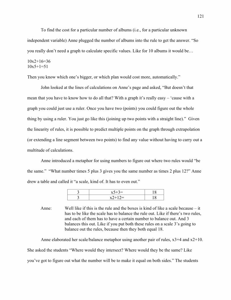
121

To find the cost for a particular number of albums (i.e., for a particular unknown

independent variable) Anne plugged the number of albums into the rule to get the answer. “So

you really don’t need a graph to calculate specific values. Like for 10 albums it would be…

10x2+16=36 10x5+1=51 Then you know which one’s bigger, or which plan would cost more, automatically.”

John looked at the lines of calculations on Anne’s page and asked, “But doesn’t that

mean that you have to know how to do all that? With a graph it’s really easy – ‘cause with a

graph you could just use a ruler. Once you have two (points) you could figure out the whole

thing by using a ruler. You just go like this (joining up two points with a straight line).” Given

the linearity of rules, it is possible to predict multiple points on the graph through extrapolation

(or extending a line segment between two points) to find any value without having to carry out a

multitude of calculations.

Anne introduced a metaphor for using numbers to figure out where two rules would “be

the same.” “What number times 5 plus 3 gives you the same number as times 2 plus 12?” Anne

drew a table and called it “a scale, kind of. It has to even out.”

3 x5+3= 18 3 x2+12= 18

Anne: Well like if this is the rule and the boxes is kind of like a scale because – it

has to be like the scale has to balance the rule out. Like if there’s two rules, and each of them has to have a certain number to balance out. And 3 balances this out. Like if you put both these rules on a scale 3’s going to balance out the rules, because then they both equal 18.

Anne elaborated her scale/balance metaphor using another pair of rules, x3+4 and x2+10.

She asked the students “Where would they intersect? Where would they be the same? Like

you’ve got to figure out what the number will be to make it equal on both sides.” The students

122

reached a consensus that applying 6 to both rules resulted in an answer of 22. Amy explained,

“Cause 6 times 3 is 18 plus 4 is 22, and then 2 times 6 is 12…plus 10 is 22, so that would be

position 6.”

Figure 13. Anne’s scale analogy.

Anne drew a scale with the rules in either pan (Figure 13). She next put a 6 at the top, and

superimposes the number 22 over the two rules on either side, to indicate that they are evenly

balanced. “So now, 6, and now they’re both 22 and so the scale is even.” All of the students

respond enthusiastically, and said her explanation “made a lot of sense.” John wrote down

?x3+4=?x2+10. He used ? to stand for the unknown number that would make the two rules

equal. He stated that the other method they had found, the difference and divide method, allowed

them to work with the numbers that are given in the two rules without the trial and error of

plugging in numbers to find the ones that balance.

Interpretation – The scale analogy and balancing rules

Anne introduced the idea of balancing rules and used an analogy to express her

understanding that rules are “balanced” if they result in the same y-value when the same x-value

was used. Her idea offered another way to think about the balancing of equations, identifying

that for two rules to “balance” both the x and y values have to be the same. The striking aspect of

this conversation was the extent to which it seemed to resonate for every member of the class.

Anne’s scale was different from other scale analogies used in early algebraic teaching, which

have one balance arm and two pans to illustrate that similar operations have to be done to values

6

22 x3+4

x2+10 22

123

in both pans in order to balance the scale. In Anne’s analogy, the pans each contained a pattern

rule that, when the correct x-value is applied, balance the scales with the same y-value.

6.2.8 Lesson 4.3 [Class 11]

Task: In this class the students were each given a graph showing two intersecting lines, and were

asked to create a word problem that would explain the graph in terms of comparing two rates of

growth, and to develop contextual questions related to the graph (going from graph to rule to

word problem). There were seven different graphs and each student was given one to work with

(Please see Appendix C).

Kate introduced the activity with reference to the previous activity:

So what I need you to do is, you need to think of some kind of story that would go along with this graph. The story you had last time was about going onto the internet and buying music. One plan had a certain amount one-time membership fee and the other had a different amount one-time membership fee, and there was a different cost for each album. And those rules looked different. You can tell from these graphs that the two rules expressed are different. The students spent the rest of the time working on stories. They had little trouble

imagining life experiences that could be described in terms of linear growth. They did, however

experience some difficulty in thinking about what the constant part of the rule could represent.

For most of the students, the constant was conceived of as something you “already have” or

“already start out with” prior to accumulating something at a steady rate. This was modeled in

the music problem, which had initial fees before you could start downloading, and then the

accumulation of cost at a given rate. Table 10 outlines the contexts students used when creating

their problems.

124

Table 10. Students’ contexts for narrative problems comparing two linear rules. Student - Context Constant Multiplier

Alan – Basketball Pre-determined number of correct free throws per game.

Increased number of baskets scored per game.

Amy – Pen pal letters Pen pal letters already received.

Number of pen pal letters delivered per day.

Anne – Saving for a trip Initial gift of money. Weekly pay cheque. Andrew – Fishing Number of fish you start out

with. Number of fish caught each day.

Ilse – Feeding Turtles Number of pellets of food the turtles have already eaten.

Number of pellets of food each turtle eats in an hour.

Jack – Video rentals Video membership fee. Cost of renting a video per day.

John – School admissions Number of students a school starts with.

Number of additional students per year.

Mandy – Babysitting jobs Initial “getting hired” to babysit fee.

Dollars per hour for babysitting.

Pete – Paintball packages Cost of paintball gun in gift package.

Cost of pellets in gift package.

Teah – Bird eggs Number of eggs each bird pair “already has.”

Number of eggs each bird pair lay each year.

Interpretation – Translating Graphs to Narrative Contexts

This discussion of the translation of a graphical representation into a narrative illustrated

the student’s construction of knowledge as they struggled to relate the values in their narratives

with the values represented on the graph. All students were able to translate the graphical

representations given into word problems in which they compared rates. In their problems, the

constant of the rules represented “something you already have.” The different trend lines

represented differences in the rate of growth, and the intersection point represented the x-value

for which the two rules had the same y-value.

6.2.9 Summary of Lessons 1 to 4

At the group level, the students had utilized the situated abstractions they had already

developed with respect to the connections between pattern rules and graphs to be able to develop

125

a sophisticated understanding about linear rules that have trend lines that intersect. This in turn

allowed them to begin to use a variety of tools and strategies meaningfully in order to find the

value of x that, when calculated with two rules, would result in the same value of y. The list of

conjectures illustrates the progression of the construction of student understanding – from

comparing linear rules, to understanding the point of intersection, to being able to “balance”

linear rules in terms of the values of x and y. This is precursory understanding of balancing two

expressions in an equation of the form ax+b=cx+d. Students had also started exploring the

incorporation of negative values in their rules, and where negative numbers would be represented

on the graph.

Table 11 outlines the activities, tools, and resulting situated abstractions forged at the

group level.

Table 11 – Situated Abstractions forged at the group level about rules that have trend lines that intersect. Lessons Activity Tool/Technique Situated Abstraction

Lesson 2 Given two rules, x3+5 and x2+6, predict where they will intersect

Patterns would have the same number of blocks. Add multiplier and constant of the two rules. Both trend lines would have a point at a particular (x,y) value

If the sum of the multiplier and constant add up to the same amount, the trend lines of the rules will intersect at position 1

Lesson 2 Construct graphical representations of x3+5 and x2+6

One trend line starts 1 lower but grows by 1 more space than the other trend line, so the trend lines “run into each other” at the first position

If one rule has a multiplier that is one higher than another rule, but a constant that is one lower, the trend lines will intersect at the first position

Lesson 2 If the multiplier of the rule is higher (by any amount) and the constant is lower (by any amount) then the trend lines will eventually cross.

Lesson 2 Anne’ questions: Will a rule with a higher multiplier and constant (HMHC) have trend line that intersects with that of

Graphical representation of x2+1 and x3+4

Trend lines can intersect somewhere “behind zero.” There may be position numbers that are negative. If the values of the multiplier and the

126

a rule that has a lower multiplier and lower constant (LMLC)?

constant are different for 2 rules the trend lines will intersect.

Lesson 2 Finding rules that have trend lines that intersect at position 3 with a given trend line. [Given a value of (x,y), what rules will result in the same y-value?]

Graphical representation illustrates trend lines start 3 spaces apart and come together by 1 space each time. Ordering rules numerically by the value of the multiplier – numeric pattern, as the multiplier decreases by 1, the value of the constant increases by 3.

If trend lines start 3 spaces apart, and come together by one space each time, they will intersect at position 3.

Lesson 2 Ordering rules that have a difference of 1 in the multiplier.

Graphical representation shows that, the number of spaces two lines start apart, if they come together by one space each time, they will intersect on the position number that has the same value as the number of spaces apart they started. Ordering rules by the value of the multiplier.

You can work out where trend lines will meet if you know how far apart they start off, and that they come together by one space each time. If the multipliers of two rules differ by one, they will have trend lines that intersect at the position that is the same value as the difference between the constants.

Lesson 3 Considering the intersection point for pairs of rules.

Graphical representation shows how far apart lines start off, and how quickly they come together. Numerically you can plug an x value into the two rules in order to determine which x value will result in the same y-value.

You can work out how long it will take for trend lines to meet if you know where they start off and know the rate at which they are coming together. If an x value, when used with two rules results in the same y-value, you know the point of intersections is (x,y). The correct x-value balances 2 rules because it results in the same y-value.

Lesson 3 Equation written in formal algebraic notation of the form ax+b=cx+d, with each side of the equation representing a linear rule.

Difference between the constants divided by the difference between the multipliers gives you the position number (x-value) of the point of intersection.

Lesson 4 Find the meaning of two rules in a given word problem.

Connect payment plans to rules, and use strategies (above) to solve the problem.

The cost per album is represented by the multiplier in the rule, and the initial membership fee is represented by the constant in the rule. The point of intersection is the number of albums for which you would pay the

127

same amount using each payment plan.

Lesson 4 Find the meaning of two trend lines.

Construct word problem to give meaning to trend lines on a graph.

The rules represent “rates of growth” of something. The constant represents “how much you start out with.” The multiplier represents “how much it increases.” The point of intersection shows the point at which the two rates of growth have the same amount, before which one rate of growth was faster, and after which the other is faster.

128

6.3 Part 3 – Negative Numbers, Pattern Rules, and Graphs

Lesson 5

This lesson was designed to formally introduce negative numbers in the students’ work

with linear relationships. Initially students were asked to brainstorm about what they already

knew about negative numbers. Some of the students (particularly John, Jack, and Pete) had

demonstrated some facility working with negative numbers, however, the rest of the students

were curious about how to incorporate negative numbers into their rules but were unsure how to

do so. The goal of this lesson was to tap into students’ intuitions about and prior experiences

with negative numbers, and to connect these intuitions to two models of representing negative

values – a horizontal number line and a vertical number line. I was interested to determine

whether this would support students in extending the x-axis and y-axis of their graphs in order to

include the other three quadrants of the Cartesian plane.

During this lesson (and subsequent lessons), I also introduced new terminology. I

introduced the convention of referring to the “position number line” as the x-axis, and the “tiles”

or “height” line as the y-axis. The students gradually incorporated these terms into their

discussions, but asked Kate to continue to write rules using the original “tiles and position

number” terminology because they found it “less confusing.”

6.3.1 Lesson 5.1 [Class 12]

Task: Brainstorm about negative numbers. Kate asked, “Where have you seen negative

numbers, or where have you used them or where has someone used them with you?”

The students’ first idea was the winter-time temperature, which in Canada is often

reported as values below zero. Pete introduced a debt analogy, “I guess it would be like you have

minus 50 bucks, you owe it.” Amy built on this idea, and introduced credit cards as a context for

129

owing money, then explicitly linked this with negative numbers. “If you owe someone 10 dollars

you have negative 10 dollars.”

Vertical Number Line

Kate asked for a volunteer to draw what “below zero” would look like in terms of

weather. Andrew drew a vertical line on the board, and added 0 in the middle of the line and

numbered it 1, 2, 3, 4 upward, and -1, -2, -3, -4 downward. Kate related his drawing to positive

numbers (warmer temperatures) and negative numbers (colder temperatures). The vertical

number line model, with values above and below zero, was established.

Anne then made a connection between the vertical number line and elevators. Amy built

onto this idea stating that “you can go to the basement and that’s like below ground, right, like

negative numbers.”

Horizontal Number Line

Kate then asked if they could think of any examples of a horizontal line that would have

negative numbers. Jack mentioned their studies of ancient civilizations.

Anne: BCE would be like before…before common era. That’s like negatives. John: So like the year 0 and then if you go before the year 0 you have BCE. Alan: It’s like 250 BCE would be like minus 250. The students then brought out an example of an ancient civilizations timeline (which the

class had been working on in the previous term). Jack pointed out 2000 to the left on the

timeline.

Jack: [Pointing to the left of the timeline] this is the year 2000 BCE. Kate: [Pointing to the right of 2000] This is 800. Jack: [Moving along the timeline from left to right] 400, 330…30…the end!

130

Amy: [Pointing to the left] It starts way back at the thousands and then goes up to

30 on the right. So the numbers get smaller the closer you get to where the end of BCE is. Like to where year 0 would be.

John: Ya, the numbers get smaller from left to right, up to 0, and then after 0 they

would get bigger. It goes down from 2000 to 30, and then 0, and then it would go up.

Andrew: All of that [indicating the timeline, which only showed years BCE] is like the

minus. If you go that way [gestured to the right of the timeline] it would be the plus.

Kate pointed out that the information on the timeline is organized horizontally, and asked

if there were any other numbers that could also be organized horizontally. Andrew responded,

“position numbers.” This was a connection to the ordinal position cards that had been used

horizontally both in pattern building and on the graph.

Interpretation – Constructing models of negative numbers

The students had several metaphors for negative numbers, including typical examples

such as debt and temperature, and the less typical example of the timeline. By using these

commonly understood metaphors, the values along the number lines were imbued with meaning.

Temperature became the basis for a vertical model of negative numbers, representing negative

(cold) and positive (warm) values. The concept of the timeline underpinned the horizontal

model, with years BCE representing negative values and years CE representing positive.

In both cases the students were familiar with how to represent negative values, “below

zero” starting with negative 1 and going down on the vertical model, and “behind zero” starting

with negative 1 and extending left on the horizontal model. Zero was used as the division

between positive and negative numbers, with the two (positive and negative) number lines

131

mirroring each other on either side. The students knew that the further away from zero, the larger

the numeral (signed or unsigned) became.

Task 2: Kate then drew a graph on the board (upper right quadrant) and numbered the x- and y-

axes with positive values.

She asked the students to think about “how we can draw a graph that will allow us to include

negative numbers. So that we could write a word problem about the weather and it could be

negative 30, or we could write a word problem about debt, and we could represent the word

problem using a graph.”

Jack and John, and Mandy and Teah worked together. The rest of the class worked

individually to create graphs that showed both positive and negative values.

Class Discussion

Kate opened the discussion by saying she was interested in how the students arrived at

their final product, why it made sense to them, and knowing about any difficulties they had had.

She referred to the fact that Amy had had problems thinking about “negative position numbers.”

Amy responded, “In pattern building, how can you have a negative position number? It didn’t

make sense to me. But then I was thinking about when we thought about trend lines that

intersected behind zero, we said like maybe it was position negative 1. Then it started to sort of

make sense.” This may be one reason why the students introduced a timeline as a way of making

132

sense of negative numbers along a horizontal axis. A negative position number in pattern

building does not make sense, but thinking of numbers as representing points along a timeline,

before and after a specific event (i.e., the division between BCE and CE) intuitively had meaning

for them.

The following discussion illustrates the individual contributions of students as they

struggled to integrate the vertical and horizontal number lines with their familiar graphing space.

Although the students had, for the most part, worked independently to construct their graphs

incorporating negative numbers, through collaborative discourse the students achieved a

common conceptual framework.

Alan

Alan had labeled the left hand side of the grid with numbers, starting in the middle at 0

and going up to 21, and then numbering down from 0 to -19. Along the bottom, Alan numbered

from 1 to 41, starting with 1 at the bottom left hand corner. As he presented his graph he said he

“messed up” because he wanted to add negative position numbers (on the horizontal axis) but

wasn’t sure where to put them.

Alan put one zero in the middle of the vertical axis, on the far left side of the page, and

imagined the top half of the graph would be positive numbers, and the bottom half would be

negative. As he was explaining his thinking to Kate, however, he indicated that he “was thinking

about the conversation from earlier, and tried to imagine this half (left side of page) is negative,

and then this half (right side) is positive.”

133

Alan decided that what he needed to do was to move the vertical axis from the left hand side of

the grid to the centre of the grid, so that he would be able to accommodate negative numbers to

the left of the zero along the horizontal axis at the bottom of the page.

Andrew’s Graph

Andrew’s graph had a vertical line in the middle of the page with a 0 in the middle,

positive values above the 0 and negative values below. His graph had a horizontal line at the

bottom of the page with a zero in the middle with positive values to the left and negative values

to the right. The two number lines were not integrated. The numbering of the vertical axis

extended down to -22, but then the next value was the 0 of the horizontal line.

Amy

Amy stated that her original graph had looked like Andrew’s. She had a vertical axis in

the middle of the page, and a horizontal axis along the bottom. Both axes had zero in the middle.

Her vertical axis was labeled with positive and negative values – the negative values from -1 to

-10 but after -10 came the 0 of the horizontal axis.

Amy: I realized that on the thermometer line it didn’t make sense to count down from -1 to -10 and then have 0 again. So I decided to lift the position number line up to the middle and kind of overlap the zeros [gesture lifting the horizontal line from the bottom of the page and placing it in the middle of the page]. That way there was room for negative numbers to go behind the zero and to go below the zero.

134

On her final graph, there was one zero at the origin and the values along each axis were

written along the axes. She initially started with two unconnected number lines, but was then

able to coordinate them by conceptually lifting the horizontal number line from the bottom of the

page and placing it across the vertical number line in the centre of the page in order that the 0s of

the two lines “overlapped” in the centre of the page.

Mandy and Teah

Mandy and Teah recognized that their first attempt looked like Alan’s graph.

Mandy: We began with the thermometer line first on the left side and put a zero in the middle and added negative numbers below zero. Just like Alan and Amy said. But then we knew we needed negative position numbers as well. So we made a second graph and put the 0 in the centre of the page. We went down like this (extending down from the origin to extend the vertical axis) and across like this (extending horizontally to the left of the origin).

Ilse

Ilse had started by drawing a 0 in the middle of her page and then had drawn the x- and y-

axes for positive values, so that her graph looked like a large L. She then extended the horizontal

axis to the left.

Ilse: So mine’s a lot like Mandy and Teah’s. I knew it was supposed to go like this [gestures extending the horizontal axis to the left] because that’s 0, position 0 and negative 1 position, negative 2 position. Those are negative

135

position numbers. And then I knew I had to go below 0, and add negative 1, negative 2, negative 3 [points to values on the vertical axis below 0].

Anne’s Graph

Anne reconfigured the numbering of the existing horizontal and vertical axes along the

bottom and left-hand side of the page.

For the horizontal-axis, she numbered across from the bottom left corner from -5 to 5. She then

numbered up from -5 to 5 on the vertical-axis. She determined where the two zeros were (in the

middle of each axis), and drew two lines, one horizontal and one vertical, from each of the two

zeros. She compared her graph to Amy’s, Ilse’s and Teah’s.

136

Anne: My graph kind of looks like Amy and Ilse and Teah’s, but I did my numbers along the side and bottom, like we usually do. Then I colour-coded it, to make it easier for me visually. So, the bottom half of the graph is red and that’s all the negative numbers, because it’s under the line…the zero line (the horizontal axis) and then these are all the positive numbers above the zero line. And here, this half (the left half) is all green, and the green is all the negative numbers that are behind zero (the vertical axis). And these (to the right) are all the positive numbers in front of zero.

Pete, John and Jack

These students recognized that their graphs were similar to Anne’s. The numbering for

the axes was along the left hand side and the bottom of the grid. There was a 0 in the middle of

each axis. The students drew a line up from, and across from the two zeros to create four

quadrants. The numeric values for each axis “run into each other” in the bottom left corner.

However, the students did not perceive this to be problematic.

Difference in Numbering

The students noticed that all the graphs had “the +,” meaning the two perpendicular axes

dividing the space into four quadrants. Most of the students had worked independently on this

task, and all of them had been able to extend the graphing space to incorporate the other three

quadrants. John pointed out the difference in the numbering – along the edge of the page versus

along the axes. Kate asked, “Does it matter where we put the numbers?” Everyone agreed that, if

you were going to use Amy’s graph or Anne’s graph to represent a rule, the line would look the

same on both graphs. Amy said, “If it was the same rule – it all has the same outcome, it’s the

same graph.” Anne added, “Well if you graphed the lines and then took away the graphs, they’d

look the same. The trend lines for the rules would be the same.”

The Zero Lines and the Zero Point (Ultra Zero)

137

Kate wondered about the fact that there were two zeros on most of the graphs. “Some of

the graphs have one zero and some have two. And the zeros are in different places.” John

compared his graph to Ilse’s to illustrate why, in his opinion, this did not matter.

John On my graph, the zero here (middle of the vertical axis on the left of the page) and the zero here (middle of the horizontal axis at the bottom of the page) end up here (middle of the page). We drew lines to show where the two zeros would meet up, right in the centre on the page. On Ilse’s graph, she just already has the zero in the middle.

Jack added that, for the two zeros, “you just have to find where their lines would intersect so

that’d be, like, here (middle of the page).” Anne called it, “the zero point.” Jack added, “the ultra

zero!”

Anne: On John and Jack’s graph and on my graph the zero point is the point where the two zeros intersect – ‘cause this whole line (vertical axis) is the zero position number, and that whole line that way (horizontal axis) is the zero tiles number.

Interpretation – Extending the graphing space

Even though the students worked independently and constructed graphs that had some

138

fundamental differences, each student (by the end of the class discussion) forged a situated

abstraction about the construction of the four-quadrant graph. All students incorporated

perpendicular linear representations of number lines with positive and negative values, based on

the integration of the vertical and horizontal models developed during the class discussion.

Connecting the two Graphs

Kate asked the students to think about the graphing space they had been used to using.

Teah and Mandy blocked off the horizontal line behind zero and the vertical line below zero on

their graph.

Kate pointed to the upper right quadrant of the graph on the board, where there are only

positive values, and asked, “Isn’t this what we were dealing with before?” Mandy said, “So the

other three areas are new.”

Kate then asked the students how they would know where they could represent negative

values, where they could represent positive values, and where they could represent negative and

positive values. John answered, “Well, Anne made it colour coded so that might be a way. Like

each box [quadrant] would have a different colour, like it could be – yellow and blue – yellow

139

could be all positive numbers and blue could be all negative and then the other two parts of the

graph would be green.”

Kate drew a large four-quadrant graph on the board and asked, “Which part of this graph

only deals with negative numbers?” Mandy identified the lower left quadrant and labeled it with

a subtraction sign. Her classmates agreed, giving a “thumbs up.” Kate labels the axes with

negative values “so in this area (lower left) it’s surrounded only by negatives. Where are the

regions that have positives and negatives?” Teah answered, “Well there’s two. Down here (lower

right) is negative [gestures down the vertical-axis] and positive [gestures along the horizontal-

axis]; and up here (upper left) is positive [gestures up the vertical-axis] and negative [gestures

along the horizontal-axis].”

Amy added, “It’s like in our little slice of graph that we always use, it’s a tiny slice, it’s a

slice that we’ve always used, and now it’s suddenly quadrupled in size. And if we have all

positives then we’re going to have to have the opposite of all positives and I think that’s what the

lower left is. And also because it’s all there, and you have to see every single number, positive or

negative.”

140

Interpretation – Representing positive and negative numbers in two-dimensional space

When considered on a horizontal number line, positive and negative integers allow two

directions to be used – to the right of 0 (positive) and to the left of 0 (negative). In this activity,

by creating a four-quadrant graph, the students could consider four combinations of values,

positive/positive (upper right), positive/negative (upper left), negative/positive (lower right), and

negative/negative (lower left). The students were able to identify values for the four quadrants or

areas of the graph and label each area according to the values (positive or negative) of the

surrounding axes. The students used colours and mathematical symbols (+ and -) to denote

positive and negative areas behind and below zero. The students had a sense of how the initial

graphing space had been “quadrupled” to incorporate negative values.

Lesson 6

This lesson was designed to have students work with rules with a negative constant,

primarily to think about how they would be represented graphically. Although John and Jack had

begun to incorporate negative numbers into their work with rules (please see Student Case

Studies, Chapter Five), the other students had expressed an interest in doing so but were not sure

how to proceed.

6.3.2 Lesson 6.1 [Class 13]

Alan was absent for this class.

Task: Creating a Graphical Representation for a Rule that has a Negative Constant

Kate wrote “y-number = position number x4-2” on the board and asked the students to

create a graph to represent the rule. I was interested to see whether their experience of creating a

graph for this rule would support two kinds of thinking about “negativity” with respect to the

negative constant – its sign as an integer, and the operation of subtraction.

141

Ilse went to the board and added values to the axes along the left side and bottom of the

graph. She then plotted the y-intercept of the rule. “So times 4 minus 2…it would be here

[plotted point at (0,-2)].

Kate asked John how he figured it out.

John: Because if you just plug 0 in for this (indicating “position number”) 0 times 4 is 0 and then 0 minus 2 is…

Amy: Negative 2! Ilse: [Plots y-intercept -2 on the graph]. Pete: [Pointing to the graph] Ya, negative 2.

John’s explanation demonstrated his understanding of “position number” as a variable for

which any number can be substituted. In this exchange, Ilse, John, Amy and Pete incorporated

their understanding of the “negativity” of the constant as both a negative integer, -2, and the

subtraction of 2 from 0. They were also able to apply their established heuristic of how to plot

the y-intercept for rules with positive constants in order to plot the y-intercept for a rule with a

negative constant.

Jack then demonstrated how to plot the points for the first few position of the rule.

142

The first position is times 4, so 1 times 4 equals 4 and then you do minus 2, which equals 2 [plots point on the graph at (1,2)]. Two times 4 equals 8 and then you subtract 2, which is 6 [plots point at (2,6)]. Three times 4 is 12 minus 2 is 10.

Interpretation – Connecting negative constant, negative numbers, and subtraction

In this class, the students were introduced to a negative constant both as a signed number

and as representing the operation of subtraction. The negative constant meant that the y-intercept

was a point at a negative value on the y-axis. The students knew where to situate the y-intercept

based on their experience of constructing graphical representations for rules with positive

constants, and knowing that the point on the y-axis (or zeroth position) represents the value of

the constant in a pattern rule.

The negative constant also meant that a constant amount had to be subtracted as each

point was plotted. Jack created a graph of a rule with a negative constant by calculating the rule

at successive position numbers and subtracting the constant amount instead of adding. The

physical plotting of points, and the contrast of counting down for a negative constant (subtracting

a constant amount from each point) vs. counting up to plot points for pattern rules that have a

143

positive constant (adding a constant amount to each point), reinforced the notion of directionality

of negative and positive numbers, in this case oriented to the vertical axis as the number line.

Task: How to Use a Rule with a Negative Position Number

This was a student-driven inquiry. Amy asked how to calculate the rule x4-2 for a

negative position number (x-value). The students had successfully figured out how to plot the

points for a rule with a negative constant for positive position numbers (x-values), but many of

the students were unfamiliar with how to multiply with negative numbers.

How would we do the rule with a negative position number? Like if you were going to times negative 1 by 4, would it get an even more negative number, or a less negative number? Would we go directly into negatives? I suppose we would, because I guess it would be there, it would be in this general area (pointing to lower left quadrant).

Amy reasoned that if the negative position number was plugged into the rule, and combined with

a negative constant, the resulting y-value would likely be negative, and the point would be

somewhere in the lower left quadrant.

Anne looked at the trend line on the graph, and agreed with Amy.

Anne: If you’re going backwards [to the left] it [the trend line] would be lower instead of higher.

Jack: Ya, like this [positive trend line] tells us the number of tiles is increasing

each time, even if in this rule you take some away. But if you go behind zero the line would go down.

Ilse: That’s really weird. John: So the line would be going down from zero if we look at it backwards. Amy: And then we have to minus the constant! How the heck do we do that?

The students’ understanding of the trajectory of a trend line on the graph (which they

knew was straight) and their understanding of negative numbers resulted in an intuition about the

144

values of the trend line “behind zero.” For negative position numbers (x-values), the y-values

decrease. The students discussed that even though the rule x4-2 incorporates multiplicative

thinking (growing by a constant amount) the value at a negative position number would actually

be lower than the y-intercept. By looking at the trajectory of the line on the graph, they knew that

the y-value at position -1 would be lower, but were unsure of how to calculate the rule with a

negative position number. They had figured it out visually, but then wanted to make sense of it

operationally/numerically. And, as Amy added, they also had to calculate the negative constant.

Task: Calculate The Rule x4-2 with Position -1. Boys’ Group Solution (John, Jack, Andrew, Pete)

Jack’s first solution was to “forget about the negative, deal with the times 4, which is…4.

And then you just add back the negative.” Pete added, “So it would be negative 4.” Jack

suggested ignoring the sign of the -1, calculating 1 x 4, and then adding the sign onto the

product. John and Pete questioned the validity of Jack’s method, “I’m not sure you can just take

the negative off and put it back on” and introduced a more conceptual approach. “Another way

to think of it is if one person doesn’t have enough cookies, and there are four people who don’t

get one, then there are four negative cookies.” Jack extended this, “Four people are each owed

one cookie. And then minus 2 is…6 cookies owed. Negative 4 minus 2. Negative 4 minus 2

equals negative 6.”

The boys then drew a number line and label it from 0 to negative 6. Pete had learned

during his preparation for the SSAT exam (Secondary School Admission Test) that “you always

go right when adding on the number line, and left when subtracting on the number line.” He

demonstrated how to start at -4, but then go left 2 spaces to end up at - 6. “So negative 4 minus 2

[written as (-4)-2] would mean going left from -4 on the number line, which would be negative

145

6.” He then related this to the vertical number line. “So if you have a point at the negative first

position at negative 4 (-1, -4) and then you subtract 2, it would mean going down 2 more to

negative 6 (-1, -6).

Interpretation – Multiplying and subtracting with negative numbers

The boys’ group proposed two strategies to conceptualize how to multiply with negative

numbers. The first was that the sign of the number could be removed and then replaced once the

calculation had been carried out. This strategy was questioned by the other members of the

group. The second strategy, based on a metaphor of multiple owing, in which 4 x -1 was equated

with 4 people who are each owed a cookie. In this conception, the minus sign of -1 takes on a

unary function of a negative multiplicand that is multiplied 4 times to result in the product of 4

-1s, or (-1)+(-1)+(-1)+(-1) = (-4).

To combine the negative constant with the negative product, Jack extended the owed

cookie analogy to include 2 more cookies owed, so (-4)+(-2)=(-6). This understanding was then

built on by Pete’s formal knowledge of the number line, and the understanding of the minus sign

as an indicator of subtraction, or moving left. This model incorporated the idea of negativity both

as a points on the number line (-4) and (-6) and the movement left to subtract 2. The boys

utilized an understanding of the direction of subtracting on a number line, and realized that to

subtract a positive number from a negative number means going “further to the left” on a

horizontal number line, or “further down” on a vertical number line.

Girls’ Group Solution (Amy, Ilse, Anne, Mandy, Teah)

Anne used similar reasoning to John’s to explain multiplying with negative numbers, but

instead of an analogy of owed cookies she used the multiplicative idea of “groups of” to explain

her thinking. “Four times negative 1 is like negative 1 four times, it is four negative 1s. Like if

146

you have 4 sets of 1, it’s 4, but if you have 4 sets of -1, it’s -4.” Amy responded, “4 negative 1s.

So it’s definitely going to be in the negatives.” Amy used the phrase “in the negatives” in terms

of where the point would be on the graph.

Amy: OK so 4 negative 1s is negative 4. So that would mean that if the position number was negative 3 it would be negative 12 because three times 4 is 12, so -12 because it would be 4 sets of -3.

Anne: Ya, now we have to add the negative 2 (the constant).

Amy: Would the minus add…if you’re in negative numbers, would the minus make it a lower negative number, as in if you have negative 4 and minus 2 it would be negative 2. OR would it make a higher negative number, as in negative 4 and you add a negative 2 is negative 6.

Amy’s use of language indicates that, at this stage, she has two ways of thinking about

negativity; as a sign, and as the operation of subtraction. However, she used the term “minus”

ambiguously, sometimes referring to the sign of the number “would the minus make it a lower

negative number” or the operation of subtraction. This ambiguity meant that Amy could

conceive of two possible results for -4-2. One was that -4 subtract 2 might result in -2, just as 4

subtract 2 is 2. Her alternative theory was that if you “add” a negative value of 2 to a negative

value of 4, this would result in a “higher” negative number, -6, just as 2 plus 4 is 6. Amy equated

a greater numeral value in a negative integer to a “higher” negative number, perhaps not

realizing that the “higher” the numeral in a negative integer, the “smaller” the numeric value.

Amy: I think negative 4 minus 2….that means that you subtract a positive value from a negative value, which would bring it, closer to the positives. So the answer must be negative 2! ‘Cause if you do 4 minus 2 it’s 2. (This was similar to Jack’s reasoning about multiplying with negative integers, do the operation as if they were positive integers and then “add back the negative” sign.)

Mandy: No, if you add a negative constant you go down.

147

Anne: Ya, you’re taking away more numbers, so you end up with more negatives. So it would be negative 6. Let’s say I owe 4 dollars, and then bought something on my credit card for 2 dollars. Now how much…if I had negative 4, and I bought something else for 2 dollars, now how much do I owe? Now how much am I in debt? How much do I need till I’m back at zero?

Amy Negative 6? But…but I think negative plus negative does equal positive,

but then what does negative minus positive equal? Does it equal negative?

Amy then looked at the trend line on the graph on the board.

Amy Oh! I guess if you add a minus to a negative number it would make it a bigger negative number! So you’d go deeper into negatives. So minus 4 subtract 2 is minus 6.

Interpretation - Multiplying and subtracting with negative numbers

This conversation exemplifies how the students were able to draw new ideas into their

conceptual framework and repair divergent thinking by using a mutually understood frame of

reference. Anne’s explanation, structurally similar to John’s, relied on an already understood

heuristic for multiplying numbers – repeated addition. So 4 x (-1) became (-1)+(-1)+(-1)+(-1) =

(-4). Amy was then able to extend this to solve 4 x (-3) as representing (-3)+(-3)+(-3)+(-3) = (-

12). However, Amy then had difficulty reasoning about the negative constant and whether that

would result in a value that was “closer to the positives” or “deeper into the negatives.” Although

Anne offered a compound debt analogy, explaining the concept of compounding negativity to

create a larger-in-negative number, Amy reverted to a half-remembered prescribed rule that had

no meaning for her. Observing the trajectory of the trend line, and Mandy’s explanation that

“adding a negative constant you go down” (based on her observation of plotting points for a rule

with a negative constant) resulted in a negotiated understanding that the resulting y-value would

be “further below zero” and the point would be at (-1,-6).

148

As the girls completed the graph, Amy confirmed her understanding of calculating with

negative numbers.

Amy: In negatives, everything’s kind of opposite, because with subtraction it actually brings you closer to 0 in the positives, because if you have a number and you subtract 2 it gets you closer to 0. But if you add the minus 2 to a negative number then you would get further away from 0.

At this point, Amy’s use of the term “minus” is less ambiguous, and seems to refer exclusively to

the sign of the number. For positive numbers, Amy understood that subtracting means moving

towards the zero on the number line. For negative numbers, she recognized “minus 2” as a

negative integer when, added to another negative integer, resulted in a number that is “further

away from zero” or “deeper into the negatives.”

Task: Construct a Graph with a Negative Constant x6-3

Kate then asked the students to individually construct a graph of the rule y-value =

position number x6-3. The following example of Ilse’s thinking is representative of how the rest

of the students constructed their graphs. To differentiate the two aspects of negativity, Ilse used

the term “negative” as the sign of a number, and “minus” to indicate subtraction.

Ilse started by plotting the y-intercept. “Now, the rule is 0 times 6 minus 3 so 0 times 6 is

0 minus 3 is negative 3.” This is a blending of the understanding of both meanings of negative

(subtraction and negative integer). She continued calculating the rule for each position number.

Ilse: Position 2, ok, so that’s 12, that’s 9 [plotted a point at (2, 9)] and then, so 3 that’s 18, that’s 15.

Kate: What are you doing in your head when you say, “3, that’s 18, that’s 15?” Ilse: Timesing it [the position number] by 6 and then minusing 3.”

149

Ilse then calculated the rule for position negative 1. “Negative 1 times 6 is negative 6,

minus 3 is negative 9.” She plotted a point at (-1,-9). I asked her if she thought that was the

correct answer. She confidently replied it was, “Because it makes a straight line. It’s a nice way

to visually check and see if I’m doing it right.” Ilse used the trajectory of the trend line to check

the correctness of her calculations.

“Ok position negative 2, that would be negative 12 so…wait…(stops and thinks) no wait

it’s negative 12, so that’s negative 15.” Ilse carried out the two operations of the rule, and

combined the resulting two negative numbers. She added this point (-2, -15) to her graph.

Ilse smiled and said, “Doing everything opposite makes me feel funny!” When

calculating the rule for positive values along the horizontal axis, a negative constant meant

subtracting the value of the constant at each point. When calculating the rule for negative values

on the horizontal axis, instead of subtracting she had to add the value of the constant to the

150

product of a negative position number and the multiplier of the rule. When plotting points in the

lower left quadrant from right to left, the trend line got lower. “And negative 3, that’s negative

18, that’s negative 21. Negative 4, that’s negative 24, that’s negative 27.” She could see that her

answers were correct, however, because they follow the trend line of the rule.

All the students were able to successfully plot the trend line for the rule x6-3 for both

positive and negative x-values. They used their knowledge that a linear trend line follows a

straight trajectory as a tool for checking their calculations for multiplying and adding with

negative integers.

Interpretation – Constructing a connection between positive and negative numbers

By the end of the tasks, the students had begun to regard both positive and negative

numbers as part of one single coherent system (rather than two separate number systems) with

unified operations that hold regardless of the sign of the number. This was evidenced in their

ability to multiply a negative and positive number, and to recognize that subtraction always

entails moving to the left (on a horizontal number line) or down (on a vertical number line)

whether the starting number is to the left of, or below, zero.

The class had started to forge a number of situated abstractions:

1. A rule with a negative constant has a trend line with a y-intercept below 0;

2. When plotting points for a rule with a positive multiplier and a negative constant,

calculate the rule for the position number and subtract the constant (move down

the graph);

3. Multiplying a positive number and a negative number leads to a negative number.

On the graph, multiplying a negative position number with a positive multiplier

151

results in a negative y-value so the point is in the lower left quadrant (this is

before adding or subtracting the value of the constant);

4. Subtracting a positive number from a negative number is like adding two negative

numbers – it results in a negative number that has a larger numeral, but is further

away from 0.

6.3.3 Lesson 6.2 [Class 14] Task: Complete a Word Problem Expressing a Rule with a Negative Constant During this class, the students completed the Liga the Dogsitter problem (see Appendix

C). In the problem, Liga is paid a certain amount every day for dog sitting, but owes overdue

fees for renting DVDs. The goal of this lesson was to provide an opportunity for students to

discern a rule with a negative constant presented in a narrative context.

All students demonstrated an understanding that the money owed meant a negative

constant, and rate of pay was the multiplier, or the steepness (growth) of the line. The students

accurately created graphical representations of the rule, and all students labeled the y-axis

“money” and the x-axis “days dogsitting.” To answer questions about the problem, the students

either worked out the answers numerically and then created a graph as a tool to check their

calculations (John, Jack, Anne, Pete, Alan), or created a graph to determine their answers (Ilse,

Mandy, Teah, Amy). Andrew created a modified able of values to represent the relationship

between money and days dogsitting.

This was a short class due to a field trip. There was no time for discussions.

6.3.4 Lesson 6.3 [Class 15] Task: Revisiting Conjectures

For this class we were joined by R, the students’ classroom teacher.

152

During this class, we decided to revisit some of the situated abstractions, or conjectures,

the students had formulated during the first four lessons. With the introduction of negative values

in their rules and the extension of the graphing space to include all four quadrants, I was

interested to see if these new experiences would influence their understanding of the situated

abstractions previously forged, and whether the students would identify a need to adapt their

situated abstractions in light of new experiences.

Kate reminded the class of their conjectures. “We sort of said these are always the case.

But we’ve changed our rules now. Now we have rules that include negative numbers. So what I

want to know is if our conjectures still stand?” Kate made copies of the conjectures to hand out

to the class. To begin the discussion she wrote two rules on the board: x4+2 and x4-2.

Conjecture 1: The multiplier of the rule is responsible for the steepness of the trend line

Kate pointed to the rule with a negative constant and asked, “When we have a negative

constant, is this x4 still responsible for the steepness of the line?” Everyone agreed that it was.

Conjecture 2: The constant is responsible for where the trend line starts on a graph.

Ilse: When we were first talking about graphing, we said that the constant was responsible for where the line starts on a graph because we always started at the 0 position. Now… it kind of doesn’t make sense. You can’t say it “starts” there because now we have behind zero as well.

Mandy: It (the constant) shows you where you start your line on position 0 (the y-

axis). Jack: The constant only tells where the line is on position 0.

The concept of “start” did not make sense since the students were now exploring the

space behind what they had originally considered to be the starting point, the y-axis or the

“zeroth position.” The students suggested altering the conjecture to read, “the constant is

153

responsible for where the line is on the y-axis.” The class agreed that this made more sense. Amy

added that it still helped to look at position 0 on the graph to figure out the value of the constant.

Conjecture 3. Rules with the same constant and different multipliers will start at the same place

but have different steepness.

The students reasoned that two rules, x4-8 and x2-8, would have trend lines that have a

similar y-intercept, but would be different in terms of steepness.

Conjecture 4. Rules that have the same multiplier will have parallel trend lines.

Kate then pointed to the two rules on the board, x4+2 and x4-2, and asked, “Are those

two rules going to have trend lines that are parallel?” Ilse, Teah, Anne and Amy all responded no

immediately. The other students look confused. Kate then led a discussion about the notion of

“parallel.” She covered the x4-2, pointed to x4+2 and asked, “What rules would result in a

parallel trend line if you thought about your rules from before, from when you worked only with

positive numbers?” Only Jack and Mandy raised their hands. Kate asked, “What is parallel?

What do I mean when I say, ‘parallel trend lines’?”

Teah gave an answer based on the visual characteristics. “It’s where two lines are right

beside each other, and one line isn’t going off to the side they’re just going perfectly beside each

other and they’ll never meet.” At the same time, both Ilse and Mandy gestured with their

hands/fingers two lines running parallel to each other.

154

Pete added that it has to do with the multiplier, because the multiplier determined the

angle, or the steepness of the line, so if the multiplier is the same, the steepness of the lines will

be the same and they will not meet.

Kate again pointed to x4+2 (covering up x4-2) and asked for an “all positive rule” that

would have a parallel trend line. Everyone raised his or her hand. Teah offered “times 4 plus

anything…”

Kate pointed to the two rules, x4+2 and x4-2 and asked, “Would the trend lines for these

two rules be parallel?” Everyone gave “thumbs up.” Teah explained that they have the same

multiplier, and so both lines would have the same steepness. Ilse agreed.

Ilse: They are parallel because it means that both the rules are at the same speed. Like the lines are going up by 4 every time the same as this one, so they’re going at the same speed.

Kate: Are they going to intersect? Ilse: No, because they have the same multiplier and so that makes them go up at the

same speed. But they start at different places. Kate asked the class why they were initially unsure whether the rules x4+2 and x4-2

would result in parallel lines.

Ilse: Because we’ve just started thinking about negative numbers, and it just kind of made us think more and before we just knew it off the top of our head. We thought it was maybe different, putting the negative constants in the rules, but it wasn’t.

Interpretation – Refining previous conjectures with negative numbers

Considering their conjectures with negative numbers gave the students an opportunity to

further refine their ideas. The new four-quadrant graphing space presented a different context for

considering the connection between the value of the constant in a rule, and the point on the

155

“zeroth position” on a graph. The constant of the rule was no longer thought of as indicating

“where the line starts” but rather where the line is on the zero position, or y-axis, since the term

“starts” was no longer meaningful given the other three quadrants of the graph

When revisiting the second conjecture, the consideration of negative numbers shook what

had seemed a firm belief that rules with the same multiplier have parallel trend lines. The

definition of “parallel” needed to be re-established – first through the use of metaphor (Teah’s

train tracks) and visual imagery (Ilse’s and Mandy’s gestures). The students then referred to their

previous situated abstraction that the multiplier is responsible for the steepness of the trend lines,

and that rules with the same multiplier have parallel trend lines. This previously held conjecture

was refined to include the idea that the value of the constant of the rules could be either positive

or negative, and that what was crucial was the value of the multiplier – as Teah put it a parallel

trend line would be the result of a rule that was “times 4 plus whatever.” The students revised the

conjecture without constructing a graphical representation, but by relying on their intuition and

logical reasoning.

The explanation that Ilse offered as to why the class was unsure whether the two rules

would be represented by parallel trend lines emphasizes the fact that the mathematical

understandings the students abstracted during their work were modified and refined as they

encountered new experiences. The situated abstraction that had seemed firmly entrenched – rules

with the same multipliers have parallel trend lines – required further consideration when one of

the rules had a negative constant. The result of this exercise meant that the students developed an

even more generalized understanding that two rules with the same multipliers, regardless of the

value of the constant (positive or negative) will have parallel trend lines.

156

Conjecture 5 - Rules with a different multiplicative and a different constant will intersect at some point.

Kate wrote two rules on the board, x5+8 and x3+2. “We have two rules with a different

multiplier and a different constant, I want to know if it’s true or false that the trend lines will

intersect at some point.”

At first, the students indicated “true,” “thumbs up.” Alan, Jack and Anne then disagreed.

Anne explained, “Because that one will start higher (pointing to x5+8)… and grow by more than

that one (x3+2).” The students referred back to one of their first situated abstractions, that in

order to have intersecting trend lines, one rule has to have a lower constant but a higher

multiplier (HMLC LMHC).

John explained why he thought the conjecture was true based on an idea that came up in

one of the first classes. When they were graphing only in the first quadrant, they could see that

two lines were angling out from each other, but they could not actually see the point of

intersection. They had had to infer it from the behaviour of the two lines that seemed to be

“moving away from each other” using the restricted window of the first quadrant. “But then we

realized they would intersect somewhere behind zero.”

Kate asked the class to prove or disprove the conjecture by constructing a graph of the

two rules. “In the past, we’ve always proved or disproved an idea by creating a graph.”

As they worked on their graphs, their teacher R asked the students how they calculated

the points for negative x-values.

R: [Pointing to (-3,-7) on Teah’s graph] What’s that point ? Teah: The negative third position. R: How do you know the value to put there?

157

Teah: I’m doing x5+8. R: Is negative 3 the variable? Teah: It’s the position number. So you take whatever position number, do the rule,

and get the y-axis number. Amy: So negative 3 times 5 is negative 15 plus 8 is negative 7. R: Wait a minute…negative 15 plus 8? Alan: Ya, cause when you add a positive to a negative, it moves it closer to zero. R: Ya, oh you’re right, I’m so sorry! Jack: Because the multiplier says the steepness, and then the plus 8 is always there. A way of checking if you’re right is to see if it’s on the line. Once they had constructed their graphs, the students agreed that the two rules on the

board had trend lines that intersected at the negative 3rd position, at negative 7 (-3,-7) in the

negative/negative quadrant of the graph.

Interpretation – Re-establishing conjectures

The students revisited the notion of rules that have trend lines that intersect behind zero.

Most of their experience with graphs had been working in the first quadrant, and their initial

conjecture about rules that had lines that intersected in the first quadrant (HMLC LMHC

conjecture) was firmly entrenched. Once they had created their graphs they realized that the

trend lines did intersect.

Also of interest was how the students plotted points for rules with positive multipliers and

positive constants at negative position numbers (x-values). Some students used an explicit

approach. For each point, the students knew they always had to add 8, whether the product of the

multiplier and position number was a negative or positive value. To plot the point for position -3,

they calculated 5 x (-3) and then added the constant by starting at point (-3,-15) and counted up 8

158

spaces to (-3,-7). Had they not realized that the sign of the number indicates the direction of the

movement (down for subtraction, or up for addition) they may have added the 8 to get a total of

(-23). In fact, in the dialogue presented, it seemed that R was confused about the direction of

adding a negative and positive number. However, the students had developed a sophisticated

heuristic for calculating rules with positive multipliers for negative position numbers. This was

grounded in their experience of adding, or “counting up” when plotting points for rules with

positive constants, along with an understanding that adding a positive to a negative number

results in a number closer to 0. The students also knew they could use the trend line to determine

whether their numeric calculations made sense.

Other students used a recursive approach. These students subtracted the value of the

multiplier as they plotted each point from right to left, and followed the trend line “behind zero.”

Lesson 7 – Negative Multiplier

This lesson was designed to allow students to explore rules with a negative multiplier,

initially using a “shrinking” linear pattern model. Students were asked to create graphical

representations of rules with negative multipliers, and to think of narrative contexts that would

express the relationship. Alan was absent for this lesson.

6.3.5 Lesson 7.1 [Class 16] Task: Experimenting with Shrinking Patterns

Kate referred to the students’ prior pattern building experiences with linear growing

patterns in Grades 4 and 5. She introduced the activity, to consider a pattern that follows the rule

“number of tiles = position number x(-2) + 8.” Kate told the students that she would be using two

different colours of tiles, and that the two colours were going to represent positive and… “ Anne

interjected, “And one colour represents the negatives!” The students decided that yellow tiles

159

would represent positive numbers, and blue tiles would represent negative numbers. Using the

rule, Kate asked how many tiles would be at the 0th position? The students agreed that there

would be 8 “positive” tiles at position 0, because the constant is “plus 8.”

Kate made a 2x4 array of yellow (positive) tiles at position 0 and asked them to predict

how many yellow (positive) tiles would be at the first position of the pattern.

Amy: So it’s 1 times negative 2 plus 8. All: Six! Kate: Six positive or negative? Anne: Positive. Amy: The positives are going to decline by 2 every time! Jack: Yep, that’s how it works. Kate built a 2x3 array of yellow tiles.

Kate: How many negatives will we have in that? Jack: Two. Anne: Ya, that’s how I was thinking of how to represent the negativeness of the

rule. The fact that 2 were taken away from 8. Maybe put the blue tiles above the yellow tiles?

Kate put the 2 blue tiles above the 6 yellow tiles, to maintain the 2x4 array established at the

zeroth position.

160

Kate: What do you think position 2 of the pattern will look like? Teah: It will have 4 yellow tiles and 4 blue tiles. If we have position 2 and we

times negative 2… Mandy: That would be negative 4. So, position 2 would have 4 blue tiles for the

negative, and like Teah said, 4 yellow ones.

Mandy and Teah calculated the rule with the position number, but also had a visual cue of the 4

yellow tiles decreasing by 2 at each position, and the number of blue tiles increasing by 2 at each

position.

Kate built the third and fourth position of the pattern.

161

Kate asked if this was similar to how they used to build patterns.

Ilse: Our patterns used to look like that, but they didn’t used to use minusing, we didn’t used to use the negatives. Now we use the blue to show how the pattern is getting smaller.

Amy: In this one (pattern), both the yellow and blue are changing. So wouldn’t

none of them be the constant? Because the constant stays the same. Anne: There’s 8 tiles at each position. There’s only 8 tiles every time. Jack: Hey, you’re right! John: So it’s like what’s being taken away from the 8 tiles every time. Kate: So in this pattern, what represents the constant? Jack: The 8 tiles. They don’t change. Kate: And so what represents the multiplier? Andrew: The blue. The multiplier is times negative 2, ‘cause you keep adding 2 blue

tiles each time.

The linear shrinking pattern represents the value subtracted at each position (negative multiplier)

from the original number of tiles (the constant represented by the number of tiles at the zeroth

position).

162

Interpretation – Using a concrete model to represent a negative multiplier

During this activity, the students started with a heuristic of how to represent a rule using a

linear pattern. In their previous pattern building, the two positive parameters of the pattern rule

(multiplier and constant) had been represented by two different colours. In this pattern, the

students were able to modify their interpretation of the role of colour in the pattern to an

understanding that yellow represented positive values and blue represented negative values. They

also recognized that it was the number of tiles, 8, which represented the value of the constant.

The linear shrinking pattern visually represented the increase of the “negative 2” of the multiplier

at each position number, and the decrease of the “positive” values.

Task: Continuing to Build the Linear Shrinking Pattern

Kate asked what would happen at position 4. Anne answered, “zero.” Kate asked, “Zero

positive or negative?” and Anne answered, “No, just zero, that’s the answer.” When the rule is

calculated numerically, (-2)x4+8 becomes (-8)+8 = 0, and so the number of positive tiles for the

fourth position would be zero. Anne was considering the numeric answer without referring to the

linear shrinking pattern.

Kate: [gesturing to the 4th position card] So we’re going to leave it with nothing? Amy: No. We’d have 8 little blue squares. Ilse: Ya! Jack: And 4 times (-2) is -8. Amy: Because you minused all you can minus from the positives and so you’d

have 8 negatives. John: It kind of makes sense that it’s (the number of yellow tiles) going down.

Because when it was times 1 (positive multiplier) it was going up by 1 [gestures upward slope], when it was times 0 it was just going straight

163

[gesture horizontal line] so if it’s times negative 2 it would be going down [gestures downward slope].

Interpretation – Connecting the pattern and numeric calculations for a rule with a negative

multiplier

Most of the students were able to use the pattern to see the multiplication of a negative

number resulted in an increase in negative values, and a decrease in positive values. Amy, Jack

and Ilse came to the conclusion that there would be 8 blue (negative) tiles at position 4. Amy

seemed to work this out by looking at the pattern, and observing that at each successive position

number the original 8 positive tiles were reduced by 2 each time, represented by the addition of 2

negative tiles, so that by the 4th position there would be only negative tiles. John connected the

decreasing yellow tiles to his previous pattern building and graphing experiences, and intuited

that, on a graph, a rule with a negative multiplier would result in a trend line that “goes down.”

Jack realized there would be 8 blue tiles by calculating the position number with the rule

to result in a value of (-8), which he knew would be represented by 8 blue tiles. Anne did not

seem to integrate her numeric heuristic with the linear shrinking pattern, as evidenced by her

164

answer that there would be 0 tiles at position 4. By this position there would be 0 yellow tiles

representing the fact that the y-value would be 0.5

Task: Constructing the Graphical Representation for a Rule with a Negative Multiplier

Kate asked the students to plot the trend line for positions 0 to 4 of the rule. The students

used two strategies to plot the trend line for the linear rule with a negative multiplier. Some

students (Anne, John, Pete, Ilse, Jack) used a strategy based on the functional relationship

between position number and y-number, carrying out the calculations with the position number

to find the value of y for the first two or three points. They then relied on a recursive strategy,

which involved subtracting the amount of the multiplier from the previous y-number (from left to

right in the upper right quadrant) so that the negative multiplier represented the successive

subtraction of 2. (Figure 14). Other students (Mandy, Teah, Andrew, Amy) plotted the y-

intercept and then used a recursive strategy of successive subtraction.

When plotting points for negative position numbers all students relied on a recursive

approach of adding the value of the negative multiplier to previous y-numbers, or “going up 2

each time” from right to left. The trend line of the graph in the upper left quadrant was a tool for

checking their calculations, and the correct placement of the points.

5 This is, of course, the x-intercept, a concept we did not explore with the students.

165

Figure 14. Plotting points using an explicit approach and/or a recursive approach.

Confusion with the linear “shrinking” pattern model

Referring back to the pattern, Kate asked, “How many tiles would there be at position 5?”

Amy: Two negative, 2 blue tiles. You’d have 2 blue tiles, right, ‘cause it’s negative 2.

John: But having only 2 blue tiles at position 5 doesn’t make sense, because

there are 2 blue tiles (along with 6 yellow tiles) at position 1. Once you go into negative numbers (once you reach position 5, and the y-value is negative) then it’s 10 blue tiles (which corresponds to -2 on the graph) and then 12 blue tiles (which corresponds to -4 on the graph).

Jack: Ya, but 8 of those are just covering these (pulling out 8 yellow tiles and

putting them underneath the 8 blue tiles at position 5) so it’s like the blue cancels the yellow.

Amy: How can you show the numbers that are going into the negatives, and the

numbers that show that you took away all the positives? Can you use a different colour?

John: That’s what I thought. I think there should be a third colour for the below

zero numbers. Ilse: Wait, what? Jack: So the blue would show how many of the yellow are taken away, and the

other colour would show when the numbers are below zero, so it’s not so confusing.

Explicit Relationship

Recursive Relationship

Recursive Relationship

166

Ilse: Oh, I get it! The students made the decision to “stick with graphs” because they were “less

confusing.” Kate wrote a rule on the board and asked them create a graph:

y-axis number = position x (-4) + 20. The students successfully constructed graphical

representations of this rule.

Interpretation – Recognizing the limitations of the concrete model

The model of the linear shrinking pattern was transparent enough that the students were

able to identify the weaknesses of this type of representation. Although they found the visual

display of positive tiles “going down” somewhat helpful, this was overshadowed by the problem

of representing the number of tiles subtracted each time, versus the number of tiles that

represented a negative y-value. The students recognized the difference between the two types of

negativity, and realized that having one colour of tile represent both “subtraction” and “a

negative value” was problematic.

The students suggested that in order to show that the values were “going into the

negatives” as opposed to just “showing that you took away all the positives” the tiles should be

differentiated by a third colour. There is a distinction between the tiles that were representing the

subtraction of 2 times the position number from the original 8, and the representation of numbers

that would be indicated by values below the x-axis, what the students term the “below zero

numbers.” This distinction does not have to be made numerically, and with the graph is visually

obvious. This is what made the model of a linear shrinking pattern, showing both the constant

and the multiplier at every position, problematic.

167

Task: Student Word Problems for rules with a negative multiplier

Kate asked the students to think of a word problem that could be illustrated by their

graphical representation of the rule x(-4)+20. For these word problems, the students had to think

of a quantity that would start at a certain amount (the constant), and then decrease at a constant

rate (the negative multiplier) (Table 12).

Table 12. Students’ contexts for narrative problems for rules with a negative multiplier. Student/Context Constant Negative Multiplier

John – Company Losses

$20 million a company starts out with

Yearly losses

Pete – Paycheque Deductions

$20 bonus for starting a job at a window company

Cost of each window broken

Amy – Movie rental $20 movie rental money given at the beginning of the week

Accumulated amount to rent a movie each day

Ilse – Buying ingredients

$20 to purchase bake sale ingredients

Amount spent each day buying ingredients

Jack – Buying Hockey Cards

$20 saved up Money spent on hockey cards each day

Anne – Killing Bugs 20 bugs in the house Number of bugs squashed each day

Mandy – Eating Bugs

20 crickets in the frog tank Number of crickets the frog eats each day

Andrew - Savings $20 saved up Amount lent to a friend each day

Interpretation – Transfer linear rules with a negative multiplier into a narrative context

All of the students present except Teah created a word problem. There were two types of

problems. One type was of the systematic disappearance of insects (squashed or eaten) to

represent linear decrease. In these problems the constant was given as an initial amount of

insects, and the negative multiplier was how many insects disappeared per day. With these word

problems, the students were able to create graphical representations of values in the upper right

quadrant, but did not extend their trend lines to the lower right quadrant as conceptually it did not

make sense to them to think about a negative amount of insects.

168

The other students based their problems on systematic decreases in money from an initial

amount. For these problems, the students recognized that they would be able to graphically

represent values for their rule in both the upper and lower right quadrants in terms of both

positive and negative y-values. This was evidenced by the inclusion of a question about the

length of time it would take to go “into debt” (negative y-value).

Task: Large X – Intersecting Lines With Positive and Negative Multipliers

Kate drew a configuration that resembled a large X on the board, with an orange trend

line with a positive slope and a purple trend with a negative slope. This activity was designed to

see whether the students would bring together their understanding of positive multipliers,

negative multipliers, and intersecting trend lines to formulate pattern rules that would result in

this kind of configuration:

As Kate finished drawing the X, the students called out, “One is positive slope and one is

a negative slope.” Kate posed the challenge to the students, “Can you think of two rules that

would have trend lines that intersect like this?” The students worked on the problem and then

shared their solutions in a class discussion.

Group Discussion

All students were able to successfully think of rules that would result in trend lines that

intersect in the configuration of X (see Case Studies, Chapter Seven). Seven out of the nine

169

students chose to use rules that had “opposite” multipliers. Kate asked the students about the

connection between their rules and their graphs.

Jack: Well, a lot of people seemed to use opposite multipliers. Like they used the same number and made one positive and one negative.

Anne: [Pointing to Mandy’s graph] Ya ‘cause like Mandy’s got two rules, and

one was negative 5, and one was plus 5, and because one was negative and one was plus, they go in different directions…

Kate: Why do they go in different directions? Amy: Because if you’re timesing it by negatives, the number keeps getting

lower and lower (points to the negative slope on her graph) but if you times it by positive it keeps getting higher, so one’s going down ‘cause it’s getting the numbers decreasing, and this one’s increasing…

Anne: And for those ones, the opposite ones, it’s like they go by the same angle,

only one goes down and one goes up. Like if the multipliers both deal with 5, like negative and positive 5, if you turned the negative to a positive 5 it would be parallel. So I think they make this X because they are going at the same angle, just different ways.

Interpretation – Comparing trend lines for rules with positive and negative multipliers

During this task, the students extended their understanding of finding rules that calculated

with a value of x would result in the same value of y, and would therefore have intersecting trend

lines. In this exercise one of the rules had a negative multiplier. The students used multiple ways

to solve the problem but all were able to formulate two rules. This is precursory knowledge for

solving equations of the form (-a)x+b=cx+d.

In addition, the students continued to build their knowledge of the direction of the trend

line on a graph as a function of the sign of the multiplier in the rule. In the above conversation,

the students identified that Mandy had chosen to use 5 as the multiplier for both of her rules –

negative 5 in one rule and positive 5 in the other. The resulting trend lines expressed a systematic

decrease in the value of y (negative slope) when the multiplier was negative, and a systematic

170

increase in the value of y (positive slope) when the multiplier was positive. An interesting

speculation introduced was that the angles of the trend lines were the same, even though they

were in opposite directions, because of the value of the multiplier. Anne’s intuition was that

since the trend lines would be parallel – have the same angle – if both multipliers were positive,

then it made sense that the angles of the trend lines were the same when one multiplier was

negative. This was a further indication to the students that the sign of the number is an integral

part of the quantity it represents.

6.3.6 Lesson 7.2 [Class 17]

This was a brief review class. Kate wrote a rule on the board. #of tiles=pos num x(-2)+17

and asked, “What happens when you create a graph for a rule with a negative multiplier?”

Amy: If you made that graph (for the rule on the board) it would keep going down by two every time because it’s times negative 2 plus 17 (gestures going down). So at position 1 it would be here (reaches up) and then down, down, down, down, down, (gestures going down gradually). And it would just keep going like that so it’s actually a really simple way to graph.

Amy built on her understanding of positive multipliers to develop an understanding of negative

multipliers as indicating steady rate of decrease – either in pattern building or the trend line of

the graph – at each successive position number.

Anne: The numbers (y-axis numbers) if you start at the zero position and keep going, the numbers got smaller. So instead of getting bigger and the line going like this [shows angle positive slope with forearm] they just went like that [angled arm downward]. The slope was going down instead of up.

171

Jack: The slope goes down from the 0th position (y-axis) but if you go backwards

from 0 to negative 1, it goes up! Amy: Ya, what’s weird is if you have a negative multiplier and a negative

position number it gets higher (the trend line in the upper left quadrant), ‘cause usually you’d think a negative multiplier and a negative position number must be getting lower, because negatives are lower, but it keeps getting higher in the positives (y-values) when you go into negative position number (negative x-values). It’s really cool.

Teah: I noticed that too. Anne, John: Me too! Pete: This can help you think about why a negative times a negative is a

positive. All: Oh, ya! Cool!

Interpretation – Extending conjectures The students forged additional situated abstractions based on their experiences of

working with negative multipliers:

1. A rule with a negative multiplier has a trend line with a downward slope;

2. A negative multiplier, times a negative position number (x-value), results in a positive y

number.

6.3.7 Summary Lessons 5 – 7

Initially students utilized horizontal and vertical number lines in order to extend the

graphing space to include all four quadrants. Once they had meaningfully created spaces “below”

and “behind” zero they were able to then apply their understanding of working with linear rules

to incorporate negative numbers. They included negative numbers in the constant or the

multiplier of the pattern rules, and calculated points for negative x-values. Students were able to

make connections between the pattern rules and the resulting trend lines on the graph – including

172

developing an understanding that pattern rules with a negative constant would have a y-intercept

below 0, and pattern rules with a negative multiplier would have a trend line that sloped

downward. All students were able to carry out addition and subtraction with negative numbers,

and some students also discovered how to multiply with negative numbers. Finally, students

were able to start to compare pattern rules with negative and positive multipliers. Table 13

outlines the group situated abstractions forged as students worked with negative numbers in the

context of graphical representations.

173

Table 13. Group Situated Abstractions of Negative Numbers.

Lessons Activity Tool/Technique Situated abstraction Lesson 5 Create a graph that

represents positive and negative numbers

Vertical model of a number line with positive and negative values (thermometer) Horizontal model of a number line with positive and negative values (timeline)

1) Overlap the vertical and horizontal number lines. 2) Extend the vertical axis downward (below zero) and the horizontal axis to the left (behind zero).

-OR- 3) Reconfigure the existing axes by re-numbering them with a 0 in the middle. Join up the two 0s with “zero lines” that intersect in the middle of the graph, the “ultra zero” point.

Lesson 6 Construct a graphical representation of a rule that has a negative constant (positive position numbers)

Y-axis as a number line, to plot a negative constant, go down the number line. Trend line as a tool to check calculations.

The y-intercept for the trend line of a rule with a negative constant is a negative number, because the multiplier is 0, and the constant is subtracted from 0. To plot a rule with a negative constant, for every point count down a certain amount to represent subtracting the constant (as opposed to counting up for every point, represented adding the constant).

Lesson 6 Multiplying a negative position number with a positive multiplier number

Multiplication is “groups of” a number, so 4x(-1) is 4 groups of -1, or -4. Take off the sign, do the multiplication, put the sign on again.

Lesson 6 Construct a graphical representation of a rule that has a negative constant (negative position numbers)

To add 2 negative numbers, go to the left on the number line, father away from 0 (boys) To add 2 negative numbers – go down the vertical number line “deeper into negatives” (girls). Trend line as a tool to check calculations.

When plotting points in the lower left quadrant, subtracting the value of the constant (negative) takes the points further away from 0. Adding two negative numbers means you go “deeper into the negatives,” further away from 0 (using either a horizontal or vertical number line).

174

Lesson 6 Solve a word problem about earning money and owing a debt.

Graphical representation of the rule outlined in the narrative – identify constant and multiplier.

Debt can be represented as a negative constant, starting “below zero.” Earning money can be represented as a positive multiplier.

Lesson 7 Linear Shrinking Pattern Linear shrinking pattern – blue (negative) tiles increase at each position, yellow (positive) tiles decrease at each position. This visually illustrates the direction of the trend line of a rule with a negative multiplier (downward slope).

Blue tiles represent the number of yellow tiles that have been “cancelled out” by negative blue tiles. They represent the amount subtracted at each position from the number of tiles you begin with (the constant). Confusion about which tiles represent the number of tiles that have been subtracted from the original number, and tiles that represent negative values (below zero numbers).

Lesson 7 Create a graphical representation of a rule with a negative multiplier

The graph shows a line that goes down a certain number of y-numbers at each successive positive position number (x-value).

Calculate the rule for each position number, multiply with a negative number and then add the constant.

-AND/OR- When plotting the rule, plot each successive point by subtracting the value of the multiplier (recursive graphing left to right). When plotting points for negative position numbers (x-values) add the value of the multiplier (right to left).

Lesson 7 Find the meaning of a graphical representation of a rule with a negative multiplier

Construct word problem to give meaning to trend line on a graph.

The rules represent “rates of decrease” of something. The constant represents “how much you start out with.” The negative multiplier represents “how much it decreases.”

Lesson 7 Determine two rules that, in a graphical representation, would result in trend lines that form the shape of X

Graphical representation Using knowledge of rules with intersecting trend lines, calculate a rule that has a negative multiplier, and a positive multiplier, thinking about how far apart they start (difference between constant) and how fast they come together.

Lesson 7 Graphical representations of a rule with a negative multiplier

Graphical representation The trend line of the graph slopes down. The trend line of the graph is higher in the upper left quadrant, the y-values are positive when you multiply a negative position number with a negative multiplier.

175

CHAPTER SEVEN

RESEARCH QUESTION TWO RESULTS

In this chapter, I present the results for Research Question 2: For each individual student,

what situated abstractions are forged through the webbing of internal resources (intuitions, past

experiences) and external resources (classroom tasks, tools, discourse experience)? One of the

fundamental tenets of Noss and Hoyles’ conception is that webbing is under the learner’s

control. In any learning situation, the student selects particular external resources from those

present in the learning experience, which then interact with the student’s own particular internal

resources (formal and informal knowledge, intuitions and past experiences). Students construct

mathematical ideas that are a product of their current understanding built onto by aspects of the

context in which the learning takes place. “The idea of webbing is meant to convey the presence

of a structure that learners can draw upon and reconstruct for support – in ways that they choose

as appropriate for their struggle to construct meaning for some mathematics.” (Noss & Hoyles,

1996).

In the classroom situation, the tasks and activities presented to the students were external

resources, since they were provided to the members of the class but designed without their input.

The tools used represented another layer of external resource, in that the tools that students

employed and the ways in which they were utilized and modified reflected the formal and

informal knowledge of the individual. Tracking individual’s use of tools within the context of

specific learning experiences made it possible to observe the construction of new internal

resources at an individual level.

In Chapter Six, I outlined the situated abstractions that were constructed collaboratively

by members of the class. However, the notion of webbing and situated abstraction allows for the

176

individual construction of understanding that can both converge and diverge with that

constructed at the group level. This is because, as previously stated, in any learning situation the

resources available signal possible user paths rather than point towards a unique, directed goal.

In this chapter, I will outline how each student constructed his or her mathematical ideas by

drawing on the webbing in unique ways, and the resulting paths of understanding. These will be

presented in two sections:

1. Students’ conceptions of the meaning of the point of intersection;

2. Students’ developing understanding of negative numbers.

These case studies are based on analyses of videotape transcripts, student interviews, and

individual student work. In each case study, I will present examples of both convergent and

divergent points of learning. I will also present tables of situated abstractions created for each

student, with divergences highlighted according to whether they were based in numerical

reasoning (italic) or grounded in graphical representations (bold). Situated abstractions were

coded as divergent 1) when they differed from the group level situated abstraction, whether they

reflected the understanding of one or more individual students, or 2) if they reflected

understanding that developed during individual or pairs/work rather than as part of a whole

group discussion.

177

Question 2 Part 1

7.1 The Meaning of the Point of Intersection

The case studies are grouped according to the primary tool used for problem solving.

Although all students developed fluency in going back and forth between different

representations during the course of the study, by the end of Lesson 4 most students had a

preferred site for problem solving, either graphical, numeric based on modified tables of values,

or numeric based on equations.

7.1.1 Graphical Representations

The following five case studies outline the different ways that students built their

understanding by extending their ability to problem solve using linear graphical representations.

Mandy and Teah developed a strategy of visualization and estimation. Ilse, Alan and Pete used

graphs as a way of meaningfully conceiving equations with two unknowns on one side of the

equal sign, for example, 3 x ____ + ____ = 18. All five students were able to use the graph as a

tool to compare pattern rules based on the “trajectories” of the trend lines (conceiving of the

trend line as modeling movement or growth), and/or on a comparison of the y-intercepts and the

slope of the trend line.

Mandy Case Study Lesson 2

When Mandy worked on the activity to find pattern rules that would have trend lines that

intersect with a given trend line at position 3, she knew the trend line on the graph represented

the rule “number of tiles = position number x5+3,” and she knew the “target” y-value was 18. To

find rules that had trend lines that intersect at (3,18), Mandy used a guess and check system of

guessing rules, checking by creating a graph, and then trying to figure out how to adjust the rules

178

so that they would have a y-value of 18 at position 3. She multiplied different numbers by 3 (the

position number), and then calculated “how much more” was needed to get to 18 to find the

value of the constant.

At the end of this activity, Mandy indicated that given a rule she could visualize what the

trend line would look like. During an in-class interview, when given different pattern rules, she

was able to sketch graphical representations of pattern rules in terms of “where they started” and

“the steepness of the line” based on the value of the constant and multiplier.

Lesson 3

When comparing sets of rules to determine the point of intersection, Mandy’s strategy

was to choose x-value 2 to plug into the two rules, and then determine if she needed to “go

higher or lower,” that is, needed to calculate the rules with a higher or lower x-value. She had a

sense of the movement of the lines on the graph and could work out the point of intersection

without having to construct a graph.

I just apply the rules to the second position [x-value] to see what the answer is. So in my head I do the rule. Like for the first question (x6+2=x5+5), when I used 2, it was just so close – the answers were 14 and 15, so at position 2 it’s just one number away from each other, I knew they [trend lines] would cross at position 3. And that’s how it worked.

Mandy started with a low x-value and calculated the y-value for both rules. She then thought

about “how far apart” the two points were. In this case, at the second position the first rule would

have a y-value of 14 (2,14) and the second rule a y-value of 15 (2,15) so Mandy was confident

that the point of intersection would be at the third position (x-value) because “they were only one

away.” Mandy’s reasoning is based on an ability to visualize the trajectory of the trend lines

based on a comparison of two points on the graph and use that to estimate the point of

intersection. Mandy’s situated abstraction for finding the point of intersection for two linear rules

can be summed up as, if you compare the y-values for an x-value of 2, you can predict the point

179

of intersection by visualizing “how far apart” the two points are, and estimating how quickly the

trend lines will come together (Figure 15.)

Figure 15. Mandy’s strategy for predicting the point of intersection.

Lesson 4

Mandy created a graph for the rules representing the two payment plans and used this to

answer the questions.

Table 14 outlines Mandy’s situated abstractions. As in the tables created for the group

situated abstractions, the students’ tables include four columns including the Lesson number

column. The “Activity” column lists the activity the students engaged in during the lesson. The

“Tools/Techniques” column outlines the tools students used, and/or the techniques they

developed, as they completed the activity. The “Situated abstraction” column contains the

generalized understanding that developed as a result of engaging in the activity and utilizing

tools and techniques in a particular way.

Point of intersection (3,20)

(2,14)

(2,15)

180

Table 14. Mandy’s situated abstractions. Lessons Activity Tool/Technique Situated Abstraction

Lesson 2 Given two rules, x3+5 and x2+6, predict where they will intersect

Add multiplier and constant of the two rules.

If the sum of the multiplier and constant add up to the same amount, the rules will intersect at position 1

Lesson 2 Finding rules that have trend lines that intersect at (3,18) with a given trend line. [Given a value of (3,18), what rules will result in the y-value 18 for position 3?]

Graphical representation – adjusting trend lines by changing the value of the parameters (multiplier or constant)

By changing the value of the multiplier or constant in the rule, you can change the position of the trend line so that it will intersect with another trend line at a specific point (x,y)

Lesson 2 Graphical representation (visualized trend lines)

Given a rule, it is possible to visualize what the trend line will look like with respect to “where it starts” and its steepness

Lesson 3 Considering the intersection point for pairs of rules.

Graphical representation (visualized) of calculated points for position 2 for both rules.

Based on comparing points at position 2 for each of the two rules, and an understanding of the “trajectories” of the trend lines, estimate the point of intersection. Plug in the estimated position number (x) to the two rules to see if this results in the same value of y. If so, the trend lines on the graph will intersect.

181

Teah Case Study

Lesson 2

Teah’s initial understanding about intersecting trend lines was based on their visual

characteristics – “intersecting lines are lines that cross” with no reference to the numeric values

of the rules. When determining rules that had trend lines that intersected at the first position (x-

value 1), Teah used the class conjecture that if the sum of the multiplier and constant for both

rules equals the same amount, then the trend lines will intersect at the first position.

When Teah worked on the activity to find pattern rules that would have trend lines that

intersect at (3,18) her strategy was to guess a rule, plot the points, and then use the graph to

determine how close the trend line was to intersecting the given trend line. “I’m putting down a

rule [graphing the trend line of a rule] and seeing how close it comes to crossing at position 3,

and then seeing how I have to adjust the rule so it will cross at position 3 at 18.” For instance,

when graphing the rule x2+2 she saw that the point for position 3 was only at a y-value of 8,

which was 10 spaces below the point at (3,18). She reasoned that if she added 10 to the constant,

this would raise the trend line “high enough” to intersect with the point at (3,18), and so changed

her rule to x2+12.

In this activity, Teah’s visual reasoning was combined with a growing understanding of

how the quantities of the multiplier and constant affected the trend lines on her graph.

Lesson 3 - Estimation Strategy

To compare two rules, Teah explained that she did not make a graph, but instead began

by calculating the value for each of the two rules at the 9th position, “I timesed 6 plus 2 by 9 and

times 5 plus 5 by 9.” She then calculated the value for each of the two rules at the 1st position,

and saw that “the rule that was higher than the other at position 9 was lower than the other at

182

position 1, it was different.” If at position 1 one rule had a higher point, and at position 9 the

other had a higher point, she knew that the two trend lines must have crossed. “So you know

where the points for the two rules are at 1, and then you know where the points are at the 9th

position, and they’ve switched. So I know that somewhere in between these two, they’ve

crossed.”

Without making a graph, Teah was able to compare two sets of points, the points for the

two rules at position 9 compared to the points at position 1, and noticed that the point for x6+2

was above the point for x5+5 at position 9 [(9,56) and (9,50)], but below the point at position 1

[(1,8) and (1,10)]. She was then able to infer that the two lines must have crossed at some point

between 9 and 1. By determining the relative “closeness” of points at each of the positions, she

then estimated that the intersection point was closer to an x-value of 1 and estimated position 3.

By plugging 3 into both rules, Teah was able to determine that this was the correct x-value and

that the trend lines intersected at (3, 20). Her strategy included visualization and a consideration

of the movement, or trajectories, of the trend lines in two-dimensional space.

The following diagrams (Figure 16) illustrate Teah’s problem solving strategy. It is

important to remember that Teah did not construct graphical representations, but that her strategy

combined numeric computation with an ability to visualize points and trend lines on a graph.

183

Figure 16. Teah’s strategy for predicting the point of intersection.

When explaining her strategy to the class, Teah went to the board to sketch a graph of the

two rules, although she reiterated that she had not made a graph to solve the problem. Referring

to the two trend lines she explained, “with x5+5, it would start off higher but go like that (flatter

line) and with x6+2 it would start lower and grow faster.” Her use of the phrase “starting off”

and “grow faster” indicated she considered the trend lines as representing movement or rates of

growth.

Point of intersection (3,20)

(1,8)

(1,10)

(9,56)

(9,50) Further apart

Closer together

184

Teah used her intuitions about the trajectories of trend lines to be able to reason about the

behaviour of the trend lines given only two sets of points and comparing their numeric values.

Teah’s situated abstraction for finding the point of intersection for two linear rules can be

summed up as, when comparing two rules, if you compare the y-values for an x-value of 1, and

an x-value of 9, you can determine the point of intersection by judging whether one rule has a

higher point at position 1 and a lower point at position 9 and comparing the relative distance

between the two sets of points.

Lesson 4

Even though Teah struggled with computation, she was able to utilize her ability to

consider the behaviour of trend lines to be able to start to compare rules. Teah used this strategy

when solving the iMusic Purchase Plans problem. After translating both purchase plans into a

rule, she estimated the cost of 6 albums for both plans and then the cost of 1 album, and then

reasoned that, if the rules were graphed, the trend lines would intersect at 5 albums. “They will

cross at 5 albums.” She then constructed a graph to double-check her answer.

Table 15 summarizes Teah’s situated abstractions.

185

Table 15. Teah’s situated abstractions. Lessons Activity Tool/Technique Situated Abstraction

Lesson 2 Given two rules, x3+5 and x2+6, predict where they will intersect

Add multiplier and constant of the two rules.

If the sum of the multiplier and constant add up to the same amount, the rules will intersect at position 1

Lesson 2 Finding rules that have trend lines that intersect at (3,18) with a given trend line. [Given a value of (3,18), what rules will result in the y-value 18 for position 3?]

Graphical representation – adjusting trend lines by changing the value of the parameters (multiplier or constant)

By changing the value of the multiplier or constant in the rule, you can change the position of the trend line so that it will intersect with another trend line at a specific point (x,y)

Lesson 2 Graphical representation (visualized trend lines)

Given a rule, it is possible to visualize what the trend line will look like with respect to “where it starts” and its steepness

Lesson 3 Considering the intersection point for pairs of rules.

Graphical representation (visualized) of two sets of calculated points for position 1 and position 9 of the rule.

Based on comparing two sets of points, at position 1 and position 9, for each of the two rules, and an understanding of the “trajectories” of the trend lines, estimate the point of intersection. Plug in the estimated position number (x) to the two rules to see if this results in the same value of y. If so, the trend lines on the graph will intersect.

186

Ilse Case Study

Lesson 2

When considering the rules x2+6 and x3+5, Ilse realized almost immediately that for

position 1 they would “be the same.” She knew that the sum of the parameters for the two rules

was 8, and declared, “they’re going to be at the same number.” However it was not until Ilse

created a graphical representation of the rules that she realized that this meant that the trend lines

would intersect. “They come together there (1,8), because that’s where they (the two rules) have

the same value.” During the class discussion she explained, “When the values of this rule are the

same as the values of this rule, then they’ll (the trend lines will) intersect.” When questioned

about what she meant by “values”, she replied, “The position number (gesturing horizontally)

and the tiles number (gesturing vertically).”

Ilse then used this understanding to figure out rules that would have trend lines that

intersect at (3,18) by understanding that the rules could be written as 3 x (multiplier) + (constant)

= 18.

I tried out rules, and then I found out that for the multiplier it would always be times 3 because you are doing the rule with the third position. So I multiplied the multiplier by 3 and then filled in the gap to equal 18. So for 1 times 3 it was 3 [pointing to (3,3) on the graph] so then that’s plus 15, and then that’s 18 [pointing to (3,18).]. (Lesson 2.3)

Although Ilse was using a numeric strategy, her site for problem solving was the graph. For each

rule, she located the point on the graph that represented the value of the (3,y) coordinate when

only the value of the multiplier was used, and then counted up to the point at (3,18) to determine

the value of the constant. “Like for this rule, I did 3x3 is 9 [pointing to (3,9)] plus another 9 is

18. So that’s x3+9.” (Figure 17).

187

Figure 17. Ilse’s use of the graph as a tool to formulate equations.

Lesson 3

Ilse created graphical representations to find the point of intersection for pairs of rules in

Lesson 3. When comparing x6+2 and x5+5 she said that she could initially visualize what the

graphical representation would look like.

I know it intersects…it has the same tiles at position 3. Because I work it out in my head. I make the graph in my head. I make the numbers (gesturing upwards) I start by thinking about position 0, whatever the constant is, and then I work it up. After I do that, I check it on a real graph and it works! (Lesson 3.1).

Lesson 4

When solving the iMusic Purchase Plan Problem, Ilse used Amy’s modified tables of

values (see Amy’s case study) and then used the graph to check that her answers were correct.

I wanted to make sure I was right so I just looked at the questions...first I wrote down the numbers. I used the way that Amy had done it. And then I made the graph and then I checked every question and they were all right. (Lesson 4.2) Table 16 outlines Ilse’s situated abstractions.

(3,9)

(3,18)

3 x 3 + 9 = 18

188

Table 16. Ilse’s situated abstractions. Lessons Activity Tool/Technique Situated Abstraction

Lesson 2 Given two rules, x3+5 and x2+6, predict where they will intersect

Patterns would have the same number of blocks. Add multiplier and constant of the two rules. Both trend lines would have a point at a particular (x,y) value

If the sum of the multiplier and constant add up to the same amount, the rules will intersect at position 1

Lesson 2 Construct graphical representations of x3+5 and x2+6

One trend line starts 1 lower but grows by 1 more space than the other trend line, so the trend lines “run into each other” at the first position

If one rule has a multiplier that is one higher than another rule, but a constant that is one lower, the trend lines will intersect at the first position

Lesson 2 Finding rules that have trend lines that intersect at (3,18) with a given trend line. [Given a value of (3,18), what rules will result in the y-value 18 for position 3?]

To find rules that will intersect when the point of intersection is known (3,18) rules can be written as 3 x (multiplier) + (constant) = 18. Graphical representation – adjusting trend lines by changing the value of the parameters (multiplier or constant)

The value of the multiplier times 3 (given x-value) can be located as a point on the graph, and you can then determine “how much more” is needed to reach 18 (given y-value). This is the value of the constant.

Lesson 2 Graphical representation (visualized trend lines)

Given a rule, it is possible to visualize what the trend line will look like with respect to “where it starts” and its steepness.

Lesson 3 Considering the intersection point for pairs of rules.

Graphical representation

Lesson 4 Find the meaning of two rules in a given word problem.

Connect payment plans to rules, and use modified ordered table of values. Graphical representation to check calculations.

You can list the cost for each of the albums for two payment plans and compare. The number of albums for which both plans have the same cost indicates the point at which the trend lines will intersect on the graph.

189

Alan Case Study

Lesson 2

Alan’s conception of intersecting trend lines was initially based on an understanding of

the trajectory of the trend lines, and the connection to the value of the parameters of a rule. For

instance, when asked for two rules that would have intersecting trend lines, Alan offered x6+3

and x5+4, and an explanation of his understanding of why the trend lines would intersect.

Alan: Um, times 6 plus 3, times 5 plus 4.

Kate: Good. How did you know that?

Alan: Well…say the multiplier 6 and the other one is 5, and then the additive…the constant…it’s like [going to the board] if it’s times 6 plus 3 and times 5 plus 4, then the multiplier in this one [points to x6+3] is more, but the constant in this one [points to x5+4] is more so…

Kate: So what does that mean? Alan: That they’re going to cross. Because one is steeper, but one starts higher,

so they’re going to cross.

When describing his thinking for finding rules that had trend lines that intersected at the

third position at (3,18), Alan used both his understanding of arithmetic operations and his

knowledge of how to plot points on the graph to determine rules that would work.

Well, first I tried a rule like times something plus 7. But I knew it had to equal 18 at position 3. So you can’t do plus 7 because 18 minus 7 is 11, and 3 doesn’t go into 11. So I did times 3, which is 9 [points to (3,9)], and then plus 9 gets you up to 18 [points to (3,18)].

Essentially, Alan found his rules by creating equations and then undoing the operations to

find the value of the multiplier. For instance, he tried 3 x ___ + 7 = 18. He then subtracted 7

from 18, leaving 3 x ___ = 11, or 3x=11. Given that we had only used positive whole numbers,

Alan knew that 11 could not be divided by 3, and so tried the nearest multiple of 3, 9. He then

worked out 3 x 3 +9=18.

190

Lesson 3

When predicting the position number at which the trend lines of two rules would

intersect, Alan wrote the rules on the board (x6+2, x5+5), one below the other and asked the

students to look at the constants of the two rules and determine the difference.

Alan: So imagine it’s in two parts. The multiplier and the constant. So, you go to the constant and …well…what plus 2 equals 5?

All: 3! Alan: So you know that they’re going to intersect at position 3!

Kate asked Alan if his strategy would always work, and he responded with another example to

prove his theory, “Ya, you always look at the difference between the constants. Like for the next

two rules (on the problem sheet) x3+3 and x4+1, they intersect at position 2.”

Alan’s reasoning was based on the class discussions (Section 6.2.3), when students

considered the difference between two constants (or where the trend lines start) as a way of

determining the position number at which they would intersect. In each of these examples, the

difference between the multipliers is one, and so the difference between the constants is the

position number at which the trend lines would (see Figures 10 and 11). However, this strategy

will only work for rules with a difference of one between the multipliers. For any other pair of

rules, the difference between the multipliers needs to also be calculated and divided by the

191

difference between the constants in order to figure out the point of intersection (see Figure 12).

At this point, Alan seemed to have over-generalized understanding that calculating the difference

between the constants would result in the position number at which any two rules would

intersect.

Lesson 4 Although Alan used equations to find a particular point of intersection for two rules,

when comparing rules in a more global way Alan constructed a graph. To compare the rules in

the iMusic Purchase Plans problem, Alan believed that a graph was the most efficient way to

determine “how expensive they each got.” A graph was also the easiest representation with

which to find the point of intersection, representing the number of albums for which the two

plans had the same cost, and to find specific values (such as how much 10 albums would cost on

each plan).

Table 17 outlines Alan’s situated abstractions.

192

Table 17. Alan’s situated abstractions. Lessons Activity Tool/Technique Situated Abstraction

Lesson 2 Given two rules, x3+5 and x2+6, predict where they will intersect

Trajectory of trend lines on a graph.

If the multiplier of one rule is higher the line will be steeper (grow faster) and the constant is lower (starts lower), but the multiplier of the other rule is lower the line will be flatter (grow slower) and the constant is higher (starts higher) then the trend lines will cross.

Lesson 2 Construct graphical representations of x3+5 and x2+6

One trend line starts 1 lower but grows by 1 more space than the other trend line, so the trend lines “run into each other” at the first position

If one rule has a multiplier that is one higher than another rule, but a constant that is one lower, the trend lines will intersect at the first position.

Lesson 2 Ordering rules that have a difference of 1 in the multiplier.

Graphical representation shows that, the number of spaces two lines start apart, if they come together by one space each time, they will intersect on the position number that has the same value as the number of spaces apart they started. Ordering rules by the value of the multiplier.

You can work out where trend lines will meet if you know how far apart they start off, and that they come together by one space each time. If the multipliers differ by one, they will have trend lines that intersect at the position that is the same value as the difference between the constants.

Lesson 2 Finding rules that have trend lines that intersect at (3,18) with a given trend line. [Given a value of (3,18), what rules will result in the y-value 18 for position 3?]

To find rules that will intersect when the point of intersection is known (3,18) rules can be written as an equation 3 x (multiplier) + (constant) = 18. .

For any known values of x and y, you can think of rules that will have intersecting trend lines using the equation x(multiplier )+ constant = y, where the multiplier and constant can be adjusted so that when calculating the value for x, the result is the value of y. When the value of the constant is subtracted from the y-value, the result must be a multiple of the position number. For instance, 3 x __ + 7=18 will not work, because 18-7=11, and 11 is not a multiple of 3.

Lesson 3 Considering the intersection point for pairs of rules.

If for two patter rules the multipliers differ by 1, then the difference between the constants works out to be the point of intersection.

If the multipliers differ by one, they will have trend lines that intersect at the position that is the same value as the difference between the constants.

193

Pete Case Study

Lesson 2

Pete knew that two trend lines would intersect if one line started lower on the y-axis,

because it had a lower value constant, and had a steeper angle because of the value of the

multiplier, and the other rule started higher but had a flatter angle. His prediction was based on

an ability to visualize the trend lines for rules written on the board.

To find rules that would have trend lines that intersected with the trend line of x5+3 at

(3,18), Pete used a numeric rather than a visual strategy. Pete said, “You multiply the position

number, 3, with other numbers and then see how much more you need to add to get to 18.”

Pete: Ok, for times 3 plus 9, on position 1 it’s going to be 12 so on position 3 it’s going to be 18!

Kate: Ok, so what about another rule? How did you figure out another rule? Pete: I did the same thing – I just counted up! Kate: [Looking at Pete’s list of rules]. How did you do times 2 plus 12? Pete: Ok, 2 times 3 is 6 and the plus 12! After working through the rules numerically, Pete created a graphical representation in

order to make sure the trend lines did intersect at (3,18). For example, he created a graph of the

rule x4+6 and noticed that the trend lines start 3 spaces apart on the y-axis, but came together by

one space at each successive position number (x-value) until they intersected.

They [the trend lines] start here [pointing to the y-intercepts (0,6) and (0,3)] and then at position 1 they’re 2 spaces apart, and then 1 space apart [at position 2] and then they intersect. So they [the trend lines] come together one space each time.

Pete used the graph as a tool to start to make sense of why the set of rules he came up with all

had trend lines that intersected at (3,18). He later shared this realization during a whole class

discussion.

194

Lesson 3

Pete and Ilse were the only two students to create graphical representations as a way of

determining the point of intersection for two rules. Both of these students indicated that they had

a “sense” of where the trend lines would intersect, and both stated that they could visualize what

the graphical representation would look like, based on the rules. After making their predictions,

they created their graphs as a means of specifying the exact point of intersection.

Lesson 4

To solve the problems of the iMusic Purchase Plan Problem, Pete created a graph labeled

Total Number of Albums Bought on the x-axis, and Cost along the y-axis. During an in-class

interview, Pete explained to Kate how he translated the two payment plans into linear rules.

Kate: How did you know which part (of the payment plan) was the multiplication and which part was the constant?

Pete: Um, because…the addition never changes. So if it was, uh, times 2 plus 16

then the 16 would never change. And the times 2 changed every time. And the other rule it was the same thing – the times 5 changed and the plus 1 didn’t.

Kate: How did you relate that to the problem? Pete: ‘Cause you pay them once and you never had to pay again – the $16 – but

you paid the $2 for every album, so every different number you have…like if you have 4 albums then it’s $8 or if you have 5 albums then it’s $10, like for different numbers of albums it (the cost) goes up. But the one time fee doesn’t change, so that’s the constant. The number of albums is like the position number.

In his explanation Pete articulated the distinction between growth and constancy in the

parameters of the linear rule. This is based on his experiences of building patterns for which one

part of the pattern “grew” and the other part of the pattern “stays the same.” This idea also

underpinned the construction of the linear graphs, with the constant as the y-intercept

representing the “starting point” of the trend line of the rule, and the multiplier as the steepness

195

or “rate of growth” of the trend line. As the number of albums increased, which Pete related to

position numbers (x-values, or independent variables) the cost would change, but that the initial

cost was not dependent on the total number of albums bought.

Table 18 outlines Pete’s situated abstractions.

196

Table 18. Pete’s situated abstractions. Lessons Activity Tool/Technique Situated Abstraction

Lesson 2 Given two rules, x3+5 and x2+6, predict where they will intersect

Visualize the trend lines, given two rules.

If the multiplier of one rule is higher the line will be steeper (grow faster) and the constant is lower (starts lower), but the multiplier of the other rule is lower the line will be flatter (grow slower) and the constant is higher (starts higher) then the trend lines will cross.

Lesson 2 Construct graphical representations of X3+5 and x2+6

One trend line starts 1 lower but grows by 1 more space than the other trend line, so the trend lines “run into each other” at the first position

If one rule has a multiplier that is one higher than another rule, but a constant that is one lower, the trend lines will intersect at the first position

Lesson 2 If the multiplier of the rule is higher (by any amount) and the constant is lower (by any amount) then the trend lines will eventually cross.

Lesson 2 Anne’ questions: Will a rule with a higher multiplier and constant (HMHC) have trend line that intersects with that of a rule that has a lower multiplier and lower constant (LMLC)?

Graphical representation of x2+1 and x3+4

Trend lines can intersect somewhere “behind zero.” There may be position numbers that are negative. If the values of the multiplier and the constant are different for 2 rules the trend lines will intersect.

Lesson 2 Finding rules that have trend lines that intersect at (3,18) with a given trend line. [Given a value of (3,18), what rules will result in the y-value 18 for position 3?]

To find rules that will intersect when the point of intersection is known (3,18) rules can be written as 3 x (multiplier) + (constant) = 18. Graphical representation illustrates trend lines start 3 spaces apart and come together by 1 space each time.

For any known values of x and y, you can think of rules that will have intersecting trend lines using the equation x(multiplier )+ constant = y, where the multiplier and constant can be adjusted so that when calculating the value for x, the result is the value of y. If rules start 3 spaces apart, and come together by one space each time, they will intersect at position 3.

Lesson 3 Considering the intersection point for pairs of rules.

Graphical representation shows how far apart lines start off, and how quickly they come together. Numerically you can plug an x value into the two rules in order to determine which x value will result in the same y-value.

You can work out how long it will take for trend lines to meet if you know where they start off and know the rate at which they are coming together. If an x value, when used with two rules results in the same y-value, you know the point of intersections is (x,y). The correct x-value balances 2 rules because it results in the same y-value.

197

Summary of Graphical Case Studies

All five of these students developed an ability to visualize the trajectories of trend lines

on the graph when given a pattern rule. For Mandy and Teah the lines were conceptualized as

having movement representing steady growth, and the point of intersection was considered as the

point at which the two lines crossed. Each point plotted on the graph was considered as a point

tracking the movement of a continuous line. Altering the numerical values in the rule resulted in

changes in the trajectory of the lines, and so manipulating the numeric values resulted in a

change in the trajectories so that the lines would intersect.

Ilse and Pete, on the other hand, used the graph as a tool for formulating equations, for

example 3 x ___ + ___ = 18. Ilse then adopted the table of values as demonstrated by some of

her classmates, and used a graph as a way of “checking her answer.” However Pete continued to

use the graph as his preferred site for problem solving. Alan also used some of the ideas that had

been discussed in class to compare the value of the multipliers and the value of the constants in

two different pattern rules in order to determine the point of intersection. However, during the

final activity Alan stated that he found the easiest way to compare pattern rules was to construct

a graph.

7.1.2 Tables of Values

By Lesson 3, Jack, Amy and Andrew focused primarily on the numeric quantities of

pattern rules and each independently constructed a modified table of values. Jack and Amy

created their tables using recursive reasoning while Andrew’s table was created using explicit

functional reasoning.

198

Jack Case Study

Lesson 2 Based on his knowledge of the connections between representations, Jack intuited that

the rules x2+6 and x3+5 would have trend lines that intersect because one rule started below the

other but grew by more, and the other started higher but was flatter. “Intersect! Right there!

They’re going to intersect and then keep going (crosses arms).” The gestures of his arms suggest

the trend lines represent a rate of movement and that they will run into each other and “keep

going.”

Jack then considered that if the sum of the multiplier and constant for two rules add up to

the same thing, then this would mean that the point of intersection would be at position 1. This

represented a shift from thinking about intersection as two trend lines running into each other, to

considering the point of intersections as representing a specific x and y value. In the next activity,

Jack and his partner John focused on numerically finding rules that, when calculated with the

position number (x-value) 3, would lead to a y-value of 18. Their strategy was to multiply 3 by

successive numbers, and then add the constant to make the value 18. For instance, “ 3 times 4

plus whatever equaled 18.” Jack and John set up a series of equations, 3 x ____ + ___ = 18 and

calculated rules with multipliers from 0 to 6. They then incorporated negative values into their

rules, either as the multiplier or the constant. Jack reasoned that the list could “go on forever”

due to the fact that the incorporation of negative integers meant that they would “never run out of

numbers.” (Lesson 2.3). Unlike John, Jack was not as interested in seeing the resulting rules in a

graphical representation.

199

Lesson 3

During the next activity, Jack also used a numeric approach to determine the point of

intersection for rules such as x6+2=x5+5. Like Amy and Andrew, Jack created a new

representational tool, a modified table of values, to record the y-values for the position numbers

for each rule, based on an understanding that the multiplier drives the growth of the pattern.

Jack created his table of values by writing position numbers 1, 2, and 3 in a column on

the right, and then listed the y-values in a column under each rule. He first explained his initial

theory about whether the trend lines would intersect, and what the y-value would be for each rule

at the first position.

I used the idea that we came up with earlier – that if one of the multipliers is bigger than the other, and the constant is smaller then they will intersect somewhere in front of 0. So, I knew they would intersect. Then I figured out what each of the rules would be at the first position. So for this rule it’s just 6 plus 2, so for the first position it will be 8, then we can add these two up for this (two parameters for the second rule), which will equal 10.

Next, Jack explained his reason for adding the value of the multiplier to each successive position

number by referring to his experience of creating graphs using a recursive strategy of adding the

value of the multiplier to plot each successive point on the graph.

Then I figured this out by looking at the previous graphs we’ve done, and I noticed that it just goes up by – the number from the first position to the second position, and from the second position to the third position, it goes up by the multiplier every time. So that means for this rule, it would go up by 6. So we know that 8 plus 6 equals 14, and then I did 10 plus 5 equals 15. And I knew those two didn’t fit, so I kept going –14 plus 6 equal 20 and 15 plus 5 equals 20. And I knew those were the same number, so that’s where they were connected, that’s where they would go together, third position. They’d intersect! They’d intersect at position 3, and they would have 20 for the tiles number.

200

Jack had originally plotted points on the graph by calculating the rule for each position

number to find the y-value. However, Jack noticed that the points on the graph “go up by” the

value of the multiplier. He then used this recursive reasoning to create a modified table of values.

The values in his chart refer to the points the two rules would have on the graph at each

successive position, as indicated by his use of the phrase “they’d [the trend lines would] go

together in the third position” and “they [the trend lines] would intersect at position 3 and would

have 20 for the tiles number.”

Lesson 4

Jack’s strategy to solve the iMusic Purchase Plan Problem was to translate the purchase

plans into rules, and then carry out the calculations necessary. For instance, when thinking about

the cost for 10 albums on each plan:

Plan A's rule is times 2 plus 16 so 10 times 2 is 20 plus 16 is 36 – ya – and then Plan B's rule is times 5 plus 1, so 10 times 5 is 50 plus 1 is 51. So . . . Plan A had the better rule if you were buying 10 albums. But like we said, if you buy 4 or less, then Plan B is better. That’s the one I would choose because I don’t like downloading music.

Jack explained that he did not use a graph and “just likes thinking about the numbers.” (Lesson

4.2). To compare the two purchase plans he created a chart showing the output values (cost per

album) for each plan and then compared the relative rate of growth of each. He knew that the

201

number of albums for which both plans would have the same cost (5 albums for $26.00) would

be represented by the point of intersection on the graph. He knew for 4 albums or less Plan B

would have a lower cost, and anything above 5 albums Plan A would be the better plan.

Table 19 outlines Jack’s situated abstractions.

202

Table 19. Jack’s situated abstractions. Lessons Activity Tool/Technique Situated Abstraction

Lesson 2 Given two rules, x3+5 and x2+6, predict where they will intersect

Patterns would have the same number of blocks. Add multiplier and constant of the two rules. Both trend lines would have a point at a particular (x,y) value

If the sum of the multiplier and constant add up to the same amount, the rules will intersect at position 1

Lesson 2 Construct graphical representations of X3+5 and x2+6

One trend line starts 1 lower but grows by 1 more space than the other trend line, so the trend lines “run into each other” at the first position

If one rule has a multiplier that is one higher than another rule, but a constant that is one lower, the trend lines will intersect at the first position

Lesson 2 Finding rules that have trend lines that intersect at (3,18) with a given trend line. [Given a value of (3,18), what rules will result in the y-value 18 for position 3?]

Generate a series of equations with different multipliers (starting with 0) of the form x (known position number) x multiplier + constant (unknown constant) = y (known tiles number). E.g., 3 x (multiplier) + (constant) = 18. Confirm by creating graphical representations.

For any known values of x and y, you can think of rules that will have intersecting trend lines using the equation x(multiplier)+ constant = y, where the multiplier and constant can be adjusted so that when calculating the value for x, the result is the value of y. The equations can contain positive values for the multiplier and the constant, a negative value for the multiplier, or a negative value for the constant.

Lesson 2 Ordering rules that have a difference of 1 in the multiplier.

Graphical representation shows that, the number of spaces two lines start apart, if they come together by one space each time, they will intersect on the position number that has the same value as the number of spaces apart they started. Ordering rules by the value of the multiplier.

You can work out where trend lines will meet if you know how far apart they start off, and that they come together by one space each time. If the multipliers differ by one, they will have trend lines that intersect at the position that is the same value as the difference between the constants.

Lesson 3 Considering the intersection point for pairs of rules.

Modified ordered table of values.

You can list the y-value for each of the position numbers (x) for two rules and compare. The position number at which both rules have the same y-value indicates the point at which the trend lines will intersect (x,y).

203

Amy Case Study Lesson 2

Amy expressed no initial intuitions about rules with intersecting trend lines, or about

what the point of intersection represented. She used a “guess and check” strategy to think of a

rule, construct a graph, and determine how close the trend line came to intersecting the given

trend line (x3+5) at a given point (3,18). She then adjusted her rules in order to alter the trend

line so that it would intersect. Amy plotted the points of the rule using a recursive strategy,

starting at the y-intercept and then adding the amount of the multiplier to each successive point

on the graph. Because of this, the adjustments made to her rules were guesses. It was not until

the group discussion that Amy realized that all the rules could be written as an equation: 3 x

(multiplier) + (constant) = 18.

Lesson 3

By Lesson 3.2, as Amy constructed the graphical representation of the rules x3 and x2+6,

she predicted that the trend lines would intersect at position (x-value) 6 based on assessing the

rate at which the lines were “coming together.”

I know they’ll intersect at position 6 because, because they keep getting closer and closer together and we know that if they’re one (space) apart at position 5, then they’re going to be together at position 6, and then they’re going to cross over and go different ways at position 7. They’ll keep going and won’t cross again. (Lesson 3.1)

Her explanation refers to the straight trajectory of the trend lines and their movement as they “get

closer” to each other, cross over, and keep going.

However, to compare other pairs of rules, Amy created a modified table of values that she

termed “a simplified graph kind of thing.” During her explanation to the class, she began by

writing down position numbers from 0 to 3 in a horizontal line on the board. She then drew a box

around the numbers and added the corresponding y-values from x6+2 above the position

204

numbers. “I put the numbers for times 6 plus 2. This would be 2, 8, 14, 20 and I always just

added by 6 (draws +6 above the top row of numbers).

She then drew another box with position numbers, and added the values for x5+5 by “adding 5

each time. I looked at both tables, and I compared the two sets of numbers. I knew that on the

graph, the lines would intersect at 3 . . . at position 3 and both at position 3 have 20.”

Lesson 4

During Lesson 4, Amy used both her numeric understanding of rules and her ability to

create graphical representations. She answered most of the questions of the problem by

translating the two purchase plans into rules and then plugging in different numbers of albums in

order to compare costs. She used the graph as a tool to check her calculations. She also used the

graph as a tool for determining the point of intersection for the two rules and her knowledge that

two linear rules will only intersect at one point in order to figure out the number of albums for

which you would pay the same amount.

You would pay the same amount for 5 albums – only for 5 albums. Before that you would pay more on Plan A, but then after that you’d pay more on Plan B. (Lesson 4.2)

Her use of the phrase “only for 5 albums” suggests an understanding that, for any two linear

rules, there is only one x-value that will result in the same y-value, or that on a graph there is

205

only one point of intersection. She also used the metaphor of the trajectories of trend lines to help

her determine which would be the best Purchase Plan.

I made a graph and you can kind of tell that Plan A just doesn’t get as high as fast as Plan B, so it kind of saves you money in the long run. Like if you order up to 4 albums then Plan B is better, but after 5 albums it just skyrockets – it starts really low but it gets higher really, really fast. (Lesson 4.2)

Table 20 outlines Amy’s situated abstractions.

206

Table 20. Amy’s situated abstractions. Lessons Activity Tool/Technique Situated Abstraction

Lesson 2 Finding rules that have trend lines that intersect at position 3 with a given trend line. [Given a value of (x,y), what rules will result in the same y-value?]

Graphical representation – adjusting trend lines by changing the value of the parameters (multiplier or constant). Adjustment through guessing.

By changing the value of the multiplier or constant in the rule, you can change the position of the trend line so that it may intersect with another trend line at a specific point (x,y).

Lesson 3 Considering the intersection point for pairs of rules.

Graphical representation. As you create a graph, you can predict where trend lines will intersect by considering the rate at which the trend lines “come together.” Trend lines have a straight trajectory. Intersecting trend lines come together, cross, and then get further apart.

Lesson 3 Considering the intersection point for pairs of rules.

Modified ordered table of values (created using recursive reasoning).

You can list the y-value for each of the position numbers (x) for two rules and compare. The position number at which both rules have the same y-value indicates the point at which the trend lines will intersect (x,y).

207

Andrew Case Study

Lesson 2

Andrew’s focus when considering rules with intersecting trend lines was on the

numerical relationships, and less on the behaviour of the trend lines on the graph. Rules that

would have trend lines that intersected at position 1 had parameters that “summed up” to the

same value. He then utilized his understanding of the commutative property of addition to

suggest “switching the plus with the times,” for instance, x2+3 and x3+2 both add up to 5, so the

point of intersection would be (1,5).

For rules that had trend lines that intersected at (3,18), Andrew’s partner Pete reasoned

that all the rules would be multiplied by 3 with “however much more you need to get to 18” as

the constant. Based on this, Andrew calculated rules numerically and checked the rules by

constructing graphical representations.

Lesson 3

To compare the y-values for two rules, Andrew created a modified table of values. When

he was first developing his table, he explained, “I’ve got a chart for each of the position numbers.

Instead of graphing I use numbers. So this is like a mini-graph.” His chart was oriented

horizontally with the position numbers written along the top. The y-value for each position for

each of the two rules was recorded in two rows below.

When Andrew shared his strategy with the class, he identified that he had done “sort of

the same thing” as Amy and Jack. He wrote the position numbers from 0 to 3 in a row and then

put a box around them. He then wrote 5, 10, 15, 20 and 2, 8, 14, 20 underneath the position

numbers, and circled the two 20s and the end of the two rows under position 3.

208

When Kate asked how he had “moved along from 5 to 10 to 15” Andrew answered that

he had done something different than Jack and Amy.

I used the rule instead of adding the multiplier each time. In my head I did 1 times 5 plus 5 – so at position 1 it was 5 times 1, which is 5, and 5 plus 5 equals 10. For position 2, 2 times 5 plus 5, so 10 plus 5 equals 15. So at position 0 it was 0 plus 5.

Andrew calculated the pattern rule for each position number in order to find the y-value, instead

of using recursive reasoning. Andrew’s table was a way of recording the x and y values for the

two rules without having to create the graph. Kate pointed to the circled 20s.

Kate: And when these are the same number… Andrew: That’s where the two lines will intersect.

Lesson 4

Andrew used his “mini-graph,” or modified table of values, to answer the questions for

the iMusic Purchase Plans Problem, and knew by comparing the two rows of y-values

representing cost per number of albums that both plans would charge the same – $26 for 5

albums. He also answered that Plan A (x2+16) was the better plan “in the long run even though it

looks more expensive but plan B costs more even though it looks less expensive.”

Table 21 outlines Andrew’s situated abstractions.

209

Table 21. Andrew’s situated abstractions. Lessons Activity Tool/Technique Situated Abstraction

Lesson 2 Given two rules, x3+5 and x2+6, predict where they will intersect

Add multiplier and constant of the two rules. Switch the value of the multiplier and constant (because a+b=b+a, therefore m+c=c+m).

If the sum of the multliplier and constant add up to the same amount, the rules will intersect at position 1. If the value of the multiplier and the constant of two rules are “switched” the trend lines will intersect at position 1.

Lesson 2 Finding rules that have trend lines that intersect at (3,18) with a given trend line. [Given a value of (3,18), what rules will result in the y-value 18 for position 3?]

To find rules that will intersect when the point of intersection is known (3,18) rules can be written as 3 x (multiplier) + (constant) = 18. Graphical representation as a tool for checking calculations.

Calculate the value of the multiplier times 3 (given x-value) and then “how much more” is needed to reach 18 (given y-value) is the value of the constant.

Lesson 3 Considering the intersection point for pairs of rules.

Modified ordered table of values (created using explicit reasoning).

You can list the y-value for each of the position numbers (x) for two rules and compare. The position number at which both rules have the same y-value indicates the point at which the trend lines will intersect (x,y).

Summary of Tables of Values

Amy and Jack seemed to “discover” recursive reasoning based on their experience of

plotting points on a graph. They then used a recursive strategy to numerically determine the

position number (x-value) at which the two rules would have the same number of tiles (y-value).

Although their modified table of values appeared recursively procedural, they were underpinned

by a great deal of conceptual understanding. Andrew constructed and used his table as a way of

keeping track of the results of successive calculations as he applied the rule to a sequence of x-

values to find the corresponding y-values.

For all three students, the table was described as a “simplified” way of representing the

co-ordinate values of the two rules without having to construct the graphical representation. The

students recognized that when both the x and the y value were the same, this indicated the point

210

at which the trend lines would intersect. They found this tool to be “easier than a graph” because

it meant they did not have to plot points, but could simply compare the numeric values.

7.1.3 Equations

Anne and John initially based their understanding of rules with intersecting trend lines on

the trajectory of trend lines. They then focused on the point of intersection. From there, their

consideration of rules developed from an understanding of where trend lines cross, to an

understanding of how to compare rules written as equations. One type of equation, similar to

those created by other students, had 2 unknowns on one side of the equal sign, x x ___+ ___ = y.

The other type of equation had unknowns on either side of the equal sign, similar to the form

ax+b=cx+d.

Anne Case Study

Lesson 2

The sense of the “movement” of trend lines enabled Anne to predict that two rules, x3+5

and x2+6, would have trend lines that intersect. “It’s (the trend line of x3+5) going to start lower

and then it’s going to keep getting steeper - and then it’s going to meet up with it (the trend line

of x2+6), and then it’s going to go past it because it’s going faster” (Lesson 2.1). Once she had

constructed a graph of the two rules, she further considered the trajectory of the trend lines as

they “come together” to the point of intersection and then “move apart.” After this activity, Anne

considered the point of intersection as the point at which trend lines cross, based on where they

start (y-intercepts) and the trajectories of the lines (based on the value of the multiplier – how

fast they “grow”).

After the final class discussion of rules that have trend lines that intersect at position 1,

Anne agreed with Jack and Ilse’s idea that the point of intersection indicates the position at

211

which two rules would “have the same number of tiles” and that it is possible to determine if

trend lines will intersect at the first position by comparing the sum of the multiplier and the

constant of both rules. This idea was further developed as she completed the activity for

determining rules that would have trend lines that intersect at (3,18). Anne made the connection

that the point of intersection is the point at which two rules, for a value of x (position number)

the values of y (number of tiles) have to be the same. Determining where the trend lines of two

rules would intersect meant knowing the position number and working out how to adjust the

multiplier and the constant of a rule in order to obtain the specified y-value. This was similar to

strategies of other students, however, Anne did not create a graphical representation to check that

her rules did intersect at (3,18). Anne explained her intuition to Kate by referring to her

experience of determining rules that had trend lines that intersected at the first position (x-value

of 1).

Anne: All you have to do…it’s the same thing as the first position. Kate: It’s the same thing. What do you mean it’s the same thing? Anne: Except with 3. You times the position number times the multiplier plus

the constant and that has to equal the same number as each other. Kate: As the other rules? Anne: Yes. Kate: So is that what you’ve been using? Anne: Uh huh. You don’t even have to graph it because you know that here on

the third position it’s 18, so you just have to think of a bunch of rules that equal 18 when you use times 3.

Anne determined rules that would have trend lines that intersect at (3,18) by creating

numeric equations. Knowing the position number was 3, she started with a multiplier of 0 and

determined the constant had to be +18, and continued using this strategy of increasing the value

212

of the multiplier by 1 each time and then determining “how much more” was needed to get to a

y-value of 18. She then generalized this understanding, and stated that it would be possible to

think of rules that would have trend lines that intersect at any position number. “You just have to

pick the numbers, the position number and tiles number, that you want them to meet at.”

Although her thinking is based on her earlier intuitions about the trajectories of trend lines, she

extended this understanding to consider the point of intersection as representing two values,

position number (x) and tile number (y), and the rules as equations that, given a value of x would

result in the same value of y.

You use the rule with whichever numbers (values of x and y) you want them to intersect at. So let’s say for the 10th position I want them (the trend lines) to intersect at 20, so I just do 10 times…and I like to go in order, 0 then 1 then 2 then 3 (for the value of the multiplier)…so 10 times 0 plus n equals 20, so 10x0+20=20. And then you just keep doing that, and if they all equal to 20, then they’ll intersect at the 10th position. (Lesson 2.3). Anne’s strategy was to multiply the position number (x) by a multiplier, and then

determine the value of the unknown constant, which she designated n, needed to equal the

desired value of y.

During the class discussion, she recognized that when the rules were written based on the

numeric value of the multiplier, as the value of the multiplier decreased, the value of the constant

increased by 3. Anne’s contribution to this class discussion was the generalized understanding

that in a set of rules, if the value of the multiplier differed by 1, the difference between the

constants was the value of x at which the two lines would intersect. Anne’s understanding was

based on her recognition of the numeric pattern, and it was her classmates who then connected

this understanding to the behaviour of the trend lines on the graph.

213

Lesson 4

Anne was absent for Lesson 3 (comparing rules). When discussing her solutions for the

iMusic Purchase Problem (Lesson 4) Anne described how she solved this problem by

formulating equations for the two rules, C=Ax2+16 and C=Ax5+1. By plugging in different

values for A (number of albums) she could determine the value of C (total cost of albums). She

used these equations to generate tables showing the total cost for a successive number of albums.

She could then “see” which rule was “going up the fastest,” that is, which payment plan would

lead to a higher total cost of albums. She could also determine the number of albums for which

both plans would charge the same amount.

Anne introduced the metaphor of a balance scale to describe how she thought about

comparing two rules to find “the number where they both equal the same thing.” Her scale was

based on the understanding that to make two rules “equal” you find the x-value that will give you

the same y-value for both rules. She used three different ways to describe her idea, based on her

experience with three different kinds of models of linear relationships. Given two rules, she

asked, “Where do they intersect, where would they be the same . . . you’ve got to figure out the

number that will make it equal on both sides.” In the first part of this statement, “they” refers to

trend lines and “where” refers to the point of intersection (x,y) on the graph. The second part of

the statement seems to refer back to pattern building, with “they” referring to values for two

linear rules, “where” meaning position number (x) and “be the same” referring to y-values. In the

third part of the statement, finding “the number” is finding the value of x that, for both rules, will

lead to the same value of y – making it “equal” for both rules.

By the end of the first four lessons, Anne’s understanding of the point of intersection

developed from considering it as the point at which trend lines crossed, to an understanding that

214

the point of intersection represents “balancing” two rules by finding the value of x that results in

the same value of y. Her site of problem solving went from being graphically based, to being

numerically based using equations and tables of values.

Table 22 outlines Anne’s situated abstractions.

215

Table 22. Anne’s situated abstractions. Lessons Activity Tool/Technique Situated Abstraction

Lesson 2 Given two rules, x3+5 and x2+6, predict where they will intersect

One trend line starts lower but has a higher multiplier so the lines will “run into each other”

If one rule has a multiplier that is one higher than another rule, but a constant that is one lower, the trend lines will intersect at the first position.

Lesson 2 Given two rules, x3+5 and x2+6, predict where they will intersect

Add multiplier and constant of the two rules.

If the sum of the multiplier and constant add up to the same amount, the rules will intersect at position 1

Lesson 2 Anne’ questions: Will a rule with a higher multiplier and constant (HMHC) have trend line that intersects with that of a rule that has a lower multiplier and lower constant (LMLC)?

Graphical representation of x2+1 and x3+4

Trend lines can intersect somewhere “behind zero.” There may be position numbers that are negative.

Lesson 2 Finding rules that have trend lines that intersect at (3,18) with a given trend line. [Given a value of (3,18), what rules will result in the y-value 18 for position 3?]

Generate a series of equations with different multipliers (starting with 0) of the form x (known position number) x multiplier + n (unknown constant) = y (known tiles number)

For any known values of x and y, you can think of rules that will have intersecting trend lines using the equation x x multiplier + n = y, where the multiplier and constant (n) can be adjusted so that when calculating the value for x, the result is the value of y. You do not have to create a graphical representation to know that the trend lines will intersect.

Lesson 2 Finding rules that have trend lines that intersect at position 3 with a given trend line. [Given a value of (x,y), what rules will result in the same y-value?]

Ordering rules numerically. by the value of the multiplier.

As the multiplier decreases by 1, the value of the constant increases by 3.

Lesson 2 Ordering rules numerically. by the value of the multiplier.

If the difference between the multipliers is one, the difference between the constants represents the position number (x) at which the trend lines will intersect.

Lesson 4 Comparing two rules in rate problem.

Create equations of the form C=A x multiplier + constant, where C = total cost, A = albums, multiplier = cost per album, and constant = membership fee. Create table of values to keep track of total cost for increasing numbers of albums for both rules (payment plans)

When given two rules, the rules can be “balanced” by finding the value of x that, for both rules, results in the same value of y. On a graph this would be the point of intersection, but it is not necessary to create a graph to know that the trend lines of the rules would intersect at (x,y).

216

John Case Study Lesson 2

John described his initial intuition about trend lines using language suggesting a

perception of trend lines as representations of linear growth. “Because if one’s higher but doesn’t

grow as much, and one’s lower but it grows more [gestures two lines coming together] then

they’re going to intersect.” (Lesson 2.1). This was grounded in a visual consideration of the trend

lines, seeing where the lines started on the y-axis, and comparing the angle of “growth” for each.

John also considered the connection between the rate of growth of a trend line and the numeric

value of the multiplier, and the value of the constant and how “high” the trend line starts at the y-

axis. Taken together, John could predict whether two rules would have trend lines that

intersected (in the first quadrant of the graph).

When considering rules that would have trend lines that intersect at the third position,

John and his partner Jack used a strategy of multiplying different numbers by 3 and then seeing

“how much more” they needed to add to get to 18. John and Jack included negative multipliers,

and negative constants in their rules (please see John’s Case Study in section 7.2.2).

Lesson 3

After completing the third activity, John investigated rules that were sequentially ordered

by the value of the multiplier, and whether the difference between the constants would be the

position at which the trend lines would intersect. This was based on an idea that he had started to

develop while working on the second activity in Lesson 2.

After working on rules that intersect at position 3 – I was trying to do it from the time that we did it before, I wanted to see if there was a difference in between the numbers. You know like the last time we were saying each time there was a difference of 3 in the constants for each rule that we made . . . before for the 3rd position, so I was trying to see if there was a pattern with that. (Lesson 3.1)

217

John then extended his thinking and developed a generalized theory for a specific set of

rules where the value of the multiplier differed by 1. For instance, he considered the rules x1+4,

x2+8, and x3+12.

When you look at the multiplier part of a rule, and there’s a difference in the (multiplier) number by one – the difference between 3 and 2 is 1, and the difference between 2 and 1 is 1, you could see the difference in between the constants and that would be 4, so that would mean they would intersect on position 4. (Lesson 3.1)

John completed the set of activities in Lesson 3, comparing pattern rules to determine the

point of intersection, by identifying numeric patterns. However, during the class discussion

(Lesson 3.2) the students identified that the numeric difference between constants was

represented graphically by “how far apart the trend lines started” on the y-axis. The difference

between multipliers was identified graphically as “the rate at which the lines come together.”

Following this discussion, John proposed his “differencing and dividing strategy.” He developed

a numerically based heuristic in which the numeric difference between the constants was divided

by the difference between the multipliers, reflecting the graphically based heuristic of

considering how far apart the trend lines start and the rate at which they come together. John

explained his strategy during an in-class interview with a Master of Arts student researcher when

asked to compare two rules written in standard notation, 2x+16=5x+1, to determine the value of

x, which he knew represented “the position number” for the rules. His explanation included

references to his experiences with graphs and pattern building.

John: Well, I would see that the difference between these two (the multipliers) is 3 and that the difference between these two

2x+16 = 5x+1

difference of 3

15 ÷ 3 = 5

difference of 15

218

(constants) is 15. I know that 15 divided by 3 is 5, so I think it’s going to intersect on the 5th position.

Researcher: How would you check?

John: Try it out. So 5 times 2 is 10 plus 16 is 26, and 5 times 5 is 25 plus 1 is 26.

Researcher: What does it mean when you get 26 for both rules?

John: Um, that’s the amount of each pattern and that’s where they would intersect.

Researcher: But I thought you said they intersect at 5?

John: The 5th position! At the 5th position they would both equal 26 tiles – that’s like the numbers they would intersect on. So it would be [drawing a dot on the graph at (5,26)] they would both end up there.

John’s situated abstraction was that for any two rules, if you calculate the difference of

the constants, and divide the difference of the constants by the difference of the multipliers, this

will give you the point of intersection (x,y). In his explanation, John incorporated a reference to

pattern building, that at the “5th position they would both equal 26 tiles,” an illustration of the

point of intersection by placing one point on the graph, and a reference to the trajectory of the

lines by stating that “they would both end up” at (5, 26). John used this strategy to solve the

iMusic Purchase Plan problem during Lesson 4.

Table 23 outlines John’s situated abstractions.

219

Table 23. John’s situated abstractions. Lessons Activity Tool/Technique Situated Abstraction

Lesson 2 Given two rules, x3+5 and x2+6, predict where they will intersect

The rule with the larger multiplier and smaller constant will have a trend line that “starts lower” but “grows faster” than the other trend line

If the multiplier of the rule is higher (by any amount) and the constant is lower (by any amount) then the trend lines will eventually cross (HMLC, LMHC)

Lesson 2 Anne’ questions: Will a rule with a higher multiplier and constant (HMHC) have trend line that intersects with that of a rule that has a lower multiplier and lower constant (LMLC)?

Graphical representation of x2+1 and x3+4

Trend lines can intersect somewhere “behind zero.” There may be position numbers that are negative. If the values of the multiplier and the constant are different for 2 rules the trend lines will intersect.

Lesson 2 Finding rules that have trend lines that intersect at position 3 with a given trend line. [Given a value of (x,y), what rules will result in the same y-value?]

Generate a series of equations with different multipliers (starting with 0) of the form x (known position number) x multiplier + constant (unknown constant) = y (known tiles number). E.g., 3 x (multiplier) + (constant) = 18. Confirm by creating graphical representations.

For any known values of x and y, you can think of rules that will have intersecting trend lines using the equation x(multiplier )+ constant = y, where the multiplier and constant can be adjusted so that when calculating the value for x, the result is the value of y. The equations can contain positive values for the multiplier and the constant, a negative value for the multiplier, or a negative value for the constant.

Lesson 2 Ordering rules that have a difference of 1 in the multiplier.

Ordering rules by the value of the multiplier.

If the multipliers differ by one, they will have trend lines that intersect at the position that is the same value as the difference between the constants.

Lesson 3 Class discussion - Considering the intersection point for pairs of rules.

Graphical representation shows how far apart lines start off, and how quickly they come together.

You can work out how long it will take for trend lines to meet if you know where they start off and know the rate at which they are coming together.

Lesson 3 Equation written in formal algebraic notation of the form ax+b=cx+d, with each side of the equation representing a linear rule.

Difference between the constants divided by the difference between the multipliers gives you the position number (x-value) of the point of intersection.

Summary Equations Both Anne and John seemed to use the graph as a mediating representation from

comparing pattern rules to solving linear equations with an unknown value on either side. By the

second lesson both of these students no longer relied on the graphical representation, but instead

worked only with the numbers. They understood that two pattern rules would be “balanced” if

220

both the x and y value for each rule was the same. Anne’s balancing analogy still required some

guessing and checking when selecting which x-values to calculate to use with the rules in order

to find the same y-value. John, on the other hand, developed a sophisticated “differencing and

dividing” strategy that allowed him to determine the x-value that would result in the same y-

value for both rules.

7.1.4 Summary – Intersecting Trend Lines

As stated in Chapter Four the students came to the instructional sequence with similar

understanding of the connection between linear rules and linear graphs, particularly the

connection between the multiplier and the steepness of the trend line, and the value of the

constant and the y-intercept. As the lessons progressed the students developed an understanding

of the point of intersection of trend lines, using both numerically based and graphically based

reasoning and associated tools and strategies.

Although all students became adept at predicting the point of intersection, or the x and y

values for two rules, and were also able to determine rules that would intersect at a particular

point, their “user paths” differed. Each student either primarily used the graph to plot x and y

values, a table of values, or carried out calculations of the form x x multiplier + constant = y.

Figure 18 illustrates the general learning pathways for the ten students.

221

Figure 18 General learning pathways for the ten students.

Numeric Graphical

Rules that have the same number of tiles at the same position number

Rules that, for the same value of x, result in the same value of y

Where the trend lines cross

The point that represents the same value of x and y for trend lines

The difference of where the line starts and the rate at which the lines

come together

table of values balance model differencing and dividing

visualizing and estimation

Amy

Andrew

Anne

Jack

John

Ilse

Mandy

Teah Pete

Alan

222

7.2 Research Question 2 Part 2

Negative Numbers

As previously stated, most of the students came to the study having had little formal

instruction in negative numbers. Because this was a new area of instruction, most students

reverted to using a graph as the site for problem solving, since this was the most familiar

representation. As the instruction progressed, some students (particularly John and Anne) began

to formulate equations. By the end of Lesson 5, all students created four-quadrant graphs by

incorporating the vertical and horizontal models of number lines. They identified the values for

each of the quadrants of the graph by considering the values on the surrounding axes:

So we're saying this is all positive [upper right quadrant] because these are positive numbers [right x-axis] and these are positive numbers [up y-axis] right? But these are negative numbers [down y-axis] and these are also negative numbers [left x-axis] so that's why this [lower left quadrant] is all negative. And we have a mix [lower right quadrant] when this is negative [down y-axis] but this is positive [right x-axis]. And the same with this [upper left quadrant] because this [up y-axis] is positive but this [left x-axis] is negative. (Alan, Lesson 5.1).

As previously outlined, there are two kinds of negativity that are important to develop

when considering negative numbers. The first is unary understanding, an understanding of

negativity as a point on the number line. The second is binary understanding, an understanding

of negativity as indicating movement along a number line that corresponds with the operation of

subtraction. Students in this study seemed to also develop what I term a multiplicative

understanding of negativity, in addition to a unary and binary understanding. Multiplicative

negativity is the understanding that the product of multiplying negative or positive position

numbers (x-values) with negative or positive multipliers results in a product that is represented

by a point in one of the four quadrants of the graph. The four quadrants as area models of

positive and negative values supported students in their ability to think multiplicatively about

223

negative values. When multiplying positive or negative multipliers with positive or negative x-

values, the resulting point on the graph expressed the sign of the x-value, and the sign of the y-

value based on the influence of the sign of the multiplier. The resulting points could be above or

below the x-axis, and in front of or behind the y-axis in different combinations of positive and

negative space.

In this study, the way in which students created their graphs corresponded to the kind of

understanding of negativity that was supported. Students who created their graphs recursively,

that is, plotting successive points by adding or subtracting the value of the multiplier, developed

an understanding of negativity as being both a point on the x- or y-axis (unary understanding), or

movement along an axis (down the y-axis or left on the x-axis) (binary understanding). These

students also began to identify points within the four quadrants of the graph as representing the

relationship between positive and negative multipliers and positive and negative x-values.

Although they did not multiply with negative numbers when plotting their graphs, they did

understand the value of each point (or trend line) based on the relative position in each of the

four quadrants.

However, some students also used a more explicit approach when creating their graphs,

and plotted points by carrying out the operations of the rule with the x-value to determine the

corresponding y-value (to plot at least some points). These students began to develop an

understanding of the operation of multiplying with negative numbers, which contributed to their

understanding of multiplicative negativity.

The following cases are sorted according to the kind of negative understanding developed

in terms of carrying out operations with negative numbers.

224

Alan missed two of the three classes, and so his case study is presented at the end of this

section.

7.2.1 Unary and Binary (Limited Multiplicative) Understanding of Negativity

In the following case studies the students used the perpendicular number lines of the two

axes to locate negative numbers in the graphing space, either below zero on the y-axis, or to the

left of zero on the x-axis. By plotting points for different rules, the students developed an

understanding of where negative numbers were represented on the graph, and how to carry out

the operations of addition and subtraction with negative numbers. They also came to the

recognition that the sign of the multiplier influences the direction of the slope of the trend line

(positive multipliers lead to upward sloping trend lines, negative multipliers lead to downward

sloping trend lines).

Teah Case Study

Lesson 6

For rules with a negative constant, Teah realized that the trend line would “start” below 0

based on her understanding of how to plot the constant of a rule, “Because the multiplication part

of the rule would be 0, and a number subtracted from 0 is a negative number, so the dot would be

below 0.” Teah articulated her understanding of the effect of a negative constant as “it pushes the

line down. It starts below zero, so having a negative constant sort of like pushes the whole trend

line down.” To plot points for positive position numbers (x-values) Teah created her graph

recursively by starting at the y-intercept and then adding the value of the multiplier to plot each

successive point. To plot points for negative position numbers (x-values), Teah simply followed

her trend line “behind zero,” behind the y-axis. She did not carry out any calculations using

negative numbers.

225

Lesson 7

When considering a rule with a negative multiplier, Teah initially counted the number of

tiles of the linear “shrinking” pattern and predicted there would be 4 blue (negative) tiles at the

second position of the pattern, and stated “2 times negative 2 is negative 4,” based on the visual

cue of blue tiles that increased by 2 at each position. This kind of recursive visual reasoning was

how Teah constructed her graphs. After plotting the y-intercept, Teah subtracted the amount of

the multiplier to plot each successive point, which resulted in a downward sloping trend line.

Table 24 outlines Teah’s situated abstractions.

226

Table 24. Teah’s situated abstractions.

Lessons Activity Tool/Technique Situated Abstraction Lesson 5 Create a graph that

represents positive and negative numbers

Vertical model of a number line with positive and negative values (thermometer) Horizontal model of a number line with positive and negative values (timeline)

Negative numbers can be represented by extending the vertical axis downward (below zero) and the horizontal axis to the left (behind zero).

Lesson 6 Construct a graphical representation of a rule that has a negative constant (positive position numbers)

Plotting points recursively on a graph.

If a rule has a negative constant, the trend line is “pushed down.” The y-intercept is a negative number because the multiplier will be 0, and 0 subtract any number results in a negative number.

Lesson 6 Construct a graphical representation of a rule that has a negative constant (negative position numbers)

Graphical representation. Follow the trend line “behind zero.”

Lesson 7 Linear Shrinking Pattern Linear shrinking pattern – blue (negative) tiles increase at each position, yellow (positive) tiles decrease at each position. This visually illustrates the direction of the trend line of a rule with a negative multiplier (downward slope).

Blue tiles represent the number of yellow tiles that have been “cancelled out” by negative blue tiles. They represent the amount subtracted at each position from the number of tiles you begin with (the constant).

Lesson 7 Creating a graphical representation of a rule with a negative multiplier.

The graph shows a line that goes down a certain number of y-numbers at each successive position (x-value)

When plotting the rule, plot each successive point by subtracting the value of the multiplier (recursive graphing left to right). This results in a downward slope. When plotting points for negative position numbers (x-values) follow the trend line.

Lesson 7 Determine two rules that, in a graphical representation, would result in trend lines that form the shape of X

Graphical representation Rules that have “opposite” multipliers (e.g., x5 and x(-5)) have the same steepness, but one trend line will slope up and the other will slope down. The trend lines will cross in the middle of the graph.

227

Mandy Case Study

Lesson 6

When creating graphical representations of a rule with a negative constant, Mandy

demonstrated some formal knowledge of working with negative numbers. When plotting points

for positive position numbers, Mandy calculated the rule for each position number and then

subtracted the value of the constant. When plotting points for negative position numbers, Mandy

articulated an understanding that, for the rule x4-2, at position -1, the y-value would be -6

because “if you add a minus number to a negative number you go further down (the y-axis),”

which indicated an understanding that adding a negative number to a negative number meant

moving further down the y-axis, resulting in a greater-in-negative number.

Lesson 7

Mandy’s understanding of a negative multiplier was based on the linear “shrinking”

pattern. For the rule x(-2)+8 she predicted that there would be 4 blue tiles at the second position

of the pattern because the number of blue (negative) tiles increased at each position of the

pattern. When creating a graphical representation of the rule, Mandy articulated that she was able

to plot points up to the sixth position by understanding that a negative multiplier meant

subtracting that number for each successive point. “You just minus 2, so you just minus 2 each

time. You start at 8 and go 6,4,2,0,-2,-4. It was pretty easy.” (Lesson 7).

To find rules that result in an X, Mandy reasoned that the same numerical value but

different sign for the multiplier would result in trend lines that crossed.

Table 25 outlines Mandy’s situated abstractions.

228

Table 25. Mandy’s situated abstractions.

Lessons Activity Tool Situated Abstraction Lesson 5 Create a graph that

represents positive and negative numbers

Vertical model of a number line with positive and negative values (thermometer) Horizontal model of a number line with positive and negative values (timeline)

Negative numbers can be represented by extending the vertical axis downward (below zero) and the horizontal axis to the left (behind zero).

Lesson 6 Construct a graphical representation of a rule that has a negative constant (positive position numbers)

Y-axis as a number line, to plot a negative constant, go down the number line.

The y-intercept for the trend line of a rule with a negative constant is a negative number, because the multiplier is 0, and the constant is subtracted from 0. To plot a rule with a negative constant, for every point count down a certain amount to represent subtracting the constant (as opposed to counting up for every point, represented adding the constant).

Lesson 6 Multiplying a negative position number with a positive multiplier number.

Multiplication is “groups of” a number, so 4x(-1) is 4 groups of -1, or -4.

Lesson 6 Construct a graphical representation of a rule that has a negative constant (negative position numbers)

To add 2 negative numbers, go to the left on the number line, father away from 0 (boys) To add 2 negative numbers – go down the vertical number line “deeper into negatives” (girls). Trend line as a tool to check calculations.

When plotting points in the lower left quadrant, subtracting the value of the constant (negative) takes the points further away from 0. Adding two negative numbers means you go deeper into the negatives, further away from 0 (using either a horizontal or vertical number line).

Lesson 7 Linear Shrinking Pattern Linear shrinking pattern – blue (negative) tiles increase at each position, yellow (positive) tiles decrease at each position.

Multiply negative multiplier and positive position number. This negative number is represented by blue tiles in the pattern.

Lesson 7 Creating a graphical representation of a rule with a negative multiplier.

The graph shows a line that goes down by the value of the negative multiplier at each successive position (x-value)

When plotting the trend line, plot each successive point by subtracting the value of the multiplier (recursive graphing left to right). This results in a downward slope. When plotting points for negative position numbers (x-values) follow the trend line.

229

Lesson 7 Determine two rules that, in a graphical representation, would result in trend lines that form the shape of X

Graphical representation Rules with “opposite” multipliers (same number with positive and negative sign) will result in trend lines that go up or down by the same angle, and so will result in an X.

230

Andrew Case Study

Lesson 6

Andrew created a graphical representation of a rule with a negative constant by

calculating the rule for each positive position number. For instance, when graphing the second

position of the rule x4-2, “Um, 2 times 4…8…8 minus 2 equals 6.” [plotted point at (2,6).] For

negative position numbers Andrew learned from his classmates that the operation of subtraction

can be represented by moving to the left on a horizontal number line. He explained how this

helped him to understand what -4-2 equaled, and illustrated by indicating movement along a

vertical number line, the y-axis. “Since you’re starting at negative 4 and you’re minusing, you

need to go that way [pointing down] 2 spaces…so that would be negative 6.”

Lesson 7

During the conversation about the linear shrinking pattern representing x(-2)+8, Andrew

made the connection that the negative part of the rule, the multiplier, was represented by the blue

tiles. He could see that the number of yellow tiles “went down by 2” each time, and that the

number of blue tiles increased by 2 each time. This recursive thinking of subtracting two each

time meant that, after the 4th position, Andrew knew that the y-value would be negative because

2 would continue to be subtracted. However, for his 5th and 6th position predictions, Andrew

added all the blue tiles together including those subtracted from the constant (-8) and so

predicted the y-values would be -10 ((-8)+(-2)) and -12 ((-8)+(-4)).

Kate: Andrew, what do you think the 3rd position of this pattern is going to look like?

Andrew: Um, 2 yellow, 6 blue.

231

Kate: [Building position 3 of the pattern]. Two yellows and 6 blue…how did you know?

Andrew: Because it goes down by 2 each time. The yellows. So for position 3 the

answer’s 2, and then it would be 0 (at position 4). Then it’d be negative 10, negative 12…et cetera.

This confusion was addressed when Andrew constructed a graphical representation of the

rule. He plotted the points recursively by starting at (0,8) and counting down 2 spaces for each

position number. When he got to positions 5 and 6, he continued to count down and realized that

the points were actually at (5,-2) and (6,-4). He reflected that this made sense, because these

values were in line with the trend line, and that points at (5,-10) and (6,-12) would be “a huge

drop” from (4,0). It also made sense because “if it’s times negative 2, it means you minus 2 each

time…and 0 minus 2 is negative 2.”

Table 26 outlines Andrew’s situated abstractions.

232

Table 26. Andrew’s situated abstractions.

Lessons Activity Tool/Technique Situated Abstraction Lesson 5 Create a graph that

represents positive and negative numbers

Vertical model of a number line with positive and negative values (thermometer) Horizontal model of a number line with positive and negative values (timeline)

Integrate the two number lines, so that each quadrant represents the dimensions of left/right (neg/pos) and the dimensions of up/down (pos/neg).

Lesson 6 Construct a graphical representation of a rule that has a negative constant (positive position numbers)

Y-axis as a number line, to plot a negative constant, go down the number line. Trend line as a tool to check calculations.

The y-intercept for the trend line of a rule with a negative constant is a negative number, because the multiplier is 0, and the constant is subtracted from 0. To plot a rule with a negative constant, for every point count down a certain amount to represent subtracting the constant (as opposed to counting up for every point, represented adding the constant).

Lesson 6 Multiplying a negative position number with a positive multiplier number.

Take off the sign, do the multiplication, put the sign on again.

Lesson 6 Construct a graphical representation of a rule that has a negative constant (negative position numbers)

To add 2 negative numbers, go to the left on the number line, father away from 0 (boys) To add 2 negative numbers – go down the vertical number line “deeper into negatives” (girls). Trend line as a tool to check calculations.

When plotting points in the lower left quadrant, subtracting the value of the constant (negative) takes the points further away from 0. Adding two negative numbers means you go deeper into the negatives, further away from 0 (using either a horizontal or vertical number line).

Lesson 7 Linear Shrinking Pattern Linear shrinking pattern – blue (negative) tiles increase at each position, yellow (positive) tiles decrease at each position. This visually illustrates the direction of the trend line of a rule with a negative multiplier (downward slope).

Blue tiles represent the negative multiplier. They indicate that you subtract the value of the multiplier at each successive position number (recursive reasoning). Confusion about which tiles represent the number of tiles that have been subtracted from the original number, and tiles that represent negative values (below zero numbers).

233

Lesson 7 Creating a graphical representation of a rule with a negative multiplier.

The graph shows a line that goes down by the value of the multiplier at each successive positive position number (x-value).

When plotting the rule, plot each successive point by subtracting the value of the multiplier (recursive graphing left to right). When plotting points for negative position numbers (x-values) add the value of the multiplier (right to left).

Lesson 7 Determine two rules that, in a graphical representation, would result in trend lines that form the shape of X

Graphical representation Rules that have “opposite” multipliers (e.g., x2 and x(-2)) will have the same steepness, but one trend line will slope up and the other will slope down. The trend lines will cross in the middle of the graph.

234

Amy Case Study

Amy had had some experience working with negative numbers, and had been instructed

in the rules of operations with negative numbers. However, she could not remember them

accurately and repeated phrases such as, “Negative plus negative is positive, right?”

Lesson 6

When first introduced to rules with a negative constant, Amy plotted the y-intercept for

x4-2, “Four times zero is zero, and it’s minus 2, so you have to minus 2 from 0 and that’s

negative 2.” Amy used both her knowledge of negative in terms of a signed integer, and negative

as the operation of subtraction to reason where -2 as a constant would be plotted on the graph.

As she continued to plot points, she used her understanding that a positive constant in a rule is

added at each position, and that a negative constant is subtracted at each position. She then

explained where the next point would be.

One times 4 is 4 and you still have to minus 2, because that’s instead of plus so that’s 2 (plotting a point at (1,2). Would that still be called a constant? I guess, because it is constantly minusing, but it isn’t an additive is it? What do you call it, a subtractive?

Plotting the points of the rules with negative constants allowed her to merge her understanding of

negative numbers with subtraction. (Lesson 6.1).

Amy used the graph as a tool to figure out that (-1)x4-2 is -6 by following the trend line.

She used the vertical axis as a number line to reason about adding negative numbers and

expressed this as an understanding that if you “add a minus to a negative number it would make

235

it a bigger negative number.” Adding two negatives makes a number that is “deeper in the

negatives” meaning further away from 0 (Lesson 6.1).

Working in the “negative quadrants” of the graph allowed Amy to reason about how

operations with signed integers lead to the “opposite” of what would happen with positive

numbers.

In negatives everything’s kind of opposite. Because with minus, it actually brings you closer to 0 in the positives because you minus 2, you take 2 away and you move 2 closer to 0. But in the minuses if you add minus 2 to a negative number then you get further away from the 0. (Lesson 6.2).

Lesson 7 Amy’s perception of the linear shrinking pattern was that it represented taking away 2

each time. When constructing a graph of a rule with a negative multiplier, she plotted the y-

intercept, and then took away the value of the multiplier each time to plot each successive point.

I know that if it is times negative 4 plus 20, it would keep going down by 4 every time (gestures going down). So at position 0 it was here and then down, down, down, down, down, down (gestures going down with each successive position number) and it just kept gong like that so it actually is a really simple way to graph. (Lesson 7.2).

This recursive strategy allowed Amy to discover that the trend lines for rules with negative

multipliers have a downward slope for positive values of x. The trend line also gave visual

confirmation that a negative multiplier number times a negative position number (x-value) results

in a positive y-value.

Table 27 outlines Amy’s situated abstractions.

236

Table 27. Amy’s situated abstractions.

Lessons Activity Tool/Technique Situated Abstraction Lesson 5 Create a graph that

represents positive and negative numbers

Vertical model of a number line with positive and negative values (thermometer) Horizontal model of a number line with positive and negative values (timeline)

Overlap the vertical and horizontal number lines.

Lesson 6 Construct a graphical representation of a rule that has a negative constant (positive position numbers)

Y-axis as a number line, to plot a negative constant, go down the number line. To add 2 negative numbers – go down the vertical number line “deeper into negatives.” Trend line as a tool to check calculations.

To plot a rule with a negative constant, for every point count down a certain amount to represent subtracting the constant (as opposed to counting up for every point, represented adding the constant). The y-intercept for the trend line of a rule with a negative constant is a negative number, because the multiplier is 0, and the constant is subtracted from 0. Adding two negative numbers means you go deeper into the negatives, further away from 0 (using either a horizontal or vertical number line).

Lesson 6 Multiplying a negative position number with a positive multiplier number.

Take off the sign, do the multiplication, put the sign on again.

Lesson 6 Construct a graphical representation of a rule that has a negative constant (negative position numbers)

To add 2 negative numbers, go to the left on the number line, father away from 0 (boys) To add 2 negative numbers – go down the vertical number line “deeper into negatives” (girls). Trend line as a tool to check calculations.

When plotting points in the lower left quadrant, subtracting the value of the constant (negative) takes the points further away from 0. Adding two negative numbers means you go deeper into the negatives, further away from 0 (using either a horizontal or vertical number line).

Lesson 7 Linear Shrinking Pattern Linear shrinking pattern – yellow (positive) tiles decrease at each position. This visually illustrates the direction of the trend line of a rule with a negative multiplier (downward slope).

Confusion about which tiles represent the number of tiles that have been subtracted from the original number, and tiles that represent negative values (below zero numbers).

237

Summary of Unary, Binary, (Limited Multiplicative) Understanding of Negativity

During Lesson 6 these students made the connection of plotting a negative y-intercept on

the graph “below zero.” Teah plotted points recursively and developed a global sense of how a

negative constant or multiplier would effect the trend line in a global way (“push the line down”

or have a downward slope). However, she did not carry out any calculations with negative

numbers. Mandy, Andrew and Amy, in addition to developing this global understanding, also

carried out some calculations when plotting trend lines, and so developed an understanding of

how to subtract with negative numbers, and that the operation of subtraction was represented by

a downward movement on the graph (moving down the y-axis).

Lesson 7 Creating a graphical representation of a rule with a negative multiplier.

The graph shows a line that goes down a certain number of y-numbers at each successive positive position number (x-value).

Calculate the rule for each position number, multiply with a negative number and then add the constant.

-AND/OR- When plotting the rule, plot each successive point by subtracting the value of the multiplier (recursive graphing left to right). When plotting points for negative position numbers (x-values) add the value of the multiplier (right to left).

Lesson 7 Determine two rules that, in a graphical representation, would result in trend lines that form the shape of X

Graphical representation Calculate rules by skip counting down (for negative multiplier) and skip counting up (for positive multiplier) until the y-value is the same. Rules with “opposite” multipliers (same number with positive and negative sign) will result in trend lines that go up or down by the same angle, and so will result in an X.

Lesson 7 Graphical representations of a rule with a negative multiplier

Graphical representation The trend line of the graph slopes down in the upper right quadrant. The trend line of the graph is higher in the upper left quadrant, the y-values are positive when you multiply a negative position number with a negative multiplier.

238

During Lesson 7 the students continued to rely on a recursive approach to plotting trend

lines, which supported their understanding of the downward slope of a trend line for a rule with a

negative multiplier. They built on this understanding to be able to predict two rules that would

have trend lines in the shape of an X. All students predicted rules with the same numerical value

but different sign (positive and negative) for the multiplier of two rules, understanding that if the

numeral was the same that the “angle” would be the same, with one trend line sloping up and the

other sloping down.

7.2.2 Unary, Binary, and Multiplicative Understanding of Negativity

The following students used both a recursive approach to plotting the points on their

graphs as well as an explicit approach. An explicit approach means that they calculated the rule

with the x-value in order to determine the corresponding y-value for at least some of the points

on the graph. This meant that, for both negative position numbers (x-values) and negative

multipliers, these students multiplied with negative numbers and then used the trend line and the

graphing space to determine the position of the point representing the product. Ilse and Pete used

an explicit approach and relied on the graph as the site for carrying out and confirming the

results of their calculations. John, Jack and Anne incorporated negative numbers into their

previous numerically based strategies, and by the end of Lesson 7 were using the graph as a tool

for checking their calculations.

239

Ilse Case Study

Lesson 6

Ilse created graphical representations of rules with negative constants by multiplying the

position number by the multiplier and then subtracting the amount of the constant to plot the first

two or three points for positive position numbers (x-values). She then used a recursive strategy of

adding the amount of the multiplier to plot successive points. When plotting points for negative

position numbers (x-values) Ilse extended the trend line “behind zero” and, in doing so,

discovered that a negative number (the constant) added to another negative number (the product

of a negative x-value multiplied by a positive multiplier) resulted in a point that was in the

negative/negative quadrant, and that the y-value was “more negative,” or further away from 0.

Lesson 7

To create a graph of a rule with a negative multiplier, Ilse first calculated the product of

the negative multiplier and positive position number (a negative value), and then used the graph

to count up the number of spaces for the positive constant, and plotted her point. For instance,

when creating a graph of the rule x(-2)+8, for the first position (x-value) Ilse multiplied 1 x (-2)

and found the point (1, -2). She then counted up 8 spaces to plot a point at (1,6). As she plotted

the points she checked that her calculations were correct by counting the number of yellow tiles

at each position of the linear shrinking pattern. To plot points for negative position numbers, Ilse

extended the trend line “behind zero.”

240

To find rules that resulted in X, Ilse was the only student to use a ruler to draw two trend

lines that intersected in the first quadrant. She numbered the y-axis by 5s, and found that it went

up to 60. She counted down diagonally from 60 by 5’s for each position number to get a y-value

of 30 at position 6 (6, 30), and then counted up diagonally from 0 by 5s to get 30 at position 6

(6,30). She wrote the rules x5+0, and x(-5)+60. She explained that it made sense because the

angles of the lines she drew were the same, so the value of the multiplier of each rule would be

the same.

Table 28 outlines Ilse’s situated abstractions.

241

Lessons Activity Tool/Technique Situated Abstraction Lesson 5 Create a graph that

represents positive and negative numbers

Vertical model of a number line with positive and negative values (thermometer) Horizontal model of a number line with positive and negative values (timeline)

Extend the vertical axis downward (below zero) and the horizontal axis to the left (behind zero).

Lesson 6 Construct a graphical representation of a rule that has a negative constant (positive position numbers)

Y-axis as a number line, to plot a negative constant, go down the number line.

The y-intercept for the trend line of a rule with a negative constant is a negative number, because the multiplier is 0, and the constant is subtracted from 0. To plot a rule with a negative constant, for every point count down a certain amount to represent subtracting the constant (as opposed to counting up for every point, represented adding the constant).

Lesson 6 Multiplying a negative position number with a positive multiplier number.

Take off the sign, do the multiplication, put the sign on again.

Lesson 6 Construct a graphical representation of a rule that has a negative constant (negative position numbers)

To add 2 negative numbers, go to the left on the number line, father away from 0 (boys) To add 2 negative numbers – go down the vertical number line “deeper into negatives” (girls). Trend line as a tool to check calculations.

When plotting points in the lower left quadrant, subtracting the value of the constant (negative) takes the points further away from 0. Adding two negative numbers means you go deeper into the negatives, further away from 0 (using either a horizontal or vertical number line).

Lesson 7 Creating a graphical representation of a rule with a negative multiplier (positive x-values)

The graph shows a line that slopes down. Linear shrinking pattern to check calculations.

Calculate the rule for each position number, multiply with a negative number and then add the constant.

Lesson 7 Creating a graphical representation of a rule with a negative multiplier (negative x-values)

Extend trend line “behind zero.”

When plotting points for negative position numbers (x-values) add the value of the multiplier (recursive graphing right to left).

Lesson 7 Determine two rules that, in a graphical representation, would result in trend lines that form the shape of X

Graphical representation Draw an X on the graph. Calculate rules by skip counting down (for negative multiplier) and skip counting up (for positive multiplier) until the y-value is the same. Rules with “opposite” multipliers (same number with positive/negative sign) will result in trend lines that go up or down by the same angle.

242

Pete Case Study

Lesson 6

Pete shared his formal knowledge of working with negative numbers during a small

group discussion about calculating the rule x4-2 for position -1, specifically how to calculate -4-

2. The boys drew a horizontal number line, with positive and negative values, and Pete explained

a directional approach to adding and subtracting.

When you add you always go this way [gestures right along the number line]. So if we had 0 and we add 1 we move this way 1 spot. And if you subtract 1 it goes this way [gestures left on the number line] so if you subtract 1 from 1 you go back to 0. So if you have negative 4 and we’re subtracting 2, subtracting goes this way [left] so you get negative 6.

This was confirmed when Pete created a graphical representation and followed the trend line to a

point at (-1,-6). Pete then decided that he wanted to explore the new quadrants of the graph, and

so constructed a graphical representation of x2+18 but only for negative position numbers

(Figure 19). To plot points in the upper left quadrant, Pete realized that the product of a negative

position number multiplied by 2 would be subtracted from the constant of 18, so “you take away

2, then 4, then 6, etc.” When he came to the x-intercept (-9,0), he reasoned that he should “just

keep on taking away 2 each time.” He continued to plot points at (-10,-2), (-11,-4) to (-18,-18).

He then explained why the points in the lower left quadrant made sense. “’Cause if you do, like,

-15 times 2 is -30, then -30 plus 18 is -12. It’s like how we had it before – if you subtract you go

down, but if you add you go up.” Even though he had used recursive reasoning to plot the points

in the lower left quadrant, he was then able to explain the logic of the position of the points using

explicit functional reasoning.

243

Figure 19. Plotting points for trend lines of rules for negative position numbers (x-values).

Lesson 7

Pete built on the experience of creating a graph for a rule with a positive multiplier for

negative x-values to create his graph of a rule with a negative multiplier for positive x-values.

For example, when plotting the points for the rule x(-4)+20, Pete carried out the multiplication to

get a negative number, and then added the positive constant. He realized that the negative

multiplier meant subtracting the product of the multiplier and the position number from the

constant, so that the resulting trend line decreased by the value of the multiplier at each

successive x-value. (Figure 20).

Subtract 2 each time

12x-2=-24 -24+18=(-6)

244

Figure 20. Plotting points for a rule with a negative multiplier.

Pete then extended the trend line into the upper left quadrant, and realized that this was a

model of a negative x-value multiplied by a negative multiplier resulted in a positive y-value.

“This is negative times negative is positive!”

Table 29 outlines Pete’s situated abstractions.

20 - 4

20 - 8

20 - 12

20 - 16

20 - 20

20 - 24

245

Table 29. Pete’s situated abstractions.

Lessons Activity Tool/Technique Situated Abstraction Lesson 5 Create a graph that

represents positive and negative numbers

Vertical model of a number line with positive and negative values (thermometer) Horizontal model of a number line with positive and negative values (timeline)

Reconfigure the existing axes by re-numbering them with a 0 in the middle. Join up the two 0s with “zero lines” that intersect in the middle of the graph, the “ultra zero” point.

Lesson 6 Construct a graphical representation of a rule that has a negative constant (positive position numbers)

Y-axis as a number line, to plot a negative constant, go down the number line. Trend line as a tool to check calculations.

The y-intercept for the trend line of a rule with a negative constant is a negative number, because the multiplier is 0, and the constant is subtracted from 0. To plot a rule with a negative constant, for every point count down a certain amount to represent subtracting the constant (as opposed to counting up for every point, represented adding the constant).

Lesson 6 Multiplying a negative position number with a positive multiplier number.

Multiplication is “groups of” a number, so 4x(-1) is 4 groups of -1, or -4.

Lesson 6 Construct a graphical representation of a rule that has a negative constant (negative position numbers)

To add 2 negative numbers, go to the left on the number line, father away from 0 (boys) To add 2 negative numbers – go down the vertical number line “deeper into negatives” (girls). Trend line as a tool to check calculations.

When plotting points in the lower left quadrant, subtracting the value of the constant (negative) takes the points further away from 0. Adding two negative numbers means you go deeper into the negatives, further away from 0 (using either a horizontal or vertical number line).

Lesson 7 Creating a graphical representation of a rule with a negative multiplier.

The graph shows a line that goes down by the value of the multiplier at each successive positive position number (x-value).

Calculate the rule for each position number, multiply with a negative number and then add the constant. When plotting points for negative position numbers (x-values) add the value of the multiplier (right to left).

Lesson 7 Determine two rules that, in a graphical representation, would result in trend lines that form the shape of X

Graphical representation Rules with “opposite” multipliers (same number with positive and negative sign) will result in trend lines that go up or down by the same angle, and so will result in an X.

246

Lesson 7 Graphical representations of a rule with a negative multiplier

Graphical representation The trend line of the graph slopes down. The trend line of the graph is higher in the upper left quadrant, the y-values are positive when you multiply a negative position number with a negative multiplier.

247

Jack Case Study

Lesson 6

As already reported, Jack had used negative numbers in some of the previous activities.

When plotting the points for a rule with a negative constant, he knew that he had to start “below

zero” and that for each point plotted, he had to calculate the rule using the position number and

then subtract the constant amount. However, his strategy for multiplying with a negative integer

was to “forget about the negative, and do 1 times 4 is 4, and then add the negative back.” It is not

clear whether Jack understood that the sign of the integer is integral to the numeric value.

Lesson 7

Jack created graphical representations for rules with a negative multiplier by calculating

the rule for each x-value. For positive x-values, he knew that the negative multiplier times a

positive x-value resulted in the number that was then subtracted from the positive constant. For

example, when graphing the rule x(-4)+20, to plot the point for x-value of 2 Jack multiplied 2x(-

4) and then subtracted 8 from 20 (2,12). When plotting points for negative x-values, Jack

reasoned that the product of the negative x-value multiplied by the negative multiplier would

then be added to the value of the constant. This was based on his knowledge of the linear

trajectory of a trend line, and observing that in the upper right quadrant “behind zero” looking

right to left, the y-value increased by the value of the multiplier.

Table 30 outlines Jack’s situated abstractions.

248

Table 30. Jack’s situated abstractions. Lessons Activity Tool/Technique Situated Abstraction

Lesson 2 Finding rules that have trend lines that intersect at position 3 with a given trend line. [Given a value of (x,y), what rules will result in the same y-value?]

Generate a series of equations with different multipliers (starting with 0) of the form x (known position number) x multiplier + constant (unknown constant) = y (known tiles number). The equations can contain positive values for the multiplier and the constant, a negative value for the multiplier, or a negative value for the constant.

Trend lines for rules with negative constants start “below zero” at a negative number on the y-axis. Trend lines for rules with negative multipliers have a downward slope.

Lesson 5 Create a graph that represents positive and negative numbers

Vertical model of a number line with positive and negative values (thermometer) Horizontal model of a number line with positive and negative values (timeline)

Negative numbers can be represented by reconfiguring the existing axes by re-numbering them with a 0 in the middle. Join up the two 0s with “zero lines” that intersect in the middle of the graph, the “ultimate zero” point, (0,0).

Lesson 6 Construct a graphical representation of a rule that has a negative constant (positive position numbers)

Y-axis as a vertical number line, to plot a negative constant, go down the number line. Trend line as a tool to check calculations.

The y-intercept for the trend line of a rule with a negative constant is a negative number, because the multiplier is 0, and the constant is subtracted from 0. To plot a rule with a negative constant, for every point count down a certain amount to represent subtracting the constant (as opposed to counting up for every point, represented adding the constant).

Lesson 6 Multiplying a negative position number with a positive multiplier number.

Take off the sign, do the multiplication, put the sign on again.

Lesson 6 Construct a graphical representation of a rule that has a negative constant (negative position numbers)

To add 2 negative numbers, go to the left on the number line, father away from 0 (boys) To add 2 negative numbers – go down the vertical number line “deeper into negatives” (girls). Trend line as a tool to check calculations.

When plotting points in the lower left quadrant, subtracting the value of the constant (negative) takes the points further away from 0. Adding two negative numbers means you go deeper into the negatives, further away from 0 (using either a horizontal or vertical number line).

249

Lesson 7 Linear Shrinking Pattern Linear shrinking pattern – blue (negative) tiles increase at each position, yellow (positive) tiles decrease at each position.

Blue tiles represent the number of yellow tiles that have been “cancelled out” by negative blue tiles. They represent the amount subtracted at each position from the number of tiles you begin with (the constant). Confusion about which tiles represent the number of tiles that have been subtracted from the original number, and tiles that represent negative values (“below zero numbers”).

Lesson 7 Creating a graphical representation of a rule with a negative multiplier.

The graph shows a line that goes down by the value of the multiplier times the position number.

Calculate the rule for each position number. Multiply the positive position number by the negative multiplier and subtract that number from the constant.

Lesson 7 Creating a graphical representation of a rule with a negative multiplier.

The graph shows a line that, from right to left, goes up by the value of the multiplier .

Calculate the rule for each position number. Multiply the negative position number by the negative multiplier and add that number to the constant.

Lesson 7 Determine two rules that, in a graphical representation, would result in trend lines that form the shape of X

Graphical representation Rules that have multipliers with a negative and positive multiplier, and the same constant will have trend lines that slope up and down, and intersect at the y-intercept.

Lesson 7 Graphical representations of a rule with a negative multiplier

Graphical representation The trend line of the graph slopes down in the upper right quadrant. The trend line of the graph is higher in the upper left quadrant, the y-values are positive when you multiply a negative position number with a negative multiplier.

250

John Case Study

Lesson 6

When constructing graphical representations of rules with negative constants, or negative

multipliers, John used a strategy of “plugging in” the x-value to the rule to find values of y. To

plot points he calculated the value of y for each value of x, including negative values of x.

Lesson 7

For the final activity, finding rules to construct a graph with trend lines that resemble an

X, John stated that he figured out his two rules by “plugging in numbers” and using his

differencing and dividing strategy to double-check that x(-2)+8 and x2+16 would have trend

lines that intersect at (-2, 12). “The difference in between this is 4 (between -2 and positive 2)

divided by the difference between this (8 and 16) which is 8, so 8 divided by 4 equals 2. But

since this (2) is higher than this (-2) and this (16) is higher than this (8) it’s negative 2. But I

don’t know why.” He decided to construct a graphical representation of both rules.

When I asked him to theorize about why the trend lines would intersect at a negative x-

value, he replied “I think it has something to do with the constant, because this (difference

between the 2 constants) shows how far away they are at the start (on the y-axis), and it’s just . . .

since the trend lines are getting closer to each other as you go behind zero then that’s where they

intersect.” The two rules are represented by trend lines that get “further apart” in the first

quadrant, and so they get “closer together” in the upper left quadrant. John used his heuristic to

figure out how far apart they start and the rate at which they will “come together” and intersect

by position number -2 at (-2,12). His graph confirmed his theory:

251

Table 31 outlines John’s situated abstractions.

252

Table 31. John’s situated abstractions.

Lessons Activity Tool/Technique Situated Abstraction Lesson 2 Finding rules that have

trend lines that intersect at position 3 with a given trend line. [Given a value of (x,y), what rules will result in the same y-value?]

Generate a series of equations with different multipliers (starting with 0) of the form x (known position number) x multiplier + constant (unknown constant) = y (known tiles number). The equations can contain positive values for the multiplier and the constant, a negative value for the multiplier, or a negative value for the constant. Confirm by creating graphical representations.

Trend lines for rules with negative constants start “below zero” at a negative number on the y-axis. Trend lines for rules with negative multipliers have a downward slope.

Lesson 5 Create a graph that represents positive and negative numbers

Vertical model of a number line with positive and negative values (thermometer) Horizontal model of a number line with positive and negative values (timeline)

Negative numbers can be represented by reconfiguring the existing axes by re-numbering them with a 0 in the middle. Join up the two 0s with “zero lines” that intersect in the middle of the graph (0,0).

Lesson 6 Construct a graphical representation of a rule that has a negative constant (positive position numbers)

Y-axis as a vertical number line, to plot a negative constant, go down the number line. Trend line as a tool to check calculations.

The y-intercept for the trend line of a rule with a negative constant is a negative number, because the multiplier is 0, and the constant is subtracted from 0. To plot a rule with a negative constant, for every point count down a certain amount to represent subtracting the constant (as opposed to counting up for every point, represented adding the constant).

Lesson 6 Multiplying a negative position number with a positive multiplier number.

Multiplication is “groups of” a number, so 4x(-1) is 4 groups of -1, or -4.

253

Lesson 6 Construct a graphical representation of a rule that has a negative constant (negative position numbers)

To add 2 negative numbers, go to the left on the number line, father away from 0 (boys) To add 2 negative numbers – go down the vertical number line “deeper into negatives” (girls). Trend line as a tool to check calculations.

When plotting points in the lower left quadrant, subtracting the value of the constant (negative) takes the points further away from 0. Adding two negative numbers means you go deeper into the negatives, further away from 0 (using either a horizontal or vertical number line).

Lesson 7 Linear Shrinking Pattern Linear shrinking pattern – blue (negative) tiles increase at each position, yellow (positive) tiles decrease at each position. This visually illustrates the direction of the trend line of a rule with a negative multiplier (downward slope).

Blue tiles represent the number of yellow tiles that have been “cancelled out” by negative blue tiles. They represent the amount subtracted at each position from the number of tiles you begin with (the constant). The yellow tiles “slope down” because the y value of each of the coordinate points decreases for each successive positive value of x. Confusion about which tiles represent the number of tiles that have been subtracted from the original number, and tiles that represent negative values (“below zero numbers”).

Lesson 7 Creating a graphical representation of a rule with a negative multiplier.

The graph shows a line that goes down a certain number of y-numbers at each successive positive position number (x-value).

Calculate the rule for each position number, multiply with a negative number and then add the constant.

Lesson 7 Determine two rules that, in a graphical representation, would result in trend lines that form the shape of X

Formulate equations of the form -ax+b=cx+d. Use graph to check calculations.

Using knowledge of rules with intersecting trend lines, calculate a rule that has a negative multiplier and a positive multiplier. Calculate the difference between the multipliers and the difference between the constants to determine the point of intersection. If the value of the multiplier and constant of one rule is higher than the other rule, the trend lines will intersect at a negative position. (From Lesson 2)

Lesson 7 Graphical representations of a rule with a negative multiplier

Graphical representation The trend line of the graph slopes down in the upper right quadrant. The trend line of the graph is higher in the upper left quadrant, the y-values are positive when you multiply a negative position number with a negative multiplier.

254

Anne Case Study

Lesson 6

Anne was also one of the first students to speculate that the constant in a rule could be

“minus something” and not just “plus something.” Initially Anne struggled when carrying out

operation with negative numbers. However, she combined her understanding of negative using a

debt analogy with her understanding of how to create graphical representations using only

positive values to be able to understand how to carry out calculations either for rules that had a

negative parameter (multiplier or constant), or for negative x-values. For instance, she (like many

of her classmates) understood that a negative constant meant that the y-intercept would be

“below zero” on the y-axis, and that to plot a rule with a negative constant meant subtracting the

constant when calculating the value of y at each value of x. For calculations involving negative x-

values, Anne reasoned that adding negative numbers was “compounding debt” to go “even more

into debt, even more into the negatives” so that the y-values for negative x-values would be

negative, or further down the vertical number line of the y-axis.

Lesson 7

For rules with a negative multiplier, Anne plotted points by calculating the rule for each

x-value, and so as the value of the positive position numbers increased, the result of the

calculation was an increasingly larger-in-negative number. This created a downward sloping

trend line for positive position numbers. Anne then extended the trend line to negative x-values

(behind zero) and noted that, when considered right to left, the trend line goes up by the value of

the multiplier. To make sense of multiplying two negative numbers (negative x-value and

negative multiplier), Anne used the debt analogy to consider “negative 2 dollars negative 1 time”

which she translated as having 2 dollars 1 time. She was able to check that her metaphor, and

255

calculation, were correct by following the trend line of the rule, for example y=(-2)x+8 on her

graph to (-1, 10). These experiences give her an understanding of why a negative multiplier

number multiplied by a negative x-value resulted in a positive y-axis number.

Although Anne had started to use the graph again as a site for problem solving as a way

of conceptualizing negative values, by the final activities she was once again relying on

equations. Anne’s rules for the X configuration were x3+5, and x(-5)+29. She started with x3+5,

and worked out that at an x-value of 3, the y-value would be 14. Then, knowing she wanted a

negative rule to intersect at the third position at 14 (3,14), she multiplied 3 by (-5) to get -15.

Finally, she worked out the difference between 14 and -15 was 29 and used that as the constant

for her second rule. Having worked it out numerically, Anne decided not to create a graphical

representation because she was confident about where the trend lines would intersect. Her final

solution was: 3x3+15=14, 3x(-5)+29=14.

Table 32 outlines Anne’s situated abstractions.

256

Table 32. Anne’s situated abstractions.

Lessons Activity Tool/Technique Situated Abstraction Lesson 5 Create a graph that

represents positive and negative numbers

Vertical model of a number line with positive and negative values (thermometer) Horizontal model of a number line with positive and negative values (timeline)

Negative numbers can be represented by reconfiguring the existing axes by re-numbering them with a 0 in the middle. Join up the two 0s with “zero lines” that intersect in the middle of the graph, the “ultra zero” point. Negative values are represented in the area “below” the horizontal zero, line and in the area “behind” the vertical zero line.

Lesson 6 Construct a graphical representation of a rule that has a negative constant (positive position numbers)

Graphical: Y-axis as a vertical number line, to plot a negative constant, go down the number line. Trend line as a tool to check calculations.

To plot a rule with a negative constant, for every point count down a certain amount to represent subtracting the constant (as opposed to counting up for every point, represented adding the constant). The y-intercept for the trend line of a rule with a negative constant is a negative number, because the multiplier is 0, and the constant is subtracted from 0. Adding two negative numbers means you go deeper into the negatives, further away from 0 (using a vertical number line). Anne’s analogy is compounding debt – if you owe money and borrow more, you go “deeper into debt, deeper into negative numbers.”

Lesson 6 Multiplying a negative position number with a positive multiplier number.

Multiplication is “groups of” a number, so 4x(-1) is 4 groups of -1, or -4.

Lesson 6 Construct a graphical representation of a rule that has a negative constant (negative position numbers)

To add 2 negative numbers, go to the left on the number line, father away from 0 (boys) To add 2 negative numbers – go down the vertical number line “deeper into negatives” (girls). Trend line as a tool to check calculations.

When plotting points in the lower left quadrant, subtracting the value of the constant (negative) takes the points further away from 0. Adding two negative numbers means you go deeper into the negatives, further away from 0 (using either a horizontal or vertical number line).

257

Lesson 7 Determine two rules that, in a graphical representation, would result in trend lines that form the shape of X

Anne used her previous heuristic of balancing equations, and extended it to include a rule with a negative multiplier.

For any known values of x and y, you can think of rules that will have intersecting trend lines using the equation x(multiplier )+ n = y, where the multiplier and constant (n) can be adjusted so that when calculating the value for x, the result is the value of y. The multiplier can be a negative number. You do not have to create a graphical representation to know that the trend lines will intersect.

258

Alan Case Study

Alan was absent for Lessons 6 and 7. However, I conducted a brief in-class interview

with Alan during which I showed him a graphical representation of x(-4)+20 and asked him if he

could determine the rule.

Alan: Well I know it’s plus 16 [pointing to the y-intercept]. And then you just keep going down by 4. Here for example is plus 20, right [points to (1,20)] so this is 20 right there, right?

Ruth: Yes. Alan: And then you minus it by 4. Times minus 4 [pointing down to (1,16)] and

it would be 16. And then you do the same for the second position [pointing to 2 on the x-axis]. Now it’s 20 [points to (2,20)] and you times 2 by minus 4, minus 8, and you’re down to 12 [points to (2,12)]. You do the same for this (third position), it’s at 20 [points to (3,20)] and minus it by 4,8,12…and it’s at 8 [points to (3,8)]. And you just keep doing it for these [position numbers 4, 5 and 6].

Ruth: Given your rule, can you figure out where the point would be at position

6? Alan: Ok so you have 20, minus 4,8,12,16,20,24…it’s negative 4. Ruth: Where would the point go? Alan: It would go below the zero, so here [plots a point at (6,-4)]. Ruth: So, what do you think the rule is? Alan: Plus 16, times minus 4 [writes +16 x -4].

Alan knew that there are two parameters of a linear rule, and that the constant is

represented by the y-intercept on the graph. He reasoned that the multiplier was “times minus 4”

because each successive point “went down by 4.” He then explained that each point on the graph

represented the subtraction of the product of the position number multiplied by negative 4 from

the value of the constant (20-4, 20-8, 20-12, etc.). Finally, Alan knew that for the 6th position (x-

value) that the point would be at -4, “below zero” because 20 – (6x4) or 20-24 is -4. The format

259

of his rule, +16 x -4, reflects the heuristic developed to understand a trend line with a negative

slope.

Table 33 outlines Alan’s situated abstractions.

Table 33. Alan’s situated abstractions.

Summary Unary, Binary and Multiplicative Understanding

Constructing graphical representations seemed to support students’ understanding of both

unary and binary conceptions of negativity, and also allowed their exploration of multiplying

with negative values. The graphs provided conceptual models for their formal and informal

understanding – for instance “three groups of negative 4” or “negative four negative one time”

and the fact that “a negative times a negative is a positive.”

Lessons Activity Tool/Technique Situated Abstraction Lesson 5 Create a graph that

represents positive and negative numbers

Vertical model of a number line with positive and negative values (thermometer) Horizontal model of a number line with positive and negative values (timeline)

Reconfigure the existing axes by re-numbering them with a 0 in the middle. Join up the two 0s with “zero lines” that intersect in the middle of the graph, the “ultra zero” point.

Discern the rule of a graphical representation of a rule with a negative multiplier.

The graph shows a line that goes down a certain number of y-numbers at each successive positive position number (x-value).

Each point on the graph represents the value of the constant minus the value of the position number times the multiplier, constant – (multiplier x position).

260

7.2.3 Summary Negative Numbers

Students used the graphing space to understand the unary function of negativity as

numbers that were situated “behind” or “below” zero on each of the axes. When plotting points

on the graph, students oriented to the y-axis as a number line to move up (for adding a positive

constant) and down (for adding a negative constant). They used this orientation to be able to

combine two negative values and went “further down” to values “further away from zero.”

Students who used recursive reasoning when plotting points for rules with a negative

multiplier realized that a negative multiplier means subtracting the value of the multiplier for

each successive point (going left to right in the upper right quadrant) and that, therefore, the

trend line had a downward slope. Following the slope of the trend line to the upper left quadrant

allowed these students to start to make sense that a negative x-value multiplied by a negative

multiplier results in a positive y-value.

Students who included explicit functional reasoning knew that successively large

negative amounts were subtracted from the initial positive constant (similar to the linear

shrinking patterns). The amount subtracted depended on the value of the position number

multiplied by a negative multiplier, so that the larger the position number, the greater the value to

be subtracted from the constant. Students who used both recursive and explicit functional

reasoning developed an understanding of multiplying with negative numbers and the resulting

placement of points in each of the four quadrants. They developed a more conceptual

understanding of why the trend lines behave the way they do in all four quadrants, based on the

relationship of signed x- and y- values and the value of the multiplier as represented by each of

the points plotted on the graph.

260

CHAPTER EIGHT

RESEARCH QUESTION THREE RESULTS

How do individual students’ situated abstractions converge/diverge as students participate in

this lesson sequence?

To answer this question, I initially coded individual students’ situated abstractions in

terms of their similarity to those of the whole group (convergent) or different from those of the

whole group (divergent). Codes were based on the tables of individual situated abstractions

developed for each student to answer research question 2, and compared to the table of the 14

group situated abstractions created to answer research question 1. Divergent situated abstractions

were sub-coded as those that incorporated different numeric strategies (Div/Num) or strategies

based on graphical representations (Div/Graph). Results are presented at the group level, and for

each individual student.

8.1 Part One - Intersecting Trend Lines

In total, there were 83 situated abstractions coded at the individual level. Figure 21

illustrates the percentage of situated abstractions that were coded as convergent,

divergent/numeric, and divergent/graphical with respect to rules with intersecting trend lines.

261

Figure 21. Percentage of convergent or divergent situated abstractions for rules with intersecting trend lines

As indicated by the graph, 63% of the situated abstractions forged at the individual level

were convergent. In terms of divergent situated abstractions, 23% were based on numerical

reasoning, and 14% based on graphical reasoning.

An analysis of classroom transcripts revealed that the majority of group situated

abstractions were the result of conversations between particular students – primarily John, Jack,

Anne, Pete, Alan, and Amy. These students were either the highest achieving students in the

class or those most comfortable with participating in whole class discussions. In order to

determine the relationship between participation and convergence/divergence at an individual

level, I considered individual students’ abstractions for whether they were similar to those of the

whole group or different with respect to the 14 situated abstractions identified at the group level

for rules with intersecting trend lines. Table 34 and Figure 22 illustrate the result at the level of

individual student.

262

Table 34. Convergent, divergent situated abstractions for each student – intersecting trend lines. Student Convergent Divergent Numerical Divergent Graphical Anne 6 4 John 7 3 Jack 6 3 Pete 9 2 1 Alan 7 2 Amy 3 2 1 Andrew 4 2 Ilse 4 1 2 Teah 3 4 Mandy 3 4

Figure 22. Convergent and divergent situated abstractions for each student – intersecting trend lines. The results show differences in the students. Students who participated regularly in class

discussions demonstrated an understanding and utilization of situated abstractions constructed at

the group level. However, an analysis of all student work, and in-class interviews with each

student, revealed that all students incorporated the group situated abstractions to a certain extent

when completing individual work. This suggests that although a few students were less

participative in group conversations (Andrew, Teah, Mandy) these students listened to,

understood, and incorporated some of the thinking of the group in their individual work.

263

As indicated, the kinds of divergent thinking differed. Eight of the ten students forged

situated abstractions that included divergent conceptual understanding based on numeric

reasoning. In particular John, Jack, Anne, and Alan moved away from the graph as the site of

problem solving, and instead began to use purely numeric strategies to balance numeric

equations. Their abstractions became grounded in the relationships between numeric quantities,

and less about the behaviour of trend lines on the graph. All of these students pursued strategies

to solve equations of the form ax+b=cx+d. Andrew also moved towards solely numeric

reasoning based on modified tables of values.

Pete, Ilse, and Amy incorporated divergent strategies based on graphical representations

and also numeric reasoning. Mandy’s and Teah’s thinking diverged with respect to their

visualization/estimation strategy grounded in their work with graphs.

8.2 Part Two - Negative Numbers

Figure 23 illustrates the percentage of situated abstractions that were convergent,

divergent/numeric, and divergent/graphical with respect to rules with negative numbers.

Figure 23. Percentage of convergent or divergent situated abstractions for rules with negative numbers.

264

Once again the majority of situated abstractions, 68%, were convergent. In contrast to

findings for abstractions for rules with intersecting trend lines, 23% of the abstractions for

negative numbers diverged based on graphical representations and only 9% were divergent with

respect to numeric reasoning. Individual students’ situated abstractions were coded for whether

they were similar to those of the whole group (convergent) or different from those of the whole

group (divergent) with respect to the 17 situated abstractions identified at the group level for

negative numbers. (Alan was not included in these analyses because he had missed 2 out of 3

classes). Table 35 and Figure 24 illustrate the number of convergent/divergent situated

abstractions for each student.

Table 35 Convergent, divergent situated abstractions for each student – negative numbers. Student Convergent Divergent Numerical Divergent Graphical Anne 8 2 2 John 11 3 2 Jack 10 3 2 Pete 8 1 2 Amy 14 1 Andrew 8 4 Ilse 7 4 Teah 3 6 Mandy 8 1 3

265

Figure 24. Convergent and divergent situated abstractions for each student – negative numbers.

When working with negative numbers, all ten students tended to use the graph as the site

for problem solving. An analysis of both the convergent situated abstractions, and the

divergent/graph situated abstractions indicate that students tended to use the graphing space as a

way of understanding mathematical operations with negative numbers by viewing operations as

movement in two-dimensional space, and the outcome of mathematical operation as a point in

two-dimensional space. Five of the students also incorporated numeric reasoning, which were

extensions of the numerically based heuristics developed during the first four lessons and were

adapted to include negative values.

266

CHAPTER NINE

RESEARCH QUESTION FOUR RESULTS In this chapter, I present results to answer Research Questions 4:

Part One: To what extent does this third-year lesson sequence support students in developing an

understanding of graphical representations of linear graphs? Specifically, will students:

1. Understand the links between the multiplier in a rule, the slope of a line, and the rate of

growth of a growing pattern; and links between the constant in rule, the y-intercept, and

the number of blocks at the “zeroth” position of a pattern that remain the same at each

position of a pattern;

2. Predict how changes in one representation affect other representations;

3. Predict and construct graphs with parallel lines and understand how to represent these

symbolically.

Evidence to answer this question came primarily from the student pre/post assessments,

which measured students’ understanding of linear graphs. A non-parametric quantitative analysis

was used to assess gains in understanding from pre to post intervention. This was supported with

a qualitative analysis of changes in strategies for answering test items from pre to post. This was

also supported by an analysis of student pre-post clinical interview videos conducted with a sub-

set of four students who represented different levels of demonstrated mathematics achievement.

Part Two: To what extent does this third-year lesson sequence support students in developing an

understanding of negative numbers in the context of linear graphs? Evidence to answer this

question came from the last item on the student pre/post assessments, which measured students’

understanding of negative slope. Qualitative data sources included classroom observations and

student work, which were coded to identify levels of understanding of negative numbers based

267

on Peled’s developmental levels of understanding and on Vlassis’ constructs of unary and binary

negativity.

9.1 Research Question 4 Part One To what extent does this lesson sequence support students in developing an understanding of

graphical representations of linear relationships?

9.1.1 Pre-Test Results

Initial evidence to answer this research question came from an analysis of the pre-test, which

was administered to students in December prior to beginning their instruction in January in the

third year of the research project (eight months after completing the activities in the second year

of the study). Students were given a pencil and paper Graphing Survey to determine retained

understanding of linear graphs. Items were designed to assess the kinds of difficulties reported in

the literature. The survey assessed four areas of ability:

1. Create a graphical representation of a rule, or discern the rule of a given graph 2. Understand the connection between m and slope and between b and y-intercept, and

determine the graphic outcome of changing m or b in a rule 3. Predict the position at which two rules would have the same number of tiles (this is also

assessing where the trend lines of two rules would intersect on a graph) 4. Offer a rule for a negative slope (not part of the initial teaching sequence).

The four areas were assessed with six items as outlined in Table 36.

268

Table 36. Content areas assessed by the Graphing Measure. Question Create a graph, or

discern the rule of a graph

Connections between m/slope and b/y-intercept

Predict position at which two rules have the same number of tiles

Offer a rule for a negative slope

1 Connect the rule the graph represents to a pictorial representation

2 Discern the rule of a given trend line

Changing the rule to result in a parallel trend line on the graph

3 Create a graphical representation of two rules to check prediction of how adding a constant to one of the rules affects the trend line.

Predict the effect on the trend line of adding a constant to a given pattern rule (higher, steeper, or higher and steeper).

4 Discerning the rule of a given trend line

Predict a rule that will result in a parallel trend line. Predict a rule that will result in a trend line that has the same y-intercept but is steeper

Predict a rule that will result in a trend line that intersects with the given trend line. Given the point of intersection values (x,y) what rules, when calculated with x, result in the same value of y?

5 May create a graph (optional strategy)

Predict the position (x) at which two given pattern rules would result in the same number of tiles (y)

6 Discern the rule for a given trend line with a negative slope

Students completed the survey during one of their mathematics classes. Results of this initial

survey indicated that eight months after their previous instruction in Grade 5, students

269

maintained an understanding of connections between pattern rules and graphic representations of

linear relationships. Table 37 shows individual scores for students in each of the four areas.

Table 37. Individual scores for students in each of the four areas.

Name

Discern/Graph a rule (/4)

Slope and y-intercept (/9)

Intersecting Lines (/4)

Negative Slope (/2)

Alan 4 7 3 1 Amy 4 5 2 0 Anne 4 6 2 1 Andrew 4 4 1 1 Ilse 4 5 1 0 Jack 4 6 2 0 John 4 9 3 1 Mandy 4 2 1 0 Pete 4 8 3 1 Teah 4 5 2 0

Table 38, below, presents the mean scores for each section of the survey for students of high, mid and low achievement levels.

Achievement Level

Discern/Graph a rule

(/4)

Slope and y-intercept

(/9)

Intersecting Lines

(/4)

Negative Slope (/2)

Total Mean Score (/19)

High (n=3) 4 7 2.3 0.6 14 (73%) Middle (n=3) 4 7 2.6 0.6 13.6 (71%) Low (n=4) 4 5.3 1.2 0.2 9.5 (50%)

9.1.2 Summary of Pretest Results:

Below is an overall summary of evidence of student understanding for each of the four

content areas assessed.

1. Create a graphical representation of a rule, or discern the rule of a given graph.

All students were able to identify rules from graphical representations, and construct

accurate graphs from rules.

2. Understand the connection between m and slope and between b and y-intercept, and

determine the graphic outcome of changing m or b in a rule.

270

When answering question 2 and question 4 on the pretest, both of which show a graphical

representation of a rule, eight students were able to identify that modifying the constant

of the pattern rule would change the y-intercept (change where the line started) and that

modifying the value of the multiplier changed the steepness of the trend line. Students

were also able to identify that rules with the same multiplier and different constants

would result in parallel trend lines.

Question 3 on the pretest was more difficult for students. For this question,

adapted from that used by Moschkovich in her 1998 study, students were given two rules:

number of tiles = position number x5, and number of tiles = position number x5+5 and

asked to predict what the trend line of the second rule would look like compared to the

trend line of the first by answering “yes” or “no” to three options; steeper, start higher on

the 0th position, start higher and steeper. Only two students were able to answer this

correctly, with eight students answering that the trend line of x5+5 would be steeper and

higher than the trend line of x5.

3. Predict the position at which two rules would have the same number of tiles / predict the

point at which the trend lines of two rules would intersect.

When answering question 4 on the pretest, students were asked for any rule that would

have a trend line that intersected with the trend line given. Seven students were able to

write down a correct rule, but were unable to explain why the trend line would intersect.

In question 5, students were asked if there would be a position at which the patterns for

two rules (x4+3 and x5) would have the same number of tiles. To answer this question,

five students created a graph to determine the point of intersection, three students carried

out calculations with the two rules using different position numbers, and two students

271

drew linear growing patterns. The students were able to determine the correct position

number, but were unable to offer justifications for their answer

4. Offer a rule for a negative slope.

Five students did not answer this question on the pretest. Five students offered a partially

correct rule for the graphical representation of y=(-3)x+16. All of the students realized

that the constant was +16, and then realized that the multiplier was taking away an

increasing amount of 3’s. They realized that the rule “plus 16 minus 3” was incorrect,

understanding that each position number had to be multiplied by -3. The students were

unsure how to represent this as a rule, and so there were variations such as “each position

you times -3 by the position number and +16,” “n=16-(px3),” and “tiles = 16 – position #

x3.

9.1.3 Pretest Interviews

To understand more about students’ reasoning I analyzed videotapes of the clinical

interviews. For this section, I will report on the reasoning of two students, Ilse, a low-achieving

student, and Anne, a higher achieving student, because they exemplified the kind of thinking

demonstrated during all four interviews.

Ilse’s Pretest Interview

During her interview, Ilse used the term “position number” to refer to values along the x-

axis, and “0” or the “0th position” to indicate the y-axis. She used “times table number” to

indicate multiplier, and “addition number” to indicate the constant. When Ilse was asked for the

rule of a given trend line (y=5x+3) she looked first at the y-intercept, then at the next x value

(position 1) to determine the multiplier.

It’s position times some number plus 3 because 0 times a number is 0 so here you have the plus three [indicating y-intercept]. Then I count up at the first position 1,2,3,4,5 so

272

without the plus 3 it would be 5, but with the plus 3 it’s at 8 (1,8) so I know it’s times 5 plus 3. The line will keep going up by 5, but the plus 3 sort of pushes the whole line higher.

In her answer for question 4 on the pretest, Ilse demonstrated an understanding of the link

between the multiplier and slope and the constant and y-intercept, and how to manipulate these to

get either parallel trend lines, or trend lines of a different steepness. In her answer, she stated that

the x5 could have “any other addition number,” a generalized understanding that it is the

multiplier that is responsible for the steepness of the line.

A parallel rule for x5+3 would be x5+6, or any other addition number. Times 5+4 would be one more up, it would start at 4, and x5+6 would just be there [sketching a parallel line]. You can’t change the times table number because if you do it will be steeper. But if you use the same times table number but a different addition number then you get a parallel line.

To predict a rule that would intersect y=5x+3, Ilse offered the rule x6+1, which intersects at

(2,13) but said she was “not sure why that would work.”

For question 5 on the pretest, to determine the position number for the intersection of

x4+3 and x5, Ilse constructed a graph and saw that the trend lines intersected at (3,15). Ilse then

reasoned about what it means to have two intersecting lines, based on her experience of building

linear growing patterns.

If you built x4+3 and x5 as patterns they would have the same number of tiles at position 3 because it intersects. A graph and tiles are just two different ways to lay it out.

This suggests that Ilse recognized that the linear growing pattern and the trend line on the graph

were both representations of the underlying linear rule. She also recognized that the point of

intersection, in this case (3,15) indicates the position number (3) at which both patterns would

have the same number of tiles (15).

Finally, Ilse was unsure how to express a negative slope, although she noted that the

trend line was “getting lower every time.”

273

Anne’s Pretest Interview

When asked about rules with trend lines that would intersect with the trend line of x5+3,

Anne’s strategy was to guess different rules, and then check by creating a trend line. Her choices

of potential rules was limited due to a constraint in her understanding – she believed that the

intersecting trend line had to start below (have a y-intercept below) the given trend line.

It has to start below this one [pointing to the y-intercept 3] because otherwise it’ll just keep being higher and never go through. So it has to multiply by more than 5 because it has to be steeper than this. And here [pointing to y-intercept] can’t be more than 3 because then it will be above it and it won’t intersect cause you’re already above it. So you have to do below it. So if I wanted to do 2 (for the y-intercept) then this is 8 (1,8) then I just have to take away 2 and that’s 6, so the rule could be x6+2.

Anne used both a global and a point-wise approach to solve the problem. Globally, she knew that

she wanted a trend line that “started lower” but was steeper, and so knew that the value of the

constant had to be less than 3, but the value of the multiplier had to be more than 5. She next

decided on the value of the constant, 2, and subtracted that from the point of intersection (1,8)

and identified that the point at (1,6) was the y-value at the first position (x-value) when the

constant (+2) was subtracted, and that this y-value (6) represented the value of the multiplier

(1x6=6, 6+2=8) (Figure 25). The two parts of her rule, x6+2, matched her criteria of lower

constant and higher multiplier.

1x6=6, 6+2=8

274

During her interview, Anne built onto her existing knowledge of how to construct a graph of

a linear rule to speculate about a rule that would have a trend line with a negative slope. When

shown a graph of y=(-3)x+16, she knew the value of the constant was 16, and then extended her

understanding of positive multipliers to consider the connection between a downward slope and

a negative multiplier.

It’s a rule that gets smaller. I thought maybe it has something to do with what position number it is, so I was looking at the 0 [y-axis] and I was thinking 16 minus 0 is 16, and then 16 minus 3 gives you the first position (1,13), and 1x3 is 3 and that’s what we took away. For the second position I thought 16 take away 6 is 10 (2,10), and 2x3 is 6 so the rule I came up with was ‘tiles equals 16 minus position number x 3’ [written as tiles=16-position # x3].

Anne knew the two parts of a linear rule, and that the constant was represented by the y-intercept

of the trend line. She then reasoned that each successive point on the graph represented the

subtraction of the product of the position number times 3 from the constant. Her reasoning is

reflected in the format of her rule.

Overall the results of the pretest indicated that students maintained a fairly robust

understanding of the connections between symbolic and graphic representations of linear

relationships, in particular, how the parameters of m and b are represented. This understanding

was grounded in students’ previous experience building and creating graphical representations of

linear growing patterns. However, students scored less well on items relating to rules with

intersecting trend lines, and a graphical representation of a rule with a negative multipliers.

9.1.4 Posttest Results As stated, the posttest was administered to the students at the end of June, two months

after their final lesson. Table 39 shows individual students scores for each of the four areas

assessed.

275

Table 39. Individual posttest scores for the four areas assessed.

Name

Discern/Graph a rule (/4)

Slope and y-intercept (/9)

Intersecting Lines (/4)

Negative Slope (/2)

Alan 4 9 3 2 Amy 4 9 4 2 Anne 4 9 4 2 Andrew 4 6 2 2 Ilse 4 8 3 2 Jack 4 9 3 2 John 4 9 4 2 Mandy 3 3 2 1 Pete 3 8 3 2 Teah 4 7 3 1

Table 40 shows the mean scores for each section of the survey for students of high, medium and

low achievement levels.

Table 40. Mean posttest score by achievement level. Achievement Level

Discern/Graph a rule (/4)

Slope and y-intercept

(/9)

Intersecting Lines

(/4)

Negative Slope (/2)

Total Mean Score (/19)

High (n=3) 4 9 3.7 2 18.3 (96%) Middle (n=3) 3.7 8.7 3.3 2 17.3 (91%) Low (n=4) 3.7 6 2.5 1.5 13.8 (70%)

9.1.5 Summary of Posttest Results: Below is an overall summary of evidence of student understanding for each of the four areas

assessed.

1. Create a graphical representation of a rule, or discern the rule of a given graph.

All students were able to identify rules from graphical representations, and construct

graphs from rules.

2. Understand the connection between m and slope and between b and y-intercept, and

determine the graphic outcome of changing m or b in a rule.

276

When answering question 2 and question 4 on the posttest, both of which show a

graphical representation of a rule, nine students were able to identify that modifying the

constant of the pattern rule would change the y-intercept (change where the line started)

and that modifying the value of the multiplier changed the steepness of the line. Students

were also able to identify that rules with the same multiplier and different constants

would result in parallel trend lines.

When answering question 3 on the posttest, nine students recognized that

modifying the rule x5 to x5+5 would result in a parallel trend line that would “start at” 5,

but which would not be steeper because “you are not adding to the multiplier, it would be

higher but not steeper.”

3. Predict the position at which two rules would have the same number of tiles/ predict

where the trend lines of two rules would intersect.

To answer the intersecting trend line in question 4 on the posttest, students provided

explanations or justifications as well as linear rules. These explanations suggested a

global approach to the graphs, for example, “x6+1 would have a line that intersect with

x5+3 because at the 0th position it would be lower but because of the x6 it would

eventually get higher and meet at position 2 at 13” and “x2+6. It starts higher but the

steepness is much flatter so it would meet at position 1(1,8).” None of the students

plotted the points for their rules.

To answer question 5 on the posttest, (x4+3=x5) four students relied on

calculations. Jack, Alan, and Anne plugged position numbers into the two rules to create

equations for which the answer (y-value) was the same – 3x4+3=15, 3x5=15. Amy and

Ilse also carried out calculations, but then each constructed a graph to determine that their

277

calculations were correct. John used the difference and divide strategy, and wrote down

the equation 3÷1=3. Teah, Mandy, Pete and Andrew constructed graphs. Seven students

included explanations with their answers, integrating their understanding of the values of

the parameters, the connection to the trend lines on the graph, and with reference to their

earlier conjectures.

I made a graff (sic) first and then got pos. 3 and then worked it out with the rules. 3x4+3=15 and 3x5=15. (Teah) I thought pos. 3 because x4 and x5 are one apart, and the constant is 3. So I calculated the rule 3x4+3 and then the rule 3x5 and then I checked by graphing it. They intersect at pos. 3 because they both are at 15. (Amy) I thought in my head where the numbers would be on each position and then I thought 3x5=15 and 4x3=12+3=15. I also knew at the beginning it would intersect because the multiplicative for x5 was bigger than x4+3 but the constant was smaller. (Jack)

4. Offer a rule for a negative slope.

For this question on the posttest students were able to successfully identify the constant

as +16 and the multiplier as (-3)x. Eight students wrote the rule in the form y-number =

position number x(-3)+16. The students described the negative slope as “the line’s going

down because it’s growing by a negative number” or “it has to be times -3 because the

number goes down by 3 each time.”

In addition, there was one question added to the posttest, included as a “bonus question” at the

end of the test, that was not included as part of the scoring for the four different areas. “Would

the trend lines for x5+6 and x5-6 be parallel? Why?” All 10 students responded yes, and 9 of the

10 gave an explanation referring to the similarity of the multiplier, and the difference of the

constant parts of the rule.

278

9.1.6 Posttest interviews

To understand more about changes in students’ reasoning, I analyzed videotapes of the

clinical interviews. For this section, I will report on the reasoning of Ilse and Anne with respect

to intersecting trend lines and negative slopes in order to highlight modifications in their post

interview answers. Once again, these students exemplified the kind of thinking found during all

four interviews.

Ilse Post Interview

To predict a trend line that would intersect the trend line for y=5x+3, Ilse reasoned that a

rule with a higher multiplier and a lower constant would have intersecting trend lines, based on

the HMLC LMHC conjecture. She used a point-wise approach to calculate the specific values

required for a rule that would have a trend line that would intersect at the “second position,”

(2,13) and at the “third position” (3,18).

To get an intersecting line you could have a lower constant and a higher multiplier. I think x6+1, the x6 is steeper, so you go from 1 (y-intercept) which is lower than 3, to 6 (1,6) but then you have to go up because it’s plus 1 (1,7) then you go to here and that’s 12 (2,12) but you have to add 1 so it’s 13 (2,13) so it crosses at position 2. You could also do just times 6, because here it’s 6 (1,6) and then 12 (2,12) and so for 3 it’s 18 (3,18) because 3 times 6 is 18. As long as for whatever rules you use the position number gives you the same number over here – the tiles number.

Ilse articulated her understanding that for any given point of intersection (x,y), when different

rules are calculated for a position number (x-value), they have to result in the same tiles number

(y-value).

When determining the rule for the given trend line ((-3)x+16), Ilse identified the two

parameters of the rule as represented by the y-intercept, and by the value by which the trend line

was going down.

Um, the rule would have to have plus 16 and times negative 3. It would be times negative 3 plus 16 (writes x -3+16) because the constant here is 16 (pointing to the y-intercept)

279

and then you have to think of how much this is going down, each one, each dot, so that means that it’s times negative 3 because it’s going down 3 every time.

Anne Post Interview

During her pretest Anne, like many of her classmates, had developed a conjecture that in

order for a trend line to intersect with a given trend line, it had to “start lower” but “grow faster.”

This limited her to rules that had lower constants and higher multipliers than those for the trend

line given. However, in her posttest answer for question 4, it appeared that Anne had freed

herself from the constraint of that particular transitional conception. In addition, she incorporated

negative values in her rules, thus demonstrating an understanding of graphical representations of

rules with a negative multiplier or a negative constant.

Anne: Um, you could do times 6 plus 0 because 3 times 6 is 18 and on the 3rd position it’s at 18, so it just has to be 18. So any rule that gives 3 times something plus something equals 18 then it’ll intersect at the third position. So you could do times 4 plus 6. Um, there’s quite a few that you could do. 3 times 4 is 12 plus 6 is 18. Or times negative 2 which would be negative 6, and then negative 6 plus 24 because negative 6 plus 24 is 18. That would start at 24 and go down like this (gestures downward slope with forearm). It’ll come from higher [higher up on the y-axis] and keep going lower and lower. You can’t do 7 times 3 cause that’s more than 18, unless you do 7 times 3 minus something, but if you do that then…well 7 times 3 is 21 and then minus 3 would be 18. Can I graph that?

Ruth: Sure! Anne: [Creating a graphical representation of 7x-3]. So times 7 minus 3 so this

would be negative 3 (adds a point at -3 for the y-intercept) and then 1 times 7 minus 3 is 4 (point at (1,4), 2 times 7 minus 3 is 11 (adds point to (2,11) and 3 times 7 is 21 minus 3 is 18! (adds point to (3,18). There could be infinite rules that have lines that intersect, because you just do minus however many…

Ruth What does it mean to have trend lines that intersect? Anne: It means that at a certain position they have the same amount. Like if two

lines cross each other, at a certain spot they have the same amount of whatever it is (gesturing along the y-axis). Like the two rules, at that position, have the same amount along here.

280

Anne’s first solutions were based on her numeric heuristic “3 x something + something = 18”

and an understanding that this will result in “quite a few rules.” As she incorporates the idea of a

negative multiplier, Anne worked this through numerically using her heuristic, but then

connected the rule x(-2)+24 to a prediction of the behaviour of the trend line which would “start

at 24 and come down.” In contrast, to determine the behaviour of x7-3 Anne created a graphical

representation, and plotted the points for each position number (x-value) by calculating the rule

each time. Her final answer about the meaning of intersecting trend lines is very similar to Ilse’s,

that the intersection means the trend lines will have the same x and y-values at one point.

9.1.7 Pre to Post Score Comparisons

To assess student gains pre to post I compared overall mean scores as a function of

student achievement level. The results indicate that the average score rose for each of the

three groups from pre to post.

Figure 26. Mean pre and posttest scores as a function of achievement level.

281

The students had begun the Year 3 study with previous experience constructing and reading

linear graphs, and had explored the connections between the parameters of the rules and the

properties of the trend lines, specifically m and slope and b and y-intercept. The previous years’

experience had only briefly touched on the idea of intersecting trend lines, and there had been no

instruction with respect to negative numbers and graphical representations. As previously stated,

the graphing survey was designed to assess four content areas:

1. Creating and reading graphs 2. Connections between the parameters of the rule and the trend lines on the graph 3. Rules with intersecting trend lines 4. Rules with a negative multiplier, trend line with a downward slope.

A comparison of the mean pretest scores for each of the four content areas is presented in

Figure 27.

Figure 27. Pretest averages (% correct) for each of the four areas by achievement level.

This demonstrates, as expected, that the students scored highest in those content areas they were

most familiar with, and less well for new content areas.

A comparison of the mean posttest scores for the four content areas (Figure 28) shows

increases for the less familiar content areas 3 and 4 (intersecting trend lines, and rules with

282

negative multipliers) as well as an increase in content area 2, connections between rules and

trend lines (particularly for high and mid achievement level students).

Figure 28. Posttest averages (% correct) for each of the four areas by achievement level.

9.1.8 Summary of Results Part One

Overall results indicate that all students retained an initial understanding of the

connection among different representations of linear relationships (pattern rules and graphs)

from their experiences in Grade 5 to this study in Grade 6.

All students developed an understanding of the specific connections between values of

the slope and y-intercept and the corresponding trend lines on the graph. And all students

developed a sophisticated understanding of the meaning of the point of intersection on the graph

Finally, students developed an understanding of the meaning of a negative slope on the graph.

As indicated by the pre and posttest results, students at all levels of achievement showed

gains in their understanding from pre- to posttest.

283

9.2 Research Question Four Part Two To what extent does this third-year lesson sequence support students in developing an understanding of negative numbers in the context of linear graphs?

Understanding of Negative Numbers At the beginning of this study it was clear that many of the students, though intrigued by

negative numbers, had not had a great deal of experience working with them. The students had

learned rote “rules” for dealing with negative values, such as “negative plus positive is negative,

right?”

I used the Cartesian coordinate system as a model of two perpendicular number lines, the

x-axis and y-axis, with both positive and negative values. In addition to considering students’

understanding of negative numbers along one dimension, as in Peled’s work, I amended and

extended Peled’s levels of understanding to include students’ understanding of negative numbers

in two dimensions (left/right and also up/down). In the sections below I will outline the learning

trajectory of the students, and the identified extensions to Peled’s framework.

9.2.1 One Dimensional Understanding – Subtraction as Movement along Number Lines During Lesson 5 the students initially constructed a horizontal (timeline) model and a

vertical (thermometer) model of a number line, and demonstrated their knowledge about the

location of negative numbers on both.

Level Components of Understanding Number line Peled’s Level Extension Level 3 • on the horizontal number

line, the positive numbers exist to the right of 0 and the negative numbers exist to the left

• on the vertical number line, the positive numbers exist above 0 and the negative numbers exist below

284

The students had a clear idea of the placement of negative numbers on their two number

lines, and knew that the “larger” number (positive or negative) were further away from 0.

However, it was unclear if they had an understanding of negative numbers in terms of quantity,

that is that the larger the amount (for example -30) the smaller the number. This is because the

analogies they used, temperature and timeline, do not lend themselves to a conceptualization of

“negativity” in terms of quantity. A temperature of -20 is not a smaller quantity than a

temperature of -2, and 3000BCE is not a smaller quantity than 2000BCE. In a research study by

Gallardo (2003), having students compute operations on negative numbers using a timeline

context supported their ability to move appropriately on the number line, but did not support

their understanding of numeric quantity of negative integers.

9.2.2 Rules with a positive multiplier and a negative constant When considering a rule with a positive multiplier and a negative constant, such as x4-2,

when plotting the y-intercept the students were able to integrate both understandings of

“negativity,” that is, that the sign in the rule meant “subtract 2,” but that the point plotted was

“negative 2” because it was below the zero on the vertical axis.

Students created graphical representations for positive position numbers by plotting each

of the points for the rule. For each point they calculated the product of the multiplier times the

position number, and then subtracted the value of the constant, moving down vertically to place

the point closer to 0. This was in contrast to plotting points for rules with positive constants,

where for each point the value of the constant was added, moving the point horizontally up

(further away from 0).

Level Components of Understanding Number line Peled’s Level Extension Level 2 • go right when adding and left

when subtracting • go up when adding and down

when subtracting

285

Level 3 • addition and subtraction involve opposite directions (right and left)

• addition and subtraction involve opposite directions (up and down)

When plotting points for negative position numbers, the students had to take into account

the sign of the numbers that were added or subtracted, and had to calculate the answer for (-4)-2.

To solve this, half of the students used a horizontal number line and reasoned that when

performing subtraction on a number line, it is possible to go left even when the starting point is a

negative number. Their solution was in terms of directionality, and an understanding that a

positive quantity, when subtracted from a negative quantity, would result in a number further left

on the number line.

Level Components of Understanding Number line Peled’s Level Extension Level 2 • when performing addition on

the number line, the student understands that they can go right even when the starting point is a negative number

• when performing subtraction on the number line, the student understands that they can go left even when the starting point is a negative number

Level 3 • Another factor appears, the sign of the numbers that are added or subtracted

• The sign of the position number, and the sign of the constant both have to be taken into account when calculating the rule

Level 3 • a positive number can be subtracted from a negative quantity resulting in the increase in the negative amount (and therefore a smaller number)

Another group used an analogy of compounding debt to think of (-4) -2 as indicating

adding a “minus” or negative number to a negative number, making it a “bigger” negative

number. In this thinking, the subtraction of 2, instead of bringing the number closer to 0, actually

increased the negativity of the number, “it would make it a bigger negative number.” This

understanding was then integrated with the understanding that subtracting meant moving down

vertically below zero. As the students expressed it, moving towards larger-in-negativity numbers

286

meant, “you go deeper into negatives.” A negative quantity added to another negative quantity

results in a number that is “greater-in-negativity.”

Level Components of Understanding Number line Peled’s Level Extension Level 2 • when performing addition on

the number line, the student understands that they can go right even when the starting point is a negative number

• when performing subtraction on the vertical number line, the student understands that they can go down even when the starting point is a negative number

Level 3 • just as addition means going towards the larger numbers in the positive world, it also means going towards the larger-in-negative numbers in the negative world i.e., one has to move towards the left when adding in this world

• just as addition means going towards the larger numbers in the positive world, it also means going towards the larger-in-negative numbers in the negative world i.e., one has to move down “deeper into negatives” when adding in this world.

Level 3 • a negative quantity can be added to a negative quantity resulting in the increase in the negative amount (and therefore a smaller number)

There is some indication that the students understood this “increase in negativity” in

terms of quantity. Anne’s compound debt analogy demonstrated an understanding that taking

away more numbers means ending up with “more negatives.” She used an example of owing 4

dollars, and then owing 2 more dollars for a total of 6 dollars owed. John used a similar kind of

analogy with cookies, 6 cookies owed is a “worse off state” than 4 cookies owed. This was then

supported by the word problem the students solved, in which “money owed” was represented by

a negative constant, and a y-intercept “below zero.”

Amy described numbers that are “deeper into the negatives” as being “further away from

the positives,” suggesting she may realize that, for example, -12 is “greater-in-negativity” than -

4.

287

Level Components of Understanding Quantity Peled’s Level Extension Level 1 • the order relation of negative

numbers is defined in an inverted way i.e., the larger the amount (-300) the smaller the number in terms of quantity, since it stands for a “worse off” state (e.g., money owed)

• a larger-in-negative number is further away from positive numbers

The students also learned how to add a positive number to a negative number. For

example, when calculating the rule x5+8 for the negative 3rd position, Jack knew how to add

negative 15 plus 8 to get negative 7, because “when you add a positive, it moves it closer to

zero.” This was grounded in Jack’s experience of moving up vertically when plotting a point for

the product of a negative position number (x-value) and positive multiplier, and then adding a

positive constant. It was also based on an understanding that smaller-in-negativity numbers are

closer to 0.

Level Components of Understanding Number Line Peled’s Level Extension Level 2 • when performing addition on

the number line, the student understands that they can go right even when the starting point is a negative number

• when performing addition on the vertical number line, the student understands they can go up even when the starting point is a negative number (below zero)

The vertical number line became the predominant model for adding and subtracting

negative numbers; because when plotting the points of rules students knew they had to move

down to subtract the amount of a negative constant, whether they were plotting points “above” or

“below” zero.

288

9.2.3 Rules with a negative multiplier and a positive constant When considering rules that have a negative multiplier, students learned that the negative

slope of the trend line was the result of multiplying each position number by a negative number,

resulting in increasingly negative numbers. With the limited help of the “negative shrinking

pattern” the students were able to identify that the amount subtracted at each successive positive

position was subtracted from the original value of the constant. Once the multiplication of a

positive position number and the negative multiplier resulted in a value that was less than the

value of the constant, the students knew that the result would be a negative number. For instance,

when multiplying position number 5 x (-2) +8, the (-5) x2 results in (-10), 2 less than +8. The

students could reason numerically, and by looking at the trend line of the graph, that the resulting

point would be at (5,-2), two spaces “below zero.”

The distinction between points that represented numbers subtracted from the constant

(based on multiplying a negative multiplier with a positive position number), and points that

represented numbers that were “below zero,” indicated that students were developing a

sophisticated understanding of negativity as indicating 1) subtraction from an initial amount, and

2) subtraction leading to a negative number. The trend line on the graph allowed students to

extend Peled’s level of understanding of subtraction leading to a negative result, both in terms of

number lines (or number quadrants) and in terms of quantity:

Level Components of Understanding

Number Line Peled’s Level Extension Level 2 • go further left beyond zero

when a large number is subtracted from a smaller number

• go further below zero when a large negative number is subtracted from a smaller positive number

289

Level Components of Understanding Quantity Peled’s Level Extension Level 2 • a larger natural number can

be subtracted from a smaller one by taking away the available amount and figuring out the amount missing to complete the operation

• the result gets labeled by a minus sign to represent the state of deficiency

• a larger negative number can be subtracted from a smaller positive number by taking away the available amount and figuring out the amount missing to complete the operation

• the result gets labeled by a minus sign to represent that it is a “below zero” number

Even though the students seemed confident when adding or subtracting with signed

numbers by the end of Lesson 6, the idea of the sign of an integer was still fragile new

knowledge. The students had been speaking confidently about “positives” and “negatives,”

however, when we revisited their conjectures about rules with trend lines that intersect, the

students were unsure if the constants for the rules x2-3 and x2+3 were in fact different numbers.

The students believed that, in this case, the sign of the number could be disregarded and that they

“technically” represented the same value. This was surprising for us since at this point the

students had carried out addition, subtraction, and multiplication with negative values. It wasn’t

until the two constants were plotted as y-intercepts on the graph that the students realized that

they represented different quantities.

9.2.4 Unary or binary conception of negativity

The integration of the vertical and horizontal number line models allowed the students to

locate positive and negative values along two single linear dimensions. These linear models

served as tools for the students to explore their developing sense of the location of negative

numbers, and operations such as addition and subtraction. The placement of the y-intercept for a

rule with a negative constant further integrated students’ conception of negativity as both a

290

signed number (a point at a negative y-value) and as denoting subtraction (the value of the

constant is subtracted at every point plotted).

I was interested in tracking students’ understanding of the minus sign as it was included

in pattern rules to see whether students developed a conception of the minus sign as having a

double status, that is, a unary or binary function as opposed to a rigid idea of a minus sign

indicating subtraction (Vlassis, 2004; Carraher, 1990). Negative numbers are either positions on

a number line (unary) or displacements on a number line representing the operation of

subtraction (binary). I was interested to examine evidence of the extent to which students

considered both aspects of negativity. Figure 29 illustrates the number of references for the

different conceptions of negative numbers for each of the three lessons.

Figure 29. Number of references to unary, binary or both understandings of negativity. As can be seen from the figure, during Lessons 6 and 7 the students referred most often to both

the unary and binary functions of the minus sign (negative numbers and subtraction).

291

9.2.5 Linear Model / Area Model of Operations with Negative Numbers

In addition to the linear number line model, the integration of the two perpendicular

number lines created area models of signed numbers. Usually when considered on a single

number line, positive and negative integers allow only two directions to be used – to the right of

0 (positive) and to the left of 0 (negative). In this study the integration of two number lines

introduced two more directions, above 0 or up (positive) and below 0 or down (negative). The

directions (left negative, right positive, down negative, up positive) seemed to be easily

understood by the students as they carried out mathematical operations with negative integers.

These directions were also understood by the students as they modified their existing

graphing space to take into account representations of negative numbers along each of the axes.

The perpendicular number lines created 2 dimensional area models of positive and negative

integers. Just as the number lines were defined by two directions, positive or negative, the four

areas of the graph allowed for 4 different combinations of values represented by points in each of

the four quadrants: positive/positive (PP), negative positive (NP), positive negative (PN) and

negative, negative (NN).

The division of the space into these four 2 dimensional areas representing combinations

of positive and negative values was supported by the students’ use of the perpendicular “zero

lines.” Although some students had created their four-quadrant graphs by extending the existing

axes below and behind one point of origin – extending each horizontal and vertical model to

include negative values – other students had carved up the graphing space to separate not only

the two sets of integers (horizontal and vertical) but to separate the graphing space itself into

positive (above zero) and negative (below zero) areas, and positive (in front of zero) and

negative (behind zero) areas. These four descriptors for numbers (PP, NP, PN, NN) gave

292

students more flexibility in thinking about operations on quantities than simply positive and

negative numbers along one dimension.

The four quadrants as area models of positive and negative values supported students in

their ability to think multiplicatively about negative values. When multiplying positive or

negative position numbers with positive or negative x-values, the resulting point on the graph

expressed the sign of the x-value, and the sign of the y-value based on the influence of the sign of

the multiplier. The resulting points could be above or below the x-axis, and in front of or behind

the y-axis in different combinations of positive and negative space.

I was interested to determine the extent to which students referred to a linear model or an

area model with respect to mathematical operations using negative numbers. A linear model

explains the movement along the number line (either horizontal or vertical) for operations of

subtraction. An area model takes into account the negative value of the multiplier and/or the

multiplicand on the sign of the product. This is represented on a graph by a point that represents

the value of the multiplicand (the position number, or x-value) which is either positive and to the

right of 0, or negative and to the left of 0, and the value of the product (the y-value) which is

either positive and above 0, or negative and below 0.

Figure 30 illustrates the frequency with which students referred to both of these models in

their discussions. This illustrates the students’ references of both a one-dimensional

consideration of negativity as a point on a number line (unary) and/or the movement of a point

on the number line (binary) as well as a conception of negativity as it related to their

understanding multiplicative relationships between positive and negative values, represented by

points in two-dimensional space.

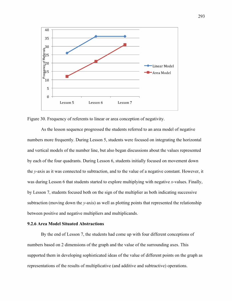
293

Figure 30. Frequency of referents to linear or area conception of negativity. As the lesson sequence progressed the students referred to an area model of negative

numbers more frequently. During Lesson 5, students were focused on integrating the horizontal

and vertical models of the number line, but also began discussions about the values represented

by each of the four quadrants. During Lesson 6, students initially focused on movement down

the y-axis as it was connected to subtraction, and to the value of a negative constant. However, it

was during Lesson 6 that students started to explore multiplying with negative x-values. Finally,

by Lesson 7, students focused both on the sign of the multiplier as both indicating successive

subtraction (moving down the y-axis) as well as plotting points that represented the relationship

between positive and negative multipliers and multiplicands.

9.2.6 Area Model Situated Abstractions

By the end of Lesson 7, the students had come up with four different conceptions of

numbers based on 2 dimensions of the graph and the value of the surrounding axes. This

supported them in developing sophisticated ideas of the value of different points on the graph as

representations of the results of multiplicative (and additive and subtractive) operations.

294

Students developed four situated abstractions about the values of the points on the graph,

based on the value of the multiplier (and constant) of the rule, the value of the position number

(x-value) to which the rule was applied, and the resulting y-value.

1. A rule with a positive multiplier and a positive constant calculated for a positive position

number (x-value) will result in a positive y-value (upper right quadrant).

2. A rule with a positive multiplier and a negative constant calculated for a negative position number (x-value) will result in a negative y-value (lower left quadrant).

3. A rule with a negative multiplier and a positive constant calculated for a negative position number (x-value) will result in a positive y-value (upper left quadrant).

295

4. A rule with a negative multiplier and positive constant calculated for a positive position number (x-value) can result in a negative y-value if the product of the negative multiplier and the position number exceeds the value of the constant.

The four-quadrant model went some way towards justifying the arithmetical operations

on negative numbers and relations between them. This model adds “obviousness” and

“correctness” to the concept of performing operations with negative numbers (terms used by

Fischbein, 1987). Students were able to utilize a combination of the four quadrants, their

knowledge of how to construct graphs through plotting points, and their understanding of how to

use trend lines as a tool for double-checking the correctness of calculations. For example, in

Lesson 6, students struggled to make sense of multiplying a negative position number (x-value)

with a positive multiplier. They arrived at two different solutions, take the sign away, calculate

the operation, and add the sign back. The other solution was to think of the negative position

number value as the multiplicand, so the positive multiplier represented “groups of” the negative

number. The correctness of the solution was evidenced by the trend line of the graph, and

students’ reasoning that a rule with a positive multiplier would have a positive slope in the upper

right quadrant, and would therefore continue its trajectory “behind zero” into the lower left

quadrant.

296

The most interesting example of this occurred during a conversation when students were

discussing their experience of multiplying a negative position number with a negative multiplier.

Initially most of the students had assumed that this would have resulting in a negative y-value,

since both given parameters were negative. However, when plotting the points of the rule they

discovered that the y-value was, in fact, positive. This made sense given that the downward slope

of the trend line, viewed left to right in the upper right quadrant, had to “start out even higher” in

the upper left quadrant. Students reasoned that, since with the downward slope represented

“taking away” a certain amount each time from the amount of the constant at the y-axis, that it

made sense to think that the pattern of decrease would be the same behind the y-axis, and so the

y-values would have to be positive in order that the same amount could be “taken away.”

9.2.7 Summary of Results Part Two

These results suggest that the construction of a four-quadrant graph, and the experience

of plotting points in the four quadrants, supported students’ understanding of negative numbers,

and operations with negative numbers. All students developed a conceptual understanding of the

operations of addition and subtraction with negative values. In addition, students came to

understand the relationship between the results of multiplication with negative numbers in the

context of plotting points for pattern rules. Some students (John, Anne, Jack, Pete, Ilse) were

able to confidently multiply with negative numbers when plotting pattern rules. Other students

relied on more recursive reasoning to plot trend lines with negative multipliers or negative

constants for positive and negative position numbers. However, all students developed an

understanding of the connections among the sign of the multiplier, the sign of the constant, and

the sign of the x-value and the resulting trend lines on the graph.

297

CHAPTER TEN

DISCUSSION

As outlined in Chapter Four, there were two primary goals for this dissertation study. The

first was to assess a new approach to teaching linear relationships and negative numbers. The

second was to use Noss and Hoyles’ framework of situated abstractions and webbing, and

Roschelle’s notion of convergent conceptual change, to investigate the capabilities of young

students to understand basic concepts of linear relationships and negative numbers, and to record

the pathways of group and individual learning.

In this chapter, I will outline the contributions of this dissertation work in relation to these

two goals. One contribution is the learning sequence I developed, and I will present the evidence

of student learning, and discuss how this particular learning sequence seems to have alleviated

some of the well-known problems in students’ understanding of both linear graphs and negative

numbers as outlined in Chapter Two. The second contribution is the use of complementary

analytical frameworks, which were adapted and combined in order to track student learning at

both the group and individual levels. I will discuss how adapting and utilizing these two

complementary frameworks allowed for an analysis not just of the development of content

understanding, but also for an analysis of the pathways of understanding that developed during

this study, and how these pathways converged and diverged for participating students.

Finally, I will outline some future directions for this research, as well as discuss the

limitations of this dissertation work.

10.1 Content Understanding

10.1.1 The Advantages of Starting with Linear Growing Patterns

Although pattern building was not directly incorporated in the third year of the

298

instructional sequence (the focus of this dissertation work), it is clear that the students’ initial

work with patterns in Grades 4 and 5 provided them with a strong foundational understanding of

linear relationships. The multiplier of a rule was at first linked to the number of additional tiles at

each position number in linear growing patterns, and students quickly ascertained that the higher

the value of the multiplier of their rule, the more the tiles increased in number at each successive

position of the pattern. This understanding then translated to an understanding of the connection

between the value of the multiplier and steepness of the slope, since by creating different graphs

for different patterns based on different rules, students could see that the higher the multiplier,

the more the tiles in the pattern increased, which resulted in a steeper trend line on the graph.

Students also developed an understanding of the constant by physically representing the constant

at each position number of a linear growing pattern, and by building the “zeroth” position of a

pattern, for which only the constant was represented. Students developed a strong sense of linear

growth, of constancy, and of the co-variational relationship between the ordinal position number

and the number of tiles at each position. The strength of using pattern building as a mediating

representation between pattern rules and graphical representations is evidenced by the

entrenched nature of the pattern building language used by students in this study – particularly

“position number” to refer to x-values, and “tiles number” for y-values.

10.1.2 Graphical Representations of Linear Relationships

As presented in Chapter Two there have been numerous studies outlining the difficulties

students experience in understanding linear graphs. These include:

1. Not making the connection between an equation of the form y=mx+b and the graph,

specifically, understanding that m represents the slope of the line, and b the y-intercept;

299

2. Not understanding how changes in one parameter affect the graph, and not realizing that

m and b are independent of each other;

3. Adopting a pointwise approach when considering linear graphs, focusing on specific

points on the graph and not understanding the meaning of slope as representing the rate

of change.

Quantitative results presented in Chapter Nine reveal a gain in student scores in all three

of these areas of difficulty that were assessed from pre- to post intervention. Students made gains

in making connections between pattern rules and trend lines on a graph, predicting how changes

in one representation would affect another representation, and in understanding the slope of the

trend line as representing the rate of change. The results also indicate that students could

articulate the meaning of the point of intersection.

A consideration of the qualitative results outlined in Chapters 6 and 7 indicates that

students developed a sophisticated understanding of graphical representations. The ability to

understand visual information on the graph is an important part of graph comprehension. In this

study, this ability to comprehend graphical representations was supported by the physical

plotting of points. This physical action of plotting points allowed students to develop the ability

to interpret graphs on a point-by-point basis. This is similar to early studies in graphing (Bell &

Janvier, 1981; Janvier, 1981; Kerslake, 1981; Preece, 1983; Swan, 1980) the results of which

indicated that having students concentrating on specific points on the graph gave rise to a

disproportionate emphasis on point-wise interpretations. “Overemphasizing pointwise

interpretations may result in a conception of a graph as a collection of isolated points rather than

as an object or a conceptual entity” (Schoenfeld et al., 1993). Subsequent researchers studied the

use of technology to alleviate this problem by incorporate graphing software such as Super Plot

300

(Moschkovich, 1996) or spreadsheet software (Ainley et al., 2000; Pratt, 1995). These studies

were designed to allow students to focus on the global aspects of the graph by removing them

from the technical work of graph construction. When using graphing software, students are

presented with the graph as a whole, and are able to see that changes in the value of the

parameters affect the trend line in particular ways. However, in these prior studies the computer

is a black box that takes an equation and converts it into a graphical representation. Students

were not involved in the process of creating graphs, and hence removed from the connection

between the x-values and y-values as represented by the trend line.

The students I worked with were required to construct their own graphs and did so by

carrying out calculations using linear rules. This provided the students with the opportunity to

understand the connections between the rules and the graphs. Students were able to explore why

changes in the constant of the rule resulted in the translation of the trend line in terms of the y-

intercept and how the trend line moved “up or down” the graphing space based on the value of

the y-intercept. They also explored how changes to the value of the multiplier resulted in changes

in the rotation or angle of the trend line.

There is also evidence that the students in this study were able to go back and forth

between a point-wise perspective and a more global consideration of the graph, and used a

combination of the two perspectives depending on the nature of the problem being solved.

Students used a point-wise approach when determining rules that would intersect at a specific

coordinate point on the graph, for example, (3,18). They also used a point-wise approach when

finding the point at which the trend lines for two rules would intersect, for example, x6+2 and

x5+3 (f(x)=6x+2 and f(x)=5x+3 respectively). A global approach was evidenced by the students’

ability to predict the behaviour of trend lines on the graph based on pattern rules, and by their

301

ability to discern rules for given trend lines. A global approach was also used when formulating

conjectures about what needed to be true for rules to have trend lines that intersect – that the

rules had to have a different multiplier and a different constant in order to have trend lines that

would intersect “at some point” because of a difference in the position on the y-axis and the

steepness of the trend lines. This global approach allowed students to compare the “rates of

growth” of rules based on the value of the multiplier in relation to “where the lines started” on

the y-axis.

This ability to go back and forth between a global and point-wise interpretation may have

developed because the students were using the graph as a tool for problem solving. Pratt (1995)

identified a problem with students’ focusing on graphing conventions and neatness of

presentation when constructing graphs, what he termed “passive graphing.” When students are

only taught how to plot points correctly, the final product – the graph – becomes the goal of the

lesson. For the students in my study, however, the task of constructing and interpreting graphs

had a clear purpose – to develop tools for problem solving. As documented, the graphs were

sometimes unconventional and were generally not terribly neat. However, the students were able

to use their graphs in many ways – for instance, to find the value of x, or to check the correctness

of solutions obtained through other means (tables of values or calculating rules). Since students

developed their own graphs in order to solve problems, they became adept at constructing and

interpreting graphs using a variety of techniques, depending on the context of the problem that

was to be solved.

10.1.3 Solving Linear Equations

Another area of concern outlined in Chapter Two was the emphasis on procedural

knowledge when teaching students how to solve linear equations. In traditional instructional

302

approaches there are few connections made between solving linear equations and considering

intersecting trend lines on a graph.

To solve equations of the form ax+b=cx+d, students are taught a standard procedure

using subtraction in order to get the variable terms on the left and the constant on the right, and

then dividing by the coefficient of the variable term. However, in this dissertation study students

used subtraction to compare the different rates of growth as represented by the multipliers, and

they used subtraction to compare the constants, or “where the two lines started”, and finally,

divided that number by the rate of growth number. If we think of ax+b and cx+d as two pattern

rules for which the value of the multiplier and the constant are different, then the solution to the

equation is analogous to finding the position number (x) at which the trend lines of the two rules

will intersect. To determine how far apart trend lines “start” on the y-axis, students found the

numeric difference between the values of the constant, or (d-b). To find the rate at which they

“come together,” students found the difference between one multiplier and the other (a-c). To

find the position number (x), they divided “how far apart they started” by “the rate at which they

come together” or x=(d-b)÷(a-c). The students in this study demonstrated conceptual

understanding of why they carried out the operations of subtraction and division. And the

solutions they devised demonstrated a capacity to invent solution procedures that may lead them

in the long run, to greater flexibility in problem solving. Research suggests that students who

invent problem-solving procedures ultimately have more flexibility and greater conceptual

understanding (Blotte et al., 2001; Carpenter et al., 1998; Carroll, 2000).

10.1.4 Implications in terms of teaching and learning negative numbers

The final main area of difficulty outlined in Chapter Two was the teaching and learning

of negative numbers. As stated, understanding negative numbers can be problematic because it is

303

difficult to represent quantities that are “not there”, and many representational tools have been

shown to be ineffective (Carraher & Peled, 2008). Difficulties include:

1. Developing an understanding that the minus sign denotes both that an integer is negative

(unary understanding of negativity) and is also an operational signifier for subtraction

(binary understanding);

2. Understanding that the number system is a single system and that operations to numbers

hold regardless of the sign of the numbers.

Examples from Chapters 6 and 7 demonstrate how students used both their understanding

of (and fluency with) the first quadrant of the Cartesian graphing space, and their understanding

of horizontal and vertical number lines to create a 2-dimensional space where the location of

negative values could be recorded. The perpendicular axes provided a map of the location of

negative numbers on two number lines. Working within this space allowed students to become

familiar with the notion of magnitude, or proximity to zero, of negative numbers.

Students also became familiar with the two connotations of negativity. For example,

when plotting rules with a negative constant, written as (y=mx-b) students reasoned that the y-

intercept would be a negative number “below zero”, and also denoted that a constant amount

would need to be subtracted when plotting points on the graph.

Students conceived of the 4-quadrant graph as the perpendicular arrangement of two

number lines. Each number line represented two sets of integers, positive and negative, separated

by 0. Since there were two number lines, most of the students considered the vertical and

horizontal axes to represent two dimensions of zero. Their experiences with plotting rules in the

4-quadrant 2-dimensional space allowed for the development of a distinction between above and

below values, and right and left values. In other words, the students exhibited some

304

understanding of two numeric worlds separated by the zero point, similar to the divided number

line model suggested by Peled, Mukhopadhyay and Resnick (1989). The students extended this

idea to allow for a number to possess two characteristics, quantity and direction. Quantity

referred to the numeric value as expressed by the numeral, and direction referred to the sign of

the number as dictated by where the number was on the 2 dimensional space in relation to 0,

above or to the right were positive values, and below and to the left were negative values. The

proximity to zero was an indication of the magnitude of the numbers, with numbers farther to the

right or higher up being larger, and numbers farther to the left or further down being “deeper into

negatives.” It was not clear whether students understood that being “deeper into negatives”

meant a number that was smaller in quantity, but it is clear that students understood these

numbers to be “greater in negativity” than numbers closer to zero.

The trend line was an important tool that provided support to the students as they

explored operations with negative numbers, particularly operations with two negative numbers,

which have been shown to be particularly problematic (Bruno & Martino, 1999). During Lesson

6, when plotting points for a rule with a negative constant, and calculating the rule with negative

x-values, the students were able to use the trend line to check whether their answer should be

plotted closer to, or farther away from, 0. Another example was plotting trend lines for rules with

a negative multiplier, which were written as (y=(-m)x+b) at a negative x-value, which resulted in

points that were (-x, +y). Working on the graph allowed students to make sense of previously

memorized rules such as “negative times negative equals positive.” The trend line thus became a

tool for checking the results of arithmetic operations using negative numbers.

Graphically, students made the connection between the sign of the multiplier of a rule

and the slope of the trend line. They reasoned that, just as a positive multiplier is represented by

305

a trend line showing a steady increase, a negative multiplier would be represented by a trend line

showing a steady decrease. Students used this understanding to begin to think about finding a

solution (x-value) for a rule with a positive multiplier and a rule with a negative multiplier. The

exercise of finding rules that would have trend lines that created an X was a precursor to the

balancing of equations of the form (-a)x+b=cx+d, since the goal of finding x, or the position

number, is the same as finding x for ax+b=cx+d.

By the end of Lesson 7 the students recognized that the number system is a single

coherent system with unified operations that are applicable regardless of the sign of the numbers.

Prior to this work, the students had some (typical) metaphors with which to understand

negativity – debt, temperature, and the timeline. However, they still regarded negative numbers

as “not like real numbers” and were, for the most part, unsure of how to carry out operations with

negative numbers. The 4-quadrant graph helped students to understand the relationship of

negative numbers to positive numbers, and to be able to start to work with them as “real

numbers.” The students also learned that operations hold for negative as well as positive

numbers. An example of this was Amy’s discovery that subtraction means moving “down” the

vertical number line, even when working with values that are already “below zero.”

The visual representation of negativity was a powerful way for students to connect their

mathematical understandings abstracted about the connections between rules that included only

positive numbers and the related trend lines on the graph, and the effect of including negative

values. In addition, the four areas of the graphing space allowed students to start abstracting

mathematical principles for carrying out arithmetic operations with negative numbers. The four

areas allowed students to associate negative numbers with space, not just organized

symmetrically around zero on two number lines, but also as existing in the areas bounded by

306

those number lines. The importance of the graph as a site for exploring negative numbers was

underscored by the fact that most of the situated abstractions constructed by individual students

were grounded in their work with graphs.

10.2 Frameworks for Analysis of Student Understanding

The other main goal of this study was to utilize two complementary analytical

frameworks in order to gain a broad understanding of the kinds of student understanding this

instructional sequence supports. Because the instructional approach is new, the aim was to get an

overview of student learning through the lens of convergent conceptual change, and also through

the related lenses of situated abstraction and webbing. I chose these two frameworks because

they both emphasize the situated nature of learning, that is, the need to take into account actions

and communications in relation to specific situations in order to understand the kind of learning

taking place.

At one level, I was interested in documenting the convergent conceptual change of the

whole group. Rochelle argues that collaborative learning is generally convergent, and his

research focuses on pairs of students who engage in refining their conceptions of the scientific

ideas (e.g., velocity), and who collaborate in order to construct an understanding that is identical

for both students. In contrast, my study involved ten participating students observed over the

course of four months of instruction. I was therefore interested in extending Rochelle’s

conception in order to document the learning of a greater number of students over a longer

period of time.

In addition, because I was working with ten students and their developing mathematical

thinking, I was interested in tracking divergence of understanding as well as convergence, and

what divergence looked like as they constructed understanding as a group. In order to do this, I

307

adapted another framework that allowed me to consider the kinds of learning constructed at the

group level, and also the kinds of learning constructed at the individual level. Noss and Hoyles’

notions of situated abstractions and webbing have for the most part been utilized by researchers

exploring the affordances of computer-based micro-worlds on individual or pairs of students’

thinking. However, I adapted this framework in order to systematically record the pathways of

understanding developed by all ten students working in a classroom setting.

10.2.1 Convergent Conceptual Change – The Socially Constructed Nature of Learning

As stated, at the group level, I was interested in focusing on the convergence of ideas as

an indication of the social nature of learning. Chapter Six documents the discussions through

which students built an understanding based on the mutual construction, refining, and accepting

of ideas. One example is the students’ final understanding of the meaning of the point of

intersection. The students developed a sophisticated understanding of the nature of the

relationship between the parameters of rules and graphs, and between graphical representations

of intersecting trend lines. They developed the ability to solve for position number, or x, when

asked to compare to rules given “position number x5+3=position number x6+2” by coordinating

their knowledge that the solution to the equation could be represented by the position number (x-

value) at which two trend lines intersected on the graph when they have the same total number of

tiles or “y-value”. All students demonstrated this understanding, whether their site for problem

solving was graphical, modified tabular, or numeric.

An indication of convergent thinking is the ability to recognize and understand diverse

solutions. This is illustrated in the discussions presented in Chapter Six concerning how to

predict the point of intersection for the trend lines of linear rules. During a series of

conversations the students brought together different understandings, creating a synthesis of both

308

numeric and graphical representations that yielded the greatest understanding for all students as

the connections to the graph provided an explanation for the numeric patterns identified.

Pete: Because for each one [rule as represented by a trend line]…you have to think about how far apart they’re starting on the graph, and how long it will take them to get to 18 at the third position. So if you have the rules with x1+15 and x2+12, they start three spaces apart and get together by one space each time, so it would take them to the third position to intersect. (Lesson 2.3, Class 6)

John: Since you know they start three apart, and you know they get together by one

space each time, so if you divide 3 (how far apart they are) by 1 (how quickly they come together at each position), you get 3. (Lesson 3.1, Class 7)

Thus students had not only developed a new method to find the solution for equations of the

form ax+b=cx+d, or x1+15=x2+12, but also the capability of explaining the meaning of the

operations (subtraction and division) used in the method. In this example, both the numeric

differencing and dividing strategy, and the understanding of trend lines that “start apart and come

together by a constant number of spaces each time” were recognized as two ways of expressing

the same method of solving the problem. The fact that the students were able to bring these two

together illustrates that the students recognized the “sameness” of the underlying mathematical

structure, even though the surface features (numbers and trend lines) were different.

Throughout the study there were many examples of collaborative social acts. Chapter Six

documents how students offered ideas, requested explanations and offered alternatives. In effect

they acted as mathematicians do, offering conjectures and engaging in intellectual debate about

ideas. The ideas came from the students themselves, based on the activities given and their use of

tools for problem solving. The class, and each student within the class, created their own

mathematical understanding. Students did not look to the teacher to orchestrate their discussions,

but took turns building emergent themes of inquiry in purposeful discussion, posing questions

309

and answers, and through the provision and refinement of intuitive understanding and formal

knowledge. Their understanding emerged as they made choices in terms of what to explore, what

questions to engage with, and what representation to focus on. They actively modified the

problems, and provided arguments and justifications to continue to move their understanding

forward.

In some instances the students focused on areas that are not usually the subject of

discussion in formal mathematics. One example is the definition of the word “height”, which

became quite a heated debate but which is not usually part of the instruction of graphical

representations of linear equations. At the same time, the students explored very sophisticated

ideas as extensions to the ideas embedded within the designed activities. An example of this was

their exploration of two rules for which the multiplier and the constant are the same, for instance

x8+2 and x8+2. This led to a discussion about whether trend lines could intersect at every point,

or whether intersection referred to only one point for at which linear trend lines cross. This then

led to students considering the different types of intersecting or non-intersecting lines they had

explored on the graph, which are analogous to different sets of equations that have one, no, or

infinite solutions.

Utilizing Roschelle’s theory of convergent conceptual change, I was able to consider the

incremental building up of meaning in a class of ten students over the course of four months.

One of Roschelle’s central questions is, “How can two (or more) people construct shared

meanings for conversations, concepts, and experiences? (Roschelle, 1992, p. 2). Chapter Six

documents the emergent mathematical understanding of the group as it evolved through

classroom negotiations. Roschelle proposes some fundamental features of the process of

310

convergent conceptual change. I believe that the situations documented in this study support

Roschelle’s theories of the processes of conceptual convergence. These are outlined in table 41.

Table 41. Roschelle’s features of convergent collaboration as demonstrated in this study. Roschelle’s Feature Feature As Demonstrated in This Study Example

The construction of a “deep-featured” situation and the ability to discuss deep features even though the “surface” features may vary.

The construction of multiple representations of the same mathematical concept, y=mx+b.

Students constructed patterns, graphs, pattern rules, and word problems to represent linear relationships.

The interplay of metaphors in relation to each other and in reference to the constructed situation.

Students constructed their understanding of multiple representations of linear relationships through the use of metaphor, and the interplay of different metaphors.

The differencing and dividing strategy was based on the metaphor of the movement of trend lines on a graph, specifically, where they “started” (comparing the value of the constants) and how quickly they “came together” (comparing the value of the multipliers).

An iterative cycle of displaying, confirming, and repairing situated actions.

Students discussed their informal understanding of linear relationships, graphs and pattern rules, and refined these early understandings into increasingly sophisticated concepts. These discussions were documented in relation to particular actions and situations and resulted in increasingly sophisticated approximations of mathematical meaning.

Students constructed their understanding from considering the point of intersection as the position at which two patterns would have the same number of tiles, to considering the point of intersection as the x-value for which two pattern rules would have the same value of y.

10.2.2 Webbing

According to Noss and Hoyles, learning is supported as students actively select the

resources from the environment that are meaningful for them. Part of this external environment,

along with the situations, tasks and tools that are available, is the body of understanding

311

developed at the group level. By interacting in a collaborative learning environment, students

develop their own internal resources, situated abstractions, which then become part of the web of

supports. This differs from Vygotsky’s notion of scaffolding, because scaffolding is generally

thought of as the relationship between a more expert and less expert peer. In this study there

were instances of this kind of relationship when students brought specific formal knowledge to

the learning situation, for instance Pete’s explanation that “every time you subtract it means you

go left on the [horizontal] number line.” However, for the most part the material presented was

new to all students, and so there were no expert peers. This situation is similar to many

mathematics learning situations, which lends credence to Noss and Hoyles’ idea of webbing

because each individual, or each group of individuals, is in control of their own learning and

“self-scaffold” by choosing resources that are most meaningful and appropriate to them at the

time. It also is helpful because, unlike Vygotsky’s scaffolding, the supports are not “gradually

faded” but are always available for the learner to select at any point in their learning, and are

continuously modified by the learner as new resources are selected.

10.2.3 Individual Situated Abstractions

An important aspect of situated abstractions that makes this framework particularly

useful for this study is that they allow for the description and validation of an activity as

mathematical without necessarily mapping onto standard mathematics. By considering individual

students’ situated abstractions in relation to those developed at a group level, I was able to track

students’ thinking that was convergent or divergent from that of the group. I discovered that

divergent thinking was usually characterized by an individual’s (or sub-group of individuals’)

use of tools. Tools were used in a novel way, modified, or invented. This marked a change in

terms of the associated situated abstractions constructed – primarily whether they were

312

numerically or graphically oriented. Chapter Seven outlines the individual situated abstractions

for each of the 10 students in the study. This allowed for the tracking of the development of

individual thinking and also allowed for an in-depth examination of the different tools that

students used and how this related to the types of situated abstractions that developed.

Although the students all developed an underlying conceptual understanding about rules with

intersecting trend lines, and the connection to “balancing equations” they had different tools

through which they developed this understanding. There was less diversity in students’

individual situated abstractions about negative numbers because this was a new area of study for

most students. Students tended to rely on their understanding of graphs in order to explore the

concept of working with negative values.

Graphical Representations

All students created graphs during the first few lessons of the study. Some students

(Teah, Mandy, Pete, Ilse) continued to choose graphs as their primary site for problem solving. It

could be argued that the students who did not move away from the graph as a site of problem

solving were overly reliant on their procedure of constructing graphs and may not have

understood the underlying algebraic concepts. However, it was evident that the graphical tool

developed new meanings for these learners. These students exhibited their conceptual

understanding by using the graphical representations in unusual or novel ways – particularly

Teah’s and Mandy’s visualization and estimation strategy (Chapter Seven, Mandy and Teah

Case Study).

Tables of Values

Both recursive and explicit functional reasoning were employed by those students who

created modified tables of values to list the coordinates of points on the line. Students had

313

generated them to keep track of x- and y-values, and used them as an alternative to plotting

points on a graph. The use of tables of values in this study is in contrast to how they are usually

used during instruction. Traditionally students are given tables of data and asked generate a

graph by plotting the points, which according to Schoenfeld et al. (1993) results in a conceptual

disconnect between the values in the table and the points on the graph.

Ordered tables of values are also used in traditional instruction as a tool for determining a

linear rule. However, typically students find rules by considering only the change in values in the

right column, the dependent variable column, and determining the amount added to each

previous value. Typically, this kind of recursive strategy either precludes students’ ability to

formulate a generalized rule. This approach limits students’ abilities to conceptualize the linear

relationship between variables and use the rules in a meaningful way for problem solving

(Stacey, 1989). In this study, the students created their tables of values as a way of keeping track

of x- and y-values, and were designed in order that students could compare the y-values of

different rules. And although Jack and Amy’s explanations of their tables of value were based on

recursive thinking, their explanations also indicated that they understood that the values in the

table as representing the rate of growth of the rule, and that the values were connected to the

steepness of the trend line on the graph. Andrew employed a more explicit functional strategy for

creating his table, using his table of values as an input/output machine to determine y-values by

calculating the rules with x-values. In both cases, the students recognized the tables as one of

many representations of the rule.

Equations

John, Jack, Anne and to some extent Alan moved away from the graph as the primary site

for problem solving and instead focused on the numeric values of the linear rules and created

314

different kinds of equations as tools for problem solving. For instance, when asked to find rules

that would have trend lines that intersected at (3,18) these students focused on finding all

possible missing parameters in an equation with two unknowns on one side of the equal sign,

such as 3 x ____ + ____= 18. As the study progressed, the focus of problem solving shifted

from finding rules that would result in intersecting trend lines on a graph, to finding a numeric

value, x, that would balance two equations by resulting in the same value of y. Students thus

considered equations such as x6+2=x5+3 which, for them, were similar to considering equations

such as 6x+2=5x+3.

10.3 Utilizing Two Frameworks to Track Student Learning

By using two analytical frameworks – convergent/divergent conceptual change, and

webbing and situated abstractions, I was able to track the development of student understanding

at both the group and individual levels in order to gain a broad understanding of the kinds of

student understanding this instructional sequence supports. Once situated abstractions were

documented at the individual and group level, it was then possible to compare abstractions that

were accepted by all of the group (convergence) and those that were accepted by either

individuals or sub-groups (divergence).

As presented in Chapter Nine, comparing the frequency of convergence and divergence

of conceptual understanding provided a clearer picture of student learning. When comparing the

tables of situated abstractions for individual students, approximately two thirds of the situated

abstractions listed were those that were constructed at the group level. This emphasizes the

importance of communication and collaboration as the ideas generated and modified at the class

level were then internalized and incorporated into individual’s developing understanding.

315

Documenting the external resources of the learning situation (collaboration in the

classroom, and tool use) and the internal resources (situated abstractions) allowed me to learn

about the nature of learning for the group, and for each individual student. The result is the

documentation of the building up of the layers of intuitions that underlie the development of

mathematical abstractions, and the interplay between situations, actions through tools, and

developing intuitions as a way of constructing mathematical meaning.

The tracking of the situated nature of the learning is important for further considering

social constructivist ideas of learning because it takes into account both the individual

interpretations of every learning experience by individual students, but also identifies instances

of group convergence when notions that have been abstracted within a particular learning

situation are recognized, agreed upon, and subsequently utilized by other members of the group.

This, then, is a way of understanding the connections between understandings that are

(necessarily) situated within particular circumstances, and the pathways to connect these

understandings to the overarching mathematics. As documented in this study, students took

multiple paths and at times achieved different levels of learning, but many of their conceptions of

linear relationships, and negative numbers, were similar.

10.4 Future Directions

In 2007, Greenes et al. assessed students’ understanding of key concepts of linearity in

4000 Grade 8 students from the United States, Korea, and Grade 9 students in Israel. The study

found that students in all three countries had minimal understanding of two major topics – points

on a line, and slope. The students did not know that the (x,y) coordinates of points on a line that

are presented in tabular form satisfy the equation for the line and, when plotted, produce a graph

of the line (Greenes et al., 2007). In addition, the students in all countries demonstrated

316

maximum difficulty when determining if the trend lines shown in the coordinate plane show

positive or negative slopes, and did not notice the relationship between the direction of a line and

the sign of its slope. Greenes et al.’s recommendation was to look at the elementary mathematics

curriculum and introduce important concepts of linearity and systematically review those

concepts, starting at a young age. Their suggestion is that the elementary curriculum be

revamped in order to “devote much more time to teaching and systematically reviewing concepts

of slope, y-intercept, and the connection between algebraic and graphical representations of a

line”.(Greenes et al., 2007 pg). The results of this 2007 study exemplify what Schoenfeld et al.

refer to as the absence of the Cartesian connection. Because the two domains of solving algebraic

equations and constructing and interpreting linear graphs are taught separately, “students can

treat the algebraic and graphical representational domains as though they are essentially

independent.” (1993).

Another recent study by Peled and Carraher (2007) demonstrates that elementary students

come with many intuitions about negative numbers. As recommended by other researchers,

Peled and Carraher believe that these initial intuitions should be capitalized on at an early age,

since it is evident that Grade 6 students can reason about, and carry out operations with, negative

numbers.

These examples of current research indicate that there is still a need for instructional

models that help students understand the connections among representations of linear rules, and

also models that tap into their intuitions about negativity. The instructional sequence described in

this dissertation was developed for students in Grade 6 who had participated in an experimental

introduction to linear relationships during the previous two years. While I cannot claim that

students have an understanding of “linear functions” per se, the findings suggest that the students

317

did develop conceptual connections among representations, and developed what I have termed

precursory understanding of concepts such as the three different types of solutions for sets of

equations (one solution, no solutions, infinite solutions). The students also successfully began to

integrate negative numbers into their work with graphs and linear rules, and this seemed to

enhance their understanding of “negativity”. What needs to be investigated is whether this

instruction has laid the groundwork for future utilization and relationships associated with such a

rich concept. By focusing only on certain aspects, the early teaching of any concept will have

limitations. Whether this instructional approach fosters the construction of sound mathematical

understandings, and sets the stage for future productive conceptions as students embark on

formal algebraic learning, remains to be studied.

10.5 Difficulties

This was a complex study of the learning of ten Grade 6 students over the course of four

months. Given the scope of this research project, and the fact that I was designing instruction,

videotaping classroom lessons, and analyzing data simultaneously, some aspects of both the data

collection, analysis and presentation were more difficult than originally anticipated. These are

outlined below.

1. Separating group situated abstractions and individual situated abstractions. I undertook

analyses to identify and record the thinking of students individually and in a group.

However, at times it was difficult to differentiate the two. Difficulties included being

aware that one individual’s idea might have been categorized as “convergent” if it was

taken up by the group, and identifying the convergence of thinking of group members

who contributed to the discussion more infrequently than others.

318

2. Categorizing tools, techniques, and situated abstractions. It is difficult to pull apart and

identify each of these three overlapping concepts and articulate the ways in which they

are similar yet different. I have chosen to identify the concepts in the following way.

Tools are representations of abstract concepts such as linear relationships, so in this study

there were multiple tools used, and connections made among different tools. These

included patterns, graphs, pattern rules and tables of values. I characterized techniques as

the way the tools were used and adapted in order to be useful for problem solving.

Finally, I considered situated abstractions to be the generalized understandings that

emerged as students engaged in problem solving in the context of specific tasks, with

specific tools used in particular ways.

3. Categorizing convergent and divergent conceptual change. In this study I primarily

focused on convergence of understanding at a group level, and the divergence from that

group understanding at an individual level. However, these are broad categories that

made it difficult to focus on the nuanced interplay between convergence and divergence

at the both the group level and individual level.

10.6 Limitations

The most serious limitation of this study concerns the generalizability of the findings and

the accounts of student learning. The sample size is small, and is comprised of a group of

students who are unique 1) because they have participated in the first two years of this study and

2) because they attend a school that follows a unique philosophy of education that emphasizes

discussion, problem solving, and the use of open-ended tasks. There are two responses to this

limitation. The first is that the purpose of the study is to determine the kinds of thinking possible

in young students who have experience in pattern building. Thus an in-depth case study of a

319

classroom at both the individual and group level is appropriate. Secondly, in the previous two

years the pattern building lessons had been implemented in a variety of different educational

contexts (including rural and suburban schools that are considered mid-SES (sosio-economic

status) and low-ESL (students who speak English as a second language), and classrooms in an

inner-city school that is considered low-SES high-ESL (Beatty, 2007; Moss & Beatty, 2006).

Results from those studies indicate there was the same increase in learning gains in all the

classrooms, which suggests that the lessons implemented in this third year of the study may also

be as effective with students in different educational contexts. Now that the particular

affordances and limitations of this lessons sequence are understood, it would be beneficial to

conduct a wider comparative study.

This was an exploratory research project. The emphasis lies on the design of new

teaching materials and in the form of a small-scale instruction experiment. The study does not

include a comparative element where the results of the experimental group of students are

compared with a control group. Nor does the duration of the study enable a longitudinal study of

individual learning processes. The present theory and instructional design should be seen as

intermediate products, which need to be refined in the future.

References

Ackermann, E. (1991). From decontextualized to situated knowledge: Revisiting Piaget’s water level experiment. In I. Harel & S. Papers (Eds.), Constructionism (pp. 269-394). New Jersey: Ablex Publishing Corporation.

Ainley, J., Nardi, E. & Pratt, D. (2000). The construction of meanings for trend in active

graphing. International Journal of Computers for Mathematical Learning, 5, 85-114. Arcavi, A. (2003). The role of visual representations in the learning of mathematics. Educational

Studies in Mathematics, 52, 215-241. Arcavi, A., & Hadas, N. Computer mediated learning: an example of an approach. International

Journal of Computers for Mathematics Learning, 5, 25-45. Balacheff, N., (1993). Artificial intelligence and real teaching. In Keitel, C. and Ruthven, K. (Eds.),

Learning from Computers: Mathematics Education and Technology. NATO Series F, Vol.121, pp. 131-158. Springer Verlag-Berlin.

Bardini, C., & Stacey, K., (2006). Students’ conceptions of m and c: How to tune a linear function. In

Novotna, J., Moraova, H., Kratka, M. & Stehlikova, N. (Eds.). Proceedings of the 30th Conference of the International Group for the Psychology of Mathematics Education, Vol. 2, pp. 113-120. Prague: PME.

Beatty, R., (2007). Young students’ emergent understanding of linear functions: Linking symbolic,

graphic and geometric representations. Paper presented at the annual meeting of the American Educational Research Association, Chicago, IL.

Beatty, R., & Moss, J., (2006a). Connecting grade 4 students from diverse urban classrooms:

virtual collaboration to solve generalizing problems. In C. Hoyles & J. Lagrange (Eds.) Proceedings of the Seventeenth ICMI Study: Technology Revisited. Hanoi, Vietnam.

Beatty, R., & Moss, J., (November, 2006b). Multiple vs. numeric approaches to developing functional understanding through patterns – affordances and limitations for grade 4 students. In Altorre, S., Cortina, J.L., Saiz, M., and Mendez, A. (Eds), Proceedings of the twenty-eight annual meeting of the Psychology of Mathematics Education, North American Chapter. Merida, Mexico.

Beatty, R. & Moss, J., (2006c). Grade 4 generalizing through online collaborative problem solving. Paper presented at the annual meeting of the American Educational Research Association, April 2006.

Beichner, R. VideoGraph development project, in H. Maurer (Ed.), Educational Multimedia and Hypermedia Annual, 1993. (Association for the Advancement of Computing in Education, Charlottesville, VA 1993), p. 627.

Bell, A. & Janvier, C. (1981). The interpretation of graphs representing situations. For the Learning of Mathematics, 2(1), 34-42.

Blanton, M., & Kaput, J., (2004). Elementary grades students' capacity for functional thinking. In M.

Jonsen Hoines & A. Fuglestad (Eds.), Proceedings of the 28th Conference of the International Group for the Psychology of Mathematics Education (Vol. 2, pp. 135-142). Oslo.

Bloch, I., (2003). Teaching functions in a graphic milieu: What forms of knowledge enable students to

conjecture and prove? Educational Studies in Mathematics, 52 (1), 3-28. Blume, G.W., & Heckman, D.S. (1997). What do students know about algebra and functions? In P.A.

Kenney & E.A. Silver (Eds.) Results for the sixth mathematics assessment of the national assessment of educational progress (pp. 225-277), Reston VA: National Council of Teachers of Mathematics.

Boester, T., & Lehrer, R. (2007). Visualizing algebraic reasoning. In J. Kaput, D. W. Carraher, & M.

Blanton (Eds.), Algebra in the early grades. Mahwah, NJ: Lawrence Erlbaum Associates. Brassel, H.M. & Rowe, M.B., (1993). Graphing skills among high school physics students.

School Science and Mathematics, 93, 63-71. Bruno, A., & Martinon, A., (1999). The teaching of numerical extensions: The case of negative

numbers. International Journal of Mathematical Education in Science and Technology, 30(6), 789-809.

Capraro, M.M., & Joffrion, H., (2006). Can middle-school students meaningfully translate from

words to mathematical symbols? Reading Psychology, 27 (2 & 3), 147-164. Carpenter, T.P., Franke, M., & Levi, L., (2003). Thinking Mathematically: Integrating arithmetic

and algebra in elementary school. Portsmouth, NH: Heinemann. Carraher, T., (1990). Negative numbers without the minus sign. Proceedings of the 14th

International Conference for the Psychology of Mathematics Education, (pp. 223-229) Oaxtepec, Mexico.

Carraher, D., & Earnest, D. (2003). Guess My Rule Revisited. Proceedings of the 27th

International Conference for the Psychology of Mathematics Education. Honolulu, HI, July, 2003.

Chambers, D.L., (1994). The right algebra for all. Educational Leadership, 51, 85-86. Clement, J., (2000). Analysis of clinical interviews: Foundation and model viability. In A.E.

Kelly & R. Lesh (Eds.) Handbook of Research Design in Mathematics and Science Education (pp. 547-589). New Jersey: Lawrence Erlbaum.

Clements, D.H. (1989). Computers in elementary mathematics education. Englewood Cliffs, N.J.: Prentice Hall.

Contino, M.A. (1995). Linear functions with two points of intersection? Mathematics Teacher,

88(5), 376-378. Cresswell, J.W., & Plano Cark, V.L., (2007). Designing and Conducting Mixed Methods

Research. Thousand Oaks: Sage Publication. diSessa, A. A., (1983). Phenomenology and the evolution of intuition. In D. Gentner A.L.

Stevens (Eds.) Mental Models (pp. 18-34). Hillsdale, NJ: Lawrence Erlbaum Associates, Inc. Dreyfus, T., & Eisenberg, T. (1982). Intuitive functional concepts: A baseline study on

intuitions. Journal for Research in Mathematics Education, 13 (5), 360-380. Ericsson, K., & Simon, H., (1993). Protocol Analysis: Verbal Reports and Data (Revised

version). Cambridge: MIT Press. Evan, R., (1998). Factors involved in linking representations of functions. Journal of

Mathematical Behavior, 17(1), 105-121. Fischer, M.H., (2003). Cognitive representation of negative numbers. Psychological Science,

14(3), 278-282. Gallardo, A. (2003) “It is possible to die before being born” Negative integers subtraction: a case

study. International Group for the Psychology of Mathematics Education, Proceedings of the 27th International Group for the Psychology of Mathematics Education Conference Held Jointly with the 25th PME-NA Conference (N.A. Pateman, B.J. Dougherty, & J.T. Zillox, Eds.) Honolulu, HI, Jul 13-18, 2003, v2 p405-411

Gallardo, A., (2002). The extension of the natural-number domain to the integers in the transition

from arithmetic to algebra. Educational Studies in Mathematics, 49, 171-192. Gallardo, A., & Romero, M., (1999). Identification of difficulties in addition and subtraction of

integers in the number line. In F. Hitt & M. Santos (Eds.), Proceedings of the Twenty-first International Conference for the Psychology of Mathematics Education, North American Chapter, Mexico, Vol. I. (pp. 275-282).

Gallardo, A., & Rojano, T., (1993). Negative solutions in the context of algebraic word

problems. In J. Becker, & B. Pence (Eds.), Proceedings of the Fifteenth International Conference for the Psychology of Mathematics Education, North American Chapter, Pacific Grove, CA, Vol I. (pp. 121-127).

Green, J. C., Caracelli, V. J., & Graham, W. F. (1989). Toward a conceptual framework

for mixed-method evaluation designs. Educational Evaluation and Policy Analysis, 11(3), 255-274.

Greenes, C., Chang, K.Y., & Ben-Chaim, D. (2007). International survey of high school

students’ understanding of key concepts of linearity. In Woo, J.H., Lew, H.C., Park, K.S. & Seo, D.Y. (Eds.). Proceedings of the 31st Conference of the International Group for the Psychology of Mathematics Education, Vol. 2, pp. 273-280. Seoul: PME.

Greenes, C., Cavanagh, M., Dacey, L., Findell, C., & Small, M. (2001). Navigating through

Algebra in Prekindergarten – Grade 2. National Council of Teachers of Mathematics, Reston, VA.

Greer, B., (2004). The growth of mathematics through conceptual restructuring. Learning and

Instruction, 14, 541-548. Griffin, S., & Case, R., (1997). Re-thinking the primary school math curriculum an approach

based on cognitive science. Issues in Education, 3 (1), 1-49. Hargreaves, M., Shorrocks-Taylor, D., & Threlfall, J. (1998). Children’s strategies with number

patterns. Educational Studies, 24(3), 315-331. Hativa, N. & Cohen, D. (1995). Self learning of negative number concepts. Educational Studies

in Mathematics, 28, (2) 401-431. Hiebert, J., & Carpenter, T.P. (1992). Learning and teaching with understanding. In D. Grouws

(Ed.), Handbook for research n mathematics teaching and learning (pp. 65-97). New York: MacMillan.

Hoyles, C., & Noss, R., (2003). What can digital technologies take from and bring to research in

mathematics education? Second International Handbook of Mathematics Education Hoyles, C., Noss, R., & Kent, P., (2004). On the integration of digital technologies into

mathematics classrooms. International Journal of Computers for Mathematical Learning, 9, 309-326.

Human, P., & Murray, H., (1987). Non-concrete approaches to integer arithmetic. Proceedings of

the Eleventh International Conference for the Psychology of Mathematics Education, (pp. 295-300).

Janvier, C., (Ed.). (1987a) Problems of representation in the teaching and learning of

mathematics. Hillsdale, New Jersey: Lawrence Erlbaum Associates. Janvier, C., (1987b). Translation processes in mathematics education. In C. Janvier (Ed.),

Problems of representation in the teaching and learning of mathematics (pp. 27-32). Hillsdale, New Jersey: Lawrence Erlbaum Associates.

Janvier, C., (1983). The understanding of directed number. Proceedings of the 8th International

Conference for the Psychology of Mathematics Education, (pp. 295-300).

Janvier, C. (1981). Difficulties related to the concept of variables presented graphically. In C. Comiti (Ed.), Proceedings of the fifth international conference of the International Group of Psychology of Mathematics Education (pp. 189-193). Grenoble, France, IGPME.

Kaput, J. (2007). What is algebra? What is algebraic reasoning? In J. Kaput, D. W. Carraher, & M.

Blanton (Eds.), Algebra in the early grades. Mahwah, NJ: Lawrence Erlbaum Associates. Kaput, J., (2000). Teaching and learning a new algebra with understanding. U.S.; Massachusetts:

National Center for Improving Student Learning and Achievement in Mathematics and Science

Kaput, J., (1998). Transforming algebra from an engine of inequity to an engine of mathematical

power by “algebrafying” the K-12 curriculum. In S. Fennel (Ed.), The nature and role of algebra in the K-14 curriculum: Proceedings of a national symposium. Washington, DC: National Research Council, National Academy Press, 25-26.

Kaput, J., (1999). Teaching and learning a new algebra. In E. Fennema, & T. Romberg (Eds.),

Mathematics classrooms that promote understanding. Mahwah, NJ: Erlbaum, 133-155. Kaput, J., & Blanton, M., (2003). Developing elementary teachers' "algebra eyes and ears."

Teaching Children Mathematics, 10(2), 70-77. Kerslake, D. (1981). Graphs, in K. Hart (ed.) Children’s understanding of mathematics 11-16, London: John Murray. Kieran, C., (1996). The changing face of school algebra. In Alsina et al. (Ed.) Selected lectures

from the 7th International Congress on Mathematical Education, Sevilla, Spain: FESPM. Kieran, C., (1992). The learning and teaching of school algebra. In T.D. Grouws (Ed.), The

Handbook of Research on Mathematics Teaching and Learning (pp. 390–419). New York: Macmillan.

Kieran, C., (1991). Helping to make the transition to algebra. Arithmetic Teacher, 38, 49–51. Kieran, C., (1990). Cognitive processes involved in learning school algebra. In P. Nesher & J.

Kilpatrick (Eds.), Mathematics and cognition: A research synthesis by the International Group for the Psychology of Mathematics Education (pp. 97-136). Cambridge: Cambridge University Press.

Kieran, C. (1981). Concepts associated with the equality symbol. Educational Studies in

Mathematics, 12, 317-326 Kieran, C. & Chalouh, L., (1993). Pre-algebra: The transition from arithmetic to algebra. In D.

Owens (Ed.) Research Ideas for the Classroom: Middle Grade Mathematics. pp. 179-198. New York: Macmillan Publishing Company.

Koichu, B., & Harel, G., (2007). Triadic interaction in clinical task-based interviews with mathematics teachers. Educational Studies in Mathematics, 65 (3), 349-365.

Lave, J., (1988). Cognition in Practice: Mind, Mathematics and Culture in Everyday Life.

Cambridge: Cambridge University Press. Lave, J., & Wenger, E., (1991). Situated Learning: Legitimate Peripheral Participation.

Cambridge: Cambridge University Press. Lee, L ., (1996). An initiation into algebraic culture through generalization activities, in N.

Bednarz, C. Kieran and L. Lee (eds.), Approaches to Algebra: Perspectives for Research and Teaching, Kluwer Academic Publishers, Dordrecht, pp. 65–86.

Lehrer, R., & Pritchard, C. (2002). Symbolizing space into being. In K. Gravemeijer, R. Lehrer,

R. van Oers, & L. Verschaffel (Eds.), Symbolization, modeling and tool use in mathematics education (pp. 59-86). Dordrecht, Netherlands: Kluwer Academic Press.

Leinhardt, G., Zaslavsky, & Stein, M.K. (1990). Functions, graphs, and graphing: tasks, learning

and teaching. Review of Educational Research, 60(1), 1-64. Luria, A.R., Cole, M., & Cole, S. (1979). The making of mind: A personal account of Soviet

psychology. Cambridge, Mass.: Harvard University Press. Mason, J. (1996). Expressing generality and roots of algebra. In N. Bednarz, C. Kieran, & L. Lee

(Eds.), Approaches to algebra: Perspectives for research and teaching (pp. 65–86). Dordrecht, Netherlands: Kluwer Academic Publishers.

McDermott, Lillian C., Mark L. Rosenquist, and Emily H. Van Zee. (1987). Student difficulties in connecting graphs and physics: Examples from kinematics. American Journal of Physics, 55, 503. McKenzie, D. & Padilla, M. (1986). The construction and validation of the Test of Graphing in

Science (TOGS). Journal of Research in Science Teaching, 23, 571-579. Mevarech, Z.R. & Kramarsky, B. (1997) From verbal descriptions to graphic representations:

Stability and change in students’ alternative conceptions. Educational Studies in Mathematics, 32(3), 229-263.

Mevarech, Z.R. & Stern, E., (1997). Interaction between knowledge and contexts on

understanding abstract mathematical concepts. Journal of Experimental Child Psychology, 65, 68-95.

Miles, M.B., & Huberman, A. M., (1994). Qualitative Data Analysis, An Experimental

Sourcebook, Second Edition. Thousand Oaks: Sage Publications.

Ministry of Education and Training. The Ontario Curriculum Grade 1-8 Mathematics. Queen's Printer for Ontario, 2003.

Monk, G. (1988). Students’ understanding of functions in calculus courses. Humantistic

Mathematics Network Newsletter, 2. Moschkovich, J., (1999). Students’ use of the x-intercept as an instance of a transitional

conception. Educational Studies in Mathematics, 37, 169-197. Moschkovich, J., (1998). Resources for refining conceptions: Case studies in the domain of

linear functions. The Journal of the Learning Sciences, 7(2), 209-237. Moschkovich, J., (1996). Moving up and getting steeper: Negotiating shared descriptions of

linear graphs. The Journal of the Learning Sciences, 5 (3), 239-277. Moschkovich, J., Schoenfeld, A., & Arcavi, A., (1993). Aspects of understanding: On multiple

perspectives and representations of linear relations, and connections among them. In T.A. Romberg, E. Fennema, & T. Carpenter (Eds.), Integrating research on the graphical representation of function (pp. 69-100). Hillsdale, NJ: Erlbaum.

Moses, B., (1997). Algebra for a New Century in: Teaching Children Mathematics, Algebraic

Thinking Focus Issue, Introduction. Reston, VA: National Council of Teachers of Mathematics. February, 1997, 264–265.

Moses, R.P., & Cobb, C.E. (2001). Radical equations: Math literacy and civil rights. Boston:

Beacon Press. Moss, J., (2004). Pipes, tubes, and beakers: Teaching rational number. In J. Bransford and S.

Donovan (Eds.), How people learn: A targeted report for teachers. National Academy Press. Moss, J. & Beatty, R., (2005). In real life math and enjoyment don’t go together – in Knowledge

Forum math = enjoyment! Grade 4 children work together to build their understanding of mathematical functions. Paper presented at the Institute for Knowledge Innovation and Technology 2004 Summer Institute. University of Toronto. (August 2005), http://ikit.org/SummerInstitute2004.

Moss, J. & Beatty, R., (2006a). Knowledge building in mathematics: Supporting collaborative

learning in pattern problems. International Journal of Computer Supported Collaborative Learning, 1(4), 441-465.

Moss, J. & Beatty, R., (July, 2006b). Knowledge building and knowledge forum: Grade 4 student collaborate to solve linear generalizing problems. In J. Navotna, H. Moraova, K.Magdalena, & N.Stehlikova (Eds.) Proceedings of the thirtieth annual meeting of the International Group for the Psychology of Mathematics Education, Vol. 4. Prague, Czeck Republic.

Moss, J., Beatty, R., McNab, S. & Eisenband, J. “The Potential of Geometric Sequences to Foster Young Students’ Ability to Generalize in Mathematics.” [Powerpoint file] presented at the Algebraic Reasoning: Developmental, Cognitive, and Disciplinary Foundations for Instruction conference, September 14, 2005, in Washington, D.C. Retrieved Jan. 9, 2007, from http://www.brookings.edu/gs/brown/algebraicreasoning.htm.

Moss, J., & Case, R., (1999). Developing Children’s Understanding of Rational Numbers: A

New Model and Experimental Curriculum. Journal for Research in Mathematics Education, 30(2), 122–147, 119.

Murray, J.C., (1985). Children’s informal conceptions of integer arithmetic. Proceedings of the

9th International Conference for the Psychology of Mathematics Education, (pp. 147-153). Noss, R., & Hoyles, C., (2006) Exploring mathematics through construction and collaboration.

In K.R. Sawyer, (Ed.) Cambridge Handbbook of the Learning Sciences, pp. 389-408. Cambridge: Cambridge University Press.

Noss, R., & Hoyles, C., (1996). Windows on mathematical meanings: Learning cultures and

computers (mathematics education library). Noss, R., Healy, L., & Hoyles, C. (1997). The Construction of Mathematical Meanings:

Connecting the Visual with the Symbolic. Educational Studies in Mathematics, 33(2), pp. 203-233.

Nunes, T., Schliemann, A.D., & Carraher, D.W., (1993). Street Mathematics and School Mathematics. Cambridge: Cambridge University Press.

Orton, J. (1997). Matchsticks, Pattern and Generalisation. Education 3-13. Orton, J., Orton, J. & Roper, T. (1999). Pictorial and practical contexts and the perception of pattern. In A. Orton (Ed.), Pattern in the Teaching and Learning of Mathematics

(pp.121-136) London, Cassell. Padgett, D.K., (1998). Rigor and Relevance in Qualitative Research. Thousand Oaks: Sage

Publications. Peled, I., (1991). Levels of knowledge about signed numbers: effects of age and ability.

Proceedings of the Fifteenth International Conference for the Psychology of Mathematics Education, (pp. 145-152.)

Peled, I. & Carraher, D.W. (2007). Signed numbers and algebraic thinking. In J. Kaput. D.

Carraher, & M. Blanton (Eds.), Algebra in the Early Grades. Mahwah, NJ, Erlbaum, pp. 303-327.

Peled, Mukhopadhyay & Resnick, (1989). Formal and informal sources of mental models for

negative numbers. In G. Vergnaud, J. Rogalski, & M. Artigue (Eds.), Proceedings of the 13th international conference for the Psychology of Mathematics Education (Vol. 3, pp. 106-110). Paris, France: Conference Committee.

Perso, T. (1996). Teaching equation solving – Again? The Australian Mathematics Teacher, 52

(1), 19-21. Pirie, S. (1991). Peer discussion in the context of mathematical problem solving. In K. Durkin &

B. Shire (Eds.), Language in mathematics education: Research and practice (pp. 143-161). Philadelphia: Open University Press.

Pratt, D., (2000). Making sense of the total of two dice. Journal for Research in Mathematics

Education, 31(5), 602-625. Pratt, D., (1995). Young children’s active and passive graphing. Journal of Computer Assisted

Learning, 11, 157-169. Preece, J. (1983). A survey of graph interpretation and sketching errors. (CAL Research Group

Tech. Rep. No. 34). Milton Keynes, England: Institute of Educational Technology, The Open University, Walton Hall.

Resnick, L.B. (1991). Shared cognition: Thinking as social practice. in L.B. Resnick, J.M.

Levine and S.D. Teasley (eds.), Perspectives on Socially Shared Cognition (pp. 1-20). Washington D.C.: American Psychological Association.

Resnick, L.B., Pontecorvo, C., & Saljo, R., (1997). Discourse, tools and reasoning: Essays on

situated cognition. In L.B. Resnick, R. Saljo, C. Pontecorvo, Y B. Burge (Eds.), Discourse, Tools and Reasoning: Essays on Situated Cognition (pp. 1-20). Berlin; New York: Springer.

Rivera, F.D., & Becker, J.R. (2008). Middle school children’s cognitive perceptions of

constructive and deconstructive generalizations involving linear figural patterns. ZDM, 40(1), 65-82.

Roschelle, J., (1992). Learning by collaborating: Convergent conceptual change. The Journal of

the Learning Sciences, 2(3), 235-276. Roschelle, J., Kaput, J., & Stroup, W. (in press). SimCalc: Accelerating student engagement with

the mathematics of change. In M.J. Jacobsen & R.B. Kozma, Learning the Sciences of the 21st Century: Research, Design, and Implementing Advanced Techology Learning Environments. Hillsdale, NJ: Earlbaum.

Romberg, T.A., & Kaput, J.J. (1999). Mathematics worth teaching, mathematics worth

undrstanding. In E. Fennema & T.A. Romberg (Eds.) Mathematics classrooms that promote understanding (pp. 181-197). Hillsdale, NJ: Lawrence Erlbaum.

Schegloff, E. (1991). Converation analysis and socially shared cognition. In L.B. Resnick, J.M.

Levine and S.D. Teasley (Eds.), Perspectives on Socially Shared Cognition (pp. 151-171). Washington, D.C.: American Psychological Association.

Schoenfeld, A., (2002). Research methods in (mathematics) education. In L.D. English (Ed.) Handbook of International Research in Mathematics Education (pp. 435-487). New Jersey: Lawrence Erlbaum.

Schoenfeld, A.H., Smith, J.P. & Arcavi, A., (1993). Learning: The microgenetic analysis of one

student’s evolving understanding of a complex subject matter domain. In R. Glaser (Ed.) Advances in Instructional Psychology, Vol. 4. pp.55-175. NJ: Erlbaum.

Smith, J., diSessa, A. & Roschelle, J. (1993). Misconceptions reconceived. The Journal of the

Learning Sciences, 3, 115-163. Star, J.R. & Seifert, C. (2006). The development of flexibility in equation solving. Contemporary

Educational Psychology, 31, 280-300. Streefland, L., (1996). Negative numbers: Reflections of a learning researcher. Journal of

Mathematical Behavior, 15, 57-77. Swan, M. (1980). The language of graphs. Nottingham, England: University of Nottingham,

Shell Centre for Mathematical Education. Tashakkori, A., and Teddlie, C. (1998). Mixed Methodology: Combining Qualitative and

Quantitative Approaches. Thousand Oaks: Sage. Tashakkori, A., and Teddlie, C. (2003). Handbook of Mixed Methods in Social and Behavioral

Research. Thousand Oaks: Sage. Valsiner, J., & Veer, R., (2000). The Social Mind: Construction of the Idea. Cambridge, UK;

New York: Cambridge University Press. Vinner S. 1983: ‘Conflicts between definitions and intuitions: the case of the tangent’, Proceedings of P.M.E. 6, Antwerp. Vlassis, J., (2001). Solving equations with negatives or crossing the formalizing gap. In M. van

den Heuvel-Panhuizen (Ed.), Proceedings of the Twenty-fifth International Conference for the Psychology of Mathematics Education, Utrecht, The Netherlands, Vol. IV. (pp. 375-382).

Vlassis, J., (2002). About the flexibility of the minus sign in solving equations. In A. Cockburn,

& E. Nardi (Eds.), Proceedings of the Twenty-sixth International Conference for the Psychology of Mathematics Education, Norwich, UK, Vol. IV. (pp. 321-328).

Vlassis, J., (2004). Making sense of the minus sign or becoming flexible in ‘negativity’.

Learning and Instruction, 14, 469-484. Vygotsky, L.S., & Cole, M., (1978). Mind in Society: The Development of Higher Psychological

processes. Cambridge: Harvard University Press.

Warren, E. & Cooper, T. (2006). Repeating and growing pattern rules: Relationships between geometric and numerical representations. Paper presented at the American Educational Research Association Annual Conference, San Francisco, April 7-11.

Wertsch, J., (1985). Vygotsky and the Social Formation of Mind. Cambridge: Harvard University

Press. Willoughby, S., (1997). “Functions from Kindergarten through Sixth Grade.” Teaching Children Mathematics 3 (February): 314–18. Yerushalmy, M. (1991) Students perceptions of aspects of algebraic function using multiple

representation software. Journal of Computer Assisted Learning. Blackwell Scientific Publications. 7, 42-57.

Yersuhalmy, M., & Shternberg, B. Charting a visual course to the concept of function. In

Cuoco, A., & Curcio, F. (Eds.) The Roles and Representations in School Mathematics, National Council of Teachers of Mathematics 2001 Yearbook. Reston, V.A: NCTM, 2001.

Zazkis, R. & Liljedahl, P. (2002). Generalization of patterns: The tension between algebraic thinking and algebraic notation. Educational Studies in Mathematics, 49, 379-402.

Appendix A Webbing and Situated Abstraction

Bas

elin

e K

now

ledg

e (P

rete

st)

Exit

Kno

wle

dge

(Pos

ttest

)

Internal Resources • Intuition • Metaphor • Experience

External Resources • Tools • Activities • Discourse

experience

Situated Abstraction

Internal Resources • Intuition • Metaphors • Experience

External Resources • Tools • Activities • Discourse

experience

Situated Abstraction

Internal Resources • Intuition • Metaphors • Experience

External Resources • Tools • Activities • Discourse

experience

Situated Abstraction

Intersecting Lines on Graphs

Negative Numbers

Situated abstractions – successive approximations of formal mathematical knowledge – forged through the interaction (webbing) of

internal and external resources at an individual level, and also at a group level as communities of practice are formed around specific activities.

Knowledge development is mediated through participating in activities, through using and developing tools, and through experiencing classroom

discourse. At each stage of the lesson sequence, mathematical abstractions, which are situated within this particular context, are forged through the interaction of internal and external resources (webbing). The

initial situated abstractions become part of the internal resources as students continue to develop their knowledge of linear graphs (continue to

refine the situated abstractions). Individual student knowledge will be considered both by tracking the situated abstractions that are developed as

students participate over the course of the intervention, and also be comparing pre and post test results (quantitatively and qualitatively).

Includes situated abstraction of function (rule) based on past experiences pattern building

Linear Graphs

Appendix B Pre/Post Survey

332

Name ________________________

Grade 6 Survey

Question 1 This is a picture of a pattern that someone built last year.

Circle the graph that shows the rule that this pattern is following:

How do you know?

0 1 2 3

Appendix B Pre/Post Survey

333

Question 2 On the graph below,

1. What rule is represented by the line of circles?

2. What would you have to do to that rule (the circle rule) to get the line of

squares?

3. How do you know?

Appendix B Pre/Post Survey

334

Question 3 If you create a graph for the rule number of tiles=position number x5 and then graph the rule number of tiles = position number x5+5, what will the new trend line on the graph look like? It will make the trend line steeper. Why or why not?

The trend line will start higher on the 0th position. Why or why not?

It will be both higher and steeper. Why or why not? It will make the line steeper. Why or why not?

The trend line will start higher on the 0th position. Why or why not?

It will be both higher and steeper. Why or why not?

Yes No

Yes No

Yes No

Yes No

Yes No

Yes No

Prediction Before Graphing

After Graphing

Appendix B Pre/Post Survey

335

Graph the rule number of tiles = position number x5. Graph the rule number of tiles = position number x5+5.

Appendix B Pre/Post Survey

336

Question 4 1. What is the rule represented by this graph?

2. What rule would give you a trend line parallel to this? Why? 3. What rule would give you a trend line that started at the same point but was steeper than this trend line? Why? 4. Can you think of a rule that would have a trend line that intersects this trend line? How do you know?

Appendix B Pre/Post Survey

337

Question 5 If you built two patterns, that followed these rules Number of tiles = position number x4+3 Number of tiles = position number x 5 Is there any position at which both patterns would have the same number of tiles? How did you figure it out?

Appendix B Pre/Post Survey

338

Appendix B Pre/Post Survey

339

Question 6 What rule do you think could give you a trend line that looks like this?

Appendix C – Lesson Sequence

340

Lesson Overview: This lesson is designed to solidify students’ experiences building and graphing patterns, and reviewing the parameters m and b. It is also a chance for students to explain their understanding of slope and y-intercept as a way of discussing the links between the symbolic, pattern and graphical representations. Lesson Materials:

! Pattern Building Challenges ! Pattern Blocks ! Position Cards ! Markers/ coloured pencils ! Large Sheets of Graph Paper with Graph Template (one per pair) ! Graph Paper to record whole group discussions

Lesson Introduction: Whole Group Have a group discussion to define the following terms: Composite rule Multiplier Additive or Constant

(let’s try to have students use the term constant – as in the component of a composite rule that stays the same, doesn’t change – is constant)

Steepness (of the trend line and connections to the value of the multiplier)

Parallel (the students have been focusing on this as “two lines that never meet”, however, for considering graphed rules, it is more helpful to think of parallel lines as lines that have the “same steepness”)

Zeroth position (connection among the value of the constant and the y-intercept)

Lesson 1 Review Pattern Building and Graphing

Appendix C – Lesson Sequence

341

Lesson Development: Pairs Work Hand out “secret pattern challenges” (see end of this lesson) to pairs of students. Before they build and graph, ask the students to record predictions of what the lines of points would look like for their rules. What would be similar on these graphs and what would be different? Half of the student pairs will graph these three rules: number of tiles = position number x2+1 number of tiles = position number x6+1 number of tiles = position number x9+1 Ask students to graph them on the same sheet of graph paper (big graph paper – with coloured pencils/markers to show the different rules). Have the other half of the student pairs will graph these three rules: number of tiles = position number x3+2 number of tiles = position number x3+6 number of tiles = position number x3+9 Whole Group Discussion When the students have finished graphing – ask a representative from each group to come to the front with their graph. Some Key Questions to lead the discussion: What are the differences and similarities between the trend lines on the graphs? What are the differences and similarities between the two sets of rules? What part of the pattern rule is responsible for the steepness of the trend lines and why? What part of the pattern rule is responsible for where the trend line starts at the 0th position?

Appendix C – Lesson Sequence

342

SECRET PATTERN BUILDING

GRAPHING CHALLENGE

You and your partner will build the first three positions for each of these three rules: BEFORE YOU BUILD YOUR PATTERN AND GRAPH THEM: What is your prediction of what the trend lines on your graph will look like? What will be similar and what will be different? Why do you think so? AFTER YOU BUILD YOUR PATTERN AND GRAPH THEM: Was your prediction correct?

Number of tiles = Position number x 2 + 1 Number of tiles = Position number x 6 + 1 Number of tiles = Position number x 9 + 1

Appendix C – Lesson Sequence

343

SECRET PATTERN BUILDING

GRAPHING CHALLENGE

You and your partner will build the first three positions for each of these three rules: BEFORE YOU BUILD YOUR PATTERN AND GRAPH THEM: What is your prediction of what the trend lines on your graph will look like? What will be similar and what will be different? Why do you think so? AFTER YOU BUILD YOUR PATTERN AND GRAPH THEM: Was your prediction correct?

Number of tiles = Position number x 3 + 2 Number of tiles = Position number x 3 + 6 Number of tiles = Position number x 3 + 9

344

Lesson Overview: This lesson is designed to have students begin to think about constructing graphs for rules for which both the coefficient and the constant are different, so that the lines intersect in the first quadrant. As students graph intersecting lines, they will be asked to think about what needs to be true if two rules will produce intersecting lines. Lesson Materials: Blank graph paper for students (a few sheets per student) Graphs for students (one per student) Lesson Introduction: Write the following two rules on the board (or chart paper): number of tiles = position number x5+3 number of tiles = position number x6+2 Ask students to predict what the graphs for these rules would look like, and why. Ask students to create graphs for the two rules using their blank graph paper. Once they have finished, lead a whole class discussion and record answers on chart paper: Were their predictions correct? Why do the trend lines intersect? What do you think it means when two trend lines intersect? What has to be true about the two rules that have trend lines that intersect? Next, ask students to think of more rules that will also have trend lines that intersect at position 1 on their graphs.

Grade 6 - Lesson 2 Graphing Rules with Intersecting Trend Lines

345

Pairs Work Hand out copies of the graph to each pair of students. Ask them to see if they can think of rules that will have trend lines that intersect at position 3. Lesson Closure Whole Group How many rules did you come up with? How did you find rules that have trend lines that intersect at position 3? Could you predict rules that would have trend lines that intersect at position 3?

346

347

How many rules can you think of that will have trend lines that intersect at position 3?

348

In this lesson, students will build on their understanding of intersecting trend lines in Lesson 2, and their understanding of rules used for pattern building, to start to predict where the trend lines for 2 rules will intersect. Students will apply what they understand about intersecting trend lines to start to consider whether two trend lines can intersect at more than one point, and whether two rules with similar coefficients can have trend lines that intersect. Students will also start to consider values along the x-axis that lie between positive integers. Materials:

! Blank graphs (if students want to use them) ! Fabulous Rule Challenge sheets (one per student) ! Chart paper ! Markers ! Tiles and position cards

Lesson Introduction: Whole Group Write these two rules on the board: number of tiles = position number x 3 number of tiles = position number x 2+6 Ask student to imagine they are going to build two patterns that follow these rules. Predict whether there will be a position number that has the same number of tiles for both rules. Write this question on the board (or chart paper): At what position number does x3 = x2+6? (at what position number would they have the same number of

tiles?) Pairs Work Have students work in pairs or small groups to work out the answer. Remind students they can draw, make a graph, work it out with numbers etc… Whole Group Ask for volunteers to share their answer, and the strategy they used.

Grade 6 - Lesson 3 Comparing Two Rules

349

Record their answer like this (below the original question): At what position number does x3 = x2+6 Position number _______ As students share how they figured out the answer (building/drawing patterns, graphing, working it out arithmetically etc). Capture their ideas on chart paper. Lesson Development Pairs Work Now give students a sheet of Rule challenges. Ask students to work in pairs to solve the challenges. Lesson Closure Whole Class Ask students to discuss their answers to their rule challenges: How did the students figure out the answers to the first two questions? What are some theories about whether or not rules will have trend lines that intersect at more than one point? Why or why not? Can rules with the same multiplier ever have trend lines that intersect? Why? Where do the trend lines for the rules in question 5 intersect?

350

Rule challenges!!

1. At what position number does

x6+2 = x5+5? (at what position would they have the same number of

tiles?)

At position number ___________

How do you know? How did you figure it out??

2. At what position number does

x3+3 = x4+1?

At position number ____________.

How do you know? How did you figure it out??

3. Would there ever be more than one position where x3+3 and x4+1 would be the same (have the same number of tiles?) Why or why not?

351

4. At what position number does

x4+6 = x4+2?

At position number _______________.

How do you know? How did you figure it out??

5. At what position number would the trend lines for the rules

number of tiles = position number x4+2 and

number of tiles = position number x8

intersect? Why?

352

353

In this lesson, students will apply what they understand about intersecting lines to start to compare rules presented in narrative format. They will also interpret two rules presented graphically by writing a word problem. Materials:

! Copies of iMusic Purchase Plans problem (one per student) ! Extra graph paper (if students need it) ! Copies of “Make up a word problem” sheets ! Blank sheets of lined paper to write word problems

Lesson Introduction: So far we’ve been thinking about rules as they look on a graph, and thinking about what it means when two rules have intersecting trend lines on a graph. Now we’re going to start to think about how this applies in the real world. Lesson Development: Give each student a copy of the iMusic Purchase Plans Problem. Read the problem aloud as a class (have a volunteer or volunteers read). Review the questions being asked. Are there any initial predictions? Pairs Work Students can work in pairs to answer the questions. Whole Group Discuss as a class how students answered the questions, strategies used etc. Next, hand out copies of the Make Up a Word Problem sheets (one per student). Tell students they will be making up word problems. Show an example of a graph, and brainstorm the kinds of scenarios the graph could be showing (e.g. race, saving money, collecting something). Make sure to ask students to consider what it means to have values at the zeroth position, and what the steepness of the line could mean. Individual/ Pairs Work Students can work individually or in pairs to make up a word problem based on the graph.

Lesson 4 Word Problem Comparing Rules

354

iMusic Purchase Plans Problem

Thursika and Dave both loved downloading music. They found a great internet site that had two different payment schemes for downloading music. Plan A was to pay a membership fee of $16 before downloading any music, and pay $2 for each album. Plan B was to pay $5 for each album, but you only had to pay $1 as a membership fee before downloading music. Thursika chose Plan A. Dave chose Plan B. 1. If they both downloaded 10 albums, who made the better choice of payment

plan? Why? 2. What is the difference in cost between 10 albums on Plan A and 10 albums

on Plan B? 3. Is there a number of albums for which Dave and Thursika will pay the same

price? 4. How many albums can Dave order and still pay less than Thursika, if they are

ordering the same number of albums?

355

Make Up a Word Problem! Now it’s your turn! Look at the graph below. Think of a story that would describe what the graph is showing. Write it down. Now think of three questions about the two rules in your story. One could be a question asking someone to compare the two rules. One could be a question asking what would happen next, or later. You could ask about what is similar and/or different about the rules.

356

Make Up a Word Problem! Now it’s your turn! Look at the graph below. Think of a story that would describe what the graph is showing. Write it down. Now think of three questions about the two rules in your story. One could be a question asking someone to compare the two rules. One could be a question asking what would happen next, or later. You could ask about what is similar and/or different about the rules.

357

Make Up a Word Problem! Now it’s your turn! Look at the graph below. Think of a story that would describe what the graph is showing. Write it down. Now think of three questions about the two rules in your story. One could be a question asking someone to compare the two rules. One could be a question asking what would happen next, or later. You could ask about what is similar and/or different about the rules.

358

Make Up a Word Problem! Now it’s your turn! Look at the graph below. Think of a story that would describe what the graph is showing. Write it down. Now think of three questions about the two rules in your story. One could be a question asking someone to compare the two rules. One could be a question asking what would happen next, or later. You could ask about what is similar and/or different about the rules.

359

Make Up a Word Problem! Now it’s your turn! Look at the graph below. Think of a story that would describe what the graph is showing. Write it down. Now think of three questions about the two rules in your story. One could be a question asking someone to compare the two rules. One could be a question asking what would happen next, or later. You could ask about what is similar and/or different about the rules.

360

Make Up a Word Problem! Now it’s your turn! Look at the graph below. Think of a story that would describe what the graph is showing. Write it down. Now think of three questions about the two rules in your story. One could be a question asking someone to compare the two rules. One could be a question asking what would happen next, or later. You could ask about what is similar and/or different about the rules.

361

Make Up a Word Problem! Now it’s your turn! Look at the graph below. Think of a story that would describe what the graph is showing. Write it down. Now think of three questions about the two rules in your story. One could be a question asking someone to compare the two rules. One could be a question asking what would happen next, or later. You could ask about what is similar and/or different about the rules.

362

n this lesson, students will apply what they know about linear equations and linear graphs, and begin to work (formally) with negative numbers. Initially, students will brainstorm about negative numbers, and then apply this in order to extend the coordinate plane to include the other three quadrants. Materials:

! Chart paper/ blackboard ! New graph paper for creating graphs that include negative numbers

Lesson Introduction: Today we’re going to think about negative numbers, what we know about negative numbers, and how we can use what we know to think about negative numbers in rules. Lesson Development: First ask students to think about negative numbers. When have they seen negative numbers, how do they think about negative numbers, what images do they use? Facilitate the conversations to see if students have images that are both vertical (e.g. elevators going to parking floors under a building, freezing temperatures etc) and horizontal (these are trickier – sometimes it is just the negative numbers on a number line….) Next tell students we are going to think about graphing with negative numbers – how we represent negative numbers on the graph, “So far our graph has just positive numbers (draw the first quadrant on board, or on flip chart) – but we want to be able to show positive and negative numbers – how can we do it???” Pairs Work Students can work in pairs to answer the question Whole Group Have students volunteer their ideas of how they incorporated negative numbers and expanded the graphing space.

Lesson 5 Introducing the other 3 quadrants Negative Constant

363

In this lesson, students will apply what they know about linear equations and linear graphs to continue to work with negative numbers. In this lesson students will reason about creating a graph for a rule with a negative constant. Students will also reconsider their conjectures in the context of working with negative numbers in their pattern rule. Finally, students will consider a negative constant in a “real world” context. Materials:

! Chart paper copy of conjectures ! Copies of Liga the Dogsitter problem (one per student) ! New graph paper for graphing rule with negative constant

Lesson Introduction: Today we’re going to think about negative numbers in our pattern rules. How could we create a graph for the rule: number of tiles = position number x4-2? Lesson Development: Ask students to think about how they have created graphs for pattern rules with only positive numbers. Pairs Work Hand out graph paper and ask students to create a graph of the rule. Whole Group Ask student how they did it (strategies)? Now, ask students to consider some of their other conjectures e.g. if you have a negative constant, will this still mean that x4+2 and x4-2 are parallel? Pairs Work Hand out a copy of the “Liga the Dogsitter” word problem. Whole Group Take up solutions to the word problem – focus on problem solving strategies.

Lesson 6 Negative Constant Revisiting Conjectures

364

Liga the Dogsitter Liga got hired to look after her neighbour’s dog for $5.00 an hour, and was looking forward to saving up all her earnings. However, Liga owed the video store $17.00 in late return fees. After the first day of dog sitting, she used her earnings to pay part of the fine. After the second day, she used her earnings and paid off more of the fine. Liga vowed that as soon as she had paid off the fine, she would save every dollar of her dog-sitting money.

1. How many days will it take Liga to pay off the fine? How do you know?

2. On the day that Liga finally finishes paying the fine, how much money can she put in her piggy bank? How do you kow?

3. On what day will Liga have saved $28.00?

365

Lesson Introduction So far, all the patterns we have built have had two positive numbers, a positive number for the multiplier, and a positive number for the constant. We have started thinking about creating graphs for rules with a negative constant. Now we are going to explore what happens when we have a negative multiplier when we build patterns, and when we create graphs of pattern rules . Lesson Development Build a shrinking pattern that follows the rule number of tiles = position number x(-2) +8. It starts with a certain number of tiles and decreases by a constant amount. This time, the two colours of tiles we use are going to show positive numbers, and negative numbers. The pattern starts off with 8 (positive) tiles at position 0. The multiplier is how many tiles are taken away, or become negative, at each position number. For instance, in the example below tiles = position number x (-2)+8, there are 8 white tiles at the 0th position. The number of white tiles decreases by 2 at each position. The number of grey, or negative, tiles increases at each position (representing multiplying each position number by -2). Applying the rule to each position number gives you the total tiles at each position number. So for the first position, 1x(-2) is -2 plus 8 = 6.

0 1 4 3 2

Lesson 7 “Shrinking” Patterns and Negative Multipliers

366

The pattern represents the constant in the form of 8 tiles above each position number, and represents the negative multiplier by the successive number of tiles that are taken away (substituted for grey negative tiles) at each position. Visually the positive (white) tiles decrease from left to right, similar to the slope of a graphic linear function with a negative multiplier. Build this pattern. Ask students how they would graph the rule number of tiles = position x(-2)+8. Once students have graphed the pattern up to position 4, ask them how they would continue the graph for position 5, and why? Next, have students work in pairs to graph tiles = position number x (-4) + 20. Finally, show students a graph that looks like this one, and issue a challenge:

Can students think of two rules that will result in a graph like this? Can they figure out how to create this kind of graph? The intersection point can be anywhere in the four quadrants.