Analytical formulation of lunar cratering asymmetries
25
A&A 594, A52 (2016) DOI: 10.1051/0004-6361/201628598 c ESO 2016 Astronomy & Astrophysics Analytical formulation of lunar cratering asymmetries Nan Wang (‘) and Ji-Lin Zhou (hN) School of Astronomy and Space Science and Key Laboratory of Modern Astronomy and Astrophysics in Ministry of Education, Nanjing University, 210046 Nanjing, PR China e-mail: [email protected] Received 28 March 2016 / Accepted 3 July 2016 ABSTRACT Context. The cratering asymmetry of a bombarded satellite is related to both its orbit and impactors. The inner solar system im- pactor populations, that is, the main-belt asteroids (MBAs) and the near-Earth objects (NEOs), have dominated during the late heavy bombardment (LHB) and ever since, respectively. Aims. We formulate the lunar cratering distribution and verify the cratering asymmetries generated by the MBAs as well as the NEOs. Methods. Based on a planar model that excludes the terrestrial and lunar gravitations on the impactors and assuming the impactor encounter speed with Earth v enc is higher than the lunar orbital speed v M , we rigorously integrated the lunar cratering distribution, and derived its approximation to the first order of v M /v enc . Numerical simulations of lunar bombardment by the MBAs during the LHB were performed with an Earth–Moon distance a M = 20-60 Earth radii in five cases. Results. The analytical model directly proves the existence of a leading/trailing asymmetry and the absence of near/far asymmetry. The approximate form of the leading/trailing asymmetry is (1+ A 1 cos β), which decreases as the apex distance β increases. The numer- ical simulations show evidence of a pole/equator asymmetry as well as the leading/trailing asymmetry, and the former is empirically described as (1 + A 2 cos 2ϕ), which decreases as the latitude modulus |ϕ| increases. The amplitudes A 1,2 are reliable measurements of asymmetries. Our analysis explicitly indicates the quantitative relations between cratering distribution and bombardment conditions (impactor properties and the lunar orbital status) like A 1 ∝ v M /v enc , resulting in a method for reproducing the bombardment conditions through measuring the asymmetry. Mutual confirmation between analytical model and numerical simulations is found in terms of the cratering distribution and its variation with a M . Estimates of A 1 for crater density distributions generated by the MBAs and the NEOs are 0.101-0.159 and 0.117, respectively. Key words. planets and satellites: surfaces – Moon – minor planets, asteroids: general – methods: analytical 1. Introduction The nonuniformity of the cratering distribution on a satellite or a planet when it comes under bombardment is called cra- tering asymmetry. There are three types. The first is the lead- ing/trailing asymmetry, which is due to the synchronous rotation of a satellite. When synchronously locked, a satellite’s velocity always points to its leading side, so that this hemisphere tends to gain a higher impact probability, higher impact speed and more normal impacts. Because the crater diameter depends on impact speed and incidence angle (e.g., Le Feuvre & Wieczorek 2011), this can also lead to an enhanced crater size on the lead- ing side. This is the so-called apex/antapex effect (Zahnle et al. 2001; Le Feuvre & Wieczorek 2011). Zahnle et al. (1998, 2001) and Levison et al. (2000) investigated this effect on the giant planets and their satellites in detail. This work focuses on the Moon. Its leading/trailing asymmetry has been proposed by theoretical works (Zahnle et al. 1998; Le Feuvre & Wieczorek 2011), confirmed by numerical simulations (Gallant et al. 2009; Ito & Malhotra 2010), and directly verified by seismic ob- servations (Kawamura et al. 2011; Oberst et al. 2012) and ob- servations of rayed craters (Morota & Furumoto 2003). The second type, the pole/equator asymmetry (or latitudinal asym- metry), which is an enhancement of low-latitude impacts com- pared to high-latitude regions resulting from the concentra- tion of low-inclination projectiles, has often been reported as well (Le Feuvre & Wieczorek 2008, 2011; Gallant et al. 2009; Ito & Malhotra 2010). The third type is the near/far asymmetry, which is most uncertain. It has been proposed that Earth focuses the projectiles onto the near side of the Moon as a gravitational lens and thus the craters there are enhanced (Wiesel 1971), or that Earth is an obstacle in the projectiles’ trajectories so that the near side is shielded from impacts (Bandermann & Singer 1973). Contradicting and limited conclusions have not led to consensus. The cratering asymmetry depends on not only the lunar or- bit, but also on the impactor population. After analyzing the size distributions of craters, Strom et al. (2005, 2015) suggested that there are two impactor populations in the inner solar system: the main-belt asteroids (MBAs), which dominated during the late heavy bombardment (LHB) ∼ 3.9 Gya, and the near-Earth ob- jects (NEOs), which have dominated since about 3.8-3.7 Gya. The two populations are different in their orbital and size distri- butions, fluxes, and origins, which means that there is no reason to expect the cratering asymmetries generated by them to be the same. We note the MBAs referred to here are the asteroids that occupied the region where the current main belt is during the LHB. Although their semi-major axes a p = 2.0-3.5 AU were the same as today, their eccentricities and inclinations were greatly excited by migrating giant planets (Gomes et al. 2005). Instead, their size distribution has changed little after the first ∼100 Myr (Bottke et al. 2005). Several surveys of the current main belt have reported power-law breaks of its size distribu- tion. The Sloan Digital Sky Survey (SDSS; Ivezi´ c et al. 2001) Open Access article, published by EDP Sciences, under the terms of the Creative Commons Attribution License (http://creativecommons.org/licenses/by/4.0), which permits unrestricted use, distribution, and reproduction in any medium, provided the original work is properly cited. A52, page 1 of 25
-
Upload
khangminh22 -
Category
Documents
-
view
1 -
download
0
Transcript of Analytical formulation of lunar cratering asymmetries

A&A 594, A52 (2016)DOI: 10.1051/0004-6361/201628598c© ESO 2016
Astronomy&Astrophysics
Analytical formulation of lunar cratering asymmetriesNan Wang (王楠) and Ji-Lin Zhou (周济林)
School of Astronomy and Space Science and Key Laboratory of Modern Astronomy and Astrophysics in Ministry of Education,Nanjing University, 210046 Nanjing, PR Chinae-mail: [email protected]
Received 28 March 2016 / Accepted 3 July 2016
ABSTRACT
Context. The cratering asymmetry of a bombarded satellite is related to both its orbit and impactors. The inner solar system im-pactor populations, that is, the main-belt asteroids (MBAs) and the near-Earth objects (NEOs), have dominated during the late heavybombardment (LHB) and ever since, respectively.Aims. We formulate the lunar cratering distribution and verify the cratering asymmetries generated by the MBAs as well as the NEOs.Methods. Based on a planar model that excludes the terrestrial and lunar gravitations on the impactors and assuming the impactorencounter speed with Earth venc is higher than the lunar orbital speed vM, we rigorously integrated the lunar cratering distribution, andderived its approximation to the first order of vM/venc. Numerical simulations of lunar bombardment by the MBAs during the LHBwere performed with an Earth–Moon distance aM = 20−60 Earth radii in five cases.Results. The analytical model directly proves the existence of a leading/trailing asymmetry and the absence of near/far asymmetry.The approximate form of the leading/trailing asymmetry is (1+A1 cos β), which decreases as the apex distance β increases. The numer-ical simulations show evidence of a pole/equator asymmetry as well as the leading/trailing asymmetry, and the former is empiricallydescribed as (1 + A2 cos 2ϕ), which decreases as the latitude modulus |ϕ| increases. The amplitudes A1,2 are reliable measurements ofasymmetries. Our analysis explicitly indicates the quantitative relations between cratering distribution and bombardment conditions(impactor properties and the lunar orbital status) like A1 ∝ vM/venc, resulting in a method for reproducing the bombardment conditionsthrough measuring the asymmetry. Mutual confirmation between analytical model and numerical simulations is found in terms of thecratering distribution and its variation with aM. Estimates of A1 for crater density distributions generated by the MBAs and the NEOsare 0.101−0.159 and 0.117, respectively.
Key words. planets and satellites: surfaces – Moon – minor planets, asteroids: general – methods: analytical
1. Introduction
The nonuniformity of the cratering distribution on a satelliteor a planet when it comes under bombardment is called cra-tering asymmetry. There are three types. The first is the lead-ing/trailing asymmetry, which is due to the synchronous rotationof a satellite. When synchronously locked, a satellite’s velocityalways points to its leading side, so that this hemisphere tendsto gain a higher impact probability, higher impact speed andmore normal impacts. Because the crater diameter depends onimpact speed and incidence angle (e.g., Le Feuvre & Wieczorek2011), this can also lead to an enhanced crater size on the lead-ing side. This is the so-called apex/antapex effect (Zahnle et al.2001; Le Feuvre & Wieczorek 2011). Zahnle et al. (1998, 2001)and Levison et al. (2000) investigated this effect on the giantplanets and their satellites in detail. This work focuses on theMoon. Its leading/trailing asymmetry has been proposed bytheoretical works (Zahnle et al. 1998; Le Feuvre & Wieczorek2011), confirmed by numerical simulations (Gallant et al. 2009;Ito & Malhotra 2010), and directly verified by seismic ob-servations (Kawamura et al. 2011; Oberst et al. 2012) and ob-servations of rayed craters (Morota & Furumoto 2003). Thesecond type, the pole/equator asymmetry (or latitudinal asym-metry), which is an enhancement of low-latitude impacts com-pared to high-latitude regions resulting from the concentra-tion of low-inclination projectiles, has often been reported aswell (Le Feuvre & Wieczorek 2008, 2011; Gallant et al. 2009;Ito & Malhotra 2010). The third type is the near/far asymmetry,
which is most uncertain. It has been proposed that Earth focusesthe projectiles onto the near side of the Moon as a gravitationallens and thus the craters there are enhanced (Wiesel 1971), orthat Earth is an obstacle in the projectiles’ trajectories so thatthe near side is shielded from impacts (Bandermann & Singer1973). Contradicting and limited conclusions have not led toconsensus.
The cratering asymmetry depends on not only the lunar or-bit, but also on the impactor population. After analyzing the sizedistributions of craters, Strom et al. (2005, 2015) suggested thatthere are two impactor populations in the inner solar system: themain-belt asteroids (MBAs), which dominated during the lateheavy bombardment (LHB) ∼ 3.9 Gya, and the near-Earth ob-jects (NEOs), which have dominated since about 3.8−3.7 Gya.The two populations are different in their orbital and size distri-butions, fluxes, and origins, which means that there is no reasonto expect the cratering asymmetries generated by them to be thesame.
We note the MBAs referred to here are the asteroids thatoccupied the region where the current main belt is during theLHB. Although their semi-major axes ap = 2.0−3.5 AU werethe same as today, their eccentricities and inclinations weregreatly excited by migrating giant planets (Gomes et al. 2005).Instead, their size distribution has changed little after the first∼100 Myr (Bottke et al. 2005). Several surveys of the currentmain belt have reported power-law breaks of its size distribu-tion. The Sloan Digital Sky Survey (SDSS; Ivezic et al. 2001)
Open Access article, published by EDP Sciences, under the terms of the Creative Commons Attribution License (http://creativecommons.org/licenses/by/4.0),which permits unrestricted use, distribution, and reproduction in any medium, provided the original work is properly cited.
A52, page 1 of 25
A&A 594, A52 (2016)
distinguished two types of asteroids with different albedos (0.04and 0.16 for blue and red asteroids) and found that for the wholesample throughout the whole belt, the cumulative size distri-bution has a slope αp = 1.3 for diameters dp = 0.4−5 kmand 3 for 5−40 km. Parker et al. (2008) also confirmed thisconclusion based on the SDSS moving object catalog 4, in-cluding ∼88 000 objects. The first (Yoshida et al. 2003) andsecond (Yoshida & Nakamura 2007) runs of the Sub-km MainBelt Asteroid Survey (SMBAS), which each found 861 MBAsin R-band and 1001 MBAs in both B and R-bands, reportedαp = 1.19 ± 0.02 for dp = 0.5−1 km and αp = 1.29 ± 0.02for dp = 0.6−1 km, claimed to be consistent with SDSS forMBAs smaller than 5 km. The size distribution of craters formedby MBAs also has a complex shape, whose cumulative slope isαc = 1.2 for crater diameters dc . 50 km, 2 for 50−100 km, and3 for 100−300 km (Strom et al. 2015).
The NEO population is relatively well understood and sug-gested to have been in steady state for the past ∼3 Gyr, con-stantly resupplied mainly from the main belt (Bottke et al. 2002).Bottke et al. (2002) derived the debiased orbital and size distri-butions of NEOs by fitting a model population to the knownNEOs: the orbits are constrained in a range ap = 0.5−2.8 AU,ep < 0.8, ip < 35, the perihelion distance qp < 1.3 AU,and the aphelion distance Qp > 0.983 AU; the size distribu-tion is characterized by a single slope αp = 1.75 ± 0.1 fordp = 0.2−4 km. The corresponding slope for the crater sizedistribution indicated by Strom et al. (2015) is αc = 2 fordc = 0.02−100 km. A few recent works have investigated thecratering asymmetry generated by NEOs based on the debi-ased NEO model described in Bottke et al. (2002). Gallant et al.(2009) ran N-body simulations and determined an apex/antapexratio (ratio of the crater density at the apex to antapex) of1.28 ± 0.01, a polar deficiency of ∼10%, and the absence of anear/far asymmetry. In a similar work but with a different nu-merical model, Ito & Malhotra (2010) found a leading/trailinghemispherical ratio of 1.32 ± 0.01 and also a polar deficiencyof ∼10%. Le Feuvre & Wieczorek (2008) analytically predictedthe lunar pole/equator ratio to be 0.90. Le Feuvre & Wieczorek(2011) followed and semi-analytically estimated that involvingboth longitudinal and latitudinal asymmetries, the lunar craterdensity was minimized at (90 E, ±65 N) and maximized at theapex with deviations of about 25% with respect to the average forthe current Earth–Moon distance, resulting in an apex/antapexratio of 1.37 and a pole/equator ratio of 0.80. From observations,Morota & Furumoto (2003) reported an apex/anntapex ratio of∼1.5 for 222 rayed craters with dc > 5 km on lunar highlands,formed by NEOs in the past ∼1.1 Gyr.
However, according to Strom et al. (2015), for craters withdiameters larger than 10 km, those that the MBAs formedexceed the other population by more than an order of mag-nitude. This underlines the need for taking the craters andthe cratering asymmetry that the MBAs contribute to into ac-count, and thus requires the awareness of the lunar orbit dur-ing the LHB, namely, the dominance of MBAs. The Earth–Moon system evolved drastically in the early history. As ageneral trend, it is accepted that the Moon has been reced-ing from Earth because of tidal dissipation, but a wide spec-trum of opinions exists for the details of this picture. After thetimescale problem was raised (Gerstenkorn 1955; MacDonald1964; Goldreich 1966; Lambeck 1977; Touma & Wisdom 1994)and then solved through ocean models (Hansen 1982; Webb1982; Ross & Schubert 1989; Kagan & Maslova 1994; Kagan1997; Bills & Ray 1999), it is known today that the tidal dissi-pation factor of Earth must have been much larger in the distant
past, or in other words, the tidal friction was much weaker thantoday (e.g., Bills & Ray 1999). Because tidal friction depends onnot only the lunar orbit but also the terrestrial ocean shape, whichis associated with continental drift, the exact history of Earth’stidal dissipation factor and hence the early evolution of the lunarorbit cannot be confirmed.
Still, we list some efforts of ocean modelers here. Hansen(1982) was the first to introduce Laplace’s tidal equations in cal-culations of oceanic tidal torque. He modeled four cases, combi-nations of two idealized continentalities and two frictional re-sistance coefficients, and found the Earth–Moon distances at4.5 Gya ranging from 38 to 53 R⊕, leading to nearly the samevalues at 3.9 Gya when the LHB occurred. Webb (1980, 1982)developed an average ocean model and obtained the dates of theGerstenkorn event as 3.9 and 5.3 Gya with and without solidEarth dissipation included, respectively. According to these tworesults, the Earth–Moon distance at 3.9 Gya should be no largerthan 25 R⊕ or about 42 R⊕. The author claimed, however, thatthe results should only be taken qualitatively. Ross & Schubert(1989) simulated a coupled thermal-dynamical evolution of theEarth–Moon system based on equilibrium ocean model, result-ing in aM being 47 R⊕ and eM being 0.04 at 3.9 Gya when theevolution timescale and parameters such as final aM and eM wererequired to be realistic. Kagan & Maslova (1994) described astochastic model that considered fluctuating effects of the con-tinental drift. Their two-mode resonance approximations gaverise to evolutions of tidal energy dissipation that were consistentwith global paleotide models. By adopting a reproduced tidalevolution with a timescale as close as possible to the realisticone, the Earth–Moon distance is estimated to be about 47 R⊕ at3.9 Gya. This timescale can vary by billions of years, of course,depending on the values of the resonance lifetime.
The uncertain lunar orbital status during the LHB means thata reliable relationship between the lunar orbit and the crater-ing asymmetry is needed. If the influence of the former on thelatter were significant and an incorrect condition of the Earth–Moon system were assumed, the estimated cratering asymmetrywould be also incorrect. Conversely, this also implies that theearly history of the Earth–Moon system could be inferred fromthe observed crater record if the portion of craters that formedduring the LHB were selected. The influence of the lunar orbitand of the impactor population on the cratering asymmetry havenot been sufficiently studied so far. Numerical simulations canonly offer an empirical estimation based on a limited numberof cases: Zahnle et al. (2001), who simulated impacts of eclipticcomets on giant planet satellites, combined the results of caseαp = 2.0 and case αp = 2.5 with the satellite orbital speedvorb = 10.9 km s−1 and the impactor speed at infinity in the restframe of the planet fixed at v∞ ≈ 5 km s−1, and thus derived asemi-empirical description of the crater density
Nc ∝
1 +vorb√
2v2orb + v2
∞
cos β
2.0+(1.4/3)αp
, (1)
where β is the angular distance from the apex; using the debiasedNEO model, Gallant et al. (2009) ran simulations with Earth–Moon distances of aM = 50, 38, 30, 20, and 10 R⊕, and confirmedthe negative correlation between aM and leading/trailing asym-metry degree. A semi-analytical method capable of producingcratering of the Moon caused by current asteroids and comets inthe inner solar system was proposed by Le Feuvre & Wieczorek(2011), who suggested a fit relation
Nc(apex)/Nc(antapex) = 1.12e−0.0529(aM/R⊕) + 1.32, (2)
A52, page 2 of 25

N. Wang and J.-L. Zhou: Analytical formulation of lunar cratering asymmetries
which is valid between 20 and 60 R⊕.In this paper, we first derive the formulated lunar cratering
distribution through rigorous integration based on a planar modelin Sect. 2, where the leading/trailing asymmetry is unambigu-ously confirmed. Then we show the numerical simulations ofthe Moon under bombardment of MBAs during the LHB overvarious Earth–Moon distances in Sect. 3. The simulation resultsare compared to our analytical predictions, and the cratering dis-tribution of coupled asymmetries is described. Last, Sect. 4 com-pares NEOs and MBAs and shows the consistence of our analyt-ical model with related works.
2. Analytical deduction
This section shows how we analytically deduced formulationseries describing the spatial distributions of impact speed, inci-dence angle, normal speed, crater diameter, impact density, andcrater density on the lunar surface under bombardment, basedon a planar model. These formulations directly prove the exis-tence of the leading/trailing cratering asymmetry and the identityof the near and far sides. The amplitude of the leading/trailingasymmetry is proportional to the ratio of the impactor encounterspeed to the lunar orbital speed, implying that it might be pos-sible to derive the lunar orbit or the impactor population fromcrater record.
2.1. Assumptions and precondition
Our model includes the Sun, Earth, the Moon, and the impactors(asteroids and/or comets) in the inner solar system, which areassumed to be located farther away from the Sun than Earth.The main assumptions we adopt are listed below.
1. The orbits of Earth, the Moon, and the impactors as well asthe lunar equator are coplanar.
2. The orbits of Earth and the Moon are circular.3. The gravitation on the impactors due to Earth and the Moon
are ignored.4. Earth is treated as a particle.
The first assumption does not allow describing latitudinal crater-ing variation, which is investigated in our numerical simulations.It helps avoiding the coupling of two cratering asymmetries andconcluding a pure leading/trailing asymmetry formulation. TheMoon’s geometrical libration is neglected by the first two as-sumptions. The third partly means that the acceleration of theimpactor velocity is not accounted for, which is valid on condi-tion that the Earth–Moon distance is larger than ∼17 R⊕, accord-ing to Le Feuvre & Wieczorek (2011). It also means the grav-itational lensing by Earth is excluded, and moreover, the lastassumption excludes the Earth’s shielding for the Moon. Thiscauses the symmetry between the near and far sides.
A precondition for the cratering asymmetry is that the Moonmust be synchronously rotating, because otherwise any longitu-dinal variation would vanish as the lunar hemisphere facing theEarth changes constantly. According to Zhou & Lin (2008), thetimescale for the Moon to reach the 1:1 spin-orbit resonance canbe estimated by
τsyn ∼
(RM
aM
)2
τtide =4Q′M63nM
mM
m⊕
(aM
RM
)3
, (3)
where τtide is the tidal circularization timescale, m⊕ is the Earthmass, nM, aM, RM, mM, and Q′M are the mean motion, semi-major axis, radius, mass, and effective tidal dissipation factor
of the Moon. A measure of this timescale is τsyn . 102 yr foraM = 10 R⊕, several orders shorter than the timescale of the tidalevolution. This precondition is therefore expected to hold for themain lifetime of the Moon, including during the LHB.
On condition that the Moon rotates synchronously, its hemi-spheres can be defined. The near side is defined as the hemi-sphere that always faces Earth, and the far side is its opposite.The leading side is defined as the hemisphere that the lunar or-bital velocity points to, and the trailing side is its opposite. Thecenters of the leading and trailing sides are the apex and the an-tapex points.
2.2. Encounter geometry
We first consider the encounter condition before exhibiting thedetails of the impact in the following subsections. In the helio-centric frame, Earth orbits the Sun circularly at 1 AU, the Moonis ignored at this pre-encounter stage, and the impactors are allmassless particles with semi-major axes ap > 1 AU and ec-centricities 0 < ep < 1. If the orbit of an impactor intersectsthat of Earth on the ecliptic, meaning that its perihelion distanceqp ≤ 1AU, an encounter is considered to occur at the mutualnode. The relative velocity between the impactor and Earth whenthey encounter is the encounter velocity uenc = up − u⊕, where upand u⊕ are orbital velocities of the impactor and Earth. With-out loss of generality, the impactor’s and Earth’s arguments ofperihelion are both assumed to be 0, so that their velocities inheliocentric ecliptic coordinates are
up =
√GM
ap(1 − e2p)
(− sin fp, ep + cos fp), (4)
u⊕ =
√GM
a⊕(− sin f⊕, cos f⊕), (5)
where G is the gravitational constant, M is the solar mass, fpand f⊕ are true anomalies, and the terrestrial semi-major axis isa⊕ = 1 AU. The mutual node is where fp = f⊕ = fenc, makingthe impactor’s heliocentric distance equal to a⊕, that is,
cos fenc =ap(1 − e2
p)
a⊕ep−
1ep· (6)
Thus, the encounter velocity depends on ap and ep (or qp):
uenc(ap, ep) = up(ap, ep, fenc(ap, ep)) − u⊕( fenc(ap, ep)). (7)
For a fixed ap, as shown in Fig. 1, the encounter speed venc isminimized when qp = 1 AU. As qp decreases (ep increases),even though the magnitudes of the two orbital velocities up andu⊕ in the moment of encounter are invariant, the angle betweenthem expands, and thus the encounter speed venc increases. Onthe other hand, if qp is fixed, larger ap can also lead to higher venc,because the impactor orbital speed in the moment of encounter
vp =
√GM
(2a⊕−
1ap
)(8)
is greater. As shown in Fig. 2, venc increases rightward (ap in-creases) and downward (qp decreases). Given a population ofimpactors, its typical venc is determined by its orbital distribu-tion and can affect the cratering distribution. Therefore, differentimpactor populations represent different cratering asymmetrieswith a given target, providing a method for deriving impactorproperties form the observed crater record.
A52, page 3 of 25

A&A 594, A52 (2016)
Fig. 1. Encounter geometry for an impactor orbit with ap = 2.0 AUand qp = 0.2−1.0 AU. Where the Earth orbit (blue dashed circle) inter-sects the impactor orbit (black solid ellipse), the angle between u⊕ (bluedashed arrow) and up (black solid arrow) decreases as qp increases, andthus uenc (red solid arrow) shrinks.
2.3. Impact geometry
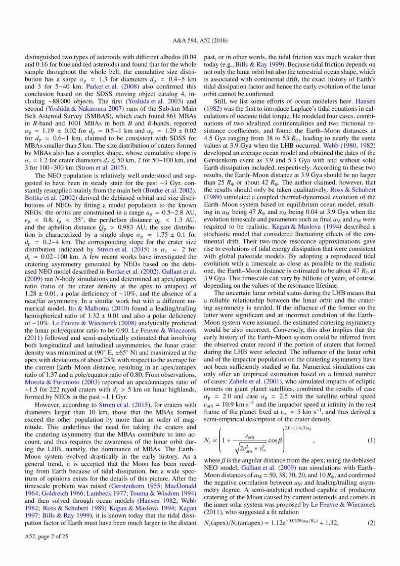
When the encounter between one impactor orbit and the Earthorbit occurs, as seen in the Earth–Moon system, the impactors inthe common orbit are treated as particles approaching along theparallel straight lines in the direction of their common encountervelocity (Fig. 3a). They are assumed to be uniformly distributedin space, and to be numerous enough to cover the Moon’s or-bit, that is, the gravitational cross section of the Moon is alwaysmaximized (lunar diameter in the planar model).
In the geocentric frame with the x-axis pointing to the lunarperigee, the direction of uenc can be random. Since we averageover the lunar period, it can be assumed to be in the positive y-axis direction without loss of generality. Figure 3a shows that theangle between the encounter velocity uenc and the lunar orbitalvelocity uM is the Moon’s true anomaly fM, which varies uni-formly at the rate of the mean motion nM. The impact velocity isthe relative velocity between the impactors and the Moon:
uenc = (0, venc), (9)uM = vM(− sin fM, cos fM), (10)u = (vM sin fM, venc − vM cos fM). (11)
Its magnitude, that is, the impact speed, is
v =
√v2
enc + v2M − 2vencvM cos fM. (12)
At any instant, the impact can only occur on one hemisphere, andthe impactors in this hemisphere have an equal v since they sharethe same venc. A normal impact point is the center of this bom-barded hemisphere, where the incidence angle and thus the nor-mal impact speed are both largest at this instant. As the impactorsare assumed to be uniformly distributed, this is also where theimpact flux is highest.
Given the encounter speed venc and lunar orbital speed vM,as long as venc > vM, the impact speed v is always minimizedwhen the Moon is at the perigee ( fM = 0) and maximized atthe apogee ( fM = 180), where the antapex and the apex becomethe normal impact points. Figure 3 shows that the normal im-pact point constantly moves westward on the lunar surface at a
Fig. 2. Contour map of the encounter speed venc (km s−1) as a functionof ap and qp.
varying rate, and that lower venc brings not only the lower v, butalso a longer time spent on the leading side for the normal im-pact point, which implies that the lower the encounter speed, thestronger the leading/trailing asymmetry. That venc > vM is takenfor granted hereafter in this work. This holds for the MBAs,whose minimum venc is 7.9 km s−1 (ap = 2.5 AU and qp = 1 AU),which is nearly equal to the maximum vM when aM = 1 R⊕. It isalso valid for those NEOs with ap > 1.2 AU, whose minimumencounter speed venc = 2.4 km s−1 (ap = 1.2 AU and qp = 1 AU)approximates to vM for aM = 11R⊕, while aM during the domi-nant epoch of the NEOs is at least about 40 R⊕.
Now we establish a rest frame of the Moon that is to be usedin the integration. As shown in Fig. 4, the positive y-axis pointsto the apex and the minus x-axis points to Earth. In this frame,
u = (vx, vy), (13)vx = venc sin fM, (14)vy = venc cos fM − vM, (15)
while its magnitude v keeps its expression of Eq. (12). We intro-duce some variables: λ is the geometric longitude ranging from−180 to +180, measured eastward from the center of near side;θ is the incidence angle ranging from 0 to 90, the angle be-tween u and the local horizon; S is the cross section. A unit area(length in planar model) at longitude λ on the bombarded hemi-sphere is
dl = RMdλ (16)
and its cross section is
dS = RM sin θdλ. (17)
Denoting with e = (− cos λ,− sin λ) the normal vector, the inci-dence angle on the unit area can be derived with
sin θ =e · uv
=vx cos λ + vy sin λ
v, (18)
and the normal speed v⊥, the normal component of u is
v⊥ = v sin θ = vx cos λ + vy sin λ. (19)
Denoting with ρ the uniform spatial density of the impactors, theimpact flux, the number of impactors received per unit time bythe unit area is
dF = ρvdS = ρRMv⊥dλ. (20)
A52, page 4 of 25
N. Wang and J.-L. Zhou: Analytical formulation of lunar cratering asymmetries
Fig. 3. Impact geometry seen in the rest frame of Earth a) and Moon b). a) The Moon is assumed to be where aM = 60 R⊕, with vM = 1.0 km s−1.The impactors, distributed extensively enough to cover the lunar orbit (black circle), are in the common direction of uenc (black dashed arrow).Where fM = 0, 45, . . . , 315, the lunar velocity uM (black solid arrow) and the impact velocity u for venc = 5 or 10 km s−1 (red or blue solidarrows) are all plotted to the same scale. b) Under the same conditions, u is plotted pointing at the normal impact points on the lunar surface.
At any instant when the lunar true anomaly is fM, the longitudeof the normal impact point is defined as λ⊥, where its normalvector e⊥ is parallel to u, so that
sin λ⊥ =vy( fM)v( fM)
, cos λ⊥ =vx( fM)v( fM)
· (21)
The bombarded hemisphere is then bounded by the longitudeinterval [λl, λu], where the lower and upper limits λl,u = λ⊥∓90,and
sin λl,u = ∓vx( fM)v( fM)
, cos λl,u = ±vy( fM)v( fM)
· (22)
As the bombarded hemisphere moves westward along the lunarequator, the moment a certain position λ enters this hemisphereand the moment it leaves are when λ becomes the lower and up-per limits λl,u, respectively, and when sin θ = 0 there. Therefore,the time interval while a certain position λ is in the bombardedhemisphere, characterized by [ fl, fu], can be derived with
sin λ = ∓vx( fl,u)v( fl,u)
, cos λ = ±vy( fl,u)v( fl,u)
· (23)
It turns out
fl = arcsin(vM
vencsin λ
)− λ, (24)
fu = π − arcsin(vM
vencsin λ
)− λ. (25)
2.4. Exact formulations
Here with venc and vM given, the spatial distributions of impactdensity, impact speed, incidence angle, normal speed, crater di-ameter, and crater density are shown after integration. We note
Fig. 4. Variables involved in integrating the cratering distribution. In therest frame of the Moon, the common velocity of impactors is u (direc-tion of the arrows). The hemisphere bounded by two positions where u(arrows on two sides) is parallel to the local horizons is the bombardedhemisphere, whose center, where u (arrow in the middle) is perpendic-ular to the lunar surface, is the normal impact point. Denotations areexplained in the text.
that the denotations of integrated variables are written uppercaseto distinguish them from the instantaneous ones with lowercaseletters.
A52, page 5 of 25
A&A 594, A52 (2016)
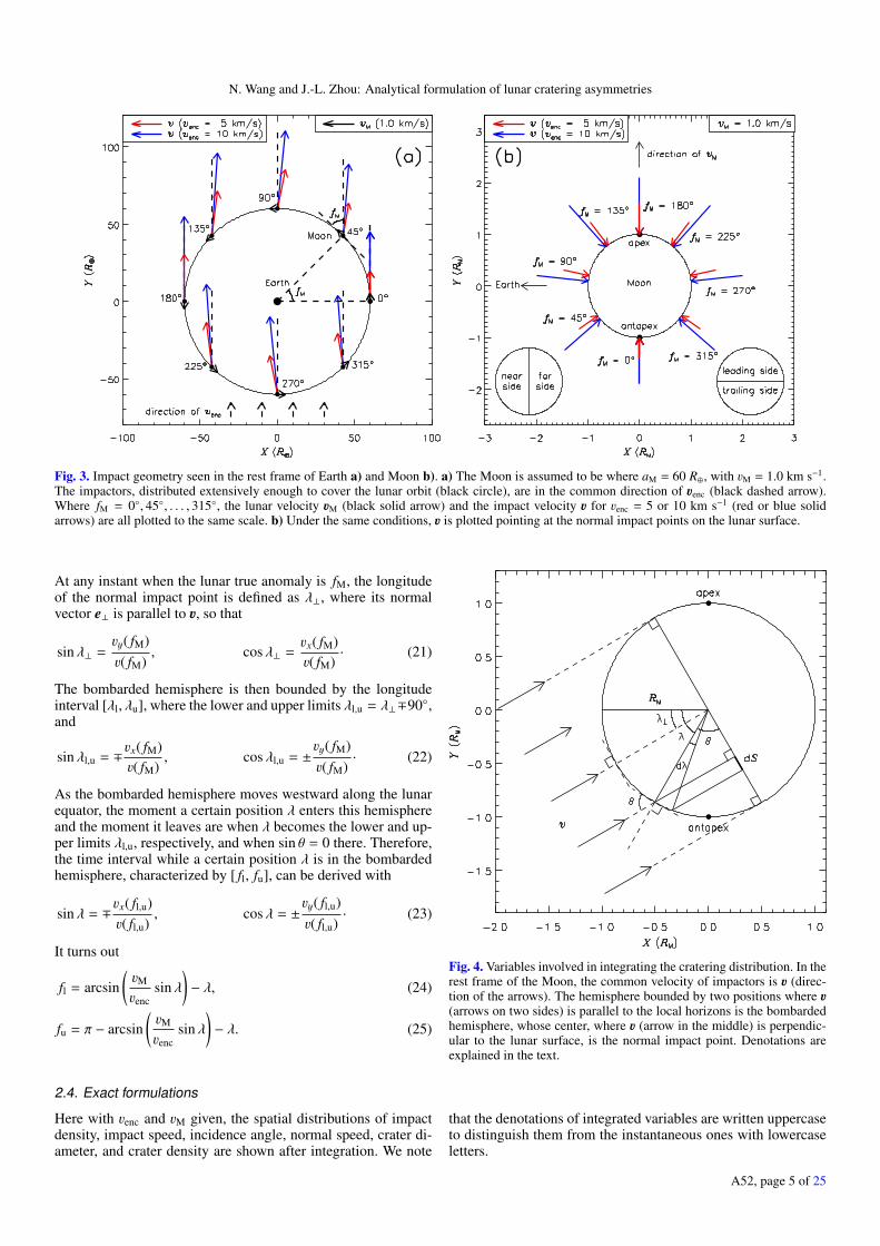
Fig. 5. Impact speed a); incidence angle b); normal speed c); crater diameter d); impact density e); and crater density f) as functions of longitude.Their variations with longitude (solid curves in red, orange, yellow, and green for venc = 10, 20, 30, and 40 km s−1) and their global averages(dashed lines in the same color for the same venc, except for those in panel b), which are all black to represent the invariant value) are calculatedwith vM = 1.0 km s−1, dmin = 0.5 km, αp = 1.75, ρ = 3.4 × 10⁻²⁵ km−2, t = 3.7 Gyr, and dc = 25 km.
The impact density N is the number of impacts on a certainregion divided by its area. For the unit area on longitude λ illus-trated in Fig. 4, its impact density during a unit time is
dN =dFdt
dl=
ρ
nM(vx cos λ + vy sin λ)d fM. (26)
Integration of dN over the interval [ fl, fu] leads to
N(λ) =2ρnM
[√v2
enc − v2M sin2 λ − vM sin λ arccos
(vM
vencsin λ
)].
(27)
A52, page 6 of 25
N. Wang and J.-L. Zhou: Analytical formulation of lunar cratering asymmetries
To simplify the expression, we define σ ∈ (0, π) by
σ = arccos(vM
vencsin λ
), (28)
which leads to
sinσ = | cos( fl,u + λ)| =
√1 −
(vM
vencsin λ
)2
, (29)
cosσ = sin( fl,u + λ) =vM
vencsin λ. (30)
Therefore,
N(λ) =2ρvenc
nM(sinσ − σ cosσ). (31)
The impact speed V , incidence angle Θ, and normal speed V⊥,as functions of longitude, are averages of v, θ, and v⊥ over onelunar period, that is, V = (
∫ fuflvdN)/N, sin Θ = (
∫ fufl
sin θdN)/N,
and V⊥ = (∫ fu
flv⊥dN)/N. The integration leads to
V(λ) = I1/I0, (32)sin Θ(λ) = I2/I0, (33)V⊥(λ) = I3/I0, (34)
where
I0 = 2venc(sinσ − σ cosσ), (35)
I1 =1
3vM[(v2
enc + v2M) cos λ + 2vMvenc sinσ]I+
− [(v2enc + v2
M) cos λ − 2vMvenc sinσ]I−+ (venc + vM)(v2
enc + 7v2M)(sin λ)∆E
− (venc + vM)(venc − vM)2(sin λ)∆F, (36)
I2 =1
3v2M
[(2v2enc − 3v2
M) cos λ − vMvenc sinσ](sin λ)I+
− [(2v2enc − 3v2
M) cos λ + vMvenc sinσ](sin λ)I−− (venc + vM)[(v2
enc − 2v2M) cos(2λ) + 3v2
M]∆E
+ (venc + vM)(venc − vM)2 cos(2λ)∆F, (37)
I3 = v2enc[(1 + 2 cos2 σ)σ − 3 sinσ cosσ], (38)
I± =
√v2
enc + v2M cos(2λ) ± 2vMvenc cos λ sinσ, (39)
∆E = E(λ − σ
2+π
4|k2
)− E
(λ + σ
2+π
4− δπ|k2
)− 2δE
(k2
),
(40)
∆F = F(λ − σ
2+π
4|k2
)− F
(λ + σ
2+π
4− δπ|k2
)− 2δF
(k2
),
(41)
k2 =4vMvenc
(venc + vM)2 , (42)
δ =
0, (λ < 0)1. (λ > 0) .
(43)
Functions F(φ|k2) and F(k2) are the incomplete and completeelliptic integrals of the first kind; E(φ|k2) and E(k2) are those ofthe second kind.
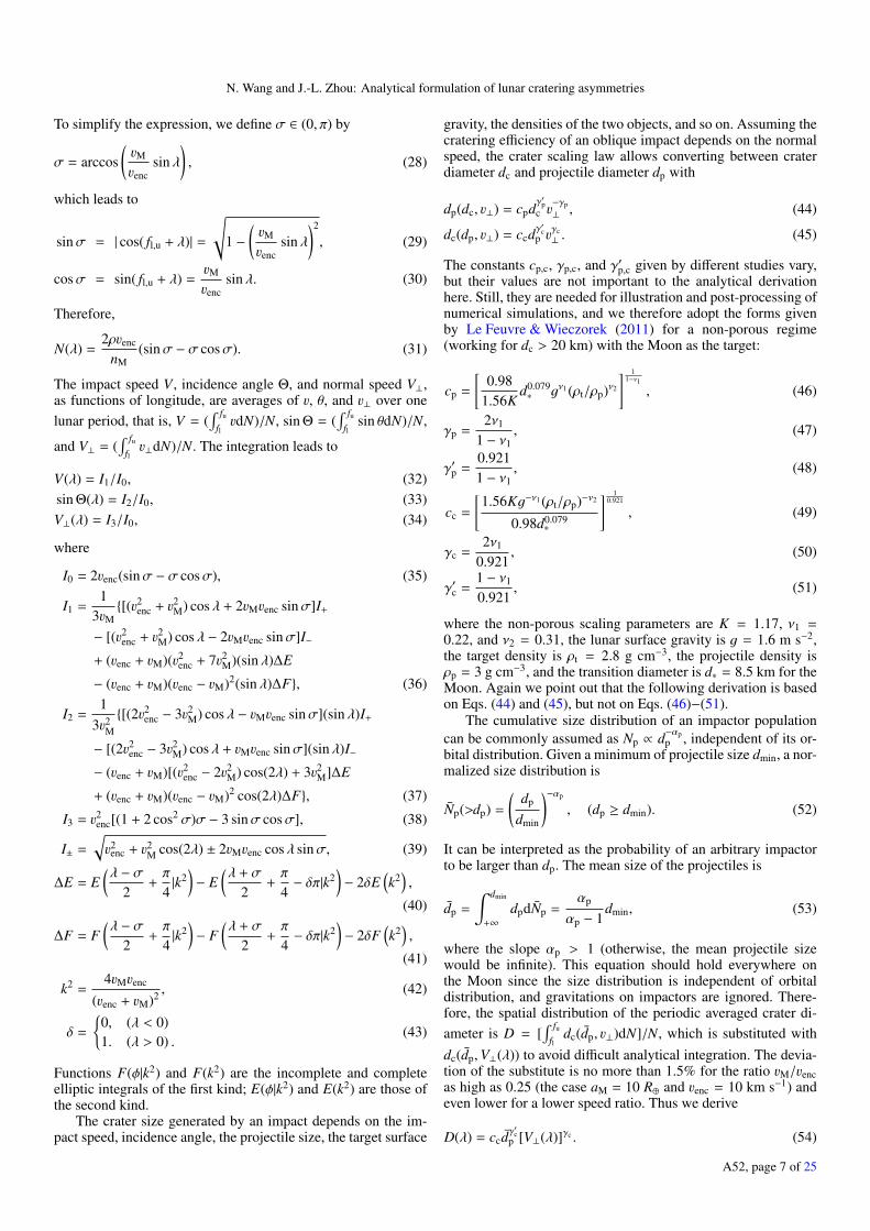
The crater size generated by an impact depends on the im-pact speed, incidence angle, the projectile size, the target surface
gravity, the densities of the two objects, and so on. Assuming thecratering efficiency of an oblique impact depends on the normalspeed, the crater scaling law allows converting between craterdiameter dc and projectile diameter dp with
dp(dc, v⊥) = cpdγ′pc v−γp⊥ , (44)
dc(dp, v⊥) = ccdγ′c
p vγc⊥ . (45)
The constants cp,c, γp,c, and γ′p,c given by different studies vary,but their values are not important to the analytical derivationhere. Still, they are needed for illustration and post-processing ofnumerical simulations, and we therefore adopt the forms givenby Le Feuvre & Wieczorek (2011) for a non-porous regime(working for dc > 20 km) with the Moon as the target:
cp =
[0.98
1.56Kd0.079∗ gν1 (ρt/ρp)ν2
] 11−ν1
, (46)
γp =2ν1
1 − ν1, (47)
γ′p =0.9211 − ν1
, (48)
cc =
[1.56Kg−ν1 (ρt/ρp)−ν2
0.98d0.079∗
] 10.921
, (49)
γc =2ν1
0.921, (50)
γ′c =1 − ν1
0.921, (51)
where the non-porous scaling parameters are K = 1.17, ν1 =0.22, and ν2 = 0.31, the lunar surface gravity is g = 1.6 m s−2,the target density is ρt = 2.8 g cm−3, the projectile density isρp = 3 g cm−3, and the transition diameter is d∗ = 8.5 km for theMoon. Again we point out that the following derivation is basedon Eqs. (44) and (45), but not on Eqs. (46)−(51).
The cumulative size distribution of an impactor populationcan be commonly assumed as Np ∝ d−αp
p , independent of its or-bital distribution. Given a minimum of projectile size dmin, a nor-malized size distribution is
Np(>dp) =
(dp
dmin
)−αp
, (dp ≥ dmin). (52)
It can be interpreted as the probability of an arbitrary impactorto be larger than dp. The mean size of the projectiles is
dp =
∫ dmin
+∞
dpdNp =αp
αp − 1dmin, (53)
where the slope αp > 1 (otherwise, the mean projectile sizewould be infinite). This equation should hold everywhere onthe Moon since the size distribution is independent of orbitaldistribution, and gravitations on impactors are ignored. There-fore, the spatial distribution of the periodic averaged crater di-ameter is D = [
∫ fufl
dc(dp, v⊥)dN]/N, which is substituted withdc(dp,V⊥(λ)) to avoid difficult analytical integration. The devia-tion of the substitute is no more than 1.5% for the ratio vM/vencas high as 0.25 (the case aM = 10 R⊕ and venc = 10 km s−1) andeven lower for a lower speed ratio. Thus we derive
D(λ) = ccdγ′c
p [V⊥(λ)]γc . (54)
A52, page 7 of 25

A&A 594, A52 (2016)
The crater density Nc(>dc) is the number of craters with diam-eters larger than dc per unit area. It is relevant to the age de-termination in the cratering chronology method. It depends onthe projectile diameter dp, the projectile size-frequency distribu-tion Np, and the impact density N. On the assumption that everyimpact leaves one and only one crater, meaning that saturation,erosion, and secondary craters are all ignored,
dNc(>dc) = Np(>dp(dc, v⊥))dN. (55)
In every unit time d fM ∈ [ fl, fu], the factor dN gives the total den-sity of craters on the longitude λ; function dp gives the projectilesize required to form a crater as large as dc there; function Npgives the fraction of impactors larger than dp, which is equivalentto the fraction of craters larger than dc; and finally the product ofNp and dN determines the required part of dN. The substitute forthe integral
∫ fufl
Np(> dp(dc, v⊥))dN is Np(> dp(dc,V⊥(λ)))N(λ),whose deviation is no more than 0.07% for a ratio vM/venc ashigh as 0.25 and even smaller for a lower speed ratio. Assumingdc is large enough to ensure dp(dc,V⊥(λ)) ≥ dmin holds every-where on the lunar surface, then
Nc(>dc, λ) =
dmin
cpdγ′pc
αp
[V⊥(λ)]γpαp N(λ). (56)
We note that Nc(>dc, λ) describes not only the spatial distribu-tion of the crater density, but also the craters’ size distribution.Equation (56) proves Nc ∝ d
−γ′pαpc on any lunar longitude, and
thus the slopes of the size distributions of impactors and cratersare related by
αc = γ′pαp. (57)
Although the integration is made over one lunar period, all ofthe distributions but N(λ) and Nc(>dc, λ) have no dependence ontime, so that they are applicable to any time interval t (multipleof lunar period, theoretically) as long as vM and venc are constant.We rewrite N(λ) after multiplying it by nMt/(2π):
N(λ) =ρtvenc
π(sinσ − σ cosσ). (58)
This form describes the impact density after a bombardment du-ration t, but its relative variation does not differ at all from theone-periodic form, which is one of the reasons we suggest us-ing the asymmetry amplitude to measure the relative variation(Sect. 2.7). Hereafter, this new expression of N(λ) takes the placeof the previous one, while Nc(>dc, λ) (Eq. (56)) is still valid.
All of the absolute spatial distributions are shown in Fig. 5with solid curves. We caution that on each unit area, there mustbe impacts with all the (instantaneous) incidence angles θ ∈ [0,90] theoretically, and thus all the normal speeds v⊥ ∈ [0, v] andcrater diameters dc ∈ [0, dc(dp, v)], nevertheless, their periodicaverages are what the figure shows. The most significant com-mon feature is that the curves all peak at the apex (λ = −90)and are lowest at the antapex (λ = +90), regardless of venc. Theleading/trailing asymmetry is unambiguously detected in distri-butions of all the investigated variables, which is to be confirmedagain through approximate expressions (Sect. 2.7). Additionally,it is apparent that higher venc leads to an upward shift of all thecurves, expect for Θ(λ). An increase in venc diminishes and en-larges the absolute amplitudes of D and Nc, while it almost doesnot influence those of N, V , and V⊥. With vM fixed, the absoluteamplitude of Θ that only depends on the speed ratio vM/venc alsoseems to decrease as venc increases. We provide the explanationin Sect. 2.7.
2.5. Near/far symmetry
Because N(λ) = N(±180 − λ), N(λ) is symmetric about λ =±90, meaning that the distribution of the impact density on thelunar surface is symmetric about the line connecting the apex andthe antapex. The same is easily found in terms of V , Θ, V⊥, D,and Nc. Therefore, the Moon’s near and far sides are exact mirrorimages of each other, with no sign of a near/far asymmetry.
This conclusion is based on the assumption that the Earth’sgravitation on the impactors and its volume are not considered,meaning that Earth is treated as if it were transparent to the im-pactors. In reality, it may block impactors like a shield, pre-venting them from impacting the Moon, or gravitationally fo-cusing them like a lens, increasing the flux that the near sidereceives. Bandermann & Singer (1973) confirmed the former ef-fect for the condition that aM < 25 R⊕; Gallant et al. (2009)claimed that there was very little asymmetry for aM in the range10−50 R⊕; Le Feuvre & Wieczorek (2011) found the asymmetrynegligible with about 0.1% more craters of the near side than thefar side, in contrast with Le Feuvre & Wieczorek (2005), whoclaimed a factor of four enhancement on the near side using im-pactors coplanar with Earth. Our deduction shows that withoutthe Earth’s effect, the near/far asymmetry cannot exist, whilethe leading/trailing asymmetry is the inherent and natural con-sequence of cratering.
We therefore use β, the angular distance from the apex, todescribe the leading/trailing asymmetry and not the longitude λ.It ranges between 0 and 180, where the apex and antapex are,respectively. For the near side, where −90 ≤ λ ≤ +90,
λ = β − 90.
Substituting λ with β, the integrated variables as functions of βare
N(β) =ρtvenc
π(sinσ − σ cosσ), (59)
V(β) = I′1/I′0, (60)
sin Θ(β) = I′2/I′0, (61)
V⊥(β) = I′3/I′0, (62)
D(β) = ccdγ′c
p [V⊥(β)]γc , (63)
Nc(>dc, β) =
dmin
cpdγ′pc
αp
[V⊥(β)]γpαp N(β), (64)
where
I′0 = 2(sinσ − σ cosσ), (65)
I′1 =venc
3η
[(1 + η2) sin β + 2η sinσ]I′+
−[(1 + η2) sin β − 2η sinσ]I′−
−(1 + η)(1 + 7η2)(cos β)∆E
+(1 + η)(1 − η)2(cos β)∆F, (66)
I′2 =1
3η2
− [(2 − 3η2) sin β − η sinσ](cos β)I′+
+[(2 − 3η2) sin β + η sinσ](cos β)I′−
+(1 + η)[(1 − 2η2) cos(2β) − 3η2]∆E
−(1 + η)(1 − η)2 cos(2β)∆F, (67)
A52, page 8 of 25

N. Wang and J.-L. Zhou: Analytical formulation of lunar cratering asymmetries
I′3 = venc[(1 + 2 cos2 σ)σ − 3 sinσ cosσ], (68)
I′± =
√1 − η2 cos(2β) ± 2η sin β sinσ, (69)
∆E = E(β − σ
2|k2
)− E
(β + σ
2− δπ|k2
)− 2δE
(k2
), (70)
∆F = F(β − σ
2|k2
)− F
(β + σ
2− δπ|k2
)− 2δF
(k2
), (71)
k2 =4η
(1 + η)2 , (72)
δ =
0,(β < π
2
)1,
(β > π
2
) (73)
σ = arccos (−η cos β) , (74)
sinσ =
√1 − (η cos β)2, (75)
cosσ = −η cos β, (76)
η =vM
venc· (77)
We note that the above equations are applicable to both the nearand the far side.
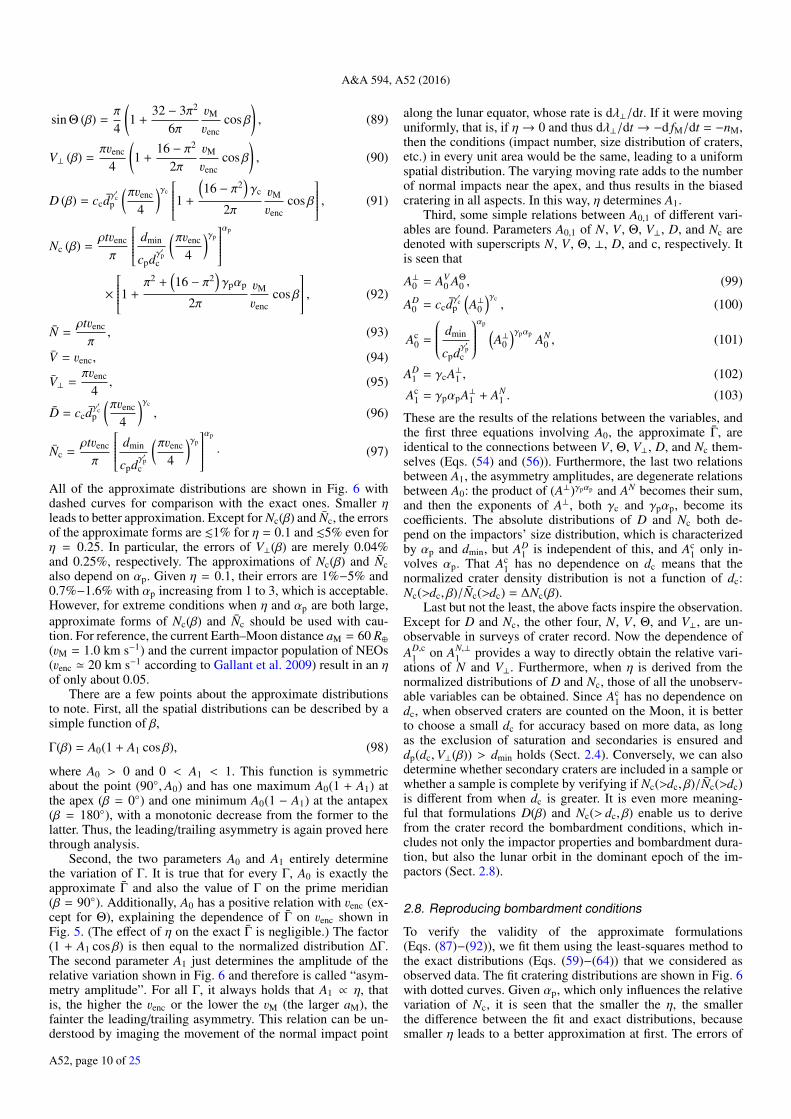
Figure 6 illustrates the relative spatial variations of N, V , Θ,V⊥, D, and Nc as functions of β with solid curves. The relativevariation is the absolute variation divided by its global average(to be derived in Sect. 2.6). All variables decrease monotonicallywith increasing β, as we show in Fig. 5. Moreover, the greaterthe encounter speed venc (the lower the speed ratio vM/venc withgiven vM), the smaller the relative variation amplitudes (to beexplained in Sect. 2.7).
2.6. Global averages
Here we derive the global averages of the impact density N, im-pact speed V , incidence angle Θ, normal speed V⊥, crater di-ameter D, and crater density Nc through integrating. The im-pact number for a unit area on the longitude λ during a unittime is
d2C = dFdt =ρRM
nM(vx cos λ + vy sin λ)dλd fM, (78)
where F is the impact flux (Eq. (20)), vx,y are elements of u(Eqs. (14) and (15)), and ρ is the uniform spatial density ofimpactors. The total number of impacts on the global lunarsurface after one lunar period is the integral
!d2C over the
λ interval [λl, λu] and fM interval [0, 360] in turn, whereλl,u( fM) are boundaries of the instantaneous bombarded hemi-sphere (Eq. (22)). Thus,
C =8ρRM
nM(venc + vM)E(k2). (79)
The global average of N for the bombardment duration t (multi-ple of lunar period) is the total impact number for one period, C,divided by the global area lgl = 2πRM (perimeter for the planarmodel) and multiplied by nMt/(2π):
N =2ρtπ2 (venc + vM)E(k2). (80)
Apparently, the global averages of V , Θ, and V⊥ are the inte-grals
!vd2C,
!sin θd2C, and
!v⊥d2C over the above λ and
fM intervals divided by C, respectively. The integration resultsin
V =π
2v2
enc + v2M
(venc + vM)E(k2), (81)
sin Θ =π
4, (82)
V⊥ =π2
8v2
enc + v2M
(venc + vM)E(k2), (83)
where Θ is defined by sin Θ = sin θ, and it is found V⊥ = V sin Θ.The global averages of D and Nc are [
!dc(dp, v⊥)d2C]/C and
[!
Np(>dp(dc, v⊥))d2C]/lgl, but to avoid analytical integration,we again substitute them by dc(dp, V⊥) and Np(> dp(dc, V⊥))N,functions (Eqs. (45) and (44)) of V⊥ and N. The substitutesare quite acceptable, for their deviations are <3% and <1%, re-spectively, for a speed ratio vM/venc as high as 0.25 (the caseaM = 10 R⊕ and venc = 10 km s−1). A lower speed ratio leads toeven smaller deviations. Thus, we derive
D = ccdγ′c
p Vγc⊥ , (84)
Nc =
dmin
cpdγ′pc
αp
Vγpαp⊥ N. (85)
The global averages are shown in Fig. 5 with horizontal dashedlines. They all exhibit positive relations with venc, except for Θ.Equation (82) explains the exception by determining the globalaverage of sin θ to be π/4 always, equivalent to Θ = 51.8, re-gardless of both the encounter speed venc and the lunar orbitalspeed vM.
2.7. Approximate formulations
We have formulated the spatial distributions N(β), V(β), Θ(β),V⊥(β), D(β), and Nc(> dc, β) (Eqs. (59)−(64)) and the globalaverages N, V , V⊥, Θ, D, and Nc (Eqs. (80)−(85)). Hereafter,we use Γ to denote any one (or every one) of the variables N,V , Θ, V⊥, D, and Nc, and use Γ to denote its global average.The normalized distribution is defined as the absolute distribu-tion divided by the global average, which describes the relativevariation
∆Γ(β) = Γ(β)/Γ. (86)
The above variables represent every aspect of cratering and theirspatial distributions are what we call cratering distribution. Eachof the formulations Γ(β) and Γ except for the constant Θ canbe taken as the product of two factors involving the encounterspeed venc and the speed ratio η = vM/venc respectively. Recallingthe assumption vM < venc, we can derive their series expansionsaround η = 0. To first order, the formulations are simplified to be
N (β) =ρtvenc
π
(1 +
π
2vM
venccos β
), (87)
V (β) = venc
(1 +
π
4vM
venccos β
), (88)
A52, page 9 of 25
A&A 594, A52 (2016)
sin Θ (β) =π
4
(1 +
32 − 3π2
6πvM
venccos β
), (89)
V⊥ (β) =πvenc
4
(1 +
16 − π2
2πvM
venccos β
), (90)
D (β) = ccdγ′c
p
(πvenc
4
)γc
1 +
(16 − π2
)γc
2πvM
venccos β
, (91)
Nc (β) =ρtvenc
π
dmin
cpdγ′pc
(πvenc
4
)γp
αp
×
1 +π2 +
(16 − π2
)γpαp
2πvM
venccos β
, (92)
N =ρtvenc
π, (93)
V = venc, (94)
V⊥ =πvenc
4, (95)
D = ccdγ′c
p
(πvenc
4
)γc
, (96)
Nc =ρtvenc
π
dmin
cpdγ′pc
(πvenc
4
)γp
αp
· (97)
All of the approximate distributions are shown in Fig. 6 withdashed curves for comparison with the exact ones. Smaller ηleads to better approximation. Except for Nc(β) and Nc, the errorsof the approximate forms are .1% for η = 0.1 and .5% even forη = 0.25. In particular, the errors of V⊥(β) are merely 0.04%and 0.25%, respectively. The approximations of Nc(β) and Ncalso depend on αp. Given η = 0.1, their errors are 1%−5% and0.7%−1.6% with αp increasing from 1 to 3, which is acceptable.However, for extreme conditions when η and αp are both large,approximate forms of Nc(β) and Nc should be used with cau-tion. For reference, the current Earth–Moon distance aM = 60 R⊕(vM = 1.0 km s−1) and the current impactor population of NEOs(venc ' 20 km s−1 according to Gallant et al. 2009) result in an ηof only about 0.05.
There are a few points about the approximate distributionsto note. First, all the spatial distributions can be described by asimple function of β,
Γ(β) = A0(1 + A1 cos β), (98)
where A0 > 0 and 0 < A1 < 1. This function is symmetricabout the point (90, A0) and has one maximum A0(1 + A1) atthe apex (β = 0) and one minimum A0(1 − A1) at the antapex(β = 180), with a monotonic decrease from the former to thelatter. Thus, the leading/trailing asymmetry is again proved herethrough analysis.
Second, the two parameters A0 and A1 entirely determinethe variation of Γ. It is true that for every Γ, A0 is exactly theapproximate Γ and also the value of Γ on the prime meridian(β = 90). Additionally, A0 has a positive relation with venc (ex-cept for Θ), explaining the dependence of Γ on venc shown inFig. 5. (The effect of η on the exact Γ is negligible.) The factor(1 + A1 cos β) is then equal to the normalized distribution ∆Γ.The second parameter A1 just determines the amplitude of therelative variation shown in Fig. 6 and therefore is called “asym-metry amplitude”. For all Γ, it always holds that A1 ∝ η, thatis, the higher the venc or the lower the vM (the larger aM), thefainter the leading/trailing asymmetry. This relation can be un-derstood by imaging the movement of the normal impact point
along the lunar equator, whose rate is dλ⊥/dt. If it were movinguniformly, that is, if η→ 0 and thus dλ⊥/dt → −d fM/dt = −nM,then the conditions (impact number, size distribution of craters,etc.) in every unit area would be the same, leading to a uniformspatial distribution. The varying moving rate adds to the numberof normal impacts near the apex, and thus results in the biasedcratering in all aspects. In this way, η determines A1.
Third, some simple relations between A0,1 of different vari-ables are found. Parameters A0,1 of N, V , Θ, V⊥, D, and Nc aredenoted with superscripts N, V , Θ, ⊥, D, and c, respectively. Itis seen that
A⊥0 = AV0 AΘ
0 , (99)
AD0 = ccdγ
′c
p
(A⊥0
)γc, (100)
Ac0 =
dmin
cpdγ′pc
αp (A⊥0
)γpαpAN
0 , (101)
AD1 = γcA⊥1 , (102)
Ac1 = γpαpA⊥1 + AN
1 . (103)
These are the results of the relations between the variables, andthe first three equations involving A0, the approximate Γ, areidentical to the connections between V , Θ, V⊥, D, and Nc them-selves (Eqs. (54) and (56)). Furthermore, the last two relationsbetween A1, the asymmetry amplitudes, are degenerate relationsbetween A0: the product of (A⊥)γpαp and AN becomes their sum,and then the exponents of A⊥, both γc and γpαp, become itscoefficients. The absolute distributions of D and Nc both de-pend on the impactors’ size distribution, which is characterizedby αp and dmin, but AD
1 is independent of this, and Ac1 only in-
volves αp. That Ac1 has no dependence on dc means that the
normalized crater density distribution is not a function of dc:Nc(>dc, β)/Nc(>dc) = ∆Nc(β).
Last but not the least, the above facts inspire the observation.Except for D and Nc, the other four, N, V , Θ, and V⊥, are un-observable in surveys of crater record. Now the dependence ofAD,c
1 on AN,⊥1 provides a way to directly obtain the relative vari-
ations of N and V⊥. Furthermore, when η is derived from thenormalized distributions of D and Nc, those of all the unobserv-able variables can be obtained. Since Ac
1 has no dependence ondc, when observed craters are counted on the Moon, it is betterto choose a small dc for accuracy based on more data, as longas the exclusion of saturation and secondaries is ensured anddp(dc,V⊥(β)) > dmin holds (Sect. 2.4). Conversely, we can alsodetermine whether secondary craters are included in a sample orwhether a sample is complete by verifying if Nc(>dc, β)/Nc(>dc)is different from when dc is greater. It is even more meaning-ful that formulations D(β) and Nc(> dc, β) enable us to derivefrom the crater record the bombardment conditions, which in-cludes not only the impactor properties and bombardment dura-tion, but also the lunar orbit in the dominant epoch of the im-pactors (Sect. 2.8).
2.8. Reproducing bombardment conditions
To verify the validity of the approximate formulations(Eqs. (87)−(92)), we fit them using the least-squares method tothe exact distributions (Eqs. (59)−(64)) that we considered asobserved data. The fit cratering distributions are shown in Fig. 6with dotted curves. Given αp, which only influences the relativevariation of Nc, it is seen that the smaller the η, the smallerthe difference between the fit and exact distributions, becausesmaller η leads to a better approximation at first. The errors of
A52, page 10 of 25
N. Wang and J.-L. Zhou: Analytical formulation of lunar cratering asymmetries
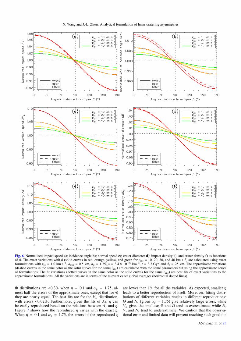
Fig. 6. Normalized impact speed a); incidence angle b); normal speed c); crater diameter d); impact density e); and crater density f) as functionsof β. The exact variations with β (solid curves in red, orange, yellow, and green for venc = 10, 20, 30, and 40 km s−1) are calculated using exactformulations with vM = 1.0 km s−1, dmin = 0.5 km, αp = 1.75, ρ = 3.4 × 10⁻²⁵ km−2, t = 3.7 Gyr, and dc = 25 km. The approximate variations(dashed curves in the same color as the solid curves for the same venc) are calculated with the same parameters but using the approximate seriesof formulations. The fit variations (dotted curves in the same color as the solid curves for the same venc) are best fits of exact variations to theapproximate formulations. All the variations are in terms of the relevant exact global averages (horizontal dotted lines).
fit distributions are <0.3% when η = 0.1 and αp = 1.75, al-most half the errors of the approximate ones, except that for Θthey are nearly equal. The best fits are for the V⊥ distribution,with errors <0.02%. Furthermore, given the fits of A1, η canbe easily reproduced based on the relations between A1 and η.Figure 7 shows how the reproduced η varies with the exact η.When η = 0.1 and αp = 1.75, the errors of the reproduced η
are lower than 1% for all the variables. As expected, smaller ηleads to a better reproduction of itself. Moreover, fitting distri-butions of different variables results in different reproductions:Θ and Nc (given αp = 1.75) give relatively large errors, whileV⊥ gives the smallest; Θ and D tend to overestimate, while N,V , and Nc tend to underestimate. We caution that the observa-tional error and limited data will prevent reaching such good fits
A52, page 11 of 25
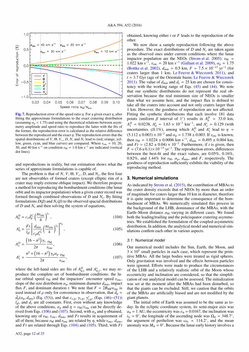
A&A 594, A52 (2016)
Fig. 7. Reproduction error of the speed ratio η. For a given exact η, afterfitting the approximate formulations to the exact cratering distribution(assuming αp = 1.75) and using the theoretical relations between asym-metry amplitude and speed ratio to reproduce the latter with the fits ofthe former, the reproduction error is calculated as the relative differencebetween the reproduced and the exact η. The reproduction errors that thespatial distributions of V , Θ, V⊥, D, N, and Nc lead to (red, orange, yel-low, green, cyan, and blue curves) are compared. Where venc = 10, 20,30, and 40 km s−1 on condition vM = 1.0 km s−1 are indicated (verticaldot lines).
and reproductions in reality, but our estimation shows what theseries of approximate formulations is capable of.
The problem is that of N, V , Θ, V⊥, D, and Nc, the first fourare not observables of formed craters (except elliptic rim of acrater may imply extreme oblique impact). We therefore proposea method for reproducing the bombardment conditions (the lunarorbit and its impactor population) when a given crater record wasformed through combined observations of D and Nc. By fittingformulations D(β) and Nc(β) to the observed spacial distributionsof D and Nc and then solving the system of equations,
AD0 = ccdγ
′c
p
(πvenc
4
)γc
, (104)
Ac0 =
Ftlgl
dmin
cpdγ′pc
(πvenc
4
)γp
αp
, (105)
AD1 =
(16 − π2
)γc
2πvM
venc, (106)
Ac1 =
π2 +(16 − π2
)γpαp
2πvM
venc, (107)
where the left-hand sides are fits of AD0,1 and Ac
0,1, we may re-produce the complete set of bombardment conditions: the lu-nar orbital speed vM and the impactors’ encounter speed venc,slope of the size distribution αp, minimum diameter dmin, impactflux F, and dominant duration t. We note that F = 2RMρvenc isused instead of ρ only for convenience in observation, that dp =
dp(αp, dmin) (Eq. (53)), and that cc,p, γc,p, γ′c,p, (Eqs. (46)−(51))lgl, and dc are all constants. First, even without any knowledgeof the above conditions, αp and η = vM/venc can be directly de-rived from Eqs. (106) and (107). Second, with αp and η obtained,knowing any of vM, venc, dmin, and Ft results in acquirement ofall of them, because vM and venc are related by η, while venc, dmin,and Ft are related through Eqs. (104) and (105). Third, with Ft
obtained, knowing either t or F leads to the reproduction of theother.
We now show a sample reproduction following the aboveprocedure. The exact distributions of D and Nc are taken againas the observed ones under current conditions where the lunarimpactor population are the NEOs (Strom et al. 2005): vM =1.022 km s−1, venc = 20 km s−1 (Gallant et al. 2009), αp = 1.75(Bottke et al. 2002), dmin = 0.5 km, F = 7.5 × 10⁻¹³ yr−1 (forcraters larger than 1 km; Le Feuvre & Wieczorek 2011), andt = 3.7 Gyr (age of the Orientale basin; Le Feuvre & Wieczorek2011). The value of dmin and dc = 25 km are chosen for consis-tency with the working range of Eqs. (45) and (44). We notethat our synthetic distributions do not represent the real ob-servation because the real minimum size of NEOs is smallerthan what we assume here, and the impact flux is defined totake all the craters into account and not only craters larger than1 km. However, the goodness of reproduction are not affected.Fitting the synthetic distributions that each involve 181 datapoints (uniform β interval of 1) results in AD
0 = 33.0 km,AD
1 = 0.0238, Ac0 = 1.63 × 10⁻⁷ km−1, and Ac
1 = 0.129 (withuncertainties .0.1%), among which AD
1 and Ac1 lead to η =
(5.112 ± 0.003) × 10−2 and αp = 1.738 ± 0.003. If venc is known,then vM = 1.0224 ± 0.0006 km s−1, dmin = 0.495 ± 0.004 km,and Ft = (2.82 ± 0.04) × 10−3. Furthermore, if t is given, thenF = (7.6±0.1)×10−13 yr−1. The reproduction errors, differencesbetween the best-fit and the exact values, are 0.05%, 0.16%,0.82%, and 1.44% for vM, αp, dmin, and F, respectively. Thegoodness of reproduction sufficiently exhibits the viability of thereproducing method.
3. Numerical simulationsAs indicated by Strom et al. (2015), the contribution of MBAs tothe crater density exceeds that of NEOs by more than an orderof magnitude for craters larger than 10 km in diameter, thereforeit is quite important to determine the consequence of the bom-bardment of MBAs. We numerically simulated this process inthe background of the LHB, dominance of the MBAs, with theEarth–Moon distance aM varying in different cases. We foundboth the leading/trailing and the pole/equator cratering asymme-tries. We established the formulation of the coupled-asymmetricdistribution. In addition, the analytical model and numerical sim-ulations confirm each other in various aspects.
3.1. Numerical model
Our numerical model includes the Sun, Earth, the Moon, and3 × 105 small particles in each case, which represent the prim-itive MBAs. All the large bodies were treated as rigid spheres.Only gravitation was involved and the effects between particleswere ignored. Efforts were made to produce the circumstancesof the LHB and a relatively realistic orbit of the Moon whoseeccentricity and inclination are considered, so that the simplifi-cation of our analytical model can be assessed. The initializationwas set at the moment after the MBAs had been disturbed, sothat the giants can be excluded. Still, we caution that the orbitsof the MBAs are artificially biased and are not modified by thegiant planets.
The initial orbit of Earth was assumed to be the same as to-day. In the ecliptic coordinate system, its semi-major axis wasa⊕ = 1 AU, the eccentricity was e⊕ = 0.0167, the inclination wasi⊕ = 0, the longitude of the ascending node was Ω⊕ = 348.7,the argument of perihelion was ω⊕ = 114.2, and the meananomaly was M⊕ = 0. Because the lunar early history involves a
A52, page 12 of 25
N. Wang and J.-L. Zhou: Analytical formulation of lunar cratering asymmetries
great uncertainty as mentioned in Sect. 1, five cases were set withthe lunar semi-major axis aM = 20, 30, 40, 50, and 60 R⊕ in turn,probably covering most durations of the lunar history. This alsohelps to examine the influence of aM on the cratering. The lunareccentricity eM was initially set to 0.04 (Ross & Schubert 1989),while the current value of the lunar inclination to the eclipticiM = 5 was adopted. The Moon’s longitude of the ascendingnode ΩM, the argument of perihelion ωM, and the mean anomalyMM were all 0, because the lunar orbital period and the periodof its precession along the ecliptic are extremely short relative tothe timescale of the tidal evolution.
Primitive MBAs mean the asteroids that occupied the re-gion where the contemporary main belt is during the LHB, thatis, 2.0 AU ≤ ap ≤ 3.5 AU. Their orbits were disturbed bythe migration of giants (Gomes et al. 2005), while their sizedistribution can be taken as invariant (Bottke et al. 2005). Weonly needed those MBAs that have the potential for encounter-ing the Earth–Moon system, namely, those with perihelion dis-tances qp no larger than 1 AU. To maximize the impact probabil-ity (Morbidelli & Gladman 1998) and avoid the interference ofthe effect of qp, the initial qp was constrained to be 1 AU, result-ing in 0.50 ≤ ep ≤ 0.71. The inclination was set to 0 ≤ ip ≤ 0.5to examine the mechanism of the latitudinal cratering asymme-try. The orbital elements Ωp, ωp, and Mp all ranged from 0 to360. Each particle’s initial orbital elements were randomly gen-erated in corresponding ranges following uniform distributions,except that its eccentricity was derived from ep = 1− qp/ap. Themass of every particle was 4 × 10¹² kg, equivalent to a diame-ter dp ∼ 1 km given a density of 3 g cm−3. This means that thesize distribution is not considered at the stage of N-body simula-tions. The total mass of the particles of 1 × 10¹⁸ kg is negligibleto that of the Moon, therefore generating a size distribution inthe simulations will not lead to statistically different results, butwill take many more simulations to derive meaningful statistics.Therefore, we only considered this in the post-processing whenthe crater diameter and crater density are calculated. Althoughthe size distribution of current MBAs has been studied by sev-eral surveys (Sect. 1), it cannot be easily modeled because of itspower-law breaks. In this work, we assumed the normalized sizedistribution (Eq. (52)) to be a single power-law characterized byαp = 3 and dmin = 5 km referring to Ivezic et al. (2001), whodetermined αp = 3 for 5 km . dp . 40 km.
Three-dimensional N-body simulations were run to integratethe orbits of the Sun, Earth, the Moon, and 3 × 10⁵ particlesin each case. The integration time was 10 Myr as a compro-mise between computing efficiency and the fact that the LHBlasted for ∼0.1 Gyr (Gomes et al. 2005). In addition, this is longenough to allow nearly all the potential impacts to occur, and it isshort enough to omit the tidal evolution. The integration consistsof two steps. We first integrated Earth, the Moon, and all theparticles in the heliocentric ecliptic reference frame using thehybrid symplectic integrator in the Mercury software package(Chambers 1999), which was altered to adapt it to our purpose.When a particle had a close encounter with the Moon, the infor-mation of Earth, the Moon, and this particle was recorded. Thenin the next step, we used the Runge-Kutta-Fehlberg method tointegrate the recorded particles and the Earth–Moon system un-til all the particles had impacted the Moon. In this step, the per-turbation of the Sun was ignored since the integration time ittook is only ∼10 min, while the lunar orbital period is five days(aM = 20 R⊕) at least.
Given that the Moon rotated synchronously during the LHB(Sect. 2.1), every impact in the simulations was precisely lo-cated on the lunar surface. Because the Moon has a longitudinal
geometrical libration due to its eccentricity (the lunar spin axiswas assumed to be perpendicular to the lunar orbital plane sothat there is no libration in latitude), the near side is defined asthe hemisphere facing Earth only when the Moon is at its perigeeand the far side is its opposite. The longitude line that the cen-ter of the near side lies on is the prime meridian, with the eastlongitude values being positive. The apex point, the center of theleading side, is at (−90, 0), while the antapex point, the centerof the trailing side, is at (90, 0). The low- and high-latitude re-gions are also defined here as the area with a latitude between±45 and the remaining area on the lunar surface, respectively.
Based on this numerical model, the bombardment condi-tions are venc = 8.32 km s−1 (estimated with Eq. (7) given qp= 1 AU and ap = 2.75 AU, the mean of the initial ap), αp = 3,dmin = 5 km (dp = 7.5 km assuming that the size distribution ofthe impactors is globally invariant), t = 107 yr, and vM = 1.78,1.45, 1.26, 1.12, and 1.03 km s−1 (with eM ignored) for cases1−5. Hereafter the above modeled bombardment conditions andthe results we derived from them using our analytical formula-tions are called “predicted”, while those directly derived formsimulations are called “simulated”.
3.2. Preliminary statistics
Cases 1−5 with aM = 20, 30, 40, 50, and 60 R⊕ in turn resultin the global impact number Cgl = 1544, 1413, 1482, 1388, and1391, respectively. Figure 8 shows the impact distribution on thelunar surface for case 1, and those of the other cases are similar.Every impact location was recorded along with the impact con-dition, namely, the impact speed v and the incidence angle θ.After this, the normal speed v⊥ = v sin θ and the size of theformed crater centered on this impact location dc = dc(dp, v⊥)were calculated. In a specific area, the averages of v, θ, v⊥, anddc are denoted by V , Θ, V⊥, and D, following Sect. 2; the im-pact density N is the number of impacts C divided by the area,while the crater density Nc is the number of craters larger than agiven size dc divided by the area. We point out that this craternumber was obtained by totalling the probability of generat-ing a crater larger than dc for every impact in this area, that is,∑C
j=1 Np(> dp(dc, v⊥, j)). This is how the size distribution of im-pactors is involved in post-processing. The given size dc was setto 100 km to ensure dp(dc, v⊥) ≥ dmin, otherwise the descriptionsof Nc distribution does not hold (Sect. 2.4). We note that the as-sumed values of dp and dc do not influence the relative spatialvariations of D and Nc at all.
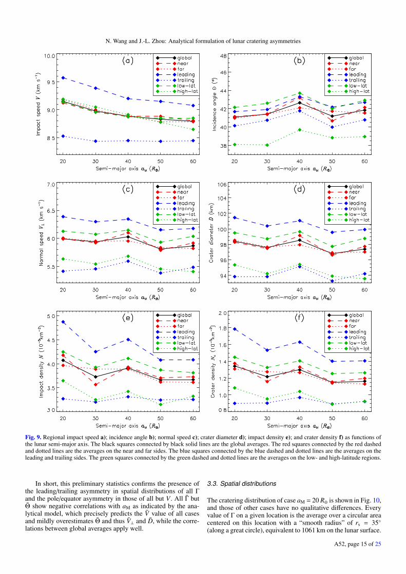
We summarize the regional Γ (denoting every/any one of V ,Θ, V⊥, D, N, and Nc following Sect. 2) for cases 1−5 in Fig. 9.The impact density of the leading side Nldg is much higher thanthat of the trailing side Ntrg for all the cases, with excesses of25%−49% (equivalent to the excesses of Cldg to Ctrg). OtherΓldg also remain larger than Γtrg with notable excesses. Theseare clear signs of the leading/trailing asymmetry, indicating itsexistence in all the investigated aspects of cratering at any aM.It also shows unambiguously that except for V , the averages ofthe low-latitude region Γlow are always higher than those of high-latitude region Γhigh, which confirms the pole/equator asymmetryregardless of aM. We note that of the investigated variables, V isthe most sensitive to the leading/trailing asymmetry, but doesnot involve a pole/equator asymmetry at all, while Θ has thegreatest dominance in the pole/equtor asymmetry over the lead-ing/trailing asymmetry. No one pair of Γnear and Γfar has a distinctand lasting discrepancy. For example, Nnear is 8% smaller thanNfar for case 2, but 1%−5% greater for other cases (the same for
A52, page 13 of 25

A&A 594, A52 (2016)
Fig. 8. Impact distribution on the lunar surface for the case aM = 20 R⊕ with 1544 impacts in total. Every impact in the simulations is shown at thelocation it occurs with a point, whose size and color represent the magnitudes of impact speed and incidence angle for this impact.
Cnear and Cfar). Therefore, the near/far asymmetry is clearly neg-ligible for the whole range 20−60 R⊕ even if it is present, in ac-cordance with Gallant et al. (2009) and Le Feuvre & Wieczorek(2011), who adopted the current impactors.
It is apparent that V monotonically decreases from 9.15 to8.80 km s−1 with aM increasing. The predicted V (Eq. (81)) is8.60−8.41 km s−1 for aM = 20−60 R⊕, only 6%−4% smallerthan simulated values. Although we consider this already an ex-cellent agreement, we continue to take the gravitational accelera-tion of the Moon into account, which is ignored in our analyticalmodel, by substituting venc = 8.32 km s−1 with
√v2
enc + v2esc =
8.65 km s−1, where the lunar escape speed is vesc = 2.38 km s−1.Then the predicted V is recalculated to be 8.92−8.74 km s−1,only 2.5%−0.7% smaller than the simulated values. The remain-ing differences may be due to the ignored acceleration fromEarth in addition to the statistical errors. It should be pointed outthat the unusually low impact speeds result from the fixed ini-tial perihelion distances of projectiles qp = 1 AU. For the wholepopulation of the MBAs without this constraint as well as theNEOs, vesc is even more negligible, so that the exclusion of theacceleration in the analytical model is quite acceptable.
Unlike the precise prediction of V , the simulated Θ are all ob-viously smaller than the analytical prediction of 51.8 (Eq. (82)).The difference between sin Θ and π/4 is 13.7%−16.4% for thefive cases. The reason probably is that our analytical model isplanar, describing the variation of Θ on the equator, while in thethree-dimensional simulations, the impacts elsewhere on the lu-nar surface are all statistically more oblique without isotropicimpactors, and thus the simulated Θ are diminished. Sincetheoretically Θ is constant regardless of how severe the lead-ing/trailing asymmetry is (Sect. 2.6), and the pole/equtor asym-metry resulting from the concentration of low-inclination im-pactors should have no dependence on vM, the simulated Θ wereexpected to be invariant with aM. In fact, we do find Θ of all thecases lying in a narrow range 41.1−42.6 with a fluctuation ofonly 2%.
V⊥ and D show a mild dependence on aM, because their vari-ations with aM are combinations of those of V and Θ (V⊥ =V sin Θ and D ∝ Vγc
⊥ ). Owing to the fluctuation of the Θvariation, their negative correlations with aM are slightly ob-scured. The dependence on Θ also causes the simulated V⊥,5.81−6.03 km s−1, to be lower by 9.3%−12.2% than the pre-dicted values of 6.61−6.75 km s−1 (Eq. (83)); this is also true forthe simulated D, 96.8−98.6 km, which are lower by 6.7%−8.3%than the predictions of 105.4−106.5 km (Eq. (84)). However, thedifference between the simulated V⊥ and the product of the sim-ulated V and sin Θ is no more than 0.3% for all the cases, andthe simulated D is lower than ccdγ
′c
p Vγc⊥ for only 2.6% at most.
This indicates that although the pole/equator asymmetry in theΘ distribution leads to an overestimation of Θ by the analyticalmodel, the relationships between the global averages derived inSect. 2.6 are still well applicable.
In general, simulated N shows a negative correlation with aMas well. (We note that the relative variation of N also representsthat of Cgl.) The approximate expression of N (Eq. (93)) indi-cates, however, that it is proportional to the constant venc, whilethe exact expression involving vM (Eq. (80)) is consistent withthis negative correlation. Of the five sets of data points, case 2(aM = 30 R⊕) seems abnormal, where N is oddly deficient andNnear is clearly smaller than Nfar. Assuming that the reason isthat the Earth’s shielding reduces the impacts on the near sideand thus the global impact number, which is supported by thefact that Nfar of this case is larger than case 3 (aM = 40 R⊕) asexpected, case 1 with its smaller aM should have suffered thesame effect. However, in case 1, Nnear is even larger than Nfar.Therefore, we prefer to consider it as a possibility instead ofconfirming it as evidence of the near/far asymmetry. BecauseNc ∝ Vγpαp
⊥ N, it is natural to see that the variation of Nc with aMcombines those of V⊥ and N. Despite of the wavy fluctuation,Nc generally decreases as aM increases. Additionally, Nc is closeto [dmin/(cpd
γ′pc )]αp Vγpαp
⊥ N with excess of 8.6%−9.7% for all thecases, in agreement with Eq. (85).
A52, page 14 of 25
N. Wang and J.-L. Zhou: Analytical formulation of lunar cratering asymmetries
Fig. 9. Regional impact speed a); incidence angle b); normal speed c); crater diameter d); impact density e); and crater density f) as functions ofthe lunar semi-major axis. The black squares connected by black solid lines are the global averages. The red squares connected by the red dashedand dotted lines are the averages on the near and far sides. The blue squares connected by the blue dashed and dotted lines are the averages on theleading and trailing sides. The green squares connected by the green dashed and dotted lines are the averages on the low- and high-latitude regions.
In short, this preliminary statistics confirms the presence ofthe leading/trailing asymmetry in spatial distributions of all Γand the pole/equator asymmetry in those of all but V . All Γ butΘ show negative correlations with aM as indicated by the ana-lytical model, which precisely predicts the V value of all casesand mildly overestimates Θ and thus V⊥ and D, while the corre-lations between global averages apply well.
3.3. Spatial distributions
The cratering distribution of case aM = 20 R⊕ is shown in Fig. 10,and those of other cases have no qualitative differences. Everyvalue of Γ on a given location is the average over a circular areacentered on this location with a “smooth radius” of rs = 35(along a great circle), equivalent to 1061 km on the lunar surface.
A52, page 15 of 25
A&A 594, A52 (2016)
Smaller rs can reveal more details, but because of the limitednumber of data points, we consider 35 as the proper choice forshowing important features.
The distribution of V (Fig. 10a) is typical of a pure lead-ing/trailing asymmetry: the maximum 10.0 km s−1 is near theapex, while the minimum 7.8 km s−1 is near the antapex; val-ues on the longitudes of 0 and ±180, the dividing line be-tween leading and trailing sides, are approximately equal to theglobal average 9.2 km s−1; there is an obvious trend for V to bemonotonously decreasing from apex to antapex. The distributionof Θ (Fig. 10b), however, combines properties of both the lead-ing/trailing and pole/equator asymmetries: the maximum 47.2is still near the apex, while the minimum seems to slide from theantapex toward the poles along the longitude 90 and turns into apair of valleys on both sides of the equator; the contours aroundthe apex tend to stretch along the latitude lines. Distributions ofV⊥, D, N, and Nc have similar structures to Θ, but with rela-tively milder pole/equator asymmetries, which is shown by thecloser proximity of their valleys. We describe in Sect. 3.5 how aspatial distribution evolves with increasing leading/trailing andpole/equator asymmetries and show that all the above distribu-tions but that of V are productions of the coupled asymmetries.Again it is not found necessary to involve the near/far asymmetryto explain the variations, as these two hemispheres are roughlyidentical in all aspects.
As expected, it is found that although θ of all the impacts liein an extended range covering 0−90 (Fig. 8), the range of Θ, theaverage of θ for every unit area, is quite limited (Fig. 10b). Theanalysis in Sect. 2.3 indicates that as the normal impact pointmoves on the lunar surface, on every unit area, impacts fromnormal to extremely oblique can all occur, and that the varyingmoving rate adds the normal impacts on the apex, resulting inthe asymmetry. In other words, the enlargement near the apexis not caused by the general upward shift of θ, but is due to theincreased relative fraction of great θ, which is now verified bysimulations.
In addition to the nonuniform moving rate of the normal im-pact point, the leading/trailing asymmetry can be understood inthis way: the lunar velocity adds to the impactors heading towardthe Moon and subtracts from the impactors chasing it, so that Nis higher near the apex; the subtraction of the lunar velocity fromthat of the impactors, how the impact velocities are derived, in-creases the velocity components along the apex-antapex axis ofthe heading impactors, but decreases those of the chasing im-pactors, meaning that statistically, not only the magnitudes ofthe impact velocities are greater near the apex, but their direc-tions are also closer to the apex-antapex axis, so that V and Θare also biased. The pole/equator asymmetry is triggered by thelow relative inclinations between the lunar equator and projectileorbits in our simulations. This initialization limits the number ofimpacts arriving at the poles, especially the normal impacts, andthus decreases N and Θ there. Although near the poles there arefewer impacts and they are statistically more oblique, the mag-nitudes of the impact velocities are not influenced, so that thepole/equator asymmetry is absent in the V distribution. Since v⊥and dc depend on both v and θ, the distributions of V⊥ and Dnaturally introduce both asymmetries in themselves. Similarly,because Nc depends on V⊥ and N, whose increases provide botha greater probability of generating large craters and more cratersin total, the Nc distribution also shows the coupled asymmetries.
To describe the pure leading/trailing asymmetry, we use theapproximate formulations derived in Sect. 2.7, whose commonform is Γ ∝ (1 + A1 cos β), where in a three-dimensional modelthe angular distance from the apex β is related to the longitude λ
and latitude ϕ by
cos β = − sin λ cosϕ. (108)
To describe the pure pole/equator asymmetry, we suggest an em-pirical function
Γ ∝ (1 + A2 cos 2ϕ) (109)
with a monotonic decrease from the equator to the poles. Aspatial distribution of the coupled asymmetries is thus assumedto be
Γ(λ, ϕ) = A0(1 + A1 cos β)(1 + A2 cos 2ϕ). (110)
It can be easily proved by integrating the right-hand side over thespherical surface that A0 = Γ still holds as Sect. 2.7 indicates.At the same time, A0 is the value of Γ at location (0,±45)or (180,±45). The parameters A1 and A2 are leading/trailingand pole/equator asymmetry amplitudes, respectively. They aremeasurements of the asymmetry degrees, and are assumed to beindependent of each other. A detailed discussion of the coupledasymmetries can be found in Sect. 3.5. We note that becauseof rs, the asymmetry amplitudes are reduced. The decrease fac-tor of A1 is estimated to be sin rs/rs, meaning that the fits of A1here are the products of this factor and A1 given in Sect. 2.7. Forrs = 35, this decrease factor is 0.939.
We fit these formulations with the nonlinear least-squaresmethod to the simulated spatial distributions shown in Fig. 10:
V(β) = AV0 (1 + AV
1 cos β), (111)
sin Θ(λ, ϕ) = AΘ0 (1 + AΘ
1 cos β)(1 + AΘ2 cos 2ϕ), (112)
V⊥(λ, ϕ) = A⊥0 (1 + A⊥1 cos β)(1 + A⊥2 cos 2ϕ), (113)
D(λ, ϕ) = AD0 (1 + AD
1 cos β)(1 + AD2 cos 2ϕ), (114)
N(λ, ϕ) = AN0 (1 + AN
1 cos β)(1 + AN2 cos 2ϕ), (115)
Nc(λ, ϕ) = Ac0(1 + Ac
1 cos β)(1 + Ac2 cos 2ϕ). (116)
Figure 11 shows the agreement between the simulated and fitvariations of the above variables, with the fits of A0,1,2 plotted.For a fixed latitude, the variables always decrease with increas-ing distance from longitude −90 toward +90, with their varia-tion amplitudes and vertical positions dependent on the latitude.Given fits of A0,1,2, the above formulations can lead to fit spatialdistributions whose configurations are determined by the relativemagnitudes of A1 and A2 (Sect. 3.5).
3.4. Fit parameters and reproduced conditions
The qualitative properties of the cratering distribution of case aM= 20 R⊕ shown above are common to any other cases. We fit thecratering distribution with Eqs. (111)−(116) for each simulationcase. In this subsection, the fit parameters, their quantitative in-terrelations, and their variations with aM are shown and com-pared with the analytical predictions. Then the bombardmentconditions are reproduced.
Fits of A0 of each Γ are plotted in terms of simulated Γ inFig. 12a. Theoretically, A0 ≈ Γ regardless of the pole/equatorasymmetry (Sect. 3.3). In Fig. 12a, the fit A0 are all slightlysmaller than the simulated Γ, but only by a few percents, whichis partly due to the approximation process itself. The largest dif-ference is no more than 7% between Ac
0 and Nc, and the small-est is only 1% between AV
0 and V . Therefore, even though wedid not rigorously prove that the pole/quator asymmetry can beformulated as Eqs. (109), (110) is clearly a good description of
A52, page 16 of 25

N. Wang and J.-L. Zhou: Analytical formulation of lunar cratering asymmetries
Fig. 10. Simulated spatial distribution of impact speed a); incidence angle b); normal speed c); crater diameter d); impact density e); and craterdensity f) for the case aM = 20 R⊕. The value at each location is the average over a circular area centered on this location with a radius of 1061 km,assuming dp = 7.5 km and dc = 100 km.
the coupled-asymmetric distribution and the fit of A0 is an ex-cellent reproduction of Γ. The reproduction goodness was ex-pected to be proportional to
√aM (inversely proportional to vM)
with a given impactor population, but this trend is not observedbecause it is obscured by the statistical fluctuation. The varia-tion of Γ with aM has been discussed in Sect. 3.2. Additionally,the interrelations between A0 (Eqs. (99)−(101)) are verified re-gardless of the involved pole/equator asymmetry: for any simula-tion case, AV
0 AΘ0 approximates to A⊥0 with a difference of .0.5%;
ccdγ′c
p (A⊥0 )γc is almost equivalent to AD0 with a difference of <3%;
and [dmin/(cpdγ′pc )]αp (A⊥0 )γpαp AN
0 is close to Ac0 with a difference
of .11%.
Our analytical model indicates that A1 ∝ vM/venc, that is,A1 ∝ a−1/2
M with a given impactor population. As shown inFig. 12b, the variation of fit AV
1 with aM reflects this relationvery well: AV
1 (aM/R⊕)1/2 = 0.490 ± 0.010, 0.469 ± 0.008,0.455 ± 0.013, 0.491 ± 0.004, and 0.493 ± 0.006 for case 1−5in turn, which is almost a constant. Because the leading/trailing
asymmetry in the Θ distribution is the faintest, the fit AΘ1 involves
relatively great fluctuation, and its relation with aM is not clearlyseen. The distributions of V⊥ and D depend on those of both Vand Θ, so that the fit A⊥1 and AD
1 correlate mildly negatively withaM. The wavy decrease of fit AN
1 and the monotonic decrease ofAc
1 are also qualitatively consistent with the above theoretic rela-tion. The interrelations between A1 (Eqs. (102) and (103)) alsoapply quite well. For all cases, the differences between γcA⊥1 andAD
1 and those between γpαpA⊥1 + AN1 and Ac
1 are .3%.We have assumed that A2 is invariant with the lunar orbit
(Sect. 3.3). As a result, no common dependence of fit A2 on aMis seen in Fig. 12c. To determine whether the assumption is re-alistic or if the relation is too weak to show itself has to waitfor further investigation in the future. However, referring to theinterrelations between the parameters A0,1, we find that similarrules are present for A2:
AD2 = γcA⊥2 , (117)
Ac2 = γpαpA⊥2 + AN
2 . (118)
A52, page 17 of 25

A&A 594, A52 (2016)
Fig. 11. Impact speed as a function of angular distance from the apex a); and the incidence angle b); normal speed c); crater diameter d); impactdensity e); and crater density f) as functions of longitude, all in terms of simulated global averages. a) Data from the simulated distribution of theimpact speed (black squares), each of which is the average over the small circle where β is fixed, are fit with Eq. (111). The best fit (black solidcurve) is generated with plotted AV
0,1. b)−f) Data from simulated distributions, each of which is the mean of the two values at location (λ, ±ϕ) with|ϕ| being 0, 30, 60, and 90 (black, red, blue, and green squares), are fit with Eqs. (112)−(116). The best fits (solid curves in the same color asthe squares for the same |ϕ|) are generated with plotted A0,1,2.
The comparisons between the left and right sides are also shownin Fig. 12c. We caution that Eqs. (117) and (118) are empiricallyderived and not guaranteed to be valid for other bombardmentconditions, although they probably are.
Given the fit A1, the speed ratio η and thus the lunar orbitalspeed vM were easily reproduced according to Eqs. (87)−(92).Figure 13 shows the reproduced η and vM in comparison with
their predictions. The decrease factor was considered in the re-production. Generally speaking, the reproductions are reason-ably consistent with each other. Still, η reproduced from AV
1is obviously smaller than its prediction. Theoretically, η =AV
1 /(π/4), but the constant quotient of the fit AV1 and predicted
η is about 0.53 (with the decrease factor considered), whichis smaller than the coefficient π/4 derived in Sect. 2.7, so that
A52, page 18 of 25

N. Wang and J.-L. Zhou: Analytical formulation of lunar cratering asymmetries
Fig. 12. Fit A0 a); A1 b); and A2 c) of spatial distributions of impact speed, incidence angle, normal speed, crater diameter, impact density, andcrater density (squares connected by solid lines in red, orange, yellow, green, cyan, and blue) as functions of lunar semi-major axis. a) Everyapproximate global average A0 is in terms of the relevant simulated global average. A⊥0 , AD
0 , and Ac0 are compared to AV
0 AΘ0 , ccd
γ′cp (A⊥0 )γc , and
[dmin/(cpdγ′pc )]αp (A⊥0 )γpαp AN
0 (squares connected by dashed lines in yellow, green, and blue). b) and c) AD1,2 and Ac
1,2 are compared to γcA⊥1,2 andγpαpA⊥1,2 + AN
1,2 (squares connected by dashed lines in green and blue).
Fig. 13. Speed ratios and lunar orbital speeds reproduced from fitleading/trailing asymmetry amplitudes of impact speed, incidence an-gle, normal speed, crater diameter, impact density, and crater density(squares connected by solid lines in red, orange, yellow, green, cyan,and blue) in comparison with predictions (black dashed curve).
the reproduced η is decreased. Although the reproduction fromAV
1 is meant to be lower (Sect. 2.8), it is not enough to explainthe difference of 32%. The reason why the fit AV
1 precisely fol-lows AV
1 ∝ a−1/2M but underestimates the predicted η and vM may
be that the leading/trailing asymmetry of the V distribution isdecreased by the introduction of the pole/equator asymmetry inthe three-dimensional numerical model, so that the coefficientdecreases from π/4 to somewhere lower. It may also be that themean venc is greater than the predicted venc because of the grav-itational acceleration, which is ignored in the analytical model,so that η is smaller than its prediction. Because the pole/equatorasymmetry is not seen in the V distribution and substituting thepredicted venc with the simulated V only reduces the reproduction
error to about 27%, other places where the numerical simulationsdeviate from the analytical model need to be checked. Althoughstatistical fluctuation results in a great error of η reproduced fromAΘ
1 , fortunately the reproductions from asymmetry amplitudes ofV⊥, D, N, and Nc are much better, especially for N, which leadsto reproduction errors of 1%−15% for all cases.
Again we followed the method of reproducing bombardmentconditions described in Sect. 2.8 and present a simple estimationbased on the fit AD,c
0,1 of case 1, for only D and Nc are observ-ables in surveys of crater records. Assuming venc = 8.32 km s−1
and t = 107 yr are known, the reproduced conditions are cal-culated to be vM = 1.45 ± 0.02 km s−1, αp = 3.23 ± 0.06,dmin = 4.71±0.03 km, and F = (1.821±0.164)×10−4 yr−1. Com-parisons of the former three to the predictions, vM = 1.78 km s−1,αp = 3, and dmin = 5 km, lead to differences of 19%, 8%, and 6%,respectively. We note that the impactor flux F is derived withEq. (105) where lgl = 2πRM is substituted by S gl = 4πR2
M, as thenumerical simulations are three-dimensional. It is equivalent to atotal number of impacts of 1821±164 during an integration timeof 107 yr, which is very close to the actual result C = 1544. Tak-ing the limited number of impacts in simulations into account,it is rather inspiring to find that this method of reproducing thebombardment conditions from the cratering distribution workswell. The importance of this method is fully shown when werecall that very many lunar craters were generated by MBAsduring the LHB, meaning that our current knowledge of theLHB and MBAs may provide clues to the early lunar dynamicalhistory.
3.5. Coupling of leading/trailing and pole/equatorasymmetries
Figure 10 illustrates the spatial distributions of Γ. All of the dis-tributions involve the leading/trailing asymmetry, and all but theV distribution also show the pole/equator asymmetry. The cou-pling of the two asymmetries can be described using Eq. (110),
A52, page 19 of 25
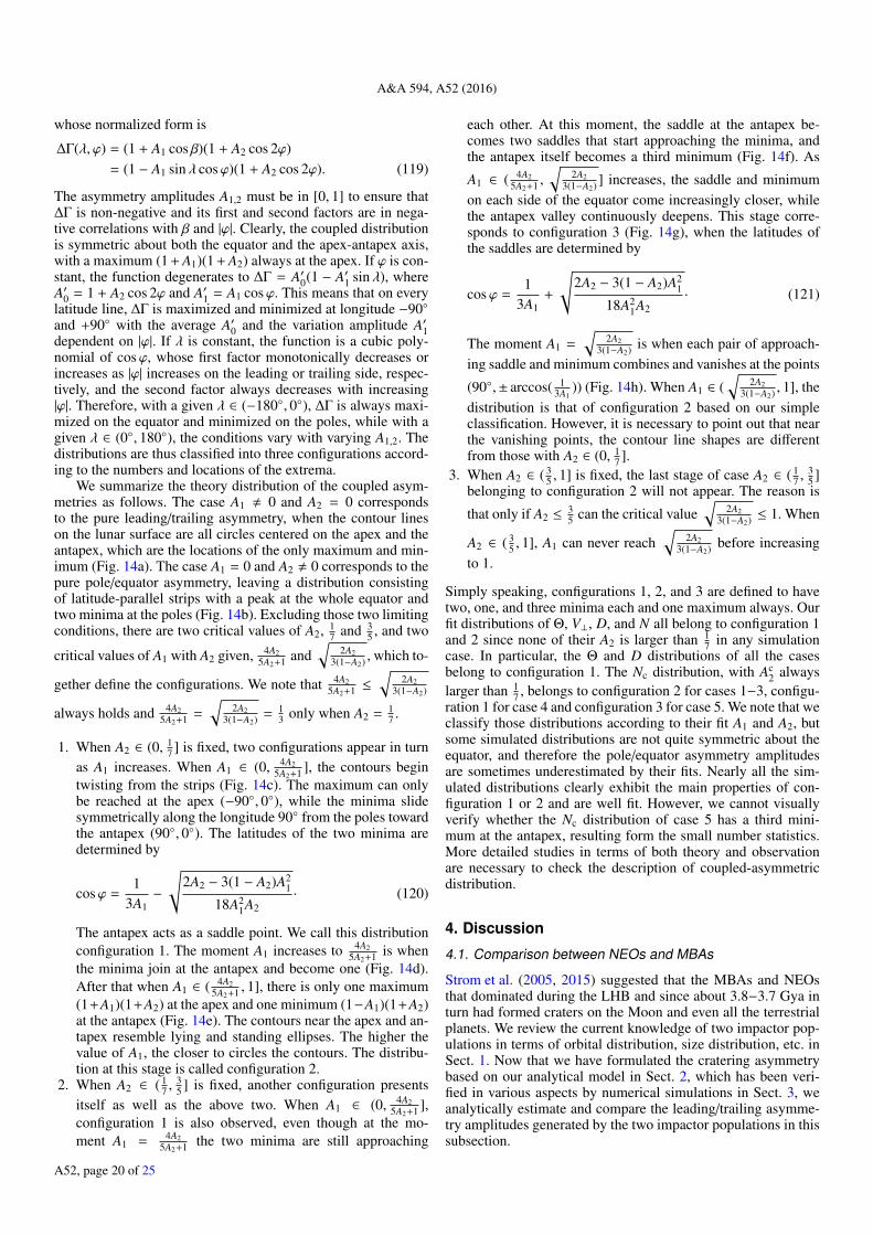
A&A 594, A52 (2016)
whose normalized form is
∆Γ(λ, ϕ) = (1 + A1 cos β)(1 + A2 cos 2ϕ)= (1 − A1 sin λ cosϕ)(1 + A2 cos 2ϕ). (119)
The asymmetry amplitudes A1,2 must be in [0, 1] to ensure that∆Γ is non-negative and its first and second factors are in nega-tive correlations with β and |ϕ|. Clearly, the coupled distributionis symmetric about both the equator and the apex-antapex axis,with a maximum (1 + A1)(1 + A2) always at the apex. If ϕ is con-stant, the function degenerates to ∆Γ = A′0(1 − A′1 sin λ), whereA′0 = 1 + A2 cos 2ϕ and A′1 = A1 cosϕ. This means that on everylatitude line, ∆Γ is maximized and minimized at longitude −90and +90 with the average A′0 and the variation amplitude A′1dependent on |ϕ|. If λ is constant, the function is a cubic poly-nomial of cosϕ, whose first factor monotonically decreases orincreases as |ϕ| increases on the leading or trailing side, respec-tively, and the second factor always decreases with increasing|ϕ|. Therefore, with a given λ ∈ (−180, 0), ∆Γ is always maxi-mized on the equator and minimized on the poles, while with agiven λ ∈ (0, 180), the conditions vary with varying A1,2. Thedistributions are thus classified into three configurations accord-ing to the numbers and locations of the extrema.
We summarize the theory distribution of the coupled asym-metries as follows. The case A1 , 0 and A2 = 0 correspondsto the pure leading/trailing asymmetry, when the contour lineson the lunar surface are all circles centered on the apex and theantapex, which are the locations of the only maximum and min-imum (Fig. 14a). The case A1 = 0 and A2 , 0 corresponds to thepure pole/equator asymmetry, leaving a distribution consistingof latitude-parallel strips with a peak at the whole equator andtwo minima at the poles (Fig. 14b). Excluding those two limitingconditions, there are two critical values of A2, 1
7 and 35 , and two
critical values of A1 with A2 given, 4A25A2+1 and
√2A2
3(1−A2) , which to-
gether define the configurations. We note that 4A25A2+1 ≤
√2A2
3(1−A2)
always holds and 4A25A2+1 =
√2A2
3(1−A2) = 13 only when A2 = 1
7 .
1. When A2 ∈ (0, 17 ] is fixed, two configurations appear in turn
as A1 increases. When A1 ∈ (0, 4A25A2+1 ], the contours begin
twisting from the strips (Fig. 14c). The maximum can onlybe reached at the apex (−90, 0), while the minima slidesymmetrically along the longitude 90 from the poles towardthe antapex (90, 0). The latitudes of the two minima aredetermined by
cosϕ =1
3A1−
√2A2 − 3(1 − A2)A2
1
18A21A2
· (120)
The antapex acts as a saddle point. We call this distributionconfiguration 1. The moment A1 increases to 4A2
5A2+1 is whenthe minima join at the antapex and become one (Fig. 14d).After that when A1 ∈ ( 4A2
5A2+1 , 1], there is only one maximum(1+A1)(1+A2) at the apex and one minimum (1−A1)(1+A2)at the antapex (Fig. 14e). The contours near the apex and an-tapex resemble lying and standing ellipses. The higher thevalue of A1, the closer to circles the contours. The distribu-tion at this stage is called configuration 2.
2. When A2 ∈ ( 17 ,
35 ] is fixed, another configuration presents
itself as well as the above two. When A1 ∈ (0, 4A25A2+1 ],
configuration 1 is also observed, even though at the mo-ment A1 = 4A2
5A2+1 the two minima are still approaching
each other. At this moment, the saddle at the antapex be-comes two saddles that start approaching the minima, andthe antapex itself becomes a third minimum (Fig. 14f). As
A1 ∈ ( 4A25A2+1 ,
√2A2
3(1−A2) ] increases, the saddle and minimumon each side of the equator come increasingly closer, whilethe antapex valley continuously deepens. This stage corre-sponds to configuration 3 (Fig. 14g), when the latitudes ofthe saddles are determined by
cosϕ =1
3A1+
√2A2 − 3(1 − A2)A2
1
18A21A2
· (121)
The moment A1 =
√2A2
3(1−A2) is when each pair of approach-ing saddle and minimum combines and vanishes at the points
(90,± arccos( 13A1
)) (Fig. 14h). When A1 ∈ (√
2A23(1−A2) , 1], the
distribution is that of configuration 2 based on our simpleclassification. However, it is necessary to point out that nearthe vanishing points, the contour line shapes are differentfrom those with A2 ∈ (0, 1
7 ].3. When A2 ∈ ( 3
5 , 1] is fixed, the last stage of case A2 ∈ ( 17 ,
35 ]
belonging to configuration 2 will not appear. The reason is
that only if A2 ≤35 can the critical value
√2A2
3(1−A2) ≤ 1. When
A2 ∈ ( 35 , 1], A1 can never reach
√2A2
3(1−A2) before increasingto 1.
Simply speaking, configurations 1, 2, and 3 are defined to havetwo, one, and three minima each and one maximum always. Ourfit distributions of Θ, V⊥, D, and N all belong to configuration 1and 2 since none of their A2 is larger than 1
7 in any simulationcase. In particular, the Θ and D distributions of all the casesbelong to configuration 1. The Nc distribution, with Ac
2 alwayslarger than 1
7 , belongs to configuration 2 for cases 1−3, configu-ration 1 for case 4 and configuration 3 for case 5. We note that weclassify those distributions according to their fit A1 and A2, butsome simulated distributions are not quite symmetric about theequator, and therefore the pole/equator asymmetry amplitudesare sometimes underestimated by their fits. Nearly all the sim-ulated distributions clearly exhibit the main properties of con-figuration 1 or 2 and are well fit. However, we cannot visuallyverify whether the Nc distribution of case 5 has a third mini-mum at the antapex, resulting form the small number statistics.More detailed studies in terms of both theory and observationare necessary to check the description of coupled-asymmetricdistribution.
4. Discussion
4.1. Comparison between NEOs and MBAs
Strom et al. (2005, 2015) suggested that the MBAs and NEOsthat dominated during the LHB and since about 3.8−3.7 Gya inturn had formed craters on the Moon and even all the terrestrialplanets. We review the current knowledge of two impactor pop-ulations in terms of orbital distribution, size distribution, etc. inSect. 1. Now that we have formulated the cratering asymmetrybased on our analytical model in Sect. 2, which has been veri-fied in various aspects by numerical simulations in Sect. 3, weanalytically estimate and compare the leading/trailing asymme-try amplitudes generated by the two impactor populations in thissubsection.
A52, page 20 of 25
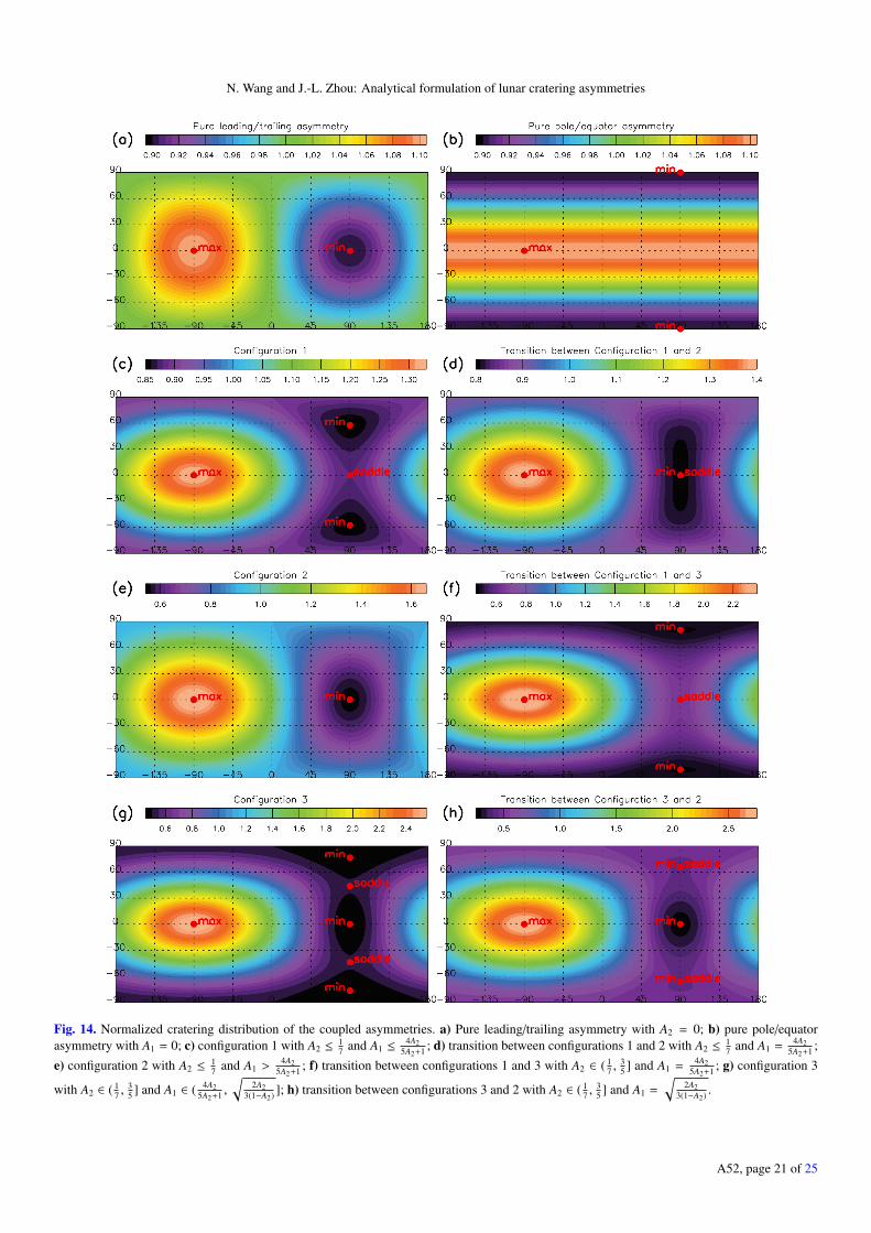
N. Wang and J.-L. Zhou: Analytical formulation of lunar cratering asymmetries
Fig. 14. Normalized cratering distribution of the coupled asymmetries. a) Pure leading/trailing asymmetry with A2 = 0; b) pure pole/equatorasymmetry with A1 = 0; c) configuration 1 with A2 ≤
17 and A1 ≤
4A25A2+1 ; d) transition between configurations 1 and 2 with A2 ≤
17 and A1 =
4A25A2+1 ;
e) configuration 2 with A2 ≤17 and A1 >
4A25A2+1 ; f) transition between configurations 1 and 3 with A2 ∈ ( 1
7 ,35 ] and A1 =
4A25A2+1 ; g) configuration 3
with A2 ∈ ( 17 ,
35 ] and A1 ∈ ( 4A2
5A2+1 ,√
2A23(1−A2) ]; h) transition between configurations 3 and 2 with A2 ∈ ( 1
7 ,35 ] and A1 =
√2A2
3(1−A2) .
A52, page 21 of 25
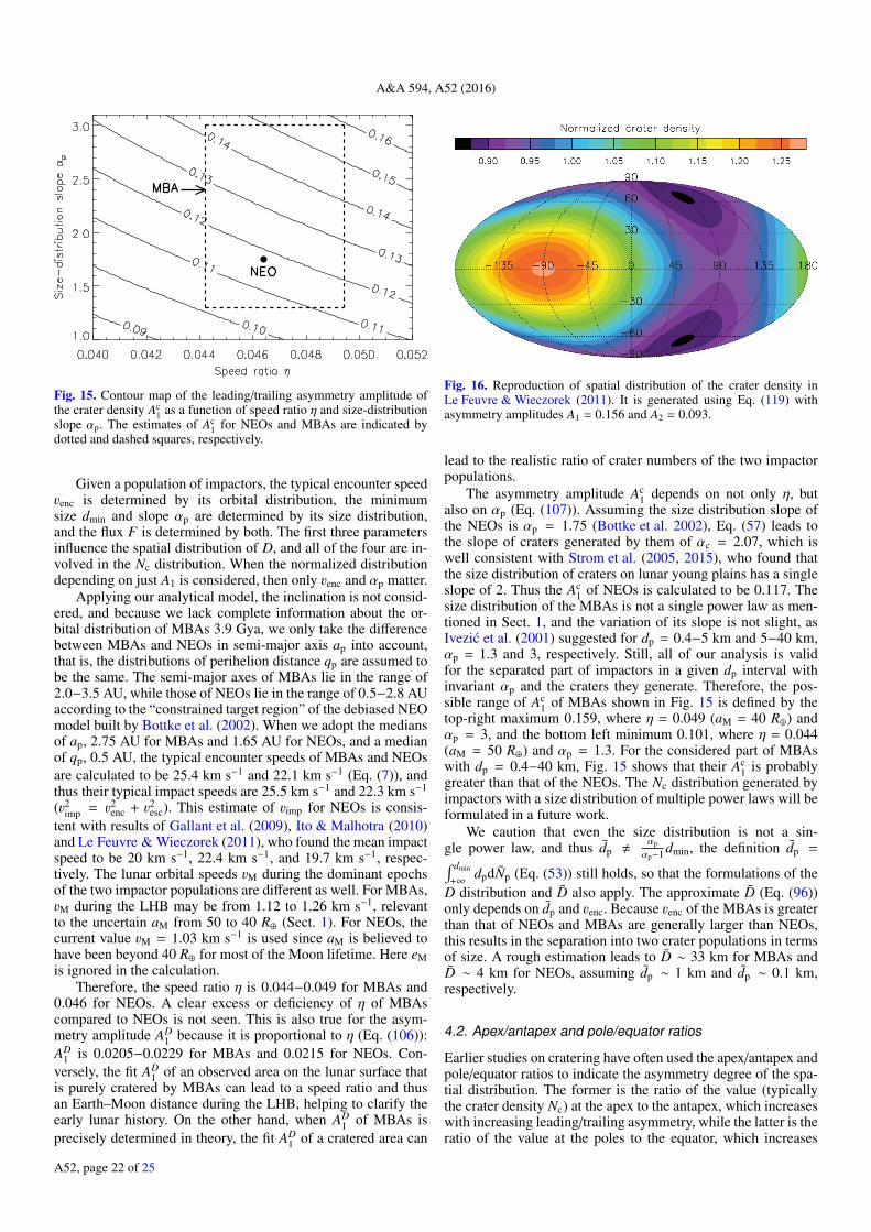
A&A 594, A52 (2016)
Fig. 15. Contour map of the leading/trailing asymmetry amplitude ofthe crater density Ac
1 as a function of speed ratio η and size-distributionslope αp. The estimates of Ac
1 for NEOs and MBAs are indicated bydotted and dashed squares, respectively.
Given a population of impactors, the typical encounter speedvenc is determined by its orbital distribution, the minimumsize dmin and slope αp are determined by its size distribution,and the flux F is determined by both. The first three parametersinfluence the spatial distribution of D, and all of the four are in-volved in the Nc distribution. When the normalized distributiondepending on just A1 is considered, then only venc and αp matter.
Applying our analytical model, the inclination is not consid-ered, and because we lack complete information about the or-bital distribution of MBAs 3.9 Gya, we only take the differencebetween MBAs and NEOs in semi-major axis ap into account,that is, the distributions of perihelion distance qp are assumed tobe the same. The semi-major axes of MBAs lie in the range of2.0−3.5 AU, while those of NEOs lie in the range of 0.5−2.8 AUaccording to the “constrained target region” of the debiased NEOmodel built by Bottke et al. (2002). When we adopt the mediansof ap, 2.75 AU for MBAs and 1.65 AU for NEOs, and a medianof qp, 0.5 AU, the typical encounter speeds of MBAs and NEOsare calculated to be 25.4 km s−1 and 22.1 km s−1 (Eq. (7)), andthus their typical impact speeds are 25.5 km s−1 and 22.3 km s−1
(v2imp = v2
enc + v2esc). This estimate of vimp for NEOs is consis-
tent with results of Gallant et al. (2009), Ito & Malhotra (2010)and Le Feuvre & Wieczorek (2011), who found the mean impactspeed to be 20 km s−1, 22.4 km s−1, and 19.7 km s−1, respec-tively. The lunar orbital speeds vM during the dominant epochsof the two impactor populations are different as well. For MBAs,vM during the LHB may be from 1.12 to 1.26 km s−1, relevantto the uncertain aM from 50 to 40 R⊕ (Sect. 1). For NEOs, thecurrent value vM = 1.03 km s−1 is used since aM is believed tohave been beyond 40 R⊕ for most of the Moon lifetime. Here eMis ignored in the calculation.
Therefore, the speed ratio η is 0.044−0.049 for MBAs and0.046 for NEOs. A clear excess or deficiency of η of MBAscompared to NEOs is not seen. This is also true for the asym-metry amplitude AD
1 because it is proportional to η (Eq. (106)):AD
1 is 0.0205−0.0229 for MBAs and 0.0215 for NEOs. Con-versely, the fit AD
1 of an observed area on the lunar surface thatis purely cratered by MBAs can lead to a speed ratio and thusan Earth–Moon distance during the LHB, helping to clarify theearly lunar history. On the other hand, when AD
1 of MBAs isprecisely determined in theory, the fit AD
1 of a cratered area can
Fig. 16. Reproduction of spatial distribution of the crater density inLe Feuvre & Wieczorek (2011). It is generated using Eq. (119) withasymmetry amplitudes A1 = 0.156 and A2 = 0.093.
lead to the realistic ratio of crater numbers of the two impactorpopulations.
The asymmetry amplitude Ac1 depends on not only η, but
also on αp (Eq. (107)). Assuming the size distribution slope ofthe NEOs is αp = 1.75 (Bottke et al. 2002), Eq. (57) leads tothe slope of craters generated by them of αc = 2.07, which iswell consistent with Strom et al. (2005, 2015), who found thatthe size distribution of craters on lunar young plains has a singleslope of 2. Thus the Ac
1 of NEOs is calculated to be 0.117. Thesize distribution of the MBAs is not a single power law as men-tioned in Sect. 1, and the variation of its slope is not slight, asIvezic et al. (2001) suggested for dp = 0.4−5 km and 5−40 km,αp = 1.3 and 3, respectively. Still, all of our analysis is validfor the separated part of impactors in a given dp interval withinvariant αp and the craters they generate. Therefore, the pos-sible range of Ac
1 of MBAs shown in Fig. 15 is defined by thetop-right maximum 0.159, where η = 0.049 (aM = 40 R⊕) andαp = 3, and the bottom left minimum 0.101, where η = 0.044(aM = 50 R⊕) and αp = 1.3. For the considered part of MBAswith dp = 0.4−40 km, Fig. 15 shows that their Ac
1 is probablygreater than that of the NEOs. The Nc distribution generated byimpactors with a size distribution of multiple power laws will beformulated in a future work.
We caution that even the size distribution is not a sin-gle power law, and thus dp ,
αp
αp−1 dmin, the definition dp =∫ dmin
+∞dpdNp (Eq. (53)) still holds, so that the formulations of the
D distribution and D also apply. The approximate D (Eq. (96))only depends on dp and venc. Because venc of the MBAs is greaterthan that of NEOs and MBAs are generally larger than NEOs,this results in the separation into two crater populations in termsof size. A rough estimation leads to D ∼ 33 km for MBAs andD ∼ 4 km for NEOs, assuming dp ∼ 1 km and dp ∼ 0.1 km,respectively.
4.2. Apex/antapex and pole/equator ratios
Earlier studies on cratering have often used the apex/antapex andpole/equator ratios to indicate the asymmetry degree of the spa-tial distribution. The former is the ratio of the value (typicallythe crater density Nc) at the apex to the antapex, which increaseswith increasing leading/trailing asymmetry, while the latter is theratio of the value at the poles to the equator, which increases
A52, page 22 of 25

N. Wang and J.-L. Zhou: Analytical formulation of lunar cratering asymmetries
Fig. 17. Apex/antapex ratio of the crater density generated by thecurrent impactors in related works compared with ours. Our rela-tion between Nc(apex)/Nc(antapex) and aM with venc = 22.1 km s−1
and αp = 1.75 (solid curve) is close to the empirical one inLe Feuvre & Wieczorek (2011), which works for aM = 20−60 R⊕(Eq. (2); dashed curve); the former with venc = 19.7 km s−1 andαp = 2.59 (dotted curve) is even nearly equal to the latter in its workingrange. Simulation results from Gallant et al. (2009) and Ito & Malhotra(2010) assuming the current lunar orbit (triangle and square) are alsoindicated.
with decreasing pole/equator asymmetry. These ratios can be ob-tained easily and are especially convenient for simulations andobservations, but their physical meanings were not understoodbefore. Neither was it possible to completely define a spatial dis-tribution through them. According to the formulation of coupledasymmetries that we established based on our analytical modeland simulation results (Eq. (110)), the ratios are each related tothe relevant asymmetry amplitude by
Γ(apex)/Γ(antapex) =1 + A1
1 − A1, (122)
Γ(pole)/Γ(equator) =1 − A2
1 + A2· (123)
(When A1 , 0, Γ(equator) means the average over the equator.)Because a whole distribution can be directly reproduced givenA1 and A2 using Eq. (119) and because the meaning of A1 hasexplicitly been determined in Sect. 2.7, the asymmetry ampli-tudes are the better measurements of the asymmetry degrees fortheories.
We now reproduce the spatial distribution of Nc shown inFig. 5 of Le Feuvre & Wieczorek (2011) through asymmetryamplitudes. They obtained it by assuming the current Earth–Moon distance and the current asteroids and comets in the in-ner solar system as impactors. The value of Nc varies from0.80 at (90,±65) to 1.25 at the apex in terms of the globalaverage, which leads to a maximum-minimum ratio of 1.5, anapex/antapex ratio of 1.37, and a pole/equator ratio of 0.80.Using their apex/antapex ratio and minimum location, we re-produce the distribution shown in Fig. 16. It is derived fromEq. (119) with the asymmetry amplitudes Ac
1 = 0.156 and Ac2 =
0.093, which are calculated with Eqs. (122) and (120) to ensureNc(apex)/Nc(antapex) = 1.37 and the latitude of the minimumϕmin = ±65. Then its maximum and minima are 1.26 at apexand 0.88 at (90,±65), whose ratio is 1.44, well consistent withthat of Le Feuvre & Wieczorek (2011), and our pole/equator
ratio 0.83 is nearly equal to theirs. Not only the Nc distribu-tion is well reproduced, but also the estimate αp = 2.6 is de-rived from Eq. (107) with the reproduced Ac
1, current vM, and themean impact speed on the Moon venc = 19.7 km s−1 accordingto Le Feuvre & Wieczorek (2011). Therefore, a power-law sizedistribution with this slope is found to be a convenient substi-tute for the 10th-order polynomial that Le Feuvre & Wieczorek(2011) used for the empirical fit in their approach.
We have determined the leading/trailing asymmetry ampli-tude of the Nc distribution generated by NEOs to be Ac
1 =0.117 (Sect. 4.1), which is equivalent to Nc(apex)/Nc(antapex) =1.27. As reviewed in Sect. 1, Morota & Furumoto (2003) re-ported the apex/antapex ratio to be ∼1.5 based on observa-tions of young craters on the lunar highlands, Gallant et al.(2009) and Ito & Malhotra (2010) found the ratio to be 1.28 ±0.01 and 1.32 ± 0.01 from their numerical simulations, andLe Feuvre & Wieczorek (2011) calculated it to be 1.37 usingtheir semi-analytical approach, all in good consistence with ourestimate. Moreover, Le Feuvre & Wieczorek (2011) also empir-ically fit the dependence of Nc(apex)/Nc(antapex) on aM andobtained Eq. (2) that is valid for aM = 20−60 R⊕. Treatingthe expression of Ac
1 (Eq. (107)) as a function of aM, that is,Ac
1(aM) = Ac1(vM(aM)) where vM(aM) =
√G(m⊕ + mM)/aM, we
can also derive a relation
Nc(apex)/Nc(antapex) =1 + Ac
1(aM)1 − Ac
1(aM)· (124)
The two relations are compared in Fig. 17 with solid and dashedlines. We note that in calculating our relation, venc = 22.1 km s−1
and αp = 1.75 are the same as used in Sect. 4.1, but aM isno longer fixed at 60 R⊕ since it is now considered a variable.Figure 17 shows that the two relations are quite close especiallywhere that of Le Feuvre & Wieczorek (2011) is valid. When wesubstitute their mean impact speed on the Moon of 19.7 km s−1
for our roughly estimated venc and adopt αp = 2.6 as reproducedfrom their Nc distribution, our function is identical to their validpart with a difference of only <2%.
We briefly point out the difference between our work andthat of Le Feuvre & Wieczorek (2011) in cratering modeling.Their model is able to produce the pole/equator asymmetrysince the anisotropic impactor population was adopted, whileour current analytical model alone can only formulate the lead-ing/trailing asymmetry, but with our empirical description of thepole/equator asymmetry based on numerical simulations, we canalso describe, reproduce, and measure the coupled asymmetries.More importantly, they integrated the cratering distribution nu-merically, while we give explicit analytical functions after rigor-ous deduction, which clearly shows the influence of every factorand makes the formulations very easy to apply.
4.3. Generalization of the analytical model
In addition to the Earth–Moon system, our analytical model(Sect. 2) can be applied to other planet-satellite systems. In theinner solar system, the NEOs and MBAs are the common im-pactor populations dominating different epochs. They encounterMars with venc ≈ 19.3 and 22.9 km s−1, respectively, whichis calculated with a⊕ replaced by the semi-major axis of MarsaMars = 1.5 AU in Eq. (7) and the typical ap of NEOs beingthe median of the interval 0.76−2.8 AU instead of 0.5−2.8 AUbecause projectiles with ap < aMars/2 on elliptic orbits can-not encounter Mars. The Martian moons, Phobos and Deimos,which lie on very circular orbits, have current orbital speeds of
A52, page 23 of 25

A&A 594, A52 (2016)
vorb = 2.14 and 1.35 km s−1 and negligible escape speeds vesc.Thus, the NEOs with a typical speed ratio η of 0.111 for Phobosand 0.070 for Deimos are expected to generate a current lead-ing/trailing asymmetry amplitude of the crater density of 0.28and 0.18, respectively, both of which are much greater than forthe Moon. Similarly, the orbital speeds of Phobos and Deimosand even their orbits during the LHB might be derived from theobserved crater records if they had been tidal-locked then.
The dominant impactors in the outer solar system are eclip-tic comets, which are generally considered to originate in theKuiper belt (Zahnle et al. 2001). Because their encounter speedsare generally lower than the orbital speeds of the satellites of thegiants, our analytical model is not completely applicable. Thedivergence starts from the behavior of the normal impact point.With our assumption venc > vorb, the normal impact point mov-ing westward along the satellite’s equator (coplanar with its orbitand ecliptic) reaches the antapex and apex when the satellite isat its pericenter (where uenc is in the same direction as uorb) andapocenter, while the impact speed v is minimized and maximized(Sect. 2.3). However, if venc < vorb, the normal impact pointreaches the apex at both the pericenter and apocenter. Specif-ically, as the satellite’s true anomaly f increases from 0 (peri-center), the normal impact point leaves the apex, moves eastwarduntil f = arccos(venc/vorb) ∈ (0, 90), turns around and returnsto the apex when f = 180; as f continues increasing, it con-tinues moving westward until f = 360 − arccos(venc/vorb) ∈(270, 360) and then returns to the apex when f = 360. Itspath is symmetric about the apex, bounded by the two return
points at equal distances of βmax = arctan(venc/
√v2
orb − v2enc) from
it. It is seen that βmax < 90, so the satellite surface is dividedinto four areas: the area centered on the antapex with the longi-tude λ ∈ (βmax, 180 − βmax) never is hit by impactors; the area(βmax − 180,−βmax) centered on the apex is always under bom-bardment; and the two remaining symmetric areas on the nearand far side each are periodically included in and excluded fromthe instant bombarded hemisphere. Apparently, the higher theratio vorb/venc, the smaller the distance βmax, and thus the greaterthe asymmetry. As a result, the leading/trailing asymmetry ismuch enhanced when venc < vorb than otherwise. A generalizedmodel including this case will be established in the future to ex-amine the cratering of giants’ satellites.
Zahnle et al. (2001) suggested a semi-empirical descriptionof Nc distribution on satellites of giant planets shown as Eq. (1).We find qualitative consistence of our approximate formulationNc(β) (Eq. (92)) with theirs since the asymmetry is amplified byspeed ratio vorb/venc and size-distribution slope αp in both forms.One difference is that αp is a coefficient of cos β in our form butacts as an exponent in theirs. Considering they derived their for-mulation based on simulation results, and referring to our analy-sis, there is a great possibility that αp is still a coefficient (in ap-proximate description) when venc < vorb and the influence of αpwas overestimated by formulation of Zahnle et al. (2001), whichwill be examined by future model.
5. Conclusions
We analytically formulated the lunar cratering distribution andconfirmed the derivation with numerical simulations. The for-mulations are quite easy to use. They are able to give resultsnearly identical to related works, avoiding the time-consumingsimulations and clarifying the physical meanings in quantitativerelations.
Based on a planar model excluding the gravitations of Earthand the Moon on the impactors, we derived series of formula-tions of the cratering distribution on the synchronously rotatingsatellite through rigorous integration. The formulations directlyand unambiguously proved the existence of a leading/trailingcratering asymmetry and the identity of the near and far sidesin all aspects of cratering, that is, impact speed V , incidenceangle Θ, normal speed V⊥, crater diameter D, impact densityN, and crater density Nc. Series expansion to the first orderof vM/venc resulted in the approximate Γ distributions in thecommon form Γ(β) = Γ(1 + A1 cos β), where Γ is in positivecorrelation with venc, except that Θ is the constant 51.8, andA1 ∝ vM/venc, that is, A1 ∝ a−1/2
M with a given venc. The relationsbetween the cratering distribution and the bombardment condi-tions including properties of impactor population and the lunarorbit during the bombardment provides a viable method of repro-ducing the latter by measuring the former. The lower the speedratio vM/venc, the better the approximation to the exact Γ distri-butions and the better the reproduction of the bombardment con-ditions. In particular, the approximation of Nc can be improvedby decreasing αp as well.
We also numerically simulated the cratering on the Moonthat is caused by the MBAs during the LHB with five simulationcases in which aM = 20−60 R⊕. Not only the leading/trailingasymmetry is present in the simulated cratering distribution inall aspects, but also the pole/equator asymmetry is seen, exceptfor the V distribution, while the signs of the near/far asymme-try are not enough. The pole/equator asymmetry is empiricallyformulated with (1 + A2 cos 2ϕ), leading to the description ofcoupled asymmetries Γ(λ, ϕ) = Γ(1 + A1 cos β)(1 + A2 cos 2ϕ),which is well fit to the simulated Γ distributions with errors ofΓ smaller than 6%. For each case, the analytical prediction of Vis only a few percent lower than the simulated V , but the pre-dicted Θ is obviously larger than the simulated Θ because thepole/equator asymmetry is involved. As predicted by the analyt-ical model, Γ except for Θ all show negative correlations withaM in general, and so do the fit A1 except for AΘ
1 , whose varia-tion with aM involves greater statistical fluctuations, while the fitA2 seem independent of aM. Additionally, the method of repro-ducing performs well, with reproduction errors being ∼10% forbombardment conditions in case 1. This means that it is possibleto speculate about the lunar orbital status during the LHB whenthe cratering distribution generated by MBAs is determined byobservations.
Based on our analytical model, the leading/trailing asym-metry amplitude of the crater density that is generated bythe MBAs is estimated to be Ac
1 = 0.101−0.159, while thatgenerated by the NEOs is Ac
1 = 0.117, which is equiv-alent to Nc(apex)/Nc(antapex) = 1.27. We easily but pre-cisely reproduced the Nc distribution and the variation ofNc(apex)/Nc(antapex) as a function of aM derived by Le Feuvre& Wieczorek (2011), with αp = 2.6, Ac
1 = 0.156, and Ac2 = 0.093.
Our analytical model is applicable to other planet-satellite sys-tems as long as venc > vorb and will be generalized to the casevenc < vorb in future.
Acknowledgements. We thank the referee Bill Bottke for constructive and in-spiring comments. This research has been supported by the Key DevelopmentProgram of Basic Research of China (Nos. 2013CB834900), the National Natu-ral Science Foundations of China (Nos. 11003010 and 11333002), the StrategicPriority Research Program “The Emergence of Cosmological Structures” of theChinese Academy of Sciences (Grant No. XDB09000000), the Natural ScienceFoundation for the Youth of Jiangsu Province (No. BK20130547) and the 985project of Nanjing University and Superiority Discipline Construction Project ofJiangsu Province.
A52, page 24 of 25

N. Wang and J.-L. Zhou: Analytical formulation of lunar cratering asymmetries
ReferencesBandermann, L. W., & Singer, S. F. 1973, Icarus, 19, 108Bills, B. G., & Ray, R. D. 1999, Geophys. Res. Lett., 26, 3045Bottke, W. F., Morbidelli, A., Jedicke, R., et al. 2002, Icarus, 156, 399Bottke, W. F., Durda, D. D., Nesvorný, D., et al. 2005, Icarus, 175, 111Chambers, J. E. 1999, MNRAS, 304, 793Gallant, J., Gladman, B., & Cuk, M. 2009, Icarus, 202, 371Gerstenkorn, H. 1955, Z. Astrophys., 36, 245Goldreich, P. 1966, Rev. Geophys. Space Phys., 4, 411Gomes, R., Levison, H. F., Tsiganis, K., & Morbidelli, A. 2005, Nature, 435, 466Hansen, K. S. 1982, Rev. Geophys. Space Phys., 20, 457Ito, T., & Malhotra, R. 2010, A&A, 519, A63Ivezic, Ž., Tabachnik, S., Rafikov, R., et al. 2001, AJ, 122, 2749Kagan, B. 1997, Prog. Oceanogr., 40, 109Kagan, B. A., & Maslova, N. B. 1994, Earth Moon and Planets, 66, 173Kawamura, T., Morota, T., Kobayashi, N., & Tanaka, S. 2011, Geophys. Res.
Lett., 38, 15201Lambeck, K. 1977, Philosophical Transactions of the Royal Society of
London A: Mathematical, Phys. Eng. Sci., 287, 545Le Feuvre, M., & Wieczorek, M. A. 2005, in Lunar and Planetary Inst. Technical
Report, eds. S. Mackwell, & E. Stansbery, 36Le Feuvre, M., & Wieczorek, M. A. 2008, Icarus, 197, 291
Le Feuvre, M., & Wieczorek, M. A. 2011, Icarus, 214, 1Levison, H. F., Duncan, M. J., Zahnle, K., Holman, M., & Dones, L. 2000, Icarus,
143, 415MacDonald, G. J. F. 1964, Rev. Geophys. Space Phys., 2, 467Morbidelli, A., & Gladman, B. 1998, Meteorit. Planet. Sci., 33, 999Morota, T., & Furumoto, M. 2003, Earth Planet. Sci. Lett., 206, 315Oberst, J., Christou, A., Suggs, R., et al. 2012, Planet. Space Sci., 74, 179Parker, A., Ivezic, Ž., Juric, M., et al. 2008, Icarus, 198, 138Ross, M. N., & Schubert, G. 1989, J. Geophys. Res.: Solid Earth, 94, 9533Strom, R. G., Malhotra, R., Ito, T., Yoshida, F., & Kring, D. A. 2005, Science,
309, 1847Strom, R. G., Renu, M., Xiao, Z.-Y., et al. 2015, RA&A, 15, 407Touma, J., & Wisdom, J. 1994, AJ, 108, 1943Webb, D. J. 1980, Geophys. J., 61, 573Webb, D. J. 1982, Geophys. J., 70, 261Wiesel, W. 1971, Icarus, 15, 373Yoshida, F., & Nakamura, T. 2007, Planet. Space Sci., 55, 1113Yoshida, F., Nakamura, T., Watanabe, J.-I., et al. 2003, PASJ, 55, 701Zahnle, K., Dones, L., & Levison, H. F. 1998, Icarus, 136, 202Zahnle, K., Schenk, P., Sobieszczyk, S., Dones, L., & Levison, H. F. 2001, Icarus,
153, 111Zhou, J.-L., & Lin, D. N. C. 2008, in IAU Symp. 249, eds. Y.-S. Sun, S.
Ferraz-Mello, & J.-L. Zhou, 285
A52, page 25 of 25