Analysis of Nash equilibria in a class of capital accumulation games

ELSEVIER Journal of Economic Dynamics and Control

20 (1996) 1209.-1235

Analysis of Nash equilibria in a class of capital accumulation games

Engelbert J. Dockner”, Ngo Van Long*-b, Gerhard Sorgef

“Departments of Management Science and Economics, University of‘ C’ienna, Vienna, Austria

hDepartment ?f‘Ecconomics, McGill University, Montrbl, Que. H3A 2T7, Canada

(Received August 1993; final version received September 1995)

Abstract

In a simple capital accumulation game we study existence and dynamic properties of the cooperative solution, two kinds of Markov perfect equilibria (MPE), and a trigger strategy equilibrium. In the cooperative solution the stock always converges towards a steady state. This property is shared by our first MPE, whereas the second type of MPE may result in complicated dynamics. A Pareto comparison of both MPE depends on the parameter specifications but can turn out either way. Finally, we show how the players can achieve the efficient payoffs of the cooperative solution as an equilibrium outcome by using trigger strategies.

Key words: Capital accumulation game: Markov perfect Nash equilibria; Trigger strategy equilibria, Efficiency JEL classijication: C73

1. Introduction

The single-agent aggregative optimal growth model is one of the most prominent paradigms in economic dynamics. The widespread use of this model stems from its analytical tractability as well as from its applicabililty to many

*Corresponding author.

This paper was partly written while E.J. Dockner and G. Sorger were Visiting Fellows at the

Australian National University, Canberra. The financial support from ANU is greatfully acknow-

ledged. We would like to thank Michael Hoel. Larry Karp, and three anonymous referees for their

useful comments.

0165-1889/96/$15.00 c 1996 Elsevier Science B.V. All rights reserved SSDI 0165-1889(95)00896-4

1210 E.J. Docker et al. /Journal of Economic Dynamics and Control 20 (1996) 1209-1235

fields in economics and finance. Recently, game theorists have started to exam- ine how the results for this model are changed when the single agent is replaced by a number of strategically acting ones. By now there are several papers available that address one or more of the following questions in capital accumulation games. (i) Do Markov perfect equilibria (MPE) exist in the dynamic game setting if the fundamentals of the model satisfy the assumptions usually made in the single-player case? (ii) How do the dynamic properties of a MPE relate to those of the collusive solution? (iii) How does the asymptotic behavior (the stable steady state if it exists) of capital accumulation paths in the noncooperative equilibrium compare to the long-run behavior of the cooperative solution? (iv) Under what conditions can efficient outcomes be supported as noncooperative equilibria consisting of trigger strategies? The existence issue for MPE is addressed by Duffie et al. (1994) for stochastic games and by Sundaram (1989) and Dutta and Sundaram (1993a) for the symmetric and deterministic case. The latter paper presents a complete characterization of stationary equilibria. Stability and turnpike properties for capital accumulation games when players design their actions as simple time paths (i.e., when they use open- loop strategies) have been derived by Fershtman and Muller (1984, 1986) and Dockner and Takahashi (1988, 1993). In a recent paper Dutta and Sundaram (1993b) address the first three questions raised above for the class of fishery games proposed by Levhari and Mirman (1980). Using various examples with different forms for the utility and production functions they demonstrate that MPE may fail to exist even under strong regularity conditions, that MPE may induce very complicated dynamics, and that there might exist MPE with multiple steady states with at least one of them resulting in overaccumulation of the stock. Question (iv) from above is not addressed in Dutta and Sundaram (1993b).’ Neither do Dutta and Sundaram discuss the possible multiplicity of MPE. In this paper we try to complement Dutta and Sundaram (1993b) by looking at these problems. Furthermore, we analyze a non-Markovian equilibrium consisting of trigger strategies. This equililbrium provides a purely noncooperative mechanism to implement the efficient outcomes of the cooperative solution.

We focus on two types of MPE: one which always leads to simple dynamics and one which may lead to chaotic dynamics. For example, in the case of quadratic cost functions it will be shown that the dynamic evolution of the stock variable in the second type of equilibrium can be described by the famous logistic difference equation.* As one varies the model parameters the period

‘See, however, Benhabib and Radner (1992) where this issue is discussed in a continuous time

framework.

‘This observation has already been made in Dutta and Sundaram (1993b). In fact, our example is structurally equivalent to the example they have used.

E.J. Dockner et al. 1 Journal of Economic Dynamics and Control 20 (1996) 1209-1235 1211

doubling cascade leads finally to a completely chaotic attractor. The main focus of the present paper, however, is on the comparison of the different kinds of equilibria. It turns out that the Nash equilibrium with simple dynamics is a strict one and is the only MPE consisting of convex and monotone strategies. In the other equilibrium the strategies of both players are chosen in such a way that they make their opponent indifferent between all feasible strategies. We shall furthermore demonstrate that either one of the equilibria discussed in this paper can be Pareto dominated by the other one (depending on the parameter specifications). In particular, it can be the case that an equilibrium generating simple dynamics is dominated by an equilibrium with chaotic dynamics. The simplicity of the model, especially the linearity of the value functions in the second MPE, allows us to consruct a trigger strategy equilibrium supporting the efficient outcomes of the cooperative solution. In that equilibrium the second MPE serves as a threat for players who deviate from the efficient path.

The class of capital accumulation games that is considered in this paper shares the common feature that there is a single stock variable (a public capital stock, a public bad, or a fish population, for example) that is influenced by the consumption (investment) decisions of the two players in the game. To fix ideas, let Pt be the common capital stock at time t and yf consumption (investment) of player i = 1, 2 at time t. The state dynamics in the case of two players is governed by the accumulation equation

P f+ 1 =f(p,) + cc’y: -t a2y,2, (1)

wherefcan either be a production function or a recruitment function (depending on the context) and where a1 and a2 are constants. The objective functions of the players are

J’ = f p’[p’yf + C’(p,)], t=o

(2)

where p is the discount rate, pi are constants, and piyi + C’(p) is a stock- dependent utility function that is linear and separable in the level of current consumption y’ and possibly nonlinear in the stock p. According to the various specifications of the accumulation equation and the objective functions the model can be given different interpretations all of which include a public good (bad) aspect.

a) Dynamic Voluntary Prouision of a Public Good. The model (1) and (2) does include a dynamic version of a voluntary provision of public goods model (see Fershtman and Nitzan, 1991) as a special case. In this case p, can be interpreted as a public capital stock like a public school system and yf is the voluntary

1212 E.J. Dockner et al. / Journal of Economic Dynamics and Control 20 (1996) 1209- 1235

contribution of individual i to the system. The accumulation equation is given by pt+i = y: + yf + (1 - p)p, which is (1) with cli = 1, f(p) = (1 - /?)p, and p E (0,l) a constant rate of depreciation. Individual i derives utility U’(p,) from the existence of the stock pt but incurs costs for contributing to the system. Thus the objective function becomes J’ = CtFYOp’[Ui(pt) - yf] which is (2) with pi = - 1 and I?(.) = U’(.).

b) Common Property Resource Model. The model can also be given the interpretation of a common property fishery game (see Levhari and Mirman, 1980). In this case the variable p, measures the size of the fish population at time t,f(p,) is a recruitment function, and yi is the level of consumption of agent i. The fish population evolves according to p,+ i =f(p,) - y: - y: which is (1) with c? = - 1. Assuming that agents derive linear utility from current consumption and that utility may also depend on the size of the fish stock the objective function is given by J’ = C~o~Z[yf + u’(p,)] so that (2) holds with pi = 1 and C’( .) = u’( .). In the classical fishery model the stock dependence of utility is usually neglected, i.e., C’( .) = 0.

c) International Pollution Control. The model (1) and (2) can also be given the interpretation of a two-country pollution control model similar to that studied in Dockner and Long (1992).3 This interpretation will be used in the remainder of the paper and is explained in the following section.

The paper is organized as follows. In the next section we present a detailed description of the pollution control model and we state all technical assumptions. Section 3 characterizes the unique cooperative solution and shows that coordination of pollution control gives rise to very simple dynamics. In Section 4 we derive two types of Markov perfect equilibria for the dynamic game. These equilibria differ quite distinctively in the dynamics they generate. In addition to illustrating the various dynamic patterns that can arise we also compare the equilibria in the Pareto sense. In Section 5 we briefly discuss existence and properties of a trigger strategy equilibrium that results in the same payoffs as the cooperative solution. Section 6 presents concluding remarks.

2. Model formulation and basic assumptions

Time is measured in discrete periods and t = 0, 1,2, . . . denotes the time variable. Consider two countries indexed by i = 1,2. Each country produces

3Although the model in Dockner and Long (1992) has a similar interpretation as the model in the

present paper, its mathematical structure is quite different.


a single consumption good that is consumed domestically. The output of country i in period t is denoted by yf. The production of the consumption good results in emissions ef that add to the current stock of pollution p,. Both countries face the same stock of pollution. We assume that emissions are proportional to output and we choose units of measurement in such a way that ef = yf. Moreover, it is assumed that there is natural purification of the environment such that the stock of pollution decays at a constant rate B E (0,l). This implies that the stock of pollution at time t + 1 is given by

Pt+ 1 = Y: + y: + (1 - P)p,, t 2 0. (3)

We assume that both countries know that increasing the pollution beyond a given stock p > 0 leads to the collapse of the ecosystem. Therefore, the two countries have agreed via preplay communications to choose their output levels in such a way that the state constraint

PI 5 P t2 1, (4)

is satisfied.4 The interval [O,p] is therefore a convenient state space for our model and we shall assume throughout the paper that the initial state of the environment p. satisfies p0 E [0, p]. Each country is assumed to choose a pollution control strategy that maximizes the discounted stream of net benefits. Net benefits consist of the utility derived from the consumption of the goods produced and of the costs associated with a polluted environment. We assume a linear utility function for consumption so that the net benefit of country i in period t is given by yf - ci(pt) where ci: [O,p] H R is a continuous and strictly convex cost function. Denoting by p E (0,l) the common discount factor of both countries and assuming an infinite time horizon, the objective of country i is to maximize

J’ = 2 p’[yf - c’(p,)],

subject to the state equation (3), the state constraint (4), the nonnegativity constraint yf 2 0, and the given initial stock of environmental pollution po.

In determining his output rate, yi, player i can use any information that is available to him in period t. We assume that each player knows at least the current pollution stock pt as well as the complete model specified by /?, p, cl, 2,

4Alternatively, we could also assume that the cost functions c1 and cz introduced below become

infinite for arguments p > j. This would lead to exactly the same results.

1214 E.J. Dockner et al. 1 Journal of Economic Dynamics and Control 20 (1996) 1209-1235

and p. It will turn out that the unique cooperative solution as well as two of the noncooperative Nash equilibria that we are going to discuss in this paper exhibit a common simple structure: they are given by stationary Markovian strategies in the following sense (see also the paper by Maskin and Tirole, 1988, for a detailed discussion). A stationary Markovian strategy for player i is a mapping Y’: [O,p] H R from the state space into the real numbers. If country i chooses the strategy Y’, then it determines its output in period t according to yf = Y’(p,). We say that a pair of strategies (Y’, Y2) is feasible if 0 I Y’(p) and Y’(p) + Y’(p) + (1 - /?)p I p hold for all p E [O,p].

We would like to point out that the state constraint (4) can also be written in the form of an additional constraint for each player, i.e., yf I p - (1 - P)pt - y! wherej denotes the opponent of i = 1,2. This shows that each player’s choice of yi influences the set of feasible actions for his opponent. The game introduced above is thus a generalized game in the sense of Debreu (1952).

3. Cooperative solution

In this section we show that there is a unique optimal path po, pi, p2, . . . of the pollution stock if both countries coordinate their efforts. Moreover, this path converges to a unique optimal steady state value p* E [O,p] and the convergence takes place in finite time whenever p* is strictly positive. The optimal steady state p* is the maximizing point of the function W: [O,p] H 174 defined by

W(P) = BP - CC’(P) + C2(P)l + 6p, (6)

where 6 is the constant discount rate related to p by p = l/(1 + 6). Note that continuity and strict convexity of the cost functions ensures that the maximizing point p* E [O,p] exists and that it is unique. The function W may be called the surrogate welfare function and it consists of three terms that can be given the following interpretation:

l /?p is the long-run sustainable output. To see this, substitute p,+ 1 = pt in (3). It follows that y: + y: = /?p,. In other words, whenever the countries wish to keep the pollution stock at a constant level they have to choose their output rates such that the joint output is equal to /?pl.

0 - (c’(p) + c2(p)) measures the utility (negative cost) of pollution. l 6p is the adjustment for the rate of time preference.

Theorem 1. If both countries coordinate their pollution control activities in order to maximize J’ + J2, then the unique optimal level of their joint outputs

E.J. Dockner et al. / Journal of Economic Dynamics and Control 20 (1996) 1209-1235 1215

(emissions) is given by

Yf + yf = max {O,p* - (1 - p)pt}. (7)

The state trajectory generated by this policy is determined by the diference equation

pt+ 1 = max ((1 - B)h P* I. (8)

It holds that lim t_ccpt = p* and the convergence takes pluce in jinite time if

p* > 0.

Proof: We define y, = y: + yf . Using (3) and (5) we obtain

J’ + J2 = f P’CY, - CYPJ - C2(Pt)l t=o

=,zo [ P’ Pr+1 - (1 - DIP* - C'(Pt) - C2(P,)l

= - (1 - B)po - c’(p0) - c2(po) + f Pf+l W(P,,I)> r=o

where the function W has been defined in (6). This has to be maximized with

respect to p1,p2,p3, ,.. subject to the constraints p,+ I E [(l - /l)p,,p] for all t. Since J’ + J2 is additively separable with respect to the variables pl, p2, p3, . . and because W is a strictly concave function it follows immediately that pt+ , has to be chosen in such a way that it maximizes W subject to the constraint pt + 1 E [(l - /l)p,,p]. This implies that pt+ 1 is given by (8). Substi- tuting this into (3) shows that (7) has to be satisfied. Finally, it is easy to verify that pt converges to p* and that it reaches p* within finite time provided that p* >o. n

Theorem 1 shows that only very simple dynamics are possible if both countries coordinate their policies. In the control theory literature this kind of dynamics is known as a most rapid approach path (MRAP) since the optimal steady state is reached within as short a time as possible. If p* > 0, convergence takes place in finite time and the model satisfies therefore what is called the exact turnpike property.

12 16 E.J. Dockner et al. J Journal of Economic Dynamics and Control 20 (1996) 1209- 1235

4. Markovian equilibria

In this section we first consider a Markovian equilibrium that generates fast convergence to a stationary pollution stock similarly to the cooperative solution. Because of this property we call this equilibrium a MRAP equilibrium. We shall then derive another equilibrium consisting of stationary Markovian strategies. This equilibrium can lead to very complicated dynamics and has the peculiar feature that each player is indifferent between all of his possible choices. Henceforth, we call such an equilibrium a make-the-opponent-indifferent (MTOI) equilibrium. In the following two subsections we investigate the two kinds of equilibria separately whereas in Section 4.3 we shall try to compare them.

4.1. MRAP equilibria

In this subsection we discuss an equilibrium in which the players use stationary Markovian strategies very similar to those of the cooperative solution. Consequently, the dynamics generated by this equilibrium also consists of a most rapid approach path to a unique optimal steady state of the pollution stock. To characterize the steady state let us define the individual surrogate welfare functions of the two players by W:(p) = p[l - (1 - /?)?I - c’(p) + 6p, i = 1, 2. Here, y E [0, l] is a real parameter and 6 is again the discount rate determined by p = l/(1 + 6). The interpretation of the surrogate welfare functions is the same as in the previous section except that now each player takes into account only his own cost of pollution, c’(p), and a different measure of the long-run sustainable output to adjust for the noncooperative situation. We impose the following assumption to derive the first Nash equilibrium in the pollution control game.

Assumption 1. There exists y E [0, l] and fi E [O,p] such that for all p E [O,p]

W:-,(P) I W:-,(F) and W:(p) I W,‘(j). (9)

The pollution level p” mentioned in this assumption will turn out to be the steady state value for the Nash equilibrium presented below. Condition (9) requires that it is the point which maximizes both players’ individual surrogate welfare functions simultaneously. In other words, there has to be a level of environmental pollution which is in some sense optimal for both players if the ‘weight parameter’ y is chosen appropriately. If at least one of the cost functions cl and c2 is continuously differentiable and p” E (0, l), then the parameter y is unique. If both cost functions are nondifferentiable at a certain point, say at p’, then it might be the case that p’ = p’ and that y can be chosen from a nontrivial interval.

E.J. Dockner et al. /Journal of Economic Dynamics and Control 20 (1996) 1209-1235 1217

Assumption 1 is not a severe restriction as long as both countries have similar cost functions, that is, if c1 is close to c2. For example, in the symmetric game with c’ = c2 we can always choose y = t and the corresponding value of p” will exist according to the continuity of the cost functions. If c1 differs from c2, then one may have to choose y # f, but an appropriate value of y can usually be found as long as c’ and c2 are not very different.

Theorem 2. Let y and p” be given such that Assumption I is satisfied. Then the pair qfstationary Markovian strategies (Y ‘, Y 2), dqfined by

Y l(p) = (1 - y) max (0, P - (1 - B)Pl, (10)

Y2(p) = Y max (0, P” - (1 - PIPI (11)

constitutes a strict Nash equilibrium for the pollution control game. The state trajectory generated by this equilibrium is determined by the difference equation

P~+~ = max{(l - Bh,FJ. (12)

It holds that lim,,, p, = 6 and the convergence takes place infinite time if@ > 0.

Proof. The proof of this result is very similar to the one of Theorem 1 and we will not present all details. Let us assume that country 2 plays strategy Y 2. Using (3) and (5) we obtain

J’ = f P’CY: - C’(PAl r=o

=,to [ Pf Pt+1 - (1 - B)Pt - C’(P,) - Y2(P,)l

= - (1 - BP0 - c’(p0) - Y2(p,) + f pf+lV;(p,+l), f=O

where the function V: is defined by Vi(p) = min { W:_,(p) - (1 - /?)yp, W:-,(p) - $1. Obviously, the function V$ is strictly concave on [0, p]. Fur- thermore, we have V:(p) I W:_,(p) - J$ I W:_,(p) - vc for all p E [O,p] by Assumption 1 and Vi(j) = min{W~_,($) - (1 - fi)y@, W:_,(@) - yi)} = W:_,(j?) - rj. This implies that Vi(p) is a strictly concave function which attains its unique maximum at the point p = 6. As in the proof of Theorem 1 we


can see that this implies that player l’s unique optimal choice for pt+ 1 (provided that player 2 sticks to Y2) is given by pt+ 1 = max { Y2(pt) + (1 - a)~,,@}. Substituting for Y ‘(p,) from (11) we obtain (12). Finally, by using the state equation (3) we can see that player 1 must choose the strategy Y 1 defined in (10) in order to achieve (12). This shows that Y ’ is the unique best response to player 2’s strategy Y 2. By a completely symmetric argument one can show that Y 2 is the unique best response to Y ’ so that (Y ‘, Y 2, is a strict Nash equilibirum. The state dynamics generated by these equilibrium strategies is, of course, given by (12) which implies convergence of pt towards jj (in finite time provided that p” > 0). W

The proof of the above theorem makes it clear that Assumption 1 is actually more than we need to establish the result. The weakest condition under which the proof remains valid is the following one.

Assumption 1’. There exists y E [0, l] and p” E [0, p] such that for all p E [0, p] it holds that w’(p;y,b) I wl(jj;y,j) and w2(p;y,fi I w2(j5;yy,p”) where the functions I7 1 and W 2 are defined as follows:

W’(p;y,d = min(W:-,(p) -U - P)YP, W:-,(P) - yq},

W2(p;y,4) = min {W,‘(P) - (1 - P)(l - Y)P, W:(P) - (1 - y)4}.

Since Assumption 1 is much easier to state and to interpret than Assumption 1’ we have chosen to formulate the theorem with Assumption 1.

Let us briefly compare the result stated in Theorem 2 with the one described in Theorem 1. The most important observation is that the steady state pollution stock under policy coordination, p*, is smaller than or equal to the steady state under noncooperative behavior, p”. This can be seen as follows: Since c maximizes both W:_, and W;, it must also maximize the sum of these two functions which is given by W:_,(p) + W,!(p) = W(p) + (1 + 6)~. At every point p the slope of this function exceeds the slope of the function W by 1 + 6. Taking into account the concavity of the functions W and W:_, + Wz, it follows that the stock p* which maximizes W cannot be greater than the stock fi which maximizes W:_ y + Wz. In fact, as long as both values p* and jj lie in the interior of the interval [O,p] and the cost functions are smooth on that interval, one can show that p” is strictly greater than p*. Economically, the reason for this result is obvious: environmental pollution is a ‘public bad’, that is, its absence is a public good, and both players try to get a free ride through a clean environment.

Although the Nash equilibrium discussed in Theorem 2 is not the only one in this game (other equilibria will be discussed shortly), it does satisfy an interesting


uniqueness property. To explain this property we call a stationary Markovian strategy Y i: [O,p] H R monotonicity preserving if the function (1 - /I)p + Y’(p) is nondecreasing in p and we call it convex if Y l(p) is a convex function of p. Moreover, we call an equilibrium (Y i, Y ‘) consisting of stationary Mar- kovian strategies degenerate if Y’(p) = 0 for all p E [O,p] or Y 2(p) = 0 for all p E [O,p]. If this is not the case, then the equilibrium is said to be nondegenerate. It is easy to see that the equilibrium from Theorem 2 is nondegenerate if and only if ~5 > 0 and y E (0,l). It is also clear that the Markovian strategies in that equilibrium are monotonicity-preserving and convex. What is interesting, though, is that the equilibrium from Theorem 2 is the only one with these properties. This is proved in the following theorem.

Theorem 3. Assume that the dynamic game from Section 2 has a Nash equilibrium (Y ‘, Y2) where Y’: [O,p] H R, i = 1, 2, are monotonicity preserving and convex stationary Markovian strategies. Then there exist constants fi E [0, p] and y E [0, l] such that (10) and (11) are true. Furthermore, if(Y ‘, Y 2, is a nondegenerate equilibrium, then Assumption 1’ holds with fi > 0 and y E (0,l).

Proof Assume that (Y ‘, Y 2, is a Nash equilibrium as described in the theorem. As in the proof of Theorem 2 we can write player l’s objective functional as

J1=-(l-P)Po-c’(Po)- Y2(p,)+ f P’+lvl(Pf+l), t=o

where V ‘(p) = (f? + S)p - c’(p) - Y 2(p). From the strict convexity of c’ and the convexity of Y2 it follows that V 1 is a strictly concave function. The control constraint for player l’s optimization problem is 0 i y: I p - Y 2(pt) - (1 - f?)p, which translates into Y ‘(p,) + (1 - /?)pt I pt+ 1 s p. From the assumption that Y2 is monotonicity-preserving and convex it follows that the correspondence p H [Y’(p) + (1 - f?)p,p] is nonincreasing and has a convex graph. From these properties and the strict concavity of L’ 1 it follows immediately that the optimal choice for player 1 is pt + 1 = max { Y 2( pt) + (1 - jI)p,, 6’ } where 6’ is the unique stock at which V ‘(p) is maximized over the interval [O,p]. This, in turn, implies that

Y’(p) = max{O, p”’ - (1 - p)p - Y’(p)} for all p E [O,P]. (13)

Analogously, one can derive

Y’(p)=max{O,fi’-(1 -/3)p- Y’(p)} for all pE[O,p], (14)

1220 E.J. Dockner et al. / Journal of Economic Dynamics and Control 20 (1996) 1209-1235

where p”’ E [O,p] is the unique stock at which V2(p) = (fl + S)p - c2(p) - Y ‘(p) is maximized over [O,p].

Now consider the following three cases: Y i(p) = 0 for all p E [O,p], Y 2(p) = 0 for all p E [O,p], or (Y ‘, Y 2, is nondegenerate. If Y ’ is identically equal to zero, then we obtain from (14) that Y’(p) = max {0,fi2 - (1 - /I)p} so that (10) and (11) are valid with y = 1 and ~5 = p2. Analogously, if Y 2 is identically equal to zero, then (10) and (11) are valid with y = 0 and i = p”‘.

Finally, let us assume that (Y ‘, Y 2, is nondegenerate. Because Y2 is monotonicity-preserving and because of (13) it follows that there exists some positive number p’ such that Y ‘(p) is positive for all p E [O,p’) and Y l(p) = 0 for p E (p’, p]. Analogously, Y’(p) must be positive for all sufficiently small p. In particular, we must have Y ’ (0) > 0 and Y ’ (0) > 0. Using this in (13) and (14) we obtain Y ‘(0) = p’ - Y ‘(0) and Y ‘(0) = jj2 - Y ‘(0) which immediately implies p”’ = fi2 (let us call the common value 6). For all p E [0, p’) we have Y l(p) > 0 so that (13) implies Y l(p) + Y 2(p) = p” - (1 - B)p. Consequently, there must exist a function y: [O,p’) H [0, l] with

Y’(P) = Cl - WI CP” - (1 - B)PI if P E P,P’), o

otherwise,

y 2 (P) = Y(P)E - (1 - PIP1 if p E [O,p’).

Since both functions Y ’ and Y2 must be convex this is only possible if y is constant on [O,p’) and if p’ = F/‘/(1 - j?) 5 p or p’ 2 p/(1 - 8) 2 p. But this implies that (10) is true. By substituting (10) into (14) we see that (11) must hold as well.

If (Y ‘, Y 2, is a nondegenerate equilibrium, then it must obviously be the case that fi > 0 and y E (0,l). What remains to be shown is that Assumption 1’ holds. From the arguments made so far we know that p” = fi’ = p”’ simultaneously maximizes the functions V’(p) = (/? + S)p -c’(p) - Y2(p) and V2(p) = (/I + S)p - c’(p) - Y l(p). By substituting (10) and (11) into these expressions one readily verifies Assumption 1’. n

An immediate consequence of Theorem 2 and Theorem 3 is the following result.

Corollary I. The game from Section 2 has a nondegenerate Nash equilibrium consisting of monotonicity-preserving and convex stationary Markovian strategies if and only if Assumption 1’ holds with p” > 0 and y E (0,l).

E.J. Dockner et al. / Journal of Economic Dynamics and Control 20 (1996) 1209-1235 1221

4.2. MTOI equilibria

We are now going to derive Markovian equillibria which generate state dynamics that are qualitatively different from those of the cooperative solution. In order to do this we replace Assumption 1 (or Assumption 1’) by the following one:

Assumption 2. For i = 1,2 and for all p E [0, p] it holds that c’(p) < (6 + b’)p and c’(p) + c*(p) 2 (1 + /? + 2S)p -p.

This assumption puts linear upper and lower bounds on the cost functions. We have the following result.

Theorem 4. If Assumption 2 is satisjied, then the pair of stationary Markovian strategies (Y ‘, Y *), given by

Y l(p) = (6 + B)p - c’(p) and Y*(P) = (6 + B)P - C’(P), (15)

constitutes a Nash equilibrium for the pollution control game. The state dynamics generated by this equilibrium are given by

Pt+1 = (1 + B + 24Pt - C’(Pt) - C2(Pt). (16)

Proot We have to show that the strategies Y ’ and Y * are feasible and that Y ’ is a best response to Y * and vice versa. Feasibility only requires that 0 I Y’(p) I j - (1 - /?)p - Y’(p) for all p E [0, p] which follows immediately from the definition of Y i and from Assumption 2. Now assume that playerj # i chooses strategy Yj. As in the proof of Theorem 3 we can rewrite player l’s objective functional as follows:

J’=-(1 -P)po-c’(po)- Y2(p,)+ &++wPt+l), t=o

where V’(p) = (/3 + S)p - c’(p) - Y*(p). Substituting for Y*(p) from (15) we obtain J 1 = - (1 + 6)p, = - p,,/p. Analogously we obtain for the objective functional of the second player J* = - p,-Jp. It follows therefore that the objective functional J i, i = 1,2, is independent of player i’s decisions if player j # i uses the equilibrium strategy Y j. Therefore, every feasible strategy of player i is a best response to Yj and, in particular, the strategy given in (15). n

It is quite easy to see that a slight strengthening of Assumption 2 yields infinitely many different Nash equilibria. In fact, exactly the same proof as the

1222 E.J. Dockner et al. /Journal of Economic Dynamics and Control 20 (1996) 1209-1235

one of Theorem 4 can be used to show that the pair (Yf, Y$) defined by Y:(p) = Y’(p) + & is also a Nash equilibrium provided that the real numbers e1 and .s2 are chosen such that c’(p) I (6 + /?)p + Ei and c’(p) + c’(p) 2 (1 + /I + 2S)p - p + e1 + e2. Consequently, whenever at least one of the inequalities in Assumption 2 holds with strict inequality, there exists a con- tinuum of different Nash equilibrium strategies for our game.

In the equilibrium described in Theorem 4 each player chooses a Markov strategy which makes his opponent indifferent between all his possible choices. This strong form of a nonstrict Nash equilibrium may appear awk- ward at first glance. We would like to mention, however, that this is exactly the same situation as in the classical symmetric Bertrand game of two firms in a homogeneous product duopoly competing in prices. In that game also the (unique) equilibrium is such that each player i sets his price pi equal to marginal cost c, thereby making his opponent completely indifferent between all prices $ 2 c.

In contrast to the MRAP equilibrium the state trajectory defined by (16) does not necessarily converge towards a steady state. Instead, even for very simple choices of the cost functions ci this difference equation may generate highly complicated solutions as will be shown in the example below. If a stable steady state pollution stock exists at all, then we have a similar result as for the MRAP equilibrium, namely that the steady state in the cooperative case is larger than in the noncooperative case. This is shown in the following lemma.

Lemma 1. Let Assumption 2 be satisjed. There exist either one or two jixed points of the diflerence equation (16). If there are two, then one of them is equal to zero. If j is a fixed point of (16) and if j is strictly positive or dynamically stable, then it holds that p^ 2 p*.

Proof: Let us denote the right-hand side of (16) by h(p,) and define C(p) = c’(p) + c2(p). Since h is continuous and maps the interval [O,p] into itself, there must be at least one fixed point. Since h is strictly concave, there can be at most two fixed points and, if this is the case, one of them has to be zero.

Now assume that i > 0 is a fixed point of (16). In this case it must hold that C(;)/i = /I + 26. If p* = 0, we are done. On the other hand, if p* is positive, then it follows that z* I /I + 6 for any subgradient z* E X(p*) since p* maximizes W in (6). Combining this with C(i)/$ = /I + 26 we obtain

z* < C(i)/6 for all z* E X(p*). (17)

Now note that Assumption 2 implies C(0) I 0. Together with the strict convexity of C this implies that C(p)/p < z for all p > 0 and all z E K(p) and that


C(p)/p is a nondecreasing function of p. From the first property and from (17) we obtain C(p*)/p* < C(p^)/p* which, together with the second property, implies p* < j.

Finally, assume that fi = 0 is a stable fixed point of (16). In this case we must have y I 1 for all subgradients y E ah(O) which translates into z 2 B + 26 for all z E X(0). Therefore, we have w < 0 for all w E alV(O) which implies that W is maximized at zero, i.e., p* = 0. n

We close this subsection by presenting an example in which the MT01 equilibrium described in Theorem 4 generates very complicated solutions. We would like to point out that this example is basically the same as Example II in

Dutta and Sundaram (1993b) although in that paper the capital stock has positive marginal value. By a simple transformation of the form pt H p - p1 one

can show that our example and the one in Dutta and Sundaram (1993b) are mathematically equivalent. We shall use this example also in a later section to illustrate our results concerning the comparison of MRAP and MT01 equilibria.

Example. Let us assume that the critical value p is equal to 1 and that both players have identical and quadratic cost functions, i.e.,

C’(P) = C’(P) = w4P2, (18)

where LY is a positive real number. It is straightforward to see that with these specifications Assumptions 2 is satisfied if and only if one of the following two inequalities is satisfied:

fl + 26 I CI I min { 1,2(8 + S)>, (19)

max ((1 + B + 26)‘/4, 1) I C( I 2(/i + 6). (20)

Moreover, if the cost functions are given by (18) and @ = 1, then Assumption 1 is also satisfied if one chooses y = i and

i = min { 1, (1 + fi + 26)/(2a)}. (21)

We shall need the following lemma which proves that the set of parameter values satisfying the restrictions in (19) or (20) is nonempty.

Lemma 2. For every p E (4 - 2,/?, 4) there exist real numbers M > 0, /3 E (0, l), and 6 > 0 such that (19) or (20) as well as the two following conditions are satisfied

p = 1 + b + 26 and c( = p2/4. (22)


Proof: Let us choose

CL = $/4, fl = 2$ - 3 + (p/2)(2 - $), 6 = 1 - Jr2[1 - (,u,‘4)]. (23)

It is straightforward to check that ~1 > 0,O < p < 1, and 6 > 0. The proof can be completed by substituting these values into (19) and (20), respectively. H

If conditions (19) or (20) are satisfied, then it follows from Theorem 4 that the pair (Y ‘, Y ‘) defined by Y’(p) = (8 + B)p - (a/2)p2, i = 1,2, is a Nash equilibrium. The dynamic evolution of the pollution stock pt on the relevant interval [0, l] which is generated by these strategies is determined by the difference equation

Pt+ 1 = 0,) := (1 + B + mp, - d. (24)

With p as given in (22) we can write the function h as h(p) = pp - (~~14)~‘. Now consider the (linear) homeomorphism g: [0, cc) H [0, co) defined by g(x) = (~/,u)x. It is straightforward to check that g- ’ 0 hog(x) = px(l - x). Furthermore, it holds that g(x) E [O, 11 if and only if x E [0,~/4]. This shows that the dynamical system (24) defined on the state space [0, l] is topologically equivalent to the dynamical system x f+ 1 = px,(l - x,) defined on the state space [0,~/4] (for details on topological equivalence we refer to Devaney, 1986). Combining these results with Theorem 4 and Lemma 2 we obtain the following.

Corollary 2. For every p E (4 - 2,/?,4) there exist parameter values c( > 0, /I E (0, l), and 6 > 0 such that Assumptions 1 and 2 are satisjied with the cost functions defined as in (18) and such that the state trajectories generated by the M TOI equilibrium of the pollution control game described in Theorem 4 are the trajectories of a dynamical system which is topologically equivalent to the system x1+ 1 = P&U - XA, xt E co, P/41.

The equation x,+ 1 = ,ux,( 1 - x,) is, of course, the famous logistic map which has been extensively investigated in the literature (see, e.g., Devaney, 1986; Rasband, 1990). There exists a unique positive stationary solution to this

equation. If ,n E (4 - 2$,3), then it is globally asymptotically stable and all trajectories converge to it as t approaches infinity. This convergence is locally monotonic if p < 2, and it exhibits damped oscillations if 2 < p < 3. At p = 3 the steady state loses its stability and a stable period-2 cycle is born through a flip bifurcation. This is the beginning of the so-called ‘period doubling route to chaos’ which culminates at p z 3.57. Beyond this value parameter regions with

B

- 2 6 0.2 0.4 0.6 0.8

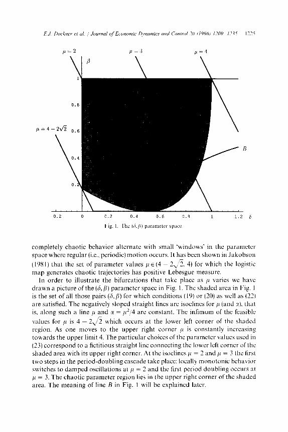
Fig. I. The (A./i) parameter space.

completely chaotic behavior alternate with small ‘windows’ in the parametet space where regular (i.e., periodic) motion occurs. It has been shown in Jakobson

(1981) that the set of parameter values ,U E (4 ~ 2,/2, 4) for which the logistic map generates chaotic trajectories has positive Lebesgue measure.

In order to illustrate the bifurcations that take place as ,U varies we have drawn a picture of the (S, /I) parameter space in Fig. 1. The shaded area in Fig. 1 is the set of all those pairs (6,/j) for which conditions (19) or (20) as well as (22) are satisfied. The negatively sloped straight lines are isoclines for 11 (and Y). that is, along such a line /i and a = ,~“,i4 are constant. The infimum of the feasible

values for Al is 4 - 24 which occurs at the lower left corner of the shaded region. As one moves to the upper right corner /L is constantly increasing towards the upper limit 4. The particular choices of the parameter values used in (23) correspond to a fictitious straight line connecting the lower left corner of the shaded area with its upper right corner. At the isoclines ,D = 2 and ,U = 3 the first two steps in the period-doubling cascade take place: locally monotonic behavior switches to damped oscillations at ,U = 2 and the first period doubling occurs at 11 = 3. The chaotic parameter region lies in the upper right corner of the shaded area. The meaning of line B in Fig. 1 will be explained later.


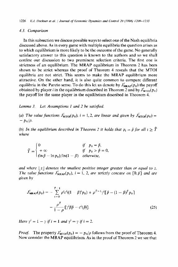
4.3. Comparison

In this subsection we discuss possible ways to select one of the Nash equilibria discussed above. As in every game with multiple equilibria the question arises as to which equilibrium is more likely to be the outcome of the game. No generally satisfactory answer to this question is known to the authors and so we shall confine our discussion to two prominent selection criteria. The first one is strictness of an equilibrium. The MRAP equilibrium in Theorem 2 has been shown to be strict whereas the proof of Theorem 4 reveals that the MT01 equilibria are not strict. This seems to make the MRAP equilibrium more attractive. On the other hand, it is also quite common to compare different equilibria in the Pareto sense. To do this let us denote by &sAP(pO) the payoff obtained by player i in the equilibrium described in Theorem 2 and by &,i(pO) the payoff for the same player in the equilibrium described in Theorem 4.

Lemma 3. Let Assumptions 1 and 2 be satisjied.

(a) The value functions J&tOI(pO), i = 1,2, are linear and given by JhTOI(pO) = - PO/P.

(b) In the equilibrium described in Theorem 2 it holds that pt = p for all t 2 i= where

if p. = P”, if po > p = 0,

(lnp - lnp,)/ln(l - /I) otherwise,

and where Lz] denotes the smallest positive integer greater than or equal to z. The value functions JLRAP(pO), i = 1, 2, are strictly concave on [O,p] and are given by

f-1

J$RAP(PO) = - 1 P’c’((~ - P)‘Po) + p’-‘yiCF - (1 - P)‘pol t=o

Jc [q/Q - c’(i)]. +1-p

Herey’=l-yifi=landy’=yifi=2.

(25)

Proof The property J&t(po) = - pa/p follows from the proof of Theorem 4. Now consider the MRAP equilibrium. As in the proof of Theorem 2 we see that

E.J. Dockner et al. /Journal of Economic Dynamics and Control 20 (1996) 1209~-1235 1221

player l’s optimization problem (given the equilibrium strategy of his opponent)

can be written as

maximize - (1 - /?)pO - c’(p,) - Y 2(p0) + f p’+’ I/ ‘(pr+i), I=0

subject to

Pt+1 EC’(R),

where V’ is a strictly concave function and C’ is a correspondence with a convex graph. Using a standard argument one can show that this implies the strict concavity of player l’s optimal value function. Analogously, player 2’s optimal value function must be strictly concave. The expression for F follows immediately from (12). Furthermore we must have pt = (1 - B)‘pO for all t < 7 - 1 and pt = p for t 2 F. Using (10) and (11) we obtain of = 0 for t I F - 2, yf = $[fi - (1 - /?)‘pO] for t = T - 1, and yf = yip@ for t 2 7. Sub- stituting these values into (5) one obtains (25). H

The above result makes it possible to compare the value functions in the two equilibria for any given parameter specification. In the following lemma we

summarize a few results which simplify this comparison.

Lemma 4. Let Assumptions I and 2 be satisjed.

(a) Assume 6 # 0 and p” # pO. The relation J ~&PO) < J~~Po) hokfs if and only if

P%m + (1 - p)W;((l - /Q’-‘pO) + qp’-f - (1 - /j)~-‘]pO

1-2

< sp2-’ ,To p’c’((1 - j3)‘po) + (1 - y’)i.

(b) Assume p0 I i/(1 - /I). Then f 5 1 holds and the relation JhRAP(pO) < J&,(p,,) is satisjied if and only if

pw:f(@) + (1 - p)W;~(po) < (1 - ?;‘)@ (26)

(c) Asssume p” = 0 < pO. The relation J iRAP < JhTOI( pO) holds if and only if

tgo P’C’(U - B)‘Po) ’ PO/P.

Proof: Assertions (a), (b), and (c) follow from the formulas for .I&+,) and J~rol(po) given in Lemma 3 by straightforward manipulations. To prove (d) consider any given initial state p. I c/(1 - 8). Using Assumption 1 and part (b) of the present lemma (applied to pO = 6) we obtain pW:i(fl -t (1 - p) Wti (p,) I W:i(ii) -c (1 - yi)ji. Applying part (b) once again we see that J&RAP(po) < &-o,(~a) and the proof is complete. I

Because of the linearity of I ho&) and the strict concavity of J&P(~O) there can, generically, be only five qualitatively different scenarios. These are illustrated in Fig. 2. The following result shows that none of these scenarios can be excluded without further assumptions.

.- P

Fig. 2. The five possibilities of dominance,

E.J. Do&w et al. /Journal of Economic Dynamics and Control 20 (1996) 1209-1235 1229

Lemma 5. For every scenario that is depicted in Fig. 2 one canjnd parameters fi, p, and ji as well as cost functions c’ and c2 such that Assumptions 1 and 2 are satisjied and such that the given scenario obtains.

Proof. We prove the lemma by constructing examples. In all these examples we consider a symmetric game, i.e., c1 (p) = c’(p) for all p E [0, p]. This implies that Assumption 1 is satisfied if we choose y = i. Moreover, in all examples we choose /I = i, p = 1, and p = i (which is equivalent to 6 = 1). Therefore, the only difference between the examples is the specification of the cost function c = c’ = c2. For the above parameter specifications Assumption 2 is satisfied if and only if $ p - i < c(p) < $ p. The individual surrogate welfare functions from Assumption 1 are given by Wfi2( p) = i p - c(p). All our examples will have continuously differentiable and strictly convex cost functions with c’(f) = i. This implies in particular that fi = 5. Together with B = + and p = 1 this shows

that p0 I F/( 1 - p) for all p,, E [0, p] so that Lemma 4(b) can be applied. For the chosen parameter values condition (26) is easily seen to be equivalent to

f(p,,):= 6 - 12c(3) + 21p, - 12c(p,) < 0.

Case (a): Let us specify c(p) = ~[+p - 11’ + ip - $ - E where E is a positive real number. It is straightforward to verify that all the conditions mentioned above are satisfied if E is chosen sufficiently small. Moreover, we have f(p) = - 2 + 24~ - 3.s(3p - 2)2 which is negative for all p E [0, 1] provided that 1: is sufficiently small. Because of Lemma 4(b) this implies that JhRAP(pO) < J&,(pO) for all possible initial states p0 which is exactly case (a) in

Fig. 2.

Case (b): Let c be any continuously differentiable and strictly convex function defined on [0, l] with c(0) = 0, c(i) = 3, c(1) = ;, and c’(3) = $. It is easy to see that such a function exists and that the general conditions mentioned above are satisfied. Moreover, we havef(0) = - 2 andf( 1) = 1 so that by Lemma 4(b) case (b) in Fig. 2 obtains.

Case (c): Let c be any continuously differentiable and strictly convex function defined on [0, l] with c(0) = - 3, ~$5) = 5, c(1) = 3, and c’(i) = 4. Again, it is easy to see that such a function exists and that the conditions mentioned above are satisfied. Moreover, we havef(0) = : andf( 1) = - i so that by Lemma 4(b) case (c) in Fig. 2 obtains. n

Case (d): Let c be any continuously differentiable and strictly convex function defined on [IO, l] with c(0) = 0, ~(3) = g, c(1) = 3, and c’(i) = $. As before, such a function exists and the conditions from above are satisfied. Moreover, we have f(0) = - ?, f(i) = 1, and f( 1) = - 3 so that by Lemma 4(b) case (d) in Fig. 2 obtains.


Case (e): Finally, let us specify c(P) = (&/9)(3P - 2)’ + :P - i where E is a positive real number. Again, all the conditions mentioned above are satisfied if E is chosen sufficiently small. Moreover, we have f(P) = 4 - :s(3P - 2)2 which is positive for all P E [0, l] provided that E is sufficiently small. Because of Lemma 4(b) this implies that &i&P,,) > J’ MTOI(PO) for all possible initial states p. so that case (e) in Fig. 2 obtains. n

We conclude this section by comparing the MRAP equilibrium and the MT01 equilibrium in the example from Section 4.2.

Example (continued). We maintain (18) and (22) and either (19) or (20). We have already noted that y = 3 satisfies Assumption 1. From (21) and (22) we obtain p”=min{l, 2/P}. F ur th ermore let us assume that (1 - /3)po I P holds for all p. E [O,p] which is easily seen to be the case if and only if 6 I (1 + p’)/ [2(1 - o)]. In Fig. 1 this corresponds to all points in the shaded area that are located above curve B. Because of the latter assumption we are in a position to apply Lemma 4(b) which shows that J CRAP <&TO~PO) if and only if

pWf,,@) + (1 - p)Wf,,(po) < P/2. Using the specification of the surrogate welfare functions and (18) we can rewrite this inequality as

(1 - P)CPPo - (P2/4)PZl + PC!@ - (P2/4)P21 < 6

where P is defined as before by P = 1 + p + 26. Let us first consider the case where P < 2. In this case we have P = 1.

Substituting P = p. = 1 into (27) we obtain ~(4 - P)/4 < 1 which is true for all P < 2. Consequently we have J&&j) < J~TOI(P). By Lemma 4(d) this implies JhRAP(pO) < J&(pO) for all p. E [O,p] provided that P < 2.

Now let us conosider the case P 7 2 where P = 2/P. We are going to show that in this case JhRAP(pO) < J~TOI(pO) holds for all initial states p. which are sufficiently small, whereas the reverse inequality holds for all sufficiently large initial states. In other words, for P > 2 case (b) of Fig. 2 obtains. To prove our claim it is sufficient to show that J’ MRAP~ < J$ToI(~) and &RAP(~) >&m(1).

Using (27) and P = 2/P we see that the first inequalilty is equivalent to p < 2/P which can also be written as 1 + /? + 26 < 2(1 + 6). Obviously this is true. Using p. = 1, p” = 2/P, and (27), the second inequality can be written as (1 - p)(P - P2/4) + p > 2/P. Using the definitions p = l/(1 + 6) and P = 1 + j3 + 26 one can show that

(1 - P)(P - $14) + P - 21~1 = P(P - 2)c4 + 56 - d(P - 1)21/(4P),

so that our claim is proven if 4 + 56 > S(P - 1)2 holds. The validity of this inequality, however, is a simple consequence of P < 4 and 6 < 1 which holds for


all points in the shaded region of Fig. 1. Therefore, panel (b) of Fig. 2 describes the situation in this example if p > 2.

5. Non-Markovian equilibria

In this section we show that under certain assumptions the two countries can achieve the outcome of the collusive solution discussed in Section 3 by means of a purely noncooperative mechanism. The easiest way to see this is to consider trigger strategies by which the players can punish deviations of their opponents from a given target path. In our model the target path is the state trajectory of the cooperative solution as described in (8). To be able to detect a deviation, a player has to have more information about the history of the system than just the current state. Consequently, a trigger strategy can no longer be a Markovian strategy.

Let us now go into the formal details. As mentioned before the target path is the state trajectory generated by the cooperative solution. It is the unique path ;o,!G, ... satisfying p^,+ 1 = max ((1 - /I)!(, p* > and i0 = p. where p* is the unique maximizer of the surrogate welfare function W from (6). In the cooperative solution only the joint level of emissions is uniquely determined, not the individual levels of both countries (see Theorem 1). Let us assume that the aim of the trigger strategies is to achieve the outcome of the cooperative solution with emisson shares q and 1 - q for country 1 and 2, respectively. In other words, we are looking for an equilibrium in which country i has total discounted utility

.Z~(P~) = f. P’C$max (0, P* - (1 - P)iil - c’Gd1~

where y~l = r] and u* = 1 - r~. We say that the cooperative solution with emission shares r~ and 1 - r~ can be supported by a trigger strategy equilibrium if there exists a Nash equilibrium consisting of trigger strategies such that the equilibrium payoffs coincide with the target payoffs ji ( po) and J^: _ ,,( po), respectively, for all feasible initial states p. E [O,p].

Now consider the trigger strategies defined as follows:

vimax {O,p* - (1 - B)p,} if yf =

ps = is for all s E (0, 1, . . . ,r}, (28)

(6 + BP, - C’CP,) otherwise.

Here, j E { 1,2} denotes the opponent of i, that is, j # i. As long as the actual state trajectory coincides with the target trajectory player i chooses the same


emission level as in the cooperative solution. If country j uses a different emission level, country i will recognize this deviation in the following period since the actual state will differ from the target state. From that period on player i chooses the MT01 strategy from (15). Note that after a deviation by country j, player i never stops to use the MT01 strategy even if the state of the system happens to return to the target path. It is clear that if neither player finds it advantageous to deviate from the target path, then the above trigger strategies support the cooperative solution. In the following theorem we give necessary and sufficient conditions for this to happen. To this end let us define Ai = - Ct~o=op’ci(j?l) for i = 1, 2 and B(pO) = Ct?Opfmax (0, p* - (1 - /I)&} where, as before, p*,,, ii, . . . denotes the target path defined by (8) with @itial state j?,, = pO. Note that B(p) > 0 holds for all p E [O,p] and that Jig(p) = A’(p) + B(p)?‘. Furthermore, we define

bJ*> if (1 - B)p I p*, z= (29)

[p*, (1 - /?)p] otherwise,

and si = sup { - [A”(p) + p/p]/B(p) jp E Z} for i = 1, 2. We are now ready to formulate the main result of this section.

Theorem 5. Let Assumption 2 be satisfied.

(a) The pair of strategies dejned in (28) supports the cooperative solution from Theorem I with emission shares n and 1 - q if and only if

q E [O, l] n [s’, 1 - s’]. (30)

(b) If the game is symmetric (that is ifc’(p) = c2(p) for all p E [0, p]), then it holds that i E [0, l] n [s’, 1 - s’] so that the cooperative solution of Theorem 1 with equal emission shares for both countries can always be supported by the trigger strategies from (28).

(c) If (1 - /I)p I p*, then one can support the cooperative solution from The- orem I with emission shares n and 1 - q tfand only if the inequalities W$(p*) 2 (1 - $)p* hold for i = 1, 2 (here, again, we have n1 = n and n2 = 1 - q).

Proof: (a) Choose any q E [0, l] and assume that both players have followed the cooperative solution [i.e., the first line in (28)] for the first t periods. In this case the pollution stock in period t is equal to it. If both players stick to the target strategy, then their total discounted utility from period t onwards (discounted back to period t) is given by

E.J. Dockner et al. 1 Journal of Economic Dynamics and Conrrol 20 (I 996) 1.?09- 1235 1233

Now assume that player i defects by choosing the emission level y # j$. In that case his instantaneous utility in period t is y - ci(ir). From period t + 1 onwards, however, he will be punished by his opponent who switches to the threat [second line in (28)]. As we have seen in the proof of Theorem 4 this deprives player i from any influence on his own objective functional. No matter which level of emissions he chooses from period t + 1 onwards he will always obtain the discounted total utility - p t+,/p [see Lemma 3(a)]. Therefore, the total discounted utility of player i after a defection in period t is given by &r = y - c’(p^,) + p( - pt+ I/p). Substituting for pt+ 1 from the system dynamics, that is, pt+ 1 = (1 - /I)& + j:’ + y and rearranging we obtain

J&F = - ci(jt) - (1 - /I)& - jt’ = jf - c’(it) - j?,+,

Deviating from the targzt path has therefore a higher utility than cooperating if and only if - j,+ 1 > pJ&,+ 1) = p[A’(j,+ 1) + B(i,+ I)qi]. Rearranging this inequality and using q1 = u and q2 = 1 - q we see that neither player will deviate from the target path if and only if

- CA’(h+,) + ~,+1lpllB(~,+1) i q I 1 + [AQr+i) + ;,+,/p]/B(&+,).

As t ranges over { 0, 1, . . . } and pO ranges over [0, p] the pollution stock fit + 1 can take on any value in the set Z from (29). Therefore we obtain s1 I q I 1 - s2 as a necessary and sufficient condition for supportability of the efficient solution and the proof of part (a) is complete.

To prove part (b) of the theorem we first note that A’(p) + A2(p) + B(p) 2

- 2p/p because the left-hand side of this inequality is the optimal (joint) utility j:,,(p) + j:,,(p) in the cooperative problem whereas the right-hand side is just one feasible joint utility (namely the one that is obtained if both players play their MT01 strategies). Because of symmetry we have A’(p) = A2(p) so that the above inequality can be written as - [A’(p) + p/p]/B(p) I l/2. This implies that si I l/2 and part (b) follows from part (a).

Finally, if (1 - JI)p I p*, then Z = {p*} by (29). It is easily seen that A’(p*) = - c’( p*)/(l - p) and B(p*) = Bp*/(l - p) so that (30) is equivalent to W ‘(p*) 2 (1 - $)p* for i = 1, 2. W

The above result seems to be quite strong given the mild conditions that we have used. Especially part (b) of the theorem which states that an efficient solution in the symmetric game can always be supported as a noncooperative equilibrium is somewhat surprising because the usual folk theorems in the literature depend crucially on the size of the discount rate. In our case the dependence on the discount rate is hidden in Assumption 2 which we have postulated in Theorem 5. It is easy to see that this assumption can only be


satisfied if the discount rate 6 is not too large. If Assumption 2 would not hold, then we could not use the MT01 strategies as threats and our construction would not work.

6. Conclusions

In this paper we have formulated a class of capital accumulation games with a single stock variable which is influenced by the consumption (investment) decisions of all players in the game. We introduced three economic interpretations of the game but in the main body of the paper we have chosen to look at it as a game on international pollution control. We have characterized the quali- tative properties of the collusive solution as well as those of two different kinds of MPE. It turned out that the collusive solution implies convergence of the pollution stock to a unique steady state as does the first MPE which is a strict Nash equilibrium. The second MPE is not strict but makes both players indifferent between all of his feasible strategies. This equilibrium generates interesting dynamic behavior including chaos. A Pareto comparison shows that for certain parameter constellations the strict MPE can be dominated by the other MPE whereas for other parameter values the strict MPE is the dominated one. We have also analyzed a trigger strategy equilibrium that uses the nonstrict MP E as a retaliation strategy and generates efficient payoffs for both players.

References

Benhabib, J. and R. Radner, 1992, The joint exploitation of a productive asset: A game-theoretic

approach, Economic Theory 2, 155- 190.

Debreu, G., 1952, A social equilibrium existence theorem, Proceedings of the National Academy of

Sciences 38, 8866893.

Devaney, R.L., 1986, An introduction to chaotic dynamical systems (Benjamin Cummings, Menlo

Park, CA).

Dockner, E.J. and N.V. Long, 1992, International pollution control: Cooperative versus non-

cooperative strategies, Journal of Environmental Economics and Management 24, 13-29.

Dockner, E.J. and H. Takahashi, 1988, Further turnpike properties of capital accumulation games,

Economics Letters 28, 321-325.

Dockner, E.J. and H. Takahashi, 1993, Turnpike properties and comparative dynamics of general

capital accumulation games, in: M. Boldrin et al., eds., General equilibrium, growth, and trade II:

The legacy of L. McKenzie (Academic Press, Orlando, FL) 352-366.

Duffie, D., Y. Geanakoplos, A. MasColeIl, and A. McLennan, 1994, Stationary Markov equilibria, Econometrica 62, 745-781.

Dutta, P.K. and R. Sundaram, 1993a, The tragedy of the commons?, Economic Theory 3,413-426.

Dutta, P.K. and R. Sundaram, 1993b, How different can strategic models be?, Journal of Economic

Theory 60,42-61.

Fershtman, C. and E. Muller, 1984, Capital accumulation games of infinite duration, Journal of Economic Theory 38, 322-339.


Fershtman, C. and E. Muller, 1986, Turnpike properties of capital accumulation games, Journal of

Economic Theory 40, 167-177.

Fershtman, C. and S. Nitzan, 1991, Dynamic voluntary provision of public goods, European

Economic Review 35, 1057-1067.

Jakobson, M.V., 1981, Absolutely continuous invariant measures for one-parameter families of

one-dimensional maps, Communications of Mathematical Physics 81, 39988.

Levhari, D. and L. Mirman, 1980, The great fish war: An example using a dynamic Cournol-Nash

solution, Bell Journal of Economics 11, 322-334.

Maskin, E. and J. Tirole, 1988, A theory of oligopoly: I. Overview and quantity competition with

large fixed costs, Econometrica 56, 5499569.

Rasband, N.S., 1990, Chaotic dynamics of nonlinear systems (Wiley, New York, NY).

Sundaram, R.K., 1989, Perfect equilibrium in non-randomized strategies in a class of symmetric

dynamic games, Journal of Economic Theory 47, 153 177.

Analysis of Nash equilibria in a class of capital accumulation games

Documents

Transcript of Analysis of Nash equilibria in a class of capital accumulation games