ANALYSIS OF HANDOVER CHARACTERISTICS IN SHADOWED LEOSATELLITE COMMUNICATION NETWORKS�

YOUNG HOON KWON AND DAN KEUN SUNG��

Department of Electrical Engineering and Computer Science, Korea Advanced Institute of Science and Technology, 373-1,Kusong-dong, Yusong-gu, Taejon, 305-701, Korea

SUMMARY

In the near future low earth orbit (LEO) satellite communication networks will partially substitute for fixed terrestrialmultimedia networks especially in sparsely populated areas. Unlike fixed terrestrial networks, ongoing calls may bedropped if satellite channels are shadowed. Therefore, in most LEO satellite communication networks more than onesatellite need to be simultaneously visible in order to hand over a call to an unshadowed satellite when the communicatingsatellite is shadowed. In this paper handover characteristics for fixed terminals (FTs) in LEO satellite communicationnetworks are analyzed. The probability distribution of multiple satellite visibility is analytically obtained and the shad-owing process of satellites for FTs are modelled. Using the proposed analysis model, shadowing effects on the trafficperformance are evaluated in terms of the number of intersatellite and interbeam handovers during a call.

KEY WORDS: multiple satellite visibility; satellite channel shadowing; intersatellite handover; interbeam handover

1. INTRODUCTION

In the emerging era of the International Mobile Telecommunications - 2000 (IMT-2000), LEO satellite com-

munication networks are expected to coexist with terrestrial networks.1 Terrestrial regional telecommuni-

cation networks with diverse transfer modes and various protocols may suffer from internetworking and

compatibility problems to provide global seamless multimedia communications.

LEO satellite networks will be able to support end-to-end connections in the near future,2];[3 and thus, they

will play both complementary and competitive roles compared with fixed telecommunication networks as

well as cellular networks, and may partially substitute for fixed networks in sparsely populated areas where

fixed telephony services are unavailable.4

LEO satellite channel characteristics affect the availability and the quality of services, depending on urban

vs. suburban areas and satellite constellation parameters.5];[6];[7 When the quality of a satellite channel is

degraded due to shadowing, an ongoing call may be dropped. Multiple satellite visibility is provided in most

LEO satellite constellations to reduce this call dropping.8];[9 If ongoing calls are dropped only when all visible

satellites are shadowed, service availability can be increased.

� This study is partially supported by the Ministry of Science & Technology.�� Correspondence to: Prof. D. K. Sung, Department of Electrical Engineering and Computer Science, Korea Advanced Institute of Scienceand Technology, 373-1 Kusong-dong, Yusong-gu, Taejon 305-701, Korea. E-mail: dksung@ee.kaist.ac.kr

2

Shadowing of satellites for mobile terminals (MTs) is caused by two mobility factors. These are satellite

mobility and user mobility. As an LEO satellite moves with a constant velocity the varying elevation angle

of the satellite from an MT affects the shadowing parameters. Furthermore, the shadowing environment of

an MT may vary with time because of the motion of the MT. For FTs with a fixed shadowing environment,

shadowing of a satellite depends on the elevation angle of the satellite. Thus, if the elevation angle is sufficient

to clear nearby obstacles a call can be connected to the satellite.

Several previous studies5];[9];[10 have dealt with shadowing parameters of satellite availability and the re-

ceived signal distribution in diverse environments. When a satellite which is communicating with an FT

is shadowed or when the coverage area of the satellite moves out of the FT, an intersatellite handover oc-

curs. Even within the coverage area of a satellite, interbeam handovers may occur in a multiple spot beam

environment.11 The numbers of intersatellite handovers and interbeam handovers vary according to the shad-

owing environment of an FT. In this paper the handover characteristics of FTs in LEO satellite communica-

tion networks are analyzed. The shadowing process of satellites is modelled, and the numbers of intersatellite

handovers and interbeam handovers are analytically obtained based on the shadowing model in a multiple-

satellite-visible condition.

The remaining part of this paper is organized as follows: Section 2 presents an analysis of the probability

distribution of the multiple satellite visibility at an arbitrary latitude; Section 3 introduces a shadowing model

and a multiple spot beam model; Section 4 shows an analysis of handover characteristics based on these

system models; Section 5 shows numerical results; and Section 6 presents conclusions.

2. MULTIPLE SATELLITE VISIBILITY

LEO satellite communication networks consist of multiple orbit planes and multiple satellites per orbit plane

in order to realize global coverage. The candidate satellite to an FT is defined as a satellite whose elevation

angle to the FT is greater than given minimum elevation angle. The number of candidate satellites, NCS

varies according to constellation parameters, such as the number of satellites, the inclination angle of an orbit

plane, and the altitude and the longitude of each satellite. The probability distribution of NCS

at a latitude of

� is now obtained.

3

Figure 1 shows the position of the i-th orbit plane to a reference point. If �i

denotes the ascending node

right ascension of the i-th orbit plane, then �i

can be expressed as

�i=

2�

NO

i ; 1 6 i 6 NO

(1)

where NO

is the number of orbit planes. For an arbitrary point Q with a latitude and longitude of � and �,

respectively, the distance between the point Q and the corresponding track on the earth’s surface of the i-th

orbit plane is given by

li= R

E

��sin�1(sin Æ cos� sin(�

i� �) + cos Æ sin�)

�� (2)

where RE

and Æ denote the radius of the earth and the inclination angle of each orbit plane, respectively.

Figure 2 illustrates the coverage area of each satellite. The altitude and the minimum required elevation

angle of a satellite are denoted by h and �min, respectively. The radius of the coverage area of each satellite is

then obtained as 12

Rs= R

E

��

2� �min � sin

�1

�RE

RE+ h

cos �min

��(3)

If the coverage area of each satellite is assumed to be a flat circle, as shown in Figure 3, the ground track

distance of a satellite in the i-th orbit moved during the time the point Q is included in the coverage area of

the satellite, (li) can be expressed as

(li) =

�2

pRs

2� l2

i; 0 6 l

i6 R

s

0 ; li> R

s

(4)

If the number of satellites in one orbit plane is denoted by NSO

, the distance between adjacent sub-satellite

points (SSPs) is given by

Ls=

2�RE

NSO

(5)

The number of candidate satellites in the i-th orbit at the point Q, Mi

depends on the relative position of the

satellites to (li). An illustration for the case of (l

i) = 5 and L

s= 2 is shown in Fig. 4. As shown in

this illustration, the number of candidate satellites in the i-th orbit at the point Q, Mi

is given byj (li)

Ls

kor

4

j (li)

Ls

k+ 1, where bxc denotes the greatest integer less than or equal to x. At an arbitrary time, the relative

position of the satellites has no correlation with the (li), and thus, the probability q

i(n;Q) that the number

of candidate satellites in the i-th orbit is n at the point Q can be expressed as

qi(n;Q) =

8>><>>:

1�

� (li)

Ls�

j (li)

Ls

k�; n =

j (li)

Ls

k (li)

Ls�

j (li)

Ls

k; n =

j (li)

Ls

k+ 1

0 ; otherwise

(6)

The number of candidate satellites NCS

at an arbitrary point Q can be obtained by summing the number of

candidate satellites in the entire constellation. That is, the probability PCS

(j;Q) that NCS

is j at the point Q

is given by

PCS

(j;Q) = PrfM1 +M2 + � � � +MNO

= j at the point Qg

=

jXn1=0

jXn2=0

� � �

jXnNO�1=0

qNO

(j � n1;Q)qNO�1(n1 � n2;Q)

� � � � q2(nNO�2 � nNO�1;Q)q1(nNO�1;Q) (7)

Therefore, the probability PCS

(j) that NCS

is equal to j at a latitude of � can be obtained as

PCS

(j) =

R 2�

0PCS

(j;Q) d�

2�(8)

NmaxXj=0

PCS

(j) = 1 (9)

where Nmax denotes the maximum number of candidate satellites. Then, the mean number of candidate

satellites E[NCS

] can be expressed as

E[NCS

] =

NmaxXj=1

jPCS

(j) (10)

3. SYSTEM MODEL

3.1. Shadowing model

Since LEO satellites move in their orbit plane the motion of each satellite relative to an FT can be modelled

as a linear motion with a constant velocity. The satellite ground track speed VSSP

depends on the altitude of

5

a satellite such that

VSSP

=RE

RE+ h

r�

RE+ h

(11)

where � = 3 � 986� 1014m

3s�2 is the gravitational parameter.

From the viewpoint of an FT, satellites whose elevation angle is greater than the minimum required el-

evation angle �min can be connected if the communication channel between the FT and the satellite is not

shadowed. The service area for an FT is defined as the virtual area in which the SSP of a satellite with an

elevation angle from the corresponding FT greater than �min can be located.13 If the coverage area of each

satellite is assumed to be a circle with a radius of Rs, the service area of an FT would also be a circle with a

radius of Rs

and each SSP inside the service area would move linearly with a constant velocity of VSSP

.

A communication channel is shadowed when the elevation angle of a satellite is lower than the required

elevation angle. This can be caused by nearby obstacles, such as tall buildings, trees, and mountains. If

the location of an FT is fixed the time variation of the shadowing is negligible. However, the shadowing

process of satellite channels varies with time because each satellite moves with time. Thus, each satellite at

an azimuth angle of with respect to the reference direction of the FT, as shown in Figure 5, can be connected

to an FT if the elevation angle is greater than the minimum unshadowed elevation angle �( ) at an azimuth

angle of , where the minimum unshadowed elevation angle is a user-specific value which is determined by

the shadowing environment of the MT.

For mathematical simplicity it is assumed that the shadowing environment of an FT is omnidirectional,

which implies that an FT has an identical minimum unshadowed elevation angle irrespective of the azimuth

angle �( ) = �. The available area of an FT is defined as the area in which the SSP of unshadowed

satellites can be located. As the minimum unshadowed elevation angle � is assumed to be omnidirectional,

the available area of an FT can be modelled as a circle with a radius Ra, which is a function of �.

The probability distribution of Ra

can be obtained with the satellite availability PA(�) that one satellite

with an elevation angle of � is available. PA(�) also implies the probability that � exceeds the minimum

unshadowed elevation angle �, that is,

PA(�) = Prf� > �g (12)

6

Satellite availability has been extensively measured and analyzed in several previous studies.5];[10];[9 The prob-

ability that � is less than � equals to the probability that one satellite with an elevation angle of � is available.

Thus, the probability distribution function (PDF) of � can be obtained as

f�(�) =

d

d�Prf� 6 �g

=d

d�PA(�) (13)

where PA(�) satisfies two boundary conditions.

�PA(0) = 0

PA(�

2) = 1

Similar to equation 3, the relationship between a radius ra

and an elevation angle � is given by

ra= R

E

��

2� � � sin

�1

�RE

RE+ h

cos �

��(14)

And, the maximum value of ra, R

a;max is obtained as

Ra;max = r

aj�=0 = R

Ecos

�1

�RE

RE+ h

�(15)

Therefore, the PDF of the radius of an available area fRa(ra) can be expressed as

fRa(ra) =

dPA(�)

d�

���� d�dra

����=

1RE

�1

RE+hcos(

ra

RE)

sin2(ra

RE) +

ncos(

ra

RE)�

RE

RE+h

o2

dPA(�)

d�

�����=tan�1

0@ cos(

raRE

)�RE

RE+h

sin(raRE

)

1A

(16)

in the range of 0 6 ra6 R

a;max.

Each FT has two independent virtual areas, a service area and an available area. As an FT has multiple

number of candidate satellites, the FT may have several SSPs in a service area. If Ra

is greater than Rs, all

satellites in the service area are unshadowed and can be connected when a call is requested. However, if Ra

is smaller than Rs, satellites outside of the available area within the service area may be shadowed, and thus,

the number of available satellites is reduced. These two cases are shown in Figure 6. Therefore, an FT can

connect a call to satellites in the circle with a radius of min(Rs; R

a).

7

3.2. Multiple spot beams

In most LEO satellite constellations, the coverage area is partitioned into multiple spot beams.14 Use of multi-

ple spot beams can increase system capacity, concentrate transmission power, and reduce FT antenna size and

required transmission power. In this case an FT may experience interbeam handovers as well as intersatellite

handovers. Intersatellite handovers occur between adjacent satellites. Thus, intersatellite handovers require

message transfer to the earth station which controls both satellites, which causes a relatively high processing

load and time delay. However, interbeam handovers occur between adjacent spot beams within a satellite.

Therefore, these handover procedures can be controlled in a satellite and yield a relatively low processing

load and time delay. Moreover, the next handover beam can be known a priori to the satellite controller.

FTs covered by each spot beam may have different path losses according to the position of the spot beam

within the coverage area of a satellite. This is due to an increase in slant range losses as the footprint moves

farther from the SSP. This path loss is assumed to be compensated by increasing the spot beam antenna gain

as the beam moves farther away. When an FT requests a call, the FT compares the received signal strengths

from multiple satellites and connects to spot beam with the maximum received signal strength. Due to the

compensation of path loss, each visible spot beam can be connected to this FT with equal probability. Thus,

the position of the selected spot beam within a coverage area of the selected satellite is uniformly located.

Therefore, the number of available satellites does not affect the residence time distribution in the coverage

area of a satellite.

The footprint of each spot beam inevitably overlaps its adjacent spot beams in order to provide seamless

coverage. The overlap area is approximated to be a circle, as illustrated in Figure 7, where the radius of

the beam footprint and the width of the overlap area are R and 2L, respectively. The distance between two

adjacent spot beam centres is Lc. If the coverage area of a satellite consists of maximum N

bspot beams in a

strip, R is related to Rs

as follows

Rs

= R+ (Nb� 1)(R� L) (17)

) R =Rs

(Nb� 1)(1� �) + 1

8

=Rs+ (N

b� 1)L

Nb

(18)

where � = L=R is the normalized overlap width. Figure 8 illustrates the structure of spot beams in a satellite

coverage area with Nb= 5. It is assumed that an FT will be handed over only to the next beam in the same

strip. Then, the residence time in the transit spot beam is Lc=V

SSP.

4. PERFORMANCE ANALYSIS

4.1. Residual distance of a satellite

D denotes the distance between an FT and an SSP inside the service area of the FT. The probability that D is

less than or equal to r, PrfD 6 rg is given by 15

PrfD 6 rg =�r2

�R2s

=r2

R2s

; 0 6 r 6 Rs

(19)

Therefore, the PDF of D can then be expressed as

fD(r) =

d

drPrfD 6 rg =

�2rR2s

; 0 6 r 6 Rs

0 ; otherwise(20)

Under the condition thatRa= r

a, available satellites for the FT can be located within a radius of min(R

s; r

a).

If D0 denotes the distance between an FT and a candidate SSP within a radius of min(Rs; r

a), the PDF of D0

is given by

fD

0(rjra) =

fD(r)

FD(ra)

(21)

where FD(ra) is the cumulative distribution function (CDF) of D such that F

D(ra) = PrfD 6 r

ag.

The residual distance of a satellite to an FT Xr

is defined as the distance travelled of the SSP from the

beginning of a new/handover call to either the time that the SSP moves out of the service area or the time

when the satellite is shadowed. When Ra= r

aand D0

= r, the CDF of the residual distance of a connected

satellite to an FT is given by

FXr

(xjr; ra) = PrfX

r6 xjD0

= r;Ra= r

ag

= Pt(x;min(R

s; r

a); r) (22)

9

where Pt(x; r0; r) denotes the probability that a user whose distance from the centre of a circle with a radius

of r0 is r, moves out of the circle when the FT moves a distance of x, such that 13

Pt(x; r0; r) =

8><>:

0 ; 0 6 x < r0 � r1�

cos�1�r20�r

2�x

2

2xr

�; r0 � r 6 x 6 r0 + r

1 ; x > r0 + r

If equation 22 is unconditioned to D0, FXr

(xjra) can be obtained as

FXr

(xjra) =

Z min(Rs;ra)

0

FXr

(xjr; ra)f

D0(rjr

a)dr

=

8<:

0 ; x < 0

2!+sin2!�

; 0 6 x 6 2min(Rs; r

a)

1 ; x > 2min(Rs; r

a)

(23)

where

! = sin�1

�x

2min(Rs; r

a)

�

Therefore, the CDF of Xr, F

Xr(x) can be obtained by unconditioning F

Xr(xjr

a) on R

a.

FXr

(x) =

ZRa;max

0

FXr

(xjra)f

Ra(ra)dr

a(24)

4.2. Handover performance

Let TM

denote the exponentially distributed call duration with a mean of TM

. As each SSP moves with a

constant velocity, the distance XM

that an SSP moves during a call is also exponentially distributed with a

mean of XM

= VSSP

TM

. If the residual distance of the connected satellite Xr

is shorter than XM

an inter-

satellite handover occurs. Therefore, the probability PHjra

that an FT with Ra= r

arequires an intersatellite

handover can be obtained as

PHjra

= PrfXM> X

rjR

a= r

ag

=

Z 2min(Rs;ra)

0

e�x=XMfXr

(xjra)dx (25)

The residual distance distribution of handed-over satellite to the FT is assumed to be identical to that of the

original satellite. Thus, PHjra

for new calls and handover calls is the same due to the memoryless property of

10

exponentially distributed call duration. The probability that the number of intersatellite handovers during a

call Ksjra

is n when Ra= r

ais given by

PrfKsjra

= kjRa= r

ag = (1� P

Hjra)P k

Hjra(26)

Then, the CDF of Ks, PrfK

s6 kg can be expressed as

PrfKs6 kg =

ZRa;max

0

PrfKsjra

6 kgfRa(ra)dr

a

=

ZRa;max

0

kXi=0

(1� PHjra

)P k

HjrafRa(ra)dr

a

=

ZRa;max

0

(1� P k+1Hjra

)fRa(ra)dr

a(27)

The mean number of intersatellite handovers when Ra= r

a, K

sjracan be obtained as

Ksjra

=

1Xk=1

k PrfKsjra

= kjRa= r

ag

=

1Xk=1

k(1� PHjra

)P k

Hjra

=PHjra

1� PHjra

(28)

Thus, the mean number of intersatellite handovers during a call can be obtained by unconditioning Ksjra

on

Ra.

Ks

=

ZRa;max

0

KsjrafRa(ra)dr

a

=

ZRa;max

0

PHjra

1� PHjra

fRa(ra)dr

a(29)

To obtain the number of interbeam handovers during a call KB

, the shadowing condition of each spot

beam should be considered first. If the minimum unshadowed elevation angle � for an FT is greater than the

minimum elevation angle �min (Rs> R

a), the spot beams located at the outer tier of a satellite coverage area

may be shadowed as shown in Figure 9. In this figure, Y denotes the length of the partly shadowed spot beam

whose elevation angle is greater than �, and can be obtained as

Y =

8<:

Lc+ L ; R

s�R

a< 0

Lc+ L� R

s+R

a; 0 6 R

s�R

a< L

c+ L

LcbRs�Ra�L

Lcc � (R

s�R

a� L� L

c) ; R

s�R

a> L

c+ L

(30)

11

Two integer random variables Kb1 and K

b2 represent the number of interbeam handovers in one satellite

when the call is completed within a satellite and when an intersatellite handover occurs, respectively. When

an interbeam handover occurs the residual distance of a handed over beam is Lc

if this beam is not shadowed.

Thus, the probabilities that Kb1jra and K

b2jra equal k when Ra= r

aare given by

PrfKb1jra = kg

= Pr

�XM> X

rjra� Y � b

Xrjra�Y

LccL

c+ (k � 1)L

cjX

M< X

rjra

=

R 2min(Rs;ra)

Y+(k�1)Lc

�FXM

(x)� FXM

(x�Y�bx�YLc

cLc+(k�1)Lc)

�fXrjra

(x)dx

1� PHjra

(31)

PrfKb2jra = kg

= PrfXrjra

> Y + (k � 1)LcjX

M> X

rjrag

=

R 2min(Rs;ra)

Y+(k�1)LcFXM

(x)fXrjra

(x)dx

PHjra

(32)

where FXM

(x) is the complementary CDF of XM

such that FXM

(x) = 1 � FXM

(x) = exp(�x=XM). If

a call is completed within the first communicating satellite the number of interbeam handovers during a call

KB

equalsKb1. However, when an intersatellite handover occursK

Brestarts at a transit satellite and is added

to the number of interbeam handovers at the first satellite. Hence, KBjra

when Ra= r

acan be expressed as

KBjra

= (1� PHjra

)Kb1jra + P

Hjra(K

Bjra+K

b2jra)

=PHjra

1� PHjra

Kb2jra +K

b1jra (33)

The mean of KBjra

, KBjra

can then be obtained as

KBjra

=PHjra

1� PHjra

E[Kb2jra ] + E[K

b1jra ]

=

Nb�1Xk=1

�PHjra

1� PHjra

PrfKb2jra > kg+ PrfK

b1jra > kg

�

=

Nb�1Xk=1

"1

1� PHjra

Z 2min(Rs;ra)

Y+(k�1)Lc

FXM

(x�Y�bx�YLc

cLc+(k�1)Lc)fXrjra(x)dx

#(34)

The mean of KB

can be obtained by unconditioning KBjra

on Ra.

KB

=

ZRa;max

0

Nb�1Xk=1

�PHjra

1� PHjra

PrfKb2jra > kg+ PrfK

b1jra > kg

�fRa(ra)dr

a

12

=

ZRa;max

0

fRa(ra)

1� PHjra

Nb�1Xk=1

Z 2min(Rs;ra)

Y+(k�1)Lc

FXM

(x�Y�bx�YLc

cLc+(k�1)Lc)fXrjra(x)dxdr

a(35)

5. NUMERICAL RESULTS

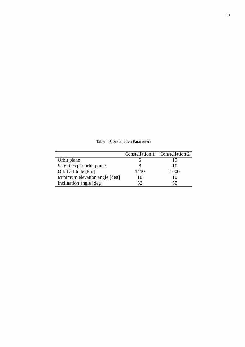
We consider two satellite constellations. Constellation 1 is a GLOBALSTAR-like constellation, and Con-

stellation 2 is a typical inclined orbit LEO satellite constellation. The constellation parameters for both are

shown in Table I.

Analytical results can be obtained straightforwardly by simple numeric integrations with finite limits and

sums with finite number of terms. Figure 10 shows the mean number of candidate satellites E[NCS

] as a

function of latitude. In this figure, the proposed analytical results are compared with simulation results. In

computer simulation, more than 20,000 samples are generated until their statistics converge. Each sample is

generated at a randomly chosen longitude and time interval. In this case, shadowing of candidate satellites

is not considered. As shown in this figure, the proposed analytical results agree well with simulation results.

Since both Constellations 1 and 2 use inclined orbits, E[NCS

] is high at medium latitude regions where the

user population is dense. Since Constellation 2 has twice as many satellites as Constellation 1, more satellites

can be seen at low latitudes compared with Constellation 1. In high latitude regions beyond the inclination

angle where no satellite passes over, the size of the coverage area affects E[NCS

], rather than the number of

satellites in a constellation. The E[NCS

] of Constellation 2, which has a lower altitude and more satellites,

decreases rapidly at latitudes higher than 50Æ.

The probability distribution of NCS

is applied to the shadowing models of an urban and a suburban areas.

Measured data for shadowing model parameters are limited. Thus, the satellite availability PA(�) cannot

be obtained directly from the measured data. Therefore, the curve-fitted data used by Karasawa et al.9 are

modified to fit the boundary condition of equation 13 with a smooth transition. The satellite availabilities for

both urban and suburban areas used here are

PA(�) =

�1�

(�2��)2

a

; �

186 � 6 �

2

�2(b1� � b2) ; 0 6 � 6 �

18

(36)

where

a =

�0 � 216�2 ; for urban area0 � 512�2 ; for suburban area

13

b1 =825 � 06

a� 376 � 182

b2 =208

a� 98 � 484

Figure 11 illustrates the satellite availabilities for both areas.

For numerical calculation the mean call duration TM

is set at 150 seconds. And, considered latitude is

35Æ north. Figure 12 shows the CDF of the residual distance of connected satellite FXr

(x) and the CDF

of the number of interbeam handovers PrfKs6 kg. Since Constellation 2 has smaller coverage area than

Constellation 1, it has shorter residual distance. And, because of heavy shadowing, Xr

for urban area is

shorter than for suburban area. Therefore, interbeam handovers occur more frequently in Constellation 2 than

in Constellation 1, and more frequently in urban area than in suburban area.

The mean number of intersatellite handovers for an FT with Ra= r

a, K

sjrafor both Constellations 1

and 2 are shown in Figure 13. As Ra

increases, the probability that an intersatellite handover occurs due

to shadowing of a communicating satellite decreases, and thus, Ksjra

decreases. Throughout our numerical

results, our analytical results are verified by computer simulation. In computer simulation, exponentially

distributed call durations are generated and the number of intersatellite and interbeam handovers for both

constellations are counted during each call. These calls are generated until handover statistics converge. As

shown in this figure, our analytical results agree well with simulation results.

Figure 14 shows the mean number of interbeam handovers with Ra= r

a, K

Bjrafor N

b= 5 and 6. In both

cases, � is set at 0 � 1. As Ra

increases, the residual distance of connected satellite increases, and thus, KBjra

decreases. If Ra

increases further and includes another boundary of spot beams, more interbeam handovers

occur before the occurrence of an intersatellite handover. Therefore,KBjra

has discontinuities at the boundary

of spot beams. If Nb

is an odd number, the nearest boundary of spot beams is located at Lc=2 from the center

of the satellite coverage area. Therefore, if Ra

is smaller than Lc=2, an intersatellite handover occurs at the

spot beam that an FT requests a call and no interbeam handovers occur. However, if Nb

is an even number,

the boundary of spot beams exists at the center of satellite coverage area. Therefore, KBjra

increases as Ra

approaches 0.

Figure 15 shows the mean number of intersatellite handovers and interbeam handovers for various values of

14

the minimum elevation angles �min in suburban and urban areas. As �min increases the service area is reduced

and the residual distance of a satellite is shortened. Thus, the probability of requesting an intersatellite

handover increases. An intersatellite handover occurs when a communicating satellite is shadowed or when

the coverage area moves out of the FT. In urban areas, shadowing of visible satellites occurs more frequently

because of poor satellite availability. Therefore, intersatellite handovers occur frequently in urban areas due

to mainly the shadowing of communicating satellites, while movement of the coverage area is the primary

reason for intersatellite handovers in suburban areas. Thus, �min affects Ks

more in suburban areas than

in urban areas. Comparing the average number of intersatellite handovers of Constellation 1 with that of

Constellation 2, Constellation 2 has more intersatellite handovers. The altitude of the satellite can explain the

reason for this. Because the altitude of a satellite in Constellation 2 is lower than that of the Constellation 1,

the ground track speed of a satellite in the Constellation 2 is faster than that of Constellation 1. Therefore,

Constellation 2 has more average number of both intersatellite handovers and interbeam handovers than the

Constellation 1. As �min increases, the number of interbeam handovers during a call KB

increases because

R is reduced and the residual distance of a spot beam is shortened. Compared with intersatellite handovers,

interbeam handovers are not affected severely by shadowing environment.

The geometry of spot beams significantly affects interbeam handovers. Figure 16 shows the effect of the

maximum number of spot beams in a strip Nb, when �min = 10

Æ. In this case suburban areas are considered.

As Nb

increases, R decreases and the residual distance of a spot beam decreases, which results in an increase

of KB

.

6. CONCLUSIONS

Handover characteristics in LEO satellite communication networks with consideration of the shadowing of

candidate satellites for an FT are analytically evaluated. The probability distribution of the number of candi-

date satellites at an arbitrary latitude is calculated and verified by simulation. For a given satellite availability

the minimum unshadowed elevation angle to an FT is approximated to be omnidirectional. The residual

distances of both a communicating satellite and a spot beam are obtained, and the traffic performance in

urban and suburban environments is evaluated in terms of the mean number of intersatellite and interbeam

15

handovers during a call. Shadowing of communicating satellite causes frequent intersatellite handovers but

yields a rather small effect on interbeam handovers.

REFERENCES1. P. Dondl, ‘Standardization of the Satellite Component of the UMTS’, IEEE Personal Commun., 2(5), 68-74 (1995).2. J. V. Evans, ‘Satellite Systems for Personal Communications’, Proc. IEEE, 86(7), 1325-1341 (1998).3. G. Maral, J. J. De Ridder, B. G. Evans and M. Richharia, ‘Low Earth Orbit Satellite Systems for Communications’, Int. J. Satell. Commun.,

9, 209-225 (1991).4. Y. F. Hu, R. E. Sheriff, E. D. Re, R. Fantacci and G. Giambene, ‘Satellite-UMTS Traffic Dimensioning and Resource Management Technique

Analysis’, IEEE Trans. Vehic. Technol., VT-47, 1329-1341 (1998).5. E. Lutz, D. Cygan, M. Dippold, F. Dolainsky and W. Papke, ‘The Land Mobile Satellite Communication Channel - Recording, Statistics,

and Channel Model’, IEEE Trans. Vehic. Technol., VT-40, 375-386 (1991).6. G. E. Corazza and F. Vatalaro, ‘A Statistical Model for Land Mobile Satellite Channels and Its Application ot Nongeostationary Orbit

Systems’, IEEE Trans. Vehic. Technol., VT-43, 738-742 (1994).7. H. Bischl, M. Werner and E. Lutz, ‘Elevation-dependent Channel Model and Satellite Diversity for NGSO S-PCNs’, 46th Vehicular Tech-

nology Conf. (VTC ’96), Atlanta, GA, April 1996, pp. 1038-1042.8. W. Krewel and G. Maral, ‘Single and Multiple Satellite Visibility Statistics of First-Generation Non-GEO Constellations for Personal

Communications’, Int. J. Satell. Commun., 16, 105-125 (1998).9. Y. Karasawa, K. Kimura and K. Minamisono, ‘Analysis of Availability Improvement in LMSS by Means of Satellite Diversity Based on

Three-State Propagation Channel Model’, IEEE Trans. Vehic. Technol., VT-46, 1047-1056 (1997).10. F. Dosi�ere, G. Maral and J. -P. Boutes, ‘Shadowing Process Models for Mobile and Personal Satellite Systems’, GLOBECOM’95, Singapore,

November 1995, pp. 536-540.11. P. Carter and M. A. Beach, ‘Evaluation of Handover Mechanisms in Shadowed Low Earth Orbit Land Mobile Satellite Systems’, Int. J.

Satell. Commun., 13, 177-190 (1995).12. K. M. S. Murthy, ‘Mobile & Multimedia Satellite Systems’, International Conf. on Communications (ICC’96), Dallas, Texas, June 1996,

Tutorial No. 15.13. Y. H. Kwon, J. Y. Yun and D. K. Sung, ‘Satellite Selection Scheme for Reducing Handover Attempts in LEO Satellite Communication

Systems’, Int. J. Satell. Commun., 16, 197-208 (1998).14. B. Pattan, Satellite-Based Global Cellular Communications, McGraw-Hill Co., New York, 1998.15. Y. H. Kwon, J. Y. Yun and D. K. Sung, ‘A Novel Satellite-Selection Method in LEO Satellite Communication Systems’, Proc. 4th Int.

Workshop on Mobile Multimedia Commun., Seoul, 1997, pp. 395-398.16. D. Hong and S. S. Rappaport, ‘Traffic Model and Performance Analysis for Cellular Mobile Radio Telephone Systems with Prioritized and

Nonprioritized Handoff Procedures’, IEEE Trans. Vehic. Technol., VT-35, 77-92 (1986).

16

Table I. Constellation Parameters

Constellation 1 Constellation 2Orbit plane 6 10Satellites per orbit plane 8 10Orbit altitude [km] 1410 1000Minimum elevation angle [deg] 10 10Inclination angle [deg] 52 50

17

0

Q( , )α β

αβ

equatorβi

l i

δ

-th orbit planei

Figure 1. Position of the i-th orbit plane

18

h

RE

R

min

s

Figure 2. Elevation angle and coverage area

19

Rli

γ ( )li

coverage area ofeach satellite

moving direction of

the -th orbiti

R

Q

s

s

Figure 3. (li) in the coverage area

20

γ(l ) = 5i

n = 2

n = 3

L = 2s L = 2s L = 2s L = 2s

L = 2sL = 2sL = 2s

Figure 4. Illustration for the case of (li) = 5 and Ls = 2

21

shadowed

unshadowed

σ(ψ)

ψ

reference direction

FT

Figure 5. Shadowing of a satellite

22

service area service area

available area

available area

Ra Rs> Ra Rs<

RaRa

RsRs

: available SSP

: shadowed SSP

FT FT

Figure 6. Comparison of the service and available areas

23

R

L2

Lc

R

Figure 7. Circular assumptions for an overlapped area between adjacent spot beams

24

R

(1−η) R

Nb = 5

Lc Lc LcL+Lc L+Lc

L

Rs

Figure 8. Structure of spot beams in a satellite coverage area

25

σ minY

L Lc + L Lc +Lc Lc Lc

Ra

Rs2

2SHADOWED SHADOWED

Figure 9. Shadowing of edge spot beam

26

0

1

2

3

4

5

6

0 10 20 30 40 50 60 70

latitude [deg]

Mea

n nu

mbe

r of

can

dida

te s

atel

lites

AnalysisSimulation

Constellation 1Analysis

Simulation

Constellation 2

Figure 10. Mean number of candidate satellites, E[NCS ] at various latitudes

27

0

0.2

0.4

0.6

0.8

1

0 10 20 30 40 50 60 70 80 90

elevation angle [deg]

urban area

suburban area

Sate

llite

ava

ilabi

lity

Figure 11. Satellite availability for urban and suburban areas

28

0

0.2

0.4

0.6

0.8

1

0 1000 2000 3000 4000 5000 6000 7000 8000

suburban area

urban area

Constellation 1Constellation 2

x

CD

F o

f re

sidu

al d

ista

nce

of

a sa

t.

(a)

0

0.2

0.4

0.6

0.8

1

0 2 4 6 8 10

k

CD

F o

f in

terb

eam

han

dove

rs

suburban area

urban area

Constellation 1Constellation 2

(b)

Figure 12. CDF of residual distance of connected satellite FXr(x) and CDF of the number of interbeam handovers PrfKs 6 kg:

(a) FXr(x); (b) PrfKs 6 kg

29

0

2

4

6

8

10

12

14

16

0 0.2 0.4 0.6 0.8 1 1.2

Analysis

Analysis

Simulation

Simulation

Constellation 2

Constellation 1

r /Ra s

Mea

n n

um

ber

of in

ters

atel

lite

han

dove

rs w

hen

R

= r

aa

Figure 13. Mean number of intersatellite handovers when Ra = ra, Ksjrafor both Constellations 1 and 2

30

0

1

2

3

4

5

6

0 0.2 0.4 0.6 0.8 1 1.2

Analysis

Analysis

Simulation

Simulation

Constellation 2

Constellation 1

r /Ra s

Mea

n n

um

ber

of in

terb

eam

han

dove

rs w

hen

R

= r

aa

(a)

0

1

2

3

4

5

6

0 0.2 0.4 0.6 0.8 1 1.2

Analysis

Analysis

Simulation

Simulation

Constellation 2

Constellation 1

r /Ra s

Mea

n n

um

ber

of in

terb

eam

han

dove

rs w

hen

R

= r

aa

(b)

Figure 14. Mean number of interbeam handovers when Ra = ra, KBjrafor Nb = 5 and 6 : (a) Nb = 5; (b) Nb = 6

31

0

0.2

0.4

0.6

0.8

1

1.2

1.4

5 10 15 20 25 30

AnalysisSimulation

Constellation 1Analysis

Simulation

Constellation 2

urban area

suburban area

minimum elevation angle, [deg]min

Mea

n n

um

ber

of in

ters

atel

lite

han

dove

rs

(a)

0

0.2

0.4

0.6

0.8

1

1.2

1.4

1.6

1.8

5 10 15 20 25 30

AnalysisSimulation

Suburban area

AnalysisSimulation

Urban area

Constellation 2

Constellation 1

minimum elevation angle, [deg]min

Mea

n n

um

ber

of in

terb

eam

han

dove

rs

(b)

Figure 15. Mean number of intersatellite handovers Ks and mean number of interbeam handovers KB for various values of �min: (a) Ks; (b) KB

32

0

0.5

1

1.5

2

2.5

3

3.5

0 2 4 6 8 10 12 14 16

Analysis

Analysis

Simulation

Simulation

Constellation 2

Constellation 1

Nb

Mea

n n

um

ber

of in

terb

eam

han

dove

rs

Figure 16. Mean number of interbeam handovers KB as a function of Nb with �min = 10Æ